EARSeL eProceedings 6, 1/2007 1

USE OF INTRA-ANNUAL SATELLITE IMAGERY TIME-SERIES FOR LAND COVER CHARACTERISATION PURPOSE

Hugo Carrão1,2

, Paulo Gonçalves3 and Mário Caetano

1

1. Portuguese Geographic Institute (IGP), Remote Sensing Unit, Rua Artilharia Um, 107,

1099-052 Lisbon, Portugal; {hugo.carrao / mario.caetano}(at)igeo.pt

2. Statistics and Information Management Institute (ISEGI), New University of Lisbon,

Campus de Campolide, 1070-312, Lisbon, Portugal

3. INRIA, RESO – ENS Lyon, 46 allée d’Italie, 69364 Lyon cedex 07, France;

paulo.goncalves(at)inria.fr

ABSTRACT

Automatic image classification often fails at separating a large number of land cover classes that

punctually may present similar spectral reflectances. To improve the classification accuracy in

such situations, multi-temporal satellite data has proven to be valuable auxiliary information. In

this paper, we present a study exploring the usefulness of intra-annual satellite images time-

series for automatic land cover classification. The reported work aims at producing a land cover

classification of continental Portugal from multi-spectral and multi-temporal MODIS satellite im-

ages acquired at a spatial resolution of 500 metres for the year 2000. We started our study by

performing a single date classification to define the month with the best score as a benchmark to

compare with classification accuracies obtained with sets of images from various dates. Then, we

considered various combinations of twelve intra-annual image observations (one per month) to

quantify the gain when integrating temporal information in the classification process. Curiously,

the results we obtained show that multi-temporal information does not significantly improve over-

all classification accuracy, but in particular it permits to better separate similar land cover classes

even if those remain wrongly identified. Surprisingly also, we show that only few (typically 2)

dates are sufficient to reach optimal performance of our multi-temporal classifier. In our study we

used a Support Vector Machine learning approach.

Keywords: MODIS, intra-annual time-series, land cover, Support Vector Machine.

INTRODUCTION

Remotely sensed images of the Earth’s surface have been widely used in the past decades for

deriving land cover information by means of automatic classification. Commonly, land cover map-

ping involves single date image analyses. However, since maximum discrimination between dif-

ferent land cover classes occurs at different stages in the growth cycle of vegetation types, this

approach has the drawback that not all differences are incorporated in the procedure (1). Thus,

mapping of land cover often requires processing satellite images collected at different time peri-

ods and at many spectral wavelengths (2,3). Still, it is not clear yet which temporal observations

are required to completely characterise land cover types, nor the specific effects of annual cli-

matic anomalies on the selection of critical dates for land cover characterization (4). Neverthe-

less, multi-temporal satellite image datasets provide valuable information on the phenological

characteristics of vegetation, thereby increasing the accuracy of cover type classifications com-

pared to single date classifications (5,6). Remote sensors capable of providing surface informa-

tion over large regions have usually a high temporal resolution but coarse spatial and spectral

resolutions. Until recently, the Advanced Very High Resolution Radiometer (AVHRR), with 1.1 km

spatial resolution and daily temporal resolution (7,8), was one of the few sensors on orbit with

such properties. Thus, several available regional and global land cover classification studies and

operational programs were based on AVHRR data, see e.g. (9) and (10), to cite but a few. In

EARSeL eProceedings 6, 1/2007 2

these situations, the multi-temporal spectral information provide a valuable substitute for the en-

hanced spectral and spatial characteristics of high resolution remote sensors (e.g., Landsat and

SPOT), which have been mainly exploited for automatic land cover classification at national and

local scales.

Nowadays, other Earth Observation (EO) sensors with high temporal resolutions, such as the

MEdium Resolution Imaging Spectrometer (MERIS) and the Moderate Resolution Imaging Spec-

troradiometer (MODIS) are also available, featuring better spatial resolutions (up to 300 and

250 m, respectively) and superior standards of calibration, georeferencing and atmospheric cor-

rection, as well as detailed per pixel data quality information. As such, the EO community has

started to explore images acquired by these two sensors for the land cover assessment at re-

gional and global scales (e.g. 11,12,13,14,15,16,17,18). In particular, spectral, temporal, and spa-

tial information acquired by these sensors are all included as part of the feature space exploited

for land cover classification of wide regions (19). Imagery time-series analysis remains an essen-

tial approach for land cover cartography production at medium spatial scales, although high spec-

tral resolution imagery allows for retrieving more detailed land cover features with single date in-

formation than before (3).

In this study we compare the accuracy of land cover classifications performed in Portugal with

single date and intra-annual MODIS time-series acquired at a nominal resolution of 500 m. Spe-

cifically, we evaluate if classification accuracy is significantly improved with multi-temporal spec-

tral information in opposition to single date spectral data. Land cover classification results were

computed with Support Vector Machine (SVM), a recently proposed supervised classification sys-

tem that is insensitive to space dimensionality (20).

STUDY AREA AND DATA

The study area is the entire Portuguese mainland territory. Portugal is in a transition zone featur-

ing diverse landscapes representing both Mediterranean and Atlantic climate environments. This

landscape heterogeneity allows for the extrapolation of the developed methodologies to other

regions of the world.

Our study relies on the MOD09A1 product, an 8 days composite of surface reflectance images,

freely available from MODIS Data Product web site (http://modis.gsfc.nasa.gov). We considered a

full year observation period, from February 2000 to January 2001 (12 cloud free images), of sur-

face reflectances measured within seven disjoint spectral bands (VIS+SWIR+MIR) and imaged at

a nominal spatial resolution of 500 metres. Moreover, two vegetation indices (i.e. Normalized Dif-

ference Vegetation Index (NDVI, Eq. 1); Enhanced Vegetation Index (EVI, Eq. 2)) were also cal-

culated for each date and used as additional band information.

)()( rednirrednirNDVI (1)

15.76

5.2

bluerednir

rednirEVI

(2)

Where nir , red and blue represent the surface reflectance of near-infrared (B2), red (B1) and

blue (B3) MOD09A1 bands, respectively.

The land cover classes used in this study are the following: Water Bodies (WB), Natural grass-

land (Ng), Broadleaved Closed Trees (BCT), Barren (B), Shrubland (S), Needleleaved Closed

Trees (NCT), Irrigated Herbaceous Crops (IHC), Rain Fed Herbaceous Crops (RHC) and Con-

tinuous Artificial Areas (CAA).

EARSeL eProceedings 6, 1/2007 3

METHODOLOGY

Sampling

In order to test the several classification approaches using the defined nomenclature, we selected

a collection of representative sample units for the nine classes of the nomenclature for the year

2000. Each sample unit represents a specific land cover class covering a surface area of 500 m

by 500 m (same as the nominal resolution of used satellite images) and the final set was acquired

following a stratified random sampling design using the CORINE Land Cover 2000 (CLC2000)

cartography (21) as strata. To recheck every sample unit collected for each land cover class and

to take into account the generalisation procedure we used ancillary data (e.g. Landsat ETM+ im-

ages acquired during the year of 2000 and orthorectified colour infrared aerial photography of

1995). At the end of this process 354 sample units were uniformly collected all over the mainland

territory and distributed among the classes as follows: WB (40), Ng (16), BCT (40), B (27), S (18),

NCT (55), IHC (52), RHC (59), and CAA (47).

Classification

Land cover classification results were computed with Support Vector Machine (SVM). SVM are a

new generation of supervised learning systems based on recent advances in statistical learning

theory (22). Pioneered by the work on learning strategy by Vapnik and collaborators (23,24), they

have rapidly and successfully been applied to numerous real-world classification problems. In

short, SVM is a kernel-based classifier that uses a non-linear mapping to transpose the data ini-

tially lying in a non-linearly separable space, onto a (possibly infinite dimension) feature space.

Due to the high complexity of this new representation, it is likely that the different classes become

linearly separable. In our specific task, we used Gaussian kernels and a regularisation strategy

that is often referred to as the -parameterisation in the SVM literature (25). The generalisation to

multiple classes’ problem was straightforward using a one-versus-the-rest strategy. See (11) and

(13) for a complete and detailed description of the SVM learning system used in this study.

Twelve classifications with SVM, each one using a single-date image from a different month, were

initially performed in order to compare the results of posterior multi-temporal images classifica-

tions against the best classification accuracy based on single date spectral information. In a sec-

ond step, land cover classifications with SVM were performed with several combinatorial subsets

of the twelve monthly images. We computed all possible classifications for subsets of two and

three dates (66 and 220 combinations, respectively). A classification based on the set comprising

all the twelve image dates was also performed. Other combinatorial subsets were discarded be-

cause we achieved the essential results with these arrangements.

There is little guidance in the literature on the criteria to be used in selecting the optimal kernel-

specific parameters for SVM computation, so a number of trials were carried out with each data-

set using different kernel-specific parameters, and taking into account classification accuracy as a

measurement of their quality (20).

All classification results have been obtained using cross validation – a standard procedure used

in longitudinal data analysis, e.g. land cover classification (26,27,28), that permits evaluating the

first and second order statistics of the classifier. Cross validation permits evaluating the perform-

ance of a classifier from a single data set used for train and test purposes simultaneously. The

data is split into n subsets of samples, and n classifications are performed using each subset as a

hold-out set. The classifier accuracy is scored on the hold-out set of each classification. The av-

erage accuracy is taken as the estimated accuracy over the entire domain that is to be classified.

We fixed to five the number of cross validation folds (26).

Analysis

In order to perform a systematic investigation of the relative gain from incorporating a temporal

dimension into the land cover classification process, standard accuracy measures were derived

EARSeL eProceedings 6, 1/2007 4

from the classification results obtained with each combinatorial subset of the twelve monthly im-

ages. The measures used were: overall accuracy, producer’s accuracy and user’s accuracy (29).

Moreover, since the comparison of classifications was fundamental to the study, a statistically

rigorous approach for asserting significant differences between our experimental setups was

adopted (26). The goal was to evaluate bao ppH : versus ba ppH :1 , in which ap and bp

indicate, respectively, the proportion of correctly classified pixels from a and b images datasets,

and moreover card (b) > card (a). The hypothesis testing for the difference between two variables

with binomial sampling distribution is based upon the standardised normal test statistic (30,31,32)

)1,0(11

)ˆ1(ˆ

ˆˆN

nmpp

ppZ

aba

(3)

in which ba pp ˆˆ is the sample estimate of ba pp , )()ˆˆ(ˆ nmpnpmp ba , and m and n the

number of samples used to derive ap̂ and bp̂ , respectively. With this test, a significant increase

in classification accuracy occurs at 95% level of confidence if 645.1Z .

RESULTS AND DISCUSSION

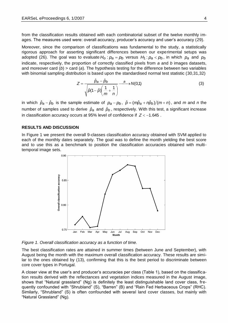
In Figure 1 we present the overall 9-classes classification accuracy obtained with SVM applied to

each of the monthly dates separately. The goal was to define the month yielding the best score

and to use this as a benchmark to position the classification accuracies obtained with multi-

temporal image sets.

Figure 1. Overall classification accuracy as a function of time.

The best classification rates are attained in summer times (between June and September), with

August being the month with the maximum overall classification accuracy. These results are simi-

lar to the ones obtained by (13), confirming that this is the best period to discriminate between

core cover types in Portugal.

A closer view at the user’s and producer’s accuracies per class (Table 1), based on the classifica-

tion results derived with the reflectances and vegetation indices measured in the August image,

shows that “Natural grassland” (Ng) is definitely the least distinguishable land cover class, fre-

quently confounded with “Shrubland” (S), “Barren” (B) and “Rain Fed Herbaceous Crops” (RHC).

Similarly, “Shrubland” (S) is often confounded with several land cover classes, but mainly with

“Natural Grassland” (Ng).

EARSeL eProceedings 6, 1/2007 5

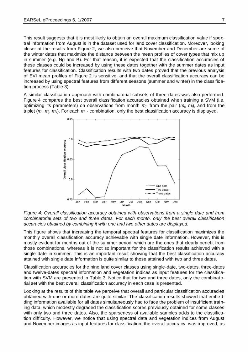
Looking at Figure 2 we perceive that the core class averaged EVI time series corresponding to

“Barren” (B) and “Natural grassland” (Ng) overlap in the entire summer period. Furthermore, the

“Natural grassland” (Ng) profile is up to a scale factor, very similar to the “Rain Fed Herbaceous

Crops” (RHC) response. Similar results were observed with NDVI and spectral bands. For these

reasons, it is not surprising that classification results computed with a single summer image re-

veal a mixture between these cover types. However, and given the different phenology of these

classes, it is reasonably expectable that adding more temporal information in the feature space,

selected at phenologically critical times (e.g. February or November), should improve their particu-

lar classification performances (6). The complexity is to define which summer and winter dates

should be combined to increase land cover classes discrimination.

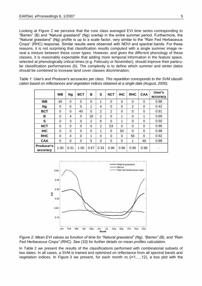
Table 1: User’s and Producer’s accuracies per class. This repartition corresponds to the SVM classifi-

cation based on reflectances and vegetation indices obtained at a single date (August, 2000).

WB Ng BCT B S NCT IHC RHC CAA User's

accuracy

WB 40 0 0 0 1 0 0 0 0 0.98

Ng 0 5 0 1 4 0 0 2 0 0.42

BCT 0 0 40 0 2 2 0 0 0 0.91

B 0 4 0 18 2 0 1 0 1 0.69

S 0 3 0 2 6 0 1 0 0 0.50

NCT 0 0 0 0 2 53 0 0 0 0.96

IHC 0 0 0 0 1 0 50 0 0 0.98

RHC 0 4 0 1 0 0 0 56 0 0.92

CAA 0 0 0 5 0 0 0 1 46 0.88

Producer's

accuracy 1.00 0.31 1.00 0.67 0.33 0.96 0.96 0.95 0.98 -

Figure 2: Mean EVI values as function of time for “Natural grassland” (Ng), “Barren” (B), and “Rain

Fed Herbaceous Crops” (RHC). See (33) for further details on mean profiles calculation.

In Table 2 we present the results of the classifications performed with combinatorial subsets of

two dates. In all cases, a SVM is trained and optimized on reflectance from all spectral bands and

vegetation indices. In Figure 3 we present, for each month mi (i=1,…,12), a box plot with the

EARSeL eProceedings 6, 1/2007 6

overall classification accuracy distribution (median, quartile, extremes and outliers) obtained for all

pair-wise combinations of mi with each of the remaining eleven months (Table 2).

Table 2: Overall land cover classification accuracies obtained with combinatorial subsets of two dates.

Jan Feb Mar Apr May Jun Jul Aug Sep Oct Nov Dec

Jan - 0.84 0.84 0.85 0.88 0.88 0.89 0.89 0.88 0.86 0.85 0.84

Feb 0.84 - 0.81 0.85 0.86 0.87 0.87 0.88 0.87 0.86 0.86 0.85

Mar 0.84 0.81 - 0.81 0.86 0.87 0.88 0.88 0.88 0.87 0.86 0.85

Apr 0.85 0.85 0.81 - 0.87 0.87 0.87 0.88 0.87 0.87 0.87 0.86

May 0.88 0.86 0.86 0.87 - 0.86 0.87 0.87 0.88 0.87 0.87 0.87

Jun 0.88 0.87 0.87 0.87 0.86 - 0.86 0.88 0.87 0.89 0.89 0.88

Jul 0.89 0.87 0.88 0.87 0.87 0.86 - 0.87 0.88 0.89 0.90 0.89

Aug 0.89 0.88 0.88 0.88 0.87 0.88 0.87 - 0.87 0.88 0.90 0.89

Sep 0.88 0.87 0.88 0.87 0.88 0.87 0.88 0.87 - 0.87 0.88 0.88

Oct 0.86 0.86 0.87 0.87 0.87 0.89 0.89 0.88 0.87 - 0.86 0.87

Nov 0.85 0.86 0.86 0.87 0.87 0.89 0.90 0.90 0.88 0.86 - 0.85

Dec 0.84 0.85 0.85 0.86 0.87 0.88 0.89 0.89 0.88 0.87 0.85 -

The most important remarks when comparing these results with those from Figure 1 is that the

best median pair-wise classifications are achieved considering at least one image from summer

time, and overall classification accuracies with summer images are those that have the smallest

intervals of variation (Figure 3). These outcomes confirm, once again, that spectral information

from summer is necessary for a superior discrimination of land cover classes in Portugal. Specif i-

cally, the maximum overall classification accuracy was obtained by combining August and No-

vember images (the same value was achieved with the subset containing July and November

dates), and the median values of the classifications achieved by combining August with all other

months proved to be greater than the combinatorial sets of all other dates.

Figure 3: Overall classification accuracy per combinatorial subsets of two dates. Each box plot

represents the lower quartile, median, and upper quartile of classification accuracy obtained for all

pair-wise combinations of each month with each of the remaining eleven months images. Classi-

fication values that are considered as outliers are represented by “+”.

EARSeL eProceedings 6, 1/2007 7

This result suggests that it is most likely to obtain an overall maximum classification value if spec-

tral information from August is in the dataset used for land cover classification. Moreover, looking

closer at the results from Figure 2, we also perceive that November and December are some of

the winter dates that maximize the distance between the mean profiles of cover types that mix up

in summer (e.g. Ng and B). For that reason, it is expected that the classification accuracies of

these classes could be increased by using these dates together with the summer dates as input

features for classification. Classification results with two dates proved that the previous analysis

of EVI mean profiles of Figure 2 is sensitive, and that the overall classification accuracy can be

increased by using spectral features from different seasons (summer and winter) in the classifica-

tion process (Table 3).

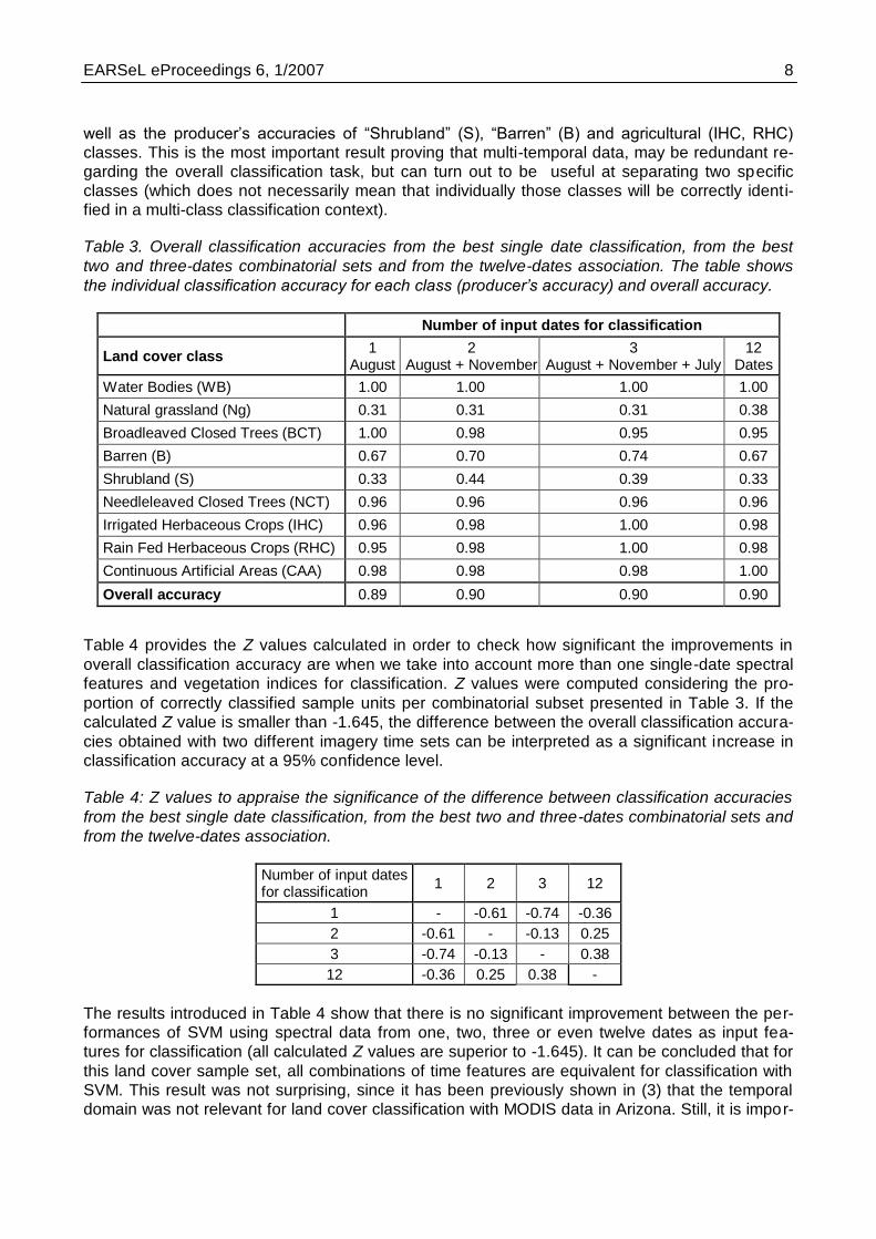
A similar classification approach with combinatorial subsets of three dates was also performed.

Figure 4 compares the best overall classification accuracies obtained when training a SVM (i.e.

optimizing its parameters) on observations from month mi, from the pair (mi, mj), and from the

triplet (mi, mj, mk). For each mi - combination, only the best classification accuracy is displayed.

Figure 4: Overall classification accuracy obtained with observations from a single date and from

combinatorial sets of two and three dates. For each month, only the best overall classification

accuracies obtained by combining it with one and two other dates are displayed.

This figure shows that increasing the temporal spectral features for classification maximizes the

monthly overall classification accuracy achievable with single date information. However, this is

mostly evident for months out of the summer period, which are the ones that clearly benefit from

those combinations, whereas it is not so important for the classification results achieved with a

single date in summer. This is an important result showing that the best classification accuracy

attained with single date information is quite similar to those attained with two and three dates.

Classification accuracies for the nine land cover classes using single-date, two-dates, three-dates

and twelve-dates spectral information and vegetation indices as input features for the classifica-

tion with SVM are presented in Table 3. Notice that for two and three dates, only the combinato-

rial set with the best overall classification accuracy in each case is presented.

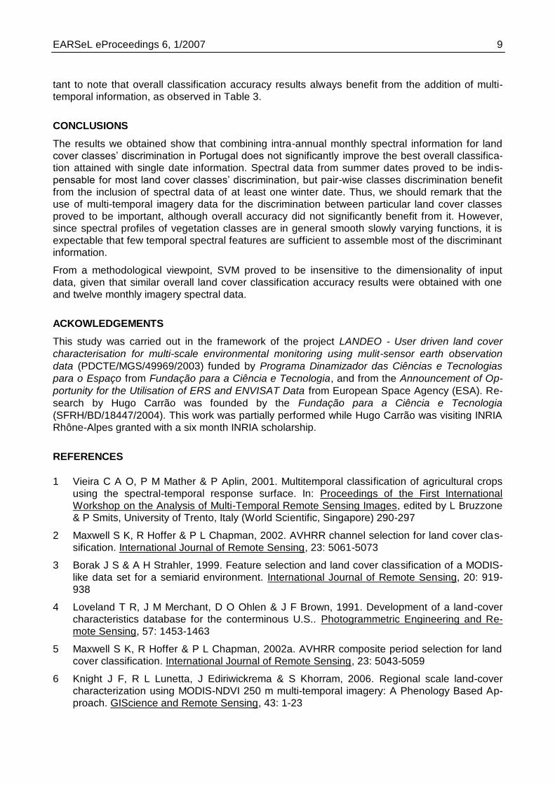
Looking at the results of this table we perceive that overall and particular classification accuracies

obtained with one or more dates are quite similar. The classification results showed that embed-

ding information available for all dates simultaneously had to face the problem of insufficient train-

ing data, which modestly degraded the classification scores previously obtained for some classes

with only two and three dates. Also, the sparseness of available samples adds to the classifica-

tion difficulty. However, we notice that using spectral data and vegetation indices from August

and November images as input features for classification, the overall accuracy was improved, as

EARSeL eProceedings 6, 1/2007 8

well as the producer’s accuracies of “Shrubland” (S), “Barren” (B) and agricultural (IHC, RHC)

classes. This is the most important result proving that multi-temporal data, may be redundant re-

garding the overall classification task, but can turn out to be useful at separating two specific

classes (which does not necessarily mean that individually those classes will be correctly identi-

fied in a multi-class classification context).

Table 3. Overall classification accuracies from the best single date classification, from the best

two and three-dates combinatorial sets and from the twelve-dates association. The table shows

the individual classification accuracy for each class (producer’s accuracy) and overall accuracy.

Number of input dates for classification

Land cover class 1

August 2

August + November 3

August + November + July 12

Dates

Water Bodies (WB) 1.00 1.00 1.00 1.00

Natural grassland (Ng) 0.31 0.31 0.31 0.38

Broadleaved Closed Trees (BCT) 1.00 0.98 0.95 0.95

Barren (B) 0.67 0.70 0.74 0.67

Shrubland (S) 0.33 0.44 0.39 0.33

Needleleaved Closed Trees (NCT) 0.96 0.96 0.96 0.96

Irrigated Herbaceous Crops (IHC) 0.96 0.98 1.00 0.98

Rain Fed Herbaceous Crops (RHC) 0.95 0.98 1.00 0.98

Continuous Artificial Areas (CAA) 0.98 0.98 0.98 1.00

Overall accuracy 0.89 0.90 0.90 0.90

Table 4 provides the Z values calculated in order to check how significant the improvements in

overall classification accuracy are when we take into account more than one single-date spectral

features and vegetation indices for classification. Z values were computed considering the pro-

portion of correctly classified sample units per combinatorial subset presented in Table 3. If the

calculated Z value is smaller than -1.645, the difference between the overall classification accura-

cies obtained with two different imagery time sets can be interpreted as a significant increase in

classification accuracy at a 95% confidence level.

Table 4: Z values to appraise the significance of the difference between classification accuracies

from the best single date classification, from the best two and three-dates combinatorial sets and

from the twelve-dates association.

Number of input dates for classification

1 2 3 12

1 - -0.61 -0.74 -0.36

2 -0.61 - -0.13 0.25

3 -0.74 -0.13 - 0.38

12 -0.36 0.25 0.38 -

The results introduced in Table 4 show that there is no significant improvement between the per-

formances of SVM using spectral data from one, two, three or even twelve dates as input fea-

tures for classification (all calculated Z values are superior to -1.645). It can be concluded that for

this land cover sample set, all combinations of time features are equivalent for classification with

SVM. This result was not surprising, since it has been previously shown in (3) that the temporal

domain was not relevant for land cover classification with MODIS data in Arizona. Still, it is impor-

EARSeL eProceedings 6, 1/2007 9

tant to note that overall classification accuracy results always benefit from the addition of multi-

temporal information, as observed in Table 3.

CONCLUSIONS

The results we obtained show that combining intra-annual monthly spectral information for land

cover classes’ discrimination in Portugal does not significantly improve the best overall classifica-

tion attained with single date information. Spectral data from summer dates proved to be indis-

pensable for most land cover classes’ discrimination, but pair-wise classes discrimination benefit

from the inclusion of spectral data of at least one winter date. Thus, we should remark that the

use of multi-temporal imagery data for the discrimination between particular land cover classes

proved to be important, although overall accuracy did not significantly benefit from it. However,

since spectral profiles of vegetation classes are in general smooth slowly varying functions, it is

expectable that few temporal spectral features are sufficient to assemble most of the discriminant

information.

From a methodological viewpoint, SVM proved to be insensitive to the dimensionality of input

data, given that similar overall land cover classification accuracy results were obtained with one

and twelve monthly imagery spectral data.

ACKOWLEDGEMENTS

This study was carried out in the framework of the project LANDEO - User driven land cover

characterisation for multi-scale environmental monitoring using mulit-sensor earth observation

data (PDCTE/MGS/49969/2003) funded by Programa Dinamizador das Ciências e Tecnologias

para o Espaço from Fundação para a Ciência e Tecnologia, and from the Announcement of Op-

portunity for the Utilisation of ERS and ENVISAT Data from European Space Agency (ESA). Re-

search by Hugo Carrão was founded by the Fundação para a Ciência e Tecnologia

(SFRH/BD/18447/2004). This work was partially performed while Hugo Carrão was visiting INRIA

Rhône-Alpes granted with a six month INRIA scholarship.

REFERENCES

1 Vieira C A O, P M Mather & P Aplin, 2001. Multitemporal classification of agricultural crops

using the spectral-temporal response surface. In: Proceedings of the First International

Workshop on the Analysis of Multi-Temporal Remote Sensing Images, edited by L Bruzzone

& P Smits, University of Trento, Italy (World Scientific, Singapore) 290-297

2 Maxwell S K, R Hoffer & P L Chapman, 2002. AVHRR channel selection for land cover clas-

sification. International Journal of Remote Sensing, 23: 5061-5073

3 Borak J S & A H Strahler, 1999. Feature selection and land cover classification of a MODIS-

like data set for a semiarid environment. International Journal of Remote Sensing, 20: 919-

938

4 Loveland T R, J M Merchant, D O Ohlen & J F Brown, 1991. Development of a land-cover

characteristics database for the conterminous U.S.. Photogrammetric Engineering and Re-

mote Sensing, 57: 1453-1463

5 Maxwell S K, R Hoffer & P L Chapman, 2002a. AVHRR composite period selection for land

cover classification. International Journal of Remote Sensing, 23: 5043-5059

6 Knight J F, R L Lunetta, J Ediriwickrema & S Khorram, 2006. Regional scale land-cover

characterization using MODIS-NDVI 250 m multi-temporal imagery: A Phenology Based Ap-

proach. GIScience and Remote Sensing, 43: 1-23

EARSeL eProceedings 6, 1/2007 10

7 Van Dijk A, S L Callis, C M Sakamoto & W L Decker, 1987. Smoothing vegetation index pro-

files: an alternative method for reducing radiometric disturbances in NOAA/AVHRR data.

Phtogrammetric Engineering and Remote Sensing, 53: 1059-1067

8 Duchemin B, D Guyon & J P Lagouarde, 1999. Potential and limits of NOAA-AVHRR tempo-

ral composite data for phenology and water stress monitoring of temperate forest ecosys-

tems. International Journal of Remote Sensing, 20: 895-917

9 Brown J, T Loveland, D Ohlen & A Zhu, 1999. The Global Land Cover Characteristis Data-

base: The Users’ Perspective. Photogrammetric Engineering and Remote Sensing, 65: 1069-

1064

10 Laporte N, S J Goetz, C O Justice & M Heinicke, 1998. A new land cover map of central Af-

rica derived from multi-resolution, multi-temporal AVHRR data. International Journal of Re-

mote Sensing, 19: 3537-3550

11 Carrão, H, P Gonçalves & M Caetano, 2006. MERIS based land cover characterization: a

comparative study. In: Proceedings of the ASPRS 2006 Annual Conference - Prospecting for

Geospatial Information Integration (Reno, Nevada) unpaginated CD-ROM, 13 pp.

12 Oliveira P, P Gonçalves & M Caetano, 2005. Land cover time profiles from linear mixture

models applied to MODIS images. In: Proceedings of the 31st International Symposium on

Remote Sensing of Environment (Saint Petersburg, Russian Federation) unpaginated CD-

ROM, 4 pp.

13 Gonçalves P, H Carrão, A Pinheiro & M Caetano, 2006. Land cover classification with Sup-

port Vector Machine applied to MODIS imagery. In: Global Developments in Environmental

Earth Observation from Space, edited by A Marçal (Rotterdam: Millpress) 517-525

14 Clevers J G P W, R Zurita Milla, M Schaepman & H Bartholomeus, 2004. Using MERIS on

Envisat for land cover mapping. In: Proceedings of the 2004 Envisat & ERS Symposium,

Salzburg, Austria (ESA SP-572, April 2005).

15 Gessner U, K P Gunther & S W Maier, 2004. Landcover/land use map of Germany based on

MERIS full resolution data. In: Proceedings of the 2004 Envisat & ERS Symposium, Salz-

burg, Austria (ESA SP-572, April 2005).

16 Skinner L & A Luckman, 2003. Deriving Land Cover information over Siberia using MERIS

and MODIS data. In: Proceedings of the MERIS User Workshop, Frascati, Italy (ESA SP-549,

May 2004)

17 Duong N D, 2004. Land cover mapping of Vietnam using MODIS 500m 32-day global com-

posites. In: International Symposium on Geoinformatics for Spatial Infrastructure Develop-

ment in Earth and Allied Sciences (Hanoi, Vietnam) 6 pp.

18 Stibig H & T Bucha, 2005. Feasibility study on the use of medium resolution satellite data for

the detection of forest cover change caused by clear cutting of coniferous forests in the

northwest of Eurasia. EUR 21579 EN (Office for Official Publication of the European Com-

munities, Luxembourg) June 2005, 42 pp.

19 Friedl M A, D K McIver, X Y Zhang, J C F Hodges, A Schnieder, A Bacinni, A H Strahler, A

Cooper, F Gao, C Schaaf & W Liu, 2001. Global land cover classification results from

MODIS. In: Geoscience and Remote Sensing Symposium 2001. IGARSS '01. IEEE 2001 In-

ternational (Sidney, Australia) 733-735

20 Pal M & P M Mather, 2005. Support vector machines for classification in remote sensing.

International Journal of Remote Sensing, 26: 1007-1011

EARSeL eProceedings 6, 1/2007 11

21 Painho M & M Caetano, 2005. Cartografia de Ocupação do Solo, Portugal Continental, 1985-

2000 (Instituto do Ambiente, Lisboa, Portugal) 56 pp. (download: 12 MB pdf file)

22 Cristianini N & J Shawe-Taylor, 2000. An Introduction to Support Vector Machines and Other

Kernel-based Learning Methods (Cambridge University Press) 204 pp.

23 Boser B E, I M Guyon & V N Vapnik, 1992. A training algorithm for optimal margin classifiers.

In: Proceedings of the 5th Annual ACM Workshop on Computational Learning Theory, edited

by D Haussler, 144-152.

24 Vapnik V, 1998. Statistical Learning Theory (Wiley) 768 pp.

25 Scholkopf B, A J Smola, R C Williamson & P L Bartlett, 2000. New support vector algorithms.

Neural Computation, 12:1207-1245

26 Foody G M, A Mathur, C Sanchez-Hernandez & D S Boyd, 2006. Training set size require-

ments for the classification of a specific class. Remote Sensing of Environment, 104: 1-14

27 Huang C, L S Davis & J R G Townshend, 2002. An assessment of support vector machines

for land cover classification. International Journal of Remote Sensing, 23: 725-749

28 Groves P & P Bajcsy, 2003. Methodology for Hyperspectral Band and Classification Model

Selection. In: IEEE Workshop on Advances in Techniques for Analysis of Remotely Sensed

Data (Washington DC) (IEEE, October 2003) 120-128

29 Jensen John R, 1996. Introductory Digital Image Processing, A Remote Sensing Perspective

(Prentice Hall, 2nd edition) 316 pp.

30 Pestana D D & S F Velosa, 2006. Introdução à Probabilidade e à Estatística (Fundação

Calouste Gulbenkian, 2.ª edição) 1164 pp.

31 Murteira B, C S Ribeiro, J A Silva & C Pimenta, 2002. Introdução à Estatística (McGraw-Hill)

647 pp.

32 Johnson R A & D W Wichern, 1998. Applied Multivariate Statistical Analysis (Prentice Hall,

4th edition) 799 pp.

33 Pinheiro A, P Gonçalves, H Carrão & M Caetano, 2006. A Toolbox for multi-temporal analysis

of satellite imagery. In: New Developments and Challenges in Remote Sensing, edited by Z

Bochenek (Rotterdam: Millpress, in press).