U.S. Coast Guard Research and Development Center1082 Shennecossett Road, Groton, CT 06340-6048

Report No. CG-D-05-05

LEEWAY DIVERGENCE

FINAL REPORTJANUARY 2005

This document is available to the U.S. public through theNational Technical Information Service, Springfield, VA 22161

Prepared for:

U.S. Department of Homeland SecurityUnited States Coast Guard

Operations (G-O)Washington, DC 20593-0001

NOTICEThis document is disseminated under the sponsorship of theDepartment of Homeland Security in the interest of informationexchange. The United States Government assumes no liability for itscontents or use thereof.

The United States Government does not endorse products ormanufacturers. Trade or manufacturers' names appear herein solelybecause they are considered essential to the object of this report.

This report does not constitute a standard, specification, or regulation.

EV iMarc B. Mandler, Ph.DTechnical DirectorUnited States Coast GuardResearch & Development Center1082 Shennecossett Road

US ct Groton, CT 06340-6048

ii

Technical Report Documentation PageI. Report No. 2. Government Accession Number 3. Recipient's Catalog No.

4. Title and Subtitle 5. Report Date

LEEWAY DIVERGENCE January 2005

6. Performing Organization CodeProject No. 1012.3.16

7. Author(s) 8. Performing Organization Report No.

Arthur A. Allen

9. Performing Organization Name and Address 10. Work Unit No. (TRAIS)

U.S. Coast GuardResearch and Development Center 1I. Contract or Grant No.

1082 Shennecossett RoadGroton, CT 06340-6048

12. Sponsoring Organization Name and Address 13. Type of Report & Period Covered

U.S. Department of Homeland Security FinalUnited States Coast GuardOperations (G-O) 14. Sponsoring Agency Code

Washington, DC 20593-0001 Commandant (G-OPR)U.S Coast Guard Headquarters

Washington, DC 20593-0001

15. Supplementary Notes

The technical point of contact is Arthur Allen, 860-441-2747, email: aallen@rdc.uscg.mil

16. Abstract (MAXIMUM 200 WORDS)

Understanding leeway divergence is key to accurately determining maritime search areas. The downwind andcrosswind components of leeway drift as a function of wind speed have been reported on in the literature for 23categories of leeway drift objects. Two additional leeway drift object categories were analyzed in this report. Theoptimal relationships between downwind and crosswind components of leeway coefficients and leeway speed anddivergence angle values are derived empirically using the 25 categories that contained both sets of coefficients.Downwind and crosswind leeway coefficients were generated for an additional 38 leeway categories based on theestimates from standard error relationships. The entire set of downwind and crosswind leeway componentcoefficients is presented for 63 leeway categories.

The crosswind component of leeway has been observed to be either positive (right of the downwind direction) ornegative (left of the downwind directions) for the duration of each individual drift run. For four drift objectcategories, forty-nine sign changes of the crosswind leeway component occurred during 1332.2 hours of sampling.This represents a frequency of sign change in the crosswind components of 4% per hour, independent of leewaycategory or wind speed. Crosswind leeway component sign changes at 4% per hour have a significant impact onthe final search area probability distribution modeled by Monte Carlo simulations.

17. Key Words 18. Distribution Statement

Leeway Leeway divergence This document is available to the U.S. publicLeeway angle Crosswind component through the National Technical InformationDownwind component Divergence angle Service, Springfield, VA 22161Search and Rescue SAR

19. Security Class (This Report) 20. Security Class (This Page) 21. No of Pages 22. Price

UNCLASSIFIEDI UNCLASSIFIED IIForm DOT F 1700.7 (8/72) Reproduction of form and completed page is authorized

iii

ACKNOWLEDGEMENTS

The comments of Penny Herring, Dr. Jennifer Dick-O'Donnell, LT Harlan Wallace, Gary Hover,LT Gregory Purvis, J. R. Frost, R. Quincy Robe, Richard Schaefer, M. J. Lewandowski andVonnie Summers are appreciated and helped to improve this report.

iv

EXECUTIVE SUMMARY

The hunt for a drifting object in the maritime environment typically requires the determination ofsearch areas. It is well established that survivors and their craft drift generally downwind due toleeway effects. It is now understood from a series of field studies conducted during the 1990sthat leeway drift is not always directly downwind, but that there is often a significant componentof drift perpendicular to the downwind direction. This perpendicular motion is the crosswindcomponent of leeway drift. The crosswind component of leeway causes an object's drift todiverge from the downwind direction. Understanding this behavior, defined as leewaydivergence, is key to accurately determining search areas. This study discusses the importanceof the leeway crosswind components and develops a Downwind Leeway (DWL) and CrosswindLeeway (CWL) component model for incorporating the effect of leeway divergence into searchplanning tools and determination of search areas.

This report is a follow on to Allen and Plourde (1999) with a particular emphasis on therelationship among leeway angle, divergence angle, and crosswind components of leeway, andtheir roles in describing and modeling leeway motion. This report also provides the backgroundand framework for on-going efforts to incorporate crosswind components of leeway into thesearch area determination model first introduced in Allen and Plourde (1999) and into manualsearch planning methods.

In the past, the unclear relationship between leeway angle and leeway divergence, and the lack ofcrosswind information, has limited accurate representation of leeway behavior in search planningtools. This report clarifies leeway divergence terms, discusses crosswind behavior, andultimately presents DWL and CWL of leeway drift, as a function of wind speed, for 63 categoriesof leeway drift objects.

The net displacement from the downwind direction is dependent on the magnitude and frequencyof sign changes of the crosswind component of leeway. Allen and Plourde (1999) providedvalues for leeway speed as function of wind speed and divergence angle for 63 leewaycategories. Leeway data for 25 of these 63 categories are available allowing direct computationof the DWL and CWL coefficients using linear regression analysis. For the other 38 categories,no actual leeway drift data are available. Using the data for the 25 leeway categories, Chapter 2of the report develops a statistically derived method to determine the remaining 38 sets of DWLand CWL coefficients. Chapter 3 then presents the entire set of downwind and crosswind leewaycoefficients for both the unconstrained and constrained DWL and CWL component regressionmodels. It is proposed that incorporating these coefficients into DWL and CWL component searchplanning models will result in better-centered and better-sized search areas than those search areasdeveloped without using the downwind and crosswind leeway components.

The investigations in Chapter 5 show that the frequency of CWL sign change appears to beindependent of wind speed. The frequency of the sign change was shown to vary betweenleeway object categories but was not consistent with the general configuration of the individualleeway object types. The overall observed frequency of these sign changes in crosswindcomponents based on the leeway drift of all four leeway object categories combined wasapproximately 4-6% per hour. It was further shown that varying the sign change frequencybetween 0% and 50% per hour has a significant impact on final search area probability

v

distribution, but varying the sign change frequency between 4% and 6% per hour does not affectthe distribution. Based on past search area modeling, it appears that a 4-6% sign changefrequency provides a search area distribution consistent with those generated by existing SARplanning tools. Accordingly, a "generic" value of 4% change in CWL sign per hour isrecommended for use in stochastic, leeway-drift models until further work in this area provides amore complete picture of CWL sign change.

Recommendations

1) Tables 3-1 and 3-2 provide a complete set of DWL and CWL coefficients for the 63categories of leeway objects in the taxonomy developed by Allen and Plourde (1999).Although 38 sets of DWL and CWL coefficients were statistically derived from theempirical data, the Table 3-1 and 3-2 coefficients should be used in numerical searchplanning tools to determine the downwind and crosswind components of leeway (as afunction of wind speed adjusted to the standard 10-meter height) in calculating searcharea distributions.

2) Incorporate into numerical search planning tools the use of a simple statistical model ofswitching between positive and negative crosswind component equations using a signchange frequency of 4% per hour, independent of wind speed or leeway category.

3) Incorporate into manual search planning tools the use of divergence angles provided byAllen and Plourde (1999) divided by an "adjustment factor" determined here to be 1.35.

4) Continue efforts to fully understand and model the drift of survivors and survivor craft bystudying targets over more drift runs and in a variety of wind conditions. The conditionsshould include wind speeds less than three meters per second (m/s) and greater than 20m/s, and periods of rapid wind direction shifts. With more drift runs the question ofinitial distribution between left and right divergence can be addressed. Collecting leewaydata under a variety of wind conditions will also allow the observation of changesbetween left and right divergence. Data collection for the 38 leeway categories for whichdata are not available will allow direct computation and verification of the DWL andCWL coefficients for these categories.

5) Further refine the collection of leeway data collected in the field to minimize the effectthat the installed or attached instrumentation has on drift of the search test object. Theuse of current meters placed directly onboard the test object may lessen the impact on theleeway object of crosswind component sign-change. However, these directly mountedcurrent meters should be verified against the more standard technique of a tetheredcurrent meter, which is well away from any local flow distortion effects. Additionalinsight into the behavior and dynamics of an object changing crosswind component signmight come with further information of the wave field and from leeway dynamicsmodeling studies.

vi

TABLE OF CONTENTS

ACKNOWLEDGEMENTS ................................................................................................... ivEXECUTIVE SUMMARY .......................................................................................................... vLIST OF ACRONYM S ............................................................................................................. xviCHAPTER 1. PRESENT UNDERSTANDING OF LEEWAY DRIFT ............................... 1-1

1.1. Introduction to Leeway - Concepts and Terminology ........................................... 1-11.2. Previous Studies Of Leeway Angle And Leeway Divergence ............................... 1-51.3. O bjectives O f The Present Study ...................................................................... 1-11

CHAPTER 2. METHOD FOR ESTIMATING DOWNWIND AND CROSSWINDCOMPONENTS OF LEEWAY FROM LEEWAY SPEED ANDDIVERGENCE ANGLE ...................................................................................... 2-1

2.1. Approach Used In Determining Downwind And Crosswind Components OfL eew ay .................................................................................................................... 2 -1

2.2. Estimation Of Downwind And Crosswind Coefficients Based On Leeway SpeedA nd D ivergence A ngle ........................................................................................... 2-2

2.3. Estimation Of Standard Error Terms (Sy/) ............................................................. 2-7CHAPTER 3. COMPILING A COMPREHENSIVE SET OF DOWNWIND AND

CROSSWIND LEEWAY COEFFICIENTS ...................................................... 3-1CHAPTER 4. DEVELOPING AN IMPROVED LEEWAY MODEL BASED ON

DOWNWIND AND CROSSWIND LEEWAY COMPONENTS ............... 4-14.1. Leeway M odel Im plem entation .......................................................................... 4-14.2 Comparison Of Leeway M odels W ith Data ............................................................ 4-4

CHAPTER 5. INVESTIGATING AND ACCOUNTING FOR CHANGES IN THE SIGNOF THE CROSSWIND LEEWAY COMPONENT .......................................... 5-1

5.1. Introduction ........................................................................................................ 5-15.2 Methods Used To Identify And Analyze Crosswind Component Sign Changes ... 5-25.3 Analysis Of Crosswind Leeway Component Sign Changes ................................... 5-5

5.3.1 5.5-M eter O pen Skiff ............................................................................................. 5-55.3.2 4-6 Person Life Rafts (with Deep Ballast Systems, Canopy) ................................. 5-85.3.3 20-Person Life R afts ............................................................................................. 5-105.3.4 O ne-Cubic M eter W harf Box ................................................................................ 5-125.3.5 Combining Four Leeway Categories Together ..................................................... 5-14

5.4 Investigating The Effects Of Crosswind Component Sign Changes On Search AreaD istributions .......................................................................................................... 5-18

5.5 Summary Of Crosswind Component Sign Changes ............................................. 5-21CHAPTER 6. CONCLUSIONS AND RECOMMENDATIONS .......................................... 6-1

6.1 C onclusions ........................................................................................................ 6-16.2 R ecom m endations ................................................................................................... 6-2

CHAPTER 7. REFERENCES .................................................................................................. 7-1APPENDIX A LEEWAY COMPONENTS OF MARITIME LIFE RAFTS (DEEP

BALLAST, CANOPY, 15-25 PERSON CAPACITY) .................................. A-iAPPENDIX B ANALYSIS OF SELECTED LEEWAY CATEGORIES TO DETERMINE

THE CONSTRAINED REGRESSION OF THE DOWNWIND ANDCROSSWIND COMPONENTS OF LEEWAY AS FUNCTIONS OF THE10-METER WIND SPEED ............................................................................ B-I

vii

APPENDIX C STATISTICAL COMPARISON OF EXPERIMENTAL DATAWITH 0 - MODEL and Y- MODEL GENERATED PREDICTIONS ..... C-I

APPENDIX D RESULTS OF ANALYSIS OF CROSSWIND COMPONENT SIGNCHANGES FOR FOUR CATEGORIES OF LEEWAY OBJECTS .......... D-1

LIST OF ILLUSTRATIONS

Figure 1-1. The relationship between the leeway speed and leeway angle and the downwind andcrossw ind com ponents of leew ay ........................................................................... 1-2

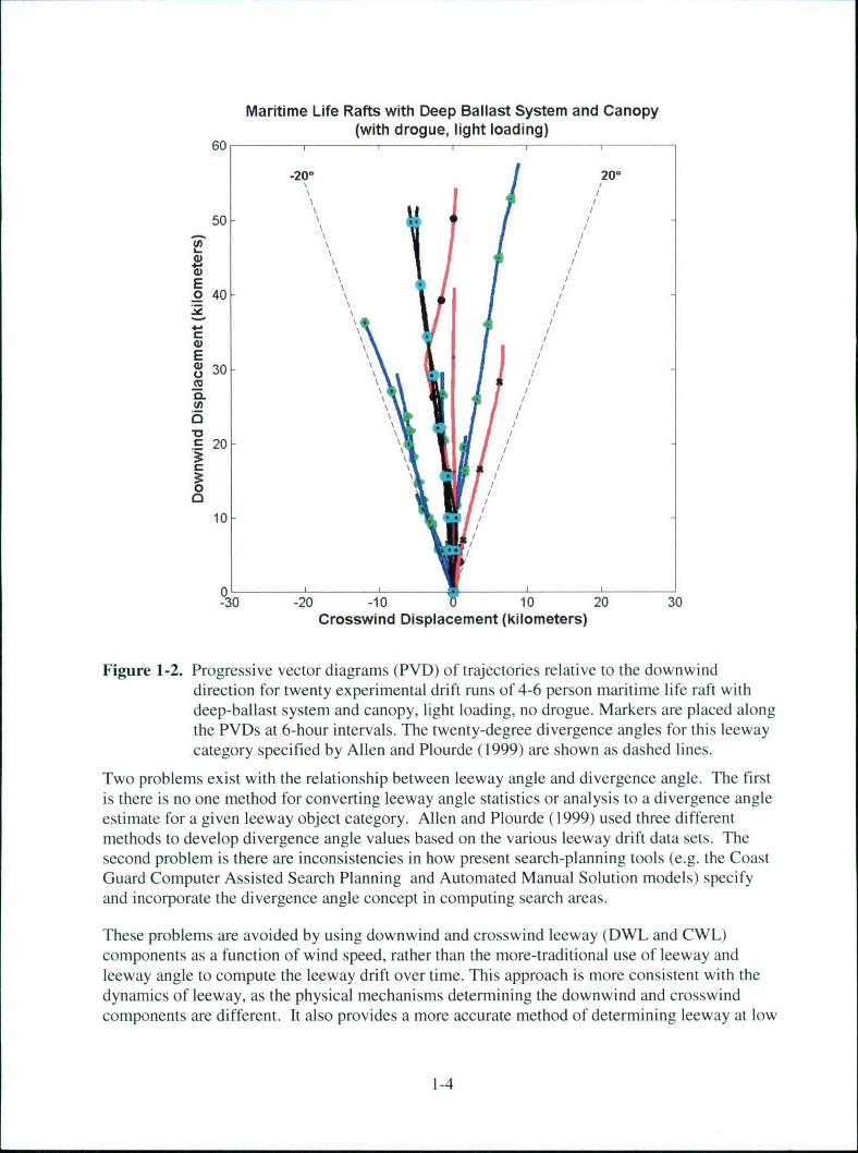
Figure 1-2. Progressive vector diagrams (PVD) of trajectories relative to the downwinddirection for twenty experimental drift runs of 4-6 person maritime life raft withdeep-ballast system and canopy, light loading, no drogue. Markers are placed alongthe PVDs at 6-hour intervals. The twenty-degree divergence angles for this leewaycategory specified by Allen and Plourde (1999) are shown as dashed lines .......... 1-4

Figure 1-3. Leeway angle versus wind speed from Hufford and Broida (1974), data set for fbursm all craft ................................................................................................................ 1-6

Figure 1-4. Leeway object taxonomy devised by Allen and Plourde (1999) ............................ 1-8Figure 2-1. The absolute difference from one of the slope coefficients of the regression of the

downwind and crosswind components of leeway against the actual coefficients ofthe downwind and crosswind components of leeway as a function of the adjustmentfacto r ....................................................................................................................... 2 -4

Figure 2-2. Predicted versus actual coefficients of the downwind components of leeway usingan adjustm ent factor of 1.35 .................................................................................... 2-6

Figure 2-3. Predicted versus actual coefficients of the crosswind components of leeway usingan adjustm ent factor of 1.35 .................................................................................... 2-7

Figure 2-4. Standard error of estimate (Sy/,) for the downwind components of leeway equationsversus standard error of estimate (Sy/X) of the leeway speed equations .................. 2-8

Figure 2-5. Standard error of estimate (Sy/,) for the crosswind components of leeway equationsversus the standard error of the estimate (Sy/,) of the leeway speed equations ...... 2-9

Figure 4-1. Downwind components of leeway versus W10m for three separate 4-6 person liferafts with deep ballast system and canopies, no drogue, light loading. Also shown isthe unconstrained linear regression and its 95% prediction limits ......................... 4-2

Figure 4-2. Histograms of slices of the downwind leeway components for maritime life raftswith deep ballast systems and canopies compared to normal distributions ............ 4-3

Figure 4-3. Downwind leeway data (blue) from maritime life rafts with deep ballast systemsand canopies versus 10-meter wind speed compared with 1000 model generatedleeway equation results: (A) 0-model values in red and (B) Y-model values ing ree n ........................................................................................................................ 4 -5

Figure 5-1. The [A] 5.5-meter V-hull, open skiff, [B] Tulmar 4-person life raft, [C] Beaufort20-person life raft, and [D] I-cubic meter wharf box ............................................. 5-3

Figure 5-2. Progressive Vector Diagram of the leeway displacement vectors for Drift Run 60,5.5 m open V-hull skiff starting at 1500 26 November, 1995. Time of day markedalong the P V D ......................................................................................................... 5-4

Figure 5-3. Time series of [A] the crosswind component of leeway (cm/s) and [BI the windspeed adjusted to the 10-meter height, during drift run 60, 5.5 m open boat.Vertical-dashed lines indicate CW L sign changes .................................................. 5-5

viii

Figure 5-4. Number of significant CWL sign changes versus 2 m/s groupings of Wjor for the5.5 m open skiff ...................................................................................................... 5-6

Figure 5-5. Hours of leeway data versus 2 m/s groupings of W10m for the 5.5m open skiff..... 5-7Figure 5-6. Frequency of CWL sign changes (percent per hour) versus 2 m/s groupings of W101 ,

for the 5.5m open skiff ........................................................................................... 5-8Figure 5-7. Number of significant CWL sign changes versus 2 m/s groupings of Wi0m for the 4-

6 person life rafts ................................................................................................ 5-9Figure 5-8. Hours of leeway data versus 2 m/s groupings of Wi1m for the 4-6 person life raft.5-9Figure 5-9. Frequency of CWL sign changes (percent per hour) versus 2 m/s groupings of Wl0m

for the 4-6 person life rafts .................................................................................... 5-10Figure 5-10.Number of significant CWL sign changes versus 2 m/s groupings of Wiom for the

20-person life rafts ................................................................................................ 5-11Figure 5-11. Hours of leeway data versus 2 m/s groupings of Wiom for the 20-person life rafts.

.................................. .............................. . °,* ............ ........... ........................ 5 -1 1Figure 5-12.Frequency of CWL sign changes (percent per hour) versus 2 m/s groupings of W10m

for the 20-person life rafts ..................................................................................... 5-12Figure 5-13. Number of significant CWL sign changes versus 2 m/s groupings of W10m for the I-

cubic m eter w harf box .......................................................................................... 5-13Figure 5-14. Hours of leeway data versus 2 m/s groupings of Wiom for the 1-cubic meter wharf

b o x ......................................................................................................................... 5 - 13Figure 5-15. Frequency of CWL sign changes (percent per hour) versus 2 m/s groupings of

W 10m for the 1 -cubic m eter wharf box .................................................................. 5-14Figure 5-16. Histogram of the number of significant change of signs in the crosswind

component of leeway for the four leeway categories combined versus 2 m/sgroupings of the 10-meter wind speed (m/s) ........................................................ 5-16

Figure 5-17. Histogram of the hours of leeway data for the four leeway categories combinedversus 2 mis groupings of the 10-meter wind speed (m/s) .................................... 5-16

Figure 5-18. Histogram of the frequency of CWL sign changes per hour for the four leewaycategories combined, versus 2 m/s groupings of the 10-meter wind speed .......... 5-17

Figure 5-19. Probability distributions at 0, 2, 4, 8, and 12 hours after start of 1000 replicationsof a flat bottom skiff in 15 m/s of south wind. The percent change of CWL signchanges per hour per replication was set to zero [A] and 1% [B] ........................ 5-19

Figure 5-20. Probability distributions at 0, 2, 4, 8, and 12 hours after start of 1000 replicationsof a flat bottom skiff in 15 m/s of south wind. The percent change of CWL signchanges per hour per replication was set to 4% [A] and 6% [B] .......................... 5-20

Figure 5-21. Probability distributions at 0, 2, 4, 8, and 12 hours after start of 1000 replicationsof a flat bottom skiff in 15 m/s of south wind. The percent change of CWL signchanges per hour per replication was set to 10% [A] and 50% [B] ...................... 5-21

Figure A-1. Beaufort circular 20-person life raft ................................................................. A-1Figure A-2. The unconstrained linear regression and 95% prediction limits of the downwind

component of leeway as function of wind speed at 10 m, maritime life rafts, deepballast systems, canopy, 15-25 person capacity, no drogue, light loading ............ A-2

Figure A-3. The unconstrained linear regression and 95% prediction limits of the positive andnegative crosswind components of leeway as function of wind speed at 10 m,maritime life rafts, deep ballast systems, canopy, 15-25 person capacity, no drogue,light load ing ........................................................................................................... A -3

ix

Figure A-4. The unconstrained linear regression and 95% prediction limits of the downwindcomponent of leeway versus wind speed at 10 m, maritime life rafts, deep ballastsystems, canopy, 15-25 person capacity, with a drogue, and heavy loading ......... A-4

Figure A-5. Unconstrained linear regression and 95% prediction limits of the positive andnegative crosswind components of leeway versus wind speed at 10 m, maritime liferafts, deep ballast systems, canopy, 15-25 person capacity, with drogue, heavylo ad in g .................................................................................................................... A -5

Figure B-1. Constrained linear regression and 95% prediction limits of the downwindcomponents of leeway versus wind speed for maritime life rafts, no-ballast systems,no-canopy, without drogue, from Hufford and Broida (1974) .............................. B-2

Figure B-2. Constrained linear regression and 95% prediction limits of the positive and negativecrosswind components of leeway versus wind speed, maritime life rafts, no-ballastsystems, no-canopy, without drogue, from Hufford and Brodia (1974) ................ B-3

Figure B-3. Constrained linear regression and 95% prediction limits of the downwindcomponents of leeway versus wind speed, maritime life rafts, no-ballast systems,no-canopy, with drogue from Hufford and Brodia (1974) .................................... B-3

Figure B-4. Constrained linear regression and 95% prediction limits of the positive and negativecrosswind components of leeway versus wind speed, maritime life rafts, no-ballastsystems, no-canopy, with drogue from Hufford and Brodia (1974) ...................... B-4

Figure B-5. Constrained linear regression and 95% prediction limits of the downwindcomponents of leeway versus wind speed, 4-6 person maritime life rafts, deep-ballast systems, canopy, without drogue, light loading, from Allen and Plourde(19 9 9 ) ..................................................................................................................... B -6

Figure B-6. Constrained linear regression and 95% prediction limits of the positive (+) andnegative (o) crosswind components of leeway versus wind speed, from Allen andPlourde (1999) 4-6 person maritime life rafts, deep-ballast systems, canopy, withoutdrogue, light loading .............................................................................................. B -7

Figure B-7. Constrained linear regression and 95% prediction limits of the downwindcomponents of leeway versus wind speed, 4-6 person maritime life rafts, deep-ballast systems, canopy, with drogue, light loading, from Allen and Plourde (1999)................................................................................................................................. B -8

Figure B-8. Constrained linear regression and 95% prediction limits of the positive crosswindcomponents of leeway versus wind speed, 4-6 person maritime life rafts, deep-ballast systems, canopy, with drogue, light loading, from Allen and Plourde (1999)............................................................................................................................. ....B -9

Figure B-9. Constrained linear regression and 95% prediction limits of the downwindcomponents of leeway versus wind speed, 4-6 person maritime life rafts, deep-ballast systems, canopy, without drogue, heavy loading, from Allen and Plourde(19 9 9 ) ................................................................................................................... B -10

Figure B-10. Constrained linear regression and 95% prediction limits of the positive crosswindcomponents of leeway versus wind speed, 4-6 person maritime life rafts, deep-ballast systems, canopy, without drogue, heavy loading, from Allen and Plourde(19 9 9 ) ................................................................................................................... B -Il

x

Figure B-11. Constrained linear regression and 95% prediction limits of the downwindcomponents of leeway versus wind speed, 4-6 person maritime life rafts, deep-ballast systems, canopy, with drogue, heavy loading, from Allen and Plourde(19 9 9 ) ................................................................................................................... B -12

Figure B-12. Constrained linear regression and 95% prediction limits of the crosswindcomponents of leeway versus wind speed, 4-6 person maritime life rafts, deep-ballast systems, canopy, with drogue, heavy loading, from Allen and Plourde(19 9 9 ) ................................................................................................................... B -13

Figure B-13. Constrained linear regression and 95% prediction limits of the downwindcomponents of leeway versus wind speed, 4-6 person maritime life rafts, deep-ballast systems, canopy, with ('+, *', lower curve) and without ('o, -' upper curve)drogue, from Allen and Plourde (1999) ............................................................. B-14

Figure B-14. Constrained linear regression and 95% prediction limits of the crosswindcomponents of leeway versus wind speed, 4-6 person maritime life rafts, deep-ballast systems, canopy, with drogue, from Allen and Plourde (1999) ........... B-15

Figure B-15. Constrained linear regression and 95% prediction limits of the crosswindcomponents of leeway versus wind speed, 4-6 person maritime life rafts, deep-ballast systems, canopy, without drogue, from Allen and Plourde (1999) ..... B-15

Figure B-16. Constrained linear regression and 95% prediction limits of the downwindcomponents of leeway versus wind speed, 4-6 person maritime life rafts, with deep-ballast systems, canopies, from Allen and Plourde (1999) .................................. B- 16

Figure B-17. Constrained linear regression and 95% prediction limits of the positive (+) andnegative (o) crosswind components of leeway versus wind speed, 4-6 personmaritime life rafts, with deep-ballast systems and canopies from Allen and Plourde(19 9 9 ) ................................................................................................................... B -17

Figure B-18. Constrained linear regression and 95% prediction limits of the downwindcomponents of leeway versus wind speed, 15-20 person maritime life rafts, withdeep-ballast systems, canopies, with light loading and no drogue, from Allen andP lourde (1999) ..................................................................................................... B -18

Figure B-19. Constrained linear regression and 95% prediction limits of the downwindcomponents of leeway versus wind speed, 15-20 person maritime life rafts, withdeep-ballast systems, canopies, with heavy loading and with a drogue, from Allenand Plourde (1999) ............................................................................................... B -19

Figure B-20. Constrained linear regression and 95% prediction limits of the downwindcomponents of leeway versus wind speed, 15-20 person maritime life rafts, withdeep-ballast systems, canopies, combined class, Allen and Plourde (1999) ....... B-19

Figure B-21. Constrained linear regression and 95% prediction limits of the crosswindcomponents of leeway versus wind speed, 15-20 person maritime life rafts, withdeep-ballast systems, canopies, with light loading and no drogue, from Allen andPlourde (1999) ............................................. B-20

Figure B-22. Constrained linear regression and 95% prediction limits of the crosswindcomponents of leeway versus wind speed, 15-20 person maritime life rafts, withdeep-ballast systems, canopies, with heavy loading and with a drogue, from Allenand Plourde (1999) ............................................................................................... B -20

xi

Figure B-23. Constrained linear regression and 95% prediction limits of the crosswindcomponents of leeway versus wind speed, 15-20 person maritime life rafts, withdeep-ballast systems canopies, combined class, from Allen and Plourde(19 9 9 ) ................................................................................................................... B -2 1

Figure B-24. Constrained linear regression and 95% prediction limits of the downwindcomponents of leeway versus wind speed, maritime life rafts, with deep-ballastsystems canopies, combined class, from Allen and Plourde (1999) .................... B-22

Figure B-25. Constrained linear regression and 95% prediction limits of the crosswindcomponents of leeway versus wind speed, maritime life rafts, with deep-ballastsystems canopies, combined class, from Allen and Plourde (1999) .................... B-23

Figure C-1. Downwind leeway data (blue) from maritime life rafts with deep ballast system andcanopies versus 10-meter wind speed; (A) compared with 1000 0-Model (red), and(B) with 1000 Y-Model (green) generated leeway equation values at 2, 4, 6, 8, 10,12, 14, 16, 18, and 20 m/s of w ind ................................................................... C-I

Figure C-2. Histograms of downwind leeway data (blue) of maritime life rafts with deep ballastsystem and canopies with histograms with (A, B, C) 0-Model (red), and (D, E, F)with Y-Model (green) generated leeway equations leeway values at 4, 6, and 8 m/sof wind. The number of data points and equal number of model values are listed onthe y-ax is ................................................................................................................ C -3

Figure C-3. Histograms of downwind leeway data (blue) of maritime life rafts with deep ballastsystem and canopies with histograms with (A, B, C) 0-Model (red), and (D, E, F)with Y-Model (green) generated leeway equations leeway values at 10, 12, and 14m/s of wind. The number of data points and equal number of model values arelisted on the y-axis ................................................................................................. C -4

Figure C-4. Box plots of downwind leeway data (left) of maritime life rafts with deep ballastsystem and canopies; 0-Model (center), and Y-Model (right) generated leewayequations leeway values at (A) 4, (B) 6, (C) 8, (D) 10, (E) 12, and (F) 14 m/s ofwind. Results of the T-Test are shown along the y-axis ....................................... C-4

Figure C-5. Plot of empirical cumulative distributions functions (cdf) of downwind leeway(cm/s) data (blue) of maritime life rafts with deep ballast system and canopies; 0-Model (red), and Y-Model (green) generated leeway equations leeway values at(A) 4, (B) 6, (C) 8, (D) 10, (E) 12, and (F) 14 m/s of wind ............................... C-5

Figure D-1. Progressive Vector Diagram of the leeway displacement vectors for Drift Run 60,5.5 m open V-hull skiff starting at 15:00, 26 November 1995. Times of day arem arked along the PV D ...................................................................................... D -1

Figure D-2. Time series of [A] the crosswind component of leeway (cm/s) and [B] the windspeed adjusted to the 10-meter height, during drift run 60, 5.5 m open boat.Vertical-dashed lines indicate CW L sign changes ................................................. D-2

Figure D-3 Progressive Vector Diagrams of the leeway displacement vectors for Drift Runs IAI21, [B] 31, [C] 46, and [D] 52; 5.5 m open V-hull skiff on 21 (Run 27) and 25 (Run33) August, 1993. Times of day are marked along the PVDs .............................. D-3

Figure D-4. Time series of the crosswind component of leeway (cm/s) (red crosses) and thewind speed adjusted to the 10-meter height (m/s) (blue dots), during drift run IA]21, [B] 31, [C] 46, and [D] 52 of the 5.5m open skiff. Vertical-dashed lines indicatethe C W L sign changes ........................................................................................... D -4

xii

Figure D-5. Progressive Vector Diagram of the leeway displacement vectors for Drift Run 38,4-6 person Life Raft starting at 1720Z 28 November 1993. Times of day are markedalong the P V D ........................................................................................................ D -5

Figure D-6. Time series of [A] the crosswind component of leeway (cm/s) and [B] the windspeed adjusted to the 10-meter height, during drift run 38, 4-6 person life raft. Avertical-dashed line indicates the CWL sign change ............................................. D-6

Figure D-7. Progressive Vector Diagrams of the leeway displacement vectors for Drift Runs[A] 15, [B] 16, [C] 17, and [DI 24; 4-6 person life rafts. Times of day are markedalong the P V D s ...................................................................................................... D -7

Figure D-8. Progressive Vector Diagrams of the leeway displacement vectors for Drift Runs[A] 54, and [B] 55, 4-6 person life rafts. Times of day are marked along the PVDs....................... ... , -,, ......................................... ... ............................................ D -8

Figure D-9. Time series of the crosswind component of leeway (cm/s) (red crosses) and thewind speed adjusted to the 10-meter height (m/s) (blue dots), during drift run [A]15, [B] 16, and [C] 17 of the 4-6 person life rafts. Vertical-dashed lines indicate theC W L sign changes ................................................................................................. D -8

Figure D-10. Time series of the crosswind component of leeway (cm/s) (red crosses) and thewind speed adjusted to the 10-meter height (m/s) (blue dots), during drift run [A]24, [B] 54, and [C] 55 of the 4-6 person life rafts. Vertical-dashed lines indicate theC W L sign changes ................................................................................................. D -9

Figure D-11. Progressive Vector Diagram of the leeway displacement vectors for Drift Run 40,20-person life raft starting at 15 1OZ, 30 November 1993. Times of day are markedalong the PV D ................................................................................................. D -10

Figure D-12. Progressive Vector Diagram of the leeway displacement vectors for Drift Run 42,20-person life raft starting at 121 OZ, 2 December, 1993. Times of day are markedalong the PV D ................................................................................................. D -10

Figure D-13. Progressive Vector Diagram of the leeway displacement vectors for Drift Run 43,20-person life raft starting at 1400Z, 2 December 1993. Times of day are markedalong the PV D ................................................................................................. D - 11

Figure D-14. Progressive Vector Diagram of the leeway displacement vectors for Drift Run 47,20-person life raft starting at 1430Z, 9 December 1993. Times of day are markedalong the PV D ................................................................................................. D - 11

Figure D-15. Progressive Vector Diagram of the leeway displacement vectors for Drift Run 48,20-person life raft starting at 1440Z 9 December 1993. Times of day are markedalong the P V D ...................................................................................................... D -12

Figure D-16. Time series of the crosswind component of leeway (cmis) (red crosses) and thewind speed adjusted to the 10-meter height (m/s) (blue dots), during drift run [A]40, [B] 42, [C] 43, [D] 47 and [E] 48 of the 20-person life rafts. Vertical-dashedlines indicate the CW L sign changes ................................................................... D-13

Figure D-17. Progressive Vector Diagram of the leeway displacement vectors for Drift Run117, 1-cubic meter Wharf Box starting at 1820Z, 21 January 1998. Times of day arem arked along the PV D ......................................................................................... D - 14

Figure D-18. Time series of [A] the crosswind component of leeway (cmis) and [B] the windspeed adjusted to the 10-meter height, during drift run 117, l-cubic meter wharfbox. Vertical-dashed lines indicate the CWL sign changes ............................. D- 14

xiii

LIST OF TABLES

Table 1-1. Leeway angle (in degrees) four small craft studied by Hufford and Broida (1974). 1-6Table 1-2. Excerpt from the Comprehensive Table of Leeway Coefficients, Allen and Plourde

(1999 ) (T ab le 8-1) ................................................................................................... 1-8Table 1-3. Divergence angles for sixty-three categories of leeway objects and methods used in

their determination by Allen and Plourde (1999) ................................................. 1-10

Table 2-1. Coefficients of Linear Unconstrained Regression of Predicted DWL versus ActualDWL Predicted CWL versus Actual CWL for 25 Leeway Categories .................. 2-5

Table 3-1. Unconstrained linear regression values for downwind and crosswind components ofleew ay values .......................................................................................................... 3-3

Table 3-2. Constrained linear regression values for downwind and crosswind components ofleew ay values .......................................................................................................... 3-8

Table 5-1. Summary of CWL sign changes statistics .............................................................. 5-15Table A-1. Unconstrained Linear Regression of the Downwind and Crosswind Components of

Leeway (cm/s), Beaufort 20-person life raft, light loading, no drogue, Wlom (m/s)............................................................ ................................................................... A -2

Table A-2. Unconstrained Linear Regression of the Downwind and Crosswind Components ofLeeway (cm/s), Beaufort 20-person life raft, heavy loading, with drogue Wilr(m /s) ....................................................................................................................... A -4

Table B-1. Constrained linear regression of the leeway components (cm/s) on wind speed (m/s)Hufford and Broida's (1974) 12-foot rubber raft with and without sea anchor ..... B-2

Table B-2. Constrained linear regression of the leeway components (cm/s), 1 0-meter windspeed (m/s) 4-6 person life rafts, deep-ballast systems, canopy, without drogue,light lo ad ing ........................................................................................................... B -5

Table B-3. Constrained linear regression of the leeway components (cm/s) on 10-meter windspeed (m/s) 4-6 person maritime life rafts, deep-ballast systems, canopy, withdrogue, light loading .............................................................................................. B -8

Table B-4. Constrained linear regression of leeway components (cm/s) on 10-meter wind speed(m/s) 4-6 person maritime life rafts, deep-ballast systems, canopy, without drogue,light loading ......................................................................................................... B -10

Table B-5. Constrained Linear Regression of the Leeway Components (cm/s) on 10-meter WindSpeed (m/s) 4-6 person Maritime Life Rafts, deep-ballast systems, canopy, withdrogue, heavy loading .......................................................................................... B -12

Table B-6. Constrained linear regression of the leeway components (cm/s) on I 0-meter windspeed (m/s) 4-6 person maritime life rafts, deep-ballast systems, canopy, with andw ithout drogue ................................................................................................. B -14

Table B-7. Constrained linear regression of the leeway components (cm/s) on 10-meter windspeed (m/s) 4-6 person maritime life rafts, deep-ballast systems, canopy, with andw ithout drogue ..................................................................................................... B -16

Table B-8. Constrained linear regression of the leeway components (cm/s) on 10-meter windspeed (nVs) 15-25 person maritime life rafts, deep-ballast systems, canopy, (withoutdrogue and light loading), (with and heavy loading), (combined) ...................... B-18

Table B-9. Constrained linear regression of leeway components (cmls) on 10-meter wind speed(m/s) maritime life rafts, deep-ballast systems, canopy ....................................... B-22

xiv

Table C-1. Summary of Wind Speed Slices for Maritime Life Rafts with Deep Ballast Systemand C anopies .......................................................................................................... C -2

Table C-2. Summary of T-tests for Models of Downwind Components of Leeway for MaritimeLife Rafts with Deep Ballast System and Canopies at different Wind Speed Slices....... . ............ .................. °°°.. ............... °"............. ........... .................................... C -5

Table C-3. Summary of Kolmogorov-Smirnov tests for models of downwind components ofleeway for maritime life rafts with deep ballast system and canopies at differentw ind speed slices .................................................................................................... C -6

Table D-1. Characteristics of the 4-6 person Life Rafts that had Significant Changes in CWLsig n ......................................................................................................................... D -6

xv

LIST OF ACRONYMS

AMM Automated Manual Method

CANSARP Canadian Search and Rescue Prediction

CASP Computer Assisted Search Planning

CDF Cumulative Distribution Function

CWL Crosswind Leeway

DWL Downwind Leeway

GDOC Geographic Display Operations Computer

LKP Last Known Position

P1W Person in the water

PVD Progressive Vector Diagrams

SAR Search and Rescue

xvi

CHAPTER 1.

PRESENT UNDERSTANDING OF LEEWAY DRIFT

1.1. Introduction to Leeway - Concepts and Terminology

The starting point for a maritime search for survivors and survivor craft is the determination ofsearch areas where there is a high probability of locating these Search and Rescue (SAR) targets.The search areas are based upon an evaluation of Last Known Position (LKP) of the target,surface currents, and leeway drift. This report focuses on leeway drift, the movement of theleeway object relative to the ocean's surface caused by the wind. Leeway object is defined asany vessel, life raft, person in the water (P1W) or object of interest (e.g. debris from a shipsinking or airplane crash) that is subject to leeway drift. The overall geographic location of theobject is determined by the leeway drift (motion relative to the upper surface layer of the ocean)added to the movement of the upper layer of water in the ocean caused by wind-driven surfacecurrents, tidal currents, and long-term ocean currents.

The National Search and Rescue Supplement to the International Aeronautical and MaritimeSearch and Rescue Manual defines Leeway as "the movement of a search object through watercaused by winds blowing against exposed surfaces"(National Search and Rescue Committee,2000). Exposed surface of the object means that portion above the water. It is important to note,however, that there are two mechanisms by which the wind causes an object to drift relative tothe surface layer of the ocean. The first of these is the drag force exerted on the object by thewind that pushes the object through the water. If the profile the object presents to the wind is inany way asymmetric, then this force will have both a downwind component and a crosswindcomponent. In addition, surface gravity waves may contribute to the leeway drift of the object.The surface gravity waves are, of course, generated by the wind and generally propagate in adownwind direction but may also be moving at an angle to the downwind direction. Thus, thewave induced leeway drift can be in either the downwind direction, cross wind direction or both.As both physical mechanisms are driven by surface winds, the composite leeway drift correlateswell with surface wind speed and direction, and is modeled as a function of wind speed usinglinear regression techniques. The leeway drift of an object is often expressed as a percentage ofthe wind speed adjusted to the 10-meter reference height for oceanic surface wind measurements.

The leeway drift phenomenon has been the subject of a number of field investigations andstudies. A comprehensive explanation of the leeway drift and review of leeway driftobservations and experiments, as well as techniques and models for predicting leeway drift, areprovided by Allen and Plourde (1999). A thorough summary and review of the results of thevarious leeway experiments as reported in the works cited above are provided in Chapter 2 of theAllen and Plourde report.

Although the larger component of leeway drift is in the downwind direction, there is often asignificant component of drift perpendicular to the downwind direction. This motionperpendicular to the downwind direction is the crosswind component of leeway drift. Thecrosswind component of leeway drift causes the object's drift trajectory to diverge from thedownwind direction. Understanding this behavior, defined as leeway divergence, is key toaccurately determining search areas. The divergence from the downwind direction is dependent

1-1

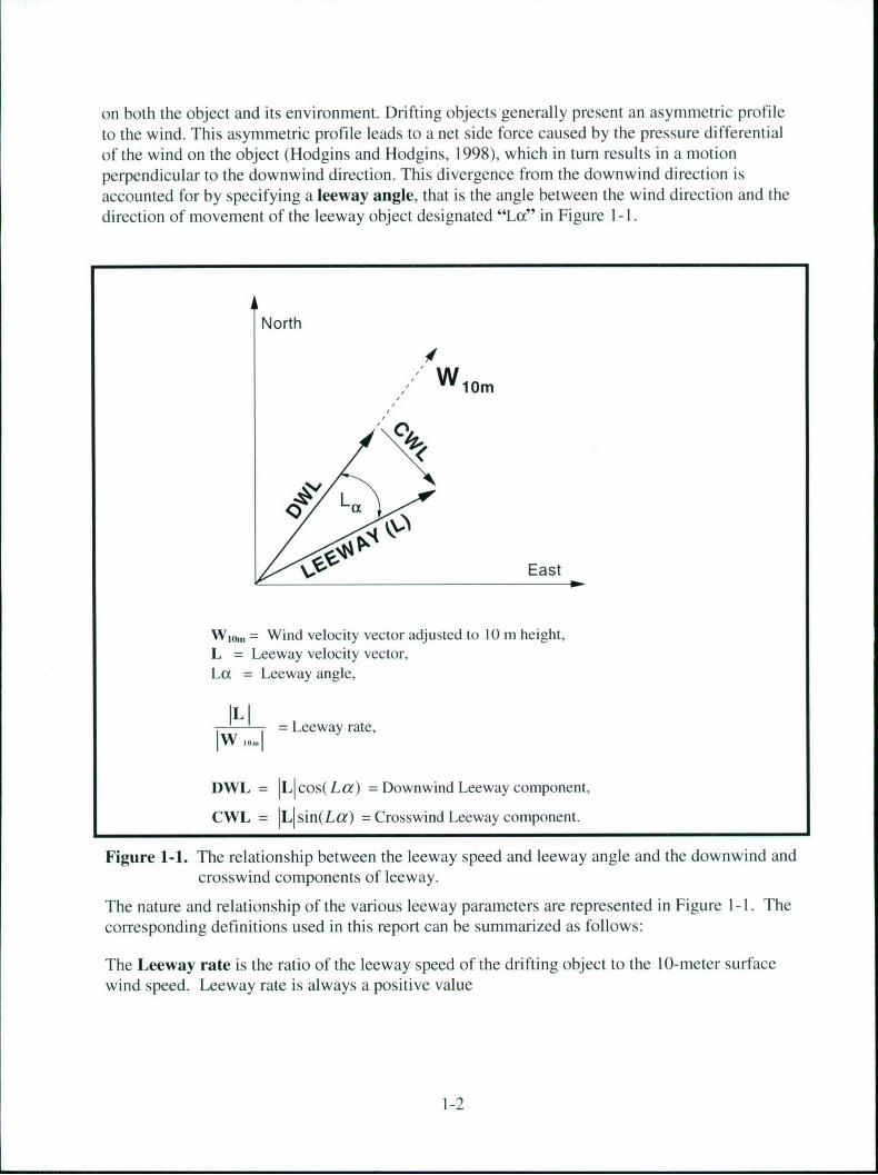
on both the object and its environment. Drifting objects generally present an asymmetric profileto the wind. This asymmetric profile leads to a net side force caused by the pressure differentialof the wind on the object (Hodgins and Hodgins, 1998), which in turn results in a motionperpendicular to the downwind direction. This divergence from the downwind direction isaccounted for by specifying a leeway angle, that is the angle between the wind direction and thedirection of movement of the leeway object designated "La" in Figure 1-1.

North

liem

East

W10.,= Wind velocity vector adjusted to 10 m height,L = Leeway velocity vector,La = Leeway angle,

IL - Leeway rate,

DWL = ILIcos(La) = Downwind Leeway component,

CWL = ILlsin(La) = Crosswind Leeway component.

Figure 1-1. The relationship between the leeway speed and leeway angle and the downwind andcrosswind components of leeway.

The nature and relationship of the various leeway parameters are represented in Figure 1-1. The

corresponding definitions used in this report can be summarized as follows:

The Leeway rate is the ratio of the leeway speed of the drifting object to the 10-meter surfacewind speed. Leeway rate is always a positive value

1-2

Leeway velocity vector (L) of a drifting object is the two-dimensional representation of the rateof the leeway object's motion through the water and the direction of motion relative to the windvelocity vector as shown in Figure l-1.

Leeway speed and leeway angle are the polar coordinate representation for the leeway velocityvector. Leeway speed is the rate of travel of the leeway object relative to the surface of theocean. Leeway angle is the angle between the wind direction and the direction of leeway driftfor a single sampling period for a particular drift object. Leeway angles to the right of the winddirection are designated as positive; leeway angles to the left of the wind direction are designatedas negative.

W10m is the surface wind speed adjusted to a height 10 meters above the water. This is thestandard meteorological convention for determining "surface winds." At a 10-meter height, it isassumed that the wind velocity is steady and not subject to the frictional boundary layer effectsof the ocean surface.

Downwind leeway (DWL) and Crosswind leeway (CWL) are the components of the leewayvelocity vector expressed in rectangular coordinates. Downwind leeway is the component in thedirection of the wind. Crosswind leeway is the component perpendicular to the wind direction.

A key parameter investigated in the report is the Divergence angle. As stated above, leewayangle refers to the angle between the direction of drift and downwind direction for a singlesampling period for a particular drift object. Over a number of sampling periods, leeway objectsof a given type may exhibit a range of leeway angles. In this report, divergence angle refers tothe representative range of leeway angles for a category of leeway objects. Divergence angle hasbeen calculated using different methods in different studies. It is calculated by obtaining the netleeway angle over time for a specific leeway object's drift trajectory, and then averaging againfor a series of leeway drift trajectories of a number of leeway objects in a leeway category, todetermine the mean leeway angle and standard deviation of the leeway angle for the category.Divergence angle is then calculated as twice the standard deviation of the leeway angle, or meanplus one standard deviation of the leeway angle, or mean plus two standard deviations of theleeway angle depending on the particular study. A more comprehensive discussion of howdivergence angle has been determined for this study is presented in Section 1.2.

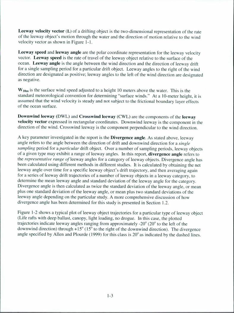
Figure 1-2 shows a typical plot of leeway object trajectories for a particular type of leeway object(Life rafts with deep ballast, canopy, light loading, no drogue. In this case, the plottedtrajectories indicate leeway angles ranging from approximately -20' (20' to the left of thedownwind direction) through +15' (15' to the right of the downwind direction). The divergenceangle specified by Allen and Plourde (1999) for this class is 200 as indicated by the dashed lines.

1-3

Maritime Life Rafts with Deep Ballast System and Canopy(with drogue, light loading)

60 1 1 , I

"-20° 200N I50-

S\ /

0 40N0 N/

E N /304

0N

E N /

N /

0320 N 1

10 ~ /

-- /

30 ' 1I I I-0 -20 -0010 20 30

Crosswind Displacement (kilometers)

Figure 1-2. Progressive vector diagrams (PVD) of trajectories relative to the downwinddirection for twenty experimental drift runs of 4-6 person maritime life raft withdeep-ballast system and canopy, light loading, no drogue. Markers are placed alongthe PVDs at 6-hour intervals. The twenty-degree divergence angles for this leewaycategory specified by Allen and Plourde (1999) are shown as dashed lines.

Two problems exist with the relationship between leeway angle and divergence angle. The firstis there is no one method for converting leeway angle statistics or analysis to a divergence angleestimate for a given leeway object category. Allen and Plourde (1999) used three differentmethods to develop divergence angle values based on the various leeway drift data sets. Thesecond problem is there are inconsistencies in how present search-planning tools (e.g. the CoastGuard Computer Assisted Search Planning and Automated Manual Solution models) specifyand incorporate the divergence angle concept in computing search areas.

These problems are avoided by using downwind and crosswind leeway (DWL and CWL)components as a function of wind speed, rather than the more-traditional use of leeway andleeway angle to compute the leeway drift over time. This approach is more consistent with thedynamics of leeway, as the physical mechanisms determining the downwind and crosswindcomponents are different. It also provides a more accurate method of determining leeway at low

1-4

wind speeds and is computationally easier to implement in SAR planning tools. To capitalize onthis advantage, Allen and Plourde demonstrated how DWL and CWL components could becalculated by linearly regressing the downwind and crosswind leeway components against windspeed. For given leeway object categories where leewaydrift data sets existed, DWL and CWLregression equations were developed. The DWL and CWL regression equations each require aseparate leeway speed coefficient (the value that W10m is multiplied by to compute leeway speedwhich corresponds to the slope of the linear regression), a Y-intercept term, and Standard Errorof the Estimate (Sy/,).

However, implementation of the DWL and CWL component approach is not completelystraightforward. First of all, the determination of the DWL and CWL regression equations for agiven category requires the existence of an adequate leeway drift data set. Secondly, althoughthere is a clear correlation between wind speed and DWL, the correlation between wind speedand CWL is less obvious (as demonstrated by Allen and Plourde (1999). There appear to beother factors beside wind speed that influence the crosswind component of leeway drift. Thirdly,there are a number of factors that influence whether a leeway object will initially drift to the rightor left of the wind, and observations indicate that the crosswind component can randomly changedirection under certain conditions. The phenomena of CWL direction and CWL directionchange have been largely unexplored. Each of these issues will be addressed in detail in thisreport.

1.2. Previous Studies Of Leeway Angle And Leeway Divergence

The relationship between wind speed, leeway angle and leeway divergence angle has beenaddressed in a number of previous studies starting in 1960. Chapline (1960); Hufford and Broida(1974); Nash and Willcox (1985, 1991); Fitzgerald, Finlayson and Allen (1994); Allen (1996);Allen and Fitzgerald (1997); and Kang (1999) all reported leeway drift that was not directlydownwind. Chapline (1960) also observed that those vessels with large underwater lateral planeshad an increased tendency to move off the downwind direction. He reported relative winddirection for sailing vessels of 9 to 13 points (101 to 146 degrees), but did not include what theirleeway angle or direction was. However, for fishing sampans, he reported relative winddirection of 10 points (112 ½/ degrees) and a leeway motion directly abeam. Chapline providedthe first reported leeway angle (2 points or 22 /2 degrees) for a commercial fishing vessel -Hawaii sampan.

Hufford and Broida (1974) provided leeway data including Leeway angle in tabular form forfour small craft (12 to 21 ft) and a 12-foot rubber raft. Four of the five targets were tested withand without (w/o) drogues; a 15-foot Barge was tested only without a drogue. Hufford andBroida's data for the four small craft were analyzed and are presented in Table 1-1 andFigure 1-3.

1-5

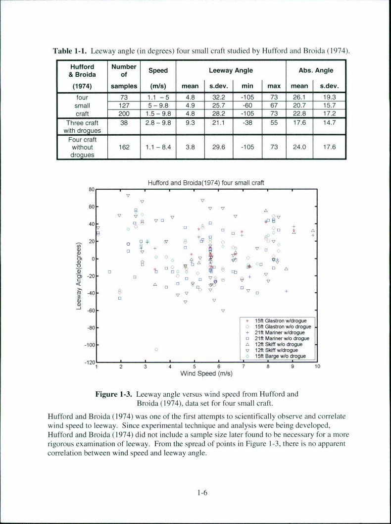
Table 1-1. Leeway angle (in degrees) four small craft studied by Hufford and Broida (1974).

Hufford Number Speed Leeway Angle Abs. Angle& Broida of

(1974) samples (m/s) mean s.dev. min max mean s.dev.

four 73 1.1 -5 4.8 32.2 -105 73 26.1 19.3small 127 5-9.8 4.9 25.7 -60 67 20.7 15.7craft 200 1.5-9.8 4.8 28.2 -105 73 22.8 17.2

Three craft 38 2.8-9.8 9.3 21.1 -38 55 17.6 14.7with droques

Four craftwithout 162 1.1 -8.4 3.8 29.6 -105 73 24.0 17.6drogues I I

Hufford and Broida(1974) four small craft80

x7

60-17 17 1A

40 75 5 5 "S+++ 0 +÷+

20 5± + 1 7

-2050

75-0 17+

" -60

+ 15ft Glastron w/drogue

-80 15ff Glastron w/o drogue+ 21ft Marner w/droguec] 21ft Manner w/o drogue

-100 A 12ft Skiff w/o droguev 12ft Skdff w/drogue

15ff Barge w/o drogue-1201•

1 2 3 4 5 6 7 8 9 10

Wind Speed (m/s)

Figure 1-3. Leeway angle versus wind speed from Hufford and

Broida (1974), data set for four small craft.

Hufford and Broida (1974) was one of the first attempts to scientifically observe and correlatewind speed to leeway. Since experimental technique and analysis were being developed,

Hufford and Broida (1974) did not include a sample size later found to be necessary for a more

rigorous examination of leeway. From the spread of points in Figure 1-3, there is no apparent

correlation between wind speed and leeway angle.

1-6

Allen and Plourde (1999) conducted a comprehensive review of previous leeway observationsand experiments reported in the literature to determine the types of leeway objects studied todate, the methods used during these studies, and the present level of understanding of leewaybehavior including the factors influencing the crosswind component of leeway and leewaydivergence. This effort was focused on determining the source and validity of the keyparameters (i.e., Leeway Rate and Divergence Angle) used to model leeway drift for variouscategories of leeway objects in the SAR Planning Tools employed by the SAR community.

Allen and Plourde (1999) investigated and reviewed the guidance provided by the National SARManual for use of leeway direction ("maximum angle off downwind"). The apparent source ofthis information is Hufford and Broida (1974), and Nash and Willcox (1985), but no specificreferences are cited, and it appears that the wording combines ideas from multiple sources. Theythen investigated in detail how leeway divergence was handled in the then-current versions ofNational SAR Manual and three SAR planning tools: the U. S. Coast Guard's GeographicDisplay Operations Computer (GDOC) Automated Manual Method (AMM), the U. S. CoastGuard's Computer Aided Search Planning (CASP) model, and the Canadian Search and RescuePrediction (CANSARP) program. They also introduced a new model (designated AP98) thatuses linear regression equations and variance of both the downwind and crosswind componentsof leeway (DWL and CWL) to predict the drift of SAR targets. AP98 incorporates many featuresof leeway behavior that have recently been observed in experiments, the most significant ofwhich is the inclusion of crosswind components of leeway to express the divergence of theleeway-object's trajectory from the downwind direction. A sensitivity study conducted as part ofAllen and Plourde (1999) showed that significant reductions in search area size (which couldlead to more efficient and more successful searches) could be achieved with the new AP98 DWLand CWL component model.

Allen and Plourde (1999) also devised and presented a comprehensive taxonomy for describingand categorizing the sixty-three types of leeway objects (vessels, life rafts and other driftingobjects). This taxonomy will facilitate assigning Leeway Rate and Divergence Angles to "new"categories of leeway objects based on existing leeway data. This taxonomy provides an orderlyframework for organizing and relating the leeway parameters derived from observations andexperiments on specific types of leeway objects, and applying them to similar types of leewayobjects for which data are not available. It also provides a structure for incorporating new typesof leeway objects (e.g. vessels, survival craft, and objects of maritime interest) that may beintroduced into maritime service as opposed to simply adding them to an ever-growing,unstructured list. The highest level, Level I, provides the major categories of leeway objects(e.g., Persons in Water, Vessels, Life Rafts, Debris, etc.). These major categories are thendivided into sub-categories in Level II and Level III based on the specific configurations of theleeway objects. The taxonomy as used in this report is depicted in Figure 1-4 below.

1-7

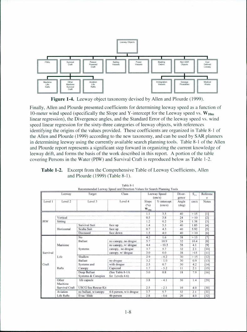
M

------,- I --- I

Figure 1-4. Leeway object taxonomy devised by Allen and Plourde (1999).Finally, Allen and Plourde presented coefficients for determining leeway speed as a function of

10-meter wind speed (specifically the Slope and Y-intercept for the Leeway speed vs. Wi~mlinear regression), the Divergence angles, and the Standard Error of the leeway speed vs. windspeed linear regression for the sixty-three categories of leeway objects, with referencesidentifying the origins of the values provided. These coefficients are organized in Table 8-1 ofthe Allen and Plourde (1999) according to the new taxonomy, and can be used by SAR planners

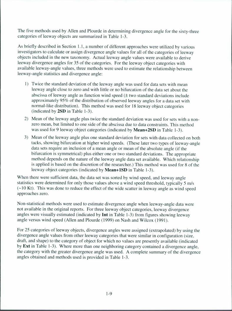
in determining leeway using the currently available search planning tools. Table 8-1 of the Allenand Plourde report represents a significant step forward in organizing the current knowledge ofleeway drift, and forms the basis of the work described in this report. A portion of the tablecovering Persons in the Water (P1W) and Survival Craft is reproduced below as Table 1-2.

Table 1-2. Excerpt from the Comprehensive Table of Leeway Coefficients, Allenand Plourde (1999) (Table 8-1).

Table 8-1Recommended Leeway Speed and Dinreetion Values aor eaarch Planning Tools

Leeway argfl a flass t Leeway Spert Dioer So Rthetbl1c Pao) i gence e

LTval I Level r L thevel 3 eivel 4 T Sale Y Lintercept C fAfglientms Noles

a Pl(%od (c(vs9 ((8g)

Verical 0.5 | 38s 24r Sea0c 1an2]

PIW Sitting 1.2 | 0.2 _2_4..... 1.38L (]-----------............Survi--val Suit face~up 14 5 s3 440 15 (4]

Loeewal Sc TarSuit Class up Speed Di7v3e40 - S_9 (5]rriDecesed acedwn15) 40 nc C4 0 6

No 4.2 L1e16 38 e 3 L7]

M iuen anupuoy, w/ drogue 4.4 -1013 38 4.1 (9] g

Systems canopy, no drogue 3.7 5.7 32 21i [1!01Survival cano y. dr ogue 3.0. 00 '- 38 ........... •t ! ilLif Shalo,, 29 -112 30 >15 [12]

Ballast L no drogue 1 3.2" . 1.0 f - 30 .. .: 0.9 [13]Craf t S stems and ...u..... 3 2.5 027 30 >4-2 [14] .... .

PI ltau CnpyI a ie 1.7 5.2 -iI 2. -- [" S

Sueepvallast fSeeTable-A u3.0 0L8 18 7.9 (16]

Other life iapsual 3.8 4u1 30 1. 291

Sureivalc(ral I-SCG eRescd eKt d2.5 2.1 'i) 7.40 [-30

ASyin oalstem anp _4n-6person~o drogue- 317 371 32 2.1 [10]

-r LifetRaf LEv . Slide 46-pnrsn 2.8 06 20 4.0 [12]

1-8

The five methods used by Allen and Plourde in determining divergence angle for the sixty-threecategories of leeway objects are summarized in Table 1-3.

As briefly described in Section 1. 1, a number of different approaches were utilized by variousinvestigators to calculate or assign divergence angle values for all of the categories of leewayobjects included in the new taxonomy. Actual leeway angle values were available to deriveleeway divergence angles for 35 of the categories. For the leeway object categories withavailable leeway-angle values, three methods were used to estimate the relationship betweenleeway-angle statistics and divergence angle:

1) Twice the standard deviation of the leeway angle was used for data sets with meanleeway angle close to zero and with little or no bifurcation of the data set about theabscissa of leeway angle as function wind speed (± two standard deviations includeapproximately 95% of the distribution of observed leeway angles for a data set withnormal-like distribution). This method was used for 18 leeway object categories(indicated by 2SD in Table 1-3).

2) Mean of the leeway angle plus twice the standard deviation was used for sets with a non-zero mean, but limited to one side of the abscissa due to data constraints. This methodwas used for 9 leeway object categories (indicated by Mean+2SD in Table 1-3).

3) Mean of the leeway angle plus one standard deviation for sets with data collected on bothtacks, showing bifurcation at higher wind speeds. (These later two types of leeway-angledata sets require an inclusion of a mean angle or mean of the absolute angle (if thebifurcation is symmetrical) plus either one or two standard deviations. The appropriatemethod depends on the nature of the leeway angle data set available. Which relationshipis applied is based on the discretion of the researcher.) This method was used for 8 of theleeway object categories (indicated by Mean+lSD in Table 1-3).

When there were sufficient data, the data set was sorted by wind speed, and leeway anglestatistics were determined for only those values above a wind speed threshold, typically 5 m/s(-10 Kt). This was done to reduce the effect of the wide scatter in leeway angle as wind speedapproaches zero.

Non-statistical methods were used to estimate divergence angle when leeway-angle data werenot available in the original reports. For three leeway object categories, leeway divergenceangles were visually estimated (indicated by Int in Table 1-3) from figures showing leewayangle versus wind speed (Allen and Plourde (1999) on Nash and Wilcox (1991).

For 25 categories of leeway objects, divergence angles were assigned (extrapolated) by using thedivergence angle values from other leeway categories that were similar in configuration (size,draft, and shape) to the category of object for which no values are presently available (indicatedby Ext in Table 1-3). Where more than one neighboring category contained a divergence angle,the category with the greater divergence angle was used. A complete summary of the divergenceangles obtained and methods used is provided in Table 1-3.

1-9

Table 1-3. Divergence angles for sixty-three categories of leeway objects and methodsused in their determination by Allen and Plourde (1999).

Leeway Object Category Oiv. MethodAng. Used

1 PIW 40 Ext2 PIW, Vertical 24 Ext3 PIW, Sitting 24 2SD4 PIW, Horizontal, Survival Suit 40 Mean + 1SD5 PIW, Horizontal, Scuba Suit 40 Ext6 PIW, Horizontal, Deceased 40 Ext7 Life Raft, No Ballast 38 Ext8 Life Raft, No Ballast, no canopy, no drogue 32 Mean + 1SD9 Life Raft, No Ballast, no canopy, w/ drogue 38 Mean + 1SD10 Life Raft, No Ballast, canopy, no drogue 32 Ext11 Life Raft, No Ballast, canopy, w/ drogue 38 Ext12 Life Raft, Shallow Ballast, canopy 30 Ext13 Life Raft, Shallow Ballast, canopy, no drogue 30 Mean + 2SD14 Life Raft, Shallow Ballast, canopy, with drogue 30 Mean + 1SD15 Life Raft, Shallow Ballast, canopy, capsized 11 Ext16 Life Raft, Deep Ballast, canopy 18 2SD17 Life Raft, Deep Ballast & Canopy, 4-6 pers 20 2SD18 Life Raft, D. Ballast & Canopy, 4-6 pers., no drogue 20 2SD19 Life Raft, D. Ballast & Canopy, 4-6 pers., no drogue, light load 20 2SD20 Life Raft, D. Ballast & Canopy, 4-6 pers, no drogue, heavy load 20 2SD21 Life Raft, Ballast & Canopy, 4-6 pers., drogue 16 2SD22 Life Raft, Ballast & Canopy, 4-6 pers., drogue, light load 32 2SD23 Life Raft, Ballast & Canopy, 4-6 pers., drogue, heavy load 27 2SD24 Life Raft, Ballast & Canopy, 15-25 pers 14 2SD25 Life Raft, Ballast &Canopy, 15-25 pers. no drogue, light load 12 2SD26 Life Raft, Ballast and Canopy, 15-25 pers. drogue, heavy load 12 2SD27 Life Raft, Capsized 16 Ext28 Life Raft, Swamped 11 Ext29 Survival Craft, Life Capsule 30 2SD30 Survival Craft, USCG Sea Rescue Kit 10 2SD31 Survival Craft, Aviation Life Raft, 4-6 pers, canopy, no drogue 32 Ext32 Survival Craft, Aviation Life Raft, Evac Slide, 4-6 pers 20 2SD33 Sea Kayak w/person on aft deck 20 2SD34 Surfboard w/ person 20 Ext35 Windsurfer w/ person and mast and sail in water 16 2SD36 Sailing Vessel, Monohull, full keel, deep draft 65 Ext37 Sailing Vessel, Monohull, fin keel, shoal draft 65 Ext38 Power Vessel, Skiff, flat bottom Boston Whaler 30 Int39 Power Vessel, V-hull, Std configuration 20 2SD40 Power Vessel, V-hull, Swamped 20 Ext41 Sports Boat, Cuddy Cabin, modified V-hull 25 Int42 Sport Fisher, Center Console, Open Cockpit 30 Int43 Commercial Fishing Vessels 65 Ext44 Commercial Fishing Vessels, Sampans 65 Ext45 Commercial Fishing Vessels, Side-stern troller 65 Ext46 Commercial Fishing Vessels, Longliners 65 Ext47 Commercial Fishing Vessels, Junk 65 Mean +1SD48 Commercial Fishing Vessels, Gill Netter 45 Mean + 1 SD

1-10

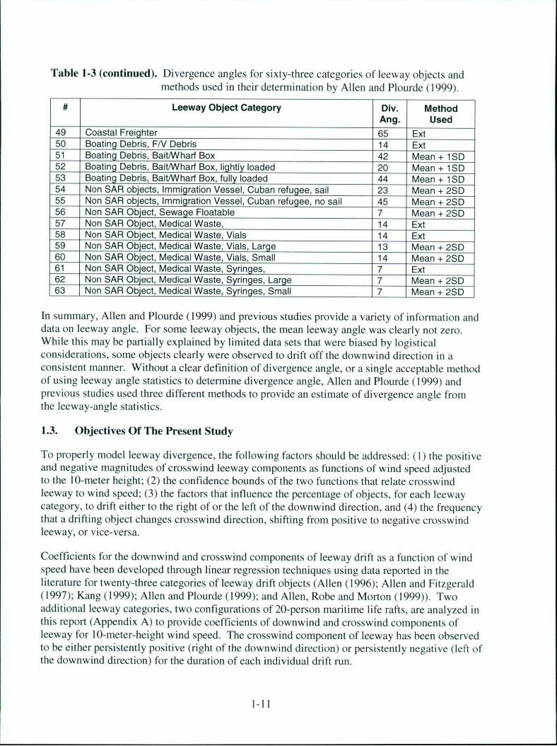
Table 1-3 (continued). Divergence angles for sixty-three categories of leeway objects andmethods used in their determination by Allen and Plourde (1999).

# Leeway Object Category Div. MethodAng. Used

49 Coastal Freighter 65 Ext50 Boating Debris, FN Debris 14 Ext51 Boating Debris, Bait/Wharf Box 42 Mean + 1SD52 Boating Debris, Bait/Wharf Box, lightly loaded 20 Mean + 1 SD53 Boating Debris, Bait/Wharf Box, fully loaded 44 Mean + 1SD54 Non SAR objects, Immigration Vessel, Cuban refugee, sail 23 Mean + 2SD55 Non SAR objects, Immigration Vessel, Cuban refugee, no sail 45 Mean + 2SD56 Non SAR Object, Sewage Floatable 7 Mean + 2SD57 Non SAR Object, Medical Waste, 14 Ext58 Non SAR Object, Medical Waste, Vials 14 Ext59 Non SAR Object, Medical Waste, Vials, Large 13 Mean + 2SD60 Non SAR Object, Medical Waste, Vials, Small 14 Mean + 2SD61 Non SAR Object, Medical Waste, Syringes, 7 Ext62 Non SAR Object, Medical Waste, Syringes, Large 7 Mean + 2SD63 Non SAR Object, Medical Waste, Syringes, Small 7 Mean + 2SD

In summary, Allen and Plourde (1999) and previous studies provide a variety of information anddata on leeway angle. For some leeway objects, the mean leeway angle was clearly not zero.While this may be partially explained by limited data sets that were biased by logisticalconsiderations, some objects clearly were observed to drift off the downwind direction in aconsistent manner. Without a clear definition of divergence angle, or a single acceptable methodof using leeway angle statistics to determine divergence angle, Allen and Plourde (1999) andprevious studies used three different methods to provide an estimate of divergence angle fromthe leeway-angle statistics.

1.3. Objectives Of The Present Study

To properly model leeway divergence, the following factors should be addressed: (1) the positiveand negative magnitudes of crosswind leeway components as functions of wind speed adjustedto the 10-meter height; (2) the confidence bounds of the two functions that relate crosswindleeway to wind speed; (3) the factors that influence the percentage of objects, for each leewaycategory, to drift either to the right of or the left of the downwind direction, and (4) the frequencythat a drifting object changes crosswind direction, shifting from positive to negative crosswindleeway, or vice-versa.

Coefficients for the downwind and crosswind components of leeway drift as a function of windspeed have been developed through linear regression techniques using data reported in theliterature for twenty-three categories of leeway drift objects (Allen (1996); Allen and Fitzgerald(1997); Kang (1999); Allen and Plourde (1999); and Allen, Robe and Morton (1999)). Twoadditional leeway categories, two configurations of 20-person maritime life rafts, are analyzed inthis report (Appendix A) to provide coefficients of downwind and crosswind components ofleeway for 10-meter-height wind speed. The crosswind component of leeway has been observedto be either persistently positive (right of the downwind direction) or persistently negative (left ofthe downwind direction) for the duration of each individual drift run.

1-11

In this report, we lay the groundwork to model the leeway drift of all 63 categories of leewayobjects reported in Allen and Plourde (1999) using the DWL and CWL component approach.The relationship between DWL and CWL components and leeway speed/divergence angle isestablished in Chapter 2. We use the 23 categories of leeway objects (plus the two additionalcategories analyzed in Appendix A) that contained values for both the downwind and crosswindcomponents of leeway and leeway speed and divergence angle. We assume that the relationshipbetween DWL and CWL components and leeway speed/divergence angle established for the 25leeway categories holds true for additional 38 leeway categories, provided by Allen and Plourde(1999) that contain values for leeway speed and divergence angle only. Thus, assuming thisconsistency, a procedure is established for estimating the downwind and crosswind componentsof leeway for these additional 38 leeway categories. Future numerical search planning tools willuse downwind and crosswind components of leeway rather than leeway speed and divergenceangle. Therefore, the entire set of downwind and crosswind components of leeway for all 63categories are provided in tabular form (Tables 3-1 and 3-2) in Chapter 3.

Chapter 4 addresses the factors influencing the change in sign of the crosswind leewaycomponent. Though the physics of drifting object, crosswind direction change was notinvestigated, statistical review showed that changes in crosswind motion do occur. Furtherstatistical analysis was conducted to determine any correlation between various factors and thechange in crosswind leeway motion. A sensitivity study of search area distributions withdifferent change frequencies in crosswind direction was conducted to identify a specific signchange frequency that can be used in SAR planning models.

Chapter 5 is the report summary, with recommendations for incorporating this new leewaymodeling approach in SAR planning tools, and further refining leeway determinationmethodology.

1-12

CHAPTER 2.

METHOD FOR ESTIMATING DOWNWIND AND CROSSWINDCOMPONENTS OF LEEWAY FROM LEEWAY SPEED AND

DIVERGENCE ANGLE

2.1. Approach Used In Determining Downwind And Crosswind Components Of Leeway

Allen and Plourde (1999) present a complete set of values for calculating leeway drift for sixty-three categories of leeway objects. Allen and Plourde's Table 8-1 includes leeway speed(expressed as a percentage of the wind speed adjusted to a height of 10 meters (Wiom)),divergence angle and standard error of the estimate (Sy/,). Present manual and numerical searchplanning tools use the leeway speed and divergence angle for determining the leeway drift ofleeway objects. However, there are inherent limitations when using leeway speed anddivergence angle for prediction of an object's leeway behavior. Specifically, the use of leewayspeed and leeway angle does not account for the fact that different physical mechanisms governthe downwind component of leeway drift (DWL) and the crosswind component of leeway drift(CWL). Although both DWL and CWL would be difficult to model analytically because of thecomplex physics involved, a statistical model can account for this difference. In addition, theprediction of leeway drift using leeway speed and divergence angle as a function of windbecomes unreliable at low wind speeds (less than 5 m/s). Expressing leeway behavior in termsof downwind and crosswind components of leeway as functions of Wiom overcomes theselimitations.

New tools that use numerical methods to estimate search distribution areas will use downwindand crosswind component (DWL and CWL) of leeway as functions of Wiom, rather than leewayspeed as a function of W10m and divergence angle. Developing linear regression leeway valuesfor DWL and CWL is a straightforward process. Allen and Plourde (1999) developed thesevalues for 23 leeway object categories. Two additional categories were analyzed here, withthose DWL and CWL linear regression values presented in Appendix A. This leaves 38categories in the Allen and Plourde leeway taxonomy without DWL and CWL linear regressionvalues because there are no actual leeway drift data available for regression analysis. Thepurpose of this chapter is to present a scheme for estimating the DWL and CWL linearregression coefficients for these 38 categories.

Two variations of linear-regression analysis can be used to derive the coefficients for thedownwind and crosswind components of leeway versus Wlom. Normally, linear regressions areunconstrained, and have a slope term (here, leeway speed coefficient) and a y-intercept term. Avariant is where the regression is constrained to pass through the origin.

The advantage of an unconstrained linear regression is a better statistical representation of a dataset than represented by a constrained linear regression (that is, a better fit of the regression line tothe data) over a greater range. For the data examined here, the unconstrained regressiongenerally has a better "fit" at low and high wind speeds. However, because an unconstrainedregression yields a y-intercept term, this could mean that leeway drift occurs in the absence ofany wind, going against the traditional concept of leeway. Additional rules, guidance orprocedures must account for the zero-wind speed (with undefined wind direction) case. In

2-1

numerical search-planning tools using Monte-Carlo simulation, this could result in a significantprocessing burden to account for an extremely rare event. Though the constrained linearregression does not provide as good a "fit" at lower wind speed, it does, by its very nature,reflect zero leeway at zero wind speed. In practice, SAR Planners are developing models thatuse both approaches; therefore, both methods of statistical regression were determined.

The procedures of Neter, Kutner, Nachtsheim and Wasserman (1996) were used for determiningthe unconstrained linear regression and the constrained linear regression. Both unconstrainedand constrained linear regressions of the downwind and crosswind components of leeway weredetermined and are presented in Chapter 3.

As described above, the coefficients for downwind and crosswind leeway versus W1 0 m1 equationsfor twenty-three of the sixty-three leeway categories have been determined experimentally andcan be found in the literature (Allen, 1996; Allen and Fitzgerald, 1997; Allen and Plourde, 1999;Allen et al. 1999; and Kang 1999). The DWL and CWL as functions of W10m for two additionalleeway categories are analyzed from experimental data and are presented in Appendix A. Thetwo additional categories are maritime life rafts (deep ballast, canopy, 15-25 person capacity)with either no-drogue with light loading or the same rafts with a drogue and heavy loading. Inaddition, there were a number of leeway categories with experimentally observed leeway driftdata for which unconstrained regression analysis have been completed, but no analysis showingconstrained linear regressions. The analyses of the constrained linear regression for these leewaycategories are presented in Appendix B.

In order to present a complete set of coefficients for all sixty-three leeway categories, theremaining thirty-eight categories required development of the coefficients for the downwind andcrosswind component leeway equations. A relationship between the downwind and crosswindregression coefficients and leeway speed and divergence angle values (presented by Allen andPlourde (1999)) was derived from the DWL and CWL coefficients previously developed for thetwenty-five categories for which leeway drift data were available. The relationships between thestandard errors of the leeway speed equation derived from experimental leeway field data and theDWL and CWL equations were also estimated. The methodology and assumptions used todevelop the 38 additional sets of regression coefficients is described in detail below.

2.2. Estimation Of Downwind And Crosswind Coefficients Based On Leeway Speed AndDivergence Angle

The regression coefficients for downwind and crosswind components of leeway for the thirty-eight categories without data were estimated as follows. First, we assume that the slopes of theregression lines for the DWL and CWL regressions (that is the leeway speed coefficients forboth components) are related to the slope of the overall leeway speed vs. wind speed regression.The slope of the leeway speed vs. wind speed regression (designated Slope (%)Wiom in Table1-2) is the coefficient by which the wind speed is multiplied to compute leeway speed in thetraditional method of calculating leeway drift. Based on the geometry presented in Figure 1 -1, itis assumed that a similar relationship holds for computing DWL and CWL, and that linearregression coefficients can be determined for DWL and CWL. The component leeway speedcoefficients are designated as DWL Slope and CWL Slope. It is further assumed that DWLSlope and CWL Slope are linearly related to Leeway Speed Slope by the cosine and sine of an

2-2

angle proportional to the Divergence angle, since the Divergence angle is a statisticalrepresentation of the Leeway angles observed for a certain category of leeway objects. TheDivergence Angle is adjusted by a second coefficient of proportionality designated as theAdjustment Factor to provide this angle. The relationship is shown in equation form below:

xcsn( Divergence Angle )2-Predicted DWL slope = Leeway speed slope x cosine ic 2-1

( Adjustment Factor)

Predicted CWL slope = Leeway speed slope x sine Divergence Angle) 2-2

The divergence angles used to determine the Adjustment Factor and DWL and CWL slopes arethose presented for the 25 leeway categories for which both leeway components and leewayspeed regressions versus wind speed have been completed. These values are available in Table8-1 in Allen and Plourde (1999). The approach used in this chapter is to determine theAdjustment Factor based on "tuning" Equations 2-1 and 2-2 to provide the best overall statisticalfit for the 25 leeway categories for which data are available, and assume that the sameAdjustment Factor applies to the remaining 38 leeway object categories for which data are notavailable.

The optimum Adjustment Factor was determined empirically as follows. The Adjustment Factorwas varied from 1.0 to 2.0 and the values of Predicted DWL and CWL Slope computed usingequations 2-1 and 2-2. The predicted values of DWL and CWL were then compared to theactual values of the DWL and CWL Slope obtained from the linear regressions using the actualdata for the twenty-five leeway categories. A linear unconstrained regression of the predictedvalues of DWL and CWL against the actual values of DWL and CWL were calculated.

If equations 2-1 and 2-2 were perfect predictors of DWL and CWL, the regressions of PredictedDWL and CWL Slope against Actual DWL and CWL Slope would have linear regression slopesof 1.0, zero intercepts, r2 of 1.0 and Sy/x of 0.0. Note: The coefficient of determination (r2) is theratio of the variability in the dependent variable explained by regression line to the originalvariability about the mean observations. The r2 is an estimate of the variance accounted for bythe regression. The standard error of estimate (Sy/,) is an estimator for the standard deviation ofthe dependent variable about the regression line. Further explanations of r2 and Sy/, can be foundin Chapter 3 of Allen (1996). The Absolute Slope Difference from 1.0 for the linear regressionslopes for the Predicted vs. Actual Slope regressions versus Adjustment Factor (varied from 1.0to 2.0) are plotted in Figure 2-1. The coefficients of the regression of the predicted DWL andCWL Slopes versus actual DWL and CWL Slopes are shown in Table 2-1.

2-3

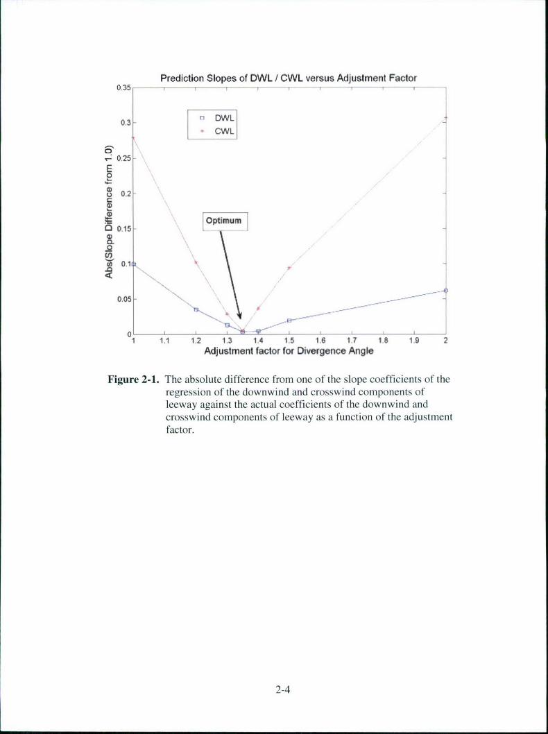
Prediction Slopes of DWL / CWL versus Adjustment Factor0,35 ---

n~ DWL *

0.3 OWL

CWL

S0.25E

o 0.2

.15 Optimum

o 0.15 -

4)

010~

0.050.05 ---.......----

1 1.1 1.2 1.3 1.4 1.5 1.6 1.7 1.8 1.9 2Adjustment factor for Divergence Angle

Figure 2-1. The absolute difference from one of the slope coefficients of theregression of the downwind and crosswind components ofleeway against the actual coefficients of the downwind andcrosswind components of leeway as a function of the adjustmentfactor.

2-4

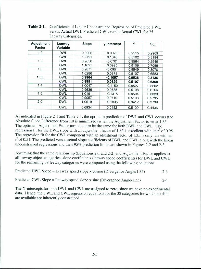
Table 2-1. Coefficients of Linear Unconstrained Regression of Predicted DWLversus Actual DWL Predicted CWL versus Actual CWL for 25Leeway Categories.

Adjustment Leeway Slope y-intercept r2 SyxFactor Variable

1.0 DWL 0.9006 0.0025 0.9515 0.2909CWL 1.2791 0.1348 0.5102 0.8194

1.2 DWL 0.9650 -0.0701 0.9564 0.2949CWL 1.1021 0.0995 0.5106 0.7055

1.3 DWL 0.9871 -0.0951 0.9549 0.3070CWL 1.0286 0.0878 0.5107 0.6583

1.35 DWL 0.9964 -0.1057 0.9538 0.3136CWL 0.9951 0.0829 0.5107 0.6368

1.4 DWL 1.0047 -0.1152 0.9527 0.3202CWL 0.9636 0.0785 0.5108 0.6166

1.5 DWL 1.0191 -0.1315 0.9504 0.3330CWL 0.9057 0.0710 0.5108 0.5795

2.0 DWL 1.0619 -0.1805 0.9412 0.3799CWL 0.6934 0.0482 0.5109 0.4436

As indicated in Figure 2-1 and Table 2-1, the optimum prediction of DWL and CWL occurs (theAbsolute Slope Difference from 1.0 is minimized) when the Adjustment Factor is set at 1.35.The optimum Adjustment Factor turned out to be the same for both DWL and CWL. Theregression fit for the DWL slope with an adjustment factor of 1.35 is excellent with an r2 of 0.95.The regression fit for the CWL component with an adjustment factor of 1.35 is only fair with anr2 of 0.51. The predicted versus actual slope coefficients of DWL and CWL along with the linearunconstrained regressions and their 95% prediction limits are shown in Figures 2-2 and 2-3.

Assuming that the same relationship (Equations 2-1 and 2-2) and Adjustment Factor applies toall leeway object categories, slope coefficients (leeway speed coefficients) for DWL and CWLfor the remaining 38 leeway categories were computed using the following equations.

Predicted DWL Slope = Leeway speed slope x cosine (Divergence Angle/1.35) 2-3

Predicted CWL Slope = Leeway speed slope x sine (Divergence Angle/1.35) 2-4

The Y-intercepts for both DWL and CWL are assigned to zero, since we have no experimentaldata. Hence, the DWL and CWL regression equations for the 38 categories for which no dataare available are inherently constrained.

2-5

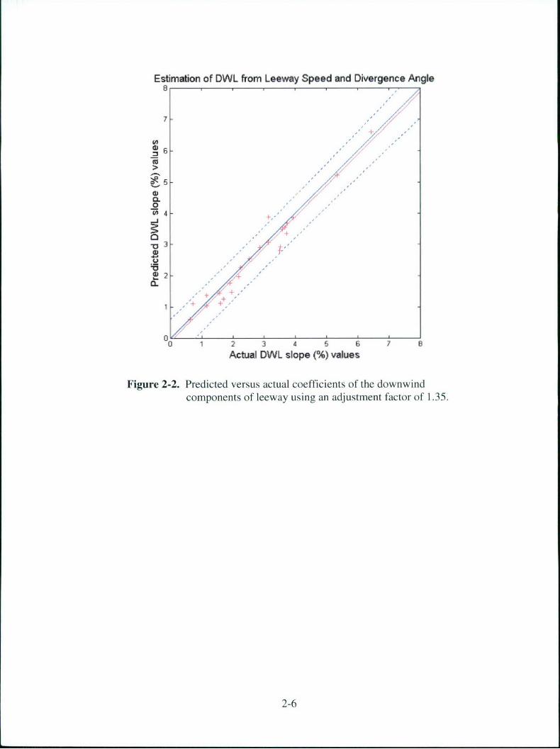
Estimation of DWL from Leeway Speed and Divergence Angle

7

S6 /

0 441

//", +

0 "

0 1 2 3 4 6 6 7 8Actual DWL slope ('A) values

Figure 2-2. Predicted versus actual coefficients of the downwindcomponents of leeway using an adjustment factor of 1.35.

2-6

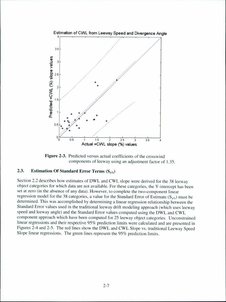
Estimation of CWL from Leeway Speed and Divergence Angle4

35-

_Z 3 . .

S2.5

CL +

0.5 +

0 0.5 1 15 2 25 3 3.5 4

Actual +CWL slope (%) values

Figure 2-3. Predicted versus actual coefficients of the crosswind

components of leeway using an adjustment factor of 1.35.

2.3. Estimation Of Standard Error Terms (SY/.)

Section 2.2 describes how estimates of DWL and CWL slope were derived for the 38 leewayobject categories for which data are not available. For these categories, the Y-intercept has beenset at zero (in the absence of any data). However, to complete the two-component linearregression model for the 38 categories, a value for the Standard Error of Estimate (Sy/,) must bedetermined. This was accomplished by determining a linear regression relationship between theStandard Error values used in the traditional leeway drift modeling approach (which uses leewayspeed and leeway angle) and the Standard Error values computed using the DWL and CWLcomponent approach which have been computed for 25 leeway object categories. Unconstrainedlinear regressions and their respective 95% prediction limits were calculated and are presented inFigures 2-4 and 2-5. The red lines show the DWL and CWL Slope vs. traditional Leeway SpeedSlope linear regressions. The green lines represent the 95% prediction limits.

2-7

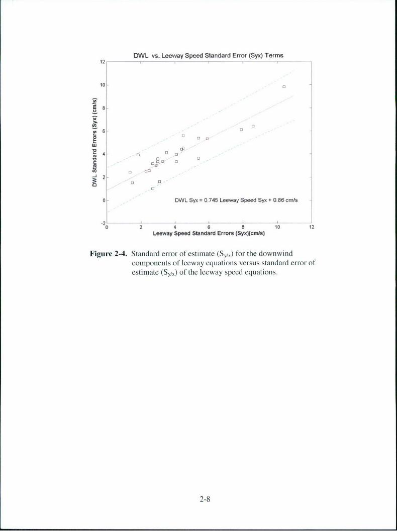
DWL vs. Leeway Speed Standard Error (Syx) Terms

12

10

E28•

(0 r 3 -

Ii3

0 DWL Syx = 0.745 Leeway Speed Syx + 0.86 crrds

-21"0 2 4 6 8 10 12Leeway Speed Standard Errors (SyxXcmnIs)

Figure 2-4. Standard error of estimate (Sy/,) for the downwindcomponents of leeway equations versus standard error ofestimate (Sy/,) of the leeway speed equations.

2-8

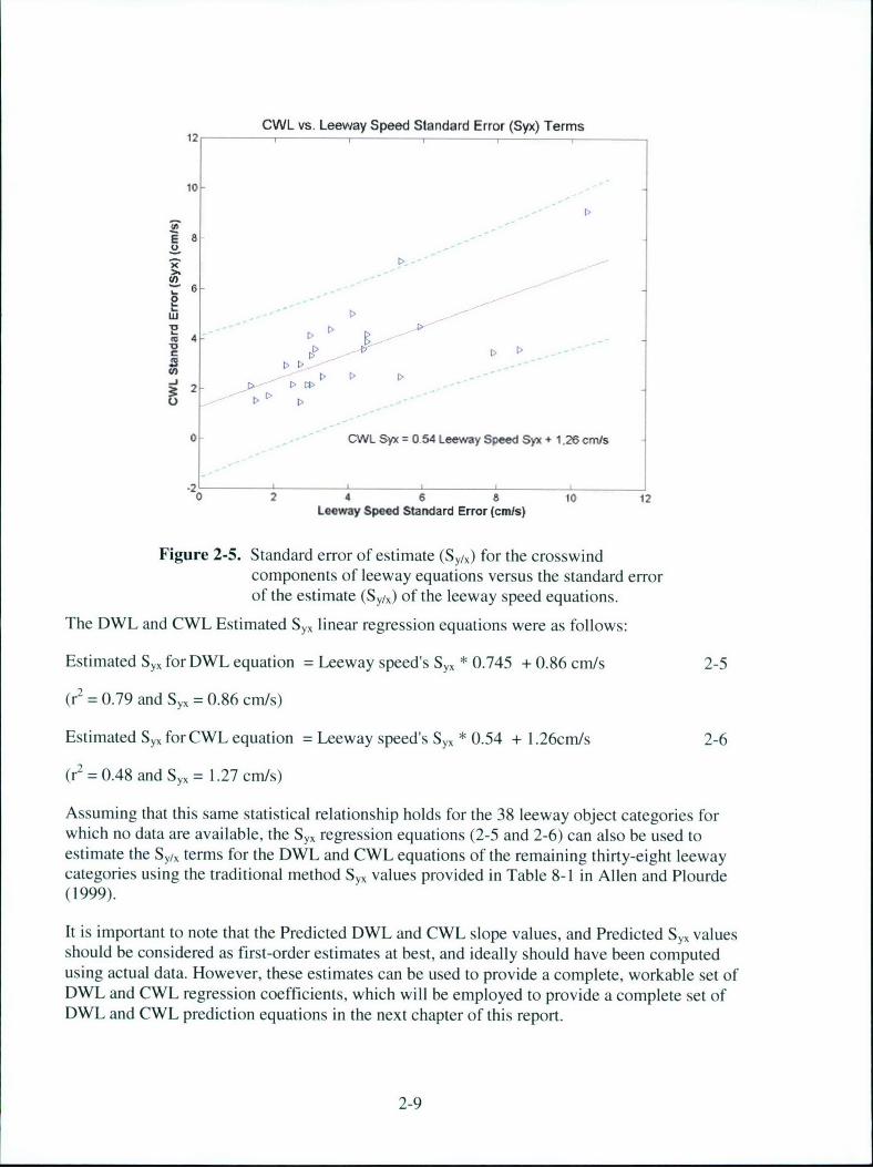
CWL vs. Leeway Speed Standard Error (Syx) Terms12 ,

10

E

t/)

0 CWL Syx054 Leeway Speed Syx+ 1,26 cm/s

-20124 6 $01

Leeway Speed Standard Error (cmls)

Figure 2-5. Standard error of estimate (Sy,/) for the crosswindcomponents of leeway equations versus the standard errorof the estimate (Sy,/) of the leeway speed equations.

The DWL and CWL Estimated Sy,, linear regression equations were as follows:

Estimated SYX for DWL equation = Leeway speed's S),X * 0.745 + 0.86 cm/s 2-5

"(r = 0.79 and S = 0.86 cm/s)

Estimated SYV for CWL equation = Leeway speed's Sey. * 0.54 + 1.26cm/s 2-6

(re2 = 0.48 and St. = 1.27 cm/s)

Assuming that this same statistical relationship holds for the 38 leeway object categories forwhich no data are available, the Syx regression equations (2-5 and 2-6) can also be used toestimate the Sy terms for the DWL and CWL equations of the remaining thirty-eight leewaycategories using the traditional method Sy, values provided in Table 8-1 in Allen and Plourde(1999).

It is important to note that the Predicted DWL and CWL slope values, and Predicted Syx valuesshould be considered as first-order estimates at best, and ideally should have been computedusing actual data. However, these estimates can be used to provide a complete, workable set ofDWL and CWL regression coefficients, which will be employed to provide a complete set ofDWL and CWL prediction equations in the next chapter of this report.

2-9

CHAPTER 3.

COMPILING A COMPREHENSIVE SET OF DOWNWIND ANDCROSSWIND LEEWAY COEFFICIENTS

The methodology outlined in Chapter 2, was used to produce estimates of the predicted leewayspeed slope and predicted Sy/, values for determining downwind and crosswind components forthirty-eight leeway categories for which actual leeway data are not available. The Y-interceptvalue in the DWL and CWL linear regression equations has been set at zero. In addition, theactual DWL and CWL linear regression values have been computed by applying linearregression analysis to actual data as reported in Allen and Plourde (1999) (for 23 leeway objectcategories) and in Appendix A of this report (for 2 additional leeway categories). Together, theselinear regression coefficients constitute a complete set for implementing a DWL and CWL linearregression model for predicting leeway drift for all 63 leeway object categories in the Allen andPlourde (1999) taxonomy.

This complete set of "optimally estimated" linear regression coefficients is provided in Tables 3-1 and 3-2 for the unconstrained and constrained linear regression models, respectively. Both setsare provided as both approaches are being used by SAR Planners in modeling leeway drift. Thedifference between the two sets in Table 3-1 and 3-2 are described as follows:

1) Table 3-1 Unconstrained Values - The unconstrained linear regression approach providesa statistically "pure" set of leeway linear regression coefficients, providing the beststatistical fit with actual data. However, it produces non-zero leeway drift at zero windspeed, which contradicts the traditional assumption of zero leeway at zero wind speed.This also introduces the need for additional computational rules or procedures for zero-wind case predictions.

2) Table 3-2 - Constrained Values - The constrained linear regression approach requiresthat the regression line pass through the origin, which reflects the traditional assumptionof zero leeway at zero wind speed. This approach is more computationally efficient (i.e.,does not require additional computational rules for the zero-wind case), but does not fitthe actual data as well, and can produce less accurate predictions at wind speeds thatapproach the higher and lower limits of wind speeds recorded in the actual data sets.

Both Tables 3-1 and 3-2 are similar in organization to Table 8-1 of Allen and Plourde (1999)which presented a complete set of leeway drift coefficients (Slope, Divergence angle, and Sy/x)for computing leeway drift for all 63 leeway categories using traditions (non-component) leewaymodels. Values in Table 3-2 that differ from the corresponding value in Table 3-1 are shown inbold.

Tables 3-1 and 3-2 are organized as follows:

The first four columns in Tables 3-1 and 3-2 delineate the leeway object for which the coefficientsare used and reflect the leeway taxonomy introduced by Allen and Plourde (1999). The boldhorizontal lines separate Level I categories.

3-1

The fifth column of Table 3-1 and 3-2 gives slope coefficients (in units of cm/s per m/s, whichcorresponds to a %) of the downwind component of leeway versus 10-m wind speed (W10m) linearregression equation

Downwind Leeway (cm/s) = [Slope (%) x Wmom(m/s)] + y-intercept (cm/s) 3-1

The sixth column is the y-intercept term (cm/s) of equation 3-1. The seventh column is the standarderror of estimate (Sy/x, in units of cm/s) for equation 3-1, that was directly determined for those 25categories for which experimental data were available, or estimated using equation 2-5 for the 38categories for which data are unavailable. Note that in Table 3-1, the y-intercept is always set to zero.

The eighth and ninth columns are the coefficients (slope and y-intercept, respectively) of the positivecrosswind component of leeway versus 10-m wind speed (W10m) linear regression equation.

Positive crosswind Leeway (cmns) = [Slope (%) x Wm0m(m/s)] + y-intercept (cm/s) 3-2

Again note that in Table 3-2 the y-intercept is set to zero.

The tenth column is the standard error of estimate (Sy/,, in units of cm/s) for equation 3-2 that wasdirectly determined for those 25 categories for which experimental data were available, or estimatedusing equation 2-6 for the 38 categories for which data are unavailable.

The eleventh and twelfth columns of Table 3-1 and 3-2 are the coefficients (slope and y-intercept,respectively) of the negative crosswind component of leeway versus 10-m wind speed (W10m)unconstrained linear regression equation.

Negative crosswind Leeway (cin/s) = [Slope (%) x Wlom(n/s)] + y-intercept (cm/s) 3-3

Again note that in Table 3-2 the y-intercept is set to zero.

The thirteenth column is the standard error of estimate (Sy/x, in units of cm/s) for equation 3-3thatwas directly determined for those 25 categories for which experimental data were available, orestimated using equation 2-6 for the 38 categories for which data are unavailable.

In Table 3-1, the fourteenth column is the wind speed (m/s) at the intersection of the two crosswindregression equations. The fifteenth column contains the rule for applying the crosswind componentsfor winds speeds below the intersection wind speed. If column fifteen is negative-one (- 1) then thenegative crosswind equation alone is used when the wind speed is below the intersection wind speed.If column fifteen is positive-one (+ 1) then the positive crosswind equation alone is used when thewind speed is below the intersection wind speed. If column fifteen is zero (0), then both crosswindequations are used equally for all wind speeds. Because Table 3-2 represents the constrainedregression, these two columns are omitted.

The last column includes reference notes for that leeway category. Reference notes follow eachtable.

3-2

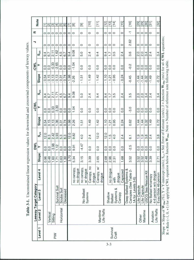
o 01 - 0 LI)O ( 1)00 loV 00000000 0 0 0 000 0 "*" 0000 0

-, CDj 00aooooo ot I, to oo 0 ooS"" -••-(O L•I)• •"0 0 "• '• •-I" I•• (0" 0 0 •"•" •

3) D o C o -It00)0) LI) N 0) 0)olr M C ) -C)N C

o U.)-- 0 c 0 0 0 000 0 0000 0 d"

0) 66C59 C6oa656 c 6 6 0i o66 6 9 666C56 0 o

& q LO COD( -l Tc 0) N 0 -LO)~ I o~'0

C o o o ,1OL Ol,-T ~jr_ U) CO r- MII• NI E -0 • o •, 0,

0 N0 N LI) l' yýI t It -N0) Nt ,r-

0 o66o- -i c; ~-6 6 6ý 0 0

ca . . . C C5 E.-. ,

00CC

"oC-o o 0 o0 -J • • ,-- D, . . )

"T 9 U) Lo '-L It~ 0ý q ll rNlI ) LQ 9I 006 (6 C\J-tTCD0, i0) LO) N 0Y) 0)-C') (\J c') C~j Cr)m CrO

00Cr) .00 0 0 0 00 0 o 00 oi C 5 C I666 o 6 o o o 6 C 66o 6

CL It Oco) i~CD t - 0) N~ 0 -LOI) cl N1 m~~0 N z_ o mc r ~ LI) 4 C~ ~ 0) C'~i (D ;Cr I M I r- (

o o 0 _:C5) ON~C 0 0 0E

~~~~~I wo "-0•n •I • • • r

• -- C: ") CrC R I? 'I: c0 C\ U? n o q 0ý COMC -qI W- N C

3 -- J

z 0o> 0' 00 coo0 00) o 0 0 0 ?00 0 0000

0i oo-6o I? c '0 6 oi o65 6i C5o11 6ooo 60

CD CO CO C LI) 0) LO) CO D c D~ CDj No N CD)0-)- q .~rc Z..co r) Acr) to (0 0) Cr) (.0 LI) LO LOIq CO) r- 0

C5 6o- .- ' Li) vic') Cr) N NNN - co C6 )iCrNCV)* N~

- 0 0

(1) CCi0d?CLo2~ oC2c:3 9 OCV-M

ca 2 2 2 E O1 crw 0 - 0)Ma)C

0* 0I~ 0 2 o: 0 n C C ýo

cn a) cc3: Jtm w4 0 6E ca C

Z 0 ->1 -E - m m => o E 0 E M 0 a

S5 o ao_j) I: ( )c

-J c i- c

Q3-

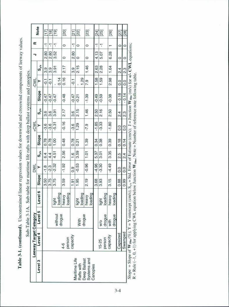
0.

o 0 0 0c DOr, cO

Z -i - NC'D N -OJJ N C'

SC C C6 0 0 0 0 ,r '- 0 0 cr00) 0 Cf

,"i 0Y• ,-) C•. m, COJ tad C COjC~NNJ 0t NO 0) 00f ) 00

: , ,7 1 ý Lq L ý'0 1 N- ,•- C5 tw

- -

o-r l o r 0)O))O 0~ a)N co ~c I

E mi d ,. c, "75 67 oo "3

0 1~CC N 99' 9- 19191 - - - ,CJ- 0.0

z" C: r_.: 6 l 6

>)2D ,- 0, CD ) 0 oo

= -o w LO C0 0

-t: NN C D N-000 co c 0) "*0)0) qC E

*6 ci o5oo o- - oo 6 o C M0ý- -0E

. - N o ) r- -0 . .LO-

-ý eecr q - ý C- q- C- U? 11 -

co N - c)

0) CfC) co -

C j ( 0--m

O ~~~~C ~C CD0 C C- 0)i

"0 0 90 C 6 6 i

0 r- N) 0) - ND aN.. V5 -r CC vi) Nvivi-.6 0S 0)C.) c 1a 9 *I

O.ý.C *~ cY 'a ca Co CD O u

-NN - 0 .P0 -C 0~.v .0J=

0 to0. ý -06 C :30 (.2

0) -CD ) C 1) cr

0 C NN CD 0 0) - (O ) - D2

--

40 (0 46 7a

(D a ~ I CL c . w 4.20

W -a LO .r w c02

+

oo Co 02

-- 0 -ic u law c

6)U' 0l

C~h3-4

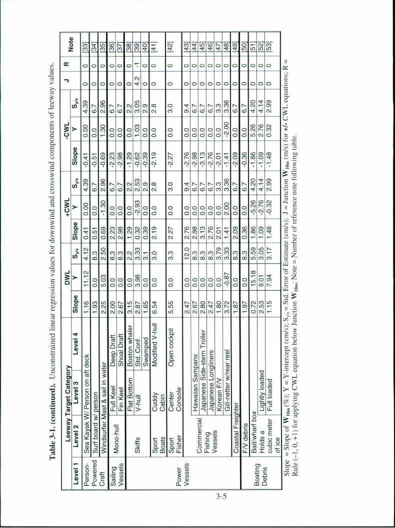
o )c c'~ ) o- 7 a o CD. C') D OO0 C O) C'.C'

III

C. ooooo'7oo C o00 000 40000000

Cur

00

cO C ) wD 0CD C~

0 0 C') g- C ?CCC- oC5o5 00 0 o00 o o0o 0 00 550 0CONC' +

S-oo-oooooo 0 ommoo o oo mm too I M I - a- _M, IN "

" " 0 IN) O C .C')" CJ 0 0 c C6 I' C CO') O "

-o ( 9 1 00 .0 .Co Co,

-*o I1 ,,, ,,,* *...,m0 C C') (D 42~

-o r. -Cl - -• ,_d _• 1l ,•lI2 0 q Dw C') 0 CDCDC\m C C)

IIN0 CO CO C

C5 di 7: ,:5 ol6d° d5 d, 66 6 .1 66. ,-Io19o , -LoO 'J c J N', c•J , C'j I C4 'CJ , -M 1- '- M M 0, -

C)j __e) 0

} •_o

>co) 00~> 00000moo0 0 9 q0 0 00~Oj o 0Z

_ 5 -D 0 6i :5, 6 19 ooC ,r-. E j

CL

m =0 ON

._ N N• In oN 0 .- -mC • ý r' o O• 0 Ei, - -

C "T0 oo " . E

_: w

0 ( 0 co

-0 0: (zJ 0Cl~ :=- a) 4) ic -o>u 000 I-- D COJ.-

o m co od* .=a-~~~ -1 t D0 w

Cua M ID~ -5

ci > ' 0uC C~~EE cCU) 0 LL I o.2cC~ >l C/CIa/L 01. 0L~ca

) a C Cl CO

Z' 0 ~'~9 D

3-5

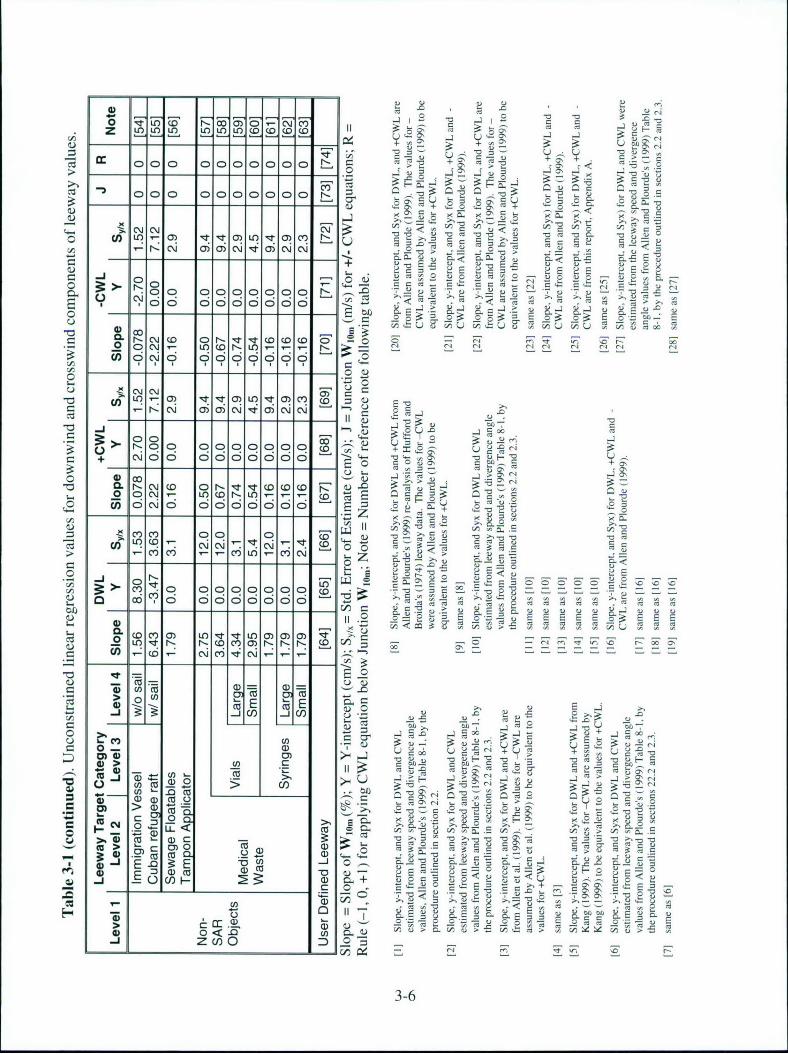
* C: o o~ o o o o - = V•= -

o~j VFW iz F =- z EE0 0 0 0 0 EE-~+

c , 000 00100000 EN: "I ý "27" _ ' 2 c

> . . . . . 0 J w • -j .E- -1 u =& - . 5<5a•- • ",- . =.>. oo oo - y -

0 o L •," oo, 010 d r' = "- Qcj ~ -C' cC'\rCC J' - 0 U,

4- C C M a2 ~E.oi

C; Ci ) 0

0 C

7-

--U o U i u U U

o ) NC\( 0N(OO( 0D -O .) -0 2r -

6 Cý oo ci a C)o o 400,I0 L' I ,, I I"- uI ,I- 'I I•

0 00

a ---o O L) - 0) 7 =1 u E~

-o t- + U-N1o o d i i 0 4-

0 0 0 0 0 co>i

Co r- to ~ wwC2 OC\j- Lt) w -LO - - - C

CD 6 6 o ooo6

C, • . . . . . ... .-.ý E g

-o Cý-E166 c

_0-• m -0c o, ca 02 ; nV

,.- t'? o oooooo•_• •_- => .-O co M - -,. 0,._ 0, , L,, o (00)0)0) ' = ' -

EE" J o - •Z? 'C. -0

0)NN==- _=

o. 0-2 . -(U

,- Z.' :E

U5 - -~ s. 2 -g: F

0~~~ ~ ~ ~ 0 0aC 0U);-

-2 E E E E EE E EO (m 0 C3) -

4-j ,--3 -~

Oi 0o -j U) 2

c/,~'- s

I- U,7;;C-,~ C 0. -''j 0*Z V0 07

-b Zc)6) u- -U- - - -

co c. "c . 11

c3-

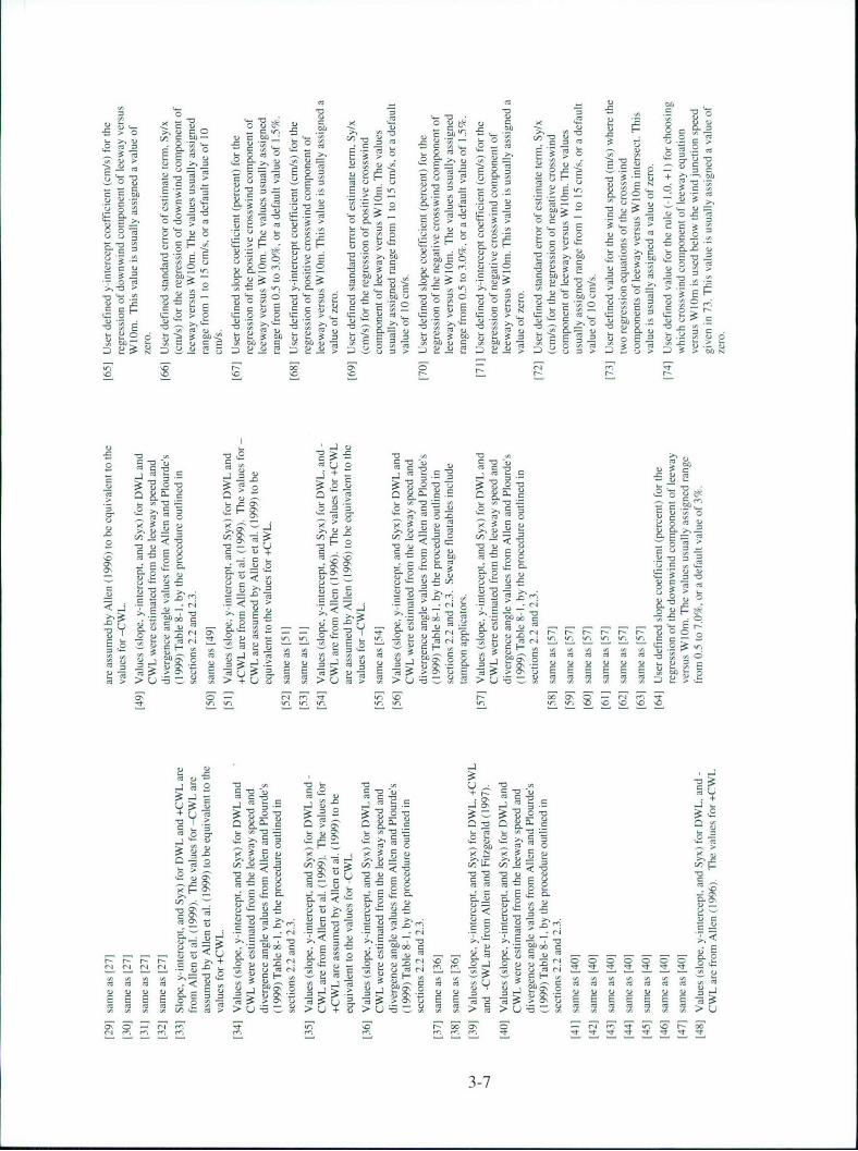
C* -U= .

to 11 ' ' ~ '

v a: :o3

.. 0 Sj;; -U > V ~ 0 5 5i ~ ~

00004 to1) _0'~ E.) -p0013s U- Vo> E *~6 1- oH VO>

E 120

u~ -v c a3g E- ~ ~

'0 >0 jo 0 > ' s0 > 0 rz t

j +.

00 c) 0 7, '--a

.0 ol CL~+. ~.

t4 E(~V~0 =

14 00"

uV 2V

o~. ~ ~ $'Is.~V0 -- 8

- ~-~,V .-- "0~ -O~E

~ ~ - ~ V .0 'o

EV.~ E E V EU E~ E E'. EI tu E

> U > V VU .. V V VU ~2~ ~-d ~ ~ >h~o'oSE S:;E

~> >.J0.'. ~ >+Q ,'.~ ~ W5Z~ =0

0'~ +- i 0 -

,E E

u ri12 tIL ~Ll-V~ri

-u r.. u V. u

E s Eo a' ESESE ESEU m' Ue~ r -Cr

3-7

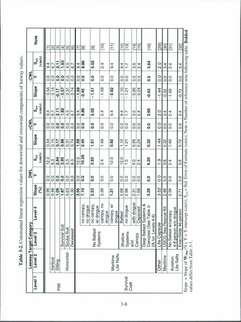
0z

C oo

0O• O- o 0 0 0 0 C Lo ( 0 0 o o) i

0 . . . .. .. . .. .. .,- I.-- - (Y)

sz -1 C14D N1 0 r- LO. 0 0 0 r I" C

"T ooooo o I- q OR q ooý oo o oR od ot Eci 6 i'i (DO mo C''I 0 ) - Co .J o oC d o) C\J oo Cd )-

o +o-Z

' d _- _ _--o0•-d

00 00 0 0 0 0 000047 0 COO o

CD E

0 o C oo .o 0

7d3 OD 4 o o do 0 o o o d

6600 i-CO)C C 00 C' 0) 0C) C0)C 0 0 6 , E)F

;> C I

"-- t- w C- C-o

0 ~ ~ ~ ~ ~ ~ O P. C o.--~jc) coCjCf

00 00 00 0, 0 0 0, 000o >+4 50•• z6o ooo 666666 d ooo•,,a_ - _"- .

0 co

00"u Ca) 0 0 a oo o 0 0 c' o ý N -

__ ---- __ - Q - o

0 0 0 0 9 ) 05 00 0 0 0 0 M cc

& co0)-.00 D Cn') 0) - (( CD (0O) fno-00)0 D O0)C - C0 N : w00 Cj( ca U~IC) c -E2

0 m M L) ,Lu0 > m w co = 4~~) ýo0 C oC

-W 0 0 ca a wc-

>4 04 0~

.0 E o>) L-)U rl N~ -4-_-c- 4

ZCJ CJ-OJ Q) 0 cu C

CL U) CE -)

>u >

3-8

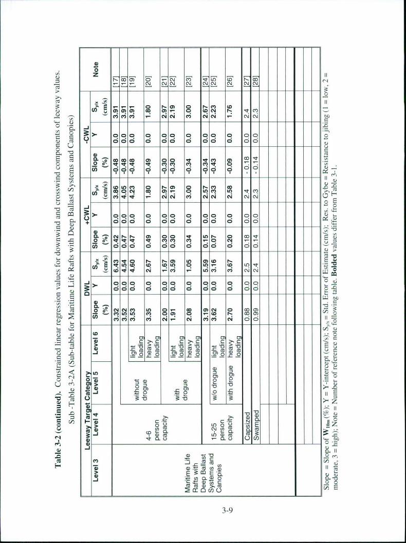
0

r- 0 ) 0 l C O 0 r or-C 14~- C~i CNCJ C"j C~j N. C'.J C~J'N

00

9 coo 0 0 oi 0 co£~ £0

- -t CL Go q co GOo CF) 00 0 00 leo) a9 0 0- 0 0 0 0 0 0 0 0 00m 14

0 - - q CC)

d s U) 00 0 0 0 00 0-oI I I I I I I I

oo >-eca , '~'

2 oq 000E0

000 o 00 0 00 00

CM 1cJ- 1'. 0 0 0 -e I r-. 0 00

cnio c; 6s6 6 6i 6s6 6 6 6-

-J -

000C- l) L 0 000)C- 0 00 0 )0

(I U)L c 0!- 0 7 (q CJ0 0 3~-I- - . CV) CU) V) 00M 0M i-4) 1 CVO) C4i6

C0. V)C) l 0

ci ) s c 4) co z _ a

131 -C 0 0 21 _0 0 .2)0 0

(1) CDtoU3 : v4

0)00~~ 0) 2

C0 >1 :3 :3 I-

2 0 E

m w C

Cid U1 Co CUa) ca LO a a c

1~00

E) 03E

a) I

3-9

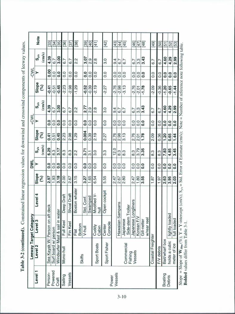
0 - -

o z ooo o o~ o)0 ooo~ _ oo oo 0o o0ooo

ot __ . . . .. O0•l• •

-* - 0- q . _ -- r C o 'lot - 0 -ca D 1" )( 0 -Ni (Y)) 0N( ((DJD) 6e(-- (0 V ) 0V, (. oD i )e -,

*o R' 0Y •-000000 000 0 000 000 0 c 0 0 005

CL Lo 00 0) Cj a) o) No D o o ( C o) (0 o 0) 0 0 U0 q*

-o

c -)N" -e 0 fD 0 N

~(C)0(0N ulclN N 1') 0)(0(0 C C0')' ( ~C4 l (R

S~II

-0>- o o 00C-I 0000 q 0 000 000 0 )000 a)+ 00 o 00o 0 666 6"- 0,-,-

La I- ,-( c l)

0) U CC) (0) 000)) 00 1 (D 0) (00 o 0 U)q "

0e M V ItN0m OC')i- N N0)C N t. 0 co-4 ( Ic;60N~ dON N NNc C ý C') NNI No 0i -0

- o oo w

I- 0 q q0 0 0)10

o 0 o d

r_ ii-Co: L(06 'L-0 ()~ 'C) ''CI c ' od'CA, CL fl c co t0 L CI-c')C') C'O r- N0O r(f(- 0 O r ,C)

. q 00000 0 00 (q , 0 o 0 0 0 0

0-1

>~~ 0 a~66 (D6 6 6 606 dU)1

(D -)M U cF- 0

CU -jc C ~ a U a*

v~~~c can n i.r ~ci,~~~~ c ~ (U- _ u 1- )

Q * c (D E' - ~ ~ )C5 >Na 0 c c D

w- >* 0 cf 05 -0 - CO c-

-- C :8 75 ý ~t2 0) cac U

_j :3 (Uut w 0 0 )EC- (J0 CO) L LL 0 Cl) ml OLL cz.EO~

U) a), ~CL (nf

.. J (D~- a OQ u (D-4 X 0 -0 "..

C M 03-10

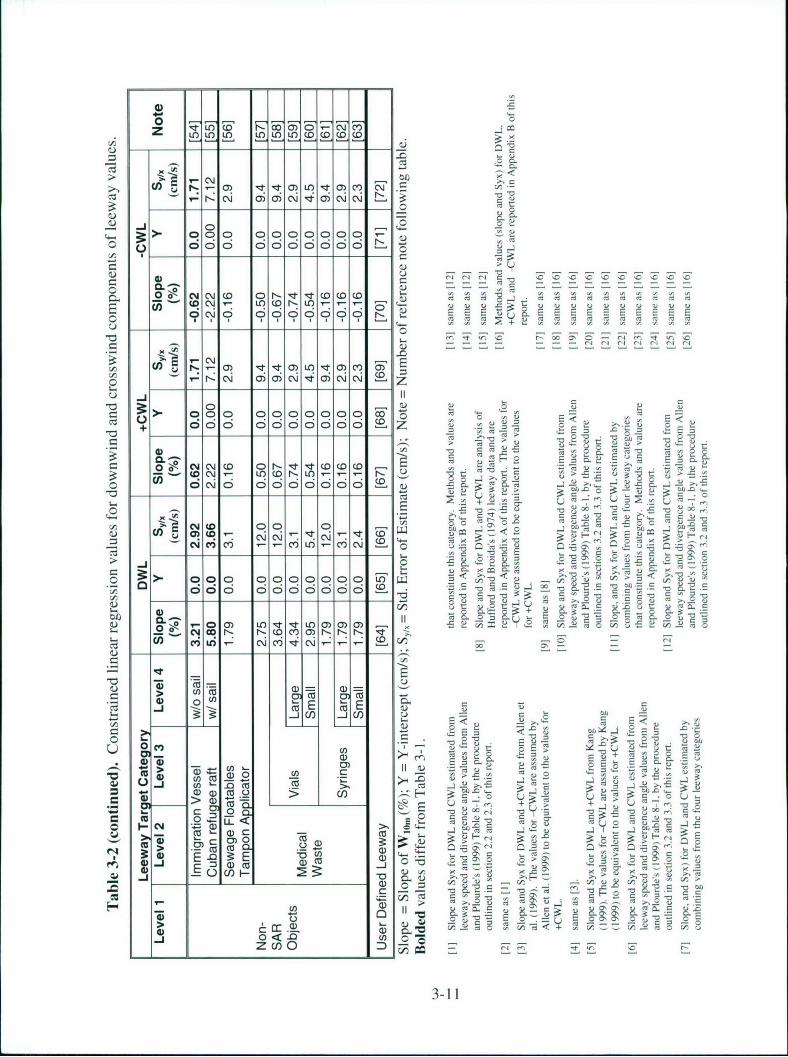
0.

LO LOLL 11 LO)U)LOLO(D(DCO(D .CJWO

:E0

030

0) Lo -. 0

-L 7- '

o cmi oooooo o r- q ( ( (-ý - - -- -0) 1-

-0 0.j 0 o0 C- o00 o a ol r, 02 E~ E .0UEE

T M M Ml Cz Ml MlCI l

0) c

r- IIj 0) 0)0llr m

6 c; 0 -0 1)+ 7, 000 00 0 0 JE E

79 2:

C-4 ' l '~CDJ 0 - 1T It(Dco(D - .-- M7

U> U

I. cm w o CD2 I

C0 CI CO 17 It c(I) - 0 8,3 l

C4C~~CFL .C )L ,-) - U0

C;o ; i i i 5 " a a: -.

)- 0 0 000 00 LO I). 'T U- a) a). 0)U

00 - ;)C-ý r,: _ý( ?c) -r - I

q00) LO ~ OOOO N- m1 q-

0i ' U0))- ~-CU - - -i -/

00

(D

>) C )Cc( C U U zc a ~ COu>

C: cm 0 Vao -I- -

-d En E U)U

0 '- V ~ CO ~ 0

0C2 <~ Cl) . -

3-1 1

ob r1.b-U.

E E> o n - .& >

o ~ ~ W~ UE

> -;

E Uu _ 0> v>

~ ~ 2>oE

v ~ t) v0~ i0 5~ >u~ E u OE Ro ~7 Q &0-15 m

r- lE >, C U ~E E

600

0 u - UEI10Onto E< m22

0 5, Eo

-0 - " . 2 2 o .> =O .- - 0' -

~> u >00

J ~ U, 2 U 00

T E7 00 F P U 0' u - i 1 U ZF U U u 0' 0'

7- 7- 0,E EE E- o,, 0' o o ~m

2 <o 0 E < o~

.= 0 p . -0 - 0,

.2~ , - - > '

~~~ <c - U 0 O

E M E o c2 ~ o

5 .- UU." -00,

F:7 .- 7~ F7 u

~r

E i v.2c U U0~ E E E E o U m. '= EU2

3-12

CHAPTER 4.

DEVELOPING AN IMPROVED LEEWAY MODEL BASED ONDOWNWIND AND CROSSWIND LEEWAY COMPONENTS

4.1. Leeway Model Implementation

Tables 3-1 and 3-2 present the results of a statistical analysis to derive a workable set ofDownwind and Crosswind Leeway (DWL and CWL) component linear regression coefficientsbased on data from field experiment data for 25 leeway object categories, and estimatedempirically for an additional 38 categories. Just as there are various statistical methods fordeveloping these regression equations, there are various modeling techniques that canincorporate results of regression analysis in SAR planning tools. In this section, two versions ofa model that utilizes DWL and CWL to compute leeway are proposed and then checked againstthe original leeway data sets. Both models utilize the coefficients given in Tables 3-1 or 3-2.

Both models share three basic assumptions in their development and implementation. The firstassumption is that a specific leeway object has a unique set of leeway equations and retains thoseequations over the drift durations, unless there is a significant state-changing event. Thisassumption implies that Monte Carlo simulations would establish "N" sets of leeway equationsfor each drifting object type where "N" equals the number of replications for that drift object.Then the Monte Carlo simulation would use those equations to establish the leeway velocitycomponents as function of wind speed at each time step over the entire drift period, as long asthe drift object did not change configuration (e.g. swamp or capsize). The evidence for eachleeway object having a unique set of leeway components is shown in Figures 7-2 and 7-3 ofAllen and Plourde (1999), reproduced here as Figure 4-1 (i.e., downwind components of leewayversus Wi0, for three separate 4-6 person life rafts with deep ballast system and canopies, nodrogue, light loading).

4-1

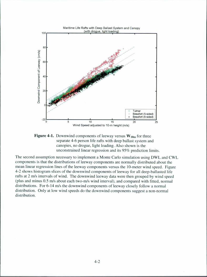
Maritime Life Rafts with Deep Ballast System and Canopy100With drogue, lightloading

80-

S60-

_J

4-J

0

0

20.

0

TulmarBeaufort (5-sided)

2 Beaufort (6-sided)-20

0 5 10 15 20 25Wind Speed adjusted to 10-m height (m/s)

Figure 4-1. Downwind components of leeway versus W1om for threeseparate 4-6 person life rafts with deep ballast system andcanopies, no drogue, light loading. Also shown is theunconstrained linear regression and its 95% prediction limits.

The second assumption necessary to implement a Monte Carlo simulation using DWL and CWLcomponents is that the distributions of leeway components are normally distributed about themean linear regression lines of the leeway components versus the 10-meter wind speed. Figure4-2 shows histogram slices of the downwind components of leeway for all deep-ballasted liferafts at 2 m/s intervals of wind. The downwind leeway data were then grouped by wind speed(plus and minus 0.5 m/s about each two-m/s wind interval), and compared with fitted, normaldistributions. For 6-14 m/s the downwind components of leeway closely follow a normaldistribution. Only at low wind speeds do the downwind components suggest a non-normaldistribution.

4-2

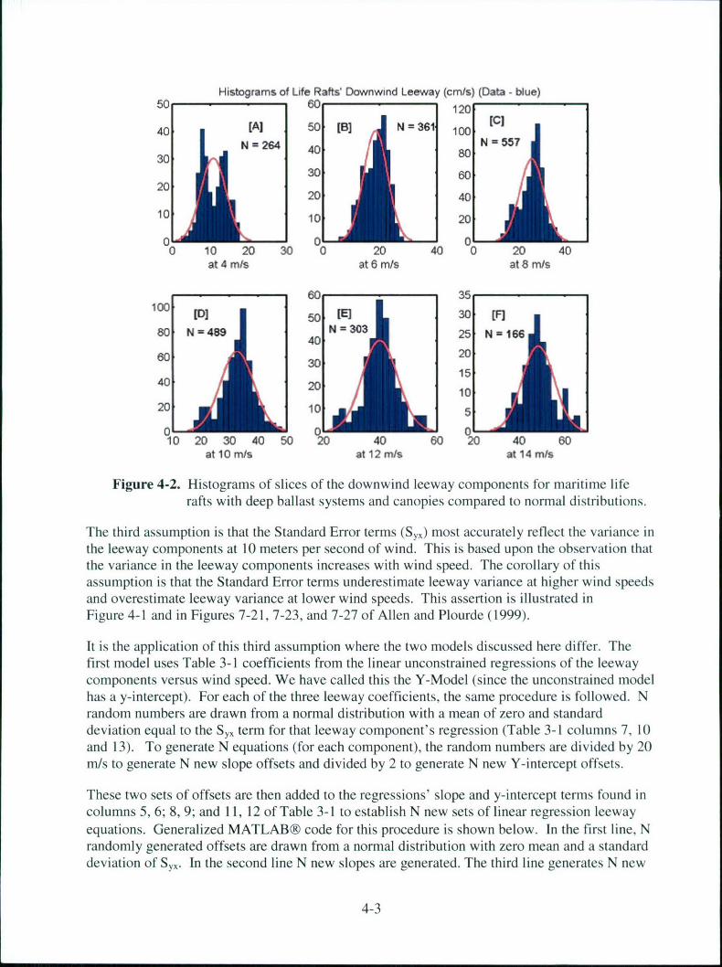
Histograms of Life Rafts' Downwind Leeway (cmls) (Data - blue)50 60 120

40 (A) 50 B] N361 C]

30 N264 40 80 N - 557

30 6020

20 4010 10 20

0 0 00 10 20 30 0 20 40 0 20 40

at 4 mts at 6 mts at 8 m/s

S~~60 -3

100o (D 50 [E] 30 (F]80 Ni-489 N=303 25 N=166

40

60 30 20

1540 20 10

20 10 5

0 0 010 20 30 40 50 20 40 60 20 40 60

at 10 m/s at 12 mts at 14 mrs

Figure 4-2. Histograms of slices of the downwind leeway components for maritime liferafts with deep ballast systems and canopies compared to normal distributions.

The third assumption is that the Standard Error terms (Sy,) most accurately reflect the variance inthe leeway components at 10 meters per second of wind. This is based upon the observation thatthe variance in the leeway components increases with wind speed. The corollary of thisassumption is that the Standard Error terms underestimate leeway variance at higher wind speedsand overestimate leeway variance at lower wind speeds. This assertion is illustrated inFigure 4-1 and in Figures 7-21, 7-23, and 7-27 of Allen and Plourde (1999).

It is the application of this third assumption where the two models discussed here differ. Thefirst model uses Table 3-1 coefficients from the linear unconstrained regressions of the leewaycomponents versus wind speed. We have called this the Y-Model (since the unconstrained modelhas a y-intercept). For each of the three leeway coefficients, the same procedure is followed. Nrandom numbers are drawn from a normal distribution with a mean of zero and standarddeviation equal to the Syx term for that leeway component's regression (Table 3-1 columns 7, 10and 13). To generate N equations (for each component), the random numbers are divided by 20m/s to generate N new slope offsets and divided by 2 to generate N new Y-intercept offsets.

These two sets of offsets are then added to the regressions' slope and y-intercept terms found incolumns 5, 6; 8, 9; and 11, 12 of Table 3-1 to establish N new sets of linear regression leewayequations. Generalized MATLAB® code for this procedure is shown below. In the first line, Nrandomly generated offsets are drawn from a normal distribution with zero mean and a standarddeviation of Sy, In the second line N new slopes are generated. The third line generates N new

4-3

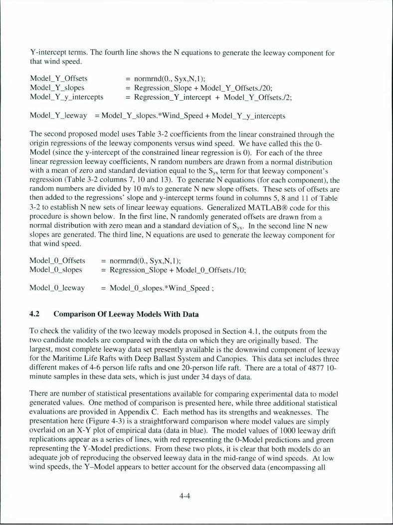
Y-intercept terms. The fourth line shows the N equations to generate the leeway component forthat wind speed.

ModelYOffsets = normrnd(0., Syx,N,l);ModelY-slopes = RegressionSlope + ModelYOffsets./20;Model_Y_yjintercepts = Regression Y intercept + ModelYOffsets./2;

ModelY leeway = ModelY slopes.*WindSpeed + ModelY-y-intercepts

The second proposed model uses Table 3-2 coefficients from the linear constrained through theorigin regressions of the leeway components versus wind speed. We have called this the 0-Model (since the y-intercept of the constrained linear regression is 0). For each of the threelinear regression leeway coefficients, N random numbers are drawn from a normal distributionwith a mean of zero and standard deviation equal to the Sy, term for that leeway component'sregression (Table 3-2 columns 7, 10 and 13). To generate N equations (for each component), therandom numbers are divided by 10 m/s to generate N new slope offsets. These sets of offsets arethen added to the regressions' slope and y-intercept terms found in columns 5, 8 and II of Table3-2 to establish N new sets of linear leeway equations. Generalized MATLAB® code for thisprocedure is shown below. In the first line, N randomly generated offsets are drawn from anormal distribution with zero mean and a standard deviation of Syx. In the second line N newslopes are generated. The third line, N equations are used to generate the leeway component forthat wind speed.

Model_0_Offsets = normrnd(0., Syx,N,l);Model_0_slopes = Regression_Slope + Model_0_Offsets./10;

Model_0_leeway = Model 0 slopes.*WindSpeed;

4.2 Comparison Of Leeway Models With Data

To check the validity of the two leeway models proposed in Section 4.1, the outputs from thetwo candidate models are compared with the data on which they are originally based. Thelargest, most complete leeway data set presently available is the downwind component of leewayfor the Maritime Life Rafts with Deep Ballast System and Canopies. This data set includes threedifferent makes of 4-6 person life rafts and one 20-person life raft. There are a total of 4877 10-minute samples in these data sets, which is just under 34 days of data.

There are number of statistical presentations available for comparing experimental data to modelgenerated values. One method of comparison is presented here, while three additional statisticalevaluations are provided in Appendix C. Each method has its strengths and weaknesses. Thepresentation here (Figure 4-3) is a straightforward comparison where model values are simplyoverlaid on an X-Y plot of empirical data (data in blue). The model values of 1000 leeway driftreplications appear as a series of lines, with red representing the 0-Model predictions and greenrepresenting the Y-Model predictions. From these two plots, it is clear that both models do anadequate job of reproducing the observed leeway data in the mid-range of wind speeds. At lowwind speeds, the Y-Model appears to better account for the observed data (encompassing all

4-4

data points). At higher wind speeds, the 0-Model appears to better account for the observed data.It is also clear that the 0-model converges to zero at zero wind speed, but thereforeunderestimates the leeway data variance at low wind speeds (as shown by the number of datapoints not encompassed by the red lines). It is not so clear from these two plots how well thetwo models compare with the data along the regression line and the effects of increasing ordecreasing the number (N) of replications. For the plots shown in Figure 4-3, the eye is drawn tothe extreme model values that are varied from run to run (at the 1000 N level). This is to say, theplots are dependent on the size of N. When 10,000 replications were used, both models cover agreater range.

Maritime Life Rafts with Deep Ballast Systems and Canopies100 100

80 [A] 80 [B]

60 60

40 - 40 /E ,.~E

-20 2' 0 /

0 0

-20 -200 5 10 15 20 25 0 5 10 15 20 25

Wind Speed adjusted to 10-m height (m/s) Wind Speed adjusted to 10r-m height (m/s)

Figure 4-3. Downwind leeway data (blue) from maritime life rafts withdeep ballast systems and canopies versus 10-meter wind speedcompared with 1000 model generated leeway equation results:(A) 0-model values in red and (B) Y-model values in green.

As stated, additional statistical comparisons are provided in Appendix C. In summary, allcomparisons used show that though the 0-Model converges to zero, it doesn't cover the datadistribution at low wind speeds as well as the Y-Model. Overall, the Y-Model does a slightlybetter job than the 0-Model covering the data (particularly at low wind speeds).

4-5

CHAPTER 5.

INVESTIGATING AND ACCOUNTING FOR CHANGES IN THE SIGN OFTHE CROSSWIND LEEWAY COMPONENT

5.1. Introduction

Since 1992 there have been over 55 days of leeway drift observations collected on variousleeway objects, (Allen and Plourde (1999); Allen, Robe and Morton (1999)). In this total dataset, leeway drift objects generally behaved in a certain manner: if the object's drift was initiallyto the right (or left) of the downwind direction, the drift remained to the right (or left) of thedownwind direction for the duration of the drift. However, on a few occasions, the object's drifttrajectory changed from right of the downwind to the left downwind or vice versa. This behavioris often referred to as "jibing" or "tacking," using the term associated with sailing, whereby thevessel sails to the left of the downwind or upwind direction, and then to the right. Because of thefocus of this report on DWL and CWL components, this phenomenon will be discussed in termsof sign changes of the CWL component.

The frequency of the occurrence of changes in the crosswind component from positive tonegative (or vice versa) is an important element for modeling search areas. In the completeabsence of changes in the crosswind component sign, search objects will maintain their initialdirection of drift relative to the wind direction throughout their entire drift. With no changes inthe crosswind component sign, the Monte Carlo initial probability distribution of replications ofleeway drift objects will eventually separate from each other over time, about the downwinddirection, with replications to the left and replications to the right, delineating two separate high-probability leeway object areas. If the drift of a leeway object changes crosswind componentsign frequently, then there will be very little net divergence from the downwind direction, aseach replication to the right of the downwind direction will be offset by a replication to the left.Accordingly, the leeway drift will not diverge from the downwind direction, but will beessentially directly downwind. If, however, there are less frequent or even infrequent changes inthe sign of the crosswind component, there will be a measurable effect on the probabilitydistribution, with the distribution biased to either side of the downwind direction.

This report does not attempt to describe the dynamics governing the CWL sign change as thephysical factors affecting the change may be numerous and subtle, and in general, were notdirectly measured in leeway experiments. However, a statistical approach may provide practicalguidance in dealing with this phenomenon. A statistical analysis of changes and frequency ofchange in the crosswind drift direction was undertaken, where data were available. Thisincluded the identification, description and statistical analysis of changes of the crosswindcomponent observed during the leeway drift field experiments for four categories of leeway driftobjects. This analysis resulted in the recommendation of a simple first-order model forestimating frequency of the change in sign of the crosswind leeway component (CWL). Theusefulness of this first-order model was investigated in a sensitivity analysis of the effect of theCWL sign-change frequency on Monte Carlo search area distributions.

5-1

5.2 Methods Used To Identify And Analyze Crosswind Component Sign Changes

The four leeway categories analyzed for this study were: 5.5-meter V-hull open skiff; 4-6 persondeep-ballasted canopied life rafts; 20-person deep-ballasted canopied life rafts; and 1-cubicmeter wharf box. These four categories were selected because each category contained 100 ormore hours of actual leeway data. These categories had data collected using the direct method oftethered InterOcean® "S4" electromagnetic current meter and an onboard wind-monitoringsystem (Allen and Plourde (1999)). This provided sufficient quantity and quality of leeway datato document changes in the crosswind component of leeway. It should be noted, however, atethered S4 current meter may have reduced the occurrences of the leeway object changingdirection and the resulting sign change of the crosswind component. Therefore, the analysispresented here represents conservative estimates of the frequency of crosswind component signchanges.

A 5.5 m V-hull open skiff, common to Newfoundland waters (shown in Figure 5-1 [A]), hasbeen extensively studied by Allen and Fitzgerald (1997). A total of 172.5 hours of leeway datahave been collected on this leeway drift object. Though Allen and Fitzgerald (1997) reportedone confirmed swamping and two suspected swampings of open skiffs during the 1995 fieldexperiments, we report only on the changes in the sign of the crosswind component of leeway forthe standard skiff configuration used during these field experiments.

Fitzgerald, Finlayson and Allen (1994), Allen and Plourde (1999) and this report have studied 4-6 person and 20-person deep-ballasted canopied life rafts, (see Figure 5-1 [B] and [CQ). Thereare 656.0 hours of useable leeway data on the 4-6-person life rafts and 268.3 hours of data for the20-person life rafts. There were three separate types of 4-6 person life rafts and one type of 20-person life raft. Life rafts were primarily set up in one of two configurations: heavily loadedwith a drogue attached or lightly loaded with no drogue. Here we used the two data sets for thegeneral combined leeway classes: 4-6 person, deep-ballasted, canopied life rafts; and 20-person,deep-ballasted, canopied life rafts.

Allen, Robe and Morton (1999) collected 102.2 hours of data on a I-cubic meter wharf boxtypically used to store ice and bait for commercial fishing vessels, (see Figure 5-1 [D]). Thesewharf/bait boxes are typically stored on the open deck of the fishing vessels and occasionally actas makeshift life rafts, since they are double-hull plastic. There were six drift runs conducted onthe wharf box, three of them with 1-person loading and three with 4-person loading. Thecombined leeway category for the wharf/bait box was used here.

5-2

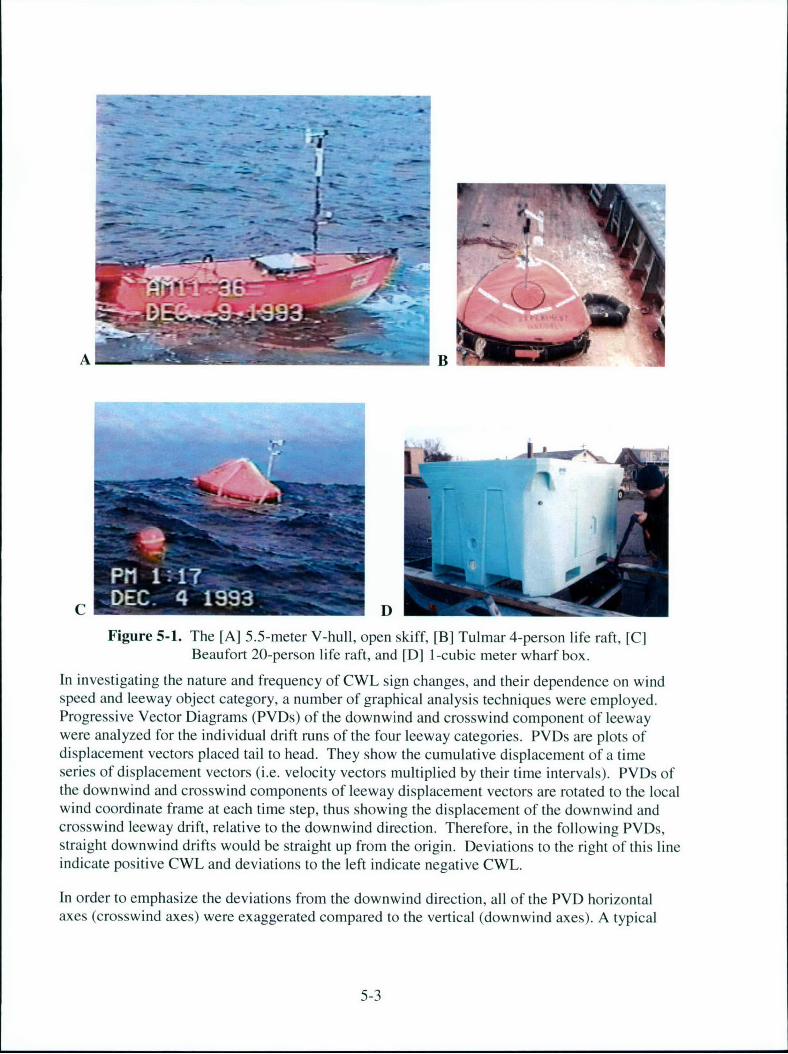
A B

C DFigure 5-1. The [A] 5.5-meter V-hull, open skiff, [B] Tulmar 4-person life raft, [C]

Beaufort 20-person life raft, and [D] 1-cubic meter wharf box.

In investigating the nature and frequency of CWL sign changes, and their dependence on windspeed and leeway object category, a number of graphical analysis techniques were employed.Progressive Vector Diagrams (PVDs) of the downwind and crosswind component of leewaywere analyzed for the individual drift runs of the four leeway categories. PVDs are plots ofdisplacement vectors placed tail to head. They show the cumulative displacement of a timeseries of displacement vectors (i.e. velocity vectors multiplied by their time intervals). PVDs ofthe downwind and crosswind components of leeway displacement vectors are rotated to the localwind coordinate frame at each time step, thus showing the displacement of the downwind andcrosswind leeway drift, relative to the downwind direction. Therefore, in the following PVDs,straight downwind drifts would be straight up from the origin. Deviations to the right of this lineindicate positive CWL and deviations to the left indicate negative CWL.

In order to emphasize the deviations from the downwind direction, all of the PVD horizontalaxes (crosswind axes) were exaggerated compared to the vertical (downwind axes). A typical

5-3

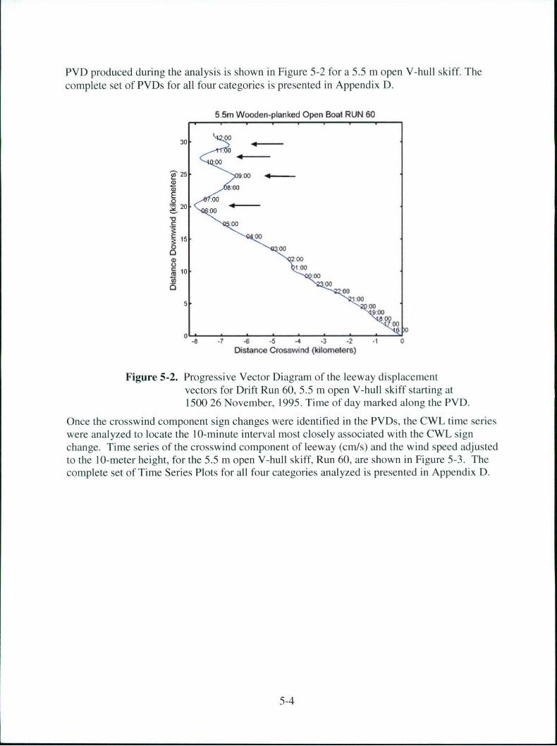
PVD produced during the analysis is shown in Figure 5-2 for a 5.5 m open V-hull skiff. Thecomplete set of PVDs for all four categories is presented in Appendix D.

5.5m Wooden-planked Open Boat RUN 60

.00

25 00 4-

:00

:0020 20

R l:000

r2 00

-10 ---000

* :00

000

19:00-00

:0000

-8 -7 -6 -5 -4 -3 -2 -1 0Distance Crosswind (kilometers)

Figure 5-2. Progressive Vector Diagram of the leeway displacementvectors for Drift Run 60, 5.5 m open V-hull skiff starting at1500 26 November, 1995. Time of day marked along the PVD.

Once the crosswind component sign changes were identified in the PVDs, the CWL time serieswere analyzed to locate the 10-minute interval most closely associated with the CWL signchange. Time series of the crosswind component of leeway (cm/s) and the wind speed adjustedto the 10-meter height, for the 5.5 m open V-hull skiff, Run 60, are shown in Figure 5-3. Thecomplete set of Time Series Plots for all four categories analyzed is presented in Appendix D.

5-4

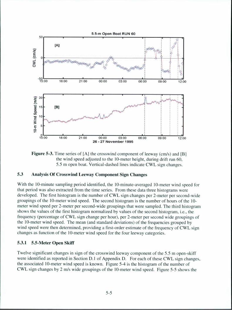
5.5-m Open Boat RUN 6050

[A)

EI

.A-

19:00 18:00 2100 00:00 03:00 06-00 09:00 12:00

-20

I- [B]

0 P

! I I

1:00 18.00 21:00 00:00 0300 06:00 0900 12:0026 - 27 November 1 M5

Figure 5-3. Time series of [A] the crosswind component of leeway (cm/s) and [B]the wind speed adjusted to the 10-meter height, during drift run 60,5.5 m open boat. Vertical-dashed lines indicate CWL sign changes.

5.3 Analysis Of Crosswind Leeway Component Sign Changes

With the 10-minute sampling period identified, the 10-minute-averaged 10-meter wind speed forthat period was also extracted from the time series. From these data three histograms weredeveloped. The first histogram is the number of CWL sign changes per 2-meter per second-widegroupings of the 10-meter wind speed. The second histogram is the number of hours of the 10-meter wind speed per 2-meter per second-wide groupings that were sampled. The third histogramshows the values of the first histogram normalized by values of the second histogram, i.e., thefrequency (percentage of CWL sign change per hour), per 2-meter per second wide groupings ofthe 10-meter wind speed. The mean (and standard deviations) of the frequencies grouped bywind speed were then determined, providing a first-order estimate of the frequency of CWL signchanges as function of the 10-meter wind speed for the four leeway categories.

5.3.1 5.5-Meter Open Skiff

Twelve significant changes in sign of the crosswind leeway component of the 5.5 m open-skiffwere identified as reported in Section D. 1 of Appendix D. For each of these CWL sign changes,the associated 10-meter wind speed is known. Figure 5-4 is the histogram of the number ofCWL sign changes by 2 m/s wide groupings of the 10-meter wind speed. Figure 5-5 shows the

5-5

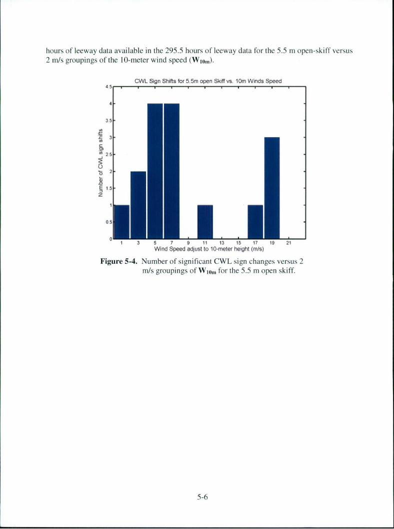
hours of leeway data available in the 295.5 hours of leeway data for the 5.5 m open-skiff versus2 m/s groupings of the 10-meter wind speed (Wi0m).

CWL Sign Shifts for 5.5mn open Skiff vs. lOmn Winds Speed45

35

- 3

25-

b 25

E 15z

05

01 3 5 7 9 11 13 15 17 19 21

Wind Speed adjust to 10-meter height (mls)

Figure 5-4. Number of significant CWL sign changes versus 2m/s groupings of W10m for the 5.5 m open skiff.

5-6

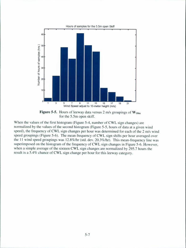
Hours of samples for the 5.5m open Skiff

60

;50

40-

M 300.E

S 20-E:3Z

! 3 5 7 9 11 13 15 17 is 21

Wind Speed adjust to 10.meter height (mis)

Figure 5-5. Hours of leeway data versus 2 m/s groupings of Wiomfor the 5.5m open skiff.

When the values of the first histogram (Figure 5-4, number of CWL sign changes) arenormalized by the values of the second histogram (Figure 5-5, hours of data at a given windspeed), the frequency of CWL sign changes per hour was determined for each of the 2 m/s windspeed groupings (Figure 5-6). The mean frequency of CWL sign shifts per hour averaged overthe 11 wind speed groupings was 12.8%/hr (std. dev. 20.3%/hr). This mean-frequency line wassuperimposed on the histogram of the frequency of CWL sign changes in Figure 5-6. However,when a simple average of the sixteen CWL sign changes are normalized by 295.7 hours theresult is a 5.4% chance of CWL sign change per hour for this leeway category.

5-7

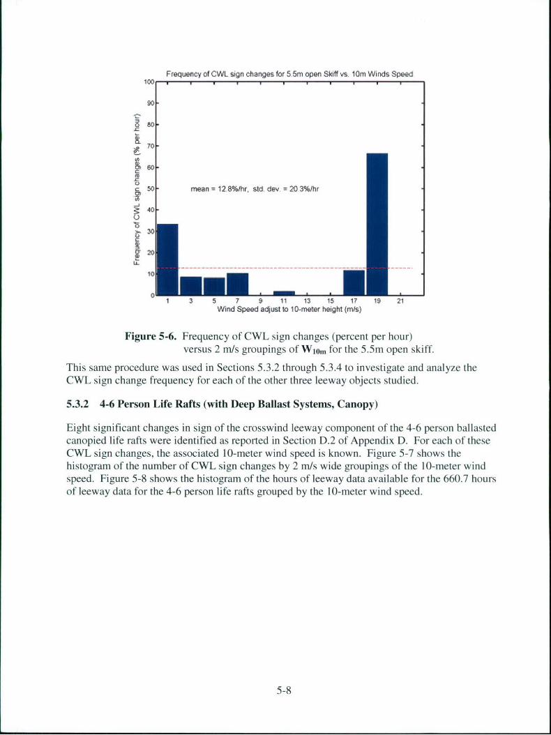
Frequency of CWL sign changes for 5 5m open Skiff vs. 10n Winds Speed100 , , . , , , , , ,

90

go.

s7o

60.

C.)

c 50 mean = 12 8%Mhr, std dev = 20 3%hr

40o

30C

~20

10

1 3 5 7 9 11 13 15 17 19 21Wind Speed adjust to 10-meter height (m/s)

Figure 5-6. Frequency of CWL sign changes (percent per hour)versus 2 m/s groupings of W1om for the 5.5m open skiff.

This same procedure was used in Sections 5.3.2 through 5.3.4 to investigate and analyze theCWL sign change frequency for each of the other three leeway objects studied.

5.3.2 4-6 Person Life Rafts (with Deep Ballast Systems, Canopy)

Eight significant changes in sign of the crosswind leeway component of the 4-6 person ballastedcanopied life rafts were identified as reported in Section D.2 of Appendix D. For each of theseCWL sign changes, the associated 10-meter wind speed is known. Figure 5-7 shows thehistogram of the number of CWL sign changes by 2 m/s wide groupings of the 10-meter windspeed. Figure 5-8 shows the histogram of the hours of leeway data available for the 660.7 hoursof leeway data for the 4-6 person life rafts grouped by the 10-meter wind speed.

5-8

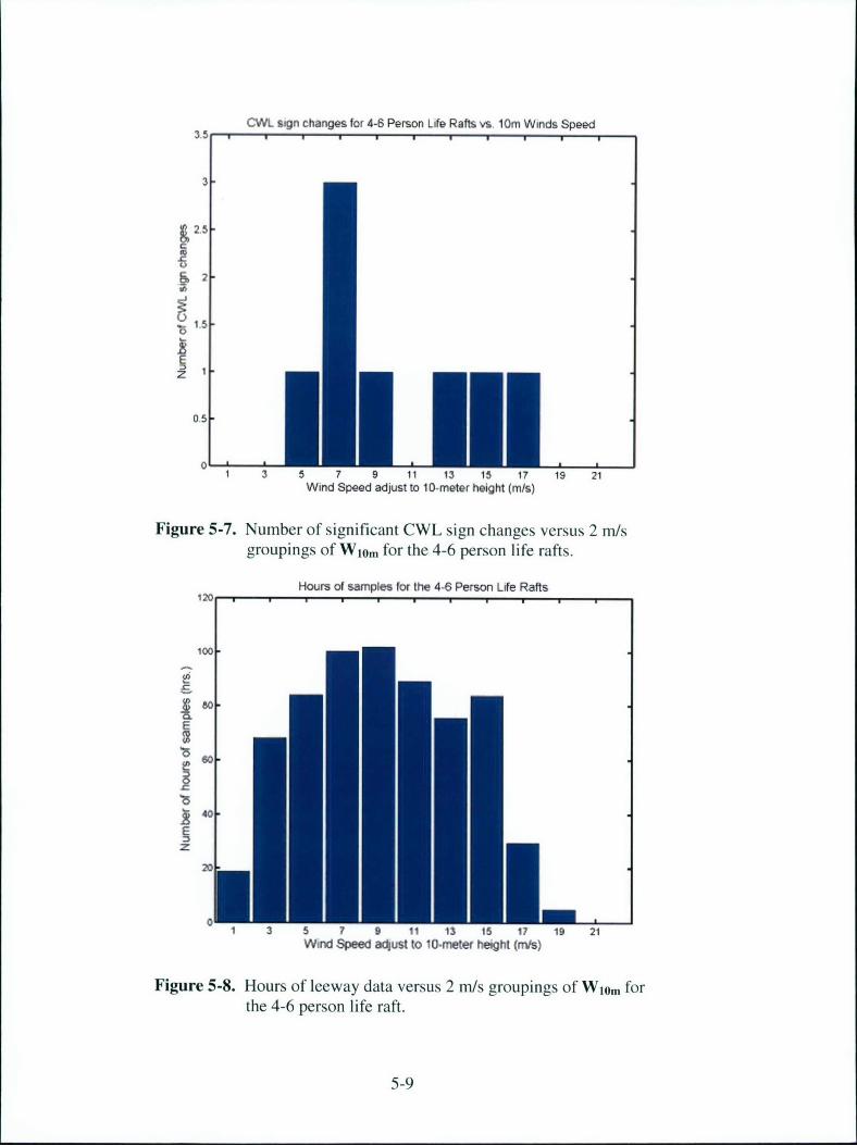
CWL sign changes for 4-6 Person Life Rafts vs. lOn Winds Speed

3

25

- 1.5

E

035

0[1 3 5 7 9 11 13 15 17 19 21

Wind Speed adjust to 10-meter height (m/s)

Figure 5-7. Number of significant CWL sign changes versus 2 m/sgroupings of Wi0m for the 4-6 person life rafts.

Hours of samples for the 4-6 Person Lie Rafts120

100-

0

E

60-

~40-Ez

20

0 -1 3 5 7 11 13 is 17 19 21

Wind Speed adjust to 10-meter heiht (m/s)

Figure 5-8. Hours of leeway data versus 2 m/s groupings of Wiom forthe 4-6 person life raft.

5-9

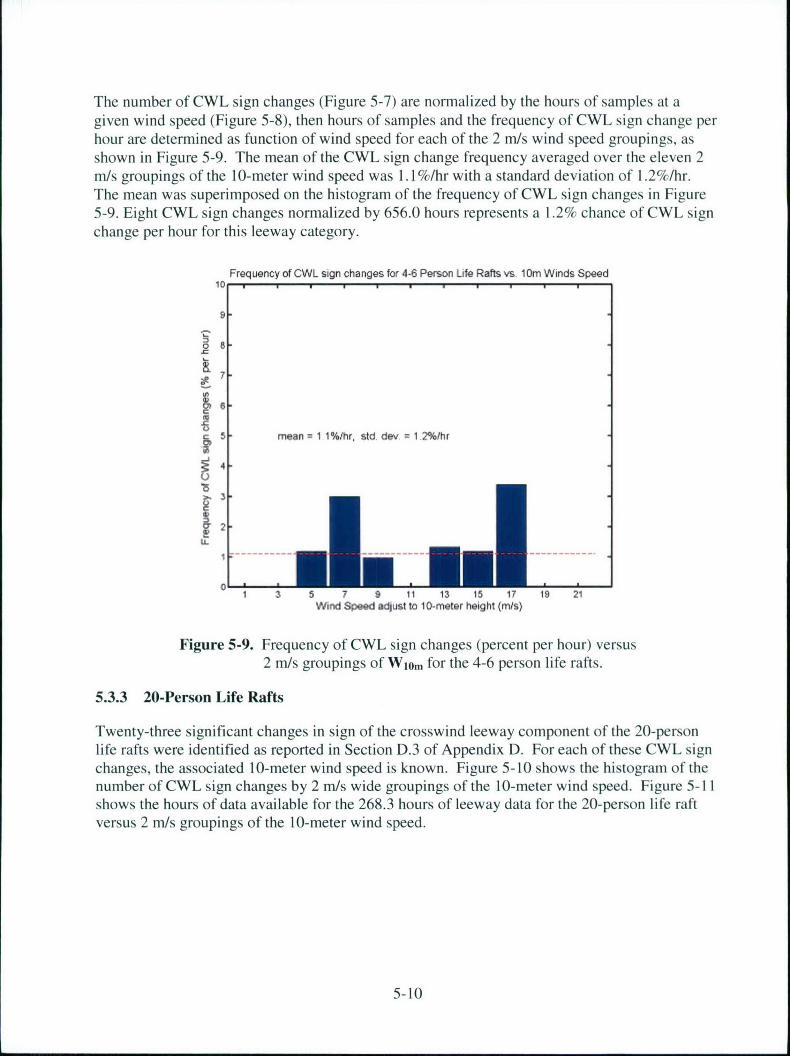
The number of CWL sign changes (Figure 5-7) are normalized by the hours of samples at agiven wind speed (Figure 5-8), then hours of samples and the frequency of CWL sign change perhour are determined as function of wind speed for each of the 2 m/s wind speed groupings, asshown in Figure 5-9. The mean of the CWL sign change frequency averaged over the eleven 2m/s groupings of the 10-meter wind speed was 1.1%/hr with a standard deviation of 1.2%/hr.The mean was superimposed on the histogram of the frequency of CWL sign changes in Figure5-9. Eight CWL sign changes normalized by 656.0 hours represents a 1.2% chance of CWL signchange per hour for this leeway category.

Frequency of CWL sign changes for 4-6 Person Life Rafts vs, 10m Winds Speed10

9-

C*

0 8-

7-

C

c mean 1 1%lr, std dev =1 2%thr

IL0

1 3 5 7 9 11 13 15 17 is 21Wind Speed adjust to 10-meter height (mis)

Figure 5-9. Frequency of CWL sign changes (percent per hour) versus

2 m/s groupings of WlOm for the 4-6 person life rafts.

5.3.3 20-Person Life Rafts

Twenty-three significant changes in sign of the crosswind leeway component of the 20-personlife rafts were identified as reported in Section D.3 of Appendix D. For each of these CWL signchanges, the associated 1 0-meter wind speed is known. Figure 5-10 shows the histogram of thenumber of CWL sign changes by 2 m/s wide groupings of the 10-meter wind speed. Figure 5-1 1shows the hours of data available for the 268.3 hours of leeway data for the 20-person life raftversus 2 m/s groupings of the 10-meter wind speed.

5-10

CWL sign changes for 20-Person Life Rafts vs, 10m Winds Speed

7

6

•4-J

E

0 1 3 5 7 9 11 13 15 17 19 21Wind Speed adjust to 1 0-meter height (mrs)

Figure 5-10. Number of significant CWL sign changes versus 2 m/sgroupings of W10 . for the 20-person life rafts.

Hours of samples for the 20 Person Life Rafts70

S50.

~40-

~30.

z

10-

01 3 5 7 9 11 13 15 17 19 21

Wind Speed adjust to lO-meter height (mis)

Figure 5-11. Hours of leeway data versus 2 m/s groupings of Wiomfor the 20-person life rafts.

5-11

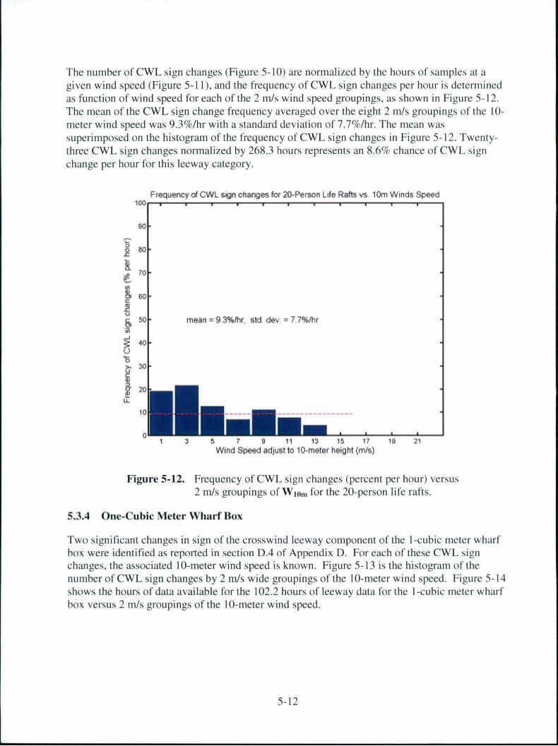
The number of CWL sign changes (Figure 5-10) are normalized by the hours of samples at agiven wind speed (Figure 5-11), and the frequency of CWL sign changes per hour is determinedas function of wind speed for each of the 2 m/s wind speed groupings, as shown in Figure 5-12.The mean of the CWL sign change frequency averaged over the eight 2 m/s groupings of the 10-meter wind speed was 9.3%/hr with a standard deviation of 7.7%/hr. The mean wassuperimposed on the histogram of the frequency of CWL sign changes in Figure 5-12. Twenty-three CWL sign changes normalized by 268.3 hours represents an 8.6% chance of CWL signchange per hour for this leeway category.

Frequency of CWL sign changes for 20-Person Life Rafts vs. lOm Winds Speed100 .

90

o807.-

60

50 mean = 9.3%/hr. std dev= 7.7%/hr

40-

104)

LL

10---- - - - - - - -

1 3 5 7 9 11 13 15 17 19 21Wind Speed adjust to 10-meter height (mis)

Figure 5-12. Frequency of CWL sign changes (percent per hour) versus2 m/s groupings of Wi0m for the 20-person life rafts.

5.3.4 One-Cubic Meter Wharf Box

Two significant changes in sign of the crosswind leeway component of the 1-cubic meter wharfbox were identified as reported in section D.4 of Appendix D. For each of these CWL signchanges, the associated 10-meter wind speed is known. Figure 5-13 is the histogram of thenumber of CWL sign changes by 2 m/s wide groupings of the 10-meter wind speed. Figure 5-14shows the hours of data available for the 102.2 hours of leeway data for the I-cubic meter wharfbox versus 2 m/s groupings of the 10-meter wind speed.

5-12

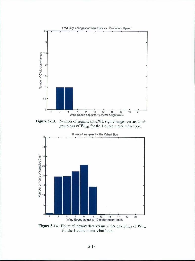
CWL sign changes for Wharf Box vs lOre Winds Speed

3

S25C

-2

OA0

U. 15-

E3z

05

1 3 5 7 9 11 13 15 17 19 21Wind Speed adjust to 10-meter height (m/s)

Figure 5-13. Number of significant CWL sign changes versus 2 m/sgroupings of W10m for the l-cubic meter wharf box.

Hours of samples for the Wharf Box40

35

LO30

S25

16 20

E=10-

1 3 5 7 9 11 13 15 17 19 21Wind Speed adjust to 10-meter height (mis)

Figure 5-14. Hours of leeway data versus 2 m/s groupings of WIomfor the 1-cubic meter wharf box.

5-13

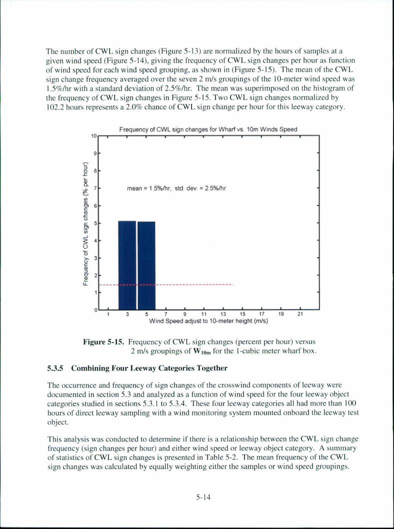
The number of CWL sign changes (Figure 5-13) are normalized by the hours of samples at agiven wind speed (Figure 5-14), giving the frequency of CWL sign changes per hour as functionof wind speed for each wind speed grouping, as shown in (Figure 5-15). The mean of the CWLsign change frequency averaged over the seven 2 m/s groupings of the 10-meter wind speed was1.5%/hr with a standard deviation of 2.5%/hr. The mean was superimposed on the histogram ofthe frequency of CWL sign changes in Figure 5-15. Two CWL sign changes normalized by102.2 hours represents a 2.0% chance of CWL sign change per hour for this leeway category.

Frequency of CWL sign changes for Wharf vs 10m Winds Speed10

9

0 8-

7 mean = 1 5%/hr, std dev, = 2 5%/hr

0

0

I.L - - - -

1

1 3 5 7 9 11 13 15 17 19 21Wind Speed adjust to 10-meter height (mls•)

Figure 5-15. Frequency of CWL sign changes (percent per hour) versus

2 m/s groupings of Wi0m for the 1-cubic meter wharf box.

5.3.5 Combining Four Leeway Categories Together

The occurrence and frequency of sign changes of the crosswind components of leeway weredocumented in section 5.3 and analyzed as a function of wind speed for the four leeway objectcategories studied in sections 5.3.1 to 5.3.4. These four leeway categories all had more than 100hours of direct leeway sampling with a wind monitoring system mounted onboard the leeway testobject.

This analysis was conducted to determine if there is a relationship between the CWL sign changefrequency (sign changes per hour) and either wind speed or leeway object category. A summaryof statistics of CWL sign changes is presented in Table 5-2. The mean frequency of the CWLsign changes was calculated by equally weighting either the samples or wind speed groupings.

5-14

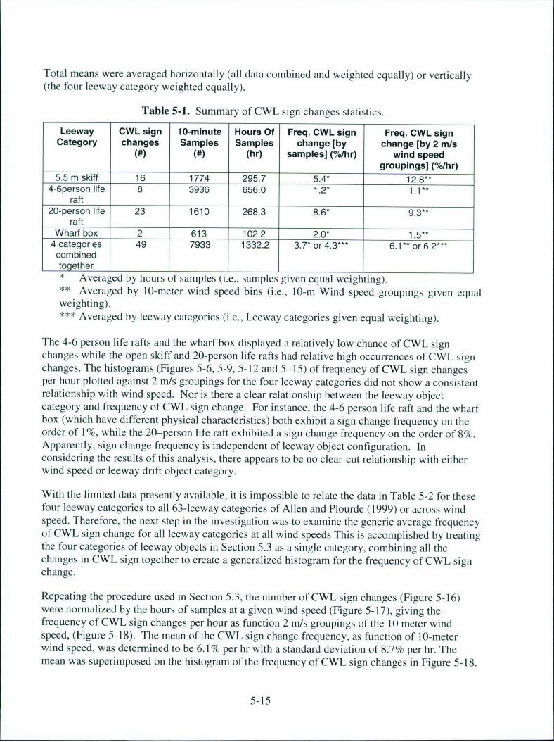
Total means were averaged horizontally (all data combined and weighted equally) or vertically(the four leeway category weighted equally).

Table 5-1. Summary of CWL sign changes statistics.

Leeway CWL sign 10-minute Hours Of Freq. CWL sign Freq. CWL signCategory changes Samples Samples change [by change [by 2 m/s

(#) (#) (hr) samples] (0/o/hr) wind speedgroupings] (%/hr)

5.5 m skiff 16 1774 295.7 5.4* 12.8**4-6person life 8 3936 656.0 1.2* 1.1 **

raft20-person life 23 1610 268.3 8.6* 9.3**

raftWharf box 2 613 102.2 2.0* 1.5*

4 categories 49 7933 1332.2 3.7* or 4.3*** 6.1 ** or 6.2***combinedtogether* Averaged by hours of samples (i.e., samples given equal weighting).** Averaged by 10-meter wind speed bins (i.e., 10-m Wind speed groupings given equalweighting).*** Averaged by leeway categories (i.e., Leeway categories given equal weighting).

The 4-6 person life rafts and the wharf box displayed a relatively low chance of CWL signchanges while the open skiff and 20-person life rafts had relative high occurrences of CWL signchanges. The histograms (Figures 5-6, 5-9, 5-12 and 5-15) of frequency of CWL sign changesper hour plotted against 2 m/s groupings for the four leeway categories did not show a consistentrelationship with wind speed. Nor is there a clear relationship between the leeway objectcategory and frequency of CWL sign change. For instance, the 4-6 person life raft and the wharfbox (which have different physical characteristics) both exhibit a sign change frequency on theorder of 1 %, while the 20-person life raft exhibited a sign change frequency on the order of 8%.Apparently, sign change frequency is independent of leeway object configuration. Inconsidering the results of this analysis, there appears to be no clear-cut relationship with eitherwind speed or leeway drift object category.

With the limited data presently available, it is impossible to relate the data in Table 5-2 for thesefour leeway categories to all 63-leeway categories of Allen and Plourde (1999) or across windspeed. Therefore, the next step in the investigation was to examine the generic average frequencyof CWL sign change for all leeway categories at all wind speeds This is accomplished by treatingthe four categories of leeway objects in Section 5.3 as a single category, combining all thechanges in CWL sign together to create a generalized histogram for the frequency of CWL signchange.

Repeating the procedure used in Section 5.3, the number of CWL sign changes (Figure 5-16)were normalized by the hours of samples at a given wind speed (Figure 5-17), giving thefrequency of CWL sign changes per hour as function 2 m/s groupings of the 10 meter windspeed, (Figure 5-18). The mean of the CWL sign change frequency, as function of 10-meterwind speed, was determined to be 6.1% per hr with a standard deviation of 8.7% per hr. Themean was superimposed on the histogram of the frequency of CWL sign changes in Figure 5-18.

5-15

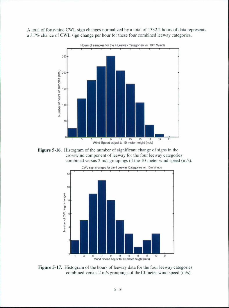
A total of forty-nine CWL sign changes normalized by a total of 1332.2 hours of data representsa 3.7% chance of CWL sign change per hour for these four combined leeway categories.

Hours of samples for the 4 Leeway Categories vs Oim Winds

250

Pj 200-

L.EN1500

0

.16 oo-

Ez

50.

0J 1 3 5 7 9 11 13 15 17 19 21Wind Speed adjust to 1 0-meter height (mis)

Figure 5-16. Histogram of the number of significant change of signs in thecrosswind component of leeway for the four leeway categoriescombined versus 2 m/s groupings of the 10-meter wind speed (m/s).

CWL sign changes for the 4 Leeway Categories vs. 1Oin Winds

12

10

C

z

1 3 5 7 9 11 13 15 17 19 21Wind Speed adjust to 10-meter height (m/s)

Figure 5-17. Histogram of the hours of leeway data for the four leeway categoriescombined versus 2 mIs groupings of the 10-meter wind speed (m/s).

5-16

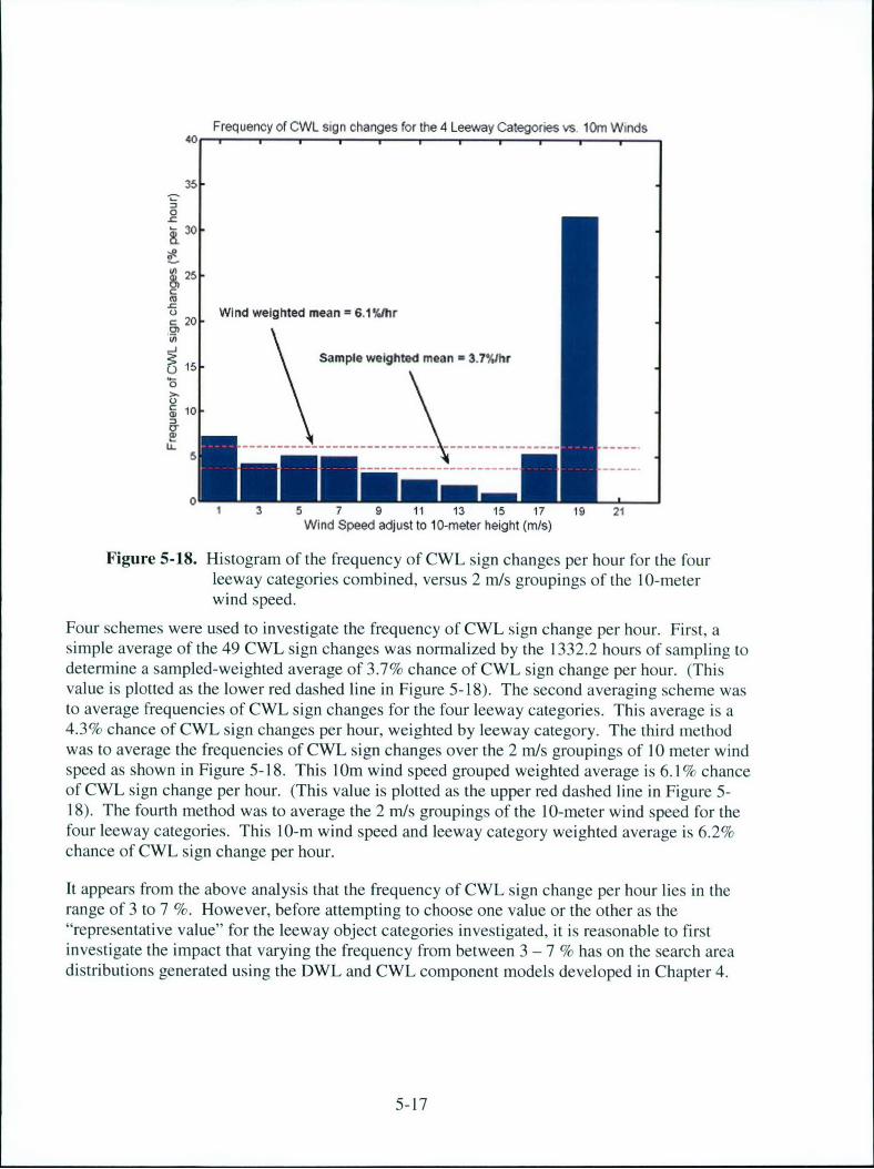
Frequency of CWL sign changes for the 4 Leeway Categories vsi 0m Winds40 . , , , ., , ,

35

0-

'-

a

Wind weighted mean 6.1%thr,20o

ý1 Sample weighted mean -3.7%/hr

i~.

10

1 3 5 7 9 11 13 15 17 19 21Wind Speed adjust to 10-meter height (m/s)

Figure 5-18. Histogram of the frequency of CWL sign changes per hour for the fourleeway categories combined, versus 2 m/s groupings of the 10-meterwind speed.

Four schemes were used to investigate the frequency of CWL sign change per hour. First, asimple average of the 49 CWL sign changes was normalized by the 1332.2 hours of sampling todetermine a sampled-weighted average of 3.7% chance of CWL sign change per hour. (Thisvalue is plotted as the lower red dashed line in Figure 5-18). The second averaging scheme wasto average frequencies of CWL sign changes for the four leeway categories. This average is a4.3% chance of CWL sign changes per hour, weighted by leeway category. The third methodwas to average the frequencies of CWL sign changes over the 2 m/s groupings of 10 meter windspeed as shown in Figure 5-18. This lOim wind speed grouped weighted average is 6.1% chanceof CWL sign change per hour. (This value is plotted as the upper red dashed line in Figure 5-18). The fourth method was to average the 2 m/s groupings of the 10-meter wind speed for thefour leeway categories. This 10-m wind speed and leeway category weighted average is 6.2%chance of CWL sign change per hour.

It appears from the above analysis that the frequency of CWL sign change per hour lies in therange of 3 to 7 %. However, before attempting to choose one value or the other as the"representative value" for the leeway object categories investigated, it is reasonable to firstinvestigate the impact that varying the frequency from between 3 - 7 % has on the search areadistributions generated using the DWL and CWL component models developed in Chapter 4.

5-17

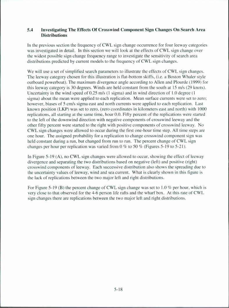
5.4 Investigating The Effects Of Crosswind Component Sign Changes On Search AreaDistributions

In the previous section the frequency of CWL sign change occurrence for four leeway categorieswas investigated in detail. In this section we will look at the effects of CWL sign change overthe widest possible sign change frequency range to investigate the sensitivity of search areadistributions predicted by current models to the frequency of CWL sign changes.

We will use a set of simplified search parameters to illustrate the effects of CWL sign changes.The leeway category chosen for this illustration is flat-bottom skiffs, (i.e. a Boston Whaler styleoutboard powerboat). The maximum divergence angle according to Allen and Plourde (1999) forthis leeway category is 30 degrees. Winds are held constant from the south at 15 m/s (29 knots).Uncertainty in the wind speed of 0.25 m/s (I sigma) and in wind direction of 1.0 degree (Isigma) about the mean were applied to each replication. Mean surface currents were set to zero;however, biases of 5 cm/s sigma east and north currents were applied to each replication. Lastknown position (LKP) was set to zero, (zero coordinates in kilometers east and north) with 1000replications, all starting at the same time, hour 0.0. Fifty percent of the replications were startedto the left of the downwind direction with negative components of crosswind leeway and theother fifty percent were started to the right with positive components of crosswind leeway. NoCWL sign changes were allowed to occur during the first one-hour time step. All time steps areone hour. The assigned probability for a replication to change crosswind component sign washeld constant during a run, but changed from run to run. The percent change of CWL signchanges per hour per replication was varied from 0 % to 50 % (Figures 5-19 to 5-21).

In Figure 5-19 (A), no CWL sign changes were allowed to occur, showing the effect of leewaydivergence and separating the two distributions based on negative (left) and positive (right)crosswind components of leeway. Each successive distribution also shows the spreading due tothe uncertainty values of leeway, wind and sea current. What is clearly shown in this figure isthe lack of replications between the two major left and right distributions.

For Figure 5-19 (B) the percent change of CWL sign change was set to 1.0 % per hour, which isvery close to that observed for the 4-6 person life rafts and the wharf box. At this rate of CWLsign changes there are replications between the two major left and right distributions.

5-18

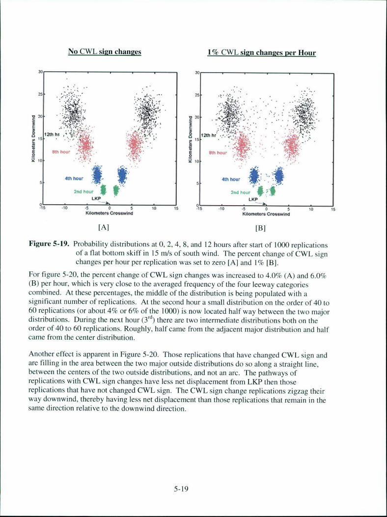
No CWL sign changes 1% CWL sign changes per Hour

30 30

25--- 25-'4

V..'~.:4~.. .- $ • , .

1020 ~20- .~.. C. . C3, ,. •...'- *.- ..

2 •th hr t h *VA,-r1 5 " - "" . . ..5.

RM Shou Oth hu

4th hour 4th hour

2nd, hour 2nd h 4uLKP LKP

?15 -10 *5 0 5 10 is ?s- .-10 .5 0 5 10 1Kilometerg Crosswind Kilometers Crosswind

[A] [B]

Figure 5-19. Probability distributions at 0, 2, 4, 8, and 12 hours after start of 1000 replicationsof a flat bottom skiff in 15 m/s of south wind. The percent change of CWL signchanges per hour per replication was set to zero [A] and 1% [B].

For figure 5-20, the percent change of CWL sign changes was increased to 4.0% (A) and 6.0%(B) per hour, which is very close to the averaged frequency of the four leeway categoriescombined. At these percentages, the middle of the distribution is being populated with asignificant number of replications. At the second hour a small distribution on the order of 40 to60 replications (or about 4% or 6% of the 1000) is now located half way between the two majordistributions. During the next hour (3 dd) there are two intermediate distributions both on theorder of 40 to 60 replications. Roughly, half came from the adjacent major distribution and halfcame from the center distribution.

Another effect is apparent in Figure 5-20. Those replications that have changed CWL sign andare filling in the area between the two major outside distributions do so along a straight line,between the centers of the two outside distributions, and not an arc. The pathways ofreplications with CWL sign changes have less net displacement from LKP then thosereplications that have not changed CWL sign. The CWL sign change replications zigzag theirway downwind, thereby having less net displacement than those replications that remain in thesame direction relative to the downwind direction.

5-19

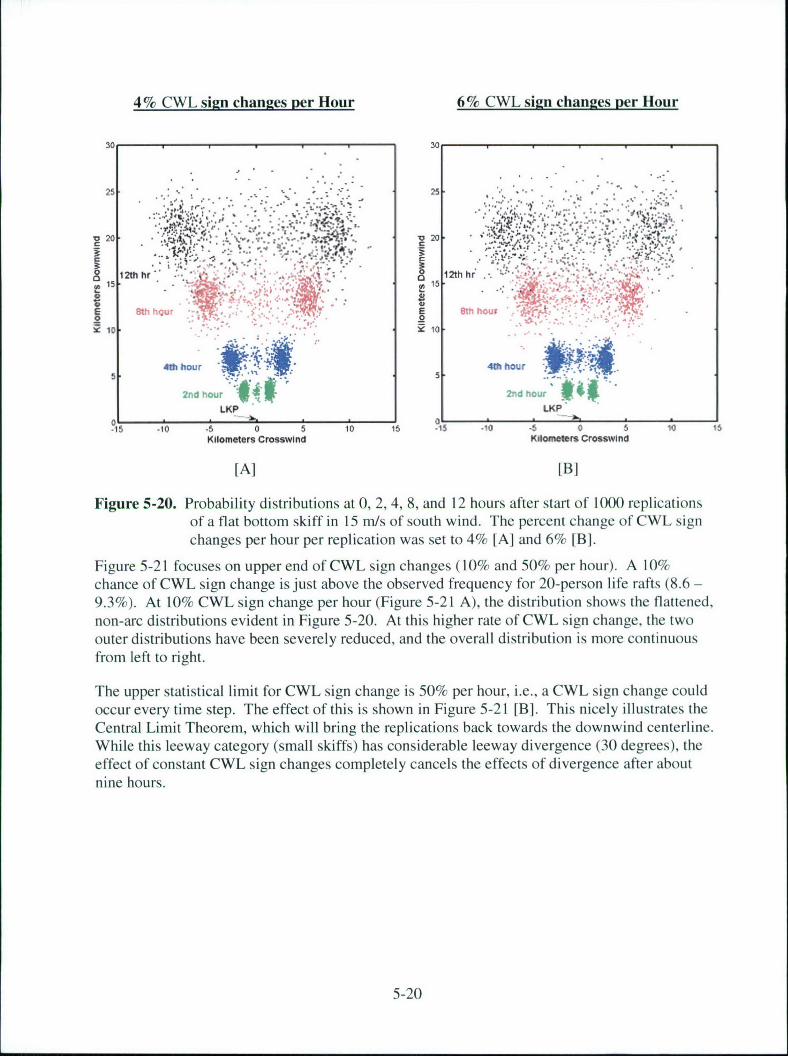
4% CWL sign changes per Hour 6% CWL sign changes per Hour

25 . . .. 25 v . * ..

A• ,, • .. , ,.- -- ..-. , " :-., '. .• •. : .':• e .,.20 A:M:

h2ourr "2 "t h ouh

10 10.

4th hour 4th hour

2 nd hou

LKP LKP

-15 -10 -5 0 5 10 16 -15 -10 -5 0 5 10 16Kilometers Crosswind Kilometers Crosswind

[A] IB]

Figure 5-20. Probability distributions at 0, 2, 4, 8, and 12 hours after start of 10(X) replicationsof a flat bottom skiff in 15 m/s of south wind. The percent change of CWL signchanges per hour per replication was set to 4% [A] and 6% [B].

Figure 5-21 focuses on upper end of CWL sign changes (10% and 50% per hour). A 10%chance of CWL sign change is just above the observed frequency for 20-person life rafts (8.6 -9.3%). At 10% CWL sign change per hour (Figure 5-21 A), the distribution shows the flattened,non-arc distributions evident in Figure 5-20. At this higher rate of CWL sign change, the twoouter distributions have been severely reduced, and the overall distribution is more continuousfrom left to right.

The upper statistical limit for CWL sign change is 50% per hour, i.e., a CWL sign change couldoccur every time step. The effect of this is shown in Figure 5-21 [B]. This nicely illustrates theCentral Limit Theorem, which will bring the replications back towards the downwind centerline.While this leeway category (small skiffs) has considerable leeway divergence (30 degrees), theeffect of constant CWL sign changes completely cancels the effects of divergence after aboutnine hours.

5-20

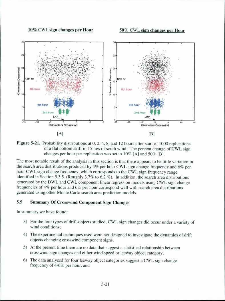
10% CWL sign changes per Hour 50% CWL sign changes per Hour

25 † . 0

I *%."U i%.

A 2th hr O~12th hr15 "15.

4th hour 48 h hour

4th hour4th hour

2nd hou,,*

LKP LKP

15 -,10 -5 0 5 10 15 --5 -10 -5 0 5 10 15K11omefers Crosswind Kikn@res Crosswind

[A] [B]

Figure 5-21. Probability distributions at 0, 2, 4, 8, and 12 hours after start of 1000 replicationsof a flat bottom skiff in 15 m/s of south wind. The percent change of CWL signchanges per hour per replication was set to 10% [A] and 50% [B].

The most notable result of the analysis in this section is that there appears to be little variation inthe search area distributions produced by 4% per hour CWL sign change frequency and 6% perhour CWL sign change frequency, which corresponds to the CWL sign frequency rangeidentified in Section 5.3.5. (Roughly 3.7% to 6.2 %). In addition, the search area distributionsgenerated by the DWL and CWL component linear regression models using CWL sign changefrequencies of 4% per hour and 6% per hour correspond well with search area distributionsgenerated using other Monte Carlo search area prediction models.

5.5 Summary Of Crosswind Component Sign Changes

In summary we have found:

3) For the four types of drift-objects studied, CWL sign changes did occur under a variety ofwind conditions;

4) The experimental techniques used were not designed to investigate the dynamics of driftobjects changing crosswind component signs,

5) At the present time there are no data that suggest a statistical relationship betweencrosswind sign changes and either wind speed or leeway object category,

6) The data analyzed for four leeway object categories suggest a CWL sign changefrequency of 4-6% per hour, and

5-21

7) Search area distributions show little difference when CWL sign change frequency variesfrom 4 to 6% per hour.

Since we do not have a dynamic model of the physics of crosswind direction change (CWL signchange), and since the statistics of CWL sign changes for the four leeway categories investigateddo not provide a rigorous enough basis for extrapolating to all leeway-object categories orindicate direct relationship between CWL sign change frequency and wind velocity or leewayobject category, we recommend that search planning tools use a simple generic average CWLsign change frequency of 4% per hour for all leeway categories with no dependence on windspeed.

5-22

CHAPTER 6.

CONCLUSIONS AND RECOMMENDATIONS

6.1 Conclusions

The prediction of the divergence of search object trajectories from the downwind direction is acritical component to the accurate establishment of a search area. The somewhat murkyrelationship among leeway angle, divergence angle, and leeway divergence has hindered theproper implementation of leeway divergence into search planning tools. Based upon the leewayfield studies of the 1990s, this report provides a review and analysis to determine a new approachto model leeway divergence based on computing the downwind (DWL) and crosswind (CWL)components of leeway. This is a different approach than that recommended in Allen and Plourde(1999), which provided coefficients for calculating leeway drift as a function of leeway speedand divergence angle (the traditional approach).

In Chapter 2, an empirical technique is developed to convert the leeway speed and divergenceangle values of Allen and Plourde (1999) to a set of linear regression coefficients for computingthe downwind and crosswind of leeway drift. This technique was used to determine the DWLand CWL coefficients for 38 leeway object categories for which actual leeway drift data are notavailable. These 38 sets of coefficients, combined with the initial set of 25 coefficientscomputed by linear regression analysis of actual data for 25 categories, forms a complete set ofDWL and CWL coefficients for the 63 leeway object categories in the comprehensive leewaytaxonomy developed by Allen and Plourde (1999). This complete set of coefficients for theunconstrained and constrained forms of the DWL and CWL component model is presented andexplained in Chapter 3.

In Chapter 4, a DWL and CWL component leeway drift model is presented that uses thecoefficients in Chapter 3 to compute leeway drift. Chapter 5 investigates the nature and impact ofCWL sign changes in modeling leeway drift. Most of the drift objects studied during the 1990sfield tests drifted to either the right or left of the downwind direction for the duration of the driftperiod. This behavior tends to generate two areas of high search probability that eventuallyseparate over time. The use of downwind and crosswind components of leeway by Monte Carlosimulation techniques readily model this behavior. However, a closer inspection of four leewaycategories that each contained over 100 hours of directly measured leeway revealed that the driftobject did change crosswind leeway drift direction from either right of the downwind direction tothe left or vice versa. These changes result in a change in the sign of the crosswind componentof leeway.

The investigations in Chapter 5 show that the frequency of CWL sign change appears to beindependent of wind speed. The frequency of the sign change was shown to vary among the fourleeway object categories, but we were not able to generalize (or extrapolate) sign changeoccurrence to the 59 other leeway categories. The overall observed frequency of these signchanges in crosswind components based on the leeway drift of all four categories of leewayobjects was approximately 4-6% per hour. It was further shown that while the differencebetween final search area probability distribution was significant for 0% and 50% sign change

6-1

frequency per hour, the difference between distributions resulting from 4% and 6% sign changefrequency per hour was not. Based on past search area modeling, it appears that a 4-6% signchange frequency provides a search area distribution consistent with those generated by existingSAR planning tools. A "generic" value of 4% per hour is recommended for use in stochasticleeway models until further study provides a more complete picture of CWL sign phenomena.

6.2 Recommendations

1) Tables 3-1 and 3-2 provide a complete set of DWL and CWL coefficients for the 63categories of leeway objects in the taxonomy developed by Allen and Plourde (1999).Although 38 sets of DWL and CWL coefficients were statistically derived from theempirical data, the Table 3-1 and 3-2 coefficients should be used in numerical searchplanning tools to determine the downwind and crosswind components of leeway (as afunction of wind speed adjusted to the standard 10-meter height) in calculating searcharea distributions.

2) Incorporate into numerical search planning tools the use of a simple statistical model ofswitching between positive and negative crosswind component equations using a signchange frequency of 4% per hour, independent of wind speed or leeway category.

3) Incorporate into manual search planning tools the use of divergence angles provided byAllen and Plourde (1999) divided by an adjustment factor 1.35.

4) Continue efforts to fully understand and model the drift of survivors and survivor craft bystudying targets over more drift runs and in a variety of wind conditions. The conditionsshould include wind speeds less than 3 m/s and greater than 20 m/s and periods of rapidwind direction shifts. With more drift run analysis, the subject of initial distributionbetween left and right divergence can be addressed. Collecting leeway data under avariety of wind conditions will also allow the observation of changes between left andright divergence. Data collection for the 38 leeway categories for which data are notavailable will allow direct computation and verification of the DWL and CWLcoefficients for these categories.

5) Further refine the collection of leeway data collected in the field to minimize the effectthat the instrumentation has on drift of the search test object. The use of current metersplaced directly onboard the test object is likely to lessen the impact on the craft switchingsigns of the crosswind component. However, these directly mounted current metersshould be verified against the more standard technique of a tethered current meter, whichis well away from any local flow distortion effects. Additional insight into the behaviorand dynamics of an object's CWL component sign change might come with furtherinformation of the wave field and from leeway dynamics modeling studies.

6-2

CHAPTER 7.

REFERENCES

Allen, A. A., 1996. "The Leeway of Cuban Refugee Rafts and a Commercial Fishing Vessel," U.S.Coast Guard Report No. CG-D-21-96.

Allen, A. A., and R.B. Fitzgerald, 1997. "The Leeway of an Open Boat and Three Life Rafts inHeavy Weather," U.S. Coast Guard Report No. CG-D-03-98.

Allen, A. A., and J.V. Plourde, 1999. "Review of Leeway: Field Experiments and Implementation,"U.S. Coast Guard Report No. CG-D-08-99.

Allen, A.A., R.Q. Robe and E.T. Morton, 1999. "The Leeway of Person-In-the-Water and ThreeSmall Craft," U.S. Coast Guard Report No. CG-D-09-00.

Chapline, W. E., 1960. "Estimating the Drift of Distressed Small Craft." Coast Guard AlumniAssociation Bulletin, U.S. Coast Guard Academy, New London, CT Vol. 22, No. 2, March-April 1960, pp 39-42.

Fitzgerald, R. B., D. J. Finlayson, and A. Allen, 1994. "Drift of Common Search and RescueObjects - Phase III." Contract report prepared for Canadian Coast Guard, Research andDevelopment, Ottawa, TP# 12179.

Hodgins, D. 0. and S. L. M. Hodgins, 1998. "Phase II Leeway Dynamics Study ProgramDevelopment and Verification of a Mathematical Drift Model for Liferafts and SmallBoats." prepared for Canadian Coast Guard College, Dept. Fisheries and Oceans.

Hufford, G.L., and S. Broida, 1974. "Determination of Small Craft Leeway." U.S. Coast GuardResearch and Development Center Report No. 39/74, December 1974.

Kang, S.Y., 1999. "A Field Experiment for the Determination of Drift Characteristics of Person-in-Water", 'Journal of the Society of Maritime Safety', Vol. 5, No. 1, pp. 29-36 (Abstract inEnglish, text in Korean).

Nash, L., and J. Willcox, 1985. "Summer 1983 Leeway Drift Experiment," U.S. Coast GuardReport CG-D-35-85.

Nash, L., and J. Willcox, 1991. "Spring 1985 Leeway Experiment," U.S. Coast Guard Report CG-D- 12-92.

National Search and Rescue Committee, 2000, "U.S. National Search and Rescue Supplement tothe International Aeronautical and Maritime Search and Rescue Manual," Washington D.C.

Neter, J., M.H. Kuter, C.J. Nachtsheim, and W. Wasserman, 1996. "Applied Linear StatisticalModels" Fourth Edition, Irwin, Inc. Chicago, IL

7-1

Smith, S.D., 1988. "Coefficients for Sea Surface Wind Stress, Heat Flux, and Wind Profiles as aFunction of Wind Speed and Temperature," J. Geophysical Res. Vol. 93, No. C12, pp.15,467-15,472, 5 December 1988.

7-2

APPENDIX A

LEEWAY COMPONENTS OF MARITIME LIFE RAFTS (DEEPBALLAST, CANOPY, 15-25 PERSON CAPACITY)

A.1 Introduction

A Beaufort 20-person circular life raft, shown in Figure A- 1, was drifted six times in twoconfigurations. Three leeway drift runs were performed with light loading and no drogue, andthree drift runs were with heavy loading and a drogue deployed (Fitzgerald et al. (1994) andAllen and Plourde (1999)). Fitzgerald et al. (1994) presented results for the downwindcomponent of leeway for the two configurations, while Allen and Plourde (1999) presentedresults for the combined class, i.e., both configurations. The results of the analysis for bothcomponents of leeway are presented here for the two configurations of the twenty-person liferaft. The configurations follow the leeway taxonomy convention of Allen and Plourde (1999).The analysis procedure follows Allen (1996), Allen and Fitzgerald (1997), Allen and Plourde(1999) and Allen et al. (1999).

LIFTING RINGLIFTING STRAPS

•'* ••VIEW PORT

Figure A-1. Beaufort circular 20-person life raft.

A.1.1 MARITIME LIFE RAFT (Deep Ballast, Canopy, 15-25 Person Capacity,No Drogue, Light Loading).

The first leeway drift configuration of the Beaufort 20-person circular life raft was with lightloading and no drogue attached. Three drift runs (Leeway Drift Runs 37, 43, and 48) in thisconfiguration combined for a total of 816 ten-minute samples or 136 hours of data. In Figure A-2, the unconstrained linear regression of the downwind component of leeway (DWL, in cm/s)versus wind speed (m/s) adjusted by Smith (1988) to the 10-meter reference level (W10m). Alsopresented in Figure A-2 are the 95% prediction limits for the 20-person lifer raft with no drogueand light loading. The value of 0.94 for r2 indicates that the regression of DWL versus Wi0 maccounts for 94% of the variance of the DWL, an excellent statistical fit.

For analysis purposes, drift runs were separated according to whether the total drift was positiveor negative. The unconstrained linear regression of the crosswind components of leeway

A-I

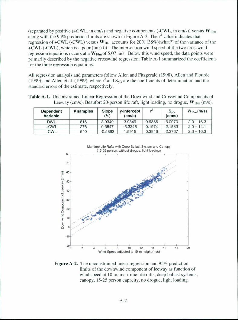
(separated by positive (+CWL, in cm/s) and negative components (-CWL, in cm/s)) versus W1 0 ,,along with the 95% prediction limits are shown in Figure A-3. The r2 value indicates thatregression of +CWL (-CWL) versus W10m accounts for 20% (38%)(what?) of the variance of the+CWL (-CWL), which is a poor (fair) fit. The intersection wind speed of the two crosswindregression equations occurs at a Wtom of 5.07 m/s. Below this wind speed, the data points wereprimarily described by the negative crosswind regression. Table A- 1 summarized the coefficientsfor the three regression equations.

All regression analysis and parameters follow Allen and Fitzgerald (1998), Allen and Plourde(1999), and Allen et al. (1999), where r2 and Sy/, are the coefficients of determination and thestandard errors of the estimate, respectively.

Table A-1. Unconstrained Linear Regression of the Downwind and Crosswind Components ofLeeway (cm/s), Beaufort 20-person life raft, light loading, no drogue, W10, (m/s).

Dependent # samples Slope y-intercept r2 Sy," W10m (m/s)Variable (%) (cmls) (cm/s)

DWL 816 3.9349 3.9349 0.9386 3.0070 2.0 - 16.3+CWL 276 0.3847 -3.3346 0.1974 2.1583 2.0-14.1-CWL 540 -0.5863 1.5915 0.3846 2.2767 2.3-16.3

Maritime Life Rafts with Deep Ballast System and Canopy(15-25 person, without drogue, light loading)

80 ,

70

S60-E

>' 50-

400

0

10-

-10

"20 4 6 8 10 12 14 16 18 20Wind Speed adjusted to 10-m height (m/s)

Figure A-2. The unconstrained linear regression and 95% predictionlimits of the downwind component of leeway as function ofwind speed at 10 m, maritime life rafts, deep ballast systems,canopy, 15-25 person capacity, no drogue, light loading.

A-2

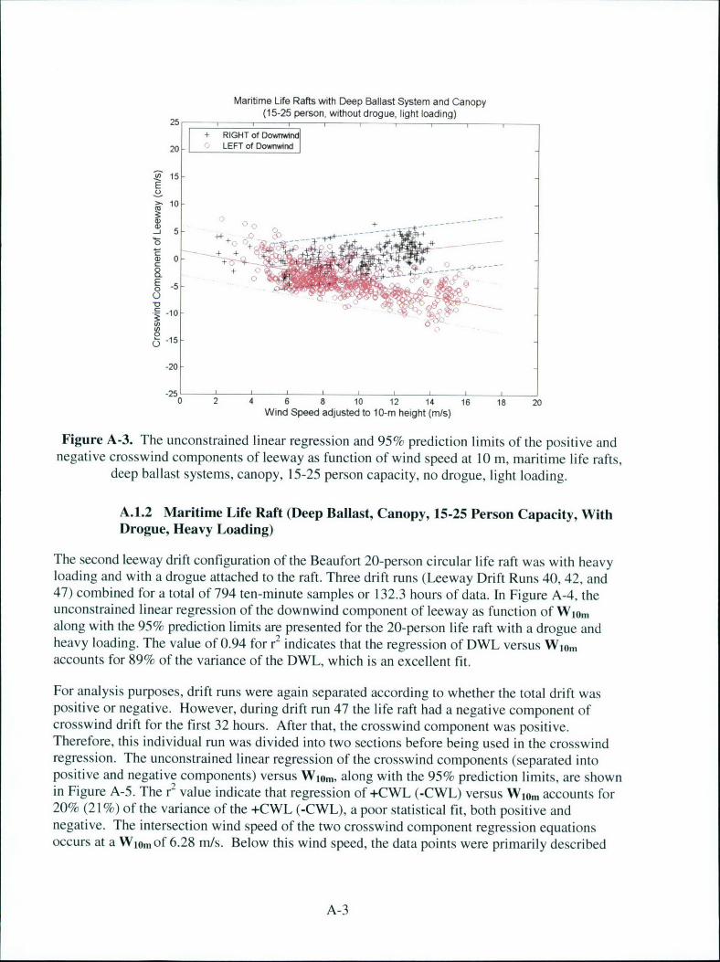
Maritime Life Rafts with Deep Ballast System and Canopy(15-25 person, without drogue, light loading)25 -- -- , ,_,

+ RIGHT of Downwind

20-1 LEFT of Downwind

E0

-15-

* -10 --

-20

0-2

Wind Speed adjusted to 10-rn height (m/s)

Figure A-3. The unconstrained linear regression and 95% prediction limits of the positive andnegative crosswind components of leeway as function of wind speed at 10 m, maritime life rafts,

deep ballast systems, canopy, 15-25 person capacity, no drogue, light loading.

A.1.2 Maritime Life Raft (Deep Ballast, Canopy, 15-25 Person Capacity, WithDrogue, Heavy Loading)

The second leeway drift configuration of the Beaufort 20-person circular life raft was with heavyloading and with a drogue attached to the raft. Three drift runs (Leeway Drift Runs 40, 42. and47) combined for a total of 794 ten-minute samples or 132.3 hours of data. In Figure A-4, theunconstrained linear regression of the downwind component of leeway as function of Wlomalong with the 95% prediction limits are presented for the 20-person life raft with a drogue andheavy loading. The value of 0.94 for r2 indicates that the regression of DWL versus Wi~maccounts for 89% of the variance of the DWL, which is an excellent fit.

For analysis purposes, drift runs were again separated according to whether the total drift waspositive or negative. However, during drift run 47 the life raft had a negative component ofcrosswind drift for the first 32 hours. After that, the crosswind component was positive.Therefore, this individual run was divided into two sections before being used in the crosswindregression. The unconstrained linear regression of the crosswind components (separated intopositive and negative components) versus Wi~m, along with the 95% prediction limits, are shownin Figure A-5. The r2 value indicate that regression of +CWL (-CWL) versus Wl~m accounts for20% (21 %) of the variance of the +CWL (-CWL), a poor statistical fit, both positive andnegative. The intersection wind speed of the two crosswind component regression equationsoccurs at a Wiom of 6.28 m/s. Below this wind speed, the data points were primarily described

A-3

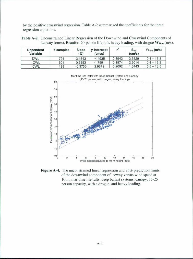
by the positive crosswind regression. Table A-2 summarized the coefficients for the threeregression equations.

Table A-2. Unconstrained Linear Regression of the Downwind and Crosswind Components ofLeeway (cm/s), Beaufort 20-person life raft, heavy loading, with drogue W1~m (m/s).

Dependent # samples Slope y-intercept r2 Sy/x WIom (m/s)Variable (%) (cmls) (cmls)

DWL 794 3.1543 -4.4935 0.8942 3.3529 0.4- 15.3+CWL 601 0.3853 -1.7991 0.1974 2.5014 0.4-15.3-CWL 193 -0.3756 2.9819 0.2092 1.6443 5.5 - 13.5

Maritime Life Rafts with Deep Ballast System and Canopy(15-25 person, with drogue, heavy loading)

80 1• • T

70-

>.50-

-J 40-LA w

S30C

48FE 20 -0

-10

-20 I -L -0 2 4 6 8 10 12 14 16 18 20

Wind Speed adjusted to 10-m height (m/s)

Figure A-4. The unconstrained linear regression and 95% prediction limitsof the downwind component of leeway versus wind speed at10 m, maritime life rafts, deep ballast systems, canopy, 15-25person capacity, with a drogue, and heavy loading.

A-4

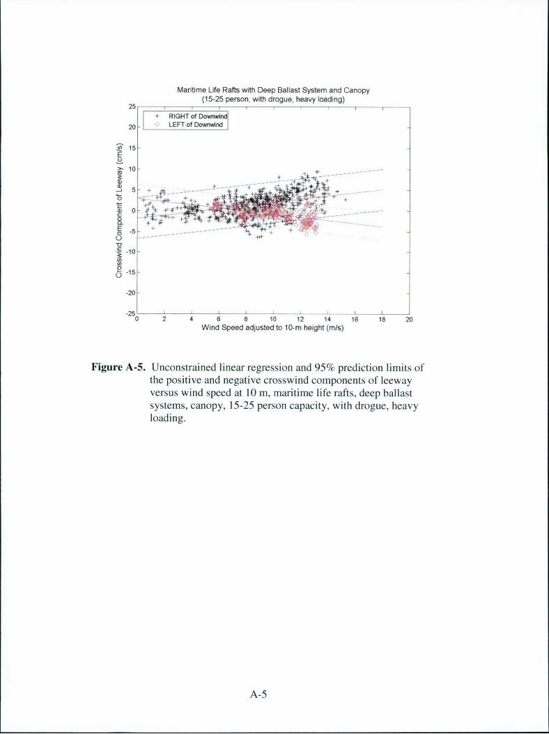
Maritime Life Rafts with Deep Ballast System and Canopy(15-25 person, with drogue, heavy loading)

25 T I I I I I ,+ RIGHT of Downwind

20 LEFT of Dowwind

S15EU>" 10 ...

-10

-5

-20-25 0- .. -

010 12 14 16 18 20Wind Speed adjusted to 10-m height (mis)

Figure A-5. Unconstrained linear regression and 95% prediction limits ofthe positive and negative crosswind components of leewayversus wind speed at 10 m, maritime life rafts, deep ballastsystems, canopy, 15-25 person capacity, with drogue, heavyloading.

A-5

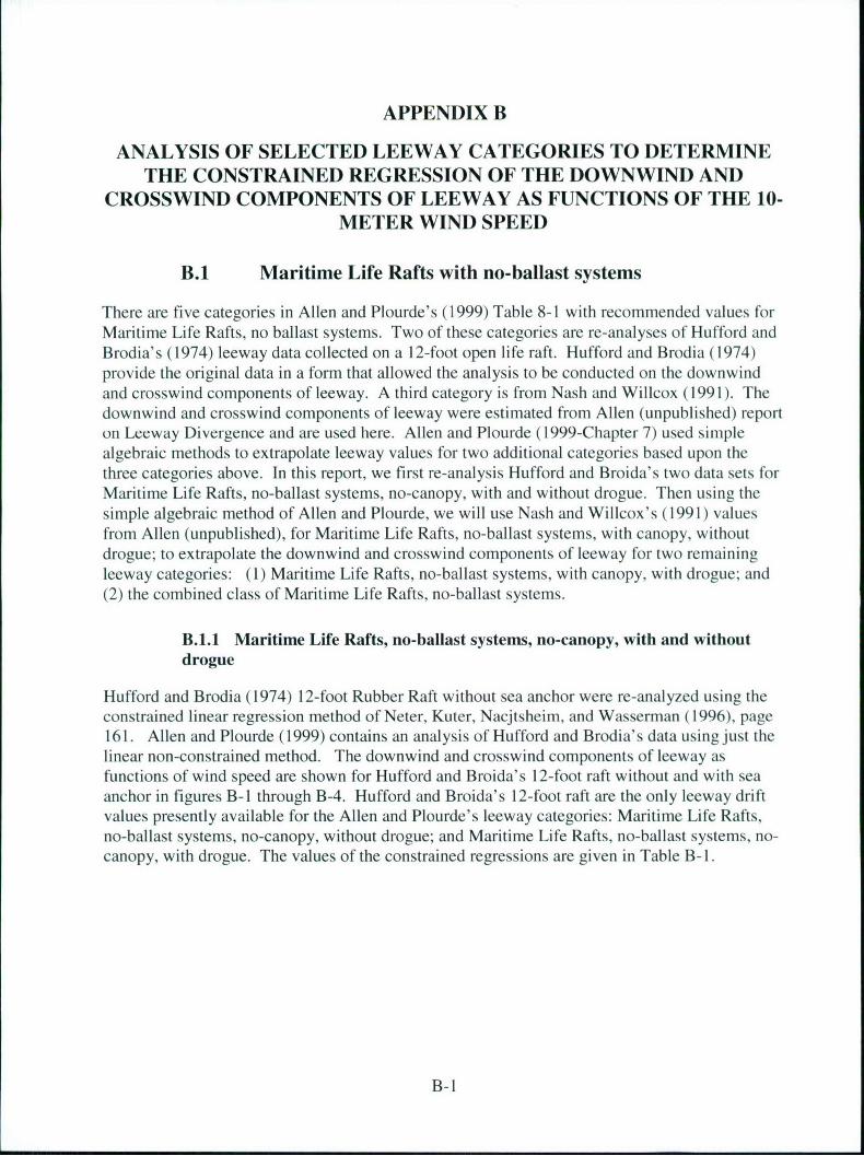
APPENDIX B

ANALYSIS OF SELECTED LEEWAY CATEGORIES TO DETERMINETHE CONSTRAINED REGRESSION OF THE DOWNWIND AND

CROSSWIND COMPONENTS OF LEEWAY AS FUNCTIONS OF THE 10-METER WIND SPEED

B.1 Maritime Life Rafts with no-ballast systems

There are five categories in Allen and Plourde's (1999) Table 8-1 with recommended values forMaritime Life Rafts, no ballast systems. Two of these categories are re-analyses of Hufford andBrodia's (1974) leeway data collected on a 12-foot open life raft. Hufford and Brodia (1974)provide the original data in a form that allowed the analysis to be conducted on the downwindand crosswind components of leeway. A third category is from Nash and Willcox (1991). Thedownwind and crosswind components of leeway were estimated from Allen (unpublished) reporton Leeway Divergence and are used here. Allen and Plourde (1999-Chapter 7) used simplealgebraic methods to extrapolate leeway values for two additional categories based upon thethree categories above. In this report, we first re-analysis Hufford and Broida's two data sets forMaritime Life Rafts, no-ballast systems, no-canopy, with and without drogue. Then using thesimple algebraic method of Allen and Plourde, we will use Nash and Willcox's (1991) valuesfrom Allen (unpublished), for Maritime Life Rafts, no-ballast systems, with canopy, withoutdrogue; to extrapolate the downwind and crosswind components of leeway for two remainingleeway categories: (1) Maritime Life Rafts, no-ballast systems, with canopy, with drogue; and(2) the combined class of Maritime Life Rafts, no-ballast systems.

B.1.1 Maritime Life Rafts, no-ballast systems, no-canopy, with and withoutdrogue

Hufford and Brodia (1974) 12-foot Rubber Raft without sea anchor were re-analyzed using theconstrained linear regression method of Neter, Kuter, Nacjtsheim, and Wasserman (1996), page161. Allen and Plourde (1999) contains an analysis of Hufford and Brodia's data using just thelinear non-constrained method. The downwind and crosswind components of leeway asfunctions of wind speed are shown for Hufford and Broida's 12-foot raft without and with seaanchor in figures B-1 through B-4. Hufford and Broida's 12-foot raft are the only leeway driftvalues presently available for the Allen and Plourde's leeway categories: Maritime Life Rafts,no-ballast systems, no-canopy, without drogue; and Maritime Life Rafts, no-ballast systems, no-canopy, with drogue. The values of the constrained regressions are given in Table B-1.

B-1

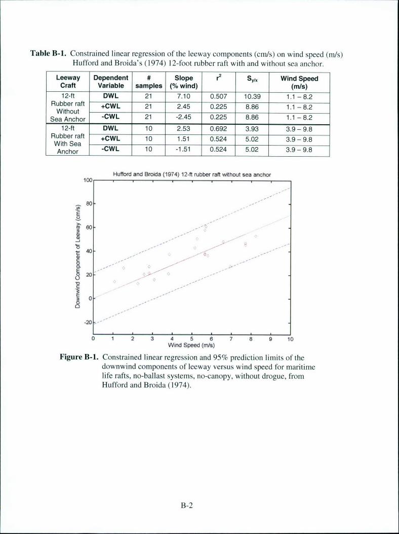
Table B-1. Constrained linear regression of the leeway components (cm/s) on wind speed (m/s)Hufford and Broida's (1974) 12-foot rubber raft with and without sea anchor.

Leeway Dependent # Slope r2 SY/x Wind SpeedCraft Variable samples (% wind) (mIs)12-ft DWL 21 7.10 0.507 10.39 1.1 -8.2

Rubber raft +CWL 21 2.45 0.225 8.86 1.1 - 8.2WithoutSea Anchor -CWL 21 -2.45 0.225 8.86 1.1 -8.2

12-ft DWL 10 2.53 0.692 3.93 3.9- 9.8Rubber raft +CWL 10 1.51 0.524 5.02 3.9 - 9.8With Sea -CWL 10 -1.51 0.524 5.02 3.9 - 9.8Anchor _______ ________ __

Hufford and Broida (1974) 12-It rubber raft without sea anchor100

E0

t60.

20

0J

-20~

0 1 2 3 4 5 6 7 8 9 10Wind Speed (mis)

Figure B-1. Constrained linear regression and 95% prediction limits of thedownwind components of leeway versus wind speed for maritimelife rafts, no-ballast systems, no-canopy, without drogue, fromHufford and Broida (1974).

B-2

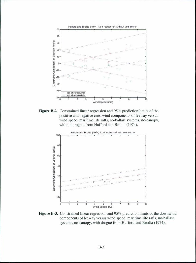
Hulford and Broida (1974) 12-ft rubber raft without sea anchor

50

40.

::30 30

20 20-

-1 0 -. . . .

0.

-10.

_ -20

S-30

-40 -pas abkcrosswvd)

1 2 3 4 5 a 7 8 9 10Wind Speed (mis)

Figure B-2. Constrained linear regression and 95% prediction limits of thepositive and negative crosswind components of leeway versuswind speed, maritime life rafts, no-ballast systems, no-canopy,without drogue, from Hufford and Brodia (1974).

Hufford and Broida (1974) 12-ft rubber raft with sea anchor100

80-g

180-

140-120-

0-

-210

0 1 2 3 4 5 6 7 8 9 10Wind Speed (mis)

Figure B-3. Constrained linear regression and 95% prediction limits of the downwindcomponents of leeway versus wind speed, maritime life rafts, no-ballastsystems, no-canopy, with drogue from Hufford and Brodia (1974).

B-3

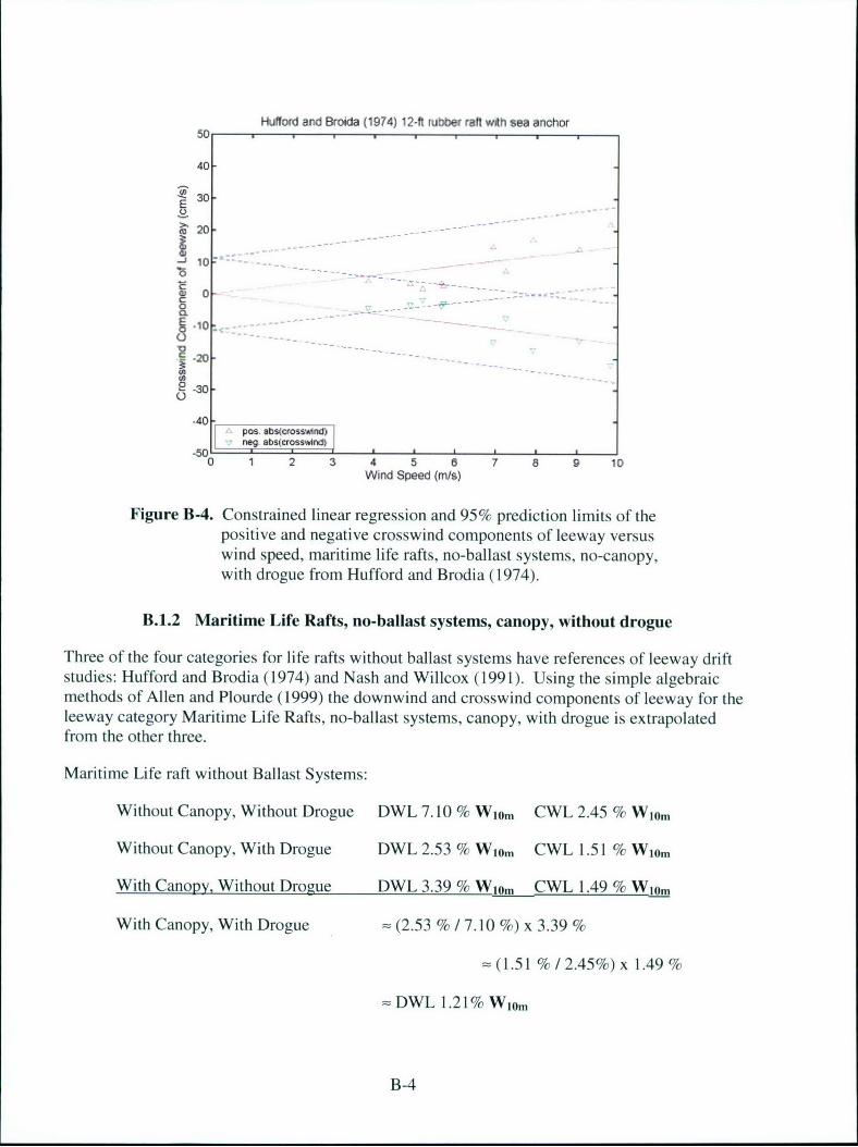
Hufford and Broida (1974) 12-ft rubber raft with sea anchor

50

40

S 30

20-00

-420-5J0 --

0105 6 9 1.0-

pO-1 . b W

Wind Speed (tr~s)

Figure B-4. Constrained linear regression and 95% prediction limits of thepositive and negative crosswind components of leeway versuswind speed, maritime life rafts, no-ballast systems, no-canopy,with drogue from Hufford and Brodia (1974).

B.1.2 Maritime Life Rafts, no-ballast systems, canopy, without drogue

Three of the four categories for life rafts without ballast systems have references of leeway driftstudies: Hufford and Brodia (1974) and Nash and Willcox (1991). Using the simple algebraicmethods of Allen and Plourde (1999) the downwind and crosswind components of leeway for theleeway category Maritime Life Rafts, no-ballast systems, canopy, with drogue is extrapolatedfrom the other three.

Maritime Life raft without Ballast Systems:

Without Canopy, Without Drogue DWL 7.10% W10m CWL 2.45% W10m

Without Canopy, With Drogue DWL 2.53 % Wjom CWL 1.51 % WIom

With Canopy, Without Drogue DWL 3.39 % Wj0m CWL 1.49 c/ Wjom

With Canopy, With Drogue = (2.53 % / 7. 10 %) x 3.39 %

= (1.51 % / 2.45%) x 1.49 %

= DWL 1.21 % W10m

B-4

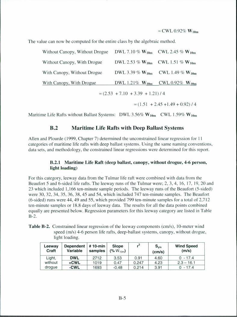
CWL 0.92% W10 m

The value can now be computed for the entire class by the algebraic method.

Without Canopy, Without Drogue DWL 7.10% WIOm CWL 2.45 % Wi0 mi

Without Canopy, With Drogue DWL 2.53 % W10m CWL 1.51 % Wiom

With Canopy, Without Drogue DWL 3.39 % W1 0 m CWL 1.49 % WI(pm

With Canopy, With Drogue DWL 1.21% W.0. CWL 0.92% Wjoi

S(2.53 +7.10 + 3.39 + 1.21)/4

= (1.51 + 2.45 +1.49 + 0.92) / 4

Maritime Life Rafts without Ballast Systems: DWL 3.56% Wjo. CWL 1.59% W1(m

B.2 Maritime Life Rafts with Deep Ballast Systems

Allen and Plourde (1999, Chapter 7) determined the unconstrained linear regression for IIcategories of maritime life rafts with deep ballast systems. Using the same naming conventions,data sets, and methodology, the constrained linear regressions were determined for this report.

B.2.1 Maritime Life Raft (deep ballast, canopy, without drogue, 4-6 person,light loading)

For this category, leeway data from the Tulmar life raft were combined with data from theBeaufort 5 and 6-sided life rafts. The leeway runs of the Tulmar were; 2, 3, 4, 16, 17, 19, 20 and23 which included 1,166 ten-minute sample periods. The leeway runs of the Beaufort (5-sided)were 30, 32, 34, 35, 36, 38, 45 and 54, which included 747 ten-minute samples. The Beaufort(6-sided) runs were 44, 49 and 55, which provided 799 ten-minute samples for a total of 2,712ten-minute samples or 18.8 days of leeway data. The results for all the data points combinedequally are presented below. Regression parameters for this leeway category are listed in TableB-2.

Table B-2. Constrained linear regression of the leeway components (cm/s), 10-meter windspeed (m/s) 4-6 person life rafts, deep-ballast systems, canopy, without drogue,light loading.

Leeway Dependent # 10-min Slope r2 Sy Wind SpeedCraft Variable samples (% Wiom) (cm/s) (m/s)

Light, DWL 2712 3.53 0.91 4.60 0 - 17.4without +CWL 1019 0.47 0.247 4.23 2.3-16.1drogue -CWL 1693 -0.48 0.214 3.91 0 -17.4

B-5

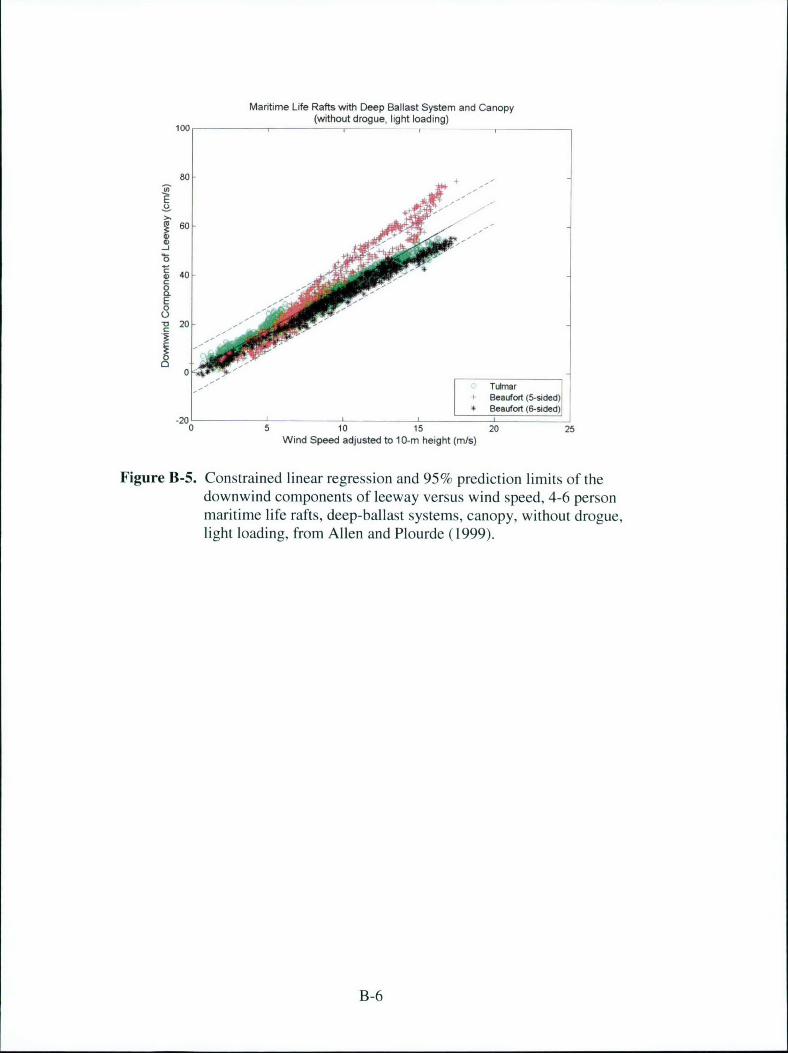
Maritime Life Rafts with Deep Ballast System and Canopy(without drogue, light loading)

100

80

.. !JS60-

-J

S40 -

E

TuirnarBeaufort (5-sded)

2 Beaufort (6-sided)

0 5 10 15 20 25Wind Speed adjusted to 10-m height (m/s)

Figure B-5. Constrained linear regression and 95% prediction limits of thedownwind components of leeway versus wind speed, 4-6 personmaritime life rafts, deep-ballast systems, canopy, without drogue,light loading, from Allen and Plourde (1999).

B-6

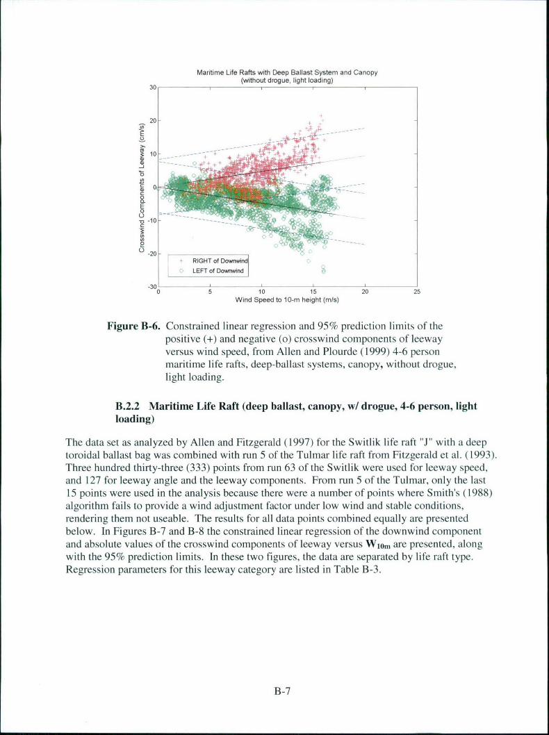
Maritime Life Rafts with Deep Ballast System and Canopy(without drogue, light loading)

30 - ; ; , ,

20-

10-

0

0

0

2-20- RIGHT of DoWn],nd

LEFT of Dowinnd

-300 5 10 15 20 25

Wind Speed to 10-m height (m/s)

Figure B-6. Constrained linear regression and 95% prediction limits of thepositive (+) and negative (o) crosswind components of leewayversus wind speed, from Allen and Plourde (1999) 4-6 personmaritime life rafts, deep-ballast systems, canopy, without drogue,light loading.

B.2.2 Maritime Life Raft (deep ballast, canopy, w/ drogue, 4-6 person, lightloading)

The data set as analyzed by Allen and Fitzgerald (1997) for the Switlik life raft "J" with a deeptoroidal ballast bag was combined with run 5 of the Tulmar life raft from Fitzgerald et al. (1993).Three hundred thirty-three (333) points from run 63 of the Switlik were used for leeway speed,and 127 for leeway angle and the leeway components. From run 5 of the Tulmar, only the last15 points were used in the analysis because there were a number of points where Smith's (1988)algorithm fails to provide a wind adjustment factor under low wind and stable conditions,rendering them not useable. The results for all data points combined equally are presentedbelow. In Figures B-7 and B-8 the constrained linear regression of the downwind componentand absolute values of the crosswind components of leeway versus Wlm are presented, alongwith the 95% prediction limits. In these two figures, the data are separated by life raft type.Regression parameters for this leeway category are listed in Table B-3.

B-7

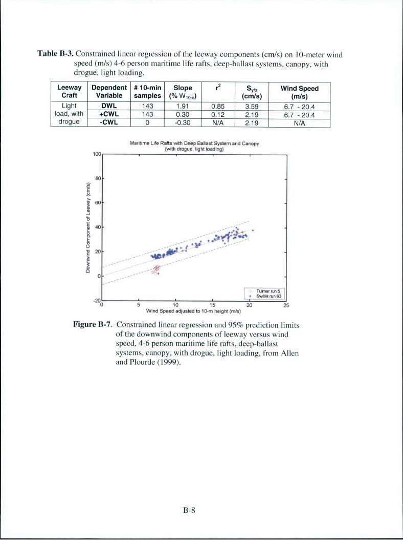
Table B-3. Constrained linear regression of the leeway components (cm/s) on 10-meter windspeed (m/s) 4-6 person maritime life rafts, deep-ballast systems, canopy, withdrogue, light loading.

Leeway Dependent # 10-min Slope r2 Syx Wind SpeedCraft Variable samples (% W10m) (cmns) (m/s)Light DWL 143 1.91 0.85 3.59 6.7 -20.4

load, with +CWL 143 0.30 0.12 2.19 6.7 -20.4drogue -CWL 0 -0.30 N/A 2.19 N/A

Maribme Life Rafts with Deep Ballast System and Canopy(with drogue. light loading)

100

80

.J 40-+

C20-

0.

F Tuv rn 5

Sllik run 63

-0 5 10 15 20 25Wind Speed adjusted to 10-rn height (mis)

Figure B-7. Constrained linear regression and 95% prediction limitsof the downwind components of leeway versus windspeed, 4-6 person maritime life rafts, deep-ballastsystems, canopy, with drogue, light loading, from Allenand Plourde (1999).

B-8

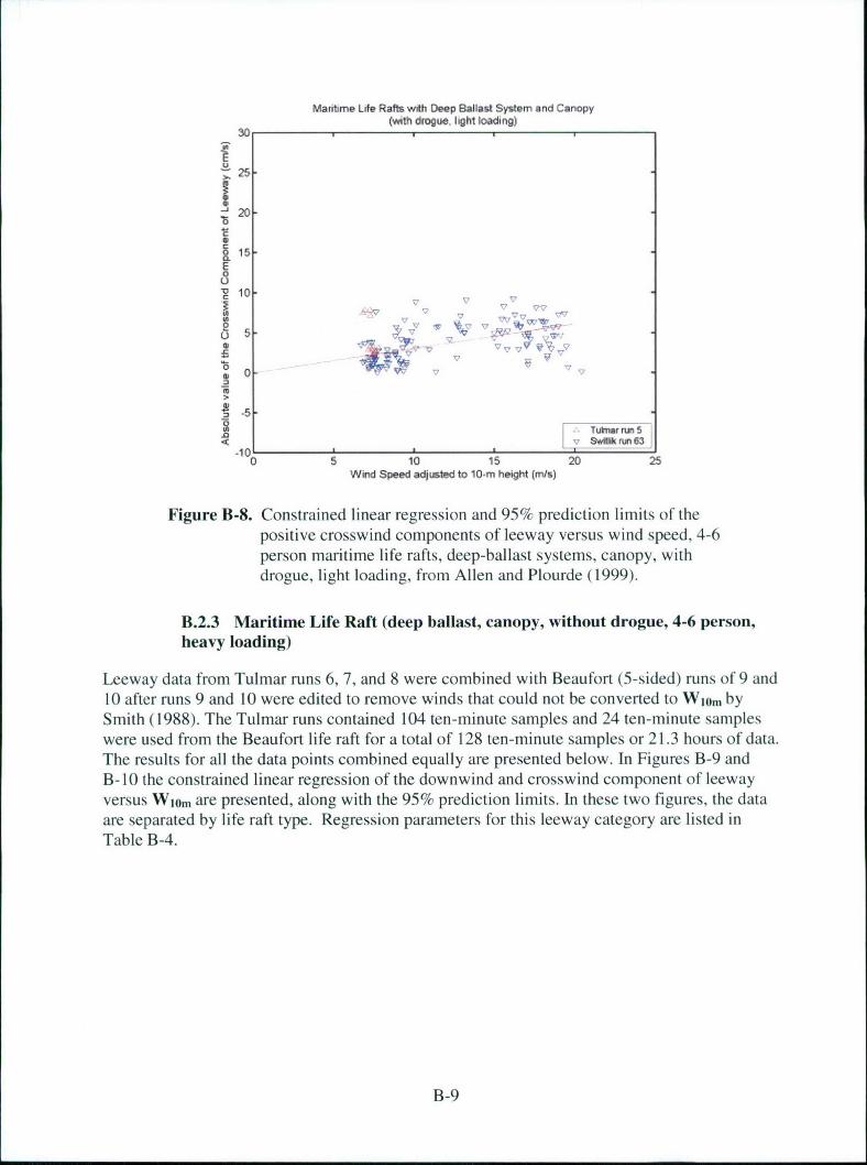
Mafitme Life Rafts with Deep Ballast System and Canopy(with drogue, light loading)

30

•25I- 20

o 15a.

10

*= 0 . v -f. ,:

0-

Tuinarrun5-. SvAilk nin 63-10 OL I L L"

5 10 15 20 25Wind Speed adjusted to 10-m height (mis)

Figure B-8. Constrained linear regression and 95% prediction limits of thepositive crosswind components of leeway versus wind speed, 4-6person maritime life rafts, deep-ballast systems, canopy, withdrogue, light loading, from Allen and Plourde (1999).

B.2.3 Maritime Life Raft (deep ballast, canopy, without drogue, 4-6 person,heavy loading)

Leeway data from Tulmar runs 6, 7, and 8 were combined with Beaufort (5-sided) runs of 9 and10 after runs 9 and 10 were edited to remove winds that could not be converted to Wj0m bySmith (1988). The Tulmar runs contained 104 ten-minute samples and 24 ten-minute sampleswere used from the Beaufort life raft for a total of 128 ten-minute samples or 21.3 hours of data.The results for all the data points combined equally are presented below. In Figures B-9 andB- 10 the constrained linear regression of the downwind and crosswind component of leewayversus Wiom are presented, along with the 95% prediction limits. In these two figures, the dataare separated by life raft type. Regression parameters for this leeway category are listed inTable B-4.

B-9

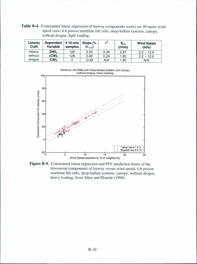
Table B-4. Constrained linear regression of leeway components (cm/s) on 10-meter windspeed (m/s) 4-6 person maritime life rafts, deep-ballast systems, canopy,without drogue, light loading.

Leeway Dependent # 10-min Slope (% r2 Syx Wind SpeedCraft Variable samples W10.) (cm/s) (m/s)Heavy DWL 128 3.35 0.94 2.67 2.2 - 12.9without +CWL 128 0.49 0.24 1.80 2.2 -12.9drogue -CWL 0 -0.49 N/A 1.80 N/A

Maritime Life Rafts with Deep Ballast System and Canopy(without drogue, heavy loading)

100

80

0.

, • Tubma rms 6,7 &8

. Beaufortrurm9&10-20 t.0 5 10 15 20 25

Wind Speed adjusted to 10-m height(mls)

Figure B-9. Constrained linear regression and 95% prediction limits of thedownwind components of leeway versus wind speed, 4-6 personmaritime life rafts, deep-ballast systems, canopy, without drogue,heavy loading, from Allen and Plourde (1999).

B-10

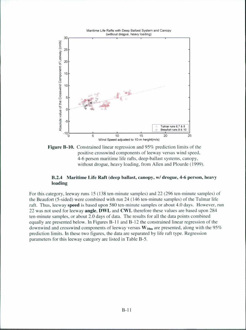
Maritime Life Rafts with Deep Ballast System and Canopy(without drogue, heavy loading)

30

25

-J 20

S15-E0

C..) 8...

0 10.

5--

40-

0 5 10 15 20 25Wind Speed adjusted to 10-m height(m2s)

Figure B-10. Constrained linear regression and 95% prediction limits of thepositive crosswind components of leeway versus wind speed,4-6 person maritime life rafts, deep-ballast systems, canopy,without drogue, heavy loading, from Allen and Plourde (1999).

B.2.4 Maritime Life Raft (deep ballast, canopy, w/ drogue, 4-6 person, heavyloading

For this category, leeway runs 15 (138 ten-minute samples) and 22 (296 ten-minute samples) ofthe Beaufort (5-sided) were combined with run 24 (146 ten-minute samples) of the Tulmar liferaft. Thus, leeway speed is based upon 580 ten-minute samples or about 4.0 days. However, run22 was not used for leeway angle, DWL and CWL therefore these values are based upon 284ten-minute samples, or about 2.0 days of data. The results for all the data points combinedequally are presented below. In Figures B- I I and B- 12 the constrained linear regression of thedownwind and crosswind components of leeway versus Witm are presented, along with the 95%prediction limits. In these two figures, the data are separated by life raft type. Regressionparameters for this leeway category are listed in Table B-5.

B-l I

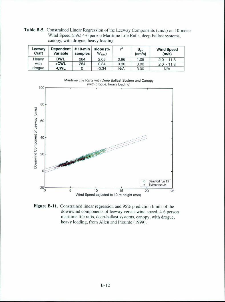
Table B-5. Constrained Linear Regression of the Leeway Components (cm/s) on 10-meterWind Speed (m/s) 4-6 person Maritime Life Rafts, deep-ballast systems,canopy, with drogue, heavy loading.

Leeway Dependent # 10-min slope (% r2 Sy/x Wind SpeedCraft Variable samples W1om) (cm/s) (m/s)Heavy DWL 284 2.08 0.96 1.05 2.0 -11.8

with +CWL 284 0.34 0.30 3.00 2.0 - 11.8drogue -CWL 0 -0.34 N/A 3.00 N/A

Maritime Life Rafts with Deep Ballast System and Canopy(with drogue, heavy loading)

100

80

~60-

Z

4) 40-0

C

0 --

Beaufort run 15* Tulmar run 24

-20 U

0 5 10 15 20 25Wind Speed adjusted to 10-m height (mis)

Figure B-1I. Constrained linear regression and 95% prediction limits of thedownwind components of leeway versus wind speed, 4-6 personmaritime life rafts, deep-ballast systems, canopy, with drogue,heavy loading, from Allen and Plourde (1999).

B-12

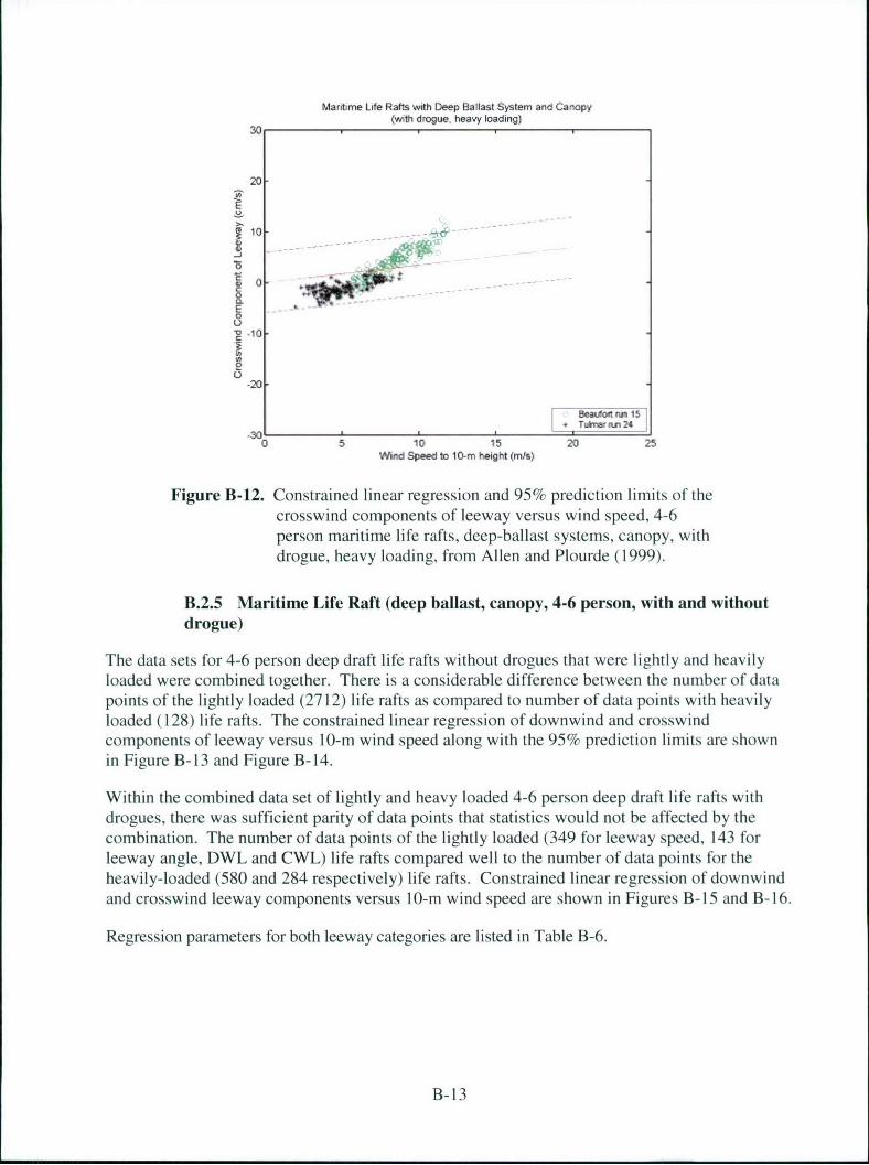
Marmime Life Rafts with Deep Ballast System and Canopy(w'th drogue, heavy loading)

30

20

10 -. .. . .• . . .

0-

t.5

E0

U

-20

,301Jý * Tuhrw Mu 24"0 5 10 15 20 25

Wind Speed to 10-m height (mls)

Figure B-12. Constrained linear regression and 95% prediction limits of thecrosswind components of leeway versus wind speed, 4-6person maritime life rafts, deep-ballast systems, canopy, withdrogue, heavy loading, from Allen and Plourde (1999).

B.2.5 Maritime Life Raft (deep ballast, canopy, 4-6 person, with and withoutdrogue)

The data sets for 4-6 person deep draft life rafts without drogues that were lightly and heavilyloaded were combined together. There is a considerable difference between the number of datapoints of the lightly loaded (2712) life rafts as compared to number of data points with heavilyloaded (128) life rafts. The constrained linear regression of downwind and crosswindcomponents of leeway versus 10-m wind speed along with the 95% prediction limits are shownin Figure B-13 and Figure B-14.

Within the combined data set of lightly and heavy loaded 4-6 person deep draft life rafts withdrogues, there was sufficient parity of data points that statistics would not be affected by thecombination. The number of data points of the lightly loaded (349 for leeway speed, 143 forleeway angle, DWL and CWL) life rafts compared well to the number of data points for theheavily-loaded (580 and 284 respectively) life rafts. Constrained linear regression of downwindand crosswind leeway components versus 10-m wind speed are shown in Figures B-15 and B-16.

Regression parameters for both leeway categories are listed in Table B-6.

B-13

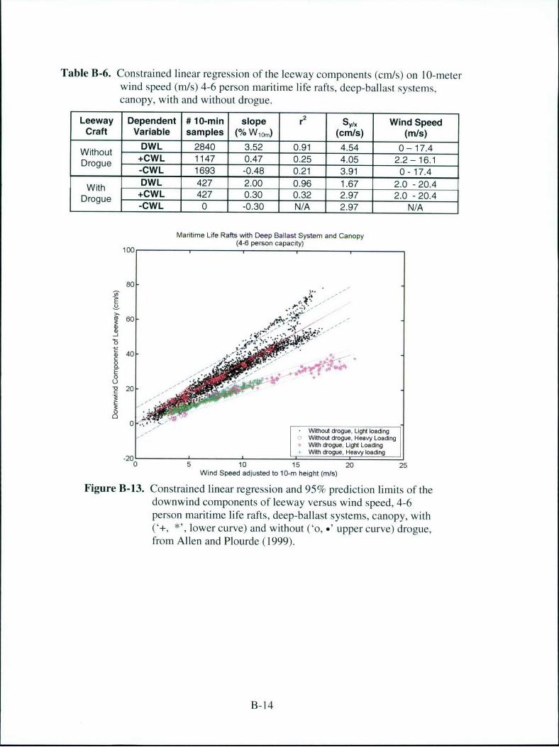
Table B-6. Constrained linear regression of the leeway components (cm/s) on 10-meterwind speed (m/s) 4-6 person maritime life rafts, deep-ballast systems,canopy, with and without drogue.

Leeway Dependent # 10-min slope r2 Sylx Wind SpeedCraft Variable samples (% Wiom) (cm/s) (m/s)

DWL 2840 3.52 0.91 4.54 0- 17.4Wtout +CWL 1147 0.47 0.25 4.05 2.2 - 16.1-CWL 1693 -0.48 0.21 3.91 0 - 17.4

DWL 427 2.00 0.96 1.67 2.0 - 20.4Drogue +CWL 427 0.30 0.32 2.97 2.0 - 20.4-CWL 0 -0.30 N/A 2.97 N/A

Maritime Life Rafts with Deep Ballast System and Canopy(4-6 person capacity)

100

80

60-

-J

C

E

Without drogue, Light loadingWithout drogue, Heavy LoadingWith drogue, Ugtt Loading

-20 ~With drogue, H .eavy loading

0 5 10 15 20 25Wind Speed adjusted to 10-rn height (mis)

Figure B-13. Constrained linear regression and 95% prediction limits of thedownwind components of leeway versus wind speed, 4-6person maritime life rafts, deep-ballast systems, canopy, with('+, *', lower curve) and without ('o, a' upper curve) drogue,from Allen and Plourde (1999).

13-14

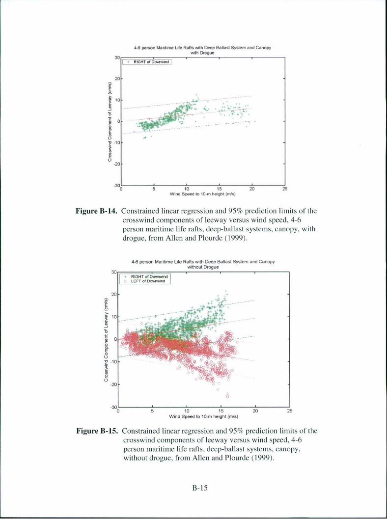
4.6 person Mantime Life Rafts with Deep Ballas System and Canopywith Drogue

30 SRIGhT of D0amw id

20

10 -. .. • . .. . .

0. 4

E

-20

_X.0 5 10 15 20 25

Wind Speed to 10-rn height (rnts)

Figure B-14. Constrained linear regression and 95% prediction limits of thecrosswind components of leeway versus wind speed, 4-6person maritime life rafts, deep-ballast systems, canopy, withdrogue, from Allen and Plourde (1999).

4-6 person Maritime Life Rafts wvith Deep Ballast System and Canopywithout Drogue

30RIGHT of DownnLEFT of DowAmwnd

20

-J

0 -1

_20 -

-30

0 5 10 15 20 25Wind Speed to 10-m height (m/s)

Figure B-15. Constrained linear regression and 95% prediction limits of thecrosswind components of leeway versus wind speed, 4-6person maritime life rafts, deep-ballast systems, canopy,without drogue, from Allen and Plourde (1999).

B-15

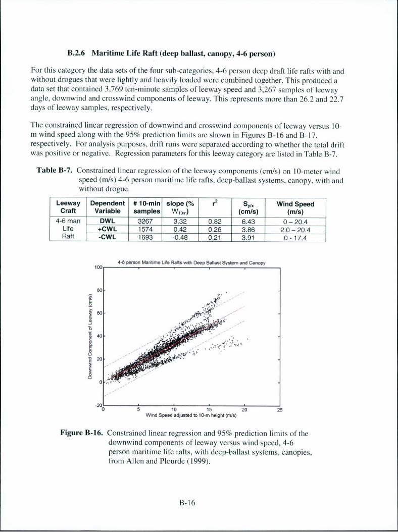
B.2.6 Maritime Life Raft (deep ballast, canopy, 4-6 person)

For this category the data sets of the four sub-categories, 4-6 person deep draft life rafts with andwithout drogues that were lightly and heavily loaded were combined together. This produced adata set that contained 3,769 ten-minute samples of leeway speed and 3,267 samples of leewayangle, downwind and crosswind components of leeway. This represents more than 26.2 and 22.7days of leeway samples, respectively.

The constrained linear regression of downwind and crosswind components of leeway versus 10-m wind speed along with the 95% prediction limits are shown in Figures B-16 and B-17,respectively. For analysis purposes, drift runs were separated according to whether the total driftwas positive or negative. Regression parameters for this leeway category are listed in Table B-7.

Table B-7. Constrained linear regression of the leeway components (cm/s) on 10-meter windspeed (m/s) 4-6 person maritime life rafts, deep-ballast systems, canopy, with andwithout drogue.

Leeway Dependent # 10-min slope (% r2 Syx Wind SpeedCraft Variable samples W10,) (cm/s) (m/s)

4-6 man DWL 3267 3.32 0.82 6.43 0-20.4Life +CWL 1574 0.42 0.26 3.86 2.0 - 20.4Raft -CWL 1693 -0.48 0.21 3.91 0 - 17.4

4-6 person Marilime Life Rafts with Deep Ballast System and Canopy100

80

EA

10 i

(-4

20-

0 5 10 15 20 25Wind Speed adjusted to 10-m height (mis)

Figure B-16. Constrained linear regression and 95% prediction limits of thedownwind components of leeway versus wind speed, 4-6person maritime life rafts, with deep-ballast systems, canopies,from Allen and Plourde (1999).

B-16

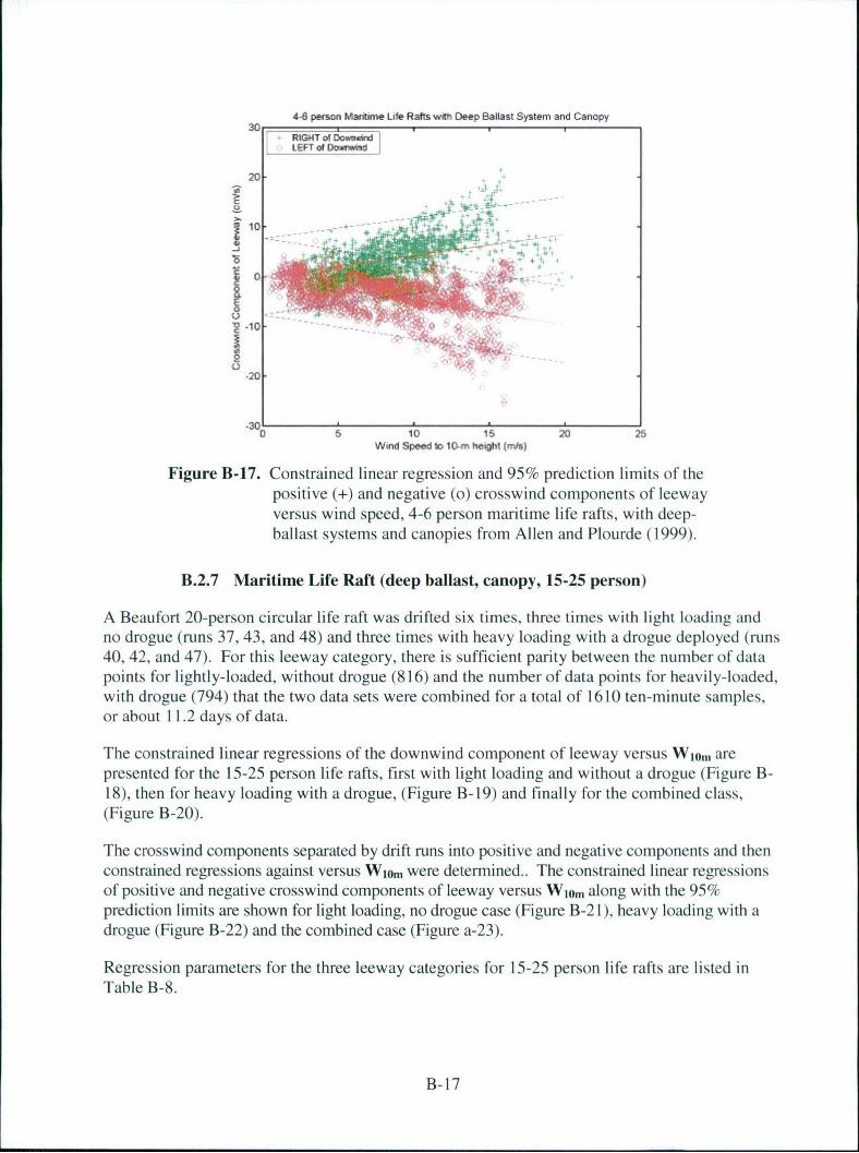
4-6 person Maritime Life Rafts with Deep Ballast System and Canopy

RIGHT of Oos~tsndLEFT of O.zAr.. iw

20

0 --

". -10

.20

0 6 10 15 20 25Wind Speed to 10-m height (mnis)

Figure B-17. Constrained linear regression and 95% prediction limits of thepositive (+) and negative (o) crosswind components of leewayversus wind speed, 4-6 person maritime life rafts, with deep-ballast systems and canopies from Allen and Plourde (1999).

B.2.7 Maritime Life Raft (deep ballast, canopy, 15-25 person)

A Beaufort 20-person circular life raft was drifted six times, three times with light loading andno drogue (runs 37, 43, and 48) and three times with heavy loading with a drogue deployed (runs40, 42, and 47). For this leeway category, there is sufficient parity between the number of datapoints for lightly-loaded, without drogue (816) and the number of data points for heavily-loaded,with drogue (794) that the two data sets were combined for a total of 1610 ten-minute samples,or about 11.2 days of data.

The constrained linear regressions of the downwind component of leeway versus Wiom arepresented for the 15-25 person life rafts, first with light loading and without a drogue (Figure B-18), then for heavy loading with a drogue, (Figure B-19) and finally for the combined class,(Figure B-20).

The crosswind components separated by drift runs into positive and negative components and thenconstrained regressions against versus Wiom were determined.. The constrained linear regressionsof positive and negative crosswind components of leeway versus W10m along with the 95%prediction limits are shown for light loading, no drogue case (Figure B-2 1), heavy loading with adrogue (Figure B-22) and the combined case (Figure a-23).

Regression parameters for the three leeway categories for 15-25 person life rafts are listed inTable B-8.

B- 17

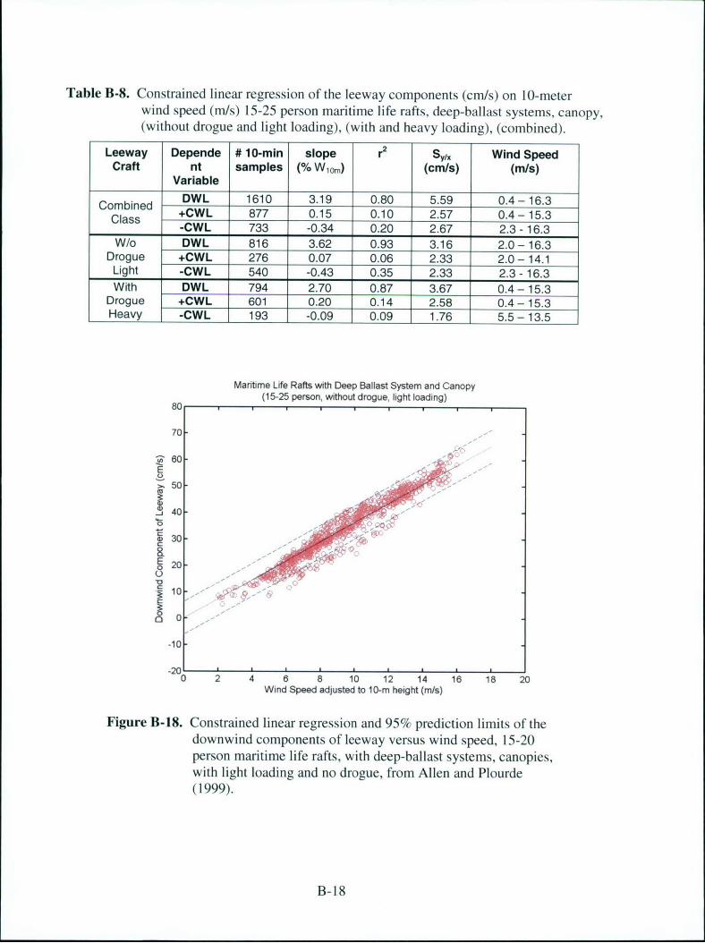
Table B-8. Constrained linear regression of the leeway components (cm/s) on 10-meterwind speed (m/s) 15-25 person maritime life rafts, deep-ballast systems, canopy,(without drogue and light loading), (with and heavy loading), (combined).

Leeway Depende # 10-min slope r2 Sy/X Wind SpeedCraft nt samples (% W1om) (cmns) (m/s)

VariableDWL 1610 3.19 0.80 5.59 0.4-16.3Class +CWL 877 0.15 0.10 2.57 0.4- 15.3

-CWL 733 -0.34 0.20 2.67 2.3 - 16.3

W/o DWL 816 3.62 0.93 3.16 2.0-16.3Drogue +CWL 276 0.07 0.06 2.33 2.0- 14.1

Light -CWL 540 -0.43 0.35 2.33 2.3 - 16.3With DWL 794 2.70 0.87 3.67 0.4 - 15.3

Drogue +CWL 601 0.20 0.14 2.58 0.4 - 15.3Heavy -CWL 193 -0.09 0.09 1.76 5.5 - 13.5

Maritime Life Rafts with Deep Ballast System and Canopy(15-25 person, without drogue, light loading)

80

70-

"Z 60-

>,50-

1 40-

30

8.0E20.•

*0

-101

-20 10 2 4 6 8 10 12 14 16 18 20

Wind Speed adjusted to 10-rn height (mis)

Figure B-18. Constrained linear regression and 95% prediction limits of thedownwind components of leeway versus wind speed, 15-20person maritime life rafts, with deep-ballast systems, canopies,with light loading and no drogue, from Allen and Plourde(1999).

B-18

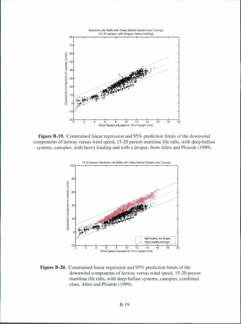
Maritime Life Rafts with Deep Ballast System and Canopy(15-25 person, with drogue, heavy loading)

80

70

•60E

L)30

E 20. I I I I

10 0

-10-

-200 2 4 6 8 10 12 14 16 18 20

Wind Speed adjusted to 10-m height (m/s)

Figure B-19. Constrained linear regression and 95% prediction limits of the downwindcomponents of leeway versus wind speed, 15-20 person maritime life rafts, with deep-ballast

systems, canopies, with heavy loading and with a drogue, from Allen and Plourde (1999).

15-25 person Maritime Life Rafts with Deep Ballast System and Canopy100,,

80

60

40-"oi 40 - ••

E0

X 20 .

ligil loading, w/o dnogueheavy loading wAlogue

-200 2 4 6 8 10 12 14 16 18 20

Wind Speed adjusted to 10-m height (m/s)

Figure B-20. Constrained linear regression and 95% prediction limits of thedownwind components of leeway versus wind speed, 15-20 personmaritime life rafts, with deep-ballast systems, canopies, combinedclass, Allen and Plourde (1999).

B- 19

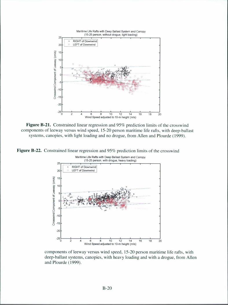
Maritime Life Rafts with Deep Ballast System and Canopy(15-25 person, without drogue, light loading)

25 1 11 1 1 1+ RIGHT of Downwin

20 • LEFT of Donwind

S15-

10-

5 +

+ ++

10

(-15

-20

-250 2 4 6 8 10 12 14 16 18 20

Wind Speed adjusted to 10-m height (m/s)

Figure B-21. Constrained linear regression and 95% prediction limits of the crosswindcomponents of leeway versus wind speed, 15-20 person maritime life rafts, with deep-ballast

systems, canopies, with light loading and no drogue, from Allen and Plourde (1999).

Figure B-22. Constrained linear regression and 95% prediction limits of the crosswindMaritime Life Rafts with Deep Ballast System and Canopy

(15-25 person, with drogue, heavy loading)25

+ RIGHT of Downwind

20 LEFT of Downwind

15-E

10

+ --15

5- + + ++ ~

0

I

-5 - - - ---

-10-

-20-

4 8 8 10 12 14 16 18 20Wind Speed adjusted to 1O-m height (m/s)

components of leeway versus wind speed, 15-20 person maritime life rafts, withdeep-ballast systems, canopies, with heavy loading and with a drogue, from Allenand Plourde (1999).

B-20

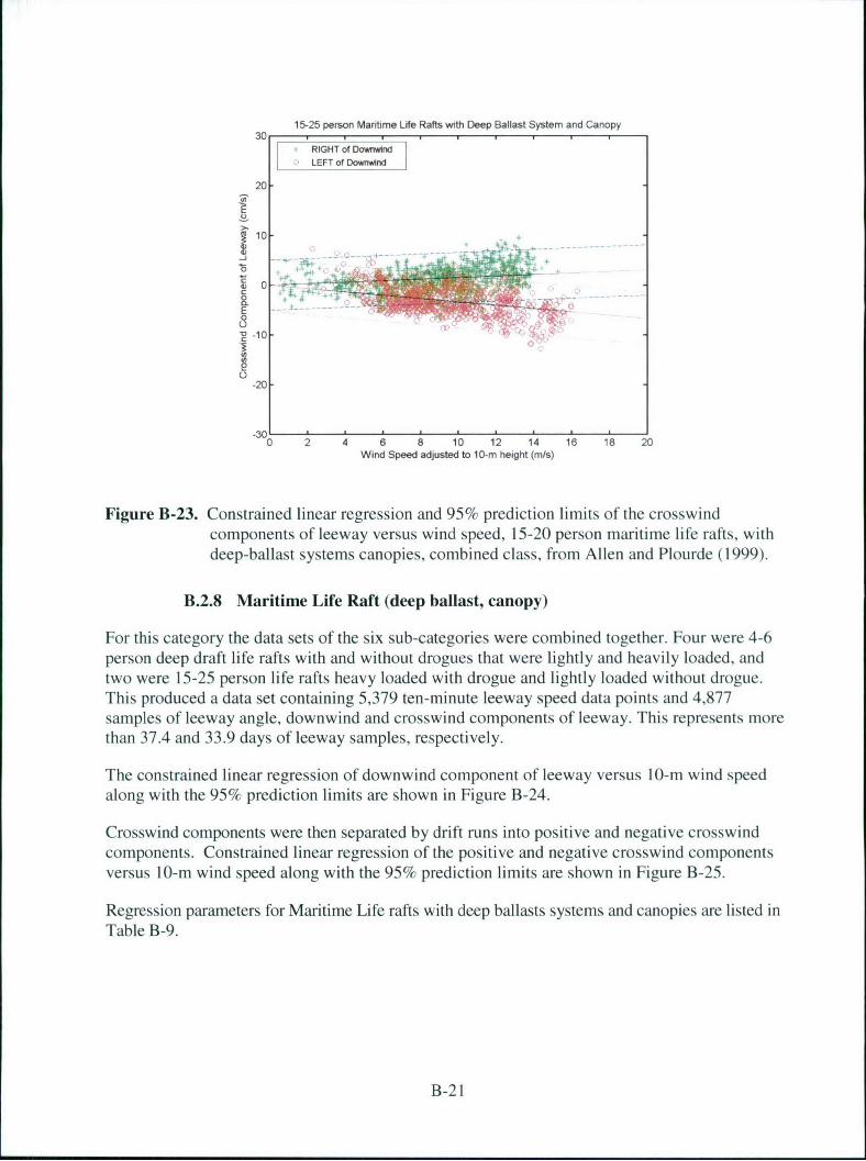
15-25 person Maritime Life Rafts with Deep Ballast System and Canopy30 1 1 1 1 1 1

RIGHT of DownwindLEFT of Dowrriind

20

10

E -0

2 '10'

-20-

-300 2 4 6 8 10 12 14 16 18 20

Wind Speed adjusted to 10-m height (m/s)

Figure B-23. Constrained linear regression and 95% prediction limits of the crosswindcomponents of leeway versus wind speed, 15-20 person maritime life rafts, withdeep-ballast systems canopies, combined class, from Allen and Plourde (1999).

B.2.8 Maritime Life Raft (deep ballast, canopy)

For this category the data sets of the six sub-categories were combined together. Four were 4-6person deep draft life rafts with and without drogues that were lightly and heavily loaded, andtwo were 15-25 person life rafts heavy loaded with drogue and lightly loaded without drogue.This produced a data set containing 5,379 ten-minute leeway speed data points and 4,877samples of leeway angle, downwind and crosswind components of leeway. This represents morethan 37.4 and 33.9 days of leeway samples, respectively.

The constrained linear regression of downwind component of leeway versus 10-m wind speedalong with the 95% prediction limits are shown in Figure B-24.

Crosswind components were then separated by drift runs into positive and negative crosswindcomponents. Constrained linear regression of the positive and negative crosswind componentsversus 10-m wind speed along with the 95% prediction limits are shown in Figure B-25.

Regression parameters for Maritime Life rafts with deep ballasts systems and canopies are listed inTable B-9.

B-21

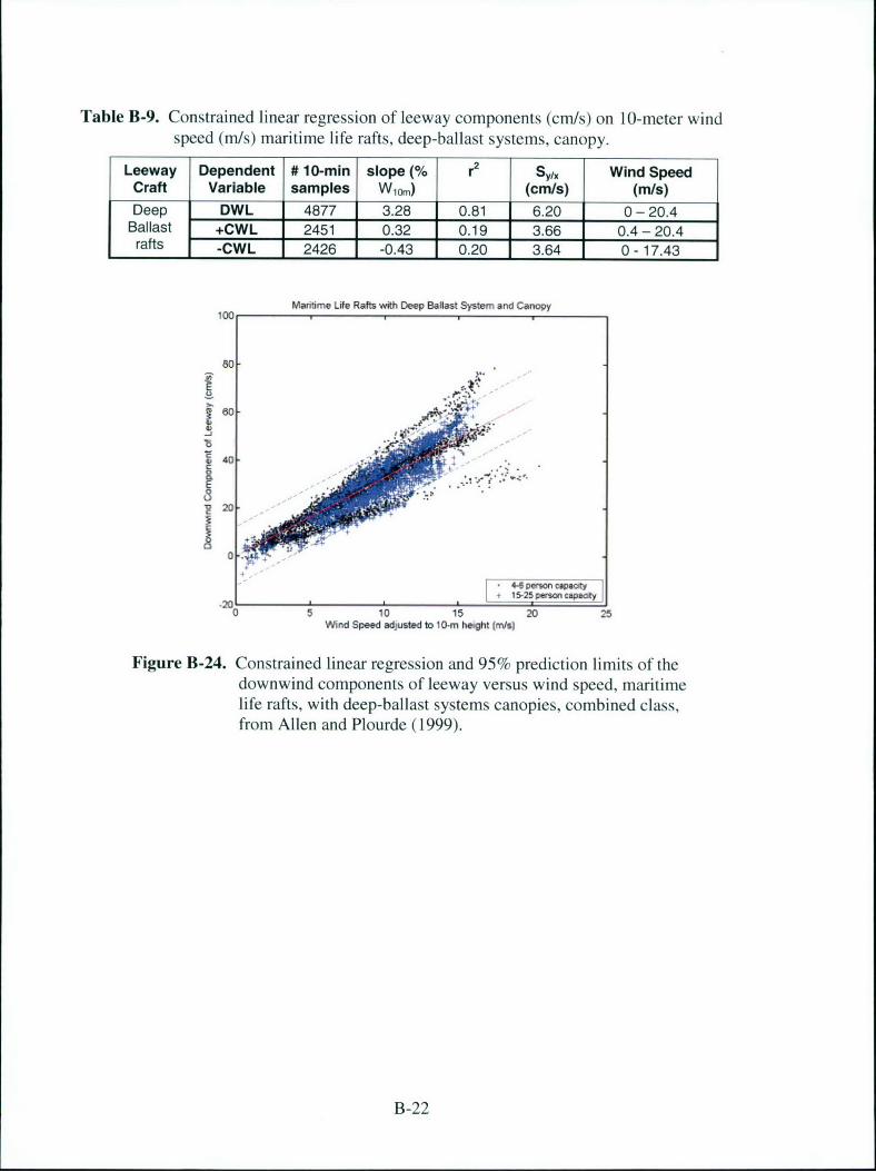
Table B-9. Constrained linear regression of leeway components (cm/s) on I 0-meter windspeed (m/s) maritime life rafts, deep-ballast systems, canopy.

Leeway Dependent # 10-min slope (% r2 Syx Wind SpeedCraft Variable samples W10.) (cm/s) (m/s)Deep DWL 4877 3.28 0.81 6.20 0 - 20.4

Ballast +CWL 2451 0.32 0.19 3.66 0.4-20.4rafts -CWL 2426 -0.43 0.20 3164 0 - 17.43

Maritime Life Raft with Deep Ballast System and Canopy100i

80-

eo ,

.40-

X20-

2 15-25pr•ao• spacstyI

0510 15 20 25Wind Speed adjusted to 10-m height (Wis)

Figure B-24. Constrained linear regression and 95% prediction limits of thedownwind components of leeway versus wind speed, maritimelife rafts, with deep-ballast systems canopies, combined class,from Allen and Plourde (1999).

B-22

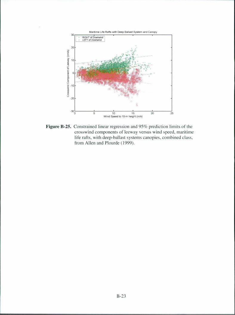
Maritime Life Rafts with Deep Ballast System and Canopy30

RIGHT of DownwvndLEFT of Downwrid

20(

10

-~-0

-20.

-300 5 10 15 20 25

Wind Speed to 10-rn height (mis)

Figure B-25. Constrained linear regression and 95% prediction limits of thecrosswind components of leeway versus wind speed, maritimelife rafts, with deep-ballast systems canopies, combined class,from Allen and Plourde (1999).

B-23

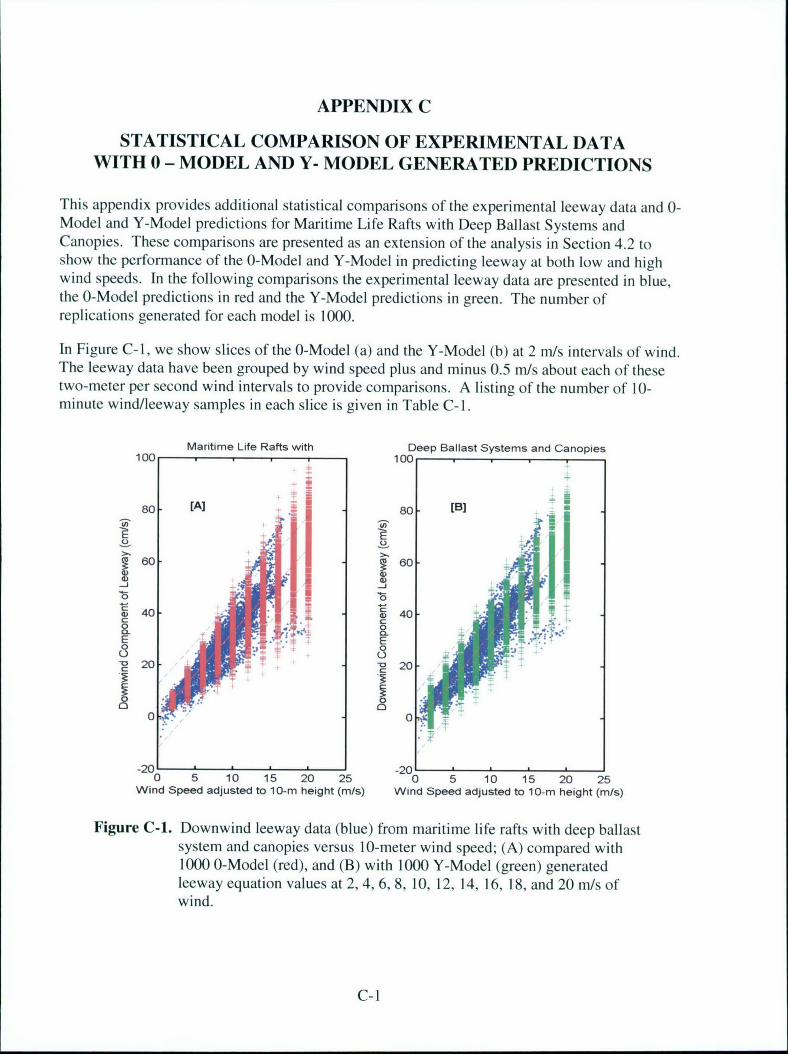
APPENDIX C

STATISTICAL COMPARISON OF EXPERIMENTAL DATAWITH 0 - MODEL AND Y- MODEL GENERATED PREDICTIONS

This appendix provides additional statistical comparisons of the experimental leeway data and 0-Model and Y-Model predictions for Maritime Life Rafts with Deep Ballast Systems andCanopies. These comparisons are presented as an extension of the analysis in Section 4.2 toshow the performance of the 0-Model and Y-Model in predicting leeway at both low and highwind speeds. In the following comparisons the experimental leeway data are presented in blue,the 0-Model predictions in red and the Y-Model predictions in green. The number ofreplications generated for each model is 1000.

In Figure C- I, we show slices of the 0-Model (a) and the Y-Model (b) at 2 m/s intervals of wind.The leeway data have been grouped by wind speed plus and minus 0.5 m/s about each of thesetwo-meter per second wind intervals to provide comparisons. A listing of the number of 10-minute wind/leeway samples in each slice is given in Table C-1.

Maritime Life Rafts with Deep Ballast Systems and Canopies100 100

80 [A] _ 80 [B]

0 60

6040 40l

-o 2 40EE

2-0 "20

0 T.

-201 -200 5 10 15 20 25 0 5 10 15 20 25

Wind Speed adjusted to 10-m height (m/s) Wind Speed adjusted to 10-m height (m/s)

Figure C-1. Downwind leeway data (blue) from maritime life rafts with deep ballastsystem and canopies versus 10-meter wind speed; (A) compared with1000 0-Model (red), and (B) with 1000 Y-Model (green) generatedleeway equation values at 2, 4, 6, 8, 10, 12, 14, 16, 18, and 20 m/s ofwind.

C-1

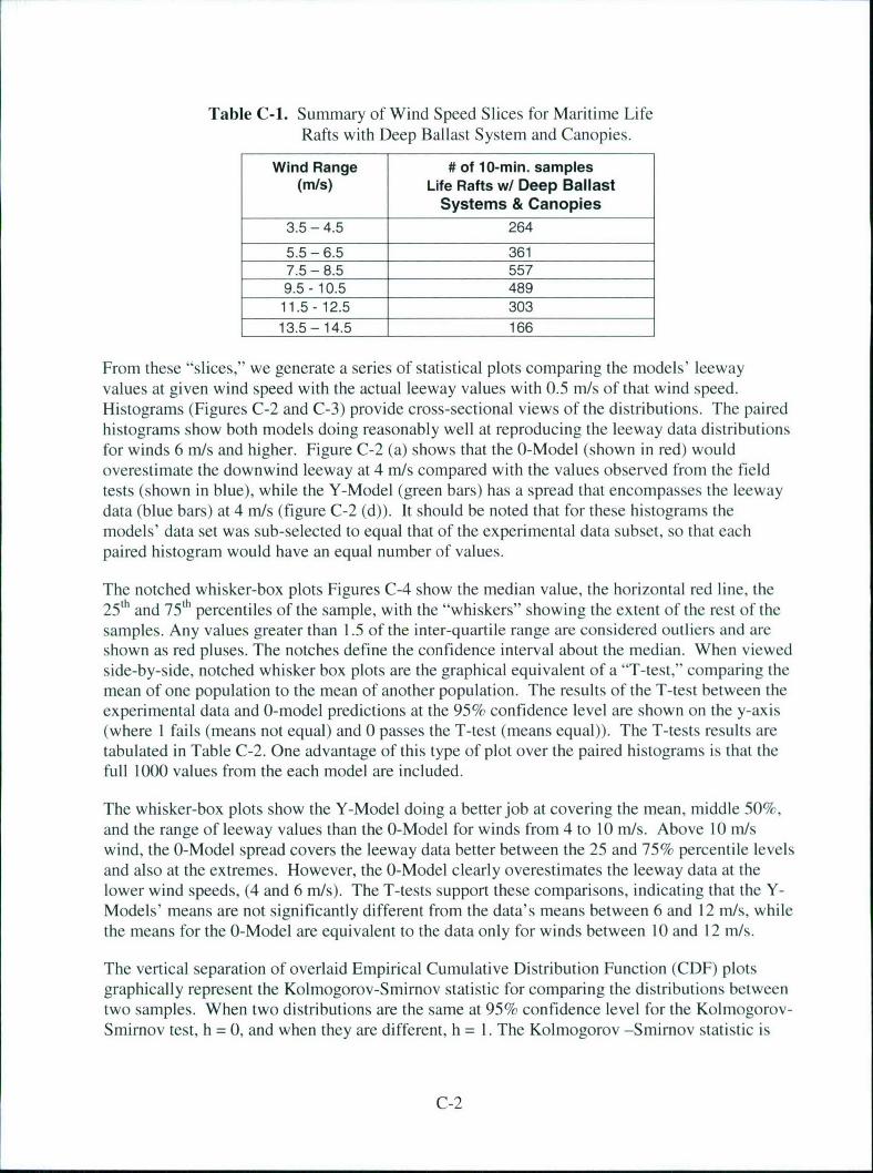
Table C-1. Summary of Wind Speed Slices for Maritime LifeRafts with Deep Ballast System and Canopies.

Wind Range # of 10-min. samples(m/s) Life Rafts w/ Deep Ballast

Systems & Canopies3.5-4.5 264

5.5 - 6.5 3617.5 - 8.5 5579.5 - 10.5 48911.5-12.5 30313.5-14.5 166

From these "slices," we generate a series of statistical plots comparing the models' leewayvalues at given wind speed with the actual leeway values with 0.5 m/s of that wind speed.Histograms (Figures C-2 and C-3) provide cross-sectional views of the distributions. The pairedhistograms show both models doing reasonably well at reproducing the leeway data distributionsfor winds 6 m/s and higher. Figure C-2 (a) shows that the 0-Model (shown in red) wouldoverestimate the downwind leeway at 4 m/s compared with the values observed from the fieldtests (shown in blue), while the Y-Model (green bars) has a spread that encompasses the leewaydata (blue bars) at 4 m/s (figure C-2 (d)). It should be noted that for these histograms themodels' data set was sub-selected to equal that of the experimental data subset, so that eachpaired histogram would have an equal number of values.

The notched whisker-box plots Figures C-4 show the median value, the horizontal red line, the2 5 th and 75 h percentiles of the sample, with the "whiskers" showing the extent of the rest of the

samples. Any values greater than 1.5 of the inter-quartile range are considered outliers and areshown as red pluses. The notches define the confidence interval about the median. When viewedside-by-side, notched whisker box plots are the graphical equivalent of a "T-test," comparing themean of one population to the mean of another population. The results of the T-test between theexperimental data and 0-model predictions at the 95% confidence level are shown on the y-axis(where I fails (means not equal) and 0 passes the T-test (means equal)). The T-tests results aretabulated in Table C-2. One advantage of this type of plot over the paired histograms is that thefull 1000 values from the each model are included.

The whisker-box plots show the Y-Model doing a better job at covering the mean, middle 50%,and the range of leeway values than the 0-Model for winds from 4 to 10 m/s. Above 10 m/swind, the 0-Model spread covers the leeway data better between the 25 and 75% percentile levelsand also at the extremes. However, the 0-Model clearly overestimates the leeway data at thelower wind speeds, (4 and 6 m/s). The T-tests support these comparisons, indicating that the Y-Models' means are not significantly different from the data's means between 6 and 12 m/s, whilethe means for the 0-Model are equivalent to the data only for winds between 10 and 12 m/s.

The vertical separation of overlaid Empirical Cumulative Distribution Function (CDF) plotsgraphically represent the Kolmogorov-Smirnov statistic for comparing the distributions betweentwo samples. When two distributions are the same at 95% confidence level for the Kolmogorov-Smirnov test, h = 0, and when they are different, h = I. The Kolmogorov -Smirnov statistic is

C-2

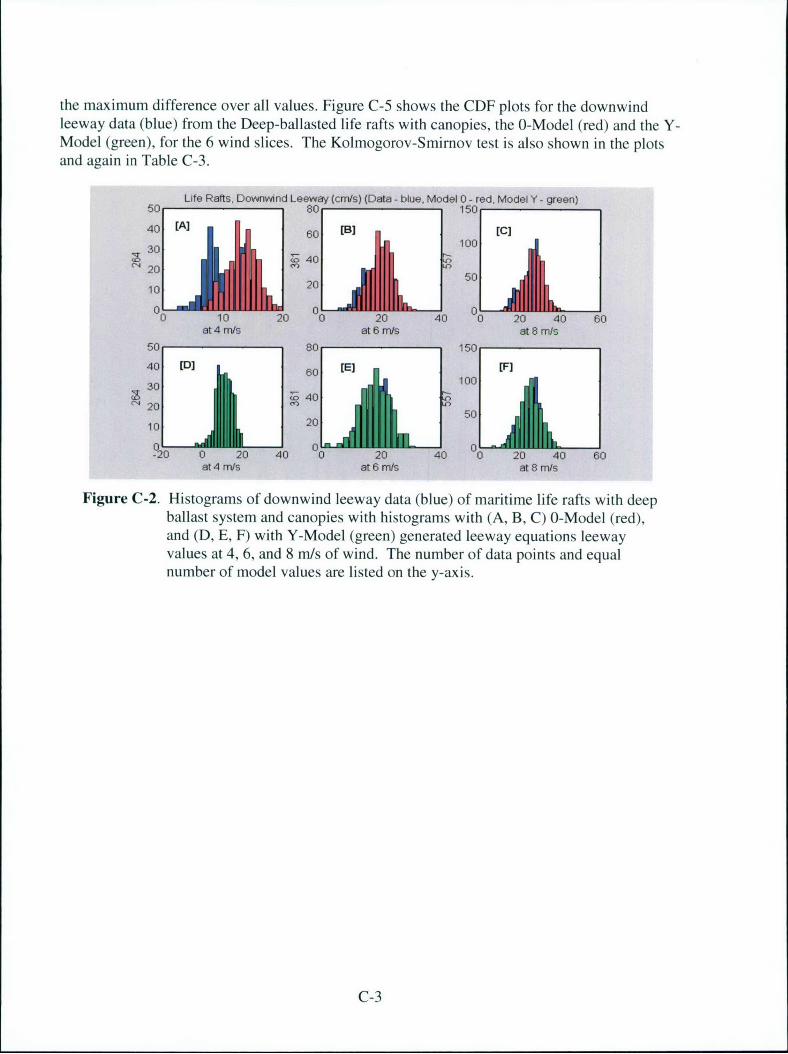
the maximum difference over all values. Figure C-5 shows the CDF plots for the downwindleeway data (blue) from the Deep-ballasted life rafts with canopies, the 0-Model (red) and the Y-Model (green), for the 6 wind slices. The Kolmogorov-Smirnov test is also shown in the plotsand again in Table C-3.

Life Rafts, Downwind Leeway (cmrs) (Data - blue. Model 0 - red, Model Y - green)5 0 80 150f40 [A] I60 [B] [C]

30 740 i10

20 20 50

0 10 20 0 20 40 0 20 40 60at4 ms at 6 nVs at8m/s

50 80 150

40 [D]L6 E F30 100o 40

-" 0 20 40 o'•, O10220 50

at 4 n/s at 6 rs at 8 m/s

Figure C-2. Histograms of downwind leeway data (blue) of maritime life rafts with deepballast system and canopies with histograms with (A, B, C) 0-Model (red),and (D, E, F) with Y-Model (green) generated leeway equations leewayvalues at 4, 6, and 8 m/s of wind. The number of data points and equalnumber of model values are listed on the y-axis.

C-3

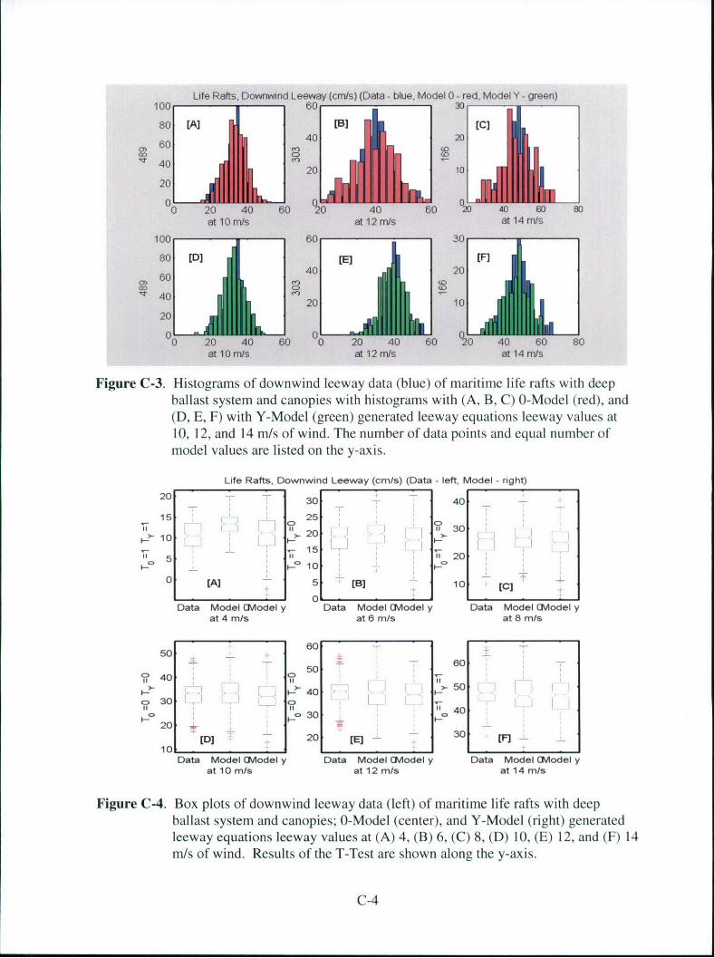
Life Rafts, Downwind Leeway (cm/s) (Data - blue, Model 0 - red, Model Y - green)

100 60

80 [A] [][C]S60 40 2000 (

S40 20

20

00 20 40 .. 60 40 60 40 o so

at 10 rots at 12 mls at 14 mrs

100 60 30

80 [D] [F]

6040 20~60j

S40 20 1020

0) 20 40 60 0 20 40 60 20 40 60 80at 10 ms at 12 mls at 14 ms

Figure C-3. Histograms of downwind leeway data (blue) of maritime life rafts with deepballast system and canopies with histograms with (A, B, C) 0-Model (red), and(D, E, F) with Y-Model (green) generated leeway equations leeway values at10, 12, and 14 m/s of wind. The number of data points and equal number ofmodel values are listed on the y-axis.

Life Rafts, Downwind Leeway (cm/s) (Data - left, Model - right)

20 30 - 40

15o 25C) CU' 0'l 2 0 ii• 30

501 20

0' [A] - 5 (]10[C

Data Model CModel y Data Model OViodel y Data Model C(viodel yat 4 m/s at 6 m/s at 8 mls

60 -50

- - 60S-- ~~50 •,C 4C) 40 4050i,..- 40

S J30,•_ 30~ 3 "o 40

o 0303020 • : 0 [l -- - 0 [] • _

[D] 20 [E]- 30101

Data Model Ciodel y Data Model CModel y Data Model CvModel yat 10 m/s at 12 m/s at 14 m/s

Figure C-4. Box plots of downwind leeway data (left) of maritime life rafts with deepballast system and canopies; 0-Model (center), and Y-Model (right) generatedleeway equations leeway values at (A) 4, (B) 6, (C) 8, (D) 10, (E) 12, and (F) 14m/s of wind. Results of the T-Test are shown along the y-axis.

C-4

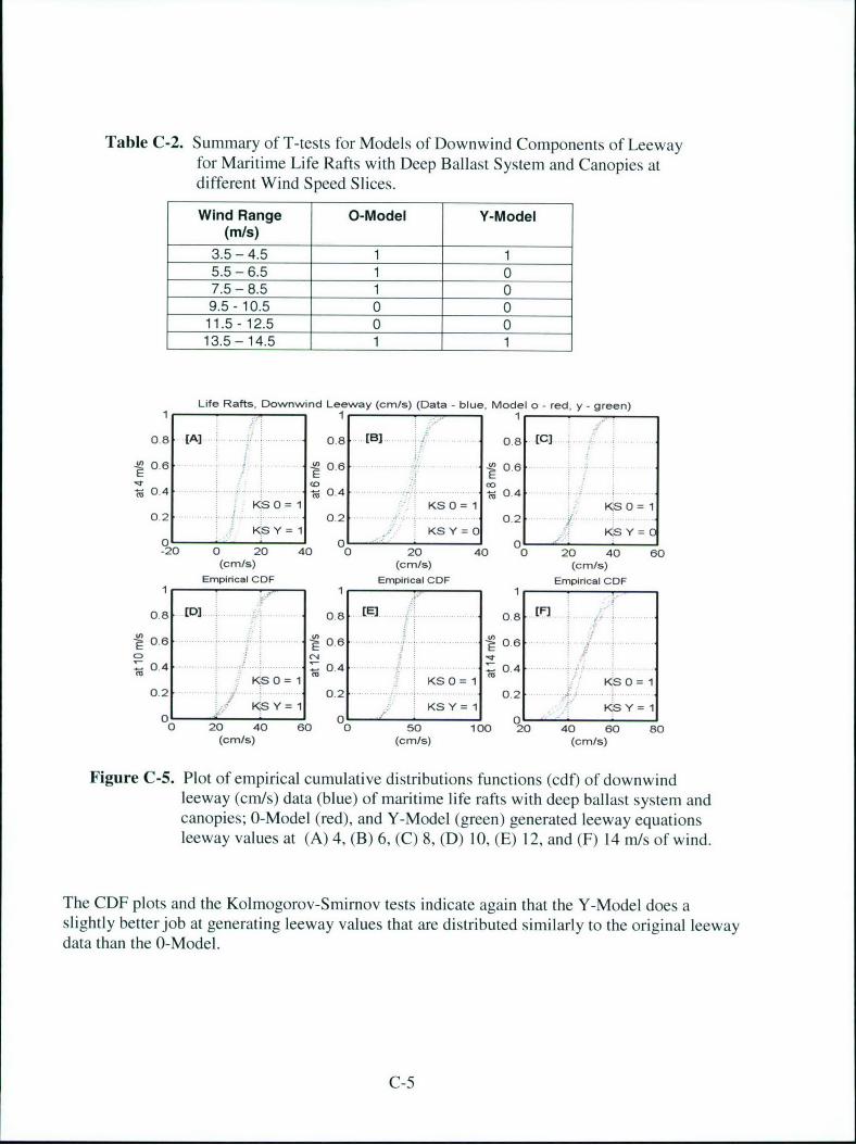
Table C-2. Summary of T-tests for Models of Downwind Components of Leewayfor Maritime Life Rafts with Deep Ballast System and Canopies atdifferent Wind Speed Slices.

Wind Range 0-Model Y-Model(m/s)

3.5-4.5 1 15.5-6.5 1 07.5-8.5 1 09.5-10.5 0 011.5-12.5 0 013.5-14.5 1 1

Life Rafts, Downwind Leeway (cm/s) (Data - blue, Model o - red, y - green)'1 . - 1 I,1,

0,8 [A ]. . 0.8 [1131, 0.8 [C]• 0.6 1 0. . .6 0.. .. 6 . : •. . .

0,44 . 4 0.4KSO= 1 KSO= 1 KS0=1

0.2- 0.2 .02KSY=1 KSY=0 KSY=

0 0 A 0-20 0 20 40 0 20 40 0 20 40 60(cm/s) (cm/s) (cm/s)

Empirical CDF Empirical CDF Empirical CDF1 -' •. 1 1-.

0.8 [D] 0. 8 te 0.8 [F)

0.6 0.6 0.6.

O. . 0.4 .0.4"Kso=1 KSO=1 KSo=1

0.2- 0.2 0.2KSY=1 KSY= 1 KSY= 10"' 1 01 1z 5'0 ,

0 20 40 60 0 50 100 20 40 60 80(cm/s) (cmls) (cmrs)

Figure C-5. Plot of empirical cumulative distributions functions (cdf) of downwindleeway (cm/s) data (blue) of maritime life rafts with deep ballast system andcanopies; 0-Model (red), and Y-Model (green) generated leeway equationsleeway values at (A) 4, (B) 6, (C) 8, (D) 10, (E) 12, and (F) 14 m/s of wind.

The CDF plots and the Kolmogorov-Smirnov tests indicate again that the Y-Model does aslightly better job at generating leeway values that are distributed similarly to the original leewaydata than the 0-Model.

C-5

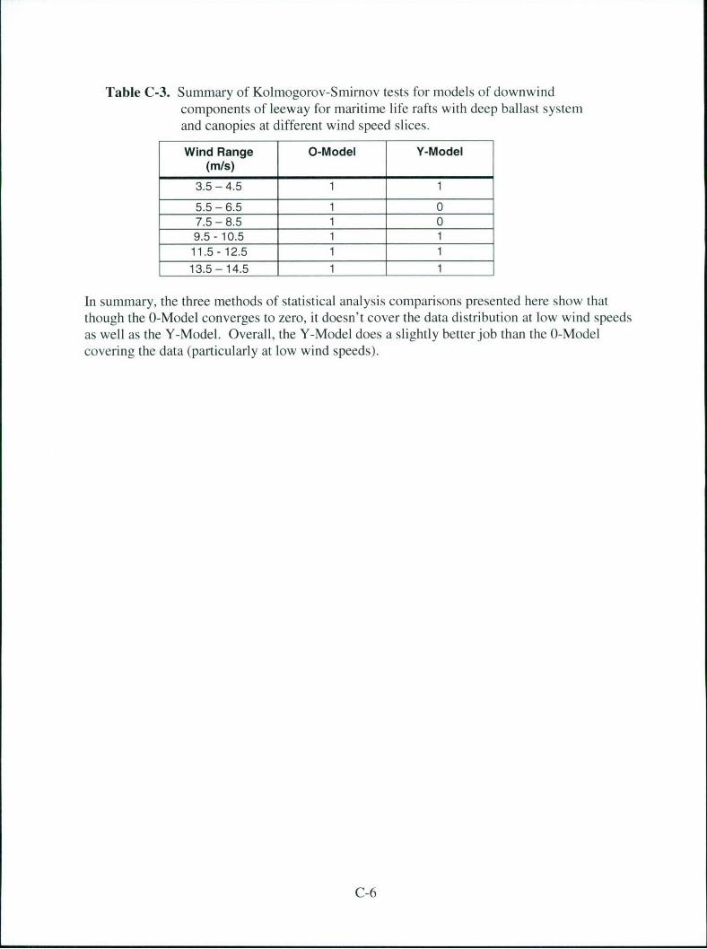
Table C-3. Summary of Kolmogorov-Smirnov tests for models of downwindcomponents of leeway for maritime life rafts with deep ballast systemand canopies at different wind speed slices.

Wind Range 0-Model Y-Model(m/s)

3.5-4.5 1 1

5.5-6.5 1 07.5-8.5 1 09.5-10.5 1 111.5-12.5 1 113.5-14.5 1 1

In summary, the three methods of statistical analysis comparisons presented here show thatthough the 0-Model converges to zero, it doesn't cover the data distribution at low wind speedsas well as the Y-Model. Overall, the Y-Model does a slightly better job than the 0-Modelcovering the data (particularly at low wind speeds).

C-6

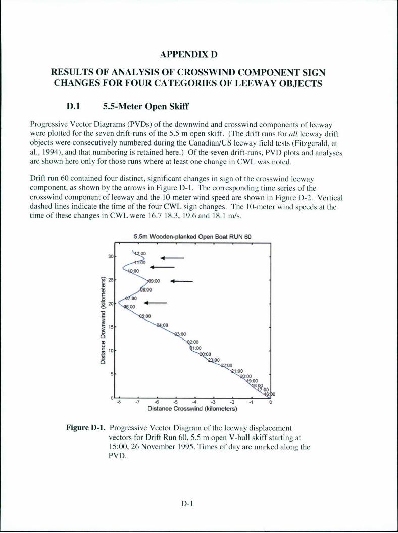
APPENDIX D

RESULTS OF ANALYSIS OF CROSSWIND COMPONENT SIGNCHANGES FOR FOUR CATEGORIES OF LEEWAY OBJECTS

D.1 5.5-Meter Open Skiff

Progressive Vector Diagrams (PVDs) of the downwind and crosswind components of leewaywere plotted for the seven drift-runs of the 5.5 m open skiff. (The drift runs for all leeway driftobjects were consecutively numbered during the Canadian/US leeway field tests (Fitzgerald, etal., 1994), and that numbering is retained here.) Of the seven drift-runs, PVD plots and analysesare shown here only for those runs where at least one change in CWL was noted.

Drift run 60 contained four distinct, significant changes in sign of the crosswind leewaycomponent, as shown by the arrows in Figure D- 1. The corresponding time series of thecrosswind component of leeway and the 10-meter wind speed are shown in Figure D-2. Verticaldashed lines indicate the time of the four CWL sign changes. The 10-meter wind speeds at thetime of these changes in CWL were 16.7 18.3, 19.6 and 18.1 m/s.

5.5m Wooden-planked Open Boat RUN 60

30. 00

:00

"1' 25 9:00 4

:00 8:00

~20

""15:00 2:00

1:00Si:0010. 1: 00

D00:00 0

700

04 -7 -8 -5 .4 -3 -2 -1 0

Distance Crosswind Qciomneters)

Figure D-1. Progressive Vector Diagram of the leeway displacementvectors for Drift Run 60, 5.5 m open V-hull skiff starting at15:00, 26 November 1995. Times of day are marked along thePVD.

D-1

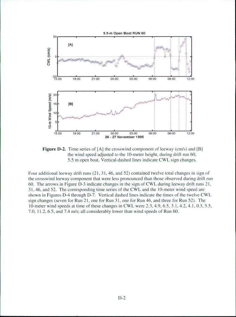
5.5-m Open Boat RUN 6050... , ; ,

[A] -

15:00 18:00 21:00 00:00 03:00 06:00 09:00 12:00

20 1,

A.,• 0I II I I5-C

15:00 18:00 21:00 00:00 03:00 06:00 09:00 12:0026 - 27 November 1995

Figure D)-2. Time series of [A] the crosswind component of leeway (cm/s) and [131the wind speed adjusted to the 10-meter height, during drift run 60,5.5 m open boat. Vertical-dashed lines indicate CWL sign changes.

Four additional leeway drift runs (21, 31, 46, and 52) contained twelve total changes in sign ofthe crosswind leeway component that were less pronounced than those observed during drift run60. The arrows in Figure D-3 indicate changes in the sign of CWL during leeway drift runs 2 1,31, 46, and 52. The corresponding time series of the CWL and the 10-meter wind speed areshown in Figures D-4 through D-7. Vertical dashed lines indicate the times of the twelve CWLsign changes (seven for Run 2 1, one for Run 3 1, one for Run 46, and three for Run 52). The10-meter wind speeds at time of these changes in CWL were 2.3, 4.9, 6.5, 3.1, 4.2, 4.1, 0.3, 5.5,7.0, 11.2, 6.5, and 7.4 m/s; all considerably lower than wind speeds of Run 60.

D-2

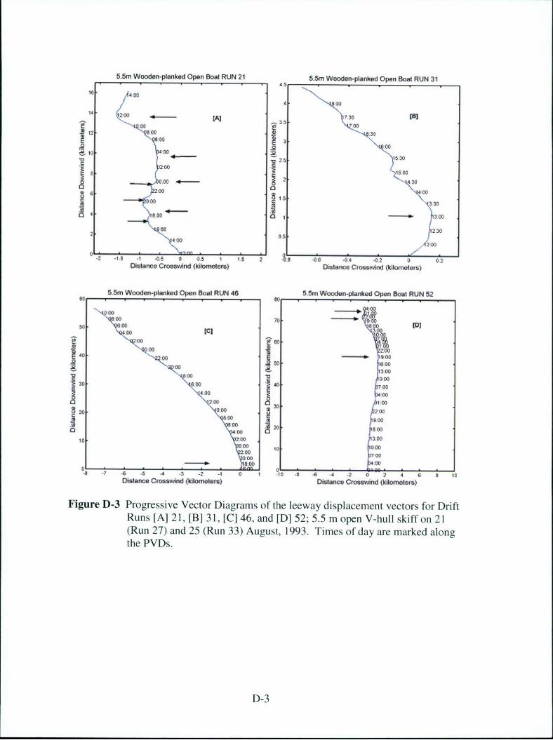
5.5m Wooden-planked Open Boat RUN 21 5.5m Wooden-planked Open Boat RUN 31

16. 400

4 -00

14- 200 35 -A 73, .B

":00 0012. .30

000 4-DO

300 So0o0

4400

00 1 " 330

4 - 500

01230

00 0200

2- 0540D 200

-2 -1.5 - -0 .0 0- 1 1.5 2 - -06 , .4 -0 .2 0 02Distance Crosswind (kilometers) Distane Crosw•nd (kilomo4ees)

R5-5 Wooden-planked Open Boat RUN 46 5.5m Wooden-planked Open Boat RUN 52

62D -3

60 8

:00.00 7 0

.00 (C)00 ~06

00 82!00140. OD 4goo0

00 31 00

00 ~ 0 M `030. 0.0 40 700

4.0 -0 002 00 0 1

20-0O 000' 00 too

too 00

43 .? 46 - .4 .3 .7 -1 0 1 -0 - 6 4 4 .2 0 2 4 a a ItDistance Ctoaswknd (kilxomeer) Eislance Crosswind (kilnsomes)

Figure D-3 Progressive Vector Diagrams of the leeway displacement vectors for DriftRuns [A] 2 1, [B] 3 1, [C] 46, and [D] 52; 5.5 m open V-hull skiff on 21(Run 27) and 25 (Run 33) August, 1993. Times of day are marked alongthe PVDs.

D-3

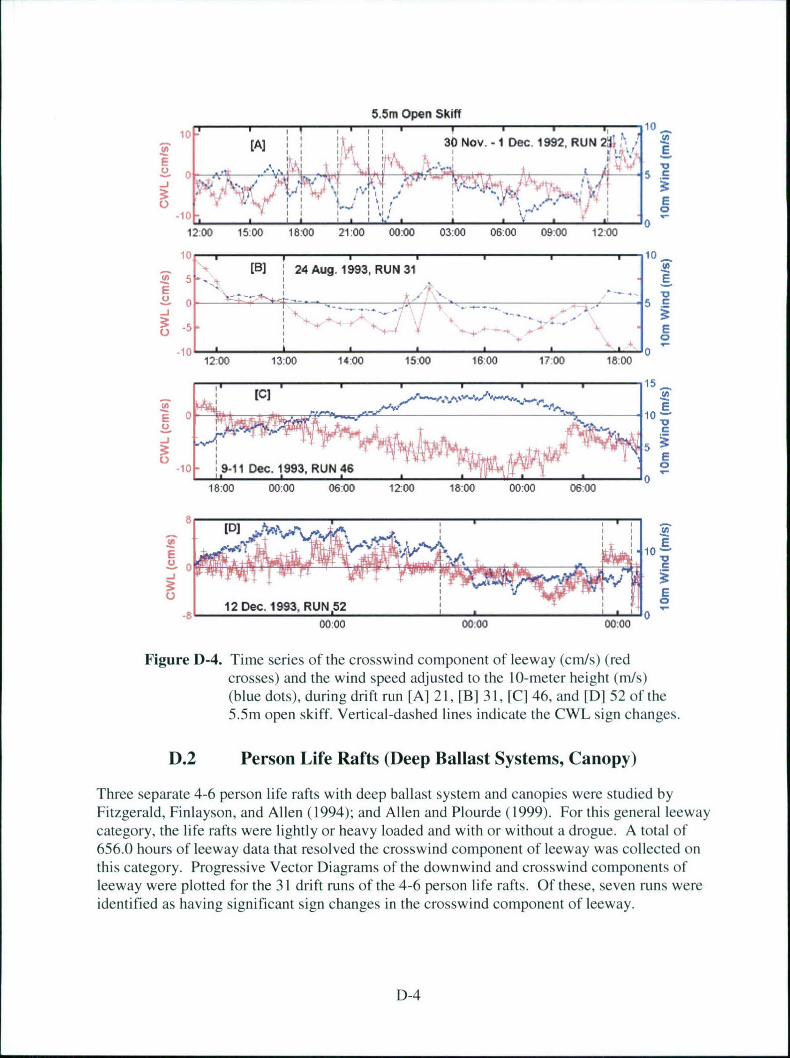
5.5m Open Skiff1 1 0 .-,

(0 [A) 30 Nov. - 1 Dec. 1992, RUN2 ,.. ',

oI t,.: :I I I•

"_______II___1_______ .1 I 13

EE

12:00 15:00 18:00 21:00 00:00 03:00 06-00 09:00 12:00

10 1 0

[B] 24 Aug. 1993, RUN 31

12:00 13:00 14:00 15:00 16:00 17:00 18:00

E

0 10

10- 9-11Dec. 1993. RUN46 r !18:00 00:00 06:00 12:00 18:00 00:00 06:00

'-a , 10

12 Dec. 1993, RUN,52 "1 : 0 _

00:00 0:0 00:00

Figure D-4. Time series of the crosswind component of leeway (cm/s) (redcrosses) and the wind speed adjusted to the 10-meter height (m/s)(blue dots), during drift run [A] 2 1, [BI 3 1, [C] 46, and [D] 52 of the5.5m open skiff. Vertical-dashed lines indicate the CWL sign changes.

D.2 Person Life Rafts (Deep Ballast Systems, Canopy)

Three separate 4-6 person life rafts with deep ballast system and canopies were studied byFitzgerald, Finlayson, and Allen (1994); and Allen and Plourde (1999). For this general leewaycategory, the life rafts were lightly or heavy loaded and with or without a drogue. A total of656.0 hours of leeway data that resolved the crosswind component of leeway was collected onthis category. Progressive Vector Diagrams of the downwind and crosswind components ofleeway were plotted for the 31 drift runs of the 4-6 person life rafts. Of these, seven runs wereidentified as having significant sign changes in the crosswind component of leeway.

D-4

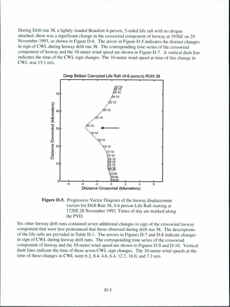
During Drift run 38, a lightly-loaded Beaufort 4-person, 5-sided life raft with no drogueattached, there was a significant change in the crosswind component of leeway at 1930Z on 29November 1993, as shown in Figure D-6. The arrow in Figure D-5 indicates the distinct changesin sign of CWL during leeway drift run 38. The corresponding time series of the crosswindcomponent of leeway and the 10-meter wind speed are shown in Figure D-7. A vertical dash lineindicates the time of the CWL sign changes. The 10-meter wind speed at time of this change inCWL was 15.1 m/s.

Deep Ballast Canopied Life Raft (4-6 person) RUN 38

:10:10

30"•~:10

Z4- 01:10E

10 210

V 10 _____

Z 30-18:10

o 6:10

10 :10:0

-6 -4 -2 0 2 4:

Distance Cross'wind (kilometers)

Figure D-5. Progressive Vector Diagram of the leeway displacementvectors for Drift Run 38, 4-6 person Life Raft starting at1720Z 28 November 1993. Times of day are marked alongthe PVD.

Six other leeway drift runs contained seven additional changes in sign of the crosswind leewaycomponent that were less pronounced that those observed during drift run 38. The descriptionsof the life rafts are provided in Table D-1. The arrows in Figures D-7 and D-8 indicate changesin sign of CWL during leeway drift runs. The corresponding time series of the crosswindcomponent of leeway and the 10-meter wind speed are shown in Figures D-9 and D-10. Verticaldash lines indicate the time of these seven CWL sign changes. The 10-meter wind speeds at thetime of these changes in CWL were 6.2, 8.4, 4.6, 6.4, 12.7, 16.0, and 7.3 m/s.

D-5

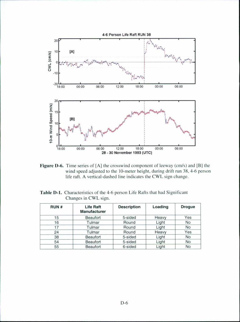
4-6 Person Life Raft RUN 3820 , ,,

-. 10 [A]

-10-

-20'.18:00 00:00 06-00 12:00 18:00 00:00 06:00

20

15

[B](a 10

A

"0-6

18:00 00:00 06:00 1200 18:00 00:00 06:0028 - 30 November 193 (UTC)

Figure D-6. Time series of [A] the crosswind component of leeway (cm/s) and [B] thewind speed adjusted to the 10-meter height, during drift run 38, 4-6 personlife raft. A vertical-dashed line indicates the CWL sign change.

Table D-1. Characteristics of the 4-6 person Life Rafts that had SignificantChanges in CWL sign.

RUN # Life Raft Description Loading DrogueManufacturer

15 Beaufort 5-sided Heavy Yes16 Tulmar Round Light No17 Tulmar Round Light No24 Tulmar Round Heavy Yes38 Beaufort 5-sided Light No54 Beaufort 5-sided Light No55 Beaufort 6-sided Light No

D-6

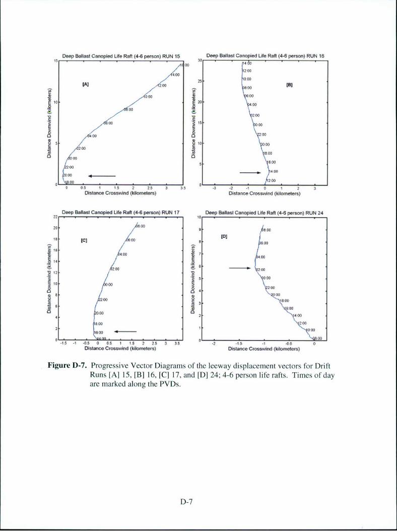
Deep Ballast Canopied Life Raft (4-6 person) RUN 15 Deep Ballast Canopied Life Raif (4-6 person) RUN 16

1 00 4&

zoo400

/1J00 25, 0.00

"ir ? .00

000 To

110 0120 .00000

00 1500

020

1000

8.00 klmes

0 05 I 15 ' 5. - 2 1 0Distance Cross"oind (Id el~l ers) Distance Crosswind (kilometers)

Deep Ballast Canopied Life Raft (4-6 person) RUN 17 Deep Ballast Canopied Life Raft (4-6 person) RUN 24210

20, 00 00

I I0 00;5 16

14 0 0

20/ 0 2 o00

1 ' :00

1000 75 0 D0

4 2 400

0600

328002,0 zoo0

6`00L (7"' 0050

-1 -1 -05 0 05 1 15 2 25 3 35 -2 -15 - -05 0Distance Cioeswind (Idlomelets) Distance Cfomswlnd (kilomelets)

Figure D-7. Progressive Vector Diagrams of the leeway displacement vectors for DriftRuns [A] 15, [B] 16, [C] 17, and [D] 24; 4-6 person life rafts. Times of dayare marked along the PVDs.

D-7

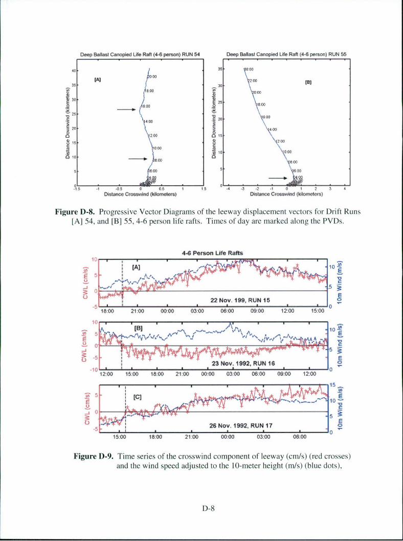
Deep Ballast Canopied Life Raft (4-6 person) RUN 54 Deep Baflast Canopied Life Rafl (4-6 person) RUN 55

40- 35l .00

30 .S

25.2 0.00 ý

200

4003

20 21 400

d) 203

bO 000

.'0 X0 0l I00It

- -1 -05 0 05 1 15 -4 -3 -2 -1 0 2 3 4

Distanoe Crosswind (klWometers) Oistance Cosswind (kilomeels)

Figure D-8. Progressive Vector Diagrams of the leeway displacement vectors for Drift Runs[A] 54, and [B] 55, 4-6 person life rafts. Times of day are marked along the PVDs.

4-6 Person Life Rafts

22 Nov. 199, RUN 15

18:00 21:00 00:00 03:00 06:00 09:00 12:00 15:00

10, -

-5

23 NOV. 1992, RUN 16 0

12:00 15:00 18:00 21:00 00:00 03:00 06:00 09:00 12:00

d• 10•

26 Nov. 1992, RUN 17

15:00 18:00 21:00 00:00 03:00 06:00

Figure D-9. Time series of the crosswind component of leeway (cm/s) (red crosses)and the wind speed adjusted to the 10-meter height (m/s) (blue dots),

D-8

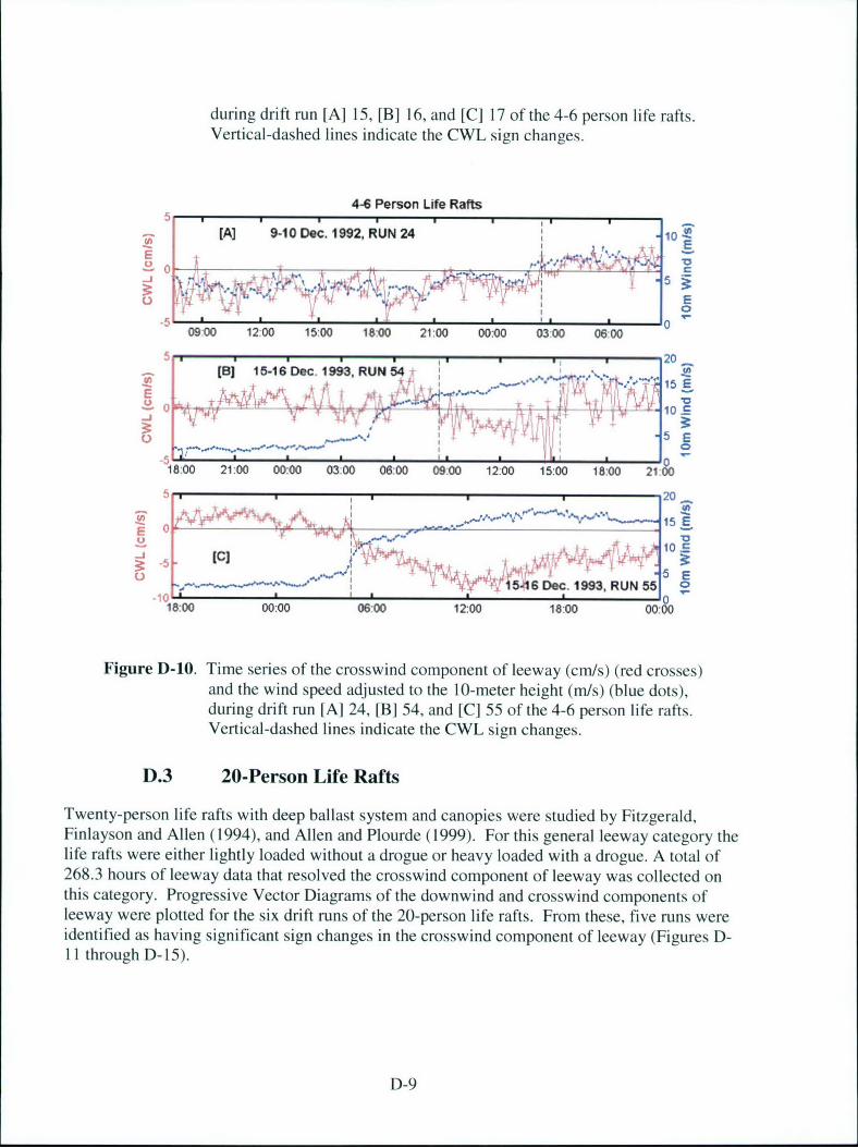
during drift run [A] 15, [B] 16, and [C] 17 of the 4-6 person life rafts.Vertical-dashed lines indicate the CWL sign changes.

4-6 Person Life Rafts

[A] 9-10 Dec. 1992, RUN 24 1

1 0

0900 1200 15:00 18:00 21:00 00t00 030 06005 ,1 , 2 0

1B6 15-l6Dec1993,RUN54 I,

.• 'It ,f .... , I•, , * -it # . -0

I.I 1, - )0.ý 7 10 C

18:00 21:00 00:00 03:00 06:00 09:00 1200 15:00 18:00 21:10

U1546 Dec. 1993, RUN 5518:00 00:00 06-00 12:00 18:00 00:00

Figure D-10. Time series of the crosswind component of leeway (cm/s) (red crosses)and the wind speed adjusted to the 10-meter height (m/s) (blue dots),during drift run [A] 24, [B] 54, and [C] 55 of the 4-6 person life rafts.Vertical-dashed lines indicate the CWL sign changes.

D.3 20-Person Life Rafts

Twenty-person life rafts with deep ballast system and canopies were studied by Fitzgerald,Finlayson and Allen (1994), and Allen and Plourde (1999). For this general leeway category thelife rafts were either lightly loaded without a drogue or heavy loaded with a drogue. A total of268.3 hours of leeway data that resolved the crosswind component of leeway was collected onthis category. Progressive Vector Diagrams of the downwind and crosswind components ofleeway were plotted for the six drift runs of the 20-person life rafts. From these, five runs wereidentified as having significant sign changes in the crosswind component of leeway (Figures D-11 through D-15).

D-9

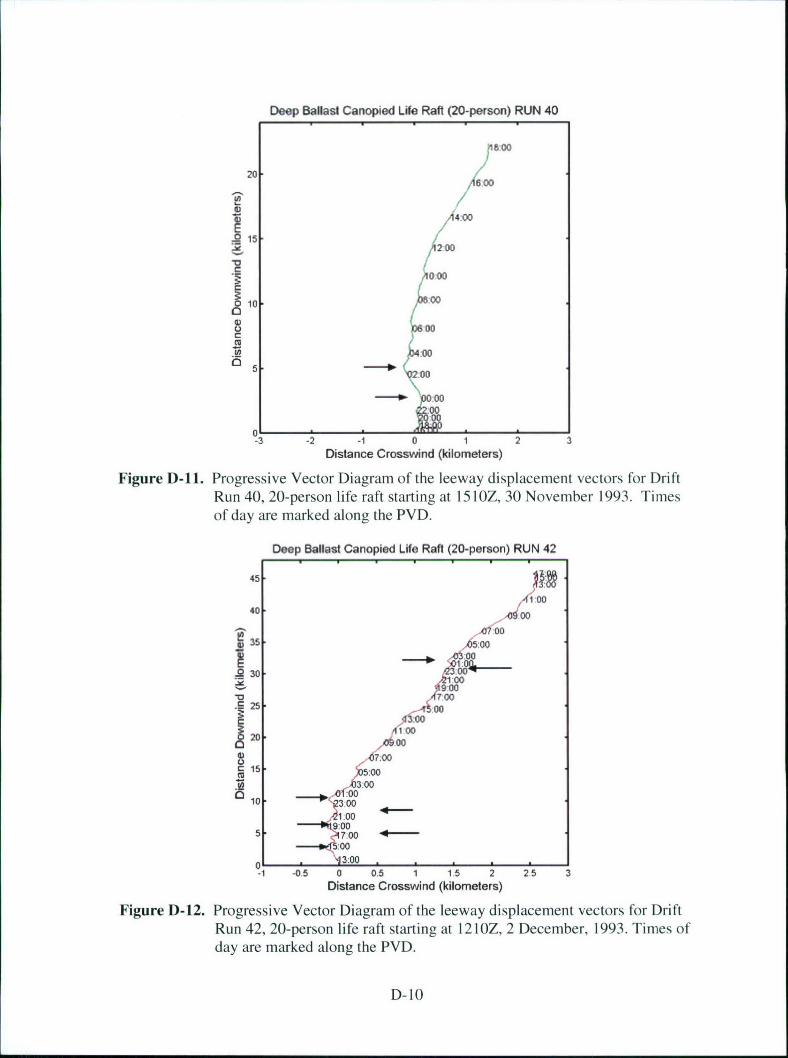
Deep Ballast Canopied Life Raft (20-person) RUN 40

18:00

20 0

0,/

14.00

S15 .

"200

S08:00

._ P:00

0 5 0200

- -000

-3 -2 -1 0 1 2 3

Distance Crosswind (kilometers)

Figure D-11. Progressive Vector Diagram of the leeway displacement vectors for DriftRun 40, 20-person life raft starting at 1510Z, 30 November 1993. Timesof day are marked along the PVD.

Deep Ballast Canopied Life Raft (20-person) RUN 42

45

40.00

315 5:007:000

10000070"300

01 000 =5 1 .

:00

Distance Crosswind (kilometers)

Figure D-12. Progressive Vector Diagram of the leeway displacement vectors for DriftRn42, 20-person life raft starting at 1210Z, 2 December, 1993. Times of

day are marked along the PVD.

D-10

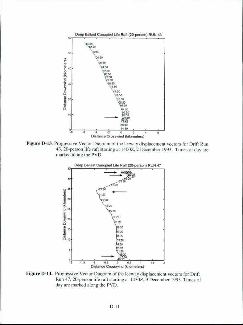
Deep Ballast Canopied Life Raft (20-person) RUN 43so

'14450

'12 50

50 '10:50

0:50

40- '04:50ý2:50

•0:503- 46:50

120 --- 500850O, 4:50

20 '4050'0250

10. 105

01 0 650 ~l-.6 +4 .2 0 2 4

Distance Crosswind (kilometers)

Figure D-13. Progressive Vector Diagram of the leeway displacement vectors for Drift Run43, 20-person life raft starting at 1400Z, 2 December 1993. Times of day aremarked along the PVD.

Deep Ballast Canopied Life Raft (20-person) RUN 47

40-A2.4320

:20- 35-

0 1,20

E 30-9:20

7:20o25 5.20

3:2020.

1 20

"15 :20

:20

120201:203:20

5~ 1:20= :20

01 w0

.2 -1,5 .1 -.05 0 05 1 15 2Distance Crosswind (kilometers)

Figure D-14. Progressive Vector Diagram of the leeway displacement vectors for DriftRun 47, 20-person life raft starting at 1430Z, 9 December 1993. Times ofday are marked along the PVD.

D-1 I

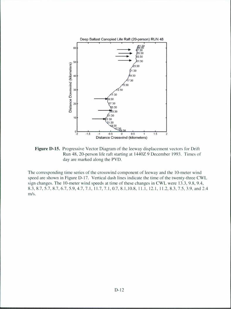
Deep Ballast Canopied Life Raft (20-person) RUN 48

60._____

- ):3030

5 4 - 1:30

P, 3:30

130

~40 9.30

;30T3

~30 .30

0130Dr il9:30

C 20 730w 530

o 3:30

1:3010 330

1:30

01 :30

.2 A15 -1 -05 0 0.5 1 15 2

Distance Crosswind (kilometers)

Figure D-15. Progressive Vector Diagram of the leeway displacement vectors for DriftRun 48, 20-person life raft starting at 1440Z 9 December 1993. Times ofday are marked along the PVD.

The corresponding time series of the crosswind component of leeway and the 10-meter windspeed are shown in Figure D-17. Vertical dash lines indicate the time of the twenty-three CWLsign changes. The 10-meter wind speeds at time of these changes in CWL were 13.3, 9.8, 9.4,8.3, 8.7, 5.7, 8.7, 6.7, 5.9, 4.7, 7.1, 11.7, 7.1,0.7, 8.1,10.8, 11.1, 12.1, 11.2, 8.3, 7.5, 3.9, and 2.4m/s.

D-12

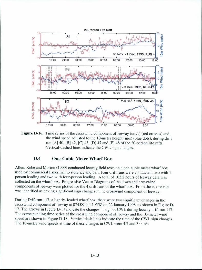
20-Person Life Raft1£ * *[A " i * " ..a 20

-JA

-1I •I I 1 II/180E0:0 0 0 200 1:0 00 06J00 120 180

17 -1

30 1Nov, -Dec.IMRU4-10 160

18:00 2100 00:00 03,00 06:00 0900 1200 15:00 1:

18:00 0000 0600 1200 1800 00:00 0600 1200

Figure D-16. Time series of the crosswind component of leeway (cm/s) (red crosses) andthe wind speed adjusted to the 10-meter height (mis) (blue dots), during drift

run [A] 40, [B] 42, [C] 43, [D] 47 and [E] 48 of the 20-person life rafts.Vertical-dashed lines indicate the CWL sign changes.

D.4 One-Cubic Meter Wharf Box

Allen, Robe and Morton (1999) conducted leeway field tests on a one-cubic meter wharf boxused by commercial fisherman to store ice and bait. Four drift runs were conducted, two with 1-person loading and two with four-person loading. A total of 102.2 hours of leeway data wascollected on the wharf box. Progressive Vector Diagrams of the down and crosswind

components of leeway were plotted for the 4 drift runs of the wharf box. From these, one runwas identified as having significant sign changes in the crosswind component of leeway.

During Drift run 117, a lightly-loaded wharf box, there were two significant changes in thecrosswind component of leeway at 0745Z and 1955Z on 22 January 1998, as shown in Figure D-

17. The arrows in Figure D-17 indicate the changes in sign of CWL during leeway drift run 117.The corresponding time series of the crosswind component of leeway and the 10-meter windspeed are shown in Figure D- 18. Vertical dash lines indicate the time of the CWL sign changes.The 10-meter wind speeds at time of these changes in CWL were 4.2 and 3.0 m/s.

D-13

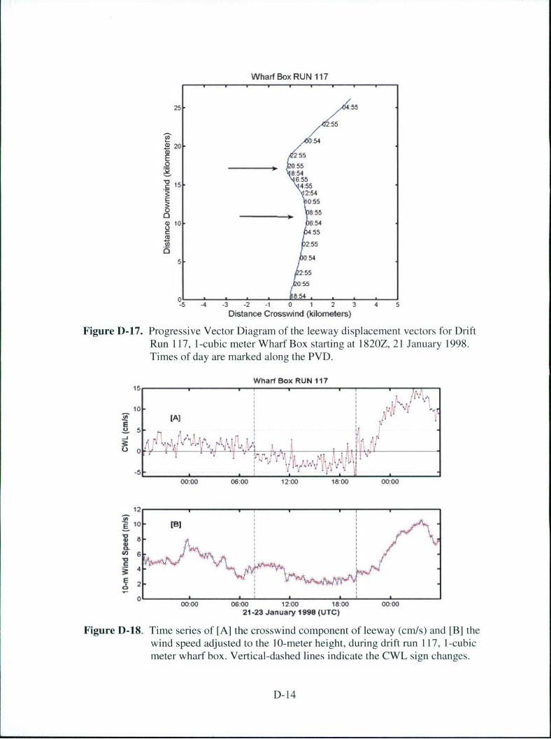
Wharf Box RUN 117

25 .55

54

.20-2_ 55

O _ 0558 .54

6,55

Sr2:552:54055

8:5510. &.54

.55

20 55

5- 54

.55

-55L_ &5 A

-5 -4 -3 -2 -1 0 1 2 3 4 5Distance Crosswind (kilometers)

Figure D-17. Progressive Vector Diagram of the leeway displacement vectors for DriftRun 117, 1-cubic meter Wharf Box starting at 1820Z, 21 January 1998.Times of day are marked along the PVD.

Wharf Box RUN 117

0 [(A] *A

0000 06:00 12:00 1800 00:00

12" "

S r

S4T

2-

0i

00:00 06:00 12:00 18:00 00:0021-23 January 1998 (UTC)

Figure D-18. Time series of [A] the crosswind component of leeway (cm/s) and [B] thewind speed adjusted to the 10-meter height, during drift run 117, 1-cubicmeter wharf box. Vertical-dashed lines indicate the CWL sign changes.

D-14