university of çukurova
84
UNIVERSITY OF ÇUKUROVA INSTITUTE OF NATURAL AND APPLIED SCIENCE MSc THESIS Kamil ÖZKAN DESIGN OF A MICROCONTROLLER-BASED PERSPECTIVE VIEW PREPROCESSOR FOR PIXEL-BASED CONSTRUCTIVE SOLID GEOMETRY (CSG) PROCESSORS DEPARTMENT OF ELECTRICAL AND ELECTRONICS ENGINEERING ADANA, 2006
-
Upload
khangminh22 -
Category
Documents
-
view
1 -
download
0
Transcript of university of çukurova

UNIVERSITY OF ÇUKUROVA INSTITUTE OF NATURAL AND APPLIED SCIENCE
MSc THESIS Kamil ÖZKAN DESIGN OF A MICROCONTROLLER-BASED PERSPECTIVE VIEW PREPROCESSOR FOR PIXEL-BASED CONSTRUCTIVE SOLID GEOMETRY (CSG) PROCESSORS
DEPARTMENT OF ELECTRICAL AND ELECTRONICS ENGINEERING
ADANA, 2006


I
ÖZ
YÜKSEK LİSANS TEZİ
Kamil ÖZKAN
ELEKTRİK ELEKTRONİK MÜHENDİSLİĞİ ANABİLİM DALI
FEN BİLİMLERİ ENSTİTÜSÜ
ÇUKUROVA ÜNİVERSİTESİ
Danışman : Yrd. Doç. Dr. Ulus ÇEVİK Yıl : Nisan 2006, Sayfa: 58 Jüri : Yrd. Doç. Dr. Ulus ÇEVİK Prof. Dr. Süleyman GÜNGÖR Yrd. Doç. Dr. Murat AKSOY
Bilgisayar uygulamalarının çoğu, sanal dünya ile insanların görsel olarak iletişimini sağlamaya çalışır. Katı cisimlerin 3-boyutlu (3B) görünümleri bilgisayar destekli tasarım, bilgisayar oyunları, araç simülasyonları ve bilimsel tasarımlar gibi alanlarda çok önemlidir. Katı cisimlerin geometrik gösterimi, bir çeşit geometric modellemedir. Bu modellemelerde bir çok piksel tabanlı sistemler kullanılmaktadır. Katı cisimlerin 3B görünümlerinin elde edilmesinde paralel donanım uygulamaları çoğunluktadır. Geometrik gösterimler, paralel ve perspektif olarak iki sınıfta toplanmaktadır. Paralel görüntüler, nesnelerin gerçek şeklini ve boyutlarını gösterirken, görüntüler perspektif gösterimden daha az gerçekçidir.
Bu tez çalışmasında, daha gerçekçi olan perspektif görüntü üreten ve parallel sistemlere entegre edilebilir, yazılım ve donanımı birlikte içeren bir system dizayn edeceğiz. Bu modül ile uzayda bir düzlem üzerinde doğrusal olmayan üç nokta yardımı ile katı cisimlerin perspektif görünümlerini veren düzlemlerin denklemlerinin katsayıları mikrodenetleyici ile elde edilecektir. Bilgisayarlarda USB portlarının gelecek teknolojide ve hız bakımından gittikçe önem kazanması sebebi ile mikrodenetleyici ve bilgisayar arasında USB portunu kullanacağız.
Anahtar Kelimeler: Pic Mikrodenetleyici, USB, Paralel Gösterim, Perspektif
Gösterim, Paralel Port
PİKSEL TABANLI YAPISAL KATI GEOMETRİ (CSG) İŞLEMCİLERİ İÇİN MİKROKONTROLCÜ TABANLI
BİR ÖNİŞLEMCİ TASARIMI

II
ABSTRACT
MSc THESIS
Kamil ÖZKAN
DEPARTMENT OF ELECTRICAL AND ELECTRONICS ENGINEERING
INSTITUTE OF NATURAL AND APPLIED SCIENCES
UNIVERSITY OF ÇUKUROVA
Supervisor: Ass. Prof. Dr. Ulus ÇEVİK Year: April 2006, Pages: 58 Jury: Yrd. Doç. Dr. Ulus ÇEVİK Prof. Dr. Süleyman GÜNGÖR Yrd. Doç. Dr. Murat AKSOY
Many computer applications work to communicate an illusion of interaction with virtual world. The generation of 3D solid objects, and more generally solid geometric modeling, is very important in Computer Aided Design (CAD), computer games, vehicle simulations and scientific visualizations. CSG (Constructive Solid Geometry) is an approach to geometric modeling. There are many parallel hardware applications for the generation of CSG images, such as pixel-based systems.
Planar geometric projections can be classified as parallel, and perspective projections. While the parallel projected scenes are useful for recording the exact shapes and measurements of objects, they exhibit less realistic views as they are lacking perspective foreshortening.
In this thesis, we will design a module which can be integrated to the pixel-based parallel rendering systems to obtain perspective views using a microcontroller. Because USB ports are getting more popular for the next generation technology and speed of data transfer, we will use the USB ports for data communication.
Keywords: Pic Microcontroller, USB, Parallel Projection, Perspective
Projection, Parallel Port
DESIGN OF A MICROCONTROLLER-BASED PERSPECTIVE VIEW PREPROCESSOR FOR PIXEL-BASED CONSTRUCTIVE SOLID GEOMETRY (CSG)
PROCESSORS

III
ACKNOWLEDGEMENTS
I would like to express my heartfelt thanks to Assistant Prof. Dr. Ulus ÇEVİK
for his supervision, guidance, encouragements and extremely useful suggestions
throughout this thesis. I am very proud of working with Mr. Ulus ÇEVİK as
supervisor.
I would like to express a special thank to Assistant Prof. Dr. Murat AKSOY
who has supported me about electronic problems with remarkable patience. I would
like to thank Mr. Zehan KESİLMİŞ for his valuable advices and practical support. I
should thank Mr. Ahmet TEKE for arranging the outlook of the theses. Their
continuous support helped me to finish this thesis.
I would like to thank Prof. Dr. Süleyman Güngör, Head of the Department,
for providing a good working environment.
I wish to thank Institute of Natural and Applied Sciences and to extend my
acknowledgements to all staff members in the department and my friends.
Finally, I would like to thank my wife, my son and the coming baby for their
endless support and encouragements.

IV
CONTENTS PAGE
ÖZ………………………………………………………………………………….....I
ABSTRACT…………………………………………………………………………II
ACKNOWLEDGEMENTS……………………………………………………….III
CONTENTS………………………………………………………………………..IV
LIST OF TABLES………………………………………………………………....VI
LIST OF FIGURES………………………………………………………………VII
LIST OF SYMBOLS…………………………………………………………….VIII
LIST OF ABBREVATIONS……………………………………………………….IX
1. INTRODUCTION……………………………………………………………….1
2. PREVIOUS WORKS……………………………………………………………..3
2.1. Pixel-Based Rendering………………………………………………..….3
2.2. Pixel-Planes……………………………………………………………....3
2.3. The FPGA-Based Renderer …………………………………………...…7
3. PROJECTIONS………………………………………………………………...11
3.1. Parallel Projection………………………………………..…………..…11
3.1.1. Orthographic projection……………………………………....11
3.1.2. Oblique Projection …………………………………………....13
3.2. Perspective Projection.…………………………………………..……...14
3.3. Vanishing Point…………………………………………………………23
3.4. Mathematics of Perspective Projection…………………………………25
4. ALGORITHM and FORMULAS…………………………………………...…28
4.1. The Module Algorithm……………………………………………...…28
4.2. Implementation and Coefficients……………………………………...29
5. HARDWARE DEVELOPMENT……………………………………………...36
5.1. General………………..………………...………………...…………...36
5.2. USB Interfacing……………………………………………….………38
5.2.1. What Is USB? ……………………………………………..…38
5.2.2. USB Features……………………………………...…………41
5.2.3. The USB Process…………………………………………….42

V
5.2.4. Interfacing PIC Microcontroller and USB…………………..43
6. RESULTS AND DISCUSSION……………………………………………..….48
6.1. Results And Discussion……………………..…………………………..48
7. CONCLUSIONS AND FUTURE WORK……………………………….……51
7.1. Conclusion And Future Work……………………………..…………….51
REFERENCES………...…………………………………………………………...54
BIOGRAPHY………………...…………………………………………………….58
APPENDIX A
FT232 USB UART (USB and SERIAL)
APPENDIX B
Microchip Pic 16f877

VI
LIST OF TABLES PAGE
Table 4.1. Determination of Three Non-collinear points………………….…....30
Table 5.1. Speed of the Communication Standards..………………………...…36
Table 6.1. The Speed of Transformation..……………………………...…….…49
Table 6.2. The comparison according to baud rate used ……….…………..….50

VII
LIST OF FIGURES PAGE
Figure 2.1. The Graphics Pipeline……………………………...............................4
Figure 2.2. Block Diagram of Pixel-Planes 5……………………………………..7
Figure 2.3. The architecture of the CSG renderer………………………………...8
Figure 2.4. The tree-structured depth generator…………………………………..9
Figure 3.1. Parallel (Orthographic) Projection……………………..……………12
Figure 3.2. Parallel (Orthographic-Isometric) Projection………………………..12
Figure 3.3. Parallel (Oblique) Projection of a point (x,y,z) with angle on the PP.13
Figure 3.4. (a) Perspective projection (b) Parallel projection…………………14
Figure 3.5. (a) One Point Perspective (b) A Painting by Canaletto ..………....24
Figure 3.6. (a) Two Point Perspective (b) A Painting by E. Hopper ..………...24
Figure 3.7. (a) Three Point Perspective (b) A Painting by GeorgiaCanaletto ...25
Figure 3.8. Perspective projection plane…………………………………………26
Figure 4.1. A Parallel Projected Cube and Its Perspective View………………..28
Figure 4.2. Integration of the perspective view module to the CSG renderer…...32
Figure 5.1. USB Connector Types (a) “A”-Type (b) “B”-Type
(c) “Mini-B”-Type…………………………………………………...40
Figure 5.2. Electrical Diagram of the USB “A” Type connector………………..42
Figure 5.3. Wiring Diagram of The Design……………………………………..44
Figure 5.4. Microcontroller and USB port Interface PCB Design ……………...45
Figure 5.5. Communicating PC Program interface……………………………...46
Figure 5.6. Block Diagram of The Module……………………………………...47
Figure 7.1 (a) Parallel projection of a pair of dices.
(b). Perspective projection of the dices……………………………...52
Figure 7.2. (a)Parallel projection of a hollow cross,
(b). Perspective projection of the hollow cross…………...…………52

VIII
LIST OF SYMBOLS
µs : Micro-second
D- : Negative Data Signal
D+ : Positive Data Signal
Gnd : Ground
mA : Mili-ampere
MHz : Mega-hertz
ms : Mili-second
V : Volt
Vcc : Source voltage

IX
LIST OF ABBREVIATIONS
3B : Three Dimension (Üç Boyutlu)
3D : Three Dimensions
A/D : Analog – Digital Conversion
Ack : Acknowledgment Signal
ALU : Arithmetic Logic Unit
BIOS : Basic Input / Output System
CAD : Computer Aided Design
CAN : Controller Area Network
COM : Communication Port
COP : Center Of Projection
CRT : Cathode Ray Tube
CSG : Constructive Solid Geometry
CTS : Clear to Send
D/A : Digital – Analog Conversion
DMA : Direct Memory Access
ECP : Extended Capabilities Mode
ECR : Extended Control Register
EPP : Enhanced Parallel Port
FIFO : First Input First Output
FPGA : Field Programmable Gate Array
IDE : Integrated Drive Electronics
In : Input
IRQ : Interrupt request
ISA : Industrie Standard Architecture
LPT : Label of Parallel Port
np : Normal Vector
Out : Output
PCB : Printed Circuit
PP : Projection Plane

X
Rx : Receive Asynchronous Data Input
SATA : Serial Integrated Drive Electronics
SCI : Serial Communication Interface
SCL : Serial Clock Line For I2C
SDA : Serial Data Line For I2C
SPP : Standard Parallel Port
SPI : Serial Peripheral Interface
Tx : Transmit Asynchronous Data Output
UART : Universal Asynchronous Receiver / Transmitter
UNC : University of Carolina
USART : Universal Synchronous Asynchronous Receiver Transmitter
USB : Universial Serial Bus
VLSI : Very Large Scale Integratıon
vpp : Dot Product

1. INTRODUCTION Kamil ÖZKAN
1
1. INTRODUCTION
Nowadays, rendering images of 3D solid objects and their processing have
become popular. Generally, they are used in Computer Aided Design (CAD),
computer games and simulators. One of the most popular method, for this purpose, is
the Constructive Solid Geometry (CSG). Processors, using this method, usually
produce parallel projections of objects. Although parallel projection is suitable for
true perception of the dimensions in CAD, produced images are not realistic. In order
to obtain near-realistic images perspective projections are needed.
In CSG, solids of more complicated objects are constructed from simpler
objects, such as cylinders, composed of planes, cubes, etc., by performing set
operations, usually union, intersection, and difference. Finding three non-collinear
points on each plane, forming those simple objects, and perspective transforming
only these points, and obtaining a new plane will result in the perspective
transformation of the whole plane, so the object.
There are many parallel hardware applications for the generation of CSG
images. There is a radically interesting approach, that we may call pixel-based,
which works by, for each pixel, determining whether that pixel is covered by a
particular polygon, and is so, to do something about it. The significance of this
approach is that provides for the possibility of massive parallelism, each pixel may
simultaneously carry out the test for overlapping calculation. This of course leads to
a system built from VLSI components, that has a simple processor for every screen
pixel, or at least for all pixels on a particular screen region.
We will describe the design of a perspective view module to be integrated to
those pixel-based CSG renderers. While choosing non-collinear points on planes, a
PIC Microcontroller will be used. When a 20 Mhz crystal is used the command cycle
speed will approach to 5 Mhz. This speed can be increased by using more advanced
PIC types. We will use Pic C to program the microcontroller.
Rendering of perspective images, using the method given above, is obtained
by a software with the expense of an extra computational burden on the processor.

1. INTRODUCTION Kamil ÖZKAN
2
However, this can be implemented by using a dedicated hardware to remove the
burden.
In Chapter 2, the pixel-based rendering, that will set up a background for our
work, is presented.
In Chapter 3, an overview to projections is presented.
In Chapter 4, the algorithm used during this work is given.
In Chapter 5, we introduce the parallel and USB ports and data transfer. We
also explain advantages and disadvantages of them.
In Chapter 6, we present the results.
And in the last chapter, Chapter 7, future works are suggested.

2. PREVIOUS WORKS Kamil ÖZKAN
3
2. PREVIOUS WORKS
2.1. Pixel-Based Rendering
The generation of 3D solid objects is an approach geometric modeling.
Solids of more complicated objects are constructed from simpler objects by
performing set operations, usually, union, intersection, and difference. A composite
object can be represented with a binary tree where each node contains a set operation
and two child nodes that may also be composite solids. The leaves of this tree are
primitive objects such as cubes, half space, etc.
For many years, visual systems have been the pursuit of truly interactive
graphics systems. Computer applications seek to create an illusion of interaction with
a virtual world. Many designers using CSG (Constructive Solid Geometry) was the
inability to create and modify CSG objects in an interactive environment. Advances
in graphics hardware have made it possible to achieve renderings of CSG objects
thank to parallelism in hardware. We can give pixel-based rendering as an example.
2.2. Pixel-Planes
One of the CSG rendering systems is Pixel-Planes research project by Fuchs
[FUCHS, H., et al. 1981]. The project began in the Fall of 1980 during a VLSI
design class taught by Henry Fuchs at the University of Carolina (UNC).
Figure 2.1 [LASTRA, et al., 1996] illustrates the traditional graphics
pipeline. Primitives (typically triangles or other polygons) enter the pipeline in a user
centered, object coordinate system [FOLEY,J. D., et al., 1995] The pipeline is
conceptually (and often physically) divided into two stages, one for the geometry
processing, the other for rasterization. A reason for this partitioning is that the work
performed in the two stages is fundamentally different. In the geometry processing
stage, the vertices of the primitives are transformed to a screen coordinate system,
vertices are lit and transformed to projection coordinates, primitives are clipped to fit
within the viewing frustum, perspectively transformed, and set up for the

2. PREVIOUS WORKS Kamil ÖZKAN
4
rasterization stage. This part of the work is floating point intensive and produces
polygon vertices in screen coordinates (integer) along with shading
information[LASTRA, et al., 1996 ].
Figure 2.1. The Graphics pipeline
The rasterization stage is responsible for scan conversion and for determining
visibility, typically a pixel by pixel process. Note that computing visibilitiy is
essentially a sorting problem, sorting by depth to find the pixel or polygon closest to
the viewpoint. After visibility has been determined, the color is computed. While
early graphics engines just assigned a constant color to each polygon, common
method today is Gouraud shading, a linear interpolation between the color at the
vertices [FOLEY J.D., et al., 1995]. The majority of the work done in the
rasterization stage is fixed-point integer computation, but the most difficult problem
is the memory bandwidth required, since access to different location in the frame
buffer is necessary for practically every operation.
One can think of a “processor per pixel” as adding local memory to all of
these pixel processors. Each processor in the pixel-planes system consists of 1-bit
Geometry Processor
Rasterization Frame Buffer
“Immediate Mode”
Primitives are generated on the fly
“Retained Mode”
Display List is edited and created.
screen
Graphic Primtives in “object” coordinates (x1,x2,x3)
Graphic Primtives in “screen” coordinates (x’1,x’2,x’3)
Pixels

2. PREVIOUS WORKS Kamil ÖZKAN
5
ALU. However, Pixel-planes is not simply a processor-per-pixel system which blind
replicates much of the scan conversion work at each processor.
A major contribution of Pixel-Planes was a way to perform as much global
computation as possible for all the processors at once. The key concept was the
realization that simple plane equation of the form F(x,y) = Ax + By + C (where x and
y are the screen coordinates of each pixel) is an excellent formulation for much of the
work performed during rasterization. The plane equation is first used to enable pixel
processors on the correct side of each polygon edge. It is then used to interpolate
depth z at each pixel in order to determine visibility, and finally it is used linear
interpolate color. Hidden surface removal is performed using a z-buffer algorithm in
which the z-coordinate of pixel is encoded in a set of coefficients A, B, C by linear
expression as equation
z=Ax + By + C (2.1)
Besides a one-bit ALU, the Pixel-Planes logic enhanced memory chips
include a global computational tree to compute the result of the plane equations for
each pixel.
The base of the project is determined about ways to implement a distributed
frame buffer for high performance interactive graphics and the project oriented class.
Pixel-Planes 1 was the original chip. It contained a 2 by 2 grid of pixel
memory and a branch of the computational tree [FUCHS, H., et al., 1981]. In
collaboration with Alan Paeth and Alan Bell of Xerox PARC, a new generation
chips, Pixel-Planes 2, was developed [FUCHS, H., et al., 1982]. Each of these chips
contained 64 pixels with 16 bits per pixel of memory. These were used at University
of North Caroline (UNC) to build a 4 x 64 pixel prototype. This prototype was used
to verify that a basic set of rendering operations could be executed on this
architecture.
In collaboration with Paeth, a third set of chips, Pixel-Planes 3, was built
[FUCHS, H., et al., 1985]. These chips included a more complex ALU, and 32 bits

2. PREVIOUS WORKS Kamil ÖZKAN
6
per pixel. There were still 64 pixels per chip but the video scan out was integrated
into the chips. These were assembled in 1983 to make a 64 x 64 pixel prototype.
In 1984, new pixel-memory chips were designed, along with a chip that
functioned as a program controller. These were assembled into a small system, pixel
Planes 4.1 [POULTON, J. et al., 1985], which was first demonstrated at the 1985
VLSI Conference in Chapel Hill. The complete machine had to include a host
computer, a base of system software, and application. This machine, Pixel-Planes 4.2
but usually referred to simply as Pixel-Planes 4, was completed just in time for
SIGGRAPH ’86, where it was demonstrated. It served as the workhorse for research
in the University of the North Caroline graphics laboratory until it was retired in
1992. The full Pixel-Planes 4 system is describe by Eyles [EYLES, J., et al. 1988 ].
Pixel-Planes 4 implemented a full-size 512 by 512 pixel frame buffer using 2048
enhanced-memory integrated circuits, running at 10 MHz. Each chip implemented a
128-pixel column of the display with 72 bits per pixel and included video scan-out
circuitry. The frame buffer was housed on thirty two boards on a common backplane.
Geometry processing was hosted by DEC MicroVAX workstation. System
performance was trailblazing for its time at 35.000 polygons per second.
Furthermore, many novel algorithms were demonstrated on Pixel-Planes 4, including
shadow casting, fast rendering of spheres [FUCHS, H. et al., 1985], antialiasing by
progressive refinement [BERGMAN, L., et al. 1986], of quadratic surfaces
[GOLDFEATHER, J., et al. 1986] and direct rendering of constructive solid
geometry (CSG) objects [GOLDFEATHER, J., et al. 1986-1989].
While designing the Pixel-Planes 5 [FUCHS, H., et al. 1989], many valuable
lessons were learned from the designed and implementation of full-sized Pixel-
Planes 4 prototype. A major lesson was that since the size of individual polygons is
rarely close to the size of the frame buffer, many pixel processors were idle during
the rendering of most polygons. The realization that s set of smaller frame buffers
could be used presented an opportunity to increase parallelism to new level,
parallelism by object. Performance could be increased dramatically if multiple
polygons were being processed at one time. To examine the space of solutions, first
let’s consider that there is inherently a sorting step in a system with fully-parallel

2. PREVIOUS WORKS Kamil ÖZKAN
7
components. Thus there must be a sorting step somewhere in the pipeline to get the
information to whichever processors are working on the correct pixels.
The rasterization on Pixel-Planes 5 is performed by a set of small Pixel-
Planes-based engines called renderer. Each renderer is housed on one board and
contains a 128 by 128 enhanced memory array executing at 40 Mhz. Each pixel of
the array has 208 bits of local, on chip memory and a backing store of 4096 bits of
memory per pixel implemented using commercial random access memory chips.
Geometry processing is processor running at 40 MHz. Each geometry
processor has 8 Mbytes of local memory and communications ports to the ring
network. The largest systems they have used contains up to 50 geometry processors
[FUCHS, H., et al. 1989],. A conceptual diagram is shown in Figure 2.2.
Workstation
Graphic Processors
Host Interface
Frame Buffer
ScreenRenderer
Ring Network
32 bits, 160 MHz
Figure 2.2. Block Diagram of Pixel-Planes 5
2.3. The FPGA-Based Renderer
This system was designed and implemented by Cevik [CEVIK, U., 2004]
using Field Programmable Gate Arrays (FPGA). The architecture of this system is
given in Figure 2.3.

2. PREVIOUS WORKS Kamil ÖZKAN
8
At the top of this system is a binary depth generator as shown Figure 2.4.
This unit receives, from a host system, Z0, the depth at the origin, dZx and dZy, the
depth increments along the x and y axes, respectively, or T0, distance to the origin,
dTx and dTy, the distance increments along the x and y axes, respectively, belonging
to a surface of a CSG primitive as input, and generates the depth, or distance values
of the plane at every pixel positions on the display window as output. The depth, at
the pixel position (x,y), of a plane of the form Ax+By+Cz+D=0 could be written as
Zx,y = Z0+xdZx+ydZy, (2.2)
where,
)(0 CDZ−
= , )(
dZX CA
dXdZ
−== , and
)(dZy C
BdYdZ
−== . (2.3)
Z0, dZx, dZy, or T0, dTx, dTy,or A, B, C, D
DepthGenerator
CornerBender
FrameBuffer
H,Y,L
Serial data flow
Depths at every pixel position
Current view ofthe scene
PixelProcessors
Parallel data flow
Figure 2.3. The architecture of the CSG renderer.
When a plane is perpendicular to the screen (C=0), then the perpendicular
distance between the plane and pixel (x,y) becomes
TX,Y=T0 + XdTX + YdTY (2.4)
where,
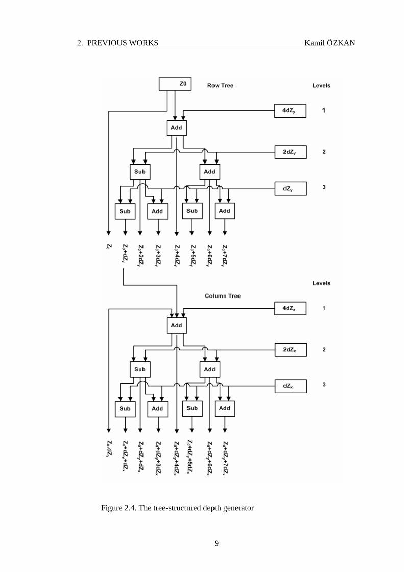
2. PREVIOUS WORKS Kamil ÖZKAN
9
Figure 2.4. The tree-structured depth generator

2. PREVIOUS WORKS Kamil ÖZKAN
10
T0 = D, AdXdT
==XdT , and BdYdT
==ydT . (2.5)
In addition to depth or distance values, for each pixel, three more common external
variables, H,Y and L, which are related to properties of the primitive, are input to
pixel processors. The meanings of these variables are the following:
H=1 plane is front surface H=0 plane is back surface
Y=1 plane is a perpendicular surface Y=0 plane is not a perpendicular surface
L=1 concave object L=0 convex object
Then the pixel processors, allocated one for each pixel, determine the
visibility of that plane, so the corresponding plane color, at every pixel positions
simultaneously. The function of the corner bender is to convert the serial flow of data
into parallel form. The frame buffer stores the colors belonging to the visible
surfaces of the scene intended. In summary, the host system supplies the coefficients
of the planes, implicitly, of a CSG primitive, and the display unit is fed from the
frame buffer to display the intended scene composed of the primitives [CEVIK, U.,
2004].

3. PROJECTIONS Kamil ÖZKAN
11
3. PROJECTIONS
Scenes are transformed by the view orientation and view mapping
transformations, back-faces are culled and clipping to a canonical view volume takes
place. The contents of the view volume are projected onto the Viewplane for display.
Projection is carried out by passing projectors through each vertex and
intersecting the projectors with the two-dimensional Viewplane. These two-
dimensional intersections give the points in the view corresponding to the original
three-dimensional points in the scene.
Projections can be classified as Parallel and Perspective projections.
3.1. Parallel Projection
All the projections considered are planar projections, i.e. the projectors are
straight lines and project onto a planar viewplane. Planar projections have the
advantage that a straight line projects to a straight line, hence only the end points
have to be projected.
Parallel projected scenes are useful for recording the exact shapes and
measurements of objects. The view of primitive objects are less realistic. In other
words, the distance between the centre of projection and the projection plane is
infinite.
There are two different types of parallel projections:
If the direction of projection is perpendicular to the projection plane then it is
an orthographic projection. If the direction of projection is not perpendicular to the
projection plane then it is an oblique projection.
3.1.1. Orthographic Projection
Engineering drawings frequently use front, side, top orthographic views of an
object and z coordinates are discarded.
Here , in figure 3.1, are three orthographic views of an object.

3. PROJECTIONS Kamil ÖZKAN
12
Front View
Side View
Top View
Figure 3.1. Parallel (Orthographic) Projection
Orthographic projections that show more than 1 side of an object are called
axonometric orthographic projections [OWEN, G.S., 1998]. The most common
axonometric projection is an isometric projection where the projection plane
intersects each coordinate axis in the model coordinate system at an equal distance as
shown in Figure 3.2.
Figure 3.2. Parallel (Orthographic-Isometric) Projection

3. PROJECTIONS Kamil ÖZKAN
13
The projection plane intersects the x, y, z axes at equal distances and the
projection plane normal makes an equal angle with the three axes.
To form an orthographic projection xL = x, yL= y , zL = 0. To form different
types e.g., Isometric, just manipulate object with 3D transformations.
3.1.2. Oblique Projection
The projectors are not perpendicular to the projection plane but are parallel
from the object to the projection plane
Parallel projection of a point (x, y, z) is given in Figure 3.3. (Note the left
handed coordinate system). The projection plane is at z = 0. x, y are the orthographic
projection values and xL, yL are the oblique projection values (at angle α with the
projection plane)
Figure 3.3. Parallel (Oblique) Projection of a point (x,y,z) with angle on the PP.
The projectors are defined by two angles α and φ where:
α = angle of line (x, y, xL, yL) with projection plane,
φ = angle of line (x, y, xL, yL) with x axis in projection plane

3. PROJECTIONS Kamil ÖZKAN
14
3.2. Perspective Projection
In planar geometric projections, the projection of an object is determined by
means of straight projection rays, starting from a centre of projection, crossing the
object at each point of the object, and intersecting a projection plane.
The perspective projection has a Centre of Projection (“eye”,”COP”) at a
finite distance from the projection plane [OWEN, G.S., 1999]. It is similar to the
human eye visual system as given in figure 3.4(a). So the distance of L1’ from the
projection plane determines its size on the projection plane, i.e. the farther the line is
from the projection plane, the smaller its image on the projection plane. In the
parallel projection, size of an object remains unchanged as seen in figure 3.4(b)
[CEVIK, U., March 2004].
Figure 3.4. (a) Perspective projection (b) Parallel projection
The rules of perspective projection are first stated in their most direct form,
then elaborated [TYLER, Christopher W, 1996];
There is only one geometry of perspective projection onto a fixed projection
plane.
All straight lines in space project to straight lines (or points, if end on) on the
projection plane.
L1
COP
Projection Plane
Cente of Projection
L1’
Projector
(a)
L2
COP
Projection Plane
Cente of Projection
L2’
Projector
(b)

3. PROJECTIONS Kamil ÖZKAN
15
The projections of all lines that are parallel in space either remain parallel in
the picture plane or intersect at a single vanishing point.
All sets of parallel lines lying within a specified plane in space have
vanishing points that fall along the horizon line defined by the orientation of
that plane.
For two sets of parallel lines at some angle in the scene, the two vanishing
points form that same angle at the viewer's eye, regardless of the orientation
of the angle in space. In particular, the vanishing points for any 90º angle in
space form a 90º angle at the viewer's eye.
Any planar figure in space is foreshortened in the direction of its slant from
the observer (up to a 45º viewing angle).
Circles in the scene, if foreshortened, project to ellipses in the picture plane.
For correct projection of its perspective, a picture should be viewed from its
center of projection in space.
When the eye is at the center of projection, the perspective geometry in the
picture plane is independent of where in the plane the eye is looking.
Implications of the Rules of Perspective [TYLER, Christopher W, 1996];
1. There is only one geometry of perspective projection onto a fixed picture plane.
Perspective is the geometry of projection from a scene through a plane to a
point (or center of projection) corresponding to the pupil of the viewing eye.
The plane is the picture plane on which the painter wishes to depict the scene.
If the perspective is correct, the depiction on the plane will generate the same
projective structure at the eye as did the scene behind it. The different forms of
perspective construction concern the rules that apply to specific structures,
allowing simplified forms of the projective geometry to be codified. But all are
subcases of the same optical transform.
2. All straight lines in space project to straight lines (or points, if end on) in the
picture plane. This fact is a simple consequence of the geometry of projection
through a point in space (corresponding to the pupil of one eye). If a line is
parallel to the picture plane, it must project to a straight line on that plane by
virtue of similar triangles. Obviously, tilting the line within the plane of

3. PROJECTIONS Kamil ÖZKAN
16
projection will not introduce any curvature, just a change in its extent within
the line of projection. In the limit, the projected head on. Lines of any
orientation can be described by this construction. Thus, all such point
projections are to straight lines or points.
2.1. The line may contract to a point in the picture plane when the line is viewed.
Introducing lens optics, as in the human eye, introduces the potential for
curvature in the projection. Such curvature may consequently be a
property of human perception at the extrema of the field, but the laws of
perspective will be considered to be those of the point projection of
pinhole optics, which permit no curvature.
2.2. Humans actually view scenes with two eyes, but the straight-line projections
in each eye are both straight lines. The average, or binocularly-fused,
projections is therefore also a straight line. No curvature is introduced by
the geometry of binocular combination.
3. The projections of all lines that are parallel in space either remain parallel in the
picture plane or intersect at a single vanishing point. This common intersection
is valid for each entire set of parallels regardless of where in the visual field the
lines arise. Each set of parallel lines intersects at a different vanishing point, of
course. Thus, the first job in perspective projection is to identify all the lines in
the scene that are parallel to a given line, then make sure that they are drawn so
as to project to a common vanishing point.
3.1. Parallel lines in space that are also parallel to the picture plane remain
parallel to each other in the projection. This leads to the particular case of
central perspective, in which all the lines on the scene are either parallel
with the line of sight or at right angles to it, parallel with the picture
plane. The first set will be horizontal and receding from a viewer looking
straight ahead. The vanishing point for this first set is directly in front of
the viewer, making a central point of convergence for these horizontal
receding lines. The second set consists of any lines at right angles to the
first set, thus at any angle within the picture plane. These lines, such as
the verticals of the sides of buildings, will all remain parallel within the

3. PROJECTIONS Kamil ÖZKAN
17
picture plane if they were parallel in space. Note that what makes central
perspective central is simply the choice of lines present in the scene.
Perspective itself is universal, an optical projection of the light rays.
3.2. The corollary of the central perspective construction is that it is implicitly
incorrect to set the "central" vanishing point is away from the viewing
center of the picture. This modification was employed in the mid
Renaissance, where the "central" vanishing point may have been moved
even to a point beyond the edge of the picture. The "frontal" sides of all
the squares nevertheless remained parallel in such constructions (usually
horizontal and vertical), so that the perspective is incorrect unless the
picture is expected to be viewed from the unlikely position of directly
front of the shifted vanishing point.
4. All sets of parallel lines lying within a specified plane in space have vanishing
points that fall along the horizon line defined by the orientation of that plane.
The particular case is the ground plane. All sets of parallel lines in the ground
plane have vanishing points in the horizon line. (The fact that the earth is not
flat means that it does not strictly conform to a ground plane, defined
geometrically. The deviation is generally too small to be of consequence in
art.)
4.1. Rules 2 and 3 may be combined to consider the vanishing points not just for
lines within a single plane but within a sheaf or stack of parallel planes.
All lines on all parallel planes still have vanishing points falling along the
same line. For example, all lines on or parallel with the ceiling or floor
have vanishing points in the line of the horizon, as do all horizontal edges
of doors and casement windows. But all the lines at angles on the sides of
a Ferris wheel, for example, would have vanishing points in a vertical
line.
5. For two sets of parallel lines at some angle in the scene, the two vanishing points
form that same angle at the viewer's eye, regardless of the orientation of the
angle in space. In particular, the vanishing points for any 90º angle in space
form a 90º angle at the viewer's eye. In particular, the vanishing points for any

3. PROJECTIONS Kamil ÖZKAN
18
right angle in space form a 90º angle at the observer's eye. This result may be
seen by considering the member of their respective parallel bundles, coming
directly toward the viewer's eye. These lines form the same angle as any other
pair from the two bundles. Their angle at the eye, and hence the viewing angle
between the vanishing points, therefore match the angle of the lines in space.
5.1. A classic case of this rule is the diagonals of any square, which are always at
90º to each other. The vanishing points (or "distance points", Leonardo,
1492) for these diagonals should therefore form a 90º angle at the center
of projection, regardless of their orientation in space. Twist the angle in
any direction whatever in three-dimensional space (even to the point of
complete foreshortening) and the vanishing points will nonetheless hold
to a strict 90º angle at the viewer's eye. In terms of pictorial distance, this
angle between the vanishing points corresponds to the same distance in
the picture plane except for the tan transform for projection of the equal
angles at the eye onto the plane.
5.2. The corollary of this principle is that, if the vanishing point in central
perspective is displaced from the center of view, the simplicity of the
central perspective construction has been violated and a second vanishing
point arises at 90º from this displaced vanishing point (for lines in the
same plane). In fact, an entire crescent of vanishing points is required to
accommodate lines of all orientations, aligned diametrically opposite the
direction of the displacement.
6. Any planar figure in space is foreshortened in the direction of its slant from the
observer (up to a 45º viewing angle). In particular, any square in space must be
foreshortened in the direction of its slant, even for the projection outside the
frame up to the range defined by the vanishing points. Beyond that, the
foreshortening becomes lengthening, but this will occur outside the range of
almost any picture (unless its edges extend beyond a 45º angle from the line of
sight).
6.1. The degree of foreshortening of a square of central perspective is defined by
its diagonals, which should project to vanishing points at a 90º angle to
3. PROJECTIONS Kamil ÖZKAN
19
the viewer. Thus, the vanishing point for the corners of horizontal
squares in central perspective should be at 45º to (and at the same height
as) the central vanishing point. The intersection of the diagonals with the
cardinal grid defines the degree of progressive foreshortening of the
receding squares. This geometry of a second vanishing point to set the
spacing of the horizontals corresponds to one version of the costruzione
legittima, or distance point method, of Leonardo (1492).
6.2. In general, foreshortening follows the construction of the multiple implicit
vanishing points even in central perspective, which is conceptualized as
having only a single vanishing point. As long as there are intersecting
lines in the scene, as there will be in any piazza grid, the vanishing points
for the construction lines through the intersections must obey rules 1, 2
and 4, lying in the same line at the horizon of the plane and at same angle
to the viewer as the intersections of the lines themselves in space.
6.3. The progressive foreshortening as equal divisions recede in space gives a
sense of curvature to the perspective transform of a regular array. All the
lines are straight, but the array elements change shape as they recede,
violating one's expectation of self-similarity. On top of this gradient of
shape, the line thickness in virtually all perspective diagrams does not
vary as it should in true perspective. Thus, the lines form an increasing
proportion of the element area and perhaps induce a sense of distortion in
an otherwise correct transform.
7. Circles in the scene, if foreshortened, project to ellipses in the picture plane.
Although perspective distorts rectangles to asymmetric trapezoids in general,
the properties of circles are such that they always project to an ellipse of some
orientation. If the circle is parallel to the picture plane, it projects to a circle,
which is the limiting case of an ellipse with no bias.
7.1. The projection for a circle may be derived by inscribing it in a square, for
which the previous rules define the perspective distortion. The requisite
ellipse is then obtained by inscribing it within the trapezoid obtained
from the projection of this square. In practice, this ellipse may be

3. PROJECTIONS Kamil ÖZKAN
20
selected from a set of ellipse templates as the one that just touches all
four sides of the trapezoid without crossing them at any point. These
constraints uniquely define the correct ellipse, since an ellipse is defined
by four points in the plane (as a circle is defined by three points). The
four 'touches' define four points and the avoidance of crossing anywhere
provides the fifth constraint.
7.2. The center of the requisite ellipse does not correspond with the center of the
circle being projected, but it displaced away from the vanishing point and
toward the observer. The projected center of the circle may be
determined by drawing the diagonals for the trapezoid, which intersect at
the center of the projected circle. The degree of displacement may be
determined by drawing the major an minor axes of the ellipse. The
intersection of these axes defines its geometric center, which will be
displaced from the projected center of the circle.
7.3. Spheres in space also project to ellipses in the picture plane, although
generally with much less distortion than circles because the roundness of
the spheres means that they are never foreshortened. Spheres always
project to circles when at the center of projection. The elongation arises
only because of marginal distortion, the stretching of the image as the
picture plane itself recedes from the viewer at increasing angles of view.
The requisite ellipse may be obtained by first projecting the sphere to a
circle in a plane at right angles to the line of sight through its center, then
projecting this circle to the picture plane. The major axis of the resulting
ellipse is thus aligned with the axis of rotation of this projection and its
ellipticity from the cosine of the (dihedral) angle between the
intermediate and final projection planes.
8. For correct projection of its perspective, a picture should be viewed from its
center of projection in space. In terms of distance, Rule 4 implies that the
vanishing points for lines at right angles should be viewed so as to be
orthogonal, forming 90º angle at the viewing position. Any parallel pair of
right angles in the picture thus defines its correct viewing distance, by defining

3. PROJECTIONS Kamil ÖZKAN
21
two orthogonal vanishing points. In terms of angle, the plane of the picture
should be viewed at the angle of slant for which the perspective was designed.
Other viewing angles, away from the center of projection in any direction, will
result in perspective distortion.
8.1. For the particular case of central perspective based on a square grid aligned
with the line of sight, the 45º angle between the diagonals and the line of
sight means that the distance points should have a 45º to the main
vanishing point at the viewer's eye. The geometry between the eye, the
central vanishing point and a distance point is therefore a 45º triangle,
which means that the picture is correctly viewed at the distance that
matches the span to each distance point. The physical distance between
the vanishing points depends on the intended viewing distance, but a
good rule of thumb is that it should correspond to a distance of at least
twice the width of the picture. Leonardo recommended at least 20 times
the height of the largest objects depicted.
8.2. Telephoto distortion and its limiting case, orthographic projection,
conversely, represent a strong magnification of the image in true
perspective. If a tiny piece of the scene is magnified, the distance of its
vanishing points is correspondingly magnified. The effect may be so
extreme that the rear of the object looks as though it curls up toward the
front of that object. The perceived distortion is so strong that it has been
termed "reverse perspective", as though the lines which should be
converging were in fact diverging. The effect is particularly strong in
orthographic projection, where parallel lines in spaces are drawn as
parallel in the picture, as though it were viewed from an infinite distance.
Nevertheless, the perceived "reversal" is an illusion obtained simply from
abnormally distant projection. Despite the distorted appearance, telephoto
distortion is a valid perspective projection if viewed at the correct
distance (although the scene may in practice be invisible at that distance).
9. When the eye is at the center of projection, the perspective geometry in the
picture plane is independent of where in the plane the eye is looking.

3. PROJECTIONS Kamil ÖZKAN
22
Perspective is an optical transform that implies a certain projective geometry
through the point in space that forms the center of projection. Perspective is not
specific to a location on the canvas but applies throughout the pictorial space.
9.1. The center of view in the picture should not be confused with the line of
sight of the viewer. The center of view is the point in the picture plane
closest to the viewer. The line of sight is the direction in which the
viewer's eye is pointing, which may be anywhere within (or outside) the
picture. Where the viewer samples the optic array does not affect the
correctness of the perspective. The perspective is correct when the
viewer's eye is placed at the center of projection in space for which the
perspective was generated (regardless of the direction of the line of
sight).
9.2. This point is contentious because most authors agree that the perspective
projection changes with viewing angle. Presumably this misconception
arises because lines that are parallel in central projection of a scene
appear to converge as the viewer looks to the side. This observation,
however, implicitly assumes that the relevant picture plane is rotated with
the rotation of the line of sight. Rule 9 refers instead to an observer
viewing a fixed picture, projecting an optic array to the viewer's eye. In
this case, if the observer's eye looks away from the center of view, the
picture plane itself will project to the eye with a perspective transform. It
is the perspective distortion of this picture plane that provides the
convergence of the parallel lines in oblique view, just as in the physical
scene itself. Thus the correct geometry for perspective in the picture
plane is indeed independent of the direction in which the viewer is
looking at this plane (assuming the eye stays at the center of projection).
9.3. As long as the viewer is directly in front of the central vanishing point (and
the picture plane is front to parallel), the verticals project to parallel lines
in the picture plane (Rule 5.1). Once the main vanishing point is moved
up or down from the viewer's eye position, the verticals are required to

3. PROJECTIONS Kamil ÖZKAN
23
converge so as to make an angle of 90º to the direction of this vanishing
point (Rule 5).
There is some disadvantage and problems with perspective projections as below;
Perspective foreshortening: Distant lines are foreshortened. For example, in
the figure, the projection of both objects A and B are of same size. Objects
that are away from center of projection appears smaller.
The perspective projection of objects behind the center of projection appear
upside down and backward onto the viewplane.
Relative dimensions of the objects are not preserved and hence the
information destroyed.
Lines parallel to view plane, i.e. perpendicular to viewplane normal are
projected as parallel lines. However, lines that are not parallel to viewplane or
receding parallel lines appear to meet at some point on the view plane called
vanishing point.
Consider a cube oriented in such a way that the edges A, B, C, recede from
the viewer. The perspective projection of the edges will meet at a vanishing point Vp.
A classic example is the illusion that railroad tracks meet at a point on the horizon.
Similarly, the parallel lines appear to be bent as they converge to a vanishing point.
3.3. Vanishing point
Lines not parallel to view plane or receding parallel lines appear to converge
at some point called the vanishing point on the view plane. Lines parallel to principal
axes (i.e. the world coordinate axes) converge to a principal vanishing point.
Different types of perspective projection are named after the finite number of
vanishing points. A perspective projection can have 1, 2, or 3 principal vanishing
points. [ROY, Gordon, et al. 1986]
One point perspective occurs when the projection plane is parallel to two
principal axes. Conversely, when the projection plane is perpendicular to one of the
principal axis, one point perspective occurs. Receding lines along one of the
principal axis converge to a vanishing point. It is shown in Figure 3.5

3. PROJECTIONS Kamil ÖZKAN
24
(a) (b) Figure 3.5. (a) One Point Perspective (b) A painting (The Piazza of St. Mark,
Venice) done by Canaletto in 1735-45 in one-point perspective.
If the projection plane is parallel to one of the principal axes or if the
projection plane intersects exactly two principal axes, a two-point perspective
projection occurs as shown in figure 3.6.
(a) (b) Figure 3.6. (a) Two Point Perspective (b) A painting in two point perspective by
Edward Hopper The Mansard Roof 1923 (240 Kb); Watercolor on paper, 13 3/4 x 19 inches; The Brooklyn Museum, New York

3. PROJECTIONS Kamil ÖZKAN
25
If the projection plane is not parallel to any principal axis, a three-point
projection occurs as shown in Figure 3.7.
yx
z vp1vp2
vp3 (a) (b) Figure 3.7. (a) Three-Point Perspective (b) A painting (City Night, 1926) by
Georgia O'Keefe, that is approximately in three-point perspective.
3.4. Mathematics of Perspective Projection
Before we introduce the basic mathematics of the perspective projection, we
are going to list two assumptions to simplify the module and to adapt it to the target
architecture.
1. The image plane (projection plane) is normal to the z-axis at z=0.
2. The centre of the projection is located anywhere on the negative side of
the z-axis at a point (xv, yv, zv).
The position (xp, yp) on the projection plane of a point at position (x, y, z) in the scene
is found by computing the coordinates (xp, yp) of the intersection of the projector
passing through the scene point (x, y, z) with the projection plane as shown in Figure
3.8.

3. PROJECTIONS Kamil ÖZKAN
26
Figure 3.8. Perspective projection plane
We find the ratios from obtaining the similar triangles
;v
v
v
vp
zzz
xxxx
+=
−
−
v
v
v
vp
zzz
yyyy
+=
−
− (3.1)
With a little algebra, the xp and yp can be found as following,
,..
v
vvp zz
zxzxx
++
= (3.2)
v
vvp zz
zyzyy
++
=..
. (3.3)
Since at projection plane zv is at the negative side, these equations can be
written as:
,..
v
vvp zz
zxzxx
−−
= (3.4)

3. PROJECTIONS Kamil ÖZKAN
27
v
vvp zz
zyzyy
−−
=..
. (3.5)
As we have considered the projection onto the z=0 plane, zp will always be 0.
However, this may not always be desirable since the depth information is lost. In
order to facilitate illumination calculation and visible surface determination the
original z value of the point can be preserved or in order to keep everything in scale
zp can be set as given below [CEVIK, U., 2006]
v
p zzzz
−= . (3.6)

4. ALGORITHM And FORMULAS Kamil ÖZKAN
28
4. ALGORTIHM and FORMULAS
4.1. The Module Algorithm
As this algorithm targets for pixel-based CSG systems and such systems
render scene primitives from half spaces (effectively from planes), we are going to
build the algorithm on the plane equations. Suppose that a cube is projected, by the
pixel-based system, onto the projection plane (the greater cube) as seen in Figure 4.1.
It is obvious that this is a parallel projection. Let P1, P2, and P3 are three non-
collinear points on one of the faces of the cube. Note that, three collinear points
define a plane. Now, if we take the perspective projection of each of these points, we
find P`1, P`2, and P`3. The plane defined by P`1, P`2, and P`3 will form the perspective
projection of the surface defined by points P1, P2, and P3. If we repeat this procedure
for the other surfaces of the parallel projected cube we obtain the perspective view of
it [CEVIK, U., 2006]. x
y
P1
P'1
P'3
P'2
P2
P3
Figure 4.1. A Parallel Projected Cube and Its Perspective View
The pseudo code of the algorithm is following:

4. ALGORITHM And FORMULAS Kamil ÖZKAN
29
read the centre of projection
while (the plane list of the graphic primitive is not empty)
do
{
read the parameters of the plane;
find three non-collinear points on the plane;
take the perspective projections of the three points;
find the coefficients of the projected plane defined by the three projected
points;
output the coefficients to the target systems;
}
4.2. Implementation and Coefficients
When the CSG renderer is considered, the parameters delivered by the host
system are composed of Z0, dZx, dZy, or T0, or dTx, or dTy , and H, Y, and L (see
Chapter 2). Using these parameters the coefficients of the plane belonging to a CSG
primitive can easily be calculated as
If Y=1 ⇒ C=0, A= dTx, B= dTy , and D=T0, (4.1)
Otherwise,
If H=1 ⇒ C=1, A=- dZx, B=- dZy, and D= Z0 (4.2)
If H=0 ⇒ C=-1, A= dZx, B= dZy, and D= Z0. (4.3)
If the host system, delivering parameters from host system to the CSG renderer, is
able to deliver plane coefficients directly, (A, B, C, D, and H, Y, and L), this step can
be skipped. The centre of projection is input to the module externally. As the next
step , three non-collinear points on the plane must be determined. These points can
be set as below Table 4.1 [CEVIK, U., 2006]..

4. ALGORITHM And FORMULAS Kamil ÖZKAN
30
Table 4.1. Determination of Three Non-collinear Points
If x1 y1 z1 x2 y2 z2 x3 y3 z3 B=0 and C=0 D/(-A) 0 0 D/(-A) 1 0 D/(-A) 0 1
A=0 and C=0 0 D/(-B) 0 1 D/(-B) 0 0 D/(-B) 1
A=0 and B=0 0 0 D/(-C) 1 0 D/(-C) 0 1 D/(-C)
A=0 and B≠0 and C≠0 0 0 D/(-C) 1 0 D/(-C) 0 1 (B+D)/(-C)
B=0 and A≠0 and C≠0 0 0 D/(-C) 1 0 (A+D)/(-C) 0 1 D/(-C)
C=0 and A≠0 and B≠0 D/(-A) 0 0 (B+D)/(-A) 1 0 D/(-A) 0 1
A≠0 and B≠0 and C≠0 0 0 D/(-C) 1 0 (A+D)/(-C) 0 1 (B+D)/(-C)
After the perspective transformation, using the transformation formulae, of
points (x1, y1, z1), (x2, y2, z2), and (x3, y3, z3), three new non-collinear points, (xp1, yp1,
zp1), (xp2, yp2, zp2), and (xp3, yp3, zp3), which are now on the perspective projected
plane, are found.
In order to calculate the coefficients of the projected plane the normal vector,
np, is needed. This is easily calculated a
np =[(yp2-yp1)*(zp3-zp1) - (zp2-zp1)*(yp3-yp1)] i - [(xp2-xp1)* (zp3-zp1) - (zp2-zp1)*(xp3-xp1)]
j + [(xp2-xp1)*( yp3-yp1) - (yp2-yp1)*( xp3-xp1)] k. (4.4)
The coefficients of the projected plane, Ap, Bp, Cp, and Dp, are derived from
the normal vector np:
Ap=[(yp2-yp1)* (zp3-zp1) - (zp2-zp1)*(yp3-yp1)], (4.5)
Bp=-[(xp2-xp1)* (zp3-zp1) - (zp2-zp1)*(xp3-xp1)], (4.6)
Cp=[(xp2-xp1)*( yp3-yp1) - (yp2-yp1)*( xp3-xp1)], (4.7)
Dp=-(Ap*xp1+Bp*yp1+Cp*zp1). (4.8)

4. ALGORITHM And FORMULAS Kamil ÖZKAN
31
Last step is the calculation of the output parameters. These are Zp0, dZpx, and
dZpy . Since the perspective projections of any set of parallel lines that are not parallel
to the projection plane converge to a point, vanishing point, it will be impossible to
have planes that are orthogonal to the projection plane. Hence, Tp0, dTpx, or dTpy
parameters are ignored, i.e. Yp=0.
)(0p
pp C
DZ
−= ,
)(dZPX
p
pp
CA
dXdZ
−== , and
)(dZpy
p
pp
CB
dYdZ
−== . (4.9)
It is obvious that a front surface, in parallel projection, may be a back surface
after the perspective projection depending on the centre of projection. So, the visible
surface determination must be examined for each plane. This is done by examining
the dot product of the vector, say vpp, that extends from the centre of projection to
the any point, say (x3, y3, z3), on the plane, with that is normal to the plane. A non-
negative dot product indicates that the plane is a back surface [FOLEY, J. D., et al.
1995]. The plane normal, n, must be determined before the perspective projection is
applied. Otherwise the direction of the normal will be distorted [ROGERS, D. F.,
1985] .
vpp=(x3-xv) i + (y3-yv) j + (z3-zv) k . (4.10)
vpp . n=(x3-xv) * A + (y3-yv) * B + (z3-zv) *C (4.11)
The parameter, Hp, which indicates whether a plane is a front surface or back
surface is directly determined from the dot product, i.e. if (vpp . n) is negative Hp=1
(plane is a front surface), if dot product (vpp . n) is non-negative Hp=0 (plane is a
back surface).
Lp, which indicates if the object primitive is convex or concave, will remain
the same (Lp=L) as the nature of an object is not changed by the perspective
proejction.
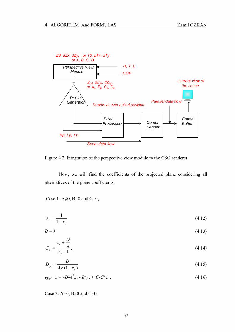
Figure 4.2 shows the final appearance of the CSG renderer after the addition
of the perspective view module.
4. ALGORITHM And FORMULAS Kamil ÖZKAN
32
Z0, dZx, dZy, or T0, dTx, dTyor A, B, C, D
DepthGenerator
CornerBender
FrameBuffer
Serial data flow
Depths at every pixel position
Current view ofthe scene
PixelProcessors
Parallel data flow
Perspective ViewModule
H, Y, L
COP
Hp, Lp, Yp
Zp0, dZpx, dZpy, or Ap, Bp, Cp, Dp
Figure 4.2. Integration of the perspective view module to the CSG renderer
Now, we will find the coefficients of the projected plane considering all
alternatives of the plane coefficients.
Case 1: A≠0, B=0 and C=0;
vp z
A−
=1
1 (4.12)
Bp=0 (4.13)
,1−
+=
v
v
p zADx
C (4.14)
)1( vp zA
DD−×
= (4.15)
vpp . n = -D-A*xv - B*yv + C-C*zv . (4.16)
Case 2: A=0, B≠0 and C=0;

4. ALGORITHM And FORMULAS Kamil ÖZKAN
33
Ap=0 (4.17)
11−
=v
p zB (4.18)
,1 v
v
p zBDy
C−
+= (4.19)
)1( −×=
vp zB
DD (4.20)
vpp . n = -A*xv –D - B*yv + C-C*zv (4.21)
Case 3: A=0, B=0, and C≠0;
Ap=0 (4.22)
Bp=0 (4.23) 2
⎥⎥⎥⎥
⎦
⎤
⎢⎢⎢⎢
⎣
⎡
+=
v
vp
zCD
zC (4.24)
3
2
)()(
.CzD
CzDD
v
vp ×+
×−= (4.25)
vpp . n = -A*xv +B - B*yv - D - C*zv (4.26)
Case 4: A=0, B≠0, and C≠0;
Ap=0 (4.27)
)()()(
2
2
CzDBDCzBCz
Bvv
vp ×++×+×
××−= (4.28)
)()()(
2
22
CzDBzCDCzByDzC
Cvv
vvvp ×++××+
×+×+××= (4.29)

4. ALGORITHM And FORMULAS Kamil ÖZKAN
34
)()()(
2
2
CzDBDCzDCz
Dvv
vp ×++×+×
××−= . (4.30)
vpp . n = -A*xv + B - B*yv - B – D - C*zv . (4.31)
Case 5: B=0, A≠0, and C≠0;
)()()(
2
2
CzDADCzACz
Avv
vp ×++×+×
××−= (4.32)
Bp=0 (4.33)
)()()(
2
22
CzDAzCDCzAxDzC
Cvv
vvvp ×++××+
×+×+××= (4.34)
)()()(
2
2
CzDADCzDCz
Dvv
vp ×++×+×
××−= (4.35)
vpp . n = -A*xv +B - B*yv - D - C*zv . (4.36)
Case 6: C=0, A≠0, and B≠0;
vp z
A−
=1
1 (4.37)
)1( vp zA
BB−×
= (4.38)
AAzDAxBy
Cv
vvp −×
+×+×= (4.39)
)1( vp zA
DD−×
= . (4.40)
vpp . n = - D - A*xv - B*yv + C-C*zv . (4.41)
Case 7: A≠0, B≠0, and C≠0;
)()()()( 2
CzADCzBDDCzACz
Avvv
vp ×++××++×+×
××−= (4.42)
4. ALGORITHM And FORMULAS Kamil ÖZKAN
35
)()()()( 2
CzADCzBDDCzBCz
Bvvv
vp ×++××++×+×
××−= (4.43)
⎥⎦
⎤⎢⎣
⎡×++×++
×××−×+×+×+×+×⎥
⎦
⎤⎢⎣
⎡+×
×=
))(())((
)(
2
CzBDCzADBAxyByCzDAxCzD
DCzCz
Cvv
vvvvvv
v
vp
(4.44)
)()()()( 2
CzADCzBDDCzDCz
Dvvv
vp ×++××++×+×
××−= (4.45)
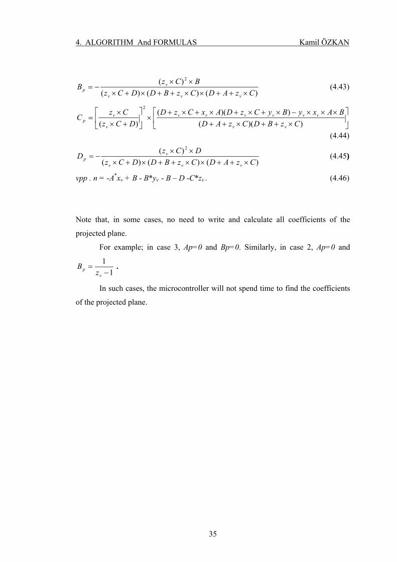
vpp . n = -A*xv + B - B*yv - B – D -C*zv . (4.46)
Note that, in some cases, no need to write and calculate all coefficients of the
projected plane.
For example; in case 3, Ap=0 and Bp=0. Similarly, in case 2, Ap=0 and
11−
=v
p zB .
In such cases, the microcontroller will not spend time to find the coefficients
of the projected plane.

5. HARDWARE DEVELOPMENT Kamil ÖZKAN
36
5. HARDWARE DEVELOPMENT
5.1. General
To connect the module, a communication port of the host (computer) must be used.
There are two communication types as parallel and serial, and some communication
protocols. Since the module includes a microcontroller, protocols to be used are
limited. The protocols, suitable for communication with different microcontrollers,
are listed as below:
• RS232 Serial Communication
• RS485 Serial Communication
• I2C
• CAN
• SPI
• USB
• Firewire
The speeds of the communication standards, used with microcontrollers [DOGAN,
İbrahim,2004], are shown in Table 5.1.
Table 5.1. Speed of the communication standards.
Communication
Protocol Speed (bits)
RS232 20-115 k
CAN 33 k
I2C 3.4 M
SPI 2.1 M
CAN (Hızlı) 1 M
USB (1.1) 12 M
USB (2.0) 480 M
Firewire 400 M

5. HARDWARE DEVELOPMENT Kamil ÖZKAN
37
The RS232 serial protocol is used commonly and is easy to communicate.
The best advantage of it that it needs only a few wires. And data can be sent to some
hundred meters. The microcontroller, supports Universal Synchronous Asynchronous
Receiver Transmitter (USART). This system works and creates the timing to
communicate and it works independent from the CPU.
SPI standard uses 4 cables (clock, master output, master input and slave
select) and communication is synchronized. This standard was found and researched
by MOTOROLA company.
Controller Area Network (CAN) standard was researched and used with
vehicles by BOSH company. It is suitable for very safe and emergency critical
cases, and is also used in all vehicle industries. All devices connect to only one bus
and CAN supports 15 bit error detection and repair feature. The microcontroller can
work with this protocol with additional hardware and program.
I2C standard is used widely with microcontrollers and was researched by
PHILIPS company. Only two cables (clock-SCL and data-SDA) are used and all
devices are connected to it.
FireWire is one of the fastest peripheral standards. It is suitable for use with
multimedia peripherals such as digital video cameras and other high-speed devices,
e.g., the latest hard disk drives and printers.
The other communication type is parallel and it is the most commonly used
port for interfacing home made projects. This port will allow the input of up to 9 bits
at any one given time, thus requiring minimal external circuitry to implement many
simpler tasks. The port is composed of 4 control lines, 5 status lines and 8 data lines.
Speed of the communication type was early 50 kbits/second and now it is 150
kbits/second. Parallel communication has some problem with connect and
communicate with PC and devices. Since using 8 data lines, hardware enlarges and
controlling the parallel port in the computer is hard commonly using Windows XP
operation system. The main problem for hardware is sink and source current.
However, PIC16F877 Microcontroller, produced by Microchip, works with 25 mA
sink and source current , the control bits of Parallel port supports and draws 1 mA
source and 7 mA sink current. While data pins of it usually 12 mA sink/source

5. HARDWARE DEVELOPMENT Kamil ÖZKAN
38
current, some of them is vary as 6 mA sink/source, 12 mA source/20 mA sink, 16
mA sink/4 mA source current. The variations mix the hardware and enlarge. On the
other hand, computers has only one parallel port and it supports only one device.
When a new device working with parallel port connects to the computer, a new
parallel card for ISA is needed. Since we can not store the data in the parallel port
and it increases time. Some buffer chips can be used, but they enlarge the system and
need to external power.
Parallel communication technique has been used for speed advantages. In the
last years, speed of serial communication is increased and it is going on the way. For
example, because of speed factor is important on Hard Drive, parallel
communication (IDE) has been used, now, new product line is support serial standart
SATA
Finally we decided using USB as the communication port. USB is becoming
popular and using a lot of area. Multiplying the USB ports are easy and the speed is
very high (12Mb/s-480Mb/s). Both USB<->Serial or USB<->Parallel chips can be
found. Some companies are researching to join microcontroller and USB standard.
5.2. USB (Universal Serial Bus) Interfacing
5.2.1. What Is USB?
For the last years, Computers are produced with one or more USB (Universal
Serial Bus) connectors. The USB connectors let us attach everything from mouse to
printers to our computers quickly and easily. If the operating system supports USB,
the installation of the device drivers is quick and easy too. The more recent
motivation for USB 2.0 stems from the fact that computers have increasingly higher
performance and are capable of processing vast amounts of data. At the same time,
PC peripherals have added more performance and functionality. User applications
such as digital imaging demand a high performance connection between the PC and
these increasingly sophisticated peripherals. USB 2.0 addresses this need by adding a
third transfer rate of 480 Mb/s to the 12 Mb/s and 1.5 Mb/s originally defined for

5. HARDWARE DEVELOPMENT Kamil ÖZKAN
39
USB.USB 2.0 is a natural evolution of USB, delivering the desired bandwidth
increase while preserving the original motivations for USB and maintaining full
compatibility with existing peripherals.
Thus, USB continues to be the answer to connectivity for the PC architecture.
It is a fast, bi-directional, isochronous, low-cost, dynamically attachable serial
interface that is consistent with the requirements of the PC platform of today and
tomorrow.
In the past, connecting devices to computer has been a real problem;
- Printers connected to parallel printer ports, and most computers only came
with one. Things like Zip drives , which need a high-speed connection into the
computer, would use the parallel port as well, often with limited success and not
much speed.
- Modems used the serial port, but so did some printers and a variety of odd
things. Most computers have at most two serial ports, and they are very slow in most
cases.
- Devices that needed faster connections came with their own cards, which
had to fit in a card slot inside the computer’s case. Unfortunately, the number of card
slots is limited and you needed very good knowledge to install the software for some
of the cards.
The goal of USB is to end all of these problems. The Universal Serial Bus
gives us a single, standardized, easy-to-use way to connect up to 127 devices to a
computer.
Just about every peripheral made now comes in a USB version. A sample list
of USB devices that you can buy today includes:
- Printers
- Scanners
- Mouse
- Joysticks
- Flight Yokes
- Digital Cameras
- Webcams

5. HARDWARE DEVELOPMENT Kamil ÖZKAN
40
- Scientific data acquisition devices
- Modems
- Speakers
- Telephones
- Video phones
- Storage devices such as Zip drives
- Network connections
To connect a USB device to a computer the device is plugged into the USB
connector. If it is a new device, the operating system will auto-detect it and ask for
the driver. If the device has already been installed, the computer activates it and
starts communicating with it. USB devices can be connected and disconnected at any
time.
Many USB device’s cable, to plug to computer, has an USB “A” connection
on it as in shown Figure 5.1.(a). Other terminal that plugs to device is USB “B” type
connector as in shown Figure 5.1.(b). Some terminal has USB “Mini B” type
connector as in shown Figure 5.1.(c).
(a) (b) (c)
Figure 5.1. USB Connector Types (a)”A”-Type (b) “B”-Type (c) “Mini B”-Type
- “A” connectors head “upstream” toward the computer and
- “B” connectors head “downstream” and connect to individual devices.
To increase the USB ports, we can use USB hubs. A hub may have more than
two new ports. Even if, by chaining hubs together, we can build up dozens of
available USB ports on a single computer [BRAIN, M., 2006].
Hubs can be powered or un-powered. USB standard allows for devices to
draw their power from USB connection. Obviously, a high-power device like printer

5. HARDWARE DEVELOPMENT Kamil ÖZKAN
41
or scanner will have its own power supply. But low-power devices like mice and
digital cameras get their power from the bus. The power (up to 500 mA at 5V)
comes from computer. If we have lots of un-powered devices, we probably need a
powered hub [AXELSON, Jan., 2001].
5.2.2. USB Features
The Universal Serial Bus has the following features:
- The computer acts as the host.
- Up to 127 devices can connect to the host, either directly or by way of
USB hubs.
- Individual USB cables can run as long as 5 meters; with hubs, devices can
be up to 30 meters away from the host.
- Low-cost solution that supports transfer rates up to 480 Mb/s with USB
2.0 . Such as connector, cable, peripheral devices.
- Full support for real-time data for voice, audio, and video
- Protocol flexibility for mixed-mode isochronous data transfers and
asynchronous messaging
- A USB cable has two wires for power (+5 volts and ground) and a twisted
pair of wires to carry the data. (In Figure 5.2)
- It creates a synergy with protocol which is simple to implement and
integrate
- On the power wires, the computer can supply up to 500mA of power at 5
volts.
- Low-power devices (such as mouse) can draw their power directly from
bus. High-power devices have their own power supplies and draw
minimal power from the bus.
- USB devices can be plugged into the bus and unplugged then any time.
- Many USB devices can be put to sleep by the host computer when the
computer enters a power-saving mode. It means energy saving.

5. HARDWARE DEVELOPMENT Kamil ÖZKAN
42
Figure 5.2. Electrical Diagram of the USB “A” Type connector
- USB is user friendly to install and assemble
- While all ports (serial, parallel) use different data bus for each port, USB
devices use only one data bus.
5.2.3. The USB Process
When the host powers up, it queries all of the devices connected to the bus
and assigns each one an address. This process is called enumeration. Devices are also
enumerated when they connect to the bus. The host also finds out from each device
what type of data transfer it wishes to perform. The USB architecture comprehends
four basic types of data transfers:
- Interrupt- A device like a mouse or a keyboard, which will be sending
very little data, would choose the interrupt mode.
- Bulk- A device like printer, which receives data in one big packet, uses
the bulk transfer mode. A block of data is sent to the printer (in 64-byte
chunks) and verified to make sure it is correct. Bulk data is sequential.
Reliable exchange of data is ensured at the hardware level by using error
detection in hardware and invoking a limited number of retries in
hardware.

5. HARDWARE DEVELOPMENT Kamil ÖZKAN
43
- Isochronous- A streaming device (such as speakers) uses the isochronous
mode. Data streams between the device and the host in real-time, and
there is no error correction.
- Control Transfers: Used to configure a device at attach time and can be
used for other device-specific purposes, including control of other pipes
on the device.
The host can also send commands or query parameters with control packets.
The Universal Serial Bus divides the available bandwidth into frames, and the
host controls the frames. Frames contain 1 500 bytes, and a new frame starts every
millisecond. During a frame, isochronous and interrupt devices get a slot so they are
guaranteed the bandwidth they need. Bulk and control transfers use whatever space is
left [BRAIN, M., 2006]..
5.2.4. Interfacing PIC Microcontroller and USB
To communicate with the Pic Microcontroller used in this mode, we preferred
the FTDI company’s FT232 USB UART (USB and Serial) chip. The FT232 chip is
the 5 x5 mm lead free QFN32 package version of the 2nd generation of FTDI’s
popular USB UART I.C. This device reduces external component count, but also
maintains a high degree of pin compatibility with the original, making it easy to
upgrade or cost reduce existing designs as well as increasing the potential for using
the device in new application areas. See application notes for more information about
the FT232 USB UART. In addition, this chip has a driver for defining a virtual port
and USB direct drivers. The driver includes Windows 9x, Windows 2000 / ME / XP
and other operating systems. Two of the FT232 are used the module for sending
USB port (host) and receiving USB port (slave - depth generator).
We used Microchip Pic 16f877 as the microcontroller. See application notes
(Appendix B) for more information about it. It can work at 4 Mhz to 20 Mhz clock
speeds. It also works with a crystal-capacitor or oscillator. In order to have an
accurate output frequency, a 20 Mhz oscillator is selected. The wiring diagram of
system is shown in Figure 5.3.

5. HARDWARE DEVELOPMENT Kamil ÖZKAN
44
Figure 5.3. Wiring Diagram of The Design.
Microcontroller systems are programmed by using ASSEMBLY Language.
Nowadays, there are many programming languages to write and compile programs
suitable for the microcontroller, e.g. PASCAL, C and BASIC. We have selected Hi-
Tech PICC compiler since ,it is more popular among technical people and is C++
based. PCB design of our system is shown in Figure 5.4. In the design, two USB
ports are used. One of them is master which sends data, and the other one is slave
which receives data.
When a device is plugged, USB ports support power from host. A device can
draw 500mA from the port. In our design, FT232 USB UART (USB and Serial) chip
draws 24 mA and other devices draw 50 mA approximately without the
microcontroller. The microcontroller is also draws 2 mA and additional 2 pins (Tx
and CTS) draw a source current of 25 mA each and 2 pin (Rx and DTR) draws a sink
current of 25 mA. Total current requirement of the microcontroller is 102-105 mA.

5. HARDWARE DEVELOPMENT Kamil ÖZKAN
45
Complete project consumes 150 mA from the host USB. This is enough for power
distribution of USB (<500 mA).
Figure 5.4. Microcontroller and USB port interface PCB Design (1. pc is master, 2. pc is slave)
We use the USART module with the microcontroller to receive and transmit
data. The Universal Synchronous Asynchronous Receiver Transmitter (USART)
module is one of the two serial I/O modules. (USART is also known as a Serial
Communication Interface or SCI.) The USART can be configured as a full duplex
asynchronous system that can communicate with peripheral devices as CRT
terminals and personal computers, or it can be configured as a half duplex
synchronous system that can communicate with peripheral devices such as A/D or
D/A integrated circuits, serial EEPROMs, etc

5. HARDWARE DEVELOPMENT Kamil ÖZKAN
46
When the USB connector is plugged into socket, since it is a new device, the
operating system will auto-detect it and ask for the driver. After the driver is installed
the new communication port USB-Serial converter is seen in the Device Manager of
computer. This is a virtual port. We can use the COM port number suggested by the
host computer. If the device has already been installed, the computer activates it and
starts communicating with it.
Of course we had to write a pc program to communicate with the hardware
designed and the PC. Hence the Borland C++ Builder Language was selected. Both
the microcontroller program and the pc program have same language base. The
program interface is shown in Figure 5.5. C++ builder supports the COM ports and
has the standard controllers with Microsoft MSCOMM32 program component.
Figure 5.5. Communicating PC Program interface
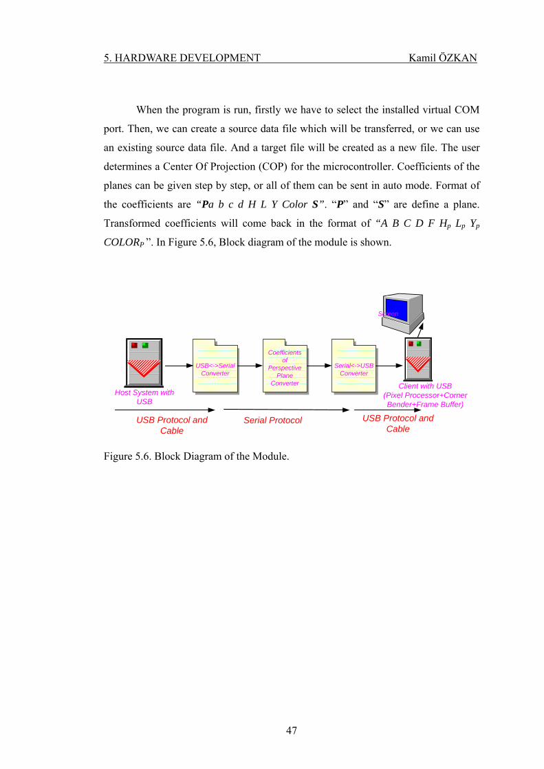
5. HARDWARE DEVELOPMENT Kamil ÖZKAN
47
When the program is run, firstly we have to select the installed virtual COM
port. Then, we can create a source data file which will be transferred, or we can use
an existing source data file. And a target file will be created as a new file. The user
determines a Center Of Projection (COP) for the microcontroller. Coefficients of the
planes can be given step by step, or all of them can be sent in auto mode. Format of
the coefficients are “Pa b c d H L Y Color S”. “P” and “S” are define a plane.
Transformed coefficients will come back in the format of “A B C D F Hp Lp Yp
COLORP ”. In Figure 5.6, Block diagram of the module is shown.
USB<->SerialConverter
Coefficients of
Perspective Plane
Converter
USB Protocol and Cable
Serial Protocol
Screen
Host System with USB
USB Protocol and Cable
Client with USB(Pixel Processor+Corner Bender+Frame Buffer)
Serial<->USBConverter
Figure 5.6. Block Diagram of the Module.

6. RESULTS AND DISCUSSION Kamil ÖZKAN
48
6. RESULTS AND DISCUSSION
6.1. Results and Discussion In our work, we used a Microchip Pic 16f877 microcontroller and the USB
communication port.
To program the microcontroller, HI-TECH PICC, based on C compiler, was
used since the assembly language programming is difficult to use. Many problems
can occur while writing and running. A basic language compiler is actually very easy
to use it. Main problem while using it, however, with it, it occupies a very large area
in the program memory of the microcontroller. Another problem wit it, unsigned
char or unsigned integer variables can not be used. The Pic 16f877 has 8K flash
program memory that must be used very carefully. In the end, Hi-Tech company’s
PICC Compiler was selected.
Any computer or microcontroller uses general purpose registers to calculate
the formulas to store the address temporarily. The microcontroller has 396 bytes of
general purpose registers. In order to calculate formulas, in chapter 4, we actually
needed more registers. To solve this problem, some variables were defined for some
parts of formulas. For example, in case 7: A≠0, B≠0, and C≠0, we could not use the
formula assigned to this directly. Firstly, we found the (x1, y1, z1), (x2, y2, z2) and (x3,
y3, z3), which was defined in Table 4.1, then points of (xp1, yp1, zp1), (xp2, yp2, zp2),
(xp3, yp3, zp3) were calculated. Finally, coefficients of transformed planes Ap, Bp, Cp,
were Dp are found.
While programming the microcontroller, all codes were not written in the
main function. There are four program banks in the microcontroller. When the
program is divided into subroutines the compiler did not give any error.
Floating point numbers are another big problem for the microcontroller.
While the microcontroller supports 24 bit and 32 bit floating types, 24 bit type was
selected not to cover a large area in the registers.
Our design was tested, and results were observed. Speed of the
transformation was varied with selected interrupt (threshold) to read data from

6. RESULTS AND DISCUSSION Kamil ÖZKAN
49
buffer, the crystal type and the type of the microcontroller, the baud rate, coefficients
of the planes, and etc. We searched some alternative cases.
Designed module was tested for 100 planes for each alternative at two
personal computers that had different types of processors, Celeron 2.4 Ghz and Intel
Pentium 4- 2.6 Ghz. The results are given in the table 6.1. Microcontroller was run
with 20 Mhz and the baud rate was 57600. The COP was at (50, 50, -50) and
interrupt length was 20 characters.
Table 6.1. The Speed of Transformation
If Incoming
data (characters)
Sent data (character)
time (msec) pentium4 -celeron 2,4
B=0 and C=0 2.440 3.070 2610 A=0 and C=0 2.480 3.000 2672 A=0 and B=0 2.460 2.390 2219 C=0 and A≠0 and B≠0 2.620 3.460 2907 B=0 and A≠0 and C≠0 2.930 2.950 3078 A=0 and B≠0 and C≠0 2.660 2.910 2920 A≠0 and B≠0 and C≠0 3.020 7.090 3375
The threshold is an interrupt to read characters from the receiving buffer. If an
interrupt occurs, data is read from the buffer, and the buffer is cleared.
The speed is not linear with the threshold, since the speed of the host
computer and that of the target also affects. In case of using a very low speed host
computer, of course a high threshold would be useful.
Another factor of the transformation speed is the communication baud rate.
While the microcontroller runs at 19.200, 28.800, and 57.600 baud rates at 20 MHz,
the results of the tests are shown in table 6.2
After comparing the results according to different baud rates, notice that, if
the speed of the communication speed is increased twice, the transformation time
does not decrease twice. While the microcontroller computes the results, it does not
accept or not send data, since the buffers are full.

6. RESULTS AND DISCUSSION Kamil ÖZKAN
50
Table 6.2. The comparison according to baud rate used.
If 19200 28800 57600 B=0 and C=0 3.766 3.093 2610 A=0 and C=0 3.860 3.203 2672 A=0 and B=0 3.343 2.797 2219 C=0 and A≠0 and B≠0 4.172 3.453 2907 B=0 and A≠0 and C≠0 4.344 3.625 3078 A=0 and B≠0 and C≠0 4.125 3.469 2920 A≠0 and B≠0 and C≠0 4.797 4.016 3375
When the baud rate is increased 3 times (19200 to 57600), the transformation
speed increases 44 % approximately.
The microcontroller can communicate healthy with max 57600 baud rate at
20 Mhz, even it works with 113600 baud rate. Since, unfortunately, this is not a
standard rate we selected 57600 value.

7. CONCLUSIONS AND FUTURE WORK Kamil ÖZKAN
51
7. CONCLUSIONS AND FUTURE WORK
7.1. Conclusion and Future Work
The aim of the thesis is to design a preprocessor for pixel-based constructive
solid geometry (CSG) processors. To design the system, Microchip company’s Pic
16f877 microcontroller was used, and the system is communicated through the USB
port that was controlled by a C-based interface program.
The comprehensive literature research was carried out in order to explain and
design the studied equipment. Our aim was to design a perspective view module. The
(CSG) renderer has a depth generator, pixel processors, a corner bender, and, to view
the scene, a frame buffer. The depth generator receives CSG primitives (in planes)
along the x and y axes from the host system. In the geometry processing stage, the
points of the primitives are transformed to a screen coordinate system with clipping,
converting, rotating, intersection. Then they are set up for corner bender (rasterizaton
step). The rasterization stage is responsible for scan conversion and for determining
visibility, colouring typically a pixel by pixel process.
The images created with the perspective view module have proved that
parallel projected views of extensive amounts of CSG objects had been successfully
converted to their perspective views. Figure 7.1.(a), Figure 7.1.(b), that is consist of
1446 planes and tarnsformation takes 48810 msec., Figure 7.2.(a), and Figure 7.2.(b)
show some example images before and after the integration of the perspective view
module to the CSG renderer. Note that the perspective foreshortening is evident in
the perspective views. When the images of the dices are examined, it can be thought
that the left dice does not seem to have a proper perspective view. This is because the
distance between the dice and the view point; if the distance between an object and
the viewpoint is large then the perspective foreshortening becomes less evident.
The 16f877 has a 14 bit and 8K flash program memory, and has 368 byte
general purpose registers. Some new microcontrollers, such as, 18C658 - 18C858 -
18C452, can run up to 40 Mhz and have 16K flash program memory, 1536 byte

7. CONCLUSIONS AND FUTURE WORK Kamil ÖZKAN
52
general purpose registers. Our system can be modified to use them easily. We could
not use them since they were expensive and not found easily on the market.
(a) (b) Figure 7.1 (a) Parallel projection of a pair of dices. (b). Perspective projection of
the dices.
(a) (b) Figure 7.2. (a)Parallel projection of a hollow cross, (b). Perspective projection of the hollow cross.

7. CONCLUSIONS AND FUTURE WORK Kamil ÖZKAN
53
To improve the speed of transformation, more than one microcontroller can
be used in parallel. If first microcontroller is busy, second one gets the plane and
transforms it.
Some company’s new microcontrollers, Atmel, Microchip Pic
(16c745,16c765), Cypress support with USB communication. To design and to find
is not easily and may not afforded by our researching. But the our system will guide
to new alternatives all time.

54
REFERENCES
AKELEY, K. and JERMOLUK, T., 1988. High Performance Polygon Rendering,
Computer Graphics, 22(4), Proceeding of SIGGRAPH, pages 239-246.
APGAR, B., BERSACK, B., MAMMEN, A., 1988. A Display System for the Stellar
Graphics Supercomputer Model GS1000, Computer Graphics, 22(4),
Proceedings of SIGGRAPH, pages 256-262.
AXELSON, Jan., 2001, Everything you Need to Develop Custom USB Peripherals,
Lakeview Research.
BERGMAN, L., FUCHS, H., GRANT, E., SPACH, S., 1986. Image Rendering by
Adaptive Refinement. Computer Graphics, 20(3), pages 29-37.
BRAIN, Marshall, 2006. How USB Ports Work, computer.howstuffworks.com.
CLARK, J. and HANNAH, M., 1980. Distributed Processing in a High-Performance
Smart Memory, LAMBDA, VLSI Design, Q4, 1980, pages 40-45.
COHEN, Micheal F., CHEN, Shenchag Eric, WALLACE, John R., and
GREENBERG, Donald P., 1988. A Progressive Refinement Approach to Fast
Radiostiy Image Generation, Computer Graphics 22(4), pages 75-84.
CROW, F., 1984. Summed-Area Tables for Texture Mapping, Computer Graphics
18(84), pages 207-212.
ÇEVİK, U., 1996. Design of an FPGA Based Parallel Architecture Processor
Displaying CSG Volumes and Surfaces. Ph.D. Thesis, University of Sussex,
Brighton, U.K.
ÇEVİK, U., March 2004. Design and Implementation of an FPGA-Based Parallel
Graphics Renderer for Displaying CSG Surfaces and Volumes. Computers
and Electrical Engineering, Volume 30, Issue 2, Pages 97-117
ÇEVİK, Ulus, . A Perspective-Projected View Module for Pixel-Based CSG
Renderer, University of Çukurova.
ÇEVİK, Ulus, 2006. An automated perspective-projected view module for pixel-
based CSG renderers to appear in AutoSoft - Intelligent Automation and Soft
Computing

55
DEERING, M., WINNER, S., SCHEDIWY, B., DUFFY, C., and HUNT, N., 1988.
The Triangle Processor and Normal Vector Shader: A VLSI System for High
Performance Graphics, Computer Graphics, 22(4), pages 21-30.
DEMETRESCU, S., 1985. High Speed Image Rasterization Using Scan Line Access
Memories, Proceedings of the 1985 Chapel Hill Conference on VLSI,
Rockville, MD, Computer Science Press, Pages 221-243.
DEMIRER, M, and GRIMSDALE, R. L., 1996. Approximation techniques for high
performance texture mapping, Computers & Graphics 20 (4), pages 483-490.
DIEDE, T., HAGENMAIER, C.,MIRANKER, G.., RUBENSTEIN, J., and
WORLEY, W.. The Titan Graphics Supercomputer Architecture, Computer,
21(9), pages 13-30.
DOĞAN, Prof. Dr. İbrahim, 2004. Pic ve PC İletişim Projeleri, Bileşim Yayıncılık,
ELLSWORTH, D.. Pixel-Planes 5 Rendering Control, University of North Carolina
Department of Computer Science Technical report TR89-003.
EYLES, J., AUSTIN, J., FUCHS, H., GREER, T., and POULTON, J., 1988. Pixel-
Planes 4: A Summary, Advances in Computer Graphics Hardware II,
Eurographics Seminars, pages 183-208.
GOLDFEATHER, J., and FUCHS., H., 1986. Quadratic Surface Rendering on a
Logic-Enhanced Frame Buffer Memory System. IEEE Computer Graphics
and Application, 6(1), pages 48-59.
GOLDFEATHER, J., MOLNAR, S., TURK, G., and FUCHS, H., 1988. Near Real-
Time CSG Rendering Using Tree Normalization and Geometric Pruning.
UNC. Department of Computer Science Technical Report TR88-006. To
appear in CG&A, 1989.
GOLDFEATHER, J., 1989. Progressive Radiosity Using Hemispheres. UNC.
Department of Computer Science Technical Report TR89-002.
FOLEY, J. D., and VAN DAM, A., and FEINER, S K, and HUGES, J F.,
PHILLIPS, R L., 1995. Introduction to Computer Graphics, Addison-Wesley,
Massachusetts.
FUCHS, Henry. Distributing a Visible Surface Algorithm over Multiple Processors,
Proceedings of the ACM Annual Conference, 449-451.

56
FUCHS, H., and JOHNSON, B., April 1979. An Expandable Multiprocessor
Architecture for Video Graphics, Proceedings of 6th ACM-IEEE Symposium
on Computer Architecture, pages 58-67.
FUCHS, Henry, POULTON, J., EYLES, J., GREER, T., GOLDFEATHER, J.,
ELLSWORTH, D., MOLNAR, S., TURK, G., TEEBS, B., and ISRAEL, L.,
1989. Pixel Planes 5: A Heterogeneous Multiprocessor Graphics System
Using Processor-Enhanced Memories, Computer Graphics, 23(3):79-88.
FUCHS, Henry, and POULTON, John, 1981. Pixel Planes: A VLSI Oriented Design
for A Raster Graphics Engine. VLSI Design, 2(3), pages 20-28.
FUCHS, H., GOLDFEATHER, J., HULTQUIST, J.P., SPACH, S., AUSTIN, J.,
BROOKS, F.P., EYLES, J., and POULTON, J., 1985. Fast Spheres, Textures,
Transparencies, and Image Enhancements in Pixel-Planes, Computer
Graphics, 19(3), Proceedings of SIGGRAPH 1985, pages 111-120.
FUCHS, Henry, POULTON, A., PAETH, A., and BELL, A., 1982. Developing Pixel
Planes, A Smart Memory-Based Raster Graphics System, Proceedings of the
1982 MIT Conference on Advanced Research in VLSI, Dedham, MA, Artech
House, pages 137-146.
GARDNER, G.., 1988. Functional Modeling of Natural Scenes, Functional Based
Modeling, SIGGRAPH Course Notes, vol. 28, pages 44-76.
GHARACHORLOO, N., and POTTLE, C., 1985. SUPER BUFFER: A Systolic
VLSI Graphics Engine for Real Time Raster Image Generation, Proceedings
of the 1985 Chapel Hill Conference on VLSI, Rockville, MD, Computer
Science Press, pages 285-305.
HELLEBUYCK, Chuck, 2003. Programming PIC Microcontrollers Using Pic Basic.
Amsterdam, Newnes.
IOVINE , John, 2004. PIC Microcontroller Project Book, McGraw Hill
JAIN, R, and KADTURI, R, and SCHUNCK, B. G., 1995. Machine Vision.
McGraw-Hill, Singapore.
KIRSCH, F and DOLLNER J, 2004. . Rendering techniques for hardware-
accelerated image-based CSG., Journal of WSCG 12 (1) , pages 221-228.

57
KOÇ, S and ÇEVİK, Ulus, 1998. Development of an algorithm for the elimination
of surface sorting in the stage of hidden surface removal in displaying
constructive solid geometry (CSG) volumes and surfaces, In Proceedings of
the 14th International Conference on CAD/CAM, Robotics and Factories of
the Future (CAR&FOF' 98), Coimbatore, India, Vol. 1. , pages 37-43.
LASTRA, Anselmo, FUCHS, H., and POULTON, J., . Harnessing Parallelism for
High-Performance Interactive Computer Graphics. UNC.
OWEN, G. S., 1998. Perspective Viewing Projection. SIGGARPH.ORG
OWEN, G. S., 1999. Perspective Viewing Projection. SIGGARPH.ORG
ÖZ, Recep, January 2004. A Perspective Projection Processor for Displaying
Constructive Solid Geometry (CSG) Volumes and Surfaces. Master Thesis,
Gaziantep University.
POULTON, J., FUCHS, H., AUSTIN, J., EYLES, J., HEINECKE, J., HSIEH, C-H,
GOLDFEATHER, J., HULTQUIST, J. P., and SPACH, S., 1985. PIXEL-
PLANES: Building a VLSI-Based Graphic System. The 1985 Chapel Hill
Conference on VLSI, Rockville, MD, Computer Science Press, pages 35-60.
PEACOCK, Craig, 1998. Interfacing the Standard Parallel Port. Beyondlogic.org .
PEACOCK, Craig, 2005. USB in a NutShell. Beyondlogic.org .
ROGERS, D. F., 1985. Procedural Elements for Computer Graphics. McGraw-Hill,
New York.
ROY, Gordon Kalley, and PLASTOCK, A., 1986. Schaum's Outline of Theory and
Problems of Computer Graphics. McGraw-Hill, Inc.
TYLER, Christopher W., 1996. Human Symmetry Perception and its Computational
Analysis. VSP, Utrecht, The Netherlands .

58
BIOGRAPHY
I was born in Silifke-Mersin, Turkey, in 1973. I completed the high school
education in Elazığ. I received B.S. degree in Electrical and Electronics Engineering
from the Anadolu University, Eskişehir, Turkey in 1995. I have completed my
military obligation in 1996. Then I worked for the Turkish Air Force in Ankara,
Merzifon-Amasya , where electronic components of F-16 planes were tested and
repaired, as an officer. After resigned from the air forces in 1998, I worked in Tamsa
Ceramic Factory as an electrical engineer, department chief, and maintenance
manager in Izmir. I have got experience in PLC systems, automation systems. Then
I resigned in 2002 and I have been working at Computer System Center Rural
Service Management in Adana.
My areas of interest include automation systems, computer networks, and
improving microcontrollers.
I am a member of Turkish Chamber of Electrical Engineers.

APPENDIX A
FT232 USB UART (USB and SERIAL)

DS232B Version 1.7 © Future Technology Devices Intl. Ltd. 2005 Page 1 of 25
FT232BM USB UART ( USB - Serial) I.C.
The FT232BM is the 2nd generation of FTDI’s popular USB UART I.C. This device not only adds extra functionality to its FT8U232AM predecessor and reduces external component count, but also maintains a high degree of pin compatibility with the original, making it easy to upgrade or cost reduce existing designs as well as increasing the potential for using the device in new application areas.
• Single Chip USB Asynchronous Serial Data Transfer
• Full Handshaking & Modem Interface Signals• UART I/F Supports 7 / 8 Bit Data, 1 / 2 Stop Bits
and Odd/Even/Mark/Space/No Parity• Data rate 300 => 3M Baud (TTL)• Data rate 300 => 1M Baud (RS232)• Data rate 300 => 3M Baud (RS422/RS485)• 384 Byte Receive Buffer / 128 Byte Transmit Buffer
for high data throughput• Adjustable RX buffer timeout• Fully Assisted Hardware or X-On / X-Off
Handshaking• In-built support for event characters and line break
condition• Auto Transmit Buffer control for RS485• Support for USB Suspend / Resume through
SLEEP# and RI# pins• Support for high power USB Bus powered devices
through PWREN# pin• Integrated level converter on UART and control
signals for interfacing to 5V and 3.3V logic • Integrated 3.3V regulator for USB IO• Integrated Power-On-Reset circuit• Integrated 6MHz – 48Mhz clock multiplier PLL• USB Bulk or Isochronous data transfer modes• 4.35V to 5.25V single supply operation• UHCI / OHCI / EHCI host controller compatible• USB 1.1 and USB 2.0 compatible • USB VID, PID, Serial Number and Product
Description strings in external EEPROM• EEPROM programmable on-board via USB• Compact 32-LD LQFP package
VIRTUAL COM PORT (VCP) DRIVERS for- Windows 98 and Windows 98 SE- Windows 2000 / ME / XP- Windows CE 4.2- MAC OS-8 and OS-9- MAC OS-X- Linux 2.40 and greaterD2XX (USB Direct Drivers + DLL S/W Interface)- Windows 98 and Windows 98 SE- Windows 2000 / ME / XP- Windows CE 4.2- Linux 2.40 and greaterAPPLICATION AREAS- USB RS232 Converters - USB RS422 / RS485 Converters- Upgrading RS232 Legacy Peripherals to USB- Cellular and Cordless Phone USB data transfer
cables and interfaces- Interfacing MCU based designs to USB - USB Audio and Low Bandwidth Video data transfer- PDA USB data transfer- USB Smart Card Readers- Set Top Box (S.T.B.) PC - USB interface- USB Hardware Modems- USB Wireless Modems- USB Instrumentation- USB Bar Code Readers
1.0 FeaturesHARDWARE FEATURES

DS232B Version 1.7 © Future Technology Devices Intl. Ltd. 2005 Page 5 of 25
FT232BM USB UART ( USB - Serial) I.C.
x8 ClockMultiplier
UARTFIFO Controller
Serial InterfaceEngine( SIE )
USBProtocol Engine
Baud RateGenerator
UART
Dual Port RXBuffer
384 Bytes
Dual Port TXBuffer
128 bytes
3.3 VoltLDO
Regulator
USBTransceiver
USB DPLL
6MHZOscillator
48MHz
48MHz
12MHzXTIN
XTOUT
USBDP
USBDM
3V3OUT
VCC
TXDRXDRTS#CTS#DTR#DSR#DCD#RI#
EEPROMInterface
TXDEN
PWREN#PWRCTL
TXLED#RXLED#
EECS
EESK
EEDATA
SLEEP#
RESET#
TESTGND
RESETGENERATOR
RSTOUT#
3V3OUT
• 3.3V LDO RegulatorThe 3.3V LDO Regulator generates the 3.3 volt reference voltage for driving the USB transceiver cell output buffers. It requires an external decoupling capacitor to be attached to the 3V3OUT regulator output pin. It also provides 3.3V power to the RSTOUT# pin. The main function of this block is to power the USB Transceiver and the Reset Generator Cells rather than to power external logic. However, external circuitry requiring 3.3V nominal at a current of not greater than 5mA could also draw its power from the 3V3OUT pin if required.
• USB TransceiverThe USB Transceiver Cell provides the USB 1.1 / USB 2.0 full-speed physical interface to the USB cable. The output drivers provide 3.3 volt level slew rate control signalling, whilst a differential receiver
and two single ended receivers provide USB data in, SEO and USB Reset condition detection.
• USB DPLLThe USB DPLL cell locks on to the incoming NRZI USB data and provides separate recovered clock and data signals to the SIE block.
• 6MHz OscillatorThe 6MHz Oscillator cell generates a 6MHz reference clock input to the x8 Clock multiplier from an external 6MHz crystal or ceramic resonator.
3.1 Functional Block Descriptions
3.0 Block Diagram (Simplified)

DS232B Version 1.7 © Future Technology Devices Intl. Ltd. 2005 Page 6 of 25
FT232BM USB UART ( USB - Serial) I.C.
• x8 Clock MultiplierThe x8 Clock Multiplier takes the 6MHz input from the Oscillator cell and generates a 12MHz reference clock for the SIE, USB Protocol Engine and UART FIFO controller blocks. It also generates a 48MHz reference clock for the USB DPPL and the Baud Rate Generator blocks.
• Serial Interface Engine (SIE)The Serial Interface Engine (SIE) block performs the Parallel to Serial and Serial to Parallel conversion of the USB data. In accordance to the USB 2.0 specification, it performs bit stuffing / un-stuffing and CRC5 / CRC16 generation / checking on the USB data stream.
• USB Protocol EngineThe USB Protocol Engine manages the data stream from the device USB control endpoint. It handles the low level USB protocol (Chapter 9) requests generated by the USB host controller and the commands for controlling the functional parameters of the UART.
• Dual Port TX Buffer (128 bytes)Data from the USB data out endpoint is stored in the Dual Port TX buffer and removed from the buffer to the UART transmit register under control of the UART FIFO controller.
• Dual Port RX Buffer (384 bytes)Data from the UART receive register is stored in the Dual Port RX buffer prior to being removed by the SIE on a USB request for data from the device data in endpoint.
• UART FIFO ControllerThe UART FIFO controller handles the transfer of data between the Dual Port RX and TX buffers and the UART transmit and receive registers.
• UARTThe UART performs asynchronous 7 / 8 bit Parallel to Serial and Serial to Parallel conversion
of the data on the RS232 (RS422 and RS485) interface. Control signals supported by the UART include RTS, CTS, DSR , DTR, DCD and RI. The UART provides a transmitter enable control signal (TXDEN) to assist with interfacing to RS485 transceivers. The UART supports RTS/CTS, DSR/DTR and X-On/X-Off handshaking options. Handshaking, where required, is handled in hardware to ensure fast response times. The UART also supports the RS232 BREAK setting and detection conditions.
• Baud Rate GeneratorThe Baud Rate Generator provides a x16 clock input to the UART from the 48MHz reference clock and consists of a 14 bit prescaler and 3 register bits which provide fine tuning of the baud rate (used to divide by a number plus a fraction). This determines the Baud Rate of the UART which is programmable from 183 baud to 3 million baud.
• RESET GeneratorThe Reset Generator Cell provides a reliable power-on reset to the device internal circuitry on power up. An additional RESET# input and RSTOUT# output are provided to allow other devices to reset the FT232BM or the FT232BM to reset other devices respectively. During reset, RSTOUT# is driven low, otherwise it drives out at the 3.3V provided by the onboard regulator. RSTOUT# can be used to control the 1.5k pull-up on USBDP directly where delayed USB enumeration is required. It can also be used to reset other devices. RSTOUT# will stay high-impedance for approximately 5ms after VCC has risen above 3.5V AND the device oscillator is running AND RESET# is high. RESET# should be tied to VCC unless it is a requirement to reset the device from external logic or an external reset generator i.c.

DS232B Version 1.7 © Future Technology Devices Intl. Ltd. 2005 Page 7 of 25
FT232BM USB UART ( USB - Serial) I.C.
• EEPROM InterfaceThough the FT232BM will work without the optional EEPROM, an external 93C46 (93C56 or 93C66) EEPROM can be used to customise the USB VID, PID, Serial Number, Product Description Strings and Power Descriptor value of the FT232BM for OEM applications. Other parameters controlled by the EEPROM include Remote Wake Up, Isochronous Transfer Mode, Soft Pull Down on Power-Off and USB 2.0 descriptor modes. The EEPROM should be a 16 bit wide configuration such as a MicroChip 93LC46B or
equivalent capable of a 1Mb/s clock rate at VCC = 4.35V to 5.25V. The EEPROM is programmable-on board over USB using a utility available from FTDI’s web site (http://www.ftdichip.com). This allows a blank part to be soldered onto the PCB and programmed as part of the manufacturing and test process. If no EEPROM is connected (or the EEPROM is blank), the FT232BM will use its built-in default VID, PID Product Description and Power Descriptor Value. In this case, the device will not have a serial number as part of the USB descriptor.
4.0 Device Pin-Out
Figure 1Pin-Out
(LQFP-32 Package )
EESK
EEDATA
VCC
RESET#
RSTOUT#
3V3OUT
USBDP
USBDM
GN
D
SL
EE
P#
RX
LE
D#
TX
LE
D#
PW
RC
TL
PW
RE
N#
TX
DE
N
VC
CIO
GND
RI#
DCD#
DSR#
DTR#
CTS#
RTS#
RXD
TX
D
VC
C
XT
OU
T
XT
IN
AG
ND
AV
CC
TE
ST
EE
CS
1
8
9 16
17
24
2532
FTDIFT232BM
XXYY
Figure 2Pin-Out
(Schematic Symbol )
25
24
23
22
21
20
19
18
12
16
11
14
15
10
6
8
7
5
27
28
4
32
1
31
2
30 3 26 13
29 179
3V3OUT
USBDP
USBDM
RSTOUT#
XTIN
XTOUT
RESET#
EECS
EESK
EEDATA
TEST
TXD
RXD
RTS#
CTS#
DTR#
DSR#
DCD#
RI#
TXDEN
PWREN#
PWRCTL
TXLED#
RXLED#
SLEEP#
GND
GND
AGND
AVVC
VCC
VCC
VCCIO

DS232B Version 1.7 © Future Technology Devices Intl. Ltd. 2005 Page 8 of 25
FT232BM USB UART ( USB - Serial) I.C.
4.1 Signal Descriptions
Table 1 - FT232BM - PINOUT DESCRIPTION
UART INTERFACE GROUPPin# Signal Type Description25 TXD OUT Transmit Asynchronous Data Output24 RXD IN Receive Asynchronous Data Input23 RTS# OUT Request To Send Control Output / Handshake signal22 CTS# IN Clear To Send Control Input / Handshake signal21 DTR# OUT Data Terminal Ready Control Output / Handshake signal20 DSR# IN Data Set Ready Control Input / Handshake signal19 DCD# IN Data Carrier Detect Control Input18 RI# IN Ring Indicator Control Input. When the Remote Wakeup option is enabled in the
EEPROM, taking RI# low can be used to resume the PC USB Host controller from suspend.
16 TXDEN OUT Enable Transmit Data for RS485
USB INTERFACE GROUPPin# Signal Type Description7 USBDP I/O USB Data Signal Plus ( Requires 1.5k pull-up to 3V3OUT or RSTOUT# )8 USBDM I/O USB Data Signal Minus
EEPROM INTERFACE GROUPPin# Signal Type Description32 EECS I/O EEPROM – Chip Select. For 48MHz operation pull EECS to GND using a 10K
resistor. For 6MHz operation no resistor is required. Tri-State during device reset. **Note 1
1 EESK OUT Clock signal to EEPROM. Tri-State during device reset, else drives out. Adding a 10K pull down resistor onto EESK will cause the FT232BM to use USB Product ID 6004 (hex) instead of 6001 (hex). All of the other USB device descriptors are unchanged.**Note 1
2 EEDATA I/O EEPROM – Data I/O Connect directly to Data-In of the EEPROM and to Data-Out of the EEPROM via a 2.2K resistor. Also, pull Data-Out of the EEPROM to VCC via a 10K resistor for correct operation. Tri-State during device reset. **Note 1

DS232B Version 1.7 © Future Technology Devices Intl. Ltd. 2005 Page 9 of 25
FT232BM USB UART ( USB - Serial) I.C.POWER CONTROL GROUPPin# Signal Type Description10 SLEEP# OUT Goes Low during USB Suspend Mode. Typically used to power-down an external
TTL to RS232 level converter i.c. in USB <=> RS232 converter designs. 15 PWREN# OUT Goes Low after the device is configured via USB, then high during USB suspend.
Can be used to control power to external logic using a P-Channel Logic Level MOSFET switch. Enable the Interface Pull-Down Option in EEPROM when using the PWREN# pin in this way.
14 PWRCTL IN Bus Powered – Tie Low / Self Powered – Tie High (to VCCIO)
MISCELLANEOUS SIGNAL GROUPPin# Signal Type Description4 RESET# IN Can be used by an external device to reset the FT232BM. If not required, tie to
VCC.5 RSTOUT# OUT Output of the internal Reset Generator. Stays high impedance for ~ 5ms after
VCC > 3.5V and the internal clock starts up, then clamps its output to the 3.3v output of the internal regulator. Taking RESET# low will also force RSTOUT# to drive low. RSTOUT# is NOT affected by a USB Bus Reset.
12 TXLED# O.C. LED Drive - Pulses Low when Transmitting Data via USB11 RXLED# O.C. LED Drive - Pulses Low when Receiving Data via USB27 XTIN IN Input to 6MHz Crystal Oscillator Cell. This pin can also be driven by an external
6MHz clock if required. Note : Switching threshold of this pin is VCC/2, so if driving from an external source, the source must be driving at 5V CMOS level or a.c. coupled to centre around VCC/2.
28 XTOUT OUT Output from 6MHz Crystal Oscillator Cell. XTOUT stops oscillating during USB suspend, so take care if using this signal to clock external logic.
31 TEST IN Puts device in I.C. test mode – must be tied to GND for normal operation.
POWER AND GND GROUPPin# Signal Type Description6 3V3OUT OUT 3.3 volt Output from the integrated L.D.O. regulator This pin should be decoupled
to GND using a 33nF ceramic capacitor in close proximity to the device pin. Its prime purpose is to provide the internal 3.3V supply to the USB transceiver cell and the RSTOUT# pin. A small amount of current (<= 5mA) can be drawn from this pin to power external 3.3v logic if required.
3,26 VCC PWR +4.35 volt to +5.25 volt VCC to the device core, LDO and non-UART interface pins.
13 VCCIO PWR +3.0 volt to +5.25 volt VCC to the UART interface pins 10..12, 14..16 and 18..25. When interfacing with 3.3V external logic in a bus powered design connect VCCIO to a 3.3V supply generated from the USB bus. When interfacing with 3.3V external logic in a self powered design connect VCCIO to the 3.3V supply of the external logic. Otherwise connect to VCC to drive out at 5V CMOS level.
9,17 GND PWR Device - Ground Supply Pins30 AVCC PWR Device - Analog Power Supply for the internal x8 clock multiplier29 AGND PWR Device - Analog Ground Supply for the internal x8 clock multiplier
**Note 1 - During device reset, these pins are tri-state but pulled up to VCC via internal 200K resistors.

APPENDIX B
Microchip Pic 16f877 Microcontroller

2001 Microchip Technology Inc. DS30292C-page 1
PIC16F87X
Devices Included in this Data Sheet:
Microcontroller Core Features:
• High performance RISC CPU• Only 35 single word instructions to learn
• All single cycle instructions except for program branches which are two cycle
• Operating speed: DC - 20 MHz clock inputDC - 200 ns instruction cycle
• Up to 8K x 14 words of FLASH Program Memory, Up to 368 x 8 bytes of Data Memory (RAM)Up to 256 x 8 bytes of EEPROM Data Memory
• Pinout compatible to the PIC16C73B/74B/76/77
• Interrupt capability (up to 14 sources)• Eight level deep hardware stack• Direct, indirect and relative addressing modes
• Power-on Reset (POR)• Power-up Timer (PWRT) and
Oscillator Start-up Timer (OST) • Watchdog Timer (WDT) with its own on-chip RC
oscillator for reliable operation• Programmable code protection• Power saving SLEEP mode
• Selectable oscillator options• Low power, high speed CMOS FLASH/EEPROM
technology• Fully static design• In-Circuit Serial Programming (ICSP) via two
pins• Single 5V In-Circuit Serial Programming capability
• In-Circuit Debugging via two pins• Processor read/write access to program memory• Wide operating voltage range: 2.0V to 5.5V
• High Sink/Source Current: 25 mA• Commercial, Industrial and Extended temperature
ranges• Low-power consumption:
- < 0.6 mA typical @ 3V, 4 MHz
- 20 µA typical @ 3V, 32 kHz- < 1 µA typical standby current
Pin Diagram
Peripheral Features:
• Timer0: 8-bit timer/counter with 8-bit prescaler• Timer1: 16-bit timer/counter with prescaler,
can be incremented during SLEEP via external crystal/clock
• Timer2: 8-bit timer/counter with 8-bit periodregister, prescaler and postscaler
• Two Capture, Compare, PWM modules- Capture is 16-bit, max. resolution is 12.5 ns- Compare is 16-bit, max. resolution is 200 ns
- PWM max. resolution is 10-bit• 10-bit multi-channel Analog-to-Digital converter• Synchronous Serial Port (SSP) with SPI (Master
mode) and I2C (Master/Slave)• Universal Synchronous Asynchronous Receiver
Transmitter (USART/SCI) with 9-bit address detection
• Parallel Slave Port (PSP) 8-bits wide, withexternal RD, WR and CS controls (40/44-pin only)
• Brown-out detection circuitry forBrown-out Reset (BOR)
• PIC16F873• PIC16F874
• PIC16F876• PIC16F877
RB7/PGDRB6/PGC
RB5
RB4RB3/PGM
RB2
RB1
RB0/INT
VDD
VSS
RD7/PSP7
RD6/PSP6RD5/PSP5
RD4/PSP4
RC7/RX/DT
RC6/TX/CK
RC5/SDO
RC4/SDI/SDARD3/PSP3
RD2/PSP2
MCLR/VPP
RA0/AN0
RA1/AN1RA2/AN2/VREF-
RA3/AN3/VREF+
RA4/T0CKI
RA5/AN4/SS
RE0/RD/AN5
RE1/WR/AN6
RE2/CS/AN7VDD
VSS
OSC1/CLKIN
OSC2/CLKOUT
RC0/T1OSO/T1CKI
RC1/T1OSI/CCP2
RC2/CCP1
RC3/SCK/SCLRD0/PSP0
RD1/PSP1
1
2
3
4
5
6
7
8
910
11
12
13
14
15
16
17
18
1920
40
39
38
37
36
35
34
33
3231
30
2928
27
26
25
24
23
2221
PIC
16F
877/
874
PDIP
28/40-Pin 8-Bit CMOS FLASH Microcontrollers

PIC16F87X
DS30292C-page 6 2001 Microchip Technology Inc.
FIGURE 1-2: PIC16F874 AND PIC16F877 BLOCK DIAGRAM
FLASH
ProgramMemory
13 Data Bus 8
14ProgramBus
Instruction reg
Program Counter
8 Level Stack(13-bit)
RAMFile
Registers
Direct Addr 7
RAM Addr(1) 9
Addr MUX
IndirectAddr
FSR reg
STATUS reg
MUX
ALU
W reg
Power-upTimer
OscillatorStart-up Timer
Power-onReset
WatchdogTimer
InstructionDecode &
Control
TimingGeneration
OSC1/CLKINOSC2/CLKOUT
MCLR VDD, VSS
PORTA
PORTB
PORTC
PORTD
PORTE
RA4/T0CKIRA5/AN4/SS
RC0/T1OSO/T1CKIRC1/T1OSI/CCP2RC2/CCP1RC3/SCK/SCLRC4/SDI/SDARC5/SDORC6/TX/CKRC7/RX/DT
RE0/AN5/RD
RE1/AN6/WR
RE2/AN7/CS
8
8
Brown-outReset
Note 1: Higher order bits are from the STATUS register.
USARTCCP1,2Synchronous
10-bit A/DTimer0 Timer1 Timer2
Serial Port
RA3/AN3/VREF+RA2/AN2/VREF-RA1/AN1RA0/AN0
Parallel Slave Port
8
3
Data EEPROM
RB0/INTRB1RB2RB3/PGMRB4RB5RB6/PGCRB7/PGD
DeviceProgram FLASH
Data MemoryData
EEPROM
PIC16F874 4K 192 Bytes 128 Bytes
PIC16F877 8K 368 Bytes 256 Bytes
In-CircuitDebugger
Low-VoltageProgramming
RD0/PSP0RD1/PSP1RD2/PSP2RD3/PSP3RD4/PSP4RD5/PSP5RD6/PSP6RD7/PSP7

2001 Microchip Technology Inc. DS30292C-page 95
PIC16F87X
10.0 ADDRESSABLE UNIVERSAL SYNCHRONOUS ASYNCHRONOUS RECEIVER TRANSMITTER (USART)
The Universal Synchronous Asynchronous ReceiverTransmitter (USART) module is one of the two serialI/O modules. (USART is also known as a Serial Com-munications Interface or SCI.) The USART can be con-figured as a full duplex asynchronous system that cancommunicate with peripheral devices such as CRT ter-minals and personal computers, or it can be configuredas a half duplex synchronous system that can commu-nicate with peripheral devices such as A/D or D/A inte-grated circuits, serial EEPROMs etc.
The USART can be configured in the following modes:
• Asynchronous (full duplex)• Synchronous - Master (half duplex)
• Synchronous - Slave (half duplex)
Bit SPEN (RCSTA<7>) and bits TRISC<7:6> have tobe set in order to configure pins RC6/TX/CK andRC7/RX/DT as the Universal Synchronous Asynchro-nous Receiver Transmitter.
The USART module also has a multi-processor com-munication capability using 9-bit address detection.
REGISTER 10-1: TXSTA: TRANSMIT STATUS AND CONTROL REGISTER (ADDRESS 98h)
R/W-0 R/W-0 R/W-0 R/W-0 U-0 R/W-0 R-1 R/W-0
CSRC TX9 TXEN SYNC — BRGH TRMT TX9D
bit 7 bit 0
bit 7 CSRC: Clock Source Select bitAsynchronous mode:Don’t careSynchronous mode:1 = Master mode (clock generated internally from BRG)0 = Slave mode (clock from external source)
bit 6 TX9: 9-bit Transmit Enable bit1 = Selects 9-bit transmission0 = Selects 8-bit transmission
bit 5 TXEN: Transmit Enable bit1 = Transmit enabled0 = Transmit disabled
Note: SREN/CREN overrides TXEN in SYNC mode.
bit 4 SYNC: USART Mode Select bit1 = Synchronous mode0 = Asynchronous mode
bit 3 Unimplemented: Read as '0'
bit 2 BRGH: High Baud Rate Select bitAsynchronous mode:1 = High speed0 = Low speedSynchronous mode:Unused in this mode
bit 1 TRMT: Transmit Shift Register Status bit1 = TSR empty0 = TSR full
bit 0 TX9D: 9th bit of Transmit Data, can be parity bit
Legend:
R = Readable bit W = Writable bit U = Unimplemented bit, read as ‘0’
- n = Value at POR ’1’ = Bit is set ’0’ = Bit is cleared x = Bit is unknown

PIC16F87X
DS30292C-page 96 2001 Microchip Technology Inc.
REGISTER 10-2: RCSTA: RECEIVE STATUS AND CONTROL REGISTER (ADDRESS 18h)
R/W-0 R/W-0 R/W-0 R/W-0 R/W-0 R-0 R-0 R-x
SPEN RX9 SREN CREN ADDEN FERR OERR RX9D
bit 7 bit 0
bit 7 SPEN: Serial Port Enable bit1 = Serial port enabled (configures RC7/RX/DT and RC6/TX/CK pins as serial port pins)0 = Serial port disabled
bit 6 RX9: 9-bit Receive Enable bit1 = Selects 9-bit reception0 = Selects 8-bit reception
bit 5 SREN: Single Receive Enable bit
Asynchronous mode:Don’t care
Synchronous mode - master:1 = Enables single receive0 = Disables single receiveThis bit is cleared after reception is complete.Synchronous mode - slave:Don’t care
bit 4 CREN: Continuous Receive Enable bit
Asynchronous mode:1 = Enables continuous receive0 = Disables continuous receiveSynchronous mode:1 = Enables continuous receive until enable bit CREN is cleared (CREN overrides SREN)0 = Disables continuous receive
bit 3 ADDEN: Address Detect Enable bit
Asynchronous mode 9-bit (RX9 = 1):1 = Enables address detection, enables interrupt and load of the receive buffer when
RSR<8> is set0 = Disables address detection, all bytes are received, and ninth bit can be used as parity bit
bit 2 FERR: Framing Error bit1 = Framing error (can be updated by reading RCREG register and receive next valid byte)0 = No framing error
bit 1 OERR: Overrun Error bit1 = Overrun error (can be cleared by clearing bit CREN)0 = No overrun error
bit 0 RX9D: 9th bit of Received Data (can be parity bit, but must be calculated by user firmware)
Legend:
R = Readable bit W = Writable bit U = Unimplemented bit, read as ‘0’
- n = Value at POR ’1’ = Bit is set ’0’ = Bit is cleared x = Bit is unknown

2001 Microchip Technology Inc. DS30292C-page 97
PIC16F87X
10.1 USART Baud Rate Generator (BRG)
The BRG supports both the Asynchronous and Syn-chronous modes of the USART. It is a dedicated 8-bitbaud rate generator. The SPBRG register controls theperiod of a free running 8-bit timer. In Asynchronousmode, bit BRGH (TXSTA<2>) also controls the baudrate. In Synchronous mode, bit BRGH is ignored.Table 10-1 shows the formula for computation of thebaud rate for different USART modes which only applyin Master mode (internal clock).
Given the desired baud rate and FOSC, the nearestinteger value for the SPBRG register can be calculatedusing the formula in Table 10-1. From this, the error inbaud rate can be determined.
It may be advantageous to use the high baud rate(BRGH = 1), even for slower baud clocks. This isbecause the FOSC/(16(X + 1)) equation can reduce thebaud rate error in some cases.
Writing a new value to the SPBRG register causes theBRG timer to be reset (or cleared). This ensures theBRG does not wait for a timer overflow before output-ting the new baud rate.
10.1.1 SAMPLING
The data on the RC7/RX/DT pin is sampled three timesby a majority detect circuit to determine if a high or alow level is present at the RX pin.
TABLE 10-1: BAUD RATE FORMULA
TABLE 10-2: REGISTERS ASSOCIATED WITH BAUD RATE GENERATOR
SYNC BRGH = 0 (Low Speed) BRGH = 1 (High Speed)
01
(Asynchronous) Baud Rate = FOSC/(64(X+1))(Synchronous) Baud Rate = FOSC/(4(X+1))
Baud Rate = FOSC/(16(X+1))N/A
X = value in SPBRG (0 to 255)
Address Name Bit 7 Bit 6 Bit 5 Bit 4 Bit 3 Bit 2 Bit 1 Bit 0Value on:
POR,BOR
Value on all other RESETS
98h TXSTA CSRC TX9 TXEN SYNC — BRGH TRMT TX9D 0000 -010 0000 -010
18h RCSTA SPEN RX9 SREN CREN ADDEN FERR OERR RX9D 0000 000x 0000 000x
99h SPBRG Baud Rate Generator Register 0000 0000 0000 0000
Legend: x = unknown, - = unimplemented, read as '0'. Shaded cells are not used by the BRG.

PIC16F87X
DS30292C-page 98 2001 Microchip Technology Inc.
TABLE 10-3: BAUD RATES FOR ASYNCHRONOUS MODE (BRGH = 0)
BAUDRATE
(K)
FOSC = 20 MHz FOSC = 16 MHz FOSC = 10 MHz
KBAUD%
ERROR
SPBRGvalue
(decimal) KBAUD%
ERROR
SPBRGvalue
(decimal) KBAUD%
ERROR
SPBRGvalue
(decimal)
0.3 - - - - - - - - -
1.2 1.221 1.75 255 1.202 0.17 207 1.202 0.17 129
2.4 2.404 0.17 129 2.404 0.17 103 2.404 0.17 64
9.6 9.766 1.73 31 9.615 0.16 25 9.766 1.73 15
19.2 19.531 1.72 15 19.231 0.16 12 19.531 1.72 7
28.8 31.250 8.51 9 27.778 3.55 8 31.250 8.51 4
33.6 34.722 3.34 8 35.714 6.29 6 31.250 6.99 4
57.6 62.500 8.51 4 62.500 8.51 3 52.083 9.58 2
HIGH 1.221 - 255 0.977 - 255 0.610 - 255
LOW 312.500 - 0 250.000 - 0 156.250 - 0
BAUDRATE
(K)
FOSC = 4 MHz FOSC = 3.6864 MHz
KBAUD
%ERROR
SPBRGvalue
(decimal) KBAUD
%ERROR
SPBRGvalue
(decimal)
0.3 0.300 0 207 0.3 0 191
1.2 1.202 0.17 51 1.2 0 47
2.4 2.404 0.17 25 2.4 0 23
9.6 8.929 6.99 6 9.6 0 5
19.2 20.833 8.51 2 19.2 0 2
28.8 31.250 8.51 1 28.8 0 1
33.6 - - - - - -
57.6 62.500 8.51 0 57.6 0 0
HIGH 0.244 - 255 0.225 - 255
LOW 62.500 - 0 57.6 - 0
TABLE 10-4: BAUD RATES FOR ASYNCHRONOUS MODE (BRGH = 1)
BAUDRATE
(K)
FOSC = 20 MHz FOSC = 16 MHz FOSC = 10 MHz
KBAUD%
ERROR
SPBRGvalue
(decimal) KBAUD%
ERROR
SPBRGvalue
(decimal) KBAUD%
ERROR
SPBRGvalue
(decimal)
0.3 - - - - - - - - -
1.2 - - - - - - - - -
2.4 - - - - - - 2.441 1.71 255
9.6 9.615 0.16 129 9.615 0.16 103 9.615 0.16 64
19.2 19.231 0.16 64 19.231 0.16 51 19.531 1.72 31
28.8 29.070 0.94 42 29.412 2.13 33 28.409 1.36 21
33.6 33.784 0.55 36 33.333 0.79 29 32.895 2.10 18
57.6 59.524 3.34 20 58.824 2.13 16 56.818 1.36 10
HIGH 4.883 - 255 3.906 - 255 2.441 - 255
LOW 1250.000 - 0 1000.000 0 625.000 - 0
BAUDRATE
(K)
FOSC = 4 MHz FOSC = 3.6864 MHz
KBAUD
%ERROR
SPBRGvalue
(decimal) KBAUD
%ERROR
SPBRGvalue
(decimal)
0.3 - - - - - -
1.2 1.202 0.17 207 1.2 0 191
2.4 2.404 0.17 103 2.4 0 95
9.6 9.615 0.16 25 9.6 0 23
19.2 19.231 0.16 12 19.2 0 11
28.8 27.798 3.55 8 28.8 0 7
33.6 35.714 6.29 6 32.9 2.04 6
57.6 62.500 8.51 3 57.6 0 3
HIGH 0.977 - 255 0.9 - 255
LOW 250.000 - 0 230.4 - 0