UNIVERSITY OF CALIFORNIASANTA CRUZ

UNCERTAINTY-ANTICIPATING STOCHASTIC OPTIMAL FEEDBACKCONTROL OF AUTONOMOUS VEHICLE MODELS

A dissertation submitted in partial satisfaction of therequirements for the degree of

DOCTOR OF PHILOSOPHY

in

APPLIED MATHEMATICS AND STATISTICS

by

Ross P. Anderson

March 2014

The Dissertation of Ross P. Anderson isapproved:

Professor Dejan Milutinovic, Chair

Professor Herbert Lee

Professor Gabriel Elkaim

Professor William Dunbar

Professor Randal Beard

Professor Tyrus MillerVice Provost and Dean of Graduate Studies

Copyright c© by

Ross P. Anderson

2014

Table of Contents

List of Figures vi

Abstract xii

Acknowledgments xv

1 Introduction 11.1 Motivation . . . . . . . . . . . . . . . . . . . . . . . . . . . . . . . . . 11.2 Thesis Contributions . . . . . . . . . . . . . . . . . . . . . . . . . . . 61.3 Outline . . . . . . . . . . . . . . . . . . . . . . . . . . . . . . . . . . 10

2 Related Work 142.1 Autonomous Vehicle and Dubins Vehicle Control . . . . . . . . . . . . 152.2 Minimum-Time Aerial Vehicle Control in an Uncertain Wind . . . . . . 182.3 Distributed Multi-Vehicle Coordinated Motion and Formation Control . 202.4 Stochastic Optimal Feedback Control with Many Degrees of Freedom

and the Path Integral Approach . . . . . . . . . . . . . . . . . . . . . . 242.5 Self-Triggering for Stochastic Control Systems . . . . . . . . . . . . . 27

3 Preliminaries and Road Map 303.1 Stochastic Modeling Approach . . . . . . . . . . . . . . . . . . . . . . 313.2 Stochastic Stability and Stabilization via the Lyapunov Direct Method . 383.3 Stochastic Optimal Feedback Control . . . . . . . . . . . . . . . . . . 41

3.3.1 The Hamilton-Jacobi-Bellman Equation . . . . . . . . . . . . . 423.3.2 As a Stabilizing Controller . . . . . . . . . . . . . . . . . . . . 453.3.3 The Markov Chain Approximation Method . . . . . . . . . . . 46

3.4 Brief Comments on Controller Implementation . . . . . . . . . . . . . 49

4 A Stochastic Approach to Dubins Vehicle Tracking Problems 554.1 Introduction . . . . . . . . . . . . . . . . . . . . . . . . . . . . . . . . 55

iii

4.2 Problem Formulation . . . . . . . . . . . . . . . . . . . . . . . . . . . 584.3 Optimal Controllers . . . . . . . . . . . . . . . . . . . . . . . . . . . . 63

4.3.1 Computing the Control . . . . . . . . . . . . . . . . . . . . . . 634.3.2 Control under continuous observations . . . . . . . . . . . . . 654.3.3 Control with observation interruptions . . . . . . . . . . . . . . 66

4.4 Simulations . . . . . . . . . . . . . . . . . . . . . . . . . . . . . . . . 684.5 Conclusion and Future Work . . . . . . . . . . . . . . . . . . . . . . . 69

5 Optimal Feedback Guidance of a Small Aerial Vehicle in the Presence ofStochastic Wind 745.1 Introduction . . . . . . . . . . . . . . . . . . . . . . . . . . . . . . . . 745.2 Problem Formulation . . . . . . . . . . . . . . . . . . . . . . . . . . . 785.3 Feedback Laws with No Wind Information . . . . . . . . . . . . . . . . 82

5.3.1 Deterministic Case . . . . . . . . . . . . . . . . . . . . . . . . 825.3.2 Stochastic Case . . . . . . . . . . . . . . . . . . . . . . . . . . 88

5.4 Feedback Laws for Wind at an Angle . . . . . . . . . . . . . . . . . . . 915.4.1 Deterministic Case . . . . . . . . . . . . . . . . . . . . . . . . 925.4.2 Stochastic Case . . . . . . . . . . . . . . . . . . . . . . . . . . 95

5.5 Performance Comparison . . . . . . . . . . . . . . . . . . . . . . . . . 975.6 Conclusions and Future Work . . . . . . . . . . . . . . . . . . . . . . . 101

6 Stochastic Optimal Enhancement of Distributed Formation Control UsingKalman Smoothers 1056.1 Introduction . . . . . . . . . . . . . . . . . . . . . . . . . . . . . . . . 1056.2 Control Problem Formulation . . . . . . . . . . . . . . . . . . . . . . . 1116.3 Path Integral Representation . . . . . . . . . . . . . . . . . . . . . . . 116

6.3.1 Control until formation (CUF) . . . . . . . . . . . . . . . . . . 1166.3.2 Discounted cost infinite-horizon control . . . . . . . . . . . . . 122

6.4 Computing the Control with Kalman Smoothers . . . . . . . . . . . . . 1246.5 Results . . . . . . . . . . . . . . . . . . . . . . . . . . . . . . . . . . . 1296.6 Discussion . . . . . . . . . . . . . . . . . . . . . . . . . . . . . . . . . 137

7 Self-Triggered p-moment Stability for Continuous Stochastic State-FeedbackControlled Systems 1417.1 Introduction . . . . . . . . . . . . . . . . . . . . . . . . . . . . . . . . 1417.2 Preliminaries and Problem Statement . . . . . . . . . . . . . . . . . . . 144

7.2.1 Notation and Definitions . . . . . . . . . . . . . . . . . . . . . 1447.2.2 Problem Statement . . . . . . . . . . . . . . . . . . . . . . . . 1477.2.3 Motivating our Approach . . . . . . . . . . . . . . . . . . . . . 148

7.3 A Lyapunov Characterization for p-moment Input-to-state Stability . . . 1507.4 Triggering Condition . . . . . . . . . . . . . . . . . . . . . . . . . . . 155

7.4.1 Predictions of the moments of the processes . . . . . . . . . . . 1567.4.2 A Self-triggering Sampling Rule . . . . . . . . . . . . . . . . . 159

iv

7.5 Numerical Examples . . . . . . . . . . . . . . . . . . . . . . . . . . . 1637.5.1 Stochastic Linear System . . . . . . . . . . . . . . . . . . . . . 1637.5.2 Stochastic Nonlinear Wheeled Cart System . . . . . . . . . . . 167

7.6 Conclusions . . . . . . . . . . . . . . . . . . . . . . . . . . . . . . . . 170

8 Concluding Remarks and Future Work 173

Bibliography 180

A PDF of State of Target (r,ϕ) after Observation used in Chapter 4 205

B Derivations for Chapter 5 207

v

List of Figures

1.1 Illustration of architectures for autonomous vehicle control. (a) Acentralized architectural model, where all communication (arrows)and commanded control (gray lines) are directed through a globalsupervisor. (b) A distributed design, where individual agents exchangerelevant information along communication channels (arrows) butpossess their own control algorithm. (c) Distributed control designwithout explicit communication, where each agent must possess acontrol algorithm capable of completing its objective using onlyinformation observable by that agent. In this case, the red vehicleobserves one proximate vehicle (arrow) but is unaware of its futuremotion or may be unaware of the presence of other agents. . . . . . . . 2

3.1 Top-down view of a Dubins vehicle at a distance r(t) and viewingangle ϕ(t) to a subject under surveillance with unknown future trajectory. 34

3.2 Illustration of a probability density function of a non-deterministictarget’s future position (computed from stochastic simulations of(3.4)). The tracking agent should respond to both the target’s currentrelative state and the distribution of its future motion. . . . . . . . . . . 36

3.3 (a) The last-observed state x interpolated to the discretized state spaceGh. The regions with the property (3.21) are shown in gray, andboundaries ∂Gh are not shown. (b) The corresponding graph G, basedon Gh with an added node †. The lengths of the red edges are set aszero, while the black edges’ lengths are based the interpolationintervals (see text). . . . . . . . . . . . . . . . . . . . . . . . . . . . . 53

4.1 (a) Diagram of a UAV that is moving at heading angle θ and trackinga randomly-moving target with distance r and relative angle ϕ . (b)Contour representation of probability density function for observingthe target in a new position (r,ϕ) after a previous observation at(r(t−),ϕ(t−)). . . . . . . . . . . . . . . . . . . . . . . . . . . . . . . 59

vi

4.2 Allowed transition probabilities based on the time since observation τ .Illustrated panels are (a) τ = 0, (b) 0 < τ < τmax, and (c) τmax. Arrowsindicate (i) spatial transition probabilities (ii) increments in variable τ ,(iii) jumps due to target observation, and (iv) reflection at τ = τmax. . . . 63

4.3 Optimal control based on distance to the target r and viewing angle ϕ

for σ = 5, ε = 0 (left) and ε = 1 (right). Indicated points are [a]heading toward target at a small angle displacement from a direct line,[b] start of clockwise rotation about target, [c] steady states at(d,±cos−1 (σ2/100v

)), [d] heading directly away from target at a

small angle displacement away from a direct line, [e] start ofcounter-clockwise rotation about target. . . . . . . . . . . . . . . . . . 66

4.4 (a) Switching curves from Fig. 4.3 for various values of σ . (b) Radii r1and r2 at which the UAV begins its entrance into a turning patternabout the target, corresponding to the labeled regions in Fig. 4.3 forσ = 5. As the noise intensity of the target increases, the UAV has lessinformation of where the turning circle should be centered and mustbegin its turn sooner. (c) Coordinate ϕ? of switching boundaryintersection with r = d. As the target noise increases, the UAV expectsa bias that tends to increase the target distance, and it reduces itssteady-state viewing angle accordingly. . . . . . . . . . . . . . . . . . 67

4.5 Control anticipating observation loss, λ12 = 0.01 / λ21 = 0.1. Controlassuming continuous observations is listed for comparison in (a).From left-to-right, top-to-bottom,τ = 0, 2.1, 8.6, 15.0, 21.4, 27.9, 34.3, 40.7, 47.1, 53.6, and 57.9 s,respectively. Color mapping is the same as in Fig. 4.3. . . . . . . . . . 68

4.6 Control anticipating observation loss, λ12 = 0.05 / λ21 = 0.5. Fromleft-to-right, top-to-bottom, the values of τ match those in Fig. 4.5. . . 69

4.7 Comparison of control policy under observation loss to continuousobservation control policy. The target, fixed at (0,0), is only observedat t = 0. The black Dubins vehicle applies the control for acontinuously-observed random walk target, while the red Dubinsvehicle applies the control anticiating observation loss with λ12 = 0.01/ λ21 = 0.1. The blue Dubins vehicle applies the same control but forλ12 = 0.05 / λ21 = 0.5. The direction of rotation is a consequence ofthe initial condition and the symmetry breaking that occurs duringvalue iterations to pick a single direction, i.e., clockwise orcounter-clockwise. . . . . . . . . . . . . . . . . . . . . . . . . . . . . 70

vii

4.8 A Dubins vehicle (red) tracking a Brownian target (blue). (a) Forε = 0, the Dubins vehicle must approach the target (t0 = 0) beforeentering into a clockwise circular pattern (t f = 42.6) and (b) itsassociated distance r (mean(r) = 50.23, std(r) = 4.97). For ε = 1,mean(r) = 49.03, std(r) = 5.02 (c) The Dubins vehicle begins nearthe target (t0 = 0) and must first avoid the target using ε = 0 beforebeginning to circle (t f = 41.6). The position of the target jumpssharply to the East near the end of the simulation, and the Dubinsvehicle is shown turning right to avoid it. (d) The associated distance(mean(r) = 48.8, std(r) = 5.98). For ε = 1,mean(r) = 48.7, std(r) = 5.94. . . . . . . . . . . . . . . . . . . . . . . 71

4.9 A UAV (red) tracking a target (blue) moving in a complex sinusoidalpath using the control for a Brownian target. (a) The UAV follows thetarget in eccentric circles whose shape is determined by the currentposition of the target along its trajectory, t ∈ [0,154.2]. (b) Thedistance r (mean(r) = 49.5 m, std(r) = 3.74). . . . . . . . . . . . . . 72

4.10 (a) A UAV (red) tracking a target using the control for λ12 = 0.01 andλ21 = 0.1 when alternating between observing the target (blue) for 10s and not observing the target (gray) for 5 s. (b) The associateddistances are the true distance (solid; mean(r) = 50.6 m,std(r) = 50.6) and the distance to the last-observed target position(dashed; mean(r) = 49.8 m, std(r) = 3.9). . . . . . . . . . . . . . . . . 73

5.1 Diagram of a DV at position [x(t), y(t)]T moving at heading angle θ inorder to converge on a target in minimum time in the presence ofwind. The target set T is shown as a circle of radius δ around thetarget. In the presence of the wind vector w at an angle θw, the DVtravels in the direction of its inertial velocity vector νin and with aline-of-sight angle ϕ to the target center. The angle between νin andthe line-of-sight angle is ϕ , and χ is the angle atan2(y, x). . . . . . . . . 79

5.2 Time-optimal partition of the control input space and state feedbackcontrol law of the MD problem with free terminal heading in theabsence of wind. One can use this control strategy as a feedback lawfor the case of a stochastic wind. Control sequences for an initial statein each time-optimal partition are indicated in red background. . . . . . 85

5.3 Level sets of the minimum time-to-go function of the MD problemwith free terminal heading. . . . . . . . . . . . . . . . . . . . . . . . . 88

viii

5.4 Dubins vehicle optimal turning rate control policy u(r,ϕ) for model(W1). (a) Stochastic optimal control policy for σW = 0.1. Forcomparison, the switching curves from the deterministic model-basedOPP control in Fig. 5.2 are outlined in red. (b) Stochastic optimalcontrol policy for σW = 0.5 yields the GPP control (5.5) fordeterministic winds. . . . . . . . . . . . . . . . . . . . . . . . . . . . . 90

5.5 Probability of hitting the target set in the time interval 0 < τ ≤ 10 foran initial condition a distance 1 [m] from the target and facing towardsthe target ((r,ϕ) = (1,0)). . . . . . . . . . . . . . . . . . . . . . . . . . 91

5.6 Time-optimal partition of the control input space and state feedbackcontrol law of the MD problem with free terminal heading in thepresence of a constant wind. (a) Tailwind (b) Headwind . . . . . . . . . 94

5.7 Correspondence between the switching surfaces of the OPP and theOPG laws via a transformation for a tailwind (blue curves) and aheadwind (red curves). . . . . . . . . . . . . . . . . . . . . . . . . . . 96

5.8 Level sets of the minimum time-to-go function of the MD problemwith free terminal heading in the presence of a constant wind(σθ = 0). (a) Tailwind (γ = 0). (b) Headwind (γ = π). . . . . . . . . . . 97

5.9 Dubins vehicle optimal turning rate control policy u(r,ϕ,γ) forstochastic model (W2) with σθ = 0.1. (a) Tailwind (γ = 0). (b)Headwind (γ = π). . . . . . . . . . . . . . . . . . . . . . . . . . . . . 98

5.10 Level sets of the minimum time-to-go function of the MD problemwith free terminal heading in the presence of a wind withstochastically varying direction and constant speed vw. . . . . . . . . . 98

5.11 DV trajectories for 500 realizations under wind model (W1) (left) and(W2) (right) starting with an initial condition that may result in adifference between trajectories resulting from the control based on thedeterministic (red) and stochastic (blue or green) wind models. Theinitial DV positions are marked with a , and the target is marked withan ×. . . . . . . . . . . . . . . . . . . . . . . . . . . . . . . . . . . . 99

5.12 Comparison of distributions of time required to hit the target underboth OPP control (5.8) and the stochastic optimal control u(r,ϕ),σW = 0.1 in the presence of the stochastic wind (W1). Left: differencein mean hitting time E(T12OPP

)−E(T12stoch

). The OPP control resultshigher E(T ) in regions where the stochastic model-based controldiffers from the OPP control. Right: difference in standard deviationstd(T12OPP

)− std(T12stoch

). As expected, the OPP control results in higherstandard deviation in the majority of cases. . . . . . . . . . . . . . . . . 100

ix

5.13 Comparison of distributions of time required to hit the target underboth OPP control (Fig. 5.6) and the stochastic optimal control(Fig. 5.9) in the presence of the stochastic wind (W2). Left: differencein mean hitting time E(T12deter

)−E(T12stoch

). Right: difference in standarddeviation std(T12deter

)− std(T12stoch

). . . . . . . . . . . . . . . . . . . . . . . 104

6.1 In this scenario, agent A observes neighbours B and C, labeled byagent A as m = 1 and m = 2, and attempts to achieve the inter-agentspacings r12 = δ12 and r13 = δ13, as well as alignment of headingangles and speeds. Agent A is unaware of any other observation(dashed lines). Consequently, both the reference control and theoptimal controls computed by agent A do not include the observationB–C. . . . . . . . . . . . . . . . . . . . . . . . . . . . . . . . . . . . . 112

6.2 Flowchart for formation control algorithm . . . . . . . . . . . . . . . . 1306.3 Optimal feedback control u(∆x1,∆y1,θ1,θ2) based on a discounted

infinite horizon for two agents with fixed speed v = 1, evaluated atθ1 = θ2 = 0. The top row is the control ω and the bottom is ω1 (i.e.,the control assumed for a neighbour m = 1). (Left column) Controlbased on Markov chain approximation with ∆x step size = ∆y step size= 1.05, θ1 step size = θ2 step size = .078, and control u step size 0.85for both ω and ω1. (Right column) Control evaluated using a Kalmansmoother on the same grid, but without control discretisation. (Centercolumn) To compare, Kalman smoother control down-sampled to thesame control step sizes 0.85 for ω and ω1 that are used in the leftcolumn’s control computation. . . . . . . . . . . . . . . . . . . . . . . 132

6.4 Five agents, starting from random initial positions and a commonspeed v = 2.5 [m/s], achieve a regular pentagon formation by anindividually-optimal choice of acceleration and turning rate, withoutany active communication. The frames (a) through (e) correspond tothe times t = 0 [s], t = 2 [s], t = 4 [s], t = 6 [s], and t = 16.4 [s]. Anexample of collision avoidance between the two upper-left agents isseen in frames (b) and (c). . . . . . . . . . . . . . . . . . . . . . . . . 135

6.5 Inter-agent distances rmn, agent heading angles θ , and agent speeds vas a function of time using the (left) stochastic optimal control (CUF)and the (right) deterministic feedback control. . . . . . . . . . . . . . . 135

6.6 Five agents, starting from random initial positions and a commonspeed v = 1 [m/s], achieve a regular pentagon formation by anindividually-optimal choice of acceleration and turning rate, withoutany active communication. Frames from (a) to (h) are 2.5 [s] to 20 [s],incrementing by 2.5 [s]. Frame (i) shows the end of the simulatedtrajectories at 60.6 [s]. . . . . . . . . . . . . . . . . . . . . . . . . . . 136

x

6.7 Inter-agent distances rmn, agent heading angles θ , and agent speeds vas a function of time using the (left) stochastic optimal control(infinite-horizon) and the (right) deterministic feedback control . . . . . 137

6.8 Comparison against MPC-computed control for the same problem. (a)The dashed trajectories are those from Figure 6.6 computed usingKalman smoothing algorithms, while the solid trajectories werecomputed using IPOPT [278]. (b) The total error between theinstantaneous formation distances and the nominal distances for theMPC control (red) and the Kalman smoother control (blue). . . . . . . 138

6.9 Following the simulation in Figure 6.6, the set of nominal distancesbetween agent m and n was modified to δmn = 5|m−n|, and thereference control was dropped. The agents are seen forming a line. . . . 138

7.1 Linear system from [248] with stochasticity added. (a) Evolution ofE(|x|2) over a 10 s simulation, averaged over 1000 sample trajectories,with standard deviation bands shown in cyan. The initial condition is avector of magnitude |x(0)|= 5 and random direction. The inset showsthe end of the simulation in greater detail. (b) Evolution of the meanE(τi) and (inset) histogram of τi. mean(τi) = 0.0104 s,std(τi) = 7.54×10−4 s, and min(τi) = 3.78×10−4 s. . . . . . . . . . . 166

7.2 Linear system from [248] using three different sampling strategies.First row: With A(|xi|,τi)≤ θB(|xi|,τi)+ dα , evolution of E(|x|2) andE(τi) for over a 10 s simulation, averaged over 1000 sampletrajectories, and with an initial condition of magnitude |x(0)|= 1.mean(τi) = 0.0143 s, std(τi) = 6.2×10−4 s, min(τi) = 0.0054 s.Second row: The same quantities using C(|xi|,τi)≤ θD(|xi|,τi)+ dα .mean(τi) = 0.0511 s, std(τi) = 0.002 s, min(τi) = 0.0056 s. Thirdrow: Initially, the same as the second row, the update rule is changedto a periodic condition (τi = 3.5×10−5 s) at t = 8 s. . . . . . . . . . . 168

7.3 (a) Diagram of wheeled cart that should drive a point N that is adistance of 0.1 from its wheel axis to the origin O. The coordinates of−→NO in the mobile frame FM are [x1,x2]ᵀ. See [216] for details. (b) Anexample trajectory under a self-triggered implementation (cart drawnnot to scale and with arbitrary heading angle). . . . . . . . . . . . . . . 169

7.4 Nonlinear wheeled cart system from [216] with stochasticity added.(a) Evolution of E(|x|2) for 1000 simulations with an initial conditionof a random vector of magnitude |x(0)|= 5, and with standarddeviation bands shown in cyan. The inset shows the end of thesimulation in greater detail. (b) Evolution of the mean E(τi) over the1000 simulations with standard deviation bands shown. The insetshows a histogram of these times. mean(τi) = 0.2375 s,std(τi) = 0.0282 s, and min(τi) = 0.195 s. . . . . . . . . . . . . . . . 171

xi

Abstract

Uncertainty-Anticipating Stochastic Optimal Feedback Control of Autonomous

Vehicle Models

by

Ross P. Anderson

Control of autonomous vehicle teams has emerged as a key topic in the control and

robotics communities, owing to a growing range of applications that can benefit from

the increased functionality provided by multiple vehicles. However, the mathemati-

cal analysis of the vehicle control problems is complicated by their nonholonomic and

kinodynamic constraints, and, due to environmental uncertainties and information flow

constraints, the vehicles operate with heightened uncertainty about the team’s future

motion. In this dissertation, we are motivated by autonomous vehicle control problems

that highlight these uncertainties, with particular attention paid to the uncertainty in

the future motion of a secondary agent. Focusing on the Dubins vehicle and unicycle

model, this dissertation proposes a stochastic modeling and optimal feedback control

approach that anticipates the uncertainty inherent to the systems. We first consider the

application of a Dubins vehicle that should maintain a nominal distance from a target

with an unknown future trajectory, such as a tagged animal or vehicle. Stochasticity

is introduced in the problem by assuming that the target’s motion can be modeled as a

xii

Wiener process, and the possibility for the loss of target observations is modeled using

stochastic transitions between discrete states. A Bellman equation based on a Markov

chain that is consistent with the stochastic kinematics is used to compute an optimal

control policy that is shown to perform well both in the case of a Brownian target and

for natural, smooth target motion. We also characterize the resulting optimal feedback

control laws in comparison to their deterministic counterparts for the case of a Dubins

vehicle in a stochastically varying wind. Turning to the case of multiple vehicles, we

develop a method using a Kalman smoothing algorithm for multiple vehicles to en-

hance an underlying analytic control law. As a result the vehicles achieve a formation

optimally and in a manner that is robust to the uncertainty caused by a lack of communi-

cation among the vehicles. Finally, as a way to deal with a key implementation issue of

these controllers on autonomous vehicle systems, we propose a self-triggering scheme

for stochastic control systems, whereby the time points at which the control loop should

be closed are computed from predictions of the process in a way that ensures stability.

xiii

To my ever faithful parents.

Acknowledgments

It goes without saying that reaching this milestone — much less reaching it in a

productive and enjoyable manner while holding on to at least a portion of my sanity —

would not have been possible without the help and support of many. My heartfelt thanks

goes out to these people. Dr.-Ing. Dejan Milutinovic, I mention you first, as would only

be proper, given how helpful and supportive you have been, both in person and behind

the scenes, of me and our work together. Owing to your guidance and resolve, I feel

I am ready for the next step, and I’m truly grateful. Next I would also like to express

my appreciation to Dr. Gabriel Elkaim, Dr. William Dunbar, Dr. Herbert Lee, and Dr.

Randal Beard, members of my Ph.D. dissertation committee, for their time and interest

in evaluating this work. Efstathios Bakolas, Panagiotis Tsiotras, Georgi Dinolov, An-

drew C. Moore, and Dimos V. Dimarogonas, I thank you for productive collaborative

work (and a particular thanks to Dimos for a rewarding visit). Beyond my immediate

collaborators, I am thankful to the other AMS faculty for shaping such a welcoming

department. I also thank the administrative support, and in particular the ever-helpful

Tracie Tucker for hiding her frustration with my incessant questions, and I promise to

first check the website in the future. To my labmate and friend Jeremy Coupe, who

shared in both the good and the bad days, thanks and good luck. Coupled with all the

work, of course, was some play, and I must thank my friends and housemates for help-

ing me to get away, relax, and clear my mind, with additional thanks to Chris Phelps for

entertaining my trivial questions along the way, and to Katelyn White for so frequently

xv

taking charge. However, I owe the greatest debt of gratitude to my parents. Every step

I’ve taken has been met with much love and selfless support, and I thank you for this

and for instilling in me the drive that brought be this far. So, I dedicate this work to you

as a token of my appreciation.

Ross AndersonSanta Cruz, November 2013

A Note on Previously Published Material

The text of this dissertation includes reprints of the following material:

I Anderson, R.P, and Milutinovic, D., “A Stochastic approach to Dubins vehicletracking problems’.’ IEEE Transactions on Automatic Control, (in press).

I Anderson, R. P., Bakolas, E., Milutinovic, D., and Tsiotras, P., “Optimal Feed-back Guidance of a Small Aerial Vehicle in a Stochastic Wind”, AIAA Journal ofGuidance, Control, and Dynamics, vol. 36, issue 4, pp. 975-985, 2013.

I Anderson, R. P., and Milutinovic, D., “Stochastic Optimal Enhancement of Dis-tributed Formation Control Using Kalman Smoothers”, Accepted for publicationin Robotica.

I Anderson, R.P, Milutinovic, D., and Dimarogonas, D.V., “Self-Triggered p-momentStability for Continuous Stochastic State-Feedback Controlled Systems”, submit-ted to the IEEE Transactions on Automatic Control.

Initial results pertaining to this paper are available in the publication

. Anderson, R.P., Milutinovic, D., and Dimarogonas, D.V., “Self-Triggeredstabilization of continuous stochastic state-feedback controlled systems,”in Proceedings of the European Control Conference, Zürich, Switzer-land, 2013.

This work was supported by University of California Santa Cruz Chancellor’s Fellowship, NASAUARC Aligned Research Program (NAS2-03144), the Graduate Research Fellowship Program of the Na-tional Science Foundation (Award No. DGE-0809125), and by the Nordic Research Opportunity, whichwas jointly funded by the National Science Foundation and the Swedish Research Council (Vetenskap-srådet). Their support is gratefully acknowledged.

xvi

With regards to the authors of these preprints, the co-author Dejan Milutinovic

(dejan@soe.ucsc.edu) listed in these publication directed and supervised the research

which forms the basis for the dissertation. The co-author Dimos V. Dimarogonas

(dimos@kth.se) co-supervised research during a research visit by the Ross Anderson to

KTH Royal Institute of Technology (Stockholm, Sweden) during Summer 2012. The

co-author Efstathios Bakolas (bakolas@austin.utexas.edu) and his Post-Doctoral Ad-

viser Panagiotis Tsiotras (tsiotras@gatech.edu) that appear in the second paper above

provided the feedback control strategy for the case of the deterministic wind in that pa-

per, whereas the author of this dissertation developed the results relevant to the stochas-

tic case.

xvii

Chapter 1

Introduction

1.1 Motivation

Mobile multi-robot systems, comprised of multiple autonomous vehicles, are playing

an increasingly important role in scientific studies, public safety, and industry [190].

The use of multiple robots introduces the advantages of scalability, reduction of a prob-

lem’s overall computational load, and the ability to operate in environments that are

hostile to humans [40]. Meanwhile, interactions among members in the group allow

for a complex or spatially-expansive task to be distributed among a potentially large

number of robots with both individual and group objectives. Environmental monitor-

ing and sampling of environmental phenomena or contaminants [67, 113, 136, 232],

for example, have demonstrated the significance and potential impact of multi-robot

1

(a) (b) (c)

Figure 1.1: Illustration of architectures for autonomous vehicle control. (a) A central-ized architectural model, where all communication (arrows) and commanded control(gray lines) are directed through a global supervisor. (b) A distributed design, whereindividual agents exchange relevant information along communication channels (ar-rows) but possess their own control algorithm. (c) Distributed control design withoutexplicit communication, where each agent must possess a control algorithm capable ofcompleting its objective using only information observable by that agent. In this case,the red vehicle observes one proximate vehicle (arrow) but is unaware of its futuremotion or may be unaware of the presence of other agents.

systems in aerial, aquatic, terrestrial, and subsoil arenas. Robotic infrastructures that

exploit mobility have also proven useful in manufacturing, health care, defense, and

other industrial areas [136].

An important engineering aspect of these systems revolves around the choice of

architecture, which can take several forms, as shown in Fig. 1.1. On one side of the

spectrum, in the centralized design paradigm, a global supervising algorithm monitors,

plans, and controls the teams of vehicles during their task (Fig. 1.1a). However, in

some circumstances, a centralized controller may not be feasible, or one may wish to

take advantage of the distributed resources provided by each of the individual robots.

Moving away from a centralized framework, one arrives at a distributed architectural

model, in which autonomous vehicles act as interacting subsystems (Fig. 1.1b). This

system architecture often relies on an underlying network of communication channels

to propagate information among the vehicles.

2

The distributed architectural model has become increasingly popular in many real

word applications, as it provides advantages from both a theoretical and practical stand-

point. However, some criticism of the distributed design paradigm has focused on

whether complex engineering systems with many degrees of freedom can be adequately

controlled in such a manner due to, for instance, information structure constraints [277]

that limit information propagation among the vehicles comprising the network, and due

to the subsequent uncertainty in the operation of the team. For example, in a team of un-

derwater autonomous vehicles, communication is often realistic only when the vehicles

intermittently surface [6]. Additionally, information exchange among a team of terres-

trial robots may be limited by transmission power and communication interference, for

example.

This criticism may be more cogent in the case of a complete failure in the commu-

nication channels, or when the control strategy is designed a priori without commu-

nication (Fig. 1.1c), which can reduce system overhead and in some applications can

be beneficial to system performance [31]. In this limiting case, the information avail-

able to one autonomous vehicle is explicitly restricted to that which it can immediately

observe, and the notion of an underlying network among vehicles is less tangible. The

vehicle could have knowledge of its current state, its local surroundings, and the observ-

able state information of proximate robots (neighbors), for example. However, without

further information exchange, the robot may be unaware of the objectives of neighbor-

ing robots, the neighboring robots’ control algorithms, the inputs to these algorithms,

3

or even the presence of certain robots.

Consequently, from the perspective of one vehicle, the future motion of a neighbor-

ing robot is highly uncertain. This uncertainty is an inherent property of distributed mo-

bile robotic systems, and is present alongside other sources of uncertainty in robotics

identified in [259]. These include unpredictable and highly dynamic environments;

noisy or range-limited sensors; failure and unpredictable behavior of robots and robotic

components; inadequate realism of the abstraction provided by mathematical models;

and issues caused by approximations made during the control design. Tantamount to

the ability for an autonomous vehicle to achieve its goals is the capacity to anticipate

and react to these sources of uncertainty.

In this dissertation, we are motivated by autonomous vehicle control problems that

highlight these uncertainties, with particular attention paid to the uncertainty in the

future motion of a secondary agent. In the case of just one vehicle, we first focus

on the application of a small unmanned aerial vehicle (UAV) that should track from

a nominal distance a target, such as a tagged animal or a vehicle under protection or

surveillance. Since the future motion of the target is unknown, our model includes this

uncertainty alongside the nonlinear motion of the tracking vehicle. This problem is fur-

ther motivated by the possibility for stochastic loss of target observation due to sensor

obstruction, for example. In this case, the control strategy for the tracking vehicle upon

observation loss is necessarily based on outdated information, and we include this in

4

our analysis. A related application1 is the navigation of a small UAV toward a target

or waypoint in an unpredictable, turbulent wind. Motivated by the potential for a sig-

nificant effect of wind on the vehicle motion, we are interested in addressing how the

control strategy for the vehicle should account for the uncertainty in the wind.

In the case of multiple vehicles, we extend our analysis to the application of forma-

tion control, which is thought to increase a robotic team’s efficiency and performance.

In this problem, each vehicle should nominally distance itself from proximate vehicles

using its individual observations. Formation control can therefore essentially be inter-

preted as a coupling of the previously-mentioned tracking problems but, with the added

degrees of freedom describing multiple vehicles, can be much more challenging of a

control problem.

The autonomous vehicles used in the aforementioned applications are typically non-

holonomic2 [48, 71, 155]. For example, an automobile is constrained by the direction

of its wheels, and a UAV must maintain a forward speed and cannot turn too sharply.

In this dissertation, we focus on control design for unicycle models and Dubins vehicle

models [82]. The former is commonly studied as an abstraction for wheeled vehicles,

while the Dubins vehicle model provides a good approximation to the motion of a

fixed-speed UAV with a bounded turning rate [204–206] or a cruising automobile, for

example. Although these models are rather idealized for practical vehicles, they are

1Based on our modeling choices, it will turn out a specific case of this problem is kinematicallyequivalent to the previously mentioned tracking problem, and could further describe the motion of anunderwater autonomous vehicle in uncertain ocean currents [9]

2In other words, they have (non-integrable) constraints on certain types of motion.

5

nonlinear and take into account kinematic limitations of the vehicles. As such, these

models simultaneously complicate the control problem solution and give rise to a rich

set of behaviors, especially when acting in response to the uncertain motion of a proxi-

mate autonomous vehicle or target.

Control problems involving these models have enjoyed considerable treatment in

the past, although they are usually approached with either Lyapunov function-based

stability analyses or through optimal control or optimization of deterministic mod-

els. The main approach used in this dissertation, however, is stochastic optimal feed-

back control3 based on the Hamilton-Jacobi-Bellman (HJB) partial differential equa-

tion (PDE) [36]. This approach lends several advantages to the problems at hand, but

also raises questions on control computation and implementation that demand treat-

ment in this dissertation. Before addressing the motivation for this approach and its

consequences in detail, however, we first turn to the scope of this dissertation and its

goals.

1.2 Thesis Contributions

The research presented in this dissertation pursues four main objectives. The primary

problem studied revolves around a modeling and control approach for a nonlinear agent

(specifically, a Dubins vehicle or unicycle) to achieve distance-based goals with respect

3To clarify, the “stochastic” in stochastic optimal feedback control refers to the model being con-trolled and not the (deterministic) mapping from state to control. All control laws presented in thisdissertation are deterministic mappings.

6

to other agents or targets in the presence of stochasticity. We aim to apply existing,

and develop new, computational methods for stochastic optimal feedback control of

nonlinear stochastic models describing autonomous vehicles. In doing so, we focus on

and control for the uncertainty due to the target’s or neighboring vehicle’s unknown

future motion, the effects of outdated state information, and the effects of uncertain

environmental phenomena (e.g., wind) on vehicle motion.

Many previous efforts along these fronts develop stabilizing feedback control laws

for deterministic autonomous vehicle systems that, due to their analytic forms, may

be considered more intuitive, or transparent, than the numerical controllers computed

herein. To this end, the second goal of this dissertation seeks to describe how the

numerical control laws that we compute relate to their analytic analogues. For the case

of Dubins vehicle motion in a stochastic wind, for example, the minimum-time optimal

feedback control in the limit of no noise, i.e., without stochastic wind, has a known

analytical form, and we aim to characterize how it should change to remain optimal

in the presence of the stochasticity. In addition, we will analyze the extent to which

the controller performance improves when accounting for stochasticity. In the limit

of light wind or turbulence, for instance, the performance increase when accounting

stochasticity may not be significant and could be outweighed by the benefits of an

analytical control law. Is it really necessary, then, to compute the stochastic optimal

feedback control? This will be examined as part of the second objective. However,

we should mention at this point that the efforts in this direction are largely application-

7

dependent, and conclusions are not intended to have scope beyond the problems at

hand.

For some autonomous vehicle problems, analytical, deterministic optimal controllers

have not previously been developed, often due, in part, to a large dimensional state

space. In the formation control problem, in particular, although deterministic opti-

mal controllers are not available, many non-optimal, stabilizing feedback controls that

(eventually) bring about a vehicle formation have been developed. The resulting vehicle

behaviors are qualitatively appealing, and they can be shown to guarantee important but

complex system requirements like collision avoidance, for example. However, the ve-

hicle trajectories are non-optimal (to a known cost function4) and are not designed with

stochasticity in mind. One can then ask — similarly to the stochastic wind case — what

additional feedback control input is necessary to drive the vehicles into a formation op-

timally and in a manner that is robust to the uncertainty induced by the distributed

nature of the system. This gives rise to the notion of a stochastic optimal enhance-

ment to stabilizing controllers for large-dimensional autonomous vehicle systems, and

forms the basis of our third objective. However, the many degrees of freedom in these

systems render traditional methods of computing an optimal feedback control, i.e., a

numerical solution to the HJB equation, impossible. We therefore turn to the so-called

path integral (PI) approach to stochastic optimal control and show how it is appropriate

for the formation control problem with unicycle vehicle models. We further develop

4A stabilizing control law could, in some instances, be optimal with respect to some cost func-tion [180], but is usually not designed with this in mind.

8

a new connection between the path integral control approach and Kalman smoothing

algorithms that allows the optimal (enhancing) feedback control to be computed in

real-time by each autonomous vehicle. While the number of degrees of freedom pro-

hibits any general remarks to be made about how the underlying stabilizing controllers

compare to the stochastic optimal feedback control, we advocate for the techniques pre-

sented herein as a new tool for the analysis and improvement of stabilizing controllers

for distributed autonomous vehicle systems.

This dissertation next identifies and subsequently addresses a key challenge that

arises during the implementation of control laws for stochastic autonomous vehicle sys-

tems. A autonomous vehicle control law, be it analytic or computationally-generated, it

is often implemented on a micro-controller or other digital controller on board the au-

tonomous vehicle. However, this practice requires a choice of the time points at which

the controller should be updated. A modern trend in real-time control system design is

self-triggered control, whereby these times are chosen using predictions based on the

most recent observation in a way that can extend the length of time between updates

while retaining the stability of the closed-loop system. Self-triggered control design

for stochastic feedback control systems has only recently begun to receive attention in

literature. Perhaps surprisingly, as this is not reported elsewhere, certain methods of

computing a numerical stochastic optimal feedback control already offer a subtle no-

tion of self-triggered update times required to keep stability, as discussed in Chapter 3.

However, we are not aware of similar results for the analytic case. The fourth objective,

9

therefore, is to develop a self-triggered control scheme for (analytic) stochastic control

systems. Particular attention is paid to the example of an autonomous wheeled cart in

the presence of environmental uncertainties.

A good portion of this dissertation is motivated by and pertains to the “analytic

versus numerical,” “stabilizing versus optimal,” and “deterministic versus stochastic”

feedback control debates, but the issues raised here are by no means exhaustive. Ad-

mittedly, many applications in autonomous vehicle control systems would be more ap-

propriately tackled by other means. It is envisioned, however, that this dissertation

will provide evidence for some of the benefits to the numerical, optimal, and stochastic

feedback control approach as applied to nonlinear, autonomous vehicle systems in the

presence of uncertainties. Moreover, it is intended to help elucidate the role of noise in

designing feedback control policies for autonomous vehicle teams.

1.3 Outline

This dissertation is organized as follows. Chapter 2 summarizes the state of available

literature. Chapter 3 introduces some of the preliminary modeling and mathematical

concepts and tools used in this dissertation. In doing so, we also present a road map

of the remainder of the dissertation and further motivate the inclusion of the results in

the sequel. Chapters 4-7 consist of appended papers detailing research results. Brief

summaries of each of these papers appear below. Chapter 8 concludes the dissertation

with a summary of remarks and directions for future research.

10

I Chapter 4: A Stochastic Approach to Dubins Vehicle Tracking Problems

An optimal feedback control is developed for fixed-speed, fixed-altitude Un-

manned Aerial Vehicle (UAV) to maintain a nominal distance from a ground

target in a way that anticipates its unknown future trajectory. Stochasticity is

introduced in the problem by assuming that the target motion can be modeled

as Brownian motion, which accounts for possible realizations of the unknown

target kinematics. Moreover, the possibility for the interruption of observations

is included by assuming that the duration of observation times of the target is

exponentially distributed, giving rise to two discrete states of operation. A Bell-

man equation based on an approximating Markov chain that is consistent with the

stochastic kinematics is used to compute an optimal control policy that minimizes

the expected value of a cost function based on a nominal UAV-target distance.

Results indicate how the uncertainty in the target motion, the tracker capabilities,

and the time since the last observation can affect the control law, and simula-

tions illustrate that the control can further be applied to other continuous, smooth

trajectories with no need for further computation.

I Chapter 5: Optimal Feedback Guidance of a Small Aerial Vehicle in the

Presence of Stochastic Wind

The navigation of a small unmanned aerial vehicle is challenging due to a large

influence of wind to its kinematics. When the kinematic model is reduced to

two dimensions, it has the form of the Dubins kinematic vehicle model. Con-

11

sequently, this paper addresses the problem of minimizing the expected time re-

quired to drive a Dubins vehicle to a prescribed target set in the presence of a

stochastically varying wind. First, two analytically-derived control laws are pre-

sented. One control law does not consider the presence of the wind, whereas the

other assumes that the wind is constant and known a priori. In the latter case it is

assumed that the prevailing wind is equal to its mean value; no information about

the variations of the wind speed and direction is available. Next, by employing

numerical techniques from stochastic optimal control, feedback control strategies

are computed. These anticipate the stochastic variation of the wind and drive the

vehicle to its target set while minimizing the expected time of arrival. The anal-

ysis and numerical simulations show that the analytically-derived deterministic

optimal control for this problem captures, in many cases, the salient features of

the optimal feedback control for the stochastic wind model, providing support

for the use of the former in the presence of light winds. On the other hand,

the controllers anticipating the stochastic wind variation lead to more robust and

more predictable trajectories than the ones obtained using feedback controllers

for deterministic wind models.

I Chapter 6: Stochastic Optimal Enhancement of Distributed Formation Con-

trol Using Kalman Smoothers

Beginning with a deterministic distributed feedback control for nonholonomic

vehicle formations, we develop a stochastic optimal control approach for agents

12

to enhance their non-optimal controls with additive correction terms based on

the Hamilton-Jacobi-Bellman equation, making them optimal and robust to un-

certainties. In order to avoid discretization of the high-dimensional cost-to-go

function, we exploit the stochasticity of the distributed nature of the problem to

develop an equivalent Kalman smoothing problem in a continuous state space

using a path integral representation. Our approach is illustrated by numerical ex-

amples in which agents achieve a formation with their neighbors using only local

observations.

I Chapter 7: Self-Triggered p-moment Stability for Continuous Stochastic

State-Feedback Controlled Systems

Event-triggered and self-triggered control, whereby the times for controller up-

dates are computed from either current or outdated sampled data, have recently

been shown to reduce the computational load or increase task periods for real-

time embedded control systems. In this work, we propose a self-triggered scheme

for nonlinear controlled stochastic differential equations with additive noise terms.

We find that the family of trajectories generated by these processes demands a

departure from the standard deterministic approach to event- and self-triggering,

and, for that reason, we use the statistics of the sampled-data system to derive

a self-triggering update condition that guarantees p-moment stability. We show

that the length of the times between controller updates as computed from the

proposed scheme is strictly positive and provide related examples.

13

Chapter 2

Related Work

In this chapter, we identify and describe some previous research efforts on topics that

are relevant to this dissertation. We begin with a review of some important results in the

field of control for autonomous robot path and motion planning, and in particular, we

focus on results related to Dubins vehicle models and unicycle models. This includes

a review of some results for single vehicles with individual objectives; single vehicles

in the presence of wind or ocean currents, and the minimum-time control problem;

and multi-vehicle problems, including formation control. With the formation control

problem in mind, we subsequently review strategies for optimal control for systems

with large dimensional state spaces with a focus on the path integral approach. Finally,

we review some results for self-triggered stabilization, with particular attention paid to

stochastic control systems. Considering the breadth of the topics touched upon by this

dissertation, the purpose of this section is to sketch the current state of the field with

the intention of revealing the need for the new results presented in this dissertation.

14

2.1 Autonomous Vehicle and Dubins Vehicle Control

There are a great deal of results in the literature for autonomous vehicle control. This

is likely caused more by the variety of vehicles and the particular applications involved

than the advances in nonlinear control theory. By far, one of the most common control

design technique involves the use of Lyapunov functions — defined in the next chapter

— to guarantee stability of the closed-loop system toward some goal. Some prototyp-

ical examples along these lines are [216], which controls a wheeled cart, the paper by

Aicardi et al. [5], which steers a unicycle-like vehicle1 to a destination, and the refer-

ences [155, 231], each of which guides a car-like vehicle to park. Another common

goal is for the vehicle to track a known reference trajectory, either by converging upon

and then matching its position [34, 35] or by maintaining a standoff distance [65].

One of the more popular vehicle models in nonholonomic path planning and control

is that which moves in the direction of its heading, with a fixed speed, and is able to

change the direction of its velocity vector with a bounded turning rate. This gives rise

to a good first approximation to fixed-speed, fixed-altitude UAVs [39] and to cruising

autonomous ground or marine vehicles that cannot turn too quickly. Finding the short-

est paths taken by this kinematic model is intrinsically related to the problem of finding

the shortest planar paths of bounded curvature, which was addressed by L. E. Dubins

in 1957 [82] and is usually referred to as the Dubins problem (or the Markov-Dubins

1A vehicle that moves in the direction of its heading angle with controlled turning rate and with eithera controlled forward speed or controlled acceleration, depending on the application.

15

problem due to the initial contributions of the Russian mathematician [243]). While

Dubins did not actually speak of a kinematic vehicle, for simplicity and to keep with

the terminology of existing works, we will also refer to the previously-mentioned kine-

matic model as the Dubins vehicle (DV) in this dissertation.

By examining the Dubins vehicle shortest path problem in the framework of time-

optimal control and geometric control, Sussmann and Tang [242] and Boissonnat et

al. [50] made rigorous the results of Dubins. Not only was this helpful for the prob-

lem of guiding a DV to a target in minimum time, but the presented techniques also

made other optimal control problems involving the Dubins vehicle more approach-

able. These include optimal DV route tracking [237], optimal control to a straight line

path [114], and other variants [236]. Further generalizations to the Dubins vehicle prob-

lem include that of Reeds and Shepp, which describes a vehicle with a variable forward

speed [203, 242], extensions to three dimensions [64, 83, 159], and problems involving

heterogeneous terrain [80, 217].

Owing to the similarity of the Dubins vehicle paths and UAV paths, the Dubins vehi-

cle model has been embraced by the UAV community for path planning, guidance, and

navigation, both for single UAV flight problems (see [39, 88, 119, 224] and the refer-

ences therein, for example) and for multiple UAVs, which will be discussed later. How-

ever, the UAV guidance problem often presents some additional challenges not found

in the Dubins problem. For problems with more complex kinematics, constraints, or

objectives than the minimum-time Dubins problem, dynamic programming [200, 201]

16

and open-loop optimal control [78] have been proposed as methods to compute the

UAV turning rate. In particular, the papers [78, 200, 201] compute optimal turning rate

controls for a UAV team with respect to a ground target with a deterministic trajectory

that is known a priori. Sensors on board the UAV [39] must also be taken into consider-

ation, and while there are several works that aim to maintain focus of a target (see [79],

for example), there are few results on control strategies when the target has been lost.

Relevant to the problem of observation loss is the optimal search problem, but this is

usually tackled in an open-loop fashion [182, 241].

One appealing characteristic of the aforementioned results dealing with the UAV

/ DV guidance problem and its variants is the prevalence of geometric segments that

can often be used to piece together an optimal path. For example, one can character-

ize minimum-time planar Dubins vehicle paths in terms of combinations of straight

line segments and curved segments [56]. In the presence of stochasticity, however,

this may no longer be the case, and the design of control laws can be much more

challenging. Nonetheless, there are a few ventures into the stochastic realm as well.

Stochastic versions of Dubins vehicle control problems usually analyze DV routing

through stochastically-generated targets [88, 89, 119, 222–224], since, conditioning on

the position of the newly-generated target, the time-optimal path is known.

While path planning and motion planning for autonomous nonholonomic vehicles

under uncertainty have received a fair deal of attention, results have largely concen-

trated on uncertainty in parameter values or on the challenges presented by an un-

17

structured environment [53, 98, 141, 246]. Kinematic uncertainties and environmental

uncertainties that are more aptly described by stochastic noise [22] are less commonly

incorporated into the control problem solution. Indeed, the role of stochastic noise

in designing feedback policies for autonomous vehicles is still not well understood.

Only a handful of relatively simple stochastic optimal control problems in the spirit of

vehicle motion have known analytical solution [20, 43]. As such, stochastic vehicle

control problems often rely on numerical methods [112, 201, 228, 229] and stability

analyses [103, 151].

2.2 Minimum-Time Aerial Vehicle Control in anUncertain Wind

A commonly-studied application related to the set of control problems discussed above

is the problem of navigating an autonomous vehicle to a target or waypoint in minimum

time2 in the presence of a velocity field, such as wind or ocean currents. The effect of

wind on the dynamics of the vehicle can be significant, as can the corresponding change

in performance [156], especially in the case of a small aerial vehicle. This has led to

a good number of works that attempt to compute or characterize minimum-time paths

under the influence of local velocity fields, a problem frequently referred to as the

Zermelo problem after [294].

It should be mentioned that there is some overlap of this problem with some of

2The nonlinear minimum-time problem has also been studied in generality in [23] and additionallywith other vehicles in mind, such as autonomous underwater vehicles [208], differential drive robots [32],and omni-directional vehicles [33].

18

the studies mentioned in the previous section. In particular, the minimum time path

problem in a wind field can be considered a generalization of the minimum-time path

path problems for a Dubins vehicle (and its variants) in the absence of wind. In fact,

some of the (sub-optimal) strategies presented for navigating in a partially-known or

unknown wind field are identical to those of navigating without wind [27]. Moreover,

the minimum-time path problem for a Dubins vehicle in an anisotropic environment

also bares some semblance to the wind problem [80].

Stabilizing controllers for navigation in a constant wind field have been presented

in [132, 215] and tested experimentally in [133, 179]. Similar approaches can be found

in [55, 296], which use on-line estimates of the velocity of the wind field. The path

planning problem in a constant wind field was framed as a numerical optimization

problem in [60, 70, 193, 213, 238].

The minimum-time Dubins vehicle problem (that is, the problem of finding the

minimum-time path) in the case of a constant wind was first posed in [165], and the

control problem was solved numerically in [26, 254]. Also for the case of a constant

wind, a full characterization of the optimal feedback control for the Dubins vehicle was

presented in [24, 29]. Conditions for the existence and uniqueness of minimum-time

trajectories in a deterministic wind field are described in [120].

A numerical algorithm that computes the minimum-time paths of the Dubins ve-

hicle in the presence of a deterministic time-varying, yet spatially invariant, wind is

presented in [167], and with temporally-constant but regionally-varying winds in [25].

19

The paper by Rhoads, Mezic, and Poje [208] considers a feedback control approach

based on the HJB equation for minimum-time control of AUVs in a deterministic,

time-varying flow field. The latter is somewhat similar to the work presented herein

and identifies some of the key issues with the computational tractability of the HJB

approach.

Common to the aforementioned references is the presence of a known, deterministic

wind; little has been said about the case of minimum-time navigation in a stochastic

wind. In [156], the statistics of wind from a weather forecast were incorporated into an

approximate dynamic programming method to generate flight paths for long-distance

travel. Strategies for Dubins vehicle navigation that are blind or partially blind to the

wind and its statistics are presented in [27]. It remains to be seen in Chapter 5 how the

minimum-time Dubins vehicle paths in the presence of a stochastically-varying wind

field change from their deterministic counterparts.

2.3 Distributed Multi-Vehicle Coordinated Motion andFormation Control

While the study of multi-vehicle systems naturally extends that of single vehicles, it also

brings about additional challenges in control. Cooperative control for autonomous vehi-

cles (see [58, 59, 106, 190] for recent surveys) has been a significant source for research

in the mobile robots community, particularly for spatially expansive tasks like coverage

control [57, 160], for multi-vehicle consensus algorithms [206], and for theoretical and

practical issues raised about the underlying vehicle communication network [136].

20

One of the first approaches to designing coordinated team motion was pioneered by

C. Reynolds [207] and led to the behavior-based (or rule-based) design strategy [69,

143, 147, 276]. Agents are endowed with a set of behaviors, e.g., steer toward the

direction of others’ velocity vectors, and these rules often give rise to qualitatively at-

tractive group trajectories. In some instances, analyses have been conducted on the

resulting trajectories of the group to show convergence to a common state or goal (con-

sensus) [47, 121], leading to, for example, flocking behaviors [184]. As an alternative

to the direct design of the agent behaviors, many authors have taken a two-tiered ap-

proach in which an artificial potential function is first constructed, and then a control

law that determines how a vehicle reacts to this potential is designed [94, 149, 150, 252]

such that the vehicles arrive at one of the field’s local minima. To avoid multiple local

minima, navigation functions [209, 212] have also been used in literature for multi-

vehicle consensus problems [76, 153, 250, 251]. However, unless care is taken in the

design of these functions, oscillatory vehicle trajectories might arise. Game-theoretical

approaches [54, 158] to distributed multi-agent control problems have also shown some

success but impose a greater structure on the assumed objective or motion of a neigh-

boring vehicle than what we seek to achieve in this work.

Problems where a particular spatial structure or pattern is desired of the vehicles are

typically refered to as formation control, and these problems include formation acqui-

sition, maintenance, and, in some instances, tracking of a reference trajectory by the

group [107]. Formations of vehicles provide have attracted much attention in the UAV

21

community [38, 214], but also have shown the potential for application in commer-

cial aviation [290], autonomous highway fleets [95], and for satellite formations [7].

Moreover, when each vehicle is equipped with a sensor or antenna, it can often be the

case that a more powerful sensor or antenna can be synthesized when vehicles are in

formation [8, 268].

Common strategies for multi-vehicle formation attainment and maintenance include

the leader-follower strategy and the virtual structure or virtual leader paradigm. In the

leader-follower strategy [72, 176, 177, 249], one vehicle acts as a leader, defining a

clear reference trajectory, and other vehicles are tasked with maintaining a specified

structure with respect to this leader. While this approach can significantly simplify

control design and analysis, the unidirectional dependence on a leader can increase the

effects of disturbances on the resulting performance [291]. Moreover, in some applica-

tions, it may be undesirable for all vehicles to rely on a single leader that may be prone

to fault. The concept of a virtual leader removes the responsibility for a real vehicle

leader and instead tasks a fictitious, “virtual" leader to provide a reference trajectory

for other vehicles to track [86, 173]. However, for the team of vehicles to agree upon

the state variables describing the leader (e.g., its position and heading), the level of

communication among the vehicles may significantly increase. Similar to the virtual

leader approach is the virtual structure approach, whereby an entire virtual formation

is synthesized, and vehicles are tasked with tracking or attaining their respective posi-

tions in the virtual structure [109, 273, 293]. Artificial potential techniques are often

22

used in unison with these methods in order to provide collision avoidance (see, for

example, [87, 145]).

UAV formation flight control [8], as with the previously-discussed applications, is

commonly designed using notions of stability (see, for example, [38, 110, 132, 138]).

However, unlike the single-vehicle case, the interaction topology of the vehicles plays

a key role in the performance of the team, and this is usually tackled by incorporating

results from graph theory into the stabilization problem [8]. Conditions under which

the attainment of a stable formation is possible are developed in [73, 147, 148], and

the references [95, 226] examine stability under the limiting case of no information

transmission between vehicles.

Recent focus on optimizing aerial vehicle motion, either for fuel efficiency [221,

240] or for formation flight, has focused on LQR methods [227] and on receding-

horizon control [52, 62, 84, 199, 284], the latter of which has proven successful at

handling complex constraints like collision avoidance. In [230], the authors piece to-

gether optimal Dubins vehicle primitive segments (i.e., curves and straight lines) to

plan the motion for the group. Dynamic programming has been used by S. Quintero

et al. [200, 201] to optimally control the motion of multiple UAVs with respect to

a ground target with known trajectory. A similar problem was posed and solved by

X. Ding, A. Rahmani, and M. Egerstedt in [78] using open-loop control. Stochastic-

ity is usually not included in these previous works. An exception is [201] in which

the authors apply a dynamic programming approach using empirically-estimated UAV

23

transition probabilities to UAV flocking, but where the target (in this case, the leader

UAV) has known control.

2.4 Stochastic Optimal Feedback Control with ManyDegrees of Freedom and the Path IntegralApproach

The most common approach to control for teams of autonomous vehicles seen in liter-

ature revolves around the use of Lyapunov functions and stability theory. This offers

some advantages, but, as will be discussed in the following chapter (along with relevant

references not included here), it can lessen the amount of influence a control designer

has on the performance of the team. Our approach in this dissertation is stochastic op-

timal feedback control, which incorporates a cost function to be minimized. However,

this method requires the solution of the HJB equation, and this usually entails a dis-

cretization of the state space. For systems with even just a few autonomous vehicles,

the number of state variables of the system is already too large to be properly handled

with the HJB equation on a discrete state space. This reflects the so-called “curse of

dimensionality” [41] of dynamic programming.

Various methods have been proposed to overcome this issue. On the modeling

side of the problem, one initial step is the reduction of the number of degrees of free-

dom of a model [81, 93] or the substitution of a model by a simpler abstraction that

sufficiently captures its dynamics [189, 247]. In terms of the solution of the HJB equa-

tion, progress toward the solution of higher order problems has been made through

24

numerical methods that allow for parallelization [112], approximations to the solution

to the HJB equation [175, 234, 261, 267], combinations of closed-loop with open-loop

numerical techniques [68], and simplifications that occur for particular Hamiltonian

structures [164].

A celebrated alternative to the backward recursion of the HJB equation and dynamic

programming is approximate, or forward, dynamic programming (ADP) [45, 46, 195,

196]. (In communities outside control, especially artificial intelligence, the term rein-

forcement learning (RL) [245] is considered more fitting.) Without backward recursion

of the cost, this method relies on the ability for forward-time sample trajectories to

explore the state space and sufficiently capture the value of the possible paths in or-

der to compute an optimal policy. Direct application of RL techniques for multi-agent

systems [186] can be difficult, however, due to the multiple simultaneous learning pro-

cesses, and convergence to an optimal policy may not occur [117]. Various algorithms

to efficiently explore the state space using sampled trajectories have also been presented

in, for example, [128, 134, 142, 210, 289].

A recent take on stochastic optimal control has examined the relation between the

solutions to optimal control PDEs and the probability distribution of stochastic differen-

tial equations [292] in both the open-loop optimal control setting [169–171, 185] and in

the closed-loop case. For the closed-loop case, through a clever logarithmic transforma-

tion [63] of the cost-to-go, W. H. Fleming discussed in a series of publications [96, 97]

a class of nonlinear Hamilton-Jacobi-Bellman equations that can be linearized without

25

any loss of generality. From the Feynman-Kac equations, there then exists a representa-

tion of the solution to the linearized HJB in terms of the expected value of a function of

samples of a forward-time, uncontrolled diffusion process. This PDE–diffusion duality

allows one to solve stochastic optimal feedback control problems using the realizations

of stochastic processes, a promising approach for systems with large-dimensional state

space. In 2005, a connection between this representation and path integrals over the

trajectories of the associated diffusion process was developed, giving rise to the field

of path integral control [124]. The PI approach transforms the (continuous-time) HJB

equation, which must be solved on a discrete state space, into an estimation problem on

the distribution of (discrete-time) optimal trajectories in continuous state space.

This relation between optimal control and estimation is perhaps more familiar in the

linear quadratic Gaussian (LQG) case [22], but this concept was also extended to the

nonlinear quadratic Gaussian (NLQG) case [37] and to the fully nonlinear case in [263].

Along these lines, optimal estimation algorithms, including Kalman filter-based algo-

rithms, have also been used in control problems directly [2, 269], but not as a method to

compute an optimal feedback control using the PI approach. Instead, the computation

of the optimal control in previous PI works has involved use of a Laplace approximation

or various Markov chain Monte Carlo (MCMC) techniques [125]. Additionally, multi-

agent systems have previously been studied using the PI approach [271, 272, 285, 286],

but in these works, the agents cooperatively compute their control from a marginal-

ization of the joint probability distribution of the group’s trajectory, requiring explicit

26

communication among the agents. The relation of path integral control to concepts

in statistical physics, reinforcement learning, and Markov decision processes has also

received considerable mathematical treatment [85, 127, 256, 257].

2.5 Self-Triggering for Stochastic Control Systems

The communication constraints imposed on many autonomous vehicle systems often

force a vehicle to use a control that is based on outdated information. Moreover, some

on-line methods to compute a control (e.g., model predictive control [MPC]) can be

slower than the time-scale of the vehicle dynamics or their control loops. Consequently,

even if a vehicle could obtain data without delay, an update to its control algorithm

could be based on outdated samples. The same issue can occur when a continuous-

time control is reformulated as a sampled-data control in the digital domain. At a

minimum, one should ensure that these outdated samples do not cause destabilization

of the closed-loop system. Event- and self-triggered control designs quite naturally

handle this type of delay, and they have proven useful for coordinated autonomous

vehicle teams in the event-triggered case [75, 91, 115, 255], and in the self-triggered

case [77, 181].

The event- and self-triggered stability problem can be traced back to some initial

investigations into sampling strategies for digital controllers [92] as alternatives to the

traditional periodic sampling strategy [1, 21]. Using the theory of input-to-state stabil-

ity [235], P. Tabuada [248] formally examined the time for which a closed-loop system

27

will remain asymptotically stable in the presence of an outdated sample. From this,

one can develop a triggering condition that designates when the controller should be

updated. In an event-triggered control implementation, the system state is updated

when it deviates from the previous sample by a sufficient amount [1, 21, 104, 172, 194,

202, 248, 281]. In the case of self-triggered control, the decision to update is computed

from predictions, based on the last update, of when the system state will surpass a given

threshold [17, 18, 144, 162, 163, 275, 282].

Common to most of these works is a deterministic system model, for which sampled

data can be used to accurately predict the system state at a future time, thereby defining

a path toward an update rule. However, for systems under the influence of disturbances

or noise, it may be more difficult to make these predictions or to guarantee that the

intended stability results are retained. Along these lines, a few works have examined

the robustness of event- or self-triggering frameworks to disturbances. For example,

the robustness of a self-triggered control strategy to disturbances was analyzed in [163]

for linear systems, and in [42] for parameter uncertainties. In [282], a self-triggered

H∞ control was developed for linear systems with a state-dependent disturbance, and

this was extended in [283] for an exogenous disturbance in L2 space. The optimality

of certainty equivalence for event-triggered LQG systems was examined in [172].

In [3], the authors develop a self-triggering rule for stochastic differential equations

(SDEs) that guarantees stability in probability, which, to our knowledge, is the first self-

triggering scheme for stochastic control systems alongside [13]. However, there are not

28

published examples to which the methods in [3] can be applied, perhaps due to the

authors’ initial assumptions. This is unlike the the deterministic case, for which many

examples provide a good sense of the duration between controller updates (see [248]

and cf. [194, 281]). Chapter 7 deals with this problem.

29

Chapter 3

Preliminaries and Road Map

This chapter serves two purposes. First, it introduces some of the preliminary concepts

and mathematical tools that will be used in later sections. In doing so, this chapter also

assists in drawing a road map of the remainder of this dissertation and motivating the

inclusion of the results of Chapters 4-7. Section 3.1 introduces the stochastic modeling

approach for describing the motion of autonomous vehicles, including an example of

how the relative motion between a vehicle and a target or proximate neighbor can be

robustly described by a controlled stochastic differential equation (SDE). Section 3.2

presents some standard results from Lyapunov stability theory that are frequently used

to develop stabilizing controllers for the SDEs. In Section 3.3, we examine the problem

of minimizing certain costs associated with the SDE solutions, leading to a formulation

of a stochastic optimal feedback control problem. This includes an introduction to

the Hamilton-Jacobi-Bellman equation, an explanation of how its solution prescribes

a stabilizing controller, and a brief summary of the numerical technique that is used

in Chapters 4-5 to compute solutions to HJB equations. Section 3.4 includes some of

30

the issues associated with the numerically-computed stochastic optimal feedback con-

trollers developed in this dissertation, and it also provides comments on a complement

to the self-triggered control strategy of Chapter 7.

3.1 Stochastic Modeling Approach

We first introduce some of the models used in this dissertation to describe vehicle mo-

tion relative to an unpredictable target or proximate neighbor, although details specific

to Chapters 4-6 can be found there. We begin with the Dubins vehicle, which is used

to describe UAV motion. Located at position [x(t), y(t)]ᵀ, the Dubins vehicle moves in

the direction of its heading angle θ at a constant speed v. The UAV model is assumed

to have sufficient autopilots such that its kinematics may be described by first-order

differential equations [198, 205]:

dx(t) = vcos(θ)dt

dy(t) = vsin(θ)dt

dθ(t) = α (θc−θ)dt,

where θc is the commanded heading angle, and α > 0 is a system parameter. With the

choice of θc = θ + u/αθ , the UAV can be modeled as a planar Dubins vehicle [82]:

dx(t) = vcos(θ(t))dt

dy(t) = vsin(θ(t))dt

Dub

ins

vehi

cle

dθ(t) = udt, u ∈ U (3.1)

31

where the bounded turning rate u ∈ U ≡ u : |u| ≤ umax must be found. In Chapter 6,

we also consider the case where the vehicle can control its acceleration with a second

control variable a, which must also be found:

dx(t) = v(t)cos(θ(t))dt

dy(t) = v(t)sin(θ(t))dt

Uni

cycl

edθ(t) = udt

dv(t) = adt. (3.2)

We refer this vehicle model the unicycle. Due to the approach used in Chapter 6, we do

not bound the control inputs u or a for the unicycle, but control inputs will be penalized,

as described in Chapter 6, so that they remain small.

As an example to motivate how one can deal with unknown future motion, let the

current position of a proximate vehicle or target be (xT ,yT ). If the neighboring vehicle

is identical to the tracking vehicle, it could have a model identical to (3.1) or (3.2).

However, without high levels of communication between the two vehicles, the control

inputs u, or u and a, of the neighboring vehicle are unknown. It could also be the

case that the proximate vehicle has completely unknown kinematics. In this case, the

evolution of the states xT (t) and yT (t) is unknown.

In the problem formulation, we consider the unknown motion as a stochastic pro-

cess. Drawing from the field of estimation, the simplest model that can be used to

describe an unknown signal suggests the use of a Wiener process [108]. In the case of

an identical neighboring vehicle, but one with unknown control inputs, we can define

32

a stochastic Dubins vehicle1 and stochastic unicycle as the complements to (3.1) and

(3.2), respectively.

dxT (t) = vcos(θT (t))dt

dyT (t) = vsin(θT (t))dt

Stoc

hast

icD

ubin

sve

hicl

e

dθT (t) = σdwθ (3.3)

dxT (t) = vT (t)cos(θT (t))dt

dyT (t) = vT (t)sin(θT (t))dt

Stoc

hast

icU

nicy

cle

dθT (t) = σdwθ

dvT (t) = σvdwv (3.4)

Here, dwv and dwθ are mutually increments of a Wiener process, and σ is a known noise

intensity that characterizes the uncertainty in the kinematics, control, or environmental

influences. We will also consider the case where the neighboring vehicle’s control

inputs are known in expectation, but otherwise uncertain, so that dθT = uT dt +σθ dwθ ,

for example. The model (3.3), while formulated here as the motion of a Dubins vehicle

with unknown turning rate control, is also used in Chapter 5 to describe wind incident

at a stochastically-varying direction. The model (3.4) is used in Chapter 6 to describe

vehicle kinematics in a formation control problem. For a neighboring vehicle or other

subject that, unlike (3.3)-(3.4), does not have a known heading angle, the target model

1Without a bounded turning rate, a more appropriate name for this model might be a stochasticunicycle, but we wish to differentiate the fixed-speed case from the controlled-speed case.

33

∆x

∆y

θ

ϕ

r

(xT (t), yT (t))

x

Figure 3.1: Top-down view of a Dubins vehicle at a distance r(t) and viewing angleϕ(t) to a subject under surveillance with unknown future trajectory.

we use to describe its unknown future motion is

dxT (t) = σdwx

dyT (t) = σdwy. (3.5)

In addition to describing the motion of an unknown target in Chapter 4, (3.5) is also

used in Chapter 5 to model a stochastic wind (without known direction) as it affects the

motion of a Dubins vehicle (3.1).

For each of these models, we can derive an equation that describes the relative

motion between a Dubins vehicle / unicycle and a proximate vehicle or target. As

an example (studied in more detail in Chapter 4), consider the case of a Dubins vehicle

(3.1) that should track a target with unknown future motion described by (3.5), as shown

in Fig. 3.1. Denoting ∆x(t) = xT (t)− x(t) and ∆yT (t) = yT (t)− y(t) as the Cartesian

components of distance, the evolution of r(t) =√

(∆x(t))2 +(∆y(t))2 can be found

34

using Itô’s Lemma [105] as

dr(t) =∆xr

d(∆x)+∆yr

d(∆y)+12

(1r− (∆x)2

r3

)(d(∆x))2

+12

(1r− (∆y)2

r3

)(d(∆y))2− (∆x)(∆y)

r3 (d(∆x))(d(∆y)).

With substitution of (3.1) and (3.5) and by taking into account that cos(θ + ϕ) = ∆x/r

and sin(θ + ϕ) = ∆y/r (Fig. 3.1), it can be shown that

dr(t) =(−vA cosϕ + σ2

2r

)dt + σ cos(θ + ϕ)dwx + σ sin(θ + ϕ)dwy.

Similarly, if we express ϕ(t) = tan−1 (∆y(t)/∆x(t))−θ(t),

dϕ(t) =−∆yr2 d(∆x)+

∆xr2 d(∆y)+

(∆x)(∆y)

r4 (d(∆x))2− (∆x)(∆y)

r4 (d(∆y))2−udt

=(vA

rsinϕ−u

)dt− σ

rsin(θ + ϕ)dwx +

σ

rcos(θ + ϕ)dwy.

Due to the invariance of a Wiener process to a rotation of the coordinate system [105],

the evolution of r(t) and ϕ(t) simplify as

dr(t) =

(−vcosϕ +

σ2

2r

)dt + σdw0

dϕ(t) =(v

r−usinϕ

)dt + σdw⊥.

Denoting x(t) = [r(t),ϕ(t)]ᵀ we can write down a stochastic differential equation (SDE)

[157] describing the relative motion between the DV and its target as

dx(t) = f (x,u)dt + g(x)dw, (3.6)

where f (x,u) describes the drift of the relative state between the tracking agent and

its target, and where g(x) captures the known noise intensity of the stochastic motion.

As before, dw are increments of a Wiener process. Similarly to this example, it is not

35

Figure 3.2: Illustration of a probability density function of a non-deterministic target’sfuture position (computed from stochastic simulations of (3.4)). The tracking agentshould respond to both the target’s current relative state and the distribution of its futuremotion.

difficult to derive similar SDEs for other autonomous vehicle and target models. The

stochastic process x(t) is formally defined on a complete probability space (Ω,P,F)

comprised of a set of possible outcomes Ω, a familyF of subsets of Ω, and a probability

measure P : F → [0,1] [157].

Under certain conditions on f (·) and g(·), the SDE (3.6) admits a solution x(t),

and we offer two interpretations of x(t) as it pertains the the problems presented in

this dissertation. Fixing an element ω ∈ Ω, the solution xω(t) describes a sample path

of the relative vehicle-target state as a function of time, one out of many drawn from

a family of trajectories. In this sense, we account for a wide variety of possible in-

fluences from the environment, neighboring vehicle control algorithms, and kinematic

uncertainties. However, as the sample paths of the Wiener process are almost never

differentiable [183], it is probably most appropriate to say that this SDE sample path

x(t) is “close to” a possible outcome of the state caused by a real vehicle trajectory. In

an alternative viewpoint, we can fix t ∈ [0,T ], in which case xω(t) ∈ Rn is a random

36

variable. The stochastic model therefore induces a prior probability distribution that

describes the probability of finding the relative system state in an interval (x,x + dx) at

a particular future time [280]. For example, the distribution for the model (3.4) is the

so-called banana distribution [154] and is illustrated (simulated) in Fig. 3.2. In solving

a control problem based on these SDEs, we not only compute the optimal control with

respect to the current system state, but also with respect to the distribution of all possi-

ble trajectories originating from the current state, leading to the notion that the control

anticipates the uncertainty inherent to the system.

Introducing a stochastic process to replace unknown dynamics or kinematics is not

a new idea. Surveys of stochastic state space models for uncertain maneuvering in

target tracking can be found in [146] and in [66] for models in biology, such as the

movement of micro-organisms and larger animals. Some previous work has also ex-

amined stochasticity as a replacement for known, fast time-scale, deterministic mo-

tion [123, 129]. Control problems involving these stochastic models, especially in au-

tonomous vehicle control, are much less common.

In the aforementioned models, we have assumed that the target is continuously ob-

served, and any noise due to observation error is assumed to be included in the noise

intensity of the model, i.e., the parameter σ . However, it may be the case that observa-

tion of the target is occluded by obstacles or sensory interference, and this possibility

is tackled in Chapter 4.

37

3.2 Stochastic Stability and Stabilization via theLyapunov Direct Method

Stochastic stability is concerned with the qualitative behaviors of the solutions to SDEs

like (3.6), including regularity, boundedness, and the tendency for the solution x(t) to

asymptotically reach the origin or a neighborhood around it. There is an extensive list

of notions of stochastic stability [260], including almost sure stability [131], moment

stability [157], and stochastic input-to-state stability [152], to name a few. However, in

most of the problems tackled in this dissertation, the noise scaling factor g(x) in (3.6)

does not necessarily vanish at the origin (e.g., g(0) 6= 0). For example, in (3.5), the

stochastic motion of the target is always present, and we should not expect the origin

x = 0 to admit an equilibrium point or trivial solution x(t)≡ 0. However, the assump-

tion g(0) = 0 is a common assumption in many stochastic stability results, including

those in [131, 157]. For that reason, we first focus here on a notion of disturbance

attenuation explored in [135].

The differential operator Lu associated with the system (3.6) under a control u,

when applied to a positive-definite, twice differentiable function V : Rn→ R+, is

LuV (x) =n

∑i=1

∂V∂xi

fi(x,u)+12

n

∑i, j=1

∂ 2V∂xi∂x j

gi j(x). (3.7)

Define a positive constant c, strictly increasing functions α1 and α2 with the properties

that αi(0) = 0 and αi(r)→ ∞ as r→ ∞, i = 1,2 (i.e., they are of class K∞ [130]), and

an increasing function γ : R+→ R+. Assume for now that the diffusion scaling factor

38

g(·) is a constant and independent of x. If, for all x ∈ Rn, V (x) is such that

α1(|x|)≤V (x)≤ α2(|x|) (3.8)

LuV (x)≤−cV (x)+ γ (|ggᵀ|) , (3.9)

then the expected value of V (x) satisfies [135]

E(V (x))≤ e−ctV (x(0))+ c−1γ (|ggᵀ|) , (3.10)

so that limt→∞EV (x(t))≤ γ(|ggᵀ|)/c.

In the case of a state-dependent g(·) such that g(0) = 0, we can also discuss sta-

bility in probability [157, Section 4.2]. Suppose the function positive-definite, twice-

differentiable function V (x) is such thatLuV ≤ 0 for all x. Then for every pair ε ∈ (0,1)

and r > 0, there exists a δ (ε) > 0 such that

P(|x|< r for all t ≥ 0)≥ 1− ε

whenever |x(0)|< δ (ε). If, alternatively, we had a Lyapunov function satisfying

LuV (x)≤−k(x)≤ 0 (3.11)

for some positive-definite function k(x), then the state x(t) is stochastically asymptoti-

cally stable, that is, for every ε ∈ (0,1) there exists a δ (ε) > 0 such that

P(

limt→∞

x(t) = 0)≥ 1− ε.

We will call the function V (x) a stochastic Lyapunov function (or Lyapunov function

for short) if it satisfies one of these types of conditions.

The Lyapunov direct method involves the analytic construction of a Lyapunov func-

39

tion V (x) that satisfies the desired conditions for stability, e.g., stability in probability.

Oftentimes, both the Lyapunov function and control u(x) are constructed simultane-

ously. If this process is successful, the resulting control is a (stochastically) stabilizing

control law with respect to the control Lyapunov function (CLF) V (x). In this case, the

system is called feedback-stabilizable.

The analytic form of the control law and its Lyapunov function can be quite ap-

pealing. In particular, provable claims of stability, safety, or performance may be

derived from the analytic form of LuV (x). However, when kinematic nonlinearities

and stochasticity are included, the control design problem becomes significantly more

complex. The ability to find a stabilizing controller often boils down to trial and error.

In some cases, recipe-like techniques, such as (stochastic) backstepping [135], can be

followed to compute a stabilizing controller. Coefficients of parameterized Lyapunov

functions also can sometimes be found using direct optimization [187, 188].

Next, let us suppose that the differential operator Lu is such that (3.11) holds with

equality, i.e.,

LuV (x)+ k(x) = 0. (3.12)

Equation (3.12) is a partial differential equation2. As we will see in the following sec-

tion, the solution V (x) to this PDE is the expected total cost incurred by the trajectory

x(t) under the control u(x) as it accumulates the instantaneous cost k(x) over an infinite

horizon. In other words, under some additional conditions on the Lu, V (x), and k(x),

2Boundary conditions are considered in the following section.

40

(3.12) has solution [131, Chapter 8]

V (x) = E(∫

∞

0k(x(t))dt

). (3.13)

In the context of the CLF approach, this means that when constructing a CLF, there is

an implicit cost associated with the state x(t) under the control u(x), but this cost is

just that which appears on the right hand side of (3.11) during the construction of the

CLF. It seems perhaps more natural and useful to instead begin with a desired objective

k(x) and, from there, develop a CLF that achieves a good performance with respect to

this objective. This idea has previously been explored in [99, 100, 197], for example.

Notably, if the feedback control u(x) is that which minimizes V (x) in (3.13), it is an

optimal feedback control, which brings us to the topic of the next section.

3.3 Stochastic Optimal Feedback Control

We now state two types of cost functionals for (3.6) that will be used to define optimal

feedback control problems.

(P1) J(x,u) = E∫

∞

0e−β tk(x(t),u)dt

(P2) J(x,u) = E

h(x(τ))+

∫τ

0k(x(t),u)dt

The first (P1) is an infinite-horizon, discounted cost function that incurs instantaneous

cost k(x,u), but with future costs weighted less heavily than immediate costs. In this

dissertation, we employ the discounted, infinite-horizon approach for the problem of

maintaining (over an infinite-horizon) a nominal distance from a target with an un-

41

known future trajectory. The second (P2) is a stochastic shortest-path problem [46],

sometimes framed as “control until a target set is reached” [137], in which cost k(x,u)

is incurred only until the time τ = inf

t > 0 : x 6∈ G0, the first exit of the state x(t)

from the interior G0 = int(G) of the set G, at which point a terminal cost h(x) is added

(for minimum-time problems, k(x,u) = 1 and h(x) = 0 for all x,u). We use the shortest-

path approach for the problem of navigating a Dubins vehicle in minimum time toward

a waypoint or target in a stochastic wind.

3.3.1 The Hamilton-Jacobi-Bellman Equation

In each problem (P1) and (P2), J(x,u) is the total cost under the control mapping u. Let

V (x) be the infimum over all admissible controls3 u ∈ A:

V (x) = infu∈A

J(x,u)

and is called the value of the cost-to-go function (or value function). The HJB PDE for

the discounted control problem for x ∈ G0 ⊂ Rn is

0 = infu∈A−βV (x)+LuV (x)+ k(x,u) (3.14)

and, for x ∈ ∂G, the boundary of G, we have the boundary condition

∇V T (x)r(x) = 0 for x ∈ ∂G (reflective) (3.15)

3A control Ut ≡ u(x(t)) is considered admissible here if a) it is non-anticipative with respect tothe Wiener process w(t) (i.e., Ut is Ft-adapted [183])” b) it satisfies any given control constraints;c) the SDE (3.6) has a strong solution; d) given a twice differentiable function φ(x), it ensures that∫ t

0 e−β s∇φ(x(s))g(x(s))dws is a martingale [183], and e) limt→∞ e−β tEV (x(t)) = 0

42

where r(x) is the reflection direction. For the shortest-path problem, the HJB equation

reads

0 = infu∈ALuV (x)+ k(x,u) (3.16)

with boundary conditions

V x) = h(x) for x ∈ ∂G (absorbing)

∇V T (x)r(x) = 0 for x ∈ ∂G (reflective)

where h(x) is a cost incurred when the process x(t) first exists G0. In the context of the

problems studied in this thesis, the solution to the HJB, the value function, measures

the total cost for a vehicle to implement its optimal control over the planning horizon

[0,∞) or [0,τ] defined in (P1) and (P2), respectively. This optimal input is given by

u∗ = argminu∈A

−βV (x)+LuV (x)+ k(x,u)

for (P1), and for (P2), it reads

u∗ = argminu∈A

LuV (x)+ k(x,u) .

Rather than showing that the PDEs (3.14) and (3.16) can be derived from their

respective optimal control problems under costs (P1) and (P2), which can involve tricky

claims of smoothness4, we approach this issue from the opposite direction and verify

that a given solution to the HJB equation is the value of the optimal control problem

cost-to-go. Furthermore, we show that the control provided by that HJB solution is the

4In particular, the question of whether or not a value function is sufficiently smooth to satisfy the HJBequation led to the theory of viscosity solutions to the HJB equations [36], which are beyond the scopeof this dissertation.

43

optimal control, i.e., the total cost of using the optimal control is equal to the value

function. We show this for the discounted, infinite-horizon control problem, and the

shortest-path problem follows similarly with β = 0.

Assume that we have computed a twice-differentiable solution φ(x) to the HJB

equation (3.14)-(3.15), and let u∗ be the unique value of u∈A that minimizes−βφ(x)+

Luφ(x)+ k(x,u):

0 = infu∈A−βφ(x)+Lu

φ(x)+ k(x,u)

u∗(x) = arg minu∈A

−βφ(x)+Luφ(x)+ k(x,u) .

Let x∗ be the corresponding state process with initial condition x under the control

u∗(x(t)). Applying Itô’s rule to the function e−β tφ(x∗), we have for t ∈ [0,∞)

e−β tφ(x∗) = φ(x)+

∫ t

0e−β s

(−βφ(x∗(s))+Lu∗

φ(x∗(s)))

ds

+∫ t

0e−β sg(x∗(s))ᵀ∇φ(x∗(s))dws.

Adding∫ t

0 k(x∗(s),u∗(x∗(s)))ds and taking the expectation of both sides,

E∫ t

0e−β sk(x∗(s),u∗(x∗(s)))ds + e−β tE(φ(x∗(t)))

= φ(x)+E∫ t

0e−β s

(−βφ(x∗(s))+Lu∗

φ(x∗(s))+ k(x∗(s),u∗(x∗(s))))

ds.

From the HJB equation (3.14), the right hand side integrand is zero. Letting t→ ∞,

φ(x) = E∫

∞

0e−β sk(x∗(s),u∗(x∗(s)))ds = J(x,u∗). (3.17)

We can now repeat the above derivation for an arbitrary u ∈ A. In doing so, in-

stead of the integrand vanishing due to the HJB equation, we now have −βφ(x(s)) +

44

Luφ(x(s))+ k(x(s),u)≥ 0, and so

φ(x)≤ E∫

∞

0e−β sk(x(s),u)ds = J(x,u).

Since u ∈ A is arbitrary, we can say φ(x) ≤ infu∈A J(x,u) = V (x), but from (3.17),

φ(x) = J(x,u∗), and so we have that V (x) = J(x,u∗), implying that u∗ is the optimal

control.

3.3.2 As a Stabilizing Controller

Part of our motivation for taking a stochastic optimal feedback control approach re-

volves around the fact that the difficulty of finding a stabilizing Lyapunov function-

based controller (as described in Section 3.2) can be avoided by instead solving the

HJB equation. This is because the solution to the HJB, the value function, prescribes a

control that guarantees stability of the trajectory in state space. In this sense, the value

function serves as a Lyapunov function that can be constructed through the solution of

a PDE. To see how the value function provides stability for the discounted problem,

we can examine the expected change in the cost-to-go in a manner analogous to [131].

Applying Itô’s lemma to the function e−β tV (x):

d(

e−β tV (x))

= e−β t(−βV (x)dt + dxᵀ∇V (x)+

12

dxᵀ∇2V (x)dx)

= e−β t(−βV (x)+ f (x,u)T

∇V +12

g(x)T∇

2V (x)g(x)

)dt

+ e−β tg(x, t)ᵀV (x)dw. (3.18)

45

Taking the expected value of both sides and adding and subtracting e−β tk(x,u),

ddt

(e−β tE(V (x))

)= e−β tE

(−βV (x)+ f (x,u)T

∇V +12

g(x)T∇

2V (x)g(x)+ k(x,u)− k(x,u)

)Inserting the HJB equation with the minimizing control (3.14) to cancel terms, we have

ddt

(e−β tE(V (x))

)=−e−β tk(x,u)≤ 0.

As this quantity is decreasing, we can then show using Markov’s inequality that

e−β tV (x(t)) will asymptotically reach zero with probability one. Fix some constant

c > 0. Then

limt→∞

P(

e−β tV (x(t))≥ c)≤ 1

climt→∞

E(e−β tV (x(t))) = 0.

3.3.3 The Markov Chain Approximation Method

While there are many numerical methods to compute an optimal feedback control from

the HJB equation in literature (see, for example, [112]), we employ the Markov chain

approximation method [137] for numerically determining the optimal feedback control

corresponding to the controlled diffusion process (3.6) and one of the HJB equations

(3.14) or (3.16). Since we use this method for computing the vehicle control policies in

Chapters 4-6, we now give a brief overview of the method.

When discretizing a state space for dynamic programming in stochastic problems,

it is often the case that the chosen spatial and temporal step sizes do not accurately

scale in the same way as the stochastic process. The Markov chain approximation

46

method explicitly ensures this notion of consistency of the discretized process with

the underlying diffusion process, and is a well-accepted technique in stochastic control

(although it is perhaps used infrequently in autonomous vehicle applications).

The technique involves the construction of a Markov chain

ξ hn , n < ∞

on a dis-

cretized state space with transition probabilities ph(y|x,u) from state x ∈ Rn to state

y ∈ Rn under an admissible control u ∈ A. The transition probabilities can be found

from the coefficients in the finite-difference approximations to the operator Lu in (3.7).

Assuming for now that the noise is uncorrelated, i.e., g(x)g(x)ᵀi j = 0 for i 6= j, and

that the discretized state space Sh = x : x = h∑i eimi, mi = 0,±1,±2, . . . is a uni-

form grid on bases ei, i = 1, . . . ,n, we can apply up-wind approximations for first-order

derivatives and the standard approximation for second-order derivatives. Then since

J(x,u) satisfies, for fixed u,

0 =−βJ(x,u)+LuJ(x,u)+ k(x,u),

a finite-difference discretization for J(x,u) with step size h is

0 =n

∑i=1

( fi(x,u))+

[J(x + eih,u)− J(x,u)

h

]+

n

∑i=1

( fi(x,u))−[

J(x,u)− J(x− eih,u)

h

]+

12

n

∑i=1

gi(x)2[

g(x + eih)−2g(x)+ g(x− eih)

h2

]−βJ(x,u)+ k(x,u)

where (a)+ = maxa,0 and (a)− = max−a,0. Collecting the J(x,u) terms on one

47

side, we can identify a finite difference form for J(x,u) as

Jh(x,u) =

n∑

i=1

(| fi(x,u)|

h + gi(x)2

h2

)β +

n∑

i=1

(| fi(x,u)|

h + gi(x)2

h2

)∑y

ph(y|x,u)Jh(y,u)+ k(x,u)∆th(x,u)

=(

1−β∆th(x,u))∑y

ph(y|x,u)Jh(y,u)+ k(x,u)∆th(x,u)

≈ exp−β∆th(x,u)

∑y

ph(y|x,u)Jh(y,u)+ k(x,u)∆th(x,u) (3.19)

where

ph(x± eih|x,u) =

(( fi(x,u))±

h + gi(x)2

2h2

)n∑

i=1

(| fi(x,u)|

h + gi(x)2

h2

)are interpreted as the transition probabilities for the Markov chain ξ h

n , and

∆t(x,u) =

[β +

n

∑i=1

( | fi(x,u)|h

+gi(x)2

h2

)]−1

is an interpolation interval for the chain. This interpolation interval allows us to define

piece-wise constant, continuous parameter interpolations ξ h(t) and uh(t) by

ξh(t) = ξ

hn , uh(t) = uh

n, t ∈[thn , t

hn + ∆th(x,u(x))

)The net effect of this representation is a Markov chain whose increments ∆ξ h

n = ξ hn+1−

ξ hn are statistically close to the original controlled diffusion. Specifically, the chain

obeys the following property of local consistency

E[∆ξ

hn

]= f (x,u)∆th

n(x,u)+ o(

∆thn(x,u)

)E[(

∆ξhn −E∆ξ

hn

)(∆ξ

hn −E∆ξ

hn

)ᵀ]= g(x)g(x)ᵀ∆th

n(x,u)+ o(

∆thn(x,u)

)limh→0

supn

∣∣∣ξ hn+1−ξ

hn

∣∣∣= 0.

The recursive equation for dynamic programming on the optimal cost for the Markov

48

chain ξ hn follows from taking the infimum over all admissible control sequences in

(3.19) and using the principle of optimality:

V h(x) = infu∈A

∑y

e−β∆t(x,u) ph(y|x,u)V h(y)+ k(x,u)∆th(x,u)

x ∈ Gh

Boundary conditions for absorbing states x ∈ ∂Gh are V h(x) = h(x). Boundary condi-

tions for reflective states should be chosen to that the Markov chain is locally consistent

to not only the process x(t), but also to the reflection directions r(x). For a rectangu-

lar domain with r(x) aligned with inward-pointing domain boundary normals ni, for

example, this is

V h(x) = V h(x− nih) x ∈ ∂Gh.

The method of value iterations is used with these recursive equations to compute the

control laws in this dissertation. At this point, it might be reasonable to assume that for

small h, the value V h(x) under the optimal control for the chain

ξ hn , n < ∞

is close

to the optimal value V (x) for the original process. This turns out to be the case, but the

relevant proofs [137, Chapters 9-10] are beyond the scope of this work.

3.4 Brief Comments on Controller Implementation

The implementation of the numerical control laws, as opposed to analytic control laws,

on autonomous vehicles introduces a few hurdles that we mention briefly here. First,

based on our approach, once a control has been computed off-line, it is valid for the

parameter regime (e.g., σ , v) used during the computations. While there is likely a

49

margin for which a given controller can be applied to other parameter ranges, we have

not examined the extent to which this is possible, and, for now, the control must be

computed off-line for each given set of parameters. Re-scaling of optimal control laws

has previously been performed in [95], but only for deterministic kinematic models.

A second issue pertains to the change in the control law from one cell in the dis-

cretized state space control law to that of an adjacent cell. Given the real, continuous

state of the vehicle, any implementation will have to decide if the control to be applied

should be chosen from the nearest cell in the discretized state space, or if it should be

interpolated from nearby cells. The former will introduce jumps in the control from

one cell to the next, for which the inner vehicle control loop should be capable of han-

dling in reasonable time, while the latter approach could change the performance of the

vehicle.

Additionally, the storage requirements for the control law scale with the resolution

of the discretized grid and with the number of state space variables. Note that the state

space of the formation control problem in Chapter 6, for example, is too large for a

feedback control to be stored off-line, but, as will be described later, this method is

intended to run in real-time.

One interesting implementation issue concerns the difference between the time

scale of the vehicle control loop and that of the actual vehicle dynamics. If a target is

moving very quickly, it may move through the discretized state space much faster than

the vehicle is capable of updating its control. If this happens, can the vehicle still use

50

the control based on an outdated observation, and if so, for how long? Conversely, how

fast does a vehicle control loop have to be to handle the target dynamics? These types

of questions are naturally handled by self-triggered and event-triggered control. At a

minimum, one should ensure that the particulars of the implementation do not destroy

the stability provided by the HJB equation. In Chapter 7, we propose a self-triggered

control scheme for stochastic control systems with analytical form. For completeness,

we also comment on a potential self-triggering control update rule for the numerical

optimal control laws computed in this thesis, but further study is left for future work.

The following proposed method to develop a self-triggering update rule from the

computed cost-to-go V (x) and control u(x) is for the case of a positive discounting

factor β > 0, but the stochastic shortest path problem can be solved similarly by setting

β = 0. The idea rests upon tallying the interpolation intervals defined in Section 3.3.3.

Let us again consider the Itô derivative of the function V (x, t) = e−β tV (x(t)) under a

fixed control u(x(t)) found in (3.18). Using finite difference methods, we can construct

a Markov chain

ξ hn ,n < ∞

on the same state space Gh as the Markov chain ξ h

n in the

previous section, using the same techniques as before. This provides a corresponding

interpolation interval

∆thn = ∆t(ξ

hn ,u

hn)

=

[(|−βV (x, t)+ f (x,u)T ∇V + 1

2g(x)T ∇2V (x, t)g(x)|h

+g(x)∇V ∇V ᵀg(x)ᵀ

h2

)]−1

51

and leads to the continuous parameter interpolations ξ (t) and uh(t) defined by

ξ (t) = ξhn , uh(t) = uh

n, t ∈[thn , t

hn + ∆t

hn

). (3.20)

Then the interpolated process ξ (t) (3.20) is locally consistent with the quantity e−β tV (x)

(3.18) whose stability properties are of interest, that is,

Eh,ux,n

[∆ξ

hn

]=

(−βV (x, t)+ f (x,u)T

∇V +12

g(x)T∇

2V (x, t)g(x)

)∆t

h(x,u)+ o

(∆t

h(x,u)

)Eh,u

x,n

[(∆ξ

hn −E∆ξ

hn

)(∆ξ

hn −E∆ξ

hn

)ᵀ]= g(x)∇V ∇V ᵀg(x)ᵀ∆t

h(x,u)+ o

(∆t

h(x,u)

).

Using this process, we can now examine the stability of the state x(t) under sample-

and-hold update scheme. Assume that the state has last been sampled (and interpolated

to the discretized state space) as x, which provides an optimal control u. We are in-

terested in how long the system will remain stable under the control u. We create a

directed graph G from the discretized state space Gh as shown in Fig. 3.3 with the

following properties

• Each cell in the discretized state space Gh is a node in the graph G

• Any two adjacent cells in the discretized state space are connected with an edge

in the graph. The edge length from a cell xi to x j is given by ∆t(xi, u), and note

that this quantity is the amount of time that the Markov chain ξ hn spends in xi

• An additional node, denoted †, is added to G. We identify all cells xi in the

52

(a)

Gh

x

(b)

G

†

x

Figure 3.3: (a) The last-observed state x interpolated to the discretized state spaceGh. The regions with the property (3.21) are shown in gray, and boundaries ∂Gh arenot shown. (b) The corresponding graph G, based on Gh with an added node †. Thelengths of the red edges are set as zero, while the black edges’ lengths are based theinterpolation intervals (see text).

discretized state space that satisfy

( f (xi, u)− f (xi,u(xi)))ᵀ

∇V (xi)≥ k(xi,u(xi)) (3.21)

and from each of these cells, an edge is added from xi to † with edge length 0.

(In dealing instead with the stochastic shortest path problem, an edge of length 0

can be added from any terminal cell to †.)

Then the shortest path in G from x to † has a total edge length equal to the duration

until the time at which the control loop should next be closed. This shortest path can be

computed using Dijkstra’s algorithm, for example. For any graph G constructed using

the above method, the shortest possible path will be strictly positive since the time

spent in the original cell x under the control u, i.e., the interpolation interval ∆t(x, u), is

strictly positive.

In lieu of a proof, we now describe the reasoning behind this algorithm. Instead

53

of confirming stability by checking if e−β tV (x) is decreasing, we examine whether

the interpolated parameter process ξ hn , which is locally-consistent with e−β tV (x), is

decreasing in expected value under the outdated sample x and control u. The grid cells

xi where this relation is violated, i.e., where dV (x, t)≥ 0, satisfy

−βV (xi, t)+ f (xi, u)T∇V (xi)+

12

g(xi)T

∇2V (xi, t)g(xi)≥ 0.

Adding zero in the form of f (xi,ui)ᵀ∇V (xi)− f (xi,ui)

ᵀ∇V (xi) + k(xi,ui)− k(xi,ui),

we obtain

−βV (xi, t)+ f (xi,ui)ᵀ∇V (xi)+

12

g(xi)T

∇2V (xi, t)g(xi)+ k(xi,ui)

+( f (xi, u)− f (xi,ui))T

∇V (xi)≥ k(xi,ui).

From the HJB equation, which was used to compute V (xi) and ui, the first four terms

cancel, leaving the condition (3.21). The minimum amount of time before stability is

lost (in the interpolated Markov chain) is given by the total amount of time spent in the

chain until the condition (3.21) is first met. Since the edge lengths are equivalent to the

interpolation intervals, the total edge length in the graph G is equivalent to the amount

of time before stability of the chain ξ h(t) is lost5. The shortest path to † in the chain is

only one possible path, of course, and with some probability the system could remain

stable for a longer period of time; this algorithm is, therefore, conservative.

5Note that the chain constructed using the method of the previous sections has the property thatp(x|x,u) = 0. Consequently, the amount of time spent in the state xi is exactly ∆t(xi, u), which isdeterministic.

54

Chapter 4

A Stochastic Approach to DubinsVehicle Tracking Problems

This chapter is a preprint to the paper

I Anderson, R. P., and Milutinovic, D., “A Stochastic approach to Dubins vehicletracking problems,” IEEE Transactions on Automatic Control, (in press).

4.1 Introduction

In path planning and trajectory optimization problems, an autonomous robot may ex-

ecute a task with limited or no knowledge of the future effects of its immediate ac-

tions [246]. For example, an Unmanned Aerial Vehicle (UAV) may wish to track, pro-

tect, or provide surveillance of a ground-based target. If the target trajectory is known,

a deterministic optimization or control problem can be solved to give a feasible UAV

trajectory. Our goal in this work is to develop a feedback control policy that allows

a UAV to optimally maintain a nominal standoff distance from the target without full

knowledge of the current target position or its future trajectory.

The UAV is assumed to fly at constant altitude and with a bounded turning rate. In

this work, its kinematics is described by that of a planar Dubins vehicle [82], which

gives a good approximation for small fixed-wing UAV trajectories. The Lyapunov

stability-based control design [197] is commonly used to develop feedback controllers

for problems of this type [139, 211, 288], but constructing a Lyapunov function may

not be a straightforward task. Alternatively, the control problem may be defined as

an infinite-horizon optimal control problem, resulting in a Hamilton-Jacobi-Bellman

(HJB) partial differential equation (PDE), whose solution, the value of the cost-to-go

function, serves as a Lyapunov function that can be constructed computationally.

In order to account for unknown target kinematics, we assume that the target motion

can be robustly described by planar Brownian motion [274]. Although, strictly speak-

ing, our tracking control is optimal in the expected value sense for the random walk, it

can be applied to a wider class of continuous and smooth target trajectories. Moreover,

since observations of the target may be disrupted in a realistic scenario due to com-

munication channel constraints, unexpected terrain, signal corruption, or asymmetric

observation capabilities, for example, we allow for a tracker to probabilistically “lose"

its target and later locate it. In our approach, the amount of time since the last target

observation is a state variable, and the change in position of the target upon observation

gives rise to a stochastic jump process [183]. The possibility of finding the target in a

costly location adds an implicit motivation for the tracker to optimally position itself in

anticipation of future observations.

Stochastic problems in the control of Dubins vehicles typically concentrate on vari-

56

ants of the Traveling Salesperson Problem and other routing problems, in which the tar-

get location is unknown or randomly-generated [90, 223, 225]. One exception is [201]

in which the authors apply a sample-based dynamic programming approach to UAV

flocking, but where the target (in this case, the leader UAV) has known control and is

continuously observed. In this article, our focus is on a novel stochastic formulation

of the problem when this information is unavailable, and on the corresponding numeri-

cal feedback control solution1. Our feedback control policy is computed off-line using

a Bellman equation discretized through an approximating Markov chain [137]. This

method is well-accepted and necessary for an accurate discretization, but it is rarely

seen in the robotics community.

In what follows, we first describe our stochastic modeling approach in Section 4.2.

In Section 4.3 we describe how to compute the optimal feedback control and analyze

the connection between the parameters of the problem and the resulting control law.

In Section 4.4 we demonstrate the effectiveness of this approach for both Brownian

targets, targets with unknown deterministic trajectories, and for the case where obser-

vations can be lost. Section 4.5 concludes this paper and provides directions for future

research.

1Preliminary versions of this work have appeared in [10, 11, 15].

57

4.2 Problem Formulation

We consider a small, fixed-wing UAV flying at a constant altitude in the vicinity of a

ground-based target, tasked with maintaining a nominal distance from the target. The

target is located at position [xT (t), yT (t)]T at the time point t (see Fig. 4.1). The UAV,

located at position [xA(t), yA(t)]T , moves in the direction of its heading angle θ at a

constant speed v.

The UAV model is that of a planar Dubins vehicle [82]:

dxA(t) = vcos(θ(t))dt

dyA(t) = vsin(θ(t))dt

dθ(t) = udt, u ∈ U (4.1)

where the turning rate u∈U ≡u : |u| ≤ umaxmust be found. This is a common model

for UAVs with autopilots sufficiently capable of achieving a commanded heading angle

θc = θ + u/α [198, 205], so that the evolution of θ could be alternatively described

by a first-order differential equation dθ(t) = α (θc−θ)dt, where α > 0 is a system

parameter.

In our problem formulation, the target motion is unknown. We therefore assume

that it is random and described by a 2D stochastic process. Drawing from the field

of estimation, the simplest signal that can be used to describe an unknown trajectory

58

∆x

∆y

θ

ϕ

r

x

(a)

ϕ(t−)ϕ

r(t− )

new position (r,ϕ)

last-observed position(r(t−),ϕ(t−))

direction of UAVmotion θ

(b)

r

Figure 4.1: (a) Diagram of a UAV that is moving at heading angle θ and tracking arandomly-moving target with distance r and relative angle ϕ . (b) Contour representa-tion of probability density function for observing the target in a new position (r,ϕ) aftera previous observation at (r(t−),ϕ(t−)).

suggests that the motion of the target should be described by 2D Brownian motion:

dxT (t) = σdwx, dyT (t) = σdwy (4.2)

where dwx and dwy are increments of unit intensity Wiener processes along the x and

y axes, respectively, which are mutually independent. The level of noise intensity σ

determining the target motion is assumed to be in a range that allows the UAV to effec-

tively pursue or maintain pace with the target with high probability (this can be checked

using, for example, the properties of a Rayleigh distribution [51]). For simplicity, any

additional noise due to UAV observation error is also incorporated into the random tar-

get motion, i.e., the parameter σ , which is assumed to be constant over the observation

area.

We frame the problem in terms of relative dynamics based on a time-varying coor-

dinate system aligned with the direction of the UAV velocity. Defining ∆x = xT − xA

and ∆y = yT − yA, the reduced system state is composed of the distance between the

UAV and target r =√

(∆x)2 +(∆y)2 and the viewing angle ϕ = tan−1 (∆y/∆x)−θ , as

59

seen in Fig. 4.1(a).

We aim to construct a feedback control policy u(r,ϕ) based on the UAV’s knowl-

edge of the target position in (r,ϕ), but this position may in reality not be observed

continuously. Moreover, in many circumstances, the length of time between observa-

tions is not known in advance. Consequently, we address here the control strategy both

for continuous observations, and that in the presence of observation loss. Introducing

the state variable τ(t) as the time since the last observation of the target, the state vari-

ables r and ϕ can then be interpreted as the distance and viewing angle, respectively, to

the last-observed target position (xT (t− τ),yT (t− τ)). Since we are not dealing with

the problem of initially locating the target, we assume that at t = 0, the tracking vehicle

is observing the target. In the case of continuous observations, τ is fixed at 0.

The tracking vehicle should achieve and maintain a nominal distance d to the target.

To this end, we seek to minimize the expectation of an infinite-horizon cost functional

V (·) with a discounting factor β > 0 and with penalty ε ≥ 0 for control:

V (r,ϕ,τ) = minu∈U

E∫

∞

0e−β t k(r(t),u) 1τ=0 dt

(4.3)

where k(r,u) = (r−d)2 + εu2. The indicator function 1τ=0 ensures that cost is only

accumulated when the UAV is currently observing the target, i.e., τ = 0. If τ > 0, the

tracking vehicle may wish to position itself near the nominal distance in anticipation of

an observation.

In the case of continuous observations (with fixed τ = 0), the differentials dr and

60

dϕ can be found using Itô’s Lemma with (4.1)-(4.2) as

dr =

(−vcosϕ +

σ2

2r

)dt + σdw0 (4.4)

dϕ =(v

rsinϕ−u

)dt +

σ

rdw⊥ (4.5)

dτ = 0 (4.6)

where dw0 = cos(θ + ϕ)dwx + sin(θ + ϕ)dwy and dw⊥ =−sin(θ + ϕ)dwx

+cos(θ + ϕ)dwy are independent Wiener process increments due to the invariance

of noise under a rotation of the coordinate frame [105]. Note the appearance of a

positive bias σ2/2r in the relation for r(t), which is a consequence of the random

process included in our analysis.

Turning to the possibility for observation loss, we define a rate λ12 of losing the

target, so that, for small dt, Pr(target lost in [t, t + dt) | observed) = λ12dt +o(dt). Then

between observations, the last-observed target position does not change, and r and ϕ

are described by the equations (4.4)-(4.6) with σ = 0. At the time of the observation,

however, the state variables may change significantly from their previous values due

to the random target motion. We model this behavior with a jump process J(t) =[Jr(t),Jϕ(t),Jτ(t)

]T . The kinematics model that accounts for observation loss is

dr(t) = (−vcosϕ)dt + dJr (4.7)

dϕ(t) =(v

rsinϕ−u

)dt + dJϕ (4.8)

dτ(t) = dt + dJτ . (4.9)

A formal definition of the jump process is possible, but for the purpose of describing our

61

approach, we only require the probability that a jump occurs in any small time interval

and the probability of a new state after a jump. We define a rate λ21 of finding the tar-

get after observation failure, so that, for small dt, Pr(target found in [t, t + dt) | lost) =

λ21dt + o(dt). If a jump due to a target observation occurs in [t, t + dt), the jump from

[r(t−),ϕ(t−),τ(t−)]T to [r(t),ϕ(t),0]T then encodes the cumulative random motion

between the target and the vehicle in state space during a loss of observation of du-

ration τ , and it also resets τ to τ = 0. The joint distribution of the components dJr,

dJϕ , and dJτ is based on the probability of the resulting state, which we denote by

p(r,ϕ|r(t−),ϕ(t−),τ(t−))×δ (τ) and derive in the Appendix A. Comparing (4.7)-(4.9)

to (4.4)-(4.6), note that both the bias term σ2/2r and the effects of the Wiener process

have been incorporated into J(t). In summary, without observation, Equations (4.7)-

(4.9) describe the motion of the observed state, which is the “relative position to the

last target observation.” Equations (4.4)-(4.6) describe the motion of the same state but

under continuous observation, that is, the relative position to the last target observation

is continuously updated.

To determine the set of admissible control U , we use (4.4)-(4.6) in the limit of no

noise (σ = 0). With the steady state of these equations in mind, the admissible set is

given by |u| ≤ v/rmin ≡ umax for the nominal distance d ∈ (rmin,rmax).

62

(ii)(ii)

(iv)

(iii)

(iii)

(ii)

. . .(i)(i)

(i)

τϕ r

(a) (b) (c)

Figure 4.2: Allowed transition probabilities based on the time since observation τ .Illustrated panels are (a) τ = 0, (b) 0 < τ < τmax, and (c) τmax. Arrows indicate (i)spatial transition probabilities (ii) increments in variable τ , (iii) jumps due to targetobservation, and (iv) reflection at τ = τmax.

4.3 Optimal Controllers

4.3.1 Computing the Control

For an accurate state space discretization for dynamic programming, we employ the

Markov chain approximation method [137] for numerically determining the optimal

control policy corresponding to the controlled diffusion processes (4.4)-(4.6) and (4.7)-

(4.9) and cost function (4.3). We now describe how one can apply these methods for

the problem at hand.

The state space of the control problem is represented in Fig. 4.2. The allowed transi-

tions among states vary based on the value of τ . In the case of continuous observations

(with fixed τ = 0), transitions occur only in r and ϕ , and the dynamic programming

equation for value iterations can be found using (4.4)-(4.5) and [137, pp. 106–113] for

states inside the computational domain. The domain boundary r = rmin and r = rmax

63

is reflective, and for the states in this boundary, we use [137, p. 143]2. The domain is

periodic in ϕ .

For the case of exponentially-distributed observation durations, we extend the ideas

of [137, Ch. 12] and devise a value iteration algorithm that includes the time variable

τ . The equation for value iterations when τ = 0 includes the state space transitions due

to (4.4)-(4.6), but with rate λ12, the state will increase in τ by ∆τ , i.e., with an explicit

treatment of τ . For 0 < τ < τmax, since the time-like variable τ is reset to 0 upon an

observation, we must also ensure consistency with respect to the jump process (4.7)-

(4.9). Based on λ21, the state will either jump to the τ = 0 plane with a new state given

by p(r,ϕ|r(t−),ϕ(t−),τ(t−)), in which case the equations for value iterations can be

found using [137, pp. 127–132], or it will not receive an observation, in which case

transition probabilities in both (r,ϕ) and τ may be found using an implicit approxima-

tion method [137, pp. 333–337]. Finally, we choose the state τ = τmax to be reflective,

since, for large τmax, the jump distribution becomes practically spatially uniform, and

the probability of reaching τ = τmax is slim.

Based on these transition probabilities, we use the standard method of value itera-

tion until the cost converges. This required approximately 10 seconds for fixed τ = 0

and 48 hours for the case of observation loss on an Intel i7 with 8GB of RAM. In

the examples, the control is obtained by interpolating the current system state to the

discretized control u(r,ϕ,τ).

2The dynamic programming update equation for these states is similar to that found in AppendixB, Equation (B.8) but with γ replaced by τ = 0. (Note: this footnote does not appear in the originalmanuscript)

64

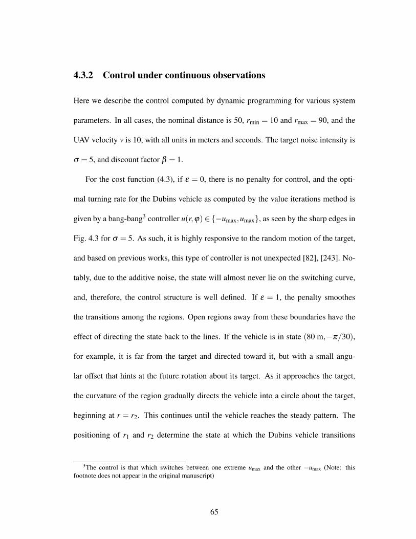
4.3.2 Control under continuous observations

Here we describe the control computed by dynamic programming for various system

parameters. In all cases, the nominal distance is 50, rmin = 10 and rmax = 90, and the

UAV velocity v is 10, with all units in meters and seconds. The target noise intensity is

σ = 5, and discount factor β = 1.

For the cost function (4.3), if ε = 0, there is no penalty for control, and the opti-

mal turning rate for the Dubins vehicle as computed by the value iterations method is

given by a bang-bang3 controller u(r,ϕ)∈ −umax,umax, as seen by the sharp edges in

Fig. 4.3 for σ = 5. As such, it is highly responsive to the random motion of the target,

and based on previous works, this type of controller is not unexpected [82], [243]. No-

tably, due to the additive noise, the state will almost never lie on the switching curve,

and, therefore, the control structure is well defined. If ε = 1, the penalty smoothes

the transitions among the regions. Open regions away from these boundaries have the

effect of directing the state back to the lines. If the vehicle is in state (80 m,−π/30),

for example, it is far from the target and directed toward it, but with a small angu-

lar offset that hints at the future rotation about its target. As it approaches the target,

the curvature of the region gradually directs the vehicle into a circle about the target,

beginning at r = r2. This continues until the vehicle reaches the steady pattern. The

positioning of r1 and r2 determine the state at which the Dubins vehicle transitions

3The control is that which switches between one extreme umax and the other −umax (Note: thisfootnote does not appear in the original manuscript)

65

[a][b]

[c]

[c]

[d] [e]

[a][b]

[c]

[c]

[d] [e]−umaxumax

−umaxumax

10 30 50 70 90 30 50 70 90

r1 r2−π

0

π

ϕ

r [m]

r1 r2

Figure 4.3: Optimal control based on distance to the target r and viewing angle ϕ forσ = 5, ε = 0 (left) and ε = 1 (right). Indicated points are [a] heading toward target at asmall angle displacement from a direct line, [b] start of clockwise rotation about target,[c] steady states at

(d,±cos−1 (σ2/100v

)), [d] heading directly away from target at a

small angle displacement away from a direct line, [e] start of counter-clockwise rotationabout target.

from the act of “avoiding" or “chasing" the target when it is too close or too far, respec-

tively, into the act of circling the target. Owing to the bias in the mean drift of dr (4.4),

|r1−d|> |r2−d|, i.e., a Dubins vehicle avoiding the target must anticipate the bias to

“help" with this action, while when chasing, the bias might hinder these efforts. The

effect of σ on this phenomenon is seen in Fig. 4.4.

In simulations, the actual evolution of the state (r,ϕ) is not smooth due to the ran-

dom motion of the target. Since we began this problem with an infinite-horizon cost,

the control is highly robust to such deviations, as we will show in simulations.

4.3.3 Control with observation interruptions

The control computed for the case of observation loss may be found in Fig. 4.5 for

λ12 = 0.01 / λ21 = 0.1 and τmax = 60 s, and in Fig. 4.6 for λ12 = 0.05 / λ21 = 0.5.

When τ = 0 s, the control policy matches that for tracking a stationary target. However,

66

σ=0.01

σ=5

σ=10

00

1

22 44 66 88 1010

10 20

30

30

32

34

36

38

60

60

62

64

66

6840 50 70 80 90

0.95

0.9

0.85

(a)

(b) (c)

ϕ

−π/2

0

π/2

π

r [m]

r 1[m

]

r 2[m

]2| ϕ∗ |/π

σ σ

Figure 4.4: (a) Switching curves from Fig. 4.3 for various values of σ . (b) Radii r1and r2 at which the UAV begins its entrance into a turning pattern about the target,corresponding to the labeled regions in Fig. 4.3 for σ = 5. As the noise intensity ofthe target increases, the UAV has less information of where the turning circle shouldbe centered and must begin its turn sooner. (c) Coordinate ϕ? of switching boundaryintersection with r = d. As the target noise increases, the UAV expects a bias that tendsto increase the target distance, and it reduces its steady-state viewing angle accordingly.

for τ > 0, the control instructs the tracker to gradually spiral in toward the position

where the target was last spotted until it reaches its minimum turning radius, as illus-

trated (simulated) in Fig. 4.7. This change is likely due to the fact that the angular

component of any radial displacement of a symmetric Brownian motion will be uni-

formly distributed. Once the target sufficiently deviates from its original position, it

becomes advantageous for the Dubins vehicle to center itself nominally to all the tar-

get’s possible positions. The spiral curvature is smaller for larger λ12.

67

ϕ[r

ad]

ϕ[r

ad]

ϕ[r

ad]

r [m]r [m]r [m]r [m]

(a)

Figure 4.5: Control anticipating observation loss, λ12 = 0.01 / λ21 = 0.1. Controlassuming continuous observations is listed for comparison in (a). From left-to-right,top-to-bottom, τ = 0, 2.1, 8.6, 15.0, 21.4, 27.9, 34.3, 40.7, 47.1, 53.6, and 57.9 s,respectively. Color mapping is the same as in Fig. 4.3.

4.4 Simulations

We show implementations of this control when the UAV is initially too far or too close

to the target in Fig. 4.8(a-d). Since a small time-step was used for simulation, the

Dubins vehicle trajectory using the control penalty ε = 0 was indistinguishable from

when ε = 1, but since its response was less sensitive to small displacements in target

location when ε = 1, the average standoff distance was slightly affected.

During observation loss, the control computed anticipating this provides a mean

distance that is nearly equal to the nominal distance (49.87 m for λ12 = 0.01 / λ21 =

0.1 and 49.83 m for λ12 = 0.05 / λ21 = 0.5), while the control assuming continuous

observations tends to be too far to the target during this time (53.21 m for λ12 = 0.01 /

λ21 = 0.1 and 51.68 m for λ12 = 0.05 / λ21 = 0.5). However, the performance decrease

is not large, indicating that, for this problem, the use of an outdated target observation

68

ϕ[r

ad]

ϕ[r

ad]

ϕ[r

ad]

r [m]r [m]r [m]r [m]

(a)

Figure 4.6: Control anticipating observation loss, λ12 = 0.05 / λ21 = 0.5. From left-to-right, top-to-bottom, the values of τ match those in Fig. 4.5.

may suffice.

Next, to emphasize the level of robustness provided by the control, the original

assumption that the target position evolves as a 2D random walk is dropped. We ex-

hibit the response to a target moving in a complex sinusoidal path with speed 4 m/s

in Fig. 4.9. Since target motion is no longer random, our control is no longer strictly

optimal. It is seen in Fig. 4.9(b), however, that the vehicle remains near the nominal

standoff distance, with the average distance slightly below d since the bias in r(t) is no

longer present. Finally, we exhibit the response to the same trajectory under observation

loss (λ12 = 0.01 / λ21 = 0.1).

4.5 Conclusion and Future Work

This paper considers the problem of maintaining a nominal distance between a Dubins

vehicle / UAV and a ground-based target. Brownian motion serves as a prior for the

69

x [m]y

[m]

0

0

20

20

40

40

60

60 80-60

-40

-40

-20

-20

Figure 4.7: Comparison of control policy under observation loss to continuous observa-tion control policy. The target, fixed at (0,0), is only observed at t = 0. The black Du-bins vehicle applies the control for a continuously-observed random walk target, whilethe red Dubins vehicle applies the control anticiating observation loss with λ12 = 0.01/ λ21 = 0.1. The blue Dubins vehicle applies the same control but for λ12 = 0.05 /λ21 = 0.5. The direction of rotation is a consequence of the initial condition and thesymmetry breaking that occurs during value iterations to pick a single direction, i.e.,clockwise or counter-clockwise.

target kinematics, and the possibility for a loss of observation is included using proba-

bilistic jumps. A Markov chain approximation that is locally consistent with the system

under control is constructed on a discrete state space, and value iterations on the asso-

ciated cost function produce a UAV turning rate control to minimize the expected mean

squared distance to the target in excess of a nominal distance.

The off-line control needs to only be computed once for a given target noise, re-

gardless of trajectory shape or initial conditions, and takes into account kinematic non-

linearities. The assumption of random target dynamics coupled with an infinite horizon

cost has the fundamental advantage of creating a highly robust control. A variety of

trajectories can be tracked using this approach, despite the fact that the intensity of

the noise in the UAV-target distance is no longer present in the case of natural motion.

70

-50 -25 0 25 50 75

-50

-25

0

25

x [m]

y[m

]

0 10 20 30 4040506070

t [sec]

r[m

]

-50 -25 0 25 50

-50

-25

0

25

50

x [m]

y[m

]

0 10 20 30 402030405060

t [sec]

r[m

]

(a)

(b)

(c)

(d)

t0

t f

t0

t f

Figure 4.8: A Dubins vehicle (red) tracking a Brownian target (blue). (a)For ε = 0, the Dubins vehicle must approach the target (t0 = 0) before enter-ing into a clockwise circular pattern (t f = 42.6) and (b) its associated distance r(mean(r) = 50.23, std(r) = 4.97). For ε = 1, mean(r) = 49.03, std(r) = 5.02 (c) TheDubins vehicle begins near the target (t0 = 0) and must first avoid the target using ε = 0before beginning to circle (t f = 41.6). The position of the target jumps sharply to theEast near the end of the simulation, and the Dubins vehicle is shown turning right toavoid it. (d) The associated distance (mean(r) = 48.8, std(r) = 5.98). For ε = 1,mean(r) = 48.7, std(r) = 5.94.

When approaching the nominal standoff distance from too close or too far a proximity,

the UAV flight pattern that initializes revolutions about the target and the revolutions

themselves are determined by the anticipated variability of the target, even if its motion

is smooth and deterministic. The computed control policies indicate that if some time

has passed since the last target observation, the tracker should spiral in toward the last-

observed target position. These conclusions are valid only for the parameter regimes

studied herein, and it is not known at this time if other behaviors could arise in different

regimes. Having faced some numerical instabilities for high observation loss rates, the

study of this question may require alternative numerical methods, as higher observation

loss rates may cause the problem to verge on open loop control territory.

71

0 50 100 150 200 250 300 350 400 450 500

-50

0

50

x [m]

y[m

]

0 20 40 60 80 100 120 14046

48

50

52

54

t [sec]

r[m

]

(a)

(b)

Figure 4.9: A UAV (red) tracking a target (blue) moving in a complex sinusoidal pathusing the control for a Brownian target. (a) The UAV follows the target in eccentric cir-cles whose shape is determined by the current position of the target along its trajectory,t ∈ [0,154.2]. (b) The distance r (mean(r) = 49.5 m, std(r) = 3.74).

Should the target also be modeled as a Dubins vehicle with a Brownian heading

angle, the knowledge of the target’s heading angle would provide the UAV with an

indicator of the target’s immediate motion and an appropriate response (control). Ex-

tensions to state-dependent or correlated noise4 are also possible, although this would

complicate the numerical method and potentially increase the state space dimension.

4Filtered noise would increase the dimension of the state space (Note: this footnote does not appearin the original manuscript)

72

x [m]

y[m

]r

[m]

t [s]0

0

0

20

40

40

60

60

70

3080 100

100

120 140

50

50

50 150 200 250 300 350 400 450

-50

(a)

(b)

Figure 4.10: (a) A UAV (red) tracking a target using the control for λ12 = 0.01 andλ21 = 0.1 when alternating between observing the target (blue) for 10 s and not observ-ing the target (gray) for 5 s. (b) The associated distances are the true distance (solid;mean(r) = 50.6 m, std(r) = 50.6) and the distance to the last-observed target position(dashed; mean(r) = 49.8 m, std(r) = 3.9).

73

Chapter 5

Optimal Feedback Guidance of aSmall Aerial Vehicle in the Presence ofStochastic Wind

This chapter is a preprint to the paper

I Anderson, R. P., Bakolas, E., Milutinovic, D., and Tsiotras, P., “Optimal Feed-back Guidance of a Small Aerial Vehicle in a Stochastic Wind”, AIAA Journal ofGuidance, Control, and Dynamics, vol. 36, issue 4, pp. 975-985, 2013.

5.1 Introduction

This paper deals with the problem of guiding an aerial vehicle with a turning rate con-

straint to a prescribed terminal position in the presence of a stochastic wind in minimum

expected time. It is assumed that the motion of the vehicle is described by a Dubins-

like kinematic model [82, 118, 191], that is, it travels only forward with constant speed,

and such that the rate of change of its forward velocity vector direction is bounded by

a prescribed upper bound. This kinematic model is referred to as the Dubins Vehicle

(DV for short). In the absence of the wind, the vehicle traverses paths of minimal length

74

and bounded curvature, known in the literature as Dubins paths or optimal paths of the

Markov-Dubins (MD for short) problem [82, 244].

The importance of designing trajectory tracking control schemes and path planning

algorithms that account for the effects of the local wind in UAVs/MAVs applications has

been recognized by many researchers. In particular, Refs. [61, 178, 215, 295] present

path tracking/following controllers for UAVs/MAVs in the presence of disturbances in-

duced by the wind based on nonlinear control tools. The problem of characterizing

minimum-time paths of a DV in the presence of a constant wind was first posed by

McGee and Hedrick in [166]. Numerical schemes for the computation of the Dubins-

like paths proposed in [166] have been presented in [26, 253]. The complete character-

ization of the optimal solution of the same problem, that is, a mapping that returns the

minimum-time control input given the state vector of the DV, is given in [24, 26]. A

numerical algorithm that computes the minimum-time paths of the DV in the presence

of a deterministic time-varying, yet spatially invariant, wind is presented in [168].

The analysis presented in the majority of the variations and extensions of the MD

problem in the literature is based on a deterministic optimal control framework (the

reader interested in a thorough literature review on variations/extensions of the MD

problem may refer to [28] and references therein). The effect of the wind, however, is

intrinsically stochastic, and approaching this problem from a stochastic point of view is

more appropriate. Some recent attempts to address optimal control problems related to

the MD problem within a stochastic optimal control framework can be found in [10, 11].

75

In particular, Refs. [10, 11] deal with the problem of a DV tracking a target with an

uncertain future trajectory using numerical techniques from stochastic optimal control

of continuous-time processes [137].

In this work, an optimal feedback control that minimizes the expected time required

to navigate the DV to its prescribed target set in the presence of a stochastic wind is

developed. Two stochastic wind models are investigated. In the first model the x and y

components of the wind are modeled as independent zero-mean Wiener processes with

a given intensity level. In the second model, the wind is modeled as having a constant

magnitude, but its direction is unknown and is allowed to vary stochastically according

to a zero-mean Wiener process. For both wind models, optimal feedback control laws

are computed numerically using a Markov chain approximation scheme. In addition,

for each control based on the stochastic wind models, feedback control laws based on

deterministic wind models are developed and compared against their stochastic model-

based counterparts in the presence of stochasticity to determine the regions of validity

of the former. The analysis and numerical simulations demonstrate, not surprisingly

perhaps, that control laws based on stochastic wind models outperform – on the aver-

age – control laws for the deterministic wind models implemented in a stochastic wind.

On the other hand, the control laws for the deterministic wind model can successfully

capture the salient features of the structure of the corresponding stochastic optimal con-

trol solution.

The contributions of the paper can be summarized as follows: First, this paper

76

offers, up to the authors’ best knowledge, for the first time, the solution of the opti-

mal path generation of an aerial vehicle with Dubins-like kinematics in the presence

of stochastic wind. This is important for small UAV path-planning and coordination

applications. Second, it shows the relationship of the optimal control solution, which

anticipates the stochastic wind, with its deterministic counterpart, and it compares the

two. This allows one to draw insights as to what level a stochastic wind-based solution

is beneficial compared to its less informed deterministic counterpart, and when it makes

sense (from a practical point of view) to use the former over the latter. The question

of the use of a feedback control law anticipating stochastic processes versus a control

law based on deterministic model assumptions is a question of a more general interest

and one that is a recurrent theme in the community, especially in terms of applications.

This paper offers a rare example where a head-to-head comparison is possible. In gen-

eral, the computation of a deterministic optimal feedback control is not an easy task, as

it requires the solution of a Hamilton-Jacobi-Bellman (HJB) partial differential equa-

tion. However, the Dubins vehicle problem in this paper serendipitously allows for a

complete solution, via a synthesis of open-loop strategies, without resorting to the HJB

equation.

The rest of the paper is organized as follows. Section 5.2 formulates the optimal

control problem. Section 5.3 presents feedback control laws based on minimal deter-

ministic and stochastic wind model assumptions. These control laws are extended in

Section 5.4 for the case when the wind has a known speed but stochastically-varying

77

direction. Simulation results for the controllers based on the two types of deterministic

and stochastic wind models are presented in Section 5.5. Finally, Section 5.6 concludes

the paper with a summary of remarks.

5.2 Problem Formulation

Here the problem of controlling the turning rate of a fixed-speed Dubins vehicle (DV)

in order to reach a stationary target in the presence of wind is formulated. The target

is fixed at the origin, while the Cartesian components of DV position are x(t) and y(t)

(see Fig. 5.1).

The DV moves in the direction of its heading angle θ at fixed speed v relative to the

wind and obeys the equations:

dx(t) = vcos(θ)dt + dwx(t,x,y), (5.1)

dy(t) = vsin(θ)dt + dwy(t,x,y), (5.2)

dθ(t) =u

ρmindt, |u| ≤ 1, (5.3)

where ρmin > 0 is the minimum turning radius constraint (in the absence of wind) and

u is the control variable, u ∈ [−1,1]. The motion of the DV is affected by the spatially

and/or temporally varying wind w(t,x,y) = [wx(t,x,y),wy(t,x,y)]T, whose increments

have been incorporated into the model (5.1)-(5.2). In this problem formulation, the

model for the wind is unknown. Therefore, it is assumed that the wind is described by

a stochastic process. Subsequently, a stochastic control problem for reaching a target

78

χ

x

x

xθ

atan2(y,x)−π

θw

ϕψ

y

δ

w

r

(x,y)

νin

Figure 5.1: Diagram of a DV at position [x(t), y(t)]T moving at heading angle θ inorder to converge on a target in minimum time in the presence of wind. The targetset T is shown as a circle of radius δ around the target. In the presence of the windvector w at an angle θw, the DV travels in the direction of its inertial velocity vectorνin and with a line-of-sight angle ϕ to the target center. The angle between νin and theline-of-sight angle is ϕ , and χ is the angle atan2(y, x).

set T =

(x,y) : x2 + y2 ≤ δ 2, which is a ball of radius δ > 0 around the target, is

formulated.

In order to minimize the time required to reach the target set, one defines a cost-to-

go function

J(x) = min|u|≤1

E

T∫0

dt

, x := [x(0),y(0),θ(0)]T, (5.4)

and assumes that upon reaching the target set T at time T , all motion ceases. In (5.4) the

expected time to reach the target set is minimized over the turning rate u, |u| ≤ 1, which

79

is the control variable. Control problems with a cost-to-go function of the form (5.4)

are sometimes referred to as “control until a target set is reached” [137] or stochastic

shortest-path problems [46].

Two stochastic process wind models that are characterized by the amount of infor-

mation known about the wind are considered. In each case, it is assumed that the wind

is a continuous-time stochastic process with respect to the DV position. In other words,

there is no explicit relation between a realization of the wind and the DV position, i.e.,

wx(t,x,y) = wx(t), and wy(t,x,y) = wy(t), although implicitly this relation may exist.

First, a feedback control when a model describing the wind is not given is devel-

oped. Drawing from the field of estimation, the simplest model to describe an unknown

2D signal suggests that the wind should be modeled as Brownian motion [105]. It is

further assumed that the Cartesian components of the wind evolve independently. Then

from (5.1)-(5.3), the kinematics of the DV in the presence of this wind, denoted model

(W1), is

dx(t) = vcos(θ)dt + σW dWx,

dy(t) = vsin(θ)dt + σW dWy,

dθ(t) =u

ρmindt, |u| ≤ 1, (W1)

where dWx and dWy are mutually independent increments of a zero mean Wiener pro-

cess, and where the level of noise intensity σW quantifies the uncertainty in the evo-

lution of the wind. Note that this kinematic model also arises when examining the

problem of tracking a target with unknown future trajectory [10, 11]. In the limiting

80

case where σW = 0, the problem is reduced to the case without the wind. A feedback

control that assumes σW = 0, therefore, would ignore the presence of the wind, while

a feedback control that assumes σW > 0 will account for the stochastic wind variation.

Along these lines, Section 5.3 develops feedback control laws that drive the DV to the

target in minimum time in both the deterministic case (σW = 0) and the stochastic case

(σW > 0). Note that in the deterministic case, the cost-to-go function is the same as

(5.4), but without the expectation operator.

Next, motivated by problems involving a wind that varies slowly in time and/or

space, a second wind model (W2) is considered. The second wind model considers a

wind that flows in the direction θw at constant speed vw < v, but where the evolution of

the direction of this wind is unknown. Then from (5.1)-(5.3), the model of the relative

motion of the DV and the target in the wind (W2) is

dx(t) = vcos(θ)dt + vw cos(θw)dt

dy(t) = vsin(θ)dt + vw sin(θw)dt

dθ(t) =u

ρmindt, |u| ≤ 1

dθw(t) = σθ dWθ , (W2)

where dWθ is an increment of a Wiener process, and where σθ is its corresponding

intensity. When σθ = 0, one obtains a model of constant wind in the direction θw.

Section 5.4 describes optimal feedback controls for the deterministic case (σθ = 0) and

the stochastic case (σθ > 0).

The proposed control schemes for the deterministic wind, which are based on ana-

81

lytic arguments, will give significant insights for the subsequent analysis and will illus-

trate some interesting patterns of the solution of the stochastic optimal control problem.

It will be shown later on that the control strategies for each deterministic wind model,

when applied to the DV in the presence of the stochastic wind, will capture the salient

features of the solution of the stochastic optimal control problem.

5.3 Feedback Laws with No Wind Information

In this section, feedback control laws are developed that drive the DV to its target in the

presence of an unknown wind (W1). First, a method for designing a feedback control

for the deterministic problem, that completely ignores the presence of a wind, is briefly

discussed. Next, an optimal feedback control will be computed for the case where the

Cartesian components of the wind vary stochastically. In all cases, the target set is a

ball of radius with δ = 0.1, and the velocity of the vehicle is constant v = 1.

5.3.1 Deterministic Case

First, a control law that is completely independent of any information about the dis-

tribution of the wind is proposed. In other words, a feedback control law is designed

under the assumption that the wind is modeled by (W1) with σW = 0. Therefore, this

control law is “blind” to the presence and the statistics of the actual wind. This ap-

proach will give two navigation laws that are similar to the pure pursuit strategy from

missile guidance [30], which is a control strategy that forces the velocity vector of the

82

controlled object (the DV in this case) to point towards its destination at every instant

of time.

Note that in the presence of a wind and with the application of a feedback law that

imitates the pure pursuit strategy, the DV will not be able to instantaneously change

its motion in order to point its velocity vector toward the target. This happens for two

reasons. The first reason is because the rate at which the DV can rotate its velocity

vector is bounded by the turning rate constraint (5.3). The second reason has to do with

the fact that, by hypothesis, the pure pursuit law does not account for the wind, and,

consequently, even if the DV were able to rotate its forward velocity vector arbitrarily

fast, it would be this forward velocity vector that points toward the target rather than

the inertial velocity.

Let ϕ be the angle between the vehicle’s forward velocity vector and the line-of-

sight to the target, given by ϕ = θ − atan2 (y,x) + π and mapped to lie in ϕ ∈ (−π,π]

(see Fig. 5.1). The proposed (suboptimal) pure pursuit-like navigation law takes the

following state-feedback form

u(ϕ) =

−1 if ϕ ∈ (0,π],

0 if ϕ = 0,

+1 if ϕ ∈ (−π,0).

(5.5)

One important observation is that the control law (5.5) does not depend on the distance

r(t) =√

(x(t))2 +(y(t))2 of the DV from the target but only on the angle ϕ . The state

feedback control law given in (5.5) will be referred to as the geometric pure pursuit

83

(GPP for short) law. Note that the GPP law drives the DV to the line S0 := (r,ϕ) : ϕ =

0, which is a “switching surface.” In the absence of wind, once the DV reaches S0,

it travels along S0 until it reaches the target (such that r = 0 at the final time T ) with

the application of the control input u = 0. Therefore, the GPP law is a bang-off control

law with one switching at most, that is, a control law which is necessarily a control

sequence ±1,0.

It is important to highlight that the GPP law turns out to be the time-optimal con-

trol law of the MD problem for the majority (but not all) of the initial configurations

[x(0),y(0),θ(0)]T (see Fig. 5.2), when there is no wind [49, 258]. However, there are

still initial configurations from which the DV driven by the navigation law (5.5) either

cannot reach the target set at all or can reach the target only suboptimally. The previous

two cases are observed, for example, when the DV is close to the target with a relatively

large |ϕ|.

In particular, it can be shown [49, 258] that if the DV starts, at time t = 0, from any

point that belongs to one of the two regions, C+ and C−, defined by (see Fig. 5.2)

C− = (r,ϕ) : r ≤ 2ρmin sin(−ϕ), ϕ < 0 (5.6)

C+ = (r,ϕ) : r ≤ 2ρmin sin(ϕ), ϕ > 0 , (5.7)

then the target cannot be reached by means of the GPP law in the absence of a stochas-

tic wind (scenarios where the stochastic wind helps the DV to reach its target even

by means of a GPP law will be shown later on). Therefore, in order to complete the

design of a feedback control law for any possible state of the DV, one needs to con-

84

0

2 4 6 8 10r

ϕ

u =−1

u = +1S−

S+

S0

−

C−

C+

−1,0

+1,0

−1,+1

+1,−1

π

−π

Figure 5.2: Time-optimal partition of the control input space and state feedback con-trol law of the MD problem with free terminal heading in the absence of wind. Onecan use this control strategy as a feedback law for the case of a stochastic wind. Con-trol sequences for an initial state in each time-optimal partition are indicated in redbackground.

85

sider the optimal solution of the MD problem in the case when the terminal heading

is free [49, 258]. It turns out that the boundaries of C+ and C−, denoted, respectively,

by S− and S+ (the choice of the subscript notation will become apparent shortly later),

correspond to two new “switching surfaces” along which the DV travels all the way to

the target. In particular, when the DV starts in the interior of C+ (respectively, C−), then

the minimum-time control action is u = +1 (respectively, u =−1), which may appear

to be counterintuitive, since its effect is to increase |ϕ| rather to decrease it. The control

input remains constant until the DV reaches the “switching surface” S− (respectively,

S+), where the control switches to u = −1 (respectively, u = +1), and subsequently,

the DV travels along S− (respectively, S+) all the way to the target driven by u = −1

(respectively, u = +1). The net effect is that when the DV starts inside the regions C±,

the DV must first distance itself from the target so that its minimum turning radius ρmin

is sufficient to turn towards the target. Note that in this case the control law is bang-

bang with one switching at most, that is, a control sequence ±1,∓1. The situation is

illustrated in Fig. 5.2 for ρmin = 1.

The GPP law given in (5.5), therefore, needs to be updated appropriately to account

for the previous remarks. In particular, the new feedback control law is given by

u(r,ϕ) =

−1 if (r,φ) ∈ Σ−,

0 if (r,φ) ∈ Σ0,

+1 if (r,φ) ∈ Σ+,

(5.8)

86

where,

Σ− := (r,ϕ) : ϕ ∈ (0,π]∩ (intC+)c∪ intC−

Σ+ := (r,ϕ) : ϕ ∈ (−π,0)∩ (intC−)c∪ intC+

Σ0 := (r,ϕ) : ϕ = 0.

The state feedback law (5.8) will be henceforth referred to as the optimal pure pursuit

(OPP for short) law, because, at every instant of time, it steers the DV to the target

based on the optimal strategy that corresponds to its current position. Note that in the

absence of wind, the OPP law is the optimal control law of the MD problem with free

final heading [49, 258]. One important remark about the OPP law is that the control

variable u may attain the value zero, which is in the interior of its admissible set [−1,1].

Thus, the control u = 0 is singular, and the part of the optimal trajectory it generates

is referred to as the singular arc of the optimal solution. As explained in detail in

Ref. [28], singular arcs may be part of the optimal solution of the MD problem in the

absence of wind, only when the so-called switching function of the constrained optimal

control problem, along with its first time derivative, vanish simultaneously (for a non-

trivial time interval). Note that while u = ±1 corresponds to turning left/right, the

control u = 0 corresponds to straight paths.

Figure 5.3 illustrates the level sets of the minimum time-to-go function, which can

be computed analytically by using standard optimal control techniques and geometric

tools, as shown in [28].

87

0

0

2

2

4

4

6

6

8

8

10

10

12

rδ

T

π

−π

ϕ

Figure 5.3: Level sets of the minimum time-to-go function of the MD problem withfree terminal heading.

5.3.2 Stochastic Case

In this section, an optimal feedback control law for the stochastic kinematic model

(W1) and cost functional (5.4) is developed. The optimal control is computed using

the Markov chain approximation method [137], which ensures that when discretizing a

state space for value iteration in stochastic optimal control problems, the chosen spatial

and temporal step sizes accurately scale in the same way as in the original stochastic

process. The method constructs a discrete-time and discrete-state approximation to the

cost function in the form of a controlled Markov chain that is “locally-consistent” with

the process under control.

Since the method involves discretization of the state space, one first reduces the

88

number of dimensions in the model (W1). Applying Itô’s differentiation rule to the

DV-target distance r(t) and the viewing angle ϕ(t) where ϕ ∈ (−π,π], as before (see

Fig. 5.1), it can be shown that the relative DV-target system coordinates obey (see the

Appendix)

dr(t) =

(−vcos(ϕ)+

σ2W

2r

)dt + σW dW‖, (5.9)

dϕ(t) =

(vr

sin(ϕ)+u

ρmin

)dt +

σW

rdW⊥, (5.10)

where |u| ≤ 1, and where dW‖ and dW⊥ are mutually independent increments of unit

intensity Wiener processes aligned with the direction of DV motion. Note the presence

of a positive bias σ2W/2r in the relation for r(t), which is a consequence of the random

process included in the analysis. In the proposed parametrization, only distances r ≥ δ

outside the target set are considered, and so (5.9)-(5.10) is well defined.

In the Appendix the equations for value iterations on the cost-to-go function using

the Markov Chain approximation method are derived. From this, the optimal angular

velocity of the DV may be obtained for any relative distance r ≥ δ and viewing angle

ϕ . The structure of the optimal control law (W1) is seen in Fig. 5.4(a) for σW = 0.1 and

discretization steps ∆r = 0.02 and ∆φ = 0.025. As in the deterministic model (σW = 0)

case (Fig. 5.2), the value iteration stationary control law is composed of bang-bang

regions instructing the DV to turn left or right and singular arcs. With smaller noise,

the optimal control is comprised of four regions, two directing the target to turn left,

and others instructing a turn to the right. The reader should note the similarity between

Fig. 5.4(a) and the OPP control illustrated in Fig. 5.2. In particular, the structure of the

89

0

2 4 6 8r

u =−1

u = +1C−

C+

π

−π

ϕ

(a)

10

0

2 4 6 8r

u =−1

u = +1

π

−π

ϕ

(b)

10

Figure 5.4: Dubins vehicle optimal turning rate control policy u(r,ϕ) for model (W1).(a) Stochastic optimal control policy for σW = 0.1. For comparison, the switchingcurves from the deterministic model-based OPP control in Fig. 5.2 are outlined in red.(b) Stochastic optimal control policy for σW = 0.5 yields the GPP control (5.5) fordeterministic winds.

regions C− and C+ have changed somewhat, as a consequence of the stochastic variation

of the wind. In Fig. 5.4(b), a higher noise intensity of σW = 0.5 causes the control to

return to GPP control (5.5). In other words, the variance of the process is so large that

it becomes exceedingly difficult to predict the relative DV-target state, and the optimal

control for the stochastic model matches a simpler, analytically-derived control for the

deterministic model that, as described in the previous section, is not optimal for some

initial conditions close to the target. This suggests that, for our problem, a deterministic

control may suffice for the optimal feedback control when the variance of the stochastic

wind is sufficiently large.

This control strategy remains optimal for even larger σW , but due to the bias in

r(t) (see Eq. (5.9)), this control policy may not be successful in guiding the DV to the

90

0.5 5 10 15 20

0

0.2

0.4

0.6

0.8

σw

P(τ≤

10|r

0,φ

0)

Figure 5.5: Probability of hitting the target set in the time interval 0 < τ ≤ 10 for aninitial condition a distance 1 [m] from the target and facing towards the target ((r,ϕ) =(1,0)).

target in a reasonable amount of time for high values of σW . Although a solution to

the backward Kolmogorov equation [105] indicates that the DV will eventually hit the

target with probability one as t → ∞, the expected value of the hitting time becomes

exceedingly large with increasing σW . Similarly, one can also consider the probability

that the DV, initially located at (r,ϕ), will hit the target set by a specified time τ as a

function of the noise intensity σW . Figure 5.5 shows this distribution as computed for

(r,ϕ) = (1,0) and τ = 10 s using 1000 simulations for each σW .

5.4 Feedback Laws for Wind at an Angle

Next, the second model (W2), in which the wind is now assumed to take on a direction

θw with known speed 0 < vw < 1, where vw is constant by hypothesis, is assumed and

91

the feedback control laws for steering the DV in the presence of this wind are discussed.

5.4.1 Deterministic Case

First, the case when σθ = 0 and 0 < vw < 1 is considered. Note that the fact that

σθ = 0 implies that the direction of the wind becomes constant, and consequently, the

wind w = [wx, wy]T, where wx := vw cosθw and wy := vw sinθw, is a constant vector.

Therefore, in this section, it is assumed that the constant wind w is known a priori. The

equations of motion of the DV become

dx = vcos(θ)dt + wxdt,

dy = vsin(θ)dt + wydt,

dθ =u

ρmindt, |u| ≤ 1. (5.11)

First, a feedback law that is similar in spirit to the GPP law given in Eq. (5.5), which

exploits the fact that the wind is known a priori, is designed. In particular, the proposed

control law tries to rotate the velocity vector of the DV to point at the target. It is easy

to show that the control law (5.5) becomes

u(ϕ) =

−1 if ψ(ϕ) ∈ (0,π],

0 if ψ(ϕ) = 0,

+1 if ψ(ϕ) ∈ (−π,0).

(5.12)

and

ψ(ϕ) := atan2(y, x)−θ + ϕ. (5.13)

92

where ψ , is the angle between the inertial velocity of the DV and the line-of-sight

(LOS) as is illustrated in Fig. 5.1 (the angle χ in this figure is equal to atan2(y, x)). As

it is shown in [30], the navigation law (5.12) is dual to the so-called parallel navigation

law from missile guidance. The control law (5.12) is henceforth referred to as the

Geometric Parallel Navigation (GPN for short) law.

As mentioned in Section 5.3.1, the GPP law that forces the forward velocity of

the vehicle to point towards the target may not always be well defined, especially in

the vicinity of the target. The same type of argument applies to the GPN law modulo

the replacement of the forward velocity with the inertial velocity. Next, a control law

that steers the DV to the target using the optimal control that correspond to the current

position of the DV and assuming a constant (e.g., average) wind is presented. This

control law is referred to as the Optimal Parallel Navigation (OPN for short) law. Note

that similarly to the GPN law, the OPN law does not consider the variations of both the

speed and the direction of the wind. By combining the type of arguments used in [49,

258], which deal with the standard MD problem with free terminal heading, along with

the analysis presented in [24, 26], one can easily show that the candidate optimal control

of the Markov-Dubins problem in the presence of a constant wind corresponds to the

four control sequences presented in Section 5.3.1, namely, ±1,0 and ±1,∓1. The

main difference between the solutions of the Markov-Dubins problem in the absence of

a wind, which was briefly presented in Section 5.3.1, and the Markov-Dubins problem

in the presence of a constant wind, is the switching conditions and, consequently, the

93

0

2 4 6 8r

u =−1u = +1

S−

S+S0

−

(a)π

−π 10

ϕ

0

2 4 6 8r

u =−1u = +1

S−

S+

S0

−

(b)π

−π 10

ϕ

Figure 5.6: Time-optimal partition of the control input space and state feedback controllaw of the MD problem with free terminal heading in the presence of a constant wind.(a) Tailwind (b) Headwind

switching times of their common control sequences.

Figure 5.6 illustrates the structure of the OPN law in the (r,ϕ) plane in the pres-

ence of a constant tailwind, that is, θw = θ(0), and a constant headwind, that is,

θw = π + θ(0), respectively. One observes that the GPN law coincides with the OPN

law for the majority of the boundary conditions especially for the case of a tailwind,

whereas in the presence of the headwind the points in the (r,ϕ) plane where the optimal

strategy is bang-bang correspond to a significantly large set. An interesting observation

is that the new switching surfaces of the OPN law are associated with those of the OPP

law by means of a particular coordinate transformationH : (x,y,θ) 7→ (x′,y′,θ), as de-

scribed in [24]. In particular, a configuration with coordinates (x,y,θ) that belongs to

the switching surface S+, S0 or S− of the OPP law corresponds to a point with coordi-

nates (x′,y′,θ) that belongs respectively to the switching surface S+, S0 and S− of the

94

OPN law, where

x′ = x + wxTDV(x,y,θ), (5.14)

y′ = y + wyTDV(x,y,θ), (5.15)

where TDV(x,y,θ) is the minimum time required to drive the DV from (x,y,θ) to the

origin with free final heading θ . It is easy to show that for a state (x,y,θ) ∈ S+ (S−),

it holds that TDV(x,y,θ) = −2ρminϕ(x,y,θ)/v (2ρminϕ(x,y,θ)/v). In addition, if the

state (x,y,θ) ∈ S0, then TDV(x,y,θ) =√

x2 + y2/v.

Figure 5.7 illustrates the correspondence of the switching surfaces of the OPN law

with those of the OPP law for a tailwind (θw = θ(0) = 0) and a headwind (θw = π +

θ(0) = π) via the previous coordinate transformation. Note that the switching surface

S0 of both the OPG and the OPP laws are the same but the surfaces S± are different.

Figure 5.8 illustrates the level sets of the minimum time-to-go function in the pres-

ence of a constant wind, whose computation entails the solution of a decoupled sys-

tem of transcendental equations as shown in [24, 26]. In particular, Fig. 5.8(a) and

Fig. 5.8(b) illustrate the level sets of the minimum time-to-go function in the presence

of a constant tailwind and a constant headwind, respectively.

5.4.2 Stochastic Case

It is now assumed that the direction of the wind θw is no longer constant, but is rather

described by the stochastic process (W2) with σθ > 0. A similar derivation to that used

95

0

0 2 4 6 8 10

ϕ

r

S−

S+

S0

H

H

H

H

Figure 5.7: Correspondence between the switching surfaces of the OPP and the OPGlaws via a transformation for a tailwind (blue curves) and a headwind (red curves).

for model (W1) yields for (W2):

dr(t) =−(vcos(ϕ)+ vw cos(ϕ + γ))dt,

dϕ(t) =

(vr

sin(ϕ)+vw

rsin(ϕ + γ)+

uρmin

)dt,

dγ(t) =u

ρmindt−σθ dWθ , (5.16)

where the state γ(t) := θ(t)−θw(t) is introduced to define the difference between the

DV heading angle and the direction of the wind θw. In the numerical example, the

following data are used: vw = 0.5, and σθ = 0.1. The discretization steps were chosen

as ∆r = 0.1, ∆φ = 0.08, and ∆γ = 0.12. As before, value iterations on the optimal

cost-to-go were performed as described in the Appendix. Two “slices” of this control,

corresponding to the cases where the DV travels in the direction of the wind (tailwind,

96

0

2 4 6 8

5

10

10

20

25

15

rT

(a)π

−π

ϕ

0

2

2

4

4

6

6

14

16

18

8

8

10

10

12

rT

(b)π

−π

ϕ

Figure 5.8: Level sets of the minimum time-to-go function of the MD problem withfree terminal heading in the presence of a constant wind (σθ = 0). (a) Tailwind (γ = 0).(b) Headwind (γ = π).

where γ = 0) and where it faces the wind (headwind, γ = π) are shown in Fig. 5.9(a)

and Fig. 5.9(b), respectively. In each fixed-γ policy, the optimal control resembles that

shown in Fig. 5.6, although the location and shape of the switching curves S± have

changed due to the stochastic variation in the wind. In Fig. 5.9(a), only small vestiges

of the switching curves are seen, while in Fig. 5.9(b), the shape of these curves has

changed. Figure 5.10 shows the expected value of the time required to hit the target in

the case of a headwind and tailwind.

5.5 Performance Comparison

In the previous sections, it is seen that the control laws for both deterministic wind

models closely resemble their respective optimal feedback control laws for the stochas-

tic wind models. In particular, the control policies for the deterministic and stochastic

wind models are identical when far from the target, but differences are seen when r is

97

0

2 4 6 8 10r

u =−1

u = +1

(a)π

−π

ϕ

0

2 4 6 8 10r

π

−π

ϕ

u =−1

u = +1

(b)

Figure 5.9: Dubins vehicle optimal turning rate control policy u(r,ϕ,γ) for stochasticmodel (W2) with σθ = 0.1. (a) Tailwind (γ = 0). (b) Headwind (γ = π).

E(T

)

2

2

2

2

1

1

1

1

1

4

4

4

4

6

6

68

8

8

0

0

0

0

0

rδ

δ

ϕϕ

E )

π

π

−π

−π

Figure 5.10: Level sets of the minimum time-to-go function of the MD problem withfree terminal heading in the presence of a wind with stochastically varying directionand constant speed vw.

98

−1.5

−0.5

0.5

−2−2

−1

−1

−1

0

0

0

0 3

2

2 1

1

1

vw←−−−

x [m]x [m]

y[m

]

8

Figure 5.11: DV trajectories for 500 realizations under wind model (W1) (left) and(W2) (right) starting with an initial condition that may result in a difference betweentrajectories resulting from the control based on the deterministic (red) and stochastic(blue or green) wind models. The initial DV positions are marked with a , and thetarget is marked with an ×.

close to δ . To see the effect of these differences, this section provides a comparison of

performance of the proposed feedback control laws against the stochastic wind models

(W1) and (W2).

As an example, Fig. 5.11 shows a collection of simulated DV trajectories under the

controls for the deterministic (red) and stochastic (blue or green) wind models, where

the left and right panels correspond to (W1) and (W2), respectively. In this figure, the

control anticipating the wind stochasticity assumes that there is a non-zero probability

that the stochastic wind may push it beyond its minimum turning radius ρmin and into

the target, and hence the control directs it to perform a left turn. Some realizations

(75.6%, shown in green) under this control reach the target, but the remainder (blue)

must circle around (see insert). The control for the deterministic wind model directs

99

− .

.

.

0

0

0

0

0

4

2

2

2

5

5

1

1

11 33 δδ

ϕ

r r

−π

π

.5

Figure 5.12: Comparison of distributions of time required to hit the target under bothOPP control (5.8) and the stochastic optimal control u(r,ϕ), σW = 0.1 in the presenceof the stochastic wind (W1). Left: difference in mean hitting time E(TOPP)−E(Tstoch).The OPP control results higher E(T ) in regions where the stochastic model-based con-trol differs from the OPP control. Right: difference in standard deviation std(TOPP)−std(Tstoch). As expected, the OPP control results in higher standard deviation in themajority of cases.

the red DVs to first distance themselves before approaching the target. Consequently,

the regions in the (r,ϕ) state space corresponding to the trajectories in this example

lead to a smaller expected time to hit the target for the stochastic model-based control,

as seen in Fig. 5.12. However, there is also a chance that the stochastic model-based

control is unsuccessful in hitting the target on its first pass, and so the DV must circle

around again. In other words, the stochastic model-based control “risks” a turn toward

the target for small r and small ϕ . Although the expected value of the hitting time

decreases under the control anticipating the stochastic winds, the standard deviation of

these times may simultaneously increase, as seen in Fig 5.12.

In the right panel of Fig. 5.11, a similar result is seen for the case of wind at an

angle (indicated by a vw arrow). In this case, a small number of the realizations for

100

the DVs under the deterministic model-based control are affected by the changing wind

and must take a longer route to reach the target, whereas the DVs under the stochastic

model-based control anticipate the changing wind direction. Similarly, Fig. 5.13 shows

the mean time-to-go under (W2) using both the control for the deterministic model

shown in Fig. 5.6 and the control law for the stochastic wind model in Fig. 5.9. As

before, the expected time-to-go is larger for the deterministic model-based control in

regions where the control laws differ. However, unlike (W1), the standard deviation

under the stochastic model-based control was consistently smaller since the control

accounts for the stochastic wind without instructing for a potentially “risky” approach

to the target.

5.6 Conclusions and Future Work

In this paper, the problem of guiding a vehicle with Dubins-type kinematics to a pre-

scribed target set with free final heading in the presence of a stochastic wind in min-

imum expected time has been addressed. Two approaches to this problem have been

proposed. The first one, which was based on analytic techniques, was to employ feed-

back control laws, based on a deterministic model, that are similar to the well-studied

pure pursuit and the parallel navigation laws from the field of missile guidance. The

proposed feedback control laws are time-optimal in the absence of wind or in the pres-

ence of a wind that is constant and known a priori.

The second approach was to tackle the problem computationally by employing nu-

101

merical tools from stochastic optimal control theory. Because these control laws are

based explicitly on the stochastic wind models, they anticipate the wind stochasticity,

and the time necessary to steer the Dubins vehicle to the target set in the presence of a

stochastic wind is, on average, lower than that under the control for the corresponding

deterministic model. However, although the feedback control laws for the deterministic

model become suboptimal in the presence of a stochastic wind, it turns out that they

still manage to steer the Dubins vehicle to its target set with an acceptable miss target

error. On the other hand, a stochastic framework leads to higher expected precision in

terms of target miss-distance and more predictable trajectories.

The fact that the deterministic model-based controls perform so well for this prob-

lem even in the presence of an unknown stochastic wind is mainly owing to the fact that

they are in a feedback form, thus providing a certain degree of robustness against uncer-

tainties. Having that in mind, it may not be surprising that the presented deterministic

model-based control laws can work in the presence of small stochastic disturbances,

although non-optimally. This may not be the case for other problems in practice where

one is only able to generate reliable deterministic open-loop trajectories. Surprisingly

perhaps, the computation of optimal feedback controls based on stochastic models gen-

erally is no more difficult (or even easier) than for their deterministic counterparts as

the latter can be consistently discretized and cast as a controlled Markov decision pro-

cess, as shown in this paper. On the other hand, the closed-form feedback laws based

on the deterministic model presented in this paper may be more appealing than their

102

stochastic model-based counterparts, owing to their ease of implementation.

Thus, the similarity between control policies under different levels of wind stochas-

ticity seems to support the use of the feedback controls for deterministic wind mod-

els in lieu of stochastic model-based feedback controls when the stochastic effects are

small, or can be used as “seeds” that may expedite the computation of the solution

to the stochastic optimal control problem, or aid in the verification of numerical re-

sults. Moreover, since the role of noise in designing feedback control policies is not

fully understood, a side-by-side comparison of the feedback laws for deterministic and

stochastic models in other problems may provide useful insights toward a more general

theory.

Future work will include the extension of the techniques presented herein to prob-

lems with a more realistic model of the wind, including wind models that depend ex-

plicitly on the position of the Dubins vehicle. Another possible extension is to charac-

terize control laws for stochastic wind models that minimize a cost function taking into

consideration both the expected value and the variance of the time-to-go.

103

00

0 2

2

2

2 11

4

44 33 55 δδ

ϕ

−π

π

(a) Tailwind (γ = 0).

00

0 4

4

4

4

2

2

2

2 55 11

66

33

88

δδ

ϕ

−π

π

(b) Headwind (γ = π).

Figure 5.13: Comparison of distributions of time required to hit the target under bothOPP control (Fig. 5.6) and the stochastic optimal control (Fig. 5.9) in the presence ofthe stochastic wind (W2). Left: difference in mean hitting time E(Tdeter)−E(Tstoch).Right: difference in standard deviation std(Tdeter)− std(Tstoch).

104

Chapter 6

Stochastic Optimal Enhancement ofDistributed Formation Control UsingKalman Smoothers

This chapter is a preprint to the paper

I Anderson, R. P., and Milutinovic, D., “Stochastic Optimal Enhancement of Dis-tributed Formation Control Using Kalman Smoothers”, Accepted for publicationin Robotica.

6.1 Introduction

The focus of this work is on an approach to optimally enhance a given distributed feed-

back control for nonholonomic agents, such as mobile robots [190], or vehicles. We

are motivated by the problem of distributed formation control, in which each agent is

tasked with attaining and maintaining pre-specified distances from its neighbours. Var-

ious control approaches have been proposed for formation control, including PID con-

trol [8, 198], artificial potentials [87, 192, 252], navigation functions [211], constraint

forces [297], geometric methods [57], adaptive control design [220, 233], sliding mode

105

control [102], and consensus algorithms[74, 206], for example. These approaches are

attractive due to their often intuitive design principles, the transparent, analytic forms of

the resulting control laws, and their generally satisfactory results. However, developing

a control law that is both optimal and robust to uncertainty presents a greater challenge.

Here, we begin with a reference distributed control policy [252] for formations of

nonholonomic vehicles consisting of a feedback-controlled turning rate and accelera-

tion and based on an artificial potential function. Next, we numerically compute the

additional additive control input necessary to drive the non-optimal system into a for-

mation optimally and in a manner that is robust to uncertainty. Consequently, our con-

trol approach is optimal, and, due to the adopted artificial potential function [252], it

provides collision-free agent trajectories. Moreover, in some sense to be defined later,

the computed optimal feedback control is “close" to the reference feedback control,

preserving many of the nicer properties of the latter, including collision avoidance and,

to some extent, qualitative behaviour of the controlled agents. We are not aware of

other works that improve upon existing, rather than build from the ground up, mobile

robot feedback control laws in this manner.

To compute an optimal feedback control, one must solve the Hamilton-Jacobi-

Bellman (HJB) equation, which is a nonlinear partial differential equation (PDE), and,

accordingly, the solution of the optimal control problem is necessarily numerical. How-

ever, the computational complexity of the solution to the HJB equation grows exponen-

tially with the state space dimension of the system (i.e., with the size of the robotic

106

team), making conventional approaches to computing the stochastic optimal feedback

control intractable. In this work, we exploit the distributed nature of the problem at

hand in order to make the solution to the HJB equation computationally feasible. The

distributed formation control problem is inherently stochastic – from the perspective of

one agent, its neighbours’ observations and control inputs are unknown as well as the

effects of these inputs on agent trajectories due to model uncertainties. Accordingly,

this work considers the problem of controlling one agent based on its own observations

of its neighbours in a way that anticipates the probability distribution of their future

motion. This probability distribution arises from an assumption that a prior for the un-

known control input of an agent can be robustly described as Brownian motion [274],

which, for the agent model considered in this paper, results in a so-called “banana dis-

tribution" prior [154]. Based on our prior and the system kinematics, we can induce a

probability distribution of the relative state x to all neighbours in an interval (x,x + dx)

at a particular future time [280]. It follows that the cost function to be minimized by

an agent not only computes the optimal control with respect to the current system state

as viewed by that agent, but also with respect to the distribution of possible trajectories

originating from the current state.

Besides aiding in the creation of a robust control law, this distribution over future

system trajectories serves several additional purposes. For example, the distribution en-

codes the same type of information that must be repeatedly transmitted among neigh-

bours in some other distributed formation control approaches [84], e.g., assumed future

107

trajectories of a neighbour. Perhaps more importantly, this distribution over future sys-

tem trajectories can be used to statistically infer the probability distribution of the con-

trol, and, hence, the optimal additive control required for the considered reference feed-

back control. In particular, the relations between the solutions to optimal control PDEs

and the probability distribution of stochastic differential equations [101, 183, 292] al-

lows certain stochastic optimal control problems to be written as an estimation problem

on the distribution of optimal trajectories in continuous state space in a manner known

as the path integral (PI) approach [124, 125, 127, 263, 264].1

Related works incorporating the PI framework for multi-agent systems [271, 272,

285, 286] designed control for systems in which agents cooperatively compute their

control from a marginalisation of the joint probability distribution of the group’s tra-

jectory. In this article2, we develop a method by which agents independently compute

their controls without explicit communication. Moreover, previous works using the PI

approach have formulated an unconstrained receding horizon optimal control problem

for which stability is difficult to guarantee [122]. We therefore consider two formula-

tions admitting time-invariant feedback control policies. The first is based on a planning

horizon that ends only when the formation is reached, while the other is based on an

infinite-horizon, discounted cost control problem.

Additionally, we establish a connection between the presented optimal feedback

control problem and nonlinear Kalman smoothing algorithms, so that each agent can

1There is also an analogous approach in the open-loop control case [169, 185].2Preliminary versions of some portions of this work have previously been presented elsewhere [12,

14].

108

compute its control in real-time in a way that preserves the optimality and stability prop-

erties of the HJB equation solution. That a Kalman smoother can be used to compute

an optimal control is related to the well-established duality between linear-quadratic-

Gaussian (LQG) control and linear-Gaussian estimation [239]. Although other robotic

control algorithms have employed Kalman filters or smoothers for motion planning and

path planning [53, 98, 140, 269, 270], the relation of the nonlinear Kalman smoothing

algorithm to the HJB equation has not been exploited. Moreover, since our Kalman

smoothing control computations are based on the current system state and do not re-

quire a global HJB equation solution, we describe how our algorithm may be used to

test, pointwise in state space, the possibility for analytic improvements to the reference

feedback control for optimality and robustness to uncertainties.

In our approach, after each agent computes and applies the optimal control com-

puted by its Kalman smoother, it observes the new state of its neighbours, and then

the process repeats. This method is similar in spirit to receding horizon control/model

predictive control (MPC) [161] and related suboptimal algorithms [44], some of which

have been used previously for vehicle formation control [62, 84, 174]. However, our

approach differs in three respects. First, as previously discussed, the control solution is

derived from the HJB equation instead of an open-loop, numerical optimization prob-

lem. In addition, for reasons that will become clear in the sequel, the system trajectories

to which the Kalman smoother is applied are uncontrolled, whereas model predictive

control treats the control along these paths as decision variables. Finally, our Kalman

109

smoother solution is generally computationally fast compared to nonlinear optimization

methods for systems with large dimensional state and control space, and the algorithm

quite naturally handles stochasticity. We point out that without the notion of uncertainty

in a neighbour’s control, an optimization problem resulting from distributed model pre-

dictive control may predict a neighbour’s trajectory incorrectly and without an explicit

remedy for this issue.

This article is organized as follows. Section 6.2 introduces the formation control

problem as viewed by a single agent in the group, followed by a derivation of a path in-

tegral representation in Section 6.3. Section 6.4 presents a Kalman smoother method for

computing individual agent control. Section 6.5 compares the optimal feedback con-

trol computed by Kalman smoothers against that computed using a numerical method

involving discretisation of the state space and examines the areas of the state space

where the analytical reference feedback control could be improved. We continue in

Section 6.5 to illustrate our method with simulations of five agents achieving forma-

tions, and we conclude with Section 6.6.

110

6.2 Control Problem Formulation

We consider a team of agents, each described by a Cartesian position (xm,ym), a heading

angle θm, a speed vm, m = 1, . . . ,Mtot, and the kinematic model:

dxm(t) = vm cosθmdt

dym(t) = vm sinθmdt

dθm(t) = ωmdt + σθ ,mdwθ ,m

dvm(t) = amdt + σv,mdwv,m, (6.1)

where ωm and am are the feedback-controlled turning rate and acceleration, respec-

tively, and where dwθ ,m and dwv,m are mutually independent Wiener process incre-

ments with corresponding intensities σθ ,m and σv,m, respectively. Our goal is for the

distances separating the agents to reach a set of predefined nominal distances δmn,

m,n = 1 . . . ,Mtot, m 6= n, and for the heading angles and speeds to be equal.

To achieve a distributed control, the problem is formulated from the perspective of

just one agent whose state (x,y,θ ,v) is notated without subscript. This agent observes

M neighbours with subscripts m = 1, . . . ,M, M≤Mtot, regardless of the total number of

agents Mtot in the team, and computes an optimal feedback control to reach a formation

with respect to its observed neighbours. No further information is assumed about the

observations made by its neighbours. In other words, the only interactions modeled by

an agent are undirected (bilateral) and only include that agent’s observed neighbours.

This is illustrated by Figure 6.1.

111

(A)

(B), m = 1

(C), m = 2

r12

r13

Figure 6.1: In this scenario, agent A observes neighbours B and C, labeled by agentA as m = 1 and m = 2, and attempts to achieve the inter-agent spacings r12 = δ12 andr13 = δ13, as well as alignment of heading angles and speeds. Agent A is unaware ofany other observation (dashed lines). Consequently, both the reference control and theoptimal controls computed by agent A do not include the observation B–C.

We introduce collision avoidance by adding to the original kinematic model an arti-

ficial potential function-based control [252] for collision-free velocity vector alignment

of groups of vehicles described by a noiseless version of (6.1). The evolution equations

for θ(t) and v(t) become

dθ(t) = ωRdt + ωdt + σθ dwθ (6.2)

dv(t) = aRdt + udt + σvdwv, (6.3)

so that the controls ω and a are interpreted as the optimal correction terms to the ref-

erence turning rate feedback control ωR and acceleration feedback control aR, respec-

tively, in the presence of uncertainty. For brevity, we omit details [252] for the equa-

tions for ωR and aR. Suffice it to say that in the deterministic case (σθ ,m = σv,m = 0),

the reference feedback control ωR and aR ensures collision avoidance, that is, the inter-

agent distances remain strictly positive3, and it aligns the agent velocity vectors. It

3Ensuring collision avoidance among agents with non-zero collision radii would require a differentdeterministic control or artificial potential function than is considered in this work.

112

guarantees that the group will tend toward a minimum of the an artificially-constructed

potential V (rm), where rm =√

(x− xm)2 +(y− ym)2, m = 1, . . . ,M. Our specific choice

of V (rm) = δ 2m||rm||−2 + 2log ||rm|| causes the potential [252] to reach minimum value

when all inter-agent distances rm→ δm.

Evolutions of the heading angle θm(t) and speed vm(t) of a neighbour m are based on

its own observations that are unknown to any other agent. Therefore, their increments

for an agent m are modeled as Gaussian random variables:

dθm(t) = ωR,mdt + N(ωmdt,σ2

θ ,mdt)

(6.4)

dvm(t) = aR,mdt + N(amdt,σ2

v,mdt), (6.5)

where ωR,m and aR,m are the reference controls computed for neighbouring agents (see

Figure 6.1 caption), and where σθ ,m and σv,m take into account both kinematic un-

certainty and control uncertainty, so that σθ ,m ≥ σθ and σv,m ≥ σv. In summary, the

kinematic model for one agent with M observed neighbours takes the form

d∆xm(t) = d(x(t)− xm(t)) = vcosθdt− vcosθmdt (6.6)

d∆ym(t) = d(y(t)− ym(t)) = vsinθdt− vsinθmdt (6.7)

dθ(t) = ωRdt + ωdt + σθ dwθ (6.8)

dv(t) = aRdt + adt + σvdwv (6.9)

dθm(t) = ωR,mdt + ωmdt + σθ ,mdwθ ,m (6.10)

dvm(t) = aR,mdt + amdt + σv,mdwv,m, m = 1, . . . ,M, M ≤Mtot. (6.11)

113

This model can be written in a general form:

dx(t) = f (x)dt + Budt + Γdw, (6.12)

where the state vector x includes the system state from the perspective of just one agent,

f (x) captures the kinematics including the deterministic, collision-avoiding reference

controls, and u = [ω,a,ω1,a1, . . . ,ωM,aM]T is a vector of optimal feedback controls

to be computed by the agent. The Wiener process dw captures the uncertainty due to

model kinematics for each agent, as well as the uncertainty due to the control executed

by neighbouring agents m = 1, . . . ,M.

We consider two types of cost functionals that aim to bring the agents into forma-

tion. In the first, our goal is to compute the feedback controls u(x) that minimize the

total accumulated cost up until the formation is reached (a problem sometimes called

control until a target set is reached). The formation is achieved when the inter-agent

distances rm =√

(∆xm)2 +(∆ym)2, m = 1, . . . ,M, reach a set of predefined nominal

distances δm, the agents’ heading angles are aligned, and the speeds are equal. Since

this is a stochastic problem, we must define the target set x ∈ F as a small ball about

the formation. We define the following cost functional:

J(x) = minu

E τ∫

0

12

(k(x)+ uTRu

)ds, (6.13)

where τ = inft > 0 : x(t) ∈ F is a (finite) first exit time, i.e., the first time that the

state reaches the formation F . We note that, unlike previous works that either use a

receding horizon approach or fix a final time, here the final time τ is not known in

114

advance. The positive semi-definite matrix R in (6.13) provides a quadratic control

penalty, and the instantaneous state cost k(x),

k(x) = (h(x)−µµµ)TQ(h(x)−µµµ), (6.14)

is a quadratic that reaches minimum value when the inter-agent distances rm equal the

predefined nominal distances δm, the heading angles are equal, and the speeds are equal:

h(x) = [r1, . . . ,rM,θ −θ1, . . . ,θ −θM,v− v1, . . . ,v− vM]T (6.15)

µµµ = [δ1, . . . ,δM,0, . . . ,0]T (6.16)

and where Q is a diagonal positive definite matrix. The form of the cost function re-

lieves the agents’ dependence on a global coordinate frame. Since all couplings be-

tween pairs of agents in the cost function are relative, the coordinate frame implied by

the Cartesian components ∆xm and ∆ym and angles θ and θm in (6.6)-(6.11) do not need

to be shared among the agents. Further note that this instantaneous state cost (6.14)

reaches minimum value when the potential V (rm) associated with the reference control

also reaches minimum value. However, the reference control also prevents collisions

using an infinite potential energy when inter-agent distances approach rm = 0. Since

the correction control u is penalized, it will not overcome this barrier, and collision

avoidance is still ensured.

The second type of control problem we consider is to minimize an infinite horizon

115

cost functional with a discounting factor β > 0:

J(x) = minu

E ∞∫

0

e−β s

2

(k(x)+ uTRu

)ds, (6.17)

where the terms Q, R, and k(x) are as in (6.13).

6.3 Path Integral Representation

In this section we show how the optimal control problem can be represented as a path

integral over possible system trajectories. The derivation is similar to that used in pre-

vious works [271], but the new types of cost functionals used in this paper warrant a

new derivation. We will first consider the cost functional for control until the formation

is reached (6.13), hereinafter abbreviated CUF.

6.3.1 Control until formation (CUF)

The (stochastic) Hamilton-Jacobi-Bellman equation for the model (6.12) and cost func-

tional (6.13) is

0 = minu

( f + Bu)T∂xJ +

12

Tr(Σ∂

2x J)

+12

k(x)+12

uTRu, (6.18)

where Σ = ΓΓT and the boundary condition for this PDE as

J(x(τ)) = 0, x ∈ F . (6.19)

The HJB equation must typically be solved numerically in a discretised state space until

a steady state is reached (see [137], for example). However, the structure of the problem

116

at hand allows us to avoid the discretisation through a suitable transformation.

The optimal control u(x) that minimizes (6.18) is

u(x) =−R−1BT∂xJ, (6.20)

which, when substituted back into the HJB equation, yields:

0 = f T∂xJ− 12

(∂xJ)TBR−1BT∂xJ +

12

Tr(Σ∂

2x J)

+12

k(x(t)). (6.21)

Next, we apply a logarithmic transformation [96] J(x) =−λ logΨ(x) for constant λ >

0 to obtain a new PDE

0 =k(x)

2λ− f T

Ψ∂xΨ− 1

21Ψ

Tr(Σ∂

2x Ψ)

− 12

λ

Ψ2 (∂xΨ)TBR−1BT∂xΨ +

12

1Ψ2 (∂xΨ)TΣ∂xΨ. (6.22)

In the model (6.6)-(6.11), it can be seen that the optimal controls u(x) act as a

correction term to the deterministic controls and the stochastic noise. Penalizing this

control (6.13) suggests that the optimal control is that which is “close” (in terms of

Kullback-Leibler divergence [264]) to the reference control. Moreover, this implies that

the possibility of a large stochastic disturbance (either due to neighbours’ unknown con-

trols or model kinematics) requires the possibility of a greater control input. Because

of this, we assume that the noise in the controlled components is inversely proportional

to the control penalty, or

Σ = ΓΓT = λBR−1BT. (6.23)

117

This selects the value of the control penalty that we shall use in the sequel as

R = λ diag(

σ−2θ

,σ−2v ,σ−2

θ ,1,σ−2v,1 , . . . ,σ

−2θ ,M,σ−2

v,M

)(6.24)

and also causes the quadratic terms on the second line of (6.22) to cancel, so that the

remaining PDE for Ψ is linear:

0 = f T∂xΨ(x)+12

Tr(Σ∂

2x Ψ)− k(x)

2λΨ(x), (6.25)

Ψ(x) = 1, x ∈ F . (6.26)

As before, this could be solved numerically until a steady state is reached. However,

the Feynman-Kac equations [183, 292] connect certain linear differential operators to

adjoint operators that describe the evolution of a forward diffusion process beginning

from the current state x(0) = x0 = x. From the Feynman-Kac equations, the solution to

(6.25) is [101]:

Ψ(x) = Ex,τ|x0

Ψ(x(τ))exp

− 12λ

τ∫0

k(x(s))ds

. (6.27)

where x(t) satisfies the path integral-associated, uncontrolled dynamics (cf. (6.12)),

dx(t) = f (x(t))dt + Γdw, (6.28)

with initial condition x(0) = x, and which, as before, includes the reference control

inputs for one agent and its observed neighbours (see Fig. 6.1). The expectation in

(6.27) is taken with respect to the joint distribution of (x,τ) of sample paths x = x(t)

that begin at x0 = x and evolve as (6.28) until hitting the formation x(τ) ∈ F at time τ .

Unlike previous PI works, where the terminal time is fixed and known in advance, this

118

stopping time is a property of the set of stochastic trajectories x(t).

The distribution (x,τ) is difficult to obtain. Monte Carlo techniques may be used

to sample trajectories x, but hitting the formation is a rare event unless there is a mech-

anism to “guide” the trajectory into the formation. In this work, we determine the

trajectory x|τ,x0 conditioned on its hitting time. From the law of total expectation,

Ψ(x) = Eτ|x0

Ex|τ,x0

Ψ(x(τ))exp

− 12λ

τ∫0

k(x(s))ds

(6.29)

= Eτ|x0 Ψ(x|x0,τ)] . (6.30)

In practice, we find that the inner distribution Ψ(x|x0,τ) exhibits small tails for most

τ and has high probability for just a small range of τ . Moreover, the range of τ with

higher likelihood Ψ(x|x0,τ) is that which appears to equally balance state and control

costs. Therefore, we consider a discrete set (τ1, . . . ,τNτ) of Nτ possible values for τ

with non-informative, uniform prior probabilities. This implies that the distribution of

the hitting times is implicitly encoded in the length (and the ensuing cost) of the path

x|τi,x0. Since Ψ(x(τi)) = 1 from (6.26), the solution (6.29) can be expanded as:

Ψ(x) =1

Nτ

Nτ

∑i=1

Ex|x0,τi

Ψ(x(τi))exp

− 12λ

τi∫0

k(x(s))ds

(6.31)

=1

Nτ

Nτ

∑i=1

Ex|x0,τi

exp

− 12λ

τi∫0

k(x(s))ds

. (6.32)

By discretising the interval [0,τi] into Ni intervals of equal length ∆t, t0 < t1 < .. . <

tNi = τi, we can consider a sample of the discretised trajectory xN |x0,τi = (x1, . . . , xNi).

Under this discretisation in time, the solution (6.32) with a right hand Riemann sum

119

approximation to the integral can be written as

Ψ(x) =1

Nτ

lim∆t→0

Nτ

∑i=1

∫dxNP(xN |x0,τi)exp

[− ∆t

2λ

Ni

∑k=1

k(xk)

], (6.33)

where dxN =Ni∏

k=1dxk and where P(xN |x0,τi) is the probability of a discretised sample

path, conditioned on the starting state x0 and hitting time τi, given by

P(xN |x0,τi) =Ni−1

∏k=0

p(xk+1|xk,τi). (6.34)

Since the uncontrolled process (6.28) is driven by Gaussian noise with zero mean and

covariance Σ = ΓΓT, the transition probabilities may be written as

p(xk+1|xk,τi) ∝ exp(−1

2(xk+1− xk− f (xk)∆t)T

× (∆tλBR−1BT)−1 (xk+1− xk− f (xk)∆t))

(6.35)

for k < Ni−1, and p(xk+1|xk,τi) = 1h(xk+1)=µµµ(xk+1) for k = Ni−1.

The path integral representation of Ψ(x) is obtained from equations (6.33)-(6.35),

and can be written as an exponential of an “action” [111] S(xN |x0,τi) along the time-

discretised sample trajectories (x1, . . . , xN):

Ψ(x) ∝1

Nτ

lim∆t→0

Nτ

∑i=1

∫dxNexp

(−S(xN |x0,τi)

)(6.36)

S(x1, . . . , xN |x0,τi) =Ni

∑k=1

∆t2λ

k(xk)+Ni−1

∑k=0

12

(xk+1− xk−∆t f (xk))T

×(λ∆tBR−1BT

)−1(xk+1− xk−∆t f (xk)) . (6.37)

Differentiating (6.36) with respect to x0, we can obtain the optimal control (6.20)

120

as [271]

u(x) = lim∆t→0

λR−1BT∂x logΨ

= lim∆t→0

1Nτ

Nτ

∑i=1

∫dxNP(xN |x0,τi)uL(xN |x0,τi) (6.38)

= lim∆t→0

1Nτ

Nτ

∑i=1

EP(xN |x0,τi)

uL(xN |x0,τi)

(6.39)

where lim∆t→0 P(xN |x0,τi) = P(x|x0,τi) is the probability of an optimal trajectory con-

ditioned to hit the formation at time τi,

P(xN |x0,τi) ∝ e−S(xN |x0,τi), (6.40)

which weights the local controls uL(xN |x0,τi) in (6.38), defined by

uL(xN |x0,τi) = R−1BT (BR−1BT)−1(

x1− x0

∆t− f (x0)

). (6.41)

Although the resulting control law is stationary, the state space is too large for it to be

computed offline. Because of this, after computing u(x) = u(x0), each agent executes

only the first increment of that control, at which point the optimal control is recomputed.

Then (6.39) is

u(x) = R−1BT (BR−1BT)−1(EP(xN |x0) x1−x

∆t− f (x)

)

= R−1BT (BR−1BT)−1(EτEP(xN |x0,τ) x1−x

∆t− f (x)

). (6.42)

In other words, the control (6.42) applied by an agent in state x is constructed from

a realisation of the unknown or random dynamics of the system that maximizes the

probability of the trajectory that starts from x and evolves until hitting the formation.

This probability is weighted by the cost accumulated along the path.

121

6.3.2 Discounted cost infinite-horizon control

For the discounted infinite-horizon costs, we will develop the derivation separately

while showing the relation to the CUF problem. We begin by writing the cost func-

tional (6.17) in terms of a finite-horizon cost functional and an error term ε:

J(x, t) = minu

E

∫ T

0

e−β s

2(k(x)+ uTRu)ds

+ ε

= minu

E∫ T

0

12

((h(x)−µµµ)TQt(h(x)−µµµ)+ uTRtu)ds

+ ε, (6.43)

where it is assumed that T > T is sufficiently large so that ε may be neglected, and

where Qt = e−β tQ and Rt = e−β tR. The feedback control u that minimizes (6.43) will

be used in a receding horizon manner over the horizon [0,T ], i.e., u(x) = u(x(0)).

The (stochastic) HJB equation for the system kinematics (6.12) and cost functional

(6.43), assuming ε = 0, is

0 = ∂tJ + minu

(( f + Bu)T∂xJ +

12

Tr(Σ∂

2x J)

+e−β t

2k(x(t))+

12

u(x)TRtu(x)

). (6.44)

Substituting the optimal control u(x, t) = −R−1t BT∂xJ(x, t) and applying the transfor-

mation J(x, t) =−λ logΨ(x, t), we obtain

1Ψ

∂tΨ = e−β t k(x)

2λ− f T

Ψ∂xΨ− 1

21Ψ

Tr(Σ∂

2x Ψ)

− 12

λ

Ψ2 (∂xΨ)TBR−1t BT

∂xΨ +12

1Ψ2 (∂xΨ)TΣt∂xΨ. (6.45)

In order for the nonlinear terms to cancel as in (6.22), we use the assumption (6.23),

122

but with time dependence due to the discounting factor included:

Σt = eβ tΓΓ

T = λBR−1t BT. (6.46)

Note that in a feedback setting, the control u(x) is based on the state x(0), and Σ0

reduces to λBR−1BT. The remaining PDE,

∂tΨ =

(e−β t k(x)

2λ− f T∂x−

12

Tr(Σt∂

2x))

Ψ, (6.47)

is linear and has solution

Ψ(x0,0) = Ex|x0

exp

− 12λ

T∫0

e−β sk(x(s))ds

. (6.48)

The reader will note that this solution also appears in the case of the CUF problem in

(6.32), but with a few changes. First, only one horizon T is considered, and so the

summation over τi is removed. Next, the discounting factor β is included inside the

expectation. Finally, the uncontrolled process x is (6.28) but with an increasing noise

intensity due to (6.46):

dx(t) = f (x(t))dt + eβ t2 Γdw. (6.49)

The path integral representation of Ψ(x0,0) corresponding to the discounted infinite-

123

horizon problem is obtained in the same manner as (6.36)-(6.37), and is

Ψ(x0,0) ∝ lim∆t→0

∫dxNexp

(−S(xN |x0)

)(6.50)

S(x1, . . . , xN |x0) =N

∑k=1

e−β tk∆t2λ

k(xk)

+N−1

∑k=0

12

(xk+1− xk−∆t f (xk))T (6.51)

×(

λ∆tBR−1BTeβ tk)−1

(xk+1− xk−∆t f (xk)) .

Along similar lines, the control may be computed as (cf. (6.42))

u(x) = R−1BT (BR−1BT)−1(EP(xN |x0) x1−x

∆t− f (x)

)(6.52)

where the path probability is

P(xN |x0) ∝ e−S(xN |x0). (6.53)

Both for the CUF problem and the infinite horizon problem, the matrix coefficients

multiplying (6.42) and (6.52) may be dropped since control is only affecting the noisy

states4. One may compute the optimal control (6.42) (resp. (6.52)) once the path prob-

ability P(xN |x0,τi) (6.40) (resp. (6.53)) has been computed, a nontrivial task to be

discussed in the following section.

6.4 Computing the Control with Kalman Smoothers

In this section we present our approach to compute the control in (6.42) and (6.52).

Although Monte Carlo techniques can be used to generate samples of the maximally-

4The reader may examine the form of Bu, taking into account that the components of the final multi-plicative factor in (6.42) or (6.52) are zero for uncontrolled states.

124

likely trajectory P(x1, . . . , xN |x0), we find them to be slow in practice due to the high

dimension of this problem (xN ∈ R4NM). Moreover, in the case of CUF, when sam-

pling a trajectory xN |x0,τi, the trajectory must be conditioned to hit the formation at

τi. Finally, it is not necessary to sample the entire distribution P(xN |x0) since only the

estimate x1 ≡ EP(xN |x0) x1 is needed.

Therefore, in this work, we treat the temporal discretisation of the optimal trajectory

xN as the hidden state of a stochastic process, where appropriately-chosen measure-

ments of this hidden state are related to the system goal µµµ (6.16). The optimal control

can then be computed from the optimal estimate x1 given the process and measurements

over a fixed interval t1, . . . ,τi for the CUF problem and t1, . . . ,T for the infinite-horizon

problem. We define the following nonlinear smoothing problem.

Nonlinear Smoothing Problem:

Given measurements yk = y(tk) for tk = t1, . . . , tN = τi (or T ), where tk+1− tk = ∆t,

compute the estimate x1:N of the hidden state x1:N from the nonlinear hidden state-space

model:

xk+1 = xk + ∆t f (xk)+ εk (6.54)

yk = h(xk)+ ηk, (6.55)

where f (·) and h(·) are as in Section 6.2, and εk and ηk are independent multivariate

125

Gaussian random variables with zero mean and with covariances chosen as follows:

Control until formation:

E(εkεT

k ) = λ∆tBR−1BT (6.56)

E(ηkηT

k ) =

λ

∆t Q−1 k = 1, . . . ,N−1

0 k = N

. (6.57)

Discounted infinite horizon:

E(εkεT

k ) = λ∆tBR−1BTeβ tk (6.58)

E(ηkηT

k ) =λ

∆tQ−1eβ tk . (6.59)

The smoothing is initialized from x0 = x, the current state of the system as viewed by

the agent. Measurements yk are always exactly yk = µµµ .

Note that the measurement and process covariances have the same structure for

both cost function types, but the noise intensity increases during the smoothing horizon

in the discounted infinite horizon case. As the covariance becomes large, the measure-

ments and state predictions contain so little information that the change in the estimated

hidden state (the trajectory) is negligible, leading to a stationary control policy.

To show the relation between the nonlinear smoothing problem and the stochastic

optimal control problem, we write the probability of a hidden state sequence xN given

measurements yk and the initial state x0, which is [108]

P(xN |x0,y1, . . . ,yN

)∝

N

∏k=1

p(yk|xk)p(xk|xk−1), (6.60)

126

where, in the case of the discounted infinite-horizon cost function5,

p(yk|xk)≡ p(µµµk|xk) = N (h(xk),ηkηT

k )

∝ exp− ∆t

2λ(h(xk)−µµµ)TQe−β t(h(xk)−µµµ)

(6.61)

p(xk|xk−1) = N (xk−1 + ∆t f (xk−1),∆tΣ)

∝ exp−1

2(xk− xk−1−∆t f (xk−1))T

×(

λ∆tBR−1BTeβ t)−1

(xk− xk−1−∆t f (xk−1))

. (6.62)

Comparing the right hand sides of (6.61)-(6.62) with (6.50)-(6.51) (resp. (6.36)-(6.37)),

it can be seen that they are identical to those in the stochastic optimal control problem.

Since the optimal control (6.42) is based on the probability of a full trajectory of

fixed length and values µµµ are available in advance, the expected value of the trajectory

originating from state x0 conditioned to hit the formation at time τi or T , that is, the

hidden states xk, k = 1, . . . ,N, can be found by filtering and then smoothing the process

given the values µµµk using a nonlinear fixed-interval Kalman smoother. Such an algo-

rithm assumes that the increments given by (6.61) and (6.62) are Gaussian6 to some

extent, but the algorithm is sufficiently fast to be applied in real-time by each unicycle

in a potentially large group with an even larger state space, motivating its use in this

work.

In the case of the first-hitting time problem, the estimated trajectory is first com-

puted for each τi, at which point the expectation over τi may be computed. This results

5Set β = 0 for the CUF case6See [154] for a discussion on the Gaussianity of these increments.

127

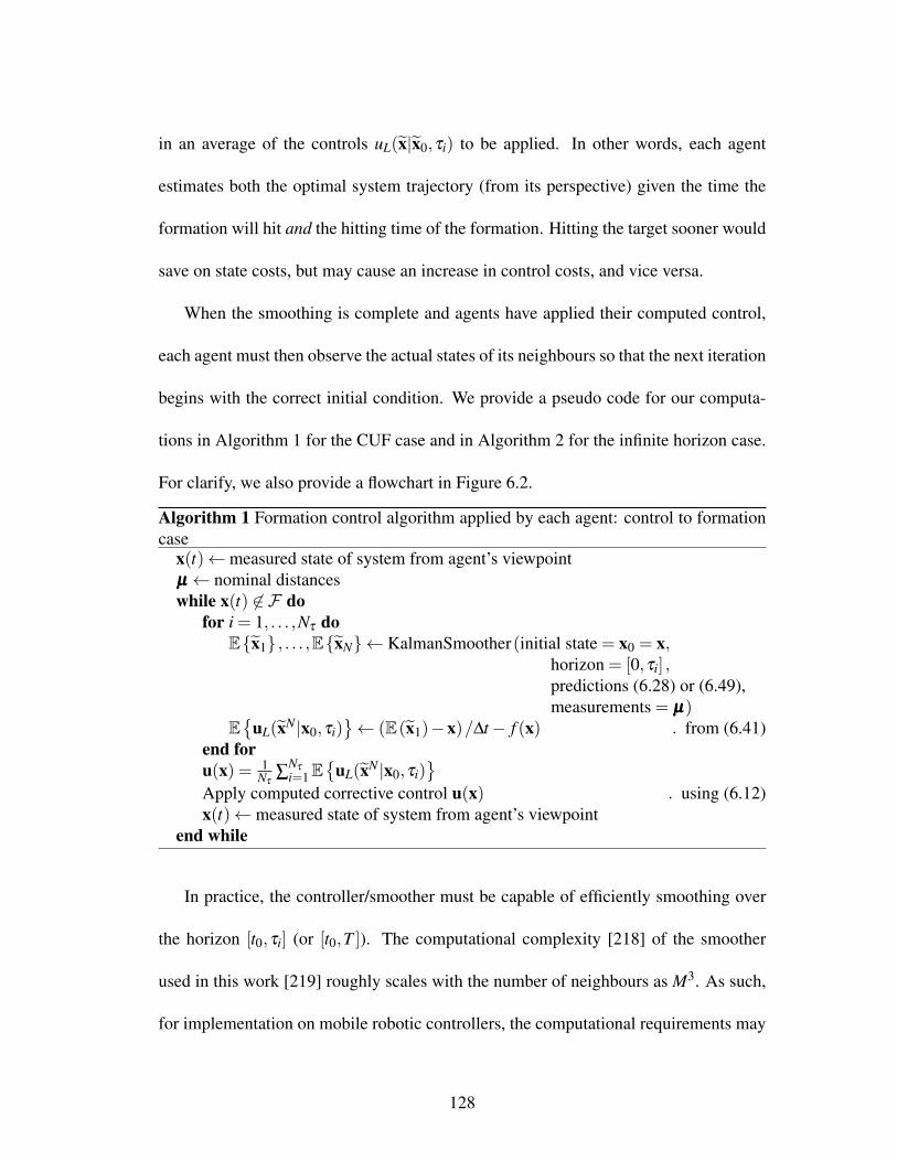
in an average of the controls uL(x|x0,τi) to be applied. In other words, each agent

estimates both the optimal system trajectory (from its perspective) given the time the

formation will hit and the hitting time of the formation. Hitting the target sooner would

save on state costs, but may cause an increase in control costs, and vice versa.

When the smoothing is complete and agents have applied their computed control,

each agent must then observe the actual states of its neighbours so that the next iteration

begins with the correct initial condition. We provide a pseudo code for our computa-

tions in Algorithm 1 for the CUF case and in Algorithm 2 for the infinite horizon case.

For clarify, we also provide a flowchart in Figure 6.2.

Algorithm 1 Formation control algorithm applied by each agent: control to formationcase

x(t)←measured state of system from agent’s viewpointµµµ ← nominal distanceswhile x(t) 6∈ F do

for i = 1, . . . ,Nτ doEx1 , . . . ,ExN← KalmanSmoother(initial state = x0 = x,

horizon = [0,τi] ,predictions (6.28) or (6.49),measurements = µµµ)

E

uL(xN |x0,τi)← (E(x1)−x)/∆t− f (x) . from (6.41)

end foru(x) = 1

Nτ∑

Nτ

i=1E

uL(xN |x0,τi)

Apply computed corrective control u(x) . using (6.12)x(t)←measured state of system from agent’s viewpoint

end while

In practice, the controller/smoother must be capable of efficiently smoothing over

the horizon [t0,τi] (or [t0,T ]). The computational complexity [218] of the smoother

used in this work [219] roughly scales with the number of neighbours as M3. As such,

for implementation on mobile robotic controllers, the computational requirements may

128

Algorithm 2 Formation control algorithm applied by each agent: infinite horizon casex(t)←measured state of system from agent’s viewpointµµµ ← nominal distancesloop

Ex1 , . . . ,ExN← KalmanSmoother(initial state = x0 = x,horizon = [0,T ] ,predictions from (6.28) or (6.49),measurements = µµµ)

u(x) = E

uL(xN |x0)← (E(x1)−x)/∆t− f (x) . from (6.52)

Apply computed corrective control u(x) . using (6.12)x(t)←measured state of system from agent’s viewpoint

end loop

prescribe a two-level approach – a high-level nonlinear fixed-interval Kalman smooth-

ing algorithm that computes reference inputs for lower-level robot control loops. How-

ever, various implementations of the smoothing algorithm can streamline the compu-

tation. For instance, a sigma point-based approximation to the two-filter smoothing

equations [279] could produce reference control values using only twice the computing

power of an unscented filtering algorithm. Moreover, through linearisation of the mea-

surement model (6.55) or of both the process and measurement models (6.54)-(6.55),

the control could be computed using extended Kalman smoother or the linear unscented

Kalman smoother, respectively. However, through full linearisation, we would effec-

tively only be solving an LQG control problem, as mentioned in Section 6.1.

6.5 Results

In this section we compare the control computed by our Kalman smoothing algorithm

against that computed by a numerical stochastic optimal control method [137], and

129

initializeprocess and

measurementmodel

UnscentedSmoothingAlgorithm

compute controlu(x) = E(x1)−x

∆t − f (x)

updateprocess

and mea-surement

model

applycontrol

(formationF reached)∩ (CUF

problem)?

stop

start

nominaldistance,relativeangles,relative

speeds µµµ

measured stateof system

from agent’sviewpoint x(t)

(E(x1), . . . ,E(xN))

no

yes

Figure 6.2: Flowchart for formation control algorithm

130

then we provide simulations in which five agents achieve formations with equal and

aligned velocities. The system and algorithm parameters were chosen as λ = 100,

σθ = σθ ,m = 0.1 (see (6.24) for R), Q = 100I, and ∆t = 0.1, with all units relative

to meters and seconds. In the case of CUF, Nτ = 10, τ = 1, . . . ,10, εr = εv = 0.1,

εθ = 10. For the infinite-horizon case, β = 0.5 and T = 10. With these parameters,

exp(−βT ) ≈ 0.007, and so the cost function (6.43) used for the algorithm is a good

approximation to a discounted infinite-horizon cost function (6.17). In each case, the

control was computed using a Discrete-time Unscented Kalman Rauch-Tung-Striebel

Smoother [218, 219].

We first apply the Markov chain approximation method [137] to compute the feed-

back control from the HJB equation for cost function (6.17) so that we may compare the

computation time and computed controls with our proposed method. In order to reduce

the dimension of the state space for the Markov chain approximation method, which

requires discretisation of the state space, we consider the problem of just two agents, fix

v1 = v2 = 1 [m/s], and aim for a nominal distance between agents of δ1 = 5 [m]. Then

the controls ω(∆x1,∆y1,θ ,θ1) and ω1(∆x1,∆y1,θ ,θ1) may be computed, although this

is computationally intensive due to the discretisation of the state space (x ∈R4) and the

control variable u ∈ R2, leading to 25,600 grid cells and 225 control possibilities for

the chosen discretisation. The left column of Figure 6.3 shows the optimal controls as

computed by the Markov chain approximation method, which, for the chosen parame-

ters, required 3.7 hours of computation time in Matlab R© on an Intel i7 at 2.7 GHz with 8

131

-

-

-

- -- .3

- .

- .

.

.

.30

0

0

0

0

0

000

0

0

0

5555

5

5

55

5

5

2

2

1

1

∆y 1

[m]

∆y 1

[m]

∆x1 [m] ∆x1 [m] ∆x1 [m]

Figure 6.3: Optimal feedback control u(∆x1,∆y1,θ1,θ2) based on a discounted infinitehorizon for two agents with fixed speed v = 1, evaluated at θ1 = θ2 = 0. The top rowis the control ω and the bottom is ω1 (i.e., the control assumed for a neighbour m = 1).(Left column) Control based on Markov chain approximation with ∆x step size = ∆ystep size = 1.05, θ1 step size = θ2 step size = .078, and control u step size 0.85 forboth ω and ω1. (Right column) Control evaluated using a Kalman smoother on thesame grid, but without control discretisation. (Center column) To compare, Kalmansmoother control down-sampled to the same control step sizes 0.85 for ω and ω1 thatare used in the left column’s control computation.

GB RAM (0.51 s per grid cell visible in Figure 6.3). To compare, the Kalman smoother

algorithm described in the previous section was applied to the same grid locations in

state space, but without the control discretisation. The Kalman smoother-based method

required only 37.26 [s] of computation time, an average of 0.09 s per grid cell, although

it is not actually necessary to compute the control for the entire state space grid.

Figure 6.3 serves two purposes. First, it is seen that the controls computed by our

method are similar to those from the Markov chain approximation method, although

with such an aggressive discretisation required by the latter, there are no guarantees

that the control solutions should be identical. Moreover, recalling that the displayed

controls are additive corrections to the non-optimal feedback controls, this figure allows

132

us to examine the regions in state space where the non-optimal feedback control is

most deficient in terms of optimality and robustness to uncertainty. For example, in

Figure 6.3 shows that little correction control is needed in regions r . 5, (i.e., u ≈ 0).

However, as agents become further separated, the reference feedback controls are not

sufficiently strong. Of course, the described corrections are only for the case θ1 = θ2 =

0 and with fixed speed, and we do not attempt in this paper to analytically improve the

reference control nor its underlying artificial potential function. However, we envision

our method being useful for control designers to analyse a “slice" or marginalisation of

their feedback control function without having to solve the HJB PDE in the entire state

space.

Next, the Kalman smoothing method is employed so that five agents achieve the

formation of a regular pentagon, where each agent is individually estimating the hid-

den optimal trajectory based on the relative kinematics of all of its neighbours. The

agents observe all others, but, as described in Section 6.2, only the inter-agent con-

nections known by an agent are used when computing the control. The instantaneous

state cost (6.14) penalizes the mean squared distance from the unicycle to all of its

M = 4 neighbours in excess of the side length of the pentagon (5 [m]) or the diagonal

of the pentagon, depending on the relative configuration of the pentagon encoded in δm,

m = 1, . . . ,4. The system parameters are the same as the previous example, with the

addition of σv = σv,m = 0.1 (see (6.24) for R).

133

For the case of CUF, we define the formation, i.e., stopping condition, as

F =

x : |rm−δm| ≤ εr,

|θ −θm| ≤ εθ ,

|v− vm| ≤ εv, m = 1, . . . ,M. (6.63)

based on tolerances εr, εθ , and εv. Figure 6.4 shows the trajectories of all agents, while

the inter-agent distances and agents’ angles and speeds can be seen in Figure 6.5. The

actual stopping time was τ = 16.1 [s], and the agents did not collide. In the last second

of the simulation, a minor deviation in the agents’ heading angles and speeds was seen.

This was due to a final correction in agents’ relative distances that was needed after

having converged in heading angle and speed. Without the addition of the optimal

controls, the collision-avoiding controls acting alone did not lead to a formation (6.63)

within the first 60 [s] of the simulation (Figure 6.5). Although the non-optimal control

aligned heading angles and, to some extent, speeds, they led to oscillatory trajectories,

which is not uncommon in the artificial potential function approach.

The infinite-horizon case may be seen in Figure 6.6, and its corresponding cost is

in Figure 6.7. The agents achieve and maintain a pentagon using the computed optimal

controls, while a simulation using only the reference feedback controls again leads to

oscillations, as seen in Figure 6.7.

As discussed in Section 6.1, the implementation of the Kalman smoothing algo-

rithm is in some ways similar to receding horizon control/model predictive control. To

compare our results against this strategy, we next consider an Euler discretisation of the

134

-4 -2 0 2 4 6 8 10

-6

-4

-2

0

2

4

6

8

10

(a)y

[m]

-4 -2 0 2 4 6 8 10

-6

-4

-2

0

2

4

6

8

10

(c)

x [m]

y[m

]

-4 -2 0 2 4 6 8 10

-6

-4

-2

0

2

4

6

8

10

(b)

-4 -2 0 2 4 6 8 10

-6

-4

-2

0

2

4

6

8

10

(d)

x [m]

-4 -2 0 2 4 6 8 10 12 14 16-8

-6

-4

-2

0

2

4

6

8

10(e)

x [m]

y[m

]Figure 6.4: Five agents, starting from random initial positions and a common speedv = 2.5 [m/s], achieve a regular pentagon formation by an individually-optimal choiceof acceleration and turning rate, without any active communication. The frames (a)through (e) correspond to the times t = 0 [s], t = 2 [s], t = 4 [s], t = 6 [s], and t = 16.4[s]. An example of collision avoidance between the two upper-left agents is seen inframes (b) and (c).

0 5 10 150

5

10

15

0 5 10 15

-100

0

100

0 5 10 150

1

2

3

t [s]

r mn

[m]

θ[d

eg]

v[m

/s]

0 10 20 30 40 50 60 700

10

20

0 10 20 30 40 50 60 700

50

100

150

0 10 20 30 40 50 60 70

0

2

4

t [s]

r mn

[m]

θ[d

eg]

v[m

/s]

Figure 6.5: Inter-agent distances rmn, agent heading angles θ , and agent speeds v asa function of time using the (left) stochastic optimal control (CUF) and the (right)deterministic feedback control.

135

-4 -2 0 2 4 6 8

-7

-5

-3

-1

1

3

5 (a)

y[m

]-2 0 2 4 6 8 10

-7

-5

-3

-1

1

3

5 (b)

0 2 4 6 8 10 12

-5

-3

-1

1

3

5

7 (c)

4 6 8 10 12 14 16-5

-3

-1

1

3

5

7(d)

8 10 12 14 16 18 20

-3

-1

1

3

5

7

9 (e)y

[m]

12 14 16 18 20 22 24

-3

-1

1

3

5

7

9 (f)

16 18 20 22 24 26 28

-3

-1

1

3

5

7

9 (g)

18 20 22 24 26 28 30

-3

-1

1

3

5

7

9 (h)

0 10 20 30 40 50 60 70 80 90

-10

0

10

20

x [m]

y[m

]

(i)

x [m] x [m] x [m] x [m]

Figure 6.6: Five agents, starting from random initial positions and a common speedv = 1 [m/s], achieve a regular pentagon formation by an individually-optimal choiceof acceleration and turning rate, without any active communication. Frames from (a)to (h) are 2.5 [s] to 20 [s], incrementing by 2.5 [s]. Frame (i) shows the end of thesimulated trajectories at 60.6 [s].

system (6.12) with noise intensity Γ = 0. At each time step, each agent must compute

the controls (u0,u1, . . . ,uN−1) that minimize the total accumulated cost (6.43) over the

horizon, at which point the first control u0 is executed, and then the process repeats.

Using the same time step (0.1 [s]) that was employed with the Kalman smoothers was

computationally prohibitive, and so we chose ∆t = 0.5 [s], resulting in 200 decision

variables. We computed the control using IPOPT [278], which required approximately

30 minutes for each time step. Figure 6.8(a) shows that the agents under MPC control

136

0 10 20 30 40 50 60 700

10

20

0 10 20 30 40 50 60 70-200

0

200

0 10 20 30 40 50 60 700

2

4

t [s]

r mn

[m]

θ[d

eg]

v[m

/s]

0 10 20 30 40 50 60 700

10

20

0 10 20 30 40 50 60 70-150

-100

-50

0

0 10 20 30 40 50 60 70

0

2

4

t [s]

r mn

[m]

θ[d

eg]

v[m

/s]

Figure 6.7: Inter-agent distances rmn, agent heading angles θ , and agent speeds v asa function of time using the (left) stochastic optimal control (infinite-horizon) and the(right) deterministic feedback control

converge to a pentagon that moves in a different direction than the Kalman smoothing-

based pentagon, but the direction of the agents’ motion was not part of the optimization

problem. The difference between the actual inter-agent distances and the nominal dis-

tances for the MPC-based trajectories are close to that from our Kalman smoothing

methods (Figure 6.8(b)), but the latter approach requires considerably less computa-

tional time (approximately 1.7 [s] to compute five agents’ controls).

Finally, we show how the choice of measurements µµµ supplied to the smoothing

algorithm can allow for dynamic morphing between formations. At the end of the

simulation in Figure 6.6, we update the nominal inter-agent distances so that agents

form a line, as seen in Figure 6.9.

6.6 Discussion

This work considers the problem of unicycle formation control in a distributed opti-

mal feedback control setting. Since this gives rise to a system with huge state space,

137

x [m]

y[m

]

0

0

20

20 40 60 80

-80

-60

-40

-20

-20

(a)

t [s]00 5

10

10 15

20

20 25

30

30

40

50

60

70

80

(b)

∑ m<

n| r m

n−

δm

n|Figure 6.8: Comparison against MPC-computed control for the same problem. (a)The dashed trajectories are those from Figure 6.6 computed using Kalman smoothingalgorithms, while the solid trajectories were computed using IPOPT [278]. (b) Thetotal error between the instantaneous formation distances and the nominal distances forthe MPC control (red) and the Kalman smoother control (blue).

80 85 90 95 100 105

10

15

20

25

30

35

x [m]

y[m

]

t = 60.6 + 8.9 [s]

Figure 6.9: Following the simulation in Figure 6.6, the set of nominal distances betweenagent m and n was modified to δmn = 5|m−n|, and the reference control was dropped.The agents are seen forming a line.

138

we exploit the stochasticity inherent in distributed multi-agent control problems in or-

der to apply a path integral method. By relating the resulting estimation problem to

Kalman smoothing algorithms, each agent can compute its optimal control using a

nonlinear Kalman smoother, greatly reducing the computational complexity associated

with multi-robot optimal control problems. The measurement and process noise of the

smoothing problem are created using the structure of the cost function and stochas-

tic kinematics. Since agents share a common prior probability distribution describing

the future trajectories of their neighbours, the formation can be attained without any

communication among agents aside from instantaneous observations of neighbours.

The typical Lyapunov function approach to problems of this type offers several

benefits, including transparency and analyticity, that are often lost in the numerical so-

lution of the Hamilton-Jacobi-Bellman equation, but the latter is also advantageous or

in some instances preferable. Our approach aims to balance the attractiveness of an

analytic feedback control for deterministic systems with the robustness to stochasticity

and optimality provided by the Hamilton-Jacobi-Bellman equation. Therefore, the op-

timal turning rate and acceleration controls affect the system alongside a non-optimal

reference feedback control law based on an artificial potential function.

Not only do the optimal correction terms improve the performance of the reference

control, leading the agents into formation faster and optimally, but the existence of an

underlying non-optimal control complements the optimal enhancement controls. For

instance, since the reference controls help to move the agents toward a formation, a

139

Kalman smoother measurement (recall that a measurement in our work is the nomi-

nal distance) does not constitute a rare event in the measurement probability model,

and, consequently, the reference controls reduce numerical issues involved in Kalman

smoothing algorithms. Moreover, without the reference controls, collision avoidance

would require complex state constraints to be added to the Kalman smoothing algo-

rithm.

Since the Kalman smoothing-based control is the additional input required along-

side the non-optimal control in order to achieve optimality and robustness, we can

envision in a future line of research using these algorithms to test feedback control laws

for multi-robot systems against various scenarios in order to derive analytical improve-

ments.

140

Chapter 7

Self-Triggered p-moment Stability forContinuous Stochastic State-FeedbackControlled Systems

This chapter is a preprint to the paper

I Anderson, R. P., Milutinovic, D., and Dimarogonas, D.V., “Self-Triggered p-moment Stability for Continuous Stochastic State-Feedback Controlled Systems”,submitted to the IEEE Transactions on Automatic Control.

7.1 Introduction

The implementation of nonlinear feedback controllers on digital computer platforms

necessitates a choice of time points at which the controller should be updated. In tra-

ditional setups, these updates are scheduled periodically with conservative, short time

periods that under all circumstances do not compromise the stability of closed loops.

However, a longer period between controller updates can offer greater design flexibil-

ity and increase the availability of computational resources. Having that in mind, a

more suitable approach for scheduling controller updates would take into account sys-

141

tem states and perform updates only when necessary. Along these lines, the approaches

of event- and self-triggering have recently been proposed to lengthen the intervals be-

tween the updates without sacrificing stability [1, 17–19, 21, 77, 104, 144, 162, 163,

172, 194, 202, 248, 275, 281–283]. The time at which the control should next be up-

dated is derived in a way that ensures asymptotic stability of the closed-loop feedback

control system with respect to errors caused by outdated samples. Since the decision

to update hinges upon a state-dependent or sample-dependent criterion, the intervals

between updates vary and may be longer than those under a periodic control imple-

mentation [21].

In an event-triggered control implementation, the system state is updated when it

deviates from the previous sample by a sufficient amount [1, 21, 104, 172, 194, 202,

248, 281]. This requires continuous monitoring of the system state, which may be im-

practical. Therefore, in this paper, we consider a self-triggering approach in which the

next update is defined based on the last sampled data [17, 18, 144, 162, 163, 275, 282].

In this case, the decision to update is computed from predictions of when the system

state will deviate by a given threshold from the last update. However, for systems under

the influence of disturbances or noise, it may be more difficult to make these predictions

or to guarantee that the intended stability results are retained. Along these lines, the ro-

bustness of a self-triggered control strategy to disturbances was analyzed in [163] for

linear systems. In [282], a self-triggered H∞ control was developed for linear systems

with a state-dependent disturbance, and this was extended in [283] for an exogenous

142

disturbance in L2 space.

In this work, we develop a self-triggered scheme for the control of stochastic dy-

namical systems described by stochastic differential equations (SDEs) [157] with ad-

ditive noise terms. In the area of control, this type of dynamical model is commonly

used for Kalman, or Extended Kalman filter designs [108]. For systems of this type,

not only can it be difficult to predict the system state at a future time, but the noise may

drastically alter the system dynamics. Because of that, we use the dynamics of certain

statistics of the state distribution to develop an update rule that guarantees p-moment

stability [116, 157] (p > 0) of the SDE solution. The length of times between controller

updates is based on the previously-measured state and is shown to be strictly positive.

Since the intensity of the noise in many stochastic systems is independent of the state,

we split our analysis into two parts, one in which the noise diminishes as the system

state approaches a stable equilibrium, and the other in which this is not the case.

In this paper, we simplify the update rule that was initially presented in [13] and bet-

ter elucidate both the reasons for, and the consequences of the differences between our

self-triggered approach and that for deterministic systems. We recently became aware

of one other attempt at self-triggered stabilization of stochastic control systems. In [3],

the authors develop a self-triggering rule for SDEs that guarantees stability in proba-

bility (note that this is weaker than p-moment stability). However, since their approach

is based on a technique found in literature for event- and self-triggered deterministic

systems, the assumptions on the control system are strict, and, as a result, no examples

143

have so far been provided with which we can compare the length of times between task

updates. Therefore, another contribution of this paper is in providing examples that will

be useful for future work comparisons. The first is a stochastic version of a linear con-

trol problem from deterministic literature [248], and the second is a stochastic wheeled

cart control problem whose motivation is detailed in [11, 15, 16].

This paper is organized as follows: In Section 7.2, we introduce relevant notation

and definitions, formulate the problem, and call attention to why the standard deter-

ministic approach for event- and self-triggering may not apply, both theoretically and

pragmatically, to stochastic systems. Section 7.3 presents some stability results for

stochastic differential equations. Section 7.4 proposes a self-triggering scheme with

strictly positive times between control updates, and Section 7.5 provides numerical ex-

amples. Finally, Section 7.6 summarizes the results of this paper and provides possible

directions for future research.

7.2 Preliminaries and Problem Statement

7.2.1 Notation and Definitions

We will consider control systems defined by stochastic differential equations of the

form

dx(t) = f (x,u)dt + g(x,u)dw, x ∈ Rn, (7.1)

144

where dw is a (multi-dimensional) increment of a standard Wiener process, u(t) :

[0,∞)→ Rm is a control input, and f (·, ·) and g(·, ·) are the drift and diffusion scal-

ing factors of the dynamics. The differential operator L associated with a system in this

form, when applied to a function V (x, t) that is twice-differentiable in its first argument,

is

LV (x, t) =∂V∂ t

+ f ᵀ∂V∂x

+12

Trace(

gᵀ∂ 2V∂x2 g

). (7.2)

Usually these systems are formally defined alongside a complete probability space

(Ω,F ,P) [183], where Ω is the set of possible outcomes, F is a filtration, and P is

a probability measure function mapping F → [0,1]. We will also need the following

definitions and notations. A function γ : R≥0→ R≥0 is of class K if it is continuous,

strictly increasing, and γ(0) = 0. It is of class K∞ if, in addition, it is unbounded. A

function β : R≥0× [0,∞)→ R≥0 is of class KL if, for each fixed t, β (x, t) is of class

K, and, for each fixed x, β (x, t) is decreasing with β (x, t)→ 0 as t → ∞. Let | · | de-

note the Euclidean norm |x| =√

xᵀx. For two constants a and b, we use the notation

a∨b = maxa,b and a∧b = mina,b.

Definition 7.2.1 (cf. [152]) A system is said to be p-moment1 input-to-state stable (ISS)

with respect to an error e(t) if there exist a class KL function β and class K functions

γ and λ such that for all t ≥ 0,

E(|x(t)|p)≤ β (E(|x(0)|p) , t)+ γ

(E

(λ (sup

t≥0|e(t)|)

)). (7.3)

1To be concise, note that p−th moment actually refers to the expected value of the Euclidean normraised to the p-th power [157].

145

In many systems, the diffusion scaling g(·, ·) is independent of the state and control

and does not vanish at the origin. For systems of this type, the second-order term in

(7.2) may be a constant. In this work, we treat that constant as an additional disturbance,

denoted d, that acts alongside the error due to sampling e(t). The following definition

will later be used to account for this.

Definition 7.2.2 (cf. [152]) A system is said to be practically p-moment stable if there

exist a class KL function β , a class K function γ , and a constant d ≥ 0 such that for

all t ≥ 0,

E(|x(t)|p)≤ β (E(|x(0)|p) , t)+ γ(d).

If d = 0, the system is said to be p-moment stable (see Definition 2.1 in [116]).

Definition 7.2.3 ([152]) A function V is said to be a stochastic input-to-state stable

Lyapunov function with respect to an error e(t) if there exist class K∞ functions α and

α and class K functions α and λ such that

α(|x|)≤V (x)≤ α(|x|) (7.4)

LV ≤ λ (|e|)−α(|x|). (7.5)

146

7.2.2 Problem Statement

We consider the state-feedback controlled system (7.1) with sample-and-hold state

measurements, i.e.,

dx(t) = f (x,u)dt + g(x,u)dw (7.6)

u(t) = k(xi), t ∈ [ti, ti+1) (7.7)

where ti, i = 0,1, . . ., is a sequence of update, or triggering, times, and xi = x(ti), i =

0,1, . . ., is the corresponding sequence of measurements of the system state that is used

to update the feedback control k(xi). Let us define the error signal e(t) as

e(t) = xi− x(t), t ∈ [ti, ti+1) . (7.8)

Then (7.6) is

dx(t) = f (x,k(x + e))dt + g(x,k(x + e))dw (7.9)

To simplify notation in the sequel, we will write with a slight abuse of notation f (x,e)

instead of f (x,k(x + e)) and g(x,e) instead of g(x,k(x + e)). We make the following

assumptions of monotone growth and local Lipschitz continuity, which are no stronger

than the standard conditions for the existence and uniqueness of the process x(t) (cf.

[157, Theorem 2.3.5] with e = 0).

Assumption 1) There exists a positive constant K such that for all x,e ∈ Rn and

t ∈ [ti, ti+1), i = 0,1, . . .,

xᵀ f (x,e)+12|g(x,e)|2 ≤ K(1 + |x|2 + |e|2) (7.10)

147

Assumption 2) For every integer m≥ 1, there exist a positive constant Lm such that

for all x,e,x′,e′ ∈ Rn with |x|∨ |x′|∨ |e|∨ |e′| ≤ m and t ∈ [ti, ti+1),

| f (x,e)− f (x′,e′)|2∨|g(x,e)−g(x′,e′)|2 ≤ Lm(|x− x′|2 + |e− e′|2)

(7.11)

The goal of this paper is to develop an update rule for the stochastic system (7.8)-

(7.9) based on the observable state xi, i = 0,1, . . . that will render the system practically

stable while guaranteeing strictly positive inter-execution times τi = ti+1− ti, that is,

there is some minimum time between sampling time points. If g(0,0) = 0, i.e., if g

admits an equilibrium point and the noise vanishes at the origin, then we will seek

p-moment stability.

7.2.3 Motivating our Approach

For the purpose of motivating the sequel, we will first begin to formulate the prob-

lem using an approach found in literature for deterministic event-triggered and self-

triggered control systems and describe how this fails when applied to stochastic control

systems.

This usually begins with an assumption of input-to-state stability [235] of the closed-

loop feedback control system with respect to errors caused by outdated samples. Along

these lines, let us assume the existence of a stochastic input-to-state Lyapunov function

148

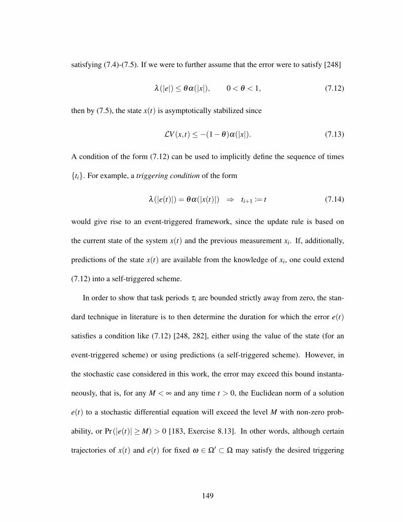
satisfying (7.4)-(7.5). If we were to further assume that the error were to satisfy [248]

λ (|e|)≤ θα(|x|), 0 < θ < 1, (7.12)

then by (7.5), the state x(t) is asymptotically stabilized since

LV (x, t)≤−(1−θ)α(|x|). (7.13)

A condition of the form (7.12) can be used to implicitly define the sequence of times

ti. For example, a triggering condition of the form

λ (|e(t)|) = θα(|x(t)|) ⇒ ti+1 := t (7.14)

would give rise to an event-triggered framework, since the update rule is based on

the current state of the system x(t) and the previous measurement xi. If, additionally,

predictions of the state x(t) are available from the knowledge of xi, one could extend

(7.12) into a self-triggered scheme.

In order to show that task periods τi are bounded strictly away from zero, the stan-

dard technique in literature is to then determine the duration for which the error e(t)

satisfies a condition like (7.12) [248, 282], either using the value of the state (for an

event-triggered scheme) or using predictions (a self-triggered scheme). However, in

the stochastic case considered in this work, the error may exceed this bound instanta-

neously, that is, for any M < ∞ and any time t > 0, the Euclidean norm of a solution

e(t) to a stochastic differential equation will exceed the level M with non-zero prob-

ability, or Pr(|e(t)| ≥M) > 0 [183, Exercise 8.13]. In other words, although certain

trajectories of x(t) and e(t) for fixed ω ∈ Ω′ ⊂ Ω may satisfy the desired triggering

149

criteria for a sufficiently large time, the same can not be said about all trajectories x(t)

and e(t) defined by (7.8)-(7.9). Moreover, the second-order differential terms required

in stochastic evolution equations can cause certain quantities found in deterministic lit-

erature (e.g., the quantity |e(t)|/|x(t)| [248]) to experience unbounded growth near the

origin. These facts make it difficult to develop a sampling rule using the trajectories e(t)

and x(t) or predictions of these processes. Because of this, we instead consider the p-th

moments of these processes, E(|e|p) and E(|x|p), and develop a triggering condition

based on these statistics to guarantee the stability of x(t) in the p-th moment [157].

As a consequence of this basis for the update rule, we must rule out an event-

triggered implementation. From a practical standpoint, the controller can only measure

an individual sample path of the process x(t), and not the statistics E(|e|p) or E(|x|p).

However, the latter quantities can be predicted on the interval [ti, ti+1) based on the

last-sampled state xi, and are therefore suitable for a self-triggered approach.

7.3 A Lyapunov Characterization for p-moment

Input-to-state Stability

Since this work deals with stability in the p-th moment, we must first revise the prelim-

inary notion of stability used to motivate this work (7.4)-(7.5) and provide a Lyapunov

function-based stability criterion for p-moment ISS. The characterization of stability in

the following theorem is similar to that provided in (7.4)-(7.5), but with the addition of

150

expectation operators so that we may examine triggering rules based on the statistics

E(|x|p) and E(|e|p) of the processes considered in this work.

Theorem 7.3.1 Suppose there exist a convex class K∞ function α , a class K∞ function

α , a non-negative function α , and non-negative function V (x, t) that is twice differen-

tiable in its first argument such that

α(|x|p)≤V (x, t)≤ α(|x|p), (7.15)

ELV (x, t)≤ E(λ (|e|))−E(α(x(t))) (7.16)

for all t ≥ 0, where lim|x|→∞ α(x)/α(|x|p)> 0. Then the system (7.6)-(7.8) is p-moment

ISS.

Theorem 7.3.1 is a specific case of [116, Theorem 3.1]. The latter applies to more

general systems with delays and Markovian switching. That the Lyapunov character-

ization we use arises from the study of stochastic differential delay equations should

not come as a surprise, since a sample xi really amounts to a delayed state variable.

However, in order to more closely tie these ideas with previous literature on event- and

self-triggered control, we have removed the notion of a delay. Nevertheless, the proof

of Theorem 7.3.1 is very similar to that of [116, Theorem 3.1], but for completeness,

we include the relevant elements of that work here. We first provide an accompanying

lemma.

Lemma 7.3.1 For any t ≥ 0, there is a constant aw > 0 such that E(α(x))≥ aw when-

ever E(V (x, t))≥ av > 0.

151

Proof: We show the existence of a class K∞ function µw(·) such that E(α(x)) ≥

µw(av) = aw whenever E(α(|x|p))≥ av > 0. Fix t and define a function b : R≥0→R≥0

b(y) = inf|x|p≥α

−1(y/2)

α(x)

α(|x|p), y≥ 0,

that is non-decreasing by construction. By the properties of α(x) and α(|x|p), we have

that b(y) > 0 whenever y > 0. Then if, for any av > 0, E(α(|x|p))≥ E(V (x, t)))≥ av,

we have that

E(α(x)) =∫Ω

α(x)dP

≥∫

|x|p≥α−1(av/2)

α(x)dP

≥ b(av)∫

α(|x|p)≥av/2

α(|x|p)dP≥ avb(av)

2,

where the lemma follows with µw(av) = avb(av)/2.

We now continue with the proof of the theorem adapted from [116].

Proof: Let eλ = supt≥0E(λ (|e|)) ≤ E(λ (supt≥0 |e(t)|)

)and α0 = α (E(|x(0)|p)).

Without loss of generality, choose µw(·) such that 0 < µ−1w (2eλ ) < α0. We will show

that

E(V (x, t))≤ α0∧µ−1w (2eλ ), t ≥ 0. (7.17)

We first show that E(V (x, t))≤ α0 for all t ≥ 0. Suppose that

ta = inft > 0 : E(V (x, t)) > α0 ,

and assume for the purpose of contradiction that ta < ∞. Since E(V (x, t)) is continuous,

152

there must be constants tb, tc, and ε > 0 satisfying 0≤ tb ≤ ta < tc andE(V (x, t)) = α0 t = tb

α0 < E(V (x, t)) < ε + α0 tb < t ≤ tc

(7.18)

However, the expected value of the Lyapunov function satisfies

E(V (x(t), t)) = E(V (x(tb), tb))+Et∫

tb

LV (x(s),s)ds

= E(V (x(tb), tb))+

t∫tb

ELV (x(s),s)ds

≤ α0 +

t∫tb

(eλ −2eλ )ds≤ α0− eλ (t− tb) < α0

for tb < t ≤ tc, which contradicts (7.18), so E(V (x, t))≤ α0 for all t ≥ 0.

Next, we show that for a time tµ satisfying tµ/eλ > α0, we have E(V (x, t)) ≤

µ−1w (2eλ ) for all t ≥ tµ . Let τ = inf

t ≥ 0 : E(V (x, t))≤ µ−1

w (2eλ )

and suppose for

the purpose of contradiction that τ > tµ . Then E(V (x, t)) ≥ µ−1w (2eλ ) for t ≤ tµ , and

by Lemma 7.3.1, we have E(α(x))≥ 2eλ , so that for all 0≤ t ≤ tµ ,

E(V (x(t), t)) = E(V (x(0),0))+

t∫0

ELV (x(s),s)ds

≤ α0 +

tµ∫0

(eλ −2eλ )ds≤ α0− eλ tµ < 0, (7.19)

which violates the fact that E(V (x, t)) ≥ 0 for all t ≥ 0, and so τ ≤ tµ . Next, let tµa =

inf

t > τ : E(V (x, t)) > µ−1w (2eλ )

and suppose that tµa < ∞. Then there must exist

153

constants tµb and tµc such that tµ ≤ tµb ≤ tµa < tµc andE(V (x, t)) = µ−1

w (2eλ ) t = tµb

µ−1w (2eλ ) < E(V (x, t)) < ε + µ−1

w (2eλ ) tµb < t ≤ tµc

Consequently, we can derive in a similar manner that E(V (x(t), t)) ≤ µ−1w (2eλ )−

eλ (t − tµb), which again contradicts the fact that E(V (x, t)) ≥ 0 for all t ≥ 0, and so

E(V (x, t))≤ µ−1w (2eλ ) for all t ≥ tµ .

We return to the statement of the theorem to show that, using Jensen’s inequality

and (7.17), for t ≥ tµ ,

α (E(|x|p))≤ E(α(|x|p))≤ E(V (x, t))

≤ µ−1w (2eλ )≤ µ

−1w

(2E

(λ (sup

t≥0|e(t)|)

)), (7.20)

which implies that

E(|x|p)≤ α−1

(µ−1w

(2E

(λ (sup

t≥0|e(t)|)

)))

≡ γ

(E

(λ (sup

t≥0|e(t)|)

)), t ≥ tµ , (7.21)

where γ(|x|) = α−1 (µ−1w (2|x|)

)is class K by construction.

Let β be a class KL function satisfying β (α(|x0|p, t) = β (α0, t)≥ 2α0−α0(t/tµ)

for all 0≤ t ≤ tµ . Then it follows from (7.17) that E(V (x, t))≤ β (α0, t) for all 0≤ t ≤

tµ , and consequently

E(|x|p)≤ α−1(

β (α0, t))

= β (E(|x(0)|p), t) (7.22)

154

for 0 ≤ t ≤ tµ , where β (x, t) = α−1(

β (α(x), t))

is a class KL function. The desired

result (7.3) follows from (7.21)-(7.22).

7.4 Triggering Condition

Suppose that there is a Lyapunov function for the system (7.6)-(7.8) satisfying (7.15)

and

ELV (x, t)≤ E(λ (|e|))−E(α(x(t)))+ d (7.23)

Here, d > 0 allows for the possibility of a constant disturbance that does not diminish at

the origin. This may occur, for example, if the second-order term in (7.2) is a constant.

In our approach, we use this secondary disturbance to our advantage and include it in

the update rule. Next, suppose that the error were to satisfy (cf. (7.12))

E(λ (|e|))≤ θE(α(x))+ θdd, (7.24)

for a constant 0 < θ < 1 and parameter θd > 0. Then from (7.16),

ELV ≤−(1−θ)E(α(x))+(1 + θd)d. (7.25)

In this case, (7.25) does not include the error e(t) due to the sampling rule, but does

include the constant disturbance (1+θd)d. By rewriting (7.16) with λ (|e|) replaced by

(1 + θd)d and using Theorem 7.3.1, one can show that the system will be practically

p-moment stable with γ(d) in (7.3) replaced by γ((1 + θd)d). If (1 + θd)d = 0, i.e., if

d = 0, then the system will be p-moment stable.

155

7.4.1 Predictions of the moments of the processes

Before developing our controller update rule, we require some relations that can be

derived from the SDE assumptions (7.10)-(7.11). These lemmas relate the predictions

of the statistics E(|e|2) and E(|x|2), which are not observable, to the norm of the last-

observed system state xi.

Lemma 7.4.1 Assume the monotone growth assumption (7.10). If the system state has

been updated as xi = x(ti), then for any t ∈ [ti, ti+1), the means of the norms |e(t)|2 and

|x(t)|2 are upper and lower bounded, respectively, based on the following inequalities

E(|e(t)|2)≤ A(|xi|, t− ti) (7.26)

E(|x(t)|2)≥ B(|xi|, t− ti) (7.27)

where

A(|xi|, t− ti) =2|xi|2 + 1

3

(e12K(t−ti)−1

)(7.28)

B(|xi|, t− ti) =5|xi|2 + 1

3e−6K(t−ti)− 2|xi|2 + 1

3(7.29)

Proof: Using Itô’s Lemma and (7.8), we get

dE(|e|2)≤ dE(2|xi|2 + 2|x|2

)= 2E

(2xᵀ f (x,e)dt + 2xᵀg(x,e)dw + |g(x,e)|2dt

)= 4E

(xᵀ f (x,e)+

12|g(x,e)|2

)dt

156

From the monotone growth condition (7.10)

ddtE(|e|2)≤ 4K

(1 +E(|x|2)+E(|e|2)

)≤ 4K

(1 +E(|xi− e|2)+E(|e|2)

)≤ 4K

(1 + 3E(|e|2)+ 2E(|xi|2)

)≤ 12KE(|e|2)+ 8K|xi|2 + 4K

Applying the comparison principle in [130], along with the fact that e(ti) = 0, we obtain

(7.26). For the second inequality (7.27), we can obtain in a similar manner

∣∣dE(|x|2)∣∣≤ ∣∣E(2xᵀ f (x,e)dt + 2xᵀg(x,e)dw + |g(x,e)|2dt

)∣∣= 2

∣∣∣∣E(xᵀ f (x,e)+12|g(x,e)|2

)dt∣∣∣∣

≤ 6KE(|x|2)dt + 4K|xi|2dt + 2Kdt,

so that

ddt

(−E(|x|2)

)≤−6K

(−E(|x|2)

)+ 4K|xi|2 + 2K. (7.30)

Using the comparison principle with x(ti) = xi yields (7.27).

Lemma 7.4.2 Assume the local Lipschitz continuity assumption (7.11) where f (·, ·)

and g(·, ·) admit an equilibrium point, i.e., f (0,0) = 0 and g(0,0) = 0. If the system

state has been updated as xi = x(ti), then for any t ∈ [ti, ti + τi), the quantities E(|e(t)|2)

and E(|x(t)|2) are upper and lower bounded, respectively, based on the following in-

157

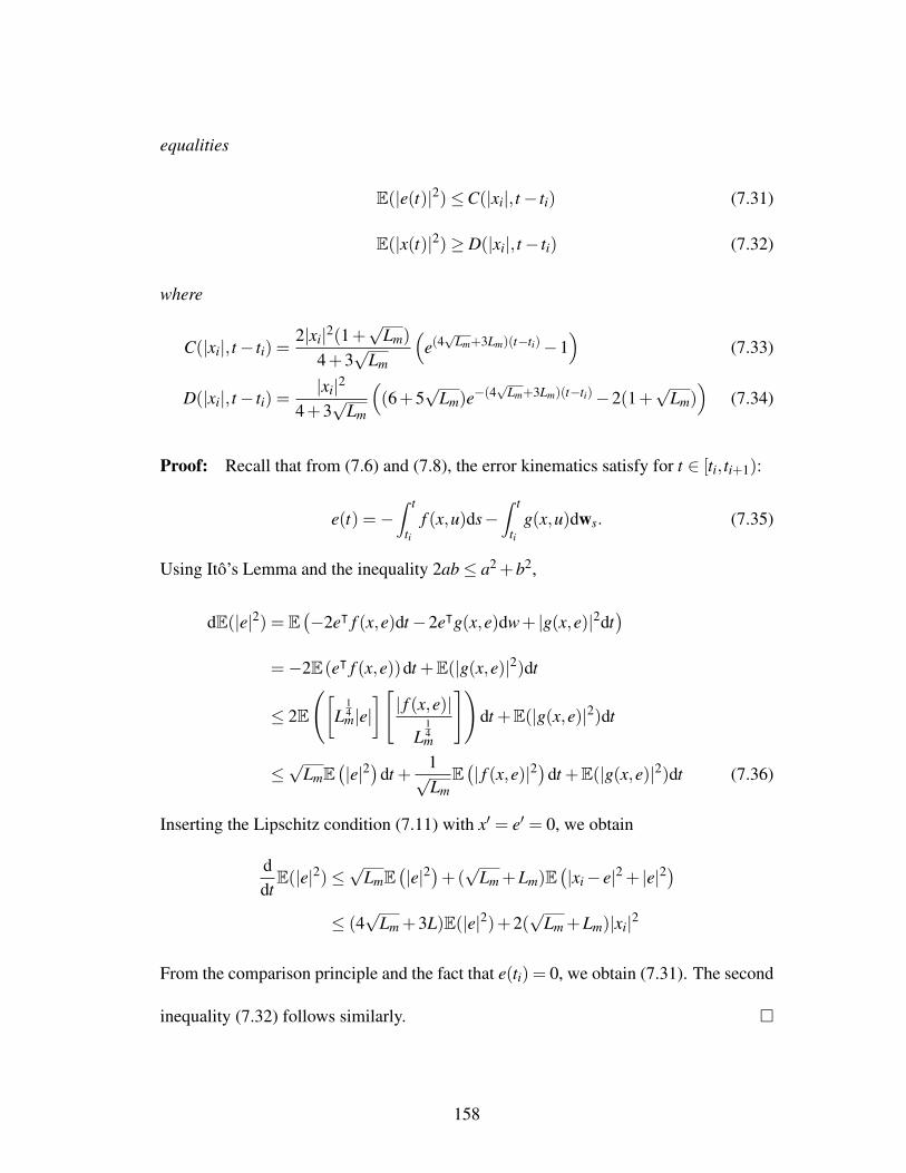
equalities

E(|e(t)|2)≤C(|xi|, t− ti) (7.31)

E(|x(t)|2)≥ D(|xi|, t− ti) (7.32)

where

C(|xi|, t− ti) =2|xi|2(1 +

√Lm)

4 + 3√

Lm

(e(4√

Lm+3Lm)(t−ti)−1)

(7.33)

D(|xi|, t− ti) =|xi|2

4 + 3√

Lm

((6 + 5

√Lm)e−(4

√Lm+3Lm)(t−ti)−2(1 +

√Lm))

(7.34)

Proof: Recall that from (7.6) and (7.8), the error kinematics satisfy for t ∈ [ti, ti+1):

e(t) =−∫ t

tif (x,u)ds−

∫ t

tig(x,u)dws. (7.35)

Using Itô’s Lemma and the inequality 2ab≤ a2 + b2,

dE(|e|2) = E(−2eᵀ f (x,e)dt−2eᵀg(x,e)dw + |g(x,e)|2dt

)=−2E(eᵀ f (x,e))dt +E(|g(x,e)|2)dt

≤ 2E

([L

14m|e|][ | f (x,e)|

L14m

])dt +E(|g(x,e)|2)dt

≤√

LmE(|e|2)

dt +1√Lm

E(| f (x,e)|2

)dt +E(|g(x,e)|2)dt (7.36)

Inserting the Lipschitz condition (7.11) with x′ = e′ = 0, we obtain

ddtE(|e|2)≤

√LmE

(|e|2)

+(√

Lm + Lm)E(|xi− e|2 + |e|2

)≤ (4√

Lm + 3L)E(|e|2)+ 2(√

Lm + Lm)|xi|2

From the comparison principle and the fact that e(ti) = 0, we obtain (7.31). The second

inequality (7.32) follows similarly.

158

7.4.2 A Self-triggering Sampling Rule

With these inequalities on E(|e(t)|2) and E(|x(t)|2), we are ready to state our main

results. The following theorems provide relations based on (7.24) that can be used to

calculate a strictly positive inter-execution time τi = ti+1− ti as a function of the last-

observed state xi. The first theorem requires Lemma 7.4.1, which does not assume

that g(0,0) = 0, and guarantees practical p-th moment stability (d > 0). The second

theorem uses Lemma 7.4.2, which assumes a state-dependent diffusion coefficient such

that g(0,0) = 0, and allows for d ≥ 0, i.e., p-moment stability can be achieved with

d = 0.

Theorem 7.4.1 Assume that in addition to the conditions of Theorem 7.3.1 and Lemma

7.4.1, there exist a convex class K function αv(·) and a concave class K function λc(·)

which satisfy

αv(2|x|2)≤ 2α(x) (7.37)

λc(|e|)≥ λ (√|e|). (7.38)

Suppose that the system (7.6)-(7.8) has been updated at t = ti with state xi, and that the

time until the next update τi = ti+1− ti is such that

λc (A(|xi|,τi))≤ θαv (B(|xi|,τi)+ dα) . (7.39)

Then (7.24) will hold with

θdd = θαv(2dα)/2, (7.40)

159

ensuring practical p-moment stability. Moreover, if dα > 0 and |xi| ≤ x < ∞, the execu-

tion times do not reach an accumulation point, i.e., τi > 0, i = 0,1, . . ..

Proof: Substitution of the inequalities (7.26) and (7.27) into (7.39) gives

λc(E(|e|2)

)≤ θαv

(E(|x|2)

+ dα

). (7.41)

Since αv(·) is convex, we have from (7.37) and Jensen’s inequality that the right hand

side of (7.41) is

θαv(E(|x|2)

+ dα

)= θαv

(2(

12E(|x|2)+

12

dα

))≤ θE

(αv(2|x|2)/2

)+ θαv(2dα)/2

≤ θE(α(|x|))+ θdd (7.42)

which is the right hand side of (7.24) with θdd = θαv(2dα)/2. Similarly, through the

concavity of λc(·) and (7.38), the left hand side of (7.41) can also be made to match

that of (7.24) using the assumption λc(E(|e|2)

)≥ E(λ (|e|)):

E(λ (|e|))≤ E(λc(|e|2)

)≤ λc

(E(|e|2)

).

In summary, we have shown that (7.39) implies (7.24), i.e.,

E(λ (|e|))≤ λc (A(|xi|,τi))≤ θαv (B(|xi|,τi)+ dα)≤ θE(α(|x|))+ θdd.

Next, to show the existence of a lower bound for the inter-execution times implicitly

160

defined by (7.39), let us define a function κ(|xi|) that is chosen to satisfy

0 < κ(|xi|) < |xi|2 + dα . for all |xi| ≥ 0 (7.43)

Clearly such a κ(·) exists, and, moreover, κ(|xi|) > A(|xi|,0) and κ(|xi|) < B(|xi|,0) +

dα . We need to verify that there exists a τi such that

λc (A(|xi|,0)) < λc (κ(|xi|))≤ λc (A(|xi|,τi))

≤ θαv (B(|xi|,τi)+ dα)≤ αv (κ(|xi|)) < αv (B(|xi|,0)+ dα) .

By solving for τi in both κ(|xi|)≤ A(|xi|,τi) and κ(|xi|)≥ B(|xi|,τi)+ dα , we obtain

τi ≥1

12Kln(

1 + κ(|xi|)3

2|xi|2 + 1

)∧ − 1

6Kln(

1− 3(|xi|2 + dα −κ(|xi|))5|xi|2 + 1

)> 0. (7.44)

where the strict positivity of the right hand side is due to the relation (7.43).

Remark 7.4.1 The inter-execution times τi, i = 0,1, . . ., may be calculated numerically

from (7.39) based on the norm of the last-observed state |xi|.

Remark 7.4.2 We have not assumed that g(0,0) = 0 for the proof of this theorem.

Therefore, this result is useful for systems where noise does not vanish at the origin. In

this case, it is likely that d > 0 (and dα > 0).

Note that for some systems the duration of the inter-execution times τi defined by

(7.39) may be lengthened with increasing dα . However, with longer inter-execution

times due to increased dα comes a larger value of γ((1 + θd)d) in (7.3).

161

If the constant disturbance is d = 0 (which is often the case when g(0,0) = 0), one

could apply Theorem 7.4.1 with a dα > 0, although this would only guarantee practical

p-th moment stability, and it would introduce a d > 0 to (7.24). To avoid this, we

next show how p-moment stability (i.e., d = 0) can be achieved for systems where

f (0,0) = g(0,0) = 0 in the following theorem.

Theorem 7.4.2 Assume that in addition to the conditions of Theorem 7.3.1 and Lemma

7.4.2, there exist a convex class K function αv(·) and a concave class K function λc(·)

as in (7.37)-(7.38). Suppose that the system (7.6)-(7.8) has been updated at t = ti with

state xi, |xi|> 0, and that the time until the next update τi = ti+1− ti is such that

λc (C(|xi|,τi))≤ θαv (D(|xi|,τi)+ dα) (7.45)

Then (7.24) will hold with θdd = θαv(2dα)/2 (and d = 0 if dα = 0), ensuring practical

p-moment stability if dα > 0 or p-moment stability if dα = 0. Moreover, for any non-

negative dα and |xi| ≤ x < ∞, the execution times do not reach an accumulation point,

i.e., τi > 0, i = 0,1, . . ..

Proof: The desired relation (7.24) follows in the same way as in the proof of Theo-

rem 7.4.1 with the use of C(|xi|,τi) and D(|xi|,τi) in place of A(|xi|,τi) and B(|xi|,τi).

For the lower bound on τi, choose a function κ(|xi|) to satisfy

0 < κλ (|xi|) < |xi|2 + dα , for all |xi|> 0 (7.46)

lim|xi|→0+

κ(|xi|)|xi|2

< 1 (7.47)

162

Inverting κ(|xi|)≤C(|xi|,τi) and κ(|xi|)≥ D(|xi|,τi) for τi, we obtain

τi ≥1

4 + 3√

Lmln(

1 +4 + 3

√Lm

2 + 2√

Lm

κ(|xi|)|xi|2

)∧ − 1

4 + 3√

Lmln(

1− 4 + 3√

Lm

6 + 5√

Lm

(|xi|2 + dα −κ(|xi|))|xi|2

)(7.48)

and using (7.46)-(7.47), τi > 0.

Remark 7.4.3 Note that (7.45) must only hold for |xi|> 0 while (7.39) assumes |xi| ≥ 0.

This is the case for two reasons. First, Theorem 7.4.2 applies to systems admitting the

trivial solution x(t) = 0, and so the case |xi|= 0 can be excluded. Moreover, choose in

the proof of Theorem 7.4.2 κ(|xi|) = a|xi|2 for 0 < a < 1, for example, and let dα = 0.

Then (7.48) becomes

τi ≥1

4 + 3√

Lmln(

1 + a4 + 3

√Lm

2 + 2√

Lm

)∧ − 1

4 + 3√

Lmln(

1− (1−a)4 + 3

√Lm

6 + 5√

Lm

)> 0.

7.5 Numerical Examples

In this section we provide examples and show how the triggering rule should change

depending on the form of the intensity of noise at x = 0.

7.5.1 Stochastic Linear System

The first example is drawn from [248]. In the example, we have added Wiener process

increments with both a constant scaling factor σ/2 and a state-dependent coefficient

163

σx|x|/2. The system is

d

x1

x2

=

0 1

−2 3

x1

x2

dt +

0

1

udt +12

(σ + σx|x|)

dw1

dw2

with u = x1− 4x2. Using V (x) = xᵀPx as a Lyapunov function, we can obtain LV ≤

−xᵀQx + σ2x |x|2 + σ2 with

P =

1 14

14 1

, Q =

12

14

14

32

Under a sampled-data implementation, this becomes

LV ≤−(a−σ2x )|x|2 + b|e||x|+ σ

2

where a = λm(Q) > 0.44 is the smallest eigenvalue of Q, and b = |KᵀBᵀP+PBK|= 8.

As our triggering results involve expectation operators, we take the expectation of both

sides and apply Hölder’s inequality

ELV ≤−(a−σ2x )E|x|2 + bE(|e||x|)+ σ

2

≤−(a−σ2x )E|x|2 + b

√E(|e|2)

√E(|x|2)+ σ

2

≤−(a−σ2x )E|x|2 + b

√E(|e|2)

√E(|x|2)+

θd

θσ2 + σ

2

where the constant term involving θd > 0 has been added in order to facilitate the

following triggering rule. If we were to assume that

E(|e|2)≤ θE(|x|2)+ θdσ2, (7.49)

for some constant 0 < θ < (a−σ2x )2/b2, then

ELV ≤−(a−σ2x −b

√θ)E|x|2 + σ

2(1 +θd√

θb)

164

and based on Theorem 7.3.1, we will obtain practical stability in the p = 2 moment, i.e.,

in the mean square sense. In light of the triggering rule (7.49), we set2 αv(|x|) = |x|,

and λc(|e|) = |e|, meaning that the update times τi given |xi| can be solved numerically

using Theorem 7.4.1 from

A(|xi|,τi)≤ θB(|xi|,τi)+ dα (7.50)

with dα = θdσ2/θ . Note that with these choices of λc(|e|) and αv(|x|), it is possible

to write down an analytic triggering rule through an appropriate choice of κ(|xi|) using

(7.43) and (7.44), but this may decrease the duration of the time between updates.

For our first simulations of this system, we choose σ = σx = 0.1. The monotone

growth and Lipschitz coefficients in (7.10) and (7.11) are

K =

( |BK|22

+σ2

x4−1)∨ |BK|

2∨ σ2

4= 7.5025

Lm = (2σ2x + 2|A + BK|2)∨2|BK|2 = 34,

respectively, and (a−σ2x )/b = 0.0537, so we choose θ = 0.0028 and θd = 0.28 (so

that dα = 1).

Fig. 7.1(a) shows E(|x|2) based on 1000 simulations from an initial condition on a

random vector of magnitude |x(0)|= 5. During simulation, after the state has been mea-

sured as xi, Theorem 7.4.1 provides a deterministic time t = ti + τi at which to update

the state. However, with each simulation, we obtain different samples xi, i = 1, . . ., and,

consequently, the values of τi are random when not conditioned on xi. Fig. 7.1(b) shows

2Recall that only concavity and convexity, and not strict concavity and convexity, are assumed forλc(·) and αv(·), respectively.

165

0 2 4 6 8 100

5

10

15

20

25

30

6 8 100

0.1

0.2

E(|x|

2 )

t [s]

t [s]

E(|x|

2)

(a)

0 2 4 6 8 100

2

4

6

8

10

12

14

0 0.005 0.01 0.015

16×10−3

E(τ i

)

t [s]

τi

p(τ i

)

(b)

Figure 7.1: Linear system from [248] with stochasticity added. (a) Evolution of E(|x|2)over a 10 s simulation, averaged over 1000 sample trajectories, with standard deviationbands shown in cyan. The initial condition is a vector of magnitude |x(0)| = 5 andrandom direction. The inset shows the end of the simulation in greater detail. (b)Evolution of the mean E(τi) and (inset) histogram of τi. mean(τi) = 0.0104 s, std(τi) =7.54×10−4 s, and min(τi) = 3.78×10−4 s.

the average E(τi) of these inter-execution times over the 1000 simulations. For compar-

ison, the inter-execution times in [248] range from 0.0058 s to 0.0237 s. As the samples

approach the origin, the average inter-execution times E(τi) increase (Fig. 7.1(b)), a

trend that can be seen in previous deterministic works [18, 248]. With respect to our

triggering condition, this is because, for larger |xi|, A(|xi|,τi) and C(|xi|,τi) increase

faster with τi, and B(|xi|,τi) and D(|xi|,τi) will decrease faster. These quantities appear

on opposing sides of an inequality in (7.39) and (7.45), and consequently, for certain

values of θ , these relations will hold for shorter periods of time with larger |xi|.

In the case where σ = 0 and σx = 0.1, we can obtain several possible execution

rules. The first is (7.50) with dα = 1, but this only guarantees practical stability in the

mean square sense. Since g(0,0) = 0, we can also use the execution rule

C(|xi|,τi)≤ θD(|xi|,τi)+ dα , (7.51)

166

which also guarantees practical p-moment stability. However, for this system, we can

also set dα = 0 in order to guarantee p-moment stability according to

ELV ≤−(a−σ2x )E(|x|2)+ b

√E(|e|2)

√E(|x|2)

≤−(a−σ2x −b

√θ)E(|x|2)

Examining the form of C(|xi|,τi) and D(|xi|,τi) in (7.51), note that the triggering rule

can be made independent of xi when dα = 0, and, therefore, it reduces to a periodic

update rule. In this case, the inter-execution time τi can be found as

τi =1

4√

Lm + 3Lmln

(1−θ)2 +√

(1−θ)2 + 2θ6+5√

Lm1+√

Lm

2

Since the periodic update rule may result in shorter inter-execution times, we first apply

(7.51) with dα > 0 (a self-triggered approach) before switching to the periodic rule to

ensure asymptotic stability. Fig. 7.2 shows E(|x|2) and E(τi) based on 1000 simulations

using each of these three update rules (with A(·, ·), B(·, ·), and dα ; C(·, ·), D(·, ·), and

dα ; and the periodic update based on C(·, ·) and D(·, ·)). The second rule (7.51) results

in the longest inter-execution times on average, and it does not appear necessary to

switch to the periodic rule in order to achieve asymptotic stability in this example.

7.5.2 Stochastic Nonlinear Wheeled Cart System

This example is based on the wheeled cart control problem from [216, Equation (54)].

It describes a wheeled cart that should steer a point on its body to the origin (see

Fig. 7.3(a)) with free final heading angle φ . We have added a stochastic disturbance

167

A(|xi|,τi)≤ θB(|xi|,τi)+ dα

0 2 4 6 8 100

0.5

1

1.5

6 8 100

2

4x 10

-3

E(|x|

2 )

t [s]

t [s]

E(|x|

2)

0 2 4 6 8 100

0.005

0.01

0.015

0 0.01

E(τ i

)

t [s]

τi

p(τ i

)

C(|xi|,τi)≤ θD(|xi|,τi)+ dα

0 2 4 6 8 100

0.5

1

1.5

6 8 100

2

4x 10

-3

E(|x|

2 )

t [s]

t [s]

E(|x|

2)

0 2 4 6 8 100

0.02

0.04

0.06

0.08

0.1

0 0.05 0.1

E(τ i

)

t [s]

τi

p(τ i

)

C(|xi|,τi)≤ θD(|xi|,τi)

0 2 4 6 8 100

0.5

1

1.5

6 8 100

2

4x 10

-3

E(|x|

2 )

t [s]

t [s]

E(|x|

2)

0 2 4 6 8 100

0.02

0.04

0.06

0.08

E(τ i

)

t [s]

Figure 7.2: Linear system from [248] using three different sampling strategies. Firstrow: With A(|xi|,τi) ≤ θB(|xi|,τi) + dα , evolution of E(|x|2) and E(τi) for over a 10s simulation, averaged over 1000 sample trajectories, and with an initial condition ofmagnitude |x(0)| = 1. mean(τi) = 0.0143 s, std(τi) = 6.2×10−4 s, min(τi) = 0.0054s. Second row: The same quantities using C(|xi|,τi) ≤ θD(|xi|,τi) + dα . mean(τi) =0.0511 s, std(τi) = 0.002 s, min(τi) = 0.0056 s. Third row: Initially, the same as thesecond row, the update rule is changed to a periodic condition (τi = 3.5× 10−5 s) att = 8 s.

with constant intensity to this example, which may describe motion in an uncertain

environment. The system is described by the equation

d

x1

x2

=

−1 x2

0 −(0.1 + x1)

udt + σ

dw1

dw2

(7.52)

where the control u = [v, φ ]ᵀ (see Fig. 7.3(a)). The feedback law u = [k1x1,k2x2]ᵀ with

positive gains k1 and k2 [216] can be shown to asymptotically stabilize [x1,x2]ᵀ to a

168

0.1

FMFO

O

φ

Nv(a)

-1 0 1 2 3 4-1

0

1

2

3

4

5

x1

x 2

(b)t = 0 s

t = 10 s

Figure 7.3: (a) Diagram of wheeled cart that should drive a point N that is a distanceof 0.1 from its wheel axis to the origin O. The coordinates of

−→NO in the mobile frame

FM are [x1,x2]ᵀ. See [216] for details. (b) An example trajectory under a self-triggeredimplementation (cart drawn not to scale and with arbitrary heading angle).

disc of radius σ/√

k1∧0.1k2. Considering now a sampled-data implementation with

u1 = k1(x1 + e1) and u2 = k2(x2 + e2),

d

x1

x2

=

−1 x2

0 −(0.1 + x1)

k1(x1 + e1)

k2(x2 + e2)

dt + σ

dw1

dw2

(7.53)

With the choice of V (x) = 12 |x|2 as a Lyapunov function,

LV =−k1x21−0.1k2x2

2− k1x1e1−0.1k2x2e2 + σ2

≤−k|x|2 + k|x||e|+ σ2

where k = k1 ∧ 0.1k2 and k = k1 ∨ 0.1k2. Taking the expectation of both sides and

applying Hölder’s inequality,

ELV ≤−kE(|x|2)+ kE(|x||e|)+ σ2

≤−kE(|x|2)+ k√

E(|x|2)√

E(|e|2)+ σ2

≤−kE(|x|2)+ k√

E(|x|2)+ θdσ2√

E(|e|2)+ σ2

169

If we were to assume that

E(|e|2)≤ θE(|x|2)+ θ2d σ

2 (7.54)

for some 0 < θ < (k/k)2, then

ELV ≤−(k− k√

θ)E(|x|2)+ σ2(1 +

θd√θ

k).

Using Gronwall’s inequality, one can then show that the triggering rule (7.54) will steer

the cart’s point [x1,x2]ᵀ to the origin such that for a sufficiently large t,

E(|x(t)|)≤ E(|x(t)|2)≤ σ2 1 + θdk/

√θ

k− k√

θ.

Similarly to the previous example, we set αv(|x|) = |x|, and λc(|e|) = |e| and use the

triggering rule (7.54) with dα = θ 2d σ2 = 1. For simulation, we let k1 = k2 = 0.5, which

requires that 0 < θ < 0.01, and so we choose θ = 0.009. With σ = 0.4, the mono-

tone growth coefficient is K = k/2∨ σ2 = 0.25. An example trajectory for the re-

sulting sampled-data scheme can be found in Fig. 7.3(b). Fig. 7.4 shows the mean

square E(|x(t)|2) of 1000 trajectories of x(t) starting from a random vector of magni-

tude |x(0)| = 5. As with the previous example, the mean inter-execution times E(τi)

increase as |xi| approaches the origin (Fig. 7.4(b)).

7.6 Conclusions

This paper presents a self-triggered control scheme for state-feedback controlled stochas-

tic differential equations. Since the inequality-based sampling conditions found in

previous event- and self-triggered control works may be instantaneously violated in

170

0 2 4 6 8 100

5

10

15

20

25

30

6 8 100

0.5

1

1.5

E(|x|

2)

t [s]E(|x|

2 )

t [s]

(a)

0 2 4 6 8 100

0.05

0.1

0.15

0.2

0.25

0.3

0.35

0.4

0 0.1 0.2 0.3 0.4 0.5

E(τ i

)

t [s]

τi [s]

p(τ i

)

(b)

Figure 7.4: Nonlinear wheeled cart system from [216] with stochasticity added. (a)Evolution of E(|x|2) for 1000 simulations with an initial condition of a random vectorof magnitude |x(0)| = 5, and with standard deviation bands shown in cyan. The insetshows the end of the simulation in greater detail. (b) Evolution of the mean E(τi) overthe 1000 simulations with standard deviation bands shown. The inset shows a histogramof these times. mean(τi) = 0.2375 s, std(τi) = 0.0282 s, and min(τi) = 0.195 s.

the presence of the stochastic noise considered in this paper, we instead focus on the

statistics of the state distribution. These quantities can be predicted based on the last-

observed state and are used here to develop a self-triggered control scheme. Since for

many systems there is no guarantee that the stochasticity will diminish at the origin,

we have considered alongside the error due to sampling a second disturbance caused

by non-vanishing noise. We presented two triggering conditions based on whether or

not this noise vanishes at the origin. The scheme is shown to produce strictly positive

inter-execution times that guarantee (practical) p-moment stability of the process.

In future work, elongation of the task periods may be obtainable by taking into ac-

count the direction of the error as compared to the current state instead of just its mag-

nitude. Further improvements may be possible by treating the error due to sampling as

a delay and more directly applying the stability result from stochastic differential delay

systems that is used in this work. The robustness of our scheme to a delay between

171

state sampling and implementation of the updated control, i.e., a task delay, will be also

examined in future work, as well as the application of this scheme for stochastic prob-

lems where control updates or state sampling are expensive or limited, e.g., multi-agent

robotic systems.

172

Chapter 8

Concluding Remarks and FutureWork

While each of the preceding paper prepints were independently concluded, we offer

here some overall remarks on this dissertation and directions for future work.

This dissertation addressed a series of related problems in the guidance and navi-

gation of autonomous vehicles in the presence of uncertainty. With primary focus on

the Dubins vehicle and the unicycle, we are motivated by the need to develop control

policies for the vehicles that a) achieve a certain level of performance with respect to

individual or group objectives; b) abide by kinodynamic constraints; c) are as transpar-

ent as possible; and d) anticipate the intrinsically stochastic nature of the vehicles, their

control algorithms, and the environment.

We began with a new take on a frequently-studied problem in the UAV community

— the feedback control of a Dubins vehicle. At first, we tackled a tracking problem for

the nonholonomic vehicle to maintain a nominal standoff distance from a target with

unknown future motion. Unlike previous works, we explicitly modeled the stochasticity

173

of the target by assuming it could be robustly described by Brownian motion. The

possibility for the loss of target observations was included by considering stochastic

transitions in and out of the act of observing the target. An optimal feedback control,

computed from the HJB equation, anticipated the future motion of this target, even if

its trajectory was deterministic. Similar to this problem was the navigation of a Dubins

vehicle in a stochastic wind. Models for the stochastic variation of the wind were used

in the computation of an optimal feedback control policy to steer the Dubins vehicle to

a target in minimum time. In this work, we also characterized how the optimal feedback

control policy changes in the presence of stochasticity.

For a control designer, the choice of a turning rate in the deterministic versions

of these vehicle control problems seems quite intuitive. For example, for the Dubins

vehicle in wind problem, it seems reasonable that a Dubins vehicle should attempt to

steer its velocity vector toward its target, and, as we have seen, this turns out to be the

optimal turning rate in the deterministic case. A clear advantage to this simplicity is that

an analytical feedback control can be developed. We have also seen that the optimal

feedback control in the stochastic versions is not always as intuitive. For example, while

in some instances, the Dubins vehicle should point its heading toward the target, there

are also cases when the Dubins vehicle should wager whether or not it can hit its target,

at risk of being blown off course. Or, with greater noise intensities, it should ignore

this possibility and again revert to pointing its velocity vector toward the target. The

noise therefore adds an element to the problem not seen in the deterministic versions,

174

and unfortunately, there is not yet an obvious or clear path to writing down a feedback

control law that is designed to perform well with respect to the modeled noise. In other

words, the role of noise in designing feedback policies is not well understood.

Granted, there is a rich theory of stochastic stability and stabilization that can be

used to develop a stabilizing control policy. However, these methods focus on whether

or not a certain function of state variables is decreasing in time, and they do not nec-

essarily follow from human intuition about the effect of noise on a problem. This can

be contrasted against the deterministic case, in which stabilization methods often do

permit some degree of qualitative behavior design when creating a feedback control.

Consider the formation control problem, for example. A feedback control that steers

each vehicle’s heading angle toward the minimum of some artificial potential func-

tion, for example, might seem like a reasonable first step. Use of Lyapunov function

techniques can then be used to show that this control law asymptotically leads to a

formation. How, then, do we account for the stochasticity of the problem?

This led us to the next topic tackled in this work, which proposed an enhancement

to the deterministic, analytic, and intuitive feedback control laws with a numerically-

computed additive input. The additive correction terms were computed from the HJB

equation, but, due to the large dimension of the state space, this could not be performed

on a discrete state space. Instead, using a path integral representation, we developed

an equivalent representation on a continuous state space and showed how a Kalman

smoothing algorithm can be used to compute the corrective control in real-time. The

175

resulting feedback controls were optimal and robust to the uncertainties introduced by

the vehicles or environment. In addition to being used in real-time for vehicle con-

trol, we showed how the speed of the Kalman smoothing algorithm can be useful for

analyzing the deterministic feedback controls for the purpose of developing analytical

improvements. We envision that the use of this approach may aide in elucidating some

of the mystery in analytic stochastic feedback control design.

Finally, we have examined a key issue in the implementation of control laws on

board the autonomous vehicle systems. In particular, we developed a scheme in which

the discrete times when a vehicle control loop should be updated are predicted using

the last-observed state (a self-triggered approach).

The four preprints included in the previous chapters represent milestones in the line

of work leading to this dissertation. Continuing on this path, there are many possible

directions for future work that build upon our results, and we now highlight some of

them.

A more thorough analysis of the bifurcations in the control law based on the pa-

rameters (e.g., noise intensity) would be an interesting direction for future research.

A quantitative characterization of the qualitative anticipatory behavior of the vehicles

would be revealing in light of the puzzling role of noise in feedback control design.

For example, the location of the boundary in state space at which the (minimum-time)

Dubins vehicle should no longer steer directly toward its target moves with increasing

noise, but later disappears with an even greater noise intensity. Additionally, as pre-

176

viously mentioned, our numerical scheme for value iterations fails to converge on an

optimal policy for some combinations of parameters. This could be due the fact that,

for some levels of stochasticity, there is no admissible control input with respect to the

objective at hand. The point at which a target becomes “too” stochastic could be exam-

ined as part of this bifurcation analysis. Characterizing the change in the control law

due to noise intensity would also help with the problem of scaling a control law for use

in different parameter regimes, as discussed in previous sections.

One of the themes discussed in this work is the effect on outdated samples on the

feedback control loop. At first, this was an outdated sample due to the loss of target

observations in the Dubins tracking problem. In this case, a probability distribution of

where the target might be found was used to maintain a good tracking performance dur-

ing target loss. However, we did not explicitly examine the stability of the control loop

under observation loss, and, in fact, there were rates of target loss for which value itera-

tion did not converge to an optimal policy, suggesting that the duration of target obser-

vation loss in these instances was too long to maintain stability. The next discussion of

outdated samples appeared in the sample-and-hold scheme of the self-triggering prob-

lem. Here, we were concerned with maintaining stability under the scheme for some

duration, but not with how to keep a good performance. There is some overlap between

these two problems, and they appear to be tackling the same issue from different angles.

A possible avenue of future work, then, could examine the steps necessary to initially

achieve a good performance during a sample hold, and, as the length of time since the

177

last sample increase, if that becomes difficult, then revert purely to stabilization.

Another application of the outdated samples not explored in this dissertation, but

closely related to the presented topics, is the option for outdated samples to be used

in lieu of observations of some proximate neighbors in large-scale control problems.

Along these lines, a vehicle could apply a control that is optimal with respect to the

current state of one proximate vehicle, but simply non-destabilizing with respect to

outdated samples of other neighbors. Based on predictions of the remaining vehicles,

it could then switch focus among the vehicles. This would decrease the size of the

state space used to compute the optimal control and would also reduce the overhead

associated with observations of all proximate vehicles at once, and is worthy of future

consideration.

The Kalman smoother-based algorithms presented in this work were shown to be

effective in creating a formation among the vehicles (even in the case where the under-

lying deterministic flocking control is removed), but we have not presented a proof of

convergence. In fact, this problem can be interpreted as a type of distributed estimation

problem that we have not seen elsewhere. In our algorithm, each vehicle estimates its

trajectory and those of its neighbors over some planning horizon. When a vehicle exe-

cutes the first step of this control and subsequently observes the state of its neighbors,

as detailed in Chapter 6, the vehicles are essentially exchanging partial information

about their estimates, i.e., they only share the first step of their estimated trajectory. As

the process repeats, the formation is reached if this distributed estimation problem also

178

reaches a consensus. Developing the conditions under which this estimation problem

converges would, threfore, be a pertinent direction for research.

The implementation of the controllers presented in this dissertation on real vehicles

is likely to present additional problems that we have not yet tackled. Some of the po-

tential implementation issues were detailed in Section 3.4 and Chapter 7. However, our

noise-anticipating control design will hopefully mitigate some of the potential hurdles

that can arise in implementation. Experiments with real robots are underway.

179

Bibliography

[1] K. Årzén. A simple event-based PID controller. In Proceedings of the 14th IFACWorld Congress, Beijing, China, 1999.

[2] P. Abbeel and K. Goldberg. LQG-MP : Optimized Path Planning for Robots withMotion Uncertainty and Imperfect State Information. International Journal ofRobotics Research, 30(7):895–913, 2010.

[3] W. Aggoune, B. Castillo, and S. Di Gennaro. Self-triggered robust control ofnonlinear stochastic systems. 2012 IEEE 51st IEEE Conference on Decisionand Control (CDC), pages 7547–7552, Dec. 2012.

[4] N. Aghasadeghi and T. Bretl. Maximum Entropy Inverse Reinforcement Learn-ing in Continuous State Spaces with Path Integrals. In Proceedings of the 2011IEEE Conference on Intelligent Robots and Systems, pages 1561–1566, 2011.

[5] M. Aicardi, G. Casalino, A. Bicchi, and A. Balestrino. Closed loop steering ofunicycle like vehicles via Lyapunov techniques. IEEE Robotics & AutomationMagazine, (March):27–35, 1995.

[6] I. F. Akyildiz, D. Pompili, and T. Melodia. Underwater acoustic sensor networks:research challenges. Ad Hoc Networks, 3(3):257–279, May 2005.

[7] K. Alfriend, S. R. Vadali, P. Gurfil, J. How, and L. Breger. Spacecraft FormationFlying: Dynamics, control, and navigation. Butterworth-Heinemann, 2009.

[8] B. Anderson, B. Fidan, C. Yu, and D. Walle. UAV formation control: theory andapplication. In V. Blondel, S. Boyd, and H. Kimura, editors, Recent Advances inLearning and Control, pages 15–34. Springer-Verlag, 2008.

[9] R. Anderson, G. Dinolov, D. Milutinovic, and A. Moore. Maximally-informativeocean modeling system (ROMS) navigation of an AUV in uncertain ocean cur-rents. In ASME Dynamic Systems and Control Conference, Fort Lauderdale, FL,2012.

180

[10] R. P. Anderson and D. Milutinovic. Dubins vehicle tracking of a target withunpredictable trajectory. In in Proc. 4th ASME Dynamic Systems and ControlConference, Arlington, VA, Oct. 31–Nov. 2, 2011.

[11] R. P. Anderson and D. Milutinovic. A Stochastic approach to Dubins feedbackcontrol for target tracking. In IEEE/RSJ International Conference on IntelligentRobots and Systems, pages 3917–3922, San Francisco, CA, Sep. 25–30, 2011.

[12] R. P. Anderson and D. Milutinovic. A Stochastic Optimal Enhancement of Feed-back Control for Unicycle Formations. In Proceedings of the International Sym-posium on Distributed Autonomous Robotic Systems, Baltimore, MD, 2012.

[13] R. P. Anderson, D. Milutinovic, and D. .V. Dimarogonas. Self-Triggered sta-bilization of continuous stochastic state-feedback controlled systems. In Pro-ceedings of the 2013 European Control Conference, Zurich, Switzerland, 2013.IEEE.

[14] R. P. Anderson and D. Milutinovic. Distributed path integral feedback controlbased on Kalman smoothing for unicycle formations. In Proceedings of the 2013American Control Conference, Washington, DC, 2013. IEEE.

[15] R. P. Anderson and D. Milutinovic. Anticipating stochastic observation lossduring optimal target tracking by a small aerial vehicle. In Proceedings of theInternational Conference on Unmanned Aircraft Systems (ICUAS), pages 278–287, Atlanta, GA, 2013. IEEE.

[16] R. P. Anderson, E. Bakolas, D. Milutinovic, and P. Tsiotras. Optimal FeedbackGuidance of a Small Aerial Vehicle in the Presence of Stochastic Wind. AIAAJournal of Guidance, Navigation, and Control, 36(4):975–985, 2013.

[17] A. Anta and P. Tabuada. Self-triggered stabilization of homogeneous controlsystems. In Proceedings of the 2008 American Control Conference, pages 4129–4134, Seattle, WA, June 2008.

[18] A. Anta and P. Tabuada. To Sample or not to Sample: Self-Triggered Control forNonlinear Systems. IEEE Transactions on Automatic Control, 55(9):2030–2042,Sept. 2010.

[19] A. Anta, P. Tabuada, and S. Member. Exploiting Isochrony in Self-TriggeredControl. IEEE Transactions on Automatic Control, 57(4):950–962, 2012.

[20] D. Assaf, L. Shepp, and Y.-C. Yao. Optimal Tracking of Brownian Motion.Stochastics and Stochastic Reports, 54:233–245, 1995.

181

[21] K. Åström and B. Bernhardsson. Comparison of Riemann and Lebesgue sam-pling for first order stochastic systems. In Proceedings of the 41st IEEE Confer-ence on Decision and Control, pages 2011–2016, Las Vegas, NV, 2002.

[22] M. Athans. The role and use of the stochastic linear-quadratic-Gaussian problemin control system design. IEEE Transactions on Automatic Control, 16(6):529–552, Dec. 1971.

[23] M. Athans and P. L. Falb. Time-Optimal Control for a Class of Nonlinear Sys-tems. IEEE Transactions on Automatic Control, 8(4):1963, 1963.

[24] E. Bakolas. Optimal steering for kinematic vehicles with applications to spa-tially distributed agents. Ph.D. dissertation, School of Aerospace Engineering,Georgia Institute of Technology, Atlanta, GA, 2011.

[25] E. Bakolas and P. Tsiotras. Minimum-time paths for a small aircraft in the pres-ence of regionally-varying strong winds. AIAA Infotech@Aerospace, Atlanta,GA, 2010.

[26] E. Bakolas and P. Tsiotras. Time-optimal synthesis for the Zermelo-Markov-Dubins problem: the constant wind case. In Proceedings of American ControlConference, pages 6163–6168, Baltimore, MD, June 30–July 2, 2010.

[27] E. Bakolas and P. Tsiotras. Feedback navigation in an Uncertain Flow Fieldand Connections with Pursuit Strategies. Journal of Guidance, Control, andDynamics, 2011.

[28] E. Bakolas and P. Tsiotras. Optimal synthesis of the asymmetric sinistral/dextralMarkov-Dubins problem. Journal of Optimization Theory and Applications, 150(2):233–250, 2011.

[29] E. Bakolas and P. Tsiotras. Optimal Synthesis of the Zermelo - Markov - Du-bins Problem in a Constant Drift Field. Journal of Optimization Theory andApplications, 2012.

[30] E. Bakolas and P. Tsiotras. Feedback navigation in an uncertain flow-field andconnections with pursuit strategies. Journal of Guidance, Control, and Dynam-ics, 35(4):1268–1279, 2012.

[31] T. Balch and R. C. Arkin. Communication in Reactive Multiagent Robotic Sys-tems. Autonomous Robots, 1:27–52, 1994.

[32] D. Balkcom and M. Mason. Time optimal trajectories for bounded velocitydifferential drive vehicles. The International Journal of Robotics Research, 21

182

(3):199-218, 2002.

[33] D. J. Balkcom, P. A. Kavathekar, and M. T. Mason. The time-optimal trajectoriesfor an omni-directional vehicle. The International Journal of Robotics Research,25(10):985-999, 2006.

[34] A. Balluchi, A. Bicchi, A. Balestrino, and G. Casalino. Path tracking controlfor Dubin’s cars. In Proceedings of the 1996 IEEE Conference on Robotics andAutomation, volume 4, pages 3123–3128. IEEE, 1996.

[35] A. Balluchi, A. Bicchi, B. Piccoli, and P. Soueres. Stability and robustness ofoptimal synthesis for route tracking by Dubins’ vehicles. Proceedings of the 39thIEEE Conference on Decision and Control, pages 581–586, 2010.

[36] M. Bardi and I. Capuzzo-Dolcetta. Optimal Control and Viscosity Solutions ofHamilton-Jacobi-Bellman Equations. Birkhauser Boston, 1997.

[37] J. Beaman. Non-linear quadratic gaussian control. International Journal of Con-trol, 39(2):343–362, 1984.

[38] R. Beard, T. Mclain, D. Nelson, D. Kingston, and D. Johanson. DecentralizedCooperative Aerial Surveillance Using Fixed-Wing Miniature UAVs. Proceed-ings of the IEEE, 94(7):1306–1324, July 2006.

[39] R. W. Beard and T. W. McLain. Small Unmanned Aircraft: Theory and Practice.Princeton University Press, Princeton, NJ, 2012.

[40] J. G. Bellingham and K. Rajan. Robotics in remote and hostile environments.Science (New York, N.Y.), 318(5853):1098–102, Nov. 2007.

[41] R. Bellman. Adaptive Control Processes: A Guided Tour. Princeton UniversityPress, Princeton, 1961.

[42] M. D. Benedetto, M. Domenica, S. Di Gennaro, and A. D’Innocenzo. Digitalself-triggered robust control of nonlinear systems. Journal of Control, (in press)2013.

[43] V. Beneš, L. A. Shepp, and H. S. Witsenhausen. Some solvable stochastic controlproblems. Stochastics, 4:39–83, 1980.

[44] D. P. Bertsekas. Dynamic Programming and Suboptimal Control: A Survey fromADP to MPC. European Journal of Control, 11(4-5):310–334, Jan. 2005.

[45] D. P. Bertsekas. Dynamic Programming and Optimal Control, Volume II: Ap-

183

proximate Dynamic Programming. 4th edition, 2012.

[46] D. P. Bertsekas and J. N. Tsitsiklis. Neuro-Dynamic Programming. AthenaScientific, Belmont, MA, 1996. Chap. 2, pp. 12–57.

[47] D. P. Bertsekas and J. N. Tsitsiklis. Comments on "Coordination of Groups ofMobile Autonomous Agents Using Nearest Neighbor Rules". IEEE Transactionson Automatic Control, 52(5):968–969, 2007.

[48] A. Bloch. Nonholonomic mechanics and control, volume 24. Springer, 2003.

[49] J. D. Boissonnat and X. N. Bui. Accessibility region for a car that only moves for-ward along optimal paths. Research Note 2181, Institut National de Rechercheen Informatique et en Automatique, Sophia-Antipolis, France, 1994.

[50] J.-D. Boissonnat, A. Cerezo, and J. Leblond. Shortest paths of bounded curvaturein the plane. Journal of Intelligent & Robotic Systems, 11(1-2):5–20, Mar. 1994.

[51] A. N. Borodin and P. Salminen. Handbook of Brownian Motion: Facts andFormulae. Birkhauser, Basel, Switzerland, 2nd edition, 2002.

[52] F. Borrelli, T. Keviczky, and G. Balas. Collision-free UAV formation flight us-ing decentralized optimization and invariant sets. 2004 43rd IEEE Conferenceon Decision and Control (CDC) (IEEE Cat. No.04CH37601), pages 1099–1104Vol.1, 2004.

[53] B. Bouilly, T. Simeon, and R. Alami. A numerical technique for planning motionstrategies of a mobile robot in presence of uncertainty. In Proceedings of the1995 IEEE International Conference on Robotics and Automation, pages 1327–1332, Nagoya, Japan, 1995. IEEE.

[54] A. Bressan, Noncooperative Differential Games. Milan J. Math. 79(2011):357–427, 2011.

[55] A. Brezoescu, R. Lozano, T. Espinoza, and P. Castillo. Adaptive trajectory fol-lowing for a xed-wing UAV in presence of crosswind. 4(1):257–271, 2013.

[56] X. Bui, J. Boissonnat, P. Soueres, and J.-P. Laumond. Shortest path synthesis forDubins non-holonomic robot. In Proceedings of the 1994 IEEE Conference onRobotics and Automation, pages 2–7, 1994.

[57] F. Bullo, J. Cortes, and S. Martinez. Distributed control of robotic networks: Amathematical approach to motion coordination algorithms. Princeton UniversityPress, Princeton, NJ, 2009.

184

[58] Y. Cao and A. Fukunaga. Cooperative mobile robotics: Antecedents and direc-tions. Proceedings of the 1995 IEEE/RSJ Conference on Human Robot Interac-tion and Cooperative Robots, 1995.

[59] Y. Cao, W. Yu, W. Ren, and G. Chen. An Overview of Recent Progress in theStudy of Distributed Multi-Agent Coordination. IEEE Transactions on Indus-trial Informatics, 9(1):427–438, Feb. 2013.

[60] N. Ceccarelli, J. J. Enright, E. Frazzoli, S. J. Rasmussen, and C. J. Schumacher.Micro UAV Path Planning for Reconnaissance in Wind. 2007 American ControlConference, pages 5310–5315, July 2007.

[61] N. Ceccarelli, J. J. Enright, E. Frazzoli, S. J. Rasmussen, and C. J. Schumacher.Micro UAV path planning for reconnaisance in wind. In Proceedings of Amer-ican Control Conference, pages 5310–5315, New York City, NY, July 11–13,2007.

[62] Z. Chao, S.-L. Zhou, L. Ming, and W.-G. Zhang. UAV Formation Flight Basedon Nonlinear Model Predictive Control. Mathematical Problems in Engineering,2012:1–15, 2012.

[63] C. Charalambous. The role of information state and adjoint in relating nonlinearoutput feedback risk-sensitive control and dynamic games. IEEE Transactionson Automatic Control, 42(8):1163–1170, 1997.

[64] H. Chitsaz and S. M. LaValle. Time-optimal paths for a Dubins airplane. InProc. 46th IEEE Conference on Decision and Control, pages 2379–2384. IEEE,2008.

[65] S.-o. L. Y.-j. Cho and M. H.-b. B.-j. You. A Stable Target-Tracking Control forUnicycle Mobile Robots. In Proceedings 2000 IEEE Conference on IntelligentRobots and Systems (IROS), pages 1822–1827. IEEE, 2000.

[66] E. A. Codling, M. J. Plank, and S. Benhamou. Random walk models in biology.Journal of the Royal Society Interface, 5(25):813–34, Aug. 2008.

[67] R. Cortez, H. Tanner, and R. Lumia. Distributed Robotic Radiation Mapping. InExperimental Robotics, pages 147–156. Springer, 2009.

[68] E. Cristiani and P. Martinon. Initialization of the Shooting Method via theHamilton-Jacobi-Bellman Approach. Journal of Optimization Theory and Ap-plications, 146(2):321–346, Feb. 2010.

[69] A. Czirók, A-L. Barabási, and T. Vicsek. Collective motion of Self-Propelled

185

Particles: Kinetic Phase Transition in One Dimension. Physical Review Letters,82(1):209–212, 1999.

[70] R. E. Davis, N. E. Leonard, and D. M. Fratantoni. Routing strategies for under-water gliders. Deep Sea Research Part II: Topical Studies in Oceanography, 56(3-5):173–187, Feb. 2009.

[71] A. De Luca and G. Oriolo. Modeling and Control of Nonholonomic MechanicalSystems. In J. Angeles and A. Kecskemethy, editors, Kinematics and Dynamicsof Multibody Systems, chapter 7. Springer-Verlag, 1995.

[72] J. Desai, J. Ostrowski, and V. Kumar. Modeling and control of formations ofnonholonomic mobile robots. IEEE Transactions on Robotics and Automation,17(6):905–908, 2001.

[73] D. Dimarogonas. A connection between formation control and flocking behaviorin nonholonomic multiagent systems. International Conference on Robotics andAutomation, 2006.

[74] D. Dimarogonas. On the rendezvous problem for multiple nonholonomic agents.IEEE Transactions on Automatic Control, 52(5):916–922, 2007.

[75] D. Dimarogonas, E. Frazzoli, and K. Johansson. Distributed event-triggered con-trol strategies for multi-agent systems. IEEE Transactions on Automatic Control,57(5):1291–1297, 2012.

[76] D. V. Dimarogonas and E. Frazzoli. Analysis of decentralized potential fieldbased multi-agent navigation via primal-dual Lyapunov theory. 49th IEEE Con-ference on Decision and Control (CDC), (1):1215–1220, Dec. 2010.

[77] D. V. Dimarogonas, E. Frazzoli, and K. H. Johansson. Distributed self-triggeredcontrol for multi-agent systems. In Proceedings of the 49th IEEE Conference onDecision and Control, pages 6716–6721, Atlanta, GA, Dec. 2010.

[78] X. C. Ding, A. R. Rahmani, and M. Egerstedt. Multi-UAV convoy protection:an optimal approach to path planning and coordination. IEEE Transactions onRobotics, 26(2), Apr. 2010.

[79] V. Dobrokhodov, K. Jones, and R. Ghabcheloo. Vision-Based Tracking and Mo-tion Estimation for Moving targets using Small UAVs. 2006 American ControlConference, pages 1428–1433, 2006.

[80] I. Dolinskaya. Optimal path finding in direction, location, and time dependentenvironments. PhD thesis, The University of Michigan, 2009.

186

[81] P. V. Dooreen. Gramian Based Model Reduction of Large-Scale DynamicalSystems. 1999.

[82] L. E. Dubins. On curves of minimal length with a constraint on average curva-ture, and with prescribed initial and terminal positions and tangents. AmericanJournal of Mathematics, 79(3):497–516, 1957.

[83] V. Duindam, J. Xu, R. Alterovitz, S. Sastry, and K. Goldberg. 3D Motion Plan-ning Algorithms for Steerable Needles Using Inverse Kinematics. The Interna-tional journal of robotics research, 57:535–549, Jan. 2009.

[84] W. B. Dunbar and R. M. Murray. Distributed Receding Horizon Control withApplication to Multi-Vehicle Formation Stabilization. Automatica, pages 1–47,2004.

[85] K. Dvijotham and E. Todorov, Linearly Solvable Optimal Control. In Reinforce-ment Learning and Approximate Dynamic Programming for Feedback Control,chapter 6. Wiley and IEEE Press, 2012.

[86] M. Egerstedt, X. Hu, and a. Stotsky. Control of mobile platforms using a virtualvehicle approach. IEEE Transactions on Automatic Control, 46(11):1777–1782,2001.

[87] G. Elkaim and R. Kelbley. A Lightweight Formation Control Methodology fora Swarm of Non-Holonomic Vehicles. In IEEE Aerospace Conference, Big Sky,MT, 2006. IEEE.

[88] J. Enright, E. Frazzoli, K. Savla, and F. Bullo. On Multiple UAV Routing withStochastic Targets: Performance Bounds and Algorithms. In AIAA Guidance,Navigation, and Control Conference, San Francisco, CA, Aug. 2005.

[89] J. J. Enright and E. Frazzoli. UAV routing in a stochastic, time-varying envi-ronment. In Proceedings of the 16th IFAC World Congress, Czech Republic,2005.

[90] J. J. Enright, E. Frazzoli, K. Savla, and F. Bullo. On multiple UAV routing withstochastic targets: performance bounds and algorithms. In Proc. AIAA Guidance,Navigation, and Control Conference and Exhibit, San Francisco, 2005.

[91] A. Eqtami, D. V. Dimarogonas, and K. J. Kyriakopoulos. Event-Based ModelPredictive Control for the Cooperation of Distributed Agents. In Proceedings ofthe 2012 American Control Conference, Montreal, QC, pages 6473–6478, 2012.

[92] M.S. Fadali and A. Visioli Digital Control Engineering: Analysis and Design.

187

2nd ed., Academic Press, Waltham, MA, 2013.

[93] P. L. Falb, W. A. Wolovich, L. M. Silverman, W. M. Wonham, I. Sugiura,R. W. Shields, B. Pearson, T. Liu, and W. K. Chen. Determining Balancing andStochastic Model Reduction. IEEE Transactions on Automatic Control, AC-30(9):921–923, 1985.

[94] S. Fan, Z. Feng, and L. Lian. Collision free formation control for multiple au-tonomous underwater vehicles. In Proceedings of the IEEE Oceans 2010, pages1–4, May 2010.

[95] J. A. Fax. Optimal and Cooperative Control of Vehicle Formations. Ph.D. dis-sertation, California Institute of Technology. Pasadena, CA, 2002.

[96] W. Fleming and H. Soner. Logarithmic Transformations and Risk Sensitivity.In Controlled Markov Processes and Viscosity Solutions, chapter 6. Springer,Berlin, 1993.

[97] W. Fleming and H. Soner. Controlled Markov Processes and Viscosity Solutions.Springer, 2nd edition, 2006.

[98] T. Fraichard and R. Mermond. Path Planning with uncertainty for Car-LikeRobots. In Proceedings of the 1998 IEEE International Conference on Robotics& Automation, number May, pages 27–32, Leuven, Belgium, 1998. IEEE.

[99] R. Freeman and J. Primbs. Control Lyapunov functions: new ideas from anold source. In Proceedings of 35th IEEE Conference on Decision and Control,volume 4, pages 3926–3931, Kobe, Japan, 1996. IEEE.

[100] R. A. Freeman and P. V. Kokotovic. Inverse Optimality in Robust Stabilization.SIAM Journal on Control and Optimization, 34(4):1365, 1996.

[101] M. Freidlin. Functional Integration and Partial Differential Equations. Prince-ton University Press, Princeton, NJ, 1985.

[102] D. Galzi and Y. Shtessel. UAV formations control using high order slidingmodes. in Proceedings of the 2006 American Control Conference, 2006.

[103] F. Gao and F. Yuan. Finite-time stabilization of stochastic nonholonomic systemsand its application to mobile robot. pages 1–21.

[104] E. Garcia and P. J. Antsaklis. Model-Based Event-Triggered Control for SystemsWith Quantization and Time-Varying Network Delays. IEEE Transactions onAutomatic Control, 58(2):422–434, Feb. 2013.

188

[105] C. Gardiner. Stochastic Methods: A Handbook for the Natural and Social Sci-ences. Springer, fourth edition, 2009. Chaps. 1–4., pp. 1–116.

[106] V. Gazi and B. Fidan. Coordination and Control of Multi-agent Dynamic Sys-tems: Models and Approaches. In E. Sahin, W. M. Spears, and A. F. T. Winfield,editors, Lecture Notes in Computer Science vol 4433: Swarm Robotics, pages71–102. Springer-Verlag, Berlin, 2007.

[107] V. Gazi and K. M. Passino. Swarm Stability and optimization. Springer, Berlin,2011.

[108] A. Gelb. Applied Optimal Estimation. The M.I.T. Press, Cambridge, MA, 1974.

[109] J. Ghommam, H. Mehrjerdi, M. Saad, and F. Mnif. Formation path followingcontrol of unicycle-type mobile robots. Robotics and Autonomous Systems, 58(5):727–736, May 2010.

[110] B. F. Giulietti, L. Pollini, and M. Innocenti. Autonomous Formation Flight.IEEE Control Systems Magazine, pages 34–44, December 2000.

[111] H. Goldstein. Classical Mechanics. Addison-Wesley, 2nd edition, 1980.

[112] F. B. Hanson. Techniques in Computational Stochastic Dynamic Programming.In Stochastic Digital Control System Techniques, vol. 76. pages 103–162, 1996.

[113] A. Hayes, A. Martinoli, and R. Goodman. Distributed odor source localization.IEEE Sensors Journal, 2(3):260–271, June 2002.

[114] S. Hota and D. Ghose. A modified Dubins method for optimal path planning ofa miniature air vehicle converging to a straight line path. In American ControlConference, 2009. ACC’09., pages 2397–2402. IEEE, 2009.

[115] J. Hu, G. Chen, and H.-x. Li. Distributed Event-triggered Tracking Control foleader-Follower Multii–agent Systems with Communication Delay. Kybernetika,47(4):630–643, 2011.

[116] L. Huang and X. Mao. On input to state stability of stochastic retarded systemswith Markovian switching. IEEE Transactions on Automatic Control, 54(8):1898–1902, 2009.

[117] S. Ikenoue, M. Asada, and K. Hosoda. Cooperative behavior acquisition by asyn-chronous policy renewal that enables simultaneous learning in multiagent envi-ronment. IEEE/RSJ International Conference on Intelligent Robots and System,(October):2728–2734, 2002.

189

[118] R. Isaacs. Games of pursuit. RAND Report P-257, RAND Corporation, SantaMonica, CA, 1951.

[119] S. Itani and M. a. Dahleh. On the Stochastic TSP for the Dubins Vehicle. InProceedings of the 2007 American Control Conference, pages 443–448. Ieee,July 2007.

[120] R. Iyer, R. Arizpe, and P. Chandler. On the Existence and Uniqueness of Mini-mum Time Optimal Trajectory for a Micro Air Vehicle under Wind Conditions.Emergent Problems in Nonlinear Systems and Control, pages 57–77, 2009.

[121] a. Jadbabaie and a.S. Morse. Coordination of groups of mobile autonomousagents using nearest neighbor rules. IEEE Transactions on Automatic Control,48(6):988–1001, June 2003.

[122] A. Jadbabaie and J. Hauser. On the stability of unconstrained receding horizoncontrol with a general terminal cost. In Proceedings of the 40th IEEE Conferenceon Decision and Control, volume 5, pages 4826–4831, Orlando, FL, 2001. IEEE.

[123] W. Just, H. Kantz, and C. R. Stochastic modelling: replacing fast degrees offreedom by noise. Journal of Physics A: Mathematical and General, 34(2001):3199–3213, 2001.

[124] H. Kappen. Path integrals and symmetry breaking for optimal control theory.Journal of statistical mechanics: theory and experiment, 2005:P11011, 2005.

[125] H. Kappen. Linear Theory for Control of Nonlinear Stochastic Systems. Physi-cal Review Letters, 95(20):1–4, Nov. 2005.

[126] H. Kappen, W. Wiegerinck, and B. van den Broek. A path integral approach toagent planning. Autonomous Agents and Multi-Agent Systems, 2007.

[127] H. J. Kappen, V. Gómez, and M. Opper. Optimal control as a graphical modelinference problem. Machine Learning, 87(2):159–182, Feb. 2012.

[128] S. Karaman and E. Frazzoli. Sampling-based algorithms for optimal motionplanning. The International Journal of Robotics Research, 2011.

[129] R. L. Kautz. Using chaos to generate white noise. Journal of Applied Physics,86(10):5794, 1999.

[130] H. K. Khalil. Nonlinear Systems. Prentice Hall, Upper Saddle River, New Jersey,3rd edition, 2002.

190

[131] R. Khasminskii. Stochastic Stability of Differential Equations. Springer-Verlag,Berlin, 2nd edition, 2012.

[132] D. Kingston. Decentralized control of multiple UAVs for perimeter and targetsurveillance. PhD thesis, Brigham Young University, 2007.

[133] D. Kingston and R. Beard. UAV Splay State Configuration for Moving Targetsin Wind. pages 109–128, 2007.

[134] M. Kobilarov. Cross-entropy randomized motion planning. In RSS, number 3,2011.

[135] M. Krstic and H. Deng. Stabilization of Nonlinear Uncertain Systems. Springer-Verlag, London, 1998.

[136] V. Kumar, D. Rus, and G. S. Sukhatme. Networked Robotics. In B. Sciliano andO. Khatib, editors, Springer Handbook of Robotics, chapter 41, pages 943–958.2008.

[137] H. J. Kushner and P. Dupuis. Numerical Methods for Stochastic Control Prob-lems in Continuous Time. Springer, second edition, 2001. Chaps. 3–5, pp. 53–151.

[138] G. Lafferriere, a. Williams, J. Caughman, and J. Veerman. Decentralized controlof vehicle formations. Systems & Control Letters, 54(9):899–910, Sept. 2005.

[139] E. Lalish, K. A. Morgansen, and T. Tsukamaki. Oscillatory control for constant-speed unicycle-type vehicles. In Proc. 46th IEEE Conference on Decision andControl, pages 5246–5251, New Orleans, LA, 2007. IEEE.

[140] A. Lambert and D. Gruyer. Safe path planning in an uncertain-configurationspace. In Proceedings of the 2003 International Conference on Robotics andAutomation, pages 85–90, 2003.

[141] L. Lapierre, D. Soetanto, and A. Pascoal. Nonsingular path following control ofa unicycle in the presence of parametric modelling uncertainties. InternationalJournal of Robust and Nonlinear Control, (April):485–503, 2006.

[142] S. M. Lavalle. Planning Algorithms. Cambridge University Press, New York,NY, 2006.

[143] J. Lawton, R. Beard, and B. Young. A decentralized approach to formationmaneuvers. IEEE Transactions on Robotics and Automation, 19(6):933–941,Dec. 2003.

191

[144] M. Lemmon, T. Chantem, X. S. Hu, and M. Zyskowski. On self-triggeredfull-information H-infinity controllers. In Proceedings of the 10th InternationalWorkshop on Hybrid Systems: Computation and Control, pages 371–384, Pisa,Italy, 2007.

[145] N. Leonard and J. Graver. Model-based feedback control of autonomous under-water gliders. IEEE Journal of Oceanic Engineering, 26(4):633–645, 2001.

[146] X. R. Li and V. P. Jilkov. Survey of Maneuvering Target Tracking. Part I : Dy-namic Models. IEEE Transactions on Aerospace and Electronic Systems, 39(4):1333–1364, 2003.

[147] X. Lin, S. L. Janak, and C. A. Floudas. A New robust optimization approach forscheduling under uncertainty: I. Bounded uncertainty. Computers and ChemicalEngineering, 28:1069–1085, 2004.

[148] Z. Lin, B. Francis, and M. Maggiore. Necessary and sufficient graphical condi-tions for formation control of unicycles. Automatic Control, IEEE Transactionson, 50(1):121–127, 2005.

[149] K. Listmann. Consensus for formation control of nonholonomic mobile robots.In Proceedings of the 2009 IEEE Conference on Robotics and Automation(ICRA), pages 3886–3891, 2009.

[150] K. Listmann, M. Masalawala, and J. Adamy. Consensus for formation control ofnonholonomic mobile robots. 2009 IEEE International Conference on Roboticsand Automation, pages 3886–3891, May 2009.

[151] S.-J. Liu and M. Krstic. Stochastic source seeking for nonholonomic unicycle.Automatica, 46(9), Sept. 2010.

[152] S.-j. Liu, J.-f. Zhang, and Z.-p. Jiang. A Notion of Stochastic Input-to-State Sta-bility and Its Application to Stability of Cascaded Stochastic Nonlinear Systems.Acta Mathematicae Applicatae Sinica, English Series, 24(1):141–156, 2008.

[153] S. Loizu, D. Dimarogonas, and K. Kyriakopoulos. Decentralized feedback sta-bilization of multiple nonholonomic agents. IEEE International Conference onRobotics and Automation, 2004. Proceedings. ICRA ’04. 2004, pages 3012–3017Vol.3, 2004.

[154] A. W. Long, K. C. Wolfe, M. J. Mashner, and G. S. Chirikjian. The BananaDistribution is Gaussian : A Localization Study with Exponential Coordinates.In Proceedings of Robotics: Science and Systems, Syndey, 2012.

192

[155] A. D. Luca, G. Oriolo, and C. Samson. Feedback Control of a NonholonomicCar-like Robot Feedback Control of a. 1998.

[156] G. Machmani. Minimum energy flight paths for uavs using mesoscale wind fore-casts and approximate dynamic programming. PhD thesis, Naval PostgraduateSchool, 2007.

[157] X. Mao. Stochastic Differential Equations and Applications. Horwood Publish-ing, Chichester, UK, 2nd edition, 2008.

[158] J.R. Marden and J.S. Shamma, Game theory and distributed control In Handbookof Game Theory, Volume 4, H. Peyton Young and S. Zamir (eds), Elsevier, 2013.

[159] H. Marino, M. Bonizzato, R. Bartalucci, P. Salaris, and L. Pallottino. Motionplanning for two 3D-Dubins vehicles with distance constraint. 2012 IEEE/RSJInternational Conference on Intelligent Robots and Systems, (1):4702–4707,Oct. 2012.

[160] S. Martinez, J. Cortes, and F. Bullo. Motion coordination with distributed infor-mation. IEEE Control Systems, (August):75–88, 2007.

[161] D. Q. Mayne, J. B. Rawlings, C. V. Rao, P. O. M. Scokaert, C. National, andF. Telecom. Constrained model predictive control : Stability and optimality.Automatica, 36(2000):789–814, 2000.

[162] M. Mazo and P. Tabuada. On event-triggered and self-triggered control over sen-sor/actuator networks. In Proceedings of the 47th IEEE Conference on Decisionand Control, pages 435–440, Cancun, Mexico, 2008.

[163] M. Mazo, A. Anta, and P. Tabuada. An ISS self-triggered implementation oflinear controllers. Automatica, 46(8):1310–1314, Aug. 2010.

[164] W. M. McEneaney. A curse-of-dimensionality-free numerical method for solu-tion of certain HJB PDEs. SIAM Journal on Control and Optimization, 46(4):1239, 2007.

[165] McGee and Hendrick. Optimal path planning with a kinematic airplane model.AIAA Journal of Guidance, Navigation, and Control.

[166] T. G. McGee and J. K. Hedrick. Optimal path planning with a kinematic airplanemodel. Journal of Guidance, Control, and Dynamics, 30(2):629–633, 2007. doi:10.2514/1.25042.

[167] R. L. McNeely, R. V. Iyer, and P. R. Chandler. Tour Planning for an Unmanned

193

Air Vehicle Under Wind Conditions. Journal of Guidance, Control, and Dynam-ics, 30(5):1299–1306, Sept. 2007.

[168] R. L. McNeely, R. V. Iyer, and P. R. Chandler. Tour planning for an unmannedair vehicle under wind conditions. Journal of Guidance, Control, and Dynamics,30(5):1299–1306, 2007. doi: 10.2514/1.26055.

[169] D. Milutinovic. Utilizing Stochastic Processes for Computing Distributions ofLarge-Size Robot Population Optimal Centralized Control. In Proceedings ofthe 10th International Symposium on Distributed Autonomous Robotic Systems,Lausanne, Switzerland, 2010.

[170] D. Milutinovic and D. P. Garg. Stochastic model-based control of multi-robotsystems. Technical Report 0704, Duke University, Durham, NC, 2009.

[171] D. Milutinovic and D. P. Garg. A sampling approach to modeling and controlof a large-size robot population. In Proceedings of the 2010 ASME DynamicSystems and Control Conference, Boston, MA, 2010. ASME.

[172] A. Molin and S. Hirche. On the Optimality of Certainty Equivalence for Event-Triggered Control Systems. IEEE Transactions on Automatic Control, 58(2):470–474, 2013.

[173] R. J. Mullen, D. Monekosso, S. Barman, and P. Remagnino. Reactive Coordi-nation and Adaptive Lattice Formation in Mobile Robotic Surveillance Swarms.Control.

[174] T. P. Nascimento, A. P. Moreira, and A. G. Scolari Conceição. Multi-robot non-linear model predictive formation control: Moving target and target absence.Robotics and Autonomous Systems, 61(12):1502–1515, Dec. 2013.

[175] C. Navasca and A. Krener. Solution of Hamilton Jacobi Bellman equations.Proceedings of the 39th IEEE Conference on Decision and Control (Cat.No.00CH37187), 1:570–574.

[176] P. Nebot and E. Cervera. Visual-aided guidance for the maintenance of multi-robot formations. DArs, pages 1–12.

[177] D. Necsulescu and E. Pruner. Control of nonholonomic autonomous vehiclesand their formations. In Proceedings of the 15th International Conference onMethods and Models in Automation and Robots, pages 37–42, 2010.

[178] D. R. Nelson, D. B. Barber, T. W. McLain, and R. W. Beard. Vector field pathfollowing for miniature air vehicles. IEEE Transanctios on Robotics and Au-

194

tomation, 23(3):519–529, 2007. doi: 10.1109/TRO.2007.898976.

[179] D. R. Nelson, D. B. Barber, T. W. Mclain, S. Member, and R. W. Beard. VectorField Path Following for Miniature Air Vehicles. 23(3):519–529, 2007.

[180] V. Nevistic and J. A. Primbs. Constrained Nonlinear Optimal Control : A Con-verse HJB Approach. Control, 1996.

[181] C. Nowzari and J. Cortés. Self-triggered coordination of robotic networks foroptimal deployment. Automatica, 48(6):1077–1087, 2012.

[182] A. Ohsumi. Optimal search for a Markovian target. Naval Research Logistics,38(4):531–554, Aug. 1991.

[183] B. Oksendal. Stochastic Differential Equations: An Introduction with Applica-tions. Springer-Verlag, Berlin, 6th edition, 2003.

[184] R. Olfati-Saber. Flocking for Multi-Agent Dynamic Systems: Algorithms andTheory. IEEE Transactions on Automatic Control, 51(3):401–420, Mar. 2006.

[185] A. Palmer and D. Milutinovic. A Hamiltonian Approach Using Partial Differen-tial Equations for Open-Loop Stochastic Optimal Control. In Proceedings of the2011 American Control Conference, San Francisco, CA, 2011.

[186] L. Panait and S. Luke. Cooperative Multi-Agent Learning: The State of the Art.Autonomous Agents and Multi-Agent Systems, 11(3):387–434, Nov. 2005.

[187] S. Panikhom and S. Sujitjorn. Numerical Approach to Construction of LyapunovFunction for Nonlinear Stability Analysis. Res. J. App. Sci. Eng. Technol. 4(17):2915–2919, 2012.

[188] A. Papachristodoulou and S. Prajna. On the construction of Lyapunov functionsusing the sum of squares decomposition. In Proceedings of the 41st IEEE Con-ference on Decision and Control., Las Vegas, NV, pages 3482–3487, 2002.

[189] G. Pappas and S. Simic. Consistent abstractions of affine control systems. IEEETransactions on Automatic Control, 47(5):745–756, May 2002.

[190] L. E. Parker. Multiple Mobile Robot Systems. In B. Sciliano and O. Khatib,editors, Springer Handbook of Robotics, chapter 40, pages 921–941. Springer,2008.

[191] V. S. Patsko and V. L. Turova. Numerical study of the “homicidal chauffeur”differential game with the reinforced pursuer. Game Theory and Applications,

195

12:123–152, 2007.

[192] T. Paul, T. R. Krogstad, J. T. Gravdahl, and E.-L. Gmbh. UAV Formation Flightusing 3D Potential Field. (4):1240–1245, 2008.

[193] C. Petres, Y. Pailhas, and P. Patron. Path planning for autonomous underwatervehicles. IEEE Transactions on Robotics, 23(2):331-341, 2007.

[194] R. Postoyan, A. Anta, D. Nesic, and P. Tabuada. A unifying Lyapunov-basedframework for the event-triggered control of nonlinear systems. In Proceedingsof the 50th IEEE Conference on Decision and Control and European ControlConference, pages 2559 – 2564, Orlando, FL, 2011.

[195] W. B. Powell. Approximate Dynamic Programming: Solving the Curses of Di-mensionality. Wiley-Interscience, Hoboken, NJ, 2007.

[196] W. B. Powell. Perspectives of approximate dynamic programming. Annals ofOperations Research, Feb. 2012.

[197] J. Primbs, V. Nevistic, and J. Doyle. Nonlinear optimal control: A control Lya-punov function and receding horizon perspective. Asian Journal of Control, 1(1):14–24, 1999.

[198] A. Proud, M. Pachter, and J. D’Azzo. Close formation flight control. In AIAAGuidance, Navigation, and Control Conference and Exhibit, pages 1231–1246,Portland, OR, 1999. AIAA.

[199] C. G. Prévost, A. Desbiens, E. Gagnon, and D. Hodouin. Unmanned AerialVehicle Optimal Cooperative Obstacle Avoidance in a Stochastic Dynamic En-vironment. Journal of Guidance, Control, and Dynamics, 34(1):29–43, Jan.2011.

[200] S. Quintero, F. Papi, D. J. Klein, L. Chisci, and J. P. Hespanha. Optimal UAVcoordination for target tracking using dynamic programming. In Proc. 49th IEEEConference on Decision and Control, 2010.

[201] S. A. P. Quintero, G. E. Collins, and P. Hespanha. Flocking with Fixed-WingUAVs for Distributed Sensing : A Stochastic Optimal Control Approach. In Pro-ceedings of the 2013 American Control Conference, pages 2028–2034, Washing-ton, DC, 2013. IEEE.

[202] M. Rabi and J. S. Baras. Level-triggered control of a scalar linear system. InProceedings of the 2007 Mediterranean Conference on Control & Automation,number 1, Athens, Greece, June 2007. IEEE.

196

[203] J. Reeds and L. Shepp. Optimal paths for a car that goes both forwards andbackwards. Pacific Journal of Mathematics, 145(2):367–393, Oct. 1990.

[204] W. Ren. Trajectory tracking control for a miniature fixed-wing unmanned airvehicle. International Journal of Systems Science, 38(4):361–368, Jan. 2007.

[205] W. Ren and R. Beard. Trajectory Tracking for Unmanned Air Vehicles WithVelocity and Heading Rate Constraints. IEEE Transactions on Control SystemsTechnology, 12(5):706–716, Sept. 2004.

[206] W. Ren and R. Beard. Distributed consensus in multi-vehicle cooperative con-trol: Theory and applications. Springer Verlag, New York, NY, 2007.

[207] C. Reynolds. Flocks, Herds, and Schools: A Distributed Behavioral Model. InM. C. Stone, editor, Proceedings of the 14th annual conference on Computergraphics and interactive techniques, pages 25–34. ACM, 1987.

[208] B. Rhoads, I. Mezi, and A. Poje. Minimum Time Feedback Control of Au-tonomous Underwater Vehicles. Mechanical Engineering, pages 5828–5834,2010.

[209] E. Rimon and D. Koditschek. Exact robot navigation using artificial potentialfunctions. IEEE Transactions on Robotics and Automation, 8(5):501–518, 1992.

[210] L. C. G. Rogers. Pathwise stochastic optimal control. pages 1–19, 2006.

[211] G. Roussos. 3D navigation and collision avoidance for nonholonomic aircraft-like vehicles. International Journal of Adaptive Control and Signal Processing,24(10):900–920, 2010.

[212] G. Roussos and K. Kyriakopoulos. Decentralized and prioritized navigation andcollision avoidance for multiple mobile robots. In A. Martinoli, F. Mondada,N. Correll, G. Mermoud, M. Egerstedt, M. A. Hsieh, L. E. Parker, and K. Stoy,editors, 10th International Symposium on Distributed Autonomous Robotic Sys-tems, pages 189–202. Springer-Verlag, 2010.

[213] G. P. Roussos, G. Chaloulos, K. J. Kyriakopoulos, and J. Lygeros. Control ofmultiple non-holonomic air vehicles under wind uncertainty using model pre-dictive control and decentralized navigation functions. In IEEE Conference onDecision and Control, pages 1225–1230, 2008.

[214] A. Ryan, M. Zennaro, A. Howell, R. Sengupta, and J. Hedrick. An overview ofemerging results in cooperative UAV control. 2004 43rd IEEE Conference onDecision and Control, pages 602–607 Vol.1, 2004.

197

[215] R. Rysdyk. Unmanned aerial vehicle path following for target observation inwind. Journal of Guidance, Control, and Dynamics, 29(5):1092–1100, 2006.

[216] C. Samson and K. Ait-Abderrahim. Mobile Robot Control, Part 1: FeedbackControl of a Nonholonomic Wheeled Cart in Cartesian Space. Technical report,Institut National de Recherche en Informatique et en Automatique, Le Chesnay,France, 1990.

[217] R. Sanfelice and E. Frazzoli. On the optimality of Dubins paths across hetero-geneous terrain. Hybrid Systems: Computation and Control, (1):1–14, 2008.

[218] S. Särkkä. Continuous-time and continuous-discrete-time unscented Rauch-Tung-Striebel smoothers. Signal Processing, 90(1):225–235, Jan. 2010.

[219] S. Sarkkä. EKF/UFK Toolbox for Matlab V1.3, Available online: http://

becs.aalto.fi/en/research/bayes/ekfukf/. 2011.

[220] R. Sattigeri, A. J. Calise, and J. H. Evers. An adaptive vision-based approach todecentralized formation control. In Proceedings of the AIAA Guidance, Naviga-tion, and Control Conference and Exhibit, number August, 2004.

[221] L. Sauter and P. Palmer. Path planning for fuel-optimal collision-free formationflying trajectories. In Proceedings of the 2011 Aerospace Conference, pages1–10, Mar. 2011.

[222] K. Savla, E. Frazzoli, and F. Bullo. On the point-to-point and traveling salesper-son problems for Dubins’ vehicle. In Proceedings of the 2005 American ControlConference, pages 786–791, Portland, OR, 2005.

[223] K. Savla, E. Frazzoli, and F. Bullo. On the dubins traveling salesperson prob-lems: novel approximation algorithms. In G. S. Sukhatme, S. Schaal, W. Bur-gard, and D. Fox, editors, Robotics: Science and Systems II, Philadelpha, PA,2006. MIT Press.

[224] K. Savla, E. Frazzoli, and F. Bullo. Traveling Salesperson Problems for theDubins Vehicle. IEEE Transactions on Automatic Control, 53(6):1378–1391,2008.

[225] K. Savla, F. Bullo, and E. Frazzoli. Traveling salesperson problems for a doubleintegrator. IEEE Transactions on Automatic Control, 54(4):788–793, 2009.

[226] P. Schermerhorn and M. Scheutz. Social coordination without communicationin multi-agent territory exploration tasks. Proceedings of the fifth internationaljoint conference on Autonomous agents and multiagent systems - AAMAS ’06,

198

page 654, 2006.

[227] C. Schumacher. Adaptive control of UAVs in close-coupled formation flight.Proceedings of the 2000 American Control Conference, (June):849–853, 2000.

[228] S. K. Shah, C. D. Pahlajani, and H. G. Tanner. Probability of success in stochasticrobot navigation with state feedback. In 2011 IEEE/RSJ International Confer-ence on Intelligent Robots and Systems, pages 3911–3916. Ieee, Sept. 2011.

[229] S. K. Shah, C. D. Pahlajani, N. a. Lacock, and H. G. Tanner. Stochastic recedinghorizon control for robots with probabilistic state constraints. In 2012 IEEEInternational Conference on Robotics and Automation, pages 2893–2898, SaintPaul, MN, May 2012.

[230] M. Shanmugavel, A. Tsourdos, B. a. White, and R. Zbikowski. DifferentialGeometric Path Planning of Multiple UAVs. Journal of Dynamic Systems, Mea-surement, and Control, 129(5):620, 2007.

[231] B. Sharma and J. Vanualailai. Lyapunov Stability of a Nonholonomic Car-likeRobotic System. Nonlinear Studies, 14(2):143 – 160, 2007.

[232] A. Singh, M. Batalin, M. Stealey, V. Chen, M. Hansen, T. Harmon, G. Sukhatme,and W. Kaiser. Mobile robot sensing for environmental applications. In Fieldand service robotics, pages 125–135. Springer, 2008.

[233] S. N. Singh, P. Chandler, C. Schumacher, S. Banda, and M. Pachter. NonlinearAdaptive Close Formation Control of Unmanned Aerial Vehicles. Dynamics andControl, 10:179–194, 2000.

[234] C. Song. Numerical optimization method for HJB equations with its applicationto receding horizon control schemes. Proceedings of the 48h IEEE Conferenceon Decision and Control (CDC) held jointly with 2009 28th Chinese ControlConference, pages 333–338, Dec. 2009.

[235] E. D. Sontag. Input to state stability: Basic concepts and results. In P. Nistriand G. Stefani, editors, Nonlinear and Optimal Control Theory, chapter 3, pages163–220. Springer-Verlag, Berlin, 2008.

[236] P. Souères and J. Boissonnat. Optimal Trajectories for Nonholonomic MobileRobots. In Robot motion planning and control. Springer Berlin, pages 93–170,1998.

[237] P. Souères, A. Balluchi, and A. Bicchi. Optimal feedback control for route track-ing with a bounded-curvature vehicle. International Journal of Control, 74(10):

199

1009–1019, Jan. 2001.

[238] M. Soulignac. Feasible and Optimal Path Planning in Strong Current Fields.IEEE Transactions on Automatic Control, 27(1):89–98, 2011.

[239] R. F. Stengel. Optimal Control and Estimation. Dover Publications, New York,1994.

[240] T. Stirling and D. Floreano. Energy-Time Efficiency in Aerial Swarm De-ployment. In Springer Tracts in Advanced Robotics: Distributed AutonomousRobotic Systems, pages 1–12. 2013.

[241] L. D. Stone. Theory of Optimal Search. Academic Press, Inc., London, 1975.

[242] H. Sussmann and G. Tang. Shortest paths for the Reeds-Shepp car: a workedout example of the use of geometric techniques in nonlinear optimal control.Technical report, 1991.

[243] H. J. Sussmann. The Markov-Dubins problem with angular acceleration control.Proc. 36th IEEE Conference on Decision and Control, pages 2639–2643, 1997.

[244] H. J. Sussmann. The Markov-Dubins problem with angular acceleration control.In Proceedings of 36th IEEE Conference on Decision and Control, pages 2639–2643, San Diego, CA, Dec. 1997.

[245] R. Sutton and A. Barto. Reinforcement Learning: An Introduction. MIT Press,Cambridge, MA, 1998.

[246] P. Svestka and M. H. Overmars. Probabilistic Path Planning. In J.-P. Laumond,editor, Robot Motion Planning and Control, chapter 5. Springer, 1998.

[247] P. Tabuada. Abstractions of Hamiltonian Control Systems. Automatica, 39(12):2025–2033, 2003.

[248] P. Tabuada. Event-Triggered Real-Time Scheduling of Stabilizing Control Tasks.IEEE Transactions on Automatic Control, 52(9):1680–1685, 2007.

[249] P. Tabuada, G. J. Pappas, and P. Lima. Feasible Formations of Multi-AgentSystems Feasible Formations of Multi-Agent Systems ’. 2001.

[250] H. Tanner and A. Kumar. Towards Decentralization of Multi-robot NavigationFunctions. Proceedings of the 2005 IEEE International Conference on Roboticsand Automation, pages 4132–4137, 2005.

200

[251] H. Tanner and A. Kumar. Formation stabilization of multiple agents using de-centralized navigation functions. MIT Press, 2005.

[252] H. Tanner, A. Jadbabaie, and G. Pappas. Coordination of multiple autonomousvehicles. In IEEE Mediterranean Conference on Control and Automation,Rhodes, Greece, 2003. IEEE.

[253] L. Techy and C. A. Woolsey. Minimum-time path-planning for unmanned aerialvehicles in steady uniform winds. Journal of Guidance, Control, and Dynamics,32(6):1736–1746, 2009. doi: 10.2514/1.44580.

[254] L. Techy, C. Woolsey, and K. Morgansen. Planar path planning for flight vehiclesin wind with turn rate and acceleration bounds. In Robotics and Automation(ICRA), 2010 IEEE International Conference on, pages 3240–3245. IEEE, 2010.

[255] B. O. Teixeira, L. a.B. Tôrres, L. a. Aguirre, and D. S. Bernstein. On unscentedKalman filtering with state interval constraints. Journal of Process Control, 20(1):45–57, Jan. 2010.

[256] E. Theodorou, J. Buchli, and S. Schaal. A Generalized Path Integral Control Ap-proach to Reinforcement Learning. The Journal of Machine Learning Research,11:3137–3181, 2010.

[257] E. Theodorou and E. Todorov. Relative entropy and free energy dualities: Con-nections to path integral and KL control. In Proceedings of the 2012 IEEE Con-ference on Decision and Control, Maui, HI, 2012.

[258] B. Thomaschewski. Dubins’ problem for the free terminal direction. Preprint,pages 1–14, 2001.

[259] S. Thrun, W. Burgard, and D. Fox. Probabilistic Robotics. The MIT Press,Cambridge, MA, 2005.

[260] U. Thygesen. A survey of lyapunov techniques for stochastic differential equa-tions. Technical Report 18, Technical University of Denmark, 1997.

[261] E. Todorov. A generalized iterative LQG method for locally-optimal feedbackcontrol of constrained nonlinear stochastic systems. Proceedings of the 2005American Control Conference, pages 300–306.

[262] E. Todorov. Finding the Most Likely Trajectories of Optimally-ControlledStochastic Systems. 1999.

[263] E. Todorov. General duality between optimal control and estimation. In 47th

201

IEEE Conference on Decision and Control, number 5, pages 4286–4292, Can-cun, Mexico, 2008. IEEE.

[264] E. Todorov. Efficient computation of optimal actions. Proceedings of the Na-tional Academy of Sciences of the United States of America, 106(28):11478–83,July 2009.

[265] E. Todorov. Efficient computation of optimal actions. Proceedings of the Na-tional Academy of Sciences of the United States of America, 106(28):11478–83,July 2009.

[266] E. Todorov. Policy gradients in linearly-solvable mdps. Advances in NeuralInformation Processing Systems, 1(1):1–10, 2010.

[267] E. Todorov and Y. Tassa. Iterative local dynamic programming. In AdaptiveDynamic Programming and Reinforcement Learning, 2009.

[268] S. Tonetti, M. Hehn, S. Lupashin, and R. D. Andrea. Distributed Control ofAntenna Array with Formation of UAVs. In Proceedings of the IFAC WorldCongress, pages 7848–7853, 2011.

[269] J. van den Berg, P. Abbeel, and K. Goldberg. LQG-MP: Optimized path plan-ning for robots with motion uncertainty and imperfect state information. TheInternational Journal of Robotics Research, 30(7):895–913, June 2011.

[270] J. van den Berg, S. Patil, R. Alterovitz, P. Abbeel, and K. Goldberg. LQG-Based Planning, Sensing, and Control of Steerable Needles. In D. Hsu, V. Isler,J.-C. Latombe, and M. C. Lin, editors, Springer Tracts in Advanced Robotics:Algorithmic Foundations of Robotics IX, pages 373–389. Berlin, 2011.

[271] B. van den Broek, W. Wiegerinck, and B. Kappen. Graphical model inferencein optimal control of stochastic multi-agent systems. Journal of Artificial Intel-ligence Research, 32(1):95–122, 2008.

[272] B. van den Broek, W. Wiegerinck, and B. Kappen. Optimal control in largestochastic multi-agent systems. Adaptive Agents and Multi-Agent Systems III.Adaptation and Multi-Agent Learning, pages 15–26, 2008.

[273] T. van den Broek. A virtual structure approach to formation control of unicyclemobile robots. In IEEE Conference on Decision and Control, pages 1–23, 2009.

[274] N. G. van Kampen. Stochastic Processes in Physics and Chemistry. Elsevier,Amsterdam, 3rd edition, 2007.

202

[275] M. Velasco, P. Marti, and J. Fuertes. The self triggered task model for real-timecontrol systems. In Work in Progress Proceedings of the 24th IEEE Real-TimeSystems Symposium, pages 67–70, Cancun, Mexico, 2003.

[276] T. Vicsek and A. Zafeiris. Collective motion. Physics Reports, 517(3-4):71–140,Aug. 2012.

[277] D. D. Šiljak. Decentralized control of complex systems. Academic Press, Inc.,San Diego, CA, 1991.

[278] A. Wächter. On the Implementation of a Primal-Dual Interior Point Filter LineSearch Algorithm for Large-Scale Nonlinear Programming. Mathematical Pro-gramming, 106(1):25–57, 2006.

[279] E. A. Wan and R. van der Merwe. Unscented Kalman Filter. In S. Haykin, editor,Kalman Filtering and Neural Networks, chapter 7, pages 221–282. John Wiley& Sons, Inc., New York, 2000.

[280] M. C. Wang and G. Uhlenbeck. On the theory of Brownian Motion II. Reviewsof Modern Physics, 17(2-3):323–342, 1945.

[281] X. Wang and M. Lemmon. Event design in event-triggered feedback controlsystems. In Proceedings of the 47th IEEE Conference on Decision and Control,pages 2105–2110, Cancun, Mexico, 2008.

[282] X. Wang and M. D. Lemmon. Self-triggered Feedback Control Systems withFinite-Gain L 2 Stability. IEEE Transactions on Automatic Control, 54(3):452–467, 2009.

[283] X. Wang and M. D. Lemmon. Self-Triggering Under State-Independent Distur-bances. IEEE Transactions on Automatic Control, 55(6):1494–1500, June 2010.

[284] X. Wang, V. Yadav, and S. Balakrishnan. Cooperative UAV formation flying withobstacle/collision avoidance. Control Systems Technology, IEEE Transactionson, 15(4):672–679, 2007.

[285] W. Wiegerinck, B. Broek, and H. Kappen. Stochastic optimal control in con-tinuous space-time multi-agent systems. In 22nd Conference on Uncertainty inArtificial Intelligence, Cambridge, MA, 2006.

[286] W. Wiegerinck, B. van den Broek, and B. Kappen. Optimal on-line scheduling instochastic multiagent systems in continuous space-time. Proceedings of the 6thinternational joint conference on Autonomous agents and multiagent systems,page 1, 2007.

203

[287] T. Wik, P. Rutqvist, and C. Breitholtz. State-constrained control based on lin-earization of the Hamilton-Jacobi-Bellman equation. In 49th IEEE Conferenceon Decision and Control, number 4, pages 5192–5197, Atlanta, GA, 2010. IEEE.

[288] R. A. Wise and R. T. Rysdyk. UAV coordination for autonomous target tracking.In AIAA Guidance, Navigation, and Control Conference, pages 1–22, Keystone,Colorado, 2006.

[289] W. Xi, X. Tan, and J. Baras. Gibbs sampler-based coordination of autonomousswarms. Automatica, 42(7):1107–1119, July 2006.

[290] M. Xue and G. S. Hornby. An Analysis of the Potential Savings from Using For-mation Flight in the NAS. AIAA Guidance, Navigation, and Control Conference,2012.

[291] D. Yanakiev and I. Kanellakopoulos. A Simplified Framework for String Stabil-ity Analysis in AHS. In Proceedings of the 13th IFAC World Congress, volume182, pages 177–182, 1996.

[292] J. Yong. Relations among ODEs, PDEs, FSDEs, BDSEs, and FBSDEs. InProceedings of the 36th IEEE Conference on Decision and Control, number De-cember, pages 2779–2784, San Diego, CA, 1997. IEEE.

[293] C. Yoshioka and T. Namerikawa. Formation Control of Nonholonomic Multi-Vehicle Systems based on Virtual Structure. Control, pages 5149–5154, 2008.

[294] E. Zermelo. Über das Navigationsproblem bei ruhender oder veränderlicherWindverteilung. Zeitschrift für Angewandte Mathematik und Mechanik (Jour-nal of Applied Mathematics and Mechanics), 11(2):114–124, 1931.

[295] S. Zhu, D. Wang, and Q. Chen. Standoff tracking control of moving target inunknown wind. In Proceedings of the 48th IEEE Conference on Decision andControl, pages 776–781, Shanghai, China, December 15–18, 2009.

[296] S. Zhu, D. Wang, S. Member, and Q. Chen. Standoff Tracking Control of Mov-ing Target in Unknown Wind. Proceedings of the 2009 IEEE Conference onDecision and Control, pages 776–781, 2009.

[297] Y. Zou, P. R. Pagilla, and R. T. Ratliff. Distributed Formation Flight ControlUsing Constraint Forces. Journal of Guidance, Control, and Dynamics, 32(1):112–120, Jan. 2009.

204

Appendix A

PDF of State of Target (r,ϕ) afterObservation used in Chapter 4

The probability density of the system state after a target observation can be found by

considering the probability density function for a symmetric bivariate Gaussian in polar

coordinates aligned with the direction of UAV motion θ (see Fig. 4.1(b)). Based on the

last-observed position in Cartesian coordinates [r(t−)cos(ϕ(t−)) , r(t−)sin(ϕ(t−))]T

and the variance σ2τ(t−), this density can be found in Cartesian coordinates as

p(x, y|r(t−),ϕ(t−),τ(t−))

∝ exp− 1

2σ2τ(t−)

((x− r(t−)cos(ϕ(t−))

)2

+(y− r(t−)sin(ϕ(t−))

)2)

= exp− 1

2σ2τ(t−)

(x2 + y2 + r(t−)2

−2xr(t−)cos(ϕ(t−))−2yr(t−)sin(ϕ(t−)))

.

205

Reverting to the (r,ϕ) parameterization, with r2 = x2 + y2, x/r = cosϕ , and y/r = sinϕ ,

the jump probability is

p(r,ϕ|r(t−),ϕ(t−),τ(t−))

∝ rexp− 1

2σ2τ(t−)

(r2 + r(t−)2

−2rr(t−)cos(ϕ−ϕ(t−)))

. (A.1)

We truncate the PDF to remain within the computational domain, normalized to unity.

206

Appendix B

Derivations for Chapter 5

Derivation of Relative Stochastic Kinematic Model

(5.9)-(5.10) for (W1)

Given a stochastic differential equation for the state x ∈ Rn in the form

dx(t) = b(x)dt + a(x)dW (t),

the Itô Lemma states that the total differential of a scalar, time-independent function

f (x) is

d [ f (x)] (t) = (b(x)dt + a(x)dW (t))T

∇x f (x)+12

(a(x)dW (t))T

∇2x f (x)(a(x)dW (t)) ,

where, if dW (t) is of dimension k, we also have by definition that dWT

dW = Ik×kdt. Ap-

plying this rule to (W1), we may obtain the total differential for r(t) =

√(x(t))2 +(y(t))2

207

as

dr(t) =xr

dx(t)+yr

dy(t)+12

(1r− x2

r3

)(dx(t))2 +

12

(1r− y2

r3

)(dy(t))2

− xyr3 (dx(t))(dy(t))

=

(−vcos(ϕ)+

σ2W

2r

)dt−σW cos(θ −ϕ)dWx−σW sin(θ −ϕ)dWy, (B.1)

where we have used the fact that x/r =−cos(θ−ϕ) and y/r =−sin(θ−ϕ). Similarly,

since tan−1(y/x) = θ −ϕ + π , the total differential for ϕ is

dϕ(t) =u

ρmindt +

yr2 dx(t)− x

r2 dy(t)− xyr4 (dx(t))2 +

xyr4 (dy(t))2

=

(vr

sinϕ +u

ρmin

)dt +

σW

rsin(θ −ϕ)dWx−

σW

rcos(θ −ϕ)dWy. (B.2)

Since the components of the original 2D Brownian motion model are scaled with the

same parameter σW , the noise is invariant under a rotation of the coordinate frame [105].

Defining dW‖(t) and dW⊥(t) as the increments dWx and dWy when viewed in a coordi-

nate frame aligned with the direction of DV motion, we obtain (5.9)-(5.10).

Derivation of Value Iteration Equations

The following derivation of the equations for value iteration is specific to the wind

model (W2). The discretization details for (W1) may be found in [10]. Denote by

Lu the differential operator associated with the stochastic process (5.16), which, for

the sake of brevity, one writes in terms of the mean drift b(x,u) ∈ R3, the diffusion

208

a(x) ∈ R3×3 and the state vector x = [r,ϕ,γ]T, as follows

dx = b(x,u)dt + a(x)dW (t)

with the associated differential operator

Lu =3

∑i=1

bi(x,u)∂

∂xi+

12

3

∑i, j=1

ai j(x)∂ 2

∂xi∂x j.

The state x is in the domain X = x | δ ≤ r < rmax,−π ≤ ϕ ≤ π,−π ≤ γ ≤ π, which

is semi-periodic because [r, π,γ]T = [r,−π,γ]T and [r, ϕ,−π]T = [r,ϕ,π]T. It follows

that the domain boundary is composed of two disjoint segments, i.e., ∂X = x : r =

δ∪x : r = rmax.

It can be shown [137] that a sufficiently smooth J(x) given by (5.4) satisfies

LuJ(x)+ 1 = 0, (B.3)

so that the stochastic Hamilton-Jacobi-Bellman equation for the minimum cost V (x)

over all control sequences is

inf|u|≤1

[LuV (x)+ 1] = 0. (B.4)

This PDE has mixed boundary conditions on ∂X. At r = rmax, one can use reflecting

boundary conditions (∇V (x))T n = 0 with the boundary normals n. For the part of

boundary r = δ that belongs to the target set T , one has to use an absorbing boundary

condition with V (x) = g(x)≡ 0.

A discrete-time Markov chain ξn,n < ∞ with controlled transition probabilities

from the state x to the state y ∈ X denoted by p(y | x,u) is introduced. A continuous-

time approximation ξ (t) to the original process x(t) is created by way of a state- and

209

control-dependent interpolation interval ∆tu = ∆t(x,u) = tn+1− tn via ξ (t) = ξn where

t ∈ [tn, tn+1) [137]. The transition probabilities p(y | x,u) then appear as coefficients in

the finite-difference approximations of the operator Lu in (B.3). Using the so-called up-

wind approximations for derivatives, the finite-difference discretizations for J(·) with

step sizes ∆r, ∆ϕ , and ∆γ are

Jh(r,ϕ,γ) = ∆tu + ∑i=1,2

p(r− (−1)i

∆r,ϕ,γ | r,ϕ,γ,u)

Jh(r− (−1)i∆r,ϕ,γ)

+ p(r,ϕ− (−1)i

∆ϕ,γ | r,ϕ,γ,u)

Jh(r,ϕ− (−1)i∆ϕ,γ)

+ p(r,ϕ,γ− (−1)i

∆γ, | r,ϕ,γ,u)

Jh(r,ϕ,γ− (−1)i∆γ)

(B.5)

where the coefficients multiplying Jh(·) are the respective transition probabilities, given

by

p(r±∆r,ϕ,γ | r,ϕ,γ,u) = ∆tu max [0,(∓vcos(ϕ)∓ vw cos(ϕ + γ))]

∆r,

p(r,ϕ±∆ϕ,γ | r,ϕ,γ,u) = ∆tu max [0,(±(v/r)sin(ϕ)± (vw/r)sin(ϕ + γ)±u/ρmin)]

∆ϕ,

p(r,ϕ,γ±∆γ | r,ϕ,γ,u) = ∆tu(

max [(±u/ρmin)]

∆γ+

σ2θ

2(∆γ)2

), (B.6)

where “max” is a result of the up-wind approximation, and where ∆tu, given by

∆tu(x) =

( |−vcos(ϕ)− vw cos(ϕ + γ)|∆r

+|(v/r)sin(ϕ + γ)+(vw/r)sin(ϕ + γ)+ u/ρmin|

∆ϕ

+|u/ρmin|

∆γ+

σ2θ

(∆γ)2

)−1

,

ensures that all probabilities sum to unity.

The Markov chain defined by these transition probabilities satisfies the requirement

210

of “local consistency,” in the sense that the drift and covariance of the Markov process

ξ (t) are consistent with the drift and covariance of the original process, and the cost-

to-go V h(·) for ξ (t), therefore, suitably approximates that associated with the original

process. The dynamic programming equation for the Markov chain used for value

iteration, is given as follows [137]:

V h(x) = min|u|≤1

∆tu(x,u)+∑

yp(y | x,u)V h(y)

, (B.7)

for all x ∈ X \ ∂X. For the reflective part of the boundary, r = rmax (see Ref. [137, pp.

143]) is used instead of (B.7):

V h(x) = ∑y

p(y | x)V h(y), (B.8)

where p(y | x) = 1 for y = [rmax−∆r,ϕ,γ]T and x = [rmax,ϕ,γ]T; otherwise, p(y | x) =

0. Finally, for those states x ∈ T in the target set, it is imposed that

V h(x) = 0. (B.9)

Equations (B.7)-(B.9) are used in the method of value iteration until the cost con-

verges. From this, given the wind speed vw, one obtains the optimal angular velocity of

the DV for any relative distance r, viewing angle ϕ , and relative wind direction γ .

211