1

UNIT-3(PART 1)

DOMAIN TESTING:

This unit gives an indepth overview of domain testing and its implementation.

At the end of this unit, the student will be able to:

Understand the concept of domain testing.

Understand the importance and limitations of domain testing.

Differentiate ugly and nice domains.

Know the properties of ugly and nice domains.

Learn the domain testing strategy for different dimension domains.

Identify the problems due to the incompatibility of domains and ranges in interface testing.

DOMAINS AND PATHS:

INTRODUCTION:

o Domain:In mathematics, domain is a set of possible values of an independant variable or the variables of a function.

o Programs as input data classifiers: domain testing attempts to determine whether the classification is or is not correct.

o Domain testing can be based on specifications or equivalent implementation information.

o If domain testing is based on specifications, it is a functional test technique. o If domain testing is based implementation details, it is a structural test

technique. o For example, you're doing domain testing when you check extreme values of

an input variable.

All inputs to a program can be considered as if they are numbers. For example, a character string can be treated as a number by concatenating bits and looking at them as if they were a binary integer. This is the view in domain testing, which is why this strategy has a mathematical flavor.

THE MODEL: The following figure is a schematic representation of domain testing.

2

Figure 4.1: Schematic Representation of Domain Testing.

o Before doing whatever it does, a routine must classify the input and set it

moving on the right path. o An invalid input (e.g., value too big) is just a special processing case called

'reject'. o The input then passses to a hypothetical subroutine rather than on

calculations. o In domain testing, we focus on the classification aspect of the routine rather

than on the calculations. o Structural knowledge is not needed for this model - only a consistent, complete

specification of input values for each case. o We can infer that for each case there must be atleast one path to process that

case.

A DOMAIN IS A SET:

o An input domain is a set. o If the source language supports set definitions (E.g. PASCAL set types and C

enumerated types) less testing is needed because the compiler does much of it for us.

o Domain testing does not work well with arbitrary discrete sets of data objects. o Domain for a loop-free program corresponds to a set of numbers defined over

the input vector.

DOMAINS, PATHS AND PREDICATES:

o In domain testing, predicates are assumed to be interpreted in terms of input vector variables.

o If domain testing is applied to structure, then predicate interpretation must be based on actual paths through the routine - that is, based on the implementation control flowgraph.

o Conversely, if domain testing is applied to specifications, interpretation is based on a specified data flowgraph for the routine; but usually, as is the nature of specifications, no interpretation is needed because the domains are specified directly.

o For every domain, there is at least one path through the routine. o There may be more than one path if the domain consists of disconnected parts

or if the domain is defined by the union of two or more domains. o Domains are defined their boundaries. Domain boundaries are also where

most domain bugs occur. o For every boundary there is at least one predicate that specifies what numbers

belong to the domain and what numbers don't.

For example, in the statement IF x>0 THEN ALPHA ELSE BETA we know that numbers greater than zero belong to ALPHA processing domain(s) while zero and smaller numbers belong to BETA domain(s).

o A domain may have one or more boundaries - no matter how many variables

define it.

For example, if the predicate is x2 + y2 < 16, the domain is the inside of a circle of radius 4 about the origin. Similarly, we could define a spherical domain with one boundary but in three variables.

o Domains are usually defined by many boundary segments and therefore by

many predicates. i.e. the set of interpreted predicates traversed on that path (i.e., the path's predicate expression) defines the domain's boundaries.

A DOMAIN CLOSURE: o A domain boundary is closed with respect to a domain if the points on the

boundary belong to the domain.

3

o If the boundary points belong to some other domain, the boundary is said to be open.

o Figure 4.2 shows three situations for a one-dimensional domain - i.e., a domain defined over one input variable; call it x

o The importance of domain closure is that incorrect closure bugs are frequent domain bugs. For example, x >= 0 when x > 0 was intended.

Figure 4.2: Open and Closed Domains.

DOMAIN DIMENSIONALITY:

o Every input variable adds one dimension to the domain. o One variable defines domains on a number line. o Two variables define planar domains. o Three variables define solid domains. o Every new predicate slices through previously defined domains and cuts them

in half. o Every boundary slices through the input vector space with a dimensionality

which is less than the dimensionality of the space. o Thus, planes are cut by lines and points, volumes by planes, lines and points

and n-spaces by hyperplanes.

BUG ASSUMPTION: o The bug assumption for the domain testing is that processing is okay but the

domain definition is wrong. o An incorrectly implemented domain means that boundaries are wrong, which

may in turn mean that control flow predicates are wrong.

o Many different bugs can result in domain errors. Some of them are: Domain Errors:

Double Zero Representation :In computers or Languages that have a distinct positive and negative zero, boundary errors for negative zero are common.

Floating point zero check:A floating point number can equal zero only if the previous definition of that number set it to zero or if it is subtracted from it self or multiplied by zero. So the floating point zero check to be done against a epsilon value.

Contradictory domains:An implemented domain can never be

ambiguous or contradictory, but a specified domain can. A

4

contradictory domain specification means that at least two supposedly distinct domains overlap.

Ambiguous domains:Ambiguous domains means that union of

the domains is incomplete. That is there are missing domains or holes in the specified domains. Not specifying what happens to points on the domain boundary is a common ambiguity.

Overspecified Domains:he domain can be overloaded with so

many conditions that the result is a null domain. Another way to put it is to say that the domain's path is unachievable.

Boundary Errors:Errors caused in and around the boundary of a

domain. Example, boundary closure bug, shifted, tilted, missing, extra boundary.

Closure Reversal:A common bug. The predicate is defined in

terms of >=. The programmer chooses to implement the logical complement and incorrectly uses <= for the new predicate; i.e., x >= 0 is incorrectly negated as x <= 0, thereby shifting boundary values to adjacent domains.

Faulty Logic:Compound predicates (especially) are subject to faulty logic transformations and improper simplification. If the predicates define domain boundaries, all kinds of domain bugs can result from faulty logic manipulations.

RESTRICTIONS TO DOMAIN TESTING:Domain testing has restrictions, as do other

testing techniques. Some of them include: o Co-incidental Correctness:Domain testing isn't good at finding bugs for

which the outcome is correct for the wrong reasons. If we're plagued by coincidental correctness we may misjudge an incorrect boundary. Note that this implies weakness for domain testing when dealing with routines that have binary outcomes (i.e., TRUE/FALSE)

o Representative Outcome:Domain testing is an example of partition testing. Partition-testing strategies divide the program's input space into domains such that all inputs within a domain are equivalent (not equal, but equivalent) in the sense that any input represents all inputs in that domain. If the selected input is shown to be correct by a test, then processing is presumed correct, and therefore all inputs within that domain are expected (perhaps unjustifiably) to be correct. Most test techniques, functional or structural, fall under partition testing and therefore make this representative outcome assumption. For example, x

2 and 2

x are equal for x = 2, but the functions are different. The

functional differences between adjacent domains are usually simple, such as x + 7 versus x + 9, rather than x

2 versus 2

x.

o Simple Domain Boundaries and Compound Predicates:Compound predicates in which each part of the predicate specifies a different boundary are not a problem: for example, x >= 0 AND x < 17, just specifies two domain boundaries by one compound predicate. As an example of a compound predicate that specifies one boundary, consider: x = 0 AND y >= 7 AND y <= 14. This predicate specifies one boundary equation (x = 0) but alternates closure, putting it in one or the other domain depending on whether y < 7 or y > 14. Treat compound predicates with respect because they’re more complicated than they seem.

o Functional Homogeneity of Bugs:Whatever the bug is, it will not change the functional form of the boundary predicate. For example, if the predicate is ax >= b, the bug will be in the value of a or b but it will not change the predicate to ax >= b, say.

o Linear Vector Space:Most papers on domain testing, assume linear boundaries - not a bad assumption because in practice most boundary predicates are linear.

o Loop Free Software:Loops are problematic for domain testing. The trouble with loops is that each iteration can result in a different predicate expression (after interpretation), which means a possible domain boundary change.

5

NICE AND UGLY DOMAINS:

NICE DOMAINS:

o Where does these domains come from? Domains are and will be defined by an imperfect iterative process aimed at achieving (user, buyer, voter) satisfaction.

o Implemented domains can't be incomplete or inconsistent. Every input will be processed (rejection is a process), possibly forever. Inconsistent domains will be made consistent.

o Conversely, specified domains can be incomplete and/or inconsistent. Incomplete in this context means that there are input vectors for which no path is specified, and inconsistent means that there are at least two contradictory specifications over the same segment of the input space.

o Some important properties of nice domains are: Linear, Complete, Systematic, Orthogonal, Consistently closed, Convex and Simply connected.

o To the extent that domains have these properties domain testing is easy as testing gets.

o The bug frequency is lesser for nice domain than for ugly domains.

Figure 4.3: Nice Two-Dimensional Domains.

LINEAR AND NON LINEAR BOUNDARIES:

o Nice domain boundaries are defined by linear inequalities or equations. o The impact on testing stems from the fact that it takes only two points to

determine a straight line and three points to determine a plane and in general n+1 points to determine a n-dimensional hyper plane.

o In practice more than 99.99% of all boundary predicates are either linear or can be linearized by simple variable transformations.

COMPLETE BOUNDARIES:

o Nice domain boundaries are complete in that they span the number space from plus to minus infinity in all dimensions.

o Figure 4.4 shows some incomplete boundaries. Boundaries A and E have gaps.

o Such boundaries can come about because the path that hypothetically corresponds to them is unachievable, because inputs are constrained in such a way that such values can't exist, because of compound predicates that

6

define a single boundary, or because redundant predicates convert such boundary values into a null set.

o The advantage of complete boundaries is that one set of tests is needed to confirm the boundary no matter how many domains it bounds.

o If the boundary is chopped up and has holes in it, then every segment of that boundary must be tested for every domain it bounds.

Figure 4.4: Incomplete Domain Boundaries.

SYSTEMATIC BOUNDARIES:

o Systematic boundary means that boundary inequalities related by a simple function such as a constant.

o In Figure 4.3 for example, the domain boundaries for u and v differ only by a constant. We want relations such as

where fi is an arbitrary linear function, X is the input vector, ki and c are constants, and g(i,c) is a decent function over i and c that yields a constant, such as k + ic.

7

o The first example is a set of parallel lines, and the second example is a set of systematically (e.g., equally) spaced parallel lines (such as the spokes of a wheel, if equally spaced in angles, systematic).

o If the boundaries are systematic and if you have one tied down and generate tests for it, the tests for the rest of the boundaries in that set can be automatically generated.

ORTHOGONAL BOUNDARIES:

o Two boundary sets U and V (See Figure 4.3) are said to be orthogonal if every inequality in V is perpendicular to every inequality in U.

o If two boundary sets are orthogonal, then they can be tested independently o In Figure 4.3 we have six boundaries in U and four in V. We can confirm the

boundary properties in a number of tests proportional to 6 + 4 = 10 (O(n)). If we tilt the boundaries to get Figure 4.5, we must now test the intersections. We've gone from a linear number of cases to a quadratic: from O(n) to O(n

2).

Figure 4.5: Tilted Boundaries.

8

Figure 4.6: Linear, Non-orthogonal Domain Boundaries.

o Actually, there are two different but related orthogonality conditions. Sets of

boundaries can be orthogonal to one another but not orthogonal to the coordinate axes (condition 1), or boundaries can be orthogonal to the coordinate axes (condition 2).

CLOSURE CONSISTENCY:

o Figure 4.6 shows another desirable domain property: boundary closures are consistent and systematic.

o The shaded areas on the boundary denote that the boundary belongs to the domain in which the shading lies - e.g., the boundary lines belong to the domains on the right.

o Consistent closure means that there is a simple pattern to the closures - for example, using the same relational operator for all boundaries of a set of parallel boundaries.

CONVEX:

o A geometric figure (in any number of dimensions) is convex if you can take two arbitrary points on any two different boundaries, join them by a line and all points on that line lie within the figure.

o Nice domains are convex; dirty domains aren't. o You can smell a suspected concavity when you see phrases such as: ". . .

except if . . .," "However . . .," ". . . but not " In programming, it's often the buts in the specification that kill you.

SIMPLY CONNECTED:

o Nice domains are simply connected; that is, they are in one piece rather than pieces all over the place interspersed with other domains.

o Simple connectivity is a weaker requirement than convexity; if a domain is convex it is simply connected, but not vice versa.

o Consider domain boundaries defined by a compound predicate of the (boolean) form ABC. Say that the input space is divided into two domains, one defined by ABC and, therefore, the other defined by its negation .

o For example, suppose we define valid numbers as those lying between 10 and 17 inclusive. The invalid numbers are the disconnected domain consisting of numbers less than 10 and greater than 17.

o Simple connectivity, especially for default cases, may be impossible.

UGLY DOMAINS:

o Some domains are born ugly and some are uglified by bad specifications. o Every simplification of ugly domains by programmers can be either good or

bad. o Programmers in search of nice solutions will "simplify" essential complexity out

of existence. Testers in search of brilliant insights will be blind to essential complexity and therefore miss important cases.

o If the ugliness results from bad specifications and the programmer's simplification is harmless, then the programmer has made ugly good.

o But if the domain's complexity is essential (e.g., the income tax code), such "simplifications" constitute bugs.

o Nonlinear boundaries are so rare in ordinary programming that there's no information on how programmers might "correct" such boundaries if they're essential.

AMBIGUITIES AND CONTRADICTIONS:

o Domain ambiguities are holes in the input space.

o The holes may lie with in the domains or in cracks between domains.

9

Figure 4.7: Domain Ambiguities and Contradictions.

o Two kinds of contradictions are possible: overlapped domain specifications

and overlapped closure specifications o Figure 4.7c shows overlapped domains and Figure 4.7d shows dual closure

assignment.

SIMPLIFYING THE TOPOLOGY:

o The programmer's and tester's reaction to complex domains is the same - simplify

o There are three generic cases: concavities, holes and disconnected pieces. o Programmers introduce bugs and testers misdesign test cases by: smoothing

out concavities (Figure 4.8a), filling in holes (Figure 4.8b), and joining disconnected pieces (Figure 4.8c).

10

Figure 4.8: Simplifying the topology.

RECTIFYING BOUNDARY CLOSURES:

o If domain boundaries are parallel but have closures that go every which way (left, right, left, . . .) the natural reaction is to make closures go the same way (see Figure 4.9).

Figure 4.9: Forcing Closure Consistency.

DOMAIN TESTING:

DOMAIN TESTING STRATEGY: The domain-testing strategy is simple, although possibly tedious (slow).

1. Domains are defined by their boundaries; therefore, domain testing concentrates test points on or near boundaries.

2. Classify what can go wrong with boundaries, then define a test strategy for each case. Pick enough points to test for all recognized kinds of boundary errors.

3. Because every boundary serves at least two different domains, test points used to check one domain can also be used to check adjacent domains. Remove redundant test points.

4. Run the tests and by posttest analysis (the tedious part) determine if any boundaries are faulty and if so, how.

5. Run enough tests to verify every boundary of every domain.

DOMAIN BUGS AND HOW TO TEST FOR THEM: o An interior point (Figure 4.10) is a point in the domain such that all points

within an arbitrarily small distance (called an epsilon neighborhood) are also in the domain.

o A boundary point is one such that within an epsilon neighborhood there are points both in the domain and not in the domain.

o An extreme point is a point that does not lie between any two other arbitrary but distinct points of a (convex) domain.

11

Figure 4.10: Interior, Boundary and Extreme points.

o An on point is a point on the boundary. o If the domain boundary is closed, an off point is a point near the boundary but

in the adjacent domain. o If the boundary is open, an off point is a point near the boundary but in the

domain being tested; see Figure 4.11. You can remember this by the acronym COOOOI: Closed Off Outside, Open Off Inside.

Figure 4.11: On points and Off points.

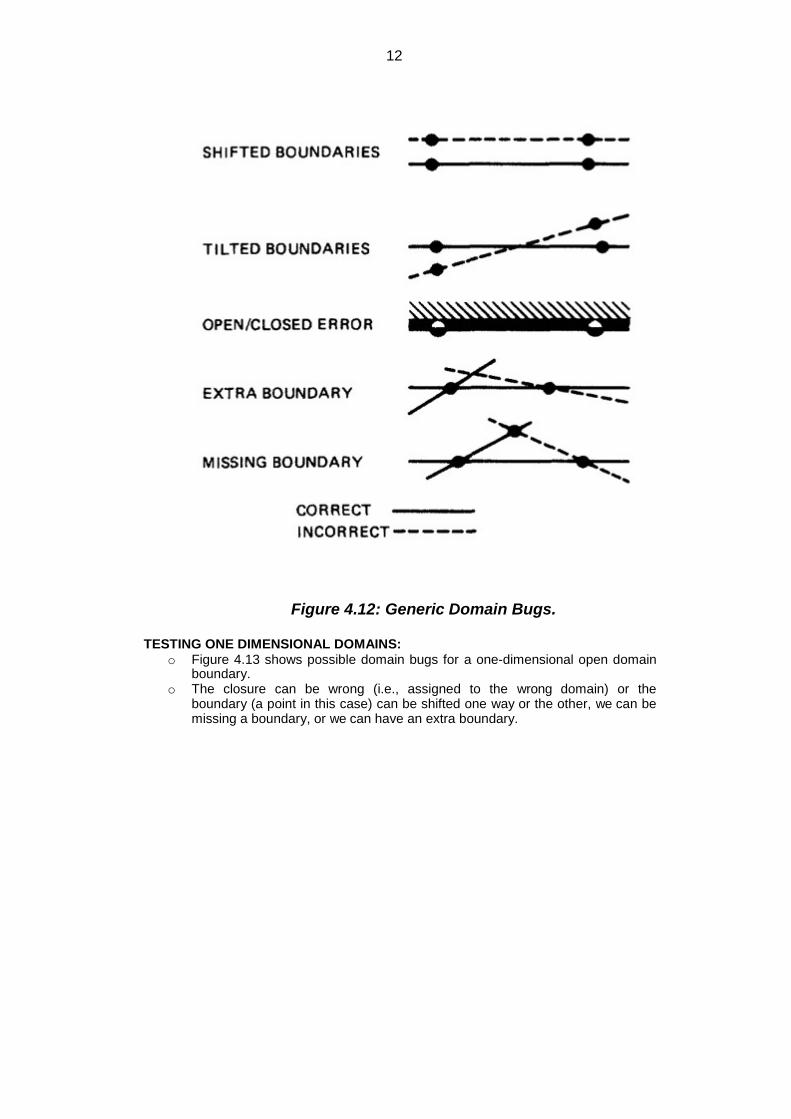
o Figure 4.12 shows generic domain bugs: closure bug, shifted boundaries, tilted

boundaries, extra boundary, missing boundary.

12

Figure 4.12: Generic Domain Bugs.

TESTING ONE DIMENSIONAL DOMAINS: o Figure 4.13 shows possible domain bugs for a one-dimensional open domain

boundary. o The closure can be wrong (i.e., assigned to the wrong domain) or the

boundary (a point in this case) can be shifted one way or the other, we can be missing a boundary, or we can have an extra boundary.

13

Figure 4.13: One Dimensional Domain Bugs, Open Boundaries.

o In Figure 4.13a we assumed that the boundary was to be open for A. The bug

we're looking for is a closure error, which converts > to >= or < to <= (Figure 4.13b). One test (marked x) on the boundary point detects this bug because processing for that point will go to domain A rather than B.

o In Figure 4.13c we've suffered a boundary shift to the left. The test point we used for closure detects this bug because the bug forces the point from the B domain, where it should be, to A processing. Note that we can't distinguish between a shift and a closure error, but we do know that we have a bug.

o Figure 4.13d shows a shift the other way. The on point doesn't tell us anything because the boundary shift doesn't change the fact that the test point will be processed in B. To detect this shift we need a point close to the boundary but within A. The boundary is open, therefore by definition, the off point is in A (Open Off Inside).

o The same open off point also suffices to detect a missing boundary because what should have been processed in A is now processed in B.

o To detect an extra boundary we have to look at two domain boundaries. In this context an extra boundary means that A has been split in two. The two off points that we selected before (one for each boundary) does the job. If point C had been a closed boundary, the on test point at C would do it.

o For closed domains look at Figure 4.14. As for the open boundary, a test point on the boundary detects the closure bug. The rest of the cases are similar to the open boundary, except now the strategy requires off points just outside the domain.

14

Figure 4.14: One Dimensional Domain Bugs, Closed Boundaries.

TESTING TWO DIMENSIONAL DOMAINS:

o Figure 4.15 shows possible domain boundary bugs for a two-dimensional domain.

o A and B are adjacent domains and the boundary is closed with respect to A, which means that it is open with respect to B.

15

Figure 4.15: Two Dimensional Domain Bugs.

o For Closed Boundaries: 1. Closure Bug: Figure 4.15a shows a faulty closure, such as might

be caused by using a wrong operator (for example, x >= k when x > k was intended, or vice versa). The two on points detect this bug because those values will get B rather than A processing.

2. Shifted Boundary: In Figure 4.15b the bug is a shift up, which

converts part of domain B into A processing, denoted by A'. This result is caused by an incorrect constant in a predicate, such as x + y >= 17 when x + y >= 7 was intended. The off point (closed off outside) catches this bug. Figure 4.15c shows a shift down that is caught by the two on points.

16

3. Tilted Boundary: A tilted boundary occurs when coefficients in the

boundary inequality are wrong. For example, 3x + 7y > 17 when 7x + 3y > 17 was intended. Figure 4.15d has a tilted boundary, which creates erroneous domain segments A' and B'. In this example the bug is caught by the left on point.

4. Extra Boundary: An extra boundary is created by an extra predicate. An extra boundary will slice through many different domains and will therefore cause many test failures for the same bug. The extra boundary in Figure 4.15e is caught by two on points, and depending on which way the extra boundary goes, possibly by the off point also.

5. Missing Boundary: A missing boundary is created by leaving a boundary predicate out. A missing boundary will merge different domains and will cause many test failures although there is only one bug. A missing boundary, shown in Figure 4.15f, is caught by the two on points because the processing for A and B is the same - either A or B processing.

PROCEDURE FOR TESTING: The procedure is conceptually is straight forward. It can be done by hand for two dimensions and for a few domains and practically impossible for more than two variables.

0. Identify input variables. 1. Identify variable which appear in domain defining predicates, such as control

flow predicates. 2. Interpret all domain predicates in terms of input variables. 3. For p binary predicates, there are at most 2

p combinations of TRUE-FALSE

values and therefore, at most 2p domains. Find the set of all non null domains.

The result is a boolean expression in the predicates consisting a set of AND terms joined by OR's. For example ABC+DEF+GHI ...... Where the capital letters denote predicates. Each product term is a set of linear inequality that defines a domain or a part of a multiply connected domains.

4. Solve these inequalities to find all the extreme points of each domain using any of the linear programming methods.

DOMAIN AND INTERFACE TESTING

INTRODUCTION:

o Recall that we defined integration testing as testing the correctness of the interface between two otherwise correct components.

o Components A and B have been demonstrated to satisfy their component tests, and as part of the act of integrating them we want to investigate possible inconsistencies across their interface.

o Interface between any two components is considered as a subroutine call. o We're looking for bugs in that "call" when we do interface testing. o Let's assume that the call sequence is correct and that there are no type

incompatibilities. o For a single variable, the domain span is the set of numbers between (and

including) the smallest value and the largest value. For every input variable we want (at least): compatible domain spans and compatible closures (Compatible but need not be Equal).

DOMAINS AND RANGE: o The set of output values produced by a function is called the range of the

function, in contrast with the domain, which is the set of input values over which the function is defined.

o For most testing, our aim has been to specify input values and to predict and/or confirm output values that result from those inputs.

o Interface testing requires that we select the output values of the calling routine i.e. caller's range must be compatible with the called routine's domain.

17

o An interface test consists of exploring the correctness of the following mappings:

o caller domain --> caller range(caller unit test)

o caller range --> called domain(integration test)

o called domain --> called range(called unit

test)

CLOSURE COMPATIBILITY: o Assume that the caller's range and the called domain spans the same

numbers - for example, 0 to 17. o Figure 4.16 shows the four ways in which the caller's range closure and the

called's domain closure can agree. o The thick line means closed and the thin line means open. Figure 4.16 shows

the four cases consisting of domains that are closed both on top (17) and bottom (0), open top and closed bottom, closed top and open bottom, and open top and bottom.

Figure 4.16: Range / Domain Closure Compatibility.

o Figure 4.17 shows the twelve different ways the caller and the called can

disagree about closure. Not all of them are necessarily bugs. The four cases in which a caller boundary is open and the called is closed (marked with a "?") are probably not buggy. It means that the caller will not supply such values but the called can accept them.

18

Figure 4.17: Equal-Span Range / Domain Compatibility Bugs.

SPAN COMPATIBILITY:

o Figure 4.18 shows three possibly harmless span incompatibilities.

Figure 4.18: Harmless Range / Domain Span incompatibility bug (Caller Span is smaller than

Called).

o In all cases, the caller's range is a subset of the called's domain. That's not

necessarily a bug. o The routine is used by many callers; some require values inside a range and

some don't. This kind of span incompatibility is a bug only if the caller expects the called routine to validate the called number for the caller.

o Figure 4.19a shows the opposite situation, in which the called routine's domain has a smaller span than the caller expects. All of these examples are buggy.

19

Figure 4.19: Buggy Range / Domain Mismatches

o In Figure 4.19b the ranges and domains don't line up; hence good values are

rejected, bad values are accepted, and if the called routine isn't robust enough, we have crashes.

o Figure 4.19c combines these notions to show various ways we can have holes in the domain: these are all probably buggy.

INTERFACE RANGE / DOMAIN COMPATIBILITY TESTING: o For interface testing, bugs are more likely to concern single variables rather

than peculiar combinations of two or more variables. o Test every input variable independently of other input variables to confirm

compatibility of the caller's range and the called routine's domain span and closure of every domain defined for that variable.

o There are two boundaries to test and it's a one-dimensional domain; therefore, it requires one on and one off point per boundary or a total of two on points and two off points for the domain - pick the off points appropriate to the closure (COOOOI).

o Start with the called routine's domains and generate test points in accordance to the domain-testing strategy used for that routine in component testing.

o Unless you're a mathematical whiz you won't be able to do this without tools for more than one variable at a time.

20

UNIT-3(part 2)

PATHS, PATH PRODUCTS AND REGULAR EXPRESSIONS

This unit gives an indepth overview of Paths of various flow graphs, their interpretations and application.

At the end of this unit, the student will be able to:

Interpret the control flowgraph and identify the path products, path sums and path

expressions.

Identify how the mathematical laws (distributive, associative, commutative etc) holds for the paths.

Apply reduction procedure algorithm to a control flowgraph and simplify it into a single path expression.

Find the all possible paths (Max. Path Count) of a given flow graph.

Find the minimum paths required to cover a given flow graph.

Calculate the probability of paths and understand the need for finding the probabilities.

Differentiate betweeen Structured and Un-structured flowgraphs.

Calculate the mean processing time of a routine of a given flowgraph.

Understand how complimentary operations such as PUSH / POP or GET / RETURN are interpreted in a flowgraph.

Identify the limitations of the above approaches.

Understand the problems due to flow-anomalies and identify whether anomalies exist in the given path expression.

PATH PRODUCTS AND PATH EXPRESSION:

MOTIVATION:

o Flow graphs are being an abstract representation of programs. o Any question about a program can be cast into an equivalent question about

an appropriate flowgraph. o Most software development, testing and debugging tools use flow graphs

analysis techniques.

PATH PRODUCTS: o Normally flow graphs used to denote only control flow connectivity. o The simplest weight we can give to a link is a name. o Using link names as weights, we then convert the graphical flow graph into an

equivalent algebraic like expressions which denotes the set of all possible paths from entry to exit for the flow graph.

o Every link of a graph can be given a name. o The link name will be denoted by lower case italic letters. o In tracing a path or path segment through a flow graph, you traverse a

succession of link names. o The name of the path or path segment that corresponds to those links is

expressed naturally by concatenating those link names. o For example, if you traverse links a,b,c and d along some path, the name for

that path segment is abcd. This path name is also called a path product. Figure 5.1 shows some examples:

21

Figure 5.1: Examples of paths.

PATH EXPRESSION:

o Consider a pair of nodes in a graph and the set of paths between those node. o Denote that set of paths by Upper case letter such as X,Y. From Figure 5.1c,

the members of the path set can be listed as follows:

ac, abc, abbc, abbbc, abbbbc.............

o Alternatively, the same set of paths can be denoted by :

ac+abc+abbc+abbbc+abbbbc+...........

o The + sign is understood to mean "or" between the two nodes of interest,

paths ac, or abc, or abbc, and so on can be taken. o Any expression that consists of path names and "OR"s and which denotes a

set of paths between two nodes is called a "Path Expression.".

PATH PRODUCTS: o The name of a path that consists of two successive path segments is

conveniently expressed by the concatenation or Path Product of the segment names.

o For example, if X and Y are defined as X=abcde,Y=fghij,then the path corresponding to X followed by Y is denoted by

XY=abcdefghij

22

o Similarly,

o YX=fghijabcde o aX=aabcde

o Xa=abcdea

XaX=abcdeaabcde

o If X and Y represent sets of paths or path expressions, their product represents the set of paths that can be obtained by following every element of X by any element of Y in all possible ways. For example,

o X = abc + def + ghi o Y = uvw + z

Then,

XY = abcuvw + defuvw + ghiuvw + abcz + defz + ghiz

o If a link or segment name is repeated, that fact is denoted by an exponent. The exponent's value denotes the number of repetitions:

o a1 = a; a2 = aa; a3 = aaa; an = aaaa . . . n times.

Similarly, if

X = abcde

then

X1 = abcde X2 = abcdeabcde = (abcde)

2

X3 = abcdeabcdeabcde = (abcde)

2abcde

= abcde(abcde)2 = (abcde)

3

o The path product is not commutative (that is XY!=YX).

o The path product is Associative.

RULE 1: A(BC)=(AB)C=ABC

where A,B,C are path names, set of path names or path expressions.

o The zeroth power of a link name, path product, or path expression is also

needed for completeness. It is denoted by the numeral "1" and denotes the "path" whose length is zero - that is, the path that doesn't have any links.

o a0 = 1 o X

0 = 1

PATH SUMS: o The "+" sign was used to denote the fact that path names were part of the

same set of paths. o The "PATH SUM" denotes paths in parallel between nodes. o Links a and b in Figure 5.1a are parallel paths and are denoted by a + b.

Similarly, links c and d are parallel paths between the next two nodes and are denoted by c + d.

23

o The set of all paths between nodes 1 and 2 can be thought of as a set of parallel paths and denoted by eacf+eadf+ebcf+ebdf.

o If X and Y are sets of paths that lie between the same pair of nodes, then X+Y denotes the UNION of those set of paths. For example, in Figure 5.2:

Figure 5.2: Examples of path sums.

The first set of parallel paths is denoted by X + Y + d and the second set by U + V + W + h + i + j. The set of all paths in this flowgraph is f(X + Y + d)g(U + V + W + h + i + j)k

o The path is a set union operation, it is clearly Commutative and Associative.

o RULE 2: X+Y=Y+X o RULE 3: (X+Y)+Z=X+(Y+Z)=X+Y+Z

DISTRIBUTIVE LAWS: o The product and sum operations are distributive, and the ordinary rules of

multiplication apply; that is

RULE 4: A(B+C)=AB+AC and (B+C)D=BD+CD

o Applying these rules to the below Figure 5.1a yields

o e(a+b)(c+d)f=e(ac+ad+bc+bd)f = eacf+eadf+ebcf+ebdf

ABSORPTION RULE: o If X and Y denote the same set of paths, then the union of these sets is

unchanged; consequently,

RULE 5: X+X=X (Absorption Rule)

o If a set consists of paths names and a member of that set is added to it, the "new" name, which is already in that set of names, contributes nothing and can be ignored.

o For example,

o if X=a+aa+abc+abcd+def then X+a = X+aa = X+abc = X+abcd = X+def = X

It follows that any arbitrary sum of identical path expressions reduces to the

same path expression.

24

LOOPS: o Loops can be understood as an infinite set of parallel paths. Say that the loop

consists of a single link b. then the set of all paths through that loop point is b0+b1+b2+b3+b4+b5+..............

Figure 5.3: Examples of path loops.

o This potentially infinite sum is denoted by b* for an individual link and by X*

when X is a path expression.

Figure 5.4: Another example of path loops.

o The path expression for the above figure is denoted by the notation:

ab*c=ac+abc+abbc+abbbc+................

o Evidently,

aa*=a*a=a+ and XX*=X*X=X+

o It is more convenient to denote the fact that a loop cannot be taken more than a certain, say n, number of times.

o A bar is used under the exponent to denote the fact as follows:

Xn = X0+X1+X2+X3+X4+X5+. ......................................................................................... +Xn

RULES 6 - 16: o The following rules can be derived from the previous rules:

o RULE 6: Xn + Xm = Xn if n>m RULE 6: Xn + Xm = Xm if m>n RULE 7: XnXm = Xn+m RULE 8: X

nX* = X

*Xn = X

*

25

RULE 9: XnX+ = X

+Xn = X

+

RULE 10: X*X+ = X

+X* = X

+

RULE 11: 1 + 1 = 1

RULE 12: 1X = X1 = X Following or preceding a set of paths by a path of zero length does not change the set.

RULE 13: 1n = 1n = 1* = 1+ = 1 No matter how often you traverse a path of zero length,It is a path of zero length.

RULE 14: 1++1 = 1*=1

The null set of paths is denoted by the numeral 0. it obeys the following rules: RULE 15: X+0=0+X=X

RULE 16: 0X=X0=0 If you block the paths of a graph for or aft by a graph that has no paths , there wont be any paths.

REDUCTION PROCEDURE:

REDUCTION PROCEDURE ALGORITHM:

o This section presents a reduction procedure for converting a flowgraph whose links are labeled with names into a path expression that denotes the set of all entry/exit paths in that flowgraph. The procedure is a node-by-node removal algorithm.

o The steps in Reduction Algorithm are as follows: 1. Combine all serial links by multiplying their path expressions. 2. Combine all parallel links by adding their path expressions.

3. Remove all self-loops (from any node to itself) by replacing them with a link of the form X*, where X is the path expression of the link in that loop.

STEPS 4 - 8 ARE IN THE ALGORIHTM'S LOOP: 4. Select any node for removal other than the initial or final node.

Replace it with a set of equivalent links whose path expressions correspond to all the ways you can form a product of the set of inlinks with the set of outlinks of that node.

5. Combine any remaining serial links by multiplying their path expressions.

6. Combine all parallel links by adding their path expressions. 7. Remove all self-loops as in step 3. 8. Does the graph consist of a single link between the entry node and

the exit node? If yes, then the path expression for that link is a path expression for the original flowgraph; otherwise, return to step 4.

o A flowgraph can have many equivalent path expressions between a given pair of nodes; that is, there are many different ways to generate the set of all paths between two nodes without affecting the content of that set.

o The appearance of the path expression depends, in general, on the order in which nodes are removed.

CROSS-TERM STEP (STEP 4): o The cross - term step is the fundamental step of the reduction algorithm. o It removes a node, thereby reducing the number of nodes by one. o Successive applications of this step eventually get you down to one entry and

one exit node. The following diagram shows the situation at an arbitrary node that has been selected for removal:

26

o From the above diagram, one can infer:

o (a + b)(c + d + e) = ac + ad + + ae +

bc + bd + be

LOOP REMOVAL OPERATIONS: o There are two ways of looking at the loop-removal operation:

o In the first way, we remove the self-loop and then multiply all outgoing links by Z*.

o In the second way, we split the node into two equivalent nodes, call them A and A' and put in a link between them whose path expression is Z*. Then we remove node A' using steps 4 and 5 to yield outgoing links whose path expressions are Z*X and Z*Y.

A REDUCTION PROCEDURE - EXAMPLE: o Let us see by applying this algorithm to the following graph where we remove

several nodes in order; that is

27

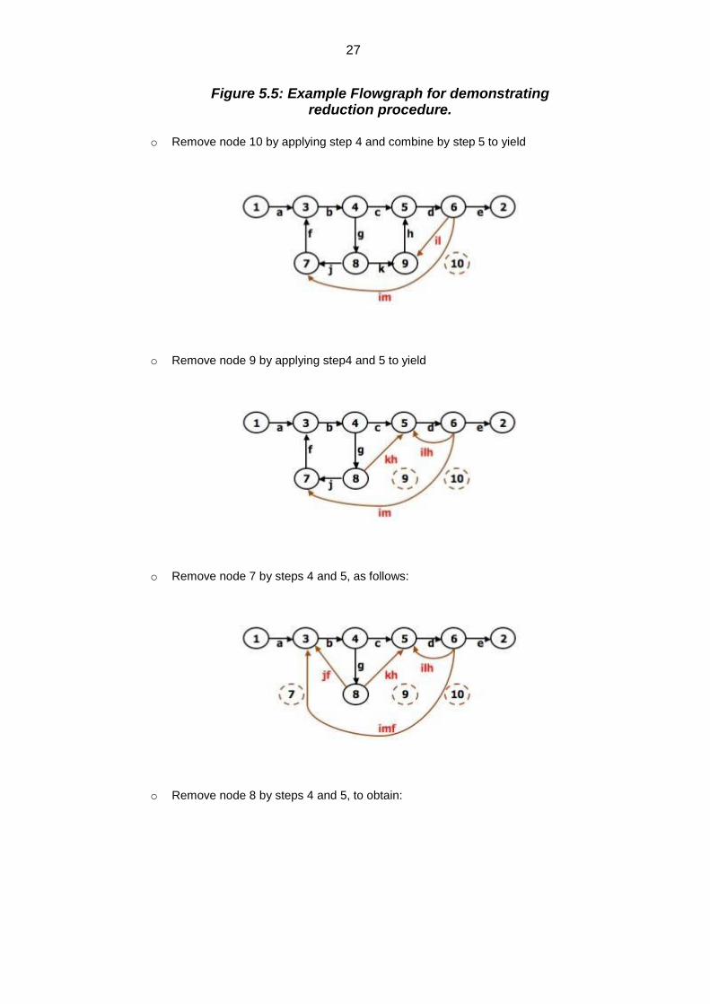
Figure 5.5: Example Flowgraph for demonstrating reduction procedure.

o Remove node 10 by applying step 4 and combine by step 5 to yield

o Remove node 9 by applying step4 and 5 to yield

o Remove node 7 by steps 4 and 5, as follows:

o Remove node 8 by steps 4 and 5, to obtain:

28

o PARALLEL TERM (STEP 6): Removal of node 8 above led to a pair of parallel links between nodes 4 and 5. combine them to create a path expression for an equivalent link whose path expression is c+gkh; that is

o LOOP TERM (STEP 7):

Removing node 4 leads to a loop term. The graph has now been replaced with the following equivalent simpler graph:

o Continue the process by applying the loop-removal step as follows:

29

o Removing node 5 produces:

o Remove the loop at node 6 to yield:

o Remove node 3 to yield:

o Removing the loop and then node 6 result in the following expression:

o

a(bgjf)*b(c+gkh)d((ilhd)*imf(bjgf)*b(c+gkh)d)*(i lhd)*e

o You can practice by applying the algorithm on the following flowgraphs and generate their respective path expressions:

30

Figure 5.6: Some graphs and their path expressions.

APPLICATIONS:

APPLICATIONS: o The purpose of the node removal algorithm is to present one very generalized

concept- the path expression and way of getting it. o Every application follows this common pattern:

1. Convert the program or graph into a path expression. 2. Identify a property of interest and derive an appropriate set of

"arithmetic" rules that characterizes the property. 3. Replace the link names by the link weights for the property of

interest. The path expression has now been converted to an expression in some algebra, such as ordinary algebra, regular expressions, or boolean algebra. This algebraic expression summarizes the property of interest over the set of all paths.

4. Simplify or evaluate the resulting "algebraic" expression to answer the question you asked.

HOW MANY PATHS IN A FLOWGRAPH ? o The question is not simple. Here are some ways you could ask it:

1. What is the maximum number of different paths possible? 2. What is the fewest number of paths possible? 3. How many different paths are there really?

31

4. What is the average number of paths? o Determining the actual number of different paths is an inherently difficult

problem because there could be unachievable paths resulting from correlated and dependent predicates.

o If we know both of these numbers (maximum and minimum number of possible paths) we have a good idea of how complete our testing is.

o Asking for "the average number of paths" is meaningless. MAXIMUM PATH COUNT ARITHMETIC:

o Label each link with a link weight that corresponds to the number of paths that link represents.

o Also mark each loop with the maximum number of times that loop can be taken. If the answer is infinite, you might as well stop the analysis because it is clear that the maximum number of paths will be infinite.

o There are three cases of interest: parallel links, serial links, and loops.

o This arithmetic is an ordinary algebra. The weight is the number of paths in each set.

o EXAMPLE: The following is a reasonably well-structured program.

Each link represents a single link and consequently is given a weight of "1" to start. Lets say the outer loop will be taken exactly four times and inner Loop Can be taken zero or three times Its path expression, with a little work, is:

Path expression:

a(b+c)d{e(fi)*fgj(m+l)k}*e(fi)*fgh

A: The flow graph should be annotated by replacing the link name with the maximum of paths through that link (1) and also note the number of times for looping.

32

B: Combine the first pair of parallel loops outside the loop and also

the pair in the outer loop. C: Multiply the things out and remove nodes to clear the clutter.

For the Inner Loop: D:Calculate the total weight of inner loop, which can execute a min. of 0 times and max. of 3 times. So, it inner loop can be evaluated as follows:

1

3 = 1

0 + 1

1 + 1

2 + 1

3 = 1 + 1 + 1 + 1 = 4

E: Multiply the link weights inside the loop: 1 X 4 = 4 F: Evaluate the loop by multiplying the link wieghts: 2 X 4 = 8. G: Simpifying the loop further results in the total maximum number

of paths in the flowgraph:

2 X 8

4 X 2 = 32,768.

33

Alternatively, you could have substituted a "1" for each link in the path expression and then simplified, as follows:

a(b+c)d{e(fi)*fgj(m+l)k}*e(fi)*fgh = 1(1 + 1)1(1(1 x 1)

31 x 1 x 1(1 + 1)1)

41(1 x 1)

31 x 1 x 1

= 2(131 x (2))

41

3

= 2(4 x 2)4 x 4

= 2 x 84 x 4 = 32,768

This is the same result we got graphically. Actually, the outer loop should be taken exactly four times. That doesn't mean it will be

taken zero or four times. Consequently, there is a superfluous "4" on the outlink in the last step. Therefore the maximum number of different paths is 8192 rather than 32,768.

STRUCTURED FLOWGRAPH: Structured code can be defined in several different ways that do not involve ad-hoc

rules such as not using GOTOs. A structured flowgraph is one that can be reduced to a single link by successive

application of the transformations of Figure 5.7.

34

Figure 5.7: Structured Flowgraph Transformations.

The node-by-node reduction procedure can also be used as a test for structured code. Flow graphs that DO NOT contain one or more of the graphs shown below (Figure 5.8)

as subgraphs are structured. 0. Jumping into loops 1. Jumping out of loops 2. Branching into decisions

3. Branching out of decisions

35

Figure 5.8: Un-structured sub-graphs.

LOWER PATH COUNT ARITHMETIC: A lower bound on the number of paths in a routine can be approximated for structured

flow graphs.

The arithmetic is as follows:

36

The values of the weights are the number of members in a set of paths.

EXAMPLE: Applying the arithmetic to the earlier example gives us the identical

steps unitl step 3 (C) as below:

From Step 4, the it would be different from the previous example:

37

If you observe the original graph, it takes at least two paths to cover and that it can be done in two paths.

If you have fewer paths in your test plan than this minimum you probably haven't covered. It's another check.

CALCULATING THE PROBABILITY: Path selection should be biased toward the low - rather than the high-probability paths. This raises an interesting question:

What is the probability of being at a certain point in a routine?

This question can be answered under suitable assumptions, primarily that all probabilities involved are independent, which is to say that all decisions are independent and uncorrelated.

We use the same algorithm as before : node-by-node removal of uninteresting nodes.

Weights, Notations and Arithmetic: Probabilities can come into the act only at decisions (including

decisions associated with loops). Annotate each outlink with a weight equal to the probability of

going in that direction. Evidently, the sum of the outlink probabilities must equal 1 For a simple loop, if the loop will be taken a mean of N times, the

looping probability is N/(N + 1) and the probability of not looping is 1/(N + 1).

A link that is not part of a decision node has a probability of 1.

The arithmetic rules are those of ordinary arithmetic.

38

In this table, in case of a loop, PA is the probability of the link leaving the loop and PL is the probability of looping.

The rules are those of ordinary probability theory. 1. If you can do something either from column A with a

probability of PA or from column B with a probability PB, then the probability that you do either is PA + PB.

2. For the series case, if you must do both things, and their probabilities are independent (as assumed), then the probability that you do both is the product of their probabilities.

For example, a loop node has a looping probability of PL and a probability of not looping of PA, which is obviously equal to I - PL.

Following the above rule, all we've done is replace the outgoing probability with 1 - so why the complicated rule? After a few steps in which you've removed nodes, combined parallel terms, removed loops and the like, you might find something like this:

39

because PL + PA + PB + PC = 1, 1 - PL = PA + PB + PC, and

which is what we've postulated for any decision. In other words, division by 1 - PL renormalizes the outlink probabilities so that their sum equals unity after the loop is removed.

EXAMPLE: Here is a complicated bit of logic. We want to know the probability

associated with cases A, B, and C.

Let us do this in three parts, starting with case A. Note that the sum of the probabilities at each decision node is equal to 1. Start by throwing away anything that isn't on the way to case A, and then apply the reduction procedure. To avoid clutter, we usually leave out probabilities equal to 1.

CASE A:

40

Case B is simpler:

41

Case C is similar and should yield a probability of 1 - 0.125 - 0.158

= 0.717:

This checks. It's a good idea when doing this sort of thing to calculate all the probabilities and to verify that the sum of the routine's exit probabilities does equal 1.

If it doesn't, then you've made calculation error or, more likely, you've left out some branching probability.

42

How about path probabilities? That's easy. Just trace the path of interest and multiply the probabilities as you go.

Alternatively, write down the path name and do the indicated arithmetic operation.

Say that a path consisted of links a, b, c, d, e, and the associated probabilities were .2, .5, 1., .01, and I respectively. Path abcbcbcdeabddea would have a probability of 5 x 10

-10.

Long paths are usually improbable.

MEAN PROCESSING TIME OF A ROUTINE: Given the execution time of all statements or instructions for every link in a flowgraph

and the probability for each direction for all decisions are to find the mean processing time for the routine as a whole.

The model has two weights associated with every link: the processing time for that link, denoted by T, and the probability of that link P.

The arithmetic rules for calculating the mean time:

EXAMPLE: 0. Start with the original flow graph annotated with probabilities and

processing time.

43

2. Combine as many serial links as you can.

3. Use the cross-term step to eliminate a node and to create the inner

self - loop.

4. Finally, you can get the mean processing time, by using the

arithmetic rules as follows:

44

PUSH/POP, GET/RETURN: This model can be used to answer several different questions that can turn up in

debugging. It can also help decide which test cases to design. The question is:

Given a pair of complementary operations such as PUSH (the stack) and POP (the stack), considering the set of all possible paths through the routine, what is the net effect of the routine? PUSH or POP? How many times? Under what conditions?

applies:

Here are some other examples of complementary operations to which this model

GET/RETURN a resource block.

OPEN/CLOSE a file.

START/STOP a device or process.

EXAMPLE 1 (PUSH / POP):

Here is the Push/Pop Arithmetic:

45

The numeral 1 is used to indicate that nothing of interest (neither PUSH nor POP) occurs on a given link.

"H" denotes PUSH and "P" denotes POP. The operations are

commutative, associative, and distributive.

Consider the following flowgraph:

P(P + 1)1{P(HH)n1HP1(P + H)1}n2P(HH)n1HPH

Simplifying by using the arithmetic tables,

=(P2 + P){P(HH)n1(P + H)}n1(HH)n1 =(P

2 + P){H

2n1(P

2 + 1)}

n2H2n1

Below Table 5.9 shows several combinations of values for the two

looping terms - M1 is the number of times the inner loop will be taken and M2 the number of times the outer loop will be taken.

46

Figure 5.9: Result of the PUSH / POP Graph Analysis.

These expressions state that the stack will be popped only if the

inner loop is not taken. The stack will be left alone only if the inner loop is iterated once,

but it may also be pushed. For all other values of the inner loop, the stack will only be pushed.

EXAMPLE 2 (GET / RETURN):

Exactly the same arithmetic tables used for previous example are used for GET / RETURN a buffer block or resource, or, in fact, for

47

any pair of complementary operations in which the total number of operations in either direction is cumulative.

The arithmetic tables for GET/RETURN are:

"G" denotes GET and "R" denotes RETURN.

Consider the following flowgraph:

G(G

=

G(G +

+ R)G(GR)*GGR*R

R)G3R*R

= (G + R)G3R*

= (G4 + G

2)R*

This expression specifies the conditions under which the resources will be balanced on leaving the routine.

If the upper branch is taken at the first decision, the second loop must be taken four times.

If the lower branch is taken at the first decision, the second loop must be taken twice.

For any other values, the routine will not balance. Therefore, the first loop does not have to be instrumented to verify this behavior because its impact should be nil.

LIMITATIONS AND SOLUTIONS: The main limitation to these applications is the problem of unachievable paths. The node-by-node reduction procedure, and most graph-theory-based algorithms work

well when all paths are possible, but may provide misleading results when some paths are unachievable.

The approach to handling unachievable paths (for any application) is to partition the graph into subgraphs so that all paths in each of the subgraphs are achievable.

The resulting subgraphs may overlap, because one path may be common to several different subgraphs.

Each predicate's truth-functional value potentially splits the graph into two subgraphs.

For n predicates, there could be as many as 2n subgraphs.

48

REGULAR EXPRESSIONS AND FLOW ANOMALY DETECTION:

THE PROBLEM:

o The generic flow-anomaly detection problem (note: not just data-flow anomalies, but any flow anomaly) is that of looking for a specific sequence of options considering all possible paths through a routine.

o Let the operations be SET and RESET, denoted by s and r respectively, and we want to know if there is a SET followed immediately a SET or a RESET followed immediately by a RESET (an ss or an rr sequence).

o Some more application examples:

1. A file can be opened (o), closed (c), read (r), or written (w). If the file is read or written to after it's been closed, the sequence is nonsensical. Therefore, cr andcw are anomalous. Similarly, if the file is read before it's been written, just after opening, we may have a bug. Therefore, or is also anomalous. Furthermore, ooand cc, though not actual bugs, are a waste of time and therefore should also be examined.

2. A tape transport can do a rewind (d), fast-forward (f), read (r), write (w), stop (p), and skip (k). There are rules concerning the use of the transport; for example, you cannot go from rewind to fast- forward without an intervening stop or from rewind or fast-forward to read or write without an intervening stop. The following sequences are anomalous: df, dr, dw, fd, and fr. Does the flowgraph lead to anomalous sequences on any path? If so, what sequences and under what circumstances?

3. The data-flow anomalies discussed in Unit 4 requires us to detect the dd, dk, kk, and ku sequences. Are there paths with anomalous data flows?

THE METHOD: o Annotate each link in the graph with the appropriate operator or the null

operator 1.

o Simplify things to the extent possible, using the fact that a + a = a and 12 = 1. o You now have a regular expression that denotes all the possible sequences of

operators in that graph. You can now examine that regular expression for the sequences of interest.

o EXAMPLE: Let A, B, C, be nonempty sets of character sequences whose smallest string is at least one character long. Let T be a two-character string of characters. Then if T is a substring of (i.e., if T appears within) AB

nC, then T

will appear in AB2C. (HUANG's Theorem)

o As an example, let

A = pp B = srr C = rp T = ss The theorem states that ss will appear in pp(srr)

nrp if it appears in pp(srr)

2rp.

o However, let

A = p + pp + ps B = psr + ps(r + ps) C = rp T = P

4

Is it obvious that there is a p4 sequence in AB

nC? The theorem states that we

have only to look at

(p + pp + ps)[psr + ps(r + ps)]2rp

49

Multiplying out the expression and simplifying shows that there is no p

4 sequence.

o Incidentally, the above observation is an informal proof of the wisdom of looping twice discussed in Unit 2. Because data-flow anomalies are represented by two-character sequences, it follows the above theorem that looping twice is what you need to do to find such anomalies.

LIMITATIONS: o Huang's theorem can be easily generalized to cover sequences of greater

length than two characters. Beyond three characters, though, things get complex and this method has probably reached its utilitarian limit for manual application.

o There are some nice theorems for finding sequences that occur at the beginnings and ends of strings but no nice algorithms for finding strings buried in an expression.

o Static flow analysis methods can't determine whether a path is or is not achievable. Unless the flow analysis includes symbolic execution or similar techniques, the impact of unachievable paths will not be included in the analysis.

o The flow-anomaly application, for example, doesn't tell us that there will be a flow anomaly - it tells us that if the path is achievable, then there will be a flow anomaly. Such analytical problems go away, of course, if you take the trouble to design routines for which all paths are achievable.