1

Understanding the Power of Pull-based StreamingProtocol: Can We Do Better?

Meng ZHANG, Student Member, IEEE, Qian ZHANG, Senior Member, IEEE, Lifeng SUN, Member, IEEE,and Shiqiang YANG, Member, IEEE

Abstract— Most of the real deployed peer-to-peer streamingsystems adopt pull-based streaming protocol. In this paper, wedemonstrate that, besides simplicity and robustness, with properparameter settings, when the server bandwidth is above severaltimes of the raw streaming rate, which is reasonable for practicallive streaming system, simple pull-based P2P streaming protocolis nearly optimal in terms of peer upload capacity utilizationand system throughput even without intelligent scheduling andbandwidth measurement. We also indicate that whether thisnear optimality can be achieved depends on the parameters inpull-based protocol, server bandwidth and group size. Then wepresent our mathematical analysis to gain deeper insight in thischaracteristic of pull-based streaming protocol. On the otherhand, the optimality of pull-based protocol comes from a cost -tradeoff between control overhead and delay, that is, the protocolhas either large control overhead or large delay. To break thetradeoff, we propose a pull-push hybrid protocol. The basic ideais to consider pull-based protocol as a highly efficient bandwidth-aware multicast routing protocol and push down packets alongthe trees formed by pull-based protocol. Both simulation andreal-world experiment show that this protocol is not only evenmore effective in throughput than pull-based protocol but alsohas far lower delay and much smaller overhead. And to achievenear optimality in peer capacity utilization without churn, theserver bandwidth needed can be further relaxed. Furthermore,the proposed protocol is fully implemented in our deployedGridMedia system and has the record to support over 220,000users simultaneously online.

Index Terms— p2p streaming, pull-based, pull-push hybrid,capacity utilization, throughput, delay

I. INTRODUCTION

With more and more peer-to-peer (P2P) streaming systems(e.g. [1], [2], [3]) deployed on Internet, P2P streaming tech-nology has achieved a great success. Most of these systemsemploy pull-based streaming protocol. In this type of protocol,each node independently selects its neighbors so as to forman unstructured overlay network. The live media content isdivided into segments and every node periodically notifies itsneighbors of what packets it has. Then each node explicitlyrequests the blocks of interest from its neighbors accordingto their notification. The well-known advantages of pull-based

Manuscript received March, 2007; revised August, 2007Meng ZHANG, Prof. Lifeng SUN and Prof. Shiqiang YANG

are with the Department of Computer Science and Technology inTsinghua University. (email: zhangmeng00@mails.tsinghua.edu.cn, and{sunlf,yangshq}@tsinghua.edu.cn)

Prof. Qian ZHANG is with the Department of Computer Science in HongKong University of Science and Technology. (email: qianzh@cse.ust.hk)

Supported by the National Basic Research Program of China (973) underGrant No. 2006CB303103 and National High-Tech Research and DevelopmentPlan of China (863) under Grant No. 2006AA01Z321, the HKUST NanshaResearch Fund NRC06/07.EG01, the HKUST RPC06/07.EG05, and CERG622407.

protocol are its simplicity and robustness [4], [5]. In peer-to-peer streaming study, there are a lot of efforts made on enhanc-ing the throughput of a P2P overlay. The maximum throughputthat a P2P overlay can achieve is the total upload capacity ofall peers divided by the peer number. Therefore, how to utilizeall the peer upload capacity is the key issue. Traditional singletree based protocol can not achieve this because the uploadcapacity of the leaf peers and those peers with upload capacityless than the streaming rate cannot be utilized. So existingapproaches slice the stream into multiple sub streams andleverage optimization theory to distributedly solve “packingspanning trees” problem [6], [7] or directly build multiple trees[8], [9] to utilize the peer upload capacity as much as possible.Recent study also employs network coding to deal with theissue of maximizing throughput [10]. However, our study byboth simulation and real-world experiment demonstrates that,when the server bandwidth is above a reasonable number oftimes of the raw streaming rate, with appropriate parametersettings, simple pull-based protocol is near-optimal in terms ofpeer bandwidth utilization and system throughput. The mostinteresting part is that the pull-based protocol can achieve thisproperty without intelligent scheduling and proactive band-width measurement. Yet this characteristic has been paid littleattention to in the literature. To explain such near optimalityof pull-based protocol, we further give mathematical analysisto help understand why pull-based protocol is effective inutilizing peer upload capacity. Moreover, we also point outthat this near optimality in bandwidth utilization depends onthe parameters in the pull-based protocol, the server bandwidthand the group size. We see that when the server bandwidth isat least 3 times of the raw streaming rate and the group sizeis less than 10,000 peers, such near optimality holds.

However, the benefit of pull-based protocol results froma cost, that is, the tradeoff between control overhead anddelay. As indicated in the literature [5], to minimize the delay,each node notifies its neighbors of packet arrivals as soonas it receives the packet and the neighbor should request thepacket immediately after receiving the notification, resulting ina remarkable control overhead. On the other hand, to diminishthe overhead, a node can wait until dozens of packets arrivedand inform these packets to its neighbors once in a packetmeanwhile the neighbors can also request a bunch of packetsonce, which obviously leads to a considerable delay. Due tothis limitation, most of the current deployed P2P streamingsystems [1], [2] only target at the delay-tolerant non-interactiveapplications. A natural question is whether it is possible to notonly achieve nearly optimal throughput but also obtain lowdelay and overhead. To break this tradeoff, in this paper, wepropose the pull-push hybrid protocol. The basic idea of this

2

protocol is to consider pull-based protocol as a highly efficientbandwidth-aware multicast routing approach and to push downthe packets along the trees formed by pull-based protocol.Both simulation and real-world experiment results indicate thatthis protocol can not only achieve nearly optimal throughputbut also has very low delay and small overhead in typicalscenarios. Furthermore, pull-push hybrid protocol can achievenear-optimal bandwidth utilization with less server bandwidththan pull-based protocol. When the server bandwidth is atleast 1.6 times of the raw streaming rate and the group sizeis less than 10,000 peers, the near optimality keeps true. Wesummarizes our contributions as follow:• We give detailed simulation analysis and real-world

experiments on PlanetLab of pull-based peer-to-peerstreaming protocol and discover an interesting fact that,when the server bandwidth is above 3 times of theraw streaming rate, with appropriate parameter settings,simple pull-based P2P streaming can nearly utilize allthe upload capacity of peers so that almost maximumthroughput is achieved. We also clarify the parametersthat have the most impact on the performance of pull-based method which is not well understood before.

• We give mathematical analysis to pull-based peer-to-peerstreaming protocol to estimate the lower bound of thedelivery ratio (defined in Section III-B.2 for throughputmeasurement). So far as we know, we are the first toanalyze the near optimality in terms of peer bandwidthutilization and throughput of pull-based P2P streaming.

• Based on the understanding that pull-based protocolis a highly efficient bandwidth-aware multicast routingscheme, we propose a novel pull-push hybrid protocol,which can not only achieve nearly optimal throughputand bandwidth utilization but also has far lower playbackdelay and much smaller overhead. And the server band-width needed can be also relaxed to about 1.6 times ofthe raw streaming rate.

• We have totally implemented the proposed pull-pushhybrid protocol and the system has been adopted bythe largest TV station in China (CCTV) for TV onlinebroadcasting. Our system has the record to support over220,000 users concurrent online to watch high-qualityInternet TV by only one server.

The remainder of this paper is organized as follows: insection II we briefly discuss the related work. And in sectionIII, we give our deep insight into pull-based protocol andpresent our interesting findings by both simulation and real-world experiment. We also give mathematical analysis toexplain our observations. Section IV describes the pull-pushhybrid protocol and gives detail performance evaluation byboth simulation and real-world experiment. In Section V, wepresent our insights obtained from our findings and give oursuggestions for future study in this area. Finally, we concludethis paper in Section VI.

II. RELATED WORK

Unlike traditional tree(s)-based protocols [11], from 2005,a new category of data-driven or pull (or swarming) based

P2P streaming protocols (very similar to the BitTorrent[12]mechanism) has been proposed, such as Chainsaw [13],DONet/CoolStreaming [4], PRIME [14] and [15]. Most of thereal P2P streaming system deployed over Internet are basedon this type of protocol ([1], [16]). However, little attentionhas been paid to the near optimality of pull-based protocolin peer bandwidth utilization and throughput. To utilize allbandwidth capacity in P2P streaming, [8] and [17] mentioneda simple strategy to construct multiple height-2 trees withina fully connected graph, which can be only apply to smallgroup since each node has to establish connections with allother nodes certainly resulting in a huge overhead. Besides,there is also much theoretical work to achieve the maximumoverlay multicast throughput using optimization theory andnetwork coding technique, such as [6], [7], [10]. However,our discovery shows that random packet scheduling strategyin pull-based P2P streaming protocol can run near-optimally interms of peer upload capacity utilization. Some results in [18],[19] confirm that the simple rarest-first policy in Bit-Torrentsystem performs near-optimally in terms of upload capacityutilization and thereby the downloading time. Why randomstrategy in P2P streaming is near-optimal in peer bandwidthutilization? An intuitive explanation is that, unlike file sharing,there are always new block generated at the server, even if therandom packet scheduling policy is used, the block diversitycan usually be satisfied.

For the mathematical analysis of the delivery ratio of pull-based P2P streaming protocol, little work has been done toanalyze this near optimality of pull-based P2P streaming. [20]gives a fluid model of BitTorrent-like file sharing system. [17]discusses the impact of the churn rate on the performance inP2P streaming. [21] gives a random distributed method to solvethe broadcast problem in edge-capacitated networks. However,none of them do analysis to explain the effectiveness of pull-based protocol in peer bandwidth utilization and throughput.

Interestingly, we can see that, the recent debate on peer-to-peer streaming focuses on whether mesh protocol (i.e. pull-based protocol) or multi-tree protocol is better [5], [22]. Themain argument on the anti-tree side is that tree construction iscomplex, and that trees are fragile. The main counter-argumentis that mesh/pull based protocol has a lot of overhead andlarge delay. However, our proposed pull-push hybrid protocolnot only inherits the robustness of pull-based protocol and canachieve nearly optimal throughput but also has much loweroverhead and delay. We note that SplitStream [23], ESM [24]and Chunkyspread [5] use multi-tree based protocol. However,it is not clear that whether these protocols can achieve nearlyoptimal throughput of the system, which is a very importantfeature of our proposed pull-push protocol.

III. DEEP INSIGHT INTO PULL-BASED METHOD

A. Protocol

In this section, we introduce the pull-based protocol we use,including overlay construction and streaming delivery.

For overlay construction, to join a P2P streaming session,nodes must first contact a rendezvous point (RP) which can bea server maintaining a partial list of current online nodes. Then

3

each node randomly finds some other nodes as its neighbors tokeep connections with so that an unstructured overlay is built.

For the streaming delivery, the video streaming is packetizedinto fixed-length packets called streaming packets marked bysequence numbers. In all of our simulations and experiments,we pack 1250-byte streaming data in each streaming packet(not including 40-byte packet header). Each node periodicallysends buffer map packets to notify all its neighbors whatstreaming packets it has in the buffer. Each node then explicitlyrequests its absent packets from neighbors. We call the packetsused for protocol control control packets, including buffer mappackets, request packets and packets for overlay construction,etc. To reduce the control packets, in our simulation andimplementation, the control packets will be piggybacked inthe streaming packets as much as possible.

More detailedly, in each request interval τ , the node asksits neighbors for all the absent packets in the current requestwindow. The request window slides forward continuously. Thehead of the request window is the latest packet with themaximum sequence number the node has ever known, which isacknowledged by the buffer map received from its neighbors.The buffer size (usually 1 minute, denoted by B) is largerthan the request window size (denoted by W ). An absentpacket that gets out of the request window (i.e. beyond theplayback deadline) will not be requested further. If multipleneighbors own the same absent packet, the packet will beassigned to one of the neighbors randomly with the sameprobability. The request interval τ is set to much smallerthan the request window W . When a packet does not arriveafter its request has been sent out for a time of Tw and it isstill in the request window, it will be requested again (i.e., aretransmission happens). Tw is called the waiting timeout fora requested packet.

We would like to emphasize our packet request and retrans-mission control here, which have some important differencefrom those described in literature, such as [13], [4], [25]. Thekey point here is to use unreliable transmission for streamingpackets. If UDP is used, the unreliability is inherent. While,if TCP is used, we set the sending buffer of TCP socket to arelatively small value, and once the sending rate is beyondthe bandwidth, the TCP sending buffer will get overflowand the packet is dropped. The benefit of using unreliabletransmission for streaming packet is that we can use relativelysmall timeout to conclude whether a packet is dropped withoutencountering redundancy. Nevertheless, if reliable transmissionis used, packets are usually queuing at the sender if the sendingrate is high and we should use a very large timeout to judgewhether the packet is dropped or will be received later. In ourpull-based protocol, once a node receives a request (containingrequests for multiple packets) from one neighbor, it will deliverall the requested packets within a constant bit rate exactly intime of one request interval τ . If the sending rate exceedsthe upload capacity or end-to-end bandwidth, the overloadedpackets will be dropped directly and never be retransmitteduntil a new request of this packet is received. Hence a packetwill either arrive within time of rtt + τ or be dropped after itis requested, where rtt is the round-trip time to the neighbor.Moreover, considering the Internet transmission delay jitter,

we set the waiting timeout Tw for a requested packet asrtt+ τ + tw, where tw is an additional waiting time to furtherprevent duplicated requests for a packet.

In a nutshell, in our streaming delivery protocol, for thereceiver side, it selfishly requests an absent packet again andagain until this packet eventually arrives or is out of the requestwindow; for the sender side, it tries to send all the packetsrequested with the best effort.

B. Evaluation by Simulation

1) Simulation Setup: We implement an event-driven packet-level simulator coded in C++ to conduct a series of simulationsin this section1. In our simulation, all streaming and controlpackets and node buffers are carefully simulated. We runour simulator on two 4-cpu 8GB-memory machines. For theend-to-end latency setup, we employ real-world node-to-nodelatency matrix (2500×2500) measured on Internet [26], inwhich, the average end-to-end delay is 79ms. We do notconsider the queuing management in the routers. The defaultnumber of nodes (i.e. the group size) is set to 10,000. Sincethe node number is larger than the latency matrix dimension,we simply map each node pair in our simulation to each pairin the latency matrix randomly. And the default raw streamingrate (not including 40-byte/packet header overhead) is set to300kbps. We assume all the control messages can be reliablydelivered (streaming packets do not). The default neighborcount is 15 and the default request window size is 20 seconds.

We assume that all peers are DSL nodes and assume thebandwidth bottleneck happens only at the last hop, i.e., atthe end host. The default upload capacity of the source nodeis 2Mbps. To simulate the bandwidth heterogeneity of thepeers, we use three different typical DSL nodes. Their uploadcapacities are 1Mbps, 384kbps and 128kbps and downloadcapacities are 3Mbps, 1.5Mbps, 768kbps respectively. Notethat the upload capacity are far lower than the downloadcapacity, hence the upload link is usually the bottleneck. Weuse the term capacity supply ratio (also known as resourceindex in [27]) to represent the bandwidth supply “tightness”,which is defined as the ratio of the total upload capacity to theraw streaming rate (default value 300kbps) times the receivernumber, i.e., the ratio of bandwidth supply to the minimumbandwidth demand. It is obvious that the necessary conditionof supporting a peer-to-peer streaming system is that the totalbandwidth supply should outstrip the minimum bandwidthdemand [17], i.e., the capacity supply ratio should be greaterthan 1. In Table I, by adjusting the fractions of different typesof the peers, we obtain several capacity supply ratios. We willinvestigate the performance of pull-based method under thesedifferent capacity supply ratios.

As the bottleneck of P2P systems are always at the uploadof the peers. The maximum throughput that can be achieved isthe total upload capacity (including the source node) dividedby the receiver number. Therefore, if every node in a systemwith capacity supply ratio of 1 can get the entire streaming,the optimal throughput is achieved.

1The simulator is available online for free downloading athttp://media.cs.tsinghua.edu.cn/∼zhangm

4

TABLE IDIFFERENT CAPACITY SUPPLY RATIOS BY ADJUSTING THE FRACTIONS OF

DIFFERENT PEER TYPES

Capacity Fractions Capacity FractionsSupply Ratio 1M 384k 128k Supply Ratio 1M 384k 128k1.02 0.1 0.346 0.554 1.2 0.15 0.39 0.461.05 0.1 0.38 0.52 1.25 0.16 0.405 0.4351.1 0.1 0.45 0.45 1.3 0.18 0.4 0.421.15 0.1 0.5 0.4 1.4 0.2 0.45 0.35

2) Metrics:• Average deliverable rate and average delivery ratio: we

define the deliverable rate of a node as the availablestreaming rate received (excluding redundant streamingpackets and control packets but including streamingpacket header) by the node. And only the packets thatarrive before the playback deadline are available ones.And we define the delivery ratio of a node as the ratioof its deliverable rate to the packetized streaming ratesent out from the source node. In our simulation andexperiment, we use the total received streaming packetsby a node and the total packets sent out from the sourcenode during the latest 10 seconds to derive the sampleddeliverable rate and delivery ratio of the node. Theaverage sampled deliverable rate and average sampleddelivery ratio of a session are the average values amongthe sampled deliverable rates and delivery ratios of allthe nodes at that time. And when the system gets steadystate, we average all the average sampled deliverable rateand delivery ratio throughout the whole duration as theaverage deliverable rate and average delivery ratio of thesession. Both the two metrics are measures of the systemthroughput. The average numbers of the following metricsof the system are similar to that of the the deliverable rateand delivery ratio.

• Average upload rate: the upload rate of a node consistsof all streaming packets and control packets that aresuccessfully uploaded. The method to derive averageupload rate of the whole session is similar as that ofaverage delivery ratio. The more the average upload rateapproaches average upload capacity, the more efficientthe upload capacity is used

• Packet arrival delay: the packet arrival delay is the delaybetween the time when it is sent out from the source nodeand when it is finally arrived at a node after one or severalhop(s).

• α-playback delay (α ≤ 1): in video streaming systems,usually, the packets should be buffered before they areplayed, and the longer time they are buffered, with higherpossibility the better playback quality (i.e. delivery ratio)may be achieved. We call the minimum buffered timewhen the delivery ratio reaches α as the α-playback time.And we define α-playback delay as the delay between thetime when a packet is sent out from the source node andα-playback time of that packet. This metric captures thetrue delay experienced by the end users. The default valueof α in our simulation is 0.99.

• Control packet rate: the control packets include buffer

map packets, request packets, member table packets,connection setup and heart-beat packets, etc. The con-trol packet rate representing the control overhead is thecontrol packet sent out per second from each node..

3) Simulation results: We first investigate the performanceof pull-based protocol in static environment. In static envi-ronment, users do not quit after they join the session. Oursimulation results here indicate the system behavior at thesteady state. For each point, we simulate s session for halfan hour. It takes about one day to perform one run for onepoint. Furthermore, we have repeated several simulation runsfor each of some points over different random seeds and wefound that the results have been very similar.

Fig. 1 gives a comparison of i) the average deliverable rate,ii) the average upload rate and iii) the average upload capacityunder different capacity supply ratios. The request intervalis set to 200ms. Generally speaking, the average upload rateshould be equal to the average download rate regardless of thepacket loss in the non-last-hop links. Obviously, the averageupload rate including both streaming and control packets,should be greater than the average deliverable rate, and bothof them are upper bounded by the average upload capacity.The dotted horizontal line in each sub figure indicates thepacketized streaming rate sent out from the source node (i.e.the best deliverable rate that can be achieved). As indicatedin the figure, we note that when the capacity supply ratiois 1.15 or above (i.e., as long as the bandwidth supply ishigher by only 15% than the minimum bandwidth demand,that is, the raw streaming rate 300kbps times the receivernumber), the average deliverable rate can reach the nearlybest deliverable rate. Considering the 3% header overheadand 5%∼10% control overhead, the deliverable rate achievesnearly the optimal throughput. And when the capacity supplyratio is lower than 1.15, we see that the average upload rate isvery close to the average upload capacity, namely, the capacityis almost fully utilized.

Fig. 2 shows the average delivery ratio under differentcapacity supply ratio and request interval. We see that whenthe capacity supply ratio is 1.15 or above and request intervalis between 200ms and 800ms, the average delivery ratio isvery close to 1 (i.e., the best delivery ratio). And we note thatwhen the capacity supply ratio is higher than 1.15, the smallerthe request interval is, the better delivery ratio is achieved.Intuitively, small request interval implies that there are morechances for a packet to be successfully retransmitted until itgets out of the request window. On the other hand, if thecapacity supply is very limited (below 1.15), the deliveryratio gets worse when the request interval is very small(such as under 400ms). This is because small request intervalcauses heavier control overhead traffic, which consumes morebandwidth resulting in lowering delivery ratio.

Fig. 3 shows the impact of request window size underdifferent request window interval. Here, the capacity supplyratio is set to 1.2. When the request windows size is small, thedelivery ratio gets poor. While, we notice that, with enlargingthe request window size, the delivery ratio can be remarkablyimproved under the same request interval. And the deliveryratio can achieve nearly 1 when the request interval is below

5

1.02 1.05 1.1 1.15 1.2 1.25 1.3200

250

300

350

400B

it ra

te (k

bps)

Capacity supply ratio

Average deliverable rateAverage upload rate (streaming+overhead packets)Average upload capacity

Fig. 1AVERAGE DELIVERABLE RATE, AVERAGE

UPLOAD RATE AND AVERAGE UPLOAD CAPACITY

IN PULL-BASED PROTOCOL

200 400 600 800 1000 1200 1400 1700 20000.75

0.8

0.85

0.9

0.95

1

Request interval (msec)

Ave

rage

Del

iver

y R

atio

Capacity supply ratio 1.02Capacity supply ratio 1.05Capacity supply ratio 1.1Capacity supply ratio 1.15Capacity supply ratio 1.2Capacity supply ratio 1.25Capacity supply ratio 1.3

Fig. 2AVERAGE DELIVERY RATIO WITH RESPECT TO

DIFFERENT REQUEST INTERVALS AND CAPACITY

SUPPLY RATIOS IN PULL-BASED PROTOCOL

4 8 12 16 200.4

0.5

0.6

0.7

0.8

0.9

1

Request window size (sec)

Ave

rage

Del

iver

y R

atio

Request interval 200msRequest interval 600msRequest interval 1000msRequest interval 1400msRequest interval 2000ms

Fig. 3DELIVERY RATIO WITH RESPECT TO DIFFERENT

REQUEST INTERVAL AND REQUEST WINDOW

SIZE IN PULL-BASED PROTOCOL

20 40 60 80200

250

300

350

400Capcity supply ratio 1.2

Bit

rate

(kbp

s)

Neighbor count20 40 60 80

200

250

300

350

400

Neighbor count

Capcity supply ratio 1.3

Average deliverable rateAverage upload rate (streaming+control packets)Average upload capacity

Fig. 4DELIVERY RATIO WITH RESPECT TO NEIGHBOR

COUNT AND CAPACITY SUPPLY RATIO.CAPACITY SUPPLY RATIO IS 1.2 AND REQUEST

INTERVAL IS 500MS.

200 400 600 800 1000 1200 1400 1700 200025

30

35

40

45

50

Request interval (msec)

Ave

rage

con

trol

pac

ket r

ate

(pac

kets

/sec

)

Capacity supply ratio 1.02Capacity supply ratio 1.1Capacity supply ratio 1.2Capacity supply ratio 1.3

Fig. 5AVERAGE CONTROL PACKET RATE WITH

RESPECT TO DIFFERENT REQUEST INTERVALS

AND CAPACITY SUPPLY RATIOS IN PULL-BASED

PROTOCOL

0 5 10 15 20 25 300

10

20

30

40

50

60

70

80

90

100

0.99−playback delay (sec)

Per

cent

ile (%

)

Request interval 400msRequest interval 600msRequest interval 800msRequest interval 1000ms

Fig. 6CDF OF 0.99-PLAYBACK DELAY AMONG ALL

PEERS UNDER DIFFERENT REQUEST INTERVAL

(CAPACITY RATIO 1.2) IN PULL-BASED

PROTOCOL

300 400 500 600 700 800 9000.6

0.65

0.7

0.75

0.8

0.85

0.9

0.95

1

Server bandwidth (kbps)

Ave

rage

Del

iver

y R

atio

Group size 2000, win size 20secGroup size 6000, win size 20secGroup size 10000, win size 20secGroup size 2000, win size 60secGroup size 6000, win size 60secGroup size 10000, win size 60sec

Fig. 7AVERAGE DELIVERY RATIO WITH RESPECT TO

THE SERVER BANDWIDTH, GROUP SIZE AND

REQUEST WINDOW SIZE

500 1000 1500 2000 2500 30000.95

0.96

0.97

0.98

0.99

1

Duration (sec)

Avg

del

iver

y

ra

tio

500 1000 1500 2000 2500 30000

5000

10000

On

line

no

des

Average delivery ratioOnline nodes

500 1000 1500 2000 2500 30000

5

10

15

20

25

30

35

Del

ay (

sec)

Duration (sec)

500 1000 1500 2000 2500 30000

5000

10000

On

line

no

des

Average 0.99−playback delay (sec)Average packet arrival delay (sec)Online nodes

Fig. 8AVERAGE DELIVERY RATIO AND AVERAGE

PLAYBACK DELAY DRIVEN BY REAL P2PSTREAMING SYSTEM USER TRACE

0 500 1000 1500 2000 2500 3000 35000.95

0.96

0.97

0.98

0.99

1

Duration (sec)

Avg

del

iver

y

ra

tio

0 500 1000 1500 2000 2500 3000 35000

100

200

300

400

500

On

line

no

des

Average delivery ratioOnline nodes

0 500 1000 1500 2000 2500 3000 35000

5

10

15

Del

ay (

sec)

Duration (sec)

0 500 1000 1500 2000 2500 3000 35000

100

200

300

400

500

On

line

no

des

Average 0.99−playback delay (sec)Online nodes

Fig. 9PLANETLAB EXPERIMENT WITH 409 NODES.

AVERAGE DELIVERY RATIO AND AVERAGE

PLAYBACK DELAY DRIVEN BY REAL P2PSTREAMING SYSTEM USER TRACE

1000 msec and the request window size reaches 20 sec. Infact, expanding the request windows size will also increasethe chances of repeated requests for a packet till an eventualsuccessful request. On the other hand, note that with thesame window size, the delivery ratio increases much when therequest interval gets smaller. The reason is almost the same:smaller request interval also results in more request retries.In fact, request interval and request window size are the twomost important parameters having impact on the delivery ratioof pull-based protocol. We analyze the relationship betweendelivery ratio and these two parameters in our mathematical

analysis in Section III-D.Fig. 4 shows the impact of the neighbor count (i.e. overlay

construction) on the performance when the capacity supplyratio is 1.2 and 1.3. Note that when the capacity supply ratiois 1.2 and the neighbor count exceeds 60, the deliverable ratedrops below packetized streaming rate (optimal rate). And theupload rate is almost fully utilized. On the other hand, we seethat when the capacity supply ratio is 1.3, the deliverable rateis nearly optimal, even if the neighbor count is up to 80. Sothe observation is that, if the upload capacity can support allthe streaming data and all control overhead, the deliverable

6

rate can achieve the near-optimal rate with a very wide rageof neighbor count.

In Fig. 5, we plot the average control packet rate (notincluding the piggyback control packets). It is found that thecontrol packet rate is usually above 30 packets/sec. We knowthat the streaming packet rate is 30 packets/sec as the rawstreaming rate 300kbps and raw packet size is 1250 bytes.Therefore, there are a dramatic number of control packets thatare even more than the streaming packets. And smaller requestinterval and capacity supply ratio causes more control packets.

Fig. 6 shows the cumulative distribution function (CDF)of 0.99-playback delay under different request interval, whichindicates the “true playback latency” experienced by the users.The capacity supply ratio is set to 1.2. Note that almost all thepeers have a playback delay over 16 seconds. In fact, in pull-based method, a packet is not relayed immediately after a nodereceives it, moreover, the retransmission is very frequent dueto the bandwidth limitation and packet loss. And these delaysare cumulated hop by hop. The minimum playback delays inwhich 90% users have 99% delivery ratio with the requestintervals of 400, 600, 800, and 1000 msec are respectively19, 23, 27 and 33 seconds, all of which are considerabledelays (note that these results are performed in the staticenvironment). And from Fig. 5 and 6, we note that smallerrequest interval results in lower delay; however, it also causesmore control packets.

Then we investigate the impact of the server bandwidth,group size and request window size to the delivery ratio inFig. 7. We use capacity supply ratio 1.2 here. As shown,the delivery ratio increases with the increase of the serverbandwidth. When the request windows size is 20 sec, thedelivery ratio can reach nearly 100% if the server bandwidthis 900kbps, i.e., 3 times streaming rate for all types of groupsizes. And we see that with the same server bandwidth, thedelivery ratio of larger group size is slightly lower. This isbecause if the server bandwidth is low, there will be verycompetitive packet requests to the server and some of theunique packets are failed to be sent out. Moreover, manypackets are received from the server after a lot of requestattempts, resulting in a very large delay, and hence manypackets will get out of the request window before spreadingto the peers after several hops. And thereby we also checkthe delivery ratio when the request window is enlarged to 60sec. As shown, under the same server bandwidth, the deliveryratio can be improved with increasing the request window size.However, this causes much control overhead and playbackdelay.

Finally, we investigate the performance of pull-basedmethod under dynamic environment. We use the traces fromreal-deployed P2P streaming system - GridMedia [3], [28].This system has been online to broadcast programs for CCTV(the largest TV station in China) since Jan. 2005. The tracesare chosen from those of “CCTV1” channel that mainly showsnews, sitcom, and interview programs. And we use the tracesbetween 8:00PM and 9:00PM on 11th-13th Nov. 2005. Theaverage user online time in the traces is 1500 sec. The totalconcurrent online number of this period on the 3 days is about9000∼10,000. To simulate a user behavior with a rough group

TABLE IISPECIAL NODES USED IN PLANETLAB EXPERIMENT

Special node URLRP planetlab1.csail.mit.edu

Source node planetlab1.cs.cornell.eduLog collecting server planetlab6.millennium.berkeley.edu

Command nodesa thu1.6planetlab.edu.cn

aCommand nodes are used to control other nodes to join and leave

size of 10,000, we use the superposition of the same periodof this three days. In the simulation, the users join and departfrom the group and the total online users increase form 0 tonearly 10,000. Note that the nodes that join the session before8:00PM are not inclusively simulated even though they maydepart within this period. So the arrival rate is greater thanthe departure rate leading to the rise of the online number.The capacity supply ratio is 1.2 and request interval is 500ms.Fig. 8 shows the results. The delivery ratio is always above0.97 and in most time is over 0.99. The packet arrival delay isalways around 17 sec and the playback delay is approximately25 sec, larger than that in static (roughly 20 sec).

C. Evaluation on PlanetLab

We have implemented both pull-based and pull-push hybridprotocol and conducted real-world experiments on PlanetLab[29]. We upload our client program to 409 nodes2 on Plan-etLab. We also limit the upload bandwidth of each nodeto 1Mbps, 384kbps and 128kbps and the capacity supplyratio is 1.2. Some special nodes are shown in Table II. Wealso use GridMedia traces of “CCTV1” channel to drivethe experiment. The traces used are between 9:00AM and10:00AM on 16th Nov. 2005 and the maximum concurrentonline number in this period is 762. In our experiment, whena node in the traces joins, we select an available node onPlanetLab to join and once a client quits, it may correspondto another node in the traces and joins again. We let each nodehave 15 neighbors and set the request interval to 500ms. Thesource node upload capacity is 2Mbps. We performed multipleexperiments for the same parameter settings. The results arevery similar to each other. To avoid verbosity, we only plot thewhole process in a single representative experiment in Fig. 9.

As shown in Fig. 9, the delivery ratio is above 99% in mostof the duration, very close to 1. The playback delay is around13 seconds. It is smaller than that in our simulation. sincethe group size in PlanetLab experiment (409) is much smallerthan that in our simulation. But the playback delay is stillconsiderable.

D. Analysis

From our simulation and real-world experiment, we haveseen that the pull-based protocol is very powerful in bandwidthcapacity utilization and throughput. In fact, with appropri-ate parameter settings, pull-based method can achieve nearly100% delivery ratio if the total upload capacity among allpeers can support the minimum bandwidth needed plus 15%

2As not all nodes are active at the same time on PlanetLab, it is almost themost nodes that we can control

7

header and control overhead. Actually, in theory, to achievethe maximum overlay multicast rate through a capacitatednetwork is known as the “packing spanning/steiner trees”problem. To solve this problem, it is usually assumed thatall the link and node capacity can be known in advance andmost proposed distributed approximate optimal protocol alsohas this assumption. However, these parameters are very hardto obtain on Internet. Recall that, in the pull-based protocol,there is no proactive bandwidth measurement and what areceiver does is just to selfishly request the absent packets inthe request window as many as possible, while what a senderdoes is just to send the requested packets with best effort.Moreover, we even do not use any intelligent packet schedulingfor packet request (a purely random way is used). However, thetraffic load is properly allocated among nodes with respect totheir upload capacity and the nearly optimal deliverable rateis reached. A natural question is how such simple protocolcan do this. In this section, we try to explain the power ofpull-based method using a simple stochastic model. To ourknowledge, we are the first to mathematically analyze the nearoptimality in capacity utilization and throughput of pull-basedP2P streaming protocol.

TABLE IIINOTATIONS

Notation Descriptionr The packetized streaming rate, kbit/sec, including the

IP, UDP and RTP headerl The streaming packet size/length, 1290bytes (includ-

ing 40-byte header)ui The upload capacity of sender i, kbit/secbi The bandwidth consumed of sender i, kbit/secτ The request intervalTw = ωτ The waiting timeout for requesting a packet again.

Tw should be greater than τ . For simplicity, weassume Tw is integral times of τ , that is, ω is aninteger.

W The request window size, in seconds. Hence rWr/lis the maximum packets in the window

B The buffer size, in seconds, and B > WM The steady number of packets to request in a request

window when stationary state is reachedk The request interval indexh Hop countpk (p(h)

k ) SRP (successful request probability) in kth interval(of the h-hop node)

qk (q(h)k ) Delivery ratio/quality within the first kth interval (of

the h-hop node)π The static SRP(successful request probability), if all

the senders had a full copy of dataDr = dτ The average request delay one hop. For simplicity,

we assume Dr is integral times of τ

n

Fig. 10CASE I: 1 RECEIVER

REQUESTS PACKETS FROM n

SENDERS

Fig. 11CASE II: 2 RECEIVERS

COMPETITIVELY REQUEST

PACKETS FROM 3 SENDERS

τb3

τu3

τu2

τu1

lM/3

Sender 1

Sender 2

Sender 3

τb1

τb2

Fig. 12ILLUSTRATION FOR STEADY REQUEST NUMBER IN ONE INTERVAL

The notations used in this section are summarized in TableIII. To understand pull-based protocol better, we first analyzetwo simple cases as illustrated in Fig. 10 and Fig. 11. In Fig.10, one receiver requests packets from n senders. We let ui,i = 1, · · · , n denote the upload capacity of each sender. In Fig.11, two receivers request packets from three senders and theyhave a request competition at sender 2. In our analysis, weassume that the download capacity of all nodes is greater thanthe streaming rate r. In these two simple cases, we assumeeach sender has already had a full copy of live streamingdata. For simplicity, we also assume that in each interval therequested packets are evenly distributed to each sender, andthe bottleneck is only at the last hop. We will discuss the casewhen the senders are internal nodes later. Here we study thesteady number M of packets requested in one interval and thesuccessful request probability in one interval. The successfulrequest probability (SRP for short) is the probability that apacket can be successfully requested in one request attempt.Particularly, when all the senders have full copies of data, wecall the successful request probability in stationary state staticSRP. Then we have the following propositions:

Proposition 1: For the topology in Fig. 10, if∑

i ui > rand the request window W is large, the number of packetsrequested in one interval within the request window willeventually reach its steady number M (rW/l > M ), whichsatisfies

n∑

i=1

min{uiτ/l, M/n} = rτ/l (1)

And the bandwidth consumed at sender i is bi =min{ui, lM/(nτ)}. The static SRP in each interval is

π = rτ/lM (2)Proof sketch: Without generality, Fig. 12 shows an exam-

ple for requesting packets from three senders. The packetsrequested from each sender in one interval is M/n sincepackets are scheduled to be evenly distributed among senders.Meanwhile, the packets that sender i can be sent in one intervalcannot exceed τui/l. So the packets sent by sender i is exactlymin{τui/l, M/n} and thus the bandwidth consumed at senderi is bi = min{ui, lM/(nτ)}. And it is obvious that the requestnumber will remain if and only if the incoming packets incurrent interval are as many as the fresh packets to request inthe next interval. The fresh packets to request in each intervalare rτ/l. Therefore, if

∑ni=1 min{τui/l, M/n} = rτ/l (it can

be satisfied because∑

i ui > r), then M is the steady requestnumber. Furthermore, in each interval, only rτ/l packets canbe successfully delivered among all M requested packets, sofor a specific packet, its static SRP is rτ/(lM). Finally, wedemonstrate the convergence of M . When the request number

8

in a interval is smaller than M , there will be less packetsarrived and these packets are requested again when timeoutoccurs, resulting in the increase of request number in the nextinterval. On the other hand, since the total upload capacity islarger than r, if the request number is larger than M , there willbe more than rτ/l packets arrived leading to the decrease ofrequest number in the next interval (in which only rτ/l freshpackets are inserted to the window). Therefore, no matter howmany packets are requested in the first interval, the requestnumber will always converge to M as long as

∑i ui > r.

Proposition 2: For the topology in Fig. 11, if u1 + u2 > r,u2 + u3 > r and

∑3i=1 ui > 2r and the request window W is

large, the number of packets requested of R1 and R2 in oneinterval within the request window will respectively reach itssteady number M1 and M2 (rW/l > M1,M2), which satisfiesmin{u1τ/l, M1/n}+min{u2τ/l· M1

M1+M2,M2/n} = rτ/l and

min{u2τ/l · M2M1+M2

,M2/n} + min{u3τ/l, M2/n} = rτ/l(where n = 2). And the bandwidths consumed at sender 1,2 and 3 are respectively b1 = min{u1, lM1/(nτ)}, b2 =min{u2, l(M1 + M2)/(nτ)} and b3 = min{u3, lM2/(nτ)}.The receiver R1 and R2’s static SRPs π1 and π2 are respec-tively rτ/lM1 and rτ/lM2.

Note that owing to the competitive requests, the successfullydelivered packets of sender 2 to each receiver are proportionalto the total request number from both receivers. The proof issimilar to that of Proposition 1 and we omit it here.

In fact, for any given topology, we can compute the steadyrequest number and static SRP of each node as long as thecapacity supply is larger than the bandwidth demand. Dueto page limitation, we do not further discuss the results forgeneral topology here.

Then we can derive the delivery ratio of the receiver. We letpk represent the SRP in the kth interval. Each packet will berequested at most W/Tw times when it is within the window.The probability that a packet fails to arrive in all intervals isbW/Twc∏

i=1

(1− piω), (here ω = Tw/τ ) and hence the probability

that a packet is finally successfully requested until the last

interval bW/τc is qbW/τc = 1 −bW/Twc∏

i=1

(1 − piω). Note that

this probability is also the delivery ratio (recall the definitionof delivery ratio). In the first case above, when it comes intostationary state, the SRP in each request interval is just thestatic SRP π of the topology, i.e., pi = π = rτ/lM , (1 ≤i ≤ bW/τc). So the delivery ratio is qbW/τc = 1 − (1 −π)bW/Twc, π = rτ

lM . And similarly, for the second case, thedelivery ratios of the two receivers are respectively qbW/τc =1− (1− πi)bW/Twc, πi = rτ

lMi, i = 1, 2.

To get an intuitive understanding, we give a numericalexample for each case by computing delivery ratio from typicalparameters. For the first case, the total upload capacity of 3senders is equal to the streaming rate r. For the second case,the total upload capacity of 3 senders is equal to 2r.

As shown in Table IV, in both cases, the delivery ratio q isalmost one.

The considered cases above is one-hop scenario. In realscenario, packets are usually delayed, so it can not be assumedthat each sender has full copy of data in every interval. The de-

TABLE IVNUMERICAL EXAMPLES FOR THE TWO SIMPLE CASES

case τ Tw r W u1,u2,u3

I 500ms 1sec 300kbps i.e.30packets/sec

20sec 50,100,150kbps

II 500ms 1sec 300kbps i.e.30packets/sec

20sec 100,300,200kbps

case M π = rτlM

q = 1− (1− π)WTw

I M = 22.5 π = 1522.5

q = 1− 3 · 10−10

II M1 = 25,M2 = 20

π1 = 1525

,π2 = 15

20

q1 = 1−10−8, q1 =1− 10−12

data packet

buffer map

previous request

Sender

Receiver

request packetdata packet

The request delay in one hop

τ

notification

wating delay

sending

delay

Request waiting

delay

Fig. 13ILLUSTRATION FOR REQUEST DELAY IN ONE HOP

lay also causes the shift between the request windows/buffersof every two peers. A natural question is whether the deliveryratio keeps high after several hops. So we want to analyze thedelivery ratio under different source-to-end delay and hops.Here, we define a term h-hop node as the node whose 99%packets are received within h hops. We then estimate the lowerbound of delivery ratio of the h-hop node at different source-to-end delay.

N3

N2

N1

Fig. 14A 4-HOP NODE WITH MAXIMUM HOPS IN EACH PATH

To investigate the problem, we first clarify that the delayin each hop is made up of two parts - retransmission delayand request delay. The retransmission delay is caused by therequest failure and request retry. Due to our analysis abovewe can easily compute the CDF of retransmission delay withthe given SRP pi in every request interval, that is, P{T <

t} = 1−bt/Twc∏

i=1

(1− piω), (ω = Tw/τ ). Lower capacity supply

results in smaller SRP and causes more retransmission delay.On the other hand, Fig. 13 shows the illustration of the requestdelay. When a packet arrives at the sender, its arrival is firstnotified to the receiver by buffer map, then it will wait for therequest from the receiver and finally the packet is sent to thereceiver. So the request delay for a packet in one hop includesthree end-to-end network delays and two waiting delays (onefor buffer map and the other for request). This delay is “hard”delay and is independent with capacity supply. We let Dr = dτ

9

denote the average request delay, where d is an integer (forsimplicity, we assume Dr is integral times of τ ).

Since we want to estimate the lower bound of the deliveryratio of the h-hop node, we consider the worst case that allthe paths from the source node to the receiver have h hops.Fig. 14 shows an example of a worst-case 4-hop node. So thisnode has the largest total retransmission and request delay andthe hence poorest delivery ratio with the same source-to-enddelay among all types of 4-hop nodes.

We let p(h)k denote the SRP in the kth interval of the h-

hop node. And let q(h)k represent the delivery ratio till the kth

request interval of the h-hop node. We assume that the sourcenode can support the requests of all its neighbors (i.e. 1-hopnode). So we have:

p(1)k =

{1 1 ≤ k ≤ bW/τc0 bW/τc < k ≤ bB/τc (3)

With given p(h)k , we can easily derive the delivery ratio q

(h)k

within any k intervals.

q(h)k =

0 1 ≤ k ≤ d

1−b(k−d)τ/Twc∏

i=1

(1− p(h)iω ) d < k ≤ d + bB/τc

q(h)d+bB/τc k > d + bB/τc

(4)In fact, since the average request delay is d intervals, the

packet request in 1st interval will arrive in the (d+1)th interval.So in the first d intervals, there are no packets arrived.

On the other hand, given the delivery ratio of the h-hopnode in every interval, i.e., q

(h)k , we can derive the SRP of

(h + 1)-hop node. As the request delay is a “hard” delay, sothe request window shifts behind by Dr = dτ in each hop.For a (h + 1)-hop node which requests packets from n h-hopnodes, its request window is from hdτ to hdτ + W . So theSRP outside the request window is zero:

p(h+1)k = 0 (1 ≤ k < hd or k > hd + bW/τc) (5)

Then, for the SRP of a packet inside the request window(that is, hd ≤ k ≤ hd+bW/τc), we assume that an (h+1)-hopnode requests from n h-hop node and the bandwidth consumedat each sender is bi and the steady state is reached. Whenthere is exactly i senders (denote by j1, j2, · · · , ji) hold thepacket, the SRP can be easily computed as (τbj1 + τbj2 +· · ·+ τbji

)/(lM), where M is the steady request number oneinterval. And the probability that exactly i senders hold thepacket and that the rest do not is (q(h)

k )i(1−q(h)k )(n−i). So for

any i-combinations (1 ≤ i ≤ n) among the senders, we cancompute its SRP. With the law of total probability, we havethe SRP of the kth interval of (h + 1)-hop node:

p(h+1)k

=n∑

i=1

{(τb1 + · · ·+ τbi

lM+

τb1 + · · ·+ τbi−1 + τbi+1

lM+

· · ·+ τbn−i+1 + τbn−i+2 + τbn

lM

)︸ ︷︷ ︸

For ∀ i-combinations of {b1, · · · , bn}. Note that there are(n−1

i−1

)items containing bj

·(q(h)k )i(1− q

(h)k )(n−i)

}

=n∑

i=1

(n− 1i− 1

)τ

lM(

n∑

i=1

bi)(q(h)k )i(1− q

(h)k )(n−i)

(Note that, in stationary state,∑n

i=1 bi = r, τrlM = π)

=n∑

i=1

(n− 1i− 1

)π(q(h)

k )i(1− q(h)k )(n−i)

= πq(h)k

n∑

i=1

(n− 1i− 1

)(q(h)

k )i−1(1− q(h)k )(n−1)−(i−1)

= πq(h)k

(6)

Finally, with Equation (3), (4), (5), (6), we can derive thedelivery ratio of h-hop node under different source-to-end byiterations. We analyze the delivery ratio of an h-hop withtypical parameters here. We set the capacity supply ratio to1.2. And request interval τ is set to 500ms and request windowand buffer windows are 20 sec and 60 sec. The request delayis estimated as 2τ . As discussed previously, the precise steadyrequest number in one interval of each node depends on theoverlay topology. We here estimate the steady request numberand static SRP in a simple way. We have three types ofnodes whose upload capacities are 1Mbps, 384kbps, 128kbpsrespectively. As each node has 15 neighbors, each receiverobtains 1/15 of its sender’s upload capacity in average. Withthe capacity supply ratio 1.2, according to the fraction of eachtype of nodes (as shown in Table I, it is 0.15 : 0.39 : 0.46),without generality, we can assume, among the 15 neighbors,the number of the three upload capacity types are 2, 6 and7, and the upload capacity of each sender that the receivercan utilize is u1, u2 = 1M/15 = 68.3kbps, u3, · · · , u8 =384k/15 = 25.6kbps and u9, · · · , u15 = 128k/15 = 8.5kbps.Employing Equation (1), we can derive the approximate steadyrequest number M in one interval, that is, M = 32.5. And thenaccording to Equation (2), we have the static SRP roughly15/32.5 = 0.468. Finally, we can compute the delivery ratioof each hop with Equation (3), (4), (5), (6) by iterations.

From our simulation, we observe that over 99% packets canbe delivered within 10 hops under the group size of 10,000.So we plot the estimated lower-bound of delivery ratio asshown in Fig. 15. The curves from left to right indicate thedelivery ratio under different source-to-end delay of 1-hopto 10-hop node respectively. The more hop count the nodehas, the worse delivery ratio it has under the same source-to-end delay. However, even the 10-hop node can achievenearly 100% delivery ratio at source-to-end delay 30 sec.This demonstrates that although the SRP is only 0.468, the

10

0 10 20 30 40 500

0.1

0.2

0.3

0.4

0.5

0.6

0.7

0.8

0.9

1

Source−to−end time (sec)

Deliv

ery

ratio

Delivery ratio under different source−to−end delay (1 to 10 hop)

Fig. 15ESTIMATED LOWER BOUND OF DELIVERY RATIO

OF 1-HOP TO 10-HOP NODES BY ANALYSIS

0 10 20 30 40 500

0.1

0.2

0.3

0.4

0.5

0.6

0.7

0.8

0.9

1

Source−to−end time (sec)

Deliv

ery

ratio

Estimated lower−bound of delivery ratio of 10−hop nodeDelivery ratio of some sampled 10−hop nodes

Fig. 16ESTIMATED LOWER BOUND OF DELIVERY RATIO

OF 10-HOP NODE AND THE DELIVERY RATIO OF

SOME RANDOMLY SAMPLED 10-HOP NODES

0 10 20 30 40 500

0.1

0.2

0.3

0.4

0.5

0.6

0.7

0.8

0.9

1

Source−to−end time (sec)

Deliv

ery

ratio

Delivery ratio under different source−to−end delay (1 to 10 hop)

Fig. 17ESTIMATED LOWER BOUND OF DELIVERY RATIO

OF 1-HOP TO 10-HOP NODES. REQUEST

WINDOW SIZE IS SET TO 5 SEC.

delivery ratio can achieve nearly optimal level even after 10hops with the proper parameters (τ=500ms and W=20sec).Fig. 16 especially shows the estimated lower bound of deliveryratio of 10-hop node, meanwhile the delivery ratio of somerandomly selected 10-hop node by simulation also plotted inthe same figure. Note that all the delivery ratios of samplednodes are above the lower-bound, which validates our analysisresults. Furthermore, with our numerical analysis, the impactof some parameters can also be observed as in our simulation.As shown in Fig. 17, we reduce the request window to 5 sec,and we can see that the lower bound of delivery ratio of 10-hopnode dramatically diminishes to only about 63%.

Above all, we can see the secret of the pull-based protocolis that although some the request packets may not be satisfiedin one request due to naive packet scheduling, however, afterseveral request retries, the probability that a packet is alwaysunsatisfied is very very low.

IV. PULL-PUSH HYBRID METHOD

In Section III-A, we have found that the pull-based pro-tocol is nearly optimal in capacity utilization. Based on thisobservation, the basic idea of our pull-push hybrid methodis to regard pull technique as a highly efficient bandwidth-aware routing protocol. Actually, in pull-based protocol, thestreaming packets are delivered along near-optimally packedspanning trees. In a nutshell, our pull-push hybrid protocol isto push down the streaming packets along the trees formed bythe pull technique.

A. Protocol

The overlay construction used in the pull-push hybrid pro-tocol is the same as that in the pull-based protocol. The peersself-organize into an unstructured random mesh. The streamingdelivery in pull-push protocol is also simple just as pull-basedprotocol. Briefly, in pull-push protocol, the packets are firstpulled from the neighbors and then pushed directly by theneighbors.

More detailedly, as illustrated in Fig. 18, we evenly partitionthe stream into n sub streams, and each sub stream is com-posed of the packets whose sequence numbers are congruent tothe same value modulo n. And we group the every continuousn packets into a packet group, as shown in Fig. 18. Moreover,we cluster every continuous g packet groups into a packet

Sub stream 0

Sub stream 2

Sub stream 1

Packet group 0

Packet party

Packet group 0Packet group 2Packet group 1

Fig. 18AN EXAMPLE THAT HAS 3 SUB STREAMS. EVERY PACKET GROUP HAS 3

PACKETS, AND 3 PACKET GROUPS MAKE UP A PACKET PARTY

party. Each packet group in a packet party is numbered from0 to g−1 and hence the packet group number can be computedby bs/nc mod g, where s is the packet sequence number. Fig.18 shows an example that has 3 sub streams and n = 3, g = 3.

In the streaming delivery of pull-push protocol, when apeer joins, it first asks its neighbor to send it buffer mapsperiodically, and then pulls the required packets accordingto the packet availability in buffer map. Unlike in pull-basedprotocol, the buffer maps in pull-push are explicitly requestedby the node and are not pushed from neighbor directly. Oncea packet in packet group 0 in one packet party is requestedsuccessfully from a neighbor, the peer will send this neighbora sub stream subscription to let it directly push the rest packetsin the same sub stream. So there are two types of streamingpackets - the pulled packets and the pushed packets. Whenover 95% packets are pushed directly from the neighbors, thenode will stop requesting buffer maps. And once the deliveryratio drops below 95% or a neighbor who provides over 5%streaming data quits, the peer will start to request buffer mapsand pull streaming packets from its neighbors.

A packet expected to be pushed directly may not arrive intime due to packet loss or bandwidth limitation. So the packetsthat do not arrive should be “pulled” from one neighbor aftera waiting timeout. Usually, there are redundant packets dueto the asynchrony between sender and receiver. We evaluateit in the simulation and experiment. In pull-push protocol,each node subscribes sub streams from its neighbors based onlocal information. A natural worry is whether there would be asubscription loop formed with the same sub stream just as theproblem in tree-based protocol [5]. In fact, a node subscribesa sub stream only according to the packets in the packet group0 of each packet party, and the sub stream is subscribed froma neighbor only if a packet is requested successfully fromthat neighbor. Moreover, in our pull-push hybrid protocol, thepackets in one packet party are set to be greater than the

11

request window size. As a packet is never requested twice,there are no chances to form subscription loops in the pull-push hybrid protocol.

B. Evaluation by Simulation

1) Metrics: Besides the metrics used in Section III-B.2, weadditionally use the following metrics to evaluate pull-pushhybrid protocol.• Redundancy and redundant packet rate: redundancy is

the ratio of the duplicated streaming packets to the totaltraffic and redundant packet rate is the rate of duplicatedstreaming packets.

• Push fraction: The fraction of the pushed streamingpackets among all streaming packets. Larger push fractionimplies a lower delay.

2) Simulation results: Fig. 19 shows the average deliverablerate, the average upload rate and the average capacity. Thedotted horizontal line indicates the packetized streaming rate(i.e. the maximum deliverable rate). We see that pull-pushprotocol is also nearly optimal in bandwidth utilization andeven more effective in throughput than the pull-based protocolcompared with Fig. 1, that is, when the capacity ratio ishigher by only 10% than the minimum bandwidth demand,the deliverable rate can achieve the optimal rate.

Fig. 20 shows the CDF of 0.99-playback delay of the twoprotocols with different capacity supply ratios. Note that inpull-push hybrid protocol, when the capacity supply ratios are1.3, 1.2 and 1.1, 90% users can respectively play back thevideo within 2.2, 3, 7 seconds. However, the playback delaysof pull-based protocol are respectively 23, 26.5 and ∞ (pull-based protocol can not achieve maximum deliverable rate whenthe capacity supply ratio is 1.1), much larger than the delayof pull-push protocol.

Fig. 21 shows the comparison of the control overhead andredundancy between pull-push hybrid protocol and pull-basedprotocol. The control packet rate of pull-push hybrid protocolis far smaller than that in pull-based protocol when the capacitysupply ratio is above 1.1. We notice that the aggregated rateof control packets and redundant packets in pull-push protocol(only about 1∼5 packets/sec) is also much smaller than thatin the pull-based protocol which is over 36 packet/sec, evenmore than the streaming packet rate.

Fig. 22 shows the impact of request interval and requestwindow size on the delivery ratio of pull-push protocol. Wealso plot the results of pull-based protocol for comparison.The capacity supply ratio used is 1.2. Interestingly, ratherthan the significant impact on pull-based protocol, the requestinterval and request window size have little impact on pull-push protocol in static environment. We see that the deliveryratio of pull-push hybrid protocol remains nearly 1 with a widerange of request intervals and window sizes. This is becausein pull-push hybrid protocol, once a packet is successfullyrequested, all the following packets in the sub stream will berelayed, and no more explicit request is needed. And there isnot so many competitive and unordered packet requests as inpull-based protocol leading to a much larger successful requestprobability.

Fig. 23 shows the impact of the neighbor count in pull-push hybrid protocol and the result of pull-based protocol isalso illustrated for comparison. The capacity supply ratio usedis 1.2. As shown, the deliverable rate keeps nearly one evenif the neighbor count is 60. And in most cases, the averageupload rate of pull-push hybrid protocol is much lower thanthe pull-based protocol, which implies the smaller overhead ofpull-push hybrid protocol.

Fig. 26 shows the impact of server bandwidth and groupsize. With the purpose of comparison, we also plot the resultof pull-based protocol here. Capacity supply ratio is set to1.2. We note that pull-push hybrid protocol can get a higherdelivery ratio under the same server bandwidth compared tothe pull-based protocol. The pull-push hybrid protocol canachieve nearly 100% quality when the server bandwidth is500kbps, i.e., 1.6 times streaming rate. So we see that pull-push hybrid protocol is superior to pull-based protocol inreducing server bandwidth. This is because, firstly, pushingpackets from server is more stable than competitive packetspulling, which increases the probability that a unique streamingpacket is sent out from the server; secondly, most of thepackets are pushed in a very low delay which depresses thepossibility that a packet gets beyond the window after severalhops.

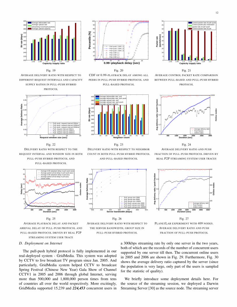
In Fig. 24 and Fig. 25, we investigate the performance ofpull-push hybrid protocol under dynamic environment. As inSection III-B.3, the simulation is driven by real deployed P2Pstreaming system traces. We use request interval 1000ms andrequest window size 10 seconds. And the capacity supplyratio is 1.2. In Fig. 24, we see that the delivery ratio remainsperfectly above 0.97 all the time and nearly 1 in most time. Thefraction of pushed packets is above 80% in most time. Fig. 25shows the delay performance of the two protocols. The averagepacket arrival delay of pull-push hybrid protocol is around 2.5seconds much smaller than that of pull-based protocol (i.e.around 17 seconds). Meanwhile, the 0.99-playback delay ofpull-push hybrid protocol rapidly decreases from 30 secondsto below 10 seconds within the first 200 seconds and thenkeeps around 6.5 seconds in most time. This is because therepeated request and retransmission is eliminated and mostpackets are relayed directly in our pull-push hybrid protocol.However, the pull-based protocol has a playback delay of 24seconds. The results show that the pull-push hybrid protocolalso has excellent performance under dynamic environment.

C. Evaluation on PlanetLab

We also conduct the experiment on PlanetLab for pull-pushhybrid protocol. The main configuration of the experiment isthe same as in Subsection III-C. We also use the trace fromreal deployed P2P streaming system to drive the node behavioras described in Subsection III-C.

As shown in Fig. 27, the delivery ratio of pull-push hybridprotocol is very close to 1 all the time. And push fraction isnear 90% which is a little larger than that in simulation becausethe group size in PlanetLab experiment is much smaller. InFig. 28, we see that the delay of pull-push hybrid protocol isaround 2 seconds much smaller than 13 seconds in pull-basedprotocol.

12

1.02 1.05 1.1 1.15 1.2 1.25 1.3200

220

240

260

280

300

320

340

360

380

400B

it ra

te (k

bps)

Capacity supply ratio

Average deliverable rateAverage upload rate (streaming+overhead packets)Average upload capacity

Fig. 19AVERAGE DELIVERY RATIO WITH RESPECT TO

DIFFERENT REQUEST INTERVALS AND CAPACITY

SUPPLY RATIOS IN PULL-PUSH HYBRID

PROTOCOL

0 5 10 15 20 25 300

10

20

30

40

50

60

70

80

90

100

0.99−playback delay (sec)

Per

cent

ile (%

)

Pull−push, CSR 1.1Pull−push, CSR 1.2Pull−push, CSR 1.3Pull, CSR 1.1Pull, CSR 1.2Pull, CSR 1.3

Fig. 20CDF OF 0.99-PLAYBACK DELAY AMONG ALL

PEERS IN PULL-PUSH HYBRID PROTOCOL AND

PULL-BASED PROTOCOL

1.02 1.05 1.1 1.15 1.2 1.25 1.30

5

10

15

20

25

30

35

40

45

50

Pac

ket r

ate

(pac

kets

/sec

)

Capacity supply ratio

Control packet rate of pull−pushControl packet plus redundant packet rate of pull−pushControl packet rate of pull

Fig. 21AVERAGE CONTROL PACKET RATE COMPARISON

BETWEEN PULL-BASED AND PULL-PUSH HYBRID

PROTOCOL

4 8 12 16 200.6

0.65

0.7

0.75

0.8

0.85

0.9

0.95

1

Request window size (sec)

Ave

rage

Del

iver

y R

atio

Pull−push, request interval 200msPull−push, request interval 1000msPull−push, request interval 2000msPull, request interval 200msPull, request interval 1000msPull, request interval 2000ms

Fig. 22DELIVERY RATIO WITH RESPECT TO THE

REQUEST INTERVAL AND WINDOW SIZE IN BOTH

PULL-PUSH HYBRID PROTOCOL AND

PULL-BASED PROTOCOL

10 20 30 40 50 60 70 80200

220

240

260

280

300

320

340

360

380

400

Neighbor count

Bit

rate

(kbp

s)

Average deliverable rate, pullAverage deliverable rate, pull−pushAverage upload rate, pullAverage upload rate, pull−pushAverage upload capacity

Fig. 23DELIVERY RATIO WITH RESPECT TO NEIGHBOR

COUNT IN BOTH PULL-PUSH HYBRID PROTOCOL

AND PULL-BASED PROTOCOL

500 1000 1500 2000 2500 30000.6

0.7

0.8

0.9

1

Duration (sec)

Avg

del

iver

y ra

tio

/ p

ush

fra

ctio

n

500 1000 1500 2000 2500 30000

5000

10000

On

line

no

des

Average delivery ratioPush fractionOnline nodes

Fig. 24AVERAGE DELIVERY RATIO AND PUSH

FRACTION OF PULL-PUSH PROTOCOL DRIVEN BY

REAL P2P STREAMING SYSTEM USER TRACES

500 1000 1500 2000 2500 30000

5

10

15

20

25

30

35

40

Del

ay (

sec)

Duration (sec)

500 1000 1500 2000 2500 30000

5000

10000

On

line

no

des

Average 0.99−playback delay in pull−push (sec)Average packet arrival delay in pull−push (sec)Average 0.99−playback delay in pull (sec)Average packet arrival delay in pull (sec)Online nodes

Fig. 25AVERAGE PLAYBACK DELAY AND PACKET

ARRIVAL DELAY OF PULL-PUSH PROTOCOL AND

PULL-BASED PROTOCOL DRIVEN BY REAL P2PSTREAMING SYSTEM USER TRACE

300 400 500 600 700 800 9000.6

0.65

0.7

0.75

0.8

0.85

0.9

0.95

1

Server bandwidth (kbps)

Ave

rage

Del

iver

y R

atio

Pull, group size 2000Pull, group size 6000Pull, group size 10000Pull−push, group size 2000Pull−push, group size 6000Pull−push, group size 10000

Fig. 26AVERAGE DELIVERY RATIO WITH RESPECT TO

THE SERVER BANDWIDTH, GROUP SIZE IN

PULL-PUSH HYBRID PROTOCOL

0 500 1000 1500 2000 2500 3000 35000.6

0.7

0.8

0.9

1

Duration (sec)

Avg

del

iver

y ra

tio

/ p

ush

fra

ctio

n

0 500 1000 1500 2000 2500 3000 35000

100

200

300

400

500

On

line

no

des

Average delivery ratioPush fractionOnline nodes

Fig. 27PLANETLAB EXPERIMENT WITH 409 NODES.

AVERAGE DELIVERY RATIO AND PUSH

FRACTION OF PULL-PUSH PROTOCOL

D. Deployment on Internet

The pull-push hybrid protocol is fully implemented in ourreal-deployed system - GridMedia. This system was adoptedby CCTV to live broadcast TV program since Jan. 2005. Andparticularly, GridMedia system helped CCTV to broadcastSpring Festival (Chinese New Year) Gala Show of ChannelCCTV1 in 2005 and 2006 through global Internet, servingmore than 500,000 and 1,800,000 person times from tensof countries all over the world respectively. More excitingly,GridMedia supported 15,239 and 224,453 concurrent users in

a 300kbps streaming rate by only one server in the two years,both of which are the records of the number of concurrent userssupported by one server till then. The concurrent online usersin 2005 and 2006 are shown in Fig. 29. Furthermore, Fig. 30shows the average delivery ratio captured by the server (sincethe population is very large, only part of the users is sampledfor the statistic of quality).

We briefly introduce some deployment details here. Forthe source of the streaming session, we deployed a DarwinStreaming Server [30] as the source node. The streaming server

13

0 500 1000 1500 2000 2500 3000 35000

5

10

15

Del

ay (

sec)

Duration (sec)

0 500 1000 1500 2000 2500 3000 35000

100

200

300

400

500

On

line

no

des

Average 0.99−playback delay in pull−push (sec)Average 0.99−playback delay in pull (sec)Online nodes

Fig. 28PLANETLAB EXPERIMENT WITH 409 NODES.COMPARISON OF AVERAGE PLAYBACK DELAY

AND PACKET ARRIVAL DELAY

20:00 21:00 22:00 23:00 00:00 01:000

0.5

1

1.5

2

2.5

3x 10

4

Time

Number of online users

0

0.5

1

1.5

2

2.5

3x 10

5

2005

2006

Fig. 29CONCURRENT ONLINE USERS ON THE CHINESE

NEW YEAR’S EVE IN 2005 AND 2006

20:30 21:00 21:30 22:00 22:30 23:00

60

70

80

90

100

Time

Average Delivery Ratio(%)

2005

2006

Fig. 30QUALITY OF STREAMING SERVICE IN TERMS OF

AVERAGE DELIVERY RATIO IN 2005 AND 2006

was equipped with Dual Core Xeon Server, 1 GB RAM andRedHat Enterprise Server 3.1. It was located in the ChinaTelecom Internet Data Center with 1Gbps upload capacity. TheTV signals were compressed and encoded in CCTV station andreal-time pushed to the streaming server through a 2Mbps fiberconnection. The encoding and streaming rate was 300Kbps. Inthe first deployment in 2005, we set the maximum connectionsto the streaming server up to 200, indicating that only 200peers could obtain contents directly from the server. Theworkload on the streaming server was thus roughly 60Mbps.In the second deployment in 2006, in face of the fact that suchkind of applications got more popular in Internet, we increasedthe maximum connections up to 800, that is, in total at most240Mbps outgoing bandwidth at server side. Considering thatthere were 224,453 users online at most and the streamingrate was 300kbps, the total peak server bandwidth demandwould be over 64Gbps if traditional Client/Server or CDN-based systems were used. And in fact, in other words, oursystem supported 224, 453/800 ≈ 270 times of users morethan Client/Server-based system.

V. DISCUSSION

A. Insights obtained

In fact, much effort has been made on maximizing through-put of peer-to-peer streaming in both systematical and theo-retical work [10], [7], [6]. A lot of approaches leverage opti-mization theory and network coding to increase the networkthroughput in P2P streaming. In this paper, we found that,in peer-to-peer streaming, optimal throughput can be nearlyachieved by a simple protocol in most typical scenarios. In fact,in our proposed pull-push hybrid protocol, the delivery ratiocan achieve 1, as long as the capacity supply is higher by only10% than the minimum bandwidth demand. Considering 3%header overhead and 2%∼3% control overhead, the deliverablerate actually achieves nearly optimal throughput. So makingfull utilization of the upload capacities of all peers in P2Pstreaming are not difficult as expected before.

B. Limitations of simple pull-based and pull-push hybridprotocol

Although pull-based and pull-push hybrid protocol havestrong capability to nearly fully utilize the peer upload ca-pacity, they have their own limitations.

First, we imagine an ideal peer-to-peer streaming protocolhere, which have the following features: a) it can satisfy allthe peers watching 100% quality video even if the total uploadcapacity supply is equal to the minimum total bandwidthdemand; b) the server bandwidth it consumes is only one timestreaming rate so that any home user can broadcast their videowith quality as high as they can; c) when the total uploadcapacity of all peers are more abundant (for instance, thereare a fraction of Ethernet users), it can minimize the ISPcore network and cross ISP traffic without affecting the peerswatching 100% quality video, d) can achieve minimum play-back delay under peer churn, with optimized peer selection andstreaming scheduling and e) when the capacity is insufficient,it can make a fair traffic allocation among peers with respectto the contribution of each peer.

In this paper, we see that simple pull-based and pull-pushhybrid protocol can nearly fulfill Feature a). However, forFeature b), although simple pull-push hybrid protocol cansupport a group of 10,000 peers to get nearly 100% deliveryratio consuming server bandwidth of 1.6 times the streamingrate without peer churn, how to only use server bandwidthof one time streaming rate is a very challenging topic. ForFeature c), due to the random peer selection and random packetscheduling, both the simple pull-based and pull-push hybridprotocol can not deal with this. In fact, “owing to” the powerfulcapability of pull-based protocol to utilize available bandwidth,the simple peer selection and random scheduling usually causetremendous core network and cross-ISP traffic. Furthermore,the cost of most of this traffic is paid by ISP itself. Thiswill result in that ISPs do not have incentives to update theirinfrastructures to promote their network capacity, since oncethey do this, their core network will be congested by moreunprofitable traffic. Thus, how to reduce the peer-to-peer trafficin core network and iter-ISP links to achieve a win-win modelis a big challenging topic. For Feature d), although pull-pushhybrid protocol has much lower playback delay than pull-basedprotocol, we can still further reduce it. For instance, we cando optimized peer selection with considering the peer onlinetime and peer upload capacity comprehensively. Some workhas been done towards optimal peer selection (such as [31]),and we believe that it can be combined with our pull-pushhybrid protocol in our future study. For Feature e), these twosimple protocols, of course, can not handle this issue. We note

14

that [24] designs elegant contribution-aware mechanism formultiple-tree based protocol. However, designing contribution-aware pull-based and pull-push hybrid protocol should befurther studied.C. Future research directions

• Minimizing ISP core network and cross-ISP traffic: inour paper, we do not discuss the link stress of suchprotocols due to topology mismatch between overlay andunderlay. Since ISPs worry much about the huge P2Ptraffic, measuring and evaluating the impact pull andpull-push protocols on link stress and try to use existingproxy cache and locality-aware peer selection techniqueto relieve the link stress are challenging topics for futurestudy. Recent work such as [32] has started to practicallysolve this problem in general P2P applications.

• Server bandwidth reduction: in typical parameter settings,pull-based and pull-push hybrid protocol need serverbandwidth of 3 and 1.6 times streaming rate respectively.How to let home users broadcast video with quality ashigh as they can is a very challenging. Can we not onlyuse only one-time-streaming-rate server bandwidth butalso deliver high quality video to all users? Can networkcoding be leveraged to handle this?

• Network coding: in peer-to-peer live streaming, leverag-ing network coding may not help much to improve the thethroughput. So other benefits of network coding shouldbe paid more attention, such as data randomization andpersistence, resistance to high churn rate and diminishingstartup waiting delay. Recent work Echelon [33] and Lava[34] has made this wise step.

• Real Internet environment: in this paper, we have theassumptions that the bandwidth bottleneck is only at theend-host and all the nodes can connect with each other,as most previous work is based on. However, on thereal Internet, the connections across the peer link bridgebetween ISPs have low rate, and NAT/firewall usuallyprevent end-host from connecting with each other. Doesthe near optimality of pull-based and pull-push hybridprotocol still hold under real Internet environment?

VI. CONCLUSION

In this paper, we first give our observation that, besidessimplicity and robustness as recognized before,the pull-basedprotocol is nearly optimal in terms of bandwidth utilization andsystem throughput when the server bandwidth is above severaltimes of the streaming rate. We also give mathematical analysisto give an insightful understanding of the pull-based protocoland explain why pull-based protocol has this characteristic.Moreover, we point out that high overhead and large delay ofpull-based protocol can be easily overcome by our proposedpull-push hybrid protocol. We highlight the proposed protocolwhich can not only approach the nearly optimal throughputbut also can reach far lower playback delay and much smalleroverhead than the pull-based protocol. Especially in staticenvironment, the near optimality in peer bandwidth utilizationcan be achieved when the server bandwidth is 1.6 times of thestreaming rate. Based on our findings, we further give some

discussions for pull/pull-push hybrid protocol and the futurework in P2P streaming.

REFERENCES

[1] “Pplive,” 2007. [Online]. Available: http://www.pplive.com/[2] “Zattoo,” 2007. [Online]. Available: http://zattoo.com/[3] “Gridmedia: http://www.gridmedia.com.cn/,” 2006.[4] X. Zhang, J. Liu, B. Li, and T.-S. P. Yum, “Coolstreaming/donet: A

data-driven overlay network for efficent media streaming,” in IEEEINFOCOM 2005, Miami, US, Mar. 2005.

[5] V. Venkataraman and P. Francis., “Chunkyspread: Multi-tree unstruc-tured end system multicast,” in IEEE ICNP 2006, San Babara, CA, USA,2006.

[6] N. Garg, R. Khandekar, K. Kunal, and V. Pandit, “Bandwidth maximiza-tion in multicasting,” in Annual European Symposium on Algorithms,Budapest, Hungary.

[7] Y. Cui, B. Li, and K. Nahrstedt, “On achieving optimized capacityutilization in application overlahy networks with multiple competingsessions,” in ACM Symposium on Parallel Algorithms and Architectures2004, Barcelona, Spain, June 2004.

[8] J. Li, P. A. Chou, and C. Zhang, “Mutualcast: An efficient mechanism forone-to-many content distribution,” in ACM SIGCOMM Asia Workshop2004, Beijing, China, 2004.

[9] T. Small, B. Li, and B. Liang, “Outreach: Peer-to-peer topology construc-tion towards minimized server bandwidth costs,” IEEE JSAC SpecialIssue on Peer-to-Peer Communications and Applications, Jan. 2007.

[10] Z. Li, B. Li, D. Jiang, and L. C. Lau, “On achieving optimal throughputwith network coding,” in IEEE INFOCOM 2005, 2005.

[11] Y. Chu, S. Rao, and H. Zhang, “A case for end system multicast,” inACM Sigmetrics 2000, Santa Clara, California, USA, June 2000.

[12] B. Cohen, “Bittorrent: http://bitconjuer.com.”[13] V. Pai, K. Kumar, K. Tamilmani, V. Sambamurthy, and A. E. Mohr,

“Chainsaw: Eliminating trees from overlay multicast,” in IPTPS 2005,Conell, US, Feb. 2005.

[14] N. Magharei and R. Rejaie, “Prime: Peer-to-peer receiver-driven mesh-based streaming,” in IEEE INFOCOM 2007, Anchorage, Alaska, USA,May 2007.

[15] S. Annapureddy, S. Guha, and et al, “Exploring vod in p2p swarmingsystems,” in IEEE INFOCOM 2007, Anchorage, Alaska, USA, May2007.

[16] “Qqlive,” 2006. [Online]. Available: http://tv.qq.com/[17] R. Kumar, Y. Liu, and K. Ross, “Stochastic fluid theory for p2p

streaming systems,” in IEEE INFOCOM 2007, Anchorage, Alaska, USA,May 2007.

[18] A. R. Bharambe, C. Herley, and V. N. Padmanabhan, “Analyzing andimproving a bittorrent networks performance mechanisms,” in IEEEINFOCOM 2006, Barcelona, Spain, Apr. 2006.

[19] A. Legout, G. UrvoyKeller, and P. Michiardi, “Rarest first and chokealgorithms are enough,” in Internet Measurement Conference 2006,Brazil, 2006.

[20] D. Qiu and R. Srikant, “Modeling and performance analysis of bittorrent-like peer-to-peer networks,” in ACM SIGCOMM 2004, Portland, OR,USA, Aug. 2004.

[21] L. Massoulie, A. Twigg, C. Gkantsidis, and P. Rodriguez, “Random-ized decentralized broadcasting algorithms,” in IEEE INFOCOM 2007,Anchorage, Alaska, USA, May 2007.

[22] N. Magharei, R. Rejaie, and Y. Guo, “Mesh or multiple-tree: A compar-ative study of p2p live streaming services,” in IEEE INFOCOM 2007,Anchorage, Alaska, USA, May 2007.

[23] M. Castro, P. Druschel, A.-M. Kermarrec, A. Nandi, A. I. T. Rowstron,and A. Singhr, “Splitstream: high-bandwidth multicast in cooperativeenvironments,” in Symposium on Operating Systems Principles (SOSP)2003, New York, USA, Oct. 2003.

[24] Y.-W. Sung, M. Bishop, and S. Rao, “Enabling contribution awareness inan overlay broadcasting system,” in ACM SIGCOMM 2006, Pisa, Italy,2006.

[25] V. Agarwal and R. Rejaie, “Adaptive multi-source streaming in heteroge-neous peer-to-peer networks,” in Multimedia Computing and Networking2005 (MMCN), San Jose, CA, USA, Jan. 2005.

[26] “Meridian node to node latency matrix (2500×2500),”2005, meridian project. [Online]. Available:http://www.cs.cornell.edu/People/egs/meridian/data.php

[27] Y. Chu, A. Ganjam, T. S. E. Ng, S. G. Rao, K. Sripanidkulchai, J. Zhan,and H. Zhang, “Early experience with an internet broadcast system basedon overlay multicast,” in USENIX 2004, Anchorage, Alaska, USA, May2007.

15

[28] M. Zhang, L. Zhao, Y. Tang, J. Luo, and S. Yang, “Large-scale livemedia streaming over peer-to-peer networks through global internet,”in ACM workshop on Advances in peer-to-peer multimedia streaming(P2PMMS), Singapore, Nov. 2005, pp. 21–28.

[29] “Planetlab,” 2007. [Online]. Available: http://www.planet-lab.org/[30] “Darwin streaming server,” 2007. [Online]. Available:

http://developer.apple.com/opensource/server/streaming/[31] J. Liang and K. Nahrstedt, “Randpeer: Membership management for

qos sensitive peer-to-peer applications,” in IEEE INFOCOM 2006,Barcelona, Spain, Apr. 2006.

[32] G. Shen, Y. Wang, Y. Xiong, B. Y. Zhao, and Z.-L. Zhang, “Hptp:Relieving the tension between isps and p2p,” in IPTPS 2007, Bellevue,Washington, USA, Feb. 2007.

[33] C. Wu and B. Li, “Echelon: Peer-to-peer network diagnosis with networkcoding,” in IEEE IWQoS 2006, New Haven, CT, USA, 2006.

[34] M. Wang and B. Li, “Lava: A reality check of network coding in peer-to-peer live streaming,” in IEEE INFOCOM 2007, Anchorage, Alaska,USA, May 2007.

Meng ZHANG (M’05) received the BEng degreein Computer Science and Technology from TsinghuaUniversity, Beijing, China, in 2004. He is currentlya PhD candidate in the Department of ComputerScience and Technology in Tsinghua University. Hisresearch interests are in all areas in multimedianetworking, particularly in QoS issue of peer-to-peerstreaming, peer-to-peer Video-on-Demand, multime-dia streaming on overlay networks, etc. And he haspublished over 10 papers in multimedia networking.Besides, he is the key designer and developer of

GridMedia - one of the earliest very large scale peer-to-peer live streamingsystem in the world.

Qian ZHANG (M00-SM04) received the B.S., M.S.,and Ph.D. degrees from Wuhan University, China, in1994, 1996, and 1999, respectively, all in computerscience.

Dr. Zhang joined Hong Kong University of Sci-ence and Technology in Sept. 2005 as an AssociateProfessor. Before that, she was in Microsoft Re-search, Asia, Beijing, China, from July 1999, whereshe was the research manager of the Wireless andNetworking Group. Dr. Zhang has published about150 refereed papers in international leading journals

and key conferences in the areas of wireless/Internet multimedia networking,wireless communications and networking, and overlay networking. She is theinventor of about 30 pending patents. Her current research interests are in theareas of wireless communications, IP networking, multimedia, P2P overlay,and wireless security. She also participated many activities in the IETF ROHC(Robust Header Compression) WG group for TCP/IP header compression.

Dr. Zhang is the Associate Editor for IEEE Transactions on WirelessCommunications, IEEE Transactions on Multimedia, IEEE Transactions onVehicular Technologies, Computer Networks and Computer Communications.She also served as Guest Editor for IEEE JSAC, IEEE Wireless Communica-tions, Computer Networks, and ACM/Springer MONET. Dr. Zhang has beeninvolved in organization committee for many important IEEE conferences,including ICC, Globecom, WCNC, Infocom, etc. Dr. Zhang has received TR100 (MIT Technology Review) world’s top young innovator award. She alsoreceived the Best Asia Pacific (AP) Young Researcher Award elected by IEEECommunication Society in year 2004. She received the Best Paper Award inMultimedia Technical Committee (MMTC) of IEEE Communication Societyand Best Paper Award in QShine 2006. She received the Oversea YoungInvestigator Award from the National Natural Science Foundation of China(NSFC) in 2006. Dr. Zhang is the vice-chair of Multimedia CommunicationTechnical Committee of the IEEE Communications Society.

Lifeng SUN (M’05). Dr. Lifeng Sun was born inXi’an, China, 1972. He received his B.S. Degreeand Ph.D. Degrees in System Engineering in 1995and 2000 separately from National University ofDefense Technology, Changsha, Hunan, China. Dr.Sun’s professional interests lie in the broad area of adhoc network streaming, peer-to-peer video stream-ing, interactive multi-view video, distributed videocoding, he has published over 50 papers in the abovedomain. He was on the Post Doctor research of theDepartment of Computer Science and Technology at

Tsinghua University from 2001 to2003; He is now on the Faculty of theDepartment of Computer Science and Technology at Tsinghua University. Dr.Sun is the secretary-general of Multimedia Committee of China ComputerFederation, Vice Director of Tsinghua-Microsoft Media and Network KeyLab of Ministry of Education (MOE). Dr. Sun serviced as TPC member ofPacific-Rim Conference on Multimedia (PCM) 2005, Pacific-Rim Conferenceon Multimedia (PCM) 2006, IEEE International MultiMedia Modelling Con-ference (MMM) 2007, IEEE International MultiMedia Modelling Conference(MMM) 2006, and reviewed papers for IEEE ICME 2006, IEEE CSVT specialissue on multiview video coding.

Shiqiang YANG is a chief professor at TsinghuaUniversity with department of Computer Science andTechnology. He r eceived the B.S, M.S in ComputerScience from Tsinghua University , Beijing , Chinain 1977 and 1983, respectively.

From 1980 to 1992, he worked as an assistant pro-fessor at Tsinghua University, Beijing, China. From1992 to 1994, he visited City University of HongKong and was a research assistant at the Departmentof Manufacture Engineering. As the associate headerof Department of Computer Science and Technology

at Tsinghua University since 1994, he served as the associate professor from1994 to 1999 and then as the professor since 1999.

He is currently the President of Multimedia Committee of China ComputerFederation, Beijing, China and the co-director of Microsoft-Tsinghua Multi-media Joint Lab, Tsinghua University, Beijing, China. His research interestsmainly include multimedia application, video procession, streaming media andembedded multimedia. In recent three years, he has published more than 60papers in international conferences and journals, as well as more than 10proposals within MPEG and AVS standardization.