Understanding Pitch Perception as a Hierarchical Process with Top-Down Modulation

Understanding Pitch Perception as a Hierarchical Processwith Top-Down ModulationEmili Balaguer-Ballester1,2*, Nicholas R. Clark3, Martin Coath1, Katrin Krumbholz3, Susan L. Denham1

1 Centre for Theoretical and Computational Neuroscience, University of Plymouth, Plymouth, United Kingdom, 2 Computational Neuroscience Group, Central Institute for

Mental Health (ZI), Ruprecht-Karls University of Heidelberg, Mannheim, Germany, 3 MRC Institute of Hearing Research, Nottingham, United Kingdom

Abstract

Pitch is one of the most important features of natural sounds, underlying the perception of melody in music and prosody inspeech. However, the temporal dynamics of pitch processing are still poorly understood. Previous studies suggest that theauditory system uses a wide range of time scales to integrate pitch-related information and that the effective integrationtime is both task- and stimulus-dependent. None of the existing models of pitch processing can account for such task- andstimulus-dependent variations in processing time scales. This study presents an idealized neurocomputational model, whichprovides a unified account of the multiple time scales observed in pitch perception. The model is evaluated using a range ofperceptual studies, which have not previously been accounted for by a single model, and new results from aneurophysiological experiment. In contrast to other approaches, the current model contains a hierarchy of integrationstages and uses feedback to adapt the effective time scales of processing at each stage in response to changes in the inputstimulus. The model has features in common with a hierarchical generative process and suggests a key role for efferentconnections from central to sub-cortical areas in controlling the temporal dynamics of pitch processing.

Citation: Balaguer-Ballester E, Clark NR, Coath M, Krumbholz K, Denham SL (2009) Understanding Pitch Perception as a Hierarchical Process with Top-DownModulation. PLoS Comput Biol 5(3): e1000301. doi:10.1371/journal.pcbi.1000301

Editor: Karl J. Friston, University College London, United Kingdom

Received August 26, 2008; Accepted January 23, 2009; Published March 6, 2009

Copyright: � 2009 Balaguer-Ballester et al. This is an open-access article distributed under the terms of the Creative Commons Attribution License, whichpermits unrestricted use, distribution, and reproduction in any medium, provided the original author and source are credited.

Funding: This work was supported by EmCAP (Emergent Cognition through Active Perception, 2005–2008), a research project in the field of Music Cognitionfunded by the European Commission (FP6-IST, contract 013123), and EPSRC grant EP/C010841/1 (COLAMN). The funders had no role in study design, datacollection and analysis, decision to publish, or preparation of the manuscript.

Competing Interests: The authors have declared that no competing interests exist.

* E-mail: [email protected]

Introduction

Modelling the neural processing of pitch is essential for

understanding the perceptual phenomenology of music and

speech. Pitch, one of the most important features of auditory

perception, is usually associated with periodicities in sounds [1].

Hence, a number of models of pitch perception are based upon a

temporal analysis of the neural activity evoked by the stimulus [2–

5]. Most of these models compute a form of short-term

autocorrelation of the simulated auditory nerve activity using an

exponentially weighted integration time window [6–13]. Autocor-

relation models have been able to predict the reported pitches of a

wide range of complex stimuli. However, choosing an appropriate

integration time window has been problematic, and none of the

previous models has been able to explain the wide range of time

scales encountered in perceptual data in a unified fashion. These

data show that, in certain conditions, the auditory system is

capable of integrating pitch-related information over time scales of

several hundred milliseconds [14–22], while at the same time

being able to follow changes in pitch or pitch strength with a

resolution of only a few milliseconds [14,15,21–24]. Limits on the

temporal resolution of pitch perception have also been explored by

determining pitch detection and discrimination performance as a

function of frequency modulation rate [25–27], the main

conclusion being that the auditory system has a limited ability to

process rapid variations in pitch.

The trade-off between temporal integration and resolution is

not exclusive to pitch perception, but is a general characteristic of

auditory temporal processing. For instance, a long integration time

of several hundred milliseconds is required to explain the way in

which the detectability and perceived loudness of sounds increases

with increasing sound duration [28,29]. In contrast, much shorter

integration times are necessary to explain the fact that the auditory

system can resolve sound events separated by only a few

milliseconds [28–30]. Therefore, it appears that the integration

time of auditory processing varies with the stimulus and task.

Previously it was proposed that integration and resolution reflect

processing in separate, parallel streams with different stimulus-

independent integration times [28]. More recently, in order to

reconcile perceptual data pertaining to temporal integration and

resolution tasks, it was suggested that the auditory system makes its

decisions based on ‘‘multiple looks’’ at the stimulus [31], using

relatively short time windows. However, to our knowledge no

model has yet quantitatively explained the stimulus- and task-

dependency of integration time constants.

Another major challenge for pitch modelling is to relate

perceptual phenomena to neurophysiological data. Functional

brain-imaging studies strongly suggest that pitch is processed in a

hierarchical manner [32], starting in sub-cortical structures [33] and

continuing up through Heschl’s Gyrus on to the planum polare and

planum temporale [34–36]. Within this processing hierarchy, there is an

increasing dispersion in response latency, with lower pitches eliciting

longer response latencies than higher pitches [37]. This suggests that

the time window over which the auditory system integrates pitch-

related information depends on the pitch itself. However, no attempt

has yet been made to explain this latency dispersion.

PLoS Computational Biology | www.ploscompbiol.org 1 March 2009 | Volume 5 | Issue 3 | e1000301

In this study, we present a unified account of the multiple time

scales involved in pitch processing. We suggest that top-down

modulation within a hierarchical processing structure is important

for explaining the stimulus-dependency of the effective integration

time for extracting pitch information. A highly idealized model,

formulated in terms of interacting neural ensembles, is presented.

The model represents a natural extension of previous autocorre-

lation models of pitch in a form resembling a hierarchical generative

process [38,39], in which higher (e.g., cortical) levels modulate the

responses in lower (e.g., sub-cortical) levels via feedback connec-

tions. Without modification, the model can account not only for a

wide range of perceptual data, but also for novel neurophysiolog-

ical data on pitch processing.

Methods

The model consists of a feed-forward process, as well as a

feedback process, which modifies the parameters of feed-forward

processing. Both components are explained in detail below and

schematic diagram of the model is shown in Figure 1.

Feed-Forward ProcessingThe role of the feed-forward process (solid lines in Figure 1) is to

predict the pitch of the incoming stimulus. The perceived pitch of

periodic sounds corresponds approximately to the reciprocal of the

repetition period of the sound waveform. This is why temporal

models of pitch perception, such as autocorrelation models, usually

analyze the periodicities of the signal within the auditory-nerve

channels, and then use these periodicities to derive a pitch estimate

by computing the reciprocal of the periodicity that is most

prevalent across frequency channels [2].

The cochlea in the inner ear acts as a frequency analyzer, in

that different sound frequencies activate different places along the

cochlea, which are in turn innervated by different auditory nerve

fibres [1]. Thus, the cochlea can be modelled as a bank of band-

pass filters. In the current model, each cochlear filter was

implemented as a dual resonant nonlinear gammatone filter, which

accounts for the sound level-dependent non-linear properties of

cochlear processing [40]. The filter output was then passed

through a hair cell transduction model [41] to simulate the

conversion of the mechanical cochlear response into auditory-

nerve spiking activity. The model was implemented using DSAM

(Development System for Auditory Modelling http://www.pdn.

cam.ac.uk/groups/dsam/). It contained a total of 30 frequency

channels with centre frequencies ranging from 100 to 10000 Hz

on a logarithmic scale.

The hair cell transduction model generates auditory-nerve spike

probabilities, p(t,k), as a function of time, t, in each frequency

channel, k. The first processing stage (open boxes in Figure 1)

computes the joint probability that a given auditory nerve fibre

produces two spikes, one at time t and another at t-l, where l is a time

delay or lag [10]. These joint probabilities are generated by

computing the cross-product of the auditory-nerve firing probability,

p(t,k), with time-delayed versions of itself for a range of time delays.

The cross-products are then summed across all frequency channels,

k, to generate the output of the first stage of the model A1(t,l):

A1 t,lð Þ~X

k

p t,kð Þp t{l,kð Þ ð1Þ

The activity at the second processing stage, A2(t,l) (green circles

in Figure 1), is computed as a leaky integration, (i.e., a low-pass

filter using an exponentially decaying function [42]) of the input

activity, A1(t,l), using relatively short time constants, t2. It may

therefore be assumed to represent sub-thalamic neural populations

[43–46]. The time constants at the second stage are lag-dependent

(t2 = t2(l)), as suggested by recent psychoacoustic studies [23,37].

However, for clarity, the lag dependency will not be explicitly

stated in the following equations. In the third stage, A3(t,l) (red

circles in Figure 1), the output of the second stage is integrated

over a longer time scale, t3, as suggested by neuroimaging studies

of pitch in the cortex [37,47]. This stage is assumed to be located

more centrally. Both integration stages can be simply described as

time-varying exponential averages,

An t,lð Þ~An t{Dt,lð Þ:e{Dt=En tð ÞzDt

tn

:An{1 t,lð Þgn tð Þ ; n~2,3 ð2Þ

In equation (2), Dt is the time step of the integration and En(t) is

the instantaneous exponential decay rate of the response at each

integration stage (En(t)#tn), which will henceforth be referred to as

the effective integration window. Establishing an appropriate time

constant is as has been mentioned one of the major difficulties in

formulating a general model of pitch perception. Hence, the value

of En(t) in the model proposed here is not constant but is controlled

by changes in the properties of the stimulus. The control of En(t)

will be explained below.

The factors gn(t) normalize the input to each stage by the

corresponding integration window (g2;1; g3(t) = E2(t)/t2).

At each time step An(t,l) will have a maximum at some value of l

which we will write as Ln. The inverse of this lag for the output of

stage 2, 1/L2(t), represents the intermediate pitch prediction of the

model (see Figure 1). Similarly, the inverse of the lag correspond-

ing to the maximum response in stage 3, 1/L3(t) is the final pitch

prediction. For convenience, we refer to the final pitch prediction

from the preceding time step 1/L3(t-Dt) as the pitch expectation, 1/

LE. In all simulations presented in the current study, we used 200

lags, with reciprocals logarithmically distributed, representing

pitches between 50 to 2000 Hz [48].

Author Summary

Pitch is one of the most important features of naturalsounds. The pitch sensation depends strongly on itstemporal context, as happens, for example, in the percep-tion of melody in music and prosody in speech. However,the temporal dynamics of pitch processing are poorlyunderstood. Perceptual studies have shown that there isapparently a wide range of time scales over which pitch-related information is integrated. This multiplicity inperceptual time scales requires a trade-off betweentemporal resolution and temporal integration, which is notexclusive to pitch perception but applies to auditoryperception in general. As far as we are aware, no existingmodel can account simultaneously for the wide range andstimulus-dependent nature of the perceptual phenomenol-ogy. This article presents a neurocomputational model,which explains the temporal resolution–integration trade-offobserved in pitch perception in a unified fashion. The maincontribution of this work is to propose that top-down,efferent mechanisms are crucial for pitch processing. Themodel replicates perceptual responses in a wide range ofperceptual experiments not simultaneously accounted forby previous approaches. Moreover, it accounts quantitative-ly for the stimulus-dependent latency of the pitch onsetresponse measured in the auditory cortex.

Top-Down Model of Pitch Perception


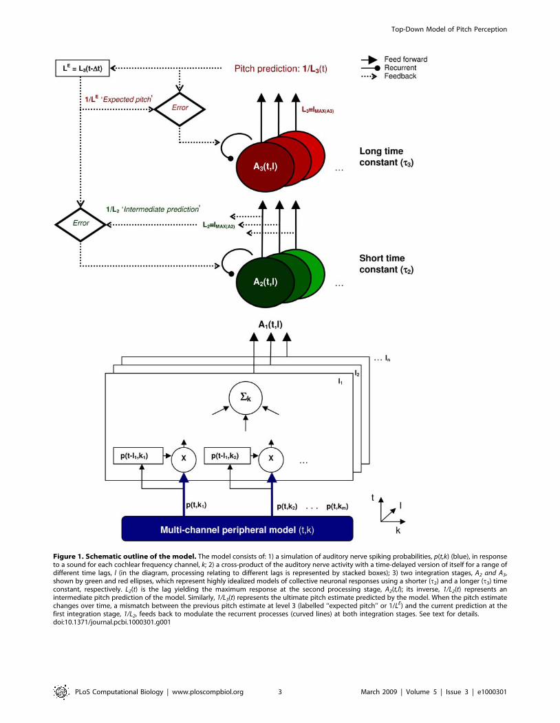
Figure 1. Schematic outline of the model. The model consists of: 1) a simulation of auditory nerve spiking probabilities, p(t,k) (blue), in responseto a sound for each cochlear frequency channel, k; 2) a cross-product of the auditory nerve activity with a time-delayed version of itself for a range ofdifferent time lags, l (in the diagram, processing relating to different lags is represented by stacked boxes); 3) two integration stages, A2 and A3,shown by green and red ellipses, which represent highly idealized models of collective neuronal responses using a shorter (t2) and a longer (t3) timeconstant, respectively. L2(t) is the lag yielding the maximum response at the second processing stage, A2(t,l); its inverse, 1/L2(t) represents anintermediate pitch prediction of the model. Similarly, 1/L3(t) represents the ultimate pitch estimate predicted by the model. When the pitch estimatechanges over time, a mismatch between the previous pitch estimate at level 3 (labelled ‘‘expected pitch’’ or 1/LE) and the current prediction at thefirst integration stage, 1/L2, feeds back to modulate the recurrent processes (curved lines) at both integration stages. See text for details.doi:10.1371/journal.pcbi.1000301.g001



As an example, Figure 2 shows the model response to a

sequence of pure tones (Figure 2A) with random frequencies and

durations. Figure 2B shows the first stage of the model A1(t,l) and

Figure 2C the effective integration windows. Figure 2D shows the

final model output; the red colour highlights the lag-channels with

strong responses. The lag of the channel with the maximum

response at a given time corresponds to the reciprocal of the pitch

predicted by the model. Note that the response A3(t,l) in Figure 2D

was normalized to a maximum of unity after each time step and

mapped exponentially onto the colour scale to make the plot

clearer. However, this transformation is monotonic and thus does

not affect the model predictions.

The necessity for stimulus-driven modulation of the effective

integration time, En(t), becomes clear from a consideration of

existing autocorrelation models. If E2(t) were constant over time,

i.e., E2(t) ; t2 , then A2(t,l) would correspond to the summary

autocorrelation function (SACF) proposed by Meddis and colleagues

[6,7]. If, in addition, E3(t) ; t3 then A3(t,l) would represent an

additional leaky integrator with a longer time constant. This is

equivalent to the cascade autocorrelation model proposed by

Balaguer-Ballester et al. [13]. The right panel in Figure 3A

illustrates the success of the purely feed-forward model in

response to a click train stimulus with alternating inter-click

intervals [49,50]. The arrow indicates the average pitch reported

by listeners. The pitch of such alternating click train stimuli has

been difficult to predict with autocorrelation models consisting of

only one integration stage with a short time constant (see right

panel in Figure 3B).

However, the longer time scale used in the second stage of the

cascade autocorrelation model prevents the detection of rapid

pitch changes such as in the sequence of pure tones shown in

Figure 2. The left panel in Figure 3A clearly shows that the

cascade autocorrelation model fails to distinguish the pitches of

individual tones in the tone sequence used in Figure 2, while the

left panel in Figure 3B shows that the SACF model does so fairly

well. Therefore, stimulus-dependent changes in the effective

integration windows are required.

Parallels with Population ModelsAutocorrelation is usually considered to be a simplified

phenomenological model of pitch perception, which is not

straightforward to implement in a biologically plausible way

[8,43]. This is also the case for the proposed model. Nevertheless,

an alternative, more formal way to express the second and third

model stages (equation 2) is shown in equation (3), below. This is

equivalent to an expression for the response of a neural population

which integrates activity from the previous stage [42]:

tn: _AAn t,lð Þ~{An t,lð Þ{Yn An t,lð Þ,An{1 t,lð Þð Þ; n~2,3: ð3Þ

The dot indicates a partial temporal derivative and tn is defined

as the processing time constant of an idealized homogeneous

population of neurons at stage n. The ‘‘activation’’ functions,Yn, in

equation (3), which typically use a fixed sigmoid function in

standard models of neural assembles [51], are in the model

proposed here time-dependent multiplicative gains:

Yn An t,lð Þ,An{1 t,lð Þð Þ~

vn tð Þln tð Þ

:An t,lð Þ{ vn{1 tð Þln{1 tð Þz1

� �:An{1 t,lð Þ;

ð4Þ

where v1/l1;0; and vn, ln are defined in the next section.

Substituting equation (4) into equation (3) and integrating,

allows us to obtain the effective integration windows, En(t), used in

equation (2):

En tð Þ~ tn

1zvn tð Þln tð Þ

; ð5Þ

Detecting Changes in the StimulusIn contrast with the feed-forward model, the goal of the

feedback processing (dotted lines in Figure 1) is to detect

unexpected changes in the input stimulus, such as the offset of a

tone in a sequence, and to modulate the integration times involved

in the feed-forward processing when such changes occur.

In the case where the stimulus is constant the pitch predictions at

successive time steps will not differ. However, if the stimulus changes

then the height of the peak corresponding to the current pitch

prediction 1/Ln(t) will change from one time step to the next. A

mismatch between the pitch predictions at each level and the pitch

expectation therefore indicates a change in the input stimulus.

A stimulus change typically requires a fast system response, so

that information occurring around the time of the change can be

updated quickly; this corresponds to using small En(t) values. Thus,

during periods when there is a significant discrepancy between the

current and expected pitch estimates, the effective integration time

windows at both integration stages should become very short, so

that the ‘‘memory’’ component of the model response is reduced

to near zero and essentially reset. Similar rapid changes of activity

in response to variations in the input have been previously

reported in neural ensemble models [51,52].

Figure 2C illustrates the dynamics of E2(t) (solid green line) and

E3(t) (dotted red line) in response to a random tone sequence, the

spectrogram of which is shown in Figure 2A. After the end of each

tone, both time constants, E2 and E3, decrease for a brief period of

time and then recover back to their maximum values (En(t)<tn)

when the next tone begins. As E2 is lag-dependent, the values

plotted in Figure 2C represent the integration time constant at the

lag, L2(t), corresponding to the current maximum of A2(t,l). The

small overshoots after the initial dips in E2 reflect transient

variations in L2 before a new stable prediction is achieved.

The effective integration windows, En(t), can vary over a large

range of values, far exceeding the range of plausible neural time

constants. However, it should be noted that the neural processing

time constants used in the model, tn (see equation 3), only take on

biologically plausible values (shown in Table 1). The effective

integration windows, derived from the activation functions

(equation 5), do not represent neural processing time constants.

This aspect will be further addressed in the Discussion section.

During the steady-state portions of each tone, the model

essentially behaves like the cascade autocorrelation model [13].

The feedback mechanism simply allows the model to adapt quickly

to changes in the stimulus.

A natural measure of the mismatch between pitch expectations

and pitch predictions is the relative error gradient of the maximum

response in An(t,Ln),

rn~d

dt

An t,LEð ÞAn t,Ln tð Þð Þ

� �; ð6Þ

where the expected lag, LE, is fixed in the temporal derivative; and

Ln(t) is the lag corresponding to the maximum response at each

time step as defined earlier.



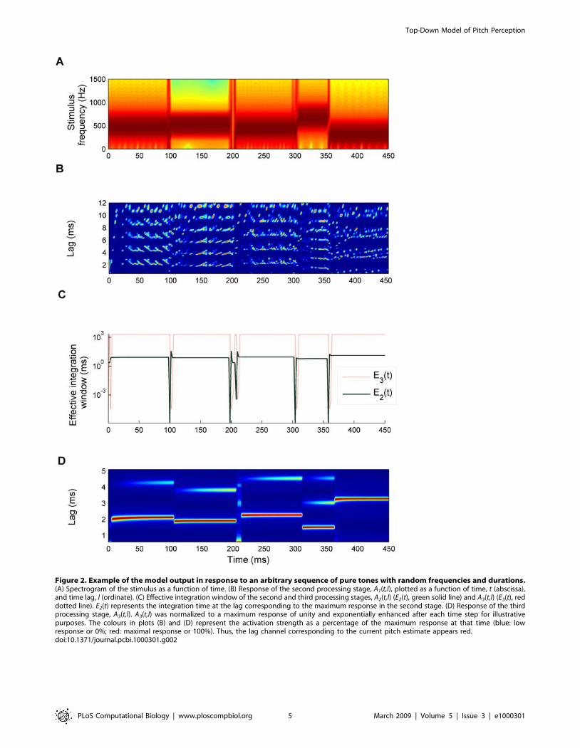
Figure 2. Example of the model output in response to an arbitrary sequence of pure tones with random frequencies and durations.(A) Spectrogram of the stimulus as a function of time. (B) Response of the second processing stage, A1(t,l), plotted as a function of time, t (abscissa),and time lag, l (ordinate). (C) Effective integration window of the second and third processing stages, A2(t,l) (E2(t), green solid line) and A3(t,l) (E3(t), reddotted line). E2(t) represents the integration time at the lag corresponding to the maximum response in the second stage. (D) Response of the thirdprocessing stage, A3(t,l). A3(t,l) was normalized to a maximum response of unity and exponentially enhanced after each time step for illustrativepurposes. The colours in plots (B) and (D) represent the activation strength as a percentage of the maximum response at that time (blue: lowresponse or 0%; red: maximal response or 100%). Thus, the lag channel corresponding to the current pitch estimate appears red.doi:10.1371/journal.pcbi.1000301.g002



The gradient at stage three in the model,

r3&1Dt

A3 t,LEð ÞA3 t,L3 tð Þð Þ{1

� �is an ‘‘error’’ measure: if there is mismatch

between the expected pitch estimate and the current prediction,

i.e., LE ? L3(t), then r3,0. Similarly, at the second stage, r2,0

represents a mismatch, or error, between the expected pitch and

the current intermediate prediction at stage two, 1/L2(t).

Feedback ModulationThe goal of the feedback modulation triggered by changes in

the stimulus is to adjust the effective time constants En(t). The error

gradients rn give us a measure of stimulus change therefore, when

rn is negative enough (compared to a threshold value hn) there is a

discrepancy between the pitch prediction and the pitch expecta-

tion which requires that the time constants be adjusted. This is

achieved by temporarily activating the recurrent term in

equation 4, i.e., by defining

vn~tn:H {hn{rnð Þ; ð7Þ

where H(x) is the Heaviside function (equal to unity if x.0 and

zero otherwise) and hn are small positive thresholds for the error

terms, rn. For example, during the gaps between tones in a

sequence of tones, rn,2hn and the gains vn(t)/ln(t) temporarily

become nonzero, thereby modulating the effective temporal

integration windows, En(t).

This approach leads to a problem with the model as described

so far in that the response to stimuli where there is a continuous

discrepancy between expectations and predictions, very short

effective time windows (En(t)%tn) produce oscillatory responses

which do not correspond to the stable pitch perceived by listeners

(see, for example, Figure 3B, right panel). The dynamics of the

‘adaptation’ variable, ln(t), defined in equation 8 below, serve to

modulate uncontrolled corrections to the effective integration

windows.

Initially the value of ln(t) is small (ln(0)%tn) so that when change

is first detected En(t) also becomes small (equation 5). However, in

situations where there is a continuous mismatch between the

predicted and the expected pitch, ln(t) grows and En(t) recovers to a

value closer to tn.

Then, when there is no longer any discrepancy between

expectation and prediction, ln(t) recovers to a small value again

but without affecting En(t) because, in the absence of a mismatch,

Figure 3. Responses of autocorrelation models with fixed time constants. (A) Response of the cascade autocorrelation model [13]; left plot:to the sequence of random tones shown in Figure 2A, and right plot: to the alternating click train shown in Figure 8A. (B) Response of short-termintegration stage of the cascaded model (corresponding to the second stage of the current model, A2(t,l), when the feedback modulation of theintegration times, equation 8, is switched off); see text for further explanation. As in panel A, the left panel shows the response to the tone sequenceand the right panel shows the response to the click train (arrows mark the reported pitches). Different colours show activation strength as apercentage of the maximum response, as in Figure 2.doi:10.1371/journal.pcbi.1000301.g003

Table 1. Model parameters used in the simulations.

Parameter h2 h3 t2(l) (ms) t3 (ms) g2 (kHz) g3 (kHz) m2 (kHz) m3 (kHz)

Value 0.04 0.07 2–80 2000 3.55 1.15 0.18 1.15

Thresholds hn are dimensionless. Sampling frequency of the sounds (1/Dt) was 176 kHz; integration period in level three was 2 ms. tn.ln(t).1029 ms.doi:10.1371/journal.pcbi.1000301.t001



vn = 0. Therefore, the dynamics of l are described in general by:

_lln tð Þ~ gnH {hn{rnð Þ{mnH rnzhnð Þð Þ:ln; gn,mnw0; ð8Þ

Where g and m are the constants that control the rate of

increase in l during periods of mismatch and the rate of decay in lduring periods where no mismatch occurs.

Figures 2C and 8B illustrate two opposite instances of the effect

of this top-down processing. In response to a sequence of tones, the

effective integration windows shorten precisely at the tone offsets

before returning to their maximum values, tn, during the tones

(Figure 2C). In response to a click train with alternating inter-click

intervals (Figure 8B), the window length settles to a maximum

value after a longer period of transient fluctuations. Figure 4

illustrates the discrete processing steps of the model in the form of

a flowchart. Table 1 gives the set of parameter values used in the

simulations. Further neurobiological justifications for the model

are presented in the Discussion. A Matlab-based software

implementation of the model is freely available from the first

author.

Results

The model was evaluated using a representative set of

psychophysical experiments, which illustrate the different time

scales of temporal integration and resolution in pitch perception. A

further experiment was conducted specifically for this study.

Finally, the last evaluation shows that the proposed model can also

replicate neurophysiological data.

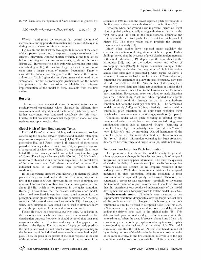
Global Pitch of Non-Simultaneous TonesHall and Peters’ experiment highlighted an unsolved problem

concerning the balance between synthetic and analytic listening in

response to a sequence of pure tones [14,15]. The stimuli of the

pioneering Hall and Peters’ study [14] consisted of three tones

played sequentially either in quiet (Figure 5A, left panel) or against

a background of white noise (Figure 5A, right panel). Each tone

lasted 40 ms and was separated from the following tone by a gap

of 10 ms. Tone frequencies were 650, 850 and 1050 Hz (similar

results were obtained with a harmonic sequence). The overall level

of the noise was about 15 dB above the level of the tones. The

individual tones in the sequence were perceived in both

conditions.

In the experiment, listeners were instructed to match the lowest

pitch that they perceived, and in the quiet condition, this was the

first of the tones (650 Hz). However, in the noise condition, the

non-simultaneous tones combine to create a lower global pitch of

about 213 Hz, which is not perceived in the quiet condition.

Recently, it was shown that the cascade autocorrelation model,

which used two fixed integration stages, could account for the

perception of the global pitch in the noise condition when the time

constant of the second stage was long enough [13]. However, the

same, long, integration stage could not be used to simultaneously

predict the perception of the individual tones in quiet.

Figure 5B shows the responses A3(t,l) over time. As in Figure 2,

the responses after each time step have been normalized for

visualization purposes (however, it should be noted that their real

magnitudes, which are close to zero during the silent gaps, are not

evident in the figure). The maximum of A3(t,l) correctly predicts

the pitches perceived in quiet, which correspond approximately to

the frequencies of the individual tones at each moment in time (left

plot). Thus, the peak in the profile of the final response at the end

of the stimulus correctly reflects the period of the last tone of the

sequence at 0.95 ms, and the lowest reported pitch corresponds to

the first tone in the sequence (horizontal arrow in Figure 5B).

However, when background noise is present (Figure 5B, right

plot), a global pitch gradually emerges (horizontal arrow in the

right plot), and the peak in the final response occurs at the

reciprocal of the perceived pitch of 213 Hz (4.7 ms, right panel of

Figure 5C). The above results match precisely the listeners’

responses in this study [14].

Many other studies have explored more explicitly the

characteristics of temporal integration in pitch perception. Earlier

findings showed that the accuracy of pitch discrimination increases

with stimulus duration [1,19], depends on the resolvability of the

harmonics [20], and on the sudden onsets and offsets of

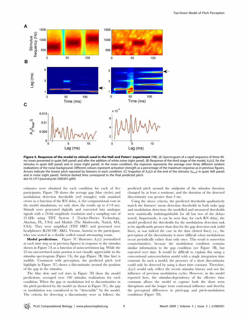
overlapping tones [21,22]. In Figure 6, another example of the

model’s ability to simulate the integration of pitch information

across noise-filled gaps is presented [17,18]. Figure 6A shows a

sequence of two unresolved complex tones of 20-ms duration,

containing 100 harmonics of a 250-Hz base frequency, high-pass

filtered from 5500 to 7500 Hz. After the first of the tones, there

was either a short silent gap (silent-gap condition) or a noise-filled

gap, having a similar mean level to the harmonic complex (noise-

burst condition). Background noise was added to mask distortion

products. In their study, Plack and White reported that subjects

perceived pitch continuity through the gap in the noise-burst

condition, but not in the silent-gap condition [17]. The normalized

model output A3(t,l) (Figure 6C) is qualitatively consistent with a

continuous pitch sensation in the noise-burst condition (right

panel), which does not occur in the silent-gap condition (left panel).

Conditions under which pitch encoding is affected by the

presence of other sounds have been also studied using non-

simultaneous stimuli such as temporal ‘‘fringes’’ (consisting of

complex tones played immediately before and after a ‘‘target’’

tone) [16,53,54]; and by mistuning delayed harmonics of the

complex [12,55–57]. The model described here also accounts for

the ‘‘reset’’ of pitch information occurring for large frequency

differences between fringe and target tones [53] (data not shown).

Temporal Resolution for Pitch InformationThe previous section shows the model’s ability to generate

stimulus-dependent changes in the effective time scale of temporal

integration for extracting pitch information. This raises the question

of whether the ability of the model to adjust the effective integration

windows could also account for the temporal resolution of the

auditory system. While there is substantial evidence for temporal

integration in pitch perception, temporal resolution in pitch

perception is perhaps still poorly understood. Therefore, we

conducted a psychoacoustic experiment specifically to investigate

the temporal resolution of pitch information. It should be stressed

that this experiment was conducted independently of the model

development and was subsequently used to test the model’s predictions.

Psychoacoustic study. Thresholds were measured in two

experimental conditions, designed to assess the temporal resolution

of the auditory system to changes in pitch strength. In both

conditions, a stimulus referred to as rippled noise (RN) was used.

RN is generated by delaying a random noise by a delay, d, and

adding the delayed copy back to the original noise [58]. This

delay-and-add process creates a degree of serial correlation in the

noise stimulus. When the delay is between about 1 and 30 ms, this

correlation gives rise to the perception of a buzzy tone with a pitch

corresponding to the reciprocal of the delay, 1/d. The serial

correlation, and thus the pitch, of RN can be switched on and off

by replacing portions of the delayed noise by an uncorrelated noise

of the same intensity. In the first condition, referred to as the gap

condition, serial correlation was switched off for a single, brief



period around the temporal centre of the stimulus, and the shortest

detectable gap in correlation, referred to as the pitch-gap detection

threshold, was measured.

In the second condition, referred to as the modulation

condition, correlation was switched on and off periodically

according to a square-wave function with a 50% duty cycle (i.e.,

the proportion of time for which correlation was high). In this case,

the pitch-modulation detection threshold was measured. This

threshold is the fastest rate at which the modulation in correlation

was just detectable. Both the pitch-gap and pitch-modulation

detection thresholds were measured for four different values of the

RN delay, d (1, 2, 4, 8, 12 and 16 ms). Figure 7A shows an

example of a RN stimulus for d = 4 ms in which the gap in

correlation is 25 ms. Note that the gap is not visible in the

spectrogram. Figure 7B shows the first peak height of the average

running autocorrelation as a function of time (Rh1[t]) for both the

modulated (red) and gap (blue) RN stimuli of the same delay and

gap sizes. Note that panels A and C in Figure 7 refer to the gap

stimulus alone.

Thresholds were obtained using a two-interval, two-alternative

forced-choice (2I2AFC) adaptive procedure using a 3-down 1-up

rule [59]. Stimuli had a duration of 1 s; they were low pass filtered

at 5 kHz (24 dB/oct.) and presented at a level of 65 dB SPL

(decibel sound pressure level). A minimum of three threshold

Figure 4. Diagrammatic representation of the computations involved in the recurrent processes of An(t,l) in flowchart form.doi:10.1371/journal.pcbi.1000301.g004



estimates were obtained for each condition for each of five

participants. Figure 7D shows the average gap (blue circles) and

modulation detection thresholds (red triangles) with standard

errors as a function of the RN delay, d, (for computational costs in

the model simulations, we only show the results up to d = 8 ms).

Stimuli were generated digitally and converted into analogue

signals with a 24-bit amplitude resolution and a sampling rate of

25 kHz using TDT System 3 (Tucker-Davies Technology,

Alachua, FL, USA) and Matlab (The Mathworks, Natick, MA,

USA). They were amplified (TDT HB7) and presented over

headphones (K240 DF, AKG, Vienna, Austria) to the participant,

who was seated in a double walled sound attenuating room.

Model predictions. Figure 7C illustrates A3(t,l) (normalized

at each time step as in previous figures) in response to the stimulus

shown in Figure 7A as a function of autocorrelation lag. While the

25-ms uncorrelated noise portion is not visually appreciable in the

stimulus spectrogram (Figure 7A), the gap (Figure 7B, blue line) is

audible. Consistent with perception, the predicted pitch (red

highlight in Figure 7C) shows a discontinuity around the position

of the gap in the stimulus.

The blue dots and red stars in Figure 7D show the model

predictions, averaged over 100 stimulus realizations for each

condition. When the gap or modulation led to discontinuities in

the pitch predicted by the model (as shown in Figure 7C), the gap

or modulation was considered to be ‘‘detectable’’ by the model.

The criteria for detecting a discontinuity were as follows: the

predicted pitch around the midpoint of the stimulus duration

changed by at least a semitone, and the duration of the detected

discontinuity was greater than 4 ms.

Using the above criteria, the predicted thresholds qualitatively

match the listeners’ mean detection thresholds in both tasks (gap

and modulation detection; the modelled and measured thresholds

were statistically indistinguishable for all but two of the delays

tested). Importantly, it can be seen that, for each RN delay, the

model predicted the thresholds for the modulation detection task

to be significantly greater than that for the gap detection task (solid

lines), as was indeed the case in the data (dotted lines); i.e., the

perception of the discontinuity is more difficult when modulations

occur periodically rather than only once. This result is somewhat

counterintuitive, because the modulation condition contains

similar information to the gap condition (see Figure 7B), but

repeated over time. It would be difficult to explain this using a

conventional autocorrelation model with a single integration time

constant. In such a model, the presence of a short discontinuity

could only be detected by using a short time constant. Therefore,

A3(t,l) would only reflect the recent stimulus history and not the

influence of previous modulation cycles. However, in the model

reported here, the stimulus-dependency of the effective time

constants allows the model to capture both the short term

disruptions and the longer term contextual influence and thereby

the perceptual differences in pitch-gap and pitch-modulation

conditions (Figure 7D).

Figure 5. Response of the model to stimuli used in the Hall and Peters’ experiment [14]. (A) Spectrogram of a rapid sequence of three 40-ms tones presented in quiet (left panel) and after the addition of white noise (right panel). (B) Response of the third stage of the model, A3(t,l), for thestimulus in quiet (left panel) and in noise (right panel). In the noise condition, the response represents the average over three different randomrealizations of the noise background. Different colours represent activation strength as a percentage of the maximum response as in previous figures.Arrows indicate the lowest pitch reported by listeners in each condition. (C) Snapshot of A3(t,l) at the end of the stimulus (tfinal) in quiet (left panel)and in noise (right panel). Vertical dashed lines correspond to the final predicted pitch.doi:10.1371/journal.pcbi.1000301.g005



Pitch of Click Train StimuliFigure 2B showed that the model uses very short integration

times for pitch information when a change in pitch occurs.

However, it is possible to construct a class of stimuli, in which the

periodicities change continually over very short time scales but

which nevertheless elicit a single pitch [49,50], suggesting that

pitch information is integrated across these rapid changes in

periodicity. The stimuli in question are high-pass-filtered click

trains where the interval between successive clicks varies.

Previously we showed that the cascade autocorrelation model

with fixed integration times [13] predicted the pitch percept

elicited by a range of click train stimuli, which had proved

problematic for conventional autocorrelation models [49,50,60–

63]. Here, we test whether the current model (which generalizes

the model reported in [13] by including variable integration times)

retains this ability. This is an important question, because a rapid

reset of pitch information is apparently in contradiction with the

long-term integration used in [13], as was illustrated in the

Methods section (Figure 3).

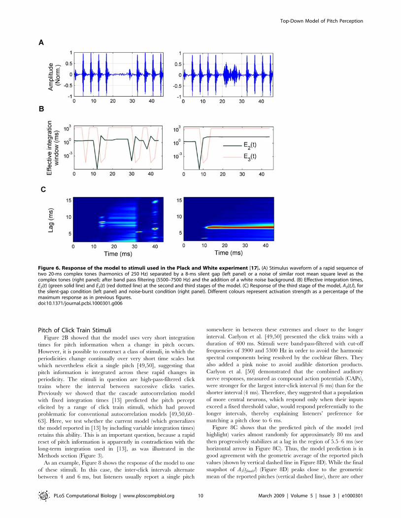
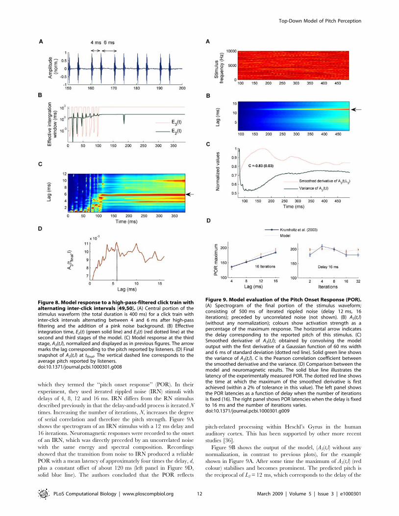
As an example, Figure 8 shows the response of the model to one

of these stimuli. In this case, the inter-click intervals alternate

between 4 and 6 ms, but listeners usually report a single pitch

somewhere in between these extremes and closer to the longer

interval. Carlyon et al. [49,50] presented the click trains with a

duration of 400 ms. Stimuli were band-pass-filtered with cut-off

frequencies of 3900 and 5300 Hz in order to avoid the harmonic

spectral components being resolved by the cochlear filters. They

also added a pink noise to avoid audible distortion products.

Carlyon et al. [50] demonstrated that the combined auditory

nerve responses, measured as compound action potentials (CAPs),

were stronger for the largest inter-click interval (6 ms) than for the

shorter interval (4 ms). Therefore, they suggested that a population

of more central neurons, which respond only when their inputs

exceed a fixed threshold value, would respond preferentially to the

longer intervals, thereby explaining listeners’ preference for

matching a pitch close to 6 ms.

Figure 8C shows that the predicted pitch of the model (red

highlight) varies almost randomly for approximately 80 ms and

then progressively stabilizes at a lag in the region of 5.5–6 ms (see

horizontal arrow in Figure 8C). Thus, the model prediction is in

good agreement with the geometric average of the reported pitch

values (shown by vertical dashed line in Figure 8D). While the final

snapshot of A3(tfinal,l) (Figure 8D) peaks close to the geometric

mean of the reported pitches (vertical dashed line), there are other

Figure 6. Response of the model to stimuli used in the Plack and White experiment [17]. (A) Stimulus waveform of a rapid sequence oftwo 20-ms complex tones (harmonics of 250 Hz) separated by a 8-ms silent gap (left panel) or a noise of similar root mean square level as thecomplex tones (right panel); after band pass filtering (5500–7500 Hz) and the addition of a white noise background. (B) Effective integration times,E2(t) (green solid line) and E3(t) (red dotted line) at the second and third stages of the model. (C) Response of the third stage of the model, A3(t,l), forthe silent-gap condition (left panel) and noise-burst condition (right panel). Different colours represent activation strength as a percentage of themaximum response as in previous figures.doi:10.1371/journal.pcbi.1000301.g006



prominent peaks in A3(tfinal,l) close to this maximum; this is

consistent with the large variability in reported pitches for these

alternating click trains. A prediction of the model yet to be tested is

that no reliable pitch estimate would be possible for stimuli shorter

than 100 ms. To conclude, it is worth remarking that this model

can similarly account for the pitches of the other click train stimuli

considered in [13].

Cortical Latency of the Pitch Onset ResponseThe model proposed here is not a formal model of neural

populations; nevertheless, it is neurophysiologically based (see

Methods and Discussion sections). This raises the question as to

whether the model can explain aspects of the responses of neural

ensembles in a pitch perception task. Krumbholz et al. [37]

identified a transient neuromagnetic response in Heschl’s Gyrus,

Figure 7. Comparison between human and model pitch-gap and pitch-modulation thresholds in a task specifically designed forassessing temporal resolution in pitch perception (see text for details). (A) Spectrogram for a rippled noise (RN) with a 4-ms delay, whichcontains a 25-ms gap in serial correlation around the centre of the stimulus, not visible in the figure. (B) First peak height of the runningautocorrelation as a function of time (Rh1[t]) for both the modulated (red) and gap (blue) RN stimuli; averaged over 105 stimulus realizations. (C)A3(t,l), for the stimulus shown in panel A, normalized and displayed as in previous figures. (D) Average detection thresholds and standard errors forthe pitch-gap (blue circles) and pitch-modulation conditions (red triangles). The corresponding model predictions are shown in the same colours(dots and stars).doi:10.1371/journal.pcbi.1000301.g007



which they termed the ‘‘pitch onset response’’ (POR). In their

experiment, they used iterated rippled noise (IRN) stimuli with

delays of 4, 8, 12 and 16 ms. IRN differs from the RN stimulus

described previously in that the delay-and-add process is iterated N

times. Increasing the number of iterations, N, increases the degree

of serial correlation and therefore the pitch strength. Figure 9A

shows the spectrogram of an IRN stimulus with a 12 ms delay and

16 iterations. Neuromagnetic responses were recorded to the onset

of an IRN, which was directly preceded by an uncorrelated noise

with the same energy and spectral composition. Recordings

showed that the transition from noise to IRN produced a reliable

POR with a mean latency of approximately four times the delay, d,

plus a constant offset of about 120 ms (left panel in Figure 9D,

solid blue line). The authors concluded that the POR reflects

pitch-related processing within Heschl’s Gyrus in the human

auditory cortex. This has been supported by other more recent

studies [36].

Figure 9B shows the output of the model, (A3(t,l) without any

normalization, in contrast to previous plots), for the example

shown in Figure 9A. After some time the maximum of A3(t,l) (red

colour) stabilises and becomes prominent. The predicted pitch is

the reciprocal of L3 = 12 ms, which corresponds to the delay of the

Figure 8. Model response to a high-pass-filtered click train withalternating inter-click intervals [49,50]. (A) Central portion of thestimulus waveform (the total duration is 400 ms) for a click train withinter-click intervals alternating between 4 and 6 ms after high-passfiltering and the addition of a pink noise background. (B) Effectiveintegration time, E2(t) (green solid line) and E3(t) (red dotted line) at thesecond and third stages of the model. (C) Model response at the thirdstage, A3(t,l), normalized and displayed as in previous figures. The arrowmarks the lag corresponding to the pitch reported by listeners. (D) Finalsnapshot of A3(t,l) at tfinal. The vertical dashed line corresponds to theaverage pitch reported by listeners.doi:10.1371/journal.pcbi.1000301.g008

Figure 9. Model evaluation of the Pitch Onset Response (POR).(A) Spectrogram of the final portion of the stimulus waveform;consisting of 500 ms of iterated rippled noise (delay 12 ms, 16iterations); preceded by uncorrelated noise (not shown). (B) A3(t,l)(without any normalization); colours show activation strength as apercentage of the maximum response. The horizontal arrow indicatesthe delay corresponding to the reported pitch of this stimulus. (C)Smoothed derivative of A3(t,l); obtained by convolving the modeloutput with the first derivative of a Gaussian function of 60 ms widthand 6 ms of standard deviation (dotted red line). Solid green line showsthe variance of A3(t,l). C is the Pearson correlation coefficient betweenthe smoothed derivative and the variance. (D) Comparison between themodel and neuromagnetic results. The solid blue line illustrates thelatency of the experimentally measured POR. The dotted red line showsthe time at which the maximum of the smoothed derivative is firstachieved (within a 2% of tolerance in this value). The left panel showsthe POR latencies as a function of delay when the number of iterationsis fixed (16). The right panel shows POR latencies when the delay is fixedto 16 ms and the number of iterations varies.doi:10.1371/journal.pcbi.1000301.g009



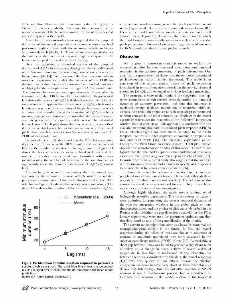
IRN stimulus. However, the maximum value of A3(t,L3) in

Figure 9B emerges gradually. Therefore, there seems to be no

obvious correlate of the latency at around 150 ms of the measured

cortical response in the model.

A number of previous studies have suggested that the temporal

derivative of the neural population responses at lower levels of

processing might correlate with the measured activity in higher

(i.e., cortical) levels [44,45,64]. Therefore we investigated whether

the latency of the pitch onset response might correspond to the

latency of the peak in the derivative of A3(t,L3).

Here, we calculated a smoothed version of the temporal

derivative of A3(t,L3) by convolving A3(t,L3) with the first differential

of a Gaussian function (representing connection efficacies to

higher areas [44,45]). We then used the first maximum of this

smoothed derivative to predict the latencies of the POR for

different pitch values. Figure 9C illustrates the smoothed derivative

of A3(t,L3) for the example shown in Figure 9A (red dotted line).

The derivative has a maximum at approximately 168 ms, which is

consistent with the POR latency for this condition. The green solid

line shows the variance of A3(t,l) (calculated at each fixed t) for the

same stimulus. It appears that the variance of A3(t,l), which might

be taken to represent the uncertainty of the pitch estimate, reaches

a minimum at a similar time as the derivative of A3(t,L3) reaches a

maximum (in general, however, the smoothed derivative is a more

accurate predictor of the experimental latencies). The red dotted

line in Figure 9D (left plot) shows the time at which the smoothed

derivative of A3(t,L3) reaches its first maximum as a function of

pitch value, which appears to correlate remarkably well with the

POR latencies (solid line).

Krumbholz et al. [37] also found that the POR latency mainly

depended on the delay of the IRN stimulus and was influenced

little by the number of iterations. The right panel in Figure 9D

shows the latencies when the delay is fixed at 16 ms and the

number of iterations varies (solid line). Consistent with experi-

mental results, the number of iterations of the stimulus do not

significantly affect the smoothed derivative of A3(t,L3(t)) (dotted

line).

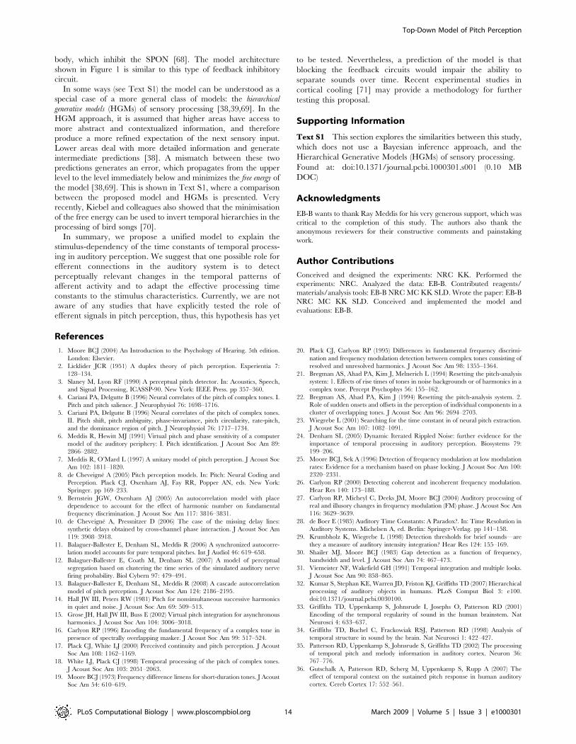
To conclude, it is worth mentioning that the model also

accounts for the minimum duration of IRN stimuli for reliable

perceptual discrimination of the pitch, also reported in [37]. The

solid line in Figure 10 indicates the average perceptual results. The

dashed line shows the duration of the transient period in A3(t,L3),

i.e., the time window during which the pitch prediction is not

stable (e.g. around 100 ms in the stimulus shown in Figure 8C).

Clearly, the model simulations match the data extremely well

(dashed line in Figure 10). Therefore, the initial period in which

the model output varies rapidly seems to correlate with unstable

pitch perception. This model prediction might be valid not only

for IRN stimuli but also for other pitched sounds.

Discussion

We propose a neurocomputational model to explain the

observed paradox between temporal integration and temporal

resolution in the auditory processing of pitch information. Our

goal was to capture essential elements in the temporal dynamics of

pitch perception within a unified framework. This model is an

extension of the autocorrelation theory of pitch perception

formulated in terms of equations describing the activity of neural

ensembles [51,65], and extended to include feedback processing.

The principal novelty of the model is the suggestion that top-

down connections to sub-cortical areas determine the temporal

dynamics of auditory perception, and that this influence is

mediated through feedback modulation of recurrent inhibitory

circuits. As a result, the responses at each stage adapt to recent and

relevant changes in the input stimulus; i.e., feedback in the model

essentially determines the dynamics of the ‘‘effective’’ integration

window used at each stage. This approach is consistent with the

available neuroimaging data: a sustained pitch response (SPR) in

lateral Heschl’s Gyrus has been shown to adapt to the recent

temporal context of a pitch sequence, enhancing the response to

rare and brief events [36]. The successful explanation of the

latency of the Pitch Onset Response (Figure 9D, left plot) further

supports the neurobiological validity of this model. Therefore, we

hypothesize that the model captures some fundamental processing

aspects of pitch processing, occurring up to Heschl’s Gyrus [37].

Consistent with this, a recent study also suggests that the auditory

sensory thalamus processes fast changes in speech, which appears

to be modulated by slower contextual states [66].

It should be noted that efferent connections to the auditory

peripheral model have not yet been implemented, although there

is evidence for those connections too [67]. The addition of this

connection could provide a method for controlling the cochlear

model, a current focus of our investigations.

Although highly idealized, the model uses a minimal set of

biologically plausible parameters. The values shown in Table 1

were optimized for generating the correct temporal dynamics of

the effective integration windows in the global pitch of non-

simultaneous tones, and the pitches of click trains, described in the

Results section. Neither the gap detection threshold nor the POR

latency experiments were used for parameter optimization; they

therefore stand as tests of the generalization of the model.

The current model might thus serve as a basis for more realistic

neurophysiological models in the future. In fact, the model

responses during the offsets of tones are similar to responses of

neurons to amplitude modulated pure tones measured in the

superior paraolivary nucleus (SPON) of rats [68]. Remarkably, a

short gap between tones was found to produce a significant burst

of spikes; i.e., a change in neural activity of several orders of

magnitude in less than a millisecond during discontinuities

between the tones. Consistent with this data, the model responses

An(t,l) vary very quickly at tone offsets, because the effective

integration windows become very short at these discontinuities

(Figure 2C). Interestingly, this very fast offset response in SPON

neurons is not a feed-forward process, but is modulated by

feedback from neurons in the medial nucleus of the trapezoid

Figure 10. Minimum stimulus duration required to perceive astable pitch sensation. The solid blue line shows the perceptualresults averaged over listeners; and the dotted red line, the mean modelpredictions.doi:10.1371/journal.pcbi.1000301.g010



body, which inhibit the SPON [68]. The model architecture

shown in Figure 1 is similar to this type of feedback inhibitory

circuit.

In some ways (see Text S1) the model can be understood as a

special case of a more general class of models: the hierarchical

generative models (HGMs) of sensory processing [38,39,69]. In the

HGM approach, it is assumed that higher areas have access to

more abstract and contextualized information, and therefore

produce a more refined expectation of the next sensory input.

Lower areas deal with more detailed information and generate

intermediate predictions [38]. A mismatch between these two

predictions generates an error, which propagates from the upper

level to the level immediately below and minimizes the free energy of

the model [38,69]. This is shown in Text S1, where a comparison

between the proposed model and HGMs is presented. Very

recently, Kiebel and colleagues also showed that the minimisation

of the free energy can be used to invert temporal hierarchies in the

processing of bird songs [70].

In summary, we propose a unified model to explain the

stimulus-dependency of the time constants of temporal process-

ing in auditory perception. We suggest that one possible role for

efferent connections in the auditory system is to detect

perceptually relevant changes in the temporal patterns of

afferent activity and to adapt the effective processing time

constants to the stimulus characteristics. Currently, we are not

aware of any studies that have explicitly tested the role of

efferent signals in pitch perception, thus, this hypothesis has yet

to be tested. Nevertheless, a prediction of the model is that

blocking the feedback circuits would impair the ability to

separate sounds over time. Recent experimental studies in

cortical cooling [71] may provide a methodology for further

testing this proposal.

Supporting Information

Text S1 This section explores the similarities between this study,

which does not use a Bayesian inference approach, and the

Hierarchical Generative Models (HGMs) of sensory processing.

Found at: doi:10.1371/journal.pcbi.1000301.s001 (0.10 MB

DOC)

Acknowledgments

EB-B wants to thank Ray Meddis for his very generous support, which was

critical to the completion of this study. The authors also thank the

anonymous reviewers for their constructive comments and painstaking

work.

Author Contributions

Conceived and designed the experiments: NRC KK. Performed the

experiments: NRC. Analyzed the data: EB-B. Contributed reagents/

materials/analysis tools: EB-B NRC MC KK SLD. Wrote the paper: EB-B

NRC MC KK SLD. Conceived and implemented the model and

evaluations: EB-B.

References

1. Moore BCJ (2004) An Introduction to the Psychology of Hearing. 5th edition.

London: Elsevier.

2. Licklider JCR (1951) A duplex theory of pitch perception. Experientia 7:

128–134.

3. Slaney M, Lyon RF (1990) A perceptual pitch detector. In: Acoustics, Speech,

and Signal Processing, ICASSP-90. New York: IEEE Press. pp 357–360.

4. Cariani PA, Delgutte B (1996) Neural correlates of the pitch of complex tones. I.

Pitch and pitch salience. J Neurophysiol 76: 1698–1716.

5. Cariani PA, Delgutte B (1996) Neural correlates of the pitch of complex tones.

II. Pitch shift, pitch ambiguity, phase-invariance, pitch circularity, rate-pitch,

and the dominance region of pitch. J Neurophysiol 76: 1717–1734.

6. Meddis R, Hewitt MJ (1991) Virtual pitch and phase sensitivity of a computer

model of the auditory periphery: I. Pitch identification. J Acoust Soc Am 89:

2866–2882.

7. Meddis R, O’Mard L (1997) A unitary model of pitch perception. J Acoust Soc

Am 102: 1811–1820.

8. de Cheveigne A (2005) Pitch perception models. In: Pitch: Neural Coding and

Perception. Plack CJ, Oxenham AJ, Fay RR, Popper AN, eds. New York:

Springer. pp 169–233.

9. Bernstein JGW, Oxenham AJ (2005) An autocorrelation model with place

dependence to account for the effect of harmonic number on fundamental

frequency discrimination. J Acoust Soc Am 117: 3816–3831.

10. de Cheveigne A, Pressnitzer D (2006) The case of the missing delay lines:

synthetic delays obtained by cross-channel phase interaction. J Acoust Soc Am

119: 3908–3918.

11. Balaguer-Ballester E, Denham SL, Meddis R (2006) A synchronized autocorre-

lation model accounts for pure temporal pitches. Int J Audiol 46: 619–658.

12. Balaguer-Ballester E, Coath M, Denham SL (2007) A model of perceptual

segregation based on clustering the time series of the simulated auditory nerve

firing probability. Biol Cybern 97: 479–491.

13. Balaguer-Ballester E, Denham SL, Meddis R (2008) A cascade autocorrelation

model of pitch perception. J Acoust Soc Am 124: 2186–2195.

14. Hall JW III, Peters RW (1981) Pitch for nonsimultaneous successive harmonics

in quiet and noise. J Acoust Soc Am 69: 509–513.

15. Grose JH, Hall JW III, Buss E (2002) Virtual pitch integration for asynchronous

harmonics. J Acoust Soc Am 104: 3006–3018.

16. Carlyon RP (1996) Encoding the fundamental frequency of a complex tone in

presence of spectrally overlapping masker. J Acoust Soc Am 99: 517–524.

17. Plack CJ, White LJ (2000) Perceived continuity and pitch perception. J Acoust

Soc Am 108: 1162–1169.

18. White LJ, Plack CJ (1998) Temporal processing of the pitch of complex tones.

J Acoust Soc Am 103: 2051–2063.

19. Moore BCJ (1973) Frequency difference limens for short-duration tones. J Acoust

Soc Am 54: 610–619.

20. Plack CJ, Carlyon RP (1995) Differences in fundamental frequency discrimi-

nation and frequency modulation detection between complex tones consisting of

resolved and unresolved harmonics. J Acoust Soc Am 98: 1355–1364.

21. Bregman AS, Ahad PA, Kim J, Melnerich L (1994) Resetting the pitch-analysis

system: 1. Effects of rise times of tones in noise backgrounds or of harmonics in a

complex tone. Percept Psychophys 56: 155–162.

22. Bregman AS, Ahad PA, Kim J (1994) Resetting the pitch-analysis system. 2.

Role of sudden onsets and offsets in the perception of individual components in a

cluster of overlapping tones. J Acoust Soc Am 96: 2694–2703.

23. Wiegrebe L (2001) Searching for the time constant in of neural pitch extraction.

J Acoust Soc Am 107: 1082–1091.

24. Denham SL (2005) Dynamic Iterated Rippled Noise: further evidence for the

importance of temporal processing in auditory perception. Biosystems 79:

199–206.

25. Moore BCJ, Sek A (1996) Detection of frequency modulation at low modulation

rates: Evidence for a mechanism based on phase locking. J Acoust Soc Am 100:

2320–2331.

26. Carlyon RP (2000) Detecting coherent and incoherent frequency modulation.

Hear Res 140: 173–188.

27. Carlyon RP, Micheyl C, Deeks JM, Moore BCJ (2004) Auditory processing of

real and illusory changes in frequency modulation (FM) phase. J Acoust Soc Am

116: 3629–3639.

28. de Boer E (1985) Auditory Time Constants: A Paradox?. In: Time Resolution in

Auditory Systems. Michelsen A, ed. Berlin: Springer-Verlag. pp 141–158.

29. Krumbholz K, Wiegrebe L (1998) Detection thresholds for brief sounds—are

they a measure of auditory intensity integration? Hear Res 124: 155–169.

30. Shailer MJ, Moore BCJ (1983) Gap detection as a function of frequency,

bandwidth and level. J Acoust Soc Am 74: 467–473.

31. Viemeister NF, Wakefield GH (1991) Temporal integration and multiple looks.

J Acoust Soc Am 90: 858–865.

32. Kumar S, Stephan KE, Warren JD, Friston KJ, Griffiths TD (2007) Hierarchical

processing of auditory objects in humans. PLoS Comput Biol 3: e100.

doi:10.1371/journal.pcbi.0030100.

33. Griffiths TD, Uppenkamp S, Johnsrude I, Josephs O, Patterson RD (2001)

Encoding of the temporal regularity of sound in the human brainstem. Nat

Neurosci 4: 633–637.

34. Griffiths TD, Buchel C, Frackowiak RSJ, Patterson RD (1998) Analysis of

temporal structure in sound by the brain. Nat Neurosci 1: 422–427.

35. Patterson RD, Uppenkamp S, Johnsrude S, Griffiths TD (2002) The processing

of temporal pitch and melody information in auditory cortex. Neuron 36:

767–776.

36. Gutschalk A, Patterson RD, Scherg M, Uppenkamp S, Rupp A (2007) The

effect of temporal context on the sustained pitch response in human auditory

cortex. Cereb Cortex 17: 552–561.



37. Krumbholz K, Patterson RD, Seither-Preisler A, Lammertmann C,

Lutkenhoner B (2003) Neuromagnetic evidence for a pitch processing center

in Heschl’s gyrus. Cereb Cortex 13: 765–772.

38. Friston K (2003) Learning and inference in the brain. Neural Netw 16:

1325–1352.

39. Friston K (2005) A theory of cortical responses. Philos Trans R Soc Lond B Biol

Sci 360: 815–836.

40. Lopez-Poveda EA, Meddis R (2001) A human nonlinear cochlear filter bank.

J Acoust Soc Am 110: 3170–3118.

41. Sumner CJ, O’Mard LP, Lopez-Poveda EA, Meddis R (2002) A revised model

of the inner-hair cell and auditory nerve complex. J Acoust Soc Am 111:

2178–2189.

42. Dayan P, Abbot LF (2001) Theoretical Neuroscience. Cambridge, Massachu-

setts: MIT Press. pp 231–239.

43. Meddis R, O’Mard L (2006) Virtual pitch in a computational physiological

model. J Acoust Soc Am 120: 3861–3868.

44. Fishbach A, Nelken I, Yeshurun Y (2001) Auditory edge detection: a neural

model for physiological and psychoacoustical responses to amplitude transients.

J Neurophysiol 85: 2303–2323.

45. Fishbach A, Yeshurun Y, Nelken I (2003) Neural model for physiological

responses to frequency and amplitude transitions uncovers topographical order

in the auditory cortex. J Neurophysiol 90: 3663–3678.

46. Winter IM (2005) The neurophysiology of pitch. In: Pitch: Neural Coding and

perception. Plack CJ, Oxenham AJ, Fay RR, Popper AN, eds. New York:

Springer. pp 99–146.

47. Winkler I, Naatanen R (1997) Two separate codes for missing-fundamental pitch

in the human auditory cortex. J Acoust Soc Am 102: 1072–1082.

48. Moore BCJ, Glasberg BR (1983) Suggested formulae for calculating auditory-

filter bandwidths and excitation patterns. J Acoust Soc Am 74: 750–753.

49. Carlyon RP, Wieringen A, Long CJ, Deeks JM, Wouters J (2002) Temporal

pitch mechanisms in acoustic and electric hearing. J Acoust Soc Am 112:

621–633.

50. Carlyon RP, Mahendran S, Deeks JM, Long CJ, Axon P, Baguley D, Bleeck S,

Winter IM (2008) Behavioural and physiological correlates of temporal pitch

perception in electric and acoustic hearing. J Acoust Soc Am 123: 973–985.

51. Gerstner W, Kistler WM (2002) Spiking Neuron Models: Single Neurons,

Populations, Plasticity. New York: Cambridge University Press. pp 211–276.

52. van Rossum MCW, van der Meer MAA, Xiao D, Oram MW (2008) Adaptative

integration in the visual cortex by depressing recurrent cortical circuits. Neural

Comput 20: 1847–1872.

53. Micheyl C, Carlyon RP (1998) Effects of temporal fringes on fundamental-

frequency discrimination. J Acoust Soc Am 104: 3006–3018.

54. Gockel H, Carlyon RP, Micheyl C (1999) Context dependence of fundamental-

frequency discrimination: lateralized temporal fringes. J Acoust Soc Am 106:3553–3561.

55. Darwin CJ, Ciocca V (1992) Grouping in pitch perception: effects of onset

asynchrony and ear of presentation of a mistuned component. J Acoust Soc Am91: 3381–3390.

56. Ciocca V, Darwin CJ (1999) The integration of nonsimultaneous frequencycomponents into a single virtual pitch. J Acoust Soc Am 105: 2421–2430.

57. Gockel H, Plack CJ, Carlyon RP (2005) Reduced contribution of a

nonsimultaneous mistuned harmonic to residue pitch. J Acoust Soc Am 118:3783–3793.

58. Yost WA (1996) Pitch and pitch strength of iterated rippled noise: is it theenvelope or fine structure?. J Acoust Soc Am 100: 2720–2730.

59. Levitt H (1971) Transformed up-down methods in psychoacoustics. J Acoust SocAm 49: 467–477.

60. Kaernbach C, Demany L (1998) Psychophysical evidence against the

autocorrelation theory of auditory temporal processing. J Acoust Soc Am 104:2298–2306.

61. Kaernbach C, Bering C (2001) Exploring the temporal mechanisms involved inthe pitch of unresolved harmonics. J Acoust Soc Am 110: 1039–1048.

62. Pressnitzer D, de Cheveigne A, Winter IM (2002) Perceptual pitch shift for

sounds with similar waveform autocorrelation. Acoust Res Lett Online 3: 1–6.63. Pressnitzer D, de Cheveigne A, Winter IM (2004) Physiological correlates of the

perceptual pitch shift for sounds with similar waveform autocorrelation. AcoustRes Lett Online 5: 1–6.

64. Coath M, Brader JM, Fusi S, Denham SL (2005) Multiple views of the responseof an ensemble of spectro-temporal features support concurrence classification of

utterance, prosody, sex and speaker identity. Network 16: 285–300.

65. Amari S (1997) Dynamics of pattern formation in lateral-inhibition type neuralfields. Biol Cybern 27: 77–87.

66. von Kriegstein K, Patterson RD, Griffiths TD (2008) Task-dependentmodulation of medial geniculate body is behaviourally relevant for speech

recognition. Curr Biol 18: 1855–1859.

67. Guinan JJ Jr (2006) Olivocochlear efferents: anatomy, physiology, function, andthe measurement of efferent effects in humans. Ear Hear 27: 589–607.

68. Kadner A, Berrebi S (2008) Encoding of the temporal features of auditorystimuli in the medial nucleous of the trapezoid body and superior paraolivary

nucleous of the rat. Neuroscience 151: 868–887.69. Friston HJ, Stephan KE (2007) Free-energy and the brain. Synthese 159:

417–458.

70. Kiebel SJ, Daunizeau J, Friston KJ (2008) A hierarchy of time-scales and thebrain. PLoS Comput Biol 4: e1000209. doi:10.1371/journal.pcbi.1000209.

71. Palmer AR, Hall DA, Sumner C, Barrett DJK, Jones S, et al. (2007) Someinvestigations into non-passive listening. Hear Res 229: 148–157.



Understanding Pitch Perception as a Hierarchical Process with Top-Down Modulation

Documents

Transcript of Understanding Pitch Perception as a Hierarchical Process with Top-Down Modulation