Uncertain boundary condition Bayesian identificationfrom experimental data: A case study on a cantilever

beam

T.G. Rittoa,∗, R. Sampaiob, R.R. Aguiarb

aFederal University of Rio de Janeiro, Department of Mechanical Engineering, Centro deTecnologia, Ilha do Fundão, 21945-970, Rio de Janeiro, Brazil

bPUC-Rio, Department of Mechanical Engineering, Rua Marquês de São Vicente, 225,22453-900, Rio de Janeiro, Brazil

Abstract

In many mechanical applications (wind turbine tower, substructure joints,etc.), the stiffness of the boundary conditions is uncertain and might de-crease with time, due to wear and/or looseness. In this paper, a torsionalstiffness parameter is used to model the clamped side of a Timoshenko beam.The goal is to perform the identification with experimental data. To repre-sent the decreasing stiffness of the clamped side, an experimental test rigis constructed, where several rubber layers are added to the clamped side,making it softer. Increasing the number of layers decreases the stiffness,thus representing a loss in the stiffness. The Bayesian approach is applied toupdate the probabilistic model related to the boundary condition (torsionalstiffness parameter). The proposed Bayesian strategy worked well for theproblem analyzed, where the experimental natural frequencies were withinthe 95% confidence limits of the computed natural frequencies probabilitydensity functions.

Keywords: Uncertain boundary condition, clamped beam, Bayesianidentification, stochastic dynamics, structural dynamics

∗Corresponding authorEmail addresses: tritto@mecanica.ufrj.br (T.G. Ritto), rsampaio@puc-rio.br

(R. Sampaio), aguiar.rr@gmail.com (R.R. Aguiar)

Preprint submitted to Mechanical System and Signal Processing June 2, 2015

1. Introduction

In many mechanical applications (e.g. turbine towers on flexible founda-tions [2], substructure joints, etc.) the stiffness of the boundary conditionsis uncertain and might decrease with time, due to wear and/or looseness.

The present article deals with this problem (1) proposing an identifica-tion strategy to estimate the stiffness parameter related to the boundarycondition, and (2) constructing a test rig to validate the identification strat-egy. To represent the decreasing stiffness of the clamped side, several rubberlayers are added to the clamped side of the experiment, making it softer.The decreasing in the stiffness might represent a continuous evolution of theboundary conditions of the system over time, or it might be a result of specificevents, such as a seismic. The Bayesian approach [3, 8, 19, 4] is employed forthe identification of the torsional stiffness parameter, related to the clampedside of a beam model. The Markov Chain Monte Carlo Method (MCMC) isused to sample from the posterior probability density function, such that theprior probability density function is updated.

There are many works interested in model parameter updating [6, 20]. Inthis context, this article proposes the identification of an uncertain boundarycondition, that varies with time, using the Bayesian framework [3]. Althoughin many situations the boundary conditions of a structure are uncertain, thereare few articles specifically concerned with the modeling of uncertain bound-ary conditions in structural dynamics. In [21], boundary conditions of a beamstructure are identified using static flexibility measurements. Translationaland rotational springs are considered in the clamped side of the beam model.In that work, only static measurements are considered, and no stochasticanalysis is performed. Mares et al. (2006) [13] consider the variability fromseveral sources in model updating. Among these sources, they include un-certainties in the boundary condition, but they are not focused specificallyon that source of uncertainty. Ritto et al. (2008) [15] propose two proba-bilistic models to take into account uncertainties on the clamped side of aTimoshenko beam. Labbaci et al. (2008) [11] analyze the effect of boundaryconditions uncertainty in composite structures. Mignolet et al. (2013) [14]propose a probabilistic model to model uncertainties on the boundary condi-tions of linear structures and on the coupling between linear substructures.Finally, Ritto et al. [16] consider uncertainty in the bit-rock interactionmodel, which is the boundary condition of a drill-string system.

This article is organized as follows. Section 2 presents the dynamical

2

model of the Timoshenko beam, with a torsional stiffness in the clampedside. Section 3 presents the identification strategy. Section 4 details thetest rig apparatus, and Section 5 shows the results obtained. Finally, theconcluding remarks are made in Section 6.

2. Mechanical Model

To illustrate the proposed Bayesian update methodology to recursivelyidentify the stiffness of a boundary condition, a Timoshenko beam is consid-ered in the present analysis.

The clamped side of the beam is modeled as a torsional spring, withuncertain stiffness; see Fig. 1. As the value of the stiffness increases, themodel approaches to the clamped condition.

xy

Kt

Figure 1: Boundary condition model. At x = 0, the cross-sectional area can not moveaxially, nor transversally, but it can rotate. This rotation is constrained by a torsionalstiffness K.

The 2D Timoshenko beam element used has three degrees of freedom ateach node: axial displacement (u); the vertical displacement (v); and therotation (θz). To developed the element equations, the variational form ofthe strain energy U and kinetic energy T are given by:

δU =

∫ L

0

[δu′(EAu′) + δv′′(EIv′′) + δθ′z(GIθ′z)]dx , (1)

δT =

∫ L

0

δu(ρAu) + δv(ρAv)dx , (2)

where ′ is the derivative with respect to x (∂/∂x) and the overdot is thederivative with respect to t (∂/∂t). E is the elastic modulus of the material,

3

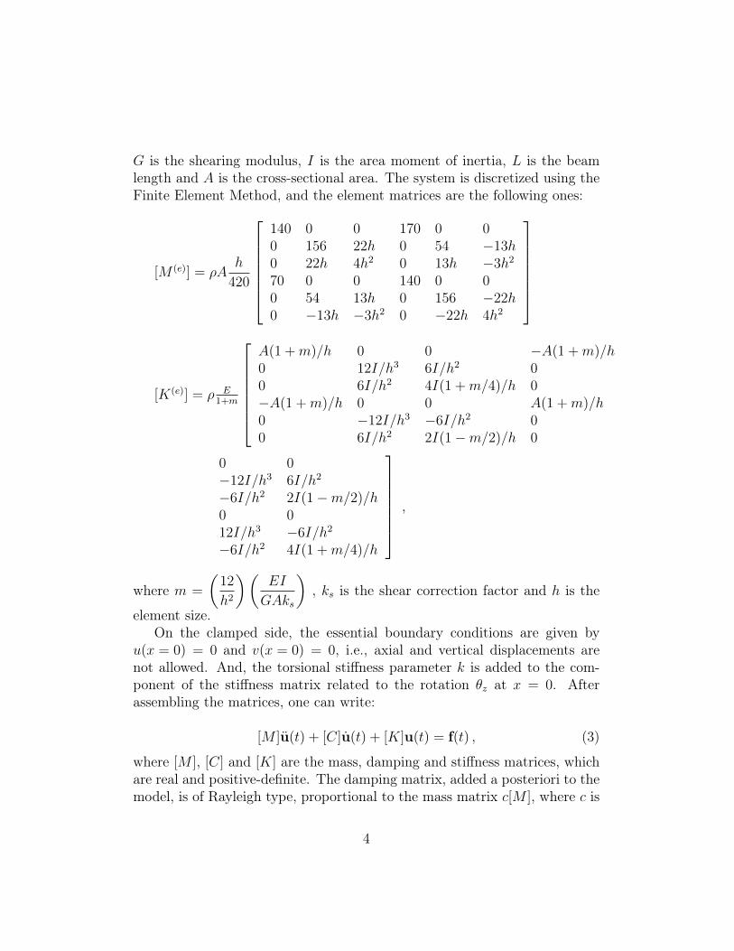
G is the shearing modulus, I is the area moment of inertia, L is the beamlength and A is the cross-sectional area. The system is discretized using theFinite Element Method, and the element matrices are the following ones:

[M (e)] = ρAh

420

140 0 0 170 0 00 156 22h 0 54 −13h0 22h 4h2 0 13h −3h2

70 0 0 140 0 00 54 13h 0 156 −22h0 −13h −3h2 0 −22h 4h2

[K(e)] = ρ E1+m

A(1 +m)/h 0 0 −A(1 +m)/h0 12I/h3 6I/h2 00 6I/h2 4I(1 +m/4)/h 0−A(1 +m)/h 0 0 A(1 +m)/h0 −12I/h3 −6I/h2 00 6I/h2 2I(1−m/2)/h 0

0 0−12I/h3 6I/h2

−6I/h2 2I(1−m/2)/h0 012I/h3 −6I/h2

−6I/h2 4I(1 +m/4)/h

,

where m =

(12

h2

)(EI

GAks

), ks is the shear correction factor and h is the

element size.On the clamped side, the essential boundary conditions are given by

u(x = 0) = 0 and v(x = 0) = 0, i.e., axial and vertical displacements arenot allowed. And, the torsional stiffness parameter k is added to the com-ponent of the stiffness matrix related to the rotation θz at x = 0. Afterassembling the matrices, one can write:

[M ]u(t) + [C]u(t) + [K]u(t) = f(t) , (3)

where [M ], [C] and [K] are the mass, damping and stiffness matrices, whichare real and positive-definite. The damping matrix, added a posteriori to themodel, is of Rayleigh type, proportional to the mass matrix c[M ], where c is

4

the damping constant. The external force is represented by the vector f(t) =(f1a, f1v, f1r, f2a, . . . , fnr) and the displacements (u1a, u1v, u1r, u2a, . . . , unr)are the components of the vector u(t).

In the frequency domain, the system can be written as:

(−ω2[M ] + iω[C] + [K])u(ω) = f(ω) . (4)

2.1. Natural frequenciesTo calculate the natural frequencies without damping, the following gen-

eralized eigenvalue problem must be solved:

(−ω2i [M ] + [K])Φi = 0 , (5)

where ωi is the i-th natural frequency and Φi is i-th vibration mode. Thei-th natural frequency with damping is calculated in the following way:

ωdi = ωi

√1− ξ2i , (6)

where ξi is the damping rate of the i-th mode, which can be calculated usingthe normal modes and the damping matrix:

ξi =ΦT

i [C]Φi

2ωi

. (7)

It should be noticed that, if a Euler-Bernoulli beam model is taken intoaccount, one can obtain analytical expressions for the natural frequencies,taken into account linear springs on the boundary [1]. However, in the presentcase it is important to test the proposed computational model, which can beused as a building block to more general applications, such as structureswith varying cross sectional area and/or different materials, structures witha viscoelastic core, and structures with different boundary conditions andexcitations.

3. Identification Strategy

The present work employs the Bayesian strategy to update the prior prob-ability density function (pdf) of the torsional stiffness of the clamped side of abeam. This strategy is used because more information can be extracted fromthe system, such as the marginal probability density functions of the parame-ters, updated with the experimental data; and statistical correlations among

5

the response of interest. A similar procedure was considered in [17], whereMCMC was applied to identify three parameters of the bit-rock interaction(boundary condition) of a drill-string dynamical model.

Let K be the random variable related to the stiffness parameter k. Theprior probability density function is updated with experimental data D. Weassume an additive Gaussian noise to model the measurement uncertainties.This is a usual assumption, and it is corroborated by the Maximum EntropyPrinciple (MaxEnt) [9, 10], if we use the following information for the noise:(1) the support is Rn (where n is the number of measurement points), (2) themean is zero and (3) the variance is finite. With this information, the MaxEntyields a Gaussian random vector with independent components. Hence, fora given K:

Yexp = f(K) + N , (8)

whereYexp represents the measured natural frequencies, f represents the nat-ural frequencies obtained with the computational model,N ∼ Normal(0, σ2

e [I])is a white noise vector with zero mean and covariance matrix σ2

e [I] (where[I] is the identity matrix). Using the Bayes strategy, we can compute theupdated (or posterior) probability density function of K, given data D:

p(K|D) ∝ p(D|K)p(K) , (9)

where ‘∝’ means ‘proportional to’, p(D|K) is the likelihood function, andp(K) is the prior pdf.

To approximate the posterior distribution, which is given up to a nor-malization constant, the Markov Chain Monte Carlo (MCMC) / Metropolis-Hasting algorithm is applied [7, 18]. The algorithm implemented is the fol-lowing:

1. Initiate the chain Kn at n = 0.2. Generate a candidate Y from a proposal distribution q.3. Generate U ∼ Uniform(0, 1).4. If U ≤ α(Kn, Y ), accept candidate Kn+1 = Y . Else, reject the candi-

date and set Kn+1 = Kn.5. Set n = n+ 1 and go back to step 2.

where α(Kn, Y ) = posterior(Y )/posterior(Kn), and q is the Normal densityfunction with mean Kn and standard deviation σq that is chosen such thatthe acceptance rate is about 50%.

6

4. Test rig apparatus and data acquisition methodology

The experimental apparatus attempts to obtain the frequency re-sponse function of the cantilever beam when the clamped condition is changed.The experimental apparatus is shown in Fig. 2.

(a) (b)

Figure 2: Test rig: a) photo; b) scheme.

The experiment is composed by a simple cantilever beam, supported bya cast iron bench. The beam is made of aluminium, with a 511 mm lengthand a rectangular section of 30.7 by 3.04 mm. The mount is composedby steel couplings, which tries to guarantee the boundary condition of zerodisplacement and zero rotation by pressing the aluminium beam against bothcouplings, and the mount is fixed at the cast iron rig, using 7/16 inch boltsfor all couplings.

The frequency response function is obtained [5, 12] using an impulse ham-mer (Endevco Model 30927). The system response is captured by two mini-accelerometers (Endevco, Model 25B), one positioned at the free end of thebeam and the other at the middle. All signals (hammer and accelerometers)are preconditioned before analyzed by the signal processor (HP 35650). Thespecification of all sensors and the hammer are shown in Tab. 1.

7

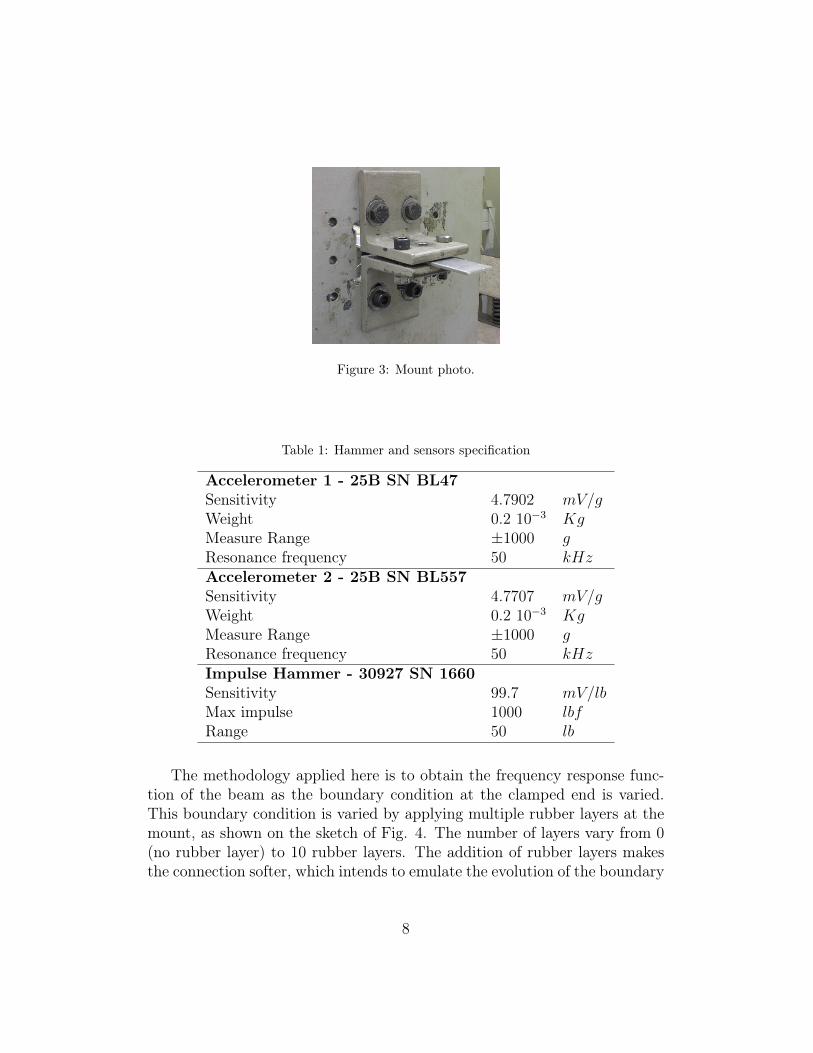
Figure 3: Mount photo.

Table 1: Hammer and sensors specification

Accelerometer 1 - 25B SN BL47Sensitivity 4.7902 mV/gWeight 0.2 10−3 KgMeasure Range ±1000 gResonance frequency 50 kHzAccelerometer 2 - 25B SN BL557Sensitivity 4.7707 mV/gWeight 0.2 10−3 KgMeasure Range ±1000 gResonance frequency 50 kHzImpulse Hammer - 30927 SN 1660Sensitivity 99.7 mV/lbMax impulse 1000 lbfRange 50 lb

The methodology applied here is to obtain the frequency response func-tion of the beam as the boundary condition at the clamped end is varied.This boundary condition is varied by applying multiple rubber layers at themount, as shown on the sketch of Fig. 4. The number of layers vary from 0(no rubber layer) to 10 rubber layers. The addition of rubber layers makesthe connection softer, which intends to emulate the evolution of the boundary

8

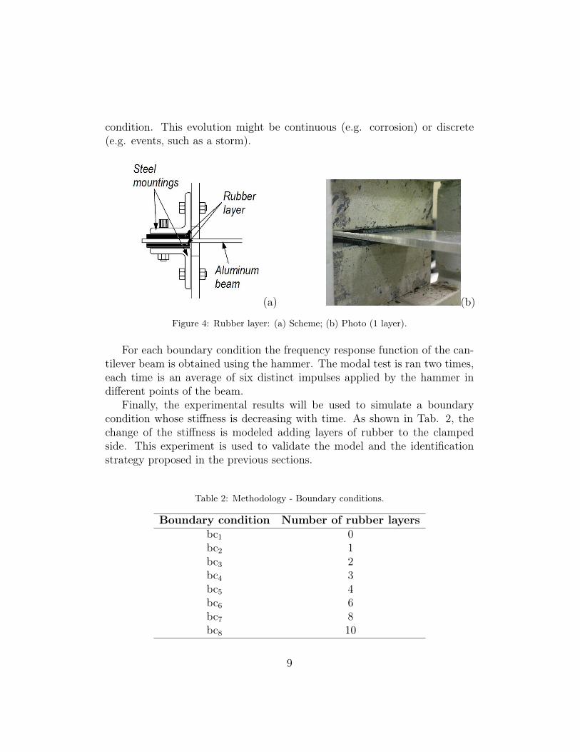
condition. This evolution might be continuous (e.g. corrosion) or discrete(e.g. events, such as a storm).

(a) (b)

Figure 4: Rubber layer: (a) Scheme; (b) Photo (1 layer).

For each boundary condition the frequency response function of the can-tilever beam is obtained using the hammer. The modal test is ran two times,each time is an average of six distinct impulses applied by the hammer indifferent points of the beam.

Finally, the experimental results will be used to simulate a boundarycondition whose stiffness is decreasing with time. As shown in Tab. 2, thechange of the stiffness is modeled adding layers of rubber to the clampedside. This experiment is used to validate the model and the identificationstrategy proposed in the previous sections.

Table 2: Methodology - Boundary conditions.

Boundary condition Number of rubber layersbc1 0bc2 1bc3 2bc4 3bc5 4bc6 6bc7 8bc8 10

9

5. Results

The data used for the numerical simulation were: c = 10 N/(m.s);E = 2e11 Pa; ρ = 7850 kg/m3; ν = 0.3; G = 0.5E/(1 + ν); ks = 5/6;L = 511 mm, b = 30.7mm; h = 3.04mm. It was assumed σe = 1 and σq ={800, 200, 150, 150, 150, 150, 150, 100} for {bc1,bc2,bc3,bc4,bc5,bc6,bc7,bc8}, suchthat the accepted rate of the chain was about 50%.

To determine the number of elements needed, the error of the sixth nat-ural frequency is calculated. It was necessary 32 elements to have an errorlower than 0.1%.

5.1. Experimental resultsAs mentioned before, for each boundary condition, which corresponds

to a measurement time, the modal tests are ran. The natural frequencies areobtained from the magnitude signal of both accelerometers and confirmedby the phase chart. Figure 5 shows the frequency response of the cantileverbeam for bc1.

Figure 5: Frequency response for bc1, data from accelerometer # 1, two modal tests.

Figure 5 shows the response of the accelerometer #1 in both experimentaldata acquisitions. All experimental data was acquired and analyzed from

10

accelerometers #1 and #2, but once the response of accelerometer #1 givesa better resolution than accelerometer #2, the results shown in this articleare from accelerometer #1. Figure 5 shows 6 major peaks, corresponding tothe first six natural frequencies, the first natural frequency at 9 Hz and thesixth natural frequency around 790 Hz. It is also noticeable the presence ofseveral minor sharp peaks in multiples of 60 Hz. Those peaks correspond tothe local electric supply and its harmonics, and those peaks should not beconsidered for the modal analysis.

Figure 6 shows the frequency response function for bc2, bc4, bc6 and bc8.

(a) (b)

(c) (d)

Figure 6: Frequency response for: (a) bc2; (b) bc4; (c) bc6; (d) bc8.

From the charts of all boundary conditions it is possible to obtain thenatural frequencies at each instant, as shown in Tab. 3.

11

Table 3: Natural frequencies - changing boundary conditions.

natural fre-quency (Hz) 1st 2nd 3rd 4th 5th 6th

Boundary Conditionbc1 9.25 58.80 163.75 321.50 534.50 793.20bc2 9.00 57.00 160.90 315.60 524.75 778.75bc3 9.00 57.00 160.75 315.25 525.40 780.00bc4 9.00 56.75 160.00 314.00 523.00 777.25bc5 9.00 56.75 160.15 314.20 523.00 777.00bc6 9.00 56.65 159.90 313.60 522.75 775.75bc7 9.00 56.50 159.75 313.20 521.50 773.50bc8 9.00 56.25 158.75 311.50 519.25 770.75

Observing the system frequency response function and the data shownin Tab. 3, it can be noticed that there is no variation of the first frequency.However, it is worth it to remark that the accuracy of the experiment is0.25Hz, what makes it difficult to distinguish 9.0Hz from 9.1Hz, for example.

The higher the number of rubber layers more flexible the boundary con-ditions become and lower the natural frequencies, compared to the conditionwithout rubber layers. A comparison between the opposite sides of the ex-periment, i.e., the frequency response function of the beam without rubberlayers (bc1) on the clamped side and the system with 10 rubber layers (bc8)is shown in Fig. 7.

12

(a) (b)

Figure 7: Frequency response, boundary condition comparison. Thin line: 0 rubber layers(bc1); thick line: 10 rubber layers (bc8). a) 0-200 Hz, b) 300-800Hz.

5.2. Identification resultsThe experimental results shown in Tab. 3 are used to identify the tor-

sional stiffness of the boundary condition for each boundary condition {bc1,bc2,...,bc8},see Tab. 2. As mentioned before, the boundary conditions represent the evo-lution of the clamped side stiffness, that might occur continuously with time,or after some specific events.

For each condition the prior pdf is set to Uniform and the updated pdf iscomputed simulating a Markov Chain. The prior pdf is set to Uniform, suchthat the previous boundary condition results do not bias the identification ofthe next instant. It is important to reset the prior to Uniform if the boundarycondition is changing with time, which is the present case.

Table 4 shows the evolution of the mean value and the coefficient of vari-ation (CV) of random variable K. The mean value is very close to the max-imum a posterior estimator (MAP). The table also shows the mean squareerror for each condition analyzed, i.e, for decreasing stiffness on the bound-ary condition. The uncertainty for bc1 is higher (9%) than at other instants,where the CV is about 4%. There is a big jump in the mean value of Kfrom bc1 to bc2, when a rubber layer is included in the experiments. Figure8 shows visually these results, where the mean value of K is plotted togetherwith errorbars.

Due to experimental uncertainties, see Tab. 3, the 4th and 5th naturalfrequencies increase from bc2 to bc3. This fact explains why the mean value

13

of K increases from bc2 to bc3, when we would expect the opposite result.From bc3 to bc8 the mean value of K decreases continuously.

Boundary MAP estimator Mean value CV Mean Squarecondition (×103 N.m) (×103 N.m) Error (Hz2)

bc1 3.7 3.8 9.0 % 8.9bc2 1.3 1.3 4.5 % 12.3bc3 1.4 1.4 4.4 % 10.9bc4 1.2 1.2 4.4 % 9.0bc5 1.1 1.1 4.4 % 9.9bc6 1.1 1.1 4.4 % 13.7bc7 1.0 1.0 4.0 % 17.2bc8 0.8 0.8 4.0 % 16.3

Table 4: MAP estimator, Mean value, coefficient of variation (CV), and mean square error,at each instant.

0 2 4 6 8 100

1000

2000

3000

4000

5000

bc

me

an

(K)

Figure 8: Evolution of the mean value of K together with errorbars; plus or minus twostandard deviations.

Figures 9 and 10 show the prior Uniform pdf of K together with theupdated (posterior) pdf for all the different boundary conditions. To better

14

visualize the probability density functions, they are shown in pairs: pdf(bc1)with pdf(bc2), pdf(bc2) with pdf(bc3), and so on. Note that the pdf is shiftingto the left, because the system is getting less stiff. The biggest shift occursfrom bc1 to bc2, when the first layer is included in the experiment. As it wasnoticed before, due to experimental uncertainties, from bc2 to bc3 there is ashift to the right, which is not expected.

0 1000 2000 3000 4000 50000

0.002

0.004

0.006

0.008

0.01

0.012

k

pdf

bc1

bc2

prior

(a)0 1000 2000 3000 4000 5000

0

0.002

0.004

0.006

0.008

0.01

0.012

k

pdf

bc2

bc3

prior

(b)

0 1000 2000 3000 4000 50000

0.002

0.004

0.006

0.008

0.01

0.012

k

pdf

bc3

bc4

prior

(c)0 1000 2000 3000 4000 5000

0

0.002

0.004

0.006

0.008

0.01

0.012

k

pdf

bc4

bc5

prior

(d)

Figure 9: Prior (dashed line) and posteriors pdf of K from bc1 to bc4.

In the proposed identification strategy, the prior pdf of the random vari-able related to the torsional stiffness at the boundary condition is set toUniform at each instant. Another possibility would be to perform the identi-fication with all data at once. Figure 11 shows the posterior pdf for bc1 andbc8, and posterior pdf using all data together. It can be noticed that the re-sults are quite different. When all data is used, there is no cleaning up beforethe new experimental data is taken into account, i.e., the data from the firstinstant will always be present in the identification process. We argue that itis more effective to set the prior to Uniform each time the identification isperformed, such that past data do not influence the new identification result.

15

0 1000 2000 3000 4000 50000

0.002

0.004

0.006

0.008

0.01

0.012

k

pdf

bc5

bc6

prior

(a)0 1000 2000 3000 4000 5000

0

0.002

0.004

0.006

0.008

0.01

0.012

k

pdf

bc7

bc8

prior

(b)

0 1000 2000 3000 4000 50000

0.002

0.004

0.006

0.008

0.01

0.012

k

pdf

bc7

bc8

prior

(c)

Figure 10: Prior (dashed line) and posteriors pdf of K from bc4 to bc8.

Now it is time to analyze the propagation of the uncertainty throughoutthe computational model, considering as input the random variable K1 ob-tained in the identification process. We are interest in the natural frequenciesof the system. Figure 12 shows the pdf of the first and sixth natural frequen-cies for bc1 and bc8. As expected, the pdf is shifted to the left, since thesystem is less stiff. The experimental result is plotted together for compari-son.

However, the uncertainty of the random natural frequencies are verysmall. For the first natural frequency, the mean values are 9.3 and 8.9 Hzand the CVs are 0.4% and 0.8%, and for the sixth natural frequency, themean values are 793.9 and 773.1 Hz and the CVs are 0.3% and 0.8%.

One unexpected result is related to the correlation among the naturalfrequencies. It turns out that the natural frequencies are very well correlatedto each other. Figure 13 shows the realizations of the first and second ran-dom natural frequencies for bc7 and of the first and sixth random naturalfrequencies also for bc7. There is a strong positive correlation among these

16

0 1000 2000 3000 4000 50000

0.002

0.004

0.006

0.008

0.01

0.012

k

pd

f

bc1

bc8

all

prior

Figure 11: Prior pdf (dashed line), posterior pdf for bc1 and bc8, and posterior pdf usingall data together.

random variables, and Fig. 13(b) shows that the relation between the firstand sixth natural frequencies is slightly nonlinear.

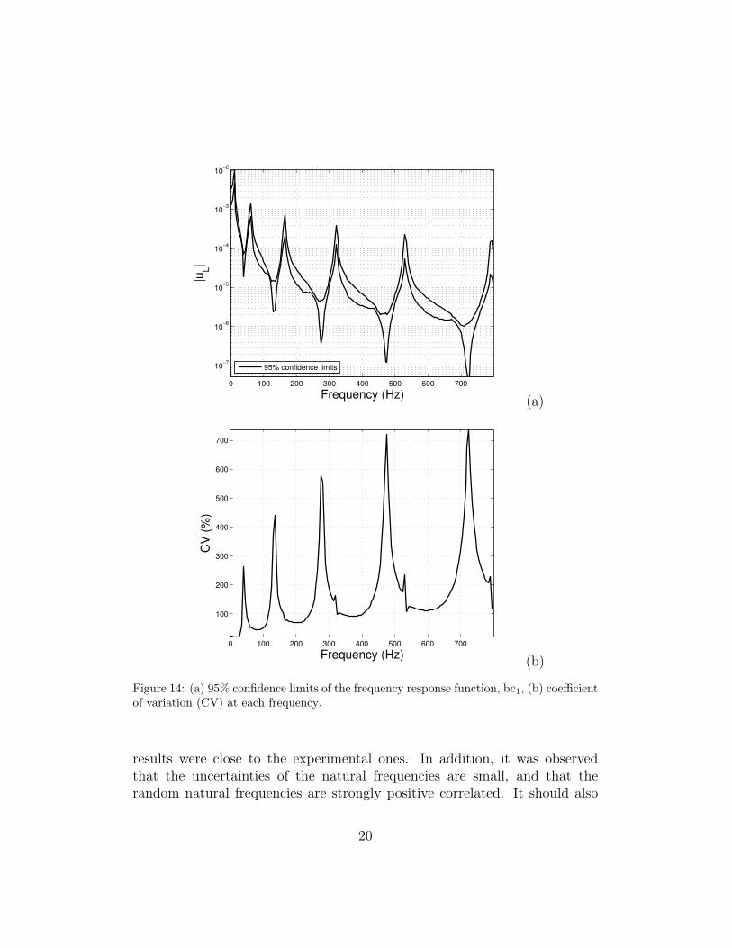
Finally, Fig. 14(a) shows the 95% confidence limits of the frequencyresponse function, for bc1, considering a unit force at x = L. It can beobserved that the uncertainty due to the random torsional stiffness has aconsiderable impact on the amplitude of the response. Figure 14(b) shows thecoefficient of variation (standard deviation over the mean) at each frequency.The coefficient of variation appears to increase with the frequency, and, inthe antiresonance regions, the coefficient of variation might be greater than700%.

6. Concluding remarks

This paper deals with uncertain boundary conditions. In many applica-tions boundary condition stiffness decreases with time, and this should betaken into account in the computational model. An identification strategy isproposed to update the information related to the stiffness of the boundarycondition. For this purpose the Bayesian update is employed and a test rigapparatus is constructed to produce experimental results.

17

8.5 9 9.50

5

10

15

w1

pdf

bc1

bc8

Exp.

(a)

760 770 780 790 8000

0.05

0.1

0.15

0.2

0.25

w6

pd

f

bc1

bc8

Exp.

(b)

Figure 12: Posterior pdf for bc8 (dashed line) and bc1. (a) first natural frequency and (b)sixth natural frequency. Experimental results are in red.

An experimental rig with a clamped beam was constructed to generatethe experimental data. Layers were added to the clampled side to representthe loss in the stiffness of the clamped condition. In a practical application,this stiffness might decrease continuously with time, or from time to time

18

8.4 8.6 8.8 9 9.2 9.454.5

55

55.5

56

56.5

57

57.5

58

58.5

w1

w2

(a)

8.4 8.6 8.8 9 9.2 9.4760

765

770

775

780

785

790

w1

w6

(b)

Figure 13: Natural frequencies t = 7s. Realization of (a) first and second random naturalfrequencies and (b) first and sixth natural frequencies.

due to some specific events, such as a seism and a storm.The strategy worked well in the sense that the computational model was

able to update the stiffness parameter of the boundary condition and the

19

0 100 200 300 400 500 600 700

10−7

10−6

10−5

10−4

10−3

10−2

Frequency (Hz)

|uL|

95% confidence limits

(a)

0 100 200 300 400 500 600 700

100

200

300

400

500

600

700

Frequency (Hz)

CV

(%

)

(b)

Figure 14: (a) 95% confidence limits of the frequency response function, bc1, (b) coefficientof variation (CV) at each frequency.

results were close to the experimental ones. In addition, it was observedthat the uncertainties of the natural frequencies are small, and that therandom natural frequencies are strongly positive correlated. It should also

20

be remarked that the prior pdf should be reset to Uniform, such that previousboundary condition results do not bias the identification of the next instant.

References

[1] S. Adhikari, S. Bhattacharya, Vibrations of wind-turbines consideringsoil-structure interaction, Wind and Structures, 14 (2) (2011) 85-112.

[2] S. Adhikari, S. Bhattacharya, Dynamic analysis of wind turbine towerson flexible foundations, Shock and Vibration, 19 (1) (2012) 37-56.

[3] J.L. Beck, L.S. Katafygiotis, Updating models and their uncertainties-Bayesian statistical framework, ASME, Journal of Engineering Mechan-ics, 124 (4) (1998), 455-461.

[4] E. Cataldo, C. Soize, R. Sampaio, Uncertainty quantification of voicesignal production mechanical model and experimental updating, Me-chanical Systems and Signal Processing, 40 (2) (2013) 718-726.

[5] D. J. Ewins, Modal Testing: Theory and Practice, John Wiley & SonsInc., 1984.

[6] M. I. Friswell, J. E. Mottershead, Finite Element Model Updating inStructural Dynamics, Kluwer Academic Publishers, 1995.

[7] D. Gamerman, Markov Chain Monte Carlo: Stochastic Simulation forBayesian Inference, Chapman and Hall/CRC, 2nd Edition, 2002.

[8] J. Kaipio, E. Somersalo, Statistical and Computational Inverse Problem.Springer, 2005.

[9] J. N. Kapur, Maximum Entropy Models in Science and Engineering,Wiley-Blackwell, 1990.

[10] E. S. de Cursi, R. Sampaio, Uncertainty Quantification and StochasticModeling with Matlab. Elsevier, 2015.

[11] B. Labbaci, O. Rahmani, M. Djermane, L. Missoum, R. Abdeldjebar,A study of the effect of the simulation of the boundary condition ondynamic response of composite structures, Journal of Applied Sciences,8 (11) (2008) 2098-2104.

21

[12] N. Maia, J. Silva. Theoretical and Experimental Modal Analysis, Me-chanical Engineering Research Studies, Wiley, 1997.

[13] C. Mares, J. E. Mottershead, M. I. Friswell, Stochastic model updating:Part 1-theory and simulated example. Mechanical Systems and SignalProcessing, 20 (7) (2006) 1674-1695.

[14] M. P. Mignolet, C. Soize, J, Avalos, Nonparametric stochastic model-ing of structures with uncertain boundary conditions/coupling betweensubstructures, AIAA Journal, 51 (6) (2013) 1296-1308.

[15] T.G. Ritto, R. Sampaio, C. Cataldo, Timoshenko beam with uncer-tainty on the boundary conditions, Journal of the Brazilian Society ofMechanical Science and Engineering, 30 (4) (2008) 295-303.

[16] T. G. Ritto, C. Soize, R. Sampaio, Non-linear dynamics of a drill-stringwith uncertain model of the bit-rock interaction, International Journalof Non-Linear Mechanics 44 (8) (2009) 865-876.

[17] T. G. Ritto, Bayesian approach to identify the bit-rock interaction pa-rameters of a drill-string dynamical model, Journal of the Brazilian So-ciety of Mechanical Science and Engineering (in press) (2014).

[18] C. Robert, G. Casella, Monte Carlo Statistical Methods, Springer, 2004.

[19] D. S. Sivia, Data Analysis - A Bayesian Tutorial., Oxford Science Pub-lications, 2006.

[20] E. Walter, L. Pronzato, Identification of Parametric Models from Ex-perimental Data, Springer-Verlag, Berlin, 1997.

[21] L. Wang, Z. Yang, Identification of boundary conditions of taperedbeam-like structures using static flexibility measurements, MechanicalSystems and Signal Processing, 25 (7) (2011) 2484-2500.

22