UC Santa Cruz - eScholarship.org

UC Santa CruzUC Santa Cruz Electronic Theses and Dissertations

TitleEnhancing Ground Penetrating Radar Signals Through Frequency Compositing

Permalinkhttps://escholarship.org/uc/item/1954n251

AuthorTilley, Roger Steven

Publication Date2019

Copyright InformationThis work is made available under the terms of a Creative Commons Attribution License, availalbe at https://creativecommons.org/licenses/by/4.0/ Peer reviewed|Thesis/dissertation

eScholarship.org Powered by the California Digital LibraryUniversity of California

https://escholarship.org/uc/item/1954n251

https://creativecommons.org/licenses/by/4.0/

https://escholarship.org

http://www.cdlib.org/

UNIVERSITY OF CALIFORNIA SANTA CRUZ

ENHANCING GROUND PENETRATING RADAR SIGNALS THROUGH FREQUENCY COMPOSITING

A dissertation submitted in partial satisfaction

of the requirements for the degree of

DOCTOR OF PHILOSOPHY

in

ELECTRICAL ENGINEERING

by

Roger S. Tilley

June 2019

The Dissertation of Roger S. Tilley is approved:

____________________________________ Professor Hamid R. Sadjadpour, chair

____________________________________ Professor John F. Vesecky

____________________________________ Professor Donald M. Wiberg

_______________________________________ Lori Kletzer Vice Provost and Dean of Graduate Studies

Copyright © by

Roger S. Tilley

2019

iii

Table of Contents

List of Figures .......................................................................................................................... vi

List of Tables ......................................................................................................................... xvi

Abstract ................................................................................................................................. xvii

Declaration ........................................................................................................................... xviii

Dedication .............................................................................................................................. xix

Acknowledgments .................................................................................................................. xx

Chapter 1 ................................................................................................................................... 1

Introduction ........................................................................................................................... 1

Chapter 2 ................................................................................................................................... 4

Ground Penetrating Radar Basics ......................................................................................... 4

2.1 Basic analysis modes .................................................................................................. 4

2.2 GPR pulses .................................................................................................................. 7

2.3 Two-Way-Travel-Time (TWTT) .............................................................................. 10

2.4 Modeling Basics ........................................................................................................ 12

Chapter 3 ................................................................................................................................. 14

Expectation-Maximization Gaussian Mixture Model Method............................................ 14

Chapter 4 ................................................................................................................................. 18

Maximum Likelihood Estimation Verses Expectation-Maximization................................ 18

Chapter 5 ................................................................................................................................. 28

Computer Generated Scans Verses Actual Scans ............................................................... 28

5.1 Actual Scans.............................................................................................................. 28

5.2 Computer Generated Scans ....................................................................................... 34

Chapter 6 ................................................................................................................................. 42

iv

EM GMM Process In Operation ......................................................................................... 42

6.1 Combining Harmonics of Sine waves ....................................................................... 42

6.2 GPR Test Case 1 ....................................................................................................... 45

6.3 GPR Test Case 2 ....................................................................................................... 50

6.3 GPR Test Case 3 ....................................................................................................... 52

Chapter 7 ................................................................................................................................. 56

Other GPR Frequency Scan Compositing Methods ............................................................ 56

7.1 Dougherty’s Method ................................................................................................. 56

7.2 Booth’s Method ........................................................................................................ 59

7.3 Bancroft’s Method .................................................................................................... 64

Chapter 8 ................................................................................................................................. 70

Comparison of EM Process with Other Methods ............................................................... 70

8.1 Dougherty’s Method Comparison ............................................................................. 70

8.2 Booth’s Method Comparison .................................................................................... 76

8.3 Bancroft’s Method Comparison. ............................................................................... 83

Chapter 9 ................................................................................................................................. 88

“Stand Off” GPR Methods .................................................................................................. 88

9.1 Test Case 1 style analysis ......................................................................................... 88



Chapter 10 ............................................................................................................................. 103

Chirp Excitation Signal Methods ...................................................................................... 103

10.1 Background ........................................................................................................... 103

10.2 Chirp Excitation Function Based Radar Signal .................................................... 104

v

10.3 Analysis Discussion .............................................................................................. 107

10.4 Test Case 1 results ................................................................................................ 108

10.5 Test Case 1 Style results ....................................................................................... 111

10.6 Compensate for Geometric Distortion of Chirp GPR Scanning ........................... 113

10.7 Test Case 2 and Test Case 2 style results .............................................................. 118

10.8 Test Case 3 style results ........................................................................................ 124

Chapter 11 ............................................................................................................................. 129

Conclusion ........................................................................................................................ 129

Future Work ...................................................................................................................... 136

Appendix A Three Coin Problem Equations based on EM Algorithm ................................ 137

Appendix B Software Routine to Solve the Three Coin Problem ....................................... 142

References ............................................................................................................................. 144

vi

List of Figures

Figure 2.1. GPR Scanning Modes [1] ....................................................................................... 4

Figure 2.2. GPR Arrival Types [10] ......................................................................................... 5

Figure 2.3. Simple CMP plot w/equations for Arrival Types [10] ........................................... 5

Figure 2.4. Shows t2– x2Analysis (st) [11] ..................................................................... 7

Figure 2.5. Gaussian, 1st derivative (Monocycle), 2nd derivative (Ricker), (normally GPR

response signals for Monocycle and Ricker are inverted) [12] ................................................. 8

Figure 2.6. Typical reflected signals without target (direct air wave and direct ground wave

visible) ...................................................................................................................................... 9

Figure 2.7. GPR trace depicting Two-way-transit-time for 2 frequencies of same target. ..... 11

Figure 2.8. Yee cell [27] ......................................................................................................... 13

Figure 2.9. FDTD Grid – made up of Yee cells [9][27] ......................................................... 13

Figure 4.1. Coin A and Coin B recorded tosses ...................................................................... 20

Figure 4.2. 2 coin problem EM Solution MATLAB code ...................................................... 25

Figure 5.1. Tin Roofing Sheets ............................................................................................... 30

Figure 5.2. Tin roofing Sheets buried at different Depths at Forest Lodge ............................ 30

Figure 5.3. MIRA Radar ......................................................................................................... 30

Figure 5.4. 3-D output of 200 MHz scan by MIRA Radar at the Forest Lodge Test area ...... 31

Figure 5.5. pulseEKKO 100 radar mounted on wheeled platform in front of test lane of buried

roofing sheets .......................................................................................................................... 33

Figure 5.6. MIRA radar and pulseEKKO 100 Radar at Forest Lodge Test Area ................... 33

Figure 5.7. pulseEKKO 100, 25 MHz Radar scan at Forest Lodge Test Area. ...................... 34

Figure 5.8. GprMax [9] 3-D model of the Forest Lodge test site of buried roofing tiles ....... 35

vii

Figure 5.9. (a) through (h) represent a 2-D slice at each of 8 receivers for the 3-D simulated

analysis of the Forest Lodge model. (a) receiver 1, (b) receiver 2, (c) receiver 3, (d) receiver

4, (e) receiver 5, (f) receiver 6, (g) receiver 7, (h) receiver 8. ................................................ 36

Figure 5.10. Typical GprMax [9] input file for a 3-D analysis ............................................... 37

Figure 5.11. GprMax [9] 2-D model of Forest Lodge test area with buried roofing sheets ... 38

Figure 5.12. Typical GprMax [9] input file for a 2-D analysis ............................................... 38

Figure 5.13. 2-D simulated analysis of Forest Lodge Test Area (25MHz). ............................ 39

Figure 5.14. 2-D Simulated analysis of Forest Lodge Test Area (900 MHz). ........................ 40

Figure 6.1. Sine Wave Frequencies 50, 150 Hz ...................................................................... 43

Figure 6.2. Sine wave Frequencies 250, 350 Hz ..................................................................... 44

Figure 6.3. Sine wave Frequencies 450, 550 Hz ..................................................................... 44

Figure 6.4. EM algorithm result with Square wave desired signal ......................................... 44

Figure 6.5. EM algorithm result with Triangle wave desired signal ....................................... 45

Figure 6.6. Test Case 1 with buried target 10 meters below ground, Txs & Rxs 5 meters

above ground. .......................................................................................................................... 46

Figure 6.7. 2-D GPR Scan at 20 MHz .................................................................................... 47



Figure 6.10. 2-D GPR Scan at 100 MHz ................................................................................ 47


Figure 6.12. 2-D GPR Scan at 500 MHz w/traces .................................................................. 48


Figure 6.14. 2-D GPR Scan at 900 MHz w/traces .................................................................. 48

viii

Figure 6.15. Sum of frequency signals with direct arrival and ground bounce signals

removed. ................................................................................................................................. 49

Figure 6.16. EM processed sum of frequencies ...................................................................... 49

Figure 6.17. EM processed signal traces ................................................................................. 49

Figure 6.18. Test Case 2, (8) roofing sheets 2 meters long, 0.1 meters thick, buried at 8

different levels ........................................................................................................................ 51

Figure 6.19. EM processed results .......................................................................................... 52

Figure 6.20. EM processed signal traces ................................................................................. 52

Figure 6.21. GPR Test Case 3, (8) roofing sheets 2 meters long, 0.1 meters thick, buried at 8

different levels, in non-uniform media. .................................................................................. 53

Figure 6.22. EM processed GPR scan of non-uniform media Test Case 3. ............................ 54

Figure 6.23. EM processed signal traces of non-uniform media Test Case 3. ........................ 54

Figure 8.1. (a) Dougherty standard response to Test Case 1. (b) Figure 6.16. (Repeated here)

EM processed sum of Frequencies ......................................................................................... 70

Figure 8.2. (a) Trace 18 of 36 traces total; roughly 5 m out of 10 m in total distance in the x

direction of Test Case 1 model, 1-D plot of Dougherty method. (b) Trace 18 of 36 traces

total; roughly 5 m out of 10 m in total distance in the x direction of Test Case 1 model, 1-D

plot of EM GMM analysis. ..................................................................................................... 71

Figure 8.3. (a) Traces 1, 18 and 30, 1-D plots of Dougherty method response for Test Case 1.

(b) Traces, 1, 18, and 30, 1-D plots of EM GMM analysis method response for Test Case 1.

................................................................................................................................................ 72

Figure 8.4. (a) Dougherty response of Test Case 2. (b) Figure 6.19. (repeated here) EM

processed results ..................................................................................................................... 73

Figure 8.5. Exponential Gain Recovery Function Example ................................................... 74

ix

Figure 8.6. Dougherty response to Test Case 1 with exponential gain function..................... 75

Figure 8.7. (a) Trace 18 of 36 traces total; roughly 5 m out of 10 m total distance in the x

direction, 1-D plot of Dougherty method with an exponential gain of 10. (b) Traces 1, 18 and

30, 1-D plots of Dougherty method with an exponential gain of 10. ...................................... 75

Figure 8.8. Dougherty response to Test Case 2 with exponential gain function..................... 76

Figure 8.9. (a) Trace 18 of 36 total; roughly 5 m out of 10 m in total distance in the x

direction of Test Case 1 model, 1-D plot of Booth method 3. (b) Trace 18 of 36 total; roughly

5 m out of 10 m in total distance in the x direction of Test Case 1 model, 1-D plot of Booth

DFAE method with the first 36 ns in time reduced to small value to eliminate the largest

portion of the remaining direct arrival/ground bounce signal. ................................................ 77

Figure 8.10. (a) Traces 1, 18 and 30, 1-D plots of Booth Method 3 for Test Case 1. (b) Traces

1, 18 and 30, 1-D plots of Booth DFAE method for Test Case 1, with the first 36ns reduced to

a small value to eliminate the largest portion of the remaining direct arrival/ground bounce

signal. ...................................................................................................................................... 77

Figure 8.11. Complete Trace 18 of 36 total; roughly 5 m out of 10 m in the x direction of Test

Case 1 model. .......................................................................................................................... 78

Figure 8.12. (a) Booth Method 3 response to Test Case 1. (b) Booth DFAE method response

to Test Case 1. ......................................................................................................................... 79

Figure 8.13. (a) Booth OSW response to Test Case 1. (b) Figure 6.16. (Repeated here) EM

processed sum of frequencies. ................................................................................................ 79


direction of Test Case 1 model, 1-D plot of Booth OSW method. (b) Trace 18 of 36 traces

total; roughly 5 m out of 10 m in total distance in the x direction of Test Case 1 model, 1-D

plot of EM GMM analysis. ..................................................................................................... 80

x

Figure 8.15. (a) Traces 1, 18 and 30, 1_D plots of Booth OSW method response for Test Case

1. (b) Traces 1, 18 and 30, 1-D plots of EM GMM analysis method response for Test Case 1.

................................................................................................................................................ 81

Figure 8.16. Wider scan axis example (30 m) for Test Case 1 showing hyperbola for 20, 30

and 100 MHz; Original scan axis width shown in Red. .......................................................... 82

Figure 8.17. (a) Booth OSW response to Test Case 2 including direct arrival/ground bounce.

(b) Figure 6.19. (repeated here) EM processed results. .......................................................... 83


direction of Test Case 1 model, 1-D plot of Bancroft AEE modified method. (b) Trace 18 of

36 traces total; roughly 5 m out of 10 m in total distance in the x direction of Test Case 1

model, 1-D plot of EM GMM analysis. .................................................................................. 85

Figure 8.19. (a) Traces 1, 18 and 30, 1_D plots of Bancroft AEE modified method response

for Test Case 1. (b) Traces 1, 18 and 30, 1-D plots of EM GMM analysis method response for

Test Case 1. ............................................................................................................................. 85

Figure 8.20. (a) Bancroft AEE response to Test Case 1, without direct arrival/ground bounce.

(b) Figure 6.16 (repeated here) EM processed results. ........................................................... 86

Figure 8.21. (a) Bancroft AEE response to Test Case 2 with direct arrival/ground bounce. (b)

Figure 6.19. (repeated here) EM processed results. ................................................................ 86

Figure 9.1. Test case 1 style, Tx/Rx 10 meters above ground. ............................................... 89

Figure 9.2. Test Case 1 style, Tx/Rx 20 meters above ground. .............................................. 90

Figure 9.3. Test Case 1 style, Tx/Rx 40 meters above ground. .............................................. 90

Figure 9.4. EM GMM response for Test Case 1 style model, Tx/Rx 10 meters above ground.

................................................................................................................................................ 91

xi


................................................................................................................................................ 92

Figure 9.6. EM GMM response for Test Case 1 style model; Tx/Rx 40 meters above ground.

................................................................................................................................................ 93

Figure 9.7. Test Case 2 style model; Tx/Rx 5 meters above ground ...................................... 94

Figure 9.8. Test Case 2 style model; Tx/Rx 10 meters above ground .................................... 94

Figure 9.9. Test Case 2 style model; Tx/Rx 20 meters above ground. ................................... 95

Figure 9.10. Test Case 2 style model; Tx/Rx 40 meters above ground. ................................. 95

Figure 9.11. EM GMM response to Test Case 2 style model; Tx/Rx 5 meters above ground; 8

sheets shown. .......................................................................................................................... 96

Figure 9.12. EM GMM response to Test Case 2 style model with (a) Tx/Rx 10 meters above

ground; 8 sheets shown. (b) Tx/Rx 20 meters above ground; barely 8 sheets shown. ........... 96

Figure 9.13. EM GMM signal traces response to Test Case 2 style model; Tx/Rx 40 meters

above ground; 7 to 8 sheets shown. ........................................................................................ 97

Figure 9.14. Test Case 3 style model; Tx/Rx 5 meters above ground. ................................... 98



Figure 9.17. Test case 3 style model; Tx/Rx 40 meters above ground. ................................ 100

Figure 9.18. EM GMM response to Test Case 3 style model; Tx/Rx 5 meters above ground; 8

sheets shown. ........................................................................................................................ 100

Figure 9.19. EM GMM response to Test Case 3 style model with (a) Tx/Rx 10 meters above

ground; 8 sheets shown. (b) Tx/Rx 20 meters above ground; barley 8 sheets are shown. .... 101

Figure 9.20. EM GMM signal traces response to Test Case 3 style model; Tx/Rx 40 meters

above ground; 8 sheets shown but no edge detection. .......................................................... 101

xii

Figure 10.1. Chirp Signal MATLAB Code........................................................................... 106

Figure 10.2. Computed Chirp Signal .................................................................................... 107

Figure 10.3. (a) EM sum of frequency signals with the direct arrival and ground bounce

signals removed (Figure 6.16, repeated here). (b) Chirp excitation signal response with direct

arrival and ground bounce removed...................................................................................... 109

Figure 10.4. (a) Trace 18 of 36 traces in total; roughly 5 m out of 10 m in total distance in the

x direction; 1-D plot of EM EMM analysis method. (b) Trace 18 of 36 traces in total; roughly

5 m out of 10 m in total distance in the x direction; 1-D plot of Chirp Excitation analysis

method. ................................................................................................................................. 110

Figure 10.5. (a) Traces 1, 18 and 30; plots of EM GMM analysis. (b) Traces 1, 18 and 30;

plots of Chirp Excitation analysis. ........................................................................................ 110

Figure 10.6. (a) Output response of EM GMM method with direct arrival and ground bounce

signals removed (Figure 9.4, repeated here). (b) Chirp Excitation function response with the

direct arrival and ground bounce signals removed. .............................................................. 111

Figure 10.7. (a) EM GMM output analysis; Trace 18 of 36 at 5 m in the x direction. (b) Chirp

Excitation analysis response; Trace 18 of 36 at 5 m in the x direction. ................................ 112

Figure 10.8. (a) Gazdag [59] translated output response for Test Case 1 model (5 m above

ground). (b) Gazdag [59] translated output response for Test Case 1 style model (10 m above

ground). ................................................................................................................................. 114

Figure 10.9. (a) 1-D plot of trace 18 of 36 at 5 m in the x -direction for a nominal chirp signal

response and a Gazdag [59] response; for Test Case 1 model (5 m above ground). (b) 1-D

plot of trace 18 of 36 at 5 m in the x direction for a nominal chirp signal response and a

Gazdag [59] response, for Test Case 1 style model (10 m above ground). .......................... 115

xiii

Figure 10.10. (a) Cross correlation of Chirp Excitation response for Test Case 1 model (5 m

height above ground). (b) Cross correlation Chirp Excitation response for Test Case 1 style

model (10 m height above ground). ...................................................................................... 116

Figure 10.11. (a)1-D plot of Cross correlation of Chirp Excitation response for Test Case 1

model (5 m height above ground). (b) 1-D plot of Cross correlation Chirp Excitation response

for Test Case 1 style model (10 m height above ground). .................................................... 116

Figure 10.12. (a) Test Case 1 model Chirp response, Tx/Rx at 5 m, filtered into 6 frequencies,

20, 30, 50 ,100, 500 & 900 MHz then processed with the EM GMM algorithm. (b) Test Case

1 style model Chirp response, Tx/Rx at 10 meters, filtered into 6 frequencies, 20 30, 50, 100,

500 & 900 MHz then processed with the EM GMM algorithm. .......................................... 117

Figure 10.13. (a) 1-D plot of Test Case 1 model Chirp response, Tx/Rx at 5 m, filtered into 6

frequencies, 20, 30, 50 ,100, 500 & 900 MHz then processed with the EM GMM algorithm.

(b) 1-D plot of Test Case 1 style model Chirp response, Tx/Rx at 10 m, filtered into 6

frequencies, 20 30, 50, 100, 500 & 900 MHz then processed with the EM GMM algorithm.

.............................................................................................................................................. 118

Figure 10.14. (a) Test Case 2 model (repeat of Figure 6.18), (8) 2 meter long plates, 0.1 meter

thick. (b) Test Case 2 Style model (repeat of Figure 9.17), (8) 2 meter long plates, 0.1 meter

thick with Tx/Rx pair 5 meters above ground. ...................................................................... 119

Figure 10.15. (a) EM processed results (Figure 6.19, repeated here); (8) sheets shown. (b)

Chirp Excitation function response to Test Case 2 model with direct arrival and ground

bounce removed; (8) sheets shown. ...................................................................................... 120

Figure 10.16. (a) EM result for Test Case 2 style model; Tx/Rx 5 meters above ground; (8)

sheets shown (Figure 9.11 repeated here). (b) Chirp Excitation function response to Test Case

2 style model with Tx/Rx 5 meters above ground; (7 barely 8) sheets shown. .................... 120

xiv

Figure 10.17. (a) Gazdag [59] migration response for Test Case 2 model using Chirp

Excitation function; (8) sheets shown. (b) Gazdag [59] migration response for Test Case 2

style model using Chirp Excitation function with Tx/Rx 5 meters above ground; (8) sheets

shown. ................................................................................................................................... 121

Figure 10.18. (a) Cross correlation of Chirp Excitation response for Test Case 2 model. (b)

Cross correlation of Chirp Excitation response for Test Case 2 style model with Tx/Rx 5

meters above ground. ............................................................................................................ 122

Figure 10.19. (a) Test Case 2 model Chirp Excitation response, filtered into 6 frequencies, 20,

30, 50, 100, 500 and 900 MHz then processed with EM GMM algorithm; (8) sheets shown.

(b) Test Case 2 style model Chirp Excitation response, filtered into 6 frequencies, 20, 30, 50,

100, 500 and 900 MHz then processed with EM GMM algorithm; (8) Sheets shown. ........ 122

Figure 10.20. Test Case 2 style model with Tx/Rx 10 meters above ground. ...................... 123

Figure 10.21. (a) EM GMM response to Test Case 2 style model with Tx/Rx 10 meters above

ground (Figure 9.12 repeated here). (b) Chirp Excitation response to Test case 2 style model

with Tx/Rx 10 meters above ground; (8) sheets shown. ....................................................... 124

Figure 10.22. (a) Test Case 3 style model with Tx/Rx 5 meters above ground (repeated Figure

9.14). (b) Test case 3 style model with Tx/Rx 10 meters above ground (repeated Figure 9.15).

.............................................................................................................................................. 125


ground (repeated Figure 9.18); 8 sheets shown. (b) Chirp Excitation response to Test Case 3

style model with Tx/Rx 5 meters above ground; 8 sheets shown. ........................................ 126


ground (repeated Figure 9.19a); 8 sheets shown. (b) Chirp Excitation response to Test Case 3

style model with Tx/Rx 10 meters above ground; 8 sheets shown. ...................................... 126

xv

Figure 10.25. Test Case 3 style model with Tx/Rx 20 meters above ground (repeated Figure

9.16). ..................................................................................................................................... 127


ground (repeated Figure 9.19a); 8 sheets shown. (b) Chirp Excitation response to Test Case 3

style model with Tx/Rx 20 meters above ground; 8 sheets shown. ...................................... 127

xvi

List of Tables

Table 4.1. Observations of coin flips coin A, B or both ......................................................... 24

Table 4.2. EM process numerical results for each Iteration .................................................... 27

Table 6.1. Periodic Signal characteristics ............................................................................... 42

xvii

Abstract

ENHANCING GROUND PENETRATING RADAR SIGNALS THROUGH FREQUENCY

COMPOSITING

by

Roger S. Tilley

In this dissertation, we explore methods to combine multiple frequency Ground Penetrating

Radar (GPR) signals in a manner to improve the resolution of images of deeply buried

targets. We propose using an optimization problem solver to combine multiple GPR

frequency scans over the same area to improve image resolution. First, we discuss GPR

basics. Second, we report on a method to simulate GPR radar scans over any type of terrain,

any frequency, and any target depth for use in our study of GPR compositing methods.

Third, we define an optimization problem solver, exploring its capability to achieve

reasonable results as well as propose a figure of merit for the best solution measurement tool.

In comparing the optimization problem solver result to methods previously explored in the

literature, detailed by Dougherty [8], then Booth [5][48] and finally Bancroft [3], we found

our algorithm exhibits a meaningful improvement compared to the named methods. As an

extension, we explored comparing scans from various heights using the optimization problem

solver method with a Chirp excitation function at the same heights, finding edge detection

improved with the response from the Chirp excitation function, but depth detection poorer

than the optimization problem solver.

xviii

Declaration

This Dissertation is the work of the author except where noted. Work presented in this

Dissertation has been previously reported in the following papers:

R. Tilley, F. Dowla, F. Nekoogar, and H. Sadjadpour, “GPR Imaging for Deeply Buried Objects: A comparative Study based on FDTD models and Field Experiments, Selected Papers Presented at MODSIM World 2011 Conference and Expo; pp. 45-51, Mar. 2012; (NASA/CP-2012-217326); (SEE 20130008625) .

R. Tilley, Hamid Sadjadpour, F. Dowla, “Combining Ground Penetrating Radar Scans of Differing Frequencies Through Signal Processing”, The Ninth International Conference on Advanced Geographic Information Systems, Applications, and Services, GEOProcessing 2017, Mar 2017.

R. Tilley, H. Sadjadpour, and F. Dowla, “Extending Ground Penetrating Radar Imaging Capabilities Through Signal Processing”, 2nd International Conference on Geotechnical Research and Engineering, ICGRE 2017, April 2017.

R. Tilley, H. Sadjadpour, and F. Dowla, “Compositing Ground Penetrating Radar Scans of Differing Frequencies for Better Depth Perception”, International Journal on Advances in Software, vol. 10, no. 3 & 4, year 2017, pp 413-431, ISSN 1942-2628.

R. Tilley, H. R. Sadjadpour and F. Dowla, “Compositing “Stand Off” Ground Penetrating Radar Scans of Differing Frequencies,”, International Journal on Advances in Software, vol. 11, no. 3 & 4, year 2018, pp 379-389, ISSN 1942-2628

R. Tilley, H. R. Sadjadpour and F. Dowla, “GPR Imaging for Deeply Buried Objects: A Comparative Study Based on Compositing of Scanning Frequencies and a Chirp Excitation Function,” Geosciences Special Issue Journal on Advances in Ground Penetrating Radar Research, vol 9, no. 3, article no. 132, March 2019, ISSN 2076-3263.

xix

Dedication

To my parents, Annie M. and Mansfield T. Tilley, who from humble

beginnings dreamed so big for all 5 of their kids, Gloria, Henry,

Patricia, Roger and Robin. In all, I think we have exceeded all their

expectations by working hard and not accepting “no you cannot”

from anyone. They led by example with patience and encouragement

where needed. Thank you for your unwavering support.

xx

Acknowledgments

I wish to thank all members of the Society for Black Scientists and Engineers at Stanford

(SBSE) for encouraging me to continue my studies and helping to maintain my mental health;

particularly these founding members N. Robert Anderson (for interesting philosophical

discussions about people, instructors, life and Motown music while road-tripping across

country), Monroe Brock, Phil McLeod, Ron Fleming (for discussions on probability,

electromagnetic theory, radar and just how to have fun at school), Benarr Dawson (for

teaching me about math, cars & how to dream about technology), John Trimble, Warren

Stewart, J. Wayne Hunt (for teaching me about Jazz, cameras, developing and printing

photos), Kenneth Perry (for interesting me in Fetal Heart monitoring, neural networks and

Basketball challenges), Michael Hunt, Mark Dickerson, Vinson Hudson and faculty advisor

Professor Clay Bates, (if I have left anyone out I do apologize). The wives, Helen Brock,

Beverly McLeod, Artelia Green Fleming, Elsa Dawson, Ellen Stewart, Josephine “Jo Jo”

Hunt, Karen Perry and Jewell Hudson.

To the individuals that started me on the Graduate degree path, thank you to Karen Bell-

Francois, formidable in her own right, for introducing me to her sister Sharon and their

amazing parents, John William (Bill) and Mary Bell. They were instrumental in me making

decisions to continue my education and striving for a more exciting work life; Trevor

Donovan Jackson, the International Engineering student from Jamaica, for keeping me on

track at Stanford; Frank Oppenheimer for teaching me about what it means to work in

science; all introduced to me by the Bell family.

To those whom helped me maintain my composure at Stanford, thank you to Professor Louis

Padulo for admissions advice and securing a tutor for control theory to help me adjust to the

xxi

rigors of Stanford; Professor Jim Gibbons for teaching me electronics and for seeking out

funds for me to continue to attend Stanford; Professor Harry Garland for structuring a final

project involving software analysis of Fetal Heart beats.

Thank you to my lifelong mentor Professor James G. Harris, from my undergraduate days at

Howard University, for always keeping me pointing toward completion of what I started and

to achieve the best work experiences through Cooperative education. Guiding me to The

Aerospace Corporation for 18 months certainly opened many paths to me.

To my West coast family, the Brown/Belyea clan – Nadolyn, Reggie and wife Robin, Ronnie,

and Darrell, thank you for keeping me out of trouble and teaching me to laugh at myself.

To the Nekoogar/Roham clan – mom – Ferah Sepahbod, dad – Ali Nekoogar, Farzad, Farhad,

Faranak (for your infinite suggestions on how to produce better work), Sassan Roham (“go to

Santa Clara” mantra) and Connor (with his endless questions); thanks for supporting my ideas

about lifetime learning and teaching me so much about international cultural norms.

To Abe and Professor Jackie Haywood of Riverside Ca. for teaching me it is never too late to

continue learning.

To the Samuels/Daley/Jones clan – Professor Wilfred Samuels (Pepie) (for teaching me about

the authors of African-American literature, including me in the discussion circles with these

influential authors, and introducing me to Black art and artists like Charles White,

acquainting me with Jamaican-born political activist Marcus Garvey and former slave,

seaman, merchant, writer Olaudah Equiano), Joise Daley, Charles, Noel, mother – Lena and

Grandma – Isabel Jones, thank you for teaching me about family while being away from my

own family and keeping my spirits up. Always a kind and uplifting word about life when I

most needed it.

xxii

To Professors Meera Blattner and Rao Vemuri for introducing me to what working toward a

Ph.D. was really about.

To the Dawson kids (though grown now) Marc, Brian, and Christopher your parents never

stopped checking to see if things were alright in my life. I thank them for that and it was my

pleasure to have babysat for you guys whenever your parents needed a break. You have

turned into fine men with wonderful families.

To Professor Farid Dowla for bringing me the problem to solve, his constant tidbits of

information to encourage me to reach further within myself for answers to the solution of a

problem and teaching me how to write papers and review proposals.

To Professor and advisor Hamid R. Sadjadpour, for his constant support of me at UCSC and

his instructions on how to write journal papers and endless discussions on research tactics,

always new and effective methods; thank you.

To my Advancement committee and Dissertation readers, Professor J.J. Garcia-Luna-Aceves

for asking the question “What are other uses for my EM method on GPR signals?” leading

me to research my topic for applications, Professor Don Wiberg for challenging me to

determine why EM works, and Professor John Vesecky for teaching me about radar scanning

techniques through our discussions and his published works.

To Professors Petre Dini and Claus-Peter Rückemann, of the IARIA conference editorial

board, for your wise consul on how to navigate University Ph.D. programs successfully.

To my beloved Rita Hargrave, M.D. no words can express the gratitude I have for you and

your constant support of me over the years of this singular struggle; thank you.

1

Chapter 1

Introduction

Interference reduction is vital in delivering a clear usable signal, whether in the form of

beamforming in a noisy environment of radar target responses or effective communication in

the presence of noise for mobile phone users, as examples. Methods used to render a

cleaner signal can also be used to combine signals of various frequencies. Compositing of

differing GPR frequencies has become popular to increase the resolution of GPR scans for

deeply buried targets.

The idea of compositing differing frequencies of GPR scans appears to be derived from the

knowledge that the best frequency for clear signals varies dependent on the depth of the item

to be imaged. Adding these signals together, smartly, eliminates having to know at what

depth an item is buried. The difficult part is determining a way to combine the differing

frequencies such that the best frequency is dominant at the depth that it images the best. Of

the methods to increase the resolution of GPR scans by compositing of differing frequencies,

none that we have found use an optimization problem solver to determine the percentage or

weight of each frequency that is combined for an optimal result.

Defining GPR scans at differing frequencies of the same object or objects, as a cluster of like

items, redefines the problem to one where an optimization problem solver can describe the

relationship of items in the cluster. The optimization problem solver of interest is the

Expectation-Maximization (EM) Algorithm. The EM algorithm, so named by Dempster,

Laird, and Rubin (DLR) [7], is used on problems where the iterative computation of

2

maximum likelihood estimation is needed. Incomplete data problems, missing data, grouped

observations, mixtures, log linear models are some of the statistical models where the EM

Algorithm has been applied. Applying the EM Algorithm to finite mixture models like a

collection of probability distributions is the statistical model we intend to explore. We have

modeled a GPR scan as a Gaussian probability distribution because Gaussian is the limit of

the infinite sum of many other probability distributions. The Gaussian distribution is used

with linear systems because of its additive and multiplicative properties. Our statistical EM

algorithm method becomes a Gaussian Mixture Model (GMM) and a solution of the mixture

weights, as the best representation of the sum of differing GPR scan frequencies over the

same area, is sought. Included with our method is a proposed a figure of merit for the best

solution measurement tool.

To develop the methodology with actual GPR scans was problematic because finding suitable

sights to scan, the availability of scanning equipment, and nominal weather conditions for soil

stability were not always readily available. A couple of software programs were found with

one we certified with actual field data to generate the data commensurate with actual scans.

A second proprietary program in shell form (not as complete as the first) provided

corroborative results. With the software in hand, test cases were developed and theoretically

scanned.

Three methods representing the state of the art from literature were compared to the EM

GMM method with interesting results. Preliminary results indicate the EM GMM method

displays data at deeper depths than the other 3, but sharpness is sacrificed. Using the EM

GMM method is the first use of technique to solve the compositing of GPR frequencies

problem. Illustrated in the following chapters are a more in-depth presentation of the

development of the EMM GMM method as it relates to GPR compositing of frequencies of

3

deeply buried objects. The dissertation is organized as follows. In Chapter 2, basic GPR

definitions are presented. In Chapter 3, the details of the EMM GMM method are described.

Chapter 4 discusses the use of the EM method over the Maximum Likelihood Expectation

method for the solution to a class of problems. A comparison of computer generated GPR

scans with actual GPR scans is presented in Chapter 5. In Chapter 6, examples of the EM

GMM method’s use on test cases are exhibited. Chapter 7, sections 7.1, 7.2 and 7.3 describe

the three competing techniques by Dougherty [8], Booth [5][48], and Bancroft [3]. A

comparison of these methods with the EM GMM method is discussed in Chapter 8. Chapter

9 explores using the EM GMM method on GPR scans from various heights above ground on

buried targets. In Chapter 10 a chirp function is developed for use as a GPR excitation

function. A comparison of results from a chirp excitation function and the EM GMM method

is discussed in that Chapter. In Chapter 11 conclusions are drawn and future work is

discussed.

4

Chapter 2

Ground Penetrating Radar Basics

2.1 Basic analysis modes

A Ground Penetrating Radar is a radar technique to map sub-surface artifacts using radio

waves. In practice, there are three modes of operation; reflection, velocity sounding

(common mid-point) and trans-illumination, all depicted in Figure 2.1. The most common

mode is the reflection mode, where a radio wave from a transmitter at or above the ground

surface propagates through ground medium to a buried artifact or target, reflecting the radar

wave back to a receiving antenna. The depth of the target can be determined by the length of

time it takes to send and then receive the radar signal combined with the speed of the radar

wave through the medium encountered during the radar path (two-way-travel-time).

Figure 2.1. GPR Scanning Modes [1]

5

2.1.1 Reflection mode

Relevant to the reflection mode method are signal arrival types, the theoretical resolution of

the system and what item is the major contributor to the velocity in a medium. Signal arrival

types are direct air wave, critically refracted wave, direct ground wave and reflected wave, all

depicted in Figures 2.2 and 2.3; where equations governing time, depth and velocity

measurements appear.

Figure 2.2. GPR Arrival Types [10] Figure 2.3. Simple CMP plot w/equations for Arrival Types [10]

The theoretical resolution is proportional to ¼ of the velocity in a medium divided by the

frequency of the radio wave (i.e. the wavelength in a medium divided by 4;

4⁄ ). The velocity in a medium is proportional to the

speed of light in a vacuum divided by the square root of the relative permittivity of the

medium. Permittivity of a medium is the major influence on the velocity in a medium.

Permittivity is a measure of how an electrical field is affected by a dielectric medium and

how it affects the same medium.

6

√⁄ ∗ 1 meters/ns (2.1)

c = speed of light (3e8 meters/sec)

– relative permittivity

2.1.2 Common mid-point mode

The velocity sounding (common mid-point) mode provides a method to determine the

velocity of the radio wave through the medium it encounters. This occurs by setting a

transmitter and receiver at a specified distance apart; instituting a scan (transmitting a radar

signal from a transmitter into media then recording the received signal at a receiving

antenna). The transmitter and receiver are then moved further apart, and the scan process is

repeated several times. The result provides a means to calculate the velocity through the

medium encountered by the radio waves.

The CMP (common mid-point) mode has two popular methods to calculate the velocity of a

radio wave in a medium. Figure 2.3 depicts the first method, a simple plot of the CMP result.

The second method depicted in Figure 2.4 is called the Time2 – Transmitter (Tx)/Receiver

(Rx) Separation2 analysis method (t2 – x2), where he slope of the plot is equal to 1/(velocity

squared). With simple manipulation of the result, the velocity can be determined.

7

Figure 2.4. Shows – (st) [11]

2.1.3 Trans-illumination mode

The trans-illumination mode is used for bore hole scanning in two ways; One, a transmitter

and receiver are moved in unison from one position to another beginning at the surface of the

bore hole, continuing lower on either side of the area of interest. Scanning is across the area

of interest. Two, with only 1 transmitter and several receivers placed at various depths

scanning is commenced and recorded by the many receivers.

2.2 GPR pulses

Typically, short radar pulses are transmitted. The most common pulses are “Ricker Pulse” or

Monocycle. A Monocycle pulse is the first derivative of a Gaussian pulse, where the second

8

derivative of a Gaussian pulse is the Ricker pulse. Figure 2.5 depicts each pulse, Gaussian,

Monocycle, and Ricker.

Figure 2.5. Gaussian, 1st derivative (Monocycle), 2nd derivative (Ricker), (normally GPR response signals for Monocycle and Ricker are inverted) [12]

Most commercial equipment manufacturers do not divulge their transmit pulse type, but the

“Ricker” pulse is assumed. Figure 2.6 depicts plots of typical reflected signals received

without a buried target at various frequencies. Of note is that the interval between the direct

arrival pulse and the ground bounce appears to change as the frequency changes. In reality, it

does not because the interval between the “first break” and the ground bounce remains

approximately the same. As the frequency increases the ground bounce becomes more well

defined and is more distinct from the direct arrival response.

9

(a) (b)

(c) (d)

Figure 2.6. Typical reflected signals without target (direct air wave and direct ground wave visible)

The antenna orientation, polarization, transmission pulse shapes and the available power

verses loss mechanisms determined by the radar range equation are of interest but are beyond

the scope of this work.

Ground Bounce

Direct Arrival

Direct Arrival

Ground Bounce

Ground Bounce

Direct Arrival

Ground Bounce

Direct Arrival

First Break

10

2.3 Two-Way-Travel-Time (TWTT)

The GPR traces depicted in Figure 2.7 represent the reflected wave at 20 MHz and 50 MHz

of a target at 10 meters below ground and 15 meters from the Transmitters (Tx) and

Receivers (Rx). There are 2 mediums the signal travels through, free space (Tx/Rx to

ground) and moist sand (ground to target). The velocities of free space and moist sand are

0.3 and 0.1 m/ns, respectively. To determine the distance to the target from Tx/Rx pairs the

following equation must be solved using Figure 2.7.

2 ∗ ⁄

2.2

TWTT = 280 ns – 40 ns = 240 ns; from the 20 MHz graph of Figure 2.7,

where 40 ns is the “first break”, the start of reflected signal.

Medium 1 – free space, velocity 0.3 m/ns, distance to ground from Tx/Rx is 5 meters.

TWTT(1) = (2 * 5 meters)/ (0.3 m/ns) ≈ 33ns (2.3)

Medium 2 – moist sand, velocity 0.1 m/ns, find distance (d1) to target from ground.

d1 = (0.1 m/ns * (240 ns – 33 ns [TWTT(1)] )) /2 ≈ 10.35 meters (2.4)

The total calculated distance (d) from Tx/Rx to target is calculated to be 15.35 meters (5

meters + 10.35 meters [d1] ). This is close to the defined 15 meter distance of the problem,

but accurate because the true distance from Tx/Rx to target is at an angle which is longer than

the perpendicular distance from the target to Tx/Rx.

11

Figure 2.7. GPR trace depicting Two-way-transit-time for 2 frequencies of same target.

TWTT

12

2.4 Modeling Basics

The Transmission-Line matrix (TLM) method [6] and the Finite Difference Time Domain

(FDTD) method [2][14][44] are the two methods used to model GPR analysis signals. Both

methods provide a solution to Maxwell’s equation subject to geometry, initial conditions, and

boundaries of the defined problem. The TLM method is implemented as an electrical

network model solution to an electromagnetic field problem. Transmission lines are

interconnected at regular intervals to form TLM nodes. Voltage and current pulses simulate

the propagation of electric and magnetic fields. The distance between TLM adjacent nodes is

defined by the model space step. The time step represents the time which a pulse takes to

travel from TLM node to the next.

The FDTD method is a solution to Maxwell’s equations expressed in differential form. The

partial derivatives in Maxwell’s equations are discretized using central difference techniques

resulting in difference equations solved by an iterative process. The FDTD model space and

time steps are included in the difference equations.

An FDTD model is formed by combining Yee cells [27] (Figure 2.8) as building blocks into

an FDTD cell. FDTD cells are combined into a grid (Figure 2.9); defining the area to

analyze. Yee cells are a discretized version of Maxwell’s curl equations applied to an FDTD

cell. Yee’s method defines the derivatives necessary to solve Maxwell’s equations in 3-D

using the FDTD method. The discretization is spatial (∆x, ∆y, ∆z) and temporal (∆t). A

solution is determined in an iterative manner. Each iteration corresponds to one-time step

representing the advance of electromagnetic fields propagating in each FDTD cell. There

remains a computational issue at the boundary of the model which is beyond the scope of this

13

dissertation. The details of the Yee cell, FDTD grid, and boundary solutions can be found in

references [9][28].

Figure 2.8. Yee cell [27]

Figure 2.9. FDTD Grid – made up of Yee cells [9][27]

14

Chapter 3

Expectation-Maximization Gaussian Mixture Model Method

3.1 Expectation-Maximization Algorithm

The EM algorithm belongs to a class of optimization problem solvers. Optimization problem

solvers are used to solve many types of problems among them grouping like items contained

in complex mixtures; solving incomplete data problems or determining the membership

weights of data points in a cluster within a finite Gaussian mixture model [13][18]. It is this

latter problem type we have exploited to combine multiple GPR frequency scans into a

composite wave. The Gaussian distribution is often used over other mathematical

distributions when the distribution of the real-valued random variables is unknown. We have

defined a finite mixture ; of K components as mixtures of Gaussian functions:

; | 3.1

Where:

- are K mixture components with a distribution defined over | with

parameters , (mean, covariance)

- ⁄ | | ⁄ (3.2)

- are the mixture weights, where ∑ 1.

- , ……… , Data set for a mixture component in d dimensional space.

15

The mixture weights ( ) are unknown, while parameters , , (mean and

covariance), are calculated from the data set for mixture components. The K mixture

components are defined as the GPR scan frequencies, and the number of points in the data set

( ) in each scan are defined as n. Equation 3.8, the log likelihood of ; , is to be solved

for the mixture weights, but taking the derivative is challenging. The solution is more easily

handled by the EM algorithm method.

The EM algorithm method can be simply described as a process where the probability of each

possible outcome of missing data is computed, (E-Step). From the probabilities of all the

possible completions or outcomes, a weighted training set, , is created; equation 3.3, (E-

Step). Then a modified MLE process uses this weighted training set to compute new

parameter values, , , equations 3.5, 3.6 and 3.7, and a new value for the convergence

designating equation; the log likelihood of ; , equation 3.8, (M-Step). Using the

weighted training set guarantees convergence to a local maximum of the likelihood function,

with the local maxima increasing for each iteration.

In each iteration of an EM algorithm there are 2 steps, the Expectation step (E-step) and the

Maximization step (M-step). The E-step computes the conditional expectation of the group

membership weights ′ for of K mixture components, including unobservable data

given parameters . The M-step computes new parameter values , to maximize the

finite mixture model using the membership weights. The E-step and M-step processes are

repeated until a stated stopping criterion is reached which we define as convergence.

Convergence is signaled by the log-likelihood of ; not appearing to change substantially

from one iteration to the next. The E-Step, M-step and log-likelihood are described as

follows:

16

E-Step –

| ∗

∑ | ∗ (3.3)

for 1 ,1 ;

with constraint ∑ 1

M-Step –

∑ (3.4)

, for 1 (3.5)

∑ ∗ (3.6)

for 1

∑ ∗ (3.7)

Convergence (log likelihood of ; ) –

Log ∑ log ; ∑ log∑ (3.8)

The Expectation-Maximization Gaussian Mixture Model process is as follows:

1. Initialize algorithm parameters; weights (mixture and group membership), mean,

covariance, for each trace.

2. Expectation step – estimate parameters.

17

3. Maximization step – maximize estimated parameters.

4. Check for convergence – log likelihood of mixture model.

5. Repeat steps 2 – 4 until the change from iteration to iteration is below or equal a

defined value.

6. Combine traces with defined mixture weights.

18

Chapter 4

Maximum Likelihood Estimation Verses Expectation-Maximization

Maximum Likelihood Estimation (MLE) and the Expectation-Maximum are complementary

optimization problem solvers. Both are methods of estimating parameters of statistical

models given a set of observations. The EM algorithm is a generalization of the MLE case

when the given set of observations is incomplete. The MLE is a method to estimate the

parameter values of a statistical model of observations that maximizes the likelihood of

making those set of observations given the parameters. In the incomplete data case, there are

multiple maxima and no closed form solution. The parameters estimated using the MLE are

dependent on the initial guess and reaching a global maximum is not guaranteed in the

incomplete data case. The EM algorithm method reduces the estimation problem into many

simpler optimization problems where a unique global maximum exists and often computed in

closed form. The sub-problems are created in a way that guarantees corresponding solutions

with each solution (local maximum) monotonically increasing towards a global maximum.

The following example explains the differences mathematically. Given a random sample X1,

X2, …, Xn independent and identically distributed (i.i.d.) with a probability density function

, ), where is the unknown parameter to be estimated; the joint probability density

function (PDF) can be derived as

L( ) = P(X1 = , X2 = , ..., Xn = ) =

; ∗ ; … ; = ∏ ; . (4.1)

Assuming the PDF is Gaussian with variance, , known and the mean, ,unknown, then the

likelihood equation is defined as the following:

19

L( ) = ∏ ; , 2 ⁄ exp ∑ 4.2

To change from the multiplication of elements to the sum of elements, take the Log of the

likelihood equation then solve for the mean by taking the partial derivative with respect to

and setting the result equal to 0, solving for ;themaximumlikelihoodestimate. To verify

that the result represents the value which maximizes the likelihood function, take the second

partial derivative of the log likelihood function with respect to , returning a negative value for

verification.

Log (L( )) = log log 2 ∑ – (4.3)

log 2 1 ∑ 0 (4.4)

Solve for ; ∑

(4.5)

The MLE process becomes hard when there is more than one data set and only part of the

combined data sets can be observed (hidden). Estimating mixture parameters with an MLE

method is difficult also. A mixture distribution has a PDF of the form

∑ ; , where there are K number of components in the mixture model for each k.

The joint PDF with n observed data for each k is defined as

| , ∏ ∑ ; , (4.6)

with mixture weights , complete observed data set x with constraints ∑ 1 and

0 for all k. The Log of the likelihood equation yields the following:

Log ( | , ∑ ∑ ; 4.7

20

The log of sums makes solving this equation using an MLE method challenging. There are

many local maxima that are less than the global maximum. The weight values must be

chosen. Choosing the weight values that arrive at a global maximum is not likely initially,

each choice a guess as to the exact weight values that reach a global maximum.

The EM algorithm provides a means to estimate the weights and guarantees convergence of

the likelihood equation to a non-decreasing local maximum with each completion of all steps

of the algorithm, ending at a global maximum for the equation. The EM algorithm reduces the

MLE optimization problem to a sequence of sub-problems, simpler, that are guaranteed to

converge.

There are two examples we encountered in the literature which illustrate the power of the EM

algorithm; both are coin toss problems described as follows. One with two coins being tossed

[21][26] and a second with three coins being tossed [20][22][23][24][25]. Both are hidden

data problems. In the first example, 2 coins are tossed creating 5 sets of 10 flip outcomes,

shown in Fig, 4.1. In the case where all data is known; which coins, A or B produced which of

the 5 sets, the MLE process is straight forward to determine the probability of coin A landing

on a head ( A) and the probability of coin B landing on a head ( B). The calculation is shown

in equations 4.12 and 4.13.

H T T T H H T H T H coin B H H H H T H H H H H coin A H T H H H H H T H H coin A H T H T T T H H T T coin B T H H H T H H H T H coin A

Figure 4.1. Coin A and Coin B recorded tosses

MLE process solution – we have data points x1, x2, x3, … xn drawn from set X, representing

coin flip heads (H) or tails (T) for any coin. For a parameter vector in a parameter space Ω

21

we have a distributionP x| for any ∈ Ω, such that ∑ | 1∈ and P(x| ) 0 for

all x. The distribution P(x | ) is defined as:

P x| 1 4.8

The likelihood is

P x1,x2,…xn| ∏ | . 4.9

The log-likelihood labeled L( ) is

L ∑ log |

log( Nh * (1- )(n – Nh)) = (Nh) log( ) + (n – Nh) log(1 – ). (4.10)

Where:

- Nh is number of heads.

- n is total number of tosses.

The maximum likelihood estimator ( ml ) = [set equal to 0 and solved for ];

4.11

Then the probabilities for coin A and B landing on a head are as follows:

,

, 24

24 60.80 4.12

,

,

99 11

0.45 4.13

22

EM process solution – we assume the same data points, parameter vector, parameter vector

space with a different distribution because it is unknown which set of 10 coin flips belongs to

coin A or coin B (hidden data). Either coin is equally likely chosen when determining the

probability of heads for coin A and coin B. The distribution P(x, y | ) is defined as follows:

P(x, y | ) = P(y | ) P(x | y, ; 4.14

Where:

– , A, B.

x – 5 sets of 10 coin flips with each flip either Heads or Tails.

y – coin A, coin B

A–probability of heads for coin A

B–probability of heads for coin B

P y|

1 4.15

P x|y, 1 1 1

4.16

h – number of heads; t – number of tails

The EM process is 2 steps, E-step and M-step. The E-step for this case is defined as:

assume coins A and B are equally likely; ( = 0.5).

start with some initial guess for probability of heads for coin A and coin B.

compute the expected number of heads and tails for each coin.

Probability of observation coming from either coin A or coin B or both:

P x| 1 1 1 4.17)

23

Probability of observation coming from coin A:

P y coinA|x, P A

4.18

Expected number of heads for coin A:

P A * numberofheadsinobservationset1,2,…5 4.19

Expected number of tails for coin A:

P A * numberoftailsinobservationset1,2,…5 4.20

Probability of observation coming from coin B:

P y coinB|x, P B

4.21

Expected number of heads for coin B:

P B * numberofheadsinobservationset1,2,…5 4.22

Expected number of tails for coin B:

P B * numberoftailsinobservationset1,2,…5 4.23

The M-step for this case is defined as:

Maximize the estimated parameters, computing new estimates.

∑

∑ ∑ 4.24

∑

∑ ∑ 4.25

Repeat E-step and M-step until A and B converge. Numerical results for one iteration of the

E-step and M-step procedures are summarized in the Table 4.1 and equation 4.26, assuming

24

that either coin chosen is equally likely for an observation ( = 0.5) and the initial guess for the

probability of coin A and B heads is A = 0.60 and B 0.50respectively.

Table 4.1. Observations of coin flips coin A, B or both

Initial guess: A = 0.60, B 0.50 Coin A Coin B Observations Nh Nt P(A) P(B) Nh Nt Nh Nt

x1: HTTTHHTHTH 5 5 0.45 0.55 2.2 2.2 2.8 2.8x2: HHHHTHHHHH 9 1 0.81 0.20 7.2 0.8 1.8 0.2x3: HTHHHHHHTH 8 2 0.73 0.27 5.9 1.5 2.1 0.5x4: HTHTTTHHTT 4 6 0.35 0.65 1.4 2.1 2.6 3.9x5: THHHTHHHTH 8 2 0.64 0.35 4.5 1.9 2.5 1.1

sum 21.2 8.5 11.8 8.5

New estimates:

21.2

21.2 8.50.71 4.26

11.8

11.8 8.50.58 4.27

After 8 iterations the probability of coin A landing on heads is 0.80 ( A) and the probability

of coin B landing on heads is 0.52 ( B), the EM solution. Figure 4.2 illustrates code that can

be used to compute Table 4.1.

25

Figure 4.2. 2 coin problem EM Solution MATLAB code

26

In the second example, 3 coins are tossed with the first coin (coin 0) determining which of the

next 2 coins, coin 1 or coin 2, will be tossed three times. A sequence is generated where coin

0 is tossed first; should the coin show heads (H), then coin 1 will be tossed three times.

Should coin 0 show tails (T), then coin 2 will be tossed three times. The process is repeated

several times producing a set of observations as follows:

Coin 0 – H, T, H, T, H

Coin 1 or 2 – HHH, TTT, HHH, TTT, HHH

As with the two coin example, to determine the probabilities of coin 0 being heads, coin 1

showing heads, and coin 2 showing heads, when all data is known, the MLE process is

straight forward. The model distribution, P(x, y | ) can be defined as before in the MLE

solution of the two coin problem, with the model parameters to be estimated defined as

– coin 0, coin 1, coin 2 = , A, B.

The MLE process solution and numerical results are defined by the following equations:

probability of coin 0 heads =

, 0 0

35

0.6 4.28


, 1

1

99

1 4.29


, 2

2

06

0 4.30

27

A hidden data problem is created when the result of the coin 0 toss is unknown. The coin (1

or 2) that generated the observation sequence is also uncertain. The EM process provides a

solution using equations defined previously for the two coin case with some modifications.

The chance of drawing a head from tossing coin 0 ( ) is not equally likely. New parameter

estimates for coin 0, coin 1 and coin 2 are generated using E-step and M-step equations

defined in Appendix A, with an initial guess of λ = 0.3, θA = 0.3, θB = 0.6 as probabilities of

coin 0, coin 1 and coin 2 showing heads when tossed. A software program (Appendix B),

written in the Python programming language, determines the EM process solution by

computing the probabilities and expected values that appear in Table 4.2. The EM process

solution and numerical results are summarized in Table 4.2.

Table 4.2. EM process numerical results for each Iteration

Iteration A B A_1 A_2 A_3 A_4 A_5 0 0.3 0.3 0.6 0.0508 0.6967 0.0508 0.6967 0.05081 0.3092 0.0987 0.8244 0.0008 0.9837 0.0008 0.9837 0.00082 0.3940 0.0012 0.9893 0.0000 1.0000 0.0000 1.0000 0.00003 0.4000 0.0000 1.0000 0.0000 1.0000 0.0000 1.0000 0.0000

The items to note are the values for λ, qA, and qB which are 0.4, 0.0, and 1.0 respectively.

This indicates that coin 0 chooses tails most often. Coin 1 chooses tails all the time while

coin 2 chooses heads all the time. For the observations shown the most likely outcome

probabilities are presented in the table; exactly opposite to the result indicated when all coin

toss data is defined, not hidden. The variables A_1, A_2, A_3, A_4 and A_5 display the

posterior probabilities of A for each of the 5 data groups of three coin tosses at each iteration

through the E-step, M-step process as EM convergence is achieved.

28

Chapter 5

Computer Generated Scans Verses Actual Scans

5.1 Actual Scans

To conduct this research, a method was needed to simulate actual scans to overcome issues

such as weather events, GPR scanning machine availability, where and what depth objects are

buried and in what media. A viable simulation engine would allow for many variations to be

attempted in short order, in a controlled environment. With some assurance, single traces of

GPR radar scans can be described, but the software that collects the traces and forms them

into an image is a bit harder. Scan descriptions point out the direct arrival, ground bounce

and target reflection portions of each trace. Forming an image of this collection of traces

requires the traces to be re-oriented and scaled to display a 3-D image. Fortunately, there are

several programs that perform this process. Among them are ReflexW [30], MATGPR

[31][50][51], and GPR-SLICE [28]. GPR solvers create GPR radar scans that are easily

processed by any of the listed scan process software programs using the TLM [6] or FDTD

[14] methods to create the end result, briefly described in Chapter 2. GPR solvers

encountered include GPRSIM [29], GprMax [9] and an unfinished proprietary program from

NEVA Electromagnetics, LLC of Yarmouth Port, Massachusetts. GprMax [9] was the

routine chosen to verify computer simulation results with actual scans because it appeared to

be the most complete with many adjustable features.

Early on during this study, an opportunity presented itself to acquire data using a state-of-the-

art scanner over an area where targets, type of media being used and weather conditions were

mostly defined. Forest Lodge or “Little Yosemite”, as it is often called, resides in the

29

Northern Sierra foothills near Greenville, California. Greenville is at the north end of Indian

Valley, one of the headwaters of the Feather River near Lake Almanor and Mount Lassen

National Park, approximately 60 miles north of Lake Tahoe. The weather is mild with

temperatures in the 70’s from May to October. Access to the site was allowed by KGO AM

radio personality Dr. Bill Wattenburg. On the site, a collection of metal (tin) roofing sheets

were buried. Each sheet was approximately 1.83 meters (6 feet) long, 66 centimeters (26

inches) wide by 1.27 millimeters (0.05 inches) thick (in depth), Figure 5.1. A total of 8

sheets were buried at different levels. The sheets were buried at depths of 0.5 meters (1.64

feet), 1.0 meter (3.28 feet), 1.5 meters (4.92 feet), 2 meters (6.56 feet), 2.75 meters (9.2 feet),

3.0 meters (9.84 feet), 3.5 meters (11.48 feet) and 4 meters (13.12 feet). The distance

between each sheet varied beginning with 1.22 meters (4 feet) continuing to 1.04 meters (3.4

feet), 0.89 meters (2.92 feet), 1.1 meters (3.6 feet), 0.33 meters (1.08 feet), 2.1 meters (6.89

feet) and 1.3 meters (4.27 feet), respectively, Figure 5.2. Without a geological survey, the

media was described as a mixture of clay and sand. To scan the Forest Lodge site, a multi-

static radar by MALA GeoScience Corporation named MALA Imaging Radar Array System

(MIRA), was used. The MIRA radar consisted of 9 transmitters and 8 receivers constructed

such that each receiver receives a signal from 2 adjacent transmitters at different times

allowing for 2 channels received by one receiver; creating 16 channels of data, Figure 5.3.

The center frequency of the MIRA radar was 200 MHz; cutting a 2 meter swath over the area

where buried targets are located, collecting data to produce a 3-D image. Figure 5.4 shows

the result of the 200 MHz scan over the area containing the buried metal sheets. Notice only

4 of the 8 sheets are visible at 200 MHz.

30

Figure 5.1. Tin Roofing Sheets

Figure 5.2. Tin roofing Sheets buried at different Depths at Forest Lodge

Figure 5.3. MIRA Radar

31

Figure 5.4. 3-D output of 200 MHz scan by MIRA Radar at the Forest Lodge Test area

A second radar was used to scan the Forest Lodge area. The second radar was built by

Sensors and Software, Inc., named pulseEKKO 100 radar. This radar consisted of 1

transmitter and 1 receiver and operates at 25 MHz. The antennas were 3.68 meters (12 feet)

in length, 11.4 centimeters (4.5 inches) in width and 1.6 centimeters (0.63 inches) thick.

Figure 5.5 shows the pulseEKKO 100 radar at the Forest Lodge Site. The pulseEKKO radar

was mounted on a platform of PVC tubing with wheels, as shown. The transmitter and

receiving antennas were separated by approximately 9.14 meters (30 feet) to avoid signal

saturation by the receiver. Figure 5.6 shows both the MIRA radar and the pulseEKKO 100

radar. Figure 5.7 depicts the 2-D scan result using MATGPR software. Due to the low

frequency, only a rough outline of the buried roofing tiles is shown and not clearly. For this

32

figure, the features of MATGPR used to generate the image include the following in order

[32]:

Removed Global Background Trace – All traces are added together, then divided by

the number of traces to form an average trace or background trace which is removed.

Remove DC Component – Remove the arithmetic mean from each trace by

subtraction.

Applied Dewow Filter – Apply a zero-phase high pass FIR (Finite Impulse

Response) filter with a cutoff frequency at 2% of Nyquist.

Trimmed Time window – Data after set cut-off time is discarded. TWTT reduced to

300 ns from 595 ns.

Resampled Scan Axis (x axis) – Increase or decrease the number of samples.

Sampling rate increased from 55 samples to 5500.

Adjust Signal Position – Modify time “time zero” of all scans by removing data up to

set amount. Removed 25 MHz radar antenna separation of 9.14 meters, moving the

time zero by 31 ns in free-space.

Resampled Time Axis – Increase or decrease the number of time samples. Sampling

increased for 86 to 860 samples.

Implementing these features provided for a cleaner image, but not enough to distinguish the

pulseEKKO 100 response from the 8 roofing sheets.

33

Figure 5.5. pulseEKKO 100 radar mounted on wheeled platform in front of test lane of buried roofing sheets

Figure 5.6. MIRA radar and pulseEKKO 100 Radar at Forest Lodge Test Area

MIRA pulseEKKO 100

34

Figure 5.7. pulseEKKO 100, 25 MHz Radar scan at Forest Lodge Test Area. 1 – Direct Arrival/Ground Bounce. 2, 3 – Curve of reflections from roofing tiles. 4, 5 - Other buried artifacts and air gaps. 6 – Scan stopped here but data storage device continued to store information.

5.2 Computer Generated Scans

A 3-D model of the Forest Lodge Test area, Figure 5.8, was created using GprMax [9]. The

roofing sheets were modeled as perfect electrical conductors; materials with infinite electrical

conductivity or equivalently zero resistivity. The model contains a 0.15 meter (0.5 feet) air

space below 9 transmitters and 8 receivers, followed by roofing sheets buried at 0.5 meters

(1.64 feet), 1.0 meter (3.28 feet), 1.5 meters (4.92 feet), 2.0 meters (6.56 feet), 2.75 meters

(9.02 feet), 3.0 meters (9.84 feet), 3.5 meters (11.48 feet), and 4.0 meters (13.12 feet), in sand

with a relative permittivity ( ) of 3.0 and an electrical conductivity of ( ) of 0.01 mS/m.

The scan area is 30 meters wide with the spacing between roofing sheets at 1.22 meters (4.0

feet), 1.04 meters (3.4 feet), 0.89 meters (2.92 feet), 1.1 meters (3.6 feet), 0.33 meters (1.08

feet), 2.1 meters (6.89 feet), and 1.3 meters (4.27 feet). In the model, each sheet is 1.83

3

2

1

4

5

6

35

meters (6 feet) long, 66 centimeters (26 inches) wide by 1.27 millimeters (0.05 inches) thick.

The scan area is 30 meters (98.42 feet) in the x (scan) direction, 5 meters (16.4 feet) in the y

direction and 2.5 meters (8.2 feet) in the z direction.

Figure 5.8. GprMax [9] 3-D model of the Forest Lodge test site of buried roofing tiles

The area was scanned at 200 MHz resulting in Figure 5.9 a-h, 2-D slices of the 3-D analysis

at each receiver. For the model case, all 8 roofing sheets are shown not just 4. This is

possible because the chosen media in the model, sand, was not exactly what the roofing

sheets were buried in. Without a geological survey, the exact mixture remains unknown, thus

the speed through the media was not the same as the actual scan, and the attenuation of the

radar signal was much greater in the actual scan. Because the model is a simulation,

variables can be adjusted to match the actual material, but no attempt was made. The

comparison of actual and computer-generated results is quite good which strengthens our

argument that GprMax can be used to simulate imaging below ground when actual equipment

is not available. Figure 5.10 shows a typical GprMax [9] input file for a 3-D analysis.

Sand ( 3

36

Figure 5.9. (a) through (h) represent a 2-D slice at each of 8 receivers for the 3-D simulated analysis of the Forest Lodge model. (a) receiver 1, (b) receiver 2, (c) receiver 3, (d) receiver 4, (e) receiver 5, (f) receiver 6, (g) receiver 7, (h) receiver 8.

a b

c d

e f

g h

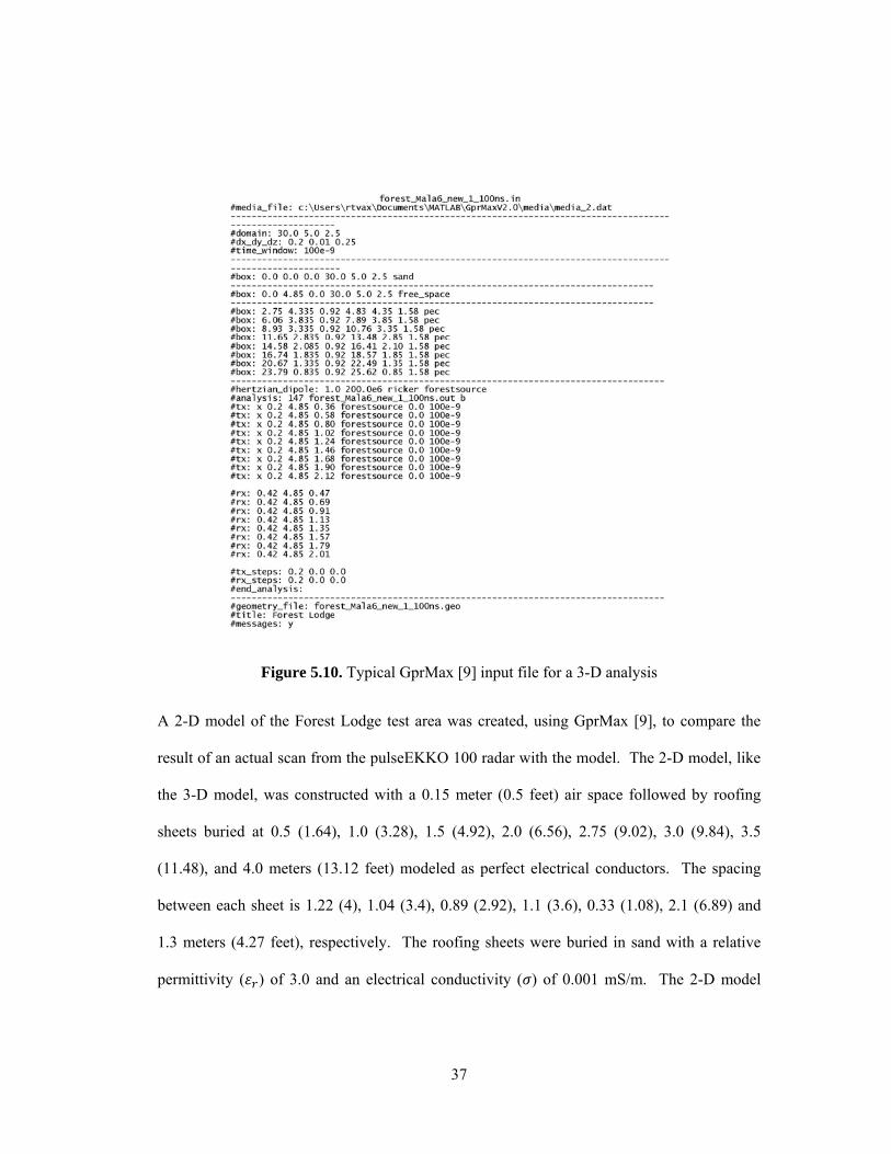
37

Figure 5.10. Typical GprMax [9] input file for a 3-D analysis

A 2-D model of the Forest Lodge test area was created, using GprMax [9], to compare the

result of an actual scan from the pulseEKKO 100 radar with the model. The 2-D model, like

the 3-D model, was constructed with a 0.15 meter (0.5 feet) air space followed by roofing

sheets buried at 0.5 (1.64), 1.0 (3.28), 1.5 (4.92), 2.0 (6.56), 2.75 (9.02), 3.0 (9.84), 3.5

(11.48), and 4.0 meters (13.12 feet) modeled as perfect electrical conductors. The spacing

between each sheet is 1.22 (4), 1.04 (3.4), 0.89 (2.92), 1.1 (3.6), 0.33 (1.08), 2.1 (6.89) and

1.3 meters (4.27 feet), respectively. The roofing sheets were buried in sand with a relative

permittivity ( ) of 3.0 and an electrical conductivity ( ) of 0.001 mS/m. The 2-D model

38

constructed was 5 meters in depth and 30 meters in width, Figure 5.11. Figure 5.12 shows an

example of a GprMax [9] input file that is used to run an analysis.

Figure 5.11. GprMax [9] 2-D model of Forest Lodge test area with buried roofing sheets

Figure 5.12. Typical GprMax [9] input file for a 2-D analysis

Sand ( 3

39

The 2-D area was scanned at 25 MHz with the results shown in Figure 5.13. As with the

actual scan result, only a rough outline of the 8 roofing tiles is shown; albeit a bit better than

the actual result. Again, this is the result of not quite modeling the actual parameters of the

media, like permittivity and conductivity. The simulated result shown depicts the signal

result at an elevated depth (TWTT less than actual scan). This is most likely due to the exact

height above the ground of the actual radar antennas not correctly depicted in the model. The

trend is correct, however. The result for 3-D and 2-D analyses confirm that actual scans can

be simulated by software programs specifically, by the GprMax [9] software program. The

actual 2-D data scan encountered unexplained problems which were not resolved because of

the unavailability of the radar equipment and scanning site.

Figure 5.13. 2-D simulated analysis of Forest Lodge Test Area (25MHz). 1 – Direct Arrival. 2 – Ground bounce. 3,4 – Curve of reflections from roofing tiles.

An analysis of the 2-D model was run at 900 MHz to ascertain the robustness of the GprMax

[9] program and the input model developed. Figure 5.14 shows the result of this analysis. As

1 2

4 3

40

expected, the 8 roofing sheets are clearly illuminated. Higher frequencies show objects with

greater detail closer to the surface. The items are delineated with better fidelity than at 200

MHz. Again, reflections below each sheet are shown as in the 200 MHz case. The software

program accurately captures the electromagnetic impedance changes that occur around an

object when being scanned by GPR. The result is an indication that this software

implementation translates well over the frequencies of interest for our EM GMM study. The

tools needed for work with the EM GMM algorithm method are in place.

Figure 5.14. 2-D Simulated analysis of Forest Lodge Test Area (900 MHz). Depicting all 8 roofing sheets

To demystify the Y-axis in Figure 5.12, (a sample GprMax [9] input file), and Figure 5.11,

(GprMax [9] 2-D model of Forest Lodge test area), the values shown are easily computed

knowing that the Y-axis values in Figure 5.12 are the reverse of what is plotted in Figure

5.11. Also, the GprMax [9] convention is to accept the last description of a defined area as

41

the media to be used in any analysis. An example is the line listing the sand media in Figure

5.12, (“#box” line), the sand media is plotted first, then the line listing the free-space media

overwrites a small portion of the sand media. The top 0.15 meters (5 – 4.85 = 0.15) is free-

space in this case. To get the Y-axis value of the first roofing sheet, take the max Y value

from the “#domain” line which is 5 and subtract the last Y value (y2) on the “#box” line

(noted as x1 y1 x2 y2) which is 4.35. The resultant outcome is 0.65. One more subtraction

must occur to get the 0.5 meter value in Figure 5.11. The free space Y value of 0.15 is

subtracted from 0.65 equaling the 0.5 meter value shown.

42

Chapter 6

EM GMM Process In Operation

6.1 Combining Harmonics of Sine waves

Having described GPR basics, discussed the EM GMM method, and the connection between

EM and MLE, (answering the question “Why does EM work?”), we continue by applying the

EM GMM method to examples or test cases. The first test case involved summing sine

waves at several frequencies to form a square wave. A square wave is the sum of odd

harmonics, all in phase, where the relative amplitude is 1/(harmonic number). A Harmonic is

defined as whole number multiples of a fundamental frequency. Table 6.1 describes the

properties of a few periodic signal characteristics.

Table 6.1. Periodic Signal characteristics

Square Wave Triangle Wave Sawtooth

Freq. components Odd # Harmonics Odd # Harmonics All harmonics

Relative Amplitude

1/Harmonic # 1/Harmonic # squared 1/Harmonic #

Phase All Harmonics in phase

Every other Harmonic 180 deg. Out of phase

Even Harmonics 180 deg. Out of phase

Harmonic – whole number multiples of the fundamental frequency

A series of six sine waves were constructed, which when weighted properly, sum to a square

wave. Figures 6.1, 6.2, and 6.3 display the six sine waves (50, 150, 250, 350, 450, and 550

Hz), all odd number harmonics (1, 3, 5, 7, 9 and 11) of a 50 Hz square wave. Each sine wave

43

shown has an initial magnitude of 1, before being used in the EM GMM algorithm. The

result, after processing with the EM GMM algorithm, is shown in Figure 6.4. Outlined in red

is the desired square wave, achieved when the six sine waves are weighted properly (1.0,

0.3333, 0.2000, 0.1429, 0.1111, 0.0909, respectively). Outlined in blue, in Figure 6.4, is the

result of the EM GMM algorithm combination of the six sine waves. The EM GMM result is

not quite square, but reasonably close. The error can be attributed to the constraints

associated with group membership weights, ( ), and/or the mixture weights, ( ). Each

are constrained to sum to 1, where the actual weights of the sine waves that create a square

wave normally sum to a value greater than 1; how much greater than 1 depends on the

number of harmonic signals added together.

Figure 6.1. Sine Wave Frequencies 50, 150 Hz

44

Figure 6.2. Sine wave Frequencies 250, 350 Hz

Figure 6.3. Sine wave Frequencies 450, 550 Hz

Figure 6.4. EM algorithm result with Square wave desired signal

45

Table 6.1 column 2 suggests that modifying the 6 odd harmonic signals, from the square

wave example, to alternate between an in phase (0o phase) harmonic signal and a 180 degree

out of phase harmonic signal, would produce a triangle wave when the signals are processed

by the EM GMM algorithm. Figure 6.5 depicts the result of such an occurrence. Again, the

generated result is less than a complete triangle wave for the same reason encountered by the

square wave example; the constraints (group membership weights, ( ), and/or the mixture

weights, ( )) limit the response required to generate an entire triangle wave.

Figure 6.5. EM algorithm result with Triangle wave desired signal

6.2 GPR Test Case 1

To judge the effectiveness of the EM GMM method on GPR analyses, the following test case

was constructed. Test case 1 consists of an object buried at 10 meters below ground with Txs

and Rxs 5 meters above ground in air or free-space. The object is modeled as a perfect

electrical conductor (infinite conductivity or zero resistivity) 2 meters wide and 0.5 meters in

depth (2-D model). The object is buried in a moist-sand medium with a relative permittivity

( ) of 9.0, an electrical conductivity of 0.5 mS/m (milli-Siemens per meter) and a velocity in

46

the medium of 0.1 m/ns. The model area is 10 meters wide by 25 meters in depth. Each

Tx/Rx is stepped along the x axis (scan axis) at 0.25 meters per step for a total of 36 scans.

The Tx starts at 0.5 meters ending at 9.5 meters; the Rx starts at 0.75 meters and ends at 9.75

meters. Each Tx/Rx remained at a height of 4.5 meters above ground as they are stepped

along the x-axis. The length of time for each scan is 425 ns; long enough to capture a

received signal from 24 meters below each Tx/Rx, in media comprised of a combination of

air and moist-sand. The model area has a grid space of 200 points in the x-direction (∆x –

0.05 meters) and 500 points in the y-direction (∆y – 0.05). Figure 6.6 depicts the 2-D model

of Test Case 1, showing the Tx/Rx positions, the target and media present for which a GPR

scan was completed.

Figure 6.6. Test Case 1 with buried target 10 meters below ground, Txs & Rxs 5 meters above ground.

Test Case 1 was scanned at six different frequencies (20, 30, 50, 100, 500, and 900 MHz) and

the result was processed using the EM GMM method to determine the weights of each

frequency for the best result for the combination of frequencies. Figures 6.7-6.14 show the

target

= 1.0 Txs & Rxs

= 9.0 Moist-sand

Free-space

47

resultant 2-D display of each frequency scan using GprMax [9]. In each case, the Target is

correctly identified at approximately 10 meters below ground (15 meters below the Txs and

Rxs) or approximately 240 ns from the direct arrival signal. The TWTT of 240 ns, reflects

the increase in length of the transmitted then received signal length above the vertical

distance due to the ray refraction produced by dissimilar mediums; free-space (velocity in the

medium of 0.3 m/ns) to moist-sand (velocity in the medium of 0.1 m/ns), resolvable by using

the Snell-Descartes law of refraction.

Figure 6.7. 2-D GPR Scan at 20 MHz Figure 6.8. 2-D GPR Scan at 30 MHz

Figure 6.9. 2-D GPR Scan at 50 MHz Figure 6.10. 2-D GPR Scan at 100 MHz

1

2

3

48

Figure 6.11. 2-D GPR Scan at 500 MHz Figure 6.12. 2-D GPR Scan at 500 MHz w/traces

Figure 6.13. 2-D GPR Scan at 900 MHz Figure 6.14. 2-D GPR Scan at 900 MHz w/traces

The direct arrival and ground bounce signals are shown in Figure 6.7, arrow 1. Arrow 2

shows the target reflection at depth for 20 MHz. The target reflection at 30 MHz is shown by

arrow 3 in Figure 6.8. All remaining arrows, unlabeled, depict the target reflection at depth

for the indicated frequency. Figure 6.12 and Figure 6.14 display each trace to better delineate

the target reflection. As expected, as the frequency increased the target became more

pronounced.

To demonstrate that just adding the different frequency scans together is not a good solution,

we added the six scan results together shown in figure 6.15. Here, we removed the ground

4

49

bounce and direct arrival signals by simply running an analysis without the target in place,

then subtracting that result from the analysis run with a target in place. The outcome of the

addition shows a very broad area of target reflection from approximately 240 ns to 320 ns

(TWTT); a very broad indication of target depth. It is possible that the broadness could be

reduced by lining up the “first break” of each frequency signal then adding.

Figure 6.15. Sum of frequency signals with direct arrival and ground bounce signals removed.

Figure 6.16. EM processed sum of frequencies Figure 6.17. EM processed signal traces

50

In Contrast to Figure 6.15 are Figure 6.16 and Figure 6.17. They demonstrate the effect of

processing the six scans using the EM GMM method to determine the weights of each

frequency scan for combining the signals. Figure 6.16 shows a very concise reflection of the

area where the target resides. However, the usual hyperbola that forms over the target is only

slightly in place; even less than what is shown in Figure 6.15. There are a couple of possible

reasons. The area being scanned is not wide enough to show the entire hyperbola; a 30-

meter-wide area should show more. The current width is more like a bore hole, twice as deep

as the width. Another reason is the fact that the object is 2 meters wide causing a much

broader hyperbola to form. Or, it could be that the EM GMM method has very bad edge

detection capability in its present form. The current scan area width (10 meters) was chosen

to limit the length of time required to run a GprMax [9] analysis to days rather than weeks.

6.3 GPR Test Case 2

A more complex test area structure was developed to test the EM GMM method. This area

corresponds to the buried sheet model constructed of the Forest Lodge test area. The

exception is the depth of each target. The structure is shown in Figure 6.18. It consists of an

area 30 meters wide and 25 meters in depth with little or no space above the ground (0.15

meters) for each Tx and Rx. The Txs and Rxs are swept along the scan axis starting at 0.5

meters (Tx) and ending at 29.5 meters (Tx). The spacing between a Tx and Rx is 0.3 meters

and each scan step is 0.2 meters. The total number of GPR scans is 145. Like the Forest

Lodge Model, the media is sand, more specifically, dry-sand with an electrical conductivity

( ) of 0.001 mS/m and a relative permittivity ( ) of 3.0; unlike the real Forest Lodge site in

which the media was more like moist-sand. The velocity through the medium is 0.1732 m/ns.

Corrugated aluminum roofing sheets, 2 meters in length and 0.1 meters thick were buried at 8

51

different levels (4.565, 6.065, 8.56, 10.065, 12.815, 14.065, 16.565, and 18.065 meters). The

unusual metric values are due to a not well-defined start depth of approximately 15 feet

(4.565). Each additional increase in depth was computed in meters (1.5, 2.5, 1.5, …etc.).

The horizontal distance between each sheet was not well thought out. The horizontal

distance, between sheets, ranges from 1.2 meters to 0.3 meters. Because they are placed like

stairsteps the physical distance is much larger than the range mentioned and should not

interfere with the scanning outcomes. Each sheet is modeled as a perfect electrical

conductor. Each scan is 425 ns in length and capable of receiving a reflected signal from

roughly 37 meters below each Tx/Rx pair in a dry-sand media. The model grid is 150 points

in the x direction (∆x – 0.2 meters) and 2500 points in the y direction (∆y – 0.01 meters).

The six scanning frequencies are the same (20, 30, 50 ,100, 500, and 900 MHz).

Figure 6.18. Test Case 2, (8) roofing sheets 2 meters long, 0.1 meters thick, buried at 8 different levels

The result of the GPR scans processed by the EM GMM method are shown in Figures 6.19

and 6.20. In both Figures 8 objects are identified at approximately the correct depth (50, 70,

100, 116, 148, 160, 190, and 208 ns for two-way travel times). To compute the depth,

Dry sand ( 3

52

multiply the velocity through the media (0.1732 m/ns) times the two-way travel time, then

divide by 2; (e.g., ∗ .

4.33 meters, approximately the depth of the first sheet). The

edges of each object are depicted, not well but reliably with less fidelity as one descends in

depth. Figure 6.20 displays the GPR trace response instead of the image response.

Figure 6.19. EM processed results Figure 6.20. EM processed signal traces

6.3 GPR Test Case 3

A repeat of Test Case 2 was structured to study the response of the EM GMM method in non-

uniform media with buried objects. A model area was created with dry-sand, clay, concrete,

granite and limestone as the media to contain the roofing sheets. Roofing sheets were again

buried at the same depths, the same distance between the sheets, and the Tx/Rx pair placed

just barely above ground at 0.15 meters, as before. The roofing sheets were, again modeled

as perfect electrical conductors. Figure 6.21 notes the model structure, materials, and the

relative permittivity of each material. Color differences for the different materials are also

noted. Dry-sand media covers an area from 0.15 to 7 meters in the y direction and 0 to 30

meters in the x direction. Dry-sand has a permittivity ( ) of 3.0 and a velocity through the

medium of 0.1732 m/ns. The clay media encloses an area from 7 to 13.5 meters in the y

53

direction and 0 to 14 meters in the x direction. Clay media has a permittivity ( ) of 5.0 and a

velocity through the media of 0.1342 m/ns. The concrete media encompasses an area from

13.5 to 16 meters in the y direction and 0 to 20 meters in the x direction. Concrete media has

a permittivity ( ) of 6.0 and a velocity through the media of 0.1225 m/ns. The granite media

covers the area of 7 to 16 meters in the y direction and 14 to 30 meters in the x direction

minus the area occupied by the concrete media of 13.5 to 16 meters in the y direction and 14

to 20 meters in the x direction. Granite has a permittivity ( ) of 4.0 and a velocity through

the medium of 0.15 m/ns. The final media in the model is limestone which encompasses an

area from 16 to 25 meters in the y direction and 0 to 30 meters in the x direction. Limestone

has a permittivity ( ) of 7.0 and a velocity through the medium of 0.1134 m/ns.

Figure 6.21. GPR Test Case 3, (8) roofing sheets 2 meters long, 0.1 meters thick, buried at 8 different levels, in non-uniform media.

Figures 6.22 and 6.23 describe the result of an EM processed GPR scan of the non-uniform

media example. All 8 roofing sheets are visible. Looking closely there are signal echoes

which represent the interference of EM waves during the scanning process. As expected,

Dry sand ( 3

Clay 5 Granite 4

Concrete 6

54

with depth the illuminated objects are less clear. Figure 6.23 displays the scanned signal

trace response of the same area.

Figure 6.22. EM processed GPR scan of non-uniform media Test Case 3.

Figure 6.23. EM processed signal traces of non-uniform media Test Case 3.

55

The importance of Figures 6.22 and 6.23 is that they show scanned complicated media

processed with the EM method can illustrate buried objects reliably. Typical sites that are

scanned are not homogenous and are littered with other artifacts included with the object that

is searched for. Having the capability of better illuminating an area of multiple media types

is an important tool to have to study problems encountered when conducting searches for

hard to find objects. Test Case 3 suffers from the problem that each medium is not very thick

and the velocity through each medium is very similar, though the media are quite different.

This lends to GPR responses similar to the homogenous media examples except for the signal

refraction occurrences at each media boundary making the signal path slightly longer. The

result is an encouraging demonstration of the capability of the EM method in illuminating

objects. Remaining items to look at are: How well does the method do from various heights

above ground? How well does the method perform compared to other state of the art

methods? and How well does the EM method perform compared to other excitation functions

like chirp?

56

Chapter 7

Other GPR Frequency Scan Compositing Methods

A constant in compositing has been the work conducted by archaeologist using various

methods. GPR time-slice analysis, overlay analysis and GPR isosurface rendering, are a few

of the methods used; all similar in approach. That approach consisted of illuminating the

strongest reflections with a color or shading then combining the information by layers of

depth, displaying the result [55]. Not like the approach being considered in this study of

weighting the individual frequency responses then summing.

Earlier than our use of the EM optimization problem solver method, other authors made

attempts to determine how to weight each GPR frequency scan to be combined to produce a

clearer signal at depth; developing an optimal result. Three of those authors were first M.

Dougherty [8], then A. Booth [5][48] followed by S. Bancroft [3]. Each author, in turn,

discussed the previous author’s work suggesting improvements. None, however, explored

the use of optimization problem solvers. Below, each author’s method is discussed, and the

result is compared to our EM GMM optimization problem solver method.

7.1 Dougherty’s Method

Dougherty’s [8] task was to combine GPR signal traces for site characterization and

bandwidth enhancement. The real data represented GPR signal traces from a former lumber

mill waste site near Boise, Idaho. The data was to aid in delineating possible areas of fill

from surrounding fluvial sediments and fill areas from undisturbed natural sediments. The

57

fill consisted of wood or organic matter intermixed with native sedimentary material

organized in layers of the following:

Tree bark

Cobblestone rock

Mixture of Sand and fine organic materials

Lumber debris consisting of planks, boards, timbers and logs

The areas were scanned with a Sensors and Software pulseEKKO IV GPR radar unit using 3

different frequencies, 50, 100 and 200 MHz. The goals of his study were to process

information on shallow reflections by removing the direct arrival (air wave) signal, then

determine the change in radar data that occurs in fill zones using cross-correlation and,

finally, to increase the resolution and depth perception by combining the 3 GPR scan

frequency results. Dougherty reports on his success and failures to solve this challenge in

reference [8].

Our interest in Dougherty’s work is two-fold, the process of removing the direct arrival signal

and his method of combining GPR frequencies. Removing the direct arrival signal is

important because it tends to be orders of magnitude greater in scale than the target response

signals, dominating any calculations made using the data. The Dougherty [8] method of

removing the direct arrival signal entails creating an estimate of the signal then subtracting

that estimate from the original signals. To remove the direct arrival signal, Dougherty [8]

horizontally aligns each trace along its time axis, for 1 frequency. DC shifts and any low

frequency “wow” components are removed, followed by scaling each trace by the L2 norm of

58

the direct arrival pulse. Summing the traces of 1 frequency creates an estimate of the direct

arrival signal for that frequency. Subtracting this estimate from each trace removes the direct

arrival signal or a major portion of it. This process is repeated for all frequencies scanned.

To combine the frequencies scanned, Dougherty [8] first applies a gain recovery function to

each processed trace (traces with the direct arrival signal removed and scaled by the L2

norm); then applies equal weighting to each trace for all frequencies, summing the result and

scaling the sum of traces by the number of frequencies summed. The Dougherty [8] result

achieved reflection enhancement and increased spectral bandwidth, but the resultant signal

was overwhelmed by the lower frequencies in the summation indicated by the spread in width

of the combined reflected signal results.

Dougherty [8] process steps:

1 Align each trace by direct arrival signal.

2 Remove the DC shift.

3 Remove low Frequency (wow).

4 Scale each trace by L2 norm of direct arrival pulse.

5 Sum traces to form an estimate of direct arrival signal.

6 Subtract estimate from each trace.

7 Apply exponential gain recovery function.

8 Apply equal weighting to each trace.

9 Sum each trace for all frequencies.

59

7.2 Booth’s Method

Booth examined five methods, with a few variations, to achieve an increased bandwidth in

the frequency domain and thus a more approximate delta function in the time domain through

evaluating composite synthetic GPR wavelets. Booth used real data acquired at a site on the

Waterloo Moraine west of Waterloo, Ontario, Canada. The data resulted from a high-

resolution stratigraphic study being conducted. The site was composed of clean, well-graded,

medium to coarse grain sand, offering good depth penetration and multiple size targets. Data

was collected using a Sensors and Software pulseEKKO 1000A system with a 200-volt

transmitter and bistatic antennas with center frequencies of 225, 450 and 900 MHz. For all

data sets the TWTT was 100 ns. All other system scan parameters were defined in reference

[5].

Booth [5] looked at the simple summation technique of Dougherty [8], as one method. For a

second method (method 2), a scaled summation approach was examined, where the

maximum value of the frequency spectra for all traces of one frequency was determined.

Each spectrum was obtained by the Fourier transform of a trace. The maximum valued

spectra for each frequency were then equalized. The values used to equalize the spectra

provided the signal weighting before summation. As a variation, the frequency spectra for

each trace was averaged for one frequency. This process was repeated for all frequencies. A

weight value was determined that would equalize the averaged spectra for all frequencies.

This value provided the signal weighting for summation.

A third method, required shifting traces such that the main peaks of the direct arrival pulses

were aligned with the most dominant peak; then the scaled summation technique of method 2

was applied. This method (method 3) provided the best result for increased spectral

60

bandwidth, the best delta function and GPR resolution for synthetic wavelets of the three

methods analyzed thus far. Booth [5] repeated this method with one variation, the time-

shifting of traces was changed to align the first break of each trace at 0 ns; then method 2 was

applied.

Method 4 involved time-shifting traces to align the first break of each trace at 0 ns. The

frequency spectra of each trace were averaged for one frequency creating an ensemble

estimate, then the frequency weight was determined as before to equalize the ensemble

spectra for all frequencies. The magnitude needed to equalize the ensemble spectra

determined the weight for that frequency. Method 4 was named dominant frequency

amplitude equalization (DFAE).

The final weighting method (method 5) involved determining weighting factors from a least

squares analysis that attempts to match the summed result to a defined optimal amplitude

spectrum. This method Booth [5] named optimal spectral whitening (OSW). A defined

optimal spectrum section over a set of frequencies determines which frequencies in the

frequency data sets would be enhanced. Frequency variant weighting functions must be

developed to implement the least squares analysis of the OSW technique [5].

The OSW process determined a time window to operate on by choosing the longest wavelet

period of the GPR scanned frequencies. A frequency spectrum of each trace for each time

window was calculated. The spectra for each trace for a frequency were averaged together

and a magnitude was determined for each scanned frequency over the defined time window.

The computed magnitude constituted a row in the OSW matrix. The process was repeated for

each scan frequency for the defined time window resulting in an over-determined linear

system for the frequency weights of a defined desired spectral amplitude. The desired

61

spectral amplitude was usually defined as identical values (constant); one for each scan

frequency. The OSW process is complete with the combining of traces for that time window

with the computed weights. A time-variant weighting function is produced by repeating the

OSW process for each time window over a GPR reflection scan [5].

The over-determined linear system for OSW consists of a matrix A, where a row represents

the spectral amplitude at one frequency (f1) over a limited frequency data set M (one column

for each component of the data set). A second row represents the spectral amplitude at

another frequency (f2) over the same limited frequency data set M. A new row definition

follows with each additional frequency. Each component in the limited data set has a weight

Wm. Matrix A multiplied by column matrix Wm produces a desired spectral amplitude for

each frequency (Sf); equation 7.1. With known values for matrix A and desired spectral

amplitude Sf the weights can be determined from the standard least squares solution,

∗ ∗ ∗ . The desired spectral amplitude is usually specified as identical values

(constant), one for each scan frequency. The OSW process is complete with the combining

of traces for that time window with the computed weights. This process can be repeated for

each time window of a GPR reflection scan, should more than one time window be defined.

Of the two strategies developed for estimating the weighting factors for amplitude scaling,

Booth pointed to the processing flexibility of the OSW process with its balanced set of

weighting factors over the DFAE process. The DFAE disadvantage was that the dominant

frequency within a data set may not represent the distribution of useful signal energy should

the spectrum of a GPR wavelet not be symmetrical. The OSW process considers the energy

distribution across the entire useful frequency range. Process steps are listed below with

some slight modifications from Booth [5].

62

∗ ⋮ … ⋮ ∗ ⋮ ⋮ (7.1)

Booth [5] process steps for methods 2-5 are as follows:

Method 2 – scaled summation

1 Determine the frequency spectrum (wavelet) of each trace at a frequency;

determining the largest magnitude for that frequency. Repeat for all frequencies.

2 Equalize spectra for all frequencies; the magnitude needed to equalize the spectra

determines the weight for that frequency. (method 2 variation – average the

frequency spectra of each trace for one frequency then, determine the weight to

equalize the average spectra, repeating for all frequencies).

3 Sum each wavelet of all frequencies with the previously determined weight for each

wavelet.

Method 3 –

1 Shift all traces such that the main peaks of the direct arrival signal are aligned.

(variation – align the first break of each trace to 0 ns).

2 Continue by applying the steps of method 2.

Method 4 – DFAE


2 Remove low frequency (wow).

63

3 Shift all traces to the first break of direct arrival signal

4 Remove direct arrival signal (mute, ramping from 0% to 100% magnitude at chosen

mute time)

5 Determine the frequency spectrum of each trace.

6 Average spectra for ensemble estimate for a frequency. Repeat for all frequencies.

7 Equalize ensemble spectra for all frequencies. The magnitude needed to equalize a

spectrum determines the weight for that frequency.

8 Sum each trace of all frequencies with appropriate weight for that frequency.

Method 5 – OSW



3 Shift all traces to the first break of direct arrival.

4 Remove direct arrival signal (mute, ramping from 0% to 100% magnitude at chosen

mute time).

5 Average traces for each frequency.

6 Compute spectra of average trace for each frequency.

7 Determine magnitude at scan frequencies for each spectrum. This becomes a row in

OSW matrix “A”, one row for each frequency.

64

8 Determine idealized frequency spectra vector “S”; vector usually set to value of one

for each scan frequency.

9 Determine weights by solving matrix equation ∗ ∗ ∗ .

10 Combine weighted frequency traces; ∗ .

11 Repeat steps 6 – 10 for all analysis time windows over the GPR reflection profile. A

time window should be greater than the longest wavelet period to be sampled.

Earlier, Booth [5] examined another site, an outwash near Guelph, Ontario, Canada with a

different Sensors and Software system (pulseEKKO IV) using first 200, 100, 50 and 25 MHz

antennas with 1000-volt transmitter and second with 200, 100 and 50 MHz antennas with a

400-volt transmitter. Booth looked at the equalization of the frequency amplitudes and

optimal spectral whitening of the composite area techniques with similar results as the

Waterloo Moraine site [48].

7.3 Bancroft’s Method

Bancroft [3] noticed that a nominal GPR data set only provides an incomplete view of the

subsurface with regards to spatial resolution and penetration depth. He noticed that

incorporating multiple GPR data sets from different center frequency radars into a single

survey could reduce the limitations of a single GPR data set; thus, interpreting multiple data

sets jointly. Bancroft discussed three ways that joint interpretation of multiple frequencies

had occurred; side-by-side analysis of multiple spatially similar profiles at different

frequencies, simple summations of multiple frequencies and combining data sets in a manner

65

that maximizes the bandwidth to increase wavelet deconvolution effectiveness (Booth [5]).

Bancroft [3] sought to develop, evaluate and compare methods to existing deconvolution-

based methods using a GPR survey of Santa Rosa Island, Florida. Our interest is in the

methods Bancroft sought to develop and evaluate.

Deconvolution attempts to remove a wavelet from a recorded seismic trace by reversing the

process of convolution which occurs during the TWTT of a GPR signal through a medium.

The attempt is to separate the source wavelet from the Earth’s reflectivity (series of

impulses), compress the source wavelet into a zero-phase spike, removing any multiple

reflections to increase the vertical resolution of the seismic data. Wavelet or spiking

deconvolution was not a topic of our interest in compositing. It is a follow-on process Booth

[5] among others (e.g. Leinbach [52]) have attempted to use to enhance the GPR response.

None of the details are discussed in this work. [53][54].

Bancroft [3] acquired data at the Eglin Air Force Base, where Santa Rosa Island resides,

located along the Florida panhandle from Destin to Pensacola Pass. Santa Rosa Island is

bounded to the north by Pensacola and Choctawhatchee Bay, to the south by the Gulf of

Mexico. Of interest, are the changes caused by hurricanes, natural deposits and erosion.

Bancroft [3] used a MALA Radar making passes over an area with 100, 250, 500 and 800

MHz antennas. Data sets were processed with ReflexW [30] and MATLAB software

programs.

Bancroft’s [3] steps for creating composite radargrams were comprised of the following: the

basic processing steps (static correction, dewow filtering, gain, spectral filter and time length

cutting), a common data definition representing each frequency data set, amplitude scaling,

applying time shifts and summation. The basic processing steps are loosely defined as:

66

Static correction – remove the DC component.

Dewow – removing low frequency energy that has yielded a slow time-varying

component added to the measured data caused by the close proximity of an Rx and

Tx with electrostatic and inductive fields.

Gain – scaling the amplitude of the data such that low amplitudes are emphasized

with respect to the data with high amplitudes.

Spectral filter – eliminate noise by bandpass filtering or compute an average trace of

all traces of one frequency and subtract the average trace from each trace.

Time length cutting – equalize scan time for all frequency traces and frequencies.

Bancroft [3] surmised that Dougherty [8] was unable to optimize the high frequency data

because at depth these signals were much lower in magnitude than the low frequency signals.

Just adding the signals together without amplitude scaling would not improve the resultant

outcome. Bancroft [3] noted that Booth’s OSW technique [5] of modifying the magnitude of

defined scan frequencies by adjusting the magnitude of a spectra over a defined range of

frequencies was equivalent to the linear ramp summation method by gradually introducing

lower frequency energy in the summation. Because of his observations, Bancroft [3]

introduced and studied three new methods to improve the compositing process of Dougherty

[8] and Booth [5]. These methods were the double ramped summation technique, the

Amplitude Envelope Equalization (AEE) technique and a subjective method to determine the

scanned frequency weighting through visual inspection of each data set.

The double ramped summation technique is where the higher frequency data is suppressed by

the same amount the lower frequency data is enhanced over the TWTT of a GPR scan. The

67

technique required working with three parameters to achieve a good result; which function to

use to create the ramps (e.g. Butterworth or linear), the ramp length of time; and the ramp

start time. Bancroft [3] used both Butterworth and linear function ramps in his studies. The

ramp length for each frequency was determined by multiplying the wavelength period of a

frequency by the arbitrary number 15, for 15 wave periods. For the double ramped method

two adjacent frequencies were used. One frequency is enhanced while the other is

suppressed. The ramp length was determined by the 15th wave period of the frequency that

is being suppressed. The third parameter, ramp start time, was defined as the point when a

frequency data set is sufficiently attenuated to begin suppressing it. This ramp start time was

determined by examining the amplitude envelope of a trace, finding the minimum value of

the log of the averaged amplitude envelope for all traces for that frequency. An averaged

amplitude envelope is calculated as the Hilbert transformation of a single trace for that

frequency averaged over the amplitude envelope of all traces of that frequency. The

compositing process involved summing each pair of frequencies, one enhanced and one

suppressed, over the ramp length of the suppressed frequency at the defined ramp start time.

Bancroft double ramped summation process steps:

1 Clip data prior to the first arrival.


3 Automatic gain control (AGC) gain.

4 Bandpass filter the data.

5 Determine the length of decreasing ramp in nanoseconds beginning with the highest

frequency.

68

6 Determine amplitude envelope of all traces (without AGC) of 1 frequency and

average them. Repeat for all frequencies.

7 Determine the suppression start time by finding the minimum value of the log of the

averaged amplitude envelope.

8 Process traces, adding them using the double ramp summation technique.

Bancroft [3] named the second method the AEE technique where a set of multipliers were

developed as the ratio of the average envelope value of the lowest frequency to the average

envelope value of the other frequency data sets, both without AGC applied. The weights

determined by this method were applied to the AGC processed frequency data sets over the

portion of time that each frequency was to be enhanced resulting in approximately equal

amplitude envelopes. The weights determined by this method were used in conjunction with

the double ramped summation method defined earlier. Determining the portion of time that

each frequency was to be enhanced was accomplished by finding the minimum value of the

log of the averaged amplitude envelope for that frequency.

Amplitude Envelope Equalization technique steps:

1 Clip data prior to first arrival.


3 Automatic gain control gain.

4 Bandpass filter the data.

5 Determine the length of decreasing ramp in nanoseconds beginning with the highest

frequency.

6 Determine amplitude envelope of all traces (without AGC) of one frequency and

average them. Repeat for all frequencies.

69

7 Determine suppression start time by finding the minimum value of the log of the

averaged amplitude envelope.

8 Determine AEE multipliers as a ratio of the averaged envelope of the lowest

frequency data set and the average envelope of the other frequency data sets, both

without AGC).

9 Apply the AEE multipliers to the ramped summation technique.

Bancroft [3] considered a third method where the length of the summation ramp(s), the

starting point of the summation ramp(s) and frequency data set weights were chosen by visual

inspection of each nominal frequency data set. However, the process to implement this

subjective method is not significantly defined well enough to duplicate his example.

70

Chapter 8

Comparison of EM Process with Other Methods

The methods described in Chapter 7 provided modeling approaches to compare the EM

GMM compositing method with the state-of-the-art methods found in the literature. The

literature search was by no means an exhaustive one, but the methods discussed appeared to

be examples of the methods with the best results. The software program MATGPR

[31][50][51] was used to plot the GprMAX [9] output analysis files.

8.1 Dougherty’s Method Comparison

Figure 8.1a depicts the Dougherty [8] process on Test Case 1 of Chapter 6, shown side-by-

side with the EM GMM result, Figure 8.1b. In comparison, the Dougherty case (Figure 8.1a)

correctly identifies the depth at 240 ns or 15 meters below the Txs and Rxs but less crisp than

the EM result (Figure 8.1b). However, Figure 8.1a shows better edge detection. The width is

better defined (approximately 5m), but still wider than the actual defined area of 2 m. The

Ground bounce is slightly visible, but the Dougherty process is still a very effective method.

(a) (b) Figure 8.1. (a) Dougherty standard response to Test Case 1. (b) Figure 6.16. (Repeated here) EM processed sum of Frequencies

71

Figures 8.2 and 8.3 compare the 1-D plots of individual traces for the Dougherty process and

the EM GMM analysis with Txs at 5 meters above ground, for Test Case 1. Figure 8.2a

shows trace (18) at 5 meters out of 10 meters in the x direction of the model, roughly over the

target for the Dougherty process. Figure 8.2b shows the same x direction trace for the EM

GMM analysis.

(a) (b) Figure 8.2. (a) Trace 18 of 36 traces total; roughly 5 m out of 10 m in total distance in the x direction of Test Case 1 model, 1-D plot of Dougherty method. (b) Trace 18 of 36 traces total; roughly 5 m out of 10 m in total distance in the x direction of Test Case 1 model, 1-D plot of EM GMM analysis.

The Dougherty trace shows the remnants of the direct arrival/ground bounce signal which

Dougherty attempted to remove (signal results occurring less than 100ns in time). The target

reflection (at approximately 240 ns) is just slightly broader in the Dougherty case verses the

EM GMM analysis case. This is indicated by a thicker area (in depth) over the target

reflection area in the 2-D plots (Figure 8.1a and Figure 8.1b).

Figure 8.3 depicts 3 traces at approximately 0.3 meters (trace 1), 5 meters (trace 18) and 8.3

meters (trace 30) in the x direction of Test Case 1 model. Figure 8.3a shows the Dougherty

method response while Figure 8.3b shows the EM GMM analysis response. As expected,

72

trace 18 has the largest reflected magnitude because it is over the target, while traces 1 and 30

are at the sides of the target.

(a) (b) Figure 8.3. (a) Traces 1, 18 and 30, 1-D plots of Dougherty method response for Test Case 1. (b) Traces, 1, 18, and 30, 1-D plots of EM GMM analysis method response for Test Case 1.

Figure 8.4a depicts the Dougherty [8] process on Test Case 2 of Chapter 6, a model of buried

roofing sheets situated in a stairstep fashion in dry sand. Comparing the Dougherty response

to the EM processed response to Test Case 2 (Figure 8.4b), it is apparent that only 5 and

barely 6 of the 8 plates are shown in the Dougherty [8] response verses all 8 plates shown in

the EM response. Plate edges are equally vague in both Figures. Of the plates shown, the

target depths are the same as the EM processed results, which are correct.

73

(a) (b) Figure 8.4. (a) Dougherty response of Test Case 2. (b) Figure 6.19. (repeated here) EM processed results

In general, the Dougherty [8] method results are not as extensive as the EM method. Buried

objects in media are not illuminated as often as with the EM processed method. However, in

reviewing the Dougherty [8] processing steps, it is apparent that a step (Chapter 7 section 7.1

step 7) was not followed as Dougherty [8] suggested. A gain recovery function was used but

not exponential. Exponential gain recovery functions increase the gain as the signal

progresses in time. Figure 8.5 shows an example result from one possible method described

by equation 8.1 [49] below with a(i), the original amplitude trace, a vector of ones. The

equation was changed slightly from that of the reference [49]; the sample rate (dt) is divided

by 1,000 instead of value 10,000 found in the reference. Plots of b(i) using both values did

not seem noticeably different.

∗ ∗ ∗ ∗ (8.1)

Where:

i - sample

a(i) - ith sample of original amplitude trace.

74

g - exponential gain constant.

dt - sample rate.

b(i) - ith sample of gain recovered trace.

Figure 8.5. Exponential Gain Recovery Function Example

Each exponential gain trace vector was scaled based on the vector’s maximum value, then the

Dougherty method continued processing with step 8. Figures 8.6 (2-D plot) and 8.7 (1-D

plots) show the result for Test Case 1 with an exponential gain constant of 10 (arbitrarily

chosen). Figure 8.6 shows the target reflection to be broader in width like the EM processed

result (Figure 6.16), due to the enhancement of weaker reflection GPR responses. This result

is not very appealing for target width detection. Figure 8.7 shows a 1-D plot of trace 18

(Figure 8.7a) and then traces 1, 18 and 30 (Figure 8.7b) of the Dougherty process response

with an exponential gain of 10. The magnitude of the target reflection at approximately 240

ns has increased significantly over the remaining direct arrival/ground bounce signal (signal

75

magnitude at less than 100 ns). The result is apparent in the 2-D plot (Figure 8.6) with

increased target width.

Figure 8.6. Dougherty response to Test Case 1 with exponential gain function

(a) (b) Figure 8.7. (a) Trace 18 of 36 traces total; roughly 5 m out of 10 m total distance in the x direction, 1-D plot of Dougherty method with an exponential gain of 10. (b) Traces 1, 18 and 30, 1-D plots of Dougherty method with an exponential gain of 10.

Figure 8.8 shows a response to Test Case 2 like the EM processed result. All 8 plates are

depicted, though plates 7 and 8 appear thicker than the EM processed counterpart (Figure

76

8.4b). We can only speculate that changing the exponential gain factor might improve this

result but put at risk losing the recognition of the plates 6 through 8. Edge detection appears

to have improved over the EM method.

Figure 8.8. Dougherty response to Test Case 2 with exponential gain function.

8.2 Booth’s Method Comparison

Booth [5] explored five methods, with some variations, to enhance GPR wavelet responses.

Booth favored the last method, optimal spectral whitening, as the best method to use. We

thought it important to mention 2 others Booth considered before settling on the OSW

method; Booth method 3 and Booth dominant frequency amplitude equalization.

Figures 8.9 and 8.10 depict 1-D plots of both methods (method 3 and DFAE), while Figure

8.12 displays the 2-D response to the Test Case 1 model for both methods. The items to

remember from the casual review of these figures are that the magnitudes are similar in the

area over the target (240 ns in time or 15 m below the Txs), the reduction in the ground

77

bounce signals through Booth’s average spectra weight equalization technique, and the poor

delineation in the 2-D plots.

(a) (b) Figure 8.9. (a) Trace 18 of 36 total; roughly 5 m out of 10 m in total distance in the x direction of Test Case 1 model, 1-D plot of Booth method 3. (b) Trace 18 of 36 total; roughly 5 m out of 10 m in total distance in the x direction of Test Case 1 model, 1-D plot of Booth DFAE method with the first 36 ns in time reduced to small value to eliminate the largest portion of the remaining direct arrival/ground bounce signal.

(a) (b) Figure 8.10. (a) Traces 1, 18 and 30, 1-D plots of Booth Method 3 for Test Case 1. (b) Traces 1, 18 and 30, 1-D plots of Booth DFAE method for Test Case 1, with the first 36ns reduced to a small value to eliminate the largest portion of the remaining direct arrival/ground bounce signal.

78

When looking at Figure 8.10, the notion of proper GPR analysis is bolstered by the fact that

as one approaches the center of target the magnitude of the GPR response increases as it

should (trace 1 to 18 to 30 or 0.3 m, 5 m, 8.3 m). The width in time on the 1-D plots (Figure

8.10) is reflected in the 2-D plots (Figure 8.12) as target thickness in depth.

Figure 8.11. Complete Trace 18 of 36 total; roughly 5 m out of 10 m in the x direction of Test Case 1 model.

Figure 8.11 is included to show the portion of the remaining direct arrival signal (less than

10ns) that became enhanced by the weighting factors from the DFAE spectra weighting

method Booth used. We have routinely used a linear ramp approach to remove the direct

arrival signal for 4 time periods calculated for each trace frequency, translated to the number

of time steps. At 0 ns the magnitude is very small, increasing as one proceeds to 200 ns

(14,133 time steps) for 20 MHz and 4.5 ns (315 time steps) for 900 MHz with 30,032 total

samples. For the composite summed frequencies, the ground bounce largely remains at

approximately the 30 ns time for TWTT or 10 meters (half being 5 m in distance, the correct

distance from Txs; Figure 8.10).

79

In Figure 8.12, the width of the target reflection cannot be determined; it is largely flat for the

entire 10 meters. There is however a slight bulge in thickness at the area of the target

reflection.

(a) (b) Figure 8.12. (a) Booth Method 3 response to Test Case 1. (b) Booth DFAE method response to Test Case 1.

Figure 8.13a is a 2-D plot comparing Booth’s OSW method response to Test Case 1 model to

our EM GMM processed response (Figure 8.13b). For this analysis, both the direct arrival

signal and the ground bounce have been removed.

(a) (b) Figure 8.13. (a) Booth OSW response to Test Case 1. (b) Figure 6.16. (Repeated here) EM processed sum of frequencies.

80

Figures 8.14 and 8.15 compare the 1-D plot for Booth OSW method and the EM GMM

method for Test Case 1. Depicted here is the width in time for Booth’s OSW method verses

the EM GMM processed result. Booth’s thicker (in time) response translates into a thickness

in depth in the 2-D plot depicting true target depth and thickness uncertainty. For multiple

traces, it is shown that the trace responses are right on top of each other for the EM GMM

method but different in height as expected. As the radar scan approaches the target the

magnitude of the reflection response increases; as the scan recedes from the target, the

magnitude of the radar response reduces. The difference in thickness in depth is evident in

the 2-D plots shown in Figure 8.13a verses Figure 8.13b. In either case, the edge detection

(width of the target in 2-D trace) is very poor.

(a) (b) Figure 8.14. (a) Trace 18 of 36 traces total; roughly 5 m out of 10 m in total distance in the x direction of Test Case 1 model, 1-D plot of Booth OSW method. (b) Trace 18 of 36 traces total; roughly 5 m out of 10 m in total distance in the x direction of Test Case 1 model, 1-D plot of EM GMM analysis.

81

(a) (b) Figure 8.15. (a) Traces 1, 18 and 30, 1_D plots of Booth OSW method response for Test Case 1. (b) Traces 1, 18 and 30, 1-D plots of EM GMM analysis method response for Test Case 1.

For Test Case 1 model, there are “bore hole” effects. Test case 1 has an area twice as deep as

it has width (bore hole); very narrow width scanning area. The significance is that the width

is not wide enough to show the usual entire hyperbola that normally forms above and around

the object being scanned. The hyperbola formation is affected by the length of the target at

depth. As the depth is increased the hyperbola tends to flatten out for a “bore hole” scan.

This seems to be occurring for Test Case 1 model examples. Widening the scan axis to 30

meters or more decreases this effect. Figure 8.16 demonstrates the effect of increasing the

scan axis width for 3 frequencies, marking in red the 10 m area that is used for Test Case 1

model analyses.

82

Figure 8.16. Wider scan axis example (30 m) for Test Case 1 showing hyperbola for 20, 30 and 100 MHz; Original scan axis width shown in Red.

10 m Scan axis used in Test Case 1 analyses

83

Figure 8.17a. depicts the response of Booth OSW method to Test case 2, compared with the

EM GMM processed response of Figure 8.17b. Not all plates are shown for Figure 8.17a.

The first 4 plates are easily shown, but plates 5 and 6 are barely visible of the 8 plates total.

Compared to the EM GMM method, Booth’s method falls short in depth and the edge

detection is poorer, but it is comparable to Dougherty’s method without exponential gain, but

worse than Dougherty’s method with exponential gain recovery. A part of the ground bounce

signal remains in the 2-D plot of Booth’s OSW method. Of the plates shown, target depths

are the same as the EM results.

(a) (b) Figure 8.17. (a) Booth OSW response to Test Case 2 including direct arrival/ground bounce. (b) Figure 6.19. (repeated here) EM processed results.

8.3 Bancroft’s Method Comparison.

Bancroft [3] explored three methods to combine multiple frequencies with two representing a

variation of each other (double ramped summation and AEE) and a third not clear on how to

implement. Figures 8.18 and 8.19 show 1-D plots of the Bancroft AEE method response to

Test Case 1. The ground bounce and direct arrival signals have been removed using the same

84

linear ramp “mute” method discussed in section 8.2 and used on Booth [5] traces. For these

results (Figures 8.18a, 8.19a and 8.20a), we applied a modified AEE method consisting of the

calculated weight multipliers only and not the ramped summation add-on because the

calculated start and end times of each ramp conflicted with each other, which is not the case

for the scan frequencies chosen by Bancroft [3]. The items to notice in the plots are the start

time of the pulse and its thickness in time. The start time (240 ns) represents the TWTT

response from the target; translating to an object approximately 15 meters below Txs and Rxs

in a moist sand and free-space environment. The thickness in time of the Bancroft [3] AEE

modified method is wider in comparison to the EM GMM method, but comparable to

Dougherty [8] (with and without exponential gain recovery) and the Booth [5] method 3

approaches, but better than the Booth [5] OSW method. Again, the 1-D thickness in time

translates to a thickness in depth in a 2-D plot, consistent with target depth uncertainty.

Therefore, the Bancroft [3] AEE modified method target depth is more uncertain than the EM

GMM method. In Figure 8.19a, three traces are shown depicting the target response from

three different vantage points. Trace 18 of 36 is the strongest response and resides directly

over the target. Traces 1 and 30 of 36 are at each end of the scan space, reflected by the

reduced magnitude compared to trace 18. Figures 8.18b and 8.19b are EM processed 1-D

plots to compare with the Bancroft [3] AEE 1-D plots.

85

(a) (b) Figure 8.18. (a) Trace 18 of 36 traces total; roughly 5 m out of 10 m in total distance in the x direction of Test Case 1 model, 1-D plot of Bancroft AEE modified method. (b) Trace 18 of 36 traces total; roughly 5 m out of 10 m in total distance in the x direction of Test Case 1 model, 1-D plot of EM GMM analysis.

(a) (b) Figure 8.19. (a) Traces 1, 18 and 30, 1_D plots of Bancroft AEE modified method response for Test Case 1. (b) Traces 1, 18 and 30, 1-D plots of EM GMM analysis method response for Test Case 1.

Figure 8.20a shows the 2-D response from the Bancroft AEE modified method compared

side-by-side to the EM GMM 2-D response. The Bancroft response suffers from “bore hole”

effects because of the problem definition but is noticeably flatter over the scan axis area than

the EM GMM (Figure 8.20b) response. Edge detection for both methods is nonexistent.

86

(a) (b) Figure 8.20. (a) Bancroft AEE response to Test Case 1, without direct arrival/ground bounce. (b) Figure 6.16 (repeated here) EM processed results.

Utilizing the Bancroft AEE modified method on the Test Case 2 area produced the 2-D plot

of the response in Figure 8.21a. This is compared to the EMM GMM method response of

Figure 8.21b. Of the 8 plates, 4 are depicted with the possibility of 3 more. Reflections or

“ghost” plates appear below for the 4 depicted plates in Figure 8.21a. No targets are buried

below the plates that are shown. Edge detection is better than Booth [5] and Dougherty [8]

(with and without exponential gain recovery). Of the plates shown, the target depths are the

same as the EM processed results.

(a) (b) Figure 8.21. (a) Bancroft AEE response to Test Case 2 with direct arrival/ground bounce. (b) Figure 6.19. (repeated here) EM processed results.

87

For Test Cases 1 and 2, the EM GMM method performed better than Dougherty [8] (without

exponential gain), Booth [5] (method 3, DFAE, OSW), and Bancroft [3] modified AEE

method approaches. The Dougherty [8] (with exponential gain) method and the EM GMM

method are comparable in response, but edge detection is worse with Dougherty [8].

88

Chapter 9

“Stand Off” GPR Methods

In earlier chapters, compositing GPR scans of various frequencies with the EM GMM

process focused on scans from 5 meters above ground with targets buried 10 meters below

ground in dry sand or moist sand materials. The targets have been buried in a uniform media

for the entire scan area. To understand the capabilities of the EM GMM process, other

heights and non-uniform materials must be studied to broaden the knowledge base around

this process. To achieve this result, heights of 10, 20 and 40 meters above ground in a

combination of uniform moist sand medium, dry-sand medium, and a non-uniform medium

of dry-sand, clay, concrete, granite and limestone for various perfect electrical conductor

targets will briefly be investigated. The height 5 meters (above ground) was chosen

originally to explore GPR scan results as though the GPR radar was suspended on an airborne

mobile platform of no specific type in a free-space or air medium. Other height choices, if

successful, expand the EM GMM capabilities.

9.1 Test Case 1 style analysis

Figures 9.1, 9.2 and 9.3 are 2-D plots in the style of Test Case 1, but at heights above ground

of 10, 20 and 40 meters, respectively. Figures 9.4, 9.5 and 9.6 represent the response of the

EM GMM compositing process for 6 different frequencies (20, 30, 50, 100, 500 and 900

MHz) at the 3 different heights above ground for Txs and Rxs. In each instance, the target is

modeled as a perfect electrical conductor buried in a medium of moist sand, 10 meters below

the ground. Moist sand has a relative permittivity ( ) of 9.0, and an electrical conductivity

of 0.5 mS/m. Each target is 2 meters in length and 0.5 meters in depth. Each model area is

89

10 meters in width and either 30, 40 or 60 meters in depth, dependent on the defined height

above ground for the free space section inserted in the model. Each Tx/Rx is moved along

the scan axis (x – axis) 0.25 meters per step for a total of 36 scans. Each Tx position starts at

0.5 meters ending at 9.5 meters, and the Rx position starts at 0.75 meters ending at 9.75

meters. The total scan time defined for 10 and 20 meter heights above ground is 550ns; for a

40 meter height above ground, the total scan time is 1100ns, long enough to receive a

reflected signal from the bottom of the model area.

Figure 9.1 shows a test area in the style of Test Case 1 with Txs and Rxs 10 meters above

ground. For the analysis, the minimum grid space of the defined model is 200 points in the x

direction, (∆x – 0.05 meters), and 600 points in the y direction, (∆y – 0.05 meters). For free

space, the velocity in the medium is 0.3 m/ns; for moist sand the velocity is 0.1 m/ns.

Figure 9.1. Test case 1 style, Tx/Rx 10 meters above ground.

Figure 9.2 shows a test area in the style of Test Case 1 with Txs and Rxs 20 meters above

ground. The minimum grid space for analysis of this defined model is 200 points in the x

Free-Space ( 1

90

direction (∆x – 0.05 meters), and 800 points in the y direction (∆y – 0.05 meters). The

mediums are the same as in Figure 9.1 therefore, the velocity in the mediums are the same.

Figure 9.2. Test Case 1 style, Tx/Rx 20 meters above ground.

Figure 9.3 depicts a test area in the style of Test Case 1 with Txs and Rxs 40 meters above

ground. The minimum grid space for this model area is 200 points in the x direction, (∆x –

0.05 meters), and 1200 points in the y direction (∆y – 0.05 meters).

Figure 9.3. Test Case 1 style, Tx/Rx 40 meters above ground.

Free-Space ( 1

Free-Space ( 1

91

Figure 9.4 depicts the ground penetrating radar response after analyzing the defined model of

Figure 9.1 with the EM GMM process. As a reminder, the direct arrival and ground bounce

signals have been removed by direct subtraction. The analysis was run with the target in

place and without the target in place; then the two results were subtracted, removing the

direct arrival and ground bounce signals along with any other common anomalies such as

boundary reflections. The target is correctly depicted at 20 meters (270 ns – TWTT) below

the Txs and Rxs. The “bore hole” effect is shown prominently with virtually no edge

detection. However, the darkened area from 3 to 6 meters on the scan axis defines a widened

target.


Figure 9.5 shows the EM GMM response to the defined model area similar to Test Case 1 but

with Txs and Rxs 20 meters above ground. The direct arrival and ground bounce signals

have been removed so they do not appear in the 2-D plot. The target area is correctly shown

buried at 30 meters (335 ns) below the Txs and Rxs in a combination of free space and moist

sand mediums. Shown is a flat response with no edge detection besides the darkened area

92

from 3 to 6 meters along the scan axis. Two other darkened areas appear on either side of the

noted area which tends to confuse where the target is located. However, the depth is correct.


Figure 9.6 depicts the ground penetrating radar response of model area similar to Test Case 1

but with Txs and Rxs 40 meters above ground using the EM GMM process. The direct

arrival and ground bounce signals have been removed as before. The target depth is correctly

identified at 50 meters (468 ns) below the Txs and Rxs. The result is similar to Figures 9.4

and 9.5 with the target area shown a bit deeper. The blackened target area from

approximately 3 to 6 meters along the scan axis is repeated as before. No edge detection is

visible.

For this simple model area, the results are interesting in that, besides the depth movement

with an increase of the height above ground, very little signal degradation occurs as the depth

increases. A study of more complicated models is warranted to better show the true result

that, signal degradation occurs as depth increases. The EM GMM method does nothing to

change that phenomenon.

93

Figure 9.6. EM GMM response for Test Case 1 style model; Tx/Rx 40 meters above ground.


Figures 9.7, 9.8 and 9.9 depict a more complicated model in the style of Test Case 2 with

heights above ground for Txs and Rxs of 5, 10, 20 and 40 meters. As in Test Case 2, the

mediums used are free space and dry sand, uniformly. The targets are tin roofing sheets

modeled as perfect electrical conductors, buried at different depths in a staircase fashion. The

dimensional specifics of the models are repeated here for clarity. Each sheet was

approximately 2 meters in length and 0.1 meters in depth. Eight sheets were buried at levels

4.565, 6.065, 8.565, 10.065, 12.815, 14.065, 16.565 and 18.065 meters plus the added free

space medium height above ground value of 5, 10, 20 or 40 meters. The odd metric values

are due to a not well-defined start depth of 15 feet (4.565 meters). Each additional increase

was computed in meters (1.5, 2.5, 1.5, …etc.). The horizontal distance, between sheets,

ranges from 1.2 to 0.3 meters. Admittedly a poorly designed model but adequate for

reasonable scanning outcomes.

Figure 9.7 shows the defined model based on Test Case 2 but with a 5 meter free space

section added between the Txs and Rxs and the modeled buried sheets. For analysis, the

94

minimum grid space was 150 points in the x direction (∆x – 0.2 meters) and 3000 points in

the y direction (∆y – 0.01 meters). For dry sand the velocity in the medium is 0.1732 m/ns.

Figure 9.7. Test Case 2 style model; Tx/Rx 5 meters above ground

Figure 9.8 depicts a Test Case 2 style model with a free space section of 10 meters added

above the buried targets but below the Txs and Rxs. The minimum grid space is 150 points

in the x direction (∆x – 0.2 meters) and 3500 points in the y direction (∆y – 0.01 meters).

Figure 9.8. Test Case 2 style model; Tx/Rx 10 meters above ground

Dry sand ( 3

Free-Space ( 1

Free-Space ( 1

Dry sand ( 3

95

Figure 9.9. shows a Test Case 2 style model with Txs and Rxs 20 meters above ground in free

space, between buried targets and Txs and Rxs. The minimum grid space used in analyses is

150 points in the x direction (∆x – 0.2 meters) and 4500 points in the y direction (∆y – 0.01

meters).

Figure 9.9. Test Case 2 style model; Tx/Rx 20 meters above ground.

Depicted in Figure 9.10 is a Test Case 2 style model with a free space section of 40 meters

between the Txs and Rxs and the buried simulated corrugated aluminum sheets, modeled as

perfect electrical conductors. The minimum grid space for this model is 150 points in the x

direction (∆x – 0.2 meters) and 6500 points in the y direction (∆y – 0.01 meters).


Free-Space ( 1

Free-Space ( 1

Dry sand ( 3

Dry sand ( 3

96

Figures 9.11, 9.12, and 9.13 show the EM GMM analysis response for Test Case 2 style

models with 5, 10, 20 and 40 meter free space section inserted between the Txs and Rxs and

the buried targets simulating buried aluminum sheets. The message to take away from these

2-D plots is that normal signal degradation occurs as the target depth increases from 5 to 40

meters. The number of plates recognizable and detection of edges diminishes with depth. No

further conclusions are realized.

Figure 9.11. EM GMM response to Test Case 2 style model; Tx/Rx 5 meters above ground; 8 sheets shown.

(a) (b) Figure 9.12. EM GMM response to Test Case 2 style model with (a) Tx/Rx 10 meters above ground; 8 sheets shown. (b) Tx/Rx 20 meters above ground; barely 8 sheets shown.

97

Figure 9.13. EM GMM signal traces response to Test Case 2 style model; Tx/Rx 40 meters above ground; 7 to 8 sheets shown.

The target depths are the same as the EM processed results after accounting for the TWTT

added for the additional height above ground in free space. Add a bit more than 30ns for

every 5 meters in height above ground per the Snell-Descartes law of refraction.


What remains to explore, for “stand off” methods, is the EM GMM response when non-

uniform media replaces the uniform media as defined in the Test Case 3 model. Figures 9.14,

9.15, 9.16 and 9.17 show defined model spaces in the style of Test Case 3 with a free space

section inserted between the Txs and Rxs and the buried targets. Each model is sectioned

such that 6 different media are present. The media are free space, dry sand, clay, granite,

concrete and limestone. Free space has a relative permittivity ( ) of 1.0, an electrical

conductivity of 0 mS/m or lossless and the velocity though the media of 0.3 m/ns. Dry sand

has a relative permittivity ( ) of 3.0, an electrical conductivity of 0.001 mS/m and the

velocity through the media of 0.1732 m/ns. Clay has a relative permittivity ( ) of 5, an

electrical conductivity of 2.0 mS/m and the velocity through the media of 0.1342 m/ns.

98

Granite has a relative permittivity ( ) of 4, an electrical conductivity of 0.01 mS/m and the

velocity through the media of 0.15 m/ns. Concrete has a relative permittivity ( ) of 6, an

electrical conductivity of 0.01 mS/m and the velocity through the media of 0.1225 m/ns.

Limestone has a relative permittivity ( ) of 7, an electrical conductivity of 0.5 mS/m and the

velocity through the media of 0.1134 m/ns. These parameter settings for free space, dry sand,

clay, granite, concrete and limestone were used in additional analyses.

Figure 9.14 depicts a non-uniform media model in the style of Test Case 3 with a 5 meter free

space area between the Txs and Rxs and the targets buried in the dry sand media. The

minimum grid space used in the analysis is 150 points in the x direction (∆x – 0.2 meters) and

3000 points in the y direction (∆y – 0.01 meters).


Figure 9.15 shows a non-uniform media model in the style of Test Case 3 with a 10 meter

free space section between dry sand media and the Txs and Rxs. The minimum grid space

used in the analysis is 150 points in the x direction (∆x – 0.2 meters) and 3500 points in the y

direction (∆y – 0.01 meters).

Free-Space ( 1

Dry sand ( 3

Clay ε 5 Granite 4

Concrete 6

Limestone ( 7

99


Figure 9.16 depicts a Test Case 3 style model of non-uniform media with a 20 meter free

space section above the dry sand section but below the Txs and Rxs. The minimum grid

space used in the analysis is 150 points in the x direction (∆x – 0.2 meters) and 4500 points in

the y direction (∆y – 0.01 meters).


Figure 9.17 displays a Test case 3 style model of non-uniform media with 40 meters of free

space above dry sand media just below the Txs and Rxs. The minimum grid space used in

Free-Space ( 1

Dry sand ( 3

Clay ε 5 Granite 4

Concrete 6

Limestone ( 7

Free-Space ( 1

Dry sand ( 3

Clay ε 5

Concrete 6

Granite 4

Limestone ( 7

100

the analysis is 150 points in the x direction (∆x – 0.2 meters) and 6500 points in the y

direction (∆y – 0.01 meters).

Figure 9.17. Test case 3 style model; Tx/Rx 40 meters above ground.

EM GMM process analysis results for the above non-uniform Test Case 3 style models are

shown in Figures 9.18, 9.19, and 9.20. Results are similar to the uniform media cases, as

expected. Also, the signal degradation as depth increases is greater than the uniform media

cases and the minimal edge detection suffers with depth; not a surprising outcome.

Figure 9.18. EM GMM response to Test Case 3 style model; Tx/Rx 5 meters above ground; 8 sheets shown.

Free-Space ( 1

Dry sand ( 3

Clay ε 5 Granite 4 Concrete 6

Limestone ( 7

101

(a) (b) Figure 9.19. EM GMM response to Test Case 3 style model with (a) Tx/Rx 10 meters above ground; 8 sheets shown. (b) Tx/Rx 20 meters above ground; barley 8 sheets are shown.

Figure 9.20. EM GMM signal traces response to Test Case 3 style model; Tx/Rx 40 meters above ground; 8 sheets shown but no edge detection.

The above analysis shows that the EM GMM process is capable and can determine buried

objects from various heights in uniform or non-uniform media. More work needs to be

performed to establish success or not with targets other than perfect electrical conductors, but

the basic result determined here is promising and headed in a positive direction. A smaller

grid space in the x direction just might improve edge detection. The target depths are the

102

same as the EM processed results after accounting for the TWTT added for the additional

height above ground in free space. Add slightly more than 30ns for every 5 meters in height

above ground in free space per the Snell-Descartes law of refraction.

103

Chapter 10

Chirp Excitation Signal Methods

To further understand the capabilities or limitations of the EM GMM method, other

excitation functions with similar characteristics to the Ricker pulse used for all previous

analyses were in need of study. To reduce the use of compositing multiple frequencies, we

explored using a chirp excitation function to replace the multiple frequency scans, comparing

the results to the EM GMM processed scans.

10.1 Background

A signal in which the frequency increases or decreases with time is called a chirp or sweep

signal after the sound often made by birds. In the literature, chirp waveforms are prominently

mentioned in reference to synthetic aperture radar (SAR) [61][62][63] pulses and a ground-

based method called the vibroseis (seismic vibrator) technique [64][65][66][67]. Chirp

waveforms were popular in SAR systems because the amount of power needed by the

transmitter was reduced. Reduced power meant smaller transmitters and smaller, lighter

airborne radar systems. Pulse or signal compression techniques employed to improve the

signal to noise ratio provided the benefit of increased range resolution, enhancing object

detection capability through the correlation of the received and transmitted signals. When

airborne, the transmitted radar signal angle and received radar signal angle were not always

the same, causing phase shifts. Stolt [60], Gazdag [59] or FK(ω-k) migration methods were

introduced to adjust for the phase shift changes.

104

Vibroseis [64][65][66][67] is a method consisting of low frequency vibrations generated by a

shaker or piston driven mass, creating a low-frequency chirp signal; often used in oil

exploration. The method was developed by Continental Oil Company (Conoco). Chirp

signals from SAR or seismic vibration devices are processed in the same manner using cross-

correlation of the reflections with the source signal, determining wavelets representing target

reflections.

10.2 Chirp Excitation Function Based Radar Signal

Creating a chirp excitation function-based radar signal required deciding among several

attributes when computing a nominal chirp signal. A few of the attributes requiring definition

were: increasing or decreasing chirp, exponential or linear, length of time the chirp signal is

applied, the start time of the chirp signal and the magnitude. For this investigation, we chose

an increasing linear chirp with a maximum amplitude of 1. Linear in that the change from

one frequency to the next increases in a linear fashion.

For use in the GprMax [9] software program, the signal must be sampled to match each time

step for the delta area (∆x and ∆y) of a 2-D analysis. The length of time the chirp signal

would be applied was arbitrarily chosen (view_width) as of the total scan time (tmax).

This length of time was commensurate with the amount of time a Ricker pulse is applied

during a computer generated GPR scan with GprMax [9]. The chirp start time was arbitrarily

defined as 10 time samples. An added feature was to include using a Hanning window to

soften the initial start and end of the created chirp radar pulse.

These defined choices were implemented in MATLAB code. Figure 10.1 displays the code

used and Figure 10.2 depicts the labeled result. The increasing linear chirp signal was

designed to encompass the frequencies used in the EM GMM analysis (20, 30, 50, 100, 500

105

and 900 MHz); accordingly, the start and end frequencies of the increasing chirp were

defined as 20 MHz and 900 MHz respectively. The frequency time step is not explicitly

shown in the code of Figure 10.1, but it can be calculated using the following equation based

on variables defined in Figure 10.2.

frequency step =

∗ (10.1)

where:

f1 – Chirp start frequency

f2 – Chirp end frequency

sweep time = tmax/view_width

view_width – length of time signal will be applied.

tmax – total scan time of a trace.

time step = dt = ∗

∆∆

(GprMax [9] magic time step) (10.2)

c = speed of light 3 10 /

(∆x, ∆y) - 2-D analysis defined delta area

106

Figure 10.1. Chirp Signal MATLAB Code

For the parameters defined in Figure 10.2, the frequency step is 0.234 MHz. This value will

vary with the model area definition. The computer code is designed to use the MATLAB

standard routine “Chirp” to generate the basic chirp signal and the MATLAB routine

“Hanning” to generate a Hanning window.

107

Figure 10.2. Computed Chirp Signal

10.3 Analysis Discussion

To examine the capabilities of a chirp excitation radar signal to replace the multiple

frequency scans combined by the EM GMM method, the examples created to judge the EM

GMM effectiveness were resurrected for use in analyses by a chirp radar signal. The result

was then compared to the EM GMM results in 1-D and 2-D. The program, GprMax [9] is

capable of 3-D analysis, but the previous work did very little exploration in that area.

Previous constructed examples or modeling spaces included heights above ground in free

space of 5, 10, 20 and 40 meters. Two target types were implemented but both were modeled

as perfect electrical conductors for maximum effectiveness when scanning. One target type

was a rectangular block, the other was a series of roofing sheets buried at various depths in a

staircase fashion. Each Tx and Receiver were positioned at equal heights above ground but

Pwv = view_width=4

dx=0.2m; dy=0.01m

108

spaced apart from each other. The direct arrival and ground bounce signals were removed by

subtraction, to allow for the analysis to focus on reflections from a target or targets.

10.4 Test Case 1 results

An increasing chirp excitation function was applied to Test Case 1 model. As a review, Test

Case 1 model (section 6.2) consisted of Txs and Rxs positioned 5 meters above the ground in

air or free space. The target was a perfect electrical conductor buried 10 meters below the

surface in a moist sand medium. The target was 2 meters in length and 0.5 meters in depth.

The model area was 10 meters in width and 25 meters in depth (Figure 6.6). Repeated here

are the medium particulars, scan length, grid space and Tx/Rx start and stop positions. Free

space or air has a relative permittivity ( ) of 1.0, considered “lossless” with an electrical

conductivity of 0 with a velocity through the media of 0.3 m/ns. Moist sand has a relative

permittivity ( ) of 9.0, an electrical conductivity of 0.5 mS/m and a velocity through the

media of 0.1 m/ns. Txs and Rxs are at the same height separated by 0.25 meters. A Tx starts

at 0.5 meters and is stepped every 0.25 meters for each scan, ending at 9.5 meters for a total

of 36 scans. An Rx starts at 0.75 meters ending at 9.75 meters. Each scan is 425 ns in length,

long enough to receive a signal from 24 meters below a Tx/Rx pair. The grid space is 200

points in the x direction (∆x – 0.05 meters) and 500 points in the y direction (∆y – 0.05

meters).

Figure 10.3 depicts the Chirp Excitation function response side-by-side with the EM GMM

result (repeated here). The target is correctly shown at approximately 15 meters below the

Tx/Rx pair (240 ns); 10 meters below ground. The increased TWTT is due to ray refraction

caused by dissimilar media, free space to moist sand, resolvable using Snell-Descartes law of

refraction. Figure 10.3b shows the result due to the chirp excitation function signal, in a 2-D

109

plot. The chirp result is more uncertain than Figure 10.3a with the same not well-defined

edge detection. “Ghost” echoes appear above and below the chirp response in Figure 10.3b.

As before, because the area is twice as deep as it is in width (bore hole) the usual hyperbola

that forms is not that clear in either plot. A wider area would fix this problem for the EM

process (Figure 8.16).

(a) (b) Figure 10.3. (a) EM sum of frequency signals with the direct arrival and ground bounce signals removed (Figure 6.16, repeated here). (b) Chirp excitation signal response with direct arrival and ground bounce removed.

Figure 10.4 depicts a 1-D plot comparison of the EM GMM result and the chirp excitation

response. Trace 18, which is directly over the target, depicts the signal response for each

GPR processing method. Figure 10.4a shows the EM GMM method and Figure 10.4b shows

the chirp excitation method. The chirp trace 18 is extended in time which accounts for the

uncertainty or “ghosting” in the 2-D plot. Of note is that the direct arrival and ground bounce

signals are shown removed in the 1-D plot.

110

(a) (b) Figure 10.4. (a) Trace 18 of 36 traces in total; roughly 5 m out of 10 m in total distance in the x direction; 1-D plot of EM EMM analysis method. (b) Trace 18 of 36 traces in total; roughly 5 m out of 10 m in total distance in the x direction; 1-D plot of Chirp Excitation analysis method.

Figure 10.5 depicts traces at approximately 0.3 meters (trace 1), 5 meters (trace 18) and 8.3

meters (trace 30) in the x direction. The 1-D plots show the EM GMM method produces a

much tighter trace spread over the width of the scanned area, Figure 10.5a. The chirp

excitation response is noticeably broader, Figure 10.5b. Both, however, depict a 240 ns

TWTT time, corresponding to a target 15 meters below the Tx/Rx pair.

Figure 10.5. (a) Traces 1, 18 and 30; plots of EM GMM analysis. (b) Traces 1, 18 and 30; plots of Chirp Excitation analysis.

240 ns

111

10.5 Test Case 1 Style results

Modifying Test Case 1 to include an added 5 meter section of free space between the Tx/Rx

pair and ground created a model in the style of Test Case 1 with a 10 meter total free space

section. The updated model area, shown in Figure 9.1, section 9.1, has an area of 10 meters

wide by 30 meters in depth. The target is now 20 meters below the Tx/Rx pair with 10

meters of free space above ground. Figure 10.6a shows 2-D plot of the output of the EM

GMM analysis compared with the Chirp Excitation response (Figure 10.6b), side-by-side.

The Chirp Excitation response, again, is not well defined in depth with “ghosting” and the

width suffers from the “bore hole” effect discussed earlier.

(a) (b) Figure 10.6. (a) Output response of EM GMM method with direct arrival and ground bounce signals removed (Figure 9.4, repeated here). (b) Chirp Excitation function response with the direct arrival and ground bounce signals removed.

Figure 10.7 shows the 1-D response at 10 meters for the EM GMM method and the Chirp

Excitation analysis. The only change is the TWTT of the target; 270 ns indicating a target

depth of 20 meters from Tx/Rx pair. Not shown is the signal degradation that occurs with

increased scanning depth. This is due to the scaling of all final output signals to values

between ±1; the signal degradation is hidden in the scaling method. Of note is the artifact at

112

approximately 470 ns, this represents the reflection at the bottom (30 meters) of the model

area. This occurs because the scan length is 550 ns well above what is needed to reach the

end of the model area for the media used. The Chirp response represents the same point

differently. A back of the envelope calculation is as follows:

Reflection time to bottom of model area = TWTT through media 1 + TWTT through media 2.

medium 1 – free space, velocity 0.3 m/ns, distance to ground from Tx/Rx is 10 m.

TWTT(1) = ( 2 * 10 m)/0.3 m/ns ≈ 70 ns.

medium 2 – moist sand, velocity 0.1 m/ns, distance from ground to model boundary is 20 m.

TWTT(2) = (2 * 20 m)/ 0.1 m/ns ≈ 400 ns.

Total time ≈ TWTT(1) + TWTT(2) ≈ 70 ns + 400 ns ≈ 470 ns.

(a) (b) Figure 10.7. (a) EM GMM output analysis; Trace 18 of 36 at 5 m in the x direction. (b) Chirp Excitation analysis response; Trace 18 of 36 at 5 m in the x direction.

Comparison results for Tx/Rx heights were computed at 20 and 40 meters but were not

included because no further conclusions were realized beyond the normal signal degradation

270 ns 470 ns

113

as depth increases. The 1-D EM GMM and Chirp plots do not reflect the degradation

because the results are normalized to a magnitude of 1.

10.6 Compensate for Geometric Distortion of Chirp GPR Scanning

When reading about SAR methods, the topic of phase shift errors was often included. Two

methods to compensate for the negative effects of phase shifts were mentioned, the phase

shift migration method of Gazdag [59] and signal compression (correlation of the received

signal with the transmitted signal). We added a third method, filtering the received signal

into six separate frequencies (the frequencies used in the earlier EM GMM analysis) then

combining them with EM GMM.

The Gazdag method [59], like the Stolt [60] and FK(ω-k) techniques, attempts to account for

phase shifts by using migration algorithms developed and implemented in the frequency

domain then translated back to the time domain. The details of the processes are not

discussed here but the results of the implementation are presented. A GPR analysis was

performed producing a 2-D output, then the Gazdag [59] algorithm was applied to translate

the data to its final form, phase shifted 2-D output. Results are shown in Figure 10.8 and 10.9

for 2 heights of above ground examples. Correlation of a received signal was the next

method implemented and those results are illustrated in Figures 10.10 and 10.11. The last

method, filtered the Chirp Excitation response with six different filters, 20 MHz low pass

filter, 30 MHz bandpass filter, 50 MHz bandpass filter, 100 MHz bandpass filter, 500 MHz

bandpass filter and a 900 MHz high pass filter to represent the six frequencies used in the EM

GMM process. Each section was scaled to unit amplitude then combined using the EM

GMM process. Figures 10.12 and 10.13 depict those results.

114

The result for each method shown in the 2-D plots (Figures 10.8, 10.10 and 10.12) was not

impressive nor did they assist in improving the edge detection capability. A multi-band

reflection remained in all plots. The 1-D plots for each method, Figures 10.9, 10.11 and

10.13, are interesting but create more questions than answers. Much was not expected

because the angles for 2-D analysis contain no azimuth corrections to be made. These

methods, for the most part, assume a 3-D environment where the moving Tx/Rx pair angles

are often not the same from transmitted pulse to received pulse.

Figure 10.8 illustrates the Gazdag translated Chirp Excitation function response to the Test

Case 1 model (5 meters above ground; Figure 10.8a) and to Test Case 1 style model (10

meters above ground; Figure 10.8b). The change from an unprocessed Chirp Excitation

response to a Gazdag [59] processed response is minimal but important. The signal echoes

above each reflected signal appear reduced. Since our analysis was in 2-D, there was no

azimuth correction to make therefore, minimal change was expected.

(a) (b) Figure 10.8. (a) Gazdag [59] translated output response for Test Case 1 model (5 m above ground). (b) Gazdag [59] translated output response for Test Case 1 style model (10 m above ground).

115

Figure 10.9 illustrates the translated output change from nominal chirp response to Gazdag

[59] processed chirp, for trace 18 (directly over the target) in 1-D. The shift in the mean of

the Gazdag [59] processed signal verses the original chirp processed signal is clear. Of note

is that the front end of the Gazdag [59] processed signal is sparse compared to the original

chirp, accounting for what appears as a reduction of reflection echoes above the main target

reflection in the 2-D plot. Figure 10.9a is the comparison of normal and Gazdag [59] chirp

responses at 5 meters above ground. Figure 10.9b is the result at 10 meters above ground.

(a) (b) Figure 10.9. (a) 1-D plot of trace 18 of 36 at 5 m in the x -direction for a nominal chirp signal response and a Gazdag [59] response; for Test Case 1 model (5 m above ground). (b) 1-D plot of trace 18 of 36 at 5 m in the x direction for a nominal chirp signal response and a Gazdag [59] response, for Test Case 1 style model (10 m above ground).

Figure 10.10 illustrates the results from cross correlation of the transmitted signal with the

received signal plotted in 2-D. Signal noise enhancement appears to have occurred. There

are less multiple lines or reflections above and below target position, closer to the EM GMM

response. Edge detection improvement is nonexistent. The target position has moved

approximately 5 ns closer to 0 ns, however. For both the 5 meter above ground case (Figure

10.10a) and the 10 meter above ground case (Figure 10.10b) the movement occurs with no

explanation at this time.

116

(a) (b) Figure 10.10. (a) Cross correlation of Chirp Excitation response for Test Case 1 model (5 m height above ground). (b) Cross correlation Chirp Excitation response for Test Case 1 style model (10 m height above ground).

Figure 10.11 shows the 1-D response comparison of the nominal chirp response with the

cross correlation processed response. Here the change in target reflection time is clearly

noted. The excursions above and below the zero magnitude value are symmetrical. Initially,

the time distance between excursions is less which may account for what appears to be noise

reduction. Figures 10.11a and 10.11b depict 5 and 10 meter above ground results.

(a) (b) Figure 10.11. (a)1-D plot of Cross correlation of Chirp Excitation response for Test Case 1 model (5 m height above ground). (b) 1-D plot of Cross correlation Chirp Excitation response for Test Case 1 style model (10 m height above ground).

117

Figure 10.12 illustrates the result of filtering the Chirp Excitation function response with six

different frequency filters. The resulting signals were composited with the EM GMM

method. The resulting 2-D plots are far from being impressive. Overall the result is worse.

The multiple lines above and below are more and farther apart. The result is like the process

of just adding the six frequencies together without special weighting noted in Figure 6.15.

Figures 10.12a and 10.12b illustrate 5 and 10 meter above ground results, respectively.

(a) (b) Figure 10.12. (a) Test Case 1 model Chirp response, Tx/Rx at 5 m, filtered into 6 frequencies, 20, 30, 50 ,100, 500 & 900 MHz then processed with the EM GMM algorithm. (b) Test Case 1 style model Chirp response, Tx/Rx at 10 meters, filtered into 6 frequencies, 20 30, 50, 100, 500 & 900 MHz then processed with the EM GMM algorithm.

Figure 10.13 1-D plots confirm the increased spacing and “ghosting” that occurs in the 2-D

plots. The excursions above and below the zero magnitude line are spread out much more

than the nominal chirp response. Again, edge detection is nonexistent, but the filtered

response is symmetrical about the zero magnitude line, unlike the chirp response. Figures

10.13a and 10.13b depict the 5 and 10 meter comparison results, respectively.

118

(a) (b) Figure 10.13. (a) 1-D plot of Test Case 1 model Chirp response, Tx/Rx at 5 m, filtered into 6 frequencies, 20, 30, 50 ,100, 500 & 900 MHz then processed with the EM GMM algorithm. (b) 1-D plot of Test Case 1 style model Chirp response, Tx/Rx at 10 m, filtered into 6 frequencies, 20 30, 50, 100, 500 & 900 MHz then processed with the EM GMM algorithm.

The results from the study of compensation methods for geometric distortion of Chirp

waveform failed to improve the 2-D analyses performed for the case of chirp generated

waveforms at various heights above ground. There was minor improvement in a few cases

and a poorer outcome in other cases, but overall no improvement was realized.

10.7 Test Case 2 and Test Case 2 style results

The Chirp Excitation function was tested on two more complex models, Test Case 2 model,

which did not have a free space medium section, and Test Case 2 style model which had a 5

meter free space section between ground and the Tx/Rx pair. The Test Case 2 model

definition, repeated here briefly from Chapter 6, section 6.3, consisted of 8 corrugated

aluminum sheets modeled as perfect electrical conductors, buried at eight different levels.

Each of these sheets was 2 meters in length and 0.1 meter in depth buried in dry sand from

4.565 meters to 18.065 meters. The model space was 30 meters wide and 25 meters in depth.

119

For analysis, the grid space was 150 points in the x direction (∆x – 0.2 meters) and 2500

points in the y direction (∆y – 0.01 meters). The spacing between the Tx and Rx in the x

direction was 0.25 meters. The scan length for each trace was 425 ns. For the Test Case 2

style model, a 5 meter free space section was placed between ground and the Tx/Rx pair,

making the model space 30 meters wide by 30 meters in depth. Each scan length for a trace

increased to 500 ns. Figure 10.14 illustrates both models.

(a) (a) Figure 10.14. (a) Test Case 2 model (repeat of Figure 6.18), (8) 2 meter long plates, 0.1 meter thick. (b) Test Case 2 Style model (repeat of Figure 9.17), (8) 2 meter long plates, 0.1 meter thick with Tx/Rx pair 5 meters above ground.

Figure 10.15a illustrates the EM GMM response to the Test Case 2 model. Figure 10.15(b),

shows the Chirp Excitation function response. Figure10.15a shows better depth delineation

whereas Figure 15b shows better edge detection coupled with the not desired “ghost”

reflections under each target plate. In both 2-D plots, the direct arrival and ground bounce

signals are removed by subtraction before analysis was begun. All 8 sheets are clearly visible

at the correct depths (50, 70, 100, 116, 148, 160, 190 and 208 ns).

Free-Space ( 1

Dry sand ( 3 Dry sand ( 3

120

(a) (b) Figure 10.15. (a) EM processed results (Figure 6.19, repeated here); (8) sheets shown. (b) Chirp Excitation function response to Test Case 2 model with direct arrival and ground bounce removed; (8) sheets shown.

Figure 10.16 repeats the analysis for a Test Case 2 style model with each Tx/Rx pair 5 meters

above ground. Again, Figure 10.16b shows better edge detection than Figure 10.16a, the EM

GMM processed result. The depth indications are increased by roughly 30 ns for the TWTT

added due to the 5 meter free space added section. The 8th sheet in Figure 10.16b is barely

visible. This is an indication of normal signal degradation as the distance from a Tx/Rx pair

increases.

(a) (b) Figure 10.16. (a) EM result for Test Case 2 style model; Tx/Rx 5 meters above ground; (8) sheets shown (Figure 9.11 repeated here). (b) Chirp Excitation function response to Test Case 2 style model with Tx/Rx 5 meters above ground; (7 barely 8) sheets shown.

121

Though the experience with geometric distortion compensation was less than positive, we

took another look at the processes with the more complicated model parameters of Test Case

2 and Test Case 2 style models. Figure 10.17 illustrates the output for Gazdag [59] migration

methods for 0 and 5 meters above ground. Figure 10.17a is less clear than the result without

a migration method applied but 8 sheets are still shown at the proper depths. Figure 10.17b is

much less clear than the results without a migration method applied. Not all sheets are

shown; up to sheet 5 and a guess for sheets 6, 7 and 8.

(a) (b) Figure 10.17. (a) Gazdag [59] migration response for Test Case 2 model using Chirp Excitation function; (8) sheets shown. (b) Gazdag [59] migration response for Test Case 2 style model using Chirp Excitation function with Tx/Rx 5 meters above ground; (8) sheets shown.

Figure 10.18 displays the results of the cross correlation geometric compensation method at 0

and 5 meters above ground. Again, the response shown in the 2-D plots are not useful and

provide no improvement at either depth.

122

(a) (b) Figure 10.18. (a) Cross correlation of Chirp Excitation response for Test Case 2 model. (b) Cross correlation of Chirp Excitation response for Test Case 2 style model with Tx/Rx 5 meters above ground.

The last geometric compensation method for comparison with EM processed data, (filtering

then combining filtered signals with the EM GMM method) is shown in Figure 10.19. Some

improvement is depicted in the reduction of the “ghosting” that occurs below the Targets

from the non-compensated response of Figure 10.15b. The depth timing indications are

accurate also. Overall, the improvement does not appear enough to routinely apply.

(a) (b) Figure 10.19. (a) Test Case 2 model Chirp Excitation response, filtered into 6 frequencies, 20, 30, 50, 100, 500 and 900 MHz then processed with EM GMM algorithm; (8) sheets shown. (b) Test Case 2 style model Chirp Excitation response, filtered into 6 frequencies, 20, 30, 50, 100, 500 and 900 MHz then processed with EM GMM algorithm; (8) Sheets shown.

123

As with the simpler models these compensation methods, (Gazdag, Cross correlation,

separate by filtering then combine with EM GMM method), are not helpful for the type of

model analyses we have conducted and presented in this work.

As a remaining test of a Chirp Excitation function, an increasing chirp signal was applied to

Test Case 2 style model with a 10 meter free space section above ground and examined for its

response. Figure 10.20 illustrates the model parameters while Figure 10.21 compares the

result of the EM GMM method with the Chirp Excitation function scan.

Figure 10.20. Test Case 2 style model with Tx/Rx 10 meters above ground.

Figure 10.21a is the EM processed result for a 10 meter free space section above ground.

Figure 10.21b is the Chirp Excitation function response. Though all 8 targets (sheets) are

shown in both plots, serious signal degradation is evident in each 2-D plot. Figure 10.21b

still shows superior edge detection.

Free-Space ( 1

Dry sand ( 3

124

(a) (b) Figure 10.21. (a) EM GMM response to Test Case 2 style model with Tx/Rx 10 meters above ground (Figure 9.12 repeated here). (b) Chirp Excitation response to Test case 2 style model with Tx/Rx 10 meters above ground; (8) sheets shown.

The information shown here is that Chirp Excitation function scans on a more complicated

model have better edge detection, suffer the same signal degradation with depth and

geometric compensation methods do not add value to the overall results for these model

types. Model examples at 20 and 40 meters though calculated were not included because no

further conclusions were realized beyond normal signal degradation as the target depth

increased.

10.8 Test Case 3 style results

A third defined space model was developed to address the Chirp Excitation function response

for targets buried in non-homogenous materials as compared to the EM GMM process

response. A Test Case 3 model (Figure 6.21) was extended to include a 5 meter section of

free space above the first ground layer. This model, named Test Case 3 style model,

consisted of the following model areas, free space, dry sand, clay, concrete, granite and

limestone with a relative permittivity ( ) of 1.0, 3.0, 5.0, 6.0, 4.0 and 7.0 respectively. The

125

velocity through each medium is 0.3m/ns (free space), 0.1723 m/ns (dry sand), 0.1342 m/ns

(clay), 0.1225 m/ns (concrete), 0.1500 m/ns (granite) and 0.1134 m/ns (limestone). Eight

corrugated aluminum sheets were buried at different depths as indicated by the Test Case 2

definition (Figure 9.7) with an added 5 meter free space section. Figure 10.22a depicts the

Test Case 3 style model with a 5 meter free space section added and Figure 10.22b depicts

the same type model with a 10 meter free space section added. The scan length is 500 ns for

Figure 10.22a model and 600 ns for the Figure 10.22b model.

(a) (b) Figure 10.22. (a) Test Case 3 style model with Tx/Rx 5 meters above ground (repeated Figure 9.14). (b) Test case 3 style model with Tx/Rx 10 meters above ground (repeated Figure 9.15).

Figure 10.23 compares the EM GMM response results to the Chirp Excitation function

results. In both 2-D plots, all 8 sheets are displayed. Both have fair edge detection of each

sheet, however, the Chirp Excitation response has far more “ghost” reflections below each

noted target reflection; making it difficult to be certain of which reflections are actual sheets

or just “ghost” targets. Experience indicates the item closest to the surface is the real

reflection from the target, indicating where the target exists.

Free-Space ( 1

Dry sand ( 3

Granite 4 Clay ε 5

Concrete 6

7

Free-Space ( 1

Dry sand ( 3

Granite 4 Clay ε 5

Concrete 6

7

126

(a) (b) Figure 10.23. (a) EM GMM response to Test Case 3 style model with Tx/Rx 5 meters above ground (repeated Figure 9.18); 8 sheets shown. (b) Chirp Excitation response to Test Case 3 style model with Tx/Rx 5 meters above ground; 8 sheets shown.

A GPR scan was repeated for a Test Case 3 style model with a 10 meter section between

ground and Tx/Rx pair. Results are the same as above except the EM GMM case (Figure

10.24a) shows more signal degradation (harder to distinguish targets) than the Chirp

Excitation function response (Figure 10.24b). The ghost feature is still very prominent in

Figure 10.24b but 8 sheets are still visible. The Chirp Excitation function response appears to

change less with signal degradation in non-homogenous materials.

(a) (b) Figure 10.24. (a) EM GMM response to Test Case 3 style model with Tx/Rx 10 meters above ground (repeated Figure 9.19a); 8 sheets shown. (b) Chirp Excitation response to Test Case 3 style model with Tx/Rx 10 meters above ground; 8 sheets shown.

127

Though very little new information has been discovered with each increasing height above

ground, a last check of the extent of the signal degradation that would appear at 20 meters

above ground was analyzed. The defined model appears in Figure 10.25.

Figure 10.25. Test Case 3 style model with Tx/Rx 20 meters above ground (repeated Figure 9.16).

(a) (b) Figure 10.26. (a) EM GMM response to Test Case 3 style model with Tx/Rx 20 meters above ground (repeated Figure 9.19a); 8 sheets shown. (b) Chirp Excitation response to Test Case 3 style model with Tx/Rx 20 meters above ground; 8 sheets shown.

Free-Space ( 1

Dry sand ( 3

Granite 4 Clay ε 5

Concrete 6

7

128

Figure 10.26 compares the EM GMM response with the Chirp Excitation function response

with Tx/Rx pair at 20 meters above ground. As expected, the signal degradation is severe in

both cases, but the EM GMM response fared the worst. Making out 8 sheets is challenging.

“Ghost” reflections still are a big part of the Chirp Excitation response; very poor depth

detection.

129

Chapter 11

Conclusion

In this dissertation, we have studied methods to combine multiple frequency Ground

Penetrating Radar signals in a manner to increase the resolution of images as the depth of

buried objects increase. The idea came from noticing that square waves and triangle waves

are the sum of frequencies; odd harmonic frequencies. Harmonic, defined as whole number

multiples of the fundamental frequency. The challenge was to create a set of weights to apply

to each frequency so that the resultant sum better delineates the object attempting to be

located. It became clear that just summing each signal was not the solution after a few

attempts to achieve a better outcome. For square waves and triangle waves, each frequency

in the sum is weighted. Determining how to weight each frequency signal to be combined for

an optimal result, posed as an optimization problem to solve. To develop optimal weights,

we chose to investigate using the data mixture feature of the Expectation and Maximization

Algorithm

First, we explained GPR basics to orient the reader in the terminology used and definitions of

the elements that make up GPR analysis. Explaining how GPR pulses are structured arriving

from common scanning devices; the arrival types, how speed through a medium is measured

and calculated; defining the parameters ground bounce, direct arrival and target reflection, all

among the parameters we defined. We elaborated on the available computer modeling

techniques for modeling GPR analysis signals, Transmission-Line matrix (TLM) and Finite

Difference Time Domain (FDTD) methods, briefly discussing the differences in the two

methods. Next, we described the Expectation-Maximization Gaussian Mixture Model (EM

GMM) and its features. The use of the Gaussian distribution because it was often used when

130

the real-valued distribution was unknown. Pointing out that the EM GMM process has two

steps, the expectation step (E-step) and the maximization step (M-step). The E-step develops

initial component values (estimated parameters) for a defined finite mixture of Gaussian

functions with mixture weights. The M-step maximizes the estimated parameters. The E-

step and M-step processes are repeated until a defined stopping criterion is reached. A

common stopping point was signaled by the log-likelihood of ; , a finite mixture of

Gaussian functions, minimally changing from one iteration to the next; E-step to M-step;

repeating. The mixture weights, defined by this process, were used as gain values for the

frequency data to be combined creating a summed mixture.

The follow-on discussion highlighted the Maximum-Likelihood Estimation (MLE) process

comparing it to the EM process. We noted that the ML process easily solved problems where

all the given set of observations of statistical models (probability density functions – PDFs)

were known. The process was defined as developing a joint probability density function,

then creating a likelihood equation of multiplied PDFs. The likelihood equation is solved by

taking the log of the equation then taking the derivative with respect to the parameter to be

solved for. Then setting the result to zero and solving for that variable.

The EM process was found to be similar to the MLE process except not all observations were

known, one or more were hidden making the derivative hard to calculate due to the creation

of a log of sums. The weight values had to be guessed at each iteration making arriving at a

global maximum unlikely in short order. The structure of the EM process, routinely solved

these observation data sets by first creating a set of weight values, (training set), representing

the probabilities of all possible outcomes of the unknown parameters, using this training set

to compute new parameter values, (maximizing them), then invoking a previously developed

131

stopping criteria, always proceeding towards a global maximum. The EM method created a

sequence of MLE sub-problems, simpler and guaranteed to converge. We presented 2

examples that re-emphasized this point. The examples were coin tossing problems where all

variables were known then secondly, making one variable unknown or hidden in each

example. Both known variables and unknown variables examples were solved by the

appropriate method, (MLE or EM). The power of EM was clearly demonstrated.

Because we had limited access to real GPR scanning devices and areas to scan with well-

defined buried objects, we searched for software to create a reasonable GPR scan. We were

able to validate real data with simulated data by taking advantage of the one occasion we had

to get real data from GPR scanning devices using multiple transmitters and receivers. We

were able to verify 3-D field results with computer generated results using GprMax [9].

Having been successful in demonstrating that computer generated GPR scans could substitute

for real GPR, we now had the tools to study illuminating deeply buried targets; up to 10

meters below ground in known media.

We tested the EM GMM method on sine wave harmonic frequencies that summed to a square

wave followed by a triangle wave attempt, with good success. Both results are documented

in this dissertation. We reported the limitations found, were due to how constraints were

defined for the weights in the E-step calculation. Additional testing of different constraint

definitions was not pursued, because our task was to check the response of the current

definitions on creating a reasonable outcome with a combination of simulated GPR scans.

Three test cases were set up. One with just one object buried below the surface, in a

homogenous medium (case 1); One with a series of objects buried in a homogenous medium

(case 2) and One with several objects buried in several non-homogenous media (case 3).

132

Results using EM GMM were successful in recognizing the objects clearly. Using cases 1

and 2, We compared our EM GMM method to the state of the art methods of the day. A

method by Dougherty [8], a method by Booth [5] and a method by Bancroft [3], were the

state-of-the-art methods found in the literature. Each were related because Booth [5] studied

Dougherty [8] and suggested improvements; Bancroft [3] studied Dougherty [8] and Booth

[5], suggesting improvements.

Dougherty [8] aligned each trace by the direct arrival signal, equalized the signal by

removing DC shifts and low frequency wow, then created an estimate of the direct arrival

signal, removing it by subtraction. Dougherty [8] instituted these operations because he

found that the combination of traces was overwhelmed by the much larger direct arrival and

ground bounce signals. Dougherty applied a gain recovery function to enhance lower

magnitude signals then applied equal weighting to each signal and added them together.

Dougherty’s results were good but not as good as the EM GMM process. The depth was not

as clear for case 1 (thicker target reflection response) and not all the buried aluminum sheets

were visible for case 2. 1-D plots of case 1 response verified the thicker presentation of the

case 1 target; edge detection was about the same as EM GMM. However, when we used an

exponential gain function we were able to get closer to the EM GMM result (all 8 roofing

sheets visible) but thicker (uncertain in depth); edge detection was a bit better though. The

drawback was that we had to guess at what gain to use in the exponential gain function to

best illustrate the compositing outcome.

Booth [5] had 3 methods we briefly looked at Method 3, Dominant amplitude frequency

equalization (DFAE) and optimal spectral whitening (OSW). Method 3 shifted the main

peaks of the direct arrival pulses until they were aligned. He then applied weights determined

by equalizing the frequency spectra of each frequency trace, all noted as the scaled

133

summation technique. The DFAE process shifted the first break to 0 ns, created an ensemble

estimate by averaging the frequency spectra of each trace for one frequency. Using these

estimates, weights were determined to equalize the ensemble spectra for all frequencies. The

weights from this process were used to combine GPR scans. For the OSW technique, an

over-determined linear system was created with each row consisting of the magnitude of the

spectra of each scanned frequency. The desired spectral output was defined, usually, with a

gain of 1. The weights for each frequency were determined by performing the standard least

squares solution on the OSW defined matrix equations, solving for the weights. Booth’s

results were not as good as the EM GMM method. For case 1, the Booth method 3, DFAE

and OSW methods had depth indications that were more uncertain than EM GMM. Edge

detection was questionable, also because of the thicker area that formed near to where the

actual target existed, which contributed to the depth detection uncertainty. The reflected

signal still went across the whole scan area like EM GMM. The 1-D traces verified a depth

uncertainty much greater than the EM GMM method. The number of roofing sheets detected

in case 2 was minimal with Booth’s [5] methods.

For case 1, we addressed the lack of a hyperbola that normally occurs where an object lies in

the medium when scanning. The width of the scan was poorly chosen and much shorter than

would allow for the usual hyperbola to form. When a wider definition was presented, the

hyperbola was easily demonstrated.

Bancroft’s [3] methods, double ramped summation and amplitude envelope equalization

(AEE) were the final methods that were compared. The double ramped technique comprised

of summing frequencies such that higher frequency data is suppressed by the same amount

the lower frequency data is enhanced over the TWTT of a GPR scan. The ramp could be

linear or created by a Butterworth function. Ramp lengths were determined by the

134

wavelength period of a frequency multiplied by an arbitrary number. Ramp start time was

determined by examining the log of the averaged amplitude envelope created by the Hilbert

transform of a single trace averaged over all Hilbert transformed traces for one frequency,

looking for the minimum value; repeating the process for each frequency in the sum. For the

AEE method, weight multipliers were determined as the ratio of the average envelope value

of the lowest frequency to the average envelope value of the other frequency data sets. The

AEE weights were then applied to the ramped summation technique. Since the AEE method

was a variation of the double ramped technique, we compared only this technique. The AEE

technique produced a much poorer image than the EM GMM method. For case 1 the AEE

response was more uncertain in depth depicted by the 1-D plots where the result was thicker

in time, translating to thicker in depth. The 2-D plot, however, was better than Booth [5] and

Dougherty [8] for case 1. For case 2, Bancroft [3] was worse than Booth [5], Dougherty [8]

with exponential gain and EM GMM, in that fewer buried roofing sheets were shown.

Bancroft [3] however, had better depth delineation than Booth [5] and Dougherty [8] with

exponential gain.

The message to take away is that except for the Dougherty [8] method with exponential gain,

the EM GMM process performs the best of the state of the art methods. The downside for the

Dougherty [8] process is that one must manually choose the exponential gain factor for the

best results. The EM GMM method adjusts itself.

Further investigations studying possible applications were conducted. GPR scans at heights

of 5, 10, 20 and 40 meters were conducted on case 1, 2 and 3 definitions. Results were very

positive. The only downside was that as the height increased, regular signal degradation was

a problem, but buried targets were visible. That outcome was expected, however.

135

The last application we reviewed was the effect of using a different excitation function as a

GPR scanning signal. A chirp excitation was chosen because it is often used in radars above

ground and in oil exploration (Vibroseis technique [64][65][66][67]). Tests were conducted

for all three test cases at various heights. Methods were studied to address phase shifts and

signal compression, otherwise known as geometric compensation. Chirp responses, for the

most part, were positive. For case 1, the target was easily delineated but extreme “ghosting”

appearing above and below the target depth, verified by 1-D plots. The correlation geometric

compensation technique helped here to reduce the ghosting above each target. For case 2 and

3, the chirp response showed better edge detection than the EM GMM method. The number

of targets shown were the same at any of the heights that were tested. The geometric

compensation methods like Gazdaq [59], correlation, filtering the response into separate

frequencies then combining by EM GMM, all failed miserably. In defense of the methods

like Gazdag [59], they are meant for correcting phase shifts when the receiver had changed

position in azimuth as well as distance from the target. That set of conditions was not the

case for our analyses. Except for the comparison of computer scans to real scans all our

analyses were in 2-D to allow for faster response from computer trials. Response from a

chirp excitation function was surprisingly accurate but not in depth; “ghosting” is a problem.

Overall the EM GMM optimization problem solver performed the best in recognizing targets

at depth. The chirp excitation function is good when a cursory look is needed because several

scans are not required for general buried target information. For detail, the EM GMM

method must be deployed. The Dougherty [8] method with exponential gain enhancement

comes the closest to matching the EM GMM approach. Responses from the studies

conducted at height indicate that scanning using air vehicles is possible with reasonable

results.

136

Future Work

There is much to do for future work. Analysis in 3-D should be explored to see how well the

2-D findings correspond. Edge detection techniques need to be developed. Developing a

method to quantify the amount the displayed target is wider than the actual target, (edge

detection overage), visible in 2-D plots for the various process methods (EM, Dougherty [8],

Booth [5], Bancroft [3]), is needed. Using the Chirp excitation response as an additional

frequency scan to be composited with the current individual GPR frequency scans has some

promise in improving edge detection in the compositing process. A method to remove the

direct arrival and ground bounce signals also needs improvement. Dougherty’s [8] idea gave

adequate results, but better is expected. We subtracted scans with the target in place from

runs without the target in place, in our EM GMM analyses. Analyses with more complicated

media and types of targets not just perfect electrical conductors should be explored.

Additionally, one might use EM to get the best gain factor for the exponential gain recovery

function applied to Dougherty [8] processed signals. Moreover, combining sound reflections

from targets with GPR scans might open new threads of research, like determining the

amount of compaction of the ground material near foundation piles.

137

Appendix A Three Coin Problem Equations based on EM Algorithm

The following equations were modified, from the two coin problem equations, to solve the

hidden data problem posed by the three coin example. These equations describe the EM

algorithm process used. The equations from the two coin example change in definition but

not substantially. New parameter estimates for coin 0, coin 1 and coin 2 are generated using

the E-step and M-step equations defined below, with an initial guess of λ = 0.3, θA = 0.3, θB =

0.6 as probabilities of coin 0, coin 1 and coin 2 showing heads when tossed.

The distribution P(x,y | θ isdefinedasfollows:P(x, y | θ ) = P(y | θ ) P(x | y, θ );

Where:

θ – λ, θA, θB

x – 5 groups of 3 coin flips where any group is either all heads or all tails.

y – H, T; coin 0:

if y = H, coin 1 is flipped three times.

if y = T, coin 2 is flipped three times.

θA – the probability of heads for coin 1.

θB – the probability of heads for coin 2.

P(y | θ ) = 1

P(x | y, θ ) = 1 1

h – number of heads; t – number of tails

138

The EM process is 2 steps, E-step and M-step. The E-step for this case is defined as:

Start with some initial guess for the probability of heads for coin 0, coin 1 and coin 2.

Compute the probability of heads for each coin.

Compute the expected number of heads and tails for each coin.

Compute the expected number of tosses for each coin.

Probability of observations coming from either coin 1 or coin 2 or both:

P(x | θ ) = P(y | θ ) P(x | y, θ ) = ∑ ,

1 + 1 1 (A.1)

Probability of heads from coin 1:

P(y = H | x, θ ) = , |

| = P(y = H | θ ) P(x | y = H, θ ) =

(A.2)

for x = HHH, P(y = H | x, θ ) =

for X = TTT, P(y = H | x, θ ) =

Probability of heads from coin 2:

P(y = T | x, θ ) = P(y = T | θ ) P(x | y = T, θ ) =

(A.3)

for x = HHH, P(y = T | x, θ ) =

139

for x = TTT, P(y = T | x, θ ) =

Expected number of heads for coin 0:

∑ | ∑ | , ∑ | , (A.4)

∑ | , sum P() over a number of groups with heads in x

for y = H 3* | ,

∑ | , sum P() over a number of groups with tails in x for

y = H 2* | ,

Expected number of tosses for coin 0:

defined as 5 in problem definition.


∑ | ∑∑ | , ∑∑ | , (A.5)

∑∑ | , sum P() over a number of groups with heads in x

for y = H, sum P() over a number of heads of 1 group (x = HHH)

3*3* | ,

∑∑ | , = sum P() over a number of groups with tails in x for

y = H, sum P() over a number of heads of 1 group (x = TTT)

3*0* | ,

Expected number of coin 1 tosses:

∑ | ∑∑ | , ∑∑ | , (A.6)

140


for y = H, sum P() over a number of heads of 1 group (x = HHH)

3*3* | ,

∑∑ | , = sum P() over a number of groups with tails in x for

y = H, sum P() over a number of tails of 1 group (x =TTT)

2*3* | ,


∑ | ∑∑ | , ∑∑ | , (A.7)


for y = T, sum P() over a number of heads for 1 group (x = HHH)

3*3* | ,

∑∑ | , sum P() over a number of groups with tails in x for

y = T, sum P() over a number of heads for 1 group (x = TTT)

2*0* | ,

Expected number of coin 2 tosses:

∑ | ∑∑ | , ∑∑ | , (A.8)


for y = T, sum P() over a number of heads for 1 group (x = HHH)

3*3* | ,

141

∑∑ | , sum P() over a number of groups with tails in x for

y = T, sum P() over a number of tails for 1 group (TTT)

2*3* | ,

The M-step for this case is defined as:

Maximize the estimated parameters, computing new estimates

λ =

=

∗ | , ∗ | ,

(A.9)

where – previous estimate of θ

θA = ∑∑ | , ∑∑ | ,

∑∑ | , ∑∑ | , =

∗ ∗ | , ∗ ∗ | ,

∗ ∗ | , ∗ ∗ | , (A.10)

where – previous estimate of θ

θB = ∑∑ | , ∑∑ | ,

∑∑ | , ∑∑ | , =

∗ ∗ | , ∗ ∗ | ,

∗ ∗ | , ∗ ∗ | , (A.11)

where – the previous estimate of θ

142

Appendix B Software Routine to Solve the Three Coin Problem

Python routine that calculates the EM algorithm solution to the Three coin problem. [20]

144

References

[1] A. P. Annan, S.W. Cosway, “Ground Penetrating Radar Design”, Proceedings of the Symposium on the Application of Geophysics to Engineering and Environmental Problems (SAGEEP), vol 2, pp. 329-351, 1992, DOI: 10.4133/1.2921946.

[2] A. P. Annan, “Electromagnetic Principles of Ground Penetrating Radar,” in Ground Penetrating Radar Theory and Applications, M. J. Harry, Ed., ed Amsterdam: Elsevier, pp. 1-40, 2009, ISBN: 978-0-444-53348-7.

[3] S. W. Bancroft, “Optimizing the Imaging of Multiple Frequency GPR Datasets using composite Radargrams: An Example from Santa Rosa Island, Florida”, Ph.D. dissertation, University of South Florida, 2010.

[4] N. Blindow, D. Eisenburger, B. Illich, H. Petzold, and T. Richter, “Ground Penetrating Radar,” in Environmental Geology, Ed. Springer Berlin Heidelberg, Handbook of Field Methods and Case Studies, Geophysics Chapter, pp. 283-335, 2007, DOI: 10.1007/978-3-540-74671-3_10.

[5] A. D. Booth, A. L. Endres, T. Murray, “Spectral Bandwidth Enhancement of GPR Profiling Data Using Multiple-Frequency Compositing”, Journal of Applied Geophysics, vol 67, pp. 88-97, Jan 2009, DOI: 10.1016/j.jappgeo.2008.09.015.

[6] C. Christopoulos, “The Transmission-Line Modeling (TLM) Method in Electromagnetics”, Synthesis Lectures on Computational Electromagnetics, vol. 1, Issue 1, pp. 1-132, Morgan & Claypool Publishers, 2006, DOI: 10.2200/S00027ED1V01Y200605CEM1007.

[7] A. P. Dempster, N. M. Laird and D. B. Rubin, “Maximum Likelihood from Incomplete Data via the EM Algorithm”, Journal of the Royal Statistical Society, Series B (Methodological) 39(1): pp. 1-38, 1977, JSTOR 2984875.MR0501537.

[8] M. E. Dougherty, P. Michaels, J. R. Pelton, L. M. Liberty, “Enhancement of Ground Penetrating Radar Data Through Signal Processing”, Symposium on the Application of Geophysics to Engineering and Environmental Problems 1994, pp. 1021-1028, Jan 1994, DOI: 10.4133/1.2922053

[9] A. Giannopoulos, “Modelling Ground Penetrating Radar by GprMax”, Construction and Building Materials, vol. 19, pp. 755-762, Dec 2005, DOI: 10.1016/j.conbuildmat.2005.06.007.

[10] J. van der Kruk, E. C. Slob, J. T. Fokkema, “Background of ground-penetrating radar measurements”, Journal of Geologie en Mijnbouw, vol. 77, Issue 2, pp. 177-188, 1998, DOI: 10.1023/A:103546619639.

[11] J. van der Kruk, “Reflection Seismic I”, Lecture Series in WS 2004/2005, Institut fȕr Geophysik ETH Zȕrich, http://www.wgeosoft.ch/Document/Reflection_ETHZ.pdf.

145

[12] Bart M. ter Haar Romeny, “Front-End Vision and Multi-Scale Image Analysis: Multi-Scale Computer Vision Theory and Applications written in Mathematica”, Springer Publishers, 2008, ISBN 978-1-4020-1507-6.

[13] Padhraic Smyth, “The EM Algorithm for Gaussian Mixtures, Probabilistic Learning: Theory and Algorithms, CS274A”, University of California, Irvine, Department of Computer Science, Lecture Note 4.

[14] A. Tavlove, “Review of the formulation and Applications of the Finite-Difference Time-Domain Method for Numerical Modeling of Electromagnetic-Wave Interactions with Arbitrary Structures,” Wave Motion, vol. 10, pp. 547-582, Dec 1988, DOI: 10.1016/0165-2125(88)90012-1.

[15] R. Tilley, Hamid Sadjadpour, F. Dowla, “Combining Ground Penetrating Radar Scans of Differing Frequencies Through Signal Processing”, The Ninth International Conference on Advanced Geographic Information Systems, Applications, and Services, GEOProcessing 2017, Mar 2017.

[16] R. Tilley, F. Dowla, F. Nekoogar, and H. Sadjadpour, “GPR Imaging for Deeply Buried Objects: A comparative Study based on FDTD models and Field Experiments, Selected Papers Presented at MODSIM World 2011 Conference and Expo; pp. 45-51, Mar. 2012; (NASA/CP-2012-217326); (SEE 20130008625) .

[17] R. Tilley, H. Sadjadpour, and F. Dowla, “Extending Ground Penetrating Radar Imaging Capabilities Through Signal Processing”, 2nd International Conference on Geotechnical Research and Engineering, ICGRE 2017, April 2017.

[18] J. J. Verbeek, N. Vlassis, and B. Krӧse, “Efficient Greedy Learning of Gaussian Mixtures”, The 13th Belgian-Dutch Conference on Artificial Intelligence (BNAIC’01), pp. 251-258, 2001, INRIA-00321510.

[19] C. R. Shalizi, “Advanced Data Analysis from an Elementary Point of View,” Book Draft from Lecture Notes for Course 36-402 at Carnegie Mellon University, Chapters 19.1-19.2.2, January 2017, http://www.stat.cmu.edu/~cshalizi/ADAfaEPoV/ADAfaEPoV.pdf. 2019.1.15

[20] A.Sarkar, “The EM Algorithm,” Lecture Notes for course CMPT 825 Natural Language Processing, Spring 2008 at Simon Fraser University, Scribe 6, Lecture 6, February 18-22, 2008, http://www.cs.sfu.ca/~anoop/courses/CMPT-825-Spring-2008/scribes/scribe6.pdf, 2019.1.15.

[21] C. B. Do, S. Batzoglou, “What is the Expectation Maximization Algorithm,” Nature Biotechnology vol. 26, Issue 8, pp. 897-899, 2008, DOI: 10.1038/NTBL1406. http://www.nature.com/nbt/journal/v26/n8/pdf/nbt1406.pdf, 2019.1.15.

[22] Mondal, “Expectation Maximization with an Example,” Notes from Stokastik Machine Learning, AI and Programming, April 2016. http://www.stokastik.in/em, 2019.1.15.

146

[23] M. Collins, “The EM Algorithm,” In fulfillment of the written Preliminary Exam II requirement, Columbia University, September 1997. web2.cs.columbia.edu/~mcollins/papers/wpeII.4.ps, 2019.1.15.

[24] M. Collins, “The EM Algorithm, Part I,” Lecture Notes for Course 6.864 Natural Language Processing, Columbia University, October 2007. http://www.cs.columbia.edu/~mcollins/6864/slides/em1.4up.pdf, 2019.1.15.

[25] R. Collins, “Gaussian Mixtures and the EM Algorithm,” Lecture Notes for CSE 586, Computer Vision II, EM lecture, Pennsylvania State University, February 2015. http://www.cse.psu.edu/~rtc12/CSE586/lectures/EMLectureFeb3.pdf, 2019.1.15.

[26] Y. Ye, “Expectation-Maximization (EM) Algorithm,” Lecture Notes from Course I529: Machine Learning in Bioinformatics, Indiana University, Spring 2013. https://pdfs.semanticscholar.org/presentation/49a2/d769df4592fab60a324f3c6eed7e4a512a8c.pdf, 2019.1.15.

[27] K. Yee, "Numerical solution of initial boundary value problems involving maxwell's equations in isotropic media," IEEE Transactions on Antennas and Propagation, vol. 14, no. 3, pp. 302-307, May 1966. DOI: 10.1109/TAP.1966.1138693, http://ieeexplore.ieee.org/stamp/stamp.jsp?tp=&arnumber=1138693&isnumber=25435, 2019.2.6.

[28] D. Goodman, GPR-SLICE, “Ground Penetrating Radar Imaging Software,” https://www.gpr-survey.com, 2019.2.6.

[29] D. Goodman, GPRSIM, “Ground Penetrating Radar SIMulation Software,” https://www.gpr-survey.com/gprsim.html, 2019.2.6

[30] K. J. Sandmeier, “GPR and seismic processing software,” https://www.sandmeier-geo.de/reflexw.html, 2019.2.6

[31] A. Tzanis, “matGPR Release 2: A freeware MATLAB® package for the analysis & interpretation of common and single offset GPR data,” FastTimes, vol. 15, no. 1, pp. 17-43, https://www.researchgate.net/publication/237102160_matGPR_Release_2_A_freeware_MATLABR_package_for_the_analysis_interpretation_of_common_and_single_offset_GPR_data, 2019.2.6

[32] A. Giannopoulos, “The Investigation of Transmission-Line Matrix and Finite-Difference Time-Domain Methods for the Forward Problem of Ground Probing Radar,” In partial fulfillment of the requirements for the Degree of Doctor of Philosophy, The University of York, Department of Electronics, March 1997.

[33] T. Grosch, C. Lee, E. Adams, C. Tran, F. Koening, K. Tom, and R. Vickers, “Detection of Surface and buried mines with UHF airborne SAR,” Proceedings of the SPIE Vol. 2496, pp. 110-120, 1995.

147

[34] R. Knight, P. Tercier, and J. Irving, “The effect of vertical measurement resolution on the correlation structure of a ground penetrating radar reflection image,” Geophysical Research Letters, Vol. 31, L21607, November 2004, DOI: 10.1029/2004GL021112.

[35] G. Smith and H. Jol, “Ground penetrating radar: antenna frequencies and maximum probable depths of penetration in Quaternary sediments.”, Journal of Applied Geophysics, Vol. 33, pp. 93-100, 1995.

[36] G. Zhu-qian and Z. Guo-qiang, “FDTD Modeling of Transient Scattering by Subsurface Targets,” Wuhan University Journal of Natural Sciences, Volume 9, Issue 3, pp. 319-322, May 2004, doi.org/10.1007/BF02907886.

[37] Q. Zhang and Y. Jin, “Aspects of Radar Imaging Using Frequency-Stepped Chirp Signals,” EURASIP Journal on Advances in Signal Processing, Volume 2006, Article ID 85823, pp. 1-8, 2006, doi.org/10.1155/ASP/2006/85823.

[38] L. van Kempen and H. Sahli, “Signal Processing Techniques for Clutter Parameters Estimation and Clutter Removal In GPR Data For Landmine Detection,” Proceedings of the 11th IEEE Signal Processing Workshop on Statistical Signal Processing, pp 158-161, DOI:10.1109/SSP.2001.955246, https://pdfs.semanticscholar.org/8122/46a790bdffc867a98515bf8d107195ff4ace.pdf, 2019.2.15.

[39] B Yang and C Rappaport, “Response of Realistic Soil for GPR Applications with 2-D FDTD,” IEEE Transactions On Geoscience and Remote Sensing, Vol. 39, No. 6, pp. 1198-1205, June 2001, DOI: 10.1109/36.927441, https://ieeexplore.ieee.org/document/927441, 2019.2.15.

[40] J. Irving and R. Knight, “Numerical modeling of ground-pentrating radar in 2-D using MATLAB,” Journal Computers and Geosciences, Volume 32, Issue 9, pp. 1247-1258, November, 2006, DOI: 10.1016/j.cageo.2005.11.006.

[41] K. Holliger and T. Bergmann, “Accurate and efficient FDTD modeling of ground-penetrating radar antenna radiation,” Geophysical Research Letters, Vol. 25, NO. 20, pp. 3883-3886, October 1998, DOI: 10.1029/1998GL900049.

[42] T. Bergmann, J. Robertson, and K. Holliger, “Finite-difference modeling of electromagnetic wave propagation in dispersive and attenuating media,” Geophysics, Vol.63, No. 3, pp. 856-867, June, 1998, doi.org/10.1190/1.1444396, https://pubs.geoscienceworld.org/geophysics/article-abstract/63/3/856/73309/finite-difference-modeling-of-electromagnetic-wave?redirectedFrom=fulltext, 2019.2.15.

[43] A. Annan and J. Davis, “Ground Penetrating Radar-Coming of Age at Last!,” Proceedings of Exploration 97: Fourth Decennial International Conference on Mineral Exploration, pp.515-522, 1997.

[44] H. M. Jol, editor, “Ground Penetrating Radar Theory and Applications,” Elsevier Science, 2009, ISBN: 978-0-444-53348-7.

148

[45] R. Tilley, H. R. Sadjadpour and F. Dowla, “Compositing Ground Penetrating Radar Scans of Differing Frequencies for Better Depth Perception,” International Journal on Advances in Software, vol. 10, no. 3 & 4, year 2017, pp. 413-431, ISSN 1942-2628.

[46] R. Tilley, H. R. Sadjadpour and F. Dowla, “Compositing “Stand Off” Ground Penetrating Radar Scans of Differing Frequencies,” International Journal on Advances in software, vol.11, no. 3 &4, year 2018, pp. 379-389, ISSN 1942-2628.

[47] R. Tilley, H. R. Sadjadpour and F. Dowla, “GPR Imaging for Deeply Buried Objects: A Comparative Study Based on Compositing of Scanning Frequencies and a Chirp Excitation Function,” Special Issue Advances in Ground Penetrating Radar Research, Geosciences 2019, 9(3), 132; https://doi.org/10.3390/geosciences9030132, 2019.3.20.

[48] A. L. Endres, A. D. Booth and T. Murray, “Multiple frequency compositing of spatially coincident GPR datasets,” Proceedings of the 10th International Conference on Ground Penetrating Radar, Delft University of Technology, Delft Netherlands, June 21-24, 2004, pp.271-274, ISBN 90-9017959-3, https://ieeexplore.ieee.org/document/1343423, 2019.3.8.

[49] S. C. Fisher, R. R. Stewart and H. M. Jol, “Processing ground penetrating radar (GPR) data,” Consortium for Research in Elastic Wave Exploration Seismology (CREWES) Research Report, Volume 4, 1992, Chapter 11, pp.1-22 https://crewes.org/ForOurSponsors/ResearchReports/1992/1992-11.pdf, 2019.3.23.

[50] A. Tzanis and G. Kafetsis, “A freeware package for the analysis and interpretation of common-offset Ground Probing Radar data, based on general purpose computing engines,” Bulletin of the Geological Society of Greece, vol. 36, no. 3, 2004, pp.1347-1354, http://www.geo.auth.gr/ege2004/articles/CG3_57.pdf, 2019.3.25.

[51] A. Tzanis, “MATGPR: A freeware MATLAB package for the analysis of common-offset GPR data,” Geophysical Research Abstracts, vol. 8, 09488, 2006, https://www.cosis.net/abstracts/EGU06/09488/EGU06-J-09488.pdf, 2019.3.25.

[52] J. Leinbach, “Wiener spiking deconvolution and minimum-phase wavelets: A tutorial,” The Leading Edge, vol. 14, March 1995, pp.189-192, https://doi.org/10.1190/1.1437110, 2019.3.30.

[53] A. A. Al-Shuhail, “Deconvolution,” Lecture Notes for Course Geop 320, Seismic Data Processing, Chapter 3: Deconvolution, King Fahd University of Petroleum & Minerals, Dharan Saudi Arabia Spring 2018, http://faculty.kfupm.edu.sa/ES/ashuhail/Undergraduate/GEOP320/Notes/Ch3/Ch3-Deconvolution-2018.pdf, 2019.3.30.

[54] T. J. Ulrych and M. D. Sacchi, “Deconvolution with Applications to Seismology,” Chapter 6: Handbook of Geophysical Exploration: Seismic Exploration, vol. 36, Information-Based Inversion and Processing with Applications, December 2005, pp. 305-368, http://doi.org/10.1016/S0950-1401(05)80027-8, 2019.4.14.

149

[55] J. A. Pena, T. Teixido, “Cover Surfaces as a New Technique for 3-D Image Enhancement, Archaelogical Applications,” Repositorio Institucional de la Universidad de Granada, Spain, 2012, http://hdl.handle.net/10481/22949, 2017.11.23.

[56] S. Vitebskiy, L. Carin, and M. Ressler, “Ultra-Wideband, Short-Pulse Ground-Penetrating Radar: Simulation and Measurement,” IEEE Transactions on Geoscience and Remote Sensing, Vol. 35, NO. 3, May 1997, pp. 762-772. https://www.math.ucdavis.edu/~saito/data/sonar/vitebskiy.pdf, 2018.7.30.

[57] M. Skjelvareid, “Synthetic aperture ultrasound imaging with application to interior pipe inspection”, Ph.D. dissertation, University of Tromso, 2012. ISBN 978-82-8236-067-8, http://hdl.handle.net/10037/4649, 2018.7.30.

[58] H. Zhang, W. Benedix, D. Plettemeier, and V. Ciarletti, “Radar Subsurface Imaging by Phase Shift Migration Algorithm,” 2013 European Microwave Conference, Nuremberg, 2013, pp. 1843-1846. DOI: 10.23919/EuMC.2013.6687039. https://ieeexplore.ieee.org/iel7/6679726/6686544/06687039.pdf, 2018.7.30.

[59] J. Gazdag, “Wave Equation with the phase-shift method”, Geophysics, Vol. 43, NO. 7, December 1978, pp. 1342-1351. DOI: 10.1190/1.1440899. https://doi.org/10.1190/1.1440899, 2018.7.30.

[60] R. Stolt, “Migration by Fourier Transform”, Geophysics, Vol. 43, NO. 1, February 1978, pp 23-48. DOI: 10.1190/1.1440826. https://www.math.ucdavis.edu/~saito/data/sonar/stolt.pdf, 2018.7.30.

[61] Y.K. Chan and V.C. Koo, “An Introduction To Synthetic Aperture Radar (SAR),”, Progress In Electromagnetics Research B, Vol. 2, 27-60, 2008. DOI: 10.2528/PIERB07110101. www.jpier.org/PIERB/pierb02/03.07110101.pdf, 2018.11.23.

[62] C. Allen, “Synthetic Aperture Radar (SAR) Basics,” Course EECS826 University of Kansas Electrical Engineering and Computer Science. https://people.eecs.ku.edu/~callen58/826/826_SAR_basics-F15.ppt, 2018.11.23.

[63] A.Moreira, P. Proats-Iraola, M. Younis, G. Krieger, I. Hajnsek and K. P. Papathanassiou, “A tutorial on Synthetic Aperture Radar,” IEEE Geoscience and Remote Sensing Magazine, Vol. 1, Issue 1, March 2013, pp 6-43, DOI: 10.1109/MGRS.2013.2248301. https://ieeexplore.ieee.org/document/6504845, 2018.11.23.

[64] L. Braile, “A Short Course In Seismic Reflection Profiling VI. E. Vibroseis,” Earth, Atmospheric, and Planetary Sciences, Purdue University, June 2016, http://web.ics.purdue.edu/~braile/sage/ShortCourseNotes.6.A.Vibroseis.pdf, 2018.11.17.

[65] R. Lindseth, “Vibroseis,” Digital Processing of Geophysical Data – A Review, Society of Exploration Geophysicists, Alberta, Canada, 1968, chapter 7, pp. 7.1-7.14, DOI: 10.1190/1.9781560802310.ch7, https://library.seg.org/doi/book/10.1190/1.9781560802310, 2018.11.17.

150

[66] G.J.M. Baeten, “Theoretical and practical aspects of Vibroseis method,” PhD dissertation, Delft University of Technology, Department of Mining and Petroleum Engineering, 1989, TR diss 1719, ISBN 90-9002817-X, https://repository.tudelft.nl/islandora/object/uuid:eb96d1ab-38a4-4552-811b-6379409876b5/datastream/OBJ/download, 2018.11.17.

[67] P. Veeken, B. Moerkerken, “The Seismic Reflection Method and its Constraints,” Chapter 2, Seismic Stratigraphy and Depositional Facies Models, Academic Press, 2013, pp 15, 17-104. https://doi.org/10.1016/B978-0-12-411455-5.50002-4, 2019.1.29.

[68] M. Holzrichter, G. Sleefe, “Resolution Enhancement of Land Mines in Ground-Penetrating Radar Images,” Proceedings SPIE 4038, Detection and Remediation Technologies for Mines and Minelike Targets V, 22 August 2000, DOI: 10.1117/12.396201.

[69] C. Özdemir, Ş. Demirci, E. Yiğit, and B. Yilmaz, “A Review on migration Methods in B-Scan Ground Penetrating Radar Imaging,” Mathematical Problems in Engineering, Vol. 2014, Article ID 280738, 16 pages, 2014. https://doi.org/10.1155/2014/280738, 2018.11.21.

UC Santa Cruz - eScholarship.org

Documents

Transcript of UC Santa Cruz - eScholarship.org