UC San Diego - eScholarship.org
194
UC San Diego UC San Diego Electronic Theses and Dissertations Title Channel Estimation for Massive MIMO Systems Based on Sparse Representation and Sparse Signal Recovery Permalink https://escholarship.org/uc/item/1hx7c4zk Author Ding, Yacong Publication Date 2018 Peer reviewed|Thesis/dissertation eScholarship.org Powered by the California Digital Library University of California
-
Upload
khangminh22 -
Category
Documents
-
view
0 -
download
0
Transcript of UC San Diego - eScholarship.org

UC San DiegoUC San Diego Electronic Theses and Dissertations
TitleChannel Estimation for Massive MIMO Systems Based on Sparse Representation and Sparse Signal Recovery
Permalinkhttps://escholarship.org/uc/item/1hx7c4zk
AuthorDing, Yacong
Publication Date2018 Peer reviewed|Thesis/dissertation
eScholarship.org Powered by the California Digital LibraryUniversity of California

UNIVERSITY OF CALIFORNIA SAN DIEGO
Channel Estimation for Massive MIMO Systems Based on Sparse Representation andSparse Signal Recovery
A dissertation submitted in partial satisfaction of therequirements for the degree
Doctor of Philosophy
in
Electrical Engineering(Communication Theory and Systems)
by
Yacong Ding
Committee in charge:
Professor Bhaskar D. Rao, ChairProfessor Sanjoy DasguptaProfessor William S. HodgkissProfessor Ken Kreutz-DelgadoProfessor Laurence B. Milstein
2018

Copyright
Yacong Ding, 2018
All rights reserved.

The dissertation of Yacong Ding is approved, and it is ac-
ceptable in quality and form for publication on microfilm and
electronically:
Chair
University of California San Diego
2018
iii

DEDICATION
To my family.
iv

TABLE OF CONTENTS
Signature Page . . . . . . . . . . . . . . . . . . . . . . . . . . . . . . . . . . . . . . . iii
Dedication . . . . . . . . . . . . . . . . . . . . . . . . . . . . . . . . . . . . . . . . . . iv
Table of Contents . . . . . . . . . . . . . . . . . . . . . . . . . . . . . . . . . . . . . . v
List of Figures . . . . . . . . . . . . . . . . . . . . . . . . . . . . . . . . . . . . . . . . viii
List of Tables . . . . . . . . . . . . . . . . . . . . . . . . . . . . . . . . . . . . . . . . xi
Acknowledgements . . . . . . . . . . . . . . . . . . . . . . . . . . . . . . . . . . . . . xii
Vita . . . . . . . . . . . . . . . . . . . . . . . . . . . . . . . . . . . . . . . . . . . . . xv
Abstract of the Dissertation . . . . . . . . . . . . . . . . . . . . . . . . . . . . . . . . . xvi
Chapter 1 Introduction . . . . . . . . . . . . . . . . . . . . . . . . . . . . . . . . . . 11.1 Massive MIMO Systems . . . . . . . . . . . . . . . . . . . . . . . . 11.2 Compressive Sensing . . . . . . . . . . . . . . . . . . . . . . . . . 51.3 Dissertation Overview . . . . . . . . . . . . . . . . . . . . . . . . 8
Chapter 2 Channel Estimation Utilizing Sparse Channel Structure . . . . . . . . . . . 112.1 Introduction . . . . . . . . . . . . . . . . . . . . . . . . . . . . . . 122.2 System Model . . . . . . . . . . . . . . . . . . . . . . . . . . . . . 142.3 Conventional Channel Estimation . . . . . . . . . . . . . . . . . . 162.4 Compressive Sensing-Based Downlink Channel Estimation . . . . . 18
2.4.1 Downlink Training . . . . . . . . . . . . . . . . . . . . . . 192.4.2 Downlink Feedback . . . . . . . . . . . . . . . . . . . . . . 21
2.5 Sparse Recovery-Based Uplink Channel Estimation . . . . . . . . . . 212.5.1 Uplink Training . . . . . . . . . . . . . . . . . . . . . . . . 222.5.2 Uplink Pilots Design . . . . . . . . . . . . . . . . . . . . . 232.5.3 Uplink User Scheduling . . . . . . . . . . . . . . . . . . . 26
2.6 Conclusion . . . . . . . . . . . . . . . . . . . . . . . . . . . . . . 28
Chapter 3 Sparse Channel Representation Using Dictionary Learning . . . . . . . . 293.1 Introduction . . . . . . . . . . . . . . . . . . . . . . . . . . . . . . 303.2 Dictionary Learning Methods . . . . . . . . . . . . . . . . . . . . . 33
3.2.1 ML Method . . . . . . . . . . . . . . . . . . . . . . . . . . 343.2.2 MAP Method . . . . . . . . . . . . . . . . . . . . . . . . . 363.2.3 MOD Method . . . . . . . . . . . . . . . . . . . . . . . . . 373.2.4 K-SVD Method . . . . . . . . . . . . . . . . . . . . . . . . 37
3.3 Predefined Sparsifying Matrix . . . . . . . . . . . . . . . . . . . . 40
v

3.4 Downlink Dictionary Learning . . . . . . . . . . . . . . . . . . . . 423.4.1 Formulation of Dictionary Learning . . . . . . . . . . . . . 423.4.2 Discussion . . . . . . . . . . . . . . . . . . . . . . . . . . 44
3.5 Joint Uplink/Downlink Dictionary Learning . . . . . . . . . . . . . 463.5.1 Motivation . . . . . . . . . . . . . . . . . . . . . . . . . . 463.5.2 Formulation of Joint Dictionary Learning . . . . . . . . . . 483.5.3 Formulation of Joint Channel Estimation . . . . . . . . . . 493.5.4 Discussion . . . . . . . . . . . . . . . . . . . . . . . . . . . 51
3.6 Numerical Results . . . . . . . . . . . . . . . . . . . . . . . . . . . 523.6.1 Sparse Representation Using DLCM . . . . . . . . . . . . . 543.6.2 Downlink Channel Estimation . . . . . . . . . . . . . . . . 573.6.3 Uplink Channel Estimation . . . . . . . . . . . . . . . . . . 653.6.4 Joint Uplink/Downlink Channel Estimation . . . . . . . . . 70
3.7 Conclusion . . . . . . . . . . . . . . . . . . . . . . . . . . . . . . . 71
Chapter 4 Massive MIMO System with Hardware-efficient Architecture . . . . . . . 754.1 Introduction . . . . . . . . . . . . . . . . . . . . . . . . . . . . . . 764.2 Quantized Sparse Channel Estimation . . . . . . . . . . . . . . . . 79
4.2.1 System Model . . . . . . . . . . . . . . . . . . . . . . . . 804.2.2 Challenges of Channel Estimation . . . . . . . . . . . . . . 854.2.3 Formulation of Quantized Sparse Channel Estimation . . . . 874.2.4 Extension to Wideband System and Multi-antenna UE . . . 89
4.3 VB-SBL Channel Estimation Algorithm . . . . . . . . . . . . . . . . 914.3.1 Sparse Bayesian Learning Framework . . . . . . . . . . . . 924.3.2 Variational Bayesian Method . . . . . . . . . . . . . . . . . 954.3.3 Solving SBL Using VB Method . . . . . . . . . . . . . . . 97
4.4 Channel Estimation With Joint Processing of Pilots and Data . . . . . 1014.4.1 Data-aided Channel Estimation . . . . . . . . . . . . . . . . 1014.4.2 VB-SBL Algorithm For Channel Estimation With JPD . . . 1034.4.3 Approximating the Distribution of Transmitted Data . . . . 106
4.5 Numerical Results . . . . . . . . . . . . . . . . . . . . . . . . . . . 1074.5.1 Comparing ADCs with Different Resolutions . . . . . . . . 1084.5.2 Comparing Different Algorithms . . . . . . . . . . . . . . . 1094.5.3 Comparing Different SNR . . . . . . . . . . . . . . . . . . 1124.5.4 Channel Estimation with JPD . . . . . . . . . . . . . . . . 1134.5.5 Effect of Gaussian Approximation . . . . . . . . . . . . . . 117
4.6 Conclusion . . . . . . . . . . . . . . . . . . . . . . . . . . . . . . 1174.7 Appendices . . . . . . . . . . . . . . . . . . . . . . . . . . . . . . 120
4.7.1 Derivations About Transmitted Data . . . . . . . . . . . . . 1204.7.2 Derivations About Angular Domain Channel . . . . . . . . . 121
vi

Chapter 5 Sensing Matrix Design With Partial Knowledge of Support . . . . . . . . 1235.1 Introduction . . . . . . . . . . . . . . . . . . . . . . . . . . . . . . 1245.2 Prior Work on Sensing Matrix Design . . . . . . . . . . . . . . . . 128
5.2.1 The Basics . . . . . . . . . . . . . . . . . . . . . . . . . . 1285.2.2 Some Representative Work . . . . . . . . . . . . . . . . . . 130
5.3 Sensing Matrix Design with Partial Knowledge of Support . . . . . . 1315.3.1 Motivation . . . . . . . . . . . . . . . . . . . . . . . . . . . 1315.3.2 Designing the Sensing Matrix . . . . . . . . . . . . . . . . 1345.3.3 SMPKS Algorithm . . . . . . . . . . . . . . . . . . . . . . 1355.3.4 Discussion . . . . . . . . . . . . . . . . . . . . . . . . . . 140
5.4 Designing the Sensing Matrix in Noisy Situation . . . . . . . . . . . 1415.4.1 Motivation . . . . . . . . . . . . . . . . . . . . . . . . . . . 1415.4.2 Sensing Matrix Design . . . . . . . . . . . . . . . . . . . . 1425.4.3 Summary of the Algorithm . . . . . . . . . . . . . . . . . . 144
5.5 Numerical Results . . . . . . . . . . . . . . . . . . . . . . . . . . . 1445.5.1 Comparing the Distribution of Coherence . . . . . . . . . . 1475.5.2 Comparing Different Error Rate and Missing Rate . . . . . 1495.5.3 Comparing Different Levels of Noise . . . . . . . . . . . . 1535.5.4 Comparing Different Recovery Algorithms . . . . . . . . . 1555.5.5 Discussion . . . . . . . . . . . . . . . . . . . . . . . . . . 158
5.6 Conclusion . . . . . . . . . . . . . . . . . . . . . . . . . . . . . . 1605.7 Appendices . . . . . . . . . . . . . . . . . . . . . . . . . . . . . . 162
5.7.1 Proof of Proposition 1 . . . . . . . . . . . . . . . . . . . . 1625.7.2 Proof of Proposition 2 . . . . . . . . . . . . . . . . . . . . 164
Bibliography . . . . . . . . . . . . . . . . . . . . . . . . . . . . . . . . . . . . . . . . 167
vii

LIST OF FIGURES
Figure 1.1: A typical illustration of a massive MIMO system. . . . . . . . . . . . . . . 2Figure 1.2: Beampattern comparison for uniform linear array with different number of
antennas. (a) 2 antennas. (b) 4 antenna. (c) 8 antenna. (d) 16 antenna. (e) 32antenna. (f) 64 antennas. . . . . . . . . . . . . . . . . . . . . . . . . . . . 3
Figure 2.1: Illustration of signal propagation in a typical cell . . . . . . . . . . . . . . 16
Figure 3.1: Cumulative distribution function of ‖β‖0. (a) Perfectly calibrated antennaarray. (b) Antenna array with uncertainties. N = 100, η = 0.1. . . . . . . . 55
Figure 3.2: Cumulative distribution function of ‖β‖1. (a) Perfectly calibrated antennaarray. (b) Antenna array with uncertainties. N = 100, η = 0.1. . . . . . . . 56
Figure 3.3: Normalized mean square error (NMSE) comparison of different sparsifyingmatrices for CS-based downlink channel estimation with ULA. (a) Perfectlycalibrated antenna array. (b) Antenna array with uncertainties. SNR = 20dB. 58
Figure 3.4: Normalized mean square error (NMSE) comparison of different sparsifyingmatrices for CS-based downlink channel estimation with URA in mmWavescenario. (a) Perfectly calibrated antenna array. (b) Antenna array withuncertainties. BS: 10× 10,UE: 3× 3,SNR = 20 dB. . . . . . . . . . . . . 60
Figure 3.5: Normalized mean square error (NMSE) comparison of different sparsi-fying matrices for CS-based downlink channel estimation with URA inmmWave scenario. Perfectly calibrated antenna array. BS: 10× 10,UE: 1×1,SNR = 20 dB. . . . . . . . . . . . . . . . . . . . . . . . . . . . . . . . . 61
Figure 3.6: Normalized mean square error (NMSE) comparison of different sparsi-fying matrices for CS-based downlink channel estimation with URA inmmWave scenario. Perfectly calibrated antenna array. BS: 10× 10,UE: 3×3,SNR = 5 dB. . . . . . . . . . . . . . . . . . . . . . . . . . . . . . . . . . 61
Figure 3.7: Normalized mean square error (NMSE) versus learning measurements SNRfor CS-based downlink channel estimation with ULA. (a) Perfectly calibratedantenna array. (b) Antenna array with uncertainties. T d = 40, SNR = 20dB. 62
Figure 3.8: Normalized mean square error (NMSE) versus learning measurements SNRfor CS-based downlink channel estimation with URA in mmWave scenario.(a) Perfectly calibrated antenna array. (b) Antenna array with uncertainties.T d = 40, SNR = 20dB. . . . . . . . . . . . . . . . . . . . . . . . . . . . . 63
Figure 3.9: Normalized mean square error (NMSE) comparison of different sparsifyingmatrices, pilots design and user scheduling schemes for SR-based uplinkchannel estimation with ULA. Orthogonal users, perfectly calibrated antennaarray. K = 6, T u = 6. . . . . . . . . . . . . . . . . . . . . . . . . . . . . 65
Figure 3.10: Normalized mean square error (NMSE) comparison of different sparsifyingmatrices, pilots design and user scheduling schemes for SR-based uplinkchannel estimation with ULA. Orthogonal users, perfectly calibrated antennaarray. K = 6, T u = 5. . . . . . . . . . . . . . . . . . . . . . . . . . . . . 66
viii

Figure 3.11: Normalized mean square error (NMSE) comparison of different sparsifyingmatrices, pilots design and user scheduling schemes for SR-based uplinkchannel estimation with ULA. Non-orthogonal users, perfectly calibratedantenna array. K = 6, T u = 5. . . . . . . . . . . . . . . . . . . . . . . . . 67
Figure 3.12: Normalized mean square error (NMSE) comparison of different sparsifyingmatrices, pilots design and user scheduling schemes for SR-based uplinkchannel estimation with ULA. Orthogonal users, antenna array with uncer-tainties. K = 6, T u = 5. . . . . . . . . . . . . . . . . . . . . . . . . . . . 68
Figure 3.13: Normalized mean square error (NMSE) comparison of different sparsifyingmatrices, pilots design and user scheduling schemes for SR-based uplinkchannel estimation with ULA. Orthogonal users, perfectly calibrated antennaarray. K = 6, T u = 6. . . . . . . . . . . . . . . . . . . . . . . . . . . . . 69
Figure 3.14: Normalized mean square error (NMSE) comparison of different sparsifyingmatrices, pilots design and user scheduling schemes for SR-based uplinkchannel estimation with ULA. Orthogonal users, perfectly calibrated antennaarray. K = 6, T u = 4. . . . . . . . . . . . . . . . . . . . . . . . . . . . . 70
Figure 3.15: Normalized mean square error (NMSE) comparison of different sparsifyingmatrices, pilots design and user scheduling schemes for SR-based uplinkchannel estimation with ULA. Non-orthogonal users, perfectly calibratedantenna array. K = 6, T u = 4. . . . . . . . . . . . . . . . . . . . . . . . . . 71
Figure 3.16: Normalized mean square error (NMSE) comparison of different sparsifyingmatrices, pilots design and user scheduling schemes for SR-based uplinkchannel estimation with ULA. Orthogonal users, antenna array with uncer-tainties. K = 6, T u = 4. . . . . . . . . . . . . . . . . . . . . . . . . . . . 72
Figure 3.17: Normalized mean square error (NMSE) comparison of different sparsifyingmatrices for joint channel estimation with ULA. (a) Perfectly calibratedantenna array. (b) Antenna array with uncertainties. SNR = 20dB. . . . . . 73
Figure 4.1: Illustration of the uplink quantized massive MIMO system model. Each UEhas a single antenna, the BS utilizes the architecture of hybrid AD processingand low-resolution ADCs. . . . . . . . . . . . . . . . . . . . . . . . . . . . 81
Figure 4.2: Beam pattern of one column ofW [t], columns ofW [t] are from DFT matrix. 82Figure 4.3: Beam pattern of one column ofW [t], columns ofW [t] are cyclically shifted
Zadoff-Chu sequences. . . . . . . . . . . . . . . . . . . . . . . . . . . . . 83Figure 4.4: Graphical model for the quantized channel estimation using SBL. . . . . . 92Figure 4.5: Student-t distribution . . . . . . . . . . . . . . . . . . . . . . . . . . . . . 94Figure 4.6: Graphical model for the channel estimation with JPD using SBL. . . . . . 102Figure 4.7: NMSE versus SNR for ADCs with different resolutions. Tp = 10, N =
32, R = 8, K = 4. . . . . . . . . . . . . . . . . . . . . . . . . . . . . . . 109Figure 4.8: NMSE versus SNR for channel estimation using different algorithms. N =
32, R = 8, K = 4, b = 4 bit. . . . . . . . . . . . . . . . . . . . . . . . . . 110Figure 4.9: NMSE versus training duration Tp for channel estimation using different
algorithms. N = 32, R = 8, K = 4,SNR = 5 dB, b = 4 bit. . . . . . . . . . 111
ix

Figure 4.10: NMSE versus number of iterations for channel estimation using differentalgorithms. N = 32, R = 8, K = 4,SNR = 5 dB, b = 4 bit, Tp = 20. . . . 112
Figure 4.11: NMSE versus training duration Tp for VB-SBL algorithm with different SNRfor each UE. N = 32, R = 8, K = 4, b = 4bit. . . . . . . . . . . . . . . . 113
Figure 4.12: NMSE versus SNR for JPD and pilots only channel estimation with differentnumber of RF chains. (a) ∞-bit ADCs. (b) 4-bit ADCs. For pilots onlychannel estimation, Tp = 10. For JPD, Tp = 10, T = 50. N = 32, K = 4. . 114
Figure 4.13: NMSE versus SNR for JPD and pilots only channel estimation with differentresolution ADCs. For pilots only channel estimation, Tp = 10. For JPD,Tp = 10, T = 50. N = 32, R = 8, K = 4. . . . . . . . . . . . . . . . . . . 115
Figure 4.14: NMSE versus JPD duration T . For JPD, Tp = 10. For pilots only channelestimation, Tp = T . N = 32, R = 8, K = 4,SNR = 5 dB. . . . . . . . . . 116
Figure 4.15: NMSE versus SNR for JPD with true distribution and Gaussian approx-imation to QPSK data symbols. (a) ∞-bit ADCs. (b) 4-bit ADCs. Forpilots only channel estimation, Tp = 10. For JPD, Tp = 10, T = 50.N = 32, R = 8, K = 4. . . . . . . . . . . . . . . . . . . . . . . . . . . . 118
Figure 4.16: NMSE versus SNR for JPD with Gaussian approximation to 64 QAM datasymbols. (a)∞-bit ADCs. (b) 4-bit ADCs. For pilots only channel estima-tion, Tp = 10. For JPD, Tp = 10, T = 50. N = 32, R = 8, K = 4. . . . . . 119
Figure 5.1: Distribution of the coherence between two columns in the equivalent dic-tionary. (a) All pairs of columns in the equivalent dictionary. (b) Pairs ofcolumns that at least one column belongs to S. T = 40, N = 80,M =160, |T S| = |S| = 12. . . . . . . . . . . . . . . . . . . . . . . . . . . . . 148
Figure 5.2: Performance comparison with different pe(pm). T = 40, N = 80,M =160, |T S| = |S| = 12. . . . . . . . . . . . . . . . . . . . . . . . . . . . . 150
Figure 5.3: Performance comparison with different pm. T = 40, N = 80,M =160, |T S| = 12, pe = 0. . . . . . . . . . . . . . . . . . . . . . . . . . . . . 151
Figure 5.4: Performance comparison with different pe. T = 40, N = 80,M = 160, |T S| =12, pm = 0. . . . . . . . . . . . . . . . . . . . . . . . . . . . . . . . . . . 152
Figure 5.5: Performance comparison with different SNR. T = 40, N = 80,M =160, pe = pm = 0.2, |T S| = |S| = 12. . . . . . . . . . . . . . . . . . . . . 154
Figure 5.6: Performance comparison with different SNR. T = 40, N = 80,M =160, pe = pm = 0.2, |T S| = |S| = 16. . . . . . . . . . . . . . . . . . . . . 156
Figure 5.7: Performance comparison with different algorithms. T = 40, N = 80,M =160, |T S| = |S| = 12, pe = pm = 0.2. . . . . . . . . . . . . . . . . . . . . 157
Figure 5.8: Performance comparison with different algorithms. T = 40, N = 80,M =160, |T S| = |S| = 12, pe = pm = 0.2,SNR = 25dB. . . . . . . . . . . . . 159
x

LIST OF TABLES
Table 2.1: Comparison of overhead for uplink and downlink training and feedback . . 18
xi

ACKNOWLEDGEMENTS
First and foremost, I am greatly indebted to my advisor, Professor Bhaskar D. Rao, for his
patience and encouragement at the beginning of my PhD study, and for his support and guidance
during my exploration of new research topics. I deeply thank him for introducing me into the
fields of wireless communication and sparse signal recovery, based on which this dissertation is
developed. I would also like to thank him for always believing in me, which helps me to build the
confidence to overcome difficulties and achieve higher goals in the research.
I would like to thank Prof. Sanjoy Dasgupta, Prof. William S. Hodgkiss, Prof. Ken
Kreutz-Delgado, and Prof. Laurence B. Milstein for serving on my committee. I have learned a
lot from their lectures and their feedback during my PhD progress. Also, I would like to thank
Prof. Robert Lugannani, Prof. Gert Lanckriet, Prof. Alon Orlitsky, Prof. Piya Pal, Prof. Paul H.
Siegel, Prof. Lawrence K. Saul, Prof. Rayan Saab, Prof. Mohan M. Trivedi and Prof. Nuno M.
Vasconcelos, from whom I have taken or audited classes. What I have learned in those courses
have laid the foundation for my research and would continue to benefit me in the future.
I would like to express my thanks to my collaborators in UCSD DSP Lab, Sung-En
Chiu, Yonghee Han, and Jing Liu. I have gained many helpful suggestions and insights from
the discussion with them. I am also thankful to other former and current colleagues at UCSD
DSP Lab, Yichao Huang, Zhilin Zhang, Sheu-Sheu Tan, Nandan Das, Eddy Kwon, Anh Nguyen,
PhuongBang Nguyen, Furkan Kovasoglu, Ritwik Giri, Elina Nayebi, David Ho, Maher Al-
Shoukairi, Igor Fedorov, Alican Nalci, Govind Gopal, Richard Bell, and Tharun Srikrishnan.
Their kindness and friendship make the UCSD DSP Lab a wonderful place to work in.
During my PhD study, I am fortunate to be supported by Dr. Huang Memorial Scholarship
at UCSD, National Science Foundation under Grant CCF-1617365, King Abdulaziz City for
Science and Technology, and Center for Wireless Communications at UCSD.
Many thanks to my supervisor, Dr. Kyeong Jin Kim, and other colleagues, Dr. Toshiaki
Koike-Akino, Dr. Milutin Pajovic, Dr. Pu Wang, Dr. Philip Orlik, and Dr. Chen Feng, during my
xii

internship at Mitsubishi Electric Research Laboratories. I would also like to thank Dr. Scott R.
Velazquez for supervising me during my internship at Innovation Digital, LLC. I am thankful to
my supervisors and other colleagues for providing me a lot of help during my internships.
I would like to thank my friends, who have made my time in San Diego a most enjoyable
experience, including Bing Fan, Shiyang Gao, Xueshi Hou, Pengfei Huang, Yihan Jiang, Han
Li, Xing Li, Yao Liu, Yao Lu, Weiheng Ni, Jiechun Sun, Zhongen Tao, Jiance Tong, Peizhi Wu,
Xichang Wu, Xiang Xu, Bentao Zhang, and Chicheng Zhang.
Finally, I want to thank my mother, Guangqin Zhang, and my father, Qihong Ding, for
their endless love and unconditional support. I also want to thank my beloved wife, Shunan Qiao,
for her love and company. This dissertation is dedicated to them.
Chapter 2, in part, is a reprint of the material as it appears in the paper: Y. Ding and
B. D. Rao, “Dictionary learning-based sparse channel representation and estimation for FDD
massive MIMO systems,” IEEE Trans. Wireless Commun., in press. The dissertation author was
the primary investigator and author of this paper.
Chapter 3, in part, is a reprint of the material as it appears in the papers: Y. Ding and B. D.
Rao, “Compressed downlink channel estimation based on dictionary learning in FDD massive
MIMO systems,” In Proc. IEEE Global Commun. Conf. (GLOBECOM), Dec. 2015, pp. 1-6,
Y. Ding and B. D. Rao, “Channel estimation using joint dictionary learning in FDD massive
MIMO systems,” In Proc. IEEE Glob. Conf. Signal Inf. Process. (GlobalSIP) , Dec. 2015, pp.
185-189, and Y. Ding and B. D. Rao, “Dictionary learning-based sparse channel representation
and estimation for FDD massive MIMO systems,” IEEE Trans. Wireless Commun., in press. The
dissertation author was the primary investigator and author of these papers.
Chapter 4, in part, is a reprint of the material as it appears in the paper: Y. Ding, S. Chiu,
and B. D. Rao, “Bayesian channel estimation algorithms for massive MIMO systems with hybrid
analog-digital processing and low resolution ADCs,” IEEE J. Sel. Topics Signal Process., vol. 12,
no. 3, pp. 499-513, June 2018. The dissertation author was the primary investigator and author of
xiii

this paper.
Chapter 5, in part is currently being prepared for submission for publication of the material.
The dissertation author was the primary investigator and author of this material, and Bhaskar D.
Rao supervised the research.
xiv

VITA
2012 Bachelor of Engineering, Xiamen University, China
2015 Master of Science, University of California San Diego
2018 Doctor of Philosophy, University of California San Diego
PUBLICATIONS
Y. Ding and B. D. Rao, “Dictionary learning-based sparse channel representation and estimationfor FDD massive MIMO systems,” IEEE Trans. Wireless Commun., in press.
Y. Ding, S. Chiu, and B. D. Rao, “Bayesian channel estimation algorithms for massive MIMOsystems with hybrid analog-digital processing and low resolution ADCs,” IEEE J. Sel. TopicsSignal Process., vol. 12, no. 3, pp. 499-513, June 2018.
Y. Ding, S. Chiu, and B. D. Rao, “Sparse recovery with quantized multiple measurement vectors,”In Proc. 51st Asilomar Conf. Signals Syst. Comput., Oct. 2017, pp. 845-849.
J. W. Choi, B. Shim, Y. Ding, B. D. Rao, and D. I. Kim, “Compressed sensing for wirelesscommunications: Useful tips and tricks,” IEEE Commun. Surveys Tuts., vol. 19, no. 3, pp.1527-1550, Feb. 2017.
Y. Ding and B. D. Rao, “Channel estimation using joint dictionary learning in FDD massiveMIMO systems,” In Proc. IEEE Glob. Conf. Signal Inf. Process. (GlobalSIP) , Dec. 2015, pp.185-189.
Y. Ding and B. D. Rao, “Compressed downlink channel estimation based on dictionary learningin FDD massive MIMO systems,” In Proc. IEEE Global Commun. Conf. (GLOBECOM), Dec.2015, pp. 1-6.
Y. Ding and B. D. Rao, “Joint dictionary learning and recovery algorithms in a jointly sparseframework,” In Proc. 49th Asilomar Conf. Signals Syst. Comput., Nov. 2015, pp. 1482-1486.
J. Liu, Y. Ding, B. D. Rao, “Sparse Bayesian learning for robust PCA,” Submitted.
S. Alzeer, S. Almatrudi, H. A. Bukhari, Y. Han, Y. Ding, B. D. Rao, “Millimeter wave channelestimation using data-aided DoA estimation,” Submitted.
Y. Ding, K. J. Kim, T. Koike-Akino, M. Pajovic, P. Wang, and P. Orlik, “Spatial scatteringmodulation for uplink millimeter-wave systems,” IEEE Commun. Lett., vol. 21, no. 7, pp.1493-1496, July 2017.
Y. Ding, K. J. Kim, T. Koike-Akino, M. Pajovic, P. Wang, and P. Orlik, “Millimeter wave adaptivetransmission using spatial scattering modulation,” In Proc. IEEE Int. Conf. on Commun. (ICC),May 2017, pp. 1-6.
xv

ABSTRACT OF THE DISSERTATION
Channel Estimation for Massive MIMO Systems Based on Sparse Representation andSparse Signal Recovery
by
Yacong Ding
Doctor of Philosophy in Electrical Engineering(Communication Theory and Systems)
University of California San Diego, 2018
Professor Bhaskar D. Rao, Chair
Massive multiple-input multiple-output (MIMO) is a promising technology for next
generation communication systems, where the base station (BS) is equipped with a large number
of antenna elements to serve multiple user equipments. With the large number of antenna
elements, the BS can perform multi-user beamforming with much narrower beamwidth, thereby
simultaneously serving more users with less interference among them. Furthermore, the large
antenna array results in large array gain which lowers the radiated energy. However, efficient
beamforming relies on the availability of channel state information at the BS. In a frequency-
xvi

division duplexing massive MIMO system, the channel estimation is challenging due to the
need to estimate a high dimensional unknown channel vector, which requires large training
and feedback overhead for the conventional channel estimation algorithms. Moreover, massive
MIMO system with fully digital architecture, where a dedicated radio frequency chain and a
high-resolution analog-to-digital converter (ADC) are connected to each antenna element, will
cause too much power and hardware cost as the size of the antenna array becomes large.
To reduce the training and feedback overhead, compressive sensing methods and sparse
recovery algorithms are proposed to robustly estimate the downlink and uplink channel by
exploiting the sparse representation of the massive MIMO channel. Previous works model this
sparse representation by some predefined matrix, while in this dissertation, a dictionary learning
based channel model is proposed which learns an efficient and robust representation from the data.
Furthermore, a joint uplink/downlink dictionary learning framework is proposed by observing the
reciprocity between the angle of arrival in uplink and the angel of departure in downlink, which
enables a joint channel estimation algorithm. To save the power and hardware cost, a hardware-
efficient architecture which contains both hybrid analog-digital processing and low-resolution
ADCs is proposed. This hardware-efficient architecture poses significant challenges to channel
estimation due to the reduced dimension and precision of the measured signal. To address the
problem, the sparse nature of the channel is exploited and the transmitted data symbols are utilized
as the virtual pilots, both of which are treated in a unified Bayesian formulation. We formulate the
channel estimation into a quantized compressive sensing problem utilizing the sparse Bayesian
learning framework, and develop a variational Bayesian algorithm for inference. The performance
of the compressive sensing can be further improved by applying a well structured sensing matrix,
and we propose a sensing matrix design algorithm which can exploit the partial knowledge of the
support.
xvii

Chapter 1
Introduction
1.1 Massive MIMO Systems
Massive multiple-input multiple-output (MIMO) systems have been considered as a key
technology for the next generation wireless communication system, which scale up MIMO by
possibly orders of magnitude compared to the current state of the art. As shown in Fig. 1.1,
in a massive MIMO system, the base station (BS) is equipped with a large antenna array and
simultaneously serves multiple user equipments (UEs) in the same time-frequency resource,
enabling significant gains in the capacity and the energy efficiency. With the large number of
antenna elements, the BS can perform multi-user beamforming with much narrower beamwidth,
thereby serving more UEs with less interference among them. Moreover, a large antenna array
also leads to larger antenna gains. In Fig. 1.2, we compare the beampattern of the uniform
linear array (ULA) with different number of antennas, all pointing to the array broadside. It can
be clearly seen from the plot that as the number of antenna elements increases, the beamwidth
becomes narrower and the beamforming gain becomes larger. As a result, the BS can focus the
power towards the desired direction and reduce the interference to other directions, leading to an
increase in the capacity (by spatial multiplexing) and energy efficiency (by energy concentration).
1

Figure 1.1: A typical illustration of a massive MIMO system.
Many other benefits of massive MIMO have been shown in the literature [1, 2], e.g., massive
MIMO can be built with inexpensive and low-power components, the large antenna array in the
massive MIMO system provides a large surplus of degree of freedoms, and the massive MIMO
increases the robustness against both unintended man-made interference and intentional jamming.
However, efficient beamforming relies on the availability of channel state information
(CSI) at the BS for both the uplink and the downlink. To obtain the uplink channel, the UEs
transmit the pilot symbols and the BS perform the channel estimation. Since the channel is
estimated at the BS, there is no feedback needed. On the other hand, to estimate the downlink
channel, the BS sends out pilot symbols, and the downlink channel is estimated at UEs and
then fed back to the BS. For the optimal downlink channel estimation, the pilots should be
mutually orthogonal between the antennas, which means that the number of pilots scales with
the number of antennas at the BS. Moreover, each UE needs to feed back the estimated channel
information to the BS, so the feedback overhead is also proportional to the number of antennas. In
a massive MIMO system, the number of antennas is large, implying a large training and feedback
2

-20-20 -10-10 00 1010 2020 -30
Beamforming Gain (dB)
0o
30o
60o90o
120o
150o
180o
(a)
-20-20 -10-10 00 1010 2020 -30
Beamforming Gain (dB)
0o
30o
60o90o
120o
150o
180o
(b)
-20-20 -10-10 00 1010 2020 -30
Beamforming Gain (dB)
0o
30o
60o90o
120o
150o
180o
(c)
-20-20 -10-10 00 1010 2020 -30
Beamforming Gain (dB)
0o
30o
60o90o
120o
150o
180o
(d)
-20-20 -10-10 00 1010 2020 -30
Beamforming Gain (dB)
0o
30o
60o90o
120o
150o
180o
(e)
-20-20 -10-10 00 1010 2020 -30
Beamforming Gain (dB)
0o
30o
60o90o
120o
150o
180o
(f)
Figure 1.2: Beampattern comparison for uniform linear array with different number ofantennas. (a) 2 antennas. (b) 4 antenna. (c) 8 antenna. (d) 16 antenna. (e) 32 antenna.(f) 64 antennas.
overhead. Furthermore, the downlink training and feedback have to be performed within the
coherence time of the channel. As a result, the downlink channel estimation is very challenging in
3

a massive MIMO system, especially with limited coherence time. On the contrary, uplink channel
estimation is relatively easy since typically the UE is assumed to have a single antenna or very
small number of antennas, so the training overhead for the uplink channel estimation only scales
with the number of UEs, which is assumed to be much smaller than the number of antennas at the
BS. Moreover, there is no feedback overhead since the channel estimation is performed at the BS.
Due to the challenges of downlink channel estimation, massive MIMO systems are
assumed to be operated in time-division duplexing (TDD) mode [1, 2], where the reciprocity
between the uplink and downlink channels is assumed. Therefore, only the uplink channel is
estimated at the BS, and the estimated channel response is directly applied for the downlink
beamforming, so the difficult downlink channel estimation can be completely avoided. However,
many current networks are operating in frequency-division duplexing (FDD) mode where the
uplink and the downlink use different frequency band, so the channel reciprocity between the
uplink and downlink is no longer valid and the downlink training and feedback are required,
imposing big challenges to the use of massive MIMO in a FDD system. With respect to the wide
deployment of the FDD system, the adoption of the massive MIMO would be much faster if the
downlink channel can be efficiently estimated. This dissertation will shed some light on this
direction by utilizing the sparse structure of the massive MIMO channel to reduce the training
and feedback overhead in the downlink channel estimation.
In a conventional MIMO system, fully digital architecture is assumed where each antenna
is equipped with a dedicated RF chain. Furthermore, a high-resolution analog-to-digital converter
(ADC) is typically used to transform the signal from the analog domain to the digital domain for
baseband processing. In a massive MIMO system, utilizing fully digital architecture and high-
resolution ADCs would incur a large power and hardware cost, since the number of RF chains and
the high-resolution ADCs would scale up with the number of antennas. To deal with the problem,
one option is to apply hybrid analog-digital (AD) processing, where only a limited number of RF
chains are used and each RF chain is connected to antennas through a group of phase shifters [3],
4

so the total number of RF chains is no longer scaling with the number of antennas. Another option
is to replace high-resolution ADCs with low-resolution ADCs [4], which can greatly reduce the
power consumption. However, despite their hardware effectiveness, such architectures also pose
significant challenges to the channel estimation due to the reduced dimension and precision of the
received signal. In this dissertation, a hardware-efficient architecture is proposed which combines
both the hybrid AD processing and the low-resolution ADCs, and a Bayesian channel estimation
algorithm is developed to deal with the challenges posed by the hardware constraints.
1.2 Compressive Sensing
Compressive sensing, or more generally speaking, sparse signal recovery, is a powerful
technique which utilizes the sparse structure of the signal to reduce the number of measurements
that is required to robustly estimate the signal. More specifically, when the signal can be sparsely
represented in some basis or dictionary, which we call the sparsifying matrix, the number of
measurements required to robustly estimate the signal no longer scales with the ambient dimension
of the signal, but only scales with the sparsity level of the corresponding representation, if some
conditions on the measurement matrix and the sparsity level are satisfied. Moreover, such recovery
process can be performed using some convex optimization algorithms, or other highly efficient
algorithms. Over the past two decades, many theoretical results as well as practical algorithms
have been developed to show what performance can be achieved by compressive sensing and
sparse recovery methods, how to achieve that performance, and they have been successfully
applied in many different areas. Readers are referred to interesting tutorial papers [5,6] and useful
books [7–9] for more details. In the following, we will briefly review the basic concept of the
compressive sensing in a setup related to our specific channel estimation problem.
Denote the interested signal as x ∈ CN×1, and the measurement matrix as A ∈ CT×N .
Each measurement is performed by correlating one row ofA with the signal x. After performing
5

T such measurements, the measured signal is given by
y = Ax+ n (1.1)
where n ∈ CT×1 denotes the measurement noise. Given y andA, the goal is to robustly estimate
x. Notice that x is an N dimensional signal and the number of measurements is T . Even without
the measurement noise n, it is required that T ≥ N such that (1.1) has a unique solution for
x. In other words, the number of measurements required to estimate the signal scales with the
dimension of the signal. For a high-dimensional signal x, the required number of measurements
is also large, which is impractical for many applications.
However, in practice, many high-dimensional signal actually resides in a low-dimensional
space, and there exists some basis or dictionary on which the high dimensional signal can be
much more efficiently represented. Assume there is a sparsifying matrixD ∈ CN×M such that
x = Dβ, where the coefficient vector β satisfies ‖β‖0 = s N . Here the `0 norm ‖β‖0
denotes the number of nonzero elements in β. The measurement scheme in (1.1) can then be
written as
y = Ax+ n = ADβ + n, (1.2)
and now the goal is to estimate β given the knowledge of y,A andD. Notice that if the locations
of nonzero elements in β are known, then based on the same arguments as before the required
number of measurements is T ≥ s. Compared to T ≥ N , the number of measurements is greatly
reduced if s is much less than N , and it only scales with the underlying sparsity level of the signal
rather than the ambient dimension of the signal.
The requirements of knowing the sparsity level s and the locations of s nonzero elements
in β are hard to satisfy in practical applications, since they depend on the specific unknown signal
x. But with the prior knowledge that β is sparse, i.e., s = ‖β‖0 is small, the problem in (1.2) can
be regularized such that we aim to find the sparsest representation of x that is consistent with the
6

measurement y by solving the following problem
arg minβ‖β‖0 s.t. ‖y −ADβ‖2 ≤ ε (1.3)
where ε is the parameter that bounds the energy in the measurement noise. Notice that the `0 norm
is not a convex function, so solving (1.3) is very difficult. One has to exhaustively enumerate all(Mk
)possible locations of nonzero elements in β, starting with k = 1 and increasing k by 1 if no
solution is found. The complexity is prohibitive even for a moderate problem size. Fortunately,
many practical algorithms have been proposed to approximately solve the problem, and we briefly
list several types of algorithms which are commonly used in practice:
• Greedy algorithms: orthogonal matching pursuit (OMP) [10] and compressive sampling
matching pursuit (CoSaMP) [11].
• Convex relaxation algorithms: basis pursuit (BP) [12] and fast iterative shrinkage-thresholding
algorithm (FISTA) [13].
• Iteratively re-weighted algorithms: reweighted `1 algorithm [14], reweighted `2 algorithm
[15] and focal underdetermined system solver (FOCUSS) [16].
• Graphical model based algorithms: approximated message passing (AMP) [17] and gener-
alized approximated message passing (GAMP) [18].
• Bayesian algorithms: relevance vector machine (RVM) [19], sparse Bayesian learning
(SBL) [20, 21], and other Bayesian-based algorithms [22, 23].
Besides the algorithms listed above, there are many other algorithms [7–9]. Each algorithm has its
own advantages and disadvantages in terms of performance guarantee, complexity, and recovery
accuracy. In practice, trade-offs among those factors have to be made in order to choose the
appropriate algorithm.
7

In addition to those practical algorithms, many theoretical results have been developed to
provide conditions on the equivalent sensing matrix Φ = AD and the sparsity level of β, such
that the problem in (1.3) (or its convex relaxation form by replacing ‖β‖0 with ‖β‖1) can be
solved. Generally speaking, the columns of Φ are expected to be as incoherent as possible, since
two highly correlated columns would mislead any recovery algorithms. Many useful measures,
such as mutual coherence [7], Spark [24], null space property (NSP) [8] and restricted isometry
property (RIP) [25], have been proposed to describe the incoherent property of Φ. And based
on those measures, the conditions imposed on the sparsity level s are provided to indicate when
specific algorithm can succeed, revealing (either explicitly or implicitly) the relationship between
the number of measurements T and the sparsity level s. One of the most notable results is
that, when specific conditions on Φ and s are satisfied, the required number of measurements
T to obtain a robust estimate of β is only proportional to the sparsity level s rather than the
signal dimension N [6]. So when the signal is very sparse, i.e., s N , the required number of
measurements can be greatly reduced. This result shows the advantage of exploring the sparse
representation of the signal and applying compressive sensing algorithms to estimate the signal,
in terms of reducing the number of measurements.
1.3 Dissertation Overview
This dissertation is organized as follows.
In Chapter 2, we present the massive MIMO system model and formulate the channel
estimation problem for both the downlink and the uplink. For the downlink, we discuss the
challenges of using conventional channel estimation algorithm due to the large training and
feedback overhead that scale with the number of antennas at the BS. Then we utilize the com-
pressive sensing-based channel estimation which exploits the sparse structure of the massive
MIMO channel to reduce the number of pilots. For the uplink, we show the benefit of utilizing
8

the channel sparse structure and propose sparse recovery-based channel estimation. With this
new formulation, robust channel estimate can be obtained with number of uplink pilots less than
the number of UEs, which is an underdetermined problem if one is using a conventional channel
estimation algorithm. A well structured sensing matrix can improve the performance of the sparse
recovery-based uplink channel estimation, indicating the importance of pilots design and user
scheduling.
In Chapter 3, we propose the dictionary learning-based channel model which learns an
efficient and robust channel representation from collected measurements. Compared to the prede-
fined sparsifying matrix, the learned dictionary leads to a more sparse channel representation and
is robust to any antenna uncertainties, which in turn can improve the performance of compressive
sensing-based channel estimation. Then we generalize the downlink sparse channel model to a
joint uplink/downlink sparse channel model based on joint uplink/downlink dictionary learning.
We discuss the motivation and present the optimization problem. A joint uplink/downlink chan-
nel estimation algorithm is proposed by utilizing the jointly learned dictionaries, which further
improves the performance compared to the downlink only channel estimation.
In Chapter 4, we consider the hardware-efficient architecture which applies both hybrid
analog-digital processing and low-resolution ADCs. Although this architecture can reduce the
hardware cost and power consumption, it also makes channel estimation challenging due to the
reduced number of measurements and the high quantization error in each measurement. We
formulate the channel estimation problem utilizing the sparse structure of the massive MIMO
channel, so the required number of measurements is decreased. Furthermore, part of the transmit-
ted data is jointly estimated with the channel, acting as the virtual pilots to improve the channel
estimation accuracy. We formulate the problem in a sparse Bayesian learning framework, and
apply the variational Bayesian method to solve the problem.
In Chapter 5, we study the sensing matrix design problem in compressive sensing, where
partial knowledge of support is assumed. When the signal can be sparsely represented using an
9

overcomplete dictionary, a carefully designed sensing matrix can improve the performance of
compressive sensing algorithms. In this dissertation, we further assume the partial knowledge
of the support, and propose an algorithm to utilize such knowledge for sensing matrix design.
Simulation results show better recovery performance of the proposed algorithm compared to
previous sensing matrix design algorithms. The algorithm proposed in this chapter can be used
to design the pilots in the massive MIMO system, since the supports of the transformed domain
channel in two consecutive blocks of coherence time are similar when the channel changes slowly.
As a result, partial knowledge of the support of the transformed domain channel in the current
block of coherence time can be obtained from the estimated channel in the previous block of
coherence time. Therefore, better pilots can be designed using the proposed algorithm when the
compressive sensing method is applied for channel estimation.
10

Chapter 2
Channel Estimation Utilizing Sparse
Channel Structure
Massive multiple-input multiple-output (MIMO) is a promising technology for next
generation communication systems, which can achieve significant gains in the capacity and the
energy efficiency by performing multi-user beamforming. However, efficient beamforming relies
on the availability of channel state information at the BS. In a frequency-division duplexing
massive MIMO system, the channel estimation is challenging due to the need to estimate a high
dimensional unknown channel vector, which requires large training and feedback overhead when
conventional channel estimation algorithms are used. Furthermore, the channel coherence time
may make the feedback delay unacceptably high. In this chapter, the compressive sensing and
sparse recovery algorithms are used to robustly estimate the downlink and uplink channel with
reduced overhead. We illustrate the intuition behind the sparse channel structure for massive
MIMO system, and utilize such structure for efficient channel estimation.
11

2.1 Introduction
Massive multiple-input multiple-output (MIMO) systems have been proposed for the
next generation of communication systems [1, 2]. By deploying a large antenna array at the
base station (BS), both receive combining and transmit beamforming can be performed with
narrow beams, thereby eliminating multiuser interference and increasing the cell throughput. For
effective uplink (UL) combining and downlink (DL) precoding, it is essential to have accurate
knowledge of the channel state information (CSI) at BS. The common assumption in massive
MIMO is that each user equipment (UE) only has a small number of antennas, therefore it is
relatively easy to have the uplink CSI since the uplink training overhead is only proportional to
the number of users [26]. In a time-division duplexing (TDD) system, downlink CSI can also be
easily obtained by exploiting the uplink/downlink channel reciprocity. On the other hand, channel
reciprocity is no longer valid in a frequency-division duplexing (FDD) system because the uplink
and downlink transmission are operated at different frequencies. In order to have downlink CSI,
the BS has to perform downlink training. Subsequently, the user needs to estimate, quantize and
feedback the channel state information. When conventional channel estimation and feedback
schemes are used, the downlink training and feedback overhead are proportional to the number
of antennas at the base station. The large antenna array in the massive MIMO system makes
such training impractical due to the high overhead and infeasible when the coherence time of
the channel is limited. However, since FDD system is generally considered to be more effective
for systems with symmetric traffic and delay-sensitive applications, most cellular systems today
employ FDD [27, 28]. And the adopt of massive MIMO system would be much faster if the large
antenna array can also be applied in current FDD system.
To alleviate the overhead of downlink channel training and feedback in a FDD massive
MIMO system, one option is to explore possible underlying channel structure whereby the high
dimensional channel vector has a low dimensional representation [27–29]. Motivated by the
12

framework of compressive sensing (CS), if the desired signal (channel response) can be sparsely
represented in some basis or dictionary, then it can be robustly recovered with the number of
measurements (downlink pilot symbols) only proportional to the number of nonzero entries in the
representation [6]. This indicates that when such basis or dictionary does exist and leads to a very
sparse representation, we are able to greatly reduce the downlink training overhead. Fortunately,
the limited scattering environment implies the low dimensionality of the channel, and the large
antenna array provides finer angular resolution to resolve the limited scattering and represent
channel sparsely [30, 31]. Many previous works have proposed efficient downlink channel
estimation and feedback algorithms based on this sparse assumption [27–29, 32]. Besides the
downlink channel estimation, we further formulate the uplink channel estimation explicitly into a
sparse recovery problem. Although the compressive sensing formulation has been applied widely
in the downlink channel estimation, utilizing sparse property for the uplink has only received
limited attention [33, 34]. We show that with both appropriate pilots design and non-overlapping
(or limited overlapping in practice) sparse supports of users, good estimation accuracy can be
achieved even with pilot symbols less than the number of users, which is the underdetermined
case for the conventional least square channel estimation.
The chapter is organized as follows. In Section 2.2, we introduce the system model.
In Section 2.3, we review the conventional channel estimation algorithms. The compressive
sensing-based downlink channel estimation algorithm is provided in Section 2.4, and we develop
the sparse recovery-based uplink channel estimation algorithm in Section 2.5. The chapter is
concluded in Section 2.6
Notations used in this chapter are as follows. Upper (lower) bold face letters are used
throughout to denote matrices (column vectors). (·)T , (·)H (·)† denotes the transpose, Hermitian
transpose, and the Moore-Penrose pseudo-inverse. Ai· andA·j represents the i-th row and j-th
column of A, and for a set S we denote AS to be the submatrix of A that contains columns
indexed by elements of S. For a vector x, diag(x) is a diagonal matrix with entries of x along
13

its diagonal. ‖x‖1, ‖x‖2 denotes the `1 and `2 norm. ‖x‖0 represents the number of nonzero
entries in x and is referred to as the `0 norm. supp(x) denotes the set of indices such that the
corresponding entries of x are nonzero.
2.2 System Model
We consider a single cell massive MIMO system operated in FDD mode. The BS is
equipped with N antennas and each UE has a single antenna. Assume a narrowband block fading
channel, we adopt a simplified spatial channel model which captures the physical propagation
structure of the uplink and the downlink transmission as
hu =Nc∑i=1
Ns∑l=1
αuilau(Ωu
il)
hd =Nc∑i=1
Ns∑l=1
αdilad(Ωd
il)
(2.1)
where the superscript u and d denotes the uplink and downlink. Nc is the number of scattering
clusters, each of which contains Ns propagation subpaths. αuil and αdil are the complex gains
of the l-th subpath in the i-th scattering cluster for the uplink and downlink. For 2D channel
model [30, 31, 35], Ωuil = θuil denotes the angle of arrival (AOA) for the uplink transmission
and Ωdil = θdil is angle of departure (AOD) for the downlink. au(Ωu
il) and ad(Ωdil) are the array
response vectors for the uplink and downlink, and for a uniform linear array (ULA)
au(θ) = [1, ej2πdλu
sin(θ), . . . , ej2πdλu
sin(θ)·(N−1)]T
ad(θ) = [1, ej2πd
λdsin(θ), . . . , ej2π
d
λdsin(θ)·(N−1)]T
(2.2)
where d is the antenna spacing and λu (λd) is the wavelength of uplink (downlink) propagation.
For 3D channel model [36, 37], Ωuil = θuil, φuil, Ωd
il = θdil, φdil, where θuil, φuil are zenith angle
14

of arrival (ZOA) and azimuth angle of arrival (AOA) for the uplink, and θdil, φdil are zenith angle
of departure (ZOD) and azimuth angle of departure (AOD) for the downlink. For a uniform
rectangular array (URA) with N1 vertical antennas spaced by d1 and N2 horizontal antennas with
d2 spacing, N1N2 = N , the array response vectors is given as [36]
au(θ, φ) = q(vu)⊗ p(wu)
ad(θ, φ) = q(vd)⊗ p(wd)
(2.3)
where we havep(w) = [1, ejw, . . . , ej(N1−1)w]T
q(v) = [1, ejv, . . . , ej(N2−1)v]T(2.4)
and wu = 2πd1cos(θ)/λu, wd = 2πd1cos(θ)/λd, vu = 2πd2sin(θ)cos(φ)/λu, and vd =
2πd2sin(θ)cos(φ)/λd.
In order to model the scattering clusters, we consider the principles of Geometry-Based
Stochastic Channel Model (GSCM) [38], as illustrated in Fig. 2.1. For a specific cell, the locations
of the dominant scattering clusters are determined by cell specific attributes such as the buildings,
and are common to all the users irrespective of user position. We assume such scattering clusters
are far away from the base station, so the subpaths associated with a specific scattering cluster
will be concentrated in a small range, i.e., having a small angular spread (AS). While modeling
the scattering effects which are user-location dependent, for example the ground reflection close
to the user, or some moving physical scatterers near the user, we assume the UE is far away from
the base station, so subpaths associated with the user-location dependent scattering cluster also
have small angular spread. Since the BS is far away and is commonly assumed to be mounted at
a height, the number of scattering clusters that contribute to the channel responses is limited, i.e.,
Nc is small. Because the number of scattering clusters is limited and each of them spans a small
AS, there are only limited dimensions being occupied when viewed from the angular domain.
Furthermore, the large antenna array at the BS leads to narrower beamwidth, resulting in smaller
15

Figure 2.1: Illustration of signal propagation in a typical cell
leakage effect of some scattering cluster to the other angular bins. Due to the limited scattering
effect and the large antenna array, it is reasonable to assume a low dimensional representation for
the large massive MIMO channel [27–29, 32].
2.3 Conventional Channel Estimation
For the downlink channel estimation in FDD system, the BS transmits training pilots. The
UE estimates the channel and feed back the channel state information to the BS. The received
signal yd at the UE is given as
yd = Ahd +wd (2.5)
where hd ∈ CN×1 denotes the downlink channel response, wd ∈ CT×1 is the received noise
vector such that wd ∼ CN (0, I). A ∈ CT d×N is the downlink pilots transmitted during the
training period of T d symbols, where ‖A‖2F = ρdT d such that ρd measures the training SNR.
Using conventional channel estimation technique such as Least Square (LS) channel estimation,
the estimated channel is given by
hdLS = A†yd (2.6)
16

whereA† is the Moore-Penrose pseudoinverse. Robust recovery of hd by LS channel estimation
requires T d ≥ N , which means the training period has to be larger than the number of antennas.
In a massive MIMO system N is very large making this infeasible. Moreover, the UE needs to
feed back channel information to the BS, which also requires feedback resources proportional to
channel dimension N . The finite channel coherence time further exacerbates the situation.
In contrast to the downlink channel estimation, uplink channel estimation is relatively
easy in a massive MIMO system. With the same assumption of N antennas at the BS and a single
antenna at the UE, for K UEs the uplink training can be written as
Y u =K∑k=1
huk√ρukT
usTk +W u = HuCS +W u (2.7)
whereHu = [hu1 , . . . ,huK ] ∈ CN×K is the uplink channel for K UEs, Y u ∈ CN×Tu denotes the
received signal at the base station and W u ∈ CN×Tu is the received noise whose elements are
assumed to be i.i.d Gaussian with zero mean and unit variance. S = [s1, . . . , sK ]T ∈ CK×Tu
denotes the uplink pilots during training period T u, where ‖sk‖22 = 1. ρuk denotes the uplink
training SNR for the k-th UE, which incorporates the transmit power, path loss and shadow
fading, and is assumed to change slowly and known a priori. C = diag(√ρu1T
u, . . . ,√ρuKT
u).
Using LS channel estimation, we have
HuLS = Y u(CS)†. (2.8)
For the robust estimation, we only require T u ≥ K, i.e., the number of pilots to be greater than
the number of users. In massive MIMO systems, it is common to assume the number of users is
much smaller than the number of antennas. Comparing to T d ≥ N for the downlink estimation,
the uplink channel estimation task is simpler. Moreover, the uplink channel is estimated at the
BS, incurring no feedback overhead.
The comparison of training and feedback overhead for uplink and downlink is summarized
17

Table 2.1: Comparison of overhead for uplink and downlink training and feedback
Training FeedbackUplink (TDD) T u ≥ K NoDownlink (FDD) T d ≥ N ∝ N
in Table 2.1. For a TDD system, only uplink training is required, since the downlink CSI can be
directly obtained from uplink CSI by channel reciprocity. The uplink training overhead is only
proportional to the number of UEs, and there is no feedback overhead. As a result, conventional
massive MIMO system is assumed to be operated in TDD mode [1, 2]. For FDD system, both the
training and feedback overhead are proportional to the number of antennas at the BS, which is
impractical for massive MIMO system. However, since FDD mode is widely deployed in current
communication system, the adoption of massive MIMO would be much faster if it can be applied
in FDD system. In the following section, we discuss how to reduce the downlink training and
feedback overhead, such that they no longer scale with the number of antennas.
2.4 Compressive Sensing-Based Downlink Channel Estima-
tion
In order to robustly estimate downlink channel with limited training overhead, compres-
sive sensing-based channel estimation has been proposed in previous works [28, 29, 32]. In the
compressive sensing framework, methods to measure a high-dimensional signal have been pro-
posed with much smaller measurements, provided the original signal can be sparsely represented
in some sparsifying matrix [6]. In our scenario, the high-dimensional signal is the channel vector
hd, and the number of measurements corresponds to the number of downlink pilots T d. By
utilizing the compressive sensing, the goal is to robustly estimate hd with reduced T d such that
T d no longer scales with the dimension of hd.
18

2.4.1 Downlink Training
Assume there exists a sparsifying matrix Dd ∈ CN×M (M ≥ N ) such that hd = Ddβd,
where the representation vector βd ∈ CM×1 is sparse, i.e., s = ‖βd‖0 N . Then the downlink
channel estimation can be written as
yd = Ahd +wd = ADdβd +wd. (2.9)
Given yd,A and Dd, if we are able to solve for βd, then the channel estimate is obtained as
hd = Ddβd. However, (2.9) is an underdetermined system if we plan to use a small number of
training samples T d < N . The system will in general have an infinite number of solutions for
βd and the sparsity assumption provides a mechanism to regularize the problem. Consider the
minimum sparsity assumption that s N and assuming ‖wd‖2 ≤ ε, then the problem, denoted
as compressive sensing-based downlink channel estimation, is given as
βd = arg minβd‖βd‖0 subject to ‖yd −ADdβd‖2 ≤ ε (2.10)
and hdCS = Ddβd. Notice that the optimization formula in (2.10) is non-convex, and a number of
suboptimal but effective algorithms have been proposed to solve the problem [39]. One of the
most widely used framework is to relax the `0 norm ‖βd‖0 to the `1 norm ‖βd‖1, which solves
the following convex optimization problem
βd = arg minβd‖βd‖1 subject to ‖yd −ADdβd‖2 ≤ ε. (2.11)
It has been shown that under certain conditions onADd, based on the `1 norm criteria a solution
of βd with bounded error can be obtained with T d ≥ c · slog(N/s), where c is some constant [6].
Instead of using a training period proportional to the channel dimension N , we can compute good
channel estimate with training period proportional to sparsity level s, which is assumed to be
19

much less than N . This makes downlink channel estimation feasible in a limited training period.
The CS-based downlink channel estimation in (2.11) is for single antenna at the UE, and
we show in the following how to extend it to scenario where UE has multiple antennas. Assume
NT antennas at BS and NR antennas at UE, then the channel Hd = [hd1, . . . ,hdNR
] ∈ CNT×NR
where the column hdk denotes the channel from NT BS antennas to the k-th UE antenna. Since the
antenna aperture at UE is much smaller than the distance between the antenna and the scattering
clusters in the environment, the scattering clusters that affect the signal transmission are the
same for all antenna elements at the UE side. With the sparse representation hdk = Ddβdk,∀k,
it implies the support of βdk is the same for all NR antennas, i.e., supp(βd1) = . . . = supp(βdNR).
Denoting Bd = [βd1 , . . . ,βdNR
], then Hd = DdBd and the matrix Bd is row sparse. Similar
observation can be made when applying the virtual channel model Hd = ATHdAH
R [29, 31],
whereAT ∈ CNT×NT andAR ∈ CNR×NR are orthogonal DFT matrices, Hd contains the virtual
channel coefficients and is assumed to be sparse. Assume the i-th row Hdi· = 01×NR , then the
whole i-th row of the combined matrix HdAHR (act similarly as Bd) is zero, implying the row
sparsity of the matrix HdAHR . The downlink training can be written as
Y d = AHd +W d = ADdBd +W d (2.12)
where Y d ∈ CT d×NR . With respect to the row sparsity ofBd, we cast the channel estimation into
solving a multiple measurement vector (MMV) problem [40–44] such as
Bd = arg minBd‖Bd‖1,2 subject to ‖Y d −ADdBd‖F ≤ ε, (2.13)
where ‖Bd‖1,2 =∑M
i=1 ‖Bdi·‖2, i.e., the summation of the `2 norm of each row in Bd. The
estimated channel is given by HdCS = DdBd. For the sparse recovery, it has been shown that
utilizing the row sparse property in the MMV formulation can achieve better recovery performance
compared to the single measurement vector (SMV) formulation as in the form of (2.11) [40–43].
20

2.4.2 Downlink Feedback
By utilizing the compressive sensing, the number of downlink training pilots no longer
scales with the number of antennas but is only proportional to the sparsity level of the channel,
i.e., ‖β‖0. As mentioned in Chapter 2.2, it is reasonable to assume that there exists a sparse
representation which leads to small ‖β‖0 for the massive MIMO channel due to the limited
scattering effect and the large antenna array, so the downlink training overhead can be reduced.
However, for traditional channel estimation scheme, the channel is estimated at UE side, and then
UEs feed back the CSI to the BS through some quantization process. This scheme will cause
large feedback overhead, since the feedback is proportional to the channel dimension, i.e., the
number of antennas. To further reduce the feedback overhead, a new scheme has been proposed
that the UE feeds back the received measurements yd to the BS and the channel is estimated
at the BS utilizing the compressive sensing-based channel estimation (2.10). This is different
from the conventional channel estimation scheme where UEs estimate the channel and feed it
back to the BS. The scheme of feeding back yd has been proposed in previous works [28, 32, 45],
which has several advantages: firstly the dimension of yd is T d, i.e., the number of training pilots.
Since the CS is utilized for channel estimation, the required T d is only proportional to ‖β‖0 and
is much less than the channel dimension N , so the feedback overhead is reduced. Moreover, the
sparse recovery algorithms (channel estimation) can be complex so it is preferably done at the BS
thus saving energy for UE. In this work, perfect uplink feedback is assumed for simplicity.
2.5 Sparse Recovery-Based Uplink Channel Estimation
As shown in Chapter 2.3, uplink channel estimation is relatively easy since the uplink
training overhead is only proportional to the number of UEs K, which is typically much smaller
than the number of antennas N . Furthermore there is no feedback overhead for uplink training
since the channel is estimated at the BS. Interestingly, although the compressive sensing formula-
21
tion (2.10) has been applied widely in the downlink channel estimation, utilizing sparse property
for the uplink channel estimation has only received limited attention [33], partially due to the ease
of the uplink training as shown in (2.8). However, given the channel is sparse, one can utilize
such prior knowledge to further improve the performance. In the following, we show that the
uplink channel can be accurately estimated even when T u < K by casting the channel estimation
problem into a sparse recovery problem.
2.5.1 Uplink Training
Similar to the sparse representation for the downlink, in the uplink we assume each
UE’s channel huk = Duβuk ,∀k, where Du ∈ CN×M is the sparsifying matrix and ‖βuk‖0 N .
DenotingBu = [βu1 , . . . ,βuK ], then the uplink training (2.7) can be written as
Y u = HuCS +W u = DuBuCS +W u. (2.14)
Let yu = vec(Y u), then we have
yu = vec(Y u)
= vec(DuBuCS) + vec(W u)
= (ST ⊗Du)vec(BuC) + vec(W u)
= Ebu +wu
(2.15)
whereE = ST⊗Du ∈ CNTu×MK denotes the equivalent sparsifying matrix, bu = vec(BuC) =[(√ρu1T
uβu1 )T , . . . , (√ρuKT
uβuK)T]T is the concatenated sparse coefficients. If bu is a sparse
vector, i.e., ‖bu‖0 =∑K
k=1 ‖βuk‖0 NT u then we can form the sparse recovery problem as
bu = arg minbu‖bu‖0 subject to ‖yu −Ebu‖2 ≤ ε (2.16)
22

where bu can be robustly estimated by many sparse recovery algorithms even when T u < K.
Once bu is estimated, the uplink channel for the user k is given by huk = Duβuk since ρuk is
assumed to be known. Notice that T u < K means the number of pilots is less than the number of
users, which is underdetermined if using LS channel estimation (2.8). We denote the formulation
in (2.15) as the sparse recovery-based channel estimation, in contrast to the downlink compressive
sensing-based channel estimation (2.9) since there are no compressed measurements in the uplink.
In order to apply the sparse recovery algorithm to solve (2.16), columns inE are expected
to be incoherent to each other, since two closely related columns may confuse any sparse recovery
algorithm. Moreover, denoting Λ = supp(bu) where |Λ| = ‖bu‖0 < NT u, given Λ a priori the
sparse recovery problem in (2.15) reduces to
yu = EΛbuΛ +wu (2.17)
which can be solved by LS estimation. In this case,EΛ is required to be a well conditioned matrix
for the robust LS estimation. To summary, we hope columns in E and EΛ to be as uncorrelated
to each other as possible. In the following, we show how to decrease the correlation of columns
in E and EΛ by designing uplink training pilots S and performing uplink user scheduling.
2.5.2 Uplink Pilots Design
To quantitatively characterize the correlation between columns in a matrixX , we utilize
the mutual coherence [8]. Several other measures, e.g., null sparse property (NSP), restricted
isometry property (RIP), etc., can provide better characterization of the geometry of a matrix.
However those measures are difficult to evaluate explicitly [8]. The mutual coherence is defined
as the largest absolute and normalized inner product between different columns. Formally,
µX = maxi 6=j
|XH·i X·j|
‖X·i‖ · ‖X·j‖. (2.18)
23

The mutual coherence provides a measure of the worst similarity between the columns of X ,
which motivates us to minimize µE and µEΛ to obtain a matrix with uncorrelated columns.
Following this intuition, we first consider µE, which is described in the following theorem [46]:
Theorem1 ( [46]) Given E = ST ⊗Du and the mutual coherence defined in (2.18), µE =
maxµST, µDu.
Proof. To simplify the notation, denote di = Dui ,dj = Du
j . For 1 ≤ i, j ≤M and 1 ≤ l, k ≤ K,
denoteeli = E[(l−1)M+i] = sl ⊗ di,
ekj = E[(k−1)M+j] = sk ⊗ dj.(2.19)
Then we have
‖eli‖22 = eHli eli = (sl ⊗ di)H(sl ⊗ di) = (sHl sl)⊗ (dHi di) = ‖sl‖2
2‖di‖22. (2.20)
So ‖eli‖2 = ‖sl‖2‖di‖2, and similarly ‖ekj‖2 = ‖sk‖2‖dj‖2. Based on the same manipulation,
|eHli ekj| = |(sl ⊗ di)H(sk ⊗ dj)| = |(sHl sk)⊗ (dHi dj)| = |sHl sk||dHi dj|. (2.21)
According to (2.18), the mutual coherence can be written as
µE = max(l−1)M+i 6=(k−1)M+j
1≤l,k≤K,1≤i,j≤M
|eHli ekj|‖eli‖2 · ‖ekj‖2
= max(l−1)M+i 6=(k−1)M+j
1≤l,k≤K,1≤i,j≤M
|sHl sk||dHi dj|‖sl‖2‖sk‖2‖di‖2‖dj‖2
=
µSTµDu, i 6= j, l 6= k;
µDu, i 6= j, l = k;
µST, i = j, l 6= k.
(2.22)
24

Notice that the mutual coherence is always smaller or equal to 1, i.e., µST ≤ 1, µDu ≤ 1,
so we have µE = maxµST, µDu for 1 ≤ l, k ≤ K, 1 ≤ i, j ≤M .
Theorem 1 indicates that to minimize µE, the larger one of µST and µDu needs
to be minimized. Notice thatDu is the sparsifying matrix which models the channel, and it has
been designed before the channel estimation. So during the channel estimation phase, µDu is
fixed and could be small depending on whichDu is used. The only way we can minimize µE
is by minimizing µST, which corresponds to design uplink pilots such that µST is small.
We discuss different situations regarding to the length of the uplink training duration T u:
• T u = 1. when T u = 1, ST = [s1, . . . , sK ] ∈ C1×K , so µST = 1 for any ST . This is the
worst case since even we pick sparsifying matrixDu such that µDu = 0, we still have
µE = 1, i.e., there exist fully correlated columns. No sparse recovery algorithm can
succeed in this situation.
• T u ≥ K. when T u ≥ K we have
minST
µST = 0 (2.23)
where the optimal ST has orthogonal columns, i.e., sHl sk = 0,∀l 6= k. So the optimal
uplink pilots design is S∗ST = IK . The orthogonal pilots among users in the same
cell are typically assumed for the uplink channel estimation in multiuser massive MIMO
systems [26, 47].
• 1 < T u < K. when 1 < T u < K, ST ∈ CTu×K is an overcomplete matrix. The famous
welch bound indicates that
µST ≥
√K − T uT u(K − 1)
(2.24)
where equality holds if and only if ST = [s1, . . . , sK ] forms an equiangular tight frame [8].
Unfortunately, equiangular tight frame does not exist for any pair T u, K. In [48], the
25

solution ST to the problem minSTµST is called Grassmannian frame, and explicit
construction of Grassmannian frame has been provided for some specific pairs T u, K.
In general, the design of Grassmannian frames is challenging. Not only is the associated
optimization problem difficult, but there is no general procedure for deciding when a frame
solves the optimization problem unless it meets the Welch bound [49]. In this work, we
design ST following the algorithm proposed in [50] which targets an average measure of
the mutual coherence. The algorithm calculates the Gram matrix of ST asG = S∗ST , and
set the average mutual coherence µt%ST such that the top t% of |Gij| is greater than
µt%ST. The algorithm then shrinks those large |Gij| by some down-scaling factor γ to
have Gij = γGij , and keeps the small ones unchanged. The estimated ST is the solution
of minST ‖G − S∗ST‖2F , which is solved by SVD of G. Then new G is calculated and
such procedure is iteratively executed until some stopping rule is satisfied. By iterative
shrinkage of those large |Gij|, the µST is also reduced. It has been shown in [50] that
the algorithm practically converged and the resulted ST can lead to better performance for
the sparse recovery problem like (2.16). Interested readers are referred to [49, 50] for more
details.
By designing the uplink pilots S, a better structured sensing matrix E can be obtained, therefore
improve the sparse recovery performance of the uplink channel estimation.
2.5.3 Uplink User Scheduling
Next we consider minimizing µEΛ. Denote Λk = supp(βk), then EΛ can be written as
EΛ =
[s1 ⊗Du
Λ1s2 ⊗Du
Λ2. . . sK ⊗Du
ΛK
]. (2.25)
We take a simple example in the following to see how Λk can affect the recovery performance
when T u < K. Assume K = 2, and both Λ1 and Λ2 are known a priori with |Λ1| = |Λ2| = 1.
26

Let T u = 1, so s1 and s2 are scalars. If Λ1 ∩ Λ2 = ∅, then rank(EΛ) = 2 and we can robustly
recover buΛ from yu = EΛbuΛ +wu when the correlation ofDu
Λ1andDu
Λ2is small. However, if
Λ1 is overlapped with Λ2, which in this example means Λ1 = Λ2, then rank(EΛ) = 1 and we
have yu = DuΛ1
(s1buΛ1
+ s2buΛ2
) +wu making recovery of buΛ1and buΛ2
impossible. In this case,
T u ≥ 2 is required to estimate buΛ1and buΛ2
. This example motivates how the non-overlapping
supports of different users can help sparse recovery when T u < K, as formally shown in the
following corollary.
Corollary1. Given EΛ in (2.25) and the mutual coherence defined in (2.18), then µEΛ =
µDu if Λl ∩ Λk = ∅,∀l 6= k.
Proof. Following the same steps as in the proof of Theorem 1, then the condition Λl ∩ Λk =
∅,∀l 6= k implies i 6= j for eli and ekj . So µEΛ = maxµSTµDu, µDu = µDu
since µST ≤ 1 for any ST .
Comparing to µE, µEΛ is no longer depending on µST when the support sets
of different users are non-overlapping. So even if µST is large 1, µEΛ can still be small
if µDu is small. This result sheds light on how user scheduling can affect the performance
of channel estimation. If given prior knowledge of Λk = supp(βk), for example from some
kind of control information or from previous estimate of βk when users are slowly moving, we
can schedule users whose supports satisfy Λl ∩ Λk = ∅,∀l 6= k, which will lead to smaller
µEΛ and better channel estimation. This result is consistent with [51], which shows that in
a multi-cell network user interference can be eliminated by simple MMSE channel estimation
when the AOA of the desired user has no overlap with AOAs of interfering users. Interestingly,
authors in [28, 45] suggest to schedule users with overlapped supports for the downlink channel
estimation, since it can be formulated into a joint sparse recovery problem which exploits the
common support information among users. For the uplink training, in contrast, common support
1In the case when the number of users is much larger than the number of pilot symbols, i.e., K Tu, we haveµST ≥ 1/
√Tu from the welch bound in (2.24).
27

increases mutual coherence when T u < K, causing decreased performance when applying sparse
recovery algorithm for channel estimation.
2.6 Conclusion
In this chapter, we study the downlink and uplink channel estimation problem in massive
MIMO systems. For conventional channel estimation algorithms, the downlink training and
feedback overhead are proportional to the number of antennas at BS. To reduce such overhead,
the sparse property of the massive MIMO channel is exploited and the compressive sensing-based
channel estimation algorithm is utilized, which can robustly estimate the downlink channel
with training and feedback overhead only proportional to the sparsity level of the channel. The
sparse channel property is also utilized for uplink channel estimation, and we develop sparse
recovery-based uplink channel estimation algorithm. The uplink channels from multiple UEs can
be robustly estimated with the number of uplink pilots smaller than the number of UEs, which
is an underdetermined problem when using the conventional channel estimation algorithm. To
efficiently perform the sparse recovery algorithm, uplink pilots design and uplink user scheduling
are required to construct a well structured sensing matrix.
Chapter 2, in part, is a reprint of the material as it appears in the paper: Y. Ding and
B. D. Rao, “Dictionary learning-based sparse channel representation and estimation for FDD
massive MIMO systems,” IEEE Trans. Wireless Commun., in press. The dissertation author was
the primary investigator and author of this paper.
28

Chapter 3
Sparse Channel Representation Using
Dictionary Learning
To reduce the training and feedback overhead for the channel estimation in a massive
MIMO system, the sparse structure of the massive MIMO channel is exploited, and compressive
sensing methods and sparse recovery algorithms are utilized for efficient channel estimation.
The success of such algorithms depends on the assumption that the channel can be sparsely
represented under some sparsifying matrix. Previous works model the channel using some
predefined sparsifying matrix. Although useful in some scenarios, such predefined sparsifying
matrices are not efficient and robust enough for a specific cell or any antenna uncertainties,
leading to performance loss in a practical system. In this chapter, we present a dictionary
learning-based channel model such that a dictionary is learned from comprehensively collected
channel measurements. The framework is further extended into a joint uplink/downlink dictionary
learning by observing the reciprocity between the uplink and downlink transmission. Simulation
results show that the learned dictionary can achieve efficient and robust sparse representation,
thereby improving the channel estimation accuracy. Moreover, by utilizing the jointly learned
dictionary, the downlink channel estimation performance can be improved by utilizing simpler
29

uplink training.
3.1 Introduction
Channel estimation is challenging for the frequency-division duplexing (FDD) massive
MIMO system. For downlink channel estimation, the base station (BS) transmits the pilot symbols,
the user equipment (UE) estimates the channel and feeds back the channel state information (CSI)
to the BS. This process causes training and feedback overhead proportional to the number of
antennas at the BS, which is large in massive MIMO system. To alleviate the overhead of downlink
channel training and feedback in a FDD massive MIMO system, sparse channel structure has been
exploited and channel estimation algorithms based on compressive sensing and sparse recovery
have been proposed which can estimate high-dimensional channel with reduced overhead. Those
algorithms are based on the assumption that there exists a sparse representation such that the high-
dimensional channel can be sparsely represented in some sparsifying matrix. Such sparsifying
matrix can either be an orthonormal basis, or an overcomplete dictionary. The corresponding
coefficient vector in the representation has only a limited number of nonzero elements, i.e., it is
a sparse representation. With this sparse representation, the number of measurements which is
required to robustly estimate the sparse coefficient is only proportional to the number of nonzero
elements in the sparse coefficient, rather than the dimension of the channel. In other words,
the training overhead only scales with the sparsity level of the channel rather than the number
of antennas. As a result, when such sparsifying matrix indeed exists and leads to a very spare
representation, the downlink training and feedback overhead can be greatly reduced.
Typically, the BS has high elevation and is far away from UEs, so the number of scattering
clusters between the BS and the UE is limited, supporting the low dimensionality of the channel.
Furthermore, the large antenna array leads to narrower beamwidth, resulting in less leakage
effect and providing finer angular resolution to resolve the scattering clusters in the environment.
30

Consequently, it is reasonable to assume a low-dimensional representation of the large massive
MIMO channel from a physical point of view [27–29, 32]. Notice that although the motivation
is based on the limited scattering effect in the angular domain, from a theoretical point of view,
we only need a sparsifying matrix which can lead to a sparse representation mathematically.
In [30,31], a virtual channel model is proposed where the discrete Fourier transform (DFT) matrix
is used as the sparsifying matrix, when a uniform linear array (ULA) is assumed to be deployed
at the BS. Many previous works based on compressive sensing utilize such virtual channel model.
However, DFT matrix causes large leakage with practical channel and a moderate number of
antennas, leading to a non-sparse representation. To alleviate the problem, overcomplete DFT
matrix has been used as the sparsifying matrix [52–55]. The overcompleteness of the sparsifying
matrix introduces the flexibility into the representation, leading to a more sparse coefficient vector.
However, for both the DFT matrix and the overcomplete DFT matrix, they are predefined before
the application. Therefore, they can not adapt to the specific cell properties. Moreover, with
the strong assumption of ULA and far-field transmission, they are not robust to any antenna
uncertainties beyond the assumed structure.
In this chapter, a new channel modeling framework based on the learning techniques is
developed. We present a dictionary learning-based channel model (DLCM), where a learned
overcomplete dictionary is used to represent the channel in some specific cell. To learn the
dictionary, a large number of channel measurements need to be collected from different locations
in a specific cell at the cell deployment stage, and used as the training samples for the dictionary
learning algorithm. The learned dictionary is able to adapt to the cell characteristics as well as
ensure a sparse representation of the channel. Since no structural constraints are placed on the
dictionary, the approach is applicable to an arbitrary array geometry and does not require accurate
array calibration. We demonstrate the improved channel estimation performance when applying
the learned dictionary, compared to existing works which utilize some predefined basis. In [56],
an aperture shaping scheme has been proposed that promotes sparse representation in the virtual
31

channel model. Notice that the dictionary learning concept itself has been widely investigated in
previous works [57–59], with many applications such as image denoising and feature extraction.
But to the best of our knowledge, our work is the first to utilize the dictionary learning framework
to model the massive MIMO channel.
By observing the reciprocity resides in the uplink and downlink channels, we further
develop a general framework of joint uplink/downlink dictionary learning-based channel model
(JDLCM) and channel estimation. Although in FDD systems the uplink and downlink are
operated in different frequency band, the propagation environment is the same for the uplink and
downlink transmission when the duplex distance is not large [60,61]. This motivates a joint sparse
representation of uplink and downlink channels, and enables the use of information from the more
easily obtained uplink training to help downlink channel estimation. In FDD systems, leveraging
uplink channel information for the downlink use has been proposed, for example using uplink
signals to compute direction of arrival (DOA) and construct downlink channel response [62], or
utilizing uplink channel covariance matrix to estimate downlink channel covariance matrix [63].
To the best of our knowledge, our work is the first to explore the jointly sparse representation
as an abstract model for the uplink and downlink channel reciprocity, and develop joint channel
estimation algorithms to improve the channel estimation performance.
The chapter is organized as follows. In Section 3.2, we provide the background knowledge
of the dictionary learning and review several dictionary learning algorithms. In Section 3.3, we
present the predefined sparsifying matrices which have been used in previous compressive sensing-
based channel estimation algorithms. The downlink dictionary learning framework is developed
in Section 3.4, and the extension to the joint uplink/downlink dictionary learning is presented in
Section 3.5. Numerical results are provided in Section 3.6 and we conclude the chapter in Section
3.7.
Notations used in this chapter are as follows. Upper (lower) bold face letters are used
throughout to denote matrices (column vectors). (·)T , (·)H (·)† denotes the transpose, Hermitian
32

transpose, and the Moore-Penrose pseudo-inverse. Ai· andA·j represents the i-th row and j-th
column of A, and for a set S we denote A·S to be the submatrix of A that contains columns
indexed by elements of S, and AS· to be the submatrix of A that contains rows indexed by
elements of S. For a vector x, diag(x) is a diagonal matrix with entries of x along its diagonal.
‖x‖1, ‖x‖2 denotes the `1 and `2 norm. ‖x‖0 represents the number of nonzero entries in x and
is referred to as the `0 norm. supp(x) denotes the set of indices such that the corresponding
entries of x are nonzero.
3.2 Dictionary Learning Methods
Consider a high dimensional signal x ∈ CN , we are interested in finding a representation
x ≈ Dβ, ‖β‖0 N , such that the signal can be well approximated by a limited number of
columns inD. The sparsifying matrixD ∈ CN×M can either be a basis (N = M ) or a dictionary
(N < M ), and it can either be chosen as a predefined matrix or learned by adapting to a given set
of training samples. Choosing a predefined sparsifying matrix is appealing due to its simplicity,
and many basis and dictionary, such as wavelets, DFT matrix, overcomplete DFT matrix, etc.,
have been shown to lead to a sparse representation for practical applications. However, those
predefined sparsifying matrices are application-independent, meaning that they are generated
beforehand and unable to exploit specific properties of signals. Moreover, the choice of which
predefined sparsifying matrix to be used is mostly based on some assumed structure of the signal.
As a result, when the true signal’s structure deviates from the assumed one, those predefined
sparsifying matrices can not fit to the true signal, and the resulted representation will no longer be
sparse. In the following, we introduce a different route for designing the sparsifying matrixD
based on the learning techniques. Given a set of signals xl, l = 1, . . . , L, the goal is to find aD
such that every xl can be sparsely represented as xl ≈Dβl, ‖βl‖0 N . We will review several
dictionary learning algorithms. Those algorithms are similar, in a sense that they all follow a two-
33

step process which is based on the concept of block coordinate descent [64]. Specifically, the first
step finds the sparse coefficient by fixing the dictionary, which actually solves a sparse recovery
problem and is refer to as sparse coding. Then given the sparse coefficient, the dictionary is
updated. Different algorithms apply different methods for sparse coding and dictionary updating.
Since generally any sparse recovery algorithm can be used for sparse coding, we will focus on
how the dictionary is updated in different algorithms.
3.2.1 ML Method
In [65, 66], a maximum likelihood (ML) method is used to learnD by assuming
xl = Dβl + vl, ∀l (3.1)
where vl ∼ N (0, σ2I) denotes the possible measurement noise in the signal or the model
mismatch error. Given a set of independent signals xl, l = 1, . . . , L as the training samples, the
likelihood function ofD is given as
P (x1, . . . ,xl|D) =L∏l=1
P (xl|D) (3.2)
and for each signal we have
P (xl|D) =
∫P (xl,βl|D) dβl
=
∫P (xl|βl,D)P (βl) dβl
(3.3)
with the assumption thatD is independent of βl. Based on (3.1), we have
P (xl|βl,D) ∼ N (Dβl, σ2I). (3.4)
34

Regarding to the sparse coefficient βl , each element of βl is assumed to be zero-mean and
identically independently distributed (i.i.d.), and is highly peaked around zero to promote the
sparsity. For example, Cauchy distribution is used in [65] and Laplace distribution is used in [66].
However, the integration in (3.3) is difficult to be evaluated. In [65], it is assumed that P (xl,βl|D)
has a fairly tightly peaked maximum in βl space, so the integral can be approximated by evaluating
P (xl,βl|D) at its maximum. As a result, the dictionary learning problem becomes [65]
D = arg maxD
logP (x1, . . . ,xl|D)
= arg maxD
L∑l=1
logP (xl|D)
= arg maxD
L∑l=1
maxβl
logP (xl,βl|D)
= arg minD
L∑l=1
minβl
‖xl −Dβl‖2
2 + λ‖βl‖1
(3.5)
which is solved by a two separate phases. In the inner phase, for each xl, (3.5) is minimized with
respect to βl by fixingD. Then in the outer phase, for all the signals xl, (3.5) is minimized with
respect to D. Notice that there is no regularization on D, so the solution tends to increase the
columns of D so the corresponding elements in βl can be decreased, leading to a smaller cost
function. To alleviate the problem, the `2 norm of each columns in D is constraint so that the
output variance of the coefficients is kept at an appropriate level [65]. The dictionary is updated
based on the gradient descent procedure in [65]:
D(t+1) = D(t) − ηL∑l=1
(D(t)βl − xl)βTl (3.6)
where η is the learning rate.
35

3.2.2 MAP Method
In [58], the ML formulation in [65] is generalized to a maximum a-posteriori (MAP)
formulation which considers the probability distribution of the dictionary D. Specifically, the
dictionary is assumed to belong to a compact submanifold D which is closed and bounded. The
dictionary is further assumed to be uniformly distributed on this constraint submanifold as
P (D) = c · 1(D ∈ D) (3.7)
where 1(·) is the indicator function and c is a constant which ensures P (D) is a valid distribution
function. Based on this, the MAP formulation aims to find D and βl,∀l by maximizing a-
posteriori probability density P (D,β1, . . . ,βL|x1, . . . ,xL) as
P (D,β1, . . . ,βL|x1, . . . ,xL)
=P (D,β1, . . . ,βL,x1, . . . ,xL)/P (x1, . . . ,xL)
∝P (D)L∏l=1
P (βl)P (xl|D,βl).
(3.8)
DenotingX = [x1, . . . ,xL] andB = [β1, . . . ,βL] and assume Laplace distribution on
each element of βl, the MAP formulation is given by
D, β1, . . . βL = arg maxD,β1,...,βL
log P (D,β1, . . . ,βL|x1, . . . ,xL)
= arg minD∈D,β1,...,βL
‖X −DB‖2F + λ
L∑l=1
‖βl‖1.
(3.9)
Again, βl,∀l andD are iteratively updated. When no prior is chosen forD, the same updating
procedure as in [65] can be obtained. In [58], two types of constraint are considered. The first
constraint enforcesD to have the unit Frobenius norm, D = D| ‖D‖F = 1. And the second
constraint requires columns in D to have unit norm so D = D| ‖D·k‖2 = 1, k = 1, . . . ,M.
36

Interested readers are referred to [58] for the updating rules and derivations.
3.2.3 MOD Method
In [57], method of optimal directions (MOD) algorithm is presented which provides a
simple way to update the dictionary. Assume the sparse coefficients B have been calculated
by any sparse recovery algorithm, then the D is calculated by minimizing the error for the
representation of all signals
D = arg minD
L∑l=1
‖xl −Dβl‖22
= arg minD‖X −DB‖2
F
(3.10)
where the optimal solution is given by
D = XB† = XBT (BBT )−1. (3.11)
Then with the newly updatedD,B is calculated again. The update procedure has no regulariza-
tion onD, so after calculatingD, each of its columns is normalized to be 1. Notice that although
the updatedD given by (3.11) is optimal for fixedB, the calculation complexity is prohibitive
due to matrix inversion.
3.2.4 K-SVD Method
An appealing dictionary learning algorithm, named K-SVD algorithm, is presented in [59].
The algorithm is based on the concept of K-means algorithm for the vector quantization, but is
generalized to represent the signal by a linear combination of multiple columns inD. Furthermore,
the columns inD is updated sequentially by fixing all the other columns, and the corresponding
coefficients are simultaneously updated. Such update procedure is conducted by an efficient SVD
37

operation.
In [59], the formulation of dictionary learning is
D, B = arg minD,B
‖X −DB‖2F s.t. ‖βl‖0 ≤ T0,∀l. (3.12)
where T0 constrains the number of nonzero elements in each βl. For the sparse coding stage,
D is assumed to be fixed, and the cost function in (3.12) can be written as the sum of L terms,
‖X −DB‖2F =
∑Ll=1 ‖xl −Dβl‖2
2. Then the problem can be decoupled into L individual
sparse recovery problem of the form
βl = arg minβl
‖xl −Dβl‖22 s.t. ‖βl‖0 ≤ T0 (3.13)
and can be solved efficiently by any sparse recovery algorithms. In [59], OMP algorithm is used.
After solving for all βl, B = [β1, . . . ,βL] is fixed and the goal is to update D by minimizing
‖X −DB‖2F similar to the MOD method. However, rather than calculating the whole D by
(3.11) as in MOD method, only one column is updated at a time. Assume the k-th column will be
updated, then the cost function can be written as
‖X −DB‖2F = ‖X −
L∑l=1
D·lBl·‖2F
= ‖X −∑l 6=k
D·lBl· −D·kBk·‖2F
= ‖Ek −D·kBk·‖2F
(3.14)
whereEk = X−∑
l 6=kD·lBl· represents the residue of the signals by removing the contributions
from all the other columns ofD except the k-th column. Notice that not all the elements inBk·
are nonzero, so not all the components of Ek can be reduced by adaptingD·k. Denoting Ωk as
38

the set of indexes corresponding to the nonzero elements inBk·, then
Ωk = l |Bkl 6= 0, 1 ≤ l ≤ L (3.15)
which also represents the indexes of those signals that indeed utilize the k-th column ofD. Then
(3.14) can be written as
‖X −DB‖2F = ‖Ek
Ωk−D·kBkΩk‖2
F . (3.16)
Unlike the other methods which do not change any of βl during the update ofD, in the K-SVD
algorithm bothD·k andBkΩk can be updated simultaneously, which increases the convergence
speed. As a result, the optimal solution to solve (3.16) is to perform the SVD to find the closed
rank-1 matrix that approximates EkΩk
. Denoting the SVD of EkΩk
as EkΩk
= UΣV T , then the
solution ofD·k andBkΩk are given by
D·k = U·1, BkΩk = Σ11VT·1 . (3.17)
After solving for BkΩk , Bk· is obtained by setting the elements whose indexes are in Ωk as BkΩk
and the others as zeros. Note that in this solution, the columns inD are enforced to be normalized
and the support of each βl remain the same as the result of the sparse coding. The K-SVD
algorithm sweeps through all the columns and for each column a SVD operation is used to update
it. Also, the most updated sparse coefficients are used after the previous SVD step to increase the
convergence speed of the algorithm. Due to its fast convergence and the efficiency in the sparse
representation, we will utilized K-SVD method to learn the dictionary in this chapter.
39

3.3 Predefined Sparsifying Matrix
Now we consider the sparse representation of the massive MIMO channel. In Chapter 2,
for both the compressive sensing-based downlink channel estimation and the sparse recovery-
based uplink channel estimation, the key assumption is that the channel can be represented in the
form of h = Dβ, where β is a sparse vector. The existing works [28–32] which consider such
a sparse representation typically use a normalized square DFT matrix as the sparsifying matrix
when an ULA is employed, i.e., h = Fβ, where
F =
[f(−1
2) f(−1
2+ 1
N) . . . f(1
2− 1
N)
]∈ CN×N ,
f(ψ) =1√N
[1, ej2πψ, . . . , ej2πψ·(N−1)]T .
(3.18)
Such a model is also known as the “virtual channel model” which transforms spatial channel
response into the angular domain [29–31]. For a ULA, the array response with the antenna
spacing d and the transmission wavelength λ is given as
a(θ) = [1, ej2πdλ
sin(θ), . . . , ej2πdλ
sin(θ)·(N−1)]T (3.19)
where the θ denotes the AOA for the uplink and AOD for the downlink. Notice that the column
f(ψ) has the same structure as the array response a(θ), where ψ can be related to θ through
ψ = dsin(θ)/λ, indicating the validity of the DFT matrix . However, in practice signals come from
arbitrary directions, so ψ = dsin(θ)/λ rarely resides on the DFT bins −12,−1
2+ 1
N, . . . , 1
2− 1
N,
leading to the “leakage” effect. Moreover, for each scattering cluster the signals’ subpaths often
span an angular spread, resulting even more leakage. So for practical channels, there will be
a lot of nonzero elements in β when we apply the representation h = Fβ, making the sparse
assumption invalid.
To achieve a better sparse representation, our first suggestion in the same realm of
40

“predefined matrix” for ULA is to apply the overcomplete DFT matrix F , which has the form
F =
[f(−1
2) f(−1
2+ 1
M) . . . f(1
2− 1
M)
]∈ CN×M . (3.20)
The columns of F has the same structure f(ψ), but the angular domain is sampled (in the sense of
ψ) more finely, i.e., M > N . The overcomplete DFT matrix introduces redundancy to the square
DFT matrix, which improves the flexibility of representing the signal as well as the capability of
inducing sparsity. When a uniform rectangular array (URA) with N1 vertical antennas and N2
horizontal antennas is applied, F is constructed as the kronecker product of two overcomplete
DFT matrix such that
F = Fh ⊗ Fv (3.21)
where Fh and Fv are N2 ×M2 and N1 ×M1 overcomplete DFT matrices as given in (3.20).
Although the overcomplete DFT matrix can alleviate the leakage effect to some extent,
both F and F suffer from performance loss due to their inability to adapt to the real channels.
Firstly, since F and F are predefined and independent of the specific cell properties, they lose
the ability to more efficiently represent the channel by exploring cell specific characteristics. For
example both F and F uniformly sample the ψ domain, but for a specific cell it is possible that
no signals may be received from some directions, then the columns in F and F corresponding
to those directions will never be used. On the other hand, for directions corresponding to those
fixed location scattering clusters, finer angular sampling can lead to a reduced leakage. Since
those fixed location scattering clusters can be seen by many different users, such finer sampling
can lead to more sparse representation for many users. Secondly, predefined matrices also lose
the ability to robustly represent the channel. They assume ideal mathematical models of channel
responses, e.g., far-field plane wave, equal antenna gain and antenna spacing, etc., which are not
robust to any propagation model mismatch or antenna array uncertainty.
41

3.4 Downlink Dictionary Learning
In this section, we propose a dictionary learning-based channel model (DLCM) which
learns an overcomplete dictionary. During the learning process, the sparse representation is
encouraged by the optimization function. Furthermore, the dictionary learning process adapts
the channel model to the channel measurements collected in the cell, which contain the specific
cell characteristics. The channel measurements describe the effect of scattering clusters on the
transmitted electromagnetic waves and the antenna array. Therefore, the underlying structure of
channel measurements collected in a specific cell can reflect the cell specific properties regarding
to both the scattering clusters and the antenna array. Notice that when the knowledge of the
underlying physical generation scheme of the channel is imperfect or even incorrect, e.g., antenna
gains and locations are different from the nominal values, or there exist near-field scattering
clusters, etc., the predefined matrix is no longer accurate and may cause severe performance
degradation. However, the learned dictionary does not have any predefined structural constraints
and is able to tune its own structure to adapt to the channel measurements, which leads to a more
robust channel representation. The insight behind the sparse dictionary learning is that the high
dimensional data (channel response in our case) usually has some structure correlated in some
dimensions, and the true degrees of freedom that generate the data is usually small. So by learning
from large amount of data, we are able to recover useful underlying structures or models, which
make the representation of the data more efficient for the desired application. In our situation,
one could view this as big data analytics applied to the physical layer.
3.4.1 Formulation of Dictionary Learning
From now, we denoteD ∈ CN×M as the learned dictionary from channel measurements.
To benefit from the flexibility of overcompleteness, we let N < M . Assuming we collect L
channel measurements as the training samples in a specific cell, the goal is to learnD such that
42

for all the channel responses hi, i = 1, . . . , L, they can be approximated as hi ≈ Dβi. The
algorithms should be able to address both model fitting ‖hi−Dβi‖2 (robustness), and encourage
small ‖βi‖0 (efficiency) for the sparse representation. If we constrain the model mismatch error
of each channel response to be bounded by η, then the dictionary learning can be formulated as
minD∈C
β1,...,βL
1
L
L∑i=1
‖βi‖0 s.t. ‖hi −Dβi‖2 ≤ η,∀i (3.22)
where the constraint set C is defined as
C = D ∈ CN×M , s.t. ‖D·j‖2 ≤ 1,∀j = 1, . . . ,M (3.23)
in order to prevent the scaling ambiguity between columns of D and corresponding elements
in β. as well as avoiding the trivial solution if we replace ‖β‖0 to other norm, e.g., ‖β‖1. The
solvedD in (3.22) leads to the sparsest representation in the sense of representing all collected
channel measurements within the model mismatch tolerance η.
Two similar formulations could alternatively be used. If we know beforehand or want to
constrain the sparsity level of each coefficient βi, then we solve:
minD∈C
β1,...,βL
1
L
L∑i=1
1
2‖hi −Dβi‖2
2 subject to ‖βi‖0 ≤ T0,∀i (3.24)
where T0 constrains the number of non-zero elements in each βi. In other words, we expect every
channel measurement can be approximately represented using at most T0 atoms from the learned
dictionary, and we solve the dictionary that minimizes the model mismatch given such constraint.
Notice that T0 is a cell specific parameter which trades off between the sparsity and the accuracy
of the representation. When larger value of T0 is used, it leads to smaller model mismatch error
since more atoms participate in the channel representation. But larger T0 also implies that more
training pilots are needed in channel estimation. In practice, we can test several different values
43

of T0 and choose the smallest one that leads to the satisfied model mismatch error.
If we do not have any explicit constraints on model mismatch error or sparsity level, we
can formulate the dictionary learning process in general form as
minD∈C
β1,...,βL
1
L
L∑i=1
1
2‖hi −Dβi‖2
2 + λ‖βi‖0 (3.25)
where λ is the parameter that trades off the data fitting and sparsity.
To solve the dictionary learning problems (3.22), (3.24), and (3.25), block coordinate
descent framework has been applied where each iteration includes alternatively minimizing with
respect to eitherD or βi,∀i, while keeping the other fixed [57–59]. WhenD is fixed, optimizing
βi, ∀i is decoupled and each of them is a sparse recovery problem, which can be solved by
any sparse recovery algorithm. When we fix βi,∀i and solve for D, many dictionary learning
algorithm can be applied [57–59]. The convergence of the iteration depends on the specific sparse
recovery algorithm and dictionary update algorithm, and to the best of our knowledge, no general
guarantees have been provided. Interested readers are referred to [59, 64] for some discussion
about the convergence under specific assumptions. Notice that in our scenario, there exists no
“true” dictionary that generates the channel. Because each channel response combines signals
coming from both fixed location scattering clusters and user location dependent scattering clusters,
where the latter depends on arbitrary user’s location. So the goal of the dictionary learning here is
not to identify any true dictionary [67], but to find an efficient and robust channel representation.
For the purpose of this work, we will show experimentally that the learned dictionary can improve
the performance in terms of both sparse representation and channel estimation.
3.4.2 Discussion
We make some comments relative to the practical implementation of the dictionary
learning process. To learn a comprehensive dictionary for users located in any place of the cell,
44

we need to collect channel measurements from all locations in a specific cell, i.e., cell specific
samples, based on an extensive measurement campaign. The learned dictionaries will only be
used for this specific cell. At this stage there is not much concern about reducing training and
feedback overhead and one would like to collect channel measurements as accurately and as
extensively as possible, since large amount of channel samples will prevent the learning algorithm
from overfitting. For example, one can perform conventional channel estimation using more
training pilots, larger transmitted power and more sophisticated equipment. Fortunately, such
channel measurements collection and dictionary learning process is offline, and assumed to be
done at the cell deployment stage. Another factor which will affect the convergence is the start
pointing of the algorithm. Due to the non-convex learning process, it is possible that the learned
dictionary converges to local optima. Starting from a reasonably good initial point, for example
an overcomplete DFT matrix, can help avoid such local optima and promote quicker convergence.
The learned dictionary Dd and Du are stored at the BS for use during downlink and
uplink channel estimation. It is straightforward for the uplink since the channel estimation is
performed at the BS, and we can directly appliedDu to estimate the uplink channel based on the
sparse recovery. In the downlink channel estimation, users feed back the received measurements
yd to the BS and the channel is estimated at the BS using compressive sensing-based downlink
channel estimation with the learned dictionaryDd. This is different from the conventional channel
estimation where users estimate the channel and feed back the channel state information to the
base station. The scheme of feeding back yd has been proposed in previous works [28, 32, 45],
which has several advantages: firstly the compressive sensing algorithms used for channel
estimation can be complex so it is preferably done at the BS thus saving energy for UE. Secondly,
yd has dimension T d which is much less than the channel dimension N in massive MIMO system,
so it also reduces feedback overhead which is now only proportional to the channel sparsity level.
Furthermore, for the downlink channel estimation, making the learned dictionary available to
all users involves significant overhead in storage at UE and also conveyance of dictionary. By
45

feeding back yd only the BS needs to know the dictionaries. For simplicity, we assume perfect
uplink feedback.
3.5 Joint Uplink/Downlink Dictionary Learning
In compressive sensing-based downlink channel estimation, larger training period T d
leads to better recovery performance since more information about the downlink channel is
collected. However, larger T d also means more downlink resources for channel estimation and
leaves less time for actual data transmission. This motivates our search for alternative information
sources that can facilitate downlink channel estimation without increasing the downlink training
overhead. In this section, we will discuss about how to use the uplink training information by
exploiting the reciprocal structure between the uplink and downlink channels.
3.5.1 Motivation
For this we draw inspiration from TDD systems, where through channel reciprocity the
uplink channel estimate provides downlink channel information [26,47]. In FDD system we do not
have such channel reciprocity because uplink and downlink transmission are operated in different
frequency bands. However, if the duplex distance is not large, i.e., the frequency difference
between the uplink and the downlink is not large, a looser and more abstract form of reciprocity
is possible and appropriate. For instance, it is reasonable to assume the AOA of signals in the
uplink transmission is the same as the AOD of signals in the downlink transmission [35, 60–63].
In other words directions of signal paths are invariant to carrier frequency shift. Consider the
46

spatial channel model proposed in Chapter 2
hu =Nc∑i=1
Ns∑l=1
αuilau(Ωu
il)
hd =Nc∑i=1
Ns∑l=1
αdilad(Ωd
il)
(3.26)
This indicates that αuil in the uplink is different and uncorrelated from αdil in the downlink due to
the frequency separation. However, both links share the same Nc, Ns and Ωuil = Ωd
il. So when
we treat hu and hd as a whole, they appear to be uncorrelated. But if we are able to resolve
them finely in the angular domain, which indeed can be achieved by the large antenna array, they
will show the common spatial structure which can be regarded as the reciprocity in the angular
domain. In [61], congruence of the directional properties of the uplink and the downlink channel
is observed experimentally, where the dominant uplink/downlink directions of arrival (DOA)
show only a minor deviation, and the uplink/downlink azimuth power spectrums (APS) have a
high correlation.
Furthermore, the directions in the angular domain are closely related to the locations of
nonzero entries in the sparse coefficients. Consider the uplink and the downlink sparse channel
model hu = Duβu and hd = Ddβd, the reciprocity in the angular domain translates to the
same locations of nonzero entries in βu and βd, i.e., supp(βu) = supp(βd). Consequently, if
we know hu, and utilize for the downlink channel estimation the common support information
supp(βu) = supp(βd), we have critical information about hd and can obtain better downlink
channel estimates without increasing the training overhead. Similar to the downlink dictionary
learning, an uplink dictionary learning is needed for efficiently and robustly uplink channel
representation. Moreover, the learned uplink dictionary should be able to encourage the support
structure supp(βu) = supp(βd) motivated from the reciprocity between the uplink and downlink
transmission.
47

3.5.2 Formulation of Joint Dictionary Learning
Based on the DLCM in the previous section, we propose a joint dictionary learning
process whereDu andDd are learned jointly with the constraint on the support, i.e., supp(βu) =
supp(βd). In order to enforce such constraint, we collect channel samples hui ,hdi in pair. Each
pair of samples is measured at the same UE location, so the assumption of the same AOA/AOD is
valid. The joint dictionary learning can be formulated as
minDu∈C,βu1 ,...,βuLDd∈C,βd1 ,...,βdL
1
L
L∑i=1
‖βui ‖0 + ‖βdi ‖0
subject to ‖hui −Duβui ‖2 ≤ ηu, ‖hdi −Ddβdi ‖2 ≤ ηd,
supp(βui ) = supp(βdi ), ∀i
(3.27)
which is very similar to the dictionary learning problem as shown in (3.22), except for the
constraint supp(βui ) = supp(βdi ). This constraint is important since it builds the connection
between the uplink and downlink channel responses, which will be utilized in the joint channel
estimation. Two alternative joint dictionary learning formulation can be extended from (3.24) and
(3.25) straightforwardly.
To solve the joint dictionary learning, we minimize (3.27) iteratively similar to (3.22). We
first fix Du,Dd and solve for βui ,βdi ,∀i, and then fix βui ,β
di ,∀i and solve for Du,Dd. Notice
that when βui ,βdi ,∀i are fixed, the solution ofDu andDd are decoupled, and can be optimized
independently using any of dictionary learning algorithms [57–59]. When Du,Dd are fixed,
different pairs of βui ,βdi are decoupled. But for each of the pair, they are coupled through the
constraint supp(βui ) = supp(βdi ), and need to be solved jointly. Algorithms aiming to solve joint
sparse recovery have been proposed in previous works, such as OMP like algorithm [68], `1 norm
algorithm [69], reweighted `p norm algorithm [70] and sparse Bayesian learning algorithm [71]. It
has been shown that joint recovery can lead to more accurate results compared to the independent
48

recovery.
In this work, we consider a group `1 formulation which is similar to the group-lasso
in [69] to solve the joint sparse recovery problem. By forming
h =
hdihui
,β =
βdiβui
,G =
Dd 0N×M
0N×M Du
(3.28)
the joint sparse recovery of βdi ,βui can be written as
minβ
M∑j=1
‖β‖Kjsubject to ‖h−Gβ‖2 ≤ η (3.29)
where ‖β‖Kj= (βHKjβ)1/2, Kj = diag([eTj e
Tj ]T ) is the group kernel, where ej ∈ RM×1 is
the standard basis with 1 in the j-th location and 0 elsewhere. The group kernel gathers the j-th
element in βdi and the j-th element in βui into the same group. The cost function in (3.29) is a
`2/`1 norm of β similar to the `p/`1 norm in [40], which encourages all the elements in the same
group to be zero or nonzero simultaneously, and the total number of nonzero groups to be small.
By applying this group `1 framework, we enforce the constraint of supp(βui ) = supp(βdi ) and
encourage a sparse representation.
3.5.3 Formulation of Joint Channel Estimation
After learningDu,Dd, we have the joint uplink and downlink sparse channel representa-
tion as hu ≈Duβu and hd ≈Ddβd. The goal is to utilize uplink training to help improving the
performance of the downlink channel estimation, by using the constraint supp(βu) = supp(βd).
Consider the uplink training for a single user, we have
Y u = hu√ρuT usT +W u (3.30)
49

where s ∈ CTu×1 denotes the uplink training pilots during T u training duration, and ‖s‖2 = 1.
ρu includes the uplink training power and the large scale fading. Denote yu = Y u(√ρuT usT )†
and wu = W u(√ρuT usT )†, we have
yu = hu +wu = Duβu +wu. (3.31)
Combined with the downlink training which is given by
yd = Ahd +wd = ADdβd +wd (3.32)
where A ∈ CT d×N denotes the downlink training pilots, the joint uplink/downlink channel
estimation can be formulated as
βu, βd = arg minβu,βd
‖βu‖0 + ‖βd‖0
subject to ‖yu −Duβu‖2 ≤ εu, ‖yd −ADdβd‖2 ≤ εd,
supp(βu) = supp(βd).
(3.33)
where we seek the most sparse uplink and downlink representation that are consistent with
the received uplink and downlink signal, which agree with the support constraint supp(βu) =
supp(βd). After solving for βu and βd, the uplink and downlink channel can be estimated as
hu = Duβu and hd = Ddβd.
Again, we face the same joint sparse recovery problem with structure constraint supp(βu) =
supp(βd) as in the joint dictionary learning problem. We utilize the same group `1 algorithm as
in (3.29) as following
minβ
M∑j=1
‖β‖Kjsubject to ‖y −Gβ‖2 ≤ ε (3.34)
50

where now we have
y =
yd
τyu
,G =
ADd 0T×M
0N×M τDu
(3.35)
and the same definition ofKj . Notice that the norm of columns inADd can be much larger than
the norm of columns in Du when ρd is large, which deemphasizes the role of uplink training
in the noisy situation. So a constant τ is multiplied to make the columns of G to have similar
norms. The solved β has the form of β = [(βd)T (βu)T ]T . By joint sparse recovery of βu,βd,
we are able to achieve improved downlink channel estimates with the help of uplink training
measurements. Notice the dimension of yu is N while dimension of yd is T d. In the massive
MIMO system where N T d, the uplink training actually has larger number of measurements,
which is beneficial for the sparse recovery algorithm. We can also improve the signal to noise
ratio of the uplink received signal by increasing the uplink training period T u. Due to the
constraint supp(βu) = supp(βd), yu and yd can regularize each other to achieve better recovery
performance compared to independent recovery. More importantly, the performance of the
downlink compressed channel estimation is improved without increasing the downlink training
period T d. In other words, we can reduce the downlink training overhead by leveraging the
information from uplink training.
3.5.4 Discussion
Similar to the DLCM, there is a joint dictionary learning phase and a joint channel estima-
tion phase. During the joint dictionary learning phase, a large amount of channel measurements
need to be collected as training samples. Each pair of uplink/downlink channel measurements has
to be collected at the same user location, in order to guarantee the same AOA/AOD for the uplink
and downlink. This requirement is important since for each pair of hui ,hdi the learning process
has the constraint supp(βui ) = supp(βdi ). The joint dictionary learning is implemented when the
cell is installed, and the learnedDu,Dd are stored at the base station. In the channel estimation
51

phase, the BS transmits downlink pilots while the UE transmits uplink pilots, then the UE feeds
back the received signal. The joint channel estimation is performed at the BS, from which the
uplink and downlink channel state information is obtained.
3.6 Numerical Results
In the simulation, we test both 2D and 3D channel model. For 2D channel, we assume the
BS is equipped with an ULA with 100 antennas and each UE has a single antenna. The channel is
generated using parameters from non line-of-sight (NLOS) urban macro scenario in [35]. Since
the learned dictionary depends on the cell characteristics, we generate cell specific scattering
clusters following the principles of Geometry-Based Stochastic Channel Model (GSCM) [38]. At
the beginning of the simulation, 21 fixed location scattering clusters are uniformly generated in a
cell with radius 900 meters and θ ∈ [−π2, π
2], and then kept constant for the simulation of both
dictionary learning and channel estimation. The user’s location is also randomly and uniformly
generated. For each channel response between the BS and the UE, it consists AOA/AOD of multi-
paths from 3 fixed location scattering clusters which are closest to the UE, and 1 user-location
dependent scattering cluster which is generated according to [35] based on the UE’s location. All
the other parameters, e.g., angular spread, delay spread, and path power, etc., are all generated
following [35]. The AOA/AOD values are identical between the uplink and downlink, while the
phases of subpaths are random and uncorrelated [35]. For 3D channel, the BS is assumed to be
equipped with a 10× 10 URA and the UE with a 3× 3 URA. The channel is generated following
the NLOS UMi-Street Canyon scenario in [37], where the carrier frequency is assumed to be
28 GHz. The generation of cell specific clusters is similar to the 2D model, except that the cell
radius is 200 meters with θ ∈ [0, π], φ ∈ [0, π], and each cluster has a height h ∈ [0.5, 30] while
hBS = 10 m and hUE = 1.5 m, so elevation angles ZOA/ZOD can be calculated. Since the carrier
frequency is 28 GHz, each channel response consists only 1 fixed location scattering cluster and 1
52

user-location dependent scattering cluster consistent with the small number of scattering clusters
at the millimeter wave (mmWave) frequency [72].
Two kinds of antenna array are considered at the BS. The first is the perfectly calibrated
antenna array, e.g., equal spacing d = λ/2 between antenna elements and equal antenna gains
as 1. In the second case, there exist antenna uncertainties in the form of unknown but fixed
calibration errors, where the antenna spacing and gains are deviating from the nominal values.
We generate them as following: in 100 antennas, 20 antennas have gains 1 + e while the other
80 have gains 1. The e ∼ N (0, 0.1), and if 1 + e > 1.2 or 1 + e < 0.8, then the gain is set to
be 1.2 or 0.8. Among 99 antenna spacings, there are 20 having values d = (1 + v)λ/2 where
v ∼ N (0, 0.1). If 1 + v > 1.2 or 1 + v < 0.8, then the spacing is set to be 1.2λ/2 or 0.8λ/2. The
rest of antenna spacings are d = λ/2. After the antenna gains and spacings are generated, they
are fixed in the whole simulation of dictionary learning and channel estimation.
For the dictionary learning, L = 10000 channel responses are generated, and for each
channel responses the UE is randomly and uniformly located in the cell with at least 300 meters
(60 meters for the mmWave scenario) from the BS. K-SVD [59] combined with `1 or group `1
algorithm (implemented using SPGL1 toolbox [73]) are applied for the dictionary learning and
sparse coding. There are many other dictionary learning and sparse recovery algorithms, which
trade off between accuracy and speed. In this work our main objective is to demonstrate the
usefulness and potential of dictionary learning-based channel modeling, and leave the problem of
optimal algorithm design/selection for future work. Unless otherwise indicated, the dictionary
is learned from the true channel responses without accounting for any measurement noise. We
should emphasize that it is an ideal assumption and our results are only to prove the concept of
using dictionary learning for channel estimation. In the simulation, we provide an experimental
study to show the effect of inaccurate training channel measurements for the dictionary learning.
We compare 100× 400 learned dictionaryD (DLCM) with 100× 100 DFT matrix F (DFT) and
100× 400 overcomplete DFT matrix F (ODFT).
53

3.6.1 Sparse Representation Using DLCM
The motivation of using DLCM is to find a dictionary which can (a) more efficiently
represent the channel response, i.e., the sparse coefficient has fewer number of nonzero entries;
and (b) more robustly represent the channel response, i.e., adapting to any model mismatches
like antenna uncertainties. To compare the channel representation, we generate 1000 channel
responses hi, normalize them to have unit norm and calculate the sparse coefficient using `1
framework:
βi = arg minβi‖βi‖1 subject to ‖hi −Dβi‖2 ≤ η (3.36)
where η is set to be 0.1, so the tolerance of model mismatch is 10%. Notice that the sparse
representation can be obtained by any sparse recovery algorithm, where different algorithm may
lead to different sparse coefficient. We use `1 framework here to be consistent with the algorithm
applied in dictionary learning and channel estimation.
We then compute ‖βi‖0 and plot its cumulative distribution function (CDF) using 1000
channel responses. Fig.3.1 (a) shows that for perfectly calibrated antenna array, the learned
dictionary can represent channel responses using fewer number of nonzero entries. For example,
90% of channel responses can be represented using about 20 columns from the learned dictionary,
while it requires about 27 or 100 columns if using overcomplete DFT matrix or square DFT
matrix. In Fig.3.1 (b), we test antenna array with uncertainties. Both predefined sparsifying
matrices are no longer able to sparsely represent the channel, since the assumed structure of ULA
does not agree with the true antenna array whose gains and spacings deviate from nominal values.
However, the learned dictionary can achieve efficient sparse representation similar to Fig.3.1
(a), due to its ability to adapt the dictionary to the channel measurements. So even there exist
antenna array uncertainties, sparse representation can still be achieved given the limited scattering
environment.
Since `1 norm is used in (3.36), we also compute ‖βi‖1 and plot its CDF. Fig. 3.2 (a)
54

0 20 40 60 80 100 120 140
0
10
20
30
40
50
60
70
80
90
100
CD
F
DLCM
ODFT
DFT
(a)
0 20 40 60 80 100 120 140
0
10
20
30
40
50
60
70
80
90
100
CD
F
DLCM
ODFT
DFT
(b)
Figure 3.1: Cumulative distribution function of ‖β‖0. (a) Perfectly calibrated antennaarray. (b) Antenna array with uncertainties. N = 100, η = 0.1.
shows the result for perfectly calibrated antenna array, and Fig. 3.2 (b) tests antenna array with
uncertainties. When the channel responses are represented using the learned dictionary, the
55

0 1 2 3 4 5 6
0
10
20
30
40
50
60
70
80
90
100
CD
F
DLCM
ODFT
DFT
(a) Perfectly calibrated antenna array
0 1 2 3 4 5 6
0
10
20
30
40
50
60
70
80
90
100
CD
F
DLCM
ODFT
DFT
(b) Antenna array with uncertainties
Figure 3.2: Cumulative distribution function of ‖β‖1. (a) Perfectly calibrated antennaarray. (b) Antenna array with uncertainties. N = 100, η = 0.1.
spare coefficient has smaller ‖β‖1, indicating a more sparse representation since `1 norm is the
convex relaxation of `0 norm. Similar to Fig. 3.1, the overcomplete DFT matrix can achieve
56

comparable performance as the learned dictionary for perfectly calibrated antenna array, but has
big performance loss when antenna array with uncertainties is used.
The results indicate that for a perfectly calibrated antenna array, the suggested overcom-
plete DFT matrix is a reasonably good sparsifying matrix with only a little inferior than the learned
dictionary, since the columns of the overcomplete DFT matrix shares the same structure as the
channel responses, and the overcompleteness brings much flexibility in representing the channel.
However, when antenna array has uncertainties, predefined matrices degrades considerably due to
the huge structure mismatches. In contrast, the learned dictionary leads to efficient and robust
representation in both situations, since it is learned from the data without any structure constraint.
In the following, we will show how this efficient and robust representation will lead to improved
channel estimation performance in both downlink and uplink.
3.6.2 Downlink Channel Estimation
To evaluate how the channel representation affects the channel estimation, we compare
the performance of compressive sensing-based downlink channel estimation when different
sparsifying matrices are applied. The training pilots inA is generated as i.i.d. CN (0, ρd/N), so
E‖A‖2F = ρdT d. The normalized mean square error (NMSE) is used as the performance metric
and defined as
NMSE = E‖h− h‖2
2
‖h‖22
=
1
K
K∑i=1
‖hi − hi‖22
‖hi‖22
. (3.37)
where K denotes the number of trials performed. We first consider the 2D channel model with
ULA. Fig.3.3 (a) plots the NMSE performance with respect to the number of downlink pilot
symbols T d, when a perfectly calibrated antenna array is applied. We also include the LS channel
estimation when T d = 100 for comparison. To achieve the same NMSE, both DLCM and ODFT
requires much less training pilots compared to DFT which is used in the virtual channel model,
and the DLCM saves more than ODFT. Antenna array with uncertainties is tested in Fig.3.3 (b).
57

30 40 50 60 70 80 90 10010
-3
10-2
10-1
100
NM
SE
DLCM
ODFT
DFT
LS
(a)
30 40 50 60 70 80 90 10010
-3
10-2
10-1
100
NM
SE
DLCM
ODFT
DFT
LS
(b)
Figure 3.3: Normalized mean square error (NMSE) comparison of different sparsifyingmatrices for CS-based downlink channel estimation with ULA. (a) Perfectly calibratedantenna array. (b) Antenna array with uncertainties. SNR = 20dB.
58

It shows that the performance of ODFT degrades considerably, while the DLCM achieves almost
the same accuracy as in Fig.3.3 (a). So when the antenna array is not perfectly calibrated, only
the learned dictionary can achieve great savings on downlink training overhead.
In Fig. 3.4, we test mmWave 3D channel model with a 10 × 10 URA at the BS and a
3× 3 URA at the UE. The MMV channel estimation
Bd = arg minBd‖Bd‖1,2 subject to ‖Y d −ADdBd‖F ≤ ε, (3.38)
is applied with respect to multiple antennas at the UE (see Chapter 2 for details). Performance
comparison with perfectly calibrated antenna array and antenna array with uncertainties are
shown in Fig. 3.4 (a) and Fig. 3.4 (b). Similar to the 2D channel model with ULA, the DLCM
achieves better performance than ODFT and DFT. The result demonstrates the applicability of the
proposed DLCM framework to different antenna geometry and frequency band. Fig. 3.5 plots the
performance with only a single antenna at the UE. Compared to Fig. 3.4 (a) where the UE has 9
antennas, the performance becomes worse. This shows the benefit of having multiple antennas at
UE and utilizing the proposed MMV formulation (3.38) to estimate the channel. The joint sparse
channel structure for different antennas at UE is exploited to improve the performance. To study
the channel estimation in low SNR range, Fig.3.6 depicts the performance when SNR = 5dB.
Compared to Fig.3.4 (a) where SNR = 20dB, the performances of all sparsifying matrices are
worse, and the differences among them become small. The reason is that when the noise is large,
the accuracy of the channel estimation is limited mostly by the noise, so the model mismatch
error from applying different sparsifying matrices has only small influence on the performance.
In a practical system, performance of channel estimation depends on many factors such as the
noise level, model mismatch error, the number of antennas, etc., and more studies are required to
show under what condition the DLCM can achieve the greatest improvement.
In previous experiments, perfect channel measurements are used for dictionary learning.
59

30 40 50 60 70 80 90 10010
-3
10-2
10-1
100
NM
SE
DLCM
ODFT
DFT
LS
(a)
30 40 50 60 70 80 90 10010
-3
10-2
10-1
100
NM
SE
DLCM
ODFT
DFT
LS
(b)
Figure 3.4: Normalized mean square error (NMSE) comparison of different sparsifyingmatrices for CS-based downlink channel estimation with URA in mmWave scenario.(a) Perfectly calibrated antenna array. (b) Antenna array with uncertainties. BS: 10×10,UE: 3× 3,SNR = 20 dB.
60

30 40 50 60 70 80 90 10010
-3
10-2
10-1
100
NM
SE
DLCM
ODFT
DFT
LS
Figure 3.5: Normalized mean square error (NMSE) comparison of different sparsifyingmatrices for CS-based downlink channel estimation with URA in mmWave scenario.Perfectly calibrated antenna array. BS: 10× 10,UE: 1× 1,SNR = 20 dB.
30 40 50 60 70 80 90 10010
-3
10-2
10-1
100
NM
SE
DLCM
ODFT
DFT
LS
Figure 3.6: Normalized mean square error (NMSE) comparison of different sparsifyingmatrices for CS-based downlink channel estimation with URA in mmWave scenario.Perfectly calibrated antenna array. BS: 10× 10,UE: 3× 3,SNR = 5 dB.
61

10 15 20 25 30 35 40
Learning Measurements SNR (dB)
10-3
10-2
10-1
NM
SE
DLCM
ODFT
DFT
(a)
10 15 20 25 30 35 40
Learning Measurements SNR (dB)
10-3
10-2
10-1
NM
SE
DLCM
ODFT
DFT
(b)
Figure 3.7: Normalized mean square error (NMSE) versus learning measurements SNRfor CS-based downlink channel estimation with ULA. (a) Perfectly calibrated antennaarray. (b) Antenna array with uncertainties. T d = 40, SNR = 20dB.
62

10 15 20 25 30 35 40
Learning Measurements SNR (dB)
10-3
10-2
10-1
100
NM
SE
DLCM
ODFT
DFT
(a)
10 15 20 25 30 35 40
Learning Measurements SNR (dB)
10-3
10-2
10-1
100
NM
SE
DLCM
ODFT
DFT
(b)
Figure 3.8: Normalized mean square error (NMSE) versus learning measurementsSNR for CS-based downlink channel estimation with URA in mmWave scenario. (a)Perfectly calibrated antenna array. (b) Antenna array with uncertainties. T d = 40, SNR= 20dB.
63

Next we investigate the performance of DLCM when the dictionary is learned from channel
responses corrupted by the noise, since in practice channel measurements can have some esti-
mation error in them. We consider the 2D channel model using ULA, and add noise ni to the
true channel response hi, where ni ∼ CN (0, σ2i I) and σi is chosen according to the “learning
measurements SNR” which is defined as
Learning Measurements SNR =‖hi‖2
2
E‖ni‖22
=‖hi‖2
2
Nσ2i
. (3.39)
Then the corrupted channel response is obtained as
hi = hi + ni (3.40)
which is used as the training channel samples for the dictionary learning. Fig. 3.7 compares
the NMSE of downlink channel estimation with respect to the learning measurements SNR,
where for each learning measurements SNR a different dictionary is learned. We also include the
performance when the true channel response hi is used as the training samples, and denoted it as
∞ learning measurements SNR. When the learning measurements SNR is low, the performance
of DLCM degrades since the dictionary learning process can not accurately capture the channel
structure from too noisy channel measurements. As the learning measurements SNR increases,
the performance of DLCM becomes better and approaches the performance of learning from
noiseless measurements. Notice that when the antenna array is not perfectly calibrated, as shown
in Fig. 3.7 (b), DLCM can obtain better performance than predefined sparsifying matrices
even with dictionary learned from very noisy measurements, because the model mismatch error
plays the dominant role for the channel representation when there exist antenna uncertainties.
Similar observations can be made when consider the URA antenna array at mmWave scenario,
which are shown in the Fig. 3.8. In this scenario, even the dictionary learned from highly noisy
measurements can obtain better channel estimation performance compared to other predefined
64

-10 -5 0 5 10 15 20
SNR (dB)
10-4
10-3
10-2
10-1
100
NM
SE
LS
SR - RP
SR - DFT
SR - ODFT
SR - DLCM
Figure 3.9: Normalized mean square error (NMSE) comparison of different sparsifyingmatrices, pilots design and user scheduling schemes for SR-based uplink channelestimation with ULA. Orthogonal users, perfectly calibrated antenna array. K =6, T u = 6.
sparsifying matrices. Since the dictionary learning is performed at the cell deployment stage, a
high learning measurements SNR can be achieved by using more training pilots, higher transmitted
power, and more sophisticated equipment. As a result, the learned dictionary is expected to
efficiently represent the sparse channel and lead to a good channel estimation performance using
DLCM.
3.6.3 Uplink Channel Estimation
We now evaluate performance of the sparse recovery-based (SR-based )uplink channel
estimation using 2D channel model. Assume there are K = 6 users. In order to preserve fairness
and evaluate the average NMSE performance for all users, we first assume the same ρuk for
all users and plot the average NMSE versus the SNR. In Fig. 3.9, the number of uplink pilots
T u = K = 6, so orthogonal pilots are used for both LS and SR with different sparsifying matrices.
65

-10 -5 0 5 10 15 20
SNR (dB)
10-4
10-3
10-2
10-1
100
NM
SE
LS
SR - RP
SR - DFT
SR - ODFT
SR - DLCM
LS - OP
Figure 3.10: Normalized mean square error (NMSE) comparison of different spar-sifying matrices, pilots design and user scheduling schemes for SR-based uplinkchannel estimation with ULA. Orthogonal users, perfectly calibrated antenna array.K = 6, T u = 5.
We also compare SR with random pilots (SR-RP), which is possibly nonorthogonal. To encourage
non-overlapping or limited overlapping sparse support, the locations of users are generated to be
far away from each other, with each user’s LOS AOA constrained in a distinct π/K range. For the
whole SNR range, SR-DLCM and SR-ODFT are better than LS, while SR-DFT is worse than LS
at high SNR. The result corroborates the conclusions made in the downlink channel estimation,
such that when perfectly antenna array is used, the overcomplete DFT matrix can obtain similar
performance as the learned dictionary. Furthermore, it shows that SR-RP can not achieve good
performance, since random pilots can not lead to small µE. So for SR-based uplink channel
estimation, it is important to design UE’s pilots to construct a well structured sensing matrix.
In Fig. 3.10, T u = 5 is tested. Compared to Fig. 3.9, the performance of LS degrades a
lot, since T u < K and the problem is underdetermined for LS estimation. On the other hand, SR
with pilots design suggested in Chapter 2.5 has only little degradation. LS using orthogonal pilots
66

-10 -5 0 5 10 15 20
SNR (dB)
10-4
10-3
10-2
10-1
100
NM
SE
LS
SR - RP
SR - DFT
SR - ODFT
SR - DLCM
LS - OP
Figure 3.11: Normalized mean square error (NMSE) comparison of different sparsi-fying matrices, pilots design and user scheduling schemes for SR-based uplink chan-nel estimation with ULA. Non-orthogonal users, perfectly calibrated antenna array.K = 6, T u = 5.
(LS-OP, where T u = 6) is also provided for comparison. Notably, SR-DLCM and SR-ODFT
with T u = 5 can achieve even better performance than LS with T u = 6, showing the great benefit
of using SR for uplink channel estimation.
In Fig. 3.11, users’ locations are randomly and uniformly generated, so their supports
can possibly be overlapped a lot. In this case the SR-based channel estimation degrades severely
at high SNR, indicating the importance of minimizing µEΛ in order to achieve good sparse
recovery performance. In other words, it is important to perform uplink user scheduling when
SR-based uplink channel estimation is performed with uplink training duration smaller than the
number of UEs.
In Fig. 3.12, the antenna array with uncertainties is used to show the robustness of
the learned dictionary. Comparing to Fig. 3.10, the learned dictionary can achieve the similar
good NMSE, while the overcomplete DFT is no longer good. The reason is that only the
67

-10 -5 0 5 10 15 20
SNR (dB)
10-4
10-3
10-2
10-1
100
NM
SE
LS
SR - RP
SR - DFT
SR - ODFT
SR - DLCM
LS - OP
Figure 3.12: Normalized mean square error (NMSE) comparison of different sparsify-ing matrices, pilots design and user scheduling schemes for SR-based uplink channel es-timation with ULA. Orthogonal users, antenna array with uncertainties. K = 6, T u = 5.
learned dictionary can lead to an accurately sparse representation by adapting to the channel
measurements.
The previous experiments assume the same SNR for all UEs, which can be done by user
scheduling or power allocation. However, in practice, it may not be able to ensure that all UEs
have exactly the same SNR. To show the performance when users have different SNR, we conduct
similar experiments as shown in Fig. 3.9 to Fig. 3.12, but with different ρuk assigned to each
UE. The NMSE performance of each user is evaluated separately since each user has a different
SNR and the results are plotted in Fig. 3.13 to Fig. 3.16. For UE1 to UE6, their SNRs are
−10,−4, 2, 8, 14, 20 dB. As shown in the plots, UEs with higher SNR can achieve lower NMSE.
And regarding to the performance comparison of different sparsifying matrices, pilots design, and
user scheduling, similar conclusions can be drawn as in the scenario of same SNR for all UEs.
The experiments in this subsection show the benefits of utilizing sparse property to perform
the uplink channel estimation, and the essential requirements are (a) sparsifying matrix which
68

1(-10 dB) 2(-4 dB) 3(2 dB) 4(8 dB) 5(14 dB) 6(20 dB)
User index (SNR)
10-4
10-3
10-2
10-1
100
101
NM
SE
SR - DLCM
SR - ODFT
SR - DFT
SR - RP
LS
Figure 3.13: Normalized mean square error (NMSE) comparison of different spar-sifying matrices, pilots design and user scheduling schemes for SR-based uplinkchannel estimation with ULA. Orthogonal users, perfectly calibrated antenna array.K = 6, T u = 6.
can lead to efficient and robust sparse representation; (b) pilots design scheme which minimizes
µE; and (c) user scheduling scheme which decreases µEΛ. Even with T u < K, SR-based
channel estimation can still achieve good performance. Notice that all the experiments consider
the single cell scenario, but can be easily extended to multi-cell scenario for pilot decontamination.
For example, consider 6 cells and each of them has 6 users. Assume the total uplink training
duration constraint T u = 30. If LS channel estimation is applied, then each cell requires at least
6 training duration, so for all 6 cells their pilots can not be orthogonal to each other and pilot
contamination occurs. However, by using SR-based channel estimation, each cell requires only 5
training duration to achieve the similar (even better) performance than LS. Training duration of
30 is enough for 6 cells to have orthogonal pilots, so there is no pilot contamination anymore.
69

1(-10 dB) 2(-4 dB) 3(2 dB) 4(8 dB) 5(14 dB) 6(20 dB)
UE index (SNR)
10-4
10-3
10-2
10-1
100
101
NM
SE
SR - DLCM
SR - ODFT
SR - DFT
SR - RP
LS
LS - OP
Figure 3.14: Normalized mean square error (NMSE) comparison of different spar-sifying matrices, pilots design and user scheduling schemes for SR-based uplinkchannel estimation with ULA. Orthogonal users, perfectly calibrated antenna array.K = 6, T u = 4.
3.6.4 Joint Uplink/Downlink Channel Estimation
For joint channel estimation, assume the uplink frequency is 1920 MHz and downlink
frequency is 2110 MHz. The antenna spacing d = c2f0
where c denotes the light speed and
f0 = 2010 MHz. 10000 uplink/downlink channel responses pair hui ,hdi are generated to
perform the joint dictionary learning. During channel estimation, we set T u = 2, and ρu = ρd.
Fig. 3.17 (a) compares downlink joint and independent channel estimation performance. Besides
the jointly learned dictionary (JDLCM), we consider the joint overcomplete DFT matrix (JODFT)
obtained by setting ψu = dsin(θ)/λu, ψd = dsin(θ)/λd and sin(θ) ∈ [−1,−1 + 2M, . . . , 1− 2
M]
as in (3.20). Smaller NMSE can be obtained by the joint channel estimation compared to
their independent counterpart. Such improvement is most obvious when T d is small, since the
additional measurements from the uplink training help a lot. Fig. 3.17 (b) shows the robustness
of JDLCM when there exist antenna uncertainties. The JODFT is no longer applicable in this
70

1(-10 dB) 2(-4 dB) 3(2 dB) 4(8 dB) 5(14 dB) 6(20 dB)
UE index (SNR)
10-4
10-3
10-2
10-1
100
101
NM
SE
SR - DLCM
SR - ODFT
SR - DFT
SR - RP
LS
LS - OP
Figure 3.15: Normalized mean square error (NMSE) comparison of different sparsi-fying matrices, pilots design and user scheduling schemes for SR-based uplink chan-nel estimation with ULA. Non-orthogonal users, perfectly calibrated antenna array.K = 6, T u = 4.
case since the structure is incorrect, and for the large T d it becomes even worse than the ODFT.
With the help of small number of uplink training (T u = 2 in the experiment), one can further
improve the performance of downlink channel estimation therefore reduce the downlink training
overhead. The simulation is conducted in the microwave scenario. More investigation, especially
real experimental measurements, are needed to support the uplink/downlink angular reciprocity
in a mmWave scenario.
3.7 Conclusion
In this chapter, we developed a dictionary learning-based channel model which learns a
cell specific dictionary from comprehensively collected channel measurements from different
locations in the cell. The learned dictionary is able to adapt to the cell characteristics and any
antenna array uncertainties, leading to a more efficient and robust channel representation compared
71

1(-10 dB) 2(-4 dB) 3(2 dB) 4(8 dB) 5(14 dB) 6(20 dB)
UE index (SNR)
10-4
10-3
10-2
10-1
100
101
NM
SE
SR - DLCM
SR - ODFT
SR - DFT
SR - RP
LS
LS - OP
Figure 3.16: Normalized mean square error (NMSE) comparison of different sparsify-ing matrices, pilots design and user scheduling schemes for SR-based uplink channel es-timation with ULA. Orthogonal users, antenna array with uncertainties. K = 6, T u = 4.
to predefined sparsifying matrices. For both CS-based downlink and SR-based uplink channel
estimation, the learned dictionary can improve the performance and reduce the training overhead.
Motivated by the angular reciprocity between the uplink and downlink channel responses, we
further develop a joint dictionary learning-based channel model in order to utilize the relatively
simpler uplink channel training to help improving the downlink channel estimation. The results
of this chapter show that concepts of utilizing sparse property and learning from the data can
be useful for future communication systems. As the dimension of the channel vector increases,
sparse representation provides an avenue to deal with the curse of dimensionality. Moreover, with
the availability of more data and computational resources, learning from the data will bring new
opportunities to improve performance.
As future work, several topics are under consideration. To learn the dictionary, extensive
channel measurements are needed as the training samples. Besides using conventional drive
tests to collect data, minimization of drive tests (MDT), specified in 3GPP release 10 [74], is a
72

30 40 50 60 70 80 90 10010
-3
10-2
10-1
NM
SE
ODFT
JODFT
DLCM
JDLCM
LS
(a)
30 40 50 60 70 80 90 10010
-3
10-2
10-1
NM
SE
ODFT
JODFT
DLCM
JDLCM
LS
(b)
Figure 3.17: Normalized mean square error (NMSE) comparison of different sparsify-ing matrices for joint channel estimation with ULA. (a) Perfectly calibrated antennaarray. (b) Antenna array with uncertainties. SNR = 20dB.
73

promising approach. The main concept is to exploit commercial user equipments, such as their
measurement capabilities and geographically spread nature, for collecting radio measurements.
Another option is to explore online dictionary learning [75], where an initial dictionary is first
learned from limited training samples, and then updated as more training samples are obtained.
Online dictionary learning can also be used to deal with the slowly changing cell and antenna
characteristics, and adapt to specific user distribution properties in the cell, which is hard to be
captured at cell deployment stage. For example, many users may appear in some specific area in
the cell, while some areas may be rarely visited. This phenomenon can be measured only after
the normal users perform real communication in the cell. Finally, for joint channel estimation,
a looser relationship between the supports of the uplink and downlink sparse coefficients may
be utilized instead of the strict constraint supp(βu) = supp(βd) to better model the angular
reciprocity, for example allowing some mismatch between supp(βu) and supp(βd) through a
Bayesian formulation.
Chapter 3, in part, is a reprint of the material as it appears in the papers: Y. Ding and B. D.
Rao, “Compressed downlink channel estimation based on dictionary learning in FDD massive
MIMO systems,” In Proc. IEEE Global Commun. Conf. (GLOBECOM), Dec. 2015, pp. 1-6,
Y. Ding and B. D. Rao, “Channel estimation using joint dictionary learning in FDD massive
MIMO systems,” In Proc. IEEE Glob. Conf. Signal Inf. Process. (GlobalSIP) , Dec. 2015, pp.
185-189, and Y. Ding and B. D. Rao, “Dictionary learning-based sparse channel representation
and estimation for FDD massive MIMO systems,” IEEE Trans. Wireless Commun., in press. The
dissertation author was the primary investigator and author of these papers.
74

Chapter 4
Massive MIMO System with
Hardware-efficient Architecture
Conventional massive MIMO systems assume that each antenna element is connected to a
dedicated RF chain and a high-resolution ADC, which will incur a large hardware and power cost
when the number of antenna elements is large. To reduce the hardware and power cost, hardware-
efficient architectures have been proposed where both hybrid analog-digital (AD) processing and
low-resolution analog-to-digital converters (ADCs) are utilized [3, 4]. The hardware-efficient
architecture is attractive from a power and cost point of view, but poses two significant challenges
on the channel estimation. One is due to the smaller dimension of the measurement signal
obtained from the limited number of RF chains, and the other is the coarser measurements from
the low-resolution ADCs. We address this problem by utilizing two sources of information.
Firstly, by exploiting the sparse nature of the massive MIMO channel, the channel estimate is
enhanced and the required number of pilots is reduced. Secondly, by utilizing the transmitted
data symbols as the “virtual pilots”, the channel estimate is further improved without adding
more pilot symbols. The constraints imposed by the architecture, the sparsity of the channel
and the data aided channel estimation are treated in a unified manner by employing a Bayesian
75

formulation. Simulation results show that the proposed algorithm can efficiently estimate the
channel even with the architectural constraints, and that significant improvements are enabled by
leveraging the transmitted data symbols.
4.1 Introduction
In massive MIMO system, the base station (BS) is equipped with a large scale antenna
array to serve multiple user equipments (UEs), enabling significant gains in the capacity and the
energy efficiency. However, conventional massive MIMO systems apply fully-digital architecture,
where each antenna element is connected to a dedicated radio-frequency (RF) chain and a high-
resolution analog-to-digital converters (ADC). Although the fully-digital architecture has more
flexibility and can achieve the largest possible gain, such architecture increases considerably
the hardware cost and power consumption of the RF circuits, due to the numerous usage of RF
chains and high-resolution ADCs. To make the massive MIMO practical, two hardware efficient
solutions have been proposed: hybrid analog-digital (AD) processing and low-resolution ADCs.
For the hybrid AD processing, instead of dedicating a separate RF chain for each antenna, there is
a limited number of RF chains each connected to all antenna elements through a network of analog
phase shifters, therefore dividing the transceiver processing into the analog and digital domains.
The power consumption can be further reduced by replacing the traditional high-resolution ADCs
with low-resolution ADCs, for example, 1-4 bit ADCs. Moreover, the amount of data that
has to be transferred from the RF sections to the baseband processor is reduced when coarser
quantization is performed, lowering the burden on the fronthaul links and digital signal processing.
However, despite their hardware effectiveness, such architectures also pose significant challenges
to the channel estimation, since both the dimension and the precision of the received signal are
reduced.
Channel estimation with hybrid AD processing has been previously studied for narrow-
76

band millimeter-wave (mmWave) systems [76], where the estimation is formulated as a sparse
recovery problem by exploiting the sparse structure of mmWave channels in the angular domain.
In [77], the dominant subspaces of the channel matrix are directly estimated through multiple
iterations of amplify-and-forward transmission between the transmitter and receiver. Observing
the large bandwidth in mmWave systems, a frequency domain channel estimation in an OFDM
setting is proposed in [78], where the frequency selective channel model is dealt with by for-
mulating the problem as distributed sparse recovery utilizing the joint sparse channel structure
over different frequency bands. Recently, a wideband mmWave channel estimation scheme [54]
has been proposed providing solutions for both frequency domain and time domain channel
estimation, which utilizes the sparsity in the delay domain in addition to the angular domain.
Channel estimation with low-resolution ADCs, especially 1-bit ADCs, has been widely
explored in previous works for both sub-6 GHz and mmWave scenarios. Also, many algorithms in
the area of compressive sensing (CS) has been applied for channel estimation. Channel estimation
using 1-bit ADCs [79,80] and multi-bit ADCs [4] are considered where the nonlinear quantization
effect is transformed into a linear form and solved by linear minimum mean square error (LMMSE)
estimation using the Bussgang decomposition. The correlation among the quantized received
signals (for 1-bit ADCs) is further considered in [80] to improve the performance. In [81, 82],
an expectation-maximization (EM) algorithm is used to obtain the maximum likelihood (ML)
channel estimation based on the quantized output, and a modified EM is proposed in [83] to
account for the sparse structure of the channel. The maximum a posteriori (MAP) channel
estimation is considered in [84], and formulated into a convex optimization problem similar
to [85] in CS. The generalized approximate message passing (GAMP) algorithm, which has been
proposed in CS [86] to deal with the quantized measurements, is also applied for the massive
MIMO channel estimation [87] and mmWave sparse channel estimation [83]. There are several
other algorithms in the area of quantized CS [88–90], which can be applied to the channel
estimation problem when the sparse structure of the channel is considered.
77

In this chapter, we consider the multi-user massive MIMO channel estimation problem,
and provides a unified treatment for a system that employs hybrid AD processing and low-
resolution ADCs. The developed algorithm exploits the sparse property of the angular domain
channel and incorporates the joint processing of pilots and data (JPD). The combined architecture
of hybrid AD processing and low-resolution ADCs poses significant challenges on the channel
estimation due to the reduced number of effective measurements from both the decreased dimen-
sion (limited number of RF chains) and reduced precision (limited number of quantization levels)
of the received signal at the baseband. Conventional channel estimation requires more training
pilots to compensate for the reduction in effective measurements, causing larger training overhead.
Instead, the algorithm developed exploits the sparse structure of the massive MIMO channel
in the angular domain, so that the required number of pilots is greatly reduced. In addition, a
portion of the transmitted data is utilized as the virtual pilots to enhance the channel estimation.
Previous works which apply the hardware efficient architectures either consider only the hybrid
AD processing [54, 76–78], or consider only the low-resolution ADCs [4, 79–84, 87], but not
both architectures simultaneously. As examples of past works which utilize data symbols for the
channel estimation [87, 91–93], the sparse channel property is explored in [91, 92] but without
considering low-resolution ADCs, while in [87,93] low-resolution ADCs are assumed but without
utilizing the sparse channel property.
All the mentioned components, such as hybrid AD processing, low-resolution ADCs,
sparsity and data-aided estimation, are addressed using a Bayesian framework which is a robust
and extensible inference framework. We formulate the problem into an sparse Bayesian learning
(SBL) framework, where the sparse signal (angular domain channel in our case) is controlled
by a hyper-parameter. Such a framework provides a robust hierarchical Bayesian model where
the whole posterior distribution of the unknown variable can be learned from the data, rather
than a point estimate. The variational Bayesian (VB) method is used to solve the quantized SBL
problem, which aims to minimize the Kullback-Leibler (KL) divergence between the desired
78

posterior density and the constrained family of distributions thereby enjoying the tractability
and the guarantees of convergence to the local optimum. Furthermore, due to the VB-SBL
framework, the approach is readily extensible to include the second order statistics of the channel
and the transmitted data symbols when estimating the channel with JPD, which leads to improved
performance and has not been considered in the previous works [91–93]. Our experimental study
shows that in terms of the channel estimation accuracy, the low-resolution ADCs lead to a small
performance gap compared to the high-resolution ADCs when the signal-to-noise ratio (SNR) is
low. By utilizing JPD, one can achieve similar or even better performance with a smaller number
of RF chains and low resolution ADCs, which is supportive of the proposed hardware-efficient
architecture. Such benefit is obtained without increasing the training overhead.
The chapter is organized as follows. In Section 4.2, we formulate the quantized sparse
channel estimation problem. In Section 4.3, we propose the VB-SBL algorithm to solve the
problem of quantized channel estimation. The channel estimation with JPD is presented in Section
4.4. Numerical results are provided in Section 4.5, and we conclude the chapter in Section 4.6.
Notations used in this chapter are as follows. Upper (lower) bold face letters are used
throughout to denote matrices (column vectors). (·)T , (·)H (·)† denotes the transpose, Hermitian
transpose, and the Moore-Penrose pseudo-inverse. Aij represents the i, j-th element of the matrix
A, andA·j (Ai· ) denotes the j-th column (i-th row) ofA. For a vector x, diag(x) is a diagonal
matrix with entries of x along its diagonal. ⊗ represents the Kronecker product, and 〈x〉p(x)
denotes taking the expectation of x under the distribution p(x). supp(x) denotes an index set
containing the indices of the nonzero entries of x.
4.2 Quantized Sparse Channel Estimation
The hardware-efficient architecture of hybrid AD processing and low-resolution ADCs
poses significant challenges on the channel estimation due to the reduced number of effective
79

measurements. For conventional channel estimation algorithms, they require more training pilots
to compensate it. By utilizing the sparse property of the massive MIMO channel, the channel
estimation problem is formulated into a compressive sensing framework, so the required number
of pilots is reduced. Due to the usage of low-resolution ADCs, the received signals at the baseband
are highly quantized, leading to a quantized compressive sensing problem.
4.2.1 System Model
We consider a single-cell uplink massive MIMO system where the BS is assumed to
have N antennas and there are K UEs, each equipped with a single antenna. The BS employs a
hybrid AD architecture as shown in Fig. 4.1, which has R RF chains. Each RF chain connects
to all the antenna elements through a network of phase shifters on one side, and links to a
low-resolution ADC on the other side. Assuming a narrowband block fading channel model, the
small-scale fading channel between the BS and K UEs is denoted asH ∈ CN×K . For the uplink
transmission, let s[t] ∈ CK×1 be the transmitted symbols from K UEs at the time instance t and
Es[t]s[t]H = IK . For the k-th UE, denote ρk = Pkβk, where Pk is the transmit power and βk is
the large-scale fading, which is assumed to change slowly over time and that an accurate estimate
is available at the BS. DenotingW [t] ∈ CN×R as the RF combining matrix at the receiver, the
received signal y[t] ∈ CR×1 after the combining by the phase shifters at the BS can be written as
y[t] = W [t]H(HCs[t] + v[t]
)= W [t]HHs[t] + n[t]
(4.1)
where C = diag(√ρ1, . . . ,
√ρK), H = HC, v[t] ∼ CN (0, σ2I) denotes the measurement
noise at the receiver antennas. n[t] = W [t]Hv[t] ∈ CR×1 and n[t] ∼ CN (0, σ2W [t]HW [t])
denotes the effective noise after combining using the phase shifters.
Each element ofW [t] represents a realization of a phase shift which can be modeled as
80

Figure 4.1: Illustration of the uplink quantized massive MIMO system model. EachUE has a single antenna, the BS utilizes the architecture of hybrid AD processing andlow-resolution ADCs.
c · exp(jθ), where c is some constant which is the same for all phase shifters. We design columns
ofW [t] ∈ CN×R to be cyclically shifted versions of a length N Zadoff-Chu sequence [94] with
the k-th element as:
wk =
1√N
exp(jMπk2
N), N is even;
1√N
exp(jMπk(k+1)N
), N is odd.(4.2)
where k = 0, . . . , N − 1. M is an integer relatively prime to N . Since cyclically shifted versions
of Zadoff-Chu sequences have zero correlation with each other, we haveW [t]HW [t] = IR. In
some previous works [27, 95, 96], columns of the discrete Fourier transform (DFT) matrix are
utilized to design precoding/combining matrices, which aims to focus the beam direction during
the downlink data transmission to increase the beamforming gain and eliminate the multi-user
interference. In contrast, at the uplink channel estimation stage, a broader beam direction is
81

-20-20 -10-10 00 1010 2020 -30
Beamforming Gain (dB)
0o
30o
60o90o
120o
150o
180o
(a)
-20-20 -10-10 00 1010 2020 -30
Beamforming Gain (dB)
0o
30o
60o90o
120o
150o
180o
(b)
Figure 4.2: Beam pattern of one column of W [t], columns of W [t] are from DFTmatrix.
preferred since the signal’s angle of arrival (AOA) is unknown. Focusing a narrow beam may lead
to very low SNR if the true AOA of the signal does not match the beamformer’s main beam. Fig.
82

-20-20 -10-10 00 1010 2020 -30
Beamforming Gain (dB)
0o
30o
60o90o
120o
150o
180o
(a)
-20-20 -10-10 00 1010 2020 -30
Beamforming Gain (dB)
0o
30o
60o90o
120o
150o
180o
(b)
Figure 4.3: Beam pattern of one column of W [t], columns of W [t] are cyclicallyshifted Zadoff-Chu sequences.
4.2 and Fig. 4.3 compare the beam patterns of differentW [t] whose columns are DFT matrix or
cyclically shifter Zadoff-Chu sequences. Fig. 4.2 shows the narrow beam of the DFT matrix, and
83

the beamforming gain towards directions other than the main beam direction are very small. In
contrast, the wide beam of the Zadoff-Chu sequence can be seen in Fig. 4.3. The beam pattern
shows no favor to any specific directions, and the beamforming gains are the same for almost
all the directions. This property makes the Zadoff-Chu sequence more suitable for the channel
estimation purpose. Notice that designing columns of W [t] as cyclically shifted Zadoff-Chu
sequence is just one option and may not be optimal. For example, in [76], an adaptive algorithm
based on adaptive Compressive Sensing is proposed to design W [t] using a multi-resolution
codebook. Moreover, the combined matrix of W [t] and s[t] acts as the sensing matrix in the
CS-based sparse channel estimation, therefore designing W [t] (jointly with s[t]) can also be
formulated as a sensing matrix design problem. Designing the optimalW [t] is beyond the scope
of this chapter and is an interesting topic for the future work.
The received signal y[t] will be down-converted and then go through the ADCs to the
baseband. Unlike the conventional high-resolution ADCs which are commonly assumed in
conventional massive MIMO system, in this work we consider low-resolution ADCs, for example,
1-4 bit ADCs, and model the received signal at baseband as
z[t] = Q(y[t])
= Q(W [t]HHs[t] + n[t]
) (4.3)
where Q(·) is the quantizer that operates component-wise on y[t]. For the k-th element in y[t],
we have zk[t] = Q(yk[t]) = Q(<yk[t]) + jQ(=yk[t]), i.e., the real and imaginary parts are
quantized independently. A b-bit quantizer Q(y) for a scalar input y ∈ R is defined as
Q(y) =
v1, y ∈ [u0, u1];
v2, y ∈ (u1, u2];
. . . , . . .;
vB, y ∈ (uB−1, uB],
(4.4)
84

whereB = 2b denotes the number of quantization levels, u0 < u1 < . . . < uB are the quantization
thresholds and v1, . . . , vB are the quantizer output value. In this work, we consider a simple
mid-point uniform quantizer similar to [87] such that
uk = (−B/2 + k)∆, k = 0, . . . , B,
vk = (uk−1 + uk)/2, k = 1, . . . , B
(4.5)
where ∆ is the quantization step size. In practice, the automatic gain control (AGC) can be
ajusted to attain the desired step size ∆. Notice that we use mid-point uniform quantizer just
for simplicity. The algorithm proposed in the following sections which solves the estimation
problem given the quantized measurements can be applied to any quantizer given the thresholds
u0, . . . , uB, irrespective of the quantizer outputs v1, . . . , vB.
4.2.2 Challenges of Channel Estimation
Assume the training duration is Tp, then for t = 1, . . . , Tp, the UEs transmit the pilot
symbols s[t] and the BS receives z[t] as (4.3). Given s[t], z[t],W [t] and C, the goal of channel
estimation is to recover the uplink channel H . Below we discuss the challenges of channel
estimation due to the use of the hybrid AD processing and low-resolution ADCs.
Use of hybrid AD processing
For now we assume that the high-resolution ADCs are used, so y[t] can be obtained
at the baseband. Since W [t]HHs[t] ∈ CR×1 is a column vector, we have W [t]HHs[t] =
vec(W [t]HHs[t]). By noting that vec(W [t]HHs[t]) = (s[t]T ⊗W [t]H)vec(H), and denoting
h = vec(H) ∈ CNK×1, we reformulate (4.1) as
y[t] = Φ[t]h+ n[t] (4.6)
85

where Φ[t] = s[t]T ⊗W [t]H ∈ CR×NK . Notice that at each training time, only an R dimen-
sional signal can be measured due to the utilization of hybrid AD processing with R RF chains.
This makes a big difference compared to the conventional fully digital architecture where N
dimensional measurements are obtained during each training slot. Collecting all Tp received
signals y[t] together, and denote yp =[y[1]T , . . . ,y[Tp]
T]T , Φp =
[Φ[1]T , . . . ,Φ[Tp]
T]T and
np =[n[1]T , . . . ,n[Tp]
T]T , we obtain
yp = Φph+ np (4.7)
where Φp ∈ CRTp×NK . To robustly estimate h from yp, for example using the least square (LS)
estimation, one requires that RTp ≥ NK, which implies that Tp ≥ NK/R. Compared to the
fully digital architecture where one only requires that Tp ≥ K, hybrid AD processing leads to an
N/R times more training overhead. Since R is usually much smaller than N in order to lower the
hardware cost, the required training overhead is largely increased in order to robustly estimate the
channel.
Use of low-resolution ADCs
Now we consider the application of low-resolution ADCs where the received signal at the
baseband is
zp = Q(yp). (4.8)
Notice that now each element of the received signal zp,k only provides the range in which yp,k
lies. The use of low-resolution ADCs implies a very coarse indication, or in other words very
large quantization noise zp,k − yp,k, making recovering of h from zp challenging.
To handle the reduction of effective measurements in both the number and the quality, we
consider two options: exploiting the sparsity of the channel and applying the data-aided channel
estimation. We explore the sparse structure of the massive MIMO channel to reduce the required
86
number of training pilots, and increase the dimension of the measured signal without sending
more training pilots by utilizing the transmitted data symbols as “virtual pilots”.
4.2.3 Formulation of Quantized Sparse Channel Estimation
As elaborated in Chapter 2, the low dimensionality of the massive MIMO channel in the
angular domain has been widely observed in previous works [27–29, 32, 51] and can be modeled
using the virtual channel model [30,31]. Typically, the BS is far away from the UEs and mounted
at a height with few scatterers around, while the UEs are located at low elevation with relatively
rich local scatterers, as shown in Fig. 4.1. This leads to a small angular spread (AS) in the angular
domain at the BS side, implying that only a small number of angular bins contain almost all the
energy from the multipath signals. In the 3GPP spatial channel model [35], for an urban macrocell
the mean AS at the BS can be 5, 8 or 15 depending on different scenarios. Denoting the AS as
σAS , we take σAS = 10 as an example [32, 51] and assume a uniform linear array (ULA) at the
BS. For a ULA with antenna spacing d = λ/2 (λ is the wavelength), the AOA θ ∈ [−90, 90],
which corresponds to the angular bin u = d/λsin(θ) ∈ [−1/2, 1/2]. For a specific user with
σAS = 10, if θ ∈ [−5, 5], it corresponds to u ∈ [−0.0436, 0.0436], i.e., only 8.72% of the
angular bins are occupied. If θ ∈ [80, 90] which corresponds to u ∈ [0.4924, 0.5], then only
0.76% of the angular bins are occupied. So after transforming the spatial channel into the angular
domain, it shows sparseness. Moreover, as the number of antennas increases, the resolution in the
angular domain becomes finer. This leads to less power leakage and smaller residues in adjacent
angular bins, which further promotes sparsity.
In this chapter, an ULA is used and we apply the sparse channel model
hk = Axk (4.9)
where hk ∈ CN×1 is the k-th column ofH that corresponds to the channel between the k-th UE
87

and the BS.A denotes the sparsifying matrix, which is defined below
A =
[a(−1
2) a(−1
2+ 1
M) . . . a(1
2− 1
M)
]∈ CN×M ,
a(u) =1√N
[1, ej2πu, . . . , ej2πu·(N−1)]T .
(4.10)
In the virtual channel model [29–31], N = M so A is an orthogonal DFT matrix that projects
the spatial domain channel at equally spaced virtual angular domain coordinates. A can also
be constructed as an overcomplete DFT matrix where M > N , which has more flexibility to
encourage sparsity [52–54, 97]. xk denotes the angular domain channel of the k-th UE, where
each element represents the angular bin that is an aggregation of all the paths whose AOAs fall
within the angular window. Based on the sparse assumption, most elements in xk are close to zero,
while only a small number of elements corresponding to AOAs of incoming multipath signals
have non-negligible values. Denoting X = [x1, . . . ,xk], we have H = AX , so H = HC =
AXC = AX , where X = XC. As a result, h = vec(H) = (IK ⊗A)vec(X) = (IK ⊗A)x,
where x = vec(X) ∈ CMK×1. Then (4.7) can be written as
yp = Φp(IK ⊗A)x+ np (4.11)
with ‖x‖0 MK, where ‖x‖0 denotes the number of nonzero elements in x. Notice that (4.11)
is in the form of the sparse recovery in CS [6, 39], with Φp as the sensing matrix, and IK ⊗A as
the dictionary. From the theories of CS, the required number of measurements, i.e., the number
of rows in Φp, needs to be proportional to ‖x‖0log(MK/‖x‖0) in order to robustly recover
x [6]. In other words, RTp ≥ c‖x‖0log(MK/‖x‖0) where c is some constant. Compared to
the previous requirement of LS estimation that RTp ≥ NK, the required Tp is now scaling with
‖x‖0 rather than NK. So the training overhead is greatly reduced when the channel is sparse,
therefore easing the challenges posed by the hybrid AD processing. After estimating x, we have
X therefore obtain H = AX . Finally, the estimated channel is given byH = HC−1 since C
88

is assumed to be known at the BS.
However, unlike the conventional CS recovery problem where the unquantized (or quan-
tized with high precision) measurements yp are available, we only have the coarse quantized
measurements
zp = Q(yp) = Q(Φp(IK ⊗A)x+ np). (4.12)
Many algorithms have been developed to solve this quantized CS problem, where Q(·) is a 1-bit
or multi-bit quantizer [85, 86, 88–90]. In this chapter, we develop an SBL framework [19–21] to
solve (4.12) using a VB approach [90, 98–100].
4.2.4 Extension to Wideband System and Multi-antenna UE
In this work, we focus on the conventional massive MIMO system operated in sub-6 GHz,
and assume narrowband channel and single-antenna UE for simplicity of illustration. However,
the framework of quantized sparse channel estimation is general and the formulation can be
readily extended to the wideband system and multi-antenna UE, which is of special interest for
the mmWave communication system. To show this, we first formulate the wideband channel
estimation where each UE is assumed to have multiple antennas and apply the hybrid AD
architecture [54, 78]. Then the formulation is transformed into the quantized CS problem that
shares the same form as (4.12). Due to the nonlinear nature of the operator Q(·) which performs
the quantization in the time domain, it is impossible to split the wideband channel into many
parallel narrowband channel like in an OFDM system [80, 84]. Therefore, we develop the time
domain wideband channel estimation similar to [54, 80, 84].
Assume the BS has Nr antennas and Rr RF chains, the UE has Nt antennas and Rt RF
chains. Denote the receiver analog combiner at the BS as W [t] ∈ CNr×Rr and the transmitter
analog precoder at the k-th UE as F k[t] ∈ CNt×Rt . The frequency selective channel is assumed
to have Nd delayed taps, where the d-th tap of the k-th UE is denoted asHkd ∈ CNr×Nt . Assume
89

perfect synchronization and a sufficiently long cyclic prefix (CP) or zero prefix (ZP). After
removal of the CP or ZP, the received signal after the phase shifters is given by
y[t] = W [t]H( K∑k=1
√ρk
Nd−1∑d=0
HkdF
k[t− d]sk[t− d] + v[t])
= W [t]H[H1
0 H11 . . . H
KNd−1
]F [t]s[t] + n[t]
(4.13)
where sk[t − d] ∈ CRt×1 is the transmitted symbols from the k-th UE at time t − d. s[t] =[s1[t]T s1[t− 1]T . . . sK [t−Nd + 1]T
]T , F [t] = diag(F 1[t],F 1[t− 1], . . . ,FK [t−Nd + 1]
),
and Hkd =√ρkH
kd . The received noise v[t] ∼ CN (0, σ2I), and n[t] ∼ CN (0, σ2W [t]HW [t]).
Denoting h = vec([H1
0 H11 . . . H
KNd−1
])∈ CKNrNtNd×1, with the same manipulation in (4.6)
we havey[t] =
((s[t]TF [t]T )⊗W [t]H
)vec([H0 H1 . . .HNd−1
])+ n[t]
= Φ[t]h+ n[t]
(4.14)
where Φ[t] = (s[t]TF [t]T ) ⊗W [t]H ∈ CRr×KNrNtNd . Notice that due to the existence of Nt
antennas at each UE and Nd delayed taps, the dimension of h is augmented by NtNd compared to
(4.6). However, at each training time the dimension of the measured signal stays the same as Rr,
which makes the estimation more difficult. Collecting y[t],Φ[t] in the whole training duration
together, we have yp = Φph+ np similar as (4.7). In [54], the whole training duration is divided
into several frames where a ZP is appended to each frame. TheW [t] and F [t] are kept the same
when t belongs to the same frame, and reconfigured from one frame to the other during the ZP
guard time. Our formulation above is general and does not assume any specific training scheme
or transmission mode (single carrier or OFDM). The detailed development and comparison of
different wideband schemes are left for the future work.
The sparse formulation for the frequency selective channel is similar to the narrowband
one, where an additional domain, i.e., delay domain, can be explored [54, 78]. In [78], perfectly
delay domain sampling is assumed, while in [54] the residue coming from sampling the raised
90

cosine pulse shaping filter is considered. For each channel Hkd in the delay domain, we have
Hkd = ArX
kdA
Ht , whereAr ∈ CNr×Mr ,Mr ≥ Nr and At ∈ CNt×Mt ,Mt ≥ Nt are sparsifying
matrices which lead to the sparse coefficient Xkd , e.g., orthogonal DFT matrices [30, 31] or
overcomplete DFT matrices [54]. Then the sparse channel representation can be formulated as
h = vec([H1
0 H11 . . . H
KNd−1
])= vec
(Ar
[X1
0 X11 . . . X
KNd−1
](IKNd ⊗AH
t
))=(IKNd ⊗A∗t ⊗Ar
)x
(4.15)
where Xkd =
√ρkX
kd , and x = vec
([X1
0 X11 . . . X
KNd−1]
). Considering the effect of the low-
resolution ADCs, the received signal can be written as
zp = Q(yp) = Q(Φp
(IKNd ⊗A∗t ⊗Ar
)x+ np) (4.16)
which has the same form as (4.12). It can be solved by the VB-SBL algorithm which will be
proposed in this chapter. Notice that the combined sensing matrix Φp
(IKNd ⊗A∗t ⊗Ar
)has
the dimension RrTp ×KMrMtNd, resulting in a very large problem size when large antenna
arrays are applied at both the BS and the UE (large Mr and Mt), or there exists a large number of
delayed taps Nd. Developing fast algorithm that can accommodate large-scale problems will be
an interesting topic for the future work.
4.3 VB-SBL Channel Estimation Algorithm
In order to deal with both the sparse channel estimation and the data-aided channel
estimation (elaborated in the next section), we adopt a Bayesian approach. A Bayesian framework,
usually a MAP framework, for dealing with the unknown data symbols is natural as they are
assumed to be selected uniformly from a chosen constellation. To deal with the sparse channel
91

Figure 4.4: Graphical model for the quantized channel estimation using SBL.
in the same setting, i.e., solving the quantized sparse recovery problem (4.12), we utilize the
SBL framework [19–21]. Conventional non-Bayesian approaches in sparse recovery or CS aim
to estimate x directly from zp, i.e., the point estimation of x. For example, `1 regularization is
used on x to encourage its sparsity in [85]. In a Bayesian formulation, sparsity of x is promoted
by utilizing a sparsity-promoting prior, usually a super-Gaussian density. For instance, when
x is given a Laplace prior, the MAP estimation of x under the Gaussian noise reduces to the
`1 regularized formulation. In SBL, x is further modeled by a hierarchical structure through an
additional layer introducing hyperparameter γ as shown in Fig. 4.4. A MAP estimate of γ is
sought and by utilizing the hierarchical structure, an approximation to the full posterior of x
given the data is obtained as p(x|zp; γ). Such an approach has been shown to yield a more robust
estimate of x [101]. Also importantly, such a framework is easier to extend to other scenarios
such as a temporally correlated channel model [32, 43] and integrate with data-aided channel
estimation, providing a framework for dealing with all issues synergistically.
4.3.1 Sparse Bayesian Learning Framework
Based on (4.12), we depict the graphical structure of the data generation model in Fig.
4.4, where squares and circles are used to denote constants and hidden variables, and a shaded
circle represents the observation. It is assumed that x conditioned on the hyperparameters is zero
92

mean complex Gaussian such that
p(x|γ) = CN (0,Γ−1) (4.17)
where Γ = diag(γ) denotes the precision matrix. The hyperparameter γ = [γ1, . . . , γMK ]T ,
where each γi represents the reciprocal of the variance of the complex Gaussian distributed
variable xi, and is assumed to be Gamma distributed such that
p(γi) = Gamma(γi; a, b)
=ba
Γ(a)γa−1i exp−bγi, γi > 0, ∀i
(4.18)
where Γ(a) is the Gamma function, a, b are the constant parameters and p(γ) =∏MK
i=1 p(γi).
By choosing γi to be Gamma distributed, p(γi) is the conjugate prior to the likelihood function
p(xi|γi), which facilitates the calculation of the posterior distribution. Furthermore, by integrating
out the hyperparameter γi, the marginal distribution of xi can be obtained as
p(xi) =
∫ ∞0
p(xi|γi)p(γi)dγi
=baΓ(a+ 1
2)
(2π)12 Γ(a)
(b+ x2i /2)−(a+ 1
2)
(4.19)
which is a Student-t distribution by setting a = b [19]. With appropriate choice of a and b in the
Gamma distribution, the Student-t distribution is strongly peaked about the origin xi = 0, and
has heavy tails thereby promoting the sparsity of x. For example, the Student-t distribution with
a = b = 10−6 is plotted in Fig. 4.5. So, this hierarchical structure leads to a sparsity promoting
distribution of p(xi), which is consistent with our assumption of a sparse angular domain channel
x.
DenotingDp = Φp(IK ⊗A), the measurement equation (4.11) is given by yp = Dpx+
np, where np =[n[1]T , . . . ,n[Tp]
T]T , n[t] ∼ CN (0, σ2W [t]HW [t]) and is independent for
93

-1 -0.8 -0.6 -0.4 -0.2 0 0.2 0.4 0.6 0.8 1
0
0.5
1
1.5
2
2.5
3
3.5
4
4.5
510
-4
Figure 4.5: Student-t distribution
different t. Since columns ofW [t] are designed to be the cyclically shifted Zadoff-Chu sequence,
we haveW [t]HW [t] = IR. Consequently, np ∼ CN (0, σ2IRTp), and
p(yp|x) = CN (Dpx, σ2IRTp). (4.20)
We assume that σ2 is known to the BS, which is a reasonable assumption given σ2 is a long term
statistic. Finally, given yp the observation data zp is distributed as
p(zp|yp) = 1(yp ∈ (l,u]) (4.21)
where 1(yp ∈ (l,u]
):= 1
(<yp ∈ (<l,<u]
)· 1(=yp ∈ (=l,=u]
), l and u
denote the lower and upper limits of the range indicated by the quantizer output zp when a
94

specific quantizer Q(·) is applied.
Considering the SBL model in Fig. 4.4, we denote all hidden (latent) variables asH, i.e.,
H = γ,x,yp, and the received signal zp is denoted as the visible (observed) variable. Ideally,
we would like to perform exact inference by finding the posterior marginal distribution p(x|zp).
Unfortunately, this is intractable due to the high dimensional integration of p(zp) =∫p(zp,H)dH.
In the following, we introduce an alternative method, i.e., VB method, to obtain a good and
tractable approximation of this posterior density and conduct effective inference.
4.3.2 Variational Bayesian Method
We now provide a brief summary of the VB method that is utilized in this chapter. The goal
in the VB inference is to find a tractable variational distribution q(H) that closely approximates
the true posterior distribution p(H|zp) [99, 100]. A starting point for this development is the
identity given below
ln p(zp) = L(q) + KL(q||p)
L(q) =
∫q(H) ln
p(zp,H)
q(H)dH
KL(q||p) = −∫q(H) ln
p(H|zp)q(H)
dH
(4.22)
where KL(q||p) is the Kullback-Leibler divergence between the true posterior p(H|zp) and the
variational approximation q(H). Since KL(q||p) ≥ 0, it follows that L(q) is a rigorous lower
bound on ln p(zp). Therefore we choose some family of distributions to represent q(H) and seek
a member from that family which maximizes L(q), hence minimizing KL(q||p). The chosen
distribution family should render a tractable evaluation and efficient optimization of L(q), even
though ln p(zp) is intractable.
Here we consider the mean field approximation [99] such that disjoint group of variables
95

in q(H) are independent. This is equivalent to choose q(H) such that
q(H) =∏i
q(Hi) (4.23)
where Hi are the disjoint groups of variables. Within this fully factorized distribution family,
L(q) can be written as
L(q)
=
∫ ∏i
q(Hi)
ln p(zp,H)−∑i
ln q(Hi)dH
=
∫q(Hi)
∫ln p(zp,H)
∏j 6=i
q(Hj) dH∼idHi −
∫q(Hi)ln q(Hi) dHi + const
=
∫q(Hi) ln p(zp,Hi) dHi −
∫q(Hi)ln q(Hi) dHi + const
=− KL(q(Hi)||p(zp,Hi)) + const
(4.24)
where const denotes constants that are irrelevant with the interested random variablesHi, and we
have
ln p(zp,Hi) =
∫ln p(zp,H)
∏j 6=i
q(Hj) dH∼i (4.25)
where the integration is performed with respect to all q(Hj), j 6= i. This leads to
p(zp,Hi) =1
Zexp∫
ln p(zp,H)∏j 6=i
q(Hj) dH∼i
=1
Zexp〈ln p(H, zp)〉∼q(Hi)
(4.26)
where 〈·〉 denotes the expectation operator, and ∼ q(Hi) means to take expectation with all q(H)
except q(Hi). Z is the normalization factor making p(zp,Hi) a valid probability distribution. To
maximize L(q), the KL distance KL(q(Hi)||p(zp,Hi)) has to be minimized, so q(Hi) is chosen
96

asq(Hi) = p(zp,Hi)
=1
Zexp〈ln p(H, zp)〉∼q(Hi)
∝ exp
〈ln p(H, zp)〉∼q(Hi)
.
(4.27)
When the probabilistic model can be expressed as a directed acyclic graph as in Fig. 4.4, the
solution for q(Hi) depends only on the distribution of variables which are in the Markov blankets
of the node i. Note that the equations for all of the factors are coupled since the solution for
each q(Hi) depends on expectations with respect to other factors q(Hj), j 6= i. The variational
optimization proceeds by cycling through each factor in turn replacing the current distribution
with the updated one given by (4.27).
4.3.3 Solving SBL Using VB Method
Applying the mean field approximation, we have
q(H) = q(γ,x,yp) = q(γ) · q(x) · q(yp). (4.28)
Based on (4.27), we derive the posterior density update for each variable γ,x,yp following
[90, 98].
97

Derivation of q(yp)
Based on (4.20) and (4.21), q(yp) can be derived from (4.27) as
q(yp) ∝ exp
ln p(zp|yp) +⟨ln p(yp|x)
⟩q(x)
∝ p(zp|yp) exp
⟨ln p(yp|x)
⟩q(x)
∝ 1(yp ∈ (l,u]) exp
⟨− 1
σ2‖yp −Dpx‖2
2
⟩q(x)
∝ 1(yp ∈ (l,u]) exp
− 1
σ2‖yp −Dp〈x〉q(x)‖2
2
(4.29)
which indicates that yp is distributed as a truncated multivariate complex Gaussian, and each
element yp,i is independent of the others. Notice that to obtain q(yp), 〈x〉q(x) is needed, which will
be evaluated when deriving q(x). This shows how q(yp) is coupled with the other distributions.
Similarly, 〈yp〉q(yp) will be needed in the later derivations. For the real part of yp,i,
i.e., <yp,i, it is distributed as a real truncated Gaussian with mean <[Dp〈x〉q(x)]i, vari-
ance σ2/2, and lies within the interval <li < <yp,i ≤ <ui. Define α =√
2(<li −
<[Dp〈x〉q(x)]i)/σ, β =√
2(<ui − <[Dp〈x〉q(x)]i)/σ, then from [102] we have
〈<yp,i〉q(yp) = <[Dp〈x〉q(x)]i+σ√2· φ(α)− φ(β)
Φ(β)− Φ(α)(4.30)
where φ(·) is the probability density function of the standard normal distribution, and Φ(·) is its
cumulative distribution function. Similarly, by defining α =√
2(=li − =[Dp〈x〉q(x)]i)/σ,
β =√
2(=ui − =[Dp〈x〉q(x)]i)/σ,
〈=yp,i〉q(yp) = =[Dp〈x〉q(x)]i+σ√2· φ(α)− φ(β)
Φ(β)− Φ(α). (4.31)
Combining the real and imaginary parts leads to
〈yp,i〉q(yp) = 〈<yp,i〉q(yp) + j 〈=yp,i〉q(yp). (4.32)
98

Applying the same approach, all 〈yp,i〉q(yp), i = 1, . . . , Tp can be obtained, leading to
〈yp〉q(yp) = [〈yp,1〉q(yp), 〈yp,2〉q(yp), . . . , 〈yp,Tp〉q(yp)]T . (4.33)
Derivation of q(x)
Based on (4.17) and (4.20), we have
q(x) ∝ exp⟨
ln p(yp|x)⟩q(yp)
+⟨ln p(x|γ)
⟩q(γ)
∝ exp
⟨− 1
σ2‖yp −Dpx‖2
2
⟩q(yp)
+⟨− xHΓx
⟩q(γ)
∝ exp
− (x− µ)HΣ−1(x− µ)
(4.34)
which indicates q(x) is a Gaussian distribution with
Σ =( 1
σ2DH
p Dp +⟨Γ⟩q(γ)
)−1
,
µ =1
σ2ΣDH
p 〈yp〉q(yp).
(4.35)
So we have 〈x〉q(x) which is needed in deriving q(yp) as
〈x〉q(x) = µ. (4.36)
Since Dp ∈ CRTp×MK , the inversion of the matrix in (4.35) requires O(M3K3) operations.
When RTp < MK, we can apply the matrix inversion lemma to reduce the complexity such that
Σ =⟨Γ⟩−1
q(γ)−⟨Γ⟩−1
q(γ)DH
p
(σ2I +Dp
⟨Γ⟩−1
q(γ)DH
p
)−1Dp
⟨Γ⟩−1
q(γ)(4.37)
where the inversion of the matrix(σ2I +Dp
⟨Γ⟩−1
q(γ)DH
p
)−1 requires only O(R3T 3p ) operations.
Notice that to obtain 〈x〉q(x), we need both 〈yp〉q(yp) and⟨Γ⟩q(γ)
. The former has been derived
when we calculated q(yp), and the latter will be given in the following.
99

Derivation of q(γ)
Based on (4.17) and (4.18), q(γ) is derived as follows:
q(γ) ∝ exp⟨
ln p(x|γ)⟩q(x)
+ ln p(γ)
∝ exp⟨− xHΓx
⟩q(x)
+ ln |Γ|+MK∑i=1
ln p(γi)
∝MK∏i=1
exp− 〈x2
i 〉q(x)γi
× γi × p(γi)
∝MK∏i=1
γ(a+1)−1i exp
− (b+ 〈x2
i 〉q(x))γi
(4.38)
which is the product of independent Gamma distribution, Gamma(γi; a, b) with a = a+ 1, b =
b+ 〈x2i 〉q(x). From the property of the Gamma distribution, we have
〈γi〉q(γ) =a
b=
a+ 1
b+ 〈x2i 〉q(x)
(4.39)
where we set a = b = 10−6 following [98], and 〈x2i 〉q(x) is the i-th element in diag(µµH + Σ),
with µ and Σ given in (4.35). Finally, 〈Γ〉q(γ) is obtained as
〈Γ〉q(γ) = diag([〈γ1〉q(γ), . . . , 〈γMK〉q(γ)
])(4.40)
which is needed when deriving 〈x〉q(x).
By iteratively updating between (4.29), (4.34) and (4.38), we obtain the variational
distributions q(yp), q(x) and q(γ), which approximate the posterior distributions p(yp|zp),
p(x|zp) and p(γ|zp) respectively. The VB method is guaranteed to converge to the local minimum
of the KL divergence [99, 100]. As with many iterative algorithms, it is important to have
a good initialization to ensure that the local minimum obtained is sufficiently close to the
global minimum. In the simulations, we found that initializing all γi to the same constant, and
100

initializing yp = zp can lead to good results. In the iterative process, many γi tend to infinity
(numerically indistinguishable from infinity), indicating those xi having negligible values, which
is equivalent to havingDp with corresponding columns excluded. So for those columns inDp
whose corresponding γi are larger than some threshold, we prune those columns fromDp, which
reduces the size of Dp and speeds up the convergence of the algorithm. Finally, the angular
domain channel can be estimated as the posterior mean, i.e., x = 〈x〉q(x), from which the spatial
domain channel is obtained as h = (IK ⊗A)x.
4.4 Channel Estimation With Joint Processing of Pilots and
Data
In the previous section, we developed the algorithm to exploit the sparse nature of the
channel so that the required number of pilots is reduced. In this section, we develop a channel
estimation scheme which involves the JPD. The motivation for this is the observation that the
transmitted data symbols can be viewed as “virtual pilots” when they are jointly estimated with the
channel, therefore increasing the number of effective measurements for the channel estimation.
4.4.1 Data-aided Channel Estimation
We denote the JPD duration as T , which includes the whole training duration Tp, and part
of the data transmission duration T − Tp. During the channel training duration Tp, the received
signal zp is given by (4.12). By the similar manipulation, we can formulate the total received
signal in duration T as being given by
z = Q(y) = Q(Φ(IK ⊗A)x+ n). (4.41)
101

Figure 4.6: Graphical model for the channel estimation with JPD using SBL.
where z =[z[1]T , . . . ,z[T ]T
]T , y =[y[1]T , . . . ,y[T ]T
]T , n =[n[1]T , . . . ,n[T ]T
]T . Φ =
[ΦTp ΦT
d ]T , where Φp is given in (4.7) and Φd =[Φ[Tp + 1]T , . . . ,Φ[T ]T
]T is composed of
the transmitted data symbols such that Φ[t] = s[t]T ⊗W [t]H , t = Tp + 1, . . . , T . Notice
that Φ ∈ CRT×NK , Φp ∈ CRTp×NK , and T > Tp. So compared to (4.12), the number of
measurements, i.e., the number of rows in Φ, is larger than Φp. As a result, it is expected to
obtain a more accurate estimate of x if Φ is known at the receiver.
However, the s[t], t = Tp + 1, . . . , T in Φd is the transmitted data which is unknown to
the receiver, so the VB-SBL approach proposed in the previous section can not be directly applied
to solve it. Therefore, we incorporate the unknown variableD = Φ(IK ⊗A) into the Bayesian
framework as shown in Fig. 4.6. Notice that the actual random variable inD is the transmitted
data s[t], t = Tp + 1, . . . , T , which are discrete random variables with probability mass function
(pmf):
p(s[t]) =
p1, s[t] = S1;
. . . , . . .;
pQ, s[t] = SQ
(4.42)
where Sq is theK dimensional vector consisting of constellation points and pq is the corresponding
102

probability. Q is the total number of discrete points for K users. For example if K = 4 and BPSK
is used, then Q = 24 = 16.
4.4.2 VB-SBL Algorithm For Channel Estimation With JPD
Similar to the previous section, we formulate the channel estimation with JPD into the
SBL framework as shown in Fig. 4.6, and develop the VB method to solve it. Note the similarity
between the structure of the graphical model in Fig. 4.4 and Fig. 4.6, we therefore omit the steps
similar to those in the previous section and only highlight the differences.
Derivation of q(y)
This is similar to (4.29) except thatD is now a random variable. We denote 〈D〉q(s) to
emphasize that the random variables that composeD are s = s[Tp + 1], . . . , s[T ]. The q(y) is
given below:
q(y) ∝ exp
ln p(z|y) +⟨ln p(y|x,D)
⟩q(x)q(s)
∝ 1(y ∈ [l,u]) exp
− 1
σ2‖y − 〈D〉q(s)〈x〉q(x)‖2
2
.
(4.43)
Compared to the derivation of q(yp), we replaceDp with 〈D〉q(s). For each component yi, <yi
is truncated Gaussian with mean <[〈D〉q(s)〈x〉q(x)]i and =yi is truncated Gaussian with
mean =[〈D〉q(s)〈x〉q(x)]i, while the other derivations are the same. The derivation of 〈D〉q(s)
is given in the Appendix 4.7.1. It involves the calculation of 〈s[t]〉q(s[t]), i.e., the posterior mean
of transmitted data symbols, which will be derived in the following. After those calculations we
are able to obtain 〈y〉q(y).
103

Derivation of q(x)
Similar to (4.34), we have
q(x) ∝ exp⟨
ln p(y|x,D)⟩q(y)q(s)
+⟨ln p(x|γ)
⟩q(γ)
∝ exp
− (x− µx)HΣ−1
x (x− µx).
(4.44)
And different from (4.35), we have
Σx =( 1
σ2〈DHD〉q(s) +
⟨Γ⟩q(γ)
)−1
µx =1
σ2Σx〈D〉Hq(s)〈y〉q(y)
(4.45)
where for Σx, the term 〈DHD〉q(s) rather thanDHp Dp is required. The calculation of 〈DHD〉q(s)
is given in Appendix 4.7.1, where the second order statistics 〈s[t]∗s[t]T 〉q(s[t]) is needed and
derived below. Finally, we have 〈x〉q(x) = µx.
Derivation of q(s[t])
Notice that when deriving 〈D〉q(s) and 〈DHD〉q(s) (in Appendix 4.7.1), 〈s[t]〉q(s[t]) and
〈s[t]∗s[t]T 〉q(s[t]) are needed. To obtain q(s[t]), we consider the form of the received signal as in
(4.1), where y[t] ∼ CN (W [t]HHs[t], σ2I), then
q(s[t]) ∝ exp⟨
ln p(y[t]|H , s[t])⟩q(x)q(y)
+ ln p(s[t])
∝ exp⟨− 1
σ2‖y[t]−W [t]HHs[t]‖2
2
⟩q(x)q(y)
p(s[t])
∝ exp− (s[t]− µs)HΣ−1
s (s[t]− µs)p(s[t])
=
c · w1p1, s[t] = S1;
. . . , . . .;
c · wQpQ, s[t] = SQ
(4.46)
104

where we apply the distribution of p(s[t]) given in (4.42), and
Σs =( 1
σ2
⟨HHW [t]W [t]HH
⟩q(x)
)−1
,
µs =1
σ2Σs
⟨W [t]HH
⟩Hq(x)
⟨y[t]⟩q(y)
,
(4.47)
wi = exp− (Si−µs)HΣ−1
s (Si−µs)
and c = 1/(w1p1 + . . .+wQpQ) is the scaling constant.
The pmf of s[t] is given by q(s[t]). To obtain µs and Σs, both terms⟨W [t]HH
⟩q(x)
and⟨HHW [t]W [t]HH
⟩q(x)
are needed, which are given in Appendix 4.7.2. Finally, the first and
second order statistics 〈s[t]〉q(s[t]) and 〈s[t]∗s[t]T 〉q(s[t]) which are needed before can be calculated
as
〈s[t]〉q(s[t]) =
Q∑i=1
c · wipiSi
〈s[t]∗s[t]T 〉q(s[t]) =
Q∑i=1
c · wipiS∗i STi .
(4.48)
Derivation of q(γ)
The derivation is the same as (4.38).
Similar to the VB-SBL algorithm in the previous section, we iteratively update q(y), q(x),
q(s[t]), t = Tp+1, . . . , T and q(γ). In terms of the initialization, it is found in the simulations that
using pilots only update to obtain an initial estimate of q(y) and q(x), then updating together with
q(s[t]), can lead to a good performance. Notice that there is a trade-off between the performance
and the complexity when applying the JPD. On one hand, the JPD can achieve better performance
by using transmitted data symbols as the “virtual pilots”, which will be shown in the simulations.
On the other hand, utilizing the transmitted data increases the problem size, thereby resulting
in higher computational complexity. For pilots only channel estimation, each iteration of the
VB-SBL algorithm requires O(R2T 2pMK) operations when RTp < MK, and O(RTpM
2K2)
operations when RTp > MK. When JPD is applied, it requires O(M3K3) operations when
RT < MK, and O(RTM2K2) operations when RT > MK. Taking an example of a small
105

training duration Tp with a large JPD duration T such that RTp < MK < RT , then utilizing JPD
will cause TMKT 2pR
times more operations compared to pilots only channel estimation.
4.4.3 Approximating the Distribution of Transmitted Data
In the previous derivation, s[t] is assumed to be a discrete random vector having pmf as
in (4.42), where Q = MK if M -QAM is used. Notice that when either M or K is large, Q will
be too large for the calculation of q(s[t]) in (4.46). For example, when 64 QAM is used, even for
4 users, Q = 644 which is impossible to calculate. In such a case, we approximate p(s[t]) as a
Gaussian distribution such that p(s[t]) ∼ CN (0, σ2sI) where σ2
s is the average signal power. Then,
the derivation of q(s[t]) is modified to
q(s[t]) ∝ exp⟨
ln p(y[t]|H , s[t])⟩q(x)q(y)
+ ln p(s[t])
∝ exp⟨− 1
σ2‖y[t]−W [t]HHs[t]‖2
2
⟩q(x)q(y)
− ‖s[t]‖22
σ2s
∝ exp
− (s[t]− µ′s)H(Σ′s)
−1(s[t]− µ′s) (4.49)
whereΣ′s =
( 1
σ2
⟨HHW [t]W [t]HH
⟩q(x)
+1
σ2s
I)−1
µ′s =1
σ2Σ′s⟨W [t]HH
⟩Hq(x)
⟨y[t]⟩q(y)
.
(4.50)
Based on the derivations above, q(s[t]) is also Gaussian distributed, and we have
〈s[t]〉q(s[t]) = µ′s
〈s[t]∗s[t]T 〉q(s[t]) =(µ′s(µ
′s)H + Σ′s
)T.
(4.51)
We will show the usefulness of this approximation in the simulations.
106

4.5 Numerical Results
In the simulation study, we consider an uplink single-cell massive MIMO system, and set
the number of antennas at the BS as N = 32, with R = 8 RF chains. There are K = 4 single-
antenna UEs. The training sequences of K UEs are cyclically shifted Zadoff-Chu sequences
so they are orthogonal to each other. The transmitted data is randomly drawn from QPSK
symbols unless otherwise indicated. We assume the same SNR for all UEs [51, 79, 80], i.e.,
ρk = ρ, ∀k, in order to compute the average performance of all UEs for ease of illustration,
and define SNR = 10log10(ρ/σ2). In practice, equal SNR can be achieved by some type
of power control or user scheduling, otherwise the channel estimation quality of the weaker
users will be heavily degraded, especially when ADCs with very low-resolution (e.g., 1-bit) are
used [79, 80]. The quantizer Q(·) is a mid-point uniform quantizer described in Section 4.2, and
for simplicity we set B∆/2 = maxi,t|<yi[t]|, |=yi[t]|
, i = 1, . . . , N, t = 1, . . . T , where
maxi,t|<yi[t]|, |=yi[t]|
is assumed to be obtained from AGC. Here we emphasize that
the proposed VB-SBL algorithm does not have to be confined to any specific quantizer. It can
be applied to any quantizer when the quantization thresholds u0, . . . , uB are given. The channel
is generated following the spatial channel model (SCM) in 3GPP standard under Urban Macro
Scenario [35], where each UE is randomly located with AOA θ ∈ [−90, 90] relative to the BS
broadside. In the sparse channel representation (4.9)A is constructed as an overcomplete DFT
matrix with M = 64. The performance metric is the normalized mean square error (NMSE)
defined as
NMSE = E‖h− h‖2
2
‖h‖22
=
1
LK
L∑l=1
K∑k=1
‖hlk − hlk‖22
‖hlk‖22
(4.52)
where L = 1000 is the total number of experimental trials.
107

4.5.1 Comparing ADCs with Different Resolutions
In Fig. 4.7, we evaluate the channel estimation performance using VB-SBL algorithm,
where hybrid AD processing is combined with ADCs of different resolutions. To compare, we also
include the result where high resolution ADC is applied, i.e., the unquantized signal y is assumed
to be available. It shows that for a specific resolution, there exists some SNR range where the
quantized channel estimation performs similarly to the unquantized one (denoted as∞-bit), and
this range enlarges as the resolutions of ADCs increase. For example, 4-bit ADC can obtain the
same performance as the∞-bit ADC when SNR is below 0 dB, while the 8-bit ADC can achieve
the same performance up to 20 dB SNR. So a decision on what resolution of ADC to be used
indeed depends on the operating SNR range. In massive MIMO system, inexpensive low-power
components can be used to improve the energy efficiency because the resulting distortions can be
eliminated by processing a large number of received signals coherently [1, 2]. Consequently, the
operating SNR range in m1assive MIMO systems is expected to be low, especially as systems
move to higher (e.g., millimeter wave) frequencies [80]. For channel estimation, we assume that
our interested SNR range is from −10 dB to 10 dB. Fig. 4.7 shows that the performance of 4-bit
ADCs is comparable to the performance of∞-bit ADCs in this SNR range.
Unlike the unquantized channel estimate, the NMSE of the quantized channel estimate
does not decrease monotonically with respect to the SNR. Above a certain SNR, the estimation
performance degrades, which means proper intensity of noise can help the estimation of the signal.
This phenomenon is known as the stochastic resonance or the dithering effect when dealing with
such nonlinear threshold systems [103], and has been observed previously for 1-bit [83] and
multi-bit (1-4 bits) [82] channel estimation using other algorithms. Fully exploring such effect is
beyond the scope of this work, and would be an interesting topic for future research.
108

-10 -5 0 5 10 15 20 25 30 35 40
SNR (dB)
-50
-40
-30
-20
-10
0
10
NM
SE
(d
B)
1-bit
2-bit
3-bit
4-bit
5-bit
6-bit
7-bit
8-bit
-bit
Figure 4.7: NMSE versus SNR for ADCs with different resolutions. Tp = 10, N =32, R = 8, K = 4.
4.5.2 Comparing Different Algorithms
In this experiment, we compare the VB-SBL algorithm with several other channel estima-
tion algorithms:
• EM-LS [81, 82]: this algorithm solves the ML channel estimation using EM algorithm.
In the E step, the posterior mean yp = Eyp|zp, h is calculated, and in the M step the
channel is given by the LS estimation h = (ΦHp Φp)
−1ΦHp yp. where no channel statistic
is assumed to be available. The LS estimation requires the number of rows in Φp to be at
least as large as the number of columns, i.e., RTp ≥ NK.
• EM-OMP [83]: this is a modified EM type algorithm which exploits the sparse property
of the channel. The E step is the same as EM-LS, and in the M step the update of h is
given by h = (IK ⊗A)x where x is calculated by the orthogonal matching pursuit (OMP)
algorithm.
109

-10 -5 0 5 10 15 20
SNR (dB)
-18
-16
-14
-12
-10
-8
-6
-4
-2
0
2
NM
SE
(d
B)
Figure 4.8: NMSE versus SNR for channel estimation using different algorithms.N = 32, R = 8, K = 4, b = 4 bit.
• BPDN [73]: we apply the basis pursuit denoise (BPDN) algorithm directly on the received
signal zp, which inherently treats the quantization error as additive noise. The algorithm is
implemented using SPGL1 toolbox [73].
• ML-L1 [84, 85]: this algorithm solves the ML channel estimation with `1 norm penalty on
x to promote the sparsity. The algorithm is implemented using the FASTA algorithm [104].
Except the EM-LS, all the other algorithms are based on CS algorithms and exploit the sparse
property of the channel, which lead to a smaller number of training pilots Tp compared to the
requirement of Tp ≥ NK/R for the EM-LS algorithm.
In Fig. 4.8, we compare the NMSE versus SNR for different algorithms when 4-bit ADCs
are used. For EM-LS, it is required that Tp ≥ 16, so we set Tp = 20. For the other CS-based
algorithms, Tp is set to 10. In Fig. 4.8, all the CS-based algorithms achieve better performance
than EM-LS at low SNR with even smaller Tp, showing the potential for reducing the number
of pilots by exploiting the sparse property of the channel. Moreover, the proposed VB-SBL
110

10 15 20 25 30 35 40-24
-22
-20
-18
-16
-14
-12
-10
-8
NM
SE
(d
B)
EM-LS
EM-OMP
BPDN
ML-L1
VB-SBL
Figure 4.9: NMSE versus training duration Tp for channel estimation using differentalgorithms. N = 32, R = 8, K = 4,SNR = 5 dB, b = 4 bit.
algorithm can be seen to achieve the best performance among the various competing algorithms,
with larger performance gap as the SNR increases. In Fig. 4.9, we compare the NMSE with
respect to the number of training pilots Tp. Similarly, the results show that CS-based algorithms
which utilize the sparse channel property can obtain better performance with smaller Tp compared
to the EM-LS , and the VB-SBL algorithm is superior to the other algorithms.
With regards to complexity, since each algorithm requires different number of iterations
to converge, we consider only the complexity of each iteration for different algorithms. The
EM-LS can only be applied when RTp ≥ NK, and has complexity of O(RTpN2K2). For all
the CS-based algorithms, since the dimension of the sparsifying matrixA in (4.9) is N ×M , so
the dimension of Dp is RTp ×MK. The complexity of EM-OMP is dominant by correlating
yp with every column ofDp, which scales as O(RTpMK). The complexities of SPGL1-based
BPDN [73] and FASTA-based ML-L1 [104] are dominant by the matrix-vector operationsDpx
and DHp yp, so their complexities also scale as O(RTpMK). The complexity of VB-SBL is
111

100 101 102 103-20
-18
-16
-14
-12
-10
-8
-6
-4
-2
NM
SE
(d
B)
EM-LS
EM-OMP
BPDN
ML-L1
VB-SBL
Figure 4.10: NMSE versus number of iterations for channel estimation using differentalgorithms. N = 32, R = 8, K = 4,SNR = 5 dB, b = 4 bit, Tp = 20.
O(R2T 2pMK) when RTp < MK, and O(RTpM
2K2) when RTp > MK. Compared to the
other algorithms, VB-SBL has higher complexity. In Fig. 4.10, we plot the NMSE versus
the number of iterations when different algorithms are applied. Fig. 4.10 shows that EM-LS
and EM-OMP converge fast, while it takes more iterations for ML-L1, BPDN and VB-SBL to
converge. However, with a few iterations, VB-SBL already obtains the smallest NMSE among all
the algorithms. In summary, VB-SBL is superior in terms of the channel estimation performance,
but it also has higher complexity. Some previous works have developed faster SBL algorithm
for the conventional unquantized problem [105, 106]. Extending those algorithms to handle the
quantized measurements would be an interesting topic for future work.
4.5.3 Comparing Different SNR
In previous simulations, we assume the same SNR for all UEs for ease of illustration of
the plot. In this experiment, we set different ρk for each UE. When all UEs have the same SNR,
112
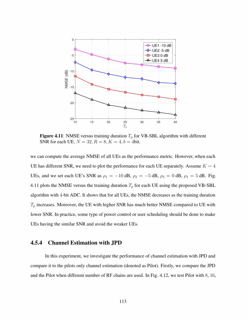
10 15 20 25 30 35 40-25
-20
-15
-10
-5
0
NM
SE
(d
B)
UE1 -10 dB
UE2 -5 dB
UE3 0 dB
UE4 5 dB
Figure 4.11: NMSE versus training duration Tp for VB-SBL algorithm with differentSNR for each UE. N = 32, R = 8, K = 4, b = 4bit.
we can compute the average NMSE of all UEs as the performance metric. However, when each
UE has different SNR, we need to plot the performance for each UE separately. Assume K = 4
UEs, and we set each UE’s SNR as ρ1 = −10 dB, ρ2 = −5 dB, ρ3 = 0 dB, ρ4 = 5 dB. Fig.
4.11 plots the NMSE versus the training duration Tp for each UE using the proposed VB-SBL
algorithm with 4-bit ADC. It shows that for all UEs, the NMSE decreases as the training duration
Tp increases. Moreover, the UE with higher SNR has much better NMSE compared to UE with
lower SNR. In practice, some type of power control or user scheduling should be done to make
UEs having the similar SNR and avoid the weaker UEs.
4.5.4 Channel Estimation with JPD
In this experiment, we investigate the performance of channel estimation with JPD and
compare it to the pilots only channel estimation (denoted as Pilot). Firstly, we compare the JPD
and the Pilot when different number of RF chains are used. In Fig. 4.12, we test Pilot with 8, 16,
113

-10 -5 0 5 10
SNR (dB)
-35
-30
-25
-20
-15
-10
-5
0
NM
SE
(d
B)
(a)
-10 -5 0 5 10
SNR (dB)
-30
-25
-20
-15
-10
-5
0
NM
SE
(d
B)
(b)
Figure 4.12: NMSE versus SNR for JPD and pilots only channel estimation withdifferent number of RF chains. (a) ∞-bit ADCs. (b) 4-bit ADCs. For pilots onlychannel estimation, Tp = 10. For JPD, Tp = 10, T = 50. N = 32, K = 4.
114

-10 -5 0 5 10
SNR (dB)
-35
-30
-25
-20
-15
-10
-5
0
NM
SE
(d
B)
Figure 4.13: NMSE versus SNR for JPD and pilots only channel estimation withdifferent resolution ADCs. For pilots only channel estimation, Tp = 10. For JPD,Tp = 10, T = 50. N = 32, R = 8, K = 4.
and 32 (fully digital) RF chains, and JPD with 8 RF chains. When both Pilot and JPD use 8 RF
chains, JPD has much better performance than the Pilot. Moreover, JPD with 8 RF chains can
obtain even smaller NMSE than Pilot with 16 RF chains. In Fig. 4.12 (b) where 4-bit ADCs are
applied, JPD with 8 RF chains only has small performance loss compared to the Pilot with fully
digital architecture. And in Fig. 4.12 (a) where∞-bit ADCs are used, JPD with 8 RF chains can
achieve the same performance as the Pilot with fully digital architecture from 0 to 10 dB. The
results imply the benefits of using JPD when hybrid AD processing is applied, such that one can
achieve better performance with reduced number of RF chains by utilizing JPD.
Next we compare the JPD and the Pilot when different resolution ADCs are used. Fig. 4.13
shows that for both high-resolution and low-resolution ADCs, JPD is better than the corresponding
Pilot. Notice that more improvements can be achieved by JPD as the resolution of ADCs increases.
Furthermore, with the help of JPD, better performance can be obtained using lower resolution
ADCs. For instance, 4-bit JPD has smaller NMSE than ∞-bit Pilot from −10 dB to 10 dB
115

10 20 30 40 50-26
-24
-22
-20
-18
-16
-14
NM
SE
(d
B)
Figure 4.14: NMSE versus JPD duration T . For JPD, Tp = 10. For pilots only channelestimation, Tp = T . N = 32, R = 8, K = 4,SNR = 5 dB.
SNR. And even 2-bit JPD is better than∞-bit Pilot at −10 dB SNR. This experiment shows the
advantages of applying JPD when low-resolution ADCs are utilized.
In Fig. 4.14, we investigate the performance of JPD with different T , i.e., utilizing
different number of data symbols. Tp in JPD is fixed as 10, and we gradually increase T from
10 to 50 (when T = Tp = 10, JPD is the same as Pilot). The performance of Pilot with Tp = T
is also provided as the benchmark, which can be treated as the best performance that JPD is
able to achieve. Fig. 4.14 shows that for both 4-bit and∞-bit ADCs, the performance of JPD
improves as more transmitted data, i.e., larger T , is utilized for the channel estimation. However,
the increment becomes slower as T increases, which means that most benefit of JPD can be
achieved with a modest T . Notice that with Tp = 10, 4-bit JPD with T = 20 is already better
than∞-bit Pilot with Tp = 10, showing the benefit of JPD even with small T . Compared to Pilot
with Tp = T , the NMSE of 4-bit JPD is only about 1 dB worse, while the∞-bit JPD can achieve
almost the same performance. Notice that the number of training pilots in JPD is only Tp = 10,
in contrast to Tp = T in Pilot. In other words, the training overhead can be reduced by using the
116

JPD scheme.
4.5.5 Effect of Gaussian Approximation
We now investigate the effects of Gaussian approximation for JPD as proposed in Section
4.4.3. In Fig. 4.15, we denote “constellation” when p(s[t]) is set to be the true distribution of
the transmitted data symbols as in (4.42), and “Gaussian” when the Gaussian approximation
in Section 4.4.3 is used such that p(s[t]) ∼ CN (0, σ2sIK) with σ2
s = 1. As shown in Fig.
4.15 (a) and Fig. 4.15 (b), the performance of JPD Gaussian is close to the JPD Constellation
when SNR = −10dB, which implies that the Gaussian approximation is useful at low SNR.
However, the performance loss due to the Gaussian approximation becomes larger as the SNR
increases. Specifically, the performance of JPD Gaussian with 4-bit ADC begins to saturate from
SNR = 5 dB.
When higher order modulation is used, for example, 64 QAM as in Fig. 4.16, applying
the true distribution to p(s[t]) becomes infeasible, whereas the Gaussian approximation provides
an simple alternative. Notice that even with the Gaussian approximation, for both∞-bit and 4-bit
ADCs there is about a 3 dB improvement when JPD is applied, especially for the SNR ranging
from −10 dB to 5 dB.
4.6 Conclusion
In this chapter, we developed a VB-SBL-based channel estimation algorithm for the
multi-user massive MIMO system where hybrid AD processing and low-resolution ADCs are
utilized at the BS. To overcome the limitations imposed by the reduced number of effective
measurements due to the hardware-efficient architecture, we exploit the sparse structure of the
massive MIMO channel to reduce the training overhead. We further leverage the transmitted data
symbols as “virtual pilots” to increase the measurement information. Experimental results show
117

-10 -5 0 5 10
SNR (dB)
-35
-30
-25
-20
-15
-10
-5
0
NM
SE
(d
B)
(a)
-10 -5 0 5 10
SNR (dB)
-24
-22
-20
-18
-16
-14
-12
-10
-8
-6
-4
NM
SE
(d
B)
(b)
Figure 4.15: NMSE versus SNR for JPD with true distribution and Gaussian approx-imation to QPSK data symbols. (a) ∞-bit ADCs. (b) 4-bit ADCs. For pilots onlychannel estimation, Tp = 10. For JPD, Tp = 10, T = 50. N = 32, R = 8, K = 4.
118

-10 -5 0 5 10
SNR (dB)
-30
-25
-20
-15
-10
-5
0
NM
SE
(d
B)
(a)
-10 -5 0 5 10
SNR (dB)
-18
-16
-14
-12
-10
-8
-6
-4
NM
SE
(d
B)
(b)
Figure 4.16: NMSE versus SNR for JPD with Gaussian approximation to 64 QAMdata symbols. (a)∞-bit ADCs. (b) 4-bit ADCs. For pilots only channel estimation,Tp = 10. For JPD, Tp = 10, T = 50. N = 32, R = 8, K = 4.
119

that the VB-SBL algorithm is superior than the other quantized channel estimation algorithms.
At low SNR, channel estimation with low-resolution ADCs can achieve very similar performance
as the high-resolution ADCs. Furthermore, the channel estimation using JPD can achieve better
performance with smaller number of RF chains and coarser ADCs compared to the traditional
pilots only channel estimation scheme, showing the significant benefits of applying JPD when the
proposed hardware-efficient architecture is used. Future work of interest would be in adaptively
designing the analog combining matrix based on previous channel estimate, developing faster
algorithms that can accommodate very large problem size, and utilizing the dithering effect to
improve the performance of low-resolution ADCs at high SNR.
Chapter 4, in part, is a reprint of the material as it appears in the paper: Y. Ding, S. Chiu,
and B. D. Rao, “Bayesian channel estimation algorithms for massive MIMO systems with hybrid
analog-digital processing and low resolution ADCs,” IEEE J. Sel. Topics Signal Process., vol. 12,
no. 3, pp. 499-513, June 2018. The dissertation author was the primary investigator and author of
this paper.
4.7 Appendices
4.7.1 Derivations About Transmitted Data
We present the derivation of 〈D〉q(s) and 〈DHD〉q(s) in this subsection. The term 〈D〉q(s)
is derived as following:
〈D〉q(s) = 〈Φ(IK ⊗A)〉q(s) = 〈Φ〉q(s)(IK ⊗A) (4.53)
where Φ = [ΦTp ΦT
d ]T . Φp contains known pilot symbols, and only Φd contains unknown
transmitted data s[t], t = Tp + 1, . . . , T which is random. So 〈Φ〉q(s) = [ΦTp 〈Φd〉Tq(s)]T and
〈Φd〉q(s) =[〈Φ[Tp + 1]〉Tq(s[Tp+1]), . . . , 〈Φ[T ]〉Tq(s[T ])
]T where for each 〈Φ[t]〉q(s[t]), t = Tp +
120

1, . . . , T we have
〈Φ[t]〉q(s[t]) = 〈s[t]〉Tq(s[t]) ⊗W [t]H . (4.54)
The term 〈s[t]〉q(s[t]) needs to be calculated from the approximated posterior q(s[t]), which is
given in (4.48).
SinceD = [DTp D
Td ]T , onlyDd = Φd(IK ⊗A) contains the random variable s[t] in Φd.
Similarly we have
〈DHD〉q(s) = DHp Dp + 〈DH
d Dd〉q(s)
= DHp Dp + (IK ⊗A)H〈ΦH
d Φd〉q(s)(IK ⊗A)
(4.55)
where 〈ΦHd Φd〉q(s) =
∑Tt=Tp+1〈Φ[t]HΦ[t]〉q(s[t]). And for each 〈Φ[t]HΦ[t]〉q(s[t]), we have
〈Φ[t]HΦ[t]〉q(s) =⟨(s[t]T ⊗W [t]H
)H(s[t]T ⊗W [t]H
)⟩q(s[t])
=⟨(s[t]∗ ⊗W [t]
)(s[t]T ⊗W [t]H
)⟩q(s[t])
= 〈s[t]∗s[t]T 〉q(s[t]) ⊗(W [t]W [t]H
) (4.56)
where 〈s[t]∗s[t]T 〉q(s[t]) is given in (4.48).
4.7.2 Derivations About Angular Domain Channel
In this subsection, we derive⟨W [t]HH
⟩q(x)
and⟨HHW [t]W [t]HH
⟩q(x)
. The deriva-
tion of⟨W [t]HH
⟩q(x)
is straightforward such that
⟨W [t]HH
⟩q(x)
= W [t]H⟨H⟩q(x)
= W [t]HA〈X〉q(x). (4.57)
The term 〈X〉q(x) can be obtained by reshaping vec(〈X〉q(x)), where vec(〈X〉q(x)) = 〈x〉q(x) =
µx as given in (4.45).
121

Similarly, regarding to the term⟨HHW [t]W [t]HH
⟩q(x)
, it can be reshaped from its
vectorized form vec(⟨HHW [t]W [t]HH
⟩q(x)
), which is given below:
vec(⟨HHW [t]W [t]HH
⟩q(x)
)= vec
(⟨XHAHW [t]W [t]HAX
⟩q(x)
)=⟨XT ⊗ XH
⟩q(x)
vec(AHW [t]W [t]HA
).
(4.58)
Notice that XT ⊗ XH consists of K × N blocks where each block is of size K × N . For
the (i, j)-th block of⟨XT ⊗ XH
⟩q(x)
, its value is 〈xj,iXH〉q(x), whose conjugate transpose
is 〈Xx∗j,i〉q(x). And the term 〈Xx∗j,i〉q(x) can be further reshaped from vec(〈Xx∗j,i〉q(x)
)=[
µxµHx +Σx
]·,(i−1)N+j
, which is the ((i−1)N + j)-th column of µxµHx +Σx, with both µx and
Σx given in (4.45). By forming all K×N blocks together, we obtain the matrix⟨XT ⊗XH
⟩q(x)
,
thereby having⟨HHW [t]W [t]HH
⟩q(x)
.
122

Chapter 5
Sensing Matrix Design With Partial
Knowledge of Support
In compressive sensing, it has been shown that a carefully designed sensing matrix is
able to improve the performance of signal recovery, when the signal can be sparsely represented
using an overcomplete dictionary. The designed sensing matrix is able to decrease the average
coherence of the combined equivalent dictionary. In this chapter, we propose a new framework
when partial knowledge of support is available. Observing that for an overcomplete equivalent
dictionary, it is impossible to make the coherence between all pairs of atoms to be arbitrarily
small, our algorithm leverages the partial knowledge of support and concentrates on minimizing
coherence between atoms where at least one of the columns belongs to the preferred support set.
In the noisy case, energy among atoms of the equivalent dictionary is non-uniformly distributed
such that atoms in the preferred support set are emphasized. To solve the underlying optimization
problem, we propose an algorithm for sensing matrix design with partial knowledge on support
(SMPKS) based on the majorization-minimization (MM) framework. Experimental results show
the superiority of the proposed SMPKS algorithm compared to other sensing matrix design
algorithms. Since the compressive sensing algorithms have been widely applied for channel
123

estimation in massive MIMO system, the proposed SMPKS algorithm can be utilized to design
better pilot symbols to improve the channel estimation performance.
5.1 Introduction
In the framework of compressive sensing, the signal of interest x ∈ RN×1, is assumed
to have a sparse representation in a dictionary D ∈ RN×M , such that x = Dβ. The sparse
coefficient vector β ∈ RM×1 is assumed to have only a few nonzero entries such that ‖β‖0 M .
The signal x is measured by a sensing matrix A ∈ RT×N such that
y = Ax = ADβ = Eβ (5.1)
where y ∈ RT×1 is the measured signal and E = AD ∈ RT×M is the combined equivalent
dictionary. The goal of compressive sensing is to recover x given y,A andD, even when the
number of measurements is less than the dimension of the signal, i.e., T < N . In [6], it has been
shown that whenD is an orthonormal basis, by utilizing a randomly generated matrixA and with
number of measurements T ∝ C · s log(N/s), the sparse coefficient β can be robustly recovered.
Here the constant C depends on the property of the sensing matrixA and s = ‖β‖0 represents the
sparsity level. The signal x can then be computed as x = Dβ. However in some applications,
the signal x can not be sparsely represented in any orthonomal basis [107], or more generally a
sparse representation of the signal is achieved using an overcomplete dictionary D which has
more columns than rows N < M , and is possibly learned from the data [58, 59]. The utilization
of an overcomplete dictionaryD will alter the geometric structure induced by the random sensing
matrixA and the equivalent dictionary E no longer satisfies the constraints required for robustly
recovering β. So a problem of interest is as follows: when given an overcomplete dictionaryD,
rather than using a randomly generatedA which is independent ofD, is it possible to design a
better sensing matrixA that adapts toD such that the performance of sparse recovery algorithms
124

can be improved?
Existing works which aim to optimize sensing matrixA can be generally categorized into
two different types. The first type is to designA as a whole, which adapts to dictionaryD such
that the combined equivalent dictionary E = AD has good geometric properties [50, 108–111].
In [50], the author consider the “average” mutual coherence between atoms in E, and try
to decrease the large entries by a shrinkage process utilizing the Gram matrix G = ETE.
In [108, 109], the sensing matrix is designed such that the distance between the Gram matrix
and an identity matrix is minimized, which can be regarded as a way to minimize the average
level of coherence. The work in [109] considers the application of measurement matrix design
in MIMO radar, with optimality criterion depending on the coherence as well as the signal to
interference ratio (SIR). In [110], the special case when the signal has a block sparse representation
is considered, and the design of A is carried out by minimizing a weighted sum of sub-block
coherence and inter-block coherence. Motivated by Grassmannian frame design, the work
in [111] attempts to make the equivalent dictionary E to be an equiangular tight frame by using
an alternating minimization algorithm.
In the second category, rows ofA are sequentially designed, using previously collected
measurements as guidance, see [21, 112, 113] and references therein. The sparse model assumes
D to be an orthonormal basis or canonical coordinate. In [21], a Bayesian signal model is adopted
and a new row ofA is chosen to maximize the increment of differential entropy h(y) as a means
for making the new measurement most informative. In [112,113], a constraint on the total sensing
energy, i.e., ‖A‖2F , is considered and sequential measurement is designed to focus sensing energy
towards the more probable non-zero elements based on knowledge from previous measurements.
This adaptive sensing can decrease the required magnitude of the smallest element in β for a
robust recovery [112, 113]. However, sequentially update rows of A such design requires the
accessibility of the previous measurements in an online fashion, which may not be feasible in
some applications.
125

In this chapter, we follow the concept in the first category to design A ∈ RT×N as a
whole with respect to a given overcomplete dictionary D ∈ RN×M . In order to guarantee the
unique representation of x, we assume spark(D) = N + 1 and ‖β‖0 < T/2 [7]. In the scenario
of an overcomplete representation and compressed sensing such that T < N < M , we have
‖β‖0 < spark(D)/2. According to [16, 24], this condition implies that β is unique and sparsest
given the representation of x = Dβ. Moreover, we consider the situation where some partial
knowledge about the support of β is available, for example a prefered support set S. Defining the
true support of β as T S(β) (or T S when β is clear from the context), then we have S = ∆∪∆e,
where ∆ = S∩T S denotes the correct components in the preferred set, and ∆e = S\T S denotes
the error in the preferred set. Similarly, T S = ∆∪∆m where ∆m = T S\S represents the correct
components that are missing from S. To measure the quality of the the preferred support S, we
define the error rate as pe = |∆e|/(|∆|+ |∆e|), and the missing rate as pm = |∆m|/(|∆|+ |∆m|).
We do not put any constraints on the size of preferred support, i.e., |S| can be smaller, equal, or
larger than |T S|.
Such partial information about the sparse support set exists in many applications. For
example ifD is an discrete wavelet transform frame and β represents the coefficient of an image,
then the entries of β that correspond to the low frequency subbands are most likely to be nonzero
and carry most of the energy, so S can be the set of location indices of those coefficients [114].
For the time series problem, S can be ˆT S which is the estimated support from the previous time
slot. Then ∆e = S\T S corresponds to coefficients that were nonzero previously but are zero
at the current time, while ∆m = T S\S is the newly added coefficients. Both ∆e and ∆m are
typically much smaller than |S|, following the empirical observation that sparsity patterns change
slowly [115]. The channel estimation problem in massive MIMO systems is of particular interest
to us, where the channel x can be sparsely represented in an overcomplete DFT dictionary or
learned dictionaryD as x = Dβ [97]. In a closed loop training, the user estimated the channel
x = Dβ from the downlink training y = Ax + n, and feeds back information such as the
126

support of sparse coefficients T S(β). Then the base station can utilize this information to design
pilotsA for the next training stage, i.e., S = T S(β). If the current channel is estimated correctly
and the feedback is perfect, when the channel is slowly changing the S obtained during the current
training stage would be a good indication for the next training stage. In the open loop training
where there is no feedback, when the duplex distance (frequency difference between the uplink
and downlink transmission) is small, it is reasonable to assume the uplink and downlink channel
have similar sparse support due to the common scattering objects during uplink and downlink
transmission, i.e., T S(βu) = T S(βd) [97]. Then the base station can utilize uplink training to
extract support information as the preferred support, S = T S(βu) and use it to design pilotsA
in the downlink channel estimation. When the uplink channel is correctly estimated, again S is a
good indication of the sparse support of the downlink channel.
In [115], a similar concept of partially known support was proposed, and a modified
basis pursuit algorithm was used to utilize such prior information and shown to require weaker
conditions for exact reconstruction. Similarly in [114] a weighted `1 minimization was proposed
where smaller weights are given to the elements in the preferred support. In our work, rather
than designing for a specific sparse recovery algorithm, e.g., modified-BP in [115], we develop a
framework to design a sensing matrix, and we demonstrate experimentally that for many sparse
recovery algorithms the designed sensing matrix leads to an improved recovery performance.
Designing sensing matrix with partial knowledge of support has also been considered in [116], in
which spectral characteristics of underlying signal are assumed to be known, and colored Gaussian
matrix with corresponding spectral shapes is used as sensing matrix to focus measurement energy.
Our work generalizes this work in that we consider an overcomplete dictionaryD, rather than
a Fourier transform matrix as used in [116] to extract spectral information. Also regarding the
design of A, we consider both structure optimization (decrease mutual coherence) as well as
energy focussing (increase signal to noise ratio), where [116] only considers the energy focussing.
The chapter is organized as follows. In Section 5.2, we review two representative works
127

on sensing matrix design. In Section 5.3, we introduce our motivation for utilizing the partial
knowledge of support, and propose an efficient algorithm to solve the sensing matrix design
problem. We then extend it to the noisy case in Section 5.4. Simulation results are presented in
Section 5.5. Conclusions and future works are discussed in Section 5.6.
Notations used in this chapter are as follows. Upper (lower) bold face letters are used
throughout to denote matrices (column vectors). (·)T , (·)† denotes the transpose and the Penrose-
Moor pseudo-inverse. xi is the i-th entry of the vector x, and Aij is the (i, j)-th entry of the
matrixA. A·j andAi· represents the j-th column and i-th row ofA. When S is an index set,A·S
andAS· correspond to a submatrix collecting corresponding columns and rows ofA, respectively.
For a vector x, diag(x) is a diagonal matrix with x being its diagonal. IN×N is an N ×N identity
matrix. For a given vector x and matrix A, ‖x‖1, ‖x‖2 denotes the `1 and `2 norm, and ‖A‖F
denotes the Frobenious norm. tr(A) denotes the trace of a matrixA. ‖x‖0 represents the number
of nonzero entries in x and is referred to as the `0 norm. For an integer M , [M ] is defined as the
set 1, . . . ,M. | · | denotes the absolute value of a scalar or cardinality of a set. bxc rounds x to
the nearest integer that is smaller than x.
5.2 Prior Work on Sensing Matrix Design
In this section we will introduce several basic concepts and terminologies which will be
used later in the chapter. We review past work and two representative algorithms [50, 108] that
motivate our work in some detail. These algorithms are used for comparison in the simulations.
5.2.1 The Basics
Mutual coherence plays an important role in compressive sensing to determine the recov-
ery performance [7, 10, 24], which is defined as [50]:
Definition1. For a dictionary E ∈ RT×M , its mutual coherence is defined as the largest absolute
128

normalized inner product between different columns in E, which is given by
µ(E) = max1≤i,j≤M,i 6=j
|ET·iE·j|
‖E·i‖2 · ‖E·j‖2
. (5.2)
Another way to understand mutual coherence is by the Gram matrix G = ETE. The
diagonal elementsGii is the squared norm of the i-th column of E, i.e.,Gii = ET·iE·i = ‖E·i‖2
2.
The off-diagonal entries Gij describes the coherence between E·i and E·j similar to (5.2), but
without normalization and maximization. If we denote E as E with normalized columns and
G = ET E, then
µ(E) = maxi 6=j|Gij|. (5.3)
We shall refer hereafter |Gij| and |Gij| as the unnormalized coherence and the coherence between
the i-th column and the j-th column of the dictionary E, to denote the similarity between two
columns.
The mutual coherence provides a measure of the worst similarity between the dictionary
columns, a value that exposes the dictionary’s vulnerability, as two closely related columns may
confuse any sparse recovery algorithm [50]. Suppose the signal x is sparse in the canonical
coordinate basis, i.e., D = IN×N , then (5.1) becomes y = ADβ = Aβ. It has been shown
that if ‖β‖0 <12(1 + 1
µ(A)), then β is the uniquely sparsest solution to y = Aβ, and both
basis pursuit (BP) and orthogonal matching pursuit (OMP) algorithms are guaranteed to recover
β [7,10,24]. This result can be applied to (5.1) with a general overcomplete dictionaryD such as
‖β‖0 <12(1 + 1
µ(AD)) = 1
2(1 + 1
µ(E)), and we can see that a smaller µ(E) implies a wider range
of solvable β (β whose sparse support has a larger cardinality). This is the motivation behind
the idea of designingA such that E = AD possesses good geometric properties, e.g., a smaller
µ(E).
However, as pointed in [50], mutual coherence µ(AD) is the worst-case measure of the
recoverability for a sparse recovery problem, which may be too pessimistic for practical problems.
129

If one allows a small fraction of signals with the same representation cardinality to fail (which
relaxes the “guaranteed” essence in the proofs), then β with cardinality of support substantially
beyond the above bound can still be recovered by the pursuit algorithms. This motivates one to
consider properties of E that can lead to performance improvement in a more “average” sense,
which will be introduced in the following subsection.
5.2.2 Some Representative Work
In [50], a “t-averaged mutual coherence” is proposed aiming to reflect average behavior
of the dictionary:
Definition2. For dictionary E, it’s t-averaged mutual coherence is defined as the average of all
absolute and normalized inner products between different columns in E (denoted as Gij) that are
above t. Formally
µt(E) =
∑1≤i,j≤M,i6=j 1(|Gij| ≥ t) · |Gij|∑
1≤i,j≤M,i6=j 1(|Gij| ≥ t). (5.4)
The notation 1(·) denotes the indicator function, such that 1(|Gij| ≥ t) = 1 if |Gij| ≥ t,
1(|Gij| ≥ t) = 0 if |Gij| < t. For t = 0, µt(E) is the average of the absolute off-diagonal
entries of G. As t grows, µt(E) grows and approaches µ(E) from below. Also from definition
µt(E) ≥ t. In [50], µt(E) was used as an “average” measure of coherence and the goal was to
minimize µt(AD) with respect toA givenD. Notice that µt(E) is defined via the entries of the
G, and an iterative algorithm is proposed such that in each iteration all Gij that are greater than t
are shrunk by a factor γ, 0 < γ < 1, andA is recalculated according to the new G. The iterations
are carried out until some termination requirement is satisfied. Although no convergence proof is
provided, it has been shown to achieve improved performance compared to the random sensing
matrix using both BP and OMP as recovery algorithms. Similar iterative shrinkage approach
has been applied to design Grassmanian frames that minimize the actual mutual coherence in
(5.2) [49]. Another related work [111], constructs a relaxed equiangular tight frame (ETF) using
130

a gradient-based alternating minimization approach.
In [108],A is designed such that the distance between the Gram matrix and the identity
matrix is minimized. This formulation lead to the following design procedure.
A = arg minA‖ETE − I‖2
F
= arg minA‖DTATAD − I‖2
F .
(5.5)
Notice that (5.5) is the same as minimizing µt(E), t = 0 if columns of E are enforced to have
unit norm. Rather than explicitly constraining columns of E to be unit norm, the diagonal terms
of DTATAD − I can be regarded as a penalty to encourage unit norm of columns of E. By
some manipulation, (5.5) can be transformed into ‖Λ−ΛΓTΓΛ‖2F where V ΛV T is the eigen-
decomposition of DDT and Γ = AV . A K-SVD [59] like algorithm is used to progressively
solve forA [108].
5.3 Sensing Matrix Design with Partial Knowledge of Sup-
port
5.3.1 Motivation
The cost function in (5.5) can also be written in terms of entries in Gram matrixG = ETE.
As shown in [110], we have
‖ETE − I‖2F = Trace(ETEETE − 2ETE + IM)
= Trace(EETEET − 2EET + IT ) + (M − T )
= ‖EET − IT‖2F + (M − T )
≥M − T
(5.6)
131

since we have ‖EET − IT‖2F ≥ 0. Also, (5.6) can be written using the Gram matrixG as given
below:
‖ETE − I‖2F =
∑i 6=j
|Gij|2 +∑i=j
|Gij − 1|2 ≥M − T. (5.7)
This means for an overcomplete equivalent dictionary E, it is impossible to minimize coherence
to be arbitrarily small between all pairs of columns. In other words, it is impossible to make all
|Gij|, i 6= j and |Gij − 1|, i = j to be arbitrarily small at the same time. However, do we really
need to minimize coherence between all pairs of columns? To address this question we draw
some inspiration from past work.
In [7], it has been shown that for y = Ax = ADβ = Eβ, if ‖β‖0 <12(1 + 1
µ(E)),
then OMP is guaranteed to find it exactly. An examination of the proof reveals that only the
coherence between two columns which are both in the true support, or the coherence between
two columns of which only one belongs to the true support and the other is outside of the
true support, are important. Coherence between columns which are both outside of the true
support do not play a role in establishing the result. In other words, the OMP algorithm can
always succeed if the sufficient condition in [7] is satisfied, no matter what value the coherence
between two columns that are both outside the true support is. Another work that supports the
above argument is [117], in which an Exact Recovery Condition (ERC) was proposed. With
the same measurement system y = Eβ as above, assume J as the true support of β, the ERC
states that if maxk 6∈J ‖E†·JE·k‖1 < 1, then the sparsest representation of the signal is unique.
Moreover, both OMP and BP identify the optimal atoms and their coefficients. Noting that
E†·J = (ET·JE·J )−1ET
·J , then the ERC becomes maxk 6∈J ‖(ET·JE·J )−1ET
·JE·k‖1 < 1. Again
in ERC, only coherence of columns that are both in the true support ET·JE·J , or only one of
them is in the true support ET·JE·k, are considered. It implies that when ERC is satisfied, the
coherence of columns that are both outside the true support do not play a role. Moreover in
both [7] and [117], by minimizing the coherence between pairs of columns when at least one
132

belongs to the true support, one is able to achieve a more favorable bound for the recovery
condition to be satisfied. In [7], this corresponds to minimize |ET·kE·t|, 1 ≤ k, t ≤ s and
|ET·iE·t|, i > s, 1 ≤ t ≤ s, and in [117] it corresponds to minimize ‖(ET
·JE·J )−1‖1,1 and
‖ET·JE·k‖1, k 6∈ J . Minimizing those terms will give tighter bounds such that the required
conditions tend to be more likely satisfied. Note that only the upper bounds but not the actual
interested terms, i.e., |∑s
t=1 βtET·kE·t|, 1 ≤ k ≤ s and |
∑st=1 βtE
T·iE·t|, i > s in [7] and
‖E†·JE·k‖1 in [117], can be improved by minimizing those terms.
The above discussion reveals the benefit of reducing the coherence between columns
when at least one of them belongs to T S(β), or formally
|Gij| = |ET·iE·j|, i or j ∈ T S(β) (5.8)
and we do not need to consider the coherence of columns when both are outside of the true
support,
|Gij| = |ET·iE·j|, i and j 6∈ T S(β). (5.9)
Since E = AD where D is a given dictionary, we can only rely on designing A in order to
minimize |Gij| = |ET·iE·j|. Moreover, rather than requiring the equivalent dictionary E = AD
to have a good geometric condition for every pair of atoms, which is demanding and potentially
unnecessary, it motivates one to concentrate on pairs of atoms when at least one has a high chance
of belonging to the true support T S(β). It is interesting to see that the previous works either
minimize mutual coherence defined in (5.3), which focusses on the maximum of all |Gij|, or
”t-averaged mutual coherence” defined in (5.4), which focusses on the average of all |Gij|. The
above observations indicate that we should choose discriminatively the more important |Gij|
rather than considering them all.
However, we do not know the true support beforehand, otherwise (5.1) reduces to a trivial
overdetermined linear inverse problem. In many practical applications, we may be able to gather
133

some information on the support, potentially an approximation which we refer as the preferred
support set S . Observing the lower bound in (5.7), even if the S we obtain is only partially correct,
it is useful to utilize it. The more confidence we have in this preferred support set S, the more
emphasis one should put on it.
5.3.2 Designing the Sensing Matrix
Based on the above discussion, we focuss on minimizing |Gij| that at least i or j belongs
to the preferred set S . For a Gram matrixG = ETE = (AD)T (AD) with elementsGij , we aim
to solve optimized sensing matrixA by minimizing |Gij|2, corresponding to the unnormalized
coherence between Ei and Ej . Define sets that describe different conditions on i, j: P1 =
i, j|i = j, i, j ∈ S,P2 = i, j|i = j, i, j 6∈ S, P3 = i, j|i 6= j, i ∈ S and j ∈ S,
P4 = i, j|i 6= j, only i or j ∈ S P5 = i, j|i 6= j, i 6∈ S and j 6∈ S, and
Wd =∑i,j∈P1
|Gij − 1|2 +∑i,j∈P2
|Gij − 1|2,
Ws =∑i,j∈P3
|Gij|2 +∑i,j∈P4
|Gij|2,
Wns =∑i,j∈P5
|Gij|2.
(5.10)
Then the sensing matrix design problem is formulated as
A = arg minA
γWd + αWs +Wns (5.11)
where γ and α are positive constants. In (5.11), we do not explicitly normalize columns ofE to be
unit norm, but implicitly encourage such constraint by minimizing Wd [108,110]. Wd controls the
distance between the diagonal elementsGii and 1, whereGii represents the squared norm of the
i-th columnE·i . If Wd = 0, then every column of the equivalent dictionaryE is normalized, and
134

the unnormalized coherenceGij reduces to the the coherence Gij . Ws represents the summation
of unnormalized coherence between two columns when at least one of them belongs to S. Wns
represents the summation of unnormalized coherence between two columns that are both out of
S.
We use γ and α to trade off among Wd,Ws and Wns. Typically we choose α > 1 to
emphasize Ws, which corresponds to the coherence of columns that are more important for
successful recovery. Since usually the dimension of sparse coefficient β is much larger than the
size of preferred support, i.e., M |S|, the value of Wns is much larger than Ws, so we need a
larger value α to favor minimizing Ws. Also we need a large value for γ, in order to guarantee
every atom in E to be nearly normalized. Large γ avoids the situation that columns in S are
driven to have too small norm. For example, assume α γ, and let i ∈ S . By makingE·i to be a
vector with all zeros will lead to a smaller Ws sinceGij = 0,∀j. Due to α γ, the optimization
process will favor this result. But it leads to a very large coherence after normalization. In
other words, the process is favoring minimizing Ws by making E·i trivial rather than making E·i
distinct with other columns, where the latter is the true purpose of minimizing Ws. In (5.11) we
also minimize the term Wns which only relates to columns outside S. This is because S may
only contain part of the correct indexes (|∆m| > 0), there are still some columns belonging to the
true support T S that are outside of S, and minimizing coherence of those columns will give a
better recovery performance. But since we have no idea about those columns, we can only treat
them in an non-informative manner and use Wns to minimize the summation of the unnormalized
coherence corresponding to those columns.
5.3.3 SMPKS Algorithm
Although the cost function in (5.11) is in the quadratic form of entries in G, the actual
variable A that we are going to solve is coupled with G through the dictionary D such that
G = ETE = DTATAD, where A ∈ RT×N ,D ∈ RN×M . With the assumption T ≤ N and
135

N ≤ M , the Gram matrix G is rank T (assume generally E = AD is full rank). Imposing
such rank constraint makes the problem non-convex, and relaxation is often used to transform
the problem into an approximate convex form. To solve (5.11), we can modify algorithms in
the existing literatures to our specific setting. For example, rather than shrink all Gij that are
larger than some threshold, we can only shrink those Gij if at least one of i or j belongs to S,
and then reduce the rank ofG and updateA following the same procedure as in [50]. However
as mentioned in [50], such an algorithm does not have any convergence guarantees, although
it works well in practice. Another possible approach is to follow [109], by settingB = ATA,
and treating B as the variable in G = DTATAD = DTBD. This transforms the problem
into convex form with respect to B, and can be solved by many software packages. Once B
is obtained, the eigenvalue decomposition is performed to reduce the rank and achieveA. But
notice theB is of size N ×N , and we need to constrain the norm of E to be one. Such a large
number of variables and constraint functions greatly increases the complexity of the approach
making it less suitable for large dimensional problems [109].
In this section, we propose an algorithm for sensing matrix design with partial knowledge
of support (SMPKS) which applies the majorization-minimization (MM) framework to iteratively
solve the problem [110, 118, 119]. In MM framework, the original cost function which is hard to
minimize is upper bounded by a surrogate function which is easier to minimize. Since the MM
approach is central to the SMPKS algorithm, we provide a brief background on the concept of
MM algorithm in general for ease of understanding. Consider a real-valued function f(θ). Let
θ(m) represents a fixed value of the parameter θ, and let g(θ|θ(m)) denote a real-valued function of
θ whose form depends on θ(m). Then the function g(θ|θ(m)) is said to majorize f(θ) at the point
θ(m) if1. g(θ|θ(m)) ≥ f(θ), ∀θ,
2. g(θ(m)|θ(m)) = f(θ(m)).
(5.12)
In each iteration, g(θ|θ(m)) rather than f(θ) is minimized. Denotes θ(m+1) as the minimizer of
136

g(θ|θ(m)) such that
θ(m+1) = arg minθg(θ|θ(m)). (5.13)
Then the decrease of the original function f(θ) in the next iteration can be shown as follows:
f(θ(m+1)) ≤ g(θ(m+1)|θ(m))
≤ g(θ(m)|θ(m))
= f(θ(m))
(5.14)
where the first inequality comes from the property 1 in (5.12), the second inequality is from (5.13),
and the last equality is from the property 2 in (5.12). By iteratively minimizing the surrogate
function, it is able to achieve a stationary point of the original function. As the iteration goes on,
the value of f(θ) keeps decreasing until a stationary point is achieved. The key point of the MM
algorithm is to find the surrogate function g(θ|θ(m)) such that properties in (5.12) are satisfied,
and the surrogate function should be amenable to easy minimization in each iteration.
To solve for a good sensing matrixA, we hope to write the cost function in (5.11) in the
form ofG rather thanGij , so it will be easier to incorporate the variableA byG = DTATAD.
Similar to [110], we define matrixHd(G),Hs(G),Hns(G) as follows:
Hdij(G) =
c1 i = j and i, j ∈ S
c2 i = j and i, j 6∈ S
Gij otherwise
Hsij(G) =
0 i 6= j, i ∈ S or j ∈ S
Gij otherwise
Hnsij (G) =
0 i 6= j, i 6∈ S and j 6∈ S
Gij otherwise
(5.15)
137

and build coefficient matrix Ω as
Ω = diag(ω) (5.16)
where ω ∈ RM×1, ωi = 1√c1,∀i ∈ S and ωi = 1√
c2,∀i 6∈ S . c1 and c2 are parameters that control
the norm of the columns of E and will be elaborated in the next section when the noisy case is
considered. For the noise free situation in this section, we just set c1 = c2 = 1, so Ω = I. Then
the cost function in (5.11) can be written as
f(G)
= γWd + αWs +Wns
= γ‖Ω(G−Hd(G))Ω‖2F + α‖Ω(G−Hs(G))Ω‖2
F + ‖Ω(G−Hns(G))Ω‖2F .
(5.17)
Note that (5.17) is in its general form. The noise free situation in this section can be regarded as a
special case where c1 = c2 = 1 and Ω = I. To avoid unnecessary duplication, the derivations and
proofs in the rest of the chapter are all based on this general form, and can be readily reduced to
the noise free case by setting Ω = I.
It is common to use a quadratic function as the surrogate function due to the ease in
minimization [110, 118, 119]. We build the surrogate function as follows:
Proposition1. g(G|G(m)) is a valid surrogate function of f(G) at the m-th iteration, where
g(G|G(m)) = γ‖Ω(G−Hd(G(m)))Ω‖2F
+ α‖Ω(G−Hs(G(m)))Ω‖2F
+ ‖Ω(G−Hns(G(m)))Ω‖2F
(5.18)
andG(m) = DTA(m)TA(m)D.
Proof. See Appendix 5.7.1.
Minimizing g(G|G(m)) with respect toA leads to the solution of sensing matrixA(m+1)
138

in the next iteration, such that
A(m+1) = arg minA
g(G|G(m))
= arg minA
g(DTATAD|G(m)).
(5.19)
The next proposition shows that the solutionA(m+1) has a closed form:
Proposition2. The minimizer of the surrogate function g(G|G(m)) at the m-th iteration is
A(m+1) = ∆12TV
TT Λ−
12UT (5.20)
where UΛUT is the eigenvalue decomposition of DΩ2DT , and V∆V T is the eigenvalue
decomposition ofH ′(G(m)). H ′(G(m)) is defined as
H ′(G(m)) := Λ−12UTDΩ2H(G(m))Ω2DTUΛ−
12 (5.21)
andH(G(m)) is defined as
H(G(m)) :=γHd(G(m))T +αHs(G(m))T +Hns(G(m))T
γ + α + 1. (5.22)
∆T denotes the T × T diagonal matrix that contains the largest T eigenvalues in ∆, and VT
denotes the corresponding T eigenvectors.
Proof. See Appendix 5.7.2.
We iteratively solve for A(m+1) and calculate the next g(G|G(m+1)) using (5.18) until
some stopping criterion is satisfied, and label the lastA(m+1) as A. Notice that the solutionA(m+1)
is not unique. Actually multiplying any orthogonal matrix to the left side ofA(m+1) also leads to a
valid solution. To see this, denote A = QA(m+1) whereQ is an orthogonal matrix, i.e.,QTQ = I.
Then G = DT AT AD = DT (QA(m+1))T (QA(m+1))D = DTA(m+1)TA(m+1)D = G(m+1).
139

5.3.4 Discussion
The goal of the sensing matrix design problem in (5.11) is to minimize the cumulative
coherence discriminatively. For the coherence corresponding to pairs of columns where at least
one of them belongs to the preferred support, it puts more weight on them. An important question
in this connection is why coherence and not other measures as the criteria for designing the
sensing matrix? Also, given that the performance bound in the form of coherence (or some
descendants of coherence) provided in [7, 117] are only sufficient conditions, is there a need to
justify that optimizing a sufficient condition provides a good sensing matrix?
The motivation of the sensing matrix design in this chapter is to designA such that the
combined dictionary E = AD has good structure. Specifically, we expect the columns in E
to be as distinct with each other as possible. Intuitively, if two columns are too alike to each
other, then it will be hard for any recovery algorithm to distinguish them. In order to measure
how distinct the columns in E are, this work utilizes coherence and tries to minimize them in
a cumulative sense. The reason we choose coherence is a pragmatic one. It is easy to compute.
There are some other measures that characterize the structure of the matrix, for example the
spark, the restricted isometry property, the null space property, etc. But these measures are
computationally intractable. On the other hand, when we deal with coherence in a cumulative
sense the summation of coherence can be transformed into the Gram matrix form, and it facilitates
the derivation of a closed form solution in each iteration by using the MM framework, which
converges under fairly general conditions. There are also other options to deal with coherence,
for example mutual coherence (largest among all coherence) and the t-averaged mutual coherence
as proposed in [50]. However, the iterative algorithm in [50] has no convergence guarantees. In
summary, the ultimate goal of minimizing coherence is not to achieve any sufficient conditions,
but to obtain a combined dictionary with better structure. We take a pragmatic approach by
utilizing an easy to compute metric, and develop a design algorithm that is easy to implement.
140

5.4 Designing the Sensing Matrix in Noisy Situation
5.4.1 Motivation
In the previous section, the noise free case (5.1) was considered. In this section, we will
consider the case where there exists measurement noise such that
y = Ax+ n = ADβ+ n = Eβ+ n (5.23)
where n ∈ RT×1 is the random measurement noise and assumed to be Gaussian distributed
as n ∼ N (0, σ2I). Furthermore, we put the norm constraint ‖A‖F ≤ P , where P represents
the total power in the sensing matrix. Assumptions of the existence of measurement noise and
constraints on the power of sensing matrix are more suitable for real practical problems. For
example, for channel estimation in a wireless communication system, A represents the pilot
signals sent by the base station, x is the channel vector that we aim to measure. y is the received
signal at the user. Obviously y which will be contaminated by some noise and the total power in
the pilot signals is constrained by the power limit imposed by the base station.
Stable reconstruction conditions similar to the exact reconstruction conditions as in [7]
and [117] have been provided for OMP [120] and BP [121]. From the derivation steps in [120,121],
similar conclusions can be drawn regarding the importance of different |Gij|. So when designing
A in the noisy situation, once again it pays to focuss efforts on minimizing |Gij| when either i or
j belongs to S, or both i and j belong to S. One big difference compared to the noise free case
is that now not only the structure of the combined dictionary E, but also the noise term n will
affect the performance of the recovery algorithm. We take the OMP algorithm as an example, and
for simplicity we assume there is only one component in β that is nonzero, and its location is k.
Then y = Eβ + n = E·kβk + n = E·k‖E·k‖2βk + n, where E·k denotes the normalized k-th
column of E, E·k = E·k/‖E·k‖2. At the first step of OMP, y is correlated with each column of
141

E and we determine the location of nonzero elements as l = arg maxl |yT E·l|. Notice that
|yT E·l| = | (E·k‖E·k‖2βk + n)T E·l |
=
| βk‖E·k‖2 + nT E·l |, l = k;
| βk‖E·k‖2(ET·kE·l) + nT E·l |, l 6= k.
(5.24)
Even ifE has a good structure, i.e., ET·kE·l is small, the existence of the term nT E·l can still make
| βk‖E·k‖2(ET·kE·l) + nT E·l | greater than | βk‖E·k‖2 + nT E·l |, thus leading to the incorrect
estimation of l. So handling of noise requires additional considerations. However, if ‖E·k‖2 is
large, then at least |βk‖E·k‖2 +nT E·l | is more likely to be large, in other words, less affected by
the noise. This sheds light on how to make the recovery more robust in noisy case: with regards to
the locations of nonzero entries in β, making the corresponding columns in E to have large norm
will combat the interference from noise. In our situation, this translates to designing a sensing
matrix A such that the columns of E = AD which correspond to the locations of nonzero
entries in β to have large norms, i.e., making ‖E·i‖2 large if i ∈ T S(β). The goal is to tuneA,
such that effects of columns inD that consist the signal x are enlarged after the application of
the sensing matrixA.
5.4.2 Sensing Matrix Design
Similar to the noise free case, we do not have the knowledge of T S and assume a preferred
support set S. To incorporate the ideas of producing larger norms to columns in S, using the
142

same definitions of P1, . . . ,P5 as before,we define
Wd =∑i,j∈P1
|Gii − c1|2
c21
+∑i,j∈P2
|Gii − c2|2
c22
Ws =∑i,j∈P3
|Gij|2
c21
+∑i,j∈P4
|Gij|2
c1c2
Wns =∑i,j∈P5
|Gij|2
c22
(5.25)
where we use Wd to optimize norm of columns contained in S and columns out of S. c1 and c2
can be regarded as “expected” squared norm of ‖E·i‖22 for i ∈ S and i 6∈ S . So as discussed above,
we set c1 to be a large number and c2 to be a small number in order to focus the measurement
energy to the parts where we believe the true nonzero elements are. If S is believed to contain a
higher percentage of true locations, then a larger value should be given to c1 in order to focus
more energy to those columns in the S. As opposite to c1, c2 should be set to a smaller number
if S contains higher percentage of true locations, since we do not want to waste measurement
energy on locations where entries of β are zero. Ws and Wns are similar to the corresponding
terms in (5.11), which control coherence between pairs. Since now the columns are optimized to
have different norms, we normalize Wd,Ws and Wns using the expected squared norm c1 and c2.
The optimization problem then becomes
A′ = arg minA
γWd + αWs +Wns
A =A′
‖A′‖FP.
(5.26)
In (5.26) the cost function does not enforce the constraint ‖A‖F ≤ P , since explicit enforcement
of the constraint ‖A‖F ≤ P requires solving (5.26) in a constrained set and is hard to be
incorporated into the MM framework. Moreover, the cost function in (5.26) which uses Gij
to describe the coherence is just an approximate way since the columns in E are not strictly
143

normalized. Actually once A′ is solved, scaling it with any positive constant does not change Gij ,
the coherence of columns inE, as well as the ratio of two columns’s norms, i.e., ‖E·i‖2/‖E·j‖2 is
preserved. So we first solve for A′ in (5.26) without the constraint ‖A‖F ≤ P , considering only
the coherence minimization and energy distribution, using the SMPKS algorithm (with c1 6= c2)
proposed in last section. Then we scale it to the largest energy limitation such that A = A′
‖A′‖FP ,
with respect to the energy limitation and the existence of noise. Since scaling up ‖E·i‖2 will
make the recovery algorithm more robust to the noise if i ∈ T S while make no difference if
i 6∈ T S. So we scale up ‖A‖F to its largest possible value to improve the performance.
5.4.3 Summary of the Algorithm
The detailed steps of the SMPKS algorithm is summarized in Algorithm 1, which is for the
noisy case. To differentiate the noise free case from the noisy case, we denote it as SMPKS-NF.
For SMPKS-NF, we do not have the norm constraint of ‖A‖F ≤ P , and we set c1 = c2 = 1. In
the algorithm, the start pointA(m),m = 1 is set to be a random matrix, where we do not assume
knowledge of any other A. Since the MM framework can not guarantee to converge to global
optimum, a good start point will help to avoid the algorithm being trapped in a local minimum.
For example, we can initialize our algorithm with anA learned from other sensing matrix design
algorithms. In the algorithm we set the stopping criterion by limiting the number of iterations
by some chosen maximum number. We can also choose other stopping criterion such as when
A(m+1) does not change much compared toA(m), or the value of cost function f(G(m+1)) does
not change much as the iteration proceed.
5.5 Numerical Results
In this section, we evaluate the performance of the proposed algorithm experimentally. The
goal is to show that when there exists a reasonable preferred support S, the proposed algorithm
144

Algorithm 1 SMPKS AlgorithmInput: Use the following parameters:
• D - the sparsifying dictionary,
• c1 - expected norm for columns belonging to S,
• c2 - expected norm for columns out of S,
• γ - weights for Wd,
• α - weights for Ws,
• MaxIter - maximal number of iterations,
• P - power constraint of sensing matrix.
Initialize:• Set m = 1,
• SetA(m) to a random matrix,
• CalculateG(m) = DT (A(m))TA(m)D,
• Calculate Ω using (5.16),
• Calculate UΛUT as eigenvalue decomposition ofDΩ2DT .
Loop: until m > MaxIter
• CalculateH ′(G(m)) using (5.21),
• Calculate V∆V T as eigenvalue decomposition ofH ′(G(m)),
• UpdateA(m+1) = ∆12TV
TT Λ−
12UT ,
• UpdateG(m+1) = DT (A(m+1))TA(m+1)D,
• Update m = m+ 1.
Output: A = A(m)
‖A(m)‖FP
145

that utilizes this information will lead to a more informative sensing matrixA, which can improve
the recovery performance. The basic setting of the experiment is as follows. D ∈ RN×M is the
dictionary consisting of i.i.d standard Gaussian variables. The signal of interest x is computed
as x = Dβ, where βk, k ∈ T S(β) are also i.i.d standard Gaussian variables with locations
uniformly distributed. For |T S(β)|, |S|, pe, pm, given any three we can obtain the fourth, as well
as |∆|, |∆m|, |∆e| (recall that |T S(β)| = |∆| + |∆m|, |S| = |∆| + |∆e|, pe = |∆e|/|S|, pm =
|∆m|/|T S| ). Then the preferred support S is generated as S = ∆ ∪∆e, where |∆| elements are
randomly picked from T S, and |∆e| elements are randomly picked form [M ]\T S. Regarding
sensing matrix A, we compare: random sensing matrix, where the elements are i.i.d Gaussian
with mean 0 and variance 1/√T (random), Elad’s algorithm in [50] (Elad), Duarte-Carvajalino
and Sapiro’s algorithm [108] (DS) the proposed algorithm for noise free case (5.11) (SMPKS-NF)
and noisy case (5.26) (SMPKS).
We run L = 1000 trials to compute an average measure of performance. In terms of
performance metric, we use success rate and location distance [7, 50]:
• Success rate: after obtaining x, we calculate the relative `2 distance Dist `2 as
Dist `2(x, x) =‖x− x‖2
2
‖x‖22
. (5.27)
When Dist `2 is smaller than some threshold, it is considered as a successful recovery. We
calculate the percentage of successful recovery out of L experiments as the success rate.
Notice that Dist `2 is calculated using x rather than β. Because D is an overcompleted
dictionary, Dist `2 calculated using x is different from using β.
• Location distance: for some application, it is important that the locations of the nonzero
entries in β are correctly detected. For example in a classification task, columns of
dictionary D represent features. Given the measurement y, classification of signal x is
achieved by detecting which features contribute to x, i.e., the location of nonzero entries in
146

β. The location distance Dist sup is defined as
Dist sup(T S(β), T S(β)) =
max|T S(β)|, |T S(β)| − |T S(β) ∩ T S(β)|max|T S(β)|, |T S(β)|
.(5.28)
5.5.1 Comparing the Distribution of Coherence
In Fig. 5.1, we present the distribution of the coherence, i.e., |Gij|, i 6= j, obtained
from combining the sensing matrixA designed using different sensing matrix design algorithms
and the same dictionary D. The distribution is calculated by the percentage of all |Gij|, i 6= j
which falls between the range [0.05(l − 1), 0.05l], where l = 1, . . . , 20. In Fig. 5.1 (a), the
coherence is calculated using all pairs of columns in the equivalent dictionary E = AD. It
shows that both the DS algorithm and the SMPKS-NF algorithm can reduce the percentage of
large coherence and increase the percentage of small coherence compared to the random sensing
matrix. Elad’s algorithm also reduces the large coherence, but makes no more effort when the
coherence becomes small enough. This is reason why there exists a peak at 0.175, where 40%
of coherence values fall between 0.15 and 0.2. Fig. 5.1 (b) shows the distribution of coherence
corresponding to columns where at least one of them belongs to S , i.e., |Gij|, i ∈ S or j ∈ S. It
shows that except for the SMPKS-NF, the distributions of the coherences corresponding to the
other three sensing matrices are very similar compared to Fig. 5.1 (a), implying that those sensing
matrix design algorithms have to favor of column pairs which includes at least one column in the
S. For SMPKS-NF, the distribution of the coherence is more concentrated around small values
compared to Fig. 5.1 (a), showing that more efforts have been put by the SMPKS-NF algorithm
to reduce the coherences of those column pairs that contain columns from S. In other words,
although the coherence distributions for all columns are similar for DS and SMPKS-NF, when
it comes to the coherence values of interest columns, SMPKS-NF is able to drive them smaller,
which is exactly the goal of minimizing (5.11). In the following subsections, we will show how
147

0 0.1 0.2 0.3 0.4 0.5 0.6 0.7 0.8 0.9 1
Coherence
0
0.05
0.1
0.15
0.2
0.25
0.3
0.35
0.4
Pe
rce
nta
ge
Random
Elad
DS
SMPKS
(a)
0 0.1 0.2 0.3 0.4 0.5 0.6 0.7 0.8 0.9 1
Coherence
0
0.05
0.1
0.15
0.2
0.25
0.3
0.35
0.4
Pe
rce
nta
ge
Random
Elad
DS
SMPKS
(b)
Figure 5.1: Distribution of the coherence between two columns in the equivalentdictionary. (a) All pairs of columns in the equivalent dictionary. (b) Pairs of columnsthat at least one column belongs to S. T = 40, N = 80,M = 160, |T S| = |S| = 12.
such effect can improve the performance of compressive sensing algorithms.
148

5.5.2 Comparing Different Error Rate and Missing Rate
In this subsection, the OMP algorithm is applied to perform the sparse recovery, and the
recovery performances using different sensing matrices are compared for different values of pe
and pm in the noise free scenario. Setting T = 40, N = 80,M = 160, and |T S| = |S| = 12
(so pe = pm), we gradually increase pe(pm) from 0 to 1 with step 0.1. Correspondingly, T S
and S change from fully overlapped, to partially overlapped, until they are non-overlapping.
Fig. 5.2 shows that the recovery performance of SMPKS-NF degrades as the pe(pm) increases,
indicating that large error rate and missing rate will make the recovery performance worse due to
the incorrect prior knowledge of the support. The performances of other sensing matrices do not
change with pe and pm, since the knowledge of preferred support is not used in those algorithms.
When pe (pm) is less than 0.7 in this setting, the SMPKS-NF can achieve better performance than
Elad and DS algorithm, and for all pe (pm) SMPKS-NF is much better than the random sensing
matrices. Notice that pe = pm = 0.7 corresponds to |∆| = 4, |∆e| = |∆m| = 8, which means for
a preferred set S containing 12 indices, only 4 of them are from the true support, and it contains 8
error indies and misses 8 true indices. The result shows that when the preferred support set is
moderately accurate, the proposed sensing matrix leads to an improved recovery performance
compared to other sensing matrices.
Next we examine the situation when the size of S is small and it is contained in T S , or the
size of S is large and it contains T S . Notice that in practice we do not know whether S is large or
small compared to the true support, or what pe and pm are. First we test S ⊆ T S such that pe = 0.
|T S| is fixed to 12 in order to keep the difficulty of the recovery problem the same, and pm
changes from 0 to 0.9 with step 0.1, corresponding to |S| changing from 12 to 1. Fig. 5.3 shows
that when pe = 0 the SMPKS-NF can achieve better recovery performance for all pm. Notice that
the best performance is achieved at pm = 0.1 rather than pm = 0. When pm = 0.1, |S| = ∆ = 11
while |S| = ∆ = 12 when pm = 0. This shows that when S ⊆ T S, a relatively small preferred
set may result in better performance, since it is easier for the SMPKS-NF algorithm to perform
149

0 0.1 0.2 0.3 0.4 0.5 0.6 0.7 0.8 0.9 1
pe ( p
m )
0.2
0.3
0.4
0.5
0.6
0.7
0.8
0.9
1
Su
cce
ss R
ate
SMPKS-NF
Elad
DS
Random
(a)
0 0.1 0.2 0.3 0.4 0.5 0.6 0.7 0.8 0.9 1
pe ( p
m )
0
0.05
0.1
0.15
0.2
0.25
0.3
0.35
0.4
Lo
ca
tio
n D
ista
nce
SMPKS-NF
Elad
DS
Random
(b)
Figure 5.2: Performance comparison with different pe(pm). T = 40, N = 80,M =160, |T S| = |S| = 12.
the optimization process when |S| is small. However, |S| should not be too small compared to
T S , in which case there will be too many missing indices from T S . The results show the benefits
150

0 0.1 0.2 0.3 0.4 0.5 0.6 0.7 0.8 0.9
pm
0.2
0.3
0.4
0.5
0.6
0.7
0.8
0.9
1
Su
cce
ss R
ate
SMPKS-NF
Elad
DS
Random
(a)
0 0.1 0.2 0.3 0.4 0.5 0.6 0.7 0.8 0.9
pm
0
0.05
0.1
0.15
0.2
0.25
0.3
0.35
0.4
Lo
ca
tio
n D
ista
nce
SMPKS-NF
Elad
DS
Random
(b)
Figure 5.3: Performance comparison with different pm. T = 40, N = 80,M =160, |T S| = 12, pe = 0.
of utilizing the SMPKS-NF algorithm to explore the knowledge of the preferred support if we
have high confidence on it, even a preferred support of small size would help to improve the
151

0 0.1 0.2 0.3 0.4 0.5 0.6 0.7 0.8 0.9
pe
0.2
0.3
0.4
0.5
0.6
0.7
0.8
0.9
1
Su
cce
ss R
ate
SMPKS-NF
Elad
DS
Random
(a)
0 0.1 0.2 0.3 0.4 0.5 0.6 0.7 0.8 0.9
pe
0
0.05
0.1
0.15
0.2
0.25
0.3
0.35
0.4
Lo
ca
tio
n D
ista
nce
SMPKS-NF
Elad
DS
Random
(b)
Figure 5.4: Performance comparison with different pe. T = 40, N = 80,M =160, |T S| = 12, pm = 0.
performance.
Lastly we consider the situation when T S ⊆ S , which means we have a preferred support
152

with size larger than the true support. Again |T S| is set to 12 as in the previous simulations, and
pe changes from 0 to 0.9 with step 0.1. This results in a preferred support S with larger size,
corresponding to |S| ∈ 12, 13, 15, 17, 20, 24, 30, 40, 60, 120. Fig. 5.4 shows that when pe is
smaller than 0.3, the SMPKS-NF has better performance than the other sensing matrices. Notice
that when pe = 0.3, |S| = 17. Higher pe results in larger |S| which contains many more error
indices and degrades the recovery performance.
5.5.3 Comparing Different Levels of Noise
We now consider the noisy case where the sensing process is performed as in (5.23),
y = Ax + n where n ∼ N (0, σ2I). The signal to noise ratio (SNR) is defined as SNR =
10log10(‖x‖22Tσ2 ). Again we use OMP for sparse recovery and compare different sensing matrix
design algorithms. For the proposed SMPKS algorithm, we solve (5.26) with different norms for
columns in and out of the preferred support, so c1 6= c2. Notice that we only need to set the ratio
c1/c2 rather than the specific values of c1 and c2, since after determining sensing matrixA using
(5.26), it is normalized which changes the specific values of ‖E·i‖22, i ∈ S and ‖E·j‖2
2, j 6∈ S , but
not the ratio of ‖E·i‖22/‖E·j‖2
2. The ratio c1/c2 determines how much preference to give to the
columns in the preferred support. In the simulation, we set c1/c2 = 2, which means within the
power constraint ‖A‖F ≤ P , the algorithm tries to achieve ‖E·i‖22 = 2‖E·j‖2
2, i ∈ S, j 6∈ S . The
SMPKS-NF algorithm which solves (5.11) in the noise free case is also included. The goal is
to compare how unequally distributed energy will affect the recovery performance. All sensing
matrices are normalized as ‖A‖F = P , and the constrained power is set as P = T . Due to the
existence of the noise, the previous threshold of 10−3 for determining the success rate in the noise
free case is too strict for low SNR scenarios, so we set different thresholds for success rate with
respect to different levels of noise. For many algorithms, the performance results show that the
recovery error is at worst proportional to the noise level ‖n‖2 [6, 11, 120], which motivates us to
set thresholds according to the noise level. Specifically, we use C · E(‖n‖22) = C · Tσ2 as the
153

5 15 25 35
SNR (dB)
0
0.1
0.2
0.3
0.4
0.5
0.6
0.7
0.8
0.9
1
Su
cce
ss R
ate
Random
DS
Elad
SMPKS-NF
SMPKS
(a)
5 15 25 35
SNR (dB)
0
0.1
0.2
0.3
0.4
0.5
0.6
0.7
0.8
0.9
1
Lo
ca
tio
n D
ista
nce
Random
DS
Elad
SMPKS-NF
SMPKS
(b)
Figure 5.5: Performance comparison with different SNR. T = 40, N = 80,M =160, pe = pm = 0.2, |T S| = |S| = 12.
threshold where C = 2 in the simulation.
In Fig. 5.5, we set T = 40, N = 80,M = 160, pe = 0.2 and |T S| = |S| = 12. It shows
154

the success rates for both SMPKS and SMPKS-NF are much higher than other algorithms, while
the location distances are much lower. Also the SMPKS algorithm achieves better performance
than SMPKS-NF, demonstrating the benefit of uneven energy distribution in the noisy situation.
Notice that to compute success rate we set different thresholds for different SNRs, so it is not
proper to compare performance across different SNR scenarios using theses plots. For example,
in Fig. 5.5 (a) the success rate of all sensing matrices at SNR=5 dB is higher than other noise
level. It does not mean that we can achieve better recovery performance at low SNR, and is just
a result of larger threshold for higher noise. In Fig. 5.6, we increase the size of both the true
support set and the preferred set to |T S| = |S| = 16 and perform the same experiment with
different SNR level. Again both SMPKS and SMPKS-NF can achieve much better performance.
Moreover the performance gap between the SMPKS-NF and SMPKS becomes larger compared
to |T S| = |S| = 12 in Fig. 5.5, showing the ability of SMPKS to handle the more difficult
recovery task in the noisy situation.
5.5.4 Comparing Different Recovery Algorithms
For both SMPKS and SMPKS-NF, the goal is to design sensing matrix that has better
structure, i.e., the columns of the combined dictionary E are distinct from each other. Such
design is expected to lead to an improved performance for different recovery algorithms. In
previous simulations, we only evaluated the OMP algorithm and the results are consistent with our
expectation. In this subsection, we compare the performance when different recovery algorithms
are applied, such as compressive sampling matching pursuit (CoSaMP) [11], basis pursuit
(BP) [12], re-weighted `2 (Rel2) algorithm [15] and sparse Bayesian learning algorithm [20, 43].
In Fig. 5.7, we test the noise-free situation. We set |T S| = |S| = 12, pe = 0.2, and
compare the performance of different sensing matrices when different recovery algorithms are
utilized. It shows that for BP and Rel2, the SMPKS-NF can achieve the best success rate and
locations distance. Especially for BP, there is a big advantage of SMPKS-NF over the other
155

5 15 25 35
SNR (dB)
0
0.1
0.2
0.3
0.4
0.5
0.6
0.7
0.8
0.9
1
Su
cce
ss R
ate
Random
DS
Elad
SMPKS-NF
SMPKS
(a)
5 15 25 35
SNR (dB)
0
0.1
0.2
0.3
0.4
0.5
0.6
0.7
0.8
0.9
1
Lo
ca
tio
n D
ista
nce
Random
DS
Elad
SMPKS-NF
SMPKS
(b)
Figure 5.6: Performance comparison with different SNR. T = 40, N = 80,M =160, pe = pm = 0.2, |T S| = |S| = 16.
algorithms. We also observe that for SBL, the SMPKS-NF does not show benefit compared to the
other sensing matrices. And for CoSaMP, although the SMPKS-NF is better than DS and Elad,
156

CoSaMP BP Rel2 SBL
0
0.2
0.4
0.6
0.8
1
Su
cce
ss R
ate
Random
DS
Elad
SMPKS-NF
(a)
CoSaMP BP Rel2 SBL
0
0.05
0.1
0.15
0.2
0.25
0.3
Lo
ca
tio
n D
ista
nce
Random
DS
Elad
SMPKS-NF
(b)
Figure 5.7: Performance comparison with different algorithms. T = 40, N = 80,M =160, |T S| = |S| = 12, pe = pm = 0.2.
the random sensing matrix achieves the best performance. Fig. 5.7 implies that different recovery
algorithms may take advantage of different properties of the sensing matrix, and the structure of
157

the combined dictionary may not play a role in improving the performance for some algorithm.
For example, all designed sensing matrices are worse than the random matrix for the CoSaMP
algorithm.
Fig. 5.8 shows the performance in the noisy situation where we utilize SMPKS to obtain
sensing matrix with unequally distributed energy. For all recovery algorithms, SMPKS can
achieve the best performance with regards to both success rate and location distance, which
demonstrates the benefit of unequally distributed energy in the noisy situation. Similar to the
noiseless case, the benefit of SMPKS is much more obvious when BP and Rel2 are applied rather
than SBL and CoSaMP. And for CoSaMP, although the random matrix is a little worse than
SMPKS, it still achieves better performance than DS and Elad. In summary, both SMPKS-NF and
SMPKS can achieve better performance when OMP, BP and Rel2 are applied for sparse recovery.
There exist some algorithms for which SMPKS-NF does not obtain improved performance.
Analysis of the specific properties of these algorithms is beyond the scope of this work, and we
leave this for the future work.
5.5.5 Discussion
The simulations in the previous subsections show that by utilizing the preferred support
set, we can achieve improved recovery performance by designing the sensing matrix. Such
improvement can be obtained without increasing the number of measurements, i.e., the number
of rows inA, which is important for applications where performing additional measurements is
expensive or infeasible. For example, in the channel estimation task of wireless communication,
the number of measurements corresponds to the training duration. Given the limited channel
coherence time in which one performs both channel estimation and data transmission, it is
desirable to keep the training duration as small as possible, so that one can have more time for real
data transmission. Then by designing pilots symbolsA, we can achieve improved performance
without increasing the training duration. Practically, we do not know beforehand the missing rate
158

CoSaMP BP Rel2 SBL
0
0.2
0.4
0.6
0.8
1
Su
cce
ss R
ate
Random
DS
Elad
SMPKS
(a)
CoSaMP BP Rel2 SBL
0
0.05
0.1
0.15
0.2
0.25
0.3
0.35
Lo
ca
tio
n D
ista
nce
Random
DS
Elad
SMPKS
(b)
Figure 5.8: Performance comparison with different algorithms. T = 40, N = 80,M =160, |T S| = |S| = 12, pe = pm = 0.2,SNR = 25dB.
pm and error rate pe, and so it is hard to tell whether it is beneficial to utilize the proposed sensing
matrix or other sensing matrices. In the first experiment, it shows that when pe = pm ≤ 0.7, the
159

SMPKS-NF can achieve better performance. For many applications, it is reasonable to assume a
small pe and pm, for example in a time sequence problem mentioned in [115]. For the channel
estimation task in wireless communication, if the channel changes relatively slowly, and the
channel estimation is mostly correct in the current coherence block, then it is reasonable to assume
pe and pm are small when utilizing the current support estimation as the preferred support for the
channel estimation task in the next coherence block.
Also in the previous simulations, the sparse recovery algorithms are applied without
utilizing the knowledge of the preferred support set. The focus of this work is at the sensing
stage, aiming to design a better sensing matrix which can improve the recovery performance for
various types of sparse recovery algorithms without any changes in exiting codes. Integrating
the prior knowledge into the recovery algorithm would further improve the performance. This
would require using recovery algorithm that can leverage prior knowledge effectively at the
recovery stage, for example modified BP [115] and weighted `1 [114] algorithms. A more optimal
approach is to design sensing matrix for a designated recovery algorithm, for example BP, by
taking into account the specific properties of the recovery algorithm and utilizing the preferred
support information both at the sensing and recovery stage. However, this topic would be more
complex and beyond the scope of this chapter, and we will leave it for the future work.
5.6 Conclusion
In this chapter, we present a framework for designing sensing matrix with partial knowl-
edge of support which is captured in the form of a preferred set. For a number of application
scenarios, it is reasonable to have some partial knowledge of the sparse support. The framework
in this chapter provides a way to utilize the preferred set to achieve improved performance.
Motivated by the theoretical proofs of guaranteed recovery using OMP and BP, as well as the
difficulty of decreasing the coherence of all pairs of columns to be arbitrarily small in an overcom-
160

plete dictionary, we propose a sensing matrix design process that concentrates on decreasing the
coherence between pairs of columns where at least one of the columns belongs to the preferred
support set. We further extend the algorithm to the noisy case, which focuses more sensing energy
to the preferred support set. An algorithm based on majorization-minimization framework is
utilized to solve the problem, which can converge under fairly general conditions.
The simulation results show the superiority of the proposed SMPKS algorithm in a wide
range of scenarios. We test the performance with various error rate and missing rate, as well
as different size of true support and preferred support. We also evaluate the performance in the
noisy case, which again shows the advantages of the proposed algorithm. For different recovery
algorithms, the proposed sensing matrix achieves the best performance for OMP, BP and Rel2, for
both noise free and noisy case. This indicates that the proposed sensing matrix design algorithm
leads to more informative measurements, which in turn results in an improvement in sparse
recovery.
Although in this chapter we use an MM framework to solve for the sensing matrix, other
algorithms can also be adjusted to solve the problem, such as the convex optimization framework
in [109] and shrinkage procedure in [50]. It would be interesting to compare these different
methods to see which one could lead to the best solution of (5.11) and (5.26). Also our focus in this
work is only at the sensing stage, i.e., designing a good sensing matrix with the preferred support,
rather than developing recovery algorithm that can benefit from the preferred support [114, 115].
Bridging the sensing stage and recovery stage, such that developing algorithm that utilizes the
preferred support jointly for both sensing and recovery, would be another interesting topic for
future work.
Chapter 5, in part is currently being prepared for submission for publication of the material.
The dissertation author was the primary investigator and author of this material, and Bhaskar D.
Rao supervised the research.
161

5.7 Appendices
5.7.1 Proof of Proposition 1
In proposition 1, we developed the surrogate function g(G|G(m)) at the m-th iteration as
following
g(G|G(m)) = γ‖Ω(G−Hd(G(m)))Ω‖2F
+ α‖Ω(G−Hs(G(m)))Ω‖2F
+ ‖Ω(G−Hns(G(m)))Ω‖2F
Now we prove that it satisfies the two properties required in (5.12) to be a valid surrogate function.
Proof. We first prove that g(G|G(m)) satisfies the first property in (5.12). Define sets that describe
different conditions of i, j as the same as in Section 5.3: P1 = i, j|i = j, i, j ∈ S,P2 =
i, j|i = j, i, j 6∈ S, P3 = i, j|i ∈ S and j ∈ S, i 6= j, P4 = i, j|only i or j ∈
S, i 6= j P5 = i, j|i 6∈ S and j 6∈ S, i 6= j. We now treat each term in the summation of
(5.18) separately.
The first term is
‖Ω(G−Hd(G(m)))Ω‖2F
=∑i,j∈P1
|Gij − c1|2
c21
+∑i,j∈P2
|Gij − c2|2
c22
+∑i,j∈P3
|Gij −G(m)ij |2
c21
+∑i,j∈P4
|Gij −G(m)ij |2
c1c2
+∑i,j∈P5
|Gij −G(m)ij |2
c22
= Wd +∑i,j∈P3
|Gij −G(m)ij |2
c21
+∑i,j∈P4
|Gij −G(m)ij |2
c1c2
+∑i,j∈P5
|Gij −G(m)ij |2
c22
≥ Wd
(5.29)
162

Similarly, the second term is
‖Ω(G−Hs(G(m)))Ω‖2F
=∑i,j∈P3
|Gij|2
c21
+∑i,j∈P4
|Gij|2
c1c2
+∑i,j∈P1
|Gij −G(m)ij |2
c21
+∑
i,j∈P2∪P5
|Gij −G(m)ij |2
c22
= Ws +∑i,j∈P1
|Gij −G(m)ij |2
c21
+∑
i,j∈P2∪P5
|Gij −G(m)ij |2
c22
≥ Ws
(5.30)
And the third term is
‖Ω(G−Hns(G(m)))Ω‖2F
=∑i,j∈P5
|Gij|2
c22
+∑
i,j∈P1∪P3
|Gij −G(m)ij |2
c21
+∑i,j∈P2
|Gij −G(m)ij |2
c22
+∑i,j∈P4
|Gij −G(m)ij |2
c1c2
= Wns +∑
i,j∈P1∪P3
|Gij −G(m)ij |2
c21
+∑i,j∈P2
|Gij −G(m)ij |2
c22
+∑i,j∈P4
|Gij −G(m)ij |2
c1c2
≥ Wns
(5.31)
Since c1 > 0, c2 > 0, the summation of squared terms are greater or equal to zero. Combine
(5.29), (5.30) and (5.31), and notice that the coefficient γ ≥ 0 and α ≥ 0, we have ∀G
g(G|G(m)) ≥ γWd + αWs +Wns = f(G)
163

which shows the first property in (5.12) holds with respect to g(G|G(m)).
The satisfaction of second property follows by our construction of g(G|G(m)) such that
g(G(m)|G(m))
= γ‖Ω(G(m) −Hd(G(m)))Ω‖2F
+ α‖Ω(G(m) −Hs(G(m)))Ω‖2F
+ ‖Ω(G(m) −Hns(G(m)))Ω‖2F
= f(G(m))
(5.32)
which follows directly from the definition of g(G|G(m)) in (5.18) and f(G) in (5.17). Because
the two properties in (5.12) are all satisfied, g(G|G(m)) is a valid surrogate function used for MM
algorithm
5.7.2 Proof of Proposition 2
We prove the surrogate function (5.18) is minimized atA(m+1) in (5.20).
Proof. We rewrite the surrogate function g(G|G(m)) as following [108, 110]
g(G|G(m))
= γ‖Ω(G−Hd(G(m)))Ω‖2F +α‖Ω(G−Hs(G(m)))Ω‖2
F
+ ‖Ω(G−Hns(G(m)))Ω‖2F
= Trace(
(γ + α + 1)(ΩGTΩ2GΩ)− 2Ω[γHd(G(m))T
+ αHs(G(m))T +Hns(G(m))T]Ω2GΩ
)+ Const
≡ Trace(ΩGTΩ2GΩ− 2ΩH(G(m))Ω2GΩ
)
(5.33)
164

where Const denotes some constant term which is irrelevant toG. H(G(m)) is defined as
H(G(m)) :=γHd(G(m))T +αHs(G(m))T +Hns(G(m))T
γ + α + 1
and the equivalence symbol ≡ is with respect to the same result of minimizing g(G|G(m)), since
γ + α + 1 > 0 and Const is independent of G. Substituting G = DTATAD into (5.33), we
have
g(G|G(m)) = Trace(Ω2GTΩ2G− 2Ω2H(G(m))Ω2G
)= Trace
(Ω2DTATADΩ2DTATAD − 2Ω2H(G(m))Ω2DTATAD
)= Trace
(ADΩ2DTATADΩ2DTAT − 2ADΩ2H(G(m))Ω2DTAT
) (5.34)
Let UΛUT be the eigenvalue decomposition ofDΩ2DT , it is reasonable to assumeD has full
row rank such that Λ has nonzero diagonal elements. Define Γ = AUΛ12 , so A = ΓΛ−
12UT
and is one-to-one with Γ. Then we have
g(G|G(m)) = Trace(AUΛUTATAUΛUTAT − 2ADΩ2H(G(m))Ω2DTAT
)= Trace
(ΓΓTΓΓT − 2ΓΛ−
12UTDΩ2H(G(m))Ω2DTUΛ−
12 ΓT
)= Trace
(ΓTΓΓTΓ− 2Λ−
12UTDΩ2H(G(m))Ω2DTUΛ−
12 ΓTΓ
)≡ ‖ΓTΓ−Λ−
12UTDΩ2H(G(m))Ω2DTUΛ−
12‖2
F
(5.35)
where the symbol ≡ is with respect to the same optimization result by omitting terms that are
independent of Γ.
Let H ′(G(m)) := Λ−12UTDΩ2H(G(m))Ω2DTUΛ−
12 . Since A and Γ has one-to-one
165

correspondence, the original problem of minimizing g(G|G(m)) to getA can be reformulated as
Γ(m+1) = arg minΓ‖ΓTΓ−H ′(G(m))‖2
F
A(m+1) = Γ(m+1)Λ−12UT
(5.36)
Notice thatH ′(G(m)) is an N ×N matrix, while Γ is with size T ×N . Let V∆V T be
the eigenvalue decomposition ofH ′(G(m)), then (5.36) can be solved in closed form as
Γ(m+1) = arg minΓ‖ΓTΓ− V∆V T‖2
F
= ∆12TV
TT
(5.37)
where ∆T denotes the T × T diagonal matrix that contains the largest T eigenvalues in ∆, and
VT denotes the corresponding T eigenvectors. Based on Γ(m+1), we have
A(m+1) = ∆12TV
TT Λ−
12UT (5.38)
which is the sensing matrix that minimizes the surrogate function g(G|G(m)) at the m-th step.
166

Bibliography
[1] T. L. Marzetta, “Noncooperative cellular wireless with unlimited numbers of base stationantennas,” IEEE Trans. Wireless Commun., vol. 9, no. 11, pp. 3590–3600, Nov. 2010.
[2] E. G. Larsson, O. Edfors, F. Tufvesson, and T. L. Marzetta, “Massive MIMO for nextgeneration wireless systems,” IEEE Commun. Mag., vol. 52, no. 2, pp. 186–195, Feb. 2014.
[3] A. F. Molisch, V. V. Ratnam, S. Han, Z. Li, S. L. H. Nguyen, L. Li, and K. Haneda, “Hybridbeamforming for massive MIMO: A survey,” IEEE Commun. Mag., vol. 55, no. 9, pp.134–141, Sept. 2017.
[4] S. Jacobsson, G. Durisi, M. Coldrey, U. Gustavsson, and C. Studer, “Throughput analysisof massive MIMO uplink with low-resolution ADCs,” IEEE Trans. Wireless Commun.,vol. 16, no. 6, pp. 4038–4051, June 2017.
[5] R. G. Baraniuk, “Compressive sensing,” IEEE Signal Process. Mag., vol. 24, no. 4, pp.118–121, July 2007.
[6] E. J. Candes and M. B. Wakin, “An introduction to compressive sampling,” IEEE SignalProcess. Mag., vol. 25, no. 2, pp. 21–30, Mar. 2008.
[7] M. Elad, Sparse and Redundant Representations: From Theory to Applications in Signaland Image Processing. Springer-Verlag New York, 2010.
[8] S. Foucart and H. Rauhut, A Mathematical Introduction to Compressive Sensing.Birkhauser Basel, 2013.
[9] Y. C. Eldar and G. Kutyniok, Compressed Sensing: Theory and Applications. CambridgeUniversity Press, 2012.
[10] J. A. Tropp and A. C. Gilbert, “Signal recovery from random measurements via orthogonalmatching pursuit,” IEEE Trans. Inf. Theory, vol. 53, no. 12, pp. 4655–4666, Dec. 2007.
[11] D. Needell and J. Tropp, “Cosamp: Iterative signal recovery from incomplete and inaccu-rate samples,” Appl. Comput. Harmon. Anal., vol. 26, no. 3, pp. 301 – 321, 2009.
167

[12] S. S. Chen, D. L. Donoho, and M. A. Saunders, “Atomic decomposition by basis pursuit,”SIAM J. Sci. Comput., vol. 20, no. 1, pp. 33–61, 1998.
[13] A. Beck and M. Teboulle, “A fast iterative shrinkage-thresholding algorithm for linearinverse problems,” SIAM J. Imag. Sci., vol. 2, no. 1, pp. 183–202, 2009.
[14] E. J. Candes, M. B. Wakin, and S. P. Boyd, “Enhancing sparsity by reweighted `1 mini-mization,” Journal of Fourier Analysis and Applications, vol. 14, no. 5, pp. 877–905, Dec.2008.
[15] R. Chartrand and W. Yin, “Iteratively reweighted algorithms for compressive sensing,” inProc. IEEE Int. Conf. Acoust., Speech, Signal Process. (ICASSP), Mar. 2008, pp. 3869–3872.
[16] I. F. Gorodnitsky and B. D. Rao, “Sparse signal reconstruction from limited data usingfocuss: a re-weighted minimum norm algorithm,” IEEE Trans. Signal Process., vol. 45,no. 3, pp. 600–616, Mar. 1997.
[17] D. L. Donoho, A. Maleki, and A. Montanari, “Message-passing algorithms for compressedsensing,” Proceedings of the National Academy of Sciences, vol. 106, no. 45, pp. 18 914–18 919, Nov. 2009.
[18] S. Rangan, “Generalized approximate message passing for estimation with random linearmixing,” in Proc. IEEE Int. Symp. Inf. Theory, July 2011, pp. 2168–2172.
[19] M. E. Tipping, “Sparse Bayesian learning and the relevance vector machine,” J. Mach.Learn. Res., vol. 1, pp. 211–244, Sept. 2001.
[20] D. P. Wipf and B. D. Rao, “Sparse Bayesian learning for basis selection,” IEEE Trans.Signal Process., vol. 52, no. 8, pp. 2153–2164, Aug. 2004.
[21] S. Ji, Y. Xue, and L. Carin, “Bayesian compressive sensing,” IEEE Trans. Signal Process.,vol. 56, no. 6, pp. 2346–2356, June 2008.
[22] D. Shutin and B. H. Fleury, “Sparse variational Bayesian SAGE algorithm with applicationto the estimation of multipath wireless channels,” IEEE Trans. Signal Process., vol. 59,no. 8, pp. 3609–3623, Aug. 2011.
[23] J. P. Vila and P. Schniter, “Expectation-maximization Gaussian-mixture approximatemessage passing,” IEEE Trans. Signal Process., vol. 61, no. 19, pp. 4658–4672, Oct. 2013.
[24] D. L. Donoho and M. Elad, “Optimally sparse representation in general (nonorthogonal)dictionaries via `1 minimization,” Proc. Nat. Acad. Sci., vol. 100, no. 5, pp. 2197–2202,2003.
[25] E. J. Candes, J. Romberg, and T. Tao, “Robust uncertainty principles: exact signal recon-struction from highly incomplete frequency information,” IEEE Trans. Inf. Theory, vol. 52,no. 2, pp. 489–509, Feb. 2006.
168

[26] T. L. Marzetta, “How much training is required for multiuser MIMO?” in Proc. 40thAsilomar Conf. Signals Syst. Comput. IEEE, Oct. 2006, pp. 359–363.
[27] A. Adhikary, J. Nam, J. Y. Ahn, and G. Caire, “Joint spatial division and multiplexing —the large-scale array regime,” IEEE Trans. Inf. Theory, vol. 59, no. 10, pp. 6441–6463, Oct.2013.
[28] X. Rao and V. K. N. Lau, “Distributed compressive CSIT estimation and feedback forFDD multi-user massive MIMO systems,” IEEE Trans. Signal Process., vol. 62, no. 12, pp.3261–3271, June 2014.
[29] W. U. Bajwa, J. Haupt, A. M. Sayeed, and R. Nowak, “Compressed channel sensing: Anew approach to estimating sparse multipath channels,” Proc. IEEE, vol. 98, no. 6, pp.1058–1076, June 2010.
[30] A. M. Sayeed, “Deconstructing multiantenna fading channels,” IEEE Trans. Signal Pro-cess., vol. 50, no. 10, pp. 2563–2579, Oct. 2002.
[31] D. Tse and P. Viswanath, Fundamentals of Wireless Communication. Cambridge Univer-sity Press, 2005.
[32] Z. Gao, L. Dai, Z. Wang, and S. Chen, “Spatially common sparsity based adaptive channelestimation and feedback for FDD massive MIMO,” IEEE Trans. Signal Process., vol. 63,no. 23, pp. 6169–6183, Dec. 2015.
[33] S. L. H. Nguyen and A. Ghrayeb, “Compressive sensing-based channel estimation formassive multiuser MIMO systems,” in Proc. IEEE Wireless Commun. Netw. Conf. (WCNC),Apr. 2013, pp. 2890–2895.
[34] Y. Ding, S. E. Chiu, and B. D. Rao, “Bayesian channel estimation algorithms for massiveMIMO systems with hybrid analog-digital processing and low-resolution ADCs,” IEEE J.Sel. Topics Signal Process., vol. 12, no. 3, pp. 499–513, June 2018.
[35] 3GPP, “Spatial channel model for multiple input multiple output (MIMO) simulations,”3rd Generation Partnership Project (3GPP), TR 25.996 version 12.0.0 Release 12, Sep.2014.
[36] D. Ying, F. W. Vook, T. A. Thomas, D. J. Love, and A. Ghosh, “Kronecker productcorrelation model and limited feedback codebook design in a 3D channel model,” in Proc.IEEE Int. Conf. Commun. (ICC), June 2014, pp. 5865–5870.
[37] 3GPP, “Study on channel model for frequencies from 0.5 to 100 GHz,” 3rd GenerationPartnership Project (3GPP), TR 38.901 version 14.0.0 Release 14, May 2017.
[38] A. F. Molisch, A. Kuchar, J. Laurila, K. Hugl, and R. Schmalenberger, “Geometry-baseddirectional model for mobile radio channels—principles and implementation,” Eur. Trans.Telecommun., vol. 14, no. 4, pp. 351–359, 2003.
169

[39] J. W. Choi, B. Shim, Y. Ding, B. Rao, and D. I. Kim, “Compressed sensing for wirelesscommunications: Useful tips and tricks,” IEEE Commun. Surveys Tut., vol. 19, no. 3, pp.1527–1550, Feb. 2017.
[40] S. F. Cotter, B. D. Rao, K. Engan, and K. Kreutz-Delgado, “Sparse solutions to linearinverse problems with multiple measurement vectors,” IEEE Trans. Signal Process., vol. 53,no. 7, pp. 2477–2488, July 2005.
[41] J. A. Tropp, A. C. Gilbert, and M. J. Strauss, “Algorithms for simultaneous sparse ap-proximation: Part I: Greedy pursuit,” Signal Process., vol. 86, no. 3, pp. 572–588, Mar.2006.
[42] D. P. Wipf and B. D. Rao, “An empirical bayesian strategy for solving the simultaneoussparse approximation problem,” IEEE Trans. Signal Process., vol. 55, no. 7, pp. 3704–3716,2007.
[43] Z. Zhang and B. D. Rao, “Sparse signal recovery with temporally correlated source vectorsusing sparse Bayesian learning,” IEEE J. Sel. Topics Signal Process., vol. 5, no. 5, pp.912–926, Sept. 2011.
[44] Y. Ding, S. E. Chiu, and B. D. Rao, “Sparse recovery with quantized multiple measurementvectors,” in Proc. 51st Asilomar Conf. Signals Syst. Comput., Oct. 2017, pp. 845–849.
[45] A. Liu, F. Zhu, and V. K. N. Lau, “Closed-loop autonomous pilot and compressive CSITfeedback resource adaptation in multi-user FDD massive MIMO systems,” IEEE Trans.Signal Process., vol. 65, no. 1, pp. 173–183, Jan. 2017.
[46] S. Jokar and V. Mehrmann, “Sparse solutions to underdetermined Kronecker productsystems,” Linear Algebra Appl., vol. 431, no. 12, pp. 2437–2447, Dec. 2009.
[47] J. Hoydis, S. ten Brink, and M. Debbah, “Massive MIMO in the UL/DL of cellularnetworks: How many antennas do we need?” IEEE J. Sel. Areas Commun., vol. 31, no. 2,pp. 160–171, Feb. 2013.
[48] T. Strohmer and R. W. Heath, “Grassmannian frames with applications to coding andcommunication,” Appl. Comput. Harmon. Anal., vol. 14, no. 3, pp. 257–275, May 2003.
[49] J. A. Tropp, I. S. Dhillon, R. W. Heath, and T. Strohmer, “Designing structured tight framesvia an alternating projection method,” IEEE Trans. Inf. Theory, vol. 51, no. 1, pp. 188–209,Jan. 2005.
[50] M. Elad, “Optimized projections for compressed sensing,” IEEE Trans. Signal Process.,vol. 55, no. 12, pp. 5695–5702, Dec. 2007.
[51] H. Yin, D. Gesbert, M. Filippou, and Y. Liu, “A coordinated approach to channel estimationin large-scale multiple-antenna systems,” IEEE J. Sel. Areas Commun., vol. 31, no. 2, pp.264–273, Feb. 2013.
170

[52] Y. Ding and B. D. Rao, “Compressed downlink channel estimation based on dictionarylearning in FDD massive MIMO systems,” in Proc. IEEE Global Commun. Conf. (GLOBE-COM), Dec. 2015, pp. 1–6.
[53] ——, “Channel estimation using joint dictionary learning in FDD massive MIMO systems,”in Proc. IEEE Glob. Conf. Signal Inf. Process. (GlobalSIP), Dec. 2015, pp. 185–189.
[54] K. Venugopal, A. Alkhateeb, N. G. Prelcic, and R. W. Heath, “Channel estimation for hy-brid architecture-based wideband millimeter wave systems,” IEEE J. Sel. Areas Commun.,vol. 35, no. 9, pp. 1996–2009, Sept. 2017.
[55] Y. Han, J. Lee, and D. J. Love, “Compressed sensing-aided downlink channel training forFDD massive MIMO systems,” IEEE Trans. Commun., vol. 65, no. 7, pp. 2852–2862, July2017.
[56] P. Schniter and A. Sayeed, “Channel estimation and precoder design for millimeter-wavecommunications: The sparse way,” in Proc. 48th Asilomar Conf. Signals Syst. Comput.,Nov. 2014, pp. 273–277.
[57] K. Engan, S. O. Aase, and J. H. Husoy, “Method of optimal directions for frame design,”in Proc. IEEE Int. Conf. Acoust., Speech, Signal Process. (ICASSP), Mar. 1999, pp. 2443–2446.
[58] K. Kreutz-Delgado, J. F. Murray, B. D. Rao, K. Engan, T.-W. Lee, and T. J. Sejnowski,“Dictionary learning algorithms for sparse representation,” Neural Comput., vol. 15, no. 2,pp. 349–396, 2003.
[59] M. Aharon, M. Elad, and A. Bruckstein, “K-SVD: An algorithm for designing overcom-plete dictionaries for sparse representation,” IEEE Trans. Signal Process., vol. 54, no. 11,pp. 4311–4322, Nov. 2006.
[60] A. J. Paulraj and C. B. Papadias, “Space-time processing for wireless communications,”IEEE Signal Process. Mag., vol. 14, no. 6, pp. 49–83, 1997.
[61] K. Hugl, K. Kalliola, and J. Laurila, “Spatial reciprocity of uplink and downlink radiochannels in FDD systems,” in Proc. COST 273 Technical Document TD (02) 066, May2002.
[62] P. Zetterberg and B. Ottersten, “The spectrum efficiency of a base station antenna arraysystem for spatially selective transmission,” IEEE Trans. Veh. Technol., vol. 44, no. 3, pp.651–660, Aug. 1995.
[63] K. Hugl, J. Laurila, and E. Bonek, “Downlink beamforming for frequency division duplexsystems,” in Proc. IEEE Global Commun. Conf. (GLOBECOM). IEEE, Dec. 1999, pp.2097–2101.
171

[64] P. Tseng, “Convergence of a block coordinate descent method for nondifferentiable mini-mization,” J. Optim. theory Appl., vol. 109, no. 3, pp. 475–494, June 2001.
[65] B. A. Olshausen and D. J. Field, “Sparse coding with an overcomplete basis set: A strategyemployed by v1?” Vision Res., vol. 37, no. 23, pp. 3311 – 3325, 1997.
[66] M. S. Lewicki and B. A. Olshausen, “Probabilistic framework for the adaptation andcomparison of image codes,” J. Opt. Soc. Am. A, vol. 16, no. 7, pp. 1587–1601, Jul 1999.
[67] R. Remi and K. Schnass, “Dictionary identification — sparse matrix-factorization via`1-minimization,” IEEE Trans. Inf. Theory, vol. 56, no. 7, pp. 3523–3539, July 2010.
[68] M. F. Duarte, S. Sarvotham, D. Baron, M. B. Wakin, and R. G. Baraniuk, “Distributedcompressed sensing of jointly sparse signals,” in Proc. 39th Asilomar Conf. Signals Syst.Comput., Oct. 2005, pp. 1537–1541.
[69] M. Yuan and Y. Lin, “Model selection and estimation in regression with grouped variables,”J. Roy. Statist. Soc. B, Statist. Methodol., vol. 68, no. 1, pp. 49–67, 2006.
[70] Y. Ding and B. D. Rao, “Joint dictionary learning and recovery algorithms in a jointlysparse framework,” in Proc. 49th Asilomar Conf. Signals Syst. Comput., Nov 2015, pp.1482–1486.
[71] S. Ji, D. Dunson, and L. Carin, “Multitask compressive sensing,” IEEE Trans. SignalProcess., vol. 57, no. 1, pp. 92–106, 2009.
[72] M. K. Samimi and T. S. Rappaport, “3-D millimeter-wave statistical channel model for 5Gwireless system design,” IEEE Trans. Microw. Theory Techn., vol. 64, no. 7, pp. 2207–2225,July 2016.
[73] E. van den Berg and M. P. Friedlander, “Probing the Pareto frontier for basis pursuitsolutions,” SIAM J. Sci. Comput., vol. 31, no. 2, pp. 890–912, 2008.
[74] W. A. Hapsari, A. Umesh, M. Iwamura, M. Tomala, B. Gyula, and B. Sebire, “Minimizationof drive tests solution in 3GPP,” IEEE Commun. Mag., vol. 50, no. 6, pp. 28–36, June2012.
[75] J. Mairal, F. Bach, J. Ponce, and G. Sapiro, “Online dictionary learning for sparse coding,”in Proc. 26th Annu. Int. Conf. Mach. Learn. (ICML). ACM, June 2009, pp. 689–696.
[76] A. Alkhateeb, O. E. Ayach, G. Leus, and R. W. Heath, “Channel estimation and hybridprecoding for millimeter wave cellular systems,” IEEE J. Sel. Topics Signal Process., vol. 8,no. 5, pp. 831–846, Oct. 2014.
[77] H. Ghauch, T. Kim, M. Bengtsson, and M. Skoglund, “Subspace estimation and decom-position for large millimeter-wave MIMO systems,” IEEE J. Sel. Topics Signal Process.,vol. 10, no. 3, pp. 528–542, Apr. 2016.
172

[78] Z. Gao, C. Hu, L. Dai, and Z. Wang, “Channel estimation for millimeter-wave massiveMIMO with hybrid precoding over frequency-selective fading channels,” IEEE Commun.Lett., vol. 20, no. 6, pp. 1259–1262, June 2016.
[79] C. Mollen, J. Choi, E. G. Larsson, and R. W. Heath, “Uplink performance of widebandmassive MIMO with one-bit ADCs,” IEEE Trans. Wireless Commun., vol. 16, no. 1, pp.87–100, Jan. 2017.
[80] Y. Li, C. Tao, G. Seco-Granados, A. Mezghani, A. L. Swindlehurst, and L. Liu, “Channelestimation and performance analysis of one-bit massive MIMO systems,” IEEE Trans.Signal Process., vol. 65, no. 15, pp. 4075–4089, Aug. 2017.
[81] T. M. Lok and V. K. W. Wei, “Channel estimation with quantized observations,” in Proc.IEEE Int. Symp. Inf. Theory (ISIT), Aug. 1998, p. 333.
[82] A. Mezghani, F. Antreich, and J. A. Nossek, “Multiple parameter estimation with quantizedchannel output,” in Proc. Int. ITG Workshop on Smart Antennas (WSA), Feb. 2010, pp.143–150.
[83] J. Mo, P. Schniter, N. G. Prelcic, and R. W. Heath, “Channel estimation in millimeterwave MIMO systems with one-bit quantization,” in Proc. 48th Asilomar Conf. Signals Syst.Comput., Nov. 2014, pp. 957–961.
[84] C. Studer and G. Durisi, “Quantized massive MU-MIMO-OFDM uplink,” IEEE Trans.Commun., vol. 64, no. 6, pp. 2387–2399, June 2016.
[85] A. Zymnis, S. Boyd, and E. Candes, “Compressed sensing with quantized measurements,”IEEE Signal Process. Lett., vol. 17, no. 2, pp. 149–152, Feb. 2010.
[86] U. S. Kamilov, V. K. Goyal, and S. Rangan, “Message-passing de-quantization withapplications to compressed sensing,” IEEE Trans. Signal Process., vol. 60, no. 12, pp.6270–6281, Dec. 2012.
[87] C. K. Wen, C. J. Wang, S. Jin, K. K. Wong, and P. Ting, “Bayes-optimal joint channel-and-data estimation for massive MIMO with low-precision ADCs,” IEEE Trans. SignalProcess., vol. 64, no. 10, pp. 2541–2556, May 2016.
[88] L. Jacques, J. N. Laska, P. T. Boufounos, and R. G. Baraniuk, “Robust 1-bit compressivesensing via binary stable embeddings of sparse vectors,” IEEE Trans. Inf. Theory, vol. 59,no. 4, pp. 2082–2102, Apr. 2013.
[89] Y. Plan and R. Vershynin, “Robust 1-bit compressed sensing and sparse logistic regression:A convex programming approach,” IEEE Trans. Inf. Theory, vol. 59, no. 1, pp. 482–494,Jan. 2013.
[90] Z. Yang, L. Xie, and C. Zhang, “Variational Bayesian algorithm for quantized compressedsensing,” IEEE Trans. Signal Process., vol. 61, no. 11, pp. 2815–2824, June 2013.
173

[91] R. Prasad, C. R. Murthy, and B. D. Rao, “Joint approximately sparse channel estimationand data detection in OFDM systems using sparse Bayesian learning,” IEEE Trans. SignalProcess., vol. 62, no. 14, pp. 3591–3603, July 2014.
[92] ——, “Joint channel estimation and data detection in MIMO-OFDM systems: A sparseBayesian learning approach,” IEEE Trans. Signal Process., vol. 63, no. 20, pp. 5369–5382,Oct. 2015.
[93] S. Jacobsson, G. Durisi, M. Coldrey, U. Gustavsson, and C. Studer, “One-bit massiveMIMO: Channel estimation and high-order modulations,” in Proc. IEEE Int. Conf. Commun.Workshop (ICCW), June 2015, pp. 1304–1309.
[94] D. Chu, “Polyphase codes with good periodic correlation properties,” IEEE Trans. Inf.Theory, vol. 18, no. 4, pp. 531–532, July 1972.
[95] A. Liu and V. Lau, “Phase only RF precoding for massive MIMO systems with limited RFchains,” IEEE Trans. Signal Process., vol. 62, no. 17, pp. 4505–4515, Sept. 2014.
[96] O. E. Ayach, S. Rajagopal, S. Abu-Surra, Z. Pi, and R. W. Heath, “Spatially sparseprecoding in millimeter wave MIMO systems,” IEEE Trans. Wireless Commun., vol. 13,no. 3, pp. 1499–1513, March 2014.
[97] Y. Ding and B. D. Rao, “Dictionary learning-based sparse channel representation andestimation for FDD massive MIMO systems,” IEEE Trans. Wireless Commun., in press.
[98] C. Bishop and M. E. Tipping, “Variational relevance vector machines,” in Proc. 16thConference on Uncertainty in Artificial Intelligence, Jan. 2000, pp. 46–53.
[99] M. J. Beal, Variational algorithms for approximate Bayesian inference. University ofLondon, London, 2003.
[100] J. Winn and C. M. Bishop, “Variational message passing,” J. Mach. Learn. Res., vol. 6, pp.661–694, Apr. 2005.
[101] D. J. C. MacKay, “Bayesian interpolation,” Neural Comput., vol. 4, no. 3, pp. 415–447,May 1992.
[102] N. Johnson, S. Kotz, and N. Balakrishnan, Continuous Univariate Probability Distributions.John Wiley & Sons Inc., 1994.
[103] L. Gammaitoni, “Stochastic resonance and the dithering effect in threshold physicalsystems,” Phys. Rev. E, vol. 52, pp. 4691–4698, Nov. 1995.
[104] T. Goldstein, C. Studer, and R. Baraniuk, “A field guide to forward-backward splittingwith a FASTA implementation,” arXiv preprint arXiv:1411.3406, 2014.
[105] M. E. Tipping and A. C. Faul, “Fast marginal likelihood maximisation for sparse Bayesianmodels,” in Proc. 9th Int. Workshop Artif. Intell. Statist., 2003, pp. 3–6.
174

[106] M. Al-Shoukairi, P. Schniter, and B. D. Rao, “A GAMP-based low complexity sparseBayesian learning algorithm,” IEEE Trans. Signal Process., vol. 66, no. 2, pp. 294–308,Jan. 2018.
[107] E. J. Candes, Y. C. Eldar, D. Needell, and P. Randall, “Compressed sensing with coherentand redundant dictionaries,” Appl. Comput. Harmon. Anal., vol. 31, no. 1, pp. 59–73, 2011.
[108] J. M. Duarte-Carvajalino and G. Sapiro, “Learning to sense sparse signals: Simultaneoussensing matrix and sparsifying dictionary optimization,” IEEE Trans. Image Process.,vol. 18, no. 7, pp. 1395–1408, July 2009.
[109] Y. Yu, A. P. Petropulu, and H. V. Poor, “Measurement matrix design for compressivesensing-based MIMO radar,” IEEE Trans. Signal Process., vol. 59, no. 11, pp. 5338–5352,Nov. 2011.
[110] L. Zelnik-Manor, K. Rosenblum, and Y. C. Eldar, “Sensing matrix optimization for block-sparse decoding,” IEEE Trans. Signal Process., vol. 59, no. 9, pp. 4300–4312, Sept. 2011.
[111] V. Abolghasemi, S. Ferdowsi, and S. Sanei, “A gradient-based alternating minimizationapproach for optimization of the measurement matrix in compressive sensing,” SignalProcess., vol. 92, no. 4, pp. 999 – 1009, 2012.
[112] M. L. Malloy and R. D. Nowak, “Near-optimal adaptive compressed sensing,” IEEE Trans.Inf. Theory, vol. 60, no. 7, pp. 4001–4012, July 2014.
[113] J. Haupt, R. Baraniuk, R. Castro, and R. Nowak, “Sequentially designed compressedsensing,” in Proc. IEEE Statist. Signal Process. Workshop (SSP), Aug. 2012, pp. 401–404.
[114] M. P. Friedlander, H. Mansour, R. Saab, and O. Yilmaz, “Recovering compressivelysampled signals using partial support information,” IEEE Trans. Inf. Theory, vol. 58, no. 2,pp. 1122–1134, Feb. 2012.
[115] N. Vaswani and W. Lu, “Modified-CS: Modifying compressive sensing for problems withpartially known support,” IEEE Trans. Signal Process., vol. 58, no. 9, pp. 4595–4607, Sept2010.
[116] Z. Wang, G. R. Arce, and J. L. Paredes, “Colored random projections for compressedsensing,” in Proc. IEEE Int. Conf. Acoust., Speech, Signal Process. (ICASSP), vol. 3, Apr.2007, pp. 873–876.
[117] J. A. Tropp, “Greed is good: algorithmic results for sparse approximation,” IEEE Trans.Inf. Theory, vol. 50, no. 10, pp. 2231–2242, Oct. 2004.
[118] D. R. Hunter and K. Lange, “A tutorial on MM algorithms,” Am. Statist., vol. 58, no. 1, pp.30–37, 2004.
175

[119] M. A. T. Figueiredo, J. M. Bioucas-Dias, and R. D. Nowak, “Majorization-minimizationalgorithms for wavelet-based image restoration,” IEEE Trans. Image Process., vol. 16,no. 12, pp. 2980–2991, Dec. 2007.
[120] D. L. Donoho, M. Elad, and V. N. Temlyakov, “Stable recovery of sparse overcompleterepresentations in the presence of noise,” IEEE Trans. Inf. Theory, vol. 52, no. 1, pp. 6–18,Jan. 2006.
[121] J. A. Tropp, “Just relax: convex programming methods for identifying sparse signals innoise,” IEEE Trans. Inf. Theory, vol. 52, no. 3, pp. 1030–1051, Mar. 2006.
176