U 93 10 1 190 - Defense Technical Information Center

AD-A270 095

ESL-TR-01-28

0

HAZARD RESPONSE MODELINGN UNCERTAINTY (A QUANTITATIVE

METHOD) VOL 11I EVALUATIONOF COMMONLY USEDHAZARDOUS GAS DISPERSIONMODELS

S. R. HANNA, D. G. STRIMAITIS,J. C. CHANG

SIGMA RESEARCH CORPORATION234 LITrLETON ROAD, SUITE 2EWESTFORD MA 01886

DTICMARCH 1993 ECT,

OJCTO 0199i3

FINAL REPORT UX APRIL 1989 - APRIL 1991

STRVP__•- APPROVED FOR PUBLIC RELEASE:DISTRIBUTION UNLIMITED

ENVIRONICS DIVISIONAir Force Engineering & Services Center

ENGINEERING & SERVICES LABORATORYTyndall Air Force Base, Florida 32403

93 10 1 190

NOTICE

PLEASE DO NOT REQUEST COPIES OF THIS REPORT FROM

HQ AFESC/RD (ENGINEERING AND SERVICES LABORATORY).

ADDITIONAL COPIES MAY BE PURCHASED FROM:

NATIONAL TECHNICAL INFORMATION SERVICE

5285 PORT ROYAL ROAD

SPRINGFIELD, VIRGINIA 22161

FEDERAL GOVERNMENT AGENCIES AND THEIR CONTRACTORS

REGISTERED WITH DEFENSE TECHNICAL INFORMATION CENrER

SHOULD DIRECT REQUESTS FOR COPIES OF THIS REPORT TO:

DEFENSE TECHNICAL INFORMATION CENTER

CAMERON STATION

ALEXANDRIA, VIRGINIA 22314

S. . . . . . . ,, , , , i l i I i i I I I I I

ECt.Q;C V C •S1,;C-•T % . "Form Approved

REPORT DOCUMENTATION PAGE OMBNo. 0704-0188

a. REPORT SECUJRITY C-ASS:;iCATION lb RESTRiCTIVE MARKiNGS

In¢ - assified ........... . ...a. SECURIl Y CLASSIFICATION AUTMORITY 3 DISTRIBUTION i AVAILA8lLiTY OF REPORT

Approved for Public Releaseb, DECLASS;FICATION DOV, NGRADING SCHEDULE Distribution Unlimited

PERFORMING ORGANiZATION REPORT NUMBER(S) S. MONITORING ORGANIZATION REPORT NuMBER(S)

ESL-TR-91-28

a. NAME OF PERFORMING ORGANIZATION 6b- OFFICE SYMBOL 7a. NAME OF MONITORING ORGANMZATION1(if applicable)Sigma Research Corporation , Air Force Engineering & Service Center

L. ADDRESS (City, State, and ZIP Code) 7b. ADDRESS(C4ty6 State, and ZIP Code)

234 Littleton Road, Suite 2E H.Q. AFESC/RDVSWestford, MA 01886 Tyndall Air Force Base, FL 32403

a. NAME OF FUNDING /SPONSORING 8b. OFFICE SYMBOL 9. PROCUREMENT iNSTRUMENT IDENTIFICATION NUMBERORGANIZATION (If applicable)

I F08635-89-C-0136C. ADDRESS(City, State, and ZIP Code) 10 SOURCE OF FUNDING NUMBERS

PROGRAM PROJECT TASK WORK UNITELEMENT NO. 1 NO. NO. ACCESSION NO.

1. TITLE (Include Securnty Claswfication)Hazard Response Modeling Uncertainty; A Quantitative Method.Volume IIEvaluation of Commonly-Used Hazardous Gas Dispersion Mcdcls2. PERSONAL AUTHOR(S)

Hanna, S.R., Strimaitis, D.G. and Chang, J.C.3a. TYPE OF REPORT 113b. TIME COVERED 0114. DATE OF REPOPT 'Year.Monthr.Dy) 1S. PAGE COUNT

6. SUPPLEMENTARY NOTATION

7. COSATI CODES 18. SUBJECT TERMS (Continue on reverse if necessary and identify by block number)

FIELD GROUP T SUB-GROUP Toxic Hazards Uncertainty in Hazard Response

4__ Dispersion Modeling Modeling

I Meteorology Evaluation of ModelsJ, ABSTRA.ACT (Continue on revere if necessary and identIfy by block number)

There are currently available many microcomputer-based hazard response models foralculating concentrations of hazardous chemicals in the atmoshere. The uncertaintiesssociated with these models are not well-known and they have not been adequately evaluatednd compared using statistical procedures where confidence limits are determined. The U.S.ir Force has a need for an objective method of evaluation these models, and this projectrovides a framework for performing these analyses and estimating the model uncertainties.

This volume provides an example of how the model evaluation procedures can be applied togroup of 14 dispersion models. A total of 8 datasets is used in the evaluation, covering

oth releases of dense gases and non-dense tracer-gases. The models and datasets are re-iewed, statistical procedures and residual plots are used to characterize performance, and

Monte Carlo technique for assessing uncertainty is demonstrated.

0. DISTRIBUTIGNi/AVAILABILITY OF ABSTRAC7 21 ABSTRACT SECURITY CLASSIFICATION-UNCLA.SSIFIED/UNLIMITED M SAME AS RPT C3 DTIC USERS Unclassified

?a. NAME OF RESPONSIBLE INDIVIDUAL 22. TELEPHONE (Include Area Code) 22c. OFrICE SYMBOL

Captain Michael Moss (904) 283-6034 1 AFESC/RDVS

3 Form 1473, JUN 86 Previous editions are obsolete. SECURITY CLASSIFICATION OF THIS PAGEi

(The reverse of this page is blank.)

EXECUTIVE SUMMARY

A. OBJECTIVE

The overall objective of this project is to develop and test computer

software containing a quantitative method for estimating the uncertainty in

PC-based hazard response models. This software is to be used by planners and

engineers in order to evaluate the predictions of hazard response models with

field observations and determine the confidence intervals on these

predictions. This particular volume (II) provides an example of the

application of the software to 14 typical hazard response models and 8 sets of

field data.

B. BACKGROUND

The U.S. Air Force and the American Petroleum Institute, among others,

have increased emphasis on calculating toxic corridors due to releases of

hazardous chemicals into the air. There are dozens of PC-based computer

models recently developed in order to calculate these toxic corridors.

However, the uncertainties in these models have not been adequately

determined, partly due to the lack of a standardized quantitative method that

could be applied to these models. Individual model developers generally

present a limited evaluation of their own model, and the USEPA has published

some partial evaluations, but a comprehensive study has not been completed.

C. SCOPE

The scope of the overall project has included acquisition and testing of

databases and models, development and application of model evaluation

software, and assessment of the components of uncertainty. The current

volume (II) emphasizes an example application of the model to a reasonably

comprehensive set of 14 hazard response models and 8 independent field

experiments. Both proprietary and publicly-available models are considered,

and the field data cover a wide variety of source scenarios and thermodynamic

behavior.

iii

D. METHODOLOGY

The statistical performance measures are tabulated and discussed for six

publicly-available computer models (AFTOX, DEGADIS, HEGADAS, INPUFF, OB/DG, and

SLAB) and six proprietary computer models (AIRTOX, CHARM, FOCUS, GASTAR,

PHAST, and TRACE). In addition, results are presented for two simple

analytical models--the Gaussian plume model (GPM) and the Britter and McQuaid

model CB&M). These models were applied to data from eight field tests, where

the source scenarios include continuous dense gas releases (Burro, Coyote,

Desert Tortoise, Goldfish, Maplin Sands, and Thorney Island-C), Instantaneous

dense gas releases (Tharney Island-I), continuous passive gas releases

(Prairie Grass and Hanford-C), and instantaneous passive gas releases

(Hanford-I).

The report contains discussions of the following major topics:

Creation of Modelers Data Archive (MDA)--Each field experiment

is described in detail and the data from all experiments are

combined in a consistent Modelers Data Archive (MDA) that can

be used to initialize and evaluate all of the models. The MDA

is listed in an Appendix to Volume II, and a floppy disk

containing the MDA Is available to all interested persons.

Application of Models to MDA--The 14 models are reviewed and

methods of applying them to the MDA are discussed. In many

cases, preprocessor and postprocessor software had to be

written so that all 14 models could begin from the same set of

input data and could produce consistent output data.

Statistical Model Evaluation--The model performance measures

(mean bias, mean square error, correlation coefficient,

fraction within a factor of two) and their confidence limits

are calculated for each model and each data group and are

presented in tables and figures. The primary mode of graphical

presentation Is a figure with mean square error on the vertical

axis and mean bias on the horizontal axis, on which points are

plotted for each model. Summary tables are provided.

iv

Residual Plots-- Many figures are given, in which ratios of

prediction to observation are plotted versus input parameter

(for example, wind speed or stability) for each model.

Conclusions are given in summary tables.

Sensitivity Study--The Monte Carlo sensitivity software is used

to determine the sensitivity of the SLAB model to variations in

input parameters.

E. CONCLUSIONS

A few models can successfully predict concentrations with a

mean bias of 20 percent or less, a relative scatter of 50

percent or less, and little variability of the residual errors

with input parameters.

The four models (BM, GPM, SLAB, and HEGADAS) that produce the

best "Factor of Two" agreement are on the list of six models

(BM, GPM, SLAB, HEGADAS, CHARM, and PHAST) that produce the

most consistent performance for the statistics describing the

mean bias and the variance.

The performance of any model is not related to its cost or

complexity.

In two of the three data groups, the "best" model is one which

was not originally developed for that scenario (that is, GPM for

continuous dense gas releases and SLAB for continuous passive

gas releases).

The BM, GPM, SLAB, and HEGADAS models demonstrate the most

consistent performance for the "fraction within a factor of

two" (FAC2) statistic.

The results of the analyses in this section lead to the

recommendation that the following simple, analytical formulas

can be confidently used for screening purposes for sources over

flat, open terrain:

v

BM (Britter and McQuaid) for continuous and instantaneous

dense gas releases.

GPM (Gaussian Plume Model) for continuous passive gas

releases.

There are insufficient field data to justify recommendations

for instantaneous passive gas releases. However, the EPA's

INPUFF model appears to perform reasonably well for the Hanford

dataset in Figure 14b.

These screening models would not be appropriate for source

scenarios and terrain types outside of those used in the model

derivations. For example, because the screening models neglect

variations in roughness length, they would be inappropriate for

urban areas or heavily industrialized areas.

F. RECOMMENDATIONS

This evaluation exercise has been by no means independent, since all of

the models have been previously tested by the developers with at least one of

the datasets. Furthermore, some of the results may be fortuitous, since, In a

few cases. certain models have been applied to source scenarios for which they

were not #..-iginally intended.

In the future, our model evaluation software should be used to evaluate

models with new Independent datasets. An attempt should be made to set up

standards for models so that they all conform to certain scenarios and to

certain input and output data requirements.

AAcccJoo For £

A 'i A" Or

v.A

PREFACE

This report was prepared by Sigma Research Corporation, 234 Littleton Road,

Suite 2E, Westford, Massachusetts 01886, under the Small Business Innovative

Research (SBIR) Phase II program, Contract Number F08635-89-C-0136, for the

Air Force Engineering and Service Center, Engineering and Services Laboratory

(AFESC/RDVS), Tyndall Air Force Base, Florida 32403. The project has been

cosponsored by the American Petroleum Institute, 1220 L Street Northwest,

Washington DC 20005 under Project Number AQ-7-305-8-9.

This report summarizes work done between 20 April 1989 and 20 April 1991.

AFESC/RDVS project office was Captain Michael Moss and API project officer was

Mr. Howard Feldman. This report has three volumes. Volume I is entitled

User's Guide for Software for Evaluating Hazardous Gas Dispersion Models.

Volume II is entitled Evaluation of Commonly-Used Hazardous Gas Dispersion

Models, and Volume III is entitled Components of Uncertainty in Hazardous Gas

Dispersion Models.

Because this is an SBIR report, it is being published in the same format in

which it was submitted.

This report has been reviewed by the Public Affairs (PA) Office and is

releasable to the National Technical Information Service (NTIS). At NTIS, It

will be available to the general public, including foreign nationals.

This technical report has been reviewed and Is approved for publication.

MICHAEL T. MOSS, Maj, USAF 'Col, USAF, BSCChief, Environmental Compliance R&D Chief, Environics Division

- HR I lnel, USAFDirector, A* For Civil Engineering

Laboratoryt/

vii(The reverse of this page is blank.)

TABLE OF CONTENTS

Section Title Page

INTRODUCTION ........................................

A. OBJECTIVES ...................................... 1B. BACKGROUND ...................................... 3

1. EPA Model Evaluation Program ................ 32. Model Sensitivity Studies ................... 53. Summary of Field Data ....................... 54. A Methodology for Evaluating Heavy Gas

Dispersion Models........................... 65. Comprehensive Model Evaluation Studies ...... 76. CMA Model Evaluation Program ................ 8

C. SCOPE ........................................... 8

II DATASETS ............................................ 10

A. CRITERIA FOR CHOOSING DATASETS .................. 10B. DESCRIPTION OF INDIVIDUAL FIELD STUDIES ......... 13

1. Burro and Coyote ............................ 132. Desert Tortoise and Goldfish ................ 153. Hanford Kr a . . . . . . . . . . . . . . . . . . . . . . . . . . . . . . . . 214. Maplin Sands ................................ 245. Prairie Grass ............................... 276. Thorney Island .............................. 31

C. CREATION OF A MODELERS' DATA ARCHIVE ............ 35D. METHODS FOR CALCULATING REQUIRED VARIABLES ...... 38

1. Burro ....................................... 392. Coyote ...................................... 403. Desert Tortoise ............................. 404. Goldfish. ..................... 415. Hanford Kr ................................ .. . 426. Maplin Sands ................................ 457. Prairie Grass ............................... 468. Thorney Island .............................. 47

E. SUMMARY OF DATASETS ............................. 48

III MODELS .............................................. 51

A. CRITERIA FOR CHOOSING MODELS .................... 51B. DESCRIPTION OF MODELS EVALUATED ................. 55

1. AFTOX 3.1 (Air Force Toxic ChemicalDispersion Model) ........................... 56

2. AIRTOX ...................................... 58

ix

TABLE OF CONTENTS

(CONTINUED)

Section Title Page

3. Britter & McQuaid Model ..................... 604. CHARM 6.1 (Complex and Hazardous Air Release

Model) ...................................... 635. DEGIJIS 2.1 (DEnse Gas DISpersion Model) .... 656. FOCUS 2.1 ................................... 677. GASTAR 2.22 (GASeous Transport from

Accidental Releases) ........................ 698. GPM (Gaussian Plume Model) .................. 719. HEGADAS (NTIS) .............................. 7110. INPUFF 2.3 .................................. 7311. OB/DG (Ocean Breeze/Dry Gulch) .............. 7412. PHAST 2.01 (Process Hazard Analysis Software

Tool) ....................................... 7413. SLAB (February, 1990) ....................... 7514. TRACE II .................................... 77

C. APPLICATION OF MODELS TO DATASETS ............... 79

1. MDA Interface ............................... 792. Initializing Individual Models .............. 87

D. SUMMARY OF MODELS ............................... 112

IV STATISTICAL MODEL EVALUATION ........................ 116

A. PERFORMANCE MEASURES AND CONFIDENCE LIMITS ...... 116B. RESULTS OF EVALUATION ........................... 118

1. Evaluation of Concentration Predictions ..... 1222. Cloud Widths (a ) ........................... 138

yV SCIENTIFIC EVALUATION BY MEANS OF RESIDUAL PLOTS .... 141

A. PROCEDURES ...................................... 141

B. RESULTS ......................................... 141

VI SENSITIVITY ANALYSIS USING MONTE CARLO PROCEDURES... 158

A. OVERVIEW ........................................ 158B. CHOICE OF MODELS AND INPUT PARAMETERS ........... 158C. IMPLEMENTATION .................................. 160D. RESULTS ......................................... 161

VII SUMMARY OF EVALUATION ............................... 170

A. CONCENTRATION PREDICTIONS ....................... 170B. WIDTHS .......................................... 172C. SCREENING MODEL RECOMMENDATIONS ................. 174

REFERENCES .......................................... 176

x

TABLE OF CONTENTS(CONTINUED)

3ection Title Page

kPPENDIXA MODELERS DATA ARCHIVE FILES ......................... 179B MODEL APPLICATION INFORMATION ....................... 197C TABULATION OF THE OBSERVED AND PREDICTED

CLOUD-WIDTHS AND CONCENTRATIONS ..................... 283D TABULATION OF THE PERFORMANCE MEASURES AND THE

RESULTS OF CONFIDENCE LIMITS ANALYSIS ............... 303

xi

LIST OF FIGURES

Title Page

Instrumentation Array for the 1980 LNG Dispersion Tests at NWC,

China Lake (Reference 14) ............................................. 14

Instrumentation Array for the Coyote Series at NWC, China Lake.

"Old" Locations Mark those used in the Burro Series (Reference 15) .... 16

Sensor Array for the Desert Tortoise Series Experiments ............... 19

Configu!ation of Meteorological Towers and Kr85 Detectors for the

Hanford Kr85 Trials (Reference 18) .................................... 23

Initial Configuration of the Maplin Sands Site ........................ 26

Revised Configuration of the Maplin Sands Site (After Trail 35) ....... 26

Configuration of Instrumentation Used for the Phase I Trials at

Thorney Island (Reference 25) ......................................... 33

Correlation for continuous releases from Britter and McQuaid

(Reference 42) ....................................................... 62

Correlation for instantaneous rel-ase form Britter and

McQuaid (Reference 42) ................................... 62

Model performance measures, Geometric Mean Bias MG = exp(nC -inC)o p

and Geometric Variance VG = exp[((nC - tnC ) 2 for concentrationo ppredictions and observations for the continuous dense gas group of

datasets (Burro, Coyote, Desert Tortoise, Goldfish, Maplin Sands,

Thorney Island). 95 percent confidence intervals on MG are

Indicated.. The solid line is the "minimum VG" curve, from

Equation (33). The dashed lines represent "factor of two"

agreement between mean predictions and observations ................... 124

xii

LIST OF FIGURES (CONTINUED)

Fi• e Title Page

1' Model performance measures, Geometric Mean Bias MG = exp(InC - ZnC )

and Geometric Variance VG = exp[(inC - InC ) 2] for concentrationo ppredictions and observations for the instantaneous dense gas data

from Thorney Island. 95 percent confidence intervals on MG are

indicated. The solid line is the "minimum VG" curve, from



L. Model performance measures, Geometric Mean Bias MG = exp(tnC- inCi )o p2and Geometric Variance VG = exp[i(nC0 - InCp ) for concentration

predictions and observations at distances greater than or equal to

200 m. a: Continuous dense gas group of datasets (Burro, Coyote,

Desert Tortoise, Goldfish, Maplin Sands, Thorney Island).

b: Instantaneous dense gas data from Thorney Island. 95 percent

confidence intervals on MG are indicated. The solid line is the

"minimum VG" curve, from Equation (33). The dashed lines represent

"factor of two" agreement between mean predictions and observations... 129

'V Model performance measures, Geometric Mean Bias MG = exp(tnC - tnC )_ _ _ _o p

and Geometric Variance VG = expl(InC - InC ) 2 for concentrationo ppredictions and observations at distances less than 200 m.

a: Continuous dense gas group of datasets (Burro, Coyote, Desert

Tortoise, Goldfish, Maplin Sands, Thorney Island). b:

Instantaneous dense gas data from Thorney Island. 95 percent

confidence intervals on MG are indicated. The solid line is the"minimum VG" curve, from Equation (33). The dashed lines

represent "factor of two" agreement between mean predictions and

observations .......................................................... 132

xiii

LIST OF FIGURES (CONTINUED)

Figure Title Page

14 Model performance measures, Geometric Mean Bias MG = exp(nCo - tnC )

and Geometric Variance VG = exp[UnC - &nC ) 2 for concentration0 p

predictions and observations, a: Continuous passive gas group of

datasets (Prairie Grass and Hanford-continuous). b: Instantaneous

passive gas dataset from Hanford. 95 percent confidence intervals

on MG are indicated. The solid line is the "minimum VG" curve,

from Equation (33). The dashed lines represent "factor of two"


15 Model performance measures, Geometric Mean Bias MG = exp(InC0 - InC )

and Geometric Variance VG = exp[(tnC° - InCp ) 2 for concentration


200 m for STABLE (class E, F) conditions, a: Continuous dense gas

group of datasets (Burro, Coyote, Desert Tortoise, Goldfish, Maplin

Sands, Thorney Island). b: Instantaneous dense gas data from

Thorney Island. 95 percent confidence intervals on MG are




16 Model performance measures, Geometric Mean Bias MG = exp(tnC° - InC )

and Geometric Variance VG - exp[(LnC - InC p)2] for plume width

predictions and observations, a: Continuous dense gas group of

datasets (Burro, Coyote, Desert Tortoise, Goldfish). b:

Continuous passive gas group of datasets (Hanford, Prairie Grass).

95 percent confidence intervals on MG are indicated. There is no

significant difference in part a among the HG and VG values for

the three better models (GPM, AIRTOX, and SLAB). The solid line

is the "minimum VG" curve, from Equation (3e). The dashed lines


observations .......................................................... 139

xiv

LIST OF FIGURES (CONCLUDED)

Figure Title Page

17 Distributions of C /C for the datasets containingp o(1continuous releases of dense-gas clouds (Burro ,

(2) (3) (4)Coyote , Desert Tortoise3, Goldfish(, Maplin

(7) (8) (10)Sands LNG7, Maplin Sands LPG , Thorney Island

The "box plots" indicate the 2nd, 16th, 40th, 84th,

and 98th percentiles of the cumulative distribution

function of the N points in the class ................. 142

18 Distributions of C /C for Thorney Island instantaneous

releases of dense-gas clouds. The "box plots" indicate

the 2nd, 16th, 50th, 84th, and 98th percentiles of the

cumulative distribution function of the N points in the

class ................................................. 148

19 Distributions of C /C for Prairie Grass continuousP 0

releases of passive-gas clouds ........................ 153

20 The probability density functions (pdf) of the

concentrations and widths (sigma-y) at 200 and 800 m

downwind based on 500 Monte Carlo simulations of

the SLAB model for the Desert Tortoise 3 experiment... 167

xv

LIST OF TABLES

Table Title Page

1 LIST OF EXPERIMENTS THAT WERE CONSIDERED FOR THE MODELEVALUATION DATA ARCHIVE .................................. 11

2 SUMMARY OF THE BURRO AND COYOTE TRIALS ................... 17

3 SUMMARY OF DESERT TORTOISE AND GOLDFISH EXPERIMENTS ...... 22

4 SUMMARY OF HANFORD KRYPTON-85 TRACER RELEASES ............ 25

5 SUMMARY OF THE MAPLIN SANDS EXPERIMENT ................... 28

6 SUMMARY OF SELECTED METEOROLOGICAL DATA FROM

PRAIRIE GRASS TRIALS ..................................... 30

7 SUMMARY DESCRIPTION OF PHASE I TRIALS AND CONTINUOUS

RELEASE TRIALS ........................................... 34

8 LIST OF INFORMATION CONTAINED IN AN MDA FILE ............. 36

9 SUMMARY OF CHARACTERISTICS OF THE DATASETS ............... 49

10 ATTRIBUTES OF MODELS ..................................... 110

11 MATRIX OF MODELS AND DATASETS FOR WHICH LATERAL CLOUD

WIDTHS ARE EVALUATED ...................................... 116

12 MATRIX OF MODELS AND DATASETS FOR WHICH MAXIMUM

CONCENTRATIONS ARE EVALUATED ............................. 117

13 SUMMARY OF FB AND NMSE RESULTS FOR PREDICTING PEAK

CONCENTRATIONS, AT DISTANCES > 200 M ..................... 132

xvi

LIST OF TABLES(CONTINUED)

Table Title Page

14 PROBLEMS REVEALED BY RES I DUAL PLOTS FOR CONT I NUOUS

RELEASES OF DENSE-GAS CLOUDS ............................. 147

15 PROBLEMS REVEALED BY RESIDUAL PLOTS FOR INSTANTANEOUS

DENSE-GAS CLOUDS (THORNEY ISLAND) ........................ 151

16 PROBLEMS REVEALED BY RESIDUAL PLOTS FOR CONTINUOUS

PASSIVE-GAS CLOUDS (PRAIRIE GRASS) ....................... 157

17 AN EXAMPLE OF THE OUTPUT FILE GENERATED BY THE MDAMC

PACKAGE, WHERE 20 MONTE CARLO SIMULATIONS OF THE SLAB

MODEL FOR THE DESERT TORTOISE 3 EXPERIMENT WERE

PERFORMED ................................................ 162

18 MODEL UNCERTAINTIES FOR THE SLAB MODEL WHEN ALL SEVEN

PRIMARY INPUT PARAMETERS (SEE TEXT) WERE PERTURBED

SIMULTANEOUSLY IN 500 MONTE CARLO SIMULATIONS FOR THE

DESERT TORTOISE 3 EXPERIMENT. (S.D.: STANDARD DEVIATION.. 163

19 MODEL UNCERTAINTIES FOR THE SLAB MODEL WHEN ONLY THE

DOMAIN AVERAGED WIND SPEED WAS PERTURBED IN IN 500 MONTE

CARLO SIMULATIONS FOR THE DESERT TORTOISE 3 EXPERIMENT.

(S.D.: STANDARD DEVIATION ................................ 163


DIFFERENCE IN WIND SPEED BETWEEN DOMAIN-AVERAGE AND A TOWER

WAS PERTURBED IN 500 MONTE CARLO SIMULATIONS FOR THE DESERT

TORTOISE 3 EXPERIMENT. (S.D.: STANDARD DEVIATION) ...... 164


DIFFERENCE IN TEMPERATURE BETWEEN TWO LEVELS ON A TOWER

WAS PERTURBED IN 500 MONTE CARLO SIMULATIONS FOR THE DESERT

TORTOISE 3 EXPERIMENT. (S.D.: STANDARD DEVIATION ...... 164

xvii

LIST OF TABLES

(CONTINUED)

Table Title Page


RELATIVE HUMIDITY WAS PERTURBED IN 500 MONTE CARLO

SIMULATIONS FOR THE DESERT TORTOISE 3 EXPERIMENT.

(S.D.: STANDARD DEVIATION ................................ 165


SURFACE ROUGHNESS WAS PERTURBED IN 500 MONTE CARLO


(S.D.: STANDARD DEVIATION) ............................... 165


SOURCE EMISSION RATE WAS PERTURBED IN 500 MONTE CARLO




SOURCE DIAMETER WAS PERTURBED IN 500 MONTE CARLO



26 RATIOS OF RELATIVE MODEL UNCERTAINTIES, oc /C, AND..-w/w,

TO THE RELATIVE INPUT DATA UNCERTAINTIES, a-i /, FOR THE

SLAB MODEL WHEN THE SEVEN PRIMARY INPUT PARAMETERS WERE

PERTURBED ONE AT A TIME IN 500 MONTE CARLO SIMULATIONS

FOR THE DESERT TORTOISE 3 EXPERIMENT ..................... 168

27 RANKING OF MODELS ACCORDING TO FAC2 (FACTOR OF TWO)

STATISTIC, WHICH EQUALS THE FRACTION OF TIME THAT THE

PREDICTIONS ARE WITHIN A FACTOR OF TWO OF THE OBSERVATIONS. 171

28 SUMMARY OF PERFORMANCE EVALUATION BASED ON GEOMETRIC MEAN

BIAS MG AND GEOMETRIC VARIANCE VG FOR CONCENTRATIONS,

NEGLECTING INSTANTANEOUS PASSIVE DATASET. THE TERMS "OVER"

AND "UNDER" REFER TO THE BIAS IN THE MEAN PREDICTIONS ...... 173

xviii

SECTION I

INTRODUCTIO

A. OBJECTIVES

This is Volume II of a three volume set describing the results of a

project in which a quantitative method has been developed to determine the

uncertainties in hazardous gas models. The first volume discusses the

user's guide for this model evaluation method and the third volume discusses

the three components of model uncertainty--data input errors, stochastic

fluctuations, and model physics errors. The current volume provides an

example of the application of the procedures.

The Phase II research has had the following eight technical objectives or

tasks. The volume of the final report that deals with each of the following

tasks is listed in parentheses at the end of the paragraphs.

Task 1: Archival of Data Sets and Preparation of Modelers Data

Bases. A computerized archive of field data sets has been

prepared. This archive includes a broad range of source

conditions, meteorological conditions, and averaging times. The

information in the data base is sufficient to run any of the

models. (Volume II)

Task 2: Archival of Hazard Response Models, including Testing. A

comprehensive archive of available microcomputer-based hazard

response models has been prepared. This Includes recently

developed or modified publicly-available models such as SLAB and

DEGADIS, as well as proprietary models that are in common use.

(Volume II)

Task 3: Application of Models to Test Data. Predictions from

the models obtained under Task 2 were produced for the field

tests obtained under Task 1. In some cases it was necessary to make

additional calculations so that the input data are in the form

acceptable by the model, or so that the model output data are in

the form required by the model evaluation software. (Volume II)

I1[

Task 4: Further Development of Model Evaluation Software. The

statistical model evaluation software has been refined and further

developed so that it is sufficiently general to take a wide variety

of input data sets and calculate a complete set of possible

performance measures. It is possible to calculate confidence

intervals (that Is, model uncertainties) from this procedure.

(Volume I)

Task 5: Application of Model Evaluation Software. The model

evaluation software was applied to the model predictions and

data sets in our archive. Estimates of typical confidence limits

for certain classes of models and sizes of data set were made.

(Volume II)

Task 6: Assessment of Data Uncertainties. The contribution of

data uncertainties to total model error were estimated. Part

of this research Involves investigation of Air Force meteorological

instrumentation and quality control/quality assurance procedures, as

well as field tests by NCAR scientists of instrument accuracy and

representativeness. (Volume III)

Task 7: Assessment of Stochastic Uncertainties. The contribution

of stochastic or random uncertainties to total model error was

further studied, and a quantitative procedure was developed for

estimating this component as a function of receptor position,

source type, sampling and averaging time, and meteorological

conditions. The effect of these fluctuations on relations for

toxic response were studied. (Volume III)

Task 8: Assessment of Model Physics Errors. Dimensional analysis

and various reduction procedures were applied to the complete

archive of data sets and models in order to isolate the

contribution of errors In model physics assumptions to the total

model uncertainty. (Volume III)

2

B. BACKGROUND

The U.S. Air Force and the American Petroleum Institute, among others,

have increased emphasis on calculating "toxic corridors" due to potential

release of hazardous chemicals. The Ocean Breeze/Dry Gulch (OB/DG) model

was originally used for calculating these corridors, and does contain an

estimate of model uncertainty. However, the OB/DG model does not account

for many important scientific phenomena, such as two-phase jets, evaporative

emissions, and dense gas slumping. The new models mentioned above are more

advanced scientifically, but do not include model uncertainty. The intent

of this research is to fully develop quantitative model evaluation

procedures, better estimate the components of the uncertainty (data input

errors, stochastic uncertainties, and model physics errors), and test the

procedures using a wide spectrum of field and laboratory experiments.

Several evaluations of dispersion models applicable to the release of

toxic material to the atmosphere were reviewed in the Phase I report for this

project. We repeat reviews of the more recent studies, and include an

overview of a recent evaluation program sponsored by EPA.

1. EPA Model Evaluation Program

The EPA has been sponsoring a related dense gas model evaluation

project being performed by TRC Environmental Consultants. We have exchanged

ideas and information with the EPA scientists, and have reviewed a

preliminary draft copy of their final report (Reference 1). The

purpose of this section Is to briefly compare the methods and results of the

two studies.

The two studies are evaluating the models in the list below:

EPA USAF/API

Publicly Available SLAB SLABDEGADIS DEGADIS

GAUSSIAN PLUME MODELINPUFFAFTOXHEGADASOB/DGBritter & McQuaid

3

EPA USAF/API

Proprietary AIRTOX AIRTOXCHARM CHARMTRACE TRACEFOCUS FOCUSSAFEMODE PHAST

GASTAR

It is seen that the USAF/API study includes six more publicly-available

models and one more proprietary model.

The following field data sets are used:

EPA USAF/API

Dense Gas Burro BurroDesert Tortoise Desert TortoiseGoldfish Goldfish

CoyoteMaplin SandsThorney Island

EPA USAF/API

Passive Gas Prairie GrassHanford Kr85

The EPA study was deliberately restricted to data sets in which aense gases

were continuously released for periods of three to ten minutes. The total

numbers of individual field tests In the EPA and USAF/API studies are 9 and

118, respectively.

The EPA contractor permitted the model developers to advise them

on how to run the models (for example, definitions of input conditions and

choices of model options), whereas the models were run in a more independent

manner in the USAF/API study. The developers were asked to comment on the

way their models were set up in the USAF/API study, but the final decision

was made by us.

The model performance measures used in the two studies are

similar. Both considered maximum concentrations and plume widths on

monitoring arcs. In any given field test, there were about two to seven

monitoring arcs.

4

The results of the EPA study were inconclusive. The TRACE, CHARM,

DEGADIS, and SLAB model performances were not significantly different, and"none demonstrated good performance consistently for all three experimental

programs". In contrast, as will be shown below, the USAF/API results were

more conclusive, perhaps because of the much larger set of data.

2. Model Sensitivity Studies

During 1986 and 1987, Professor Carney of Florida State University

prepared several papers for the AFESC on the sensitivity of the AFTOX, CHARM,

and PUFF models to uncertainties in input data (Reference 2). His 1987 paper

applied the uncertainty formula suggested by Freeman et al. (Reference 3),

which has also been applied by Hanna (Reference 4) to a simplified air

quality model. If concentration, C, is an analytical function of thevariables xi (i = 1 to n), then the uncertainty or variance Vc = c2 is given

by the equation

n n nvc = I (aC/axiJ2 VxcI +1 E (a 2C/8 ax Ii~ )2 v~ xiv (1)

+ 0.5 a 2 2Clax2) V 2i E1l xi

where Vx1 is the uncertainty or variance in input variable xi. This equation

is a Taylor expansion and implicitly assumes that the individual uncertainties

are much less than one. Carney (Reference 2) finds that the wind speed, u,

contributes the most uncertainty to the concentration, C, predicted by the

AFTOX model.

3. Summary of Field Data

Ermak et al. (Reference 5) has put together a comprehensive

summary of 26 "bench mark" field experiments, including data from Burro (LNG),

Coyote (LNG), Eagle (N2 04 ), Desert Tortoise (NH 3), Maplin Sands (LNG and LPG)

and Thorney Island (Freon). This study (funded by AFESC) presents input data

5

required by models and Includes observed peak concentrations, average

centerline concentrations, and average height and width of the cloud as a

function of downwind distance. These data are sufficiently complete for

anyone to run and evaluate his model.

4. A Methodology for Evaluating Heavy Gas Dispersion Models

In another recent draft report prepared for AFESC, Ermak and Merry

(Reference 6) review methods for evaluating heavy gas dispersion models. They

first list several specific criteria of Interest to th, Air Force:

The methodology Is to be based on comparison of model

predictions with field-scale experimental observations.

The methods of comparison must be quantitative and statistical

In nature.

The methods must help Identify limitations of the models and

levels of confidence.

The methodology must be compatible with atmospheric dispersion

models of Interest to the Air Force.

These criteria are similar to those for our present study.

The Ermak and Merry (Reference 6) report Is a review of general

evaluation methods and heavy gas model data sets, and does not contain

examples of applications of any new evaluation methods with field data sets.

They first review the general philosophy of model evaluation, pointing out

that sometimes evaluations of model physics are just as important as

quantitative statistical evaluations. Much of their philosophical

discussion follows the points made In a review paper by Venkatram (Reference

7). For example, a model whose predictions agree with field data but which

contains an irrational physical assumption (for example, dense gas plumes

accelerate upward) is not a good model. Also, they recognize that most

model predictions represent ensemble averages, whereas field experiments

represent only a single realization of the countless data that make up an

6

ensemble. They emphasize that observed concentrations are strong functions

of averaging time, and that most heavy gas dispersion models do not include

the effects of averaging time.

Heavy gas dispersion models are distinguished from other dispersion

models by three effects: reduced turbulent mixing, gravity spreading, and

lingering. The main parameters of interest in evaluations of these models

are the maximum concentration, the average concentration over the cloud, and

the cloud width and height (all as a function of downwind distance, x).

Ermak and Merry emphasize the ratio of predicted to observed variables and

define several statistics, such as the mean and the variance. Methods of

estimating confidence limits on these statistics are suggested, and the report

closes with an example of the application of some of their suggested

procedures to a concocted data set drawn from a Gaussian distribution.

5. Comprehensive Model Evaluation Studies

Mercer's (Reference 8) review emphasizes estimation of variability

or uncertainty in model predictions, which he finds is typically an order of

magnitude when outliers are considered. He includes the following quote from

Lamb (Reference 9), which is also appropriate for our discussion.

"The predictions even of a perfect model cannot be expected

to agree with observations at all locations. Consequently, the common goal

of model validation should be one of determining whether observed

concentrations fall within the interval indicated by the model with the

frequency indicated, and if not, whether the failure is attributable to

sampling fluctuations or is due to the failure of the hypotheses on which

the model is based. From the standpoint of regulatory needs the utility of

a model is measured partly by the width of the interval in which a majority

of observations can be expected to fall. If the width of the interval is

very large, the model may provide no more information than one could gather

simply by guessing the expected concentration. In particular, when the

width of the interval of probable concentration values exceeds the allowable

error bounds on the model's predictions, the model is of no value in that

particular application."

7

Mercer (Reference 8) then produces concentration predictions of

ten different models for a dense gas source equivalent to that used in the

Thorney Island experiments. This comparison shows that the 10 model

predictions range over ar order of magn'tude at any given downwind distance.

6. CHA Model Evaluation Program

The Chemical Manufacturers' Association (CMA) sponsored an

evaluation of eight dense gas dispersion models ana nine spill evaporation

models (References 10 and ii). The authors ran some of the models

themselves and requested the developers of proprietary models to run their

own models using standard input data sets. Model uncertainty Is typically a

factor of two to five. The comparisons are clouded by the use of some data

sets that had already been used to "tune" certain of the models tested.

C. SCOPE

This introductory section has provided an overview of the objectives of

the entire project, which was initiated because there are no standard

objective quantitative means of evaluating microcomputer-based hazard

respcnse models. There are dozens of such models including several

sponsored wholly or in part by the U.S Air Force and the American Petroleum

Institute: ADAM, AFTOX, CHARM, DEGADIS, SLAB, and OB/DG. A few data sets

exist for testing these models, but, up until now, the models have not been

tested or Intercompared with these data on the basis of standard statistical

significance tests. The U.S. EPA recently sponsored a related model

evaluation project (Reference 1), which had a more limited scope and

considered fewer models and datasets.

In this volume, wL focus on a demonstration of the system to evaluate the

performance of micro-computer-based dispersion models that are applicable to

releases of toxic chemicals into the atmosphere. The study includes a total

of 14 models and 8 datasets. The datasets are described in Section II, and

the models are described in Section III. Results of the statistical

evaluations are presented in Section IV, and a scientific evaluation of the

distribution of residuals is presented in Section V. One example of how Monte

Carlo procedures described in Volume I can be used to investigate the

8

sensitivity of a model to uncertainties in the input data is discussed in

Section VI. The overall results are presented in Section VII.

When reading about the evaluations presented in Section IV and V. it is

important to remember that, in many cases, there can be more than one way to

apply a given model to a given dataset. Our approach has been to retain a

fair degree of "independence" from the developers of the models being

tested. We assembled/developed the data required as input to the models,

assembled/developed the data against which the models are compared, applied

the models, and then requested comments on our approach from the developers

of the models. We supplied each developer with a description of the

datasets and the procedure used to apply the developer's model to each

dataset. We also provided a list of the concentrations obtained from the

model, and those concentrations against which the modeled concentrations are

compared, but we did not provide any indication of model performance

relative to other models used in the study. Comments solicited in this way

resulted in changes to our evaluation only if errors in the application were

discovered. In this way, we were able to maintain a uniform approach to all

of the models, and we consider the results indicative of what would be

obtained by modelers "in the field."

This approach did not, however, preclude earlier discussions with the

model developers. Upon reading the user's manuals, clarifications were

sometimes needed, and these were addressed by means of telephone

conversations and/or letters. Some of the models in the study underwent

revisions during the study, so that some interaction focused on implementing

new versions of the models. Such new versions sometimes contained bugs that

became obvious as we began to use them, and this information was immediately

passed on to the developer, and generally resulted in a revision. We

emphasize, however, that none of these interactions focused on model

performance issues arising from work performed during this study. Section

III B characterizes the nature of our interactions with each of the model

developers.

9

SECTION II

DATASETS

A. CRITERIA FOR CHOOSING DATASETS

The hazard response models included in this study (see Section 3) possess

widely varying capabilities, but the majority do have several traits that

influence the choice of datasets for evaluating this group of models. Chief

among these is a preference for treating near-surface releases. As a result,

we have not included datasets in which an elevated (say, more than a meter or

two above the surface) source is used. Beyond this restriction, our criteria

for selecting the datasets include:

I. Concurrent meteorological data must be available, obtained from

sensors located near the site of the trials.

2. Concentrations should be available at more than one distance

downwind, with sufficient lateral resolution to document the spatial

structure of the cloud.

3. Temporal resolution of the concentration measurements should be less

than the smaller of the duration of the release or the

time-of-travel from the point of release to the nearest monitor.

4. Datasets chosen should document dispersion over a wide range of

meteorological dispersion regimes.

5. Datasets chosen should include passive or "tracer" gas releases as

well as dense-gas releases.

6. Datasets chosen should Include instantaneous releases and continuous

releases.

Many field experiments have been conducted for the purpose of evaluating

dispersion models. Draxler (Reference 12) reviews many carried out with

positively or neutrally buoyant sources. Hanna and Drivas (Reference 13)

review many carried out with negatively buoyant sources. A total of 16

datasets derived from these reviews were considered for inclusion in this

10

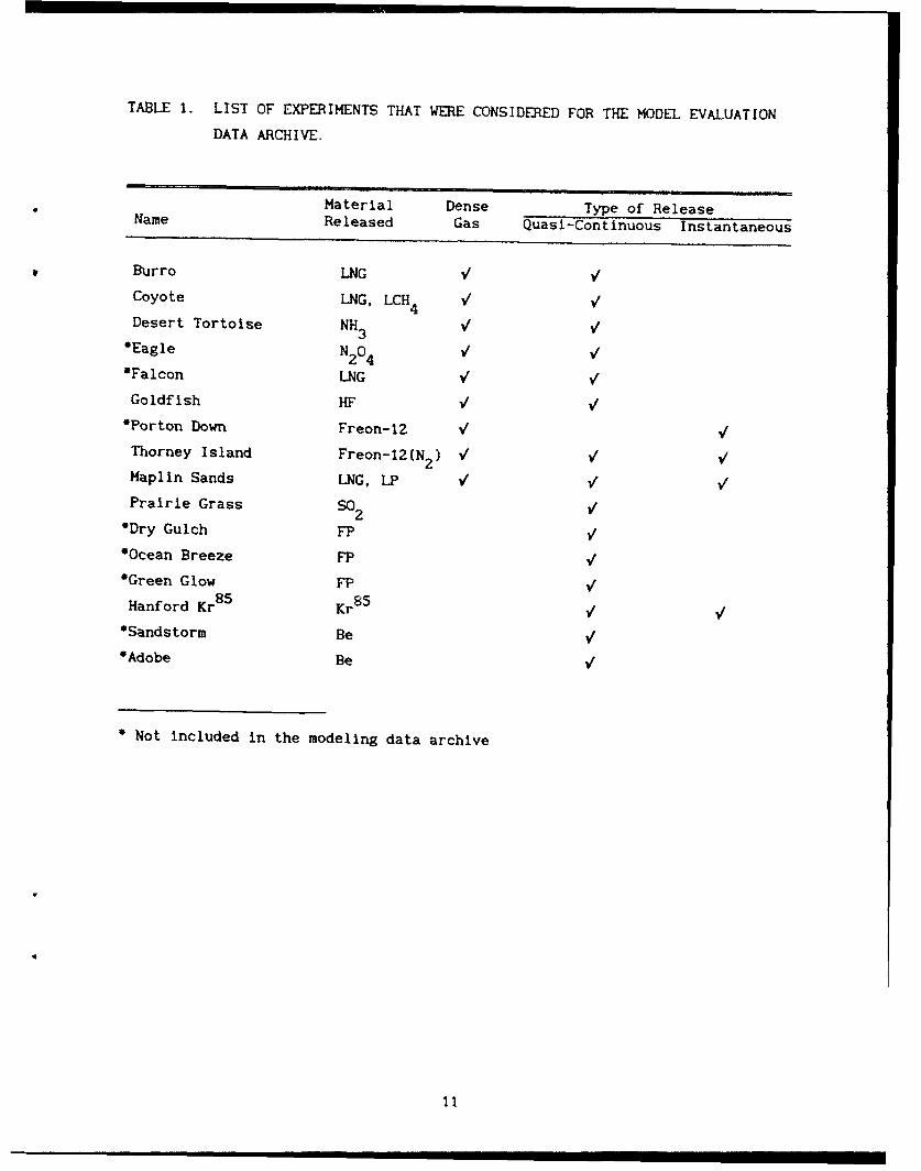
TABLE 1. LIST OF EXPERIMENTS THAT WERE CONSIDERED FOR THE MODEL EVALUATION

DATA ARCHIVE.

Material Dense Type of ReleaseName Released Gas Quasi-Continuous Instantaneous

Burro LNG V VCoyote LNG, LCH 4 VDesert Tortoise NH3 V V

"Eagle NO2 V V"Falcon LNG V VGoldfish HF V

"Porton Down Freon-l2 V VThorney Island Freon-12(N ) V V VMaplin Sands LNG, LP V V VPrairie Grass so2

"Dry Gulch FP

"Ocean Breeze FP V"Green Glow FPHanford Kr8 5 Kr 85V

"Sandstorm Be"Adobe Be

" Not included in the modeling data archive

I1

'" , , , , ~ ~I iI I IIIl

project, and are listed in Table 1. Nine involve releases of denser-than-

air gases, while seven Involve the release of gases or suspended particles in

amounts small enough to act as passive tracers.

Based on a review of the data and the documentation for these 16

experiments, a decision was made not to consider seven of them. Neither the

ADOBE nor Sandstorm experiments were included in the study, since they were

concerned with the transport and diffusion of buoyant exhaust clouds from

rocket motors. Few of the models tested in this project can accommodate a

buoyant cloud, and furthermore, there are not sufficient data on the exhaust

characteristics of the rocket motors In the data reports to adequately define

the temperature and volume flux of the jet. Data from the Falcon Experiments

were excluded from the study for two reasons: only one of the trials was

successful from the point of view of evaluating diffusion models, and a data

report is not available. The Eagle tests were also excluded, since some of

the tests involved the use of a barrier to the flow, which sets them apart

from the remainder of the datasets used In the study, and there were

instrument problems with the remaining tests.

Of the remaining ii experiments, 5 are tracer experiments (that is, the

chemical that Is released behavss as an inert or passive non-buoyant substance

as it disperses downwind). The Prairie Grass experiment provides high quality

dispersion data over a wide range of turbulence regimes at an Ideal site. The

Dry Gulch, Ocean Breeze, and Green Glow data are not included because they are

simiiar to the Prairie Grass data, yet cover a more limited range of

stabilities. The Kr85 tracer experiment conducted in Hanford, WA Is included

because it provides good data for puff releases as well as quasi-continuous

releases of neutral-density or passive gases.

One of the remaining dense-gas dispersion datasets was recently dropped

from consideration as well. The Porton Down dataset includes 42 trials in

which mixtures of Freon-12 and air were released in the form of an

Instantaneous cloud. Those trials Include variations in initial cloud

density, wind speed, and surface roughness, but they lack an extensive

array of monitors capable of providing continuous concentration measurements.

The primary monitors provided only dosage measurements. These dosages can be

used to estimate a mean concentration during the time over which the cloud

passed through the monitoring array, but we found that these estimates

contribute little to the goal of quantifying model performance. We expected

12

that the models would tend to produce estimates of peak concentration which

would exceed the average concentrations estimated from the dosages--and all of

the models did. No additional information could be obtained from the dataset.

As a result, we have excluded the Porton Down trials from any further

discussion in this report.

Hence, the performance evaluations are based on a total of 8 datasets.

In the remainder of this section, we provide: a description of each of the

field studies (Section II B); a description of the MDA containing data from

each dataset (Section II C); a summary of the methods used to calculate

information required by the MDA (Section II D); and an overall summary of the

datasets (Section II E).

B. DESCRIPTION OF INDIVIDUAL FIELD STUDIES

1. Burro and Coyote

Both the Burro (Reference 14) and Coyote (Reference 15)

series of trials were conducted at the Naval Weapons Center (NWC) at China

Lake, California. Sponsored by the U.S. Dept. of Energy and the Gas Research

Institute, the trials consisted of releases of LNG onto the surface of a 1 m

deep pool of water, 58 m in diameter. In addition, the Coyote series expanded

on the earlier Burro trials by studying the occurrence of rapid-phase-

transitions (RPT), and included releases of liquefied methane and liquid

nitrogen. The Burro series focused on the transport and diffusion of vapor

from spills of LNG on water. The Coyote series focused on the characteristics

of fires resulting from ignition of clouds from LNG spills, and the series

also focused on the RPT explosions. In all, eight trials from the Burro

series and four trials from the Coyote series are suitable for testing

transport and diffusion models.

For the Burro series, twenty cup-and-vane anemometers were located

at a height of 2 m at various positions within the test array in order to map

the wind field. There were six 10 m tall turbulence stations, one upwind and

five downwind, which had bivane anemometers at three levels and thermocouples

at four levels. Humidities were measured close to the array centerline at

eight stations, including the upwind turbulence station. Ground heat-flux

sensors were mounted at seven downwind stations along with the humidity

sensors. Figure I shows the configuration of the test site.

13

46414 wi

&;- 0 &old~

-wig

-1 Ann~.

013 61

0 w- -

wS #Am

Figure 1. Instrumentation Array for the 1980 LNG Dispersion Tests at NWC,China Lake (Reference 14).

14

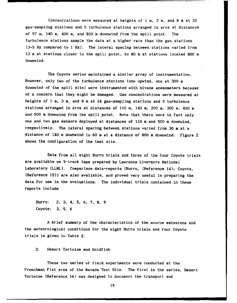
Concentrations were measured at heights of 1 m, 3 m, and 8 m at 25

gas-sampling stations and 5 turbulence stations arranged in arcs at distances

of 57 m, 140 m, 400 m, and 800 m downwind from the spill point. The

turbulence stations sample the data at a higher rate than the gas stations

(3-5 Hz compared to 1 Hz). The lateral spacing between stations varied from

13 m at stations closer to the spill point, to 80 m at stations located 800 m

downwind.

The Coyote series maintained a similar array of Instrumentation.

However, only two of the turbulence stations (one upwind, one at 300 m

downwind of the spill site) were instrumented with bivane anemometers because

of a concern that they might be damaged. Gas concentrations were measured at

heights of 1 m, 3 m, and 8 m at 24 gas-sampling stations and 5 turbulence

stations arranged in arcs at distances of 110 m, 140 m, 200 m, 300 m, 400 m

and 500 m downwind from the spill point. Note that there were In fact only

one and two gas sensors deployed at distances of 110 m and 500 m downwind,

respectively. The lateral spacing between stations varied from 30 m at a

distance of 140 m downwind to 60 m at a distance of 800 m downwind. Figure 2

shows the configuration of the test site.

Data from all eight Burro trials and three of the four Coyote trials

are available on 9-track tape prepared by Lawrence Livermore National

Laboratory (LLNL). Comparison data-reports (Burro, (Reference 14); Coyote,

(Reference 15)) are also available, and proved very useful In preparing the

data for use In the evaluations. The individual trials contained in these

reports Include

Burro: 2, 3. 4, 5, 6, 7, 8, 9

Coyote: 3, 5, 6

A brief summary of the characteristics of the source emissions and

the meteorological conditions for the eight Burro trials and four Coyote

trials Is given in Table 2.

2. Desert Tortoise and Goldfish

These two series of field experiments were conducted at the

Frenchman Flat area of the Nevada Test Site. The first In the series, Desert

Tortoise (Reference 16) was designed to document the transport and

15

-i;--

'GI

'GI

00*

Vol~O Gla "1

G23

!91 GO ow

Figue 2 Insrumntaton rrayforthe oyoe Seiesat NC, hinaLak

Figureld Locntumnations Mrark thoseuedi the Burroe Series (Referencena 15)e

16

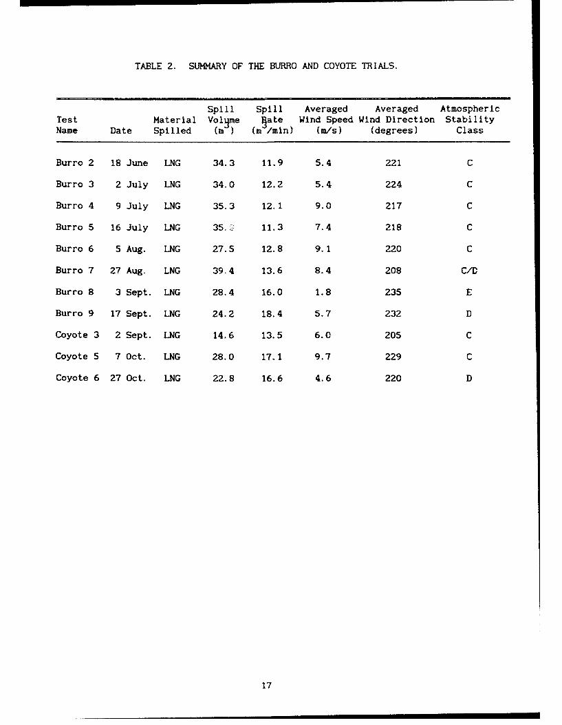
TABLE 2. SUMMARY OF THE BURRO AND COYOTE TRIALS.

Spill Spill Averaged Averaged AtmosphericTest Material Volrjme §ate Wind Speed Wind Direction StabilityName Date Spilled (m ) (m /mlin) (m/s) (degrees) Class

Burro 2 18 June LNG 34.3 11.9 5.4 221 C

Burro 3 2 July LNG 34.0 12.2 5.4 224 C

Burro 4 9 July LNG 35.3 12.1 9.0 217 C

Burro 5 16 July LNG 35.Z 11.3 7.4 218 C

Burro 6 5 Aug. LNG 27.5 12.8 9.1 220 C

Burro 7 27 Aug. LNG 39.4 13.6 8.4 208 C/D

Burro 8 3 Sept. LNG 28.4 16.0 1.8 235 E

Burro 9 17 Sept. LNG 24.2 18.4 5.7 232 D

Coyote 3 2 Sept. LNG 14.6 13.5 6.0 205 C

Coyote 5 7 Oct. LNG 28.0 17.1 9.7 229 C

Coyote 6 27 Oct. LNG 22.8 16.6 4.6 220 D

17

diffusion of ammonia vapor resulting from a cryogenic release of liquid

ammonia. For each of the four trials, pressurized liquid NH3 was released

from a spill pipe pointing downwind at a height of about 1 m above the ground.

The liquid jet flashed as it exited the pipe and its pressure decreased,

resulting in about 18 percent of the liquid changing phase to become a gas.

The remaining 82 percent of the NH3 -jet remained as a liquid, which was broken

up into an aerosol by the turbulence inside the jet. Very little, if any of

the unflashed liquid was observed to form a pool on the ground. Dispersion of

the vapor-aerosol cloud was dominated by the dynamics of the turbulent Jet

near the point of release, but the slumping and horizontal spreading of the

cloud downwind of the jet zone indicated the dominance of dense-gas dynamics

at later stages.

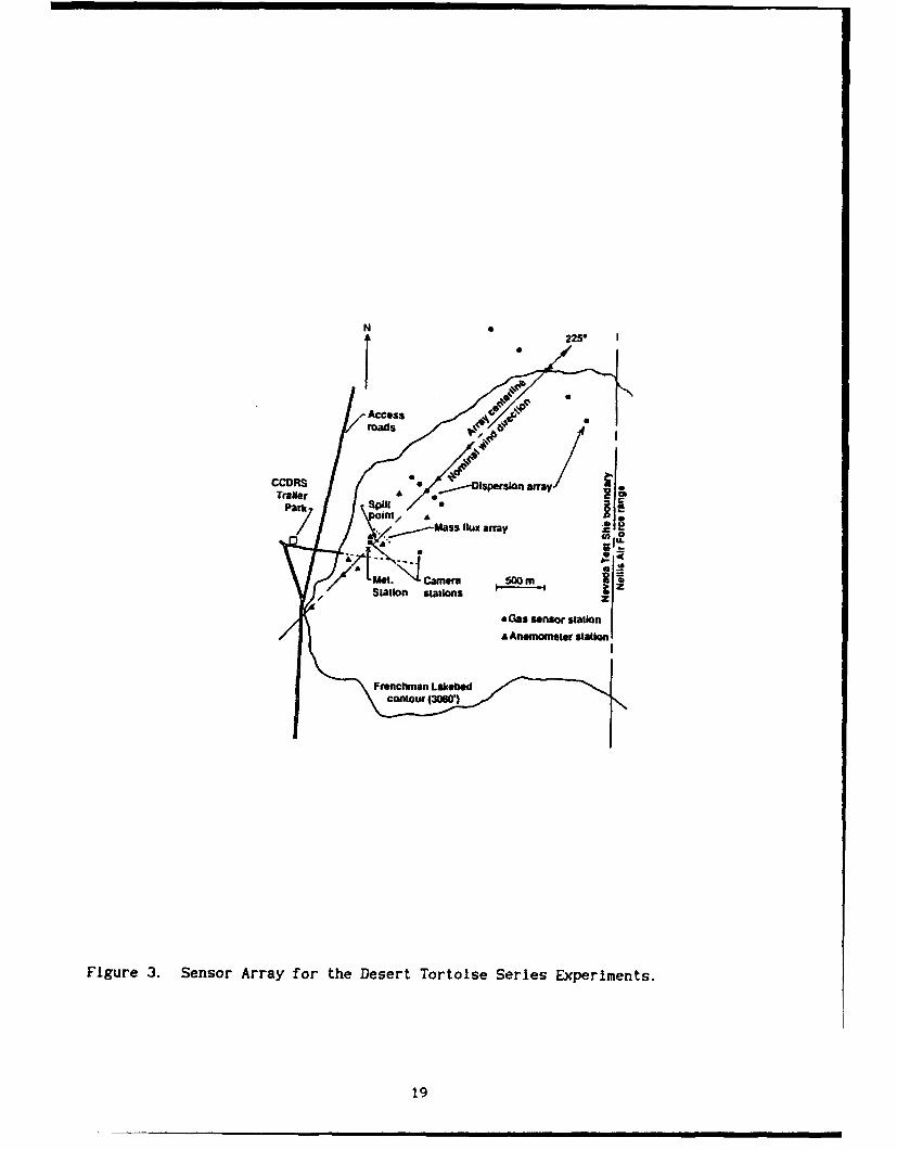
Figure 3 shows the configuration of instrumentation used during

Desert Tortoise. Eleven cup-and-vane anemometers were located at a height of

2 m at various positions within the test array in order to define the wind

field for the planning of field experiments and the subsequent calculation of

plume trajectories. In additioi., a 20 m tall meteorological tower was located

just upwind of the spill area, with temperature measured at four levels and

wind speed and turbulence at three levels. Ground heat fluxes were measured

at that tower and at three locations just downwind of the spill.

NH3 concentrations and temperatures were obtained at elevations of

1, 2.5, and 6 m on seven towers located along an arc at a distance of 100 m

downwind of the source. In most cases, nearly all of the plume was below the

6 m level of the towers and within the lateral domain of the towers.

Additional NH3 concentration observations at elevations of 1, 3.5, and 8.5 m

were taken on five monitoring towers at a distance of 800 m from the source,

where the lateral spacing of the towers was 100 m. Finally there were two

arcs with up to eight portable ground-level stations at distances of 1400 m or

2800 m, and on occasion at 5500 m downwind. No information on vertical

distrlbution of NH3 concentration was available from these more distance arcs.

The Goldfish trials are very similar to the Desert Tortoise NH3

trials described above. Hydrogen fluoride (HF) was released using a similar

release mechanism and some of the same sets of instruments. Note that

18

N H • 225*

TraUor £ E ra

1 0 0 0

Station stations way z

park sssopsatn

Stto statoions stto

Figure 3. Sensor Array for the Desert Tortoise Series Experiments.

19

although six trials were conducted, the last three involved a study of the

effectiveness of water sprays, and are not included in this evaluation

demonstration. A portion of the liquid HF flashed upon release, creating a

turbulent jet in which the unflashed liquid was broken up into an aerosol that

remained in the jet-cloud. No pooling of the liquid was observed.

HF samplers were located on cross-wind lines at distance of 300,

1000, and 3000 m from the source. The closest line has 11 sampling locations,

with instruments at heights of 1, 3, and 8 m at the inner 5 positions and

instruments at a height of 1 m on the outer 6 positions. The 1000 m line has

13 sampling locations, with three levels of measurement on the inner 9 and

only one level on the outer 4. The 3000 m line has 11 sampling locations,

with a similar variation in sampler heights. In general the observed height

of the HF cloud was less than the highest sampler level at the 300 m sampling

line, but appeared to extend above the highest sample levels at the larger

distances. The maximum ground level concentration and the cloud width could

be accurately estimated in each test.

Data from the Desert Tortoise experiment are available on a 9-track

tape from LLNL, and a companion report similar to the ones prepared for Burro

and Coyote is also available (Reference 16). No such report is scheduled to

be produced for the Goldfish experiment. Data for the 3 dispersion trials

(not the three mitigation effectiveness trials) were obtained from Mr.

D. Blewitt of AMOCO (one of the sponsors of Goldfish), and much of the

documentation for these trials may be found in a paper that appeared in the

International Conference on Vapor Cloud Modeling (Reference 17). The

individual trials contained in these reports include:

Desert Tortoise: 1, 2, 3, 4

Goldfish: 1, 2, 3

20

Table 3 provides an overview of these two field experiments. Most

of the trials were performed during "neutral" stability conditions, with

moderate wind speeds of 3 to 7 m/s. Although generally similar, note that

Desert Tortoise trials differ from Goldfish trials in that the spill rates are

about an order of magnitude greater.

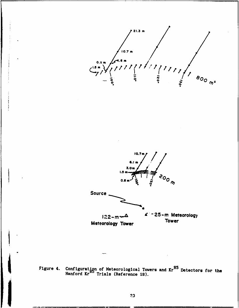
3. Hanford Kr 8 5

The results from 13 dispersion trials conducted at the Atomic Energy

Commission's Hanford reservation are reported by Nickola (Refierence 18). Five

of these trials involved the instantaneous release of small quantities of the

inert radioactive gas krypton-85 (Kr 85), and the other eight involved

short-period releases of Kr85 over periods of ten to twenty minutes.

Up to as many as 64 detectors were operated along arcs located 200 m

and 800 m downwind of the point of release. This section of the Hanford field

diffusion grid is nearly flat, and is covered with sagebrush and steppe

grasses. Most of the detector locations consisted of one detector set at 1.5 m

above the surface. However, each row also included three towers on which five

detectors provided a vertical profile of the Kr85 clouds. The configuration is

shown in Figure 4. Note that the uppermost detectors did not extend above

the top of the diffusing clouds.

Meteorological data are reported for averaging periods of 1 minute, 5

minutes, and the period over which data were collected during a trial. These

data are taken from the faster-response instruments mounted on the 25 m tower

located near the source, when available. Otherwise, the data are reported

from strip-charts recorded by instruments on the 122 m tower. Tabulations of

time-series of meteorological and concentration data for both the

instantaneous and continuous releases of Kr85 are printed in the data report

for the study (Reference 18). Wind speed, the standard deviation of

wind speed and wind direction, and temperature are reported for consecutive

1-minute periods during each trial. Concentration data from the near-surface

samplers (1.5 m above the ground) and the elevated sampling masts are reported

at intervals of 38.4 seconds for the continuous release trials, and are

reported at intervals of either 1.2, 2.4, or 4.8 seconds for the instantaneous

release trials.

21

TABLE 3. SUMMARY OF DESERT TORTOISE AND GOLDFISH EXPERIMENTS.

Spill Averaged Averaged AtmosphericTrial Duration §ate Wind Speed Wind Direction StabilityName Date (sec) (mmin) (m/s) (degrees) Class

DT 1 24 Aug. 126 7.0 7.4 224 D

DT 2 29 Aug. 255 10.3 5.7 226 D

DT 3 1 Sept. 166 11.7 7.4 219 D

DT 4 6 Sept. 381 9.5 4.5 229 E

GF 1 1 Aug. 125 1.78 5.6 - D

GF 2 14 Aug. 360 0.66 4.2 D

GF 3 20 Aug. 360 0.65 5.4 D

22

21.3 m

10.7,

0.6. 0-4;So -o / . - / l

* 00

o.

" 9r

10.7./I

1.5m

0.8 m

Source

122_mwZ i -25-m MeteorologyMeteorology Tower Tower

Figure 4. Configuratign of Meteorological Towers and Kr8 5 Detectors for theHanford Kr Trials (Reference 18).

--3

As part of a project funded by the EPA, TRC Environmental

Consultants, Inc. had entered the concentration data and meteorological data

for six of the eight instantaneous release trials Into computer files. The

two trials dropped from use for this project were less desirable than the

others because portions of the clouds drifted to the side of the array of

detectors. We obtained these data and entered data for the five continuous-

release trials into LOTUS I-2-3 worksheets, preserving all of the Information

and structure of the original tables. The following trials comprise the data

recorded on magnetic media:

Continuous-Release Trials: C1, C2, C3, C4, CS

Instantaneous Release Trials: P2, P3, P5, P6, P7, PS

A summary of the meteorological data for six of the eight instantaneous-

release trials and all five continuous-release trials is presented In

Table 4.

4. Maplin Sands

The dispersion and combustion trials conducted at Maplin Sands in

1980 (Reference 19) Involved the release of liquefied natural gas (LNG) and

refrigerated liquid propane (LPG) onto the surface of the sea. Each liquid was

released in both a continuous and an instantaneous mode. The size of a spill3

during each trial was approximately 20 M.

Because the objective of the trials was to study the behavior of LNG

and LPG vapor clouds over the sea, the site was located on the tidal flats of

the Thames estuary. A shallow dike 300 m in diameter was constructed around

the spill area to meet the requirement that the spill occur on the sea

surface. Pontoons with either 4 m masts or 10 m masts were used to position

meteorological Instruments and sampling instruments along arcs downwind of the

spill area. Figure 5 shows the pontoon configuration at the start of the

series, and Figure 6 shows the revised configuration used after Trial 35. A

24

TABLE 4. SUMMARY OF HANFORD KRYPTON-85 TRACER RELEASES.

Duration Total Release Wind Speed QualitativeTrial Date Start End (min & Emitted Rate at 1.5 m ThermalNo.- (1967) (PST) (PST) sec) (Ci) (Ci/Sec) (mps) Stability

P2 Sep 14 2300:00 - - 10.0 - 1.3 Very StableC1 Sep 15 0000:00 0015:28 15:28 10.9 0.0117 1.3 Very Stable

P3 Oct 17 0738:00 - - 10.0 - 4.2 NeutralC2 Oct 17 0801:50 0801:50 15:05 10.9 0.0120 3.9 Unstable

P5 Oct 23 1052:40 - - 10.0 - 8.0 UnstableC3 Oct 23 1101:25 1115:40 14:15 23.8 0.0278 7.1 Unstable

P6 Oct 23 1130:00 - - 10.0 - 7.3 Unstable

P7 Oct 24 1052:30 - - 10.0 - 4.6 UnstableC4 Oct 24 1104:30 1114:28 9:58 22.8 0.0388 3.9 Unstable

CS Nov 8 0512:22 0532:13 19:51 20.4 0.0171 2.6 StableP8 Nov 8 0602:00 - - 10.0 - 1.5 Stable

"P: Denotes a puff (instantaneous) releaseC: Denotes a continuous (short-period) release

25

0 STANDiRC PON4TOONS WIv d&IST

MEdTEORGLM WITh tW MAT

Figure 5. Initial Configuration of the Maplin Sands Site.

o XTANOMMPMMDWM4~h4BNLMS

Figure 6. Revised Configuration of the Maplin Sands Site (After Trial 35).

26

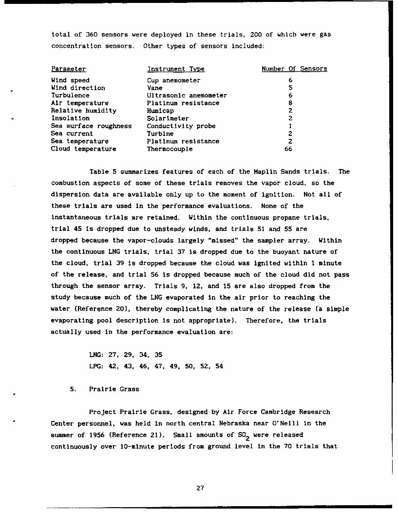
total of 360 sensors were deployed in these trials, 200 of which were gas

concentration sensors. Other types of sensors included:

Parameter Instrument Type Number Of Sensors

Wind speed Cup anemometer 6Wind direction Vane 5Turbulence Ultrasonic anemometer 6Air temperature Platinum resistance 8Relative humidity Humicap 2Insolation Solarimeter 2Sea surface roughness Conductivity probe ISea current Turbine 2Sea temperature Platinum resistance 2Cloud temperature Thermocouple 66

Table 5 summarizes features of each of the Maplin Sands trials. The

combustion aspects of some of these trials removes the vapor cloud, so the

dispersion data are available only up to the moment of Ignition. Not all of

these trials are used in the performance evaluations. None of the

instantaneous trials are retained. Within the continuous propane trials,

trial 45 is dropped due to unsteady winds, and trials 51 and 55 are

dropped because the vapor-clouds largely "missed" the sampler array. Within

the continuous LNG trials, trial 37 is dropped due to the buoyant nature of

the cloud, trial 39 is dropped because the cloud was Ignited within i minute

of the release, and trial 56 is dropped because much of the cloud did not pass

through the sensor array. Trials 9, 12, and 15 are also dropped from the

study because much of the LNG evaporated in the air prior to reaching the

water (Reference 20), thereby complicating the nature of the release (a simple

evaporating pool description Is not appropriate). Therefore, the trials

actually used in the performance evaluation are:

LNG: 27, 29, 34, 35

LPG: 42, 43, 46, 47, 49, 50, 52, 54

5. Prairie Grass

Project Prairie Grass, designed by Air Force Cambridge Research

Center personnel, was held In north central Nebraska near O'Neill in the

summer of 1956 (Reference 21). Small amounts of SO2 were released

continuously over 10-minute periods from ground level in the 70 trials that

27

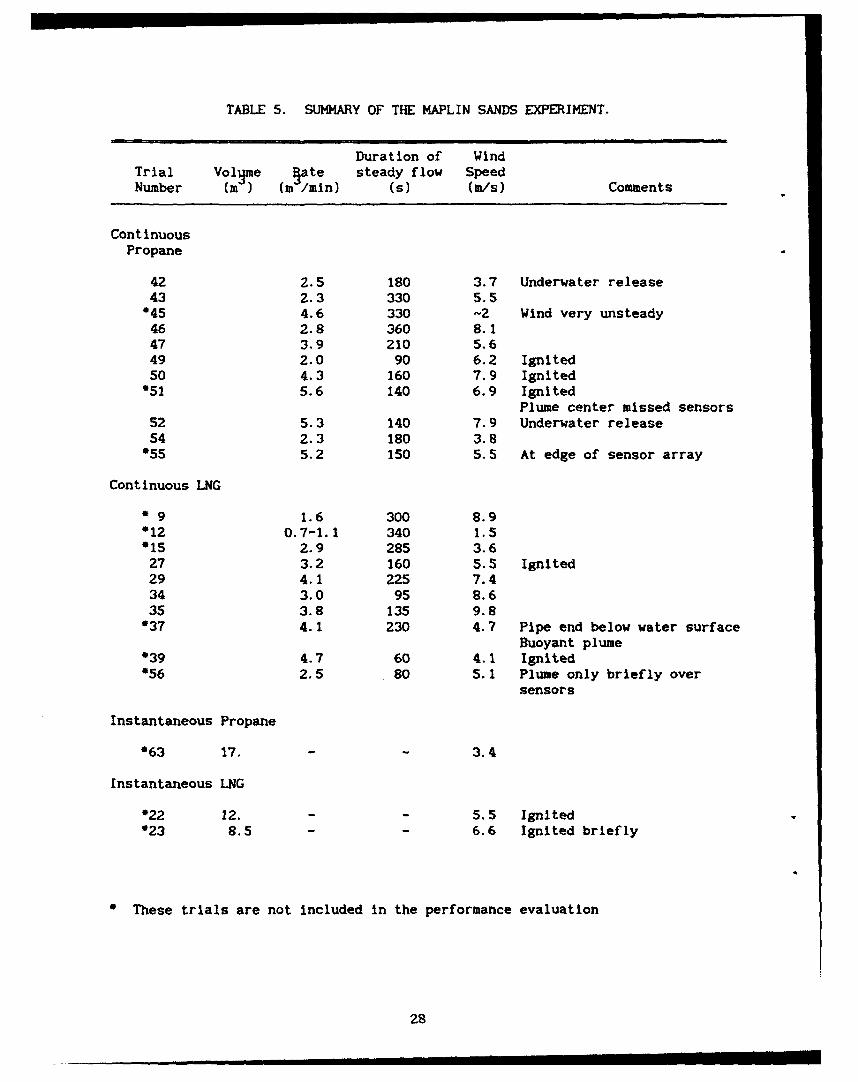
TABLE 5. SUMMARY OF THE MAPLIN SANDS EXPERIMENT.

Duration of WindTrial Volrme §ate steady flow SpeedNumber (m ) (m /min) (s) (m/s) Comments

ContinuousPropane

42 2.5 180 3.7 Underwater release43 2.3 330 5.5

045 4.6 330 -2 Wind very unsteady46 2.8 360 8.147 3.9 210 5.649 2.0 90 6.2 Ignited50 4.3 160 7.9 Ignited

*51 5.6 140 6.9 IgnitedPlume center missed sensors

52 5.3 140 7.9 Underwater release54 2.3 180 3.8

055 5.2 150 5.5 At edge of sensor array

Continuous LNG

& 9 1.6 300 8.9'12 0.7-1.1 340 1.5*15 2.9 285 3.6

27 3.2 160 5.5 Ignited29 4.1 225 7.434 3.0 95 8.635 3.8 135 9.8

037 4.1 230 4.7 Pipe end below water surfaceBuoyant plume

039 4.7 60 4.1 Ignited*56 2.5 80 5.1 Plume only briefly over

sensors

Instantaneous Propane

063 17. - 3.4

Instantaneous LNG

022 12. - - 5.5 Ignited023 8.5 - - 6.6 Ignited briefly

0 These trials are not Included in the performance evaluation

28

comprised the project. Dosage measurements were made on arcs located at

distances of 50, 100, 200, 400, and 800 meters downwind. About half of the

trials were conducted during unstable daytime conditions and the rest were

held at night with temperature inversions present. Meteorological

measurements included wind speed, direction, and fluctuations in direction

from cup anemometers and airfoil type wind vanes. Micrometeorological data,

rawinsonde data, and aircraft soundings were also taken.

The site was located on virtually flat land covered with natural

prairie grasses. The roughness length determined for the site by some of the

researchers was 0.6 centimeters. Dosages were measured at a height of 1.5

meters along the arcs using midget impingers. The meteorological data were

given as 10-minute averages.

Earlier, the Porton Down dataset was dropped because most of the

data obtained in the monitoring array are in the form of dosages. Why, then,

are the dosages obtained during Prairie Grass acceptable? The reason is that

the duration of the Prairie Grass releases (10 minutes) is long enough to

create a quasi-steady plume over the monitoring array. In the absence of

meandering, the time series of concentrations that might have been measured

would have a plateau-like appearance. The average concentration estimated

from the dosage (assuming a time-scale equal to the duration of the release

= 10 minutes) would then be a fair estimate of the peak concentration. The

Porton Down data, on the other hand, involve instantaneous releases, which

would result in a time series of concentrations that might have been measured

which would have a peak-like appearance. The mean concentration estimated

from the dosage and the time it takes such a cloud to pass a monitor is a poor

estimate of the peak concentration. Hence, the dosages from the Prairie Grass

dataset are more useful for evaluating model performance. Note, however, that

the average concentrations are still expected to be less than the peak

concentrations.

Table 6 provides a summary of the meteorology for a subset of 44

trials that will be used on this project. These 44 represent the best of the

program, and have been used extensively by other researchers (for example,

Reference 22; Reference 23; Reference 24).

29

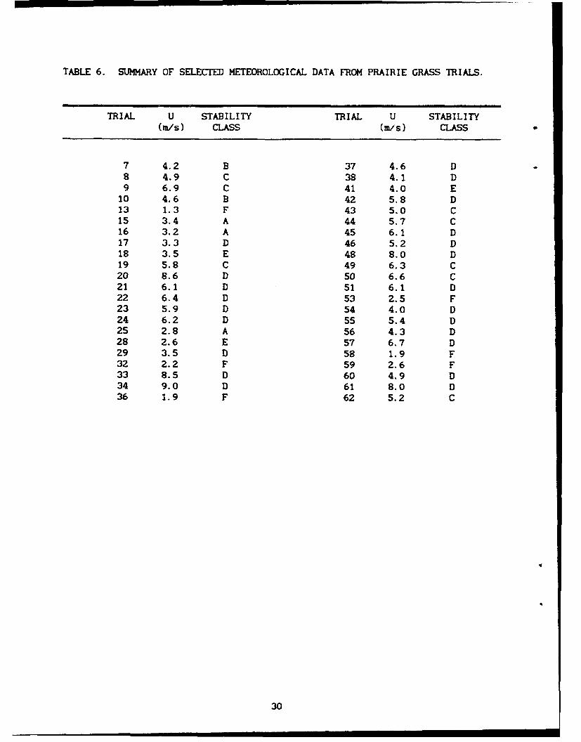
TABLE 6. SUMMARY OF SELECTED METEOROLOGICAL DATA FROM PRAIRIE GRASS TRIALS.

TRIAL U STABILITY TRIAL U STABILITY(mCs) CLASS (m/s) CLASS

7 4.2 B 37 4.6 D8 4.9 C 38 4.1 D9 6.9 C 41 4.0 E

10 4.6 B 42 5.8 D13 1.3 F 43 5.0 C15 3.4 A 44 5.7 C16 3.2 A 45 6.1 D17 3.3 D 46 5.2 D18 3.5 E 48 8.0 D19 5.8 C 49 6.3 C20 8.6 D 50 6.6 C21 6.1 D 51 6.1 D22 6.4 D 53 2.5 F23 5.9 D 54 4.0 D24 6.2 D 55 5.4 D25 2.8 A 56 4.3 D28 2.6 E 57 6.7 D29 3.5 D 58 1.9 F32 2.2 F 59 2.6 F33 8.5 D 60 4.9 D34 9.0 D 61 8.0 D36 1.9 F 62 5.2 C

30

6. Thorney Island

The Heavy Gas Dispersion Trials project at Thorney Island (Reference

25) organized by the British Health and Safety Executive consists of the

following five types of trials:

(1) Phase I - the instantaneous release of a preformed cloud of

approximated 2000 m3 of dense gas over flat terrain. Sixteen

trials were carried out.

(2) Phase II - Ten trials were carried out to study the effects of

obstacles on Phase I-type releases.

(3) Continuous release trials - Three trials in which approximately

2000 m3 of heavy gas was released at a rate of 5 m 3/sec over

flat terrain.

(4) GRI trial - A single Phase I-type of release.

(5) Phase III- Six continuous release trials in which a fenced

enclosure surrounded the gas container.

For this project, we are focusing on the Phase I trials (item #1) and the

continuous-release trials (item #3). The instantaneous-release trials of

Phase I are similar in design to those conducted earlier at Porton Down, but

the size of the source is approximately fifty times larger, and continuous

monitors were used to obtain concentration measurements.

A gas container with a volume of 2000 m3 was filled with a mixture

of freon and nitrogen. For instantaneous release trials, the sides of the gas

container collapsed to the ground upon release. For continuous release

trials, the gas container simply served as a storage tank. The gas would

then be ducted below the ground to the chosen release position. The release

mechanism was designed to give a ground-level release with zero vertical

momentum.

31

A 30 m tall meteorological tower was was located 150 m upwind from

the release point. The Instrumentation consisted of five cup anemometers,

five temperature sensors, two sonic anemometers, and one sensor each for

relative humidity, solar radiation and barometric pressure. Four

trailer-mounted towers, with a total of eight sonic anemometers, were also

deployed. Note that the 30 m tall tower was replaced by a 20 m tall tower for

continuous release trials.

Thirty-eight towers were used to measure gas concentrations.

Measurements were taken at four levels. The lowest gas sensor was positioned

at a height of 0.4 m; and the highest at 4 m on towers close to the spill

point, 10 m at most other towers, and 14.5 m at towers in the far field. The

towers were placed on a rectangular grid with distances up to about 800 m from

the release point. The four trailer-mounted towers mentioned previously also

had gas sensors mounted at four different heights. The configuration of

instrumentation at the site is shown in Figure 7.

Copies of the 9-track tapes containing data for the instantaneous

release trials were obtained through the API, who had contributed to the

experiments, and who are co-funding this model performance evaluation. We

have averaged the 20-Hz data in blocks of 0.6 seconds each. Data for the

continuous release trials were obtained from TRC Environmental Consultants,

Inc., who had digitized plots of the data to produce data corresponding to

30-s averages. A total of 9 of the 16 continuous release trials and 2 of the

3 instantaneous release trials were retained for the evaluation. Trials 10,

11, and 46 were dropped because of wind-shifts during the trial; trial 4 was

dropped because the cloud became elevated; trial 5 was dropped because the

release mechanism malfunctioned, producing 2 clouds rather than 1; and trials

14, 15, and 16 were dropped because the density of the initial cloud appeared

to be stratified. The trials Included In this study are:

Instantaneous releases: 6, 7, 8, 9, 12, 13, 17, 18, 19

Continuous releases: 45, 47

A brief summary of the characteristics of the source emissions and

the meteorological conditions for the Phase I and continuous release trials

Is given in Table 7.

32

VA as tCode

GRID NORTHiIFO= MI

= M2 11)•= M21b)M= M3

0-0I ri4,= Significant

obstructions

HANGAR

fgo,CONTROL 0 CI *TOWER (

IWEST THORNEY

Meat Code IskuntatWon

A 6 cup anemomutem2 sonic anemnometers5 thermomte.1 solauimetet

2 relative humidity enms1 wind avne

v 1 bI wiedai

F 4 gua•enso., (1 Hz)

M1 I sonic anemnometg4 uus sensou (1 Hz)2 gm sernmo (10 Hz)

M2 (a) 4gm meNnbo (1 Hs)2 moakt anenometem2 gm ensou (10 Hz)

M2 (b) 4 gmsensur (1 Hz)2 sonk aenmometu1 m sensor (10 Hz)

M3 4 gm snsov (1 Ha)3 sonic anemoimeters3 go nmm (10 HS)

D 4 goasensrsn (1 H)I cup anemomete1 wind vane1 relative humdlty saenor1 Uteromnetaer

Figure 7. Configuration of Instrumentation Used for the Phase I Trials at

Thorney Island (Reference 25).

33

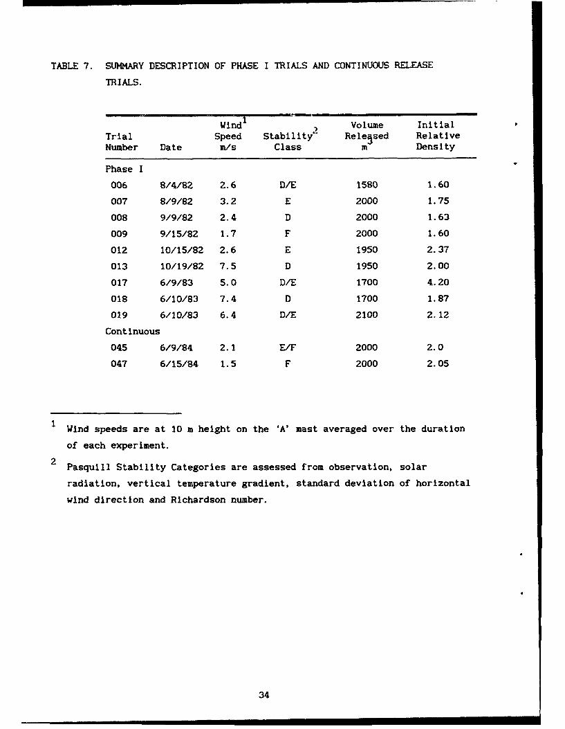
TABLE 7. SUMMARY DESCRIPTION OF PHASE I TRIALS AND CONTINUOUS RELEASE

TRIALS.

WindI Volume InitialTrial Speed Stability" Rele 5 sed RelativeNumber Date m/s Class m Density

Phase I

006 8/4/82 2.6 D/E 1580 1.60

007 8/9/82 3.2 E 2000 1.75

008 9/9/82 2.4 D 2000 1.63

009 9/15/82 1.7 F 2000 1.60

012 10/15/82 2.6 E 1950 2.37

013 10/19/82 7.5 D 1950 2.00

017 6/9/83 5.0 D/E 1700 4.20

018 6/10/83 7.4 D 1700 1.87

019 6/10/83 6.4 D/E 2100 2.12

Continuous

045 6/9/84 2.1 E/F 2000 2.0

047 6/15/84 1.5 F 2000 2.05

1 Wind speeds are at 10 m height on the 'A' mast averaged over the duration

of each experiment.

2 Pasquill Stability Categories are assessed from observation, solar

radiation, vertical temperature gradient, standard deviation of horizontal

wind direction and Richardson number.

34

C. CREATION OF A MODELERS' DATA ARCHIVE

Application of 14 dissimilar models to 8 databases containing a total of

96 trials demands that the data be placed In a common format. Furthermore,

this format must include enough information to satisfy the input requirements

of all of the models. We have developed what may be called a Modelers' Data

Archive (MDA) to perform this function. It certainly does not contain all of

the data from each experiment; rather, it contains only that information that

we have used in running the 14 models. As such, the MDA is a subset of the

complete database. Table 8 lists the information contained in an MDA file.

Most of the entries are self-explanatory.

At the beginning of the MDA, information is given that defines the

experiment and trial, followed by a listing of several chemical properties of

the released substance. Chemical properties include the molecular weight,

normal boiling point, latent heat of evaporation, heat capacity of the vapor

phase, heat capacity of the liquid phase, the density of the liqui,'. and the

Antoine coefficients. The coefficients for the Antoine equation for

calculating vapor pressure as a function of temperature are taken from the

SLAB user's guide, since only SLAB requires these as input. Physical

properties of the release are then given, which not only provide specific

dimensions, but also information on the general type of the release (source

type and source phase) so that appropriate information can be passed to each

of the models. Meteorological data appear next. Temperatures at two

specified heights and wind speed at one specified height are used to estimate

the Monin-Obukhov length scale, L (although this may be specified directly).

What is termed "domain average" values of wind speed and two measures of

turbulence follow. This speed is the value actually used in the models, along

with either the calculated value of L, or that observed. The earlier wind

speed is used only in estimating L. If many near-surface measurements of wind

speed are available, than a true "domain-average" sDeed can be used. However,

if only one tower is available, then the speed measured near the surface (for

near-surface releases) should be used as the "domain-average" speed. Site

information includes the surface roughness length, soil (or water)

temperature, and a soil moisture indicator. The Bowen ratio is a measure of

the importance of the latent heat flux in computing the Monin-Obukhov length.

35

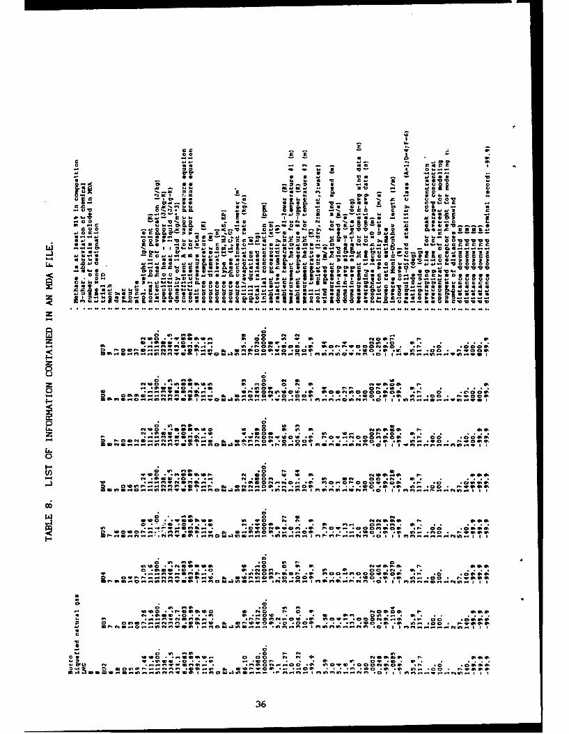
UV C

0 0U-0 a. a 11 U b.-" 00 g 1 20 -

-c =0 .0 c cU c

0 -b 64 em Uw e 1 0

U a--a,0 0V. 0.9. WM W A L Naca I 00 aC0W-0v

1. .. ,aa.- W55 5.5 : a I W. &' 00 - -a4 W01

a ..4 a P .s40 0.. 0 a4 .U 6 cE.in in 0 00EU006

0- 000~5 U 4 V UC WM Vc .V. C21, 00 b.. 0 0 o 'L.~~ ~ 00 1 0'55ii~. U- 2- 14£5 U ~

5 4.

I. "S a c_::-"= p a .wse .suC WeC r- - 0.u 11V! U01C 14. J4 W.c ab -0 UU0.VWWW6

I U 0 0,I gc...r-. Dou to, 01 00 0 410000- 0- go~bV0 4 .U ag 6UC.C~ ~~~~ ~~~~~ max v-- V644455514--U--.U-.SUU as. W0 6 b"4.iU09 .

0 Vmi o-W44.0 N0N1-

zC; N 0 ma 44

It 0: .. n 0 UU

0 e" n4 Iro 0 t1 41 0 i! IO!

.UU w 0 * * w ft 03 . a 145 C4. CN C; C;a ;ONW~~~~~~ "UOI. 10 .NONU 1. *U NO .4OONO e!00 .

4: 1ý 1.U F- .WA 0 01U@

060

W0 .M.N :C.4 0. U4.S O :.. ..0 . . C W00 1*mU go, W..I r 00 No cc .0am U@ wl

i%0 C U 0 aU

0; 'n 55 .; IanO*.~4UU 40 In U U N UNU

10 *UQ .0. 0 N0 *n U 001 *N* . .4".IN M U.. W UU4nO M0 I-O now Or *U .U00 * N UU

0 WO In W.U W% a4 sl roUmMb" b m t

- U N U U O O O U

* N UUS 0 *. .NU .~0U . . U U Oin . . U . .

*0It

14~~m 0 C". . Ni

36

It is the ratio of the sensible heat flux to the latent heat flux, and is

generally estimated rather than calculated or measured. The last information

in the file describes what specific information should be obtained from the

model when applied to a particular experiment and trial: concentration

averaging time, concentration of interest (for specifying the lateral extent

of the cloud or signaling how far downwind the model calculations should

extend), and receptor height and distances. Two averaging times are

given. These correspond to the shortest averaging time contained in a

dataset, and a longer averaging time that corresponds to the duration of the

release (for qu, si-continuous releases).

In many cases, not all of the entries are needed to characterize a trial.

For example, no heat exchange or changes in phase occur in the Thorney Island

trials, so the thermal properties of the gas are not used. Whenever this is

the case, a value of "-99.9" may be contained in the MDA file.

The structure of the MDA file allows information describing a turbulent,

two-phase jet-release to be specified within the same framework as a

single-phase, evaporating pool-release. We have developed a set of programs

to read the MDA files and produce tables of data needed to run each model.

These tables provide all data in the units requested by the model. At the

same time, the programs create all input files read by many of the models at

the time of execution, so that these models are essentially driven directly

from the MDA files. The goals satisfied in producing the MDA and software in

this way are:

1. To document assumptions used to initialize the models in a consistentway,

2. To automate the process of preparing model-runs to the maximumpossible extent,

3. To develop a way to easily implement alternate methods ofinitialization, and

4. To develop a framework for investigating the influence of datauncertainty on assessing model performance.

In addition to an MDA file for each experiment, concentration files were

also prepared for the distances and averaging times contained in the MDA.

Concentrations reported in these files represent the largest values measured

37

at each distance, for each averaging time. For some datasets, a measure of

the scale of the lateral half-width of the concentration distribution is

characterized as a at each location downwind. Both the concentrations andy

the values of a are compared to predicted values to produce measures of modelyperformance as described in Section IV.

D. METHODS FOR CALCULATING REQUIRED VARIABLES

Much of the information required to complete the MDA for each dataset Is

readily obtained. However, some entries do require explanation. In the

following sections, we discuss how the MDA for each of the datasets was

prepared. The MDA for each dataset is listed In Appendix A.

Measures of the observed concentration field must also be derived from

the datasets. The performance of the models is assessed by comparing modeled"centerline" or "peak" concentrations and crosswind cloud-widths (or ) with

those derived from the measured concentrations. The method used to

characterize the observed values is best illustrated by considering generic

dataset In which time series of measured concentrations are available at

several heights and locations along several monitoring arcs downwind of the

point of release. For each arc, the peak concentrations and a are obtainedyas follows:

A peak "instantaneous" concentration Is found by selecting the single

largest measured concentration from among all concentrations reported by all

samplers at all heights, along the arc. No "instantaneous" 0 Is estimated.YNext, a peak average concentration Is found. To do this, we review the time

series of concentrations along the arc, and define an averaging window that

excludes the leading and trailing edges of the cloud. The length of this

window is typically of the same order as the duration of the release for a

quasi-continuous source. Concentrations are averaged over this window at each

receptor, thereby producing a cross-section of average concentrations along

the arc (across the cloud). The largest concentration in the cross-section

is selected to represent the peak average concentration. Note that there is a

likelihood that this method will slightly underestimate the peak, which may

fall between receptors. A second-moment calculation involving the averaged

concentrations at the lowest measurement-height along the arc then determines

a. . However, several conditions must be satisfied before such a a. can bey y

considered valid:

38

1. There must be at least four monitors reporting non-zero values

of average concentration.

2. The receptor showing the maximum concentration must not be

located at either end of the arc.

3. The lateral distribution must not exhibit a clear bi-modal

pattern.

Departures from this treatment of a generic dataset are identified in the

following discussions for each dataset.

1. Burro

The data report (Reference 14) contains summary sheets for

the trials, which serve as the basis for most of the data placed in the MDA.

The following comments should be noted:

The mixture of methane, ethane, and propane that makes up the LNG

is reported in the summary sheets. We use this Information to

calculate the molecular weight of the mixture, but all other

properties in the MDA are for pure methane.

The source diameter is calculated by assuming that the spill rate is

equal to the total evaporation rate. Using an evaporation rate per

unit area of 0.085 kg/m2 /s for LNG on water, the diameter varies as

a function of the rate of release.

The source containment diameter is set equal to the diameter of the

water test basin created for the series of experiments.

The relative humidity is that termed "downwind humidity" in the

summary sheets.

The temperatures and wind speed used in calculating the

Monln-Obukhov length are obtained from the "upwind vertical profile"

data.

39

The domain-averaged wind speed and turbulence data use the average

values listed on the summary sheets.

The Pasquill-Gifford stability class values are assigned on the

basis of characterizations such as "neutral", slightly stable", etc.

The following correspondence was assumed:

unstable, slightly unstable C

neutral D

slightly stable E

Peak concentrations (both "instantaneous" and average), and the ay,

for the average concentration distribution along each monitoring arc

are found as described for the generic dataset. Cross-sections of

concentrations along each arc, which are plotted in the data report,

provided the means for defining the windows for averaging the

concentrations.

2. Coyote

The structure and documentation for the Coyote dataset is nearly the

same as that for Burro, so that the process of preparing the MDA is virtually

the same. The only departure is in specifying the Pasquill-Gifford stability

class. The data report for Coyote (Reference 15) does not provide the

stability classification. However, a later summary of a dataset for

dispersion modeling (Reference 26) does report the stability class for each of

the three trials in the MDA.

3. Desert Tortoise

The information placed in the MDA for this experiment is taken from

the data report (Reference 16). The following comments should be

noted:

The exit pressure is assumed to equal the pressure measured prior to

the point of discharge. It is not the tank pressure that is listed.

40

The wind speed and the temperatures used to calculate the

Monin-Obukhov length are those measured at site G01.

The domain-averaged wind data are those reported as the average

values at 2 m.

The spill rate Is the rate actually listed, with no adjustments for

the results of the mass-flux estimates made from the data obtained

along the arc at 100m downward of the point of release.

Peak concentrations and values of o for the arcs at distances ofy100 m and 800 m downwind of the point of release are obtained in the

manner described for the generic dataset.

4. Goldfish

The MDA for the Goldfish experiment was prepared from informationcontained In Blewitt (Reference 17), and from information obtained directly from

Mr. D. Blewitt of AMOCO, one of the sponsors of the experiment. The following

points should be noted:

Some chemical properties listed for HF vary among several

references. The latent heat of vaporization listed in Perry's

Handbook (Reference 27) Is 7460 cal/mol, which is equivalent to

1.558x106 J/kg. But Lange's Handbook of Chemistry (Reference 28)

and a basic chemistry textbook (Reference 29) list the latent heat

of vaporization as 1.8 Kcal/mol, which is equivalent to

3.76x105 J/kg. Several of the models that are evaluated also list

the physical properties of HF. PHAST uses 1.266x106 J/kg at 293 K,

and the user's guide for SLAB contains an example in which the

latent heat of vaporization for HF is 3.732xl05 J/kg. These

differences may be due to different assumptions by the references

regarding the degree of polymerization of the HF. We have chosen

the number used by SLAB for this property of HF, because personnel

at LLNL have developed SLAB and have conducted the Goldfish tests.

The diameter of the discharge orifice Is not listed In any of the

references for this experiment. The values used In the MDA were

obtained from Mr. D. Blewitt of AMOCO.

41

Concentration measurements for short sampling times (of order Is)

are not available. Instead, averaging times are assumed to be

either 66.6s, or 88.3s, depending on the sampler position. As a

result, we only characterize the peak concentration for the

averaging time associated with all samplers in a particular arc. A

corresponding value of o Is calculated from the concentrationsYreported at monitors along the arc during the same period that

contains the peak concentration. The methodology follows that for

the generic case except no averaging Is performed. Hence, the

averaging time associated with iy Is either 88.3 or 66.6s.

5. Hanford Kr 8 5

Kr85 is a radioactive gas, and was released in very small quantities

both as a continuous release and as an instantaneous release. The

instantaneous releases were accomplished by sealing a small volume of the gas

in a quartz vial, and then dropping a weight onto the container to crush It.

The continuous releases were accomplished by adding a very small amount of

Kr to a cylinder of compressed argon gas, and releasing the mixture at a

controlled rate. In both cases, the Kr85 was quantified in terms of its

disintegration rate: Cl/s for the continuous releases, and CI for the

Instantaneous releases. Concentrations downwind of the release were measured

as radiation counts, and converted to the equivalent Cl/mi3 (actually expressed

as pCi/m3).

Using a half-life of 10.4 years, we calculate that there are 2x10"8

kg-moles of Kr85 associated with I Ci. Because the instantaneous release made

use of only 10 Ci, the mass and volume of the gas in the vial was very small.85

The continuous release rate did not exceed 0.0388 Cl/s of Kr , which amounts

to approximately 7.8xl0-10 kg-mole/s. However, because the Kr85 was

Introduced into an argon carrier-gas at an unspecified mixing ratio, we do not85

know the Initial dilution of Kr

Based on these considerations, we have modeled the Hanford Kr 8 5

trials with a neutral-density gas, released at a small rate. The gas is taken

to be "dry air", which ensures that dense-gas effects will not be significant

In the simulations. Emission rates (kg/s) or total mass released (kg) of the

42

"dry air" are established by arbitrarily assigning 1 kg of mass to 1 Ci, so

that the instantaneous releases are modeled as if 10 kg (- 1/3 kg-mole) of

"dry air" were released, and the continuous releases are modeled as if 0.0388

kg/s (at most) of "dry air" were released.

Smaller amounts of "dry air" could have been modeled. For example,

we could have assigned I g of mass to 1 Ci. This may alter model predictions.

To gauge the effect of choosing 1 kg/Cl rather than 1 g/Ci In obtaining

modeled normalized concentrations (that Is, C/Q In ps/m3 or /m 3), we ran the

SLAB model both ways. The results are:

SLAB

1 kg/Cl 1 g/CiTRIAL DIST C(ppm) C(ppm) RATIO/IO00

HC1 200 110.3 0.1093 1.009800 13.21 0.0132 1.001

HC2 200 3.384 0.00338 1.001800 0.255 0.000255 1.000

HC3 200 6.121 0.00612 1.000800 0.467 0.000467 1.000

HC4 200 6.785 0.00679 0.999800 0.486 0.000486 1.000

HC5 200 15.44 0.0155 0.996800 1.274 0.00127 1.003

H12 200 1583 2.489 0.636800 87.85 0.0995 0.883

H13 200 430.5 0.5049 0.853800 14.61 0.01526 0.957

HI5 200 388.2 0.4497 0.863800 14.31 0.01486 0.963

H16 200 375.6 0.4346 0.864800 13.58 0.0141 0.963

HP7 200 328.8 0.3784 0.869800 10.88 0.01127 0.965

HI8 200 785.5 0.979 0.802800 29.99 0.0318 0.943

These results indicate that the initial size of the source (within SLAB at

least) has a minor influence on scaled concentrations predicted at distances

of 200 and 800 m from the source for the continuous release trials WHC's), but

can have a significant influence on the prediction of concentrations for the

instantaneous release trials (HI's). Note that 10 kg of "dry air" at standard3temperature and pressure occupies approximately 7.7 m , which corresponds to a

cube that Is almost 2 m on a side.

43

Tables for INPUFF and GPH were also prepared to see to what extentthe size of the source affects the scaled concentrations that are predicted.In applying both of these models, we specified an initial a and a to assurethat the peak concentration at the source did not exceed the density of thegas at the source. Therefore, we expect to see at least a small effect ofinitial source volume on the predicted concentrations.

INPUJFF Model1 kg/Ci 1 g/Ci

TRIAL DIST C(ppm) C(ppm) RATIO/I00

HC1 200 69.21 0.06942 0.997800 7.53 0.007535 0.999

HC2 200 2.366 0.002369 0.999800 0.1933 0.000193 0.999

HC3 200 3.054 0.003058 0.999800 0.2534 0.000253 1.000

HC4 200 7.677 0.007691 0.998800 0.6247 0.000625 1.000

HC5 200 21.69 0.02173 0.998800 2.281 0.002282 1.000

H12 200 3408 3.68 0.926800 110.2 0.1133 0.973

H13 200 452 0.4415 1.024800 12.94 0.01305 0.992

HI5 200 111.3 0.1132 0.983800 3.034 0.003048 0.995

H16 200 113.7 0.1156 0,984800 3.029 0.003044 0.995

H17 200 132.1 0.1349 0.979800 3 0.003016 0.995

HI8 200 1059 1.136 0.932800 31.11 0.03167 0.982

GPM ModelI kg/Cl 1 g/Ci

TRIAL DIST C(ppm) C(ppm) RATIO/I00

HC1 200 86.62 0.08803 0.984800 7.661 0.007695 0.996

HC2 200 2.139 0.002145 0.997800 0.1465 0.000146 0.999

HC3 2UO 3.463 0.003475 0.997800 0.2373 0.000237 0.999

HC4 200 8.71 0.008758 0.995800 0.5978 0.000598 0.999

HCS 200 23.68 0.02386 ).992800 1.875 0.001879 0.998

44

The continuous release trials show little Influence, as was found for the SLAB

runs. A greater effect is seen in the predictions at 200 m for the

instantaneous releases, but It is not as large as the effect seen In the SLAB

runs.

Because the trials are modeled as if "dry air" were released, the

information on chemical properties in the MDA is taken from standard

references. Release rates and meteorological data are taken from the data

report (Reference 18). The following points should be noted:

The source temperature is set equal to the ambient temperature

measured at the lower instrument-height.

The release rate of Kr85 in Ci/s is numerically equal to the release

rate of our surrogate in kg/s.

No distinction Is made between the "wind speed" entry, and the

"domain-averaged wind speed."

Concentrations reported in units of Ci/m3 are converted to ppm by

dividing by the factor p x 10-6, where p is the density of dry air

at ambient temperature and pressure.

For the instantaneous releases, only peak concentrations for an

averaging time of 4.8s are available. No v' values are calculated.y

For the continuous releases, short-term peak concentrations are

obtained for an averaging time of 38.4s. Longer averages are

calculated, and values of a- are calculated following theymethodology of the generic dataset.

6. Maplin Sands

A series of data reports (Reference 30), one for each trial,

contains information used to prepare the MDA for the LNG and the LPG trials.

The following points should be noted:

Molecular weights are calculated on the basis of the listed

composition of the LNG or LPG for each trial. All other properties

are those for methane (for LNG) or propane (for LPG).

45

The temperature of the source is the boiling point temperature.

The source diameter is calculated by assuming that the spill rate Is

equal to the total evaporation rate. We use an evaporation rate per

unit area of 0.085 kg/m2 /m for LNG on water, and a rate of

0.120 kg/m2 /s for LPG on water.

The duration of the spill is that listed as the period of steady

discharge.

Relative humidity for trials 29, 34, and 35 is not that listed in

the data reports. Dr. J. Puttock informed us that the fetch for

these three trials was over open water, rather than land. Relative

humidities derived from measurements made at I m above the surface

near the point of release are more representative than those listed

in the data reports. We have placed the revised values in the MDA.

Cloud cover is not reported, but photographs are Included for each

trial. We have estimated the cloud cover on the basis of these

photographs.

Concentration data are available in the form of plots, rather than

on magnetic tape. We have obtained the peak concentration at a

number of distances downwind of the release from plots of maximum

concentration versus distance. Because the spacing of samplers

along each arc was not small relative to the size of the

vapor-clouds, reported concentrations cannot be considered good

measures of the "true" peak concentrations, and no calculations of

a were attempted.Y

7. Prairie Grass

Data used to prepare the MDA for this dataset are derived from

several sources. The 44 trials chosen for this evaluation are those deemed

most useful by Briggs (Reference 22). Much of the meteorological data, and

all source data and concentration data were obtained from Mr. B. Kunkel of

AFGL, who had created data files from the original data report (Reference 21).

Later analyses of the Prairie Grass data provided estimates of u, and L

(Reference 24), and a (Reference 23). The following points should be noted:

y

46

S SO2 is the tracer-gas released, so all chemical properties are thosefor SO2.

Concentrations are derived from dosages, for releases of 10 min

duration. Therefore, no short-term concentrations are available.

Because the Prairie Grass data are frequently cited as having been

used in the development of the Pasquill-Gifford [PG) dispersion

curves, which are said to be applicable for a surface roughness of

0.03 m, the roughness length for the Prairie Grars site might be

thought to be 0.03 m. This is not true. All values of c obtainedz

from Prairie Grass had been "re-scaled" to be consistent with the

roughness length 0.03 m when these data were used to develop the PG

curves. The actual roughness for the site is 0.006 m.

8. Thorney Island

The data report (Reference 31) provided most of the

information used to prepare the MDA. Additional analyses by Puttock

(Reference 32) provided estimates of the roughness length for each trial (this

varied by wind direction), and provided computed values of u, and heat flux,

from which the Monin-Obukhov length was calculated without requiring surrogate

methods (as were employed for the other datasets). The following additional

points should be noted:

Molecular weight is calculated from the relative density of the

cloud. The density of the air at ambient temperature and pressure

is computed, and multiplied by the relative density. Knowing the

molar volume of a perfect gas at ambient conditions, the molecular

weight of the Freon/Nitrogen mixture is found. All other chemical

properties listed in the MDA are those for pure Freon-12.

The temperature of the cloud is set equal to the ambient temperature

at "level I."

No distinction is made between the tower wind speed and the

domain-averaged wind speed.

47

Peak concentrations for the continuous releases are limited to

averaging times of 30s, because these data were digitized from plots

of the time series. No further averaging was applied, and no

estimates of c were attempted due to the nature of the monitoring

array. The array is rectangular, but the orientation was generally

not orthogonal to the wind direction, which means that sampling rows

or arcs across the cloud could not be formed. However, it was still

possible to determine peak concentrations at certain distances with

reasonable accuracy.

Peak concentrations for the instantaneous releases represent an

averaging time of 0.6s, so these are considered "instantaneous"

values. Because the release was not quasi-continuous, and because

of the nature of the monitoring array, no values of r wereY

estimated.

E. SUMMARY OF DATASETS

An overview of the general characteristics of each of the experiments

contained in the MDA is useful when Interpreting the performance of the models

that have been evaluated. Table 9 lists important characteristics of each

dataset.

Three experiments document releases of LNG on water: Burro, Coyote, and

Maplin Sands. A small pool of water was used In the 11 trials of Burro and

Coyote, while the 4 Maplin Sands LNG trials were performed over shallow water

at the coast. The duration of spills during these trials covers a similar

range, but the total spilled during Maplin Sands trials was less than that at

the other sites. The most significant difference between Maplin Sands and the

Burro-Coyote trials is seen in the averaging times and the qualitative

assessment of the lateral resolution of the sampling array. Concentrations

from both Burro and Coyote were averaged over a period of "steady" release

conditions, which correspond to periods when each sampler was within the

vapor-cloud. With good spatial coverage along each sampling arc, the

resulting concentrations are viewed as being representative of average,

in-cloud concentrations (but not peak concentrations). Spatial coverage of

the Maplin Sands vapor clouds was not good, and we have used the peak

48

41~ N-o z

00

U. 41- M10 0 - O

0.4 a 'A 0

410

08 0-~ 0'.41 00(

OD 93

6.4 -, In 404 p CIO,

8 rLai 0 0

U) 8 '

00 ?A

aa

0.0

~ 0 (5 . . hI h I 3

an clu

in L

c !~ " )

49 4

3-second-average concentration data. Thus, we may have a good measure of

peak, short-term concentrations at some distances during some trials, but not

others. We would expect there to be greater scatter in the performance of

models on the Maplin Sands trials than on the Burro and Coyote trials as a

result of these differences. As a separate model comparison, short term peaks

are also evaluated for the continuois dense gas data sets.

The Desert Tortoise and Goldfish experiments document two-phase turbulent

jets. Although similar in many respects, the difference in the minimum

averaging time of the concentrations is significant. This minimum averaging

time is only I second In the Desert Tortoise experiments, but is 66.6 or 88.3

seconds (approximately half the duration of the releases), In the Goldfish

experiments. Consequently it is difficult to assess whether or not reported

concentrations in the Goldfish experiments represent in-cloud averages.

One experiment, Thorney Island, involves the release of mixtures of freon

and nitrogen to simulate a generic dense gas release in which density

differences are controlled only by dilution. Because the total mixture was

sampled, rather than just the freon, these trials need not be modeled as

releases of freon that are Initially diluted.

Finally, two experiments Involve the release of "trace" amounts of gases

which are meant to document passive dispersion processes. Both are"continuous" releases of at least 10 minutes duration (the longest durations

in the study). Because of the long duration, use of dosage data from Prairie

Grass to infer average concentrations does not raise the same problems found

In the Porton Down dataset. We have modeled the Kr85 releases as a neutral

gas, with mass taken to be equivalent to its radioactive content (in Curies).

The SO2 released in the Fairie Grass trials is denser than air, but It Is

released in small quantity as a jet, so that It behaves as a neutral-density

gas cloud. We have initialized each of the dense-gas models with the actual

conditions of the release so that some dense-gas calculations may actually be

performed for the initial stages of the dispersion, especially for those

models that do not simulate the effects of entralnment of air Into turbulent

jets.

50

4. To develop a framework for Investigating the influence of datauncertainty on assessing model performance.

In addition to an MDA file for each experiment, concentration files were

also prepared for the distances ane averaging times contained in the MDA.

Concentrations reported in these files represent the largest values measured

37

SECTION III

MODELS

A. CRITERIA FOR CHOOSING MODELS

Several dispersion models that are either publicly available or

proprietary were initially considered for Inclusion in this demonstration of

the system to evaluate the performance of micro-computer-based models

applicable to releases of toxic chemicals into the atmosphere. The list of

potential models was derived from the tabulation presented in the Phase I

report for this project, and from the list of models of interest to the two

sponsors of this project (USAF and API). Criteria considered in selecting

the models for the demonstration included the following:

1. The model must be available in a version that runs on a "PC."

2. If the model is proprietary, the developers must be willing to "loan"

a copy for use on this project.

3. Models that obtain chemical properties from an internal database must

either Include all the chemicals required for the datasets included

In the evaluation, or they must provide a mechanism for altering the

chemical database.

Models that satisfy these criteria were also judged on the ease with which

they can be applied to many trials. Those that are readily "automated" and

for which a postprocessor can be prepared to extract specific information for

each trial, were given preference over similar models that require far more

user-involvement.

A total of 24 candidate models are listed below: 14 that have been

included in this demonstration are marked with an asterisk:

ACTOR CADM -INPUFF

ADAM *CHARM LOMPUFF

51

*AFTOX *DEGADIS 9OB/DG

*AIRTOX *FOCUS (EAHAP) *PHAST (SAFETI/WJHAZAN)

ALOHA *GASTAR *SLAB

ARCHIE *GPM *TRACE

*Britter & McQuaid *HEGADAS .TRACE

Three of the models not chosen are closely related to models that are

included, and so are listed in parentheses. FOCUS is essentially a later

version of EAHAP. SAFETI and WHAZAN, along with PHAST, are part of the family

of models developed by Technica Ltd. for different computer systems. PHAST,

the representative that we include In the evaluation, Is the version

specifically designed for use on micro-computers. Also, LOMPUFF, which

requires a VAX computer rather than a micro-computer, uses the INPUFF

dispersion model, which is included in the evaluation. Reasons for not

Including the remaining six models are:

ACTOR (Analysis of Consequences of Toxic Releases): This model was developed

by the New Jersey Department of Environmental Protection (Reference 33).

It operates within the framework of a LOTUS worksheet, and contains

algorithms for treating negatively and neutrally buoyant vapors resulting

from either continuous or Instantaneous releases. This was submitted to us

as a new model late in the program, so there was not sufficient time to

incorporate ACTOR in our model evaluation software system.

ADAM (Air Force Dispersion Assessment Model): The ADAM model was originally

developed for the U.S. Air Force by Raj and Morris (Reference 34) as an

improvement to the OB/DG model, which does not account for dense gases or

In-plume chemistry and thermodynamic effects. The model was recently modified

to include the special chemical properties of HF and liquid fluorine (LF 2).

With this change, ADAM can be applied to releases of nitrogen tetroxide (N2 0 4)

phosgene (COC12 ), anhydrous ammonia (NH3 ), chlorine (Cl 2), sulfur dioxide

(S02), hydrogen sulfide (H 2S), fluorine (F'2 ), and hydrogen fluoride (HF). For

these chemicals, it includes algorithms for chemical reactions, aerosols, and

mixing processes for up to 16 types of releases. It was not included In this

demonstration because several chemicals required for the datasets are not among

those treated by ADAM, and no simple facility Is provided to incorporate "new"

chemicals in the database.

52

ALOHA (Areal Locations of Hazardous Atmospheres): The NOAA (National Oceanic

and Atmospheric Administration) ALOHA air model is designed to provide

atmospheric dispersion estimates based on the Gaussian equations. Version 4 of

the ALOHA air model is equivalent to a simple Gaussian plume model with an

averaging time of ten minutes, and does not consider effects of dense gases,

chemical reactions, liquid-vapor mixtures, and liquid releases. The ALOHA

model is the "air" part of the comprehensive NOAA CAMEO model (Reference 35),

and is still under active development. For example, Version 5 has been urder

development during the past two years, and contains algorithms that

approximate the dense gas dispersion model DEGADIS. It is intended for

application to hazardous vapors released at ground-level. As implemented on

Macintosh machines, ALOHA is straightforward and easy to use. We have not

included ALOHA in our evaluation because (1) version 5 is designed to emulate

the DEGADIS model, which is included in the evaluation, (2) version 4 is

functionally equivalent to the simple Gaussian plume calculation coded as GPM

in the evaluation, and (3) both versions are designed for the Macintosh

computer environment, and are not compatible with the systems used for the

rest of the models. We note that a windows-based DOS version is under

development, but is unavailable for this effort.

ARCHIE (Automated Resources for Chemical Hazard Incident Evaluation): ARCHIE

was developed for the Federal Emergency Management Agency (FEMA), the U.S.

Department of Transportation (DOT), and the U.S. Environmental Protection

Agency (EPA), and is described in a handbook that can be obtained from

regional FEMA offices (Reference 36). The primary purpose of ARCHIE is to

provide emergency preparedness personnel with several integrated estimation

methods that may be used to assess the vapor dispersion, fire, and explosion

impacts associated with episodic discharges of hazardous materials into the

terrestrial (that is, land) environment. The program is also intended to

facilitate a better understanding of the nature and sequence of events that

may follow an accident and their resulting consequences.

The dispersion model within ARCHIE is essentially the Gaussian plume

model for point-source releases, with correction terms for releases of

finite-duration. No heat transfer, chemical effects, or dense-gas effects are

simulated. We do not include ARCHIE in the evaluation because the Gaussian

plume and puff calculations of GPM and INPUFF are representative of this

class of dispersion modeling techniques.

53

CADM (Calm Air Dispersion Model): CADM was developed by and is available from

SoftSkills, Inc. Moser (Reference 37) describes It as a generalized program for

modeling the spreading and dispersion of dense-gas clouds during calm

periods. We have not included CADM In this evaluation because the number of

trials In which dense-gas clouds are released during calm or low-wind-speed

meteorological conditions Is small.

HGSYSTEK (Heavy Gas System): HGSYSTEM is a recently-developed revision to the

HEGADAS model, designed especially for modeling releases of hydrogen fluoride

(HF). The development of the model, first known as HFSYSTEM, focused on three

areas (Reference 38): (1) the modeling of the complex thermodynamics

of HF/H 20/Air mixtures (including aerosol effects on cloud density); (2) the

treatment of a wide range of surface roughness conditions (including possible

multiple surface roughness conditions); and (3) jet flow and air entrainment

for pressurized releases of HF, followed by transition to ground-based dense

gas dispersion. First, the HEGADAS model was modified to meet these

objectives. The HFPLUME model was developed and tested to simulate jet flows

from pressurized releases, dispersing Initially as an elevated HF plume. The

touchdown and slumping of an initially-elevated dense HF plume were also

modeled In HFPLUME, with a link into HEGADAS to complete the modeling of the

transition from an elevated to grounded dense gas cloud. Later, a source

estimation model, a pool evaporation model, and a far-field Gaussian model

(linked to HFPLUME) were added to provide a more complete source and

dispersion modeling package.

We have not Included HGSYSTEM in this evaluation because the code was not

received until late In the study and there was Insufficient time to

thoroughly test the program and correct the few "bugs" that were found during

initial test runs. Furthermore, It was found that the formats of the outputs

vary depending upon which of thi major modules Is used In a simulation, so that

significant work still remains In being able to efficiently obtain results from

the model when simulating the many trials used In the evaluation.

54

B. DESCRIPTION OF MODELS EVALUATED

14 models were evaluated--8 of these are publicly-available (AFTOX,

Britter & McQuaid, DEGADIS, GPM, HEGADAS, INPUFF, OB/DG, and SLAB), and 6 are

proprietary ('AIRTOX, CHARM, FOCUS, GASTAR, PHAST, and iRACE). Those termed"publicly-available" can be obtained from published texts, from their

developers, or from the EPA for the cost of reproduction. The source-code

for these models is distributed along with the user's guides. Those termed"proprietary" are sold by individual companies, which typically provide

technical support for the product and reference materials, but do not provide

the source-code. Primary references for these 14 models are listed below:

AFTOX (3.1) Kunkel (Reference 39)

AIRTOX Heinold et al. (Reference 40),

Mills (Reference 41)

BM Britter & McQuaid (Reference 42)

CHARM (6.1) Eltgroth (Reference 43)

DEGADIS (2.1) Havens (Reference 44),

Spicer and Havens (Reference 45)

FOCUS (2.1) Quest Consultants (Reference 46)

GASTAR (2.22) CERC (Reference 47)

GPM (Gaussian Plume Model) Hanna et al. (Reference 48)

HEGADAS (NTIS) Witlox (Reference 49)

INPUFF (2.3) Peterson and Lavdas (Reference 50)

OB/DG Nou (Reference 51)

PHAST (2.01) Technica (Reference 52)

SLAB (Feb, 1990) Ermak (Reference 53)

TRACE II DuPont (Reference 54)

All of the developers of the proprietary models have provided us with

copies of the software, with the stipulation that the models be used only for

this one project. We have independently applied these proprietary models to

the datasets, and have discussed the procedures for doing this with the model

developers only when user's guides were unclear or when problems were

encountered, much as any purchaser of the models would. Comments on our

methods of applying all of the models were solicited from the developers only

after the evaluations were completed, and responses were incorporated into

revisions to the evaluation only when these were considered major. In this

way, we believe that the results of this evaluation are consistent with

"routine" use of the models.

55

1. AFTOX 3.1 (Air Force Toxic Chemical Dispersion Model)

The U.S. Air Force AFTOX model, version 3.1, was developed by Kunkel

(Reference 39), and is based on the SPILLS model developed by the Shell Oil

Company (Reference 55). AFTOX is intended to be an Improvement over the Ocean

Breeze/Dry Gulch (OB/DG) dispersion model, which is an empirical regression

equation derived more than two decades ago from a series of diffusion experiments

conducted by the Air Force at Cape Canaveral, Florida, Vandenberg AFB,

California, and in Kansas . The data from over 200 diffusion tests were used to

derive the OB/DG equation, and these same data have been used in the development

and testing of the AFTOX model.

AFTOX is an Interactive Gaussian puff/plume model. AFTOX does not

consider dense gas effects, but does treat five different types of releases:

* Continuous gas

* Continuous liquid

• Instantaneous gas

* Instantaneov's liquid

* Continuous buoyant gas released from a stack

The model determines whether the release is a gas or liquid based on

whether the air temperature is above or below the boiling point temperature of

the chemical. Gas releases are assumed to be point sources and liquid

releases are assumed to be area sources. For the latter case, the geometry of

the area source is assumed to have little affect on concentrations at most

distances of interest.

AFTOX uses either one of two methods to determine stability:

1) wind speed and solar elevation angle (Reference 56), or

2) observed (Reference 57)

Concentration estimates are adjusted for the effect of averaging

time on the degree of lateral meandering. Default values of the concentration

averaging time are assumed by the model for quasi-continuous releases. For

56

release durations equal to or greater than fifteen minutes, the default

averaging time is fifteen minutesI. For shorter releases, the default

averaging time is equal to the actual duration of release. The user can

override the default averaging times in the range from one to fifteen minutes.

For instantaneous releases, the averaging time is one minute and the user does

not have the option of choosing other values.

AFTOX does not accept a variable emission rate. For continuous

releases, the release duration can be specified as either finite or infinite,

and a duration of 10,000 minutes will be assumed internally by AFTOX for the

latter case.

Because AFTOX runs only in the interactive mode, repeated runs

become very time-consuming, and repeated runs are frequently needed because

solutions are given as a function of time. The user must specify the elapsed

time after the spill as an input parameter for the diffusion calculation.

Multiple AFTOX runs, each one with a different elapsed time, are necessary in

order to find the maximum concentration at a fixed distance downwind of the

source. A more efficient way to find the maximum concentration at a given

location is to run AFTOX using the assumption that the release duration is

infinite, and specify a relatively long elapsed time, say 30 minutes.

However, such a procedure is appropriate only if the source duration is longer

than the averaging time.

The latest version of AFTOX was received in August, 1989. Among

other changes, version 3.1 has remedied several problems encountered by Sigma

in running version 2.1 and reported to the developer. Changing times and

locations of interest is handled properly now, and the model now considers

distances of travel greater than 1000 m during unstable meteorological regimes.

However, another problem has been identified that affects concentrations

calculated within 100 m downwind of an instantaneous release. We found that

the time-series of such concentrations shows an abrupt (nearly instantaneous)

rise from zero.

IA previous version of AFTOX only lets the user specify the concentrationaveraging time if the release is equal to or greater than one hour duration.For shorter releases, the model assumes a default ten-minute averaging time.

57

This results in a distorted time-series of calculated concentration. At

receptors further downwind, the calculated time-series of concentration agrees

with that from a simple Gaussian puff model. Because AFTOX is based on the

simple puff model, modeled concentrations near the source are considered

suspicious. This apparent problem was reported to the developer, but has not

been rectified.

2. AIRTOX

The AIRTOX modeling system was developed and is distributed by ENSR

Consulting and Engineering. The system operates within a user-interface

developed as a LOTUS 1-2-3 spreadsheet. ENSR provided Sigma with a

configuration of AIRTOX that requires the user to specify the "release

profile" (the Information required to initialize the dispersion model). They

point out that a number of auxiliary programs (spreadsheets) are available

from ENSR for calculating release characteristics for a wide range of source

types. However, because our model evaluation and comparison activities focus

on simulating trials in which the characteristics of the release are known,

the auxiliary programs are not required.

AIRTOX calculates concentrations of toxic or flammable chemical

concentrations downwind of time dependent releases. The chemical releases can

take the form of a liquid, gas, or a two-phase combination of liquid and gas.

The model user must input the release rate and meteorological conditions as a

function of time. For each release scenario, the user must specify whether

the release is a "catastrophic" (non-jet) or an "engineered" (Jet) release. A

catastrophic release would occur in conjunction with a general failure of a

containment vessel. Engineering releases would occur through specially

designed orifices such as relief valves or rupture disks.

All emissions from a release, including those attributed to a liquid

pool, are assumed to occur at ground level. Concentrations due to the

directly-released gas, flashed gas, and suspended aerosol are calculated

separately from the concentrations due to pool emissions. These component

concentrations are later combined by the model in the calculation of the

temporal and spatial concentration profiles.

58

Three different types of dispersion are treated in the AIRTOX model.

For jet releases, the growth and dilution of the plume is controlled by the

turbulence generated by the difference in velocity between the ambient air and

the core of the jet. The effective gravitational acceleration felt by the jet

is proportional to the relative density difference between the jet and the

ambient air. Either one of two criteria are used to determine the transition

of the jet to a buoyancy dominated plume. The first is the criterion that the

jet velocity falls to a value equal to the ambient wind speed. The second

criterion is that the upward or downward velocity, due solely to buoyancy

effects, equals the jet velocity.

When it reaches the ground, whether from a catastrophic or jet

release, a heavier-than-air plume will spread in the lateral direction due to

gravitational slumping. The height and width of a jet release plume, which

falls to the ground, are assumed to be the same. For catastrophic releases,

the height is assumed to be equal to one-fourth of the width. The rate of

air entrainment is modeled as a function of plume height, atmospheric

stability, wind speed and surface roughness. The plume rate of spread in the

lateral direction is slowed as more ambient air is entrained into the plume,

thereby reducing its density with respect to air. An analytical expression

is used to compute the height and width of the slumping plume as a function

of downwind distance. When the lateral growth rate of the plume equals that

which would occur under passive dispersion, then the concentrations downwind

from that point are calculated by use of a conventional Gaussian plume model.

The Gaussian model uses the Briggs dispersion coefficients for rural

surroundings. The influence of building wakes upon the passive dispersion

coefficients is modeled in a fashion similar to that used in the EPA

Industrial Source Complex (ISC) model.

Prior to soliciting comments on our modeling approach, interaction

between Sigma Research and the developer of AIRTOX was limited to clarifying

aspects of the "snap shot" representation of the predicted concentrations.

During the review, the developer noted an inappropriate specification of the

cloud temperature within the model. This was corrected in the final statistics

used in our evaluation, as noted in section III.C.2.

59

3. Britter & McQuaid Model

The Britter and McQuaid (B&M) model is given as a set of simple

equations and nomograms In their Workbook on the Dispersion of Dense Gases

(Reference 42). The authors collected the results of many laboratory

and field studies of dense gas dispersion, plotted the data In

dimensionless form, and drew curves that best fit the data. The model is best

suited to instantaneous or continuous ground level area or volume sources of

dense gases. Sigma has reduced the nomograms to electronic form to create the

model referred to as "BM."

The following parameters are used in the model:

1° (m 3) Initial cloud volume

q (m 3/s) Initial plume volume flux

u (m/s) Wind speed at z = 10 m

T (s) Duration of release

x (m) Downwind distance

p0 (kg/m ) Initial gas density

Pa (kg/m ) Ambient gas density

go' = g (Po-Pa)/Pa Initial buoyancy term

D (m) Characteristic source dimension

DI = Qo1/3 instantaneous release

D = (q /u)1/2 continuous release

Roughness length, averaging time, and atmospheric stability class are not

included in this list because the available data do not show any strong

influence of these parameters. It can be stated that the representative

averaging time for the continuous plumes In these experiments is about 3 to 10

minutes, the representative roughness length Is a few cm (that is, a flat

grassy surface), and the representative stability class is about C or D (that

Is, neutral to slightly unstable).

The following criteria are used to decide whether the release should

be considered to be instantaneous or continuous:

60

uT /x 2 2.5 4 Continuous0

uT /x s 0.6 4 Instantaneous0

0.6 S uT /x s 2.5 4 Calculate both ways, take minimum concentration.0

The following criteria are used to decide whether the release is

sufficiently dense that dense gas formulas should be used:

(go'q /u 3 Dc)1/3 a 0.15 Continuous

goQo) /2/uDi 2 0.20 Instantaneous

where go' = g(Po - Pa )/Pa Is the reduced buoyancy parameter,

Dc = (q0 /u)1/2 is the representative source dimension for the continuous

case, and DI = Qo1/3 is that for the instantaneous case.

Computer software containing equations for the two nomograms

presented in Figures 8 and 9 are then used to estimate the normalized downwind

distance x/DI for an instantaneous release or x/Dc for a continuous release)

that a given normalized concentration (C m/Cof where C is the maximum

concentration in the cloud or plume and C is the initial concentration)0

occurs, as a function of the initial stability parameter ((go'Q 1/ 3 ) 1 /2/u for

an instantaneous release or (go"2 q0 ) 1//u for a continuous release).

In order to assure that C /C smoothly approaches I as x approachesa o0.0, we include the following Interpolation formulas at small x (that is, for

x S 30 De or x s 3 Di):

306(x/Dc)-2C /C = Continuous (2)m 0 I + 306(x/Dc )-2

c

3.24 (x/Di -

C /Co = Instantaneous (3)SI + 3.24(x/Di)- 2

61

J, ~ ~ 12Y C Y/5

620

The B&M method is not really appropriate for the near-source region

of jets or for two-phase plumes. However, the authors point out that the jet

effect is usually minor at downwind distances beyond about 100 m.

Furthermore, they suggest a method for accounting for the effects of a two-

phase ammonia cloud. ,or example, on page 73 of the Workbook they discuss the

cloud initialization procedure for the Potchefstroom ammonia accident. They

assume that enough ambient air is mixed into the ammonia plume to completely

evaporate the unflashed liquid and that the initial density equals the

air-ammonia mixture density at the normal boiling point of ammonia

(T = 2400 K). After calculating this initial density, pop and volume, Qo0 they

assume that there are no thermodynamic processes acting in the cloud (that is,

Tcloud = T a) in subsequent calculations. We have used this method for

simulating the datasets that involve 2-phase clouds.

We emphasize that the B&M model is included in this analysis as a

benchmark screening model. It should not be applied to scenarios outside of

its range of derivation. For example, it would be inappropriate for

application in urban areas.

4. CHARM 6.1 (Complex and Hazardous Air Release Model)

The CHARM model, developed by the Radian Corporation (Reference 43),

is a Gaussian puff model. CHARM treats any release to be a series of puffs,

each of which can be described by procedures reviewed below. The following

four types of releases are considered by CHARM:

* Continuous liquid

• Continuous gas

* Instantaneous liquid

• Instantaneous gas

If the release is continuous, the user is asked to input the emission duration

together with information on whether the emission rate is constant, decreasing

linearly, or decreasing exponentially.

63

CHARM allows the puff characteristics of the source to be calculated

from the input release data, or it accepts puff information directly from the

user. For continuous or instantaneous liquid releases, CHARM calculates, if

required by the user, the rate of emission of mass from the storage

container. It then uses the Shell SPILLS (Reference 55) model to

calculate the length of time required for the liquid to evaporate into the

air, the size of the liquid pool which will form, and ultimately, the puff

dimension. No water vapor or air is assumed to be mixed with the puff

material during the source term calculation. However, the newly released

version 6 does include an entrainment algorithm for jet-releases.

CHARM uses the conventional Pasquill-Gifford dispersion parameters

to estimate the widths for elevated puffs (not in contact with the ground) or

any puffs not heavier than air. CHARM ultimately reduces to a standard

Gaussian model for neutrally buoyant material. On the other hand, CHARM uses

the dispersion parameters in the Eidsvik (Reference 58) model to estimate the

widths of heavier-than-air puffs on the ground. CHARM allows a variable

concentration averaging time, but the effects of wind meandering are not

simulated.

The CHARM model is operated by means of a sequence of menus or

screens in an interactive process whereby the properties of a series of puffs

are determined and meteorological data are entered. Results of the subsequent

transport and dispersion calculations are presented in the form of on-screen

graphics; centerline concentrations at (or near) specified distances downwind,

and crosswind distance to a specific concentration are obtained from the plot

of concentration contours on the screen. This process is feasible because a

movable "cross-hair" can be invoked to define a position, and the

concentration at this position is displayed at the bottom of the screen.

One particular refinement contained in Version 6 of the model has

pi-oven essential in applying CHARM to the datasets that include instantaneous

releases :zd monitors placed within 100 m of the point of release. The new

version can be Implemented with a time-step of 1 sec ýnd, rather than I minute.

With a transport speed greater than 1.5 m/s, a puff would pass by all

receptors located within 100 m by the end of the first 1-min time-step. With

64

the resolution afforded by the 1-s time-step, all trials can be modeled with

adequate resolution.

Version 6 of CHARM was sent to Sigma Research for use in this study

after efforts to apply version 5 to instantaneous release trials proved

unsatisfactory. We notified the developer of our problem, and were told of the

release of version 6. The first copy of version 6 sent to us would not load

properly, and after discussing a problem found in its replacement, one other

bug was identified and f*xed by the developer. All other interactions with the

developer were initiated in response to our request for comments on our methods

for applying CHARM in this study. These discussions are summarized in Section

III.C. 2.

5. DEGADIS 2.1 (DEnse Gas DISpersion Model)

The DEGADIS model was first developed by Havens and Spicer (Reference

59) for the U.S. Coast Guard for application to LNG spills from tankers. It isan adaptation of the Shell HEGADAS model, designed to model the dispersion of

dense gas (or aerosol) clouds released at ground-level with zero initial

momentum, into an atmospheric boundary layer flow over flat, level terrain. More

recently, an algorithm for the dispersion of vertical jets emitted perpendicular

to the mean wind (Reference 60) has been included by Havens (Reference 44) as a

"front end" to the DEGADIS 2.1 model. Note that this model does not include a"release model", so that the characteristics of the source must be provided by

the user.

The DEGADIS model uses the concept of atmospheric take-up rate, or

the rate at which source material can be taken up or absorbed by the

atmosphere, to determine the possible formation of a so-called secondary

source blanket. If the gas release rate does not exceed the potential

atmospheric take-up rate, the model assumes that the gas is taken up directly

by the atmospheric flow and is dispersed downwind. However, if the gas

release rate exceeds the potential atmospheric take-up rate, the model

assumes that a denser-than-air secondary source blanket is formed over the

primary source. The blanket is represented as a cylindrical gas volume which

spreads laterally as a density-driven flow with entrainment from the top of

the source blanket by wind shear and air entrainment into the advancing front

65

edge. The blanket spreads laterally until the atmospheric take-up rate from

the top is balanced by the air entrainment rate from the side and, if

applicable, by the rate of gas addition from under the blanket. The blanket

center is ass, ned stationary over the source. The atmospheric take-up rate

is assumed to increase with increasing friction velocity and decreasing

density excess of the gas (relative to the ambient air).

Once the secondary source blanket (if any) stops growing, DEGADIS

proceeds to calculate the downwind dispersion. The model treats the

dispersion of gas entrained from the secondary vapor cloud as if it were

emitted from an area-source. Concentration profiles are assumed to have a

horizontally homogeneous central core with Gaussian edges. Once enough air

has been entrained to reduce the density of the cloud, entrainment rates

(that is, dispersion rates) nearly conform to dispersion rates for passive

(neutrally buoyant) clouds. The lateral length scale is consistent with the

PG (Reference 61) a Y-curves, but the vertical scale is not always consistent

with the PG a' . The formulation for the vertical scale approaches the PG a-z z

for neutral conditions in the far-field, and the values for stable conditions

are similar to the corresponding PG v' values. But the vertical length scale

in the far-field does not approach the PG a' values during convectivez

conditions.

DEGADIS always requires the user to input the concentration

averaging time, regardless of whether the simulation is steady or transient.

DEGADIS assumes that the effects of averaging time on observed plume

properties arise primarily as a result of horizontal plume meander. Spicer

and Havens (Reference 45) state that for a concentration averaging time, tap

other than 600 seconds, the a- contained in the model is scaled by:Y

(t /600s) 0 . 2 (4)a

The most recent version (2.1) of DEGADIS includes an algorithm for

vertical momentum Jets, based on the model of Ooms et al. (Reference 60). The

"Jet model" serves as a front-end for the DEGADIS model, and a "bridge" is used

to Initialize DEGADIS by means of the output from the jet model. However, we

note that DEGADIS will not be invoked if the cloud that results from the jet

66

model is effectively passive (not dense relative to air). In this case, the jet

model calculates concentrations using dispersion rates that match the PG rates

for both a- y and o- z . Hence, If the complete DEGADIS (2.1) system were to be

applied to trials from "tracer" experiments, the jet model would be used

exclusively, and the results should be similar to those obtained with a simple

Gaussian plume model.

DEGADIS 2.1 is supported through an electronic bulletin board run by

the EPA. Several minor updates have been made to the model during the duration

of this study, and we have kept our version current. The only Interaction with

the developer, which was specifically related to applying DEGADIS to the

datasets used in this study, was a discussion related to Initializing an

instantaneous, dense-gas release. The model would not run properly If the

height of the cloud were large compared to Its radius. In fact, the initial

cloud should more closely resemble a "pancake" than a top-hat. No other

Interactions specifically related to the application of DEGADIS in this study

occurred between Sigma Research and the developer prior to our request for

comments. Issues raised by the developer at that time are summarized In

Section III.C.2.

6. FOCUS 2. 1

The FOCUS model is being maintained and distributed by Quest

Consultants, Inc., and is descended from the EAHAP model developed by Energy

Analysts, Inc. A comprehensive hazards analysis software package, it

Includes the following release models:

Instantaneous gas

Instantaneous liquid

Regulated gas (constant emission rate with finite duration)

Regulated liquid (constant emission rate with finite duration)

Transient gas

Transient liquid

Transient two-phase

If any of the above release models produces a liquid flow, a liquid pool

vaporization model will be executed before the dispersion models are run.

67

Release of liquid onto water, soil, concrete, and Ice is treated in this pool

vaporization model.

FOCUS contains the following four vapor dispersion models to

determine the transient (strict steady state dispersion is not considered by

FOCUS) behavior of vapor introduced to the atmosphere: (1) Instantaneous

lighter-than-air gas dispersion model, where a version of the Gaussian

instantaneous area source model is included; (2) Transient heavier-than-air

gas dispersion model, where a version of the algorithms used in DEGADIS is

included; (3) Transient lighter-than-air gas dispersion model, where a version

of the Gaussian transient area source model is included; (4) Momentum jet gas

dispersion model, where a version of the Ooms momentum jet gas dispersion

model is included, and the jet can have any orientation.

Having an extensive set of release models, FOCUS is designed to be

run with only the basic information such as chemical species, release

temperature and pressure, meteorological conditions, release rate and orifice

size. Other information such as the exact type of release (for example,

cryogenic pool spill and horizontal jet), jet speed, and aerosol fraction will

all be determined within the model. FOCUS either accepts the release rate

specified by the user for a regulated release, or for an unregulated release,

calculates the release rate internally according to the geometry of the

release. User-specified release rates were always used for this model

evaluation exercise.

In addition to the vapor dispersion, FOCUS also has models that

perform hazard analyses on explosion and fire radiation. FOCUS is the only

model under evaluation that is able to calculate thermodynamic properties of a

mixture of many (up to ten) chemical components.

FOCUS requires the user to specify a dispersion coefficient averaging

time to account for plume meandering. There is a minimum of I minute and a

maximum of 600 minutes for the averaging time. Different averaging times for

concentration estimates only affect dispersion predictions in the far field,

but not in the near field due to the dominating source effect.

68

FOCUS is designed mainly to be run in the Interactive mode. FOCUS

can also be run in the batch mode; but this requires a working knowledge of

the model. The execution time of FOCUS is comparable to that of DEGADIS.

Comprehensive graphics capabilities are also built into the model.

The developer of FOCUS provided a tutorial at Sigma Research in the

use of the model. This was especially helpful in developing the procedure used

to "automate" the process of applying the model. As stated above, driving the

model In batch mode rather than In interactive mode requires a working

knowledge of the model. Although this Interaction with the developer is

different from that associated with other models in this study, we must

emphasize that the tutorial was directed towards the mechanics of the modeling

system, rather than the specifics for modeling each of the trials In our study.

7. GASTAR 2.22 (GASeous Transport from Accidental Releases)

The GASTAR model, developed jointly by Cambridge Environmental

Research Consultants (CERC) of England and EnviroTech Research Ltd. of

Canada, is a system of computer programs written in FORTRAN for simulating

the dispersion of dense and passive gases released into the atmosphere. The

version that Sigma currently has is 2.22. GASTAR covers a wide spectrum of

different release scenarios. The following three basic types of releases are

considered by GASTAR:

* Isothermal

* Thermal

* Aerosol

and each type of release can be characterized as:

* Instantaneous

* Continuous (finite duration)

* Time-varying

As a result, releases such as cryogenic pool spill, catastrophic release, and

two-phase Jet can all be treated by the model.

69

For continuous or time-varying releases, a secondary source blanket

forms as a result of the balance between the emission rate and the rate of

uptake by the atmosphere. The jet module of GASTAR simulates a jet of

arbitrary orientation. The aerosol fraction for an aerosol release is

specified by the user, rather than calculated by the model. GASTAR also

simulates a release In calm wind conditions.

The basic dispersion algorithm used in GASTAR is similar to that

used in HEGADAS and DEGADIS. In brief, the similarity approach is used to

reduce the basic equations of motion to a set of ordinary equations. These

equations are then further written In a bulk (or box-model) form, and modified

to re-introduce the assumed profiles. The horizontal concentration profiles

used in the model are a uniform central core with error-function edges. The

vertical concentration profiles are In the form of exp(-z 15) for the passive

plumes, and exp(-z) when the puffs or plumes are dense. Effects of

atmospheric turbulence and cloud top entrainment on the dilution of the source

cloud are included in the model.

GASTAR has an averaging time option available for plumes to account

for meandering. There is a minimum of 20 seconds for the averaging time,

consistent with the puff dispersion parameters. The usual 0.2-power law is

used by GASTAR to modify the dispersion coefficients according to the

averaging time.

GASTAR Is highly modular in design. It has a simple 1/0 structure

in that all the input files, Interface files between modules, and the output file

are very compact. The model runs very fast among the models under evaluation,

even for transient releases. It also has built-in comprehensive graphics

capabilities. The model can be run in either the batch or the interactive

mode.

Several interactions with the developer of GASTAR occurred prior to

our request for comments. The version of the model originally sent to us did

not yet have a momentum jet algorithm. When first tested, we ran the model for

several hypothetical scenarios. The use of a roughness length of I m In our

scenario caused the model to crash. When the developer was informed of this, a

revision was sent to us. Later, the jet module was finished, and the new

70

version was delivered by the developer. No other substantive interactions with

the developer occurred prior to our request for comments.

8. GPM (Gaussian Plume Model)

Any evaluation of modeling techniques can benefit from comparisons

with simple, well-known techniques. With this in mind, we have prepared a

simple Gaussian plume model. This model follows the general practice

explained in many applied air pollution modeling texts, such as Hanna et al.

(Reference 48). It is designed for point-source releases with the added

flexibility of accepting an initial value for the plume-spread parameters a andyTz* We use initial values to obtain peak "centerline" concentrations at thesource that, when expressed in ppm, do not exceed an Initial value for the

concentration (most of the time, the initial concentration is one million ppm,

which corresponds to a pure gas).

The curves for a and o are similar to the PG values, but arey zformulated as by Briggs (Reference 62) for open-country sites. No adjustments

are made for surface roughness, density, aerosol chemistry, or wind speed

measuring height, but an averaging time Is included. This is done by0.2multiplying the applicable value of ay by (t/t )0 , where t is the averaging

time (min) and t is equal to 10 min.o

9. HEGADAS (NTIS)

HEGADAS, a model developed by Shell U.K., is designed to model the

dispersion of a ground-level, area-source dense cloud released with zero

Initial momentum. The basic model was first described by Colenbrander

(Reference 63) and a user's guide for the latest version Is written by Witlox

(Reference 49). The version obtained for this project (available from NTIS)

does not treat aerosols. Heavy gas effects are due to either large molecular

weight or low temperature. Heat and water vapor transfer are considered. No"source-modules" are contained in the model, so that all emission Information

must be provided by the user.

Because HEGADAS Is written in ANSI FORTRAN, the program can be

transported to other computer environments with ease. The model Is run In

71

batch mode and it permits validation of the input parameters, so that the

possibility of user input errors Is reduced.

The algorithms in HEGADAS are similar to those In DEGADIS with

regard to the area-source formulation, the secondary source blanket, and the

dispersion formulation. As In DEGADIS, the lateral dispersion parameter is

calculated by:

0 = 6.xf (5)y

where 6 and f are functions of the stability class, but these must be

specified by the user (tables are provided). Furthermore, according to the

user's guide, 3 for continuous releases should be scaled based on the

averaging time, tav

6 = 5 (t /600s)0.2 (6)= 10mmn av

where t is in seconds, and 610 min are the tabulated values for an averaging

time of ten minutes. In other words, HEGADAS does not accept the averaging

time explicitly. Instead, It is the user's responsibility to specify a value

of 5 for a particular averaging time. The user's guide also tabulates values

of Sit which are applicable to instantaneous releases. It is assumed that

a10min m 2-61 (7)

for all stability classes. Thus, a lower limit of 18.75s for the averaging

time is Implied. However, as Just stated, HEGADAS does not accept the

averaging time explicitly.

The user must also provide the Monin-Obukhov length, L, which is a

measure of atmospheric stability. A figure containing the Monin-Obukhov

length as a function of surface roughness is provided in the user's guide.

However, the practical usefulness of such a figure is limited. Therefore,

Sigma has developed the following empirical equations for different stability

classes to approximate the curves in the figure:

72

Class A: L = -11.43 * Zo0"103 (both L and z0 are in meters)

Class B: L = - 25.98 z00 171

0. 304Class C: L = -123.40 * zo

Class D: L = w(9999 is actually input)

Class E: L = 123.40 * Zo

0. 171Class F: L = 25.98 * z0

Finally, HEGADAS should not be applied to instantaneous releases.

The developers note that the HEGABOX model would be needed for this class of

releases. As a result, we have not applied HEGADAS to trials that involve

instantaneous releases. This direction from the developer was obtained after

we had requested comments on our approach. No interactions occurred before

this.

10. INPUFF 2.3

INPUFF version 2.3 is the current version of EPA's Gaussian puff

model that is applicable to multiple sources. The Gaussian puff diffusion

equation Is used to compute the contribution to the concentration of each puff

at each receptor during each time step. Computations in INPUFF can be made

for single or multiple point sources at up to 100 receptor locations. In the

default mode, the model assumes a homogeneous wind field. However, the user

has the option of specifying the wind field for each meteorological period at

up to 100 user-defined grid locations. Three dispersion algorithms are

utilized within INPUFF for dispersion downwind of the source. These include

Pasquill's scheme as discussed by Turner (Reference 61) and a dispersion

algorithm discussed by Irwin (Reference 64), which Is a synthesis of Draxler's

(Reference 65) and Cramer's (Reference 66) ideas. The third dispersion scheme

is used for long travel times in which the growth of the puff becomes

proportional to the square root of travel time. Optionally the user can

incorporate his own subroutines for dispersion and plume rise. Removal is

incorporated through deposition and gravitational settling algorithms

(Reference 67). A software plotting package is provided to display

73

concentration versus time for a given receptor and the puff trajectories after

each simulation time.

Because INPUFF contains no dense-gas algorithm, its use on this

project will highlight the importance of dense-gas effects in the near-field

of the release. Farther downwind, the lack of a dense-gas module may not be

as important.

11. OB/DG (Ocean Breeze/Dry Gulch)

The Ocean Breeze/Dry Gulch (OB/DG) model (Reference 51) was developed

for use in support of rocket fuel handling operations at Cape Canaveral and

Vandenberg. Dispersion data were collected at those two sites (Cape Canaveral,

Florida = Ocean Breeze; Vandenberg AFB, California = Dry Gulch) and at the

Prairie Grass, Kansas, site during the 1950s and 1960s. These data were used

to develop a purely empirical correlation known as the OB/DG model:

/Q = 0.00211 x-196 -0.506AT + 10)( 8)

or C p/Q = 0.000175 x- 1 .95 (AT + 10)4.92 (9)

-3where the ratio of the concentration to the source strength C p/Q is in s m3,

the downwind distance x is in m, the standard deviation of wind direction

fluctuations a is in deg, and AT Is defined as the temperature difference

(OF) between the 54 ft. and 6 ft. levels on a tower. Wind speed is absent

beca*•se it is strongly correlated with AT. Equation (2), which is the

version used in this evaluation, accounts for the strong correlation between

and AT. Stabilities ranged from neutral to unstable during most of these

tests.

12. PHAST 2.01 (Process Hazard Analysis Software Tool)

PHAST is a PC-based model developed by Technica Ltd., who provided

Sigma with version 2.01. The system includes modules for calculating the

characteristics of a release, and for simulating initial mixing in turbulent

jets, dense-cloud dispersion, and passive dispersion.

74

The release module includes emissions calculations for two-phase

flow from an orifice In an infinite reservoir or from a pipe connected to a

storage vessel. A flow rate calculated from the initial conditions is held

constant in the subsequent analyses until all of the material has been

released. The presence of aerosols in vapor released to the atmosphere is

explicitly treated. The result of the calculation of droplet size in the

cloud tends to produce "small" droplets that tend to remain suspended in the

cloud. When liquid released to the atmosphere collects on the ground, PHAST

uses a liquid spill model to estimate the vaporization rate.

Dense-gas dispersion is modeled after Cox and Carpenter (Reference

68). Concentrations within the cloud cross-section are uniform. Mixing occurs

by means of entrainment across the top of the cloud and entrainment at the

edges of the cloud. The former depends on the turbulence of the atmosphere and

the Richardson number of the cloud. The latter depends on the rate at which

the cloud is spreading due to gravity. This model is used until the rate of

spreading by gravity becomes less than that due to passive dispersion, at which

point a Gaussian model is used.

The developer of PHAST had been contacted a number of times prior to

our request for comments. These earlier interactions centered on specific

requests about the formulas used in the model. In particular, more guidance on

the definition of the surface roughness parameter was requested, and a request

was made for the equations used to model a cloud as if it were released from a

virtual line-source. No other interactions occurred before comments on our

methods for applying the model were requested.

13. SLAB (February, 1990)

The SLAB model was first developed at Lawrence Livermore National

Laboratory (LLNL) for application to data from field experiments at their

testing facility. The original SLAB model included only the transient mode and

there was minimal documentation. The code has been further improved by Ermak

(Reference 53) so that now both transient and steady modes are Included.

75

To date, Sigma has received five versions of SLAB, dated 12/88,

1/89, 2/89, 11/89, and 2/90. A comprehensive user's guide was delivered with

the 11/89 version. The latest version includes revisions to the plume rise

formulas, the time-averaging formulas, and formulas for calculating maximum

concentrations at receptors elevated above the surface. The 1989 version

of the SLAB model Is designed to consider the following source types:

• Continuous evaporating pool

* Horizontal jet

* Vertical Jet

* Instantaneous or short duration evaporating pool

In the case of an evaporating pool release, the source is assumed to

be all vapor. However, in the case of Jet and Instantaneous source releases,

the source may be part vapor and part liquid droplets, and the user must

specify the Initial liquid mass fraction.

Transport and dispersion are calculated by solving the conservation

equations of mass, momentum, energy, species, and half-width, with the cloud

modeled as either a steady state plume, a transient puff, or a combination of

both depending on the the duration of release. In the steady state plume

mode, the crosswind-averaged conservation equations are solved, and all

variables depend only on the downwind distance. In the transient puff mode,

the volume-averaged conservation equations are solved, and all variables

depend only on the downwind travel time of the puff center of mass. Time is

related to downwind distance by the height-averaged ambient wind speed. The

basic conservation equations are solved using the Runge-Kutta numerical

integration scheme (in space or time).

The instantaneous ensemble averaged concentration is obtained as a

solution to the basic conservation equations. The time-averaged concentration

at any given location is then calculated using the instantaneous ensemble

averaged concentration, the concentration averaging time, and the assumed

profiles in the lateral and vertical directions. Calculation of the

time-averaged volume concentration in SLAB includes the effects of lateral

cloud meander and the finite length of the spill on the averaged value.

76

SLAB is not run in the interactive mode. The required input file is

easily prepared and many simulations can be run in batch mode. Because SLAB

is coded in ANSI FORTRAN, it can be transported to other computer environments

with few problems.

In spite of the fact that five versions of SLAB were submitted during

the course of this study, Interactions with the developer were limited. The

versions were not being developed in response to our use of the model In this

study.

14. TRACE II

Version II of TRACE uses release and dispersion algorithms similar to

those contained In Dupont's SAFER system. It Is able to model Instantaneous,

steady-state, and transient releases of toxic chemicals. Dense, neutrally

buoyant, and positively buoyant gas releases may be modeled as well as liquid

pool evaporation, liquid release flashing, and aerosol formation. Physical

properties for over 100 chemicals are available through a chemical data base

that may be expanded by the user.

TRACE computes emission rates and the thermodynamic state of the

emission from information on the chemical properties, environmental variables

(atmospheric pressure and ambient temperature), tank specifications (length,

breadth, height or diameter), rupture geometry (circular, rectangular, smooth

or jagged edges) and the containment variables (pressure, temperature).

Release scenarios are grouped into three categories:

1. Gas flow through a rupture

2. Two-phase flow-through rupture

3. Liquid flow-through rupture

Depending upon the Initial containment variables, the release may

undergo a flashing phenomena and TRACE will calculate the fraction of liquid

that flashes to vapor, and the resultant temperature of the cloud. The

aerosol content of this stream (liquid droplet fraction entrained) depends

upon the flashing fraction, the liquid/vapor density ratio, the ratio of heat

77

transfer between the liquid and vapor phases, the velocity of the stream, and

the surface tension. Depending upon the condition during th3 ielease, it is

possible to have a flash, an aerosol, and a liquid pool fraction.

The Initial vapor cloud, in general, consists of a flashed vapor and

liquid droplets. An initial air entrainment formulation determines the

quantity of air in the cloud.

The model for the liquid stream that forms the pool consists of a

system of coupled ordinary differential equations for the pool volume, pool

radius, and mass evaporated. The amount of liquid evaporating from a pool is

dependent upon the exposure area and the heat balance of the pool. In the

case of multicomponent liquid spill, the model treats the spill as an Ideal

liquid solution. The mass transfer rate equation for evaporation is applied

to each component, and the total evaporation rate is obtained by summing all

compounds.

For dense gases, the model uses different modules for simulating

behavior In the air and on the ground. When the cloud is in the air, the

model solves conservation equations for mass, momentum (horizontal and

vertical), and energy. On the ground, "'- equations additionally include the

simulation of gravity slumping and frictional drag/mixing due to surface

roughness effects. The motion of the cloud on the ground Is determined by the

height-averaged wind speed within the cloud. The dense gas model has a

transition Into a Gaussian phase when the density difference between the cloud

and the ambient air is less than a specified ratio and/or the rate of change

of cloud dimension is comparable to the rate of change of the crosswind

Gaussian dispersion coefficient.

Prior to requesting comments on our use of the model, interactions

with the developer were limited to questions about specifying the depth of a

liquid pool, and the Implementation of averaging time in the model. After

requesting comments, the developer made several suggestions, which are

discussed in Section III.C.2.

78

C. APPLICATION OF MODELS TO DATASETS

All 14 models have been "interfaced" with the Modelers' Data Archive

(MDA), and 12 have been "automated." The "interface" between a model and the

MDA Is a program designed to extract information from the MDA file, and to

prepare a table of input parameters and data required for each model. These

tables would allow an analyst to enter all data In the requested units while

executing each of the models. Choices about methods of Initialization are

made In the program. "Automated" models do not require us to manually enter

data from these tables. That Is, programs have been developed to construct

all necessary input files, so that the automated models can be run in batch

mode.

I. MDA Interface

Missing data in the MDA files are denoted by the value "-99.9", and

may be present because no measurements are available, or because particular

data are not relevant to the type of release. The first step In processing

the data in the MDA is to replace certain types of missing data with either

default or calculated values. These are summarized here.

Initial Concentration 1.OE+06 ppm (no dilution)

Ambient Pressure 1.0 atm

Exit Temperature ambient temperature (K) measured nearest

the ground

Soil Temperature ambient temperature (K) as above

Normal Boiling Point ambient temperature (K) as above

Relative Humidity 80 percent if over water

50 percent if over wet soil

20 percent if over dry land

Bowen Ratio 5 (essentially dry)

M-O Length, u., PG Class estimated

The last of the entries above indicate that the Monin-Obukhov length scale

(L), the friction velocity (u,), and the Pasquill-Gifford stability class may

be estimated. L and u, are normally calculated from a pair of temperature

measurements, a wind speed, the surface roughness length (z ), and the Bowen

ratio. This is accomplished by solving the surface similarity profile

79

equations, and the calculated values usually replace any that may be reported

in the M)A. This is done if values reported in the MDA were derived In a

similar way (that is, from profile measurements of wind speed and

temperature). A special case is the Thorney Island dataset. As pointed out

in Section II, flux measurements were used to calculate the Monin-Obukhov

length for these trials, rather than the profile method. Therefore, the

interface program does not replace the values reported in the MDA for the

Thorney Island trials. If the P-G stability class is missing, this is

estimated from Golder's curves, making use of the calculated value of L, and

the surface roughness.

If temperature measurements at two elevations near the surface are

not available, either the reported values of L and u, are retained, or these

are estimated from the reported P-G stability class by making use of Golder's

curves once again. This clearly requires that some information on the

stability or turbulence regime must be provided in the MDA.

Several consistency checks are also made. Of particular note is a

check on whether the diameter of the release is provided. This must be

provided for releases characterized as an evaporating pool, or as a

horizontal jet. If it is missing for these types of releases, processing of

the dataset is halted, and an error message is written to the screen.

In addition to supplying default values and providing estimates of

missing data, the MDA interface programs also provide calculated properties

of the release. These calculated properties are needed to initialize models

that do not have extensive modules for estimating the source-term. The MDA

contains primary data obtained from data files and reports for each of the

experiments used in this program. However, the application of any one of the

models typically forces the modeler to, at a minimum, convert some of the

units of measure, or compute a volume flux from mass flux and density

information. In some cases, such as the application of a model that does not

treat aerosols at all to the Desert Tortoise trials , the user needs to do

far more to initialize the model in such a way that aerosol effects are

simulated to some degree.

Recognizing that data in the archive are not complete in this

sense, the second step in processing the data in the MDA is to calculate a

80

number of quantities from the information provided In the MDA, which are

needed to Initialize one or more of the models to be evaluated. These

quantities are discussed below.

Wind Speed at 1 and 10 m: Several models assume, either explicitly

or Implicitly, that the wind speed provided by the user is that measured at a

height of lOm above the surface. Other models implicitly require a measure

of the transport speed near the surface (which we take to be I m above the

surface) in order to initialize them properly as discussed later In

estimating the diameter of an area source. Many of the datasets Include wind

speed measured at some other height (u(z)). We have used the wind speed

profile from surface similarity theory to calculate the speed at lOm from a

knowledge of L, u(z), and zo*

ln(lO/zO 0 TIO/L)

ws(1O) - u(z) n (10)ln(z/zO) - %z/L

The functions * m are quite complex, and are thoroughly described in equations

(6) through (9) in Volume il1. The wind speed at I m is calculated by means

of the same equation, with the "10's" replaced with "I's."

The use of the symbol "u" for wind speed on the right-hand side of

the equation has a specific purpose. Two wind speeds are entered into the

MDA. The first is denoted as "ws", and is the speed measured on the same

tower, and for the same averaging time, as the temperature measurements.

This speed is used in concert with the temperature measurements to estimate

the Monin-Obukhov length scale. The second is denoted as "u", and Is the

transport speed, which may represent an averaging time longer or shorter than"ws", or even an average of wind speed measurements from several locations.

We use "u" rather than "ws" to estimate the wind speed at 1 and 10 m, because

these estimates are related to transport. We assume that the Monin-Obukhov

length calculated on the basis of "ws" applies to the entire duration and

domain of the particular trial.

Bolling Point Temperature at Ambient Pressure: Several of the

trials were performed at atmospheric pressures different from "I atm", so the

boiling point temperature is not equal to the normal boiling point

81

temperature. If the coefficients (A,B) for the vapor pressure equation are

provided in the MDA, the actual boiling point temperature is calculated.

This calculation uses the same formulation as the SLAB model:

T T + B ln(P) (11)bp nbp A [A - ln(P)]

where P is the ambient pressure in atmospheres.

Volumes and Densities: The ambient temperature, the temperature of

the material at the point of release, and the boiling point temperature of

the material can differ. Depending on the type of release, the properties of

the release given to a model may be any one of these. Therefore, several

volumes and densities are calculated for each of these temperatures, assuming

ldza.l gas behavior. These include

Molar Volume,

Vapor Density,

Volume Flux, and

Total Volume Released.

Properties of Moist Air: Moisture In the air alters many of its

properties. Those that are calculated are the molecular weight and density:

P sat 00603 e 5 4 1 7 .8{ 1/273.2 - 1/T (12)Psat .063e1)

RH MW(water)100 (-1 + P MW(dry air)/Psat) (13)

Ma MW(dry air) ( 1 + r (14)

~a 1 + r MW(dry air) / MW(water)

Pa =MWa / MV(ambient) (15)

where MW denotes molecular weight, MV denotes molar volume, and RH is the

relative humidity in percent.

82

Treatment of Aerosols: For cryogenic releases, a portion of the

liquid that is released flashes to vapor, and the remaining liquid is

frequently broken up into fine aerosols which remain suspended in the cloud.

The mass fraction that flashes to vapor is calculated from the relation for

simple flashing:

f = cc (Ts-Tbp A (16)

where Ts is the storage temperature just before the liquid reaches the

atmosphere (the exit temperature in the MDA), Tbp is the boiling-point

temperature, A is the latent heat of vaporization, and c is the specific

heat of the liquid. This mass fraction that is in the vapor state allows us

to calculate the following properties of the mixture at the boiling-point

temperature:

Density,

Effective Molecular Weight,

Volume Flux, and

Total Volume Released.

These properties could be used to initialize a model that does not treat

two-phase vapor clouds if we assume that the aerosols evaporate so slowly

that the simulation should not consider any heat exchanges due to

evaporation. In this case, the cloud of suspended aerosols is treated as if

it were a gas with an effective molecular weight that is adjusted so that the

proper density is achieved.

A second method for initializing this type of model allows all of

the liquid to evaporate, so that none of the aerosols survives. Because this

requires heat from the ambient air, a substantial amount of air is mixed into

the cloud, which possesses a temperature equal to the boiling-point

temperature. This dilution assumption represents the extreme opposite to

first method. Rather than never allowing the aerosol to evaporate, which

emphasizes the Importance of the initial density of the mixture, all of the

aerosol is Immediately evaporated, with much dilution, which emphasizes the

importance of the mixing that takes place during the rapid phase changes.

83

The following properties are calculated for a diluted vapor cloud at the

boiling point temperature:

Density,

Mole Fraction Vapor,

Contaminant Mass Fraction,

Total Volume Released, and

Volume Flux.

Models that are able to simulate the dispersion of a single-phase mixture of

air and vapor can use these calculated properties of the diluted source cloud

at the boiling-point temperature. Note that the molecular weight for these

models is that of the chemical released. Models which cannot accept a diluted

source directly must be given an effective molecular weight, as before, but

this time the molecular weight is chosen to produce that density at ambient

conditions which equals the density of the diluted cloud at the boiling point

temperature. Several of the properties of the diluted cloud are computed as

follows:

Initial mole fraction of vapor in the clod (MFV):

= kg-moles vapor = kg-moles air (17)

kg-moles air + kg-moles vapor kg-moles vapor

MW -I

a

Contaminant mass fraction (CMF);

CMF= mass contaminant - + mass air (1-f) (18)mass contaminant + mass air mass aerosol

+ 1 (1 -f))

for dE =c p(air) [ T(air) - Tbp]

84

Density of the cloud:

MFV MW + (1 - MFV) MW

MV bp

where MW is the molecular weight of the vapor, MW is the molecular weightv aof the air, f is the fraction of contaminant that flashes to vapor

(initially), A is the latent heat of vaporization of the contaminant, and dE

is the heat released in cooling the air to the boiling point temperature of

the contaminant.

Specifying Source Dimensions: Not all models accept source

dimensions that are explicitly provided in the MDA. A good example is

DEGADIS, which must characterize a source as a ground-level area source,

regardless of whether the source is a rapidly evaporating pool, or a

turbulent horizontal jet. Also, the MDA for a cryogenic release may provide

information on the physical dimensions of the point at which the material is

released to the atmosphere, but the ensuing flashing process largely

determines the initial character of the resulting two-phase jet, so that the

initial properties of the source must be estimated. The following discussion

outlines the assumptions made in estimating the dimension of the release for

various types of releases, and for various types of models.

(1) Liquid Release Into an Evaporating Pool (EP)

This release is characterized as an area source in all of the

models that require a source-dimension, and the diameter of the pool (either

bounded or unbounded) must be provided in the MDA (a missing value indicator

is not allowed). Therefore, the MDA values are used without alteration.

(2) Instantaneous Release (IR) of a Gas or a Cryogenic Liquid

This type of release is also characterized as an area source in all

of the models that require a source-dimension. If the MDA should contain the

diameter of the cloud resulting from the instantaneous release of a gas, as

in the Thorney Island trials for example, that diameter is used without

85

alteration. However, if the diameter is not provided, or if the cloud

results from a cryogenic release, the diameter is calculated for a volume

shaped as a cylinder in which the radius of the base is equal to the height:

diameter = 2 (volume / I) 1/3 (20)

The volume used depends on the temperature of the cloud, and in the case of

cryogenic liquids, the method selected for the simulation of aerosol effects.

(3) Extended Release of a Gas as an Area Source (AS)

The diameter of the source region contained in the MDA is used when

available. However, if the diameter of the source is missing from the MDA,

it is estimated in the following way. The volume flux is known, having been

calculated from other information contained in the MDA. When divided by a

velocity scale, an area! scale is obtained. Taking the transport wind speed

at a height of I m as the velocity scale, we interpret the resulting scale as

the area of the equivalent area source which produces the volume flux.

Hence, the diameter of the source is estimated as:

diameter = 2 x (21)

where Q is the volume flux for the gas at the exit temperature. Note that

the volume flux must contain any air which may be mixed with the gas before

reaching the atmosphere.

(4) Extended Release as a Horizontal Jet (Either a Gas or

Cryogenic Liquid)

Several of the models included in the evaluation can accept

information that describes a jet, while others cannot. Methods used to

specify the dimension of the source will first be described for those models

that do accept a jet. For gases, the diameter contained in the MDA is used

without modification. (Remember that this diameter must be provided in the

MDA for sources characterized as horizontal jets.) For cryogenic liquids,

the initial diameter of the jet must be consistent with the total volume

flux, including the fraction of the liquid that flashes to vapor. Or if all

86

of the liquid is evaporated by mixing in air, the volume flux must include

the air as well. We assume that the speed of the jet is equal to the speed

of the liquid at the orifice, and that the cross-sectional area of the jet

enlarges to accommodate the change in density. Denote the density of the jet

as p and the density of the liquid as pI. then:

jet diameter = orifice diameter p j (22)

For models that simulate aerosols, p equals the density of the vapor/aerosol

mixture at the boiling point temperature. It is assumed that the droplets

are small enough to remain airborne. For those that do not simulate

aerosols, pj would equal either the density of the vapor/aerosol mixture at

the boiling point temperature if we assume that the aerosols never evaporate,

or pj equals the density of the vapor/air mixture of the diluted jet if we

assume that all of the aerosols are evaporated at the source as a result of

entraining a sufficient amount of air.

Models that do not accept a jet as a source are initialized as an

area source. Equation 21 is described previously. Note that the treatment

of aerosols influences the value of the volume flux used in this equation, as

does the presence of air.

2. Initializing Individual Models

The final step in processing the data in the MDA is the preparation

of files specifically designed for each of the models that are being

evaluated. A subset of the MDA "interface" files is presented in Appendix B

to illustrate how each model is applied to the different types of releases.

As an overview of the procedures employed in initializing the models,

the following sections address each model in turn, and summarize procedures

for each type of release. This discussion is organized into several

categories which cover aspects of specifying chemical properties,

meteorological data, treatments of various types of sources, and our approach

to extracting results for comparisons with observed data. The final category

summarizes major comments received from the developer of each model.

87

AFTOX

AFTOX does not contain algorithms for simulating dense gas effects,

aerosols, or initially dilute mixtures, but It does contain an evaporative

emissions algorithm. Initialization procedures In this evaluation are

limited to defining the meteorology, and specifying the mass emission rate

(or total mass released if the spill is an instantaneous release) and pool

area (if the spill is an evaporating liquid).

CHEMICAL DATABASE: A chemical database is contained In the model.

primarily to provide information on slowly evaporating pools, and to convert

between mass concentrations and volume concentrations. We modified AFTOX so

that it always obtains the molecular weight of the vapor-cloud from the input

file, rather than making use of the chemical database. This simplifies our

evaluation, because the molecular weight Is the only property required to

model all of the trials, and is only used In converting concentrations from

mass units to volume units.

WIND SPEED MEASUREMENT HEIGHT: AFTOX requests both a wind speed

and the height at which the speed Is measured. These are obtained from the

MDA.

AVERAGING TIME ISSUES: Averaging time for the concentrations

predicted by the model are supplied by the user, and this is used to

approximate the effects of meanders in the flow. However, the minimum

averaging time allowed is 60 s. No dosage-type averaging is done.

INITIAL CONCENTRATION: AFTOX dispersion calculations do not

consider volumetric aspects of the Initial vapor cloud, which can at times

lead to near-field concentrations in excess of I part-per-part. In the case

of source clouds that are diluted with air, we have specified an effective

molecular weight for the vapor-air mixture (the model has been changed to

allow the user to specify this molecular weight). AFTOX uses this molecular

weight to convert from mass concentrations to volume concentrations. Near

the source, we have applied an adjustment to all of the concentration

predicted by AFTOX to force the results to values that do not exceed I

part-per-part. The adjustment Is given by:

88

C' = C/01 + C) (23)

where C' and C are .n parts-per-part.

EVAPORATING POOL SOURCES: This type of source is not explicitly

contained in the trials used in this evaluation, because AFTOX treats a

bciling pool as a gaseous release.

TWO-PHASE JET SOURCES: AFTOX does not treat aerosols or density

effects, so the phase of the material release does not matter. The

consequences of this neglect of density effects will be seen In the model

evaluations with field data in Section IV. Note that AFTOX is basically a

point-source model, so that the area of the jet is not needed.

VAPOR-JET SOURCES: This type of source Is simply modeled as a

point-source.

POSTPROCESSING: Concentrations and sigma-y values can be reported

at distances specified by the user, so no further processing Is needed to

extract these.

ISSUES RAISED IN REVIEW: AFTOX computes a stability class from

either v6' or from the wind speed and solar elevation provided by the

modeler. We have always provided a value for a-. If 06 was not available

within the MIDA, we calculated a value for a0 that would produce the stability

class listed in the MDA, or derived from other information in the KDA. This

was accomplished by "inverting" the calculation contained in AFTOX. This

method assures consistency in the evaluation in that all models that make use

of a stability class are using the same value.

AIRTOX

The version of AIRTOX that is being evaluated does not contain a

source-model, so that all emission rate, temperature, aerosol fraction, and

Jet velocity information is calculated from the HDA. The model will

89

explicitly account for initial dilution, aerosol evaporation, and entrainment

for turbulent jets, which simplifies initialization procedures.

CHEMICAL DATABASE: AIRTOX has an extensive chemical database,

which contains most of the chemicals used in these trials. Those that are

not included are:

(1) Freon-12 We have changed the molecular weight listed for

Freon in the database to 121.39 g/mole, and have left all other properties

unchanged.

(2) Freon+N2 The Thorney Island trials used a mixture of

Freon-12 and Nitrogen as the vapor cloud. We simulate the density of these

mixtures by creating a "chemical" for each of the trials. Using Freon as the

base for all other properties, we change the molecular weight to reflect the

mixture.

(3) Kr 8 5 The Hanford trials used the radioactive

properties of Krypton-85 to track the tracer-cloud. We model these trials as

if an amount of "dry air" were released, equal in mass emission rate to the

radiation rate. Chemical properties of "dry air" were obtained by starting

with nitrogen (MW=30). and changing the molecular weight to 29.0. This

procedure essentially results in a small amount of gas being released which

is nearly equal to the density of the air.

(4) LPG LPG is modeled as pure propane.

(5) LNG LNG is modeled as pure methane.

Note that the cases in which Freon-12 or a mixture of Freon-12 and

Nitrogen was released are isothermal; the temperature of the cloud and air

are equal, and heat transfer from the ground is not important. This aspect

allowed us to modify the molecular weight without regard for any of the other

properties of the gas, because the transport and dispersion processes are not

influenced by the thermodynamic calculations.

WIND SPEED MEASUREMENT HEIGHT: The model assumes that wind speeds

90

are equivalent to those measured at 10 m above the surface. We estimate

winds at 10 m if the MDA contains winds measured at some other height.

AVERAGING TIME ISSUES: No averaging times can be specified.

AIRTOX does not adjust for meander effects, and does not produce dosage

Information, as the output Is in terms of concentration "snapshots."

INITIAL CONCENTRATION: A dilution factor can be provided to

simulate releases that are diluted, so that any initial concentration can be

matched.

EVAPORATING POOL SOURCES: The emission rate, pool area, and pool

temperature can be explicitly given to the model. A nominal pool depth of

0.01 m has been assumed for these simulations.

TWO-PHASE JET SOURCES: Aerosols and jets are explicitly treated,

so that the properties of the jet calculated from the MDA can be accepted by

the model. The only adjustment to the initial condition of the jet is that

due to flashing. As described in subsection 3.3, the initial diameter of the

jet Is estimated from the diameter of the orifice, and the density of the

mixture (see Equation 22).

VAPOR-JET SOURCES: Jets are explicitly treated, so that no other

initialization procedures are i-quired.

POSTPROCESSING: Concentrations and sigma-y values are reported at

distances that are determined within the model. We obtain information at

other distances in the following way. The files produced by AIRTOX report

information in the form of "snapsho*&" at fixed Intervals in time. We search

through the time-history of concentrations at each distance to locate the

maximum value at each distance. Concentrations and sigma-y values at the

distances listed in the MDA are then found by interpolating linearly between

these.

ISSUES RAISED IN REVIEW: Two changes were made to the way in which

AIRTOX was applied to the trials.

91

(1) Releases of boiling liquids onto water had made use of values

of thermal diffusivity and conductivity for wet soil, rather than those for

water. This was done because no values for water were listed as options in

AIRTOX. The developers have suggested, and we have used, the following

values for water:

conductivity: 1.41 E-03 kcal/m-s-K

diffusivity: 1.41 E-06 m2 /s

(2) The version of AIRTOX used in this study reports

concentrations that are converted from mass units to volume units by assuming

a cloud temperature equal to the ambient temperature. The actual cloud

temperature should have been used, and this change has been implemented in

later versions of AIRTOX. We have changed all concentrations from AIRTOX to

account for the cloud temperature. The correction factor depends on the

initial temperature of the cloud, the ambient temperature, the heat

capacities of the cloud and air, and the concentration (mole fraction)

originally reported by AIRTOX.

BRITTER & MCQUAID (BM)

BM is a "workbook" model applicable to either continuous or

instantaneous releases of vapor clouds that are denser than air. The

nomograms that form the basJs of the model require only a limited amount of

information.

CHEMICAL DATABASE: None.

WIND SPEED MEASUREMENT HEIGHT: The model implicitly assumes that a

wind speed measured at 10 m will be provided. We estimate the speed at 10 m

if the MDA contains winds measured at some other height.

AVERAGING TIME ISSUES: No averaging time is explicitly

incorporated in the procedure.

92

INITIAL CONCENTRATION: The model requires an initial volume or

volume flux, and an initial density, so that any initial concentration can be

accor, sated.

EVAPORATING POOL SURFACES: These are modeled as a continuous

release of vapor; the size of the pool is not needed.

TWO-PHASE JET SOURCES: Aspects of the jet are not included, but

aerosols are modeled by mixing enough air into the cloud to evaporate all

aerosol.

VAPOR-JET SOURCES: Aspects of the jet are not modeled.

POSTPROCESSING: The model provides the ratio of the concentration

at each distance to the initial concentration, so that concentration

estimates in ppm are easily calculated without the need for interpolation.

No estimate for a- is made.y

CHARM

CHARM is operated by means of a sequence of menus or screens in an

interactive process whereby the properties of a series of puffs are

determined and meteorological data are entered. Because the menu system

makes use of the special cursor keys (those without standard ASCII equivalent

codes), the model could not be "automated" for use during this project.

CHARM allows the source data to be calculated directly from primary

release information (for example, tank pressure, hole size, etc.), or it

accepts puff information specified by the user. We have used the"user-specified" release option in order to obtain source-parameters directly

comparable to those used in the other models being evaluated. We note that

this is Version 6.1 of the model, which has only recently been released.

This version allows a minimum resolution of 1 second in simulating releases,

rather than the 1 minute used in Version 5, when properly initialized. This

is particularly important in obtaining concentrations at receptors near the

source, because concentrations are only provided at distances equal to the

product of the wind speed and the time-step.

93

CHEMICAL DATABASE: A chemical database is used by CHARM. As in

the application of AIRTOX, most of the chemicals needed for the evaluation

are provided. We note the following exceptions:





mixture.

(2) Kr8 5 The Hanford trials used the radioactive


if an amount of "dry air" were released, equal in mass emission rate to

the radiation rate. The chemical properties of "dry air" were obtained by

using the entry for oxygen, and changing the molecular weight to 29.0. This

procedure essentially results in a small amount of gas being released which

is nearly equal to the density of the air.



WIND SPEED MEASUREMENT HEIGHT: CHARM requests both a wind speed

and the height at which the speed is measured. These are obtained from the

MDA.

AVERAGING TIME ISSUES: We make no allowance for averaging time

because meander effects are not explicitly Included. 'CHARM 6.1 does provide

average concentrations as an option, but this average Is related to the

predicted dose--it does not include averaging time effects on the dispersion

process.

INITIAL CONCENTRATION: The initial fraction of air contained in

the vapor cloud Is specified by the user, so that any Initial concentration

can be modeled.

94

SOURCES: When operated in the "user-specified" mode, there is no

difference in the types of data needed to initialize the different types of

sources. For each type, CHARM needs characteristics to define each puff,

including temperature, diameter, initial horizontal and vertical velocity,

molar air fraction, and aerosol fraction.

POSTPROCESSING: No postprocessing is done in applying CHARM,

because the concentration data are obtained "manually" by means of the screen

options. Typically, a cursor is placed at the required distance, and time

series of concentrations Is generated for that distance. The peak value is

read from the display. No information on the lateral scale of the cloud has

been obtained. Note that all concentrations were estimated for receptors

placed on the ground.

ISSUES RAISED IN REVIEW:

(i) The application procedure for the Thorney Island trials was

questioned, because rather than modifying the molecular weight of "Freon-12"

to represent the mixture of Freon-12 and nitrogen, the nitrogen could have

been treated as "air." That is, the release could have been considered a

diluted release, and the simulated concentrations of Freon could have been

adjusted later to represent the original cloud (Freon + "air"). This me'hod

would be preferred if heat transfer were important. However, we have

demonstrated that the methods are equivalent in this application to the

Thorney Island trials.

(2) The Hanford trials were originally modeled as if carbon

monoxide (MW=28) were the gas released. Although CO is only slightly less

dense than air, this cloud was predicted to rise. After this problem was

diagnosed by the developer, we modeled the Hanford trials with all models by

using gases with molecular weight set equal to 29.0. The developer also

pointed out the inherent problem of using a surrogate gas for the

tracer-releases that cannot preserve the actual volumetric aspects of the

release (see the discussion of the Hanford dataset In Section II).

(3) The size of the discharge orifice used during the Goldfish

trials was questioned by the developer. Previous CHARM simulations of these

95

trials had used a larger value, which resulted in a flow speed of I to 3 m/s

at the point of release, rather than a flow speed of about 20 m/s. However,

the size of the orifice contained in our MDA Is the reported value. The

developer also suggested that the size of the jet be set equal to the size of

the orifice, without allowing for the volume of the liquid that flashes to

vapor. This latter suggestion is not consistent with methods used to

initialize other models, and was not adopted for this study.

DEGADIS

Although DEGADIS 2.1 contains the Ooms jet model (JETPLUME) for

vertical jets, none of the trials in this evaluation involve vertical jets.

But because the two passive gas continuous source experiments (Prairie Grass

and Hanford) involved releases of small volumes of tracer material from a

horizontally-oriented orifice, it was possible to simulate them as

vertically-oriented jets with insignificant change in the initial jet

elevation. Consequently these two experiments were modeled with JETPLUME.

The initializations of all other experiments were made compatible with the

basic area source formulation of the dispersion model.

CHEMICAL DATABASE: Properties of a few chemicals are contained in

the code, but allowance is made for modifying any of these properties when

setting up individual runs. Therefore, no "database" information was relied

upon in this series of evaluations.

WIND SPEED MEASUREMENT HEIGHT: DEGADIS requests both a wind speed

and the height at which the speed is measured. These are obtained from the

MDA.

AVERAGING TIME ISSUES: An adjustment for averaging time is made to

the rate of growth of the "tails" of the lateral distribution of

concentrations. The lower limit allowed varies by stability class, with the

minimum value equal to approximately 18 s. No mechanism is provided to

perform dosage calculations, even for the transient version of the model.

Time-series of predicted concentrations could be averaged in this way, but

this would require the development of additional code.

96

INITIAL CONCENTRATION: A chemical mass fraction can be specified

by the user, so that any initial concentration can be simulated at the

source.

EVAPORATING POOL SOURCES: The LNG and LPG trials involve rapidly

boiling pools. These are readily simulated as an area source, with the cloud

temperature and pool area specified from the MDA.

TWO-PHASE JET SOURCES: Aerosols are not treated explicitly in the

model. When using the isothermal source option, a series of data describing

the concentration-density relationship is supplied by the user, and this can

simulate density effects resulting from evaporation of the aerosols. In

these evaluations, we have used a simple form of this relationship: a series

of points describing the density of the vapor-aerosol-air mixture and the

mass concentration of the vapor-aerosol in the cloud (as a function of the

mole fraction of vapor-aerosol in the cloud) obtained by assuming complete

adiabatic mixing. That is, the heat released by cooling the air (which is

entrained) to the boiling-point temperature of the vapor is used to evaporate

a portion of the aerosol. Once sufficient air is entrained to evaporate all

of the aerosol, additional air raises the temperature of the cloud of vapor

and air. This is what a user would be able to do without access to

supplementary aerosol calculations.

VAPOR-JET SOURCES: Being an area source formulation, Jets must be

represented as an "equivalent" area source. The approach is described in

Section III.C.I.

POSTPROCESSING: Concentrations are obtained at the distances

specified in the MDA by interpolating linearly between those concentrations

listed in the output files. Widths are calculated from interpolated values

of "half width" and "Sy", which describe the lateral distribution of

concentrations. The width, measured as "a ", is equivalent to the distancey

from the center of the cloud to the point at which the concentration drops to

EXP(-O.5) times the concentration at the center of the cloud.

97

ISSUES RAISED IN REVIEW:

(1) The developers noted initially that the area-source part of

DEGADIS should not be applied to passive tracer releases. Consequently, we

modified our test procedures and applied JETPLUME to those experiments.

(2) We had originally treated aerosols by providing DEGADIS with

initial conditions In which all aerosol had been evaporated by the entrainment

of a sufficient amount of air. The developers recommended that the fuller

treatment of the evaporation process be used. Because the adiabatic mixing

relationships are readily implemented, we did change our method for treating

aerosols. This method was described above.

FOCUS

FOCUS Is operated by means of a sequence of menus or screens in an

interactive process whereby the material properties, and characteristics of

the weather, release, and terrain are entered. FOCUS can be run either in

batch mode or In interactive mode once the Input file is created. Our

approach is to create one template input file for each of the datasets by

running the input module of FOCUS. The MDA then creates the Input file for

each trial by updating the meteorological and release conditions in the

corresponding template input file, so that all FOCUS runs can be run in batch

mode. We note that because the Thorney Island trials use mixtures of

Freon-12 and nitrogen, which affects the thermodynamic calculations of the

input module, all Input files for the Thorney Island dataset were created

manually.

FOCUS allows the source data to be calculated directly from primary

release Information (for example, vessel volume, hole size, pipe length,

etc.) or it accepts regulated release information specified by the user. We

have used the regulated release option in order to obtain source-parameters

directly comparable to those used in the other models being evaluated. FOCUS

contains algorithms to treat aerosols, turbulent entrainment for Jets, and

evaporating pools. FOCUS has a dispersion algorithm similar to those of

DEGADIS.

98

CHEMICAL DATABASE: A chemical database is used by FOCUS. All of

the chemicals needed for the evaluation are provided. FOCUS is the only

model in this study that deals with multi-component releases explicitly, like

the Thorney Island trials. The model calculates the thermodynamic properties

of the mixture internally. We note the following exceptions:



if an amount of Carbon Monoxide were released, equal in mass emission rate to the

radiation rate. CO, with a molecular weight of 28, is slightly less dense

than air. Because we cannot alter the chemical properties in the database,

wp decided to use a gas slightly less dense than air rather than a gas that

is slightly heavier than air.

(2) LPG LPG is modeled as pure propane, since its mole

fraction is very close to unity.

(3) LNG LNG is modeled as pure methane, since its mole

f-ctlnn Is very close to unity.

WIND SPEED MEASUREMENT HEIGHT: FOCUS assumes that the wind speeds

are measured at 10 m. We estimate winds at 10 m if the MDA contains winds

measured at some other height.

AVERAGING TIME ISSUES: Averaging time for the dispersion

coefficients is specified by the user. No dosage-type averaging is done.

INITIAL CONCENTRATION: The initial fraction of air contained in

the vapor cloud can be specified as additional components of the mixture

being released, so that any initial concentration can be modeled.

SOURCES: The user can either specify the release as an unregulated

release, where emission rate is calculated internally based on primary

release information (for example, vessel volume, hole size, pipe length,

etc.), or specify the release as a regulated release, where emission rate is

input by the user. Other parameters such as aerosol fraction and jet

velocity are all calculated internally by FOCUS.

99

SURFACE ROUGHNESS: FOCUS Is one of only two models in this

evaluation study (the other is AFTOX) that allows the user to specify the

surface roughness both at the spill point and the surrounding area. Due to

the uniform sites for our datasets, we use the same roughness for both.


specified in the MDA by interpolating linearly between values contained In

the output files. No estimates for a are provided.Y

GASTAR

GASTAR mainly is operated by means of a sequence of menus or

screens in an interactive process whereby the material properties, and

characteristics of the weather and release are entered. However, because of

the simple I/O structure, GASTAR can also be easily run In batch mode.

GASTAR contains algorithms to treat aerosols, turbulent entrainment

for Jets, and evaporating pools. GASTAR has a dispersion algorithm similar

in concept to those of HEGADAS and DEGADIS.

CHEMICAL DATABASE: GASTAR Includes an extensive chemical database.

Most of the chemicals included in this evaluation can be drawn directly from

the database, but there are several exceptions:

(1) Freon+N2 The Thorney Island trials u'ied a mixture of


mixtures by creating a "chemical" for each of the trials. Using Freon as

the base for all other properties, we change the molecular weight to reflect

the mixture.

(2) KR85 The Hanford trials used the radioactive


if an amount of "dry air" were released, equal In mass emission rate to the

radiation rate. One of the gases in the database is dry air, so

modifications were not needed. This procedure essentially results In a small

amount of gas being released which is nearly equal to the density of air.

100


(4) LNG LNG Is modeled as pure methane.

WIND SPEED MEASUREMENT HEIGHT: The model assumes that the wind

speeds are equivalent to those measured at i0 m above the surface. We

estimate winds at i0 m if the MDA contains winds measured at some other

height.

AVERAGING TIME ISSUES: Averaging times for the dispersion

coefficients is specified by values in the MDA. No dosage-type averaging Is

done.

INITIAL CONCENTRATION: A dilution factor can be provided tosimulate releases that are diluted, so that any initial concentration can be

matched.

EVAPORATING POOL SOURCES: The emission rate, pool radius, and pool

temperature can be explicitly given to the model.


so that the properties of the jet calculated from the MDA can be accepted bythe model. The only adjustment to the initial condition of the jet Is that

due to flashing. As described In Section III.C.1, the Initial diameter ofthe jet is estimated from the diameter of the orifice, and the density of the

mixture.

VAPOR-JET SOURCES: Jets are explicitly treated, so that no other

Initialization procedures are required.

POSTPROCESSING: Concentrations and width parameters (from which

sigma-y values can be derived) are reported at distances that are determinedwithin the model. Concentrations and sigma-y values at the distances listed

in the MDA are then found by Interpolating linearly between these.

101

GAUSSIAN PLUME MODEL/INPUFF

These models are applied in this evaluation as point source models,

and contain no algorithms to simulate aerosols or density effects.

CHEMICAL DATABASE: There is no chemical database.

WIND SPEED MEASUREMENT HEIGHT: No measurement height is required,

as these models assume that a wind speed representative of the transport

speed is supplied. We have used the "reported" wind speed from the MDA,

regardless of the height at which it was measured. Note that this is seldom

equal to the wind speed estimated at 10 m for these trials.

AVERAGING TIME ISSUES: The steady-state GPM does include an

adjustment to the lateral spreading parameter which is meant to incorporate

meander effects on mean concentration distributions. INPUFF does not. The

lower limit allowed for this adjustment is 20 s.

INITIAL CONCENTRATION: The initial concentration produced by these

models is controlled by the initial size of the plume or puff. Initial

values of sigma-y and sigma-z are calculated to produce a peak mass

concentration at x=0 which is equal to the density of the cloud at the

source. This automatically provides the proper specification of the volume

concentration at the source.

EVAPORATING POOL SOURCES: These are treated as sources of pure

vapor emanating from a point.

TWO-PHASE JET SOURCES: Because aerosols are not treated by these

models, we have initialized these sources by including enough air to

evaporate all of the aerosols, as described in subsection 3.3. Aspects

related to the jets themselves are ignored.

VAPOR-JET SOURCES: Aspects related to the jets are ignored. These

sources are modeled as simple point sources.

102

POSTPROCESSING: Concentrations are provided in the output at the

distances specified in the MDA. Widths (sigma-y) are also provided by GPM at

these distances, but no information on the width is provided in the output

from INPUFF.

ISSUES RAISED IN REVIEW: Three options are provided In INPUFF for

specifying the puff coefficients o and a . We used the option that Invokesy zthe PG values of a and r that are typically employed In plume-models. This

was done to be as consistent as possible with the GPM calculations, so that

together, GPM and INPUFF represent a well-known benchmark against which the

performance of other models may be compared.

HEGADAS (NTIS)

This version of HEGADAS is very similar in operation to DEGADIS.

The basic formulation is that of an area source from which a dense gas

emanates.

CHEMICAL DATABASE: No chemical database is incorporated in HEGADAS.

WIND SPEED MEASUREMENT HEIGHT: The height at which the wind is

measured is a required input to the model, and is provided by the MDA.

AVERAGING TIME ISSUES: Averaging time is included by altering the

parameters that determine the growth rate of the lateral tails of the

horizontal distribution. The approach is equivalent to that contained in

DEGADIS, except that the user must specify the parameters rather than the

averaging time.

INITIAL CONCENTRATION: There is no provision for an initial

concentration other than that of a pure gas. We must use an effective

molecular weight for the air/chemical mixture in those trials that require an

initially dilute cloud, and adjust predicted concentrations to reflect the

concentration of the chemical in air. Isothermal conditions are imposed.

EVAPORATING POOL SOURCES: The rapidly boiling pools of LNG and LPG

are treated as area sources, as in DEGADIS.

103

TWO-PHASE JET SOURCES: The inability to accept a diluted vapor

cloud results in the need to use the "pseudo-gas" approach described in

Section III.C.i. Aerosols are evaporated by adding air to the source, but

the resultant "chemical" is characttrlzed by a molecular weight that depends

on the mixture of gas and air at the boiling point temperature of the gas.

At the suggestion of the developers of HEGADAS, we employ a non-isothermal

simulation for the dispersion of this "pseudo-gas." The initial temperature

of the cloud is the boiling-point temperature, and the heat capacity is the

mole-fraction-weighted mean of that for the vapor, and that for air.

VAPOR-JET SOURCES: The initialization described in Section III.C.1

that allows a jet to be characterized as an area source is followed in the

application of HEGADAS. However, a lower limit to the size of the area

source (8 m square) was imposed in order to obtain results at distances

contained in the sampler arrays. The model provides concentration estimates

at internally determined distances, which are based on the scale of the area

source. We had explored the sensitivity of the predictions to changes in the

size of the area source, and found that to be small for those trials in which

the limit-values were required.


specified in the MDA by interpolating linearly between those concentrations

listed in the output files. Widths are calculated from interpolated values

of "MIDP" and "Sy", which describe the lateral distribution of concentrations.

Note that the definition of "Sy" in HEGADAS differs by a constant factor from

the definition used in DEGADIS.

ISSUES RAISED IN REVIEW: In addition to the suggestion that the

non-isothermal option be used in simulating aerosols, the following were

raised:

(1) The surface transfer parameter for dispersion over water

should be set to 4, not 3. We have reset this parameter to 4 for the Burro,

Coyote, and Maplin Sands trials.

104

(2) The linear interpolation used to obtain concentrations at

points between those provided by the mcdel can lead to significant

underestimates of the predicted concentrations close to the source. The

parameter XSTEP controls the spacing of points provided by HEGADAS. We

revised the algorithm used to specify XSTEP (it depends on the length of the

area-source) so that an absolute step-size of 5 m is always obtained. This

minimized interpolation errors.

SLAB

SLAB explicitly allows the user to model horizontal jets, with or

without aerosols, as well as evaporating pools. Therefore, much of the data

contained in the MDA can go directly into the model.

CHEMICAL DATABASE: There is no chemical database. Chemical

properties required by the model are listed for 14 substances in the users

guide. We note that the following chemicals are not contained in the table,

and must be constructed from outside sources of information:



mixtures by taking properties of Freon as the base for all other properties,

and we change the molecular weight to reflect the mixture. Isothermal

conditions must be assumed, and are appropriate for these trials.



if a small amount of "dry air" (with molecular weight equal to 29 g/mole) were

released, equal in mass emission rate to the radiation rate. This procedure

essentially results in a small amount of gas being released which is nearly

equal to the density of the air.



105



AVERAGING TIME ISSUES: SLAB explicitly accounts for meandering

effects and time-averaging of concentrations (such as for dose calculations)

for the period specified by the user. None of the other models in this

evaluation do both.

INITIAL CONCENTRATION: The model assumes that the material

released is pure, being undiluted.

EVAPORATING POOL SOURCES: The emission rate, size of the pool, and

temperature of the pool are explicitly accepted as input.

TWO-PHASE JET SOURCES: SLAB includes algorithms for the treatment

of evaporation of aerosols, and entrainment due to turbulent jets. This type

of source is characterized by the liquid mass fraction, temperature, and

cross-sectional area of the jet. This area includes the fraction of the

material that flashes to vapor, as discussed in Section III.C.i (Equation

22). The velocity of the jet is determined internally by conservation of

mass.

VAPOR-JET SOURCES: These sources are specified In the same way as

the two-phase jets, except that the liquid mass fraction is zero, and the

area of the release is simply the area of the orifice through which the gas

is emitted.


specified in the MDA by Interpolating linearly between values contained in

the output files. Linear Interpolation is also used to estimate the lateral

distance between the center of the distribution and the point at which the

concentration equals C * EXP(-0.5), which is our operational definition ofo

sigma-y.

106

TRACE

TRACE contains algorithms to treat aerosols, and allows for sources

that are initially diluted with air, but does not contain a turbulent

entrainment algorithm for jets.

CHEMICAL DATABASE: TRACE includes an extensive chemical database.

Most of the chemicals included in this evaluation can be drawn directly from

the database, but there are several exceptions:





mixture.

(2) Kr 8 5 The Hanford trials used the radioactive


if an amount of "dry air" were released, equal in mass emission rate to

the radiation rate. The chemical properties of "dry air" are obtained by

modifying the file for nitrogen. We change the molecular weight to 29.0.

This procedure essentially results in a small amount of gas being released

which Is nearly equal to the density of the air.





AVERAGING TIME ISSUES: Averaging time is an input to the model,

and is used to simulate the effects of meander for "longer" averaging times.

However, the formulation produces insignificant adjustments to the predicted

concentrations if the averaging time is less than 900 s, which is the case

for most of the trials included in this evaluation.

107

INITIAL CONCENTRATION: The initial concentration is specified as

an air/chemical mole ratio.

EVAPORATING POOL SOURCES: Evaporation from pools is characterized

by the initial pool radius, pool temperature, and flow rate into the pool.

These quantities are obtained from the MDA. In addition, a minimum pool

depth, and an albedo is required, and we have used default values of 0.01 m

for the minimum depth, and an albedo of 0.15. The emission rate for the

vapor is calculated within the model.

TWO-PHASE JET SOURCES: The amount of liquid that flashes to vapor

is computed by TRACE, but the amount of liquid that remains suspended as

aerosol in the jet (rather than deposited on the ground) can be specified by

the user in the form of an "aerosol/flash" mass ratio. The mass ratio chosen

in this evaluation is 10000., which is large enough to force all of the

liquid to remain in the cloud. A second option allows the user to specify

how much air is entrained as some portion of the aerosol is evaporated. We

have followed the recommendations contained in the manual, and selected the

default mode for this option. This default mode mixes in sufficient air to

evaporate all of the aerosol, but unlike the method described in Section III.

C.1, the thermodynamic calculations allow the cloud to become supercooled.

As a result, less air is required, and the resulting mixture is denser due to

the lower temperature, and the smaller fraction of air.

VAPOR-JET SOURCES: No entrainment calculations are performed for

turbulent jets, so this type of source is simply initialized as a release of

gas from an area derived from the diameter of the release reported in the

MDA.

POSTPROCESSING: Concentrations are predicted at up to 4 distances

provided by the user. Therefore, trials that involved more than 4 distances

were simulated several times in order to avoid the use of interpolations

based on only 4 points. No information compatible with sigma-y is provided

in the output from the model.

ISSUES RAISED IN REVIEW: The developers of TRACE suggested that

linear interpolation not be used in obtaining concentrations at specific

108

distances. As a result, no interpolation was used, as noted above. A

suggestion was also made that we perform off-centerline calculations for

comparisons with the Thorney Island trials. We retain the centerline

calculations because a clear trajectory for the observed cloud is not

well-defined and we wish to apply all of the models in a similar way.

OB/DG

This regression formula requires distance, and At over a specified

height interval. It provides concentration in mass units, divided by the

emission rate. Therefore, to perform the OB/DG calculation, we obtain two

temperatures and the heights at which they were measured, and the distance to

each monitor from the MDA. Concentrations are converted to ppm (volume) by

means of the emission rate, molar volume, and the molecular weight of the

gas. Finally, we avoid predicting concentrations in excess of I part-per

part by using the adjustment formula discussed for AFTOX. No estimates of .Ycan be obtained from OB/DG.

PHAST

PHAST requires a release scenario, rather than specific information

on the rate of release, aerosol fraction, source-induced entrainment, etc.

For example, liquids may be released from some sort of container, through a

hole or release valve, and the user must specify the storage conditions and

the size of the hole. With this type of information, PHAST calculates the

properties of the release, including the emission rate. Because our aim is

to reproduce controlled experiments in which the properties of the release

are fairly well known, we must "engineer" the description of the release in

order to obtain the stated properties of the release. This generally

requires some iteration in which tank pressure or hole size is varied. As a

result, the input data listed on the top portion of each page in Appendix B

are not those actually used in reproducing the stated emission rates.

CHEMICAL DATABASE: PHAST has an extensive chemical database,

which contains most of the chemicals used in these trials. Those that are

not included are:

109

(1) Freon+N2 The Thorney Island trials used a mixtureof Freon-12 and Nitrogen as the vapor cloud. We simulate the density of

these mixtures by creating a "chemical" for each of the trials. Using Freon

as the base for all other properties, we change the molecular weight to

reflect the mixture.

(2) Kr 85 The Hanford trials used the radioactive


if an amount of "dry air" were released, equal in mass emission rate to the

radiation rate. Chemical properties for the "dry air" are specified by

taking the property-file for NO (MW=30), and changing the molecular weight to

29.0. This procedure essentially results in a small amount of gas begin

released which is nearly equal to the density of the air.


(4) LI1G LNG is modeled as pure methane.

Note that the cases in which Freon-12 or a mixture of Freon-12 and

Nitrogen were release are isothermal; the temperature of the cloud and air

are equal, and heat transfer from the ground is not important. This aspect

allowed us to modify the molecular weight without regard for any of the other

properties of the gas, because the transport and dispersion processes are not

influenced by the thermodynamic calculations.

WIND SPEED MEASUREMENT HEIGHT: The model assumes that wind speeds

are equivalent to those measured at 10 m above the surface. We estimate

winds at 10 m if the MDA contains winds measured at some other height. A

related parameter is the Surface Roughness Parameter (SRP), which depends on

the roughness length (z ), and the height at which the wind speed is assumed

to be measured (10 m). The SRP is defined as SRP = 0.4/ln(iO/z ).

AVERAGING TIME ISSUES: No averaging times can be specified.

EVAPORATING POOL SOURCES: The emission rate, pool area, and pool

temperature are provided in the MDA, but PHAST generally performs its own

evaporation calculations, so It does not use these data. We found that the

110

evaporation rate and the size of the pool determined by PHAST results In a

net emission rate that Is less than that given to all of the other models.

To circumvent this situation, the developer of PHAST indicated that something

like a "user-specified" mode of release can be obtained by altering the

chemical property database. If a chemical is listed as a "reactive liquid",

PHAST allows the modeler to specify the area of the source, and the emission

rate. We implemented this approach for all LNG and LPG spills.


so that the properties of the two-phase Jet are calculated within PHAST on

the basis of the storage conditions and exit circumstances. We use the

liquid leak from a Padded Liquid Vessel scenario in which the temperature and

pressure are obtained from the MDA, and the hole size is varied until the

stated emission rate is obtained. Note that the chemical properties of HF

(for the Goldfish trials) differ from those assumed In the MDA, and as a

result, the fraction flashed is on the order of 1.5 percent, rather than the

15 percent used to initialize other models In this evaluation program.

VAPOR-JET SOURCES: Jets are explicitly treated, so the only

initialization procedure required is specifying the release scenario. We use

the Pressurized Gas Vessel scenario in which the vapor escapes from a hole in

a short (1 m long) line or, for the Prairie Grass trials, from a hole in the

vessel. The diameter of the hole is taken from the MDA, and the pressure is

varied in order to obtain the stated emission rate.

POSTPROCESSING: Concentrations are reported at thce fixed

distances as well as at an extensive list of other distances that are

determined within the model. These are tabulated manually. Measures related

to a are also listed at these distances. Recall that o, is defined as they y

lateral distance from the center of the cloud to the point at which the

concentration equals EXP(-0.5) times the concentration at the center. A box

model is used to simulate the initial development of the cloud when the

material is denser than air. This produces an estimate of the mean

concentration in the cloud, and its "radius." Because the box model employs

a "top-hat" profile for the lateral distribution of concentration in the

cloud, the distance from the center of the cloud to the point at which the

concentration "equals" EXP(-0.5) times the concentration at the center of the

111

cloud, is equal to the reported "radius." Therefore, we use the reported"radius" as our measure of a . Once a transition to "passive" dispersion isysignaled in the model, a virtual line-source formulation is matched to the

cloud and the lateral distribution of concentration is characterized in terms

of the half-width of the virtual line-source, L, and a lateral "dispersion

coefficient", S From the equations describing a line-source, the condition

that is given by:

EXP(-O. = + ERF ] 2 ERF L (24)

[;2 yy y

where ERF is the error function. This implicit equation for a as a functionyof L and S for a line-source is solved using an iterative method.y

ISSUES RAISED IN REVIEW: The central issue raised by the developer

was the use of the "reactive liquid" specification that allowed us to model

the evaporating pools of LNG and LPG in a manner consistent with the other

models. Also noted, was a difference between version 2.01 used here, and the

current version--the new version accounts for upwind spread of the cloud

during the slumping phase, which results in larger concentrations. This

effect would be most noticeable for the Thorney Island trials.

D. SUMMARY OF MODELS

The models evaluated here have considerable variation In their

capabilities and input requirements. Some models simulate all aspects of a

complex release typified by the Desert Tortoise and Goldfish experiments,

including aerosols, entrainment processes associated with momentum jets.

variable averaging times, detailed meteorological data, and site roughness.

Others contain no modules that explicitly simulate aerosols, or dense-gas

effects for that matter. These attributes are summarized here in order to

highlight differences among the models which influence how each is applied to

the various datasets. In Section II.E, we summarized significant attributes

of the datasets included in this evaluation. Table 10 summarizes the ability

of each of the models to account for these and other attributes.

112

UU6D.~ u

* IIac

4.1.

L.

'A. ,1. 1 C

61 4. -a,.I

16*. I*a. *a a

60 me *~- . -U'c

lowI

.4cA

Z 414.. 0 -1

C ~100I I I I I

-CI do III ictoC

*c

U5 2

I- -a..' I *'. 113

The type of release (neutral, dense, 2-phase) has obvious implications

for the dataset. The chief question that arises is: "How well do models

perform in simulating dense-gas dispersion trials when no dense-gas

algorithms are included?" Four models (AFTOX, GPM, INPUFF, and OB/DG) are

designed for neutral releases only, and one (BM) is designed for dense-gas

releases only. The character of the release indicates if entrainment and

mixing induced by the turbulence associated with Jet-like releases are

included. Half of the models do not treat Jets, which may influence their

relative performance on the Desert Tortoise and Goldfish datasets. The

duration of the release identifies models that are not able to treat

instantaneous releases. Three models (GPM, HEGADAS, and OB/DG) do not, and

so these models are not applied to the datasets with instantaneous releases.

Note that as we have defined the various releases, all that are not

instantaneous are considered continuous, regardless of the actual duration.

Furthermore, we use a constant emission rate for those releases, so that

"transient release" modes available in some of the models are not evaluated.

The next two categories describe attributes of the surface beneath the

cloud. Six models distinguish among several categories (for example, dry

soil, wet soil, water) in order to better represent heat and water vapor

exchanges between the cloud and the surface. The rest either ignore heat

exchange altogether (these models do not treat dense-gas clouds) or request

just the temperature of the surface. Most of the models do require the

roughness of the surface in order to characterize the turbulent surface-layer

of the atmosphere. The simple Gaussian models GPM and INFUFF do not require

a roughness length, because the length of 0.03 m is implicit in the PG

dispersion rates that they use. BM and OB/DG, on the other hand, do nct

consider the roughness of the surface.

The averaging time is broken down into a meteorological averaging time,

and a dosage averaging time. The meteorological averaging time refers to the

use of algorithms that recognize the effect of averaging time on the

atmospheric motions which affect the dispersion process. For a continuous

release, the meander of the plume over longer averaging times increases the

lateral spread of the "average plume." Eight of the models allow this type

of averaging to be specified, and four more implicitly fix this averaging

114

period to approximately 10 min by their use of PG dispersion rates in the

passive limit, or the far-field. The dosage averaging time refers to the

process whereby a time series of predicted concentrations are averaged over

some specified period. This generally is relevant to instantaneous releases,

or true transient releases. Two models, CHARM and INPUFF, allow the user to

control the aeraging period for this type of average, but dc not alter the

corresponding meteorological averaging period, so the result must be

interpreted carefully. SLAB, on the other hand, incorporates both types of

averaging, so that when an averaging period is specified, both aspects are

treated consistently.

The last attribute in the table is the height at which concentrations

are provided. This height cannot be adjusted in eight of the models (six

of these place receptors at the surface, which Is appropriate if peak

concentration estimates are needed for surface-level releases). We note that

all of the other models except CHARM were applied to the datasets with the

actual height of the near-surface monitors specified. The height of the

receptors used in a model can be very important when evaluating model

performance against observed concentrations, especially with thin, dense-gas

clouds. Monitors are usually placed above the surface. Measurements made near

the point of release may not capture the largest concentrations if the depth of

the cloud is less than the height of the sensor. Furthermore, the modeled

cloud may be very shallow, so that a receptor placed at the height of the

monitors may "miss" the modeled cloud. Depending on the formulation of the

model, and the details of the trial, large underpredictions or overpredictions

may result. Given this component of uncertainty in the evaluation, the results

obtained at monitors/receptors placed near the point of release may not, in

general, be "reliable."

115

SECTION IV

STATISTICAL MODEL EVALUATION

A. PERFORMANCE MEASURES AND CONFIDENCE LIMITS

The statistical evaluation methods used in this study are those described

in Volume I. The model evaluation software package, BOOT, is based on

recommendations by Hanna (Reference 69), who has applied an earlier version of

the software to several air quality modeling scenarios. The software package

can calculate the model performance measures known as the fractional bias (FB),

geometric mean bias (MG), normalized mean square error (NMSE), geometric mean

variance (VG), correlation coefficient (R), and fraction within a factor of two

(FA2), which are defined below:

T - TFB = o p (25)

O.5(R- + 3F)o p

MG = exp(iY--- - tZ--) (26)0 p

(X - X )2

NMSE = 0 p (27)

op

VG= exp [lnX0 - tnXp)2] (28)

(X - )(Xp - X)

R =p p (29)p 0

FAC2 = fraction of data for which 0.5 s X /X s 2. (30)

where X is an observed quantity, and Xp is the corresponding modeled

quantity.

116

Because the logarithmic forms of the mean bias and the variance (equations

26 and 28) are more difficult to visualize than the absolute forms (equations

25 and 27), we prefer to use the absolute versions whenever possible. However,

use of the absolute performance measures (FB and NMSE) is most justified only

if X and X are never very different (say, within a factor of two). Foro pexample, this situation would occur if all data were taken on a monitoring arc

at a fixed distance downstream, if the source emission rate were constant over

all experiments, and if meteorological conditions were similar. However, if a

data set contains several pairs of data with X /X and X /X equal to 10, 100,o p p oor more, then the logarithmic forms (MG and VG) are more appropriate. Since

the observed concentrations vary over many orders of magnitude in the current

study, due to the use of field data from a wide range of downwind distances,

for a wide range of source emission rates, and from variable meteorological

conditions, and also since C /C or C /C are often large in our data sets, we

use MG and VG In the following analyses.

Because of certain characteristics of the logarithm (that is,

(UnX - tInX p) = fn(X /X p)), equations (26) and (28) can be rewritten:

MG = exp[tn(X /X )] (31)

VG = exp[[en(X0 /Xp))2] (32)

A "perfect" model would have both MG and VG equal to 1.0. Geometric mean bias

(MG) values of 0.5 and 2.0 can be thought of as "factor of two"

overpredictions and underpredictions in the mean, respectively. A geometric

variance (VG) value of about 1.6 Indicates a typical factor of two scatter

between the individual pairs of observed and predicted values.

If there is only a mean bias in the predictions and no random scatter,

then the following relation Is valid:

exp[(tnVG) I/2 = MG (33)

117

The line representing this relation is drawn on the figures presented later in

this section. At a given MG, the value of VG cannot be less than the values

given by equation (33).

The values for the performance measures do not, alone, "tell the whole

story." We would also like to know whether the mean bias for a particular

model is siRnificantly different from zero, for example. In addition, if

model A has a geometric mean bias (MG) = 1.1, and model B has MG = 1.3, we may

judge model A to have a "better" MG, but this conclusion may not be

significant. Therefore, we also wish to know if MG (or any other measure) for

model A is significantly different from that for model B. These questions

require estimates of the 95 percent confidence intervals about the performance

measure, and the differences between performance measures.

Our software employs bootstrap resampling methods to estimate the

standard deviation, a,, of the variable in question. Then the 95 percent

confidence intervals are calculated using the student-t procedure:

95% confidence limits = mean ± t 9 5 0.(n/(n-l))I/ 2 (34)

where n is the number of data pairs. Tables in which the student-t parameter,

t95, is given as a function of degrees of freedom, n-i, can be found in most

statistics textbooks (for example, for large n, t95 - 2). In the figures that

follow, 95 percent confidence limits on the geometric mean bias, MG, are drawn as

horizontal lines, and significant differences in MG or VG values between

different models are discussed for the few models with the best performance.

B. RESULTS OF EVALUATION

Performance measures are calculated from modeled and observed

concentrations, and modeled and observed cloud-widths. The individual

observed values and the modeled values for each monitoring arc (distance) of

each trial, for each model, are listed in Appendix C. Two groups of

concentrations are presented for the continuous dense gas field trials. The

first includes modeled and observed concentrations that represent the longest

averaging period available for that particular field trial, up to the period

over which the observed concentrations can be considered steady. The second

118

group represents the shortest averaging period available, but only for those

four datasets that Include both long and short averaging times. The data for

the shorter averaging time are included because the predictions of some models

are intended to represent short-term maximum concentrations. Matrices of the

models and datasets Included In Appendix C are presented in Tables 11 and 12.

Performance measures for concentrations can be evaluated for all 14

models and eight datasets, but there are several "holes." The holes arise

because GPM, HEGADAS, and OB/DG are not applicable to instantaneous releases,

and because modeled concentrations could not be obtained from DEGADIS and FOCUS

when applied to the Hanford Instantaneous releases. Furthermore, the Britter

and McQuaid (BM) model is not appropriate for passive gas releases.

Performance measures for cloud-widths can be evaluated for eight models and

six datasets (in some cases, the model is incapable of predicting cloud widths,

and in other cases, the dataset Is insufficient for estimating the observed

cloud width).

Overall statistics could be calculated by combining results from all of

the trials without regard for whether individual records were from a dataset

containing instantaneous releases of a dense-gas cloud, or from a dataset of

quasi-continuous releases of a passive tracer-gas. However, these datasets are

sufficiently different that we wish to identify the performance of models for

each type of dataset separately. To do this, we have identified four distinct

groups of datasets, and have divided the continuous dense gas datasets into two

separate groups--one for short averaging times (Group 1), and one for long

averaging times (Group 2). The five groups are defined below:

Group 1 All continuous-release dense-gas datasets, for short averagingtimes--that is, minimum time resolution Jn the data. (Burro,Coyote, Desert Tortoise, Goldfish, MaplIn Sands, ThorneyIsland-Continuous)

Group 2 Same as Group 1 but for longer averaging times approximately equalto the duration of release (several minutes)

Group 3 All continuous-release, neutral-buoyancy passive-gas datasets(Prairie Grass and Hanford-Continuous)

119

4Ia24,

a Iv.

FA-

C3

5gUA .611 4a 01a a a a

C.. a a a a a a a a a a4w- 3I

I.120

±l (a - '. -

0-u

CA

Li LU .

to.V)

w I aI-

-J L iL

Wj a

I-W -

Cuu

"44.

1121

Group 4 All instantaneous-release dense-gas datasets (ThorneyIsland-Instantaneous)

Group 5 All instantaneous-release neutral-buoyancy passive-gas datasets(Hanford-Instantaneous)

Groups 1, 2, and 3 each Include two or more experimental sites, but groups

4 and 5 each include a single experimental site. Obtaining performance measures

for a group of several datasets brings up the difficult statistical problem of

the best way of combining performance measures when several different types of

field experiments are being analyzed. Hanna (Reference 69) recommends a method

suggested by Tukey (Reference 70) in which, if the total dataset can be broken

down into m datasets or blocks consisting of I points each, then the meanmstatistical parameters are calculated for the entire group of data, and 95

percent confidence Intervals are calculated by blocked bootstrap or Jackknife

resampling. These m groups or blocks of data are separated by some sort of

difference in input variables or environmental parameters (for example, one

block may be high-wind cases and another block may be low-wind cases). In

this blocking procedure, the resampling is done within blocks so that there

always are Ia points resampled from a given block.

Predicted cloud widths are also evaluated. Because the monitoring

network In several of the field tests (for example, Maplin Sands and Thorney

Island) had Insufficient resolution to define cloud widths, only two distinct

groups of datasets are represented:

Group 2 above, minus Maplin Sands and Thorney Island-Continuous.

Group 3 above.

1. Evaluation of Concentration Predictions

a. Group 1: Continuous Dense Gas Releases with Short Averaging

Times, All Distances

Statistics calculated for Group 1 (continuous dense gas

releases with short averaging times) are listed in Appendix D-i, and the

overall geometric mean bias, MG, and geometric variance, VG, for each model

122

are shown in Figure 10a. A perfect model compared against perfect

observations would be placed at the MG = 1 and VG = I point on this figure. A

model that has no random scatter but suffers a mean bias would be placed

somewhere along the parabolic curve that represents the minimum possible value

of VG that corresponds to a particular MG (see Equation 33). Therefore, all

of the points must lie "within" the parabola. Furthermore, the dotted lines

on the figures mark the values of MG that correspond to "factor-of-two"

differences in the means. Models that fall between the dotted lines produce

estimates that are within a factor of two of observed values, on average.

The results illustrated in Figure 10a include all trials and

all monitoring arcs for the datasets that involve short-term averages from

quasi-continuous releases of dense-gas clouds (Burro, Coyote, Desert Tortoise,

Goldfish, Maplin Sands, and Thorney Island (continuous)). The geometric mean

bias MG values for all of the models except FOCUS, AIRTOX, INPUFF, and OBDG

are within the dashed vertical lines, indicating that, on average, peak

modeled concentrations are within a factor of two of peak observed

concentrations. The tendencies of these models to overpredict or underpredict

in Figure 10a can be summarized as follows:

Models that Overpredict by More Than a Factor of Two:

FOCUS

Models that Overpredict by Less Than a Factor of Two:

GASTAR, HEGADAS, PHAST, DEGADIS

Models with No Significant Overprediction or Underprediction:

BM, AFTOX, TRACE

Models that Underpredict by Less Than a Factor of Two:

SLAB, GPM, CHARM

Models that Underpredict by More Than a Factor of Two:

AIRTOX, OBDG, INPUFF

The FOCUS, AIRTOX, OBDG, and INPUFF models have a relatively

large geometric variance, VG. The other models are "bunched" within a VG

range of about 1.4 to 2.6. GASTAR has the smallest VG, indicating a typical

123

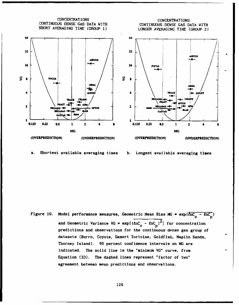
CONCENTRAT IONS CONCENTRATIONSCONTINUOUS DENSE GAS DATA WITH CONTINUOUS DENSE GAS DATA WITHSHORT AVERAGING TIME (GROUP 1) LONGER AVERAGING TIME (GROUP 2)

64 64

32 32

AARTOX _16 16 roas

Focus

4 4 TRMf4I1IPUV

2 .01-1 W GM4 2i~ MM AA W GMA

NIGADAS W,~ 4H~I

0.125 0.25 0.5 1 2 4 8 0.125 0.25 05 1 2 4 $

MG MG

(OVERPREDICTION) (UNDERPREDICTION) (OVERPREDICTION) (UNDERPREDICION)

a. Shortest available averaging times b. Longest available averaging times

Figure 10. Model performance measures, Geometric Mean Bias MG - exp(lnC - InC)

and Geometric Variance VG - exp[((nC - tnC )2] for concentration

predictions and observations for the continuous dense gas group of

datasets (Burro, Coyote. Desert Tortoise, Goldfish, Maplin Sands,

Thorney Island). 95 percent confidence intervals on MG are



agreement between mean predictions and observations.

124

scatter of slightly less than a factor of two. Note that the model (TRACE)

with the best geometric mean does not have the smallest variance, and the

model (GASTAR) with the smallest variance does not have the best geometric

mean.

b. Group 2: Continuous Dense Gas Releases with Long Averaging

Time, All Distances

Figure iOb shows the results for Group 2, for the same models

and datasets as Group I, but for concentrations associated with the "longest

available" averaging times (approximately equal to the duration of the

release). Actually, the only datasets that are altered by this distinction

between Groups I and 2 are Burro, Coyote, and Desert Tortoise, which comprise

approximately 1/3 of the data points in the combined set. Statistics tabulated

for Group 2 that are plotted in Figure 1Ob are listed in Appendix D-2.

Comparison of Figure 10b with Figure 10a shows, as expected, a shift of all

models towards the left of the figure (that is, towards the overprediction side).

The tendencies of the models to overpredict or underpredict In Figure lOb is

summarized below.


FOCUS


GASTAR, DEGADIS, TRACE, HEGADAS, PHAST


BM, AFTOX


CHARM, GPM, SLAB

Models that Underpredict by About a Factor of Two:

AIRTOX, OBDG, INPUFF

125

Except for the FOCUS and AIRTOX models, which have a relatively

large geometric variance (VG), all models have moderate values of VG, In the

range from about 2 to 5. These values indicate that the random scatter Is

typically about two to four times the mean. Five models (GASTAR, SLAB, GPM, and

BM) have the lowest values of VG. In this figure, It is Interesting that the

Gaussian plume model (GPM) has relatively low geometric mean bWas MG and

geometric variance VG, which may be a fortuitous result, since that model is

the simplest of all and does not include dense gas effects. However, another

possibility is that the centerline concentration in a plume is not highly

influenced by the plume density, since the changes In plume width are

compensated by changes in plume depth.

c. Group 4: Instantaneous Dense Gas Releases, All Distances

In order to keep the discussions of the dense gas datasets

together, we next consider Group 4, the Thorney Island (Instantaneous release)

trials. Figure 11 shows the results for Group 4 and the statistics are

tabulated in Appendix D-3. These results are markedly different from those

for the continuous releases of dense-gas clouds, since there is relatively

little random scatter (except for the DEGADIS model) and the variance for all

models tends to be dominated by the mean bias (that Is, the points lie near

the parabola marking minimum variance values, from Equation 33).

Analysis of the geometric mean bias, MG, In Figure 11 leads to

the following conclusions:

Models That Overpredict by More Than a Factor of Two:

INPUFF, AFTOX

Models that Overpredict by about a Factor of Two:

TRACE, FOCUS


BM, PHAST, DEGADIS


AIRTOX

126

CONCENTRATIONS, INSTANTANEOUS DENSE

GAS DATASET (GROUP 4) THORNFY ISLAND

64 1

AFrOX

32 Vt ,

16DEGADIS

~PUF CHAM

FOCUS

2 SLABPHAST o GAAR

AJRTOX

B&M~

12

0.125 0.25 0.5 1 2 4 8

MG

(OVERPREDICTON) (UNDERPREDICTION)

Figure 11. Model performance measures, Geometric Mean Bias MG = exp(InC - nC0 pand Geometric Variance VG =exp[((nC 0- InC p) 2 for concentration

predictions and observations for the Instantaneous dense gas data

from Thorney Island. 95 percent confidence Intervals on MG are

Indicated. The solid line Is the "minimum VG" curve, from



127


GASTAR

Models that Underpredict by About a Factor of Two:

SLAB, CHARM

There are two models (BM and AIRTOX) with relatively low

geometr1c variance of about 1.4 In Figure 11 Indicating a typical scatter less

than the mean. The AIRTOX model has the best geometric mean and the

second-best variance, while the BM model has the best variance and the

second-best geometric mean. The AFTOX and DEGADIS models have large variances.

d. Groups 1 and 4 (Dense Gas Releases), Distances > 200 m

Each of these evaluations for the dense-gas datasets in Groups

1, 2, and 4 include monitored and modeled concentrations at all downwind

monitoring arcs. However, comparisons of predicted and modeled concentrations

near the source may be misleading. Peak concentrations at the ground surface

in shallow clouds may not be adequately detected by monitors placed on short

masts above the ground (even at heights of I to 2 m), because the cloud may lie

nearer the surface. A bias could result from Insufficient resolution In either

the vertical or lateral array of samplers. Concentrations modeled at the

surface may appear to be overestimates in such cases, and overall performance

evaluations that Include these data may lead to inappropriate conclusions.

Therefore, we have reduced the number of data points in Groups 1 and 4 by

removing monitoring data from arcs closer than 200 m to the release point.

This criterion removes the closest monitoring arc In all of the dense-gas

datasets. The resulting statistics for this reduced set of data are tabulated

In Appendices D-4 and D-5, and are summarized for Groups I and 4 in Figures

i2a and 12b, respectively. With fewer data points, the 95 percent confidence

limits on the statistical measures Increase, especially for Group 4 (Thorney

Island--instantaneous), shown in Figure 12b.

After removal of the data from the closest monitoring arcs,

many of the models show a shift toward either less overpredictions or more

underpredictions (that is, the mean ratio C /C has decreased). This would be

128

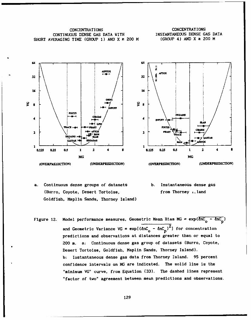
CONCENTRATIONS CONCENTRATIONSCONTINUOUS DENSE GAS DATA WITH INSTANTANEOUS DENSE GAS DATA

SHORT AVERAGING TIME (GROUP 1) AND X r 200 M (GROUP 4) AND X a 200 M

64 64-

-rO

32 32 *ArrxI

16 16

GPM G

TRAMro CootesrtTrtse from Tony•ln

I-W ArFQ

2 2DEGADE ~U&M

GASnAd MeAtri Vrn

0.125 0.25 0.5 1 2 4 o o.tis 0g25 0.5 1 2 4 t

MG MG

(OVERPMEDIMITON) (UNERPREDIMTON) (OVERPREDIC1TION) (UNERPREDICTON)

a. Continuous dense groups of datasets b. Instantaneous dense gas

(Burro, Coyote, Desert Tortoise, from Thorney neland

Goldfish, Maplin Sands, Thorney Island)

Figure 12. Model performance measures, Geometric Mean Bias MG = exp(onC 0n - &C

and Geometric Variance VG = exp[UnC 0- tnC p) 2 1 for concentration


200 m. a: Continuous dense gas group of datasets (Burro, Coyote,

Desert Tortoise, Goldfish, Maplin Sands, Thorney Island).

b: Instantaneous dense gas data from Thorney Island. 95 percent

* confidence Intervals on MG are Indicated. The solid line Is the"minimum VG" curve, from Equation (33). The dashed lines represent

"factor of two" agreement between mean predictions and observations.

129

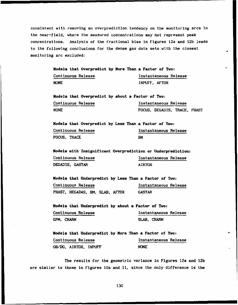
consistent with removing an overprediction tendency on the monitoring arcs in

the near-field, where the measured concentrations may not represent peak

concentrations. Analysis of the fractional bias in Figures 12a and 12b leads

to the following conclusions for the dense gas data sets with the closest

monitoring arc excluded:


Continuous Release Instantaneous Release

NONE INPUFF, AFTOX



NONE FOCUS, DEGADIS, TRACE, PHAST



FOCUS, TRACE BM

Models with Insignificant Overprediction or Underprediction:


DEGADIS, GASTAR AIRTOX



PHAST, HEGADAS, BM, SLAB, AFTOX GASTAR

Models that Underpredict by about a Factor of Two:


GPM. CHARM SLAB, CHARM

Models that Underpredict by More Than a Factor of Two:


OB/DG, AIRTOX, INPUFF NONE

The results for the geometric variance in Figures 12a and 12b

are similar to those in Figures lOa and 11, since the only difference is the

130

removal of the monitoring arcs with x < 200 m. With this change, most

variances were reduced slightly. The largest variance in Group I Is still

given by the AIRTOX model, and the largest variance in Group 4 is still given

by the AFTOX model. .he GASTAR and BM models still show good performance

for Group 4 (Thorney Island), although the AIRTOX model has "moved up" Into

one of the top three positions.

e. Groups 1 and 4 (Dense Gas Releases), Distances < 200 m

In order to assess the differences between model performance at

far and near monitoring arcs, the data for x < 200 m are presented in Figure

13. Any dense gas effects will be amplified at these close distances.

However, the observations may not indicate the true maximum concentration,

because of inadequate horizontal and vertical resolution of the monitoring

network.

Comparing Figures 12 and 13, it is seen that there indeed are

more cases of model overprediction at close distances. Because of the shifts

in the points, some of the models (for example, SLAB, GPM, TRACE, CHARM,

AIRTOX) demonstrate improved performance at close distances for the continuous

sources (parts a of the figures). Shifts also occur for the instantaneous

sources (parts b of the figures), with the performance of some models (for,

example, DEGADIS) deteriorating at the close distances, while the performance

of other models (for example, PHAST) improves.

f. Groups 3 and 5: Passive Gas Releases

The statistics for the passive gas releases in Group 3

(continuous passive-gas releases) and Group 5 (instantaneous passive-gas

releases) are tabulated in Appendices D-6 and D-7, and the plots of geometric

mean bias MG versus geometric variance VG are shown in Figures 14a and 14b,

respectively. Note that statistics for the continuous releases are dominated by

the Prairie Grass dataset, while those for instantaneous releases are derived

solely from the Hanford dataset.

The confidence limits on the geometric mean bias, MG, for the

continuous releases of passive gases shown in Figure 14a are small, because

131

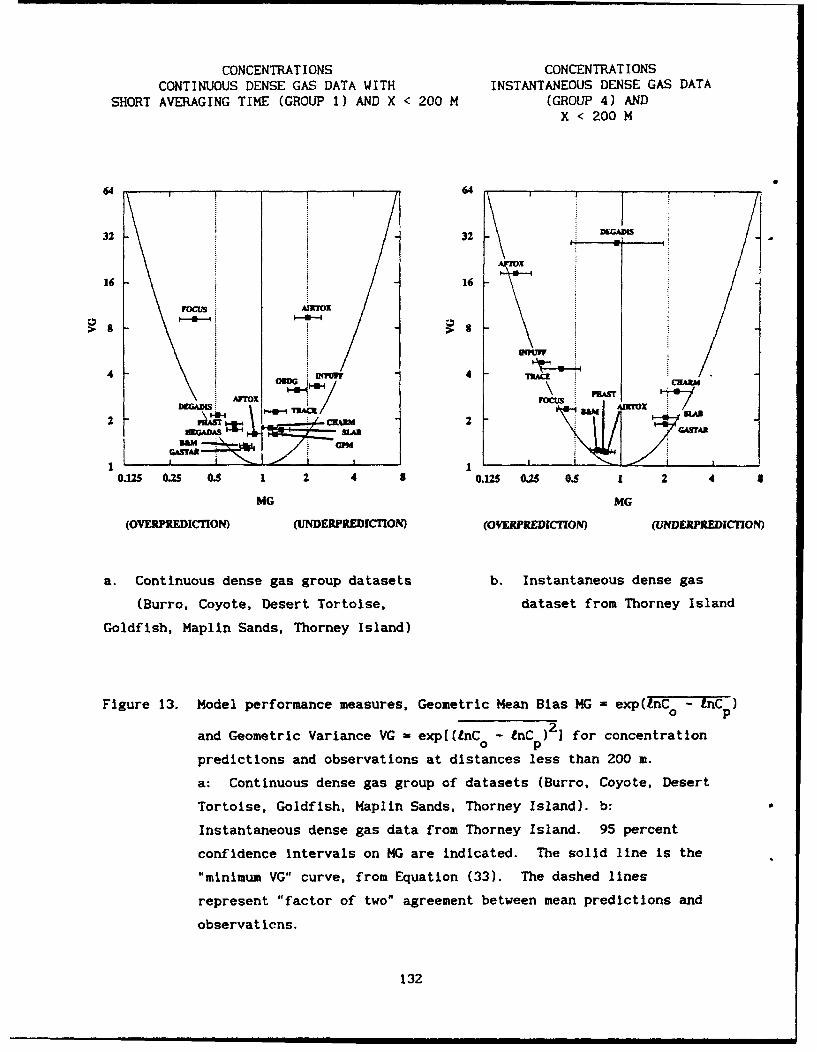
CONCENTRATIONS CONCENTRATIONSCONTINUOUS DENSE GAS DATA WITH INSTANTANEOUS DENSE GAS DATA

SHORT AVERAGING TIME (GROUP 1) AND X < 200 M (GROUP 4) ANDX < 200 M

64 r 64

32 32

16 16

44 TK~

Arrox rocu

2 r3**1Ua cEROM 2

0.125 0.25 0.5 1 2 4 .

MG MG

(OVERPREDICrION) (UNDERPREDrCION) (OVWREDICT7ON) (UNDEtPREDI•cnON)

a. Continuous dense gas group datasets b. Instantaneous dense gas

(Burro, Coyote, Desert Tortoise, dataset from Thorney Island

Goldfish, Maplin Sands, Thorney Island)

Figure 13. Model performance measures, Geometric Mean Bias MG = exp(InC - tnC )__ _ _o p

and Geometric Variance VG = exp[(unC - tnC 2) for concentrationpredictions and observations at distances less than 200 m.

a: Continuous dense gas group of datasets (Burro, Coyote, Desert

Tortoise, Goldfish, Maplin Sands, Thorney Island). b:

Instantaneous dense gas data from Thorney Island. 95 percent

confidence Intervals on MG are indicated. The solid line is the

"minimum VG" curve, from Equation (33). The dashed lines


observaticns.

132

CONCENTRATION CONCENTRATIONCONTINUOUS PASSIVE RELEASES INSTANTANEOUS PASSIVE RELEASES

(GROUP 3) (GROUP 5)

64 64

32 32

16 16

4 C 4

*4 G MG

TRAME : " HA CRAIM

(OVERPREDICTrIoN (UNDERPREDICTION)OEPEITO (NEPEITO

a. Continuous passive gas group of b. Instantaneous passive gas dataset

datasets (Prairie Grass and from Hanford

Hanford-continuous)

Figure 14. Model performance measures, Geometric Mean Bias MG = exp(lnC - InC)__ _ _o p

2 2

and Geometric Variance VO = exp[(LnC - InC )2] for concentrationo p

predictions and observations, a: Continuous passive gas group of

datasets (Prairie Grass and Hanford-continuous). b: Instantaneouspassive gas dataset from Hanford. 95 percent confidence intervals

on MG are indicated. The solid line is the "minimum VG" curve,

from Equation (33). The dashed lines repres p t "factor of two"


133

the Prairie Grass dataset provides many data-points. The GASTAR, TRACE, and

CHARM models have relatively large variances. The geometric mean biases for

Group 3 can be summarized as follows:


TRACE, GASTAR


AFTOX, DEGADIS, HEGADAS, SLAB


INPUFF, GPM, OBDG, PHAST, FOCUS, AIRTOX

The models with the lowest variance (VG - 1.5) for Group 3 are

the HEGADAS and SLAB models. The magnitude of the scatter for these models is

slightly less than the mean value. The good performance of the HEGADAS model

is surprising and probably fortuitous since that model is being initialized

assuming a small area source, whereas the actual release was a small point

source. A group of other models (AIRTOX, DEGADIS, OBDG, FOCUS, GPM. INPUFF,

PHAST, and AFTOX) have relatively low VG values in the range from about 1.6 to

2.2, indicating that their scatter is approximately equal to the mean.

The Hanford dataset (Group 5) In Figure 14b has few numbers,

leading to a large span in 95 percent confidence limits for the geometric mean

bias, MG. Even so, all of the models tend to overpredict the peak

concentrations on average. The GASTAR, AIRTOX, PHAST. INPUFF, and CHARM

models have the best performance, with mean overpredictions of about 10 to SO

percent and scatters approximately equal to the mean. The TRACE model is

unique in Its very large degree of overprediction.

g. Analysis of Differences among Models

Up to this point we have characterized the tendency of each

model to either overpredict or underpredict peak concentrations, based on the

statistical measure, but we have not selected a "best" model. One way to

characterize a "best" group of models is to Identify the models with the

134

smallest mean bias and the smallest scatter, and then ask the question: which

other models have a bias or a scatter which is not significantly different

from that of the "best" model? The answer provides one basis for defining the

"best" group of models.

Appendix D-8 contains tabulations showing whether or not the

difference in the geometric variance between pairs of models is significantly

different from zero, at the 95 percent confidence level. Consider first the

results for the continuous releases of dense gas shown in Figure 12a (Group 1,

for distances greater than 200 m). GASTAR appears to have the best overall

performance, but we see that its variance is not significantly different from

the variance for HEGADAS. However, we see that the geometric mean bias MG

found for GASTAR is significantly different from and closer to zero than the

bias for the HEGADAS model, although there is no difference between the biases

of the GASTAR and DEGADIS models. We conclude that, in general, this group of

three models does a better Job than the others of matching the peak observed

concentrations at distances of 200 m or greater for continuous releases of

dense gases.

A summary of model performance for the better performing models

at distances greater than 200 m is given in Table 13 for Data Groups 1, 3, 4,

and 5. There are no models that appear on the list of better models for all

four data groups.

h. Analysis of Model Performance for Stable Ambient Conditions

Another facet of model performance that can be evaluated with

these data is the question of how the models perform for the subset of the

dense-gas data for which the atmospheric stability class is either E or F

(that is, stable ambient conditions). Because "worst-case" dispersion

conditions are usually found for these stabilities, many model applications

focus on these stable ambient conditions. Figures 15a and 15b show the

geometric mean bias (MG) and geometric variance (VG) results, and the

statistics themselves are tabulated in Appendices D-9 and D-10 for the

continuous and passive dense-gas releases, respectively.

135

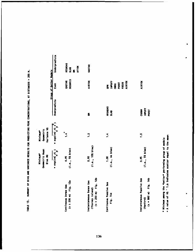
W46' 04 .

40 0

41.

AAI

tv I

31 gt41-

4c w

SA D 0 b t A

c4 a 30.

136U

CONCENTRAT IONS CONCENTRAT IONSCONTINUOUS DENSE GAS DATA WITH SHORT INSTANTANEOUS DENSE GAS DATA

AVERAGING TIME (GROUP 1) X t 200 M, (GROUP 4) X t 200 M, AND STABLEAND STABLE AMBIENT CONDITIONS AMBIENT CONDITIONS

64 64

Sii32 32

16 16

OBOG

>88

CRA*M

4 04

2 sro D t h rnaeyGASIsan~STAI C 0M

TotisGldih MGli ans

Thorney Island )

Figure 15. Model performance measures, Geometric Mean Bias MG = exp(2nC - 9nC

and Geometric Variance VG =exp[ (nC - InC )2] for concentrationo p


200 m for STABLE (class E, F) conditionst a: Continuous dense gas

*group of datasets (Burro, Coyote, Desert Tortoise, Goldfish, Maplin

Sands, Thorney Island). b: Instantaneous dense gas data from

Thorney Island. 95 percent confidence intervals on MG are


Equation (33). The dashed lines represent "factor of two"agreement between mean predictions and observations.

137

Sads Th e Isan) b: Intnaeu des ga daafo

Comparing Figure iSa with Figure 12a, which includes all

ambient stabilities, the models tend more towards overpredictions of peak

concentrations during stable ambient conditions. In fact, only the OB/DG

model shows a significant underprediction in Figure 15a. Although confidence

limits are large due to the smaller number of points, one group of models

appears to provide better performance. This group Includes BM, HEGADAS, SLAB,

CHARM, GASTAR, AFTOX, and INPUFF. Note that when the unstable and neutral

ambient conditions are eliminated, the FOCUS model performance greatly

improves.

Comparing Figures 15b and 12b, which both apply to

instantaneous releases of dense gases, it is seen that the models show a

greater tendency towards underpredictions during stable conditions. As

before, the variance is dominated by the mean bias for most models. However,

all the 95 percent confidence limits on the mean bias are fairly broad, since

this sample of the dataset contains few points. The performance of the

AIRTOX, B&M, and TRACE models is fairly good, while the performance of the

AFTOX, CHARM, DEGADIS, and INPUFF models is relatively poor.

2. Cloud Widths (a )

Another measure of model performance is the ability of the model to

simulate cloud widths, which are very important for defining regions of toxic

impacts. Figures 16a and 16b show the geometric mean bias MG and geometric

variance VG results for predicting the width of the clouds for continuous

dense-gas releases and continuous passive-gas releases, respectively. The

corresponding statistics are tabulated in Appendices D-11 and D-12. These

figures correspond to the performance measures for concentration predictions

in Figures lOb and 14a. Comparing the figures, it is immediately evident that

predictions of the widths are generally more successful, overall, than are the

predictions of concentration. The largest values of variance are smaller,

probably due to the smaller range of observed values of cloud widths.

Furthermore, the variations in variance are largely due to variations in mean

bias, as expressed by Equation (33).

138

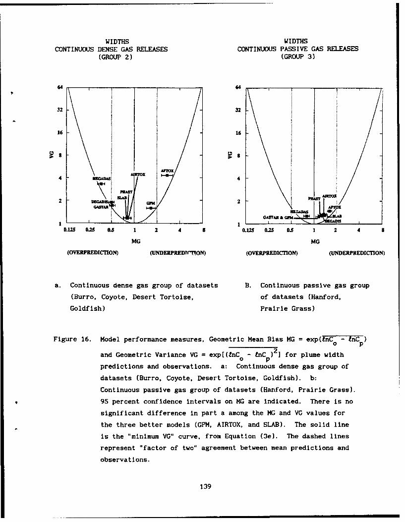
WIDTHS WIDTHSCONTINUOUS DENSE GAS RELEASES CONTINUOUS PASSIVE GAS RELEASES

(GROUP 2) (GROUP 3)

32 32

16 16

4 113cA S 4

2 GM2

1AA Ar GITR

0.2 0.25 0. 1 2 4 8 0.15 0.25 0.5 1 2 4

MG MG

(OVERPREDICON) (UNDERPREDI!ON) (OVERPREDICTION) (UNDERPREDICTION)

a. Continuous dense gas group of datasets B. Continuous passive gas group

(Burro, Coyote, Desert Tortoise, of datasets (Hanford,

Goldfish) Prairie Grass)

Figure 16. Model performance measures, Geometric Mean Bias MG = exp(tnC - tnC )

and Geometric Variance VG = exp[(InC - tnC ) 2] for plume widtho p

predictions and observations, a: Continuous dense gas group of

datasets (Burro, Coyote, Desert Tortoise, Goldfish). b:

Continuous passive gas group of datasets (Hanford, Prairie Grass).

95 percent confidence Intervals on MG are indicated. There is no

significant difference in part a among the MG and VG values for

the three better models (GPM, AIRTOX, and SLAB). The solid line

is the "minimum VG" curve, from Equation (3e). The dashed lines


observations.

139

For the dense-gas releases, models such as GPM and AFTOX that do not

treat dense gases (and hence dense gas slumping) underpredict the width, as

might be anticipated. The other models that do simulate dense gases tend to

overpredict. AIRTOX, PHAST, and SLAB overpredict the width by less than about

30 percent, on the average. DEGADIS, GASTAR, and HEGADAS overpredict the

width by a factor of two or more.

For the passive releases, only HEGADAS tends to overpredict the

widths. The rest underpredict by a small amount. There is no distinction

between the performance of the simple passive dispersion model, GPM, and the

dense-gas models. Overall, it is interesting to note that the models tend to

slightly underpredict the width, and overpredict the peak concentrations

resulting from continuous releases of passive gases.

140

SECTION V

SCIENTIFIC EVALUATION BY MEANS OF RESIDUAL PLOTS

A. PROCEDURES

One way of evaluating the scientific credibility of a model is through

the use of residual plots, where "residual" is defined in this application as

the ratio of the predicted to the observed concentration (note that the

logarithm of this ratio equals the difference between the logarithm of the two

concentrations). In other applications, the residual could be defined as the

arithmetic difference between the observed and predicted concentrations.

Values of the residual can be plotted versus variables such as wind speed or

stability. The residual of a good model (1) should not exhibit any trend with

variables such as wind speed and stability class, and (2) should not exhibit

large deviations from unity (implying a perfect match between the model and

the observed). The SIGPLOT plotting package described in Volume I was used to

generate the residual plots for this evaluation.

The residuals are grouped for plotting by means of "box plots."

Grouping is usually necessary because of the large number of data points.

The cumulative distribution function (cdf) of the residuals within each group

is represented by the 2nd, 16th, 50th, 84th, and 98th percentiles. These five

significant points in the cdf are then plotted in a "box" pattern. As

mentioned above, the residual boxes should not exhibit any systematic

dependence on primary variables. It is also desirable that the residual boxes

should be compact and should not deviate too much from unity.

B. RESULTS

Residuals for the continuous dense-gas releases are shown in Figure 17,

where four "variables" are used: downwind distance (XM, ambient wind speed

(U), ambient Pasquill-Gifford stability class (PG CLASS), and the number of

the experiment (EXPERIMENT). The PG CLASS numbers follow the normal

convention in which 1 = very unstable (A), 2 = unstable (B), 3 = slightly

unstable (C), 4 = neutral (D), 5 = slightly stable (E), and 6 = stable (F).

The number of the experiment is based on the following alphabetical ordering

of the datasets:

141

iiCP '4 i t-'

-6 13s #4

C(4

'441

m/i~~0 0nos'w

00 ) 06 41.4. i. 1 . E

oe 41 0 t ) 4

40 a0 10

to 0 (d .9. 0 U

*~~ 04 41.4N ~.441 q - C

IU 4o- 0

It4 3*=4)24

3X=3.14 0 c -0 0

f FE ) V r 0

0 41- 0 0 1 U**3~~~~g CI! E ~ ; ~ * ! ) C 0 -

-4 ) 1 -. fl -4( . -it O0

4) %0

Ii. 4)

'140

0et-U flC 1

a0 U).4C

I * 0.00-4 0 -.4

1 42h~ .) I '. ~ 4

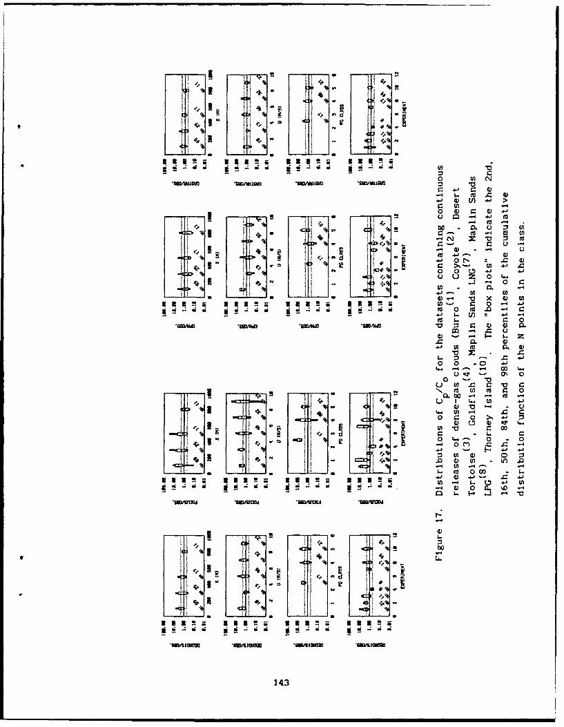
44

(-ch u~ ~-- no I

41

o n 0Z a n-) 0 0 A

.-4 0. m .0 0

.4- " n4 -4

to "O r. 0~

V Y2 = . 0 Q.

34- >,n rn .- '

0 0 .0*~ -

4- -44 - - ý 00 o0. -

.- 1- 44J w 4- P -

4t 4ý th0 . 0 )

V)- Vn a 004

o0 (no44-4 A4j 41

V u- W V.0 ( In . U l

W b0 (U

Im v

1 * 4 4444. I -I .

oi 1] 411.4'

a i 3-~ a143~.-

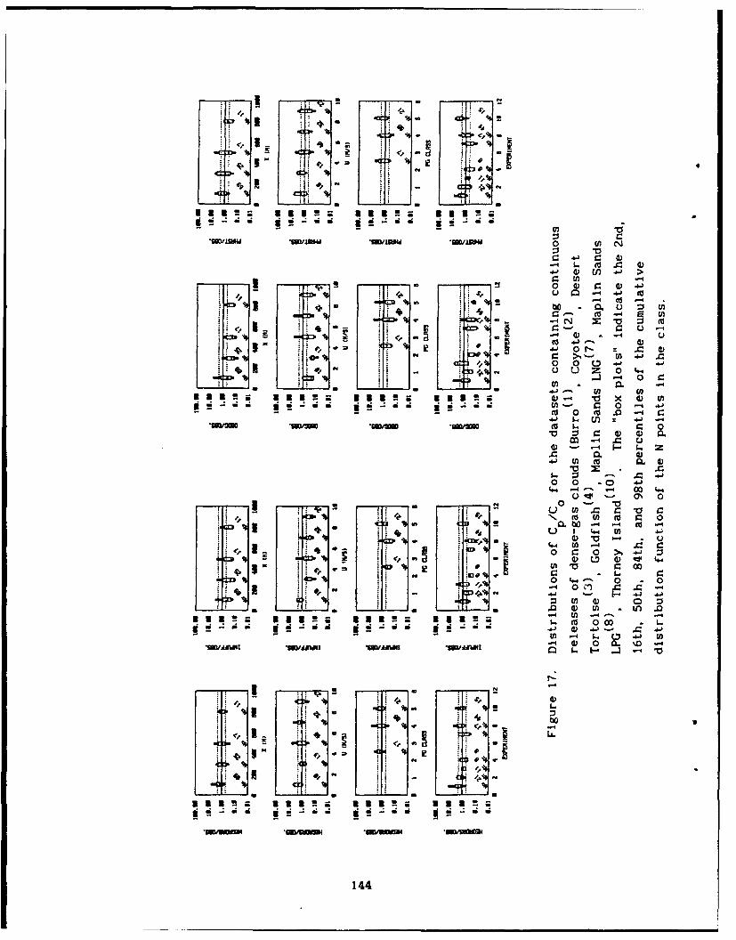
C, t C -

L 4 1-0 . -

-- z L

0 n >

00 ~

tl- 4 f

o r- c .4 -04 0.0 ~ I

0 0-(,U~~U a 40 --

4V Nx O 041 - 0 m. .0-

V 0 Z 0 '4-a

-4 - -4 00* -0 - 0%- 0

0 - V0 .w CU 9. v 0

u 1 64 En C

r_ 00

0 0 0o~-

0 11) C

U0 c .L n .n .tA -4 0b - -41

0D 0 * U

4100 '.~

41 ~ ~ i ei 4 0A,isn 0

* - -,0 0 In - LA %

3U3!~ li!~ **.~ *1in -WIn -

~ * ! n *d **1- U 0144I

0n U) N:3 10

0 0 0 Q

4). 0A C 1 > 00 -4 L)

0 0 4' "1C

0; :0 01 4_ .. ~4 0 C:

-p -4 .41r in

*~ !0 00 0.cd m.00

0.0 0.

44. 4> 0 0 40w.

(U Cr ON 00

(d'. -n 0. d r_'. 0U00 -4 . cc - C

L) 44. (-4 0 bjI>. d)u U ~(.

00 r. 00 nif do *a r. 00

20 0 0a a a .1.4 02 -) = -4

0-4 -. 4 .."4 0 0 00 L.

-4

w

145

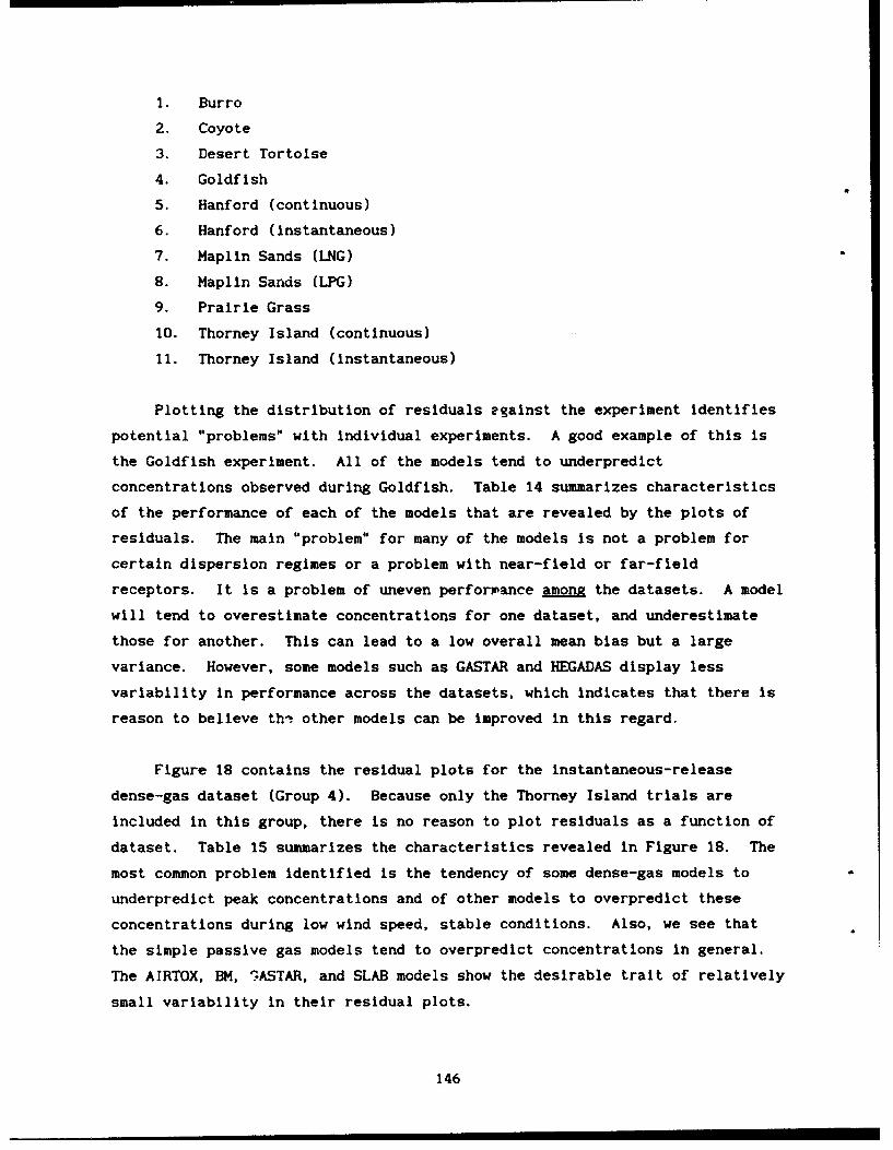
I. Burro

2. Coyote

3. Desert Tortoise

4. Goldfish

5. Hanford (continuous)

6. Hanford (instantaneous)

7. Maplin Sands (LNG)

8. Maplin Sands (LPG)

9. Prairie Grass

10. Thorney Island (continuous)

11. Thorney Island (instantaneous)

Plotting the distribution of residuals egainst the experiment identifies

potential "problems" with individual experiments. A good example of this is

the Goldfish experiment. All of the models tend to underpredict

concentrations observed during Goldfish. Table 14 summarizes characteristics

of the performance of each of the models that are revealed by the plots of

residuals. The main "problem" for many of the models is not a problem for

certain dispersion regimes or a problem with near-field or far-fleld

receptors. It is a problem of uneven performance among the datasets. A model

will tend to overestimate concentrations for one dataset, and underestimate

those for another. This can lead to a low overall mean bias but a large

variance. However, some models such as GASTAR and HEGADAS display less

variability in performance across the datasets, which indicates that there is

reason to believe thi other models can be improved in this regard.

Figure 18 contains the residual plots for the instantaneous-release

dense-gas dataset (Group 4). Because only the Thorney Island trials are

included in this group, there is no reason to plot residuals as a function of

dataset. Table 15 summarizes the characteristics revealed in Figure 18. The

most common problem identified is the tendency of some dense-gas models to

underpredict peak concentrations and of other models to overpredict these

concentrations during low wind speed, stable conditions. Also, we see that

the simple passive gas models tend to overpredict concentrations in general.

The AIRTOX, BM, 'ASTAR, and SLAB models show the desirable trait of relatively

small variability in their residual plots.

146

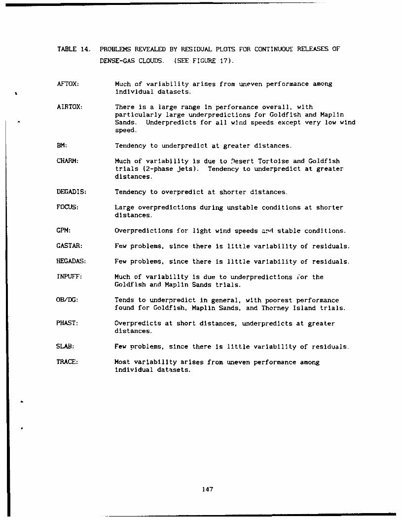
TABLE 14. PROBLEMS REVEALED BY RESIDUAL PLOTS FOR CONTINUOUS RELEASES OF

DENSE-GAS CLOUDS. (SEE FIGURE 17).

AFTOX: Much of variability arises from uneven performance amongindividual datasets.

AIRTOX: There is a large range in performance overall, withparticularly large underpredictions for Goldfish and MaplinSands. Underpredicts for all wind speeds except very low windspeed.

BM: Tendency to underpredict at greater distances.

CHARM: Much of variability is due to Desert Tortoise and Goldfishtrials (2-phase Jets). Tendency to underpredict at greaterdistances.

DEGADIS: Tendency to overpredict at shorter distances.

FOCUS: Large overpredictions during unstable conditions at shorterdistances.

GPM: Overpredictions for light wind speeds and stable conditions.

GASTAR: Few problems, since there is little variability of residuals.

HEGADAS: Few problems, since there is little variability of residuals.

INPUFF: Much of variability is due to underpredictions ior theGoldfish and Maplin Sands trials.

OB/DG: Tends to underpredict in general, with poorest performancefound for Goldfish, Maplin Sands, and Thorney Island trials.

PHAST: Overpredicts at short distances, underpredicts at greaterdistances.

SLAB: Few problems, since there is little variability of residuals.

TRACE: Most variability arises from uneven performance amongindividual datasets.

147

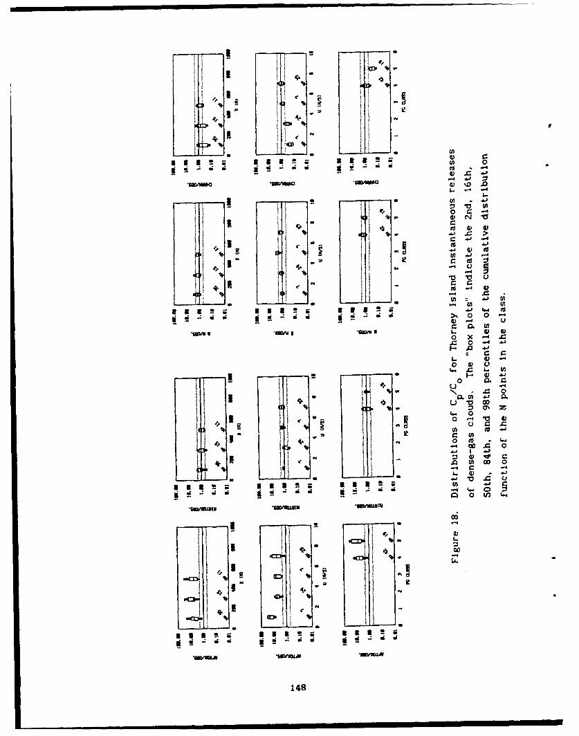
S a

L, it- 0

4>5MN VD~k

~~mot w= 1~ 4

I IA

a* co9-

9' tv

4>5-4

M i 0 - 4 4

* aact I-4 ) .

U 0.

148.~

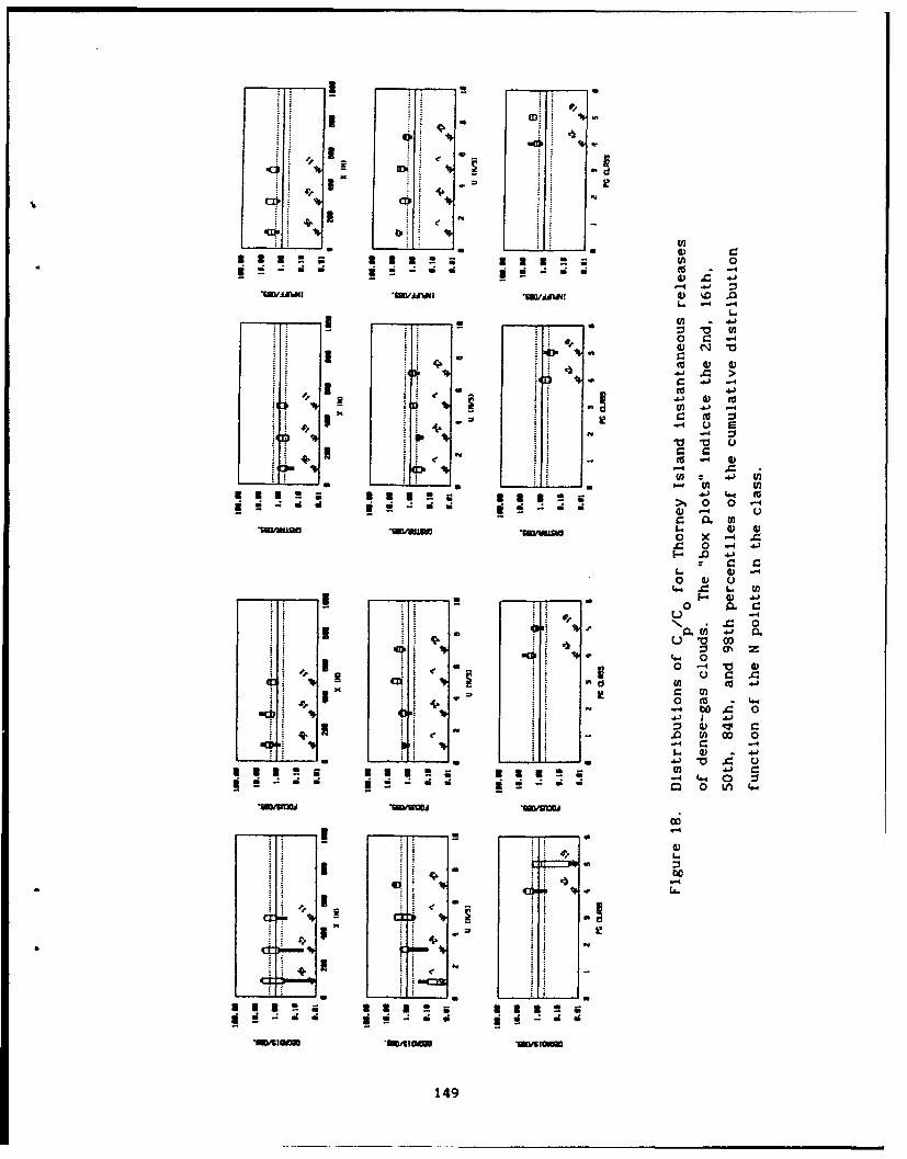
I a 2

ii.

*0 -D V

&J, -4

0 0

u

a a 0 0

U) 0

•i .- 4)=:o

/ 4 a0 4'0 -

•u ..0,. ,-- 0

4

0

.)0

41,U .0 W D

C U

Q 40 E 4

C- a i ) U

3U3!

1049

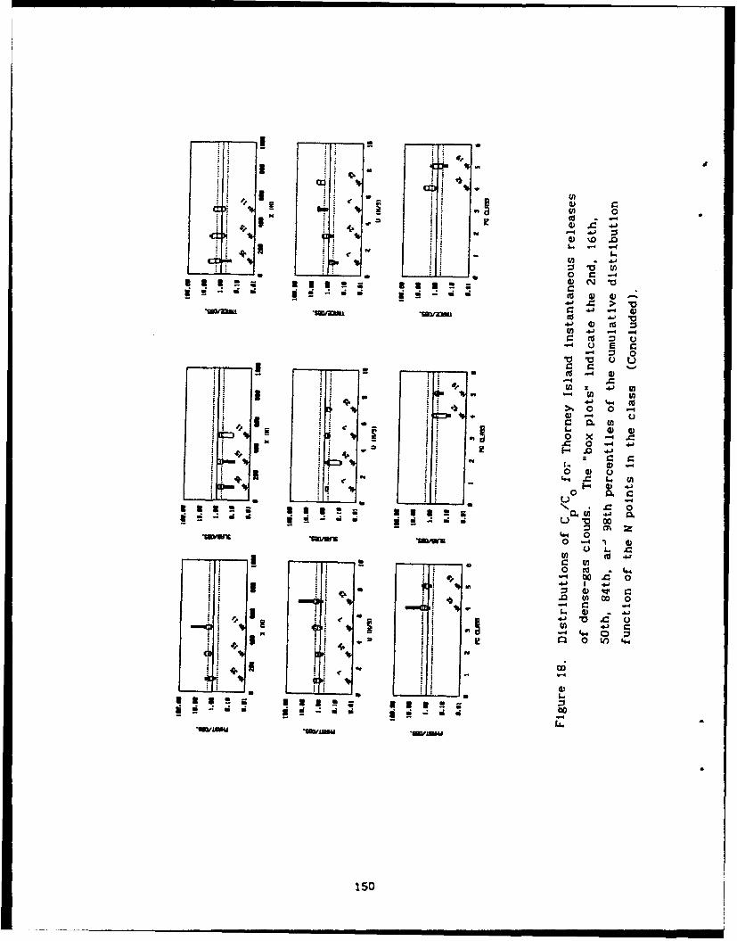
i ' 9-,"

U ~4Pdi Ii oPd_

41 P I: .,..4

UO/l I ,i4 o0u E

0 0U 4 0

9 i v I - 000

: ... +.+.. +(. ,l - L. 43,

9 i=' . + l . H - , -..

005P 0 1o.. In

4.4 04

q 2' 0 to

m* DO

333!; 3u~l w0

150L~I4' 0

TABLE 15. PROBLEMS REVEALED BY RESIDUAL PLOTS FOR INSTANTANEOUS DENSE-GASCLOUDS (THORNEY ISLAND). (SEE FIGURE 18).

AFTOX: Large overpredictions; worse for light wind speed, stableconditions

AIRTOX: Few problems, since there is little variability in residualplots.

BM: Few problems, since there is little variability in residualplots.

CHARM: Underpredicts during low wind speed, stable conditions, atshort distances.

DEGADIS: Underpredicts during low winds and overpredicts during highwinds.

FOCUS: Moderate overpredictions throughout, with little variability.

GASTAR: Few problems, since there is little variability in residualplots.

INPUFF: General overpredictions throughout, with little variability.

PHAST: A few large overpredictions during high wind speed conditions.

SLAB: Few problems, since there is little variability in residualplots.

TRACE: Underpredicts during low wind speed conditions andoverpredicts during high wind speed conditions.

151

Because there are few data-points in the dataset for Instantaneous

releases of passive-gas clouds (Hanford), we have not produced residual plots

for this dataset (Group 5). The plots for continuous releases of passive-gas

clouds (Prairie Grass - Group 3) are shown in Figure 19, and the results are

summarized in Table 16. Among the models designed for dense-gas clouds,

several tend to increasingly overpredict concentrations during increasingly

unstable conditions or higher wind conditions. The CHARM, GPM, HEGADAS,

INPUFF, and SLAB models have the desirable trait that there is relatively

little variability in their residual plots for this group of data.

152

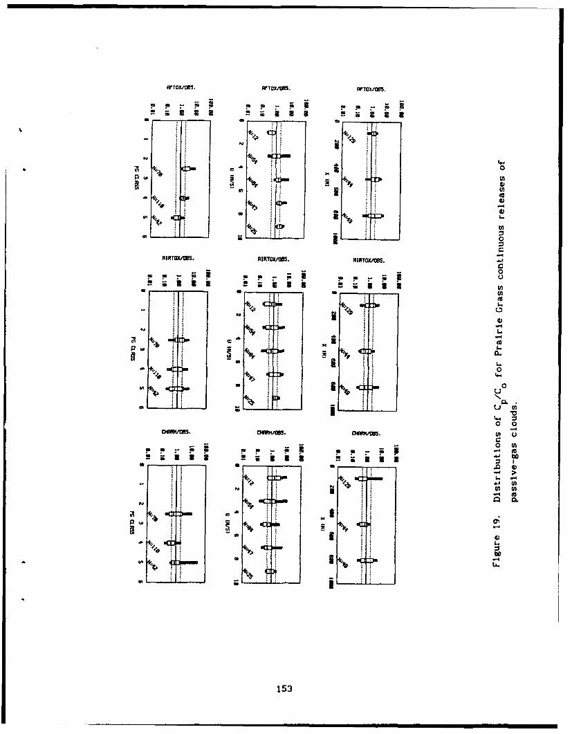
FTU/ .FFTOX/tIB. WTOc/iS TXIWS.

N 3ý

0

- l

0

U')

(d

oa, J 0

44

00mmR/05 UHRKM .MX5 *n - ia

40

-414.

153U

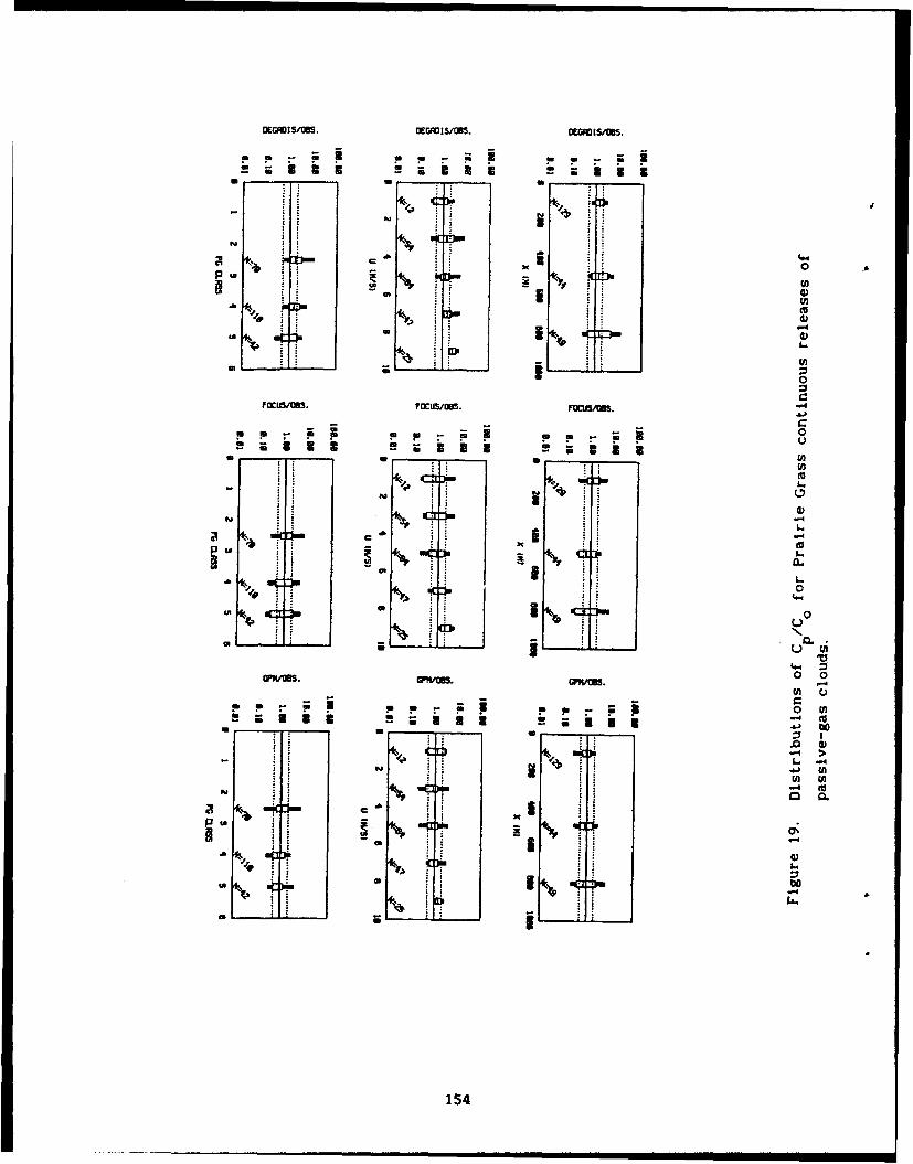
I~G~I/US.DEGADIS/08S. MMeI3SM.

- aU

FOCUS/ . 2OU/05 313S/

&0

U)uK 110

oc' J. a U

3.

u u00

WHAMS. 3. 7asS. ..r.'

LL.

1544

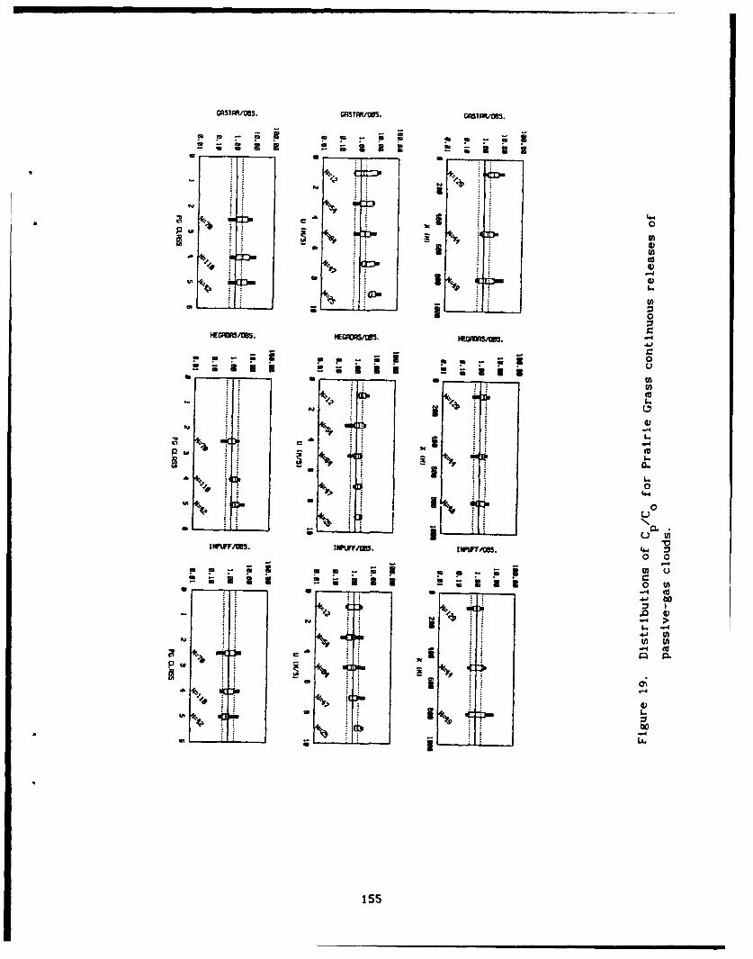
GATUO.GR3TTAt/S. GRS1AOBS.

4-,11433

qSJq

* 04C k*

-~00

Mmas EGADIS/. HGDS0

CD-.

06

MWW

ti

U4

'44

Ps155

a ok a

-k IN A1

P) P

U'd

0 u

0 0

(U)

-4

'a 3j

ItU)

156

TABLE 16. PROBLEMS REVEALED BY RESIDUAL PLOTS FOR CONTINUOUS PASSIVE-GAS

CLOUDS (PRAIRIE GRASS). (SEE FIGURE 19).

AFTOX: Slightly underpredicts during light wind speed, stableconditions.

AIRTOX: Trend towards underpredictions at greater distances, lightwinds, and stable conditions.

CHARM: Few problems, since there Is little variability in residualplots.

DEGADIS: Overpredicts slightly in general, but with little variabilityin residual plots.

FOCUS: Relative underpredictions at low wind speeds andoverpredictions at high wind speeds.

GPM: Few problems, since there Is little variability in residualplots.

GASTAR: Overpredicts at shorter distances and higher wind speeds.

HEGADAS: Few problems, since there is little variability in residualplots.

INPUFF: Few problems, since there is little variability In residualplots.

OB/DG: Underprediction tendency during light wind speeds.

DHAST: Overpredicts during high wind speed conditions.

SLAB: Few problems, since there Is little variability in residualplots.

TRACE: Overpredicts with increasingly higher winds and unstabledispersion conditions

157

SECTION VI

SENSITIVITY ANALYSIS USING MONTE CARLO PROCEDURES

A. OVERVIEW

The Monte Carlo method is one way of estimating the magnitude of model

uncertainties due to input data errors. The method involves running the model

multiple times, with the input parameters slightly perturbed each time (see

Volume I, Section IX). It is necessary to implement the Monte Carlo

sensitivity analyses on a platform where the user can easily run the model

repeatedly, efficiently extract the information of interest, and not be

overwhelmed by the amount of the output generated. The MDA (Modeler Data

Archive) software package previously described in this volume serves as an

ideal choice for this platform in that the execution of most of the dispersion

models has been automated, and in that the extraction of useful information

from the outputs can be achieved by the post-processors that have already been

developed. In the following, we shall call the software package that

implements the Monte Carlo method MDAMC.

B. CHOICE OF MODELS AND INPUT PARAMETERS

There are some important criteria that should be heeded in choosing

specific dispersion models for application of the Monte Carlo sensitivity

analyses. First, it is desirable that the input, the execution and the

post-processing of the model be fully automated. Second, it is desirable that

the model can execute reasonably fast (say, less than 10 seconds for each run),

since it is necessary to run the model hundreds to thousands of times. Last,

as a somewhat less stringent requirement, the model should have a simple I/O

structure, such as a small number of compact input and output files are

involved. Based on these criteria, the SLAB model was chosen for

testing of MDAMC. The AFTOX, DEGADIS, GASTAR and GPM models also satisfy these

criteria, but were not used in the sensitivity study reported in this section.

The input parameters accepted by the models can be classified as primary

and secondary. Secondary input parameters are derived from the primary input

parameters. Wind and temperature measurements, and surface roughness are the

examples of primary input parameters. Monin-Obukhov length and stability class

are the examples of secondary input parameters. In the Monte Carlo study, only

158

variations in the primary input parameters are considered. The following seven

primary input parameters are perturbed at each Monte Carlo simulation in our

example:

domain averaged wind speed (u),

* difference in wind speed between the domain-average and a tower (du),

* difference in temperature between two levels on a tower (dW),

* relative humidity (RH),

* surface roughness (zo).

• source emission rate (0), and

* source diameter (D).

The first four parameters are related to the meteorology, the fifth

parameter is related to the site condition, and the last two parameters are

related to the source condition. In this application, it is assumed that there

is no correlation among the primary input parameters. Other secondary

variables such as Monin-Obukhov length, friction velocity, and stability

parameter are calculated from the above seven primary parameters.

Currently, the MDAMC package uses Qoncentrations and cloud widths at

certain downwind distances as indicators of model uncertainty due to input data

errors.

Perhaps the most difficult problem encountered in Monte-Carlo sensitivity

analyses is the specification of the distributions of the primary input

parameters. The Gaussian distribution (for example, Reference 71) and the

log-normal distribution (for example, Reference 72) are common choices for

many ambient measurements. However, there is a lack of knowledge about the

distributions for some parameters. Moreover, in the case of the surface

roughness and the source emission rate, the need for a detailed description of

their distributions becomes less clear. O'Neill et al. (Reference 73) found

out the results of a Monte Carlo analysis of their stream ecosystem model were

not sensitive to the choice of parameter distributions. Therefore, it was

decided that a simple uniform distribution would be used for all parameters in

this example. For a uniform distribution the probability of occurrence of the

parameter is the same at all points within an upper and lower bound. Outside

of these bounds, the probability of occurrence is zero.

159

The range of a parameter is the only information needed to fully define a

uniform distribution. The ranges of uncertainties associated with

meteorological observations depend on the kind of the instrument used, the

averaging time, the orientation with the wind direction, and the atmospheric

stability (see Volume III of this report). For simplicity, the MDAMC package

assumes the following default values for the ranges of uncertainties for the

input parameters; however, the user always has the option of specifying his

own ranges.

wind speed (u and du): the mean ± larger of 0.5 m/s and

temperature difference (dT): the mean ± 0.2 0 C

relative humidity (RH): the mean ± 10 percent

surface roughness (z ): the mean ± 1/2 order of magnitudesource emission rate {Q): the mean ± 1/2 order of magnitude

source diameter (D): the mean ± 1/2 order of magnitude

For example, if the observed domain-averaged wind speed, u, is 5.6 m/s and

the standard deviation, a', is 0.9 m/s, is the wind speed for each Monte Carlo

simulation will be drawn randomly from the range between 4.7 and 6.5 m./s. If

the reported surface roughness is 0.0316 m, the surface roughness for each

Monte Carlo simulation will be drawn randomly from the range between 0.01 and

0. 1 m.

C. IMPLEMENTATION

During the execution of MDAMC, the user has to specify: 1) a dispersion

model whose uncertainty due to data input errors is to be investigated, 2) a

trial from which perturbations on the primary input parameters will be created,

3) the number of Monte Carlo simulations to be made, and 4) the ranges for the

primary input parameters, if the default values provided by the program were

not desired.

The output file created by MDAMC echoes most of the user inputs just

described previously. As an option, the file lists the values of the input and

output parameters for each Monte Carlo simulation. Finally, the file includes

the minimums, maximums, means and standard deviations for all the parameters

160

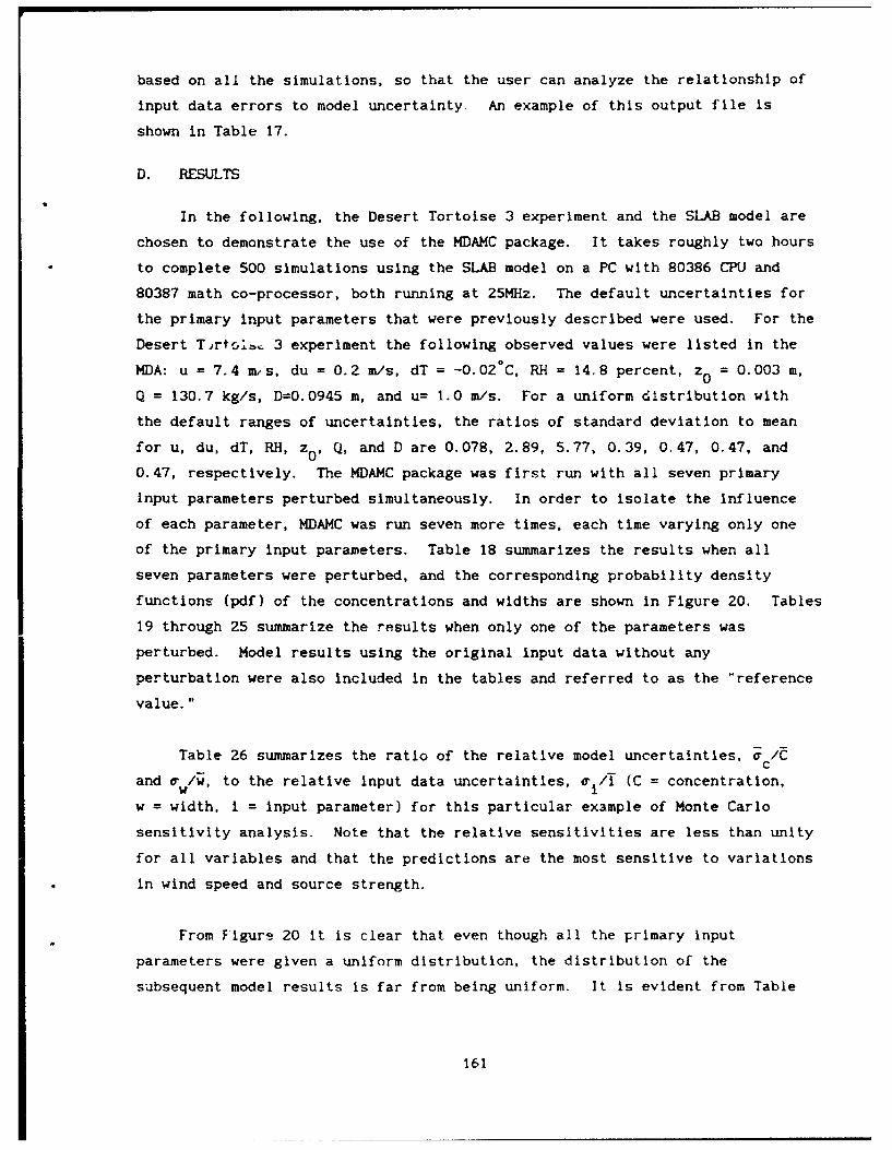
based on all the simulations, so that the user can analyze the relationship of

Input data errors to model uncertainty An example of this output file is

shown in Table 17.

D. RESULTS

In the following, the Desert Tortoise 3 experiment and the SLAB model are

chosen to demonstrate the use of the MDAMC package. It takes roughly two hours

to complete 500 simulations using the SLAB model on a PC with 80386 CPU and

80387 math co-processor, both running at 25MHz. The default uncertainties for

the primary input parameters that were previously described were used. For the

Desert Tortc!,, 3 experiment the following observed values were listed in the

MDA: u = 7.4 m/s, du = 0.2 m/s, dT = -0.020 C, RH = 14.8 percent, z0 = 0.003 m,

Q = 130.7 kg/s, D=0.0945 m, and u= 1.0 m/s. For a uniform distribution with

the default ranges of uncertainties, the ratios of standard deviation to mean

for u, du, dT, RH, zo, Q, and D are 0.078, 2.89, 5.77, 0.39, 0.47, 0.47, and

0.47, respectively. The MDAMC package was first run with all seven primary

Input parameters perturbed simultaneously. In order to isolate the influence

of each parameter, MDAMC was run seven more times, each time varying only one

of the primary input parameters. Table 18 summarizes the results when all

seven parameters were perturbed, and the corresponding probability density

functions (pdf) of the concentrations and widths are shown In Figure 20. Tables

19 through 25 summarize the results when only one of the parameters was

perturbed. Model results using the original input data without any

perturbation were also included In the tables and referred to as the "reference

value."

Table 26 summarizes the ratio of the relative model uncertainties, a /Cc

and aw/w, to the relative Input data uncertainties, ai/I (C = concentration,

w = width, I = Input parameter) for this particular example of Monte Carlo

sensitivity analysis. Note that the relative sensitivities are less than unity

for all variables and that the predictions are the most sensitive to variations

in wind speed and source strength.

From Figure 20 It is clear that even though all the primary Input

parameters were given a uniform distribution, the distribution of the

subsequent model results is far from being uniform. It is evident from Table

161

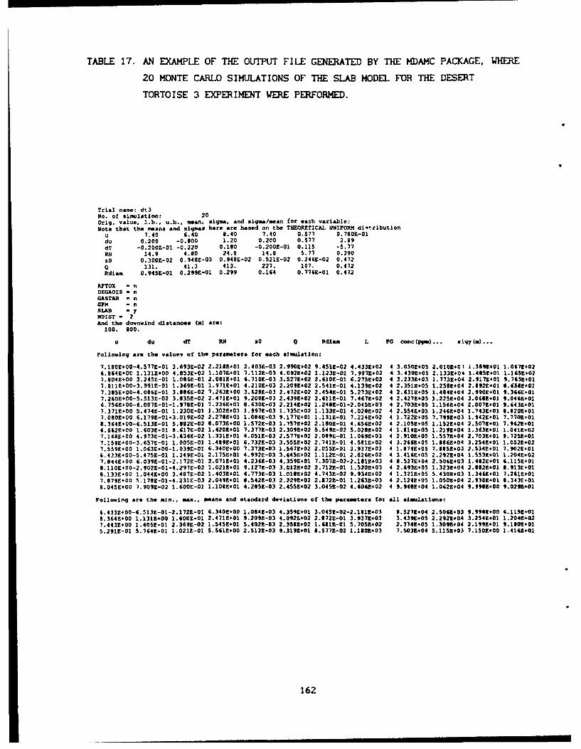
TABLE 17. AN EXAMPLE OF THE OUTPUT FILE GENERATED BY THE MDAMC PACKAGE, WHERE

20 MONTE CARLO SIMULATIONS OF THE SLAB MODEL FOR THE DESERT

TORTOISE 3 EXPERIMENT WERE PERFORMED.

Trial name: dt3No. Of simulation~ 20Orig . value, 1.b., U. b., mean, 0 igma, and sigma/mean for each variable:Note that the means and sigmas here are based on the THEORETICAL UNIFORM4 die'ribution

u 7.4 40 0 8.4 7.140 0.577 0.7800-01dv 0.200 -0.800 1.0 0:20 1.17 i.89du -0.200E-01 -0.220 0.180 -0.2'0'0.-0 0.115 -5.77

RH 14. 4.s0 24.8 14. 5.77 0.;902 0 0.300E-02 0.9480-03 0.948E-02 0.5210E-02 0.2460-02 0.472

0 131 . 41.3 413. 227. 107. 0.412Irdiam 0.945E-01 0.299E-01 0.299 0.164 0.7760-01 0.472

AFTOX -DEGADIS - nGASTAX .-GPM! - nSLAB -yNOIST - 2An~d the downwintd distances tmj are:

100. 300.

u du dT AM so a Adieu L PG conc(ppm) ... sigyf.) ...

Following are the values of the parameters for each simulation:

7.180E*00-4.577E-01 3.6930-02 2.2180+01 2.4030-03 2.9900+02 9.451E-02 4.433E+02 4 3.050=+05 2.010z+01 1.3899401 1.0679+026.8640+00 1.131E+00 4.853E-02 1.101E+01 7.112E-03 4.0920+02 1.123E-01 7.9970+02 4 3.439E+05 2.1330+04 1.485Z+01 1.165Z+021.004E+00 3.2450-01 1.086E-01 2.081E.01 6.710E-03 3.527E+02 2.6100-01 6.275E+02 4 3.233E#05 1.773Z+04 2.f170401 5.763Z+011.911t+00-3.991E-01 1.369E-01 1.971E+01 4.210E-03 2.2090.02 2.541E-01 4.139E+02 4 2.351E+05 1.2580104 2.192E+01 9.6380.017.3850.00-4.0880-01 3.8086E-02 1.263E,00 3.6280-03 2.472E+02 2.454E-01 5.273E402 4 2.631E+05 1.484E,04 2.990E+01 9.3660.017.260E+00-5.513E-02 3.835E-02 2.471E+01 9.2000-03 2.439E402 2.6212-01 7.467E+02 4 2.4270+05 1.2250.04 3.0680+01 9.046+0.06.7560.00-6.007E-01-1.9780-01 1.236E+01 8.630E-03 2.214E#02 1.2492-01-2.0459#03 4 2.7030.05 1.156t+04 2.0070,01 9.6430.011.371E+00 5.474E-01 1.230E-01 1.302E+01 1.997E-03 1.735&402 1.133E-01 4.0290402 4 2.554E+05 1.246z+04 1.7430401 8.8200.017.080E+00 6.179E-01-3.0190-0? 2.2788,01 1.004E-03 9.177E401 1.131E-01 7.224E+02 4 1.7220+05 7.799E+03 1.942E401 7.7700+018.364E.00-6.S13E-01 5. 802E-02 8.0730.00 1.572E-03 1.7570+02 2.190E-01 4.656E.02 4 2.1058.05 1.152Z+04 2.5070.01 7.962t*016.662E+00 1.603E-01 8.617E-02 1.420E+01 7.3770-03 2.309E.02 5.5492-02 5.0280+02 4 2.81420.0 1.2190404 1.3630401 1.0410.027.168E#00 4.973E-01-3.6369-02 1.331E+01 4.051E-03 2.5770.02 2.0899-01 1.0690+03 4 2.9100+05 1.557Z+04 2.7030+01 9.725E+017.159E#00-3.6S7E-01 1 .005E-01 1.4990+01 6.732E-03 3.555E+02 2.141E-01 4.5810+02 4 3.266E+05 1.886E+04 3.2540+01 1.052E+027.559E+00 1.0630.00-1.0390-01 6.340E+00 7.313E-03 1.567E+02 2.055E-01 3.937E+03 4 1.374E+05 7.085E+03 2.534E+01 7.9020.016.433E.00-5.47SE-01 1.3490-01 2.115E+01 4.992E-03 3.645E+02 1.112E-01 2.8240.02 4 3.416Z405 2.212Z+04 1.5530.401 1.2040.027.944E+00 6.0390-01-2.1720-01 2.071E+01 4.2360-03 4.3590+01 7.3072-02-2.181E+03 4 8.5270+04 2.506E403 1.462E+01 6.11504018.1100.00-2.9020-01-4.2970-02 1.0210.01 9.1270-03 3.0122+02 2.7120-01 1.5200+03 4 2.693E+05 1.323E+04 2.182E.01 1.913E+018.133E#00 1.044E+00 3.487E-02 1.403E401 4.773E-03 1.013Z+02 4.7430-02 9.934E+02 4 1.321E405 5.430E+03 1.3460.01 7.2619+017.979E400 5.1789-01-4.231E-03 2.0490.01 8.5422-03 2.2290.02 2.8720-01 1.2630.03 4 2.1249+05 1.0500.04 2.930E+01 6.343E+018.0450+00 1.909Z-02 1.600E-01 1.108E+01 4.285E-03 2.4550.02 3,0452-02 4.40GE+02 4 9.9480404 1.0620+04 9.9593+00 9.0290401

Following ar, the uam., xmeg., means and atandard deviations of the paramesters for all siul~Atioris:

6.4330400-6.5130-01-2.1720-01 6.3400.00 1.0840-03 4.3590+01 3.0451-02-2.1810+03 8.527E+04 2.5060+03 9.9980+00 6.11504018.3640+00 1.1310+00 1.6000-01 2.4710+01 9.2090-03 4.0920+02 2.172E-01 3.9370+03 3.4390.05 2.29210.04 3.2540.01 1.204E.027.4439+00 1.405f-01 2.3690-02 1.545E+01 5.4020-03 2.35#E+02 1.6110-01 5.7050+02 2.374E+05 1.3092+04 2.1990401 9.180t+015.2910-01 5.7640-01 1.021E-01 5.5610.00 2.5130-03 9.3190+01 8.5772-02 1.1800+03 7.5030+04 5.1250.03 1.1500400 1.4160.01

162

TABLE 18. MODEL UNCERTAINTIES FOR THE SLAB MODEL WHEN ALL SEVEN PRIMARY INPUT

PARAMETERS (SEE TEXT) WERE PERTURBED SIMULTANEOUSLY IN 500 MONTE

CARLO SIMULATIONS FOR THE DESERT TORTOISE3 EXPERIMENT. (S. D.:

STANDARD DEVIATION)

conc (ppm) conc (ppm) width (m) width (m)@ loom @ 800m @ loom @ 800m

Reference value 210000 8546 16.8 81.3

minimum 66709 2074 9.4 57.6

maximum 424204 31130 38.5 127.7

mean 236500 13230 21.0 92.2

s.d. 87390 6032 6.7 15.1

s.d/mean 0.37 0.46 0.32 0.16

TABLE 19. MODEL UNCERTAINTIES FOR THE SLAB MODEL WHEN ONLY THE DOMAIN AVERAGED

WIND SPEED WAS PERTURBED IN 500 MONTE CARLO SIMULATIONS FOR THE

DESERT TORTOISE 3 EXPERIMENT. (S.D.: STANDARD DEVIATION)

wonc (ppm) conc (ppm) width (m) width (m)@ lOOm @ 800m @ loom @ 800m

Reference value 210000 8545 16.8 81.3

minimum 203398 7593 15.4 74.0

maximum 215402 9595 18.6 90.4

mean 209600 8540 17.0 81.7

s.d. 3431 582 0.9 4.8

s.dimean 0.016 0.068 0.053 0.059

163

TABLE 20. MODEL UNCERTAINTIES FOR THE SLAB MODEL WHEN ONLY THE DIFFERENCE IN

WIND SPEED BETWEEN DOMAIN-AVERAGE AND A TOWER WAS PERTURBED IN 500

MONTE CARLO SIMULATIONS FOR THE DESERT TORTOISE 3 EXPERIMENT. (S. D.:

STANDARD DEVIATION)

conc (ppm) conc (ppm) width (m) width (m)

@ loom @ 800m @ loom @ 800m

Reference value 210000 8545 16.8 81.3

minimum 209700 8459 16.E 81.0

maximum 209700 8541 16.8 81.2

mean 209700 8488 16.8 81.1

s.d. 0 21 0 0.06

s.dJmean 0 0.0025 0 0.0007

TABLE 21. MODEL UNCERTAINTIES FOR THE SLAB MODEL WHEN ONLY THE DIFFERENCE IN

TEMPERATURE BETWEEN TWO LEVELS ON A TOWER WAS PERTURBED IN 500 MONTE

CARLO SIMULATIONS FOR THE DESERT TORTOISE 3 EXPERIMENT. (S. D.:

STANDARD DEVIATION)

conc (ppm) conc (ppm) width (m) width (m)

@ lOOm * 800m O lOOm @ 800m

Reference value 210000 8545 16.8 81.3minimum 208698 8249 16.8 80.9

maximum 209702 8713 16.9 81.2

mean 209500 8494 16.9 81.1

s.d. 311 132 0.02 0.06

s.d/mean 0.0015 0.016 0.0012 0.0007

164

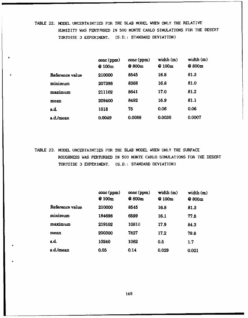
TABLE 22. MODEL UNCERTAINTIES FOR THE SLAB MODEL WHEN ONLY THE RELATIVE

HUMIDITY WAS PERTU1RBED IN 500 MONTE CARLO SIMULATIONS FOR THE DESERT

TORTOISE 3 EXPERIMENT. (S.D.: STANDARD DEVIATION)

conc (ppm) cone (ppm) width (m) width (m)

@ lOOm @ 800m @ loom @ 8OOm

Reference value 210000 8545 16.8 81.3

minimum 207398 8368 16.8 81.0

maximum 211102 8641 17.0 81.2

mean 209400 8492 16.9 81.1

s.d. 1018 75 0.06 0.06

s.d/mean 0.0049 0.0088 0.0036 0.0007

TABLE 23. MODEL UNCERTAINTIES FOR THE SLAB MODEL WHEN ONLY THE SURFACE

ROUGHNESS WAS PERTURBED IN 500 MONTE CARLO SIMULATTIONS FOR THE DESERT


conc (ppm) conc (ppm) width (m) width (m)@ loom @8OOm @ 100m @ 800m

Reference value 210000 8545 16.8 81.3

minimum 184698 6599 16.1 77.5

maximum 219102 10810 17.9 84.3

mean 200300 7827 17.2 79.8

s.d. 10240 1062 0.5 1.7

s.d/mean 0.05 0.14 0.029 0.021

165

TABLE 24. MODEL UNCERTAINTIES FOR THE SLAB MODEL WHEN ONLY THE SOURCE EMISSION

RATE WAS PERTURBED IN 500 MONTE CARLO SIMULATIONS FOR THE DESERT


conc (ppm) conc (ppm) width (m) width (m)@ loom @ 800m @,100m @ 800m

Reference value 210000 8545 16.8 81.3

minimum 84789 2749 12.5 61.8

maximum 321303 23880 17.7 114.5

mean 257500 14450 15.0 94.5

s.d. 61460 6049 1.6 14.4

s.d/mean 0.24 0.42 0.11 0.15

TABLE 25. MODEL UNCERTAINTIES FOR THE SLAB MODEL WHEN ONLY THE SOURCE DIAMETER

WAS PERTURBED IN 500 MONTE CARLO SIMULATIONS FOR THE DESERT TORTOISE 3

EXPERIMENT. (S. D.: STANDARD DEVIATION)

conc (ppm) cone (ppm) width (m) width (m)

* lOOm @ 800m O lOOm @ 800m

Reference value 210000 8545 16.8 81.3

minimum 99209 7475 11.6 79.0

maximum 210402 8504 28.4 86.2

mean 180200 8305 21.7 80.7

s.d. 23450 1955 5.3 2.1

s.dJmean 0.13 0.24 0.24 0.026

166

X z 20M X BOMM

18 80

2.

2 L

0 1380 2=001 311811 411 5BK I5 a l 12 29M 3KM UMCONCIPPH) CONC(PPM)X = 200M X - 8BOM

1 11A

0 is 2 30 4,8 sB so 70 go 119 130 156

SIGM,-Y (N) SIGNR-Y (M)

Figure 20. The probability density functions (pdf) of the concentrations and

widths (sigma-y) at 200 and 800m downwind based on 500 Monte Carlo

simulations of the SLAB model for the Desert Tortoise3 experiment.

167

TABLE 26. RATIOS OF RELATIVE MODEL UNCERTAINTIES, v" /C AND o" /w, TO THE RELATIVE INPUT

DATA UNCERTAINTIES, -/i. FOR THE SLAB MODEL WHEN THE SEVEN PRIMARY INPUT

PARAMETERS (SEE TEXT) WERE PERTURBED ONE AT A TIME IN 500 MONTE CARLO

SIMULATIONS FOR THE DESERT TORTOISE 3 EXPERIMENT. (oa = STANDARD DEVIATION,

OVERBAR = MEAN, C = CONCENTRATION, w CLOUD-WIDTH, AND I = INPUT PARAMETER). 4

DownwindDistance u du dT RH Q0Q

oi/Ji 0.078 2.89 5.77 0.30 0.472 0.472 0.472

o /C 200 m 0.21 0 0.0026 0.012 0.11 0.51 0.28C

800 m 0.87 0.00087 0.0027 0.023 0.29 0.89 0.050

S/w 200 m 0.71 0 0.00024 0.0085 0.058 0.23 0.52

a1/i"I 800 m 0.75 0.00025 0.00012 0.0017 0.045 0.32 0.055

168

18 that large ranges of the model results due to input data uncertainties are

observed. However, for the SLAB model and a horizontal aerosol jet release

like Desert Tortoise 3, Table 26 shows that the large ranges in predictions are

mainly attributed to uncertainties in the wind speed (u), the source emission

rate (Q), and the source diameter (D). Uncertainties in the surface roughness

(z ) have a moderate influence. Uncertainties in the wind speed difference,

(du), the temperature, WdT), and the relative humidity, (RH), are found to be

relatively inconsequential. The results of this example point out the

importance for a dispersion model to simulate the source term correctly for a

horizontal aerosol jet release.

The calculated sensitivities could depend strongly on the model

formulation and on the value of the original (reference) data. For example,

if the uncertainty range of AT crosses a threshold where the PG class jumps

from C to D, D to E, etc., then a large change in concentration or cloud width

may result.

169

SECTION VII

SUMMARY OF EVALUATION

The tables and figures In the previous sections provide quantitative

estimates of the model performance measures for individual groups of

experiments (for example, dense-gas continuous releases or neutrally-buoyant

gas instantaneous releases). Emphasis was on the geometric mean bias, MG, and

the geometric variance, VG, for each group. It is difficult to combine these

results, since the problem often reduces to comparing "apples" to "oranges."

For example, how can the BM model, which applies only to dense gas releases,

be compared with the Gaussian plume model, which applies only to continuous

releases of neutrally-buoyant gases?

In this section, the model evaluation exercise is generalized by

combining the information from the different datasets in a qualitative manner.

For this purpose, we use the following three groups of datasets:

Group 1: Continuous dense gas releases, with short averaging times

(several of the models state that they are most applicable to

short rather than long averaging times)

Group 3: Instantaneous dense gas releases (Thorney Island)

Group 4: Continuous passive gas releases (mostly Prairie Grass)

The experiments with instantaneous passive gas releases are not included in

this final summary since there were relatively few runs and all the models

tended to overpredict.

A. CONCENTRATION PREDICTIONS

The evaluations discussed in Section IV emphasized use of the logarithm

of concentration, which lessens the influence of outliers and which gives

equal weight to over- or under-predictions. The FAC2 statistic is also a

logarithmic measure, since it is the fraction of the predictions that are

within a factor of two of observations. Ranking of models according to the

FAC2 results is given in Table 27, where the ranges of FAC2 are arbitrarily

170

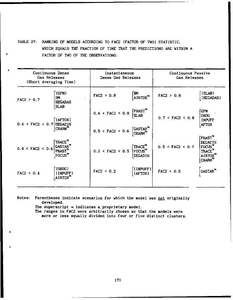
TABLE 27. RANKING OF MODELS ACCORDING TO FAC2 (FACTOR OF TWO) STATISTIC,

WHICH EQUALS THE FRACTION OF TIME THAT THE PREDICTIONS ARE WITHIN A

FACTOR OF TWO OF THE OBSERVATIONS.

Continuous Dense Instantaneous Continuous PassiveGas Releases Dense Gas Releases Gas Releases

(Short Averaging Time)

[(GPM) FAC2 > 0.8 [ZM [(SLAB)FAC2 > 0.7 BM IRTOXm FAC2 > 0.8 L (HEGADAS)

HEGADAS-S L A B 0P T -

0.6 < FAC2 < 0.8 07<FC<OBDG

"[AFTOX) INPUFF0.6 < FAC2 < 0.7 DEGADIS [AFTOX

LCHARe 0.5 < FAC2 < 0.6 [GASTAR 1CR "PHAST'

"TRACEYN DEGAI IS< FAC2 < 0.6 GASTAR' fTRACE 0.5 < FAC2 < 0.7 FOCUS T

0.4PHAT O.2 < FAC2 < 0.5 FOCUSe TRACET"

LFOCUS LDEGADIS AIRTOX T

CHARMi7

"[OBDG) FAC2 < 0.2 (INPUFF) FAC2 < 0.5 [GASTAR'FAC2 < 0.4 (INPUFF) (AFTOX) L

LAIRTOXI

Notes: Parentheses indicate scenarios for which the model was not originallydeveloped.

The superscript -m indicates a proprietary model.The ranges in FAC2 were arbitrarily chosen so that the models were

more or less equally divided into four or five distinct clusters.

171

chosen in each group such that the models are divided into four or five

distinct clusters. Several conclusions can be made from this table:

The FAC2 performance of any model is not related to Its cost or

complexity.

In two of the three groups, the "best" model Is one which was not

originally developed for that scenario (that Is, GPM for continuous

dense gas releases and SLAB for continuous passive gas releases).

The better models can have their predictions within a factor of two

of the observations about 70 or 80 percent of the time.

The BM, GPM, SLAB, and HEGADAS models demonstrate the most

consistent performance for the FAC2 statistic.

Qualitative assessments based on the geometric mean bias, MG, and the

geometric variance, VG, are given in Table 28. These results are sometimes

slightly different from those from the "Factor of Two" analysis in Table 27.

However, the four models (BM, GPM, SLAB, and HEGADAS) that produced the best

"Factor of Two" agreement are on the list of six models (BM. GPM, SLAB,

NfADAS, CHARM, and PHAST) that produce the most consistent performance for

the statistics MG and VG.

For safety purposes it may be better if a model overpredicts than

underpredicts concentration. From this viewpoint, of the "top six" models,

the SLAB and CHARM models may be less desirable because of their tendency to

underpredict by a slight amount in Table 28.

B. WIDTHS

Figures 16a and 16b presented the geometric mean bias, MG, and the

geometric variance, VG, for each model for the predicted and observed widths

at the continuous release datasets. The better models for the dense gas

releases were the AIRTOX, PHAST, and SLAB models. The AFTOX width predictions

were about a factor of three low and the HEGADAS predictions were about a

172

TABLE 28. SUMMARY OF PERFORMANCE EVALUATION BASED ON GEOMETRIC MEAN BIAS MG

AND GEOMETRIC VARIANCE VG FOR CONCENTRATIONS. NEGLECTING

INSTANTANEOUS PASSIVE DATASET. THE TERMS "OVER" AND "UNDER" REFER

TO THE BIAS IN THE MEAN PREDICTIONS.

Continuous Instantaneous ContinuousDense Gas Releases Dense Gas Passive Gas

(Short Averaging Time) Releases Releases

AFTOX (Good) (Poor-Way Over) Fair-Over

AIRTOX Poor-Under +Good +Fair"BM Good +Good --

*CHARM h Fair-Under Fair-Under +Fair-UnderDEGADIS Good-Over Poor (Fair-Over)

FOCUS Poor-Over Poor-Over GoodGASTAR!N +Good +Fair-Under Poor-Over

*GPM (Good-Under) -- +Good

"HEGADAS +Good -- +(Good)INPUFF (Poor-Under) (Poor-Over) +Good

OB/DG (Poor-Under) -- Good

*PHAST Fair Fair-Over Good*SLAB +Good-Under +Fair-Under +(Good)

TRACE Fair Poor-Over Poor-Over

Notes: Parentheses indicate scenarios for which the model was not originallydeveloped.

The superscript m indicates a proprietary model.The symbol * marks a "better" model.The symbol + marks a model with minimal trend in its residual plots.

173

factor of three high, while the GPM width predictions were about 40 percent

low and the GASTAR and DEGADIS predictions were about a factor of two high.

For the passive gas releases, all models performed reasonably well, with

little difference among the results. It is difficult to choose a "better"

model from these data because of this lack of variation. As before, it is

concluded that the ability of a model to accurately simulate plume widths is

not a function of its cost or complexity.

C. SCREENING MODEL RECOMMENDATIONS

The results of the analyses in this section lead to the recommendation

that the following simple, analytical formulas can be confidently used for

screening purposes for sources over flat, open terrain:

BM (Britter and McQuaid) for continuous and instantaneous dense gas

releases.

GPM (Ga .. jian Plume Model) for continuous passive gas releases.

There are insufficient field data to Justify recommendations for instantaneous

passive gas releases. However, the EPA's INPUFF model appears to perform

reasonably well for the Hanford dataset in Figure 14b.

These screening models would not be appropriate for source scenarios and

terrain types outside of those used in the model derivations. For example,

because the screening models neglect variations in roughness length, they

would be inappropriate for urban areas or heavily industrialized areas.

174

Acknowledgements:

The success of this project has depended upon the cooperation of dozens

of model developers and experimenters, who have shared their models, data, and

insights. We sincerely acknowledge the contributions of these scientists and

engineers.

Captain Michael Moss of the U.S. Air Force and Mr. Howard Feldman of the

American Petroleum Institute (API) have been the project monitors over the

course of the study. Much useful guidance was received from the API Air

Modeling Task Force (Chairman: Mr. Kenneth Steinberg of Exxon).

175

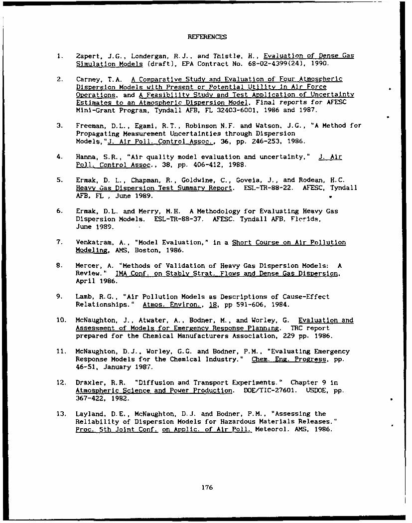
REFERENCES

1. Zapert, J.G., Londergan, R.J., and Thistle, H., Evaluation of Dense GasSimulation Models (draft), EPA Contract No. 68-02-4399(24), 1990.

2. Carney, T.A. A Comparative Study and Evaluation of Four AtmosphericDispersion Models with Present or Potential Utility in Air ForceOperations, and A Feasibility Study and Test Application of UncertaintyEstimates to an Atmospheric Dispersion Model, Final reports for AFESCMini-Grant Program, Tyndall AFB, FL 32403-6001, 1986 and 1987.

3. Freeman, D.L., Egami, R.T., Robinson N.F. and Watson, J.G., "A Method forPropagating Measurement Uncertainties through DispersionModels,"J. Air Poll. Control Assoc., 36, pp. 246-253, 1986.

4. Hanna, S.R., "Air quality model evaluation and uncertainty," J. AirPoll. Control Assoc., 38, pp. 406-412, 1988.

5. Ermak, D. L., Chapman, R., Goldwine, C., Govela, J., and Rodean, H.C.Heavy Gas Dispersion Test Summary Report. ESL-TR-88-22. AFESC, TyndallAFB, FL , June 1989.

6. Ermak, D.L. and Merry, M.H. A Methodology for Evaluating Heavy GasDispersion Models. ESL-TR-88-37. AFESC. Tyndall AFB, Florida,June 1989.

7. Venkatram, A., "Model Evaluation," in a Short Course on Air PollutionModeling, AMS, Boston, 1986.

8. Mercer, A. "Methods of Validation of Heavy Gas Dispersion Models: AReview." IMA Conf. on Stably Strat. Flows and Dense Gas Dispersion,April 1986.

9. Lamb, R.G., "Air Pollution Models as Descriptions of Cause-EffectRelationships." Atmos. Environ., 18, pp 591-606, 1984.

10. McNaughton, J., Atwater, A., Bodner, M., and Worley, G. Evaluation andAssessment of Models for Emergency Response Planning. TRC reportprepared for the Chemical Manufacturers Association, 229 pp. 1986.

ii. McNaughton, D.J., Worley, G.G. and Bodner, P.M., "Evaluating EmergencyResponse Models ftr the Chemical Industry." Chem. Eng. Progress, pp.46-51, January 1987.

12. Draxler, R.R. "Diffusion and Transport Experiments." Chapter 9 inAtmospheric Science and Power Production. DOE/TIC-27601. USDOE, pp.367-422, 1982.

13. Layland, D.E., McNaughton, D.J. and Bodner, P.M., "Assessing theReliability of Dispersion Models for Hazardous Materials Releases."Proc. 5th Joint Conf. on Applic. of Air Poll. Meteorol. AMS, 1986.

176

14. Koopman, R.P., Baker, J., Cederwall, R.T., Goldwin Jr., H.C., Hogan,W.J., Kamppinen, L.M., Kiefer, R.D.., McClure, J.W., McRae, T.G., Morgan,D.L., Morris, L.K., Spann Jr., M.W. and Lind, C.D., Burro series datareport. LLNL/NWC 1980 LNG Spill Tests, UCID-19075, Lawrence LivermoreNational Laboratory, Livermore, CA, 1982.

15. Goldwire, H.C. Jr., Rodean, H.C., Cederwall, R.T., Kansa, E.J., Koopman,R.P., McClure, J.W., McRae, T.G., Morris, L.K., Kamppinen, L., Kiefer,R.D., Urtiew P.A. and Lind, C.D., Coyote series data report. LLNL/NWC1981 LNG Spill Tests: Dispersion, vapor burn, and rapid phasetransition, UCID-199953, Lawrence Livermore National Laboratory,Livermore, CA, 1983.

16. Goldwire, H.C. Jr., McRae, T.G., Johnson, G.W., Hipple, D.L., Koopman,R.P. McClure, J.W., Morris L.K. and Cederwall, R.T., Desert Tortoiseseries data report: 1983 pressurized ammonia spills, UCID-20562,Lawrence Livermore National Laboratory, Livermore, CA, 1985.

17. Blewitt, D.N., Yohn, J.F., Koopman R.P. and Brown T.C., "Conduct ofAnhydrous Hydrofluoric Acid Spill Experiments," Proc. Int. Cqnf. OnVapor Cloud Modeling, AIChE, New York, pp. 1-38, 1987.

18. Nickola, P.W., Ramsdell Jr., J.V. and Ludwick, J.D., Detailedtlme-histories of concentrations resulting from Puff and short-periodreleases of an inert radioactive fas: A volume of atmospheric diffusiondata, BNWL-1272, UC-53, Battelle Pacific Northwest Laboratories,Richland, WA 99352, 1970.

19. Puttock, J.S., Blackmore, D.R., Colenbrander, G.W., Davies, P.T., Evans,A., Homer, J.B., Redfearn, J.J., Van't Sant, W.C. and Wilson, R.P., Spilltests of LNG and refrigerated liguld Propane on the sea, Maplin Sands.198Q: Experimental details of the dispersion tests, TNER.84.046, ShellResearch Ltd., Thornton Research Centre, Combustion Division, 1984.

20. Colenbrander, G.W., and Puttock, J.S, "Dense Gas Dispersion Behaviour,Experimental Observations and Model Developments," Proc. 4thInternational Svmposium on Loss Prevention and Safety Promotion in theProcess Industries, Harrogate, 1983.

21. Barad, M.L., Project Prairie Grass, A Field Proaram In Diffusion,Vol. I. AFCRC-TR-58-235 (I), AD 152572. AFGL, Hanscom AFB,MA 01731, 1958.

22. Briggs, G.A., "Similarity Forms for Ground-Source Surface-LayerDiffusion," Boundary Layer Meteor., 23, pp. 489-502, 1982.

23. Nieuwstadt, F.T.M., "Application of mixed-layer similarity to theobserved dispersion from a ground-level source," J. Appl. Meteorol., 19,pp. 157-162, 1980.

24. van Ulden, A.P., "Simple estimates for vertical diffusion from sourcesnear the ground," Atmos. Environ., 12, pp. 2125-2129, 1978.

177

25. McQuaid, J. (ed.), Heavy Gas Dispersion Trials at Thorney Island.Proceedings of Symposium at the University of Sheffield, Great Britian,3-5 April, 1984, Elsevier, Amsterdam, The Netherlands, 1985.

26. Ermak, D.L., Chapman, R., Goldwire, C., Govela, J., and Rodean, H.C.Heavy Gas Dispersion Test Summary Report. Report for AFESC, 1988.

27. Perry, R.H. and Green, D., Perry's Chemical Engineer's Handbook. 6thedition. McGraw-Hill, New York, 1984.

28. Dean, J.A., Lange's Handbook of Chemistry, 13th edition, McGraw-Hill, NewYork, 1985.

29. Paul, M.A., King E.J. and Farinholt, L.H., General Chemistry. Harcourt,Brace, & World, Inc., New York, 1967.

30. Colenbrander, G.W., Evans, A., Puttock, J.S., Spill Tests of LNG andRefrigerated Liquid Propane on the Sea, Maplin Sands. 1980: DispersionData Digests, TNER.83.063 through TNER.83.073, and TNER. 84.025 throughTNER. 84.043, Thornton Research Centre, Shell Research Ltd.. 1984.

31. McQuaid, J. and Roebuck, B., Large Scale Field Trials on Dense Gas VaporDispersion: Final Report to Sponsors-on the Heavy Gas Dispersion Trialsat Thorney Island 1982-84, Health and Safety Executive, SafetyEngineering Laboratory, Sheffield, England, 1985.

32. Puttock, J.S., "Comparisons of Thorney Island Data with Predictions ofHEGABOX/HEGADAS." J. Haz. Mat., 16, pp 439-455, 1987.

33. Akuma, E., Costanza, P., and Hagen, G., "Consequence Analysis ofAtmospherically Dispersed Toxic Chemical Releases: Modeling for Planningand Emergency Response," Proc. of the 7th Technical Seminar on ChemicalSpills, sponsored by Environment Canada, Edmonton, Alberta, 1990.

34. Raj, P.K. and Morris, J.A., Source Characterization and Heavy GasDispersion Models for Reactive Chemical, AFGL-TR-88-0003(I). AFGL,Hanscom AFB, MA 01731, 1987.

35. Harris, L.A., ed. The CAMEO Manual. National Oceanic and AtmosphericAdministration, Hazardous Materials Response Branch, Modeling andSimulation Studies, Seattle, WA, 218 pp, 1987.

36. Handbqok.-of Chemical Hazard Analysis Procedures, FEMA, PublicationsOffice, 500 C Street, S.W., Washington, D.C. 20472, 1989.

37. Moser, J.H., CADM: A Computer Program for Modeling the Dispersion ofHeavy Gas In Calm Air, SoftSkills, Inc., P.O. Box 989, Cypress, TX 77429,1989.

38. McF~r]anp, K., Prothero, A., Puttock, J.S., Roberts, P.T., and Witlox,H.W.M, Development and Validation of Atmospheric Dispersion Models forHydrogen Fluoride. Part I: Technical Reference Model, TNER.90.015, ShellResearch Ltd., Thornton Research Centre, Chester, England, 1990.

178

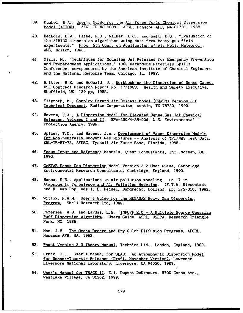
39. Kunkel, B.A., User's Guide for the Air Force Toxic Chemical DispersionModel (AFTOX), AFGL-TR-88-0009. AFGL, Hanscom AFB, MA 01731, 1988.

40. Heinold, D.W., Paine, R.J., Walker, K.C., and Smith D.G., "Evaluation ofthe AIRTOX dispersion algorithms using data from heavy gas fieldexperiments." Proc. 5th Conf. on Application of Air Poll. Meteorol.,AMS, Boston, 1986.

41. Mills, M., "Techniques for Modeling Jet Releases for Emergency Preventionand Preparedness Applications," 1988 Hazardous Materials SpillsConference, co-sponsored by the American Institute of Chemical Engineersand the National Response Team, Chicago, IL, 1988.

42. Britter, R.E. and McQuaid, J., Workbook on the Dispersion of Dense Gases.HSE Contract Research Report No. 17/1988. Health and Safety Executive,Sheffield, UK, 129 pp, 1988.

43. Eltgroth, M., Complex Hazard Air Release Model (CHARM) Version 6.0Technical Document, Radian Corporation, Austin, TX 78720, 1990.

44. Havens, J.A., A Dispersion Model for Elevated Dense Gas Jet ChemicalReleases, Volumes I and II, EPA-450/4-88-006, U.S. EnvironmentalProtection Agency, 1988.

45. Spicer, T.O., and Havens, J.A., Development of Vapor Dispersion Modelsfor Non-neutrally Buoyant Gas Mixtures -- Analysis of TFI/NH3 Test Data,ESL-TR-87-72, AFESC, Tyndall Air Force Base, Florida, 1988.

46. Focus Input and Reference Manuals, Quest Consultants, Inc.,Norman, OK,1990.

47. GASTAR Dense Gas Dispersion Model Version 2.2 User Guide, CambridgeEnvironmental Research Consultants, Cambridge, England, 1990.

48. Hanna, S.R., Applications in air pollution modeling. Ch. 7 inAtmospheric Turbulence and Air Pollution Modeling. (F.T.M. Nieuwstadtand H. van Dop, eds.), D. Reidel, Dordrecht, Holland, pp. 275-310, 1982.

49. Witlox, H.W.M., User's Guide for the HEGADAS Heavy Gas DispersionProgram, Shell Research Ltd, 1988.

50. Petersen, W.B. and Lavdas, L.G. INPUFF 2.0 - A Multiple Source GaussianPuff Dispersion Algorithm. Users Guide, ASRL, USEPA, Research TrianglePark, NC, 1986.

51. Nou, J.V. The Ocean Breeze and Dry Gulch Diffusion Programs, AFCRL,

Hanscom AFB, MA, 1963.

52. Phast Version 2.0 Theory Manual, Technica Ltd., London, England, 1989.

53. Ermak, D.L., User's Manual for SLAB: An Atmospheric Dispersion Modelfor Denser-Than-Air Releases (Draft. November Version), LawrenceLivermore National Laboratory, Livermore, CA 94550, 1989.

54. User's Manual for TRACE II, E.I. Dupont DeNemours, 5700 Corsa Ave.,Westlake Village, CA 91362, 1989.

179

55. Fleischer, M.T. SPILLS. An Evaporation/Air Dispersion Model forChemical Spills on Land. Shell Development Center, Westhollow ResearchCenter, P.O. Box 1380, Houston, TX, 77001, 1980.

56. Golder, D., "Relations Between Stability Parameters in the surface layer.Bound. Layer Meteorol., 3, pp. 46-68, 1972.

57. Mitchell, A.E., Jr., "A comparison of short-term dispersion estimatesresulting from various atmospheric stability classification methods,"Atmos. Environ., 16, pp. 765-773, 1982.

58. Eidsvik, K.J., "A Model for Heavy Gas Dispersion in the Atmosphere,"Atmos. Environ., 14, pp. 69-77, 1980.

59. Havens, J.A. and Spicer, T.O., Development of an Atmospheric DispersionModel for Heavier-than-Air Gas Mixtures, Final report to U.S. CoastGuard, CG-D-23-85, USCG HQ, Washington, DC, 1985.

60. Ooms, G., Mahieu A.P. and Zelis, F., The plume path of vent gases heavierthan air. Proc. First International Symposium on Loss Preventionand Safety Promotion in the Process Industries, C.H. Buschman, Ed.,Elsevier Press, 1974.

61. Turner, D.B., Workbook of Atmospheric dispersion estimates, Office ofAir Programs Publication No. AP-26 (NITS PB 191-482). U.S. EnvironmentalProtection Agency, Research Triangle Park, NC, 84 pp, 1970.

62. Briggs, G.A. Diffusion Estimation for Small Emissions. ATDLContribution File No. 79, Atmospheric Turbulence and DiffusionLaboratory, 1973.

63. Colenbrander, G.W., "A Mathematical Model for the Transient Behaviour ofDense Gas Vapour Clouds," Proc. Third International Symposium on LossPrevention and Safety Promotion in the Process Industries, Basle, 1980.

64. Irwin, J.S., Estimating plume disperison--A comparison of several sigmaschemes. J. Climate Applied Meteorol., 22, pp. 92-114, 1983.

65. Draxler, R.R., "Determination of Atmospheric Diffusion Parameters,"Atmos. Environ., 10, pp. 99-105, 1976.

66. Cramer, H.E., "Improved Techniques for Modeling the Dispersion of Tallstack plume," In: Proceedings of the Seventh International TechnicalMeeting on Air Pollution Modeling and its Application, No. 51, NATO/CCMS,pp. 731-780, (NTIS PB 270-799), 1976.

67. Rao, K.S., Analytical solutions of a gradient-transfer model for plumedeposItion and sedimentation, NOAA Tech. Memo. ERL ARL-109, 75 pp.,EPA-600/3-82-079, U.S. Environmental Protection Agency, Research TrianglePark, NC, (NTIS PB 82-215 153), 1982.

68. Cox, R.A. and Carpenter, R.J., "Further Development of a Dense CloudDispersion Model for Hazard Analysis," In F. Hartwig (ed.), Heavy Gasand Risk Assessment. D. Reldel, Dordrecht FRG, 1980.

180

69. Hanna, S.R., "Confidence limits for air quality model evaluations, asestimated by bootstrap and jackknife resampling methods," Atmos.Environ., 23, pp. 1385-1398, 1989.

70. Tukey, J.W., Kinds of Bootstraps and Kinds of Jackknifes, Discussed inTerms of a Year of Weather-Related Data, Tech. Report 292, Dept. ofStatistics, Princeton University, 08544, 1987.

71. Lewellen, W.S. and Sykes, R.I., "Meteorological Data Needs forModeling Air Quality Uncertainties." J. Atmos. and Oceanic Tech., 6,pp. 759-768, 1989.

72. Irwin, J.S., Rao, S.T., Petersen, W.B. and Turner, D.B., "RelatingError Bounds for Maximum Concentration Estimates to Diffusion MeteorologyUncertainty," Atmos. Environ., 21, pp. 1927-1937, 1987.

73. O'Neill, R.V., Gardner, R.H. and Carney, J.H., "Parameter Constraintsin a Stream Ecosystem Model: Incorporation of a Priori Information InMonte Carlo Error Analysis," Ecological Modeling. 16, pp. 51-65, 1982.

181(The reverse of this page is blank.)

APPENDIX A

MODELERS DATA ARCHIVES FILES

Included in this Appendix are the listing of the Modelers Data

Archives (MDA) files for the following experiments:

Burro

CoyoteDesert Tortoise

Goldfish

Hanford (continuous)

Hanford (instantaneous)

Maplin Sands (LNG)Maplin Sands (LPG)Prairie Grass

Thorney Island (continuous)

Thorney Island (instantaneous)

183

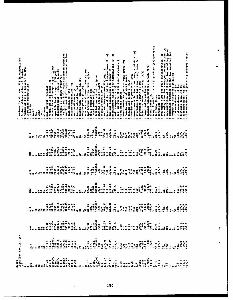
00 V c v

--- 0 Q- 00%

o~~4 :34 - a'

.0~~~~ 0% - . I O.

Ml 64MW 1 -0 -. -

*~~~0 - 4. . a M M60.0 v

0. -. 0-, 0 04 0 g41. .4 -.2 f !: . . 000 ...

.4% v =v UP W 0.. 041 ' a .4 ; -2so a 406 ca-o ). 6 -

0.0 IsC =.C1.. W0.4).,j. V13.044 E- O o0am0

0 ;..0c c . 0 b. c6 6. c - .. 40l-16-22a* 41 01C .60.cg o 4 a40~l0 -- -(~ -J a .00az0-.0-.0

* ~ ~ ~ ~ ~ ~ ~ ~ ~ ~ ~ 0 66C -2U L.60.J. M60m u4 6 .10 N .20a a *Na asu u-....a g a o - 0 . a a -u a m u .

WW Mqo a0 60 w1 00-a

c;o mm a0 4, o0 NNUoe *ý 4; n %0%0%U2! a!0 .. n 4% NO%4 V- f. f

0 % N 0 % 0 % 0 % 0...4-...... I. V-9(f' I I ~ I46440

oh a, o! 0! N v% m U)c

LID 0 ..... UN .% %01.41...... a.1 %.N U N ft4 I memo-.m

N , Iwo0 .w If la0 m% .000 *~. . U) U). 04 .0 * 0

U)0%N0%N..IU)NNO0%64 ~ ~ ~ ~ w q4 v;.4U64..I. 4~. I;fo 90UU N .0 o I' T ... NI4. 4 "t

a 0 a; N0% .0 4-

N ~~~ ~ 1 .600. .. N 0ONU w4 00 *N * 0% .0. .U4 o,.qN0 N %. " m0 0 040. v0 O O-00 %0 4 0 .690

0~ m0 .! *. a, .0 0 . . .9 (' . . o N 9N e%

0 U19 :r; .0 U) 4- 0mc9400f *m wQ w .N0%0%U)0 I) NO 0 64 0%N0%-0 - 0

0.94 0.0. .0 % . QN . . 94 0% 0 .N * 0% .;

0 0 -a.02 144I%.0

U

18

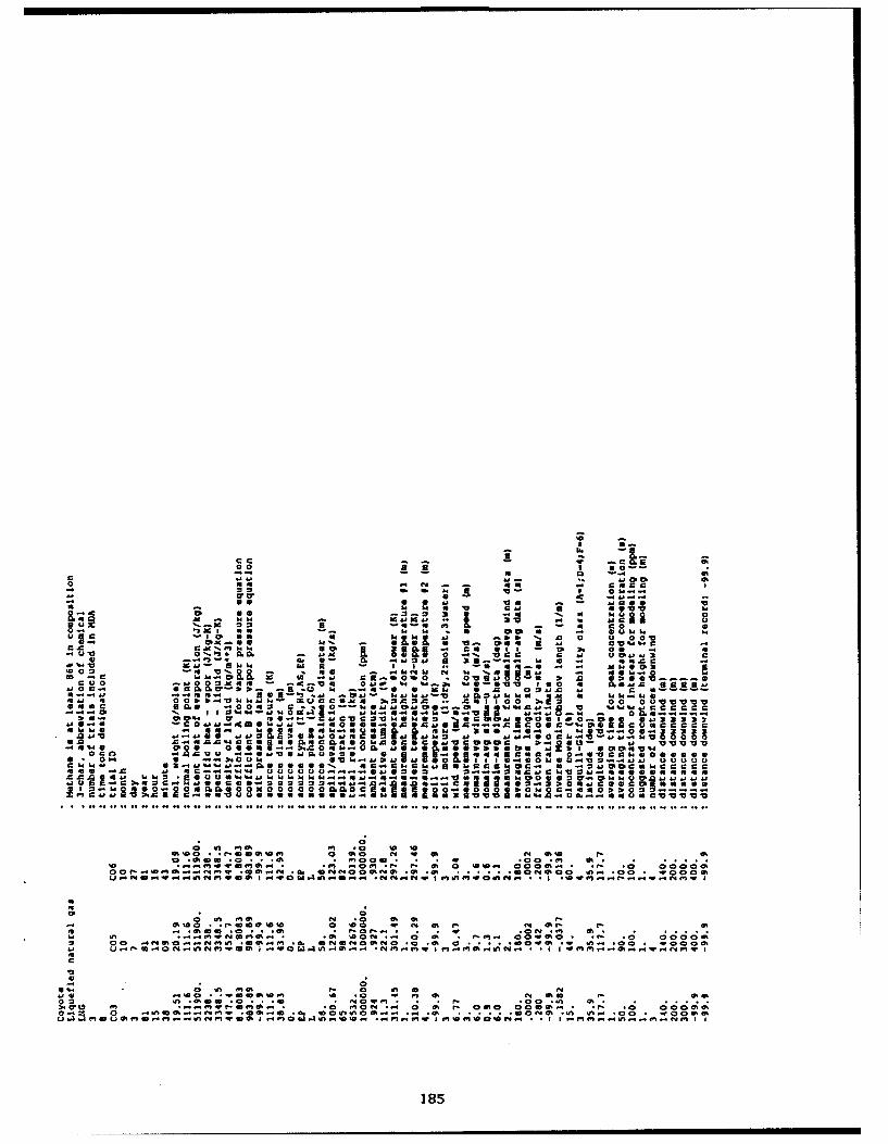
'0

00 Is a c a-

0 2--C000 o 0 0- N - flU CCG"- C a2 4.. A 00 o h~

we I I w. sa. I- C6 a.w -0 U-wa-. tpl t5 a-- UN 9 C0e lZ* t cs !! .

Ce- C V 40111 '- 0 C.u~

ae gl 0 0.C4 4 o5 0. 6 10 0 00CP

o c .-.. ~ C 0. U to-.- "m Co 960 M.Ue ' :& *' 0 - --6 -..- - I* 11 ? -? I- s "wo .. 1~ l.. ~1 r~ -U.0~ 0 01, 0 c ac

:3-w0 fx1 0 00 .f. 0IU24.4w xC 0.M 0U 000a 0 Mac 222CZ -40 ow. sam"Ou"We"..-f0 Iwo 41 aC ~ eu. 1104 aI 6006.

.C-ffl.~~.G1.G~~u IC C0..UC; I. C w : G00c~. 555.

* ~ ~ 0 1* 0.- ... 1GU...uC1CýC 0! "13 ,01 Aa a 01 1Cý01CCCIJ'L. 0%-414u.-QCC e. UC3 U bC Cf... 0 -OOe:CC

0:0 4,qwwd% fC4 -a m0 t'0

0%'0 In N4U0 W 0 0% 0 K %' =

In0% * 0

atI10%N . 0 %4

2 09.0-0N9~* 0..4 *. * NO 4 O * 0 0 . . C% . .14.. '00 "1 CO000

~18

1 00

w to -u 9v2 - =1 3. a

2 00 c lp a 41 I!I - D. .. 00 0

c 0 '4 U -I

a u 0 14 0 q a4~

.0 1. k a 40 -4 3 S c' t o0

-~~~. s-M -C _r_ 0C4ci~~U .4. C2 01.-

*~~~~ 11:.1 14 a. a wf 2E 0 . 4 0 .4

4 0=MOW" cc*' 1 .M US i:1 F .,0 *.l tU- , -6 paMI.001

CI0400* 4 - -... .0 14 142 4 44,1.04W IS SO C&444C 4

W. II014J1 19 2 ; 8 23 2 sm1 044 14 "14- z4 !_:0 4.4 - a..~ ' 0 c;-.*;

0 f ý l tj U1ft 'D .4 d, "

f, a0i05 ! - W o o - 01 0 .. . . 1 :0 0 p

* ~ ~ ~ ~ ~ ~ fr4 01- In4.Q. ~54 4M OS C £ . 0m Ine4 C 0. - 44JUU fn-..0.* g*@6 UCI.G143'CC I0 .4%0%04%c,.CUI.

In ib10l fO.4O0U*el0 q.0s0n 000.mf" V I . .O - 130 20 4 004%m

0I 0

*00 w an mom M

a,@- 0% .0%. ft P 0 *; ...4 10 -MOW el 0mv - -0ca 0 0om a m 1 c .114 .. .E~ .0 0 .1. ... 40 '0 *:! . 0 . 0 c

10.00 n 40 - V

1-I- 0 0 1-Ie! -m -v 4 1000.10 0' a 0 a a 000 0o .e!0"01.0-0.1 !,0 0 0'0 .0 1

*0

0 01-186

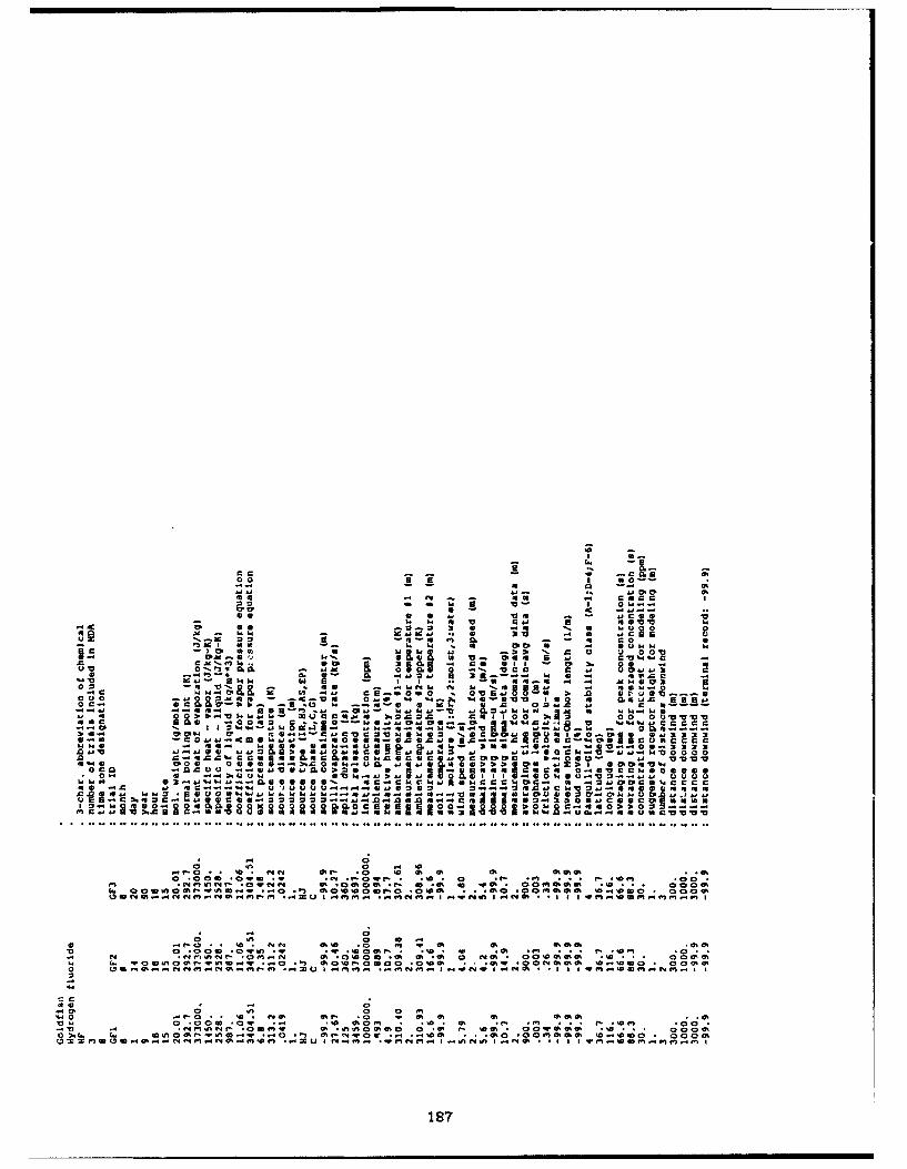
0 g--

v a-

0p 0 a AI U0At -. -1 x .0 -- a

.24 0 0 ' owc Ia 0 u 0 0 0b..

V - CP a0

-0- 2 2 6C a4U0. .0 2P ~ 0. -1 U CO 11

= mm 4 0 w 0'0 m *

4T' 0- U 0 00b M'.II v0 w w900-0,

10 8. r 0.5 sax 0 2U '.. b 0 UC

CUo 41 a . a.. a. a4 '40 0 i ga 41

a C ~O CX .1 i 0aaa&-aa0 M .. Cm D.-: A, o I3c. 5-4-0111.. 0 00.4---.0,00'0" 00 U02=9"QCm zU ~ a 0 @ % C''l00(UI O.'g 0 2.0 -COw13W 14~ga.. -U g1g4.CJ uC-, a CO 0 ."0'S 1,_rlUW 0 toU00 00ww04 d0Ue-.Ogk22R

a~d 0 U0 gOb. C I U --0 0.Z. OC I i 0022 0.'. .(.

Oi~~ ~ 8.8, C. aoU_- Ls~olbCgEU UU cz:4Jog0C' mmI 'ag~0O. " ONOM 00000.40. C4 U31 q00- 00 0 0.W 0 4-4 2 O Q 'A

Ct 0 ,g c ;Coh 'A - .- C 0 0. mc '40

00 = A Z* . I4 -MM%' 0 4 0 % 0 000 0

4 0 0 C n4 W .0 '4 Mra 4 .n '' .N '4 . 3 0%' .0 01 a C% 'm OW0%k .,,ol %0%I

04*)40M~ .n N 0% *0'4O .0% ý 0% .0ow 4%* 0'0%%% . 000M0

C. C. * W'0 %I~SlW~ .O ~ %04.0 00*040 *%~.Oa400%% 4.'W187O00

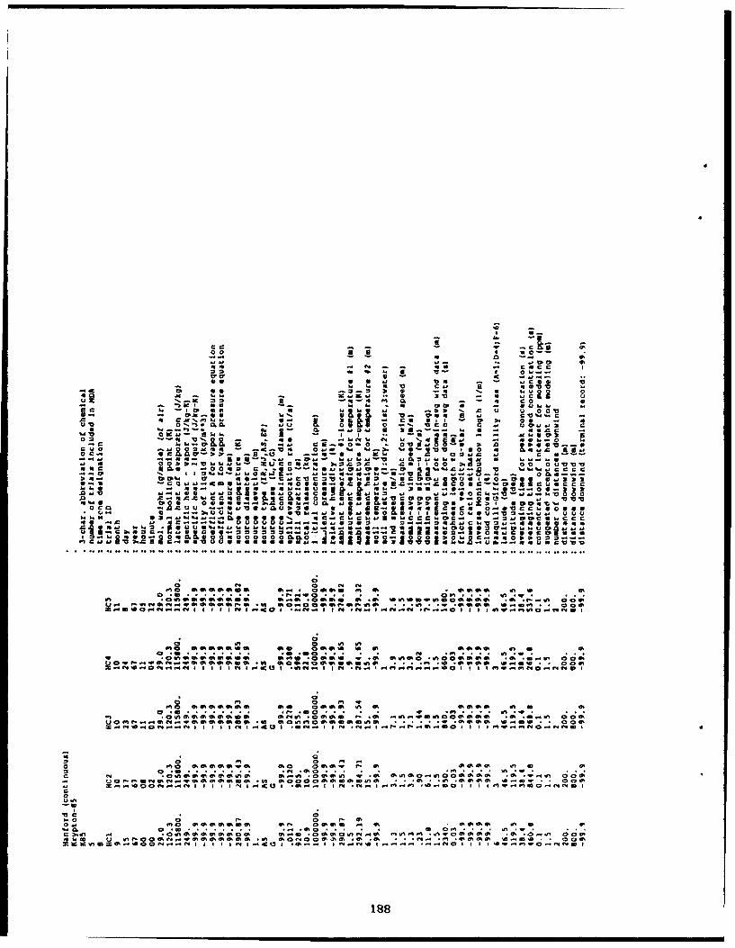
c c C6

'0

00 -.00 0 0 v

D. *- A - q 0 -- v

A. L. W 0 2~0. r - - -11 m U C~ 20 c

9.0 90 a v q.0 Q U 3 0 - 40

0*1 a ý4 t lo'

SI - - 05o

-'go O04 0~b wz cu *0 It.. -*g

411 ... U u C '4.19. f0 U &U4m 0 51O 1..m S.S . 8. , z..9. Cc twl olhW CI ,; U3a 32 00 *.! "'a am ,W ~ 0* U z .c .00 00 00 a

UU3..u. - 0 Ov n 1 14 010,.... 9 4 O'V

c.00 *0Meoo 22:00"-ota'Q v,., u m~ e9.

coo ~ M000 a~o M- jS 5 4 10 0 O *V0.00

.00

0' 0 1 19 *I. 9 *11 .1 .0 0' .Q a

10 ..09. a! . w. .t ot It.at -f 9 .09 .. 0, .9. 19 @ . 1.0.99 .9. *1.9 00atV!9!

M 0. 40 Ma0 .9 . .~~ .m e . .- i.. 9..9.

=-N aft NN O..90I I I NO..INN1UIt-

0 d0

O0 C0,

0- A ý*. 9 . *N;. 0; 0N*: C;9.'4c;'9. M ma

C ~ ~~~~~~~~~~~~~~~~ Mull.......9 .- 9 0... .9 ..... f09.... .. . . 09

00

00 a

00 af ifgý I a- ~0 ve 3-aZ a6 0- . a~ 0Q. Z A - W CC 7

C. 16 TO 0 0 a ae 9

r ~ 0==. .C A. a IiU C3 00 C6 uO

-m 17 .,_2 CC 0- 'e, =0 c C o0 Cj - OUC,Xi 2 10 oCC26. a a.3 6. .0 U 00

-, z c~S r.. 0062 =4 11. 4C if0 vu0%~0J~~..2M2. ~~ 6. W f - U.i - 03160 3. 0-c00 0ýo* c.J 0. Ow0. 00 w~ slo -". 0 a0

w~ $12. N. af a I- c ~haawc 4 c - a C.C.C - c c263 i00 ~ ~ ~ ~ ~ ~ ~ ~ ~ ~ M zO 0 4 AU - ... 2 N . . if fa - c6. 0

COO v wt z4z =- !!a i00-A %i~..U ia =V %la U6U 60 0'.CJ.

10., 0 f 0.x0 0 " - u62 U.. ~ O -- q ... a.0 ... a 00v0v0

ch r- m a, 4 2 - C . -. . - C a,.O - 00 4 -

2.12.6~~~ C- CC.. 2.664 0~.I U 10 1. 12 'AC W6 - -.UU -

0aUU aC; aa .f t a 0U0S f. 2 a aa 6 C . U a 2 U 0.0 ~ ~ ~ ~ ~ 4 th~..C~C 0% oU.C C0.4,0U w! aU00 -. 6CI..600 006 C-3 .002.. a o a .. 6 C3 U C . E 16O CU.

000~~ -. 0.002.2 MOIR~0. 3 6 6 U ~ ~ C ~ fc c - oc i.o

fl A . 2 . .::"- ! os 42121TAT ; 2~22 I II I.- C- - - - - C 1~ 2.4. N2 IT 2.2. '

d.d m o m m ~Ii !- o 't t :

NONOOOO~~~~r-0 W~ 00000 . 1ll . . . o a .~ . a~.I0O0 C'.-..NI I I I ftI 022( I I I. I.2 I Ni ." I I all .22 mw ww I2- W . . .

o0

om a o CO,mc, mm0l01ft ol0 000 o02f 0.0 00. . . . . .. 0 .-... 01 1 l a zw znamm o o.0m000000.fl0tollgh 13 001 * 0 0 0

0 o oam 0 m-O OOO6N o06 0on 0002

0. . . ..c. o . . . e o. .m -.~o o0 ~ ~ ~ ~ ~ ~ ~ ~ ~ a '0 0 0 0 060 oo=*2 0oM'I000 0.f 0

'OCN-W000000oi ýi T000 0 I, I0. . 0 0 .~N0M .. I g I I 0 20 I -- I N 0 IC~r OI 2 2M ~ 0.2 N D,

18

S 6.0

-- :--4 0-22w - *0U Z U00010

r'06 IL u sv6 Nd 6 6 w4 w6 - - .5 6

C Iw w4 14 k a CU

c.. u -a? 4 C, 'a-~~ Aj C . C. 0

M.4 414. CI22o S

0 C a 60 0 -1p4 - E N 0 14 . 6 6 1 . A a- C

66a3- -4 04 - -~0 4! M ~ ~ . 4. 66444 5. -. U U.1n..4CX CC

0014 0 66.i.4 - aCC U 46 . 2~ C W . 3 1 " P ub-o 6 m 3 3)3 3 3 2

A-649.39-00"" .30 488 O0000060440 U4C 2K.st.2 U 6 C 4 4 4 U. . 4 0 0 0 0M C 4 4= 61a At A 40 0 ON a50. CO 6601. a C C 0.4CO. -2Q*. a v 0W UUUUUvv vv

6146 110 10 m1:1 !V !10!661 o o , 0 0e !1 ! "tIo 2*l 1a !lý0 06664.3.l.61C!UO .4ý "106 63 0 11c 6 1to,0IcW 0! 0!6et0050 8.5 .Z - -46U 6 W,32 * I 66-46 6aft65 M-0, 00 -"-Mm646

12 in4 -.00 42040014440 4000 In0..) a @U 0 Clam 1u6~1 953 0022. . . . .1x.544 U.C K.,5 in466 6 66 .- 6145 NO 6 M-U 4% 64141 4,~6 4 C U a 0

~~0fl4444q~~~~Moo 4 IN 60 - 4.I . 44 1 444

Ma - .

O44~~~I.. 14444 .004 4 6 I I4 44.1 N 4. 0

'0"n e4 -

'4 f4I W

444440N6.-06446444- 40 46444~04.-04 19.0g~044sm4444o.4. 44~40.N.4

c1 c

uad 00 co0~-29 1 --. 0101

*8 V8 Ma 41 Lk C

91~ ~~~ 91 VI . 0 h0.0'0 0 -

00 C 60 w 1 ~ 9 - . e0 0.. 1. .9 M0 0 4 8 0U NW ' w

40 a1 -C.0..91818 * 0 20 mo a a 88. .4 0.1 - .9 QO . .V9o'

WI0.u _- 48 .. 2 2. .- ; (8 00 -u0~~~~~ o=U. 0..0 0 C2~ W -.

0 w c1J. w 0. -404 C9 21'-. C.: U - Q CC

-IZ e .. 0g c1 98 "~ 0 00 a 06 80.9 2 .0 %.60Cu N4 0 0 * .10 0 2680 j C .8 - 0 0 J_ q ..a 48. o n4

00-8 ~ ~ ~ ~ ~ ~ 0 a00G0 . . . - .~ 9 C 8 . 8 C 4~~6"Mao c 0U. 4 .. 4' 1.8.8 4886 11 9 8.8-848~~~ ~ ~~~~~ m902.8h8.8. Z CM 0. .. 6 0 . 0oo 0'00 0

v,.9 g 0. I809 C D I... v too0J.8..--. 6 .840J.0 844C-- 851...8 O c%_ O 48O 1ý Bb' .9" ' . 54 - 40. 00. - - -

0.1.. 0 01 4608.180 ". 00 'In86.601.. 0.60 9422 22CO.2~68488-.BOg.'0.0C40 .0--. TC 0@'ý.0 Pý CA C(.9CC

8.884W M n88. t~ W0. I.8~U woo ID 0 8 T" 8- 4'.... g.2 2 2.f.. 4.4... 882.2.480810 E4 480 .j 884004'48.-8N0000

.0.C..IU 8.CC 6O~C .8008.C000.48000..0 2. 6j 8 0'10'

0.0 11900 60.'- 2.0 18.8U. 80 80060 222 0. 4828 .900cc9000 .4.0.00.0 ~ (8250 0 1 .. 8&UB.9.9 5 CBC9 0'0Kh0 0 6 0

.90 ~ ~ -M 0 oM. 4..-ad 890 4%19 (8U.9..4...4890 *--0 .48 8 1- .. 006.q .....

m 0 -~A .00- a Sýw a 0 ! B0 0 0 0 00 0.. 009It9 M O 0 niv!0 00 M0!0.01 0! 0!9 02 0 9 ! 0 -'

@0910919100018=9101.408 000090.0.41'10 .08...0001ammo 0- ccW01180000

z 08O ON008 "c.~ftT M10 .4 .. 410.C 0000 0191 Ti 00. 11

f4 a 0 4

WN 0191 90 N N

WN4991f MalI gz.8 808 8=8 9 9 18 88Q.I m9 91 Nh Ný 0

04 Q 2 h

091 IQ=1 .4 0 N ' 9 1 1 4 4 a1. 0 0 1 1 0 . 8 4 0 N 9 0 0 0 0 0 0 0 0 1 0 1 84 * . 1 0 0 N 0.00..W *. .80 0 '11.0 . . .41 . . . O 0 N99N

0.4019 001 9 91.49 01 001101 019 .40801aW. cm918N0018. .4 =1041.1.0m1* 80 '4'9 9 401 000 01.. 0 .... 8800WN04919191~~~0 *8c i 14 18 9 1 N 8 8 88

W.4N 091 91 N 1N 1

10 0

0 a0-0

Z., ow vI soZ0-r-r

.-4 !. a *U- w 0I Z

09 0 9 0's..~

C - - w. a 3'O -a. Me- Va --a 160.. 0 M 40 0 .- a c

l0 0 i 4~" 0 C 0v0 0M~1I 0 110 SZ no0 -U R., k. 1. W)j . I'D 'a 00

Qu 12- 05. 0 a~. W-C a "j U@., , , o w0 :I ;.Q.-.i. 0. V 0. 41 0. 0 b,0U

011 Cd Z. -, I I I '! 0 0 b.a - V a.!- 0 Uia aa a- m.41. 01 C. '.. w .a- C-0'a14- 00 b.CCC -

0000. 0.1U 00 a0 v

0; C; C; CCeC-0 16 E0uC P;en 16 C- U4 f" 9 to ok4-U ao 6 !0 a 0.1 0. ahI 0.6 10 - 6i-.0632 23.J01jJe C 1E0sDos ý .U.4

. D.516C4VsI.000

0 mm a.0fm a-- -2 n CieO600 f4ma;0T 1600%0 00-9tC200

IN fn o 10 in % in on en

.4104 *0A " *aaho on1 0Coo.. 01 0%61.01 ~ ~ 0 *010 C; .'I .m *61 .1.4 .1 0

01 ~ G 401016111 e40 .0661 0; .61 W; 5.111 0011 * .3 M".0 00

010 meC; i0C., 10 0.616.. 1 0!1 .a .C! 6! 0: aaIRie 0! 0

01 ~ ~ ~ "e .0106011..0 i 10 Ioa diig .61M 0; 010 .0 . . .0 .~ .006

.1 C" 4 aek a4 %4010 .me m 1 0 0: C4 .0; -4' 4 ` :ý 4c n C ;C ýon05 %D C4 a.q f" am.- at a% 010 ICo mýMi .01 ~ 0 ..10 2 . . .61Q .1 ....... ........... .12001.. 11a. I.100101a0 ~ on0 4ý i ""% .0 w 00 1 M w 0 io -Aaa

An0 9D 0 0 WI L, N* ~ a e4a.. a *.a,.- a am a

- ~ ~ w01W0101.aaa0!1.0n ac a0 I a6 ,1 ,10 00 10 I P00 C; oaaaok 01001000w6669 .a. a.oa a C!w 0 C .a m o a. *o~..0600

01 me '04n mk 0 ft oiIM *aa... 610 ta aa.. 1 0 qf 1 a wq a 0a aO 0 4

m 4k D0 010

m 0 m e 0 gn g.. 01I Iaa.. Iq~ no.. wi a a %Do

0 0 1OM 010 WIW10ý -. 0 Mi Mi

Mo -.110..0011100 tI11 1 I 01w.i.1 I t01010101I010010 5010110 . I I 00t010 .... Mii..N W

1192

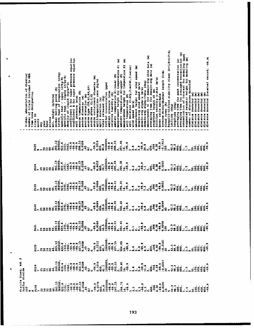
j. 0%

Q. 4 .l0 0%

-~~~ 0 010~ 1..-

U- -- Q . ---- C C Cq U OE

k!! ý1 ; - C o ,03

al -.- l, 14 m,2 - 6U-.t -1. 41

:0~I0l.ll =C~lI v wU w 10 0 00 0U'VvvmU0-- 'C II W01 Mm9 10 EllC4C041.l.l '.G OOC 0l OU. 10 . 6 l El.C

41WZ C0KEl.~ ZvOllU.E. r1..ll.....~E O g ." 4 E C J C C C

EllI~~l 006 0661 .- O l1 -I 0. ..0 =l vz Sýl l E C~ C C

C 44 A EC0,2 r0 a0 .CocecJU z C0 0CLO. U030 00Cl1ICCC

00MOw C-0 C0 0 Cn In 0 ,C - 2 0Cc C cI

:C 0001C .10 0.- 00" 00000.O 01.' 000%6 no. a1 0%010

13~.,e 1M1100M %0!00 .l 3 0 0011%.101. 00q .00 .010 110 00

*.1.ln..0 0 M1..... 14 .O .1010.1 4 1.1 01001 .00 .' 0 1 1..'I~..10

M 0aMW01 .M' Mo1%0. 0 a %.'n 00,010 1 M ! 1!014 . 0110c 0o=; a a

.. (-011n0101f.4M10...w.. I 00. J 01 1..i I 0110.. I *100110 I 01010 . I I00100'M~~~l10 I- M

MO~ 010 40 s 0 n n0!01 at .000.I 01 .,a l.- at -t wo .-0 .

M ~ 'In M.0 'a ' 'h a. Chao n . . . . ..0 00 .0 M

U 11 .. 0E'1 01 1M l. 10 0% % ." 0 *0 0 010 0 .0 1 % m, .. l 0 . % * 0 0 0 C; 000 0

M I 010 0ý In In N1

01 'In l.'101~~~~ -, 'I ' 00 .. .. .100 ' ~

0!01 m! 0!00M1.0 0 0 0010... 0 01 v! 010M, 0!- 'In ... N . ' c 0; 'I 01ý 'Ic . . . . 0001 0 M

0%001001000110.4.. i i IMO C I 010M.' I I lq"M.-. .1 ft1 I 100110 .0 I .'10%1.*'Inn.101I

0 .Mn .. no Ne 0 n I 0

wt01 6* .0 01.. a ;."1 0.110%.. 00 ft M 1 0 1m.'. 000 01

N ~ ~ ~ ~ ~ ~ ý -M0 M 0 1 % %-0 a%'I a01 1' 1t a0 10 0,rM 00 00 ' ' 0 In .00 00O.I'0In.I101M0.~.I I IMo -=u 1010Ma..I IM"NM..I*01010110WNW01 to UP01 k0100 11...In-n...01vt

MO 0110 O0 00 In n0,

ft " 1. 0 0M.0% I-01.' V, 01.. a00 - 01% 0% 01 ElM 'n0%cEl 01 .1 0.' .; 00 4M 'In '0 owl, * .!. .010 C .1001 00 "mM 20 a

1M1001M10010101N0In94 I11 '0 11 0 .% 01 101 .04M 0 1 1 % 009 4W I00 0

El~ ~ onl 0! .10'0010M % % .10 01 '0101 .010 1 4! .0.- '00 .010 WM10100; . . .00 0

0, 0

119

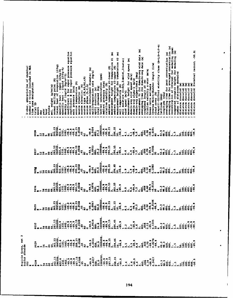
00 0:

a " 9 .ft - -W. V z :01 r

-~~~~ .30 v VW 0 ~.Z39 0.0 Ve MVhI a ., 'o A 0

Z 1 .01. 1~ -r 0' Uv 0U . a V V

013.~a Z F ~ 0. OVO. 0 ~ Gc* 46 ;t u 0. w E-. . * - W ~

13 k15. 'so 44- CPU. V - M.VonO V. 014 0 . VE *. V~ 0'

- C Iw!!-'a, 0 I C 00 a 0.I0 UCU0 0. a*--=0. ~ V W '@ .W.C UU E

1. 0 we 0O-U44 1 -2 aC WM )..jZ ..; C 100 (1) 00An,0 0VUC~~ ~ 00. 00V -- 3 024I.4'.00~ ~b'C ~ U ~ s.cc

"IS4 0'0 060 - 01V . ~ V6 V~ V

a441 c I.- - - - - -a u 0 14 0'UaV0....'5.D.U0'

0 "55001 .1 . 0 01 01 C-

0~~~~1 13.............. Z*i1., .I.a -L. a -C .a .4 C.a~ 0000. a .00 o

M 1c 1"e 01 0 01 .f u.ow *.aa.o,.. ao 0 a,- in a a. se A.0 .4u .. .1 .. 'a .4-4 0.................. .'aa. Mel. 010

M041 a ot at 0 1w 00V L" o .ý 0 . a o " "' I 'a0. '0C,1 .ai voolaý Iz.00 n C.000010.1R f toa a o' wru"M "a aa,0 .6 a oa a...ao a o a.. 0 wo 1; .1 c ac

010 010 0,0, 1.,n0 n ~ 0 . . . . . . . . . . . . .

.. ... ..s 00M 'o 01 W0NI vsacadw w a s: a. o'a;" ole,~a 10wa . 1 . ' .a. C; *oo Wa. c; 00 .ý . Z

tm INC ft00 .4 %0044. 6N.0N .0 M00WWO-v010 -ftwo

010010 a. 0 n US C4

'a .01 ~ I *.. . ., .: .0 .a. .a............. a. ft- M M0 t .0,0" a., Q:'a001 oa, oa 2a "' 01 s! I , ! 00 0a.0 ow. . ; C80 -I! 400aao o0, WUaV001aa. 11, a. . oa~ao M,;a. .7.a .0.50 01 0 1 00 o oam

010 40 V 0 01 01 a.* .~aa.- h r.' 4,sI. ... a .a

-0 C00a OM In 4h p 0 *a', a. .aoaa0 a.0 M4-a ý 0 w .61 .;00 .ace . a a oca.a.*.0.IW5401~ II 10 0 045.4 I014V)- If* IT @N T .. ;N T0 v 0 I 1 0%~ 1 1.0 ;,

' 010wýX "DM ý T1 00 c; c 0 0nIIo % Z r a1 01 a0

-0 *.a4 ..% a... d%.- 0 a a. a.01 ~ ~ ~ ~ 4 .0'N004aa010 a a .aa.a0 a.MMo.N.I 0.4.1 *.0 1 o o~

'n 010 w 0 .1 01 k

t4a .01 .f . . .- 01 ' 6 10 10 *N *ý 010 fM C%0010~~a00 Ino -Aaa a. ýW w :O .61 01 .us0 OOa.a co n0 01 .oaaaMe

-V 0 '0woo O 6a05..a . a~.15 a.a W%* .05~lM%" ft .00 .a. .0 4N00 0000.005

a 1 0

1400040 *= 10aC 2 0 01 01 0

01 ~ ~ ~ ~ M ,0'N1aa01Of 5 0 .05aI. e a .05 0 '0' O.. .00.c4 01 0,00a.~~~~~~~tcv" 4con MJ '0.4.004a00a .) a ~10aa a, . .. a a . 0 ,.5* 000 .. o o o42. -A4n du m 44n01a100"5W00 I .I Wft40 .~I0 1 I 5N N-I.NN NIO1I@ wft 09 00040'0...11..4

194

01

0 .

ah I5 D. U 00 -0 u 0002 -0 So" aS f 0- I 1

um 0 Q0 a... 3 4 * U .m02 46 El W, -4 a 0 00 W-0

V0 4--o a 04 - ý a A)0 0 0 - -U4 -02 ZC azld 11, D4 00 0 !4.O4 a4 -' -r '11 U9 U 0

C r6N 0 0 -4 :s C 3EQ. -aU 0 - W a. ). m 0- - a 0!..UU~~W 0* I' 0.0 a WI. U. OtU. 00 0 6" W.. 4 -

220ý CMI a1 0"- so -0 10 " -m qo.. -0-- , - .-..u 41 N . 4 '.0 2. -6 * - 1a4-o 2 A3a02 j 0 " 02= 1- 00U 0a : " =c c .-.-.- =.-ým- 0 00

A~ 0= C. -9 r".6.4 .19 C0.101ý C44~ 40600 @0 'O "..1 v

ca20 003 U1 e.l). 4 OU0,04 3S O . ~ 0 3 0 U 0 U0

60.004 W - w0- a C C W0C W El 8 El = .ECO 0 0U IO-0@ "or W 0 Cm 5.0 -. -- .q. .. .: a. 0l _u -6- -c 05Z o e 0 a o,C0 a W 0 . . WW b. b. 0. 00 -000 .145.J4.001.4.l1..40000

0.40 ~~~~!I0ý0I E00000--3.AOOZOIOCUa W4.1 U.0E 330 431C000M M 86 B

U~~~ W.C~ 2- 14.M0 D 0%6% 2 2 2-..1.-0 CA 0.4.'C EEC 00 -33 010 0 0 m0 000I~~~~ 644 0 0 0 S 0 0 a . U . 0 0 0 0 0 0 0 . . 0 .00 2 0 - 0 0 9 0 7. 0 0 Qc 0 -C c0o o e

00

MO ý tO 10 M W oe n nS

01 .S~n .. n4 C; W, - CSn .0 .Nc * 0 01n.01~~~ WM 1 1 1 1 .~ C4-S fn0 01 wn 4%1 Ch m40 in on10 ;a . 0 0Ii 000g1eo11100 .01.4 .1 .~.0000 .000 ..1. .0.Oeo .0 . .000

oo n01mCc !wf" rnwe ew m 0149 . 00 Sn0 Sn S

.400w m 000.0 00 0 055 001 01 a, . 01...ý 01

In 0n0 .0 0 Sn 0) 01

0 nn

MO1 1n0 01t 0; C; Sn;

01 ~ ~ ~ m -M=4M310001S I MO .00 1011 m1 .0 4 .00 0 0 00 S0 c0000ft

0t4 .04 -0 fMO n0 MOO 0 Sn cn 0

ZMAOf0 .00 "" m e .010101e. 010 00101.4 00ý 10-10 01 C!. 01. . 01 0.1 01c 1; 0 1

*Sn *4 0 *n 1.0 .1 . . . . 54 .1 .0 !MM

C, w 001m01 w0m54 W0m01me1.W 91. moo .00010.. .0001 . 5.4ý 9 201. .007V 4ý .00 40100o W! . 0000,01

0 Sn1 l~~l m m - ý c , m2 0

CO 1001 01 0 Sn Sn w.401* 001.0 010 0011. a 01 01 0110

mm 0

0 .WIAW- m w 41001 1 .000.0 010 I00. Sn 0w101110

00 0.1.Snnn0NM.4..II I NO aC SD1.. I I .44.o4 low~ 0.0 0 OI0000...S~..00

19195

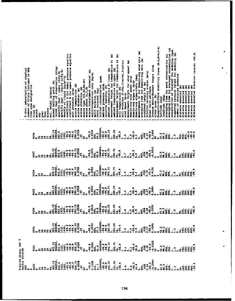
00 z w w u 01.2 -1. .04P a c- ow

: a. 1. c 0 0 0k- DUS1 U 1 6 j' 'a

4.4 0. .. 9. 46 1 1

ZZC I. a~ a aA U 0 CP

2.9 ..- N .CP 0~~B ! - 4* .4

C~- u . 4 0 %W0 0044IV 1 U S i

440 01.U -. 0 C 14 0W.~ @4 . 4 @ 44 U4.4C2U...c a -W4hCgvvvm

a.44 - -4. 0. I4. 4 -~ 9 4 A 4 -U 6 U ~ 4 @43)9

.0 .1' cc:u 64- c4M V0.V v 6o v~-9

A s; [email protected] 0. . . .. SUUU

460-' 6 000UOO OO0 0.0.0C 0U a0.4 1.j~ .1 C-4044 -2 -46V UO 4U UU U4 Ic4 UU2 0.M - 5 a l0 - 0 a49 -u04.. cit - a 00000- vv

ow'

* .04 400 * ~ .401 ~ .c; In.. a. tf44 C, W1 t'

I4. ft0 .4 `: T4 c;S 2T 1 o.4,; to9.4004~~~~~c v ow@44.. ft. 0004. I4 5I@00

P. ~ ~ ~ ~ t .61 c;...1 . 00 . .. . 0W. 40.4.4.440044000. 4.0.0444 04 ( 404 0.5 . .. 0 4 .0 0 0

at,0 Sao0 ,. 0 00 .

et441 n1 %a 0- w` "I ('w4Ot o

.400 * .4.4@ .. ( @46 00 04 1 @4 4 @44 I

45 .4 *4N .*.4 . .4~ *4@4 .. 4 4.40 .

1"1 .40 a4 0, *.a. -a;.4 O taSS

6.44*tt.(4 1 t 6 .4:1 vo *('4 004 o0 at0 a, a. De4( .4r'004 44.0Ih ft0 .042 4 0, #R 4 .00 0000 0 ( 0 0

042: " : o6lolc 4,oc 011 4(4 .14S 004 2 100.44 0404 04 4.. ft In ft 0461 @4

.4l c64 C;44 4 .. 4 .4. 0 . . . . .0. (4 00

64~11 wk144444444. 40*0.4i 4. 0 .0 0'@0 *.0 6 0 0.(5 ~e o:0. .00.44440!0 444 @ .0 40.44 .e,0 0 *.0.4* '00 0 0

5.0f64004094404.4.. tem,~ ZjIOf. 44.444.I..0.4 4'0 040.w404...4 1.0q

tn Sc; t o" ý 1; In 04 4 1 01 6 1 0

c l 0 V I

a.4 0 4 0' * 0 0 @ .( 0 . 0 0 @ 4@ 00

44. 1o 4lt alTat C64 2*4' a... T. ;Sb 0 . . ... c"1'm"ot 4 1 n 043 . *o 3 3 ninc R.

c;i 4 o in LUt in0 010, 0 64 64 .

U n wl .6n *.4444 - .6 .0.0 . . . . 0. ~ 0064 .0ba0ti0n040404404106 6;.. .040. c; I5 .4C64 t 0 .4 l c M oav-'0000

c;

-- ~~~ . .6 *N a! a a6 In ot0. . . .5 l04 .0 0444.4P4~ ~~~~~ o( a-0440000446 4m4. .40 .1 m' @4n 04 040 . 408.4 . . 0 6 '0 004.. ~ ~ ~ ~ ~ ~c0& T a4. 400.044.044 2,~ 04* 6o44 000 *4 0 .40 ('00.. 000

*040.0404.4...4044I4in f4 in 44.4 SZL 40-44 4 4.0.(006 4.01 40 1 10 44 424. ow42D.4..nn61..04

a19

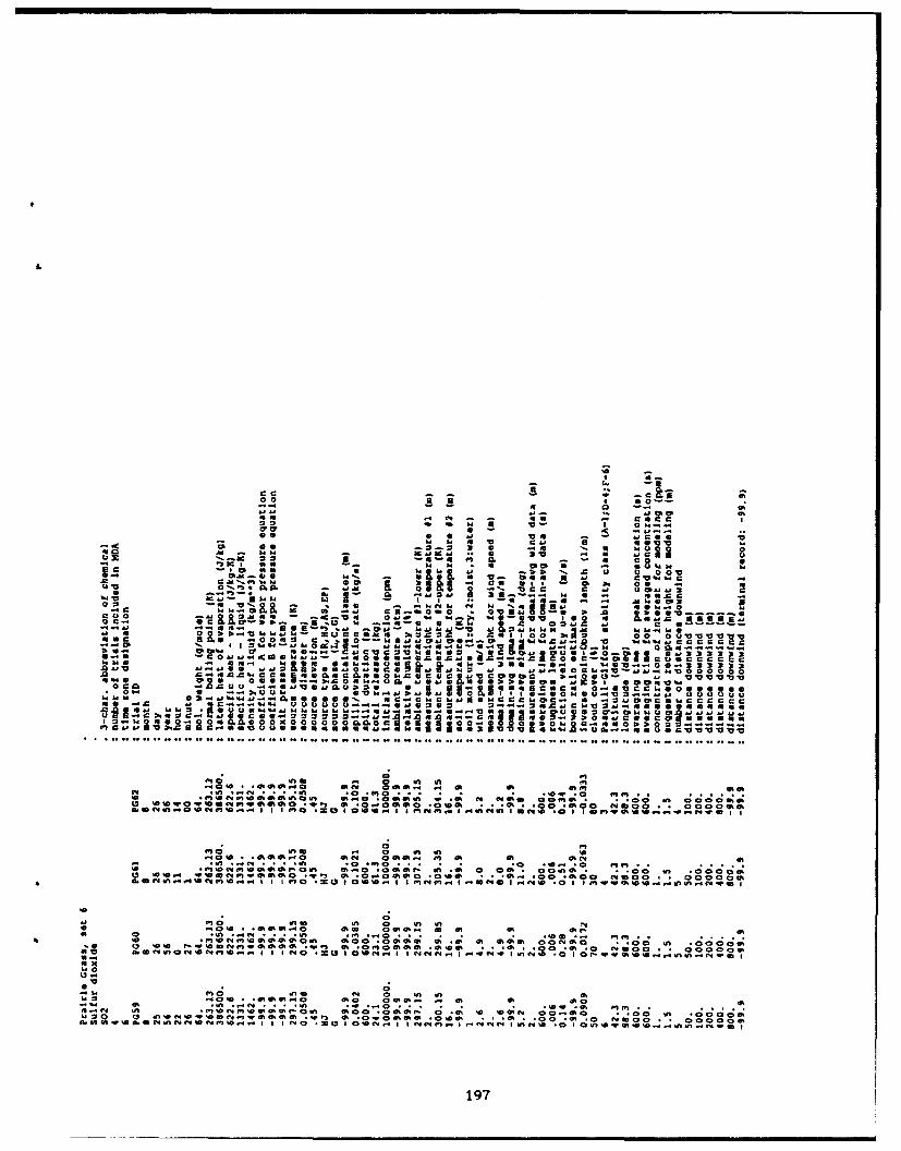
a0.

0*

001 - ;- 0

-C - - 4 0 0 Va S UOAW t.Za p

4 6 96 U a.. - 21.0 a 13 c a- i w

4 0 2.0 00 I=D 0K 66 W 0. av - 4 C 8Cý 46 2L 0 2 " a N_

On~ 0 1'~0,A "0 10, a 2t~ 0 %44" .Ago _ 0C#"c " C U 001*~~~~~~ .... 4W -. oAL. i.x1 3 U - 4 4.

0=a -q .0 S&N 14 . UI d 4. . 9 0 1 4 c I ' 5 . 1 0 0 * 0 ~ ' ~ 4 A 6 0 0 . . . . . . .

U C U M 0. .2.. 04 1 0 0 0 0.0 0al

ft - -c b. l-C

'a4C0 U4. W 2gU 22 405,2 4 0. 6 C 6 ~ 0 6 ' 0C C

WO I 1-4. A 4 C 4 ~ U . C 0 60 C S C 1C 10 0 In a * ', .1 _ýino

4% ~ ~ ~ A in Qt 6UC;0.6* -4-1000" *Uah.-44411c1; m oobo

4.4~~~,0 C- Z4* C O.2 00....'. - m C .040 U,* , I 4coo

In; 0 In In 10

0 'a'aw0 -t'4MW .1%0. . q , :4 1 *0 00 .0'0 ..- 10 0!.0 .010 " 00 . 0 00 0

0 M4jmOC InS to 0 n VI"On0' It .0!0 0 I "it 0! i1 !4, 0101.. 0 ! m P,0(40

m 4' naC4a*r .M a 1 1 % 0 M w1. C0010f I'l .0. 01 0w 001ý T' to-l0 W" -W lop . 00

WO m1 0 n In 4* it.4 14 .0:0 0.4 In 0 1 1. 01 ww .1fM 0mW. a 0M (4 ' 0%1a0 0 010 00100 vv .0 1 00010 4 10 * . 0 I 0 0.lu0 'A 0' 40 II 0000 4'~ 0 #on01 0 0'_D . 0* *1 C; T0 .0 ; .0ý Z' 0 l . . 000o

1190

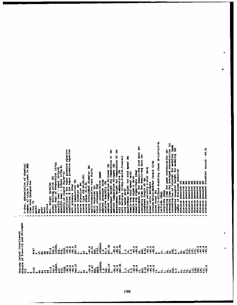
00 . a 1. 1 -4

All 5 4- C

000 a 4£ U 1..

66 0 &' & 41 U6.SC 1 *54 14 k6 0 .0_I4 '01" 47"66 - .. 00016 ... S 1430

66 L4 a4 ., . a . a - 51566 6 4 65444 .3 ..3

.00 '0.351 60 .0 .4 .0, 651 .0 .0, .0

~~ 0.0. -~~a00 0 C 5 0555

L:5 a11 Lo -I j 8. as ~ 00 &6 ~ I I I I I.u.441141 14 _%6 EE 'C' 'a465 =a4.40cItc

00 ~ ~ C..0045 * 0UU4 006 A *0* *0

.. 44 4.4 U6U In5 co4 N4545 M 4.n %n5 .a, 6; .1414.4W14

660 w "0. w06 w.. 6164 4 54 5 .11 C; 444401 OP ;0 4 .fd,. ' .a0 64444 C0 00 -n , 01,*1a - ":a o A. -OCR 514 £..nm "mw I54444- I ITdP 4.4Q-

36- 00 4 6* 4 .4 4 CU U 4 1464 4% Ck 05 53 04 E -0 6wo4 a e

4.60644o .. a 6 6 4 O O f .4 . 4 0 0 4 6 6 0 0 0 0 0 C

V144 C; w4. .46 .444669 .. ..4 3 6 65 - 6 6d . 4 6 3 3 3.9* 546 54 . ~6 a. .. 540 .4E56 4 5.-004 U55. 5U0 0 000

.9 ~ ~~~~~ 14..040 5, 110 111 668 *I66 64 U S S o 3.. 613 45 WU d

464 50 006 . 064.. 0.4545@6663366 4 3361908

04

p 0 0 a W S 00

t 4 m No Q a- 44m A 04100

-c t 441 T 0 C, a,.400C6 6 -4.4-46~~~ - 6- 4 AM - . c

U.2 0 2L q Z. A 6 04r- wt v -0 0 4 6 -2v. 4i"UOO

46 SO..4 !w o - = C En4 'C4 i 2.0 IQ 4 , 10 0 D' o.406 aI2 ... 00 R - 6 41 4 4 0" p .0 V 4 % 00 w 6. .c. I

4 4 I a. w. cc aU. I0 a-M 0Q -604.4

A 0U a; ... :0 6 -. 4..~4 0.44 114* 449 oo6U Cal w a" 4.=..Z0 ! 10 00 0 0 00A" M*0 .C%- C C M .. 4) 4.. r C6.4 6 0. co~ 0 00.4. .4 0, v vV

-- 0 r I w v*444 40 4j.5 CA j. a ~ a- .6' .f .- 0 . 4.-'j44 0 G,-'0. 000 .646. Do 0441 40040 k N -. 96 .. 2 2 3) 2

444.6 -~~~~~~~~ ~ 414- 41 o4 0 0. 0. ..... 24 '-. - 4 6 -- 6 . . )2 2 2SI O c I. a-.64 a 0. alS a W U I q.406 w .2.4 s4 M 44-o 44D- v- w 2Ce og

* ~ ~ % 0,. 6. 444.0. cc444.4.64 .00 c; 4;. c6 W 44 04w0-.. 0000000000014 .%4 a4- i14 03-4o U 1, T11 21.6a:6&Z X0.'4 4.04 5 44 0 444 AD _'j 2 IN c I t c r" w mi

0

* 0 .- 040 .4.4 .. a 4- *.4 *.'

oD 1 'a. .. mr 0 40 . w..4040I Ift6644 14464. 0 44 04466440

*a o c w `0 -@- ".44. -5000 -446 -0 cc 04~o 0 _09. 406

ac4 0 c- w! 1Zo ;1 !I' , sw . .1ol . v4o040 .66t44 ft46 1 4 40 1 40 044.4 in 0464646464 II II

00

40 at 0t 4h .4 4

2 40. .. 0 :.4 9 .. 00 0 M in a. 4- ... .. .

0 4D 0 44 4

7c0. . . . . ..,00. c; o! o!.44 .ý" to ýe

.0

6h c* 0!o0!lo 40 0 4 ! 401 064

60 ~ ~ ~ ~ ~ ~ ~ ~ ~ ~ -D w 140 10664 6444 04 0 44 4 0604 4666

044 ... 0004 . . 40 199.

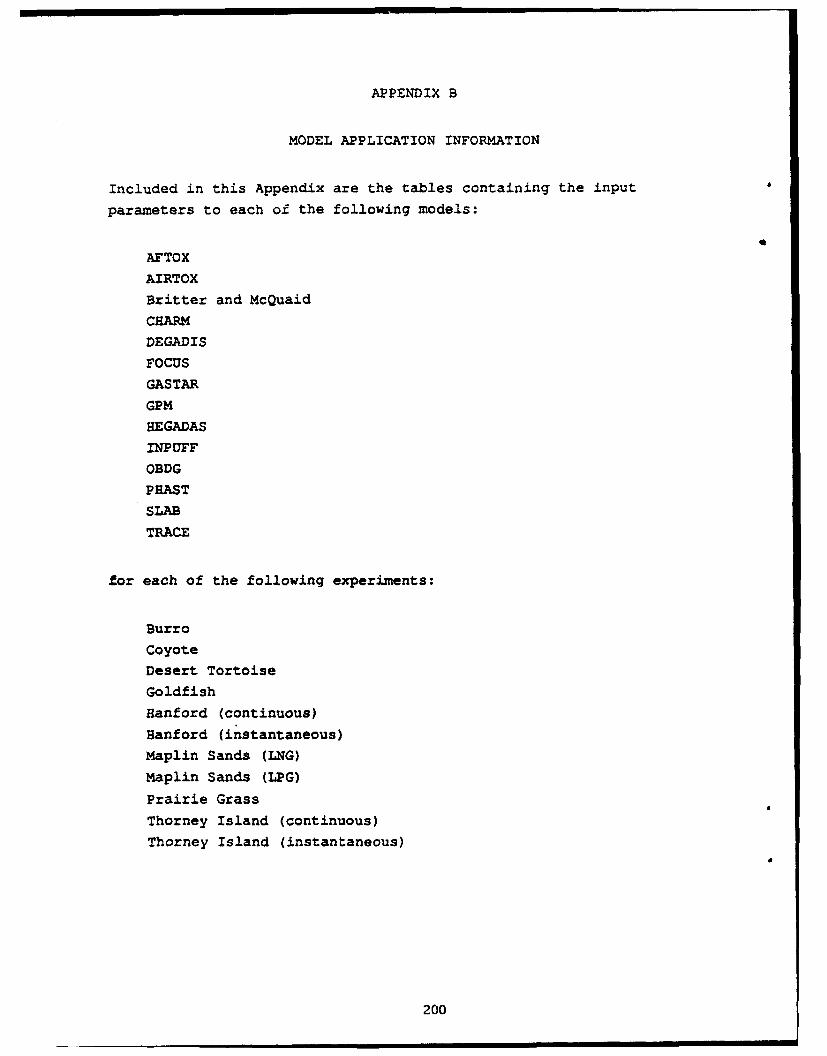
APPENDIX B

MODEL APPLICATION INFORMATION

Included in this Appendix are the tables containing the input

parameters to each og the following models:

AFTOX

AIRTOX

Britter and McQuaid

CHARM

DEGADIS

FOCUS

GASTAR

GPMREGADAS

INPUFF

OBDG

PHAST

SLAB

TRACE

for each of the following experiments:

Burro

CoyoteDesert Tortoise

GoldfishHanford (continuous)

Hanford (instantaneous)

Maplin Sands (LNG)

Maplin Sands (LPG)

Prairie Grass

Thorney Island (continuous)

Thorney Island (instantaneous)

200

AFTOX INPUT DATA FOR; BurroCHEMICAL RELEASED : Liquefied natural gas

IS PRINTER ON? NSTATION No.?7 3CHANGL DATE/TIME? : YUNIT SYSTEM? : METRICTIME ZONE 8TRIAL 8U2 BU3 BU4 Do$ 8U6 Bus7 3S 89MONTH 6 7 7 7 6 6 9 ,DAY 18 2 9 16 5 27 3 17YEAR o80 80 a80 80 80 80 80HOUR 15 15 14 1i 16 19 .9 18MINUTE 59 8 7 20 5 12 9 37TYPE OF SPILL 1 1 1 1 1 1 1 1STATION NO. 15 15 15 15 15 15 15 15CHEMICAL NO. 56 56 56 56 56 56 56 56MOLECULAR WEIGHT 17.460 17.260 17.050 17.080 17.240 18.220 18.120 18.820CONC. OF INTEREST 100.00 100.00 100.00 100.00 100.00 100.00 100.00 100.00MEAS. HEIGHT (m) 2.0 2.0 2.0 2.0 2.0 2.0 2.0 2.0ANB. TEMP. (C) 38.1 34.5 35.9 41.1 39.5 33.8 32.8 35.3WIND DIR. (deg) 0.0 0.0 0.0 0.0 0.0 0.0 0.0 0.0WIND SPEED (r/I) : 5.4 5.4 9.0 7.4 9.1 8.4 1.8 5.7HAVE STDV. OF DIR? Y Y Y Y Y Y Y ySTD. DEV. DIR. (dog): 13.5 13.3 7.3 11.1 6.7 5.2 5.6 4.4AVERAGING TIME (mnn): 6.00 6.00 6.00 6.00 6.00 6.00 6.00 6.00CLOUD COV. (8ths) 0 0 0 0 0 0 0 1S1IL MOISTURE : 2 2 2 2 2 2 2 2INVERSION? ft n a n n nt n nSITE ROUGHNESS (c,) : 0.020 0.020 0.020 0.020 0.020 0.020 0.020 0.020RELEASE HT (a) 0.00 0.00 0.00 0.00 0.00 0.00 0.00 0.00CONTINUOUS GAS RELEASEEMIS. RATE (kg/min) : 5166.0 5278.8 5217.6 4975.0 5533.2 5967.6 7015.8 8158.8STILL LEAKING? : fn n n n n nELAPSED TIME Jmin) : 2.88 2.78 2.42 3.17 2.15 2.90 1.78 1.32CONC. AVG TIME (min): 1.00 1.67 1.33 2.17 1.17 2.33 1.33 1.00SPECIFIED CONC (pp=): 100. 100. 100. 100. 100. 100. 100. 100.DOWNWIND DIST. (m) : 57.0 57.0 57.0 57.0 57.0 57.0 57.0 57.0TRAVEL TIME (min) 0.2 0.2 0.1 0.1 0.1 0.1 0.4 0.1DOWNWIND DIST. (m) : 140.0 140.0 140.0 140.0 140.0 140.0 140.0 140.0TRAVEL TIKE (min) : 0 4 0.4 0.2 0.3 0.2 0.2 0.9 0.3DOWNWIND DIST. (m) -99.9 -99.9 -99.9 -99.9 -99.9 400.0 400.0 400.0TRAVEL TIME (min) 0.0 0.0 0.0 0.0 0.0 0.7 :.6 1.0DOWNWIND DIST. (m) : -99.9 -99.9 -99.9 -99.9 -99.9 -93.9 800.0 800.0TRAVEL TIME (min) : 0.0 0.0 0.0 0.0 0.0 0.0 5.2 2.0SOlAR ANGLE (dog) : 35.76 46.49 58.54 31.53 32.29 1.90 -11.25 -9.22

201

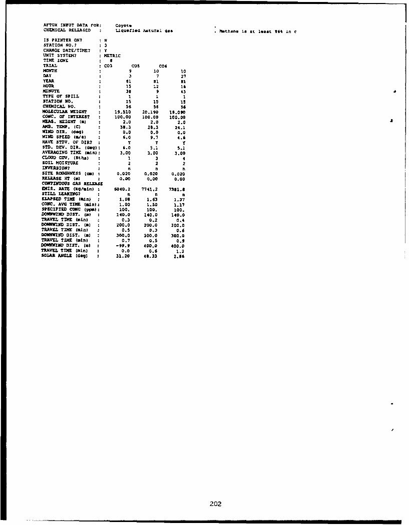
AFTOX INPUT DATA FOR: CoyoteCHEMICAL RELEASED Liqueti*. natural gas M.ethano IS at least 664 In C

IS PRINTER ON? NSTATION NO.? : 3CHANGE DATE/TIME? : YUNIT SYSTEM? : METRICTIME ZONE 8TRIAL : C03 COs C06MONTH : 9 10 10DAY . 3 7 27YEAR : al 81 61HOUR : 15 12 16MINUTE : 36 9 43TYPE OF SPILL : 1 1 1STATION NO. 15 15 15CHEMICAL NO. : 56 56 56MOLECULAR WEIGHT : 19.510 20.190 19.090CONC. OF INTEREST : 100.00 100.00 100.00MEAS. HEIGHT (a) 2.0 2.0 2.0AND. TEMP. (C) 38.3 28.3 24.1WIND DIR. (dog) 0.0 0.0 0.0WIND SPEED (L/4) 6.0 9.7 4.6HAVE STDV. OF DIR? : Y Y ySTD. DEV. DIR. (dog): 6.0 5.1 5.1AVERAGING TIME (ain): 3.00 3.00 3.00CLOUD cov. (St.hs) 1 3 4SOIL MOISTURE : 2 2 2INVERSION? .n n nSITE ROUGHNESS (m) : 0.020 0.020 0.020RELEASE HT (m) : 0.00 0.00 0.00CONTINUOUS GAS RELEASEEMIS. RATE (kg/ain) 6040.2 1741.2 7381.8STILL LEAKING? n n nELAPSED TIME Wlan) : 1.06 1.63 1.37CONC. AVG TIM (m.in): 1.00 1.50 1.17SPECIFIED CONC (ppis): 100. 100. 100.DOWNWIND DIST. (mi) 140.0 140.0 140.0TRAVEL TIE (min) 0.3 0.2 0.4DOWNWIND DIST. (m) : 200.0 200.0 200.0TRAVEL TIME (mini 0.5 0.3 0.6DOlMflND DIST. (a) : 300.0 300.0 300.0TRAVEL TIUE (min) 0.7 0.5 0.9DOWNWIND DIST. (m) : -99.9 400.0 400.0TRAVEL TIME (min) 0.0 0.6 1.2SOLAR ANGLE (dg) 31.20 48.33 2.46

202

AFTOX INPUT DATA FOR: Desert TortoiseCHDI1CAL RELEASED : Anhyarous Amonia

IS PRINTER ON? NSTATION NO.? 3CHANGE DATE/TIME? YUNIT SYSTEM? METRICTIME ZONE 6TRIAL : DT2 DT3 DT4MONTH a U 8 9 9DAY : 24 29 1 6YEAR : 83 83 $3 63HOUR : 16 11 15 1iMINUTE : 37 20 37 15TYPE OF SPILL 1 1 1 1STATION NO. : 12 12 12 12CHEMICAL NO. : 13 13 13 13MOLECULAR WEIGHT : 17.030 17.030 17.030 17.030CONC. OF INTEREST : 100.00 100.00 100.00 100.00M EAS. HEIGHT (m) : 2.0 2.0 2.0 2.0AMB. TEMP. (C) 28.6 30.4 33.9 32.4WIND DIR. (deq) : 0.0 0.0 0.0 0.0WIND SPEED (m/s) : 7.4 5.8 7.4 4.3HAVE SThV. OF DIR? : Y Y YSTD. DEV. DIR. (deo): 5.7 7.5 8.3 5.0AVERAGING TIME (min): 3.00 3.00 3.00 3.00CLOUD COV. (8ths) : 0 0 5 0SOIL MOISTURE : 2 2 2 1INVERSION? : n n nSITE ROUGHNESS (cm) : 0.300 0.300 0.300 0.300RELEASE HT (m) : 0.79 0.79 0.79 0.79CONTINUOUS GAS RELEASE

4MIS. RATE (kq/min) : 4782.0 6690.0 7842.0 5602.0STILL LEAKING? :n n n, fELAPSED TIME (&in) 2.10 4.25 2.77 6.35CONC. AVG TIME (min): 1.33 2.67 2.00 5.00SPECIFIED CONC (pm): 100. 100. 100. 100.DOWNWIND DIST. (a) : 100.0 100.0 100.0 100.0TRAVEL TINE (min) : 0.2 0.2 0.2 0.3DOWNWIND DIST. (m) : 800.0 800.0 $00.0 8O0,0TRAVEL TIME (ain) : 1.4 1.7 1.4 2.1SOI•AR ANGLE (deq) : 20.68 62.41 30.46 -2.43

203

ArTOX INPUT DATA FOR: GoldfishCHEMICAL RELEASED : Hydrogen fluoride

IS PRINTER ON? NSTATION NO.? : 3CHANGE DATE/TIME? YUNIT SYSTEM? : METRICTIME ZONE : aTRIAL : GFI 0F2 GF3MONTH a 8 8 aDAY 1 1 14 20YEAR 90 90 90HOUR i is 18 18MINU•E = 15 15 15TYPE OF SPILL : 1 1 1STATION NO. : 12 12 12CHEMICAL NO. 40 43 43MOLECULAR WEIGHT : 20.010 20.010 20.010CONC. OF INTEREST : 30.00 30.00 30.00CUAS. HEIGHT (m) : 2.0 2.0 2.0ANB. TDEP. (C) : 37.2 36.2 34.4WIND D0R. (dog) 2 0.0 0.0 0.0WIND SPEED Ia/s) : 5.6 4.2 5.4HAVE STDV. OF DXR? : YY YSTD. DEV. DIR. (dog): 10.7 14.9 10.7AVERAGING TIME (Kin): 15.00 15.00 15.00CLOUD COy. (8th.) : 0 0 0SOIL MOISTURE : 1 1 1INVERSION? . n n nSITE ROUGHNESS (c : 0.300 0.300 0.300RELEASE HT (a) : 1.00 1.00 1.00CONTINUOUS GAS RELEASEEmIS. RATE (kq/mln) : 1660.2 627.6 616.2STILL LEAKING? n nELAPSED TIME (win) : 2.08 6.00 6.00CONC. AVG TIME (nin): 1.47 1.47 1.47SPECIFIED CONC (pIm): 30. 30. 30.DOWNWIND DIST. (m) 300.0 300.0 300.0TRAVEL TIME (min) 2 0.7 0.9 0.7DOWNWIND DIST. (a) : 1000.0 1000.0 1000.0TRAVEL TUME (min) : 2.3 3.1 2.2DOWNWIND DIST. (,) : 3000.0 -99.9 3000.0TRAVEL TIME (mini : 6.8 0.5 6.7SOLAR ANGLE (des) 2 6.06 3.60 2.21

I

204

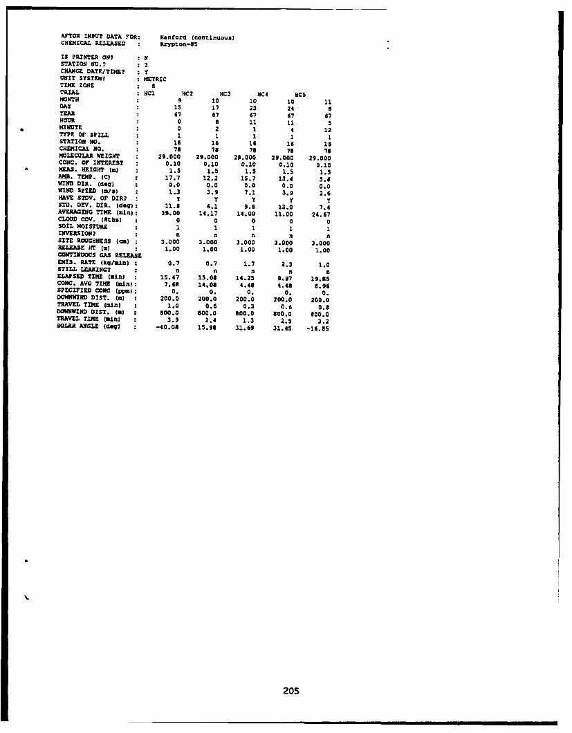
AFTOX INPUT DATA FOR: Nantora (continuous)CHEMICAL RELEASED : Krypton-65

IS PRINTER ON? : NSTATION NO.? 3CHANGE DATE/TIME? YUNIT SYSTEM? METRICTIME ZONE aTRIAL d e HC2 HC3 HC4 KCSMONTH . 9 10 10 10 11DAY 15 17 23 24 6YEAR : 67 67 67 67 67HOUR : 0 a 11 11 5MINUTE . 0 2 1 4 12TYMEO SPILL : 1 1 1 1 1STATION NO. : 16 16 16 16 16CHEMICAL NO. : 78 78 78 78 76MOLECULAR WEIGHT : 29.000 29.000 29.000 29.000 29.000CONC. OF INTEREST 0.10 0.10 0.10 0.10 0.10WEAS. HEIGHT (a) : 1.5 1.5 1.5 1.5 1.5AMD. TEMP. (C) 17.7 12.2 15.7 13.4 5.6WIND DIR. (dea) : 0.0 0.0 0.0 0.0 0.0WIND SPEED (|i5) 1.3 3.9 7.1 3.9 2.6HAVE STDV. OF DIR? Y Y 1 y YSTD. DEV. DIR. (deq): 11.6 6.1 9.6 13.0 7.4AVERAGING TIME (mn) : 39.00 14.17 14.00 11.00 24.67CLOUD COV. (Bths) 0 0 0 0 0SOIL MOISTURE 1 1 1 1 1INVERSION? :n n n n nSITE ROUGHNESS (cm) : 3.000 3.000 3.000 3.000 3.000RELEASE HT (m) : 1.00 1.00 1.00 1.00 1.00CONTINUOUS GAS RELEASEEKIS. RATE (kq/amn) : 0.7 0.7 1.7 2.3 1.0STILL LEAKING? : n n n n aELAPSED TIME (min) : 15.47 13.08 14.25 9.97 19.85COlIC. AVG TIME (.inI: 7.68 14.06 4.48 4.40 8.96SPECIFIED CONC (ppm): 0. 0. 0. 0. 0.DOWNWIND DIST. (a) : 200.0 200.0 200.0 200.0 200.0TRAVEL TIME (min) : 1.0 0.6 0.3 0.6 0.6DOWNWIND DIST. (m) 800.0 800.0 800.0 600.0 800.0TRAVEL TIME (min) : 3.9 2.4 1.3 2.5 3.2SOLAR ANGLE (deq) : -40.08 15.98 31.69 31.45 -16.65

205

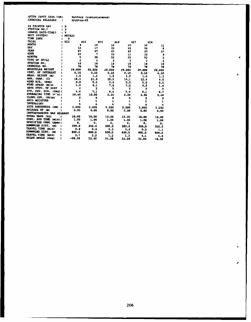
AFTOX INPUT DATA FOR: HarfOrd (instantanfous)CHEMICAL RELEASED Krypton-85

IS PRINTER ON? : NSTATION NO.? : 3CHANGE DATEITIME? YUNIT SYSTEM? : METRICTIME ZONE aTRIAL : R12 H13 HIS H16 H17 HISMONTH . 9 10 10 10 10 11DAY . 14 17 23 23 24 8YEAR 6 67 67 67 67 67 67HOUR . 23 7 10 11 10 6MINUTE . 0 38 S3 30 53 2TYPE OF SPILL : 2 2 2 2 2 2STATION NO. : 16 16 18 16 16 16CHRIUCAL, NO. 78 78 78 78 78 78MOLECULAR NWIGHT 29.000 29.000 29.000 29.000 29.000 29.000CONC. OF INTEREST : 0.10 0.10 0.10 0.10 0.10 0.10MEAS. HEIGHT (n) 1.5 1.5 1.5 1.5 1.5 1.5AMS. TEMP. (C) : 18.3 11.9 15.5 15.1 12.4 4.6WIND DIR. (dog) 0.0 0.0 0.0 0.0 0.0 0.0WIND SPEED (u/al : 1.3 4.1 7.6 7.2 4.5 1.6HAVE STOV. OF DIR? Y Y Y y Y TSTD. DEV. DIR. (dog): 4.4 5.1 6.4 5.4 9.1 8.7AVERAGING TIME (mln): 20.U0 10.00 3.33 4.00 3.50 9.00CLOUD COV. (Sths) : 0 0 0 0 0 0SOIL MOISTURE :1 1 1 1 1 1INVERSION? . n n n n nSITE ROUGHNESS (,m) 3.000 3.000 3.000 3.000 3.000 3.000RELEASE HT (a) 0.00 0.00 0.00 0.00 0.00 0.00INSTANTANEOUS GAS RELEASETOTAL MASS (kg) 10.00 10.00 10.00 10.00 10.00 10.00CONC. AVG TIN lain): 1.00 1.00 1.00 1.00 1.00 1.00SPECIFIED CONC (ppm): 0. 0. 0. 0. 0. 0.DOWNWIND DIST. (m) : 200.0 200.0 200.0 200.0 200.0 200.0TRAVEL TIME gan) : 0.9 0.6 0.3 0.3 0.5 1.1DOWNNM-D DIST. (a) : 800.0 800.0 800.0 800.0 800.0 o00.0TRAVEL TIME (ain) 3.7 2.2 1.2 1.3 2.1 4.6SOLAR ANGLE (doq) -38.34 12.40 31.38 32.36 31.04 -8.40

206

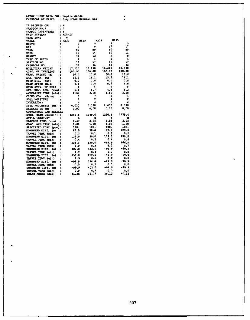
ArTOX INPUT DATA FOR: Mplin SandsCHDEICAL RELEASED Liquitled Natural Gas

IS PRINTER ON? NSTATION NO.? 3

CHANGE DATE/TIME? YUNIT SYSTEM? METRICTIME ZONE 0TRIAL MS27 M529 MS34 MS3SMONTH : 9 9 9 9

DAY . 9 9 17 17YEAR s0 s0 So soHOUR 10 14 10 11MINUTE 41 12 9 6TYPE OF SPILL 1 1 1 1STATION NO. 17 17 17 17CHEMICAL NO. 56 56 56 56MOLECULAR WEIGHT 17.110 16.260 16.660 16.390CONC. OF INTEREST 100.00 100.00 100.00 100.00"k ME.AS. HEIGHT (m : 10.0 10.0 10.0 10.0AKE. TEMP. (C) 14.9 16.1 15.2 16.1WIND DIR. (dog) 0.0 0.0 0.0 0.0WIND SPEED (W/O) 5.6 7.4 8.5 9.6HAVE STDV. OF DIR? • Y Y YSTD. DEV. DIR. (deq): 5.4 5.7 4.6 5.2AVERAGING TIME (min): 2.67 3.75 1.50 2.25C.OUD Clvy. (Sths) 0 7 1 1SOIL MOISTURE 2 2 2 2INVERSION? :n n n n

SITE ROUGHNESS (cm) 0.030 0.030 0.030 0.030

RELEASE HT (a) 0.00 0.00 0.00 0.00CONTINUOUS GAS RELEASEEMIS. RATE (kg/min) 1392.6 1749.6 1290.6 1625.4STILL LEAKING? In n n nELAPSED TIME (min) 2.67 3.75 1.58 2.25CONC. AVG TIME (min): 1.00 1.00 1.00 1.00

SPECIFIED CONC (pp): 100. 100. 100. 100.

DONNNIN DIST. (a) 89.0 56.0 87.0 129.0

TRAVEL TIME (min) 0.3 0.1 0.2 0.2DOWININNb DIST. (m) 131.0 90.0 179.0 250.0TRAVEL TIME (,in) 0.4 0.2 0.4 0.4DOWNWIND DIST. (a) 324.0 130.0 -99.9 406.0TRAVEL TINE (mini 1.0 0.3 6.7 0.7DOWhMIN DIST. (m) 400.0 182.0 -99.9 -99.9TRAVEL TIME (min) 1.2 0.4 1.2 0.0DONWIfIIO DIST. (m) 650.0 252.0 -99.9 -99.9

TRAVEL TIME (min) 1.9 0.6 0.0 0.0DOWIOKIII DIST. (a) -99.9 324.0 -99.9 -99.9TRAVEL TIME (min) 0.0 0.7 0.0 0.0DOWNWIND DIST. (W) -99.9 403.0 -99.9 -99.9

TRAVEL TIME (min) : 0.0 0.9 0.0 0.0SOLAR ANGLE (dog) 41.35 36.77 36.12 40.12

207

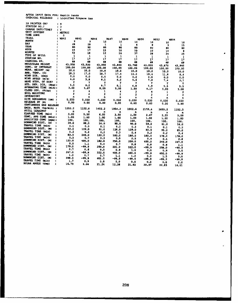
AFTOX INPUT DATA FOR: Maplin SandsCHEIICAL RELEASED : L.iqullsta Propane Gas

IS PRINTER ON? : NSTATION NO.? : 3CHANGE DATE/TIME? : YUNIT SYSTEM? : METRICTIME ZONE aTRIAL MS42 MS43 MS46 MS47 M349 MS50 M352 KSS4MONTH . 9 9 10 l0 10 10 10 10DAY * 23 28 1 1 6 8 9 15YEAR : 80 go so so so s0 so s0HOUR . is 17 15 16 10 10 14 8MINUTE 53 33 12 16 37 38 34 25TYPE OF SPILL : 1 1 1 1 1 1 1 1STATION NO. : 17 17 17 17 17 17 17 17CHEMICAL NO. 68 63 66 46 68 66 68 68MOLECULAR WEIGHT 43.930 43.930 43.950 43.840 43.760 43.930 43.070 43.940CONC. Or INTEREST : 100.00 100.00 100.00 100.00 100.00 100.00 100.00 100.00MEAS. HEIGHT (m : 10.0 10.0 10.0 10.0 10.0 10.0 10.0 10.0AMR. TEMP. (C) : 18.3 17.0 18.7 17.4 13.3 10.4 11.s 8.4WIND DIR. (deq) 0.0 0.0 0.0 0.0 0.0 0.0 0.0 0.0WIND SPEED Waes) : 4.0 5.8 6.1 6.2 5.5 7.9 7.4 3.7HAVE STDV. OF DIR? Y Y Y Y Y Y Y YSTD. DEV. DIR. (deq): 5.5 6.2 6.7 6.1 4.6 5.9 5.5 5.5AVERAGING TIME (min): 3.00 5.67 8.00 5.00 1.50 4.17 3.00 3.00CLOUD COV. (8ths) : 2 4 1 4 3 6 1 0SOIL MOISTURE ± 2 2 2 2 2 2 2 2INVERSION? n n n n n nSITE ROUGHNESS (m) : 0.030 0.030 0.030 0.030 0.030 0.030 0.030 0.030RELEASE HT Ws) 0.00 0.00 0.00 0.00 0.00 0.00 0.00 0.00

CONTINUOUS GAS RELEASEEMIS. RATE (kg/min) : 1252.2 1152.0 1402.2 1954.2 1002.6 2153.4 2655.0 1152.0STILL LEAKING7 n n n a n n n ftELAPSED TIME (min) 3.00 5.50 6.00 3.50 1.50 2.67 2.33 3.00CONC. AVG TIME (min): 1.00 1.00 1.00 1.00 1.00 1.00 1.00 1.00SPECIFIED CONC (ppm): 100. 100. 100. 100. 100. 100. 100. 100.DOWNWIND DIST. (m) : 28.0 86.0 34.0 90.0 90.0 59.0 61.0 56.0TRAVEL TIME (min) : 0.1 0.3 0.1 0.2 0.3 0.1 0.1 0.3DOWNWIND DIST. (a) 53.0 129.0 91.0 128.0 129.0 93.0 95.0 85.0TRAVEL TIME (min) : 0.2 0.4 0.2 0.3 0.4 0.2 0.2 0.4DOWNWIND DIST. (m) 83.0 249.0 130.0 182.0 180.0 182.0 170.0 178.0TRAVEL TIME (min) : 0.3 0.7 0.3 0.5 0.5 0.4 0.4 0.9DOWNWIND DIST. (m) ± 123.0 400.0 132.0 250.0 250.0 400.0 249.0 247.0TRAVEL TIME (min) 0 0.5 1.1 0.4 0.7 0.9 0.8 0.6 1.1DOWNWIND DIST. (al 179.0 -99.9 250.0 321.0 322.0 -99.9 398.0 -99.9TRAVEL TIME lain) 0.7 0.6 0.5 0.9 1.0 0.0 0.9 0.0DOWNWIND DIST. (m) : 247.0 -99.9 322.0 400.0 400.0 -99.9 650.0 -99.9TRAVEL TINE (mini : 1.0 0.7 0.7 1.1 1.2 0.0 1.5 0.0DOWNWIND DIST. (a) : 398.0 -99.9 401.0 -99.9 -99.9 -99.9 -99.9 -99.9TRAVEL TIME (min) 1.7 0.9 0.6 0.0 0.0 0.0 0.0 0.0SOLAR ANGLE (deq) 16.79 4.04 21.24 12.38 31.63 30.97 22.83 16.01

208

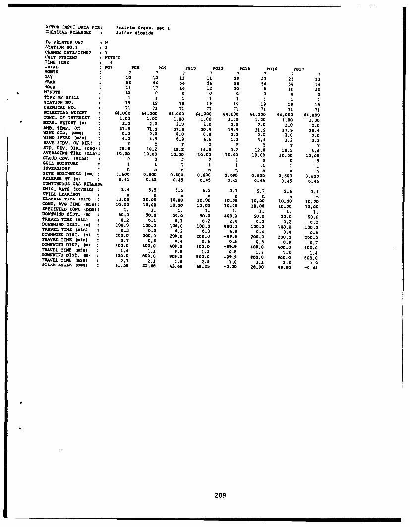
AFTOX INPUT DATA FOR: Prairie Gran*. set 1CHEMICAL RELEASED Sulfur dliaide

IS PRINTER ON? : NSTATION NO.7 3CHANGE DATE/TIME? YUNIT SYSTEM? METRICTIME ZONE 6TRIAL : PG7 Pas PG9 PalO POX? P015 PG16 PG17MONTH . 7 7 7 7 7 7 7 7DAY . 10 10 11 11 22 23 23 23YEAR * 56 56 56 56 56 56 SE 56HOUR . 14 17 1X 12 20 a 10 20MINUTE . 15 0 0 0 0 0 0 0TYPE OF SPILL : 1 1 1 1 1 1 1 1STATION NO. : 19 19 19 19 19 19 19 19CHEMICAL NO. 71 71 71 71 71 71 71 71

MOLECULAR WEIGHT : 64.000 64.000 64.000 64.000 64.000 64.000 64.000 64.000CONC. OF INTEREST : 1.00 1.00 1.00 1.00 1.00 1.00 1.00 1.00MEAS. HEIGHT (m) 2.0 2.0 2.0 2.0 2.0 2.0 2.0 2.0AMD. TEMP. (C) : 31.9 31.9 27.9 30.9 19.9 21.9 27.9 26.9WIND DIR. (49q) : 0.0 0.0 0.0 0.0 0.0 0.0 0.0 0.0WIND SPEED (ar/s) : 4.2 4.9 6.9 4.6 1.3 3.4 3.2 3.3HAVE STDV. OF DIR? :y Y Y Y Y Y y YSTD. DEV. DIR. (deo): 25.6 10.2 10.2 16.8 3.2 12.8 18.5 5.6AVERAGING TIME (min): 10.00 10.00 10.00 10.00 10.00 10.00 10.00 10.00CLOUD COV. laths) 0 0 2 2 1 0 0 5SOIL MOISTURE : 1 1 1 1 1 .1 1 1INVERSION? : n n n n n n n nSITE ROUGHNESS (cm) : 0.600 0.600 0.600 0.600 0.600 0.600 0.600 0.600RELEASE FFT (m) : 0.45 0.45 0.45 0.45 0.45 0.45 0.45 0.45CONTINUOUS GAS RELEASEg41s. RATE (kg/min) 5.4 5.5 5.5 5.5 3.7 5.7 5.6 3.4STILL LEAKING? : n n n a n n nELAPSED TIME lain) 10.00 10.00 10.00 10.00 10.00 10.00 10.00 10.00CONC. AVG TIME lain): 10.00 10.00 10.00 10.00 10.00 10.00 10.00 10.00SPECIFIED CONC (p9M): 1. 1. 1. 1. 1. 1. 1. 1.DOWNWIND DIST. (m) 50.0 50.0 50.0 50.0 400.0 50.0 50.0 50.0TRAVEL TIME (min) : 0.2 0.1 0.1 0.2 2.4 0.2 0.2 0.2DOWNWIND DIST. (a) 100.0 100.0 100.0 100.0 300.0 100.0 100.0 100.0TRAVEL TIME (min) : 0.3 0.3 0.2 0.3 4.9 0.4 0.4 0.4DOWNWIND DIST. (m) : 200.0 200.0 200.0 200.0 -99.9 200.0 200.0 200.0TRAVEL TIME (ain) : 0.7 0.6 0.4 0.6 0.5 0.8 0.9 0.7DOWNWIND DIST. (W) 400.0 400.0 400.0 400.0 -99.9 400.0 400.0 400.0TRAVEL TIME (min) 1.4 1.1 0.8 1.2 0.8 1.7 1.1 1.4DOWNWIND DIST. (a) : 800.0 800.0 800.0 800.0 -99.9 800.0 800.0 800.0TRAVEL TIME (min) : 2.7 2.3 1.6 2.5 1.0 2.2 3.6 2.9SOLAR ANGLE (deg) : 61.58 32.60 43.68 68.25 -0.30 28.00 49.80 -0.44

209

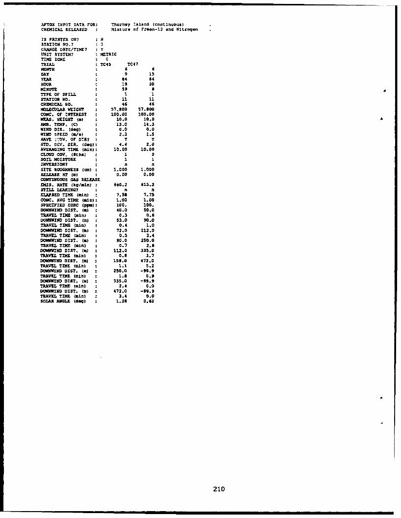
AFTOX INPUT DATA FOR: Thorney Island (continuous)CHEMICAL RELEASED : Mixture of Freon-12 and Nitrogen

IS PRINTER ON? : NSTATION NO.? : 3CHANGE DATE/TIME? : YUNIT SYSTEM? : METRICTIME ZONE : 0TRIAL ; TC45 TC47MONTH . 6 6DAY . 9 15YEAR. : 64 04HOUR 19 20MINUTE 59 8

TYPE OF SPILL 1 1STATION NO. 11 11CHEMICAL NO. : 46 46MOLECULAR WEIGHT 57.800 57.800CONC. OF INTEREST 100.00 100.00MRAS. HEIGHT (m) : 10.0 10.0AMN. TEMP. (C) : 13.0 14.3WIND DIR. (dog) 0.0 0.0WIND SPEED (W/a) 2.3 1.5NAVE .DV. OF DRT? Y YSTD. DEV. DIR. (deq): 4.4 2.0

AVERAGING TIME (min): 10.00 10.00CLOUD COV. (NthsM 1 0SOIL MOISTURE : 1 1INVERSION? * n nSITE ROUGHNESS (cm) 1.000 1.000RELEASE HT (a) : 0.00 0.00CONTINUOUS GAS RELEASEEMIS. RATE (kg/min) 640.2 613.2STILL LEAKING? ft nELAPSED TINE (min) 7.58 7.75CONC. AVG TIME (min): 1.00 1.00SPECIFIED CONC (ppo): 100. 100.DOWNWIND DIST. (m) : 40.0 50.0TRAVEL TIME (min) 0.3 0.6

DOWNWIND DIST. (m) : 53.0 90.0TRAVEL TIME (imn) : 0.4 1.0

DOWNWIND DIST. (m) : 72.0 212.0TRAVEL TIME (rin) : 0.5 2.4DOWNWIND DIST. (m) : 90.0 250.0TRAVEL TIME (min) : 0.7 2.8DOWNWIND DIST. (W) 112.0 335.0TRAVEL TIME (min) 0.8 3.7DOWNWIND DIST. (m) 158.0 472.0TRAVEL TIME (min) : 1.1 5.2DOWNWIND DIST. (m) 250.0 -99.9TRAVEL TIME (min) 1.6 0.9DOWNWIND DIST. (m) : 335.0 -99.9TRAVEL TINE (min) 2.4 0.0DOWNWIND DIST. (a) : 472.0 -99.9TRAVEL TIME (min) : 3.4 0.0SOLAR ANGLE (dog) 1.28 0.62

210

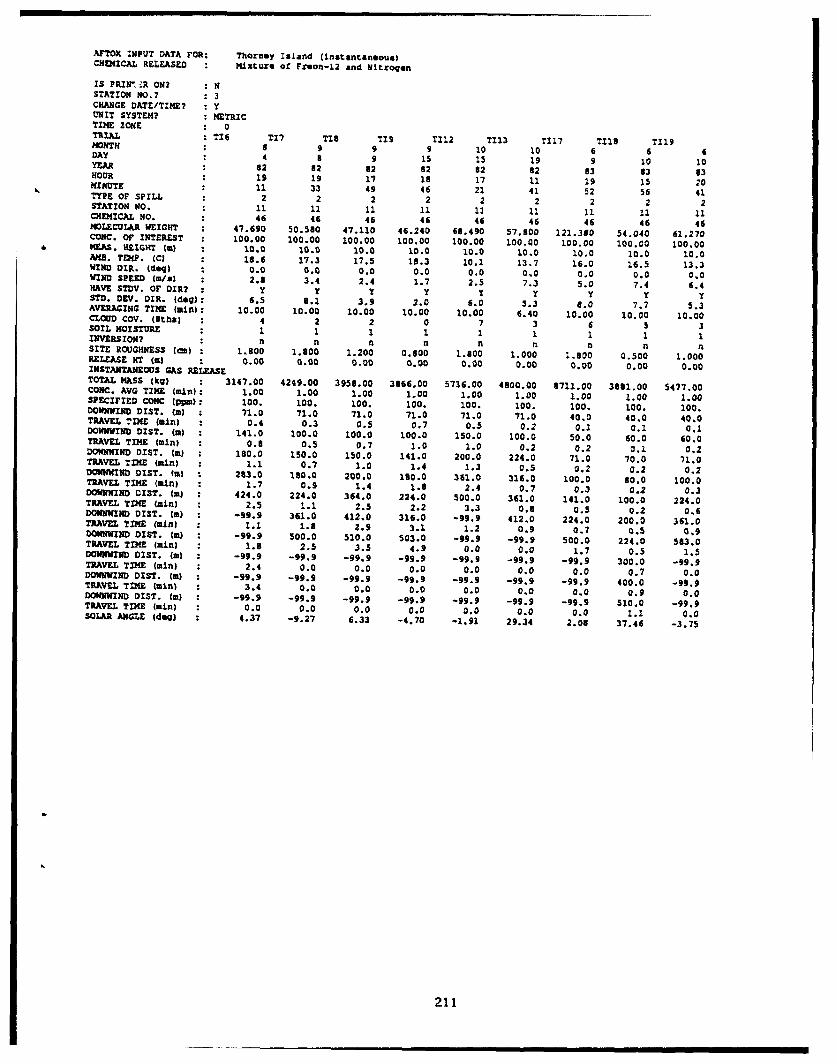
AFTOX INPUT DATA FOR: Thornoy Island (instantaneous,CHEMICAL RELEASED : Mixture of Fteon-12 and Nitroqen

IS PRIN. ,R ON? : NSTATION NO.? : 3CHANGE DATE/TIME? yUNIT SYSTEM? METRICTIME ZONE : 0TRIAL : TI6 T17 TI8 TI9 TI12 TI13 TI17 TIll TI19MONTH 0 6 9 9 9 10 10 6 6 6DAY . 4 a 9 15 15 19 9 10 10YEAR 62 82 82 82 82 82 63 03 83HOUR 19 19 17 18 17 11 19 15 20MINOTE . 11 33 49 46 21 41 52 56 41TYPE OF SPILL : 2 2 2 2 2 2 2 2 2STATION NO. 11 11 11 11 11 11 11 11 11CHEMICAL NO. : 46 46 46 46 46 46 46 46 46MOLECULAR WEIGHT 47.690 50.580 47.110 46.240 68.490 57.$00 121.380 54.040 61.270CONC. OF INTEREST : 100.00 100.00 100.00 100.00 100.00 100.00 100.00 100.00 100.00MEAS. HEIGHT (am : 10.0 10.0 10.0 10.0 10.0 10.0 10.0 10.0 10.0AND. TERP. (C) : 18.6 17.3 17.5 16.3 10.1 13.7 16.0 16.5 13.3WIND DIR. (deg) : 0.0 0.0 0.0 0.0 0.0 0.0 0.0 0.0 0.0WIND SPEED (m/s) : 2.8 3.4 2.4 1.7 2.5 7.3 5.0 7.4 6.4HAVE STDV. OF DIR? : Y Y Y Y Y Y TSTD. DEV. DIR. (deq): 6.5 8.1 3.9 2.0 6.0 5.3 8.0 7.7 5.3AVERAGING TIME Cmin): 10.00 10.00 10.00 10.00 10.00 6.40 10.00 10.00 10.00CL Cov. (8oth) : 4 2 2 0 7 3 6 5 3SOIL MOISTURE 1 1 1 1 1 1 1 1 1INVERSION? . n n n n n n n n nSITE ROUGHNESS (m) : 1.800 1.800 1.200 0.600 1.600 1.000 1.800 0.500 1.000RELEASE HT Wa) : 0.00 0.00 0.00 0.00 0.00 0.00 0.00 0.00 0.00INSTANTANEOUS GAS RELEASE

TOTAL MASS (kq) 3147.00 4249.00 3958.00 3866.00 5736.00 4800.00 8711.00 3681.00 5477.00CONC. AVG TIME (min)-: 1.00 1.00 1.00 1.00 1.00 1.00 1.00 1.00 1.00SPECIFIED CONC (pp):} 100. 100. 100. 100. 100. 100. 100. 100. 100.DOWNWIND DIST. (a) : 71.0 71.0 71.0 71.0 71.0 71.0 40.0 40.0 40.0TRAVEL TIME (ain) 0.4 0.3 0.5 0.7 0.5 0.2 0.1 0.1 0.1DOWNWIND DIST. (m) : 141.0 100.0 100.0 100.0 150.0 100.0 50.0 60.0 60.0TRAVEL TIME (ain) 0.6 0.5 0.7 1.0 1.0 0.2 0.2 0.1 0.2DOWNWIND DIST. (m) : 180.0 150.0 150.0 141.0 200.0 224.0 71.0 70.0 71.0TRAVEL TIME (min) 1.1 0.7 1.0 1.4 1.3 0.5 0.2 0.2 0.2DOWNWIND DIST. (m) 283.0 180.0 200.0 160.0 361.0 316.0 100.0 80.0 100.0TRAVEL TIME (min) : 1.7 0.9 1.4 1.8 2.4 0.7 0.3 0.2 0.3DOWNWIND DIST. (m) : 424.0 224.0 364.0 224.0 500.0 361.0 141.0 100.0 224.0TRAVEL TINE (ain) 2.5 1.1 2.5 2.2 3.3 0.8 0.5 0.2 0.6DOWNWIND DIST. (m) : -99.9 361.0 412.0 316.0 -99.9 412.0 224.0 200.0 361.0TRAVEL TIME (min) 1.1 1.8 2.9 3.1 1.2 0.9 0.7 0.5 0.9DOWNWINO DIST. (m) : -99.9 500.0 510.0 503.0 -99.9 -99.9 500.0 224.0 563.0TRAVEL TIME Cain) 1.6 2.5 3.5 4.9 0.0 0.0 1.7 0.5 1.5DOWNWIND DIST. (m) : -99.9 -99.9 -99.9 -99.9 -99.9 -99.9 -99.9 300.0 -99.9TRAVEL TIME (min) : 2.4 0.0 0.0 0.0 0.0 0.0 0.0 0.7 0.0DOWNWIND DIST. (m) : -99.9 -99.9 -99.9 -99.9 -99.9 -99.9 -99.9 400.0 -99.9TRAVEL TIME (min) : 3.4 0.0 0.0 0.0 0.0 0.0 0.0 0.9 0.0DOWNWIND DIST. (m) : -99.9 -99.9 -99.9 -99.9 -99.9 -99.9 -99.9 510.0 -99.9TRAVEL TIME (ain) : 0.0 0.0 0.0 0.0 0.0 0.0 0.0 1.1 0.0SOLAR ANGLE (dog) : 4.37 -9.27 6.33 -4.70 -1.91 29.34 2.08 37.46 -3.75

211

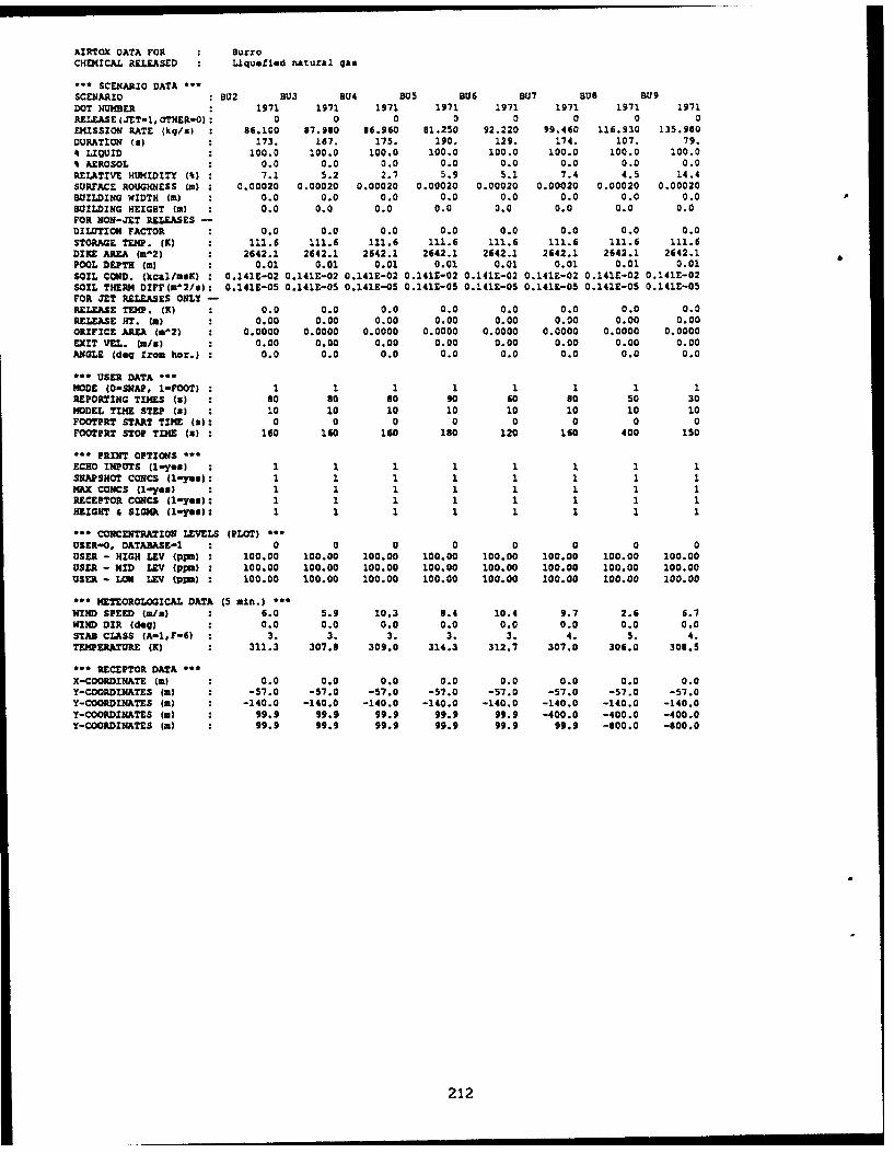
AIRTOX DATA FOR BurroCHEMICAL RELEASED Liquefied natural gas

SCENARIO DATA ,SCENARIO 302 BU3 3U4 BUS 306 BU07 U8 3U9DOT NUMBER 1971 1971 1971 1971 1971 1971 1971 1971RELEASE (JET-1, OTHER-0) : 0 0 0 0 0 0 0 0EMISSION RATE (kg/a) : 86.100 87.980 86.960 81.250 92.220 99.460 116.930 135.980

DURATION (a) 173. 167. 175. 190. 129. 174. 107. 79.4 LIQUID 100.0 100.0 100.0 100.0 100.0 100.0 100.0 100.0% AEROSOL 0.0 0.0 0.0 0.0 0.0 0.0 0.0 0.0RELATIVE HUMIDITY (t) 7.1 5.2 2.7 5.9 5.1 7.4 4.5 14.4SURFACE ROUGHNESS (m) 0.00020 0.00020 0.00020 0.00020 0.00020 0.00020 0.00020 0.00020BUILDING WIDTH (m) 0.0 0.0 0.0 0.0 0.0 0.0 0.0 0.0 A

BUILDING HEIGHT (m) 0.0 0.0 0.0 0.0 0.0 0.0 0.0 0.0FOR NON-JET RELEASESDILUTION FACTOR 0.0 0.0 0.0 0.0 0.0 0.0 0.0 0.0STORAGE TEMP. (K) 111.6 111.6 111.6 111.6 111.6 111.6 111.6 111.6DIKE AREA (am2) 2642.1 2642.1 2642.1 2642.1 2642.1 2642.1 2642.1 2642.1POOL DEPTH (m) 0.01 0.01 0.01 0.01 0.01 0.01 0.01 0.01

SOIL CORD. (kcal/m*K) 0.141E-02 0.141E-02 0.141E-02 0.1419-02 0.141E-02 0.141E-02 0.141E-02 0.141E-02SOIL THERM DITF(u"2/s): 0.141E-05 0.141E-05 0.141E-05 0.141E-05 0.141E-05 0.141E-05 0.141E-05 0.141E-05FOR JET RELEASES ONLY -RELEASE TEMP. (K) 0.0 0.0 0.0 0.0 0.0 0.0 0.0 0.0RELEASE HT. (a) 0.00 0.00 0.00 0.00 0.00 0.00 0.00 0.00ORIFICE AREA (ma2) 0.0000 0.0000 0.0000 0.0000 0.0000 0.0000 0.0000 0.0000EXIT VEL. (m/s) 0.00 0.00 0.00 0.00 0.00 0.00 0.00 0.00ANGLE (doq from hor.) : 0.0 0.0 0.0 0.0 0.0 0.0 0.0 0.0

*'* USER DATA -*-MODE (0-SNAP, 1-FOOT) : 1 1 1 1 1 1 1 1REPORTING TIMES (a) 80 80 80 90 60 s0 50 30MODEL TIME STEP (n) 10 10 10 10 10 10 10 10FOOTPRT START TIME (a): 0 0 0 0 0 0 0 0FOOTPRT STOP TIME (a) 160 160 160 180 120 1S0 400 150

*** PRINT OPTIONS l**ECHO INPUTS (1-yea) 1 1 1 1 1 1 1 1SNAPSHOT CONCS (1-yes): 1 1 1 1 1 1 1 1MAX CONCS (1-yes) : 1 1 1 1 1 1 1 1RECEPTOR CONCS (1-yes): 1 1 1 1 1 1 1 1HEIGHT a SIGMA (1-yes): 1 1 1 1 1 1 1 1

; CONCENTRATION LEVELS (PLOT) ***

*SER-O, DATASASE-1 0 0 0 0 0 0 0 0USER - HIGH LEV (ppm) : 100.00 100.00 100.00 100.00 100.00 100.00 100.00 100.00USER - MID LEV (ppm) : 100.00 100.00 100.00 100.00 100.00 100.00 100.00 100.00USER - LOW LEV (pim) : 100.00 100.00 100.00 100.00 100.00 100.00 100.00 100.00

*w* METEOROLOGICAL DATA (5 min.) ***WIND SPEED (a/s) 6.0 5.9 10.3 3.4 10.4 9.7 2.6 6.7WIND DIR (dog) : 0.0 0.0 0.0 0.0 0.0 0.0 0.0 0.0STAS CLASS (A-i,Fr-6) 3. 3. 3. 3. 3. 4. 5. 4.TEMPERATURE (K) 311.3 307.8 309.0 314.3 312.7 307.0 306.0 308.5

*'* RECEPTOR DATA *"X-COORDINATE (a) : 0.0 0.0 0.0 0.0 0.0 0.0 0.0 0.0Y-COORDINATES (m) -57.0 -57.0 -57.0 -57.0 -57.0 -57.0 -S7.0 -57.0Y-COORDINATES (m) -140.0 -140.0 -140.0 -140.0 -140.0 -140.0 -140.0 -140.0T-COORDINATES (a) 99.9 99.9 99.9 99.9 99.9 -400.0 -400.0 -400.0Y-COORDINATES (m) 99.9 99.9 99.9 99.9 99.9 99.9 -800.0 -800.0

212

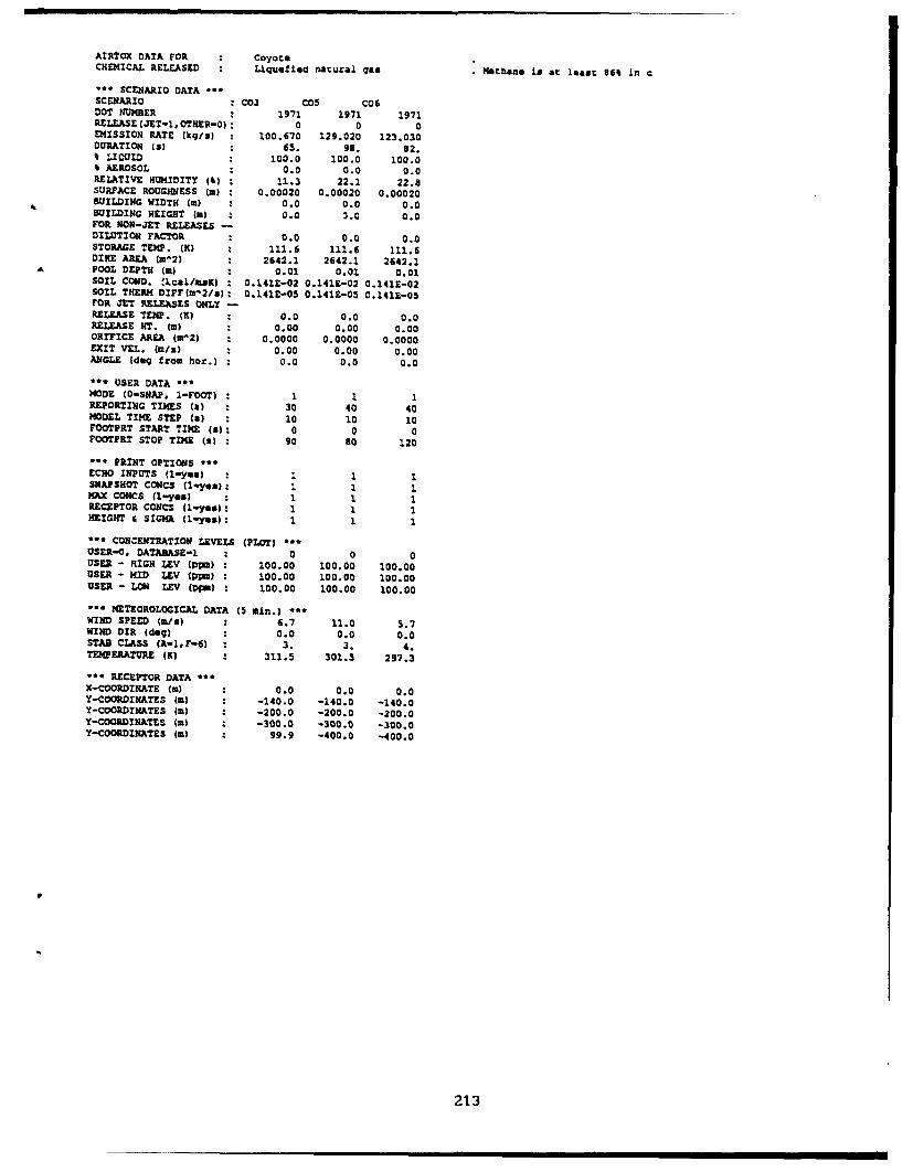
AIRTOX DATA FOR CoyoteCHEMICAL RELEASED Liquefied natural qas . Methane is at least 860 in c

*** SCENARIO DATA *eSCENARIO C03 COs CO6DOT NUMBER 1971 1971 1971RELEASE(JET-1,OTHER-0)'. 0 0 0EMISSION RATE (kq/s) 100.670 129.020 123.030DURATION (a) 65. 98. 82."0 LIQUID 100.0 100.0 100.0% AEROSOL . 0.0 0.0 0.0RELATIVE HUMIDITY (4) 11.3 22.1 22.8SURFACE ROUGHNESS (m) 0.00020 0.00020 0.00020BUILDING WIDTH (m) 0.0 0.0 0.0BUILDING HEIGHT (m) 0.0 :.0 0.0FOR NON-JET RELEASES -DILUTION FACTOR 0.0 0.0 0.0STORAGE TEMP. (K) 111.6 111.6 111.6DIKE AREA (m-2) 2642.1 2642.1 2642.1POOL DEPTH (a) 0.01 0.01 0.01SOIL COND. ,kcal/JhK) 0.1412-02 0.141E-02 0.141E-02SOIL THERM DIFF(m"2/s); 0.141E-05 0.141E-05 0.141E-05FOR JET RELEASES ONLY -RELEASE TEMP. (K) 0.0 0.0 0.0RELEASE MT. (m) 0.00 0.00 0.00ORIFICE AREA (a'2) 0.0000 0.0000 0.0000EXIT VEL. (m/a) 0.00 0.00 0.00ANGLE (dog from hor.) 0.0 0.0 0.0

*"* USER DATA "**MODE (0-SNAP, 1-FOOT) 1 1 1REPORTING TIMES (a) 30 40 40MODEL TIME STEP (a) 10 10 10FOOTPRT START TIME (a): 0 0 0FOOTPRT STOP TIME (g) : 90 8s 120

"*** PRINT OPTIONS *ECHO INPUTS (1-yes) 1 1 1SNAPSHOT CONCS (1.y*2): 1 1 1MAX CONCS (-yes) 1 1 1RECEPTOR CONCS (1-yes): 1 1 1HEIGHT & SIGMA (1-yes): 1 1 1

*"* CONCENTRATION LEVELS (PLOT) *USER-O, DATADASE-3- : 0 0 0USER - HIGH LEV (ppm) 100.00 100.00 100.00USER - MID LEV (ppm) : 100.00 100.00 100.00USER - LOW LEV (ppm) : 100.00 100.00 100.00

"*** METEOROLOGICAL DATA (5 min.) ***WIND SPEED (m/&) 6.7 11.0 5.7WIND DIR (dog) 2 0.0 0.0 0.0STAB CLASS (A-1,F-6) - 3. 3. 4.TEMPERATURE (K) 311.5 301.5 297.3

"* RECEPTOR DATA **X-COORDINATE (m) : 0.0 0.0 0.0Y-COORDINATES (m) : -140.0 -140.0 -140.0Y-COORDINATES (m) : -200.0 -200.0 -200.0Y-COORDINATES (m) -300.0 -300.0 -300.0Y-COORDINATES (m) 99.9 -400.0 -400.0

213

AIRTOX DATA FOR : Desert TortoiseCHDEICAL RELEASED Anhydrous Ammonia

.*' SCENARIO DATA *.SCENARIO : DT1 DT2 DT3 DT4DOT NUMBER 1005 1005 i005 1005RELEASE(JET-1,OTHER-O): 1 1 1 1EMISSION RATE (kg/s) 79.700 111.500 130.700 96.700DURATION (a) 126. 255. 166. 381.% LIQUID 81.3 31.7 81.1 80.4t AEROSOL 100.0 100.0 100.0 100.0RELATIVE HUMIDITY (%) 13.2 17.5 14.0 21.3SURFACE ROUGHNESS (Wt : 0.00300 0.00300 0.00300 0.00300BUILDING WIDTH (2) : 0.0 0.0 0.0 0.0BUILDING HEIGHT (m) 0.0 0.0 0.0 0.0FOR NON-JET RELEASES --DILUTION FACTOR 0.0 0.0 0.0 0.0STORAGE TEMP. (K) : 0.0 0.0 0.0 0.0DIME AREA (W"2) : 0.0 0.0 0.0 0.0POOL DEPTH (a) : 0.00 0.00 0.00 0.00SOIL COND. (kcal/nsK) : 0.000E+00 0.000OE+00 0.QOOE.00 0.0006+00SOIL THERM DIFF(m^2/s): 0.000E+00 0.0009+00 0.000E+00 0.0006÷00FOR JET RELEASES ONLY -RELEASE TEMP. (I) : 237.5 237.6 237.5 237.4RELEASE HT. (m) 0.79 0.79 0.79 0.79ORIFICE AREA (m'2) : 0.8445 1.1199 1.1647 1.2115EXIT VEL. (W/O) 22.65 23.28 27.29 20.19ANGLE (dog from hor.) : 0.0 0.0 0.0 0.0

*** USER DATA -**MODE (0-SNAP, I-FOOT) : 1 1 1 1REPORTING TIMES (a) : 60 120 80 10MODEL TIME STEP (a) 10 10 10 10FOOTPRT START TIME (a): 0 0 0 0FOOTPRT STOP TIME (a) 190 240 240 380

*** PRINT OPTIONS **ECHO INPUTS (1.,yes) 1 1 1 1SNAPSHOT CONCS (1-yes); 1 1 1 1MAX CONCS (1-yes) 1 1 1 1RECEPTOR CONCS (1-yes): 1 1 1 1HEIGHT A SIGMA (1-yes): 1 1 1 1

*** CONCENTRATION LEVELS (PLOT) '*USER-O, DATABASE-i : 0 0 0 0USER - HIGH LEV (ppm) 100.00 100.00 100.00 100.00USER - MID LEV (ppm) 100.00 100.00 100.00 100.00USER - LOW LEV (ppm) : 100.00 100.00 100.00 100.00

*** METEOROLOGICAL DATA (5 min.) ***WIND SPEWD (We.) 9.7 7.6 9.3 6.2WIND DIR (dog) 0.0 0.0 0.0 0.0STAB CLASS (A-1,F-6) : 4. 4. 4. 5.TEMPERATURE (X) 302.0 303.6 307.1 305.6

*** RECEPTOR DATA ,eX-COORDINATE (m) : 0.0 0.0 0.0 0.0Y-COORDINATES (m) : -100.0 -100.0 -100.0 -100.0Y-COORDINATES (a) : -600.0 -800.0 -800.0 -800.0

214

AIRTOX DATA FOR GoldfishCHE4ICLL RELEASED : Hydroqen fluolride

,** SCENARIO DATA ...SCENARIO : GF1 CF2 GF3DOT NUMBER : 1052 1052 1052RELEASE (JET-I, OTHER-0): 1 1 1EMISSION RATE (kg/s) 27.670 10.460 10.270DURATION (a) : 125. 360. 360.4 LIQUID : 84.0 85.3 84.71 AEROSOL 100.0 100.0 100.0RELATIVE HUMIDITY (i) : 4.9 10.7 17.7SURFACE ROUGHNESS (m) : 0.00300 0.00300 0.00300BUILDING WIDTH (m) : 0.0 0.0 0.0BUILDING HEIGHT (ml 0.0 0.0 0.0FOR MON-JET RELEASES --DILUTION FACTOR : 0.0 0.0 0.0STORAGE TEMP. (K) : 0.0 0.0 0.0DIKE AREA (m-2) : 0.0 0.0 0.0POOL DEPTH (m) 0.00 0.00 0.00SOIL COND. (kcal/maK) : 0.OOOE+O0 0.O00E+O0 0.000E+00SOIL THERM DIFF(m'2/s): 0.000E+O0 0.O00E+00 0.000E+00FOR JET RELEASES ONLY -RELEASE TEMP. (K) 289.6 289.5 239.6RELEASE HT. (a) 1.00 1.00 1.00ORIFICE AREA (M^2) 0.2906 0.0896 0.0926EXIT VEL. (m/a) 20.33 23.04 22.62ANGLE (dog from hor.) 0.0 0.0 0.0

*** USER DATA *'*MODE (0-SNAP, 1-FOOT) : 1 I 1REPORTING TIMES (a) o60 130 10MODEL TIME STEP (s) 10 10 10FOOTPRT START TIME (a): 0 0 0FOOTPRT STOP TIME (X) : 480 540 720

*** PRINT OPTIONS -**ECHO INPUTS (1-yes) 1 1 1SNAPSHOT CONCS (1-yes): 1 1 1MAX CONCS (1-yes) 1 1 1RECEPTOR CONCS (1-yes): 1 1 1HEIGHT & SIGMA (1-yea): I 1 1

* CONCENTRATION LEVELS (PLOT) ...USER-C, DATABASE-1 0 0 0USER - HIGH LEV (pm) : 30.00 30.00 30.00USER - KED LEV (ppm) : 30.00 30.00 30.00USER - LOW LEV (pm) : 30.00 30.00 30.00

*** METEOROLOGICAL DATA (5 min.) *"*WIND SPEED (m/s) 7.3 5.4 7.5WIND DIR (dog) 0.0 0.0 0.0STrA1 CLASS (A-1,F-6) 4. 4. 4.TEMPERATURE (K) 310.4 309.4 307.6

*** RECEPTOR DATA ***X-COORDINATE (m) : 0.0 0.0 0.0Y-COORDIUATES (m) -300.0 -300.0 -300.0Y-COORDINATES (m) : -1000.0 -1000.0 -1000.0Y-COORDINATES (a) : -3000.0 99.9 -3000.0

215

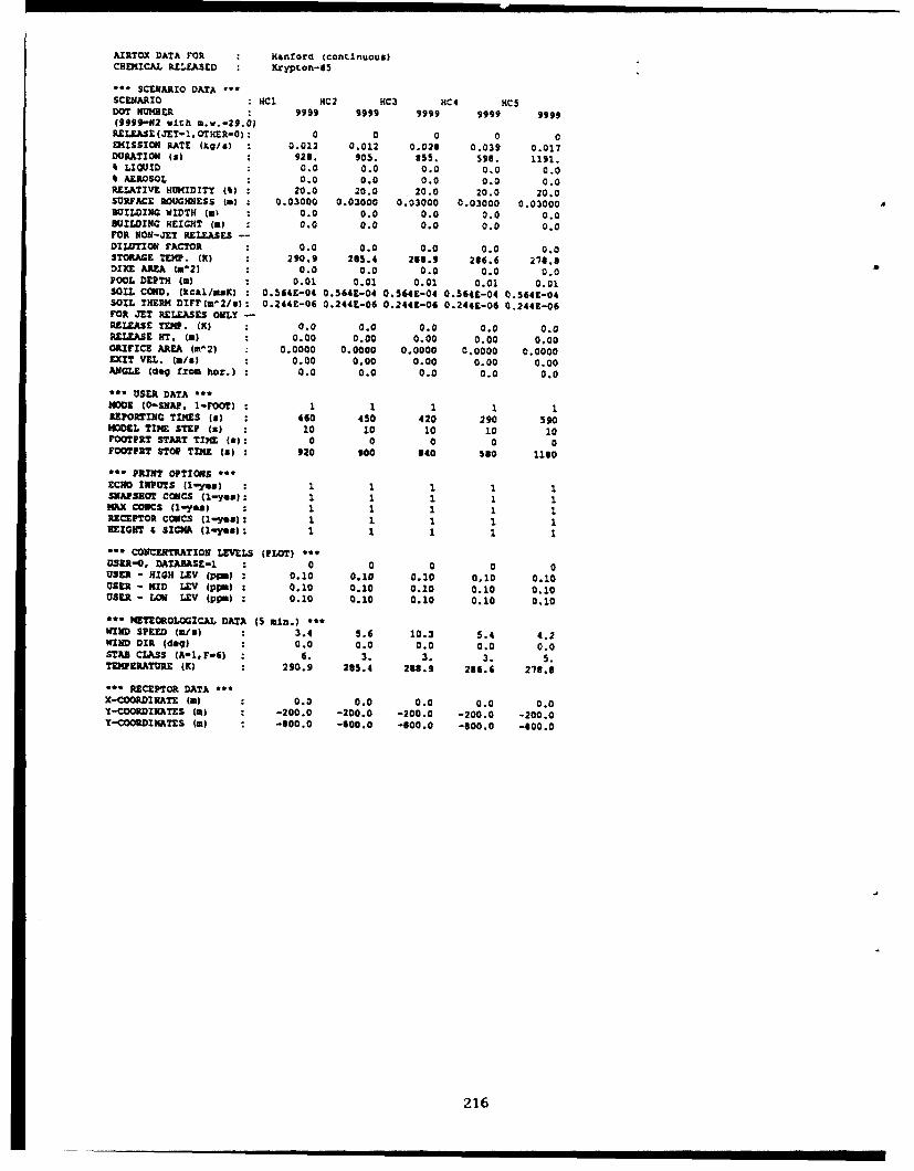
A.IRTOX DATA FOR Hanfora (contlnuous)CHEMICAL R£ELA•SED Kcypton-85

** SCENARIO DATA "SCENARIO HC1 HC2 HC3 HC4 HCSDOT NUMBER 9999 9999 9999 9999 9999(9999-N2 with m.w.-29.0)RELEASE (JET-1 oOTHER-0) : 0 0 0 0 0DEISSION RATE (kq/s) : 0.012 0.012 0.028 0.039 0.017DURATION (a) 923. 905. 855. 593. 1191.3 LIQUID 0.0 0.0 0.0 0.0 0.0% AEROSOL 0.0 0.0 0.0 0.0 0.0RELATIVE HUMID1TY (4) : 20.0 20.0 20.0 20.0 20.0SURFACE ROUGHmESS (a) : 0.03000 0.03000 0.03000 0.03000 0.03000BUILDING WIDTH (a) 0.0 0.0 0.0 0.0 0.0BUILDING HEIGHT (ml 0.0 0.0 0.0 0.0 0.0FOR NON-JET RELEASES --DILUTION FACTOR 0.0 0.0 0.0 0.0 0.0STORAGE TEMP. (K) 290.9 285.4 283.9 286.6 21S.0DIXE AREA (m^2) 0.0 0.0 0.0 0.0 0.0POOL DEPTHI (a) 0.01 0.01 0.01 0.01 0.01SOIL COND. (kcal/m.K) 0.564E-04 0.564E-04 0.564E-04 0.5641-04 0.564E-04SOIL THERM DIFF(m,2/a): 0.244E-06 0.244E-06 0.2441-06 0.244E-06 0.244E-06FOR JET RELEASES ONLY -RELEASE TEOP. (K) 0.0 0.0 0.0 0.0 0.0RELZASE HT. (a) 0.00 0.00 0.00 0.00 0.00OItFICE AREA (m02) 0.0000 0.0000 0.0000 0.0000 0.0000EXIT VEL. (a/u) 0.00 0.00 0.00 0.00 0.00ANGLE (dag fzom hor.) 0.0 0.0 0.0 0.0 0.0

*'** USER DATA tooNODE (0-SNAP. 1-FOOT) 1 1 1 1 1REPORTING TIMES (a) 460 450 420 290 590NOOEL TIN STEP (a) 10 10 10 10 10IFOOTPRT START TIME (a) 0 0 0 0 0FOOTPRT STOP TIME (al) 920 900 340 580 1160

'* PRINT OPTIONS **ECHO INPUTS (1.2.ye) 1 1 1 1 1SNAPSHOT CONCS (1-yes): 1 1 1 1 1MAX CONCS (1-yea) : 1 1 1 1 1RECEPTOR COWCS (1-yeal: I 1 1 I 1HEIGHT & SIGMA (1-yea); 1 1 I I I

*** CONCENTRATION LEVELS (PLOT) ***DSER-O, DATABASE-i 0 0 0 0 0USER - HIGH LEV (pPm) : 0.10 0.10 0.10 0.10 0.10USER - KID LEV (pp) : 0.10 0.10 0.10 0.10 0.10USER - LO LEV (ppm) : 0.10 0.10 0.10 0.10 0.10

*** METEOROLOGICAL DATA (S win.) t*oWIND SPEED (a16) 3.4 5.6 10.3 5.4 4.2WIND DIR (dog) 0.0 0.0 0.0 0.0 0.0STAB CLASS (A-lF-6) 6. 3. 3. 3. 5.TEMPERATURE (K) 290.9 235.4 288.9 286.6 278.8

*** RECEPTOR DATA **X-COORDINATE (3) 0.0 0.0 0.0 0.0 0.0Y-COORDINATES (a) : -200.0 -200.0 -200.0 -200.0 -200.0Y-COORDIhATES (a) -600.0 -300.0 -300.0 -600.0 -400.0

216

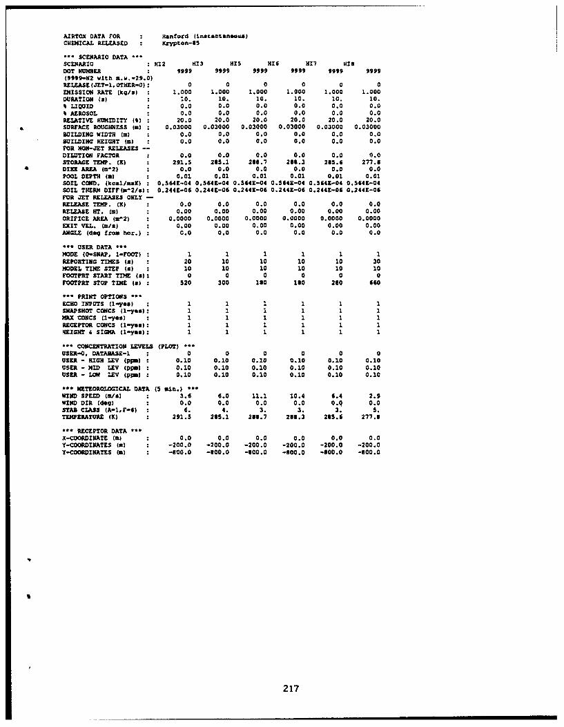
AIRTOX DATA FOR : Hanfofrd (instantaneous)CHEMICAL RELEASED "KCypon-as

SSCENARIO DATA ...SCENARIO : H12 H13 HIS HI H147 HISDOT NUMBER 9999 9999 9999 9999 9999 9999(9999-N2 with U.w.-29.0)

RELEASE(JET-1, OTHER-0): 0 0 0 0 0 0

EMISSION RATE (kq/s) 1.000 1.000 1.000 1.000 1.000 1.000DURATION (s) 10. 10. 10. 10. 10. 10.I LIQOID . 0.0 0.0 0.0 0.0 0.0 0.0% AEROSOL : 0.0 0.0 0.0 0.0 0.0 0.0RELATIVE HUMIDITY (b) : 20.0 20.0 20.0 20.0 20.0 20.0SPMACE ROUGHNESS (m) : 0.03000 0.03000 0.03000 0.03000 0.03000 0.03000WUILDING WIDTH (m) 0.0 0.0 0.0 0.0 0.0 0.0BUILDING HEIGHT (m) 0.0 0.0 0.0 0.0 0.0 0.0FOR NON-JET RELEASES -

DILUTION FACTOR : 0.0 0.0 0.0 0.0 0.0 0.0STORAGE TEMP. (K) : 291.5 285.1 208.7 283.3 285.6 277.3DIEX AREA (m'2) 0.0 0.0 0.0 0.0 0.0 0.0POOL DEPTH (W) : 0.01 0.01 0.01 0.01 0.01 0.01SOIL COND. (kcal/mmK) 0.564E-04 0.564E-04 0.5641-04 0.5649-04 0.5641-04 0.5641-04SOIL THERM DIFF(m^2/a): 0.244E-06 0.244E-06 0.244E-06 0.244E-06 0.244E-06 0.244E-06FOR JET RELEASES ONLY -

RELEASE TEMP. (M) : 0.0 0.0 0.0 0.0 0.0 0.0RELEASE HIT. (M) : 0.00 0.00 0.00 0.00 0.00 0.00ORIFICE AREA im^2) 0.0000 0.0000 0.0000 0.0000 0.0000 0.0000EXIT VEL. (m/s) 0.00 0.00 0.00 0.00 0.00 0.00ANGLE (deog from hor.) 0.0 0.0 0.0 0.0 0.0 0.0

*** USER DATA **MODE (0-SNAP, 1-FOOT) : 1 1 1 1 1 1REPORTING TIMES (s) : 20 10 10 10 10 30MODEL TIME STEP (a) 10 10 10 10 10 10FOOTPRT START TIME (a): 0 0 0 0 0 0FOOTPRT STOP TIME (a) : 520 300 160 10 280 660

**- PRINT OPTIONS ***ECHO INPUTS (l-yes) : 1 1 1 1 1 1SNAPSHOT CONCS (1-yea): 1 1 1 1 1 1MAX CONCS (1-yes) 1 1 1 1 1 1RECEPTOR CONCS (1-yea): 1 1 1 1 1 1REIGHT A SIGMA (l,-yea): 1 1 1 1 1 1

*-- CONCENTRATION LEVELS (PLOT) ...

USER-O, DATABASE-I * 0 0 0 0 0 0USER - HIGH LEV (ppm) : 0.10 0.10 0.10 0.10 0.10 0.10USER - MID LEV (ppm) : 0.10 0.10 0.10 0.10 0.10 0.10USER - LOW LEV (ppo) : 0.10 0.10 0.10 0.10 0.10 0.10

*** METEOROLOGICAL DATA (5 %Ln.) ***WIEND SPEED (ua/) . 3.6 6.0 11.1 10.4 6.4 2.9WIND DIR (dog) : 0.0 0.0 0.0 0.0 0.0 0.0

STAB CLASS (A-1,F-6) : 6. 4. 3. 3. 3. 5.TEMPERATURE (K) : 291.5 265.1 281.7 268.3 285.6 277.8

*** RECEPTOR DATA *

X-COORDINATE (m) : 0.0 0.0 0.0 0.0 0.0 0.0Y-COORDINATES Cm) : -200.0 -200.0 -200.0 -200.0 -200.0 -200.0Y-COORDINATES (W) : -600.0 -600.0 -000.0 -600.0 -600.0 -300.0

217

AIRTOX DATA FOR : apIln SandaCHEIICAL RELEASED : Llquified Natural Gas

*;* SCENARIO DATA ---SCENARIO MS27 KS29 MS34 KS35DOT NUMBER " 1971 1971 1971 1971RLLEASE(JET1,,OrH"R-O): 0 0 0 0EMISSION RATE (kq/s) 23.210 29.160 21.510 27.090DURATION (a) 10. 225. 95. 135.4 LIQUID 100.0 100.0 100.0 100.0F AEROSOL 0.0 0.0 0.0 0.0RELATIVE HUNMDIX (8) 53.0 71.0 90.0 77.0SURFACE ROUGIHNSS (m) 0.00030 0.00030 0.00030 0.00030WUILDING WIDTH (a) 0.0 0.0 0.0 0.0

BUILDING HEIGHT (m) : 0.0 0.0 0.0 0.0FOR NOR-JET RELEASES --

DILUTION FACTOR : 0.0 0.0 0.0 0.0STORAGE TEMP. (K) 111.7 111.7 111.7 111.7DI]E AREA (A-2) 0.0 0.0 0.0 0.0POOL DEPTH (W) • 0.01 0.01 0.01 0.ý1SOIL CWID. (kcal/msK) 0.141E-02 0.141E-02 0.141E-02 0.141E-02SOIL THERM DIFF(mu2/s): 0.141K-05 0.141K-05 0.1412-05 0.141E-05FOR JET RELEASES ONLY -RELEASE TEMP. (K) 0.0 0.0 0.0 0.0RELEASE HT. (a) : 0.00 0.00 0.00 0.00ORIFICE AREA (mu2) : 0.0000 0.0000 0.0000 0.0000EXIT VZL. (m/z) : 0.00 0.00 0.00 0.00ANGLE (dog from hor.) : 0.0 0.0 0.0 0.0

",,* USER DATA *-,MODE (0-SNAP, 1-FOOT) : 1 1 1 1REPORTING TIMES (a) : 30 110 40 60MODEL TINE STEP (a) : 10 10 10 10FOOTPRT START TIME (a): 0 0 0 0FOOTIRT STOP TINE (a) : 240 220 30 120

*** PRINT OPTIONS ***ECHO INPUTS (1-yes) : 1 1 1 1SNAPSHOT CONCS (1-you): 1 1 1 1)B CONCS (1-yes) : 1 1 1 1RECEPTOR CONCS (1-yea): 1 1 1 1HEIGHT A SIGMA (1-yes): 1 1 1 1

*** CONCENTRATION LEVELS (PLOT) ***USER-0, DATABASE-I 0 0 0 0USER - HIGH LEV (plm) : 100.00 100.00 100.00 100.00USER - KID LEV (ppm) : 100.00 100.00 100.00 100.00USER - LOW LEV (ppm) : 100.00 100.00 100.00 100.00

*M* METEOROLOGICAL DATA (S mln.) "'

WIND SPEED (/-a) : 5.6 7.4 8.5 9.6MIND DIR (deq) : 0.0 0.0 0.0 0.0STAB CLASS (A.1,F-6) 4. 4. 4. 4.TEMPERATURE (K) : 238.1 209.3 283.4 239.3

*** RECEPTOR DATA **

X-COORDIXNATE (m) : 0.0 0.0 0.0 0.0Y-COORDINATES (a) : -89.0 -58.0 -37.0 -129.0Y-COORDINATES (a) -131.0 -90.0 -179.0 -250.0Y-COORDINATES (m) : -324.0 -130.0 99.9 -406.0Y-C0ORDINATES (m) -400.0 -182.0 99.9 99.9Y-COORDINATES (a) : -650.0 -252.0 99.9 99.9Y-COORDINATES (M) : 99.9 -324.0 99.9 99.9Y-C0ORDINATES (a) 99.9 -403.0 99.9 99.9

218

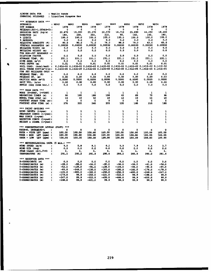
AIRTOX DATA FOR : Maplin SandsCHOD(CALX RELEASED : Liquilfed Propane Gas

'*- SCENARIO DATA *--

SCENARIO : KS42 NS43 MS46 HS47 MS49 KSSO K352 NS54

DOT NUMBER 1978 1978 1978 1978 1978 1978 1978 1978

RELEASE (JET-1, OTHER-0): 0 0 0 0 0 0 0 0EMISSION RATE (kg/s) 20.870 19.200 23.370 32.570 16.710 35.890 44.250 19.200DURATION (s) : 180. 330. 360. 210. 90. 160. 140. 180.3 LIQUID 100.0 100.0 100.0 100.0 100.0 100.0 100.0 100.04 AEROSOL 0.0 0.0 0.0 0.0 0.0 0.0 0.0 0.0RELATIVE HMI1DITY (4) : 80.0 80.0 71.0 78.0 88.0 79.0 63.0 85.0SURFACE ROUGHNESS (m) : 0.00030 0.00030 0.00030 0.00030 0.00030 0.00030 0.00030 0.00030BUILDING WIDTH (M) 0.0 0.0 0.0 0.0 0.0 0.0 0.0 0.0BUILDING HEIGHT (m) 0.0 0.0 0.0 0.0 0.0 0.0 0.0 0.0FOR NON-JET RELEASES --

DILUTION FACTOR : 0.0 0.0 0.0 0.0 0.0 0.0 0.0 0.0STORAGE TEM/. (K) 231.1 231.1 231.1 231.1 231.1 231.1 231.1 231.1DIKE AREA (m^2) 0.0 0.0 0.0 0.0 0.0 0.0 0.0 0.0

S POOL DEPTH (m : 0.01 0.01 0.01 0.01 0.01 0.01 0.01 0.01SOIL COND. (kcal/msK) 0.141E-02 0.141E-02 0.141E-02 0.141E-02 0.141E-02 0.1412-02 0.141E-02 0.141E-02SOIL THERM DIFF(m"2/s): 0.141E-05 0.141E-05 0.1419-05 0.1419-05 0.141E-05 0.141E-05 0.141E-05 0.141£-05FOR JET RELEASES ONLY -

RELEASE TEMP. (R) 0.0 0.0 0.0 0.0 0.0 0.0 0.0 0.0RELEASE MT. (a) 0.00 0.00 0.00 0.00 0.00 0.00 0.00 0.00ORIFICE AREA (m^2) 0.0000 0.0000 0.0000 0.0000 0.0000 0.0000 0.0000 0.0000EXIT VTEL. (mIs) 0.00 0.00 0.00 0.00 0.00 0.00 0.00 0.00ANGLE (dog from hor.) 0.0 0.0 0.0 0.0 0.0 0.0 0.0 0.0

*** USER DATA ".MODE (0-SNAP, 1-FOOT) 1 1 1 1 1 1 1 1REPORTING TIMES (a) 90 160 180 100 40 80 70 90MODEL TIME STEP (a) : 10 10 10 10 10 10 10 10FOOTPRT START TIME (a): 0 0 0 0 0 0 0 0FOOTPRT STOP TIME (a) : 270 320 360 200 120 160 210 10

*;* PRINT OPTIONS ***

ECHO INPUTS (1-yes) : 1 1 1 1 1 1 1 1SNAPSHOT CONCS (1-yes): 1 1 1 1 1 1 1 1MAX CONCS (1-yes) : 1 1 1 1 1 1 1 1RECEPTOR CONCS (1-yes): 1 1 1 1 1 1 1 1HEIGHT & SIGaM (1-yes): 1 1 1 1 1 1 1 1

". CONCENTRATION LEVELS (PLOT) *'*USER-O, DATABASE-i : 0 0 0 0 0 0 0 0USER - HIGH LEV (ppm) : 100.00 100.00 100.00 100.00 100.00 100.00 100.00 100.00USER - MI= LE (plm) ; 100.00 100.00 100.00 100A0 100.00 100.00 100.00 100.00USER - LOW LEV (ppm) : 100.00 100.00 100.00 100.00 100.00 100.00 100.00 100.00

*** METEOROLOGICAL DATA (S ain.) -**WIND SPEED (Wms) : 4.0 5.8 8.1 6.2 5.5 7.9 7.4 3.7MIND DIR (dog) : 0.0 0.0 0.0 0.0 0.0 0.0 0.0 0.0STAB CLASS (A-1,F-6) : 4. 4. 4. 4. 4. 4. 4. 4.TEMPERATURE (K) : 291.5 290.2 291.9 290.6 286.5 283.6 285.0 281.6

*** RECEPTOR DATA ***X-COORDINATE (m) : 0.0 0.0 0.0 0.0 0.0 0.0 0.0 0.0Y-COORDINATES (M) : -28.0 -88.0 -34.0 -90.0 -90.0 -59.0 -61.0 -56.0Y-COORDINATES (m) : -53.0 -129.0 -91.0 -128.0 -129.0 -93.0 -95.0 -85.0Y-COORDINATES (a) : -83.0 -249.0 -130.0 -182.0 -180.0 -182.0 -178.0 -170.0Y-COORDINATES (a) : -123.0 -400.0 -182.0 -250.0 -250.0 -400.0 -249.0 -247.0Y-COORDINATES (m) : -179.0 99.9 -250.0 -321.0 -322.0 99.9 -398.0 99.9Y-COORDINATES (m) : -247.0 99.9 -322.0 -400.0 -400.0 99.9 -650.0 99.9Y-COORDINATES (S) : -398.0 99.9 -401.0 99.9 99.9 99.9 99.9 99.9

219

AIRTOX DATA FOR Prairie Grass, set 1CHEMICAL RELEASED Sulfur dioxide

*** SCENARIO DATA ***SCENARIO PG7 PG8 PG9 PG10 PG13 PG15 PG16 PG17DOT NUMBER 1079 1079 1079 1079 1079 1079 1079 1079RELEASE(JET-1,OTHER-0) : 1 1 1 1 1 1 1 1EMISSION RATE (k/sa) 0.090 0.091 0.092 0.092 0.061 0.095 0.093 0.056DURATION (a) 600. 600. 600. 600. 600. 600. 600. 600.4 LIQUID : 0.0 0.0 0.0 0.0 0.0 0.0 0.0 0.04 AEROSOL 0.0 0.0 0.0 0.0 0.0 0.0 0.0 0.0

RELATIVE HUMIDITY (t) : 20.0 20.0 20.0 20.0 20.0 20.0 20.0 20.0SURFACE ROUGHNESS (m) 0.00600 0.00600 0.00400 0.00600 0.00600 0.00600 0.00600 0.00600BUILDING WIDTH Wm) : 0.0 0.0 0.0 0.0 0.0 0.0 0.0 0.0BUILDING HEIGHT (a) : 0.0 0.0 0.0 0.0 0.0 0.0 0.0 0.0

FOR RON-JET RELEASES -

DILUTION FACTOR : 0.0 0.0 0.0 0.0 0.0 0.0 0.0 0.0STORAGE TEMP. (W) : 0.0 0.0 0.0 0.0 0.0 0.0 0.0 0.0DIKE AREA (m^2) 0.0 0.0 0.0 0.0 0.0 0.0 0.0 0.0POOL DEPTH (a) : 0.00 0.00 0.00 0.00 0.00 0.00 0.00 0.00SOIL CORD. (kcal/maK) : 0.000÷+00 0.0009+00 0.000E+00 0.O000+00 0.000t+00 0.000E+00 0.000÷+00 0.000t+00SOIL THERK DIFFrmw2/s): 0.0001+00 0.000&+00 0.0001+00 0.000k.t30 0.000t+00 0.000E+00 0.0001+00 0.0009+00FOR JET RELEASES ONLY -RELEASE TEMP. (K) 305.1 305.1 301.1 304.1 293.1 295.1 301.1 300.1RELEASE RT. (ma 0.45 0.45 0.45 0.45 0.45 0.45 0.45 0.45ORIFICE ARMA (W2) : 0.0020 0.0020 0.0020 0.0020 0.0020 0.0020 0.0020 0.0020EXIT VEL. (m/0) : 17.34 17.57 17.51 17.71 11.32 17.02 17.70 10.72ANGLE (doq froa hor.) 0.0 0.0 0.0 0.0 0.0 0.0 0.0 0.0

*** USER DATA -**MODE (0-SAP, I-FOOT): 1 1 1 1 1 1 1 1REPORTING TIMES (a) 300 300 300 300 300 300 300 300MODEL TIME STEP (s) 10 10 10 10 10 10 10 10FOOTPRT START TIE (W): 0 0 0 0 0 0 0 0FOOTPRT STOP TIME (s) : 600 600 600 g00 600 g00 600 600

". PRINT OPTIONS ***ECHO INPUTS (1-yea) 1 1 1 1 1 1 1 1SNAPSHOT CONCS (1-yea): 1 1 1 1 1 1 1 1

AX COSICS (1-yea) 1 1 1 1 1 1 1 1RECEPTOR CONCS (1-yes): 1 1 1 1 1 1 1 1HEIGHT 6 SIGMA (1-yes): 1 1 1 1 1 1 1 1

* CONCENTRATION LEVELS (PLOT) ***

USER-0, DATABASe-1 0 0 0 0 0 0 0 0USER - HIGH LEV (ppm) : 1.00 1.00 1.00 1.00 1.00 1.00 1.00 1.00USER - MID LEV (ppa) : 1.00 1.00 1.0o 1.00 1.00 1.00 1.o0 1.O0USZR - LOW LV (pu) : 1.00 1.00 1.00 1.00 1.00 1.00 1.00 1.00

*** METEOROLOGICAL DATA (5 &in.) ***IErD SPEED (rn/) 4.9 5.9 8.4 5.4 2.7 4.0 3.7 4.6

WIND DIR (deq) : 0.0 0.0 0.0 0.0 0.0 0.0 0.0 0.0STAB CLASS (A-1,F-6) 2. 3. 3. 2. 6. 1. 1. 4.T•3UERATURE (K) : 305.1 305.1 301.1 304.1 293.1 295.1 301.1 300.1

*** RECEPTOR DATA ***X-COORDINATE (m) : 0.0 0.0 0.0 0.0 0.0 0.0 0.0 0.0Y-COORDINATES (a) : -50.0 -S0.0 -50.0 -S0.0 -400.0 -50.0 -50.0 -50.0Y-COORDINATES (a) -100.0 -100.0 -100.0 -100.0 -800.0 -100.0 -100.0 -100.0Y-COORDINATES (m) : -200.0 -200.0 -200.0 -200.0 93.9 -200.0 -200.0 -200.0Y-COORDINATES (W) : -400.0 -400.0 -400.0 -400.0 93.9 -400.0 -400.0 -400.0Y-COORDINATES (a) : -600.0 -400.0 -600.0 -400.0 99.9 -600.0 -600.0 -600.0

220

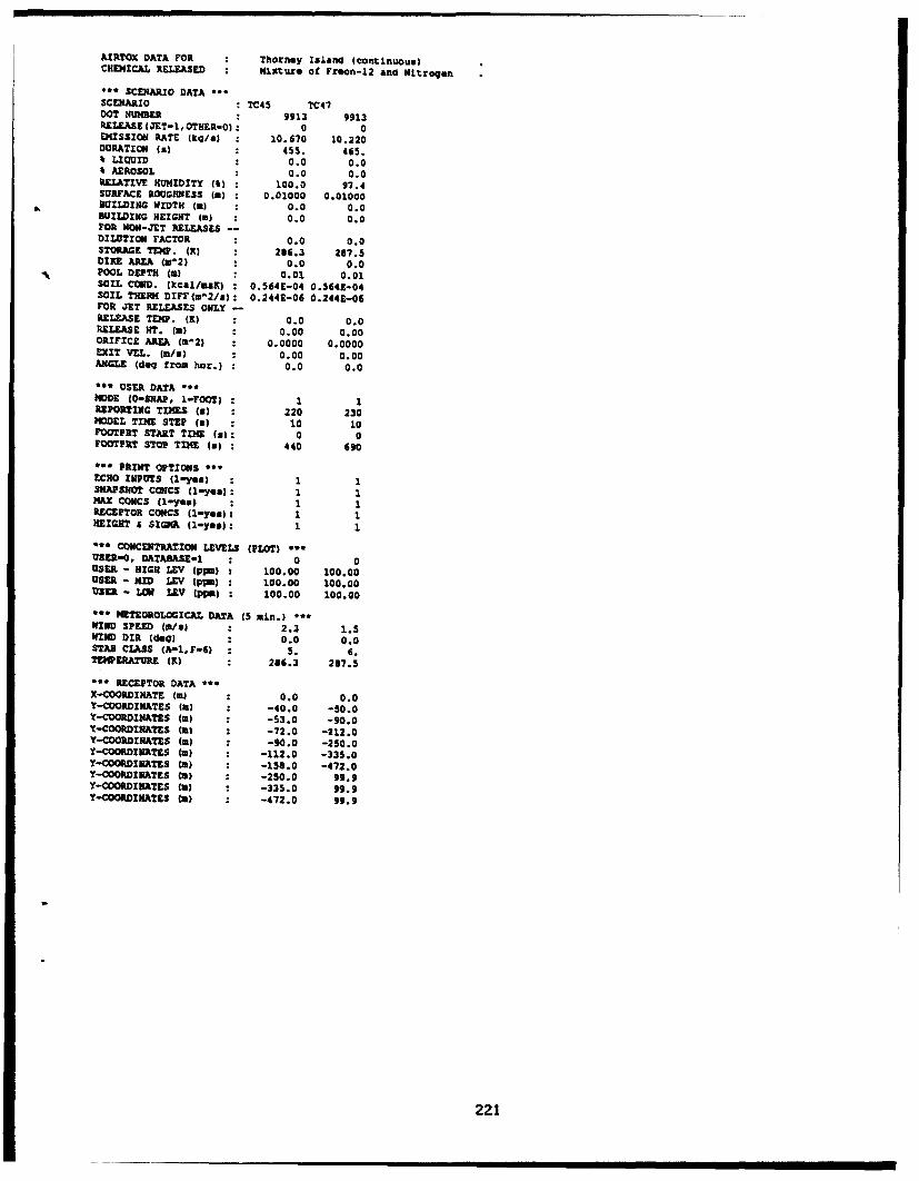
AIRTOX DATA FOR : Thorney Island (continuous)CHEMICAL RELEASED : MlXture of Froon-12 and Nitrogen

*** SCENARIO DATA tSCENARIO TC45 TC4?DOT NUM•ER 9913 9913RELEASE (JET-1, OTHER-0) : 0 0EMISSION RATE (kg/a) : 10.670 10.220DURATION (a) 455. 465.SLIQUID . 0.0 0.0

I AEROSOL . 0.0 0.0REIATIVE HUMZDITY (4) : 100.0 97.4SURFACE ROUGHNESS (m) : 0.01000 0.01000BUILDING WIDTH (a) . 0.0 0.0BUILDING HEIGHT (m) . 0.0 0.0FOR NOW-J£T RELEASES --DILUTIXO FACTOR : 0.0 0.0STORAGE TEMP. (K) : 206.3 287.5DIKE AREA (&2) 0.0 0.0POOL DEPTH (a) 0.01 0.01SOIL COND. (kcal/nmK) : 0.564E-04 0.564E-04SOIL THERN DIFF(m^2/s): 0.244E-06 0.244E-06FOR JET RELEASES ONLY -RELEASE TEMP. (K) 0.0 0.0RELEASE HT. (m) 0.00 0.00ORIFICE AREA (mL2) 0.0000 0.0000EXIT VEL. (W/a) 0.00 0.00ANGLE (dog from har.) : 0.0 0.0

"** USER DATA ***NODE (0-SNAP, 1-FOOT) : 1 1REPORTING TINES (a) : 220 230NODEL TIME STEP (a) 10 10POOTPRT START TIME (a): 0 0FOOTPIT STOP TIME (a) : 440 690

"*** PRINT OPTIONS **"ECHO INPUTS (1-yes) : 1 1SNAPSHOT CONCS (1-yes): 1 1MAX CONCS (1-yes) : 1 1RZ=hPTCR CONCS (1-yea): I IHEIGHT & SIGMA (1-yea) : 1 1

*** CONCENTRATION LEVELS (PLOT) "**US11-0, DATABASE-1 0 0USER - NIGH LEV (ppm) 100.00 100.00USER - MID LEV (ppm) : 100.00 100.00USER - L4 LIV (ppn) : 100.00 100.00

*** METEOROLOGICAL DATA (5 min.) ***WIND SPEED (m/a) 2.3 1.5WIND DIR (deog) : 0.0 0.0STAB CLASS (A-,F-d) : 5. 6.TEMPERATURE (K) 286.3 217.5

"' RECEPTOR DATA teeX-COORDINATE (m) : 0.0 0.0Y-COORDINATES (a) : -40.0 -50.0Y-COORDINATES (a) : -53.0 -90.0Y-COORDINATES (a) -72.0 -212.0Y-COO.DINATE$ (01) : -90.0 -250.0Y-COORDINATES (m) : -112.0 -335.0T-COORDIMATES (a) : -158.0 -472.0Y-COORDINATZS (a) : -250.0 99.9Y-COORDINATES (a) -335.0 99.9Y-COORDIMATES (a) : -472.0 99.9

221

AIRTOX DATA POR Thorney Island (infstantaneoualCHEMICAL RELEASED Klxiure of Ftron-12 and Nitroqen

*** SCENARIO DATA .SCENARIO TI6 T17 T18 T19 T112 T113 T117 TI18 T119DOT NUMBER 9906 9907 9908 9909 9912 9913 9917 9918 9919RELEASE(JET-1,OTHER.,0): 0 0 0 0 0 0 0 0 0EMISSION RATE (kg/a) 314.700 424.900 395.800 386.600 573.600 480.000 871.100 383.100 547.700DURATION (a) . 10. 10. 10. 10. 10. 10. 10. 10. 10.r LIoQoID 0.0 0.0 0.0 0.0 0.0 0.0 0.0 0.0 0.0& AEROSOL : 0.0 0.0 0.0 0.0 0.0 0.0 0.0 0.0 0.0RELATIVE HUMIDITY (M) 74.8 30.7 87.6 87.3 66.2 74.1 94.0 81.3 94.8SURFACE ROUGHNESS (an) 0.01800 0.01800 0.01200 0.00800 0.01800 0.01000 0.01300 0.00500 0.01000BUILDING WIDTH (m) : 0.0 0.0 0.0 0.0 0.0 0.0 0.0 0.0 0.0BUILDING HEID (m) . 0.0 0.0 0.0 0.0 0.0 0.0 0.0 0.0 0.0

FOR MON-JET RELEASES --DILUTION FACTOR 0.0 0.0 0.0 0.0 0.0 0.0 0.0 0.0 0.0STORAGE TEMP. (K) 291.8 290.5 290.7 291.5 283.3 216.9 239.2 289.7 236.5DIKE ARMA (RA2) . 0.0 0.0 0.0 0.0 0.0 0.0 0.0 0.0 0.0POOL DEPTH (a) 0.01 0.01 0.01 0.01 0.01 0.01 0.01 0.01 0.01SOIL COND. (kcal/mmK) 0.564E-04 0.564E-04 0.5644-04 0.564E-04 0.564E-04 0.564t-04 0.5649-04 0.564E-04 0.564E-04SOIL THERM DIFF(mu21s): 0.244E-06 0.2441-06 0.244E-06 0.244E-06 0.244E-06 0.2449-06 0.244E-04 0.244E-06 0.244E-06FOR JET RELEASES ONLY -RELEASE TEMP. (K) 0.0 0.0 0.0 0.0 0.0 0.0 0.0 0.0 0.0RELEASE MT. (m) 0.00 0.00 0.00 0.00 0.00 0.00 0.00 0.00 0.00ORIFICE AREA (m^2) 0.0000 0.0000 0.0000 0.0000 0.0000 0.0000 0.0000 0.0000 0.0000EXIT VEL. (m/s) 0.00 0.00 0.00 0.00 0.00 0.00 0.00 0.00 0.00ANGLE (deq from hor.) 0.0 0.0 0.0 0.0 0.0 0.0 0.0 0.0 0.0

*** USER DATA *-*MODE (O-SAP, 1-FOOT): 1 1 1 1 1 1 1 1 1REPORTING TDIS (8) 10 10 10 20 10 10 10 10 10MODEL TIME STEP (a) 10 10 10 10 10 10 10 10 10FOOTPRT START TIME (a): 0 0 0 0 0 0 0 0 0FOOTPRT STOP TIME (a) 340 320 460 640 440 140 240 160 220

*** PRINT OPTIONS ***ECHO IPUTS (1-yes) 1 I 1 1 1 1 1 1 1SNAPSHOT CONCS (1-yea): 1 1 1 1 1 1 1 1 1MAX CONCS (1-yesa 1 1 1 1 1 1 1 1 1RECEPTOR CONCS (1-yes): 1 1 1 1 1 1 1 1 1UZIGHT & SIGHA (1-yes): 1 1 1 1 1 1 1 1 1

"*** CONICETRATION LEVELS (PLOT) ***U33R-0, DATABASE-1 0 0 0 0 0 0 0 0 0USER - HIGH LEV (pm) : 100.00 100.00 100.00 100.00 100.00 100.00 100.00 100.00 100.00USER - MID IEV (ppm) : 100.00 100.00 100.00 100.00 100.00 100.00 100.00 100.00 100.00USER - LON L&V (pza) : 100.00 100.00 100.00 100.00 100.00 100.00 100.00 100.00 100.00

*** ?MTZOROLOGICAL DATA (5 min.) ***1113 08 D (/-a) 2.8 3.4 2.4 1.7 2.5 7.3 5.0 7.4 6.4um a (dg) 0.0 0.0 0.0 0.0 0.0 0.0 0.0 0.0 0.0n Ca (A-1,F-6) 4. 5. 4. 6. 5. 4. 4. 4. 4.TWE TUORE (K) 291.8 290.5 290.7 291.5 233.3 286.9 289.2 289.7 236.5

*** RECEPTOR DATA **X-COORDINATE (a) 0.0 0.0 0.0 0.0 0.0 0.0 0.0 0.0 0.0Y-COORDXNATES (a) -71.0 -71.0 -71.0 -71.0 -71.0 -71.0 -40.0 -40.0 -40.0Y-COORDINATES (a) -141.0 -100.0 -100.0 -100.0 -150.0 -100.0 -50.0 -60.0 -60.0Y-COORDIMATES (a) -130.0 -150.0 -150.0 -141.0 -200.0 -224.0 -71.0 -70.0 -71.0Y-COORDINATES W) -283.0 -130.0 -200.0 -130.0 -361.0 -316.0 -100.0 -60.0 -100.0¥-COORDINATES (a) -424.0 -224.0 -364.0 -224.0 -500.0 -361.0 -141.0 -100.0 -224.0Y-COORDINATES (a) 99.9 -361.0 -412.0 -316.0 99.9 -412.0 -224.0 -200.0 -361.0Y-COORDINATES (a) 99.9 -500.0 -510.0 -503.0 99.9 99.9 -500.0 -224.0 -583.0Y-COORDINATES (a) 99.9 99.9 99.9 99.9 99.9 99.9 99.9 -300.0 99.9Y-COORDINATES (a) 99.9 99.9 99.9 99.9 99.9 99.9 99.9 -400.0 99.9T'-COORDINATES (a) 99.9 99.9 99.9 99.9 99.9 99.9 99.9 -510.0 99.9

222

34M INPUT DATA FOR BurroCHDEICAL RELEASED Liquefied natural gas

TRIAL B32 303 804 BU5 8UG 307 BOB B09INITIAL CONC(ppp) 1.000000 1.000000 1.000000 1.000000 1.000000 1.000000 1.000000 1.000000DENSE ENOUGH? (anst): Y Y Y YY 1Y Y rDENSE ENOUGH? (cnst): Y Y Y Y Y Y T YMIN DIST INST (ma 1735. 1651. 2996. 2660. 2236. 2822. 456. 881.COR. PARM. (nst) 1.94 1.91 1.10 1.3B 1.07 1.26 4.49 1.771/1D (1/m) : 0.491E-01 0.493E-01 0.485E-01 0.482E-01 0.527t-01 0.475E-01 0.529E-01 0.562E-01MAX DIST CNST (m) 416. 396. 719. 638. 537. 677. 110. 211.COR. PARAM. Ccn•t) 0.77 0.77 0.44 0.54 0.45 0.50 1.95 0.801/De (1/m) : 0.352 0.345 0.453 0.423 0.443 0.425 0.201 0.306

SAM INPUT DATA FOR : coyoteCHEMICAL RELEASED : Liqefied natural gas M eothane In at least 664 In c

TRIAL CO3 COS COGINITIAL CONC(ppp) 1.000000 1.000000 1.000000DENSE ENOUGH? (anst): Y Y YDENSE ENOUGH? (cnst); Y Y YMIN DIST INST (W) 723. 1794. 784.COR. PARAN. (irst) 1.70 1.15 1.98I/D1 (W/i) 0.671E-01 0.544E-01 0.576E-01MAX DIST CNST (W) : 174. 431. 188.COR. PARAX. (cart) 0.78 0.50 0.89i/Dc (1/m) : 0.362 0.417 0.301

34M INPUT DATA FOR Desert TortoleCHEMICAL RELEASED : Anhydrous Amonia

TRIAL : T DT2 DT3 DT4INITIAL CONC(ppp) 0.089979 0.091419 0.096518 0.095455DENSE ENOUGH? (1nst): Y Y Y YDENSE ENOUGH? (cnst): Y Y Y yMEIN DIST INST (a) 2033. 3241. 2568. 3952.COR. PARAN. (last) 1.11 1.69 1.35 2.181/Di (1/21 : 0.192Z-01 0.136E-01 0.1529-01 0.1262-01MAX DIST CNST (m) 488. 778. 616. 949.COR. PARAN. (crst) 0.58 0.79 0.63 0.94I/Dc (W/E) 0.926E-01 0.701E-01 0.7329-01 0.6922-01

&KN INPUT DATA FOR : GoldfishCHEMICAL RELEASED Hydrogen fluoride

TRIAL : GFI GF2 GF3INITIAL CONC(ppp) : 0.088112 0.083367 0.076311DENSE ENOUGH? (laot): Y y yDENSE ENOUGH? (cnat): Y Y YM1IN 0DST INST (0) 1521. 3227. 4482.COR. PARAM. (lout) : 0.54 0.74 0.511/01 (1/i) : 0.2682-01 0.255E-01 0.2502-01MAX DIST CUST (a) : 365. 774. 1076.COP.. PARAN. (cnat) : 0.32 0.36 0.251/Dc (1/a) : 0.132 0.179 0.204

223

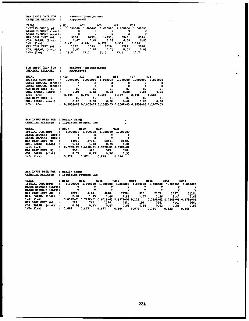
86M INPUT DATA FOR Hanford (continuous)CHEMICAL RELEASED Krypton-I5

TRIAL : HC1 HC2 HC3 HC4 HC5INITIAL CONC(ppp) : 1.000000 1.000000 1.000000 1.000000 1.000000DENSE ENOUGH? (Inat): N N N N NDENSE ENOUGH? (cnst): N N N N NMIN DIST rST (mW 5258. 8452. 14691. 5346. 8374.COR. PARAM. (lnot) : 0.07 0.04 0.02 0.05 0.051/D. (1/m) 0.481 0.484 0.372 0.318 0.396MAX DIST CNST (m) 1262. 2029. 3526. 1283. 2010.COR. PARAH. (cnat) : 0.03 0.02 0.01 0.02 0.02I/Dc (1/i) : 19.8 24.1 21.3 13.1 17.7

B&M INPUT DATA FOR : Hanford (instantaneous)CHEMICAL RELEASED "rypton-aS

TRIAL :1H12 H13 HI5 H16 1117 HisINITIAL CONC(ppp) 1.000000 1.000000 1.000000 1.000000 1.000000 1.000000DENSE ENOUGH? (onst): N N N N N NDENSE ENOUGH? lcont): N N N N N NMIN DIST INST (a) 0. 0. 0. 0. 0. 0.COR. PA*AN. (inst) : 0.06 0.03 0.02 0.02 0.03 0.061/D0 (1/m) : 0.495 0.499 0.497 0.497 0.498 0.503MAX DIST CNST (a) : 0. 0. 0. 0. 0. 0.COR. PARAM. (cnat) : 0.00 0.00 0.00 0.00 0.00 0.001/Do (1/m) : 0.100E+05 0.100E+05 0.100t+05 0.100E+05 0.1001+05 0.100Z+05

EMN INPUT DATA FOR : Naplin SandsCHDEICAL RELEASED : Liquifled Natural Gas

TRIAL : MS27 14829 KS334 M535INITIAL CONC(ppp) : 1.000000 1.000000 1.000000 1.000000DENSE ENOUGH? (lost).: '1 Y yDENSE ENOUGH? (cost): y 'f 'yMIS DIST INST (m) 1493. 2775. 1346. 2160.CO. PARAN. (rst) : 1.44 1.13 0.83 0.801/0± (1/m) 0.7951-01 0.6479-01 0.962E-01 0.718E-01MAX DIST CN1T (a) : 358. 666. 323. 518.COR. PARAN. (crst) : 0.57 0.43 0.36 0.331/Dc (1/m) : 0.671 0.671 0.848 0.796

36N INPUT DATA FOR : Naplin SandsCRENICAL RELEASED : Liquified Propane Gas

TRIAL : 1S42 M143 MS46 1447 K549 5S50 SS2 K534INITIAL CONC(ppp) : 1.000000 1.000000 1.000000 1.000000 1.000000 1.000000 1.000000 1.000000DENSE ENOUGK? (lnst): y Y y y y y Y yDENSE ENOUGH? (chat): y y y y y y yIMIN DIST INST (a) 1200. 3190. 4860. 2170. 825. 2107. 1727. 1110.CO.. PARAN. (inur) : 2.53 1.93 1.46 1.83 1.57 1.36 1.47 2.641/D9 (1/ml : 0.8511-01 0.7151-01 0.651Z-01 0.6971-01 0.115 0.739t-01 0.7201-01 0.3751-01MAX DIST CNST (a) 288. 766. 1166. 521. 198. 506. 414. 266.COP. PAWAN. (cost) : 0.94 0.63 0.47 0.66 0.64 0.52 0.58 0.971/Dc (W/i) : 0.667 0.837 0.897 0.664 0.372 0.714 0.622 0.634

224

36M INPUT DATA FOR Prairie Grass, set 1CHEMICAL RELEASED Sulfur dioxide

TRIAL P07 PG P09 PG10 PG13 PG15 PG16 PG17INITIAL CONC(ppp) 1.000000 1.000000 1.000000 1.000000 1.000000 1.000000 1.000000 1.000000DENSE ENOUGH? (inst): Y y Y Y Y Y yDENSE ENOUGH? (Cnst): y Y Y Y y Y y TKIN DIST INST (m) 4926. 5880. 8385. 5383. 2737. 3982. 3749. 4625.COR. PARAM. (inst) 1.17 0.96 0.69 1.07 1.95 1.45 1.54 1.141/Di (1/a) 0.362 0.360 0.361 0.359 0.417 0.359 0.359 0.425MAX DIST CNST (a) 1182. 1411. 2012. 1292. 657. 956. 900. 1110.COR. PARM. (Cnat) : 0.28 0.24 0.16 0.26 0.46 0.35 0.37 0.271/Dc (1/m) : 11.8 12.8 15.4 12.2 10.9 10.5 10.2 14.6

DIN INPUT DATA FOR Thorney Island (continuous)CHEIOCAL RELEASED Mixture of Freon-12 and Nitrogen

TRIAL TC4S TC47INITIAL CONC(ppp) : 1.000000 1.000000DENSE ENOUGH? (nst): y yDENSE ENOUGH? (Chat): Y YMIN DIST INST (a) 1744. 1163.COR. PARAM. (lUst) : 4.84 7.401/Di (I/=) : 0.798E-01 0.802E-01MAX DIST CNST (m) 419. 279.COR. PAMAN. (cast) 1.46 2.22I/Dc (1/m) 0.729 0.600

B&M INPUT DATA FOR Thorney Island (instantaneous)CHEMICAL RELEASED Mizture of Freon-12 and NLtroqen

TRIAL : TI6 T17 TI8 T19 T112 T113 T117 TIl8 T119INITIAL CONC(ppp) : 1.000000 1.000000 1.000000 1.000000 1.000000 1.000000 1.000000 1.000000 1.000000DENSE ENOUGH? (inst): Y Y y Y y Y y Y YDENSE ENOUGH? (cnst): N N N N N N N N NIN DIST INST (a) : 0. 0. 0. 0. 0. 0. 0. 0. 0.

COR. PARAM. (Lnst) : 3.09 2.84 3.69 5.09 5.18 1.52 3.88 1.37 1.861/D1 (1/m) : 0.859E-01 0.796E-01 0.796E-01 0.796E-01 0.8012-01 0.8029-01 0.836E-01 0.835E-01 0.7793-01AX DIST CNST (3) : 0. 0. 0. 0. 0. 0. 0. 0. 0.

COR. PARAN. (cnat) : 0.00 0.00 0.00 0.00 0.00 0.00 0.00 0.00 0.001/Dc (1/m) : 0.100E+05 0.100E+05 0.100E+05 0.100E+05 0.100E+05 0.100&+05 0.100E+05 0.100E+05 0.1002+05

225

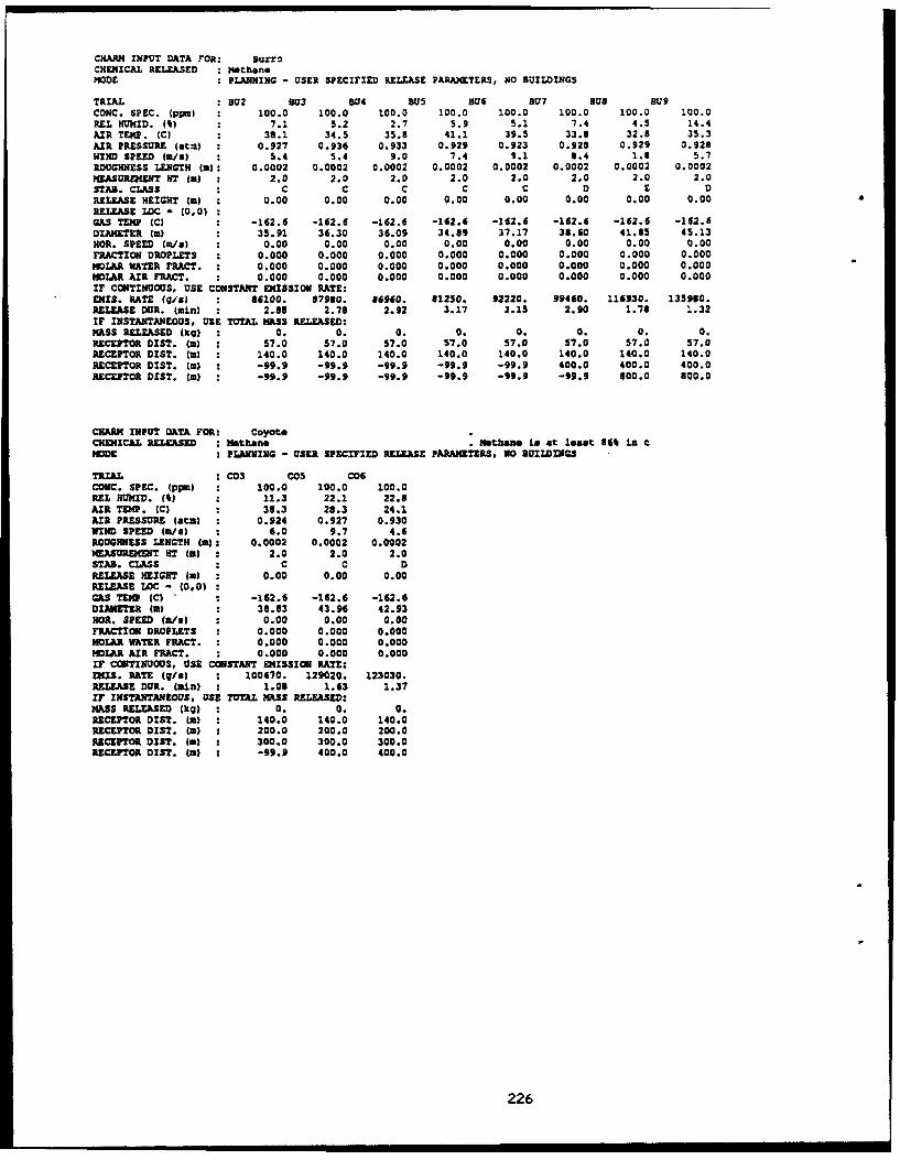
CHARM INPUT DATA FOR: BurroCHEMICAL RELEASED Methane"MODE : PLANNING - USER SPECIFIED RELEASE PARAMETERS, NO BUILDINGS

TRIAL : 302 8U3 3U4 805 806 8U7 Bu8 BU9CONC. SPEC. (pLn) 100.0 100.0 100.0 100.0 100.0 100.0 100.0 100.0REL HUMID. (lb) 7.1 5.2 2.7 5.9 5.1 7.4 4.5 14.4AIR TEMP. (C) : 38.1 34.5 35.8 41.1 39.5 33.8 32.0 35.3AIR PRESSURE (atm) 0.927 0.936 0.933 0.929 0.923 0.928 0.929 0.928WIND SPEED (m/as) 5.4 5.4 9.0 7.4 9.1 0.4 1.$ 5.7ROUGHNESS LENGTH (m): 0.0002 0.0002 0.0002 0.0002 0.0002 0.0002 0.0002 0.0002MEASUREMENT HT (i) 2.0 2.0 2.0 2.0 2.0 2.0 2.0 2.0STAB. CLASS : C C C C C D E DRELEASE HEIGHT (a) 0.00 0.00 0.00 0.00 0.00 0.00 0.00 0.00RELEASE LOC - (0.0)GAS TEMP (C) -162.6 -162.6 -162.6 -162.6 -162.6 -162.6 -162.6 -162.6DIAMETER (a) : 35.91 36.30 36.09 34.89 37.17 38.60 41.85 45.13HOR. SPEED (W/a) : 0.00 0.00 0.00 0.00 0.00 0.00 0.00 0.00FRACTION DROPLETS 0.000 0.000 0.000 0.000 0.000 0.000 0.000 0.000MOLAR WATER FRACT. : 0.000 0.000 0.000 0.000 0.000 0.000 0.000 0.000MOLAR AIR FRACT. 0.000 0.000 0.000 0.000 0.000 0.000 0.000 0.000IF CONTINUOUS, USE CONSTANT EMISSION RATE:EMIS. RATE (9/m) : 66100. 67980. 86960. 61250. 92220. 99460. 116930. 135930.RELEASE DOUR. (min) 2.88 2.76 2.92 3.17 2.15 2.90 1.78 1.32IF INSTANTANEOUS, USE TOTAL MASS RELEASED:MASS RELEASED tkg) : 0. 0. 0. 0. 0. 0. 0. 0.RECEPTOR DIST. (W) : 57.0 57.0 57.0 57.0 57.0 57.0 57.0 57.0RECEPTOR DIST. (m) : 140.0 140.0 140.0 140.0 140.0 140.0 140.0 140.0RECEPTOR DIST. Wm) : -99.9 -99.9 -99.9 -99.9 -99.9 400.0 400.0 400.0RECEPTOR DIST. (m) -99.9 -99.9 -99.9 -99.9 -99.9 -99.9 800.0 800.0

CRNAN INPUT DATA FOR: CoyoteCHEMICAL RELEASED : Methane . Methane Li at least 86% in aMODE : PLANNING - USER SPECIFIED RELEASE PARAMETERS, NO BUILDINGS

TRIAL : C03 COS CO0CONC. SPEC. (ppm) : 100.0 100.0 100.0REl HUMID. (M) : 11.3 22.1 22.8AIR T•eP. (C) : 38.3 28.3 24.1AIR PRESSURE (atm) : 0.924 0.927 0.930WIND SPEED (ada) : 6.0 9.7 4.6ROUGHNESS LENGTH (a): 0.0002 0.0002 0.0002M.EASUREMENT HT (a) 2.0 2.0 2.0STAR. CLASS : C C DRELEASE HEIGHT (m) : 0.00 0.00 0.00RELEASE LOC - (0,0)GAS TEMP (C) : -162.6 -162.6 -162.6DIAMETER (m) : 38.83 43.96 42.93NOR. SPEED (a/a) : 0.00 0.00 0.00FRACTION DROPLETS : 0.000 0.000 0.000MOLAR WATER FRACT. 0.000 0.000 0.000MOLAR AIR FRACT. : 0.000 0.000 0.000IF CONTINUOUS, USE CONSTANT EMISSION RATE:08TS. RATE (gas) : 100670. 129020. 123030.RELEASE DUR. (min) : 1.05 1.63 1.37IF INSTANTANEOUS, USE TOTAL MASS RELEASED:MASS RELEASED (kg) : 0. 0. 0.RECEPTOR DIST. (m) : 140.0 140.0 140.0RECEPTOR DIST. (m) : 200.0 200.0 200.0RECEPTOR DIST. (a) : 300.0 300.0 300.0RECEPTOR DIST. (m) : -99.9 400.0 400.0

226

CHARM INPUT DATA FOR: Desert TortoiseCHEMICAL RELEASED Anhydrous AmmoniaMODE PLANNING - USER SPECIFIED RELEASE PARAMETERS, NO BUILDINGS

TRIAL DTI DT2 DT3 DT4CONC. SPEC. (ppm) 100.0 100.0 100.0 100.0REL HUMID. (M) 13.2 17.5 14.8 21.3AIR TEMP. (C) 28.8 30.4 33.9 32.4AIR PRESSURE (aim) 0.897 0.898 0.s95 0.891WIND SPEED (m/s) : 7.4 5.8 7.4 4.5ROUGHNESS LENGTH (a): 0.0030 0.0030 0.0030 0.0030MEASUREMENT HT 1m) 2.0 2.0 2.0 2.0STAB. CLASS D 0 D ERELEASE HEIGHT (a) : 0.79 0.79 0.79 0.79

RELEASE LOC - (0,0)GAS TEMP (C) -35.7 -35.7 -35.7 -35.7DIAMETER (m) 1.04 1.19 1.22 1.24HOR. SPEED (u/a) 22.65 23.23 27.29 20.19FRACTION DROPLETS 0.313 0.817 0.811 0.804MOLAR WATER FRACT. : 0.000 0.000 0.000 0.000MOLAR AIR FRACT. : 0.000 0.000 0.000 0.000IF CONTINUOUS, USE CONSTANT EMISSION RATE:EKIS. RATE (W/O) : 79700. 111500. 130700. 96700.RELEASE OUR. (min) : 2.10 4.25 2.77 6.35IF INSTANTANEOUS, USE TOTAL MASS RELEASED:MASS RELEASED (kq) 0. 0. 0. 0.RECEPTOR DIST. Cm) 100.0 100.0 100.0 100.0RECEPTOR DIST. (m) 300.0 800.0 800.0 800.0

CHARM INPUT DATA FOR: GoldfishCHEMICAL RELEASED Hydroqen flUorideMODE PLANNING - USER SPECIFIED RELEASE PARAMETERS# NO BUILDINGS

TRIAL : M1 GF2 GF3CONC. SPEC. (ppm) 30.0 30.0 30.0REL HUMID. (0) 4.9 10.7 17.7AIR TEMP. (C) : 37.2 36.2 34.4AIR PRESSURE (atm) : 0.893 0.889 0.894WIND SPEED (a/u) : 5.6 4.2 5.4ROUGHNESS LENGTH (m): 0.0030 0.0030 0.0030MEASUREDENT HT (m) 2.0 2.0 2.0STAB. CLASS :D D DRELEASE HEIGHT (a) : 1.00 1.00 1.00RELEASE LOC - (0,0)GAS TEMP (C) 16.4 16.4 16.4DIAMETER (m) : 0.61 0.34 0.34HOR. SPEED (a/s) : 20.33 23.04 22.62FRACTION DROPLETS : 0.840 0.853 0.847MOLAR WATER FRACT. : 0.000 0.000 0.000MOLAR AIR FRACT. 0.000 0.000 0.000IF CONTINUOUS. USE CONSTANT EMISSION RATE:EKIS. RATE (4i1) : 27670. 10460. 10270.RELEASE OUR. (min) : 2.08 6.00 6.00IF INSTANTANEOUS, USE TOTAL MASS RELEASED:HASS RELEASED (kq) : 0. 0. 0.RECEPTOR DIST. (m) : 300.0 300.0 300.0RECEPTOR DIST. (m) : 1000.0 1000.0 1000.0RECEPTOR DIST. (m) ; 3000.0 -99.9 3000.0

227

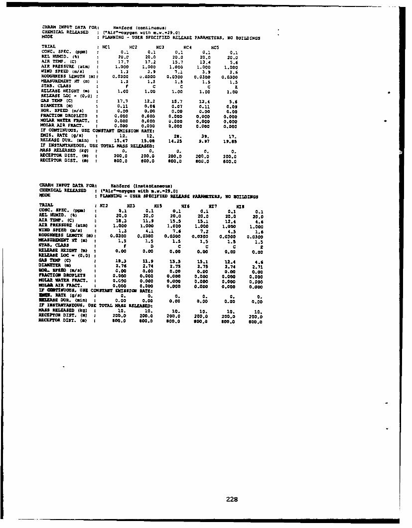
ZHARM INPUT DATA FOR: Hantford (continuous)CHEMICAL RELEASED ("Lir-..oxygen with m.w.-29.01MODE PLANNING - USER SPECIFIED RELEASE PARAM'ETERS, NO BUILDINGS

TRIAL HCI HC2 HC3 HC4 HCSCONC. SPEC. (plm) : 0.1 0.1 0.1 0.1 0.1REL HUMID. (t) 29.C 20.0 20.0 20.0 20.0AIR TEMP. (C) : 17.7 17.2 15.7 13.4 5.6AIR PRESSURE (atm) : 1.000 1.000 1.000 1.000 1.000WIND SPEED (WIs) 1.3 3.9 7.1 3.9 2.6ROUGHIESS LENGTH (a): 0.0300 u.0300 0.0300 0.0300 0.0300MEASUREMENT HT (m) 1.5 1.5 1.5 1.5 1.5STAB. CLASS : F C C C ERELEASE HEIGHT W 1.00 1.00 1.00 1.00 1.00RELEASE LOC - (0,0)GAS TEMP (C) 17.7 12.2 15.7 13.4 5.6DIAMETER (a) : 0.11 0.06 0.07 0.11 0.09NOR. SPEED (m/&) 0.00 0.00 0.00 0.00 0.00FRACTION DROPLETS 0.000 0.000 0.000 0.000 0.000MOLAR WATER FRACT. 0.000 0.000 0.000 0.000 0.000MOLAR AIR FRACT. 0.000 0.000 0.000 0.000 0.000IF CONTINUOUS, USE CONSTANT EMISSION RATE:EMIS. PATE (g/ul : 12. 12. 20. 39. 17.RELEASE DUR. (mLin) : 15.47 15.08 14.25 9.97 19.85IF INSTANTANEOUS. USE TOTAL MASS RELEASED:MASS RELEASED jkq) : 0. 0. 0. 0. 0.RECEPTOR DIST. Wm) : 200.0 200.0 200.0 200.0 200.0RECEPTOR DIST. (m) : 800.0 800.0 800.0 800.0 800.0

CHARM INPUT DATA FOR: Hanford (Instantaneous)CHEMICAL RELEASED : (Aiz--Oygen with m.v.-29.0)MODE : PLANNING - USER SPECIFIED RELEASE PARAMETERS, NO aOmmimDTS

TRIAL : 9112 U113 HIS HS6 HI7 Hi8CONiC. SPEC. (pinm) : 0.1 0.1 0.1 0.1 0.1 0.1REX HUMID. (t) : 20.0 20.0 20.0 20.0 20.0 20.0AIR TEM. (C) 10.3 11.9 15.5 15.1 12.4 4.6AIR PRESSURE (atm) 1.000 1.000 1.000 1.000 1.000 1.000WIND SPEED (a/s) : 1.3 4.1 7.6 7.2 4.5 1.6ROUGHNESS LENGTH (a): 0.0300 0.0300 0.0300 0.0300 0.0300 0.0300MEASURDEENT lET C() : 1.5 1.5 1.5 1.5 1.5 1.5STAB. CLASS F D C C C ERELEASE HEIGHT (a) : 0.00 0.00 0.00 0.00 0.00 0.00RELEASE LOC - (0,0)GaS TE (C) : 18.3 11.9 15.5 15.1 12.4 4.6DXTUKV in) : 2.76 2.74 2.73 2.75 2.74 2.71

EOR. SPEED (a/s) : 0.00 0.00 0.00 0.00 0.00 0.00FRACTION DROPLETS : 0.000 0.000 0.000 0.000 0.000 0.000MOLAR WATER TRACT. : 0.C0o 0.000 0.000 0.000 0.000 0.000MOLI& AIR TRACT. : 0.000 0.000 0.000 0.000 0.000 0.000Ur CT INUOUS, USE CONSTANT EMISSION pATE:MEE. PATAE (/s) : 0. 0. 0. 0. 0. 0.

ZErASE DUR. (mini : 0.00 0.00 0.00 0.00 0.00 0.00Ir INSTANTANEOUS, USE TOTAL MhSS RELEASED:MASS RELEASED (kq) : 10. 10. 10. 10. 10. 10.RECZPTOR DIST. (3) : 200.0 200.0 200.0 200.0 200.0 200.0RECEPTOR DIST. (a) : 800.0 300.0 800.0 800.0 800.0 800.0

2.28

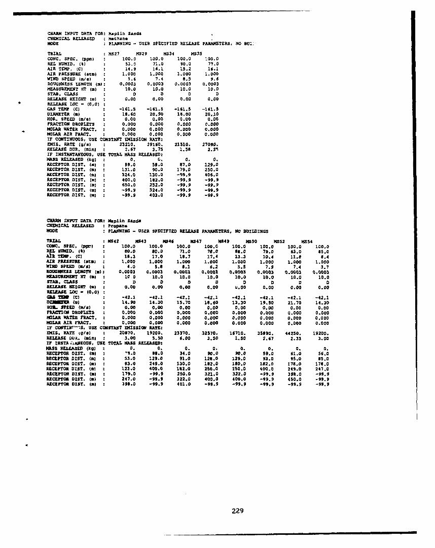
CHARM INPUT DATA FOR: Maplin SandsCHEMICAL RELEASED : meothn*MODE : PLANNING - USER SPECIFIED RELEASE PARAMETERS, NO 80:I

TRIAL : 1M527 K529 MS34 MS35CONe. SPEC. (pm) 100.0 100.0 100.0 100.0REL HUMID. (%) 53.0 71.0 90.0 77.0AIR TEMP. (C) 14.9 16.1 15.2 16.1AIR PRESSURE (atm) : 1.000 1.000 1.000 1.000WIND SPEED Im/l) : 5.6 7.4 8.5 9.6ROUGHNESS LENGTH (m): 0.0003 0.0003 0.0003 0.0003MEASUREKENT HT (Wn) : 10.0 10.0 10.0 10.0STAS. CLASS : 0 0 DRELEASE HEIGHT (m) 0.00 0.00 0.00 0.00RELEASE LOC - (0,0)GAS TEMP (C) -161.5 -161.5 -161.5 -161.5DIAMETER (m) : 18.60 20.90 16.00 20.10

OR. SPEED (W/ei : 0.00 0.00 0.00 0.00FRACTION DROPLETS : 0.000 0.000 0.000 0.000MOIAR WATER TRACT. : 0.000 0.000 0.000 0.000MOLAR AIR FRACT. 0.000 0.000 0.000 0.000IF CONTINUOUS, USE CONSTANT EMISSION RATE:EMIS. RATE (g/O) : 23210. 29160. 21510. 27090.RELEASE OUR. (min) 1 2.67 3.75 1.58 2.2'1IF INSTANTANEOUS, USE TOTAL MASS RELEASED:MASS RELEASED (k.g) 0. 0. 0. 0.RECEPTOR DIST. (m) : 59.0 58.0 57.0 129.0RECEPTOR DIST. (m) 131.0 90.0 179.0 250.0RECEPTOR DIST. (a) : 324.0 130.0 -99.9 406,0RECEPTOR DIST. (m) 400.0 182.0 -99.9 -99.9RECEPTOR DIST. (m) : 650.0 252.0 -99.9 -99.9RECEPTOR DIST. (m) : -99.9 324.0 -99.9 -99.9RECEPTOR DIST. (m) : -99.9 403.0 -99.9 -99.9

CHARM INPUT DATA FOR: Maplin SandaCHEMICAL RELEASED PropaneMODE : PLANNING - USER SPECIFIED RELEASE PARAMETERS, NO BUILOINGS

TRIAL :MS42 1043 16546 MS47 M549 M950 MS52 MS54CONC. SPEC. (ppiv 100.0 100.0 100.0 100.0 100.0 100.0 100.0 100.0REL HUMID. (m) : 80.0 80.0 71.0 78.0 86.0 79.0 63.0 15.0AIR TEMP. (C) 18.3 17.0 18.7 17.4 13.3 10.4 11.8 6.4AIR PRESSURE (a&t) : 1.000 1.000 1.000 1.000 1.000 1.000 1.000 1.000WIND SPEED (W/s) : 4.0 5.8 0.2 6.2 5.5 7.9 7.4 3.7ROUGHNESS LENGTH (a): 0.0003 0.0003 040003 0.0003 0.0003 0.0003 0.0003 0.0003

MEASURDIENT HT (a) : 1c 0 10.0 10.0 10.0 10.0 10.0 10.0 10.0STAS. CLASS : 0 D D D 0 D 0RELEASE HEIGHT (a) 0.00 0.00 0.00 0.00 U.0O 0.00 0.00 0.00RELAS•E. LOC - (0,0)G" Tw (C) : -42.1 -42.1 -42.1 -42.1 -42.1 -42.1 -42.1 -42.1OE01 U (m) : 14.90 14.30 15.70 18.60 13.30 19.50 21.70 14.30HOM SPEED (We/) : 0.00 0.00 0.00 0.00 0.00 0.00 0.00 0.00FRACTION DROPLETS 0.000 0.000 0.000 0.000 0.000 0.000 0.000 0.000MOLAR WATER FRACT. : 0.000 0.000 0.000 0.000 0.000 0.000 0.000 0.000MOLAR AIR FRACT. : 0.000 0.000 0.000 0.000 0.000 0.000 0.000 0.000IF COI•TINr--S, USE CONSTANT EMISSION RATE:DMIS. RATE Ws/a) : 20870. 19200, 23370. 32570. 16710. 35690. 44250. 19200.RELEASE OUa. (mlin) : 3.00 5.50 6.00 3.50 1.50 2.67 2.33 3.00IF INSTJ .*ANEOUS, USE TOTAL MASS RELEASED:MASS RELEASED (kg) : 0. 0. 0. 0. 0. 0. 0. 0.RECEPTOR DIST. (m) : '5.0 81.0 34.0 90.0 90.0 59.0 61.0 56.0RECEPTOR DIST. (mW : 53.0 129.0 91.0 128.0 129.0 93.0 95.0 65.0RECEPTOR DIST. (m) : 83.0 249.0 130.0 182.0 180.0 162.0 178.0 176.0RECEPTOR DIST. (a) : 123.0 400.0 182.0 250.0 250.0 400.0 24S.0 241.0RECEPTOR DIST. (m) 179.0 -99.9 250.0 321.0 322.0 -99.9 398.0 -99.9RECEPTOR DIST. (W) : 247.0 -99.9 322.0 400.0 400.0 -99.9 650.0 -99.9R=EPTOR DIST. (I) : 398.0 -99.9 402.0 -99.9 -99.9 -99.9 -99.9 -99.9

229

CHARM INPUT DATA FOR: Prairie Grass, sae 1CHEMICAL RELEASED : Sulfur dioxideMODE : PLANNING - USER SPECIFIED RELEASE PARAMETERS, NO BUILDINGS

TRIAL : PG7 PG6 PG9 PG10 PG13 PG15 PG16 PG17CONC. SPEC. (ppm) : 1.0 1.0 1.0 1.0 1.0 1.0 1.0 1.0REL HUMID. (t) : 20.0 20.0 20.0 20.0 20.0 20.0 20.0 Z0.0AIR TEMP. (C) : 31.9 31.9 27.9 30.9 19.9 21.9 27.9 26.9AIR PRESSURE (atm) 1.000 1.000 1.000 1.000 1.000 1.000 1.000 1.000WIND SPEED WmAi) : 4.2 4.9 6.9 4.6 1.3 3.4 3.2 3.3ROUGHNESS LENGTH (a): 0.0060 0.0060 0.0060 0.0060 0.0060 0.0060 0.0060 0.0060MEASUREMENT HT (m) 2.0 2.0 2.0 2.0 2.0 2.0 2.0 2.0STAB. CLASS a C C B F A A 0RELEASE HEIGHT (W) : 0.45 0.45 0.45 0.45 0.45 0.45 0.45 0.45RELEASE LOC - (0.0)GAS TEMP (C) 31.9 31.9 27.9 30.9 19.9 21.9 27.9 26.9DIAMETER (a) 0.05 0.05 0.05 0.05 0.05 0.05 0.05 0.05NOR. SPEED (1ls) : 17.34 17.57 17.51 17.71 11.32 17.82 17.70 10.72FRACTION DROPLETS 0.000 0.000 0.000 0.000 0.000 0.000 0.000 0.000NOLAR MATER rRACT. : 0.000 0.000 0.000 0.000 0.000 0.000 0.000 0.000MOLAR AIR FRACT. 0.000 0.000 0.000 0.000 0.000 0.000 0.003 0.000IF CONTINUOUS, USE CONSTANT EMISSION RATE:EK(IS. RATE (g/s) : 90. 91. 92. 92. 61. 96. 93. 57.RELEASE DOUR. (min) : 10.00 10.00 10.00 10.00 10.00 10.00 10.00 10.00IF INSTANTANEOUS, USE TOTAL MASS RELEASED:MASS RELEASED (kq) 0. 0. 0. 0. 0. 0. 0. 0.RECEPTOR DIST. (m) 50.0 50.0 50.0 50.0 400.0 50.0 50.0 50.0RECEPTOR DIST. (mW : 100.0 100.0 100.0 100.0 100.0 100.0 100.0 100.0RECEPTOR DIST. (m) : 200.0 200.0 200.0 200.0 -99.9 200.0 200.0 200.0RECEPTOR DIST. (m) 400.0 400.0 400.0 400.0 -99.9 400.0 400.0 400.0RECEPTOR DIST. (W) : 300.0 300.0 800.0 800.0 -99.9 600.0 000.0 800.0

CHARM INPUT DATA FOR: Thorney Island (continuouslCHEMICAL RELEASED : Use TRIAL-SPECIFIC name for Tharnay Is.MODE : PLANNING - USER SPECIFIED RELEASE PARAMETERS, NO BUILDINGS

TRIAL : TC45 TC47COliC. SPEC. (ppm) : 100.0 100.0REL HUMID. (%1 : 100.0 97.4AIR TEMP. (C) 13.0 14.3AIR PRESSURE (at=) : 1.000 1.000WIND SPEED (mWs) : 2.3 1.5ROUGHNESS LENGTH (a): 0.0100 0.0100MEASUREMENT HT (m) : 10.0 10.0STAB. CLASS : E FRELEASE HEIGHT (m) : 0.00 0.00RELEASE LOC - (0.0)GAS TEMP (C) : 13.0 14.3DIAMETER (a) : 2.00 2.00HOR. SPEED (m/a) : 0.00 0.00FRACTION DROPLETS : 0.000 0.000MOLAR WATER FRACT. : 0.000 0.000MOLAR AIR FRACT. : 0.000 0.000IF CONTINUOUS, USE CONSTANT EMISSION RATE:EMIS. RATE (g/s) : 10670. 10220.RELEASE DOUR. (min) : 7.58 7.75IF INSTANTANEOUS, USE TOTAL MASS RELEASED:MASS RELEASED (kq) " 0. 0.RECEPTOR DIST. (m) : 40.0 50.0RECEPTOR DIST. (m) : 53.0 90.0RECEPTOR DIST. (m) : 72.0 212.0RECEPTOR DIST. (m) : 90.0 250.0RECEPTOR DIST. (m) : 112.0 335.0RECEPTOR DIST. (m) : 158.0 472.0RECEPTOR DIST. (m) : 250.0 -99.9RECEPTOR DIST. (m) : 335.0 -99.9RECEPTOR DIST. Wa) : 472.0 -99.9

230

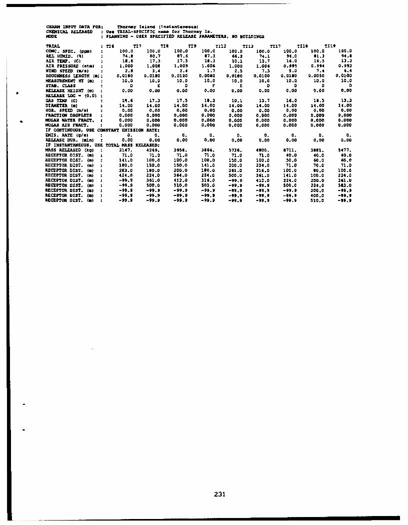
CARAM INPUT DATA FOR: Thorany Island (instantaneous)CHEMICAL RELEASED :Us TRIAL-SPECIFIC namt for Thorney In.MODE : PLANNING - USER SPECIFIED RELEASE PARAMETERS. NO BUIImGS

TRIAL T16 TVT TI6 T19 T112 T113 T117 TII8 T119CONC. SPEC. (ppm) : 100.0 100.0 100.0 100.0 100.0 100.0 100.0 100.0 100.0REL HUMID. (%) : 74.8 80.7 87.6 07.3 66.2 74.1 84.0 01.3 94.8AIR TEMP. (C) : 18.6 17.3 17.5 18.3 10.1 13.7 16.0 16.5 13.3AIR PRESSURE (atm) 1.000 1.006 1.009 1.006 1.000 1.006 0.995 0.994 0.993WIND SPEED (m/s) : 2.3 3.4 2.4 1.7 2.5 7.3 5.0 7.4 6.4ROUOGINESS LENGTH (m): 0.0130 0.0180 0.0120 0.0080 0.0160 0.0100 0.0160 0.0050 0.0100MEASUREDMENT T (M) : 10.0 10.0 10.0 10.0 10.0 10.0 10.0 10.0 10.0STAB. CLASS :D E D z D D D 0RELEASE HEIGHT (m) : 0.00 0.00 0.00 0.00 0.00 0.00 0.00 0.00 0.00RELEASE LOC - (0,0)GAS TEMP (C) : 18.6 17.3 17.5 18.3 10.1 13.7 16.0 16.5 13.3DIAMETER (a) 14.00 14.00 14.00 14.00 14.00 14.00 14.00 14.00 14.00HOE. SPEED (m/s) : 0.00 0.00 0.00 0.00 0.00 0.00 0.00 0.00 0.00FRACTION DROPLETS : 0.000 0.000 0.000 0.000 0.000 0.000 0.000 0.000 0.000MOLAR WATER tRACT. : 0.000 0.000 0.000 0.000 0.000 0.000 0.000 0.000 0.000MOLAR AIR FRACT. : 0.000 0.000 0.000 0.000 0.000 0.000 0.000 0.000 0.000IF CONTINUCOUS, USE CONSTANT EMISSION RATE:D6IS. RATE (g/s) 0. 0. 0. 0. 0. 0. 0. 0. 0.RELEASE DUR. (ain) 0.00 0.00 0.00 0.00 0.00 0.00 0.00 0.00 0.00IF INSTANTANEOUS, USE TOTAL MASS RELEASED:MASS RELEASZD (kq) 3147. 4249. 3958. 3866. 5736. 4600. 8711. 3861. 5477,RECEPTOR DIST. (M) 71.0 71.0 71.0 71.0 71.0 71.0 40.0 40.0 40.0RECEPTOR DIST. (m) : 141.0 100.0 100.0 100.0 150.0 100.0 50.0 60.0 60.0RECEPTOR DIST. (m) : 160.0 150.0 150.0 141.0 200.0 224.0 71.0 70.0 71.0RECEPTOR DIST. (a) : 283.0 180.0 200.0 180.0 361.0 316.0 100.0 80.0 100.0RECEPTOR DIST. (a) : 424.0 224.0 364.0 224.0 500.0 361.0 141.0 100.0 224.0RECEPTOR DIST. (m) : -99.9 361.0 412.0 316.0 -99.9 412.0 224.0 200.0 361.0RECEPTOR DIST. (m) -99.9 500.0 510.0 503.0 -99.9 -99.9 500.0 224.0 583.0RECEPTOR DIST. (W) -99.9 -99.9 -99.9 -99.9 -99.9 -99.9 -99.9 300.0 -99.9RECEPTOR DIST. (W) : -99.9 -99.9 -99.9 -99.9 -99.9 -99.9 -99.9 400.0 -99.9RECEPTOR DIST. (a) : -99.9 -99.9 -99.9 -99.9 -99.9 -99.9 -99.9 510.0 -99.9

231

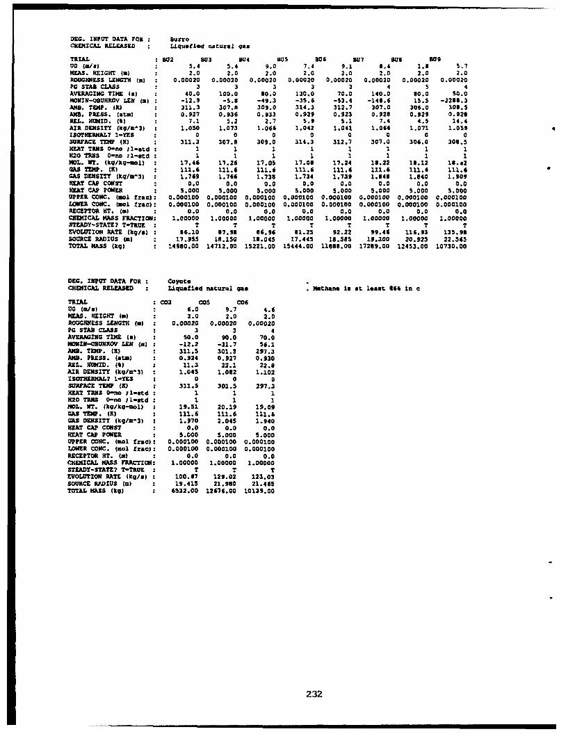
DEG. INPUT DATA FOR : BurroCHEMICAL RELEASED : Lquefled natural qa.

TRIAL B02 303 304 SU 5 W06 307 80 30900 (m/4) 1 5.4 5.4 9.0 7.4 9.1 8.4 1.8 5.7KEAS. HEIGHT (W) : 2.0 2.0 2.0 2.0 2.0 2.0 2.0 2.0ROUGHNESS LENGTH (m) : 0.00020 0.00020 0.00020 0.00020 0.00020 0.00020 0.00020 0.00020PG STAB CLASS : 3 3 3 3 3 4 5 4AVERAGING TIME (a) : 40.0 100.0 80.0 130.0 70.0 140.0 30.0 S0.0MONIN-OBUHKDV LEN (m) -12.9 -5.8 -49.3 -35.6 -53.4 -148.6 15.5 -2288.3AMD. TEMP. (X) : 311.3 307.8 309.0 314.3 312.7 307.0 306.0 308.5AME. PRESS. (ato) : 0.927 0.936 0.933 0.929 0.923 0.923 0.929 0.928REL. HUMID. (0) : 7.1 5.2 2.7 5.9 5.1 7.4 4.5 14.4AIR DENSITY lk9g/w3) 1.050 1.073 1.066 1.042 1.041 1.066 1.071 1.059ISOTHERMAL? 1-YES 0 0 0 0 0 0 0 0SURFACE TEMP (K) : 311.3 307.8 309.0 314.3 312.7 307.0 306.0 308.5HEAT TRNS 0Ono ;1-std : 1 1 1 1 1 1 1 1H20 TRNS 0-no ;1-std : 1 1 1 1 1 1 1 1MOL. WT. (kg/kg-mol) : 17.46 17.26 17.05 17.06 17.24 18.22 16.12 18.*2GAS TEMP. (K) 111.6 111.6 111.6 111.6 111.6 111.6 111.6 111.6GAS DENSITY (kg/Ml3) = 1.769 1.766 1.738 1.734 1.739 1.048 1.840 1.909NEAT CAP CONST 0.0 0.0 0.0 0.0 0.0 0.0 0.0 0.0HEAT CAP POWER : 5.000 5.000 5.000 5.000 5.000 5.000 5.000 5.000UPPER CONC. (mol frac): 0.000100 0.000100 0.000100 0.000100 0.000100 0.000100 0.000100 0.000100LOWEE CONC. (mol frac): 0.000100 0.000100 0.000100 0.000100 0.000100 0.000100 0.000100 0.000100RECEPTOR HT. (W) : 0.0 0.0 0.0 0.0 0.0 0.0 0.0 0.0CHEMICAL MASS FRACTION: 1.00000 1.00000 1.00000 1.00000 1.00000 1.00000 1.00000 1.00000STEADY-STATE? T-TRUE : T T T T T T T TEVOLUTION RATE (kq/&) : 86.10 67.98 36.96 81.25 92.22 99.46 116.93 135.93SOURCE RADIUS (a) : 17.955 18.150 18.045 17.445 18.385 19.300 20.925 22.565TOTAL MASS (kq) 14980.00 14712.00 15221.00 15444.00 11388.00 17289.00 12453.00 10730.00

DEG. INPUT DATA FOR CoyoteCHMDICAL RELEASED Liquefied naturlz gas . methane is at least 884 in c

TRIAL : C03 COs CO600 (a/a) . 6.0 9.7 4.6MEAS. HEIGHT (W) 2.0 2.0 2.0ROUGHNESS LENGTH (m) 0.00020 0.00020 0.00020PG STAB CLASS 3 3 4AVERAGING TIME (a) 50.0 90.0 70.0NONIN-Q9DNKOV LEN (a) : -12.2 -31.7 56.1AMN. TEMP. (K) : 311.5 301.5 297.3ANR. PRESS. (atm) : 0.924 0.927 0.930REL. HUMID. (8) : 11.3 22.1 22.3AIR DENSITY (kq/M'31 : 1.045 1.032 1.102ISOTHERKAL? 1-YES 2 0 0 0SURFACE TEMP (X) : 311.5 301.5 297.3HEAT TRUS 0-no I1-.td : 1 1 1R20 TRNS 0-no i1-atd 3 1 1 1MaX.. WT. (kg/kg-mol) : 19.51 20.19 19.09GAS TEMP. (K) : 111.6 111.6 111.6GAS DENSITY (kg/m'3) : 1.970 2.04S 1.940

am CAP COSST 0.0 0.0 0.0NEAT CAP POWER : 5.000 5.000 5.000UPPER CONC. (3o1 frac): 0.000100 0.000100 0.000100LOWER CONC. (Inl fraC): 0.000100 0.000100 0.000100RECEPTOR HT. (m) : 0.0 0.0 0.0CHEMICAL MASS FRACTION: 1.00000 1.00000 1.00000STZADY-STATE? T-TRUE : T T TEVOLUTION RATE (kq/a) : 100.67 129.02 123.03SOURCE RP.DIUS (a) : 19.415 21.980 21.465TOTAL MASS (kg) : 6532.00 12676.00 10139.00

232

DEG. INPUT DATA FOR Desert TortolaeCHEMICAL RELEASED ± Anhydrous AmonlaAEROSOL MODELED WITH MIXT RE FILE

TRIAL DTI DT2 DT3 DT400 (a/a) . 7.4 5.8 7.4 4.5HM•. HEIGHT (m) 2.0 2.0 2.0 2.0ROUGHNESS LENGTH (a) 0.00300 0.00300 0.00300 0.00300PG STAB CLASS : 4 4 4 5AVERAGING TIME (a) 80.0 160.0 120.0 300.0IDNIN-OBUHKOV LEN (m) 93.2 84.3 647.3 41.0AND. TEMP. (K) 302.0 303.6 307.1 305.6AND. PRESS. (atr) 0.897 0.898 0.895 0.691RIL. HUMID. (t) 13.2 17.5 14.8 21.3AIR DENSITY (kg/m^3) 1.047 1.041 1.026 1.025ISOTHERMAL? 1-YES 1 1 1 1SURFACE TEMP (K) 302.0 303.6 307.1 305.6HEAT TRNS 0-no ;I-asd : 0 0 0 0H20 TRMS 0-no ;1-std : 0 0 0 0MOL. WT. (kq/kg-aol) : 17.03 17.03 17.03 17.03GAS TEM. (K) 302.0 303.6 307.1 305.6GAS DENSITY (kg/ma3) 4.166 4.276 4.112 3.953HAT CAP CONST 0.0 0.0 0.0 0.0HEAT CAP POWER 0.000 0.000 0.000 0.000UPPER CONC. (aol frac): 0.000100 0.000100 0.000100 0.000100LOWER COLIC. (mol frac): 0.000100 0.000100 0.000100 0.000100RECEPTOR HT. (m) : 0.0 0.0 0.0 0.0Ci•EICAL MASS FRACTION: 1.00000 1.00000 1.00000 1.00000STEADY-STATE? T-TRUE T T T TEVOLUTION RATE (Xq/a) : 79.70 111.50 130.70 96.70SOURCE RADIUS (m) 0.963 1.271 1.238 1.403TOTAL MASS (kg) 10042.20 28432.50 21696.20 36842.70

DEG. INPUT DATA FOR : GoldfishCHEMICAL RELEASED : Hydrogen fluorideAEROSOL MODELED WITH MIXTURE FILE

TRIAL GF1 G2 GF300 Ia/s) . 5.6 4.2 5.4WEAS. HEIGHT (W) : 2.0 2.0 2.0ROUGHNESS LENGTH (a) : 0.00300 0.00300 0.00300PG STAB CLASS 4 4 4AVERAGING TINE (a) 88.3 38.3 88.3MO1iN-OBDUHOV LEN (a) 101.3 173.1 40.9AND. TEMP. (K) : 310.4 309.4 307.6AND. PRESS. (ata) : 0.893 0.889 0.894RUl. HUMID. (0) 4.9 10.7 17.7AIR DENSITY (kg/md3) : 1.015 1.012 1.023ISOTHERMAL? 1-YES : 1 1 1SURFACE TEMP (K) 310.4 309.4 307.6HEA TTRS 0-no ;1-std : 0 0 0H20 TRINS O-no ;1-Itd : 0 0 0MOL. WT. (kg/ko-aol) : 20.01 20.01 20.01GAS TEMP. (K) 310.4 309.4 307.6GAS DENSITY (kg/n^3) : 4.683 5.065 4.900HEAT CAP COIIST : 0.0 0.0 0.0HEAT CAP POWER : 0.000 0.000 0.00001UPPER CONC. (aol frald, 0.000030 0.000030 0.000030LOWER CONC. (mol frac): 0.000030 0.000030 0.000030RECEPTOR HT. (m) : 0.0 0.0 0.0CHENICAL MASS FRACTION: 1.00000 1.00000 1.00000STEADY-STATE? T-TROE : T T TEVOLUTION RATE (kg/a) : 27.67 10.46 10.27SOURCE RADIUS (M) 0.615 0.419 0.375TOTAL MASS (kg) : 3459.00 3766.00 3697.00FILE OF ORDERED TRIPLES: dggf.amz

233

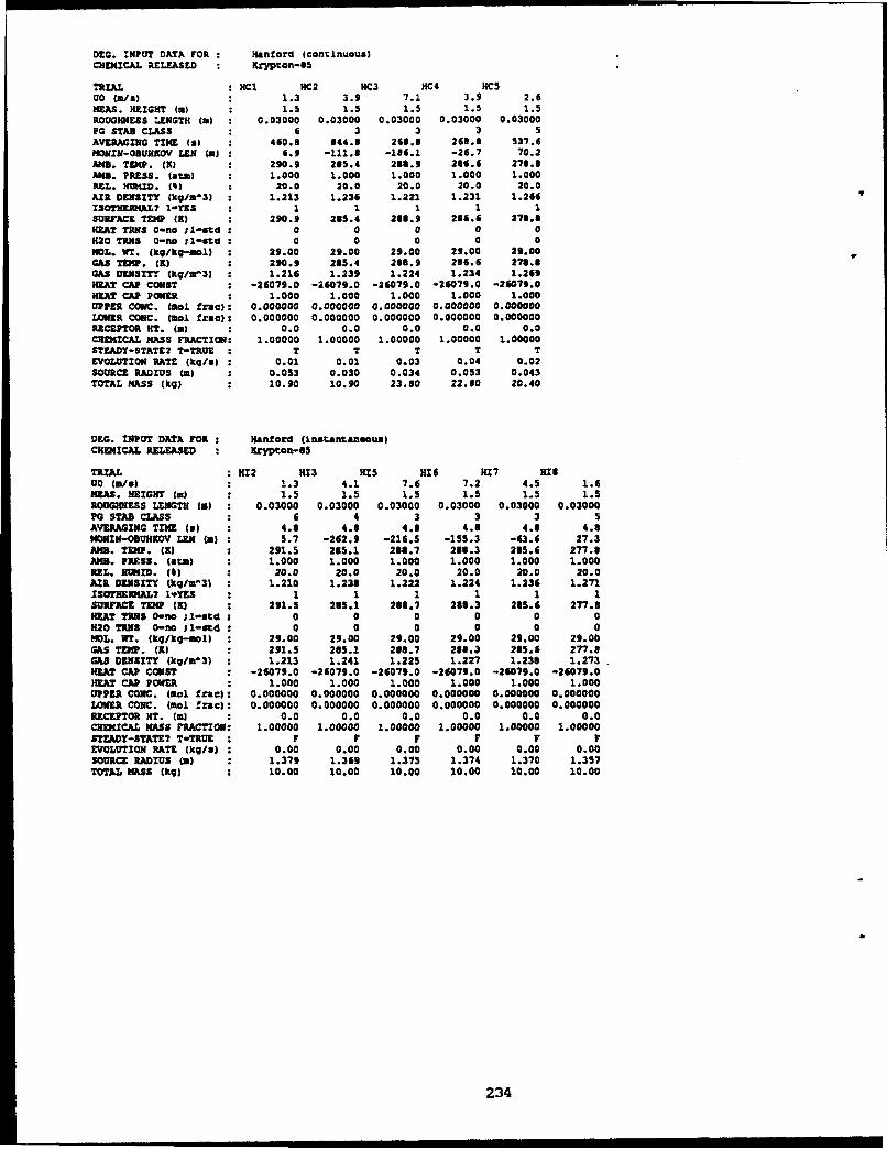
DEG. INPUT DATA FOR : Hanford (continuous)CHEMICAL RELEASED : Krypton-05

TRIAL : HC1 HC2 HC3 HC4 HC500 (a/a) 1.3 3.9 7.1 3.9 2.6HEAS. HEIGHT (m) 1.5 1.5 1.5 1.5 1.5ROUGHNESS LENGTH (a) : 0.03000 0.03000 0.03000 0.03000 0.03000PC STAR CLASS : 6 3 3 3 5AVE.AGING T1IME (a) : 460.8 344.8 268.8 261.8 537.6

QNOIM-OBUHKOV LEN (m) 6.9 -111.8 -184.1 -26.7 70.2AND. TEMP. (W) 290.9 235.4 238.9 236.6 273.8AlS. PRESS. (an) : 1.000 1.000 1.000 1.000 1.000RIL. HUMID. (0) 20.0 20.0 20.0 20.0 20.0AIR DENSITY (kg/im3) 1.213 1.236 1.221 1.231 1.266ISOTHERMAL? 1-YES 1 1 1 1 1SUIRFACE TEMP (K) 290.9 285.4 233.9 286.6 278.3HEAT TAUS 0-no ;I-std : 0 0 0 0 0H20 TRNS O-no sI1-td : 0 0 0 0 0IOL. WT. (kg/kG-Mol) 29.00 29.00 29.00 29.00 29.00GAS TIf. (K) 290.9 215.4 238.9 236.6 271.SGAS DENSITY (kg/23) : 1.216 1.239 1.224 1.234 1.259HEAT CAP COEMST : -26079.0 -26079.0 -26079.0 -26079.0 -26079.0HUET CAP POWER 1.000 1.000 1.000 1.000 1.000UPPER CONC. (aol fraa): 0.000000 0.000000 0.000000 0.000000 0.000000LOWER COiC. (mol fz•a): 0.000000 0.000000 0.000000 0.000000 0.000000RECEPTOR HT. (m) 0.0 0.0 0.0 0.0 0.0CHEMICAL MASS FRACTION: 1.00000 1.00000 1.00000 1.00000 1.00000STEADY-STATE? "-TRUE : T T T T TEVOLUTION RATE (kq/s) : 0.01 0.01 0.03 0.04 0.02SOURCE RADIUS (a) 1 0.053 0.030 0.034 0.053 0.043TOTAL MASS (kg) : 10.90 10.90 23.50 22.10 20.40

D0G. INPUT DATA FOR : Hanlord (lnstant.aneous)CHEI1CAL RELEASED : rypton-IS

TRIAL :H12 13 H15 HI6 H1.7 HisDO (a/s) . 1.3 4.1 7.6 7.2 4.5 1.6MUNS. HEIGHT (m) 1.5 1.5 1.5 1.5 1.5 1.5ROUGHNESS LENGTH (n) : 0.03000 0.03000 0.03000 0.03000 0.03000 0.03000PG STAB CASS 6 4 3 3 3 5AVZRAGING TIME (a) : 4.8 4.8 4.8 4.8 4.8 4.8)tE)NI-OBUHfDV LEN (m) : 5.7 -262.9 -216.5 -155.3 -63.6 27.3AMR. TEMP. (K) : 291.5 235.1 288.7 288.3 285.6 277.8MEB. PRESS. (at.) 1.000 1.000 1.000 1.000 1.000 1.000azL. HUMID. (0) : 20.0 20.0 20.0 20.0 20.0 20.0AIR. DENSITY (kg/u^3) : 1.210 1.230 1.222 1.224 1.236 1.271ISOTHERMAL? IqYES : 1 1 1 1 1 1SUlRFAC TEMP W(K) 291.5 205.1 233.7 286.3 235.6 277.8HNAT TRS 0-no ;1-std : 0 0 0 0 0 0120 TIES 0-no ;1-std : 0 0 0 0 0 0M6L. WT. (kg/kg-mol) : 29.00 29.00 29.00 29.00 29.00 29.00

GAS TEMP. (K) 291.5 205.1 288.7 203.3 235.6 277.1GAS DENSITY (kg/a3) : 1.213 1.241 1.225 1.227 1.230 1.273HEAT CAP CONST : -26079.0 -26079.0 -26079.0 -26073.0 -26079.0 -26079.0HEAT CAP POWER : 1.000 1.000 1.000 1.000 1.000 1.000UPPER CONC. (aol frac): 0.000000 0.000000 0.000000 0.000000 0.000000 0.000000LOW•R CONC. (aol frac): 0.000000 0.000000 0.000000 0.000000 0.000000 0.000000RECEPTOR HT. (a) : 0.0 0.0 0.0 0.0 0.0 0.0CHEMICAL MASS FRACTION: 1.00000 1.00000 1.00000 1.00000 1.00000 1.00000STEADY-STATE? T-TRUE : F F F F F FEVOLUTION RATE (kg/*) : 0.00 0.00 0.00 0.00 0.00 0.00SOURCE RADIUS (a) : 1.379 1.369 1.375 1.374 1.370 1.357TO AL MS (kg) 10.00 10.00 10.00 10.00 10.00 10.00

234

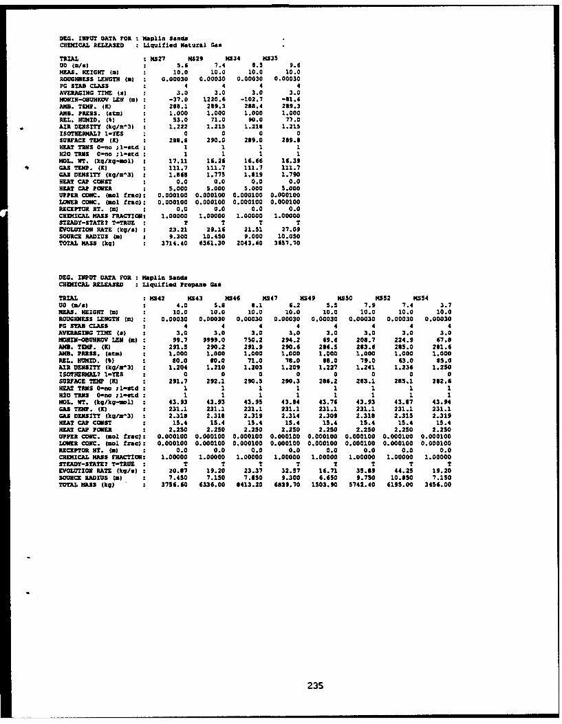
D£G. INPUT DATA FOR Haplin SandsCH.IICAL RELEASED iquflied Natiural Gas

TRIAL : MS27 NS29 K534 M535DO (n/u) . 5.6 7.4 8.5 9.6HMAS. HEIGHT (a) : 10.0 10.0 10.0 10.0ROUGHNIESS LENGTH (a) 0.00030 0.00030 0.00030 0.00030PG STAB CLASS . 4 4 4 4AVERAGING TIME (a) 3.0 3.0 3.0 3.0MONIN-OBUHKOV LEN (a) -37.0 1220.6 -102.1 -61.6ANN. TEMP. (K) 280.1 289.3 288.4 289.3AND. PRESS. (atm) 1.000 1.000 1.000 1.000ALL. HUMID. (1)* 53.0 71.0 90.0 77.0AIR DENSITY (kg/m03) 1.222 1.215 1.210 1.215ISOTHERMAL? 1-YES 0 0 0 0SURFACE TEMP (K) 208.0 290.0 289.0 289.8HEAT TRNS 0-no ;1-std 1 1 1 1H20 TONS 0-no ;1-std: 1 1 1 1HOL. WT. (kg/kq-aml) 17.11 16.26 16.66 16.39GAS TEMP. (K) : 111.7 111.7 111.7 111.7GAS DENSITY (kq/m'3) : 1.868 1.775 1.819 1.790HEAT CAP CONST 0.0 0.0 0.0 0.0HEAT CAP POWER 5.000 5.000 5.000 5.000UPPER CONC. (Uol frac): 0.000100 0.000100 0.000100 0.000100LOWER CONC. (Uol frac): 0.000100 0.000100 0.000100 0.000100RECEPTOR HT. (m) : 0.0 0.0 0.0 0.0CHEMICAL MASS FRACTION: 1.00000 1.00000 1.00000 1.00000STEADY-STATE? T-TRUE T T T TEVOLUTION RATE (kg/u) : 23.21 29.16 21.51 27.09SOURCE RADIUS (a) : 9.300 10.450 9.000 10.050TOTAL MASS (kg) 3714.40 6561.30 2043.60 3657.70

DEG. INPUT DATA FOR : Maplin SandsCHEMICAL RELEASED : Liquified Propane Gas

TRIAL : M042 11S43 MS46 NS47 NS49 1M550 NS52 NS54DO (a/S) . 4.0 5.8 8.1 6.2 5.5 7.9 7.4 3.7HEAS. HEIGHT (M) 10.0 10.0 10.0 10.0 10.0 10.0 10.0 10.0ROUGIHESS LENGTH (m) 0.00030 0.00030 0.00030 0.00030 0.00030 0.00030 0.00030 0.00030PG STAB CLASS 4 4 4 4 4 4 4 4AVERAGING TIME (a) . 3.0 3.0 3.0 3.0 3.0 3.0 3.0 3.0

HIMI-OBUHKOV LEN (a) 99.7 9999.0 750.2 294.2 69.6 208.7 224.9 67.0AND. TEMP. (M) 291.5 290.2 291.9 290.6 286.5 233.6 285.0 281.6ANM. PRESS. (fta) : 1.000 1.000 1.000 1.000 1.000 1.000 1.000 1.000REL. HUMID. (4) : 80.0 80.0 71.0 78.0 83.0 79.0 63.0 85.0AIR DENSIT (kq/u^3) 1.204 1.210 1.203 1.209 1.227 1.241 1.236 1.250ISOTHERMAL2 1-YZS : 0 0 0 0 0 0 0 0SURFACE TEM (K) : 291.7 292.1 290.5 290.3 286.2 283.1 285.1 282.8HEAT TRNS 0-no ;Il-td : 1 1 1 1 1 1 1 1H20 TMN 0-no ;Il-std : 1 1 1 1 1 1 1 1MOL. WT. (kg/kg-wol) : 43.93 43.93 43.95 43.84 43.76 43.93 43.87 43.94GAS TOM. (K) 231.1 231.1 231.1 231.1 231.1 231.1 231.1 231.1GAS DENSITY (kg/am3) : 2.318 2.318 2.319 2.314 2.309 2.310 2.315 2.319HEAT CAP COMIST : 15.4 15.4 15.4 15.4 15.4 15.4 15.4 15.4HEAT CAP POWER 2.250 2.250 2.250 2.250 2.250 2.250 2.250 2.250UPPER CONC. (aol free).: 0.000100 0.000100 0.000100 0.000100 0.000100 0.000100 0.000100 0.000100LOWER CONC. (Mol free): 0.000100 0.000100 0.000100 0.000100 0.000100 0.000100 0.000100 0.000100RECEPTOR NT. Ma) : 0.0 0.0 0.0 0.0 0.0 0.0 0.0 0.0CHEKICAL MASS FRACTION: 1.00000 1.00000 1.00000 1.00000 1.00000 1.00000 1.00000 1.00000STEADY-STATE? T-TRUE : T T T T T T T TEVOLUTION RATE (kg/u) : 20.87 19.20 23.37 32.57 16.71 35.89 44.25 19.20SOURCE RADIUS (M) : 7.450 7.150 7.850 9.300 6.650 9.750 10.850 7.150TOTAL MASS (kq) : 3756.60 6336.00 8413.20 6839.70 1503.90 5742.40 6195.00 3456.00

235

DEG. INPUT DATA FOR Prairie Grams. set 1CHEMICAL RELEASED sulfur dioxide

TR : PG7 PC* PG9 PG10 PG13 PCI5 Pa16 PG1700 (m/x) 4.2 4.9 6.9 4.6 1.3 3.4 3.2 3.3HEAS. HEIGHT (a) 2.0 2.0 2.0 2.0 2.0 2.0 2.0 2.0ROUGHNESS LENGTH (i) : 0.00600 0.00600 0.00600 0.00600 0.00600 0.00600 0.00600 0.00600PC STAR CLASS 2 3 3 2 6 1 1 4AVERAGING TIME (a) : 600.0 600.0 600.0 600.0 600.0 600.0 600.0 600.0MONIN-OBUHKOV LEN (W) : -8.2 -20.6 -34.1 -7.5 6.0 -7.7 -7.8 49.8ANN. TEMP. (K) : 305.1 305.1 301.1 304.1 293.1 295.1 301.1 300.1ANN. PRESS. (atm) 1.000 1.000 1.000 1.000 1.000 1.000 1.000 1.000REL. HUMID. (%) 20.0 20.0 20.0 20.0 20.0 20.0 20.0 20.0AIA DENSITY (kq/m^3) 1.154 1.154 1.170 1.156 1.203 1.195 1.170 1.174ISOTHERMAL? 1-YES : 1 1 1 1 1 1 1 1SURFACE TEMP (K) 305.1 305.1 301.1 304.1 293.1 295.1 301.1 300.1HEAT TRNS 0-no ;1-std : 0 0 0 0 0 0 0 0H20 TRNS 0-no ;1-std : 0 0 0 0 0 0 0 0)4OL. WT. (kg/kg-mol : 64.00 64.00 64.00 64.00 64.00 64.00 64.00 64.00GAS TENP. (K) 305.1 305.1 301.1 304.1 293.1 295.1 301.1 300.1GAS DENSITY jkg/mu3) 2.558 2.551 2.592 2.566 2.663 2.645 2.592 2.601MEAT CAP CONST : 6546.4 6546.4 6546.4 6546.4 6546.4 6546.4 6546.4 6546.4HEAT CAP POWER : 1.000 1.000 1.000 1.000 1.000 1.000 1.000 1.000UPPER CONC. (mol frac): 0.000001 0.000001 0.000001 0.000001 0.000001 0.000001 0.000001 0.000001LOWER CONC. (mol frac): 0.000001 0.000001 0.000001 0.000001 0.000001 0.000001 0.000001 0.000001RECEPTOR HT. (a) : 0.0 0.0 0.0 0.0 0.0 0.0 0.0 0.0CHEMICAL MASS FRACTION: 1.00000 1.00000 1.00000 1.00000 1.00000 1.00000 1.00000 1.00000STEADY-STATE? T-TRUE T T T T T T T TEVOLUTION RATE (kg/a) 0.09 0.09 0.09 0.09 0.06 0.10 0.09 0.06SOURCE RADIUS (m) 0.054 0.051 0.043 0.052 0.064 0.061 0.063 0.049TOTAL MASS (kg) 53.90 54.70 55.20 55.30 36.70 57.30 55.80 33.90

0D0. INPUT DATA FOR : ThOrony Island (contlnuous)CHEMICAL PRELEASED : MiXture of Freton-12 and Nitrogen

TRIAL TC45 TC47U0 (a/*) 2.3 1.5HW.AS. HEIGHT (m) 10.0 10.0ROOGHNDESS LENGTH (a) 0.01000 0.01000PG STAB CLASS 5 6AVERAGING TIME (a) 30.0 30.0MONIN-OBUHKOV LEN (a) : 21.7 10.8AND. TEMP. (K) 266.3 287.5AM. PRESS. (atm) 1.000 1.000

"EL. HUMID. (t) 100.0 97.4AIR DENSITY lkgl/a3) 1.227 1.222ISOTHE1MAL? 1-YES : I 1SURFACE TEMP (K) : 286.3 287.5HEAT TRNS 0-no ;1-std : 0 0H20 TRUS 0-no ;1-mid : 0 0NOL. WT. (kg/kg-mol) : 57.80 57.80GAS TEMP. (K) 286.3 287.5GAS DENSITY (kq/m^3) : 2.463 2.452HUAT CAP CONS? 1958.0 1955.0HEAT CAP POWER : 1.000 1.000UPPER CONC. (ol frec): 0.000100 0.000100LONER CONC. (aol frac): 0.000100 0.000100RECEPTOR HT. (a) : 0.0 0.0CHEMICAL MASS FRACTION: 1.00000 1.00000STEADY-STATE? T-TRUE : T TEVOLUTION RATE (kq/a) : 10.67 10.22SOURCE RADIUS (a) 1.000 1.000TOTAL MASS (kg) : 4055.00 4752.00

236

DEG. INPUT DATA FOR : ?homey ialand (inStantan*ous)CHEMICAL RELEASED ; Mlxtuzr of Freon-12 and NitroQen

TRIAL : TI1 T27 ?I6 TI9 T112 T113 T117 T7I8 T119V0 (a/u) : 2.8 3.4 2.4 1.7 2.5 7.3 5.0 7.4 6.4HEAS. HEIGHT (a) 10.0 10.0 10.0 10.0 10.0 10.0 10.0 10.0 10.0ROUGHNESS LENGTH (m) : 0.01000 0.01800 0.01200 0.00800 0.01600 0.01000 0.01000 0.00500 0.01000PC STAB CLASS 4 5 4 6 5 4 4 4 4AVERAGING TIME (a) : 0.6 0.6 0.6 0.6 0.6 0.6 0.6 0.6 0.6MONIN-O8UHKOV LEN (m) : 9999.0 90.9 -9.1 1.5 10.0 -90.9 -200.0 -43.5 333.3AND. TEMP. (K) 291.8 290.5 290.7 291.5 203.3 286.9 209.2 239.7 286.5AN8. PRESS. (atm) 1.000 1.008 1.009 1.006 1.000 1.006 0.995 0.994 0.993REL. HUMITD. (%) 74.8 60.7 87.6 61.3 66.2 14.1 $4.0 21.3 94.6AIR DENSITY (kg/213) : 1.203 1.219 1.218 1.211 1.243 1.234 1.208 1.205 1.218ISOTHERMAL? 1-YES : 1 1 1 1 0 1 0 0 1SURFACE TEMP (K) : 291.8 290.5 290.7 291.5 285.1 286.9 291.0 297.5 216.5HEAT TINS 0-no ;l-td: 0 0 0 0 1 0 1 1 0N2O TRUS 0-no :1-std: 0 0 0 0 0 0 0 0 0ML. WT. (ko/kg-wol) 47.69 50.50 47.11 46.24 68.49 57.80 121.36 54.04 61.27GAS TEN?. (K) : 291.8 290.5 290.7 291.5 283.3 286.9 289.2 239.7 206.5GAS DENSITY (kq/R'3) 1.993 2.141 1.994 1.947 2.949 2.472 5.093 2.262 2.590HEAT CAP CONST s -4209.1 -2446.2 -4562.9 -5093.6 8478.9 1956.0 40741.6 -335.6 4074.7HEAT CAP POWER 1.000 1.000 1.000 1.000 1.000 1.000 1.000 1.000 1.000UPPER CONC. (sol frac): 0.000100 0.000100 0.000100 0.000100 0.000100 0.000100 0.000100 0.000100 0.000100LOWER CONC. (mol frac): 0.000100 0.000100 0.000100 0.000100 0.000100 0.000100 0.000100 0.000100 0.000100RECEPTOR NT. (a) : 0.0 0.0 0.0 0.0 0.0 0.0 0.0 0.0 0.0CHEMICAL MASS FRACTION: 1.00000 1.00000 1.00000 1.00000 1.00000 1.00000 1.00000 1.00000 1.00000STEADY-STATE? T-TRUE : F F F F F F F FEVOLUTION RATE (kg/*) : 0.00 0.00 0.00 0.00 0.00 0.00 0.00 0.00 0.00

SOURCE RADIUS (m) 7.000 7.000 7.000 7.000 7.000 7.000 7.000 7.000 7.000TOTAL MASS (kq) 3147.00 4249.00 3956.00 3866.00 5736.00 4800.00 6711.00 3861.00 5477.00

237

FOCUS INPUT DATA FOR BurroCHEMICAL RELE.ASED Liquefled natural gasTITLE SCREEN:TRIAL NAME bu2 bu3 bu4 buS bu8 but buS bugTYPE OF UNITS : Metric units

MATERIAL SCREEN:PRIMARY CHEMICAL NO. 1 1 1 1 1 1 1 1MOLE FRACTION 1.00000 1.00000 1.00000 1.00000 1.00000 1.00000 1.00000 1.00000MATERIAL TEMPERATURE (C) -162.55 -162.55 -162.55 -162.55 -162.55 -162.55 -162.55 -162.55MATERIAL PRESSURE (kPa) : 93.9 94.8 94.5 94.1 93.5 94.0 94.1 94.0

WEATHER SCREEN:WIND SPEED I IOM (W/e) 6.02 5.93 10.27 8.40 10.40 9.73 2.57 6.69REL. HUMIDITY (t) : 7.10 5.20 2.70 5.90 5.10 7.40 4.50 14.40AMBIENT TEMP. (C) 38.12 34.60 35.90 41.12 39.52 33.81 32.87 35.37P-G CLASS : C C C C C 0 E D

RELEASE SCREEN:CONTINUOOS RELEASERELEASE DURATION (min) : 2.583 2.703 2.917 3.157 2.150 2.900 1.783 1.317PIPE DIAMETER (a) : 0.15000 0.15000 0.15000 0.15000 0.15000 0.15000 0.15000 0.15000EXIT AREA (m2) 0.01767 0.01767 0.01767 0.01767 0.01767 0.01767 0.01767 0.01767FLOW RATE (kq/s) 86.1000 87.9800 86.9600 81.2500 92.2200 99.4600 116.9300 135.9800RELEASE HEIGHT (m) . 0.000 0.000 0.000 0.000 0.000 0.000 0.000 0.000ANGLE FR4M HORIZON TO EXIT : 270.0 270.0 270.0 270.0 270.0 270.0 270.0 270.0REGULATED RELEASE

TERRAIN SCREEN:SURFACE ROUGHNESS (a) : 0.00020 0.00020 0.00020 0.00020 0.00020 0.00020 0.00020 0.00020CAIN OPEN SEASURFACE TEMP. (C) 1 38.12 34.60 35.90 41.12 39.52 33.1 32.87 35.37

DIKING SCREEN:UNCONFINED

VD/VE SCREEN:TRACK ONE COMPONENTEXPRESS CONCENTRATION IN PPMLOWEST CONC. LIMIT, PPM 100.000 100.000 100.000 100.000 100.000 100.000 100.000 100.000MIDDLE CONC. LIMIT, PPM : 200.000 200.000 200.000 200.000 200.000 200.000 200.000 200.000HIGHEST CONC. LIMIT, PPM 400.000 400.000 400.000 400.000 400.000 400.000 400.000 400.000DISP. COEFF. AVG. TINE (min): 0.667 1.667 1.333 2.167 1.167 2.333 1.333 0.833USE DEFAULT TIME STEP POSITIONS

FOC=5 INPUT DATA FOR : CoyoteCHEMICAL RELEASED : Liquefied natural gas . Netbane Is at least 868 in aTITLE SCREEN:TRIAL RUME : co3 CO5 Co6TYPE OF UNITS : Metric units

MATERIAL SCREEN:PRIMARY CHEMICAL NO. : 1 1 1MOLE FRACTION : 1.00000 1.00000 1.00000MATERIAL TEMPERATURE (C) : -162.55 -162.55 -162.55MATERIAL PRESSURE (kPa) : 93.6 93.9 94.2

WEATHER SCREEN:WIND SPEED 6 10M (a/e) : 6.68 10.99 5.74REL. HUMIDITY (8) 11.30 22.10 22.80AMBIENT TEMP. (C) 36.30 28.34 24.11P-G CLASS : C C 0

RELEASE SCREEN:CONTINUOUS RELEASERELEASE DURATION (min) : 1.083 1.633 1.367PIPE DIAMETER (a) 0.15000 0.15000 0.15000EXIT AREA (m2) 0.01767 0.01767 0.01767FLOW RATE (kq/s) : 100.6700 129.0200 123.0300RELEASE HEIGHT (a) : 0.000 0.000 0.000ANGLE FROM HORIZON TO EXIT : 270.0 270.0 270.0REGULATED RELEASE

TERRAIN SCREEN:SURFACE ROUGHNESS (a) : 0.00020 0.00020 0.00020CALJ4 OPEN SEASURFACE TEMP. (C) : 38.30 28.34 24.11


VD/VE SCREEN:TRACK ONE COMPONENTEXPRESS CONCENTRATION IN PPMLOWEST CONC. LIMIT, PPM : 100.000 100.000 100.000MIDDLE CONC. LIMIT, PPM : 200.000 200.000 200.000HIGHEST CONC. LIMIT, PPM 400.000 400.000 400.000DISP. COEFF. AVG. TIME (min): 0.833 1.500 1.167USE DEFAULT TIME STEP POSITIONS

238

FOCUS INPUT DATA FOR D: e-.Zt TOrtoiseCHEMICAL RELEASED : Anhydrous AmmoniaTITLE SCREEN-:TRIAL NAME : dtl dt2 dt3 dt4TYPE OF UNITS : Metric units

MATERIAL SCREEN:PRIMARY CHEMICAL NO. 53 53 53 53MOLE FRACTION 1.00000 1.00000 1.00000 1.00000MATERIAL TEMPERATURE (C) : 21.55 20.15 22.15 24.15MATERIAL PRESSURE (kPa) 1013.3 1116.6 1137.9 1179.4

WEATHER SCREEN:WIND SPEED I 10[ (m/a) : 9.68 7.63 9.28 6.22REL. HUMIDITY (0) 13.20 17.50 14.50 21.30AMBIENT TEMP . (C) 28.86 30.48 33.92 32.48P-G CLASS .D D D £

RELEASE SCREEN:CONTINUOUS RELEASERELEASE DURATION (min) : 2.100 4.250 2.767 6.350PIPE DIAMETER (m) 0.08100 0.09450 0.09450 0.09450EXIT AREA (W2) : 0.00515 0.00701 0.00701 0.00701FLOW RATE (kg/*) : 79.7000 111.5000 130.7000 96.7000RELEASE HEIGHT (W) 0.790 0.790 0.790 0.790ANGLE FROM HORIZON TO EXIT 0.0 0.0 0.0 0.0REGULATED RELEASE

TERRAIN SCREEN:SURFACE ROUGHNESS (a) : 0.00300 0.00300 0.00300 0.00300MOD FLATSSURFACE TEMP. (C) 31.65 30.65 31.65 30.85

D01IMG SCREEN:UNCONFINED

VD/VE SCREEN:TRACK ONE CmeoIPENTEXPRESS CONCENTRATION IN PPMLOWEST CONC. LIMIT, PPM : 100.000 100.000 100.000 100.000MIDDLE CONC. LIMIT, PPM 200.000 200.000 200.000 200.000HIGHEST CONC. LIMIT, PPM : 400.000 400.000 400.000 400.000DZISP. COEFF. AVG. TIME (min): 1.333 2.667 2.000 5.000USE DEFAULT TIME STEP POSITIONS

FOCUS INPUT DATA FOR GoldfishCHEMICAL RELEASED Hydrogen fluoriteTITLE SCRumoTRIAL NAE : gfl gf2 gf3TYPE OF UNITS : metric units

MATERIAL SCREEN:PRIMARY CHEMICAL NO. 50 50 50MOLE FRACTION : 1.00000 1.00000 1.00000MATERITAL TEMPERATURE (C) : 40.05 38.05 39.05MATERIAL PRESSURE (kPa) : 689.0 744.7 757.9

WEATHER SCREEN:WIND SPEED I i0N (mis) : 7.30 5.38 7.47REL. HUMIDITY (t) : 4.90 10.70 17.70AIN•ENT TEMP. (C) 37.25 36.23 34.46P-G CLASS :D D

RELEASE SCREEN:CONTINUOUS RELEASERELEASE DURATION (min) : 2.083 6.000 6.000PIPE DIAMETER (W) : 0.04190 0.02420 0.02420EXIT AREA (W2) 0.00138 0.00046 0,00046FLOW RATE (kg/u) : 27.6700 10.4600 10.2700RELEASE HEIGHT (a) : 1.000 1.000 1.000ANGLE FROM HORIZON TO EXIT : 0.0 0.0 0.0REGULATED RELEASE

TERRAIN SCREEN:SURFACE ROUGHNESS (W) 0.00300 0.00300 0.00300MUD FLATSSURFACE TEMP. (C) : 37.25 36.23 34.46


VD/VE SCREEN:TRACK ONE COMPONENTEXPRESS CONCENTRATION IN PPMLOWEST CONC. LIMIT, PPM : 30.000 30.000 30.000MIDDLE CONC. LIMIT, PPM : 60.000 60.000 60.000HIGHEST CONC. LIMIT, PPM 120.000 120.000 120.000DISP. COEFF. AVG. TIME (min): 1.472 1.472 1.472USE DEFAULT TIME STEP POSITIONS

239

FOCUS INPUT DATA FOR Hanford (continuous)CHEMICAL RELEASED Krypton-e5TITLE SCREEN:TRIAL NAME : hcl hc2 hc3 hc4 ha5TYPE OF UNITS : Metric units

MATERIAL SCREEN:PRIMARY CHEMICAL NO. 62 62 62 62 62MOLE FRACTION : 1.00000 1.00000 1.00000 1.00000 1.00000MATERIAL TEMPERATURE (C) : 17.72 12.28 15.78 13.50 5.67MATERIAL PRESSURE (kPa) : 101.3 101.3 101.3 101.3 101.3

WEATHER SCREEN:WIND SPEED I 10 (a/*) : 3.40 5.60 10.31 5.36 4.22REL. HUMIDITY (I) 20.00 20.00 20.00 20.00 20.00ANBZST TEMP. (C) 17.72 12.28 15.78 13.50 5.67P-G CLASS . F C C C z

RELEASE SCREEN:CONTINUOUS RELEASERELEASE DURATION Cain) 15.447 15.083 14.250 9.967 19.850PIPE DIAMETER (a) : 0.10553 O.u5930 0.06734 0.10849 0.08611EXIT AREA (W2) 0.00075 0.00276 0.00356 0.00891 0.00582FLOW RATE (kg/a) . 0.0117 0.0120 0.0278 0.0380 0.0171RELEASE HEIGHT (a) * 1.000 1.000 1.000 1.000 1.000ANGLE FROM HORIZON TO EXIT : 0.0 0.0 0.0 0.0 0.0REGULATED RELEASE

TERRAIN SCREEN:SURFACE ROUGHNESS (a) : 0.03000 0.03000 0.03000 0.03000 0.03000TALL GRASSSURFACE TEMP. (C) : 17.72 12.28 15.78 13.50 5.67


VDiVt SCREEN:TRACK ONE COMPONENTEXPRESS CONCENTRATION IN PPMLOWEST CONIC. LIMIT, PPM : 0.100 0.100 0.100 0.100 0.100MIDDLE CONC. LIMIT, PM : 0.200 0.200 0.200 0.200 0.200HIGHEST CONC. LIMIT, PPM : 0.400 0.400 0.400 0.400 0.400DISP. COEFF. AVG. TIME (,mn): 7.680 14.080 4.480 4.480 8.960USE DEFAULT TIME STEP POSITIONS

FOCUS INPUT DATA FOR : HafnfOid (instanltaneous)CEMICAL RELEASED Kryptoan-85TITLE SCREEN:TRIAL NAME : hL2 U43 his 1h6 h17 hisTYPE OF UNITS : metric units

MATERIAL SCREEN:PRIMARY CHEMICAL NO. : 62 62 62 62 62 62MOLE FRACTION : 1.00000 1.00000 1.00000 1.00000 1.00000 1.00000MATERIAL TEMPERATURE (C) : 18.39 11.94 15.56 15.11 12.44 4.61MATERIAL PRESSURE (kPa) : 101.3 101.3 101.3 101.3 101.3 101.3

WEATHER SCREEN:WIND SPEED 0 10H (We8) : 3.62 5.99 11.06 10.42 6.37 2.92REL. HUMIDITY (8) : 20.00 20.00 20.00 20.00 20.00 20.00AMBIENT TEMP. (C) : 10.39 11.94 15.56 15.11 12.44 4.61P--G CLASS : F D C C C E

RELEASE SCREEN:INSTANTANEOUS RELEASE]MASS SPILLED (kg) : 10.00 10.00 10.00 10.00 10.00 10.00

TERRAIN SCREEN:SURFACE ROUGHNESS (a) * 0.03000 0.03000 0.03000 0.03000 0.03000 0.03000TALL GRASSSURFACE TEMP. (C) : 18.39 11.94 15.56 15.11 12.44 4.61


VD/VE SCREEN:TRACK ONE COMPONENTEXPRESS CONCENTRATION IN PPMLOWEST CONC. LIMIT, PPM 0.100 0.100 0.100 0.100 0.100 0.100MIDDLE CONC. LIMIT, PPM : 0.200 0.200 0.200 0.200 0.200 0.200HIGHEST CONC. LIMIT, PPM : 0.400 0.400 0.400 0.400 0.400 0.400DISP. COSFF. AVG. TIME (Win): 0.00 0.000 0.080 0.060 0.080 0.080USE DEFAULT TIME STEP POSITIONS

240

FOCUS INPUT DATA FOR : Maplin SandsCHEMICAL RELEASED : LLqulelod Natural GasTITLE SCREEN:TRIAL NAME : mx27 as29 =34 mm35TYPE OF UNITS : Metric units

MATERIAL SCREEN:P•IMARY CHEMICAL NO. 1 1 1 1MOLE FRACTION : 1.00000 1.00000 1.00000 1.00000MATERIAL TEMPERATURE (C) -162.45 -162.45 -162.45 -162.45MATERIAL PRESSURE (kPa) 101.3 101.3 101.3 101.3

WEATHER SCREEN:WIND SPEED Q IOM (m/a) : 5.60 7.40 8.50 9.60REL. HUMIDITY (M) : 53.00 71.00 90.00 77.00AMBIENT TEMP. (C) 14.95 16.15 15.25 16.15P-G CLASS .D D D 0

RELEASE SCREEN,CONTINUOUS RELEASERELEASE DURATION (min) : 2.667 3.750 1.563 2.250PIPE DIAMETER (a) . 0.15000 0.15000 0.15000 0.15000EXIT AREA (W2) 0.01767 0.01767 0.01767 0.01767FLOW RATE (kQ/s) . 23.2100 29.1600 21.5100 27.0900RELEASE HEIGHT (m) 0.000 0.000 0.000 0.000ANGLE FROM HORIZON TO EXIT : 270.0 270.0 270.0 270.0REGULATED RELEASE

TERRAIN SCREEN:SURFACE ROUGHNESS (a) : 0.00030 0.00030 0.00030 0.00030CAM OPEN SEASURFACE TEMP. (C) : 15.65 16.85 15.65 16.65


VD/VE SCREEN:TRACK ONE COMPONENTEXPRESS CONCENTRATION IN PPMLOWEST CONC. LIMIT, PPM : 100.000 100.000 100.000 100.000MIDDLE CONC. LIMIT, PPM : 200.000 200.000 200.000 200.000HIGHEST CONC. LIMIT, PPM : 400.000 400.000 400.000 400.000DISP. COEFF. AVG. TIME (min): 0.050 0.050 0.050 0.050USE DEFAULT TIME STEP POSITIONS

FOCUS INPUT DATA FOR : Maplin SandsCHEMICAL RELEASED : Liquified Propane GasTITLE SCREEN:TRIAL NAME : s42 3m43 m=46 3,47 =a49 -,-50 s52 Ua54TYPE OF UNITS :Metric units

MATERIAL SCREEN:PRMUARY CHEMICAL NO. : 3 3 3 3 3 3 3 3MOLE FRACTION : 1.00000 1.00000 1.00000 1.00000 1.00000 1.00000 1.00000 1.00000MATERIAL TEMPERATURE (C) -43.05 -43.05 -43.05 -43.05 -43.05 -43.05 -43.05 -43.05MATERIAL PRESSURE (kPa) : 101.3 101.3 101.3 101.3 101.3 101.3 101.3 101.3

W.EATHER SCREEN:WIND SPEED I ION (m/s) : 4.00 5.80 8.10 6.20 5.50 7.90 7.40 3.70REL. HUMIDITY (o) : 80.00 30.00 71.00 78.00 88.00 79.00 63.00 85.00AMBIENT TEMP. (C) : 18.35 17.05 18.75 17.45 13.35 10.45 11.85 8.45P-G CLASS .D D D 0 D 0 D 0

RELEASE SCREEN:CONTINUOUS RELEASERELEASE DURATION (min) : 3.000 5.500 6.000 3.500 1.500 2.667 2.333 3.000PIPE DIAMETER (m) : 0.15000 0.15000 0.15000 0.15000 0.15000 0.15000 0.15000 0.15000EXIT AREA (32) : 0.01767 0.01767 0.01767 0.01767 0.01767 0.01767 0.01767 0.01767FLOW RATE (kq/s) : 20.8700 19.2000 23.3700 32.5700 16.7100 35.8900 44.2500 19.2000RELEASE HEIGHT (m) : 0.000 0.000 0.000 0.000 0.000 0.000 0.000 0.000ANGLE FROM HORIZON TO EXIT : 270.0 270.0 270.0 270.0 270.0 270.0 270.0 270.0REGULATED RELEASE

TERRAIN SCREEN:SURFACE ROUGHNESS (m) : 0.00030 0.00030 0.00030 0.00030 0.00030 0.00030 0.00030 0.00030CALM OPEN SEASURFACE TEMP. (C) : 13.55 18.95 17.35 17.15 13.05 9.95 11.95 9.45


,D/VE SCREEN:TRACK ONE COMPONENTEXPRESS CONCENTRATION IN PPMLOWEST CONC. LIMIT, PPM : 100.000 100.000 100.000 100.000 100.000 100.000 100.000 100.000MIDDLE CONC. LIMIT, PPM : 200.000 200.000 200.000 200.000 200.000 200.000 200.000 200.000HIGHEST CONC. LIMIT, PPM : 400.000 400.000 400.000 400.000 400.000 400.000 400.000 400.000DrSP. COEFF. AVG. TIME (min): 0.050 0.050 0.050 0.050 0.050 0.050 0.050 0.050USE DEFAULT TIME STEP POSITIONS

241

7OCUS INPUT DATA FOR Prairie G"ass, set 1CHEMICAL RELEASED Sulfur dioxideTITLE SCREEN:TRIAL NAME :p7 pg8 p99 pqlo pq13 Pql5 pg16 pq17TYPE OF UNITS : Metric unitsMATERIAL SCREEN:PRIMARY CHEMICAL NO. : 44 44 44 44 44 44 44 44HOLE FRACTION : 1.00000 1.00000 1.00000 1.00000 1.00000 1.00000 1.00000 1.00000MATERIAL TEMPERATURE (C) : 32.00 32.00 28.00 31.00 20.00 22.00 28.00 27.00MATERIAL PRESSURE IkPa) 101.3 101.3 101.3 101.3 101.3 101.3 101.3 101.3

WEATHER SCREEN:WIND SPEED 0 1ON Cods) 4.93 5.88 8.3S 5.38 2.74 3.98 3.75 4.62REL. H•MIDITY (1) * 20.00 20.00 20.00 20.00 20.00 20.00 20.00 20.00AMBIENT TEMP. CC) : 32.00 32.00 28.00 31.00 20.00 22.00 20.00 27.00P-G =SS : 8 C C 5 F A A D

RELEASE SCREEN:CONTINUOUS RELEASERELEASE DURATION (min) : 10.000 10.000 10.000 10.000 10.000 10.000 10.000 10.000PIPE DIAMETER (m) . 0.05080 0.05010 0.05080 0.05080 0.05080 0.05080 0.05080 0.05080EXIT AREA (m2) . 0.00203 0.00203 0.00203 0.00203 0.00203 0.00203 0.00203 0.00203FLOW RATE (k8/sl * 0.0899 0.0911 0.0920 0.0921 0.0611 0.0955 0.0930 0.0565RELEASE HEIGHT (m) 0.450 0.450 0.450 0.450 0.450 0.450 0.450 0.450ANGLE FROM HORIZON TO EXIT : 0.0 0.0 0.0 0.0 0.0 0.0 0.0 0.0REGULATED RELEASE

TERRAIN SCREEN:SURFACE ROUGHNESS (a) : 0.00600 0.00600 0.00600 0.00600 0.00600 0.00600 0.00600 0.00600CUT GRASSSURFACE TEMP. (C) : 32.00 32.00 28.00 31.00 20.00 22.00 28.00 ^7.00

DIKING SCREEN:UNCONPINED

VD/VE SCREEN:TRACK ONE COMPONENTEXPRESS CONCENTRATION IN PPMLOWEST CONC. LIMIT, PPM : 1.000 1.000 !.ooo 1.000 1.000 1.000 -. 000 1.000MIDDLE CONC. LIMIT, PPM : 2.000 2.000 2.000 2.000 2.000 2.000 2.000 2.000HIGHEST CONC. LIMIT, PPM : 4.000 4.000 4.000 4.000 4.000 4.000 1.000 4.000DZSP. COEFF. AVG. TIME (ain): 10.000 10.000 10.000 10.000 10.000 10.000 10.000 10.000USE DEFAULT TIME STEP POSITIONS

F=US INPUT DATA FOR Thorney Island (continuous)CHEMICAL RELEASED nlzuare of Freon-12 and NitrogenTITLE SCREEN:TRIAL NA : te4S tc47TYPE OF UNITS : Metric unitsMATERIAL SCREEN:PR.MARY CHEMICAL NO. : 56 56HOLE FRACTION 0.32043 0.32043SECONDARY CHEMICAL NO. : 16 16HOLE FRACTION * 0.67957 0.67957MATERIAL TEMPERATURE (C) : 13.10 14.30MATERIAL PRESSURE (kPs) : 101.3 101.3

WEATHER SCREEN:WIND SPEED I 1014 (a/s) : 2.30 1.50REL. HUMIDITY (4) : 100.00 97.40AMBIENT TEMP. (C) : 13.10 14.30P-G CLASS E F

RELEASE SCREEN:CONTINUOUS RELEASERELEASE DURATION Cinn) 7.583 7.750PIPE DIAMETER (a) : 2.00000 2.CVISOEXIT AREA (K2) : 3.14159 3.14159FLOW RATE (kg/s) : 10.6700 10.2200RELEASE HEIGHT (m) : 0.000 0.000ANGLE FROM HORIZON TO EXIT : 0.0 0.0REGULATED RELEASE

TERRAIN SCREEN:SURFACE ROUGHNESS 1m) : 0.01000 0.01000CUT GRASSSURFACE TEMP. (C) : 12.80 14.50


V¶/VE SCREEN:TRACK ONE COMPONENTEXPRESS CONCENTRATION IN PPMLOWEST CONC. LIMIT, PPM 100.000 100.000MIDDLE CONC. LIMIT, PPM : 200.000 200.000HIGHEST CONC. LIMIT, PPM : 400.000 400.000DSP. COEFF. AVG. TIME Cain): 0.500 0.500USE DEFAULT TIME STEP POSITIONS

242

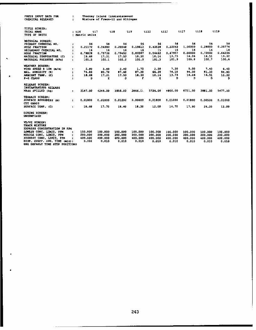
FOCUS INPUT DATA FOR Thornmy Island (instantaneous)CHEMICAL RELEASED Mixture of Fruon-12 and Nitrogen

TITLE SCREEN:TRIAL NAME t16 t17 ti8 ti9 ti12 t112 ti17 t118 t119TYPE OF UNITS Metric units

MATERIAL SCREEN:PRIMARY CHEMICAL NO. 56 56 56 56 56 56 56 56 56MOLE FRACTION 0.21172 0.24280 0.20548 0.19613 0.43538 0.32043 1.00000 0.28000 0.35774SECONDARY CHEMICAL NO. 16 16 16 16 15 16 16 16 16MOLE FRACTION 0.7882S 0.75720 0.79452 0.80387 0.56462 0.67957 0.00000 0.72000 0.64226MATERIAL TEMPERATURE (C) : 18.68 17.31 17.53 18.30 10.14 13.73 16.06 16.51 13.32MATERIAL PRESSURE (kPal : 101.3 102.1 102.2 101.9 101.3 101.9 100.8 100.7 100.6

WEATHER SCREEN:WIND SPEED I 10 (m/s) : 2.80 3.40 2.40 1.70 2.50 7.30 5.00 7.40 6.40REL. HUMIDITY (t) : 74.80 80.70 87.60 87.30 66.20 74.10 94.00 61.30 94.80AMBIENT TEMP. (C) : 18.68 17.31 17.53 16.30 10.14 13.73 16.06 16.51 13.32P-G CLASS D D E 0 F E 0 D 0 D

RELEASE SCREEN:INSTANTANEOUS RELEASEMASS SPILLED (kq) 3147.00 4249.00 3958.00 3866.0C 5736.00 4800.00 6711.00 3861.00 5477.00

TERRAIN SCREEN:SURFACE ROUGHNESS (m) 0.01800 0.01800 0.01200 0.00800 0.01800 0.01000 0.01800 0.00500 0.01000CUT GRASSSURFACE TEMP. (C) 18.68 17.70 18.40 18.30 12.00 14.70 17.90 24.30 13.00


VD/VE SCREEN:TRACK MIXTUREEXPRESS CONCENTRATION IN PPMLOWEST CONC. LIMIT, PPM : 100.000 100.000 100.000 100.000 100.000 100.000 100.000 100.000 100.000MID3LE CONC. LIMIT, PPM : 200.000 200.000 200.000 200.000 200.000 200.000 200.000 200.000 200.000HIGHEST CONC. LIMIT, PPM : 400.000 400.000 400.000 400.000 400.000 400.000 400.000 400.000 400.000DISP. COEFF. AVG. TIME (min): 0.010 0.010 0.010 0.010 0.010 0.010 0.010 0.010 0.010USE DEFAULT TIME STEP POSITIONS

243

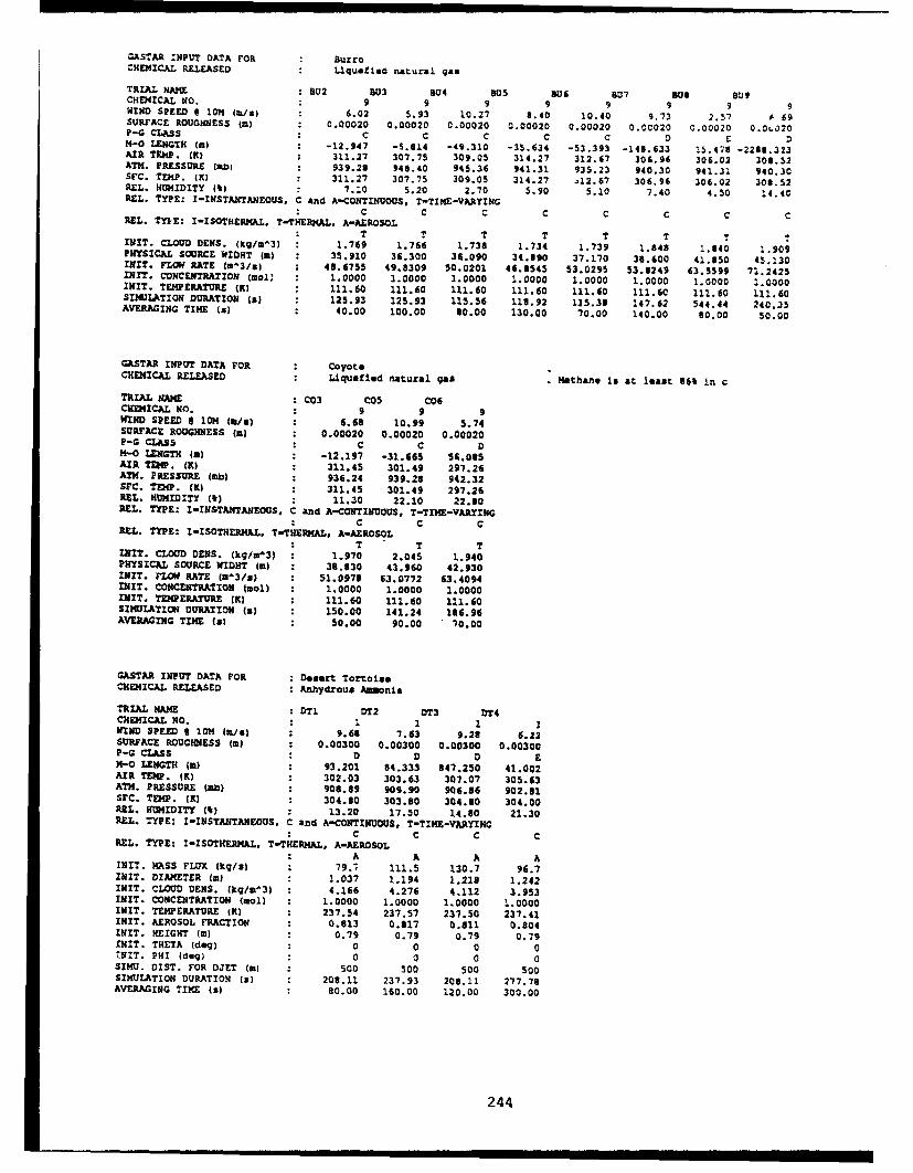
GASTAR INPUT DATA FOR BurroCHEMICAL RELEASED Llqueflac natural gas

TRIAL N•ME :U2 B03 BU4 Bus 8U6 8W7 Bus 89CHD4ICAL NO. 9 9 9 9 9 9 9 9WIND SPEED 0 10M (mW) : 6.02 5.93 10.27 8.40 10.40 9.73 2.57 it 69SURFACE ROUGHNESS (m) 0.00020 0.00020 0.00020 0.00020 0.00020 0.00020 0.00020 0.0u020P-G CLASS : C C C C C D E DM-0 LENGTH (mW : -12.947 -5.814 -49.310 -35.634 -53.393 -145.633 15.478 -2285.323AIR TEMP. (K) : 311.27 307.75 309.05 314.27 312.67 306.96 306.02 308.52ATM. PRESSURE (mbi 939.29 948.40 945.36 941.31 935.23 940.30 941.31 94C.30SFC. TEMP. (K) 311.27 307.75 309.05 314.27 a12.67 306.96 306.02 300.52REL. HUMIDITY (4) 7.10 5.20 2.70 5.90 5.10 7.40 4.50 14.40REL. TYPE: I-INSTANTANEOUS, C and A-CONTINUOUS, T-TIME-VAAYINGC C C C C C C CREL. TYI-E: I-ISOTHERM.L, T-THERMAL, A-AEROSOL:T T T T T T T T

INIT. CLOUD DENS. (kg/m^3) 1.769 1.766 1.738 1.734 1.739 1.848 1.840 1.909PHYSICAL SOURCE WIDHT (m) 35.910 36.300 36.090 34.890 37.170 38.600 41.350 45.130I9(T. FLOW RATE (Mu3/s) 48.6755 49.8309 50.0201 46.8545 53.0295 53.8249 63.5599 71.2425IXZT. CONCENTRATION (Mal) 1.0000 1.0000 1.0000 1.0000 1.0000 1.0000 1.0000 1.0000IMIT. TEMPERATURE (K) 111.60 111.60 111.60 111.60 111.60 111.60 111.60 111.60SIMULATION DURATION (s) 125.93 125.93 115.56 113.92 115.30 147.62 544.44 240.35AVERAGING TIME (s) 40.00 100.00 40.00 130.00 70.00 140.00 30.00 50.00

GASTAR INPUT DATA FOR : CoyoteCHEMICAL RELEASED Liquefied natural gas . Methane is at least 964 in c

TRIAL NAME 003 C05 c06CHEMICAL NO. : 9 9 9WIND SPEED I 10O (m/s) 6.60 10.99 5.74SURFACE ROUGHNESS (m) : 0.00020 0.00020 0.00020P-G CLASS : C C DM-O LENGTH (m) -12.197 -31.665 56.085AIR TEW9. (K) W 311.45 301.49 297.26ATM. PRESSURE (Mb) : 936.24 939.28 942.32SFC. TEMP. (K) : 311.45 301.49 297.26REL. HUMIDITY (0) : 11.30 22.10 22.80PEL. TYPE: I-INSTARTmEoUS, C and A-CONTINUOUS, T-TIME-VAR•ING

C C CREL. TYPE: I-ISOTHERMAL, T-THEPMAL, A-AEROSOL

T T TINIT. CLOUD DENS. (kg/m*3) : 1.970 2.045 1.940PHYSICAL SOURCE WIDHT (m) : 38.330 43.960 42.930INIT. FLOW RATE (a-3/s) : 51.0978 63.0772 63.4094INIT. CONCENTRATION (mol) 1.0000 1.0000 1.0000IAITT. TEMPERATURE (K) 111.60 111.60 111.60SIMULATION DURATION (s) 150.00 141.24 156.96AVERAGING TIMI Is) : 50.00 90.00 70.00

GASTAR INPUT DATA FOR : Desert TortolseCHEMICAL RELEASED : Anhydrous Ammonia

TRIAL NAME : DT1 12 DT3 DT4CHEMICAL NO. 1 I 1 1WIND SPEED 3 IO (m/s) 9.66 7.63 9.28 6.22SUtf"ACE ROUGHNESS (m) 0.00300 0.00300 0.00300 0.00300P-G CLASS D D 0 E14-0 LENGTH (W) 93.201 84.333 047.250 41.002AIR TEMP. (K) 302.03 303.63 307.07 305.63ATM. PRESSURE (mb) 908.89 909.90 906.86 902.81SFC. TEMP. (K) 304.80 303.80 304.80 304.00REL. HUMIDITY (4) : 13.20 17.50 14.80 21.30REL. TYPE: I-INSTANTANEOUS. C and A-CONTINUOUS, T-TIME-VARYING

C C C cREL. TYPE: I-ISOTHERMAL, T-THERMAL, A-AEROSOLA A A AINIT. MASS FLUX (kq/a) 79.1 111.5 130.7 96.7

INIT. DIAMETER (a) 1.037 1.194 1.218 1.242INIT. CLOUD DENS. (kq/m^3) 4.166 4.276 4.112 3.953INIT. CONCENTRATION (mol) : 1.0000 1.0000 140000 1.0000INIT. TEMPERATURE (K) 237.54 237.57 237.50 237.41INIT. AEROSOL FRACTION 0.813 0.317 0.811 0.804IMIT. HEIGHT (W) 0.79 0.79 0.79 0.79rMIT. THETA (dog) 0 0 0 0,NIT. PHI (deq g 0 0 0 0SIMU. DIST. FOR DJET (m) 500 500 500 500SIMULATION DURATION (s) 208.11 237.93 208.11 277.78AVERAGING TIME (s) 80.00 160.00 120.00 300.00

244

GASTAR INPUT DATA FOR : Maplin SandsCHEMICAL RELEASED LlqIflaed Natural Gas

TRIAL NAME NS27 MS29 KS34 KS35CHEMICAL NO. 9 9 9 9WIND SPEED 9 10M (m,/sl 5.60 7.40 5.50 9.60SURFACE ROUGHNESS (m) : 0.00030 0.00030 0.00030 0.00030P-G CLASS : D D DM-0 LENGTH (m) -36.953 1220.632 -102.720 -61.570AIR TEMP. (K) 268.10 289.30 280.40 259.30ATM. PRESSURE (ibn) : 1013.25 1013.25 1013.25 1013.25SFC. TEMP. (K) 288.80 290.00 289.00 239.80REL. HUMIDITY (t) : 53.00 71.00 90.00 77.00REL. TYPE: I-INSTANTANEOUS, C and A-CONTINUOUS, T-TIME-VARYING

C C C CREL. TYPE: I-ISOTHERMAL, T-THERMAL, A-AEROSOL

T T T TINIT. CLOUD DENS. (kq/m^3) 1.868 1.775 1.819 1.790PHYSICAL SOURCE WIDT (a) 18.600 20.900 18.000 20.100INIT. FLOW RATE (m"3/s) : 12.4235 16.4243 11.8246 15.1374INIT. CONCENTRATION (mCI) 1.0000 1.0000 1.0000 1.0000IN!T. TEMPERATURE (K) 111.70 111.70 111.70 111.70SIMULATION DURATION (a) : 216.07 154.46 121.06 142.29AVERAGING TIME (a) : 3.00 3.00 3.00 3.00

GASTAR INPUT DATA FOR : Maplin SandsCHEMICAL RELEASED : LLquified Propane Gas

TRIAL NAME : K542 11543 1S46 NS47 1S49 M450 )S52 11854CHEMICAL NO. 12 12 12 12 12 12 12 12WIND SPEED @ 10M (m/s) 4.00 5.80 8.10 6.20 5.50 7.90 7.40 3.70SURFACE ROUGHNESS (W) : 0.00030 0.00030 0.00030 0.00030 0.00030 0.00030 0.00030 0.00030PG CLASS D D D D D D 0 D

M-0 LENGTH (m) : 99.735 9999.000 750.151 294.223 49.596 205.744 224.903 67.837AIR TEMP. '(K) : 291.50 290.20 29J.90 290.60 236.50 283.60 285.00 231.60ATM. PRESSURE (mb) : 1013.25 1013.25 1013.25 1013.25 1013.25 1013.25 1013.25 1013.25SFC. TEMP. (K) : 291.70 292.10 290.50 290.30 286.20 233.10 285.10 282.60REL. HUMIDITY (b) : 80.00 80.00 71.00 78.00 88.00 79.00 63.00 85.00REL. TYPE: I-INSTANTANEOUS, C and A-CONTINUOUS, T-TIME-VARYING

C C C C C C C CREL. TYPE: I-ISOTHERMAL, T-THERMAL, A-AEROSOL

T T T T T T T TINIT. CLOUD DENS. (kq/wm3) 2.318 2.316 2.319 2.314 2.309 2.318 2.315 2.319PHYSICAL SOURCE WIDHT (W) : 14.900 14.300 15.700 16.600 13.300 19.500 21.700 14.300IN!T. FLOW RATE (=u3/a) 9.0018 6.2615 10.0755 14.0771 7.2355 15.4603 19.1123 8.2796INIT. CONCENTRATION (ool) : 1.0000 1.0000 1.0000 1.0000 1.0000 1.0000 1.0000 1.0000

INIT. TEMPERATURE (K) : 231.10 231.10 231.10 231.10 231.10 231.10 231.10 231.10SIMULATION DURATION (a) 199.50 168.97 149.51 164.52 172.73 150.63 187.84 166.76AVERAGING TIME (a) : 3.00 3.00 3.00 3.00 3.00 3.00 3.00 3.00

GASTAR INPUT DATA FOR : Prairie Grass, set 1CHEMICAL RELEASED Sulfur dioxide

TRIAL NAME : P7 PG8 PG9 Po10 PG13 PG15 PG16 PG17CHEMICAL NO. : 13 13 13 13 13 13 13 13WIND SPEED 6 1014 (m/s) 4.93 5.88 8.36 5.36 2.74 3.96 3.75 4.62SURFACE ROUGHNESS (a) : 0.00600 0.00600 0.00600 0.00600 0.00600 0-00600 0.00600 0.00600P-G CLASS : C C C a F A A D1-0 LENGTH (a) : -8.178 -20.611 -34.123 -7.452 6.014 -7.736 -7.834 49.806

AIR TEMP. (K) : 305.15 305.15 301.15 304.15 293.15 295.15 301.15 300.15ATM. PRESSURE (mb) : 1013.25 1013.25 1013.25 1013.25 1013.25 1013.25 1013.25 1013.25SFC. TEMP. (K) : 305.15 305.15 301.15 304.15 293.15 295.15 301.15 300.15REL. HUMIDITY (%) 20.00 20.00 20.00 20.00 20.00 20.00 20.00 20.00RE.. TYPE: I-INSTANTANEOUS, C and A-CONTINUOUS, T-TIME-VARYING

C C C C C C C CMEL. TYPE: I-ISOTHERMAL, T-THERMAL, A-AEROSOL

I I I I I I I IINIT. CLOUD DENS. (kq/m^3) : 2.558 2.558 2.592 2.566 2.663 2.645 2.592 2.601PHYSICAL SOURCE WIDHT (m) : 0.051 0.051 0.051 0.051 0.051 0.051 0.051 0.051INIT. FLOW RATE (tm3/x) : 0.0351 0.0356 0.0355 0.0359 0.0229 0.0361 0.0359 0.0217INIT. CONCENTRATION (mol) : 1.0000 1.0000 1.0000 1.0000 1.0000 1.0000 1.0000 1.0000SIMULATION DURATION (a) : 290.48 263.27 215.94 273.91 715.38 335.29 350.00 342.42AVERAGING TIME (I) : 600.00 600.00 600.00 600.00 600.00 600.00 600.00 600.00

245

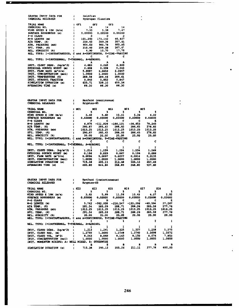
GASTAR INPUT DATA FOR GoldflishCHEMICAL RELEASED Hydrogen fluoride

TRIAL RAWE : GFi GF2 GF3CHEMICAL NO. 14 14 14WIND SPEED I 10M (m/x) 7.30 5.38 7.47SURFACE ROUGHNESS (W) 0.00300 0.00300 0.00300P-G CLASS :D D DM-0 LENGTH (m) 101.293 173.142 40.927AIR TEMP. (K) : 310.40 309.38 307.61ATM. PRESSURE |rob) 904.83 900.78 905.85SFC. T!NP. (K) : 310.40 309.38 307.61REL. HUMIDITY (8) : 4.90 10.70 17.70REL. TYPE: I-INSTANTANEOUS. C and A-CONTINUOUS, T-TIME-VARYING

: C C CREL. TYPE: I-ISOTIERMAL. T-TKERMAL. A-AEROSOL

: A A AINIT. CLOW- DENS. (kg/n'3) : 4.683 5.065 4.900PHYSICAL SOURCE WIDNT (W) : 0.608 0.338 0.343EMIT. rFLr RATE m^3/) : 5.9087 2.0653 2.0957INIT. CONCENTRATION (mol) 1.0000 1.0000 1.0000INIT. TEMPERATURE (K) 239.58 209.46 289.61INIT. AEROSOL FRACTION : 0.840 0.853 0.847SIMULATION DURATION (s) : 635.71 333.10 655.56AVERAGING TINE (s) : 66.30 80.30 68.30

GASTAR INPUT DATA FOR Hanford (continuous)CHEMICAL RELEASED Krypton-eS

TRIAL NAME HC1 HC2 HC3 NC4 mCsCHEMICAL NO. 5 5 5 5 5WIND SPEED I lox (W/e) 3.40 5.60 10.31 5.36 4.22SUpFACE ROUGHNESS (a) : 0.03000 0.03000 0.03000 0.03000 0.03000P-G CLASS . F C C C &M-O LENGTH (a) : 6.875 -111.826 -186.121 -26.653 70.243AIR TEMP. (K) 290.87 285.43 288.93 286.65 278.82ATM. PRESSURE (mb) : 1013.25 1013.25 1013.25 1013.25 1013.25SFC. TEMP. (K) : 290.87 285.43 285.93 286.65 278.32REL. HUMIDITY (t) 20.00 20.00 20.00 20.00 20.00REL. TYPE: I-INSTANTANEOUS. C and A-CONTINUOUS, T-TIE--VARYING

C C C C CR•L. TYPE: I-ISOTHERMAL, TTHERMAL, A-AEROSOL

I I I I IINIT. CLOUD DENS. (kg/=^3) : 1.216 1.239 1.224 1.234 1.269PHYSICAL SOURCE WIDHT (a) 0.106 0.059 0.067 0.106 0.086WMIT. FLOW RATE (&^3/a) 0.0096 0.0097 0.0227 0.0314 0.0135M111T. CONCENTRATION (mol) 1.0000 1.0000 1.0000 1.0000 1.0000

SIMULATION DURATION (a) : 715.38 305.13 212.68 305.13 407.69AVERAGING TINE (a) 460.80 844.80 268.80 268.80 537.60

GASTAR INPUT DATA FOR Hanford (instantaneous)CHEMICAL RELEASED : Krypton-65

TRIAL MA : 12 H13 HI5 M1 HI7 His8CHEMICAL NO. : 5 5 5 5 5 5WIND SPEED I 10H (W/e) : 3.62 5.99 11.06 10.42 6.37 2.92SURFACE ROUGHNESS (m) : 0.03000 0.03000 0.03000 0.03000 0.03000 0.03000P-G CLASS : F D C C C EM-O LENGTH (a) : 5.742 -262.928 -216.547 -155.306 -63.594 27.267AIR TEMP. (K) : 291.54 285.09 288.71 288.26 285.59 277.76ATM. PRESSURE (mb) 1013.25 1013.25 1013.25 1013.25 1013.25 1013.25SFC. TEMP. (K) : 291.54 285.09 288.71 288.25 285.59 277.76REL. HUMIDITY (4) 20.00 20.00 20.00 20.00 20.00 20.00REL. TYPE: I-INSTANTANEOUS, C and A-CONTINUOUS, T-TUM-VARYING

I I I I I IREL. TYPE: I-ISOTHERMAL, T-THEZRAL, A-AEROSOL

I I I I I IEMIT. CLOUD DENS. (kg/a^3) : 1.213 1.241 1.225 1.227 1.238 1.273INIT. CLOUD RAD. (m) : 1.3792 1.3690 1.3743 1.3740 1.36H 1.3572INIT. CLOUD VOL. (m'3) : 8.243 8.060 3.163 0.150 a.074 7.853INIT. CONCENTRATION (mol) : 1.0000 1.0000 1.0000 1.0000 1.0000 1.0000INIT. MOMENTUM MIXING: A. WELL MIXED, a: OTHERWISE

a8 8 8 5 B

SIMULATION DURATION (a) 715.38 295.12 205.26 211.11 277.78 600.00

246

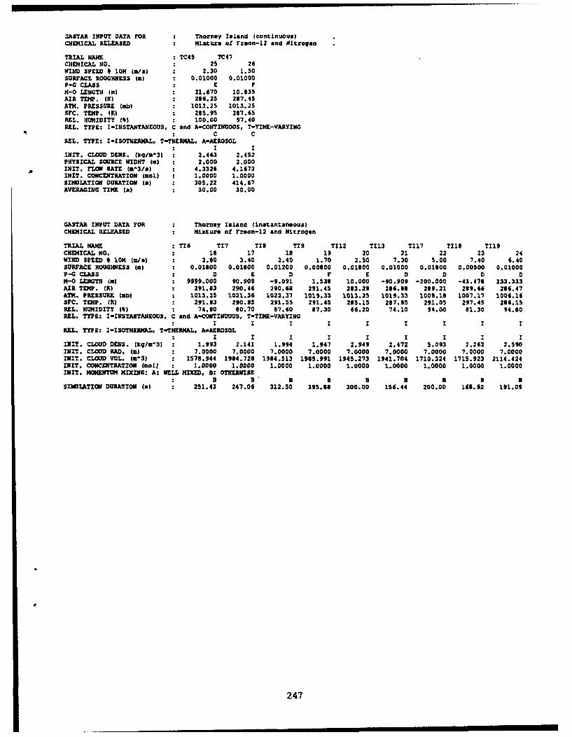
SASTAR INPUT DATA FOR Thorney Island (contlnuous)CHEMICAL RELEASED Mixture of Freon-L2 and Nitrogen

TRIAL HM• TC45 TC41CHEMICAL NO. 25 26WIND SPEED I 1OM (m/X) : 2.30 1.50SURFACE ROUGHNESS (A) 0.01000 0.01000P-G CLASS . E FM-0 LENGTH (a) 21.670 10.635AIR TEMP. (K) : 266.25 267.45ATM. PRESSURE (ab) 1013.25 1013.25SFC. TEMP. (K) 265.95 267.65REL. HUMIDITY (%) 100.00 97.40REL. TYPE: I-INSTANTANEOUS, C and A-CONTINUOUS, T-TINE-VARYING

* C CREL. TYPE: I-ISOTHEPRHAL, T-THNERAL, A.AEROSOL

I IINIT. CLOUD DENS. (kq/ma3) 2.463 2.452PHYSICAL SOURCE WIDIIT (m) : 2.000 2.000

A INIT. FLOW RATE (W'3/0) 4.3326 4.1673INIT. CONCENTRATION (mol) 1.0000 1.0000SIMULATION DURATION (a) : 305.22 414.67AVERAGING TIME (a) : 30.00 30.00

GASTAR INPUT DATA FOR Thorney Island (instantaneous)CHEMICAL RELEASED Mixture of Freon-12 and Nitrogen

TRIAL NAME TZ6 T17 T78 T19 TI12 T113 T117 T118 T119CHEMICAL NO. : 16 17 1i 19 20 21 22 23 24WIND SPEED lom (a/&) : 2.60 3.40 2.40 1.10 2.50 7.30 5.00 7.40 6.40SURFACE ROUGHNESS (a) : 0.01800 0.01800 0.01200 0.00600 0.01800 0.01000 0.01800 0.00500 0.01000P-G CLASS D E 0 F £ D 0 D 0M-O LENGTH in) 9999.000 90.909 -9.091 1.536 10.000 -90.909 -200.000 -43.476 333.333AIR TEMP. (K) : 291.83 290.46 290.66 291.45 233.29 266.66 269.21 289.66 266.47ATM. PRESSURE (m0) : 1013.25 1021.36 1022.37 1019.33 1013.25 1019.33 1008.18 1007.17 1006.16SFC. TEMP. (K) : 291.33 290.65 291.55 291.45 265.15 287.85 291.05 297.45 286.15REL. HUMIDITY (%) : 74.00 60.70 67.60 87.30 66.20 74.10 94.00 81.30 94.80REL. TYPE: I-INSTANTANEOUS, C and A-CONTINUOUS, T-TIME-VARYING

I I I I

REL. TYPE: I-ISOTHMRMKL, T-THERMAL, A-AEROSOLI I I I I I I I I

IN!T. CLOUD DENS. (k•q/a3) : 1.993 2.141 1.994 1.947 2.949 2.472 5.093 2.262 2.590INIT. CLOUD RAD. (W) : 7.0000 7.0000 7.0000 7.0000 7.0000 7.0000 7.0000 7.0000 7.0000INIT. CLOUD VOL. (ma3) : 1578.944 1984.728 1984.513 1985.991 1945.273 1941.704 1710.324 1715.923 2114.424IN!T. CONCENTRATION (maol : 1.0000 1.0000 1.0000 1.0000 1.0000 1.0000 1.0000 1.0000 1.0000INIT. MOMENTUM MIXING: A: WELL MIXED, B: OTHERWISE

a 3 3 B S B B 2 3SIMULATION DURATION (a) : 251.43 247.06 312.50 395.88 300.00 156.44 200.00 166.92 191.09

247

GPM INPUT DATA FOR BarroCHEMICAL RELEASED Liquefled natural qas

TRIAL 3U2 B03 B04 B05 506 307 s0o 809EMIS. PATE (q/s) 86100. 87960. 86960. 81250. 92220. 99460. 116930. 133960.WIND SPEED (m/s) 5.4 5.4 9.0 7.4 9.1 8.4 1.8 5.7STAB. CLASS C C C C C 0 9 DAVG. TIME (min) 0.67 1.67 1.33 2.17 1.17 2.33 1.33 0.13INITIAL SIGMA-Y (m) 2.82892 2.84606 2.21339 2.35234 2.27966 2.36857 5.55167 3.31640INITIAL SI(GA-Z (a) 2.82892 2.84606 2.21339 2.38234 2.27966 2.36857 5.55167 3.31640PLUME HEIGHT (m) 0.0 0.0 0.0 0.0 0.0 0.0 0.0 0.0REC. MT. (m) 1. 1. 1. 1. 1. 1. 1. 1.1: RU•AL 2: UBAN : 1 1 1 1 1 1 1 1CONC. SPEC. (ppm) 100. 100. 100. 100. 100. 100. 100. 100.MOLEC. WT. (9/nol) : 17.46 17.26 17.05 17.08 17.24 16.22 10.12 14.12AIR TEMP. (K) 311.3 307.6 309.0 314.3 312.7 307.0 306.0 300.5

NOTE: Initial sigmas are used to be consistent withthe initial concentration at the source

GPM INPOT DATA FOR CoyoteCHEMICAL RELEASED Liquefied natural gas . Methane i. at least 066 In c

TRIAL C03 CO5 COGEMIS. RATE (gi/) : 100670. 129020. 123030.WIND SPEED (m/s) : 6.0 9.7 4.6STAB. CLASS : C C D"AVG. TInE (ain) : 0.63 1.50 1.17INITIAL SIGNA-Y (m) : 2.75051 2.36472 3.41669INITIAL SIGMA-Z (m) : 2.75051 2.36472 3.41669PLDM HEIGHT (a) 0.0 0.0 0.0REC. HT. (=) 1. 1. 1.1. RURAL 2: ORBAN 1 1 1CONC. SPEC. (pm) 100. 100. 100.MOLEC. WT. (g/aol) 19.51 20.19 19.09AIR TEMP. (W) : 311.5 301.5 297.3

NOTE: initial Sigma* are used to be consistent withthe initial concentration at the source

GPN INPUT DATA FOR Desert TortoiseCHEDIC&L RELEASED Anhydrous Amonia

TRIAL : OTi 0T2 D"3 DT4DEIS. RATE (9/s) : 79700. 111500. 130700. 96700.WIND SPEED (a/*) 7.4 5.8 7.4 4.5STAB. CLASS : D D D 9AVG. TIUE (min) : 1.33 2.67 2.00 5.00INITIAL SIGMA-Y (m) : 1.63536 2.18545 2.10040 2.32223INITIAL SIGMK-Z (m) : 1.63536 2.16545 2.10040 2.32223PLUME HEIGHT (m) 0.8 0.6 0.5 0.8REC. HT. (a) : 1. 1. 1. 1.1: RURAL 2: URBAN : 1 1 1 1CONC. SPEC. (ppm) : 100. 100. 100. 100.MOLEC. WT. (9/mol) 17.03 17.03 17.03 17.03AIR TEMP. (K) : 302.0 303.6 307.1 305.6

NOTE: initial sigmas are used to be consistent withthe initial concentration at the source

248

GPM INPUT DATA FOR GoldfishCHEMICAL RELEASED Hydrogen fluoride

TRIAL GF1 O12 Gr3EWXS. RATE (g/s) 27670. 10460. 10270.WIND SPEED Wa/s) 5.6 4.2 5.4STAB. CLASS D D DAVG. TIME (min) 1.47 1.47 1.47INITIAL SIGMA-Y (m) : 1.21901 0.86714 0.75548INITIAL SIGMA-Z (a) : 1.21901 0.86714 0.75548PLUME HEIGHT (W) 1.0 1.0 1.0REC. HT. Wm) : 1. 1. 1.1:RURA.L 2,01RBA 1 1 1CONC. SPEC. (pfo) 30. 30. 30.MOLEC. WT. (q/reol) 20.01 20.01 20.01AIl TEMP. (K) 310.4 309.4 307.6


GPM INPUT DATA FOR Hanford (continuous)CHEMICAL RELEASED Krypton-85

TRIAL XCI HC2 HC3 HC4 HCSEMIS. RATE (g9s; 12. 12. 28. 39. 17.WIND SPEED (M/s)e 1.3 3.9 7.1 3.9 2.6STAB. CLASS F C C C EAVG. TIME (min) 7.68 14.08 4.48 4.48 8.96INITIAL SIGMA-y (m) : 0.04854 0.02811 0.03191 0.05066 0.04062INITIAL SIGKA-Z (a) : 0.04854 0.02411 0.03191 0.0S066 0.04062PLUME EIGHT? (m) : 1.0 1.0 1.0 1.0 1.0REC. HT. (W) : 2. 2. 2. 2. 2.1: ROMA 2: URBAN 1 1 1 1 1CONC. SPEC. (pm) 2 0. 0. 0. 0. 0.MOLEC. WT. (g/mol) 29.00 29.00 29.00 29.00 29.00AIR TEMP. (K) 290.9 285.4 288.9 286.6 278.8

NOTZ: initial sigmas are used to be consistent withthe initial concentration at the source

GPM INPUT DATA FOR : Maplin sandsCHEICAL RELEASED : Liquifled Natural Gas

TRJL : S27 MS29 NS34 MS35WIS. RATE (g/s) : 23210. 29160. 21510. 27090.WIND SPEED (n/a) : 5.6 7.4 8.5 9.6STAB. CLASS D 0 0 DAVG. TIME (min) 0.05 0.05 o.0s 0.03INITIAL SIGMA-Y (m) 1.34958 1.35270 1.06925 1.14015INITIAL SIGMA-z (a) : 1.34958 1.35270 1.06925 1.14015PLUME HEIGHT Wm) 0.0 0.0 0.0 0.0REC. HT. (m) 1. 1. 1. 1.1:RURAL 2:ORRANi 1 1 1 ICONe. SPEC. (Ipm) 100. 100. 100. 100.NOLEC. WT. (q/mol) : 17.11 16.26 16.66 16.39AIR TEMP. (K) 248.1 289.3 268.4 289.3


249

GPM INPUT DATA FOR :Maplin sandsCHEMICAL RELEASED Liquified Propane Gas

TRIAL 1M542 K543 KS46 K(547 KS49 MS50 KS52 KS54EMIS. RATE (W/e) : 20870. 19200. 23370. 32570. 16710. 35890. 44250. 19200.WIND SPEED (m1/) 4.0 5.8 8.1 6.2 5.5 7.9 7.4 3.7STA8. CLASS D D D D D D D DAVG. TIME (min) 0.05 0.05 0.05 0.05 0.05 0.05 0.05 0.05INITIAL SIGMA-Y (m) 0.95056 0.75546 0.70719 0.95331 0.72051 0.87409 1.00690 0.93163INITIAL SIG4A-Z (m) : 0.95056 0.75546 0.70719 0.95331 0.72051 0.87489 1.00690 0.93163PLUME HEIGHT Wu) : 0.0 0.0 0.0 0.0 0.0 0.0 0.0 0.0REC. NT. (m) : 1. 1. 1. 1. 1. 1. 1. 1.1:RURAL 2:URBANI 1 1 1 1 1 1 1 1CONC. SPEC. (ppm) 100. 100. 100. 100. 100. 100. 100. 100.HOLEC. WT. (gCial) 43.93 43.93 43.95 43.84 43.76 43.93 43.$7 43.94AIR TEM. (K) 291.5 290.2 291.9 290.6 286.5 203.6 205.0 281.6

NOTE: nitial aiqsima are used to be consistent withthe Initial concentration at the source

GPM INPUT DATA FOR : Prairie GrasS, aet 1CHEID(CAL RELEASED : Sulfur dioxide

TRIAL : PG7 ?Go 1G9 PGb0 F613 PG15 PG16 PG17EMIS. RATE (9/&) 90. 91. 92. 92. 61. 96. 93. 57.WIND SPEED (m/s) : 4.2 4.9 6.9 4.6 1.3 3.4 3.2 3.3STAR. CLASS : a C C a F A A DAVG. TIME (min) 10.00 10.00 10.00 10.00 10.00 10.00 10.00 10.00INITIAL SIGMA-Y (m) : 0.05161 0.04810 0.04046 0.04293 0.07496 0.05814 0.05974 0.04578INITIAL SIGNA-Z (a) : 0.05161 0.04810 0.04046 0.04903 0.07496 0.05914 0.05974 0.04576PLUME HEIGHT I1) 0.4 0.4 0.4 0.4 0.4 0.4 0.4 0.4REC. HT. (m) : 2. 2. 2. 2. 2. 2. 2. 2.1:RURAL 2:URBAN : 1 1 1 1 1 1 1 1CONC. SPEC. (ppm) 1. 1. 1. 1. 1. 1. 1. 1.MOLEC. WT. (C/aol) : 64.00 64.00 64.00 64.00 64.00 64.00 64.00 44.00AIR TE••. (K) : 305.1 305.1 301.1 304.1 293.1 295.1 301.1 300.1

NOTE: Initial algagS are used to be consistent withthe Initial concentration at the source

GPM INPUT DATA FOR : Thorney Island (continuous)CEDIICAL RELEASED : Mixture of Freon-12 and Nitrogen

TRIAL : TC45 TC47DWIS. PRAT (g1s) : 10670. 10220.WIND SPEED (2/a) : 2.3 1.5STAB. CLASS E rAVG. TIME (ain) 0.50 0.50INITIAL SIGDA-Y (a) 0.77435 0.94039INITIAL SIMA-Z (m) : 0.77435 0.94039PLUME HEIGHT (m) : 0.0 0.0REC. NT. (i) 0 0. 0.1:*DRJL 2:URSAN : 1 1CONC. SPEC. (ppm) 100. 100.MOULC. WT. Wg/moo) : 57.80 57.30AIR TEMP. (X) : 286.3 287.5

NOTE: Initial sigma are used to be consistent withthe initial concentration at the souroe

250

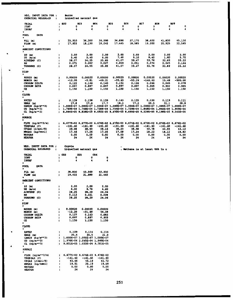
HEG. INPUT DATA FOR ; BurroCHEMICAL RELEASZD : Liquefied natural qaa

TRIAL BU2 B93 84 Bu5 806 307 sue 909

ICNT a 0 0 0 0 0 0 0ISURF * 4 4 4 4 4 4 4 4

POOL DATA

PLL (a) 35.910 36.300 36.090 34.890 37.170 38.600 41.850 45.130PLMHW m) 17.955 18.150 18.045 17.445 18.585 19.300 20.925 22.565

AMBIENT CONDITIONS

ZO (m) 2.00 2.00 2.00 2.00 2.00 2.00 2.00 2.0000 (a/s) 5.40 5.40 9.00 7.40 9.10 8.40 1.80 5.70

AIRTEMP (C) 38.07 34.55 35.85 41.07 39.47 33.76 32.82 35.32RH 0.071 0.052 0.027 0.059 0.051 0.074 0.045 0.144TGROUND (C) 38.07 34.55 35.85 41.07 39.47 33.76 32.82 35.32

DISP

ROUGH (m) 0.00020 0.00020 0.00020 0.00020 0.00020 0.00020 0.00020 0.00020HONIN (m) -12.95 -5.81 -49.31 -35.63 -53.39 -148.63 15.48 -500.00CROSS)l DELTA 0.122 0.146 0.140 0.154 0.136 0.096 0.065 0.078CROSSW BETA 0.897 0.897 0.897 0.897 0.897 0.905 0.902 0.905CE 1.150 1.150 1.150 1.150 1.150 1.150 1.150 1.150

CLOUD

XSTEP 0.139 0.138 0.139 0.143 0.135 0.130 0.119 0.111mKAX (M) 17.8 17.6 17.7 18.3 17.2 23.3 31.1 28.9CAMIN (ko/z**3) : 1.000E-07 1.0009-07 1.000E-07 1.000E-07 1.000E-07 1.0009-07 1.000E-07 1.0008-07CU (kq/m**3) : 1.769E-04 1.7668-04 1.7388-04 1.7348-04 1.7398-04 1.848E-04 1.8408-04 1.9098-04CL (kg/m**3) : 8.8448-05 8.8288-05 0.6928-05 8.6702-05 8.6958-05 9.239E-05 9.198E-05 9.543E-05

SOURCE

FLUX (kq/m**2/s) z 6.677E-02 6.677E-02 6.6769-02 6.675E-02 6.675E-02 6.675E-02 6.676E-02 6.676E-02TEMPGAS (C) : -161.60 -161.60 -161.60 -162.60 -161.60 -161.60 -161.60 -161.60

CPGAS (J/mol/K) 39.08 38.63 36.16 38.23 38.58 40.78 40.55 42.12MWGAS (kq/kmol) 17.46 17.26 17.05 17.08 17.24 18.22 18.12 18.82WATGAS 0.00 0.00 0.00 0.00 0.00 0.00 0.00 0.00HEA•3GR . 24 24 24 24 24 24 24 24

H1G. INPUT DATA FOR : CoyoteCHEMICAL RELEASED : Liquefied natural qas v )atha is at leasa 866 iii c

TRIAL C03 COS Cos

ICNT : 0 0 0ISU"F . 4 4 4

FOOL DATA

PLL (m) 38.830 43.960 42.930

P1H1 (a) 19.415 21.9$0 21.465

AMBIENT CONDITIONS

Z0 (a) 2.00 2.00 2.0000 (M/a) 6.00 9.70 4.60ARXMD (C) 38.25 28.29 24.06RH 0.113 0.221 0.228TGRDOUND (C) 38.25 26.29 24.04

DISP

ROUGH (M) 0.00020 0.00020 0.00020MONIN (m) -12.20 -31.65 56.08CROSS0 DELTA 0.127 0.143 0.083CROSSW BETA 0.897 0.897 0.905CE 1.150 1.150 1.150

CLOUD

XSTEP 0.129 0.114 0.116XKAX (m) 20.6 20.5 21.0CAMHI (kq/,**3) 1.0008-07 1.000E-07 1.0008-07CO (kq/m,,3) 1.970E-04 2.0458-04 1.940E-04CL (kq/m**3) 9.851E-05 1.023E-04 9.701E-05

SOURCE

FLUX (kq/m**2/) 6.6778-02 6.6768-02 6.768-02TEHPGAS (C) -161.60 -161.60 -161.60CPGAS (J/Mol/K) 43.66 45.19 42.72MWGAS (kq/knol) 19.51 20.19 19.09WATGAS 0.00 0.00 0.00HEATGR . 24 24 24

251

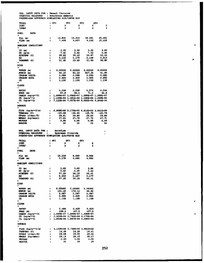
NEG. INPUT DATA FOR : Desert TortoiseCHEMI4CAL RELEASED : Anhydrous AmmoniaPSEUDO-GAS APPROACH SIMULATING AIR/VAPOR MIX

TRIAL T'1 OT2 DT3 DT4XCNT . 0 0 0 0

ISURF . 2 2 2 2

POOL DATA

PLL (m) 14.301 19.615 18.261 20.451PLiH" (m) 7.400 9.807 9.130 10.225

AMBIENT CONDITIONS

Z0 (ia) 2.00 2.00 2.00 2.0000 (m/s) 7.40 5.80 7.40 4.50AIRTE4P (C) 28.83 30.43 33.87 32.43RH 0.132 0.175 0.148 0.213TGROUND CC) 31.60 30.60 31.60 30.80

D'SP

ROUGH (a) 0.00300 0.00300 0.00300 0.00300HOKIN (2) 93.20 84.33 347.25 41.00CROSSN DELTA 0.086 0.098 0.093 0.005CROSSM BETA 0.905 0.905 0.905 0.902CE 1.150 1.150 1.150 1.150

CLOUD

XSTEP 0.338 0.255 0.274 0.244XDAX (a) 87.8 66.3 71.2 63.6CNIN (kq/m**3) 1.00OE-07 1.000E-07 1.0003-07 1.000E-07CU (kg/mu*3) 1.4253-03 1.401E-03 1.3203-03 1.329t-03CL (kq/m•*3) 7.123E-04 7.007,-04 6.6023-04 6.6443-04

SOURCE

IFLUX (kq/aee2/s) 6.608E+00 5.1733+00 6.612&+00 3.9413+00TEMPGAS (C) -35.66 -35.63 -35.70 -35.79CPGAS (J/o1/K) : 29.81 29.80 29.64 29.80INGAS (kq/kmol) 27.83 27.79 27.73 27.71NATUAS 0.00 0.00 0.00 0.00EAATGR 24 24 24 24

NEG. ZINPUT DATA FOR GoldflshCHEMICAL RELEASED Hydroqen fluoridePSEUDO-GAS APPROACH SI"OLhTING AXP,'APOR MIX

TRIAL G11 G02 0'3ICOT . 0 0 0ISUO" : 2 2 2

POOL DATA

PLL Wu) 10.339 8.000 8.000PLN Wm) 5.170 4.000 4.000

AMBIWT CONDITIONS

Z0 (mu 2.00 2.00 2.00U0 (Wes) 5.60 4.20 5.40ARfPTZt (C) 37.20 36.10 34.41RH 0.049 0.107 0.177TGROUND (C) 37.20 36.18 34.41

OZSP

ROUGH (m) 0.00300 0.00300 0.00300"MOnly (a) 201.29 173.14 40.93CROSSM DELTA 0.087 0.083 0.007CROSSW BETA 0.905 0.905 0.905CE 1.150 1.150 1.150

CLOUD

XSTEP 0.484 0.62S 0.625AX Wm) 338.5 187.5 437.5

CAMIN (kq/m*•3) : 1.0003-07 1.0003-07 1.0003-07CU (kq/m**3) : 3.604E-04 3.794E-04 4.170E-04CL (kq/mu*3) : 1.802Z-04 1.897E-04 2.085E-04

SOURCE

FLUX (kq/me*2/s) : 4.132E+00 2.758E+00 2.9613+00TENPGAS (C) 16.36 16.26 16.41CPGAS (J3mol/K) 29.09 29.05 29.02NNGAS (ko/kmol) 28.14 28.15 23.17WATGAS 0.00 0.00 0.00HEATGR . 24 24 24

252

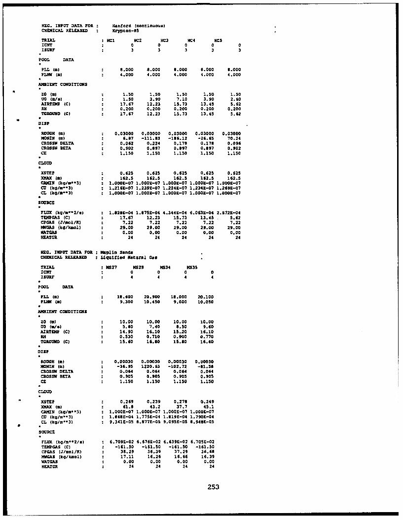
HEG. INPUT DATA FOR Hanford (continuous)CHEMICAL P.ELFASED Krypton-85

TRIAL HC1 HC2 HC3 HC4 HC5ICNT . 0 0 0 0 0ISURF . 3 3 3 3 3

POOL DATA

PLL (W) 8.000 8.000 6.000 8.000 8.000PLHW () 4.000 4.000 4.000 4.000 4.000

MUIMNT CONDITIONS

ZO (m) 1.50 1.50 1.50 1.50 1.50UO (/8) 1.50 3.90 7.10 3.90 2.60AI;TMlP (C) 17.67 12.23 15.73 13.45 5.62R: 0.200 0.200 0.200 0.200 0.200TGROUND (C) 17.67 12.23 15.73 13.45 5.62

DISP

ROUGH (a) 0.03000 0.03000 0.03000 0.03000 0.03000MOHIN (1) 6.87 -111.33 -186.12 -26.65 70.24CROSSW DELTA 0.062 0.224 0.178 0.178 0.096CROSSW BETA 0.902 0.897 0.897 0.897 0.902CE 1.150 1.150 1.150 1.150 1.150

CLOUD

XSTEP 0.625 0.625 0.625 0.625 0.625XKAX (W) 162.5 162.5 162.5 162.5 162.5CUAMN (kq/"**3) : 1.0001-07 1.000E-07 1.0001-07 1.000E-07 1.000E-07CU (kg/m**3) : 1.2161-07 1.2398-07 1.2241-07 1.234E-07 1.269E-07CiL (kq/m**3) : 1.0001-07 1.000E-07 1.0001-07 1.000E-07 1.000E-07

SOURCE

FLUX (kg/e**2/n) : 1.8281-04 1.875E-04 4.344E-04 6.063E-04 2.672E-04TE4PGAS (C) 17.67 12.23 15.73 13.45 5.62CPG&S (J/mol/K) 7.22 7.22 7.22 7.22 7.22MKGAS (kq/kmol) 29.00 29.00 29.00 29.00 29.00NWATGAS 0.00 0.00 0.00 0.00 0.00HEATGR * 24 24 24 24 24

MEG. INPUT DATA FOR : Maplin SandsCHEMICAL RELEASED : Liquifled Natural 0"a

TRIAL NS27 MS29 MS34 MS35ICNT * 0 0 0 0ISUrF : 4 4 4 4

POOL DATA

PLL (a) 18.600 20.900 18.000 20.100PLHf (a) 9.300 10.450 9.000 10.050

AMBIENT CONDITIONS

ZO (m) 10.00 10.00 10.00 10.0000 (m/*) 5.60 7.40 8.50 9.60

AIRTENP (C) 14.90 16.10 15.20 16.10RH 0.530 0.710 0.900 0.770TOROUND (C) 15.60 16.80 15.80 16.60

DISP

ROUGH (W) 0.00030 0.00030 0.00030 0.00030MORIN (W) 2 -36.95 1220.63 -102.72 -81.58CROSSW DELTA 0.064 0.064 0.064 0.064CROSSW BETA 0.905 0.905 0.905 0.905CE 1.150 1.150 1.150 1.150

CLOUD

XSTEP 0.269 0.239 0.278 0.249XNAX (M) 61.8 43.2 37.7 45.1CAMIN (kq/m**3) : 1.0001-07 1.0001-07 1.000Z-07 1.000E-07CU (kq/m*"3) : 1868-04 1.7751-04 1.819E-04 1.790E-04CL (kq/1**3) : 9.341E-05 8.877E-05 9.0951-05 8.9481-05

SOURCE

FLUX (kqlm32/s) : 6.709E-02 6.6761-02 6.639E-02 6.705E-02TEMPGAS (C) -161.50 -161.50 -161.50 -161.50CPGAS (W/mol/K) 38.29 36.39 37.29 36.68MWGAS (kq/kmol) 17.11 16.26 16.66 16.39WATGAS 0.00 0.00 0.00 0.00HEATGR . 24 24 24 24

253

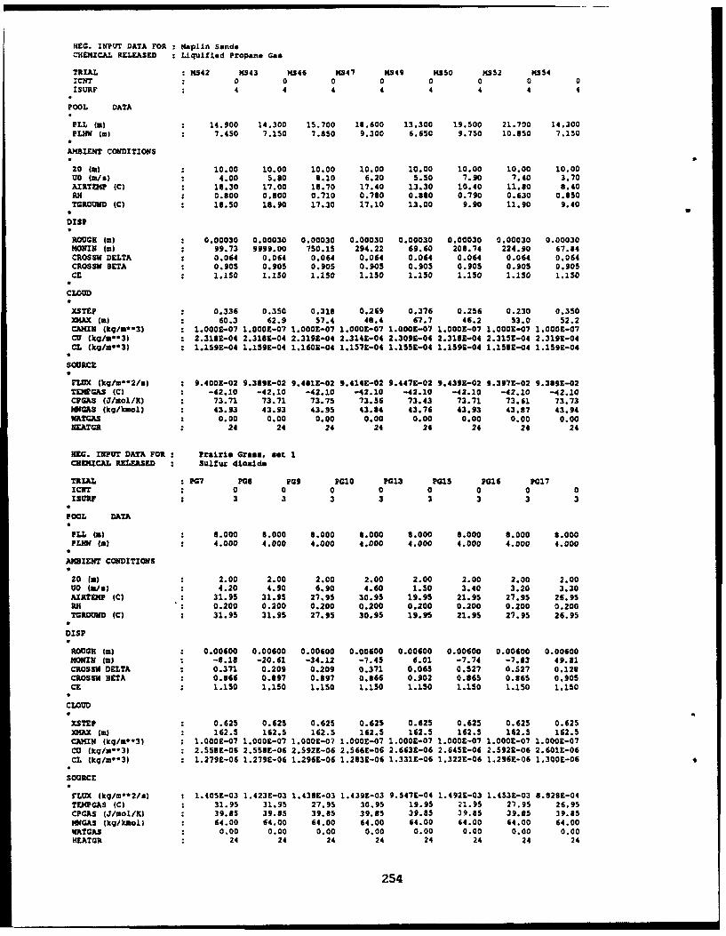
KEG. INPUT DATA FOR IMaplin SandsCHEI•CAL RELEAPSED Liqu•lied Propane Gas

TRIAL M542 KS43 M546 KS47 MS49 M350 1552 KS54ICNT * 0 0 0 0 0 0 0 0ISUtiF * 4 4 4 4 4 4 4 4

POOL DATA

PLL (im) 14.900 14.300 15.700 18.600 13.300 19.500 21.700 14.300PLH (1) 7.450 7.150 7.850 9.300 6.650 9.750 10.850 7.150

AMBIENT CONDITIONS

Z0 (M) 10.00 10.00 10.00 10.00 10.00 10.00 10.00 10.0000 (mIW) 4.00 5.80 8.10 6.20 5.50 7.90 7.40 3.70AIXRTEP (C) 18.30 17.00 18.70 17.40 13.30 10.40 11.80 8.40R• 0.800 0.300 0.710 0.780 0.380 0.790 0.630 0.850TGROUND (C) 13.50 18.90 17.30 17.10 13.00 9.90 11.90 9.40

;sP

ROUGH (m) 0.00030 0.00030 0.00030 0.00030 0.00030 0.00030 0.00030 0.00030ON8IN (m) 99.73 9999.00 750.15 294.22 69.60 208.74 224.90 67.54

CROSSW DELTA 0.064 0.064 0.064 0.064 0.064 0.064 0.064 0.064CROS-8 BETA 0.905 0.905 0.905 0.905 0.905 0.905 0.905 0.905Cc 1.150 1.150 1.150 1.150 1.150 1.150 1.150 1.150

CLOUD

XSTEP 0.336 0.350 0.312 0.269 0.376 0.256 0.230 0.350XNAX (m) 60.3 62.9 57.4 48.4 67.7 46.2 53.0 52.2CAWN (kg/am*3) : 1.000E-07 1.000E-07 1.000E-07 1.0008-07 1.0003-07 1.000E-07 1.000E-07 1.000L-07CU (kq/m*3) : 2.3181-04 2.3181-04 2.3198-04 2.314E-04 2.309E-04 2.3183-04 2.315t-04 2.319E-04CL (kgui**3) : 1.159E-04 1.1598-04 1.1603-04 1.1579-04 1.1559-04 1.1593-04 1.158E-04 1.159E-04

SOURCE

FLUX (kq/m**2/I) : 9.400E-02 9.389E-02 9.481E-02 9.414E-02 9.4478-02 9.439E-02 9.3971-02 9.389E-02TEMEGAS (C) -42.10 -42.10 -42.10 -42.10 -42.10 -42.10 -42.10 -42.10CPGAS (Jlmog1/) 73.71 73.71 73.75 73.56 73.43 73.71 73.61 73.73MWGM (kg/kmol) 43.93 43.93 43.95 43.84 43.76 43.93 43.87 43.94VATGAS 0.00 0.00 0.00 0.00 0.00 0.00 0.00 0.00HEATGR . 24 24 24 24 24 24 24 24

WIG. INPUT DATA FOR : Prairie Grass, set ICHEMICAL RELEASED : Sulfur dioxide

TRIAL PG7 P0s PG9 PG20 PG13 Pa1s PG16 PG17lCNT . 0 0 0 0 0 0 0 0ISmUR : 3 3 3 3 3 3 3 3

POOL DATA

P1., (m) 8.000 8.000 8.000 8.000 8.000 8.000 8.000 8.000PLHN (a,) 4.000 4.000 4.000 4.000 4.000 4.000 4.000 4.000

NMIENT CONDITIONS

20 Ia) 2.00 2.00 2.00 2.00 2.00 2.00 2.00 2.0000 (a/8) 4.20 4.90 6.90 4.60 1.50 3.40 3.20 3.30AXIRTIP (C) 31.95 31.95 27.95 30.95 19.95 21.95 27.95 26.95RH 0.200 0.200 0.200 0.200 0.200 0.200 0.200 0.200TGROUID (C) 31.95 31.95 27.95 30.95 19.95 21.95 27.95 26.95

DI,?

ROUGH (i) 0.00600 0.00600 0.00800 0.00600 0.00600 0.00600 0.00600 0.00600MONKIN (m) -6.18 -20.61 -34.12 -7.45 6.01 -7.74 -7.83 49.81CROSSM DELTA 0.371 0.209 0.209 0.371 0.065 0.527 0.527 0.128CROSSW 5 BETA 0.366 0.897 0.897 0.866 0.902 0.865 0.865 0.905CE 1.150 1.150 1.150 1.150 1.1S0 1.150 1.150 1.150

CLOUD

XSTEZ 0.625 0.625 0.625 0.625 0.625 0.625 0.625 0.625M4AX (m) 162.5 162.5 162.5 162.5 162.5 162.5 162.5 162.5

CAMIN (kq/ml*3) : 1.0001-07 1.0001-07 1.0001-07 1.0002-07 1.OOOE-07 1.000E-07 1.000E-07 1.000E-07CU (kq/ml*3) ; 2.55SE-06 2.558E-06 2.592E-06 2.566E-06 2.663E-06 2.645E-06 2.592E-06 2.6011-06CL (kq/m.*3) : 1.279E-06 1.279E-06 1.296E-06 1.283E-06 1.331E-06 1.322E-06 1.2961-06 1.300E-06

SOURCE

FLUX (kg/m**2/s) : 1.4051-03 1.423E-03 1.438E-03 1.4393-03 9.547E-04 1.492E-03 1.453E-03 8.8281-04TEJMPGAS (C) 31.95 31.95 27.95 30.95 19.95 21.95 27.95 26.95CPGAS (J/2el/K) 39.85 39.85 39.85 39.85 39.85 39.85 39.85 39.85WMOAS (kg/knol) 64.00 64.00 64.00 64.00 64.00 64.00 64.00 64.00WATGAS 0.00 0.00 0.00 0.00 0.00 0.00 0.00 0.00HEAJVGR . 24 24 24 24 24 24 24 24

254

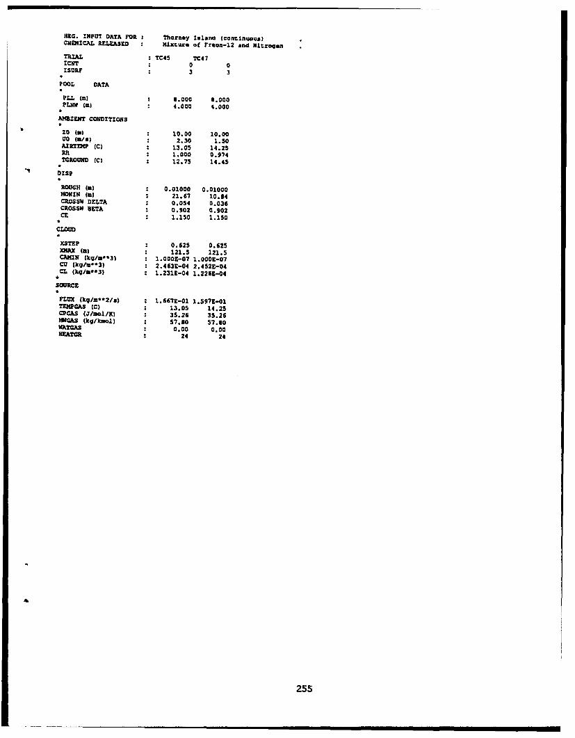
H1G. INPUT DATA FOR : Thorney Islam (contlnuous)CHIf4ICAL RELEASED : Mixture of Freon-12 and Nitrogen

TRIAL TC45 TC47ICNT . 0 0ISURF : 3 3

POOL DATA

PLL (m) 8.000 8.000PLIW (m) 4.000 4.000

A'IENT CONDITIONS

20 (a) 10.00 10.00CO (r/an) . 2.30 1.50AIRTEIP (C) 13.05 14.253-1 1.000 0.974TG0OUND (C) 12.75 14.45

DISP

ROUGH (m) 0.01000 0.01000MONIN (M) 21.67 10.84CROsSW DELTA 0.054 0.036CROSSW BETA 0.902 0.902CE 1.150 1.150

CLOUD

XSTEP 0.625 0.625X(AX (a) 121.5 121.5CAKIN (kq/m"*3) : 1.000E-07 1.000E-07CU (kq/m**3) : 2.463E-04 2.452E-04CL (kg/a'*3) : 1.231E-04 1.2263-04

*

SOURCE

FLUX (kq/m*'2/s) : 1.667E-01 1.5973-01TEMPGAS (C) 13.05 14.25CPGAS (J/mol/K) 35.26 35.26M/GAS (kg/kmol) 57.80 57.80VATCAS 0.00 0.00HEATGR . 24 24

255

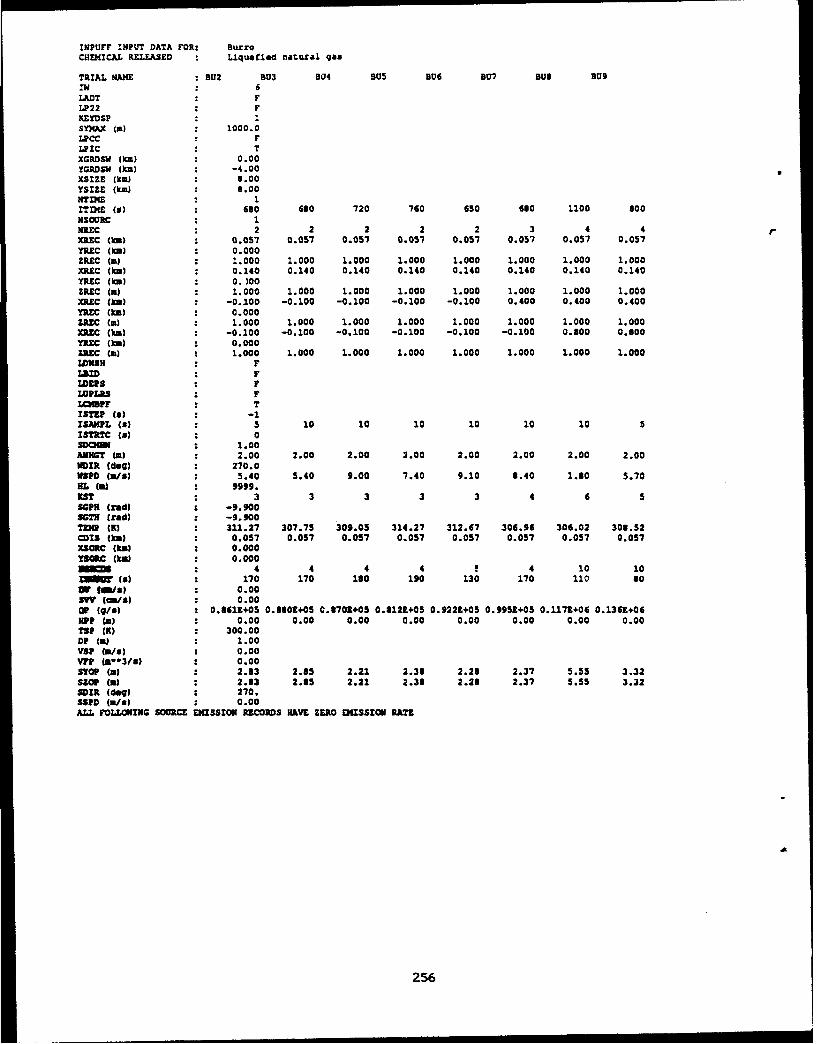
INPUFF INPUT DATA FOR: BurroCHEMICAL RELEASED : Liquefied natural 94S

TRIAL NAME 1132 303 904 S05 BU6 BU7 sue Bug

LADT . FLP22 * FICEYD5E' . 1

SYI4AX (m) 1000.0LPCC . FLPIC T TXGRDS• {ke) : 0.00YGRDSW (km) -4.00XSIZZE (k) : 6.00YSIZE (kin) : 0.00NTDmE : 1ITnIE (s) 660 660 720 760 650 660 1100 600N$OURC I 1NREC . 2 2 2 2 2 3 4 4 rXUEC (0) 0.057 0.057 0.051 0.051 0.051 0.057 0.057 0.057YREC (M) : 0.000ZREC (M) 1.000 1.000 1.000 1.000 1.000 1.000 1.000 1.000XREC (W) : 0.140 0.140 0.140 0.140 0.140 0.140 0.140 0.140YR-C (kin) 0. )00ZREC (m) : 1.000 1.000 1.000 1.000 1.000 1.000 1.000 1.000XREC (,,) -0.100 -0.100 -0.100 -0.100 -0.100 0.400 0.400 0.400YREC (ko) : 0.000ZRIC (at) : 1.000 1.000 1.000 1.000 1.000 1.000 1.000 1.000XREC (kin) -0.100 -0.100 -0.100 -0.100 -0.100 -0.100 0.300 0.800YREC (Ike) : 0.000ZREC (a) : 1.000 1.000 1.000 1.000 1.000 1.000 1.000 1.000LDWSH . FLSID . FLDIUS FLUPLRS r FLCISPF TISTP (a) -1ISJMPL (a) : S 10 10 10 10 10 10 5ISTRTC (a) : 0SDC3M 1.00AUNGT (m) : 2.00 2.00 2.00 2.00 2.00 2.00 2.00 2.00MOIR (deqo : 270.0WSPD (We/) : 5.40 5.40 9.00 7.40 9.10 8.40 1.60 5.70ML (a) 9999.KST : 3 3 3 3 3 4 6 5SGPM (red) -9.900SOTH (rad) -9.900meW M 311.27 307.75 309.05 314.27 312.67 306.96 306.02 306.52

CUIS (Ik) 0.057 0.057 0.057 0.057 0.057 0.057 0.057 0.057XSORC (ha) : 0.000YSO? C (kI) : 0.000

4 4 4 4 4 10 10S(8) : 170 170 10 190 130 170 110 s0or 4wa : 0.00SVV' (or/) : 0.000r (g) : 0.8611+05 0.6080+05 0.8701÷05 0.2121+05 0.9229+05 0.995Z+05 0.117Z+06 0.1361+06HPP (m) 0.00 0.00 0.00 0.00 0.00 0.00 0.00 0.00TSP (W) : 300.00DP (a) : 1.00VSP (Wae) : 0.00Vl, (2--3/s) : 0.00SYOP (a) : 2.83 2.85 2.21 2.38 2.28 2.37 5.55 3.32S30¢ (C) : 2.83 2.85 2.21 2.38 2.28 2.37 5.55 3.32SDIR (deq) : 270.SSD (Wja) : 0.00ALL FOLLOWING SOURCE EMISSION RICORDS HAVE ZERO DMISSION RATE

256

IMPUFF INPUT DATA FOR: CoyoteCHEMICAL RELEASED : Liquefied natUral gas . Methane Is at least 0S6 in c

TRIAL NAME C03 Cos C06IN $;#LAD? " FLP22 . FKEYDSP . 1SYMAX (m) : 1000.0LPCC . FLPIC : TXGRDSW (km) 0.00YGRDSW (km) 2 -4.00XSIZE (5m) 8.00YSIZE (km) 8.00NTInE I 1ITIME (a) : 700 700 720NSOURC I 1NmuC . 3 4 4XREC (km) 0.140 0.140 0.140YREC (km: 0.000ZREC (m) 1.000 1.000 1.000XREC (km) : 0.200 0.200 0.200YTC (km) : 0.000ZREC (m) 2 1.000 1.000 1.000XRLC (km) 0.300 0.300 0.300YREC (km ) 0.000ZREC W3) 2 1.000 1.000 1.000XREC (km) -0.100 0.400 0.400mREC (km) : 0.000ZRzC (m) 2 1.000 1.000 1.000

DWSH : FLaID . FLvEPS * FLOPLRS : FLCNBPF * TISTEP (a) : -1ISAMPL s() 5 5 10 10ISTRTC (.) . 0SDON 2 1.00ANmGT (m) 2.00 2.00 2.00WDIR (deg) 270.0WSPD (m/s) : 6.00 9.70 4.60HI (a) 9999.KST * 3 3 4SGPH (tad) 2 -9.9008M (rtd) : -9.900Tug i 311.45 301.4) 297.26CDIS (kia) 2 0.140 0.140 0.140XSORC (km) 0.000YSO4C 00) 0.000

10 7 9s m : 70 100 soOY gia) 2 0.00Sw (c/s) : 0.00OP (g/s) : 0.101E+06 0.129E+06 0.123E+06hPP (a) 0.00 0.00 0.00TSP (K) W 300.00DP W.) 1.00VsP (&/s) 2 0.00VFP 52*3/s) : 0.00STOP (a) : 2.75 2.36 3.42SZOP m2) 2.75 2.36 3.42SDIR (dog) 270.SSPL (m/s) 0.00ALL FOLLOWING SOURCE EMISSION RECORDS HAVE ZERO EMISSION RATE

257

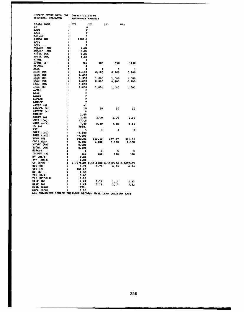
INPUFF INPUT DATA FOR: Desert TortoiseCHEMICAL RELEASED : Anhydrorus Awsonia

TRIAL NAME : DTI DT2 DT3 DT4ItN . 6LADT . FLP22 . FKEYDSP 1SYMAX (a) : 1000.0LPCC . FLPIC . TXGRDSW (ka) : 0.00YGROSw (km) : -4.00XSIZE (1um) : 8.00YSIZE (km) 8.00NTIME k 1ITnME (u) * 790 780 950 1140NS5U(C : 1NIRC I 2 2 2 2XNREC 2km) 0.100 0.100 0.100 0.100YcEc (Wk) 0.000ZREC (m) 1.000 1.000 1.000 1.00REC (1m) : 0.800 0.000 0.000 0.000McEC 0k0) 0.000

ZREC (m) 1.000 1.000LDWSH FLaID : FLDEPS . FLUPLRS FLCOMPF TISTEP (a) : -1ISAMPL (s) : 10 10 10 10ISTRTC (u) : 0SDCmBI 1.00ANHGT (M) 2.00 2.00 2.00 2.00WOIR (deg) : 270.0WSPD (m/s) 7.40 5.80 7.40 4.50HL 1.) M 9999.KST . 4 4 4 6SGPH (rud) -9.900SGTH (red) : -9.900TEMP (K) : 302.03 303.63 307.07 305.63(MIS MkS) 0.100 0.100 0.100 0.100XSORC (km) 0.000YSORC (km) 0.000NSRCDS . 6 3 5 3ISUPDT is) : 130 260 170 380DV (m/al : 0.00SVV (um/4) 0.00QP (gus) 0.797Z+05 0.111E÷06 0.131E+06 0.967E+05KPP (W) : 0.79 0.79 0.79 0.79TSP (K) : 300.00DP (M) . 1.00VSP sm/u) 0.00VFP (m**3/u) 0.00SYOP (inW 1.64 2.19 2.10 2.32SZOP (m) : 1.64 2.19 2.10 2.32SDIR (deg) : 270.SSPD Cu/u) : 0.00ALL FOLLOVING SOURCE EMISSION RECORDS HAVE ZERO EMISSION RATE

258

:NPUFF INPUT DATA FOR: GoldfishCHEMICAL RELEASED Hydrogen fluoride

TRIAL AMKE GF1 GF2 GF31W . 6

LAOT * FLP22 : FKEYDSP . 1SYMAX (m) 1000.0LPCC * FLPIC : TXGRDSW (km) 0.00YGPDSW (kh) : -4.00XSUZE (kh) : 8.00YSIZE (ka) : 8.00NTDIM . 1ITIME (s) : 1170 1080 1440HSOURC : 1HREC . 3 2 3XREC (ka) : 0.300 0.300 0.300YREC (ha) 0.000ZREC (a) : 1.000 1.000 1.000XRZC (Wa) 1.000 1.000 1.000YREC (ka) : 0.000ZREC (m) : 1.000 1.000 1.000XREC (km) 3.000 -0.100 3.000

C (h)k : o0.000ZREC (m) 1.000 1.000 1.000LONSH FLBID : FLDEPS : FLUPLRS FLCHAUF T 7ISTZP (C : -1ISAMPL (a) : 10 10 10ISTRTC (s) : 0SDOABN : 1.00ANH;T 1m) : 2.00 2.00 2.00MUIR (dog) : 270.01SPD (m2/) : 5.60 4.20 5.40HL (m) . 9999.KST : 4 4 4SGPH (tad) : -9.9005071 (Irad) -9.900TEMP (K) 310.40 309.38 307.61CIS (km) : 0.300 0.300 0.300XSOUC (wa) : 0.000YSORC (ha) : 0.000NSRcDS . 9 3 4

0SUPDT CE : 130 360 360DV (cm/s) : 0.00SVV ( /s) 0.00OP (g/s) 0.277E+05 0.105E+05 0.103E+05HPP (m) 1.00 1.00 1.00TSP (K) : 300.00Up (a) . 1.00VSP Ca/&) 0.00VFp (m**3/s) 0.00SYOP (m) 1.22 0.87 0.76SZOP (a) 1.22 0.87 0.76SOIR (deg) 270.SSPD (m/s) : 0.00ALL FOLLOWING SOURCE EZISSION RECORDS HAVE ZERO EMISSION RATE

259

INPUFF INPUT DATA FOR: Hanford (continuous)CHEHICAL RELEASFED K:rypton-85

TRIAL NAME HC1 HC2 14C3 HC4 H¢5IW : 6LAOT : FLP22 . FKEYOSP I 1S"MAX (al ) 1000.0LPCC . FLPIC TXGRVDSW (l) 0.00YGEDSW (lk) * -4.00XSIZE (km) 8.00YSZZE (kin) 8.00NTumE . 1ITI]E () : 1860 2730 2530 1200 3570NSOURC I 1NR: 0 2 2 2 2 2XEC (ka) : 0.200 0.200 0.200 0.200 0.200YRZC C•i 0.000ZRLC Wm) 1.500 1.500 1.500 1.500 1.500XRE0 (ka) 0.800 0.800 0.300 0.800 0.800YRZC (k): 0.000ZREC (a) 1.500 1.500 1.500 1.500 1.500L, WSH :1Lab : FWEPS :LUPLRS : FL42MPF T TISTEP (8) -1ISAkPJL (a) 10 10 10 10 10ISTRTC (s) 0SDOCIl( 1.00ANNOT (): 1.50 1.50 1.50 1.50 1.50

VDIR (doq) : 270.0ffSPD (a/u) 1.30 3.90 7.10 3.90 2.60HL (m) 999gg.KST . 7 3 3 3 6SGPX (rad) : -9.900SGTH (rad) : -9.900TEPQ (X) : 290.87 285.43 288.93 286.65 270.82CODIS (I=) : 0.200 0.200 0.200 0.200 0.200XSORC (km) 0.000YSORC (M) 0.000NSRCDS . 2 3 3 2 3IS10T (a) 930 910 $60 600 1190DV (•m/C ) 0.00sVV (cr/8) 0.00OP (9/0) 11.7 12.0 27.6 31.8 17.1HIP (m) : 1.00 1.00 1.00 1.00 1.00TSP (R) : 300.00DP (m) : 1.00VSP (2/a) 0.00VFP (n**3/s) 0.00SYOP (m) : 0.05 0.03 0.03 0.05 0.04SZOp (m) * 0.05 0.03 0.03 0.05 0.04SOIR (dog) 270.ss5O (a/$) 0.00ALL FOLLOWING SOURCE EMISSION RECORDS RAVE ZERO EMISSION RATE

260

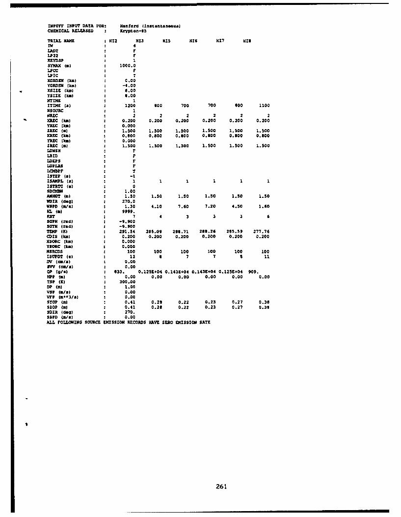
INPUFT INPUT DATA FOR: Hanford (Instantaneous)CHEMICAL iRLEASED Kzypton-65

TRIAL NAME H12 H13 115 HI6 H17 HIS1Wl . 6LAD? . F

LP22 F FKETDSP . 1SYMAX (m) 1000.012CC F FLPIC T IXGRDSW (kw) 0.00YGRDSW (km) : -4.00XSIZE (kn) : 8.00YSIZE (km) 8.00NTME . 1ITIDE (a) : 1200 800 700 700 600 1100NSOURC I 1N.EC * 2 2 2 2 2 2XRZC (ka) 0.200 0.200 0.200 0.200 0.200 0.200YREC 1km) : 0.000ZREC (a) 1.500 1.500 1.500 1.500 1.500 1.500XRZC (Mm) : 0.600 0.800 0.800 0.800 0.800 0.600YRhC (ka) 0.000ZREC (m) 1.500 1.500 1.500 1.500 1.500 1.500LOWSH . FLEID . VLDEPS * FLV.P.3. : FL,•BIP F :T

ISTEP (s) : -1ISNWL (S) 1 1 1 1 1 1ISTRTC (a) 0SOOCNBN 1.00ANMMT (W) . 1.50 1.50 1.50 1.50 1.50 1.5010DIR (deq) 270.0WSIPD (m/6) 1.30 4.10 7.60 7.20 4.50 1.60H(L W) 9999.KST . 7 4 3 3 3 6SGPH (rad) : -9.900SGTH (rad) -9.900TEMP (K) 291.54 285.09 268.71 286.26 285.59 277.76CDIS (km) 0.200 0.200 0.200 0.200 0.200 0.200XSORC (kin) 0.000TSORC M(Ia) 0.000NSRCDS : 100 100 100 100 100 100

S0PDT (a) : 12 a 7 7 6 1lDV (cu•/) . 0.00SVV (cm/8) 0.00OP (g/3) 633. 0.1259+04 0.143E+04 0.1431404 0.125E+04 909.1P1 (a) . 0.00 0.00 0.00 0.00 0.00 0.00TSP (K) 300.00DP (m) : 1.00VSP (mal) . 0.00VrP (W93/0) : 0.00STOP (a) . 0.41 0.26 0.22 0.23 0.27 0.33SO2P (m) . 0.41 0.26 0.22 0.23 0.27 0.38SOIR (dWg) 270.S8D0 (d/e) 70.0

ALL FOLLOWING SOURCE EMISSION RECORDS HAVE ZERO EMISSION RATE

261

INPUrF INPUT DATA FOR: Haplin SansnCHM41CJL, REL•ASED Liquified Na4tural Gas

TRIAL NAME MS27 MS29 MS34 MS35i"W . 6LAD? FL1P22 . FKEYDSP I 1SIhAX (i) 1000.0LFCC . FLPIC * TXGRDSW (ku) 0.00YGRDIXW (ka) -4.00XSIZE (tkn) 3.00YTZil (ka) l .00

ITIE (a) : 0o 690 700 700NSOURC I 1mIUC :5 7 2 3XREC (ka) : 0.089 0.053 0.087 0.129YREC (WIn) : 0.000ZREC (a) : 0.900 0.900 0.900 0.900XREC (kl) 0.131 0.090 0.179 0.250YREC (Wi) 0.000ZAEC Wu) : 0.900 0.900 0.900 0.900XREC (km) : 0.324 0.130 -0.100 0.406TREC (km) 0.000ZREC (m) : 0.900 0.900 0.900 0.900)RaC (ki) : 0.400 0.182 -0.100 -0.100YREC (ka) 0.000ZREC (m) . 0.900 0.900 0.900 0.900XREC (ku) 0.650 0.252 -0.100 -0.100YSC (kR) : 0.000ZIEC (m) 0.900 0.900 0.900 0.900XREC (MIM : -0.100 0.324 -0.100 -0.100YREC (k) 0.000ZREC (m) : 0.900 0.900 0.900 0.900XREC (km) : -0.100 0.403 -0.100 -0.100YlEC (w) 0.000ZREC (W) : 0.900 0.900 0.900 0.900

LBID * FLVEPS : FWPLISP F

ZSSEP (a) : -1ZSAMiL (a) 1 1 2 1ISTRTC (a) 0sDOIM . 1.00ANUCT (m) : 10.00 10.00 10.00 10.00UDIR (dog) : 270.0WSPD (u/a) : 5.60 7.40 8.50 9.60HL (a) : 9999.

ST . 4 4 4 4SGPH (Cad) : -9.900S3TH (rad) : -9.900TEMP (K) : 238.10 289.30 263.40 289.30COIS (ka) : 0.089 0.058 0.007 0.129XSORC (ka) : 0.000YSORC (ka) : 0.000

SRPCDS : 5 3 7 5ISUPOT (a) : 160 230 100 140OV (cm/s) : 0.00SVV (ca/a) : 0.00QP (9/s) : 0.232X+05 0.2929+05 0.215E.05 0.271ZE05H1Pp u) : 0.00 0.00 0.00 0.00TSP (K) 300.00OF (a) : 1.00YaP (a/*) : 0.00V~rP (a**3/ml 0.00STOP 00) : 1.35 1.35 1.07 1.14SZOP (W) : 1.35 1.35 1.07 1.14SD0R (dog) : 270.SSd (m/a) : 0.00ALL FOLLOWING SOURCE EMISSION RECORDS HAVE ZERO EMISSZON RATE

262

:NPUFF INPUT DATA FOR: Kaplin SandsCHEMICAL REL, SED Liqulfled Propane Gas

a•JU. NAME •S42 NS43 M546 1S47 1449 M550 M$52 M$54lIv : 6

LAT : FLP22 FKEYDSP I 1SYMAX (m) : 1000.0LPCC • FLPIC . TXGRDSW (wcm) : 0.00YGADSW (l) : -4.00XSIZZE (kM) : 8.00YSIZE (km) : 8.00NTXZC . 1

ITIM2. (7) 120 990 720 640 120 S00 700 120NSOD.C I 1NREC . 7 4 7 6 6 4 6 4)M= (Ncm) : 0.026 0.088 0.034 0.090 0.090 0.059 0.061 0.056YREC (km) 0.000ZREC (m) . 0.900 0.900 0.900 0.900 0.900 0.900 0.900 0.500XR£C Ckm) 0.053 0.129 0.091 0.126 0.129 0.093 0.095 0.065YREC O1m) 0.000ZREC (m) . 0.900 0.900 0.900 0.900 0.900 0.900 0.900 0.500XRfC (km) : 0.083 0.249 0.130 0.182 0.160 0.162 0.178 0.176YRXC (kun) : 0.000ZItEC () : 0.900 0.900 0.900 0.900 0.900 0.900 0.900 0.500XP.ZC (kU) : 0.123 0.400 0.182 0.250 0.250 0.400 0.249 0.247RtC (k1M) : 0.000

ZAEC (ml : 0.900 0.900 0.900 0.900 0.900 0.900 0.900 0.500XMtC (ka) : 0.179 -0.100 0.250 0.321 0.322 -0.100 0.396 -0.100YPJc (ks) : 0.000ZREC (m) . 0.900 0.900 0.900 0.900 0.900 0.900 0.900 0.500XRIC (ka) : 0.247 -0.100 0.322 0.400 0.400 -0.100 0.650 -0.1007UC (kin) : 0.000ZREC (a) . 0.900 0.900 0.900 0.900 0.900 0.900 0.900 0.500XRiC (kw) : 0.398 -0.100 0.401 -0.100 -0.100 -0.100 -0.100 -0.1007RE(n) : 0.000ZSEC (a) : 0.900 0.900 0.900 0.900 0.900 0.900 0.900 0.500LOWSIH : FLSID . FL;)PS : FL=PLRS : 1LCMBPF T TIST1 Cs) a-1ISA4PL (C) : 1 1 1 1 1 1 1 1ISTRC (C) : 0SD001W 1.00AMUC (to) 10.00 10.00 10.00 10.00 10.00 10.00 10.00 10.00OIRi (dog) 270.0Van W/1) 4.00 5.80 6.10 6.20 5.50 7.90 7.40 3.70E IN S 9999.u? * 4 4 4 4 4 4 4 451 (rad) -9.900SGTH (rsd) : -9.900

4 ({K) 291.50 290.20 291.90 290.60 286.50 263.60 265.00 261.60CDIS (P) . 0.02S 0.088 0.034 0.090 0.090 0.059 0.061 0.056XSORC (kin) * 0.000YSORC (a) . 0.000NSRCDS : 4 3 2 4 8 5 5 4IS5P0T (s) 160 330 360 210 90 160 140 130OV (asi/ ) : 0.00SVV (cm/s) 0.00OP (i/8) : 0.209E+05 0.1929+05 0.2349+05 0.3269+05 0.1679+05 0.359E+05 0.4422*05 0.192Z+05u19p (a) . 0.00 0.00 0.00 0.00 0.00 0.00 0.00 0.00TSP (K) : 300.00VP (I) : 1.00

VSP (3/u) : 0.00

SYOP (a) : 0.95 0.76 0.71 0.95 0.72 0.67 1.01 0.93SZOP (a) . 0.95 0.76 0.71 0.95 0.72 0.87 1.01 0.93SDIl (deq) 270.SS9 (m/s) : 0.00ALL FOLLOWING SOURCE EMISSION RECORDS HAVE ZERO EMISSION RATE

263

INPUFF INPUT DATA FOR: Prairle Grase, act ICHEMICAL RELEASED Sulfur dioxlde

TRIAL NAME PG7 P0s PG9 PG10 PC13 PGIS PG.6 PG171"W : 6

LADT : FLP22 : FKEYDS? I 1SYMAX (m) 1000.0LPCC * FLPIC T TXGRDSW (kai) 0.00YCGRSW (ka) -4.00XSIZE (kn 3 8.00YSZZE (kin) 8.00mTn4E IITIME (a) 1200 1200 1200 1200 1800 1200 1200 1200NSOORG . 1N1RC 5 5 S 5 5 2 5 5 5X)mC (kw) 0.050 0.050 0.050 0.050 0.400 0.050 0.050 0.050mC (Ma) 0.000ZREC (m) 1.500 1.500 1.500 1.500 1.500 1.500 1.500 1.500XREC ()w 0.100 0.100 0.100 0.100 0.800 0.100 0.100 0.100YREC (ka) 0.000ZREC (a) 1.500 1.500 1.500 1.500 1.500 1.500 1.500 1.500XREC (km) 0.200 0.200 0.200 0.200 -0.100 0.200 0.200 0.200YTaC (0i.) : 0.000ZREC (a) 1.500 1.500 1.500 1.500 1.500 1.500 1.500 1.500)UERC (km) 0.400 0.400 0.400 0.400 -0.100 0.400 0.400 0.400"tEaC (kin) 0.000ZA•C (n) 1.500 1.500 1.500 1.500 1.500 1.500 1.500 1.500xERC (km) 0.800 0.800 0.800 0.000 -0.100 0.800 0.800 0.800YiEC (hm) 0.000ZPEC (in) 1.500 1.500 1.500 1.500 1.500 1.500 1.500 1.500LDWSH F FL£ID * FLDEPS .

LUPIRS : FLCOEPF TISTEP (a) * -1ISAWPL (a) . 10 10 10 10 10 10 10 10ISTATR (a) : 0SDCIMB 1.00ANHOT (a) 2.00 2.00 2.00 2.00 2.00 2.00 2.00 2.00TDIR (dog) 270.0WSPo (Wa/) 4.20 4.90 6.90 4.60 1.30 3.40 3.20 3.30HI, (a) 9999.KST : 2 3 3 2 7 1 1 5SGPK (rad) -9.900SGTH frad) -9.900TEMP (K) 305.15 305.15 301.15 304.15 293.15 295.15 301.15 300.15CIS (ME) 0.050 0.050 0.050 0.050 0.400 0.050 0.050 0.050xSORC Mal) 0.000YSORC (ka) 0.000NS1CDS . 2 2 2 2 3 2 2 2ISPDDT (a) 600 600 600 600 600 600 600 600Dv (,,/a) 0.00SVV (cm/s) 0.00OP (q/8) 39.9 91.1 92.0 92.1 61.1 95.5 93.0 56.5HPP (a) 0.45 0.45 0.45 0.45 0.45 0.45 0.45 0.45TSP (1) 300.00Up (a) 1.00VSP (m/a) 0.00VFP (&*-3/*) 0.00STOP (mW 0.05 0.05 0.04 0.05 0.07 0.06 0.06 0.05Stop (W) 0.05 0.05 0.04 0.05 0.07 0.06 0.06 0.05SOIR (dog) 270.SSPD (a/a) 0.00ALL FOLLOWING SOURCE EMISSION RECORDS HAVE ZERO DEISSION RATE

264

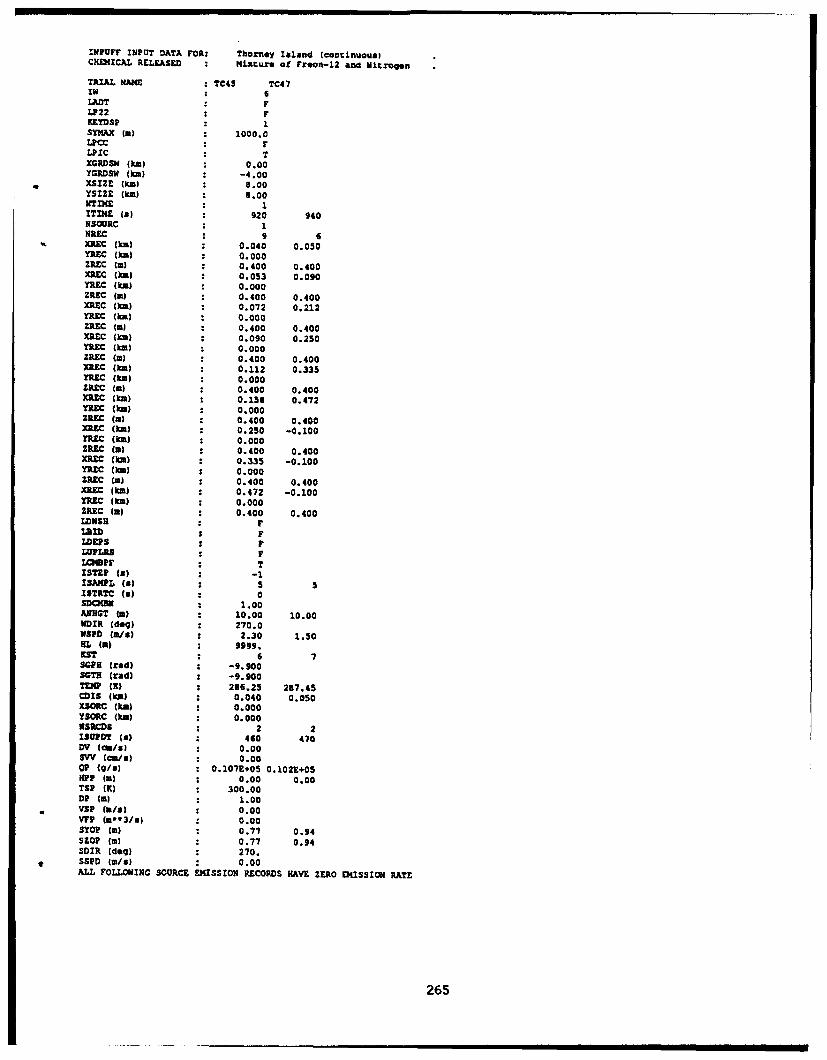
INPUFF INPUT DATA FOR: Thorney Island (contniUou-)CHEMICAL RELEASED : HJlXtur of Fraon-12 and Jitzogen

TRIAL NANE TC45 TC471N : 6LA : FLP22 * FKE!DSP : 1SYXAX Wm) : 1000.0LPCC • FLPIC T 7XGRDSW (kg) : 0.00YGRDSW (kin) -4.00

do XSIZE (kim) 8.00YSIZE (kin) 0.00

1T7ME (a) 920 940NSOUIRC 1NtEC : 9 6X3=EC (km) 0.040 0.050YREC (kg) : 0.000ZRiC (m) 0.400 0.400XREC (kg) : 0.053 0.090YREC (kin) : 0.000ZREC (m) 0.400 0.400XREC (kg) 0.072 0.212

REC (k) : 0.000ZREC (m) : 0.400 0.400XREC (kg) : 0.090 0.250YRZC (kg) 0.000ZREC (m) : 0.400 0.400XUSC (kg) 0.112 0.335YREC (km) 0.000ZRrC (m) : 0.400 0.400USC (kg) 0.158 0.472YTEC (kg) : 0.000ZIEC (a) : 0.400 0.400XUSC (kg) : 0.250 -0.100

(RuC (k) 0.000ZRZC (W) : 0.400 0.400USC (kg) : 0.335 -0.100YRZc (kg) : 0.0002REC (m) : 0.400 0.400usREC (kg) 0.472 -0.100TREC (jki) : 0.000ZREC (a) : 0.400 0.400LDWSH rLID W~l*FlamI • FLDORS : rLOPIRIq . FLCMBPF T 7ISTEP (a) : -1ISANPL (a) S 5ISTRTC (a) a 0SDQf3 1.00ARHGT (a) : 10.00 10.00MDIR (dog) 270.0WSPD (2/8) : 2.30 1.50HlL (a) : 9999.K-T * 6 7SGPH (rad) : -9.900SGTH (lad) : -9.900TEMP (K) : 286.25 287.45CDIS (kg) 0.040 0.050XSOR.C (kg) 0.000YSORC (km) : 0.000NS1CDS 2 2ISUPDT (a) : 460 470DV (cr/u) : 0.00SVV (c/2) : 0.00QP (910) : 0.107E+05 0.102E+05HiP (m) : 0.00 0.00TSP (K) 300.00DP (W) : 1.00VSP (a/a) 0.00VFP ('w3/1) : 0.00STOP (W) 0.77 0.94SZOP (W) 0.77 0.94SDIR (dog) 270.SSND (m/$) : 0.00ALL FOLLOWING SOURCE EMISSION RECORDS HAVE ZERO D4iiSSIw RATE

265

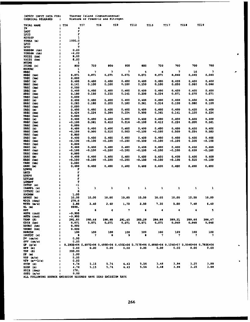
:NPUFF INPUT DATA FOR: Thorney Island (instantaneous)CHE(MICAL RELEASED MtJ•ture of Freon-12 and Nitrogen

TRIAL NAME TI6 T17 TIS T19 T112 T113 TI1T Till TI111w : 6LADT * FLP22 FKEYDSP : 1S•MAX (m) : 1000.0LPCC . F

LPIC . TXGRDSW (km) 0.00YGRDSW (kin) -4.00XSIZE (k..) : 8.00YSIU2 (km) 8.00ETIME • 1

ITDME (a) 800 700 goo 900 800 700 700 700 700KSOURC . 1EREC . 5 7 7 7 5 6 7 10 7MIC ()km) 2 0.071 0.071 0.071 0.071 0.071 0.071 0.040 0.040 0.040YRIC (ka) : 0.000ZREC (a) 0.400 0.400 0.400 0.400 0.400 0.400 0.400 0.400 0.400XREC (km) 0.141 0.100 0.100 0.100 0.150 0.100 0.050 0.060 0.060YREC (kal) 0.000ZRIC (m) : 0.400 0.400 0.400 0.400 0.400 0.400 0.400 0.400 0.400XPEC (km) : 0.180 0.150 0.150 0.141 0.200 0.224 0.071 0.070 0.071YREC (km) : 0.000ZRIC (m) 0.400 0.400 0.400 0.400 0.400 0.400 0.400 0.400 0.400

(XC() : 0.283 0.180 0.200 0.180 0.361 0.316 0.100 0.080 0.100YREC (km) : 0.0002REC (a) 0.400 0.400 0.400 0.400 0.400 0.400 0.400 0.400 0.400XRIC (km) 0.424 0.224 0.364 0.224 0.500 0.361 0.141 0.100 0.224YRI (kin) : 0.000ZEIC (m) 0.400 0.400 0.400 0.400 0.400 0.400 0.400 0.400 0.400XRUC (ka) : -0.100 0.361 0.412 0.316 -0.100 0.412 0.224 0.200 0.361YREC (ka) : 0.000ZERC (m) : 0.400 0.400 0.400 0.400 0.400 0.400 0.400 0.400 0.400X)aC (ko) -0.100 0.500 0.510 0.503 -0.100 -0.100 0.500 0.224 0.583YR•C (XE) 0.000ZREC (m) 0.400 0.400 0.400 0.400 0.400 0.400 0.400 0.400 0.400)R0C (ka) : -0.100 -0.100 -0.100 -0.100 -0.100 -0.100 -0.100 0.300 -0.100YREC (kin) : 0.000ZREC (m) : 0.400 0.400 0.400 0.400 0.400 0.400 0.400 0.400 0.400XREC ()=) : -0.100 -0.100 -0.100 -0.100 -0.100 -0.100 -0.100 0.400 -0.100

REC (kin) : 0.000ZREC (m) : 0.400 0.400 0.400 0.400 0.400 0.400 0.400 0.400 0.400XRIC (wE) -0.100 -0.100 -0.100 -0.100 -0.100 -0.100 -0.100 0.510 -0.100YRIG (km) 0.000ZREC (a) 0.400 0.400 0.400 0.400 0.400 0.400 0.400 0.400 0.400LOWSH : FL3ZD : F

LEPS r FWPL5 : FLCMBP TISTZ? (a) : -1ISAKPL Is) . 1 1 1 1 1 1 1 1 1ISTRTC (a) : 0SDOOSM 1.00AMNT (a) : 10.00 10.00 10.00 10.00 10.00 10.00 10.00 10.00 10.00WDIR (deg) : 270.0WSPD (m/s) : 2.80 3.40 2.40 1.70 2.50 7.30 5.00 7.40 6.40HL (a) 2 9999.KST * 4 6 4 7 6 4 4 4 5SGPM (red) : -9.900SMTh (rad) -9.900T M(K) 291.83 290.46 290.68 291.45 283.29 286.88 289.21 219.66 286.47CDIS (kX) : 0.071 0.071 0.071 0.071 0.071 0.071 0.040 0.040 0.040XSORC (kia) : 0.000YSORC ()ci) : 0.000NSRcDB : 100 100 100 100 100 100 100 100 100ISTPDT (a) : 8 7 8 9 3 7 7 7 7DV (ma/u) : 0.00SVV (cm/) 1 0.00OP (i/8) 0.393E+06 0.607E+06 0.495E+06 0.430E+06 0.717E+06 0.6861+06 0.124E+07 0.554E+06 0.7821+06iPP (m) : 0.00 0.00 0.00 0.00 0.00 0.00 0.00 0.00 0.00

TSP (K) 300.00oP (a) 1.00vs? (a/a) 0.00VFP (m*03/s) 0.00STOP (1) 4.74 5.15 5.74 6.43 5.56 3.48 3.94 3.25 3.88SZOP (m) 4.74 5.15 5.74 6.43 5.56 3.48 3.94 3.25 3.38SOIR (dog) 270.SS£D (m/s) 0.00ALL FOLLOWING SOURCE EMISSION RECORDS HAVE ZERO EMISSION RATE

266

OS/DG INPUT DATA FOR BurroCHEMICAL RELEASED L14qufiod natural qgaHEASURED TEMPERATURE (K) 311.27 307.75 309.05 314.27 312.67 306.96 306.02 308.52MEASUREMENT HEIGHT (a) 1.0 1.0 1.0 1.0 1.0 1.0 1.0 1.0MEASURED TEMPERATURE (K) 310.22 306.03 307.97 313.28 311.64 306.53 306.28 30S.42MEASUREMENT HEIGHT (a) 10.0 10.0 10.0 10.0 10.0 10.0 10.0 10.016-2m TEMP DIFFERENCE (F) -1.48 -2.28 -1.62 -1.47 -1.56 .0.76 0.55 -0.27EMISSIoN RATE (KG/S) 86.1000 87.9800 66.9600 81.2500 92.2200 99.4600 116.9300 135.9800

OR/DG INPUT DATA roR CoyoteCHEMzCAL RELEASED Liquefied natural qas . methane Is at least 86r in cMEASURED TEMPERATURE (K) 311.45 301.49 297.26MEASUREMENT HEIGHT (M) 1.0 1.0 1.0MEASURED TEMPERATURE (K) 310.38 300.29 297.46MEASUREMENT HEIGHT (a) 4.0 4.0 4.016-22 TEMP DIFFERENCE (F) -2.13 -2.55 0.58EMISSION RATE (KG/S) 100.6700 129.0200 123.0300

0O/DG INPUT DATA FOR Desert TortoiseCHEMICAL RELEASED Anhydrous Ammonia

MEASURED TEMPERATURE (K) 302.03 303.63 307.07 305.63MEASUREMENT HEIGHT (m) 0.8 0.8 0.8 0.8MEASURED TEMPERATURE (K) 303.31 304.31 307.05 306.90MEASUREMENIT HEIGHT (a) 16.2 16.2 16.2 16.216-2z TEMP DIFFERENCE (F) 1.67 0.87 -0.08 1.75EMISSION RATE (KG/S) 79.7000 111.5000 130.7000 96.7000

O/DG INPUT DATA FOR GoldfishCHEMICAL REEASED Hydrogen fluoride

MEASURED TEMPERATURE (K) 310.40 309.38 307.61MEASMURENT HEIGHT (m) 2.0 2.0 2.0MEASURED TEMPERATURE (K) 310.93 309.41 303.96MEASUREMENT HEIGHT (m) 16.6 16.6 16.616-2z TEMP DIFFERENCE (F) 0.94 0.06 2.36EMISSION RATE (KG/I) 27.6700 10.4600 10.2700

OB/DG INPUT DATA FOR Hanford (oontinuous)CHEMICAL RELEASED KrY;.on-es

MEASURED TEMPERATURE (K) 290.87 285.43 289.93 286.65 278.82MEASUREMENT HEIGHT (mz 1.5 0.9 0.9 0.9 0.9MEAS URED TEMPERATURE (I) 292.19 284.71 287.54 284.65 279.32MEASUREMENT HEIGHT (m) 6.1 15.0 15.0 15.0 15.016-2m TEMP DIFFERENCE (F) 6.10 -0.97 -1.83 -2.30 0.68EMISSION RATE (KGIS) 0.0117 0.0120 0.0278 0.0388 0.0171

2

267

O9/DG INPUT DATA FOR : Haplin SandsCHEMICAL RELEASED ; Liqulfled Natural Gam

1E0SURED TEMPERATURE (K) : 288.10 289.30 260.40 209.30MEASUREMENT HEIGHT (W) 1.9 1.9 1.9 1.9MEASURED TEMPERATURE (K) 2S7.78 269.24 29S.06 2S.681

MEASUREMENT HEIGHT (a) 0.1 10.1 10.1 10.116-2z TEMP DIFFERENCE (F) -0.74 -0.20 -0.60 -1.11EMISSION RATE (KG/S) 23.2100 29.1600 21.5100 27.0900

OB/DG ZNPUT DATA FOR Maplin SandsCHEMICAL RELEASED Liquifled Propane Gas

MEASURED TEMPERATURE (K) 291.50 290.20 291.90 290.60 266.50 203.60 295.00 291.60MEASUREMENT HEIGHT (W) 1.9 1.9 1.9 1.9 1.9 1.9 1.9 1.9MEASURED TEMPERATURE (K) 291.49 290.12 291.86 290.57 296.71 263.66 265.05 261.63MEASURDEMNT HEIGHT ia) 10.1 10.1 10.1 10.1 10.1 10.1 10.1 10.116-2. TEMP DIFFERENCE (F) -0.06 -0.25 -0.16 -0.13 0.47 0.08 0.06 0.02EMISSION RATE (KG/S) 20.8700 19.2000 23.3700 32.5700 16.7100 35.8900 44.2500 19.2000

OS/DG INPUT DATA FOR Prairle Grass, set 1CHEMICAL RELEASED Sulfur dioxide

MEASURED TEMPERATURE (K) 305.15 305.15 301.15 304.15 293.15 295.15 301.15 300.15MEASUREMENT HEIGHT (m) 2.0 2.0 2.0 2.0 2.0 2.0 2.0 2.0MEASURED TEMPERATURE (K) 303.55 303.95 299.55 302.15 295.05 294.05 300.15 300.65MEASUREMENT HEIGHT (W) 16.0 16.0 16.0 16.0 16.0 16.0 16.0 16.036-22 TEMP DIFFERENCE (F) -2.36 -2.16 -2.66 -3.60 3.42 -1.98 -1.60 0.90EMISSION RATE (KG/S) 0.0699 0.0911 0.0920 0.0921 0.0611 0.0955 0.0930 0.0565

OS/DG INPUT DATA FOR Thorney Island (continuous)CHEMICAL RELEASED Mixture of Freon-12 an Nittrogen

MEASURED TEMPERATURE (K) 286.25 267.45MEASUREMENT HEIGHT (a) 2.0 2.0MEASURED TEMPERATURE (K) -99.90 -99.90MEASUREMENT HEIGHT (W) -99.9 -99.916-2m TEMP DIFFERENCE (F) 0.54 0.45EMISSION RATE (K$IS) 10.6700 10.2200

268

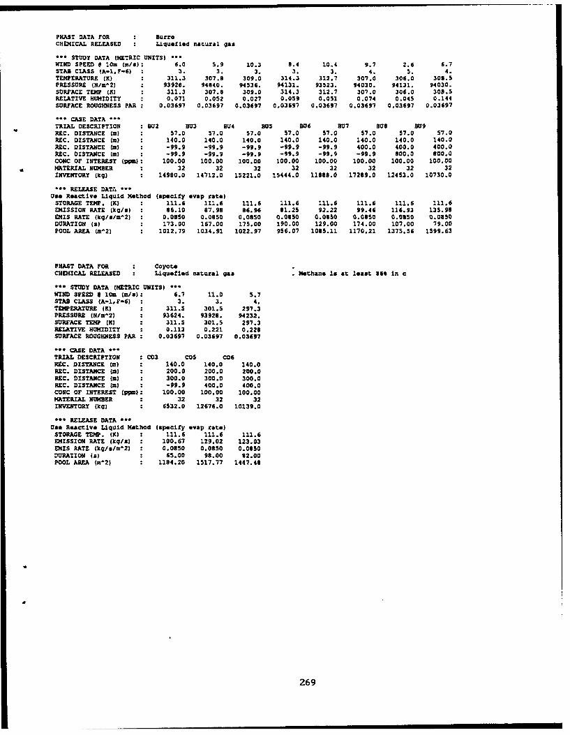
PHAST DATA FOR BurroCHEMICAL RELEASED Liquefied natural gas

*** STUDY DATA (METRIC UNITS) *-*WIND SPEED 8 lore (m/s): 6.0 5.9 10.3 8.4 10.4 9.7 2.6 6.7STAB CLASS (A-1.F-6) : 3. 3. 3. 3. 3. 4. 5. 4.TEMPERATURE (K) 311.3 307.8 309.0 314.3 312.7 307.0 306.0 308.5PRESSURE (N/m'2) : 93928. 94840. 94536. 94131. 93523. 94030. 94131. 94030.SURFACE TEMP (K) 311.3 307.8 309.0 314.3 312.7 307.0 306.0 308.5RELATIVE HUMIDITY 0.071 0.052 0.027 0.059 0.051 0.074 0.045 0.144SURFACE ROUGHNESS PAR : 0.03697 0.03697 0.03697 0,03697 0.03697 0.03697 0.03697 0.03697

-** CASE DATA ...TRIAL DESCRIPTION : BU2 BU3 BU4 BUS U06 SU7 BOS B09REC. DISTANCE Wm) 57.0 57.0 57.0 57.0 57.0 57.0 57.0 57.0REC. DISTANCE (W) 140.0 140.0 140.0 140.0 140.0 140.0 140.0 140.0REC. DISTANCE (W) -99.9 -99.9 -99.9 -99.9 -99.9 400.0 400.0 400.0REC. DISTANCE (m) -99.9 -99.9 -99.9 -99.9 -99.9 -99.9 800.0 800.0CONC OF INTEREST (ppm): 100.00 100.00 100.00 100.00 100.00 100.00 100.00 100.00MATERIAL NUMBER : 32 32 32 32 32 32 32 32INVENTORY (kg) : 14980.0 14712.0 15221.0 15444.0 11888.0 17289.0 12453.0 10730.0

-*- RELEASE DATA *--Use Reactive Liquid Method (specify evap rate)

STORAGE TEMP. (K) 111.6 111.6 111.6 111.6 111.6 111.6 111.6 111.6EMISSION RATE (ku/s) : 86.10 87.98 86.96 81.25 92.22 99.46 116.93 135.98EMIS RATE (kg/sa/^2) 0.0850 0.0850 0.0850 0.0850 0.0350 0.0850 0.0850 0.0850DURATION (a) 173.00 167.00 175.00 190.00 129.00 174.00 107.00 79.00POOL AREA (m-2) 1012.79 1034.91 1022.97 956.07 1085.11 1170.21 1375.56 1599.63

PHAST DATA FOR : CoyoteCHEMICAL RELEASED Liquefied natural gas Methane Is at least 864 in c

*** STUDY DATA (METRIC UNITS) ***WIND SPEED 8 lore (Ws/): 6.7 11.0 5.7STAB CLASS (A-1,F-6) = 3. 3. 4.TEMPERATURE (K) : 311.5 301.5 297.3PRESSURE (N/m^2) : 93624. 93928. 94232.SURFACE TEMP (K) : 311.5 301.5 297.3RELATIVE HUMIDITY : 0.113 0.221 0.228SURFACE ROUGHNESS PAR : 0.03697 0.03697 0.03697

-** CASE DATA *'TRIAL DESCRIPTION : C03 Cos CosREC. DISTANCE (W) : 140.0 140.0 140.0RZC. DISTANCE (m) : 200.0 200.0 200.0REC. DISTANCE (W) : 300.0 300.0 300.0REC. DISTANCE (m) -99.9 400.0 400.0CONC OF INTEREST (ppm): 100.00 100.00 100.00MATERIAL NUMBER : 32 32 32INVENTORY (kg) : 6532.0 12676.0 10139.0

-** RELEASE DATA **-Use Reactive Liquid Method (specify ovap rate)

STORAGE TEMP. (K) 111.6 111.6 111.6EMISSION RATE (kq/s) : 100.67 129.02 123.03EMIS RATE (kg/s/m^2) : 0.0850 0.0850 0.0850DURATION is) : 65.00 98.00 82.00POOL AREA (mW2) : 1184.20 1517.77 1447.48

269

PKAST DATA FOR Desert TortoiseCHEMICAL RELEASED Anhydrous Ammonia

--- STUDY DATA (METRIC UNITS) -**WIND SPEED a lo (m/s): 9.7 7.6 9.3 6.2STAB CLASS (A-1,F-6) 4. 4. 4. 5.TEMPERATURE (W) 302.0 303.6 307.1 305.6PRESSURE (N/m^2) 90889. 90990. 90686. 90281.SURFACE TEMP (K) : 304.8 303.8 304.8 304.0RELATIVE HUMIDITY : 0.132 0.175 0.148 0.213SURFACE ROUGHNESS PAR : 0.04931 0.04931 0.04931 0.04931

--- CASE DATA .*.TRIAL DESCRIPTION OT1 DT2 DT3 DT4RFC. DISTANCE (ia) 100.0 100.0 100.0 100.0RAC. DISTANCE (W) : 800.0 800.0 100.0 300.0CONC OF INTEREST (ppm): 100.00 100.00 100.00 100.00MATERIAL NMMBER : 5 5 5 5NVENKTORY (kg) : 10042.2 28432.5 21696.2 36842.7

"r* RELEASE DATA ***

Use Padded Liquid Vesseland Liquid Leak (nominal 3m head)

STORAGE TEMP. (W) : 294.7 293.3 295.3 297.3STORAGE PRESS. (bar-g): 10.00000 11.02000 11.23000 11.64000DIKE AREA (m^2) : 0.0 0.0 0.0 0.01-wet, 2.dry, 4-vater : 4 4 1 2HOLE DIAMETER (mm) 81. 95. 95. 95.RELEASE HT. (m) 0.79 0.79 0.79 0.79DIRECTION (Up/Hor.) :H H H H

Vary the storage pressure or the hole diameter to obtain the actual mission rate:EMISSION RATE (kg/s) : 79.70 111.50 130.70 96.70

PHAST DATA FOR GoldLfishCHEMICAL RELEASED : Hydrogen fluoride

*** STUDY DATA (METRIC UNITS) ***WIND SPEED I 10 (it/W): 7.3 5.4 7.5STAB CLASS (A-I,F-6) : 4. 4. 4.TEMPERATURE (K) : 310.4 309.4 307.6PRESSURE (N/mnt2) 90483. 90070. 90585.SURFACE TEMP (K) : 310.4 309.4 307.6RELATIVE HUMIDITY : 0.049 0.107 0.177SURFACE ROUGHNESS PAR C 0.04931 0.04932 0.04931

*CC ChaE DATA ***

TRIAL DESCRIPTION : GFi F2 GF3RAC. DISTANCE (a) : 300.0 300.0 300.0REC. DISTANCE (m : 1000.0 1000.0 1000.0REC. DISTANCE W) : 3000.0 -99.9 3000.0COUC OF INTEREST (ppm): 30.00 30.00 30.00MATERIAL NUMBER : 27 27 27INVENTORY (kq) : 3459.0 3766.0 3697.0

S** RELEASE DATA ***Use Padded Liquid Vessel

and Liquid Leac (nominal 3m head)STORAGE TEMP. (K) : 313.2 311.2 312.2STORAGE PRESS. (bar-g): 6.80000 7.35000 7.48000DIKE AREA (m^2) 0.0 0.0 0.01-wet.2-dry,4-water - 2 2 2HOLE DIAMETER (m0) : 42. 24. 24.RELEASE HT. (a) 1.00 1.00 1.00DIRECTION (Up/Nor.) : I H HN

Vary the storage premsure or the hole diameter to obtain the actual emiasion rat*:EEISSION RATE (kg/u) : 27.67 10.46 10.27

270

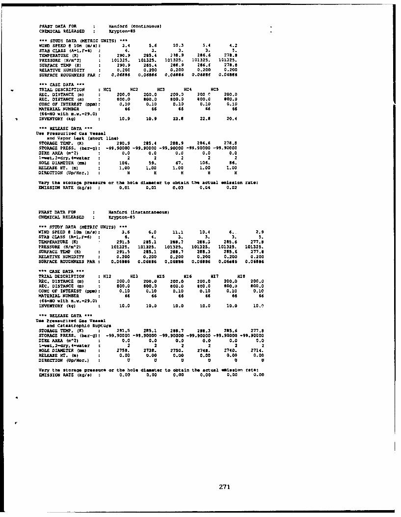
PHAST DATA FOR Hanford (continuous)CHEMICAL RELEASED Krypzon-8S

"-- STUDY DATA (METRIC UNITS) ---WIND SPEED 6 10M (M/s): 3.4 5.6 10.3 5.4 4.2STAB CLASS (A-1,F-6) 6. 3. 3. 3. 5.TEMPERATURE (K) 290.9 205.4 238.9 266.6 278.8PRESSURE (N/m^2) : 101325. 101325. 101325. 101325. 101325.SURFACE TEMP (X) 290.9 285.4 286.9 266.6 278.6RELATIVE HUMIDITY : 0.200 0.200 0.200 0.200 0.200SURFACE ROUGHNESS PAR : 0.06886 0.06886 0.06886 0.06886 0.06886

--- CASE DATA ---TRIAL DESCRIPTION : HC1 HC2 HC3 HC4 HC5REC. DISTANCE (m) : 200.0 200.0 200.0 200.C 200.0REC. DISTANCE (m) : 800.0 800.0 800.0 600.0 800.0CONC OF INTEREST (ppm): 0.10 0.10 0.20 0.10 0.10MATERIAL NUMBER : 66 66 66 66 66(66-HO with m.w.-29.0)INVENTORY (kQ) : 10.9 10.9 23.3 22.8 20.4

'** RELEASE DATA *"'Use Pressurized Gas Vessel

and Vapor Leak (short line)STORAGE TEMP. (K) 290.9 285.4 288.9 286.6 278.8STORAGE PRESS. (bar-q): -99.90000 -99.90000 -99.90000 -99.90000 -99.90000DIKE AREA (m^2) : 0.0 0.0 0.0 0.0 0.01-wet, 2-dry, 4-water : 2 2 2 2 2HOLE DIAMETER (m) : 106. 59. 67. 106. 86.RELEASE HT. (m) : 1.00 1.00 1.00 1.00 1.00DIRECTION (Up/Hor.) : H H H H H

Vary the storage pressure or the hole diameter to obtain the actual emission rate:EMISSION RATE (kg/a) : 0.01 0.01 0.03 0.04 0.02

PHAST DATA FOR : Hanftrd (instantaneous)CHEMICAL RELEASED : Krypton-05

--- STUDY DATA (METRIC UNITS) "tWIND SPEED 6 10m (m/s): 3.6 6.0 11.1 10.4 6.. 2.9STAB CLASS (A-1.F-6) : 6. 4. 3. 3. 3. 5.TEMPERATURE (K) • 291.5 285.1 286.7 288.3 285.6 277.8PRESSURE (N/m^2) 101325. 101325. 101325. 101325. 101325. 101325.SURFACE TEMP (K) : 291.5 265.1 288.7 288.3 285.6 277.8RELATIVE HUMIDITY : 0.200 0.200 0.200 0.200 0.200 0.200SURFACE ROUGHNESS PAR 0.06886 0.06886 0.06886 0.06886 0.06866 0.06886

-*- CASE DATA '*t

TRI DESCRIPTION : H12 HI3 HI5 H16 H17 HIsREC. DISTANCE (m) : 200.0 200.0 200.0 200.0 200.0 200.0REC. DISTANCE (m) : 800.0 800.0 800.0 800.0 800.0 800.0CONC OF INTEREST (ppm): 0.10 0.10 0.10 0.10 0.10 0.10MATERIAL NUMBER : 66 66 66 66 66 66(66-NO with m.w.-29.0)INVENTORY (kq) 10.0 10.0 10.0 10.0 10.0 10.0

** RELEASE DATA *i*Use Pressurized Gas Vessel

and Catastrophic RuptureSTORAGE TEMP. (K) : 291.5 285.1 288.7 288.3 285.6 277.8STORAGE PRESS. (bar-9): -99.90000 -99.90000 -99.90000 -99.90000 -99.90000 -99.90000DIKE AREA (m^2) : 0.0 0.0 0.0 0.0 0.0 0.01-vet,2-dry,4-water : 2 2 2 2 2 2HOLE DIAMETER (mm) 2758. 2738. 2750. 2748. 2740. 2714.RELEASE HT. (a) : 0.00 0.00 0.00 0.00 0.00 0.00DIRECTION (Up/Hor.) : U U U U a U

Vary the storage pressure or the hole diameter to obtain the actual emission rate:EMISSION RATE (kg/a) : 0.00 0.00 0.00 0.00 0.00 0.00

271

7RAST DATA FOR : Naplin SandsCAEKIICAL RELEASED Liquified Natural Gas

,** STUDY DATA (METRIC UNITS) ---WIND SPEED 6 10 (Wal): 5.6 7.4 8.5 9.6STAR CLASS (A-1,F-6) • 4. 4. 4. 4.TEMPERATURE (K) 288.1 289.3 208.4 269.3PRESSURE (N/a^2) 101325. 101325. 101325. 101325.SURFACE TEMP (K) : 283.8 250.0 269.0 269.8RELATIVE H)UMIDMTY 0.530 0.710 0.900 0.770SURFACE ROUGHNESS PAR 0.03641 0.03641 0.03641 0.03641

-** CASE DATA *--TRIAL DESCRIPTION : KS27 (529 K534 NS35REC. DISTANCE (a) 69.0 58.0 67.0 129.0REC. DISTANCE (a) 131.0 90.0 179.0 250.0REC. DISTANCE (W) 324.0 130.0 -99.9 406.0REC. DISTANCE (m) 400.0 182.0 -99.9 -99.9REC. DISTANCE (m) : 650.0 252.0 -99.9 -99.9REC. DISTANCE (1) -99.9 324.0 -99.9 -99.9REC. DISTANCE (W) -99.9 403.0 -99.9 -99.9CONC OF INTEREST (ppm): 100.00 100.00 100.00 100.00MATERIAL NUMBER 32 32 32 32INVENTORY (kq) 3714.4 6561.3 2043.6 3651.7

*.. RELEASE DATA t**US* Reactive Liquid Method (specify evap rate)

STORAGE TEMP. (K) : 111.7 111.7 111.7 111.7EMIESSION RATE (kg/a) 23.21 29.16 21.51 27.09EKIS RATE (kg/s/m-2) 0.0854 0.0650 0.0845 0.0854DURATION (a) 160.00 225.00 95.00 135.00POOl, AREA Cma2) 271.72 343.07 254.47 317.31

PHAST DATA FOR Maplin SandsCHEMICAL RELEASED Liquified Propane Gas

**, STUDY DATA (METRIC UNITS) ***WIND SPEED I 10m (a/l): 4.0 5.6 6.1 6.2 5.5 7.9 7.4 3.7STAB CLASS (A-1,F-6) : 4. 4. 4. 4. 4. 4. 4. 4.TEMPERATURE (K) : 291.5 290.2 291.9 290.6 286.5 263.6 205.0 261.6PRESSURE (N/m'2) : 101325. 101325. 101325. 101325. 101325. 101325. 101325. 101325.SURFACE TEMP (K) 291.7 292.1 290.5 290.3 266.2 203.1 285.1 282.6RELATIVE HUMIDITY 0.600 0.600 0.710 0.760 0.860 0.790 0.630 0.850SURFACE ROUGHNESS PAR 0.03641 0.03841 0.03841 0.03841 0.03641 0.03841 0.03641 0.03641

'** CASE DATA .."TRIAL DESCRIPTION : MS42 M343 11S46 NS47 NS49 1(850 (452 X854RIC. DISTANCE (a) 26.0 68.0 34.0 90.0 90.0 59.0 61.0 56.0REC. DISTANCE (a) : 53.0 129.0 91.0 126.0 129.0 93.0 95.0 65.0REC. DISTANCE (m) 83.0 249.0 130.0 102.0 160.0 182.0 178.0 178.0REC. DISTANCE (3W 123.0 400.0 182.0 250.0 250.0 400.0 249.0 247.0AEC. DISTANCE (a) 179.0 -99.9 250.0 321.0 322.0 -99.9 398.0 -99.9REC. DISTANCE (m) 247.0 -99.9 322.0 400.0 400.0 -99.9 650.0 -99.9REC. DISTANCE (3) : 396.0 -99.9 401.0 -99.9 -99.9 -99.9 -99.9 -99.9COC OF INTEREST (ppm): 100.00 100.00 100.00 100.00 100.00 100.00 100.00 100.00MATERIAL NUMBER : 45 45 45 45 45 45 45 45INVENTORY (kg) 3756.6 6336.0 6413.2 6839.7 1503.9 5742.4 6195.0 3456.0

R RELEASE DATA '**Use Reactive Liquid Method (specify evap rate)

STORAGE TEMP•. (K) 231.1 231.1 231.1 231.1 231.1 231.1 231.1 231.1EI3SSION RATE (kg/s) : 20.67 19.20 23.37 32.57 16.71 35.69 44.25 19.20E4IS RATE fk0/s/m'2) : 0.1197 0.1195 0.1207 0.1199 0.1203 0.1202 0.1196 0.1195DURATION (a) 160.00 330.00 360.00 210.00 90.00 160.00 140.00 130.00POOL AREA (ma2) : 174.37 160.61 193.59 271.72 138.93 298.65 369.84 160.61

272

?HAST DATA FOR Prairie Grass, set 1CHEMICAL RELEASED : Sulfur dioxide

"** STUDY DATA IMETRIC UNITS) ***WIND SPEED I 10m (m/s): 4.9 5.9 8.4 5.4 2.7 4.0 3.7 4.6STAB CLA-.3 (A-1,F-6) 2. 3. 3. 2. 6. 1. 1. 4.TEMPERATURE (W) 305.1 305.1 301.1 304.1 293.1 295.1 301.1 300.1PRESSURE CN/m-2) : 101325. 101325. 101325. 101325. 101325. 101325. 101325. 101325.SURFACE TEMP (K) : 305.1 305.1 301.1 304.1 293.1 295.1 301.1 300.1RELATIVE HUMIDITY : 0.200 0.200 0.200 0.200 0.200 0.200 0.200 0.200SURFACE ROUGHNESS PAR 0.05392 0.05392 0.05392 0.05392 0.05392 0.05392 0.05392 0.05392

.*. CASE DATA *..TRIAL DESCRIPTION PG7 Ps8 PG9 PG10 PG13 PG15 PG16 PG11REC. DISTANCE (W) : 50.0 50.0 50.0 50.0 400.0 50.0 50.0 50.0REC. DISTANCE (m) 100.0 100.0 100.0 100.0 800.0 100.0 100.0 100.0REC. DISTANCE 1m) : 200.0 200.0 200.0 200.0 -99.9 200.0 200.0 200.0REC. DISTANCE Wm) 400.0 400.0 400.0 400.0 -99.9 400.0 400.0 400.0REC. DISTANCE (m) : 800.0 800.0 800.0 800.0 -99.9 600.0 800.0 600.0CONC OF INTEREST (ppm): 1.00 1.00 1.00 1.00 1.00 1.00 1.00 1.00MATERIAL NUMBER 49 49 49 49 49 49 49 49INVENTORY (kg) : 53.9 54.7 55.2 55.3 36.7 57.3 55.8 33.9

*** RELEASE DATA *'-

Use Pressurized Gas Vesseland Vapor Leak (short line)

STORAGE TEMP. (K) 305.1 305.1 301.1 304.1 293.1 295.1 301.1 300.1STORAGE PRESS. (bar-q): -99.90000 -99.90000 -99.90000 -99.90000 -99.90000 -99.90000 -99.90000 -99.90000DIKE AREA Wm2) : 0.0 0.0 0.0 0.0 0.0 0.0 0.0 0.01-met.2-dry,4-water 2 2 2 2 2 2 2 2HOLE DIAMETER (mC) 51. 51. 51. 51. 51. 51. 51. 51.RELEASE HT. (m) : 0.45 0.45 0.45 0.45 0.45 0.45 0.45 0.45DIRECTION (Up/Hor.) :H H H H H H H H

Vary the storage pressure or the hole diameter to obtain the actlual emision rate:EMISSION RATE (kg/*) : 0.09 0.09 0.09 0.09 0.06 0.10 0.09 0.06

PKAST DATA FOR Thorney Island (continuous)CHEMICAL RELEASED Mixture of Freon-12 and Nitrogen

*** STUDY DATA (METRIC UNITS) *-*WIND SPEED I 10m (m/s): 2.3 1.5STAB CLASS (A-1,F-6) : 5. 6.TEMPERATURE (K) : 286.3 287.5PRESSURE (N/m^2) 101325. 101325.SURFACE TEMP (K) 286.0 287.6RELATIVE HUMIDITY 1.000 0.974SURFACE ROUGHNESS PAR : 0.05791 0.05791

**- CASE DATA ***TRIAL DESCRIPTION : TC45 TC47REC. DISTANCE (mlC 40.0 50.0REC. DISTANCE (W) 53.0 90.0REC. DISTANCE (m) : 72.0 212.0REC. DISTANCE Wm) : 90.0 250.0REC. DISTANCE (W) : 112.0 335.0REC. DISTANCE (a) : 159.0 472.0REC. DISTANCE (W) : 250.0 -99.9REC. DISTANCE (W) : 335.0 -99.9REC. DISTANCE (m) : 472.0 -99.9CONC OF INTEREST (ppm): 100.00 100.00MATERIAL NUMBER 62 62INVENTORY (kg) : 4855.0 4752.0

-** RELEASE DATA ***Use Pressurized Gas Vessel

and Vapor Leak (short line)STORAGE TEMP. (K) : 286.3 287.5STORAGE PRESS. (bar-9): -99.90000 -99.90000DIKE AREA (mW2) : 0.0 0.01,weat,2-dry,4-water : 2 2HOLE DIAMETER (mm) : 2000. 2000.RELEASE HT. (W) 0.00 0.00DIRECTION (Up/Hor.) : H H

Vary the storage pressure or the hole diameter to obtain the actual emission rate:EMISSION RATE (kg/s) 10.67 10.22

273

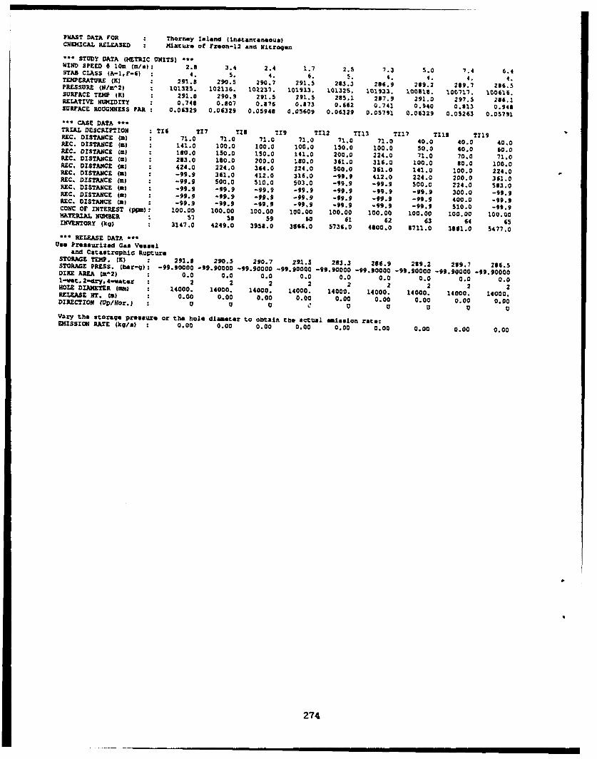
PHAST DATA FOR Thorney Island (instantanooal)CHEDMCAL RELEASED : Mixture of Freon-12 and Nitroqen

*** STUDY DATA (METRIC UNITS) ***WIND SPEED 3 10m (m/s): 2.8 3.4 2.4 1.7 2.5 7.3 5.0 7.4 6.4STAB CLASS (A-1,F-6) 4. 5. 4. 6. 5. 4. 4. 4. 4.TOERATuRt (K) 291.8 290.5 290.7 291.5 283.3 286.9 289.2 289.7 286.5PRESSURE (N/w-2) 101325. 102136. 102237. 101933. 101325. 101933. 100813. 100711. 100616.SURFACE TEMP (K) 291.8 290.9 291.5 291.5 285.1 237.9 291.0 297.5 286.1RELATIVE HWUIDITY : 0.740 0.807 0.876 0.873 0.662 0.741 0.940 0.313 0.948SURFACE ROUGHNESS PAR : 0.06329 0.06329 0.05948 0.05609 0.06329 0.05791 0.06329 0.05263 0.05791

"*" CASE DATA **"TRIAL DESCRIPTION : TI8 T17 T18 T19 T112 TI13 T117 T11l T119REC. DISTANCE (m) * 71.0 71.0 71.0 71.0 71.0 71.0 40.0 40.0 40,0REC. DISTANCE (m) 141.0 100.0 100.0 100.0 150.0 100.0 50.0 60.0 60.0AEC. DISTANCE (a) : 180.0 150.0 150.0 141.0 200.0 224.0 71.0 70.0 71.0REC. DISTANCE (m) 283.0 180.0 200.0 180.0 361.0 316.0 100.0 30.0 100.0REC. DISTANCE (2) 424.0 224.0 364.0 224.0 500.0 361.0 141.0 100.0 224.0.EC. DISTANCE (a) -99.9 361.0 412.0 316.0 -93.9 412.0 224.0 200.0 361.0REC. DISTANCE (mj -99.9 500.0 510.0 503.0 -99.9 -99.9 500.0 224.0 583.0REC. DISTANCE (a) -99.9 -99.9 -99.9 -99.9 -99.9 -99.9 -99.9 300.0 -99.9REC. DISTANCE (i) -99.9 -99.9 -99.9 -99.9 -99.9 -99.9 -99.9 400.0 -99.3REC. DISTANCE (a) : -99.9 -99.9 -99.9 -99.9 -99.9 -99.9 -99.9 510.0 -99.9CONC OF INTEREST (ppm): 100.00 100.00 100.00 100.00 100.00 100.00 100.00 100.00 100.00MATERIAL NMBkER 57 58 59 60 61 62 63 64 65INVENTORy (kg) : 3147.0 4249.0 3958.0 3866.0 5736.0 4300.0 8711.0 3301.0 5477.0

• RELEASE DATA -',Use Pressurized Gas Vessel

and Catastrophic RuptureSTORAGE TEMP. IK) 291.3 290.5 290.7 291.5 283.3 236.9 239.2 239.7 206.5STORAGE PRESS. (bar-g): -99.90000 -99.90000 -99.90000 -99.90000 -99.90000 -99.90000 -99.90000 -99.90000 -99.90000DIKE AREA (mA2) 0.0 0.0 0.0 0.0 0.0 0.0 0.0 0.0 0.0I-wiet.2-.dry,4,,watsr : 2 2 2 2 2 2 2 2 2HOLE DIAMETER (m) : 14000. 14000. 14000. 14000. 14000. 14000. 14000. 14000. 14000.RELEASE (fT. (m) : 0.00 0.00 0.00 0.00 0.00 0.00 0.00 0.00 0.00DIRECTION (up/Nor. j U U 9 C U U U U U

Vary the straQge pressure or the hole diameter to obtain the actual meission rate:EMISSION RATE (kq/g) 0.00 0.00 0.00 0.00 0.00 0.00 0.00 0.00 0.00

274

SLAB INPUT DATA FOR : BurroCHEMICAL RELEASED : Liquetled natural gasTHE SPILL !D CMDE !IOSPL) HAS THE F•LCWIF FLy.

I: EVAPORATING POOL2: HORIZONTAL JET3: VERTICAL JET4: INSTANTANEOUS OR SHORT DURATION

TRIAL : BU2 8U3 804 BUS BU6 307 gUt 89IDSPL • 1 1 1 1 2 1 1NCALC (sub-atop mult.): 1 1 1 1 1 1 1MOL. WT. (kq/maol) : 0.01746 0.01726 0.01703 0.01703 0.01724 0.01522 0.01312 0.01882Cp-qas (J/kq-K) 2238.0 2230.0 2238.0 2238.0 2235.0 2230.0 2238.0 2238.0NORMAL BOILING PT (K) : 111.6 111.6 111.6 111.6 111.6 111.6 111.6 111.6LIO MASS FRACTION : 1.000 1.000 1.000 1.000 1.000 1.000 1.000 1.000KAT OF VAP. (J/kg) : 511900. 511900. 511900. 511900. 511900. 511900. 511900. 511900.LI HEAT CAP (J/kg-K) : 3348.5 3348.5 334S.5 3348.5 3348.5 3348.5 3348.5 3348.5LZQ DENSITY (kq/m^3) 434.1 432.7 431.2 431.4 432.3 438.8 438.5 443.4B VAP PRESS CONST - 983.39 983.89 983.69 933.89 933.39 933.89 953.59 963.89C VA? PRESS CONST : 0.10 0.10 0.10 0.10 0.10 0.10 0.10 0.10GAS TEMPERATURE (m) : 111.6 111.6 111.6 111.6 111.6 111.6 111.6 111.6

MASS EKIS RATE (kg/s) : 86.10 87.98 86.96 81.25 92.22 99.46 116.93 135.98SOURCE AREA (m2) : 1012.79 1034.91 1022.97 956.07 1085.11 1170.21 1375.56 1599.63SOURCE DURATION (s) : 173. 167. 175. 190. 129. 174. 107. 79.TOTAL MASS (kg) 14980.0 14712.0 15221.0 15444.0 11886.0 17289.0 12453.0 10730.0SOURCE HEIGHT Wa) 0.00 0.00 0.00 0.00 0.00 0.00 0.00 0.00CONC AVG TINE (s) 40. 100. 80. 130. 70. 140. 80. 30.MAX DIST Wa) : 640. 640. 640. 640. 640. 900. 1300. 1300.REC HEIGHT (a) : 1.0 1.0 1.0 1.0 1.0 1.0 1.0 1.0REC HEIGHT (m) : 0.0 0.0 0.0 0.0 0.0 0.0 0.0 0.0REC HEIGHT (m) 0.0 0.0 0.0 0.0 0.0 ;.0 0.0 0.0REC UEIGHT (a) UJ.0 0.0 0.0 0.0 0.0 0.0 0.0 0.0ROUGHNESS LENGTH (m) : 0.00020 0.00020 0.00020 0.00020 0.00020 0.00020 0.00020 0.00020MET SENSOR NT (a) : 2.0 2.0 2.0 2.0 2.0 2.0 2.0 2.0WIND SPEED (Wls) : 5.4 5.4 9.0 7.4 9.1 8.4 1.8 5.7TEMPERATURE (K) 311.3 307.8 309.0 314.3 312.7 307.0 306.0 308.5REL HUMID (4) : 7.1 5.2 2.7 5.9 5.1 7.4 4.5 14.4SPECIFIC CONC (ppm) : 100. 100. 100. 100. 100. 100. 100. 100.STAB CLASS (A-1,F-6) : 0. 0. 0. 0. 0. 0. 0. 0.1/MONIN-OBUKHOV (1/m) : -0.0772 -0.1720 -0.0203 -0.0281 -0.0187 -0.0067 0.0646 -0.0004ENDING RECORD : -1. -1. -1. -1. -1. -1. -1. -1.

SLAB INPUT DATA FOR : CoyoteCHEMICAL RELEASED : Liquefied natural gas . Methane is at 1l.ast 36 in .THE SPILL ID CODE (IDSPL) HAS THE FOLLGIING KEY:

1: EVAPORATING POOL2: HORIZONTAL JET3: VERTICAL JET4: INSTANTANEOUS OR SHORT DURATION

TRIAL : C03 COS COGIDSPL . 1 1 1NCALC (sub-step mult.): 1 1 1MOL. WT. (kg/mol) : 0.01951 0.02019 0.01909Cp-qaa (J/kq-K) : 2238.0 2238.0 2238.0NORMAL BOILING PT (K) : 111.6 111.6 111.6LIQ MASS FRACTION : 1.000 1.000 1.000HEAT OF VAP. (J/kg) : 511900. 511900. 511900.LO HNEAT CAP (J/kg-K) : 3348.5 3346.5 3346.5L1O DENSITY (ko/m'3) : 447.4 452.7 444.7B VAP PRESS CONST : 983.89 983.39 983.89C VAP PRESS CONST : 0.10 0.10 0.10GAS TEMPERATURE (K) : 111.6 111.6 111.6MASS EMIS RATE (kg/s) : 100.67 129.02 123.03SOURCE AREA (^2) : 1184.20 1517.77 1447.46SOURCE DURATION (a) : 65. 98. 82.TOTAL MASS (kg) : 6532.0 12676.0 10139.0SOURCE HEIGHT (a) : 0.00 0.00 0.00CONC AVG TIME (s) : 50. 90. 70.MAX DIST (a) : 800. 900. 900.REC HEIGHT (a) : 1.0 1.0 1.0REC HEIGHT (m) : 0.0 0.0 0.0REC HEIGHT (a) : 0.0 0.0 0.0NEC HEIGHT (a) 0.0 0.0 0.0ROUGHNESS LENGTH 1m) : 0.00020 0.00020 0.00020NET SENSOR HT (m) : 2.0 2.0 2.0WIND SPEED (W/s) : 6.0 9.7 4.6TEMPERATURE (K) : 311.5 301.5 297.3REL HUMID (%) : 11.3 22.1 22.8SPECIFIC CONC (ppm) : 100. 100. 100.STAB CLASS (A-1,F-6) : 0. 0. 0.1/MONIN-OBUKHOV (1/m) : -0.0820 -0.0316 0.0178ENDING RECORD : -1. -1. -1.

275

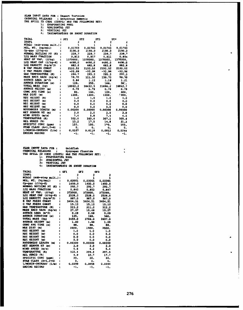
SLAB INPUT OATA FOR : Desert TortoiseCHMDICAL RELEASED : Anhydrous AmonliaTHE SPILL ID CODE (IDSPL) HAS THE FOLLOWING KEY:


TRIAL : DTI DT2 DT3 DT4IDSPL . 2 2 2 2NCALC (sub-st•p mult.).: 1 1 1 1MOL. WT. (kq/mol) : 0.01703 0.01703 0.01703 0.01703Cp-qaS (J/kq-K) : 2190.0 2190.0 2190.0 2190.0NORMAL BOILING PT (K) : 239.7 239.7 239.7 239.7LIQ MASS FRACTION : 0.013 0.317 0.811 0.604HEAT OF VAP. (J/kq) : 1370000. 1370000. 1370000. 1370000.LI. HEAT CAP (J/kq-K) : 4490.0 4490.0 4490.0 4490.0LIQ DENSITY (kq/m^3) : 682.8 682.8 662.8 662.89 VAP PRESS CONST : 2132.52 2132.52 2132.52 2132.52C VAP PRESS CONST : -32.96 -32.96 -32.96 -32.96GAS TE•PERATURE (K) : 294.7 293.3 295.3 297.3MASS EMIS RATE (kq/s) : 79.70 111.50 130.70 96.70SOURCE AREA (a'2) : 0.84 1.12 1.16 1.21SOURCE DURATION (s) : 126. 255. 166. 3081.TOTAL MASS (kg) : 10042.2 28432.5 21496.2 34642.7SOURCE HEIGHT (m) : 0.79 0.79 0.79 0.79CONC AVG TIME (s) : 60. 160. 120. 300.MAX DIST (m) : 1300. 1300. 1300. 1300.REC HEIGHT (a) : 1.0 1.0 1.0 1.0REC HEIGHT (m) : 0.0 0.0 0.0 0.0REC HEIGHT (a) : 0.0 0.0 0.0 0.0REC HEIGHT (a) : 0.0 0.0 0.0 0.0ROUGHNDESS LENGTH (a) : 0.00300 0.00300 0.00300 0.00300MET SENSOR HT (a) : 2.0 2.0 2.0 2.0WIND SPEED (a/*) : 7.4 5.6 7.4 4.5TEMPERATURE (K) : 302.0 303.6 307.1 305.6REL HUMID (4) : 13.2 17.5 14.6 21.3SPECIFIC CONC (Ppm) : 100. 100. 110. 100.STAB CLASS (A-1,F-6) : 0. 0. 0. 0.1/MONIN-OBUKHOV (1/m) : 0.0107 0.0119 0.0012 0.0244ENDING RECORD : -1. -1. -1. -1.

SLAB INPUT DATA FOR : GoldfishCHEMICAL RELEASED : Hydroqen fluorideTHE SPILL ID CODE (rDSPL) HAS THE FOLLOWING IEY:


TRIAL : GFl GF2 GF3IDSPL . 2 2 2NCALC (sub-stop mult.): 1 1 1MOL. WT. (kq/nol) : 0.02001 0.02001 0.02001Cp-qas (J/kq-K) : 1450.0 1450.0 1450.0NORMAL OILING PT (K) : 292.7 292.7 292.7LIO MASS FRACTION : 0.840 0.853 0.847HEAT OF VAP. (./kq) : 373000. 373000. 373000.LEO HEAT CAP (./kq-K) : 2528.0 2523.0 2523.0LIG DENSITY (kg/m.3) : 967.0 967.0 967.0B VAP PRESS CONST : 3404.51 3404.51 3404.51C VAP PRESS CONST : 15.12 15.12 15.12GAS TMPERATURE (K) 313.2 311.2 312.2MASS EMIS RATE (kg/a) : 27.67 10.46 10.27SOURCE AREA (a-2) 0.29 0.09 0.09SOURCE DURATION (a) : 125. 360. 360.TOTAL MASS (kg) : 3459.0 3766.0 3697.0SOURCE HEIGHT (m) 1.00 1.00 1.00COiC AVG TIME (a) : B6. 66. si.MAX ST (aS : 3500. 1500. 3500.REC HEIGHT (I) 1.0 1.0 1.0UEC HEIGHT (m) : 0.0 0.0 0.0REC HEIGHT (W) : 0.0 0.0 0.0REC HEIGHT (W) : 0.0 0.0 0.0ROUG•NESS LENGTH (a) : 0.00300 0.00300 0.00300MET SENSOR HT (a) : 2.0 2.0 2.0WIND SPEED (m/c) : 5.6 4.2 5.4TMP ERATURE (K) 310.4 309.4 307.6RtL HUMID (1) : 4.9 10.7 17.7SPECIFIC CONC (ppm) : 30. 30. 30.STAB CLASS (A.1,F-6) 0. 0. 0.1/MONIN-OBUICHOV (1/m) : 0.0099 0.0056 0.0244ENDING RECORD -1. -1. -1.

276

SLAB INPUT DATA FOR : Hanford (continuoualCHEMICAL RELEASED : Krypton-65THE SPILL ID CODE (IDSPL) HAS THE FOLLOWING KEY:


TRIAL HC1 HC2 HC3 HC4 HC5IDSPL . 2 2 2 2 2NCALC (sub-*tep mult.); 1 1 1 1 1MOL. WT. (kg/mol) 0.02900 0.02900 0.02900 0.02900 0.02900Cp-qas (J/kg-KI 249.0 249.0 249.0 249.0 249.0NORMAL BOILING PT (K) : 120.3 120.3 120.3 120.3 120.3LE1 MASS FRACTION : 0.000 0.000 0.000 0.000 0.000HEAT OF VAP. (J/kq) iseco. 115000. 115800. 115100. 115800.LIQ HEAT CAP (3/kg-K) ± -99.9 -99.9 -99.9 -99.9 -99.9LIQ DENSITY (kg/m3) -99.9 -99.9 -99.9 -99.9 -99.98 VAP PRESS CONST : -1.00 -1.00 -1.00 -1.00 -1.00C VAP PRESS CONST 0.00 0.00 0.00 0.00 0.00GAS TEMPERATURE (K) : 290.9 285.4 283.9 286.6 278.8MASS EMIS RATE (kq/a) : 0.01 0.01 0.03 0.04 0.02SOURCE AREA (m'2) : 0.01 0.00 0.00 0.01 0.01SOURCE DURATION (a) : 928. 905. 155. 596. 1191.TOTAL MASS (kg) : 10.9 10.9 23.8 22.8 20.4SOURCE HEIGHT (a) : 1.00 1.00 1.00 1.00 1.00CONC AVG TIME (a) : 461. 845. 269. 269. 538.MAX DIST (m) 1300. 1300. 1300. 1300. 1300.REC HEIGHT (m) 1.5 1.5 1.5 1.5 1.5REC HEIGHT (m) 0.0 0.0 0.0 0.0 0.0REC HEIGHT (a) : 0.0 0.0 0.0 0.0 0.0REC HEIGHT (mS) : 0.0 0.0 0.0 0.0 0.0ROUGHNESS LENGTH (m) : 0.03000 0.03000 0.03000 0.03000 0.03000MET SENSOR HT (l) : 1.5 1.5 1.5 1.5 1.5WIND SPEED (mls) : 1.3 3.9 7.1 3.9 2.6TEMPERATURE (K) : 290.9 285.4 288.9 286.6 278.8REL H•MID (9) : 20.0 20.0 20.0 20.0 20.0SPECIFIC CONC (pIm) : 0. 0. 0. 0. 0.STAB CLASS (A-1,F-6) : 0. 0. 0. 0. 0.I/mOlnN-OBHOV (1/m) : 0.1455 -0.0089 -0.0054 -0.0375 0.0142ENDING RECORD -1. -1. -1. -1. -1.

SLAB INPUT DATA FOR Hanford (instantaneous)CHEMICAL RELEASED : Krypton-I5THE SPILL ID CODE (IDSPL) HAS THE FOLLOWING KEY:

1: EVP.PO"XINA G POOL2: HORIZONTAL JET3: VERTICAL JET4: INSTANTANEOUS OR SHORT DURATION

TRIAL : H12 H13 HIS HIs H17 HISIDSPL : 4 4 4 4 4 4NCALC (sub-stop mul.): 1 1 1 1 1 1MOL. WT. (kg/aol) : 0.02900 0.02900 0.02900 0.02900 0.02900 0.02900Cp-gas (J/kq-K) : 249.0 249.0 249.0 249.0 249.0 249.0NORMAL BOILING PT (K) : 120.3 120.3 120.3 120.3 120.3 120.3LIQ MASS FRACTION : 0.000 0.000 0.000 0.000 0.000 0.000HEAT OF VAP. (O/kg) : 115800. 115800. 115800. 115890. 115300. 115800.LQ HEAT CAP (J/kg-g) : -99.9 -99.9 -99.9 -99.9 -99.9 -99.910 DENSITY (kq/a^3) : -99.9 -99.9 -99.9 -99.9 -99.9 -99.98 VAP PRESS CONST : -1.00 -1.00 -1.00 -1.00 -1.00 -1.00C VAP PRESS CONST : 0.00 0.00 0.00 0.00 0.00 0.00GAS TEMPERATURE (K) : 291.5 285.1 288.7 280.3 285.6 277.8MASS EMIS RATE (kg/a) : 0.00 0.00 0.00 0.00 0.00 0.00SOURCE AREA (u"2) 5.98 5.89 5.94 5.93 5.39 5.79SOURCE DURATION (W) : 0. 0. 0. 0. 0. 0.TOTAL MASS (kg) : 10.0 10.0 10.0 10.0 10.0 10.0SOURCE HEIGHT (a) : 0.00 0.00 0.00 0.00 0.00 0.00CONC AVG TIME (a) : 5. 5. 5. 5. 5. 5.MAX DIST (a) : 1300. 1300. 1300. 1300. 1300. 1300.REC HEIGHT (n) : 1.5 1.5 1.5 1.5 1.5 1.5REC HEIGHT (m) : 0.0 0.0 0.0 0.0 0.0 0.0REC HEIGHT (w) 0.0 0.0 0.0 0.0 0.0 0.0REC HEIGHT (a) : 0.0 0.0 0.0 0.0 0.0 0.0ROUGHNESS LENGTH (m) : 0.03000 0.03000 0.03000 0.03000 0.03000 0.03000MET SENSOR HT (m) : 1.5 1.5 1.5 1.5 1.5 1.5WIND SPEED (u/s) : 1.3 4.1 7.6 7.2 4.5 1.6TEMPERATURE (K) : 291.5 285.1 288.7 288.3 285.6 277.8REL HUMID (0) : 20.0 20.0 20.0 20.0 20.0 20.0

SPECIFIC CONC (ppm) : 0. 0. 0. 0. 0. 0.STAB CLASS (A-1.F-61 : 0. 0. 0. 0. 0. 0.1/MONIN-OBUKHOV (1/m) : 0.1742 -0.0038 -0.0046 -0.0064 -0.0157 0.0367ENDING RECORD : -1. -1. -1. -1. -1. -1.

277

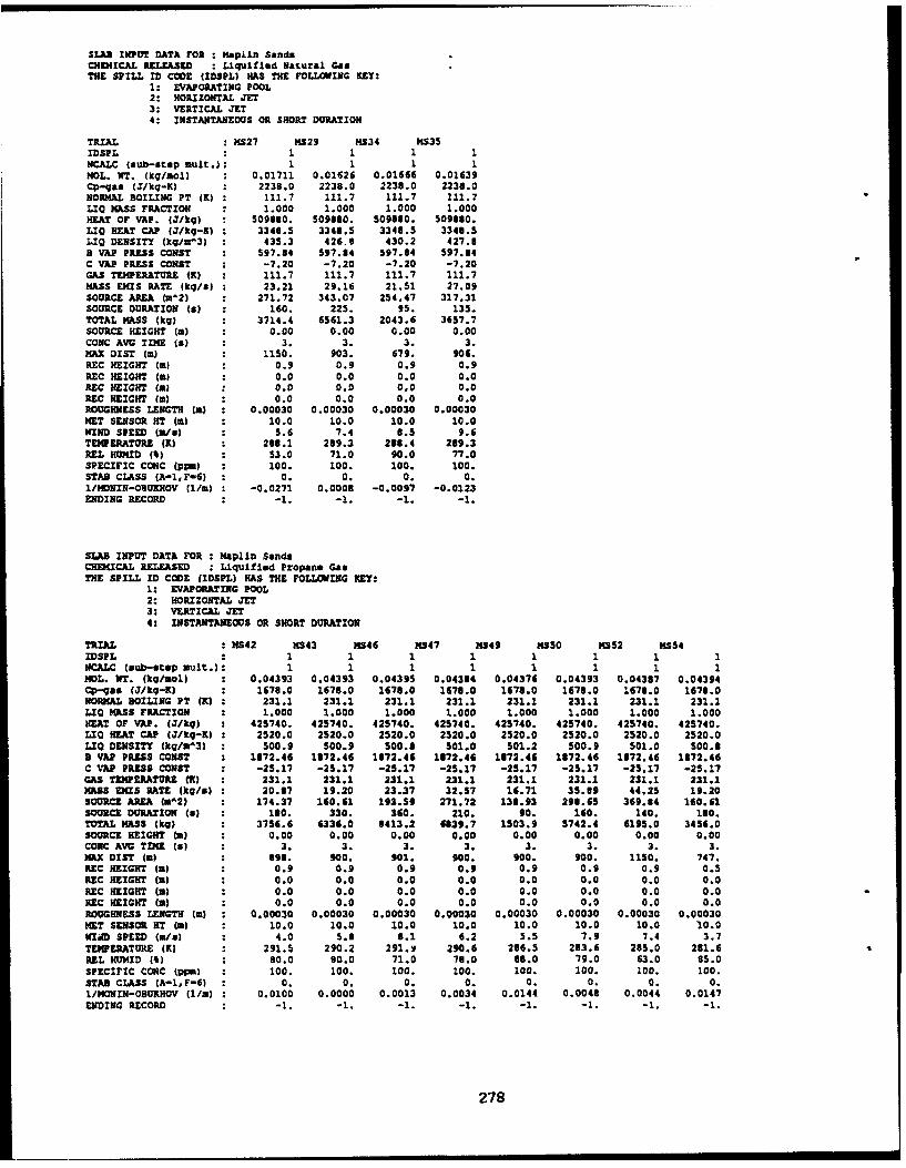
SLAB INPUT DATA FOR : Maplin SandsCHEMICAL RELEASED : Liquitled Natural GanTHE SPILL ID CODE (IDSPL) HAS THE FOLLOWING KEY:


TRIAL : KS.27 1S29 MS34 M535IDSPL . 1 1 1 1NCALC (sub-atep mult.): 1 1 1 1MOL. MT. (kgt/ol) : 0.01711 0.01626 0.01666 0.01639Cp-qaa (J/kg-K) : 2238.0 2238.0 2238.0 2230.0NORMAL BOILING PT (K) : 111.7 111.7 111.7 111.7LIQ MASS FRACTION : 1.000 1.000 1.000 1.000HEAT OF VAP. (J./kq) 509180. 509860. 509080. 509330.LIQ HEAT CAP (J/kq-K) : 3346.5 3348.5 3348.5 3340.5LIQ DENSITY (kg/=^3) : 435.3 426,9 430.2 427.B8 VAP PRESS CONST : 597.84 597.54 597.84 597.84C VAP PRESS CONST : -7.20 -7.20 -7.20 -7.20GAS TEMPERATURE (K) : 111.7 111.7 111.7 111.7MASS EM£S RATE (kg/s) : 23.21 29.16 21.51 27.09SOURCE AREA (m^2) : 271.72 343.07 254.47 317.31SOURCE DURATION (As) : 160. 225. 95. 135.TOTAL MASS (kg) : 3714.4 6561.3 2043.6 3657.7SOURCE HEIGHT (a) : 0.00 0.00 0.00 0.00CONC AVG TIME (a) : 3. 3. 3. 3.MAX DIST (m) 1150. 903. 679. 906.REC HEIGHT (m) : 0.9 0.9 0.9 0.9REC HEIGHT (a) : 0.0 0.0 0.0 0.0REC HEIGHT (a) : 0.0 0.0 0.0 0.0REC HEIGHT (a) : 0.0 0.0 0.0 0.0ROUGHNESS LENGTH (a) : 0.00030 0.00030 0.00030 0.00030MET SENSOR HT (a) : 10.0 10.0 10.0 10.0WIND SPEED (a/u) : 5.6 7.4 8.5 9.6TEMPERATURE (K) : 288.1 289.3 288.4 289.3REL H•ID (4) : 53.0 71.0 90.0 77.0SPECIFIC CONC (ppm) : 100. 100. 100. 100.STAB CLASS (A-1,F-6) 0. 0. 0. 0.1/MDNIN-OBUKHOV (l/m) : -0.0271 0.0008 -0.0097 -0.0123ENDING RECORD : -1. -1. -1. -1.

SLAB INPUT DATA FOR : Haplin SandsCHEKICAL RELEASED : Liquifled Propane GasTHE SPILL ID CODE (IDSPL) HAS THE FOLLOWING KEY:


TRIAL NS42 M343 NS46 14547 M549 1S50 NS52 NS54IDSPL :1 1 1 1 1 1 1 1NCALC (sub-stop mult.): 1 1 1 1 1 1 1 1MOL. WT. (kq/mol) : 0.04393 0.04393 0.04395 0.04384 0.04376 0.04393 0.04387 0.04394Cp-gaa (J/kq-K) : 1678.0 1678.0 1676.0 1678.0 1678.0 1678.0 1678.0 1678.0NORMAL BOILING PT (K) : 231.1 231.1 231.1 231.1 231.1 231.1 231.1 231.1LIQ MASS FRACTION : 1.000 1.000 1.000 1.000 1.000 1.000 1.000 1.000HEAT OF VAP. (J/kq) 425740. 425740. 425740. 425740. 425740. 425740. 425740. 425740.LIQ HEAT CAP (J/kg-K) : 2520.0 2520.0 2520.0 2520.0 2520.0 2520.0 2520.0 2520.0LIQ DENSITY (kg/n^3) : 500.9 500.9 500.8 S01.0 501.2 500.9 S01.0 500.8B VAP PRESS CONST : 1172.46 1872.46 1872.46 1872.46 1172.46 1672.46 1872.46 1872.46C VAP PRESS CONST -25.17 -25.17 -25.17 -25.17 -25.17 -25.17 -25.17 -25.17GAS TEMPERATURE (M) : 231.1 231.1 231.1 231.1 231.1 231.1 231.1 231.1MASS EIS RATE (kg/a) : 20.87 19.20 23.37 32.57 16.71 35.89 44.25 19.20SOURCE AREA (a^2) : 174.37 160.61 193.59 271.72 138.93 293.65 363.84 140.61SOURCE DURATION (a) : 180. 330. 360. 210. 90. 160. 140. 130.TOTAL MASS (kg) : 3756.6 6336.0 3413.2 4839.7 1503.9 5742.4 6195.0 3456.0SOURCE HEIGHT (a) : 0.00 0.00 0.00 0.00 0.00 0.00 0.00 0.00CONC AVG TINE (a) : 3. 3. 3. 3. 3. 3. 3. 3.MAX DIST (a) : 898. 900. 901. 900. 900. 900. 1150. 747.REC HEIGHT (a) 2 0.9 0.9 0.9 0.9 0.9 0.9 0.9 0.5REC HEIGHT (a) : 0.0 0.0 0.0 0.0 0.0 0.0 0.0 0.0REC HEIGHT (m) : 0.0 0.0 0.0 0.0 0.0 0.0 0.0 0.0REC HEIGHT (a) : 0.0 0.0 0.0 0.0 0.0 0.0 0.0 0.0ROUGHNESS LENGTH (m) : 0.00030 0.00030 0.00030 0.00030 0.00030 0.00030 0.00030 0.00030MET SENSOR NT (a) : 10.0 10.0 10.0 10.0 10.0 10.0 10.0 10.01IAID SPEED (a/a) : 4.0 5.8 8.1 6.2 5.5 7.9 7.4 3.7TEMPERATURE (K) : 291.5 290.2 291.! 290.6 286.5 283.6 285.0 281.6REL HUMID (4) : 80.0 60.0 71.0 78.0 66.0 79.0 63.0 85.0SPECIFIC COmc (ppm) : 100. 100. 100. 100. 100. 100. 100. 100.STAB CLASS (A-1,F-6) : 0. 0. 0. 0. 0. 0. 0. 0.1/NONIN-OBUNHOV (1/a) : 0.0100 0.0000 0.0013 0.0034 0.0144 0.0048 0.0044 0.0147ENDING RECORD -1. -1. -1. -1. -1. -1. -1. -1.

278

SLAB INPUT DATA FOR : Prairie Grass, set 1CHEMICAL RELEASED Sulfur dioxiieTHE SPILL ID COOE (IDSPL) HAS THE FOLLOWING KEY:

1: EVAPORATING POOL2: HORIZONTAL JET3t VERTICAL JET4: INSTANTANEOUS OR SHORT DURATION

TRIAL pG7 PG8 PG9 PG10 PG13 PC15 PG16 PG17IDSPL : 2 2 2 2 2 2 2 2HCALC tsub-stap mult.): 1 1 I 1 1 1 1 1MOL. WT. (kgi/ol) : 0.06400 0.06400 0.06400 0,06400 0.06400 0.06400 0.06400 0.06400Cp-qas (J/kq-K) : 622.6 622.6 622.6 622.6 622.6 622.6 622.6 622.6NORMAL BOILING PT (K) : 263.1 263.1 263.1 263.1 263.1 263.1 263.1 263.1LIQ MASS FRACTION : 0.000 0.000 0.000 0.000 0.000 0.000 0.000 0.000HEAT OF VAP. (J/kq) : 386500. 386500. 386500. 386500. 386500. 386500. 386S00. 386500.LIQ HEAT CAP (J/kg-K) 1331.0 1331.0 1331.0 1331.0 1331.0 1331.0 1331.0 1331.^LIC DENSITY (kg/m"3) : 1462.0 1462.0 1462.0 1462.0 1462.0 1462.0 1462.0 1462.0B YAP PRESS CONST : -1.00 -1.00 -1.00 -1.00 -1.00 -1.00 -1.00 -1.00C VAP PRESS CONST : 0.00 0.00 0.00 0.00 0.00 0.00 0.00 0.00GAS TEMPERATURE (K) 305.1 305.1 301.1 304.1 293.1 295.1 301.1 300.1MASS EMIS RATE (kq/s) : 0.09 0.09 0.09 0.09 0.06 0.10 0.09 0.06SOURCE AREA (mW2) 0.00 0.00 0.00 0.00 0.00 0.00 0.00 0.00SOURCE DURATION (a) : 60C. 600. 600. 600. 600. 600. 600. 600.TOTAL MASS (kq) : 53.9 54.7 55.2 55.3 36.7 57.3 55.8 33.9SOURCE HEIGHT (W) : 0.45 0.45 0.45 0.45 0.45 0.45 0.45 0.45CONC AVG TIME (a) : 600. 600. 600. 600. 600. 600. 600. 600.MAX DIST (m) : 1300. 1300. 1300. 1300. 1300. 1300. 1300. 1300.REC HEIGHT (m) : 1.5 1.5 1.5 1.5 1.5 1.5 1.5 1.5REC HEIGHT (m) : 0.0 0.0 0.0 0.0 0.0 0.0 0.0 0.0REC HEIGHT (m) 0.0 0.0 0.0 0.0 0.0 0.0 0.0 0.0REC HEIGHT (m) : 0.0 0.0 0.0 0.0 0.0 0.0 0.0 0.0ROUGHINESS LENGTH (m) 0.00600 0.00600 0.00600 0.00600 0.00600 0.00600 0.00600 0.00600MET SENSOR HT (m) : 2.0 2.0 2.0 2.0 2.0 2.0 2.0 2.0WIND SPEED (mis) 4.2 4.9 6.9 4.6 1.3 3.4 3.2 3.3TEMPERATURE (K) : 305.1 305.1 301.1 304.1 293.1 295.1 301.1 300.1REL HUMID (t) : 20.0 20.0 20.0 20.0 20.0 20.0 20.0 20.0SPECIFIC CCXC (ppm) 1. 1. 1. 1. 1. 1. 1. 1.STAB CLASS (A-l,F-6) 0. 0. 0. 0. 0. 0. 0. 0.1/MONIN-ODUWCOV (1/a) : -0.1223 -0.0485 -0.0293 -0.1342 0.1663 -0.1293 -0.1277 0.0201ENDING RECORD -1. -1. -1. -1. -1. -1. -1. -1.

SLAB INPUT DATA FOR : Thorney Island (continuous)CHEMICAL RELEASED : Mixture of Freon-12 and NitrogenTH9E PIL.L ID CODE (IDSPL) HAS THE FOLLOWING KEY:


TRIAL : TC45 TC47IDSPL : 2 2HCALC (sub-step mult.): 1 1MOL. NT. (kq/maol) : 0.05780 0.05780Cp-sax (J/kg-K) 610.0 610.0NORMAL BOILING PT (K) 243.4 243.4wo1 MASS FRACTION : 0.000 0.000

HEAT OF VAP. (3/kq) 165000. 165000.IIQ HEAT CAP (J/kq-K) : 970.0 970.0LIg DENSITY (kq/mi3) : 1520.0 1520.03 VAP PRESS CONST : -1.00 -1.00C VAP PRESS CONST : 0.00 0.00GAS TEMPERATURE (K) : 286.3 237.5MASS ENES RATE (kg/s) 10.67 10.22SOURCE AREA (1m2) : 3.14 3.14SOURCE DURATION (a) : 455. 465.TOTAL MASS (kq) 4855.0 4752.0SOURCE HEIGHT (a) : 0.00 0.00CONC AVG TIME (a) : 30. 30.MAX DIST (m) : 972. 972.REC HEIGHT (m) : 0.4 0.4REC HEIGHT (Ma : 0.0 0.0REC HEIGHT (a) : 0.0 0.0REC HEIGHT Wa) : 0.0 0.0ROUGHNESS LENGTH (W) : 0.01000 0.01000MET SENSOR HT (W) : 10.0 10.0WIND SPEED (m/s) : 2.3 1.5TEMPERATURE (K) : 286.3 287.5REL HUMID (M) 100.0 97.4SPECIFIC CONC (pIm) : 100. 100.STAB CLASS (A-I1,F-6) : 0. 0.1/MONIN-OBUKHOV (1/m) : 0.0461 0.0923ENDING RECORD : -1. -1.

279

i I I I I I I I "

SLAS INPUT DATA FOR : Thorney Island (instantafneoualCHDEICAL RELEASED : nixtEue of Freon-12 and NitzoqgenTHE SPILL 1D CODE (IDSPL) HAS THE FOLLOWING KEY:

1: EVAPORATING POOL2: HORI ZONTAL JET3: VERTICAL JET4: INSTANTANEOUS OR SHORT DURATION

TRIAL T,6 TI7 T17 TIT T112 T113 TIlT TIl8 T119IDSPL . 4 4 4 4 4 4 4 4 4NCALc (SUb-stop mult.): 1 1 1 1 1 1 1 1 1MOL. WT. (kg/mol) 0.04769 0.05058 0.04711 0.04624 0.06849 0.05780 0.12138 0.05404 0.06127CD-qm. (J/ko-K) 610.0 610.0 610.0 610.0 610.0 610.0 610.0 610.0 610.0NORMAL SOILING PT (K) : 243.4 243.4 243.4 243.4 243.4 243.4 243.4 243.4 243.41.1Q MASS FRACTION : 0.000 0.000 0.000 0.000 0.000 0.000 0.000 0.000 0.000HEAT OF VAP. (J/kq) : 165000. 165000. 165000. 165000. 165000. 165000. 165000. 165000. 165000.LIQ HEAT CAP (J/kq-K) : 970.0 970.0 970.0 970.0 970.0 970.0 970.0 970.0 970.0LIQ DENSITY (kg/=w3) : 1520.0 1520.0 1520.0 1520.0 1520.0 1520.0 1520.0 1520.0 1520.08 VAP PRESS CONST : -1.00 -1.00 -1.00 -1.00 -1.00 -1.00 -1.00 -1.00 -1.00C VAP PRESS CONST : 0.00 0.00 0.00 0.00 0.00 0.00 0.00 0.00 0.00GAS TEMPERATURE (K) 291.8 290.5 290.7 291.5 203.3 266.9 269.2 289.7 286.5MASS EMIS RATE (kg/a) : 0.00 0.00 0.00 0.00 0.00 0.00 0.00 0.00 0.00SOURCE AREA (W*21 : 153.94 153.94 153.94 153.94 153.94 153.94 153.94 153.94 153.94SOURCE DURATION (a) : 0. 0. 0. 0. 0. 0. 0. 0. 0.TOTAL MASS (kg) : 3147.0 4249.0 3958.0 3666.0 5736.0 4600.0 6711.0 3861.0 5477.0SOURCE HEIGHT (a) : 0.00 0.00 0.00 0.00 0.00 0.00 0,00 0.00 0.00CONC AVG TIME is) : 1. 1. 1. 1. 1. 1. 1. 1. 1.MAX DIST (a) 924. 1000. 1010. 1003. 1000. 912. 1000. 1010. 1063.REC HEIGHT (m) 0.4 0.4 0.4 0.4 0.4 0.4 0.4 0.4 0.4REC HEIGHT (m) : 0.0 0.0 0.0 0.0 0.0 0.0 0.0 0.0 0.0REC HEIGHT (m) : 0.0 0.0 0.0 0.0 0.0 0.0 0.0 0.0 0.0REC HEIGHT (m) : 0.0 0.0 0.0 0.0 0.0 0.0 0.0 0.0 0.0ROUGHNESS LENGTH (m) : 0.01800 0.01800 0.01200 0.00800 0.01500 0.01000 0.01800 0.00500 0.01000MET SENSOR HT (m) : 10.0 10.0 10.0 10.0 10.0 10.0 10.0 10.0 10.0WIND SPEED (m/a) : 2.5 3.4 2.4 1.7 2.5 7.3 5.0 7.4 6.4TEMPERATURE (K) : 291.6 290.5 290.7 291.5 283.3 266.9 289.2 289.7 286.5REL HUMID (A) : 74.0 80.7 87.6 67.3 66.2 74.1 94.0 61.3 94.8SPECIFIC COUC (pm) : 100. 100. 100. 100. 100. 100. 100. 100. 100.STAB CLASS (A-1,F-6) 0. 0. 0. 0. 0. 0. 0. 0. 0.1/MONIN-OBUKHOV (1/r) : 0.0000 0.0110 -0.1100 0.6500 0.1000 -0.0110 -0.0050 -0.0230 0.0030ENDING RECORD : -1. -1. -1. -1. -1. -1. -1. -1. -1.

280

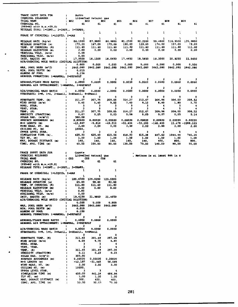
TRACE INPUT DATA FOR BurroCHEMICAL RELEASED Liquefied naltural gasTRIAL NAME BU2 8U3 B04 SO5 BU6 BU7 Bus 309CHEMICAL NO. . 61 61 61 61 61 61 61 61(999-W2 with m.w.-29.0)

RELEASE TYPE: 1-CONT., 2-INST., 3-TRANS.: 1 1 1 1 1

PHASE OF CHEMICAL: I-LIQUID. 2-GAS* 1 1 1 1 1 1

RELEASE RATE (kq/s) : 86.1000 87.9800 86.9600 81.2500 92.2200 99.4600 116.9300 135.9600RELEASE DURATION (a) 173.00 167.00 175.00 190.00 129.00 174.00 107.00 79.00TFJ. OF CHEMICAL (K) 111.60 111.60 111.60 111.60 111.60 111.60 111.60 111.60RELEASE ELEVATION (mi : 0.00 0.00 0.00 0.00 0.00 0.00 0.00 0.00VERTICAL VELO. (m/s) : 0.00HORIZONAL VELO. (ix.) 0.00INIT. RADIUS (m) : 17.9550 10.1500 18.0450 17.4450 18.5850 19.3000 20.9250 22.5650AIR/CHEKICAL MOLE RATIO (INITIAL DILUTION)

0.000 0.000 0.000 0.000 0.000 0.000 0.000 0.000MAX. POOL AREA (m^2) 2642.030 2642.060 2642.080 2642.030 2642.080 2642.080 2642.030 2642.080MIN. POOL OEPTH (a) 0.010ALBEDO OF POOL 0.150AEROSOL FORMATION: I-MANUAL, 2-DEFAULT

: 2 2 2 2 2 2 2 2AEROSOL/FLASH MASS RATIO 0.0000 0.0000 0.0000 0.0030 0.0000 0.0000 0.0000 0.0000AEROSOL AIR ENTRAINMENT: I-MANUAL, 2-DEFAULT

* 2 2 2 2 2 2 2 2AIR/CHEMICAL MASS RATIO : 0.0000 0.0000 0.0000 0.0000 0.0000 0.0000 0.0000 0.0000SUBSTRATE: 0-W, 1-C, 2-AsOi1, 3-SDacil, 4-SMaOil

0 0 0 0 0 0 0 0SUBSTRATE TEMP. (K) 311.27 307.75 309.05 314.27 312.67 306.96 306.02 308.52WIND SPEED (m/a) 5.40 5.40 9.00 7.40 9.10 8.40 1.60 5.70HORZ. STAB. * 3 3 3 3 3 4 5 4VERT. STAB. . 3 3 3 3 3 4 5 4TEMP. (K) . 311.27 307.75 309.05 314.27 312.67 306.96 306.02 306.52HUMIDITY (FRACTION) : 0.07 0.05 0.03 0.06 0.05 0.07 0.05 0.14SOLAR RAD. (w/re2) 300.00SURFACE ROUGHNESS (m) : 0.00020 0.00020 0.00020 0.00020 0.00020 0.00020 0.00020 0.0002014-0 LENGTH (m) -12.947 -5.814 -49.310 -35.634 -53.393 -148.633 15.478 -2238.323WIND MEAS. HT. (m) : 2.00 2.00 2.00 2.00 2.00 2.00 2.00 2.00CEILING HT. (m) : 10000.UPPER LEVEL STAB. : 3 3 3 3 3 4 5 4SIMOLATION TIME (a). 625.93 625.93 615.56 618.92 615.38 647.62 1044.44 740.35TLV HT. Wm) . 1.00 1.00 1.00 1.00 1.00 1.00 1.00 1.00MAX. DOSAGE DISTANCE (a) : 140. 140. 140. 140. 140. 400. 600. 800.CONC. AVG. TIME (a) : 40.00 100.00 60.00 130.00 70.00 140.00 80.00 50.00

TRACE INPUT DATA FOR CoyoteCHEMICAL RELEASED : Liquefled natural gas . Methane is at least 066 in cTRIAL NAME C03 C05 C06CHEMICAL NO. * 61 61 61(999-N2 with M.w.-29.0)RELEASE TYPE: 1-CONT., 2-INST., 3-TRANS.

1 1 1PHASE OF CHEMICAL: I-LIQUID, 2-GAS

:1 1 1RELEASE RATE (kg/a) : 100.6700 129.0200 123.0300RELEASE DURATION (a) . 65.00 98.00 82.00TEMP. OF CHEMICAL (M) : 111.60 111.60 111.60RELEASE ELEVATION (a) 0.00 0.00 0.00VERTICAL VELO. (a/a) 0.00HORIZONAL VELO. (m/8) 0.00INIT. RADIUS (m) 19.4150 21.9800 21.4650AIR/CHEMICAL MOLE RATIO (INITIAL DILUTION)

0.000 0.000 0.000MAX. POOL AREA (X^2) : 2642.080 2642.080 2642.080MIN. POOL DEPTH (m) : 0.010AL.EDO Or POOL 0.150AEROSOL FORMATION: I-MANUAL. 2-DEFAULT

2 2 2AEROSOL/FLASH MASS RATIO : 0.0000 0.0000 0.0000AEROSOL AIR ENTRAINMENT: I-MANUAL, 2-DEFAULT

2 2 2AIR/CHEMICAL MASS RATIO : 0.0000 0.0000 0.0000SUBSTRATE: 0-1, I-C, 2-Asoil, 3-SOsoil, 4-Macil

0 0 0SUBSTRATE TEMP. (K) 311.45 301.49 297.26WIND SPEED (8/2) : 6.00 9.70 4.60HORZ. STAB. : 3 3 4VERT. "TAB. . 3 3 4TEMP. (K) . 311.45 301.49 297.26HUMIDITY (FRACTION) 0.11 0.22 0.23SOLAR PAD. (w/m'2) 300.00SURFACE ROUGHNESS (m) 0.00020 0.00020 0.00020N-0 LENGTH (m) . -12.197 -31.665 56.085WIND MEAS. HT. (m) : 2.00 2.00 2.00CEILING HT. Im) . 10000.UPPER LEVEL STAB. * 3 3 4SIMULATION TIME (a) : 650.00 641.24 686.96TLV MT. 4m) . 1.00 1.00 1.00MAX. DOSAGE DISTANCE (m) 300. 400. 400.CONC. AVG. TIME (s) 50.00 90.00 70.00

281

TRACE INPUT DATA FOR Desert TortoiseCHICAL RELEASED Anhydrous AmmoniaTRIAL NA: DTI DT2 DT3 DT4CHDMICAL NO. . 22 22 22 22(999-112 with m.w.-29.0)RELEASE TYPE: I'CONT., 2-INST., 3-TRANS.* 1 1 2. 1

PHASE OF CHEMICAL. I-LIQUID. •'wAS,

RELEASE RATE (kq/a) : 79.7000 111.5000 130.7000 96.7000RELEASE DURATION (a) : 126.00 255.00 166.00 381.00TEDM. OF CHEMICAL (CR 294.70 293.30 295.30 297.30RELEASE ELEVATION (m3 Z 0.79 0.79 0.79 0.79VERTICAL VELO. in/•$ 0.00HORIZONAL VELO. (m/a) : 0.00,XIT. RADIJS (a) 0.5185 0.5971 0.6089 0.6210AIR/CRHMICAL MOLE RATIO (INITIAL DILUTION)

* 0.000 0.000 0.000 0.000"•AX. POOL AREA (0^2) : 10000.000 10000.000 10000.000 10000.000?'.M. POOL DEPTH (a) : 0.010ALBEDO OF POOL : 0.150ALEROSOL FQP).&TIOW 1-MANUAL, 2-OW'ADLT

1 1 1 1AEROSOLWFLASH MASS RATIO : 10000.000010000.000010000.000010000.0000AEROSOL AIR ENTRAINMIENT: 1-1ANUAL, 2-DEFAULT

: 2 2 2 2AIR/CHE[ICAL MASS RATIO 0.0000 0.0000 0.0000 0.0000SUBSTRATE: 0-41, 1-C, 2-Asoil, 3-SD8o01, 4-SNscil

0 0 4 2SUBSTRATE TEMP. (K) 304.80 303.80 304.80 304.00WIND SPEED (s/a) : 7.40 5.30 7.40 4.50HORZ. STAB. . 4 4 4 5VER. STAB. . 4 4 4 5TEMP. (K) 302.03 303.63 307.07 305.63OUMIDITY (FRACTION) 0.13 0.17 0.15 0.21SOLAR PAD. (v/wm'2) 300.00SURFACE ROUGHIESS (a) : 0.00300 0.00300 0.00300 0.003006-0 LENGTH (a) 93.201 84.333 847.250 41.002

WIND NEAS. HT. in) 2.00 2.00 2.00 2.00CEILING HT. (a) : 10000.UPPER LEVEL STAB. : 4 4 4 5SIMUZLATION TIME (a) : 708.11 737.93 708.11 777.78TLV MT. (a) : 1.00 1.00 1.00 1.00MAX. DOSAGE DISTANCE (a) : 800. 300. 800. 600.CONC. AVG. TIMl4 (a) : 80.00 160.00 120.00 300.00

TRACE INPUT DATA FOR GoldfiLshCXHMICAL RELEASED : Hydrogen fluorideTRIAL NAME GFI GF2 Gi3CHEMICAL NO. . 17 17 17(999-112 with m.W.-29.0)RELEASE TYPE: I-CONT., 2-INST., 3-TRANS.

I 1 1PHASE OF CHEMICAL: 1-LIQUID, 2-GAS

1 1 1REZLUASE RATE lkas) : 27.6700 10.4600 10.2700RELEAS DURATION (a) : 125.00 360.00 360.00TEMP. OF CHEMICA, (K) 313.20 311.20 312.20RELEASE ELEVATION (3) 1.00 1.00 1.00VERTICAL VELO. (n/a) 0.00HORIZONAL VELO. (n/s) : 0.00INIT. RADIUS (a) : 0.3041 0.1689 0.1717AIR/CHEDECAL MOLE RATIO (INITIAL DILUTION)

0.000 0.000 0.000MAX. POOL AREA (W2) : 10000.000 10000.000 10000.000MIN. POOL DEPTH (a) : 0.010ALB£DO OF POOL : 0.150AEROSOL FO, ATION: 1-4A•M, 2-OEFZALT

R 1 1 1AEROSOL/FLASH MASS RATO : 10000.000010000.000010000.0000AEROSOL AIR ENTRAIWENT: 1-,ML. 2-OEF'ALT

2 2 2AIR/CHEMICAL MASS RATIO 0.0000 0.0000 0.0004SUBSTRATE: 0"-, 1-C, 2-Aoil, 3-6aoi1l, 4-Ia.o0l

2 2 2SUBSTRATE TEMP. (K) : 310.40 309.38 307.61WIND SPEED (1/s) : 5.60 4.20 5.40HORI. STAB. . 4 4 4VERT. STAB. . 4 4 4TEMP. (K) : 310.40 309.30 307.61HUMIDITY (FRACTION) 0.05 0.11 0.18SOLAR MAD. (NiW21 : 300.00SURFACE ROUGHNPSS (a) : 0.00300 0.00300 0.00300M-0 LENGTH (a) : 101.293 173.142 40.927WIND NEAS. HT. (W3 * 2.00 2.00 2.00CEILING UT. (a) 10000.UPPER LEVEL STAB. : 4 4 4SIMULATION TIME (a) : 1135.71 838.10 1155.56TLV HT. (a) : 1.00 1.00 1.00MAX. DOSAGE DISTANCE (a) : 3000. 1000. 3000.CONC. AVG. TIME (a) 88.30 38.30 68.30

282

TRACE INPUT DATA FOR Hanford (continuous)CHEMICAL RELEASED Krypton-85TRIAL NAME : HCI HC2 HC3 P)4 HCSCHEMICAL NO. 999 999 999 999 999(999-N2 with m.w.-29.0)

RELEASE TYPE: 1-CONT., 2-INST.. 3-TRANS.1I 1 1 1

PHASE Or CHEMICAL: 1-LIQUID, 2-.GAS:2 2 2 2 2

RELEASE RATE (kq/s) 0.0117 0.0120 0.0278 0.0388 0.0171RELEASE DURATION IS) * 928.00 905.00 855.00 598.00 1191.00TEMP. OF CHEMICAL (K) : 290.87 235.43 288.93 286.65 278.82RELEASE ELEVATION Wu) : 1.JO 1.00 1.00 1.00 1.00VERTICAL VELO. (m/s) : 0.00HORIZONAL VELO. (rn/l : 0.00INIT. RADIUS Wm) 0.0528 0.0296 0.0337 0.0532 0.0431AIR/CHEMICAL MOLE RATIO (INITIAL DILUTION)

* 0.000 0.000 0.000 0.000 0.000MAX. POOL AREA (m^2) 10000.000 10000.000 10000.000 10000.000 10000.000KIN. POOL DEPTH (m) : 0.010ALSEDO or POOL * 0.150AEROSOL FORMATION: I-MANUAL. 2-DEFAULT

2 2 2 2 2AEROSOL/FLASH MASS RATIO : 0.0000 0.0000 0.0000 0.0000 0.0000AEROSOL AIR ENTP.AIIO4T: 1-MANUAL, 2-OEFAULT

2 2 2 2 2AIR/CHEMICAL MASS RATIO : 0.0000 0.0000 0.0000 0.0000 0.0000SUBSTRATE: 0-W, 1-C, 2"Aaotil 3-SOsOiI, 4-SMaoil

2 2 2 2 2SUBSTRATE TEMP. (K) 290.87 285.43 268.93 286.65 278.82WIND SPEED (m/s) 1.30 3.90 7.10 3.90 2.60

.ORZ. STAB. : 6 3 3 3 5VERT. STAB. : 6 3 3 3 5TEMP. (R) . 290.87 235.43 288.93 286.65 278.62HUMIDITY (FRACTION) 0.20 0.20 0.20 0.20 0.20SOLAR RAD. (v/m^2) 300.00SURFACE ROUGIHESS Wm) 0.03000 0.03000 0.03000 0.03000 0.03000M-O LENGTH (m) . 6.875 -111.826 -186.121 -26.653 70.243WIND MEAS. NT. (m) : 1.50 1.50 1.50 1.50 1.50CEILING ST. (m) : 10000.UPPER LEVEL STAB. 6 3 3 3 5SIMULATION TIME (a) : 1215.38 805.13 712.68 805.13 907.69TLV MT. CW) : 1.50 1.50 1.50 1.50 1.50M9X. DOSAGE DISTANCE (a) : 800. 800. 300. 800. 800.CONC. AVG. TIME (a) 460.80 844.80 268.80 268.80 537.60

TRACE INPUT DATA FOR. Hanford (insutananeom)CHEMICAL RELEASED : "ypton-85TRIAL NANE : H12 H13 HI5 H16 H17 HISCHEMICAL NO. : 999 999 999 999 999 999(999-142 with m.v.-29.0)RELEASE TYPE: 1-CONT., 2-13ST., 3-TRANS.

2 2 2 2 2 2PHASE OF CHEMICAL: I-LIQUID, 2-GAS

2 2 2 2 2 2TO MASS RELEASED (kg) 10.00 10.00 10.00 10.00 10.00 10.00RELEASE DURATION (a) 0.00 0.00 0.00 0.00 0.00 0.00TEMP. OF CHEMICAL (K) 291.54 285.09 286.11 216.26 285.59 277.76RELEASE ELEVATION (m) 0.00 0.00 0.00 0.00 0.00 0.00VERTICAL VELO. (a/a) : 0.00IORIZONAL VELO. (us/0 : 0.00INIT. RADIUS ti) 1.3792 1.3690 1.3748 1.3740 1.3698 1.3572AIR/CHMIICAL MOLE RATIO (INITIAL DILUTION)

0.000 0.000 0.000 0.000 0.000 0.000XAX. POOL AREA (m^2)1 10000.000 10000.000 10000.000 10000.000 10000.000 10000.000KIN. POOL DEPTH (m) : 0.0o0Ala= OF POOL * 0.150AEROSOL FORMATION: I-MANUAL, 2-OEFAULT

* 2 2 2 2 2 2AEROSOL/FLASK MASS RATIO : 0.0000 0.0000 0.0000 0.0000 0.0000 0.0000AEROSOL AIR EXTRAINM•NT: 1-KANUAL, 2-DEFAULT

2 2 2 2 2 2AIR/CHEMICAL MASS RATIO 0.0000 0.0000 0.0000 0.0000 0.0000 0.0000SUBSTRATE: 0-il, 1-C, 2-Asaoil, 3-SDaoil, 4-SMasoil

2 2 2 2 2 2SUBSTRATE TEMP. (K) 291.54 265.09 263.71 298.26 285.59 277.76WIND SPEED (a/a) 1.30 4.10 7.60 7.20 4.50 1.60HORZ. STAB. . 6 4 3 3 3 5VERT. STPA8. . 6 4 3 3 3 5TDE. (K) . 291.54 285.09 288.71 268.26 285.59 277.76HUMIDITY (FRACTION) 0.20 0.20 0.20 0.20 0.20 0.20SOLAR RAD. (w/m^2) 300.00SURFACE ROUGHNESS (a) : 0.03000 0.03000 0.03000 0.03(00 0.03000 0.03000M-0 LENGTH (m) : 5.742 -262.928 -216.547 -155.306 -63.594 27.267WIND MEAS. HT. (a) : 1.50 1.50 1.50 1.50 1.50 1.50CEILING HT. (m) : 10000.UPPER LEVEL STAB. : 6 4 3 3 3 5SIMULATION TIME (a) 1215.38 795.12 705.26 711.11 777.78 1100.00TLV HT. (W) . 1.50 1.50 1.50 1.50 1.50 1.50MAX. DOSAGE DISTANCE Wa) 800. 800. 300. 800. 800. 800.CONC. AVG. TIME (x) : 4.80 4.80 4.80 4.80 4.80 4.80

283

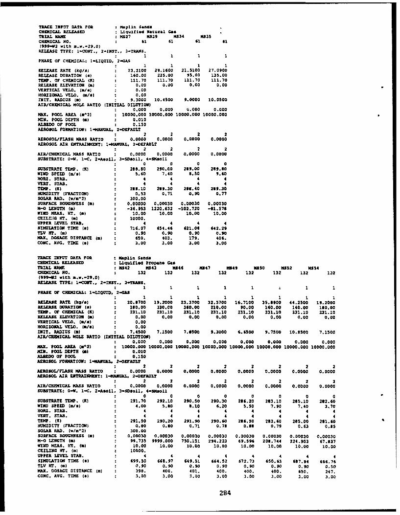
TRACE INPUT DATA FOR : NapLin SandsCHDMICAL RELEASED Llqutlfed Natural GasTRIAL MAME : NS27 MS29 4534 K1135CHEMICAL NO. 61 61 61 611999-,42 with m.w.-29.0)RELEASE TYPE: I-CObT., 2-INST., 3-TRA.lS.

S1 1 1 1

PHASE OF CHEMICAL: I-LIQUID, 2-GAS1 1 1 1

RELEASE RATE (kq/s) 23.2100 29.1600 21.5100 27.0900RELEASE DURATION (a) : 160.00 225.00 95.00 135.00TEMP. OF CHEMICAL (K) : 111.70 111.70 111.10 111.70RELEASE ELEVATION (a) 0.00 0.00 0.00 0.00VERTICAL VELO. (rn/s) : 0.00HORIZONAL VELO. (W/s) 0.00I34T. RADIUS (a) 9.3000 10.4500 9.0000 10.0500AIR/CHEMICAL OLE . RATIO (INITIAL DILUTION)

0.000 0.000 0.000 0.000MAX. POOL AMEA (W2) 10000.000 10000.000 10000.000 10000.000MIN. POOL DEPTH (a) 0.010ALAEDO OF POOL : 0.150AEROSOL FORMATION: 1-mANuAL, 2-oEFAULT

2 2 2 2AEROSOL/FLASH MASS RATIO 0.0000 0.0000 0.0000 0.0000AEROSOL AIR ENTRAINMENT: I-IANUAL, 2-OEFAULT

2 2 2 2AIR/CHEMICAL MASS RATIO 0.0000 0.0000 0.0000 0.0000SUBSTRATE: 0,-4. I-C, 2-Asoil, 3-SDsoL1, 4-S13oil

0 0 0 0SUBSTRATE TEMP. (K) : 280.80 290.00 239.00 289.00WIND SPEED (r/a) : 5.60 1.40 8.50 9.60HORZ. STAB. . 4 4 4 4VERT. STAB. * 4 4 4 4TEMP. (M) . 288.10 289.30 203.40 289.30HUMIDITY (FRACTION) : 0.53 0.71 0.90 0.77SOLAR RAD. (w/a^2) : 300.00SURFACE ROUGHNESS (a) : 0.00030 0.00030 0.00030 0.0003036-0 LENGTH (a) : -36.953 1220.632 -102.720 -81.578WIND MEAS. HT. (=I 10.00 10.00 10.00 10.00CEILING HT. (a) : 10000.UPPER LEVEL STAB. 4 4 4 4SIMJULATION TIME (a) : 716.07 654.46 621.06 642.29TLV MT. (a) . 0.90 0.90 0.90 0.90MAX. DOSAGE DISTANCE (a) 650. 403. 179. 406.CONC. AVG. TIME Is) 3.00 3.00 3.00 3.00

TRACE INPUT DATA FOR Kaplin SandsOR CHMICAL RELEASED z LLquified Propane GasTRIAL AMAE M542 NS43 NS46 M347 M549 4350 3432 1S54CEI=CAL 1)0. * 132 132 132 132 132 132 132 132(999-N2 with A.v.-29.0)

RElUASE TYPE. 1-cCON., 2-INST., 3-TRANS.1 1 11 1 1 11 1 1

PHASE Or CHEMICAL: I-LIQUID, 2-GAS1 1 1 1 1 1 1 1

RELEASE RATE (kG/a) 20.1700 19.2000 23.3700 32.5700 16.7100 35.8900 44.2500 19.2000RZLEASE DURATION (a) 130.00 330.00 360.00 210.00 90.00 140.00 140.00 180.00TEMP. OF CHEMICAL (K) : 231.10 231.10 231.10 231.10 231.10 231.10 231.10 231.10RELEASE ELEVATION (a) : 0.00 0.00 0.00 0.00 0.00 0.00 0.00 0.00VERTICAL VELO. (W/e) 0.00HORIZON1AL VELO. (u/a) 0.00INIT. RADIUS (mW 7.4500 7.1500 7.8500 9.3000 6.6500 9.7500 10.8500 7.1500AIR/CKEMICAL MOLE RATIO (INITIAL DILUTION)

0.000 0.000 0.000 0.000 0.000 0.000 0.000 0.000NKX. POOL AREA (M42) : 10000.000 10000.000 10000.000 10000.000 10000.000 10000.000 10000.000 10000.000MIN. POOL DEPTH (a) : 0.010ALDo OF POOL 0.150AEROSOL FORMATION: 1-ANAUAL. 2-OEFAULT

2 2 2 2 2 2 2 2AEROSOL/FLASH MASS RATIO 0.0000 0.0000 0.0000 0.0000 0.0000 0.0000 0.0000 0.0000AEROSOL AIR EXTRAIMUNT: I-MOANUAL, 2-ODFAULT

2 2 2 2 2 2 2 2AIRJCHEMICAL MASS RATIO 0.0000 0.0000 0.0000 0.0000 0.0000 0.0000 0.0000 0.0000SUBSTRATE: 0-W, 1-C, 2-Asoil, 3-SDsoil, 4-SUsoil

0 0 0 0 0 0 0 0SUBSTRATE TEMP. (K) 291.70 292.10 290.50 290.30 286.20 283.10 265.10 282.60WIND SPIED (M/u) 4.00 5.80 0.10 6.20 5.50 7.90 7.40 3.70KORZ. STAB. . 4 4 4 4 4 4 4 4VERT. STAB. * 4 4 4 4 4 4 4 4TEMP. (K) . 291.50 290.20 291.90 290.60 236.50 233.60 285.00 231.60HUMIDITY (FRACTION) : 0.30 0.80 0.71 0.73 0.83 0.79 0.63 0.85SOLAR HAD. (w/u^2) 300.00SURFACE ROUGHNESS (m) : 0.00030 0.00030 0.00030 0.00030 0.00030 0.00030 0.00030 0.00030M-0 LENGTH (ml 99.735 9999.000 750.151 294.223 69.596 208.744 224.903 67.337WIND MEAS. HT. Wm) 10.00 10.00 10.00 10.00 10.00 10.00 10.00 10.00CEILING HT. (W) 10000.UPPER LEVEL STAB. : 4 4 4 4 4 4 4 4SIMULATION TIME (a) : 699.50 663.97 649.51 664.52 672.73 650.63 687.04 666.76TLV HT. (W) . 0.90 0.90 0.90 0.90 0.90 0.90 0.90 0.50MAX. DOSAGE DISTANCE (m) 398. 400. 401. 400. 400. 400. 650. 247.CONC. AVG. TIME (a) : 3.00 3.00 3.00 3.00 3.00 3.00 3.00 3.00

284

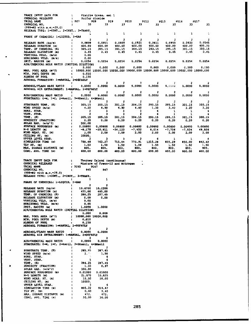
TRACE INPUT DATA FOR Prairie Grass, met 1CHEMICAL RELEASED : Sulfur dioxideTRIAL NAME PG7 PCs PG9 PGIO PG13 PG15 PG16 PG17CHEMICAL HO. . 33 33 33 33 33 33 33 33(999-N2 with m.w.-29.0)

RELEASE TYPE: I-CONT., 2-INST., 3-.TRAS.S1 1 1 1 1 1

PRAE OF CHEMICAL: 1-LIQUID, 2-GAS: 2 2 2 2 2 2 2 2

RELEASE RATE (kq/s) 0.0699 0.0911 0.0920 0.0921 0.0611 0.0955 0.0930 0.0565RELEASE DURATION (a) 600.00 600.00 600.00 600.00 600.00 600.00 600.00 600.00TEMP. OF CHEMICAL (K) 305.15 305.15 301.15 304.15 293.15 295.15 301.15 300.15RELEASE ELEVATION (m) : 0.45 0.45 0.45 0.45 0.45 0.45 0.45 0.45VERTICAL VELO. (3/a) 0.00HORIZOHAL VELO. (m/s) : 0.00WNIT. RADIUS (ma 0.0254 0.0254 0.0254 0.0254 0.0254 0.0254 0.0254 0.0254

AIR/CHEMICAL MOLE RATIO (INITIAL DILUTION)0.000 0.000 0.000 0.000 0.000 0.000 0.000 0._00

MhX. POOL AREA (m^2) : 10000.000 10000.000 10000.000 10000.000 10000.000 10000.000 10000.000 10000.000MIN. POOL DEPTH (mW : 0.010ALBEDO OF POOL : 0.150AEROSOL FORMATION: I-KANUAL. 2,OEFAOLT

2 2 2 2 2 2 2 2AEROSOL/FLASH MASS RATIO : 0.0000 0.0000 0.0000 0.0000 0.0000 0. C 0.0000 0.0000AEROSOL AIR ENTRAINMENT: 1-mANUAL, 2-DEFAULT

2 2 2 2 2 2 2 2AIR/CHEMICAL MASS RATIO 0.0000 0.0000 0.0000 0.0000 0.0000 0.0000 0.0000 0.0000SUBSTRATE: 0-W, 1-C, 2-Asoil, 3-SOsoil, 4-DMsoil

* 2 2 2 2 2 2 2 2SUBSTRATE TEMP. (K) : 305.15 305.15 301.15 304.15 293.15 295.15 301.15 300.15WIND SPEED (We) : 4.20 4.90 6.90 4.60 1.30 3.40 3.20 3.30HORZ. STAB. . 2 3 3 2 6 1 1 4VERT. STAB. . 2 3 3 2 6 1 1 4TEMP. (K) . 305.15 305.15 301.15 304.15 293.15 295.15 301.15 300.15HUMIDITY (FRACTION) : 0.20 0.20 0.20 0.20 0.20 0.20 0.20 0.20SOIAR. RAO. (w/m-2) 300.00SURFACE ROUGHNESS (W) : 0.00600 0.00600 0.00600 0.00600 0.00600 0.00600 0.00600 0.00600M-0 LENGTH (mW -8.178 -20.611 -34.123 -7.452 6.014 -7.736 -7.834 49.806WIND MEAS. HT. (W) : 2.00 2.00 2.00 2.00 2.00 2.00 2.00 2.00CEILING HT. (m) : 10000.UPPER LEVEL STAB. 2 3 3 2 6 1 1 4SIMULATION TIME (s) : 790.48 763.27 715.94 773.91 1215.38 835.29 850.00 042.42TLV iT. (m) : 1.50 1.50 1.50 1.50 1.50 1.50 1.50 1.50MAX. DOSAGE DISTANCE (W4 800. 800. 800. 000. 800. 800. 600. 800.CONC. AVG. TIME (a) : 600.00 600.00 600.00 600.00 600.00 600.00 600.00 600.00

TRACE INPUT DATA FOR : Thorney Island (continuous)CHEMICAL RELEASED Mixture of Freon-12 and NitrogenTRIAL NAME TC45 TC47CHEMICAL NO. . 945 947(999-4•2 with m.w.-29.0)

RELEASE TYPE: I-CONT., 2-INST., 3,,TRANS.1 1

PHASE OF CHEMICAL: 1-LIQUID. 2-GAS2 2

RELEASE RATE (kq/*) : 10.6700 10.2200RELEASE DURATION (a) : 455.00 465.00TEMP. OF CHEMICAL (K) : 266.25 287.45RELEASE ELEVATION (W) : 0.00 0.00VERTICAL VELO. We/s) 0.00HORIZONAL VELO. (We/) : 0.00INIT. RADIUS (W) : 1.0000 1.0000AIR/CHEMICAL MOLE RATIO (INITIAL DILUTION)

0.000 0.000MAX. POOL AREA (m'2) 10000.000 10000.000

MIN. POOL DEPTH (a) * 0.010ALBEDO OF POOL . 0.150AEROSOL FORMATION: I-MANUAL, 2-DEFAULT

2 2AEROSOL/FLASH MASS RATIO : 0.0000 0.0000AEROSOL AIR ENTRAINMENT: 1-MANUAL, 2-OErAULT

2 2AIR/CHEMICAL MASS RATIO : 0.0000 0.0000SUBSTRATE: 0"-, 1-C, 2-Asoil, 3-SD~til, 4-"kmoil

2 2SUBSTRATE TEMP. (K) 215. 95 261.65WIND SPEED (a/u) 2.7 1.50HORZ. STAB. 6VERT. STAB. . 5 6TEMP. (K) . 2S6.25 287.45HUMIDITY (FRACTION) 1.00 0.97SOLAR WD. (w/m'2) : 300.00SURFACE ROUGHNESS (mW : 0.01000 0.01000H-O LEHGTH (m) 21.670 10.835WIND MEAS. HT. (mW 10.00 10.00CEILING HT. (m) 10000.UPPER LEVEL STAB. 5 6SIMULATION TIME (s) 805.22 914.67TLV HT. (W) : 0.40 0.40MAX. DOSAGE DISTANCE (W4 472. 472.CONC. AVG. TIME (a) 30.00 30.00

285

TRACE INPUT DATA FOB Thorney Island (lnstantaneous)CHEMICAL RELEASED Mixture of Freon-12 and Nitrogen

TRIAL NAME TI T T17 TI3 T19 T112 T113 T117 T123 T119CHEIICAL NO. . 906 907 906 909 912 913 917 913 919(999-N2 with a.w.-29.0)RELEASE TYPE: I-CONT., 2-INST., 3-TRANS.

2 2 2 2 2 2 2PHASE c 'EMCAL: 1-LIQUID, 2-GAS

* 2 2 2 2 2 2 2 2 2TOTAL mA.S RELEASED (kg) 3147.00 4249.00 3958.00 3066.00 5736.00 4800.00 0711.00 3081.00 5477.00RELEASE DURATION (a) 0.00 0.00 0.00 0.00 0.00 0.00 0.00 0.00 0.00TOW. OF CHEMICAL (K) : 291.83 290.46 290.68 291.45 263.29 286.36 239.21 289.64 236.47RELEASE ELEVATION Wa : 0.00 0.00 0.00 0.00 0.00 0.00 0.00 0.00 0.00VERTICAL V.LO. (a/&) * 0.00HORIZONAL VELO. Wa/a) 0.00iHZT. RADIUS (a) 7.0000 7.0000 7.0000 7.0000 7.0000 7.0000 1.0000 7.0000 7.0000AIR/CHl•ICAL MOLE RATIO (INITIAL DILUTION)

* 0.000 0.000 0.000 0.000 0.000 0.000 0.000 0.000 0.000MAX. POOL AREA (=^2) : 10000.000 10000.000 10000.000 10000.000 10000.000 10000.000 10000.000 10000.000 10000.000MIN. POOL DEPTH (a) . 0.010hLisDO OF POOL 0.150AEROSOL FORMATION: 1-OAJIAL, 2-DEFAULT

2 2 2 2 2 2 2 2 2AROSOL/FLASH NMASS RATIO 0.0000 0.0000 0.0000 0.0000 0.0000 0.0000 0.0000 0.0000 0.0000AEROSOL AIR ENTRAImKENT: 1-KANUAL. 2"OEFAULT

2 2 2 2 2 2 2 2 2AIR/CHEIXCAL MASS RATIO 0.0000 0.0000 0.0000 0.0000 0.0000 0.0000 0.0000 0.0000 0.0000SUBSTRATE: 0"-., 1-C, 2-Asoil, 3-SDaoiI, 4-Sasoil

* 2 2 2 2 2 2 2 2 2SUBSTRATE TEMP. (K) 291.63 290.65 291.55 291.45 265.15 287.35 291.05 297.45 236.15HIND SPEED (a/a) 2.80 3.40 2.40 1.70 2.50 7.30 5.00 7.40 6.40HORZ. STAB. . 4 5 4 6 5 4 4 4 4VEIT. STAR. . 4 5 4 6 5 4 4 4 4TEM. (K) * 291.83 290.46 290.68 291.45 283.29 216.18 239.21 289.66 286.47HUXIDITY (FRACTION) 0.75 0.81 0.88 0.87 0.66 0.74 0.94 0.31 0.95SGLAR RAD. (w/=^2) : 300.00SURFACE ROUGHNESS (W) 0.01800 0.01800 0.01200 0.00800 0.01100 0.01000 0.01300 0.00500 0.01000M-O LENGTH (a) 9999.000 90.909 -9.091 1.538 10.000 -90.909 -200.000 -43.470 333.333WIND MFAS. HT. (a) 10.00 10.00 10.00 10.00 10.00 10.00 10.00 10.00 10.00CEILING MT. (m) 10000.UPPER LEVEL STAB. 4 5 4 6 5 4 4 4 4SIMULATION TIME (a) : 751.43 747.06 812.50 395.83 800.00 656.44 700.00 668.92 691.09TLV HT. (m) . 0.40 0.40 0.40 0.40 0.40 0.40 0.40 0.40 0.40MAX. DOSAGE DISTANCE (a) 424. 500. 510. 503. 500. 412. $00. 510. 513.CONC. AVG. TDME (a) : 0.60 0.60 0.60 0.60 0.60 0.60 0.60 0.60 0.60

286

APPENDIX C

TABULATION OF THE OBSERVED AND PREDICTED CLOUD-WIDTHS AND

CONCENTRATIONS

287

APPENDIX C-I

THE OBSERVED AND PREDICTED MAXIMUM CONCENTRATION (PPM) FOR THE LONGESTAVAILABLE AVERAGING TIME

288

00 00 00 00 00 000 .0000 0000 000 0000 0000 OS 00Oa0 SoC 00 00 00 0010 .000 0004 000 0000 0000 X. 05

u N0 M 1W00 0 0.4 N04~ 01 0.1 1 a two V.-e.b N. ~

Co 04 0' 0' ON 0 Qao0., oOo-r- On- WO . 0 . a 0001 a- ao

N o ON .N Oa 0%W 0010 04-N0 O.-Se SOva OQO0 aooO' c-S o

00 00 00 00 00 000 0000 0000 000 0000 0000 00 010 00 00 001 00 00 : 00 05 O . 000 0a 0.s Wea00 . .

01 11 01 10 N SO N S WN 000.- "a0 - W. oWW.4 - 00 W I10 NN w1 V- NO M1 N IO N- WN.-

00 00 00 00 00 ov0 00010 0000 9 N 00010 90000 00 0500% 00 05ý O1 ON 000 00100 00010 0 1 SO0 O owmm en. Q.

O 00 WO 2N SW -i Iýt- -0NNN SOO C0 0 O SO0M1W 15- I 'I N N N n .- 4

I~00 00 00 00 00 000 0000 COON 00W OSON 0000 0. Ow

27 o OW On ae n- o- .w 0000 0.-S 01N I W01O .-. SO O1 1 M MM m , m M a I oN'm "r NO N- W- I S On N10 IOO N.4N a ~ -O On. nt" - OW

C in -M WN ON SN w1, ML~ mSN MM.- A, OWAN 0am

Qa Oa0 0 0 0 000 0000 0000 000 0000 0000 010 00SN 0 00 .10. ONoLO 01011 NOW 0N00, 0005 MO S

0 On W N- SON NON onSoO 010N IO w S omNO .5W 11h

0.4 00 0N4 NOI-O M W, 4 ý

00 00 00 00 00 000 0000 0000 000 0000 0000 0m ON00 0. c0 Oa Co Cam 00.-0 0000 000 10W10 000W 01 0

ow10 nO Sw IO MO NC WOO SONM .410 .- 0 t-01 OSSS 01. 0 SSm

CWt SN We O SO.. N w 1"0NW n-0f NNN Iom0 NOOw NI0D N- N.- .4. NN4 A1, 4i4 0N .44N-.

00 00 00 00 00 000 0000 00010 000 CONO 0000 00n 0000 ow O- 00 040 QN- 00-n 00010 01- WSw It-N 0- ONWe 010 I= SW. 010 -010 nn 1 INN N" Nt-N "401 SO. O

0 -. 0 - .4 O .4 m 24 10N N Nm" aa.

00 00 0. 00 00 000 00a 0-00 0009 0000 0000 ON 0010 00 00 00 00 00 00W 0000 004M 00 0000 O SO -W 010

NO* NS NO No Sýt 00 WWI-4 000 ONNO 1NNW $4 M5

- 00 0 0 00 00 000 0000 0000 000 0000 0000 0.4 000a 00 00 00 00 C0S 0000 0000 00.- Oo Ne 0000 ON Ow

w N0. OS OI *CSMI 010 MIN, 1 00A 0 NN$4 N M N I NN N OW O4I QN

EL 04 1N I N SOa 010 00.1-S n1 0 N -MN SOIIN ' .W 1N 0 , O OWI

O ON SON $4a Oa.- 01.- Oa. aQ O NO a NOa 0 0000 0 .0

00 0 0 00 00 00a 0.4 000a 0 000 000 000S 0 000 O a Q ,W OW'00~0n .44 OSOaSOOa a - .N OW.-.- 00 ON

C MN SON -41 010 OW~ NWo 0100 NOt WN O NN WNWO ON NO

0 0.4 05 0 W14 00 ON4 W~-S .9-N OLN 1000 ON N No N.4 N. NO NO 0 .- 0 0

00 00 00 00 00 000 000Wz 000. 000 0000 0000 OW 0000a 00 0 0 00 0 0 0001 COON 010 0W 0 N, 01N 005-I OSS

W54~~QO NO 1W 10 10 100 0 0 W 1 1W OWS.w . 40 0 NOS N I1 1 01 010 NO0N aOOWO ONWOL WO m WN a w I W ON 01

M0-I .:, 10 WO NO WO N 00. a- . 0010 ON 1N n N.4 NI

x~ 00 00 0 00 00 000 0000 0000 000 0000 0000 010 00O 0 00 00 00 00 000 cOO 004 002 0a0 00.S ON N2

0 0,4 .- SN 0 00 .4 NO OQQNi. a_.,W '00W W . S 40 W 0 N

0. 0 Q 00 00 010 00 Oao 000010 ~ 0000 OCSa COO 00 W 5

M"NCW NN Nw 00 NN I0 0.4 SI~ N, Nl I-s- NO 0 N

S I 0I ON 100 OW O 000 1 W 0 0 0 40 WN 0N 0 .O

* 0 N 0 00 I1 w -.- 0 S s-Wo 0 0 NN , StNM 100 N 00 NO10 .0 0 0 00 NW I11 WN0O 010- 14 W S S44 5 0

mm S I NW S ISO NO IIN 0,WON 4 WN.- 10MC ONl OWN"4 1 SO

1001 100 a0 10W 100 1001 1000 .0010 0100 01000 0000 00 00 O. . . . . . . . .. . . . .. 01 ,5N oo .00 .4N W NO -Oý .4

C r0 0 0 0 01 0 0 0 45 -

289

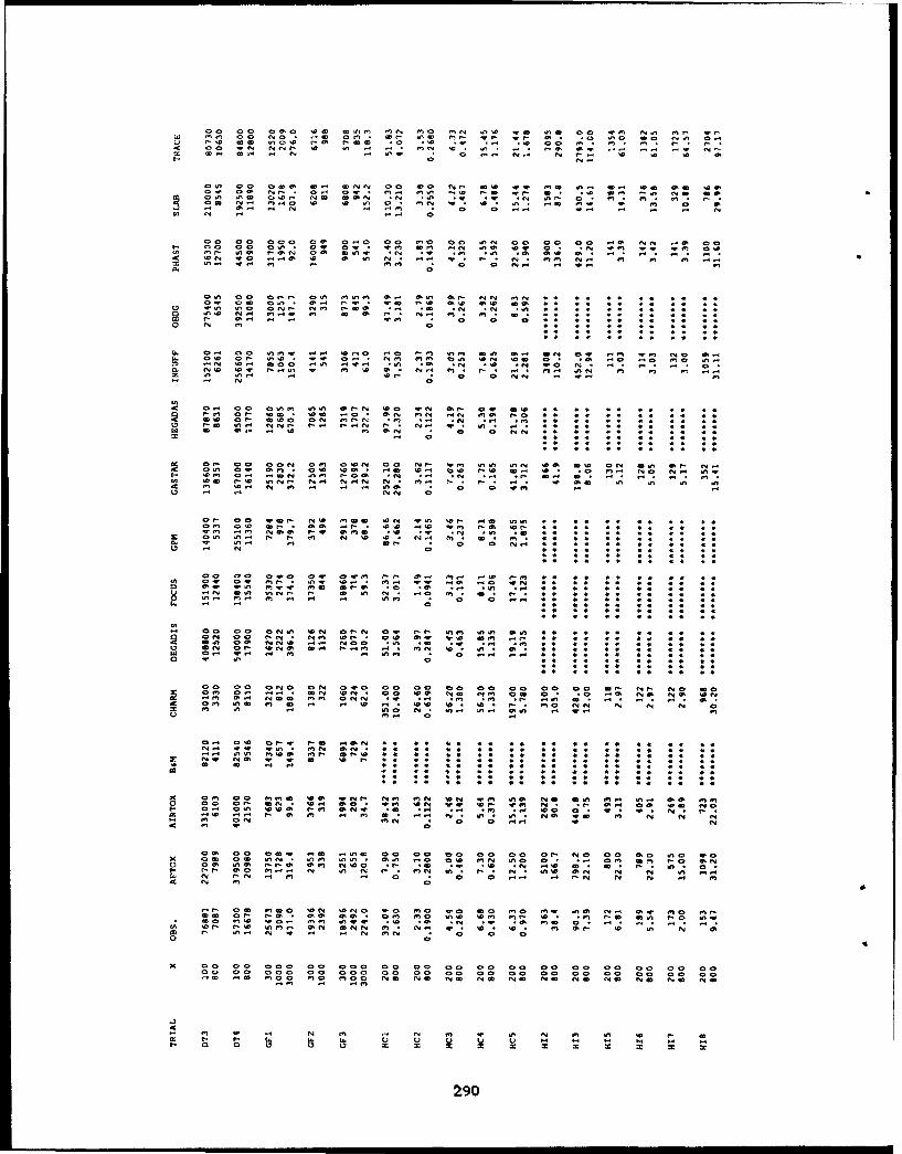
to 00 00 aO 04 On -Or o r O O 0 00 0 O C

C 00 00 0-4 10 1 1 - N '. 0 M 0 * T

W 00z 00 N- 0 * 0 - N. N MO 4 ' 0

0- 0 N.

NO QO~ Nn a0 00 0i cN Ir v

~ CO NO oo - 40 0 n 'p . .4 * 0 r40 - 0

ao N1 "M -- 0W N W ' ýo

a 00 00 0 : 0 00 0 0 aO a . tc 00 Nn"

0.4 00 err4 C4 000 0- 00 r NN nI. . . . . . . .

m 20 .0 .N N. Mo *i SP *N *N N.. . . . . . . . . .

C ~ ~ ~ ~ m o r1 0.0 . 0 * 0 * . . . . .

0 No nt m0W CD. . . . . . . .t

C.. 04 or owc WN g04 0.4 ma Na 000 ma ow *c .0 .0 s0 n

I N P

C0 00 000 Clan a 00 rN We o Or QW aW. . . . . . . . .

mM 04Ca mN ý0M *0d .0 * N 0 .0. 04. . . . . . . . . .N

to ~ L a 00 0x00 O N . . . . .

= 0 04. . . . . . . . .

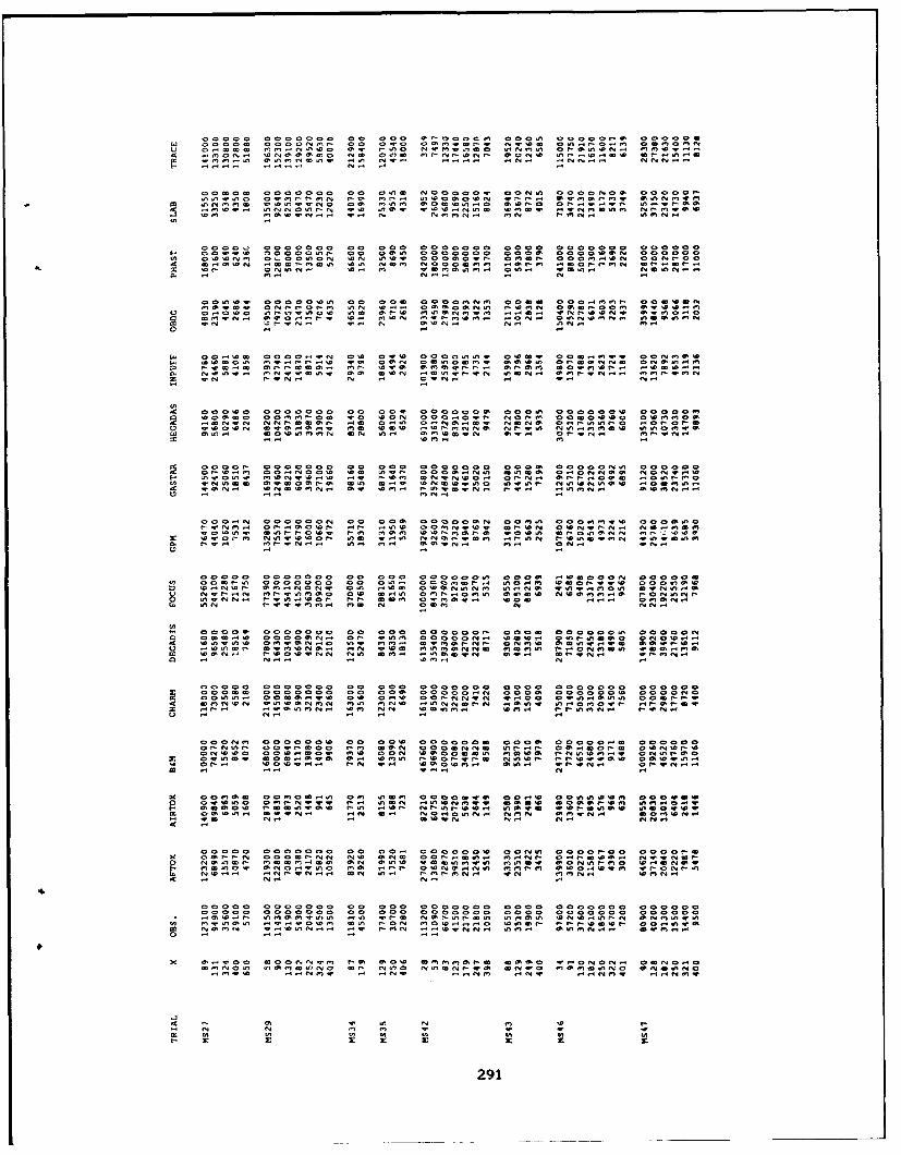
00000 Q000 00 .. 0 00 *f-OO 000.* 0O2C-CS .00000W4 0000: 00...Nr~- 00 0 .0 0S .U - NO- wo .. r04 OUCO

o O fU S C.SN tflfVo NO a-bO W~e N0 CNoa¶ 0 mw .1ON. fC w-b

C .. 0N-4 0 50 9zmOM - ll - ~ -Sf SON'Saw .11,lfU Sf-ýn-4mmmC.* - WNNUO0 ami NM -M NNN.a wl 0- ~ ~ ~ ~ ~ - M~ ,-r..- 4-"i4 NeS .

00000 0000000 00 01*90 oao NO-C 00NS 000000. 0000Cr-

- 0 lo f-C 0019000 0% CCC 000C-00 00090 ooo oa oa reS

C000) 000000 00 000 0000000 0000 30000000 000000

owwn QOON 050 1 0 WN .0:. aoCoSO: f Q09,f 00C-,%N 000f-C

Qo0,510 aooow9 40.5 NUC aa0000CC 00s9r- 540r-mmf- 0f-slf0. - -s-S Ne-5s oc -N Nw ý -m -

O rOlww Snf-I0.JfO ow of-S aoao~-" s-s-s-s ovf-OONO SCom.

Wo - - -o 1 lo lg

AC 00000 0000000 00 009 00OaOoC 0001* 0000 00 000

m- 01 -a,

W -- f- 0 00000 CC 00 w0 0 0 WNS 000000. 000000

OaQ, QO OsOOO ac0 sf0.- OaoCS.-No 5*505 0,-SoNNUS NoNoa

U - - "- f-vw w m Ne- s-b: x m l~

K 0 r- 50440r *0 o.S* wNOmm-WU s-If N f-'0u90fN WC~s

00000 0000000 00 000 oao000 1 a09 0005 I -SOO 00 000000omw 00Sf-SO 00 0 00 0 05*.- OO. f-ef-e .fl ýs- .10f w0 00C -01

NON- -09-40- f-f- . . 00595..-. .0. s-f-fr CC0 -

aaaa oa9 f-a-a- CU N OUC

CUsS aCoSN.-S Of- W.S- oCOOCN -f O',' Off5fS ON:fWsi-i

Li SO~-S f-M 0 0N W" f-s-S s-""SUNN S I Of-ýONrIMfO-MF4 N m54- N- fs-

"00000 000 C 0C CM 000 00 .000 0 0000 000000

0050ao 00 0 0 0 00S 00000.-N COOS, 0000000w oCC N~ ~ ifs4 00 5 40 C'S 0.9w OW-O N .0 Cta.fýl* 000f-f-

o 1 ý -o ~ o Ns4 s-S - o mN -r - ý ý Og w

QC~f 00 0 0 CC 005 00 0 0 000 -WOCCC.4U:m 000000

ft Cof-SO COCO,-fý 0C UOC 000900:: a0rf OzV-mn5fwm 0000fl

00000 0000000 00 00,- 000000%0 0005* 000Cc-CC 00a0Crxt 0Sf-f- OOCa f-NN Nw N 04asl- .S'~- 04-45S O n N r

v N. '0s-N54C

00000 0000000 00 000 0000000 0000 0000000 00000000000 0000000 00 000 0000000 00CC 0000000 000000gm* -sa-f- MaIC Cmz flý If O- N0*9-Cf- -MO wr55 wSNS ,-ffN gom-*9Oý

5S CQ lSI r40- NwOmf SMn f-O f-OO-.s-N-f wownf s-ff-SOw f O ~-S v

x N 4 In0-SUN OW Of- 0ma0 04500 f-fl MNOC Sf- -ONg 0054,00

N 14 m 9 NC 'N m 'Al C %A0

291

000000, 0009- oCoo N- 0000 ,11 C lr-on I_4.- .- bo 00.I nIU 00 40 1 00 00 00 0-c- 0 - mo 09) 1o 0 *. cOOý 0 a 01

4 00 000 00 M .100-0o- N- . I. w. ~ ~ o .4- m to,~ N~0

go-. N4 -00 0 , . 0 w- 0

00 0. 0 CO 0 00 0 000 00 0. w-wI0 a'14- 00..lI N

00. W"00 400 0010 w IMN W.' 0m9 -00 M W N '1 !

.W 0 00 00. .0. . 0 0 0

0 00 N00W 0000 N90 M cc N - 0 N 1'4 C - -I

f. - 00 r-MW 0040 00:0 *MO O **00 *(N:N. *90 0

O ~ ~ ~ ~ ~ ~ ~ I !00 04 . 0 N 00 0 0 0 0 N N t$,0$ 00 * 0 94 '9 .Ao - M

II MN "00M9 N aro r- ;;.-:- a 0 09. -0 1) ! !'0. 0: Ow : 0 t 14 *' -0 0" I - I000 0000 000 0. 000 WNON 000 NN 'C 0 -r . I M 0 0 *0 0r-M M_ 0. ON -N04 O

0 W.0

Cd 00 0 .4 0 0 004 00 0 0 0 .0 rO 00 N 09 N

.- I Ir NI- 0o M

4 000 00 000010 0000 n0 0 0. *P 0 ka 0 000 0ý0 0 A VM:1 2I 0:ý _ oa4 C w

00000. 0000 00000 0000 00000 00000 mg* 0000

w N" 0 0

I4 0 0 0 0 0 0 0 0 0 0 0 0 0 0 0 0 c '1 0 . 0 ' 0 0 0 0 0 '

000-m 0000 Qo4000 a1 0. Mow" ..Ccc OQ4 0. g00 0. .. .0

M -I 00 0N 0000 000000 0000 00000 00 0 0 0 0 0 00 0"0 '00 0 00 0 0 0 No '' I ' '00 10 cc . 0

o5 00000 0000 000000ý 100 00' 00 00I 0 0 0Cd 000.4 0.4 00 0. 100 0 0, ' *a, 00 0 .4

0000 0 00 0 0 0000 0000 .00 0 ' 940 . ..0 .000.. .

000 00 00 000000 0000. . . . . .. *4 *0oo 1i o 7 o a M c o n

Z 040 0 0.0 000000 0000 _4.4. 0 *0 * *0 4* 0 4

o , 0000 00 0000 000 000 0000 00000- 0a oQi 0 000 00

00 00 0000~ 00000 0000w 00000 0oo 0000 00000 00000 00

00 00 0000 000000 0000 M 0 00000 I00000 00000 00000000~M 00 0 0 0 0 0 0 1 10N*' 0 0 . 0 0 ' 0 0~

,4 0 01 0 40 0 00 0 00 0 * 00 00 I N 4 ' 0292'0

C~ ~~~ OC '0 0 9 0 *50C C Cm@a9- * SO C 5 -0 NoN'" 9S

rn~ ~~~~ w4 el *ý! mt. 9 * 0 N o w ... -sowD .

WNMN9 Wf C.. SDNW D SD ',r- Na,-sfS 9 @9CSow 9-.4t CC .- I W 9 N@efl*.909 N D Sdk 9.'fr . 0. C9@ * @ . .- 4fO M @9

M ' S 'N N ~ CC -- *550 0 '80 I ''9 0 '9 0 N

S~~~~~aM~~~~l -N -mm-M4 M9 . 0 .SDO N N * @ 0

09 ~ ~ ~ ~ ~ ~ ~ ~ ~ ~ ~ ~ V g40*N N N - - - N 4*.M4 0 .4, 0 N N

Sfl 0 0o

.480 800 M9.l D9r -Ih'm ose . e o o w o SN0

I- .- S4f 0 4!0 Mo '.99 0*. 0 .. 900 *D W 0495 ~ W9 9,'5f

fl~~~~~~~~~~~~~~~~r 9- : 59 S 5- O** 4 9 OS 0 1 5''0 M*'-CNN~~~~~~ ~~~~ 194 C N'- 5M 949N .N- 9 8 0 ' 9. 85. .00'~~~ o- 0t t O .5r9 4

mo. w"0

9,)0-. 9'0 C 00 544 SD959N NM99- MDSN I--MNM -- 9500 9S I9La 9S- .- lO 90 M 00 4 '~ ,- .5 *-CS .- O

.9 . .N .4 N . . .4 .S . . .- 09 .0 ... .. .40.4 0 . 9 NO

a lo 0 a It w0. l ý v wm

5 *OM C .9,50. a: 't0C 1w 9d" '9-n m- w40 n9 elDM 'N mO 01

r4 ~ o -i a~ .ý e!-5 a o oS m5 w!~ NrSS o SON 'CU 0 a aS4 Mý a c5 a- o a c0 l o - 9 90. M N . ON ' 19SC* O C -S o 01.0 '0 o -r- o SDNSD o0

Z~~~~ ~ ~~~ m O .,.-M * N 0 N 0 N 9S

dc00

N *MS 09o-. "mm. awamS mo r :.- *N N '509 - N S - N0 54N. SN 09 m-9- m. c844. mMS . C- N 0090 CN

03 - 54 M M4M -o94 9-SMo oo *o 4C.-4 9-So .41.5

0 293

000.- N 00 400 n mN4 4,?-4,C t-N. Nw-0-4a0.40mw -0 00%N ( O Nn %*4t

E. 0404 .~ *M arO V004 N 4i44 n O44 M 1!40. .% 1 4.4m,.40 0 0 4 4tr! C,-M on4.4 "- w 44 -: výaý w . : 4- N . ; N 1 N .4! . 4-io

4~I0 4i.N li 1 .0% 1* 1o 1* C: I. i 1 4ýo ýNZ0 It0t4, * 04 M t- w w% w

00 ~ ~ .4,N mrN 0%40,ýw.i lo~ N ,Ime: N C4MO * 7e NNM "-t e .ýN NO4c mN -, ct 4 Ww - M, 4 wo4 0- 0 0 N O. "4_-MO-

It N 0 - 0. 0 V! 4 a It r! NI!N0 0

Nr-0%400M owrrM rC O 0- . 404,40 04N00 N40-t- 40 ,0 C

0O 't -ml *NWN ft *44 tt- 0 0 N rr i .N NC m0 0N * ' .0 0.W 4 . n

o; 0 4

0% . .- 10 -! 0.-1 0a ý1 - 0! lo4-. 1 0 . - 1! Nm, N4c 0

t-.40 0; *_M a40 NN C. w-4 &40 NO * 0, .( N * 4 N0 . 0.

44]~ ~~~~ .-4,..M 1c: 0ý 0 -! 4- M N N v4mt4 4 - 4n -

4 M.'4N Inw 4- =0 (N_: N 4, 9 -. N, N: " In N .4ý .0 N -ý .444 We0a 0

N O.400~ IV0t- 0440 4 0:.44 W N e 0 N O O N M M o d t .40.4 0*4-r4,0 404M(N 440 *4.4 .40 4 4o .0 *ý *.4N .40%N? ý040 04-( *4 NI

W% I 44, 0% . * .040 NN~nt- 4n M0 a 0( 140 0 4.y a 04 _0*40 4 . ( IN 40t I - QO 4. 0%NN M N 4 tNt 44( ((NN ' 00' 1 4

0: Qo 4-ia 0:1!0 0 O* .4 0 4- 0 0 0 N w 0a

0 - 'NM 4, .. 4040 In N m N w1 w ,40 4040, fn 40 .* I 44 *0 4444 4. 0

040 o 7'O 40"Nm .4000 0N44¶4 iio:N 0!4 40 M O N 00(N mg o 4- 040 40440 m4 .40t a.4 0. 4l 40!0(N 0 N N I a 0 Mo w4ýV 4-N m 0

0

"00 00 0N04 4, ý. Q*o 0C- *' O N *'00 * '0:00 400 'N904((N_ ~ ' .00 420N Co. 'ý 0oo0 '40~ 404-ý OO * 0 0 **, N 4 04

0 O N-- 4 0. N t400 N 000 * 0 0 * 00aN.N

M4 C644.4 M- a.4 - 4 4 4-4 - . - 4 -N 40- r

0294

U ' 'I *MI~*0 104 * *IW IO 0 C-IU * 0 N. 1 0 N- "0W

IC l'004 0%-N0 W1't I NM00 M. 0*4NW N S W N.4 o -. !MI *11AL m.1 N1 -m m a Nt w W.N N N - # *44

F-C;

9L CD N: W - N~ -" 0 w *40 w4 0 N 1 .4 N N N 4 0

& 44 -0 - NO * 0 N . -w., Nl *4M - -m 0 O.w *- 0

*4.4'IOo WINIO NNO I' m.4~fl C!40 w*- M-4 0....IM 10.041 N NO

ra 1! . 1 44-. 0 Ilf ** 0 .10 * * 10 .o007 mo *1ý1 ,- **M C *

O ~ M- .. 44I 0: I, -I w 4 4 0 *.I 0 . 0

U. OO1.t- W4N170 '05 11W -100* 401.. OIC 000*4 10e1.. N Mo N

z 1 - : 0- ~ M NO C *4 moo 4-4 - - *1 . at N

0*4 0 - M' .0.4 q4O* *ý WON1 .0 0 *.10 *5* 0SI .0

0 000 ', SIN W ! 00 *0* 00 . 0. SIN 0 *4. *i 01 0* o 0

0)00 1. 0 N N4 N4 o.M-II . - 0 'N 00.

0. *41..4% WWISWI0 t-IW* MI N0 aaaoe. aOOO. MWI'O .- I.4OC gaa400300IC .104- .. *I- * M .r-c-f * **0%.- IQ o *1-0.0 .000% *a , OQOO- * M00

F- * * **0 10 o-N- *ý Q gN -N *W -N*'i 1 M NM ** 0 1*1I 0 *.I

11 *004 *00, 45 0 * 41.4 * ,1*44 M M * 00 % 0 029S*44

4 N ---nO04 .4 04ý 04l_ aNI "N WNW4( ---N

n0.4 . 100 1- n 'n * Vfl * ao) ' 0(W .0140 W . 00 4 4 n(

O4ýN . '1 0.00 0 N N0 ('4 '"WI04 NO 10 (00 * N'-

.- 0404 ' 044 -0 0.0 , -NO M 404W * r(N4 . 0d0 0

03 (404 N I .4 .4 N44 N N a40 0 M - .

N m w 0 1W. -4 ý_ I C 04,0( m0-.40 M-04. fV.4-4 V: 00fl N f.W 0 0( 4r

* 4 0 0 0 rI - - O n . 0. 40 04 0 *t ' 0 * 0li( * . 0 0 ( w 4 0 W *i * s S N We . ' 0

O ' ' N 04 5 05 * 0 -WN *ON N.,*N. 0'M *5m w4 N . 0040(

0)~ ~~~ ~~~~ "w CQ 4 040 4 . .f.4 W (4 N -

La. ~ ~ ~ lw .NNO40 044054 40.44. 0!4( 05004 I00C 7n0040 W40 P- C(. ~ ~ ~ ~ ~ w~ 4040 1! C!4O ON *'4': '0 0 0 O 04 ' 0 S ' 505 0 40l

N0N3 .4~l 0ac .4 M4.44( 0 N: 04 (4 - a

V'''N ~ ~ ~ ~ I 0a * 0 0404 . N .0 N 04 -M *r M00 'N .N * 04

03 l VON i C C ; .4 0 : 4 W 4 N Ný 0:0( It A40 N M.1 0: 0 ;4 P4 ý .4 .1

Sf- 1;nfV WWMO410 W CO.wN .10( N'a44 O tn.4.0 0W.4S W I n I'aNONO

.' 0 .. ...'. NV . V. 4 ( ''...0 ..... ..... ..... .. OV

4 4 041 4

"a'aWW (04eV 404 * "a *400

4V 'NW40 It 0 4-4 *'440 a *0 iW *'

0' oa 04ao M'0 04 04 . 0 !04 02 04ga 0 g4 14 0 ý0 1 n

x Oa0400 04-0040. 0(00040 0.47'00 '~aVN( 900%a0( 0W 00 0WN 04000a12.0.0:0 10 .''aWN 120 ' 0 40040 1 OOQ0 '040.0 ' .000 'ý '04 040

o ''0 (40 *'wW 044N0 a N04 .N. 'V N 4'0 04 . N W * I 'N 404Nw4400

CM 04 0 44 0 00 100 4 .4.I

449L

- 00(04 Nf-00 .440 4(5.5 044400 00..0 0(0040 f-(296440(

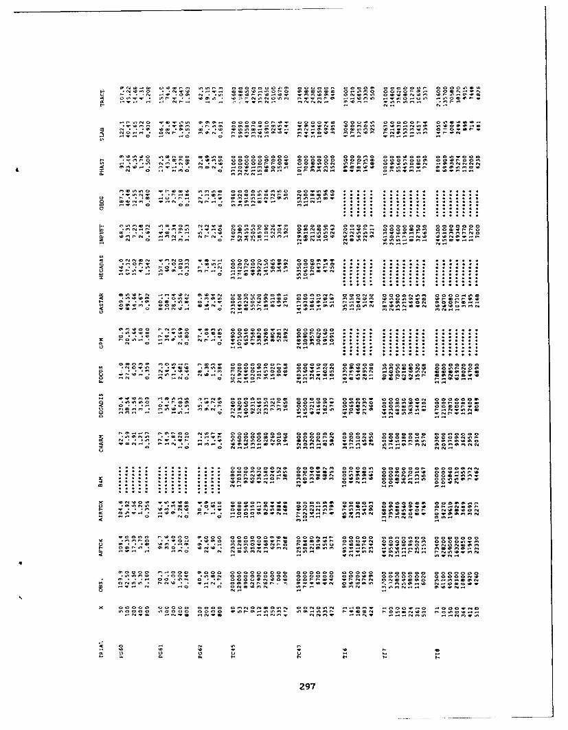
0'NO,0 ~ ~ ~ ~ ~ .. . ... .. ..an ra O a a ~ s' 0 0 cr 0 0 ' c o O r 0 0 0

*.oaa ~ ~ ~ ~ ~ ~ ~ ~ . . . .......- 0 00r. o tn O C NO O a 'C ~ ,N S0 0 0 0

N. .4 .0 .O .0

.S . .0 ..n o ' - ..C .0 0 .0n~ 'O .CCa~ . ~

N~0 0 m- -N. 0 'w C O - a .Oa .ao

0'OtnOoo VO- .0 0 0 0 . 0 0 0 0 0 00000 00000 0000000 OýtnOOOf-C *~~-0 * .r- *O o 000 00w-, 000000 00000 cOQOt-Co 000,-Co

Cr -atJN N -m a

'0000~aO 00 0,V *tae *0C C NC OO r0 OC

CC 00 C.I ON .C Nta . -O .o. a tnC-NM-

0:000 1OOPCON . aoa ota O 00000000O aocOO a 0000C- 0000000 0000000Li. *a.-C- . .0'C, .o Nc oOC-0'00 00N00* OC OW't 0OoOOON OOOitC-r-

00N 00 a OOCt0O 0 C-UeNo-w4a NCo"Q4 N-OmN ~-00 .- C *009:N0

-000aO - OO.0 C00 .C-Nw 0.

S a.-. I297

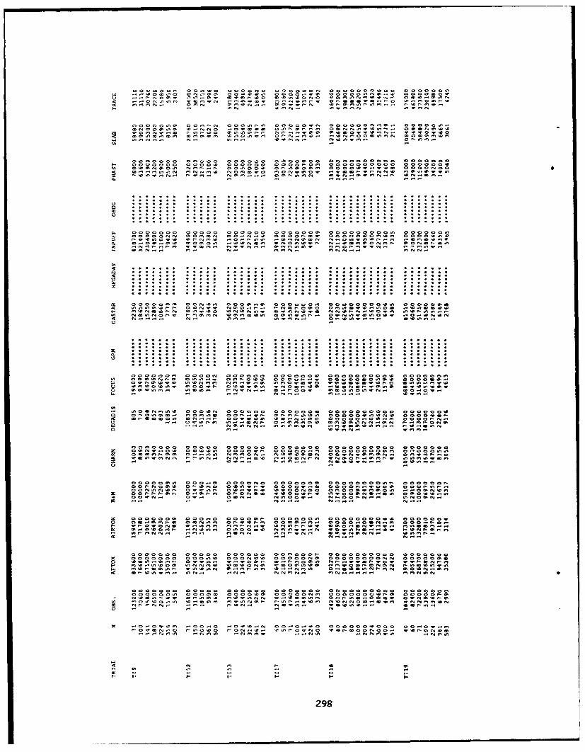
00 0 0 - 0 0 0 0 0 0 00 0 0 0 0 0 0 0 0 0 0

4~ -111000 0 00.400' 004. 0 a, 0~. 1 0 0 04f 0. 0 0 0

U ~~~ -N9I0 w0. 0 Nam-W 'a . oW 0 w0 0 0 ..- 00. 004M" ,- 0 n n r o . .oOX . r I40 r. O -e 0 0 4 ' 0 /. 0

It IN, . 0... .. .4... . 0 r n r 0..-, - W r-.. . . .. . .. .. .~'..0'00 0

0000000Qo 00,1r- a00000. 00000 000000.- 0000

.0044040 -Or O .Oo o0004-0 N0.0p..4. 010000'oag 04-400000

00

4 0~00O0 0140 0 00 0 0.00 . Ofr-00 4 0000 J

ItI

LI 0 00 0 0 00 000 00 0000000 0000000000 0000000

LI. Oooooro ca ... o -.-.. 000NQ0 0gý a 0000400.00 a:00.04

0. 01100401 00000 .4000 . 40 -4 40000m 01 0001-0Q

14-

0.00000 0=0440 00001 00000 0o000000010 0000000ý0wý l WINo0 0 .-m. .0-000.0 0 00 000 4.a 400 0400 044

0 0aoa0roý 0-.00 . 10 000.a. 00000..- 00000000a0 O40,4404

4 a o a oo.-4 000.4 Qaaoooo 000lgagaol 010200..00O.

0

£4 0%O N .oI 04 0.a4-. N V.0 0 00 0 .. ' 00 0 00 1 0 0 00 ~ Nm 00 0 0 1 10 0 0 0 0 0 o ' 0 .0 1 0 0 1 0- 0 . 0

001 01 00 00 .0. 01 00 0 440,- O 40 0r. 00 29800

APPENDIX C-2

THE OBSERVED AND PREDICTED MAXIMUM CONCENTRATION (PPM) FOR THESHORTEST AVERAGING TIME AVAILABLE FOR BURRO, COYOTE, DESERT TORTOISE,

AND HANFORD (CONTINUOUS)

299

00 00 Q0 00 00 00 0000 0000 000 0000 0000 cc 00 4.0 0 00 00 0041 C ON 00C 00 000 000 .

$14 04 N 10 MMNN O * O -. 0 0 * 0. 0 N

-o 0.f 00 oo OO.* oa oa a 04. aa.. 00 .90 0. ON a .- 000 00 9. *M0 Sote " 0 M-.

00 00 00 00 Co 000 10000 0000 CCC .000 0000 0. 0000 Sr1 SO So So a CV 0 00. 00 CaM 000 9.. 000 oN 0

0 , 4 N -0 NO NO - 0 -- -

00 00 00 0o 00 000 0000 0 000 a 00 0 00 0 0 00 044 00 o0 Co 00 00C,0 09 0 0 0 . 40 0

00 SO a N ,M 00 ~ 009M 1 S:O OP . 0 .00. 000 Co.e 00. 4.noC

0M 0 00 00 00 000 f 00m 000 00 000 000 00 --

00 0=4 4.4 co4 04$.co 0000 0400 000 000o Q0a...f 04. 00O 0 3 .0 NO 0 0 a - M. a~4 a.9.0 CO W.9. 0 ~ O

M 0 A a-0Z1 .9 .0 40.9 SO a. 41 SO 04 $40 00$. NN$ #M.9 a-k. ft M- o Me .4 WN N N 0.

00 00 00000 c0 00oo 0000 0000 OoO 0000 0 00009 .00 0 , S0 4.0 a N J e4O Ma aMO M a -M 00 ON SO'A 0.9 0-4 W- N ý N NON 0.0.0 'a.M a04 00 .0 4. NM 00

* ~ ~ ý oN 00w, MNN ftx MP O 4 .00 00 0 .0. O O SO4.0 0 ed 0 fir -4 00O- - N-4

00 0 a0 00 010 00000 0 0 00 00 0000o0000 C. 0$00 CC 0 0 0 O 0 . 0 009 0C 4.. 0 0 00 00

O 04. 0$. 40 Po Z0.9 4.0 00a .00 AO 0 904. 0 0 0W, NO. . . . .- .4.n4 a0 -9 00 N- mf"

oC 00: 00 SO CC0 000: 0000 00,00 000 'a00 000 ON C00 Cr4 09 CM: 04. O 9 000$ '0004 0 No~g 0000 COO3 C 0

NO MO MV If." 00 * MV v::000 0.9;0 WMCOý MCO NO

S N m W a N 4..4 .9 "4 N N4aa ''

O0 00 00 00 00 000 0000 0000 000 00000000 00 000~ ~~~~ 00 00 00 0 0 0 00 000 00 0 00 0. 9 M 0

04.0 -0. 00 .0 04. ow".4 :=:2M O . 0 ' . 09 M

a o e4 a- 3ON3 0. 0 9 0 Mg 0 00 l O - W .9 0.9

.. 0 00 CO 00 ' 00 00 aC 0000 00000 000 08 00 00,0.00 002 C0a 00o 00 0 0 00 a M 0004 000 00. 00X 00 N

CO 00 Ca 0 * 100 00 0 0:0001 00.0.0- 4, o 00 0000 0000 00 0000 00 00 00 0 0 o0 0 0 000 00 000 000 . 00

U N N NO NO .90 N4. ON 04 0

0~~0.. 00 090 9. .0 04 p4 MO 49. 0 0

0O 00 0 0 00 . 0 CON 004 000 .90.9- 0 -0..4 N Cg . 0-0 00 4.0 00 M O 0 0 0 0 ... M 0:290 Or., 4X.0.:

4 ~ ~ ~ ~ ~ C M4 .94 00 NfNtN 0f N n N 0

00 100 a 00 0 0 00 0aS a00 0000 0000 000 00 00 0000 ON 00.90 NO 00 00 00 00. M C N M 000 W.00 0 0 O 000CA 0 00 Z N 004 00 a9 0 Af o 00$ wON 1 . A M 0.9a

O r. OM M 00 ON 0040 0000 2 - w o 9N '" O '* 00 .9 0 a-4. 00 0* 00N0 Am 0 N0 P40 00- 000 MOMO 0 NO

00CC 00 00 00 000 00 0 00 0 000, 0000 0000 00 :00" M0 0 0 0 fi 0 O.w P P M 0.400 02 .00 N0 -f 9. 0 0 0.9 0 0 0 n0

* 0 l 00 00 40 ý040 P.000 0000 04.0 P4oMo 0000 NO 00

04. N~ MO f

0 ca40 0

N M M MO P. M MO M CC CC 0 0 0 00 0003C00

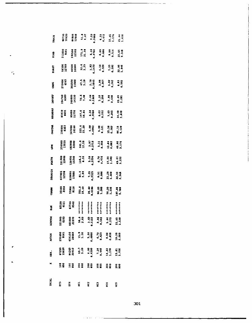
00ý 00 1- MC M S. *

3C Ca 3 , '! 3 *i;: *NA 9 e n C Me . n

0*0

N~ N

00 CC0 CM aC 00wN

00 CC M N m .M C4 in wa M ve e . . ~ *

V4 C M -

ni 41. ow " C mo "ft-

NO N. C! NM 0 M*

0- CMop.,4n Si, -

0- OM N

C. C r . . C M . . C

00 0 0M

4 M Cii 0n . i * , *

M CM N. iC C0, 1. 1. 00 .C, -41 0

CO 0 44 '40 P4 aN C..

CM Ca *V S..i ion C CCC SC ii .u

3 CM e. C. MN Sn * N301

APPENDIX C-3

THE OBSERVED AND PREDICTED CLOUD-WIDTHS (a.) (M)

302

TRIAL x OBS. AFTOX AIRTOX DEGADIS GASTAR GPM HEGADAS PHAST SLAB

BU3 57 20.0 4.7 20.3 23.7 30.2 7.2 34.1 17.5 19.5

BU4 57 14.9 3.0 15.9 18.5 23.0 6.4 23.6 7.2 14.5

BUS 57 13.2 4.1 17.0 19.7 24.6 7.0 26.5 12.1 15.0140 10.1 9.0 24.0 28.6 31.9 13.6 36.2 14.9 21.4

BU6 140 20.3 6.3 20.4 26.6 29.1 12.2 32.3 15.0 19.5

BU? 140 20.9 7.2 23.1 30.2 33.8 10.6 35.2 21,1 21.2

BUS 57 27.1 2.1 35.7 41.7 33.1 7.8 112.6 44.0 81.2400 84.2 11.4 120.4 139.9 190.5 21.1 185.6 112.0 134.2

BU9 57 22.1 1.8 19.1 28.3 33.7 6.1 42.5 17.7 21.8140 26.7 3.7 29.4 42.3 52.6 10.0 53.6 33.4 31.3400 44.6 9.3 52.8 67.9 77.8 22.3 89.0 62.3 51.7800 57.1 17.1 76.7 87.1 84.5 40.5 118.7 66.3 73.5

CO3 140 23.5 6.1 24.8 38.3 45.0 12.0 48.1 30.4 28.0

C06 140 15.4 6.3 30.6 46.1 55.7 10.6 64.0 37.0 39.0200 17.1 8.6 36.4 53.7 64.8 13.7 71.7 43.9 45.1

DTI 100 11.8 4.8 14.4 41.3 27.5 6.9 74.2 12.0 16.6800 61.8 30.5 52.7 169.9 167.5 42.7 202.2 89.2 69.1

DT2 100 14.7 5.5 22.1 57.3 26.5 8.3 97.2 13.9 20.7800 88.2 35.0 76.3 255.4 213.5 49.3 288.8 116.8 93.6

DT3 100 15.2 5.7 18.9 46.8 23.5 7.8 86.8 12.7 16.8800 73.4 36.1 57.4 202.4 175.2 46.6 236.4 103.3 81.3

DT4 100 15.7 4.4 26.3 70.8 32.5 7.5 110.9 14.8 25.5800 86.0 28.0 103.8 335.9 327.5 42.4 353.1 132.4 112.0

GFI 300 25.1 13.2 20.1 57.6 55.5 17.3 69.8 41.0 25.01000 63.0 38.8 70.1 96.5 96.6 53.1 124.0 88.3 57.03000 113.9 104.1 204.6 153.6 174.0 144.4 219.7 160.4 128.2

GF2 300 29.9 18.4 20.0 55.9 59.2 17.0 65.0 42.5 24.61000 54.7 54.2 70.0 93.6 98.4 52.8 117.8 81.3 57.6

GF3 300 25.1 13.2 21.5 41.0 35.1 16.9 52.6 32.2 20.51000 49.8 38.8 74.0 68.2 66.1 52.7 95.0 54.2 48.93000 75.2 104.1 208.5 138.8 150.6 144.1 195.1 170.2 112.8

HC1 200 15.6 15.9 7.9 7.6 7.5 7.6 11.9 6.1 6.3800 70.7 54.9 30.8 26.2 29.1 29.3 37.6 19.0 23.4

303

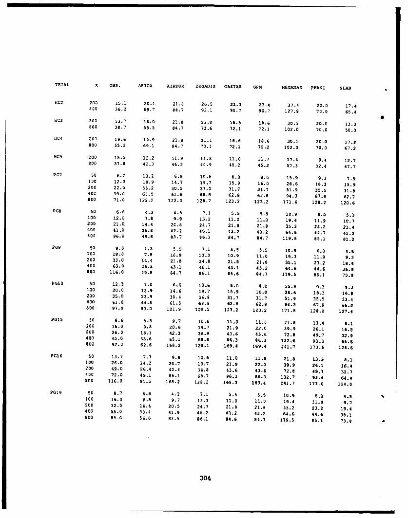
TRIAL X OBS. AFTOX AIRTOX DEGADIS GASTAR GPM HEGADAS PHAST SLAB

HC2 200 15.1 20.1 21.8 26.5 23.3 23.4 37.4 20.0 17.4Boo 36.2 69.7 84.7 92.1 90.7 90.7 127.8 70.0 65.4

HC3 200 13.7 16.0 21.8 21.0 18.5 18.6 30.1 20.0 13.3Soo 38.7 55.5 84.7 73.6 72.1 72.1 102.0 70.0 50.3

HC4 200 19.6 19.9 21.8 21.1 18.6 18.6 30.1 20.0 17.8800 55.2 69.1 84.7 73.1 72.1 72.2 102.0 70.0 67.2

HC5 200 15.5 12.2 11.9 11.8 11.6 11.7 17.4 9.4 12.7800 37.8 42.3 46.2 40.9 45.2 45.2 57.5 32.4 47.7

PG7 50 6.2 10.2 6.8 10.6 8.0 8.0 15.9 9.3 7.9100 12.0 18.9 14.7 19.7 15.9 16.0 28.6 18.3 15.9200 22.0 35.2 30.5 37.0 31.7 31.7 51.9 35.5 31.8400 39.0 65.5 61.6 68.8 62.8 62.8 94.3 67.9 62.7800 71.0 122.2 122.0 128.7 123.2 123.2 171.6 128.2 120.6

PG8 50 6.6 4.3 4.5 7.1 5.5 5.5 10.9 6.0 5.3100 12.0 7.8 9.9 13.2 11.0 11.0 19.4 11.9 10.7200 21.0 14.4 20.8 24.7 21.8 21.8 35.2 23.2 21.4400 41.0 26.8 42.2 46.1 43.2 43.2 64.6 44.7 42.2800 86.0 49.8 83.7 86.1 84.7 84.7 119.6 85.1 81.2

PG9 50 9.0 4.3 5.5 7.1 5.5 5.5 10.9 6.0 4.6100 18.0 7.8 10.9 13.3 10.9 11.0 19.3 11.9 9.3200 33.0 14.4 21.8 24.8 21.8 21.8 35.1 23.2 18.6400 63.0 26.8 43.1 46.1 43.1 43.2 64.6 44.6 36.8800 116.0 49.8 84.7 86.1 84.6 84.7 119.5 85.1 70.8

PG1o 50 12.3 7.0 6.6 10.6 8.0 8.0 15.9 9.3 8.3100 20.0 12.9 14.6 19.7 15.9 16.0 28.6 18.3 16.8200 35.0 23.9 30.4 36.8 31.7 31.7 51.9 35.5 33.4400 61.0 44.5 61.5 68.8 62.8 62.8 94.3 67.9 66.0800 97.0 83.0 121.9 128.5 123.2 123.2 171.6 128.2 127.4

PG15 50 8.6 5.3 9.7 10.6 11.0 11.0 21.8 13.4 8.1100 16.0 9.8 20.6 19.7 21.9 22.0 39.9 26.1 16.5200 26.0 18.1 42.3 36.9 43.6 43.6 72.8 49.7 32.9400 45.0 33.6 85.1 68.8 86.3 86.3 132.6 93.3 64.6800 92.0 62.6 168.2 128.1 169.4 169.4 241.7 173.6 124.6

PG16 50 13.7 7.7 9.8 10.6 11.0 11.0 21.8 13.5 8.1100 26.0 14.2 20.7 19.7 21.9 22.0 39.9 26.1 16.4200 49.0 26.4 42.4 36.8 43.6 43.6 72.8 49.7 32.7400 72.0 49.1 85.1 68.7 86.3 86.3 132.7 93.4 64.4800 116.0 91.5 168.2 128.2 169.3 169.4 241.7 173.6 124.0

PG19 50 8.7 4.8 4.2 7.1 5.5 5.5 10.9 6.0 4.8100 16.0 8.8 9.7 13.3 11.0 11.0 19.4 11.9 9.7200 32.0 16.4 20.5 24.7 21.8 21.8 35.2 23.2 19.4400 55.0 30.4 41.9 46.2 43.2 43.2 64.6 44.6 38.1800 85.0 56.6 83.5 86.1 84.6 84.7 119.5 85.1 73.8

304

TRIAL X OBS. AFTOX AIRTOX DEGADIS GASTAR GPM HEGADAS PHAST SLAB

PG20 50 7.9 4.0 4.0 4.6 4.0 4.0 7.6 3.9 4.5100 14.0 7.4 7.9 8.6 8.0 8.0 13.0 7.7 9.2200 27.0 13.7 15.8 16.0 15.9 15.9 23.1 15.1 18.3400 49.0 25.4 31.4 29.8 31.4 31.4 42.1 29.2 36.0Boo 90.0 47.2 61.6 55.7 61.6 61.6 77.8 55.8 69.5

PG25 50 16.2 10.0 10.0 10.6 11.1 11.0 21.8 13.5 7.2100 36.0 18.5 20.9 19.7 22.0 22.0 39.9 26.1 14.6200 72.0 34.3 42.6 36.9 43.6 43.6 72.8 49.7 29.1400 134.0 64.0 85.3 68.9 86.3 86.3 132.1 93.4 51.3800 214.0 119.3 168.4 128.7 169.3 169.4 241.7 173.7 110.3

PG43 50 10.5 5.1 4.5 7.1 5.5 5.5 10.9 6.0 5.6100 21.0 9.3 9.9 13.3 11.0 11.0 19.4 11.9 11.4200 40.0 17.2 20.8 24.7 21.8 21.8 35.2 23.2 22.7400 89.0 32.0 42.1 46.1 43.1 43.2 64.6 44.7 44.6800 200.0 59.6 83.7 86.1 84.7 84.7 119.6 85.1 86.4

PG44 50 11.4 5.3 4.3 7.1 5.5 5.5 10.9 6.0 5.1100 22.0 9.7 9.7 13.2 11.0 11.0 19.4 11.9 10.4200 43.0 17.9 20.6 24.7 21.8 21.8 35.2 23.2 20.7400 73.0 33.3 42.0 46.1 43.2 43.2 64.6 44.7 40.6800 126.0 62.1 83.6 86.0 84.7 84.7 119.5 85.1 78.8

PG49 50 8.9 4.9 4.1 7.1 5.5 5.5 10.9 6.0 5.2100 17.0 9.1 9.6 13.2 10.9 11.0 19.3 11.9 10.5200 35.0 16.8 20.4 24.7 21.8 21.8 35.1 23.2 21.0400 72.0 31.2 41.8 46.1 43.2 43.2 64.6 44.7 41.4800 118.0 58.1 83.4 86.1 84.7 84.7 119.5 85.1 80.0

PG50 50 8.2 4.5 4.0 '.1 5.5 5.5 10.9 6.0 4.6100 15.0 8.3 9.5 13.3 10.9 11.0 19.3 11.9 9.4200 28.0 15.4 20.4 24.8 21.8 21.8 35.1 23.2 18.7400 55.0 28.6 41.7 46.1 43.1 43.2 64.6 44.7 36.9800 115.0 53.2 83.3 86.2 84.7 84.7 119.5 85.1 71.3

PG51 50 9.6 4.5 3.0 4.6 4.0 4.0 7.7 3.9 4.8100 18.0 8.2 7.0 8.6 8.0 8.0 13.1 7.7 9.6200 32.0 15.2 14.9 16.0 15.9 15.9 23.2 15.1 19.2400 60.0 28.3 30.5 29.8 31.4 31.4 42.2 29.2 37.7800 77.0 52.7 60.7 55.8 61.5 61.6 77.9 55.8 73.0

PG61 50 10.4 4.6 4.0 4.6 4.0 4.0 7.6 3.9 4.4100 19.0 8.4 8.0 8.6 8.0 8.0 13.0 7.7 8.9200 35.0 15.5 15.8 16.0 15.9 15.9 23.1 15.1 17.8400 65.0 28.8 91.4 29.9 31.4 31.4 42.2 29.2 34.9800 109.0 53.7 61.6 55.8 61.5 61.6 77.8 55.8 67.3

305

APPENDIX D

TABULATION OF THE PERFORMANCE MEASURES AND THE RESULTS OF CONFIDENCE

LIMITS ANALYSIS

3

306

APPENDIX D-1

THE PERFORMANCE MEASURES FOR THE PREDICTED CONCENTRATIONS FOR THE

CONTINUOUS DENSE GAS RELEASES (BURRO, COYOTE, DESERT TORTOISE,

GOLDFISH, MAPLIN SANDS, AND THORNEY ISLAND), INCLUDING ALL DOWNWIND

DISTANCES. THE SHORTEST AVAILABLE AVERAGING TIME WAS USED.

307

PERFORMANCE MEASURES FOR CONCENTRATIONS FOR CONTINUOUS DENSE GAS RELEASES(BURRO, COYOTE, DESERT TORTOISE, GOLDFISH, MAPLIN SANDS, THORNEY ISLAND),SHORT AVERAGING TIME, ALL X'S.

All observations, (N- 124)model mean sigma bias vg fa2 mqOBS. 10.44 1.25 0.00 1.00 1.000 l.CocAFTOX 10.35 1.70 0.10 1.78 0.661 1.100AIRTOX 9.48 2.13 0.96 17.68 0.242 2.623B&M 10.36 1.62 0.08 1.53 0.742 1.087CHARM 10.05 1.71 0.40 2.49 0.613 1.485DEGADIS 10.83 1.66 -0.39 1.84 0.629 0.677FOCUS 11.19 1.99 -0.75 6.51 0.419 0.474GPM 10.07 1.64 0.37 2.14 0.524 1.450GASTAR 10.60 1.41 -0.16 1.28 0.815 0.856HEGADAS 10.59 1.60 -0.15 1.58 0.742 0.862INPUFF 9.47 1.58 0.97 4.63 0.242 2.628OBDG 9.54 1.82 0.90 4.98 0.290 2.468PHAST 10.58 1.72 -0.13 2.14 0.492 0.874SLAB 10.10 1.41 0.34 1.68 0.702 1.408TRACE 10.47 1.47 -0.03 2.35 0.581 0.973

Block 1: BURRO (N- 21)model mean sigma bias V9 fa2 mnOS. 11.38 0.85 0.00 1.00 1.000 1.000AFTOX 12.13 0.93 -0.75 2.56 0.476 0.471AIRTOX 12.02 0.83 -0.64 2.08 0.571 0.530B&M 11.53 1.47 -0.15 1.95 0.667 0.857CHARM 11.68 1.12 -0.30 1.44 0.762 0.744DEGADUS 12.29 1.03 -0.91 2.91 0.238 0.401FOCUS 12.90 1.22 -1.52 15.81 0.238 0.219GPM 11.64 0.92 -0.26 1.47 0.810 0.771GASTAR 11.72 0.69 -0.34 1.49 0.810 0.712HEGADAS 12.11 1.09 -0.73 2.41 0.476 0.481INPUFF 11.01 1.06 0.37 1.77 0.476 1.451OBDG 11.30 1.32 0.08 1.61 0.762 1.081PHAST 12.06 1.08 -0.68 2.31 0.476 0.505SLAB 11.45 0.88 -0.07 1.31 0.857 0.931TRACE 11.75 0.60 -0.37 1.59 0.667 0.689

Block 2: COYOTE (N- 11)model mean sigma bias vg fa2 mgOBS. 10.89 0.64 0.00 1.00 1.000 1.000AFTOX 11.44 0.66 -0.56 1.46 0.727 0.574AIRTOX 11.23 1.10 -0.34 2.39 0.182 0.712B&M 10.75 0.71 0.13 1.10 1.000 1.141CHARM 10.97 0.62 -0.08 1.03 1.000 0.919DEGADIS 11.69 0.60 -0.80 2.08 0.273 0.447FOCUS 12.54 1.02 -1.66 42.16 0.091 0.190GPM 10.70 0.75 0.18 1.27 0.818 1.203GASTAR 11.48 0.57 -0.59 1.72 0.455 0.554HEGADAS 11.15 0.95 -0.27 1.38 0.636 0.764INPUFF 9.96 0.88 0.93 3.32 0.455 2.527OBDG 10.18 1.01 0.70 2.49 0.364 2.019PHAST 11.23 1.15 -0.35 2.37 0.182 0.705SLAB 10.95 0.72 -0.07 1.19 0.909 0.936TRACE 12.13 0.36 -1.24 6.40 0.273 0.288

Block 3: DESERT TORTOISE (N- 8)model mean sigma bias vq fa2 nqOBS. 10.53 0.87 0.00 1.00 1.000 1.000AFTOX 11.01 1.62 -0.48 2.34 0.500 0.619AIRTOX 10.83 1.97 -0.30 3.91 0.125 0.743SAM 9.84 1.48 0.69 2.39 0.500 1.985 hCHARM 9.30 1.13 1.23 5.34 0.125 3.429DEGADIS 11.17 1.77 -0.65 3.51 0.500 0.524FOCUS 10.63 1.23 -0.10 1.20 0.875 0.902GPM 11.07 1.53 -0.54 2.20 0.500 0.583GASTAR 10.59 1.35 -0.07 1.39 0.750 0.936HEGADAS 10.22 1.14 0.30 1.20 1.000 1.354INPUFF 10.43 1.63 0.10 1.87 0.500 1.102OBDG 10.89 1.83 -0.36 3.19 0.250 0.700PHAST 10.06 0.77 0.47 1.30 0.875 1.601SLAB 10.65 1.51 -0.12 1.56 0.625 0.887TRACE 10.22 1.02 0.31 3.14 1.000 1.361

308

PERFORMANCE MEASURES FOR CONCENTRATIONS FOR CONTINUOUS DENSE GAS RELEASES(BURRO, COYOTE, DESERT TORTOISE, GOLDFISH, MAPLIN SANDS, THORNEY ISLAND),

SHORT AVERAGING TIME. ALL X'S.

Block 4: GOLDFISH (N- 8)model mean sigma bias vq fa2 mgOBS. 8.11 1.66 0.00 1.00 1.000 1.000AFTOX 7.05 1.50 1.06 4.44 0.500 2.897AIRTOX 6.30 1.74 1.81 31.25 0.000 6.112B&M 7.06 1.79 1.06 3.30 0.125 2.884CHARM 6.19 1.20 1.92 64.75 0.000 6.855DEGADIS 7.52 1.53 0.59 1.55 0.500 1.812FOCUS 7.56 2.18 0.56 1.95 0.500 1.750GPM 6.70 1.50 1.42 8.48 0.000 4.135GASTAR 7.75 1.73 0.37 1.23 0.875 1.447HEGADAS 7.75 1.19 0.36 1.51 0.750 1.440INPUFF 6.72 1.58 1.40 7.65 0.000 4.044OBDG 6.98 1.70 1.13 4.46 0.125 3.097PHAST 7.31 2.20 0.81 2.77 0.500 2.239SLAB 7.30 1.53 0.82 2.08 0.500 2.268TRACE 7.31 1.52 0.80 2.05 0.375 2.226

Block 5: MAPLIN SANDS, LNG (N- 17)model mean sigma bias vg fa2 mqOBS. 10.66 0.88 0.00 1.00 1.000 1.000AFTOX 10.37 1.06 0.29 1.27 0.824 1.331AIRTOX 8.53 1.54 2.13 244.60 0.118 8.396B&M 10.22 1.09 0.44 1.47 0.706 1.554CHARM 10.49 1.29 0.17 1.51 0.765 1.185DEGADIS 10.86 0.94 -0.21 1.16 0.941 0.814FOCUS 12.13 1.29 -1.47 22.67 0.176 0.230GPM 9.96 1.02 0.70 1.89 0.471 2.021GASTAR 10.73 0.85 -0.07 1.11 1.000 0.929HEGADAS 10.35 1.14 0.30 1.67 0.765 1.357INPUFF 9.36 1.02 1.30 6.30 0.059 3.677OBDG 9.50 1.33 1.16 6.05 0.235 3.198PHAST 9.99 1.39 0.67 2.43 0.353 1.950SLAB 9.90 1.16 0.75 2.72 0.412 2.126TRACE 11.48 0.64 -0.82 2.79 0.471 0.441

Block 6: MAPLIN SANDS, LPG (N- 44)model mean sigma bias vq fa2 mgOBS. 10.34 0.87 0.00 1.00 1.000 1.000AFTOX 9.89 1.21 0.45 1.66 0.614 1.575AIRTOX 8.58 1.49 1.76 48.56 0.136 5.825B&M 10.49 1.15 -0.15 1.36 0.795 0.857CHARM 9.96 1.28 0.38 2.02 0.659 1.460DEGADIS 10.56 1.31 -0.22 1.54 0.795 0.806FOCUS 10.59 1.65 -0.25 4.34 0.477 0.780GPM 9.54 1.19 0.80 2.54 0.364 2.233GASTAR 10.45 1.06 -0.11 1.21 0.818 0.892HEGADAS 10.58 1.27 -0.24 1.50 0.773 0 145INPUFF 8.89 1.17 1.45 10.72 0.091 4.254OBDG 9.15 1.38 1.19 7.30 0.205 3.297PHAST 10.46 1.35 -0.12 1.64 0.636 0.888SLAB 9.82 0.88 0.52 1.80 0.727 1.688TRACE 9.84 0.83 0.50 2.47 0.636 1.651

Block 7: THORNEY ISLAND (N- 15)model mean sigma bias Vg fa2 mgOBS. 10.04 1.46 0.00 1.00 1.000 1.000* AFTOX 9.76 1.31 0.29 1.18 1.000 1.331AIRTOX 9.32 1.28 0.72 6.68 0.467 2.060B&N 10.21 1.44 -0.17 1.07 1.000 0.843CHARM 9.28 0.85 0.76 3.80 0.400 2.137DEGADIS 10.50 1.53 -0.46 1.92 0.733 0.629FOCUS 10.72 1.28 -0.67 1.78 0.733 0.509GPM 10.37 1.24 -0.32 1.76 0.733 0.723GASTAR 10.16 1.34 -0.12 1.14 0.867 0.884HEGADAS 10.04 1.75 0.00 1.23 0.933 1.001INPUFF 9.77 1.17 0.27 1.70 0.400 1.306OBDG 8.43 1.57 1.61 14.07 0.000 5.019PHAST 11.03 1.21 -0.99 3.86 0.267 0.371SLAB 9.83 0.99 0.21 1.33 0.733 1.239TRACE 9.97 0.81 0.08 2.21 0.533 1.078

309

APPENDIX D-2

THE PERFORMANCE MEASURES FOR THE PREDICTED CONCENTRATIONS FOR THECONTINUOUS DENSE GAS RELEASES (BURRO, COYOTE, DESERT TORTOISE,

GOLDFISH, MAPLIN SANDS, AND THORNEY ISLAND), INCLUDING ALL DOWNWINDDISTANCES. THE LONGEST AVAILABLE AVERAGING TIME WAS USED.

A3

310

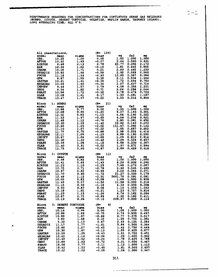
PERFORMANCE MEASURES FOR CONCENTRATIONS FOR CONTINUOUS DENSE GAS RELEASES(BURRO, COYOTE, DESERT TORTOISE, GOLDFISH, MAPLZN SANDS, THORNEY ISLAND),

LONG AVERAGING TIME, ALL X'S.

All observations, (N- 124)model mean sigma bias V9 fa2 mqOBS. 10.25 1.20 0.00 1.00 1.000 1.000AFTOX 10.32 1.69 -0.07 2.44 0.540 0.931AIRTOX 9.48 2.13 0.78 22.77 0.202 2.172B&M 10.36 1.62 -0.10 1.81 0.645 0.900CHARM 10.05 1.71 0.21 2.93 0.492 1.230DEGADIS 10.83 1.66 -0.58 2.92 0.589 0.560FOCUS 11.18 1.99 -0.93 13.60 0.387 0.396GPM 9.87 1.55 0.38 2.11 0.556 1.464GASTAR 10.61 1.41 -0.35 1.72 0.694 0.703HEGADAS 10.59 1.60 -0.34 2.07 0.637 0.714INPUFF 9.46 1.57 0.79 4.08 0.355 2.201OBDG 9.54 1.82 0.71 5.04 0.298 2.044PHAST 10.58 1.72 -0.32 2.78 0.476 0.724SLAB 10.08 1.41 0.17 1.93 0.581 1.187TRACE 10.47 1.47 -0.22 3.53 0.516 0.806

Block 1: BURRO (Nm 21)model mean sigma bias vg fa2 mgOBS. 10.88 0.77 0.00 1.00 1.000 1.000AFTOX 12.08 0.95 -1.20 6.27 0.143 0.301AIRTOX 12.02 0.83 -1.13 4.86 0.190 0.322B&M 11.53 1.47 -0.65 4.06 0.238 0.521CHARM 11.68 1.12 -0.79 2.80 0.381 0.452DEGADIS 12.30 1.03 -1.42 10.92 0.143 0.242FOCUS 12.90 1.20 -2.02 111.47 0.095 0.133GPM 11.10 1.07 -0.22 1.55 0.857 0.802GASTAR 11.76 0.70 -0.88 2.98 0.333 0.416HEGADAS 12.11 1.09 -1.23 6.89 0.190 0.292INPUFF 10.97 1.06 -0.09 1.49 0.810 0.914OBDG 11.30 1.32 -0.42 2.29 0.524 0.657PHAST 12.06 1.08 -1.18 6.58 0.333 0.307SLAB 11.40 0.91 -0.52 1.97 0.571 0.594TRACE 11.75 0.60 -0.87 2.89 0.429 0.418

Block 2: COYOTE (N- 11)model mean sigma bias vg fa2 mqOBS. 9.98 0.82 0.00 1.00 1.000 1.000AFTOX 11.41 0.68 -1.43 8.29 0.000 0.240AIRTOX 11.23 1.10 -1.25 7.05 0.273 0.287BAM 10.75 0.71 -0.78 2.40 0.545 0.460CHARM 10.97 0.62 -0.99 3.24 0.364 0.371DEGADIS 11.70 0.60 -1.72 21.27 0.000 0.179FOCUS 12.49 1.12 -2.51 3661.70 0.091 0.081GPM 10.05 0.83 -0.08 1.09 1.000 0.928GASTAR 11.49 0.57 -1.52 11.58 0.000 0.219HEGADAS 11.15 0.95 -1.18 4.33 0.000 0.308INPUFF 9.93 0.87 0.05 1.14 1.000 1.053OBDG 10.18 1.01 -0.21 1.23 0.727 0.814PHAST 11.23 1.15 -1.26 6.76 0.182 0.284SLAB 10.87 0.75 -0.89 2.32 0.182 0.411TRACE 12.13 0.36 -2.15 208.97 0.000 0.116

Block 3: DESERT TORTOISE (N- 8)model mean sigma bias vq fa2 MCOBS. 10.16 0.96 0.00 1.00 1.000 1.000AFTOX 10.86 1.64 -0.70 2.74 0.500 0.497AIRTOX 10.83 1.97 -0.66 4.77 0.375 0.517B&M 9.84 1.48 0.32 1.55 0.750 1.381CHARM 9.30 1.13 0.87 2.45 0.125 2.384DEGADIS 11.17 1.77 -1.01 5.86 0.500 0.364FOCUS 10.60 1.27 -0.43 1.42 0.750 0.649GPM 10.30 1.67 -0.13 1.85 0.625 0.877GASTAR 10.59 1.35 -0.43 1.51 0.750 0.651HEGADAS 10.22 1.14 -0.06 1.09 1.000 0.942INPUFF 10.40 1.62 -0.24 1.78 0.625 0.788OBDG 10.89 1.83 -0.72 4.01 0.500 0.487PRAST 10.06 0.77 0.11 1.12 1.000 1.113SLAB 10.62 1.53 -0.45 1.81 0.500 0.637TRACE 10.22 1.02 -0.05 1.06 1.000 0.947

311

PERFORMANCE MEASURES FOR CONCENTRATIONS FOR CONTINUOUS DENSE GAS RELEASES(BURRO, COYOTE. DESERT TORTOISE, GOLDFISH, MAPLIN SANDS, THORNEY ISLAND),

LONG AVERAGING TIME, ALL X'S.

Block 4: GOLDFISH (N- 8)model mean sigma bias vq fa2 mgOBS. 8.11 1.66 0.00 1.00 1.000 1.000AFTOX 7.05 1.50 1.06 4.44 0.500 2.897AIRTOX 6.30 1.74 1.81 31.25 0.000 6.112B&M 7.06 1.79 1.06 3.30 0.125 2.884 &CHARM 6.19 1.20 1.92 64.75 0.000 6.855DEGADIS 7.52 1.53 0.59 1.55 0.500 1.812FOCUS 7.56 2.18 0.56 1.95 0.500 1.750GPM 6.70 1.50 1.42 8.48 0.000 4.135GASTAR 7.75 1.73 0.37 1.23 0.875 1.447HEGADAS 7.75 1.19 0.36 1.51 0.750 1.440INPUFF 6.72 1.58 1.40 7.65 0.000 4.044OBDG 6.98 1.70 1.13 4.46 0.125 3.097PHAST 7.31 2.20 0.81 2.77 0.500 2.239SLAB 7.30 1.53 0.82 2.08 0.500 2.268TRACZ 7.31 1.52 0.80 2.05 0.375 2.226

Block 5: MAPLIN SANDS, LNG (N- 17)model mean sigma bias vq fa2 mqOBS. 10.66 0.88 0.00 1.00 1.000 1.000AFTOX 10.37 1.06 0.29 1.27 0.824 1.331AIRTOX 8.53 1.54 2.13 244.60 0.118 8.396B&M 10.22 1.09 0.44 1.47 0.706 1.554CHARM 10.49 1.29 0.17 1.51 0.765 1.185DEGADIS 10.86 0.94 -0.21 1.16 0.941 0.814FOCUS 12.13 1.29 -1.47 22.67 0.176 0.230GPM 9.96 1.02 0.70 1.89 0.471 2.021GASTAR 10.73 0.85 -0.07 1.11 1.000 0.929HEGADAS 10.35 1.14 0.30 1.67 0.765 1.357INPUFF 9.36 1.02 1.30 6.30 0.059 3.677OBDG 9.50 1.33 1.16 6.05 0.235 3.198PHAST 9.99 1.39 0.67 2.43 0.353 1.950SLAB 9.90 1.16 0.75 2.72 0.412 2.126TRACE 11.48 0.64 -0.82 2.79 0.471 0.441

Block 6: MAPLIN SANDS, LPG (N- 44)model mean sigma bias vq fa2 mqOBS. 10.34 0.87 0.00 1.00 1.000 1.000AFTOX 9.89 1.21 0.45 1.66 0.614 1.575AIRTOX 8.58 1.49 1.76 48.56 0.136 5.825B&M 10.49 1.15 -0.15 1.36 0.795 0.857CHARM 9.96 1.28 0.38 2.02 0.659 1.460DEGADIS 10.56 1.31 -0.22 1.54 0.795 0.806FOCUS 10.59 1.65 -0.25 4.34 0.477 0.780GPM 9.54 1.19 0.80 2.54 0.364 2.233GASTAR 10.45 1.06 -0.11 1.21 0.818 0.892HEGADAS 10.58 1.27 -0.24 1.50 0.773 0.785INPUFF 8.89 1.17 1.45 10.72 0.091 4.254OBDG 9.15 1.38 1.19 7.30 0.205 3.297PHAST 10.46 1.35 -0.12 1.64 0.636 0.888SLAB 9.82 0.88 0.52 1.80 0.727 1.688TRACE 9.84 0.83 0.50 2.47 0.636 1.651

Block 7: THORNEY ISLAND (N- 15)model mean sigma bias vg fa2 MqOBS. 10.04 1.46 0.00 1.00 1.000 1.000AFTOX 9.76 1.31 0.29 1.18 1.000 1.331AIRTOX 9.32 1.28 0.72 6.68 0.467 2.060B&M 10.21 1.44 -0.17 1.07 1.000 0.843CHARM 9.28 0.85 0.76 3.80 0.400 2.137DEGADIS 10.50 1.53 -0.46 1.92 0.733 0.629FOCUS 10.72 1.28 -0.67 1.78 0.733 0.509GPM 10.37 1.24 -0.32 1.76 0.733 0.723GASTAR 10.16 1.34 -0.12 1.14 0.867 0.884HECPADAS 10.04 1.75 0.00 1.23 0.933 1.001INPUFF 9.77 1.17 0.27 1.70 0.400 1.306OBDG 8.43 1.57 1.61 14.07 0.000 5.019PHAST 11.03 1.21 -0.99 3.86 0.267 0.371SLAB 9.83 0.99 0.21 1.33 0.733 1.239TRACE 9.97 0.81 0.08 2.21 0.533 1.078

312

APPENDIX D-3


INSTANTANEOUS DENSE GAS RELEASE (THORNEY ISLAND), INCLUDING ALL

DOWNWIND DISTANCES.

313

PERFORMANCE MEASURES FOR CONCENTRATIONS FOR INSTANTANEOUS DENSE GAS RELEASE(THORNEY ISLAND), ALL X' S.

THORNEY ISLAND (N- 61)model mean sigma bias vq fa2 mgOBS. 10.08 1.14 0.00 1.00 1.000 1.000AFTOX 11.86 1.08 -1.78 36.83 0.033 0.169AIRTOX 10.14 1.37 -0.06 1.23 0.869 0.9448&M 10.34 1.20 -0.26 1.20 0.934 0.772CHARM 9.42 1.13 0.67 2.45 0.541 1.948DEGADIS 10.34 1.75 -0.26 11.22 0.344 0.771FOCUS 10.89 1.19 -0.81 2.29 0.410 0.445GASTAR 9.53 1.06 0.55 1.66 0.557 1.736INPUFF 11.20 1.24 -1.12 4.16 0.180 0.327PHAST 10.53 0.97 -0.45 1.58 0.770 0.637SLAB 9.40 1.26 0.68 2.33 0.689 1.979TRACE 10.77 1.53 -0.69 2.92 0.459 0.502

314

APPENDIX D-4



GOLDFISH, MAPLIN SANDS, AND THORNEY ISLAND), FOR DOWNWIND DISTANCES

Z 200M ONLY. THE SHORTEST AVAILABLE AVERAGING TIME WAS USED.

315

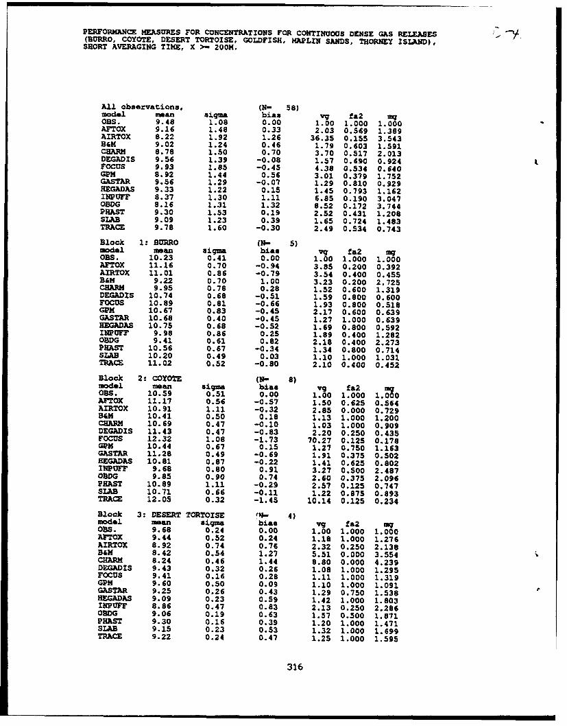
PERFORMANCE MEASURES FOR CONCENTRATIONS FOR CONTINUOoS DENSE GAS RELEASES U(BURRO, COYOTE, DESERT TORTOISE, GOLDFISH, MAPLIN SANDS, THORNEY ISLAND),SHORT AVERAGING TIME, X >- 200M.

All observations, (N- 58)model mean si9qma bias vq fa2 99OBS. 9.48 1.08 0.00 1.00 1.000 1.000AFTOX 9.16 1.48 0.33 2.03 0.569 1.389AIRTOX 8.22 1.92 1.26 36.35 0.155 3.543B&M 9.02 1.24 0.46 1.79 0.603 1.591CBARM 8.78 1.50 0.70 3.70 0.517 2.013DEGADIS 9.56 1.39 -0.08 1.57 0.690 0.924FOCUS 9.93 1.85 -0.45 4.38 0.534 0.640GPM 8.92 1.44 0.56 3.01 0.379 1.752GASTAR 9.56 1.29 -0.07 1.29 0.810 0.929HEGADAS 9.33 1.22 0.15 1.45 0.793 1.162INPUFF 8.37 1.30 1.11 6.85 0.190 3.047OBDG 8.16 1.31 1.32 8.52 0.172 3.744PHAST 9.30 1.53 0.19 2.52 0.431 1.208SLAB 9.09 1.23 0.39 1.65 0.724 1.483TRACE 9.78 1.60 -0.30 2.49 0.534 0.743

Block 1: BURRO (N- 5)model mean sigma bias vq fa2 mgOBS. 10.23 0.41 0.00 1.00 1.000 1.000AFTOX 11.16 0.70 -0.94 3.85 0.200 0.392AIRTOX 11.01 0.86 -0.79 3.54 0.400 0.455B&M 9.22 0.70 1.00 3.23 0.200 2.725CHARM 9.95 0.78 0.28 1.52 0.600 1.319DEGADIS 10.74 0.68 -0.51 1.59 0.800 0.600FOCUS 10.89 0.81 -0.66 1.93 0.800 0.518GPM 10.67 0.83 -0.45 2.17 0.600 0.639GASTAR 10.68 0.40 -0.45 1.27 1.000 0.639BEGADAS 10.75 0.68 -0.52 1.69 0.800 0.592INPUFF 9.98 0.86 0.25 1.89 0.400 1.282OBDG 9.41 0.61 0.82 2.18 0.400 2.273PHAST 10.56 0.67 -0.34 1.34 0.800 0.714SLAB 10.20 0.49 0.03 1.10 1.000 1.031TRACE 11.02 0.52 -0.80 2.10 0.400 0.452

Block 2: COYOTE (N- 8)model mean sigma bias V9 fa2 mgOS. 10.59 0.51 0.00 1.00 1.000 1.000AFTOX 11.17 0.56 -0.57 1.50 0.625 0.564AIRTOX 10.91 1.11 -0.32 2.85 0.000 0.729B&M 10.41 0.50 0.18 1.13 1.000 1.200CHARM 10.69 0.47 -0.10 1.03 1.000 0.909DEGADIS 11.43 0.47 -0.83 2.20 0.250 0.435FOCUS 12.32 1.08 -1.73 70.27 0.125 0.178GPM 10.44 0.67 0.15 1.27 0.750 1.163GASTAR 11.28 0.49 -0.69 1.91 0.375 0.502HEGADAS 10.81 0.87 -0.22 1.41 0.625 0.802INPUFF 9.68 0.80 0.91 3.27 0.500 2.487OBDG 9.85 0.90 0.74 2.60 0.375 2.096PHAST 10.89 1.11 -0.29 2.57 0.125 0.747SLAB 10.71 0.66 -0.11 1.22 0.875 0.893TRACE 12.05 0.32 -1.45 10.14 0.125 0.234

Block 3: DESERT TORTOISE tv- 4)model man siqma bias vq fa2 aqOBS. 9.68 0.24 0.00 1.00 1.000 1.000AFTOX 9.44 0.52 0.24 1.18 1.000 1.276AIRTOX 8.92 0.74 0.76 2.32 0.250 2.138B&M 8.42 0.54 1.27 5.51 0.000 3.554CHARM 8.24 0.46 1.44 8.80 0.000 4.239DEGADIS 9.43 0.32 0.26 1.08 1.000 1.295FOCUS 9.41 0.16 0.28 1.11 1.000 1.319GPM 9.60 0.50 0.09 1.10 1.000 1.091GASTAR 9.25 0.26 0.43 1.29 0.750 1.538HEGADAS 9.09 0.23 0.59 1.42 1.000 1.803INPUFF 8.86 0.47 0.83 2.13 0.250 2.286OBDG 9.06 0.19 0.63 1.57 0.500 1.871PHAST 9.30 0.16 0.39 1.20 1.000 1.471SLAB 9.15 0.23 0.53 1.32 1.000 1.699TRACE 9.22 0.24 0.47 1.25 1.000 1.595

316

PERFORMANCE MEASURES FOR CONCENTRATIONS FOR CONTINUOUS DENSE GAS RELEASES(BURRO, COYOTE, DESERT TORTOISE, GOLDFISH, MAPLIN SANDS, THORNEY ISLAND),SHORT AVERAGING TIME, X >- 200M.

Block 4: GOLDFISH (N- 8)model man sigma bias vq fa2 01OBS. 8.11 1.66 0.00 1.00 1.000 1.000AFTOX 7.05 1.50 1.06 4.44 0.500 2.897AIRTOX 6.30 1.74 1.81 31.25 0.000 6.112B&M 7.06 1.79 1.06 3.30 0.125 2.884CHARM 6.19 1.20 1.92 64.75 0.000 6.855DEGADIS 7.52 1.53 0.59 1.55 0.500 1.812FOCUS 7.56 2.18 0.56 1.95 0.500 1.750GPM 6.70 1.50 1.42 8.48 0.000 4.135GASTAR 7.75 1.73 0.37 1.23 0.875 1.447HEGADAS 7.75 1.19 0.36 1.51 0.750 1.440INPUFF 6.72 1.58 1.40 7.65 0.000 4.044OBDG 6.98 1.70 1.13 4.46 0.125 3.097PHAST 7.31 2.20 0.81 2.77 0.500 2.239SLAB 7.30 1.53 0.82 2.08 0.500 2.268TRACE 7.31 1.52 0.80 2.05 0.375 2.226

Block 5: MAPLIN SANDS, LNG (N- 8)model mean sigma bias vg fa2 mq0BS. 9.86 0.55 0.00 1.00 1.000 1.000AFTOX 9.40 0.48 0.47 1.50 0.625 1.595AIRTOX 7.42 0.81 2.44 673.47 0.000 11.515B&M 9.21 0.51 0.66 1.94 0.500 1.928CHARM 9.33 0.82 0.54 2.16 0.500 1.715DEGADIS 10.01 0.49 -0.15 1.21 0.875 0.862FOCUS 11.12 1.19 -1.25 23.55 0.375 0.286GPM 9.02 0.46 0.84 2.44 0.500 2.321GASTAR 9.95 0.46 -0.09 1.21 1.000 0.917HEGADAS 9.42 0.92 0.44 2.65 0.500 1.556INPUFF 8.42 0.46 1.44 9.60 0.000 4.222OBDG 8.31 0.70 1.55 16.60 0.125 4.728PHAST 8.75 0.53 1.12 4.25 0.125 3.061SLAB 8.93 0.80 0.93 4.53 0.375 2.539TRACE 10.97 0.60 -1.11 5.47 0.250 0.330

Block 6: MAPLIN SANDS, LPG (N- 18)model mean sigma bias vq fa2 aqOBS. 9.52 0.49 0.00 1.00 1.000 1.000AFTOX 8.71 0.50 0.81 2.25 0.389 2.253AIRTOX 7.15 0.73 2.36 417.75 0.000 10.644B&M 9.33 0.49 0.19 1.29 0.778 1.203CHARM 8.71 0.83 0.81 3.58 0.500 2.248DEGADIS 9.27 0.51 0.25 1.22 0.889 1.283FOCUS 9.41 1.06 0.11 1.80 0.667 1.114GPM 8.38 0.49 1.14 4.22 0.111 3.124GASTAR 9.42 0.46 0.10 1.15 0.889 1.105HEGADAS 9.34 0.49 0.17 1.18 0.889 1.190INPUFF 7.76 0.49 1.76 25.66 0.000 5.816OBDG 7.81 0.50 1.71 22.99 0.056 5.532PHAST 9.13 0.91 0.39 1.87 0.556 1.480SLAB 8.99 0.47 0.52 1.49 0.667 1.686TRACE 9.31 0.53 0.21 1.31 0.833 1.234

Block 7: THORNEY ISLAND (N- 7)model mean sigma bias V9 fa2 MqOBS. 8.62 0.54 0.00 1.00 1.000 1.000AFTOX 8.54 0.57 0.07 1.09 1.000 1.074AIRTOX 8.59 0.69 0.03 1.35 0.857 1.028BDM 8.86 0.48 -0.24 1.09 1.000 0.787CHARM 8.63 0.65 -0.02 1.39 0.857 0.982DEGADIS 9.25 1.20 -0.64 3.33 0.429 0.529FOCUS 9.S2 0.59 -0.90 2.65 0.429 0.405GPM 9.39 0.87 -0.77 2.95 0.429 0.463GASTAR 8.94 0.62 -0.32 1.29 0.714 0.723REGADAS 8.45 0.60 0.16 1.10 1.000 1.178INPUFF 8.84 0.80 -0.23 1.58 0.571 0.796OBOG 6.93 0.56 1.68 17.49 0.000 5.374PHAST 9.90 0.61 -1.29 6.34 0.143 0.275SLAB 8.89 0.44 -0.27 1.11 1.000 0.760TRACE 9.30 0.69 -0.69 2.22 0.571 0.502

317

APPENDIX D-5

THE PERFORMANCE MEASURES FOR THE PREDICTED CONCENTRATIONS FOR THEINSTANTANEOUS DENSE GAS RELEASE (THORNEY ISLAND), FOR DOWNWIND

DISTANCES a 200M ONLY.

318

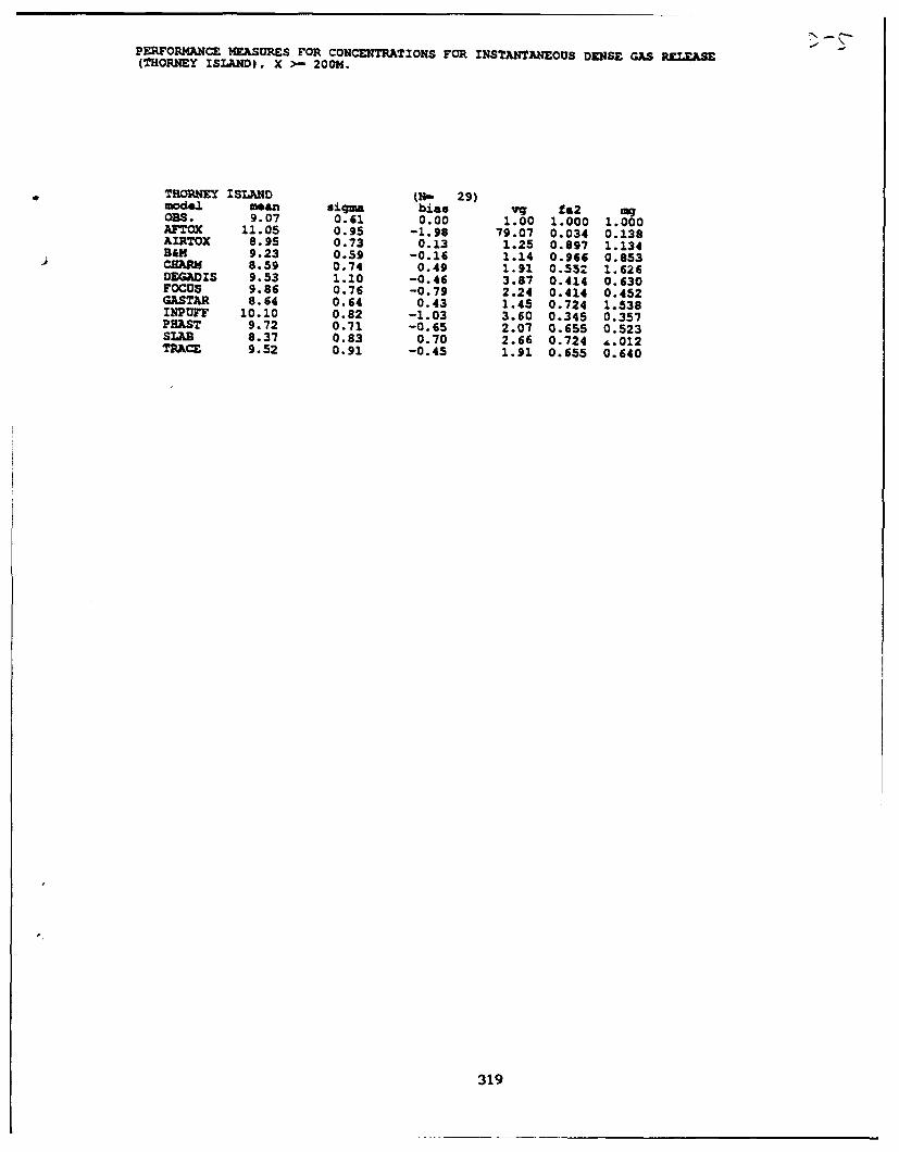
PERFORMANCE MEASURES FOR CONCENTRATZONS FOR INSTANTANEOUS DENSE GAS RELEASE -(THORNEY ISLAND), X >- 200M.

*THORNEY ISLAND (N- 29)model mean sigma bias vq Wa2 mgOBS. 9.07 0.61 0.00 1.00 1.000 1.000AFTOX 11.05 0.95 -1.98 79.07 0.034 0.138AIRTOX 8.95 0.73 0.13 1.25 0.897 1.134RaN 9.23 0.59 -0.16 1.14 0.966 0.853ClAiim 8.59 0.74 0.49 1.91 0.552 1.626DEGADIS 9.53 1.10 -0.46 3.87 0.414 0.630FOCUS 9.86 0.76 -0.79 2.24 0.414 0.452GASTAR 8.64 0.64 0.43 1.45 0.724 1.538INPUFF 10.10 0.82 -1.03 3.60 0.345 0.357PHAST 9.72 0.71 -0.65 2.07 0.655 0.523SLAB 8.37 0.83 0.70 2.66 0.724 6.012TRACE 9.52 0.91 -0.45 1.91 0.655 0.640

319

APPENDIX D-6

THE PERFORMANCE MEASURES FOR THE PREDICTED CONCENTRATIONS FOR THECONTINUOUS PASSIVE RELEASES (HANFORD, AND PRAI:!TE GRASS), INCLUDING

ALL DOWNWIND DISTANCES.

320

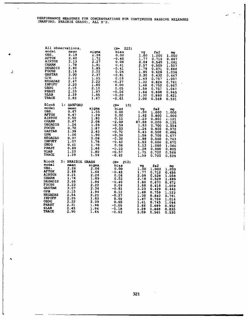
PERFORMANCE MEASURES FOR CONCENTRATIONS FOR CONTINUOUS PASSIVE RELEASES(HANFORD, PRAIRIE GRASS), ALL X'S.

All observations, (N- 222)model mean sigma bias vg fa2 mgOBS. 2.19 2.06 0.00 1.00 1.000 1.000AFTOX 2.60 1.72 -0.40 1.77 0.716 0.667AIRTOX 2.13 2.27 0.06 2.04 0.545 1.061CHARM 1.78 1.91 0.41 2.57 0.505 1.507DEGADIS 2.60 1.85 -0.41 1.79 0.671 0.666FOCUS 2.16 2.22 0.04 1.85 0.626 1.036GASTAR 3.00 2.37 -0.81 3.30 0.432 0.447GC"M 2.10 i.55 0.09 1.49 0.757 1.097HEGADAS 2.47 2.22 -0.27 1.32 0.824 0.761INPUFF 2.20 1.85 0.00 1.48 0.752 0.997OBDG 2.15 2.10 0.05 1.59 0.757 1.047PHAST 2.25 1.97 -0.06 1.64 0.698 0.945SLAB 2.39 1.95 -0.20 1.30 0.860 0.821TRACE 2.83 1.67 -0.63 3.00 0.568 0.531

Block 1: HANFORD (N- 10)model mean sigma bias vg fa2 mgOBS. 0.67 1.55 0.00 1.00 1.000 1.000AFTOX 0.67 1.29 0.00 1.62 0.800 1.000AIRTOX 0.55 1.80 0.11 1.23 0.90C ±.121CHARM 2.67 2.08 -2.00 87.68 0.000 0.135DEGADIS 1.26 1.59 -0.59 1.53 0.700 0.554FOCUS 0.70 1.87 -0.03 1.26 0.800 0.972GASTAR 1.39 2.40 -0.72 5.43 0.500 0.486GPM 1.06 1.90 -0.39 1.58 0.700 0.677HEGADAS 0.97 2.08 -0.30 1.98 0.500 0.743INPUFF 1.07 1.78 -0.40 1.53 0.600 0.670OBDG 0.61 1.70 0.06 1.12 1.000 1.060PHAST 0.89 1.66 -0.22 1.28 0.900 0.805SLAB 1.23 1.80 -0.57 1.75 0.700 0.568TRACE 1.29 1.59 -0.62 1.59 0.700 0.539

Block 2: PRAIRIE GRASS (N- 212)model mean sigma bias vg fa2 mgOBS. 2.26 2.06 0.00 1.00 1.000 1.000AFTOX 2.69 1.68 -0.42 1.77 0.712 0.655AIRTOX 2.21 2.26 0.06 2.09 0.528 1.058CHARM 1.74 1.89 0.52 2..8 0.528 1.689DEGADIS 2.66 1.84 -0.40 1.80 0.670 0.672FOCUS 2.23 2.22 0.04 1.88 0.618 1.039GASTAR 3.07 2.34 -0.81 3.23 0.429 0.445GPM 2.15 1.94 0.12 1.48 0.759 1.123HEGADAS 2.54 2.20 -0.27 1.30 0.840 0.761INPUFF 2.25 1.83 0.02 1.47 0.759 1.016OBDG 2.22 2.09 0.05 1.61 0.745 1.046PHAST 2.31 1.96 -0.05 1.66 0.689 0.952SLAB 2.45 1.94 -0.18 1.28 0.868 0.835TRACE 2.90 1.64 -0.63 3.09 0.561 0.530

321

APPENDIX D-7

THE PERFORMANCE MEASURES FOR THE PREDICTED CONCENTRATIONS FOR THEINSTANTANEOUS PASSIVE RELEASE (HANFORD), AT 800M DOWNWIND ONLY.

322

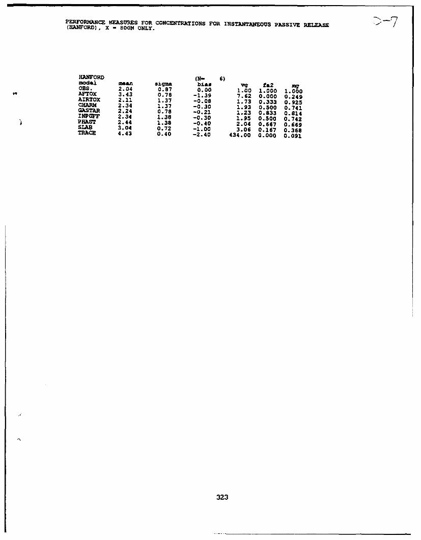
PERFORMANCE KEASUIRES FOR CONCENTRATIONS FOR INSTATANEOUS PASSIVE RELEASE /(HANFORD), X - 800M ONLY.

HANFORD (N- 6)modtl mean sigma bias v9 fa2 m7OBS. 2.04 0.87 0.00 1.00 1.000 1.000SAFTOX 3.43 0.78 -1.39 7.62 0.000 0.249AIRTOX 2.11 1.37 -0.08 1.73 0.333 0.925CHARM 2.34 1.37 -0.30 1.93 0.500 0.741GASTAR 2.24 0.78 -0.21 1.23 0.833 0.814INPUFF 2.34 1.38 -0.30 1.95 0.500 0.742PHAST 2.44 1.38 -0.40 2.04 0.667 0.669SLAB 3.04 0.72 -1.00 3.06 0.167 0.368TRACE 4.43 0.40 -2.40 434.00 0.000 0.091

323

APPENDIX D-8

THE CONFIDENCE LIMITS ANALYSIS FOR THE PERFORMANCE MEASURES LISTED IN

APPENDICES D-4, D-5, AND D-6.

324

PERFORMANCE MEASURES FOR CONCENTRATIONS FOR CONTINUOUS DENSE GAS RELEASES(BURRO, COYOTE, DESERT TORTOISE, GOLDFISH, MAPLIN SANDS, THORNEY ISLAND),

SHORT AVERAGING TIME, X >- 200M.

SUMMARY OF CONFIDENCE LIMITS ANALYSES

D(log(vg)) among models: an 'X" indicates significantly different from zero

A A B C D F G G H I 0 P S TF I & H E 0 P A E N B H L RT R M A G C M S G P D A A A0 T R A U T A U G S B CX 0 M D S A D F T E

X I R A FS S

AFTOX X X X X X X X X X X

AIRTOX X X X X X X X X X X X XB&M X X X X X X X X XCHARM X X X X X X XDEGADIS X X X X X X XFOCUS X X X X XGPM X X X X XGASTAR x X X X XHEGADAS X X X X X

INPUFFx x xINPUFF X X XOBDG X XPHAST XSLAB X

D(log(mg)) among models: an 'X' indicates significantly different from zero

A A B C D F G G H I 0 P S TF I & H E 0 P A E N B H L RT R M A G C M S G P D A A AO T R A U T A U G S B CX 0 M D S A D F T E

X I R A FS S

AFTOX X X x x x I X x X X X

AIRTOX X X X X X X X X X X XB&M X I X X X X X XCHARM X X X X X X X X X XDEGADIS X X X X X X X XIFOCUS X X X X X X XGPM X X X X X X XGASTAR X X X X XHEGADAS X X X XINPUFF X X X XOBDG X X XPHAST X XSLAB X

log(vg) for each model. an 'X' indicates significantly different from zero

A A B C D F G G H I 0 P S TF I & H E 0 P A E N B H L RT R M A G C M S G P D A A AO T R A U T A U G S B CX 0 M D S A D F T E

X I R A FS S

IC I X IC X XC X C IC C XC IC I X

log(mg) for each model: an 'X' indicates significantly different from zero

A A B C D F G G H I 0 P S TF I & H E 0 F A E N B H L RT R M A G C M S G P D A A AO T R A U T A U G S B CX 0 M D S A D F T E

X I R A FS S

C X XC X X I I I X I 3 X

325

PERFORMANCE MEASURES FOR CONCENTRATIONS FOR INSTANTANEOUS DENSE GAS RELEASE(THORNEY ISLAND), X >- 200M.


D(log(vg)) among models: an 'VX indicates significantly different from zero

A A B C D F G I P S TF I 6 H E 0 A N H L RT R M A G C S P A A A0 T R A U T U S B CX 0 M D S A F T E

X I R FS

AFTOX X X X X X X X X X X

AIRTOX X X X X X X XB&M X X X X X X XCHARM X X XDEGADIS XFOCUS X XGASTAR XINPUFF XPHASTSLAB


A A B C D F G I P S TF I & H E 0 A N H L RT R M A G C S P A A A0 T R A U T U S B CX 0 M D S A F T E

X I R FS

AFTOX I X X X X X X X X X X

AIRTOX I X X X X X X X X XB&M I X X X X X X XCHARM I X X X X XDEGADIS X X XFOCUS x :. xGASTAR x X X XINPUFF x x xPHAST I XSLAB I X

log(vg) for each model: an 'X' indicates significantly different from zero

A A B C D F G I P S TF I 6 H E 0 A N H L RT R M A G C S P A A AO T R A U T U S B CX 0 M D S A F T E

X I R FS

X X X X X X X X X X X

log(mg) for each model: an 'VX indicates significantly different from zero

A A B C D F G I P S TF I & H E 0 A N H L RT R M A G C S P A A AO T R A U T U S B CX 0 M D S A F T E

X I R FS

X X X X X X X X X X

326

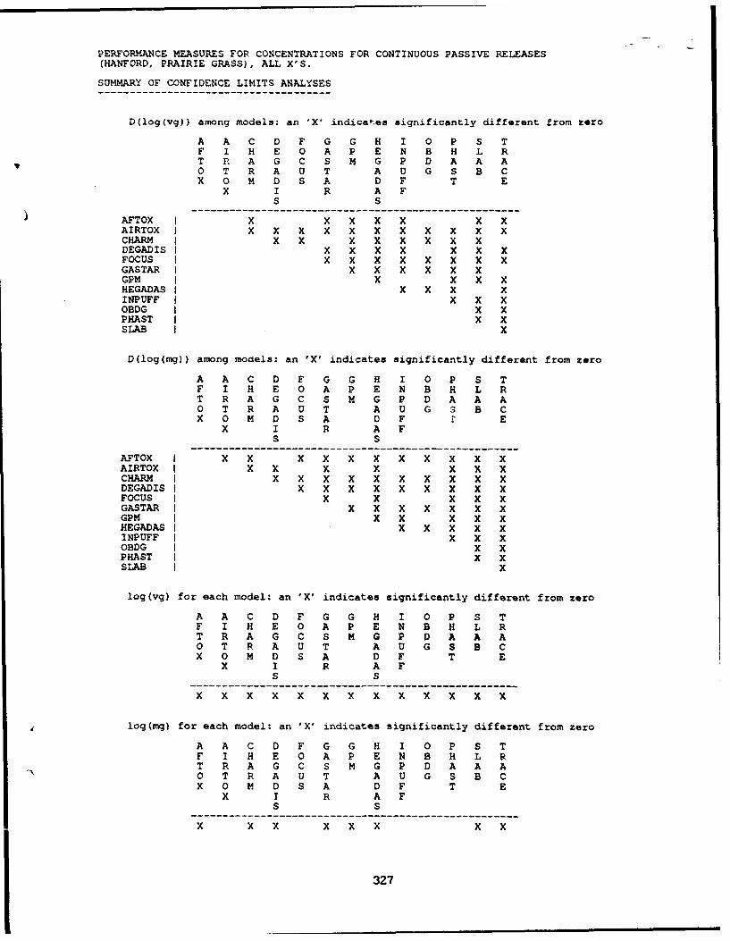
PERFORMANCE MEASURES FOR CONCENTRATIONS FOR CONTINUOUS PASSIVE RELEASES(HANFORD, PRAIRIE GRASS), ALL X'S.


D(log(vg)) among models: an 'X' indicates significantly different from zero

A A C D F G G H I 0 P S TF I H E 0 A P E N B H L RT R A G C S M G P D A A A0 T R A U T A U G S B CX 0 M D S A D F T E

X I R A FS S

AFTOX X x x x x x x

AIRTOX IX X X X X X X X X X XCHARM I X X X X X X X XDEGADIS X X X X X X XFOCUS X X X X X X X XGASTAR X X X X X XGPM X X X XHEGADAS X X X XINPUFF x x xOBDG x XPHAST x xSLAB x


A A C D F G G H I 0 P S TF I H E 0 A P E N B H L RT R A G C S M G P D A A AO T R A U T A U G S B CX 0 M D S A D F _ E

X I R A FS S

AFTOX I X X X X X X X X X X

AIRTOX X X X X X X XCHARM X X X X X X X X X XDEGADISS X X X X X X X X XFOCUS x X x x xGASTAR I X X X X X X XGPM X X x x xHEGADAS x x x x xINPUFF X X XOBDG x xPHAST X XSLAB X



X I R A FS S

X X X K X K X K X K K X X



X I R A FS S

K X X - X X X X

327

APPENDIX D-9



GOLDFISH, MAPLIN SANDS, AND THORNEY ISLAND), FOR DOWNWIND DISTANCES

> 200M AND STABLE CONDITIONS ONLY. THE SHORTEST AVAILABLE AVERAGING

TIME WAS USED.

328

PERFORMANCE MEASURES FOR CONCENTRATIONS FOR CONTINUOUS DENSE GAS RELEASES(BURRO, COYOTE, DESERT TORTOISE, GOLDFISH, MAPLIN SANDS. THORNEY ISLAND),SHORT AVERAGING TIME, X >- 200M, STABLE.

All observations, (N- 10)model mean sigma bias vq f&2 mgOBS. 9.07 0.84 0.00 1.00 1.000 1.000AFTOX 9.33 1.36 -0.26 1.61 0.800 0.770AIRTOX 9.37 1.43 -0.30 2.06 0.700 0.744B&M 8.89 0.51 0.18 1.68 0.700 1.196CHARM 9.05 0.97 0.02 1.45 0.700 1.020DEGADIS 9.65 1.27 -0.58 2.80 0.500 0.559FOCUS 9.87 0.90 -0.80 2.55 0.500 0.451GPM 9.92 1.15 -0.85 3.12 0.400 0.428GASTAR 9.39 0.91 -0.32 1.29 0.800 0.728HEGADAS 9.10 1.23 -0.03 1.38 0.900 0.973INPUFF 9.32 1.06 -0.25 1.53 0.600 0.780OBDG 7.69 1.29 1.38 8.75 0.200 3.964PHAST 9.99 0.66 -0.92 3.94 0.400 0.400SLAB 9.20 0.67 -0.13 1.12 1.000 0.881TRACE 9.67 0.93 -0.60 2.09 0.600 0.547

Block 1: BURRO (N- 2)model mean sigma bias v9 f&2 mgOBS. 10.22 0.26 0.00 1.00 1.000 1.000AFTOX 11.62 0.51 -1.40 7.49 0.000 0.247AIRTOX 11.79 0.61 -1.56 12.93 0.000 0.210B&M 8.88 0.69 1.34 7.23 0.000 3.824CHARM 10.53 0.68 -0.31 1.31 0.500 0.732DEGADIS 10.98 0.85 -0.76 2.51 0.500 0.470FOCUS 11.18 0.82 -0.96 3.43 0.500 0.383GPM 11.56 0.42 -1.33 6.08 0.000 0.263GASTAR 10.80 0.18 -0.58 1.41 1.000 0.561HEGADAS 11.22 0.61 -0.99 3.03 0.500 0.370INPUT? 10.86 0.50 -0.63 1.58 0.500 0.530OBDG 9.54 0.67 0.68 1.88 0-500 1.980PHAST 10.62 0.41 -0.40 1.20 1.000 0.672SLAB 10.16 0.52 0.06 1.07 1.000 1.064TRACE 11.08 0.44 -0.86 2.15 0.500 0.425

Block 2: DESERT TORTOISE (N- 1)model mean sigma bias f12 MCOBS. 9.95 0.00 0.00 1.00 1.000 1.000AFTOX 10.26 0.00 -0.32 1.10 1.000 0.730AIRTOX 9.98 0.00 -0.03 1.00 1.000 0.969B&M 9.16 0.00 0.78 1.85 0.000 2.190CHARM 9.00 0.00 0.95 2.45 0.000 2.578DEGADIS 9.79 0.00 0.16 1.02 1.000 1.169FOCUS 9.65 0.00 0.30 1.09 1.000 1.346GPM 10.38 0.00 -0.43 1.20 1.000 0.652GASTAR 9.69 0.00 0.26 1.07 1.000 1.296HEGADAS 9.37 0.00 0.57 1.39 1.000 1.777INPUFF 9.57 0.00 0.38 1.15 1.000 1.459OBDG 9.31 0.00 0.64 1.50 1.000 1.887PEAST 9.30 0.00 0.65 1.53 1.000 1.918SLAB 9.42 0.00 0.52 1.32 1.000 1.688TRACE 9.46 0.00 0.49 1.27 1.000 1.634Block 3: THORNEY ISLAND (N- 7)model mean sigma bias vq f&2 mgOBS. 8.62 0.54 0.00 1.00 1.000 1.000AFTOX 8.54 0.57 0.07 1.09 1.000 1.074AIRTOX 8.59 0.69 0.03 1.35 0.857 1.028BIM 8.86 0.48 -0.24 1.09 1.000 0.787CHARM 8.63 0.65 -0.02 1.39 0.857 0.982DEGADIS 9.25 1.20 -0.64 3.33 0.429 0.529FOCUS 9.52 0.59 -0.90 2.65 0.429 0.405GPM 9.39 0.87 -0.77 2.95 0.429 0.463GASTAR 8.94 0.62 -0.32 1.29 0.714 0.723HEGADAS 8.45 0.60 0.16 1.10 1.000 1.178INPUFF 8.84 0.80 -0.23 1.58 0.571 0.796OBDG 6.93 0.56 1.68 17.49 0.000 5.374PIAST 9.90 0.61 -1.29 6.34 0.143 0.275SLAB 8.89 0.44 -0.27 1.11 1.000 0.760TRACE 9.30 0.69 -0.69 2.22 0.571 0.502

329

APPENDIX D-10


INSTANTANEOUS DENSE GAS RELEASE (THORNEY ISLAND), FOR DOWNWIND

DISTANCES Z 200M AND STABLE CONDITIONS ONLY.

33

330

PERFORMANCE MEASURES FOR CONCENTRATIONS FOR INSTANTANEOUS DENSE GAS RELEASE(THORNEY ISLAND), X >- 200M, STABLE

THORNEY ISLAND (N- 9)model mean sigma bias vg fa2 aqOBS. 9.23 0.58 0.00 1.00 1.000 1.000AFTOX 11.30 1.21 -2.07 208.19 0.111 0.127AIRTOX 9.13 0.63 0.10 1.09 1.000 1.110B&M 9.13 0.64 0.11 1.03 1.000 1.115CHARM 8.05 0.46 1.18 4.38 0.000 3.268DEGADIS 8.56 1.23 0.67 7.15 0.667 1.959FOCUS 9.68 0.80 -0.44 1.36 0.778 0.641GASTAR 8.52 0.59 0.71 1.79 0.556 2.039INPUFF 10.71 0.72 -1.47 9.94 0.000 0.229PHAST 9.73 0.60 -0.50 1.35 0.778 0.606SLAB 8.72 0.52 0.51 1.34 0.778 1.665TRACE 9.00 0.82 0.23 1.20 1.000 1.259

331

APPENDIX D-11

THE PERFORMANCE MEASURES FOR THE PREDICTED CLOUD-WIDTHS FOR THE


GOLDFISH, MAPLIN SANDS, AND THORNEY ISLAND), FOR DOWNWIND DISTANCES t

Z 200M ONLY.

332

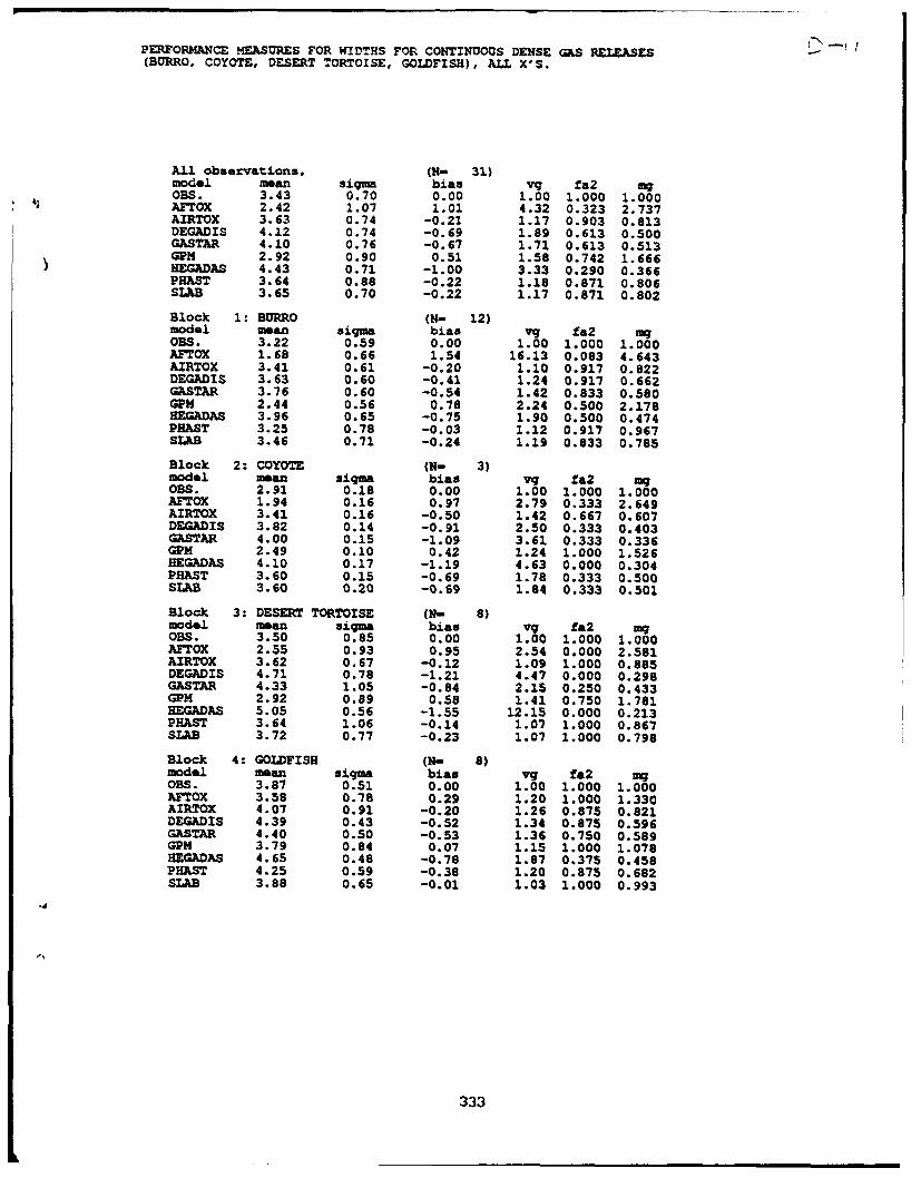
D E RISI - IPERFORMANCE EASURES FOR WIDTHS FOR CONTINUOUS DENSE GAS RELEASES-(BURRO, COYOTE, DESERT TORTOISE, GOLDFISH), ALL X'S.

All observations, (N- 31)modal mean siqma bias vg fa2 mgOBS. 3.43 0.70 0.00 1.00 1.000 1.000AFTOX 2.42 1.07 1.01 4.32 0.323 2.737AIRTOX 3.63 0.74 -0.21 1.17 0.903 0.813DEGADIS 4.12 0.74 -0.69 1.89 0.613 0.500GASTAR 4.10 0.76 -0.67 1.71 0.613 0.513GPM 2.92 0.90 0.51 1.58 0.742 1.666HEGADAS 4.43 0.71 -1.00 3.33 0.290 0.366PHAST 3.64 0.88 -0.22 1.18 0.871 0.806SLAB 3.65 0.70 -0.22 1.17 0.871 0.802

Block 1: BURRO (N- 12)model mean sigma bias vq fa2 MqOBS. 3.22 0.59 0.00 1.00 1.000 1.000AFTOX 1.68 0.66 1.54 16.13 0.083 4.643AIRTOX 3.41 0.61 -0.20 1.10 0.917 0.822DEGADIS 3.63 0.60 -0.41 1.24 0.917 0.662GASTAR 3.76 0.60 -0.54 1.42 0.833 0.580GPM 2.44 0.56 0.78 2.24 0.500 2.178HEGADAS 3.96 0.65 -0.75 1.90 0.500 0.474PHAST 3.25 0.78 -0.03 1.12 0.917 0.967SLAB 3.46 0.71 -0.24 1.19 0.833 0.785

Block 2: COYOTE (N- 3)model mean sigma bias vq fa2 mqOS. 2.91 0.18 0.00 1.00 1.000 1.000AFTOX 1.94 0.16 0.97 2.79 0.333 2.649AIRTOX 3.41 0.16 -0.50 1.42 0.667 0.607DEGADIS 3.82 0.14 -0.91 2.50 0.333 0.403GASTAR 4.00 0.15 -1.09 3.61 0.333 0.336GPM 2.49 0.10 0.42 1.24 1.000 1.526HEGADAS 4.10 0.17 -1.19 4.63 0.000 0.304PHAST 3.60 0.15 -0.69 1.78 0.333 0.500SLAB 3.60 0.20 -0.69 1.84 0.333 0.501

Block 3: DESERT TORTOISE (N- 8)model mean sigma bias vq fa2 mqOBS. 3.50 0.85 0.00 1.00 1.000 1.000AFTOX 2.55 0.93 0.95 2.54 0.000 2.581AIRTOX 3.62 0.67 -0.12 1.09 1.000 0.885DEGADIS 4.71 0.78 -1.21 4.47 0.000 0.298GASTAR 4.33 1.05 -0.84 2.15 0.250 0.433GPM 2.92 0.89 0.58 1.41 0.750 1.781HEGADAS 5.05 0.56 -1.55 12.15 0.000 0.213PHAST 3.64 1.06 -0.14 1.07 1.000 0.867SLAB 3.72 0.77 -0.23 1.07 1.000 0.798

Block 4: GOLDFISH (N- 8)model mean sigma bias vq fa2 mqOBS. 3.87 0.51 0.00 1.00 1.000 1.000AFTOX 3.58 0.78 0.29 1.20 1.000 1.330AIRTOX 4.07 0.91 -0.20 1.26 0.875 0.821DEGADIS 4.39 0.43 -0.52 1.34 0.875 0.596GASTAR 4.40 0.50 -0.53 1.36 0.750 0.589GPM 3.79 0.84 0.07 1.15 1.000 1.078HEGADAS 4.65 0.48 -0.78 1.87 0.375 0.458PHAST 4.25 0.59 -0.38 1.20 0.875 0.682SLAB 3.88 0.65 -0.01 1.03 1.000 0.993

-d

333

APPENDIX D-12

THE PERFORMANCE MEASURES FOR THE PREDICTED CLOUD-WIDTHS FOR THECONTINUOUS PASSIVE RELEASES (HANFORD, AND PRAIRIE GRASS), INCLUDING

ALL DOWNWIND DISTANCES.

334

PERFORMANCE MEASURES FOR WIDTHS FOR CONTINUOUS PASSIVE RELEASES(HANFORD, PRAIRIE GRASS), ALL X'S.

All observations, (N- 85)model mean sigma bias vg fa2 IngOBS. 3.47 0.88 0.00 1.00 1.000 1.000AFTOX 2.99 0.91 0.48 1.48 0.647 1.617AIRTOX 3.17 1.05 0.30 1.34 0.765 1.346DEGADIS 3.27 0.92 0.20 1.24 0.871 1.223GASTAR 3.22 1.00 0.25 1.28 0.847 1.284GPM 3.22 1.00 0.25 1.28 0.847 1.282HEGADAS 3.69 0.90 -0.22 1.26 0.824 0.801PHAST 3.25 0.99 0.22 1.29 0.847 1.248SLAB 3.14 0.97 0.34 1.30 0.847 1.398

Block 1: HANFORD (N- 10)model mean sigma bias vg fa2 mgOBS. 3.29 0.57 0.00 1.00 1.000 1.000AFTOX 3.43 0.65 -0.13 1.09 1.000 0.875AIRTOX 3.44 0.80 -0.14 1.37 0.700 0.867DEGADIS 3.40 0.77 -0.10 1.41 0.700 0.903GASTAR 3.37 0.79 -0.08 1.35 0.700 0.927GPM 3.37 0.79 -0.08 1.35 0.700 0.924HEGADAS 3.75 0.74 -0.46 1.68 0.600 0.631PHAST 3.22 0.80 0.07 1.48 0.800 1.077SLAB 3.20 0.76 0.09 1.30 0.800 1.096

Block 2: PRAIRIE GRASS (N- 75)model mean sigma bias vg fa2 mgOBS. 3.50 0.91 0.00 1.00 1.000 1.000AFTOX 2.93 0.92 0.56 1.54 0.600 1.755AIRTOX 3.14 1.08 0.36 1.34 0.773 1.428DEGADIS 3.25 0.93 0.24 1.22 0.893 1.274GASTAR 3.20 1.03 0.29 1.27 0.867 1.341GPM 3.20 1.02 0.29 1.27 0.867 1.339HEGADAS 3.69 0.92 -0.19 1.21 0.853 0.827PHAST 3.25 1.01 0.24 1.27 0.853 1.273SLAB 3.13 0.99 0.37 1.30 0.893 1.444

335

APPENDIX D-13

THE CONFIDENCE LIMITS ANALYSIS FOR THE PERFORMANCE MEASURES LISTED INAPPENDICES D-11, and D-12.

336

PERFORMANCE MEASURES FOR WIDTHS FOR CONTINUOUS DENSE GAS RELEASES(BURRO, COYOTE, DESERT TORTOISE, GOLDFISH), ALL X'S.



A A D G G H P SF I E A P E H LT R G S M G A AO T A T A S BX 0 D A D T

X I R AS S

AFTOX X X X X X XAIRTOX X X X XDEGADIS X X XGASTAR X X XGPM X X XHEGADAS X XPHAST


A A D G G H P SF I E A P E H LT R G S M G A A0 T A T A S BX 0 D A D T

X I R AS S

AFTOX X X X X X X X

AIRTOX x x x xDEGADIS x x x xGASTAR x x x xGPM x x xHEGADAS x XPHAST



X I R AS S

X X X X X X X X



X I R AS S

X X X X X X X X

337

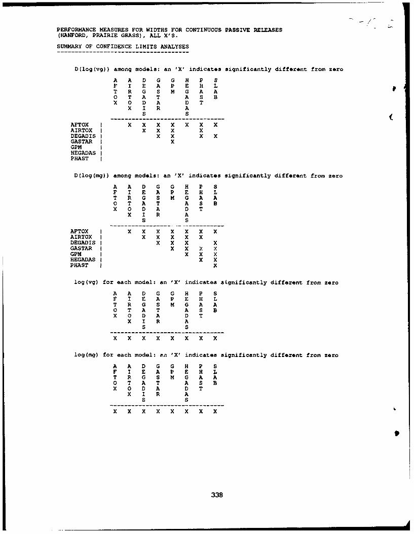
PERFORMANCE MEASURES FOR WIDTHS FOR CONTINUOUS PASSIVE RELEASES(HANFORD, PRAIRIE GRASS), ALL X'S.




X I R AS S (

AFTOX X X X X X X XAIRTOX I X X X XDEGADIS I X X X XGASTAR XGPM IHEGADASPHAST



X I R AS S

AFTOX X X X X X X X

AIRTOX X X X X XDEGADISS X X X XGASTAR. x x x xGPM x x xHEGADAS x xPHAST x



X I R AS S

x x x x x x x x



X I R AS S

X X X X X X X X

338

U 93 10 1 190 - Defense Technical Information Center

Documents

Transcript of U 93 10 1 190 - Defense Technical Information Center