Numer Algor (2011) 58:315–331DOI 10.1007/s11075-011-9457-6

ORIGINAL PAPER

Two effective hybrid conjugate gradient algorithmsbased on modified BFGS updates

Saman Babaie-Kafaki · Masoud Fatemi ·Nezam Mahdavi-Amiri

Received: 5 September 2010 / Accepted: 3 March 2011 /Published online: 2 April 2011© Springer Science+Business Media, LLC 2011

Abstract Based on two modified secant equations proposed by Yuan, andLi and Fukushima, we extend the approach proposed by Andrei, and intro-duce two hybrid conjugate gradient methods for unconstrained optimizationproblems. Our methods are hybridizations of Hestenes-Stiefel and Dai-Yuanconjugate gradient methods. Under proper conditions, we show that one ofthe proposed algorithms is globally convergent for uniformly convex functionsand the other is globally convergent for general functions. To enhance theperformance of the line search procedure, we propose a new approach forcomputing the initial value of the steplength for initiating the line search pro-cedure. We give a comparison of the implementations of our algorithms withtwo efficiently representative hybrid conjugate gradient methods proposedby Andrei using unconstrained optimization test problems from the CUTErcollection. Numerical results show that, in the sense of the performanceprofile introduced by Dolan and Moré, the proposed hybrid algorithms arecompetitive, and in some cases more efficient.

Keywords Unconstrained optimization ·Hybrid conjugate gradient algorithm · Modified BFGS method ·Global convergence

S. Babaie-KafakiDepartment of Mathematics, Semnan University, Semnan, Iran

M. Fatemi · N. Mahdavi-Amiri (B)Faculty of Mathematical Sciences, Sharif University of Technology, Tehran, Irane-mail: nezamm@sharif.ir, nezamm@sharif.edu

316 Numer Algor (2011) 58:315–331

1 Introduction

Conjugate gradient (CG) methods comprise a class of unconstrained optimiza-tion algorithms characterized by low memory requirements and strong localand global convergence properties [9]. CG methods have played special rolesin solving large scale nonlinear optimization problems.

Generally, a CG method is designed to solve the following unconstrainedoptimization problem,

minx∈Rn

f (x), (1)

where f : Rn → R is a smooth nonlinear function. The iterative formula of a

CG method is given by

xk+1 = xk + sk, sk = αkdk, (2)

where αk is a steplength and dk is the search direction defined by

d0 = −∇ f (x0),

dk+1 = −∇ f (xk+1) + βkdk, k ≥ 0, (3)

where βk is a scalar. The stepsize αk is usually chosen to satisfy certain linesearch conditions [23]. Among them, the so-called strong Wolfe line searchconditions require that

f (xk + αkdk) − f (xk) ≤ δαk∇ f (xk)Tdk,

|∇ f (xk + αkdk)Tdk| ≤ −σ∇ f (xk)

Tdk,(4)

where dk is a descent direction (∇ f (xk)Tdk < 0) and 0 < δ < σ < 1.

Notation 1 Throughout the paper, for a suf f iciently dif ferentiable function fat xk, we consider the following notations:

fk = f (xk), gk = ∇ f (xk), Gk = ∇2 f (xk),

sk = xk+1 − xk, yk = ∇ f (xk+1) − ∇ f (xk). (5)

Also, ||.|| stands for the Euclidean norm.

Some well known formulae for βk in (3) are given by Hestense–Stiefel (HS)[18], Fletcher–Reeves (FR) [13], Polak-Ribière-Polyak (PRP) [24, 25], Liuand Storey (LS) [22], and Dai and Yuan (DY) [11]. Good reviews of the CGmethods and their convergence properties can be seen in [9, 17].

There are some merits and demerits in each method (see [23]). In the FRmethod, if a bad direction and a tiny step from xk−1 to xk are generated,then the next direction dk and the next step sk are also likely to be poorunless a restart along the gradient direction is made. In spite of such a defect,Zoutendijk [34] proved that the FR method with exact line search is globallyconvergent on general functions. Al-Baali [1] extended this result for the in-exact line search. Although one would be satisfied with global convergence of

Numer Algor (2011) 58:315–331 317

the FR method, this method numerically performs much worse than the PRPand HS methods. Also, Powell [26] constructed a counter example and showedthat the PRP and HS methods could cycle infinitely without convergence toa solution; that is, they lack global convergence in certain circumstance. Ingeneral, the FR and DY methods have strong global convergence properties,but they may have modest computational performance. On the other hand,the methods of HS, PRP and LS may not always be convergent, but they oftenhave better computational performance [2].

Recently, to attain good computational performance, more attention hasbeen paid to hybridize the above CG methods, while maintaining the attractivefeature of strong global convergence; for example, hybridizations of PRP andFR methods proposed by Touati-Ahmed and Storey [27], Hu and Storey [19],and Gilbert and Nocedal [14], hybridizations of HS and DY methods proposedby Dai and Yuan [10], and Andrei [3, 5], and hybridization of PRP and DYmethods proposed by Andrei [4].

Among the different hybrid CG methods, hybridizations of HS and DYmethods have shown promising numerical behavior [2]. The HS method hasthe nice property of satisfying the conjugacy condition yT

k dk+1 = 0, for all k ≥0, independent of the line search conditions and objective function convexity.On the other hand, the DY method has remarkable strong convergenceproperties in contrast to the other CG methods [8]. For example, in additionto generation of descent directions, DY method has proved to have a certainself-adjusting property independent of the line search conditions and objectivefunction convexity; more exactly, if there exist positive constants γ1 and γ2such that γ1 ≤ ||gk|| ≤ γ2, for all k ≥ 0, then for any p ∈ (0, 1) there exists apositive constant τ such that the sufficient descent condition gT

i di ≤ −τ ||gi||2holds for at least �pk� indices i ∈ [0, k], where � j� denotes the largest integerless than or equal to j. Also, under mild assumptions on the objective function,DY method is shown to be globally convergent under a variety of line searchconditions. These advantages motivated us to study the hybridizations of HSand DY methods following the effective approach proposed in [3, 5].

The formula for βk in [3, 5], namely βCk , is obtained by a convex combination

of βHSk and βDY

k . That is,

βCk = (1 − θk)β

HSk + θkβ

DYk = (1 − θk)

gTk+1 yk

yTk dk

+ θkgT

k+1gk+1

yTk dk

, (6)

where θk, namely the hybridization parameter, is a scalar parameter satisfying0 ≤ θk ≤ 1. Therefore, from (3) we have,

dk+1 = −gk+1 + (1 − θk)gT

k+1 yk

yTk dk

dk + θkgT

k+1gk+1

yTk dk

dk, (7)

or equivalently,

dk+1 = −gk+1 + (1 − θk)gT

k+1 yk

yTk sk

sk + θkgT

k+1gk+1

yTk sk

sk. (8)

318 Numer Algor (2011) 58:315–331

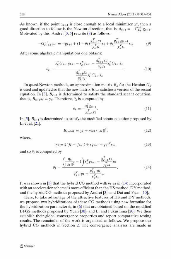
As known, if the point xk+1 is close enough to a local minimizer x∗, then agood direction to follow is the Newton direction, that is, dk+1 = −G−1

k+1gk+1.Motivated by this, Andrei [3, 5] rewrite (8) as follows:

−G−1k+1gk+1 = −gk+1 + (1 − θk)

gTk+1 yk

yTk sk

sk + θkgT

k+1gk+1

yTk sk

sk. (9)

After some algebraic manipulations one obtains:

θk =sT

k Gk+1gk+1 − sTk gk+1 − gT

k+1 yk

yTk sk

sTk Gk+1sk

gTk+1gk

yTk sk

sTk Gk+1sk

. (10)

In quasi-Newton methods, an approximation matrix Bk for the Hessian Gk

is used and updated so that the new matrix Bk+1 satisfies a version of the secantequation. In [3], Bk+1 is determined to satisfy the standard secant equation,that is, Bk+1sk = yk. Therefore, θk is computed by

θk = − sTk gk+1

gTk+1gk

. (11)

In [5], Bk+1 is determined to satisfy the modified secant equation proposed byLi et al. [21],

Bk+1sk = yk + ηksk/||sk||2, (12)

where,

ηk = 2( fk − fk+1) + (gk+1 + gk)Tsk, (13)

and so θk is computed by

θk =

(ηk

||sk||2 − 1)

sTk gk+1 − gT

k+1 yk

yTk sk

ηk

gTk+1gk + gT

k+1gk

yTk sk

ηk

. (14)

It was shown in [5] that the hybrid CG method with θk as in (14) incorporatedwith an acceleration scheme is more efficient than the HS method, DY method,and the hybrid CG methods proposed by Andrei [3], and Dai and Yuan [10].

Here, to take advantage of the attractive features of HS and DY methods,we propose two hybridizations of these CG methods using new formulae forthe hybridization parameter θk in (6) that are obtained based on the modifiedBFGS methods proposed by Yuan [30], and Li and Fukushima [20]. We thenestablish their global convergence properties and report comparative testingresults. The remainder of the work is organized as follows. We propose ourhybrid CG methods in Section 2. The convergence analyses are made in

Numer Algor (2011) 58:315–331 319

Section 3. In Section 4, we propose our initial estimate for the steplengththat is needed to start the line search procedure. In Section 5, we numericallycompare our methods with two efficiently representative hybrid CG methodsusing the hybridization parameters θk in (11) and (14) as proposed by Andrei[3, 5]. Finally, we conclude in Section 6.

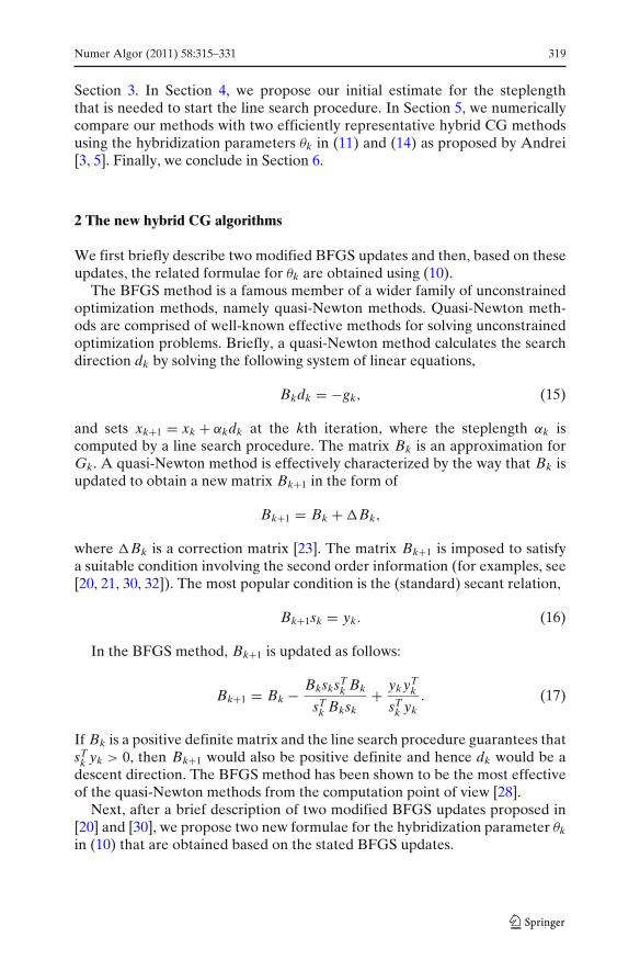
2 The new hybrid CG algorithms

We first briefly describe two modified BFGS updates and then, based on theseupdates, the related formulae for θk are obtained using (10).

The BFGS method is a famous member of a wider family of unconstrainedoptimization methods, namely quasi-Newton methods. Quasi-Newton meth-ods are comprised of well-known effective methods for solving unconstrainedoptimization problems. Briefly, a quasi-Newton method calculates the searchdirection dk by solving the following system of linear equations,

Bkdk = −gk, (15)

and sets xk+1 = xk + αkdk at the kth iteration, where the steplength αk iscomputed by a line search procedure. The matrix Bk is an approximation forGk. A quasi-Newton method is effectively characterized by the way that Bk isupdated to obtain a new matrix Bk+1 in the form of

Bk+1 = Bk + Bk,

where Bk is a correction matrix [23]. The matrix Bk+1 is imposed to satisfya suitable condition involving the second order information (for examples, see[20, 21, 30, 32]). The most popular condition is the (standard) secant relation,

Bk+1sk = yk. (16)

In the BFGS method, Bk+1 is updated as follows:

Bk+1 = Bk − BksksTk Bk

sTk Bksk

+ yk yTk

sTk yk

. (17)

If Bk is a positive definite matrix and the line search procedure guarantees thatsT

k yk > 0, then Bk+1 would also be positive definite and hence dk would be adescent direction. The BFGS method has been shown to be the most effectiveof the quasi-Newton methods from the computation point of view [28].

Next, after a brief description of two modified BFGS updates proposed in[20] and [30], we propose two new formulae for the hybridization parameter θk

in (10) that are obtained based on the stated BFGS updates.

320 Numer Algor (2011) 58:315–331

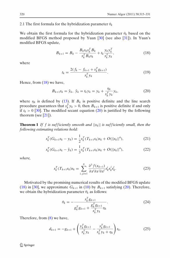
2.1 The first formula for the hybridization parameter θk

We obtain the first formula for the hybridization parameter θk based on themodified BFGS method proposed by Yuan [30] (see also [31]). In Yuan’smodified BFGS update,

Bk+1 = Bk − BksksTk Bk

sTk Bksk

+ tkyk yT

k

sTk yk

, (18)

where

tk = 2( fk − fk+1 + sTk gk+1)

sTk yk

. (19)

Hence, from (18) we have,

Bk+1sk = yk, yk = tk yk = yk + ηk

sTk yk

yk, (20)

where ηk is defined by (13). If Bk is positive definite and the line searchprocedure guarantees that sT

k yk > 0, then Bk+1 is positive definite if and onlyif tk > 0 [30]. The modified secant equation (20) is justified by the followingtheorem (see [21]).

Theorem 1 If f is suf f iciently smooth and ||sk|| is suf f iciently small, then thefollowing estimating relations hold:

sTk (Gk+1sk − yk) = 1

2sT

k (Tk+1sk)sk + O(||sk||4), (21)

sTk (Gk+1sk − yk) = 1

3sT

k (Tk+1sk)sk + O(||sk||4), (22)

where,

sTk (Tk+1sk)sk =

n∑i, j,l=1

∂3 f (xk+1)

∂xi∂x j∂xlsi

ks jksl

k. (23)

Motivated by the promising numerical results of the modified BFGS update(18) in [30], we approximate Gk+1 in (10) by Bk+1 satisfying (20). Therefore,we obtain the hybridization parameter θk as follows:

θk = − sTk gk+1

gTk gk+1 + gT

k gk+1

sTk yk

ηk

. (24)

Therefore, from (8) we have,

dk+1 = −gk+1 +(

yTk gk+1

sTk yk

− sTk gk+1

sTk yk + ηk

)sk. (25)

Numer Algor (2011) 58:315–331 321

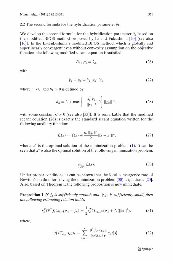
2.2 The second formula for the hybridization parameter θk

We develop the second formula for the hybridization parameter θk based onthe modified BFGS method proposed by Li and Fukushima [20] (see also[16]). In the Li–Fukushima’s modified BFGS method, which is globally andsuperlinearly convergent even without convexity assumption on the objectivefunction, the following modified secant equation is satisfied:

Bk+1ss = yk, (26)

with

yk = yk + hk||gk||rsk, (27)

where r > 0, and hk > 0 is defined by

hk = C + max

{− sT

k yk

||sk||2 , 0

}||gk||−r, (28)

with some constant C > 0 (see also [33]). It is remarkable that the modifiedsecant equation (26) is exactly the standard secant equation written for thefollowing auxiliary function:

fa(x) = f (x) + hk||gk||r2

||x − x∗||2, (29)

where, x∗ is the optimal solution of the minimization problem (1). It can beseen that x∗ is also the optimal solution of the following minimization problem:

minx∈Rn

fa(x). (30)

Under proper conditions, it can be shown that the local convergence rate ofNewton’s method for solving the minimization problem (30) is quadratic [20].Also, based on Theorem 1, the following proposition is now immediate.

Proposition 1 If fa is suf f iciently smooth and ||sk|| is suf f iciently small, thenthe following estimating relation holds:

sTk (∇2 fa(xk+1)sk − yk) = 1

2sT

k (Tak+1 sk)sk + O(||sk||4), (31)

where,

sTk (Tak+1 sk)sk =

n∑i, j,l=1

∂3 fa(xk+1)

∂xi∂x j∂xlsi

ks jksl

k. (32)

322 Numer Algor (2011) 58:315–331

The modified quasi-Newton equation (26) has a nice property: for each k, ifthe line search procedure guarantees that sT

k yk > 0, then we have,

sTk yk = sT

k yk + C||gk||r||sk||2 + max

{− sT

k yk

||sk||2 , 0

}||sk||2 ≥ C||gk||r||sk||2 > 0,

(33)ensuring Bk+1, generated by the BFGS update, to inherit the positivedefiniteness of Bk [23, 28]. Moreover, from the strong Wolfe line searchconditions (4), we have,

sTk yk = sT

k gk+1 − sTk gk ≥ σ sT

k gk − sTk gk = −(1 − σ)sT

k gk > 0. (34)

Hence, from (28) and (34), we have hk = C and yk becomes

yk = yk + C||gk||rsk. (35)

Now, taking advantage of the good global and superlinear convergenceproperties of Li–Fukushima’s modified BFGS method, not needing convexityassumptions on the objective function (and thus having applicability to a largeclass of objective functions), we approximate Gk+1 in (10) by Bk+1 satisfying(26). Hence, we obtain the hybridization parameter θk as follows:

θk =(C||gk||r − 1)sT

k gk+1 − yTk gk+1

sTk yk

C||gk||r||sk||2

gTk gk+1 + gT

k gk+1

sTk yk

C||gk||r||sk||2, (36)

and therefore, from (8) we have,

dk+1 = −gk+1 + gTk+1(yk + (C||gk||r − 1)sk)

sTk yk + C||gk||r||sk||2 sk. (37)

3 Convergence analysis

We analyze the convergence property of the two hybrid CG methods using ournewly proposed hybridization parameter θk as in (24) and (36), respectively.Throughout this section, we assume gk = 0, for k ≥ 1; otherwise, a stationarypoint is at hand. We make the following basic assumptions on the objectivefunction.

Assumption 1

1. The level set L = {x| f (x) ≤ f (x0)} is bounded; that is, there exists a constantB > 0 such that

||x|| ≤ B, ∀x ∈ L. (38)

Numer Algor (2011) 58:315–331 323

2. In some convex neighborhood N of L, f is continuously dif ferentiable, andits gradient is Lipschitz continuous; that is, there exists a constant L > 0 suchthat

||g(x) − g(y)|| ≤ L||x − y||, ∀x, y ∈ N . (39)

The following proposition is now immediate.

Proposition 2 Under Assumption 1, there exists a constant γ > 0 such that

||g(x)|| ≤ γ, ∀x ∈ L. (40)

Proof Consider a constant point y0 ∈ L. From Assumptions 1, for an arbitrarypoint x ∈ L, we have,

||g(x)|| − ||g(y0)|| ≤ ||g(x) − g(y0)|| ≤ L||x − y0||≤ L(||x|| + ||y0||) ≤ L(B + ||y0||). (41)

From the above relation we get,

||g(x)|| − ||g(y0)|| ≤ L(B + ||y0||) ⇒ ||g(x)|| ≤ L(B + ||y0||) + ||g(y0)||. (42)

So, if we let γ = L(B + ||y0||) + ||g(y0)||, then the proof is complete. �

Definition 1 We say that a search direction dk is a descent direction if we have

gTk dk < 0. (43)

We recall that for any CG method with the strong Wolfe line searchconditions (4), the following general result was proved in [9].

Lemma 1 Suppose that Assumption 1 hold. Consider any CG method in theform (2) and (3), with a descent direction dk and computing αk using the strongWolfe line search conditions (4). If

∑k≥1

1||dk||2 = ∞, (44)

then we have,

lim infk→∞

||gk|| = 0. (45)

We will show that our first hybrid CG method is globally convergent foruniformly convex functions and the second one is globally convergent forgeneral functions. To proceed any further, we need the following definition.

324 Numer Algor (2011) 58:315–331

Definition 2 A twice continuously differentiable function f is said to beuniformly convex on the nonempty open convex set S if and only if there existsM > 0 such that

(g(x) − g(y))T(x − y) ≥ M||x − y||2, ∀x, y ∈ S, (46)

or equivalently, there exists μ > 0 such that

zT∇2 f (x)z ≥ μ||z||2, ∀x ∈ S, ∀z ∈ Rn. (47)

Corollary 1 Under Assumption 1, if f is a uniformly convex function on N ,then we have,

| fk − fk+1 + sTk gk+1| ≥ 1

2μ||sk||2. (48)

Proof Using Taylor expansion, we write,

fk = f (xk+1 − sk) = fk+1 − sTk gk+1 + 1

2sT

k ∇2 f (xk+1 − αsk)sk, (49)

or,

fk − fk+1 + sTk gk+1 = 1

2sT

k ∇2 f (xk+1 − αsk)sk, (50)

where α ∈ (0, 1). Since N is a convex set, then xk+1 − αsk ∈ N . So, from (47)the proof is complete. �

We are now ready to prove the following global convergence theorems forour two hybrid CG methods with hybridization parameter θk as in (24) and(36), respectively.

Theorem 2 Suppose that Assumption 1 and the descent condition (43) hold.Consider the hybrid CG method in the form of (8) with θk def ined by (24),where αk is computed using the strong Wolfe line search conditions (4). If theobjective function f is uniformly convex, then

lim infk→∞

||gk|| = 0. (51)

Numer Algor (2011) 58:315–331 325

Proof Because the descent condition holds, we have dk+1 = 0. So, usingLemma 1, it is sufficient to prove that ||dk+1|| is bounded above. From (25),Assumption 1, Proposition 1, Corollary 1, and (46), we have,

||dk+1|| = || − gk+1 +(

yTk gk+1

sTk yk

− sTk gk+1

sTk yk + ηk

)sk||

= || − gk+1 +(

yTk gk+1

sTk yk

− sTk gk+1

2( fk − fk+1 + sTk gk+1)

)sk||

≤ || − gk+1|| +(

|yTk gk+1|sT

k yk+ |sT

k gk+1|2| fk − fk+1 + sT

k gk+1|

)||sk||

≤ γ +⎛⎜⎝ Lγ ||sk||

M||sk||2 + γ ||sk||2

12μ||sk||2

⎞⎟⎠ ||sk||

= γ +(

Lγ

M+ γ

μ

)= (1 + L

M+ 1

μ)γ,

which completes the proof. �

Theorem 3 Suppose that Assumptions 1 and the descent condition (43) hold.Consider the hybrid CG method in the form of (8) with θk def ined by (36),where αk is computed from the strong Wolfe line search conditions (4). Then,we have,

lim infk→∞

||gk|| = 0. (52)

Proof We proceed by contradiction. Suppose that (52) is not true. Then, thereis a positive constant E such that ||gk|| > E, for k ≥ 1. From the descentconditions (43), (34) and (35) we have,

sTk yk = sT

k yk + C||gk||r||sk||2≥ −(1 − σ)sT

k gk + CEr||sk||2> CEr||sk||2. (53)

Now, from Assumption 1, Proposition 2, (37) and (53), we have,

||dk+1|| =∣∣∣∣∣∣∣∣ − gk+1 + gT

k+1(yk + (C||gk||r − 1)sk)

sTk yk + C||gk||r||sk||2 sk

∣∣∣∣∣∣∣∣

≤ || − gk+1|| + |gTk+1 yk| + |C||gk||r − 1| |gT

k+1sk|sT

k yk + C||gk||r||sk||2 ||sk||

326 Numer Algor (2011) 58:315–331

≤ γ + γ L||sk|| + |C||gk||r − 1| γ ||sk||CEr||sk||2 ||sk||

≤(

1 + L + �

CEr

)γ = E1,

where � = max{1, Cγ r}. From the latter inequality, we obtain,∑k≥1

1||dk||2 ≥

∑k≥1

1E2

1= +∞, (54)

and so, using Lemma 1, we get (52), a contradiction. �

4 The line search procedure

A line search procedure requires an initial estimate αk0 for the steplengthαk in (2) and generates a sequence {αki}∞i=0 that either terminates with asteplength satisfying the conditions specified by the user or determines thatsuch a steplength does not exist.

Our numerical experiments showed that the performance of a CG methodwas much influenced by the choice of the initial value of the steplength αk0 atthe kth iteration, so that an improper setting of αk0 would cause a significantincrease in the number of iterations, function and gradient evaluations toachieve a required accuracy. Several proper choices for αk0 are proposed in[3, 7, 23]. The proposed initial value of the steplength in [3, 7], namely αO

k+10, is

computed by the following formula:

αOk+10

= ||sk||||dk+1|| . (55)

Here, we propose a modification of formula (55) that turns out to serve quitewell for the line search. Note that when a CG method is convergent, we have,

limk→∞

||sk|| = 0, (56)

or equivalently, the sequence {sk}∞k=1 is convergent to the vector (0, 0, ..., 0)T ∈R

n. In other words, the sequence {sk}∞k=1 is a Cauchy sequence. Therefore, wehave,

||sk+1 − sk|| → 0. (57)

Motivated by this, we define,

w(α) = ||αdk+1 − sk||2. (58)

So, the initial value for the steplength αk+10 can be considered as the minimizerof w; that is,

αNk+10

= sTk dk+1

||dk+1||2 . (59)

Numer Algor (2011) 58:315–331 327

But, from the Cauchy–Schwarz inequality, we have,

|αNk+10

| = |sTk dk+1|

||dk+1||2 ≤ αOk+10

= ||sk||||dk+1|| .

Thus, we propose to use a convex combination of the values of αk+10 in (55)and (59) as follows:

αk+10 = λsT

k dk+1

||dk+1||2 + (1 − λ)||sk||

||dk+1|| , (60)

where λ ∈ (0, 1). Note that we need to have αk+10 > 0. So, if sTk dk+1 < 0, then

we set λ = 0 (or equivalently, we use the value of αOk+10

as proposed in [3, 7]).

5 Numerical results

We present some numerical results obtained by applying a MATLAB 7.7.0.471(R2008b) implementation of our proposed hybrid CG methods (M3 and M4below) comparing them with two other efficient hybrid CG methods proposedby Andrei in [3, 5] (M1 and M2 below), that outperform the HS method, theDY method, and the hybrid CG method of Dai and Yuan [10] (as previouslyshown in [3, 5]), on a mobile computer, Intel(R)Core(TM)2 Duo CPU 2.00GHz, with 1 GB of RAM. So, our results are reported for the following fouralgorithms:

1. Hybrid CG Method M1: θk is computed by (11).2. Hybrid CG Method M2: θk is computed by (14).3. Hybrid CG Method M3: θk is computed by (24).4. Hybrid CG Method M4: θk is computed by (36).

Since CG methods are efficient for solving large scale problems, our experi-ments have been done on a set of 89 unconstrained optimization test problemsof CUTEr collection [15] with the minimum dimension equal to 50 as specifiedin [29].

In our implementation, when gTk dk > −10−4||gk||||dk||, we consider dk as an

uphill search direction. Although the descent property (43) may not alwayshold, but the uphill search direction seldom occurred in our numerical ex-periments. When we encountered an uphill search direction, we restarted thealgorithm with dk = −(sT

k sk)/(sTk yk)gk (similar to the direction proposed by

Barzilai and Borwein [6]). We used the strong Wolfe line search conditions (4)with δ = 0.01 and σ = 0.1, and computed the steplength αk using Algorithm 3.5in [23] with the initial steplength αk0 computed by (60), in which, if sT

k dk+1 < 0,then we set λ = 0; otherwise, we set λ = 0.5. All attempts to solve the testproblems were limited to reaching maximum of 10000 iterations or achievinga solution with ||gk||∞ < 10−6.

All the four algorithms successfully solved 69 out of 89 problems, andfailures occurred for all the algorithms on a set of 17 test problems includingARGLINB, BDQRTIC, CRAGGLVY, CURLY10, CURLY20, CURLY30,

328 Numer Algor (2011) 58:315–331

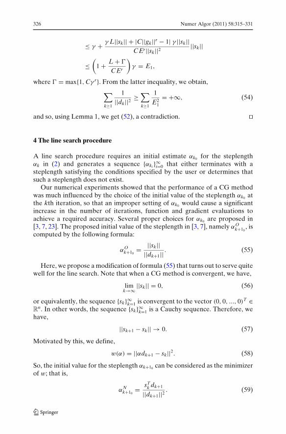
Fig. 1 Iteration performanceprofiles for the fouralgorithms

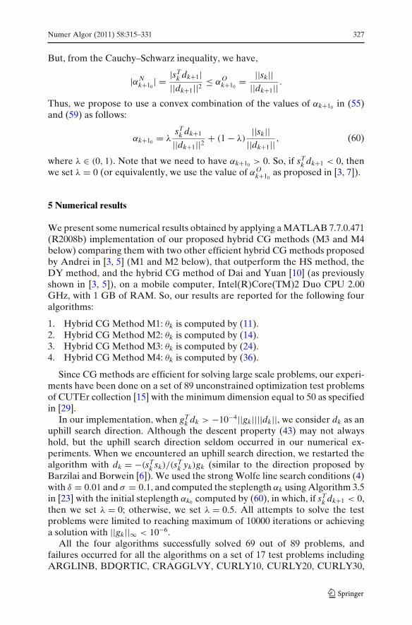
Fig. 2 Function evaluationperformance profiles for thefour algorithms

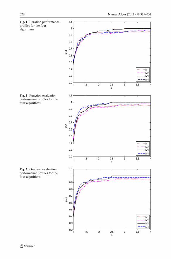
Fig. 3 Gradient evaluationperformance profiles for thefour algorithms

Numer Algor (2011) 58:315–331 329

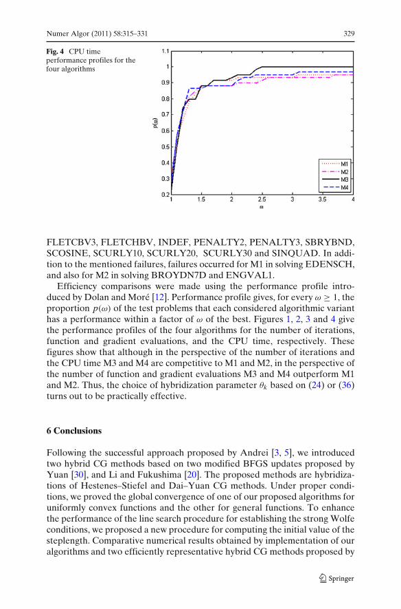
Fig. 4 CPU timeperformance profiles for thefour algorithms

FLETCBV3, FLETCHBV, INDEF, PENALTY2, PENALTY3, SBRYBND,SCOSINE, SCURLY10, SCURLY20, SCURLY30 and SINQUAD. In addi-tion to the mentioned failures, failures occurred for M1 in solving EDENSCH,and also for M2 in solving BROYDN7D and ENGVAL1.

Efficiency comparisons were made using the performance profile intro-duced by Dolan and Moré [12]. Performance profile gives, for every ω ≥ 1, theproportion p(ω) of the test problems that each considered algorithmic varianthas a performance within a factor of ω of the best. Figures 1, 2, 3 and 4 givethe performance profiles of the four algorithms for the number of iterations,function and gradient evaluations, and the CPU time, respectively. Thesefigures show that although in the perspective of the number of iterations andthe CPU time M3 and M4 are competitive to M1 and M2, in the perspective ofthe number of function and gradient evaluations M3 and M4 outperform M1and M2. Thus, the choice of hybridization parameter θk based on (24) or (36)turns out to be practically effective.

6 Conclusions

Following the successful approach proposed by Andrei [3, 5], we introducedtwo hybrid CG methods based on two modified BFGS updates proposed byYuan [30], and Li and Fukushima [20]. The proposed methods are hybridiza-tions of Hestenes–Stiefel and Dai–Yuan CG methods. Under proper condi-tions, we proved the global convergence of one of our proposed algorithms foruniformly convex functions and the other for general functions. To enhancethe performance of the line search procedure for establishing the strong Wolfeconditions, we proposed a new procedure for computing the initial value of thesteplength. Comparative numerical results obtained by implementation of ouralgorithms and two efficiently representative hybrid CG methods proposed by

330 Numer Algor (2011) 58:315–331

Andrei [3, 5], on a set of unconstrained optimization test problems from theCUTEr collection and in the sense of the performance profile introduced byDolan and Moré [15], showed the efficiency of our algorithms.

Acknowledgements The authors are grateful to the Research Council of Sharif Universityof Technology for its support, and two anonymous referees for their valuable comments andsuggestions that helped improve the presentation. They are also grateful to Professor MichaelNavon for providing the strong Wolfe line search code.

References

1. Al-Baali, A.: Descent property and global convergence of the Fletcher–Reeves method withinexact line search. IMA J. Numer. Anal. 5, 121–124 (1985)

2. Andrei, N.: Numerical comparison of conjugate gradient algorithms for unconstrained opti-mization. Stud. Inform. Control 16, 333–352 (2007)

3. Andrei, N.: Another hybrid conjugate gradient algorithm for unconstrained optimization.Numer. Algor. 47, 143–156 (2008)

4. Andrei, N.: Hybrid conjugate gradient algorithm for unconstrained optimization. J. Optim.Theory Appl. 141, 249–264 (2009)

5. Andrei, N.: Accelerated hybrid conjugate gradient algorithm with modified secant conditionfor unconstrained optimization. Numer. Algor. 54(1), 23–46 (2010)

6. Barzilai, J., Borwein, J.M.: Two-point step size gradient methods. IMA J. Numer. Anal. 8(1),141–148 (1988)

7. Birgin, E.G., Martínez, J.M.: A spectral conjugate gradient method for unconstrained opti-mization. Appl. Math. Optim. 43, 117–128 (2001)

8. Dai, Y.H.: New properties of a nonlinear conjugate gradient method. Numer. Math. 89, 83–98(2001)

9. Dai, Y.H., Han, J.Y., Liu, G.H., Sun, D.F., Yin, H.X., Yuan, Y.X.: Convergence properties ofnonlinear conjugate gradient methods. SIAM J. Optim. 10(2), 348–358 (1999)

10. Dai, Y.H., Yuan, Y.X.: An efficient hybrid conjugate gradient method for unconstrainedoptimization. Ann. Oper. Res. 103, 33–47 (2001)

11. Dai, Y.H., Yuan, Y.X.: A nonlinear conjugate gradient method with a strong global conver-gence property. SIAM J. Optim. 10, 177–182 (1999)

12. Dolan, E.D., Moré, J.J.: Benchmarking optimization software with performance profiles.Math. Program. 91, 201–213 (2002)

13. Fletcher, R., Revees, C.M.: Function minimization by conjugate gradients. Comput. J. 7, 149–154 (1964)

14. Gilbert, J.C., Nocedal, J.: Global convergence properties of conjugate gradient methods foroptimization. SIAM J. Optim. 2, 21–42 (1992)

15. Gould, N.I.M., Orban, D., Toint, Ph.L.: CUTEr, a constrained and unconstrained testingenvironment, revisited. ACM Trans. Math. Softw. 29, 373–394 (2003)

16. Guo, Q., Liu, J.G. Wang, D.H.: A modified BFGS method and its superlinear convergencein nonconvex minimization with general line search rule. J. Appl. Math. Comput. 29, 435–446(2008)

17. Hager, W.W., Zhang, H.: A survey of nonlinear conjugate gradient methods. Pacific J. Optim.2, 35–58 (2006)

18. Hestenes, M.R., Stiefel, E.L.: Methods of conjugate gradients for solving linear systems. J. Res.Natl. Bur. Stand. 49(5), 409–436 (1952)

19. Hu, Y.F., Storey, C.: Global convergence result for conjugate gradient methods. J. Optim.Theory Appl. 71, 399–405 (1991)

20. Li, D.H., Fukushima, M.: A modified BFGS method and its global convergence in nonconvexminimization. J. Comput. Appl. Math. 129, 15–35 (2001)

21. Li, G., Tang, C., Wei, Z.: New conjugacy condition and related new conjugate gradientmethods for unconstrained optimization. J. Comput. Appl. Math. 202(2), 523–539 (2007)

Numer Algor (2011) 58:315–331 331

22. Liu, Y., Storey, C.: Efficient generalized conjugate gradient algorithms, part 1: theory. J.Optim. Theory Appl. 69, 129–137 (1991)

23. Nocedal, J., Wright, S.J.: Numerical Optimization, 2nd edn. Springer (2006)24. Polak, E., Ribière, G.: Note sur la convergence de méthodes directions conjugées, Rev.

Francaise êInform. Rech. Opér. 16, 35–43 (1969)25. Polyak, B.T.: The conjugate gradient method in extreme problems. USSR Comp. Math. Math.

Phys. 9, 94–112 (1969)26. Powell, M.J.D.: Nonconvex minimization calculations and the conjugate gradient method. In:

Lecture Notes in Mathematics, vol. 1066, pp. 122–141. Springer, Berlin (1984)27. Touati-Ahmed, D., Storey, C.: Efficient hybrid conjugate gradient techniques. J. Optim.

Theory Appl. 64, 379–397 (1990)28. Sun, W., Yuan, Y.X.: Optimization Theory and Methods: Nonlinear Programming. Springer

(2006)29. Xiao, Y., Wang, Q., Wang, D.: Notes on the Dai-Yuan-Yuan modified spectral gradient

method. J. Comput. Appl. Math. 234(10), 2986–2992 (2010)30. Yuan, Y.X.: A modified BFGS algorithm for unconstrained optimization. IMA J. Numer.

Anal. 11, 325–332 (1991)31. Yuan, Y.X., Byrd, R.H.: Non-quasi-Newton updates for unconstrained optimization. J.

Comput. Math. 13(2), 95–107 (1995)32. Zhang, J.Z., Deng, N.Y., Chen, L.H.: New quasi-Newton equation and related methods for

unconstrained optimization. J. Optim. Theory Appl. 102, 147–167 (1999)33. Zhou, W., Zhang, L.: A nonlinear conjugate gradient method based on the MBFGS secant

condition. Optim. Methods Softw. 21(5) 707–714 (2006)34. Zoutendijk, G.: Nonlinear programming computational methods. In: Abadie, J. (ed.) Integer

and Nonlinear Programming, pp. 37–86. North-Holland, Amsterdam(1970)