
Turning Points and Classification - University of Oregon
40
Chapter 18 Turning Points and Classification Jeremy Piger Abstract Economic time-series data is commonly categorized into a discrete number of persistent regimes. I survey a variety of approaches for real-time prediction of these regimes and the turning points between them, where these predictions are formed in a data-rich environment. I place particular emphasis on supervised machine learning classification techniques that are common to the statistical classification literature, but have only recently begun to be widely used in economics. I also survey Markov- switching models, which are often used for unsupervised classification of economic data. The approaches surveyed are computationally feasible when applied to large datasets, and the machine learning algorithms employ regularization and cross- validation to prevent overfitting in the face of many predictors. A subset of the approaches conduct model selection automatically in forming predictions. I present an application to real-time identification of U.S. business cycle turning points based on a wide dataset of 136 macroeconomic and financial time-series. 18.1 Introduction It is common in studies of economic time series for each calendar time period to be categorized as belonging to one of some fixed number of recurrent regimes. For example, months and quarters of macroeconomic time series are separated into periods of recession and expansion, and time series of equity returns are divided into bull vs. bear market regimes. Other examples include time series measuring the banking sector, which can be categorized as belonging to normal vs. crises regimes, and time series of housing prices, for which some periods might be labeled as arising from a ‘bubble’ regime. A key feature of these regimes in most economic settings is that they are thought to be persistent, meaning the probability of each regime occurring increases once the regime has become active. Jeremy Piger Department of Economics, University of Oregon, Eugene, OR 97403, e-mail: [email protected] 597
-
Upload
khangminh22 -
Category
Documents
-
view
0 -
download
0
Transcript of Turning Points and Classification - University of Oregon

Chapter 18Turning Points and Classification
Jeremy Piger
AbstractEconomic time-series data is commonly categorized into a discrete numberof persistent regimes. I survey a variety of approaches for real-time prediction of theseregimes and the turning points between them, where these predictions are formed ina data-rich environment. I place particular emphasis on supervised machine learningclassification techniques that are common to the statistical classification literature,but have only recently begun to be widely used in economics. I also survey Markov-switching models, which are often used for unsupervised classification of economicdata. The approaches surveyed are computationally feasible when applied to largedatasets, and the machine learning algorithms employ regularization and cross-validation to prevent overfitting in the face of many predictors. A subset of theapproaches conduct model selection automatically in forming predictions. I presentan application to real-time identification of U.S. business cycle turning points basedon a wide dataset of 136 macroeconomic and financial time-series.
18.1 Introduction
It is common in studies of economic time series for each calendar time period tobe categorized as belonging to one of some fixed number of recurrent regimes.For example, months and quarters of macroeconomic time series are separated intoperiods of recession and expansion, and time series of equity returns are dividedinto bull vs. bear market regimes. Other examples include time series measuring thebanking sector, which can be categorized as belonging to normal vs. crises regimes,and time series of housing prices, for which some periods might be labeled as arisingfrom a ‘bubble’ regime. A key feature of these regimes in most economic settingsis that they are thought to be persistent, meaning the probability of each regimeoccurring increases once the regime has become active.
Jeremy PigerDepartment of Economics, University of Oregon, Eugene, OR 97403, e-mail: [email protected]
597

598 Jeremy Piger
In many cases of interest, the regimes are never explicitly observed. Instead,the historical timing of regimes is inferred from time series of historical economicdata. For example, in the United States, the National Bureau of Economic Research(NBER) Business Cycle Dating Committee provides a chronology of business cycleexpansion and recession dates developed from study of local minima and maximaof many individual time series. Because the NBER methodology is not explicitlyformalized, a literature has worked to develop and evaluate formal statistical meth-ods for establishing the historical dates of economic recessions and expansions inboth U.S. and international data. Examples include Hamilton (1989), Vishwakarma(1994), Chauvet (1998), Harding and Pagan (2006), Fushing, Chen, Berge, and Jordá(2010), Berge and Jordá (2011) and Stock and Watson (2014).
In this chapter I am also interested in determining which regime is active based oninformation from economic time series. However, the focus is on real-time predictionrather than historical classification. Specifically, the ultimate goal will be to identifythe active regime toward the end of the observed sample period (nowcasting) orafter the end of the observed sample period (forecasting). Most of the predictiontechniques I consider will take as given a historical categorization of regimes, andwill use this categorization to learn the relationship between predictor variables andthe occurrence of alternative regimes. This learned relationshipwill then be exploitedin order to classify time periods that have not yet been assigned to a regime. I willalso be particularly interested in the ability of alternative prediction techniques toidentify turning points, which mark the transition from one regime to another. Whenregimes are persistent, so that there are relatively few turning points in a sample,it is quite possible for a prediction technique to have good average performancefor identifying regimes, but consistently make errors in identifying regimes aroundturning points.
Consistent with the topic of this book, I will place particular emphasis in thischapter on the case where regime predictions are formed in a data-rich environment.In our specific context, this environment will be characterized by the availability of alarge number of time-series predictor variables from which we can infer regimes. Intypical language, our predictor dataset will be a ‘wide’ dataset. Such datasets createissues when building predictive models, since it is difficult to exploit the informationin the dataset without overfitting, which will ultimately lead to poor out-of-samplepredictions.
The problem of regime identification discussed above is an example of a sta-tistical classification problem, for which there is a substantial literature outside ofeconomics. I will follow the tradition of that literature and refer to the regimes as‘classes,’ the task of inferring classes from economic indicators as ‘classification,’and a particular approach to classification as a ‘classifier.’ Inside of economics,there is a long history of using parametric models, such as a logit or probit, asclassifiers. For example, many studies have used logit and probit models to predictU.S. recessions, where the model is estimated over a period for which the NBERbusiness cycle chronology is known. A small set of examples from this literatureinclude Estrella andMishkin (1998), Estrella, Rodrigues, and Schich (2003), Kauppiand Saikkonen (2008), Rudebusch andWilliams (2009) and Fossati (2016). Because

18 Turning Points and Classification 599
they use an available historical indicator of the class to estimate the parameters ofthe model, such approaches are an example of what is called a ‘supervised’ classifierin the statistical classification literature. This is in contrast to ‘unsupervised classi-fiers,’ which endogenously determine clustering of the data, and thus endogenouslydetermine the classes. Unsupervised classifiers have also been used for providingreal-time nowcasts and forecasts of U.S. recessions, with the primary example beingthe Markov-switching framework of Hamilton (1989). Chauvet (1998) proposes adynamic factor model with Markov-switching (DFMS) to identify expansion andrecession phases from a group of coincident indicators, and Chauvet and Hamilton(2006), Chauvet and Piger (2008) and Camacho, Perez-Quiros, and Poncela (2018)evaluate the performance of variants of this DFMS model to identify NBER turningpoints in real time. An important feature of Markov-switching models is that theyexplicitly model the persistence of the regime, by assuming the regime indicatorfollows a Markov process.
Recently, a number of authors have applied machine learning techniques com-monly used outside of economics to classification problems involving time-seriesof economic data. As an example, Qi (2001), Ng (2014), Berge (2015), Davig andSmalter Hall (2016), Garbellano (2016) and Giusto and Piger (2017) have appliedmachine learning techniques such as artificial neural networks, boosting, naïve bayes,and learning vector quantization to forecasting and nowcastingU.S. recessions, whileWard (2017) used random forests to identify periods of financial crises. These studieshave generally found improvements from the use of the machine learning algorithmsover commonly used alternatives. For example, Berge (2015) finds that the perfor-mance of boosting algorithms improves on equal weight model averages of recessionforecasts produced by logistic models, while Ward (2017) finds a similar result forforecasts of financial crises produced by a random forest.
Machine learning algorithms are particularly attractive in data-rich settings. Suchalgorithms typically have one or more ‘regularization’ mechanisms that trades offin-sample fit against model complexity, which can help prevent overfitting. Thesealgorithms are generally also fit using techniques that explicitly take into account out-of-sample performance, most typically using cross validation. This aligns the modelfitting stage with the ultimate goal of out-of-sample prediction, which again canhelp prevent overfitting. A number of these methods also have built in mechanismsto conduct model selection jointly with estimation in a fully automated procedure.This provides a means to target relevant predictors from among a large set of pos-sible predictors. Finally, these methods are computationally tractable, making themrelatively easy to apply to large datasets.
In this chapter, I survey a variety of popular off-the-shelf supervised machinelearning classification algorithms for the purpose of classifying economic regimesin real time using time-series data. Each classification technique will be presentedin detail, and its implementation in the R programming language will be discussed.1Particular emphasis will be placed on the use of these classifiers in data-rich envi-ronments. I will also present DFMSmodels as an alternative to the machine learning
1 http://www.R-project.org/

600 Jeremy Piger
classifiers in some settings. Finally, each of the various classifiers will be evaluatedfor their real-time performance in identifying U.S. business cycle turning points from2000 to 2018.
As discussed above, an existing literature in economics uses parametric logitand probit models to predict economic regimes. A subset of this literature hasutilized these models in data-rich environments. For example, Owyang, Piger, andWall (2015) and Berge (2015) use model averaging techniques with probit and logitmodels to utilize the information inwide data sets, while Fossati (2016) uses principalcomponents to extract factors from wide datasets to use as predictor variables inprobit models. I will not cover these techniques here, instead opting to provide aresource for machine learning methods, which hold great promise, but have receivedless attention in the literature to date.
The remainder of this chapter proceeds as follows. Section 18.2 will formalizethe forecasting problem we are interested in and describe metrics for evaluating classforecasts. Section 18.3 will then survey the details of a variety of supervised machinelearning classifiers and their implementation, while section 18.4 will present detailsof DFMS models for the purpose of classification. Section 18.5 will present anapplication to real-time nowcasting of U.S. business cycle turning points. Section18.6 concludes.
18.2 The Forecasting Problem
In this section I lay out the forecasting problem of interest, as well as establishnotation used for the remainder of this chapter. I also describe some features ofeconomic data that should be recognized when conducting a classification exercise.Finally, I detail common approaches to evaluating the quality of class predictions.
18.2.1 Real-time classification
Our task is to develop a prediction of whether an economic entity in period t + h is(or will be) in each of a discrete number (C) of classes. Define a discrete variableSt+h ∈ {1, . . . ,C} that indicates the active class in period t + h. It will also be usefulto define C binary variables Sc
t+h= I (St+h = c), where I () ∈ {0,1} is an indicator
function, and c = 1, . . . ,C.Assume that we have a set of N predictors to draw inference on St+h . Collect these
predictors measured at time t in the vector Xt , with an individual variable inside thisvector labeled Xj ,t , j = 1, . . . ,N . Note that Xt can include both contemporaneousvalues of variables as well as lags. I define a classifier as Sc
t+h(Xt ), where this
classifier produces a prediction of Sct+h
conditional on Xt . These predictions willtake the form of conditional probabilities of the form Pr
(St+h = c |Xt
). Note that
a user of these predictions may additionally be interested in binary predictions of

18 Turning Points and Classification 601
Sct+h
. To generate a binary prediction we would combine our classifier Sct+h(Xt )
with a rule, L (), such that L(Sct+h(Xt )
)∈ {0,1}. Finally, assume we have available
T observations on Xt and St+h , denoted as {Xt,St+h}Tt=1. I will refer to this in-sample period as the ‘training sample.’ This training sample is used to determinethe parameters of the classifier, and I refer to this process as ‘training’ the classifier.Once trained, a classifier can then be used to forecast Sc
t+houtside of the training
sample. Specifically, given an XT+q , we can predict ScT+q+h
using ScT+q+h
(XT+q
)or
L(ScT+q+h
(XT+q
) ).
I will also be interested in the prediction of turning points, which mark thetransition from one class to another. The timely identification of turning points ineconomic applications is often of great importance, as knowledge that a turningpoint has already occurred, or will in the future, can lead to changes in behavioron the part of firms, consumers, and policy makers. As an example, more timelyinformation suggesting the macroeconomy has entered a recession phase should leadto quicker action on the part of monetary and fiscal policymakers, and ultimatelyincreased mitigation of the effects of the recession. In order to predict turning pointswe will require another rule to convert sequences of Sc
t+h(Xt ) into turning point
predictions. Of course, how cautious one is in converting probabilities to turningpoint predictions is determined by the user’s loss function, and in particular therelative aversion to false positives. In the application presented in Section 18.5, Iwill explore the real-time performance of a specific strategy for nowcasting turningpoints between expansion and recession phases in the macroeconomy.
18.2.2 Classification and economic data
As is clear from the discussion above, we are interested in this chapter in classificationin the context of time-series data. This is in contrast to much of the broader clas-sification literature, which is primarily focused on classification in cross-sectionaldatasets, where the class is reasonably thought of as independent across observa-tions. In most economic time series, the relevant class is instead characterized bytime-series persistence, such that a class is more likely to continue if it is alreadyoperational than if it isn’t. In this chapter, I survey a variety of off-the-shelf ma-chine learning classifiers, most of which do not explicitly model persistence in theclass indicator. In cases where the forecast horizon h is reasonably long, ignoringpersistence of the class is not likely to be an issue, as the dependence of the futureclass on the current class will have dissipated. However, in short horizon cases, suchas that considered in the application presented in Section 18.5, this persistence ismore likely to be important. To incorporate persistence into the machine learningclassifiers’ predictions, I follow Giusto and Piger (2017) and allow for lagged values

602 Jeremy Piger
to enter the Xt vector. Lagged predictor variables will provide information aboutlagged classes, which should improve classification of future classes.2
Economic data is often characterized by ‘ragged edges,’ meaning that some valuesof the predictor variables are missing in the out-of-sample period (Camacho et al.(2018)). This generally occurs due to differences in the timing of release datesfor different indicators, which can leave us with only incomplete observation ofthe vector XT+j . There are a variety of approaches that one can take to deal withthese missing observations when producing out-of-sample predictions. A simple,yet effective, approach is to use k nearest neighbors (kNN) imputation to impute themissing observations. This approach imputes the missing variables based on fullyobserved vectors from the training sample that are similar on the dimension of thenon-missing observations. kNN imputation is discussed in more detail in Section18.3.3.
18.2.3 Metrics for evaluating class forecasts
In this section I discussmetrics for evaluating the performance of classifiers. Supposewe have a set of T class indicators, Sc
t+h, and associated classifier predictions,
Sct+h(Xt ), where t ∈ Θ. Since Sc
t+h(Xt ) is interpreted as a probability, an obvious
metric to evaluate these predictions is Brier’s Quadratic Probability Score (QPS),which is the analogue of the traditional mean squared error for discrete data:
QPS =1
T
∑t∈Θ
C∑c=1
(Sct+h − Sc
t+h (Xt ))2
The QPS is bounded between 0 and 2, with smaller values indicating better classifi-cation ability.
As discussed above, in addition to predictions that are in the form of probabilities,we are often interested in binary predictions produced as L
(Sct+h(Xt )
). In this case,
there are a variety of commonly used metrics to assess the accuracy of classifiers. Indescribing these, it is useful to restrict our discussion to the two class case, so thatc ∈ {1,2}.3 Also, without loss of generality, label c = 1 as the ‘positive’ class andc = 2 as the ‘negative’ class. We can then define a confusion matrix:
2 When converting Sct+h(Xt ) into turning point predictions, one might also consider conversion
rules that acknowledge class persistence. For example, multiple periods of elevated class probabil-ities could be required before a turning point into that class is predicted.3 Generalizations of these metrics to the multi-class case generally proceed by considering eachclass against all other classes in order to mimic a two class problem.

18 Turning Points and Classification 603
Predicted
Actual
positive negative
positive TP FP
negative FN T N
where TP is the number of true positives, defined as the number of instances ofc = 1 that were classified correctly as c = 1, and FP indicates the number of falsepositives, defined as the instances of c = 2 that were classified incorrectly as c = 1.FN and T N are defined similarly.
A number of metrics of classifier performance can then be constructed from thisconfusion matrix. The first is Accuracy, which simply measures the proportion ofperiods that are classified correctly:
Accuracy =TP + T N
TP + T N + FP + FNOf course, Accuracy is strongly affected by the extent to which classes are balancedin the sample period. If one class dominates the period under consideration, then itis easy to have very high accuracy by simply always forecasting that class with highprobability. In many economic applications, classes are strongly unbalanced, and asa result the use of Accuracy alone to validate a classifier would not be recommended.Using the confusion matrix we can instead define accuracy metrics for each class.Specifically, the true positive rate, or TPR, gives us the proportion of instances ofc = 1 that were classified correctly:
TPR =TP
TP + FNwhile the true negative rate, or T NR, gives us the proportion of instances of c = 2that were classified correctly:
T NR =T N
T N + FPIt is common to express the information in T NR as the false positive rate, which isgiven by FPR = 1 − T NR.4
It is clear that which of these metrics is of primary focus depends on the relativepreferences of the user for true positives vs. false positives. Also, it should be
4 In the classification literature, TPR is referred to as the sensitivity and TNR as the specificity.

604 Jeremy Piger
remembered that the confusion matrix, and the metrics defined from its contents, aredependent not just on the classifier Sc
t+h(Xt ), but also on the rule L used to convert
this classifier to binary outcomes. In many cases, these rules are simply of the form:
L(Sct+h (Xt )
)=
{1 if Sc
t+h(Xt ) > d
2 if Sct+h(Xt ) ≤ d
such that c = 1 is predicted if Sct+h(Xt ) rises above the threshold d, and 0 ≤ d ≤ 1
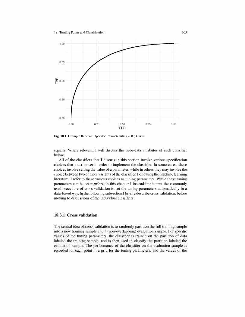
since our classifier is a probability. A useful summary of the performance of aclassifier is provided by the ‘receiver operator characteristic’ (ROC) curve, which isa plot of combinations of TPR (y-axis) and FPR (x-axis), where the value of d isvaried to generate the plot. When d = 1 both TPR and FPR are zero, since bothTP and FP are zero if class c = 1 is never predicted. Also, d = 0 will generateTPR and FPR that are both one, since FN and T N will be zero if class c = 1 isalways predicted. Thus, the ROC curve will always rise from the origin to the (1,1)ordinate. A classifier for which Xt provides no information regarding Sc
t+h, and is
thus constant, will haveTPR = FPR, and the ROC curve will lie along the 45 degreeline. Classifiers for which Xt does provide useful information will have a ROC curvethat lies above the 45 degree line. Figure 18.1 provides an example of such a ROCcurve. Finally, suppose we have a perfect classifier, such that there exists a value ofd = d∗ where TPR = 1 and FPR = 0. For all values of d ≥ d∗, the ROC curve willbe a vertical line on the y-axis from (0,0) to (0,1), where for values of d ≤ d∗, theROC curve will lie on a horizontal line from (0,1) to (1,1).
As discussed in Berge and Jordá (2011), the area under the ROC curve (AUROC)can be a useful measure of the classification ability of a classifier. TheAUROC for the45 degree line, which is the ROC curve for the classifier when Xt has no predictiveability, is 0.5. The AUROC for a perfect classifier is 1. In practice, the AUROCwill lie in between these extremes, with larger values indicating better classificationability.
In the application presented in Section 18.5, I consider both the QPS and theAUROC to assess out-of-sample classification ability. I will also evaluate the abilityof these classifiers to forecast turning points. In this case, given the relative rarityof turning points in most economic applications, it seems fruitful to evaluate per-formance through case studies of the individual turning points. Examples of such acase study will be provided in Section 18.5.
18.3 Machine Learning Approaches to Supervised Classification
In this section I will survey a variety of off-the-shelf supervised machine learningclassifiers. The classifiers I survey have varying levels of suitability for data-richenvironments. For all the classifiers considered, application to datasets with manypredictors is computationally feasible. Some of the classifiers also have built inmechanisms to identify relevant predictors, while others use all predictor variables
18 Turning Points and Classification 605
Fig. 18.1 Example Receiver Operator Characteristic (ROC) Curve
equally. Where relevant, I will discuss the wide-data attributes of each classifierbelow.
All of the classifiers that I discuss in this section involve various specificationchoices that must be set in order to implement the classifier. In some cases, thesechoices involve setting the value of a parameter, while in others they may involve thechoice between two ormore variants of the classifier. Following themachine learningliterature, I refer to these various choices as tuning parameters. While these tuningparameters can be set a priori, in this chapter I instead implement the commonlyused procedure of cross validation to set the tuning parameters automatically in adata-based way. In the following subsection I briefly describe cross validation, beforemoving to discussions of the individual classifiers.
18.3.1 Cross validation
The central idea of cross validation is to randomly partition the full training sampleinto a new training sample and a (non-overlapping) evaluation sample. For specificvalues of the tuning parameters, the classifier is trained on the partition of datalabeled the training sample, and is then used to classify the partition labeled theevaluation sample. The performance of the classifier on the evaluation sample isrecorded for each point in a grid for the tuning parameters, and the values of the

606 Jeremy Piger
tuning parameters with the best performance classifying the evaluation sample isselected. These optimal values for the tuning parameters are then used to trainthe classifier over the full training sample. Performance on the evaluation sample isgenerally evaluated using a scalarmetric for classification performance. For example,in the application presented in Section 18.5, I use the AUROC for this purpose.
In k-fold cross validation, k of these partitions (or ‘folds’) are randomly generated,and the performance of the classifier for specific tuning parameter values is averagedacross the k evaluation samples. A common value for k, which is the default inmany software implementations of k-fold cross validation, is k = 10. One canincrease robustness by repeating k-fold cross validation a number of times, andaveraging performance across these repeats. This is known as repeated k-fold crossvalidation. Finally, in settings with strongly unbalanced classes, which is common ineconomic applications, it is typical to sample the k partitions such that they reflectthe percentage of classes in the full training sample. In this case, the procedure islabeled stratified k-fold cross validation.
Cross validation is an attractive approach for setting tuning parameters becauseit aligns the final objective, good out-of-sample forecasts, with the objective used todetermine tuning parameters. In other words, tuning parameters are given a valuebased on the ability of the classifier to produce good out-of-sample forecasts. Thisis in contrast to traditional estimation, which sets parameters based on the in-samplefit of the model. Cross validation is overwhelmingly used in machine learning al-gorithms for classification, and it can be easily implemented for a wide variety ofclassifiers using the caret package in R.
18.3.2 Naïve Bayes
We begin our survey of machine learning approaches to supervised classificationwith the Naïve Bayes (NB) classifier. NB is a supervised classification approachthat produces a posterior probability for each class based on application of BayesRule. NB simplifies the classification problem considerably by assuming that insideof each class, the individual variables in the vector Xt are independent of eachother. This conditional independence is a strong assumption, and would be expectedto be routinely violated in economic datasets. Indeed, it would be expected to beviolated in most datasets, which explains the ‘naïve’ moniker. However, despite thisstrong assumption, the NB algorithm works surprisingly well in practice. This isprimarily because what is generally needed for classification is not exact posteriorprobabilities of the class, but only reasonably accurate approximate rank orderingsof probabilities. Two recent applications in economics include Garbellano (2016),who used a NB classifier to nowcast U.S. recessions and expansions in real time,and Davig and Smalter Hall (2016), who used the NB classifier, including someextensions, to predict U.S. business cycle turning points.
To describe the NB classifier I begin with Bayes rule:

18 Turning Points and Classification 607
Pr(St+h = c |Xt
)∝ f
(Xt |St+h = c
)Pr (St+h = c) . (18.1)
In words, Bayes Rule tells us that the posterior probability that St+h is in phase c isproportional to the probability density for Xt conditional on St+h being in phase cmultiplied by the unconditional (prior) probability that St+h is in phase c.
The primary difficulty in operationalizing (18.1) is specifying a model for Xt
to produce f(Xt |St+h = c
). The NB approach simplifies this task considerably by
assuming that each variable in Xt is independent of each other variable in Xt ,conditional on St+h = c. This implies that the conditional data density can befactored as follows:
f(Xt |St+h = c
)=
N∏j=1
fj(Xj ,t |St+h = c
),
where Xj ,t is one of the variables in Xt . Equation (18.1) then becomes:
Pr(St+h = c |Xt
)∝
N∏j=1
fj(Xj ,t |St+h = c
) Pr (St+h = c) . (18.2)
How do we set fj(Xj ,t |St+h = c
)? One approach is to assume a parametric distri-
bution, where a typical choice in the case of continuous Xt is the normal distribution:
Xj ,t |St+h = c ∼ N(µj ,c, σ
2j ,c
),
where µj ,c and σ2j ,c are estimated from the training sample. Alternatively, we could
evaluate fj(Xj ,t |St+h = c
)non-parametrically using a kernel density estimator fit
to the training sample. In our application of NB presented in Section 18.5, I treatthe choice of whether to use a normal distribution or a kernel density estimate as atuning parameter.
Finally, equation (18.2) produces an object that is proportional to the conditionalprobability Pr
(St+h = c |Xt
). We can recover this conditional probability exactly as:
Pr(St+h = c |Xt
)=
[N∏j=1
fj(Xj ,t |St+h = c
) ]Pr (St+h = c)
C∑c=1
©«[N∏j=1
fj(Xj ,t |St+h = c
) ]Pr (St+h = c)ª®¬
.
Our NB classifier is then Sct+h(Xt ) = Pr
(St+h = c |Xt
).
The NB classifier has a number of advantages. First, it is intuitive and inter-pretable, directly producing posterior probabilities of each class. Second, it is easilyscalable to large numbers of predictor variables, requiring a number of parameterslinear to the number of predictors. Third, since only univariate properties of a pre-dictor in each class are estimated, the classifier can be implemented with relatively

608 Jeremy Piger
small amounts of training data. Finally, ignoring cross-variable relationships guardsagainst overfitting the training sample data.
A primary drawback of the NB approach is that it ignores cross-variable rela-tionships potentially valuable for classification. Of course, this drawback is also thesource of the advantages mentioned above. Another drawback relates to the appli-cation of NB in data-rich settings. As equation (18.2) makes clear, all predictors aregiven equal weight in determining the posterior probability of a class. As a result, theperformance of the classifier can deteriorate if there are a large number of irrelevantpredictors, the probability of which will increase in data-rich settings.
Naïve Bayes classification can be implemented inR via thecaret package, usingthe naive_bayes method. Implementation involves two tuning parameters. Thefirst is usekernel, which indicates whether a Gaussian density or a kernel densityestimator is used to approximate fj
(Xj ,t |St+h = c
). The second is adjust, which
is a parameter indicating the size of the bandwidth in the kernel density estimator.
18.3.3 k-nearest neighbors
The k-nearest neighbor (kNN) algorithm is among the simplest of supervised clas-sification techniques. Suppose that for predictor data Xt , we define a neighborhood,labeled Rk (Xt ), that consists of the k closest points to Xt in the training sample (notincluding Xt itself). Our class prediction for St+h = c is then simply the proportionof points in the region belonging to class c:
Sct+h (Xt ) =
1
k
∑Xi ∈Rk (Xt )
I (Si+h = c)
In other words, to predict Sct+h
, we find the k values of X that are closest to Xt , andcompute the proportion of these that correspond to class c.
To complete this classifier we must specify a measure of ‘closeness.’ The mostcommonly used metric is Euclidean distance:
d(Xt,Xi) =
√√√ N∑j=1
(Xj ,t − Xj ,i)2
Other distance metrics are of course possible. The region Rk (Xt ) can also be definedcontinuously, so that training sample observations are not simply in vs. out of Rk (Xt ),but have declining influence as they move farther away from Xt .
kNN classifiers are simple to understand, and can often provide a powerful clas-sification tool, particularly in cases where Xt is of low dimension. However, kNN isadversely affected in cases where the Xt vector contains many irrelevant predictors,as themetric defining closeness is affected by all predictors, irregardless of their clas-sification ability. Of course, the likelihood of containing many irrelevant predictorsincreases with larger datasets, and as a result kNN classification is not a commonly
18 Turning Points and Classification 609
used classifier when there are a large number of predictors. Other approaches, suchas the tree-based methods described below, are preferred in data-rich settings, in thatthey can automatically identify relevant predictors.
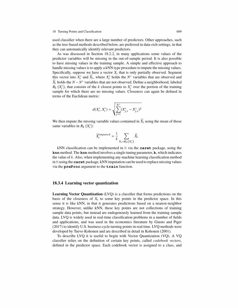
As was discussed in Section 18.2.2, in many applications some values of thepredictor variables will be missing in the out-of-sample period. It is also possibleto have missing values in the training sample. A simple and effective approach tohandle missing values is to apply a kNN type procedure to impute the missing values.Specifically, suppose we have a vector Xt that is only partially observed. Segmentthis vector into X∗t and Xt , where X∗t holds the N∗ variables that are observed andXt holds the N − N∗ variables that are not observed. Define a neighborhood, labeledRk
(X∗t
), that consists of the k closest points to X∗t over the portion of the training
sample for which there are no missing values. Closeness can again be defined interms of the Euclidean metric:
d(X∗t ,X∗i ) =
√√√ N∗∑j=1
(X∗j ,t − X∗j ,i)2
We then impute the missing variable values contained in Xt using the mean of thosesame variables in Rk
(X∗t
):
X imputedt =
1
k
∑Xi ∈Rk (X∗t )
Xi
kNN classification can be implemented in R via the caret package, using theknnmethod. The knnmethod involves a single tuning parameter, k, which indicatesthe value of k. Also, when implementing any machine learning classification methodinR using thecaret package, kNN imputation can be used to replacemissing valuesvia the preProc argument to the train function.
18.3.4 Learning vector quantization
Learning Vector Quantization (LVQ) is a classifier that forms predictions on thebasis of the closeness of Xt to some key points in the predictor space. In thissense it is like kNN, in that it generates predictions based on a nearest-neighborstrategy. However, unlike kNN, these key points are not collections of trainingsample data points, but instead are endogenously learned from the training sampledata. LVQ is widely used in real-time classification problems in a number of fieldsand applications, and was used in the economics literature by Giusto and Piger(2017) to identify U.S. business cycle turning points in real time. LVQmethods weredeveloped by Tuevo Kohonen and are described in detail in Kohonen (2001).
To describe LVQ it is useful to begin with Vector Quantization (VQ). A VQclassifier relies on the definition of certain key points, called codebook vectors,defined in the predictor space. Each codebook vector is assigned to a class, and
610 Jeremy Piger
there can be more than one codebook vector per class. We would generally havefar fewer codebook vectors than data vectors, implying that a codebook vectorprovides representation for a group of training sample data vectors. In other words,the codebook vectors quantize the salient features of the predictor data. Once thesecodebook vectors are singled out, data is classified via a majority vote of the nearestgroup of k codebook vectors in the Euclidean metric.
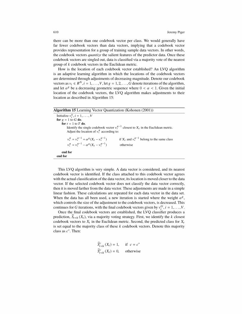
How is the location of each codebook vector established? An LVQ algorithmis an adaptive learning algorithm in which the locations of the codebook vectorsare determined through adjustments of decreasing magnitude. Denote our codebookvectors as vi ∈ RN , i = 1, . . . ,V , let g = 1,2, . . . ,G denote iterations of the algorithm,and let αg be a decreasing geometric sequence where 0 < α < 1. Given the initiallocation of the codebook vectors, the LVQ algorithm makes adjustments to theirlocation as described in Algorithm 15:
Algorithm 15 Learning Vector Quantization (Kohonen (2001))Initialize v0i , i = 1, . . . ,Vfor g = 1 to G do.
for t = 1 to T do.Identify the single codebook vector vg−1∗ closest to Xt in the Euclidean metric.Adjust the location of vg∗ according to:
vg∗ = v
g−1∗ + αg(Xt − v
g−1∗ ) if Xt and v
g−1∗ belong to the same class
vg∗ = v
g−1∗ − αg(Xt − v
g−1∗ ) otherwise
end forend for
This LVQ algorithm is very simple. A data vector is considered, and its nearestcodebook vector is identified. If the class attached to this codebook vector agreeswith the actual classification of the data vector, its location is moved closer to the datavector. If the selected codebook vector does not classify the data vector correctly,then it is moved farther from the data vector. These adjustments are made in a simplelinear fashion. These calculations are repeated for each data vector in the data set.When the data has all been used, a new iteration is started where the weight αg,which controls the size of the adjustment to the codebook vectors, is decreased. Thiscontinues for G iterations, with the final codebook vectors given by vGi , i = 1, . . . ,V .
Once the final codebook vectors are established, the LVQ classifier produces aprediction, St+h (Xt ), via a majority voting strategy. First, we identify the k closestcodebook vectors to Xt in the Euclidean metric. Second, the predicted class for Xt
is set equal to the majority class of these k codebook vectors. Denote this majorityclass as c∗. Then:
Sct+h (Xt ) = 1, if c = c∗
Sct+h (Xt ) = 0, otherwise

18 Turning Points and Classification 611
Here I have laid out the basic LVQ algorithm, which has been shown to workwell in many practical applications. Various modifications to this algorithm havebeen proposed, which may improve classification ability in some contexts. Theseinclude LVQ with nonlinear updating rules, as in the Generalized LVQ algorithmof Sato and Yamada (1995), as well as LVQ employed with alternatives to theEuclidean measure of distance, such as the Generalized Relevance LVQ of Hammerand Villmann (2002). The latter allows for adaptive weighting of data series in thedimensions most helpful for classification, and may be particularly useful whenapplying LVQ to large datasets.
LVQ classification can be implemented in R via the caret package using thelvqmethod. The lvqmethod has two tuning parameters. The first is the number ofcodebook vectors to use in creating the final classification, k, and is labeled k. Thesecond is the total number of codebook vectorsV , and is labeledsize. To implementthe classifier, one must also set the values of G and α. In the lvq method, G is setendogenously to ensure convergence of the codebook vectors. The default value ofα in the lvq method is 0.3. Kohonen (2001) argues that classification results fromLVQ should be largely invariant to the choice of alternative values of α providedthat αg → 0 as g → ∞, which ensures that the size of codebook vector updateseventually converge to zero. Giusto and Piger (2017) verified this insensitivity intheir application of LVQ to identifying business cycle turning points.
The LVQ algorithm requires an initialization of the codebook vectors. This ini-tialization can have effects on the resulting class prediction, as the final placementof the codebook vectors in an LVQ algorithm is not invariant to initialization. Asimple approach, which I follow in the application, is to allow all classes to havethe same number of codebook vectors, and initialize the codebook vectors attachedto each class with random draws of Xt vectors from training sample observationscorresponding to each class.
18.3.5 Classification trees
A number of commonly used classification techniques are based on classificationtrees. I will discuss several of these approaches in subsequent sections, each of whichuses aggregations of multiple classification trees to generate predictions. Beforedelving into these techniques, in this section I describe the single classification treesupon which they are built.
A classification tree is an intuitive, non-parametric, procedure that approachesclassification by partitioning the predictor variable space into non-overlapping re-gions. These regions are created according to a conjunction of binary conditions. Asan example, in a case with two predictor variables, one of the regions might be of theform {Xt |X1,t ≥ τ1,X2,t < τ2}. The partitions are established in such a way so as toeffectively isolate alternative classes in the training sample. For example, the regionmentioned above might have been chosen because it corresponds to cases where

612 Jeremy Piger
St+h is usually equal to c. To generate predictions, the classification tree would thenplace a high probability on St+h = c if Xt fell in this region.
How specifically are the partitions established using a training sample? Here Iwill describe a popular training algorithm for a classification tree, namely the clas-sification and regression tree (CART). CART proceeds by recursively partitioningthe training sample through a series of binary splits of the predictor data. Each newpartition, or split, segments a region that was previously defined by the earlier splits.The new split is determined by one of the predictor variables, labeled the ‘splitvariable,’ based on a binary condition of the form Xj ,t < τ and Xj ,t ≥ τ, whereboth j and τ can differ across splits. The totality of these recursive splits partitionthe sample space into M non-overlapping regions, labeled A∗m, m = 1, . . . ,M , wherethere are T∗m training sample observations in each region. For all Xt that are in regionA∗m, the prediction for St+h is a constant equal to the within-region sample proportionof class c:
PcA∗m=
1
T∗m
∑Xt ∈A
∗m
I(St+h = c) (18.3)
The CART classifier is then:
Sct+h (Xt ) =
M∑m=1
PcA∗m
I(Xt ∈ A∗m
)(18.4)
How is the recursive partitioning implemented to arrive at the regions A∗m? Sup-pose that at a given step in the recursion, we have a region defined by the totalityof the previous splits. In the language of decision trees, this region is called a‘node.’ Further, assume this node has not itself yet been segmented into subregions.I refer to such a node as an ‘unsplit node’ and label this unsplit node genericallyas A. For a given j and τ j we then segment the data in this region according to{Xt |Xj ,t < τ j,Xt ∈ A} and {Xt |Xj ,t ≥ τ j,Xt ∈ A}, which splits the data in thisnode into two non-overlapping regions, labelled AL and AR respectively. In theseregions, there are TL and TR training sample observations. In order to determinethe splitting variable, j, and the split threshold, τ j , we scan through all pairs { j, τ j},where j = 1, . . . N and τ j ∈ T A, j , to find the values that maximize a measure ofthe homogeneity of class outcomes inside of AL and AR.5 Although a variety ofmeasures of homogeneity are possible, a common choice is the Gini impurity:
5 In a CART classification tree, TA, j is a discrete set of all non-equivalent values for τ j , whichis simply the set of midpoints of the ordered values for Xj ,t in the training sample observationsrelevant for node A.

18 Turning Points and Classification 613
GL =
C∑c=1
PcAL (1 − Pc
AL )
GR =
C∑c=1
PcAR (1 − Pc
AR )
The Gini impurity is bounded between zero and one, where a value of zero indicatesa ‘pure’ region where only one class is present. Higher values of the Gini impurityindicate greater class diversity. The average Gini impurity for the two new proposedregions is:
G =TL
TL + TRGL +
TR
TL + TRGR (18.5)
The split point j and split threshold τ j are then chosen to create regions AL and AR
that minimize the average Gini impurity.This procedure is repeated for other unsplit nodes of the tree, with each additional
split creating two new unsplit nodes. By continuing this process recursively, thesample space is divided into smaller and smaller regions. One could allow therecursion to run until we are left with only pure unsplit nodes. A more commonchoice in practice is to stop splitting nodes when any newly created region wouldcontain a number of observations below some predefined minimum. This minimumnumber of observations per region is a tuning parameter of the classification tree.Whatever approach is taken, when we arrive at an unsplit node that is not going tobe split further, this node becomes one of our final regions A∗m. In the language ofdecision trees, this final unsplit node is referred to as a ‘leaf.’ Algorithm 16 providesa description of the CART classification tree.
Algorithm 16A Single CART Classification Tree (Breiman, Friedman, Olshen, andStone (1984))1: Initialize a single unsplit node to contain the full training sample2: for All unsplit nodes Au with total observations > threshold do3: for j = 1 to N and τ j ∈ TAu , j do4: Create non-overlapping regions AL
u = {Xt |Xj ,t < τj , Xt ∈ Au } and
ARu = {Xt |Xj ,t ≥ τ
j , Xt ∈ Au } and calculate G as in (18.5).5: end for6: Select j and τ j to minimize G and create the associated nodes AL
u and ARu .
7: Update the set of unsplit nodes to include ALu and AR
u .8: end for9: For final leaf nodes, A∗m , form Pc
A∗mas in (18.3), for c = 1, . . . ,C and m = 1, . . .M
10: Form the CART classification tree classifier: Sct+h(Xt ) as in (18.4).
Classification trees have many advantages. They are simple to understand, requireno parametric modeling assumptions, and are flexible enough to capture complicatednonlinear and discontinuous relationships between the predictor variables and classindicator. Also, the recursive partitioning algorithm described above scales easily to

614 Jeremy Piger
large datasets, making classification trees attractive in this setting. Finally, unlike theclassifierswe have encountered to this point, a CART classification tree automaticallyconducts model selection in the process of producing a prediction. Specifically, avariablemay never be used as a splitting variable, which leaves it unused in producinga prediction by the classifier. Likewise, another variablemaybe usedmultiple times asa splitting variable. These differences result in varying levels of variable importancein a CART classifier. Hastie, Tibshirani, and Friedman (2009) detail a measure ofvariable importance that can be produced from a CART tree.
CART trees have one significant disadvantage. The sequence of binary splits, andthe path dependence this produces, generally produces a high variance forecast. Thatis, small changes in the training sample can produce very different classification treesand associated predictions. As a result, a number of procedures exist that attempt toretain the benefits of classification trees, while reducing variance. We turn to theseprocedures next.
18.3.6 Bagging, random forests, and extremely randomized trees
In this section we describe bagged classification trees, their close variant, therandom forest, and a modification to the random forest known as extremely ran-domized trees. Each of these approaches average the predicted classification comingfrommany classification trees. This allows us to harness the advantages of tree-basedmethods, while at the same time reducing the variance of the tree-based predictionsthrough averaging. Random forests have been used to identify turning points in eco-nomic data byWard (2017), who uses random forests to identify episodes of financialcrises, and Garbellano (2016), who uses random forests to nowcast U.S. recessionepisodes. Bagging and random forests are discussed in more detail in Chapter 13 ofthis book.
We begin with bootstrap aggregated (bagged) classification trees, which wereintroduced in Breiman (1996). Bagged classification trees work by training a largenumber, B, of CART classification trees and then averaging the class predictionsfrom each of these trees to arrive at a final class prediction. The trees are differentbecause each is trained on a bootstrap training sample of size T , which is createdby sampling {Xt,St+h} with replacement from the full training sample. Each treeproduces a class prediction, which I label Sc
b,t+h(Xt ), b = 1, . . . ,B. The bagged
classifier is then the simple average of the B CART class predictions:
Sct+h (Xt ) =
1
B
B∑b=1
Scb,t+h (Xt ) (18.6)
Bagged classification trees are a variance reduction technique that can give substan-tial gains in accuracy over individual classification trees. As discussed in Breiman(1996), a key determinant of the potential benefits of bagging is the variance of the

18 Turning Points and Classification 615
individual classification trees across alternative training samples. All else equal, thehigher is this variance, the more potential benefit there is from bagging.
As discussed in Breiman (2001), the extent of the variance improvement alsodepends on the amount of correlation across the individual classification trees thatconstitute the bagged classification tree, with higher correlation generating lowervariance improvements. This correlation could be significant, as the single classifi-cation trees used in bagging are trained on overlapping bootstrap training samples.As a result, modifications to the bagged classification tree have been developed thatattempt to reduce the correlation across trees, without substantially increasing thebias of the individual classification trees. The most well know of these is the randomforest (RF), originally developed in Breiman (2001).6
An RF classifier attempts to lower the correlation across trees by adding anotherlayer of randomness into the training of individual classification trees. As with abagged classification tree, each single classification tree is trained on a bootstraptraining sample. However, when training this tree, rather than search over the entireset of predictors j = 1, . . . ,N for the best splitting variable at each node, we insteadrandomly chooseQ << N predictor variables at each node, and search only over thesevariables for the splitting variable. This procedure is repeated to train B individualclassification trees, and the random forest classifier is produced by averaging theseclassification trees as in equation (18.6). Algorithm 17 provides a description of theRF classifier.
Algorithm 17 Random Forest Classifier (Breiman (2001))1: for b = 1 to B do2: Form a bootstrap training sample by sampling {Xt , St+h } with replacement
T times from the training sample observations.3: Initialize a single unsplit node to contain the full bootstrap training sample4: for All unsplit nodes Au with total observations > threshold do5: Randomly select Q predictor variables as possible splitting variables. Denote
these predictor variables at time t as Xt
6: for Xj ,t ∈ Xt and τ j ∈ TAu , j do7: Create two non-overlapping regions AL
u = {Xt |Xj ,t < τj , Xt ∈ Au } and
AR = {Xt |Xj ,t ≥ τj , Xt ∈ Au } and calculate G as in (18.5).
8: end for9: Select j and τ j to minimize G and create the associated nodes AL
u and ARu .
10: Update the set of unsplit nodes to include ALu and AR
u
11: end for12: For final leaf nodes, A∗m , form Pc
A∗mas in (18.3), for c = 1, . . . ,C and m = 1, . . .M
13: Form the single tree classifier: Scb ,t+h
(Xt ) as in (18.4).14: end for15: Form the Random Forest classifier: Sc
t+h(Xt ) =
1B
B∑b=1
Scb ,t+h
(Xt ).
6 Other papers that were influential in the development of random forest methods include Amit andGeman (1997) and Ho (1998).

616 Jeremy Piger
When implementing a RF classifier, the individual trees are usually allowed togrow to maximum size, meaning that nodes are split until only pure nodes remain.While such a tree should produce a classifier with low bias, it is likely to be undulyinfluenced by peculiarities of the specific training sample, and thus will have highvariance. The averaging of the individual trees lowers this variance, while the ad-ditional randomness injected by the random selection of predictor variables helpsmaximize the variance reduction benefits of averaging. It is worth noting that bysearching only over a small random subset of predictors at each node for the optimalsplitting variable, the RF classifier also has computational advantages over bagging.
Extremely Randomized Trees, or ‘ExtraTrees,’ is another approach to reduce cor-relation among individual classification trees. Unlike both bagged classification treesand RF, ExtraTrees trains each individual classification tree on the entire trainingsample rather than bootstrapped samples. As does a random forest, ExtraTrees ran-domizes the subset of predictor variables considered as possible splitting variablesat each node. The innovation with ExtraTrees is that when training the tree, foreach possible split variable, only a single value of τ j is considered as the possiblesplit threshold. For each j, this value is randomly chosen from the uniform interval[min(Xj ,t |Xj ,t ∈ A),max(Xj ,t |Xj ,t ∈ A)
]. Thus, ExtraTrees randomizes across both
the split variable and the split threshold dimension. ExtraTrees was introduced byGeurts, Ernst, and Wehenkel (2006), who argue that the additional randomizationintroduced by ExtraTrees should reduce variance more strongly than weaker ran-domization schemes. Also, the lack of a search over all possible τ j for each splitvariable at each node provides additional computational advantages over the RFclassifier. Algorithm 18 provides a description of the ExtraTrees classifier:
Algorithm 18 Extremely Randomized Trees (Geurts, Ernst, and Wehenkel (2006))1: for b = 1 to B do2: Initialize a single unsplit node to contain the full training sample3: for All unsplit nodes Au with total observations > threshold do4: Randomly select Q predictor variables as possible splitting variables. Denote
these predictor variables at time t as Xt
5: for Xj ,t ∈ Xt do6: Randomly select a single τ j from the uniform interval:[
min(Xj ,t |Xj ,t ∈ Au ),max(Xj ,t |Xj ,t ∈ Au )]
7: Create two non-overlapping regions ALu = {Xt |Xj ,t < τ
j , Xt ∈ Au } andAR = {Xt |Xj ,t ≥ τ
j , Xt ∈ Au } and calculate G as in (18.5).8: end for9: Select j to minimize G and create the associated nodes AL
u and ARu .
10: Update the set of unsplit nodes to include ALu and AR
u
11: end for12: For final leaf nodes, A∗m , form Pc
A∗mas in (18.3), for c = 1, . . . ,C and m = 1, . . .M
13: Form the single tree classifier: Scb ,t+h
(Xt ) as in (18.4).14: end for15: Form the ExtraTrees classifier: Sc
t+h(Xt ) =
1B
B∑b=1
Scb ,t+h
(Xt ).

18 Turning Points and Classification 617
RF and ExtraTrees classifiers have enjoyed a substantial amount of success inempirical applications. They are also particularly well suited for data-rich envi-ronments. Application to wide datasets of predictor variables is computationallytractable, requiring a number of scans that at most increase linearly with the numberof predictors. Also, because these algorithms are based on classification trees, theyautomatically conduct model selection as the classifier is trained.
Both RF and ExtraTrees classifiers can be implemented in R via the caret pack-age, using the ranger method. Implementation involves three tuning parameters.The first is the value of Q and is denoted mtry in the caret package. The secondis splitrule and indicates whether a random forest (splitrule= 0) or an ex-tremely randomized tree (splitrule= 1) is trained. Finally, min.node.sizeindicates the minimum number of observations allowed in the final regions estab-lished for each individual classification tree. As discussed above, it is common withrandom forests and extremely randomized trees to allow trees to be trained until allregions are pure. This can be accomplished by setting min.node.size= 1.
18.3.7 Boosting
Boosting has been described by Hastie et al. (2009) as “one of the most power-ful learning ideas introduced in the last twenty years" and by Breiman (1996) as“the best off-the-shelf classifier in the world." Many alternative descriptions andinterpretations of boosting exist, and a recent survey and historical perspective isprovided inMayr, Binder, Gefeller, and Schmid (2014). In economics, several recentpapers have used boosting to predict expansion and recession episodes, includingNg (2014), Berge (2015) and D opke, Fritsche, and Pierdzioch (2017). Boosting isdescribed in more detail in Chapter 14 of this book.
The central idea of boosting is to recursively apply simple ‘base’ learners to atraining sample, and then combine these base learners to form a strong classifier.In each step of the recursive boosting procedure, the base learner is trained ona weighted sample of the data, where the weighting is done so as to emphasizeobservations in the sample that to that point had been classified incorrectly. Thefinal classifier is formed by combining the sequence of base learners, with betterperforming base learners getting more weight in this combination.
The first boosting algorithms are credited to Schapire (1990), Freund (1995)and Freund and Schapire (1996) and are referred to as AdaBoost. Later work byFriedman, Hastie, and Tibshirani (2000) interpretedAdaBoost as a forward stagewiseprocedure to fit an additive logistic regressionmodel, while Friedman (2001) showedthat boosting algorithms can be interpreted generally as non-parametric functionestimation using gradient descent. In the following I will describe boosting in moredetail using these later interpretations.
For notational simplicity, and to provide a working example, consider a two classcase, where I define the two classes as St+h = −1 and St+h = 1. Define a functionF (Xt ) ∈ R that is meant to model the relationship between our predictor variables,

618 Jeremy Piger
Xt , and St+h . Larger values of F (Xt ) signal increased evidence for St+h = 1, whilesmaller values indicate increased evidence for St+h = −1. Finally, define a lossfunction, C(St+h,F (Xt )), and suppose our goal is to choose F (Xt ) such that weminimize the expected loss:
ES,XC(St+h,F (Xt )) (18.7)
A common loss function for classification is exponential loss:
C(St+h,F (Xt )) = exp(−St+hF (Xt )
)The exponential loss function is smaller if the signs of St+h and F (Xt ) match thanif they do not. Also, this loss function rewards (penalizes) larger absolute values ofF (Xt ) when it is correct (incorrect).
For exponential loss, it is straightforward to show (Friedman et al. (2000)) thatthe F (Xt ) that minimizes equation (18.7) is:
F (Xt ) =1
2ln
[Pr
(St+h = 1|Xt
)Pr
(St+h = −1|Xt
) ]which is simply one-half the log odds ratio. A traditional approach commonly foundin economic studies is to assume an approximating parametric model for the logodds ratio. For example, a parametric logistic regression model would specify:
ln
[Pr
(St+h = 1|Xt
)Pr
(St+h = −1|Xt
) ] = X ′t β
A boosting algorithm alternatively models F (Xt ) as an additive model (Friedmanet al. (2000)):
F (Xt ) =
J∑j=1
αjTj
(Xt ; βj
)(18.8)
where each Tj
(Xt ; βj
)is a base learner with parameters βj . Tj
(Xt ; βj
)is usually
chosen as a simple model or algorithm with only a small number of associatedparameters. A very common choice for Tj
(Xt ; βj
)is a CART regression tree with a
small number of splits.Boosting algorithms fit equation (18.8) to the training sample in a forward stage-
wise manner. An additive model fit via forward stagewise iteratively solves for theloss minimizing αjTj
(Xt ; βj
), conditional on the sum of previously fit terms, la-
beled Fj−1 (Xt ) =j−1∑i=1
αiTi(Xt ; βi
). Specifically, conditional on an initial F0 (Xt ), we
iteratively solve the following for j = 1, . . . , J:
{αj, βj} = minαj ,β j
T∑t=1
C(St+h,
[Fj−1 (Xt ) + αjTj
(Xt ; βj
) ] )(18.9)
18 Turning Points and Classification 619
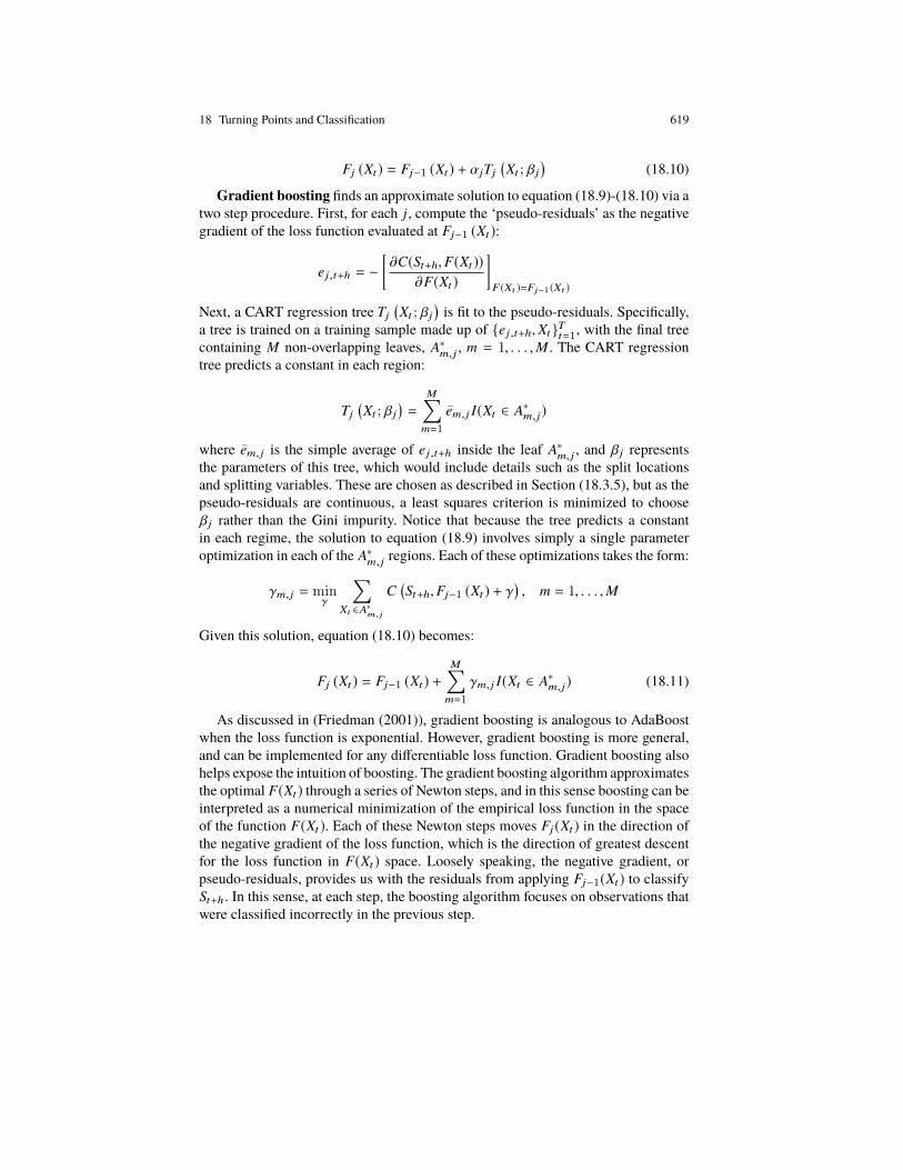
Fj (Xt ) = Fj−1 (Xt ) + αjTj
(Xt ; βj
)(18.10)
Gradient boosting finds an approximate solution to equation (18.9)-(18.10) via atwo step procedure. First, for each j, compute the ‘pseudo-residuals’ as the negativegradient of the loss function evaluated at Fj−1 (Xt ):
ej ,t+h = −[∂C(St+h,F(Xt ))
∂F(Xt )
]F(Xt )=Fj−1(Xt )
Next, a CART regression tree Tj
(Xt ; βj
)is fit to the pseudo-residuals. Specifically,
a tree is trained on a training sample made up of {ej ,t+h,Xt }Tt=1, with the final tree
containing M non-overlapping leaves, A∗m, j , m = 1, . . . ,M . The CART regressiontree predicts a constant in each region:
Tj
(Xt ; βj
)=
M∑m=1
em, j I(Xt ∈ A∗m, j)
where em, j is the simple average of ej ,t+h inside the leaf A∗m, j , and βj representsthe parameters of this tree, which would include details such as the split locationsand splitting variables. These are chosen as described in Section (18.3.5), but as thepseudo-residuals are continuous, a least squares criterion is minimized to chooseβj rather than the Gini impurity. Notice that because the tree predicts a constantin each regime, the solution to equation (18.9) involves simply a single parameteroptimization in each of the A∗m, j regions. Each of these optimizations takes the form:
γm, j = minγ
∑Xt ∈A
∗m, j
C(St+h,Fj−1 (Xt ) + γ
), m = 1, . . . ,M
Given this solution, equation (18.10) becomes:
Fj (Xt ) = Fj−1 (Xt ) +
M∑m=1
γm, j I(Xt ∈ A∗m, j) (18.11)
As discussed in (Friedman (2001)), gradient boosting is analogous to AdaBoostwhen the loss function is exponential. However, gradient boosting is more general,and can be implemented for any differentiable loss function. Gradient boosting alsohelps expose the intuition of boosting. The gradient boosting algorithm approximatesthe optimal F(Xt ) through a series of Newton steps, and in this sense boosting can beinterpreted as a numerical minimization of the empirical loss function in the spaceof the function F(Xt ). Each of these Newton steps moves Fj(Xt ) in the direction ofthe negative gradient of the loss function, which is the direction of greatest descentfor the loss function in F(Xt ) space. Loosely speaking, the negative gradient, orpseudo-residuals, provides us with the residuals from applying Fj−1(Xt ) to classifySt+h . In this sense, at each step, the boosting algorithm focuses on observations thatwere classified incorrectly in the previous step.

620 Jeremy Piger
Finally, Friedman (2001) suggests a modification of equation (18.11) to introducea shrinkage parameter:
Fj (Xt ) = Fj−1 (Xt ) + η
M∑m=1
γm, j I(Xt ∈ A∗m, j),
where 0 < η ≤ 1 controls the size of the function steps in the gradient basednumerical optimization. In practice, η is a tuning parameter for the gradient boostingalgorithm.
Gradient boosting with trees as the base learners is referred to under a variety ofnames, including a Gradient BoostingMachine,MART (multiple additive regressiontrees), TreeBoost and a Boosted Regression Tree. The boosting algorithm for ourtwo class example is shown in Algorithm 19.
Algorithm 19 Gradient Boosting with Trees (Friedman (2001))
1: Initialize F0 (Xt ) = minγ
T∑t=1
C(St+h , γ)
2: for j = 1 to J do3: e j ,t+h = −
[∂C(St+h ,F (Xt ))
∂F (Xt )
]F (Xt )=Fj−1(Xt )
, t = 1 . . .T
4: Fit T(Xt ; β j
)to {e j ,t+h , Xt }
Tt=1 to determine regions A∗m, j , m = 1, . . .M
5: γm, j = minγ
∑Xt ∈A
∗m, j
C(St+h , Fj−1 (Xt ) + γ
), m = 1, . . .M
6: Fj (Xt ) = Fj−1 (Xt ) + ηM∑
m=1γm, j I
(Xt ∈ A∗m, j
)7: end for
Upon completion of this algorithmwe have FJ (Xt ), although inmany applicationsthis function is further converted into a more recognizable class prediction. Forexample, AdaBoost uses the classifier sign(FJ (Xt )), which for the two-class examplewith exponential loss, classifies St+h according to its highest probability class. Inour application, we will instead convert FJ (Xt ) to a class probability by invertingthe assumed exponential cost function, and use these probabilities as our classifier,St+h . Again, for the two class case with exponential loss:
Sc=1t+h (Xt ) =
exp(2FJ (Xt ))
1 + exp(2FJ (Xt ))
Sc=−1t+h (Xt ) =
1
1 + exp(2FJ (Xt ))
Gradient boosting with trees scales very well to data-rich environments. Theforward-stagewise gradient boosting algorithms simplify optimization considerably.Further, gradient boosting is commonly implemented with small trees, in part toavoid overfitting. Indeed, a common choice is to use so called ‘stumps’, which aretrees with only a single split. This makes implementation with large sets of predictors

18 Turning Points and Classification 621
very fast, as at each step in the boosting algorithm, only a small number of scansthrough the predictor variables is required.
Two final aspects of gradient boosting bear further comment. First, as discussedin Hastie et al. (2009), the algorithm above can be modified to incorporate K > 2classes by assuming a negative multinomial log likelihood cost function. Second,Friedman (2001) suggests a modified version of Algorithm 19 in which, at eachstep j, a random subsample of the observations is chosen. This modification, knownas ‘stochastic gradient boosting,’ can help prevent overfitting while also improvingcomputational efficiency.
Gradient boosting can be implemented in R via the caret package, using thegbm method. Implementation of gbm where regression trees are the base learnersinvolves four tuning parameters. The first is n.trees, which is the stopping pointJ for the additive model in equation (18.8). The second is interaction.depth,which is the depth (maximum number of consecutive splits) of the regression treesused as weak learners. shrinkage is the shrinkage parameter, η in the updatingrule equation (18.3.7). Finally, n.minobsinnode is the minimum terminal nodesize for the regression trees.
18.4 Markov-Switching Models
In this section we describe Markov-switching (MS) models, which are a popularapproach for both historical and real-time classification of economic data. In contrastto the machine learning algorithms presented in the previous section, MS modelsare unsupervised, meaning that a historical time series indicating the class is notrequired. Instead, MS models assume a parametric structure for the evolution of theclass, as well as for the interaction of the class with observed data. This structureallows for statistical inference on which class is, or will be, active. In data-richenvironments, Markov-switching can be combined with dynamic factor models tocapture the information contained in datasets with many predictors. Obviously, MSmodels are particularly attractivewhen a historical class indicator is not available, andthus supervised approaches cannot be implemented. However, MS models have alsobeen used quite effectively for real-time classification in settings where a historicalindicator is available. We will see an example of this in Section 18.5.
MSmodels are parametric time-series models in which parameters are allowed totake on different values in each of C regimes, which for our purposes correspond tothe classes of interest. A fundamental difference from the supervised approaches wehave already discussed is that these regimes are not assumed to be observed in thetraining sample. Instead, a stochastic process assumed to have generated the regimeshifts is included as part of the model, which allows for both in-sample historicalinference on which regime is active, as well as out-of-sample forecasts of regimes. Inthe MS model, introduced to econometrics by Goldfeld and Quandt (1973), Cosslettand Lee (1985), and Hamilton (1989), the stochastic process assumed is a C-stateMarkov process. Also, and in contrast to the non-parametric approaches we have

622 Jeremy Piger
already seen, a specific parametric structure is assumed to link the observed Xt to theregimes. Following Hamilton (1989), this linking model is usually an autoregressivetime-series model with parameters that differ in the C regimes. The primary use ofthese models in the applied economics literature has been to describe changes in thedynamic behavior of macroeconomic and financial time series.
The parametric structure of MS models comes with some benefits for classifi-cation. First, by specifying a stochastic process for the regimes, one can allow fordynamic features that may help with both historical and out-of-sample classification.For example, most economic regimes of interest display substantial levels of persis-tence. In an MS model, this persistence is captured by the assumed Markov processfor the regimes. Second, by assuming a parametric model linking Xt to the classes,the model allows the researcher to focus the classification exercise on the objectof interest. For example, if one is interested in identifying high and low volatilityregimes, a model that allows for switching in only conditional variance of an ARmodel could be specified.7
Since the seminal work of Hamilton (1989), MS models have become a verypopular modeling tool for applied work in economics. Of particular note are regime-switching models of measures of economic output, such as real Gross DomesticProduct (GDP), which have been used to model and identify the phases of thebusiness cycle. Examples of such models include Hamilton (1989), Chauvet (1998),Kim and Nelson (1999a), Kim and Nelson (1999b), and Kim, Morley, and Piger(2005). A sampling of other applications include modeling regime shifts in timeseries of inflation and interest rates (Evans and Wachtel (1993); Garcia and Perron(1996); Ang and Bekaert (2002)), high and low volatility regimes in equity returns(Turner, Startz, and Nelson (1989); Hamilton and Susmel (1994); Hamilton and Lin(1996); Dueker (1997); Guidolin and Timmermann (2005)), shifts in the FederalReserve’s policy “rule” (Kim (2004); Sims and Zha (2006)), and time variation inthe response of economic output to monetary policy actions (Garcia and Schaller(2002); Kaufmann (2002); Ravn and Sola (2004); Lo and Piger (2005)). Hamiltonand Raj (2002), Hamilton (2008) and Piger (2009) provide surveys of MS models,while Hamilton (1994) and Kim and Nelson (1999c) provide textbook treatments.
Following Hamilton (1989), early work on MS models focused on univariatemodels. In this case, Xt is scalar, and a common modeling choice is a pth-orderautoregressive model with Markov-switching parameters:
Xt = µSt+h + φ1,St+h
(Xt−1 − µSt+h−1
)+ · · · + φp,St+h
(Xt−p − µSt+h−p
)+ εt
εt ∼ N(0, σ2
St+h
)(18.12)
7MSmodels generally require a normalization in order to properly define the regimes. For example,in a two regime example where the regimes are high and low volatility, we could specify thatSt+h = 1 is the low variance regime and St+h = 2 is the high variance regime. In practice this isenforced by restricting the variance in St+h = 2 to be larger than that in St+h = 1. See Hamilton,Waggoner, and Zha (2007) for an extensive discussion of normalization in the MS model.

18 Turning Points and Classification 623
where St+h ∈ {1, . . . ,C} indicates the regime and is assumed to be unobserved, evenin the training sample. In this model, each of the mean, autoregressive parametersand conditional variance parameters are allowed to change in each of the C differentregimes. Hamilton (1989) develops a recursive filter that can be used to constructthe likelihood function for this MS autoregressive model, and thus estimate theparameters of the model via maximum likelihood.
A subsequent literature explored Markov-switching in multivariate settings. Inthe context of identifying business cycle regimes, Diebold and Rudebusch (1996)argue that considering multivariate information in the form of a factor structurecan drastically improve statistical identification of the regimes. Chauvet (1998)operationalizes this idea by developing a statistical model that incorporates both adynamic factormodel andMarkov switching, now commonly called a dynamic factorMarkov-switching (DFMS) model. Specifically, if Xt is multivariate, we assume thatXt is driven by a single-index dynamic factor structure, where the dynamic factor isitself driven by a Markov-switching process. A typical example of such a model isas follows:
Xstdt =
λ1 (L)
λ2 (L)...
λN (L)
Ft + vt
where Xstdt is the demeaned and standardized vector of predictor variables, λi (L) is
a lag polynomial, and vt =(v1,t, v2,t, . . . , vN ,t
) ′ is a zero-mean disturbance vectormeant to capture idiosyncratic variation in the series. vt is allowed to be seriallycorrelated, but its cross-correlations are limited. In the so-called ‘exact’ factor modelwe assume that E(vi,tvj ,t ) = 0, while in the ‘approximate’ factor model vt is allowedto have weak cross correlations. Finally, Ft is the unobserved, scalar, ‘dynamicfactor.’ We assume that Ft follows a Markov-switching autoregressive process as inequation (18.12), with Xt replaced by Ft .
Chauvet (1998) specifies a version of this DFMS model where the number ofpredictors is N = 4 and shows how the parameters of both the dynamic factorprocess and the MS process can be estimated jointly via the approximate maximumlikelihood estimator developed in Kim (1994). Kim and Nelson (1998) develop aBayesian Gibbs-sampling approach to estimate a similar model. Finally, Camacho etal. (2018) developmodifications of the DFMS framework that are useful for real-timemonitoring of economic activity, including mixed-frequency data and unbalancedpanels. Chapter 2 of this book presents additional discussion of the DFMS model.
As discussed in Camacho, Perez-Quiros, and Poncela (2015), in data-rich en-vironments the joint estimation of the DFMS model can become computationallyunwieldy. In these cases, an alternative, two-step, approach to estimation of modelparameters can provide significant computational savings. Specifically, in the firststep, the dynamic factor Ft is estimated using the non-parametric principal compo-

624 Jeremy Piger
nents estimator of Stock and Watson (2002). Specifically, Ft is set equal to the firstprincipal component of Xstd
t . In a second step, Ft is fit to a univariateMSmodel as inequation (18.12). The performance of this two-step approach relative to the one-stepapproach was evaluated by Camacho et al. (2015), and the two step approach wasused by Fossati (2016) for the task of identifying U.S. business cycle phases in realtime.
For the purposes of this chapter, we are primarily interested in the ability of MSmodels to produce a class prediction, Sc
t+h. In a MS model, this prediction comes
in the form of a ‘smoothed’ conditional probability: Sct+h= Pr
(St+h = c | XT
), c =
1, . . . ,C, where XT denotes the entire training sample, XT = {Xt }Tt=1. Bayesian es-
timation approaches of MS models are particularly useful here, as they produce thisconditional probability while integrating out uncertainty regarding model parame-ters, rather than conditioning on estimates of these parameters.
In the application presented in Section 18.5 I will consider two versions of theDFMS model for classification. First, for cases with a small number of predictorvariables, we estimate the parameters of the DFMSmodel jointly using the Bayesiansampler of Kim and Nelson (1998). Second, for cases where the number of predictorvariables is large, we use the two step approach described above, where we estimatethe univariate MS model for Ft via Bayesian techniques. Both of these approachesproduce a classifier in the form of the smoothed conditional probability of the class.A complete description of the Bayesian samplers used in estimation is beyond thescope of this chapter. I refer the interested reader to Kim and Nelson (1999c), wheredetailed descriptions of Bayesian samplers for MS models can be found.
18.5 Application
In this section I present an application of the classification techniques presented aboveto nowcasting U.S. expansion and recession phases at the monthly frequency. In thiscase, St+h ∈ {1,2}, where St+h = 1 indicates a month that is a recession and St+h = 2indicates a month that is an expansion. As I am interested in nowcasting, I set h = 0.As the measure of expansion and recession regimes, I use the NBER business cycledates, which are determined by the NBER’s Business Cycle Dating Committee. Iwill evaluate the ability of the alternative classifiers to accurately classify out-of-sample months that have not yet been classified by the NBER, and also to providetimely identification of turning points between expansion and recession (peaks) andrecession and expansion (troughs) in real time.
Providing improved nowcasts of business cycle phases and associated turningpoints is of significant importance because there are many examples of turning pointsthat were not predicted ex-ante. This leaves policymakers, financial markets, firms,and individuals to try to determine if a new business cycle phase has already begun.Even this is a difficult task, with new turning points usually not identified until manymonths after they occur. For example, the NBER has historically announced new

18 Turning Points and Classification 625
turning points with a lag of between 4 and 21 months. Statistical models improve onthe NBER’s timeliness considerably, with little difference in the timing of the turningpoint dates established.8However, thesemodels still generally identify turning pointsonly after several months have passed. For example, Hamilton (2011) surveys a widerange of statistical models that were in place to identify business cycle turning pointsin real time, and finds that such models did not send a definitive signal regarding theDecember 2007 NBER peak until late 2008.
There have been a number of existing studies that evaluate the performance ofindividual classifiers to nowcast U.S. business cycle dates. In this chapter I contributeto this literature by providing a comparison of a broad range of classifiers, includingseveral that have not yet been evaluated for the purpose of nowcasting businesscycles. In doing so, I also evaluate the ability of these classifiers to provide improvednowcasts using large N vs. small N datasets. Most of the existing literature hasfocused on small N datasets, usually consisting of four coincident monthly serieshighlighted by the NBER’s Business Cycle Dating Committee as important in theirdecisions. Notable exceptions are Fossati (2016), Davig and Smalter Hall (2016) andBerge (2015), each of which uses larger datasets to classify NBER recessions in realtime.
For predictor variables, I begin with the FRED-MD dataset, which is a monthlydataset on a large number of macroeconomic and financial variables maintained bythe Federal Reserve Bank of St. Louis. The development of FRED-MD is describedin McCracken and Ng (2015). I use the most recent version of this dataset available,which as of the writing of this chapter was the vintage released at the end of Novem-ber 2018. This vintage provides data for 128 monthly series covering months froma maximum of January 1959 through October 2018. I then delete six series that arenot regularly available over the sample period, and add seven series on manufactur-ing activity from the National Association of Purchasing Managers, obtained fromQuandl (www.quandl.com.) I also add seven indices of ‘news implied volatility’ asconstructed in Manela and Moreira (2017). The addition of these series is motivatedby Karnizova and Li (2014), who show that uncertainty measures have predictivepower for forecasting U.S. recessions. Finally, I restrict all series to begin in January1960, which eliminates missing values during 1959 for a number of series.
For all series that are from the original FRED-MD dataset, I transform the seriesto be stationary using the transformation suggested in McCracken and Ng (2015),implemented using the Matlab code available from Michael McCracken’s website.For the seven NAPM series and NVIX series, I leave the series without transfor-mation. In some cases, the transformation involves differencing, which uses up theinitial observation. To have a common starting point for our sample, I begin mea-suring all series in February 1960. The final raw dataset then consists of 136 series,where all series begin in February 1960 and extend to a maximum of October 2018.
In the analysis I consider three alternative datasets. The first, labeled Narrow inthe tables below, is a small dataset that uses four coincident indicators that havebeen the focus of much of the U.S. business cycle dating literature. These series are
8 See, e.g., Chauvet and Piger (2008), Chauvet and Hamilton (2006) and Giusto and Piger (2017).

626 Jeremy Piger
the growth rate of non-farm payroll employment, the growth rate of the industrialproduction index, the growth rate of real personal income excluding transfer receipts,and the growth rate of real manufacturing and trade sales. The second dataset,labeled Real Activity, is a larger dataset consisting of the 70 variables that are in thegroupings ‘output and income’, ‘labor market’, ‘housing’ and ‘consumption, ordersand inventories’ as defined in McCracken and Ng (2015). These variables define thereal activity variables in the dataset, and as such target the most obvious variableswith which to date turning points in real economic activity. The third dataset, labeledBroad, consists of all the variables in the dataset.
To evaluate the performance of the classifiers using these datasets, I conduct apseudo out-of-sample nowcasting exercise that covers the last two decades. Specifi-cally, consider an analyst applying a classification technique in real time at the endof each month from January 2000 to November 2018. For each of these months,I assume the analyst has a dataset covering the time period that would have beenavailable in real time. That is, I accurately replicate the real-time data reporting lagsthe analyst would face. The reason this is a pseudo out-of-sample exercise is that Ido not use the vintage of each dataset that would have been available in real time, assuch vintage data is not readily available for all the variables in our dataset. Chauvetand Piger (2008) show that data revisions do not cause significant inaccuracies inreal time dating of turning points. That said, interesting future work would replicatethis analysis with a fully vintage dataset.
In each month, the analyst uses the available dataset to train the supervisedclassifiers over a period for which the NBER classification of St is assumed known.At each month, the lag with which the NBER classification is assumed known isallowed to vary, and is set using the approach taken in Giusto and Piger (2017).Specifically, I assume that: 1) The date of a new peak or trough is assumed to beknown once it is announced by the NBER. 2) If the NBER does not announce anew peak within twelve months of a date, then it is assumed that a new peak didnot occur at that date. Twelve months is the longest historical lag the NBER hastaken in announcing a new business cycle peak. 3) Once the date of a new turningpoint is announced by the NBER, the new NBER business cycle phase (expansionor recession) is assumed to last at least six months. Since the unsupervised DFMSclassifier does not require knowledge of the NBER classification, I estimate theparameters of this model over the full period for which the predictor data is availableto the analyst. After training, the analyst then uses the classifier to classify thosemonths through the end of the relevant sample of predictor variables for which theNBER dates are not known.
Somewhatmore formally, suppose the data sample of predictor variables availableto the analyst ends in time H, and the NBER dates are known through time H − J.Then the supervised classifiers would be trained on data through H − J, and theDFMS model would be estimated on data through H. After training and estimation,all classifiers will be used to classify the unknown NBER dates frommonth H− J+1through H, and the accuracy of these monthly classifications will be evaluated. I willalso use these out-of-sample classifications to identify new business cycle turningpoints in real time.

18 Turning Points and Classification 627
Before discussing the results, there are several details of the implementation todiscuss. First, when the analyst applies the classifiers to predict the NBER date outof sample, the most recent data to be classified will be incomplete due to differentialreporting lags across series. In general, I handle these ‘ragged edges’ by filling inthe missing values using kNN imputation, as discussed in Section 18.3.3, prior toperforming any subsequent analysis. Second, for the supervised classifiers, I classifySt on the basis of the contemporaneous values of the predictor variables (month t) andthe first lag (month t − 1). That is, the Xt vector contains both the contemporaneousand first lag of all variables in the relevant sample. For the unsupervised DFMSapproach, all available values of Xt are used in forming the smoothed posteriorprobability for each class. Third, for each dataset, I replace outliers, defined asdatapoints that are greater than four standard deviations from the mean, with themedian of a six quarter window on either side of the outlier. Finally, as is typical inthe classification literature, I standardize and demean all variables prior to analysis.9
For each of the supervised classifiers, I use the caret package in R to train andform predictions. In each case, repeated, stratified k-fold cross validation is used fortuning parameters, with k set equal to 10, and the number of repeats also set equalto 10.10 The objective function used in the cross validation exercise was AUROC.Default ranges from caretwere used in tuning parameters. Note that both the kNNimputation for missing values, as well as outlier detection, were done separately oneach fold of the cross-validation exercise, which prevents data from outside the foldfrom informing the within-fold training.
For the unsupervised DFMS model, we must specify a specific version of theMarkov-switching equation to apply to the factor Ft . In order to provide a comparisonto the existing literature, I use specifications that most closely match those in existingstudies. Specifically, for themodel applied to the narrow dataset, for which theDFMSmodel is estimated jointly, I follow Chauvet (1998) and Kim and Nelson (1999b)and allow the factor to follow an AR(2) process with regime switching in mean:
Ft = µSt + φ1(Xt−1 − µSt−1
)+ φ2
(Xt−2 − µSt−2
)+ εt
εt ∼ N(0, σ2
)For the DFMS model applied to the real activity dataset, for which the DFMS modelis estimated via a two-step procedure, I follow Camacho et al. (2015) and use asimple AR(0) process with a switching mean:
9 In unreported results, I also considered a version of each supervised classifier that classified basedon predictor variables formed as principal components from the relevant dataset. The performanceof this version of the classifier was similar in all cases to the results applied to the full dataset ofindividual predictors.10 This is a relatively small number of repeats, andwas chosen to reduce the computational burden ofthe recursive out-of-sample nowcasting exercise. In unreported results, I confirmed the robustnessof several randomly chosen reported results to a larger number of repeats (100).

628 Jeremy Piger
Ft = µSt + εt
εt ∼ N(0, σ2
)I do not consider the broad dataset for the DFMS model, as the diversity of series inthis dataset is likely not well described by only a single factor as is assumed by theDFMS model.
Table 18.1 presents the QPS and AUROC statistics for each classifier appliedto each dataset, calculated over all the out-of-sample observations in the recursivenowcasting exercise. There are several conclusions that can be drawn from theseresults. First of all, in general, the AUROC statistics are very high, suggesting thateach of these classifiers has substantial ability to classify expansion and recessionmonths out of sample. Second, there are only relatively small differences in thesestatistics across classifiers. The DFMS model applied to the narrow dataset providesthe highest AUROC at 0.997, which is very close to perfect classification ability,while the kNN classifier applied to the narrow dataset produces the lowest QPS.However, most classifiers produce AUROCs and QPS values that are reasonablyclose to these best performing values.
Third, Table 18.1 suggests that the out-of-sample evaluation metrics are onlymoderately improved, it at all, by considering predictor variables beyond the narrowdataset. The differences in the evaluation statistics that result from changing datasetsize are small, and in many cases these changes are not in a consistent directionacross the QPS vs. AUROC. Overall, these results do not suggest that consideringa larger number of predictors over the narrow dataset is clearly advantageous fornowcasting business cycle phases in U.S. data. Note that some of this result likelycomes because there is limited room for improvement over the narrow dataset.
Table 18.1 also presents results for a simple ensemble classifier, which is formedas the average of the alternative classifiers. The ensemble classifier averages the clas-sification from all six classifiers for the narrow and real activity dataset, and averagesthe classification of the five supervised classifiers for the broad dataset. By averagingacross approximately unbiased classifier that are not perfectly correlated, an ensem-ble classifier holds out the possibility of lower variance forecasts than is producedby the individual classifiers. Interestingly, the ensemble classifiers perform well inthis setting, with the ensemble classifier applied to the real activity dataset havingthe lowest QPS and second highest AUROC of any classifier / dataset combinationin the table.
The results inTable 18.1 do not speak directly to the question of identifying turningpoints (peaks and troughs) in real time. To evaluate the ability of the classifiers toidentify turning points, we require a rule to transform the classifier output intoturning point predictions. Here I employ a simple rule to identify a new turningpoint, which can be described as follows: If the most recent known NBER classifiedmonth is an expansion month, a business cycle peak is established if S1
t (Xt ) ≥ 0.5for the final month in the out-of-sample period. Similarly, if the most recent knownNBER classified month is a recession month, a business cycle trough is establishedif S1
t (Xt ) < 0.5 for the final month in the out-of-sample period. This is a rather
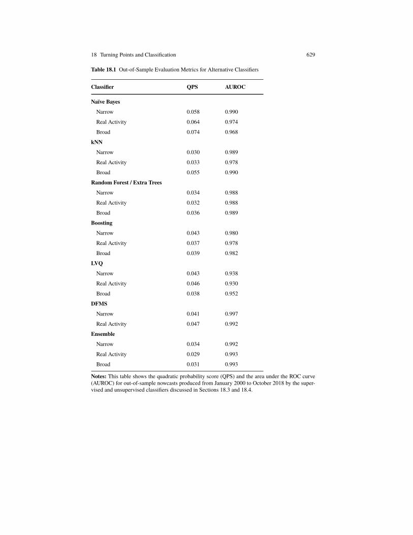
18 Turning Points and Classification 629
Table 18.1 Out-of-Sample Evaluation Metrics for Alternative Classifiers
Classifier QPS AUROC
Naïve Bayes
Narrow 0.058 0.990
Real Activity 0.064 0.974
Broad 0.074 0.968
kNN
Narrow 0.030 0.989
Real Activity 0.033 0.978
Broad 0.055 0.990
Random Forest / Extra Trees
Narrow 0.034 0.988
Real Activity 0.032 0.988
Broad 0.036 0.989
Boosting
Narrow 0.043 0.980
Real Activity 0.037 0.978
Broad 0.039 0.982
LVQ
Narrow 0.043 0.938
Real Activity 0.046 0.930
Broad 0.038 0.952
DFMS
Narrow 0.041 0.997
Real Activity 0.047 0.992
Ensemble
Narrow 0.034 0.992
Real Activity 0.029 0.993
Broad 0.031 0.993
Notes: This table shows the quadratic probability score (QPS) and the area under the ROC curve(AUROC) for out-of-sample nowcasts produced from January 2000 to October 2018 by the super-vised and unsupervised classifiers discussed in Sections 18.3 and 18.4.

630 Jeremy Piger
aggressive rule, which puts a high value on speed of detection. As such, we will beparticularly interested in the tendency of this rule to identify false turning points.
Table 18.2 shows the performance of each classifier for identifying the four U.S.business cycle turning points over the 2000-2018 time period. In the table, the datesshown are the first month in which the analyst would have been able to identify aturning point in the vicinity of the relevant turning point. For example, consider thecolumn for the December 2007 business cycle peak. An entry of ‘Mar 2008’ meansthat an analyst applying the classifiers at the end of March 2008 would have detecteda business cycle peak in the vicinity of the December 2007 peak. Because there isa minimum one month lag in data reporting for all series in the FRED-MD dataset,the analyst would have been using a dataset that extended through February 2008 toidentify this turning point. An entry of ‘NA’ means that the relevant turning pointwas not identified prior to the NBER Business Cycle Dating Committee making theannouncement of a new business cycle turning point.
I begin with the two business cycle peaks in the out-of-sample period. If wefocus on the narrow dataset, we see that most of the classifiers identify the March2001 business cycle peak by the end of May 2001, and the December 2007 peak bythe end of May 2008. This is a very timely identification of both of these turningpoints. For theMarch 2001 peak, identification at the end ofMay 2001means that theclassifiers identified this recession using data throughApril 2001, which was the veryfirst month of the recession. For the December 2007 peak, Hamilton (2011) reportsthat other real-time approaches in use at the time did not identify a business cyclepeak until late 2008 or early 2009, and the NBER business cycle dating committeeannounced the December 2007 peak in December 2008. Thus, identification at theend of May 2008 is relatively very fast. This timely performance does come witha single false business cycle peak being called for several, although not all, of theclassifiers. The date of this false peak was in September 2005 for most classifiers.
If we move to the larger real activity and broad datasets, in most cases theperformance of the classifiers for identifying business cycle peaks deteriorates. Twoof the classifiers, kNN and Random Forests, fail to identify the 2001 businesscycle peak, while several classifiers identify peaks more slowly when using thelarger datasets than the narrow dataset. There are some cases where moving fromthe narrow to the real activity dataset does improve with detection. The primaryexample is the DFMS model, where three of the four turning points are identifiedmore quickly when using the real activity dataset, and the false peak that occursunder the narrow dataset is eliminated. Overall, a reasonable conclusion is that thereare limited gains from using larger datasets to identify business cycle peaks in realtime, with the gains that do occur coming from the use of the real activity datasetwith certain classifiers.
Moving to troughs, the five supervised classification techniques identify troughsvery quickly in real time when applied to the narrow dataset. For the November 2001trough, these classifiers identify the trough by January or February of 2002, while theJune 2009 trough is identified by August or September of 2009. This is impressiveconsidering the very slow nature of the recovery following these recessions. As anexample, the NBER business cycle dating committee didn’t identify the November
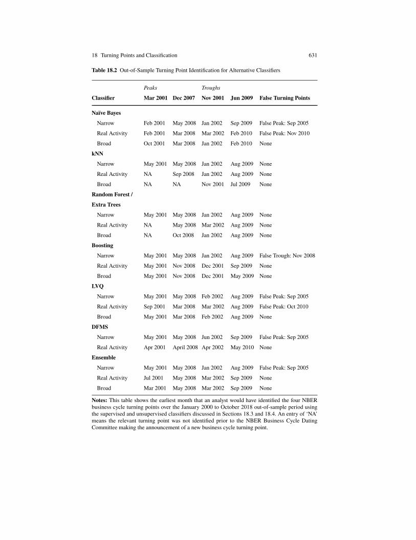
18 Turning Points and Classification 631
Table 18.2 Out-of-Sample Turning Point Identification for Alternative Classifiers
Peaks Troughs
Classifier Mar 2001 Dec 2007 Nov 2001 Jun 2009 False Turning Points
Naïve Bayes
Narrow Feb 2001 May 2008 Jan 2002 Sep 2009 False Peak: Sep 2005
Real Activity Feb 2001 Mar 2008 Mar 2002 Feb 2010 False Peak: Nov 2010
Broad Oct 2001 Mar 2008 Jan 2002 Feb 2010 None
kNN
Narrow May 2001 May 2008 Jan 2002 Aug 2009 None
Real Activity NA Sep 2008 Jan 2002 Aug 2009 None
Broad NA NA Nov 2001 Jul 2009 None
Random Forest /
Extra Trees
Narrow May 2001 May 2008 Jan 2002 Aug 2009 None
Real Activity NA May 2008 Mar 2002 Aug 2009 None
Broad NA Oct 2008 Jan 2002 Aug 2009 None
Boosting
Narrow May 2001 May 2008 Jan 2002 Aug 2009 False Trough: Nov 2008
Real Activity May 2001 Nov 2008 Dec 2001 Sep 2009 None
Broad May 2001 Nov 2008 Dec 2001 May 2009 None
LVQ
Narrow May 2001 May 2008 Feb 2002 Aug 2009 False Peak: Sep 2005
Real Activity Sep 2001 Mar 2008 Mar 2002 Aug 2009 False Peak: Oct 2010
Broad May 2001 Mar 2008 Feb 2002 Aug 2009 None
DFMS
Narrow May 2001 May 2008 Jun 2002 Sep 2009 False Peak: Sep 2005
Real Activity Apr 2001 April 2008 Apr 2002 May 2010 None
Ensemble
Narrow May 2001 May 2008 Jan 2002 Aug 2009 False Peak: Sep 2005
Real Activity Jul 2001 May 2008 Mar 2002 Sep 2009 None
Broad Mar 2001 May 2008 Mar 2002 Sep 2009 None
Notes: This table shows the earliest month that an analyst would have identified the four NBERbusiness cycle turning points over the January 2000 to October 2018 out-of-sample period usingthe supervised and unsupervised classifiers discussed in Sections 18.3 and 18.4. An entry of ‘NA’means the relevant turning point was not identified prior to the NBER Business Cycle DatingCommittee making the announcement of a new business cycle turning point.

632 Jeremy Piger
2001 troughs until July 2003 and the June 2009 trough until September 2010. Thisperformancewas achievedwith only a single false trough identified by one algorithm,Boosted Classification Trees. The DFMS classifier was somewhat slower to detectthese troughs than the other classifiers, although still substantially faster than theNBER announcement. Finally, consistent with the results for peaks, larger datasetsdid not substantially improve the timeliness with which troughs were identified onaverage.
Given the small number of turning points in the out-of-sample period, it is hardto distinguish definitively between the performance of the individual classifiers. Ifone were forced to choose a single classifier for the purpose of identifying turningpoints, both the kNN classifier and the random forest classifier applied to the narrowdataset were quick to identify turning points while producing no false positives. Theother classifiers had similar performance, but produced a single false positive. Thatsaid, the kNN classifier and random forest classifier both failed to identify businesscycle peaks when applied to the larger datasets, which may give us some pause as tothe robustness of these classifiers. If one looks more holistically across the variousdatasets, the boosting algorithm emerges as a possible favorite, as it identifies all fourturning points for all four datasets, and does sowith speed comparable to the top set ofperformers for each dataset. Finally, the ensemble classifier has overall performancesimilar to the boosting algorithm. We might also expect, given the potential effectof averaging on reducing classifier variance, that the ensemble classifier will be themost robust classifier across alternative out-of-sample periods.
18.6 Conclusion
In this chapter I have surveyed a variety of approaches for real-time classification ofeconomic time-series data. Special attention was paid to the case where classifica-tion is conducted in a data-rich environment. Much of the discussion was focusedon machine learning supervised classification techniques that are common to thestatistical classification literature, but have only recently begun to be widely usedin economics. I also presented a review of Markov-switching models, which is anunsupervised classification approach that has been commonly used in economicsfor both historical and real-time classification. Finally, I presented an application toreal-time identification of U.S. business cycle turning points based on a wide datasetof 136 macroeconomic and financial time-series.
References
Amit, Y., & Geman, D. (1997). Shape quantization and recognition with randomizedtrees. Neural Computation, 9, 1545–1588.

18 Turning Points and Classification 633
Ang, A., &Bekaert, G. (2002). Regime switches in interest rates. Journal of Businessand Economic Statistics, 20, 163–182.
Berge, T. (2015). Predicting recessions with leading indicators: Model averaging andselection over the business cycle. Journal of Forecasting, 34(6), 455–471.
Berge, T., & Jordá, O. (2011). The classification of economic activity into expansionsand recessions. American Economic Journal: Macroeconomics, 3(2), 246–277.
Breiman, L., Friedman, J., Olshen, R., & Stone, C. (1984). Classification and re-gression trees. Belmont, CA: Wadsworth.
Breiman, L. (1996). Bagging predictors. Machine Learning, 26(2), 123–140.Breiman, L. (2001). Random Forests. In Machine learning (pp. 5–32).Camacho, M., Perez-Quiros, G., & Poncela, P. (2015). Extracting nonlinear signals
from several economic indicators. Journal of Applied Econometrics, 30(7),1073–1089.
Camacho, M., Perez-Quiros, G., & Poncela, P. (2018). Markov-switching dynamicfactor models in real time. International Journal of Forecasting, 34, 598–611.
Chauvet, M. (1998). An econometric characterization of business cycle dynamicswith factor structure and regime switching. International Economic Review,39, 969–996.
Chauvet, M., & Hamilton, J. D. (2006). Dating business cycle turning points. InP. R. Costas Milas & D. van Dijk (Eds.), Nonlinear time series analysis ofbusiness cycles (pp. 1–53). Elsevier, North Holland.
Chauvet, M., & Piger, J. (2008). A comparison of the real-time performance ofbusiness cycle dating methods. Journal of Business and Economic Statistics,26(1), 42–49.
Cosslett, S., & Lee, L.-F. (1985). Serial correlation in discrete variable models.Journal of Econometrics, 27, 79–97.
D opke, J., Fritsche, U., & Pierdzioch, C. (2017). Predicting recessions with boostedregression trees. International Journal of Forecasting, 33, 745–759.
Davig, T., & Smalter Hall, A. (2016). Recession forecasting using Bayesian classi-fication. Federal Reserve Bank of Kansas City Research Working paper no.1606.
Diebold, F. X., & Rudebusch, G. D. (1996). Measuring business cycles: A modernperspective. The Review of Economics and Statistics, 78(1), 67–77.
Dueker, M. (1997). Markov switching in garch processes and mean-reverting stock-market volatility. Journal of Business and Economic Statistics, 15, 26–34.
Estrella, A., & Mishkin, F. S. (1998). Predicting U.S. recessions: Financial variablesas leading indicators. The Review of Economics and Statistics, 80(1), 45–61.
Estrella, A., Rodrigues, A. P., & Schich, S. (2003). How stable is the predictivepower of the yield curve? Evidence from Germany and the United States. TheReview of Economics and Statistics, 85(3), 629–644.
Evans, M., & Wachtel, P. (1993). Inflation regimes and the sources of inflationuncertainty. Journal of Money, Credit and Banking, 25, 475–511.
Fossati, S. (2016). Dating U.S. business cycles with macro factors. Studies in Non-linear Dynamics and Econometrics, 20, 529–547.

634 Jeremy Piger
Freund, Y. (1995). Boosting a weak learning algorithm by majority. Information andComputation, 121(2), 256–285.
Freund, Y., & Schapire, R. (1996). Experiments with a new boosting algorithm.Proceedings of ICML, 13, 148–156.
Friedman, J. (2001). Greedy function approximation: A gradient boosting machine.The Annals of Statistics, 29(5), 1189–1232.
Friedman, J., Hastie, T., & Tibshirani, R. (2000). Additive logistic regression: Astatistical view of boosting. The Annals of Statistics, 28(2), 337–407.
Fushing, H., Chen, S.-C., Berge, T.,& Jordá, O. (2010).A chronology of internationalbusiness cycles through non-parametric decoding. SSRN Working Paper no:1705758.
Garbellano, J. (2016). Nowcasting recessions with machine learning: New tools forpredicting the business cycle (Bachelor’s Thesis, University of Oregon).
Garcia, R., & Schaller, H. (2002). Are the effects of monetary policy asymmetric?Economic Inquiry, 40, 102–119.
Garcia, R., & Perron, P. (1996). An analysis of the real interest rate under regimeshifts. Review of Economics and Statistics, 78(1), 111–125.
Geurts, P., Ernst, D., & Wehenkel, L. (2006). Extremely randomized trees.MachineLearning, 63(1), 3–42.
Giusto, A., & Piger, J. (2017). Identifying business cycle turning points in real timewith vector quantization. International Journal of Forecasting, 33, 174–184.
Goldfeld, S. M., & Quandt, R. E. (1973). A markov model for switching regressions.Journal of Econometrics, 1(1), 3–16.
Guidolin, M., & Timmermann, A. (2005). Economic implications of bull and bearregimes in uk stock and bond returns. Economic Journal, 115(500), 111–143.
Hamilton, J. D. (1989). A new approach to the economic analysis of nonstationarytime series and the business cycle. Econometrica, 57(2), 357–384.
Hamilton, J. D. (1994). Time series analysis. Princeton, NJ: Princeton UniversityPress.
Hamilton, J. D. (2008). Regime switching models. In S. N. Durlauf & L. E. Blume(Eds.), New palgrave dictionary of economics, 2nd edition, Palgrave MacMil-lan.
Hamilton, J. D. (2011). Calling recessions in real time. International Journal ofForecasting, 27(4), 1006–1026.
Hamilton, J. D., & Lin, G. (1996). Stock market volatility and the business cycle.Journal of Applied Econometrics, 11, 573–593.
Hamilton, J. D., & Raj, B. (2002). New directions in business cycle research andfinancial analysis. Empirical Economics, 27(2), 149–162.
Hamilton, J. D., & Susmel, R. (1994). Autoregressive conditional heteroskedasticityand changes in regime. Journal of Econometrics, 64, 307–333.
Hamilton, J. D., Waggoner, D. F., & Zha, T. (2007). Normalization in econometrics.Econometric Reviews, 26(2-4), 221–252.
Hammer, B., & Villmann, T. (2002). Generalized relevance learning vector quanti-zation. Neural Networks, 15(8-9), 1059–1068.

18 Turning Points and Classification 635
Harding, D., & Pagan, A. (2006). Synchronization of cycles. Journal of Economet-rics, 132(1), 59–79.
Hastie, T., Tibshirani, R., & Friedman, J. (2009). The elements of statistical learning.data mining, inference and prediction. New York, NY: Springer.
Ho, T. K. (1998). The random subspace method for constructing decision forests.IEEE Transactions on Pattern Analysis and Machine Intelligence, 20(8), 832–844.
Karnizova, L., & Li, J. (2014). Economic policy uncertainty, financial markets andprobability of U.S. recessions. Economics Letters, 125(2), 261–265.
Kaufmann, S. (2002). Is there an asymmetric effect of monetary policy over time?A bayesian analysis using austrian data. Empirical Economics, 27, 277–297.
Kauppi, H., & Saikkonen, P. (2008). Predicting u.s. recessions with dynamic binaryresponse models. The Review of Economics and Statistics, 90(4), 777–791.
Kim, C.-J. (1994). Dynamic linear models withmarkov switching. Journal of Econo-metrics, 60(1-2), 1–22.
Kim, C.-J. (2004). Markov-switching models with endogenous explanatory vari-ables. Journal of Econometrics, 122, 127–136.
Kim, C.-J., Morley, J., & Piger, J. (2005). Nonlinearity and the permanent effects ofrecessions. Journal of Applied Econometrics, 20(2), 291–309.
Kim, C.-J., & Nelson, C. R. (1998). Business cycle turning points, a new coincidentindex, and tests of duration dependence based on a dynamic factor model withregime switching. Review of Economics and Statistics, 80(2), 188–201.
Kim, C.-J., & Nelson, C. R. (1999a). Friedman’s plucking model of business fluctu-ations: Tests and estimates of permanent and transitory components. Journalof Money, Credit and Banking, 31, 317–334.
Kim, C.-J., & Nelson, C. R. (1999b). Has the U.S. economy become more stable? Abayesian approach based on a Markov-switching model of the business cycle.Review of Economics and Statistics, 81(4), 608–616.
Kim, C.-J., & Nelson, C. R. (1999c). State-space models with regime switching.Cambridge, MA: The MIT Press.
Kohonen, T. (2001). Self-organizing maps. Berlin: Spring-Verlag.Lo, M. C., & Piger, J. (2005). Is the response of output to monetary policy asymmet-
ric? Evidence from a regime-switching coefficients model. Journal of Money,Credit and Banking, 37, 865–887.
Manela, A., & Moreira, A. (2017). News implied volatility and disaster concerns.Journal of Financial Economics, 123(1), 137–162.
Mayr, A., Binder, H., Gefeller, O., & Schmid, M. (2014). The evolution of boost-ing algorithms: From machine learning to statistical modelling. Methods ofInformation in Medicine, 6(1), 419–427.
McCracken, M. W., & Ng, S. (2015). Fred-md: A monthly database for macroe-conomic research. St. Louis Federal Reserve Bank Working Paper no. 2015-012B.
Ng, S. (2014). Boosting recessions. Canadian Journal of Economics, 47(1), 1–34.Owyang, M. T., Piger, J., &Wall, H. J. (2015). Forecasting national recessions using
state-level data. Journal of Money, Credit and Banking, 47(5), 847–866.

636 Jeremy Piger
Piger, J. (2009). Econometrics: Models of regime changes. In R. A. Meyers (Ed.),Encyclopedia of complexity and system science (pp. 2744–2757). Springer.
Qi, M. (2001). Predicting u.s. recessions with leading indicators via neural networkmodels. International Journal of Forecasting, 17, 383–401.
Ravn, M., & Sola, M. (2004). Asymmetric effects of monetary policy in the unitedstates. Federal Reserve Bank of St. Louis Review, 86, 41–60.
Rudebusch, G., &Williams, J. (2009). Forecasting recessions: The puzzle of the en-during power of the yield curve. Journal of Business and Economic Statistics,27(4), 492–503.
Sato, A., & Yamada, K. (1995). Generalized learning vector quantization. In D. T.G. Tesauro & T. Leen (Eds.), Advances in neural information processingsystems (pp. 423–429). Elsevier, North Holland.
Schapire, R. E. (1990). The strength of weak learnability. Machine Learning, 5,197–227.
Sims, C. A., & Zha, T. (2006). Were there regime switches in U.S. monetary policy?American Economic Review, 96(1), 54–81.
Stock, J. H., &Watson, M. W. (2002). Forecasting using principal components froma large number of predictors. Journal of the American Statistical Association,97, 1167–1179.
Stock, J. H., & Watson, M. W. (2014). Estimating turning points using large datasets. Journal of Econometrics, 178(1), 368–381.
Turner, C. M., Startz, R., & Nelson, C. R. (1989). A Markov model of heteroskedas-ticity, risk, and learning in the stock market. Journal of Financial Economics,25(1), 3–22.
Vishwakarma, K. (1994). Recognizing business cycle turning points by means of aneural network. Computational Economics, 7, 175–185.
Ward, F. (2017). Spotting the danger zone: Forecasting financial crises with classifi-cation tree ensembles and many predictors. Journal of Applied Econometrics,32, 359–378.


![Turning Back [updated 6.5.2015]](https://static.fdokumen.com/doc/165x107/6335f35102a8c1a4ec01fd86/turning-back-updated-652015.jpg)

