Cementerios, mezquitas y lugares de culto de la Carmona andalusí
Upload
khangminh22Category
view
0download
0
TREBALL DE FI DE GRAU
TFG TITLE: A preliminary study of space debris mitigation based on a swingingtether system
DEGREE: Bachelor’s Degree in Aerospace Systems Engineering
AUTHOR: Ivan Carmona Lopez
ADVISOR: Santiago Arias Calderon
DATE: October 28, 2021


Tıtol: Estudi preliminar de la mitigacio de la brossa espacial basat en una lligadura balan-cejantAutor: Ivan Carmona Lopez
Director: Santiago Arias Calderon
Data: 28 d’octubre de 2021
Resum
Des dels inicis d’enviar satel·lits a l’espai amb l’Sputnik 1 el 1957, la humanitat ha estatenviant repetidament i despreocupadament mes i mes naus i satel·lits fora de l’atmosferasense adonar-se’n al principi de les repercusions futures que tindria. Les escombrarieso deixalles espacials son el que s’anomena a les restes de les missions inoperatives.L’augment de la quantitat no es nomes rellevant en el camp de l’exploracio espacial, sinoque a la llarga es un problema que afectaria la nostra vida quotidiana i fins i tot al propiestat del planeta Terra.
Aquest no es un problema ignorat, ja que moltes agencies espacials van comencar atractar amb aquest problema de manera indirecta fent les seves missions espacials ambparts blindades adicionals per estar segurs de que cap deixalla externa danyes les sevesmissions. A mes a mes, recentment s’han desenvolupat alguns metodes per detectar lesdeixalles, aixı com lleis espacials que recomanen alguns passos addicionals en les missi-ons espacials que s’afegeixen a la idea de prevenir i intentar no incrementar el nombre dedeixalles en orbita.
Tambe es discuteix un enfocament mes directe, on en aquest document es presentarandiverses solucions d’eliminacio de deixalles i al final se’n seleccionara una: el sistema delligadures. Posteriorment, es presentara un esquema del sistema, s’obtindran les sevesequacions de moviment i el punt mes optim per alliberar les deixalles a una orbita mesbaixa perque es desintegri sera l’objectiu principal d’aquest estudi.
Al final s’afegiran les condicions inicials del sistema i, amb aixo, es discutiran diversosgrafics i conclusions. Tres d’aquestes condicions inicials se sometran a algunes iteracionsper veure el grau d’afectacio en tot el sistema per aquestes variacions en els parametresd’entrada.


Title : A preliminary study of space debris mitigation based on a swinging tether systemAuthor: Ivan Carmona Lopez
Advisor: Santiago Arias Calderon
Date: October 28, 2021
Overview
Since the very beginning of sending satellites into space with Sputnik 1 in 1957, humankindhas been repeatedly and nonchalantly sending more and more spacecrafts outside theatmosphere without caring at first the future repercussions of that. Space junk or debrisare what the remains of all the inoperative missions are called. The rise in quantity is notonly relevant in the field of space exploration, but in the long run is a problem that wouldaffect our daily lives and even the state of planet Earth.
This is not an unaware problem, as many space agencies started handling this issue inan indirect way by making their space missions with extra shielded parts to be positivethat no external debris will damage their missions. Moreover, recently some space debrisdetection methods have been developed, as well as space laws that recommend someextra steps in space missions that add to the idea of prevention and to try not add to thenumber of orbiting debris.
A more direct approach is also discussed, where several debris removal solutions willbe presented and at the end one of them is selected: the tether system. Thereafter,a schematic of the system will be presented, its equations of motion obtained, and thedetermination of the optimal point to release the debris into a lower orbit to disintegrate itwill be the overall objective of this study.
At the end, the initial conditions for the system will be added, and with that several graphsand conclusions will be discussed. Three of these initial conditions will be subjected tosome iterations to see to which degree the whole system is affected by those variations ofthe input parameters.


ACKNOWLEDGMENTS
I want to thank my family and friends that stood by my side and tried to cheer me up inthe most difficult moments, and congratulated me as well when things were back on trackafter a mental block.
Moreover, a virtual thanks to all the people in the forums of Matlab for helping me endlesstimes to find the exact answer to the issues I had while typing the code for this project. Inthe topic of thanking strangers, part of the interest of delving into this TFG topic comesfrom a TV show called ”Planetes”. Acknowledgments to the creative team.
Last but certainly not least, I would like to thank my advisor Santiago Arias Calderon for theeffort and dedication that he put to guide me along this project. From the countless timesthat we met to solve any issues and looked for the path forward, to the many suggestionsand corrections that he made over my work. I am truly grateful and could have not askedfor a better advisor.
vii

”We’re in very bad troubleif we don’t understand
the planet we’re trying to save.”
Carl Sagan

CONTENTS
Acknowledgments . . . . . . . . . . . . . . . . . . . . . . . . . . . . . . . . vii
Introduction . . . . . . . . . . . . . . . . . . . . . . . . . . . . . . . . . . . . 1
CHAPTER 1. Space Debris: Risks and Mitigation . . . . . . . . . . . 3
1.1. Current detection methods . . . . . . . . . . . . . . . . . . . . . . . . . . . 3
1.2. Space regulation . . . . . . . . . . . . . . . . . . . . . . . . . . . . . . . . 4
1.3. Prevention and mitigation . . . . . . . . . . . . . . . . . . . . . . . . . . . 5
CHAPTER 2. Active Removal Solutions . . . . . . . . . . . . . . . . . . 9
2.1. Lasers . . . . . . . . . . . . . . . . . . . . . . . . . . . . . . . . . . . . . . 9
2.2. Web capture . . . . . . . . . . . . . . . . . . . . . . . . . . . . . . . . . . . 11
2.3. Metal claws . . . . . . . . . . . . . . . . . . . . . . . . . . . . . . . . . . . 12
2.4. Spaceblower . . . . . . . . . . . . . . . . . . . . . . . . . . . . . . . . . . 13
2.5. Tethers . . . . . . . . . . . . . . . . . . . . . . . . . . . . . . . . . . . . . . 14
CHAPTER 3. The Tethered System . . . . . . . . . . . . . . . . . . . . . 19
3.1. Mechanical principles and elliptical parameters . . . . . . . . . . . . . . . 193.1.1. Elliptical orbit expressions . . . . . . . . . . . . . . . . . . . . . . . 19
3.1.2. Conservation of energy and momentum . . . . . . . . . . . . . . . 21
3.1.3. Particularizing parameters . . . . . . . . . . . . . . . . . . . . . . . 22
3.2. Parametric model . . . . . . . . . . . . . . . . . . . . . . . . . . . . . . . . 233.2.1. Equations of Motion . . . . . . . . . . . . . . . . . . . . . . . . . . 23
3.2.2. Release . . . . . . . . . . . . . . . . . . . . . . . . . . . . . . . . 28
3.3. Validations . . . . . . . . . . . . . . . . . . . . . . . . . . . . . . . . . . . . 33
CHAPTER 4. Results and Discussion . . . . . . . . . . . . . . . . . . . 39
4.1. Varying the orbit’s eccentricity . . . . . . . . . . . . . . . . . . . . . . . . 40

4.2. Varying the length of the tether . . . . . . . . . . . . . . . . . . . . . . . . 46
4.3. Varying the radius of the perigee . . . . . . . . . . . . . . . . . . . . . . . 51
Conclusions . . . . . . . . . . . . . . . . . . . . . . . . . . . . . . . . . . . . 55
Bibliography . . . . . . . . . . . . . . . . . . . . . . . . . . . . . . . . . . . . 57
APPENDIX A. Matlab Code . . . . . . . . . . . . . . . . . . . . . . . . . . 63

LIST OF FIGURES
1 Low Earth Orbit debris illustration [2] . . . . . . . . . . . . . . . . . . . . . . . 12 High Earth Orbit debris illustration [2] . . . . . . . . . . . . . . . . . . . . . . 2
1.1 Screenshot of MASTER software tool [6] . . . . . . . . . . . . . . . . . . . . . 41.2 Estimated area of landing of the Chinese rocket Long March 5B [14] . . . . . . 7
2.1 Schematic of a laser facility operating onto a debris target [18]. . . . . . . . . . 102.2 Deformation of two webs with an object of 1x1x1m with a velocity of 100 m/s [19] 112.3 Wrapping process of the web around the target objects [20] . . . . . . . . . . . 122.4 ClearSpace-1 simulation where it captures Vega’s payload adapter [23] . . . . 132.5 CNES’ Spaceblower ejecting particles to deviate the debris’ trajectory [24] . . . 142.6 Space tether representation [25] . . . . . . . . . . . . . . . . . . . . . . . . . 152.7 Assembled ESTCube-1 at the Guiana Space Centre [27] . . . . . . . . . . . . 16
3.1 Visual representation of the parameters of an ellipse [32] . . . . . . . . . . . . 203.2 Diagram of the desired rendezvous maneuver . . . . . . . . . . . . . . . . . . 223.3 Geometry of a swinging tether in 2D . . . . . . . . . . . . . . . . . . . . . . . 243.4 Trajectory of the released debris as well as the tether’s body . . . . . . . . . . 283.5 Distances in vector form and angles regarding the main body-side of the tether
(left figure) and the debris-side (right figure) . . . . . . . . . . . . . . . . . . . 293.6 Geometry of an out-of-plane tether [38] . . . . . . . . . . . . . . . . . . . . . 333.7 Graphs of rotation angle ψ along 5 orbits. Left side is Ziegler’s sketch and right
side is the Matlab output . . . . . . . . . . . . . . . . . . . . . . . . . . . . . 343.8 Graphs of α angle in this scenario; left side Ziegler’s plot, right side Matlab
verification . . . . . . . . . . . . . . . . . . . . . . . . . . . . . . . . . . . . 353.9 Variation of the CoM orbit height along the trajectory . . . . . . . . . . . . . . 353.10Variation of the true anomaly θ along the trajectory . . . . . . . . . . . . . . . 363.11Total velocities of the debris and the tether’s body in Ziegler scenario . . . . . . 37
4.1 Variation of the rotation angle ψ and its time derivative ψ alongside the trajectorywith e = 0 . . . . . . . . . . . . . . . . . . . . . . . . . . . . . . . . . . . . . 40
4.2 Variation of the rotation angle ψ and its time derivative ψ with e= [0,0.05,0.1,0.15] 414.3 Orbit height of the center of mass of the tether system throughout the trajectory
with e = [0,0.05,0.1,0.15] . . . . . . . . . . . . . . . . . . . . . . . . . . . . 414.4 Modulus of the velocity components of the debris (left) and the tether’s body
(right) with the CoM eccentricity e = [0,0.05,0.1,0.15] . . . . . . . . . . . . . 424.5 Radial, normal and total velocity of the debris (left) and the tether’s body (right)
with respect of time with e = [0,0.05,0.1,0.15] . . . . . . . . . . . . . . . . . 434.6 Possible and final semi-major axis values for the debris (left) and a zoom in the
release spot (right) with e = [0,0.05,0.1,0.15] . . . . . . . . . . . . . . . . . . 444.7 Possible and final semi-major axis values for the tether’s body (left) and a zoom
in the release spot (right) with e = [0,0.05,0.1,0.15] . . . . . . . . . . . . . . 444.8 New orbital trajectory of the debris after release (left) and a zoom in the new
perigee (right) with e = [0,0.05,0.1,0.15] . . . . . . . . . . . . . . . . . . . . 45

4.9 New orbital trajectory of the tether’s body after release (left) and a zoom in thenew perigee (right) with e = [0,0.05,0.1,0.15] . . . . . . . . . . . . . . . . . . 46
4.10Variation of the rotation angle ψ and its time derivative ψ alongside the trajectory 474.11Orbital height of the center of mass of the tether system with respect to the
number of orbits . . . . . . . . . . . . . . . . . . . . . . . . . . . . . . . . . 474.12Modulus of the velocity components of the debris (left) and the tether’s body
(right) with Ltet = [80,100,120,140]m and Ldeb = [800,1000,1200,1400]m. . . 484.13Radial, normal and total velocity of the debris (left) and the tether’s body (right)
with respect of time with Ltet = [80,100,120,140]m and Ldeb = [800,1000,1200,1400]m. 484.14Possible and final semi-major axis values for the debris (left) and a zoom in the
release spot (right) with Ltet = [80,100,120,140]m and Ldeb = [800,1000,1200,1400]m 494.15Possible and final semi-major axis values for the tether’s body (left) and a zoom
in the release spot (right) with Ltet = [80,100,120,140]m and Ldeb = [800,1000,1200,1400]m 494.16New orbital trajectory of the debris after release (left) and a zoom in the new
perigee (right) with Ltet = [80,100,120,140]m and Ldeb = [800,1000,1200,1400]m 504.17New orbital trajectory of the tether’s body after release (left) and a zoom in the
new perigee (right) with Ltet = [80,100,120,140]m and Ldeb = [800,1000,1200,1400]m 504.18Orbital height of the center of mass of the tether system with the conditions of
hper = [2000,3000,4000,5000]km . . . . . . . . . . . . . . . . . . . . . . . . 514.19Modulus of the velocity components of the debris (left) and the tether’s body
(right) with hper = [2000,3000,4000,5000]km . . . . . . . . . . . . . . . . . . 524.20Radial, normal and total velocity of the debris (left) and the tether’s body (right)
with respect of time with hper = [2000,3000,4000,5000]km . . . . . . . . . . . 524.21Possible and final semi-major axis values for the debris (left) and a zoom in the
release spot (right) with hper = [2000,3000,4000,5000]km . . . . . . . . . . . 534.22Possible and final semi-major axis values for the tether’s body (left) and a zoom
in the release spot (right) with hper = [2000,3000,4000,5000]km . . . . . . . . 534.23New orbital trajectory of the debris after release (left) and a zoom in the new
perigee (right) with hper = [2000,3000,4000,5000]km . . . . . . . . . . . . . 544.24New orbital trajectory of the tether’s body after release (left) and a zoom in the
new perigee (right) with hper = [2000,3000,4000,5000]km . . . . . . . . . . . 54

LIST OF TABLES
1 Latest estimated numbers about space debris (as of January 8th, 2021) [3] . . 2
1.1 Main guidelines proposed by the IADC in Vienna, 2010 [9] . . . . . . . . . . . 51.2 Russian proposals for space debris mitigation [12] . . . . . . . . . . . . . . . . 6
2.1 Success rates of a debris-deviating beam in several locations [18] . . . . . . . 102.2 Summary of the characteristics of each active debris removal solution. . . . . . 18
3.1 All the velocities that take part in the motion of the tether (in modulus) . . . . . 303.2 Initial conditions of Ziegler’s scenario . . . . . . . . . . . . . . . . . . . . . . . 34
4.1 Initial conditions of the swinging tether to study . . . . . . . . . . . . . . . . . 394.2 Approximated values of atmospheric density at different altitudes [44] . . . . . . 40


INTRODUCTION
Once a space mission’s operative life is over, the people responsible for it can take actionin two ways: one of them is to have planned a re-entry maneuver to get the orbiting objectback to Earth, but often those inoperative missions stay orbiting the Earth, with the objec-tive of disintegrating them via the atmosphere in the long run. However, in the eyes of otheroperative satellites and missions, those forgotten objects are considered space debris.Those debris are typically pieces of space craft and rockets (result of the collision betweenthem), inoperative satellites and flecks of paint from spacecrafts that keep increasing innumber every year [1]. The amalgamation of space debris is a problem specially relevantin LEO orbits, where one could say that they have become an orbital graveyard. Figure1 shows how the atmosphere is covered in this black layer composed of numerous blackdots; the clutter in these low altitudes is caused by the over saturation of the orbit, as itscloseness to the surface of the Earth allows the satellites to take images of higher resolu-tion. In addition, telecommunication satellite constellations are usually deployed in LEOsto cover more regions in Earth as they would in higher altitudes [40].
If we jump into higher orbits as depicted in Figure 2, the over saturation in lower orbitsbecomes even more apparent. Moreover, the importance of geosynchronous orbits alsoemerge from observing it. That is because any object at that altitude orbits the Earth witha period of 24h, the same as the rotational motion of the Earth. Thus, the geosynchronousorbit is a valuable spot for monitoring weather, surveillance or communications over aspecific area of the world [41].
Figure 1: Low Earth Orbit debris illustration [2]
1

2 A preliminary study of space debris mitigation based on a swinging tether system
Figure 2: High Earth Orbit debris illustration [2]
To put into perspective the figures above, Table 1 depicts ESA’s updated list of estimateddata about debris and satellites in Earth orbits. The estimated objects go from 34000objects greater than 10 cm to more than 128 million remains from between 1 mm and 1cm; there is an exponential increase of debris as we keep decreasing their size.
Perhaps the most concerning fact about these data is that less than 30000 debris objectsare fully tracked, which means that most of the times what can be done to avoid a potentialcollision with space debris is reactive avoidance, and not a proactive solution. This firstchapter is about the way that current technology is able to detect those orbiting debris, andhow each region of the world reacts to the space debris issue.
Launches since 1957 ∼ 6020 (excluding failures)Satellites placed into orbit ∼ 10680
Satellites still in space ∼ 6250Satellites still functioning ∼ 3600
Tracked debris objects ∼ 28210Anomalies due to fragmentation >550
Total mass of space objects >9200 tonnesDebris objects (>10 cm) 34000
Debris objects (>1 cm and <10 cm) 900.000Debris objects (>1 mm and <1 cm) 128 million
Table 1: Latest estimated numbers about space debris (as of January 8th, 2021) [3]

CHAPTER 1. SPACE DEBRIS: RISKS ANDMITIGATION
One of the first topics to be brought up in space debris history is the so called ”KesslerSyndrome or Effect”. That is a concept first proposed by Donald J. Kessler in 1978, oneyear before NASA began its official Orbital Debris Program, and it tells us that Earth’slow orbit has so much density of objects that a single collision is enough to develop acascade, in which each collision generates space debris that increases the likelihood offurther collisions [4].
Since the discovery of that syndrome, currently it is still unknown formally that such cas-cade effect has occurred. What we do know is that the mass of the orbital population hasincreased by more than three hundred objects each year [4].
The increase in debris not only is worrying due to the congestion of space and consequentdifficulty in doing tasks such as space exploration and astronomical observation, but alsois dangerous for the existing satellites and modules already orbiting the Earth, as debris ina low earth orbit can achieve velocities of 8 km/s [5], making their collision with satellites afatal accident.
1.1. Current detection methods
Nowadays there are more precise methods of detecting and extrapolating the number ofdebris orbiting the Earth. For instance, in Europe ESA has the Meteoroid and SpaceDebris Terrestrial Environment Reference (MASTER) and the Debris Environment Long-Term Analysis (DELTA) tools available [6].
MASTER uses the information derived from all the known generated debris, and deter-mines impact flux information for a given satellite. It can cover sizes of debris of the orderof micrometers, and predict their trajectories in the environment until 2050. Figure 1.1 isa screenshot of MASTER program; in the left the user inputs the thresholds and the de-sired time intervals to study, and then the program obtains the plot in the right side, whichgraphs a spatial density with respect to the altitude and declination (i.e., the angle fromEarth’s equator to a point north or south from that line) of the region of study. A mesh iscreated, where the peaks in the surface show the densest regions, in the case of Figure1.1 being the cases of ∼ 800 km of altitude in the declinations of 80º and -80º.
This program will have an updated version that will also allow to assess the flux charac-teristics in Lagrange point orbits. These points are valued because they are the locationswhere the gravitational pull of two large masses equals the centripetal force required for asmall object to move with them [42]. This means that any satellite sent there will remain inplace.
Another tool that is used especially for long-term forecasts is DELTA, that examines differ-ent debris environment scenarios if we input some mitigation measures.
DELTA uses a semi-deterministic model that usually extracts the initial population fromthe previous program MASTER, then, it forecasts the evolution of the objects larger thana previously defined size, in low, medium and geosynchronous Earth orbits, for severaldecades.
3

4 A preliminary study of space debris mitigation based on a swinging tether system
Figure 1.1: Screenshot of MASTER software tool [6]
The collisions between objects are first predicted with a tool that is target-centred to anobject and it does the prediction stochastically. Then, it is computed via a model usedby NASA: the EVOLVE 4.0 break-up model, that is a program that went through severaliterations [7]; the last one added additional tracking and radar resources, perfected theestimations, as well as extended the time window period from which to observe the decayof objects.
Debris of an environment are fragmented due to explosions or collisions, and the number,size and mass of the fragments are estimated with results that are, with each iteration ofEVOLVE, closer to reality as time flows.
1.2. Space regulation
Any space mission has its launch phase, where it tries to surpass Earth’s gravitationalpull. To do so it is more efficient that launch vehicles have several separate stages. Alas,it also means that whenever phase separations happen these elements will begin to roamaround Earth’s orbit, unless the stages come back to Earth [8], with a consequent chanceof falling into Earth’s surface while not being able to disintegrate fully.
The Inter-Agency Space Debris Mitigation Coordination Committee (IADC) is an interna-tional forum of governmental bodies for the coordination of activities related to debris inspace. 13 space agencies are the members of this committee, including names such asNASA, ESA and JAXA. In 2002 the IADC created the Space Debris Mitigation Guidelines,which every mission should consider in every phase of an operation (launch, mission anddisposal). This list, however, is not mandatory. Each country (regardless of it being a partof IADC or not) has the right to follow or to ignore some or all of these guidelines; a sum-mary of the seven of them is described in Table 1.1.

CHAPTER 1. SPACE DEBRIS: RISKS AND MITIGATION 5
IADC, in its guidelines document, also states that in case a space object needs to de-orbit and burn into the atmosphere, it should not take longer than 25 years to do so, tominimize the possible collisions it would produce [11].
The aforementioned rules are all referring to the mitigation solutions; the indirect approach;the prevention aspect of the problem. However, the Committee also tells us what to dowhen the objective is to launch a system to remove debris [10].
The theory states that if a space object damages one of another country, if the action canbe proven, the culprit must take responsibilities. It is also stated that a country, currently,is not responsible for its own debris in outer space. In the future, though, when a seriesof countries will have their own space debris removal objects, it will be essential the co-operation between countries to allow the removal of other countries’ debris, as well as toencourage each of them to control their debris and to remove them as much as possible.
Guideline Comments
Limit debris releasedIf by design the not release is not feasible, at least thedebris should be minimized.
Minimize the potential for break-upsFailure modes that lead to accidental break-upsshould be replaced with disposal and prevention mea-sures.
Limit the probability of accidentalcollisions
The probability should be estimated and limited. Ifa potential collision is detected, an adjustment of thelaunch time should be considered.
Avoid intentional destructionIf intentional break-ups are necessary, they should beconducted at low altitudes to limit the lifetime of theresulting fragments.
Minimize post-mission break-upsresulting from stored energy
All on-board sources of stored energy should be de-pleted when they are no longer required for missionoperations.
Limit the long-term presence ofstages in LEO region after a mis-sion’s end
Low Earth Orbit graveyards should only be planned aslong as the disposed objects have a short-term pres-ence.
Limit the long-term presence ofstages in GEO region after a mis-sion’s end
Leaving objects in orbits above the GEO region shouldbe considered, to avoid future potential collisions nearthe GEO region.
Table 1.1: Main guidelines proposed by the IADC in Vienna, 2010 [9]
1.3. Prevention and mitigation
As seen before with the space debris guidelines, the focus right now is on the mitigation ofdebris with upcoming missions, not in removing the existing ones.
Apart from the aforementioned IADC, each individual space agency around the world istrying, each one with its own differences, methods to try to decrease the amount of debriscreated, or procedures to avoid them.

6 A preliminary study of space debris mitigation based on a swinging tether system
Russia for instance, alongside the previous guidelines, kept track of the detected objectswith distances less than 50 km from each mission, as well as also tracking the events withdistances less than 10 km. Finally, they focused on one of their missions, the ExpressAM-11, and they performed the necessary correction maneuvers to then extract someconclusions that later would be proposed as additions to the already established IADCguidelines [12], as seen in Table 1.2.
Project Title The ProposalUnmanned spacecraft, estimating massof remaining usable propellant
Measurements of fuel remainders shouldbe included as reference
Management for Debris MitigationTo harmonize the Standard with STSCSpace Debris Mitigation Document
Disposal of Satellites Operating atGeosynchronous Altitude
The Standard should be based on the�IADC Space Debris Mitigation Guide-lines�
Table 1.2: Russian proposals for space debris mitigation [12]
ISRO, the Indian Space Research Organisation, initiated in 2019 Project NETRA [13],which is a warning collision system in LEO orbits for their satellites, and it can track andcatalogue objects as small as 10 cm. Although their priority is to develop that trackingsystem to be able to detect collisions in GEO orbits and also to protect their satellites fromother’s countries range, the focus on mitigating space debris to protect their missions isalso there.
Although the majority of countries in the world meet and even expand the Space DebrisMitigation Guidelines, there are some countries that opt for not following them to somedegree. That could be due to, for instance, the space agency determining that other mis-sion requirements are more important, and leaving the debris mitigation in a lower positionwithin the priority list.
This is the case of China: in April of this year 2021 they launched a rocket, the LongMarch 5B, which was not programmed to make a reentry into the Earth and land properly.Instead, they planned to let the rocket fall and disintegrate into the atmosphere. However,as the rocket was out-of-control, in practice it was considered as space debris [14]. TheEuropean Space Agency estimated a ”risk zone” that affected several countries, but in theend the debris landed south of India in the sea, as can be seen in the estimated area oflanding of Figure 1.2.

CHAPTER 1. SPACE DEBRIS: RISKS AND MITIGATION 7
Figure 1.2: Estimated area of landing of the Chinese rocket Long March 5B [14]
NASA and other space agencies criticized China for not planning a so-called ”graveyardorbit” to place their rocket once its usage was over, or try and effectuate a controlled reentrymission, where the rocket would be re-used as the ones Space-X creates. This shows thatalthough the guidelines are optional, that does not mean that this issue can be taken lightly,as many political issues and human lives are taken into account in this regard. And as timepasses those regulations will tend to be less and less optional due to the problem of spacedebris being increasingly more worrying.


CHAPTER 2. ACTIVE REMOVAL SOLUTIONS
Besides prevention and mitigation, there are some Agencies such as JAXA in Japan withits Debris Removal Satellite ELSA planned to be tested [15], and SpaceX with its Starshipmission [16], that are already looking up a direct approach to clean up space debris usingtheir missions. In that regard, NASA proposed a classification of the active debris removalmethods and their viability in the nearby future [17].
It must be noted that the methods listed in this classification are not the only ones currentlybeing studied. Methods such as solar sails and solid rocket propulsion modules couldalso be listed, but they will not be considered due to the lack of information and highercomplexity with respect to the other solutions.
All the technologies aiming to remove space debris ideally would want to clear the higheramount of objects possible, i.e., the smaller ones. That is because the number of them isseveral orders of magnitude higher, as seen in Table 1. However, with our current technol-ogy, the removal of the small-sized debris is out of the scope of any solution. That is whyall the listed removal methods focus on the larger objects: because they are easier to bedetected, are more stable in their shape, and their number is several orders of magnitudeless than the smaller debris objects.
2.1. Lasers
Lasers emit light through a process of optical amplification, that is based on the stimulationof electromagnetic radiation. That process is the reason why the beam of light can be sofocused in a point. In the case of aiming to space debris with it, the intention of destroying alarge debris object with it would not be feasible, as the laser would need to be steadily andslowly disintegrating every inch of the object. Instead, letting the beam deviate or displacedebris from its original orbit would be an easier task, and it would reduce the applicationtime of the laser.
The physics behind this deviation phenomenon are the following: the beam would addan extra force to the equations of motion of the irradiated piece of debris; that additionwould result in a modification in the semi-major axis of the debris, lowering or raising itdepending on the orientation of the beam at the moment of the application. While it is truethat the most interesting solution would be to lower debris orbits to eventually cease thetrajectory of the object, the act of raising a target’s orbit could be used as a way to, in shortterms, bring that debris into a space region less cluttered and with less risk of collidingwith another object.
The laser methodology is depicted in Figure 2.1, where from a given point in space, andthroughout a certain arc of the trajectory, the laser keeps applying a net force to the target,that at the end results in the debris raising (or in this case, lowering) the altitude of its orbit.
This beam solution is quite troublesome because it interferes with space law and generatespossible conflicts with the potential shooting of an undesired space object property ofanother country. Nevertheless, the debris contemplated in the methodology are largeenough to be tracked without any possible mistake. The same could not be said if instead,the laser was aimed towards a smaller-sized debris, which would result in a higher chanceof accidentally impacting another object.
9

10 A preliminary study of space debris mitigation based on a swinging tether system
Figure 2.1: Schematic of a laser facility operating onto a debris target [18].
A study has been made that evaluated how a 5 kW and 10 kW beam deviated debrisin Antarctica, the ideal location to install a facility that contained the laser, as that locationhas the maximum engagement opportunities with debris thanks to being situated in a pole,as well as due to the reduction of atmospheric beam losses and turbulence effects [18].However, due to the unfeasibility of installing a laser in a harsh-environmental place suchas the Antarctica, 3 other feasible locations were tested.
The modus operandi of this experiment is the following: the beam would be assigned toone target at a time for an average time of 103 minutes per day. Moreover, it would only beoperative to engage an average of 10 objects per day, which makes the system one thatstill needs more research and optimizations to cope with the sheer amount of debris in lowearth orbits.
Table 2.1 shows the locations and their altitude in the globe, for each power level of thelaser; success rates are defined then to each of these scenarios. They are the number ofspace objects deviated from 50 to 1000 meters away. Objects deviated 50 to 100 metershave a mass of more than 100 kg, thus being comparatively less affected in their trajectoryas opposed to the smaller-sized debris, which comprises from 200 m to 1 km of deviation.These smaller debris sizes vary from locations, but the smallest size to be detected isaround 10 cm in diameter.
Site Parameters Success RatesPower Location Altitude 50 m 100 m 200 m 500 m 1000 m5 kW PLATO, Antarctica 4.09 km 74 56 43 13 55 kW AMOS, Hawaii 3.00 km 30 13 5 4 25 kW Mt. Stromlo, Australia 0.77 km 11 4 4 3 05 kW Eielson AFB, Alaska 0.50 km 31 12 5 4 210 kW PLATO, Antarctica 4.09 km 89 74 56 34 1310 kW AMOS, Hawaii 3.00 km 42 30 13 5 410 kW Mt. Stromlo, Australia 0.77 km 29 12 4 4 310 kW Eielson AFB, Alaska 0.50 km 48 31 12 4 4
Table 2.1: Success rates of a debris-deviating beam in several locations [18]

CHAPTER 2. ACTIVE REMOVAL SOLUTIONS 11
Targets are all approximately sun synchronous and that explains why the results differ somuch between the Antarctica and the other locations: because space objects elsewhereare more difficult to track. Moreover, the results show that the increase in double the powerin the beam does not turn out in an increase in double the debris displaced, but rather animprovement of +25% of the objects deviated with 5 kW of power. The results in Amos,Hawaii and Eielson, Alaska turn out to be rather similar but for different cases: Alaskathanks to it being in a high latitude and Hawaii because the altitude of the laser placementis nearly as much as in Antarctica.
2.2. Web capture
A web capture system would be optimal for the small and medium sized debris scatteredaround low earth orbits. These webs would be made of zylon, a very strong and thermallystable material which is used for instance in tennis racquets and some of the Martian rovers[19]. The negative part about this model is that these webs cannot handle the enormousvelocities of the medium and small sized debris objects, so they are mostly suited for largeobjects.
As shown in Figure 2.2, a web capture would intentionally deform the strings from whichthe web is composed of. That would decelerate the debris velocity and thus creating areaction force that the web’s material must endure. Moreover, the shape of the grid alsoimpacts on the capabilities of repulsion.
The simulation was made by assuming an initial target velocity of 100 m/s and a kineticenergy of 1.6 MJ. In Figure 2.2, it is depicted the different shapes that were consideredin the design of the web that would catch the debris and, similar to the way spiders useoctagonal shapes to build their cobwebs, the space web shape that is more resilient toimpacts is the octagonal one, as opposed to a squared shape.
Figure 2.2: Deformation of two webs with an object of 1x1x1m with a velocity of 100 m/s[19]
Once the catch were successful, the object or objects would be wrapped up by the web,that ideally thanks to the material’s strength and high energy absorption properties wouldnot create a hole in the mesh and instead would continue to close on itself until the endsof the web would be tied up, as visually represented in the following Figure.

12 A preliminary study of space debris mitigation based on a swinging tether system
Figure 2.3: Wrapping process of the web around the target objects [20]
The wrapping process, when simulated [20], showed a strong dependency with the shapeof the debris, the number of simultaneous catches, relative velocities and rotational angularvelocities. Therefore, achieving a perfectly orthogonal catch (i.e., the velocity vector of themoving debris form a 90º angle with the spread-out web) with an almost perfectly roundtarget seems very unlikely.
This technology has already been tested in SpaceX [21], that contemplates to send theFalcon 9 with a Japanese Experiment Module inside. This mission, removeDEBRIS, wouldhave a harpoon with a net to capture targets and also drag sails that would deploy to makethe experiment fall into the atmosphere. The tests are already in place, where in 2018 theysecured a 20 cm cube of a bit more than 1 kg. Two more tests were performed, the mostrecent one happening in march 2019, where two more cubes were secured successfully.However, this mission still has to be able to reduce its velocity (and thus, its orbital altitude)by deploying its drag sails to burn in the atmosphere upon re-entry.
2.3. Metal claws
A similar device to a web capture device is a claw-shaped one. The motion of the capturewouldn’t be reactive as it is in the web solution, but instead would need to actively close itsclaws to the right position to capture the target.
ESA signed at the end of 2020 a contract alongside a Swiss start-up named ClearSpaceS.A., which states the intention of launching the debris removal mission ClearSpace-1 in2025 [22]; This would be ESA’s first space debris removal mission.
The mission is expected to be launched initially to an orbit of 500 km and then to begin therendezvous maneuver to reach a payload adapter that was used by the Vega launcher in2013, and since then has been wandering in space. This payload adapter has a diameterof 1 m, a mass of 112 kg and an orbital altitude of around 600 and 800 km. The targetis catalogued as a small size satellite, thus enabling the metal claws to correctly close onthemselves further securing the target as opposed of a hypothetically larger object, wherethe same claws would be more loose.
Once the target is secured (depicted in Figure 2.4), both the metal claws and the satellitewould start descending into the atmosphere to disintegrate steadily. This means that theclaw debris removal system, at least conceptually, would involve a one-use-time usage.ESA’s plan is to use those types of missions not only to remove space debris, but also toallow in-orbit refuelling and servicing of other satellites, extending their life-span [22].

CHAPTER 2. ACTIVE REMOVAL SOLUTIONS 13
Figure 2.4: ClearSpace-1 simulation where it captures Vega’s payload adapter [23]
2.4. Spaceblower
Similar to lasers, another technology whose intention is to deviate debris and not erasethem is the Spaceblower [24]. It consists in a rocket that would be sent once we knewa collision between two satellites would happen no matter what. To avoid that, and withthe mindset of not wanting to generate even more debris, a three-phase rocket would bedeployed.
The procedure of the Spaceblower, once it was about a hundred kilometers away from thetarget, would be to rotate itself so that the nozzle of the Spaceblower pointed towards theincoming debris object. Then, it would spray out a cloud of particles of around 5 micronsacross, made of materials abundant in Earth such as copper [24]. This spray would collidewith the debris in question, deviating the object of its current trajectory or, by spraying theobject in the opposite direction of the movement of the debris, decelerating the object’smotion enough to avoid any potential collision.
A visual representation of the moment of the spraying is depicted in Figure 2.5, wherethe arc in the bottom illustrates the current phase at which the mission is at the moment,the ejection of particles is during a 10 second time-window, at a distance from the targetin that instant of 100 m, and an altitude of 800 kilometers. The debris in question isaround 12 meters in diameter, so at the moment the project is aiming to deviate the largestorbiting objects. The particles ejected by the nozzle would slow down the debris velocityby 10 cm/s, then to let the Spaceblower fall into the atmosphere once its goal has beencompleted.

14 A preliminary study of space debris mitigation based on a swinging tether system
Figure 2.5: CNES’ Spaceblower ejecting particles to deviate the debris’ trajectory [24]
CNES, the French Space Agency behind the design of the Spaceblower, is aiming to havethe first two stages of the mission reusable, with an estimated cost, after 5 or 6 launchestesting it out, of 2 to 3 million euros. This technology, however, would only be deployedin gaps of 5 years or so, where a major debris collision would be detected and would bedesirable to avoid, and their first testing is expected to happen in 2030.
2.5. Tethers
The last type of active debris removal technology in this classification is the Space Tether.It consists in a rope or thread that connects two end masses, where one of them is thepayload (debris in this scenario), and the other end mass is the tether’s main body, whichcould be a satellite or simply act as a counter mass with no usage outside of that.
The most interesting part about space tethers is their capability of staying in orbit whileacting as a debris removal system: if the tether’s main body is connected to an object witha lower orbit, the release of it would cause the payload to fall into a lower altitude (giventhat the bond with the main body resulted in the payload losing the speed it should haveat that altitude). At the same time, that release would result in the rise of the orbit of thetether’s main body. The same could be said in the opposite case, if the target were to bein a higher orbit than the tether’s body, the bonding and then release of the object wouldresult in the target reaching higher altitudes than before, and the main body having a lowerorbit than before.
CHAPTER 2. ACTIVE REMOVAL SOLUTIONS 15
This principle, consequence of the conservation of momentum, enables the tether to havea multiple usage: on one hand, extending the rope into a lower object, that in all caseswill be debris, would result in it falling into a lower orbit and thus falling and burning in theatmosphere. On the other hand, higher-altitude objects could also be targeted given thatthe release of debris would rise the orbit of our tether. By grabbing and then releasingother satellites that could need a higher orbit, our tether could once again reach a loweraltitude and continue its operation of removing debris in a cycle of rising and lowering itsorbit.
Figure 2.6 depicts an example of tether, where the main body is a satellite and it is tied toa debris object, which in the image is being burned up as a consequence of entering theatmosphere. The next step in this representation would be to release the object with theconsequence being the rise of the satellite. Moreover, the rope would need to be reeledup to then be extended on the other side of the satellite. Then, by picking up and thenreleasing any on-demand satellite that could need an uplift, the tether would return to itsinitial orbit.
Figure 2.6: Space tether representation [25]
Space tethers can be modified or enhanced to complement autonomously the methodol-ogy described above. The simplest type of tether is the so called hanging tether, wherethe rope of the system is always in the direction of the gravity, and it does not spin what-soever.
An upgrade in the efficiency if we want to optimize the debris removal part of the systemwould be the second type of space tether: the swinging one. This time the system willkeep oscillating as a result of an initial perturbation of one of the end masses, as forinstance a pendulum clock would do. This oscillation is beneficial if for example the payloadis released at the point in the arc swing which the velocity of the end mass is minimal, ormaximum. The method of obtaining that swinging initial condition will not be discussedin this TFG, as it will be assumed that as soon as the tether is fully joined, the swing willbegin. Regardless, to be able to start the oscillations an external perturbation would needto be the catalyst in this type of tether.

16 A preliminary study of space debris mitigation based on a swinging tether system
The last space tether that could be designed is the so called spinning tether. The name isoften interchangeable with the last tether type but the main difference is that this time theswing does not follow a pendulum-like trajectory, but rather a full 360º rotation, apart fromthe one that the tether performs around the Earth. To be able to achieve that constant spinan engine needs to be implemented in the center of mass of the tether, so that the extrapush that the system would need to keep rotating is added and thus the full 360º spin isreached.
The concept of space tethers comes from a refinement of another idea, first proposed byKonstantin Tsiolkovsky in 1895: the space elevator. It would be a tower constructed tallenough to reach into space, and be held together by the Earth’s rotation motion. Never-theless, that concept required an unrealistic amount of resources to be implemented. Theidea of joining objects of space to the Earth remained, though, as the next iteration of theidea was a concept proposed by Jerome Pearson in 1970: the moon elevator, that con-ceived an elevator that could go between the Moon and points at a given distance from it.After some more improvements over the idea, the concept was conceived not as means tojoin something to the Earth or the Moon, but to an artificial satellite. It was at that moment,in 1979, when NASA started to examine the feasibility of tethers that connected satellitesto other objects such as other satellites, space probes or other astronomical objects, andthe idea of space tethers were finally conceived.
Tether systems are currently being tested and researched. One example is the ESTCube-1, as depicted in Figure 2.7. It is one of the three satellite payloads that the VEGA launchvehicle brought to space in 2013. It is a cubic satellite developed by Estonia that oncedeployed extends a conductive tether for testing electric solar wind technologies [26]. Thissatellite happens to be the first in the world that used that technology, and is one of theseveral examples of satellites that use tethers in space with the objective of testing or an-alyzing, or as it is called, they use tethers as probes.
Figure 2.7: Assembled ESTCube-1 at the Guiana Space Centre [27]

CHAPTER 2. ACTIVE REMOVAL SOLUTIONS 17
In addition to the base idea of space tethers, they could be attached not to the desireddebris object but to an adhesion compartment instead. In this regard NASA proposesspace tugs that would be attached in between the target and the end rope, the other endbeing the tether’s main body, such as a satellite [29]. This addition to the base idea of atether would allow to de-orbit objects from further away orbits, as well as to gain a muchpowerful grabbing force to make sure that the debris does not detach the tether.
In this classification, tethers are not considered as a probe, but as a pendulum. This meansthat the objective in mind is not to deploy the tether’s rope and take measurements with it,but rather to connect the other end of the rope and with that achieve some kind of motion.This is the methodology behind the space debris removal with tethers, as they are basedon momentum exchange between both ends of the rope to, for instance, lower the orbitof the payload attached to the tether, at the expense of the system gaining altitude [28].On the other hand, it could also drop the payload into a higher orbit, causing the tether’smain body to lose altitude. This concept is the key idea of the space tether and this TFGobjective.
The swinging tether has been chosen over the other two types of tether because the pen-dulum movement that it provides is a direct improvement from the hanging tether and and itis not too complicated to implement it. Nevertheless, due to the increase in complexity dueto the addition of an engine, the spinning tether will not be considered. The reasons whythe tether system as a whole is also picked over the other aforementioned debris removalsolutions are listed in Table 2.2.
Laser technologies would be around 1 or 2 million dollars in overall cost, would be reusableas the laser would always remain in the same place in Earth, with enough precision it coulddeviate objects of 10 cm in diameter but always one at a time, to prevent undesired laserimpacts to other countries’ satellites.
In the case of the web capture, if we use the definition of the kinetic energy K = 12MV 2
and apply it to the simulation values of a kinetic energy of 1.6 · 106 Joules and a targetvelocity of 100 m/s, we get a target mass of 320 kg. Furthermore, multiplying that valueby the average of 10000$ that costs launching a 1 kg object to a low Earth orbit [30], weobtain a launch cost of 3.2 M$, to which we should also add the costs of the zylon webconstruction. Depending on the nature of the debris and the objective in deploying theweb, instead of burning into space the wrapped target could be reeled back into a spacestation, making the deploy of another web possible and, thus, accounting for re-usability.Moreover, various small enough debris could be captured at the same time making themulti-target capture a reality.
The metal claws target is a satellite of 112 kg of mass, which implies a cost to be sentinto space of 1.2 M$, plus the construction of the claws cost. The designers at ESA arealready working on the design of space claws that could embrace more than one object.
Spaceblower already has an estimated cost of 2 to 3 million dollars, but the debris thatis intended to be deviated is of 12 m of diameter, making the targets of this solution thelargest in the classification.
Tethers are the most difficult to predict cost-wise, because they can be of several types,one of them incorporating a motor in its center of mass, that would add to their cost.However, what can be said about tethers is that they can be reusable by altering theiraltitude via rising and lowering space objects on the other end of the rope.

18 A preliminary study of space debris mitigation based on a swinging tether system
For this reason, space tethers are the only solution that could also be applied to rise othersatellites orbits, as well as to remove debris, of course. Hanging tethers have been testedby testing and checking space conditions via a probe in one end of the tether’s rope,although a test in a swinging tether in order to remove debris is yet to come.
This TFG has chosen the tether because, among the solutions that feature re-usability (themost attractive characteristic in order to seize the launch of an object to space), tetherswere the ones that had other applications while keeping their objective of removing spacedebris. With that exchange, fuel cost once the system is already orbiting would be none,as opposed to other removal systems. Proper tethers, though, would be the spinning type,so that their other application of rising other satellites to maintain the tether’s orbit wouldnot be necessary; but as previously stated it is considered the swinging type of tether, theone without an engine in its rope that instead relies on the pendulum-swing of the endmasses of the rope to boost the debris to the atmosphere.
Laser Web captureMetalclaws
Spaceblower Tethers
Operational cost 1-2 M$3.2 M$ + webconstruction
∼1.2 M$ +claw con-struction
2-3 M$ Variable
Debris’ sizes avail-able
> 10 cm > 1 m > 3 m > 12 mOrder ofmeters
Re-usable Yes Kinda No Kinda YesAlready tested No Kinda No No KindaOther applications No No Yes No YesMulti-target capabili-ties
No Yes Yes No No
Table 2.2: Summary of the characteristics of each active debris removal solution.

CHAPTER 3. THE TETHERED SYSTEM
This chapter analyses the physics behind a tethered system, from which a series of ex-pressions will be deduced and validated in order to interpret and characterize them.
3.1. Mechanical principles and elliptical parameters
Before jumping into the equations of motion that our swinging tether will have, this first partof the section sets the hypothesis that will be assumed in regards of the tethered system.
The rope that joins each end masses will be considered rigid, that is, the tether does notbend, undergo torsion or change in length once it connects both ends. Moreover, despitenot happening in reality, in order to simplify the otherwise much complex problem, the endmasses and the rope that ties them will be mass-less, with no moments of inertia.
Another hypothesis made to reduce the complexity of this analysis is to limit the tether’smovement in a single spatial plane: it will be a two-dimensional study. This simplificationchanges the number of equations of motion from 2 to 1, and it reduces the complexityof the expressions at the expense of lacking the third dimension study. The number ofequations may change, but the conclusions of this study will not differ with or without thatextra parameter.
The last consideration comes from assuming the tether as a conservative system; thismeans that its mechanical energy will always remain constant. It also means that aero-dynamic drag, solar radiation, electrodynamic forces and gravitational perturbations areneglected. This idea can be applied to obtain expressions based on the conservation ofenergy and momentum. But because those equations will be based on an ellipse, the firststep is to define the parameters and expressions of the type of orbit that our tether willhave: an elliptic one.
3.1.1. Elliptical orbit expressions
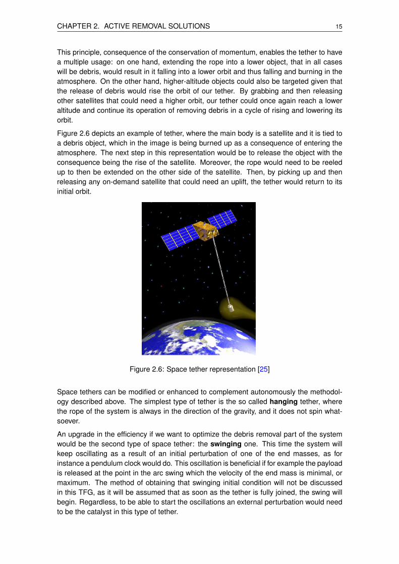
The parameters of an ellipse are shown in Figure 3.1, that depicts a given ellipse, wherethe Earth is one of the ellipse’s focus. Those are defined such as the sum of the distancesbetween both foci and a given point in the ellipse is constant. Instead of a constant radius,in an ellipse it is defined a semi-major axis (a in the representation), and a semi-minoraxis (b in Figure 3.1). The parameter r in this scenario is the distance between one of thefocus (the Earth in this case) and a given point set on the elliptic trajectory. Finally θ is theangle that the point has along the trajectory (or that object’s direction): the true anomaly.To obtain an expression for r two more elliptical parameters are needed.
19
20 A preliminary study of space debris mitigation based on a swinging tether system
Figure 3.1: Visual representation of the parameters of an ellipse [32]
The first one is the eccentricity of an orbit, which characterizes the shape of the ellipse:whether it is more or less flattened. It is defined by a relation of the ellipse axis, where c isthe distance from the center of the ellipse to one of its focus,
e =ca=
√a2−b2
a(3.1)
The other parameter that is needed is the semi-latus rectum p (already depicted in Figure3.1) . It is the distance (perpendicular to the semi-major axis) from a focus to a point of thecurve. It is a consequence of the system being ruled by Kepler’s laws [37], and its expres-sion is a result of the Pythagoras theorem application. It can be defined in multiple ways,depending on which parameter is more desirable: the semi-major axis a, the periapsis(shortest distance from the trajectory to the focus) Rper, or the apoapsis (longest distanceto the focus) Rapo. In all cases the definition depends on the eccentricity of the orbit.
p = a(1− e2) = Rper(1+ e) = Rapo(1− e) (3.2)
With both p and e parameters defined, an expression for the (changing) radius of a pointfollowing an elliptical path as in Figure 3.1 is the following.
r =p
1+ e · cos(θ)(3.3)
Expression 3.3 gives a way to obtain the trajectory of all the parts of the tether. How-ever, an expression for the angular velocity θ is missing, and to obtain it, the principles ofconservation of energy and momentum are introduced.

CHAPTER 3. THE TETHERED SYSTEM 21
3.1.2. Conservation of energy and momentum
Our tether system can be simplified as one object that, while it keeps subject another object(the debris), it is being attracted by the Earth, but as the tether is orbiting around the planet(or infinitely falling to it) in an elliptic trajectory, its mechanical energy is conserved [31].This is equivalent to stating that the sum of the system’s potential and kinetic energy at anypoint in the orbital trajectory will be the same. Equation 3.4 states this equivalence, whereE, T and U are the mechanical, kinetic and potential energy, respectively. By substitutingeach energy with its definition, other parameters come to light, such as G, the gravitationalconstant consequence of connecting the gravitational force between two bodies; m and M,the masses of both objects; V , the total velocity of m; and r, the distance from the focus ofthe ellipse (the Earth) to the orbiting object.
E = T +U =12
mV 2 +
(−GMm
r
)= constant (3.4)
We can equal the mechanical energy for two points in the trajectory, for instance the apoap-sis and periapsis, as well as changing the energy to a specific one (i.e., energy by unit ofmass), which from rearranging gets us to expression 3.5. The subscript ”apo” correspondsto the apoapsis parameters and ”per” to the periapsis ones.
V 2apo
2−
V 2per
2=
GMrapo− GM
rper(3.5)
An absence of external momentum in a system equals to a constant angular momentumwith respect to an arbitrary point [33]. With that in mind, a procedure similar to the conser-vation of energy can be made, where the specific angular momentums (H) in the apoapsisand periapsis of the elliptic trajectory are equal, obtaining with that an expression for thevelocity at the periapsis,
H = rper ·Vper = rapo ·Vapo = constant =>Vper =rapo
rper·Vapo (3.6)
Given that the apoapsis is the furthest distance from the focus of the ellipse and the peri-apsis the closest one, from Figure 3.1 an equivalence can be made,
2a = rper + rapo (3.7)
By substituting expressions 3.6-3.7 into 3.5 the so called vis-viva equation is obtained [32].It gives the orbital velocity of any point following an ellipse in its trajectory.
V 2 = GM(
2r− 1
a
)(3.8)

22 A preliminary study of space debris mitigation based on a swinging tether system
3.1.3. Particularizing parameters
Going from the general case of an ellipse to our particular case of the swinging tether, priorto particularize the expressions to our tether, the rendezvous maneuver must be done, toconnect the tether’s main body to the orbiting debris. This TFG will not get an in-depth lookinto this procedure, as the initial point of the calculations is set when the tether is created.Nevertheless, there are some considerations regarding the rendezvous process.
The condition to rendezvous between the two objects is such as the distance from thetether to the target is much lower than the distance from Earth’s center to the desireddebris [36]. Figure 3.2 depicts both debris and tether when the rope would be deployedand the two end masses joined (indicated by the thick dotted line). At that moment acenter of mass is created in the rope that will define the tether’s orbiting trajectory as awhole. Each end mass has its own orbital radius and system of reference (depicted by thesubscripts ”tet” for tether and ”deb” for debris), and those references have (in this sectionand across all the parametric study) their x-component following the direction of Earth’sgravity, and the y-component being perpendicular and following the direction of the orbitalmotion. As soon as the system is created both distances from the center of the Earth toeach end mass Rtet and Rdeb will change their trajectories and it is at that moment that ourparametric analysis will begin.
As previously stated the trajectory of the chosen debris is assumed to be close-to-circular.However, as soon as the tether is formed, that trajectory will become an elliptic one, similarto the tether’s main body orbit but with its respective orbital parameters.
Figure 3.2: Diagram of the desired rendezvous maneuver

CHAPTER 3. THE TETHERED SYSTEM 23
Targets in this study will be debris large enough to resemble the size of the main tether’sbody. That is due to the numerous debris of smaller size having a larger range of orbitaltitudes, inclinations and eccentricities; debris of larger sizes (above 10cm in diameter)are more stable in their size and characteristics, including their close-to-circular orbits [35].This is because the smaller sized debris are known by the breakup models that are primar-ily a result of fragmentation or collisions between larger debris objects, making their orbitsmore random and harder to predict. Clear concentrations and the best approximations thatverify the close-to-circular patterns of large debris can be seen in less than 2000 km or-bits (LEO), around 20000 km (semi-synchronous orbits, i.e., where objects have a periodof rotation of 12 hours), and at 36000 km (GEO) [43]. This TFG analyses debris in LEOorbits as these are the closest ones to Earth and also because debris at lower altitudeshave the benefit of being able to burn down into the atmosphere; an action that cannot bedone at GEO altitudes.
When the tether is formed, the system’s movement is ruled by the center of mass, thatkeeps the whole tether in place. Nevertheless, apart from that point the two end masseswill be swinging as the tether orbits around the Earth. This means that our system shouldbe perceived as three independent points, which happen to be united. However, as soonas the tether’s rope is cut, all the elliptic parameters (eccentricity, semi-major axis, etc.)that we previously had and could consider as a whole are now separated intro three newpacks of values: the ones of the new debris orbit, the new tether’s main body orbit and thenew center of mass (now imaginary) orbit.
With the expressions brought up due to the elliptical trajectory, and the tether already setand orbiting, the next step is to reach a parametric model that explains how the systemmoves and behaves.
3.2. Parametric model
The goal of this parametric model is to arrive to the equations of motion that the systemhas, and with them to obtain the velocities of each of the tether’s parts along their trajec-tories. The swings that will affect the tether’s behaviour are explained by the equations ofmotion that will be obtained.
3.2.1. Equations of Motion
If we took a picture of the swinging tether at any point in the trajectory, adding the anglesand velocities that will be needed, Figure 3.3 would be the result of it.
This picture is divided into three sections, each one of them being the angles and veloc-ities corresponding to either the tether’s main body (subscript ”tet”), the center of mass(subscript ”CoM”) and the debris (subscript ”deb”). Each of these system sections has theparameters that fix their position in the plane of space: a radial component R and an an-gular component θ, each one with the corresponding subscripts. The only variable θ thatwill be considered along the study is that of the CoM, because neither that of the debrisnor that of the tether’s body is brought up in the upcoming expressions. This is the reasonwhy that angle will not have any subscript at all.

24 A preliminary study of space debris mitigation based on a swinging tether system
Apart from θ, the other key angle in this study will be ψ, which is related to the pendulum-swinging of the tether, and is defined as the angle between the x-axis of the center of massand the tether’s rope. Therefore, when ψ is equal to 0, the sections debris-CoM-tether’sbody are aligned with the local gravity. Other angles that appear in Figure 3.3 are φ andλ; however, they are arbitrary angles needed in some calculations later in the chapter andwill not take part in obtaining the equations of motion. At the same time, the three kindsof velocities (represented by the colors orange, green and violet) depicted in the figure willbe useful afterwards, and will be brought up in the Release section.
The tether’s center of mass CoM separates the original rope’s length into two shorter L’s:the one in the tether’s side and the one in the debris’ side. These lengths of the rope donot change, as initially stated, the tether’s rope will not vary its length once it joined bothtether and debris. They also meet the condition that the end masses and lengths are re-lated such as Ldeb ·Mdeb = Ltet ·Mtet . This means that the relation between the two ropesection lengths will be given by the relation of the masses of the tether’s body and thedebris.
Figure 3.3: Geometry of a swinging tether in 2D
CHAPTER 3. THE TETHERED SYSTEM 25
The initial elliptical trajectory of the tether system is given by two parameters: the varyingradius that the center of mass has along the orbit RCoM, and the angular velocity it achieveswhile doing that motion θ. The first parameter comes from equation 3.3, but with theaddition that in the definition of this radius, the definition of p that will be taken is the one inexpression 3.2, that has the periapsis as an input. Knowing that the Earth will be the focusof our elliptic trajectory, from now on the periapsis and apoapsis will be called perigee andapogee, respectively. That is, the planet Earth is the focal point of the ellipse.
RCoM =Rper(1+ eCoM)
1+ eCoM · cos(θ)(3.9)
The time derivative of RCoM is also defined as it will be relevant in later calculations.
RCoM = Rper(1+ eCoM) · eCoM · sin(θ) · θ[1+ eCoM · cos(θ)]2
(3.10)
The expression of the angular velocity of an elliptical object comes from equating the grav-itational force and the centripetal force of the object along the orbit [45], but because it isan elliptical and not circular orbit, the term (1+ e · cos(θ)) is added to compensate that ateach point in the elliptical trajectory the orbital velocity will be different [46]. In the follow-ing equation, we also take into account that our desired angular velocity θ is equal to theinstantaneous velocity V over the radius of the orbit RCoM. A new parameter µ is added inthis equation, which is equal to the gravitational constant G times the Earth’s mass M. Theother mass m relates to the mass of the smaller object (the tether system in our case), butthat parameter becomes irrelevant, as the only mass that is relevant in the angular velocityof an orbiting object is the one at the focus of the ellipse (the Earth, this time).
Fc =Fg[1+e·cos(θ)]=>mV 2
RCoM(θ)=G
MmR2
CoM(θ)[1+e·cos(θ)]=> θ=
√µ[1+ e · cos(θ)]
R3CoM(θ)
(3.11)
With the main schematic introduced and the center of mass’ expressions defined, theequations of motion will be now derived based on Lagrangian mechanics. The require-ments to follow that formulation include having the expressions of the Cartesian coordi-nates of both the tether’s body and the debris, as well as having obtained Rdeb and Rtet .
By applying trigonometry in Figure 3.3, the Cartesian coordinates of the tether system endmasses are the following:
xtet = RCoM · cos(θ)+Ltet · cos(ψ+θ) (3.12)
ytet = RCoM · sin(θ)+Ltet · sin(ψ+θ) (3.13)
xdeb = RCoM · cos(θ)−Ldeb · cos(ψ+θ) (3.14)
ydeb = RCoM · sin(θ)−Ldeb · sin(ψ+θ) (3.15)
26 A preliminary study of space debris mitigation based on a swinging tether system
The time derivatives of the previous equations with respect to time are relevant enough tobe listed as follows:
xtet = RCoM · cos(θ)−RCoM · θ · sin(θ)−Ltet · (ψ+ θ) · sin(ψ+θ) (3.16)
ytet = RCoM · sin(θ)+RCoM · θ · cos(θ)+Ltet · (ψ+ θ) · cos(ψ+θ) (3.17)
xdeb = RCoM · cos(θ)−RCoM · θ · sin(θ)+Ldeb · (ψ+ θ) · sin(ψ+θ) (3.18)
ydeb = RCoM · sin(θ)+RCoM · θ · cos(θ)−Ldeb · (ψ+ θ) · cos(ψ+θ) (3.19)
Although RCoM in Figure 3.3 is already defined in expression 3.9, we also need to ex-press Rtet and Rdeb. Using expressions 3.12-3.15 an equation for both distances can beobtained.
Rtet =
√x2
tet + y2tet =
√L2
tet +R2CoM +2 ·Ltet ·RCoM · cos(ψ) (3.20)
Rdeb =√
x2deb + y2
deb =√
L2deb +R2
CoM−2 ·Ldeb ·RCoM · cos(ψ) (3.21)
From this point forward, Lagrangian mechanics will be used, therefore, the next step is toexpress the kinetic and potential energy of our system in order to put their derivatives inLagrange equation. The upcoming method is a practical application of the conservation ofenergy principle from expression 3.4.
T =12
Mtet [(xtet)2 +(ytet)
2]+12
Mdeb[(xdeb)2 +(ydeb)
2] (3.22)
If we put expressions 3.16-3.19 into equation 3.22 we get the kinetic energy that the tethersystem will possess:
T =12(Mtet +Mdeb)(R2
CoM +R2CoM · θ2)+
12(Mtet ·L2
tet +Mdeb ·L2deb)(ψ+ θ)2 (3.23)
By applying the expression of the potential energy present in equation 3.4, but to ourswinging tether; as well as by substituting the radius expressions of 3.20 and 3.21, we getequation 3.24.
U =−µ ·Mtet
Rtet− µ ·Mdeb
Rdeb=− µ ·Mtet√
L2tet +R2
CoM +2 ·Ltet ·RCoM · cos(ψ)−
µ ·Mdeb√L2
deb +R2CoM−2 ·Ldeb ·RCoM · cos(ψ)
(3.24)

CHAPTER 3. THE TETHERED SYSTEM 27
Expression 3.25 is Lagrange’s equation; it gives the equations of motion by partially differ-entiating Lagrange’s function with respect to q, where these finite number of q representeach independent variable of our system [38]. Lagrange’s equation is equal to the termthat accounts for the non conservative forces that act on a system FNC.
ddt[∂L∂qi
]− ∂L∂qi
= FNC, i = 1,2, ...,N (3.25)
Once the extended expressions of the kinetic and potential energy are set, we put them intoLagrange’s function (expression 3.26), keeping in mind that we only need one equation,the one that gives us the tether’s rotation angle ψ, because as stated earlier this study willbe two-dimensional. Thus, the parameter q1 will be our only variable in the expression: ψ.Moreover, in our scenario FNC is equal to 0 because one of our initial assumptions wasthat no non-conservative forces act on the tether.
L(qi, qi, t) = T (qi, qi, t)−U(qi, t) (3.26)
Once expression 3.26 is set, substituting this L into equation 3.25 gives us the equationof motion of the swinging tethered system, keeping in mind the assumptions previouslystated. This expression 3.27 tells us how the system will be moving alongside time.
ψ+ θ+µ ·RCoM · sin(ψ)
Ltet +Ldeb[(R2
CoM +L2deb
−2 ·RCoM ·Ldeb · cos(ψ))−32 − (R2
CoM +L2tet +2 ·RCoM ·Ltet · cos(ψ))−
32 ] = 0
(3.27)
However, from this point on-wards we consider the variables as a function of the trueanomaly θ. This way, we are able to reduce its complexity by assuming the orbit to remainin a Keplerian orbit. Such transformations are listed the following expressions, where thequotation marks represent the derivative with respect to θ.
ψ =dψ
dθ
dθ
dt= θψ
′ (3.28)
ψ =ddt(θψ
′) = θ2ψ′′+ θ · θ′ ·ψ′ (3.29)
Some extra simplifications have been made to expression 3.27. The first one is to considerthe tether lengths negligible in comparison with the orbital radius [38]. The other comesfrom chapter 3.2.1, where the assumption Ldeb ·Mdeb = Ltet ·Mtet was set. If we applythose simplifications to the potential energy expression 3.24, and change the current timederivatives to theta derivatives from the previous expressions, we get a simplified versionof the equation of motion:
ψ′′−[
2 · eCoM · sin(θ)1+ eCoM · cos(θ)
](ψ′+1)+
3 · sin(2ψ)
2[1+ eCoM · cos(θ)]= 0 (3.30)
With the knowledge of our ψ, the velocities of the tether system end masses will be ob-tained. Afterwards, the optimal point of release in the trajectory will be found, with theobjective of rising the orbit of the tether’s body and lowering the one of the debris.
28 A preliminary study of space debris mitigation based on a swinging tether system
3.2.2. Release
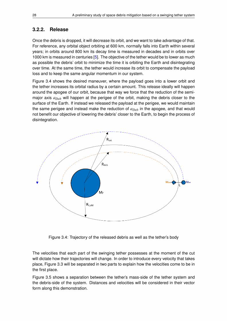
Once the debris is dropped, it will decrease its orbit, and we want to take advantage of that.For reference, any orbital object orbiting at 600 km, normally falls into Earth within severalyears; in orbits around 800 km its decay time is measured in decades and in orbits over1000 km is measured in centuries [5]. The objective of the tether would be to lower as muchas possible the debris’ orbit to minimize the time it is orbiting the Earth and disintegratingover time. At the same time, the tether would increase its orbit to compensate the payloadloss and to keep the same angular momentum in our system.
Figure 3.4 shows the desired maneuver, where the payload goes into a lower orbit andthe tether increases its orbital radius by a certain amount. This release ideally will happenaround the apogee of our orbit, because that way we force that the reduction of the semi-major axis aDeb will happen at the perigee of the orbit, making the debris closer to thesurface of the Earth. If instead we released the payload at the perigee, we would maintainthe same perigee and instead make the reduction of aDeb in the apogee, and that wouldnot benefit our objective of lowering the debris’ closer to the Earth, to begin the process ofdisintegration.
Figure 3.4: Trajectory of the released debris as well as the tether’s body
The velocities that each part of the swinging tether possesses at the moment of the cutwill dictate how their trajectories will change. In order to introduce every velocity that takesplace, Figure 3.3 will be separated in two parts to explain how the velocities come to be inthe first place.
Figure 3.5 shows a separation between the tether’s mass-side of the tether system andthe debris-side of the system. Distances and velocities will be considered in their vectorform along this demonstration.

CHAPTER 3. THE TETHERED SYSTEM 29
Both plots have the center of mass in common, and its distance to the center of the Earth~RCoM, in pink. The distance from the latter to the tether’s body and the debris are, respec-tively, ~Rtet and ~Rdeb. The whole length of the tether’s rope is split into two, where in theleft drawing is the distance CoM-tether’s body (~Rtet,CoM), and the right plot is the distancedebris-CoM (~Rdeb,CoM). That way, the total longitude from the debris to the tether’s bodywould be the vector sum ~Rdeb,CoM +~Rtet,CoM.
Figure 3.5: Distances in vector form and angles regarding the main body-side of the tether(left figure) and the debris-side (right figure)
If we focus firstly on the tether’s body sketch (left side), the expression of the velocity of thetether’s body with respect to the Earth ~Vtet will be given by three components: the velocityof the CoM with respect to the Earth ~VCoM, the relative velocity of the tether with respectto the CoM ~Vtet,CoM and the effect of the rope orbiting along with the system~ωCoM,Earth∧~Rtet,CoM.
Equations 3.31, 3.32 and 3.33 develop the terms described previously. ~VCoM has a com-ponent consequence of the elliptical path changing the radius of the orbit ~RCoM and thepart accounting for the CoM orbiting around the Earth, which equals to the cross product
of the angular velocity of the CoM ~θ times the vector ~RCoM. The term ~Vtet,CoM is defined
by the rotational velocity of the tether itself, i.e., ~ψ.
~VCoM = ~RCoM +~θ∧~RCoM (3.31)
~ωCoM,Earth∧~Rtet,CoM =~θ∧~Rtet,CoM (3.32)
~Vtet,CoM = ~ψ∧~Rtet,CoM (3.33)
Once these components are defined, adding all of them gives expression 3.34: the totalvelocity of one end of the tether, its main body. In this expression it is merged together the
terms with ~θ, and their vector sum result in the new term ~θ∧~Rtet . That is because, from
Figure 3.5, ~Rtet = ~Rtet,CoM +~RCoM.

30 A preliminary study of space debris mitigation based on a swinging tether system
~Vtet =~VCoM +~Vtet,CoM +~ωCoM,Earth∧~Rtet,CoM = ~RCoM +~ψ∧~Rtet,CoM +~θ∧~Rtet (3.34)
The same process can be made but to the right side of Figure 3.5 to obtain the totalvelocity of the debris. Definitions for the components of the total debris velocity are listedin equations 3.35 and 3.36.
~ωCoM,Earth∧~Rdeb,CoM =~θ∧~Rdeb,CoM (3.35)
~Vdeb,CoM = ~ψ∧~Rdeb,CoM (3.36)
Due to the debris being closer to Earth than the CoM, the total velocity for the debris is notthe sum of its components. This is because this time ~Rdeb = ~RCoM−~Rdeb,CoM.
~Vdeb =~VCoM−~Vdeb,CoM−~ωCoM,Earth∧~Rdeb,CoM = ~RCoM−~ψ∧~Rdeb,CoM+~θ∧~Rdeb (3.37)
Previously in Figure 3.3 some velocities were shown, and each of them relate to the previ-ous vector components of the tether velocities.
VR is parallel to the xCoM axis and it tells how the orbital radius varies along the ellipticaltrajectory. It is the modulus of ~RCoM of expression 3.31.
VDebCoM is perpendicular to the distance from Earth’s center and the debris Rdeb, and isthe modulus of the terms of expression 3.36. If we change the notation from vector to onlymodulus form, and to the same one as Figure 3.3, we get that the distances ~Rdeb,CoM and~Rtet,CoM become Ldeb and Ltet , respectively.
VRot coincides with the direction of the y component of each system of reference (debris,tether’s body and CoM), and is the term accounting for the rotation due to the orbitalvelocity θ. It is the last term of expression 3.34 for the debris and the last of expression3.37 for the tether’s body, while the definition for the CoM is the distance RCoM times theangular velocity θ.
Table 3.1 classifies the previously described velocities. However, it must be noted that thistable lists the modulus of the velocities, and in order to know the total velocity that bothtether’s main body and debris have, those velocity components need to be split to everyradial component on one side and every normal component on the other one.
Definition NotationRadial Velocity VR = RCoM
CoM rotation velocity due to θ VRotCoM = RCoM · θDebris’ rotation velocity due to θ VRotDeb = Rdeb · θ
Debris’ rotation velocity due to CoM VDebCoM = Ldeb · ψTether’s rotation velocity due to θ VRotTet = Rtet · θ
Tether’s rotation velocity due to CoM VTetCoM = Ltet · ψ
Table 3.1: All the velocities that take part in the motion of the tether (in modulus)

CHAPTER 3. THE TETHERED SYSTEM 31
Those radial and normal components will be with respect to each respective system ofreference: velocities that belong to the debris’ end of the tether will be radial and nor-mal to that system of reference and the tether’s main body velocities will be referencedthrough that system of reference instead. Using trigonometry in Figure 3.3, we classifythe velocities of the debris in the xdeb and the ydeb axis. An important thing to consider inexpressions 3.38 and 3.39 is that the term Vdeb,CoM, due to the distance ~Rdeb,CoM beingdefined opposite from the one corresponding to the tether’s body, it carries a negative signthat changes the trigonometry analysis of this velocity.
VRadDeb =−VDebCoM · cos(φ1)+VR · cos(λ1) (3.38)
VNormDeb =VRotDeb +VDebCoM · sin(φ1)+VR · sin(λ1) (3.39)
VRadTet =−VTetCoM · sin(φ2)+VR · cos(λ2) (3.40)
VNormTet =VRotTet +VTetCoM · cos(φ2)−VR · sin(λ2) (3.41)
Angles λ1, λ2, φ1 and φ2 are obtained again from the same figure. First apply the sine ruleto get φ1:
RCoM
sin(π
2 +φ1)=
Rdeb
sin(ψ)(3.42)
φ1 = arcsin(
RCoM · sin(ψ)Rdeb
)− π
2(3.43)
Then we can know the value of λ by doing:
λ1 =π
2−φ1−ψ = π−arcsin
(RCoM · sin(ψ)
Rdeb
)−ψ (3.44)
Repeating the process for the other end of the tether (main body), the difference is thetrigonometry used to obtain the respective orbital and rotational velocity, as the radial oneis the same. In order to obtain the expressions, two new angles λ2 and φ2 are introduced(present in Figure 3.3), and going along the same procedures, we get expressions 3.45and 3.46 for the radial and normal components of the tether’s body, and the definitions ofthe new angles in 3.47 and 3.48.
VRadTet =−VTetCoM · sin(φ2)+VR · cos(λ2) (3.45)
VNormTet =VRotTet +VTetCoM · cos(φ2)−VR · sin(λ2) (3.46)
φ2 = arcsin(
RCoM
Rtet· sin(π−ψ)
)(3.47)

32 A preliminary study of space debris mitigation based on a swinging tether system
λ2 = ψ−φ2 (3.48)
At some point in the trajectory the goal is to detach the debris from the tether. The equationthat hints where that release point should be comes from isolating a from equation 3.8. Inorder to lower the debris as much as we can, the new semi-major axis of that object aDebmust be as low as possible. Expression 3.49 shows that in order to do so, two conditionsmust be met. The first one is that the total velocity of the debris must be minimal, to makethe denominator larger. That moment of less total velocity of the debris, which is defined
as√
V 2NormDeb +V 2
RadDeb, occurs in the apogee. This information is given to us by equation
3.11: the larger RCoM is, the lower θ will become. The second condition is that Rdeb mustbe minimal, and that occurs at the perigee. However, by releasing the debris at the perigeewe would get a reduction in the height of the apogee, contrary of what we want. Thus, theoptimal release point will be the instants of our trajectory where those two conditions alignand result in the lowest adeb values possible.
We will simulate several orbits, to then pick from the multiple minimums of adeb, the onewith the best balance of being the lowest value possible but also being close to the apogee,to make the change in semi-major axis influence the height of the debris’ perigee, loweringit.
aDeb =µ ·Rdeb
2µ−V 2TotDeb ·Rdeb
(3.49)
The final step will be to calculate the new orbital radius of the debris. Prior to that expres-sion, the new eccentricity eDeb and semi-latus rectum pDeb are defined.
On one hand, from equation 3.2 an expression for the eccentricity that our debris will havecan be derived.
eDeb =
√1− pDeb
aDeb(3.50)
On the other hand, to know the semi-latus rectum pDeb, we can use the definition of thatdistance in terms of the specific angular momentum H.
pDeb =H2
µ=
(VNormDeb ·Rdeb)2
µ(3.51)
By inserting equations 3.49, 3.50 and 3.51 into equation 3.3, the expression of the newradius of the debris is obtained. Note that we must add θRelease to the iterative values ofθ in the expression of the new radius; this new parameter is the true anomaly the debrishad at the moment of the release, and this addition will result in the new orbit starting atthe moment the rope is cut.
An equivalent process but changing the subscripts ”deb” to ”tet” can be made to obtain theexpressions from 3.49 to 3.52 respective to the tether’s body.
RNewDeb =pDeb
1+ eDeb · cos(θ+θRelease)(3.52)

CHAPTER 3. THE TETHERED SYSTEM 33
3.3. Validations
This section will validate the equations of motion used in chapter 3.2. Nevertheless, inorder to check them a new parameter must be added into the equations, as the doctoratethat was used to obtain the equations of motion uses a swinging tether in three dimensions[38]. In this case, presented by Ziegler in 2003, the motion of the tether is not restrictedto a plane, and instead is a more generic scenario. Figure 3.6 shows how the geometryof the tether changes, as now an angle accounting for the degree of inclination in the orbitplane needs to be defined: α. In our study this angle was 0, due to always working in a 2Dorbital plane.
Figure 3.6 has θ and ψ the same way as before, R as our RCoM, the subscripts 1 and 2 asdeb and tet, and the system of reference x0−y0− z0 as the one of the center of mass. Ontop of that, the angle α is the inclination of the tether with respect to the orbital plane, andis defined as the angle between that plane and the tether’s rope L1 (or L2).
Figure 3.6: Geometry of an out-of-plane tether [38]
From this point, a study equivalent to the one done in chapter 3.2 can be made, wherethe Cartesian coordinates of each mass are defined, and the Lagrangian function is found,this time with the alpha parameter in the equations. All the related information about theprocess can be found in Ziegler’s document [38]. Equations 3.53 and 3.54 are what resultfrom following that process and making the same simplifications as the ones made before.In this case the equations of motion are two, as now the tether’s self-rotation angle canhappen both in the plane x0− y0 (being that angle ψ) and the plane y0− z0 (being in thisother case the angle α).

34 A preliminary study of space debris mitigation based on a swinging tether system
ψ′′−[
2 ·α′ · tan(α)+2 · e · sin(θ)
1+ e · cos(θ)
](ψ′+1)+
3 · sin(2ψ)
2[1+ e · cos(θ)]= 0 (3.53)
α′′− 2 · e · sin(θ)
1+ e · cos(θ)α′+
12
sin(2α)
[(ψ′+1)2 +
3 · cos2(ψ)
1+ e · cos(θ)
]= 0 (3.54)
Ziegler in his doctorate plotted a couple graphs showing the variation of ψ and α angleswith respect to the number of orbits, given the initial conditions shown in Table 3.2. Heconsidered a several kilometers long tether with both end masses of 1 tonne, with a radiusof the perigee of 7000 km (or a height of 629 km, if we subtract the radius of the Earth).The only initial condition different from 0 is α(0).
Mtet Mdeb Ltet Ldeb e Rper ψ(0) ψ(0) α(0) α(0)1000 kg 1000 kg 10 km 10 km 0.25 7000 km 0 rad 0 rad/s 0.1 rad 0 rad/s
Table 3.2: Initial conditions of Ziegler’s scenario
Given the initial conditions in this scenario, and solving equations 3.53 and 3.54 with them,Ziegler in his doctorate obtains the left side of Figure 3.7, which shows the rotation angleψ with respect to the number of orbits. To test the validity of those equations of motion (aset of more complete equations than our main case, which has α = 0), expressions 3.53and 3.54 were solved in Matlab, with the initial conditions in Table 3.2, and the right plotof Figure 3.7 resulted from it. Both graphs are a match, and they show that the angle thetether rotates with, ψ, never tilts the end masses more than 0.4 radians.
0 0.5 1 1.5 2 2.5 3 3.5 4 4.5 5
Orbits
-0.5
-0.4
-0.3
-0.2
-0.1
0
0.1
0.2
0.3
0.4
0.5
Figure 3.7: Graphs of rotation angle ψ along 5 orbits. Left side is Ziegler’s sketch and rightside is the Matlab output
In addition, the same validation process was made with angle α in Figure 3.8. The resultis again the same plot, and we observe that α never goes beyond 0.15, which reflects thatthe orbital plane does not vary that much. However, it shows a more periodical and clearerpattern than the previous angle.
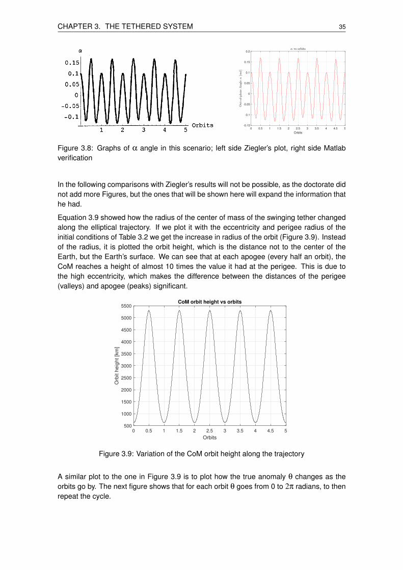
CHAPTER 3. THE TETHERED SYSTEM 35
0 0.5 1 1.5 2 2.5 3 3.5 4 4.5 5
Orbits
-0.15
-0.1
-0.05
0
0.05
0.1
0.15
0.2
Figure 3.8: Graphs of α angle in this scenario; left side Ziegler’s plot, right side Matlabverification
In the following comparisons with Ziegler’s results will not be possible, as the doctorate didnot add more Figures, but the ones that will be shown here will expand the information thathe had.
Equation 3.9 showed how the radius of the center of mass of the swinging tether changedalong the elliptical trajectory. If we plot it with the eccentricity and perigee radius of theinitial conditions of Table 3.2 we get the increase in radius of the orbit (Figure 3.9). Insteadof the radius, it is plotted the orbit height, which is the distance not to the center of theEarth, but the Earth’s surface. We can see that at each apogee (every half an orbit), theCoM reaches a height of almost 10 times the value it had at the perigee. This is due tothe high eccentricity, which makes the difference between the distances of the perigee(valleys) and apogee (peaks) significant.
0 0.5 1 1.5 2 2.5 3 3.5 4 4.5 5
Orbits
500
1000
1500
2000
2500
3000
3500
4000
4500
5000
5500
Orb
it h
eig
ht
[km
]
CoM orbit height vs orbits
Figure 3.9: Variation of the CoM orbit height along the trajectory
A similar plot to the one in Figure 3.9 is to plot how the true anomaly θ changes as theorbits go by. The next figure shows that for each orbit θ goes from 0 to 2π radians, to thenrepeat the cycle.
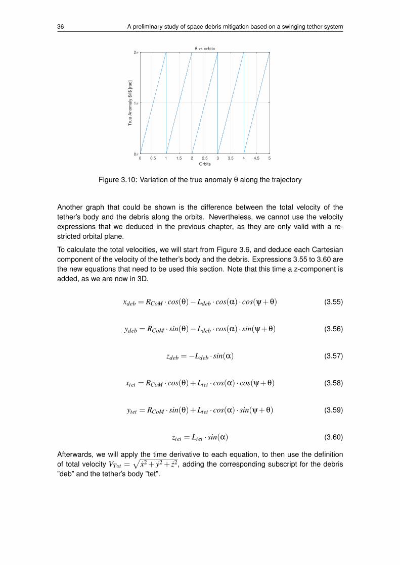
36 A preliminary study of space debris mitigation based on a swinging tether system
0 0.5 1 1.5 2 2.5 3 3.5 4 4.5 5
Orbits
0
1
2
Tru
e A
nom
aly
$$ [ra
d]
Figure 3.10: Variation of the true anomaly θ along the trajectory
Another graph that could be shown is the difference between the total velocity of thetether’s body and the debris along the orbits. Nevertheless, we cannot use the velocityexpressions that we deduced in the previous chapter, as they are only valid with a re-stricted orbital plane.
To calculate the total velocities, we will start from Figure 3.6, and deduce each Cartesiancomponent of the velocity of the tether’s body and the debris. Expressions 3.55 to 3.60 arethe new equations that need to be used this section. Note that this time a z-component isadded, as we are now in 3D.
xdeb = RCoM · cos(θ)−Ldeb · cos(α) · cos(ψ+θ) (3.55)
ydeb = RCoM · sin(θ)−Ldeb · cos(α) · sin(ψ+θ) (3.56)
zdeb =−Ldeb · sin(α) (3.57)
xtet = RCoM · cos(θ)+Ltet · cos(α) · cos(ψ+θ) (3.58)
ytet = RCoM · sin(θ)+Ltet · cos(α) · sin(ψ+θ) (3.59)
ztet = Ltet · sin(α) (3.60)
Afterwards, we will apply the time derivative to each equation, to then use the definitionof total velocity VTot =
√x2 + y2 + z2, adding the corresponding subscript for the debris
”deb” and the tether’s body ”tet”.
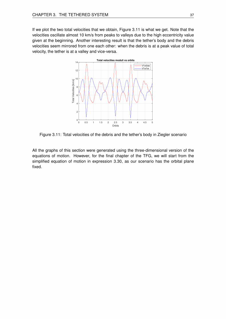
CHAPTER 3. THE TETHERED SYSTEM 37
If we plot the two total velocities that we obtain, Figure 3.11 is what we get. Note that thevelocities oscillate almost 10 km/s from peaks to valleys due to the high eccentricity valuegiven at the beginning. Another interesting result is that the tether’s body and the debrisvelocities seem mirrored from one each other: when the debris is at a peak value of totalvelocity, the tether is at a valley and vice-versa.
0 0.5 1 1.5 2 2.5 3 3.5 4 4.5 5
Orbits
0
2
4
6
8
10
12
14
To
tal V
elo
citie
s [
km
/s]
Total velocities moduli vs orbits
VTotDeb
VTotTet
Figure 3.11: Total velocities of the debris and the tether’s body in Ziegler scenario
All the graphs of this section were generated using the three-dimensional version of theequations of motion. However, for the final chapter of the TFG, we will start from thesimplified equation of motion in expression 3.30, as our scenario has the orbital planefixed.


CHAPTER 4. RESULTS AND DISCUSSION
In this final chapter we will give similar results as the ones shown in section 3.3, but nowwith the equations of motion found in section 3.2 (i.e., without the parameter α). Theinitial conditions used are fixed values, but tests will be made where each time one ofthese parameters is going to vary. Those variations will bring the main results that can beobtained in this study, regarding the removal of space debris.
The initial values from which the variations and calculations this section are based on arelisted in Table 4.1. As opposed to the previous scenario, values such as the tether’s ropelength and the eccentricity are reduced, while the radius of the perigee is at a higher point.Rper is set at 9371 km (or 3000 km of height) because we will consider a hypotheticaldebris that orbits around that height.
Moreover, the tether’s main body will be 10 times heavier than the debris. This is to addto the pendulum effect that we want to occur, because due to the identity Mtet · Ltet =Mdeb ·Ldeb, that difference in mass is equivalent to having a rope where the debris-partlength (Ldeb) is 10 times longer than the tether’s, which means that the debris will swingwith more intensity than the other end of the rope. The system will begin with an initial ψ
different from zero, because otherwise the pendulum motion would not occur.
Mtet Mdeb Ltet Ldeb e Rper ψ(0) ψ(0)1000 kg 100 kg 120 m 1200 m 0.1 9371 km 0.2 rad 0 rad/s
Table 4.1: Initial conditions of the swinging tether to study
The parameters of this table that will vary are the eccentricity of the initial orbit e, the lengthof the tether’s side of the rope Ltet (and consequently Ldeb), and the radius of the CoMperigee Rper. The former parameter has an effect on the atmospheric drag that will act onthe debris once it is in a low enough orbit: If we have an excessively eccentric orbit, dragwill be acting mostly in the perigee of the trajectory, and the orbit will tend to circularizeitself, while the radius of the perigee will tend to remain the same [44]. If instead, we havean orbit with the same value of perigee, but a low value of eccentricity, the orbit will havean atmospheric drag acting almost constantly along the trajectory, and the orbit will keepdecreasing its altitude in an homogeneous way.
The released debris needs to end up in an orbit with a low enough altitude so that it canbegin its process of disintegration. This process is given by the exponential increase inatmospheric drag as we approach the Earth’s surface. Table 4.2 gives an estimation ofthe density of the atmosphere depending on the altitude that an object has in an elliptictrajectory. At 1000 km the density is, comparatively to the largest numbers in the table,almost negligible, but is sufficient enough to, in the long run, keep decreasing the debrisaltitude. With that, we will set the threshold of the lowest point in the new debris’ orbit in1000 km, to guarantee that the released debris will eventually disintegrate.
39
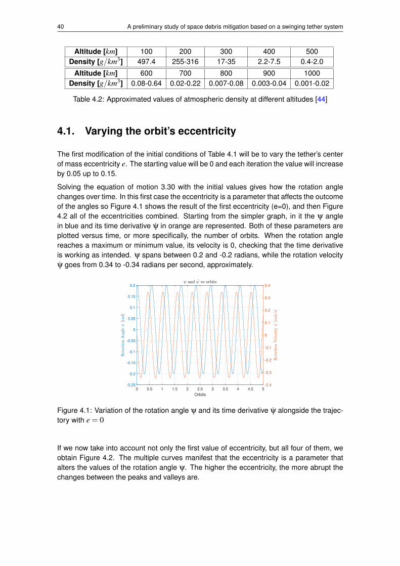
40 A preliminary study of space debris mitigation based on a swinging tether system
Altitude [km] 100 200 300 400 500Density [g/km3] 497.4 255-316 17-35 2.2-7.5 0.4-2.0
Altitude [km] 600 700 800 900 1000Density [g/km3] 0.08-0.64 0.02-0.22 0.007-0.08 0.003-0.04 0.001-0.02
Table 4.2: Approximated values of atmospheric density at different altitudes [44]
4.1. Varying the orbit’s eccentricity
The first modification of the initial conditions of Table 4.1 will be to vary the tether’s centerof mass eccentricity e. The starting value will be 0 and each iteration the value will increaseby 0.05 up to 0.15.
Solving the equation of motion 3.30 with the initial values gives how the rotation anglechanges over time. In this first case the eccentricity is a parameter that affects the outcomeof the angles so Figure 4.1 shows the result of the first eccentricity (e=0), and then Figure4.2 all of the eccentricities combined. Starting from the simpler graph, in it the ψ anglein blue and its time derivative ψ in orange are represented. Both of these parameters areplotted versus time, or more specifically, the number of orbits. When the rotation anglereaches a maximum or minimum value, its velocity is 0, checking that the time derivativeis working as intended. ψ spans between 0.2 and -0.2 radians, while the rotation velocityψ goes from 0.34 to -0.34 radians per second, approximately.
0 0.5 1 1.5 2 2.5 3 3.5 4 4.5 5
Orbits
-0.25
-0.2
-0.15
-0.1
-0.05
0
0.05
0.1
0.15
0.2
-0.4
-0.3
-0.2
-0.1
0
0.1
0.2
0.3
0.4
Figure 4.1: Variation of the rotation angle ψ and its time derivative ψ alongside the trajec-tory with e = 0
If we now take into account not only the first value of eccentricity, but all four of them, weobtain Figure 4.2. The multiple curves manifest that the eccentricity is a parameter thatalters the values of the rotation angle ψ. The higher the eccentricity, the more abrupt thechanges between the peaks and valleys are.

CHAPTER 4. RESULTS AND DISCUSSION 41
0 0.5 1 1.5 2 2.5 3 3.5 4 4.5 5
Orbits
-0.5
-0.4
-0.3
-0.2
-0.1
0
0.1
0.2
0.3
0.4
0.5
-0.8
-0.6
-0.4
-0.2
0
0.2
0.4
0.6
e = 0
e = 0.05
e = 0.1
e = 0.15
Figure 4.2: Variation of the rotation angle ψ and its time derivative ψ with e =[0,0.05,0.1,0.15]
Before going into the velocities, we can graph equation 3.9, the radius of the center ofmass, with respect to the number of orbits, depicted in Figure 4.3. There we can see thatthe higher the eccentricity, the higher the value of the apogee (at every peak) will be. Thisis because we impose from the start that the radius of the perigee will be 9371 km, so theapogee is the distance that keeps increasing instead. The y-axis of the graph is the orbitheight, instead of radius. If we subtract the radius of the Earth (6371 km) to the initial 9371km of perigee radius, we get the orbit height of the center of mass instead: 3000 km in thecase of the perigee. Hereafter, and for the sake of clarity, all the radius-related values willbe in terms of the height (distance with respect to the Earth’s surface).
If we were to plot the orbit height graphs for the debris and tether’s body, we would see thatboth of them would be almost identical to the CoM one, because initially the only differencebetween the three distances are the rope lengths; distances almost irrelevant next to themagnitudes of thousands of kilometers that are displayed in this Figure 4.3.
0 0.5 1 1.5 2 2.5 3 3.5 4 4.5 5
Orbits
3000
3500
4000
4500
5000
5500
6000
6500
Orb
it h
eig
ht [k
m]
CoM orbit height vs orbits
e = 0
e = 0.05
e = 0.1
e = 0.15
Figure 4.3: Orbit height of the center of mass of the tether system throughout the trajectorywith e = [0,0.05,0.1,0.15]

42 A preliminary study of space debris mitigation based on a swinging tether system
Figure 4.4 depicts the modulus of the velocities that were shown in Figure 3.3, each onewith their own corresponding color. VRot and VR are the same in both plots, the formerbeing the predominant velocity with around 6 km/s that keeps oscillating more the highere is, and the latter centered in 0 and also deviating more as the eccentricity increases.VDebCom and VTetCom are the differential factor in these plots since they are the velocitiesthat come from the end masses being attached to a center of mass, which means thatthey are proportional to Ldeb and Ltet . In our case those lengths are different by an orderof magnitude of 10. The difference in both green curves explains how in the pendulum-effect, the debris-side of the tether is the one swinging the most, while the other side keepsits ups and downs in velocity in a less pronounced way. The direction of the black arrowsindicates how each velocity changes as we keep increasing the eccentricity e, with theeffect of varying more the maximum and minimum values of every velocity.
0 0.5 1 1.5 2 2.5 3 3.5 4 4.5 5
Orbits
-1
0
1
2
3
4
5
6
7
Velo
citie
s [km
/s]
Debris velocities vs orbits
VDebCom
VRotDeb
VR
e
ee
0 0.5 1 1.5 2 2.5 3 3.5 4 4.5 5
Orbits
-1
0
1
2
3
4
5
6
7
Velo
citie
s [km
/s]
Tethers body velocities vs orbits
VTetCom
VRotTet
VR
e
e
e
Figure 4.4: Modulus of the velocity components of the debris (left) and the tether’s body(right) with the CoM eccentricity e = [0,0.05,0.1,0.15]
The graph that depicts the radial and normal components of the previously shown veloc-ities is Figure 4.5. Apart from those components, the total velocity is also added in thisplot. It can be seen that the left plot is much more erratic in its behaviour than the rightone, and that is due to VDebCom having more impact in the debris than its counterpart inthe tether’s body. Another interesting aspect to highlight is VRadDeb, that is inverted withrespect to its tether’s body counterpart. This behaviour is explained by the initial conditionsof ψ, where that initial push results in the debris swinging with a radial component inwards(i.e., towards the Earth), making the initial motion negative in this component, as opposedto the tether that initially keeps increasing its radial component as it moves towards theapogee.
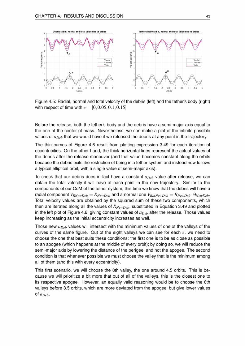
CHAPTER 4. RESULTS AND DISCUSSION 43
0 0.5 1 1.5 2 2.5 3 3.5 4 4.5 5
Orbits
-1
0
1
2
3
4
5
6
7
8
Velo
citie
s [km
/s]
Debris radial, normal and total velocities vs orbits
Vradial
Vnormal
Vtotal
e
e
0 0.5 1 1.5 2 2.5 3 3.5 4 4.5 5
Orbits
-1
0
1
2
3
4
5
6
7
8
Velo
citie
s [km
/s]
Tethers body radial, normal and total velocities vs orbits
Vradial
Vnormal
Vtotal
e
e
Figure 4.5: Radial, normal and total velocity of the debris (left) and the tether’s body (right)with respect of time with e = [0,0.05,0.1,0.15]
Before the release, both the tether’s body and the debris have a semi-major axis equal tothe one of the center of mass. Nevertheless, we can make a plot of the infinite possiblevalues of aDeb that we would have if we released the debris at any point in the trajectory.
The thin curves of Figure 4.6 result from plotting expression 3.49 for each iteration ofeccentricities. On the other hand, the thick horizontal lines represent the actual values ofthe debris after the release maneuver (and that value becomes constant along the orbitsbecause the debris exits the restriction of being in a tether system and instead now followsa typical elliptical orbit, with a single value of semi-major axis).
To check that our debris does in fact have a constant aDeb value after release, we canobtain the total velocity it will have at each point in the new trajectory. Similar to thecomponents of our CoM of the tether system, this time we know that the debris will have aradial component VRNewDeb = RNewDeb and a normal one VRotNewDeb = RNewDeb · θNewDeb.Total velocity values are obtained by the squared sum of these two components, whichthen are iterated along all the values of RNewDeb, substituted in Equation 3.49 and plottedin the left plot of Figure 4.6, giving constant values of aDeb after the release. Those valueskeep increasing as the initial eccentricity increases as well.
Those new aDeb values will intersect with the minimum values of one of the valleys of thecurves of the same figure. Out of the eight valleys we can see for each e, we need tochoose the one that best suits these conditions: the first one is to be as close as possibleto an apogee (which happens at the middle of every orbit); by doing so, we will reduce thesemi-major axis by lowering the distance of the perigee, and not the apogee. The secondcondition is that whenever possible we must choose the valley that is the minimum amongall of them (and this with every eccentricity).
This first scenario, we will choose the 8th valley, the one around 4.5 orbits. This is be-cause we will prioritize a bit more that out of all of the valleys, this is the closest one toits respective apogee. However, an equally valid reasoning would be to choose the 6thvalleys before 3.5 orbits, which are more deviated from the apogee, but give lower valuesof aDeb.

44 A preliminary study of space debris mitigation based on a swinging tether system
The right plot of Figure 4.6 zooms in the spot of release of this scenario, where the valuesshown are the minimum of each respective curve. Upon iterating the new values of totalvelocity into equation 3.49, the new values of aDeb are the same as each respective min-ima graphed in Figure 4.6 (right). Note that as we keep increasing the eccentricity of ourorbit, the release point will be every time a bit more to the right.
0 0.5 1 1.5 2 2.5 3 3.5 4 4.5 5
Orbits
0.8
0.9
1
1.1
1.2
1.3
1.4
1.5
1.6
Sem
i-m
ajo
r axis
[km
]
104 Possible and final semi-major axis of the debris
e = 0
e = 0.05
e = 0.1
e = 0.15
4.3 4.4 4.5 4.6 4.7 4.8 4.9
Orbits
8500
9000
9500
10000
10500
Sem
i-m
ajo
r axis
[km
]
Possible and final semi-major axis of the debris
e = 0
e = 0.05
e = 0.1
e = 0.15
X 4.5944
Y 10111.5341
X 4.5389
Y 9446.4951
X 4.5194
Y 8861.202
X 4.5194
Y 8345.482
Figure 4.6: Possible and final semi-major axis values for the debris (left) and a zoom in therelease spot (right) with e = [0,0.05,0.1,0.15]
The same process is repeated for the tether’s body, and in doing so we can see a left plotwith less oscillations, signifying a less intense pendulum-like motion as opposed to theprevious figure. Also, note that each curve is mirrored from their corresponding counterpartin Figure 4.6: when the tether’s body has a valley, the debris has a peak.
The right plot of Figure 4.7 tells us that a minimum value of aDeb not necessarily equals tothe maximum one of aTet , as in this case we see that all four points of the new axis of thetether’s body happen after the maximum value of aTet . In some cases the difference in themaximum and the chosen value will be closer together than others. In this scenario, forinstance, as we increase e, that difference seems to increase as well.
0 0.5 1 1.5 2 2.5 3 3.5 4 4.5 5
Orbits
0.9
0.95
1
1.05
1.1
1.15
Sem
i-m
ajo
r axis
[km
]
104Possible and final semi-major axis of the tethers body
e = 0
e = 0.05
e = 0.1
e = 0.15
4.2 4.3 4.4 4.5 4.6 4.7 4.8 4.9
Orbits
0.94
0.96
0.98
1
1.02
1.04
1.06
1.08
1.1
1.12
Sem
i-m
ajo
r axis
[km
]
104Possible and final semi-major axis of the tethers body
e = 0
e = 0.05
e = 0.1
e = 0.15
X 4.5944
Y 11126.4278
X 4.5389
Y 10523.2231
X 4.5194
Y 9981.2228
X 4.5194
Y 9491.8244
Figure 4.7: Possible and final semi-major axis values for the tether’s body (left) and a zoomin the release spot (right) with e = [0,0.05,0.1,0.15]

CHAPTER 4. RESULTS AND DISCUSSION 45
In order to obtain the new values of semi-major axis the debris had, we needed RNewDeb.We can iterate expression 3.52 through all the values of θ (the starting point being therelease of the debris) and then plot the result in order to obtain Figure 4.8. There theresulting new orbits of the debris for the four cases of eccentricity are shown in terms ofheight, and their starting point is their respective moments of release. As we can corrobo-rate in the zoom plot of the new perigees in the right, the higher the eccentricity, the earlierwe arrive at the new perigees, and the higher they are.
All four cases reduced the perigee of the debris. However, our valid cases are the first threeeccentricities, as the case of e = 0.15 does not achieve a perigee close to our thresholdvalue of 1000 km. The third case does not achieve that value either, but taking into accountthe variations in the atmospheric density due to solar cycles, debris at that height couldalso be pulled into the atmosphere and eventually disintegrated, so we will count the caseof e = 0.1 as a valid one.
5 5.5 6 6.5 7 7.5 8 8.5 9 9.5
Orbits
0
1000
2000
3000
4000
5000
6000
7000
Orb
it h
eig
ht [k
m]
New orbit heights of the debris after release
e = 0
e = 0.05
e = 0.1
e = 0.15
4.9 5 5.1 5.2 5.3 5.4 5.5
Orbits
800
900
1000
1100
1200
1300
1400
1500
1600
1700
1800
Orb
it h
eig
ht [k
m]
New orbit heights of the debris after release
e = 0
e = 0.05
e = 0.1
e = 0.15
X 5
Y 1330.7185
X 5.0556
Y 1090.1794X 5.075
Y 998.1412
X 5.075
Y 950.1638
Figure 4.8: New orbital trajectory of the debris after release (left) and a zoom in the newperigee (right) with e = [0,0.05,0.1,0.15]
On the other hand, the tether’s main body in Figure 4.9 results in an orbit that instead ofdecreasing, has increased its perigee from when it was tied to the debris. We observe inthe right plot that similar to the debris’ case, the higher we set the eccentricity, the earlierthe new orbit will reach its perigee. However, it can be seen that as we increase e, we willget lower values of height, which in this case is not desirable, as we want to also increasethe tether’s body height as much as we can. The exception here is the case of e= 0, whichdue to the prior orbit having a perigee and apogee of the same distance, it limits how muchthe tether’s body can go up in its new perigee.

46 A preliminary study of space debris mitigation based on a swinging tether system
5 5.5 6 6.5 7 7.5 8 8.5 9 9.5
Orbits
3000
3500
4000
4500
5000
5500
6000
6500O
rbit h
eig
ht [k
m]
New orbit heights of the tethers body after release
e = 0
e = 0.05
e = 0.1
e = 0.15
4.8 4.9 5 5.1 5.2 5.3
Orbits
2950
3000
3050
3100
3150
3200
3250
3300
3350
3400
3450
Orb
it h
eig
ht [k
m]
New orbit heights of the tethers body after release
e = 0
e = 0.05
e = 0.1
e = 0.15
X 5.075
Y 3000.12
X 5
Y 3175.7457
X 5.0556
Y 3216.8599
X 5.075
Y 3232.5377
Figure 4.9: New orbital trajectory of the tether’s body after release (left) and a zoom in thenew perigee (right) with e = [0,0.05,0.1,0.15]
4.2. Varying the length of the tether
This time the varying parameter will be the length of both ends of the tether system: Ldeband Ltet . A previously stated hypothesis guaranteed us the center of mass of our tetherwas in place: Ltet ·Mtet = Ldeb ·Mdeb. If we want to change the lengths of the tether, thatidentity must be true. The length of the tether body’s side of the rope will increase froman initial value of 80 m with intervals of 20 m each iteration, and thanks to the previousidentity we know that the other side of the rope will be 10 times longer, as a consequenceof the values of mass that are written in Table 4.1.
The reason why the varying values are the lengths and not the masses is that in realitywe can know better the masses of a certain target and our own tether’s body, instead of atheoretical rope that will be extended a certain amount of meters.
The variation in ψ and its time derivative along the orbits is different from the previouscase, but that is because this time the eccentricity plotted is 0.1, the initial condition of thetable, instead of 0 (the initial value from the previous section). Moreover, in sections 4.2and 4.3, ψ will only have one curve, because unlike before with the eccentricity, the tether’slength or the radius of the perigee, unless we set them to 0, do not vary the values of ψ. Inthis second scenario, Figure 4.10 shows a more abrupt difference between the higher andlower points of the curves, result of increasing the initial eccentricity of the system.

CHAPTER 4. RESULTS AND DISCUSSION 47
0 0.5 1 1.5 2 2.5 3 3.5 4 4.5 5
Orbits
-0.4
-0.3
-0.2
-0.1
0
0.1
0.2
0.3
0.4
Ro
tatio
n A
ng
le [
rad
]
-0.6
-0.4
-0.2
0
0.2
0.4
0.6
0.8
Ro
tatio
n V
elo
city [
rad
/s]
Figure 4.10: Variation of the rotation angle ψ and its time derivative ψ alongside the tra-jectory
The orbit the center of mass follows at the beginning is given in the following Figure 4.11.It can only be seen a single curve, which tells us that changing the tether’s length doesnot have an impact in the orbit of the CoM, opposite of what happened if we changed epreviously.
0 0.5 1 1.5 2 2.5 3 3.5 4 4.5 5
Orbits
3000
3500
4000
4500
5000
5500
Orb
it h
eig
ht
[km
]
CoM orbit height vs orbits
Figure 4.11: Orbital height of the center of mass of the tether system with respect to thenumber of orbits
In this second scenario the modulus of the velocities behave in a similar way to varying theeccentricity, with the difference that this time VRot velocities are much closer to each other(because we are not varying the eccentricity in this scenario). VDebCom and VTetCom are stilldifferent because the values of their respective lengths of the rope differ in one order ofmagnitude. In addition to that, the more we increase the tether’s length, the more intensethe variations in VDebCom (and VTetCom) are.

48 A preliminary study of space debris mitigation based on a swinging tether system
0 0.5 1 1.5 2 2.5 3 3.5 4 4.5 5
Orbits
-2
-1
0
1
2
3
4
5
6
7
Ve
locitie
s [
km
/s]
Debris velocities vs orbits
VDebCom
VRotDeb
VR
Ltet
0 0.5 1 1.5 2 2.5 3 3.5 4 4.5 5
Orbits
-1
0
1
2
3
4
5
6
7
Ve
locitie
s [
km
/s]
Tethers body velocities vs orbits
VTetCom
VRotTet
VR
Ltet
Figure 4.12: Modulus of the velocity components of the debris (left) and the tether’s body(right) with Ltet = [80,100,120,140]m and Ldeb = [800,1000,1200,1400]m.
Figure 4.13 shows us that the radial, normal and total components of the debris velocitiesdepict more variance as opposed to the much stable behaviour of the tether’s body veloci-ties. Nevertheless, varying the lengths of the tether’s rope seems to bring a set of velocitiesmuch closer to each other for the normal velocities and specially for the radial ones, againdue to the eccentricity being fixed this time. This is because varying the tether’s lengthdoes not affect as much velocity-wise as changing the eccentricity. Moreover, in the graphwe can see that as the tether’s length increases, all the velocities will remain almost con-stant except for the normal (and thus total) components for the debris, that will have highermaximums and lower minimums in their values.
0 0.5 1 1.5 2 2.5 3 3.5 4 4.5 5
Orbits
-1
0
1
2
3
4
5
6
7
8
Ve
locitie
s [
km
/s]
Debris radial, normal and total velocities vs orbits
Vrad
Vnormal
Vtotal
Ltet
Ltet
0 0.5 1 1.5 2 2.5 3 3.5 4 4.5 5
Orbits
-1
0
1
2
3
4
5
6
7
Ve
locitie
s [
km
/s]
Tethers body radial, normal and total velocities vs orbits
Vrad
Vnormal
Vtotal
Figure 4.13: Radial, normal and total velocity of the debris (left) and the tether’s body (right)with respect of time with Ltet = [80,100,120,140]m and Ldeb = [800,1000,1200,1400]m.
The possible semi-major axis the debris will have after release, and the actual values, aregiven in the next figure.
Similar to the previous scenario, we should find the lowest values of aDeb while being suf-ficiently close to the apogee. In this second scenario, we will choose the 5th valley of thecurves, at around 2.8 orbits. This is because now we will prioritize the fact of being a valleyas low as possible (but not so much as to choosing the second or seventh valley, as theyare very much situated at the perigee).

CHAPTER 4. RESULTS AND DISCUSSION 49
By selecting that spot as our release window, a zoom can be seen in the right plot ofFigure 4.14, where the minimum values of aDeb are depicted. Additionally, as we increasethe tether’s length, we get slightly earlier release spots and lower semi-major axis values.
0 0.5 1 1.5 2 2.5 3 3.5 4 4.5 5
Orbits
0.8
0.9
1
1.1
1.2
1.3
1.4
1.5
1.6
Sem
i-m
ajo
r axis
[km
]
104 Possible and final semi-major axis of the debris
Ltet=80m, Ldeb=800m
Ltet=100m, Ldeb=1000m
Ltet=120m, Ldeb=1200m
Ltet=140m, Ldeb=1400m
2.75 2.8 2.85 2.9 2.95
Orbits
8500
8600
8700
8800
8900
9000
9100
9200
Sem
i-m
ajo
r axis
[km
]
Possible and final semi-major axis of the debris
Ltet=80m, Ldeb=800m
Ltet=100m, Ldeb=1000m
Ltet=120m, Ldeb=1200m
Ltet=140m, Ldeb=1400mX 2.8194
Y 9042.1063
X 2.8167
Y 8871.6332
X 2.8111
Y 8706.1394
X 2.8083
Y 8546.1214
Figure 4.14: Possible and final semi-major axis values for the debris (left) and a zoom in therelease spot (right) with Ltet = [80,100,120,140]m and Ldeb = [800,1000,1200,1400]m
The semi-major axis values in the case of the tether’s body are depicted in Figure 4.15,where the oscillations of the possible values of aTet are less intense than the debris’, andmore importantly, the release spots deduced earlier get us close-to-maximum spots for thesemi-major axis of the tether’s body. The right plot show that even though we are not atthe maximum value that we could obtain in rising our tether’s body height, we are closeenough. The longer we set our tether’s rope is beneficial in this case as well, because itgets us higher values of aTet .
0 0.5 1 1.5 2 2.5 3 3.5 4 4.5 5
Orbits
1.01
1.02
1.03
1.04
1.05
1.06
1.07
1.08
Sem
i-m
ajo
r axis
[km
]
104Possible and final semi-major axis of the tethers body
Ltet=80m, Ldeb=800m
Ltet=100m, Ldeb=1000m
Ltet=120m, Ldeb=1200m
Ltet=140m, Ldeb=1400m
2.7 2.75 2.8 2.85 2.9 2.95 3 3.05
Orbits
1.056
1.058
1.06
1.062
1.064
1.066
Sem
i-m
ajo
r axis
[km
]
104Possible and final semi-major axis of the tethers body
Ltet=80m, Ldeb=800m
Ltet=100m, Ldeb=1000m
Ltet=120m, Ldeb=1200m
Ltet=140m, Ldeb=1400m
X 2.8083
Y 10653.9816
X 2.8111
Y 10623.8923
X 2.8167
Y 10591.9522
X 2.8194
Y 10563.5275
Figure 4.15: Possible and final semi-major axis values for the tether’s body (left)and a zoom in the release spot (right) with Ltet = [80,100,120,140]m and Ldeb =[800,1000,1200,1400]m

50 A preliminary study of space debris mitigation based on a swinging tether system
Arguably the most important graphs in each scenario are plots such as 4.16, which showsthe new trajectories that the debris has once released. This time we do not start at almostthe apogee, but afterwards, because we chose not to be as close to the apogee as we didthe first scenario. This is also reflected in the values of the new apogees, that will varyfrom each value of Ltet . The two first tether lengths give us perigee heights of more than1000 km, our threshold value, and thus are not good enough for our goals. Note that theinstant we get to the new perigees is slightly earlier as we decrease the tether’s length.
3 3.5 4 4.5 5 5.5 6 6.5 7 7.5
Orbits
500
1000
1500
2000
2500
3000
3500
4000
Orb
it h
eig
ht [k
m]
New orbit heights of the debris after release
Ltet=80m, Ldeb=800m
Ltet=100m, Ldeb=1000m
Ltet=120m, Ldeb=1200m
Ltet=140m, Ldeb=1400m
2.9 2.95 3 3.05 3.1 3.15 3.2 3.25 3.3 3.35
Orbits
600
800
1000
1200
1400
1600
Orb
it h
eig
ht [k
m]
New orbit heights of the debris after release
Ltet=80m, Ldeb=800m
Ltet=100m, Ldeb=1000m
Ltet=120m, Ldeb=1200m
Ltet=140m, Ldeb=1400m
X 3
Y 542.7009
X 2.9972
Y 852.9249
X 2.9917
Y 1185.6547
X 2.9889
Y 1496.7272
Figure 4.16: New orbital trajectory of the debris after release (left) and a zoom in the newperigee (right) with Ltet = [80,100,120,140]m and Ldeb = [800,1000,1200,1400]m
Figure 4.17 depicts the new trajectory of the tether’s body, which goes from a height of3100 km to around 5400 km in the apogee. It can be seen that all four cases start at almostthe same height, and the difference between the new perigees are not as significant asthe last figure. All four tether lengths give us higher perigees than we had before, but dueto the debris not achieving its desirable height in the first two tether lengths, we cannothave them as valid here either. As we increase Ltet and Ldeb, we get higher values of theperigee at a slightly delayed instants.
3 3.5 4 4.5 5 5.5 6 6.5 7 7.5
Orbits
3000
3500
4000
4500
5000
5500
Orb
it h
eig
ht [k
m]
New orbit heights of the tethers body after release
Ltet=80m, Ldeb=800m
Ltet=100m, Ldeb=1000m
Ltet=120m, Ldeb=1200m
Ltet=140m, Ldeb=1400m
2.95 3 3.05 3.1
Orbits
3060
3070
3080
3090
3100
3110
3120
3130
3140
3150
Orb
it h
eig
ht [k
m]
New orbit heights of the tethers body after release
Ltet=80m, Ldeb=800m
Ltet=100m, Ldeb=1000m
Ltet=120m, Ldeb=1200m
Ltet=140m, Ldeb=1400m
X 3
Y 3104.8824
X 2.9972
Y 3090.4984
X 2.9917
Y 3073.1639
X 2.9889
Y 3060.5945
Figure 4.17: New orbital trajectory of the tether’s body after release (left) and a zoom in thenew perigee (right) with Ltet = [80,100,120,140]m and Ldeb = [800,1000,1200,1400]m

CHAPTER 4. RESULTS AND DISCUSSION 51
4.3. Varying the radius of the perigee
The last variation that will be done to the initial conditions set at the beginning of thechapter is to change the radius of the initial perigee of the CoM orbit. The iteration startsat 2000 km of height (8371 km in terms of radius, adding the radius of the Earth) and keepsincreasing 1000 km to reach a final height of 5000 km in the perigee, or hper notation-wise.
The graph corresponding to ψ is the same as the previous case, because neither thetether’s length nor the radius of the perigee affects the outcome of the equation of motionthat gives us the rotation angle ψ.
In order to interpret the new orbits of the debris and tether’s body, 4.18 shows the initialCoM orbit heights along time. It is relevant to note the 4 curves one on top of each otheras we keep increasing the perigee. The valleys of each curve represent each of the valuesof hper that we stated at the beginning of this third scenario.
0 0.5 1 1.5 2 2.5 3 3.5 4 4.5 5
Orbits
1000
2000
3000
4000
5000
6000
7000
8000
Orb
it h
eig
ht
[km
]
CoM Orbit height vs orbits
hper = 2000km
hper = 3000km
hper = 4000km
hper = 5000km
Figure 4.18: Orbital height of the center of mass of the tether system with the conditionsof hper = [2000,3000,4000,5000]km
The graphs of the modulus of the different velocities of the debris and tether’s body arenext. As represented in Figure 4.19, VRotDeb and VRotTet can be distinguished from eachother, because this time the radius (the most significant variable of VRot ) varies in everyiteration. As we keep increasing the height of the initial perigee, the values of VRot and VRdecrease all-together: their peaks and valleys are reduced.

52 A preliminary study of space debris mitigation based on a swinging tether system
0 0.5 1 1.5 2 2.5 3 3.5 4 4.5 5
Orbits
-1
0
1
2
3
4
5
6
7
8
Ve
locitie
s [
km
/s]
Debris velocities vs orbits
VDebCom
VRotDeb
VR
hper
hper
0 0.5 1 1.5 2 2.5 3 3.5 4 4.5 5
Orbits
-1
0
1
2
3
4
5
6
7
8
Ve
locitie
s [
km
/s]
Tethers body velocities vs orbits
VTetCom
VRotTet
VR
hper
hper
Figure 4.19: Modulus of the velocity components of the debris (left) and the tether’s body(right) with hper = [2000,3000,4000,5000]km
For the third time, differentiating between radial and normal components, as well as plottingthe total component, Figure 4.20 is created. Same as before, the radial component of thedebris mirrors the tether’s body’s radial component. As we keep increasing the radius ofthe perigee, VNorm will be slower in both end masses. The same outcome can be seen,but in a more subtle way, in the values of VRad , as we increase hper.
0 0.5 1 1.5 2 2.5 3 3.5 4 4.5 5
Orbits
-1
0
1
2
3
4
5
6
7
8
Ve
locitie
s [
km
/s]
Debris radial, normal and total velocities vs orbits
Vrad
Vnormal
Vtotal
hper
hper
0 0.5 1 1.5 2 2.5 3 3.5 4 4.5 5
Orbits
-1
0
1
2
3
4
5
6
7
8
Ve
locitie
s [
km
/s]
Tethers body radial, normal and total velocities vs orbits
Vradial
Vnormal
Vtotal
hper
hper
Figure 4.20: Radial, normal and total velocity of the debris (left) and the tether’s body(right) with respect of time with hper = [2000,3000,4000,5000]km
From the orbital height of the CoM and the total velocity of the debris, the graph of itspotential (and final) semi-major axis values are plotted here as well.
Naturally, as we increase the height of the perigee, the virtual semi-major axis while weare in the tether system will increase as well. Out of the eight valleys that we have, in thisscenario we will pick the 3rd one, the one after 1.5 orbits. The eighth valleys are closer totheir apogee, but since the third ones have a lower value of aDeb, we will go with them.
The right plot of Figure 4.21 shows that as we keep increasing hper, and in order to ob-tain the minimum values of aDeb, we will get the instants for release slightly sooner eachiteration.

CHAPTER 4. RESULTS AND DISCUSSION 53
0 0.5 1 1.5 2 2.5 3 3.5 4 4.5 5
Orbits
0.7
0.8
0.9
1
1.1
1.2
1.3
1.4
1.5
1.6
1.7S
em
i-m
ajo
r axis
[km
]
104 Possible and final semi-major axis of the debris
hper = 2000km
hper = 3000km
hper = 4000km
hper = 5000km
1.5 1.55 1.6 1.65 1.7 1.75 1.8 1.85 1.9 1.95 2
Orbits
8500
9000
9500
10000
10500
11000
11500
Sem
i-m
ajo
r axis
[km
]
Possible and final semi-major axis of the debris
hper = 2000km
hper = 3000km
hper = 4000km
hper = 5000km
X 1.6278
Y 11289.4436
X 1.6278
Y 10342.4365
X 1.6306
Y 9388.7652
X 1.6333
Y 8427.9534
Figure 4.21: Possible and final semi-major axis values for the debris (left) and a zoom inthe release spot (right) with hper = [2000,3000,4000,5000]km
The possible semi-major axis values of the tether’s body aTet are displayed in Figure 4.22on the left, with a zoom in the release window on the right plot. A less oscillating behaviourtells us the less intense motion nature of our tether’s body in every swing. Same as before,an increase in hper result in an increase of the possible, as well as final, semi-major axis.
0 0.5 1 1.5 2 2.5 3 3.5 4 4.5 5
Orbits
0.9
0.95
1
1.05
1.1
1.15
1.2
1.25
1.3
Sem
i-m
ajo
r axis
[km
]
104Possible and final semi-major axis of the tethers body
hper = 2000km
hper = 3000km
hper = 4000km
hper = 5000km
1.4 1.5 1.6 1.7 1.8 1.9 2 2.1
Orbits
0.95
1
1.05
1.1
1.15
1.2
1.25
Sem
i-m
ajo
r axis
[km
]
104Possible and final semi-major axis of the tethers body
hper = 2000km
hper = 3000km
hper = 4000km
hper = 5000km
X 1.6278
Y 12787.6659
X 1.6278
Y 11656.7547
X 1.6306
Y 10525.2291
X 1.6333
Y 9395.0832
Figure 4.22: Possible and final semi-major axis values for the tether’s body (left) and azoom in the release spot (right) with hper = [2000,3000,4000,5000]km
The new orbit of the debris in this scenario starts at the moment of each respective release,and at their respective heights, as seen in Figure 4.23.
By doing the same zoom as before, the right plot of the same figure shows that the newvalues of the debris’ perigee occur at practically the same time, with a slight tendency ofdelaying the instant of the lowest point in the curve as we increase hper. Moreover, as wekeep decreasing this initial condition, we will get closer to Earth values of the perigee.
That being said, the only valid value of hper is when it is equal to 2000 km, because theother ones do not achieve our new perigee threshold of 1000 km, even though all of themsucceed in lowering the orbit of the debris from when it was tied to our tether.

54 A preliminary study of space debris mitigation based on a swinging tether system
2 2.5 3 3.5 4 4.5 5 5.5 6 6.5
Orbits
0
1000
2000
3000
4000
5000
6000
7000
8000O
rbit h
eig
ht [k
m]
New orbit heights of the debris after release
hper = 2000km
hper = 3000km
hper = 4000km
hper = 5000km
1.85 1.9 1.95 2 2.05 2.1 2.15 2.2 2.25 2.3
Orbits
500
1000
1500
2000
2500
3000
Orb
it h
eig
ht [k
m]
New orbit heights of the debris after release
hper = 2000km
hper = 3000km
hper = 4000km
hper = 5000km
X 2.0056
Y 2584.2369
X 2.0056
Y 1883.8335
X 2.0028
Y 1180.846
X 2
Y 461.6467
Figure 4.23: New orbital trajectory of the debris after release (left) and a zoom in the newperigee (right) with hper = [2000,3000,4000,5000]km
Finally, doing the same procedures for the tether’s body, Figure 4.24 shows curves that forevery iteration succeeds in rising the lowest point the tether’s body had previously: above2000 km in the blue curve, above 3000 km in the orange one and so on, as seen in thezoomed out plot in the right. The increase in height is every time more significant as wekeep increasing hper.
Nevertheless, we can only pick the blue curve as the valid one, because the other threedid not achieve our objective of lowering enough the debris.
2 2.5 3 3.5 4 4.5 5 5.5 6 6.5
Orbits
2000
3000
4000
5000
6000
7000
8000
Orb
it h
eig
ht [k
m]
New orbit heights of the tethers body after release
hper = 2000km
hper = 3000km
hper = 4000km
hper = 5000km
1.9 2 2.1 2.2 2.3 2.4 2.5
Orbits
2000
2500
3000
3500
4000
4500
5000
5500
Orb
it h
eig
ht [k
m]
New orbit heights of the tethers body after release
hper = 2000km
hper = 3000km
hper = 4000km
hper = 5000km
X 2.0056
Y 5239.1702
X 2.0056
Y 4208.5218
X 2.0028
Y 3174.7736
X 2
Y 2143.8046
Figure 4.24: New orbital trajectory of the tether’s body after release (left) and a zoom inthe new perigee (right) with hper = [2000,3000,4000,5000]km

CONCLUSIONS
After stating the situation of space debris nowadays, choosing the space tether as theactive debris removal system to be studied, and giving the main equations to take resultsfrom, we arrived at the graphs of chapter 4.
From Table 4.1, we iterated the parameters of the 3rd column (which in essence was thesame as altering the 1st, 2nd and 4th one), the 5th column and the 6th column. Thoseare, naturally, the length of the tether’s body-side of the rope Ltet , the initial eccentricity eand the radius of the perigee Rper, respectively.
In the first scenario where we varied the eccentricity of our orbit, we chose the momentof release very close to the 4.5 orbits. The resulting graphs of the new orbits showed thatincreasing e too much meant that our debris would not reach our threshold of 1000 km, butkeeping e = 0 resulted in our tether’s body rising, but not a significant amount. In order toobtain good enough values, we need to set an eccentricity as low as possible, in our casee = 0.05 or e = 0.1, but keeping it different than 0.
For the tether’s length case we chose to prioritize a lower value of adeb even if it deviatedmore from the apogee, at 2.8 orbits. The results in the new orbit height plots were thatthe more length we gave to our tether, the lower our debris got in its new perigee and thehigher it got in the case of the tether’s body. For our initial conditions, lengths below 120m for the tether’s body-side, resulted in the debris not reaching our threshold value in theperigee.
Lastly, for the case of increasing the radius of the perigee, we set the release spot at thevalley of semi-major axis that was at 1.6 orbits, and it meant a decrease of the debris inall cases, but the one corresponding to hper = 2000 km was the only valid curve, for thesame reasons as before. Nevertheless, as we increased the radius of the perigee, wegot difference in heights that were more significant each iteration: debris got increasinglylower values of perigee, comparatively; and the tether’s body had risen each iteration morekilometers than before.
From these three scenarios we get that in order to place debris into a low enough orbit(1000 km in the perigee) we must get the lowest adeb possible at release, and also be asclose as possible to an apogee in that instant. This, however, is a problem with differentanswers, as the release point chosen can vary if we prioritize different aspects. All in all,the result from varying the three parameters that we chose was that in order to de-orbitdebris to 1000 km, we need the lowest possible (different than 0) eccentricity, as muchlength of tether’s rope as we can, and to set a low value of the initial perigee (the closerthis value is to 1000 km, the better).
This leads us to the final thought, which is that once the debris reaches its final value ofthe perigee, it would start disintegrating, while the tether’s body, at which that point wouldhave rose its height from before, could attach to a satellite at a higher orbit to then proceedwith another release maneuver, where this time the tether’s main body would aim for alower orbit, and the attached satellite a higher orbit. Future projects could develop thatrelease maneuver to end up placing our tether’s body at the same orbital height it hadat the beginning of this project. Moreover, a study of the tether system and its releasemaneuvers in 3D could also be developed, to have a more complete insight on how thependulum motion of the tether works in three dimensions, the angle α accounting for that.
55

56 A preliminary study of space debris mitigation based on a swinging tether system

BIBLIOGRAPHY
[1] Space Debris - NASA. https://www.nasa.gov/centers/hq/library/find/bibliographies/space_debris. On-line (04/2021) 1
[2] Orbital Debris Program Office - NASA’s Earth Observatory. https://earthobservatory.nasa.gov/images/40173/space-debris. On-line (04/2021)xi, 1, 2
[3] Space debris by the numbers - ESA. https://www.esa.int/Safety_Security/Space_Debris/Space_debris_by_the_numbers. On-line (04/2021) xiii, 2
[4] The Kessler syndrome - Louis de Gouyon Matignon. https://www.spacelegalissues.com/space-law-the-kessler-syndrome/. On-line (04/2021)3
[5] FAQs: Orbital Debris - NASA. https://www.nasa.gov/news/debris_faq.html.On-line (05/2021) 3, 28
[6] Analysis and Prediction of Space Debris - ESA. https://www.esa.int/Safety_Security/Space_Debris/Analysis_and_prediction. On-line (05/2021) xi, 3, 4
[7] NASA’s new breakup model of evolve 4.0 - N.L.Johnson, P.H. Krisko, J.C.Liou,P.D.Anz-Meador. https://www.sciencedirect.com/science/article/abs/pii/S0273117701004239. On-line (05/2021) 4
[8] Falcon 9 First Stage Landing - SpaceX’s Youtube channel. https://www.youtube.com/watch?v=rvsP-mPh9hY. On-line (05/2021) 4
[9] Space Debris Mitigation Guidelines - United Nations. https://orbitaldebris.jsc.nasa.gov/library/space-debris-mitigation-guidelines_copuos.pdf. On-line (05/2021) xiii, 5
[10] Space Law and Hazardous Space Debris (page 12) - International Institute of SpaceLaw https://oxfordre.com/planetaryscience/view/10.1093/acrefore/9780190647926.001.0001/acrefore-9780190647926-e-70?print=pdf. On-line (05/2021) 5
[11] Orbital debris mitigation guidelines still useful, if compliedwith - Jeff Foust (Space News) https://spacenews.com/orbital-debris-mitigation-guidelines-still-useful-if-complied-with/.On-line (06/2021) 5
[12] Activity of Russian Federation on Space Debris Problem - Federal Space Agencyof Russia http://www.unoosa.org/pdf/pres/stsc2007/tech-26.pdf. On-line(06/2021) xiii, 6
[13] ISRO initiates ‘Project NETRA’ to safeguard Indian spaceassets from debris and other harm - Madhumathi D.S.(The Hindu) https://www.thehindu.com/sci-tech/science/isro-initiates-project-netra-to-safeguard-indian-space-assets-from\-debris-and-other-harm/article29497795.ece. On-line (06/2021) 6
57

58 A preliminary study of space debris mitigation based on a swinging tether system
[14] NASA criticizes China’s handling of rocket re-entry as de-bris lands near Maldives - Jackie Wattles (CNN) https://edition.cnn.com/2021/05/08/app-international-edition/china-space-debris-long-march-rocket-reentry-scn/index.html. On-line (07/2021) xi, 6, 7
[15] Harnessing the Power of the Private Sector to Clean Up Space Junk -JAXA https://global.jaxa.jp/article/2017/special/debris/okada.html.On-line (07/2021) 9
[16] SpaceX’s Starship may help clean up space junk - Mike Wall (Space.com) https://www.space.com/spacex-starship-space-junk-cleanup. On-line (07/2021) 9
[17] Space Debris Removal methods classification (pages 29-30) - NASAhttps://www.nasa.gov/pdf/692076main_Orbital_Debris_Management_and_Risk_Mitigation.pdf. On-line (07/2021) 9
[18] Orbital Debris-Debris Collision Avoidance - James Mason, Jan Stupl, William Mar-shall, Creon Levit https://arxiv.org/pdf/1103.1690.pdf. On-line (06/2021) xi,xiii, 10
[19] Bionic Design and Experimental Study for the Space Flexible Webs Capture System- Boting Xu, Yueneng Yang, Bin Zhang, Ye Yan, Zhiyong Yi https://ieeexplore.ieee.org/document/9022992?denied=. On-line (06/2021) xi, 11
[20] Dynamics of the Net Systems, Capturing Space Debris (page 7) - Pavel M. Trivailo,Hirohisa Kojima https://www.jstage.jst.go.jp/article/tastj/14/ists30/14_Pr_57/_pdf. On-line (06/2021) xi, 12
[21] Swiss technology hunting space debris - Mehdi Atmani (House of Switzerland)https://www.houseofswitzerland.org/swissstories/science-education/swiss-technology-hunting-space-debris. On-line (07/2021) 12
[22] ESA purchases world-first debris removal mission from start-up - ESAhttps://www.esa.int/Safety_Security/ESA_purchases_world-first_debris_removal_mission_from_start-up. On-line (07/2021) 12
[23] ESA’s debris removal mission - ESA’s Youtube channel https://www.youtube.com/watch?v=il5cvSzYMfE&feature=emb_title. On-line (07/2021) xi, 13
[24] Spaceblower: A Rocket to Combat Space Debris- CNES https://sciences-techniques.cnes.fr/en/space-blower-rocket-combat-space-debris. On-line (06/2021) xi, 13, 14
[25] The Terminator Tether Aims to Clean Up Low Earth Or-bit - Bill Christensen (Space.com) https://www.space.com/537-terminator-tether-aims-clean-earth-orbit.html. On-line (06/2021) xi,15
[26] Europe’s Vega launch vehicle - Anatoly Zak (Russian Space Web) http://www.russianspaceweb.com/vega_lv.html. On-line (08/2021) 16

BIBLIOGRAPHY 59
[27] ESTCube-1 nanosatellite for electric solar wind sail in-orbit tech-nology demonstration - Silver Latt, Andris Slavinskis, Erik Il-bis, Mart Noorma https://www.researchgate.net/figure/Assembled-ESTCube-1-satellite-at-the-Guiana-Space-Centre-in-French\-Guiana_fig1_262821715. On-line (07/2021) xi, 16
[28] Space Transportation with a Twist - NASA https://www.nasa.gov/vision/universe/roboticexplorers/tethered_spacecraft.html. On-line (07/2021)17
[29] Design and Analysis of Preload Control for Space Debris Impact Adhesion Cap-ture Method - Zhengyou Xie, Xinlong Chen, Yajing Ren, Yangyang Zhao https://ieeexplore.ieee.org/document/9252955?denied=. On-line (06/2021) 17
[30] Applications of Tethered Space Systems in Spacecraft Propulsion (page 12) -Brandon Copp https://www.colorado.edu/faculty/kantha/sites/default/files/attached-files/final_report_copp.pdf. On-line (06/2021) 17
[31] Mecanica newtoniana (page 68) - Joan Josep Martınez Benjamın (2001). 21
[32] Vis-viva equation - (The Space Techie) https://www.thespacetechie.com/vis-viva-equation/. On-line (08/2021) xi, 20, 21
[33] Mecanica newtoniana (page 63) - Joan Josep Martınez Benjamın (2001). 21
[34] Tethered Satellites - Forces And Motion (1994) - AIRBOYD https://www.youtube.com/watch?v=tsEKGxoMGdA. On-line (08/2021)
[35] Orbital Debris: A Technical Assessment (page 70) - Committee on Space Debrishttps://www.nap.edu/read/4765/chapter/670. On-line (08/2021) 23
[36] Orbital Mechanics for Engineering Students (pages 338-340) - Howard Curtis (2005).22
[37] Semilatus Rectum - Mathworld (Wolfram) https://mathworld.wolfram.com/SemilatusRectum.html. On-line (08/2021) 20
[38] The Rigid-body Dynamics of Tethers in Space (pages 34-38)- Spencer Wilson Ziegler(2003). xi, 27, 33
[39] Modern Astrodynamics (pages 210-225) - Pini Gurfil (2006)
[40] LEO details - ESA https://www.esa.int/ESA_Multimedia/Images/2020/03/Low_Earth_orbit. On-line (08/2021) 1
[41] What Is a Geosynchronous Orbit? - Elizabeth Howell (Space.com) https://www.space.com/29222-geosynchronous-orbit.html. On-line (08/2021) 1
[42] What is a Lagrange Point? - Neil J. Cornish (NASA Science) https://solarsystem.nasa.gov/resources/754/what-is-a-lagrange-point/. On-line (08/2021) 3
[43] Orbital Debris: A Technical Assessment (page 63) - Committee on Space Debris(1995) https://www.nap.edu/read/4765/chapter/6. On-line (08/2021) 23

[44] Mecanica newtoniana (page 162) - Joan Josep Martınez Benjamın (2001). xiii, 39,40
[45] Kepler’s Laws of Planetary Motion - LumenCandela https://courses.lumenlearning.com/suny-osuniversityphysics/chapter/13-5-keplers-laws-of-planetary-motion/. On-line (09/2021) 25
[46] Orbital Velocity Formula - Vedantu https://www.vedantu.com/formula/orbital-velocity-formula. On-line (09/2021) 25

APPENDICES


APPENDIX A. MATLAB CODE
——————————————– ZIEGLER FUNCTION ——————————————–
1 function dxdt = D i f f e r e n t i a l Z i e g l e r ( t , x , e )2 dxdt ( 1 ) = x ( 2 ) ;3 dxdt ( 2 ) = (2 * x ( 4 ) * tan ( x ( 3 ) ) + (2*e* sin ( t ) ) / ( 1 + e * cos ( t
) ) ) * ( x ( 2 ) + 1) − (3 * sin (2* x ( 1 ) ) ) / ( 2 * (1+e*cos ( t ) ) ) ;4 dxdt ( 3 ) = x ( 4 ) ;5 dxdt ( 4 ) = (2*e* sin ( t ) ) / ( 1 + e * cos ( t ) ) * x ( 4 ) − ( sin (2* x ( 3 ) )
/ 2) * ( ( x ( 2 ) + 1) ˆ2 + ( ( 3 * ( cos ( x ( 1 ) ) ) ˆ 2 ) / (1+ e*cos ( t ) ) )) ;
6 dxdt = dxdt ’ ;7 end
———————————————– MAIN FUNCTION ———————————————–
1 function [ dxdt ] = D i f f e r e n t i a l ( t , x , e )2 dxdt ( 1 ) = x ( 2 ) ;3 dxdt ( 2 ) = ( ( 2 * e * sin ( t ) ) / ( 1 + e * cos ( t ) ) ) * ( x ( 2 ) +
1) − (3 * sin (2 * x ( 1 ) ) ) / (2 * (1 + e * cos ( t ) ) ) ;4 dxdt = dxdt ’ ;5 end
——————————————– ZIEGLER SCENARIO ——————————————–
1 clc ; clear ; close a l l ;2 syms y ( x ) w( x ) ;3 %THETA = x, PSI = y, ALPHA = w4
5 G = 6.674e−11;6 Me = 5.972e24 ;7 mu = G * Me;8 rad = pi / 180 ;9 Re = 6371000;
10
11 %ORBIT INTERVAL12 x0 = 0;13 x f = 5 * 2* pi ;14 x i n t e r v a l = ( x0 : rad *1 : x f ) ;15
16 % INITIAL ANGLES17 y0 = 0;18 w0 = 0 . 1 ;19 dy0 = 0;20 dw0 = 0;
63

21 i n i t i a l c o n d i t i o n s = [ y0 ; dy0 ; w0 ; dw0 ] ;22
23 %RADIUS PERIGEE24 rp = 7000000;25
26 %MASSES AND LENGTHS27 Md = 1000;28 Mt = 1000;29 Ld = 10000;30 Lt = 10000;31
32 %ECCENTRICITY33 e = 0 .25 ;34
35 %VELOCITIES36 [ theta , Y ] = ode45 (@( theta , Y) D i f f e r e n t i a l Z i e g l e r ( theta ,Y, e ) ,
x i n t e r v a l , i n i t i a l c o n d i t i o n s ) ;37 ps i = Y ( : , 1 ) ;38 dps i = Y ( : , 2 ) ;39 alpha = Y ( : , 3 ) ;40 dalpha = Y ( : , 4 ) ;41
42 for i =1: length ( the ta )43 Rcom( i ) = ( rp *(1+e ) ) / (1+ e*cos ( the ta ( i ) ) ) ;44 dtheta ( i ) = sqrt ( (mu/ (1+ e*cos ( the ta ( i ) ) ) ) / ( (Rcom( i ) ) ˆ 3 ) ) ;45 dRcom( i ) = rp * (1+e ) * (1 / (1+e*cos ( the ta ( i ) ) ) ˆ 2 ) * ( e* sin (
the ta ( i ) ) ) * dtheta ( i ) ;46 Rtet ( i ) = sqrt ( L t ˆ2+(Rcom( i ) ) ˆ2+2* Lt *Rcom( i ) *cos ( alpha ( i ) ) *
cos ( ps i ( i ) ) ) ;47 Rdeb( i ) = sqrt ( Ld ˆ2+(Rcom( i ) ) ˆ2−2*Ld*Rcom( i ) *cos ( alpha ( i ) ) *
cos ( ps i ( i ) ) ) ;48
49 dx te t ( i ) = dRcom( i ) *cos ( the ta ( i ) ) − Rcom( i ) * dtheta ( i ) * sin (the ta ( i ) ) + L t *( − dalpha ( i ) * sin ( alpha ( i ) ) *cos ( ps i ( i ) + the ta (i ) ) + cos ( alpha ( i ) ) * ( dps i ( i ) +d theta ( i ) ) *−sin ( ps i ( i ) + the ta (i ) ) ) ;
50 dy te t ( i ) = dRcom( i ) * sin ( the ta ( i ) ) +Rcom( i ) * dtheta ( i ) *cos ( the ta( i ) ) + L t * (−dalpha ( i ) * sin ( alpha ( i ) ) * sin ( ps i ( i ) + the ta ( i ) )+ cos ( alpha ( i ) ) * ( dps i ( i ) +d theta ( i ) ) *cos ( ps i ( i ) + the ta ( i ) ) )
;51 dz te t ( i ) = L t * dalpha ( i ) *cos ( alpha ( i ) ) ;52
53 dxdeb ( i ) = dRcom( i ) *cos ( the ta ( i ) )−Rcom( i ) * dtheta ( i ) * sin ( the ta( i ) ) − Ld * (−dalpha ( i ) * sin ( alpha ( i ) ) *cos ( ps i ( i ) + the ta ( i ) )+ cos ( alpha ( i ) ) * ( dps i ( i ) +d theta ( i ) ) *−sin ( ps i ( i ) + the ta ( i ) )
) ;54 dydeb ( i ) = dRcom( i ) * sin ( the ta ( i ) ) +Rcom( i ) * dtheta ( i ) *cos ( the ta
( i ) ) − Ld * (−dalpha ( i ) * sin ( alpha ( i ) ) * sin ( ps i ( i ) + the ta ( i ) )

+ cos ( alpha ( i ) ) * ( dps i ( i ) +d theta ( i ) ) *cos ( ps i ( i ) + the ta ( i ) ) );
55 dzdeb ( i ) = − Ld * dalpha ( i ) *cos ( alpha ( i ) ) ;56
57 VTotTet ( i ) = sqrt ( dx te t ( i ) ˆ2 + dy te t ( i ) ˆ2 + dz te t ( i ) ˆ 2 ) ;58 VTotDeb ( i ) = sqrt ( dxdeb ( i ) ˆ2 + dydeb ( i ) ˆ2 + dzdeb ( i ) ˆ 2 ) ;59 end60
61 %PSI PLOT62 f igure ;63 plot ( the ta / ( 2 * pi ) , ps i , ’r’ ) ; grid on ;64 xlabel (’Orbits’ ) ; l g = ylabel (’Rotation Angle $\psi$[rad]’ ) ;65 t l = t i t l e (’$\psi$ vs orbits’ ) ;66 set ( lg , ’Interpreter’ , ’latex’ ) ; set ( t l , ’Interpreter’ , ’latex’ ) ;67
68 %ALPHA PLOT69 f igure ;70 plot ( the ta / ( 2 * pi ) , alpha , ’r’ ) ; grid on ;71 xlabel (’Orbits’ ) ; l g = ylabel (’Out-of-plane Angle $\alpha$ [rad]’
) ;72 t l = t i t l e (’$\alpha$ vs orbits’ ) ;73 set ( lg , ’Interpreter’ , ’latex’ ) ; set ( t l , ’Interpreter’ , ’latex’ ) ;74
75 %RADIUS PLOT76 f igure ;77 plot ( the ta / ( 2 * pi ) ,Rcom / 1000 − (Re / 1000) ,’k’ ) ; grid on ;78 xlabel (’Orbits’ ) ; ylabel (’Orbit height [km]’ ) ;79 t i t l e (’CoM orbit height vs orbits’ ) ;80
81 %THETA PLOT82 f igure ;83 plot ( the ta / ( 2 * pi ) , wrapTo2Pi ( the ta ) ) ; grid on ;84 xlabel (’Orbits’ ) ; ylabel (’True Anomaly $\theta$ [rad]’ ) ;85 l g = t i t l e (’$\theta$ vs orbits’ ) ;86 pmin = min ( the ta ) ;87 pmax = max( the ta ) ;88 pimin = f loor ( pmin / pi ) ;89 pimax = c e i l (pmax / pi ) ;90 y l im ( [ 0 2* pi ] )91 y t i c k s ( ( pimin : pimax ) * pi ) ;92 y t i c k l a b e l s ( s t r i n g ( pimin : pimax ) + ”\ pi ” )93 set ( lg , ’Interpreter’ , ’latex’ ) ; set ( t l , ’Interpreter’ , ’latex’ ) ;94
95 %VELOCITIES PLOT96 f igure ;97 plot ( the ta / ( 2 * pi ) ,VTotDeb / 1000 ,’r’ ) ; hold on ;98 plot ( the ta / ( 2 * pi ) , VTotTet / 1000 ,’b’ ) ; grid on ;99 legend (’VTotDeb’ , ’VTotTet’ ) ;

100 xlabel (’Orbits’ ) ; ylabel (’Total Velocities [km/s]’ ) ;101 t i t l e (’Total velocities moduli vs orbits’ ) ;
———————————————– MAIN SCENARIO ———————————————–
1 %———- Varying eccentricity ———-2
3 clc ; clear ; close a l l ;4 syms y ( x ) ;5 %THETA = x, PSI = y6
7 G = 6.674e−11;8 Me = 5.972e24 ;9 mu = G * Me;
10 rad = pi / 180 ;11 Re = 6371000;12
13 %ORBIT INTERVAL14 x0 = 0;15 x f = 5 * 2* pi ;16 x i n t e r v a l = ( x0 : rad *1 : x f ) ;17
18 % INITIAL ANGLES19 y0 = 0 . 2 ;20 dy0 = 0;21 i n i t i a l c o n d i t i o n s = [ y0 ; dy0 ] ;22
23 %RADIUS PERIGEE24 rp = 3000000 + Re ;25
26 %MASSES AND LENGTHS27 Md = 100;28 Mt = 1000;29 Lt = 120;30 Ld = ( Mt / Md) * Lt ;31
32 %ECCENTRICITY33 e = 0;34 for k=2:435 e ( k ) = e ( k−1) + 0 .05 ;36 end37
38 %VELOCITIES39 for k =1: length ( e )40 [ theta , Y ] = ode45 (@( theta , Y) D i f f e r e n t i a l ( theta ,Y, e ( k ) ) ,
x i n t e r v a l , i n i t i a l c o n d i t i o n s ) ;41 ps i ( : , k ) = Y ( : , 1 ) ;42 dps i ( : , k ) = Y ( : , 2 ) ;
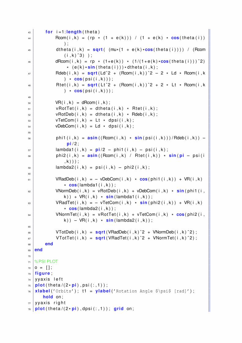
43 for i =1: length ( the ta )44 Rcom( i , k ) = ( rp * (1 + e ( k ) ) ) / (1 + e ( k ) * cos ( the ta ( i ) )
) ;45 dtheta ( i , k ) = sqrt ( (mu* (1 + e ( k ) *cos ( the ta ( i ) ) ) ) / (Rcom
( i , k ) ˆ 3 ) ) ;46 dRcom( i , k ) = rp * (1+e ( k ) ) * ( 1 / ( 1+ e ( k ) *cos ( the ta ( i ) ) ) ˆ 2 )
* ( e ( k ) * sin ( the ta ( i ) ) ) * dtheta ( i , k ) ;47 Rdeb( i , k ) = sqrt ( Ld ˆ2 + (Rcom( i , k ) ) ˆ2 − 2 * Ld * Rcom( i , k
) * cos ( ps i ( i , k ) ) ) ;48 Rtet ( i , k ) = sqrt ( L t ˆ2 + (Rcom( i , k ) ) ˆ2 + 2 * Lt * Rcom( i , k
) * cos ( ps i ( i , k ) ) ) ;49
50 VR( i , k ) = dRcom( i , k ) ;51 vRotTet ( i , k ) = dtheta ( i , k ) * Rtet ( i , k ) ;52 vRotDeb ( i , k ) = dtheta ( i , k ) * Rdeb( i , k ) ;53 vTetCom ( i , k ) = L t * dps i ( i , k ) ;54 vDebCom( i , k ) = Ld * dps i ( i , k ) ;55
56 phi1 ( i , k ) = asin ( (Rcom( i , k ) * sin ( ps i ( i , k ) ) ) / Rdeb ( i , k ) ) −pi / 2 ;
57 lambda1 ( i , k ) = pi /2 − phi1 ( i , k ) − ps i ( i , k ) ;58 phi2 ( i , k ) = asin ( (Rcom( i , k ) / Rtet ( i , k ) ) * sin ( pi − ps i ( i
, k ) ) ) ;59 lambda2 ( i , k ) = ps i ( i , k ) − phi2 ( i , k ) ;60
61 VRadDeb( i , k ) = − vDebCom( i , k ) * cos ( phi1 ( i , k ) ) + VR( i , k )
* cos ( lambda1 ( i , k ) ) ;62 VNormDeb( i , k ) = vRotDeb ( i , k ) + vDebCom( i , k ) * sin ( phi1 ( i ,
k ) ) + VR( i , k ) * sin ( lambda1 ( i , k ) ) ;63 VRadTet ( i , k ) = − vTetCom ( i , k ) * sin ( phi2 ( i , k ) ) + VR( i , k )
* cos ( lambda2 ( i , k ) ) ;64 VNormTet ( i , k ) = vRotTet ( i , k ) + vTetCom ( i , k ) * cos ( phi2 ( i ,
k ) ) − VR( i , k ) * sin ( lambda2 ( i , k ) ) ;65
66 VTotDeb ( i , k ) = sqrt (VRadDeb( i , k ) ˆ2 + VNormDeb( i , k ) ˆ 2 ) ;67 VTotTet ( i , k ) = sqrt ( VRadTet ( i , k ) ˆ2 + VNormTet ( i , k ) ˆ 2 ) ;68 end69 end70
71 %PSI PLOT72 o = [ ] ;73 f igure ;74 yyax is l e f t75 plot ( the ta / ( 2 * pi ) , ps i ( : , 1 ) ) ;76 xlabel (’Orbits’ ) ; t1 = ylabel (’Rotation Angle $\psi$ [rad]’ ) ;
hold on ;77 yyax is r i g h t78 plot ( the ta / ( 2 * pi ) , dps i ( : , 1 ) ) ; grid on ;

79 xlabel (’Orbits’ ) ; t2 = ylabel (’Rotation Velocity $\dot{\psi}$ [rad/s]’ ) ;
80 t l = t i t l e (’$\psi$ and $\dot{\psi}$ vs orbits’ ) ;81 set ( t l , ’Interpreter’ , ’latex’ ) ; set ( t1 , ’Interpreter’ , ’latex’ ) ;
set ( t2 , ’Interpreter’ , ’latex’ ) ;82
83 f igure ;84 yyax is l e f t85 o ( : , 1 ) = plot ( the ta / ( 2 * pi ) , ps i ) ;86 xlabel (’Orbits’ ) ; t1 = ylabel (’Rotation Angle $\psi$ [rad]’ ) ;
hold on ;87 yyax is r i g h t88 o ( : , 2 ) = plot ( the ta / ( 2 * pi ) , dps i ) ; grid on ;89 xlabel (’Orbits’ ) ; t2 = ylabel (’Rotation Velocity $\dot{\psi}$ [
rad/s]’ ) ;90 legend ( o ( : , 1 ) , ’e = 0’ , ’e = 0.05’ , ’e = 0.1’ , ’e = 0.15’ ) ;91 t l = t i t l e (’$\psi$ and $\dot{\psi}$ vs orbits’ ) ;92 set ( t l , ’Interpreter’ , ’latex’ ) ; set ( t1 , ’Interpreter’ , ’latex’ ) ;
set ( t2 , ’Interpreter’ , ’latex’ ) ;93
94 %RADIUS PLOT95 f igure ;96 plot ( the ta / ( 2 * pi ) ,Rcom / 1000 − (Re / 1000) ) ; grid on ;97 legend (’e = 0’ , ’e = 0.05’ , ’e = 0.1’ , ’e = 0.15’ ) ;98 xlabel (’Orbits’ ) ; ylabel (’Orbit height [km]’ ) ;99 t i t l e (’CoM orbit height vs orbits’ ) ;
100
101 %DEBRIS VELOCITIES PLOT102 o = [ ] ;103 f igure ;104 o ( : , 1 ) = plot ( the ta / ( 2 * pi ) ,vDebCom / 1000 , ’-’ , ’color’ , [ 0 , 0 .5 ,
0 ] ) ; hold on ;105 o ( : , 2 ) = plot ( the ta / ( 2 * pi ) , vRotDeb / 1000 , ’-’ , ’color’ , [0 .8500 ,
0.3250 , 0 .0980 ] ) ; hold on ;106 o ( : , 3 ) = plot ( the ta / ( 2 * pi ) ,VR / 1000 , ’-’ , ’color’ , [0 .4940 ,
0.1840 , 0 .5560 ] ) ; grid on ;107 legend ( o ( 1 , : ) , ’VDebCom’ , ’VRotDeb’ , ’VR’ ) ;108 xlabel (’Orbits’ ) ; ylabel (’Velocities [km/s]’ ) ;109 t i t l e (’Debris velocities vs orbits’ ) ;110
111 f igure ;112 o ( : , 1 ) = plot ( the ta / ( 2 * pi ) ,VRadDeb / 1000 , ’k’ ) ; hold on ;113 o ( : , 2 ) = plot ( the ta / ( 2 * pi ) ,VNormDeb / 1000 , ’b’ ) ; hold on ;114 o ( : , 3 ) = plot ( the ta / ( 2 * pi ) ,VTotDeb / 1000 , ’r’ ) ; grid on ;115 legend ( o ( 1 , : ) , ’Vradial’ , ’Vnormal’ , ’Vtotal’ ) ;116 xlabel (’Orbits’ ) ; ylabel (’Velocities [km/s]’ ) ;117 t i t l e (’Debris radial, normal and total velocities vs orbits’ ) ;118

119 %TETHER’S BODY VELOCITIES PLOT120 f igure ;121 o ( : , 1 ) = plot ( the ta / ( 2 * pi ) , vTetCom / 1000 , ’-’ , ’color’ , [ 0 , 0 .5 ,
0 ] ) ; hold on ;122 o ( : , 2 ) = plot ( the ta / ( 2 * pi ) , vRotTet / 1000 , ’-’ , ’color’ , [0 .8500 ,
0.3250 , 0 .0980 ] ) ; hold on ;123 o ( : , 3 ) = plot ( the ta / ( 2 * pi ) ,VR / 1000 , ’-’ , ’color’ , [0 .4940 ,
0.1840 , 0 .5560 ] ) ; grid on ;124 legend ( o ( 1 , : ) , ’VTetCom’ , ’VRotTet’ , ’VR’ ) ;125 xlabel (’Orbits’ ) ; ylabel (’Velocities [km/s]’ ) ;126 t i t l e (’Tethers body velocities vs orbits’ ) ;127
128 f igure ;129 o ( : , 1 ) = plot ( the ta / ( 2 * pi ) ,VRadTet / 1000 , ’k’ ) ; hold on ;130 o ( : , 2 ) = plot ( the ta / ( 2 * pi ) ,VNormTet / 1000 , ’b’ ) ; hold on ;131 o ( : , 3 ) = plot ( the ta / ( 2 * pi ) , VTotTet / 1000 , ’r’ ) ; grid on ;132 legend ( o ( 1 , : ) , ’Vradial’ , ’Vnormal’ , ’Vtotal’ ) ;133 xlabel (’Orbits’ ) ; ylabel (’Velocities [km/s]’ ) ;134 t i t l e (’Tethers body radial, normal and total velocities vs orbits
’ ) ;135
136 %TRANSFER ORBIT CALCULATIONS137 for k =1: length ( e )138 for i = 1 : length ( the ta )139 adeb ( i , k ) = (mu * Rdeb( i , k ) ) / (2*mu − ( VTotDeb ( i , k ) ) ˆ2*
Rdeb( i , k ) ) ;140 a t e t ( i , k ) = (mu * Rtet ( i , k ) ) / (2*mu − ( VTotTet ( i , k ) ) ˆ2*
Rtet ( i , k ) ) ;141 end142 [A ] = i s l o c a l m i n ( adeb ) ;143 Minimum = f ind (A ( : , k ) == 1) ;144
145 ReleasePosi t ion ( k ) = Minimum ( 8 ) ; %Of all the valleys ofadeb, thisvaluerepresentstheonethatischosentobethereleaseinstant
146 VNormDebRelease ( k ) = VNormDeb( ReleasePosi t ion ( k ) , k ) ;147 VTotDebRelease ( k ) = VTotDeb ( ReleasePosi t ion ( k ) , k ) ;148 VNormTetRelease ( k ) = VNormTet ( ReleasePosi t ion ( k ) , k ) ;149 VTotTetRelease ( k ) = VTotTet ( ReleasePosi t ion ( k ) , k ) ;150
151 ps i re lease ( k ) = ps i ( ReleasePosi t ion ( k ) , k ) ;152
153 adebrelease ( k ) = (mu * Rdeb( ReleasePosi t ion ( k ) , k ) ) / (2*mu −( VTotDebRelease ( k ) ˆ 2 ) *Rdeb( ReleasePosi t ion ( k ) , k ) ) ;
154 pdeb ( k ) = ( VNormDebRelease ( k ) *Rdeb( ReleasePosi t ion ( k ) , k ) ) ˆ2 /mu;
155 edeb ( k ) = sqrt (1 − pdeb ( k ) / adebrelease ( k ) ) ;156 a te t r e l ease ( k ) = (mu * Rtet ( ReleasePosi t ion ( k ) , k ) ) / (2*mu −
( VTotTetRelease ( k ) ˆ 2 ) * Rtet ( ReleasePosi t ion ( k ) , k ) ) ;

157 p t e t ( k ) = ( VNormTetRelease ( k ) * Rtet ( ReleasePosi t ion ( k ) , k ) ) ˆ2 /mu;
158 e t e t ( k ) = sqrt (1 − p t e t ( k ) / a t e t r e l ease ( k ) ) ;159
160 for i = 1 : length ( the ta )161 Rnewdeb( i , k ) = pdeb ( k ) / (1 + edeb ( k ) * cos ( the ta ( i ) +
the ta ( ReleasePosi t ion ( k ) ) ) ) ;162 Rnewtet ( i , k ) = p t e t ( k ) / (1 + e t e t ( k ) * cos ( the ta ( i ) +
the ta ( ReleasePosi t ion ( k ) ) ) ) ;163 dthetadeb ( i , k ) = sqrt ( (mu* (1 + edeb ( k ) *cos ( the ta ( i ) +
the ta ( ReleasePosi t ion ( k ) ) ) ) ) / (Rnewdeb( i , k ) ˆ 3 ) ) ;164 d t h e t a t e t ( i , k ) = sqrt ( (mu* (1 + e t e t ( k ) *cos ( the ta ( i ) +
the ta ( ReleasePosi t ion ( k ) ) ) ) ) / ( Rnewtet ( i , k ) ˆ 3 ) ) ;165 dRnewdeb( i , k ) = pdeb ( k ) * ( 1 / ( 1+ edeb ( k ) *cos ( the ta ( i ) +
the ta ( ReleasePosi t ion ( k ) ) ) ) ˆ 2 ) * ( edeb ( k ) * sin ( the ta ( i )+ the ta ( ReleasePosi t ion ( k ) ) ) ) * dthetadeb ( i , k ) ;
166 dRnewtet ( i , k ) = p t e t ( k ) * ( 1 / ( 1+ e t e t ( k ) *cos ( the ta ( i ) +the ta ( ReleasePosi t ion ( k ) ) ) ) ˆ 2 ) * ( e t e t ( k ) * sin ( the ta ( i )+ the ta ( ReleasePosi t ion ( k ) ) ) ) * d t h e t a t e t ( i , k ) ;
167 VTotDeb2 ( i , k ) = sqrt ( dRnewdeb ( i , k ) ˆ2 + ( dthetadeb ( i , k ) *Rnewdeb( i , k ) ) ˆ 2 ) ;
168 VTotTet2 ( i , k ) = sqrt ( dRnewtet ( i , k ) ˆ2 + ( d t h e t a t e t ( i , k ) *Rnewtet ( i , k ) ) ˆ 2 ) ;
169
170 adeb2 ( i , k ) = (mu * Rnewdeb( i , k ) ) / (2*mu − ( VTotDeb2 ( i , k )) ˆ2*Rnewdeb( i , k ) ) ;
171 a te t2 ( i , k ) = (mu * Rnewtet ( i , k ) ) / (2*mu − ( VTotTet2 ( i , k )) ˆ2* Rnewtet ( i , k ) ) ;
172
173 o r b i t s ( i , k ) = the ta ( i ) / ( 2 * pi ) + the ta ( ReleasePosi t ion ( k ) )/ ( 2 * pi ) ;
174 end175 end176
177 o = [ ] ;178 f igure ;179 o ( : , 1 ) = plot ( the ta / ( 2 * pi ) , adeb / 1000) ;180 xlabel (’Orbits’ ) ; ylabel (’Semi-major axis [km]’ ) ; hold on ;181 plot ( the ta / ( 2 * pi ) , adeb2 ( : , 1 ) / 1000 ,’-’ , ’color’ , [ 0 , 0.4470 ,
0 .7410] ,’LineWidth’ , 1 . 5 ) ; hold on ;182 plot ( the ta / ( 2 * pi ) , adeb2 ( : , 2 ) / 1000 ,’-’ , ’color’ , [0 .8500 ,
0.3250 , 0 .0980] ,’LineWidth’ , 1 . 5 ) ; hold on ;183 plot ( the ta / ( 2 * pi ) , adeb2 ( : , 3 ) / 1000 ,’-’ , ’color’ , [0 .9290 ,
0.6940 , 0 .1250] ,’LineWidth’ , 1 . 5 ) ; hold on ;184 plot ( the ta / ( 2 * pi ) , adeb2 ( : , 4 ) / 1000 ,’-’ , ’color’ , [0 .4940 ,
0.1840 , 0 .5560] ,’LineWidth’ , 1 . 5 ) ; grid on ;185 legend ( o ( : , 1 ) , ’e = 0’ , ’e = 0.05’ , ’e = 0.1’ , ’e = 0.15’ ) ;186 t i t l e (’Possible and final semi-major axis of the debris’ ) ;

187
188 o = [ ] ;189 f igure ;190 o ( : , 1 ) = plot ( the ta / ( 2 * pi ) , a t e t / 1000) ;191 xlabel (’Orbits’ ) ; ylabel (’Semi-major axis [km]’ ) ; hold on ;192 plot ( the ta / ( 2 * pi ) , a te t2 ( : , 1 ) / 1000 ,’-’ , ’color’ , [ 0 , 0.4470 ,
0 .7410] ,’LineWidth’ , 1 . 5 ) ; hold on ;193 plot ( the ta / ( 2 * pi ) , a te t2 ( : , 2 ) / 1000 ,’-’ , ’color’ , [0 .8500 ,
0.3250 , 0 .0980] ,’LineWidth’ , 1 . 5 ) ; hold on ;194 plot ( the ta / ( 2 * pi ) , a te t2 ( : , 3 ) / 1000 ,’-’ , ’color’ , [0 .9290 ,
0.6940 , 0 .1250] ,’LineWidth’ , 1 . 5 ) ; hold on ;195 plot ( the ta / ( 2 * pi ) , a te t2 ( : , 4 ) / 1000 ,’-’ , ’color’ , [0 .4940 ,
0.1840 , 0 .5560] ,’LineWidth’ , 1 . 5 ) ; grid on ;196 legend ( o ( : , 1 ) , ’e = 0’ , ’e = 0.05’ , ’e = 0.1’ , ’e = 0.15’ ) ;197 t i t l e (’Possible and final semi-major axis of the tethers body’ ) ;198
199 f igure ;200 for k =1: length ( e )201 plot ( o r b i t s ( : , k ) , ( Rnewdeb − Re) /1000) ; grid on ;202 legend (’e = 0’ , ’e = 0.05’ , ’e = 0.1’ , ’e = 0.15’ ) ;203 xlabel (’Orbits’ ) ; ylabel (’Orbit height [km]’ ) ;204 x l im ( [ o r b i t s (1 , k ) o r b i t s (1 , k ) +5 ] )205 t i t l e (’New orbit heights of the debris after release’ ) ;206 end207
208 f igure ;209 for k =1: length ( e )210 plot ( o r b i t s ( : , k ) , ( Rnewtet − Re) /1000) ; grid on ;211 legend (’e = 0’ , ’e = 0.05’ , ’e = 0.1’ , ’e = 0.15’ ) ;212 xlabel (’Orbits’ ) ; ylabel (’Orbit height [km]’ ) ;213 x l im ( [ o r b i t s (1 , k ) o r b i t s (1 , k ) +5 ] )214 t i t l e (’New orbit heights of the tethers body after release’ ) ;215 end216
217
218
219 %———- Varying tether’s length ———-220
221 clc ; clear ; close a l l ;222 syms y ( x ) ;223 %THETA = x, PSI = y224
225 G = 6.674e−11;226 Me = 5.972e24 ;227 mu = G * Me;228 rad = pi / 180 ;229 Re = 6371000;230

231 %ORBIT INTERVAL232 x0 = 0;233 x f = 5 * 2* pi ;234 x i n t e r v a l = ( x0 : rad *1 : x f ) ;235
236 % INITIAL ANGLES237 y0 = 0 . 2 ;238 dy0 = 0;239 i n i t i a l c o n d i t i o n s = [ y0 ; dy0 ] ;240
241 %RADIUS PERIGEE242 rp = 3000000 + Re ;243
244 %MASSES AND LENGTHS245 Md = 100;246 Mt = 1000;247 Lt = 120;248 for k=2:4249 Lt ( k ) = L t ( k−1) + 20;250 end251 Ld = ( Mt / Md) * Lt ;252
253 %ECCENTRICITY254 e = 0 . 1 ;255
256 %VELOCITIES257 [ theta , Y ] = ode45 (@( theta , Y) D i f f e r e n t i a l ( theta ,Y, e ) , x i n t e r v a l ,
i n i t i a l c o n d i t i o n s ) ;258 ps i = Y ( : , 1 ) ;259 dps i = Y ( : , 2 ) ;260 for k =1: length ( L t )261 for i =1: length ( the ta )262 Rcom( i , k ) = ( rp *(1+e ) ) / (1 + e* cos ( the ta ( i ) ) ) ;263 dtheta ( i , k ) = sqrt ( (mu*(1+e*cos ( the ta ( i ) ) ) ) / ( (Rcom( i , k )
) ˆ 3 ) ) ;264 dRcom( i , k ) = rp * (1+e ) * ( 1 / ( 1+ e*cos ( the ta ( i ) ) ) ˆ 2 ) * ( e*
sin ( the ta ( i ) ) ) * dtheta ( i , k ) ;265 Rdeb( i , k ) = sqrt ( Ld ( k ) ˆ2+(Rcom( i , k ) ) ˆ2−2*Ld ( k ) *Rcom( i , k ) *
cos ( ps i ( i ) ) ) ;266 Rtet ( i , k ) = sqrt ( L t ( k ) ˆ2+(Rcom( i , k ) ) ˆ2+2* Lt ( k ) *Rcom( i , k ) *
cos ( ps i ( i ) ) ) ;267
268 VR( i , k ) = dRcom( i ) ;269 vRotTet ( i , k ) = dtheta ( i , k ) * Rtet ( i , k ) ;270 vRotDeb ( i , k ) = dtheta ( i , k ) * Rdeb( i , k ) ;271 vTetCom ( i , k ) = L t ( k ) * dps i ( i ) ;272 vDebCom( i , k ) = Ld ( k ) * dps i ( i ) ;273

274 phi1 ( i , k ) = asin ( (Rcom( i , k ) * sin ( ps i ( i ) ) ) / Rdeb ( i , k ) ) −pi / 2 ;
275 lambda1 ( i , k ) = pi /2 − phi1 ( i , k ) − ps i ( i ) ;276 phi2 ( i , k ) = asin ( (Rcom( i , k ) / Rtet ( i , k ) ) * sin ( pi − ps i ( i
) ) ) ;277 lambda2 ( i , k ) = ps i ( i ) − phi2 ( i , k ) ;278
279 VRadDeb( i , k ) = − vDebCom( i , k ) * cos ( phi1 ( i , k ) ) + VR( i , k )
* cos ( lambda1 ( i , k ) ) ;280 VNormDeb( i , k ) = vRotDeb ( i , k ) + vDebCom( i , k ) * sin ( phi1 ( i ,
k ) ) + VR( i , k ) * sin ( lambda1 ( i , k ) ) ;281 VRadTet ( i , k ) = − vTetCom ( i , k ) * sin ( phi2 ( i , k ) ) + VR( i , k )
* cos ( lambda2 ( i , k ) ) ;282 VNormTet ( i , k ) = vRotTet ( i , k ) + vTetCom ( i , k ) * cos ( phi2 ( i ,
k ) ) − VR( i , k ) * sin ( lambda2 ( i , k ) ) ;283 VTotDeb ( i , k ) = sqrt (VRadDeb( i , k ) ˆ2 + VNormDeb( i , k ) ˆ 2 ) ;284 VTotTet ( i , k ) = sqrt ( VRadTet ( i , k ) ˆ2 + VNormTet ( i , k ) ˆ 2 ) ;285 end286 end287
288 %PSI PLOT289 f igure ;290 yyax is l e f t291 plot ( the ta / ( 2 * pi ) , ps i ) ;292 xlabel (’Orbits’ ) ; ylabel (’Rotation Angle [rad]’ ) ; hold on ;293 yyax is r i g h t294 plot ( the ta / ( 2 * pi ) , dps i ) ; grid on ;295 xlabel (’Orbits’ ) ; ylabel (’Rotation Velocity [rad/s]’ ) ;296 l g = legend (’Rotation Angle $\psi$’ , ’Rotation Velocity $\dot{\
psi}$’ ) ;297 t l = t i t l e (’$\psi$ and $\dot{\psi}$ vs orbits’ ) ;298 set ( lg , ’Interpreter’ , ’latex’ ) ; set ( t l , ’Interpreter’ , ’latex’ ) ;299
300 %RADIUS PLOT301 f igure ;302 plot ( the ta / ( 2 * pi ) ,Rcom / 1000 − (Re / 1000) ) ; grid on ;303 xlabel (’Orbits’ ) ; ylabel (’Orbit height [km]’ ) ;304 t i t l e (’CoM orbit height vs orbits’ ) ;305
306 %DEBRIS VELOCITIES PLOT307 o = [ ] ;308 f igure ;309 o ( : , 1 ) = plot ( the ta / ( 2 * pi ) ,vDebCom / 1000 , ’-’ , ’color’ , [ 0 , 0 .5 ,
0 ] ) ; hold on ;310 o ( : , 2 ) = plot ( the ta / ( 2 * pi ) , vRotDeb / 1000 , ’-’ , ’color’ , [0 .8500 ,
0.3250 , 0 .0980 ] ) ; hold on ;311 o ( : , 3 ) = plot ( the ta / ( 2 * pi ) ,VR / 1000 , ’-’ , ’color’ , [0 .4940 ,
0.1840 , 0 .5560 ] ) ; grid on ;

312 legend ( o ( 1 , : ) , ’VDebCom’ , ’VRotDeb’ , ’VR’ ) ;313 xlabel (’Orbits’ ) ; ylabel (’Velocities [km/s]’ ) ;314 t i t l e (’Debris velocities vs orbits’ ) ;315
316 f igure ;317 for k =1: length ( Ld )318 o ( : , 1 ) = plot ( the ta / ( 2 * pi ) ,VRadDeb ( : , k ) / 1000 , ’k’ ) ; hold on
;319 o ( : , 2 ) = plot ( the ta / ( 2 * pi ) ,VNormDeb ( : , k ) / 1000 , ’b’ ) ; hold
on ;320 o ( : , 3 ) = plot ( the ta / ( 2 * pi ) ,VTotDeb ( : , k ) / 1000 , ’r’ ) ; grid on
;321 legend ( o ( 1 , : ) , ’Vrad’ , ’Vnormal’ , ’Vtotal’ ) ;322 xlabel (’Orbits’ ) ; ylabel (’Velocities [km/s]’ ) ;323 t i t l e (’Debris radial, normal and total velocities vs orbits’ )
;324 end325
326 %TETHER’S BODY VELOCITIES PLOT327 f igure ;328 o ( : , 1 ) = plot ( the ta / ( 2 * pi ) , vTetCom / 1000 , ’-’ , ’color’ , [ 0 , 0 .5 ,
0 ] ) ; hold on ;329 o ( : , 2 ) = plot ( the ta / ( 2 * pi ) , vRotTet / 1000 , ’-’ , ’color’ , [0 .8500 ,
0.3250 , 0 .0980 ] ) ; hold on ;330 o ( : , 3 ) = plot ( the ta / ( 2 * pi ) ,VR / 1000 , ’-’ , ’color’ , [0 .4940 ,
0.1840 , 0 .5560 ] ) ; grid on ;331 legend ( o ( 1 , : ) , ’VTetCom’ , ’VRotTet’ , ’VR’ ) ;332 xlabel (’Orbits’ ) ; ylabel (’Velocities [km/s]’ ) ;333 t i t l e (’Tethers body velocities vs orbits’ ) ;334
335 f igure ;336 o ( : , 1 ) = plot ( the ta / ( 2 * pi ) ,VRadTet / 1000 , ’k’ ) ; hold on ;337 o ( : , 2 ) = plot ( the ta / ( 2 * pi ) ,VNormTet / 1000 , ’b’ ) ; hold on ;338 o ( : , 3 ) = plot ( the ta / ( 2 * pi ) , VTotTet / 1000 , ’r’ ) ; grid on ;339 legend ( o ( 1 , : ) , ’Vrad’ , ’Vnormal’ , ’Vtotal’ ) ;340 xlabel (’Orbits’ ) ; ylabel (’Velocities [km/s]’ ) ;341 t i t l e (’Tethers body radial, normal and total velocities vs orbits
’ ) ;342
343 %TRANSFER ORBIT CALCULATIONS344 for k =1: length ( Ld )345 for i = 1 : length ( the ta )346 adeb ( i , k ) = (mu * Rdeb( i , k ) ) / (2*mu − ( VTotDeb ( i , k ) ) ˆ2*
Rdeb( i , k ) ) ;347 a t e t ( i , k ) = (mu * Rtet ( i , k ) ) / (2*mu − ( VTotTet ( i , k ) ) ˆ2*
Rtet ( i , k ) ) ;348 end349 [A ] = i s l o c a l m i n ( adeb ) ;

350 Minimum = f ind (A ( : , k ) == 1) ;351
352 ReleasePosi t ion ( k ) = Minimum ( 5 ) ;353 VNormDebRelease ( k ) = VNormDeb( ReleasePosi t ion ( k ) , k ) ;354 VTotDebRelease ( k ) = VTotDeb ( ReleasePosi t ion ( k ) , k ) ;355 VNormTetRelease ( k ) = VNormTet ( ReleasePosi t ion ( k ) , k ) ;356 VTotTetRelease ( k ) = VTotTet ( ReleasePosi t ion ( k ) , k ) ;357
358 ps i re lease ( k ) = ps i ( ReleasePosi t ion ( k ) ) ;359
360 adebrelease ( k ) = (mu * Rdeb( ReleasePosi t ion ( k ) , k ) ) / (2*mu −( VTotDebRelease ( k ) ˆ 2 ) *Rdeb( ReleasePosi t ion ( k ) , k ) ) ;
361 pdeb ( k ) = ( VNormDebRelease ( k ) *Rdeb( ReleasePosi t ion ( k ) , k ) ) ˆ2 /mu;
362 edeb ( k ) = sqrt (1 − pdeb ( k ) / adebrelease ( k ) ) ;363 a te t r e l ease ( k ) = (mu * Rtet ( ReleasePosi t ion ( k ) , k ) ) / (2*mu −
( VTotTetRelease ( k ) ˆ 2 ) * Rtet ( ReleasePosi t ion ( k ) , k ) ) ;364 p t e t ( k ) = ( VNormTetRelease ( k ) * Rtet ( ReleasePosi t ion ( k ) , k ) ) ˆ2 /
mu;365 e t e t ( k ) = sqrt (1 − p t e t ( k ) / a t e t r e l ease ( k ) ) ;366
367 for i = 1 : length ( the ta )368 Rnewdeb( i , k ) = pdeb ( k ) / (1 + edeb ( k ) * cos ( the ta ( i ) +
the ta ( ReleasePosi t ion ( k ) ) ) ) ;369 Rnewtet ( i , k ) = p t e t ( k ) / (1 + e t e t ( k ) * cos ( the ta ( i ) +
the ta ( ReleasePosi t ion ( k ) ) ) ) ;370 dthetadeb ( i , k ) = sqrt ( (mu* (1 + edeb ( k ) *cos ( the ta ( i ) +
the ta ( ReleasePosi t ion ( k ) ) ) ) ) / (Rnewdeb( i , k ) ˆ 3 ) ) ;371 d t h e t a t e t ( i , k ) = sqrt ( (mu* (1 + e t e t ( k ) *cos ( the ta ( i ) +
the ta ( ReleasePosi t ion ( k ) ) ) ) ) / ( Rnewtet ( i , k ) ˆ 3 ) ) ;372 dRnewdeb( i , k ) = pdeb ( k ) * ( 1 / ( 1+ edeb ( k ) *cos ( the ta ( i ) +
the ta ( ReleasePosi t ion ( k ) ) ) ) ˆ 2 ) * ( edeb ( k ) * sin ( the ta ( i )+ the ta ( ReleasePosi t ion ( k ) ) ) ) * dthetadeb ( i , k ) ;
373 dRnewtet ( i , k ) = p t e t ( k ) * ( 1 / ( 1+ e t e t ( k ) *cos ( the ta ( i ) +the ta ( ReleasePosi t ion ( k ) ) ) ) ˆ 2 ) * ( e t e t ( k ) * sin ( the ta ( i )+ the ta ( ReleasePosi t ion ( k ) ) ) ) * d t h e t a t e t ( i , k ) ;
374 VTotDeb2 ( i , k ) = sqrt ( dRnewdeb ( i , k ) ˆ2 + ( dthetadeb ( i , k ) *Rnewdeb( i , k ) ) ˆ 2 ) ;
375 VTotTet2 ( i , k ) = sqrt ( dRnewtet ( i , k ) ˆ2 + ( d t h e t a t e t ( i , k ) *Rnewtet ( i , k ) ) ˆ 2 ) ;
376
377 adeb2 ( i , k ) = (mu * Rnewdeb( i , k ) ) / (2*mu − ( VTotDeb2 ( i , k )) ˆ2*Rnewdeb( i , k ) ) ;
378 a te t2 ( i , k ) = (mu * Rnewtet ( i , k ) ) / (2*mu − ( VTotTet2 ( i , k )) ˆ2* Rnewtet ( i , k ) ) ;
379
380 o r b i t s ( i , k ) = the ta ( i ) / ( 2 * pi ) + the ta ( ReleasePosi t ion ( k ) )/ ( 2 * pi ) ;

381 end382 end383
384 o = [ ] ;385 f igure ;386 o ( : , 1 ) = plot ( the ta / ( 2 * pi ) , adeb / 1000) ;387 xlabel (’Orbits’ ) ; ylabel (’Semi-major axis [km]’ ) ; hold on ;388 plot ( the ta / ( 2 * pi ) , adeb2 ( : , 1 ) / 1000 ,’-’ , ’color’ , [ 0 , 0.4470 ,
0 .7410] ,’LineWidth’ , 1 . 5 ) ; hold on ;389 plot ( the ta / ( 2 * pi ) , adeb2 ( : , 2 ) / 1000 ,’-’ , ’color’ , [0 .8500 ,
0.3250 , 0 .0980] ,’LineWidth’ , 1 . 5 ) ; hold on ;390 plot ( the ta / ( 2 * pi ) , adeb2 ( : , 3 ) / 1000 ,’-’ , ’color’ , [0 .9290 ,
0.6940 , 0 .1250] ,’LineWidth’ , 1 . 5 ) ; hold on ;391 plot ( the ta / ( 2 * pi ) , adeb2 ( : , 4 ) / 1000 ,’-’ , ’color’ , [0 .4940 ,
0.1840 , 0 .5560] ,’LineWidth’ , 1 . 5 ) ; grid on ;392 legend ( o ( : , 1 ) , ’Ltet=80m, Ldeb=800m’ , ’Ltet=100m, Ldeb=1000m’ , ’
Ltet=120m, Ldeb=1200m’ , ’Ltet=140m, Ldeb=1400m’ ) ;393 t i t l e (’Possible and final semi-major axis of the debris’ ) ;394
395 o = [ ] ;396 f igure ;397 o ( : , 1 ) = plot ( the ta / ( 2 * pi ) , a t e t / 1000) ;398 xlabel (’Orbits’ ) ; ylabel (’Semi-major axis [km]’ ) ; hold on ;399 plot ( the ta / ( 2 * pi ) , a te t2 ( : , 1 ) / 1000 ,’-’ , ’color’ , [ 0 , 0.4470 ,
0 .7410] ,’LineWidth’ , 1 . 5 ) ; hold on ;400 plot ( the ta / ( 2 * pi ) , a te t2 ( : , 2 ) / 1000 ,’-’ , ’color’ , [0 .8500 ,
0.3250 , 0 .0980] ,’LineWidth’ , 1 . 5 ) ; hold on ;401 plot ( the ta / ( 2 * pi ) , a te t2 ( : , 3 ) / 1000 ,’-’ , ’color’ , [0 .9290 ,
0.6940 , 0 .1250] ,’LineWidth’ , 1 . 5 ) ; hold on ;402 plot ( the ta / ( 2 * pi ) , a te t2 ( : , 4 ) / 1000 ,’-’ , ’color’ , [0 .4940 ,
0.1840 , 0 .5560] ,’LineWidth’ , 1 . 5 ) ; grid on ;403 legend ( o ( : , 1 ) , ’Ltet=80m, Ldeb=800m’ , ’Ltet=100m, Ldeb=1000m’ , ’
Ltet=120m, Ldeb=1200m’ , ’Ltet=140m, Ldeb=1400m’ ) ;404 t i t l e (’Possible and final semi-major axis of the tethers body’ ) ;405
406 f igure ;407 for k =1: length ( Ld )408 plot ( o r b i t s ( : , k ) , ( Rnewdeb − Re) /1000) ; grid on ;409 legend (’Ltet=80m, Ldeb=800m’ , ’Ltet=100m, Ldeb=1000m’ , ’Ltet
=120m, Ldeb=1200m’ , ’Ltet=140m, Ldeb=1400m’ ) ;410 xlabel (’Orbits’ ) ; ylabel (’Orbit height [km]’ ) ;411 x l im ( [ o r b i t s (1 , k ) o r b i t s (1 , k ) +5 ] )412 t i t l e (’New orbit heights of the debris after release’ ) ;413 end414
415 f igure ;416 for k =1: length ( Ld )417 plot ( o r b i t s ( : , k ) , ( Rnewtet − Re) /1000) ; grid on ;
418 legend (’Ltet=80m, Ldeb=800m’ , ’Ltet=100m, Ldeb=1000m’ , ’Ltet=120m, Ldeb=1200m’ , ’Ltet=140m, Ldeb=1400m’ ) ;
419 xlabel (’Orbits’ ) ; ylabel (’Orbit height [km]’ ) ;420 x l im ( [ o r b i t s (1 , k ) o r b i t s (1 , k ) +5 ] )421 t i t l e (’New orbit heights of the tethers body after release’ ) ;422 end423
424
425
426 %———- Varying radius of the perigee ———-427
428 clc ; clear ; close a l l ;429 syms y ( x ) ;430 %THETA = x, PSI = y431
432 G = 6.674e−11;433 Me = 5.972e24 ;434 mu = G * Me;435 rad = pi / 180 ;436 Re = 6371000;437
438 %ORBIT INTERVAL439 x0 = 0;440 x f = 5 * 2* pi ;441 x i n t e r v a l = ( x0 : rad *1 : x f ) ;442
443 % INITIAL ANGLES444 y0 = 0 . 2 ;445 dy0 = 0;446 i n i t i a l c o n d i t i o n s = [ y0 ; dy0 ] ;447
448 %RADIUS PERIGEE449 rp = 2000000 + Re ;450 for k=2:4451 rp ( k ) = rp ( k−1) + 1000000;452 end453
454 %MASSES AND LENGTHS455 Md = 100;456 Mt = 1000;457 Lt = 120;458 Ld = ( Mt / Md) * Lt ;459
460 %ECCENTRICITY461 e = 0 . 1 ;462
463 %VELOCITIES464 [ theta , Y ] = ode45 (@( theta , Y) D i f f e r e n t i a l ( theta ,Y, e ) , x i n t e r v a l ,

i n i t i a l c o n d i t i o n s ) ;465 ps i = Y ( : , 1 ) ;466 dps i = Y ( : , 2 ) ;467 for k =1: length ( rp )468 for i =1: length ( the ta )469 Rcom( i , k ) = ( rp ( k ) *(1+e ) ) / (1+ e*cos ( the ta ( i ) ) ) ;470 dtheta ( i , k ) = sqrt ( (mu*(1+e*cos ( the ta ( i ) ) ) ) / ( (Rcom( i , k )
) ˆ 3 ) ) ;471 dRcom( i , k ) = rp ( k ) *(1+e ) * ( 1 / ( 1 + e*cos ( the ta ( i ) ) ) ˆ 2 ) * ( e* sin
( the ta ( i ) ) ) * dtheta ( i , k ) ;472 Rdeb( i , k ) = sqrt ( Ld ˆ2+(Rcom( i , k ) ) ˆ2−2*Ld*Rcom( i , k ) *cos (
ps i ( i ) ) ) ;473 Rtet ( i , k ) = sqrt ( L t ˆ2+(Rcom( i , k ) ) ˆ2+2* Lt *Rcom( i , k ) *cos (
ps i ( i ) ) ) ;474
475 VR( i , k ) = dRcom( i , k ) ;476 vRotTet ( i , k ) = dtheta ( i , k ) * Rtet ( i , k ) ;477 vRotDeb ( i , k ) = dtheta ( i , k ) * Rdeb( i , k ) ;478 vTetCom ( i , k ) = L t * dps i ( i ) ;479 vDebCom( i , k ) = Ld * dps i ( i ) ;480
481 phi1 ( i , k ) = asin ( (Rcom( i , k ) * sin ( ps i ( i ) ) ) / Rdeb ( i , k ) ) −pi / 2 ;
482 lambda1 ( i , k ) = pi /2 − phi1 ( i , k ) − ps i ( i ) ;483 phi2 ( i , k ) = asin ( (Rcom( i , k ) / Rtet ( i , k ) ) * sin ( pi − ps i ( i
) ) ) ;484 lambda2 ( i , k ) = ps i ( i ) − phi2 ( i , k ) ;485
486 VRadDeb( i , k ) = − vDebCom( i , k ) * cos ( phi1 ( i , k ) ) + VR( i , k )
* cos ( lambda1 ( i , k ) ) ;487 VNormDeb( i , k ) = vRotDeb ( i , k ) + vDebCom( i , k ) * sin ( phi1 ( i ,
k ) ) + VR( i , k ) * sin ( lambda1 ( i , k ) ) ;488 VRadTet ( i , k ) = − vTetCom ( i , k ) * sin ( phi2 ( i , k ) ) + VR( i , k )
* cos ( lambda2 ( i , k ) ) ;489 VNormTet ( i , k ) = vRotTet ( i , k ) + vTetCom ( i , k ) * cos ( phi2 ( i ,
k ) ) − VR( i , k ) * sin ( lambda2 ( i , k ) ) ;490 VTotDeb ( i , k ) = sqrt (VRadDeb( i , k ) ˆ2 + VNormDeb( i , k ) ˆ 2 ) ;491 VTotTet ( i , k ) = sqrt ( VRadTet ( i , k ) ˆ2 + VNormTet ( i , k ) ˆ 2 ) ;492 end493 end494
495 %PSI PLOT496 f igure ;497 yyax is l e f t498 plot ( the ta / ( 2 * pi ) , ps i ) ;499 xlabel (’Orbits’ ) ; ylabel (’Rotation Angle [rad]’ ) ; hold on ;500 yyax is r i g h t501 plot ( the ta / ( 2 * pi ) , dps i ) ; grid on ;
502 xlabel (’Orbits’ ) ; ylabel (’Rotation Velocity [rad/s]’ ) ;503 l g = legend (’Rotation Angle $\psi$’ , ’Rotation Velocity $\dot{\
psi}$’ ) ;504 t l = t i t l e (’$\psi$ and $\dot{\psi}$ vs time’ ) ;505 set ( lg , ’Interpreter’ , ’latex’ ) ; set ( t l , ’Interpreter’ , ’latex’ ) ;506
507 %RADIUS PLOT508 f igure ;509 plot ( the ta / ( 2 * pi ) ,Rcom / 1000 − (Re / 1000) ) ; grid on ;510 legend (’hper = 2000km’ , ’hper = 3000km’ , ’hper = 4000km’ , ’hper =
5000km’ ) ;511 xlabel (’Orbits’ ) ; ylabel (’Orbit height [km]’ ) ;512 t i t l e (’CoM orbit height vs orbits’ ) ;513
514 %DEBRIS VELOCITIES PLOT515 o = [ ] ;516 f igure ;517 o ( : , 1 ) = plot ( the ta / ( 2 * pi ) ,vDebCom / 1000 , ’-’ , ’color’ , [ 0 , 0 .5 ,
0 ] ) ; hold on ;518 o ( : , 2 ) = plot ( the ta / ( 2 * pi ) , vRotDeb / 1000 , ’-’ , ’color’ , [0 .8500 ,
0.3250 , 0 .0980 ] ) ; hold on ;519 o ( : , 3 ) = plot ( the ta / ( 2 * pi ) ,VR / 1000 , ’-’ , ’color’ , [0 .4940 ,
0.1840 , 0 .5560 ] ) ; grid on ;520 legend ( o ( 1 , : ) , ’VDebCom’ , ’VRotDeb’ , ’VR’ ) ;521 xlabel (’Orbits’ ) ; ylabel (’Velocities [km/s]’ ) ;522 t i t l e (’Debris velocities vs orbits’ ) ;523
524 f igure ;525 o ( : , 1 ) = plot ( the ta / ( 2 * pi ) ,VRadDeb / 1000 , ’k’ ) ; hold on ;526 o ( : , 2 ) = plot ( the ta / ( 2 * pi ) ,VNormDeb / 1000 , ’b’ ) ; hold on ;527 o ( : , 3 ) = plot ( the ta / ( 2 * pi ) ,VTotDeb / 1000 , ’r’ ) ; grid on ;528 legend ( o ( 1 , : ) , ’Vrad’ , ’Vnormal’ , ’Vtotal’ ) ;529 xlabel (’Orbits’ ) ; ylabel (’Velocities [km/s]’ ) ;530 t i t l e (’Debris radial, normal and total velocities vs orbits’ ) ;531
532 %TETHER’S BODY VELOCITIES PLOT533 f igure ;534 o ( : , 1 ) = plot ( the ta / ( 2 * pi ) , vTetCom / 1000 , ’-’ , ’color’ , [ 0 , 0 .5 ,
0 ] ) ; hold on ;535 o ( : , 2 ) = plot ( the ta / ( 2 * pi ) , vRotTet / 1000 , ’-’ , ’color’ , [0 .8500 ,
0.3250 , 0 .0980 ] ) ; hold on ;536 o ( : , 3 ) = plot ( the ta / ( 2 * pi ) ,VR / 1000 , ’-’ , ’color’ , [0 .4940 ,
0.1840 , 0 .5560 ] ) ; grid on ;537 legend ( o ( 1 , : ) , ’VTetCom’ , ’VRotTet’ , ’VR’ ) ;538 xlabel (’Orbits’ ) ; ylabel (’Velocities [km/s]’ ) ;539 t i t l e (’Tethers body velocities vs orbits’ ) ;540
541 f igure ;
542 o ( : , 1 ) = plot ( the ta / ( 2 * pi ) ,VRadTet / 1000 , ’k’ ) ; hold on ;543 o ( : , 2 ) = plot ( the ta / ( 2 * pi ) ,VNormTet / 1000 , ’b’ ) ; hold on ;544 o ( : , 3 ) = plot ( the ta / ( 2 * pi ) , VTotTet / 1000 , ’r’ ) ; grid on ;545 legend ( o ( 1 , : ) , ’Vradial’ , ’Vnormal’ , ’Vtotal’ ) ;546 xlabel (’Orbits’ ) ; ylabel (’Velocities [km/s]’ ) ;547 t i t l e (’Tethers body radial, normal and total velocities vs orbits
’ ) ;548
549 %TRANSFER ORBIT CALCULATIONS550 for k =1: length ( rp )551 for i = 1 : length ( the ta )552 adeb ( i , k ) = (mu * Rdeb( i , k ) ) / (2*mu − ( VTotDeb ( i , k ) ) ˆ2*
Rdeb( i , k ) ) ;553 a t e t ( i , k ) = (mu * Rtet ( i , k ) ) / (2*mu − ( VTotTet ( i , k ) ) ˆ2*
Rtet ( i , k ) ) ;554 end555 [A ] = i s l o c a l m i n ( adeb ) ;556 Minimum = f ind (A ( : , k ) == 1) ;557
558 ReleasePosi t ion ( k ) = Minimum ( 3 ) ;559 VNormDebRelease ( k ) = VNormDeb( ReleasePosi t ion ( k ) , k ) ;560 VTotDebRelease ( k ) = VTotDeb ( ReleasePosi t ion ( k ) , k ) ;561 VNormTetRelease ( k ) = VNormTet ( ReleasePosi t ion ( k ) , k ) ;562 VTotTetRelease ( k ) = VTotTet ( ReleasePosi t ion ( k ) , k ) ;563
564 ps i re lease ( k ) = ps i ( ReleasePosi t ion ( k ) ) ;565
566 adebrelease ( k ) = (mu * Rdeb( ReleasePosi t ion ( k ) , k ) ) / (2*mu −( VTotDebRelease ( k ) ˆ 2 ) *Rdeb( ReleasePosi t ion ( k ) , k ) ) ;
567 pdeb ( k ) = ( VNormDebRelease ( k ) *Rdeb( ReleasePosi t ion ( k ) , k ) ) ˆ2 /mu;
568 edeb ( k ) = sqrt (1 − pdeb ( k ) / adebrelease ( k ) ) ;569 a te t r e l ease ( k ) = (mu * Rtet ( ReleasePosi t ion ( k ) , k ) ) / (2*mu −
( VTotTetRelease ( k ) ˆ 2 ) * Rtet ( ReleasePosi t ion ( k ) , k ) ) ;570 p t e t ( k ) = ( VNormTetRelease ( k ) * Rtet ( ReleasePosi t ion ( k ) , k ) ) ˆ2 /
mu;571 e t e t ( k ) = sqrt (1 − p t e t ( k ) / a t e t r e l ease ( k ) ) ;572
573 for i = 1 : length ( the ta )574 Rnewdeb( i , k ) = pdeb ( k ) / (1 + edeb ( k ) * cos ( the ta ( i ) +
the ta ( ReleasePosi t ion ( k ) ) ) ) ;575 Rnewtet ( i , k ) = p t e t ( k ) / (1 + e t e t ( k ) * cos ( the ta ( i ) +
the ta ( ReleasePosi t ion ( k ) ) ) ) ;576 dthetadeb ( i , k ) = sqrt ( (mu* (1 + edeb ( k ) *cos ( the ta ( i ) +
the ta ( ReleasePosi t ion ( k ) ) ) ) ) / (Rnewdeb( i , k ) ˆ 3 ) ) ;577 d t h e t a t e t ( i , k ) = sqrt ( (mu* (1 + e t e t ( k ) *cos ( the ta ( i ) +
the ta ( ReleasePosi t ion ( k ) ) ) ) ) / ( Rnewtet ( i , k ) ˆ 3 ) ) ;578 dRnewdeb( i , k ) = pdeb ( k ) * ( 1 / ( 1+ edeb ( k ) *cos ( the ta ( i ) +
t he ta ( ReleasePosi t ion ( k ) ) ) ) ˆ 2 ) * ( edeb ( k ) * sin ( the ta ( i )+ the ta ( ReleasePosi t ion ( k ) ) ) ) * dthetadeb ( i , k ) ;
579 dRnewtet ( i , k ) = p t e t ( k ) * ( 1 / ( 1+ e t e t ( k ) *cos ( the ta ( i ) +the ta ( ReleasePosi t ion ( k ) ) ) ) ˆ 2 ) * ( e t e t ( k ) * sin ( the ta ( i )+ the ta ( ReleasePosi t ion ( k ) ) ) ) * d t h e t a t e t ( i , k ) ;
580 VTotDeb2 ( i , k ) = sqrt ( dRnewdeb ( i , k ) ˆ2 + ( dthetadeb ( i , k ) *Rnewdeb( i , k ) ) ˆ 2 ) ;
581 VTotTet2 ( i , k ) = sqrt ( dRnewtet ( i , k ) ˆ2 + ( d t h e t a t e t ( i , k ) *Rnewtet ( i , k ) ) ˆ 2 ) ;
582
583 adeb2 ( i , k ) = (mu * Rnewdeb( i , k ) ) / (2*mu − ( VTotDeb2 ( i , k )) ˆ2*Rnewdeb( i , k ) ) ;
584 a te t2 ( i , k ) = (mu * Rnewtet ( i , k ) ) / (2*mu − ( VTotTet2 ( i , k )) ˆ2* Rnewtet ( i , k ) ) ;
585
586 o r b i t s ( i , k ) = the ta ( i ) / ( 2 * pi ) + the ta ( ReleasePosi t ion ( k ) )/ ( 2 * pi ) ;
587 end588 end589
590 o = [ ] ;591 f igure ;592 o ( : , 1 ) = plot ( the ta / ( 2 * pi ) , adeb / 1000) ;593 xlabel (’Orbits’ ) ; ylabel (’Semi-major axis [km]’ ) ; hold on ;594 plot ( the ta / ( 2 * pi ) , adeb2 ( : , 1 ) / 1000 ,’-’ , ’color’ , [ 0 , 0.4470 ,
0 .7410] ,’LineWidth’ , 1 . 5 ) ; hold on ;595 plot ( the ta / ( 2 * pi ) , adeb2 ( : , 2 ) / 1000 ,’-’ , ’color’ , [0 .8500 ,
0.3250 , 0 .0980] ,’LineWidth’ , 1 . 5 ) ; hold on ;596 plot ( the ta / ( 2 * pi ) , adeb2 ( : , 3 ) / 1000 ,’-’ , ’color’ , [0 .9290 ,
0.6940 , 0 .1250] ,’LineWidth’ , 1 . 5 ) ; hold on ;597 plot ( the ta / ( 2 * pi ) , adeb2 ( : , 4 ) / 1000 ,’-’ , ’color’ , [0 .4940 ,
0.1840 , 0 .5560] ,’LineWidth’ , 1 . 5 ) ; grid on ;598 legend ( o ( : , 1 ) , ’hper = 2000km’ , ’hper = 3000km’ , ’hper = 4000km’ ,
’hper = 5000km’ ) ;599 t i t l e (’Possible and final semi-major axis of the debris’ ) ;600
601 o = [ ] ;602 f igure ;603 o ( : , 1 ) = plot ( the ta / ( 2 * pi ) , a t e t / 1000) ;604 xlabel (’Orbits’ ) ; ylabel (’Semi-major axis [km]’ ) ; hold on ;605 plot ( the ta / ( 2 * pi ) , a te t2 ( : , 1 ) / 1000 ,’-’ , ’color’ , [ 0 , 0.4470 ,
0 .7410] ,’LineWidth’ , 1 . 5 ) ; hold on ;606 plot ( the ta / ( 2 * pi ) , a te t2 ( : , 2 ) / 1000 ,’-’ , ’color’ , [0 .8500 ,
0.3250 , 0 .0980] ,’LineWidth’ , 1 . 5 ) ; hold on ;607 plot ( the ta / ( 2 * pi ) , a te t2 ( : , 3 ) / 1000 ,’-’ , ’color’ , [0 .9290 ,
0.6940 , 0 .1250] ,’LineWidth’ , 1 . 5 ) ; hold on ;608 plot ( the ta / ( 2 * pi ) , a te t2 ( : , 4 ) / 1000 ,’-’ , ’color’ , [0 .4940 ,
0.1840 , 0 .5560] ,’LineWidth’ , 1 . 5 ) ; grid on ;
609 legend ( o ( : , 1 ) , ’hper = 2000km’ , ’hper = 3000km’ , ’hper = 4000km’ ,’hper = 5000km’ ) ;
610 t i t l e (’Possible and final semi-major axis of the tethers body’ ) ;611
612 f igure ;613 for k =1: length ( Ld )614 plot ( o r b i t s ( : , k ) , ( Rnewdeb − Re) /1000) ; grid on ;615 legend (’hper = 2000km’ , ’hper = 3000km’ , ’hper = 4000km’ , ’
hper = 5000km’ ) ;616 xlabel (’Orbits’ ) ; ylabel (’Orbit height [km]’ ) ;617 x l im ( [ o r b i t s (1 , k ) o r b i t s (1 , k ) +5 ] )618 t i t l e (’New orbit heights of the debris after release’ ) ;619 end620
621 f igure ;622 for k =1: length ( Ld )623 plot ( o r b i t s ( : , k ) , ( Rnewtet − Re) /1000) ; grid on ;624 legend (’hper = 2000km’ , ’hper = 3000km’ , ’hper = 4000km’ , ’
hper = 5000km’ ) ;625 xlabel (’Orbits’ ) ; ylabel (’Orbit height [km]’ ) ;626 x l im ( [ o r b i t s (1 , k ) o r b i t s (1 , k ) +5 ] )627 t i t l e (’New orbit heights of the tethers body after release’ ) ;628 end
Copyright © 2022 FDOKUMEN