Trades and Defining Sets: Theoretical and ... - CiteSeerX
223
Trades and Defining Sets: Theoretical and Computational Results Colin RAMSAY B.Comp.Sci., B.Sc. (Hons) (Northern Territory University) Submitted to the Centre for Discrete Mathematics and Computing, Department of Computer Science & Electrical Engineering and Department of Mathematics, in fulfilment of the requirements of the degree of Doctor of Philosophy The University of Queensland Brisbane, Qld. 4072 February 26, 1998
-
Upload
khangminh22 -
Category
Documents
-
view
0 -
download
0
Transcript of Trades and Defining Sets: Theoretical and ... - CiteSeerX

Trades and Defining Sets:
Theoretical and Computational Results
Colin RAMSAY
B.Comp.Sci., B.Sc. (Hons)
(Northern Territory University)
Submitted to the
Centre for Discrete Mathematics and Computing,
Department of Computer Science & Electrical Engineering
and Department of Mathematics,
in fulfilment of the requirements of
the degree of Doctor of Philosophy
The University of Queensland
Brisbane, Qld. 4072
February 26, 1998

Statement of originality
The work presented in this thesis is, to the best of my knowledge and belief, original,
except as acknowledged in the text. No part of this work has been previously
submitted for a degree at this, or any other, university.
Colin Ramsay
February 26, 1998
Note: Some sections of the work were undertaken jointly with Brenton D. Gray;
this work comprises Sections 3.1–3.7, Sections 4.1–4.6, Theorem 4.42, and Appen-
dices C and D.
ii

Acknowledgements
I am indebted to my supervisors Dr. George Havas and Prof. Anne Penfold Street
for providing support and encouragement during their overseeing of my efforts.
I am beholden to Brenton Gray and Tony Moran for many discussions concerning
the subject matter of this thesis, and to the fellow students, members of staff and
visiting academics who aided me in my endeavours.
I was supported during my candidature by an Australian Postgraduate Award from
the Australian Research Council.
A significant part of the work reported herein is of a computational nature. I am
grateful to the Department of Computer Science and Electrical Engineering, the
Department of Mathematics, the Queensland Parallel Supercomputer Facility, and
The University of Queensland’s High Performance Computing Unit for providing
computing facilities.
I am also extremely grateful to the girls at my local Muffin Break franchise, for
keeping me supplied with coffee and cake during the gestation of this thesis.
iii

Abstract
Given a particular combinatorial structure, there may be many distinct objects
having this structure. When investigating these, two natural questions to ask are:
. Given two objects, where and how do they differ?
. How much of an individual object is necessary to uniquely identify it?
These two questions are obviously related, with the first leading to the concept of
a trade, and the second to that of a defining set. In this thesis we study trades and
defining sets, in the context of t-(v, k, λ) designs. In our enquiries, we make use of
both theoretical and computational techniques.
We investigate the spectrum of trades, and prove an extant conjecture regarding
this. Our results also suggest a more general version of this conjecture. A t-(v, k, λ)
design where λ = 1 is called a Steiner design, and the related trades are called
Steiner trades. In the case t = 2, we establish the spectrum of Steiner trades for
each value of k, except for a finite number of values in each case.
The connection between trades and defining sets is used to obtain some new the-
oretical results on defining sets of designs, and is exploited throughout the thesis.
We also consider the collections of all trades and all defining sets in a design.
A simple design is one which is a set, as opposed to a multiset. We present an
algorithm to enumerate all the trades in simple designs. For non-simple designs we
introduce the concept of a discriminating set, and present an algorithm to enumerate
these. Output from these algorithms was used to investigate the trades and defining
sets of a number of designs, and some new results were obtained.
Given part of a design, its completions are all those designs that contain it. An
existing algorithm to complete partial designs is examined, and a heuristic yielding
a much improved algorithm for Steiner designs is discussed. This completion routine
was used to investigate a number of designs, and new information on the size and
distribution of their defining sets was obtained.
iv

Contents
Statement of originality ii
Acknowledgements iii
Abstract iv
Contents v
List of figures ix
List of tables x
1 Introduction 1
1.1 Problems addressed . . . . . . . . . . . . . . . . . . . . . . . . . . . . 1
1.2 Motivation . . . . . . . . . . . . . . . . . . . . . . . . . . . . . . . . . 4
1.3 Organisation of thesis . . . . . . . . . . . . . . . . . . . . . . . . . . . 5
1.4 Conventions . . . . . . . . . . . . . . . . . . . . . . . . . . . . . . . . 7
1.5 Computational environment . . . . . . . . . . . . . . . . . . . . . . . 7
2 Background 9
2.1 Designs . . . . . . . . . . . . . . . . . . . . . . . . . . . . . . . . . . 9
2.2 Trades . . . . . . . . . . . . . . . . . . . . . . . . . . . . . . . . . . . 14
2.3 Defining sets . . . . . . . . . . . . . . . . . . . . . . . . . . . . . . . . 18
3 General trades 23
3.1 A proof of Conjecture 2.15(1) . . . . . . . . . . . . . . . . . . . . . . 24
3.2 Preliminaries . . . . . . . . . . . . . . . . . . . . . . . . . . . . . . . 25
3.3 General results regarding foundations . . . . . . . . . . . . . . . . . . 27
3.4 Proof of a special case of Conjecture 2.15(2) . . . . . . . . . . . . . . 31
3.5 Solutions of S[v, k, 1] and S[v, 3, 2] . . . . . . . . . . . . . . . . . . . 33
3.6 Spectrum investigations . . . . . . . . . . . . . . . . . . . . . . . . . 37
3.7 Conjectures . . . . . . . . . . . . . . . . . . . . . . . . . . . . . . . . 40
3.8 The structure of [v, k, 2] trades when 2v = mk . . . . . . . . . . . . . 41
3.9 Trades of volumes s1 . . . . . . . . . . . . . . . . . . . . . . . . . . . 43
3.10 Conclusions . . . . . . . . . . . . . . . . . . . . . . . . . . . . . . . . 45
v

4 Steiner trades 47
4.1 Preliminary results . . . . . . . . . . . . . . . . . . . . . . . . . . . . 47
4.2 Solely t-balanced families . . . . . . . . . . . . . . . . . . . . . . . . . 49
4.3 The spectrum of Steiner (k, 2) trades . . . . . . . . . . . . . . . . . . 51
4.4 Steiner (k, 2) trades, volume 2k + 1: preliminaries . . . . . . . . . . . 58
4.5 Regular and linked trades . . . . . . . . . . . . . . . . . . . . . . . . 62
4.6 Steiner (k, 2) trades, volume 2k + 1: solution . . . . . . . . . . . . . . 64
4.7 Results for t > 2 . . . . . . . . . . . . . . . . . . . . . . . . . . . . . 67
4.7.1 Steiner (t + 1, t) trades, when t = 4 . . . . . . . . . . . . . . . 68
4.7.2 Steiner (5, 3) trades . . . . . . . . . . . . . . . . . . . . . . . . 68
4.8 Conclusions . . . . . . . . . . . . . . . . . . . . . . . . . . . . . . . . 70
5 Trades and defining sets in designs 71
5.1 An infinite family . . . . . . . . . . . . . . . . . . . . . . . . . . . . . 71
5.2 An upper bound . . . . . . . . . . . . . . . . . . . . . . . . . . . . . 72
5.3 Defining sets for 1-designs . . . . . . . . . . . . . . . . . . . . . . . . 73
5.4 Number of trades and defining sets . . . . . . . . . . . . . . . . . . . 74
6 Trade enumeration in simple designs 77
6.1 Algorithm . . . . . . . . . . . . . . . . . . . . . . . . . . . . . . . . . 77
6.2 Defining sets . . . . . . . . . . . . . . . . . . . . . . . . . . . . . . . . 80
6.2.1 Minimising the collection of trades . . . . . . . . . . . . . . . 80
6.2.2 Member and class defining sets . . . . . . . . . . . . . . . . . 81
6.3 Timing information . . . . . . . . . . . . . . . . . . . . . . . . . . . . 83
6.4 Variations of the algorithm . . . . . . . . . . . . . . . . . . . . . . . . 84
6.5 Conclusions . . . . . . . . . . . . . . . . . . . . . . . . . . . . . . . . 86
7 Results on simple designs 87
7.1 Trade enumerations and defining sets . . . . . . . . . . . . . . . . . . 87
7.1.1 The 2-(8, 4, 3) designs . . . . . . . . . . . . . . . . . . . . . . . 88
7.1.2 The 2-(10, 4, 2) designs . . . . . . . . . . . . . . . . . . . . . . 89
7.1.3 The 2-(9, 4, 3) designs . . . . . . . . . . . . . . . . . . . . . . . 89
7.1.4 The 3-(10, 5, 3) designs . . . . . . . . . . . . . . . . . . . . . . 89
7.1.5 The 2-(10, 5, 4) designs . . . . . . . . . . . . . . . . . . . . . . 91
7.2 Some n = 1 examples . . . . . . . . . . . . . . . . . . . . . . . . . . . 92
7.3 Expected value of |msD| . . . . . . . . . . . . . . . . . . . . . . . . . 93
vi

7.4 The trade volumes . . . . . . . . . . . . . . . . . . . . . . . . . . . . 93
7.5 Searches for trades . . . . . . . . . . . . . . . . . . . . . . . . . . . . 94
7.6 Concluding Remark . . . . . . . . . . . . . . . . . . . . . . . . . . . . 95
8 Reduced discriminating sets 96
8.1 Multiset notation . . . . . . . . . . . . . . . . . . . . . . . . . . . . . 96
8.2 Running example . . . . . . . . . . . . . . . . . . . . . . . . . . . . . 97
8.3 Discriminating sets . . . . . . . . . . . . . . . . . . . . . . . . . . . . 98
8.4 An integer linear programme . . . . . . . . . . . . . . . . . . . . . . . 103
8.5 Minimal discriminating sets . . . . . . . . . . . . . . . . . . . . . . . 105
8.6 Conclusion . . . . . . . . . . . . . . . . . . . . . . . . . . . . . . . . . 107
9 Results on non-simple designs 108
9.1 The 2-(6, 3, λ) designs . . . . . . . . . . . . . . . . . . . . . . . . . . . 108
9.2 The 2-(7, 3, λ) designs . . . . . . . . . . . . . . . . . . . . . . . . . . . 110
9.3 The 3-(8, 4, λ) designs . . . . . . . . . . . . . . . . . . . . . . . . . . . 112
9.4 The 2-(9, 3, 2) designs . . . . . . . . . . . . . . . . . . . . . . . . . . . 113
9.5 Conclusions . . . . . . . . . . . . . . . . . . . . . . . . . . . . . . . . 115
10 Completing partials 116
10.1 The basic paradigm . . . . . . . . . . . . . . . . . . . . . . . . . . . . 116
10.2 The complete routine . . . . . . . . . . . . . . . . . . . . . . . . . . 117
10.3 The λ = 1 routines . . . . . . . . . . . . . . . . . . . . . . . . . . . . 119
10.4 Implementation issues . . . . . . . . . . . . . . . . . . . . . . . . . . 121
10.5 Performance tests . . . . . . . . . . . . . . . . . . . . . . . . . . . . . 124
10.5.1 Basic tests . . . . . . . . . . . . . . . . . . . . . . . . . . . . . 125
10.5.2 Profiling information . . . . . . . . . . . . . . . . . . . . . . . 126
10.5.3 Completion rate . . . . . . . . . . . . . . . . . . . . . . . . . . 127
10.5.4 No completions . . . . . . . . . . . . . . . . . . . . . . . . . . 127
10.5.5 Partial size . . . . . . . . . . . . . . . . . . . . . . . . . . . . 128
10.5.6 Partials of fixed size . . . . . . . . . . . . . . . . . . . . . . . 130
10.6 Applications . . . . . . . . . . . . . . . . . . . . . . . . . . . . . . . . 131
10.6.1 Completing, embedding & extending partials . . . . . . . . . . 131
10.6.2 Finding minimal defining sets . . . . . . . . . . . . . . . . . . 133
10.6.3 Generating trades in designs . . . . . . . . . . . . . . . . . . . 134
10.6.4 Lower bounds on |dsD|, via exhaustion . . . . . . . . . . . . . 135
vii

10.6.5 Distribution of defining sets . . . . . . . . . . . . . . . . . . . 136
10.7 Conclusions . . . . . . . . . . . . . . . . . . . . . . . . . . . . . . . . 137
11 Results on Steiner designs 138
11.1 Smallest defining sets of the STS(15) . . . . . . . . . . . . . . . . . . 138
11.2 Minimal defining sets of the STS(15) . . . . . . . . . . . . . . . . . . 140
11.3 The 3-(17, 5, 1) inversive plane . . . . . . . . . . . . . . . . . . . . . . 142
11.4 A survey of small cases . . . . . . . . . . . . . . . . . . . . . . . . . . 143
A Reference tables 151
B Summary of results 159
C The swap matrix technique (Chapter 4) 162
C.1 Steiner (5, 2) trades of volume 11 . . . . . . . . . . . . . . . . . . . . 163
C.2 Steiner (6, 2) trades of volume 13 . . . . . . . . . . . . . . . . . . . . 166
C.3 Steiner (5, 2) trades of volume 10 . . . . . . . . . . . . . . . . . . . . 169
D G-trades (Chapter 4) 171
E Tables for Chapter 7 174
F Tables for Chapter 9 183
G Tables for Chapter 11 190
References 204
viii

List of figures
2.1 A semitriangular basis for (8, 5, 2) trades . . . . . . . . . . . . . . . . 17
3.1 The sets Ft and Ft . . . . . . . . . . . . . . . . . . . . . . . . . . . . 39
4.1 A Steiner (7, 2) trade of volume 15 . . . . . . . . . . . . . . . . . . . 58
4.2 The trade T1 − T2 of subcase (a) . . . . . . . . . . . . . . . . . . . . . 60
4.3 The trade T1 of subcase (b) . . . . . . . . . . . . . . . . . . . . . . . 61
4.4 The unique 2-(9, 3, 1) design . . . . . . . . . . . . . . . . . . . . . . . 65
4.5 The blocks of P, in rows of Fano planes . . . . . . . . . . . . . . . . . 66
4.6 The Steiner (7, 2) trade of volume 15 from BIG(P ) . . . . . . . . . . 67
6.1 The algorithm to enumerate all trades . . . . . . . . . . . . . . . . . 78
8.1 Some example DS and RDS . . . . . . . . . . . . . . . . . . . . . . . 100
8.2 The pseudo-BILP for R2 (in D) . . . . . . . . . . . . . . . . . . . . . 105
9.1 The 12 distinct 2-(6, 3, 2) designs . . . . . . . . . . . . . . . . . . . . 109
9.2 The 30 distinct 2-(7, 3, 1) designs . . . . . . . . . . . . . . . . . . . . 111
10.1 A completion example for a 3-(14, 4, 1) design . . . . . . . . . . . . . 120
10.2 The set cardinality function . . . . . . . . . . . . . . . . . . . . . . . 121
11.1 The distribution of defining sets in W2 and W80 . . . . . . . . . . . . 141
11.2 The 3-(17,5,1) inversive plane I . . . . . . . . . . . . . . . . . . . . . 142
11.3 Some smallest defining sets of I . . . . . . . . . . . . . . . . . . . . . 143
11.4 The blocks of the STS(13) . . . . . . . . . . . . . . . . . . . . . . . . 144
11.5 The blocks of the 2-(16, 4, 1) . . . . . . . . . . . . . . . . . . . . . . . 146
11.6 The blocks of the 3-(10, 4, 1) . . . . . . . . . . . . . . . . . . . . . . . 148
11.7 The blocks of the 4-(11, 5, 1) . . . . . . . . . . . . . . . . . . . . . . . 149
D.1 An example G-trade . . . . . . . . . . . . . . . . . . . . . . . . . . . 171
D.2 The three blocks of (x, R, D) . . . . . . . . . . . . . . . . . . . . . . . 172
ix

List of tables
5.1 Some example w-sizes . . . . . . . . . . . . . . . . . . . . . . . . . . . 75
6.1 The running times to generate all trades . . . . . . . . . . . . . . . . 84
7.1 Some simple designs, with n = 1 . . . . . . . . . . . . . . . . . . . . . 92
8.1 The ten 2-(7, 3, 3) designs . . . . . . . . . . . . . . . . . . . . . . . . 98
9.1 Results for the 2-(9, 3, 2) designs . . . . . . . . . . . . . . . . . . . . . 114
10.1 The admissible Steiner systems, v ≤ 32 and b < 1000 . . . . . . . . . 123
10.2 The basic tests . . . . . . . . . . . . . . . . . . . . . . . . . . . . . . 125
10.3 The tree sizes . . . . . . . . . . . . . . . . . . . . . . . . . . . . . . . 126
10.4 The no completions tests . . . . . . . . . . . . . . . . . . . . . . . . . 128
10.5 The varying partial size tests . . . . . . . . . . . . . . . . . . . . . . . 129
10.6 The partials of four blocks of the 3-(10,4,1) . . . . . . . . . . . . . . . 131
11.1 Summary of results for the STS(15) . . . . . . . . . . . . . . . . . . 139
11.2 The minimal defining sets of D1 . . . . . . . . . . . . . . . . . . . . . 145
11.3 The minimal defining sets of D2 . . . . . . . . . . . . . . . . . . . . . 145
11.4 The minimal defining sets of the 2-(16, 4, 1) . . . . . . . . . . . . . . . 146
11.5 The minimal defining sets of the 2-(21, 5, 1) . . . . . . . . . . . . . . . 146
11.6 The minimal defining sets of the 3-(10, 4, 1) . . . . . . . . . . . . . . . 149
11.7 The smallest defining sets of the 4-(11, 5, 1) . . . . . . . . . . . . . . . 149
A.1 Symbols & notation used (I) . . . . . . . . . . . . . . . . . . . . . . . 151
A.2 Symbols & notation used (II) . . . . . . . . . . . . . . . . . . . . . . . 152
A.3 Symbols & notation used (III) . . . . . . . . . . . . . . . . . . . . . . 153
A.4 Terms, abbreviations & acronyms (I) . . . . . . . . . . . . . . . . . . 154
A.5 Terms, abbreviations & acronyms (II) . . . . . . . . . . . . . . . . . . 155
A.6 Terms, abbreviations & acronyms (III) . . . . . . . . . . . . . . . . . 156
A.7 Terms, abbreviations & acronyms (IV) . . . . . . . . . . . . . . . . . 157
A.8 Terms, abbreviations & acronyms (V) . . . . . . . . . . . . . . . . . . 158
x

B.1 Smallest defining set sizes, t = 2 . . . . . . . . . . . . . . . . . . . . . 159
B.2 Smallest defining set sizes, t = 3 . . . . . . . . . . . . . . . . . . . . . 160
B.3 Smallest defining set sizes, t ≥ 4 . . . . . . . . . . . . . . . . . . . . . 160
B.4 Other results on defining set sizes . . . . . . . . . . . . . . . . . . . . 160
B.5 Distribution of smallest/minimal defining sets . . . . . . . . . . . . . 161
B.6 Trades in designs . . . . . . . . . . . . . . . . . . . . . . . . . . . . . 161
C.1 The swap matrices for Steiner (5,2) trades with rx = 3 . . . . . . . . 164
C.2 The swap matrices and templates for Steiner (6,2) trades . . . . . . . 167
E.1 The number of distinct trades in the 2-(8, 4, 3) designs . . . . . . . . 174
E.2 The number of minimal trades in the 2-(8, 4, 3) designs . . . . . . . . 174
E.3 Smallest defining set sizes of the 2-(8, 4, 3) designs . . . . . . . . . . . 174
E.4 The number of distinct trades in the 2-(10, 4, 2) designs . . . . . . . . 175
E.5 The number of minimal trades in the 2-(10, 4, 2) designs . . . . . . . . 175
E.6 Smallest defining set sizes of the 2-(10, 4, 2) designs . . . . . . . . . . 175
E.7 The number of distinct trades in the 2-(9, 4, 3) designs . . . . . . . . 176
E.8 The number of minimal trades in the 2-(9, 4, 3) designs . . . . . . . . 176
E.9 Smallest defining set sizes of the 2-(9, 4, 3) designs . . . . . . . . . . . 176
E.10 The number of distinct trades in the 3-(10, 5, 3) designs . . . . . . . . 177
E.11 The number of minimal trades in the 3-(10, 5, 3) designs . . . . . . . . 177
E.12 Smallest defining set sizes of the 3-(10, 5, 3) designs . . . . . . . . . . 177
E.13 The number of distinct trades in the 2-(10, 5, 4) designs (I) . . . . . . 178
E.14 The number of distinct trades in the 2-(10, 5, 4) designs (II) . . . . . . 178
E.15 The number of minimal trades in the 2-(10, 5, 4) designs (I) . . . . . . 179
E.16 The number of minimal trades in the 2-(10, 5, 4) designs (II) . . . . . 179
E.17 The blocks, with defining sets, of the 2-(10, 5, 4) designs (I) . . . . . . 180
E.18 The blocks, with defining sets, of the 2-(10, 5, 4) designs (II) . . . . . 180
E.19 Smallest defining set sizes of the 2-(10, 5, 4) designs . . . . . . . . . . 181
E.20 The distribution of trades (I) . . . . . . . . . . . . . . . . . . . . . . 181
E.21 The distribution of trades (II) . . . . . . . . . . . . . . . . . . . . . . 182
F.1 Results for the 4 × 2-(6, 3, 4) designs . . . . . . . . . . . . . . . . . . 183
F.2 Results for the 6 × 2-(6, 3, 6) designs . . . . . . . . . . . . . . . . . . 183
F.3 Results for the 13 × 2-(6, 3, 8) designs . . . . . . . . . . . . . . . . . . 183
xi

F.4 Results for the 19 × 2-(6, 3, 10) designs . . . . . . . . . . . . . . . . . 184
F.5 Results for the 34 × 2-(6, 3, 12) designs . . . . . . . . . . . . . . . . . 185
F.6 Results for the 4 × 2-(7, 3, 2) designs . . . . . . . . . . . . . . . . . . 186
F.7 Results for the 10 × 2-(7, 3, 3) designs . . . . . . . . . . . . . . . . . . 186
F.8 Results for the 35 × 2-(7, 3, 4) designs . . . . . . . . . . . . . . . . . . 187
F.9 Results for the 4 × 3-(8, 4, 2) designs . . . . . . . . . . . . . . . . . . 188
F.10 Results for the 10 × 3-(8, 4, 3) designs . . . . . . . . . . . . . . . . . . 188
F.11 Results for the 31 × 3-(8, 4, 4) designs . . . . . . . . . . . . . . . . . . 189
G.1 Blocks and smallest defining sets for W1 – W10 . . . . . . . . . . . . . 190
G.2 Blocks and smallest defining sets for W11 – W20 . . . . . . . . . . . . 191
G.3 Blocks and smallest defining sets for W21 – W30 . . . . . . . . . . . . 192
G.4 Blocks and smallest defining sets for W31 – W40 . . . . . . . . . . . . 193
G.5 Blocks and smallest defining sets for W41 – W50 . . . . . . . . . . . . 194
G.6 Blocks and smallest defining sets for W51 – W60 . . . . . . . . . . . . 195
G.7 Blocks and smallest defining sets for W61 – W70 . . . . . . . . . . . . 196
G.8 Blocks and smallest defining sets for W71 – W80 . . . . . . . . . . . . 197
G.9 Sampled specm(Wi) for W1 – W5 . . . . . . . . . . . . . . . . . . . . 198
G.10 Sampled specm(Wi) for W6 – W10 . . . . . . . . . . . . . . . . . . . . 198
G.11 Sampled specm(Wi) for W11 – W15 . . . . . . . . . . . . . . . . . . . . 198
G.12 Sampled specm(Wi) for W16 – W20 . . . . . . . . . . . . . . . . . . . . 199
G.13 Sampled specm(Wi) for W21 – W25 . . . . . . . . . . . . . . . . . . . . 199
G.14 Sampled specm(Wi) for W26 – W30 . . . . . . . . . . . . . . . . . . . . 199
G.15 Sampled specm(Wi) for W31 – W35 . . . . . . . . . . . . . . . . . . . . 200
G.16 Sampled specm(Wi) for W36 – W40 . . . . . . . . . . . . . . . . . . . . 200
G.17 Sampled specm(Wi) for W41 – W45 . . . . . . . . . . . . . . . . . . . . 200
G.18 Sampled specm(Wi) for W46 – W50 . . . . . . . . . . . . . . . . . . . . 201
G.19 Sampled specm(Wi) for W51 – W55 . . . . . . . . . . . . . . . . . . . . 201
G.20 Sampled specm(Wi) for W56 – W60 . . . . . . . . . . . . . . . . . . . . 201
G.21 Sampled specm(Wi) for W61 – W65 . . . . . . . . . . . . . . . . . . . . 202
G.22 Sampled specm(Wi) for W66 – W70 . . . . . . . . . . . . . . . . . . . . 202
G.23 Sampled specm(Wi) for W71 – W75 . . . . . . . . . . . . . . . . . . . . 202
G.24 Sampled specm(Wi) for W76 – W80 . . . . . . . . . . . . . . . . . . . . 203
xii

Chapter 1
Introduction
In this thesis, we study trades and defining sets, and the relationship between them.
These are general concepts, applicable to many combinatorial structures. We restrict
our attention to t-(v, k, λ) designs. (The survey article [69] considers these concepts
applied to Latin squares and graphs, in addition to designs. The article [85] considers
vertex colourings of graphs and Latin rectangles.) Throughout our investigations
we make use of both theoretical and computational techniques.
In this introductory chapter, we start by defining the problems we address in Sec-
tion 1.1, and present some motivational material in Section 1.2. We only include
enough material in this chapter to define our problems. The required background
material on designs, trades, and defining sets, including definitions of various tech-
nical terms, is given in the next chapter.
In Section 1.3 the organisation of this thesis is detailed, while Section 1.4 outlines
the conventions used throughout. Details of the computational environment used
are given in Section 1.5.
1.1 Problems addressed
Definition 1.1: Let V be a v-set, and suppose that B is a collection of k-subsets
of V , with the property that each t-subset of V is in exactly λ of the elements of B.
Then the ordered pair (V,B) is called a t-(v, k, λ) design. The elements of V are
called points, and the elements of B blocks.
The number of blocks, |B|, in a design is denoted by b, and each point appears in
exactly r blocks. The parameters of a design are t, v, k, λ, b and r. A generic
design is denoted by D = (V,B). Throughout, when we speak of a design or a
t-design we will always mean a t-(v, k, λ) design.
Definition 1.2: The set of distinct blocks in B is called the support of the design,
and the number of distinct blocks is called the support size, denoted b∗. If b∗ = b,
1

then the design is said to be simple.
Definition 1.3: A design with λ = 1 is called a Steiner design; such designs are
necessarily simple.
Suppose that D1 = (V,B1) and D2 = (V,B2) are two t-(v, k, λ) designs on the same
point set, and that B1 6= B2. Let I = B1 ∩B2 and consider B1 \ I and B2 \ I. These
two collections are disjoint and non-empty, and each t-subset of V occurs the same
number of times in each collection. We think of them as representing the ‘difference’
between D1 and D2.
Notation: We follow the standard convention of writing pairs of collections such
as B1 \ I and B2 \ I in the form B1 \ I − B2 \ I. Here ‘−’ does not represent the
set-difference binary operation, which is always represented by ‘\’. We think of the
blocks of B1 \I as being labelled ‘+’ and those of B2 \I as being labelled ‘−’.
Definition 1.4: Let V be a v-set and T1, T2 be collections of m k-subsets of V .
We say that T1 and T2 are t-balanced if each t-subset of V is contained in the same
number of blocks of T1 and of T2. If T1 and T2 are disjoint and t-balanced, then
T = T1 − T2 is said to be a (v, k, t) trade. If T1 = T2 = ∅, the trade is said to be
void or null. We call m the volume of the trade.
If T = T1−T2 is a (v, k, t) trade, we often refer to the single collection T1 as a trade.
If D = (V,B) is a t-(v, k, λ) design with T1 ⊆ B, then the design is said to contain
the trade. If D2 = (V,B2) is disjoint from D, then D is itself a trade; that is, B−B2
is a trade. All designs contain the void trade, which is the difference between the
design and itself. Obviously, any trade in a t-(v, k, λ) design is a (v, k, t) trade.
However, not every (v, k, t) trade need appear in a particular t-(v, k, λ) design, even
allowing for the t-subset multiplicity; that is, the value of λ.
Definition 1.5: Suppose that the collection T1 is a non-void (v, k, t) trade. If, for
all proper subcollections R, ∅ ⊂ R ⊂ T1, there does not exist a disjoint collection Q
such that R and Q are t-balanced, then the trade is said to be minimal.
Let T be the collection of all non-void trades in a design. If we delete from T all
trades that properly contain another trade in T , then the collection is said to be
minimised. The trades in such a minimised collection are obviously minimal. If T
is a collection of only some of the trades in a design, or an arbitrary collection of
trades, then we can also minimise it. In this case, the resulting trades need not be
2

minimal. However we may speak loosely, and call these trades minimal, with the
qualification “with reference to the collection T ” being understood.
Definition 1.6: Suppose that T = T1 − T2 is a (v, k, t) trade. If neither T1 nor T2
contains any repeated blocks, then the trade is said to be simple. If no t-subset of
V occurs more than once in T1, then T is said to be Steiner.
Remark: Note that the Steiner property is well-defined, since T1 and T2 are t-
balanced. It is possible for T1 to be simple and T2 to be non-simple; consider, for
example, the non-simple (6, 2, 1) trade with T1 = +{{1, 3}, {1, 4}, {2, 5}, {2, 6}} and
T2 = −{{1, 2}, {1, 2}, {3, 4}, {5, 6}}.
Although we have defined trades in the context of designs, they are interesting in
their own right. In this thesis we are interested in the spectrum – that is, the possible
volumes – and ‘structure’ of general, simple and Steiner trades. We also consider
what structure the collection of minimal trades in a design might have.
The number of designs with given parameters and the number of blocks in a design
can both be very large. To uniquely specify a particular design, must we list all b
of its blocks, or will a smaller number suffice?
Definition 1.7: Given a t-(v, k, λ) design D = (V,B), a subset S ⊆ B of the blocks
of D that occurs in no other t-(v, k, λ) design is called a defining set of D. If no
proper subset of S is a defining set, then S is called a minimal defining set of D.
If S is a minimal defining set of D and all other defining sets of D have at least |S|
blocks, then S is called a smallest defining set of D.
Trivially, the answer to our question is yes, a smaller number will suffice. Any b− 1
blocks of D uniquely define it, since the final block is forced. So all designs have
defining sets that are proper subsets of B, and thus non-trivial smallest defining
sets.
Notation: We use dD to denote a defining set of D, and dmD (resp. dsD) to
denote a minimal (resp. smallest) defining set. We use |dsD| to denote the number
of blocks in a smallest defining set of D.
In this thesis we are interested in |dsD|, the range of values which |dmD| can take,
and how many different smallest, or minimal, defining sets there are in a design.
We also consider what structure the collection of smallest/minimal defining sets of
a design might have.
3

Given a collection C of k-subsets of V , any design D which contains C is said to be
a completion of C, and C is said to complete to D. If C is in only one design D,
and is thus a defining set, C is said to complete uniquely, and D is said to be the
unique completion of C. Irrespective of whether or not C completes to any design,
we call C a partial design, or simply a partial.
When investigating defining sets, an efficient programme for completing partials is
an obvious desideratum. In this thesis we are interested in completion programmes;
in particular, we are concerned with improving their efficiency and the uses to which
they can be put.
1.2 Motivation
As well as being interesting in their own right, trades have many uses in the theory
of designs. They can be used to construct designs with different support sizes and
to construct non-isomorphic designs from a given design [61, 62, 63, 84]. They are
closely related to the design intersection problem [7]. Trades are also frequently
used implicitly, in a variety of guises: for example, (n, t)-partitionable sets are used
in [2] in halving the full design. If n = 2, then (n, t)-partitionable sets are trades.
Designs, trades and signed or integral designs can all be subsumed in the same
algebraic setting, and consideration of this may perhaps lead to a general method
of constructing designs [65, 77, 59].
Obviously, when constructing defining sets of a design D, the differences between
D and the other designs with the same parameters must be taken into account. So
trades and defining sets are intimately linked. This close connection is illustrated
by the following two results.
Lemma 1.8: ([50]) Every defining set of a design D = (V,B) contains a block of
every possible trade T1 ⊆ B. 2
Lemma 1.9: ([50]) If D = (V,B) is a design and S ⊆ B contains a block of every
minimal trade in D, then S is a defining set of D. 2
Throughout, we are interested in how we can make use of the connection between
trades and defining sets. Many of our results use knowledge in one area to derive
results in the other.
One potential application of defining sets is to secret sharing schemes or access
4

schemes. Here, each participant in the scheme is given some partial information or
share. Various subsets of participants can combine their shares to form a key, thereby
gaining access to the secret (the key itself can constitute the secret). Designs could
perhaps be used as keys, with the participants’ shares being some of the blocks
of the design. Knowledge about a design’s defining sets would be very useful in
allocating the participants’ shares. See [15, 44, 109], and the references therein, for
more details.
Although developed to assist the study of defining sets, completion routines are
useful in other areas. They can be used to study embeddings; that is, can a t-
(v, k, λ) design be completed to a t-(u, k, λ) design, for some u > v? They can also
be used to study extensions; that is, can a t-(v, k, λ) design, with a new point added
to each block, be completed to a (t + 1)-(v + 1, k + 1, λ) design.
1.3 Organisation of thesis
In the next chapter we present the background material on designs we require in
the remainder of the thesis, and review the existing results on trades and defining
sets. We open the thesis proper with a study of trades. In Chapter 3 we investigate
the spectrum and structure of general (v, k, t) trades, and do the same for Steiner
trades in Chapter 4.
In Chapter 5 we move on to consider trades and defining sets in designs. The con-
nections between these are used to obtain some new theoretical results on defining
sets of designs. We also briefly discuss the collections of trades and defining sets in
designs.
The remaining six chapters can be loosely grouped into pairs, with the first mem-
ber of each pair describing a particular computational technique and the second
member detailing some of the results obtained via this technique. In Chapter 6 we
present an algorithm to enumerate all the trades in simple designs, and we use this
algorithm in Chapter 7 to investigate several parameter sets. In Chapters 8 and 9
we present a ‘generalisation’ of trades to multisets, and show how these can be used
to investigate non-simple designs. In Chapter 10 we examine an existing algorithm
to complete partial designs, and present an improved algorithm for Steiner designs.
In Chapter 11 we use this algorithm to investigate several designs.
Appendix A collects the various symbols, notation, abbreviations, acronyms and
5

terms used throughout the thesis into a series of tables for ease of reference. Entries
in these tables include a section reference (for example, §8.1) or a page reference
(for example, p. 9) to the point of definition or first use.
In Appendix B we summarise all the results of which we are aware on defining sets
of specific designs. Tables B.1, B.2 and B.3 contain all known values of |dsD|. The
designs are arranged in lexicographic order of (t, v, k, λ); we also give r, b, and n,
the number of non-isomorphic designs. In the |dsD| column, we use the notation
sm to mean that m of the designs have |dsD| = s. If the reference column includes
a section reference, then the result, or part thereof, is original work and is presented
in the section listed.
We do not list in Table B.1 et al. cases where all the blocks of a design are forced.
These trivial designs have |dsD| = 0; for example, the 2-(4, 2, 1) and 2-(4, 3, 2)
designs mentioned in [46, 47]. We also do not list complementary designs, such as
the 4-(11, 6, 3) design tabulated in [111]; |dsD| for this can be found using Lemma 1.8
of [47] and the value for the 4-(11, 5, 1) design, as discussed in [93, p. 100].
Table B.4 summarises the results obtained for various generalisations of the con-
cept of a defining set, while Table B.5 summarises what is known regarding the
distribution of smallest and minimal defining sets in designs.
In Table B.6 of Appendix B, we summarise results regarding trades in particular
designs. This summary includes only results obtained as part of our work; results
in the literature are included only if they are discussed in the text.
Throughout the thesis, many of our results are presented in tabular form. Where
convenient, these are incorporated into the relevant chapters. If there is a large
amount of tabular material associated with a chapter, the bulk of the material is
collected into an appendix at the end of the thesis. We also relegate some tangential
material and longer proofs to appendices. The appendices from Appendix C onwards
contain all of this material.
During the course of our work we verified many of the results in the literature. We
may not explicitly note these verified results. We do, however, always note where
our results extend existing results or, in one case (see §7.1.4), conflict with them.
6

1.4 Conventions
Throughout this thesis, V always stands for a v-set. The points of our trades and
designs are normally drawn from V, which is taken to be either {0, . . . , v − 1} or
{1, . . . , v}. For convenience, we sometimes use a, . . . , z to stand for 10, . . . , 35. We
also use the notation · or · to indicate an element distinct from those already used.
To avoid trivialities, we assume throughout that 0 < t < k < v. We use bxc (resp.
dxe) to stand for the greatest (resp. least) integer ≤x (resp. ≥x).
Our trades and designs may be multisets; however, we generally use set notation,
trusting to context to disambiguate this. Only in Chapter 8, where we explicity ma-
nipulate multisets, do we depart from this convention. We use the terms collection
and family freely as synonyms of set. When writing blocks and sets of blocks, we
normally omit separating commas and braces where possible. In particular, we write
blocks as square-free monomials; thus {012, abc} stands for {{0, 1, 2}, {a, b, c}}.
When terms are defined, we use a bold font thus: trade. Where terms are used
before their definition or left undefined, we use an emphasised font thus: com-
plementary. We also use this font for terms that we do not use but mention en
passant. We indicate the first occurrence of terms used imprecisely by single quotes
thus: ‘difference.’
The names of our programmes, third-party programmes, and operating system util-
ities are indicated using a typewriter font thus: opbdp, prof. We occasionally use
this monospaced typewriter font to represent points, where we wish to neatly align
tables or to distinguish between points from V and integers.
1.5 Computational environment
All the computational work described was performed in a Unix environment, with
the programmes being written in C. The GNU project’s C compiler, gcc [28], was
used throughout. For information about any of the standard Unix utilities and tools
mentioned, or programming in C, consult any good reference text, such as [70, 106],
or the on-line manuals.
Extensive use was made of the utility nauty [91], which is a set of procedures for
determining the automorphism group of a vertex-coloured graph. It provides a set
of generators, the size of the group, and its orbits. It can also produce a canonically-
7

labelled isomorph of the graph, for isomorphism testing. If a design is represented
by a bipartite graph, then the automorphism group of this graph is the same as
that of the design. The algorithm is fully described in [90], while [79] contains a
tutorial-style introduction to the techniques employed.
Remark: The output of nauty has to be interpreted with care if the design is non-
simple, since a permutation of repeated blocks is considered to be an automorphism.
Occasional use was made of the computer language magma [9]. In particular, it was
used to investigate the transitivity of various automorphism groups.
Given a list of trades, or trade-like structures, in a design D, a lower bound for
|dsD| can be obtained by solving a certain Boolean, or pseudo-Boolean, optimisation
problem. The utility opbdp [5] was used to find optimal solutions for these problems.
Existing utilities for completing partials (complete [18]) and finding defining sets
(bds [21]) were used as references, for comparison with our programmes.
Apart from the utilities noted above, all computations were performed using pro-
grammes developed by the author. A variety of systems was used. These included:
Sun or PC-based servers and workstations in the Department of Computer Science
& Electrical Engineering and the Department of Mathematics at The University
of Queensland; the Queensland Parallel Supercomputer Facility’s IBM SP2 super-
computer; and the Silicon Graphics’ Power Challenge array supercomputer at The
University of Queensland’s High Performance Computing Unit.
8

Chapter 2
Background
In this chapter we present the background material necessary for the remainder of
the thesis. There is a wealth of material available concerning designs; we content
ourselves with presenting only that required. As has been noted, trades are used
frequently, often implicitly, throughout design theory. We review the basic theory
that we need. For defining sets the material is more limited; we review the greater
part of the extant literature.
2.1 Designs
The material in this section is drawn in the main from standard texts. For further
material on t-(v, k, λ) designs, other types of designs, and design and combinatorial
theory see, for example, [4, 6, 58, 112] or a handbook such as [14].
Standard counting arguments show that the parameters of a design are related by
rv = bk and λ
(
v
t
)
= b
(
k
t
)
.
Further, each u-subset of V appears in exactly
λu = λ
(
v − u
t − u
)
/
(
k − u
t − u
)
blocks of the design, for 0 ≤ u ≤ t. Note that λ0 = b, λ1 = r and λt = λ. For a
t-(v, k, λ) design to exist, it is necessary that all of these λu be integers. A set of
parameters for which this is the case is called admissible. Admissibility does not
imply existence. It is an open, and difficult, problem in design theory to establish
sufficient conditions for the existence of designs.
Let Sv denote the symmetric group of permutations on a v-set. Two designs, D1 =
(V,B1) and D2 = (V,B2), are said to be isomorphic if there exists ρ ∈ Sv such
that ρB1 = B2. (For a block B = {x1, . . . , xk} we define ρB = {ρx1, . . . , ρxk}.
We also define ρB = {ρB : B ∈ B}.) If no such ρ exists, then D1 and D2 are
non-isomorphic. We sometimes use different as a synonym for non-isomorphic. If
9

B1 6= B2, then D1 and D2 are said to be distinct. Distinct designs may or may not
be isomorphic.
Notation: We normally use n to denote the number of non-isomorphic t-(v, k, λ)
designs with a given set of parameters, and work with D = {D0, . . . , Dn−1}, a
transversal of the designs. That is, any t-(v, k, λ) design is isomorphic to precisely
one Di, 0 ≤ i ≤ n−1. We use N (resp. Ni) to represent the total number of distinct
designs (resp. number of distinct designs isomorphic to Di), and D∗ (resp. D∗i ) to
represent the set of all distinct designs (resp. distinct designs isomorphic to Di). If
n = 1 we often say that the design is unique, even if N > 1.
Given a design D, if ρ ∈ Sv is such that ρB = B, then ρ is called an automorphism
of D. The set of all automorphisms of D is denoted by aut(D), and is a subgroup of
Sv; that is, aut(D) ⊆ Sv. If the only automorphism of D is the identity permutation,
then aut(D) is said to be trivial, and D is said to be rigid. If D is a t-(v, k, λ) design,
then the number of distinct designs isomorphic to D is given by |Sv|/|aut(D)| =
v!/|aut(D)|.
The automorphism group of a design partitions both the set of blocks and the set
of points into orbits. Two blocks, or two points, are in the same orbit if and only
if there is an element of aut(D) that maps one to the other. If there is a single
orbit of blocks (resp. points), the design is said to be block-transitive (resp. point-
transitive). If any set of s blocks (resp. s points) can be mapped to any other set
of s blocks (resp. s points), then the design is said to be block s-transitive (resp.
point s-transitive). We use transitive as a shorthand for block-transitive.
If there exists ρ ∈ aut(D) of order v = |V |, then the design is said to be cyclic.
In a cyclic design, the set of points V can be identified with Zv, the residue group
of integers modulo v. In this case, we have ρ : i 7→ i + 1 (mod v). The cyclic
automorphism ρ partitions B into block orbits. Orbits of size v are said to be full,
and orbits that are not full are called short. An arbitrary block from each orbit can
be chosen as the starter block, and the design can be generated by developing the
set of starter blocks.
For a starter block B = {x1, . . . , xk} define 4B = {xi − xj : i, j = 1, . . . , k; i 6= j},
and for a family of starter blocks F define 4F =⋃
B∈F 4B. In a cyclic 2-(v, k, 1)
design, either all the orbits are full or there is precisely one short orbit. If all the
orbits are full, then 4F = Zv \ {0}, and F is called a (v, k, 1) difference set or
10

difference family, depending on whether |F| = 1 or |F| > 1.
Example 2.1: The 2-(7, 3, 1) design is unique, and an example is D = (V,B),
where V = {0, . . . , 6} and B = {013, 124, 235, 346, 450, 561, 602}. So D is cyclic,
with a single full orbit, and can be developed from, say, starter block 013. That
is, {0, 1, 3} is a (7, 3, 1) difference set. Aut(D) has order 168, is 2-transitive on the
points and on the blocks, and there are exactly 30 distinct designs. 2
Remark: A transitive design need not be cyclic, nor need a cyclic design be tran-
sitive.
Given t, k and v, the collection of all k-subsets of V obviously forms a simple t-(
v, k,(
v−t
k−t
))
design. This design is called the full design, and we define λ∗ =(
v−t
k−t
)
.
The minimum λ for which the parameter set is admissible is denoted by λ∗ and, in
any t-(v, k, λ) design, λ = mλ∗ for some m > 0. Of course, given a simple t-(v, k, λ)
design D with λ < λ∗, if we subtract the blocks of D from the full design then we
obtain a t-(v, k, λ∗ − λ) design.
Given a t-(v, k, λ) design D, the t-(v, k, mλ) design formed by taking m > 1 copies
of D is called a multiple design. If t < k < v − t, we can complement the blocks
of D with respect to V to obtain a t-(v, v − k, λ(
v−k
t
)
/(
k
t
)
) design, called the com-
plementary design. If a design is equal to its complement, it is said to be self-
complementary. Given this complementation process, we normally work with the
design that has k ≤ v/2. This, together with the condition 0 < t < k, also ensures
that our designs are not trivial; that is, they are not empty, nor are they necessarily
the full design or a multiple thereof.
Fisher’s Inequality states that b ≥ v in a 2-design. If b = v in a 2-(v, k, λ) design,
then k = r, and the design is called symmetric. In a linked design, any pair of
blocks intersect in the same number of points; this number is called the linkage.
Symmetric designs are necessarily linked, with linkage λ. In a quasi-symmetric
design each pair of blocks intersect in one of two possible numbers of points.
If the blocks of a design can be partitioned into classes each of which contains each
point exactly α times, the design is said to be α-resolvable. A 1-resolvable design
is said to be resolvable and, in this case, the classes are called parallel classes.
Example 2.2: The 2-(7, 3, 1) design in Example 2.1 is symmetric, with linkage 1.
Consider the 2-(9, 3, 1) design whose twelve blocks are given by the rows, columns,
11

forward diagonals, and backward diagonals of the array
1 2 3
4 5 6
7 8 9
.
This design is resolvable, with the parallel classes being the rows, columns, forward
diagonals, and backward diagonals. The design is also quasi-symmetric, with blocks
in the same class being disjoint, and those in different classes intersecting in one
point. 2
Suppose that D = (V,B) is a symmetric 2-(v, k, λ) design, and let B be any block
in B. Then the collection of intersections of B with the remaining blocks of B forms
a 2-(k, λ, λ − 1) design, called the derived design. If B and the derived design are
removed from B, then a 2-(v − k, k − λ, λ) design, called the block-residual design,
is obtained.
Suppose that D = (V,B) is a t-(v, k, λ) design, and let x be any point in V . The
restriction of D on x is the (t− 1)-(v − 1, k − 1, λ) design formed by taking all the
blocks that contain the point x and deleting x. The point-residual design is the
(t− 1)-(v − 1, k, λ(v − k)/(k − t + 1)) design formed by taking the blocks of D that
do not contain the point x. A t-(v, k, λ) design has v possible restrictions. If these
are all isomorphic, the design is said to be homogeneous; if not, inhomogeneous.
Suppose that D = (V,B) is a t-(v, k, λ) design, and let x be a new point not in
V . It may be possible to extend D to a (t + 1)-(v + 1, k + 1, λ) design, called an
extension of D, by adding x to all the blocks of B and then completing this set of
blocks. Extension and restriction are each other’s inverse; however extension is not
always possible, unlike restriction. If the set of blocks added when completing an
extension is the complement of the original blocks (with respect to V ∪ {x}), then
the process is called extension by complementation. An extended design formed
by complementation is necessarily self-complementary.
Example 2.3: The 2-(7, 3, 1) design can be extended to a 3-(8, 4, 1) design. The
extension is by complementation, and so the 3-design is self-complementary. The
3-design is unique and is homogeneous, since the 2-(7, 3, 1) design is unique. 2
If D is a t-design and S ⊆ B is also a t-design, then S is a subdesign of D.
Subdesigns have the same values of t and k, but may have smaller v and/or λ. If D
is a t-(v, k, λ) design with a t-(u, k, λ) subdesign S for some 0 < u < v, then S is said
to be embedded in D. If D is a t-(v, k, λ) design with a t-(v, k, κ) subdesign for some
12
0 < κ < λ, then D is said to be decomposable; otherwise it is indecomposable.
(The terms reducible and irreducible are sometimes used in the literature.)
For given t, v and k the number of indecomposable designs is finite [26]. This number
is not known, in general. However, when all the indecomposable designs are known,
all t-(v, k, λ) designs can be constructed [57]. Note that a design may have more
than one decomposition into indecomposable designs. In fact, designs exist where
such decompositions give different partitionings of λ; see [13] for a 2-(9, 3, 3) design
where λ can be decomposed as {1, 1, 1} or {2, 1}. We produce another example in
Chapter 9.
The set of all subspaces of the (n+1)-dimensional vector space over the Galois field
GF [q] is called the projective geometry of dimension n over GF [q] (notation,
PG(n, q)). The subspaces of dimension 1, 2, 3 and n are called points, lines,
planes and hyperplanes respectively. Various designs can be constructed from the
incidence relationship between subspaces of PG(n, q). In particular, the points and
lines of PG(2, q) yield the projective plane of order q, a 2-(q2 + q + 1, q + 1, 1)
design. Projective planes are cyclic, symmetric, and have linkage 1.
Given PG(n, q), if a line and all its points is removed we obtain the affine geometry
of dimension n over GF [q] (notation, AG(n, q)). The points and lines of AG(2, q)
yield the affine plane of order q, a 2-(q2, q, 1) design. Affine planes are block-
residual designs of the projective planes, and are resolvable and quasi-symmetric,
with linkages 0 and 1. An extension of an affine plane to a 3-(q2 +1, q +1, 1) design
is an inversive plane.
Example 2.4: The 2-(7, 3, 1) design is the projective plane of order 2, and is called
the Fano plane. The 2-(9, 3, 1) design is the affine plane of order 3, and is the
block-residual of the projective plane of order 3. The 2-(9, 3, 1) design has three
extensions to the unique 3-(10, 4, 1) inversive plane. 2
The 2-(v, 3, 1) and 3-(v, 4, 1) Steiner designs are called Steiner triple systems and
Steiner quadruple systems of order v (abbreviated STS(v) and SQS(v)) respec-
tively. They exist for all v ≡ 1, 3 (mod 6) and v ≡ 2, 4 (mod 6) respectively. A
symmetric 2-(4m − 1, 2m − 1, m − 1) design is called a Hadamard design. Any
Hadamard design can be extended by complementation to a Hadamard 3-design,
a 3-(4m, 2m, m − 1) design.
Given a particular group G, we can sometimes construct a design D with G =
13

aut(D) or G ⊂ aut(D). In particular, for the small Mathieu groups M11, M12 and the
large Mathieu groups M22, M23, M24, we can construct 4-(11, 5, 1), 5-(12, 6, 1) and 3-
(22, 6, 1), 4-(23, 7, 1), 5-(24, 8, 1) designs having these groups as their automorphism
groups. These designs are called the small/large Mathieu designs. (They are often
referred to in the literature as the Witt designs.)
Example 2.5: The 2-(7, 3, 1) and the 3-(8, 4, 1) designs given previously are the
unique STS(7) and SQS(8). The Fano plane is a Hadamard design, and the SQS(8)
is a Hadamard 3-design. The small and large Mathieu designs are successive exten-
sions of the projective planes of order 3 and 4 respectively. 2
2.2 Trades
In Chapters 3 and 4 we derive many new results on trades. In these chapters we
make use of existing results, often recasting them into a form more suitable for our
needs. In this section, we review some basic trade theory. We start our review with
a fundamental observation.
Lemma 2.6: ([61, 67]) Let T = T1 − T2 be a (v, k, t) trade.
(1) For all 0 < t′ < t, T1 and T2 are t′-balanced, and T is a (v, k, t′) trade.
(2) For all v′ > v, T is a (v′, k, t) trade. 2
So, if T = T1 − T2 is a (v, k, t) trade, then there may exist elements of V which
occur in no block of T. The set of elements of V contained in a set of blocks X is
called the foundation of X, denoted by F (X). Obviously F (T1) = F (T2), and so
we define F (T ) = F (T1). We set f(T ) = |F (T )|, so f(T ) ≤ v = |V |. We also let
m(T ) = |T1| = |T2| denote the volume of the trade. We sometimes use t-trade for
(v, k, t) trade.
Example 2.7: T = T1 − T2 = +135 + 146 + 236 + 245− 136− 145− 235− 246 is a
(6, 3, 2) trade, with F (T ) = {1, 2, 3, 4, 5, 6}, f(T ) = 6 and m(T ) = 4. By Lemma 2.6
T is also, for example, a (7, 3, 1) trade. 2
It was shown in [67] that, if T is a non-void (v, k, t) trade, then m(T ) ≥ 2t and
v ≥ f(T ) ≥ k + t+1. Trades of volume 2t always exist, and are called basic trades.
Theorem 2.8: ([67, 75]) If v ≥ k + t + 1 and k ≥ t + 1, then there exists a (v, k, t)
trade of volume 2t. Such a trade has the following form:
T = T1 − T2 = S0(S1 − S2)(S3 − S4) · · · (S2t+1 − S2t+2),
14

where Si ⊂ V for i = 0, . . . , 2t + 2, Si ∩ Sj = ∅ for i 6= j, |S2i−1| = |S2i| ≥ 1 for
i = 1, . . . , t + 1, and |S0| +∑t+1
i=1 |S2i| = k. 2
A (k + t + 1, k, t) basic trade is called a smallest trade. These trades were called
minimal in [67, 75], but we avoid this usage here, to prevent confusion with the
minimal trades of Definition 1.5.
Example 2.9: If we put S0 = ∅ and Si = {i}, i = 1, . . . , 6, in Theorem 2.8, then
we obtain the (smallest) trade of Example 2.7. 2
In a basic trade, we call S0 the tail of the trade, and note that if the tail is non-empty
then it occurs in all blocks of the trade. If k = t + 1, then the tail is necessarily
empty, as in Example 2.9. Smallest trades are unique and, amongst the (v, k, t)
basic trades, have maximum-sized tails. The smallest (6, 3, 2) trade of Example 2.7
is called a Pasch trade, and a set of blocks isomorphic to T1 of this trade is called
a Pasch configuration.
Lemma 2.10: ([61]) Let V be a v-set, and suppose T = T1 − T2 and R = R1 − R2
are (v, k, t) trades, with F (T ), F (R) ⊆ V . Then T + R = (T1 + R1) − (T2 + R2) is
a (v, k, t) trade. 2
Remark: The definition of a trade T = T1 − T2 requires that T1 ∩ T2 = ∅. So if in
Lemma 2.10 the two halves of T + R have blocks in common, these ‘cancel’ in the
sum; that is, they are deleted. Note also that F (T + R) ⊆ F (T ) ∪ F (R).
Hence the (v, k, t) trades are closed under addition, with the null trade being the
additive identity. The inverse of T = T1 − T2 is T2 − T1, and addition is obviously
associative and commutative. So the collection of all (v, k, t) trades is an (infinite)
abelian group, and thus a Z-module.
The (v, k, t) basic trades are a spanning set for this module – see [33, 35, 67] – so any
trade can be written as a sum of basic trades. In fact, this Z-module has dimension(
v
k
)
−(
v
t
)
, and several authors have described bases for it; see the review in [76].
Definition 2.11: Let T = T1 − T2 be a trade. Then B ∈ T1 ∪ T2 is the starting
block of T if B is first, in lexicographic order, among all the blocks of T1 ∪ T2. An
ordered set of trades {T 1, . . . , T n}, with respective starting blocks {B1, . . . , Bn}, is
semitriangular if i < j implies that Bi precedes Bj, in lexicographic order.
The construction of a semitriangular basis of smallest trades was described in [73];
see also [111, 76]. We now describe this construction, which was the one used in
15

some of our computer-based searches for trades.
In a smallest trade |S0| = k − t − 1, and all other Si are singletons. We set V =
{1, . . . , v}, and take (b1 − c1) · · · (bt+1 − ct+1)bt+2 · · · bk as a smallest trade, where
bi, ci ∈ V and all the bi, ci are distinct. Since T and −T have the same starting
block, we can assume that the starting block is b1 · · · bk, and that b1 < · · · < bt+1,
bt+2 < · · · < bk, and bi < ci for 1 ≤ i ≤ t + 1.
Remark: The construction was developed under the assumption that bt+1 < bt+2.
Lemma 2.12: ([73]) The block B = {b1, . . . , bk}, in which b1 < · · · < bk, is the
starting block of a smallest (v, k, t) trade if and only if:
(1) bi ≤ v − k − t + 2i − 2, for 1 ≤ i ≤ t + 1;
(2) bi ≤ v − k + i, for t + 2 ≤ i ≤ k. 2
Lemma 2.13: ([73]) For k > t > 0 and v ≥ k + t + 1 there are precisely(
v
k
)
−(
v
t
)
starting blocks. 2
From each starting block B = {b1, . . . , bk}, a smallest trade is constructed by setting
ct+1 = min({bt+1 + 1, . . . , v} \ {bt+2, . . . , bk}),
and then setting
ci = min({bi + 1, . . . , v} \ {ci+1, . . . , ct+1, bi+1, . . . , bk}),
for i = t, . . . , 1 (in that order). Since the collection of these trades is semitriangular,
and there are precisely(
v
k
)
−(
v
t
)
of them, they obviously form a basis for the module.
Example 2.14: In Figure 2.1 the semitriangular basis, of dimension 28, for the
Z-module of (8, 5, 2) trades obtained by this construction is given. The trade poly-
nomials, ordered by starting block, are given down the left-hand column. Along the
top, the 56 5-subsets of V are given in lexicographic order, with the blocks written
vertically. Each row of ‘+’s and ‘-’s represents the trade to its left. The ‘.’s are
purely a visual aid. The rows (i.e., basic trades) can be thought of as 56-element
vectors, with entries drawn from {−1, 0, +1}, 2
Recall that a non-void trade has volume at least 2t. This condition is only sufficient
when t = 1. For 0 ≤ i ≤ t, define si = 2t + 2t−1 + · · · + 2t−i = 2t+1 − 2t−i. A trade
of volume s0 = 2t is a basic trade. In [86], (v, k, t) trades of volume si, i = 1, 2, 3
and t ≥ i, were constructed. It was further shown that trades of volume s, where
s0 < s < s1, do not exist. This led to the following conjecture, which we investigate
in the next chapter.
16
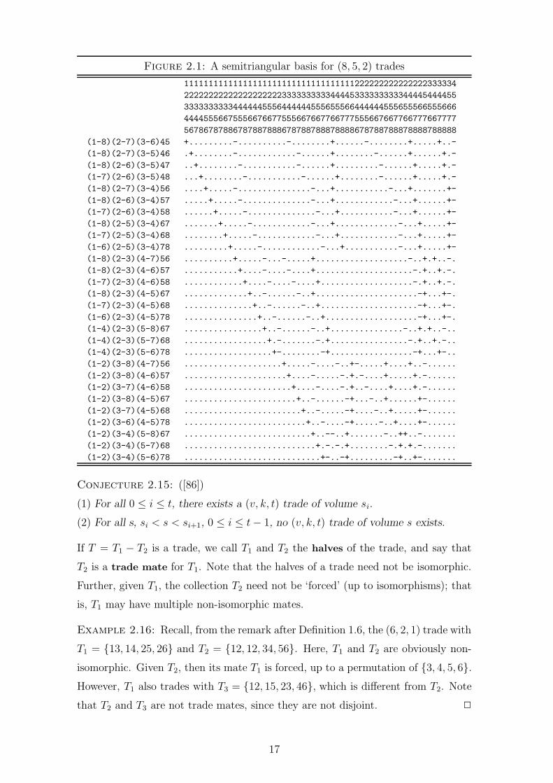
Figure 2.1: A semitriangular basis for (8, 5, 2) trades
11111111111111111111111111111111111222222222222222333334
22222222222222222222333333333344445333333333344445444455
33333333334444445556444444555655566444444555655566555666
44445556675556676677555667667766777555667667766777667777
56786787886787887888678788788878888678788788878888788888
(1-8)(2-7)(3-6)45 +.........-..........-........+......-........+.....+..-
(1-8)(2-7)(3-5)46 .+........-............-......+........-......+......+.-
(1-8)(2-6)(3-5)47 ..+........-...........-......+.........-......+.....+.-
(1-7)(2-6)(3-5)48 ...+........-...........-......+........-......+.....+.-
(1-8)(2-7)(3-4)56 ....+.....-...............-...+...........-...+.......+-
(1-8)(2-6)(3-4)57 .....+.....-..............-...+............-...+......+-
(1-7)(2-6)(3-4)58 ......+.....-..............-...+...........-...+......+-
(1-8)(2-5)(3-4)67 .......+.....-............-...+.............-...+.....+-
(1-7)(2-5)(3-4)68 ........+.....-............-...+............-...+.....+-
(1-6)(2-5)(3-4)78 .........+.....-............-...+...........-...+.....+-
(1-8)(2-3)(4-7)56 ..........+.....-...-.....+...................-..+.+..-.
(1-8)(2-3)(4-6)57 ...........+....-....-....+....................-.+..+.-.
(1-7)(2-3)(4-6)58 ............+....-....-....+...................-.+..+.-.
(1-8)(2-3)(4-5)67 .............+..-......-..+.....................-+...+-.
(1-7)(2-3)(4-5)68 ..............+..-......-..+....................-+...+-.
(1-6)(2-3)(4-5)78 ...............+..-......-..+...................-+...+-.
(1-4)(2-3)(5-8)67 ................+..-......-..+...............-..+.+..-..
(1-4)(2-3)(5-7)68 .................+.-.......-.+................-.+..+.-..
(1-4)(2-3)(5-6)78 ..................+-........-+.................-+...+-..
(1-2)(3-8)(4-7)56 ....................+.....-....-..+-.....+....+..-......
(1-2)(3-8)(4-6)57 .....................+....-.....-.+.-....+.....+.-......
(1-2)(3-7)(4-6)58 ......................+....-....-.+..-....+....+.-......
(1-2)(3-8)(4-5)67 .......................+..-......-+...-..+......+-......
(1-2)(3-7)(4-5)68 ........................+..-.....-+....-..+.....+-......
(1-2)(3-6)(4-5)78 .........................+..-....-+.....-..+....+-......
(1-2)(3-4)(5-8)67 ..........................+..--..+.......-..++..-.......
(1-2)(3-4)(5-7)68 ...........................+.-.-.+........-.+.+.-.......
(1-2)(3-4)(5-6)78 ............................+-..-+.........-+..+-.......
Conjecture 2.15: ([86])
(1) For all 0 ≤ i ≤ t, there exists a (v, k, t) trade of volume si.
(2) For all s, si < s < si+1, 0 ≤ i ≤ t − 1, no (v, k, t) trade of volume s exists.
If T = T1 − T2 is a trade, we call T1 and T2 the halves of the trade, and say that
T2 is a trade mate for T1. Note that the halves of a trade need not be isomorphic.
Further, given T1, the collection T2 need not be ‘forced’ (up to isomorphisms); that
is, T1 may have multiple non-isomorphic mates.
Example 2.16: Recall, from the remark after Definition 1.6, the (6, 2, 1) trade with
T1 = {13, 14, 25, 26} and T2 = {12, 12, 34, 56}. Here, T1 and T2 are obviously non-
isomorphic. Given T2, then its mate T1 is forced, up to a permutation of {3, 4, 5, 6}.
However, T1 also trades with T3 = {12, 15, 23, 46}, which is different from T2. Note
that T2 and T3 are not trade mates, since they are not disjoint. 2
17
2.3 Defining sets
The concept of a defining set of a design was formally introduced in the series of
articles [47, 46, 45], although an isolated earlier result concerning the 5-(24, 8, 1)
design from the large Mathieu group M24 was given in [16]. Two recent surveys are
[110, 111]. Appendix B should be consulted for results regarding specific designs.
Throughout the thesis, we use µ to stand for |dsD|/b, the proportion of the blocks
of a design in a smallest defining set.
The first thing to note is that the property of having a unique completion is invariant
under permutations. This observation yields the following results.
Lemma 2.17: ([47]) Suppose that S is a defining set of D and ρ ∈ aut(D). Then
ρS is a defining set of D, and aut(S) ⊆ aut(D). 2
Theorem 2.18: ([45]) Suppose that S is a defining set of D. Then
aut(D) = {ρ : ρS ⊆ D, ρ ∈ Sv}. 2
Definition 2.19: ([45]) A permutation ρ ∈ Sv of the form (ij), i 6= j ∈ V, is called
a single transposition. A single-transposition-free (STF) design D is one whose
automorphism group does not contain any single transpositions.
It was established in [47, 45, 93] that t-(v, k, 1) and symmetric 2-(v, k, λ) designs are
STF. The following results have been obtained for STF designs.
Theorem 2.20: ([47, 45]) Let D be an STF t-(v, k, λ) design, and suppose that S
is a dD, with |S| = s. Then:
(1) f(S) ≥ v − 1;
(2) if points i 6= j each appear once only in S, they appear in separate blocks;
(3) s ≥ 2(v − 1)/(k∗ + 1), where k∗ = min(k, v − k);
(4) 2s−1 ≥ max(k, v − k);
(5)(
s
2
)
+ s + 1 ≥ v, if λ = 1. 2
Theorem 2.21: ([45]) Let S be a defining set of a simple STF design D, and denote
the number of configurations of blocks of D isomorphic to S by n(S : D). Then
n(S : D) =|aut(D)|
|aut(S)|. 2
Theorem 2.22: ([45]) Let D be a transversal of the t-(v, k, λ) designs, all of which
are simple and STF. Let D ∈ D, and suppose that S is a configuration on v or v− 1
points such that:
18

(1) D has precisely |aut(D)|/|aut(S)| subsets of blocks isomorphic to S;
(2) any design containing a subset of blocks isomorphic to S is isomorphic to D.
Then S is a defining set for some design isomorphic to D. 2
These results have been used as the basis for algorithms to find and catalogue
(smallest) defining sets, or to improve the efficiency of such algorithms [48, 53, 51,
52, 17]. In [37] the concept of an automorphism group of a set of blocks B was
extended to include those points in V but not in F (B). This allowed analogues of
Theorem 2.21 and 2.22 to be proved for all simple designs.
The bounds of Theorem 2.20 are generally weak, and only apply to STF designs.
Various other bounds, including upper bounds, have been proved.
Theorem 2.23: ([44]) Suppose that D is a cyclic symmetric 2-(v, k, λ) design, and
contains a trade of volume m. If m - v, then |dsD| ≥ v/m. 2
Theorem 2.24: ([44]) Suppose that D is a t-(v, k, 1) design, with b blocks. Then
the size of a minimal defining set of D satisfies
|dmD| ≤ b −2(
v
t−1
)
(
k
t−1
)
+ 1. 2
Lemma 2.25: ([44]) Suppose that D = (V,B) is a t-(v, t + 1, λ) design, then
|dsD| ≤ λ0 − λ1 = b − r.
Proof: Let S ⊆ B consist of all blocks of D that do not contain some point, say
0, so that |S| = b − r. Then any t-subset of V that does not appear in λ blocks of
S must appear an appropriate number of times as a block with 0. So S completes
uniquely. 2
Various asymptotic results regarding smallest defining sets of infinite families have
been proved, or conjectured.
Theorem 2.26: ([38]) Let Dd be the cyclic Hadamard design arising from the
points and hyperplanes of PG(d, 2), d ≥ 2, and let µd be the proportion of blocks
in a smallest defining set. Then µd → 1 as d → ∞. 2
Theorem 2.27: ([38]) Let D∗d be the block-residual design of Dd, d ≥ 3, and let µ∗
d
be the proportion of blocks in a smallest defining set. Then µ∗d → 1 as d → ∞. 2
Theorem 2.28: ([38]) Let Ld be the STS(2d+1 − 1) obtained from the points and
lines of PG(d, 2), d ≥ 2, and let ηd be the proportion of blocks in a smallest defining
19

set. Then the sequence {ηd}∞d=2 is non-decreasing and bounded above by 1; thus, it
converges. 2
Remark: Although a family of minimal defining sets where |dmD|/b → 1 is known
(see Theorem 2.29 below), the limiting value of ηd is not known. It is known that
η3 = 16/35 [93].
If p ≡ 1 (mod 4) is a prime power, then a Hadamard 2-(2p + 1, p, 12(p − 1)) design
can be constructed using quadratic residues in GF (p). Similarly, if p ≡ 3 (mod 4),
then a Hadamard 2-(p, 12(p − 1), 1
4(p − 3)) design can be constructed. It has been
conjectured that a particular set of p (resp. 12(p− 1)) blocks from these designs is a
defining set; so, in particular, µ < 1/2 for both families. This conjecture has been
proved for p = 5, 7, 9, 11, 13, 17, 19, 23, 25, 27, 29, 43, 47, 59 and 67 [105, 104, 80].
Remark: These conjectured families of designs with µ < 1/2 should be contrasted
with that of Theorem 2.26, where µ → 1.
Using particular sets of hyperplanes in projective and affine geometries, two infinite
families of minimal defining sets were described in [31, 32]. Note that in both these
cases |dmD|/b, the proportion of blocks in the minimal defining set, tends to 1 as
d → ∞.
Theorem 2.29: ([31]) Let D be the STS(2d+1 − 1) obtained from the points and
lines of PG(d, 2), d ≥ 2. Then D has a minimal defining set of size
1
6((2d+1 − 1)(2d+1 − 2) − 3d+1 + 3). 2
Theorem 2.30: ([32]) Let D be the STS(3d) obtained from the points and lines
of AG(d, 3), d ≥ 2. Then D has a minimal defining set of size
1
6(3d(3d − 1) − 7d + 1). 2
Since the number of indecomposable designs is finite, the majority of t-(v, k, λ)
designs are decomposable and the following result is helpful. Note that, since a
design may have more than one decomposition, for the best lower bound we should
take the maximum over all decompositions. We investigate this bound in more
detail in Chapter 9.
Lemma 2.31: ([47]) Suppose that the design D has a decomposition into the designs
Di, i = 1, . . . , m. Then
|dsD| ≥m
∑
i=1
|dsDi|. 2
20

The relationships between a design and its complement, its extensions, and its
derived or residual designs yield results concerning the sizes of smallest defining
sets of all these designs. Many of the specific results quoted in Appendix B were
obtained using these connections.
Lemma 2.32: ([47]) If S is a defining set of D, then the complement of S is a
defining set of the complement of D. 2
Lemma 2.33: ([95]) If a t-design D has exactly one extension E to a (t+1)-design,
then any defining set of D, when extended, is a defining set of E. Hence |dsE| ≤
|dsD|. 2
Lemma 2.34: ([95]) If D is a t-design, t even, and E is an extension by comple-
mentation of D, then |dsE| ≥ |dsD|. 2
Theorem 2.35: ([47]) If D is a 3-(2n + 2, n + 1, λ) design, where all such designs
are necessarily obtainable by extension by complementation, and Dx its restriction
on x, then |dsD| = |dsDx|. 2
Lemma 2.36: ([95]) If D1 and D2 are t-designs, t even, with a common extension
by complementation E, then |dsD1| = |dsD2|. Further, D1 and D2 have the same
number of smallest defining sets. 2
Lemma 2.37: ([95]) Suppose D is a t-design, t even, and the only extension of
D is the extension by complementation E. If D has precisely n smallest defining
sets, of size q, and E has precisely m smallest defining sets, then n ≤ m ≤ n2q.
The upper bound is attained if all designs with the same parameters as E are self-
complementary. 2
Lemma 2.38: ([93]) Let D = (V,B) be a t-(v, k, λ) design, and suppose that S1 ⊆ B
completes to precisely m other t-(v, k, λ) designs D1, . . . , Dm. Let S2 ⊆ B \ S1 be
such that S2 6⊆ Bi, i = 1, . . . , m. Then S1 ∪ S2 is a defining set of D. 2
The previous lemma is a convenient source of ‘small’ defining sets, if a suitable set
S1 can be found. In particular, it can be used to prove a series of results regarding
defining sets of residual designs [93].
Let M be the collection of all minimal defining sets of a design D. Given the
various results and bounds on smallest/minimal defining sets, it is of interest to
consider specm(D) = {|M | : M ∈ M}, the defining spectrum of D, see [44]. A
defining spectrum specm(D) contains a hole if there exist l < m < n such that
21

l, n ∈ specm(D) and m 6∈ specm(D). If D is the STS(15) constructed from the
points and lines of PG(3, 2), then it was shown in [39], using [93, 31, 44], that
specm(D) = {16, 17, 18, 19, 20, 21, 22}. We revisit the defining spectrum problem in
Chapter 11, and obtain many new results.
In this thesis we consider defining sets of designs consisting of sets of blocks from the
design; that is, blockwise defining sets. We do not consider defining sets containing
incomplete blocks; that is, pointwise defining sets [17, 20, 19]. Nor do we consider
defining sets for large sets or overlarge sets [17, 22, 82].
22

Chapter 3
General trades
Suppose that T = T1 − T2 is a (v, k, t) trade. Recall that not all elements of V need
appear in a block of T. If, however, f(T ) = v then we introduce a new notation,
and refer to T as a [v, k, t] trade. Where we do not know, or have no interest in,
the value of v, we speak of a (k, t) trade instead of a [v, k, t] trade.
An obvious question to ask is, given parameters v, k and t, for which volumes does
there exist a [v, k, t] trade or a (k, t) trade? Accordingly, we make the following
definitions.
Definition 3.1: The spectrum of all [v, k, t] trades is
S[v, k, t] = {m(T ) : T is a [v, k, t] trade} ∪ {0}.
We also define the spectra
S(k, t) =⋃
v
S[v, k, t] and S(t) =⋃
k
S(k, t).
Note that the void trade is a [0, k, t] trade; we have defined 0 ∈ S[v, k, t] for nota-
tional convenience. Clearly, S[v, k, t] ⊆ S(k, t) ⊆ S(t). We do not formally define
the spectrum of (v, k, t) trades, S(v, k, t), since we do not study this herein.
Example 3.2: Combining results from [7, 67, 86], it is known that S(1) = {0, 2,
3, 4, . . .}, S(2) = {0, 4, 6, 7, 8, . . .} and S(3) = {0, 8, 12, 14, 15, 16, . . .} ∪ X, where
X = ∅ or {13}. 2
In this chapter we are mainly interested in [v, k, t] and (k, t) trades. We study
their spectra and structure, using both theoretical techniques and computer-based
searches. We prove Conjecture 2.15(1) and partially characterise the foundations of
trades having volume si. We also prove, as a special case of Conjecture 2.15(2), that
2t + 2t−1 + 1 /∈ S(t + 1, t), for t ≥ 3. We raise a number of conjectures, including
an extended version of Conjecture 2.15. The spectra S[v, k, 1] and S[v, 3, 2] are
completely determined, and a variety of structural theorems are proved.
23
We consider general trades in this chapter, deferring to the next chapter our study
of Steiner trades. We do not address the spectra of simple trades directly in these
chapters, but note that many of our constructions can be applied to this problem.
In passing, we also note that a simple [v, k, t] trade can have volume at most(
v
k
)
/2,
and that constructing a simple [v, k, t] trade of this volume is equivalent to halving
the full design [60].
The work reported in Sections 3.1–3.7 of this chapter has been published in [42, 43].
3.1 A proof of Conjecture 2.15(1)
To illustrate one of our main techniques, we provide, in Theorem 3.4, a proof of
Conjecture 2.15(1). (This result is also proved implicitly later in the chapter.)
When adding basic trades, we show how we can manipulate the exact form of these
trades to control the number of cancellations and hence the resulting volume. Later
in this chapter, we also show how this allows us to achieve a range of foundations.
All the trades we construct in this section are simple.
Recall, from Lemma 2.10, that we can add trades. If, in this lemma, F (T )∩F (R) =
∅, then m(T + R) = m(T ) + m(R) and f(T + R) = f(T ) + f(R). Obviously, if we
take c copies of a [v, k, t] trade of volume m, we obtain a [v, k, t] trade of volume
cm. When adding different trades, we have to consider the possibility of blocks
cancelling.
Lemma 3.3: Suppose T a = T a1 − T a
2 and T b = T b1 − T b
2 are (k, t) trades. Then
T = T a + T b = T a1 + T b
1 − T a2 − T b
2 is a (k, t) trade of volume
m(T a) + m(T b) − |T a1 ∩ T b
2 | − |T a2 ∩ T b
1 |.
Proof: The volume of T equals m(T a) + m(T b) minus the number of blocks in
T a1 ∩ T b
2 and T a2 ∩ T b
1 . 2
Theorem 3.4: For all 0 ≤ i ≤ t, there exists a (k, t) trade of volume si.
Proof: Let T and R be basic (k, t) trades of the form
T = T1 − T2 = S0(S1 − S2)(S3 − S4) . . . (S2t+1 − S2t+2),
R = R1 − R2 = −S0(S1 − S2) . . .
. . . (S2t−2i−1 − S2t−2i)(S2t−2i+1 − S2t−2i+2) . . . (S2t+1 − S2t+2),
where 0 ≤ i ≤ t, and Sj is chosen so that Sj ∩ Sl = ∅ for j = 2t − 2i + 1, 2t − 2i +
3, . . . , 2t + 1 and l = 0, 1, . . . , 2t + 2.
24

That T +R is a (k, t) trade follows from Lemma 2.10. It remains to find m(T +R).
There are two cases to consider, i = t and i < t, depending on whether 2t−i is odd
or even. When i = t, the only block common to T and R is S0S2 · · ·S2t+2. This
block is in T1 ∩ R2 or T2 ∩ R1, hence m(T + R) = m(T ) + m(R) − 1 = 2t+1 − 1.
When 0 ≤ i ≤ t − 1, |T1 ∩ R2| = |T2 ∩ R1| = 2t−i−1. Therefore,
m(T + R) = m(T ) + m(R) − 2.2t−i−1 = 2t+1 − 2t−i,
as required. 2
Example 3.5: Let T = (1−2)(3−4)(5−6), and choose R = −(1−2)(3−4)(5−6).
Then
T + R = +135 + 236 + 245 + 136 + 145 + 235
−136 − 145 − 235 − 135 − 236 − 245
is an (8, 3, 2) trade with m(T + R) = 6 and f(T + R) = 8. 2
Corollary 3.6: For s ≥ (2t − 1)2t there exists a (v, k, t) trade of volume s.
Proof: Let 0 ≤ a ≤ 2t −1. Then a has a unique binary representation∑t
i=1 ai2t−i,
where ai ∈ {0, 1}. Therefore, if s∗ = t.2t+1 − a, where 0 ≤ a ≤ 2t − 1, then
s∗ =
t∑
i=1
aisi +
t∑
i=1
(1 − ai)2t+1.
Any integer s > (2t − 1)2t can be written in the form s = b.2t + s∗, where s∗ =
t.2t+1 − a, with 0 ≤ a ≤ 2t − 1, and b ≥ 0. Using disjoint foundations, choose b
basic trades, for each ai = 1 a trade of volume si, and for each ai = 0 two trades
of volume 2t (or a trade of volume 2t+1 as in [86], if a smaller foundation size is
required). Now use Lemma 2.10 to construct a trade of volume s as required.
For s = (2t − 1)2t, choose (2t − 1) basic trades on disjoint foundations, and use
Lemma 2.10 to construct the required trade. 2
Remark: Note that (2t−1)2t = 2(t−1)2t +2t, and so a trade of this volume can be
constructed by adding a basic trade and t− 1 pairs of basic trades. By introducing
cancellations between the members of each pair, it is possible to reduce the lower
bound to 2(t − 1)2t + 2.
3.2 Preliminaries
In this section we present some results and constructions which we will require later
in the chapter. Some of these are new, and some are drawn from the literature
25

but have been recast in terms of [v, k, t] trades, in order to make the foundations
explicit.
Notation: For a collection A of l-subsets and an element x /∈ F (A), xA denotes
the collection of (l + 1)-subsets formed by adjoining x to each of the l-subsets in A.
Lemma 3.7: If m ∈ S[v, k, t], then m ∈ S[v + 1, k + 1, t].
Proof: Let T = T1 − T2 be a [v, k, t] trade of volume m, and choose x /∈ F (T ).
Then xT1 − xT2 is easily seen to be a [v + 1, k + 1, t] trade of volume m, using
Lemma 2.6 for the t-subsets containing x. 2
It follows that S(k, t) ⊆ S(k + i, t) for all i > 0. So, to prove that a (k, t) trade of
volume m exists for all k > t, it suffices to prove the case k = t + 1.
Example 3.8: Consider the (Steiner) trade T of Example 2.7, and choose x 6∈
F (T ). Then a (non-Steiner simple) [7, 4, 2] trade is given by +135x+146x+236x+
245x − 136x − 145x − 235x − 246x. 2
Lemma 3.9: Suppose T a and T b are [va, k, t] and [vb, k, t] trades of volumes ma and
mb respectively. Then ma + mb ∈ S[va + vb − i, k, t] for all 0 ≤ i ≤ k − 1.
Proof: Relabel F (T a) and F (T b) so that |F (T a) ∩ F (T b)| = i. Then T a + T b is a
[va +vb − i, k, t] trade. Since i < k, T a and T b cannot contain any block in common,
so m(T a + T b) = ma + mb. 2
It is a consequence of this result that S(k, t) is closed under addition. Thus, when
investigating S(k, t) or S(t), we need only find a contiguous range of 2t volumes for
which trades exist, since we can then add basic trades to obtain all larger volumes.
Lemma 3.10: Suppose T a = T a1 − T a
2 and T b = T b1 − T b
2 are [va, k, t] and [vb, k, t]
trades of volumes ma and mb respectively, such that F (T b) ⊆ F (T a) and T a1 ∩T b
2 =
T a2 ∩ T b
1 = ∅. Then ma + cmb ∈ S[va + i, k, t] for all c > 0 and 0 ≤ i ≤ cvb.
Proof: Simply add c copies of T b to T a, relabelling the foundations of the T b as
necessary to yield the required overall foundation. 2
Lemma 3.11: Suppose T a = T a1 − T a
2 and T b = T b1 − T b
2 are [va, k, t] and [vb, k, t]
trades of volumes ma and mb respectively, and that one of T b1 , T b
2 , T a1 or T a
2 contains
some block once only. Then ma + mb − 1 ∈ S[va + vb − k, k, t].
Proof: Suppose, without loss of generality, that block B occurs in T a1 exactly once.
Relabel the elements of any block C of T b2 so that C = B and relabel the elements
26

of F (T b) \B so that F (T a)∩ (F (T b) \B) = ∅. Now B is the only block common to
T a and T b, and hence m(T a + T b) = ma + mb − 1. 2
Remark: Since basic trades are simple and always exist, and since 2t and 2t+1 − 1
are coprime, this result implies that the complement of S(k, t) is finite – although
it does not give a bound as strong as that of Corollary 3.6.
Lemma 3.12: ([86]) If m ∈ S[v, k, t] then 2m ∈ S[v + 2, k + 1, t + 1].
Proof: Let T = T1 − T2 be a [v, k, t] trade of volume m, and choose x, y /∈ F (T )
with x 6= y. Then (xT1 ∪ yT2)− (yT1 ∪ xT2) is a [v + 2, k + 1, t + 1] trade of volume
2m. 2
Remark: Lemmas 3.11 and 3.12 can be used to provide an alternative proof of
Theorem 3.4. All the even si can be obtained by inducting on t, while st can be
obtained using two basic trades and Lemma 3.11.
Definition 3.13: Suppose A is a collection of k-subsets and x ∈ F (A). Then
Rx(A) = {a \ {x} : a ∈ A, x ∈ a} is the restriction on x of A. We say that
rx(A) = |Rx(A)| is the multiplicity of x in A. We call Lx(A) = {a : a ∈ A, x 6∈ a}
the leave of x in A.
Suppose that T = T1 − T2 is a (k, t) trade of volume m and that x ∈ F (T ). Note
that Lemma 2.6 implies that rx(T1) = rx(T2); so we define rx(T ) = rx(T1), and
use rx when no confusion arises. It was shown in [67] that Rx(T1) − Rx(T2) is a
(k − 1, t − 1) trade of volume rx(T1) and that Lx(T1) − Lx(T2) is a (k, t − 1) trade
of volume m − rx.
3.3 General results regarding foundations
In this section we fully determine the possible foundation sizes of trades of volume
r2t, r > 0. We also investigate when S[v, k, t] contains si. We start by giving an
inequality relating the foundation size and volume of a trade.
Lemma 3.14: Suppose that T = T1 − T2 is a [v, k, t] trade of volume m. Then
rx(T ) ≥ 2t−1 for all x ∈ F (T ), and so v2t−1 ≤ mk.
Proof: For t = 1, rx(T ) ≥ 1, by definition. For t > 1, Rx(T1) − Rx(T2) is a non-
void (k − 1, t − 1) trade, and so must have volume at least 2t−1. Thus rx(T ) ≥ 2t−1
for all x ∈ F (T ), and the result follows. 2
27

Recall that v ≥ k+t+1 in a non-void [v, k, t] trade. We now show that this, together
with Lemma 3.14, yields necessary and sufficient conditions for the existence of
[v, k, t] trades of volume r2t, r > 0. Trades of these volumes can be constructed
by adding r (non-cancelling) basic trades. We first characterise the foundations of
basic trades.
Lemma 3.15: A [v, k, t] trade of volume 2t exists if and only if k + t + 1 ≤ v ≤ 2k.
Proof: In Theorem 2.8,
t+1∑
i=1
|S2i| =
t+1∑
i=1
|S2i−1| = k − |S0|.
Thus,
f(T ) = 2(k − |S0|) + |S0| = 2k − |S0|.
Now 0 ≤ |S0| ≤ k − (t + 1) and we can always choose |S0| to be any value in this
range, so the result follows. 2
Theorem 3.16: For r > 0, there exists a [v, k, t] trade of volume r2t if and only if
k + t + 1 ≤ v ≤ 2rk.
Proof: That k + t + 1 ≤ v ≤ 2rk is necessary follows from f(T ) ≥ k + t + 1 and
Lemma 3.14. For k + t + 1 ≤ v ≤ 2k, take r copies of a basic trade with foundation
v, which exists by Lemma 3.15. For 2k < v ≤ 2rk, apply Lemma 3.10 with T a = T b
both basic trades of foundation 2k. 2
The following result shows that v ≥ k + t + 1 and Lemma 3.14 are not sufficient
for existence, in general. In particular, as st = 2t+1 − 1 is odd, it shows that
[2t + 2, t + 1, t] trades of volume st do not exist. Note that this result, along with
Theorem 3.16, also shows that both S[2t+2, t+1, t] and its complement are infinite.
Theorem 3.17: Let T be a [2t + 2, t + 1, t] trade. Then m(T ) is even.
Proof: T is also a (2t+2, t+1, t) trade and thus we can assume that T =∑r
i=1 T i,
for some r > 0, where the T i are (2t + 2, t + 1, t) basic trades (not necessarily
distinct). If m(T ) = r2t there is nothing to prove. If m(T ) < r2t, then there must
exist T a = T a1 − T a
2 and T b = T b1 − T b
2 , 1 ≤ a < b ≤ r, such that either T a1 ∩ T b
2 6= ∅
or T b1 ∩ T a
2 6= ∅.
Since v = k + t + 1 = 2t + 2, in Theorem 2.8 S0 = ∅ and all the Si, i 6= 0, are
singleton sets. So we can assume, without loss of generality, that T a = (1 − 2)(3 −
4) · · · ((2t + 1) − (2t + 2)) and that B = {1, 3, . . . , 2t + 1} ∈ T a1 ∩ T b
2 . Since B ∈ T b2 ,
28

we can write T b in the form −(1 − σ(2))(3 − σ(4)) · · · ((2t + 1) − σ(2t + 2)), where
σ is a permutation of {2, 4, . . . , 2t + 2}.
Thus the block B∗ = {2, 4, . . . , 2t + 2} must be in both T a and T b. If t is even, then
B∗ ∈ T a2 and B∗ ∈ T b
1 , while if t is odd, then B∗ ∈ T a1 and B∗ ∈ T b
2 . In either case,
both B and B∗ cancel in T a + T b. That is, blocks cancel in pairs, and the result
follows. 2
We now investigate trades with volume si. For a [vi, k, t] trade of volume si, 1 ≤
i ≤ t, since vi ≥ k + t + 1 and by Lemma 3.14, we must have k + t + 1 ≤ vi ≤
sik/2t−1 = 4k−k/2i−1. Our first construction shows when the minimum foundation
can be achieved.
Lemma 3.18: For 1 ≤ i ≤ t, si ∈ S[k + t + 1, k, t] if and only if (k, i) 6= (t + 1, t).
Proof: Given Theorem 3.17, since st is odd, we need only demonstrate existence.
For volume si, 1 ≤ i ≤ t − 1, and k ≥ t + 1, consider the two [k + t + 1, k, t] basic
trades
S0(1 − 2)(3 − 4)(5 − 6) · · · ((2t+1) − (2t+2)),
(−1i)S0(1 − (2i+4))(2− 3) · · · ((2i+2) − (2i+3))
((2i+5) − (2i+6)) · · · ((2t+1)− (2t+2)),
where S0 is a set of k− t−1 elements disjoint from {1, . . . , 2t+2}. These trades have
the same foundation, and when summed they cancel in the 2t−i−1 blocks containing
S013 · · · (2i+3) and the 2t−i−1 blocks containing S024 · · · (2i+4). So the sum is a
[k + t + 1, k, t] trade of volume 2.2t − 2.2t−i−1 = 2t+1 − 2t−i = si.
For volume st and k ≥ t + 2, consider the two [k + t + 1, k, t] basic trades
S00(1 − 2)(3 − 4)(5 − 6) · · · ((2t+1)− (2t+2)),
−S01(3 − 2)(5 − 4)(7 − 6) · · · ((2t+1)− 2t)(0 − (2t+2)),
where S0 is a set of k − t − 2 elements disjoint from {0, . . . , 2t+2}. These trades
have the same foundation, and when summed the block S0013 · · · (2t+1) cancels. 2
Recall that S0 is called the tail of a basic trade. If T = T1 − T2 is a basic trade,
then any element of F (T ) not in the tail appears in exactly 2t−1 blocks in each of
T1 and T2. In the constructions that follow we add two basic trades T a = T a1 − T a
2
and T b = T b1 − T b
2 with F (T a) 6= F (T b) and cancel less than 2t−1 blocks from each
of T a1 , T a
2 , T b1 and T b
2 . So F (T a + T b) will always equal F (T a) ∪ F (T b).
We now consider the volume st case for vi ≥ k + t + 2.
29

Lemma 3.19: For all k + t + 2 ≤ v ≤ 3k, st ∈ S[v, k, t].
Proof: For k + t + 2 ≤ v ≤ k + 2t + 2 consider the two basic trades
S0(1 − 2)(3 − 4)(5 − 6) · · · ((2t+1) − (2t+2)),
−S0(1 − (2t+3))(3 − 2)(5 − 4) · · · ((2t+1)− 2t),
where S0 is a set of k − t − 1 elements disjoint from {1, . . . , 2t + 3}. When added,
these trades cancel in the single block S013 · · · (2t + 1), and yield a [k + t + 2, k, t]
trade of volume st.
If we now replace 2 in the second trade by the new element 2t + 4, we obtain a
[k + t + 3, k, t] trade. We can continue replacing the even elements in the second
trade in this manner, obtaining all foundations up to k + 2t + 2.
For k + 2t + 2 ≤ v ≤ 3k, the result follows directly from Lemmas 3.15 and 3.11. 2
We now consider the si, 1 ≤ i ≤ t − 1, for vi ≥ k + t + 2.
Lemma 3.20: For all 1 ≤ i ≤ t − 1 and k + t + 2 ≤ v ≤ 3k − (t − i), si ∈ S[v, k, t].
Proof: Consider the two basic trades
S0(S1 − S2)(S3 − S4) · · · (S2t+1 − S2t+2),
−S0(S1 − S2) · · · (S2(t−i)−1 − S2(t−i))(S2(t−i)+1 − S2(t−i)+2) · · · (S2t+1 − S2t+2),
These cancel in the 2t−i blocks containing S0S2(t−i)+1S2(t−i)+3 · · ·S2t+1, yielding a
(k, t) trade of the required volume. We will achieve the required range of foundations
by manipulating the Sy.
(1) 2k +1+ i ≤ v ≤ 3k− (t− i): Suppose that |S2t+1| = |S2t+2| = |S2t+2| = k− t, so
|S0| = 0 and all other Sx and Sy are singletons. Then F (T a+T b) = 3k−(t−i). If we
now reduce |S2t+1|, |S2t+2| and |S2t+2| by one, and increase |S1| and |S2| by one, then
F (T a + T b) = 3k − (t− i)− 1. We can continue reducing |S2t+1|, |S2t+2| and |S2t+2|
and increasing |S1| and |S2| in this manner until |S2t+1| = |S2t+2| = |S2t+2| = 1,
when F (T a + T b) = 2k + 1 + i.
(2) k + t + 2 + i ≤ v ≤ 2k + 1 + i: Suppose that |S0| = k − t − 1, with all other Sx
and Sy being singleton sets. Then F (T a + T b) = k + t + 2 + i. If we now reduce
|S0| by one, and increase |S1| and |S2| by one, F (T a + T b) = k + t + 3 + i. We can
continue in this manner until S0 = ∅, when F (T a + T b) = 2k + 1 + i.
(3) k + t + 2 ≤ v ≤ k + t + 1 + i: Suppose we replace S2(t−i)+2 by S2(t−i)+4. Then
the number of cancellations, and hence the volume, remains unchanged. However,
30

in parts (1) and (2) these sets are singletons, so the foundations decrease by one. So
we obtain the range k + t+2+ i−1 ≤ v ≤ 3k− (t− i+1). In general, for 1 ≤ j ≤ i,
we can replace the j singleton sets S2(t−i)+2, . . . , S2(t−i)+2j by the j singleton sets
S2(t−i)+4, . . . , S2(t−i)+2j+2, to obtain the range k+ t+2+ i− j ≤ v ≤ 3k− (t− i+ j).
When j = i this provides v = k+t+2, and when j = 1 this provides v = k+t+1+i.
Since the j ranges overlap, this provides all the required foundations. 2
The results in this section on trades of volumes si prove the following theorem. We
make a conjecture regarding the remaining possible foundations in Section 3.7.
Theorem 3.21: For all 1 ≤ i ≤ t and k + t + 1 ≤ vi ≤ 3k − (t − i) there exists a
[vi, k, t] trade of volume si, except that no [2t + 2, t + 1, t] trade of volume st exists.
2
3.4 Proof of a special case of Conjecture 2.15(2)
As noted earlier, Conjecture 2.15(2) has been proved for volumes s, s0 < s < s1.
The smallest unsettled volume is thus s1 +1, for t ≥ 3, and we now prove this in the
special case k = t + 1. To do this, we require the following definition and structural
lemma.
Definition 3.22: Let T = T1 −T2 be a (k, t) trade, and suppose that ∅ 6= S1 ⊂ T1
and ∅ 6= S2 ⊂ T2. If S1 − S2 is a (k, t) trade, then it is called a subtrade of T. Note
that, in this case, (T1\S1) − (T2\S2) is also a subtrade of T.
Lemma 3.23: Suppose that T = T1−T2 is a (t+1, t) trade of volume r+2t−1, t > 1
and r > 0, and there exists x ∈ F (T ) with rx(T ) = r. Then T contains a subtrade
of volume 2t or 2t + 2t−1.
Proof: Recall Definition 3.13, and its following remarks. Since Lx(T ) is a (t +
1, t − 1) trade of volume 2t−1, then Lx(T ) is (t − 1)-balanced, but need not be t-
balanced. However, T is t-balanced, so any t-subset in Lx(T2) that is not in Lx(T1)
must occur as a block in Rx(T1), and similarly for the t-subsets in Lx(T1). Call this
set of t-subsets in Rx(T1) (resp. Rx(T2)) S1 (resp. S2). Obviously, S1 ∩ S2 = ∅.
Now Lx(T1) ∪ S1 and Lx(T2) ∪ S2 are t-balanced. We will show that |S1| (= |S2|)
is either 2t−1 or 2t, and that S1 and S2 are (t − 1)-balanced. So (Lx(T1) ∪ xS1) −
(Lx(T2)∪xS2) is a (t+1, t) trade, and the result will follow. By Theorem 2.8, Lx(T )
has one of two forms.
31

(1) Lx(T ) = 0(1− 2)(3− 4) · · · ((2t − 1)− 2t): Any t-subset of Lx(T ) that contains
0 occurs in precisely one block in each of Lx(T1) and Lx(T2), so will not appear in
S1 or S2. Any t-subset of Lx(T ) not containing 0 appears exactly once in Lx(T ), so
appears in one of S1 or S2. There are exactly 2t such t-subsets, so |S1| = |S2| = 2t−1.
Any (t − 1)-subset of these t-subsets must appear in exactly two of them, once in
each of S1 and S2.
(2) Lx(T ) = (12−34)(5−6) · · · ((2t+1)−(2t+2)): Since this has exactly t terms, any
t-subset of Lx(T ) must contain at least one of {1, 2, 3, 4}. The t-subsets containing
12 or 34 are in a single block of both Lx(T1) and Lx(T2), so will not appear in S1 or
S2. Any t-subset of Lx(T ) containing exactly one of {1, 2, 3, 4} appears exactly once
in Lx(T ), so appears in one of S1 or S2. There are exactly 4·2t−1 such t-subsets, so
|S1| = |S2| = 2t. Any (t − 1)-subset, containing one of {1, 2, 3, 4}, of these t-subsets
must appear in exactly two of them, once in each of S1 and S2. Any (t− 1)-subset,
containing none of {1, 2, 3, 4}, of these t-subsets must appear in exactly four of them,
twice in each of S1 and S2. 2
The proof of our result is inductive, with the following result providing our base
case.
Lemma 3.24: 13 6∈ S(4, 3).
Proof: Suppose that T = T1 −T2 is a (4, 3) trade of volume thirteen, and consider
any x ∈ F (T ). Note that rx ≥ 4, by Lemma 3.14, and that rx < 13, since, if x was
in all blocks of T1 and T2, then T1 ∩ T2 6= ∅ since T is 3-balanced. Now Rx(T ) is a
(3, 2) trade and Lx(T ) is a (4, 2) trade. Since S(3, 2) = S(4, 2) = {0, 4, 6, 7, 8, . . .},
then rx = 4, 6, 7 or 9. By Lemma 3.23 and the final remark in Definition 3.22,
rx 6= 9, since 13 − 8, 13 − 12 6∈ S(3).
We now show that rx 6= 4. Suppose that rx = 4, and that x 6= y ∈ F (T ). Now
suppose that x and y do not occur together in a block of T. Since Rx(T ) and Ry(T )
are disjoint (3, 2) trades, the blocks containing x or y are disjoint (4, 2) trades. So
the remaining blocks of T (that is, Ly(Lx(T ))) form a (4, 2) trade, with volume five,
three or two, which is impossible. So any multiplicity four element occurs with every
other element of F (T ) in some block. Now consider Rx(T ). This is a (3, 2) trade
of volume four, which has a unique structure, with foundation six (Theorem 2.8).
But we have just shown that x must occur with every other element of F (T ), so
f(T ) = 6 + 1 = 7, which contradicts f(T ) ≥ k + t + 1 = 8.
32

So rx = 6 or 7. Suppose there are n6 (resp. n7) elements of F (T ) of multiplicity six
(resp. seven). Then 6n6 +7n7 = 13× 4 = 52 has unique solution n6 = n7 = 4. Thus
f(T ) = 8 = 2t + 2, contradicting Theorem 3.17, as the volume is odd. 2
Theorem 3.25: For all t ≥ 3, s1 + 1 = 2t + 2t−1 + 1 /∈ S(t + 1, t).
Proof: We will induct on t, using Lemma 3.24 for the case t = 3. So assume that
T is a (t + 1, t) trade of volume m = 2t + 2t−1 + 1 for some t > 3, and consider any
x ∈ F (T ). Note that rx ≥ 2t−1 and rx < m, as in the proof of Lemma 3.24. Now
Rx(T ) is a (t, t− 1) trade and Lx(T ) is a (t + 1, t− 1) trade, so rx ∈ S(t, t − 1) and
m−rx ∈ S(t+1, t−1). Consequently, rx = 2t−1 or 2t−1+2t−2, with rx = 2t−1+2t−2+1
disallowed by the induction hypothesis and rx = 2t + 1 disallowed by Lemma 3.23.
Suppose that there are a (resp. b) elements in F (T ) of multiplicity 2t−1 (resp. 2t−1 +
2t−2). Thus
a2t−1 + b(2t−1 + 2t−2) = km = (t + 1)(2t + 2t−1 + 1).
This implies that t+1 ≡ 0 (mod 2t−2). That is, 2t−2 | (t+1), which is not possible,
since t ≥ 4. 2
3.5 Solutions of S[v, k, 1] and S[v, 3, 2]
In this section we prove some results on the spectra of trades with particular pa-
rameters. We start with the case t = 1, and show that the necessary conditions
relating v and m quoted so far are sufficient for existence. The following analogue
of Lemma 3.7 facilitates our proof of this.
Lemma 3.26: If m ∈ S[v, k, 1] then, for all 1 ≤ i ≤ m, m ∈ S[v + i, k + 1, 1].
Proof: Let T = T1 − T2 be a [v, k, 1] trade of volume m and let e1, . . . , ei be i
elements not in F (T ). Select i blocks of T1 and i blocks of T2, and adjoin a single
new element to each block, using each of e1, . . . , ei exactly once for the blocks from
T1 and for the blocks from T2. Adjoining the element ei to each of the remaining
m − i blocks of T1 and of T2 gives a [v + i, k + 1, 1] trade of volume m. 2
Theorem 3.27:
S[v, k, 1] =
{m : m ≥ 2, m ≡ 0 (mod 2)} if k = 2, v = 4; (a)
{m : m ≥ 2} if k ≥ 3, k + 2 ≤ v ≤ 2k; (b)
{m : mk ≥ v} if k ≥ 2, v > 2k; (c)
∅ otherwise. (d)
33

Proof: First, recall that k ≥ t + 1 = 2, v ≥ k + t + 1 = k + 2, m ≥ 2t = 2
and v2t−1 = v ≤ mk are necessary. These, with Theorem 3.17, prove (d) and the
necessity of the conditions. It remains to show that these conditions are sufficient.
For (a), the sufficiency follows from Theorem 3.16.
For (b), use Theorem 3.16 for the even volumes. For the odd volumes we will
construct trades of volume three and then invoke Lemma 3.10 to repeatedly add a
suitable trade of volume two. For the [5, 3, 1] and [6, 3, 1] trades of volume three,
take
T 5 = +123 + 245 + 345 − 145 − 234 − 235,
T 6 = +123 + 456 + 456 − 145 − 246 − 356.
Lemma 3.26 now yields [v, k, 1] trades of volume three for all k ≥ 3 and k +2 ≤ v ≤
3k − 3, which includes the required range for v. For the trades of volume two we
use [k + 2, k, 1] trades, with the [5, 3, 1] trade being T 2 = +124 + 135 − 125 − 134
and the others obtained by using Lemma 3.26. If, whenever we use Lemma 3.26,
we always use the smallest possible natural numbers as our new elements, then it
is easy to check that we can repeatedly apply Lemma 3.10 to construct the desired
trades.
For (c), put m = dv/ke. We will consider the cases of volumes m+2r and m+1+2r
(r ≥ 0) separately.
For the volumes m+2r we will use Lemma 3.10 with the [k+2, k, 1] trade of volume
two given by (1 − 3)(2 − 4)56 · · · (k + 2) as our addendum. For the [v, k, 1] trade
T1 − T2 of volume m we define two m × k arrays A and B, the rows of which will
be the blocks of T1 and T2. The positions of A are filled in row-major order by the
elements 1 to v, and the last mk − v positions of the last row of A are filled with
the elements 1 to mk − v. Array B is formed from A by cycling the first column
down by one position: that is, bi,1 = ai−1,1, with b1,1 = am,1.
As an example, when k = 3 and v = 8 then m = 3 and we obtain T1 =
{123, 456, 781} and T2 = {723, 156, 481}, and the trade of volume two is +125 +
345− 145− 235. It is straightforward to see that there is never any conflict between
the trades of volumes two and m, so Lemma 3.10 now gives all the required volumes.
Using Lemma 3.11, we now construct trades with volumes of the form m + 1 + 2r
by adding a basic [k + 2, k, 1] trade to a trade of volume m + 2r. This gives all the
34

required trades, except those having v = 2k + 1, 2k + 2. However, for these values
of v, m = 2r + 4 = (r + 2)2, and these trades exist by Theorem 3.16. 2
We now fully determine S[v, 3, 2]. To do this, we need the following result on Steiner
[v, 3, 2] trades from [11].
Lemma 3.28: ([11]) For all n > 0:
(1) A Steiner [6n, 3, 2] trade of volume 4n + 1 does not exist;
(2) A Steiner [6n + 1, 3, 2] trade of volume 4n + 1 does not exist;
(3) A Steiner [6n + 3, 3, 2] trade of volume 4n + 2 does not exist;
(4) A Steiner [6n + 4, 3, 2] trade of volume 4n + 3 does not exist. 2
To use this result, we will need the following definition and lemma.
Definition 3.29: Suppose that T is a [v, 3, 2] trade of volume m. Then 3m − 2v
is called the excess of T.
Since each element in the foundation of a 2-trade must occur in at least two blocks,
the excess can be thought of as the number of places in the trade ‘in excess’ of those
required to use each element twice.
Lemma 3.30: Suppose that T = T1 − T2 is a [v, 3, 2] trade. If T has an excess of
at most three, then T is Steiner.
Proof: We will assume that T is non-Steiner and prove that the excess is at least
four. We can suppose that the pair 12 occurs in two blocks of T1. Recall that if
x ∈ F (T ) then rx ≥ 2, and note that if B ∈ T1 then the three 2-subsets of B must
occur in separate blocks of T2, else T1 ∩ T2 6= ∅. There are two cases to consider:
without loss of generality, {123, 123} ⊆ T1 or {123, 124} ⊆ T1.
The first of these is easily dealt with by noting that all six of the pairs 12, 13, 23,
12, 13 and 23 must occur in separate blocks of T2, giving an excess of at least six.
For the second case, consider the possible arrangements of the six pairs 12, 13, 23,
12, 14 and 24 in T2. If all six of these are in separate blocks of T2, then the excess is
at least four. If not, then T2 must contain at least one of the blocks 134 or 234. If
T2 contains both these blocks then, to balance pairs, the pair 34 must occur in two
blocks of T1. So suppose that {34a, 34b} ⊆ T1. Then the newly introduced pairs 3a,
4a, 3b and 4b must also occur in blocks of T2. So both 3 and 4 must occur at least
once more in T2, giving an excess of at least four.
35

The only subcase remaining is when T2 contains exactly one of 134 or 234, say 134;
note that the pair 34 must now occur in T1. At this stage, the excess of T2 is three.
Let the pairs 12, 12, 23 and 24 in T2 occur with a, b, c and d respectively. Note that
if {1, 2, 3, 4} ∩ {a, b, c, d} 6= ∅ then the excess in T2 is at least four, and the result
follows. So suppose that {1, 2, 3, 4} ∩ {a, b, c, d} = ∅. Now T is also 1-balanced so
1 (resp. 2) must occur at least once (resp. twice) more in T1. If 1 (resp. 2) occurs
more than once (resp. twice) in T1 then the excess is at least four, and the result
follows. So assume that 1 (resp. 2) occurs exactly once (resp. twice) more in T1 and
that 3 and 4 do not occur again in T1.
Now the newly introduced pairs a1, a2, b1, b2, c2, c3, d2 and d4 in T2 must occur in
T1 also. This forces c = d and c34 ∈ T1, otherwise the excess of T1 is at least four.
So the other sets introduced must be 2ac, 2bc and 1ab. Now the excess is at least
four and the result follows. 2
We are now in a position to prove our result.
Theorem 3.31: There is a [v, 3, 2] trade of volume m if and only if :
6 ≤ v ≤ 6n for m = 4n and n > 0; (a)
6 < v ≤ 6n − 1 for m = 4n + 1 and n > 1; (b)
6 ≤ v ≤ 6n + 2 for m = 4n + 2 and n > 0; (c)
6 < v ≤ 6n + 3 for m = 4n + 3 and n > 0. (d)
Proof: The necessity of the conditions follows from Lemmas 3.30 and 3.28, Lemma
3.14, Theorem 3.17, and v ≥ k+t+1 and m(T ) ≥ 4. Sufficiency for (a) is immediate,
from Theorem 3.16. For the minimal n of (b), (c) and (d), we exhibit example trades
for each possible v.
(b) For the volume nine [v, 3, 2] trades of foundations 7, 8, 9, 10 and 11 use
+124 + 125 + 136 + 167 + 236 + 246 + 257 + 345 + 456
−123 − 126 − 146 − 157 − 245 − 245 − 267 − 346 − 356,
+157 + 168 + 235 + 246 + 278 + 347 + 368 + 458 + 567
−156 − 178 − 234 − 257 − 268 − 358 − 367 − 457 − 468,
+147 + 156 + 238 + 246 + 257 + 357 + 369 + 459 + 468
−146 − 157 − 237 − 248 − 256 − 359 − 368 − 457 − 469,
+134 + 157 + 168 + 235 + 246 + 279 + 28a + 378 + 39a
−135 − 146 − 178 − 234 − 257 − 268 − 29a − 379 − 38a,
+145 + 168 + 179 + 246 + 257 + 28a + 29b + 389 + 3ab
−146 − 157 − 189 − 245 − 268 − 279 − 2ab − 38a − 39b.
36

(c) For the volume six [v, 3, 2] trades of foundations 6, 7 and 8 use
+125 + 134 + 156 + 236 + 246 + 345 − 126 − 135 − 145 − 234 − 256 − 346,
+125 + 345 + 136 + 246 + 147 + 237 − 126 − 346 − 137 − 247 − 145 − 235,
+127 + 347 + 567 + 148 + 258 + 368 − 128 − 348 − 568 − 147 − 257 − 367.
(d) For the volume seven [v, 3, 2] trades of foundations 7, 8 and 9 use
+134 + 157 + 235 + 237 + 246 + 356 + 457 − 135 − 147 − 234 − 236 − 257 − 357 − 456,
+134 + 156 + 235 + 246 + 278 + 358 + 367 − 135 − 146 − 234 − 258 − 267 − 356 − 378,
+156 + 179 + 247 + 258 + 269 + 348 + 357 − 157 − 169 − 248 − 256 − 279 − 347 − 358.
The trades in (b), (c) and (d) can now be used as in Lemma 3.10 to generate all
larger m and v. In all three cases, the [6, 3, 2] basic trade (1 − 4)(2 − 3)(5 − 6) can
be used for T b. 2
3.6 Spectrum investigations
Unlike the (v, k, t) trades, the [v, k, t] trades do not form a Z-module. Nonetheless,
all [v, k, t] trades can be generated as sums of (v, k, t) basic trades. One basis for
the Z-module associated with (v, k, t) trades is the semitriangular basis of smallest
trades described in Section 2.2. The construction of this basis has been implemented
as a computer programme, and used to search for (k, t) and [v, k, t] trades.
These searches were conducted by first nominating values of v, k and t, and generat-
ing the basis. Then, for some fixed i > 1, for each combination of i basic trades from
the basis (with repetitions allowed or not, as desired), all possible sums/differences
of the vectors representing the basis elements were formed. The resulting vectors
represent (v, k, t) trades, and are easily processed to extract volume, foundation
and structural information. This technique proved capable of yielding useful results
concerning the existence of trades up to t = 8.
Theoretically, our technique can also demonstrate non-existence, since if a trade of
a particular volume exists it can be formed by adding some finite number of basic
trades. In practice, however, this exhaustive search is not feasible. Suppose that we
wish to investigate t-trades of a particular volume m, with m = j2t − x for some
j > 1 and 0 ≤ x < 2t. Obviously, we must add at least j basis elements when
37

attempting to construct such a trade. If a comprehensive search using a range of
values for v, k and i ≥ j fails to find any trade of volume m, we regard this as strong
evidence that m 6∈ S(t).
Our results support Conjecture 2.15(2), but suggest that there are also disallowed
volumes in the range above 2t+1. To discuss these results, we start with a generali-
sation of the si.
Definition 3.32: Fix t > 0 and let 0 ≤ l ≤ t and 0 ≤ i ≤ t − l. Define
sli = 3·2t − 2t−l − 2t−l−i.
The sli are those values that can be obtained from 3·2t by subtracting two powers
of 2. The larger of these powers is controlled by l, which is called the level. Note
that when l = 0 then sli = si. The definition of sl
i leads directly to a proof of the
following analogue of Conjecture 2.15(1).
Lemma 3.33: For all 0 ≤ l ≤ t, 0 ≤ i ≤ t − l and k ≥ t + 1 there exists a (k, t)
trade of volume sli.
Proof: We prove the result for k = t + 1, and rely on Lemma 3.7 for all greater
k. Given our proof of Conjecture 2.15(1), we need only prove volumes of the form
3·2t − 2a − 2b, with 0 ≤ b ≤ a ≤ t − 1. Now let
T = (1 − 2)(3 − 4) · · · ((2t+1) − (2t+2)),
T a = −(1 − 2) · · · ((2a−1) − (2a))((2a+1)− (2a+2)) · · · ((2t+1) − (2t+2)),
T b = −(1 − 2) · · · ((2b−1) − (2b))((2b+1) − (2b+2)) · · · ((2t+1) − (2t+2)).
The trades T and T a cancel in the 2a blocks containing (2a+1) · · · (2t+1), and T
and T b cancel in the 2b blocks containing (2b+2) · · · (2t+2). As T a and T b have
no blocks in common, and the two sets of cancelling blocks are disjoint, the result
follows. 2
To characterise the pattern of missing volumes observed, we build on selected sli.
With each of these we associate a set of ‘disallowed’ volumes Dli. We introduce the
parameter t = bt/2c, as the pattern changes for every increase of t by two.
Definition 3.34: Fix t > 0 and, for all 0 ≤ l ≤ t − 1 and 0 ≤ i ≤ t − 2l − 2, let
Dli = {sl
i + a2t−2l−i−1 + b : 0 ≤ a ≤ 2l − 1, 1 ≤ b ≤ 2t−2l−i−1 − 1}.
For all other l and i, let Dli = ∅.
38

Figure 3.1: The sets Ft and Ft
t = 2 4 6 7
t = 3 8 12 1415 t = 4
16 24 28 303132 34 36373839
t = 5
32 48 56 60 626364 68 72 74 76777879
t = 6
Note that the sli and the sets Dl
i are disjoint, with the elements in Dli falling between
sli and sl
i+1. In the pattern of the sli, successive sl
i on the same level are separated
by decreasing powers of two, while moving between levels repeats the last half of
the previous pattern. In the pattern of the sets Dli, when moving from one level to
the next the last half of the previous pattern is repeated, with the difference that
each ‘range’ is split into two by removing the middle value.
Definition 3.35: For t > 0, let
Ft =⋃
l,i
Dli,
Ft = {s : 2t ≤ s < 3·2t − 2t+1−t, s 6∈ Ft}.
It is the sets Ft and Ft that we will use to describe the observed spectra. They are
defined to include only those values up to the highest level that contains non-empty
Dli. Figure 3.1 illustrates these sets for 2 ≤ t ≤ 6. The values are arranged in levels,
to highlight how the pattern for Ft at one level is obtained by ‘halving’ the pattern
at the previous level. The numbered boxes represent the values of Ft (except for
t = 6, where space considerations preclude this), while the boxes containing a filled
square represent values of Ft. Level zero is partitioned by the s0i and D0
i , while in
higher levels there are values in Ft that are not values of any sli (for t = 4, 5, these
values are underlined). Note that some sli are greater than max(Ft).
In an extensive series of searches using values of t ≤ 8, no trade with volume in Ft was
ever constructed. For 1 ≤ t ≤ 6 trades of all volumes in Ft were constructed; in fact,
trades of all volumes in {s : s ≥ 2t}\Ft were found. For t = 7 all volumes in Ft were
constructed, but isolated volumes greater than max(Ft) remained unconstructed.
For t = 8 six volumes in Ft remained unconstructed, and isolated volumes greater
than max(Ft) remained unconstructed. Given the large dimensions in these latter
two cases, the searches were far from being comprehensive.
39

For S(1), S(2) and S(3) the non-existent volumes greater than 2t are precisely
those less than 2t+1 that are not si (except that volume thirteen is undetermined
for S(k, 3) when k > 4). So our results are intriguing, and suggest that there are
disallowed volumes greater than 2t+1 when t > 3.
We cannot, as yet, prove non-existence for any of the Ft that are more than 2t+1.
However, we can prove existence for all other volumes when t = 4. These techniques
can be used for higher values of t, albeit requiring increasing intricacy.
Lemma 3.36: For all k > 4, {s : s ≥ 16, s 6∈ F4} ⊆ S(k, 4).
Proof: We prove the result for k = 5, and rely on Lemma 3.7 for all greater k.
Applying Lemma 3.12 to S(4, 3) = {0, 8, 12, 14, 15, 16, . . .} yields {16, 24, 28, 30, 32,
. . .} ⊆ S(5, 4). Since the basic (5, 4) trade is simple, Lemma 3.11 now gives {31, 39,
43, 45, 47, . . .} ⊆ S(5, 4). This construction provides all volumes in {s : s ≥ 16, s 6∈
F4} except for 37 and 41.
Consider the two sets of three basic trades
(0 − 1)(2 − 3)(4 − 5)(6 − 7)(8 − 9)
−(0 − 1)(2 − 3)(4 − 5)(6 − 7)(8 − 9)
(0 − 0)(2 − 3)(4 − 5)(6 − 7)(8 − 9),
and(0 − 1)(2 − 3)(4 − 5)(6 − 7)(8 − 9)
−(0 − 1)(2 − 3)(4 − 5)(6 − 7)(8 − 9)
(0 − 0)(2 − 3)(4 − 5)(6 − 7)(8 − 9).
When added, the first set of basic trades yields a trade of volume 37, and the second
set yields a trade of volume 41. To see this, simply note that 37 = 48 − 8 − 2 − 1
and 41 = 48− 4− 2− 1, and that, for example, the first pair of basic trades cancel
in 8 blocks. 2
3.7 Conjectures
It is tempting to speculate that S(t) contains all volumes of at least 2t except those
in Ft. However, the evidence in support of this is largely empirical, and extends
only to t = 8; it is possible that for larger values of t a more complicated pattern of
disallowed volumes would emerge. Obviously, S(t) needs to be further investigated.
We do, however, offer the following extended version of Conjecture 2.15.
40
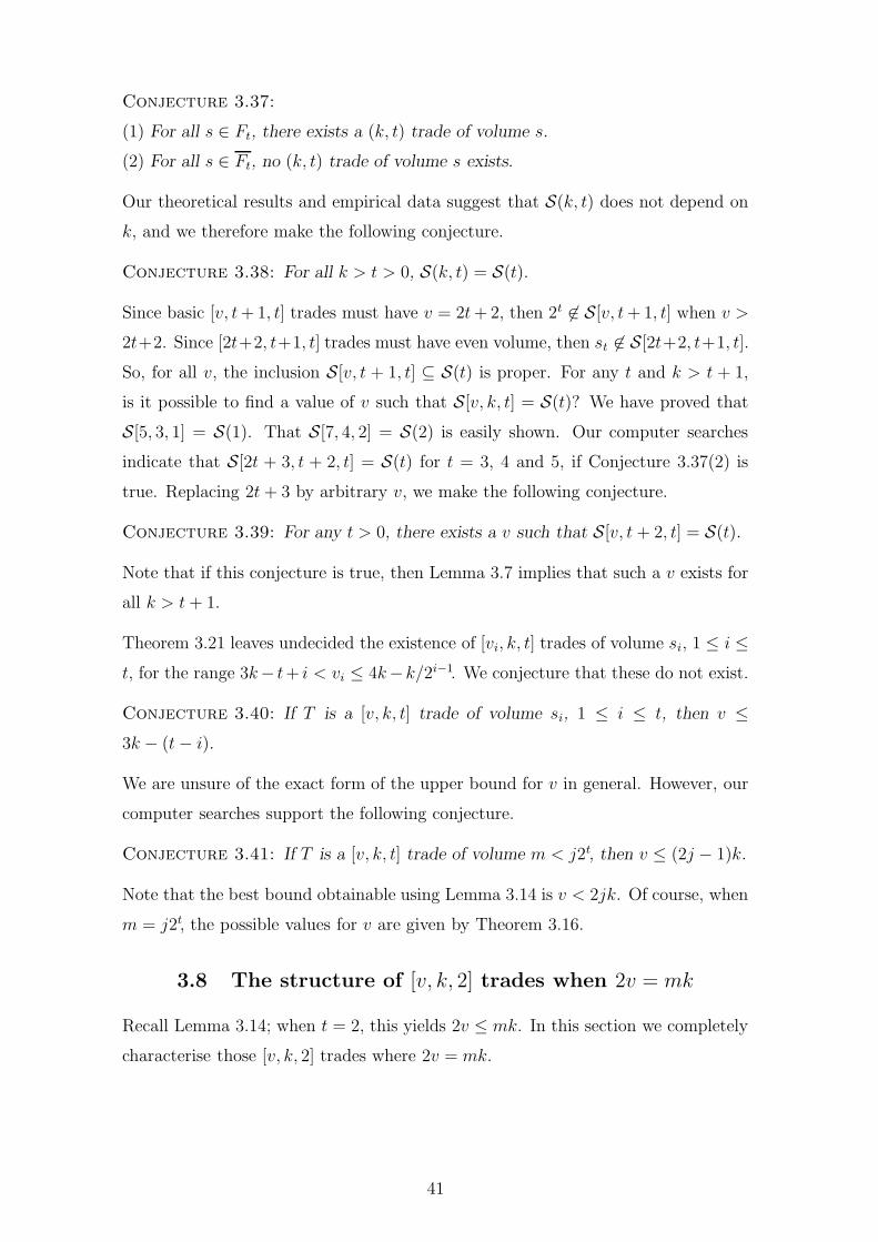
Conjecture 3.37:
(1) For all s ∈ Ft, there exists a (k, t) trade of volume s.
(2) For all s ∈ Ft, no (k, t) trade of volume s exists.
Our theoretical results and empirical data suggest that S(k, t) does not depend on
k, and we therefore make the following conjecture.
Conjecture 3.38: For all k > t > 0, S(k, t) = S(t).
Since basic [v, t + 1, t] trades must have v = 2t + 2, then 2t 6∈ S[v, t + 1, t] when v >
2t+2. Since [2t+2, t+1, t] trades must have even volume, then st 6∈ S[2t+2, t+1, t].
So, for all v, the inclusion S[v, t + 1, t] ⊆ S(t) is proper. For any t and k > t + 1,
is it possible to find a value of v such that S[v, k, t] = S(t)? We have proved that
S[5, 3, 1] = S(1). That S[7, 4, 2] = S(2) is easily shown. Our computer searches
indicate that S[2t + 3, t + 2, t] = S(t) for t = 3, 4 and 5, if Conjecture 3.37(2) is
true. Replacing 2t + 3 by arbitrary v, we make the following conjecture.
Conjecture 3.39: For any t > 0, there exists a v such that S[v, t + 2, t] = S(t).
Note that if this conjecture is true, then Lemma 3.7 implies that such a v exists for
all k > t + 1.
Theorem 3.21 leaves undecided the existence of [vi, k, t] trades of volume si, 1 ≤ i ≤
t, for the range 3k− t+ i < vi ≤ 4k−k/2i−1. We conjecture that these do not exist.
Conjecture 3.40: If T is a [v, k, t] trade of volume si, 1 ≤ i ≤ t, then v ≤
3k − (t − i).
We are unsure of the exact form of the upper bound for v in general. However, our
computer searches support the following conjecture.
Conjecture 3.41: If T is a [v, k, t] trade of volume m < j2t, then v ≤ (2j − 1)k.
Note that the best bound obtainable using Lemma 3.14 is v < 2jk. Of course, when
m = j2t, the possible values for v are given by Theorem 3.16.
3.8 The structure of [v, k, 2] trades when 2v = mk
Recall Lemma 3.14; when t = 2, this yields 2v ≤ mk. In this section we completely
characterise those [v, k, 2] trades where 2v = mk.
41

Definition 3.42: A partition of a trade T into subtrades is said to be a decom-
position of T. If all the subtrades in a decomposition are basic trades, then the
decomposition is said to be a basic decomposition.
The trades constructed in Theorem 3.16 all have a basic decomposition. In fact,
the trades of Theorem 3.16 include all those [v, k, 2] trades that attain the bound
2v = mk.
Theorem 3.43: Suppose that T = T1 − T2 is a [v, k, 2] trade of volume m. If 2v =
mk then T is either a [2k, k, 2] basic trade or T has a unique basic decomposition,
with the basic trades in the decomposition being [2k, k, 2] basic trades on disjoint
foundations. Thus T is a [2rk, k, 2] trade of volume 4r, and such trades exist for all
k > 2 and r > 0.
Proof: First note that the maximum foundation for a basic trade is 2k, and
that such maximum trades have a unique form and always exist (Theorem 2.8 and
Lemma 3.15). So we can assume that m > 4. Existence of a [2rk, k, 2] trade of
volume 4r follows from Theorem 3.16. It remains to prove that T has a unique
basic decomposition into [2k, k, 2] trades on disjoint foundations.
By Lemma 3.14, rx = 2 for all x ∈ F (T ). So let A1 and B1 be the two blocks in T1
that contain x ∈ F (T ), and suppose that |A1 ∩ B1| = i. Now if i = k or i = k − 1,
then balancing pairs containing x forces T1 ∩ T2 6= ∅. So 0 < i < k − 1, and we can
assume that
A1 = xa1 · · ·ai−1b1 · · · bk−i,
B1 = xa1 · · ·ai−1c1 · · · ck−i,
where x and the a’s, b’s and c’s are distinct elements. Let A2 and B2 be the two
blocks in T2 that contain x. Then, without loss of generality, we can write
A2 = xa1 · · ·ai−1b1 · · · bjc1 · · · ck−i−j,
B2 = xa1 · · ·ai−1bj+1 · · · bk−ick−i−j+1 · · · ck−i,
for some 0 < j < k − i.
Now all pairs of the form brbs (1 ≤ r ≤ j, j+1 ≤ s ≤ k−i) and crcs (1 ≤ r ≤ k−i−j,
k − i − j + 1 ≤ s ≤ k − i) appear in blocks of T1 but not T2. Since each of
the b’s and c’s must occur in exactly one more block of T2, it must contain the
partial blocks X2 = b1 · · · bk−i and Y2 = c1 · · · ck−i. Similarly, the partial blocks
X1 = b1 · · · bjc1 · · · ck−i−j and Y1 = bj+1 · · · bk−ick−i−j+1 · · · ck−i must be in T1.
42

If X1 ∪ Y1 is in a block of T1 then to balance pairs such as b1ck−i we must have
X2 ∪ Y2 in a block of T2. But now pairs such as b1bk−i are not balanced. So X1 and
Y1 (and similarly, X2 and Y2) are in separate blocks of T1 (resp. T2), say C1 and D1
(resp. C2 and D2).
Now consider any d ∈ C1 \ X1. To balance pairs such as db1 and dc1 (say), d must
be in both X2 and Y2. Now d occurs with all of the b’s and c’s in T2, so d ∈ D1.
Thus all of C1, D1, C2 and D2 contain the partial block d1 · · ·di for some new set
of distinct d’s.
Now R = +A1 + B1 + C1 + D1 − A2 − B2 − C2 − D2 is a [2k, k, 2] trade of volume
four; that is, a basic trade of maximum foundation. But now T −R is a [v−2k, k, 2]
trade of volume m − 4, and 2(v − 2k) = (m − 4)k. So T − R is either a [2k, k, 2]
basic trade or we can recursively decompose it into a [2k, k, 2] basic trade and a
[v − 4k, k, 2] trade of volume m − 8. Since m is finite, the result now follows. 2
3.9 Trades of volumes s1
Having established the existence of (k, t) trades of volume m, and the values of v
for which such trades exist, we might now ask, “how many non-isomorphic trades
are there?” One motivation for this is to enable us to enumerate, via some form of
exhaustive search, all the trades of a particular volume in a design.
The structure of basic trades is given by Theorem 2.8. When k = t+1, basic trades
are unique and are Steiner. The number of different basic trades grows rapidly for
larger k, as the number of ways of partitioning k − t − 1, the maximum size of the
trade’s tail, increases [75]. When k > t + 1 basic trades are always simple and,
except in the case t = 1, are never Steiner.
The next case to consider is volume s1 = 2t +2t−1. We first discuss the case k = t+1
for t = 1 and t = 2. When t = 1, it is trivial to verify that there are exactly two
non-isomorphic (2, 1) trades of volume three; the simple non-Steiner [5, 2, 1] trade
+12+13+45−14−15−23, and the Steiner [6, 2, 1] trade +12+34+56−13−25−46.
43

Lemmas 3.18 and 3.20 yield (3, 2) trades of volume six with foundations 6, 7 and 8.
T a = +146 + 236 + 245 + 125 + 134 + 635
−136 − 145 − 235 − 124 − 625 − 634,
T b = +146 + 236 + 245 + 136 + 165 + 266
−136 − 145 − 246 − 166 − 236 − 265,
T c = +146 + 236 + 245 + 136 + 145 + 246
−136 − 145 − 246 − 146 − 236 − 245.
All three of these are simple, but only T c is Steiner. Note that T b and T c could also
have been obtained from the (2, 1) trades via Lemma 3.12.
Another [7, 3, 2] trade of volume six is
T d = +145 + 167 + 246 + 257 + 347 + 356
−146 − 157 − 247 − 256 − 345 − 367.
This trade is Steiner and, like T c, is described in Lemma 4.20 of the next chapter. In
the terminology of the next chapter, T a is regular and T d is linked. Note that none
of these four trades contains a subtrade. However, T d1 and T d
2 are non-minimal; the
halves of the other trades are minimal.
Lemma 3.44: If T is a (3, 2) trade of volume six, then T is isomorphic to one of
the four trades T a, T b, T c, T d exhibited above.
Proof: If T is Steiner, we prove in Lemma 4.20 of the next chapter that it must
be isomorphic to T c or T d. Thus we need only prove the non-Steiner case here. If T
is also non-simple, then we can assume that {123, 123} ∈ T1. To match pairs, and
since T1 ∩ T2 = ∅, the six pairs 12, 13, 23, 12, 13 and 23 must occur in separate sets
of T2. Since f(T ) ≥ k + t + 1, and rx ≥ 2 for all x ∈ F (T ), then f(T ) = 6 and the
other elements of F (T ), say 4, 5 and 6, must have multiplicity 2. It is now easy to
check that, no matter how, say, 4 is placed in T2, it must occur at least thrice in T2,
a contradiction.
So we can assume that T is simple, but non-Steiner; that is, we assume that
{123, 124} ∈ T1. Of the six pairs 12, 13, 23, 12, 14 and 24 that must appear in
T2, the four pairs 12, 13, 23 and 12 must appear in separate sets. The elements
that appear with 12 and 12 must be distinct from 4 and from each other (since T is
simple); say they are 5 and 6. Note that the pairs 15, 25, 16 and 26 must now occur
in T1. Now the pairs 14 and 24 must appear in T2; we consider the three cases.
44

(1): If 4 occurs with 13 and 23 in T2, then the pair 34 must occur twice in T1. These
must be in two of the remaining 4 sets of T1, and this forces 156 and 256 to be in
T1. This, in turn, forces the pair 56 to occur in the two remaining sets of T2. This
forces 345 and 346 in T1 and 356 and 456 in T2, and T is isomorphic to T a.
(2): Exactly one of the pairs 14 and 24 appears separately in T2. Suppose, without
loss of generality, that 4 occurs with 13 and 24 occurs separately in T2. Now the five
pairs 15, 25, 16, 26 and 34 must appear in the four undetermined sets of T1. Thus
34 is in a separate set of T1. Since 56 can appear in T2 once only, T1 contains either
156, 25 and 26 or 256, 15 and 16. In either case, it is easy to check that the three
positions remaining in T1 cannot contain any of 1,. . . ,6. So these positions must all
contain a new element, 7 say. In the first case T is isomorphic to T b. In the second,
T is not a trade.
(3): If the pairs 14 and 24 appear separately in T2, then a total of four positions of
T2, all singletons, remain unfilled. The pairs 15, 25, 16 and 26 must now occur in
T1 in separate sets, else the pair 56 would be present and this pair cannot be in T2.
This partial completion of T is 2-balanced, but not 1-balanced, since, for example,
3 must occur again in T1. It is easy to check that 3 cannot occur in any of the four
unfilled positions of T1. For example, if 153 ∈ T1, then the pairs 13 and 53 must be
added to T2. This forces 235, 143 ∈ T2, and the newly introduced pair 34 cannot be
in T1. The other positions are similar, and so this case cannot occur. 2
For general k, t and i, Lemmas 3.18 and 3.20, along with repeated application of
Lemmas 3.7 and 3.12, can be used to generate simple trades of volume si with many
different foundations and structures – although not all trades can be obtained in
this way. The number of different trades grows rapidly; for example, there are at
least ten non-isomorphic simple non-Steiner minimal (4, 2) trades of volume six [93,
Table 5.12]. To obtain non-simple (k, t) trades of volume si for all t and k > t + 1
the [6, 3, 1] trade +123 + 123 + 456 − 124 − 135 − 236 can be used.
Remark: No non-simple (t + 1, t) trades of volume m < 2t+1 are known.
3.10 Conclusions
The study of S[v, k, t] and its related spectra is a challenging problem. Although all
trades can be generated as sums of basic trades, using this knowledge to determine
spectra and foundations of trades in general is not necessarily straightforward. Our
45

technique of manipulating the exact form of the basic trades to be added is powerful,
and enables us to construct trades with a nominated volume or foundation. However,
it becomes unwieldy as the number of basic trades to be added, and hence the
number of potential pair-wise cancellations, increases. It also does not address the
problem of proving non-existence, which seems to be very difficult.
Our computerised search for trades was very successful, and was the inspiration
for many of the results and conjectures presented in this chapter. Our programme
produced general trades efficiently. However, simple and Steiner trades are much
‘harder’ to generate. The particular basis used is only one of the inequivalent bases
available [76]. It would be interesting to implement some of these other bases as
computer programmes, and assess their effectiveness in generating trades having
particular properties.
46

Chapter 4
Steiner trades
Recall that a trade T1 − T2 where each t subset appears at most once in T1, and
thus also in T2, is a Steiner trade.
Notation: For the spectrum of Steiner (k, t) trades, we specialise the notation
S(k, t) to S1(k, t). We also define S1(k, t) = {m : m ≥ 0, m /∈ S1(k, t)}.
It is S1(k, t) that we study in this chapter. It is already known that S1(3, 2) =
{0, 4, 6, 7, 8, . . .}, S1(4, 2) = {0, 6, 8, 9, 10, . . .} and S1(4, 3) = {0, 8, 12, 14, 15, 16, . . .}
[7]. We determine S1(5, 2) and S1(6, 2), and leave only the odd volumes m, 2k+1 <
m < 3k − 3, undetermined for S1(k, 2), k ≥ 7. Additionally, the structure of trades
of certain volumes is categorised. We also briefly consider the case t > 2, both when
k = t+1 and when k > t+1. Our main result, which we prove in parts throughout
this chapter, is the following.
Theorem 4.1: (1) If 0 < m < 2k − 2 or m = 2k − 1, then m /∈ S1(k, 2);
(2) If m ≥ 3k − 3, or m is even and 2k − 2 ≤ m ≤ 3k − 4, then m ∈ S1(k, 2);
(3) A Steiner (k, 2) trade of volume 2k − 2 has a unique structure;
(4) A Steiner (k, 2) trade of volume 2k has a unique structure precisely when k > 4;
(5) 2k + 1 ∈ S1(k, 2) precisely when k ∈ {3, 4, 7};
(6) A Steiner (k, 2) trade of volume 2k+1 has a unique structure precisely when
k=7.
Appendix C contains an account of the swap matrix technique developed to prove
some specific cases. Appendix D shows how some of our work can applied to the
more general concept of a G-trade.
The work reported in Sections 4.1–4.6 and Theorem 4.42 of this chapter, and in
Appendices C and D, has been accepted for publication [40, 41].
4.1 Preliminary results
For completeness, we first determine S1(k, 1).
47

Theorem 4.2: S1(k, 1) = {0, 2, 3, 4, . . .}. Further, if T = T1 −T2 is a (k, 1) Steiner
trade of volume m, then T1 consists of m disjoint k-subsets.
Proof: Clearly, the volume of a (k, t) trade cannot equal one. If T1 is a Steiner
(k, 1) trade, then the blocks of T1 must be disjoint or else a 1-subset is repeated.
Let T1 be any collection of m ≥ 2 mutually disjoint k-subsets {A1, A2, . . . , Am} and
choose xi ∈ Ai for i = 1, 2, . . . , m. Let Bi = Ai \ {xi} for i = 1, 2, . . . , m. Then
T1 = {x1B1, x2B2, . . . , xmBm} trades with T2 = {xmB1, x1B2, x2B3, . . . , xm−1Bm}
and T1 − T2 is a Steiner (k, 1) trade of volume m. 2
Lemma 4.3: Suppose m1, m2 ∈ S1(k, t), where m1 and m2 may be equal. Then:
(1) m1 + m2 − 1 ∈ S1(k, t);
(2) m1 + m2 ∈ S1(k, t). That is, S1(k, t) is closed under addition.
Proof: Let T a = T a1 − T a
2 and T b = T b1 − T b
2 be Steiner (k, 2) trades such that
m(T a) = m1 and m(T b) = m2.
(1) We first show that m1 + m2 − 1 ∈ S1(k, t). Choose a block B of T a1 . Relabel
the elements of any block C of T b2 so that C = B. Now relabel the elements of
F (T b) \ B so that F (T a) ∩ (F (T b) \ B) = ∅. To show that T a + T b is Steiner we
need only consider t-subsets of B because of the choice of F (T b). However, since T a
and T b are Steiner, any t-subset S of B occurs precisely once in each of T a1 , T a
2 , T b1
and T b2 . Since B is common to T a
1 and T b2 , B /∈ T a
1 − T b2 and so S occurs precisely
once in each half of T a + T b. Finally, as B is the only block common to T a and T b,
m(T a + T b) = m1 + m2 − 1.
(2) To show that m1 + m2 ∈ S1(k, t), relabel the elements of F (T b) so that F (T a)∩
F (T b) = ∅. Then T a + T b is a Steiner (k, t) trade of volume m1 + m2. 2
We illustrate the construction method of Lemma 4.3(1) with the following example.
Example 4.4: Two Steiner (3, 2) trades of volume six are
T a = T a1 − T a
2 = +134 + 156 + 178 + 235 + 247 + 268
−135 − 147 − 168 − 234 − 256 − 278,
T b = T b1 − T b
2 = +134 + 156 + 235 + 246 + 036 + 045
−135 − 146 − 236 − 245 − 034 − 056.
We show how to construct a Steiner (3, 2) trade of volume eleven. Let B = 134 ∈ T a1
and C = 135 ∈ T b2 . We form T c by first transposing the elements 4, 5 ∈ F (T b) so
that B = C and then relabelling the elements of F (T b) \ B to {0, 2, 5, 6} so that
48

F (T a) ∩ {0, 2, 5, 6} = ∅. Thus,
T c = T c1 − T c
2 = +135 + 146 + 234 + 256 + 036 + 045
−134 − 156 − 236 − 245 − 035 − 046.
It is simple to check that T a + T c is a Steiner (3, 2) trade of volume eleven. 2
Lemma 4.3 is a very powerful result since, if a single non-void Steiner (k, t) trade
exists, the problem of determining S1(k, t) reduces to a finite number of cases.
Theorem 4.5: Exactly one of the following is true:
(1) S1(k, t) = {0};
(2) S1(k, t) is finite.
Proof: If (1) is true, then (2) is trivially false. If S1(k, t) 6= {0}, then m ∈ S1(k, t)
for some m > 0. By Lemma 4.3(1), 2m−1 ∈ S1(k, t). As m and 2m−1 are coprime
and S1(k, t) is closed under addition, S1(k, t) is finite. 2
Corollary 4.6: S1(t + 1, t) is finite.
Proof: In Theorem 2.8 the tail of a basic (t + 1, t) trade is empty and all the Si,
1 ≤ i ≤ 2t + 2, are singletons. So basic (t + 1, t) trades are Steiner. 2
4.2 Solely t-balanced families
Definition 4.7: Let A1 and A2 be collections of s-subsets of V. If A1 − A2 is a
Steiner (s, t) trade and A1 and A2 contain no common (t+1)-subset, then A1 and A2
are said to be solely t-balanced. A set {A1, . . . , Am} of collections of s-subsets such
that Ai and Aj are solely t-balanced for each i 6= j is said to be a solely t-balanced
family.
The following analogue of Lemma 3.12 illustrates how solely t-balanced families can
be used to generate Steiner (t + 1)-trades.
Lemma 4.8: Let A1 and A2 be collections of (k − 1)-subsets such that {A1, A2} is
a solely t-balanced family. Choose distinct x, y /∈ F (A1), and let T1 = xA1 + yA2
and T2 = xA2 + yA1. Then T = T1 − T2 is a Steiner (k, t + 1) trade.
Proof: By Lemma 3.12, T is a (k, t+1) trade; it remains to show that T is Steiner.
Let α be a (t + 1)-subset of elements in a block of T1. It suffices to show that α
is contained in precisely one k-subset in each of T1 and T2. There are two cases to
consider.
49

Case 1: Suppose α ∩ {x, y} = ∅. Without loss of generality, suppose α is contained
in a block of A1. As A1 and A2 are solely t-balanced, α does not occur in A2. Hence
α is contained exactly once in each of T1 and T2.
Case 2: Suppose α ∩ {x, y} 6= ∅. In this case, without loss of generality, suppose
that x ∈ α and that the t-subset α \ {x} is contained in a block of A1. But α \ {x}
is contained precisely once in each of A1 and A2, as A1 − A2 is a Steiner (k − 1, t)
trade. Thus α is contained precisely once in each of T1 and T2. 2
Example 4.9: Let A1 = {12, 34}, A2 = {13, 24} and x, y be distinct elements not
equal to 1, 2, 3 or 4. Then A1 and A2 are solely 1-balanced, and
T = xA1 + yA2 − xA2 − yA1
= +x12 + x34 + y13 + y24 − x13 − x24 − y12 − y34
is a Steiner (3, 2) trade; in fact, the Pasch trade. 2
Our primary concern in this chapter is Steiner (k, 2) trades, and our main tool for
constructing these is solely 1-balanced families. These families are straightforward
to construct, and we now give the particular construction we use.
Notation: Let A(k) equal the (k − 1) × (k − 1) array with entries
aij = (i − 1)(k − 1) + j, for i, j = 1, 2, . . . , (k − 1).
Write R, C and F for the collections of elements of each of the rows, columns and
forward diagonals of A(k) respectively, suppressing k, since it will be fixed. Define
A(k, r), 1 ≤ r ≤ k − 1, to be the (k − 1) × (k − 1) array with each of the elements
aij of the first r rows of A(k) replaced by aij , where
aij 6= alm for 1 ≤ i, l ≤ r, 1 ≤ j, m ≤ k − 1.
Rr and Cr are the sets of elements of each of the rows and columns of A(k, r)
respectively. It is easy to see that {Rr, Cr} and {R, C, F} are solely 1-balanced
families.
Example 4.10: Let k = 4. Then,
R = {123, 456, 789}, C = {147, 258, 369},
R1 = {123, 456, 789}, C1 = {147, 258, 369},
F = {159, 267, 348}.
2
50

4.3 The spectrum of Steiner (k, 2) trades
In this section, we determine S1(k, 2) for all k, except for the odd volumes in the
range 2k + 1 to 3k − 4. To prove our results, we will need some technical lemmas
regarding the multiplicity of a set of elements in the blocks of a trade. We start by
extending our definition of multiplicity.
Definition 4.11: For an s-subset S and trade T = T1 − T2, let rS(T1) equal the
number of blocks in T1 containing S. We say that S has multiplicity rS(T1) in T1. If
s ≤ t, then rS(T1) = rS(T2), and so we define rS(T ) = rS(T1) in this case. If S = {x},
we write rx for rx(T ) = r{x}(T1), as before. Also define r(T ) = min{rx : x ∈ F (T )}.
Lemma 4.12: If S is an s-subset, where 1 ≤ s < t, and T is a (k, t) trade, then
rS(T ) 6= 1, m(T ) − 1.
Proof: See, for example, the proof of Lemma 3 in [67]. 2
Corollary 4.13: If T is a (k, t) trade and t > 1, then r(T ) ≥ 2. 2
Lemma 4.14: If T is a Steiner (k, 2) trade and x ∈ F (T ), then
2 ≤ rx ≤k m(T )
(2k − 1).
Proof: The rx(k − 1) elements occurring with x in T1 must all be distinct, since
the trade is Steiner. Since r(T ) ≥ 2 by Corollary 4.13, each of these elements
must appear at least once more. Thus, k m(T ) ≥ rx + 2rx(k − 1) and so rx ≤
k m(T )/(2k − 1). 2
Lemma 4.15: If T = T1 − T2 is a Steiner (k, 2) trade with r(T ) > 2, then m(T ) ≥
2k + 1.
Proof: If a1a2 . . . ak is a block of T1, then the elements a1, a2, . . . , ak each occur at
least two more times in the blocks of T1 since r(T ) > 2. As no pair of these elements
can occur in more than one block of T1, there are at least 2k + 1 blocks in T1. 2
Lemma 4.16: Suppose T = T1 − T2 is a Steiner (k, 2) trade, with rα = 2 for some
α ∈ F (T1) and either (1) m(T ) < 4k − 10; or (2) m(T ) ≤ 2k − 1. If B1 and B2
are the two blocks of T1 containing α, then there exist distinct elements x ∈ B1 and
y ∈ B2 such that at least k − 1 blocks of T1 contain x but not y, and at least k − 1
blocks of T1 contain y but not x.
51

Proof: For α ∈ F (T ) with rα = 2, without loss of generality, let B1 = αa1 . . . ak−1
and B2 = αb1 . . . bk−1 represent the two distinct blocks in T1 containing α. Let C1
and C2 represent the two blocks in T2 also containing α. As T1 and T2 contain
precisely the same pairs involving α, each of a1, . . . , ak−1, b1, . . . , bk−1 is contained in
exactly one of C1, C2. Let ja = |(B1 ∩ C1) \ {α}|, so 1 ≤ ja ≤ k − 2. Relabel C1, C2
and the elements of B1 and B2 as necessary so that, without loss of generality,
C1 = αa1 . . . ajab1 . . . bjb
, C2 = αaja+1 . . . ak−1bjb+1 . . . bk−1,
where ja + jb = k − 1 and 1 ≤ ja ≤ jb. Note that, subject to these constraints, the
minimum of the product jajb occurs when (ja, jb) = (1, k − 2).
Let i1 ∈ {1, . . . , ja}, i2 ∈ {1, . . . jb}, i3 ∈ {ja + 1, . . . , k − 1}, i4 ∈ {jb + 1, . . . , k −
1}. The pairs {ai1 , bi2} and {ai3 , bi4} occur in T2 and thus must also occur in T1.
Moreover, each of these pairs must occur in a separate block of T1 not containing α as
T is a Steiner trade. This implies m(T ) ≥ 2+jajb+(k−1−ja)(k−1−jb) = 2+2jajb.
If (ja, jb) 6= (1, k−2), then jajb ≥ 2(k−3) which implies that m(T ) ≥ 2+4(k−3) =
4k − 10. So if (1) is true, then (ja, jb) = (1, k − 2). If (2) is true (and (1) is not),
then 4k − 10 ≤ m(T ) ≤ 2k − 1 which implies k ≤ 4. For k = 3, 4, ja and jb are
uniquely determined as 1 and k − 2 respectively. Thus (ja, jb) = (1, k − 2) in all
cases and the element a1 occurs in blocks with b1, b2, . . . , bk−2. As B2 ∈ T1 and
T is Steiner, each of these k − 2 blocks in T1 is distinct and cannot contain bk−1.
However block B1 also contains a1 and does not contain bk−1, and thus there are at
least k− 1 blocks in T1 containing a1 and not bk−1. By symmetry, there are at least
k − 1 blocks containing bk−1 and not a1 in T1. Letting x = a1 and y = bk−1 yields
the result. 2
Lemma 4.17: Suppose T = T1 −T2 is a Steiner (k, 2) trade and there exist distinct
elements x, y ∈ F (T ) such that either
(1) k = 3, rx + ry = m(T ) and r{x,y} = 0; or
(2) k > 3, rx + ry ≥ m(T ).
Then T1 = xA1 + yA2 and T2 = xA2 + yA1 where A1 and A2 are solely 1-balanced
and x, y /∈ F (A1). Thus rx = ry = m(T )/2.
Proof: The proof of (1) when k = 3 is simple and thus omitted. So, assume that
k > 3. For (2), we first show that r{x,y} = 0. Suppose not; then r{x,y} = 1 as T is
Steiner, and B, say, is the unique block in T1 containing both x and y. There is at
most one block in T1 which contains neither x nor y. Thus any two elements distinct
52

from x and y which occur in B cannot both occur again in T1 without repeating a
pair. Hence r{x,y} = 0.
It is now obvious that rx + ry = m(T ) and the blocks of T1 can be written as
{xA1, yA2} for some collections A1, A2 of disjoint (k − 1)-subsets. However, as each
element in A1 must occur at least twice in the blocks of T1 by Lemma 4.12, it follows
that F (A1) = F (A2) and {A1, A2} is a solely 1-balanced family.
It is easy but tedious to show that any block (that is, (k − 1)-subset) S of A1 must
also occur in T2. It then follows that T2 = xA2 + yA1 as claimed. 2
Lemma 4.16 allows us to prove the following two non-existence results for the vol-
umes of Steiner (k, 2) trades. Additionally, using Lemma 4.17, the structure of
Steiner (k, 2) trades with certain volumes can be determined.
Theorem 4.18: If T = T1 − T2 is a Steiner (k, 2) trade, then m(T ) ≥ 2k − 2. If
m(T ) = 2k − 2, then T1 = xA1 + yA2 and T2 = xA2 + yA1 where A1 and A2 are
solely 1-balanced and x, y /∈ F (A1).
Proof: If m(T ) < 2k − 2, then by Lemma 4.15 r(T ) = 2. By Lemma 4.16, there
exist at least k− 1 blocks which contain x but not y and at least k− 1 blocks which
contain y but not x. Thus m(T ) ≥ 2(k−1), a contradiction. When m(T ) = 2(k−1),
then the structure of T follows from Lemmas 4.15, 4.16 and 4.17. 2
Theorem 4.19: If T = T1 − T2 is a Steiner (k, 2) trade, then m(T ) 6= 2k − 1.
Proof: Assume T is a Steiner (k, 2) trade and m(T ) = 2k − 1. Then r(T ) = 2 by
Lemma 4.15. By Lemma 4.16 there exists two elements a and b each occurring in at
least (k − 1) blocks of T1 in which the other element does not occur. We show that
a and b are contained in precisely k − 1 blocks each. Suppose there is a block in T1
that contains both a and b. Any other element of this block must occur in at least
one other block by Lemma 4.12 but all the remaining blocks contain either a or b
which contradicts the fact that T is Steiner. Also, one of a or b is not contained in
k blocks by Lemma 4.17. Thus there is a block B ∈ T1 containing neither a nor b,
and a and b are each contained in precisely k − 1 blocks.
Consider any element α other than a or b; we show that for k > 4, if α occurs in
a block with a, then it must also occur in a block with b. For if not, then rα = 2
and α ∈ B. By Lemma 4.16 there exists element c contained in B such that c is
contained in at least (k − 1) blocks. We have shown that c cannot equal a or b and
53

so there are three distinct elements a, b, c each occurring in at least k − 1 blocks.
Further, there is no block containing both a and b and so the number of blocks in
T1 is at least 3(k − 1) − 2 > 2k − 1 for k > 4. This is a contradiction and so we
conclude that any element occurring in a block with a occurs in a block with b and
conversely.
Now, consider the k elements of the block B. Each of these elements occurs in at
least one more block of T1 and so each of these elements occurs in a block with a.
But a is contained in exactly k − 1 blocks and so one of the pairs of elements in B
is repeated in T1 contradicting the fact that T1 is a Steiner (k, 2) trade.
That the result holds when k = 3 or 4 is known, see [7], and this completes the
proof. 2
Lemma 4.20: Suppose k = 3, 4 or 5 and let T = T1 − T2 be a Steiner (k, 2) trade
with m(T ) = 2k.
(1) If k = 3, then either T1 = xA1+yA2 and T2 = xA2+yA1, or T1 = xA1+yA2+zA3
and T2 = xA2 +yA3 + zA1, where A1 and A2 (respectively A1, A2 and A3) are solely
1-balanced and x, y, z /∈ F (A1);
(2) If k = 4, then there are at least two structures for T. One of these has T1 = xA1+
yA2 and T2 = xA2 + yA1, where A1 and A2 are solely 1-balanced and x, y /∈ F (A1);
(3) If k = 5, then T1 = xA1 + yA2 and T2 = xA2 + yA1, where A1 and A2 are solely
1-balanced and x, y /∈ F (A1).
Proof: If k = 3 and m(T ) = 6, then all the elements of F (T ) have multiplicity
two or three, by Lemma 4.14, and it is straightforward to check that T must be as
claimed. The trades T a and T b in Example 4.4 illustrate these two structures.
For k = 4, it is easy to construct the trade based on solely 1-balanced families. For
another structure, consider the fact that no element in
T = +045a + 069b + 167a + 158b + 289a + 247b + 3468 + 3579
−046a − 059b − 158a − 167b − 279a − 248b − 3457 − 3689
has multiplicity four.
See Appendix C for a proof of the case where k = 5. 2
Theorem 4.21: Suppose k > 5, T = T1 − T2 is a Steiner (k, 2) trade, and m(T ) =
2k. Then T1 = xA1+yA2 and T2 = xA2+yA1, where A1 and A2 are solely 1-balanced
and x, y /∈ F (A1).
54

Proof: If m(T ) = 2k then, by Lemma 4.15, r(T ) = 2. For k > 5, m(T ) = 2k <
4k − 10 and by Lemma 4.16 there exist at least k − 1 blocks in T1 which contain x
but not y and at least k − 1 blocks which contain y but not x. Suppose there is a
block B in T1 which contains both x and y. The remaining k−2 elements of B must
occur at least twice in T1. All, except possibly one, blocks of T1 contain either x or
y and so the remaining k − 2 elements cannot occur again in T1 without repeating
a pair. Thus x and y do not occur in a block together.
Suppose that B is a block in T1 which contains neither x nor y. We show that the
multiplicity of any element c which is contained in B is at least three. Suppose
rc = 2. Then by Lemma 4.16, there exists a distinct element, say z, such that z
is in B and z is contained in at least k − 1 blocks of T1. This would imply that
m(T ) ≥ 3(k− 1)− 2 = 3k− 5. Thus m(T ) > 2k for k > 5, which is a contradiction,
so rc ≥ 3.
The only possible values for (rx, ry) are (k− 1, k− 1), (k, k− 1), (k − 1, k) or (k, k),
and we consider each of these cases separately.
Case (k − 1, k − 1): Consider the two blocks C and D which contain neither x nor
y. One of the k elements of C, say a, is not contained in any of the k − 1 blocks
in which y occurs (or else a pair is repeated in the blocks of T1). But we have
already shown that ra ≥ 3. This implies that a ∈ D and in a block containing x.
Similarly, one of the elements of C, say b, is not contained in any of the k−1 blocks
in which x occurs. But rb ≥ 3, which implies b ∈ D. The case a = b is disallowed
by our construction and the pair {a, b} is repeated in the blocks C and D which is
a contradiction.
Case (k, k − 1) or (k − 1, k): Without loss of generality, we show only that the case
(k, k − 1) is impossible. Consider the block C which contains neither x nor y. One
of the k elements of C, say a, is not contained in any of the k − 1 blocks in which y
occurs (or else a pair is repeated in the blocks of T1). As ra ≥ 3, this would imply
that a is contained in two blocks which contain x and the pair {a, x} is repeated, a
contradiction.
Case (k, k): This case must hold. Now rx+ry = m(T ) and the structure of T follows
from Lemma 4.17. 2
We now use the solely 1-balanced families {R, C, F} and {Rr, Cr} of Section 4.2
to construct Steiner (k, 2) trades for all the required volumes. We start with an
55

example, to illustrate the technique.
Example 4.22: Recall Example 4.10. Now let
T a = +xR + yF − xF − yR,
T b = −xR1 − zC1 + xC1 + zR1,
where x, y, z /∈ F (R ∪ R1). Then
T a + T b = +x123 + y159 + y267 + y348
+x147 + x258 + x369 + z123 + z456 + z789
−x159 − x267 − x348 − y123 − y456− y789
−x123 − z147 − z258 − z369,
is a Steiner (4, 2) trade of volume ten. Note how +x456 and +x789 are in T a and
−x456 and −x789 are in T b and that these blocks cancel in T a + T b. 2
The straightforward construction of Example 4.22 will be modified to prove our
existence results. In Lemmas 4.23 and 4.24 we choose the foundations of T a and T b
so that T a + T b is a Steiner trade of the required volume.
Lemma 4.23: There exists a Steiner (k, 2) trade of volume 2(k − 1) + 2r for each
r = 0, 1, . . . k − 1.
Proof: Let T a = T a1 − T a
2 = +xR + yF − xF − yR and T b = T b1 − T b
2 = +xCr +
yRr −xRr−yCr with distinct x, y /∈ F (R∪Rr). That T a, T b and T a +T b are trades
follows from Lemmas 3.3 and 4.8. It remains to show that T a +T b is a Steiner trade
of the required volume.
Any pair of elements in xR that occurs more than once in T a1 + T b
1 must occur in
yRr or xCr. Any pair of elements in yF that occurs more than once in T a1 + T b
1
must occur in yRr. However, the blocks containing such pairs cancel in the addition
of T a and T b; either in the k − 1 − r blocks in xR which cancel with xRr or in the
k− 1− r blocks in yRr which cancel with yR. Thus T a +T b is a Steiner (k, 2) trade
of volume
m(T a + T b) = 4(k − 1) − |xR ∩ xRr| − |yR ∩ yRr|
= 4(k − 1) − 2(k − 1 − r)
= 2(k − 1) + 2r,
as required. 2
56

Lemma 4.24: There exists a Steiner (k, 2) trade of volume 3(k − 1) + r for each
r = 0, 1, . . . k − 1.
Proof: Let T a = +xR + yF − xF − yR and Tb = +xCr + zRr − xRr − zCr, with
distinct x, y, z /∈ F (R ∪ Rr). Then, as in the proof of Lemma 4.23, T a + T b is a
Steiner (k, 2) trade of volume
4(k − 1) − |xR ∩ xRr| = 4(k − 1) − (k − 1 − r) = 3(k − 1) + r. 2
Lemma 4.25: There exists a Steiner (k, 2) trade of volume 4(k − 1) + r for each
r = 0, 1, . . . k − 1.
Proof: First note that by Lemma 4.23, 2(k − 1) ∈ S1(k, 2), as are all even values
between 2(k−1) and 3(k−1) inclusive. Thus all values between 4(k−1) and 5(k−1)
inclusive are in S1(k, 2) by Lemma 4.3. This completes the proof. 2
Theorem 4.26: If m ≥ 3(k−1), then there exists a Steiner (k, 2) trade of volume
m.
Proof: We have shown that 2(k − 1) ∈ S1(k, 2) and that {3k − 3, 3k − 2, . . . , 5k −
5} ⊆ S1(k, 2). As S1(k, 2) is closed under addition, the result follows. 2
It remains to determine whether the odd integers between 2k+1 and 3k−4 inclusive
are in S1(k, 2), for k ≥ 5. We complete the cases k = 5 and 6, and leave one volume
unresolved for the case k = 7.
Theorem 4.27: S1(5, 2) = {0, 8, 10, 12, 13, 14, . . .}.
Proof: By the results of this section, the only unresolved volume for S1(5, 2) is
eleven. A proof that 11 /∈ S1(5, 2) is given in Appendix C. 2
Theorem 4.28: S1(6, 2) = {0, 10, 12, 14, 15, 16, . . .}.
Proof: By the results of this section, the only unresolved volume for S1(6, 2) is
thirteen. A computer-assisted proof that 13 /∈ S1(6, 2) is given in Appendix C.
(There is also a theoretical proof in Section 4.6.) 2
Theorem 4.29: S1(7, 2) ⊇ {0, 12, 14, 15, 16, 18, 19, 20, . . .} and S1(7, 2) ⊇ {1, 2,
. . . , 11, 13}. The existence of a Steiner (7, 2) trade of volume seventeen is unresolved.
Proof: By the results of this section, the only unresolved volumes for S1(7, 2) are
fifteen and seventeen. A Steiner (7, 2) trade T = T1 − T2 of volume fifteen is given
in Figure 4.1. (This trade is discussed in Section 4.6.) 2
57

Figure 4.1: A Steiner (7, 2) trade of volume 15
T1 =
0 1 2 3 4 5 60 7 8 9 10 11 120 13 14 15 16 17 181 7 13 19 20 21 221 8 14 23 24 25 262 7 14 27 28 29 302 8 13 31 32 33 343 9 15 19 23 27 313 10 16 20 24 28 324 9 16 21 25 29 334 10 15 22 26 30 345 11 17 19 24 29 345 12 18 20 23 30 336 11 18 21 26 27 326 12 17 22 25 28 31
, T2 =
0 1 2 7 8 13 140 3 4 9 10 15 160 5 6 11 12 17 181 3 5 19 20 23 241 4 6 21 22 25 262 3 6 27 28 31 322 4 5 29 30 33 347 9 11 19 21 27 297 10 12 20 22 28 308 9 12 23 25 31 338 10 11 24 26 32 34
13 15 17 19 22 31 3413 16 18 20 21 32 3314 15 18 23 26 27 3014 16 17 24 25 28 29
4.4 Steiner (k, 2) trades, volume 2k + 1: preliminaries
We have proved that Steiner (k, t) trades of volume 2k − 1 do not exist. The odd
volume 2k + 1, when this is less than 3(k − 1) (that is, when k > 4), has only
been solved for k = 5, 6, 7. We complete the solution of this case, and show how the
volume fifteen Steiner (7, 2) trade was constructed. Our solution depends essentially
on the following lemma, which, in turn, depends on Lemmas 4.16 and 4.17.
Lemma 4.30: Suppose k > 5 and T = T1 − T2 is a Steiner (k, 2) trade. If m(T ) =
2k + 1 and α ∈ F (T ), then rα 6= 2.
Proof: Suppose there exists α ∈ F (T ) with rα = 2. For k > 5, m(T ) = 2k + 1 <
4k − 10. By Lemma 4.16 there exist elements x, y such that at least k − 1 blocks of
T1 contain x but not y and at least k − 1 blocks of T1 contain y but not x.
(i) Suppose there is a block B in T1 which contains both x and y. The remaining
k−2 elements of B must occur at least twice in T1. All, except possibly two, blocks
of T1 contain either x or y and so the remaining k − 2 elements of B cannot occur
again in T1 without repeating a pair for k > 5. Thus x and y do not occur in a
block together.
(ii) Suppose that B is a block in T1 which contains neither x nor y. We show that
the multiplicity of any element e which is contained in B is at least three. Suppose
that re = 2. Then by Lemma 4.16, there exists a new element z such that z is in
B and z is contained in at least k − 1 blocks of T1. Either there exists a fourth
58

element contained in at least k − 1 blocks of T1, which is clearly impossible, or at
least one of the pairs {x, z} or {y, z} does not occur in the blocks of T1 by (i). Thus
m(T ) ≥ 3(k − 1) − 1 = 3k − 4 > 2k + 1 for k > 5, which is a contradiction. Hence
re ≥ 3.
Without loss of generality suppose rx ≥ ry. By (i), the only possible values for
(rx, ry) are (k−1, k−1), (k, k−1), (k +1, k−1), (k+2, k−1), (k, k) and (k +1, k).
We shall now use (ii) and other techniques to show that all these cases lead to a
contradiction. The most troublesome case is dealt with first.
Case (k−1, k−1): Consider the k elements of any of the three blocks which contain
neither x nor y. At least one of these elements, e say, is not contained in a block
with y since T is Steiner and only k − 1 blocks contain y; that is, r{e,y} = 0.
Subcase (a): Suppose that e is not contained in a block with x, that is r{e,x} =
r{e,y} = 0. It is immediate from (ii) that re = 3. Let A = {e, a1, a2, . . . , ak−1},
B = {e, b1, b2, . . . , bk−1} and C = {e, c1, c2, . . . , ck−1} represent the three blocks
which contain e. It follows that each of x, y, e, ai, bj, cl is distinct. Each of
the elements ai, bi, ci must occur in at least three blocks of T1. Thus T1 can be
represented as in Figure 4.2 where A1 and A2 are solely 1-balanced. Note that
each of the blocks in which x or y occurs contains precisely three elements from
A ∪ B ∪ C \ {e}. Now consider T2. Let A∗, B∗ and C∗ represent the three blocks
of T2 which contain e. To balance pairs containing e in T1 and T2, it is immediate
that A ∪ B ∪ C \ {e} = A∗ ∪ B∗ ∪ C∗ \ {e}. By symmetry, each of the blocks in T2
in which x or y occurs contains precisely three elements from A∗ ∪ B∗ ∪ C∗ \ {e}.
Let n1 = |A∗ ∩ A \ {e}|, n2 = |B∗ ∩ A \ {e}| and n3 = |C∗ ∩ A \ {e}|. Note that
n1 + n2 + n3 = k − 1.
We show that for k > 5, one of n1, n2 or n3 = k− 1 and thus T1 ∩T2 6= ∅, which is a
contradiction. We count pairs of the form {ai, aj}. Consider a block D in T2 which
contains x. It has been shown that precisely three elements from A ∪ B ∪ C \ {e}
are contained in D.
We first show that these three elements cannot all be from the same block, A say. As
k > 5, there exists a point q in D which is in a (k − 4)-subset of A1. As q ∈ F (A1),
rq = 2. Thus the three elements of A occur in a pair with q in T2. However, any
three elements from A \ {e} occur in distinct blocks of T1 \ {A}. But rq = 2 and
hence three elements from A cannot all be contained in block D.
59

Figure 4.2: The trade T1 − T2 of subcase (a)
C e c1 c2 c3 c4 · · · ck−1
B e b1 b2 b3 b4 · · · bk−1
A e a1 a2 a3 a4 · · · ak−1
y
k−1 ai bi ci A2
y
x
k−1 ai bi ci A1
x
1 3 k−4
T1
6
?
6
?
-� -� -�
n1 n2 n3
C∗ e ai
B∗ e ai
A∗ e ai
y
ai, bi, ci
y
x
ai, bi, ci
D x q
1 3 k−4
T2
-� -� -�
-� -� -�
So at most two of the ai occur in a block with x in T2. An ai can occur in at most
one block with x in T2 and thus there are at most (k − 1)/2 pairs from A in the
blocks containing x in T2. Similarly, there are at most (k− 1)/2 pairs from A in the
blocks containing y in T2.
Suppose that the exact number of pairs from A in the blocks of T2 containing x
or y equals s. The total number of pairs from A in T1 equals(
k−12
)
. However the
number of pairs from A in T1 and T2 is equal as T is a trade. This, together with
the constraints s ≤ k − 1 and n1 + n2 + n3 = k − 1, yields
(
k−12
)
= s +(
n1
2
)
+(
n2
2
)
+(
n3
2
)
⇒ (k − 1)2 − 2s = n21 + n2
2 + n23
⇒ (k − 1)2 − 2(k − 1) ≤ n21 + n2
2 + n23
⇒ (k − 2)2 − 1 ≤ n21 + n2
2 + n23. (∗)
Recall that ni 6= k−1 for i = 1, 2, 3. If {n1, n2, n3} 6= {k−2, 1, 0}, then n21+n2
2+n23 ≤
(k − 3)2 + 22 which for k > 5 clearly contradicts (∗). So {n1, n2, n3} = {k − 2, 1, 0},
which forces s = k − 2. But for these values of the ni, the maximum value of s is
seen to be two. This implies that k ≤ 4, which contradicts k > 5. Hence ni = k − 1
for some i, which completes the proof of Subcase (a).
Subcase (b): For this case we suppose that the element e is contained in a block
with x, that is r{e,x} = 1 and r{e,y} = 0. If re = 4, consider any block B which
60

Figure 4.3: The trade T1 of subcase (b)
D b1 c1 d1 · · · dk−2
C e c1 c2 · · · ck−1
B e b1 b2 · · · bk−1
y bk−1 c1
k−1 b2 ck−1 k−3
y b1 c2
x bk−1 ck−1
k−1 b2 c2
x e
k
6
?
6
?
-�
6?
contains e but neither x nor y. By (ii), the k − 1 elements of B other than e must
each have multiplicity at least three. However, this is impossible as there are only
k − 2 blocks which contain x and not e.
Thus re = 3 and the two blocks of T1 that contain neither x nor y can be written,
without loss of generality, as B = {e, b1, b2, . . . , bk−1} and C = {e, c1, c2, . . . , ck−1}.
Each of the elements bi, ci occur in at least three blocks of T1. By considering the
fact that there are only k − 2 blocks occurring with x and not with e, it is easily
seen that the block D in T1 which does not contain x, y or e must contain exactly
one bi and one ci (say b1 and c1). Moreover, as each of the bi, ci has multiplicity
at least three, b1 and c1 must both occur in (different) blocks with y. Without
loss of generality, let D = {b1, c1, d1, d2, . . . , dk−2} and note that di 6= x, y, e, bj, cj
for i = 1, . . . , k − 2, j = 1, . . . , k − 1. We thus have the representation of T1 in
Figure 4.3.
Again, each of the di must have multiplicity three in T1. There are only k − 3
blocks containing y in which the di can be placed as two of the blocks containing y
contain b1 or c1. Thus, at least one di has multiplicity less than three, which is a
contradiction.
Case (k, k − 1): There must be at least k − 1 elements which occur in a block with
x but do not occur in a block with y. Each of these k − 1 elements must occur in a
block that contains neither x nor y. As the multiplicity of such elements must be at
least three, this implies that each of these elements is contained in the two blocks
61

which contain neither x nor y. A pair of elements is thus repeated contradicting the
fact that T is Steiner.
Case (k+1, k−1): There are at least 2(k−1) elements which occur in a block with x
but do not occur in a block with y. Each of these elements must occur twice, which
is impossible as there is only one remaining block in which they can be placed.
Case (k + 2, k − 1): This is not possible by Lemma 4.17.
Case (k, k): Consider the block B in T1 which contains neither x nor y. Each of
the elements in B must occur in exactly three blocks of T1. Hence, each of these
elements must occur in exactly three blocks of T2. In T2, they can occur in precisely
one block with x, one block with y and in the block B∗ which contains neither x
nor y. This implies that B∗ = B, contradicting the fact that T is a trade.
Case (k + 1, k): This is not possible by Lemma 4.17. 2
4.5 Regular and linked trades
We now introduce the concepts of regular and linked trades. It may well be interest-
ing to study regular and linked trades in their own right, but here we do only what
is necessary for the problem at hand. To this end, we have restricted the following
definition to Steiner (k, 2) trades.
Definition 4.31: Let T = T1 − T2 be a Steiner (k, 2) trade. We say that:
(1) T is regular of degree d if rx = d for all x ∈ F (T );
(2) T is linked if each pair of blocks from T1, and each pair of blocks from T2,
intersect in precisely one element.
An example of a linked and regular Steiner (7, 2) trade of volume 15 was exhibited
in Figure 4.1, while a linked but non-regular Steiner (4, 2) trade of volume 9 is given
in Example 4.36. A regular, but non-linked, Steiner (3, 2) trade can be obtained by
summing Pasch trades on disjoint foundations.
In this and the next two sections we show, amongst other things, how these trades
were constructed. We now present some elementary results regarding the volumes
of regular Steiner trades.
Lemma 4.32: Suppose that T = T1 − T2 is a Steiner (k, 2) regular trade of degree
r. Then m(T ) ≥ k(r − 1) + 1.
62

Proof: Consider any block {a1, a2, . . . , ak} in T1. Each of the elements a1, a2, . . . , ak
occurs r − 1 more times in the blocks of T1. As no pair of these elements can occur
in more than one block of T1, there are at least k(r − 1) + 1 blocks in T1. 2
Lemma 4.33: Suppose that T = T1 − T2 is a Steiner (k, 2) regular trade of degree
r and minimum volume m(T ) = k(r − 1) + 1. Then T is linked.
Proof: Let f = f(T ) and m = m(T ). Let I be the total number of pairs of
intersecting blocks in, say, T1. Then I =(
r
2
)
f . However, f = mk/r, and some
algebra yields I =(
m
2
)
. Thus every pair of blocks of T1, and of T2, intersects in one
element and T is linked. 2
In Section 4.3, we showed that 2k+1 ∈ S1(k, 2) if k = 3, 4 or 7 and 2k+1 /∈ S1(k, 2)
if k = 5 or 6. For the latter two cases, we introduced the concept of a swap matrix.
We now present an alternative method, which allows us to extend these results, by
showing that Steiner (k, 2) trades of volume 2k + 1, k > 5, are necessarily regular
of degree three and hence linked.
Lemma 4.34: Suppose that k > 5 and T is a (k, 2) Steiner trade of volume 2k + 1.
Then T is a regular trade of degree three.
Proof: By Lemma 4.30, no element in T has multiplicity two. Assume there exists
an element x of multiplicity rx strictly greater than three. Let B be any block in T1
containing x. The k − 1 elements of B other than x each have multiplicity at least
three. However, other than in B, no pair of these elements can occur in a block of
T1. Also, none of these elements can appear in any other block of T1 that contains
x. Thus m(T ) ≥ rx + 2(k − 1) > 2k + 1, a contradiction. Hence, every element in
T has multiplicity three. 2
Note that the previous lemma immediately implies that if k > 5 and 2k + 1 ∈
S1(k, 2), then k ≡ 0, 1 (mod 3).
Lemma 4.35: Suppose that T = T1 − T2 is a Steiner (k, 2) regular trade of degree
r and m(T ) = k(r − 1) + 1. Then T1 is the dual of a 2-(v, r, 1) design with v =
k(r − 1) + 1.
Proof: By Lemma 4.33, T1 is necessarily linked. Let T ∗1 be the dual of T1. Then
each element of T ∗1 is contained in k blocks. Each block of T ∗
1 contains r elements.
Finally, as T1 is linked, each pair of elements of T ∗1 is contained in precisely one
block of T ∗1 . Thus T ∗
1 is a 2-(v, r, 1) design, where v = m(T1) = m(T ). 2
63
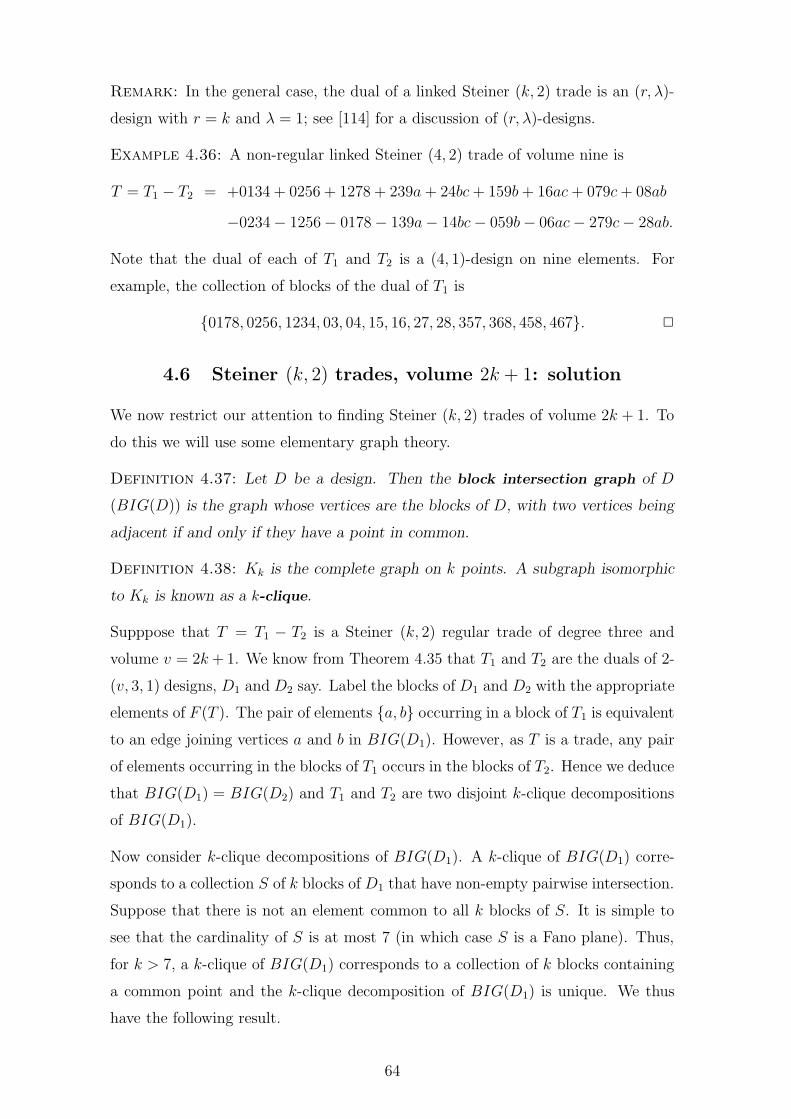
Remark: In the general case, the dual of a linked Steiner (k, 2) trade is an (r, λ)-
design with r = k and λ = 1; see [114] for a discussion of (r, λ)-designs.
Example 4.36: A non-regular linked Steiner (4, 2) trade of volume nine is
T = T1 − T2 = +0134 + 0256 + 1278 + 239a + 24bc + 159b + 16ac + 079c + 08ab
−0234 − 1256 − 0178 − 139a − 14bc − 059b − 06ac − 279c − 28ab.
Note that the dual of each of T1 and T2 is a (4, 1)-design on nine elements. For
example, the collection of blocks of the dual of T1 is
{0178, 0256, 1234, 03, 04, 15, 16, 27, 28, 357, 368, 458, 467}. 2
4.6 Steiner (k, 2) trades, volume 2k + 1: solution
We now restrict our attention to finding Steiner (k, 2) trades of volume 2k + 1. To
do this we will use some elementary graph theory.
Definition 4.37: Let D be a design. Then the block intersection graph of D
(BIG(D)) is the graph whose vertices are the blocks of D, with two vertices being
adjacent if and only if they have a point in common.
Definition 4.38: Kk is the complete graph on k points. A subgraph isomorphic
to Kk is known as a k-clique.
Supppose that T = T1 − T2 is a Steiner (k, 2) regular trade of degree three and
volume v = 2k + 1. We know from Theorem 4.35 that T1 and T2 are the duals of 2-
(v, 3, 1) designs, D1 and D2 say. Label the blocks of D1 and D2 with the appropriate
elements of F (T ). The pair of elements {a, b} occurring in a block of T1 is equivalent
to an edge joining vertices a and b in BIG(D1). However, as T is a trade, any pair
of elements occurring in the blocks of T1 occurs in the blocks of T2. Hence we deduce
that BIG(D1) = BIG(D2) and T1 and T2 are two disjoint k-clique decompositions
of BIG(D1).
Now consider k-clique decompositions of BIG(D1). A k-clique of BIG(D1) corre-
sponds to a collection S of k blocks of D1 that have non-empty pairwise intersection.
Suppose that there is not an element common to all k blocks of S. It is simple to
see that the cardinality of S is at most 7 (in which case S is a Fano plane). Thus,
for k > 7, a k-clique of BIG(D1) corresponds to a collection of k blocks containing
a common point and the k-clique decomposition of BIG(D1) is unique. We thus
have the following result.
64

Figure 4.4: The unique 2-(9, 3, 1) design
a : 123 d : 147 g : 159 j : 168b : 456 e : 258 h : 483 k : 249c : 789 f : 369 i : 267 l : 357
Lemma 4.39: For k > 7, 2k + 1 /∈ S1(k, 2). 2
It is known that for Steiner 2-(v, k, 1) designs D1 and D2, with v > k(k2−2k+2), if
BIG(D1) is isomorphic to BIG(D2), then D1 is isomorphic to D2 [30]. For STS(v),
this result also holds when v ≤ 15. The only difficult case is when v = 15, and this
case was done in, for example, [12].
Lemma 4.40: For 5 < k ≤ 7, the following are equivalent:
(1) The existence of a Steiner (k, 2) trade T of volume 2k + 1;
(2) The existence of a 2-(2k+1, 3, 1) design D with BIG(D) possessing two distinct
k-clique decompositions.
Proof: From the preceeding discussion, it is immediate that (1) implies (2). Cer-
tainly (2) implies the existence of a Steiner (k, 2) trade T of volume no more than
2k + 1 and with element multiplicities no greater than three. The structures of
Steiner trades of volumes 2k − 2 and 2k have been determined in Theorem 4.18,
Lemma 4.20 and Theorem 4.21. Trades of such volumes contain two distinct ele-
ments of multiplicity at least k − 1 > 4, so T must be as claimed. 2
Although the previous lemma will be used to discuss the case 5 < k ≤ 7, we can
illustrate the general method by constructing a Steiner (4, 2) trade of volume nine
which is regular of degree three and linked.
Example 4.41: Let D be the unique 2-(9, 3, 1) shown in Figure 4.4, where the
letters represent block labels. BIG(D) is the complete multipartite graph with parts
{a, b, c}, {d, e, f}, {g, h, i} and {j, k, l}. One 4-clique decomposition of BIG(D) is
T1 = adgj + aeik + afhl + bdhk + begl + bfij + cdil + cehj + cfgk.
It is easy to see that the permutation (abc) applied to the block labelling of D
induces the 4-clique decomposition
T2 = bdgj + beik + bfhl + cdhk + cegl + cfij + adil + aehj + afgk.
T = T1 − T2 is then a Steiner (4, 2) trade of volume nine which is regular of degree
three and linked. 2
65

Figure 4.5: The blocks of P, in rows of Fano planes
F1: 1 1 2 5 4 4 5 8 15 15 1 4 16 1 8 10 23 15 2 8 25 2 4 10 31 15 5 10F2: 2 2 3 6 5 5 6 9 1 1 2 5 17 2 9 11 24 1 3 9 26 3 5 11 32 1 6 11F3: 3 3 4 7 6 6 7 10 2 2 3 6 18 3 10 12 25 2 4 10 27 4 6 12 33 2 7 12F4: 4 4 5 8 7 7 8 11 3 3 4 7 19 4 11 13 26 3 5 11 28 5 7 13 34 3 8 13F5: 5 5 6 9 8 8 9 12 4 4 5 8 20 5 12 14 27 4 6 12 29 6 8 14 35 4 9 14F6: 6 6 7 10 9 9 10 13 5 5 6 9 21 6 13 15 28 5 7 13 30 7 9 15 31 5 10 15F7: 7 7 8 11 10 10 11 14 6 6 7 10 22 7 14 1 29 6 8 14 16 8 10 1 32 6 11 1F8: 8 8 9 12 11 11 12 15 7 7 8 11 23 8 15 2 30 7 9 15 17 9 11 2 33 7 12 2F9: 9 9 10 13 12 12 13 1 8 8 9 12 24 9 1 3 16 8 10 1 18 10 12 3 34 8 13 3
F10: 10 10 11 14 13 13 14 2 9 9 10 13 25 10 2 4 17 9 11 2 19 11 13 4 35 9 14 4F11: 11 11 12 15 14 14 15 3 10 10 11 14 26 11 3 5 18 10 12 3 20 12 14 5 31 10 15 5F12: 12 12 13 1 15 15 1 4 11 11 12 15 27 12 4 6 19 11 13 4 21 13 15 6 32 11 1 6F13: 13 13 14 2 1 1 2 5 12 12 13 1 28 13 5 7 20 12 14 5 22 14 1 7 33 12 2 7F14: 14 14 15 3 2 2 3 6 13 13 14 2 29 14 6 8 21 13 15 6 23 15 2 8 34 13 3 8F15: 15 15 1 4 3 3 4 7 14 14 15 3 30 15 7 9 22 14 1 7 24 1 3 9 35 14 4 9
We now complete our search for k-clique decompositions for the case 5 < k ≤ 7. For
k = 6, it is simple to verify that the 6-clique decompositions of the block intersection
graphs of the two non-isomorphic 2-(13, 3, 1) designs are unique; in fact, the only
6-cliques in these graphs correspond to an element of the design.
The 7-cliques in the block intersection graph of a 2-(15, 3, 1) design are either a
v-type, corresponding to an element of the design, or an f-type, corresponding to a
Fano plane subdesign. A v-type and an f -type clique intersect each other in either 0
or 3 vertices. However, a counting argument, analagous to that used in Lemma 4.33,
shows that the k-cliques of a decomposition of BIG(D) for a 2-(2k + 1, 3, 1) design
D must intersect each other in precisely one vertex. Thus, if there are two distinct
7-clique decompositions of the block intersection graph of a 2-(15, 3, 1) design D,
then D necessarily contains at least 15 Fano planes. There is only one such 2-
(15, 3, 1) design; see, for instance, [88]. This is the design associated with PG(3, 2).
The blocks of this design, P say, are listed in Figure 4.5 (block labels in bold). In
BIG(P ), there are precisely 15 f -type cliques (intersecting each other in one vertex).
Two distinct decompositions of BIG(P ) into v-type and f -type cliques are given in
Figure 4.6; this trade is isomorphic to that given in the proof of Theorem 4.29.
Summarising the results of the previous two paragraphs in terms of volumes of
Steiner (k, 2) trades, we have that 13 /∈ S1(6, 2) and that 15 ∈ S1(7, 2), with the
latter trades obviously having a unique structure. Two structurally different Steiner
(4, 2) trades of volume nine were presented in Examples 4.36 and 4.41. Two struc-
66

Figure 4.6: The Steiner (7, 2) trade of volume 15 from BIG(P )
V1 : 1 12 15 16 22 24 32 F1 : 1 4 15 16 23 25 31V2 : 2 13 1 17 23 25 33 F2 : 2 5 1 17 24 26 32V3 : 3 14 2 18 24 26 34 F3 : 3 6 2 18 25 27 33V4 : 4 15 3 19 25 27 35 F4 : 4 7 3 19 26 28 34V5 : 5 1 4 20 26 28 31 F5 : 5 8 4 20 27 29 35V6 : 6 2 5 21 27 29 32 F6 : 6 9 5 21 28 30 31V7 : 7 3 6 22 28 30 33 F7 : 7 10 6 22 29 16 32V8 : 8 4 7 23 29 16 34 F8 : 8 11 7 23 30 17 33V9 : 9 5 8 24 30 17 35 F9 : 9 12 8 24 16 18 34
V10 : 10 6 9 25 16 18 31 F10 : 10 13 9 25 17 19 35V11 : 11 7 10 26 17 19 32 F11 : 11 14 10 26 18 20 31V12 : 12 8 11 27 18 20 33 F12 : 12 15 11 27 19 21 32V13 : 13 9 12 28 19 21 34 F13 : 13 1 12 28 20 22 33V14 : 14 10 13 29 20 22 35 F14 : 14 2 13 29 21 23 34V15 : 15 11 14 30 21 23 31 F15 : 15 3 14 30 22 24 35
turally different Steiner (3, 2) trades of volume seven are
T a = +124 + 235 + 346 + 457 + 561 + 672 + 713
−134 − 245 − 356 − 467 − 571 − 612 − 723,
T b = +123 + 145 + 624 + 635 + 178 + 928 + 947
−135 − 623 − 645 − 128 − 147 − 924 − 978.
Recall that 11 /∈ S1(5, 2) (proved in Appendix C). Combining the results of this
section with those of Section 4.3 establishes Theorem 4.1.
4.7 Results for t > 2
In this section we briefly consider the problem of determining S1(k, t) when t > 2.
We know that the volume of a (k, t) trade is at least 2t. However, the volume of
a smallest Steiner (k, t) trade grows rapidly with k, as the following result demon-
strates.
Theorem 4.42: If T = T1 − T2 is a Steiner (k, t) trade, t > 1, then
m(T ) ≥ 1 +
(
k
t − 1
)
.
Proof: Let B be a block in T1. By Lemma 4.12, each (t − 1)-subset of B must
occur in at least one other block of T1. If any two of these (t − 1)-subsets occur
together in a block other than B, then a t-subset is repeated in T1, contradicting
the fact that T is Steiner. The number of (t−1)-subsets in B is(
k
t−1
)
and the result
follows. 2
67

Our success in the theoretical investigation of Steiner (k, 2) trades is due, in large
part, to our ability to construct solely 1-balanced families. We do not have any
general construction of solely t-balanced families for t > 1 and arbitrary block-
size. However, two simple constructions are briefly illustrated in the following two
subsections. We start with S1(t + 1, t). Since S1(2, 1), S1(3, 2) and S1(4, 3) are
known, we consider the case t = 4. We then investigate S1(5, 3), the first unsolved
case for t = 3.
4.7.1 Steiner (t + 1, t) trades, when t = 4
When k = t+1, Steiner trades themselves are a source of solely t-balanced families.
Lemma 4.43: Let T = T1 − T2 be a Steiner (t + 1, t) trade. Then T1 and T2 are
solely t-balanced.
Proof: Any (t + 1)-subset in T is a block, in T1 say. Since T is Steiner and
T1 ∩ T2 = ∅, this block occurs only once in T1 and cannot occur in T2. 2
So Steiner (4, 3) trades are solely 3-balanced families, and we can use Lemma 4.8
to construct Steiner (5, 4) trades, giving S1(5, 4) ⊇ {16, 24, 28, 30, 32, . . .}. Using
Lemma 4.3 with these values gives S1(5, 4) ⊇ {31, 39, 43, 45, 47, . . .}. It is straight-
forward, but tedious, to verify that the (5, 4) trades of volumes 37 and 41 constructed
in the proof of Lemma 3.36 are Steiner. We know that S1(5, 4) ⊇ {1, . . . , 15, 17, . . . ,
23, 25} (Section 2.2 and Theorem 3.25), and we believe that S1(5, 4) ⊇ {26, 27, 29,
33, 35} (Conjectures 2.15 and 3.37).
Let X = {0, 16, 24, 28, 30, 31, 32, 34, 36, 37, 38, . . .}. Then we have proved that
S1(5, 4) ⊇ X, and we conjecture that equality holds.
4.7.2 Steiner (5, 3) trades
If T is a non-void Steiner (5, 3) trade of volume m, then Theorem 4.42 gives a lower
bound of eleven for m. Now Theorem 4.42 is proved by counting (t − 1)-subsets.
We can obtain a stronger result by counting the multiplicity of subsets of F (T ) of
other sizes.
Lemma 4.44: Suppose that T = T1−T2 is a non-void Steiner (5, 3) trade of volume
m. Then m > 14.
Proof: Let B = 12345 be an arbitrary block in T1. As in the proof of Theorem 4.42,
the ten pairs in B must occur again, and in separate sets of T1. Each point of B
68
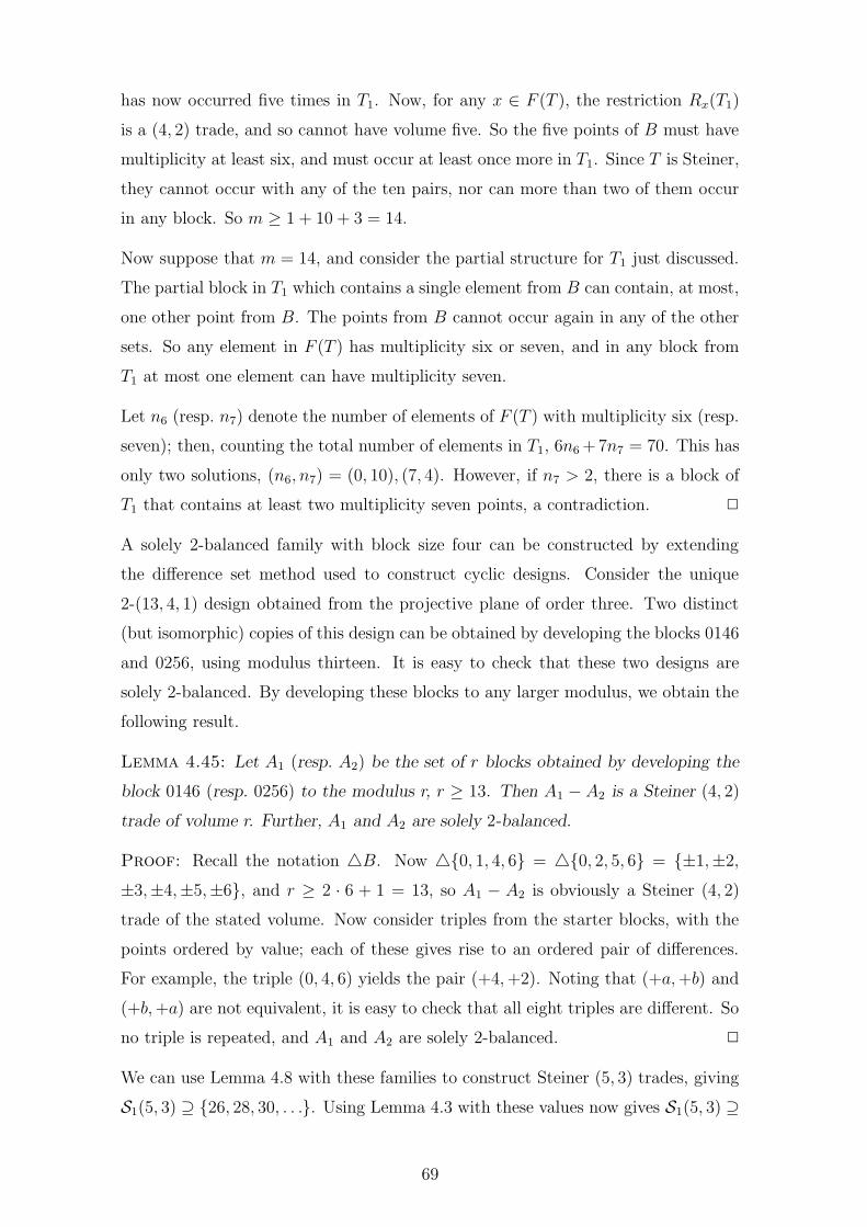
has now occurred five times in T1. Now, for any x ∈ F (T ), the restriction Rx(T1)
is a (4, 2) trade, and so cannot have volume five. So the five points of B must have
multiplicity at least six, and must occur at least once more in T1. Since T is Steiner,
they cannot occur with any of the ten pairs, nor can more than two of them occur
in any block. So m ≥ 1 + 10 + 3 = 14.
Now suppose that m = 14, and consider the partial structure for T1 just discussed.
The partial block in T1 which contains a single element from B can contain, at most,
one other point from B. The points from B cannot occur again in any of the other
sets. So any element in F (T ) has multiplicity six or seven, and in any block from
T1 at most one element can have multiplicity seven.
Let n6 (resp. n7) denote the number of elements of F (T ) with multiplicity six (resp.
seven); then, counting the total number of elements in T1, 6n6 +7n7 = 70. This has
only two solutions, (n6, n7) = (0, 10), (7, 4). However, if n7 > 2, there is a block of
T1 that contains at least two multiplicity seven points, a contradiction. 2
A solely 2-balanced family with block size four can be constructed by extending
the difference set method used to construct cyclic designs. Consider the unique
2-(13, 4, 1) design obtained from the projective plane of order three. Two distinct
(but isomorphic) copies of this design can be obtained by developing the blocks 0146
and 0256, using modulus thirteen. It is easy to check that these two designs are
solely 2-balanced. By developing these blocks to any larger modulus, we obtain the
following result.
Lemma 4.45: Let A1 (resp. A2) be the set of r blocks obtained by developing the
block 0146 (resp. 0256) to the modulus r, r ≥ 13. Then A1 − A2 is a Steiner (4, 2)
trade of volume r. Further, A1 and A2 are solely 2-balanced.
Proof: Recall the notation 4B. Now 4{0, 1, 4, 6} = 4{0, 2, 5, 6} = {±1,±2,
±3,±4,±5,±6}, and r ≥ 2 · 6 + 1 = 13, so A1 − A2 is obviously a Steiner (4, 2)
trade of the stated volume. Now consider triples from the starter blocks, with the
points ordered by value; each of these gives rise to an ordered pair of differences.
For example, the triple (0, 4, 6) yields the pair (+4, +2). Noting that (+a, +b) and
(+b, +a) are not equivalent, it is easy to check that all eight triples are different. So
no triple is repeated, and A1 and A2 are solely 2-balanced. 2
We can use Lemma 4.8 with these families to construct Steiner (5, 3) trades, giving
S1(5, 3) ⊇ {26, 28, 30, . . .}. Using Lemma 4.3 with these values now gives S1(5, 3) ⊇
69

{51, 53, 55, . . .}.
Various searches for Steiner (5, 3) trades, either by considering the difference be-
tween ‘random’ 3-(v, 5, 1) designs (see Section 7.5) or by adding basic trades (see
Section 3.6) produced many trades different from those constructed above. How-
ever, the only new volume obtained was 45. In fact, any permutation, such as (012),
that shifts precisely three points of a 3-(17, 5, 1) design – say, the inversive plane I
of Figure 11.2 – generates a pair of designs whose difference is a Steiner (5, 3) trade
of volume 45 and foundation 17.
4.8 Conclusions
For S1(k, 2), k ≥ 7, our results leave undetermined the inclusion of odd volumes in
the range 2k+3 and 3k−4. Very recently, it has been proved that such trades do not
exist, so S1(k, 2) is now fully determined. This proof, which builds on our results
and uses essentially the same techniques, has been accepted for publication [72].
The material in Appendix D demonstrates that our techniques are robust enough
to be applied to the more general problem of G-trades.
For t > 2, the k = t+1 case is special, since we can induct on t. As Subsection 4.7.1
illustrates, si ∈ S1(t + 1, t) for 0 ≤ i ≤ t, and m ∈ S1(t + 1, t) for all large enough
m. Proving the remaining values becomes increasingly difficult for higher values of
t. Based on our results, we conjecture that S1(t + 1, t) = S(t).
For t > 2 and k > t + 1, the Steiner trade problem seems to be very difficult. The
various theoretical and computational methods discussed do not produce Steiner
trades with ‘small’ volumes for these values of t and k. Our results indicate that a
lower bound stronger than that of Theorem 4.42 should be sought, but it is unclear
what form this should take.
70
Chapter 5
Trades and defining sets in designs
The two themes of our thesis are trades and defining sets. Recall that any defining
set of a design D must have at least one block in common with any trade in D.
In this chapter we present a potpourri of results on defining sets which make use
of this connection. Various bounds on |dsD| were reviewed in Chapter 2, both for
the general case and for infinite families. In Sections 5.1 and 5.2 we present some
further bounds. In Section 5.3 we consider the problem of defining sets in 1-designs.
In the final section we address the question of how many minimal trades or defining
sets a design may contain.
The material presented in Section 5.1 has been published in [101], and has recently
been extended by other workers [34]. The bound given in Section 5.2 has been
published as part of [100].
5.1 An infinite family
Recall that µ = |dsD|/b. Putting t = 2 and k = 3 in Theorem 2.20, and noting
that b = v(v − 1)/6 in a STS(v), we have that µ ≥ 3/v for a STS(v). Note that
limv→∞ 3/v = 0. We describe an infinite family of STS(v) where at least a quarter
of the blocks are necessary to form a defining set.
The following consequence of Lemma 1.8 is trivial, following directly from the dis-
jointness of the trades. However, it seems not to have been recorded in the literature.
Corollary 5.1: Let D = (V,B) be a t-(v, k, λ) design, and suppose that B con-
tains m mutually disjoint (v, k, t) trades. Then |dsD| ≥ m. 2
A number of authors have examined the problem of partitioning the family of blocks
of a Steiner triple system into sets of blocks isomorphic to a given set of blocks;
such a partitioning is called a decomposition, and the given set of blocks is called
a configuration. See, for example, [55, 54, 66]. The configuration that interests us
71

is the Pasch configuration. Recall that this is the unique smallest (3, 2) trade. In
[1], the following result is proved.
Theorem 5.2: For all v ≡ 1, 9 (mod 24), v ≥ 25, there exists a STS(v) which
can be decomposed into Pasch configurations. 2
Combining Corollary 5.1 and Theorem 5.2 immediately gives our required family.
Theorem 5.3: For all v ≡ 1, 9 (mod 24), v ≥ 25, there exists a STS(v) with
µ = |dsD|/b ≥ 1/4. 2
Remark: The example Pasch-decomposable STS(25) given in [1] is cyclic, with the
four starter blocks forming the Pasch configuration {016, 02a, 1ad, 26d}. Attempts
to find |dsD| for this design using the computational techniques described later
were not successful, due to the large number of blocks. However, a defining set of
47 blocks was found, so 0.25 ≤ µ ≤ 0.47.
5.2 An upper bound
In several places throughout this thesis, we use the smallest volume trades in a
design to give an upper bound on |dsD|, a bound on max(specm(D)), or an upper
bound on the size of a partial that is not a defining set.
Since non-void (k, t) trades have volume at least 2t, any set of at least b − 2t + 1
blocks from a design must be a defining set. However, a t-(v, k, λ) design need not
contain a trade of volume 2t; for example, the unique STS(9) does not contain any
Pasch configurations. If we consider the smallest volume trades in a design, then
we are led, via Lemma 1.9, to the following result.
Lemma 5.4: Let D = (V,B) be a t-(v, k, λ) design with |B| = b, and let m denote
the size of a smallest volume non-void trade in D. Then any collection, C ⊆ B, of
more than b − m blocks from D completes uniquely.
Proof: If C = B, the result is trivial. Let C be a collection of blocks from B, with
b − m < |C| < b, and suppose that C completes to two distinct designs D1 and D2.
Now B1\C 6= B2\C, and both B1\C and B2\C are non-empty. Thus (B1\C)− (B2\C)
contains a trade with volume less than m, which is not possible. 2
Corollary 5.5: For any minimal defining set, |dsD| ≤ |dmD| ≤ b − m + 1. 2
72

5.3 Defining sets for 1-designs
The sizes of smallest defining sets of 1-designs have not been considered in the liter-
ature. However, these are of interest; in particular, given the relationship between
the sizes of smallest defining sets of a design and its extensions, they can assist
in finding |dsD| for designs with t > 1. For 1-designs in general, we expect that
|dsD| = b − x, where x is ‘small’, since 1-designs contain large numbers of small-
volume trades. However, there are non-trivial cases where b − |dsD| is arbitrarily
large.
Lemma 5.6: (1) For any x > 0 there exists a 1-design D with b − |dsD| ≥ x;
(2) There exists a 1-design with µ ≤ 1/2.
Proof: To prove both parts, consider the 1-(4, 2, x) design formed by taking x
copies of {12, 34}; this has 2x blocks. Obviously, the partial consisting of x copies
of the block 12 completes uniquely, and is a smallest defining set. 2
To obtain more precise results, we consider when a collection of blocks can be, or
can contain, a 1-trade. For (k, 1) trades of volume two, it is simple to see that any
pair of blocks A and B have a trade mate if and only if |A ∩ B| ≤ k − 2.
Definition 5.7: A design D = (V,B) is said to be i-simple if |A ∩ B| ≤ k − i for
all A, B ∈ B, A 6= B.
Lemma 5.8: Let D = (V,B) be a 1-(v, k, λ) design. Then |dsD| ≤ b − 1, with
equality if and only if D is 2-simple.
Proof: That |dsD| ≤ b − 1 is obvious. If D is 2-simple, then any two blocks of D
are a (k, 1) trade, so |dsD| = b − 1. If |dsD| = b − 1, then any two blocks of D are
a (k, 1) trade, since if not there would be a partial of b − 2 blocks which completed
uniquely. So any two blocks intersect in at most k − 2 points, and D is 2-simple. 2
Corollary 5.9: Let D = (V,B) be a t-(v, k, 1) design. Then, considered as a
1-design, |dsD| = b − 1.
Proof: Since D is Steiner, and k ≥ t + 1, then D is 2-simple. 2
We now consider a sufficient condition for a set of blocks not to contain a 1-trade.
Definition 5.10: Let D = (V,B) be a t-(v, k, λ) design, with |B| = b. Let(
V
l
)
73

denote the set of all l-subsets of V. Define
s(D) = maxS∈( V
k−1)( |{B : S ⊆ B ∈ B}| ).
If S is any set of s(D) blocks satisfying this definition, then any collection of blocks
from S intersect in at least k − 1 points, and thus cannot have a trade mate. Note
however, that if S is any set of blocks any pair of which intersect in at least k − 1
points, then it is not necessarily the case that the blocks of S have a (k − 1)-subset
in common – consider the collection {12,13,23}.
Theorem 5.11: Let D = (V,B) be a 1-(v, k, λ) design, with |B| = b. Then |dsD| ≤
b − s(D).
Proof: Let S be a set of s(D) blocks having a (k−1)-subset in common. Obviously
S does not contain any 1-trade, and so B \ S completes uniquely. Thus |dsD| ≤
b − s(D). 2
5.4 Number of trades and defining sets
A collection of subsets is called an antichain (or Sperner family) if no member of
the collection properly contains another. The collections of minimal trades and of
minimal defining sets in a simple design are obviously antichains. The following two
results are standard; see, for example, [3].
Theorem 5.12: Let A be an antichain of subsets of an n-set. Then
|A| ≤
(
n
bn/2c
)
,
with equality if and only if A consists of all the n2-subsets if n is even, or all the
n−12
-subsets or all the n+12
-subsets if n is odd. 2
Theorem 5.13: (The LYM Inequality) Let A be an antichain of subsets of an
n-set, and suppose that pi members of A have cardinality i, for 0 ≤ i ≤ n. Then
n∑
i=0
pi(
n
i
) ≤ 1. 2
These two results give bounds on the number of minimal trades or minimal defining
sets in a simple design, with the LYM Inequality being the stronger of the two.
We call the sum in Theorem 5.13 the w-size (for weighted size) of the antichain,
and use wd (resp. wt) for the w-size of the antichain of minimal defining sets (resp.
trades). In Chapters 7 and 11 we count the number of minimal trades and minimal
74

Table 5.1: Some example w-sizes
design wd wt
2-(6,3,2) 0.250 0.0482-(7,3,1) 0.800 0.2002-(8,4,3), α∗ - 0.0232-(8,4,3), β∗ - 0.0322-(8,4,3), γ∗ - 0.0562-(8,4,3), δ∗ - 0.0332-(9,3,1) 0.382 0.0392-(10,4,2), H1 - 0.0332-(10,4,2), H2 - 0.0152-(10,4,2), H3 - 0.0342-(13,3,1), D1 0.019 -2-(13,3,1), D2 0.031 -2-(13,4,1) 0.682 -2-(16,4,1) 0.299 -2-(21,5,1) 0.424 -2-(25,5,1) ≈ 0.15 -2-(31,6,1) ≈ 0.16 -3-(8,4,1) 0.615 0.002333-(10,4,1) ? 0.255 0.0000613-(17,5,1) ≈ 0.13 -4-(11,5,1) > 0.181 0.0000175-(12,6,1) ≥ 0.168 -
defining sets in a design. These results are collected and displayed in Table 5.1; a
‘≈’ indicates that the value is an estimate obtained by sampling, a ‘?’ indicates that
the value is correct if specm(D) has no holes, and a ‘≥’ or ‘>’ indicates that only a
partial enumeration was performed.
We do not expect the bound from the LYM Inequality to be tight, and this is borne
out by our results. (We do not include the void trade in our count of trades, and
we ignore the trivial cases where |dsD| = 0.) However, for some designs the w-size
is quite large, with wd being more than one half in several cases.
In all the examples considered wd > wt, and the ratio wd/wt can be very large. For a
given family of designs the w-sizes decrease as the designs get ‘larger’; for example,
wd for the projective and affine planes decreases as the order increases. However,
the w-sizes need not tend to 0 in a series of designs. In particular, for non-simple
designs, although the number of different trades can be small, the number of times
each is contained in the design can grow rapidly.
Example 5.14: Let D be a simple 2-(v, 3, λ) design with b blocks which contains n
copies of the Pasch trade. Now consider the 2-(v, 3, xλ) design D′ formed by taking
75

x copies of D. Each Pasch trade in D gives rise to x4 Pasch trades in D′, since there
are x copies of each block. So
wt ≥nx4
(
xb
4
) =24nx4
xb(xb − 1)(xb − 2)(xb − 3)>
24n
b4. 2
Remark: Any superset of a defining set is also a defining set, so the collection of all
defining sets in a design forms an upset or filter [3], with the antichain of minimal
defining sets being the minimal members of this upset. The collection of all trades
in a design is not an upset.
76

Chapter 6
Trade enumeration in simple designs
Although any (v, k, t) trade is contained in some design (simply take the appropriate
multiple of the full design), it is not necessarily the case that a particular design
contains a particular trade. For a (k, t) trade T to be contained in a t-(v, k, λ) design
it is obviously necessary that v ≥ f(T ), b ≥ m(T ), and that λ is ‘large enough.’
However, these conditions are not sufficient. For example, for all v ≡ 3 (mod 6)
there is an anti-Pasch STS(v); that is, an STS(v) with no trade of volume 4 [10].
To assist in investigating the trades contained in a t-(v, k, λ) design, an algorithm
to enumerate all the trades in the simple designs with a given set of parameters was
developed. We show how the lists of trades generated by the algorithm can be used
to find the sizes of smallest defining sets of designs. By considering only some of
the trades in a design, the technique discussed leads to the new concepts of member
and class defining sets of designs.
Some of the material from this chapter and the next chapter – where the main
results obtained using this algorithm are presented – has been published in [100].
6.1 Algorithm
Recall that n is the number of different designs with the same parameters, and sup-
pose that all n of these designs are simple. Given the transversal D = {D0, . . . , Dn−1}
we wish to enumerate, for each Di, the subsets of Di that are trades.
Suppose that T1 − T2 is a trade and that T1 ⊆ Bi is a trade in Di. Then, by the
definition of a trade, (Bi \T1)∪T2 is also a t-(v, k, λ) design, say D′. Now D′ will be
isomorphic to Dj, for some j. It may be that i = j, but this is not true in general.
Note that, since T1 and T2 are non-empty and disjoint, D′ 6= Di. We say that T1 is
a trade from Di to D′ and that T2 is a trade from D′ to Di.
Conversely, given Di and any design D′ 6= Di, suppose that Bi = B ∪ T1 and
B′ = B ∪T2, with T1 ∩T2 = ∅. Thus B is the set of blocks common to both designs,
77

Figure 6.1: The algorithm to enumerate all trades
1 for all permutations of V2 for all j in 0 . . . n − 13 permute design Dj
4 for all i in 0 . . . n − 15 find the trade from Di to permuted Dj
6 process/store trade7 end for8 end for9 end for
while T1, T2 6= ∅, since D′ 6= Di. Now T1 − T2 is a trade, and Di contains T1. Note
that, if Bi ∩ B′ = ∅, B will be empty, and the trade consists of the designs Di and
D′ themselves.
So we can generate all the trades in a design Di by comparing Di to every other
design with the same parameters and eliminating common blocks. Given D, it is
easy to generate all possible designs by applying all permutations of V to the designs
in D. Thus we arrive at the simple algorithm given in Figure 6.1.
This algorithm is obviously non-polynomial, since the outer loop 1–9 will be executed
v! times. It is possible to enumerate all permutations so that successive permutations
differ by a single transposition, see for example [97, 103]. Such an enumeration yields
a constant amortised time (CAT) algorithm, and thus the overhead to generate all
the permutations of V is O(v!).
For each iteration of the loop 1–9, statement 3 will be executed n times and state-
ments 5 and 6 will be executed n2 times each. If we restrict v to be less than the
machine’s word size (normally 32 bits) and implement sets as unsigned integers,
then set operations are constant time, so the complexity of statement 3 depends
only on the number of blocks in the design and will be O(b). For statement 5, we
have to compare every block in Di with every block in the permuted Dj and strike
out matched pairs. Since the permuted design is not sorted, this will be O(b2).
So, the overall complexity of the algorithm will be O(v!+v!n(b+n(b2 +C6))), where
C6 stands for the complexity of statement 6. The trades are stored in binary trees,
one tree to each of the n2 ordered pairs of designs, with the trades ordered first
by volume and then lexicographically. We call the first design (Di) in the ordered
pair the initial design and the second (Dj) the final design. For an ordered pair
of designs, we regard trades as distinct if the sets of blocks of the trades in the
78

initial design are different, and only these blocks are stored. We do not differentiate
between trades with different sets of blocks in the final design; that is, we do not
consider different trade mates.
Since comparing trades will be O(b), searching the tree is an O(b log2 NT ) operation,
where NT stands for the number of trades in the tree. Insertion of a new trade
requires memory allocation and O(b) time. We assume that the total time to execute
statement 6 amortises to O(b2), or less, for each call. Thus, the complexity of
the algorithm reduces to O(v!n2b2). We investigate the validity of this expression
empirically in Section 6.3. As some justification for our assumption, consider the
following points:
. The trade may be void, in which case statement 6 can be skipped.
. The number of distinct trades is much less than the number of times, v!n2, that
statement 6 is executed. So, in most cases, only a partial traversal of the tree
is required before the current trade is found and insertion proves unnecessary.
. The trees are kept as small as possible by there being one for each ordered
pair of designs.
. The trees are initially empty, so the search time is initially small and grows
as the tree grows.
Note that the running time of the algorithm is independent of the parameters t, k, λ,
except as these affect b. In practice, calculating the permutations accounts for only
a minor part of the running time of the algorithm. Profiled runs of the algorithm,
using the prof Unix utility, revealed that the bulk of the time is spent building the
trades in statement 5 or, to a lesser extent, comparing trades in the tree searches as
part of statement 6.
The algorithm takes no account of the automorphism groups of the designs. Let Ai
denote the order of the automorphism group of Di and recall that Ni denotes the
number of distinct designs isomorphic to Di. Then N =∑n−1
i=0 v!/Ai is the total
number of distinct designs, and the maximum number of trades from Di is N − 1.
The maximum number of trades from Di to designs isomorphic to Dj, i 6= j, is
Nj, and each of these will be enumerated at least Aj times. The maximum number
of trades from Di to isomorphic designs is Ni − 1 and, if the permutation is an
automorphism, the trade will be void.
In general, since a trade may have many trade mates, these upper bounds on the
79

number of distinct trade halves in a design are poor. So the algorithm may do much
redundant work, generating empty trades or trades already listed. We make use of
the empty trades, and keep a count of their number. Since void trades only arise
when the permutation leaves the set of blocks unchanged, this count is, in fact, the
order of the automorphism group of the design. Of course, this value is available
from other sources, but its calculation here is convenient and provides a check on
the operation of the algorithm.
6.2 Defining sets
Given a design D, suppose that we have enumerated the family of distinct trades
T = {T i}i∈I in D using our algorithm, and that |T | = d. This family can be
represented by a d×b incidence matrix M = [mij], with mij = 1 if trade T i contains
block bj and 0 otherwise. In a similar manner to that of [71], each row of M can be
thought of as a linear inequality
mi,0b0 + · · ·+ mi,b−1bb−1 ≥ 1.
Here the binary variables bi, 0 ≤ i ≤ b−1, are our unknowns, and they stand for the
blocks of D. In view of Lemma 1.9, since T contains all trades in D, any solution to
this system of d inequalities is a defining set for D. Further, in view of Lemma 1.8,
any defining set for D will be a solution to the system of inequalities.
So we formulate the binary integer linear programme (BILP): minimise
b−1∑
i=0
bi ,
subject to the system of inequalites represented by M , with bi ∈ {0, 1}, 0 ≤ i ≤ b−1.
Any optimal solution to this BILP yields a smallest defining set, and thus the value
of |dsD|.
6.2.1 Minimising the collection of trades
As a practical matter, to reduce the number of inequalities, we may choose to
minimise T before solving the system, since this does not affect the validity of the
solutions. Our enumeration algorithm stores the family of trades on binary trees,
ordered first by volume and then lexicographically. An in-order traversal of such a
tree processes the trades in order of increasing volume. As each trade is processed
it is compared with the previously processed trades having smaller volume. If it is a
superset of such a trade, it is non-minimal. If not, it is minimal. It is never the case
80

that a previously processed trade is a superset of a later trade. This naıve algorithm
is quadratic in the number of trades, and suffices for our purposes. Merging trees
or lists, if required, is straightforward.
Remark: Note that building a separate list of minimal trades by copying across
the data required is not necessary. The list can be built by ‘threading’ through the
existing tree, at the small expense of an extra pointer field in each node.
6.2.2 Member and class defining sets
To motivate what follows, consider the problem of identifying a unique design D
among the N t-(v, k, λ) designs. To do so, we need to supply information about
D. If the information consists solely of blocks of D then it is a defining set. If the
information also includes block intersection numbers then it is a specifying set , see
[94]. An arbitrary collection of information about a design, sufficient to identify it
uniquely, will be called an establishing set.
If an establishing set includes information about D that is invariant under isomor-
phisms, then we may be able to partition D into two or more parts and say which
part D lies in. The invariants may or may not be sufficient to identify uniquely
the isomorphism class to which D belongs. Examples of design invariants include
whether or not the design is simple and the order of the automorphism group of the
design. An example of establishing information about D that is not an invariant is
the knowledge that the design does not contain a particular k-subset of V.
Given D, for each isomorphism class D∗i our algorithm enumerates the trades in D
to designs in D∗i . Each such set of trades represents a BILP. An optimum solution
of this BILP represents the smallest number of blocks of D required to ensure that
no completion lies in D∗i , or in D∗ \ {D} if D∗
i = D∗.
If D∗i = D∗, then the trades in D are all to another member of the class D∗. Such
trades will be called member trades, or m-trades. Any solution, not necessarily
optimal, to the BILP formulated from the collection of all m-trades is a member
defining set. A member defining set of D is denoted mD, and we note that, while
it may have more than one completion, exactly one of these completions is in D∗
and this completion is D. Just as we can define minimal and smallest defining sets,
we can define minimal and smallest member defining sets. These are denoted mmD
and msD respectively.
81

If D∗i 6= D∗, then the trades in D are to designs in another isomorphism class.
Such trades will be called class trades, or c-trades. Any solution, not necessarily
optimal, to the BILP formulated from the collection of all the c-trades in D is a
class defining set. A class defining set of D is denoted cD, and we note that, while
it may have more than one completion, all of these completions are in D∗ and one
of them is D. Just as we can define minimal and smallest defining sets, we can
define minimal and smallest class defining sets. These are denoted cmD and csD
respectively.
A set of blocks that is a class defining set is a class defining set for every design to
which it completes. It is possible for a set of blocks to be a member defining set for
more than one design. For example, if a set of blocks S completes in only two ways,
to two non-isomorphic designs D′ and D′′, then S is a member defining set of both
D′ and D′′.
Remark: Note that, unlike a member defining set, a class defining set is not an
establishing set for a single design. It could, perhaps, be considered an establishing
set for a class of designs.
Obviously, any defining set is also a member and a class defining set, and a member
and a class defining set together constitute a defining set, so
|msD|, |csD| ≤ |dsD| ≤ |msD| + |csD|.
In the case n = 1, |msD| = |dsD| and |csD| = 0. In the case n > 1, for each of these
inequalities the results quoted in the next chapter contain examples where equality
holds and where it does not, except that no non-trivial example is known where
|dsD| = |msD|+ |csD|. (If D is the full design, then |aut(D)| = v! and so |msD| = 0
and |csD| = |dsD|.) Our results also show that |msD| < |csD|, |msD| = |csD| and
|msD| > |csD| are all possible.
Member defining sets are particularly interesting, since we can find |msD| given only
the design D, by using the list of m-trades in D generated by a simplified version
of our algorithm. We do not need a transversal of all the n classes and, in fact, we
need not know what n is. Since |msD| = |dsD| in at least two cases where n > 1,
|msD| is a potentially tight lower bound on |dsD|. In general, |csD| is a better lower
bound for |dsD|, being tight in many of the examples given, but it is not so readily
calculable.
Remark: If the proof of parts (1)–(3) of Theorem 2.20 is examined, we see that
82

they go through when S is a member defining set, as opposed to a defining set [36].
Thus, if D is STF, we can use the lower bound of Theorem 2.20(3) for smallest
member defining sets.
Suppose now that we wish to estimate the value of |msD|. That is, given a design
D ∈ D∗i , what is the smallest number of blocks of D that uniquely identifies it
among all the designs in D∗i ? The total number of blocks in the Ni designs in D∗
i is
bNi, and the total number of k-subsets of V is(
v
k
)
. So, each k-subset of V appears
in an average of bNi/(
v
k
)
designs of D∗i . Let the factor f =
(
v
k
)
/b. Then 1/f is the
average proportion of the designs in D∗i that contain a given k-subset.
Now all designs in D∗i are isomorphic, differing only in the labelling of the elements.
If we assume that the k-subsets of V are randomly distributed among the Ni designs
of D∗i , then f is the reciprocal of the probability that a particular k-subset of V
appears in a given design. So, the knowledge that a design contains a particular
k-subset of V means that the design is one of Ni/f designs from the Ni designs in
D∗i . If we assume further that the blocks in a design are independent of each other,
then the knowledge of x blocks of a design means that the design is one of Ni/fx
designs from the Ni designs in D∗i . To specify D uniquely, this value must be at
most 1; that is, Ni ≤ fx. Taking logarithms to base f yields x ≥ logf Ni. The
value logf Ni is thus the expected value of |msD|, under the assumptions stated.
We investigate the validity of this expression in Section 7.3.
6.3 Timing information
In an effort to validate the expression for the complexity of the algorithm, and
to establish whether or not the cost of processing the trees of trades did, in fact,
amortise to no more than O(b2), timing data was recorded for runs of the programme.
This data is presented in Table 6.1, and covers the parameter sets (for both n > 1
and n = 1) discussed in the next chapter. The first column gives the parameters
of the design, with the next two columns giving n and b. The next two columns
give the value of v!n2b2 and this value normalised to that for the 2-(8, 4, 3) designs.
The final two columns give the running times to generate all the trades in all the
designs, both actual and normalised.
The running time is the amount of actual CPU time used by the programme, and
does not include system or I/O time. The runs were performed on a Sun-4m SPARC-
based server, with a 100MHz clock. Note that the time does not include the time
83

Table 6.1: The running times to generate all trades
design n b v!n2b2 norm time norm2-(6, 3, 2) 1 10 72000 0.00057 0m00.03s 0.000722-(7, 3, 1) 1 7 246960 0.00195 0m00.10s 0.002393-(8, 4, 1) 1 14 7902720 0.06250 0m01.73s 0.041382-(9, 3, 1) 1 12 52254720 0.41327 0m16.42s 0.392732-(8, 4, 3) 4 14 126443520 1.00000 0m41.81s 1.000003-(10, 4, 1) 1 30 3265920000 25.8291 11m28.90s 16.47692-(11, 5, 2) 1 11 4829932800 38.1983 21m42.70s 31.15762-(10, 4, 2) 3 15 7348320000 58.1154 33m46.09s 48.45952-(9, 4, 3) 11 18 14226347520 112.511 1h44m01.72s 149.2884-(11, 5, 1) 1 66 173877580800 1375.14 7h56m14.11s 683.4284-(11, 6, 3) 1 66 173877580800 1375.14 8h05m24.27s 696.5863-(10, 5, 3) 7 36 230443315200 1822.50 14h26m53.62s 1244.052-(10, 5, 4) 21 18 518497459200 4100.63 64h10m47.71s 5526.14
to process the list of trades – say to extract and minimise a particular collection of
trades – nor the time to solve any BILP problem. These additional times can be
non-trivial.
The normalised running times are in good agreement with the times obtained using
the expression for the complexity, with the ratio of actual to ‘predicted’ time varying
from 1/2 to 4/3. So it appears that tree processing times can be ignored in assessing
the complexity of the algorithm, and that v!n2b2, suitably normalised, predicts the
running time to within a factor of two.
6.4 Variations of the algorithm
Despite its simplicity, the algorithm presented has proved effective, as evidenced by
the results given in the next chapter. However, due to its high complexity, extending
its reach to other parameter sets would require substantial efficiency improvements.
One possible approach would be to take into account the automorphism groups of
the designs. Consideration of only the distinct designs in each class would replace
the n2v! term in the expression for the complexity by the term n∑n−1
i=0 v!/Ai = nN .
This represents a reduction in the amount of work by a factor of n/(∑n−1
i=0 1/Ai).
This is a potentially significant reduction, with the actual value depending on the
automorphism group orders. Parameter sets where one or more of the designs has
a trivial automorphism group yield smaller reductions. For the five parameter sets
with n > 1 given in Table 6.1, the work would be reduced by factors of 26.2, 47.0,
3.0, 19.1 and 2.7. However, to realise this reduction we would have to generate,
84

for each design, a set of coset representatives of the automorphism group in the
group of permutations of V. Whether or not the complexity of doing this would be
outweighed by the reduction in the number of executions of statements 5 and 6 of
the algorithm has not been investigated.
In cases where the running time is too long, a modified version of the algorithm can
be used to generate partial lists of trades. This can be done in several ways: by
imposing a time limit; by imposing a limit on the number of trades generated; or by
generating only some of the permutations. The first two of these are straightforward
and effective, since a significant proportion of the distinct trades are found early in a
run. The last technique is the most versatile, although its efficacy depends heavily
on the particular designs and the trades ‘required.’ Three possible implementa-
tions of this technique are: generate the first permutations in some order; generate
some number of random permutations; or generate only those permutations that
are derangements of exactly u of the v points, for some 1 < u ≤ v.
Partial lists of trades can be used to find lower bounds for |msD|, |csD| and |dsD|,
in the manner discussed in [71], to help eliminate sets of blocks from consideration
as defining sets, as discussed in [17, 53, 51], or as part of an investigation of trades,
as discussed in Section 7.5.
As our results indicate, the number of trades can be very large, and this can cause
memory or disk-space problems. To overcome these it may be necessary to modify
the algorithm to generate only those trades required, or to process the trades as
they are generated. The algorithm only stores trade halves, not full trades. This is
done partly to reduce the size of the data structures needed to store the trades, and
partly because, since our intended application is finding the size of defining sets, we
do not need the discarded information. Additionally, distinguishing trades on the
basis only of the sets of blocks in the initial design cuts down the number of ‘distinct’
trades generated. If we were interested in studying the number or structures of trade
mates, it would be straightforward to amend our algorithm to record these.
If it is not possible to generate all the trades in all the designs at once, it is simple
to modify the algorithm to generate and store only the trades in a particular design.
Thus n runs, each taking O(v!nb2) time, are required to generate all the trades
in all the designs, but the memory usage for each run is decreased by a factor of
approximately n.
85

6.5 Conclusions
The algorithm described has proved very useful, and we make free use of trades
produced by it, without commenting on their provenance. The specific purpose for
which the algorithm was originally written – that is, defining sets – is discussed in
the next chapter, along with some details of the trades in the designs considered.
One area not addressed by our algorithm is that of non-simple designs. Here the
design, and their trades, are not sets, but multisets. The algorithm presented gen-
erates a representative of each trade which uses blocks repeated in the design, but
does not generate a full list of these trades, since we need to distinguish between
‘identical’ blocks. When the trade contains blocks which are also contained in the
untraded portion of the design, the duplicated blocks of the trade cannot be used
to distinguish between the initial and the final designs. The discriminating sets
described in Chapter 8 are intended to address these problems.
Remark: Given a set of parameters with n > 1 it is often the case that some of
the designs are simple and some are non-simple. The algorithm generates a full list
of trades in the simple designs, enabling |msD|, |csD| and |dsD| to be calculated for
these designs. For the non-simple designs, the partial list of trades generated could
be used to find lower bounds for these values.
86

Chapter 7
Results on simple designs
In this chapter we present some results obtained by enumerating trades in designs.
In Sections 7.1 and 7.2 we use the algorithm of the previous chapter to enumerate
all trades in simple designs. We give counts of the number of various trades in
the designs and calculate the sizes of smallest member, smallest class, and smallest
defining sets. In Section 7.3 we discuss the accuracy of our estimate for |msD|.
In Section 7.4 we discuss the distribution, by volume, of the trades in the designs.
Finally, in Section 7.5 we indicate how even a partial enumeration of trades can
assist in their study.
7.1 Trade enumerations and defining sets
In this section we present results for five sets of parameters, where n > 1 and all
the designs are simple. Each set of results is briefly discussed in a subsection. The
results themselves are presented in tabular form in Appendix E, with three tables,
or pairs of tables, per parameter set.
The first table for each set lists the number of distinct sets of tradeable blocks in
each design. The first column of this table gives the label of the design, as given
in the reference from which the transversal is drawn. The next n columns list the
number of distinct trades from each design to each of the other designs; that is,
to designs in the given isomorphism class. The number of m-trades in Di can be
obtained from column Di of this n × n array of values. The c-trades column lists
the total number of distinct c-trades in the design. The final column lists the total
number of distinct trades in the design.
Note that the number of trades listed in these last two columns can be less than
the sum of the number of trades in the appropriate columns from the first n. This
is because a trade in a design may trade to both isomorphic and non-isomorphic
designs, and may have many or few trade mates. The variation in the number of
trade mates also explains why the n × n array of values is not symmetric; that is,
87

the number of trades from Di to Dj need not equal that from Dj to Di.
The number of distinct c-trades in Di is bounded below by the maximum number of
c-trades from Di to each of the non-isomorphic designs. The total number of distinct
trades in Di is bounded below by the maximum of the number of m-trades and the
number of c-trades. The tables contain examples where the number of c-trades and
trades are equal. However, there are no examples where these numbers match those
for a particular initial/final pair of designs.
The second table lists the sizes of the collections of trades in the same manner as
the first, but here the collections of trades have been minimised. That is, any trade
which is a proper superset of another trade in the collection has been removed.
Note the significant, but very variable, reduction in the number of trades after
minimisation.
The final table for each parameter set gives the order of the automorphism group,
Ai, and the number of distinct designs, Ni = v!/Ai, in each isomorphism class.
The logarithm of Ni, to the base f , gives the expected value of |msD|, under the
assumption that the blocks in a design are random and independent.
The values of |msD|, |csD| and |dsD|, found by solving the BILP optimisation
problems represented by the lists of appropriate trades, are given in the final three
columns. The values of |msD| and |csD| are all new. The values of |dsD| for
four of the parameter sets have previously been calculated. Our results match the
published results, except in one case, which is discussed in the relevant subsection.
The values of |dsD| for the 21 2-(10, 5, 4) designs are new, although they were
obtained independently at the same time in [74]; our results were reported in [100].
Our rationale for including this wealth of material regarding trades between pairs of
designs is to highlight the very variable nature of the results. In the subsections that
follow, we remark upon various points of interest; however we are unable to draw
any general conclusions from the data. It does, however, provide a ready source of
counterexamples for refuting conjectures.
7.1.1 The 2-(8, 4, 3) designs
There are four non-isomorphic 2-(8, 4, 3) designs. The transversal used here is that
given in [47], which also gives |dsD| for each design.
Note that there are 30 distinct designs isomorphic to γ∗ and that there are 30 distinct
88

trades from δ∗ to designs isomorphic to γ∗. So the upper bound on the number of
distinct trades given in Section 6.1 is attained, and all the designs isomorphic to γ∗
can be generated from δ∗ by trading different sets of blocks of δ∗.
7.1.2 The 2-(10, 4, 2) designs
There are three non-isomorphic 2-(10, 4, 2) designs, with each design being a residual
design of a 2-(16, 6, 2) design. The transversal used here is that given in [52], which
also gives |dsD|, and enumerates all smallest defining sets. Note that |msH3| =
|csH3| = |dsH3| = 5.
7.1.3 The 2-(9, 4, 3) designs
There are 11 non-isomorphic 2-(9, 4, 3) designs. The transversal used here is that
given in [95], which also gives |dsD|, counts the number of distinct smallest defining
sets, and lists several examples for each design.
Note that the transversal can be partitioned into the parts {M1,M2}, {M3,M4},
{M5,M6,M7}, {M8,M9} and {M10,M11}. Within each of these parts, the total
number of distinct, or minimal distinct, trades is the same. These parts match the
possible extensions to 3-(10, 5, 3) designs, see [95]. For example, a 2-(9, 4, 3) design
extends to the 3-(10, 5, 3) designs N1 or N2 if and only if it is design M1 or M2.
Interestingly, M8 and M9 have more than twice as many distinct minimal c-trades
and trades as any of the other designs, but they have the lowest values of both |csD|
and |dsD|.
7.1.4 The 3-(10, 5, 3) designs
There are seven non-isomorphic 3-(10, 5, 3) designs, all of which are extensions of
2-(9, 4, 3) designs. The transversal used here is that given in [95], which also gives
|dsD|, counts the number of distinct smallest defining sets, and lists several examples
for each design. Note that the total number of distinct minimal c-trades in the
design N4 is less than the number of such trades from N4 to any of the individual
non-isomorphic designs.
The value calculated for |dsD| for design N1 does not match the value of 6 originally
given in [95]. The blocks of design N1, after sorting into lexicographic order, are:
89

01247, 01259, 01268, 01346, 01358, 01379, 01489, 01567, 02348,02357, 02369, 02456, 02789, 03459, 03678, 04578, 04679, 05689,12345, 12367, 12389, 12469, 12578, 13478, 13569, 14568, 14579,16789, 23479, 23568, 24589, 24678, 25679, 34567, 34689, 35789.
The underlined values are an optimal solution of the BILP, in five blocks. That
this putative defining set of five blocks from N1 completes uniquely was checked by
performing partial completions by hand and then using the complete utility (see
[18]) to find all completions.
First note that b = 36, r = 18, and that each pair of points occurs in λ2 = 8 blocks.
Consider the five underlined blocks. The triple 345 has not yet appeared, so the
block 345-- must be in any completion three times. Each of the pairs 34, 35 and 45
has now appeared four times. Thus the blocks 34---, 35--- and 45--- must appear
four more times each. The elements 3, 4 and 5 have now appeared 13, 14 and 13
times each respectively. Thus the blocks 3----, 4---- and 5---- must appear 5, 4 and
5 more times each respectively. This gives, in partial form, all but two of the blocks
of the design.
The element 8 has appeared four times, so must appear in fourteen other blocks.
Each of the triples 348, 358 and 458 has appeared once, so each must appear twice
more. We distinguish three cases, with the block 3458- occuring zero, one or two
times. Taking the value of λ2 into account, we obtain the three respective partial
completions:
02348, 04679, 16789, 23568, 24589, 345, 345, 345, 348, 348, 34, 34, 358, 358, 35, 35,458, 458, 45, 45, 38, 38, 3, 3, 3, 48, 48, 4, 4, 58, 58, 5, 5, 5, 8, 8;
02348, 04679, 16789, 23568, 24589, 3458, 345, 345, 348, 34, 34, 34, 358, 35, 35, 35,458, 45, 45, 45, 38, 38, 38, 3, 3, 48, 48, 48, 4, 58, 58, 58, 5, 5, 8, -;
02348, 04679, 16789, 23568, 24589, 3458, 3458, 345, 34, 34, 34, 34, 35, 35, 35, 35,45, 45, 45, 45, 38, 38, 38, 38, 3, 48, 48, 48, 48, 58, 58, 58, 58, 5, -, -.
These three partial completions were used as input to the complete utility. The
first of them completed uniquely, to N1. The other two have no completions to
3-(10, 5, 3) designs. Thus, the set of blocks found by solving the BILP generated
from the trades is a defining set, and |dsN1| = 5. This being the case, the comment
at the end of [95] regarding a case where the unique extension of a design D has
a smaller smallest defining set than D is incorrect. (Note that the corrigendum to
[95] was issued after its author was made aware of our results.)
90

Note that N1 has very many more minimal trades than any of the other designs,
yet has the smallest value of |dsD|. Similarly, N5 and N6 have more trades than the
remaining four designs, yet smaller values of |dsD|.
7.1.5 The 2-(10, 5, 4) designs
The 21 non-isomorphic 2-(10, 5, 4) designs have been enumerated in [29, 113]. Each
of these designs is the residual of a 2-(19, 9, 4) Hadamard design, see [94, 113]. The
transversal used here is that given in [113], with the bracketed numbers in the first
column of Table E.19 giving the numbering used in [29] – nauty was used to perform
the cross-referencing.
The values of |dsD| for these designs have not previously been given. For conve-
nience, the blocks of these designs are given in Tables E.17 and E.18, in lexicographic
order. Sample smallest member defining sets, class defining sets and defining sets
are marked in these tables. The defining sets are indicated by ‘flagging’ the blocks
in them with a ‘ ’ symbol. The position of this symbol – bottom, middle, top – indi-
cates which type of smallest defining set – resp. member defining set, class defining
set, defining set – the block is in. These defining sets were those obtained from
optimal solutions to the BILP. No attempt was made to find smallest member or
class defining sets which were subsets of smallest defining sets, or were distinct from
smallest defining sets.
Note that, in most cases, |csD| = |dsD| and that the smallest class defining set given
is also a smallest defining set. However, this is not always the case. For example,
for design D5, |csD5| = |dsD5| = 6 and the smallest class defining set found differs
from the smallest defining set. Further, the smallest class defining set is a proper
class defining set, in the sense that it has more than one completion. In fact it has
two distinct, but isomorphic, completions. One of these is D5, and the other is:
01269, 01357, 01456, 01789, 02348, 02358, 02479, 03469, 05678,12359, 12367, 12478, 13468, 14589, 24567, 25689, 34579, 36789.
Note that as given in [113] the pairs of designs 1 and 2, 3 and 4, 6 and 7, 8 and
9, 10 and 11, 12 and 13, and 16 and 17 are complementary. Designs 20 and 21 are
isomorphic to each other’s complement. The remaining five designs are isomorphic
to their own complements. The values of |msD|, |csD| and |dsD| are the same for
the complementary pairs, as are the total numbers of m-trades, c-trades and trades.
This pairing of designs yields many ‘symmetries’ in the tables. For example, the
91

Table 7.1: Some simple designs, with n = 1
design A0 N0 f logf N0 distinct minimal |dsD|2-(6, 3, 2) 60 12 2 3.58 11 10 32-(7, 3, 1) 168 30 5 2.11 15 7 32-(9, 3, 1) 432 840 7 3.46 188 36 42-(11, 5, 2) 660 60480 42 2.95 298 66 53-(8, 4, 1) 1344 30 5 2.11 15 7 33-(10, 4, 1) 1440 2520 7 4.02 1526 415 44-(11, 5, 1) 7920 5040 7 4.38 4181 3465 54-(11, 6, 3) 7920 5040 7 4.38 4181 3465 5
number of trades from D1 to D2 is the same as the number from D2 to D1.
Note that, when compared with the expected value log14 Ni, the value of |msD| is
not monotonic – the values for designs D16 and D17 are too low.
7.2 Some n = 1 examples
Although the intended use of the algorithm is in the case where n > 1, it can be run
where n = 1. We can obtain a count of the number of distinct and minimal distinct
trades in these designs, all of these being m-trades. If |dsD| is not known, it can
be calculated from these lists of trades. Since |msD| = |dsD|, this provides further
test data concerning our expression for the expected value of |msD|. Additionally,
it provides a wide range of v!n2b2 values on which to perform timing tests.
Accordingly, in Table 7.1, we present the results of some runs in the n = 1 case,
where the unique design is simple. The parameters of the design are listed in the
first column, with the order of the automorphism group and the number of distinct
designs listed in the following two columns. The next two columns contain the
value of f and then the expected value of |msD| (that is, |dsD|). The next two
columns list the number of distinct trades and the number of distinct minimal
trades respectively. The final column lists the value of |dsD|, obtained by solving
the BILP optimisation problems represented by the trades. These values match
those available in the literature [46, 47, 52].
Note that, for the 2-(6, 3, 2) design, the number of distinct non-minimal trades is
equal to the upper bound of N0 − 1 = N − 1 = 11. Thus, any 2-(6, 3, 2) design
can be generated from a given design by trading a different set of blocks. The ten
minimal trades are equally split between volume four and volume six trades, while
the non-minimal trade is that to the disjoint design.
92
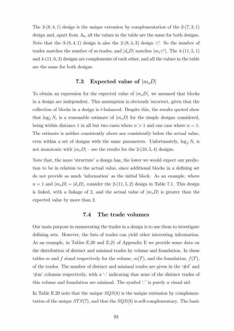
The 3-(8, 4, 1) design is the unique extension by complementation of the 2-(7, 3, 1)
design and, apart from A0, all the values in the table are the same for both designs.
Note that the 3-(8, 4, 1) design is also the 2-(8, 4, 3) design γ∗. So the number of
trades matches the number of m-trades, and |dsD| matches |msγ∗|. The 4-(11, 5, 1)
and 4-(11, 6, 3) designs are complements of each other, and all the values in the table
are the same for both designs.
7.3 Expected value of |msD|
To obtain an expression for the expected value of |msD|, we assumed that blocks
in a design are independent. This assumption is obviously incorrect, given that the
collection of blocks in a design is t-balanced. Despite this, the results quoted show
that logf Ni is a reasonable estimate of |msD| for the simple designs considered,
being within distance 1 in all but two cases where n > 1 and one case where n = 1.
The estimate is neither consistently above nor consistently below the actual value,
even within a set of designs with the same parameters. Unfortunately, logf Ni is
not monotonic with |msD| – see the results for the 2-(10, 5, 4) designs.
Note that, the more ‘structure’ a design has, the lower we would expect our predic-
tion to be in relation to the actual value, since additional blocks in a defining set
do not provide as much ‘information’ as the initial block. As an example, where
n = 1 and |msD| = |dsD|, consider the 2-(11, 5, 2) design in Table 7.1. This design
is linked, with a linkage of 2, and the actual value of |msD| is greater than the
expected value by more than 2.
7.4 The trade volumes
Our main purpose in enumerating the trades in a design is to use them to investigate
defining sets. However, the lists of trades can yield other interesting information.
As an example, in Tables E.20 and E.21 of Appendix E we provide some data on
the distribution of distinct and minimal trades by volume and foundation. In these
tables m and f stand respectively for the volume, m(T ), and the foundation, f(T ),
of the trades. The number of distinct and minimal trades are given in the ‘#d’ and
‘#m’ columns respectively, with a ‘-’ indicating that none of the distinct trades of
this volume and foundation are minimal. The symbol ‘.’ is purely a visual aid.
In Table E.20 note that the unique SQS(8) is the unique extension by complemen-
tation of the unique STS(7), and that the SQS(8) is self-complementary. The basic
93

trades in the two designs are related by Lemmas 4.43 and 4.8. The other trades in
the STS(7) are obtained as restrictions of the trades in the SQS(8). Recall that γ∗
is the 3-design considered as a 2-design. Each basic trade in the SQS(8) yields eight
basic trades in γ∗, as the leaves of the eight points. Each of the other trades in the
SQS(8) yields sixteen trades in γ∗, two for each of the eight points. The 2-(8, 4, 3)
designs have b = 14, and in three of the four designs any set of twelve blocks is a
trade. So, for any pair of blocks in these designs, another design exists which is
disjoint apart from the nominated pair of blocks.
In Table E.21 note that the 4-design is an extension of the 3-design, which, in turn,
is an extension of the STS(9). In these designs the(
v
2
)
trades of volume 2(r − λ2)
produced by a single-transposition permutation of V are always minimal, and are
among the smallest volume trades in the designs. Considered as a 2-design, the
SQS(10) can be decomposed into two copies of H1, see [52]. The 2-(10, 4, 2) designs
have b = 15, and in all four designs any set of twelve blocks is a trade. So, for any
triple of blocks in any of these designs, another design exists which is disjoint apart
from the nominated triple of blocks.
7.5 Searches for trades
When investigating the structure or spectrum of trades, one convenient source of
examples is our enumeration algorithm, or its variants. It is a simple matter to print
out any trades of interest, or to log the volume/foundation combinations found.
Obviously, simple designs yield simple trades, and Steiner designs yield Steiner
trades.
As an example, when investigating S1(5, 3) the volumes of the trades in the 3-
(17, 5, 1) design were recorded, in an attempt to find Steiner (5, 3) trades of ‘small’
volume. Only a partial enumeration can be performed using our algorithm, since
v!n2b2 = 17!12682 ≈ 1.6 × 10¹⁸. This incomplete enumeration produced trades of
volumes 30, 44, 45, 48, 51, 52 and 54, . . ., 68. A volume 45 Steiner (5, 3) trade was
previously unknown, and the one found is that given in Subsection 4.7.2.
This technique has been found to be very useful for producing large numbers
of trades in a design, with many different volumes, foundations, and structures.
Throughout our investigations, such incomplete enumerations were used to find ex-
ample trades or to investigate the trades in a particular design.
94

7.6 Concluding Remark
When solving the BILP, no attempt was made to enumerate or analyse all optimal
solutions, and thus all smallest defining sets. One interesting question for further
investigation is: “under what circumstances can a smallest class defining set, or a
smallest member defining set, be embedded in a smallest defining set?”
95

Chapter 8
Reduced discriminating sets
For simple designs, the problem of finding smallest defining sets can be addressed
by enumerating trades and solving the BILP optimisation problems represented by
these, as discussed in Chapter 6. For non-simple designs, Lemmas 1.8 and 1.9 are
still valid, but repeated blocks introduce problems in the handling of trades.
Example 8.1: Consider the 2-(7, 3, 2) design D consisting of two copies of the Fano
plane of Example 2.1. This contains the Pasch trade {013, 124, 235, 450}. However,
due to the repeated blocks, D contains sixteen ‘copies’ of this particular trade. 2
We must distinguish between all these copies of a trade, and intersect them all in
any defining set. So we need to uniquely label the blocks of a design, and consider
the design as a multiset instead of a set. We could proceed using trades in this
fashion, but we are not interested here in the trades per se, only in their ability to
help us find defining sets. The difference between two designs is a trade, and we are
actually using these trades to discriminate between designs. Developing this idea
leads to the notion of a reduced discriminating set and we show how collections of
these can be used to find defining sets for non-simple designs.
8.1 Multiset notation
Recall that B is the set of blocks of a design D, that B contains b blocks, and that
b∗ of these are distinct. For a non-simple design, b∗ < b. We let B = {b0, . . . , bb−1}.
As a matter of convention, and for later convenience, the blocks of D are assumed
to be labelled in lexicographic order. Note that this means that repeated blocks will
have consecutive subscripts.
We represent a multiset M of subsets of V as a set of ordered pairs (si, mi), where
si is a subset of V and mi is its multiplicity in M . The ordered pairs will be called
melts – for multiset elements – and two melts (si, mi), (sj, mj) are equal if and only
if si = sj and mi = mj. We require that mi > 0 (that is, we do not record subsets
96

of zero multiplicity) and that, if si = sj, then i = j. The cardinality |M | of M is
the number of distinct subsets of V in M ; that is, the support size of M . The total
number of subsets of V in M is denoted by T (M), with T (M) =∑
i mi.
When our multiset M is a design D, or a submultiset of a design, the si will be
blocks of the design, drawn from B. For definiteness, we will identify each si with
the lowest indexed block bj of B such that bj = si. Thus, (si, mi) stands for the
blocks bj, . . . , bj+mi−1.
We define union (∪), difference (\) and intersection (∩) for multisets in the following
fashion. For union, we add the multiplicities of matching blocks thus, {(s, m1)} ∪
{(s, m2)} = {(s, m1+m2)}. For difference, we remove a block’s melt only if it has the
same multiplicity in both multisets. That is, {(s, m1)} \ {(s, m2)} = ∅ if m1 = m2,
and if m1 6= m2 then the melt (s, m1) is unchanged in the difference. This definition
is, perhaps, not the most intuitive one, but it is the one that suits our needs. For
intersection, we use the minimum of the multiplicities thus, {(s, m1)}∩ {(s, m2)} =
{(s, min{m1, m2})}.
We also define a binary operation u, analogous to intersection, but taking into
account multiplicities. A melt (s, m) is in M u M ′ if and only if (s, m) ∈ M and
(s, m) ∈ M ′. Note that D \ D′ = D \ (D u D′). We define the binary relation
subset (⊆) in the obvious way; with D ⊆ D′ if and only if for every (s, m) ∈ D,
(s, m + e) ∈ D′, for some e ≥ 0. For convenience, given a melt (s, m), any melt
(s, m+e), e > 0, is called a supermelt of (s, m), and any melt (s, m−e), 0 < e < m,
is called a submelt of (s, m).
Remark: When a multiset is a set, then \, ∩, and ⊆ have their usual meanings,
with ∩ and u being equivalent. However, ∪ does not have its usual meaning.
8.2 Running example
To illustrate the ideas to be discussed, we will use the ten non-isomorphic 2-(7, 3, 3)
designs, as given in [47]. We label the indecomposable design I and the nine de-
composable designs R1, . . . , R9. Thus, our transversal D = {I, R1, . . . , R9}. The
blocks of these designs, along with the automorphism group orders, Ai, the number
of distinct designs in each isomorphism class, Ni, and the support sizes, b∗, are given
in Table 8.1. The points have been relabelled 0 . . . 6 instead of 1 . . . 7, and the blocks
have been arranged in lexicographic order; the starred entries will be discussed later.
97

Table 8.1: The ten 2-(7, 3, 3) designs
design I R1 R2 R3 R4 R5 R6 R7 R8 R9
b0 012 012 012 012 012 012 012 012 012 012b1 *014 012 012 012 012 012 012 012 012 012b2 016 012 012 *015 012 012 013 *013 013 013b3 024 034 034 026 *034 034 026 026 024 026b4 025 034 034 034 *034 035 034 034 034 034b5 034 034 035 034 035 *036 034 034 035 *035b6 035 056 046 035 046 045 045 045 046 045b7 036 056 *056 046 056 046 056 056 056 046b8 056 056 *056 056 056 056 056 056 056 056b9 123 *135 *134 123 135 134 124 125 *126 *124b10 125 *135 135 134 135 135 135 135 135 135b11 135 *135 135 135 136 136 135 136 136 136b12 136 146 146 146 145 145 *146 145 145 145b13 145 146 146 146 146 146 *146 146 145 146b14 146 146 156 156 146 156 156 146 146 156b15 234 236 236 236 234 234 235 234 234 234b16 236 236 236 236 236 235 236 235 235 235b17 246 236 236 245 236 236 236 236 236 236b18 256 245 245 245 245 *245 245 245 245 245b19 345 245 245 245 245 246 245 246 256 256b20 456 245 245 356 *256 256 *346 *356 346 346Ai 42 168 24 8 12 144 21 3 6 6Ni 120 30 210 630 420 35 240 1680 840 840b∗ 21 7 11 15 13 19 14 17 18 20
Example 8.2: As an example of the multiset representation used, consider R2 =
{(012, 3), (034,2), (035,1), (046,1), (056,2), (134,1), (135,2), (146,2), (156,1), (236,3),
(245,3)}. Here, s0 = b0 = 012, s1 = b3 = 034, . . . , s10 = b18 = 245. Note that
|R2| = 11 = b∗ is the support size of the design, and that T (R2) = 21 = b is the
number of blocks in the design. 2
For ease of exposition in our examples, we take the ten designs listed in Table 8.1
as being all the distinct 2-(7, 3, 3) designs, and find smallest defining sets under this
assumption. That is, we use D instead of D∗. So we will find, for each of the ten
designs, the smallest number of blocks needed to distinguish it from the other nine.
Remark: This is a type of establishing set, where the information we are given
includes a list of all designs which are ‘allowable’ completions.
8.3 Discriminating sets
Suppose that we have a distinguished design D ∈ D∗, and we wish to find a defining
set for D. That is, we wish to uniquely identify D among all the designs in D∗,
98

using only a list of blocks drawn from D. Let D′ be any design in D∗ \ {D}. How
can we discriminate in favour of D, and against D′? Obviously, we must do this on
the basis of the differences between D and D′.
Definition 8.3: Let D = {(s0, m0), . . . , (si, mi)} and D′ = {(t0, n0), . . . , (tj, nj)}
be distinct designs, and suppose that C = D u D′ is the set of melts common to
both D and D′. Then DS(D, D′) = (D \C, D′ \C), is the discriminating set (DS)
for the pair D and D′.
Example 8.4: The top half of Figure 8.1 shows the discriminating sets for some
pairs of designs from D. The blocks are in lexicographic order, reading down
the columns. Blocks in both designs, but with different multiplicities, are on the
same row. Thus, for example, DS(R8, R9) = ({(024, 1), (056,2), (126,1), (145,2)},
{(026,1), (045,1), (056,1), (124,1), (145,1), (156,1)}). 2
Remark: Note that DS are mutually t-balanced. If the designs are simple, then
a DS is a trade. If the designs are non-simple, the two parts of a DS need not be
disjoint; so it need not be a trade, although it does contain a trade.
Given DS(D, D′), the knowledge that a particular melt of DS(D, D′) is in, or is
not in, the design we are attempting to identify enables us to discriminate between
D and D′. Note that we need both the block and its multiplicity to discriminate.
We may speak loosely, and say that D \ C is a discriminating set of D, and that it
discriminates for D and against D′. Any melt of D \ C is said to discriminate for
D and against D′.
Example 8.5: {(024,1), (056,2), (126,1), (145,2)} is a discriminating set of R8,
and it discriminates for R8 and against R9. The melt (145, 2) discriminates for
R8 and, in fact, identifies it uniquely among the designs of D. The melt (146, 2)
discriminates for R2, R3, R4, R6 and R7 and against the other five designs. 2
If our aim is to find defining sets of designs, DS are not quite what we require.
Defining sets consist solely of lists of blocks of the design, with no multiplicity
information. If a block occurs m times in a defining set, it must occur at least m
times in the completed design, but may occur more than m times. Further, the
multiplicities of blocks in a DS are sometimes more than is required to discriminate
between the particular pair of designs.
Example 8.6: The set {012, 012, 012, 056, 056, 156, 236, 236, 236, 245, 245}
is a defining set of R2, among the designs in D∗, but only contains the block 245
99

Figure 8.1: Some example DS and RDS
I R1 R1 R2 R2 R8 R8 R9
(012,1) (012,3) (034,3) (034,2) (012,3) (012,2) (024,1) -(014,1) - - (035,1) - (013,1) - (026,1)(016,1) - - (046,1) - (024,1) - (045,1)(024,1) - (056,3) (056,2) (034,2) (034,1) (056,2) (056,1)(025,1) - - (134,1) - (126,1) - (124,1)(034,1) (034,3) (135,3) (135,2) (134,1) - (126,1) -(035,1) - (146,3) (146,2) (135,2) (135,1) (145,2) (145,1)(036,1) - - (156,1) - (136,1) - (156,1)(056,1) (056,3) - (145,2)(123,1) - (146,2) (146,1)(125,1) - (156,1) -(135,1) (135,3) - (234,1)(136,1) - - (235,1)(145,1) - (236,3) (236,1)(146,1) (146,3) (245,3) (245,1)(234,1) - - (256,1)(236,1) (236,3) - (346,1)
- (245,3)(246,1) -(256,1) -(345,1) -(456,1) -
- (012,2) (034,3) - (012,3) - (024,1) -(014,1) - - (035,1) - (013,1) - (026,1)(016,1) - - (046,1) - (024,1) - (045,1)(024,1) - (056,3) - (034,2) - (056,2) -(025,1) - - (134,1) - (126,1) - (124,1)
- (034,2) (135,3) - (134,1) - (126,1) -(035,1) - (146,3) - (135,2) - (145,2) -(036,1) - - (156,1) - (136,1) - (156,1)
- (056,2) - (145,1)(123,1) - (146,2) -(125,1) - (156,1) -
- (135,2) - (234,1)(136,1) - - (235,1)(145,1) - (236,2) -
- (146,2) (245,2) -(234,1) - - (256,1)
- (236,2) - (346,1)- (245,1)
(246,1) -(256,1) -(345,1) -(456,1) -
twice. The third occurrence of the block in the completed design is forced. The
melt (245, 3) discriminates for R2 and against R8. However, the knowledge that the
design (that is, R2) has at least two copies of the block 245 in it is sufficienct to
discriminate in its favour and against R8. 2
100

Since we wish to find defining sets and, in particular, smallest defining sets, we
accordingly reduce the amount of information in each DS to the minimum necessary
to discriminate between a pair of designs.
Definition 8.7: Let DS(D, D′) = (M, M ′) be the discriminating set of the designs
D and D′. We form the reduced discriminating set (RDS) of the designs D and
D′, RDS(D, D′) = (R, R′), as follows. If (s, m) ∈ M and s is not represented in M ′,
then (s, 1) ∈ R. If s is not represented in M and (s, m′) ∈ M ′, then (s, 1) ∈ R′. If
(s, m) ∈ M , (s, m′) ∈ M , and m > m′ (m 6= m′, by definition), then (s, m′ +1) ∈ R;
if m < m′, then (s, m + 1) ∈ R′.
The rationale behind this definition should be obvious. For example, in the case
m > m′, the knowledge that the design contains at least m′ copies of the block s is
not sufficient to discriminate between D and D′. On the other hand, the knowledge
that it contains more than m′ copies of s is sufficient to discriminate for D and
against D′. We say that the first set of melts in the ordered pair RDS(D, D′) (that
is, those melts or submelts drawn from D) is the RDS of D with respect to D′.
Example 8.8: The bottom part of Table 8.1 gives the RDS derived from the cor-
responding DS in the top part of the table. Note that a melt containing a particular
block can be in one or other of the pair of designs as part of an RDS, but not both.
For example, although both R2 and R8 contain copies of the block 245, this block
can only be used, as part of a defining set, to discriminate for R2 and against R8.
In the absence of precise multiplicity information, it cannot be used to discriminate
in favour of R8 and against R2. 2
Remark: Suppose that m > m′ in the melts (s, m) and (s, m′) of DS(D, D′). Then
any value in the range m′ +1, . . . , m for the number of occurrences of s in a defining
set is sufficient to discriminate for D and against D′.
To use RDS to find all defining sets of a design, we need the following two results,
analogous to Lemmas 1.8 and 1.9 for trades.
Lemma 8.9: Any defining set S of a design D contains a melt, or a supermelt, of
every reduced discriminating set of D.
Proof: We will prove the contrapositive; so, suppose D′ ∈ D∗ \ {D} is such that
S ⊆ D does not contain a melt, or a supermelt, of the RDS of D with respect to D′.
101

Suppose C = D u D′ and let D = C ∪ E and D′ = C ∪ E ′. Note that C ∩ E = ∅,
C ∩E ′ = ∅ and E uE ′ = ∅. Then DS(D, D′) = (E, E ′) and RDS(D, D′) = (F, F ′),
with F ⊆ E and F ′ ⊆ E ′. Let E = F ∪H and E ′ = F ′ ∪H ′. Now a melt u = (s, m)
can be in H for two reasons. If u ∈ E, and a supermelt of u is in E ′, then u was
deleted from the DS when it was reduced. If (s, m + m′ + 1) ∈ E and (s, m′) ∈ E ′,
then m copies of s (that is, u) were removed from the DS when it was reduced. Call
these cases (α) and (β), respectively.
Now, if S ⊆ C, then S ⊆ D and S ⊆ D′. Thus S is not a defining set of D, and
the result follows. So let u = (s, m) ∈ E and suppose that S contains the melt
(s, m∗), for some 0 < m∗ ≤ m. Now, in case (α), u ∈ H and, by the definition of
RDS, F ′ contains (s, m + 1). In case (β), F will contain the melt (s, m∗), for some
m∗ > 0. But m∗ < m∗, since S does not contain a melt or a supermelt of F , and
(s, m∗ − 1) ∈ H ′, by the definition of RDS.
So, in either case, E ′ contains (s, m∗), or a supermelt of (s, m∗). Thus, S ⊆ D′, and
S is not a defining set of D. 2
Lemma 8.10: Any submultiset S of blocks of a design D which contains a melt, or
a supermelt, of every reduced discriminating set of D is a defining set of D.
Proof: Let D′ ∈ D∗\{D} be any design distinct from D and consider RDS(D, D′).
By assumption, S contains u = (s, m), a melt of RDS(D, D′) that belongs to D,
or contains u = (s, m + e), e > 0, a supermelt of a melt (s, m) of RDS(D, D′) that
belongs to D. In either case, by the definition of a reduced discriminating set, s can
be in D′ with multiplicity at most m − 1. Thus, u discriminates for D and against
D′ and S 6⊆ D′. 2
Together, these lemmas give the connection we require between reduced discrimi-
nating sets and defining sets.
Theorem 8.11: A submultiset S of a design D is a defining set of D if and only if
it contains a melt, or a supermelt, of every reduced discriminating set of D. 2
Example 8.12: Since I is the only design of D that contains the block 014, (014,1)
is in every RDS of I and {014} is a defining set. It is obviously a smallest defining
set. As noted previously, R8 is the only design that contains at least two copies
of the block 145. Thus, every RDS of R8 contains either (145, 1) or (145, 2), and
{145,145} is a defining set of R8. This is a minimal defining set, but it is not a
smallest one – consider {126}. 2
102

8.4 An integer linear programme
In light of the results of the last section, we see that, given a list of all the RDS in
all the designs in D, we can find all the defining sets of all the designs. We wish to
find smallest defining sets, and one way to do this is to construct an integer linear
programme (ILP), the optimal solutions of which correspond to smallest defining
sets.
The problem here is to handle those melts that have, in the RDS, multiplicities of
more than one. There may be several melts in different RDS with the same block
s of the design, but different multiplicities. We must have s occur the appropriate
number of times in the ILP’s solution S if we choose it as the representative of a
particular RDS, but we must minimise the total cardinality T (S) of the solution.
When working with trades, we could frame an ILP where both the coefficients and
the variables were binary, and where the bounds on our inequalities were 1’s. That
is, a BILP. For RDS, we frame a pseudo-BILP. Here the variables and bounds are
still binary, but the coefficients need not be; in our case, they can be −1, 0 or +1.
Recall that the blocks of the designs are indexed in lexicographic order. Now, given
a melt (s, m) of an RDS R of D, suppose that the blocks equal to s in D are
bi, . . . , bi+m∗, for some m∗ ≥ m − 1. We use the block bi+m−1 as the representative
of (s, m) in framing the inequality for R. Recall that we use the bi’s as variables
in our ILP to stand for the presence or absence of the bi’s in our solution. Now, if
(s, m) is used as part of our optimal solution, then we require bi = . . . = bi+m−1 = 1.
To enforce this, when m > 1, we add the m − 1 inequalities bi − bi+1 ≥ 0, . . . ,
bi+m−2−bi+m−1 ≥ 0 to our system. That is, we require bj ≥ bj+1, for i ≤ j ≤ i+m−2.
Thus, fixing the value of bi+m−1 at 1 as part of our solution forces all of the lesser
indexed blocks, for the same s, to be 1 also. A value of 0 for bi+m−1 does not force
the values for the lesser indexed blocks.
Note that the values of bi+m, . . . , bi+m∗ are undetermined by the particular RDS
R. These are 0 by default, since our objective is to minimise T (S) =∑
bi, while
some of them may be set to 1 by other RDS. If s is represented in several RDS, it
will figure in several of the inequalities of the system, perhaps under different block
numbers. Among all of these, the one with the highest indexed bi which is set to 1
will determine the values for all the others. Those with lesser indices will be set to
1 and those with greater to 0.
103

Example 8.13: For the designs of D, our objective is to minimise∑20
i=0 bi. If we
are trying to find a defining set for R8, then RDS(R8, R9) yields the inequalities
b3 + b8 + b9 + b13 ≥ 1, b7 − b8 ≥ 0 and b12 − b13 ≥ 0. Note that, in practice, we would
list all the possible bi − bi+1 ≥ 0 inequalites once and then have a single additional
inequality for each RDS. Thus, for R8, the full set of multiplicity control inequalities
is b0 − b1 ≥ 0, b7 − b8 ≥ 0 and b12 − b13 ≥ 0. 2
Given a solution S, not necessarily optimal, of an ILP, if no proper subset of S is
also a solution, then S is called a critical solution. The following result, in light of
the theorem of the last section, and the formulation of the pseudo-BILP, is obvious.
Theorem 8.14: (1) A submultiset S of blocks of a design D is a defining set of D
if and only if it is a solution to the pseudo-BILP obtained from the complete list of
reduced discriminating sets of D in the manner prescribed;
(2) S is a minimal defining set of D if and only if S is a critical solution to the
pseudo-BILP;
(3) S is a smallest defining set of D if and only if it is an optimal solution to the
pseudo-BILP. 2
When using this theorem, we must take care when moving between designs and
defining sets on the one hand, and the pseudo-BILP on the other. In the former,
we do not distinguish between identical blocks in the design. In the latter, each
block is assigned a unique number, and is distinguished from all other blocks. Thus,
given a smallest defining set S of D, when we come to select the bi to represent the
blocks of S, we must use the lowest indexed blocks, to match the fashion in which
we constructed the pseudo-BILP. If we used as representatives the highest indexed
blocks, it would be possible for S to be a smallest defining set without, formally,
being an optimal solution to the pseudo-BILP as presented.
Given the design D, it is possible to form all possible multiplicity control inequalities
of the form bi − bi+1 ≥ 0 without knowledge of any of the RDS in D. It may
be the case that not all of these inequalites are forced on us by the RDS in the
design. Inclusion or not of any unforced inequalities does not affect the above
result, provided we recall that the separate identity of blocks is lost when moving
from the pseudo-BILP to defining sets.
Example 8.15: There are no examples of unforced inequalities among the RDS of
the designs of D. The full pseudo-BILP for R2 is given in Figure 8.2. One optimal
104

Figure 8.2: The pseudo-BILP for R2 (in D)
Minimise20
∑
i=0
bi,
subject to
b0 − b1 ≥ 0,
b1 − b2 ≥ 0,
b3 − b4 ≥ 0,
b7 − b8 ≥ 0,
b10 − b11 ≥ 0,
b12 − b13 ≥ 0,
b15 − b16 ≥ 0,
b16 − b17 ≥ 0,
b18 − b19 ≥ 0,
b19 − b20 ≥ 0,
and
b1 + b4 + b6 + b8 + b9 + b11 + b13 + b14 + b16 + b18 ≥ 1,
b5 + b6 + b9 + b14 ≥ 1,
b2 + b8 + b11 + b17 ≥ 1,
b9 + b14 + b17 + b20 ≥ 1,
b4 + b8 + b11 + b13 + b16 + b19 ≥ 1,
b2 + b5 + b6 + b9 + b17 + b20 ≥ 1,
b2 + b5 + b6 + b9 + b11 + b14 + b16 + b19 ≥ 1,
b2 + b4 + b9 + b11 + b13 + b14 + b16 + b19 ≥ 1,
b2 + b4 + b8 + b9 + b11 + b13 + b16 + b19 ≥ 1.
solution to this system is b7 = b8 = b9 = 1, so {056, 056, 134} is a smallest defining
set for R2, with respect to the other nine designs in D. 2
Remark: Note that there are exactly b−b∗ possible multiplicity inequalities. Thus,
in practice, the impact of these on the number of inequalities in the ILP is negligible.
However, they are responsible for transforming what would be a BILP into a pseudo-
BILP.
Example 8.16: The starred blocks of the designs in Table 8.1 correspond to small-
est defining sets obtained via optimal solutions to the pseudo-BILP. 2
8.5 Minimal discriminating sets
Recall that D∗ is the set of all distinct designs with given parameters, and that
|D∗| = N. Now D ∈ D∗ has an RDS with each of the other N − 1 designs.
However, as in the case of trades, these RDS need not be distinct. Thus, N − 1
105

is an upper bound on the number of distinct RDS of D, where distinct is taken to
mean “containing a different set of melts or submelts of D”.
Example 8.17: Each of the ten designs of D can have at most nine distinct RDS.
For an example where this upper bound is not achieved, note that the RDS of R6
with respect to R1 equals that with respect to R4. That is, {(013,1), (026,1), (045,1),
(124,1), (156,1), (235,1), (346,1)}. Of course, the RDS of R1 and R4 with respect
to R6 are different. 2
As in the case of trades, the number of distinct RDS in a design could be very large.
This could cause the running time to solve the pseudo-BILP to become too long to
be practical. Are all the RDS in a design necessary to find all the defining sets of a
design, or can we minimise the collection in a similar fashion to trades?
Suppose that the collection of RDS of D contains the distinct RDS R′ and R′′.
Suppose further that, for every melt (s, m′) in R′, the melt (s, m′′) is contained in
R′′, and that m′ ≥ m′′ > 0. Then any subset S of D that contains a melt, or a
supermelt, of R′ will also contain a melt, or a supermelt, of R′′. Of course, the
converse will not be true in general.
We say that the RDS R′ covers the RDS R′′. Given a collection of RDS, any RDS in
the collection that is not covered by another RDS is said to be minimal. A collection
of RDS where no RDS is covered by another RDS is said to be minimised.
Example 8.18: The RDS of R8 with respect to R9, {(024,1), (056,2), (126,1),
(145,2)}, covers the RDS of R8 with respect to R3, {(013,1), (024,1), (056,2), (126,1),
(136,1), (145,1), (234,1), (235,1), (256,1), (346,1)}. 2
Remark: If all the designs are simple, then RDS are trades, and the definition of
minimal accords with our previous usage.
The next result follows immediately from the definition of the covering relation.
Lemma 8.19: A submultiset S of a design D is a solution to the pseudo-BILP
obtained from the collection of all reduced discriminating sets of D if and only if
it is a solution to the pseudo-BILP obtained from the minimised collection of all
reduced discriminating sets of D. 2
Suppose that R and R′ are distinct RDS, and that R covers R′. Obviously, |R| ≤ |R′|,
but both |R| < |R′| and |R| = |R′| are possible. We can say nothing about the
relative values of T (R) and T (R′). However, we can minimise a list of RDS using a
106

simple variation of the technique of Subsection 6.2.1. We order RDS by cardinality
– that is, number of melts – and process them in increasing order. We first compare
each RDS of a given size with the list of smaller (minimal) RDS, eliminating any
that are covered. We now compare the RDS of a given size that remain among
themselves, eliminating any that are covered. The remaining RDS are the minimal
RDS of this cardinality.
Remark: The covering relation is a partial order on RDS, and so a collection of
RDS forms a partially ordered set or poset [3]. The problem of finding minimal RDS
is thus equivalent to the problem of finding minimal elements in a poset; similarly
for trades. Trades can be ranked by their cardinality, with two trades of the same
rank being incomparable. Neither | · | nor T (.) can be used to rank RDS, hence the
more complicated algorithm for minimisation.
8.6 Conclusion
The algorithm given in Chapter 6 can be modified, in the obvious manner, to enu-
merate RDS instead of trades; the complexity remains O(v!n2b2). With a complete
list of the RDS in a design to hand, the appropriate collection of RDS can be ex-
tracted, minimised if necessary, and a pseudo-BILP generated. The utility opbdp
that we use is actually intended for solving pseudo-BILP, albeit of a more general
form than ours. It can thus be used to solve the pseudo-BILP, generated from lists
of RDS, of the form described in Section 8.4. We present some results obtained by
this technique in the next chapter.
107

Chapter 9
Results on non-simple designs
In this chapter, lists of all the minimal RDS in a design are used to obtain informa-
tion regarding its defining sets. We consider three series of t-(v, k, λ) designs, where
we fix t, v and k, and vary λ. We are interested in investigating how good the bound
of Lemma 2.31 is for decomposable designs, and the size of smallest member and
class defining sets. A simple algorithm to generate a series of designs is described.
We prove the value of |dsD| for all 2-(6, 3, λ) designs, the first time this has been
done for an infinite family of designs. A method of generating the 3-(8, 4, λ) designs
from the 2-(7, 3, λ) is developed. A good upper bound on |dsD| for these two fami-
lies of designs is proved. We also revisit the 2-(9, 3, 2) designs, and obtain some new
information on their various defining sets.
9.1 The 2-(6, 3, λ) designs
For 2-(6, 3, λ) designs, λ∗ = 2 and λ∗ = 4. The 2-(6, 3, 2) design is unique and is
the only indecomposable design [56]. A fifth degree polynomial in λ is known which
gives the number of different designs for each even λ, see [27]. A smallest defining
set of the 2-(6, 3, 2) design has three blocks, see [46]. A smallest defining set is
isomorphic to {012, 013, 024}, is unique, and occurs 30 times in the design. It is the
only minimal defining set of the design.
For our 2-(6, 3, 2) design, we will take the smallest design in lexicographic order.
We call this design P0, and list its blocks in Figure 9.1. Now |aut(P0)| = 60,
and so there are twelve distinct designs. The eleven designs distinct from P0 are
labelled P1, . . . , P9, Pa, Pb. A permutation generating each of these from P0 is given
in Figure 9.1.
With this list of designs to hand, it is a simple matter to generate all different
designs for a particular λ as unions of Pi’s, using nauty to eliminate isomorphs. We
can now use lists of RDS from these designs to calculate the sizes of various smallest
defining sets. The results, for λ ≤ 12, are collected in Tables F.1–F.5 of Appendix F.
108
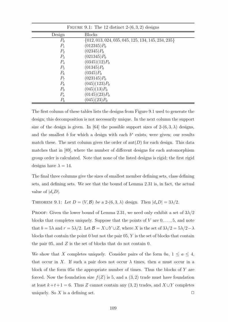
Figure 9.1: The 12 distinct 2-(6, 3, 2) designs
Design BlocksP0 {012, 013, 024, 035, 045, 125, 134, 145, 234, 235}P1 (012345)P0
P2 (02345)P0
P3 (021345)P0
P4 (0345)(12)P0
P5 (01345)P0
P6 (0345)P0
P7 (023145)P0
P8 (045)(123)P0
P9 (045)(13)P0
Pa (0145)(23)P0
Pb (045)(23)P0
The first column of these tables lists the designs from Figure 9.1 used to generate the
design; this decomposition is not necessarily unique. In the next column the support
size of the design is given. In [64] the possible support sizes of 2-(6, 3, λ) designs,
and the smallest b for which a design with each b∗ exists, were given; our results
match these. The next column gives the order of aut(D) for each design. This data
matches that in [89], where the number of different designs for each automorphism
group order is calculated. Note that none of the listed designs is rigid; the first rigid
designs have λ = 14.
The final three columns give the sizes of smallest member defining sets, class defining
sets, and defining sets. We see that the bound of Lemma 2.31 is, in fact, the actual
value of |dsD|.
Theorem 9.1: Let D = (V,B) be a 2-(6, 3, λ) design. Then |dsD| = 3λ/2.
Proof: Given the lower bound of Lemma 2.31, we need only exhibit a set of 3λ/2
blocks that completes uniquely. Suppose that the points of V are 0, . . . , 5, and note
that b = 5λ and r = 5λ/2. Let B = X∪Y ∪Z, where X is the set of 3λ/2 = 5λ/2−λ
blocks that contain the point 0 but not the pair 05, Y is the set of blocks that contain
the pair 05, and Z is the set of blocks that do not contain 0.
We show that X completes uniquely. Consider pairs of the form 0a, 1 ≤ a ≤ 4,
that occur in X. If such a pair does not occur λ times, then a must occur in a
block of the form 05a the appropriate number of times. Thus the blocks of Y are
forced. Now the foundation size f(Z) is 5, and a (3, 2) trade must have foundation
at least k+ t+1 = 6. Thus Z cannot contain any (3, 2) trades, and X∪Y completes
uniquely. So X is a defining set. 2
109

For class defining sets, we note that |csD| = |dsD| if 4 divides λ. If not, then
|csD| is either |dsD| or |dsD| − 1. For the member defining sets, the results vary
considerably, with many intriguing patterns. We prove two simple results.
Lemma 9.2: If D is a multiple of the 2-(6, 3, 2) design E, then |msD| = |dsE| = 3.
Proof: Since E is simple, and has a smallest defining set of size three, any block or
pair of blocks from D obviously has more than one completion to designs isomorphic
to D. A 3-block smallest defining set of E completes uniquely to E and then, since
D is known to be a multiple of a 2-(6, 3, 2) design, D is forced. 2
Lemma 9.3: If D is a multiple of the full 2-(6, 3, 4) design, then |msD| = 0.
Proof: The full design, and its multiples, has |aut(D)| = v!, and so there is only
one distinct design in the isomorphism class. 2
9.2 The 2-(7, 3, λ) designs
For 2-(7, 3, λ) designs, λ∗ = 1 and λ∗ = 5. The smallest defining set sizes for the
designs with λ ≤ 3 were found in [47]; we extend these results to λ = 4, and
also find the sizes of smallest member and class defining sets. There are only two
indecomposable 2-(7, 3, λ) designs for λ ≤ 4, one each for λ = 1 and λ = 3 [56]. In
fact, these are the only indecomposable 2-(7, 3, λ) designs, see [81].
For the indecomposable 2-(7, 3, 1) design – the Fano plane – we take the cyclic design
developed from the starter block 013. For the indecomposable 2-(7, 3, 3) design, we
remove the two disjoint Fano planes developed cyclically from 013 and 023 from the
full design. We label these designs 1.0 and 3.0 respectively, and list the blocks of
1.0 in Figure 9.2.
Now |aut(1.0)| = 168, and so there are 30 distinct designs. The 29 designs distinct
from 1.0 are labelled 1.1, . . . , 1.29. A permutation generating each of these from 1.0
is given in Figure 9.2. For 3.0, |aut(3.0)| = 42, and so there are 120 distinct designs;
we do not list these, since our designs are constructed using at most one copy of the
2-(7, 3, 3) design, and this copy is always 3.0.
The non-isomorphic designs obtained by taking unions of the indecomposable de-
signs are tabulated in Tables F.6–F.8 of Appendix F. Note that the 2-(7, 3, 4) design
marked with a (+) also has a decomposition into four 2-(7, 3, 1) designs. The second
column of these tables give the support of the design and the block multiplicities,
110

Figure 9.2: The 30 distinct 2-(7, 3, 1) designs
Design Blocks Design Blocks1.0 {013, 124, 235, 346, 450, 561, 602} 1.15 (0456)(132)1.01.1 (023456)1.0 1.16 (01456)(23)1.01.2 (0213456)1.0 1.17 (0456)(23)1.01.3 (03456)(12)1.0 1.18 (012456)1.01.4 (013456)1.0 1.19 (02456)1.01.5 (03456)1.0 1.20 (021456)1.01.6 (0312456)1.0 1.21 (0456)(12)1.01.7 (02456)(13)1.0 1.22 (01456)1.01.8 (0231456)1.0 1.23 (0456)1.01.9 (0456)(123)1.0 1.24 (0234156)1.0
1.10 (031456)1.0 1.25 (034156)1.01.11 (0456)(13)1.0 1.26 (0324156)1.01.12 (0132456)1.0 1.27 (04156)(23)1.01.13 (032456)1.0 1.28 (024156)1.01.14 (0321456)1.0 1.29 (04156)1.0
with the value of ni giving the number of k-subsets that occur i times in the design.
The third column gives the automorphism group order for the designs. Note that
the data in the second and third columns distinguishes among all the designs, except
for the 2-(7, 3, 4) pair with block multiplicity vector (16,6,0,0) and |aut(D)| = 2.
The values of the various smallest defining sets are given in the final three columns.
Note that if a design has a decomposition into Fano planes, then |dsD| = 3λ. How-
ever, if all decompositions of a design necessarily contain a copy of the indecom-
posable 2-(7, 3, 3) design, then the lower bound of Lemma 2.31 need not be tight.
Smallest class defining set sizes usually equal |dsD|, although |dsD| − |csD| = 2 for
one of the 2-(7, 3, 4) designs. As for the 2-(6, 3, λ) designs, the results for |msD|
exhibit considerable variability, and results similar to Lemmas 9.2 and 9.3 are easily
proved.
Lemmas 2.25 and 2.31 between them imply that, for any 2-(7, 3, λ) design, 1/3 ≤
µ ≤ 4/7. We prove a better upper bound, which shows that any 2-(7, 3, λ) design
can be defined by less than half its blocks.
Theorem 9.4: If D is a 2-(7, 3, λ) design, then |dsD| ≤ 16λ/5.
Proof: Let V = {0, . . . , 6}, and suppose that D = (V,B) is a 2-(7, 3, λ) design,
with b = 7λ and r = 3λ. Let B = X ∪ Y , where X is the set of blocks that do not
contain the point 0. As in the proof of Lemma 2.25, X is a defining set of D, in
b − r = 4λ blocks. We show that X contains a set of at least 4λ/5 blocks that can
111

be deleted without destroying its unique completion property.
Consider the 3λ blocks in Y . These contain a total of 3λ pairs from V \ {0}. Since
there are(
62
)
= 15 possible pairs, there must be a pair, say ab, that occurs at most
3λ/15 = λ/5 times in Y . Since each pair occurs λ times in D, there must be at least
4λ/5 blocks in X that contain ab. Let the set of blocks in X that contain ab be Z,
and consider X \ Z.
Now X is a 1-(6, 3, 2λ) design, and the blocks of Z have a common pair, so, by
Theorem 5.11, X \Z completes uniquely to X. Hence, X \Z is a defining set of D,
and |dsD| ≤ 4λ − 4λ/5 = 16λ/5. 2
Corollary 9.5: For any 2-(7, 3, λ) design, 1/3 ≤ µ ≤ 16/35. 2
Theorem 9.4, together with Lemma 2.31, is sufficient to prove the value of |dsD| for
all 2-(7, 3, λ) designs which are decomposable into Fano planes and have λ ≤ 4.
9.3 The 3-(8, 4, λ) designs
The 3-(8, 4, λ) designs are self-complementary, and can all be obtained by extending
uniquely the 2-(7, 3, λ) designs by complementation [78]. It is easy to see that the
extension of an indecomposable 2-(7, 3, λ) design is an indecomposable 3-(8, 4, λ)
design, while any restriction of an indecomposable 3-(8, 4, λ) design is an inde-
composable 2-(7, 3, λ) design. So there are precisely two indecomposable 3-(8, 4, λ)
designs, one for λ = 1 and one for λ = 3.
We could proceed as for the 2-(7, 3, λ) designs, and enumerate the 3-designs by
taking unions of the two indecomposable designs. However, since each 2-design
extends uniquely, the number of 3-(8, 4, λ) designs is bounded above by the number
of 2-(7, 3, λ) designs. Hence, the 3-designs can be enumerated simply by extending
the 2-(7, 3, λ) designs and then using nauty to eliminate isomorphs. For 1 ≤ λ ≤ 3,
all the extensions are non-isomorphic, while for λ = 4, the 35 extensions yield 31
non-isomorphic 3-(8, 4, 4) designs – first enumerated in [68].
The smallest defining set sizes for the designs with λ ≤ 3 were found in [47]; we
extend these results to λ = 4. Of course, given Theorem 2.35, we know that a
3-(8, 4, λ) design and its restrictions have the same values of |dsD|. However, we are
also interested in the values of smallest member and class defining sets. The results
are presented in Tables F.9–F.11 of Appendix F, with each design listed being the
extension of the corresponding design in Tables F.6–F.8. Note the doubling of b∗
112

and the entries in the block multiplicity vector, caused by the extension process (cf.
[78]). For the 3-(8, 4, 4) designs we indicate, in the first column of Table F.9, which
extensions of the 2-designs are isomorphic.
Recall that all 8 of the restrictions of a homogeneous 3-(8, 4, λ) design are isomorphic.
All 3-(8, 4, 2), 3-(8, 4, 3), and 27 of the 31 3-(8, 4, 4) are homogeneous. For each of
these designs all three smallest defining sets have the same values in the 2-design
and its extension, and |aut(D)| for the 3-design is eight times that of the 2-design.
For the inhomogeneous 3-designs, the values of |dsD| for the 3-design and its various
restrictions are equal, as required by Theorem 2.35. However, the values of |msD|
in the restrictions need not match, nor need the relationship between the values of
|aut(D)| hold.
Again, results similar to Lemmas 9.2 and 9.3 are easily proved. Further, since the 2-
designs extend uniquely, the defining set of the 2-designs described in Theorem 9.4
is also a defining set of the extensions to 3-designs. Since the extension process
doubles the number of blocks, we have 1/6 ≤ µ ≤ 8/35 in any 3-(8, 4, λ) design.
9.4 The 2-(9, 3, 2) designs
Recall that the STS(9) is unique, and has |dSD| = 4, see [46]. There are precisely
36 different 2-(9, 3, 2) designs, see [96, 87]. Smallest defining sets are given in [71].
We take the designs, and their properties, from these listings, labelling them K1 to
K36. Lists of RDS in the designs were used to verify the sizes of smallest defining
sets, and were also used to find the sizes of smallest member and class defining
sets. Additionally, the sizes of smallest establishing sets were found, where the
establishing information is a set of blocks together with the knowledge of whether
or not the design is simple.
The results are collated in Table 9.1. The second column gives the support size
of the design; if this is 24 the design is simple. The next column gives the single
transpositions of the system; if none, the design is STF. The fourth column indicates
whether or not the design is decomposable, while the fifth indicates the smallest α
for which the design is α-resolvable.
Given a 3-subset {a, b, c}, we can regard it as being ordered cyclically and containing
the three ordered pairs (a, b), (b, c) and (c, a). A collection of such cyclically ordered
blocks that contains each ordered pair from V exactly once is called a Mendelsohn
113

Table 9.1: Results for the 2-(9, 3, 2) designs
Design b∗ STF Dec α Men |A| |msKi| |csKi| |dsKi| |Est|K1 12 Yes Yes 1 1 432 4 8 8 8K2 18 (12) Yes 1 1 24 5 8 8 8K3 20 Yes Yes 1 1 32 6 8 8 8K4 20 Yes No 2 1 8 6 9 9 9K5 20 Yes No 2 0 24 6 8 8 8K6 21 Yes Yes 1 0 6 6 8 8 8K7 22 Yes Yes 1 0 4 6 8 8 8K8 22 Yes No 2 0 2 7 9 9 8K9 22 Yes No 2 1 2 6 9 9 8K10 22 Yes No 2 1 4 6 9 9 8K11 22 Yes No 2 1 2 6 9 9 9K12 22 Yes No 2 0 8 6 9 9 9K13 22 Yes No 2 0 4 6 10 10 9K14 21 Yes Yes 1 1 108 5 9 9 9K15 23 Yes Yes 1 0 4 7 9 9 8K16 23 Yes No 2 0 2 7 8 8 8K17 23 Yes No 2 0 1 7 8 9 8K18 23 Yes No 2 0 2 7 9 9 8K19 23 Yes No 2 1 4 6 9 9 8K20 23 Yes No 2 0 3 6 9 9 8K21 23 Yes No 2 0 1 6 9 9 8K22 23 Yes No 2 2 6 6 10 10 9K23 24 Yes Yes 1 0 18 6 9 9 8K24 24 Yes No 2 0 6 6 9 9 7K25 24 Yes No 2 1 8 6 8 8 8K26 24 Yes No 2 0 1 7 9 9 8K27 24 Yes No 2 0 1 7 9 9 8K28 24 Yes No 2 0 1 7 9 9 8K29 24 Yes Yes 1 1 6 7 8 8 8K30 24 Yes No 2 1 6 7 10 10 9K31 24 Yes No 2 1 2 6 9 9 8K32 24 Yes No 2 0 2 6 7 8 8K33 24 Yes No 2 0 2 6 9 9 9K34 24 Yes No 2 0 8 6 10 10 9K35 24 (23), (67) No 2 1 80 5 9 9 9K36 20 Yes No 2 2 24 6 10 10 10
triple system of order v (abbreviated MTS(v)). Two MTS(v) are equivalent if
they are isomorphic or if reversing the cyclic order of all triples in one system gives
the other. If the order is ignored, then an MTS(v) is obviously a 2-(v, 3, 2) design.
In the sixth column of the table the number of inequivalent MTS(9) that each
2-(9, 3, 2) design admits is given.
The seventh column of Table 9.1 gives the order of aut(Ki). The last four columns
give, respectively, the sizes of smallest member defining sets, class defining sets,
114

defining sets, and simple/non-simple establishing sets. Note that three of the de-
composable designs do not achieve the bound of eight from Lemma 2.31, and that
|csKi| = |dsKi| in all but two cases. For the establishing sets, |dsKi| − |Est| equals
0, 1 and 2 in 17, 18 and 1 cases respectively. There is no overt relationship between
the sizes of the various smallest defining sets and any of a design’s properties.
9.5 Conclusions
The theory of RDS was developed specifically to address the problem of investigating
defining sets in non-simple designs. In this chapter, we have demonstrated that the
theory can be successfully applied to obtain results on defining sets. There are other
designs to which the technique could be applied, but RDS themselves do not seem
to be of any independent interest.
The techniques used to enumerate the 2-(7, 3, λ) and 3-(8, 4, λ) designs are capable
of considerable refinement. However, they are only applicable if the indecomposable
designs are known, and not too numerous.
Inspired by the computational results, new theoretical bounds on the sizes of the
various defining sets for some of the designs were obtained. The techniques used
can be generalised to other designs.
The lower bound on |dsD| from Lemma 2.31 is not tight in general. Further work
is needed to establish the conditions under which it is tight, and to derive a better
bound in those cases where it is not.
115

Chapter 10
Completing partials
In this chapter we consider the problem of completing a partial. That is, given a
collection S of not necessarily distinct k-subsets of a v-set V , with 0 ≤ |S| ≤ b, list
all distinct t-(v, k, λ) designs that contain S.
The utility used to date to complete designs is the programme complete, as de-
scribed in [18]. This programme is general purpose, in that it can handle comple-
tions to designs with any parameters. We describe a new completion programme,
using a heuristic specific to the case λ = 1; that is, to Steiner designs. We describe
the paradigm common to both programmes, and compare their performances. We
also discuss the various uses to which a ‘fast’ completion routine can be put.
Some of the material from this chapter, and from Sections 11.1 and 11.2 of the next
chapter, has been presented in the Technical Report [98] or has been published [99].
10.1 The basic paradigm
The approach used by both of the completion routines is a standard backtrack
search. This is effectively a depth-first traversal of a tree of potential solutions,
where we do not explore any sub-trees that we know cannot contain a solution.
In this search, the k-subsets of V are ordered (usually in the lexicographic order
induced by the standard numeric ordering on the points) and, at each node of the
tree, we iterate over those blocks that come after that chosen at the parent of the
current node, making a recursive call to the search routine for each choice of block.
This ensures that all potential completions are processed and that no solution is
processed more than once.
Of course, the search-space is exponential in size, with the branching factor at each
node being the number of blocks available, and the depth of the tree being b − |S|.
Note that the branching factor is not constant, and can be as bad as(
v
k
)
in non-
simple designs. In developing completion routines our main efforts are directed at
116

devising heuristics to cut down the size of the tree and the portion of it that is
traversed. We do this by decreasing the tree’s depth, by reducing its branching
factor, or by backtracking sooner.
For the completion routines being described, the main strategy is to maintain two
lists of blocks, called the feasible list and the required list. These lists are updated
dynamically as the completion proceeds. The feasible list consists of those k-subsets
of V from which the remainder of the completion must be drawn. That is, any block
which cannot appear in the remainder of the completion has been deleted from the
feasible list. The required list is a subset of the feasible list, and has the property
that at least one of its members must be in the remainder of a completion.
At each stage, the required list is formed from the feasible list, and then the next
block in the completion is iterated over the required list. For each choice, the
feasible list is updated, and then a recursive call is made to the search routine.
Good heuristics are those that keep list sizes as small as possible, and which provide
information to assist in backtracking.
By keeping track of the list sizes, the number of undetermined blocks remaining
in the partial, and counts of the number of times that u-subsets of V, for some
1 ≤ u ≤ t, have appeared in the partial, we can implement backtracking and
forcing. If the lists are too small, then we backtrack. As an example of forcing,
suppose that the required list is produced by tracking the highest frequency u-subset
that has not appeared λu times in the partial so far. Then it may be the case that
the size of the required list is exactly right to bring the count of this particular
u-subset up to λu. In this case either all the blocks in the required list can be added
to the design – that is, they are forced – or else completion of the current partial is
not possible and we backtrack. Forced blocks can be regarded as either reducing the
depth of the current subtree or reducing the branching factor of the current node
to one.
10.2 The complete routine
The complete routine is described in detail in [18], with some of the results obtained
using it being given in [17]. Complete can cope with arbitrary parameter sets
(provided that v is less than the machine’s word size) and can handle pointwise as
well as blockwise completions. We consider only blockwise completions, and outline
the heuristics used.
117

The feasible list is called the hitlist. It is generated initially by picking all k-subsets
of V that do not conflict with the partial supplied. If the design is flagged as being
simple or if λ = 1 (which implies that the design is simple) the feasible list is
updated as blocks are added to and removed from the partial, otherwise it remains
unchanged throughout the completion. The required list is called the options list.
It is generated from the feasible list using the most frequently occurring t-subset
that has not occurred λ times. All blocks from the feasible list that contain the
t-subset are put on the required list, provided they do not conflict with the current
partial.
Remark: Note that producing the required list in this way means that completions
are not produced in lexicographic order. We also have to take care when updating
the feasible list for each choice of block from the required list to ensure that each
completion will be produced once only and that none are missed. The comp03 and
comp04 routines described in the next section also exhibit this behaviour.
The main control structures are lists of the blocks in the current partial and lists
of the frequencies of occurrence of the (t − 1) and t-subsets of V in the current
partial; both lists are maintained in order of decreasing frequency. There are also
some housekeeping lists to track blocks which have been tried or removed from lists.
The lists of (t − 1) and t-subsets are used to attempt block forcing at each stage.
This is done by looking for (t − 1)-subsets which need to occur again, and adding
elements which give t-subsets which can occur again. If exactly k − t + 1 such
elements exist, a block which must be in the design has been constructed. If this
block is not on the hitlist, or conflicts with the current partial, then we backtrack.
Otherwise, the block is added to the design, and the whole process is repeated until
all (t − 1)-subsets have been checked. If no such blocks can be generated then no
forcing is possible, and we simply iterate over the required list.
Complete allows the user to supply information about the design to help speed up
completions. The design (that is, all designs with the given parameters) can be
flagged as simple or linked. Additionally, if the partial is not a defining set, a limit
on the number of completions produced can be set.
118

10.3 The λ = 1 routines
Suppose that we are given a parameter set with λ = 1. Then any designs must
be simple. However, we can say more. No two distinct blocks in the design can
intersect in t or more points, else a t-subset would be repeated. In the terminology of
Section 5.3, a Steiner design is (k−t+1)-simple. When completing, we ensure that at
all times our feasible list has the property that no block in it intersects a block in the
current partial in more than t−1 points. We do not maintain any count whatsoever
of the frequencies of occurrence of the t-subsets; the intersection heuristic just
described ensures that each t-subset occurs at most once in any completion. Thus,
completions automatically contain each t-subset exactly once.
If, at any time, the feasible list becomes too small to supply the remaining blocks
in the current partial, then we backtrack. If the feasible list is exactly the correct
size to fill the remaining blocks, and the feasible list itself is (k− t+1)-simple, then
completion is forced, else we backtrack. Note that, in general, pairs of blocks in the
feasible list can intersect in t or more points.
Calculating intersections, and finding their cardinality, can be done efficiently and
the intersection heuristic has been found to be very effective in reducing the size
of the feasible list. Since the required list is drawn from the feasible list, it too is
substantially reduced in size.
Two versions of the routine were written, differing in the heuristic used to produce
the required list. Programme comp03 uses 1-subset counting (that is, element multi-
plicities), while programme comp04 counts (t−1)-subsets. The required list contains
those members of the feasible list that contain the most frequently occurring 1-subset
(resp. (t − 1)-subset) that has not occurred λ1 (resp. λt−1) times.
Remark: When t = 2 the heuristics of comp03 and comp04 are the same. When
t > 2, we expect comp04 to be the better of the two heuristics. It is easier to code
1-subset counting than (t − 1)-subset counting; it was originally hoped that this
simpler code would yield a faster programme for the case t = 2.
We keep track of the size of the required list, in relation to λ1 or λt−1 as appropriate,
using this to implement forcing or backtracking if possible. Otherwise we iterate
over the required list, adding the current iterate to the partial. The new feasible list
is generated from the old by removing all members that intersect the block chosen
from the required list in more than t−1 points, and any members of the required list
119

Figure 10.1: A completion example for a 3-(14, 4, 1) design
The input partial has 12 blocks:0 6 9 111 4 10 121 6 9 132 3 6 112 4 9 112 4 8 123 4 7 104 5 7 124 5 8 134 8 9 106 7 11 126 8 11 13
Completion number #0:1 5 6 11 <-- first added block4 6 10 110 4 10 132 4 5 100 2 4 61 2 4 72 3 4 130 1 4 53 4 5 114 5 6 90 3 4 80 4 7 90 4 11 12... <-- blocks deleted5 9 10 117 9 10 138 9 11 1210 11 12 13
Single completion - partial is 3-(14,4,1) defining set
that precede the currently chosen block from the required list. (This last is required
to prevent multiple counting of completions.)
Remark: The technique of picking only a single block at a time from the required
list may not be the most effective one. If m 1-subsets (resp. (t− 1)-subsets) remain
to be placed in the partial, and the required list has n > m blocks in it, it might
be more effective to generate and test all(
n
m
)
ways of filling out the requisite count
of 1-subsets (resp. (t − 1)-subsets) from the required list. Of course, the iteration,
recursion, forcing and backtracking do this implicitly, since once a 1-subset (resp.
(t− 1)-subset) becomes the most frequently occurring one that has not occurred λ1
(resp. λt−1) times, it remains so until it has occurred λ1 (resp. λt−1) times. However,
it might be more efficient to do this explicitly.
Example 10.1: One utility constructed using comp04 was cad04. This simply
completes partials to designs in all possible ways, in a similar fashion to cad [18],
which uses complete. Figure 10.1 illustrates how cad04 processed a twelve block
120

Figure 10.2: The set cardinality function
int card(SET ss) /* SET is type ‘unsigned int’ */
{
int temp = 0;
while (ss != 0)
{ temp++; ss = AND(ss,ss-1); } /* AND is bit-wise ‘&’ */
return temp;
}
defining set of one of the four 3-(14,4,1) designs. The search-tree generated had
383 516 nodes, the total running time was 60 sec., and the single completion was
produced after 18 sec. Note that λ2 = 6, and that the only pair of points that
appears in the partial four or more times is 6b (that is, 6 and 11), which appears
four times. Thus 6b is used to build the first required list. After the two blocks
containing 6b are added to the partial, the pair 4a now occurs four times, with every
other pair occuring three times or less. Thus 4a is used to build the next required
list. The next pair chosen is 24 (being the first pair in order that occurs three times),
and so on. 2
10.4 Implementation issues
The comp03 and comp04 routines were developed to investigate defining sets of
designs. Previous workers had considered the ‘smaller’ designs, and were having
difficulty using the existing routines for the next ‘larger’ designs. Thus, programme
speed was very important, and efficiency of implementation took precedence over
elegance. Some of the factors considered are described in this section.
As in complete, sets are implemented as unsigned integers. This limits v to the
machine’s word size, typically 32 bits, but means that basic set operations are fast
and constant time. Since the intersection heuristic is predicated on the ability to
find set cardinalities, an efficient means of calculating the number of elements in a
set is required. We use the card routine shown in Figure 10.2. This uses one of
the bit-counting techniques discussed in [102], and takes O(|ss|) time. Although
[102] also gives routines which are constant time, in our case |ss| is always small –
certainly less than k, and usually less than t – and card is very efficient.
The complete routine makes extensive use of dynamic data structures, in the form
of linked-lists. While this allows the programme to cope with an arbitrary set of
parameters, it is not necessarily the best choice from an efficiency perspective. Some
121

points to consider are:
. Allocating and deallocating memory are operating-system functions. In the
absence of failure, they can be regarded as taking a fixed time; however, they
are much slower than standard arithmetic operations.
. Lists can only be accessed sequentially, and so a significant amount of time
can be spent following pointer chains.
. While it is straightforward to build a sorted list, if the data items are changed
it is expensive to re-sort the list.
. Modern compilers have very sophisticated inbuilt optimisers. Unfortunately,
the presence of pointers restricts the optimisations possible.
For these reasons, arrays were used as the primary data structures in comp03 and
comp04. Array operations are very fast, and optimising compilers are very effective
when dealing with arrays. The only place where sorting is needed in comp03 or
comp04 is to find the most frequently occurring element or (t − 1)-subset in the
current partial to assist in building the required list. Instead of maintaining the
arrays containing these counts sorted, we simply make a single pass over the arrays
as required, and pick out the largest element.
Sorting a singly-linked list using the method adopted in complete is an O(n2)
operation. Picking the largest element of an array can be done simply in O(n) time.
If the number of sorts is the same as the number of times that we need to find the
maximum, as is the case in our routines, there is no advantage in maintaining the
array sorted.
The only potential problem with arrays in C is that their sizes have to be predeclared.
The usual procedure is to pick some maximum size, and use this for all arrays,
irrespective of the actual parameters. The approach adopted for comp03 and comp04
is slightly different.
Since we are limited to λ = 1 and v ≤ 32, the number of admissible parameter sets is
not large. In practice, the number of blocks in a design strongly affects the running
time of completion routines. If we take, say, b < 1000, there are only 39 admissible
parameter sets. Table 10.1 lists the parameters of these 39 designs, as well as the
number of different designs. This table was compiled from [14, 25]. Note that the
2-(16, 6, 1) and 2-(21, 6, 1) designs fail Fisher’s Inequality, and so cannot exist. All
of these parameters sets are recorded in a header file, with one set being ‘active.’
122

Table 10.1: The admissible Steiner systems, v ≤ 32 and b < 1000
design r b n design r b n2-(7,3,1) 3 7 1 3-(8,4,1) 7 14 12-(9,3,1) 4 12 1 3-(10,4,1) 12 30 12-(13,3,1) 6 26 2 3-(14,4,1) 26 91 42-(13,4,1) 4 13 1 3-(16,4,1) 35 140 ≥313012-(15,3,1) 7 35 80 3-(17,5,1) 20 68 12-(16,4,1) 5 20 1 3-(20,4,1) 57 285 ≥1017
2-(16,6,1) 3 8 0 3-(22,4,1) 70 385 ≥212-(19,3,1) 9 57 ≥1.1 × 10⁹ 3-(22,6,1) 21 77 12-(21,3,1) 10 70 ≥2 × 10⁶ 3-(22,7,1) 14 44 02-(21,5,1) 5 21 1 3-(26,4,1) 100 650 ≥12-(21,6,1) 4 14 0 3-(26,5,1) 50 260 ≥12-(25,3,1) 12 100 ≥1014 3-(26,6,1) 30 130 ≥12-(25,4,1) 8 50 18 3-(28,4,1) 117 819 ≥4 × 10²⁰
2-(25,5,1) 6 30 1 4-(11,5,1) 30 66 12-(27,3,1) 13 117 ≥1011 4-(15,5,1) 91 273 02-(28,4,1) 9 63 ≥145 4-(17,5,1) 140 476 ?2-(31,3,1) 15 155 ≥6 × 10¹⁶ 4-(18,6,1) 68 204 02-(31,6,1) 6 31 1 4-(23,7,1) 77 253 1
5-(12,6,1) 66 132 15-(16,6,1) 273 728 05-(24,8,1) 253 759 1
This set of parameters is that used by the completion routine, and any programmes
that incorporate it.
The parameters are thus compile-time constants, allowing the compiler’s optimiser
to perform constant-folding; that is, they can be treated as constants at compile
time, and expressions involving them can be partially evaluated by the compiler. All
arrays are just big enough to contain their maximum data. Of course, programmes
have to be recompiled if a different set of parameters is considered.
We avoid memory allocation problems for the feasible and required lists, and simplify
their handling, by building these in local storage for each call to the search routine,
as opposed to updating single copies of each. The arrays used are fixed size, and
are allocated as part of the normal local-variable allocation from the stack during
the usual function-call handling. Thus, our storage allocation and deallocation is
essentially ‘free,’ although it is wasteful.
Remark: If b−|S| and(
v
k
)
are large, the total amount of memory used by the recur-
sive calls to the search routine may exceed the default amount of stack space. The
depth of the call stack depends on b−|S|, while(
v
k
)
is the main factor in determining
the amount of local storage for each call. If problems occur, the programme’s stack
allocation should be increased, or local storage for the arrays dynamically allocated
123

at entry.
Although the number of parameter sets seems limited, note that it contains Steiner
triple systems, Steiner quadruple systems, projective and affine planes, and both
the small and the large Mathieu designs. The sizes and distributions of defining sets
of these are of interest, and the 39 designs contain examples where these are not yet
known or fully enumerated.
Finally, complete’s method of handling completions is to store them on a list, and
return this list to the user when all completions – or up to the requested number,
if some maximum number of completions has been specified – have been found.
This can cause the allocation of a large amount of memory, which it is the user’s
responsibility to deallocate. It is also not very flexible, and can lead to long waiting
times. The comp03 and comp04 routines are designed to ‘pause’ each time a new
completion is found, to allow the user to process it. A user-supplied function is
called at each completion, then the search is continued. The user’s routine can be
used to abort the search, if no more completions are required. If no user-supplied
function is present, the default is simply to print out and count the completions.
10.5 Performance tests
Assessing the performance of a completion routine, and comparing one routine with
another, turned out to be a challenging task. The results depend on the parameter
set, which of the non-isomorphic designs is being used and the number of blocks in
the partial relative to b. Interestingly, they also depend strongly on which particular
partial of a given size is chosen. Thus, the results are highly case-specific, and
predicting the performance is difficult.
Accordingly, in this section, we present a series of vignettes detailing the results of
a succession of case studies. Each one is intended to illustrate a particular aspect
of performance, and is accompanied by a brief commentary. The coverage is not
exhaustive, but the examples include cases where comp03 and comp04 were used to
obtain new results.
All test runs were on a SPARC-based machine, clocked at 60MHz. Times listed are
the ‘user’ times as reported by the time command, running under the ksh shell.
Time provides a resolution of 0.01 second, so times less than, say, 0.1 second should
be interpreted with care, since they may not accurately reflect the actual CPU time
124
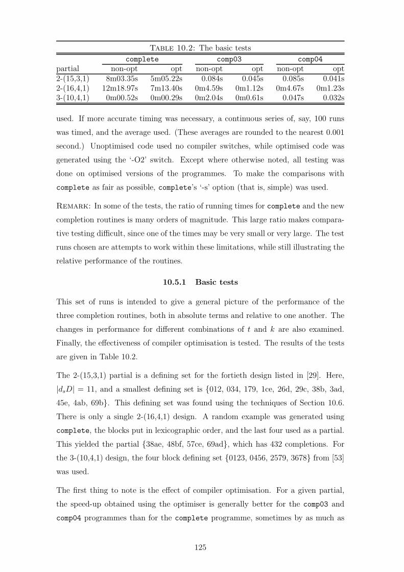
Table 10.2: The basic tests
complete comp03 comp04
partial non-opt opt non-opt opt non-opt opt2-(15,3,1) 8m03.35s 5m05.22s 0.084s 0.045s 0.085s 0.041s2-(16,4,1) 12m18.97s 7m13.40s 0m4.59s 0m1.12s 0m4.67s 0m1.23s3-(10,4,1) 0m00.52s 0m00.29s 0m2.04s 0m0.61s 0.047s 0.032s
used. If more accurate timing was necessary, a continuous series of, say, 100 runs
was timed, and the average used. (These averages are rounded to the nearest 0.001
second.) Unoptimised code used no compiler switches, while optimised code was
generated using the ‘-O2’ switch. Except where otherwise noted, all testing was
done on optimised versions of the programmes. To make the comparisons with
complete as fair as possible, complete’s ‘-s’ option (that is, simple) was used.
Remark: In some of the tests, the ratio of running times for complete and the new
completion routines is many orders of magnitude. This large ratio makes compara-
tive testing difficult, since one of the times may be very small or very large. The test
runs chosen are attempts to work within these limitations, while still illustrating the
relative performance of the routines.
10.5.1 Basic tests
This set of runs is intended to give a general picture of the performance of the
three completion routines, both in absolute terms and relative to one another. The
changes in performance for different combinations of t and k are also examined.
Finally, the effectiveness of compiler optimisation is tested. The results of the tests
are given in Table 10.2.
The 2-(15,3,1) partial is a defining set for the fortieth design listed in [29]. Here,
|dsD| = 11, and a smallest defining set is {012, 034, 179, 1ce, 26d, 29c, 38b, 3ad,
45e, 4ab, 69b}. This defining set was found using the techniques of Section 10.6.
There is only a single 2-(16,4,1) design. A random example was generated using
complete, the blocks put in lexicographic order, and the last four used as a partial.
This yielded the partial {38ae, 48bf, 57ce, 69ad}, which has 432 completions. For
the 3-(10,4,1) design, the four block defining set {0123, 0456, 2579, 3678} from [53]
was used.
The first thing to note is the effect of compiler optimisation. For a given partial,
the speed-up obtained using the optimiser is generally better for the comp03 and
comp04 programmes than for the complete programme, sometimes by as much as
125

Table 10.3: The tree sizes
partial complete comp03 comp04
2-(15,3,1) 415728 375 3752-(16,4,1) 581432 14159 141593-(10,4,1) 258 10413 136
a factor of two. The apparent improvement in optimisation for the longer running
times for comp03 and comp04 is due to the fact that, for small running times, most
of the computation is unavoidable set-up, not backtrack search. The second point
to note is that for designs where t = 2 there is little to choose between comp03 and
comp04. The slightly more complicated code required to handle (t − 1)-subsets as
opposed to 1-subsets does not have a significant speed impact.
When t = 3 the 1-subset counting heuristic is a poor choice, with comp03 actually
being slower than complete. The (t− 1)-subset counting of comp04 yields a speed-
up over comp03 of nineteen times. Note that the ratio of running times between
complete and the better of comp03/comp04 is very variable, being 7444, 387 and
9.1 for the three partials considered, for the optimised code.
10.5.2 Profiling information
The prof family of utilities allow a running programme to be profiled. We can use
this to find the number of calls to the recursive search routine and thus the size of
the search tree that is built. This allows us to assess how efficient our heuristics
are at pruning the tree. For this series of tests the same partials as in the previous
subsection were used. The results are presented in Table 10.3.
The tree size reductions are respectively 1108, 41 and 1.9. If we assume that running
time is proportional to tree size, these ratios can be regarded as the potential speed-
up from the intersection heuristic. Dividing these ratios into those of the running
times from the last subsection we obtain 6.7, 9.4 and 4.8. These final ratios can
be regarded as the ‘non-heuristic’ speed-up of comp03 and comp04 over complete.
That is, more efficient programming techniques and data structures yield a speed-
up of, very roughly, an order of magnitude in the time to process each node of the
search tree.
Remark: Most of the running time of the programme (c. 90%) is accounted for by
the recursive search routine, with the cardinality function card accounting for the
remainder. Although card is very efficient, the intersection heuristic means that it
126

is called frequently. If timing is critical, the function card can be changed to an
inline function; that is, the compiler replaces each function-call by the body of the
function, eliminating the function-call and return overheads. Inlining is not part of
ANSI C, but is supported by many compilers, including gcc.
10.5.3 Completion rate
In the tests described so far, a single completion was performed. If a succession
of completions have to be done, then some of the necessary setup – for example,
building the initial list of k-subsets of V – is common to each completion, and thus
its cost can be amortised. In some of the applications discussed in Section 10.6, large
numbers of partials from a design are tested. It is of interest to find the ‘completion
rate’ in such circumstances.
In an attempt to find smallest defining sets of size eleven for STS(15), random
collections of 12–15 blocks were taken from a design. These were then tested to see
whether or not they were defining sets. If they were, an attempt was made to see
whether or not they contained any smaller defining sets. This was done by removing
up to four blocks from the partial, in all possible ways, and testing the resulting
reduced partial to see whether or not it was a defining set.
During a series of tests on one particular design (W33 of Table 11.1) random partials
of twelve blocks were generated, tested and ‘minimised’ at an average rate of 270
per second. (In fact, since |dsW33| = 12, all defining sets found were minimal.)
For designs W38 and W47, 11 and 10-block subsets, respectively, were tested to see if
any were defining sets. The overall average rate of subset generation and completion
testing for the two designs was 246 and 224 per second respectively. Note that the
larger partials yield the faster rate, as we would expect, since they require less work
in general to complete.
10.5.4 No completions
The purpose of this test is to examine performance in the case where the partial has
no completions. A secondary concern is to look at the performance with ‘higher’
values of t, v or k. The easiest way to obtain partials with no completions is to
choose a parameter set for which a design does not exist. Among the parameter
sets listed in Table 10.1, there are six cases where designs are known not to exist.
Testing was done on the 2-(16,6,1), the 2-(21,6,1) and the 4-(18,6,1) cases. The
127

Table 10.4: The no completions tests
partial complete comp03 comp04
2-(16,6,1) 0m1.40s 0m0.55s -2-(21,6,1) 5h28m37.11s 0m5.28s -4-(18,6,1) >72h51m45.12s - 0m0.11s
results obtained are given in Table 10.4.
For the 2-(16,6,1) and 2-(21,6,1) designs, the partials used consisted of the block
012345 and the pair of blocks {012345, 06789a} respectively; note that these partials
would represent an eighth and a seventh of the blocks of the designs. For the
relatively small v value of 16, complete is slower than comp03 by a factor of only
2.5. However, when v is increased to 21, while comp03 slows down by a factor of
9.6, complete slows down by a factor of 14084, yielding a speed ratio of 3734.
For the 4-(18,6,1) design λt−1 = λ3 = 5, and it is easy to see that, if such a design
did exist, we could assume without loss of generality that it contained the blocks
{012345, 012678, 0129ab, 012cde, 012fgh}. The triple 013 must appear four more
times, so we ‘arbitrarily’ add the blocks {01369c, 0137af, 0138dg, 013beh}. Adding
the further block {0146ae} yields a 10-block partial that is processed by comp04 in
0.11s, with a tree size of only seven nodes. Complete had still not finished after
three days – after which it was aborted – but its running time was long enough to
indicate that comp04 is faster than it by at least six orders of magnitude.
It seems to be the case that the performance of complete degrades rapidly as the
number of combinations(
v
k
)
,(
v
t
)
,(
v
t−1
)
,(
k
t
)
or(
k
t−1
)
; this accords with anecdotal
evidence from the existing body of users of programmes based on complete. The
intersection heuristic used in comp04 seems to be less sensitive to these parameters.
10.5.5 Partial size
The aim of this series of tests is to investigate how the running times of the comple-
tion routines vary as the size of a partial is increased. We are also interested in how
the order in which blocks are added to a partial affects these running times. The
2-(19,3,1) designs were chosen for this test, and a random example was generated
using a partial-completion programme based on comp03. The techniques described
in Section 10.6 were then used to find a random 24-block minimal defining set of this
design. This partial was completed by both complete and comp03, and the orders
in which they added blocks to the partial were recorded. Two series of larger and
128

Table 10.5: The varying partial size tests
ordered by complete ordered by comp03
|dD| complete comp03 #calls complete comp03 #calls24 (min) 3h31m58.05s 0.193s 5659 3h31m45.27s 0.196s 565925 18m07.78s 0.054s 624 1h19m30.69s 0.191s 560326 2m32.45s 0.047s 457 40m19.22s 0.188s 557027 1m12.56s 0.038s 289 16m17.32s 0.188s 556728 0m06.94s 0.036s 288 16m16.75s 0.187s 556629 0m05.33s 0.029s 129 6m41.93s 0.178s 549130 0m03.86s 0.031s 101 2m05.29s 0.178s 548831 0m02.44s 0.028s 98 2m05.11s 0.178s 548732 0m02.46s 0.030s 97 0m26.20s 0.069s 147533 0m01.39s 0.026s 69 0m10.41s 0.063s 147134 0m00.58s 0.028s 46 0m10.27s 0.069s 147035 0.170s 0.028s 46 0m04.21s 0.040s 50336 0.169s 0.029s 45 0m01.26s 0.041s 45837 0.213s 0.028s 73 0m01.26s 0.040s 45738 0.152s 0.027s 42 0m00.60s 0.031s 18439 0.043s 0.027s 29 0m00.23s 0.031s 8740 0.045s 0.026s 28 0m00.25s 0.028s 8641 0.041s 0.026s 27 0m00.11s 0.028s 32
larger defining sets were then generated by adding blocks to the minimal defining
set in the same order. Both series of partials were then run through both completion
routines, recording the running times and, for comp03, the number of recursive calls.
The results are recorded in Table 10.5.
In general, the running times decrease as the partial sizes increase. However, the
results depend strongly on which blocks are added to increase a partial’s size. In
fact, a ‘bad’ choice of block can even cause the running time to increase; cf. the
results for the 37-block partial.
For complete, the difference between the two orderings is very marked. This differ-
ence is less obvious for comp03, but note the sudden decrease in running time (and
number of calls) when the partial size is increased from 24 to 25, using complete’s
ordering. This suggests that, in this case at least, complete’s heuristic for selecting
a block from the required list is better that comp03’s.
For a given ordering, comp03 is always faster than complete, but its advantage
varies between the orderings and with partial size. Note the ‘step-like’ reductions
in running time with partial size and, for comp03, their correlation with reductions
in the size of the search tree.
The running time for comp03 levels out when it reaches approximately 30 millisec-
129

onds, and does not reduce further. This behaviour is characteristic of completion
routines. If the partial is ‘large’ in relation to |dD| or is a ‘substantial’ fraction
of b, completion times are not very sensitive to the size of a partial or its exact
composition. In these cases the tree size is small, and most of the running time is
due to the overhead of starting the programme and initialising the data structures.
This setup time puts a lower bound on the running time of the comp03 and comp04
routines. The main factor is the time to build the list of k and (t − 1)-subsets of
V . When a succession of runs is being performed, this cost can be amortised over
the runs. However, when a single run is performed, or when(
v
k
)
becomes large, this
setup time impacts the shortest attainable running time.
10.5.6 Partials of fixed size
For fixed size partials in a given design, some partials are more ‘difficult’ to complete
than others. The aim of this section is to illustrate the timing differences among
partials of a given size in a given design. For this series of tests, we again use the
3-(10,4,1) design, which has |dsD| = 4. In [53] the 43 isomorphism classes of 4-block
subsets of the design are listed. The representatives listed for each class were used
as the input partials, and the results are given in Table 10.6. (The class used in
Section 10.5.1 was class 3.) The first column is the class number i from [53], with
the second column being the number of completions. The third, fourth and fifth
columns are the running times for complete, comp03 and comp04.
The results for this test are very interesting, and reinforce the comments made
earlier regarding the difficulty of predicting performance. For each of the routines
there is a wide variation in the time required to complete a partial, with the ratio
of the maximum to minimum times being 6.5, 21.1 and 3.6 for the three routines
respectively. The timings for each routine are well scattered throughout the range,
and there seems to be no correlation between the timings for the three routines.
Note that comp04 is always faster than complete, but the speed advantage varies
from 31.8 (class 40) to 5.1 (class 9). Comp04 is also always faster than comp03, with
the speed advantage being 41.7 (class 18) to 3.5 (class 21). Between complete and
comp03, the advantage depends on which partial is used. For class 23 comp03 is
faster than complete by a factor of 7.0, while for class 9 complete is the faster by
a factor of 7.1.
130

Table 10.6: The partials of four blocks of the 3-(10,4,1)
class #com complete comp03 comp04 class #com complete comp03 comp04
1 24 0.607s 2.150s 0.090s 23 3 0.716s 0.102s 0.029s2 24 1.563s 0.424s 0.077s 24 1 0.730s 0.280s 0.025s3 1 0.269s 0.621s 0.033s 25 1 0.336s 0.222s 0.027s4 4 0.624s 1.096s 0.031s 26 2 0.813s 0.321s 0.030s5 4 0.778s 0.358s 0.035s 27 2 0.614s 0.285s 0.028s6 6 0.848s 0.512s 0.038s 28 2 0.405s 0.223s 0.029s7 8 0.519s 0.592s 0.049s 29 2 0.494s 0.293s 0.031s8 8 0.387s 0.489s 0.045s 30 4 0.424s 0.364s 0.032s9 8 0.242s 1.727s 0.047s 31 4 0.731s 0.344s 0.033s
10 6 1.093s 0.512s 0.039s 32 4 0.895s 0.406s 0.033s11 4 0.450s 0.151s 0.039s 33 4 0.350s 0.532s 0.035s12 4 0.688s 0.431s 0.034s 34 4 0.312s 0.438s 0.035s13 4 0.788s 0.424s 0.033s 35 6 0.435s 0.162s 0.037s14 4 0.542s 1.210s 0.037s 36 6 0.401s 0.418s 0.047s15 4 0.542s 0.301s 0.034s 37 6 0.843s 0.149s 0.039s16 4 0.538s 0.412s 0.035s 38 2 0.727s 0.306s 0.030s17 4 0.264s 0.964s 0.032s 39 2 0.769s 0.322s 0.028s18 4 0.292s 1.377s 0.033s 40 4 1.018s 0.421s 0.032s19 4 0.298s 1.318s 0.039s 41 4 0.520s 0.331s 0.031s20 6 1.240s 0.455s 0.040s 42 6 0.626s 0.169s 0.036s21 12 0.719s 0.174s 0.050s 43 4 0.612s 0.365s 0.032s22 12 0.425s 0.267s 0.046s
10.6 Applications
As the behaviour of the new completion routines was investigated, and as they
were used to study defining sets for a variety of designs, a range of utilities using
them was developed. In the subsections that follow we discuss these applications
of completion routines. The results given in Chapter 11 were obtained by utilising
these techniques.
10.6.1 Completing, embedding & extending partials
The first utility developed was, of course, a simple programme which, given a partial,
generates all of its completions. This is intended to test whether or not partials
complete to designs and, if they do, whether or not they are defining sets. It is
useful for checking putative defining sets obtained by other methods, but does not
directly assist in the determination of |dsD|.
The completions of an empty partial are all the distinct designs. When enumerating
all the designs for a given set of parameters we normally only want one example
of each non-isomorphic design. That is, when searching, we reject isomorphs of
designs already found. See [68] for an algorithm for enumerating the designs with
131
given parameters. We do not reject isomorphs when completing a partial, since it
is often the case that a partial is in many distinct, but isomorphic, completions.
So although our completion utility does not enumerate designs in a very efficient
manner, it is sometimes convenient to use it to produce ‘random’ designs. For
example, the number of non-isomorphic 2-(19,3,1) designs is not known, but is at
least 1.1 × 10⁹ (recall Table 10.1). A completion utility based on comp03 produces
distinct 2-(19,3,1) designs at the rate of about 30 per second.
If we wish to produce example designs containing particular configurations of blocks,
if these exist, we simply supply a partial consisting of the configuration to the utility.
For example, the 80 2-(15,3,1) designs contain varying numbers of copies of the Pasch
configuration, from 105 to none. However, if the utility is run with the two disjoint
(in the sense that they have no point in common) Pasch configurations {012, 034,
513, 524, 678, 69a, b79, b8a} as the input partial, no completions are found. Thus,
no 2-(15,3,1) system contains a pair of disjoint Pasch configurations. Running time
was approximately four seconds.
A similar attempt with 2-(19,3,1) systems rapidly produces many examples which
contain two disjoint Pasch configurations. In fact, there are 2-(19,3,1) designs with
three disjoint Pasch configurations; this is obviously the best possible.
Remark: It might be interesting to investigate, for a given configuration of blocks
and value of c, the spectrum for Steiner triple systems that contain c disjoint copies
of the configuration.
A particular instance of embedding a partial is the problem of embedding one design
in another; that is, finding a design that contains a given design as a subdesign. It is
known, see [24], that a 2-(v, 3, 1) design can be embedded in some 2-(w, 3, 1) design
if and only if w is admissible and w ≥ 2v + 1. For example, the completion utility
produced distinct STS(15) containing a copy of the Fano plane at the rate of 45
per second.
Despite this use of the completion routine, the problem of completing a partial is
different from that of embedding a partial. In the former, the parameters are fixed
and known, while in the latter, the parameter v can be varied. For a survey of some
results on embeddings, see [83]. To find an embedding, a non-enumerative technique
such as hill-climbing can be used. See, for example, [30, 107]. Such techniques could
obviously be adapted to find one or two completions. Finding one completion proves
132

that the partial completes to a design, while finding at least two proves that it is
not a defining set. Such techniques cannot find all completions, or prove that none
exist.
We can also use our completion routine to investigate extensions of designs. It is
an open problem whether or not every STS(v) can be extended to an SQS(v + 1).
However, it is known that this is true for v = 7, 9, 13, 15; the three smaller cases
are straightforward, while the case v = 15 was completed in [23]. There are two
STS(13) and four SQS(14), with the two STS(13) having 26 and 65 extensions [92].
In both cases, the completion utility based on comp04 took ≈20 minutes to produce
a complete list of the extensions. Given smallest defining sets for the STS(13), these
lists can be used with Lemma 2.38 to find upper bounds for |dsD| for the SQS(14).
10.6.2 Finding minimal defining sets
If a random selection of s blocks from a design D completes uniquely, then |dsD| ≤ s.
By attempting to find a defining set of a designated size and, if successful, then trying
to find one of the next smaller size, we can obtain a succession of upper bounds for
|dsD|. Despite the crudity of this technique, it is surprisingly effective, although its
efficacy depends critically on the speed of completion, and on the density of defining
sets of particular sizes.
Remark: Note that testing whether or not a set of blocks is a defining set does not
mean that all completions of a partial must be found. If a partial is not a defining
set, completion can be aborted as soon as a second completion is found. Only if a
partial is a defining set must the completion routine be run to its conclusion.
Given a defining set, it may contain a proper subset which is also a defining set; that
is, it may be non-minimal. When searching for ‘small’ defining sets, it is often more
efficient to search for defining sets slightly larger than required and then attempt to
minimise them.
When minimising defining sets, note that if a set of blocks is not a defining set,
then no subset of it is a defining set. Thus, given a defining set S, we can divide
the blocks in it into two classes, essential and non-essential. Any proper subset of
S that is a defining set must contain all the essential blocks. It is easy to classify
the blocks, and test for minimality, by trying to complete the s partials that result
from deleting a single block from S.
133

Suppose our s-block partial S = {b0, . . . , bs−1}. Then, if S \ {bi}, for some bi,
0 ≤ i ≤ s− 1, does not have a unique completion, the block bi is essential and must
be in any subset of S that is a defining set. If S \{bi} has a unique completion, then
bi is non-essential, S is non-minimal, and we have found a smaller defining set. If
S \ {bi} does not have a unique completion for all 0 ≤ i ≤ s− 1, then all the blocks
are essential, and S is minimal.
Remark: The technique quoted in [93, Lemma 9.17] is a faster method of testing
whether or not a defining set is minimal, as it uses larger-sized partials. However,
it does not yield a smaller defining set from a non-minimal defining set.
By successively removing non-essential blocks, we can find all the minimal defining
sets contained in a given defining set, and thus the smallest defining sets it contains.
Of course, these need not in general be smallest defining sets for the design. In
practice, such an exhaustive search may not be feasible, and some limit must be put
on the amount of minimisation attempted for each random partial. With a ‘good’
choice of partial sizes and amount of minimisation, this technique has proved to be
very useful.
The opposite technique, of starting with the essential blocks from the partial and
adding non-essential blocks until a defining set is obtained, is not so useful. In
practice, the number of essential blocks in a defining set can be very small, even
zero. Given that we have some lower bound on |dsD|, the number of ways of building
up the essential blocks into a partial of at least this size is too large to make testing
them all feasible.
For the 80 2-(15,3,1) designs (see the next chapter) the above techniques rapidly
found defining sets that were smallest. The majority of the designs required signifi-
cantly less than a day of computer time, although in some cases runs over a weekend
were required.
10.6.3 Generating trades in designs
An interesting application of completion routines is the generation of trades in a
design. These can be put to many uses: they can be used as part of a study of
trades, either in themselves or as subsets of a design; the algorithm for finding
defining sets described in [51] eliminates partials that do not intersect with any of a
list of trades, and thus cannot be defining sets; the BILP formed from a collection
of trades in a design can be used to provides a lower bound on |dsD|, as used in [71]
134
to assist in finding smallest defining sets for the 36 2-(9,3,2) designs.
We have already described algorithms to enumerate all trades in simple designs, or
all RDS in arbitrary designs. Unfortunately, the high complexity of these algorithms
means that they have limited applicability. An alternative method, in the case of
trades, is to note that, given a partial S ⊆ B which is not a defining set of D, a
completion of S distinct from D defines a trade. Let such a completion be D′; then
it is easy to see that T1 = B \ (B ∩ B′) is a trade contained in D.
Thus, to generate trades in a design D, all we need do is take random partials of
D, find their completions, and then compare these to D. A partial that has c > 1
completions defines up to c − 1 distinct trades in the design. Provided we have a
fast completion algorithm, this technique is very effective in finding large numbers
of trades. In fact, it is so effective that some method for restricting the number
of trades is required. Usually, we consider only minimal trades, put a limit on the
volume of the trades, or consider only some of the completions of each partial.
The random nature of the partials used means that the technique is both non-
deterministic and non-enumerative. Successive runs produce different collections of
trades and there is no guarantee that all (minimal) trades with less than a given
volume have been generated. However, provided the sizes of the random partials
are chosen carefully, good results are generally obtained.
The technique just described was the primary one used to find lower bounds for
|dsD| for the 80 2-(15,3,1) designs. It is iterative, in that the trades from successive
runs are accumulated until the solution to the BILP that these trades represent
– that is, the lower bound on |dsD| – matches the upper bound produced by the
methods of the previous subsection.
10.6.4 Lower bounds on |dsD|, via exhaustion
If the list of trades available for a design is not sufficient to provide a good lower
bound, an exhaustive testing technique can be used. We test all s-block subsets of
B; if none of these is a defining set, then |dsD| > s.
Example 10.2: An STS(15) has 35 blocks, and has 417 225 900 11-block subsets.
On a Pentium-based PC clocked at 133 MHz, it takes 10–11 days to test whether or
not each of these is a defining set, with approximately 450 partials being processed
each second.
135

Since the completion properties of a partial are invariant under isomorphisms, it
might seem that it would be more efficient to divide the s-block subsets into iso-
morphism classes and then complete one representative of each class. This is the
technique used in bds (see [21]), a standard utility for finding smallest defining sets
and based on the algorithm described in [51]. However, to divide the subsets into
classes, a programme such as nauty must be run on each partial to obtain its canonic
form. For the 11-block partials of an STS(15), it was found that completion was
faster than nauty, so the naıve approach is faster. In other cases, it is more efficient
to classify the partials first.
If the automorphism group of a design is non-trivial, we can go some way towards
classifying the partials, without incurring the expense of running nauty on each
partial, by making use of the block orbits under the action of the group. Obviously,
if bi and bj are two distinct blocks in the same orbit, then there is an s-block
defining set containing bi if and only if there is one containing bj. So we can pick a
representative for each orbit, and need only consider partials that contain at least
one of these representatives.
If the design is transitive this can be particularly effective. If not, suppose that the
orbits can be partitioned into two sets O and O∗ such that | ∪i O∗i | < s. Then any
s-block partial must contain a block from an orbit in O. Thus we need only consider
partials which contain one or more representatives of orbits in O .
Example 10.3: The 79th STS(15) – design W79 of the next chapter – has four
block orbits, of sizes 2, 6, 9 and 18. So, when testing 10-block subsets, to establish
that |dsW79| > 10, only partials that contain a representative of the 9 or 18-block
orbit need be tested.
10.6.5 Distribution of defining sets
As well as finding the size of smallest defining sets, we would like to enumerate all
smallest defining sets. In fact, given a design, we would ideally like to classify all
subsets of the design in terms of their defining properties. It is a simple matter to
enumerate all partials in a given design and test them. Obviously, such exhaustive
testing is only possible for the smallest designs.
Where such testing is feasible, it can be used to prove the existence or non-existence
of (minimal) defining sets of a particular size, the number of these, and the number,
size and automorphism groups of their isomorphism classes. Some examples are
136

given in the next chapter.
Where such testing is not feasible, testing random subsets of the blocks of a design
for their defining properties can be helpful in building up a picture of the distribution
of defining sets. Of course, the results are only probabilistic, but they are interesting
nonetheless. We give an example of this technique in the next chapter, where we
investigate specm(D), the spectrum of minimal defining sets, for the 80 STS(15).
10.7 Conclusions
The standard heuristic to speedup the completion of partials involves keeping track
of the u-subsets of V that have appeared so far in the partial, for one or more
values of u, 1 ≤ u ≤ t. This information allows a tree of potential solutions to be
built and traversed efficiently. The intersection heuristic allows t-subset occurrence
to be controlled implicitly, simply by monitoring block intersection sizes. As the
performance tests show, this is very effective, and we present some of our results in
the next chapter. Unfortunately, this heuristic is limited to the case λ = 1.
Monitoring block intersection sizes will not count t-subsets in the general case.
However, if information is available about a design’s block intersection properties, it
can be a very effective heuristic for controlling feasible lists. The complete routine
has a switch to allow it to cope with linked designs, where any pair of distinct blocks
has a fixed intersection size. This could be generalised to affine or quasi-symmetric
designs, where there are two possible intersection sizes, or to any case where all
possible block intersection sizes are known for a particular parameter set.
The intersection heuristic is effectively a very fast method of counting t-subsets. In
general the key to writing fast completion routines seems to be to keep track of
the multiplicities of all u-subsets, 1 ≤ u ≤ t, and then to use this information to
select the ‘best’ next block to add to the partial. There is still considerable scope
for investigating how best to do this, as the most effective method seems to be case
dependent [82].
As the applications listed in Section 10.6 indicate, completion routines are very
useful in investigating defining sets. However, their utility depends critically on
completions being performed rapidly. So it is important that we try to identify ad-
ditional properties of designs that can be used to build efficient completion routines
for other sub-classes of designs.
137

Chapter 11
Results on Steiner designs
The techniques discussed in the previous chapter were applied to a range of Steiner
systems, and a selection of the results obtained are given in this chapter. These
results are of several types: values for |dsD|; enumerations of smallest defining sets;
results on specm(D); and enumerations of minimal defining sets.
11.1 Smallest defining sets of the STS(15)
For v = 7, 9 and 13, there are one, one, and two non-isomorphic STS(v) respectively.
The sizes of smallest defining sets for these were determined in [47, 46, 51], being
three, four, and eight/nine respectively. There are 80 non-isomorphic STS(15) and
we follow [93] in using the standard listing as given in [88], and labelling them W1
to W80. Our results are summarised in Table 11.1. The first two columns are the
design’s label and automorphism group order.
Recall that a Pasch configuration is a set of four blocks isomorphic to {012, 034, 513,
524}, and is a (6,3,2) trade. The number of Pasch configurations, #P, in each design
is given in Table 11.1. Any defining set of Wi must intersect all Pasch configurations
in Wi, and we can use these to obtain a lower bound on |ds(Wi)| by formulating
and solving a BILP. These BILPs were solved using opbdp, and the results, LB, are
given in Table 11.1.
The final column, s, in Table 11.1 gives the size of a smallest defining set. Note
that the bound LB is tight in six cases (it was claimed erroneously in [98] that this
was never the case) and is too low by one in a further ten cases. In Tables G.1–G.8
of Appendix G the blocks of the designs are listed. The points {1, . . . , 15} of [93]
have been relabelled {0, . . . , 9, a, . . . , e}. For each design the blocks of a smallest
defining set are marked with a ‘*’. These smallest defining sets were obtained by
the random sampling and minimising method discussed, so the particular defining
set given has no significance.
138

Table 11.1: Summary of results for the STS(15)
D |A| #P LB s D |A| #P LB sW1 20160 105 15 16 W41 1 12 7 11W2 192 73 14 14 W42 2 8 3 11W3 96 57 14 14 W43 6 10 5 11W4 8 49 12 13 W44 2 8 5 11W5 32 49 12 13 W45 1 9 4 11W6 24 37 11 12 W46 1 7 4 11W7 288 33 11 13 W47 1 10 5 11W8 4 37 12 12 W48 1 8 4 11W9 2 31 11 12 W49 1 7 4 11W10 2 31 11 12 W50 1 6 4 11W11 2 23 9 11 W51 1 9 4 11W12 3 32 10 12 W52 1 9 4 12W13 8 33 11 12 W53 1 10 5 11W14 12 37 12 13 W54 1 11 5 11W15 4 25 11 11 W55 1 9 4 11W16 168 49 14 14 W56 1 8 4 11W17 24 25 11 12 W57 1 5 4 11W18 4 25 11 11 W58 1 8 5 11W19 12 17 9 11 W59 3 13 6 12W20 3 20 9 11 W60 1 7 4 11W21 3 20 7 11 W61 21 14 7 12W22 3 17 5 11 W62 3 7 4 11W23 1 18 8 11 W63 3 7 6 11W24 1 19 8 12 W64 3 10 7 12W25 1 20 10 11 W65 1 7 3 11W26 1 23 10 12 W66 1 6 3 11W27 1 14 8 11 W67 1 5 3 11W28 1 15 8 11 W68 1 6 3 11W29 3 19 10 12 W69 1 5 3 11W30 2 14 7 11 W70 1 9 6 11W31 4 18 8 11 W71 1 5 3 11W32 1 13 7 11 W72 1 5 2 11W33 1 12 7 12 W73 4 6 2 11W34 1 12 7 12 W74 4 8 4 11W35 3 13 7 12 W75 3 7 4 11W36 4 10 6 11 W76 5 10 8 12W37 12 6 3 11 W77 3 2 1 11W38 1 9 4 12 W78 4 6 4 11W39 1 12 6 11 W79 36 6 2 11W40 1 13 7 11 W80 60 0 0 12
For 63 of the 80 values of |dsWi|, the lower bound was proved using a collection of
trades. For the remaining 17, the trade-based lower bound and the upper bound
differed by one. In each case, an exhaustive completion-testing of partials showed
that no partial of the smaller size completed uniquely.
In [93] the nine values of |dsWi| for i ∈ {1, . . . , 8, 16} were determined. Bounds were
given for all the other Wi; of these, 4 lower bounds and 40 upper bounds are tight.
Note that neither |A| nor #P is monotonic with |dsWi|. However, the coefficient
139

of linear correlation between |dsWi| and #P is +0.766. The design W1 arises from
the lines of the geometry PG(3, 2), and contains the maximum possible number
of Pasch configurations; that is, v(v − 1)(v − 3)/24, see [108]. If we regard W1 as
atypical, and omit its data, the coefficient becomes +0.800.
11.2 Minimal defining sets of the STS(15)
Recall the definition of specm(D) in Section 2.3. The comp03 completion utility is
fast enough to allow a large number of partials from each STS(15), for each of a
range of partial sizes, to be tested for their completion properties. Those partials
that are defining sets are counted, and then tested for minimality. For each partial
size of each design, a total of 4 000 000 ‘random’ partials was generated and tested;
total running time was 102 days. The rand function was used to select blocks
of the design uniformly at random. Although rand is not truly random, being a
multiplicative congruential generator, its period of 232 is very much longer than
the number of values required during each run of 4 000 000 partials. Seeding the
generator with the time of day before each run ensures that the runs are independent.
The results of these tests are given in Tables G.9–G.24. The left hand column in
these tables is the partial size, and for each design we list the number of defining
sets and minimal defining sets encountered. A ‘-’ indicates that the partial size is
less than |dsWi| for this design. Note that results are probabilistic; only specm(W1)
and the 80 values of |dsWi| have been proved. It is likely that larger samples would
extend some of the spectra slightly. So the discussion in the following paragraphs
should be read with these caveats in mind.
The design derived from the geometry, W1, has the largest value of max(specm(Wi))
of all the designs, at 22. One and three of the designs have values of 21 and 19
for max(specm(Wi)) respectively, the remainder have values of 18 or 17. None of
the designs have holes in their spectra. All the designs, apart from W1 and W2,
have a ‘smooth’ distribution of minimal defining sets. The ‘spike’ in specm(W2) is
particularly marked; the reason for this is unknown.
The size of the spectrum, |specm(Wi)|, varies from 5 to 8, with there being 2, 9, 48
and 21 designs with each size, respectively. The general shape of the specm(Wi),
for 3 ≤ i ≤ 80, is very similar. However, the probability that a random partial of a
particular size is a minimal defining set, calculated at the ‘peak’ of the distribution,
is very variable, ranging from 0.000234 for W2 to 0.008414 for W80.
140

Figure 11.1: The distribution of defining sets in W2 and W80
0.1 0.2 0.3 0.4 0.5 0.6 0.7 0.8 0.9 1.0
partial size(normalised)
10
10
10
10
10
10
10
probability
-6
-5
-4
-3
-2
-1
0
#2: P(ds)
#2: P(min|ds)
#2: P(min ds)
#80: P(min|ds)
#80: P(ds)
#80: P(min ds)
Note that smallest defining sets are ‘rare,’ with only 26 of the 80 designs yielding
sample ones. However, in 30 of the remaining cases a non-minimal defining set of
size |dsWi| + 1 was found, while a non-minimal defining set of size |dsWi| + 2 was
found in all remaining cases. This supports the claim in Subsection 10.6.2 that
the random search and minimisation technique discussed is an efficient method for
finding small defining sets.
Note that all designs other than W80 contain trades of volume 4 and thus any
collection of 32 or more blocks must be a defining set, and no collection of 33 or
more blocks can be a minimal defining set. The smallest trades in W80 have volume
6, so the corresponding limits here are 30 and 31 blocks. Note that, of the 52 360
31-block partials of a design, the number which are not defining sets of Wi is equal
to the number of Pasch configurations in Wi.
To compare data on the distribution of defining sets for several designs, it can
be helpful to graph the information obtained from samples of partials. This is
illustrated in Figure 11.1 for the two STS(15) W2 and W80 – labelled #2 and #80.
Recall that these are the designs with the minimum and maximum peak probabilities
that a partial is a minimal defining set. For each partial size we calculate P (ds),
P (min ds), and P (min|ds); these are respectively, the probability that a random
partial of the given size is a defining set, a minimal defining set, or a minimal
defining set given that it is a defining set. We plot the probabilities vertically, using
a logarithmic scale. The size of the partials, s, is normalised to s/b.
141

Figure 11.2: The 3-(17,5,1) inversive plane I
0) 0 1 2 3 4 1) 0 1 5 6 7 2) 0 1 8 9 10 3) 0 1 11 12 134) 0 1 14 15 16 5) 0 2 5 8 11 6) 0 2 6 9 14 7) 0 2 7 12 158) 0 2 10 13 16 9) 0 3 5 10 15 10) 0 3 6 11 16 11) 0 3 7 9 13
12) 0 3 8 12 14 13) 0 4 5 13 14 14) 0 4 6 10 12 15) 0 4 7 8 1616) 0 4 9 11 15 17) 0 5 9 12 16 18) 0 6 8 13 15 19) 0 7 10 11 1420) 1 2 5 9 13 21) 1 2 6 12 16 22) 1 2 7 8 14 23) 1 2 10 11 1524) 1 3 5 11 14 25) 1 3 6 9 15 26) 1 3 7 10 12 27) 1 3 8 13 1628) 1 4 5 10 16 29) 1 4 6 8 11 30) 1 4 7 13 15 31) 1 4 9 12 1432) 1 5 8 12 15 33) 1 6 10 13 14 34) 1 7 9 11 16 35) 2 3 5 7 1636) 2 3 6 8 10 37) 2 3 9 11 12 38) 2 3 13 14 15 39) 2 4 5 6 1540) 2 4 7 9 10 41) 2 4 8 12 13 42) 2 4 11 14 16 43) 2 5 10 12 1444) 2 6 7 11 13 45) 2 8 9 15 16 46) 3 4 5 8 9 47) 3 4 6 7 1448) 3 4 10 11 13 49) 3 4 12 15 16 50) 3 5 6 12 13 51) 3 7 8 11 1552) 3 9 10 14 16 53) 4 5 7 11 12 54) 4 6 9 13 16 55) 4 8 10 14 1556) 5 6 8 14 16 57) 5 6 9 10 11 58) 5 7 8 10 13 59) 5 7 9 14 1560) 5 11 13 15 16 61) 6 7 8 9 12 62) 6 7 10 15 16 63) 6 11 12 14 1564) 7 12 13 14 16 65) 8 9 11 13 14 66) 8 10 11 12 16 67) 9 10 12 13 15
11.3 The 3-(17, 5, 1) inversive plane
The unique 2-(16,4,1) design is the affine plane of order 4. This design has 6 distinct
extensions to a 3-(17,5,1) design, all of them isomorphic. So, since the restrictions
of any 3-(17,5,1) design are 2-(16,4,1) designs, the 3-(17,5,1) design is unique. The
3-(17,5,1) design is an inversive plane, and we use the example given in Figure 11.2.
The blocks containing 0 are the extended affine plane, and the extension is the first
in lexicographic order.
We label the design of Figure 11.2 I, and its 68 blocks 0 . . . 67. Now the affine plane
has |dsD| = 7, and each of its six extensions contains a block not in any of the
others. So |dsI| ≤ 8 by Lemma 2.38, while the lower bound from Lemma 2.20 is 6.
We use comp04 and the techniques of the previous chapter to show that |dsI| is, in
fact, 7.
Now |aut(I)| = 16320, and I is transitive. So we need only test all isomor-
phism classes of 6 or 7 blocks from I that contain block 0, and at least 16 points
(Lemma 2.20). There are 3 408 498 such sets of 6 blocks, falling into 2 298 isomor-
phism classes, and none of these is a defining set. There are 7 397 880 such sets
of 7 blocks, falling into 36 065 isomorphism classes, and 4 439 of these classes are
defining sets. Of these, 4 368 have trivial automorphism groups and 71 have groups
of order 2; so the total number of smallest defining sets is
4368 ·16320
1+ 71 ·
16320
2= 71865120.
Lemma 11.1: The unique 3-(17, 5, 1) design has a smallest defining set size of 7
blocks. There are 4 368 classes of smallest defining set with trivial automorphism
142
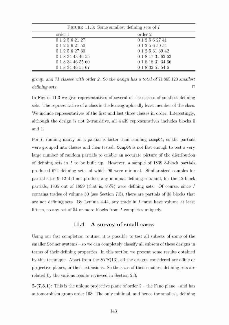
Figure 11.3: Some smallest defining sets of I
order 1 order 20 1 2 5 6 21 27 0 1 2 5 6 27 410 1 2 5 6 21 50 0 1 2 5 6 50 540 1 2 5 6 27 30 0 1 2 5 31 39 420 1 8 34 43 46 55 0 1 8 17 31 62 630 1 8 34 46 55 60 0 1 8 18 31 34 660 1 8 34 46 55 67 0 1 8 32 51 54 6
group, and 71 classes with order 2. So the design has a total of 71 865 120 smallest
defining sets. 2
In Figure 11.3 we give representatives of several of the classes of smallest defining
sets. The representative of a class is the lexicographically least member of the class.
We include representatives of the first and last three classes in order. Interestingly,
although the design is not 2-transitive, all 4 439 representatives includes blocks 0
and 1.
For I, running nauty on a partial is faster than running comp04, so the partials
were grouped into classes and then tested. Comp04 is not fast enough to test a very
large number of random partials to enable an accurate picture of the distribution
of defining sets in I to be built up. However, a sample of 1839 8-block partials
produced 624 defining sets, of which 96 were minimal. Similar-sized samples for
partial sizes 9–12 did not produce any minimal defining sets and, for the 12-block
partials, 1805 out of 1899 (that is, 95%) were defining sets. Of course, since I
contains trades of volume 30 (see Section 7.5), there are partials of 38 blocks that
are not defining sets. By Lemma 4.44, any trade in I must have volume at least
fifteen, so any set of 54 or more blocks from I completes uniquely.
11.4 A survey of small cases
Using our fast completion routine, it is possible to test all subsets of some of the
smaller Steiner systems – so we can completely classify all subsets of these designs in
terms of their defining properties. In this section we present some results obtained
by this technique. Apart from the STS(13), all the designs considered are affine or
projective planes, or their extensions. So the sizes of their smallest defining sets are
related by the various results reviewed in Section 2.3.
2-(7,3,1): This is the unique projective plane of order 2 – the Fano plane – and has
automorphism group order 168. The only minimal, and hence the smallest, defining
143
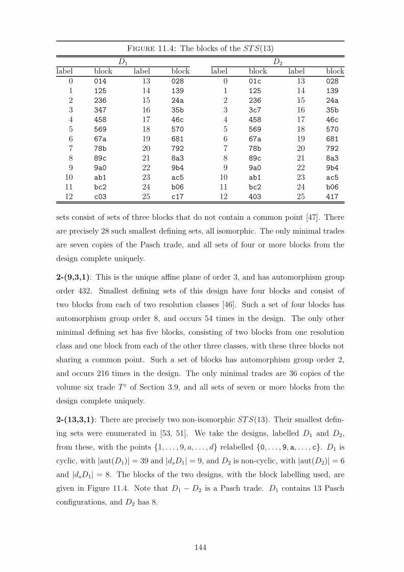
Figure 11.4: The blocks of the STS(13)
D1 D2
label block label block label block label block0 014 13 028 0 01c 13 028
1 125 14 139 1 125 14 139
2 236 15 24a 2 236 15 24a
3 347 16 35b 3 3c7 16 35b
4 458 17 46c 4 458 17 46c
5 569 18 570 5 569 18 570
6 67a 19 681 6 67a 19 681
7 78b 20 792 7 78b 20 792
8 89c 21 8a3 8 89c 21 8a3
9 9a0 22 9b4 9 9a0 22 9b4
10 ab1 23 ac5 10 ab1 23 ac5
11 bc2 24 b06 11 bc2 24 b06
12 c03 25 c17 12 403 25 417
sets consist of sets of three blocks that do not contain a common point [47]. There
are precisely 28 such smallest defining sets, all isomorphic. The only minimal trades
are seven copies of the Pasch trade, and all sets of four or more blocks from the
design complete uniquely.
2-(9,3,1): This is the unique affine plane of order 3, and has automorphism group
order 432. Smallest defining sets of this design have four blocks and consist of
two blocks from each of two resolution classes [46]. Such a set of four blocks has
automorphism group order 8, and occurs 54 times in the design. The only other
minimal defining set has five blocks, consisting of two blocks from one resolution
class and one block from each of the other three classes, with these three blocks not
sharing a common point. Such a set of blocks has automorphism group order 2,
and occurs 216 times in the design. The only minimal trades are 36 copies of the
volume six trade T c of Section 3.9, and all sets of seven or more blocks from the
design complete uniquely.
2-(13,3,1): There are precisely two non-isomorphic STS(13). Their smallest defin-
ing sets were enumerated in [53, 51]. We take the designs, labelled D1 and D2,
from these, with the points {1, . . . , 9, a, . . . , d} relabelled {0, . . . , 9, a, . . . , c}. D1 is
cyclic, with |aut(D1)| = 39 and |dsD1| = 9, and D2 is non-cyclic, with |aut(D2)| = 6
and |dsD1| = 8. The blocks of the two designs, with the block labelling used, are
given in Figure 11.4. Note that D1 − D2 is a Pasch trade. D1 contains 13 Pasch
configurations, and D2 has 8.
144

Table 11.2: The minimal defining sets of D1
size |A| #classes example total9 1 17 0 1 2 3 5 7 8 10 15 663
10 1 1146 0 1 2 3 4 5 6 7 8 14 446943 5 0 1 2 6 8 11 16 18 21 22 65
11 1 1747 0 1 2 3 4 5 6 7 8 9 20 681333 3 0 1 4 6 13 17 20 21 23 24 25 39
12 1 474 0 1 2 3 4 5 6 8 9 14 18 19 184863 3 0 1 2 7 10 11 13 17 18 19 21 24 39
13 1 13 0 1 2 3 4 5 8 14 18 19 20 22 25 5073 1 0 1 10 13 15 16 17 18 20 21 22 23 24 13
Table 11.3: The minimal defining sets of D2
size |A| #classes example total8 1 2 0 2 6 8 14 15 22 23 129 1 864 0 1 2 3 4 5 6 7 15 5184
2 23 0 1 2 5 6 8 12 14 15 6910 1 15597 0 1 2 3 4 5 6 7 9 21 93582
2 99 0 1 2 3 6 7 8 14 15 21 2976 2 0 3 5 13 15 19 20 21 23 25 2
11 1 14019 0 1 2 3 4 5 6 7 12 13 16 841142 61 0 1 2 3 6 8 10 12 13 18 21 1833 1 2 4 5 9 12 16 19 20 22 23 24 2
12 1 1051 0 1 2 3 4 5 7 8 9 13 18 19 63062 5 0 1 2 3 5 8 13 15 17 19 21 25 15
13 1 3 0 1 2 3 6 10 11 15 17 19 23 24 25 18
The STS(13) are small enough for a complete enumeration of all minimal defining
sets to be feasible. The results are presented in Tables 11.2 and 11.3. For each size
where there are minimal defining sets, we list the possible automorphism groups
orders, the number of classes of each order, an example, and the total number of
minimal defining sets of this type.
2-(13,4,1): This is the unique projective plane of order 3, and has automorphism
group order 5616. The example we take is developed from the started block 0139,
and the blocks are labelled 0, . . . ,12, in the order they are developed. A smallest
defining set has 6 blocks [46].
There are two classes of smallest defining sets [52]: one having representative {0 1
2 3 4 5} and automorphism group order 24; and one having representative {0 1 2
3 4 6} and group order 6. So the design has a total of 1 170 smallest defining sets.
Exhaustive testing established that the only minimal defining sets are smallest.
2-(16,4,1): This is the unique affine plane of order 4, and has automorphism group
145

Figure 11.5: The blocks of the 2-(16, 4, 1)
label block label block label block label block0 0123 5 147a 10 25af 15 367f
1 0456 6 158d 11 268c 16 38ae
2 0789 7 16be 12 27bd 17 48bf
3 0abc 8 19cf 13 34cd 18 57ce
4 0def 9 249e 14 359b 19 69ad
Table 11.4: The minimal defining sets of the 2-(16, 4, 1)
size |A| #classes example total7 2 1 0 1 2 7 8 10 17 2880
4 1 0 1 2 7 8 10 16 14406 1 0 1 2 5 7 11 12 960
12 1 0 1 2 7 8 10 12 4808 1 3 0 1 2 3 5 6 7 11 5760
0 1 2 3 5 6 9 12 57600 1 2 3 5 6 10 12 5760
2 3 0 1 2 3 5 6 7 9 28800 1 2 3 5 6 7 10 28800 1 2 3 5 6 9 11 2880
4 1 0 1 2 3 6 7 12 18 14406 1 0 1 2 5 6 9 11 14 960
Table 11.5: The minimal defining sets of the 2-(21, 5, 1)
size |A| #classes example total8 48 1 0 1 2 3 4 7 8 12 25209 2 1 0 1 2 3 4 5 6 7 9 60480
4 1 0 1 2 3 4 5 6 7 8 302406 1 0 1 2 3 4 5 6 11 12 20160
12 1 0 1 2 3 4 5 6 8 10 10080
order 5760. A smallest defining set has 7 blocks [46], and all smallest defining sets
were given [52]. We take the design given in Figure 11.5 as our example, and all
minimal defining sets are enumerated in Table 11.4. Note that all representatives
have blocks 0, 1 and 2 in common.
2-(21,5,1): This is the unique projective plane of order 4, and has automorphism
group order 120 960. The example we take is developed from the starter block
014eg, and the blocks are labelled 0, . . . , 21, in the order they are developed. The
smallest defining set of eight blocks given in [46] is unique, and the only other
minimal defining sets are four classes of nine blocks. The results are summarised in
Table 11.5. Note that all representatives have blocks 0–4 in common.
By our results on Steiner trades, a Steiner (5, 2) trade has volume at least eight,
146

and trades of volume eight or ten have a unique structure. The 2-(21, 5, 1) design
cannot contain any trades of volume ten, since these have foundation 22. However,
it does contain(
212
)
= 210 copies of the volume eight trade, generated by the single
transpositions in S21. The BILP formed from these trades has an optimal solution
of eight blocks and, at least in the examples tested, is a smallest defining set.
This design has too large a v value for our trade enumeration algorithm, but some
partial enumerations were undertaken. The design contains: foundation 18 trades
of volume 8; foundation 19 trades of volume 12; foundation 20 trades of volumes 12
and 14; and foundation 21 trades of volumes 12 and 14–21.
2-(25,5,1): This is the unique affine plane of order 5, and has automorphism group
order 12 000. A smallest defining set has 10 blocks [44]. A sampling technique
was adopted for this design: 2427 out of 77349 samples of ten blocks were smallest
defining sets; 23032 out of 77441 samples of eleven blocks were defining sets, and
of these, 8929 were minimal; similar sized samples for 12–15 block partials failed
to find any other minimal defining sets. Since Steiner (5, 2) trades have volume at
least eight, all partials of 23 or more blocks complete uniquely.
This design has too large a v value for our trade enumeration algorithm, but some
partial enumerations were undertaken. The design contains: foundation 22 trades of
volume 10; foundation 24 trades of volume 16; and foundation 25 trades of volumes
16, 18, 20 and 22–30.
2-(31,6,1): This is the unique projective plane of order 5, and has automorphism
group order 370 000. A smallest defining set has 11 blocks [44]. A sampling technique
was adopted for this design: 267 out of 17614 samples of eleven blocks were smallest
defining sets; 4714 out of 17568 samples of twelve blocks were defining sets, and
of these, 2535 were minimal; similar sized samples for 13–21 block partials failed
to find any other minimal defining sets. Since Steiner (6, 2) trades have volume at
least ten, all partials of 22 or more blocks complete uniquely.
3-(8,4,1): The unique 3-(8, 4, 1) design is the extension by complementation of the
Fano plane, has automorphism group order 1344, and has a smallest defining set of
three blocks [47]. In fact, the only minimal defining sets are the smallest defining
sets. There is a single class of smallest defining sets, consisting of sets of three blocks
with a common point, but no common pair. These are extensions of the smallest
defining sets of the Fano plane, and so the class has 8 × 28 = 224 members.
147

Figure 11.6: The blocks of the 3-(10, 4, 1)
label block label block label block0 0123 12 2347 21 56891 0456 13 1358 22 46792 0789 14 1269 23 45783 0147 15 1567 24 23894 0258 16 2468 25 13795 0369 17 3459 26 12786 0159 18 1489 27 23567 0267 19 2579 28 13468 0348 20 3678 29 12459 0168
10 024911 0357
3-(10,4,1): The 3-(10, 4, 1) design is unique, has automorphism group order 1440,
and is an extension of the 2-(9, 3, 1) design. The design has |dsD| = 4, and there are
three isomorphism classes of smallest defining sets [52]. The example design we use
is given in Figure 11.6. The automorphism group is transitive, so we need only test
partials that contain a nominated block, say 0. All partials of eight or less blocks
were tested, and the results are given in Table 11.6. Note that there are no minimal
defining sets of seven or eight blocks. If specm(D) is hole-free, then Table 11.6 lists
all the minimal defining sets.
When extending the 2-(9, 3, 1), the set of blocks added is a 2-(9, 4, 3) design. There
are three possible choices for this, and these are mutually disjoint [52]. Since a 2-
(9, 4, 3) design has eighteen blocks, the 54 (resp. 216) minimal defining sets of 4 (resp.
5) blocks for the 2-(9, 3, 1) design give rise to 54.18 = 972 (resp. 216.18 = 3888)
defining sets of 5 (resp. 6) blocks for the 3-(10, 4, 1) design. These defining sets have
a point common to 4 out of 5 (resp. 5 out of 6) of the blocks. Since the minimal
defining sets of the 2-(9, 3, 1) have maximum point multiplicity 2 (resp. 3), then the
point on which to restrict in the 3-(10, 4, 1) defining sets obtained in this way is
uniquely determined. Thus such a set of defining sets exist for each point, so there
are a total of 9720 (resp. 38880) defining sets in the 3-(10, 4, 1) design which are
extensions of minimal defining sets of the 2-(9, 3, 1). Of course, these need not be
minimal, but the last four example minimal defining sets in Table 11.6 do arise in
this way. In total, 8 (resp. 4) of the classes of minimal defining sets of 5 (resp. 6)
blocks of the 3-(10, 4, 1) design arise in this way.
4-(11,5,1): The 4-(11, 5, 1) design is unique, has a transitive automorphism group
148

Table 11.6: The minimal defining sets of the 3-(10, 4, 1)
size |A| #classes example total4 2 2 0 1 3 13 720
0 1 3 19 72024 1 0 1 18 19 60
5 1 15 0 1 3 22 28 216002 7 0 1 3 4 21 50408 1 0 1 3 4 29 180
6 1 4 0 1 3 6 11 21 57602 2 0 1 3 6 10 29 1440
Figure 11.7: The blocks of the 4-(11, 5, 1)
label block label block label block label block30 02359 39 02378 48 12368 57 1457931 04678 40 02457 49 12349 58 2567832 01367 41 01389 50 12357 59 3468933 04589 42 02689 51 24569 60 1347834 01248 43 01345 52 34567 61 1258935 05679 44 03479 53 14568 62 2367936 03568 45 01256 54 35789 63 1246737 01279 46 01578 55 16789 64 2345838 01469 47 02346 56 24789 65 13569
Table 11.7: The smallest defining sets of the 4-(11, 5, 1)
size |A| #classes example total5 1 194 0 1 3 13 30 1536480
2 21 0 1 3 13 37 8316010 1 0 1 18 42 64 792
of order 7920 (the small Mathieu group, M11), and is an extension of the 3-(10, 4, 1)
design. The 3-(10, 4, 1) design has two extensions to a 4-(11, 5, 1), with the added
blocks of the extensions being disjoint. The design has |dsD| = 5, and the 1 500
smallest defining sets of four blocks of the 3-(10, 4, 1) give rise to 54 000 smallest
defining sets [52].
There are, however, many more smallest defining sets. We use the example design
M of [52], with blocks 0–29 being the design of Figure 11.6 extended by the point
10, and blocks 30–65 as in Figure 11.7. All sets of five blocks containing the block 0
were tested, and the results are given in Table 11.7. Although the six-block subsets
were not exhaustively tested, M contains at least 865 classes of minimal defining
sets of six blocks; for example, {0,1,3,4,21,32} and {0,1,3,22,26,43}, having group
orders 1 and 2 respectively.
149

5-(12,6,1): The 5-(12, 6, 1) design is unique, and has a transitive automorphism
group of order 95 040 (the small Mathieu group, M12). The design is the unique
extension by complementation of the 4-(11, 5, 1) design, and so is self-complementary
and has |dsD| = 5. Since the design is self-complementary, a smallest defining set
cannot contain a complementary pair of blocks, as then it would not be smallest.
Thus any block in a smallest defining set can be replaced by its complement without
destroying the unique completion property. So each smallest defining set of five
blocks of the 4-(11, 5, 1) design yields 25 = 32 smallest defining sets of the 5-(12, 5, 1);
cf. Lemma 2.37. So the 5-(12, 5, 1) design has precisely 32(1536480+83160+792) =
51853824 smallest defining sets.
150

Appendix A
Reference tables
Table A.1: Symbols & notation used (I)
symbol description reference
u,∩,∪, \,=,⊆ multiset binary operations/relations §8.1δ(G) the minimum degree of G p. 171λ multiplicity of t-subset in a design p. 1λ0, λ1, λt the parameters b, r, λ respectively p. 9λu multiplicity of u-subset in a design, 0 ≤ u ≤ t p. 9λ∗ the minimum admissible λ p. 11
λ∗ (
v−tk−t
)
, the λ for a full design p. 11
µ |dsD|/b p. 18ν(G) the number of vertices in G p. 1714B the set of differences generated by a block p. 104F a difference set / family p. 10AG(n, q) affine geometry, dimension n, over field of order q p. 13aut(D) automorphism group of D p. 10b the number of blocks in a design p. 1b∗ the support size a design p. 1B the (multi-)set of blocks of a design p. 1BIG(D) block intersection graph of a design p. 64cD a class defining set of D p. 82cmD a minimal class defining set of D p. 82csD a smallest class defining set of D p. 82D a generic design, with D = (V,B) p. 1Di representative of the ith class of designs p. 10dD a defining set of D p. 3dmD a minimal defining set of D p. 3dsD a smallest defining set of D p. 3|dsD|, etc. size of a smallest defining set of D, etc. p. 3DS(D1, D2) discriminating set for D1 and D2 p. 99Dl
i set of disallowed volumes associated with sli p. 38
D transversal of the n different designs p. 10D∗ set of all distinct designs p. 10D∗
i set of all distinct designs isomorphic to Di p. 10f (designs)
(
vk
)
/b p. 83f (trades) f(T ), a trade’s foundation size -f(T ) foundation size, of the trade T p. 14F (T ) foundation set, of the trade T p. 14Ft set of allowed volumes p. 39F t set of disallowed volumes p. 39G (graph) a generic (simple) graph p. 171
151

Table A.2: Symbols & notation used (II)
symbol description reference
G (group) a generic group p. 13GF [q] the Galois field of order q p. 13k number of points in a block p. 1(k, t) trade trade with no restiction on foundation size p. 23Kn the complete (simple) graph on n vertices p. 64Lx(T1) the leave of T1 on point x p. 27M11,M12 the small Mathieu groups p. 14M22,M23,M24 the large Mathieu groups p. 14m (trade) m(T ), the volume of a trade p. 2m (general) counter, size of collection -m(T ) volume of the trade T p. 14mD a member defining set of D p. 81mmD a minimal member defining set of D p. 81msD a smallest member defining set of D p. 81MTS(v) Mendelsohn triple system of order v p. 114n (designs) number of non-isomorphic designs, |D| p. 10n (general) general (counting) variable -N total number of distinct designs p. 10Ni total number of distinct designs in ith class p. 10n(S : D) number of subsets of D isomorphic to S p. 18P (ds) probability that partial is a defining set p. 141PG(n, q) projective geometry, dimension n, over field of order q p. 13P (min ds) probability that partial is a minimal defining set p. 141P (min|ds) conditional probability partial is a minimal defining set p. 141RDS(D1, D2) reduced discriminating set for D1 and D2 p. 101Rx(T1) the restriction of T1 on point x p. 27r the multiplicity of a point in a design p. 1rS(T ) multiplicity of the set S (in trade) p. 51r(T ) smallest non-zero point multiplicity in trade T p. 51rx (trade) multiplicity of the point x pp. 27,51rx(T ) (trade) multiplicity of the point x p. 27s (trade) volume of a trade -s (defining set) size of smallest defining set -s(D) number of blocks of D with common (k − 1)-subset p. 74si special trade volumes between 2t and 2t+1 p. 16(si,mi) a block and its multiplicity in a multiset p. 96sli generalisation of the si p. 38
specm(D) the defining spectrum p. 21SQS(v) Steiner quadruple system on v points p. 13STS(v) Steiner triple system on v points p. 13Sv the (symmetric) group of permutation of an v-set p. 9
152

Table A.3: Symbols & notation used (III)
symbol description reference
S[v, k, t] spectrum of [v, k, t] trades p. 23S(k, t) spectrum of (k, t) trades p. 23S(t) spectrum of (t) trades p. 23S1(k, t) spectrum of Steiner (k, t) trades p. 47
S1(k, t) complement of S1(k, t) p. 47t size of subset balanced (trade) or counted (design) p. 1t bt/2c p. 38T (M)
∑
(si,mi)∈M mi, total number of blocks in a multiset M p. 97
T1 − T2 trade, difference of T1 and T2 p. 2t-(v, k, λ) parameters of a design p. 1v number of points in V p. 1(v, k, t) trade trade with upper bound on foundation size p. 2[v, k, t] trade trade with specified foundation size p. 23V a generic v-set, standard set of points p. 1(V,B) a generic design p. 1(
Vl
)
the set of all l-subsets of V p. 73wd, wt w-sizes for minimal defining sets and trades p. 74xA the blocks of A, with the point x adjoined to each p. 26bxc, dxe floor and ceiling functions p. 7x, x new, distinct points p. 7
Zv the integers, mod v p. 10
153

Table A.4: Terms, abbreviations & acronyms (I)
term description referenceα-resolvable partitionable with point multiplicity α p. 11admissible used of the parameters of a design p. 9affine geometry residual geometry of projective geometry p. 13affine plane a 2-(q2, q, 1) design p. 13against (DS) a melt not in this design, but in the other p. 99ANSI American National Standard Institute -antichain a pairwise incomparable family p. 74anti-Pasch does not contain a Pasch configuration p. 77automorphism permutation preserving the set of blocks p. 10basic decomposition a partition of a trade into basic subtrades p. 41basic (trade) a t-trade of volume 2t p. 14bds standard utility for finding defining sets p. 136BILP binary/Boolean/0-1 integer linear programme p. 80block a k-subset of B p. 1block based on G a graph isomorphic to G p. 171block intersection graph graph based on a design’s block intersections p. 64block-residual design produced by non-intersections p. 12block-transitive all blocks in same orbit p. 10blockwise containing only complete blocks p. 22broken pair points paired in only half of a (partial) trade p. 162by complementation a self-complementary extension p. 12cad general-purpose completion utility, complete p. 120cad04 general-purpose completion utility, comp04 p. 120card function to find a set’s cardinality p. 121CAT constant amortised time p. 78class defining set uniquely defines isomorphism class p. 82class trade trade to a non-isomorphic design p. 82collection synonym of set p. 7comp03 Steiner completion utility, t = 2 p. 119comp04 Steiner completion utility, t > 2 p. 119complementary design formed by complementing blocks p. 11complete construct design(s) containing a given partial p. 4complete standard, general-purpose completion utility p. 116complete uniquely contained in only one design p. 4completion design containing given set of blocks p. 4configuration a particular set of blocks p. 71contain blocks of design contain (half) of a trade p. 2covers (RDS) redundancy relation between RDS p. 106CPU central processor unit -critical ILP solution containing no smaller solution p. 104c-trade class trade p. 82cyclic (design) having an automorphism of order v p. 10decomposable partitionable into subdesigns, same v p. 13decomposition (design) a partition into configurations p. 71decomposition (trade) a partition into subtrades p. 41
154

Table A.5: Terms, abbreviations & acronyms (II)
term description referencedefining set subset of design defining it uniquely p. 3defining spectrum the spectrum of minimal defining sets p. 21degree (regular trade) number of times each element occurs p. 62derangement permutation with no fixed points p. 85derived design produced by intersections p. 12design a t-(v, k, λ) design p. 1develop generate orbit from starter block p. 10difference (designs) the difference of two designs is a trade p. 2difference family a set of blocks that generates all differences p. 11difference set a single block that generates all differences p. 10different non-isomorphic p. 9discriminating set the (multiset) difference between designs p. 99distinct not equal p. 10DS discriminating set p. 99embedded subdesign with same λ, smaller v p. 12establishing set any information that defines a unique design p. 81essential if omitted, not a defining set p. 133equivalent (MTS) isomorphic/same under reversal of all pairs p. 114excess (2-trade) positions left after each point used twice p. 35extend (design) add point to blocks, complete to (t + 1)-design p. 12extension design built by extending p. 12family (general) synonym of set p. 7family (Steiner trades) a collection of solely t-balanced sets p. 49Fano plane the 2-(7, 3, 1) projective plane of order 2 p. 13feasible list blocks that could be added to a partial p. 117feasible (swap matrix) potentially a trade p. 162filter upset p. 76final (design) second member of ordered pair p. 78Fisher’s Inequality b ≥ v, in a 2-design p. 11for (DS) a melt in one design, but not the other p. 99forced (block) there is no choice about including it p. 3forcing finding forced blocks p. 117foundation the set of elements in a collection of blocks p. 14from, to a tradeable set of blocks in a design p. 77f -type (clique) clique corresponding to a Fano plane p. 66full design the design consisting of all k subsets of V p. 11full (orbit) cyclic orbit of size v p. 10gcc GNU project C compiler p. 7GNU GNU’s not Unix p. 7G-trade a trade consisting of blocks based on G p. 171Hadamard design symmetric 2-(4m − 1, 2m − 1, m − 1) design p. 13Hadamard 3-design extension of Hadamard design p. 13half (trade) T1 or T2 of a trade T1 − T2 p. 17hole a gap in a defining spectrum p. 21homogeneous all restrictions isomorphic p. 12hyperplane (geometry) n dimensional subspace p. 13
155

Table A.6: Terms, abbreviations & acronyms (III)
term description referenceILP integer linear programme p. 103indecomposable not decomposable p. 13inhomogeneous not homogeneous p. 12initial (design) first member of ordered pair, trade generation p. 78intersection heuristic heuristic for building feasible list p. 119inversive plane a 3-(q2 + 1, q + 1, 1) design p. 13I/O input/output -irreducible indecomposable p. 13i-simple any pair of blocks intersect in ≤ k − i points p. 73isomorphic the same, up to relabelling p. 9k-clique a subgraph isomorphic to Kk p. 64leave (trade) the blocks not containing a point p. 27level (trade) value of l in sl
i p. 38line (geometry) 2 dimensional subspace p. 13linkage intersection size of linked design p. 11linked (design) pairwise block intersections constant size p. 11linked (trade) blocks pairwise intersect in one point p. 62LYM Inequality Lubell, Yamamoto & Meschalkin inequality p. 74mate (trade) given T1, any T2 such that T1 − T2 is a trade p. 17Mathieu designs design from small/large Mathieu groups p. 14melt multiset element, an ordered pair (si, mi) p. 96member trade trade to isomorphic design p. 81member defining set defines member of isomorphism class p. 81Mendelsohn triple system a design with ordered pairs balanced p. 113minimal (defining set) contains no smaller defining set p. 3minimal (trade) contains no smaller trade p. 2minimal (RDS) not covered by another RDS p. 106minimised (trades) non-minimal members removed p. 2minimised (RDS) collection of RDS, covered members removed p. 106m-trade member trade p. 81multiple (design) a design consisting of copies of another p. 11multiplicity frequency of point or subset pp. 27,51nauty the ne plus ultra of isomorphism programmes p. 7non-isomorphic not isomorphic p. 9non-essential can be omitted when minimising defining set p. 133non-simple not simple (i.e., a (proper) multiset) -non-void not empty -null (trade) empty, void p. 2orbit blocks/points related by an automorphism p. 10parallel class set of blocks containing each point once p. 11parameters t, v, k, λ, b, r (design) p. 1partial (design) a family of k-subsets of V p. 4partially-ordered set a set, with an order relation p. 107
156

Table A.7: Terms, abbreviations & acronyms (IV)
term description referencePasch (configuration) one half of the Pasch trade p. 15Pasch (trade) the unique (6, 3, 2) trade of volume 4 p. 15PC personal computer p. 135Pentium Intel marketing-speak for the ’586 processor p. 135plane (geometry) 3 dimensional subspace p. 13point (design/trade) an element of V p. 1point (geometry) 1 dimensional subspace p. 13point-residual design from blocks not containing a point p. 12point-transitive all points in same orbit p. 10pointwise containing partial blocks p. 22poset partially-ordered set p. 107projective geometry all subspaces of a particular vector space p. 13projective plane a 2-(q2 + q + 1, q + 1, 1) design p. 13pseudo-BILP pseudo-binary integer linear programme p. 103quasi-symmetric two possible intersection sizes p. 11ranked not defined p. 107RDS reduced discriminating set p. 101reduced discriminating set reduced multiset difference between designs p. 101reducible decomposable p. 13regular (trade) all points occur the same number of times p. 62required list at least one must be in any completion p. 117resolvable can be partitioned into parallel classes p. 11restriction (design) design from blocks containing a point p. 12restriction (trade) the blocks containing a point p. 27rigid (design) having a trivial automorphism group p. 10self-complementary design equal to its complement p. 11semitriangular starting blocks strictly increasing p. 15short (orbit) cyclic orbit of size < v p. 10simple (trade/design) having no repeated blocks (i.e., a set) p. 2single transposition a permutation of the form (ij) p. 18single transposition free not containing any single transpositions p. 18smallest (defining set) no defining set is smaller p. 3smallest (trade) a (k + t + 1, k, t) trade of volume 2t p. 15solely t-balanced t-balanced, but no repeated (t + 1)-subset p. 49SPARC scalable processor architecture -specifying set defining set using block intersection sizes p. 81spectrum (trades) the possible volumes p. 23Sperner family antichain p. 74starter block block used in developing orbit p. 10starting block first block of trade, in lexicographic order p. 15Steiner (trade/design) any t-subset occurs (at most) once p. 2Steiner quadruple system a 3-(v, 4, 1) design p. 13
157

Table A.8: Terms, abbreviations & acronyms (V)
term description referenceSteiner triple system a 2-(v, 3, 1) design p. 13STF single transposition free p. 18s-transitive transitive on sets of s blocks/points p. 10subdesign subset of design which is also a design p. 12subtrade a trade within a trade p. 31submelt a melt containing fewer copies of a block p. 97supermelt a melt containing more copies of a block p. 97support set of distinct blocks in a collection p. 1support size size of the support p. 1symmetric (design) has b = v, k = r, and is linked p. 11swap matrix describes distribution of elements in trade p. 162tail (trade) set of points common to all blocks p. 15t-design a t-(v, k, λt) design p. 1trade a pair of disjoint and balanced collections p. 2trade mate a matching half of a trade p. 17transitive block-transitive p. 10transversal representatives of the isomorphism classes p. 10trivial (design) empty, or necessarily full/multiple p. 11trivial (general) euphemism for ‘uninteresting’ or ‘boring’ -trivial (group) only member is the identity p. 10t-balanced having the same t-subsets p. 2t-trade a (v, k, t) trade p. 14unique (design) there is a single isomorphism class p. 10unique completion the only design containing a given set of blocks p. 4upset a family that contains all supersets of its members p. 76wholly undetermined a block none of whose elements are yet fixed p. 168viable template a partially constructed trade p. 162void (trade) empty, null p. 2volume (trade) size of each collection p. 2v-type (clique) clique corresponding to points p. 66Witt designs design from small/large Mathieu groups p. 14w-size weighted size of an antichain p. 74
158

Appendix B
Summary of results
For some results on 1-trades in designs and on defining sets of 1-designs see §5.3.
Table B.1: Smallest defining set sizes, t = 2
design r b n |dsD| reference2-(6,3,2) 5 10 1 3 [46]2-(6, 3, λ) 5λ/2 5λ see [27] 3λ/2 §9.12-(7,3,1) 3 7 1 3 [47]2-(7,3,2) 6 14 4 64 [47]2-(7,3,3) 9 21 10 7, 99 [47]2-(7,3,4) 12 28 35 10, 1234 §9.22-(7, 3, λ) 3λ/7 7λ see [14] 7λ/3–16λ/5 §9.22-(8,4,3) 7 14 4 64 [47]2-(9,3,1) 4 12 1 4 [46]2-(9,3,2) 8 24 36 810, 921, 105 [71]2-(9,4,3) 8 18 11 62, 89 [95]2-(10,4,2) 6 15 3 5, 6, 8 [52]2-(10,4,4) 12 30 >998 16 (3) [52]2-(10,5,4) 9 18 21 62, 718, 8 [74, 100], §7.1.52-(11,5,2) 5 11 1 5 [46]2-(13,3,1) 6 26 2 8, 9 [51]2-(13,4,1) 4 13 1 6 [46]2-(15,3,1) 7 35 80 1152, 1220, 134, 143, 16 [93, 99], §11.12-(15,7,3) 7 15 5 73, 8, 9 [48, 49]2-(16,4,1) 5 20 1 7 [46]2-(16,6,2) 6 16 3 72, 9 [52]2-(19,9,4) 9 19 6 86 [94]2-(21,5,1) 5 21 1 8 [46]2-(25,5,1) 6 30 1 10 [44]2-(23,11,5) 11 23 1103 8 (q) [94]2-(27,13,6) 13 27 ≥7 ≤11 (q) [94]2-(31,6,1) 6 31 1 11 [44]2-(31,15,7) 15 31 ≥106 ≤10 (q) [94]
24 (pg) [38]2-(63,31,15) 31 63 ≥1017 52–55 (pg) [38]
(3): the 3-(10, 4, 1) as a 2-design(q): the Hadamard design from the quadratic residues(pg): the design associated with PG(d,2)
159

Table B.2: Smallest defining set sizes, t = 3
design r b n |dsD| reference3-(8,4,1) 7 14 1 3 [47]3-(8,4,2) 14 28 4 64 [47]3-(8,4,3) 21 42 10 7, 99 [47]3-(8,4,4) 28 56 31 10, 1230 §9.33-(8, 4, λ) 7λ 14λ see §9.3 7λ/3–16λ/5 §9.33-(10,4,1) 12 30 1 4 [52]3-(10,5,3) 18 36 7 5, 62, 84 [95, 100], §7.1.43-(12,6,2) 11 22 1 5 [94]3-(16,8,3) 15 30 5 73, 8, 9 [94]3-(17,5,1) 20 68 1 7 §11.33-(20,10,4) 19 38 3 83 [94]3-(22,6,1) 21 77 1 8 [93]3-(24,12,5) 23 46 ≥1 8 (q) [94]3-(28,14,6) 27 54 ≥1 ≤11 (q) [94]3-(32,16,7) 31 62 ≥1 ≤10 (q) [94]
(q): the Hadamard design from the quadratic residues
Table B.3: Smallest defining set sizes, t ≥ 4
design r b n |dsD| reference4-(11,5,1) 30 66 1 5 [52]4-(23,7,1) 77 253 1 8 [93]5-(12,6,1) 66 132 1 5 [52]5-(24,8,1) 253 759 1 8 [16, 93]
Table B.4: Other results on defining set sizes
design |msD| |csD| establishing reference2-(6, 3, λ)
√ √- §9.1
2-(7,3,3) - - within transversal §8.42-(7, 3, λ)
√ √- §9.2
2-(8,4,3)√ √
- §7.1.12-(9,3,2) - - simple/non-simple §9.42-(9,4,3)
√ √- §7.1.3
2-(10,4,2)√ √
- §7.1.22-(10,5,4)
√ √- §7.1.5
3-(8, 4, λ)√ √
- §9.33-(10,5,3)
√ √- §7.1.4
160

Table B.5: Distribution of smallest/minimal defining sets
design description reference2-(7,3,1) minimal defining sets (all) §11.42-(9,3,1) minimal defining sets (all) §11.42-(13,3,1) minimal defining sets (all) §11.42-(13,4,1) minimal defining sets (all) §11.42-(15,3,1) minimal defining sets (sampled) §11.22-(16,4,1) minimal defining sets (all) §11.42-(21,5,1) minimal defining sets (all) §11.42-(25,5,1) minimal defining sets (sampled) §11.42-(31,6,1) minimal defining sets (sampled) §11.43-(8,4,1) minimal defining sets (all) §11.43-(10,4,1) minimal defining sets (all) §11.33-(17,5,1) smallest defining sets (all) §11.3
minimal defining sets (sampled) §11.34-(11,5,1) smallest defining sets (all) §11.3
minimal defining sets (partial count) §11.35-(12,6,1) smallest defining sets (all) §11.3
Table B.6: Trades in designs
design description reference2-(7,3,1) all trades by volume/foundation §7.42-(8,4,3) all trades by volume/foundation §7.42-(9,3,1) all trades by volume/foundation §7.42-(13,3,1) Pasch trades §11.42-(10,4,2) all trades by volume/foundation §7.42-(15,3,1) number of Pasch trades §11.22-(15,3,1) disjoint Pasch trades §10.6.12-(19,3,1) disjoint Pasch trades §10.6.12-(21,5,1) discussion §11.42-(25,5,1) discussion §11.43-(8,4,1) all trades by volume/foundation §7.43-(10,4,1) all trades by volume/foundation §7.43-(17,5,1) known trade volumes §7.54-(11,5,1) all trades by volume/foundation §7.4
. See also Appendix E, and Chapter 7
161

Appendix C
The swap matrix technique (Chapter 4)
The proofs in this appendix use what we term the swap matrix technique. Suppose
that an element x has multiplicity rx in a Steiner (k, 2) trade T = T1−T2. The idea
is to list the possible arrangements of elements in the blocks containing x in T1 and
T2.
Recall that the rx(k − 1) elements with which x occurs must all be distinct. Since
T1 ∩ T2 = ∅, the 2rx blocks in T1 ∪ T2 containing x must all be distinct. Label the
blocks of each of T1 and T2 containing x with 1, 2, . . . , rx. Let
S = [sij], 1 ≤ i, j ≤ rx,
be an rx × rx matrix where sij is the number of elements, other than x, from block
j of T1 that appear in block i of T2. S is called a swap matrix and it is simple to
see that 0 ≤ sij ≤ k− 2 and the row and column sums of S equal k− 1. Thus, each
row and column of S is a partition of k − 1 into rx parts, at least two of which are
non-zero.
Any swap matrix can occur in many distinct but equivalent forms. Permutations of
rows and columns lead to equivalent swap matrices. Permuting rows is equivalent
to reordering the blocks of T2 and permuting columns to reordering the blocks of
T1. Transposing S is equivalent to exchanging T1 and T2. We will always use a
form where s11 ≥ sij and s12 ≥ s21, and where the first row and the first column
are non-increasing. Note that this is not sufficient to eliminate all equivalences but
suffices in the cases we consider.
Suppose that xab ⊆ B ∈ T1, and that no block of T2 which contains x also contains
both a and b. Then the pair ab is called a broken pair. A swap matrix is said
to be feasible if all the broken pairs can be contained, as partial blocks, in the
m(T ) − rx remaining blocks of T2 without violating the Steiner property. Given a
feasible swap matrix, an apportioning of the broken pairs to the remaining blocks
of T2 is called a viable template. Note that a feasible swap matrix may yield more
162

than one viable template, and that a viable template is not necessarily extendable
to a Steiner trade.
We will determine possible swap matrices for Steiner (k, 2) trades of volume m for
specific values of k and m. In the first two sections of this appendix, these are used
to prove non-existence for the cases where k = 5, m = 11 and k = 6, m = 13. In the
final section, they are used to show structural uniqueness for the case where k = 5,
m = 10.
C.1 Steiner (5, 2) trades of volume 11
For Steiner (5,2) trades, the only volume where existence is not yet settled is eleven.
We will assume that such a trade, T = T1 − T2, exists and obtain a contradiction.
Including repetitions, there are 11× 5 = 55 elements in T1 and hence there must be
an element in F (T ) with odd multiplicity. Since each element must occur at least
twice and no more than six times, by Lemma 4.14, there must be an element with
multiplicity three or five. We will show that both cases are impossible.
Lemma C.1: If T is a Steiner (5, 2) trade with m(T ) < 12, then there is no element
with multiplicity three.
Proof: Let x ∈ F (T ) and rx = 3. The possible partitions in a swap matrix for x
are {3,1,0}, {2,2,0} and {2,1,1}. It is easy to see that, up to equivalence, there are
only six possible swap matrices. These are shown in the first column of Table C.1.
Let the elements occurring with x be 1, 2, . . . , 9, a, b, c. The column headed T2
is obtained by applying the swap matrix to T1. The broken pairs are listed in the
final column. Each row of broken pairs comes from the corresponding block of T1.
We will show that none of these swap matrices is feasible in less than 12 blocks.
For a given swap matrix, any two broken pairs from two different rows contain four
distinct elements. Since there are only three rows containing x, two such broken
pairs cannot appear together in a block in T2 without duplicating a pair already in
the blocks of T2.
The rows of broken pairs labelled with a star are generated by columns of the swap
matrix with a partition of {3,1,0} or {2,2,0}. These rows have the property that
no two broken pairs in the same row can occur in the same block of T2 without
violating the Steiner propery. Thus we see that the third and fourth swap matrices
imply that there are at least twelve and fifteen blocks in T2 respectively. Similarly,
163

Table C.1: The swap matrices for Steiner (5,2) trades with rx = 3
Swap Matrix No. T1 T2 Broken Pairs
3 1 01 2 10 1 3
1 x 1 2 3 4x 5 6 7 8x 9 a b c
x 1 2 3 5x 4 6 7 9x 8 a b c
14, 24, 34∗
56, 57, 58, 68, 789a, 9b, 9c∗
3 1 01 1 20 2 2
2 x 1 2 3 4x 5 6 7 8x 9 a b c
x 1 2 3 5x 4 6 9 ax 7 8 b c
14, 24, 34∗
56, 57, 58, 67, 689b, 9c, ab, ac∗
3 1 01 0 30 3 1
3 x 1 2 3 4x 5 6 7 8x 9 a b c
x 1 2 3 5x 4 9 c bx 6 7 8 c
14, 24, 34∗
56, 57, 58∗
9c, ac, bc∗
2 2 02 0 20 2 2
4 x 1 2 3 4x 5 6 7 8x 9 a b c
x 1 2 5 6x 3 4 9 ax 7 8 b c
13, 14, 23, 24∗
57, 58, 67, 68∗
9b, 9c, ab, ac∗
2 2 01 1 21 1 2
5 x 1 2 3 4x 5 6 7 8x 9 a b c
x 1 2 5 6x 3 7 9 ax 4 8 b c
13, 14, 23, 24, 3457, 58, 67, 68, 789b, 9c, ab, ac∗
2 1 11 2 11 1 2
6 x 1 2 3 4x 5 6 7 8x 9 a b c
x 1 2 5 9x 3 6 7 ax 4 8 b c
13, 14, 23, 24, 3456, 57, 58, 68, 789a, 9b, 9c, ab, ac
to generate a trade in less than twelve sets from the second swap matrix would
require that all of the pairs in the second row occurred in the same set, which would
repeat the pair 78 in T2.
The remaining three swap matrices all contain rows of five broken pairs derived from
the partition {2,1,1}. All these sets of five broken pairs are isomorphic to the set
{56, 57, 58, 68, 78} from swap matrix No. 1. The pair 67 already appears in T2, so
the pairs 56 and 57 must occur in different blocks in T2, as must the pairs 68 and
78. If we used the two partial blocks 568 and 578 to cover all broken pairs, the pair
58 would occur twice. Thus each row of broken pairs without a star requires at least
three blocks in T2.
The first, fifth and sixth swap matrices would require an additional nine, ten and
nine blocks respectively in T2. Thus the total number of blocks in T2 is greater than
eleven. 2
Lemma C.2: If T is a Steiner (5, 2) trade of volume eleven, then there is no element
with multiplicity six.
Proof: Suppose y ∈ F (T ) and ry = 6. Then y is paired with 6(k−1) = 24 distinct
elements. Each of these elements must occur at least once in the five blocks not
containing y, leaving exactly one position of these blocks unaccounted for. This
position cannot contain a new element, since it would have multiplicity one. Thus
164

one of the elements occurring with y must have multiplicity three, contradicting
Lemma C.1. 2
As the number of elements with odd multiplicity is necessarily odd and because there
is no element with multiplicity three, there must be an odd number of elements with
multiplicity five. It is easy to see that three or more elements with multiplicity five
cannot be contained in eleven blocks without duplicating a pair. Thus there must
be exactly one element with multiplicity five.
For 2 ≤ i ≤ 6, let ni denote the number of elements of F (T ) that have multiplicity
i. We have shown that n3 = n6 = 0 and that n5 = 1. Thus 2n2 +4n4 +5 = 55; that
is, n2 + 2n4 = 25. Given that n5 = 1, it is straightforward to check that there are
at most four elements with multiplicity four; that is, n4 ≤ 4.
The following analogue of Lemma 4.16 is needed to complete our analysis.
Lemma C.3: Let T = T1 − T2 be a Steiner (5, 2) trade with rα = 2 for some
α ∈ F (T ), and suppose that∑
i≥3 ni ≤ 7. If B1 and B2 are the two blocks of T1
containing α, then there exist (distinct) elements x ∈ B1 and y ∈ B2 such that at
least four blocks of T1 contain x but not y and at least four blocks contain y but
not x.
Proof: The possible partitions are {3,1} and {2,2} and there are only two inequiv-
alent swap matrices for α,
S1 =
3 1
1 3
, S2 =
2 2
2 2
.
Without loss of generality, let B1 = α1234 and B2 = α5678. We first prove that S2
is not feasible.
If S2 is feasible then, without loss of generality, α1256 and α3478 are in T2. This
yields the set of broken pairs {13, 14, 23, 24, 57, 58, 67, 68}. Now, no two of these
pairs can occur together in T2, since the trade is Steiner. Thus each of the elements
1, . . . , 8 must occur at least three times in T2, contradicting∑
i≥3 ni ≤ 7.
We now show S1 is feasible and yields a single viable template. We can assume,
without loss of generality, that α1235 and α4678 are in T2. This yields the set of
broken pairs {14, 24, 34, 56, 57, 58}. Now, no two of these pairs can occur together
in T2, since the trade is Steiner. Thus both x = 4 and y = 5 occur in at least four
blocks that do not contain the other element. 2
165

Theorem C.4: If T is a Steiner (5, 2) trade, then m(T ) 6= 11.
Proof: Assume that T = T1 − T2 is a Steiner (5, 2) trade of volume eleven. We
will derive a contradiction.
The only integral solutions (n2, n4) to n2 + 2n4 = 25 satisfying the necessary condi-
tion n4 ≤ 4 are (17,4), (19,3), (21,2), (23,1) and (25,0). The case (25,0) is eliminated
immediately by Lemma C.3. Recall that n5 = 1 and note that n4 > 0 in all remain-
ing cases. Let x be the element with multiplicity five. Since n4 ≤ 4, there must
be at least one block, say B, which contains x and none of the multiplicity four
elements.
First, suppose that each of the elements of multiplicity four occurs in some (but
not necessarily the same) block in which x occurs. The four elements that occur
with x in B must be multiplicity two elements. Thus the elements of multiplicity at
least four that these elements are paired with must be x and one of the multiplicity
four elements. But all multiplicity four elements are paired with x, contradicting
Lemma C.3.
Thus there exists an element, say y, with multiplicity four which does not occur in
a block with x. Let U and V be the two blocks containing neither x nor y. Consider
the 5(k − 1) = 20 distinct elements contained in a block with x. Since n4 ≤ 4, at
least 17 of these have multiplicity two. Now at most 4(k − 1) = 16 of these can
occur in blocks containing y. Thus one of them, say z, occurs in one of U or V, say
U. By Lemma C.3, z occurs with two elements, say α and β, each of which occurs
in four blocks not containing the other. Now, at least one of α or β, say α, must
have multiplicity four and be contained in U . The other three occurrences of α
must be in V, in a block with y, and a block with x (not that containing z). Now
consider β. We cannot have β = x, since we already have the pair αx, contradicting
Lemma C.3. Thus rβ = 4, and it must occur in the block containing xz, in a block
with y, and in both U and V. But the pair αβ is repeated and this completes the
proof. 2
C.2 Steiner (6, 2) trades of volume 13
The only volume for Steiner (6,2) trades whose existence is unresolved is thirteen.
Such a trade would have a total of 78 elements in T1, with possible element mul-
tiplicities of r = 2, . . . , 7. Exhaustive searches by computer programmes based on
166

Table C.2: The swap matrices and templates for Steiner (6,2) trades
r Swap Matrix T1 T2
2 4 11 4
x 1 2 3 4 5x 6 7 8 9 a
x 1 2 3 4 6x 5 7 8 9 a1 5 ∗ ∗ ∗ ∗2 5 ∗ ∗ ∗ ∗3 5 ∗ ∗ ∗ ∗4 5 ∗ ∗ ∗ ∗6 7 ∗ ∗ ∗ ∗6 8 ∗ ∗ ∗ ∗6 9 ∗ ∗ ∗ ∗6 a ∗ ∗ ∗ ∗∗ ∗ ∗ ∗ ∗ ∗∗ ∗ ∗ ∗ ∗ ∗∗ ∗ ∗ ∗ ∗ ∗
5 1 1 1 1 11 1 1 1 11 1 1 1 11 1 1 1 11 1 1 1 1
x 1 2 3 4 5x 6 7 8 9 ax b c d e fx g h i j kx l m n o p
x 1 6 b g lx 2 7 c h mx 3 8 d i nx 4 9 e j ox 5 a f k p1 2 3 4 5 ∗6 7 8 9 a ∗b c d e f ∗g h i j k ∗l m n o p ∗∗ ∗ ∗ ∗ ∗ ∗∗ ∗ ∗ ∗ ∗ ∗∗ ∗ ∗ ∗ ∗ ∗
6 1 1 1 1 1 01 1 1 1 0 11 1 1 0 1 11 1 0 1 1 11 0 1 1 1 10 1 1 1 1 1
x 1 2 3 4 5x 6 7 8 9 ax b c d e fx g h i j kx l m n o px q r s t u
x 1 6 b g lx 2 7 c h qx 3 8 d m rx 4 9 i n sx 5 e j o tx a f k p u1 2 3 4 5 ∗6 7 8 9 a ∗b c d e f ∗g h i j k ∗l m n o p ∗q r s t u ∗∗ ∗ ∗ ∗ ∗ ∗
the swap matrix method yielded a single equivalence class of feasible swap matrices
for each of r = 2, 5 and 6, and showed that none existed for r = 3 or 4. Each fea-
sible swap matrix yielded a single viable template. The matrices, with T1 and the
templates for T2, are shown in Table C.2. Note that all three of the swap matrices
are symmetric, so the templates for T1 are isomorphic to those for T2. Using these
templates, we will show that it is not possible to construct a Steiner (6, 2) trades of
volume thirteen.
167
Lemma C.5: If T = T1 − T2 is a Steiner (6, 2) trade of volume thirteen, then there
is no element with multiplicity seven.
Proof: Suppose there exists an element of multiplicity seven in T1. Such an element
is paired with 7(k−1) = 35 distinct other elements. Each of these 35 elements must
occur at least once more which leaves one position of the trade unaccounted for.
This remaining position must be filled by an element of multiplicity one or three.
However, multiplicity one is not possible and there are no viable templates for r = 3.
This completes the proof. 2
Theorem C.6: If T is a Steiner (6, 2) trade, then m(T ) 6= 13.
Proof: Let n2, n5 and n6 denote the number of elements of F (T ) that have mul-
tiplicity 2, 5 and 6 respectively. Then 2n2 + 5n5 + 6n6 = 78. Now it is easy to see
that n5 ≤ 3 and n6 ≤ 2, else the Steiner property is violated. Further, the feasible
template for r = 2 shows that, if n2 ≥ 1, then n5 + n6 ≥ 2. Considering all these
equations and inequalities, and noting that n5 must be even, we see that the only
integral solutions (n2, n5, n6) are (28,2,2), (31,2,1), (33,0,2) and (34,2,0). Note that
f(T ) = n2 + n5 + n6, and that the templates use 11, 26 and 31 distinct elements
respectively. The last three, three and one blocks of these templates respectively
are said to be wholly undetermined.
Case (28,2,2): Clearly this contradicts the Steiner property.
Case (31,2,1): Three distinct new elements must be added to the multiplicity six
template to reach the final foundation size of 34. At most two of the existing
elements could occur again (as multiplicity five elements). Thus there are at most
five distinct elements unplaced to fill the six places of the wholly undetermined block
in the template.
Case (33,0,2): Four distinct new elements must be added to the multiplicity six
template to reach the final foundation size of 35. At most one of the existing
elements could occur again (as a multiplicity six element). Thus there are at most
five distinct elements unplaced to fill the six places of the wholly undetermined block
in the template.
Case (34,2,0): The template for multiplicity two shows that the two elements that
occur five times each do not occur together. Thus, in the template for multiplicity
five the element other than x of multiplicity five, say y, is distinct from 1, . . . , p.
Now at least two of the five occurrences of y must be in the partially filled sets of T2.
168

By the symmetry of the swap matrix, it is easy to see that the second occurrences
of the five elements, distinct from y, of such a set are in separate sets in T1. Thus,
to balance pairs, all five occurrences of y in T1 and in T2 must be with the partial
sets in the templates for T1 and T2. But now the ten sets containing x or y in T1
and in T2 form a Steiner (6, 2) subtrade of volume ten. Thus the three remaining
sets in T1 and in T2 must form a Steiner (6, 2) subtrade of volume 3 < 2(k−1) = 10,
which is impossible by Theorem 4.18. 2
C.3 Steiner (5, 2) trades of volume 10
Suppose that T = T1 −T2 is a Steiner (5, 2) trade of volume ten. We will prove that
T has the structure given in Lemma 4.20(3). By Lemma 4.14, 2 ≤ rx ≤ 5 for all
x ∈ F (T ). For 2 ≤ i ≤ 5, let ni denote the number of elements in F (T ) that have
multiplicity i. Then 2n2 + 3n3 + 4n4 + 5n5 = 50. By Lemma C.1, n3 = 0, and it
is easy to see that n5 ≥ 3 is not possible, since T is Steiner. So, since n5 must be
even, we need only consider the cases n5 = 0 or 2.
Lemma C.7: If n5 = 2, then T1 = xA1 + yA2 and T2 = xA2 + yA1, where A1 and
A2 are solely 1-balanced and x, y /∈ F (A1).
Proof: This follows immediately from Lemma 4.17. 2
Lemma C.8: If n5 = 0, then T does not exist.
Proof: Since n3 = n5 = 0, then n2 + 2n4 = 25. It is straightforward to check that
n4 ≤ 5, and that n4 = 4 or 5 requires that any two multiplicity four elements occur
together in a block. Since n2 > 0 in all the remaining cases, Lemma C.3 implies that
n4 ≥ 2 and that the n4 = 4 or 5 cases are not possible. So n4 = 2 or 3. We now use
the unique multiplicity two template for T2 given in the proof of Lemma C.3, with
foundation size nine and elements 4 and 5 of multiplicity four. Since m(T ) = 10,
there are two blocks, say U and V, which are wholly undetermined.
Case n2 = 21, n4 = 2: Here f(T ) = 23, so fourteen new elements are to be
added to the multiplicity two template. By Lemma C.3, each of these multiplicity
two elements has to occur with both of the multiplicity four elements, which is
impossible.
Case n2 = 19, n4 = 3: Here f(T ) = 22, so thirteen new elements are required. If
each of these has multiplicity two, then the argument of the previous case applies.
So one of these elements, say α, has multiplicity four. Now α must occur in both
169

U and V, in a block with 4, and a block with 5. Suppose β is a new multiplicity
two element that occurs in the block U. One of the multiplicity four elements that
β occurs with must be α. But α occurs with both of the other multiplicity four
elements, contradicting Lemma C.3. 2
170
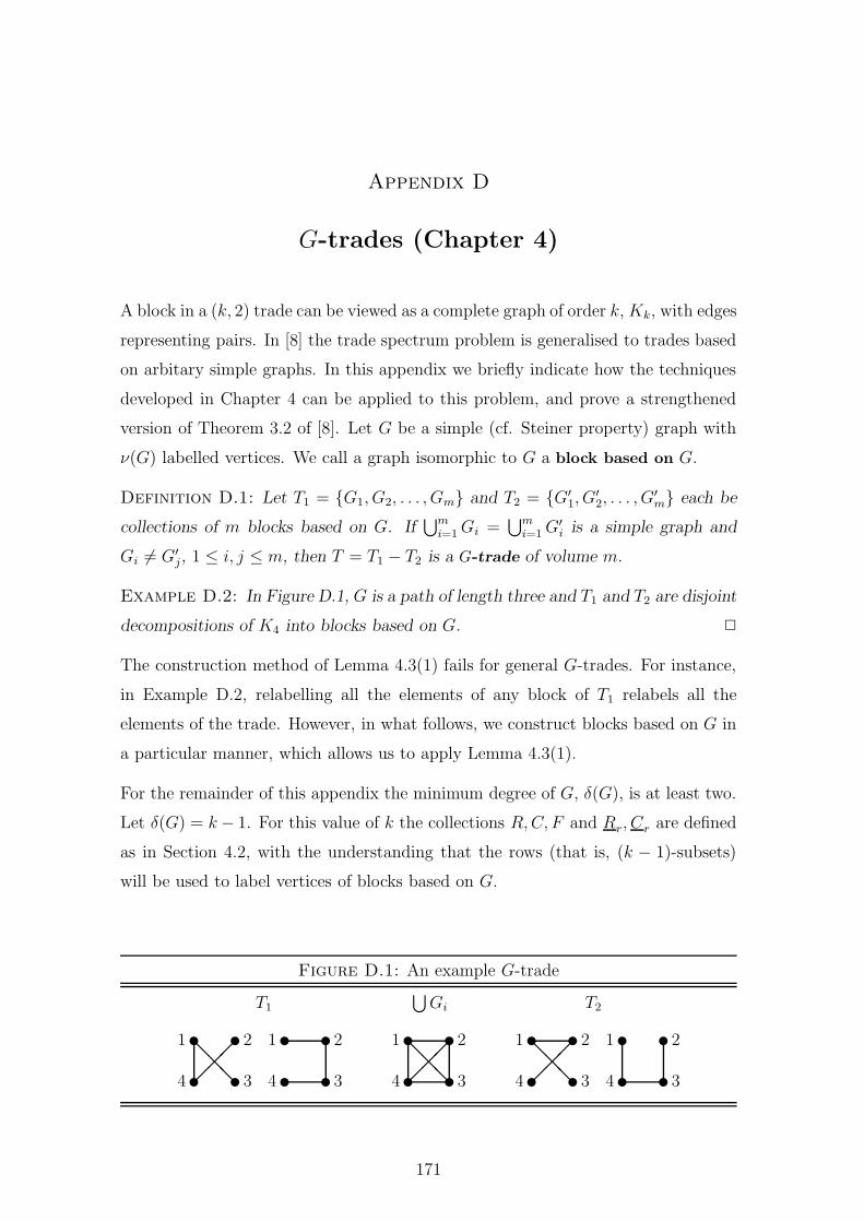
Appendix D
G-trades (Chapter 4)
A block in a (k, 2) trade can be viewed as a complete graph of order k, Kk, with edges
representing pairs. In [8] the trade spectrum problem is generalised to trades based
on arbitary simple graphs. In this appendix we briefly indicate how the techniques
developed in Chapter 4 can be applied to this problem, and prove a strengthened
version of Theorem 3.2 of [8]. Let G be a simple (cf. Steiner property) graph with
ν(G) labelled vertices. We call a graph isomorphic to G a block based on G.
Definition D.1: Let T1 = {G1, G2, . . . , Gm} and T2 = {G′1, G
′2, . . . , G
′m} each be
collections of m blocks based on G. If⋃m
i=1 Gi =⋃m
i=1 G′i is a simple graph and
Gi 6= G′j, 1 ≤ i, j ≤ m, then T = T1 − T2 is a G-trade of volume m.
Example D.2: In Figure D.1, G is a path of length three and T1 and T2 are disjoint
decompositions of K4 into blocks based on G. 2
The construction method of Lemma 4.3(1) fails for general G-trades. For instance,
in Example D.2, relabelling all the elements of any block of T1 relabels all the
elements of the trade. However, in what follows, we construct blocks based on G in
a particular manner, which allows us to apply Lemma 4.3(1).
For the remainder of this appendix the minimum degree of G, δ(G), is at least two.
Let δ(G) = k − 1. For this value of k the collections R, C, F and Rr, Cr are defined
as in Section 4.2, with the understanding that the rows (that is, (k − 1)-subsets)
will be used to label vertices of blocks based on G.
Figure D.1: An example G-trade
T1
1 2u u
4 3u u
@@
@��
�1 2u u
4 3u u
⋃
Gi
1 2u u
4 3u u
@@
@��
�
T2
1 2u u
4 3u u
@@
@��
�1 2u u
4 3u u
171

Figure D.2: The three blocks of (x, R, D)
u
u
u
u
u
u
@@
@
��
�
���
HHH
���
HHH
x
3
2
1
b
au
u
u
u
u
u
@@
@
��
�
���
HHH
���
HHH
x
6
5
4
d
cu
u
u
u
u
u
@@
@
��
�
���
HHH
���
HHH
x
9
8
7
f
e
We use triples of the form (x, N, D) to represent k − 1 blocks based on G con-
structed as follows. Here, x represents a fixed vertex of minimum degree k − 1,
N ∈ {R, C, F, Rr, Cr} and D is a collection of k − 1 disjoint sets (rows) each of
ν(G) − k vertices. The k − 1 blocks based on G are formed by placing a copy of G
on x and the ordered ith rows of N and D in a consistent manner; ensuring, for in-
stance, that the neighbourhood of x equals the ith row of N for each i = 1, . . . , k−1,
and that two vertices from the same positions of N and D in different blocks are
either always adjacent or non-adjacent depending on how the first copy of G was
placed.
Example D.3: In Figure D.2, our notation is illustrated for a graph G with δ(G) =
3. So k = 4 and R = {123, 456, 789}. If we choose D = {ab, cd, ef} as shown, then
the three blocks based on G can be written as (x, R, D). 2
We will now show how our constructions in Section 4.3 can be applied to G-trades.
The following result is analogous to Lemma 4.24. Recall that Ar represents A with
the elements aij of the first r rows of A relabelled to aij . Dr is defined similarly.
Lemma D.4: There exists a G-trade of volume 3(k − 1) + r for all 0 ≤ r ≤ k − 1.
Proof: Let
T a = T a1 − T a
2 = +(x, R, D1) + (y, F, D2) − (x, F, D2) − (y, R, D1),
T b = T b1 − T b
2 = +(x, Cr, D3) + (z, Rr, D
1r) − (z, Cr, D
3) − (x, Rr, D1r),
where the F (Di) are mutually disjoint, F (Di ∪ Dir) ∩ F (R ∪ Rr) = ∅ for i = 1, 2, 3
and x, y, z /∈ F (D1 ∪ D1r ∪ D2 ∪ D3 ∪ R ∪ Rr).
Then T a + T b is a G-trade if each edge in the positive half of T a + T b occurs
precisely once. Suppose that there exists an edge e in the positive half of T a + T b
occurring twice. It is immediate that e is not incident with y, z or any vertices of
D2 or D3. Additionally e is not in F. Therefore, e is necessarily in (x, R, D1) and
(x, Cr, D3) ∪ (z, Rr, D
1r). However, this implies that e is in one of the blocks of
(x, R, D1) that cancels. Hence T a + T b is a G-trade of the required volume. 2
172

A lemma for G-trades analogous to Lemmas 4.23 is similarly proved, while the
analogue of Lemma 4.3(2) is trivial. Although, as we have noted, there is no general
analogue of Lemma 4.3(1), our construction of blocks based on G, utilising the solely
1-balanced families and mutually disjoint Di, allows us to apply a restricted version
of this result. So we can also prove an analogue of Lemma 4.25. Combining these
results we obtain the following.
Theorem D.5: Let G be a simple graph with minimum degree δ(G) = δ ≥ 2. If
m ≥ 3δ, or m ≥ 2δ and m is even, then there exists a G-trade of volume m. 2
This is a significant improvement on Theorem 3.2 of [8], which proves the existence
of G-trades for volumes of at least 5δ + ε, where ε ∈ {−3,−1, 0, +2} depends on the
congruence class of δ(G) modulo 6.
173

Appendix E
Tables for Chapter 7
Table E.1: The number of distinct trades in the 2-(8, 4, 3) designs
initial final designdesign α∗ β∗ γ∗ δ∗ c-trades totalα∗ 981 343 27 819 983 1508β∗ 710 251 22 535 1088 1203γ∗ 428 154 15 478 1046 1053δ∗ 1172 379 30 848 1214 1599
Table E.2: The number of minimal trades in the 2-(8, 4, 3) designs
initial final designdesign α∗ β∗ γ∗ δ∗ c-trades totalα∗ 136 6 5 68 62 28β∗ 120 72 2 112 122 32γ∗ 112 56 7 16 56 56δ∗ 14 35 16 133 14 70
Table E.3: Smallest defining set sizes of the 2-(8, 4, 3) designs
design Ai Ni log5 Ni |msD| |csD| |dsD|α∗ 12 3360 5.05 5 6 6β∗ 48 840 4.18 4 6 6γ∗ 1344 30 2.11 3 6 6δ∗ 21 1920 4.70 5 6 6
174

Table E.4: The number of distinct trades in the 2-(10, 4, 2) designs
initial final designdesign H1 H2 H3 c-trades totalH1 66 546 1401 1461 1461H2 133 900 1879 1882 2049H3 228 1268 2102 1279 2363
Table E.5: The number of minimal trades in the 2-(10, 4, 2) designs
initial final designdesign H1 H2 H3 c-trades totalH1 15 45 255 45 45H2 11 135 18 21 21H3 23 9 221 9 105
Table E.6: Smallest defining set sizes of the 2-(10, 4, 2) designs
design Ai Ni log14 Ni |msD| |csD| |dsD|H1 720 5040 3.23 4 8 8H2 48 75600 4.26 5 6 6H3 24 151200 4.51 5 5 5
175

Table E.7: The number of distinct trades in the 2-(9, 4, 3) designs
initial final designdesign M1 M2 M3 M4 M5 M6 M7 M8 M9 M10 M11 c-trades total
M1 994 4423 12616 7981 17638 17134 9256 6412 3016 21076 5737 35293 35293M2 1071 4506 14266 6641 21996 15262 8894 6704 3248 20722 7017 35277 35293M3 1107 4967 15583 6869 21646 15163 8968 7089 3335 21563 7175 34164 35821M4 1082 4912 14647 7524 19791 15894 9300 6852 3278 21686 6466 35267 35821M5 1119 5065 15803 6975 21894 15354 9054 7214 3333 21392 7251 32087 35889M6 1131 5053 15302 7322 21066 15774 9231 7061 3325 21481 6866 34026 35889M7 1146 5026 15306 7309 20937 15693 9070 7084 3336 21447 6906 35319 35889M8 980 4492 15274 6816 21449 14972 8821 7152 3234 20524 7141 33324 34228M9 1000 4492 14204 7652 19532 16596 8956 7048 3268 20940 6455 33908 34228M10 1143 5122 15857 7247 21292 15414 9099 7156 3326 21663 7083 32388 36002M11 1081 5092 16144 6766 22036 14935 8941 7351 3361 21490 7409 35596 36002
Table E.8: The number of minimal trades in the 2-(9, 4, 3) designs
initial final designdesign M1 M2 M3 M4 M5 M6 M7 M8 M9 M10 M11 c-trades total
M1 342 342 2592 54 3168 1080 1032 828 486 2844 828 378 378M2 214 536 64 510 1136 1248 944 644 558 2676 896 378 378M3 213 551 1204 770 330 933 838 627 522 1114 587 298 298M4 107 663 1340 620 2046 300 604 720 390 1140 894 298 298M5 218 699 742 832 1142 894 765 648 528 441 457 282 294M6 148 748 1100 371 1117 885 714 696 474 343 708 286 294M7 164 717 972 459 1047 885 958 687 477 339 625 294 294M8 228 616 1400 824 1596 1418 1122 295 402 1592 972 978 757M9 192 512 1280 624 1648 1456 1024 312 718 1632 752 808 757M10 183 762 1025 627 417 511 646 681 506 993 564 288 298M11 267 756 990 1134 189 1476 945 639 540 936 871 288 298
Table E.9: Smallest defining set sizes of the 2-(9, 4, 3) designs
design Ai Ni log7 Ni |msD| |csD| |dsD|M1 144 2520 4.03 4 8 8M2 16 22680 5.15 5 8 8M3 2 181440 6.22 5 8 8M4 8 45360 5.51 5 8 8M5 1 362880 6.58 6 8 8M6 2 181440 6.22 5 8 8M7 6 60480 5.66 5 8 8M8 8 45360 5.51 5 4 6M9 32 11340 4.80 5 4 6M10 1 362880 6.58 6 8 8M11 9 40320 5.45 5 8 8
176

Table E.10: The number of distinct trades in the 3-(10, 5, 3) designs
initial final designdesign N1 N2 N3 N4 N5 N6 N7 c-trades total
N1 3765 20151 130561 280051 9487 38296 200371 446232 448287N2 4311 4723 15541 27418 7138 7456 21634 46245 46263N3 4455 5291 17243 26764 8170 7792 22548 46113 48171N4 4549 5393 17514 26991 8581 7915 22421 42006 48735N5 3755 8856 62192 107907 7928 20752 81667 149986 156932N6 3763 4724 16708 26500 7692 7940 21516 44422 45590N7 4627 5458 17830 26962 8731 7945 22637 44998 49070
Table E.11: The number of minimal trades in the 3-(10, 5, 3) designs
initial final designdesign N1 N2 N3 N4 N5 N6 N7 c-trades total
N1 1619 5300 23760 34560 2556 9540 36480 24056 25271N2 1664 522 54 1248 2124 630 2868 380 380N3 1632 598 1362 264 2316 606 1176 306 306N4 1466 749 876 1475 2352 624 357 352 370N5 1184 3200 8480 12000 3326 10 10560 858 951N6 1568 616 1584 1936 2234 149 1600 1562 759N7 1518 807 1107 234 2358 639 1048 402 412
Table E.12: Smallest defining set sizes of the 3-(10, 5, 3) designs
design Ai Ni log7 Ni |msD| |csD| |dsD|N1 720 5040 4.38 5 4 5N2 144 25200 5.21 5 8 8N3 16 226800 6.34 6 8 8N4 6 604800 6.84 6 8 8N5 320 11340 4.80 5 4 6N6 64 56700 5.63 5 4 6N7 9 403200 6.63 6 8 8
177

Table E.13: The number of distinct trades in the 2-(10, 5, 4) designs (I)
initial final designdesign 1 2 3 4 5 6 7 8 9 10 11 12
1 18373 18487 18791 18750 13111 14098 14256 13859 14064 8553 8603 48162 18487 18373 18750 18791 13111 14256 14098 14064 13859 8603 8553 47623 18679 18685 18957 18945 13305 14313 14628 13610 13776 8458 8648 47834 18685 18679 18945 18957 13305 14628 14313 13776 13610 8648 8458 47215 18603 18603 18922 18922 12315 14267 14267 13749 13749 8614 8614 45436 18405 18497 19044 19320 13315 14537 13844 13852 13542 8744 8379 46237 18497 18405 19320 19044 13315 13844 14537 13542 13852 8379 8744 48528 18443 18655 17940 18156 12876 14016 13690 14137 13959 8715 8486 47589 18655 18443 18156 17940 12876 13690 14016 13959 14137 8486 8715 486910 18457 18495 17853 18526 12979 14329 13093 14467 13609 8782 8419 464211 18495 18457 18526 17853 12979 13093 14329 13609 14467 8419 8782 502612 18508 18132 17568 16684 11838 11828 13444 14424 14404 8308 8916 497413 18132 18508 16684 17568 11838 13444 11828 14404 14424 8916 8308 444914 18352 18352 17100 17100 11424 13044 13044 14492 14492 8644 8644 471015 16684 16684 15388 15388 11878 10576 10576 14299 14299 8275 8275 514016 18103 18016 16870 17496 12572 13232 12521 14449 14036 8681 8425 482517 18016 18103 17496 16870 12572 12521 13232 14036 14449 8425 8681 500818 18676 18676 19165 19165 12345 14192 14192 13940 13940 8578 8578 452119 18236 18236 18601 18601 13382 13891 13891 13426 13426 8479 8479 459620 18448 18460 19594 19900 13426 14368 14830 13309 13552 8320 8563 475921 18460 18448 19900 19594 13426 14830 14368 13552 13309 8563 8320 4594
Table E.14: The number of distinct trades in the 2-(10, 5, 4) designs (II)
initial final designdesign 13 14 15 16 17 18 19 20 21 c-trades total
1 4762 5200 2229 7242 7255 10674 8041 7514 7464 35474 366772 4816 5200 2229 7255 7242 10674 8041 7464 7514 35474 366773 4721 5148 2075 6956 7034 10729 8190 7729 7645 35724 371924 4783 5148 2075 7034 6956 10729 8190 7645 7729 35724 371925 4543 4966 2007 6965 6965 10095 7799 7825 7825 36066 371036 4852 5072 2007 7009 6946 10704 7950 7653 7893 36281 369647 4623 5072 2007 6946 7009 10704 7950 7893 7653 36281 369648 4869 5272 2330 7391 7325 10574 7978 7173 7260 35479 360829 4758 5272 2330 7325 7391 10574 7978 7260 7173 35479 3608210 5026 5197 2303 7405 7231 10483 7841 7102 7509 36034 3624111 4642 5197 2303 7231 7405 10483 7841 7509 7102 36034 3624112 4449 5224 2460 7528 7636 9710 7252 6875 6363 34823 3490513 4974 5224 2460 7636 7528 9710 7252 6363 6875 34823 3490514 4710 5091 2416 7620 7620 10070 7308 6899 6899 35196 3525315 5140 5026 2965 7819 7819 8602 6385 5509 5509 34069 3406916 5008 5223 2487 7558 7624 10158 7541 6489 6912 35017 3520917 4825 5223 2487 7624 7558 10158 7541 6912 6489 35017 3520918 4521 5092 1966 6942 6942 10071 7656 7830 7830 36819 3726319 4596 4996 1953 6881 6881 10442 7435 7692 7692 36533 3660520 4594 5209 1930 6766 6859 10933 8206 7739 7834 37888 3806021 4759 5209 1930 6859 6766 10933 8206 7834 7739 37888 38060
178

Table E.15: The number of minimal trades in the 2-(10, 5, 4) designs (I)
initial final designdesign 1 2 3 4 5 6 7 8 9 10 11 12
1 1415 1272 924 991 1064 1317 1217 942 1006 990 775 6382 1272 1415 991 924 1064 1217 1317 1006 942 775 990 6693 1023 1074 1509 1460 1053 1397 960 1365 1191 959 895 6764 1074 1023 1460 1509 1053 960 1397 1191 1365 895 959 7435 2061 2061 1991 1991 385 1648 1648 1616 1616 1265 1265 5766 1687 1585 1362 890 1059 1218 1379 1097 1667 845 1222 7907 1585 1687 890 1362 1059 1379 1218 1667 1097 1222 845 5858 739 858 1524 1340 966 1101 1489 1227 997 858 882 6369 858 739 1340 1524 966 1489 1101 997 1227 882 858 53210 1656 513 1371 1452 1230 777 1737 1245 1071 937 1248 75011 513 1656 1452 1371 1230 1737 777 1071 1245 1248 937 48912 2104 2192 1768 2448 736 1936 1208 1960 1176 1272 736 24613 2192 2104 2448 1768 736 1208 1936 1176 1960 736 1272 27914 1440 1440 1880 1880 840 1796 1796 1688 1688 1080 1080 17015 2196 2196 2826 2826 1998 1638 1638 828 828 660 660 46816 1484 1252 1832 2360 1234 1102 1586 682 684 314 1208 55317 1252 1484 2360 1832 1234 1586 1102 684 682 1208 314 46418 2238 2238 1853 1853 186 1503 1503 1826 1826 1212 1212 56819 2436 2436 1592 1592 862 462 462 1560 1560 1154 1154 61720 1449 1476 297 1782 1089 1368 954 1800 1485 1008 945 70221 1476 1449 1782 297 1089 954 1368 1485 1800 945 1008 801
Table E.16: The number of minimal trades in the 2-(10, 5, 4) designs (II)
initial final designdesign 13 14 15 16 17 18 19 20 21 c-trades total
1 669 736 260 821 815 1321 1192 929 990 437 4422 638 736 260 815 821 1321 1192 990 929 437 4423 743 776 286 918 1032 1182 1082 778 1056 482 4954 676 776 286 1032 918 1182 1082 1056 778 482 4955 576 737 312 1054 1054 437 1148 1168 1168 953 4636 585 848 280 818 982 1078 876 1054 925 512 4907 790 848 280 982 818 1078 876 925 1054 512 4908 532 746 230 631 693 1421 1111 1023 953 401 4019 636 746 230 693 631 1421 1111 953 1023 401 40110 489 723 230 342 1089 1158 1065 921 898 372 37211 750 723 230 1089 342 1158 1065 898 921 372 37212 279 250 224 888 520 1202 1040 1128 1252 759 51313 246 250 224 520 888 1202 1040 1252 1128 759 51314 170 457 256 760 760 824 1272 1140 1140 544 54515 468 684 270 27 27 990 486 1242 1242 378 37816 464 685 159 772 836 1246 883 1028 1186 330 33017 553 685 159 836 772 1246 883 1186 1028 330 33018 568 720 292 1048 1048 802 1210 1192 1192 552 49719 617 900 278 843 843 1166 922 1264 1264 434 41820 801 900 330 1152 1152 1224 1143 1114 1035 495 49621 702 900 330 1152 1152 1224 1143 1035 1114 495 496
179

Table E.17: The blocks, with defining sets, of the 2-(10, 5, 4) designs (I)
1 2 3 4 5 6 7 8 9 10 11
01234 01268 01234 01268 01234 01234 01267 01234 01279 01234 0126701235 01369 01235 01369 01235 01235 01389 01235 01368 01235 0136801567 01459 01567 01459 01567 01567 01459 01567 01459 01578 0145901789 01478 01789 01478 01789 01789 01468 01789 01468 01789 0146902467 02379 02479 02379 02479 02478 02379 02478 02367 02467 0238902689 02458 02689 02458 02689 02689 02458 02689 02458 02689 0245803489 02579 03468 02567 03469 03469 02569 03469 02569 03479 0257903578 03467 03578 03467 03578 03568 03467 03589 03479 03569 0347804569 03568 04569 03589 04568 04579 03578 04567 03578 04568 0356712479 12378 12467 12378 12478 12469 12368 12469 12389 12489 1237912589 12469 12589 12469 12569 12589 12479 12568 12467 12569 1247813468 12567 13489 12579 13468 13478 12578 13478 12578 13468 1256813679 13457 13679 13457 13679 13679 13457 13679 13457 13679 1345714568 13589 14568 13568 14589 14568 13569 14589 13569 14567 1358923569 23456 23569 23456 23589 23579 23456 23579 23456 23578 2345623678 23489 23678 23489 23678 23678 23489 23678 23489 23678 2346924578 46789 24578 46789 24567 24567 46789 24579 46789 24579 4678934579 56789 34579 56789 34579 34589 56789 34568 56789 34589 56789
Table E.18: The blocks, with defining sets, of the 2-(10, 5, 4) designs (II)
12 13 14 15 16 17 18 19 20 21
01234 01267 01234 01234 01234 01279 01234 01234 01234 0123401235 01389 01235 01235 01235 01368 01235 01235 01259 0138901468 01569 01468 01467 01468 01567 01469 01468 01378 0147801479 01578 01479 01489 01479 01589 01478 01479 01679 0156902568 02389 02569 02569 02569 02367 02568 02578 02457 0235802579 02469 02578 02689 02689 02458 02789 02689 02689 0246903678 02478 03678 03578 03578 02478 03589 03569 03456 0257903679 03456 03679 03789 03789 03459 03679 03789 03489 0346704589 03457 04589 04567 04567 03469 04567 04567 05678 0567812689 12367 12689 12578 12578 12389 12567 12569 12367 1235712789 12458 12789 12678 12678 12456 12689 12678 12468 1245613569 12459 13569 13569 13569 12469 13579 13578 13589 1267813578 13468 13578 13679 13679 13457 13678 13679 14569 1367914567 13479 14567 14589 14589 13478 14589 14589 14578 1458923469 23568 23468 23468 23467 23568 23469 23467 23568 2368923478 23579 23479 23479 23489 23579 23478 23489 23579 2478924567 46789 24567 24579 24579 46789 24579 24579 24789 3456834589 56789 34589 34568 34568 56789 34568 34568 34679 34579
180

Table E.19: Smallest defining set sizes of the 2-(10, 5, 4) designs
design Ai Ni log14 Ni |msD| |csD| |dsD|
1 (XV) 1 3628800 5.72 5 7 7
2 (XI) 1 3628800 5.72 5 7 7
3 (XII) 1 3628800 5.72 5 7 7
4 (XIV) 1 3628800 5.72 5 7 7
5 (XVI) 2 1814400 5.46 5 6 6
6 (XIX) 2 1814400 5.46 5 7 7
7 (VI) 2 1814400 5.46 5 7 7
8 (XVII) 2 1814400 5.46 5 7 7
9 (III) 2 1814400 5.46 5 7 7
10 (XX) 6 604800 5.04 5 7 7
11 (V) 6 604800 5.04 5 7 7
12 (VIII) 16 226800 4.67 5 6 7
13 (XVIII) 16 226800 4.67 5 6 7
14 (X) 16 226800 4.67 5 7 7
15 (II) 72 50400 4.10 4 8 8
16 (IV) 8 453600 4.94 4 7 7
17 (I) 8 453600 4.94 4 7 7
18 (IX) 4 907200 5.20 5 6 6
19 (VII) 8 453600 4.94 5 7 7
20 (XIII) 9 403200 4.89 5 7 7
21 (XXI) 9 403200 4.89 5 7 7
Table E.20: The distribution of trades (I)
2-(8, 4, 3)
α∗ β∗ γ∗ δ∗ 3-(8, 4, 1) 2-(7, 3, 1)
m f #d #m #d #m #d #m #d #m #d #m #d #m
4 6 . . . . . . . . . . 7 7
4 7 17 17 26 26 56 56 14 14 . . . .
4 8 3 3 6 6 . . . . . . . .
6 7 7 - 14 - 56 - 7 - . . 7 -
6 8 21 8 26 - 56 - 21 14 . . . .
7 7 1 - 2 - 8 - 1 - . . 1 -
7 8 129 - 146 - 8 - 99 - . . . .
8 8 199 - 187 - 175 - 217 42 7 7 . .
9 8 316 - 168 - . . 406 - . . . .
10 8 477 - 334 - 532 - 462 - . . . .
11 8 232 - 194 - 56 - 266 - . . . .
12 8 91 - 85 - 91 - 91 - 7 - . .
13 8 14 - 14 - 14 - 14 - . . . .
14 8 1 - 1 - 1 - 1 - 1 - . .
181

Table E.21: The distribution of trades (II)
2-(10, 4, 2)
H1 H2 H3 4-(11, 5, 1) 3-(10, 4, 1) 2-(9, 3, 1)
m f #d #m #d #m #d #m #d #m #d #m #d #m
4 8 45 45 21 21 9 9 . . . . . .
6 8 . . . . . . . . . . 36 36
6 9 60 - 12 - 4 - . . . . . .
6 10 15 - 3 - 1 - . . . . . .
7 9 . . 24 - 36 - . . . . . .
7 10 . . 48 - 72 - . . . . . .
8 8 . . . . . . . . . . 9 -
8 9 . . 24 - 12 - . . . . . .
8 10 195 - 123 - 79 24 . . . . . .
9 9 . . . . 4 - . . . . 76 -
9 10 . . 252 - 150 - . . . . . .
10 9 . . . . . . . . . . 54 -
10 10 270 - 486 - 630 72 . . . . . .
11 9 . . . . . . . . . . 12 -
11 10 300 - 480 - 790 - . . . . . .
12 9 . . . . . . . . . . 1 -
12 10 455 - 455 - 455 - . . . . . .
13 10 105 - 105 - 105 - . . . . . .
14 10 15 - 15 - 15 - . . . . . .
15 10 1 - 1 - 1 - . . . . . .
16 10 . . . . . . . . 45 45 . .
18 9 . . . . . . . . 10 10 . .
22 10 . . . . . . . . 360 360 . .
24 10 . . . . . . . . 165 - . .
26 10 . . . . . . . . 765 - . .
28 10 . . . . . . . . 180 - . .
30 10 . . . . . . . . 1 - . .
36 10 . . . . . . 11 11 . . . .
36 11 . . . . . . 55 55 . . . .
48 11 . . . . . . 495 495 . . . .
54 11 . . . . . . 1540 1320 . . . .
60 11 . . . . . . 2079 1584 . . . .
66 11 . . . . . . 1 - . . . .
182

Appendix F
Tables for Chapter 9
Table F.1: Results for the 4 × 2-(6, 3, 4) designs
Design b∗ |aut(D)| |msD| |csD| |dsD|P0, P0 10 60 3 6 6P0, P1 20 720 0 6 6P0, P2 16 24 5 6 6P0, P3 14 24 4 6 6
Table F.2: Results for the 6 × 2-(6, 3, 6) designs
Design b∗ |aut(D)| |msD| |csD| |dsD|P0, P0, P0 10 60 3 9 9P0, P0, P1 20 60 6 9 9P0, P0, P2 16 12 7 9 9P0, P0, P3 14 12 6 8 9P0, P2, P3 17 6 7 8 9P0, P2, P4 19 36 3 9 9
Table F.3: Results for the 13 × 2-(6, 3, 8) designs
Design b∗ |aut(D)| |msD| |csD| |dsD|P0, P0, P0, P0 10 60 3 12 12P0, P0, P0, P1 20 60 6 12 12P0, P0, P0, P2 16 12 7 12 12P0, P0, P0, P3 14 12 6 12 12P0, P0, P1, P1 20 720 0 12 12P0, P0, P1, P2 20 24 8 12 12P0, P0, P1, P3 20 24 6 12 12P0, P0, P2, P2 16 24 6 12 12P0, P0, P2, P3 17 3 9 12 12P0, P0, P2, P4 19 6 8 12 12P0, P0, P3, P3 14 24 5 12 12P0, P0, P3, P6 17 6 9 12 12P0, P2, P3, P6 18 8 8 12 12
183

Table F.4: Results for the 19 × 2-(6, 3, 10) designs
Design b∗ |aut(D)| |msD| |csD| |dsD|P0, P0, P0, P0, P0 10 60 3 15 15P0, P0, P0, P0, P1 20 60 6 15 15P0, P0, P0, P0, P2 16 12 7 15 15P0, P0, P0, P0, P3 14 12 6 15 15P0, P0, P0, P1, P1 20 60 9 15 15P0, P0, P0, P1, P2 20 12 11 15 15P0, P0, P0, P1, P3 20 12 11 15 15P0, P0, P0, P2, P2 16 12 9 15 15P0, P0, P0, P2, P3 17 3 11 15 15P0, P0, P0, P2, P4 19 6 9 15 15P0, P0, P0, P3, P3 14 12 7 14 15P0, P0, P0, P3, P6 17 6 8 15 15P0, P0, P1, P2, P3 20 6 10 15 15P0, P0, P1, P2, P4 20 36 4 15 15P0, P0, P2, P2, P3 17 6 8 15 15P0, P0, P2, P2, P4 19 6 11 15 15P0, P0, P2, P3, P3 17 3 11 14 15P0, P0, P2, P3, P4 19 4 8 15 15P0, P0, P2, P3, P6 18 2 11 14 15
184

Table F.5: Results for the 34 × 2-(6, 3, 12) designs
Design b∗ |aut(D)| |msD| |csD| |dsD|P0, P0, P0, P0, P0, P0 10 60 3 18 18P0, P0, P0, P0, P0, P1 20 60 6 18 18P0, P0, P0, P0, P0, P2 16 12 7 18 18P0, P0, P0, P0, P0, P3 14 12 6 18 18P0, P0, P0, P0, P1, P1 20 60 9 18 18P0, P0, P0, P0, P1, P2 20 12 12 18 18P0, P0, P0, P0, P1, P3 20 12 11 18 18P0, P0, P0, P0, P2, P2 16 12 9 18 18P0, P0, P0, P0, P2, P3 17 3 11 18 18P0, P0, P0, P0, P2, P4 19 6 10 18 18P0, P0, P0, P0, P3, P3 14 12 7 18 18P0, P0, P0, P0, P3, P6 17 6 8 18 18P0, P0, P0, P1, P1, P1 20 720 0 18 18P0, P0, P0, P1, P1, P2 20 24 11 18 18P0, P0, P0, P1, P1, P3 20 24 8 18 18P0, P0, P0, P1, P2, P2 20 24 10 18 18P0, P0, P0, P1, P2, P3 20 3 13 18 18P0, P0, P0, P1, P2, P4 20 6 11 18 18P0, P0, P0, P1, P3, P3 20 24 8 18 18P0, P0, P0, P1, P3, P6 20 6 13 18 18P0, P0, P0, P2, P2, P2 16 24 7 18 18P0, P0, P0, P2, P2, P3 17 3 12 18 18P0, P0, P0, P2, P2, P4 19 3 13 18 18P0, P0, P0, P2, P3, P3 17 3 11 18 18P0, P0, P0, P2, P3, P4 19 2 13 18 18P0, P0, P0, P2, P3, P6 18 2 13 18 18P0, P0, P0, P3, P3, P3 14 24 5 18 18P0, P0, P0, P3, P3, P6 17 3 13 18 18P0, P0, P1, P2, P3, P6 20 8 10 18 18P0, P0, P2, P2, P3, P3 17 6 10 18 18P0, P0, P2, P2, P3, P4 19 2 12 18 18P0, P0, P2, P2, P3, P6 18 4 11 18 18P0, P0, P2, P2, P4, P4 19 36 5 18 18P0, P0, P2, P3, P3, P6 18 2 12 18 18
185

Table F.6: Results for the 4 × 2-(7, 3, 2) designs
Design b∗; n1, n2 |aut(D)| |msD| |csD| |dsD|1.0, 1.0 7; 0,7 168 3 6 61.0, 1.1 11; 8,3 48 4 6 61.0, 1.2 13; 12,1 24 5 6 61.0, 1.7 14; 14,0 42 4 6 6
Table F.7: Results for the 10 × 2-(7, 3, 3) designs
Design b∗; n1, n2, n3 |aut(D)| |msD| |csD| |dsD|3.0 21; 21,0,0 42 6 7 71.0, 1.0, 1.0 7; 0,0,7 168 3 9 91.0, 1.0, 1.1 11; 4,4,3 24 5 8 91.0, 1.0, 1.2 13; 6,6,1 12 6 9 91.0, 1.0, 1.7 14; 7,7,0 21 5 9 91.0, 1.1, 1.2 15; 10,4,1 8 6 8 91.0, 1.1, 1.6 17; 13,4,0 3 6 8 91.0, 1.2, 1.5 19; 18,0,1 144 2 9 91.0, 1.2, 1.6 18; 15,3,0 6 6 9 91.0, 1.2, 1.10 20; 19,1,0 6 5 8 9
186

Table F.8: Results for the 35 × 2-(7, 3, 4) designs
Design b∗; n1, n2, n3, n4 |aut(D)| |msD| |csD| |dsD|3.0, 1.0 28; 28,0,0,0 168 7 12 123.0, 1.1 (+) 25; 22,3,0,0 3 6 12 123.0, 1.2 22; 16,6,0,0 3 8 9 101.0, 1.0, 1.0, 1.0 7; 0,0,0,7 168 3 12 121.0, 1.0, 1.0, 1.1 11; 4,0,4,3 24 5 12 121.0, 1.0, 1.0, 1.2 13; 6,0,6,1 12 6 12 121.0, 1.0, 1.0, 1.7 14; 7,0,7,0 21 5 12 121.0, 1.0, 1.1, 1.1 11; 0,8,0,3 48 4 12 121.0, 1.0, 1.1, 1.2 15; 6,6,2,1 4 6 12 121.0, 1.0, 1.1, 1.3 15; 8,2,4,1 8 6 12 121.0, 1.0, 1.1, 1.6 17; 10,3,4,0 3 7 12 121.0, 1.0, 1.1, 1.7 17; 9,5,3,0 3 7 12 121.0, 1.0, 1.2, 1.2 13; 0,12,0,1 24 5 12 121.0, 1.0, 1.2, 1.5 19; 12,6,0,1 24 7 12 121.0, 1.0, 1.2, 1.6 18; 10,6,2,0 2 8 12 121.0, 1.0, 1.2, 1.7 17; 7,9,1,0 3 7 12 121.0, 1.0, 1.2, 1.10 20; 13,6,1,0 3 7 12 121.0, 1.0, 1.7, 1.7 14; 0,0,14,0 42 4 12 121.0, 1.0, 1.7, 1.10 20; 12,8,0,0 6 7 12 121.0, 1.1, 1.2, 1.3 17; 8,8,0,1 16 6 12 121.0, 1.1, 1.2, 1.6 20; 13,6,1,0 1 8 12 121.0, 1.1, 1.2, 1.7 19; 12,5,2,0 2 7 12 121.0, 1.1, 1.2, 1.8 19; 13,3,3,0 6 7 12 121.0, 1.1, 1.2, 1.10 21; 15,5,1,0 2 7 12 121.0, 1.1, 1.6, 1.7 20; 12,8,0,0 4 6 12 121.0, 1.1, 1.6, 1.11 22; 16,6,0,0 2 7 12 121.0, 1.1, 1.6, 1.15 23; 18,5,0,0 6 7 12 121.0, 1.1, 1.6, 1.20 23; 18,5,0,0 2 8 12 121.0, 1.1, 1.6, 1.21 23; 19,3,1,0 6 6 10 121.0, 1.1, 1.6, 1.22 22; 16,6,0,0 2 7 12 121.0, 1.1, 1.6, 1.27 20; 12,8,0,0 12 6 12 121.0, 1.2, 1.6, 1.8 22; 16,6,0,0 12 6 12 121.0, 1.2, 1.6, 1.11 22; 16,6,0,0 4 7 12 121.0, 1.2, 1.6, 1.14 22; 16,6,0,0 24 6 12 121.0, 1.2, 1.10, 1.13 26; 24,2,0,0 16 4 12 12
187

Table F.9: Results for the 4 × 3-(8, 4, 2) designs
b∗; n1, n2 |aut(D)| |msD| |csD| |dsD|14; 0,14 1344 3 6 622; 16,6 384 4 6 626; 24,2 192 5 6 628; 28,0 336 4 6 6
Table F.10: Results for the 10 × 3-(8, 4, 3) designs
b∗; n1, n2, n3 |aut(D)| |msD| |csD| |dsD|42; 42,0,0 336 6 7 714; 0,0,14 1344 3 9 922; 8,8,6 192 5 8 926; 12,12,2 96 6 9 928; 14,14,0 168 5 9 930; 20,8,2 64 6 8 934; 26,8,0 24 6 8 938; 36,0,2 1152 2 9 936; 30,6,0 48 6 9 940; 38,2,0 48 5 8 9
188

Table F.11: Results for the 31 × 3-(8, 4, 4) designs
Extension b∗; n1, n2, n3, n4 |aut(D)| |msD| |csD| |dsD|0+ 56; 56,0,0,0 1344 7 12 121+ 50; 44,6,0,0 24 6 12 122+ 44; 32,12,0,0 24 8 9 103+ 14; 0,0,0,14 1344 3 12 124+ 22; 8,0,8,6 192 5 12 125+ 26; 12,0,12,2 96 6 12 126+ 28; 14,0,14,0 168 5 12 127+ 22; 0,16,0,6 384 4 12 128+ 30; 12,12,4,2 32 6 12 129+ 30; 16,4,8,2 64 6 12 1210+ 34; 20,6,8,0 24 7 12 1211+ 34; 18,10,6,0 24 7 12 1212+ 26; 0,24,0,2 192 5 12 1213+ 38; 24,12,0,2 192 7 12 1214+ 36; 20,12,4,0 16 8 12 1215+ 34; 14,18,2,0 24 7 12 1216+ 40; 26,12,2,0 24 7 12 1217+ 28; 0,28,0,0 336 4 12 1218+ 40; 24,16,0,0 48 7 12 1219+ 34; 16,16,0,2 128 6 12 1220+ 40; 26,12,2,0 8 8 12 1221+ 38; 24,10,4,0 16 7 12 1222+ 38; 26,6,6,0 48 7 12 1223+ 42; 30,10,2,0 16 7 12 1224+ 40; 24,16,0,0 24 7 12 1225+ 44; 32,12,0,0 8 7 12 1226+ 46; 36,10,0,0 12 8 12 1227+ = 26+28+ 46; 38,6,2,0 48 6 10 1229+ = 25+30+ = 24+31+ 44; 32,12,0,0 24 8 12 1232+ = 31+33+ 44; 32,12,0,0 192 6 12 1234+ 52; 48,4,0,0 128 4 12 12
189

Appendix G
Tables for Chapter 11
Table G.1: Blocks and smallest defining sets for W1 – W10
W1 W2 W3 W4 W5 W6 W7 W8 W9 W10
*012 *012 *012 *012 *012 *012 *012 *012 *012 *012
*034 034 *034 034 034 034 *034 *034 *034 *034
056 *056 056 *056 *056 *056 056 056 056 056
*078 *078 078 078 078 078 078 078 078 078
09a *09a 09a 09a 09a 09a 09a 09a 09a 09a
0bc 0bc *0bc *0bc 0bc *0bc *0bc 0bc *0bc 0bc
0de 0de 0de 0de *0de 0de 0de *0de 0de 0de
135 135 *135 135 135 135 135 135 135 135
146 146 146 *146 *146 146 *146 *146 146 146
179 179 *179 *179 *179 179 *179 179 *179 *179
*18a *18a 18a 18a 18a *18a 18a *18a 18a 18a
1bd 1bd *1bd 1bd 1bd 1bd 1bd 1bd 1bd 1bd
*1ce *1ce 1ce 1ce 1ce 1ce *1ce 1ce 1ce *1ce
236 *236 236 236 236 236 236 236 236 *236
*245 245 245 245 245 *245 245 245 *245 *245
27a 27a *27a 27a *27a 27a *27a 27a 27a 27a
289 289 289 *289 289 *289 289 28b *28b 28b
*2be *2be 2be 2be *2be *2be 2be 29e 29e *29e
2cd 2cd 2cd *2cd 2cd 2cd 2cd 2cd 2cd 2cd
37b 37b 37b *37b 37b 37b *37b 37c 37c 37c
38c 38c *38c 38c *38c *38c 38d 389 389 389
*39d *39d *39d 39d 39e 39e *39e *3ad *3ad *3ad
*3ae *3ae 3ae *3ae *3ad *3ad 3ac *3be 3be 3be
*47c *47c 47d *47d 47d *47d 47e 47e 47e 47e
48b *48b *48e 48b *48e 48e *48c 48d *48d *48d
*49e 49e 49b *49e *49c 49c 49b *49c 49b 49c
4ad 4ad 4ac 4ac 4ab 4ab 4ad 4ab *4ac *4ab
*57d 57e *57e 57e *57c 57c 57c *57d *57d *57d
58e 58d 58d *58d 58b 58d 58e 58e 58e 58c
*59b *59c *59c 59c 59d *59b *59d *59b 59c 59b
5ac 5ab 5ab *5ab 5ae 5ae *5ab 5ac 5ab 5ae
67e *67d 67c 67c 67e 67e *67d *67b 67b 67b
*68d 68e 68b 68e 68d 68b 68b *68c 68c *68e
*69c 69b *69e 69b *69b 69d 69c 69d *69d 69d
*6ab 6ac *6ad 6ad 6ac *6ac 6ae 6ae *6ae 6ac
190

Table G.2: Blocks and smallest defining sets for W11 – W20
W11 W12 W13 W14 W15 W16 W17 W18 W19 W20
*012 012 *012 *012 012 012 *012 012 012 012
034 *034 *034 *034 *034 034 *034 034 *034 034
*056 056 056 056 *056 056 056 056 *056 *056
078 078 *078 078 078 *078 078 078 *078 *078
09a *09a 09a *09a *09a 09a 09a 09a *09a 09a
0bc *0bc 0bc 0bc 0bc 0bc *0bc *0bc 0bc 0bc
*0de 0de 0de *0de *0de *0de 0de *0de 0de 0de
*135 *135 135 135 135 135 135 *135 *135 *135
146 146 *146 *146 146 *146 146 *146 146 146
*179 179 179 179 179 *179 *179 *179 179 179
18a *18a *18a 18a 18a 18a 18a *18a 18a 18a
1bd 1bd 1bd 1bd 1bd 1bd 1bd 1bd *1bd 1bd
1ce 1ce *1ce *1ce 1ce 1ce 1ce 1ce *1ce *1ce
236 236 236 236 *236 *236 *236 236 236 *236
245 *245 245 245 245 *245 245 *245 245 245
*27a *27a 27a *27a *27b 27b 27b 27b 27b 27b
28b 28b 28b 28b *28c 28c 28c *28c 28d *28d
29e 29e *29e 29e 29d 29d 29d 29e 29c 29e
2cd *2cd *2cd 2cd 2ae *2ae *2ae 2ad 2ae 2ac
*37c 37c 37c 37c 37e 37e 37e 37e 37e *37e
38d 38d 38e *38e 389 *38d *38d 389 38b 389
*39b *39b 39b 39b 3ab *39c 39c 3ab 39d *3ab
3ae 3ae 3ad *3ad *3cd 3ab *3ab *3cd *3ac 3cd
47e 47e 47e 47d 47d 47a 47a *47a 47c 47a
48c 48c 48d *489 48b 489 48b 48d *489 *48c
49d 49d 49c 4ac *49e *4be *49e 49c 4ad *49d
4ab 4ab *4ab 4be 4ac *4cd 4cd 4be 4be 4be
57d 57b *57d 57e 57a *57d *57d 57d 57a 57d
589 58e 589 58d 58d 58e *589 58e 58e 58b
5ac 59c 5ac *59c 59c 59b 5ac 59b 59b 59c
*5be *5ad *5be *5ab *5be *5ac 5be 5ac *5cd *5ae
67b *67d 67b *67b *67c 67c 67c 67c 67d 67c
*68e 689 68c 68c 68e *68b 68e 68b 68c 68e
69c 6ac *69d 69d 69b 69e 69b 69d *69e 69b
*6ad *6be 6ae 6ae 6ad 6ad *6ad *6ae 6ab 6ad
191

Table G.3: Blocks and smallest defining sets for W21 – W30
W21 W22 W23 W24 W25 W26 W27 W28 W29 W30
012 *012 *012 *012 *012 *012 012 012 012 012
034 034 034 034 034 *034 034 034 034 *034
*056 *056 056 *056 *056 056 *056 056 056 056
078 078 078 078 078 078 078 078 078 *078
*09a 09a *09a 09a *09a 09a *09a *09a *09a 09a
0bc 0bc *0bc 0bc 0bc *0bc 0bc 0bc 0bc 0bc
0de *0de 0de 0de 0de 0de 0de 0de *0de *0de
135 135 *135 135 135 135 135 *135 135 *135
146 *146 146 146 146 146 146 146 *146 146
179 179 179 179 179 179 179 179 179 179
*18b *18b 18a *18a 18a *18a *18a 18a 18a 18a
1ad 1ad 1bd 1bd 1bd 1bd 1bd *1bd *1bd 1bd
*1ce 1ce 1ce *1ce *1ce 1ce *1ce *1ce 1ce *1ce
*236 236 236 236 236 236 *236 *236 *236 236
*245 245 247 247 247 *247 *247 247 *247 247
27a 27a 25a 25a *25a *25b 25b *25b 25b 25b
*28c *28c 28b *28b *28b 289 28c 28c *28c 28d
29e 29e 29e *29e 29e 2ae 29d 29e 29e 29c
2bd 2bd 2cd 2cd 2cd *2cd 2ae 2ad 2ad *2ae
37b 37b 37c 37c *37c *37c *37d 37d 37e 37d
*38d 38d *38d 38d *38e 38b 389 389 *38b *389
39c 39c 39b *39b *39d *39e 3ac *3ac 39d 3ac
3ae 3ae 3ae *3ae 3ab 3ad *3be 3be *3ac 3be
*47c 47e *45d *45b 45e 45e *45a 45a 45a 45a
*48e *48a *489 *48e *48c 48d 48e 48e 489 *48b
49d *49b *4ac 49c 49b *49b 49b *49b *4be 49e
4ab 4cd 4be 4ad 4ad *4ac 4cd 4cd 4cd 4cd
57d *57c *57b 57e *57b 57a 57c 57e *57d 57c
589 58e *58e 58c 58d 58c *58d *58d 58e 58e
5ac *59d 59c *59d 59c 59d 59e 59c *59c 59d
5be 5ab 67e *67d 67d 67d *67e *67c 67c *67e
67e *67d 68c 689 689 *68e 68b 68b 68d 68c
68a 689 69d 6ac 6ac 69c 69c 69d 69b 69b
*69b 6ac *6ab 6be 6be 6ab 6ad *6ae 6ae *6ad
6cd 6be 7ad 7ab 7ae 7be 7ab 7ab 7ab *7ab
192

Table G.4: Blocks and smallest defining sets for W31 – W40
W31 W32 W33 W34 W35 W36 W37 W38 W39 W40
*012 *012 012 012 *012 012 012 *012 012 *012
*034 034 *034 034 *034 034 *034 *034 034 *034
056 056 *056 *056 056 056 *056 056 056 056
*078 078 078 078 078 078 078 078 078 078
09a 09a 09a 09a *09a 09a 09a 09a 09a 09a
*0bc 0bc 0bc *0bc 0bc 0bc 0bc *0bc *0bc 0bc
0de *0de *0de *0de 0de 0de 0de *0de *0de 0de
135 *135 135 135 135 *135 135 135 *135 135
146 146 *146 146 146 *146 146 146 *146 146
179 179 *179 *179 179 179 *179 *179 *179 *179
18a *18a 18a 18a *18a *18a *18a 18a *18a 18a
1bd 1bd 1bd 1bd *1bd *1bd *1bd *1bd 1bd 1bd
1ce *1ce 1ce 1ce 1ce 1ce *1ce 1ce 1ce *1ce
236 236 236 *236 237 *237 237 237 *237 237
247 247 247 *247 248 248 248 248 248 248
25b 25b *25b 25b 25b 25b *25b *25b 25b 25b
28d 28d 28d 28d *26c *26c *26c 26d 26d *26d
29c 29c 29e 29e 29d *29e *29e 29c 29c *29c
*2ae *2ae *2ac 2ac 2ae 2ad 2ad 2ae 2ae 2ae
37d 37c *37c 37d 36d 36d 369 *369 *369 36c
*38b *389 389 38b *38b *38b 38d *38c 38d *38b
39e 3ad 3ad *39c 39e *39c 3ac *3ad 3ac 39e
3ac 3be 3be *3ae 3ac 3ae 3be 3be 3be *3ad
*45a 45a 45a 45a *45e 45e *45a 45c 45a *45e
489 48e *48e *48e *47d *47c 47e 47e 47b 47c
4be *49b *49b *49b *49c 49d 49b 49d 49e 49d
*4cd 4cd 4cd 4cd 4ab *4ab 4cd 4ab *4cd *4ab
57c 57d 57e 57e *57c 57d 57c 57a *57e 57d
58e 58c 58c 58c *589 589 58e 58d *58c 589
*59d 59e 59d 59d 5ad 5ac 59d 59e 59d 5ac
67e 67e 67d 67c 67a 67a 67d 67b 67c 67a
*68c *68b 68b 689 68e 68e 68b *68e 68e 68e
69b *69d 69c *6ad 69b 69b 6ae *6ac 6ab *69b
*6ad 6ac *6ae *6be 7be 7be 7ab 7cd 7ad 7be
7ab *7ab *7ab 7ab 8cd 8cd *89c 89b 89b 8cd
193
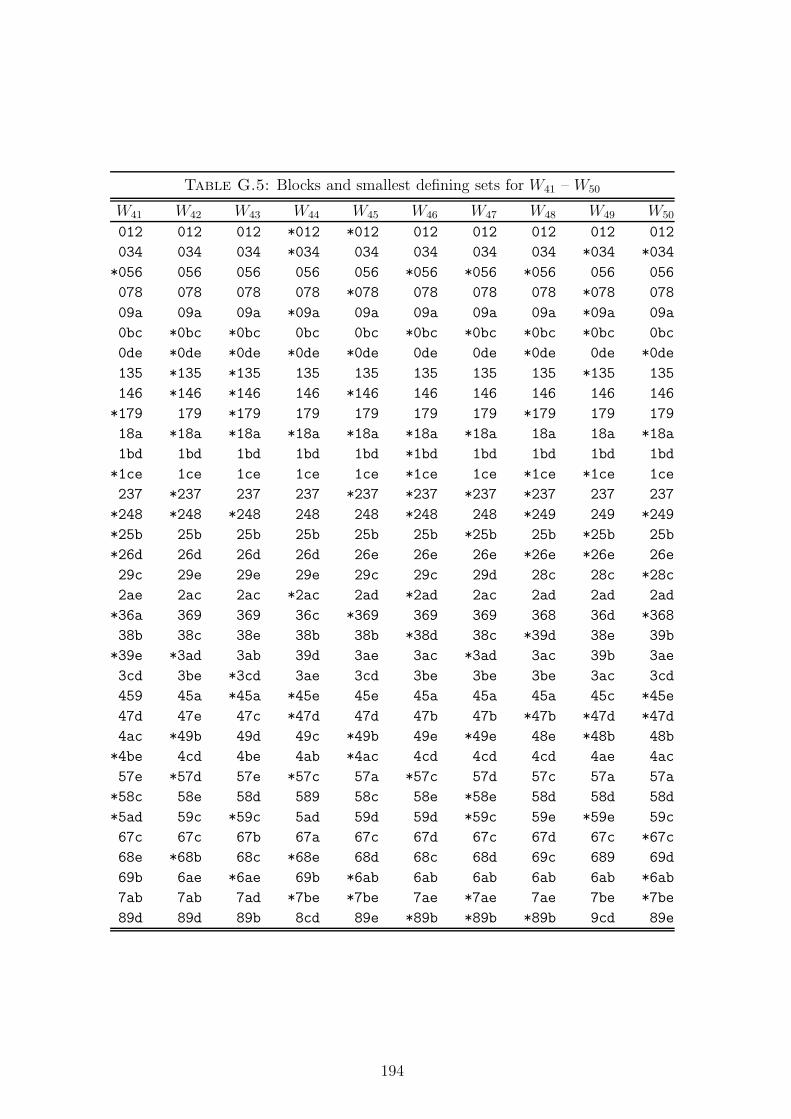
Table G.5: Blocks and smallest defining sets for W41 – W50
W41 W42 W43 W44 W45 W46 W47 W48 W49 W50
012 012 012 *012 *012 012 012 012 012 012
034 034 034 *034 034 034 034 034 *034 *034
*056 056 056 056 056 *056 *056 *056 056 056
078 078 078 078 *078 078 078 078 *078 078
09a 09a 09a *09a 09a 09a 09a 09a *09a 09a
0bc *0bc *0bc 0bc 0bc *0bc *0bc *0bc *0bc 0bc
0de *0de *0de *0de *0de 0de 0de *0de 0de *0de
135 *135 *135 135 135 135 135 135 *135 135
146 *146 *146 146 *146 146 146 146 146 146
*179 179 *179 179 179 179 179 *179 179 179
18a *18a *18a *18a *18a *18a *18a 18a 18a *18a
1bd 1bd 1bd 1bd 1bd *1bd 1bd 1bd 1bd 1bd
*1ce 1ce 1ce 1ce 1ce *1ce 1ce *1ce *1ce 1ce
237 *237 237 237 *237 *237 *237 *237 237 237
*248 *248 *248 248 248 *248 248 *249 249 *249
*25b 25b 25b 25b 25b 25b *25b 25b *25b 25b
*26d 26d 26d 26d 26e 26e 26e *26e *26e 26e
29c 29e 29e 29e 29c 29c 29d 28c 28c *28c
2ae 2ac 2ac *2ac 2ad *2ad 2ac 2ad 2ad 2ad
*36a 369 369 36c *369 369 369 368 36d *368
38b 38c 38e 38b 38b *38d 38c *39d 38e 39b
*39e *3ad 3ab 39d 3ae 3ac *3ad 3ac 39b 3ae
3cd 3be *3cd 3ae 3cd 3be 3be 3be 3ac 3cd
459 45a *45a *45e 45e 45a 45a 45a 45c *45e
47d 47e 47c *47d 47d 47b 47b *47b *47d *47d
4ac *49b 49d 49c *49b 49e *49e 48e *48b 48b
*4be 4cd 4be 4ab *4ac 4cd 4cd 4cd 4ae 4ac
57e *57d 57e *57c 57a *57c 57d 57c 57a 57a
*58c 58e 58d 589 58c 58e *58e 58d 58d 58d
*5ad 59c *59c 5ad 59d 59d *59c 59e *59e 59c
67c 67c 67b 67a 67c 67d 67c 67d 67c *67c
68e *68b 68c *68e 68d 68c 68d 69c 689 69d
69b 6ae *6ae 69b *6ab 6ab 6ab 6ab 6ab *6ab
7ab 7ab 7ad *7be *7be 7ae *7ae 7ae 7be *7be
89d 89d 89b 8cd 89e *89b *89b *89b 9cd 89e
194

Table G.6: Blocks and smallest defining sets for W51 – W60
W51 W52 W53 W54 W55 W56 W57 W58 W59 W60
012 012 012 012 012 *012 012 012 012 012
034 034 *034 034 034 034 034 *034 034 034
056 *056 056 056 056 *056 056 056 *056 056
078 078 078 *078 078 078 078 078 078 *078
09a 09a *09a *09a 09a 09a *09a 09a *09a *09a
*0bc *0bc 0bc 0bc *0bc 0bc *0bc 0bc 0bc 0bc
*0de *0de 0de 0de 0de *0de 0de 0de *0de *0de
*135 135 135 135 *135 *135 *135 135 135 *135
*146 146 *146 *146 146 146 146 146 *146 146
*179 179 179 179 *179 179 179 *179 179 *179
*18a *18a *18a 18a 18a *18a 18a 18a 18a 18a
1bd 1bd 1bd 1bd *1bd 1bd 1bd 1bd *1bd 1bd
1ce *1ce *1ce *1ce 1ce 1ce 1ce *1ce 1ce 1ce
*237 237 237 237 237 237 *237 237 237 237
24a *24a 24a 24a *24a 24a 24a *24a 24e *24e
25b *25b *25b 25b 25b 25b 25b 25b 25b *25b
26e 26e 26e 26e *26e *26e 26e 26e 26a 26a
*28c 28c 28c 28c *28c 28d 28d 28d 28c *28c
29d 29d 29d *29d 29d 29c 29c *29c *29d 29d
*369 *36c 36b 36b *368 36d 369 *36b 36c 36d
38d 38d 38d *38e 39c *38c 38c 38c *38b 38e
3ac *39e 39e *39c 3ad 39e *3ad 39e *39e 39b
3be 3ab 3ac *3ad 3be *3ab 3be *3ad 3ad *3ac
458 *458 458 459 *459 *458 *458 458 45d *45c
47e *47e 47e *47e 47e *47e 47e 47e *47b 47b
49b *49b 49b *48b 48b 49b *49b 49b 489 489
*4cd 4cd *4cd 4cd 4cd 4cd 4cd 4cd *4ac 4ad
57d 57d 57d 57c 57c 57c *57c *57c *57a 57a
59c 59c 59c 58d *58d 59d 59d *59d 58e 58d
5ae 5ae *5ae 5ae 5ae 5ae 5ae 5ae 59c 59e
67c 67b *67c 67d 67d *67b *67d 67d 67e *67e
68b 689 689 689 69b 689 *68b *689 *68d 68b
6ad 6ad 6ad *6ac *6ac 6ac 6ac 6ac 69b 69c
*7ab 7ac *7ab 7ab 7ab 7ad 7ab *7ab 7cd 7cd
89e 8be *8be 9be 89e 8be *89e 8be abe abe
195

Table G.7: Blocks and smallest defining sets for W61 – W70
W61 W62 W63 W64 W65 W66 W67 W68 W69 W70
012 012 012 *012 012 012 012 *012 012 012
034 034 034 034 *034 034 *034 034 034 034
056 056 *056 056 056 056 *056 *056 *056 *056
*078 *078 *078 078 078 078 078 078 078 078
09a 09a 09a *09a 09a 09a *09a 09a 09a *09a
*0bc 0bc *0bc 0bc 0bc *0bc 0bc 0bc *0bc *0bc
0de *0de 0de 0de *0de 0de 0de 0de *0de 0de
*135 135 135 *135 135 *135 135 135 *135 135
146 *146 *146 146 *146 146 146 146 146 *146
*179 179 179 179 *179 179 179 *179 *179 179
18b 18b 18b 18b *18b 18b *18b 18b 18b 18b
1ad *1ad *1ad 1ad 1ad *1ad *1ad 1ad 1ad 1ad
1ce 1ce 1ce 1ce 1ce 1ce 1ce 1ce 1ce *1ce
*236 *236 236 236 *237 237 237 237 *237 237
*245 247 247 *247 248 *24b 249 *248 *249 *24d
27a 25a *25a *25c *25d 25d 25c 25a 25b *25b
28e 28d 28e *28d 26a 26a 26b 26d 26c 26a
29c *29c 29c 29b 29c 28c *28d *29c 28d 28e
2bd *2be *2bd 2ae *2be *29e 2ae 2be 2ae 29c
37b 37c 37d 37e 36e 36e *36e *36e 36e 36e
*38a *389 389 38c 389 *389 389 389 *389 389
*39e 3ae 3ac *39d 3ab 3ab 3ab *3ab 3ab *3ac
3cd 3bd 3be 3ab *3cd *3cd 3cd 3cd 3cd 3bd
47e 45b 45b 45a 45b 458 45a 45b 45a 45c
*48c 48e 48c *48e 47e *47e 47e 47e 47e 47e
49d 49d *49d 49c 49d 49d *48c *49d 48c 48a
4ab 4ac *4ae 4bd 4ac 4ac *4bd 4ac *4bd 49b
57d *57d *57c *57d 57a 57a *57b 57c 57d 57a
589 58c 58d 589 58c 59c 58e 58d 58e *58d
5ac 59e 59e 5be 59e *5be 59d 59e *59c 59e
*5be 67e *67e 67b *67c 67c 67d *67a 67b 67b
*67c 68a 68a *68a 68d *68d 68a *68c 68a 68c
*68d *69b 69b *69e *69b *69b *69c 69b 69d *69d
69b 6cd 6cd 6cd 7bd 7bd 7ac 7bd *7ac 7cd
6ae *7ab 7ab *7ac 8ae 8ae 9be *8ae 9be *abe
196

Table G.8: Blocks and smallest defining sets for W71 – W80
W71 W72 W73 W74 W75 W76 W77 W78 W79 W80
012 012 *012 012 *012 *012 012 012 012 012
*034 *034 *034 034 034 034 034 034 034 *034
056 056 056 *056 *056 *056 056 056 056 *056
078 078 078 078 078 078 078 078 *078 078
09a 09a 09a 09a *09a *09a *09a 09a 09a 09a
0bc *0bc 0bc *0bc 0bc 0bc 0bc *0bc *0bc 0bc
0de 0de 0de *0de 0de 0de *0de *0de *0de *0de
*135 *135 *135 135 135 135 *135 *135 *135 135
146 146 146 146 146 146 *146 146 146 147
179 *179 179 179 *179 *179 179 179 179 168
18b 18b *18b 18b 18b *18b *18b 18b 18b *19b
*1ad 1ad 1ad 1ad *1ad 1ad 1ad 1ad *1ad 1ad
*1ce 1ce 1ce 1ce 1ce 1ce 1ce *1ce 1ce 1ce
237 237 237 *237 237 *237 237 *237 237 239
*24c 24d 24c *24a 24c 24d 24d *24a 249 *246
25a 25c 259 25b 25d 25a *258 25c 25e 25a
*26b *26b 26b 26d *26b 268 26c *268 26c 27e
*28d *28a 28d *28c 28a 29c *29e 29e 28a 28c
*29e 29e 2ae 29e 29e *2be 2ab 2bd 2bd *2bd
36e 36e 36e 36e *36e 36e *36e 36e 36a 36b
389 *389 38c 38d *38d 389 389 *38a *38e 37c
*3ac 3ac 39d 39b 39b *3ac *3ac 39b 39b 38d
3bd 3bd *3ab *3ac 3ac 3bd 3bd 3cd 3cd *3ae
45d 45a 45a 45c *45a *45c 45a 459 458 45d
47e 47e *47e 47e 47e 47b 47c *47c 47d 489
48a 48c 489 489 489 *48a 48e 48d *4ac 4ac
*49b 49b 4bd *4bd 4bd 49e 49b *4be 4be 4be
57b 57b 57b 57a 57b 57d 57d 57d *57c *57b
58e *58e 58e *58e *58e *58e 59c *58e 59d 58e
59c *59d *5cd *59d 59c 59b 5be 5ab *5ab *59c
67a *67a *67d 67b 67a 67c 67b 67b 67b 67a
68c 68d *68a *68a *68c 69d 68a 69d *68d 69e
*69d 69c *69c 69c 69d 6ab *69d 6ac *69e *6cd
7cd 7cd *7ac 7cd 7cd 7ae *7ae 7ae 7ae *79d
abe *abe 9be abe abe *8cd 8cd 89c 89c *8ab
197

Table G.9: Sampled specm(Wi) for W1 – W5
W1 W2 W3 W4 W5
|S| #ds #min #ds #min #ds #min #ds #min #ds #min
12 - - - - - - - - - -13 - - - - - - 4 4 2 214 - - 4 4 30 30 373 323 320 28015 - - 137 98 1272 729 5086 1696 4807 161916 12 12 2039 657 10931 1282 31082 1321 29895 130917 510 345 15012 936 51913 624 111848 350 106750 39018 5756 564 65559 397 163135 119 286920 40 277429 4719 35254 960 195914 144 385044 7 580546 3 562641 320 133932 111 450890 2 736031 0 982510 0 963503 021 366237 341 842254 31 1197309 0 1462905 0 1445859 022 768119 1 1348553 0 1726848 0 1974405 0 1960681 023 1317122 0 1909763 0 2256409 0 2470146 0 2463417 0
Table G.10: Sampled specm(Wi) for W6 – W10
W6 W7 W8 W9 W10
|S| #ds #min #ds #min #ds #min #ds #min #ds #min
11 - - - - - - - - - -12 0 0 - - 0 0 0 0 2 213 65 64 193 193 47 44 250 235 190 18314 2759 1917 5045 2828 2315 1681 6202 3772 6075 369815 24924 4019 39511 5601 21644 3533 47593 5594 46054 562216 103854 1303 148633 1569 92921 978 173918 1223 171208 132317 278629 124 364728 205 255350 77 416026 64 410470 6618 565965 3 690999 1 531507 4 766991 0 759405 019 955330 0 1105465 0 911245 0 1198043 0 1190782 020 1411744 0 1571571 0 1367819 0 1667924 0 1659750 0
Table G.11: Sampled specm(Wi) for W11 – W15
W11 W12 W13 W14 W15
|S| #ds #min #ds #min #ds #min #ds #min #ds #min
11 0 0 - - - - - - 0 012 5 5 0 0 1 1 - - 5 413 435 397 79 73 139 137 58 58 549 48914 11209 6457 3387 2274 4606 2895 2403 1704 12468 671515 80234 9179 30460 5071 36751 4632 22564 3466 84692 802616 275130 1862 126696 1486 139907 1067 96324 1102 279680 138017 616876 95 335128 145 350891 71 264864 95 605706 6618 1061291 3 666020 6 674157 1 543535 0 1026439 219 1548782 0 1092828 0 1087889 0 924970 0 1490897 020 2032739 0 1570662 0 1553598 0 1381182 0 1959778 0
198

Table G.12: Sampled specm(Wi) for W16 – W20
W16 W17 W18 W19 W20
|S| #ds #min #ds #min #ds #min #ds #min #ds #min
11 - - - - 0 0 0 0 0 012 - - 1 1 3 3 12 10 2 113 - - 488 482 550 500 1073 938 693 63114 138 138 11890 6476 12635 6921 22595 11643 16026 876215 3269 1538 80777 7656 84928 8103 144150 14077 106431 1035716 23109 1638 268806 1460 278649 1375 450633 2471 345509 183717 91345 467 589426 50 603794 54 917735 112 734060 7318 248813 8 1007827 0 1022026 0 1444571 2 1212447 019 526638 0 1474516 0 1486780 0 1955807 0 1717212 020 923582 0 1945007 0 1957300 0 2414857 0 2193086 0
Table G.13: Sampled specm(Wi) for W21 – W25
W21 W22 W23 W24 W25
|S| #ds #min #ds #min #ds #min #ds #min #ds #min
11 0 0 0 0 0 0 - - 0 012 4 4 6 6 5 5 1 1 3 213 627 548 861 760 1017 920 649 595 720 65914 13467 7292 18087 9432 21923 11679 15887 9213 16678 893215 93228 9982 120028 12352 137974 12772 109927 11743 108512 1043016 315258 1924 393275 2453 425209 2107 357426 2199 346999 179017 691854 102 832819 95 860072 70 761064 70 734349 7118 1171892 2 1357820 0 1367509 1 1250848 1 1207590 019 1682545 0 1886577 0 1868283 0 1756802 0 1708163 020 2173295 0 2364990 0 2331224 0 2234500 0 2180795 0
Table G.14: Sampled specm(Wi) for W26 – W30
W26 W27 W28 W29 W30
|S| #ds #min #ds #min #ds #min #ds #min #ds #min
11 - - 0 0 0 0 - - 0 012 1 1 5 5 13 12 5 5 15 1413 392 375 1272 1158 1138 1040 847 792 1101 97514 10627 6238 27851 14580 24277 12934 18241 9854 23605 1259215 76159 8622 172351 15920 152324 14446 118902 11439 152691 1508416 264569 1669 520553 2459 466540 2318 376291 1965 478574 273617 594884 80 1029335 75 940774 75 783548 72 973687 9618 1030759 1 1584260 1 1476553 1 1271128 0 1533631 119 1513724 0 2104446 0 1997295 0 1774439 0 2065973 020 2002847 0 2557853 0 2460582 0 2246362 0 2531959 0
199

Table G.15: Sampled specm(Wi) for W31 – W35
W31 W32 W33 W34 W35
|S| #ds #min #ds #min #ds #min #ds #min #ds #min
11 0 0 0 0 - - - - - -12 9 9 13 13 10 10 8 8 7 713 1252 1115 1177 1074 1185 1090 1341 1231 1192 109314 23833 12467 25401 13682 27563 14887 28603 15008 25342 1328615 147492 13000 162951 16153 174942 16811 176687 16559 160287 1517716 449448 1978 503859 2732 535286 2574 531789 2534 494816 257417 894271 68 1010989 115 1062818 84 1054675 104 993905 7918 1401766 0 1574712 0 1640643 3 1624722 2 1553702 119 1900897 0 2108740 0 2178103 0 2158736 0 2087454 020 2353829 0 2569013 0 2638426 0 2616892 0 2554090 0
Table G.16: Sampled specm(Wi) for W36 – W40
W36 W37 W38 W39 W40
|S| #ds #min #ds #min #ds #min #ds #min #ds #min
11 1 1 0 0 - - 0 0 0 012 37 31 45 44 18 18 10 9 11 1013 2276 1883 2927 2480 1688 1523 1231 1111 1279 113314 41424 19540 51229 24075 34937 17539 26651 13954 26691 1388415 239634 19739 289554 23447 210108 19362 168516 16251 168441 1584516 687644 2834 812376 3422 623214 2970 518616 2638 515511 257517 1293239 85 1490573 101 1205401 110 1039028 99 1028140 8418 1903939 0 2140450 0 1814379 0 1617364 0 1596120 019 2430275 0 2671230 0 2358026 0 2158866 0 2132996 020 2851931 0 3070963 0 2801082 0 2624525 0 2589778 0
Table G.17: Sampled specm(Wi) for W41 – W45
W41 W42 W43 W44 W45
|S| #ds #min #ds #min #ds #min #ds #min #ds #min
11 0 0 0 0 0 0 0 0 0 012 12 11 22 21 19 16 23 23 12 1113 1431 1303 1396 1238 1682 1480 2474 2156 1778 159514 29532 15157 29017 14787 33997 17349 45614 21951 35233 1796315 182488 16548 182635 17271 210040 19155 261510 21597 212927 1928016 552391 2609 560942 2913 625498 3044 742056 3109 629588 297317 1085431 109 1117908 119 1212127 109 1379847 76 1214861 9318 1663592 0 1731731 1 1824181 0 2008451 0 1823059 019 2198973 0 2295567 0 2369888 0 2538302 0 2366333 020 2651793 0 2764929 0 2809608 0 2951049 0 2810690 0
200

Table G.18: Sampled specm(Wi) for W46 – W50
W46 W47 W48 W49 W50
|S| #ds #min #ds #min #ds #min #ds #min #ds #min
11 0 0 0 0 0 0 0 0 1 112 20 20 22 19 20 18 29 29 24 2313 2065 1808 1801 1599 2271 1977 2202 1951 2472 216114 40381 19754 36049 18245 42240 20388 42461 20799 45634 2173915 238774 20988 218367 19820 247522 21181 250784 21645 268693 2294616 695471 3204 638244 2972 711761 3033 721485 3215 768350 337717 1321449 89 1225373 97 1336367 96 1359757 99 1437345 9018 1955805 0 1831451 0 1964476 1 2000379 1 2093734 019 2503042 0 2364049 0 2502353 0 2544162 0 2638537 020 2935943 0 2798543 0 2923536 0 2966683 0 3049707 0
Table G.19: Sampled specm(Wi) for W51 – W55
W51 W52 W53 W54 W55
|S| #ds #min #ds #min #ds #min #ds #min #ds #min
11 0 0 - - 0 0 0 0 0 012 12 11 12 12 12 11 9 9 10 1013 1486 1358 1796 1638 1753 1543 1227 1124 1674 153314 31522 16245 34735 17625 35391 17678 26833 14188 32943 1687015 192823 17946 209232 19021 212281 18904 171130 16605 198992 1807516 581761 2875 617891 2898 626406 2897 528070 2791 595234 278917 1145370 92 1201008 95 1205811 91 1057258 95 1163478 12018 1752566 0 1813476 0 1811408 0 1643378 1 1766968 119 2304842 0 2358661 0 2350301 0 2189190 0 2315728 020 2764667 0 2804548 0 2790389 0 2653915 0 2769265 0
Table G.20: Sampled specm(Wi) for W56 – W60
W56 W57 W58 W59 W60
|S| #ds #min #ds #min #ds #min #ds #min #ds #min
11 0 0 0 0 0 0 - - 0 012 15 15 45 42 21 21 7 7 14 1413 2102 1856 3175 2741 2530 2216 846 786 1730 151714 38730 19179 55644 25801 45714 21989 19136 10735 35530 1788115 231586 20449 311745 24973 266217 22124 127105 13662 215986 1977816 675261 3110 866527 3628 758129 3345 411251 2518 640675 316917 1286900 92 1576434 97 1407322 88 867456 98 1242786 10218 1913330 0 2242200 0 2045327 1 1410855 1 1872759 119 2457428 0 2769478 0 2574091 0 1956000 0 2428203 020 2890782 0 3155768 0 2982305 0 2452404 0 2876631 0
201

Table G.21: Sampled specm(Wi) for W61 – W65
W61 W62 W63 W64 W65
|S| #ds #min #ds #min #ds #min #ds #min #ds #min
11 - - 0 0 0 0 - - 0 012 9 9 34 34 26 24 5 5 17 1713 1096 983 3134 2787 3019 2641 1162 1068 2075 187214 23489 11948 55285 25646 52852 25047 27771 15146 39976 1975715 149496 14185 309845 24426 299132 24339 180522 18144 238437 2108016 471666 2458 848694 3303 831541 3515 558319 2940 692680 318117 970249 65 1533216 82 1513812 93 1118361 106 1320066 11418 1535525 1 2173707 0 2158900 0 1725748 1 1955270 019 2079480 0 2690052 0 2678681 0 2282794 0 2503870 020 2549625 0 3076406 0 3064864 0 2744288 0 2937928 0
Table G.22: Sampled specm(Wi) for W66 – W70
W66 W67 W68 W69 W70
|S| #ds #min #ds #min #ds #min #ds #min #ds #min
11 0 0 0 0 0 0 0 0 0 012 15 14 23 23 34 33 38 38 20 1913 2230 1994 2429 2140 2882 2471 2968 2572 1861 165914 44009 21428 45811 22104 51234 24184 51603 24431 36219 1834615 257342 22239 268976 23341 292346 24219 293713 24418 217626 1962116 741770 3301 771325 3485 816488 3354 826199 3571 636033 307517 1393756 105 1444892 116 1497835 96 1517047 120 1223842 8518 2041843 0 2107539 2 2148461 0 2175994 0 1832827 119 2591189 0 2656400 0 2678768 0 2710935 0 2371369 020 3017328 0 3071716 0 3078479 0 3113543 0 2814077 0
Table G.23: Sampled specm(Wi) for W71 – W75
W71 W72 W73 W74 W75
|S| #ds #min #ds #min #ds #min #ds #min #ds #min
11 0 0 0 0 0 0 0 0 0 012 31 31 34 33 16 16 25 23 25 2513 3193 2795 2496 2161 1658 1499 2411 2116 2107 181214 55236 26078 45819 22378 32723 17064 45767 22851 41502 2027915 312691 25596 267689 23184 205193 20057 265926 22554 244576 2115316 866879 3604 770254 3475 625720 3426 754917 3289 706588 309217 1576127 100 1439226 105 1230102 100 1401444 95 1333047 12618 2240964 1 2104339 0 1871115 0 2034637 0 1965263 119 2769171 0 2653491 0 2440826 0 2562492 0 2505380 020 3158706 0 3070697 0 2900824 0 2969799 0 2935273 0
202

Table G.24: Sampled specm(Wi) for W76 – W80
W76 W77 W78 W79 W80
|S| #ds #min #ds #min #ds #min #ds #min #ds #min
11 - - 0 0 0 0 0 0 - -12 25 25 43 42 20 20 35 32 33 3313 2048 1873 3792 3321 2543 2227 2443 2088 3774 337814 40343 20301 66801 30942 46122 22207 46116 22844 69222 3365615 238563 20251 368098 29012 267811 23127 273730 24683 393623 3318716 683978 2965 999690 4074 766349 3504 793453 3900 1077769 471217 1286351 98 1776234 111 1432597 97 1485468 92 1916910 11918 1892405 0 2470519 1 2084708 0 2150225 0 2650092 119 2416782 0 2995152 0 2626649 0 2689069 0 3175825 020 2838715 0 3357446 0 3039857 0 3092476 0 3518887 0
203

References
[1] Peter Adams, Elizabeth J. Billington, and C.A. Rodger. Pasch decompositions
of lambda-fold triple systems. Journal of Combinatorial Mathematics and
Combinatorial Computing, 15:53–63, 1994.
[2] S. Ajoodani-Namini and G.B. Khosrovashahi. More on halving the complete
designs. Discrete Mathematics, 135:29–37, 1994.
[3] Ian Anderson. Combinatorics of Finite Sets. Clarendon Press, Oxford, 1987.
[4] Ian Anderson. Combinatorial Designs: construction methods. Ellis Horwood
Ltd., Chichester, 1990.
[5] Peter Barth. A Davis-Putman based enumeration algorithm for linear pseudo-
boolean optimisation. Report MPI-I-95-2-003, Max-Planck-Institut fur Infor-
matik, 1995.
[6] Thomas Beth, Dieter Jungnickel, and Hanfried Lenz. Design Theory. Cam-
bridge University Press, 1986.
[7] Elizabeth J. Billington. The intersection problem for combinatorial designs.
Congressus Numerantium, 92:33–54, 1993.
[8] Elizabeth J. Billington and D.G. Hoffman. Trades and graphs. Submitted.
[9] W. Bosma, J. Cannon, and C. Playoust. The Magma algebra system I: the
user language. Journal of Symbolic Computation, 24:235–265, 1997.
[10] A.E. Brouwer. Steiner triple systems without forbidden subconfigurations.
Technical Report ZW104-77, Mathematisch Centrum Amsterdam, 1977.
[11] Darryn E. Bryant. On the volume of trades in triple systems. Australasian
Journal of Combinatorics, 15:161–176, 1997.
[12] F.C. Bussemaker and J.J. Seidel. Symmetric Hadamard matrices of order 36.
T.H. Report 70-WSK-02, Department of Mathematics, Technological Univer-
sity, Eindhoven, Netherlands, 1970.
[13] Charles J. Colbourn and Janelle J. Harms. Partitions into indecomposable
triple systems. Annals of Discrete Mathematics, 34:107–118, 1987.
[14] C.J. Colbourn and J.H. Dinitz, editors. CRC Handbook of Combinatorial
Designs. CRC Publishing Co., Boca Raton, Florida, 1996.
[15] Joan Cooper, Diane Donovan, and Jennifer Seberry. Secret sharing schemes
204

arising from Latin squares. Bulletin of the Institute of Combinatorics and its
Applications, 12:33–43, 1994.
[16] R.T. Curtis. Eight octads suffice. Journal of Combinatorial Theory (Series
A), 36:116–123, 1984.
[17] Catherine M. Delaney. Computational aspects of defining sets of combinatorial
designs. Master’s thesis, The University of Queensland, 1995.
[18] Cathy Delaney. complete – rationale and user’s guide. Research Report
CCRR–01–95, Centre for Combinatorics, Department of Mathematics, The
University of Queensland, 1995.
[19] Cathy Delaney, Brenton D. Gray, Ken Gray, Barbara M. Maenhaut, Martin J.
Sharry, and Anne Penfold Street. Pointwise defining sets and trade cores.
Australasian Journal of Combinatorics, 16:51–76, 1997.
[20] Cathy Delaney, Barbara M. Maenhaut, Martin J. Sharry, and Anne Penfold
Street. pds – rationale and user’s guide. Research Report CCRR–04–96,
Centre for Combinatorics, Department of Mathematics, The University of
Queensland, 1996.
[21] Cathy Delaney, Martin J. Sharry, and Anne Penfold Street. bds – rationale
and user’s guide. Research Report CCRR–02–96, Centre for Combinatorics,
Department of Mathematics, The University of Queensland, 1996.
[22] Cathy Delaney, Martin J. Sharry, and Anne Penfold Street. lds – rationale
and user’s guide. Research Report CCRR–05–96, Centre for Combinatorics,
Department of Mathematics, The University of Queensland, 1996.
[23] Immo Diener, Eberhard Schmitt, and Hans Ludwig de Vries. All 80 Steiner
triple systems on 15 elements are derived. Discrete Mathematics, 55:13–19,
1985.
[24] J. Doyen and R.M. Wilson. Embeddings of Steiner triple systems. Discrete
Mathematics, 5:229–239, 1973.
[25] Jean Doyen and Alexander Rosa. An updated bibliography and survey of
Steiner systems. Annals of Discrete Mathematics, 7:317–349, 1980.
[26] Konrad Engel. The number of indecomposable designs is finite. Ars Combi-
natoria, 17:33–34, 1984.
[27] Konrad Engel. On the number of t-(v, k, λ) designs. Ars Combinatoria, 28:273–
277, 1989.
[28] Free Software Foundation, Inc., 59 Temple Place, Suite 330, Boston, MA
02111-1307, USA. GNU CC Manual, v2.7.2 edition, 1995.
205

[29] Peter B. Gibbons. Computing techniques for the construction and analysis
of block designs. Technical Report No. 92, Department of Computer Science,
University of Toronto, 1976.
[30] Peter B. Gibbons. Computational methods in design theory. In C.J. Colbourn
and J.H. Dinitz, editors, CRC Handbook of Combinatorial Designs, pages 718–
740. CRC Publishing Co., Boca Raton, Florida, 1996.
[31] Rebecca A.H. Gower. Minimal defining sets in a family of Steiner triple sys-
tems. Australasian Journal of Combinatorics, 8:55–73, 1993.
[32] Rebecca A.H. Gower. Defining sets for the Steiner triple systems from affine
spaces. Journal of Combinatorial Designs, 5:155–175, 1997.
[33] R.L. Graham, S.-Y.R. Li, and W.-C.W. Li. On the structure of t-designs.
SIAM Journal of Algebraic Discrete Methods, 1:8–14, 1980.
[34] M.J. Grannell, T.S. Griggs, and J. Wallace. The smallest defining set of a
Steiner triple system. Preprint.
[35] J.E. Graver and W.B. Jurkat. The module structure of integral designs. Jour-
nal of Combinatorial Theory (Series A), 15:75–90, 1973.
[36] Brenton D. Gray. Personal communication, August 1995.
[37] Brenton D. Gray. Defining sets of simple designs. Bulletin of the Institute of
Combinatorics and its Applications, 19:23–26, 1997.
[38] Brenton D. Gray. Smallest defining sets of designs associated with PG(d, 2).
Australasian Journal of Combinatorics, 16:87–98, 1997.
[39] Brenton D. Gray, Rudi Mathon, Tony Moran, and Anne Penfold Street. Min-
imal defining sets of the STS associated with PG(3, 2). In preparation.
[40] Brenton D. Gray and Colin Ramsay. On the spectrum of Steiner (v, k, t) trades
(I). Journal of Combinatorial Mathematics and Combinatorial Computing. To
appear.
[41] Brenton D. Gray and Colin Ramsay. On the spectrum of Steiner (v, k, t) trades
(II). Graphs and Combinatorics. To appear.
[42] Brenton D. Gray and Colin Ramsay. On a conjecture of Mahmoodian and
Soltankhah regarding the existence of (v, k, t) trades. Ars Combinatoria,
48:191–194, 1998.
[43] Brenton D. Gray and Colin Ramsay. On the spectrum of [v, k, t] trades. Jour-
nal of Statistical Planning and Inference, 69:1–19, 1998.
[44] Brenton Donald Gray. Trades and defining sets. PhD thesis, The University
of Queensland. Submitted.
206

[45] Ken Gray. Defining sets of single-transposition-free designs. Utilitas Mathe-
matica, 38:97–103, 1990.
[46] Ken Gray. Further results on smallest defining sets of well-known designs.
Australasian Journal of Combinatorics, 1:91–100, 1990.
[47] Ken Gray. On the minimum number of blocks defining a design. Bulletin of
the Australian Mathematical Society, 41:97–112, 1990.
[48] Ken Gray and Anne Penfold Street. Smallest defining sets of the five non-
isomorphic 2-(15, 7, 3) designs. Bulletin of the Institute of Combinatorics and
its Applications, 9:96–102, 1993.
[49] Ken Gray and Anne Penfold Street. The smallest defining set of the 2-(15, 7, 3)
design associated with PG(3, 2): a theoretical approach. Bulletin of the In-
stitute of Combinatorics and its Applications, 11:77–83, 1994.
[50] Kenneth Raward Gray. Special subsets of the block sets of designs. PhD thesis,
The University of Queensland, 1990.
[51] Catherine S. Greenhill. An algorithm for finding smallest defining sets of
t-designs. Journal of Combinatorial Mathematics and Combinatorial Com-
puting, 14:39–60, 1993.
[52] Catherine S. Greenhill and Anne Penfold Street. Smallest defining sets of some
small t-designs and relations to the Petersen graph. Utilitas Mathematica,
48:5–31, 1995.
[53] Catherine Suzanne Greenhill. An algorithm for finding smallest defining sets
of t-designs. Master’s thesis, The University of Queensland, 1992.
[54] Terry S. Griggs, Eric Mendelsohn, and Alexander Rosa. Simultaneous decom-
positions of Steiner triple systems. Ars Combinatoria, 37:157–173, 1994.
[55] T.S. Griggs, M.J. de Resmini, and A. Rosa. Decomposing Steiner triple sys-
tems into four-line configurations. Annals of Discrete Mathematics, 52:215–
226, 1992.
[56] Hans-Dietrich O.F. Gronau. A survey of results on the number of t-(v, k, λ)
designs. Annals of Discrete Mathematics, 26:209–220, 1985.
[57] Martin Gruttmuller. On the number of indecomposable block designs. Aus-
tralasian Journal of Combinatorics, 14:181–186, 1996.
[58] Marshall Hall, Jr. Combinatorial theory. John Wiley & Sons, second edition,
1986.
[59] Alan Hartman. Algorithmic aspects of integral designs. Australasian Journal
of Combinatorics. To appear.
207

[60] Alan Hartman. Halving the complete design. Annals of Discrete Mathematics,
34:207–224, 1987.
[61] A. Hedayat. The theory of trade-off for t-designs. In D. Raychaudhuri, editor,
Coding Theory and Design Theory, Part II: Design Theory, number 21 in IMA
Volumes in Mathematics and its Applications, pages 101–126. Springer-Verlag,
1990.
[62] A. Hedayat and H.L. Hwang. Construction of BIB designs with various sup-
port sizes – with special emphasis for v = 8 and k = 4. Journal of Combina-
torial Theory (Series A), 36:163–173, 1994.
[63] A. Hedayat and Shuo -Yen Robert Li. The trade-off method in the construction
of BIB designs with variable support sizes. Annals of Statistics, 7:1277–1287,
1979.
[64] A.S. Hedayat and G.B. Khosrovshahi. An algebraic study of BIB designs:
a complete solution for v = 6 and k = 3. Journal of Combinatorial Theory
(Series A), 30:43–52, 1981.
[65] A.S. Hedayat, G.B. Khosrovshahi, and D. Mujumdar. A prospect for a general
method of constructing t-designs. Discrete Applied Mathematics, 42:31–50,
1993.
[66] Peter Horak and Alexander Rosa. Decomposing Steiner triple systems into
small configurations. Ars Combinatoria, 26:91–105, 1988.
[67] H.L. Hwang. On the structure of (v, k, t) trades. Journal of Statistical Planning
and Inference, 13:179–191, 1986.
[68] A.V. Ivanov. Constructive enumeration of incidence systems. Annals of Dis-
crete Mathematics, 26:227–246, 1985.
[69] A.D. Keedwell. Critical sets for Latin squares, graphs and block designs: a
survey. Congressus Numerantium, 113:231–245, 1996.
[70] Brian W. Kernighan and Dennis M. Ritchie. The C programming language.
Prentice Hall, second edition, 1988.
[71] A. Khodkar. Smallest defining sets for the 36 non-isomorphic twofold triple
systems of order nine. Journal of Combinatorial Mathematics and Combina-
torial Computing, 17:209–215, 1994.
[72] A. Khodkar and Dean G. Hoffman. On the non-existence of Steiner (v, k, 2)
trades with certain volumes. Australasian Journal of Combinatorics. To ap-
pear.
208
[73] G.B. Khosrovshahi and S. Ajoodani-Namini. A new basis for trades. SIAM
Journal of Discrete Mathematics, 3(3):364–372, 1990.
[74] G.B. Khosrovshahi and H.R. Maimani. Smallest defining sets for 2-(10, 5, 4)
designs. Australasian Journal of Combinatorics, 15:31–35, 1997.
[75] G.B. Khosrovshahi, Dibyen Majumdar, and Mario Widel. On the structure
of basic trades. Journal of Combinatorics, Information & System Sciences,
17(1–2):102–107, 1992.
[76] G.B. Khosrovshahi and Ch. Maysoori. On the bases for trades. Linear Algebra
and its Applications, 226–228:731–748, 1995.
[77] G.B. Khosrovshahi, A. Nowzari-Dalini, and R. Torabi. Trading signed designs
and some new 4-(12,5,4) designs. Designs, Codes and Cryptography, 11:279–
288, 1997.
[78] G.B. Khosrovshani and F. Vatan. On 3-(8, 4, λ) designs. Ars Combinatoria,
32:115–120, 1991.
[79] William Kocay. On writing isomorphism programs. In W.D. Wallis, editor,
Computational and Constructive Design Theory, pages 135–175. Kluwer Aca-
demic Publishers, 1996.
[80] Thomas Kunkle and Jennifer Seberry. A few more small defining sets for
SBIBD(4t − 1, 2t − 1, t − 1). Bulletin of the Institute of Combinatorics and
its Applications, 12:61–64, 1994.
[81] I. Landgev. Nondecomposable block designs with v = 7 and k = 3. In
G. Gerov, editor, Mathematics and mathematical education (Bulgarian) (Al-
bena, April 6–10, 1989), pages 386–389, Sofia, 1989. Bulgarian Academy of
Sciences.
[82] Julie L. Lawrence. Personal communication, November 1997.
[83] C.C. Lindner. A survey of embedding theorems for Steiner systems. Annals
of Discrete Mathematics, 7:175–202, 1980.
[84] Ebadollah S. Mahmoodian. On the support size of 3-designs with repeated
blocks. Ars Combinatoria, 30:13–22, 1990.
[85] E.S. Mahmoodian, Reza Naserasr, and Manouchehr Zaker. Defining sets
in vertex colorings of graphs and latin rectangles. Discrete Mathematics,
167/168:451–460, 1997.
[86] E.S. Mahmoodian and Nasrin Soltankhah. On the existence of (v, k, t) trades.
Australasian Journal of Combinatorics, 6:279–291, 1992.
209

[87] R. Mathon and A. Rosa. A census of Mendelsohn triple systems of order nine.
Ars Combinatoria, 4:309–315, 1977.
[88] R.A. Mathon, K.T. Phelps, and A. Rosa. Small Steiner triple systems and their
properties. Ars Combinatoria, 15:3–110, 1983. Corrigendum, ibid., 16:286,
1983.
[89] Rudolf Mathon. Computational methods in design theory. In W.D. Wallis,
editor, Computational and Constructive Design Theory, pages 29–48. Kluwer
Academic Publishers, 1996.
[90] Brendan D. McKay. Practical graph isomorphism. Congressus Numerantium,
30:45–87, 1981.
[91] Brendan D. McKay. nauty user’s guide (version 1.5). Technical Report TR-
CS-90-02, Department of Computer Science, Australian National University,
1990.
[92] N.S. Mendelsohn and Stephen H.Y. Hung. On the Steiner systems S(3, 4, 14)
and S(4, 5, 15). Utilitas Mathematica, 1:5–95, 1972.
[93] Anthony Terence Moran. Block designs and their defining sets. PhD thesis,
The University of Queensland, 1997.
[94] Tony Moran. Defining sets for 2-(19, 9, 4) designs and a class of Hadamard
designs. Utilitas Mathematica. To appear.
[95] Tony Moran. Smallest defining sets for 2-(9, 4, 3) and 3-(10, 5, 3) designs.
Australasian Journal of Combinatorics, 10:265–288, 1994. Corrigendum, ibid.,
14:311–312, 1996.
[96] Elizabeth J. Morgan. Some small quasi-multiple designs. Ars Combinatoria,
3:233–250, 1977.
[97] Albert Nijenhuis and Herbert S. Wilf. Combinatorial Algorithms. Academic
Press, second edition, 1978.
[98] Colin Ramsay. An improved version of complete for the case λ = 1. Research
Report CCRR–03–96, Centre for Combinatorics, Department of Mathematics,
The University of Queensland, 1996.
[99] Colin Ramsay. An algorithm for completing partials, with an application to
the smallest defining sets of the STS(15). Utilitas Mathematica, 52:205–221,
1997.
[100] Colin Ramsay. An algorithm for enumerating trades in designs, with an ap-
plication to defining sets. Journal of Combinatorial Mathematics and Combi-
natorial Computing, 24:3–31, 1997.
210

[101] Colin Ramsay. On a family of STS(v) whose smallest defining sets contain
at least b/4 blocks. Bulletin of the Institute of Combinatorics and its Appli-
cations, 20:91–94, 1997.
[102] Edward M. Reingold, Jurg Nievergelt, and Narsingh Deo. Combinatorial Al-
gorithms: theory and practice. Prentice-Hall, 1977.
[103] Frank Ruskey. Combinatorial generation. Unpublished manuscript (Working
Version (1h), December 1996).
[104] Dinesh Sarvate and Jennifer Seberry. A note on small defining sets for some
SBIBD(4t − 1, 2t − 1, t − 1). Bulletin of the Institute of Combinatorics and
its Applications, 10:26–32, 1994.
[105] Jennifer Seberry. On small defining sets for some SBIBD(4t−1, 2t−1, t−1).
Bulletin of the Institute of Combinatorics and its Applications, 4:58–62, 1992.
Corrigendum, ibid., 6:62, 1992.
[106] Mark G. Sobell. A Practical Guide to the UnixTM System. The Ben-
jamin/Cummings Publishing Company, Inc., second edition, 1989.
[107] D.R. Stinson. Hill-climbing algorithms for the construction of combinatorial
designs. Annals of Discrete Mathematics, 26:321–334, 1985.
[108] D.R. Stinson and Y.J. Wei. Some results on quadrilaterals in Steiner triple
systems. Discrete Mathematics, 105:207–219, 1992.
[109] Anne Penfold Street. Defining sets for t-designs and critical sets for Latin
squares. New Zealand Journal of Mathematics, 21:133–144, 1992.
[110] Anne Penfold Street. Defining sets for block designs: an update. In C.J.
Colbourn and E.S. Mahmoodian, editors, Combinatorics Advances, pages 307–
320. Kluwer Academic Press, Norwell, Massachusetts, 1995.
[111] Anne Penfold Street. Trades and defining sets. In C.J. Colbourn and J.H.
Dinitz, editors, CRC Handbook of Combinatorial Designs, pages 474–478.
CRC Publishing Co., Boca Raton, Florida, 1996.
[112] A.P. Street and D.J. Street. Combinatorics of Experimental Design. Clarendon
Press, Oxford, 1987.
[113] J.H. van Lint, H.C.A. van Tilborg, and J.R. Wiekema. Block designs with
v = 10, k = 5, λ = 4. Journal of Combinatorial Theory (Series A), 23:105–
115, 1977.
[114] John van Rees. (r, λ)-designs. In C.J. Colbourn and J.H. Dinitz, editors,
CRC Handbook of Combinatorial Designs, pages 434–436. CRC Publishing
Co., Boca Raton, Florida, 1996.
211