TPC-BiH: A Benchmark for Bitemporal Databases

TPC-BiH: A Benchmark for BitemporalDatabases

Martin Kaufmann1,2, Peter M. Fischer3, Norman May1, Andreas Tonder1, andDonald Kossmann2

1 SAP AG, 69190 Walldorf, Germany{norman.may,andreas.tonder}@sap.com2 ETH Zurich, 8092 Zurich, Switzerland

{martin.kaufmann,donald.kossmann}@inf.ethz.ch3 Albert-Ludwigs-Universitat, Freiburg, Germany

[email protected]

Abstract. An increasing number of applications such as risk evalua-tion in banking or inventory management require support for temporaldata. After more than a decade of standstill, the recent adoption of somebitemporal features in SQL:2011 has reinvigorated the support amongcommercial database vendors, who incorporate an increasing number ofrelevant bitemporal features. Naturally, assessing the performance andscalability of temporal data storage and operations is of great concernfor potential users. The cost of keeping and querying history with noveloperations (such as time travel, temporal joins or temporal aggregations)is not adequately reflected in any existing benchmark. In this paper, wepresent a benchmark proposal which provides comprehensive coverageof the bitemporal data management. It builds on the solid foundationsof TPC-H but extends it with a rich set of queries and update scenar-ios. This workload stems both from real-life temporal applications fromSAP’s customer base and a systematic coverage of temporal operatorsproposed in the academic literature. We present preliminary results ofour benchmark on a number of temporal database systems, also high-lighting the need for certain language extensions.

Keywords: Bitemporal Databases, Benchmark, Data Generator

1 Introduction

Temporal information is widely used in real-world database applications, e.g.,to plan for the delivery of a product or to record the time a state of an orderchanged. Particularly the need for tracing and auditing the changes made to adata set and the ability to make decisions based on past or future assumptions areimportant use cases for temporal data. As a consequence, temporal features wereincluded into the SQL:2011 standard [9], and an increasing number of databasesystems offer temporal features, e.g., Oracle, DB2, SAP HANA, or Teradata. Astemporal data is often stored in an append-only mode, temporal tables quicklygrow very large. This makes temporal processing a performance-critical aspect

2 M. Kaufmann, P. Fischer, N. May, A. Tonder, D. Kossmann

of many analysis tasks. Clearly, an understanding of the performance character-istics of different implementations of temporal queries is required to select themost appropriate database system for the desired workload. Unfortunately, atthis time there is no generally accepted benchmark for temporal workloads.For non-temporal data the TPC has defined TPC-H and TPC-DS for analyticaltasks and TPC-C and TPC-E for transactional workloads. Especially TPC-Hand TPC-C are popular for comparing database systems. These benchmarksquery only the most recent version of the data. We propose to leverage the in-sights gained with TPC-H and to TPC-C while widening the scope for temporaldata. In particular, it should be possible to evaluate all TPC-H queries at dif-ferent system times. This allows us to compare results on temporal data withthose on non-temporal data. We carefully introduce additional parameters toexamine the temporal dimension. Furthermore, we propose additional queriesthat resemble typical use cases we encountered in real-world use cases at SAPbut also during literature review. In some cases, the expressiveness of SQL:2011is not sufficient to express these queries in a succinct way. For example, the sim-ulation of temporal aggregation in SQL:2011 results in rather complex queries.More precisely, we propose a novel benchmark for temporal queries which arebased on real-world use cases. As such, these queries retrieve both previousstates of the system (i.e., a certain system time) but they also examine time in-tervals defined in the business domain (i.e., application time); this concept wasintroduced as the bitemporal data model by Snodgrass [12]. The benchmark wepropose contains a data generator which first generates a TPC-H data set ex-tended with some temporal data. In contrast to previous related work (such as [1]and [2]) it also generates a history of values using various business transactionson this data to generate system times. These transactions are inspired by theTPC-C benchmark, and they are designed to keep the characteristics generatedby TPC-H dbgen at every point in time. Consequently, all TPC-H queries canbe executed on the generated data, and their result properties for certain systemtimes are comparable to those in the standard TPC-H benchmark. However, overtime the overall data set grows as the previous versions are preserved in orderto support time travel to a previous state of the system. In order to evaluate thetime dimension, for this benchmark, we define additional queries which retrievedata at different points in time.The remainder of this paper is structured as follows: In Section 2 we summarizethe design goals for our proposed benchmark TPC-BiH. We survey related workon benchmarking temporal databases in Section 3. In the core part of the paper(Section 4), we define the schema, the data generator for temporal data, andthe queries comprising the benchmark. We analyze two systems that supporttemporal queries, and we present performance measurements for our benchmark(Section 5). In Section 6, we summarize our findings and point out future work.

TPC-BiH: A Benchmark for Bitemporal Databases 3

2 Goals and Methodology

The goal of this paper is to present a comprehensive benchmark for bitempo-ral query processing. This benchmark includes all necessary definitions as wellas the relevant tools such as data generators. The benchmark setting reflectsreal-life customer workloads (which have typically not been formalized to matchthe current expression of the bitemporal model) and is complemented by syn-thetic queries to test certain operations. The benchmark is targeted towardsSQL:2011, which has recently adopted core parts of the temporal data model.Since the expressiveness of SQL:2011 is limited (no complex temporal join, notemporal aggregation), we provide alternative versions of the queries using lan-guage extensions. Similarly, in order to support DBMS’s which provide temporalsupport, but have not (yet) adopted SQL:2011 (like Oracle or Teradata), we pro-vide alternative queries.

The schema builds on a well-understood existing non-temporal analyticsbenchmark: TPC-H. Its tables are extended with different types of history classes,such as degenerated, fully bitemporal or multiple user times. The benchmarkdata is designed to provide a range of different temporal update patterns, vary-ing the ratio of history vs. initial data, the types of operations (UPDATE, INSERTand DELETE) as well as the temporal distributions within and between the tem-poral dimensions. The data distributions and correlations stay stable with regardto system time updates and evolve according to well-defined update scenarios inthe application time domain. The data generator we developed can be scaled inthe dimensions of initial data size and history length independently, providingsupport for many different scenarios.

Our query workload provides a coverage of common temporal DB require-ments. It covers operations such as time travel, key in time, temporal joins, andtemporal aggregations – the latter is not directly expressible in SQL:2011. Simi-larly, we investigate many patterns of storage access and time- vs. key-orientedaccess with varying ranges and selectivity. The query workload also covers thedifferent temporal dimensions (system and application time): The focus of thequeries is on stressing the system for individual time dimensions while consider-ing correlations among the dimensions whenever relevant.

In summary, our benchmark fulfills the requirements mentioned in the bench-mark handbook by Jim Gray [3], i.e., it is

– relevant, since it covers all typical temporal operations.– portable, since it targets SQL:2011 and provides extensions for systems not

completely supporting SQL:2011.– scalable, since it provides well-defined data which can be generated in differ-

ent sizes for base data and history.– understandable, since all queries have a meaning in application scenarios and

in terms of operator/system “stress”.


3 Related Work on Temporal Benchmarks

The foundation of the bitemporal data model was established in the proposal forTSQL2 [12]. For a single row the system time – in the original paper called trans-action time – defines different versions as they were created by DML statementson a row. The system time is immutable, and the values are implicitly generatedduring transaction commit. Orthogonal to that, validity intervals can be definedon the application level – called valid time in the original paper. An exampleis the specification of the visibility of some marketing campaigns to users. Un-like the system time, the application time can be updated, and both intervalboundaries may refer to times in the past, present, or future. The concept ofthe bitemporal model is now also applied in the SQL:2011 standard [9]. Thisstandard focuses on basic operations like time travel on a single table. Complextemporal joins or aggregations are out of scope, but they are acknowledged asrelevant scenarios for future versions of the SQL standard.

The benchmarks published by the TPC are the most commonly used bench-marks for databases. While these benchmarks used to focus either on analyticalor transactional workloads, recently a combination has been proposed: The CH-benCHmark [2] extends the TPC-C schema by adding three tables from theTPC-H schema. Yet, no time dimension is included in these benchmarks.

Benchmarking the temporal dimension has been the focus of several stud-ies: In 1995, a research proposal by Dunham et al. outlined possible directionsand requirements for such a benchmark. The approach for building a temporalbenchmark and the query classes come close to our methods. A later work byKuala and Robertson [5] provides logical models of several temporal databaseapplication areas alongside with queries expressed in an informal manner. Thetest suite of temporal database queries [4] from the TSQL2 editors providesa large number of temporal queries focused on functional testing rather thanperformance evaluation. A study on spatio-temporal databases by Werstein [13]evaluates existing benchmarks and concludes that the temporal aspects of thesebenchmarks are insufficient. In turn, a number of queries are informally definedto overcome this limitation. The work that is most closely related to ours waspresented at TPCTC 2012 and includes a proposal to add a temporal dimensionto the TPC-H Benchmark [1]. The authors also use TPC-H as a starting point,extend some tables with temporal columns to express bitemporal data, and relyon the data generator and the original queries of TPC-H as part of their work-load. Yet, this work seems to be more focused on sketching the possibilities forthe bitemporal data model rather than providing explicit definitions of data andqueries. Specific differences exist in the language used (we focus on SQL:2011,in [1] a variant of TSQL2 is applied) as well as the derivation of applicationtimestamps (we use existing temporal information in TPC-H for the initial ver-sion). Our update scenarios and queries cover a broader range of cases and aimto provide more properties on data and queries.


PART

SUPPLIER

PARTSUPP

CUSTOMER

NATION

LINEITEM

COMMENT

ACTIVE_TIME

SYS_TIME

REGIONKEY

NAME

COMMENT

REGION

ORDERS

NATIONKEY

NAME

REGIONKEY

COMMENT

PARTKEY

NAME

MFGR

BRAND

TYPE

SIZE

CONTAINER

RETAILPRICE

COMMENT

AVAILABILITY_TIME

SYS_TIME

PARTKEY

SUPPKEY

AVAILQTY

SUPPLYCOST

COMMENT

VALIDITY_TIME

SYS_TIME

SUPPKEY

NAME

ADDRESS

NATIONKEY

PHONE

ACCTBAL

COMMENT

SYS_TIME

ORDERKEY

PARTKEY

SUPPKEY

LINENUMBER

QUANTITY

EXTENDEDPRICE

DISCOUNT

TAX

RETURNFLAG

LINESTATUS

SHIPDATE

COMMITDATE

RECEIPTDATE

SHIPINSTRUCT

SHIPMODE

CUSTKEY

NAME

ADDRESS

NATIONKEY

PHONE

ACCTBAL

MKTSEGMENT

COMMENT

VISIBLE_TIME

SYS_TIME

ORDERKEY

CUSTKEY

ORDERSTATUS

TOTALPRICE

ORDERDATE

ORDERPRIORITY

CLERK

SHIPPRIORITY

COMMENT

ACTIVE_TIME

RECEIVABLE_TIME

SYS_TIME

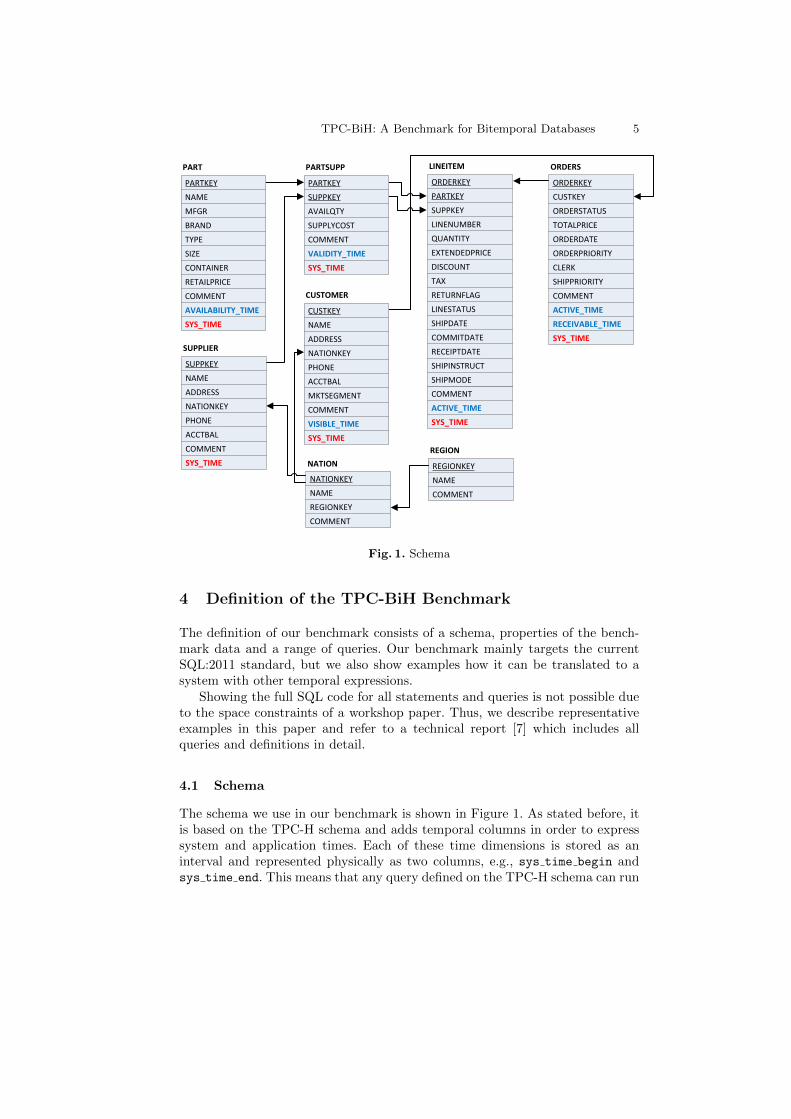
Fig. 1. Schema

4 Definition of the TPC-BiH Benchmark

The definition of our benchmark consists of a schema, properties of the bench-mark data and a range of queries. Our benchmark mainly targets the currentSQL:2011 standard, but we also show examples how it can be translated to asystem with other temporal expressions.

Showing the full SQL code for all statements and queries is not possible dueto the space constraints of a workshop paper. Thus, we describe representativeexamples in this paper and refer to a technical report [7] which includes allqueries and definitions in detail.

4.1 Schema

The schema we use in our benchmark is shown in Figure 1. As stated before, itis based on the TPC-H schema and adds temporal columns in order to expresssystem and application times. Each of these time dimensions is stored as aninterval and represented physically as two columns, e.g., sys time begin andsys time end. This means that any query defined on the TPC-H schema can run


on our data set, and will give meaningful results, reflecting the current systemtime and the full range of application time versions. Specific other temporaldimensions can be added in a fairly straightforward manner. The additionaltemporal columns are chosen in such a way that the schema contains tables withdifferent temporal properties: Some tables are kept unversioned, some express acorrelated/degenerated behavior. Most tables are fully bitemporal, and we alsoconsider the case in which a table has multiple “user” times. Even if the latteris not well specified in the standard, we observe it a lot in customer use cases.

More specifically, we do not add any temporal columns to REGION andNATION. This is also plausible from application semantics, since this kind ofinformation rarely ever changes. All other relations at least include a systemtime dimension. For SUPPLIER we simulate a degenerated table by only givinga system time. Since this single time dimension is determined by the loading/up-dating timing, we do not use any temporal correlation queries between this tableand truly bi-dimensional tables. For all the remaining relations, we determinethe application time from the existing information present in the data: Tuplesin LINEITEM are valid as long as any operation like shipping them is pending.Likewise, tuples from PART are valid when they can be ordered, tuples fromCUSTOMER when the customer is visible to the system, tuples from PART-SUPP when the price and the amount are valid. Finally, ORDERS has two timedimensions: ACTIVE TIME : when was the order “active” (i.e., placed, but notdelivered yet) and RECEIVABLE TIME : when the bill for the order can be paid(i.e., invoice sent to customer, but not paid yet). Both application times becomepart of the schema. Since current DBMSs only support a single application time,we designate ACTIVE TIME as such, and keep RECEIVABLE TIME as a “reg-ular” timestamp column. Likewise, if a DBMS does not provide any support forapplication time, application times are mapped to normal timestamp columns.

4.2 Benchmark Data

Complementing TPC-H with an extensive update workload has been proposedbefore. Given the structural similarity and the wide recognition, TPC-C hasbeen used for this purpose, e.g., in [2]. We also used a similar approach (withadditional timestamp assignment) in a previous version of the benchmark [8], butthis proved to not be fully adequate: The set of update scenarios is quite small,and does not provide much emphasis on temporal aspects such as timestampcorrelations. The query mix also constrains the flexibility in terms of temporalproperties, e.g., since a fixed ratio of updates needs to go to specific tables.

The standard TPC-H has only a very limited number of “refresh” queries,which furthermore do not contain any updates to values. Nonetheless, the dataproduced by the data generator serves a good “initial” data set. The applica-tion time columns defined in the schema are initialized with the temporal dataalready present in this data: Extreme values of shipdate, commitdate and receipt-date define the validity interval of LINEITEM. Given the dependencies amongthe data items (e.g., LINEITMES in an ORDER), we can now derive plausibleapplication times for all bitemporal tables. Where needed, we complement this


information with random distributions. The resulting data will contain data tu-ples with “open” time intervals, since customers or parts may have a validity farinto the future.

To express the evolution of data, we define nine update scenarios, stressingdifferent aspects among tables, values, and times:

1. New Order : Choose or create a customer, choose items and create an orderon them.

2. Cancel Order : Remove an order, its dependent lineitems and adapt the num-ber of available parts

3. Deliver Order : Update the order status and the lineitem status, adapt theavailable parts and the customer’s balance.

4. Receive Payment : Update currently pending orders and the related cus-tomers’ balances.

5. Update Stock : Increase available parts of a supplier.6. Delay Availability : Postpone the date after which items are available from a

supplier to a later date, e.g., due to a shipping backlog.7. Price Change: Adapt the price of parts, choosing times from a range spanning

from past to future application time.8. Update Supplier : Update the supplier balance. This update stresses a degen-

erated table.9. Manipulate Order Data: Choose an “old” order (with the application time

far before system time) and update its price. This update changes valueswhile keeping the application times (i.e., trying to hide this change).

Since the initial data generation and the data evolution mix are modeledindependently, we can control the size of the initial data (called h like in TPC-H) and the length of the history (called m) separately, thus permitting cases likelarge initial data with a short history (h � m), small initial data with a longhistory (h � m) or any other combination. Similarly to the scaling settings inTPC-H, where h = 1.0 corresponds to 1 GB of data, we normalize m = 1.0 tothe same size, and use the same (linear) scaling rules.

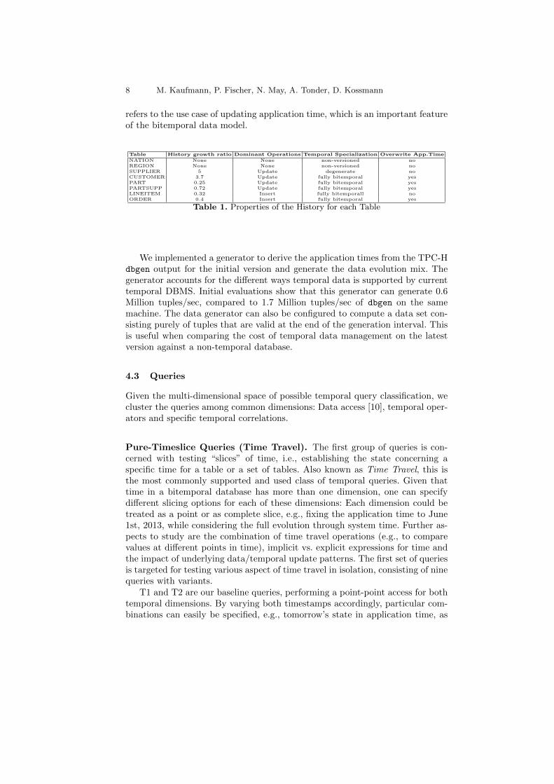
Table 1 describes the outcome of applying a mix of these queries on thevarious tables. The history growth ratio describes how many update operationsper initial tuple happen when h = m. As we can see, CUSTOMER and SUP-PLIER get a fairly high number of history entries per tuple, while ORDERS andLINEITEM see proportionally fewer history operations. When taking the sizes ofthe initial relations into account, the bulk of history operations is still performedon LINEITEM and ORDER. A second aspect on which the tables differ is thekind of history operations: SUPPLIER, CUSTOMER and PARTSUPP only re-ceive UPDATE statements, whereas the remaining bitemporal relations will see amix of operations. LINEITEM is strongly dominated by INSERT operations (>60 percent), ORDERS less so (50 percent inserts and 42 percent updates). CUS-TOMERS in turn see mostly UPDATE operations (> 70 percent). The temporalspecialization follows the specification in the schema, providing SUPPLIER asa degenerate table. Finally, existing application time periods can be overwrit-ten with new values for CUSTOMER, PART, PARTSUPP and ORDERS which


refers to the use case of updating application time, which is an important featureof the bitemporal data model.

Table History growth ratio Dominant Operations Temporal Specialization Overwrite App.Time

NATION None None non-versioned noREGION None None non-versioned noSUPPLIER 5 Update degenerate noCUSTOMER 3.7 Update fully bitemporal yesPART 0.25 Update fully bitemporal yesPARTSUPP 0.72 Update fully bitemporal yesLINEITEM 0.32 Insert fully bitemporall noORDER 0.4 Insert fully bitemporal yes

Table 1. Properties of the History for each Table

We implemented a generator to derive the application times from the TPC-Hdbgen output for the initial version and generate the data evolution mix. Thegenerator accounts for the different ways temporal data is supported by currenttemporal DBMS. Initial evaluations show that this generator can generate 0.6Million tuples/sec, compared to 1.7 Million tuples/sec of dbgen on the samemachine. The data generator can also be configured to compute a data set con-sisting purely of tuples that are valid at the end of the generation interval. Thisis useful when comparing the cost of temporal data management on the latestversion against a non-temporal database.

4.3 Queries

Given the multi-dimensional space of possible temporal query classification, wecluster the queries among common dimensions: Data access [10], temporal oper-ators and specific temporal correlations.

Pure-Timeslice Queries (Time Travel). The first group of queries is con-cerned with testing “slices” of time, i.e., establishing the state concerning aspecific time for a table or a set of tables. Also known as Time Travel, this isthe most commonly supported and used class of temporal queries. Given thattime in a bitemporal database has more than one dimension, one can specifydifferent slicing options for each of these dimensions: Each dimension could betreated as a point or as complete slice, e.g., fixing the application time to June1st, 2013, while considering the full evolution through system time. Further as-pects to study are the combination of time travel operations (e.g., to comparevalues at different points in time), implicit vs. explicit expressions for time andthe impact of underlying data/temporal update patterns. The first set of queriesis targeted for testing various aspect of time travel in isolation, consisting of ninequeries with variants.

T1 and T2 are our baseline queries, performing a point-point access for bothtemporal dimensions. By varying both timestamps accordingly, particular com-binations can easily be specified, e.g., tomorrow’s state in application time, as


recorded yesterday. The difference between T1 and T2 is according to the un-derlying data: T1 uses CUSTOMER, a table with many update operations andlarge history, but stable cardinalities. T2, in turn, uses ORDERS, a table witha generally smaller history and a focus on insertions. This way, we can studythe cost of time travel operations on significantly different histories. T3 and T4correlate data from two time travel operations within the same table. Compar-ing their results with T2 (very selective) and T5 (entire history) gives an insightinto whether any sharing of history operations is possible. T4 adds a TOP Ncondition, providing possible room for optimization in the database system. T5retrieves the complete history of the ORDERS table. Given that all data is re-quested, it should serve as a yardstick for the maximal cost of simple time traveloperations. T6 performs temporal slicing, i.e., retrieving all data of one tempo-ral dimension, while keeping the other to a point. This provides insights if theDBMS prefers any dimension, and a comparison of T2 and T5 yields insightsif any optimization for points vs. slices are available. T7 complements T6 byimplicitly specifying current system time, providing an understanding as to ifdifferent approaches of specifying current time work equally well. T8 and T9 in-vestigate the behavior of additional application times, as outlined in Section 4.1.Since the standard currently only allows a single, designated application time, wecan study the benefits of explicit vs. implicit application times. In that context,T8 uses point data (like T2), while T9 uses slicing (like T6).

The second set of timeslice queries focuses on application-oriented workloads,providing insights on how well synthetic time travel performance translates intocomplex analytical queries, e.g., accounting for additional data access cost andpossibly disabled optimizations. For this purpose, we use the 22 standard TPC-Hqueries (similar to what [1] proposes) and extend them to allow the specificationof both a system and an application time point. Possible evaluations mightcontain determining the cost of accessing the current version (in both systemas well as current application time) compared against the logically same datastored in a non-temporal table (see Section 4.2).

Pure-Key Queries (Audit). The next class of queries we study poses an or-thogonal problem: Instead of retrieving all tuples for a particular point in time,we process the history of a specific tuple or a small set of tuples. This way, wecan investigate how tuples evolve over time, e.g., for auditing or trend detec-tion. This evolution can be considered along the system time, the applicationtime(s) or both. Additional aspects to study are the effects of constraints onthe version range (complete time range, some time period, some versions) andtype of tuple selection, e.g., keys or predicates. In total, we specify 6 queries,each with small variants to account for the different time dimensions: K1 selectsthe tuple using a primary key, returns many columns and does not place anyconstraints on the temporal range. For key-based histories, this should providethe yardstick, and also offers clear insights into the organization of the storage oftemporal data. The cost of this operation can also be compared against T5 andT6, which retrieve all versions of all tuples (for both dimensions or each time


dimension, each). To allow easy comparison with the T queries, all queries areexecuted on the ORDERS relation. K2 alters K1 by placing a constraint on thetemporal range. Compared to K1, this additional information should provide anoptimization possibility. K3 alters K2 even further by only retrieving a singlecolumn, providing optimization potential for decomposition or column stores.K4 complements K2 by constraining not the temporal range (by a time inter-val), but the number of versions (by using TOP N). While the intent is quitesimilar to K2, the semantics and possible execution strategies are quite different.K5 constitutes a special case of K4 in which only the immediately preceding ver-sion is retrieved, employing no TOP N expression, but a timestamp correlation.From a technical point of view, this provides additional potential for optimiza-tion. From a language point of view, such an access is required for queries thatperform change detection. K6 chooses the tuples not via a key of the underlyingtable, but using a range predicate on a value (o totalprice). Besides a generalcomparison to key-based access, choosing the value of this parameters allows usto study the impact of the selectivity on the computation cost.

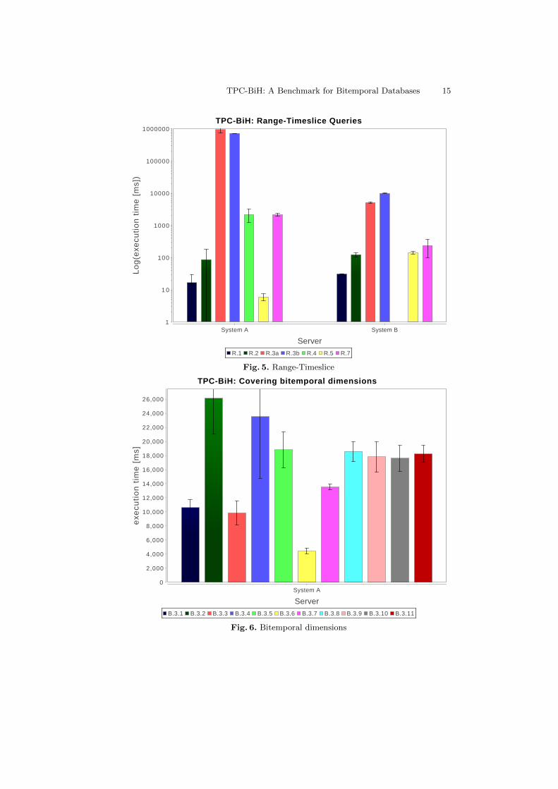
Range-Timeslice Queries. As the most general access pattern, range-timeslicequeries permit any combination of constraints on both value and temporal as-pects. As a result, a broad range of queries falls into that range. We will provide aset of application-derived workloads here, highlighting the variety and the differ-ent challenges it brings. As before, these queries contain variants which restrictone time dimension to a point, while varying the other.

R1 considers state change modeling by querying those customers who movedto the US at a particular point in time and still live there. The SQL expressioninvolves two temporal evaluations on the same relation and a join of the results.R2 also handles state modeling, but instead of detecting changes, it computesstate durations for LINEITEMs (the shipping time). Compared to R1, the in-termediate results are much bigger, but no temporal filters are applied whencombining them. R3 expresses temporal aggregation, i.e., computing aggregatesfor each version or time range of the database. At SAP, this turned out to beone of the most sought-after analyses of temporal data. However, SQL:2011 doesnot provide much support for this use case. The first query (R3.a) computes thegreatest number of unshipped items in a time range. In SQL:2011, this requiresa rather complex and costly join over the time interval boundaries to determinechange points, followed by a grouping on these boundaries for the aggregates.The second query (R3.b) computes the maximum value of unshipped orderswithin one year. As before, interval joins and grouping are required. R4 com-putes the products with the smallest difference in stock levels over the history.While the temporal semantics are rather easy to express, the same tables needto be accessed multiple times, and significant amount of post-processing is re-quired. R5 covers temporal joins by computing how often a customer had abalance of less than 5000 while also having orders with a price greater than 10.The join therefore not only includes value join criteria (on the respective keys),but also time correlation. R7 computes changes between versions over a full set,


retrieving those suppliers who increased their prices by more than 7.5 percentin a single update. R7 thus generalizes K4/K5 by determining previous versionsfor all keys, not just specific ones.

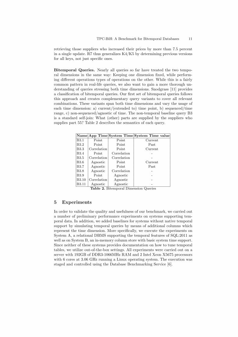
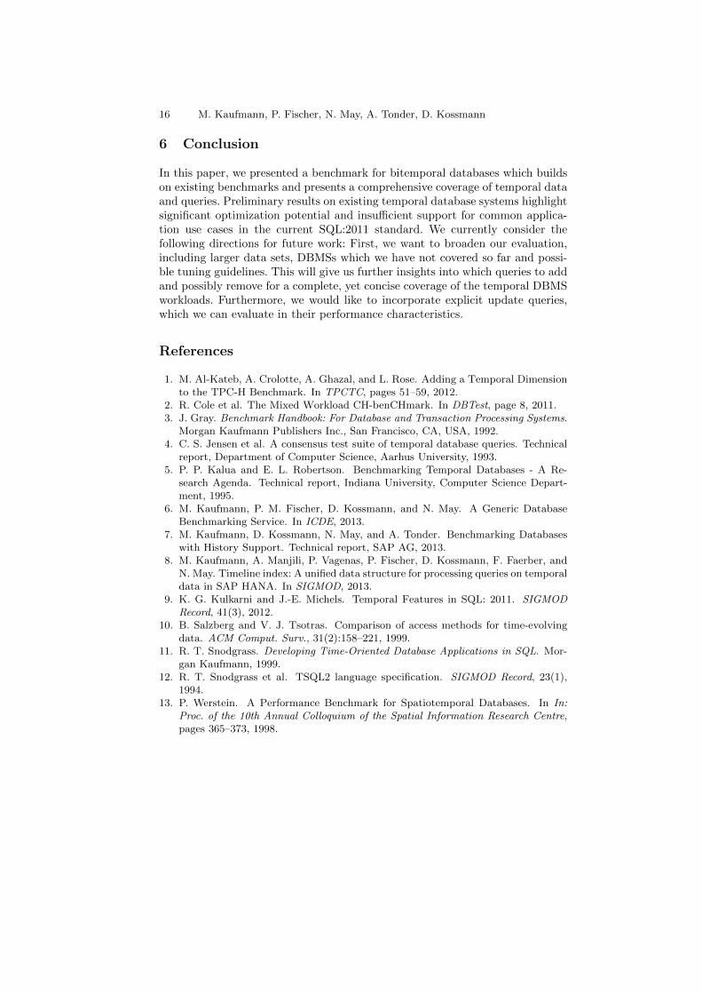
Bitemporal Queries. Nearly all queries so far have treated the two tempo-ral dimensions in the same way: Keeping one dimension fixed, while perform-ing different operations types of operations on the other. While this is a fairlycommon pattern in real-life queries, we also want to gain a more thorough un-derstanding of queries stressing both time dimensions. Snodgrass [11] providesa classification of bitemporal queries. Our first set of bitemporal queries followsthis approach and creates complementary query variants to cover all relevantcombinations. These variants span both time dimensions and vary the usage ofeach time dimension: a) current/(extended to) time point, b) sequenced/timerange, c) non-sequenced/agnostic of time. The non-temporal baseline query B3is a standard self-join: What (other) parts are supplied by the suppliers whosupplies part 55? Table 2 describes the semantics of each query.

Name App Time System Time System Time value

B3.1 Point Point CurrentB3.2 Point Point PastB3.3 Correlation Point CurrentB3.4 Point Correlation -B3.5 Correlation Correlation -B3.6 Agnostic Point CurrentB3.7 Agnostic Point PastB3.8 Agnostic Correlation -B3.9 Point Agnostic -B3.10 Correlation Agnostic -B3.11 Agnostic Agnostic -

Table 2. Bitemporal Dimension Queries

5 Experiments

In order to validate the quality and usefulness of our benchmark, we carried outa number of preliminary performance experiments on systems supporting tem-poral data. In addition, we added baselines for systems without native temporalsupport by simulating temporal queries by means of additional columns whichrepresent the time dimension. More specifically, we execute the experiments onSystem A, a relational DBMS supporting the temporal features of SQL:2011 aswell as on System B, an in-memory column store with basic system time support.Since neither of these systems provides documentation on how to tune temporaltables, we utilize out-of-the-box settings. All experiments were carried out on aserver with 192GB of DDR3-1066MHz RAM and 2 Intel Xeon X5675 processorswith 6 cores at 3.06 GHz running a Linux operating system. The execution wasstaged and controlled using the Database Benchmarking Service [6].


Most of our experiments were performed on data sizes with an initial datascaling factor h of 1.0 and a history size m of 1.0. The most significant obstaclethat currently prohibits us from reaching larger scale factors is the loading pro-cess into the database servers. In order provide a suitable system time history forour measurements, individual update cases need to be performed as individualupdate transactions. The loading process is therefore rather time-consuming, asit cannot benefit from bulk loading. With this loading approach, the timestampsof the system time history are compressed to the period of the loading time, thusrequiring adaptations when correlating system and application times.

5.1 Pure Timeslice

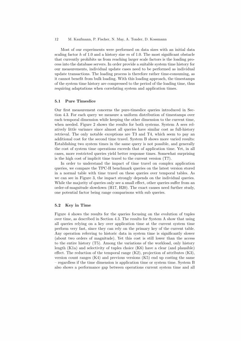
Our first measurement concerns the pure-timeslice queries introduced in Sec-tion 4.3. For each query we measure a uniform distribution of timestamps overeach temporal dimension while keeping the other dimension to the current time,when needed. Figure 2 shows the results for both systems. System A sees rel-atively little variance since almost all queries have similar cost as full-historyretrieval. The only notable exceptions are T3 and T4, which seem to pay anadditional cost for the second time travel. System B shows more varied results:Establishing two system times in the same query is not possible, and generallythe cost of system time operations exceeds that of application time. Yet, in allcases, more restricted queries yield better response times. Somewhat surprisingis the high cost of implicit time travel to the current version (T7).

In order to understand the impact of time travel on complex applicationqueries, we compare the TPC-H benchmark queries on the latest version storedin a normal table with time travel on these queries over temporal tables. Aswe can see in Figure 3, the impact strongly depends on the individual queries.While the majority of queries only see a small effect, other queries suffer from anorder-of-magnitude slowdown (H17, H20). The exact causes need further study,one potential factor being range comparisons with sub queries.

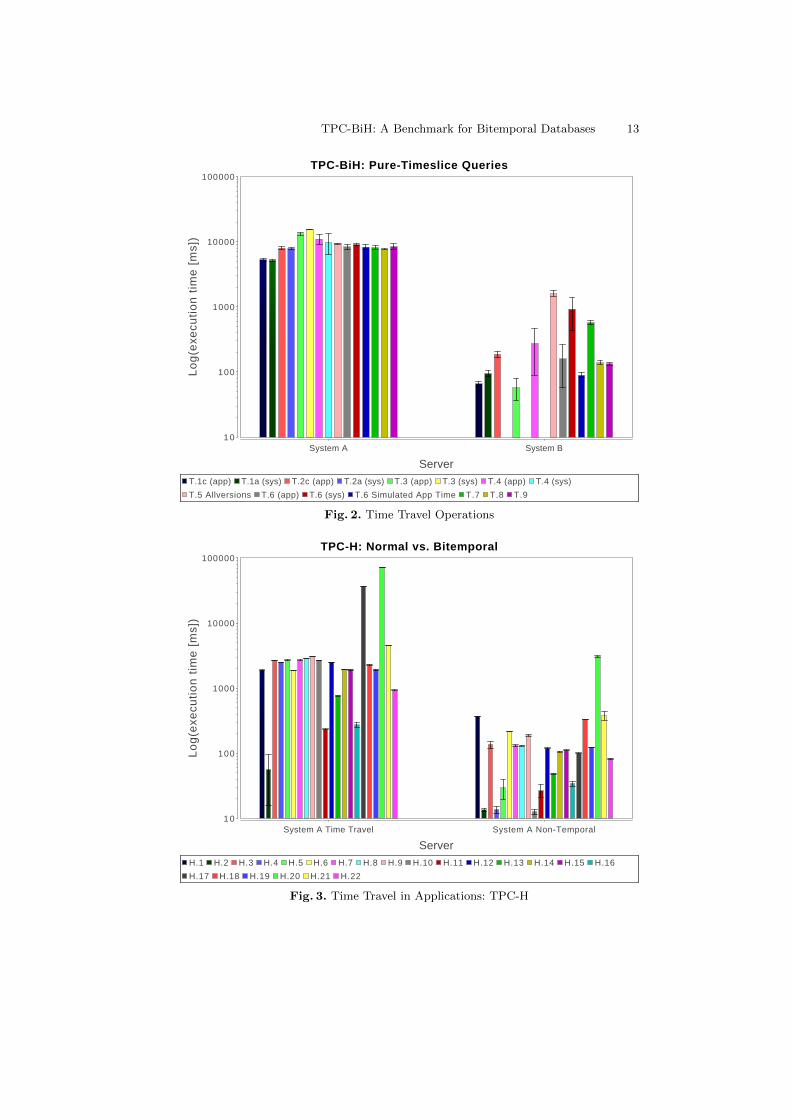
5.2 Key in Time

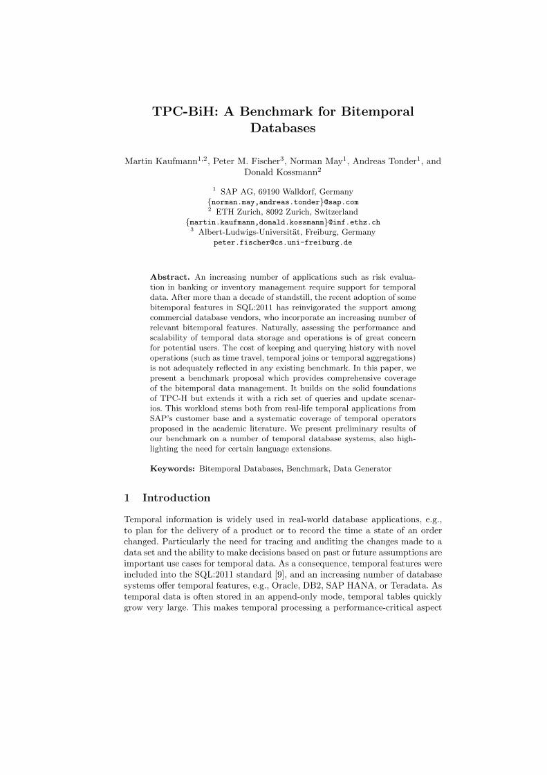
Figure 4 shows the results for the queries focusing on the evolution of tuplesover time, as described in Section 4.3. The results for System A show that usingall queries relying on a key over application time at the current system timeperform very fast, since they can rely on the primary key of the current table.Any operation referring to historic data in system time is significantly slower(about two orders of magnitude). Yet this cost is still lower than the accessto the entire history (T5). Among the variations of the workload, only historylength (K1a) and selectivity of tuples choice (K6) have a clear (and plausible)effect. The reduction of the temporal range (K2), projection of attributes (K3),version count ranges (K4) and previous versions (K5) end up costing the same– regardless if the time dimension is application time or system time. System Balso shows a performance gap between operations current system time and all


TPC-BiH: Pure-Timeslice Queries

T.1c (app) T.1a (sys) T.2c (app) T.2a (sys) T.3 (app) T.3 (sys) T.4 (app) T.4 (sys)

T.5 Allversions T.6 (app) T.6 (sys) T.6 Simulated App Time T.7 T.8 T.9

System A System B

Server

1 0

100

1000

10000

100000

Lo

g(e

xecu

tio

n t

ime

[m

s])

Fig. 2. Time Travel Operations

TPC-H: Normal vs. Bitemporal

H.1 H.2 H.3 H.4 H.5 H.6 H.7 H.8 H.9 H.10 H.11 H.12 H.13 H.14 H.15 H.16

H.17 H.18 H.19 H.20 H.21 H.22

System A Time Travel System A Non-Temporal

Server

1 0

100

1000

10000

100000

Lo

g(e

xecu

tio

n t

ime

[m

s])

Fig. 3. Time Travel in Applications: TPC-H


TPC-BiH: Simple Aggregation over Time

K.1 (app) K1-past (App Time in Past System Time) K.1 (both) K.1 (sys) K.1a (app)

K1a-past (App Time in Past System Time) K.1a (both) K.1a (sys) K.2 (app) K.2 (app-past)

K.2 (both) K.2 (sys) K.3 (app) K.3 (app - system past) K.3 (both) K.3 (sys) K.4 (app)

K.4 (app - system past) K.4 (sys) K.5 (app) K.5 (app - system past) K.5 (sys) K.6 (app) K.6 (sys)

K.6 (app) - high selectivity K.6 (app - system past) - high selectivity

System A System B

Server

1

1 0

100

1000

10000L

og

(exe

cuti

on

tim

e [

ms]

)

Fig. 4. Key in Time

other data, but it is much less pronounced. Similar effects exist for the valuepredicate selection.

5.3 Range-Timeslice

For the application-oriented queries in range-timeslice, we notice that the costcan become very significant (see Figure 5). To prevent very long experimentexecution times, we measured this experiment on a smaller data set, containingdata for h=0.1 and m=0.1. Nonetheless, we see that the more complex queries(R3 and R4) lead to serious problems: For System A, the response times of R3aand R3b (temporal aggregation) are more than two orders of magnitude moreexpensive than a full access to the history (measured in T5). While SystemB fares somewhat better on the T3 queries, it runs into a timeout after 1000seconds on R4. Generally speaking, the higher raw performance of System Bdoes not translate into lower response times for the remaining queries.

5.4 Bitemporal Dimensions

The results for combining all temporal dimensions with different types of oper-ations (Figure 6) show some similar patterns: Measurements running purely oncurrent system time perform rather well (3.1, 3.3, 3.5), whereas history accessesare expensive. Application time operations are cheapest when time can be ig-nored (3.5/3.6 vs 3.1/3.2), followed by temporal joins which are more expensive.


TPC-BiH: Range-Timeslice Queries

R.1 R.2 R.3a R.3b R.4 R.5 R.7

System A System B

Server

1

1 0

100

1000

10000

100000

1000000L

og

(exe

cuti

on

tim

e [

ms]

)

Fig. 5. Range-Timeslice

TPC-BiH: Covering bitemporal dimensions

B.3.1 B.3.2 B.3.3 B.3.4 B.3.5 B.3.6 B.3.7 B.3.8 B.3.9 B.3.10 B.3.11

System A

Server

0

2,000

4,000

6,000

8,000

10,000

12,000

14,000

16,000

18,000

20,000

22,000

24,000

26,000

exe

cuti

on

tim

e [

ms]

Fig. 6. Bitemporal dimensions


6 Conclusion

In this paper, we presented a benchmark for bitemporal databases which buildson existing benchmarks and presents a comprehensive coverage of temporal dataand queries. Preliminary results on existing temporal database systems highlightsignificant optimization potential and insufficient support for common applica-tion use cases in the current SQL:2011 standard. We currently consider thefollowing directions for future work: First, we want to broaden our evaluation,including larger data sets, DBMSs which we have not covered so far and possi-ble tuning guidelines. This will give us further insights into which queries to addand possibly remove for a complete, yet concise coverage of the temporal DBMSworkloads. Furthermore, we would like to incorporate explicit update queries,which we can evaluate in their performance characteristics.

References

1. M. Al-Kateb, A. Crolotte, A. Ghazal, and L. Rose. Adding a Temporal Dimensionto the TPC-H Benchmark. In TPCTC, pages 51–59, 2012.

2. R. Cole et al. The Mixed Workload CH-benCHmark. In DBTest, page 8, 2011.3. J. Gray. Benchmark Handbook: For Database and Transaction Processing Systems.

Morgan Kaufmann Publishers Inc., San Francisco, CA, USA, 1992.4. C. S. Jensen et al. A consensus test suite of temporal database queries. Technical

report, Department of Computer Science, Aarhus University, 1993.5. P. P. Kalua and E. L. Robertson. Benchmarking Temporal Databases - A Re-

search Agenda. Technical report, Indiana University, Computer Science Depart-ment, 1995.

6. M. Kaufmann, P. M. Fischer, D. Kossmann, and N. May. A Generic DatabaseBenchmarking Service. In ICDE, 2013.

7. M. Kaufmann, D. Kossmann, N. May, and A. Tonder. Benchmarking Databaseswith History Support. Technical report, SAP AG, 2013.

8. M. Kaufmann, A. Manjili, P. Vagenas, P. Fischer, D. Kossmann, F. Faerber, andN. May. Timeline index: A unified data structure for processing queries on temporaldata in SAP HANA. In SIGMOD, 2013.

9. K. G. Kulkarni and J.-E. Michels. Temporal Features in SQL: 2011. SIGMODRecord, 41(3), 2012.

10. B. Salzberg and V. J. Tsotras. Comparison of access methods for time-evolvingdata. ACM Comput. Surv., 31(2):158–221, 1999.

11. R. T. Snodgrass. Developing Time-Oriented Database Applications in SQL. Mor-gan Kaufmann, 1999.

12. R. T. Snodgrass et al. TSQL2 language specification. SIGMOD Record, 23(1),1994.

13. P. Werstein. A Performance Benchmark for Spatiotemporal Databases. In In:Proc. of the 10th Annual Colloquium of the Spatial Information Research Centre,pages 365–373, 1998.

TPC-BiH: A Benchmark for Bitemporal Databases

Documents

Transcript of TPC-BiH: A Benchmark for Bitemporal Databases