Towards High-Quality and Resource-Efficient Mobile Streaming
222
University of Calgary PRISM: University of Calgary's Digital Repository Graduate Studies The Vault: Electronic Theses and Dissertations 2017 Towards High-Quality and Resource-Efficient Mobile Streaming Zakerinasab, Mohammad Reza Zakerinasab, M. R. (2017). Towards High-Quality and Resource-Efficient Mobile Streaming (Unpublished doctoral thesis). University of Calgary, Calgary, AB. doi:10.11575/PRISM/28481 http://hdl.handle.net/11023/3851 doctoral thesis University of Calgary graduate students retain copyright ownership and moral rights for their thesis. You may use this material in any way that is permitted by the Copyright Act or through licensing that has been assigned to the document. For uses that are not allowable under copyright legislation or licensing, you are required to seek permission. Downloaded from PRISM: https://prism.ucalgary.ca
-
Upload
khangminh22 -
Category
Documents
-
view
0 -
download
0
Transcript of Towards High-Quality and Resource-Efficient Mobile Streaming
University of Calgary
PRISM: University of Calgary's Digital Repository
Graduate Studies The Vault: Electronic Theses and Dissertations
2017
Towards High-Quality and Resource-Efficient Mobile
Streaming
Zakerinasab, Mohammad Reza
Zakerinasab, M. R. (2017). Towards High-Quality and Resource-Efficient Mobile Streaming
(Unpublished doctoral thesis). University of Calgary, Calgary, AB. doi:10.11575/PRISM/28481
http://hdl.handle.net/11023/3851
doctoral thesis
University of Calgary graduate students retain copyright ownership and moral rights for their
thesis. You may use this material in any way that is permitted by the Copyright Act or through
licensing that has been assigned to the document. For uses that are not allowable under
copyright legislation or licensing, you are required to seek permission.
Downloaded from PRISM: https://prism.ucalgary.ca
UNIVERSITY OF CALGARY
Towards High-Quality and Resource-Efficient Mobile Streaming
by
Mohammad Reza Zakerinasab
A THESIS
SUBMITTED TO THE FACULTY OF GRADUATE STUDIES
IN PARTIAL FULFILLMENT OF THE REQUIREMENTS FOR THE
DEGREE OF DOCTOR OF PHILOSOPHY
GRADUATE PROGRAM IN COMPUTER SCIENCE
CALGARY, ALBERTA
May, 2017
© Mohammad Reza Zakerinasab 2017
Abstract
Video streaming is one of the most popular applications on Internet-connected devices. In
particular, the increasing deployment of LTE/4G technologies and the advancements in
display quality and computing power of modern smartphones and tablets have led to a
significant growth in video streaming traffic in mobile networks. In these networks, commu-
nication and computational resources are not as abundant as that of wired networks or IPTV
systems. Therefore, numerous challenges need to be addressed to provide a low cost, high
quality video streaming service. Most importantly, adequate computational and networking
resources must be available and the streaming service must be adaptive to heterogeneous
end user devices and varying network conditions. Towards high-quality and resource-efficient
video streaming in mobile networks, in this thesis we propose innovative techniques to address
the computational resource efficiency in cloud and on the end user devices. Furthermore, we
address the network fluctuation and noise using a carefully-designed forward error correction
technique that also considers the energy limitations of end user devices such as smartphones.
Finally, we propose significant improvements over the state-of-the-art techniques to promote
collaborative video streaming in smartphones.
ii

Acknowledgments
My deepest gratitude to my wife Sarah, for her continuous and unparalleled love, help and
support. She encouraged me to start this journey years ago and stood beside me to the end.
She has been my inspiration and motivation for continuing to improve my knowledge and
move my research forward. She is my rock, and I gratefully dedicate this thesis to her. I
also thank my son Ali, for bringing more joy, color and motivation to our lives.
I am forever indebted to my parents for giving me the opportunities and experiences that
have made me who I am. They selflessly encouraged me to explore new directions in life and
seek my own destiny. This journey would not have been possible if not for them.
Finally, I owe my gratitude to my supervisor Dr. Mea Wang. Without her enthusiasm
and continuous support this thesis would hardly have been completed. I express my warmest
gratitude to my supervisory committee members, Professor Carey Williamson and Dr. Peter
Hoyer. Their guidance and support have been valuable assets towards the completion of this
thesis.
iii
Table of Contents
Abstract . . . . . . . . . . . . . . . . . . . . . . . . . . . . . . . . . . . . . . . . iiAcknowledgments . . . . . . . . . . . . . . . . . . . . . . . . . . . . . . . . . . iiiTable of Contents . . . . . . . . . . . . . . . . . . . . . . . . . . . . . . . . . . . . ivList of Tables . . . . . . . . . . . . . . . . . . . . . . . . . . . . . . . . . . . . . . viList of Figures . . . . . . . . . . . . . . . . . . . . . . . . . . . . . . . . . . . . . . viiList of Symbols . . . . . . . . . . . . . . . . . . . . . . . . . . . . . . . . . . . . . x1 Introduction . . . . . . . . . . . . . . . . . . . . . . . . . . . . . . . . . . . . 11.1 Objectives . . . . . . . . . . . . . . . . . . . . . . . . . . . . . . . . . . . . . 51.2 Contributions . . . . . . . . . . . . . . . . . . . . . . . . . . . . . . . . . . . 61.3 Structure of the Thesis . . . . . . . . . . . . . . . . . . . . . . . . . . . . . . 92 Background and Related Works . . . . . . . . . . . . . . . . . . . . . . . . . 102.1 Video Coding and Compression . . . . . . . . . . . . . . . . . . . . . . . . . 10
2.1.1 Preliminaries . . . . . . . . . . . . . . . . . . . . . . . . . . . . . . . 102.1.2 Single-layered Video Coding: H.264/AVC . . . . . . . . . . . . . . . . 142.1.3 Layered Video Coding: H.264/SVC . . . . . . . . . . . . . . . . . . . 25
2.2 Related Works . . . . . . . . . . . . . . . . . . . . . . . . . . . . . . . . . . . 302.2.1 Analyzing the Performance of Scalable Video Coding . . . . . . . . . 302.2.2 Distributed Video Transcoding in the Cloud . . . . . . . . . . . . . . 322.2.3 Unequal Error Protection for Streaming Layered Videos . . . . . . . . 332.2.4 Cooperative Ad-Hoc Networks and WiFi Offloading . . . . . . . . . . 38
3 Detailed Analysis of Layered Video Coding . . . . . . . . . . . . . . . . . . . 423.1 Experiment Setup . . . . . . . . . . . . . . . . . . . . . . . . . . . . . . . . . 45
3.1.1 Experiment Testbed . . . . . . . . . . . . . . . . . . . . . . . . . . . 453.1.2 Selecting the Raw Video Dataset . . . . . . . . . . . . . . . . . . . . 453.1.3 Performance Metrics . . . . . . . . . . . . . . . . . . . . . . . . . . . 49
3.2 Performance Analysis . . . . . . . . . . . . . . . . . . . . . . . . . . . . . . . 523.2.1 The Effect of Frame Size . . . . . . . . . . . . . . . . . . . . . . . . . 533.2.2 The Effect of Temporal Scalability . . . . . . . . . . . . . . . . . . . 563.2.3 The Effect of Spatial Layering . . . . . . . . . . . . . . . . . . . . . . 603.2.4 The Effect of Quality Layering . . . . . . . . . . . . . . . . . . . . . . 633.2.5 The Effect of Quantization Parameter . . . . . . . . . . . . . . . . . . 66
3.3 Summary and Discussion . . . . . . . . . . . . . . . . . . . . . . . . . . . . . 684 Preparing Video in the Cloud . . . . . . . . . . . . . . . . . . . . . . . . . . 704.1 Distributed Video Transcoding in the Cloud . . . . . . . . . . . . . . . . . . 73
4.1.1 The Necessity of Considering GOP Dependencies . . . . . . . . . . . 754.2 Dependency-Aware Distributed Video Transcoding . . . . . . . . . . . . . . 77
4.2.1 GOP-Dependency Graph . . . . . . . . . . . . . . . . . . . . . . . . . 774.2.2 Dependency-Aware Distributed Video Transcoding in the Cloud . . . 84
4.3 Performance Evaluation . . . . . . . . . . . . . . . . . . . . . . . . . . . . . 874.3.1 The overhead of the transcoding scheme . . . . . . . . . . . . . . . . 884.3.2 Bitrate and Transcoding Time . . . . . . . . . . . . . . . . . . . . . . 89
4.4 Summary . . . . . . . . . . . . . . . . . . . . . . . . . . . . . . . . . . . . . 92
iv
5 Video Transmission in Wireless Networks . . . . . . . . . . . . . . . . . . . . 935.1 Coding and Prediction in SVC . . . . . . . . . . . . . . . . . . . . . . . . . . 945.2 Coding-Aware UEP for Layered Video Streaming . . . . . . . . . . . . . . . 98
5.2.1 Coding and Dependency-Aware Unequal Error Protection . . . . . . 1005.2.2 Performance Evaluation . . . . . . . . . . . . . . . . . . . . . . . . . 110
5.3 Adaptive FEC for Layered Video Multicast . . . . . . . . . . . . . . . . . . . 1195.3.1 Adaptive FEC for Video Multicast . . . . . . . . . . . . . . . . . . . 1205.3.2 Case Study: Application in a Mobile Network . . . . . . . . . . . . . 1255.3.3 Performance Evaluation . . . . . . . . . . . . . . . . . . . . . . . . . 128
5.4 Summary . . . . . . . . . . . . . . . . . . . . . . . . . . . . . . . . . . . . . 1366 Video Reception in Smartphones . . . . . . . . . . . . . . . . . . . . . . . . 1396.1 Energy-Efficient Collaborative Streaming . . . . . . . . . . . . . . . . . . . . 142
6.1.1 General transmission scheme . . . . . . . . . . . . . . . . . . . . . . . 1426.1.2 Two-Level Coding Scheme . . . . . . . . . . . . . . . . . . . . . . . . 1436.1.3 Distributed Scheduling Algorithm . . . . . . . . . . . . . . . . . . . . 147
6.2 Optimal Resource Allocation and Scheduling . . . . . . . . . . . . . . . . . . 1486.2.1 Modeling the Cooperative Streaming System . . . . . . . . . . . . . . 1506.2.2 The Power Consumption Minimization Problem . . . . . . . . . . . . 1556.2.3 The Rate Allocation and Scheduling (RAS) Algorithm . . . . . . . . 1606.2.4 Overhead Analysis . . . . . . . . . . . . . . . . . . . . . . . . . . . . 163
6.3 Performance Evaluation . . . . . . . . . . . . . . . . . . . . . . . . . . . . . 1646.3.1 Cooperative Streaming using Different Coding Strategies . . . . . . . 1666.3.2 Centralized Optimal RAS vs. Distributed Heuristic Algorithms . . . 1696.3.3 Impact of the Session Elongation Constraint . . . . . . . . . . . . . . 171
6.4 Summary . . . . . . . . . . . . . . . . . . . . . . . . . . . . . . . . . . . . . 1757 Concluding Remarks and Future Works . . . . . . . . . . . . . . . . . . . . . 178Bibliography . . . . . . . . . . . . . . . . . . . . . . . . . . . . . . . . . . . . . . 182A High Efficiency Video Coding . . . . . . . . . . . . . . . . . . . . . . . . . . 204
v
List of Tables
3.1 Selected video sequences and their properties. . . . . . . . . . . . . . . . . . 493.2 Comparing the performance of SVC when DTQ = (1, 4, 1) and H.264/AVC
for full HD video coding. . . . . . . . . . . . . . . . . . . . . . . . . . . . . . 553.3 The effect of additional I-pictures on performance of SVC when DTQ =
(2, 4, 3) and Intra Period = GOP size. . . . . . . . . . . . . . . . . . . . . . . 603.4 Dyadic vs. non-dyadic spatial layering results. Subcolumns show the respec-
tive overhead for one and two spatial layers (NDY1 vs. DY1 and NDY2 vs.DY2) respectively. . . . . . . . . . . . . . . . . . . . . . . . . . . . . . . . . . 63
3.5 Encoding configuration for quality (SNR) layering study. . . . . . . . . . . . 643.6 caption . . . . . . . . . . . . . . . . . . . . . . . . . . . . . . . . . . . . . . . 67
4.1 Reference videos and their visual properties. . . . . . . . . . . . . . . . . . . 884.2 Overhead of the proposed algorithm. . . . . . . . . . . . . . . . . . . . . . . 894.3 Comparing bitrate and average chunk size . . . . . . . . . . . . . . . . . . . 904.4 Comparing transcoding time . . . . . . . . . . . . . . . . . . . . . . . . . . . 91
5.1 Reference video sequences and their properties. . . . . . . . . . . . . . . . . 1135.2 Dependency statistics for different video sequences using a fixed layering con-
figuration of DTQ = (2,4,0). . . . . . . . . . . . . . . . . . . . . . . . . . . . 1145.3 Computational overhead of the proposed UEP model compared to the video
encoding time . . . . . . . . . . . . . . . . . . . . . . . . . . . . . . . . . . . 1185.4 Y-PSNR of the transmitted videos when varying the video specification. . . . 1185.5 Packet loss rate of the multicast groups . . . . . . . . . . . . . . . . . . . . . 1265.6 The specification of PA layered video substreams (full-HD, 24 fps) . . . . . . 1265.7 PA substream specification for different quality layers . . . . . . . . . . . . . 1275.8 Energy profile of the reference mobile device. . . . . . . . . . . . . . . . . . . 130
6.1 Summary of notations . . . . . . . . . . . . . . . . . . . . . . . . . . . . . . 1546.2 Energy consumption optimization problem for video streaming in a coopera-
tive network . . . . . . . . . . . . . . . . . . . . . . . . . . . . . . . . . . . . 1586.3 Throughput and energy efficiency of wireless transmissions and coding oper-
ations . . . . . . . . . . . . . . . . . . . . . . . . . . . . . . . . . . . . . . . 1656.4 Specification of heterogeneous nodes for experiment II . . . . . . . . . . . . . 1716.5 Specification of heterogeneous nodes . . . . . . . . . . . . . . . . . . . . . . 172
vi
List of Figures and Illustrations
1.1 The life cycle of a video streaming episode. . . . . . . . . . . . . . . . . . . . 2
2.1 Block diagram of AVC encoder / decoder [145]. . . . . . . . . . . . . . . . . 172.2 The temporal hierarchy of frames and the concept of group of pictures in
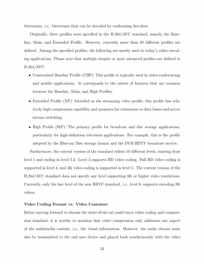
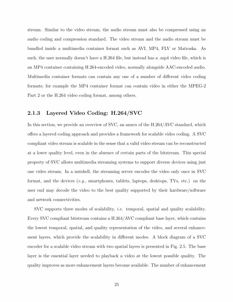
H.264/AVC. The number on each frame specifies the encoding order. . . . . 182.3 Dividing a frame into slice groups using flexible macroblock ordering. . . . . 192.4 H.264/AVC prediction directions for Intra 4× 4 prediction [145]. . . . . . . . 212.5 Block diagram of a SVC encoder for two spatial layers [112]. . . . . . . . . . 262.6 Layered design of SVC. The numbers on each frame specify the coding order
inside the spatial layer. . . . . . . . . . . . . . . . . . . . . . . . . . . . . . . 272.7 Block diagonal and ladder shaped coefficient matrices for two video layers L1
and L2, in which each video segment is divided into k1 and k2 data blocks,respectively. These matrices are multiplied into k1 + k2 data blocks to createk1 + k2 reconstruction blocks and d1 + d2 redundant coded blocks for forwarderror correction. . . . . . . . . . . . . . . . . . . . . . . . . . . . . . . . . . . 37
3.1 Sample frames from the selected video sequences. . . . . . . . . . . . . . . . 503.2 Comparing the performance of H.264/AVC, SVC and Simulcast over the video
sequence Big Buck Bunny (BB) when the frame size is varied from 512× 288pixels to 1920× 1080 pixels. . . . . . . . . . . . . . . . . . . . . . . . . . . . 53
3.3 The effect of increasing the GOP size from 2 to 16 on the performance ofH.264/SVC for encoding test video sequences. . . . . . . . . . . . . . . . . . 57
3.4 The effect of varying Intra Period parameter on the performance of H.264/SVCwhen encoding different layered representations of Pedestrian Area (PA) videosequence. . . . . . . . . . . . . . . . . . . . . . . . . . . . . . . . . . . . . . 59
3.5 The effect of SVC spatial layering on (a) the streaming server side and (b)the receiver side. . . . . . . . . . . . . . . . . . . . . . . . . . . . . . . . . . 61
3.6 The effect of varying the number of quality layers from zero to four on theperformance of H.264/SVC for different video sequences. . . . . . . . . . . . 65
3.7 The effect of varying quantization parameter on the performance of H.264/SVCwhen different layering structure is used to encode Pedestrian Area (PA) videosequence. The horizontal axis is the value of the highest quantization param-eter used in the layered structure. . . . . . . . . . . . . . . . . . . . . . . . . 67
4.1 Workflow of distributed video transcoding in the cloud. . . . . . . . . . . . . 744.2 The effect of increasing the size of video chunks from 1 GOP to 64 GOPs on
the video bitrate and transcoding time. The numbers are adjusted accordingto the video chunks with size of unit GOP. . . . . . . . . . . . . . . . . . . . 76
4.3 Top: Prediction dependency links between two consecutive GOPs in the baselayer (layer S0) of the SVC video from Fig. 2.6. Bottom: Macroblock depen-dency graph modelling inter-GOP prediction. . . . . . . . . . . . . . . . . . 79
vii
4.4 Different types of dependencies between macroblocks in SVC. (a) Using a fullmacroblock as a reference, (b) Using a macroblock created from portions of2 or 4 macroblocks as a reference, (c) Using a submacroblock as a reference(after proper upsampling), and (d) Using multiple macroblocks as references. 82
4.5 Converting a macroblock-dependency graph Gm (a) to a frame-dependencygraph Gf (b), to a GOP-dependency graph Gg (d), and at last to a GOP-distance graph (e). . . . . . . . . . . . . . . . . . . . . . . . . . . . . . . . . 83
4.6 The modified JSVM encoder software. Components in gray are modifiedJSVM components. Components in white are added to JSVM. . . . . . . . . 88
5.1 Prediction tree of the scalable video coding standard. The blocks with dashedlines may or may not exist at the discretion of the encoder. . . . . . . . . . . 95
5.2 Spatial prediction with dyadic settings in SVC. Each 16× 16 rectangle repre-sents a single macroblock. . . . . . . . . . . . . . . . . . . . . . . . . . . . . 97
5.3 An example of a dependency graph with 6 nodes, where m1 serves as anabsolute reference macroblock and m6 is not used by any other macroblock. . 101
5.4 Different types of dependencies among macroblocks in SVC. (a) Using a fullmacroblock as a reference, (b) Using a macroblock created from portions of2 or 4 macroblocks as a reference, (c) Using a submacroblock as a reference(after proper upsampling), and (d) Using multiple macroblocks as reference. 102
5.5 An example of a 10-node weighted dependency graph G. Nodes representmacroblocks and arcs represent the dependencies. (a) Before propagatingthe weights. (b) After propagating the weights by traversing the nodes intopological order and updating the weight of reference nodes according toEq. 5.5. . . . . . . . . . . . . . . . . . . . . . . . . . . . . . . . . . . . . . . 105
5.6 The prediction dependencies in a SVC video sequence with two spatial andthree temporal layers. Dependency links between key pictures are shownin black. The grey links represent dependency among pictures between twoconsecutive key pictures. . . . . . . . . . . . . . . . . . . . . . . . . . . . . . 108
5.7 The architecture of the performance evaluation system. Components in grayare modified JSVM components and those in white are developed from scratch.111
5.8 Performance of different UEP models over a packet erasure channel with vary-ing packet loss rate and fixed layering configuration of DTQ = (1,3,1). . . . 117
5.9 The proposed coding scheme for FEC blocks in layered video streaming. . . . 1235.10 Assigning layers in OFDMA. . . . . . . . . . . . . . . . . . . . . . . . . . . . 1285.11 Block diagonal and ladder shaped coefficient matrices for two video layers L1
and L2, in which each video segment is divided into k1 and k2 data blocks,respectively. These matrices are multiplied into k1 + k2 data blocks to createk1 + k2 reconstruction blocks and d1 + d2 redundant coded blocks for forwarderror correction. . . . . . . . . . . . . . . . . . . . . . . . . . . . . . . . . . . 129
5.12 Three minutes trace of the packet loss rate. . . . . . . . . . . . . . . . . . . . 1315.13 The objective video quality when using different layered protection mecha-
nisms and varying the loss rate from 0% to 20%. . . . . . . . . . . . . . . . . 1325.14 Transmission overhead of different multicast groups using different layered
protection mechanisms. . . . . . . . . . . . . . . . . . . . . . . . . . . . . . . 133
viii
5.15 Transmission delay and waiting delay of different multicast groups using dif-ferent layered protection mechanisms. . . . . . . . . . . . . . . . . . . . . . . 134
5.16 Energy consumed by the reference mobile device per hour of streaming session.1355.17 Time needed to prepare all the redundant coded blocks. . . . . . . . . . . . . 137
6.1 An overview of a collaborative streaming system for smartphones . . . . . . 1406.2 Streaming segment i from the Cloud to all collaborative nodes in the proposed
transmission scheme . . . . . . . . . . . . . . . . . . . . . . . . . . . . . . . 1446.3 Network model. . . . . . . . . . . . . . . . . . . . . . . . . . . . . . . . . . . 1516.4 Modeling the cooperative streaming system. . . . . . . . . . . . . . . . . . . 1526.5 Impact of cooperation arrangements and coding strategies on average energy
consumption . . . . . . . . . . . . . . . . . . . . . . . . . . . . . . . . . . . . 1676.6 A break-down of the average energy consumption . . . . . . . . . . . . . . . 1686.7 Effectiveness of the RAS algorithm . . . . . . . . . . . . . . . . . . . . . . . 1686.8 Average transmission delay of video segments offered by different scheduling
algorithm . . . . . . . . . . . . . . . . . . . . . . . . . . . . . . . . . . . . . 1726.9 Length of the streaming session when varying shared session elongation coef-
ficient ψ . . . . . . . . . . . . . . . . . . . . . . . . . . . . . . . . . . . . . . 1736.10 Average energy consumption for different values of the shared session elonga-
tion coefficient . . . . . . . . . . . . . . . . . . . . . . . . . . . . . . . . . . . 1746.11 Average transmission delay of video segments when varying the shared session
elongation coefficient . . . . . . . . . . . . . . . . . . . . . . . . . . . . . . . 175
A.1 The block diagram of HEVC encoder / decoder (with decoder elements shadedin light gray) [125]. . . . . . . . . . . . . . . . . . . . . . . . . . . . . . . . . 206
A.2 Subdivision of a coding tree block (CTB) into coding blocks (CB) and trans-form blocks (TB). Solid lines indicate CB boundaries and dotted lines indicateTB boundaries. (a) CTB with its partitioning. (b) Corresponding quadtree[125]. . . . . . . . . . . . . . . . . . . . . . . . . . . . . . . . . . . . . . . . . 206
ix
Symbols, Abbreviations and Nomenclature
Symbol Definition
3G 3rd Generation (of mobile telecommunications technology)
4CIF 4x Common Intermediate Format, 704 x 576 pixels
4G 4th Generation (of mobile telecommunications technology)
AAC Advanced Audio Coding
ACM Association for Computing Machinery
AMVP Advanced Motion Vector Prediction
AVC Advanced Video Coding
AVI Audio Video Interleave
B-frame/picture Bi-predictive frame/picture
CAVLC Context-Adaptive Variable Length Coding
CB Coding Block
CBP Constrained Baseline Profile (H.264/AVC)
CCITT Consultative Committee for Int. Telephony and Telegraphy
CGS Coarse Grain Scalability
CIF Common Intermediate Format, 352 x 288 pixels
CTB Coding Tree Block
CTU Coding Tree Unit
CU Coding Unit
DCT Discrete Cosine Transform
DSCQS Double Stimulus Continuous Quality Scale
DVB Digital Video Broadcasting
EEP Equal Error Protection
ESS Extended Spatial Scalability (H.264/SVC)
x
EWFC Expanding Window Fountain Codes
FEC Forward Error Correction
FGS Fine Grain Scalability
FHD Full High Definition, 1080p, 1920 x 1080 pixels
FLV Flash Video
FMO Flexible Macroblock Ordering
FR-IQA Full Reference Image Quality Assessment
GF Galois Field
GOP Group of Pictures
H.264 Advanced Video Coding
H.265 High Efficiency Video Coding
HD High Definition, 720p, 1280 x 720 pixels
HDMI High-Definition Multimedia Interface
HDTV High Definition TV
HEVC High Efficiency Video Coding, H.265/HEVC
HiP High Profile (H.264/AVC)
IDR Instantaneous Decoding Refresh
IEEE Institute of Electrical and Electronics Engineers
I-frame/picture Intra-coded frame/picture
ITU-TThe International Telecommunication Union - Telecommunication
Standardization Sector
JSVM Joint Scalable Video Model
LDPC Low Density Parity Check
LTE Long Term Evolution
LW-UEP Layer Weighted Unequal Error Protection
MB Macroblock
MGS Medium Grain Scalability
xi
MOS Mean Opinion Score
MP4 MPEG-4 Part 14 digital multimedia format
MPEG The Moving Picture Experts Group
MSE Mean Square Error
MS-SSIM Multi-Scale Structural Similarity Index
MVC Multi-view Video Coding
NAL Network Abstraction Layer
NC Network Coding
NQM Noise Quality Measure
OFDM Orthogonal Frequency Division Multiplexing
OFDMA Orthogonal Frequency Division Multiple Access
OPTICS Ordering Points To Identify the Clustering Structure
P2P Peer-to-Peer
PB Prediction Block
P-frame/picture Predicted frame/picture
PSNR Peak Signal to Noise Ratio
PU Prediction Unit
PW-UEP Packet Weighted Unequal Error Protection
QCIF Quarter Common Intermediate Format, 176 x 144 pixels
QP Quantization Parameter
RCPC Rate Compatible Convolutional Codes
RLNC Random Linear Network Coding
RS Reed-Solomon codes
SAO Sample Adaptive Offset
SD Standard Definition
SDTV Standard Definition TV
xii
SHVC Scalable High Efficiency Video Coding, H.265/SHVC
SNR Signal to Noise Ratio
SS-SIM Structural Similarity Index
SVC Scalable Video Coding
TB Transform Block
TCP Transmission Control Protocol
TDMA Time Division Multiple Access
TU Transform Unit
UDP User Datagram Protocol
UEP Unequal Error Protection
UHD Ultra High Definition
UQI Universal Quality Index
VCL Video Coding Layer
VIF Visual Fidelity Index
VLC Variable Length Coding
VSNR Visual Signal to Noise Ratio
WSNR Weighted Signal to Noise Ratio
XP Extended Profile (H.264/AVC)
xiii
Chapter 1
Introduction
The increasing deployment of high speed telecommunication technologies such as LTE/4G
and the growing computing power and display quality of modern smartphones along with
the access to more than four million mobile applications [122] has enormously increased the
mobile data usage. Cisco predicted that the global mobile data traffic will increase eight-fold
from 44 exabytes1 in 2015 to 367 exabytes in 2020 [36]. Among different services provided for
Internet-connected mobile devices, video streaming accounted for 55% of total mobile data
traffic in 2015, i.e., more than half of all mobile data traffic, and it is expected to surpass
75% of mobile data traffic in 2020 [36]. Such a massive amount of video traffic in mobile
networks where resources such as spectrum and data transmission infrastructure are scarce
and expensive inevitably causes many technical and operational problems. These problems
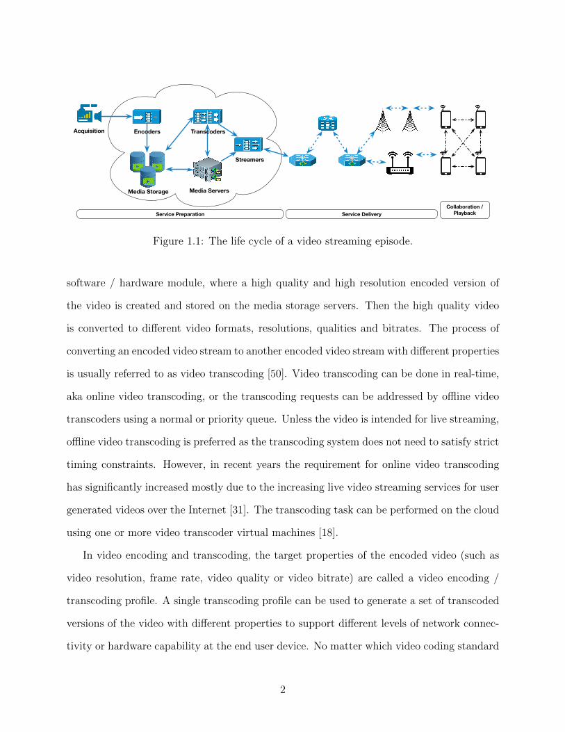
can be classified according to the life cycle of a video streaming episode as shown in Fig. 1.1.
Generally speaking, the life cycle of a video streaming service can be divided into three
phases:
• service preparation inside the cloud, where the video is processed and prepared to be
delivered to the end user devices per request;
• service delivery to the end nodes, where the video is packetized, shielded against noise,
and then transmitted over the noisy communication channels to the end user device;
• and finally, the reception and playback phase, where the video packets are received,
missing packets are reconstructed, and video is played on the end user device.
In the service preparation phase, the high quality non-compressed raw video (or lossless
compressed video) is sent from the camera or the editing desk to the online video encoder
1 Each exabyte is 1018 bytes which is roughly equal to one billion gigabytes.
1
Acquisition
Media ServersMedia Storage
TranscodersEncoders
Streamers
Service Preparation Service DeliveryCollaboration /
Playback
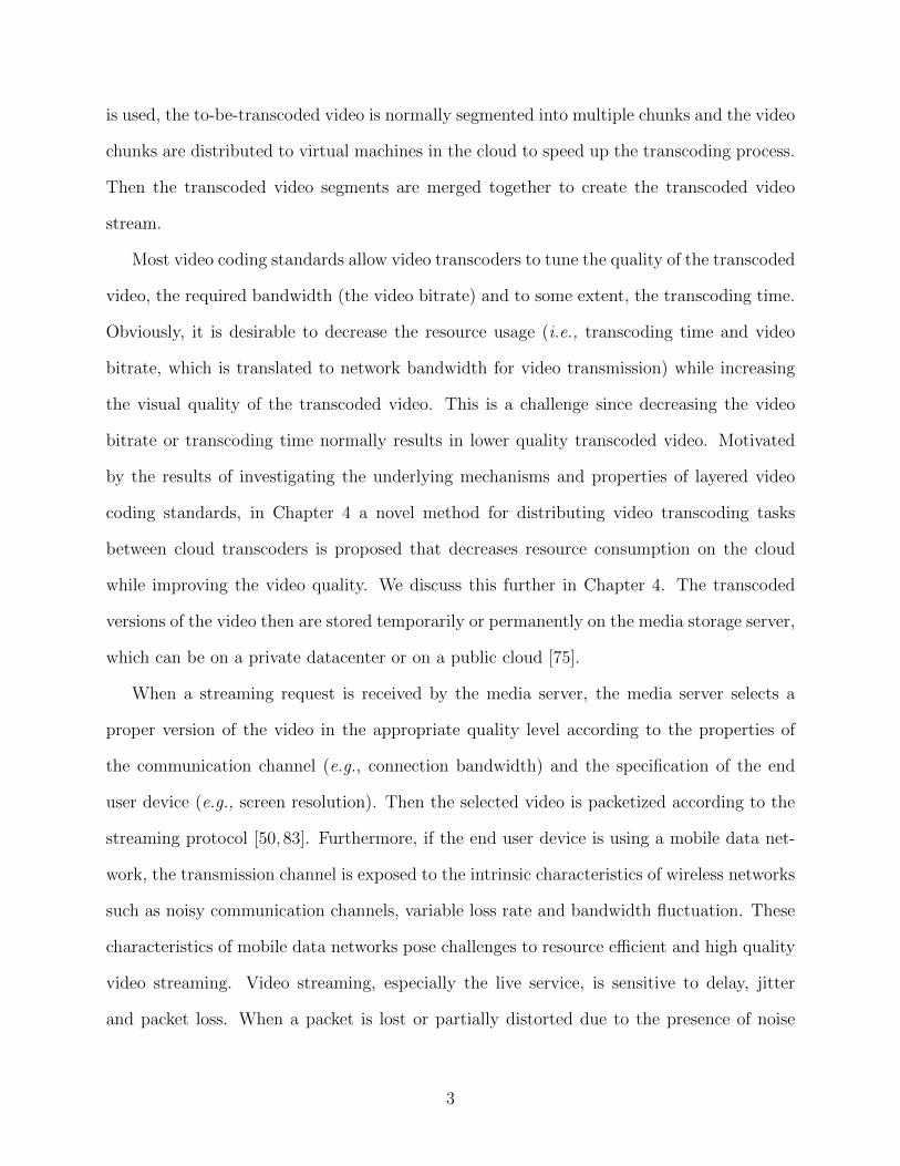
Figure 1.1: The life cycle of a video streaming episode.
software / hardware module, where a high quality and high resolution encoded version of
the video is created and stored on the media storage servers. Then the high quality video
is converted to different video formats, resolutions, qualities and bitrates. The process of
converting an encoded video stream to another encoded video stream with different properties
is usually referred to as video transcoding [50]. Video transcoding can be done in real-time,
aka online video transcoding, or the transcoding requests can be addressed by offline video
transcoders using a normal or priority queue. Unless the video is intended for live streaming,
offline video transcoding is preferred as the transcoding system does not need to satisfy strict
timing constraints. However, in recent years the requirement for online video transcoding
has significantly increased mostly due to the increasing live video streaming services for user
generated videos over the Internet [31]. The transcoding task can be performed on the cloud
using one or more video transcoder virtual machines [18].
In video encoding and transcoding, the target properties of the encoded video (such as
video resolution, frame rate, video quality or video bitrate) are called a video encoding /
transcoding profile. A single transcoding profile can be used to generate a set of transcoded
versions of the video with different properties to support different levels of network connec-
tivity or hardware capability at the end user device. No matter which video coding standard
2
is used, the to-be-transcoded video is normally segmented into multiple chunks and the video
chunks are distributed to virtual machines in the cloud to speed up the transcoding process.
Then the transcoded video segments are merged together to create the transcoded video
stream.
Most video coding standards allow video transcoders to tune the quality of the transcoded
video, the required bandwidth (the video bitrate) and to some extent, the transcoding time.
Obviously, it is desirable to decrease the resource usage (i.e., transcoding time and video
bitrate, which is translated to network bandwidth for video transmission) while increasing
the visual quality of the transcoded video. This is a challenge since decreasing the video
bitrate or transcoding time normally results in lower quality transcoded video. Motivated
by the results of investigating the underlying mechanisms and properties of layered video
coding standards, in Chapter 4 a novel method for distributing video transcoding tasks
between cloud transcoders is proposed that decreases resource consumption on the cloud
while improving the video quality. We discuss this further in Chapter 4. The transcoded
versions of the video then are stored temporarily or permanently on the media storage server,
which can be on a private datacenter or on a public cloud [75].
When a streaming request is received by the media server, the media server selects a
proper version of the video in the appropriate quality level according to the properties of
the communication channel (e.g., connection bandwidth) and the specification of the end
user device (e.g., screen resolution). Then the selected video is packetized according to the
streaming protocol [50, 83]. Furthermore, if the end user device is using a mobile data net-
work, the transmission channel is exposed to the intrinsic characteristics of wireless networks
such as noisy communication channels, variable loss rate and bandwidth fluctuation. These
characteristics of mobile data networks pose challenges to resource efficient and high quality
video streaming. Video streaming, especially the live service, is sensitive to delay, jitter
and packet loss. When a packet is lost or partially distorted due to the presence of noise
3
in wireless channels, different bit-level, byte-level or segment-based forward error correc-
tion (FEC) methods might be used to reconstruct the distorted packets [40]. Clearly, extra
bandwidth is needed to transmit the FEC packets along with the original video packets. Fur-
thermore, extra processing resources are needed to apply the forward error correction codes
and retrieve the distorted packets. FEC codes strongly improve the visual quality of the
transmitted video stream [93], which has resulted in widespread use of these techniques in
video streaming over wireless networks by industrial manufacturers such as Qualcomm [41].
If the conventional FEC methods cannot recover the distorted packets, to preserve the
video quality, the lost packets must be retransmitted. In a live or low latency video streaming
application, such a retransmission may lead to unacceptable delay. To address this issue to
some extent, the video decoder is equipped with tools to recover from the lost video packets
by estimating the missing parts of the video frame [145]. This solution inevitably introduces
error to the video signal and reduces the visual quality of the video. Furthermore, due to the
prediction dependencies between video packets, some video packets can be more important
than others for the quality of the decoded video. This property is exploited to improve the
performance of forward error correction techniques by better protecting the more important
video packets, a technique called unequal error protection [74]. Towards higher quality of
the transmitted video stream in wireless networks, one research direction in the unequal
error protection literature is to construct better error correction codes or adjust the existing
ones to the application of video streaming. Furthermore, more accurate determination of the
importance of video packets results in higher visual quality of the transmitted video stream.
Towards resource efficiency, the employed UEP technique must adapt to the fluctuating
conditions of the wireless networks such that the bandwidth is not wasted. We investigate
these challenges in Chapter 5.
Finally, when the video is received on the end user device and the missing network packets
are recovered as much as possible, the video stream is sent to the requesting application for
4
decoding and playback. Using an ad-hoc network of devices in close proximity to each
other, the end user device may also share the video packets with other devices as part of a
collaborative network [48]. Depending on the network configuration and the collaboration
algorithm in place, the ad-hoc network may be a P2P network [123] or use a usual client-
server configuration [73]. In such a collaborative system, the quality of the transmitted
video stream can be improved by offloading mobile data transmission to short-range wireless
networks. The main challenge is to efficiently use the pool of shared resources to reduce
resource usage on each node of the network and increase the visual quality of the received
video. We investigate these challenges in Chapter 6.
1.1 Objectives
In this thesis, we study different phases of the lifecycle of video streaming service and in-
vestigate how to improve the resource efficiency and the visual quality of the transmitted
video stream. Towards these goals, we explore various challenges of video streaming in mo-
bile networks and propose innovative ideas, methods and algorithms to better address these
issues. In contrast to existing work, this thesis builds a bridge between video coding and
compression research and the networking components of the video preparation and delivery.
This approach is not very common in the related research since the researchers mostly belong
to either the video coding community or the networking community, hence trying to address
the issues from a simple perspective.
Recently, research works such as SoftCast [66] have tried to consider the networking prob-
lems directly in the design of the video coding and compression techniques. In comparison,
in this thesis we delve into the video coding and compression techniques to find out how
different the aforementioned issues can be addressed if a deeper knowledge of video com-
pression techniques is utilized. As mentioned earlier, we envision that the video stream is
delivered to the end user devices in three phases; namely, service preparation on the cloud,
5
service delivery to the end user device over the mobile network, and video reception and
display along with collaboration among the end nodes. In each phase, we go beyond the
past research works by considering the underlying mechanisms and properties of the state-
of-the-art video coding and compression techniques. The main objectives in the research
presented in this thesis are to reduce the computational complexity of video preparation on
the cloud; to minimize the negative effects of intrinsic properties of wireless networks, such
as fluctuating packet loss rate and network bandwidth; to improve the quality of the video
perceived by the mobile end user; and to reduce the resource usage at the end user mobile
devices.
1.2 Contributions
The contributions of this thesis can be summarized as follows:
• Investigating the underlying mechanisms and properties of the state-of-the-art video
coding standards
– Reviewing the related literature reveals that many ideas proposed in research papers
suffer from an inadequate knowledge of the underlying mechanism and properties
of video coding standards2. To avoid such a mistake and to fabricate a solid base
for this research, a thorough and deep study of the state-of-the-art single-layer and
layered video coding standards, i.e. H.264/AVC and H.264/SVC, respectively, is
performed3. Along with reading the standard and the source code of the reference
2 For example, numerous publications addressing the unequal protection of video packets in layeredvideo coding assume that the inter-layer prediction dependencies form a complete graph between consequentspatial, temporal and quality layers. Not only is this wrong according to the internal mechanism of layeredvideo coding standards, but also is neither practical nor possible due to the computational burden of requiredprediction loops, hence rendering the ideas, observations and analysis unreliable.
3 Even though H.265/HEVC video coding standard and its layered video coding extension H.265/HSVCare introduced recently, they still are not on the verge of common use on mobile video streaming applicationsdue to the heavy computational burden of encoding tasks. However, in Chapter 7 we discuss how the resultsof the presented research can contribute to video streaming on mobile networks when H.264/AVC andH.264/SVC are replaced with their descendants.
6
software published by the standardization group, in this study the effect of modifying
different coding parameters on computational complexity and video quality is broadly
investigated. We discuss this further in Chapter 3.
• Video preparation on the Cloud
– Motivated by the results of investigating the underlying mechanisms and properties
of layered video coding standards, in Chapter 4 a novel method for distributing
video transcoding task between cloud transcoders is proposed. The proposed model
takes the properties of the to-be-transcoded video into account and suggests a new
transcoding paradigm that adaptively changes the length of the video segments. The
suggested technique improves resource efficiency by decreasing the video bitrate and
the computational resource consumption on the cloud. It also increases the visual
quality of the transcoded video for more complex video sequences. We discuss this
further in Chapter 4.
• Video delivery over the mobile networks
– Video coding and compression techniques are based on extracting similarities be-
tween portions of video frames and exploiting these similarities toward lossy com-
pression of the video signal. Hence, some video packets are more important than
other packets for video playback. That is, the negative effect of losing different video
packets on the quality of the reconstructed video can be significantly different. Con-
sidering the lossy nature of wireless and mobile communication networks, the more
important video packets must receive more protection no matter which forward er-
ror correction (FEC) technique is employed. In this thesis, we propose a novel video
unicast model that, for the first time, considers the internal design of the video cod-
ing standards and brings a significant video quality improvement over the previous
unequal protection proposals for video streaming. The proposed model considers
an independent and identically distributed random packet loss model. Furthermore,
7
the proposed model is extended to video multicast service and its application in a
common mobile communication network is studied. The model improves the quality
of the transmitted video and also reduces the energy consumption on mobile phones.
We discuss this further in Chapter 5.
• Cooperative streaming
– The adjacent end user devices may create a collaborative ad-hoc network to collec-
tively download the video packets over the mobile network. Such an arrangement
can significantly reduce the mobile data usage per end user device. Simultaneously,
the battery consumption can be decreased since data transmission over mobile net-
works is more battery consuming than that of ad-hoc wireless networks. To maximize
these benefits, the video segments must be wisely associated to the end nodes and
the segment downloads should be scheduled properly. Towards these goals, we pro-
pose an optimal rate allocation and scheduling algorithm that maximizes the benefit
of collaboration among end nodes.
– Furthermore, a novel two-level coding scheme is proposed to protect the video packets
against losses while transmitting over the mobile network and the ad-hoc network.
The coding scheme manages to keep the computational complexity of the coding
scheme on the server side, hence saving the battery of the end user devices. The
proposed model considers an independent and identically distributed random packet
loss model. We discuss these further in Chapter 6.
The results of the research reported in this thesis are presented in six reputable confer-
ences including ACM Multimedia [160], IEEE LCN (IEEE Conference on Local Computer
Networks) [157,159], IEEE MASCTOS (IEEE International Symposium on Modeling, Analy-
sis and Simulation of Computer and Telecommunication Systems) [156], IEEE/ACM IWQoS
(IEEE/ACM International Symposium on Quality of Service) [154], and IEEE WCNC (IEEE
Wireless Communications and Networking Conference) [158]. Furthermore, some primary
8
research results are presented as posters in IEEE ICDCS (IEEE International Conference on
Distributed Computing Systems) [162] and IEEE/ACM IWQoS [161] conferences.
In parallel with the research presented in this thesis, an efficient model was developed for
the update problem in network coding enabled cloud storage systems [153, 155, 163]. This
was the preliminary research topic of this PhD. It was left aside in favor of the current topic
before the candidacy exam. Results are not presented in this report as they were not strongly
related to the main topic of this thesis.
Along with modifying numerous available open source tools, more than ten thousand
lines of code were written in duration of this research to evaluate the presented ideas, run
the experiments, and analyze the results. The code was mostly written in C++, Python
and shell scripting language. Computing resources were obtained from Cybera Rapid Access
Cloud, Amazon EC2 and Microsoft Azure. Furthermore, a private server cluster of ten
powerful nodes was used for the experiments from early 2012 to late 2015.
1.3 Structure of the Thesis
The rest of this thesis is organized as follows. Chapter 2 provides background and related
works. Chapter 3 investigates the underlying mechanism and performance of the state of the
art layered video coding standard, i.e. H.264/SVC. Chapter 4 addresses a novel proposal
on how to decrease resources needed to transcode the videos on the cloud while achieving
better quality of the transcoded videos. Chapter 5 presents the proposed dependency aware
unequal error protection technique along with the novel adaptive FEC method for layered
video streaming. Chapter 6 studies the collaboration among end user devices and how such
a collaboration can be used to reduce the resource usage in transmission network and the
end nodes simultaneously. Finally, Chapter 7 concludes the thesis and proposes directions
for future research.
9
Chapter 2
Background and Related Works
This chapter provides a concise summary of the key-enabling technologies that are employed
in this thesis, including state-of-the-art single-layer and multi-layered video coding standards
used in mobile video streaming and the use of Cloud technology as an enabler for this
application. Furthermore, a review of the related research work is presented. The emphasis
is particularly on related work most relevant to the research proposed in this thesis.
2.1 Video Coding and Compression
In this section, we briefly review the basic concepts related to video coding and compression.
Next, we review the state-of-the-art video coding standards for single-layered videos. Finally,
multi-layered video coding is reviewed. Only the essential information related to this research
is reviewed in this section. Whenever needed to better understand the topic, proper referrals
are provided.
2.1.1 Preliminaries
Digital video compression standards first appeared in the early 1980’s and have made enor-
mous progress since then. The first generation of video coding standards was published by
the CCITT (now the ITU-T) in 1984 and more than 10 new standards have been published
afterward. Expectedly, video compression techniques have deep roots in image compression
since the compression of still frames is an important part of all video coding standards.
However, in this section we keep the focus on the basic concepts that are more related to
video coding and compression.
10
Video Scene Capture and Representation
Before compressing the video, it is necessary to capture the video scene properly. In the cur-
rent methodology of video capturing, the video scene is captured as a sequence of temporal
samples (aka pictures or frames), where each temporal sample is often composed of a rect-
angular grid of spatial samples (aka points or pixels). Furthermore, a proper representation
of color information is essential for video capture and compression, since the human visual
system is more sensitive to luminance than to chrominance.
Among different color spaces that can be used to represent the color information of a
spatio-temporal sample (a pixel of a frame), YCbCr is often used in video compression.
In YCbCr, Y represents the luminance and Cb and Cr represent the chrominance (color)
components of the pixel. Along with the color space, the sampling format specifies how
many bits are required to represent a single pixel. To decrease the number of bits required
to represent the color information of a pixel, it is very customary to ignore most of the
chrominance components of adjacent pixels. The most common sampling format used in
video compression is 4:2:0. In 4:2:0, the luminance component of color sample is captured
and stored for all the pixels. However, the chrominance samples are captured only for the
top-left pixel of each 2 × 2 rectangle of pixels. This halves the amount of bits needed to
represent luminance and chrominance of each pixel before compressing the video scene and
without significant reduction in visual quality of the captured video scene. For example, if
the color depth is 8 bits in a target color space, 4:2:0 sampling requires 12 bits to represent
a pixel1. In contrast, in 4:4:4 sampling format the chrominance components have the same
resolution as the luminance component.
Along with the color space and sampling format, the number of pixels captured for each
picture of a video scene is an important factor that affects the perceptual quality of the
captured scene and the performance of video compression techniques. The number of pixels
1In contrast to still images, in usual video applications there is no notion of transparency or blending.Therefore, all the colors are assumed to be opaque and there is no need to store the transparency informationfor the pixels.
11
in each picture is determined by the height and width of the video frames, mostly referred
to as video frame format. Many different video frame formats are used in video coding
standards and technologies, starting from 144p (256× 144 pixels per frame) and increasing
to 8K (7680× 4320). Nowadays, 720p (HD, 1280× 720) and 1080p (Full-HD, 1920× 1080)
are the most common video frame formats on the web, while more content providers are
presenting 4K (UHD, 3840× 2160) content every day.
Finally, when the video is compressed by a chosen video encoder, which specifies the
video coding format, it should be encapsulated with audio, subtitles, etc., inside a multi-
media container format such as AVI, MP4, FLV or Matroska. As such, the user normally
doesn’t have an encoded or transcoded video file, but instead has a container file normally
containing H.264-encoded video alongside AAC-encoded audio. Multimedia container for-
mats can contain any one of a number of different video coding formats; for example the
MP4 container format can contain video in either the MPEG-2 Part 2 or the H.264 video
coding format, among others.
Video Quality Assessment
In order to evaluate the performance of video coding standards and video communication
systems, it is necessary to assess the quality of the encoded or transmitted video. Video
quality assessment can be either subjective or objective.
Subjective video quality assessment aims to measure the quality of the video as perceived
by the end user. However, this is not straightforward since a viewer’s opinion on quality of
a played video is influenced by many subjective factors such as the viewing environment,
the observer’s state of mind and the extent to which the observer interacts with the visual
scene [115]. Therefore, it’s very common to measure the video quality using mathematical
algorithms. Developers of video compression and video processing systems rely heavily on
so-called objective (algorithmic) quality measures. The most widely used measure is Peak
Signal to Noise Ratio (PSNR). PSNR is measured on a logarithmic scale and depends on the
12
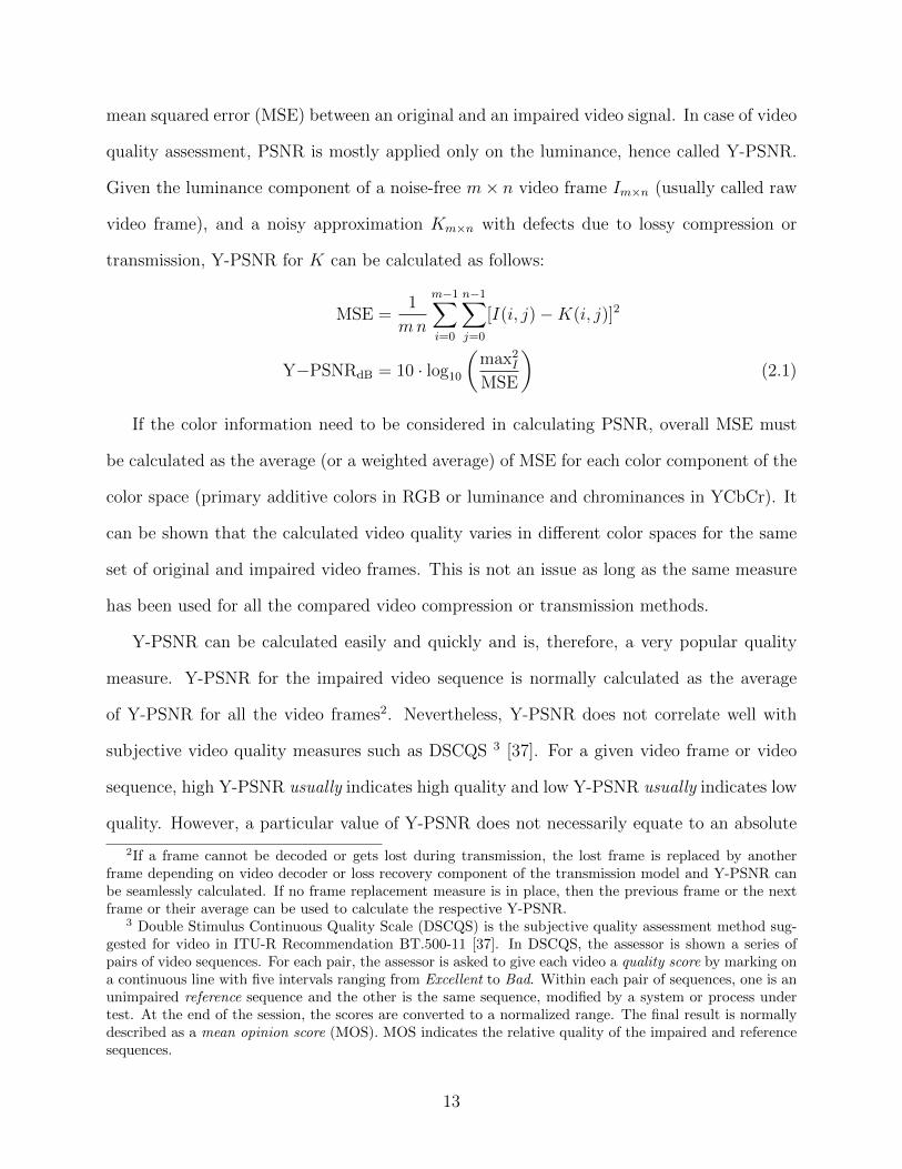
mean squared error (MSE) between an original and an impaired video signal. In case of video
quality assessment, PSNR is mostly applied only on the luminance, hence called Y-PSNR.
Given the luminance component of a noise-free m× n video frame Im×n (usually called raw
video frame), and a noisy approximation Km×n with defects due to lossy compression or
transmission, Y-PSNR for K can be calculated as follows:
MSE =1
mn
m−1∑i=0
n−1∑j=0
[I(i, j)−K(i, j)]2
Y−PSNRdB = 10 · log10
(max2
I
MSE
)(2.1)
If the color information need to be considered in calculating PSNR, overall MSE must
be calculated as the average (or a weighted average) of MSE for each color component of the
color space (primary additive colors in RGB or luminance and chrominances in YCbCr). It
can be shown that the calculated video quality varies in different color spaces for the same
set of original and impaired video frames. This is not an issue as long as the same measure
has been used for all the compared video compression or transmission methods.
Y-PSNR can be calculated easily and quickly and is, therefore, a very popular quality
measure. Y-PSNR for the impaired video sequence is normally calculated as the average
of Y-PSNR for all the video frames2. Nevertheless, Y-PSNR does not correlate well with
subjective video quality measures such as DSCQS 3 [37]. For a given video frame or video
sequence, high Y-PSNR usually indicates high quality and low Y-PSNR usually indicates low
quality. However, a particular value of Y-PSNR does not necessarily equate to an absolute
2If a frame cannot be decoded or gets lost during transmission, the lost frame is replaced by anotherframe depending on video decoder or loss recovery component of the transmission model and Y-PSNR canbe seamlessly calculated. If no frame replacement measure is in place, then the previous frame or the nextframe or their average can be used to calculate the respective Y-PSNR.
3 Double Stimulus Continuous Quality Scale (DSCQS) is the subjective quality assessment method sug-gested for video in ITU-R Recommendation BT.500-11 [37]. In DSCQS, the assessor is shown a series ofpairs of video sequences. For each pair, the assessor is asked to give each video a quality score by marking ona continuous line with five intervals ranging from Excellent to Bad. Within each pair of sequences, one is anunimpaired reference sequence and the other is the same sequence, modified by a system or process undertest. At the end of the session, the scores are converted to a normalized range. The final result is normallydescribed as a mean opinion score (MOS). MOS indicates the relative quality of the impaired and referencesequences.
13
subjective quality. For example, equivalent distortion inside or outside a region of interest
in a video frame equally decrease Y-PSNR but the effect on subjective quality is different.
The limitations of PSNR and Y-PSNR metrics have led to many efforts to develop more
sophisticated measures that approximate the subjective video quality. In a recent work [92],
the correlation of common objective quality measurement algorithms with the subjective
quality of a large set of videos is investigated. The videos are played on mobile devices,
which makes the results more useful for this research. In this work nine objective quality
measures are investigated, namely signal-to-noise ratio (SNR), peak signal-to-noise ratio
(PSNR), weighted signal-to-noise ratio (WSNR) [89], visual signal-to-noise ratio (VSNR)
[30], structural similarity index (SS-SSIM) [139], multi-scale structural similarity index (MS-
SSIM) [141], visual information fidelity (VIF) [116], universal quality index (UQI) [140], and
noise quality measure (NQM) [38]. Based on the correlation between the video quality
assessment algorithm scores and the subjective video quality, it has been shown that VIF
has the highest correlation with the subjective quality assessment results [92].
In this research, we use both Y-PSNR and VIF for video quality assessment to maintain
the comparability of the reported results with previous research work. Furthermore, we
look at other performance metrics wherever appropriate. Most importantly, we discuss the
coding efficiency of the video compression systems whenever needed. Coding efficiency can
be defined as the ratio of the bitrate of the un-coded video to the coded-video, or the ratio of
the bitrate of the coded video when encoded using different video compression systems. The
computational complexity of encoding and decoding operations are other metrics of interest.
2.1.2 Single-layered Video Coding: H.264/AVC
H.264/AVC or Advanced Video Coding standard was introduced in 2003 for encoding and
decoding single-layer video streams [145]. Different annexes and extensions have been added
to the standard in subsequent years. Most importantly, the scalable extension of AVC, called
14
SVC, was introduced in 2007 and the multi-view extension, called MVC, was introduced in
2011. Later in 2012, a new video coding standard, named High Efficiency Video Coding
(H.265/HEVC) was introduced [125]. HEVC is designed to answer the challenge of efficient
encoding of ultra high resolution videos, i.e., 4K and 8K videos. It is reported that compared
to H.264/AVC, HEVC reduces the bitrate of the encoded video sequences by an average of
40% to 50% (i.e., roughly halving the bandwidth needed to stream the video at the same
objective quality) [98]. However, the saving comes with a steep price in terms of coding
complexity.
The main bottleneck of the new HEVC video coding standard (along with its competitors
such as Google VP9) is the significantly higher computational complexity, which is the
inevitable cost of the higher compression rate and more complex coding loop. This bottleneck
has significantly slowed down the widespread use of these video codecs since they need more
expensive encoding equipment in the media server and more expensive end user devices for
the playback. Currently, only high-end smartphones can decode HEVC videos, and they
consume significantly more energy to do that. In fact, it has been reported that decoding an
H.265/HEVC encoded video needs up to three times more CPU time compared to the same
video when encoded with H.264/AVC. The difference in energy usage gets more significant
when considering that most of the smartphones use hardware decoders for H.264/AVC but
even the high end smartphones mostly use software decoders to decode H.265/HEVC videos
[88].
Accordingly, in the remainder of this chapter, we focus on the coding and compression
in H.264/AVC and SVC. As mentioned earlier, throughout this thesis the research work and
results are presented for H.264/AVC and its layered extension, H.264/SVC. H.265/HEVC
is briefly introduced in Appendix A. In Chapter 7, we illustrate how the research results
reported in this thesis can be applied to H.265/HEVC and its multi-layered extension after
proper calibration.
15
Coding and Compression in H.264/AVC
Towards optimizing the rate distortion of the encoded video sequences (i.e., improving the
quality of the encoded video subject to video bitrate and the capacity of the communication
channel), H.264/AVC, like other video coding standards, exploits the redundancy of visual
information in time and scale domains. For example, in the case where a camera pans
slowly through the scene or the scenery is stationary, the video sequence may be highly
compressed without noticeable loss of quality due to high visual similarity in consecutive
frames. H.264/AVC is agnostic to the underlying characteristics of the video sequence, e.g.,
the progressive or interlaced nature of the captured video scene. Therefore, in an interlaced
video sequence fields are merged into frames before arriving into the encoding unit.
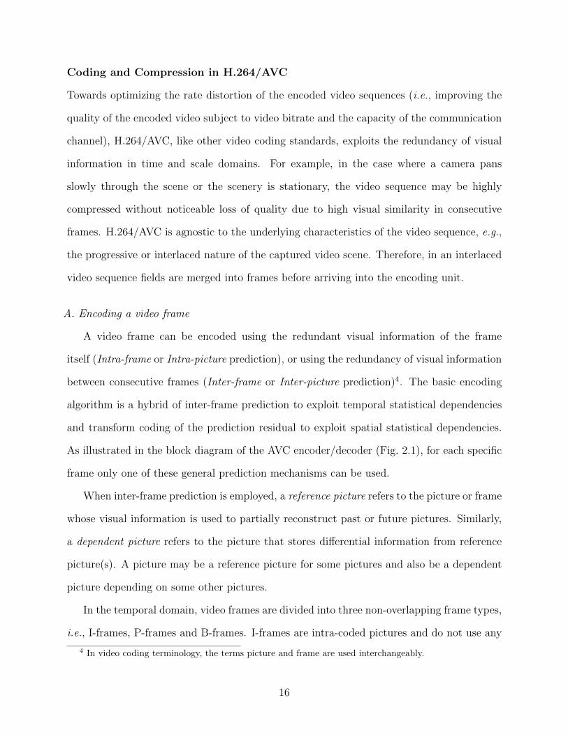
A. Encoding a video frame
A video frame can be encoded using the redundant visual information of the frame
itself (Intra-frame or Intra-picture prediction), or using the redundancy of visual information
between consecutive frames (Inter-frame or Inter-picture prediction)4. The basic encoding
algorithm is a hybrid of inter-frame prediction to exploit temporal statistical dependencies
and transform coding of the prediction residual to exploit spatial statistical dependencies.
As illustrated in the block diagram of the AVC encoder/decoder (Fig. 2.1), for each specific
frame only one of these general prediction mechanisms can be used.
When inter-frame prediction is employed, a reference picture refers to the picture or frame
whose visual information is used to partially reconstruct past or future pictures. Similarly,
a dependent picture refers to the picture that stores differential information from reference
picture(s). A picture may be a reference picture for some pictures and also be a dependent
picture depending on some other pictures.
In the temporal domain, video frames are divided into three non-overlapping frame types,
i.e., I-frames, P-frames and B-frames. I-frames are intra-coded pictures and do not use any
4 In video coding terminology, the terms picture and frame are used interchangeably.
16
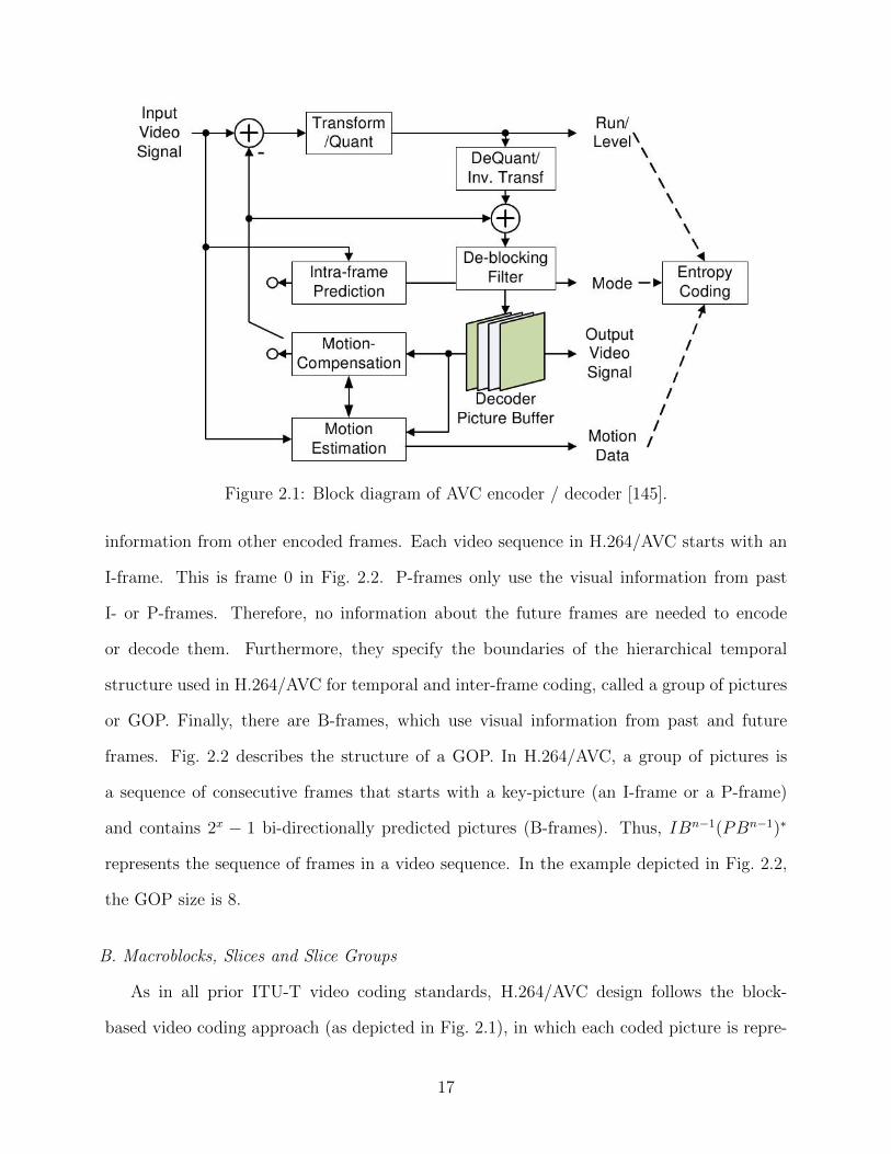
Figure 2.1: Block diagram of AVC encoder / decoder [145].
information from other encoded frames. Each video sequence in H.264/AVC starts with an
I-frame. This is frame 0 in Fig. 2.2. P-frames only use the visual information from past
I- or P-frames. Therefore, no information about the future frames are needed to encode
or decode them. Furthermore, they specify the boundaries of the hierarchical temporal
structure used in H.264/AVC for temporal and inter-frame coding, called a group of pictures
or GOP. Finally, there are B-frames, which use visual information from past and future
frames. Fig. 2.2 describes the structure of a GOP. In H.264/AVC, a group of pictures is
a sequence of consecutive frames that starts with a key-picture (an I-frame or a P-frame)
and contains 2x − 1 bi-directionally predicted pictures (B-frames). Thus, IBn−1(PBn−1)∗
represents the sequence of frames in a video sequence. In the example depicted in Fig. 2.2,
the GOP size is 8.
B. Macroblocks, Slices and Slice Groups
As in all prior ITU-T video coding standards, H.264/AVC design follows the block-
based video coding approach (as depicted in Fig. 2.1), in which each coded picture is repre-
17
0 4 5 7 8 13 2 6
Group of Pictures (GOP)
P-frameI-frame B-frames
Figure 2.2: The temporal hierarchy of frames and the concept of group of pictures inH.264/AVC. The number on each frame specifies the encoding order.
sented in block-shaped units of associated luma and chroma samples called macroblocks. In
H.264/AVC, each picture is partitioned into fixed-size macroblocks that each cover a rect-
angular picture area of 16× 16 samples of the luma component and 8× 8 samples of each of
the two chroma components. Considering the greater sensitivity of the human visual system
towards the brightness of the image, H.264/AVC main profile uses YCbCr colour space and
4:2:0 luminance and chrominance sampling with 8 bits of precision per sample. Therefore,
the number of chrominance samples is one fourth of that of luminance samples, as discussed
in Chapter 1, and representing each uncoded sample in a raw video frame requires 12 bits.
Macroblocks are the basic building blocks of the standard for which the decoding process
is specified. The coding algorithm, however, may use submacroblocks of 16 × 8 or 8 × 8
samples.
In H.264/AVC, a picture is a collection of one or more slices. Slices are a sequence
of macroblocks that are processed in the order of a raster scan when not using flexible
macroblock ordering (FMO), which is described later in this paragraph. Slices are self-
contained in the sense that each slice can be correctly decoded standalone, with no data
from other slices needed5. Flexible macroblock ordering (FMO) modifies the way pictures
are partitioned into slices by utilizing the concept of slice groups. Each slice group is a
set of macroblocks. Each macroblock has exactly one slice group identification number
5Some information from other slices might be needed to apply the de-blocking filter across slice boundaries.
18
that specifies the slice group to which the macroblock belongs. Each slice group can be
partitioned into one or more slices, such that the macroblocks within the same slice are
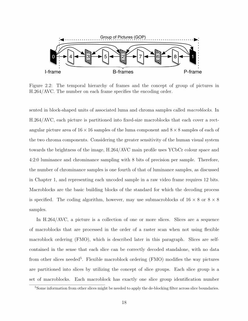
processed in the order of a raster scan. Using FMO, a picture can be split into many
macroblock scanning patterns such as interleaved slices, a dispersed macroblock allocation,
one or more foreground slice groups and a leftover slice group, or a checker-board type of
mapping. For example, in Fig. 2.3 the left-hand side mapping can be used in region-of-
interest type of coding applications and the right-hand side can be used for concealment in
video conferencing applications where slice group 0 and 1 are transmitted in separate packets
and one of them is lost.
Slice Group #0
Slice Group #1
Slice Group #2
(a)
Slice Group #0
Slice Group #1
(b)
Figure 2.3: Dividing a frame into slice groups using flexible macroblock ordering.
Slices can also be categorized based on how the contained macroblocks are coded. The
most important categories, as in frames, are I-, P- and B-slices. In an I-slice, all macroblocks
are coded using intra-frame prediction. In a P-slice, in addition to the coding type of the
I-slice, some macroblocks can be coded using inter-frame prediction from the same slice in
past frames. Finally, in a B-slice, in addition to the coding types available in a P-slice,
some macroblocks can be coded using inter-frame prediction from the same slice in past and
future frames. More information on intra- and inter-frame prediction is provided later in this
section. For more information about slice types, including SI and SP switching slice types,
19
please refer to [145].
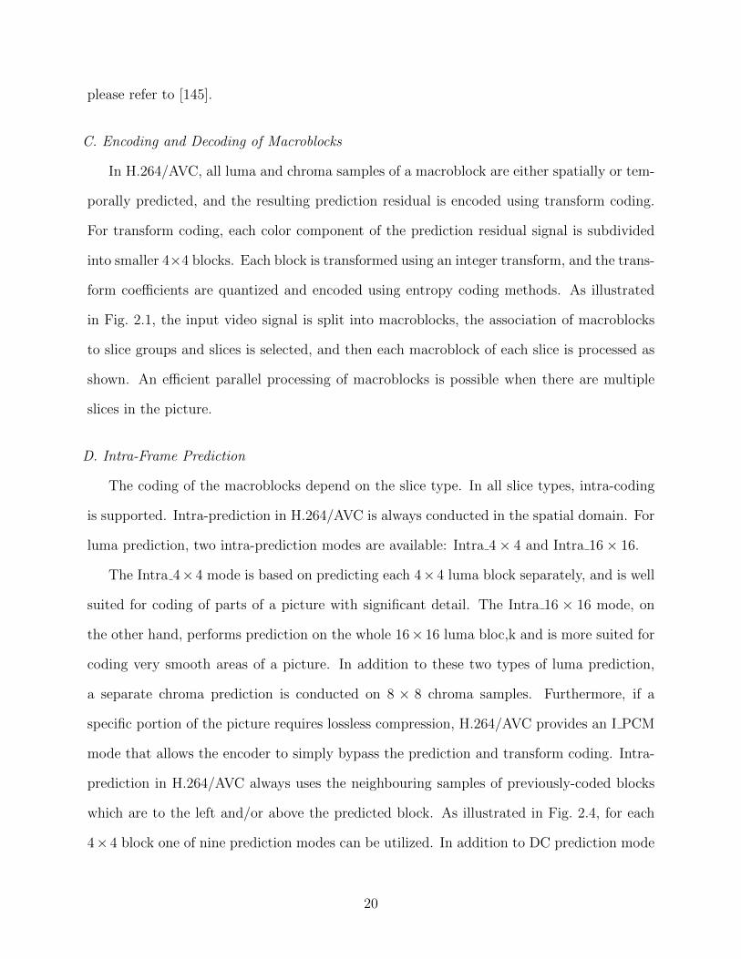
C. Encoding and Decoding of Macroblocks
In H.264/AVC, all luma and chroma samples of a macroblock are either spatially or tem-
porally predicted, and the resulting prediction residual is encoded using transform coding.
For transform coding, each color component of the prediction residual signal is subdivided
into smaller 4×4 blocks. Each block is transformed using an integer transform, and the trans-
form coefficients are quantized and encoded using entropy coding methods. As illustrated
in Fig. 2.1, the input video signal is split into macroblocks, the association of macroblocks
to slice groups and slices is selected, and then each macroblock of each slice is processed as
shown. An efficient parallel processing of macroblocks is possible when there are multiple
slices in the picture.
D. Intra-Frame Prediction
The coding of the macroblocks depend on the slice type. In all slice types, intra-coding
is supported. Intra-prediction in H.264/AVC is always conducted in the spatial domain. For
luma prediction, two intra-prediction modes are available: Intra 4× 4 and Intra 16× 16.
The Intra 4×4 mode is based on predicting each 4×4 luma block separately, and is well
suited for coding of parts of a picture with significant detail. The Intra 16 × 16 mode, on
the other hand, performs prediction on the whole 16× 16 luma bloc,k and is more suited for
coding very smooth areas of a picture. In addition to these two types of luma prediction,
a separate chroma prediction is conducted on 8 × 8 chroma samples. Furthermore, if a
specific portion of the picture requires lossless compression, H.264/AVC provides an I PCM
mode that allows the encoder to simply bypass the prediction and transform coding. Intra-
prediction in H.264/AVC always uses the neighbouring samples of previously-coded blocks
which are to the left and/or above the predicted block. As illustrated in Fig. 2.4, for each
4× 4 block one of nine prediction modes can be utilized. In addition to DC prediction mode
20
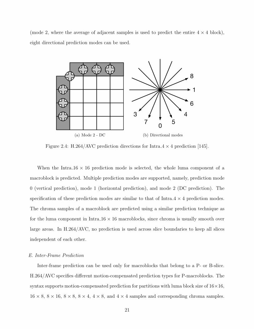
(mode 2, where the average of adjacent samples is used to predict the entire 4 × 4 block),
eight directional prediction modes can be used.
(a) Mode 2 - DC
0
1
37 5
46
8
(b) Directional modes
Figure 2.4: H.264/AVC prediction directions for Intra 4× 4 prediction [145].
When the Intra 16 × 16 prediction mode is selected, the whole luma component of a
macroblock is predicted. Multiple prediction modes are supported, namely, prediction mode
0 (vertical prediction), mode 1 (horizontal prediction), and mode 2 (DC prediction). The
specification of these prediction modes are similar to that of Intra 4 × 4 prediction modes.
The chroma samples of a macroblock are predicted using a similar prediction technique as
for the luma component in Intra 16× 16 macroblocks, since chroma is usually smooth over
large areas. In H.264/AVC, no prediction is used across slice boundaries to keep all slices
independent of each other.
E. Inter-Frame Prediction
Inter-frame prediction can be used only for macroblocks that belong to a P- or B-slice.
H.264/AVC specifies different motion-compensated prediction types for P-macroblocks. The
syntax supports motion-compensated prediction for partitions with luma block size of 16×16,
16 × 8, 8 × 16, 8 × 8, 8 × 4, 4 × 8, and 4 × 4 samples and corresponding chroma samples.
21
The reference partition for each motion-compensation predicted P-partition is specified by
a translational motion vector and a picture reference index. The motion vector compo-
nents are differentially coded using either median or directional prediction from neighbouring
blocks. No motion vector component prediction takes place across slice boundaries. The syn-
tax supports multipicture motion-compensated prediction, i.e., more than one prior coded
picture can be used as reference for motion-compensated prediction. Multi-frame motion-
compensated prediction requires both encoder and decoder to store the reference pictures
used for inter-prediction in a buffer.
B-macroblocks may use a weighted average of two distinct motion-compensated predic-
tion values for building the predicted signal. H.264/AVC specifies four different inter-frame
prediction modes: list 0, list 1, bi-predictive, and direct prediction. In list 0 and list 1 predic-
tion modes, the prediction signal uses macroblock(s) belonging to past and future frame(s),
respectively. For the bi-predictive mode, the prediction signal is formed by a weighted aver-
age of motion-compensated list 0 and list 1 prediction signals. The direct prediction mode
is inferred from previously transmitted syntax elements and can be either list 0 or list 1
prediction or bi-predictive.
F. Transform, Scaling, and Quantization
Similar to previous video coding standards, H.264/AVC utilizes transform coding of the
prediction residual. However, in H.264/AVC, the transformation is applied to smaller 4× 4
blocks, and instead of a 4× 4 discrete cosine transform (DCT), an integer transform is used.
The basic transform coding process is very similar to that of previous standards. At the
encoder, the process includes a forward transform, zig-zag scanning, scaling, and rounding
as the quantization process followed by entropy coding. At the decoder, the inverse of the
encoding process is performed except for the rounding. More details on the specific aspects
of the transform in H.264/AVC can be found in [145]. A quantization parameter is used
for determining the quantization of transform coefficients in H.264/AVC. The quantization
22
parameter can take 52 values. Theses values are arranged such that an increase of 1 in
quantization parameter means an increase of quantization step size by approximately 12%
(an increase of 6 means an increase of quantization step size by exactly a factor of 2). It can
be noticed that a change of step size by approximately 12% also means roughly a reduction
of bit rate by approximately 12% [145].
G. Entropy Coding
In H.264/AVC, two methods of entropy coding are supported. The simpler entropy
coding method uses a codeword table for all syntax elements except the quantized transform
coefficients. Thus, instead of designing a different variable length code (VLC) table for each
syntax element, only the mapping to the single codeword table is customized according to
the data statistics. The chosen single codeword table is an exponential Golomb code. For
transmitting the quantized transform coefficients, a more efficient method called Context-
Adaptive Variable Length Coding (CAVLC) is employed. In this scheme, VLC tables for
various syntax elements are switched depending on already transmitted syntax elements.
As expected, the performance of entropy coding is better than schemes using a single VLC
table. In the CAVLC entropy coding, the number of non-zero quantized coefficients (N) and
the actual size and position of the coefficients are coded separately. After zig-zag scanning
of transform coefficients, their statistical distribution typically shows large values for the low
frequency part, decreasing to small values later in the scan for the high-frequency part.
H.264/AVC Profiles and Levels
Profiles and levels specify conformance points. They facilitate interoperability between var-
ious applications that have similar functional requirements. A profile defines a set of coding
tools or algorithms that can be used to generate a conforming bitstream, whereas a level
places constraints on certain key parameters of the bitstream. All decoders conforming to a
specific profile must support all features in that profile. Encoders are not required to make
use of any particular set of features supported in a profile but have to provide conforming
23
bitstreams, i.e., bitstreams that can be decoded by conforming decoders.
Originally, three profiles were specified in the H.264/AVC standard, namely the Base-
line, Main, and Extended Profile. However, currently more than 20 different profiles are
defined. Among the specified profiles, the following are mostly used in today’s video encod-
ing applications. Please note that multiple simpler or more advanced profiles are defined in
H.264/AVC:
• Constrained Baseline Profile (CBP): This profile is typically used in video-conferencing
and mobile applications. It corresponds to the subset of features that are common
between the Baseline, Main, and High Profiles.
• Extended Profile (XP): Intended as the streaming video profile, this profile has rela-
tively high compression capability and measures for robustness to data losses and server
stream switching.
• High Profile (HiP): The primary profile for broadcast and disc storage applications,
particularly for high-definition television applications. For example, this is the profile
adopted by the Blue-ray Disc storage format and the DVB HDTV broadcast service.
Furthermore, the current version of the standard enlists 19 different levels, starting from
level 1 and ending in level 5.2. Level 3 supports HD video coding. Full HD video coding is
supported in level 4, and 4K video coding is supported in level 5. The current version of the
H.264/AVC standard does not specify any level supporting 8K or higher video resolutions.
Currently, only the last level of the new HEVC standard, i.e., level 6, supports encoding 8K
videos.
Video Coding Format vs. Video Container
Before moving forward to discuss the state-of-the-art multi-layer video coding and compres-
sion standard, it is worthy to mention that video compression only addresses one aspect
of the multimedia content, i.e., the visual information. However, the audio stream must
also be transmitted to the end user device and played back synchronously with the video
24
stream. Similar to the video stream, the audio stream must also be compressed using an
audio coding and compression standard. The video stream and the audio stream must be
bundled inside a multimedia container format such as AVI, MP4, FLV or Matroska. As
such, the user normally doesn’t have a H.264 file, but instead has a .mp4 video file, which is
an MP4 container containing H.264-encoded video, normally alongside AAC-encoded audio.
Multimedia container formats can contain any one of a number of different video coding
formats; for example the MP4 container format can contain video in either the MPEG-2
Part 2 or the H.264 video coding format, among others.
2.1.3 Layered Video Coding: H.264/SVC
In this section, we provide an overview of SVC, an annex of the H.264/AVC standard, which
offers a layered coding approach and provides a framework for scalable video coding. A SVC
compliant video stream is scalable in the sense that a valid video stream can be reconstructed
at a lower quality level, even in the absence of certain parts of the bitstream. This special
property of SVC allows multimedia streaming systems to support diverse devices using just
one video stream. In a nutshell, the streaming server encodes the video only once in SVC
format, and the devices (e.g., smartphones, tablets, laptops, desktops, TVs, etc.) on the
user end may decode the video to the best quality supported by their hardware/software
and network connectivities.
SVC supports three modes of scalability, i.e. temporal, spatial and quality scalability.
Every SVC compliant bitstream contains a H.264/AVC compliant base layer, which contains
the lowest temporal, spatial, and quality representation of the video, and several enhance-
ment layers, which provide the scalability in different modes. A block diagram of a SVC
encoder for a scalable video stream with two spatial layers is presented in Fig. 2.5. The base
layer is the essential layer needed to playback a video at the lowest possible quality. The
quality improves as more enhancement layers become available. The number of enhancement
25
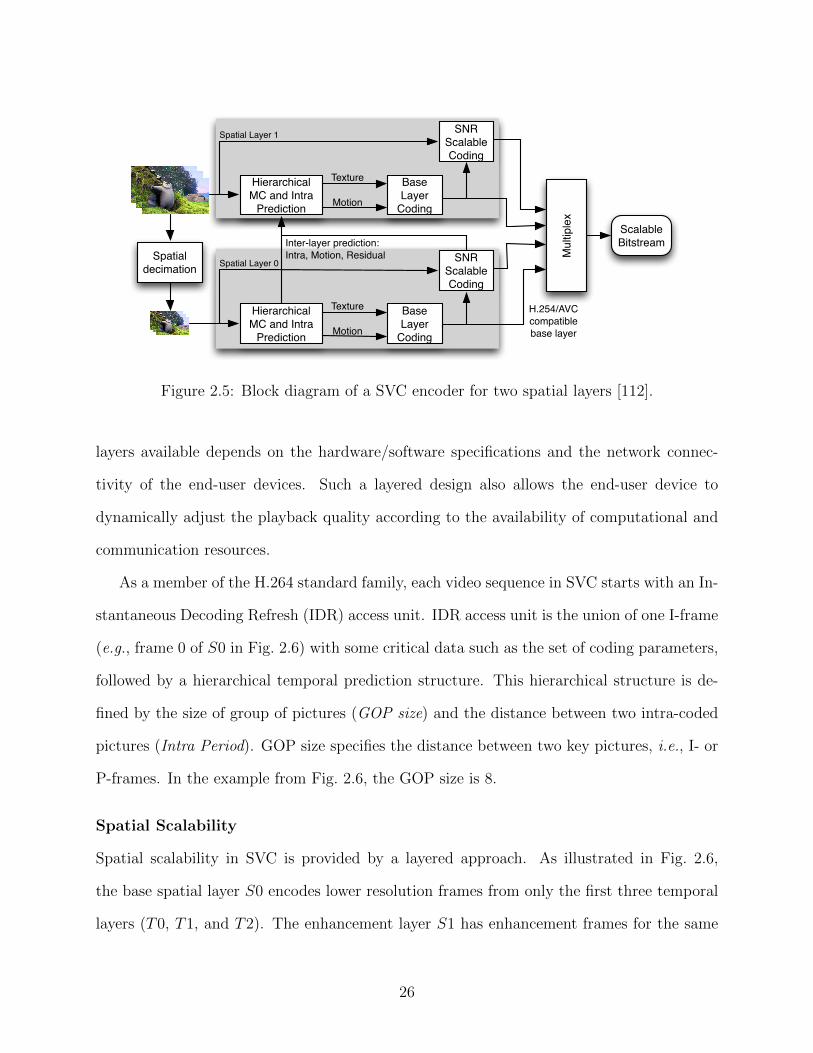
Hierarchical MC and Intra
Prediction
Base Layer
Coding
SNR Scalable Coding
Mul
tiple
x
Texture
Motion
Spatial Layer 1
Hierarchical MC and Intra
Prediction
Base Layer
Coding
SNR Scalable Coding
Texture
Motion
Spatial Layer 0
Inter-layer prediction:Intra, Motion, ResidualSpatial
decimation
Scalable Bitstream
H.254/AVCcompatiblebase layer
Figure 2.5: Block diagram of a SVC encoder for two spatial layers [112].
layers available depends on the hardware/software specifications and the network connec-
tivity of the end-user devices. Such a layered design also allows the end-user device to
dynamically adjust the playback quality according to the availability of computational and
communication resources.
As a member of the H.264 standard family, each video sequence in SVC starts with an In-
stantaneous Decoding Refresh (IDR) access unit. IDR access unit is the union of one I-frame
(e.g., frame 0 of S0 in Fig. 2.6) with some critical data such as the set of coding parameters,
followed by a hierarchical temporal prediction structure. This hierarchical structure is de-
fined by the size of group of pictures (GOP size) and the distance between two intra-coded
pictures (Intra Period). GOP size specifies the distance between two key pictures, i.e., I- or
P-frames. In the example from Fig. 2.6, the GOP size is 8.
Spatial Scalability
Spatial scalability in SVC is provided by a layered approach. As illustrated in Fig. 2.6,
the base spatial layer S0 encodes lower resolution frames from only the first three temporal
layers (T0, T1, and T2). The enhancement layer S1 has enhancement frames for the same
26
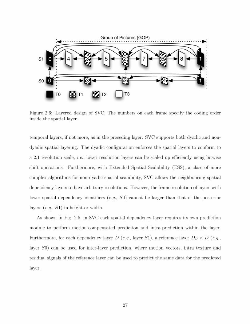
0 4 5 7 8 1
0
3 2 6
1
Group of Pictures (GOP)
S1
S0
T0 T1 T2 T3
23 4
Figure 2.6: Layered design of SVC. The numbers on each frame specify the coding orderinside the spatial layer.
temporal layers, if not more, as in the preceding layer. SVC supports both dyadic and non-
dyadic spatial layering. The dyadic configuration enforces the spatial layers to conform to
a 2:1 resolution scale, i.e., lower resolution layers can be scaled up efficiently using bitwise
shift operations. Furthermore, with Extended Spatial Scalability (ESS), a class of more
complex algorithms for non-dyadic spatial scalability, SVC allows the neighbouring spatial
dependency layers to have arbitrary resolutions. However, the frame resolution of layers with
lower spatial dependency identifiers (e.g., S0) cannot be larger than that of the posterior
layers (e.g., S1) in height or width.
As shown in Fig. 2.5, in SVC each spatial dependency layer requires its own prediction
module to perform motion-compensated prediction and intra-prediction within the layer.
Furthermore, for each dependency layer D (e.g., layer S1), a reference layer DR < D (e.g.,
layer S0) can be used for inter-layer prediction, where motion vectors, intra texture and
residual signals of the reference layer can be used to predict the same data for the predicted
layer.
27
Temporal Scalability
To support temporal scalability, SVC relies on a hierarchical temporal prediction mechanism
that is extended from H.264/AVC. While previous scalable standards such as H.263 and
MPEG-4 Visual basically provide dyadic temporal scalability by segmenting video layers
according to different frame types (i.e. I, P and B frame types), in SVC the basis of temporal
scalability is found on a hierarchical temporal prediction structure. In the example shown
in Fig. 2.6, there are four temporal layers (T0, T1, T2, and T3), where T0 is the temporal
base layer. Within a spatial layer, frames in layer T0 are predicted only from frames in layer
T0. Frames in layer T1 are predicted from layers T0 and T1, whereas frames in layer T3,
contained in spatial layer S1, are predicted by adjacent frames from any preceding layers.
The hierarchical temporal prediction structure can be characterized by GOP size and
Intra Period parameters. Assume that the initial frame rate of a video sequences is 24 fps.
With GOP size of 8, there are 3 fps frames for layer T0, 6 fps frames for layer T1, 12 fps
frames for layer T2, and 24 fps frames for layer T3. The Intra Period specifies how often a
P-frame at the end of a GOP can be replaced by an I-frame. It must be multiples of the
GOP size. For example, for Intra Period of 2 and GOP size of 8, the P-frame at the end of
every other GOP is replaced by an I-frame.
Quality Scalability
H.264/SVC allows the encoder to use complementary data in different layers to generate
video streams that provide distinct quality levels for the reconstructed video. Quality layering
applies after spatial and temporal scalability, hence, dependent quality layers have the same
frame size and frame rate. As illustrated in Fig. 2.5, each layer has a SNR refinement module
that provides the necessary mechanisms for quality scalability. Three quality scalability
modes are supported, namely CGS, MGS and FGS.
CGS (Coarse Grain Scalability) can be considered as a special case of spatial scaling
where upsampling and inter-layer deblocking of the intra-coded macroblocks of the reference
28
layer are not required, since the predicted macroblocks and the reference ones are the same
size. In CGS, the enhancement layer typically contains the residual texture signal that is
quantized with a smaller quantization step compared to that of preceding layers [112], hence,
providing incremental visual information.
In MGS (Medium Grain Scalability), both the base and enhancement layers can be used
to predict a layer at the same time, hence improving the coding efficiency when a variety of
bitrates are required in a scalable bitstream. MGS uses periodic key pictures to immediately
resynchronize the prediction module. Furthermore, MGS allows switching between different
MGS layers at any access unit, hence increasing the flexibility of bitstream adaptation [112].
FGS (Fine Grain Scalability) provides a continuous adaptation of bitstream bitrate by
using an advanced bit-plane technique. In this technique, different quality layers contain dis-
tinct subsets of bits for each macroblock. By supporting progressive refinement of transform
coefficients, FGS allows the decoder to truncate the bitstream at arbitrary points [112].
Besides these three scalability modes, quantization parameter (QP) is another factor
that affects the quality of the encoded layers. The value of QP ranges from 0 to 51. At the
beginning of the encoding process, where DCT transformation of macroblocks is performed,
the result is quantized by dividing the matrices of luma and colour components into two
specific matrices of integers. QP directly affects this process since the denominator matrices
are multiplied by QP before the division. Therefore, higher value of QP eliminates more
coefficients, hence increases coarseness and decreases the bitrate and quality of the encoded
video. To optimize the rate-distortion ratio, SVC adjusts the QP of each frame according to
its location in the respective group of pictures.
As shown in Fig. 2.5, all the enhancement layers and the H.264/AVC-compliant base layer
are merged by multiplex, and different temporal, spatial and quality layers are integrated
into a single scalable bitstream. We use a triplet (D,T,Q) to specify the number of spatial,
temporal and quality layers of a SVC-compliant bitstream. Interested readers may refer to
29
[112] for a more detailed discussion.
2.2 Related Works
In this section a summarized review of the related research work is presented. Since this
thesis covers cloud-assisted video streaming on mobile networks, the related work has been
categorized such that it conforms to the structure of the next chapters.
2.2.1 Analyzing the Performance of Scalable Video Coding
Scalable video coding (SVC) allows the media server to prepare and maintain a single copy
of a layered video and stream different numbers of layers to diverse devices with different
network connection qualities. Due to the diverse hardware/software capabilities and network
connectivities of end-user devices, the scalable approach to video streaming has received
much research attentions. The SVC research work related to this study can be briefly
summarized into three directions: comparing SVC with other standards, addressing the
impact of different layering configurations in SVC from an objective quality perspective, and
the subjective video quality offered by SVC. This section provides a brief review for each
direction and relates this work to the research results presented in Chapter 3.
Comparing SVC with other standards: Researchers have compared the performance of
SVC with a diverse set of other video coding standards, mainly focusing on the rate-distortion
performance, i.e., the objective quality of the video (normally measured by Y-PSNR) as a
function of average bitrate. Wien et al. [146] analyzed the effect of quality scalability and
spatial scalability (both dyadic and non-dyadic modes) on the objective quality of eight video
sequences in two quality classes, common intermedia format (CIF) (352 × 288 pixels) and
quarter CIF (QCIF) (176 × 144 pixels). In this study, the rate-distortion performance of
SVC is compared with that of H.264/AVC, MPEG-4 Visual [5] and Simulcast. Simulcast is
a method for broadcasting video content in which a video is encoded in different settings and
30
the different versions of the video are sent together. Results show that SVC imposes overhead
compared to single layer H.264/AVC, and outperforms Simulcast [22, 146]. Furthermore, it
has been reported that SVC slightly outperforms Google’s VP8 [113] and MPEG-4 Part
2 [131] in terms of rate-distortion but exhibits higher values of rate variability [113, 131].
The rate variability is defined as the covariance of the frame sizes in bytes. From another
perspective, it has been reported that in terms of time required to extract a substream
from a scalable bitstream, SVC bitstream extractor slightly outperforms MPEG-21 DIA
[43]. MPEG-21 DIA is a standard that provides videos in the form of substreams to support
interoperable access to them [132]. Finally, in [35] Choi et al. have compared the performance
of H.264/SVC with H.265/SHVC for two data sets of 240p and 480p video sequences. It
has been reported that at the same video quality (PSNR), SHVC outperforms SVC by 10%
average reduction in video bitrate [35].
Impact of different layering configurations in SVC: The effect of temporal, spatial
and quality layering on the performance of SVC has been investigated in [52,82,106,120,130].
In [130], it has been reported that increasing the number of temporal layers can increase the
objective quality of the encoded video in a constant bitrate, while using spatial or quality
layers has a negative impact due to the bitrate overhead. In [82], it has been reported that
SVC inter-layer prediction provides higher subjective quality when SVC is used to encode
fast and complex video sequences compared to that of slow and simple scenarios. However,
the visual properties of the video sequences is identified according to the visual experience
of the authors, and no methodical analysis of the video properties is performed. Comparison
studies on the performance of different quality scalability modes of SVC (namely CGS and
MGS) over five long CIF videos revealed that MGS provides higher objective quality at the
cost of higher rate variability [52, 106]. Finally, Slanina et al. [120] studied the impact of
the number of temporal and quality layers on the rate distortion performance of SVC, using
two full HD video sequences encoded with constant frame rate.
31
Subjective video quality offered by SVC: As discussed earlier, in contrast to objective
video quality, subjective video quality is the visual quality of the video as perceived by the
human viewers. Several research works have investigated the subjective video quality of
SVC [44,79,92,97,105]. For instance, Politis et al. measured the effect of user mobility and
handover on the objective and subjective video quality of SVC and H.264/AVC codecs using
two CIF video sequences, and reported that SVC outperforms H.264/AVC in both objective
and subjective video qualities [105]. Contrarily, a comparison based on four full HD video
sequences concludes that in three out of four video sequences AVC slightly outperforms SVC
[97]. However, according to [97] with a bitrate overhead of 10% for SVC, the visual quality
should be indistinguishable from that of single layer AVC.
Compared to the previous research work, in Chapter 3 a systematic study is conducted on
using H.264/AVC and SVC for full HD video streaming. In this study the video properties
are methodically extracted and the performance of different parameters of SVC encoding is
analyzed according to the visual and statistical properties of the test video sequences.
2.2.2 Distributed Video Transcoding in the Cloud
Due to the increasing demand for video streaming and the massive computing power offered
by the cloud, video transcoding in the cloud has recently received great attention. The most
simple and straight-forward use of the cloud is utilizing the virtual instances to perform
conventional video transcoding upon request [136, 167]. The cloud is also utilized to assist
mobile devices for customized transcoding services [32], for cloud-assisted video transcoding
[33] [149], and for energy conservation on mobile devices [165].
To better utilize the computing resources in the cloud, there have been proposals on
consolidating under-utilized VMs for cost effectiveness [20], predicting transaction load for
precise resource provisioning [69], and scheduling video transcoding tasks [21, 57, 151]. Fur-
thermore, to better utilize storage space in the cloud, there have been proposals on caching
32
transcoded versions of requested videos [83]. The trade-off between computation and storage
is investigated in [68], and a cost-efficient virtual machine provisioning strategy is proposed
for cloud-assisted video transcoding. The computational cost, storage cost, and video pop-
ularity of individual transcoded videos is used in [68] to decide how long a video should be
stored or how frequently it should be re-transcoded from the source version.
Towards efficient video transcoding in the cloud, a new approach is suggested in [70] to
reduce the bitrate of the transcoded video by encoding the video using a higher quantization
parameter without reducing frame size or frame rate. Furthermore, there are proposals on
transcoding only part of a video to reduce the transcoding time [49, 77]. To implement
distributed video transcoding in the cloud, MapReduce (along with other components of
Hadoop, if needed) is used to distribute video content to virtual machines [55, 58, 76]. For
example, CloudStream [58] segments SVC video into chunks of unit GOP size and uses
MapReduce [39] to parallelize SVC video transcoding among virtual machines in the cloud.
Furthermore, two approximate solutions are proposed to minimize the transcoding delay and
reduce the transcoding jitter.
Compared to the previous research work, in Chapter 4 a novel scheme towards distributed
video transcoding is proposed. In summary, this scheme takes the visual similarity of the
video frames into account to reduce bitrate and transcoding time. More detail is provided
in Chapter 4.
2.2.3 Unequal Error Protection for Streaming Layered Videos
Unequal error protection (UEP) is a special form of forward error correction (FEC) where a
stronger forward error correction code is used to protect more important data. The applica-
tion of UEP in data transmission over noisy channels was first proposed in [90]. Since then,
the use of UEP for fault tolerant streaming of layered videos has been widely investigated.
The existing research work on UEP for streaming layered videos can be summarized into
33
three focuses: coding paradigms, importance measures, and unequal error protection across
video layers.
Coding paradigms: Any coding technique that can generate code at an arbitrary code rate
can be used to provide unequal protection by applying stronger codes with more redundant
data to more important information. In [135], the performance of different random linear
coding strategies for unequal protection of data over lossy packet erasure links is analyzed.
Common coding techniques for UEP, among others, include rate-compatible convolutional
codes (RCPC) [100], low-density parity-check (LDPC) codes [51], growth codes [108], ex-
panding window fountain codes (EWFC) [95], and Raptor codes [96]. While the aforemen-
tioned work are mostly on packet erasure channels, i.e., they set up the UEP mechanism in
the application layer, there is a large body of research on UEP in the physical and transport
layers using bit-level UEP schemes [61]. Since the focus of the research work presented in
Chapter 5 is on UEP for layered videos in the application layer, different coding techniques
for UEP are not investigated and general random linear codes are used as the FEC code in
the proposed UEP model.
Importance metrics: Whatever coding paradigm is selected, unequal protection technique
requires the to-be-transmitted data to be divided into different categories of importance. In
the case of layered videos, various information can be used as the input to the video packet
importance metric:
• Layer information: A basic importance measure of a video packet is the posi-
tion of its corresponding video layer inside the layer dependency structure. For
example, a video packet may contain information of a reference or a dependent
picture, which can be used as an importance measure [166].
• Data partitioning: AVC generates three separate data partitions: header data,
intra-predicted macroblocks (macroblocks that are predicted from macroblocks
from the same picture), and inter-picture predicted macroblocks (macroblocks
34
that are predicted from other pictures). In [96] and [124], the data partition
is used as the importance metric for corresponding video packets.
• Bitrate of the video frame: In [166], the bitrate of the encoded video frames is
considered as an importance metric for the corresponding video packets. The
rationale behind this design is that larger frames contain more information
due to less compression. Similarly, in [95] and [96], the bitrate of video slices
is used for the same purpose.
• Slice order: An experimental study showed that early slices are more important
than the later ones [94]. Hence, in [94] the order of slices in video frames
is used as an importance metric. In [126], the flexible macroblock ordering
(FMO) capability of the H.264 family of video coding standards is used to
dynamically associate the macroblocks to the slices. This mechanism can be
used to improve the performance of UEP by keeping the macroblocks of the
same importance level in the same slice.
• Error propagation zone: Error propagation zone is the set of processing units
(frames, slices, or macroblocks) that depend on a specific reference unit. In
[53], error propagation zone of each frame is employed to create a hierarchy of
importance levels.
• Motion information: In [104], the size of motion information of each slice is
used as an importance measure at the slice level. Similarly, in [42] motion
energy, defined as macroblock size times the motion vector size, is used as the
importance measure at the frame level.
We note that none of the proposed UEP mechanisms for layer-coded video streaming
considers the internal design of the video codec standard in use. In fact, most of the proposed
mechanisms can be used for any data with different importance levels, such as data partitions
35
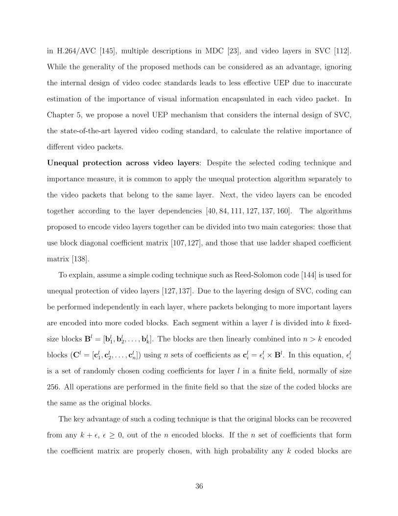
in H.264/AVC [145], multiple descriptions in MDC [23], and video layers in SVC [112].
While the generality of the proposed methods can be considered as an advantage, ignoring
the internal design of video codec standards leads to less effective UEP due to inaccurate
estimation of the importance of visual information encapsulated in each video packet. In
Chapter 5, we propose a novel UEP mechanism that considers the internal design of SVC,
the state-of-the-art layered video coding standard, to calculate the relative importance of
different video packets.
Unequal protection across video layers: Despite the selected coding technique and
importance measure, it is common to apply the unequal protection algorithm separately to
the video packets that belong to the same layer. Next, the video layers can be encoded
together according to the layer dependencies [40, 84, 111, 127, 137, 160]. The algorithms
proposed to encode video layers together can be divided into two main categories: those that
use block diagonal coefficient matrix [107,127], and those that use ladder shaped coefficient
matrix [138].
To explain, assume a simple coding technique such as Reed-Solomon code [144] is used for
unequal protection of video layers [127,137]. Due to the layering design of SVC, coding can
be performed independently in each layer, where packets belonging to more important layers
are encoded into more coded blocks. Each segment within a layer l is divided into k fixed-
size blocks Bl = [bl1,bl2, . . . ,b
lk]. The blocks are then linearly combined into n > k encoded
blocks (Cl = [cl1, cl2, . . . , c
ln]) using n sets of coefficients as cli = εli ×Bl. In this equation, εli
is a set of randomly chosen coding coefficients for layer l in a finite field, normally of size
256. All operations are performed in the finite field so that the size of the coded blocks are
the same as the original blocks.
The key advantage of such a coding technique is that the original blocks can be recovered
from any k + ε, ε ≥ 0, out of the n encoded blocks. If the n set of coefficients that form
the coefficient matrix are properly chosen, with high probability any k coded blocks are
36
sufficient to recover the original blocks, i.e., the transmission overhead ε is minimal. To this
end, block diagonal [107, 127] and ladder shaped [138] coefficient matrices, as illustrated in
Fig. 5.3.3, are used in most of the proposed coding schemes for unequal protection of video
layers. The low triangular design of the coefficient matrix is expected to provide progressive
decoding when receiving the first k coded blocks.
Coefficients for Layer 1
Coefficients for Layer 2
Redundancy coefficientsfor Layer 1
Zeros(a) Block DiagonalCoefficient Matrix
(b) Ladder ShapedCoefficient Matrix
Redundancy coefficientsfor Layer 2
k1
d1
k2
d2
k1
d1
k2
d2
12
34
12
34
1
2
3
4
Figure 2.7: Block diagonal and ladder shaped coefficient matrices for two video layers L1 andL2, in which each video segment is divided into k1 and k2 data blocks, respectively. Thesematrices are multiplied into k1 + k2 data blocks to create k1 + k2 reconstruction blocks andd1 + d2 redundant coded blocks for forward error correction.
For each video segment of each layer, the block diagonal coefficient matrix is a combi-
nation of a lower triangular and a general coefficient matrix, as illustrated in Fig. 5.3.3(a),
where each coded block i of layer l is a linear combination of blocks 1 to i of the same video
segment. There will be exactly k such coded blocks for each segment that consists of k orig-
inal blocks. Redundant coded blocks are produced and sent to recover any loss during the
transmission of the first k coded blocks. However, if any of the first k coded blocks are lost,
the decoding must wait for the redundant coded blocks to recover the loss, which introduces
an extra delay.
The ladder shaped coefficient matrix is an extension over the block diagonal coefficient
matrix, as illustrated in Fig. 5.3.3(b). It trades computation and bandwidth for increasing
redundancy in higher priority layers by including the higher priority layers in the coded
blocks from lower priority layers [138]. In this approach, each coded block i of layer l is a
37
linear combination of blocks from the same video segment in layers 1 to l − 1 and blocks 1
to i in layer l. Hence, the base layer of SVC is decodable with higher probability since it is
included in every coded block.
Compared to block-diagonal and ladder-shaped coefficient matrices, in Chapter 5 a novel
coding scheme is proposed for delivering layered video in lossy packet networks. The pro-
posed coding scheme is based on a coefficient matrix that combines the diagonal coefficient
matrix with the ladder-shaped coefficient matrix. Besides eliminating unnecessary coding
operations, the proposed scheme also reduces the delays due to packet loss and out-of-order
delivery. Similar to existing proposals for using erasure codes in wireless communication
[13, 19], erasure coding is employed to cope with channel loss. However, it does not du-
plicate the source bits (as in [19]), that would impose extra multiplexing/demultiplexing,
nor assumes single channel transmissions (as in [13]). Furthermore, any coding paradigm or
importance metric can be used along with the proposed scheme for UEP across video layers,
since we assume that such schemes are in place to provide erasure transmission channels.
More details are covered in Chapter 5.
2.2.4 Cooperative Ad-Hoc Networks and WiFi Offloading
The idea of utilizing WiFi communication among cooperative smartphones was originally
proposed in [15], in which unicast connections over WiFi are used to locally distribute data.
The main motivation for utilizing opportunistic communication over local short-range links,
e.g., Bluetooth and WiFi, in mobile devices is to offload the cellular traffic, while maintaining
short delays [54, 62, 143]. For example, a system may stream video segments over WiFi
and share error recovery code over Bluetooth [81], or schedule transmission over multiple
WiFi hotspots [121] to receive one flow of data. In [26, 59], mobile phone users use social
relationships along with the geographical proximity to disseminate information stored on
the devices through WiFi instead of cellular links. In [34, 109], the same idea has been
38
extended to simultaneous Internet connections over cellular and WiFi channels. Similarly,
by exploiting multiple cellular and WiFi connections, digital content may be delivered to
mobile devices over multiple paths [128].
In [123], a collaboration model is proposed that aggregates cellular and local WiFi band-
width to provide higher downlink bitrate for participant nodes. To disseminate data, multi-
hop peer-to-peer unicast communication is used, which introduces additional delay to the
streaming session and limits the potential saving in terms of energy consumption. In contrast,
in [72,114] it has been proposed to use the overhearing nature of wireless communication and
WiFi Direct [9] to obtain single-hop unicast transmission between collaborating node. WiFi
Direct is a standard that allows smartphones to create peer-to-peer connections without the
need for a wireless access point. The connected devices can transfer data between each other
while maintaining their connection to the Internet. In WiFi Direct, one of the phones plays
the role of a software access point, centrally managing the WiFi network.
In Chapter 6, we use the same idea and utilize both the cellular networks and WiFi
communication opportunities to improve the quality of multimedia streaming on smartphone
devices while conserving energy. The goal is to allow each user to enjoy the aggregated
downlink for an energy conserving, continuous, high bitrate, and low delay video streaming
experience. Toward this goal, we propose a light-weight distributed scheduling algorithm
along with simple, yet effective, collaboration policies for the cooperating nodes. Nonetheless,
both wireless networks that are engaged in the proposed collaborative streaming system are
subject to noise and can significantly benefit from protection against packet loss. In the
proposed system, we use network coding.
Network coding offers a simple yet effective loss recovery mechanism, with minimum
communication overhead. Network coding (NC) was originally proposed in the field of in-
formation theory to achieve optimal communication throughput [12]. After the introduction
of random linear NC (RLNC) [56], the concept of NC has been widely applied in practical
39
content distribution systems [85]. Instead of encoding and decoding the data only at the
source and destination nodes as in usual applications of erasure codes, network coding allows
any intermediate node to decode and/or re-encode disseminated data. In RLNC, the new
coded blocks are encoded by using randomly generated coding coefficients in GF(2x). If
a sufficiently large field size is used, with high probability any k coded blocks are linearly
independent.
One of the challenges of applying NC is the computational complexity of the encoding
and decoding operations. This challenge has prevented the application of NC on mobile
devices due to limited computing and battery power until recent advances in processing
power on mobile devices. The first implementation of NC on mobile devices was presented
in [103], followed by an implementation of NC on iPhone in [117]. These studies have
shown that it is now feasible to perform coding operations on mobile devices, which leads to
investigations of various applications of NC in mobile networks. For instance, Pedersen et
al. proposed Pictureviewer, a mobile application that utilizes NC to transfer pictures among
mobile devices over WiFi links [102]. Furthermore, network coding is utilized as an effective
mechanism to recover losses and errors with minimum communication overhead in wireless
networks [101]. Towards multimedia streaming, Vingelmann et al. applied NC to stream
video content among a group of iPhone devices [133].
Recently, network coding has been applied in cooperative streaming systems to reduce
traffic in the cellular network and to simplify the cooperation mechanism in the WiFi network
[72]. Microcast performs RLNC in GF(256) to encode the video content. The coded content
is transmitted from the source to smartphones over a cellular network and is then shared
among smartphones in local WiFi network [72]. However, this design trades higher power
consumption on mobile devices for less traffic in the cellular network and better system
throughput. Although it has been shown that modern smartphones can perform coding
operations in GF(256) at a decent rate [103, 117], the operations still consume a noticeable
40
amount of energy.
To address these issues, in Chapter 6 a two-level coding scheme is utilized that reduces the
computational complexity of NC on mobile devices [154]. Furthermore, for the first time, the
power consumption minimization problem in the NC-based cooperative streaming systems
is formulated and an optimal rate allocation and scheduling (RAS) algorithm is proposed
[157]. The proposed cooperative streaming system minimizes both the streaming traffic in
the cellular network and the energy consumed by streaming applications on mobile devices.
The system carefully employs NC only when necessary to minimize the communication
and computational overhead introduced by coding operations. Finally, the system enforces
fairness in battery drainage among mobile devices so that the system can support longer
streaming sessions.
41
Chapter 3
Detailed Analysis of Layered Video Coding
The growing number of makes and models of modern smartphones, tablets and smart TVs
has led to an increasing diversity of devices used for streaming multimedia content from the
Internet. Despite the diversity in hardware/software capabilities and variations in network
connectivity, end users expect the best possible quality in the video streaming experience.
Moreover, increasing traffic from cellular networks poses another challenge in maintaining
the playback quality throughout a streaming session since the network characteristics may
fluctuate significantly.
One solution to this problem is to prepare several versions of a video for a predefined
set of resolutions. For example, YouTube [152] encodes videos in H.264/AVC [145] and VP9
[142] formats and supports a variety of video resolutions. Currently, YouTube offers nine
recommended video resolutions, starting from 144p (256× 144 pixels) to 8K (7680× 4320).
This range of video resolutions can offer various video bitrates from less than 256 Kbps to
more than 10 Mbps. A user may manually select the video resolution, and may also leave it to
YouTube to send the video in the quality that best suits the device and network conditions.
On the one hand, extra storage is needed on the server side to store different versions
of the video. On the other hand, users are limited to the bitrates and video resolutions
offered by YouTube. Scalable video coding (SVC), an extension of H.264/AVC, has emerged
to support ultra and full high definition video streaming to diverse devices with different
network connection qualities. With SVC, the server maintains a single version of each video,
but the video content is delivered to end-user devices at different quality levels according to
the device capabilities and network conditions.
Moreover, SVC can address another deficiency in the YouTube-like streaming systems.
42
In these systems, if a user views the same video on different devices at different quality
levels, a copy at each quality level must be downloaded, which leads to increasing network
traffic and high workload demand on the video server. With SVC, the video server may
serve one copy of the video in a properly chosen format to the router or the edge media
server that is adjacent to the end-user devices. Then the router or the edge media server
may serve video streams that best match the characteristics of each device by sending a
proper set of layers. This not only alleviates the heavy burden on the streaming server and
the Internet routers, but also delivers the video in better quality to each end-user device,
thanks to the extra available bandwidth and the fine-grained bitrate adaptation provided by
the multi-dimensional scalability of SVC [112].
As opposed to conventional single-stream videos, a scalable video consists of multiple
video substreams at different quality levels. The substreams are normally referred to as
layers [112]. In a nutshell, SVC encodes a video with spatial scalability (layers with different
resolutions), temporal scalability (layers with different frame rates), quality scalability (layers
with different qualities), or any arbitrary combination of them. Furthermore, SVC can
tolerate frame losses, i.e., even if frames are dropped during transmission, the original video
can still be rendered with little distortion. For this reason, SVC has received great research
attention and has been used in many proposals for improving multimedia streaming systems
[148]. Nevertheless, in contrast to H.264/AVC [145], which is the de facto standard for single
layer video coding, just a few commercial streaming systems utilize SVC as the video codec.
The main reason is the bitrate and computational overhead that is introduced by the multi-
stream representation of the video. In this chapter, we conduct a systematic study on the
use of SVC for full HD video streaming. Our goal is to identify the good and bad uses of
SVC, to quantify the coding overhead, and to benchmark the video quality under different
spatial, temporal, and quality settings. Using a set of carefully selected and diverse video
sequences, we also identify the types of video that can benefit from SVC. Our study reveals
43
that the efficiency and computational gap between SVC and H.264/AVC is much less when
encoding high quality videos, e.g., in full HD resolution. There are three more interesting
observations: (1) Replacing P-frames with I-frames in complex video sequences can decrease
the encoding complexity with a very mild increase in the bitrate of the encoded video; (2)
When the video is complex and the consecutive frames are considerably different, adding
spatial layers may decrease the bitrate of the encoded video; and (3) Increasing the frame
size decreases the computational and bitrate overhead of non-dyadic spatial layers, which
can be helpful as the diverse screen resolutions of end user devices limits the application of
SVC if only dyadic spatial resolution is employed.
Towards understanding the underlying properties of SVC, we need a thorough analysis of
the performance of the coding standard in different scenarios. The current body of research
in this field is reported in Section 2.2. We note that the existing studies have one or several
of the following problems: (1) the number of test video sequences is not sufficiently large
to represent different types of videos, therefore the conclusions may be biased towards the
particular video sequences used; (2) the criteria used to select the test video sequences is not
clear; (3) the video resolutions are too small to be relevant in today’s applications; and (4)
the performance of SVC is limited to only a few scalability modes. To address these issues,
we conduct a systematic analysis on the performance of SVC in full HD video streaming.
We carefully select a set of video sequences from 29 full HD video sequences. The video
sequences represent a variety of content properties, which also allows us to identify any
linkage between performance and video content. We also examine the complete range of
video resolution, from 288p to 2160p. Furthermore, we conduct the analysis on different
aspects of SVC, including the decoding complexity and considering the effect of frame size
and all the scalability modes provided by the SVC standard.
44
3.1 Experiment Setup
To conduct a systematic study on H.264/AVC and SVC for high resolution video streaming,
a careful design of the experiments is necessary. In this section, we describe the experiment
setup and performance metrics.
3.1.1 Experiment Testbed
We conduct all the experiments on a server cluster of 10 nodes. Each server node is equipped
with four Intelr Xeonr E5640 CPUs and 16 GB of 1066 MHz memory. Each Xeonr E5640
CPU has four CPU cores at 2.67 GHz and 12 MB of shared CPU cache. To avoid the effect of
multi-core operation on core performance and CPU cache hit ratio, we utilize only one core
on each CPU and at most three CPUs on each machine. To ensure the full compliance of
the used encoder/decoder software with the standard specification, we decided to use open-
source reference encoder and decoder software published by the Joint Video Team (JVT)
of ITU-T and MPEG, i.e., JM-18.6 [65] for H.264/AVC and JSVM-9.19.15 [1] for SVC.
Since the emphasis of the reference software is on compliance with specifications and not
the optimization of the coding process, these software are much slower than the third party
codecs such as x264 [91]. Both software were compiled on RedHatr Linux with kernel v2.6.18
and gcc v4.1.2. In addition, MPEG-7 Visual Description Tools [118] was used to partially
extract some visual features of video sequences and EPFL Video Quality Measurement Tool
v1.1 [2] was used to calculate different objective video quality metrics. Tools to extract
the motion vectors and calculate descriptive video features such as Detail [99] and Motion
Activity [67], as will be described later, were developed from scratch.
3.1.2 Selecting the Raw Video Dataset
To perform the aforementioned experiments, a proper set of high resolution raw video se-
quences is needed. By raw video sequence, we mean a video sequence in which the video
45
frames are not compressed even by a lossless encoder. For example, a raw video frame that
uses 4:4:4 color presentation can be considered as a bitmap image. In conformance with the
main profile of H.264/AVC and SVC, we used raw video sequences with 4:2:0 color presen-
tation. We collected 29 raw video sequences from Xiph.org Test Media collection [3], with
frame size of 1920 × 1080 pixels and frame rate of 24 frames per second (i.e. 1080p24).
This is the minimum frame size and frame rate for full HD in ATSC standards [4]. After
investigating the video sequences, we decided to use a precisely selected subset of collected
raw video sequences, since the video sequences were not well spread across different genres
and visual features. Furthermore, considering the limited available computational resources,
using all the video sequences would severely affect the number and quality of the potential
experiments, let above the time and effort needed to accumulate and analyze the results.
A. Selection of Video Features
A proper sampling method must be utilized to select a proper set of reference video
sequences such that the selected samples represent a variety of content types that a video
streaming server might need to encode and stream. Toward finding proper and descriptive
features, we reviewed different visual features suggested in the literature, including the fea-
tures suggested in MPEG-7 Visual standard [67, 78, 119, 147]. Consequently, we selected
three feature categories, representing color, texture and motion, as described below.
• Color: Video compression algorithms are neutral to the exact value of the color but are
sensitive to the diversity and spatial dispersion of the colors in a video frame. Therefore,
to represent the color properties of each video frame, the Dominant Color descriptor as
defined in MPEG-7 Visual standard [119] was used. This descriptor characterizes an
image by a small number of representative colors. The colors are selected by quantizing
pixel colors into up to eight principal clusters. The description then consists of the
fraction of the image or region represented by each color cluster and the variance of each
one. A measure of overall spatial coherency of the clusters is also defined. Altogether,
46
this descriptor provides a very compact description of the representative colors in an
image. To represent the color properties of a video sequence, we extracted the number of
dominant colors (with maximum of 8) and the spatial coherency of the color clusters for
each frame of the video sequences. Then we used the average of the calculated feature
values of the frames as the value of that feature for the respective video sequence.
• Texture: To represent the texture property of the video frames in each raw video se-
quence, we extracted the MPEG-7 edge histogram descriptor [118] for each frame. Next,
we quantized the average of edge histogram values over all frames of each video sequence
as suggested in [99]. This descriptor is known as Detail [67].
• Motion: The motion features of a video sequence are best represented by the motion
vectors and Motion Activity. Motion vectors provide the gross motion characteristics
of a video segment. However motion vectors cannot be extracted from a raw video
sequence, since there is no motion data in a raw video. To extract the motion vectors,
we first encoded each video sequence using JSVM-9.19.15 in single layer mode1, i.e.,
without any spatial or quality layers. Then the JSVM-9.19.15 decoder tool was modified
to report the motion vectors for each inter-frame motion compensated macroblock and
sub-macroblock prediction. Next, the extracted motion vectors were used to calculate
the Motion Activity [67]. Motion Activity considers the intensity, direction, spatial
distribution and temporal distribution of activity in a video sequence. To calculate
the motion activity, according to [67], the standard deviation of the magnitudes of all
motion vectors of each frame was quantized between 1 and 5, and the average of the
quantized motion activity values over all the frames was used as the Motion Activity
of each video sequence.
To ensure that calculating the features and performing the experiments are feasible on
1The most important encoder parameters were GOP size of 8, base quantization parameter of 32, motionprediction buffer size of 16 frames, and using fast bi-directional motion search. However, in this special case,the selection of coding parameters does not affect the results as long as the same set of parameters are usedfor all the video sequences.
47
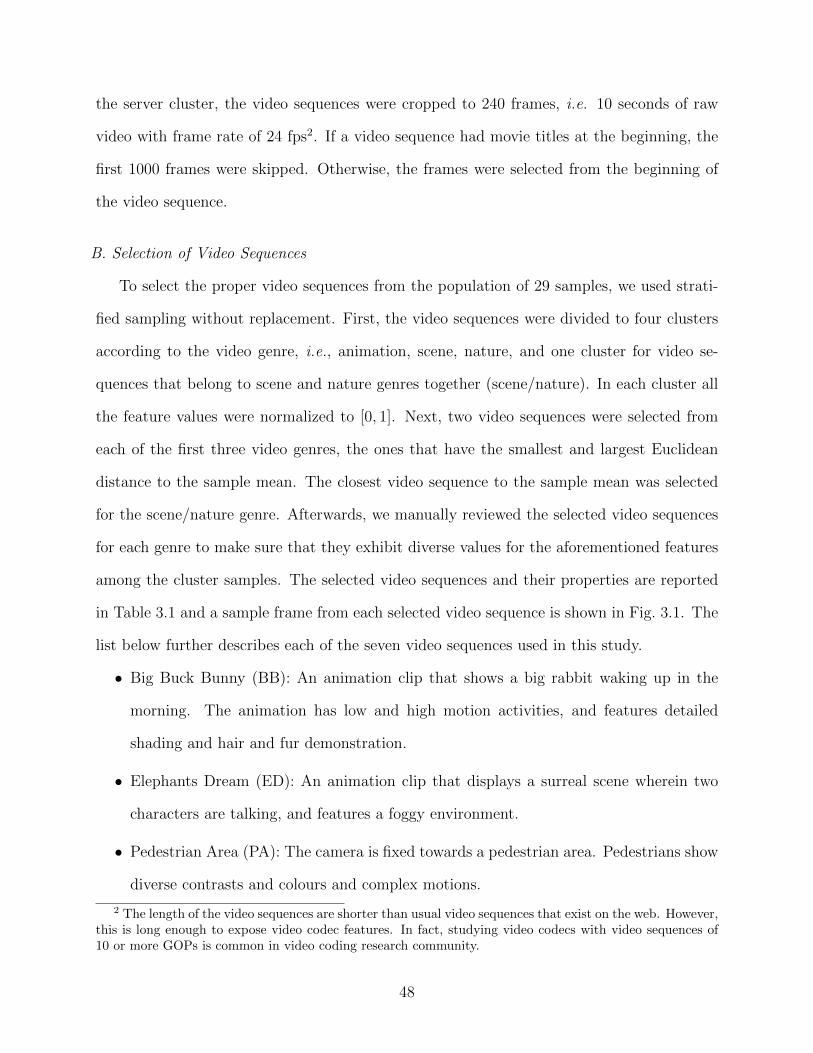
the server cluster, the video sequences were cropped to 240 frames, i.e. 10 seconds of raw
video with frame rate of 24 fps2. If a video sequence had movie titles at the beginning, the
first 1000 frames were skipped. Otherwise, the frames were selected from the beginning of
the video sequence.
B. Selection of Video Sequences
To select the proper video sequences from the population of 29 samples, we used strati-
fied sampling without replacement. First, the video sequences were divided to four clusters
according to the video genre, i.e., animation, scene, nature, and one cluster for video se-
quences that belong to scene and nature genres together (scene/nature). In each cluster all
the feature values were normalized to [0, 1]. Next, two video sequences were selected from
each of the first three video genres, the ones that have the smallest and largest Euclidean
distance to the sample mean. The closest video sequence to the sample mean was selected
for the scene/nature genre. Afterwards, we manually reviewed the selected video sequences
for each genre to make sure that they exhibit diverse values for the aforementioned features
among the cluster samples. The selected video sequences and their properties are reported
in Table 3.1 and a sample frame from each selected video sequence is shown in Fig. 3.1. The
list below further describes each of the seven video sequences used in this study.
• Big Buck Bunny (BB): An animation clip that shows a big rabbit waking up in the
morning. The animation has low and high motion activities, and features detailed
shading and hair and fur demonstration.
• Elephants Dream (ED): An animation clip that displays a surreal scene wherein two
characters are talking, and features a foggy environment.
• Pedestrian Area (PA): The camera is fixed towards a pedestrian area. Pedestrians show
diverse contrasts and colours and complex motions.
2 The length of the video sequences are shorter than usual video sequences that exist on the web. However,this is long enough to expose video codec features. In fact, studying video codecs with video sequences of10 or more GOPs is common in video coding research community.
48
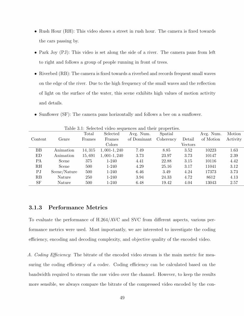
• Rush Hour (RH): This video shows a street in rush hour. The camera is fixed towards
the cars passing by.
• Park Joy (PJ): This video is set along the side of a river. The camera pans from left
to right and follows a group of people running in front of trees.
• Riverbed (RB): The camera is fixed towards a riverbed and records frequent small waves
on the edge of the river. Due to the high frequency of the small waves and the reflection
of light on the surface of the water, this scene exhibits high values of motion activity
and details.
• Sunflower (SF): The camera pans horizontally and follows a bee on a sunflower.
Table 3.1: Selected video sequences and their properties.
Content GenreTotal Selected Avg. Num. Spatial
DetailAvg. Num. Motion
Frames Frames of Dominant Coherency of Motion ActivityColors Vectors
BB Animation 14, 315 1, 001-1, 240 7.49 8.85 3.52 10223 1.63ED Animation 15, 691 1, 001-1, 240 3.73 23.97 3.73 10147 2.39PA Scene 375 1-240 4.41 22.88 3.15 10116 4.42RH Scene 500 1-240 4.29 25.16 3.17 11041 3.12PJ Scene/Nature 500 1-240 6.46 3.49 4.24 17373 3.73RB Nature 250 1-240 3.94 24.33 4.72 8612 4.13SF Nature 500 1-240 6.48 19.42 4.04 13043 2.57
3.1.3 Performance Metrics
To evaluate the performance of H.264/AVC and SVC from different aspects, various per-
formance metrics were used. Most importantly, we are interested to investigate the coding
efficiency, encoding and decoding complexity, and objective quality of the encoded video.
A. Coding Efficiency: The bitrate of the encoded video stream is the main metric for mea-
suring the coding efficiency of a codec. Coding efficiency can be calculated based on the
bandwidth required to stream the raw video over the channel. However, to keep the results
more sensible, we always compare the bitrate of the compressed video encoded by the con-
49
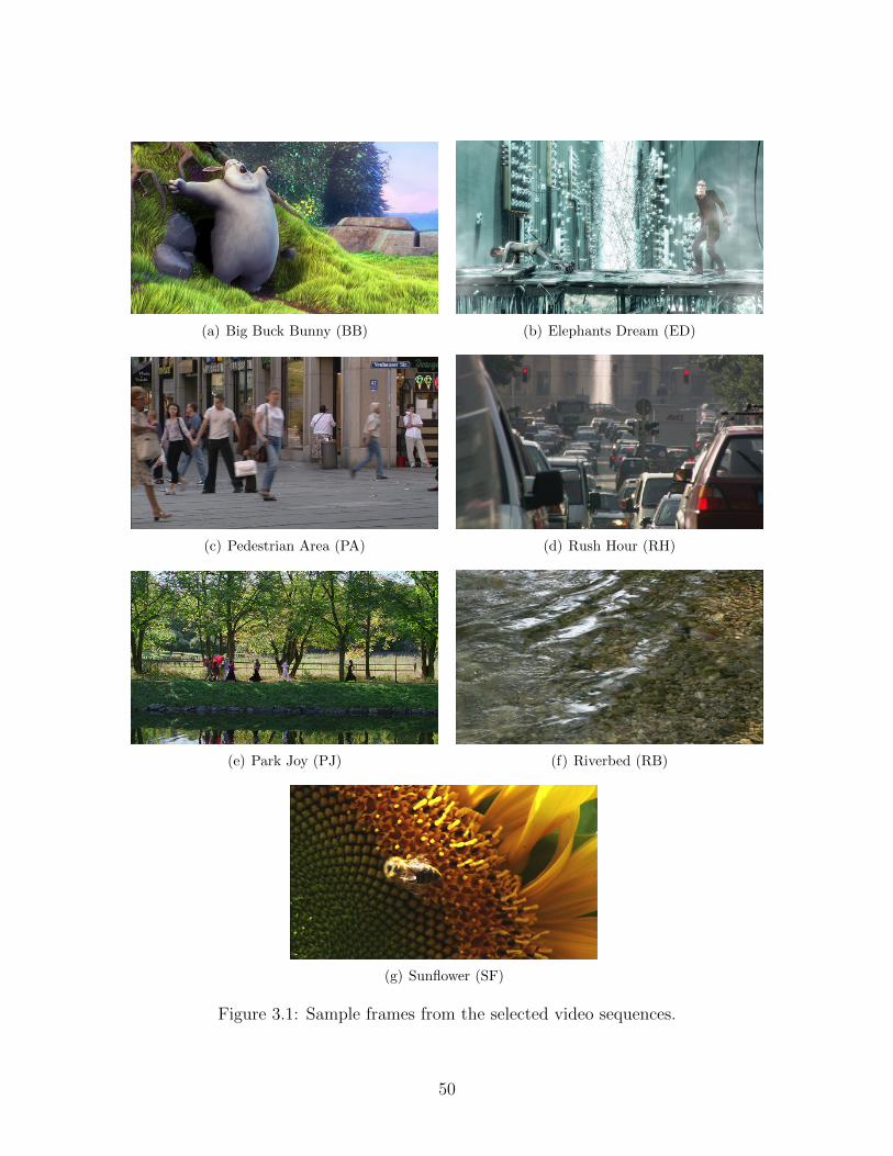
(a) Big Buck Bunny (BB) (b) Elephants Dream (ED)
(c) Pedestrian Area (PA) (d) Rush Hour (RH)
(e) Park Joy (PJ) (f) Riverbed (RB)
(g) Sunflower (SF)
Figure 3.1: Sample frames from the selected video sequences.
50
figuration of interest with the bitrate of the same video encoded by the reference coding
configuration. Along with the bitrate of the encoded video, MPEG-7 motion activity of the
encoded video is also used wherever it helps the discussion.
B. Encoding and Decoding Complexity: We measure the CPU time required to encode and
decode each video sequence. We compare the performance of SVC with the single layer
H.264/AVC and Simulcast, all performed using JM-18.6 and JSVM-9.19.15 software. The
performance difference in terms of encoding and decoding time reflects the difference be-
tween SVC and other coding standards. Both JM and JSVM software packages are strict
implementations of the standard. Therefore, no optimization is performed, and no part of
specification is sacrificed for better encoding or decoding performance.
C. Objective Quality: In this chapter (and in the future ones), we focus on the objective video
quality instead of subjective video quality. As a reminder, for any subjective measure to be
representative, we need a large pool of participants and a large collection of videos. Such
a user-based study is orthogonal to this work. To quantify the objective video quality, we
meaured Y-PSNR (the PSNR value of the luma component of the video sequence), SSIM
(structural similarity index) [139], MS-SSIM (multi-scale structural similarity index) [141]
and the pixel domain version of VIF (visual information fidelity) [116] for each encoded
video sequence. All these metrics are calculated as the average value of a full reference
image quality assessment (FR-IQA) metric over raw and decoded video frames. To keep the
discussion concise, only the results for Y-PSNR and VIF metrics are included in Sec. 3.2.
Compared to other objective video quality metrics, VIF is known for its high correlation
with the subjective video quality [92].
Throughout the performance analysis, we use a combination of the aforementioned per-
formance metrics and overhead of the performance metrics wherever appropriate. We define
the overhead of a performance metric as the ratio of the performance of the configuration
51
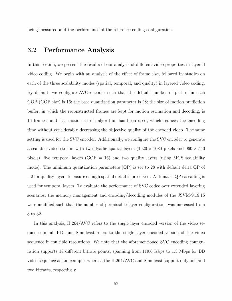
being measured and the performance of the reference coding configuration.
3.2 Performance Analysis
In this section, we present the results of our analysis of different video properties in layered
video coding. We begin with an analysis of the effect of frame size, followed by studies on
each of the three scalability modes (spatial, temporal, and quality) in layered video coding.
By default, we configure AVC encoder such that the default number of picture in each
GOP (GOP size) is 16; the base quantization parameter is 28; the size of motion prediction
buffer, in which the reconstructed frames are kept for motion estimation and decoding, is
16 frames; and fast motion search algorithm has been used, which reduces the encoding
time without considerably decreasing the objective quality of the encoded video. The same
setting is used for the SVC encoder. Additionally, we configure the SVC encoder to generate
a scalable video stream with two dyadic spatial layers (1920 × 1080 pixels and 960 × 540
pixels), five temporal layers (GOP = 16) and two quality layers (using MGS scalability
mode). The minimum quantization parameters (QP) is set to 28 with default delta QP of
−2 for quality layers to ensure enough spatial detail is preserved. Automatic QP cascading is
used for temporal layers. To evaluate the performance of SVC codec over extended layering
scenarios, the memory management and encoding/decoding modules of the JSVM-9.19.15
were modified such that the number of permissible layer configurations was increased from
8 to 32.
In this analysis, H.264/AVC refers to the single layer encoded version of the video se-
quence in full HD, and Simulcast refers to the single layer encoded version of the video
sequence in multiple resolutions. We note that the aforementioned SVC encoding configu-
ration supports 18 different bitrate points, spanning from 119.6 Kbps to 1.3 Mbps for BB
video sequence as an example, whereas the H.264/AVC and Simulcast support only one and
two bitrates, respectively.
52
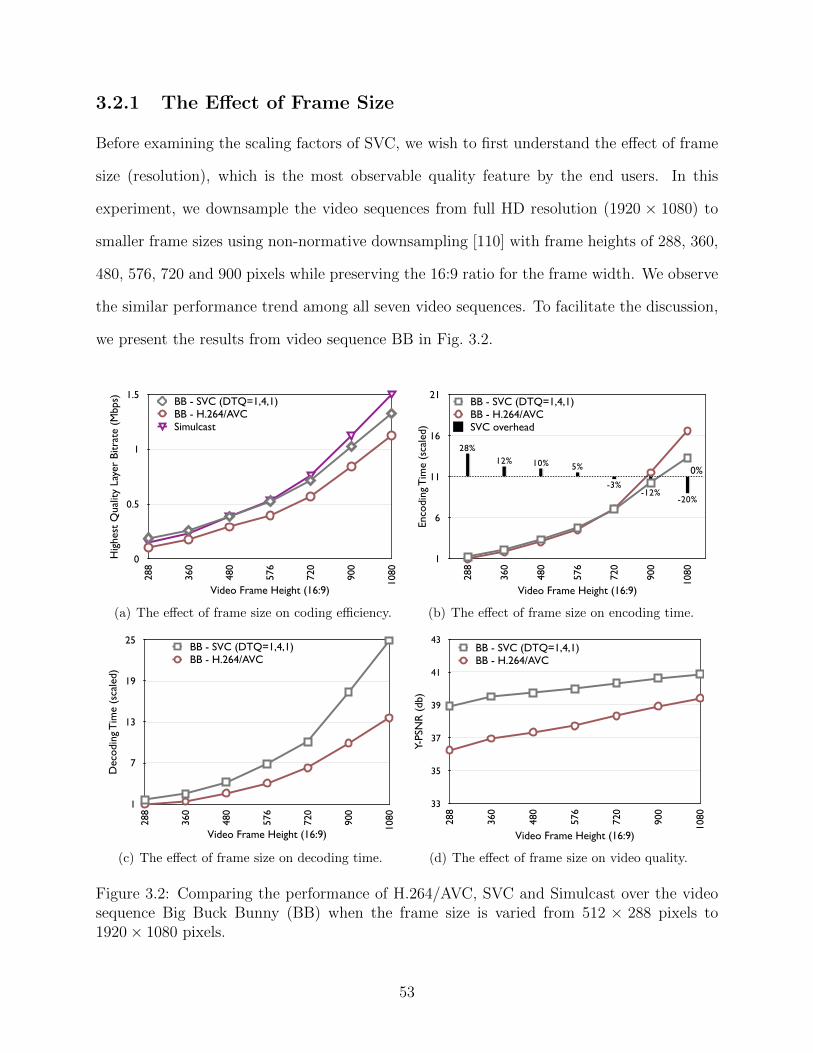
3.2.1 The Effect of Frame Size
Before examining the scaling factors of SVC, we wish to first understand the effect of frame
size (resolution), which is the most observable quality feature by the end users. In this
experiment, we downsample the video sequences from full HD resolution (1920 × 1080) to
smaller frame sizes using non-normative downsampling [110] with frame heights of 288, 360,
480, 576, 720 and 900 pixels while preserving the 16:9 ratio for the frame width. We observe
the similar performance trend among all seven video sequences. To facilitate the discussion,
we present the results from video sequence BB in Fig. 3.2.
Hig
hest
Qua
lity
Laye
r Bi
trat
e (M
bps)
0
0.5
1
1.5
288
360
480
576
720
900
1080
BB - SVC (DTQ=1,4,1)BB - H.264/AVCSimulcast
Video Frame Height (16:9)
(a) The effect of frame size on coding efficiency.
1
6
11
16
21
288
360
480
576
720
900
1080
BB - SVC (DTQ=1,4,1)BB - H.264/AVCSVC overhead
-20%-12%
-3%
5%10%12%28%
Video Frame Height (16:9)
0%
Enco
ding
Tim
e (s
cale
d)
(b) The effect of frame size on encoding time.
Dec
odin
g T
ime
(sca
led)
1
7
13
19
25
288
360
480
576
720
900
1080
BB - SVC (DTQ=1,4,1)BB - H.264/AVC
Video Frame Height (16:9)
(c) The effect of frame size on decoding time.
Y-PS
NR
(db
)
33
35
37
39
41
43
288
360
480
576
720
900
1080
BB - SVC (DTQ=1,4,1)BB - H.264/AVC
Video Frame Height (16:9)
(d) The effect of frame size on video quality.
Figure 3.2: Comparing the performance of H.264/AVC, SVC and Simulcast over the videosequence Big Buck Bunny (BB) when the frame size is varied from 512 × 288 pixels to1920× 1080 pixels.
53
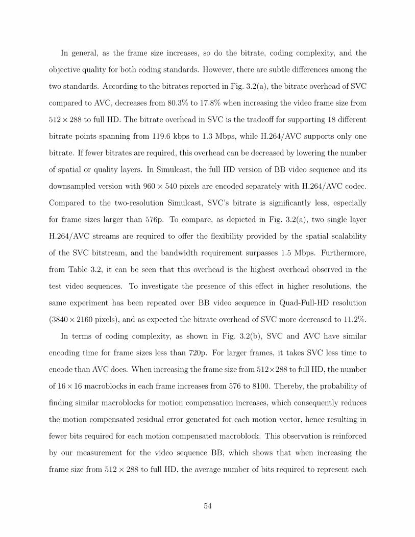
In general, as the frame size increases, so do the bitrate, coding complexity, and the
objective quality for both coding standards. However, there are subtle differences among the
two standards. According to the bitrates reported in Fig. 3.2(a), the bitrate overhead of SVC
compared to AVC, decreases from 80.3% to 17.8% when increasing the video frame size from
512× 288 to full HD. The bitrate overhead in SVC is the tradeoff for supporting 18 different
bitrate points spanning from 119.6 kbps to 1.3 Mbps, while H.264/AVC supports only one
bitrate. If fewer bitrates are required, this overhead can be decreased by lowering the number
of spatial or quality layers. In Simulcast, the full HD version of BB video sequence and its
downsampled version with 960× 540 pixels are encoded separately with H.264/AVC codec.
Compared to the two-resolution Simulcast, SVC’s bitrate is significantly less, especially
for frame sizes larger than 576p. To compare, as depicted in Fig. 3.2(a), two single layer
H.264/AVC streams are required to offer the flexibility provided by the spatial scalability
of the SVC bitstream, and the bandwidth requirement surpasses 1.5 Mbps. Furthermore,
from Table 3.2, it can be seen that this overhead is the highest overhead observed in the
test video sequences. To investigate the presence of this effect in higher resolutions, the
same experiment has been repeated over BB video sequence in Quad-Full-HD resolution
(3840× 2160 pixels), and as expected the bitrate overhead of SVC more decreased to 11.2%.
In terms of coding complexity, as shown in Fig. 3.2(b), SVC and AVC have similar
encoding time for frame sizes less than 720p. For larger frames, it takes SVC less time to
encode than AVC does. When increasing the frame size from 512×288 to full HD, the number
of 16×16 macroblocks in each frame increases from 576 to 8100. Thereby, the probability of
finding similar macroblocks for motion compensation increases, which consequently reduces
the motion compensated residual error generated for each motion vector, hence resulting in
fewer bits required for each motion compensated macroblock. This observation is reinforced
by our measurement for the video sequence BB, which shows that when increasing the
frame size from 512× 288 to full HD, the average number of bits required to represent each
54
motion compensated macroblock by H.264/AVC and SVC is reduced by 34.8% and 48.7%,
respectively. The decoding complexity is different from encoding complexity. Fig. 3.2(c)
shows that SVC has higher decoding complexity compared to AVC, which is expected due to
the growing number of motion vectors needed for layered prediction of motion compensated
macroblocks during the decoding process. More interestingly Fig. 3.2(b) shows that enlarging
the video frame size to HD (1280×720) fills the computational gap between H.264/AVC and
SVC in this specific encoding setting; and according to Table 3.2 when encoding BB video
sequence in full HD and Quad-Full-HD the encoding complexity of SVC codec is lower than
that of SVC codec by 20.3% and 28.7%, respectively. Since SVC uses motion prediction
in each enhancement layer, it better benefits from the increased number of higher similar
macroblocks.
Increasing the frame size also improves the objective quality of the video, since more
similar macroblocks allows the rate distortion optimization module of the encoder to select
higher quality points when encoding the video sequence. Fig. 3.2(d) shows that both SVC
and H.264/AVC codecs experience a similar growth in objective video quality measured in
Y-PSNR. SVC consistently has higher Y-PSNR values than AVC does.
The first two observations of this measurement study are important since the main reason
for not utilizing scalable coding in video content distribution industry is the bitrate and
complexity overhead of SVC. To confirm these results, the same set of experiments have
been repeated for other source video sequences. The results are presented for the full HD
video sequences in Table 3.2.
Table 3.2: Comparing the performance of SVC when DTQ = (1, 4, 1) and H.264/AVC forfull HD video coding.
ED PA RH PJ RB SF
Bitrate Overhead 18.1% 3.3% −3.4% 12.5% 17.7% 5.4%Encoding Overhead −18.9% −34.5% −30.6% −38.1% −43.2% −44.2%Decoding Overhead 114.3% 107.4% 106.8% 91.8% 106.2% 104.5%Quality Improvement (dB) 1.3 0.7 1.1 0.5 1.2 0.4
55
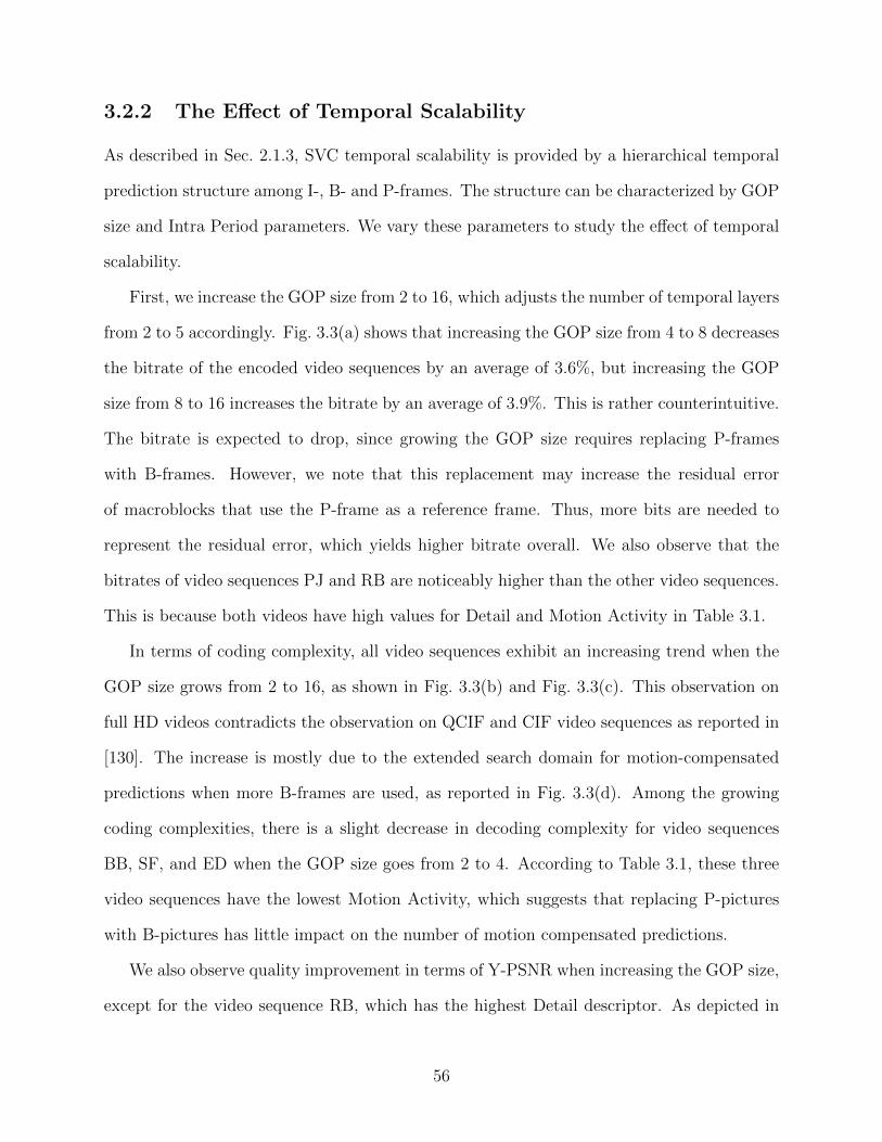
3.2.2 The Effect of Temporal Scalability
As described in Sec. 2.1.3, SVC temporal scalability is provided by a hierarchical temporal
prediction structure among I-, B- and P-frames. The structure can be characterized by GOP
size and Intra Period parameters. We vary these parameters to study the effect of temporal
scalability.
First, we increase the GOP size from 2 to 16, which adjusts the number of temporal layers
from 2 to 5 accordingly. Fig. 3.3(a) shows that increasing the GOP size from 4 to 8 decreases
the bitrate of the encoded video sequences by an average of 3.6%, but increasing the GOP
size from 8 to 16 increases the bitrate by an average of 3.9%. This is rather counterintuitive.
The bitrate is expected to drop, since growing the GOP size requires replacing P-frames
with B-frames. However, we note that this replacement may increase the residual error
of macroblocks that use the P-frame as a reference frame. Thus, more bits are needed to
represent the residual error, which yields higher bitrate overall. We also observe that the
bitrates of video sequences PJ and RB are noticeably higher than the other video sequences.
This is because both videos have high values for Detail and Motion Activity in Table 3.1.
In terms of coding complexity, all video sequences exhibit an increasing trend when the
GOP size grows from 2 to 16, as shown in Fig. 3.3(b) and Fig. 3.3(c). This observation on
full HD videos contradicts the observation on QCIF and CIF video sequences as reported in
[130]. The increase is mostly due to the extended search domain for motion-compensated
predictions when more B-frames are used, as reported in Fig. 3.3(d). Among the growing
coding complexities, there is a slight decrease in decoding complexity for video sequences
BB, SF, and ED when the GOP size goes from 2 to 4. According to Table 3.1, these three
video sequences have the lowest Motion Activity, which suggests that replacing P-pictures
with B-pictures has little impact on the number of motion compensated predictions.
We also observe quality improvement in terms of Y-PSNR when increasing the GOP size,
except for the video sequence RB, which has the highest Detail descriptor. As depicted in
56
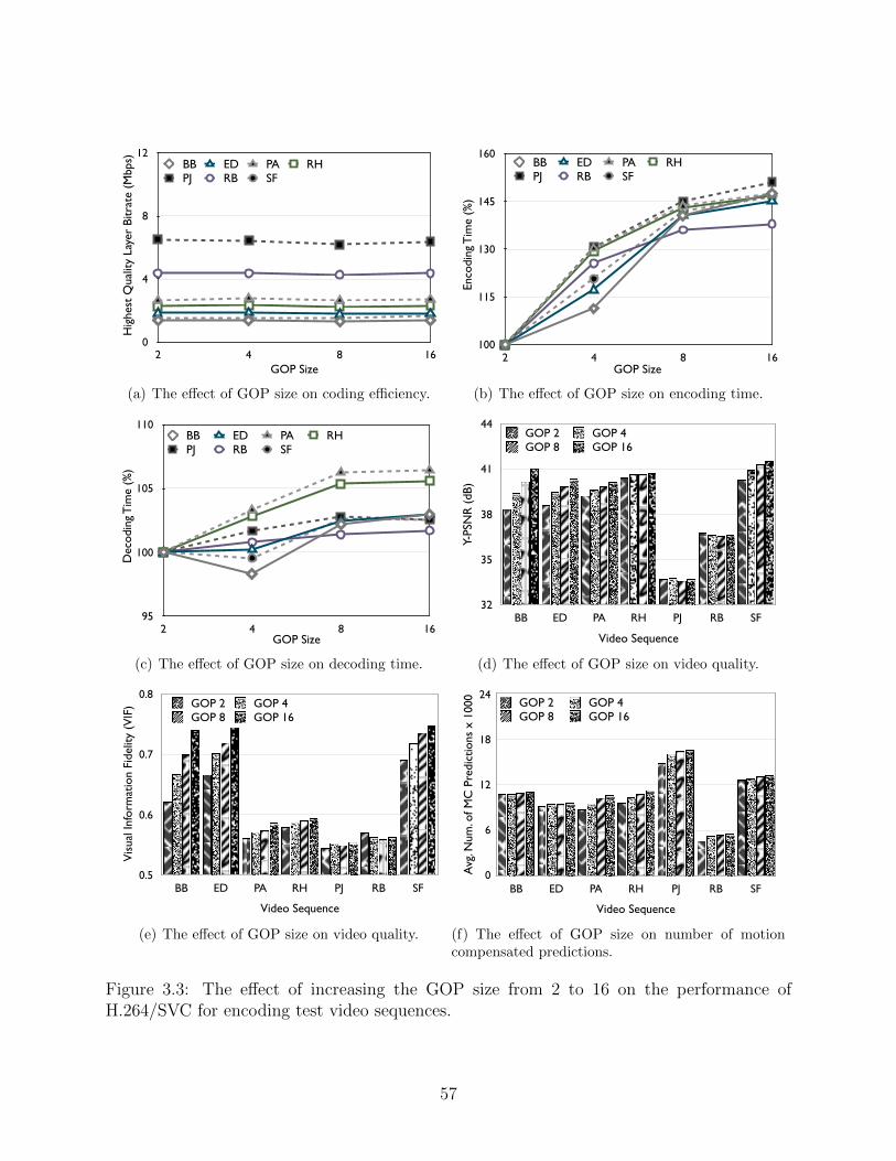
0
4
8
12
2 4 8 16
BB ED PA RHPJ RB SF
Hig
hest
Qua
lity
Laye
r Bi
trat
e (M
bps)
GOP Size
(a) The effect of GOP size on coding efficiency.
100
115
130
145
160
2 4 8 16
BB ED PA RHPJ RB SF
Enco
ding
Tim
e (%
)
GOP Size
(b) The effect of GOP size on encoding time.
95
100
105
110
2 4 8 16
BB ED PA RHPJ RB SF
Dec
odin
g T
ime
(%)
GOP Size
(c) The effect of GOP size on decoding time.
32
35
38
41
44
Video Sequence
BB ED PA RH PJ RB SF
GOP 2 GOP 4GOP 8 GOP 16
Y-PS
NR
(dB
)
(d) The effect of GOP size on video quality.
0.5
0.6
0.7
0.8
Video Sequence
BB ED PA RH PJ RB SF
GOP 2 GOP 4GOP 8 GOP 16
Vis
ual I
nfor
mat
ion
Fide
lity
(VIF
)
(e) The effect of GOP size on video quality.
Video Sequence
BB ED PA RH PJ RB SF
GOP 2 GOP 4GOP 8 GOP 16
24
18
12
6
0Avg
. Num
. of M
C P
redi
ctio
ns x
100
0
(f) The effect of GOP size on number of motioncompensated predictions.
Figure 3.3: The effect of increasing the GOP size from 2 to 16 on the performance ofH.264/SVC for encoding test video sequences.
57
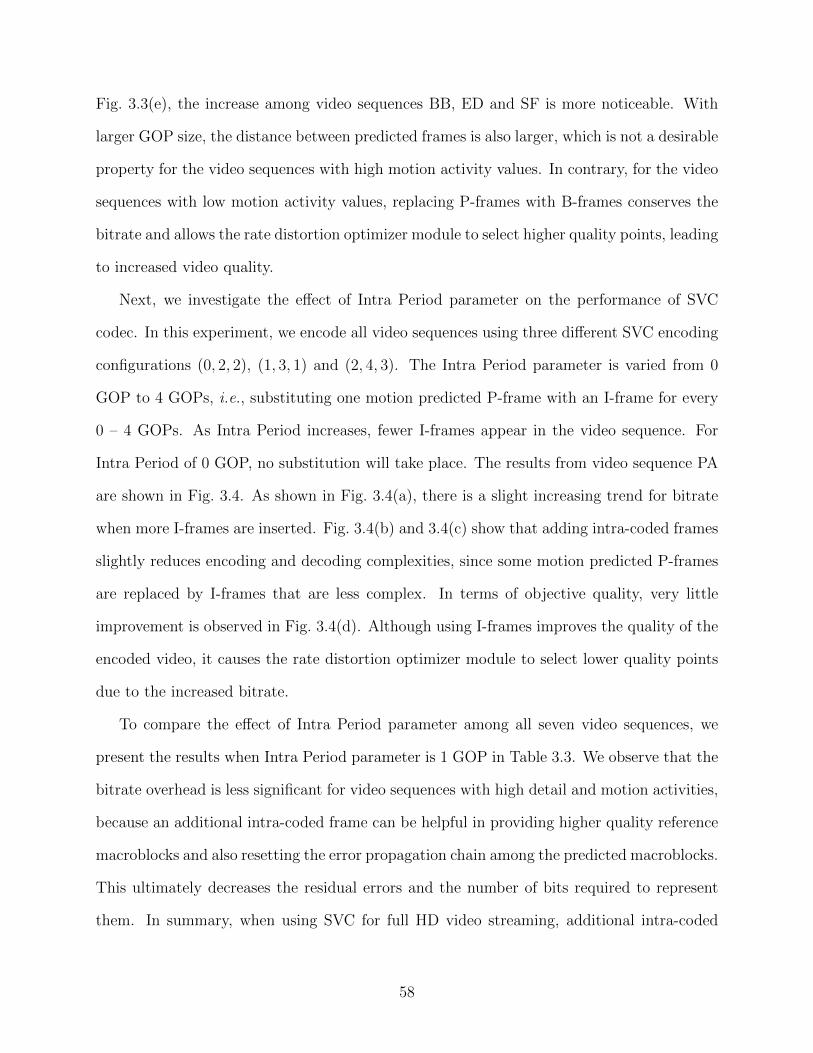
Fig. 3.3(e), the increase among video sequences BB, ED and SF is more noticeable. With
larger GOP size, the distance between predicted frames is also larger, which is not a desirable
property for the video sequences with high motion activity values. In contrary, for the video
sequences with low motion activity values, replacing P-frames with B-frames conserves the
bitrate and allows the rate distortion optimizer module to select higher quality points, leading
to increased video quality.
Next, we investigate the effect of Intra Period parameter on the performance of SVC
codec. In this experiment, we encode all video sequences using three different SVC encoding
configurations (0, 2, 2), (1, 3, 1) and (2, 4, 3). The Intra Period parameter is varied from 0
GOP to 4 GOPs, i.e., substituting one motion predicted P-frame with an I-frame for every
0 – 4 GOPs. As Intra Period increases, fewer I-frames appear in the video sequence. For
Intra Period of 0 GOP, no substitution will take place. The results from video sequence PA
are shown in Fig. 3.4. As shown in Fig. 3.4(a), there is a slight increasing trend for bitrate
when more I-frames are inserted. Fig. 3.4(b) and 3.4(c) show that adding intra-coded frames
slightly reduces encoding and decoding complexities, since some motion predicted P-frames
are replaced by I-frames that are less complex. In terms of objective quality, very little
improvement is observed in Fig. 3.4(d). Although using I-frames improves the quality of the
encoded video, it causes the rate distortion optimizer module to select lower quality points
due to the increased bitrate.
To compare the effect of Intra Period parameter among all seven video sequences, we
present the results when Intra Period parameter is 1 GOP in Table 3.3. We observe that the
bitrate overhead is less significant for video sequences with high detail and motion activities,
because an additional intra-coded frame can be helpful in providing higher quality reference
macroblocks and also resetting the error propagation chain among the predicted macroblocks.
This ultimately decreases the residual errors and the number of bits required to represent
them. In summary, when using SVC for full HD video streaming, additional intra-coded
58
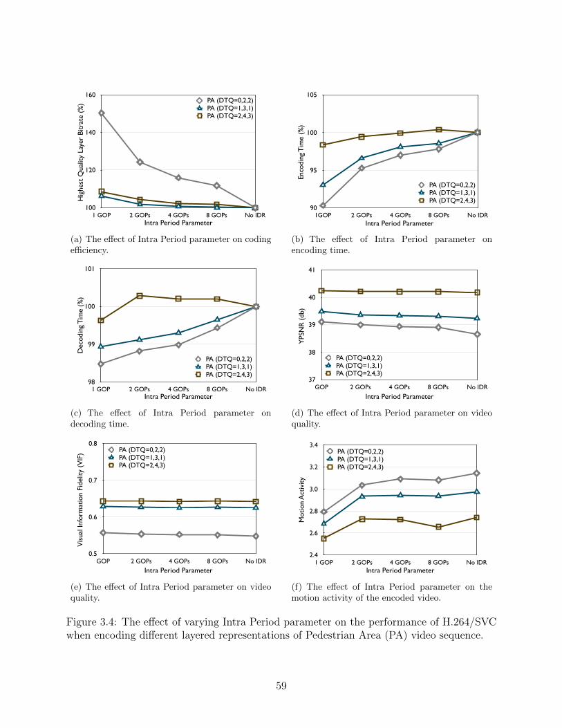
100
120
140
160
1 GOP 2 GOPs 4 GOPs 8 GOPs No IDR
PA (DTQ=0,2,2)PA (DTQ=1,3,1)PA (DTQ=2,4,3)
Hig
hest
Qua
lity
Laye
r Bi
trat
e (%
)
Intra Period Parameter
(a) The effect of Intra Period parameter on codingefficiency.
Enco
ding
Tim
e (%
)
90
95
100
105
1GOP 2 GOPs 4 GOPs 8 GOPs No IDR
PA (DTQ=0,2,2)PA (DTQ=1,3,1)PA (DTQ=2,4,3)
Intra Period Parameter
(b) The effect of Intra Period parameter onencoding time.
Dec
odin
g T
ime
(%)
98
99
100
101
1 GOP 2 GOPs 4 GOPs 8 GOPs No IDR
PA (DTQ=0,2,2)PA (DTQ=1,3,1)PA (DTQ=2,4,3)
Intra Period Parameter
(c) The effect of Intra Period parameter ondecoding time.
YPS
NR
(db
)
Intra Period Parameter
37
38
39
40
41
GOP 2 GOPs 4 GOPs 8 GOPs No IDR
PA (DTQ=0,2,2)PA (DTQ=1,3,1)PA (DTQ=2,4,3)
(d) The effect of Intra Period parameter on videoquality.
Vis
ual I
nfor
mat
ion
Fide
lity
(VIF
)
Intra Period Parameter
0.5
0.6
0.7
0.8
GOP 2 GOPs 4 GOPs 8 GOPs No IDR
PA (DTQ=0,2,2)PA (DTQ=1,3,1)PA (DTQ=2,4,3)
(e) The effect of Intra Period parameter on videoquality.
Mot
ion
Act
ivity
Intra Period Parameter
2.4
2.6
2.8
3.0
3.2
3.4
1 GOP 2 GOPs 4 GOPs 8 GOPs No IDR
PA (DTQ=0,2,2)PA (DTQ=1,3,1)PA (DTQ=2,4,3)
(f) The effect of Intra Period parameter on themotion activity of the encoded video.
Figure 3.4: The effect of varying Intra Period parameter on the performance of H.264/SVCwhen encoding different layered representations of Pedestrian Area (PA) video sequence.
59
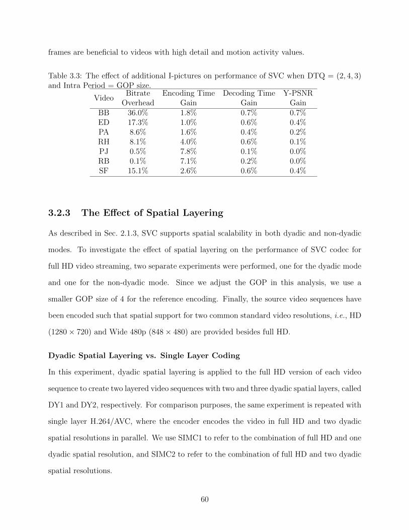
frames are beneficial to videos with high detail and motion activity values.
Table 3.3: The effect of additional I-pictures on performance of SVC when DTQ = (2, 4, 3)and Intra Period = GOP size.
VideoBitrate Encoding Time Decoding Time Y-PSNR
Overhead Gain Gain GainBB 36.0% 1.8% 0.7% 0.7%ED 17.3% 1.0% 0.6% 0.4%PA 8.6% 1.6% 0.4% 0.2%RH 8.1% 4.0% 0.6% 0.1%PJ 0.5% 7.8% 0.1% 0.0%RB 0.1% 7.1% 0.2% 0.0%SF 15.1% 2.6% 0.6% 0.4%
3.2.3 The Effect of Spatial Layering
As described in Sec. 2.1.3, SVC supports spatial scalability in both dyadic and non-dyadic
modes. To investigate the effect of spatial layering on the performance of SVC codec for
full HD video streaming, two separate experiments were performed, one for the dyadic mode
and one for the non-dyadic mode. Since we adjust the GOP in this analysis, we use a
smaller GOP size of 4 for the reference encoding. Finally, the source video sequences have
been encoded such that spatial support for two common standard video resolutions, i.e., HD
(1280× 720) and Wide 480p (848× 480) are provided besides full HD.
Dyadic Spatial Layering vs. Single Layer Coding
In this experiment, dyadic spatial layering is applied to the full HD version of each video
sequence to create two layered video sequences with two and three dyadic spatial layers, called
DY1 and DY2, respectively. For comparison purposes, the same experiment is repeated with
single layer H.264/AVC, where the encoder encodes the video in full HD and two dyadic
spatial resolutions in parallel. We use SIMC1 to refer to the combination of full HD and one
dyadic spatial resolution, and SIMC2 to refer to the combination of full HD and two dyadic
spatial resolutions.
60
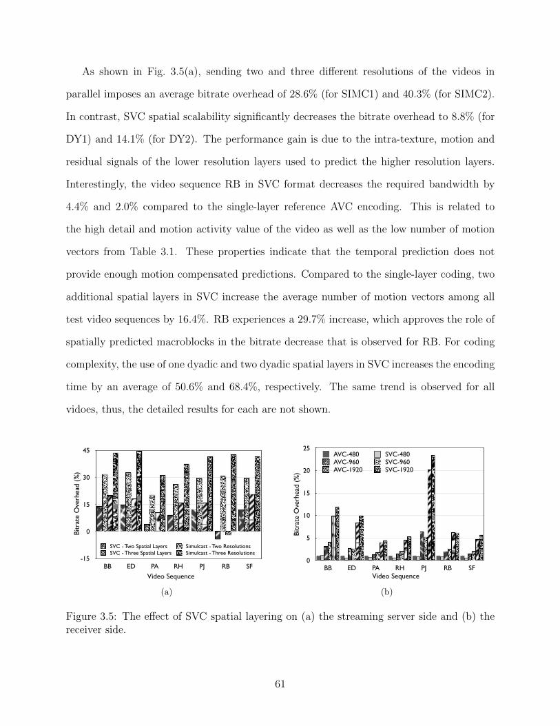
As shown in Fig. 3.5(a), sending two and three different resolutions of the videos in
parallel imposes an average bitrate overhead of 28.6% (for SIMC1) and 40.3% (for SIMC2).
In contrast, SVC spatial scalability significantly decreases the bitrate overhead to 8.8% (for
DY1) and 14.1% (for DY2). The performance gain is due to the intra-texture, motion and
residual signals of the lower resolution layers used to predict the higher resolution layers.
Interestingly, the video sequence RB in SVC format decreases the required bandwidth by
4.4% and 2.0% compared to the single-layer reference AVC encoding. This is related to
the high detail and motion activity value of the video as well as the low number of motion
vectors from Table 3.1. These properties indicate that the temporal prediction does not
provide enough motion compensated predictions. Compared to the single-layer coding, two
additional spatial layers in SVC increase the average number of motion vectors among all
test video sequences by 16.4%. RB experiences a 29.7% increase, which approves the role of
spatially predicted macroblocks in the bitrate decrease that is observed for RB. For coding
complexity, the use of one dyadic and two dyadic spatial layers in SVC increases the encoding
time by an average of 50.6% and 68.4%, respectively. The same trend is observed for all
vidoes, thus, the detailed results for each are not shown.
-15
0
15
30
45
BB ED PA RH PJ RB SF
SVC - Two Spatial Layers Simulcast - Two ResolutionsSVC - Three Spatial Layers Simulcast - Three Resolutions
Bitr
ate
Ove
rhea
d (%
)
Video Sequence
(a)
0
5
10
15
20
25
BB ED PA RH PJ RB SF
AVC-480 SVC-480AVC-960 SVC-960AVC-1920 SVC-1920
Bitr
ate
Ove
rhea
d (%
)
Video Sequence
(b)
Figure 3.5: The effect of SVC spatial layering on (a) the streaming server side and (b) thereceiver side.
61
Fig. 3.5(b) compares the bitrate required on the client side to receive the video in either
AVC or SVC format with the specified dyadic resolutions (480p, 960p, and 1920p). The
average bitrate required to receive the base layer of SVC bitstream (SVC-480), which is also
AVC compatible, is 70.4% that of single-layer AVC (AVC-480). This inevitably leads to a
lower objective video quality. Our measurements show that using SVC with the specified
settings decreases the objective video quality of 480×270, 960×540 and full HD reconstructed
videos by an average of 0.98, 1.17 and 1.05 dBs, respectively. Furthermore, the average
bandwidth required to receive the videos in 960× 540 and full HD resolutions in SVC mode
are 10.1% and 15.0% more than that of single-layer AVC mode, respectively. For coding
complexity, there is no significant difference between SVC-480 and AVC-480, since they are
both AVC compatible. The added spatial layers in SVC require 27.1% (for SVC-960) and
84.6% (for SVC-1920, full HD) more decoding time. Hence, full-HD SVC is not recommended
on battery-operated devices or devices with limited CPU power. However, the decoding time
of the SVC bitstream can be dramatically decreased at the expense of minor limitations in
spatial layering capabilities [25]. Again, PJ and RB exhibit a different behaviour, since they
need less bandwidth for their 960× 540 and full HD resolutions, respectively, which can be
due to their high values of detail and motion activity.
Dyadic vs. Non-Dyadic Spatial Layering
To compare dyadic and non-dyadic spatial layering, we modify the resolution and the frame
ratio of the spatial layers so that the number of macroblocks in each layer remains unchanged
and the layer resolutions are non-dyadic. This version of coding is referred to as NDY1
and NDY2 for one and two non-dyadic spatial layers, respectively. We repeat the same
spatial layering experiment as in Sec. 3.2.3 with the new non-dyadic layers. Furthermore, to
investigate the effect of frame size, the same experiments are repeated with 480× 270 pixels
frames in the highest resolution layer. The average overheads from all video sequences are
reported in Table 3.4. We observe that increasing the frame size to full HD in non-dyadic
62
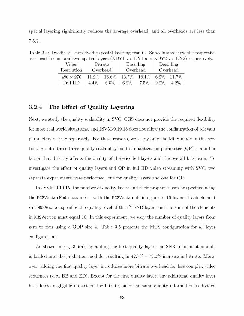
spatial layering significantly reduces the average overhead, and all overheads are less than
7.5%.
Table 3.4: Dyadic vs. non-dyadic spatial layering results. Subcolumns show the respectiveoverhead for one and two spatial layers (NDY1 vs. DY1 and NDY2 vs. DY2) respectively.
Video Bitrate Encoding DecodingResolution Overhead Overhead Overhead
480× 270 11.2% 16.6% 13.7% 18.1% 6.2% 11.7%Full HD 4.4% 6.5% 6.2% 7.5% 2.2% 4.2%
3.2.4 The Effect of Quality Layering
Next, we study the quality scalability in SVC. CGS does not provide the required flexibility
for most real world situations, and JSVM-9.19.15 does not allow the configuration of relevant
parameters of FGS separately. For these reasons, we study only the MGS mode in this sec-
tion. Besides these three quality scalability modes, quantization parameter (QP) is another
factor that directly affects the quality of the encoded layers and the overall bitstream. To
investigate the effect of quality layers and QP in full HD video streaming with SVC, two
separate experiments were performed, one for quality layers and one for QP.
In JSVM-9.19.15, the number of quality layers and their properties can be specified using
the MGSVectorMode parameter with the MGSVector defining up to 16 layers. Each element
i in MGSVector specifies the quality level of the ith SNR layer, and the sum of the elements
in MGSVector must equal 16. In this experiment, we vary the number of quality layers from
zero to four using a GOP size 4. Table 3.5 presents the MGS configuration for all layer
configurations.
As shown in Fig. 3.6(a), by adding the first quality layer, the SNR refinement module
is loaded into the prediction module, resulting in 42.7% – 79.0% increase in bitrate. More-
over, adding the first quality layer introduces more bitrate overhead for less complex video
sequences (e.g., BB and ED). Except for the first quality layer, any additional quality layer
has almost negligible impact on the bitrate, since the same quality information is divided
63
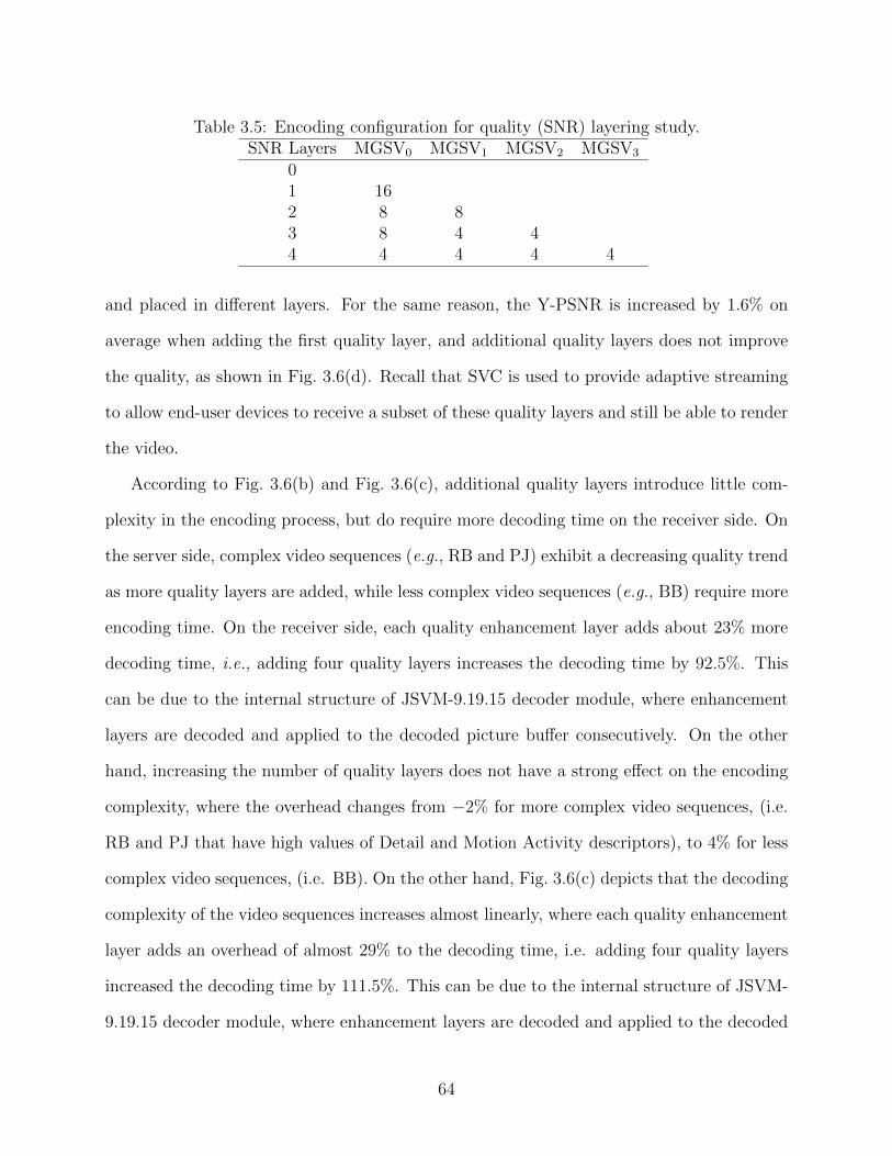
Table 3.5: Encoding configuration for quality (SNR) layering study.SNR Layers MGSV0 MGSV1 MGSV2 MGSV3
01 162 8 83 8 4 44 4 4 4 4
and placed in different layers. For the same reason, the Y-PSNR is increased by 1.6% on
average when adding the first quality layer, and additional quality layers does not improve
the quality, as shown in Fig. 3.6(d). Recall that SVC is used to provide adaptive streaming
to allow end-user devices to receive a subset of these quality layers and still be able to render
the video.
According to Fig. 3.6(b) and Fig. 3.6(c), additional quality layers introduce little com-
plexity in the encoding process, but do require more decoding time on the receiver side. On
the server side, complex video sequences (e.g., RB and PJ) exhibit a decreasing quality trend
as more quality layers are added, while less complex video sequences (e.g., BB) require more
encoding time. On the receiver side, each quality enhancement layer adds about 23% more
decoding time, i.e., adding four quality layers increases the decoding time by 92.5%. This
can be due to the internal structure of JSVM-9.19.15 decoder module, where enhancement
layers are decoded and applied to the decoded picture buffer consecutively. On the other
hand, increasing the number of quality layers does not have a strong effect on the encoding
complexity, where the overhead changes from −2% for more complex video sequences, (i.e.
RB and PJ that have high values of Detail and Motion Activity descriptors), to 4% for less
complex video sequences, (i.e. BB). On the other hand, Fig. 3.6(c) depicts that the decoding
complexity of the video sequences increases almost linearly, where each quality enhancement
layer adds an overhead of almost 29% to the decoding time, i.e. adding four quality layers
increased the decoding time by 111.5%. This can be due to the internal structure of JSVM-
9.19.15 decoder module, where enhancement layers are decoded and applied to the decoded
64
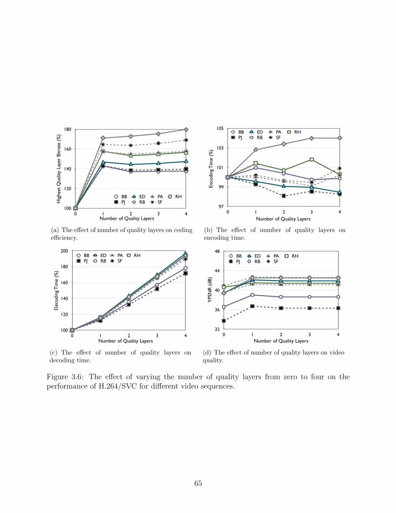
Hig
hest
Qua
lity
Laye
r Bi
trat
e (%
)
Number of Quality Layers
100
120
140
160
180
0 1 2 3 4
BB ED PA RHPJ RB SF
(a) The effect of number of quality layers on codingefficiency.
Enco
ding
Tim
e (%
)
Number of Quality Layers
97
99
101
103
105
0 1 2 3 4
BB ED PA RHPJ RB SF
(b) The effect of number of quality layers onencoding time.
Dec
odin
g T
ime
(%)
Number of Quality Layers
100
120
140
160
180
200
0 1 2 3 4
BB ED PA RHPJ RB SF
(c) The effect of number of quality layers ondecoding time.
YPS
NR
(dB
)
Number of Quality Layers
32
36
40
44
48
0 1 2 3 4
BB ED PA RHPJ RB SF
(d) The effect of number of quality layers on videoquality.
Figure 3.6: The effect of varying the number of quality layers from zero to four on theperformance of H.264/SVC for different video sequences.
65
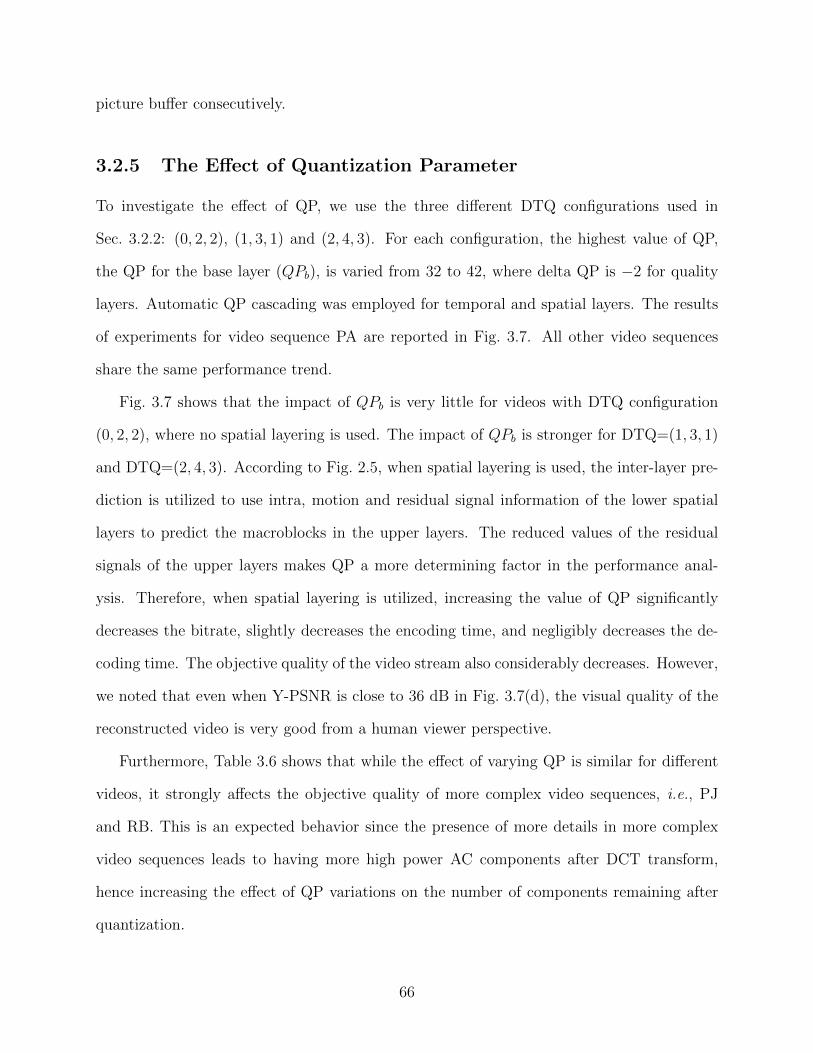
picture buffer consecutively.
3.2.5 The Effect of Quantization Parameter
To investigate the effect of QP, we use the three different DTQ configurations used in
Sec. 3.2.2: (0, 2, 2), (1, 3, 1) and (2, 4, 3). For each configuration, the highest value of QP,
the QP for the base layer (QPb), is varied from 32 to 42, where delta QP is −2 for quality
layers. Automatic QP cascading was employed for temporal and spatial layers. The results
of experiments for video sequence PA are reported in Fig. 3.7. All other video sequences
share the same performance trend.
Fig. 3.7 shows that the impact of QPb is very little for videos with DTQ configuration
(0, 2, 2), where no spatial layering is used. The impact of QPb is stronger for DTQ=(1, 3, 1)
and DTQ=(2, 4, 3). According to Fig. 2.5, when spatial layering is used, the inter-layer pre-
diction is utilized to use intra, motion and residual signal information of the lower spatial
layers to predict the macroblocks in the upper layers. The reduced values of the residual
signals of the upper layers makes QP a more determining factor in the performance anal-
ysis. Therefore, when spatial layering is utilized, increasing the value of QP significantly
decreases the bitrate, slightly decreases the encoding time, and negligibly decreases the de-
coding time. The objective quality of the video stream also considerably decreases. However,
we noted that even when Y-PSNR is close to 36 dB in Fig. 3.7(d), the visual quality of the
reconstructed video is very good from a human viewer perspective.
Furthermore, Table 3.6 shows that while the effect of varying QP is similar for different
videos, it strongly affects the objective quality of more complex video sequences, i.e., PJ
and RB. This is an expected behavior since the presence of more details in more complex
video sequences leads to having more high power AC components after DCT transform,
hence increasing the effect of QP variations on the number of components remaining after
quantization.
66
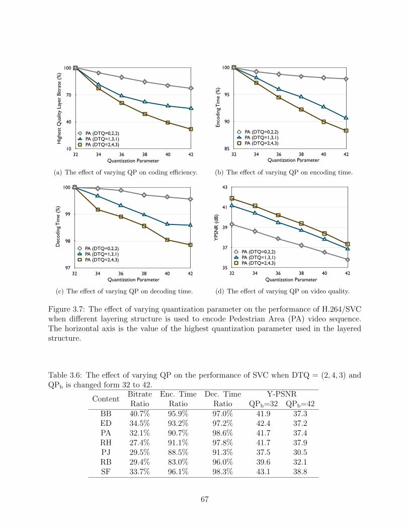
Quantization Parameter
Hig
hest
Qua
lity
Laye
r Bi
trat
e (%
)
10
40
70
100
32 34 36 38 40 42
PA (DTQ=0,2,2)PA (DTQ=1,3,1)PA (DTQ=2,4,3)
(a) The effect of varying QP on coding efficiency.
Quantization Parameter
Enco
ding
Tim
e (%
)
85
90
95
100
32 34 36 38 40 42
PA (DTQ=0,2,2)PA (DTQ=1,3,1)PA (DTQ=2,4,3)
(b) The effect of varying QP on encoding time.
Quantization Parameter
Dec
odin
g T
ime
(%)
97
98
99
100
32 34 36 38 40 42
PA (DTQ=0,2,2)PA (DTQ=1,3,1)PA (DTQ=2,4,3)
(c) The effect of varying QP on decoding time.
Quantization Parameter
YPS
NR
(dB
)
35
37
39
41
43
32 34 36 38 40 42
PA (DTQ=0,2,2)PA (DTQ=1,3,1)PA (DTQ=2,4,3)
(d) The effect of varying QP on video quality.
Figure 3.7: The effect of varying quantization parameter on the performance of H.264/SVCwhen different layering structure is used to encode Pedestrian Area (PA) video sequence.The horizontal axis is the value of the highest quantization parameter used in the layeredstructure.
Table 3.6: The effect of varying QP on the performance of SVC when DTQ = (2, 4, 3) andQPb is changed form 32 to 42.
ContentBitrate Enc. Time Dec. Time Y-PSNRRatio Ratio Ratio QPb=32 QPb=42
BB 40.7% 95.9% 97.0% 41.9 37.3ED 34.5% 93.2% 97.2% 42.4 37.2PA 32.1% 90.7% 98.6% 41.7 37.4RH 27.4% 91.1% 97.8% 41.7 37.9PJ 29.5% 88.5% 91.3% 37.5 30.5RB 29.4% 83.0% 96.0% 39.6 32.1SF 33.7% 96.1% 98.3% 43.1 38.8
67
3.3 Summary and Discussion
In this chapter, we conducted a systematic study on the use of H.264/AVC and SVC for full
HD video streaming. Compared to the previous research work listed in Sec.2.2.1, this research
is different from several perspectives. First, the number of test video sequences is sufficiently
large to represent different types of videos, therefore the conclusions are not biased to the
selected video sequences. Second, the criteria used to select the test video sequences is clear
and ensures diversity in their visual properties. Third, the video resolutions are large enough
to be relevant in today’s applications. Finally, in this research, all the scalability modes of
layered video coding and their different modes, wherever applicable, are investigated.
We learned that in spite of the results reported in previous research works for using SVC
for low resolution videos (e.g., CIF and 4CIF), SVC requires less computational resources
in the encoding phase and also benefits from higher video quality in higher resolutions (as
much as multiple dBs in terms of Y-PSNR). At the same time, SVC requires higher bitrate
due to the higher quality of the encoded video and also the presence of multiple video layers.
According to Fig. 3.7(a), a reduction of 2 dBs of quantization parameter can result in as
much as 20% reduction in the layered video bitrate. This will cover the higher bitrate of
layered coded video in expense of erasing its quality advantage over single-layer video.
SVC suffers from higher decoding complexity. However, it must be noted that due to
the presence of hardware decoders in mobile devices, decoding the video does not consume
significant energy compared to that of receiving the video over the wireless links and playing
the video on the screen. We will come back to this issue in Chapter 6. In return, SVC is
efficient in serving streaming sessions in multiple quality levels.
We identify that SVC is more advantageous in full HD streaming, since the efficiency and
computational gap between SVC and H.264/AVC is much less when encoding high quality
videos. When using SVC for full HD video streaming, additional intra-coded frames are
beneficial to videos with high detail and motion activity values. Using a set of carefully
68
selected and diverse video contents, we also discovered that certain SVC configurations have
advantages over H.264/AVC for complex video sequences with high detail and motion activity
values. For example, replacing P-frames with I-frames in such video sequences can decrease
the encoding complexity without increasing the bitrate of the encoded video, and additional
spatial layers may decrease the bitrate of the encoded video.
In addition to investigating the performance of layered video coding in higher video
resolutions, understanding the internal mechanism of video codecs was another outcome
of this study. In the following chapter, this knowledge is applied to the distributed video
transcoding problem as a part of preparing the multimedia streaming service in the cloud.
More specifically, the properties of the to-be-transcoded video are extracted from the high
quality encoded video stream and used to adaptively change the length of the video segments.
We discuss this further in the following chapter.
69
Chapter 4
Preparing Video in the Cloud
When the raw video is acquired from a camera feed, it requires significant bandwidth for
transmission and storage. For example, using 4:2:0 color space, a full HD raw video with
24 frames per second has a bitrate of 570 Mbps. The storage requirement for such a video
bitrate is 268 TB per hour of video. These numbers would double if 4:4:4 color space is used
and quadruple if the video is recorded in 4K resolution. Therefore, the raw video must be
encoded into a high quality lossless or lossy compressed video prior to further processing.
Such an encoding procedure usually uses the same video resolution and frame rate as those
of the raw video input to create and store a reference version of the video in the system.
Furthermore, if lossy compression is used, the encoding parameters are set such that the
video quality does not significantly degrade. This version of the video may still require
lots of bandwidth due to its high bitrate, especially for streaming over wireless network
connections. Instead, it is used as a high quality input for the video transcoders to generate
lower-quality and lower-bitrate copies of the video for streaming.
Transcoding is the process of encoding a previously encoded video using new encoding
parameters. These new parameters normally decrease frame rate, frame resolution, objective
video quality, or all of them together. It is possible to design a special transcoder to increase
frame rate (by frame interpolation), frame resolution (by upsampling) or subjective video
quality (by using heuristics extracted from the characteristics of the human visual system,
e.g., by increasing the picture contrast). However, these topics are orthogonal to our dis-
cussion here. To summarize, in a usual video streaming scenario, transcoding is utilized to
convert a high frame rate, high resolution, high quality reference video into a version that
can be served over network toward end user devices.
70
The reference video must be transcoded to different resolutions, frame rates and quality
levels. The various versions of the video are served subject to network conditions and hard-
ware specifications of the end user device. If the target video profile uses the same video
codec as that of the reference video, depending on the video codec and the transcoding
profile, it might be possible to transcode the reference video directly to the target video
sequence. For example, if a video transcoding profile only enforces reducing the frame rate,
it can be done by dropping some frames. However, generally speaking, video transcoding
requires to first decode the high-quality encoded reference video and then re-encode it to
the target quality level. Such a transcoding process may lead to significant delay in video
preparation phase due to the computational complexity of the encoding task. To address
this delay, distributed video transcoding is used to speed up the transcoding process. A
cloud-assisted video transcoding system segments a video into chunks and distributes video
chunks to virtual transcoder instances in the cloud for parallel transcoding. This paradigm
greatly reduces the video access delay [49, 58, 77]. In addition, layered video encoding can
be used along with cloud-assisted video transcoding to allow the media service provider to
transcode a video once and use it for several target bitrates and resolutions [32,58,136].
We summarized the previous related research work in Section 2.2. We note that existing
proposals for cloud-assisted video transcoding treat the encoded video no different from a
raw video. A fixed number of consecutive frames or group of pictures (GOP) are grouped into
a video chunk [58]. The chunks are assigned to virtual machines using a scalable technique
such as MapReduce [39]. The transcoded video chunks then can be merged into a single
video sequence to be delivered to the end user or transmitted as is. By inspecting video
codec standards, we learn that due to the high similarity of consecutive frames in video
sequences, certain important inter-frame dependency exist among them. This dependency
may get broken when segmenting a video into fixed-size chunks. For example, two GOPs
with very dissimilar pictures (e.g., due to change of scenery) may be grouped into one video
71
chunk, and two consecutive GOPs with high degree of similarity may be separated into two
video chunks. Since video encoding techniques, like other compression techniques, are based
on utilizing the similarity between the to-be-encoded pictures, encoding dissimilar group of
pictures as a video segment can increase the video bitrate and the transcoding time and
decrease the video quality. Intuitively, this problem can be addressed by proper adjustments
of video chunks according to the visual similarity of the consecutive video frames or group
of pictures. We investigate the correctness of this statement in Sec. 4.1.1.
Exploiting this statement, in this chapter we propose a distributed video transcoding
scheme that improves resource efficiency by decreasing the video bitrate and the compu-
tational resource consumption on the cloud. It also increases the visual quality of the
transcoded video for more complex video sequences. The proposed model exploits depen-
dency among GOPs of the encoded reference video and creates video chunks of variable size.
Inter-frame dependencies reflect the visual similarity between the consecutive frames and
GOPs. High amount of inter-frame dependency means that the encoder was able to find
many similarities between consecutive frames, hence higher visual similarity is expected.
Similarly, lack of inter-frame dependencies among consecutive frames can be interpreted as
lack of visual similarity. The goal is to reduce the bitrate and transcoding time for fast
delivery of transcoded video to end users. The key to achieve this goal is the variable-size
chunk. In the proposed scheme, the chunk size is determined according to the prediction de-
pendency among GOPs in an encoded video. Highly dependent GOPs are encoded together
to take advantage of visual similarity among enclosed video frames. We utilize layered video
coding along with video transcoding to produce transcoded videos that can satisfy certain
range of quality requirements [32, 58, 136]. The experimental results on a set of real video
sequences with diverse visual features show that the proposed transcoding scheme reduces
bitrate and transcoding time compared to conventional video transcoding schemes that use
fixed-size video chunks.
72
In general, the cloud provides a scalable, responsive, and cost-effective solution for video
transcoding services. We note that existing proposals on video transcoding in the cloud are
all performing conventional video transcoding of a video on either a single virtual machine
or multiple virtual machines. The performance gains are mostly due to efficient use of cloud
resources or parallelism managed by a Map-Reduce model. None of these proposals considers
information that can be extracted from the video. In fact, an encoded video encapsulates
useful dependency information among GOPs, frames, slices or even macroblocks. In this
chapter, we propose a dependency-aware distributed video transcoding scheme.
4.1 Distributed Video Transcoding in the Cloud
Our proposed distributed video transcoding scheme is a cloud-based solution that exploits
the coding and prediction dependency in layered video coding to transcode a video satisfying
certain requirements. Fig. 4.1 illustrates the workflow of distributed video transcoding in
the cloud. Upon receiving a video streaming request, the streaming server instructs the
transcoding controller to load the requested source video from the video repository. The
controller segments the video into chunks and distributes video chunks to virtual instances in
the cloud using a parallel computing model such as Map-Reduce [39]. At last, the transcoded
video chunks are merged into a video sequence to be delivered to end users, and if desired,
stored in the video repository for future requests.
Towards improving the distributed video transcoding process, numerous models and algo-
rithms have been proposed to minimize transcoding delay, number of transcoding virtual ma-
chines needed, energy consumption, and transcoding cost in the cloud [32,136,149,165,167].
By intuition, encoding each GOP separately reduces encoding time, since the encoder does
not need to consider the information from other GOPs. But counter-intuitively, this ap-
proach leads to poor coding efficiency, i.e., more bits are needed to present the video at
a specific level of quality [161]. On the one hand, the larger the chunk size is, the more
73
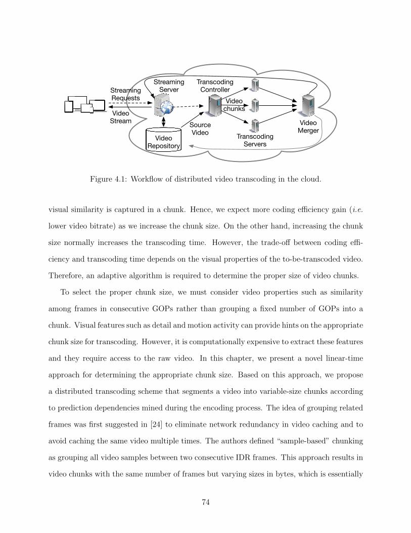
VideoRepository
StreamingRequests
StreamingServer
TranscodingController
TranscodingServers
VideoStream Video
MergerSourceVideo
Videochunks
Figure 4.1: Workflow of distributed video transcoding in the cloud.
visual similarity is captured in a chunk. Hence, we expect more coding efficiency gain (i.e.
lower video bitrate) as we increase the chunk size. On the other hand, increasing the chunk
size normally increases the transcoding time. However, the trade-off between coding effi-
ciency and transcoding time depends on the visual properties of the to-be-transcoded video.
Therefore, an adaptive algorithm is required to determine the proper size of video chunks.
To select the proper chunk size, we must consider video properties such as similarity
among frames in consecutive GOPs rather than grouping a fixed number of GOPs into a
chunk. Visual features such as detail and motion activity can provide hints on the appropriate
chunk size for transcoding. However, it is computationally expensive to extract these features
and they require access to the raw video. In this chapter, we present a novel linear-time
approach for determining the appropriate chunk size. Based on this approach, we propose
a distributed transcoding scheme that segments a video into variable-size chunks according
to prediction dependencies mined during the encoding process. The idea of grouping related
frames was first suggested in [24] to eliminate network redundancy in video caching and to
avoid caching the same video multiple times. The authors defined “sample-based” chunking
as grouping all video samples between two consecutive IDR frames. This approach results in
video chunks with the same number of frames but varying sizes in bytes, which is essentially
74
different from this proposal.
4.1.1 The Necessity of Considering GOP Dependencies
We mentioned that the size of video chunks might significantly affect the performance of
the video transcoding system in terms of coding efficiency and transcoding time. Hence, we
need to wisely select the size of video chunks according to the visual properties of the source
encoded video1. To support this claim, we performed a set of video transcoding experiments
over the full-HD source video sequences that were discussed in Sec. 3.1. To better evaluate
the effect of the length of video segments, 1600 frames of each video was selected. If the length
of the original video sequence was less than 1600 frames, multiple copies of the video were
concatenated until enough number of frames were provided. We transcoded the source video
sequence from full-HD (1080p) to HD (720p) video frame format and used the layer settings
of two spatial, four temporal and two quality layers, i.e., DTQ=(1, 3, 1). To investigate
our claim, we divided each reference video sequence into video chunks that contain a fixed
number of GOPs, starting from one GOP per video chunk and multiplying by two up to 64
GOPs per video chunk. Results are presented in Fig. 4.2.
Due to the propagation of prediction information from past GOPs to future GOPs, we
essentially expect coding efficiency to increase with the number of GOPs in each video chunk.
From Fig. 4.2.a, it can be seen that while this general assumption is true, this observation
is much stronger for video sequences with less detail and motion activity, such as BB and
SF, and is less significant or negligible for video sequences with highly detailed and changing
scenery, such as PJ and RB. On the one hand, compared to long video chunks, say 64
GOPs, if we set the size of video chunks to a small number of GOPs, say 1 GOP, the size
of the transcoded video will be up to three times for video sequences such as BB while the
computation time is decreased only by 25%. On the other hand, compared to short video
1 Our experiments revealed no significant change in the quality of the encoded videos. In fact, increasingthe size of video chunks from 1 GOP to 64 GOPs increased the average Y-PSNR of the transcoded videosby 0.3 dB, where the average Y-PSNR for one GOP per video chunk was 37.4 dB.
75
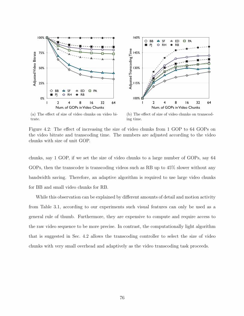
0%
25%
50%
75%
100%
1 2 4 8 16 32 64
BB SF ED PAPJ RH RB
Num. of GOPs in Video Chunks
Adj
uste
d V
ideo
Bitr
ate
(a) The effect of size of video chunks on video bi-trate.
100%
115%
130%
145%
160%
1 2 4 8 16 32 64
BB SF ED PAPJ RH RB
Num. of GOPs in Video Chunks
Adj
uste
d Tr
ansc
odin
g T
ime
(b) The effect of size of video chunks on transcod-ing time.
Figure 4.2: The effect of increasing the size of video chunks from 1 GOP to 64 GOPs onthe video bitrate and transcoding time. The numbers are adjusted according to the videochunks with size of unit GOP.
chunks, say 1 GOP, if we set the size of video chunks to a large number of GOPs, say 64
GOPs, then the transcoder is transcoding videos such as RB up to 45% slower without any
bandwidth saving. Therefore, an adaptive algorithm is required to use large video chunks
for BB and small video chunks for RB.
While this observation can be explained by different amounts of detail and motion activity
from Table 3.1, according to our experiments such visual features can only be used as a
general rule of thumb. Furthermore, they are expensive to compute and require access to
the raw video sequence to be more precise. In contrast, the computationally light algorithm
that is suggested in Sec. 4.2 allows the transcoding controller to select the size of video
chunks with very small overhead and adaptively as the video transcoding task proceeds.
76
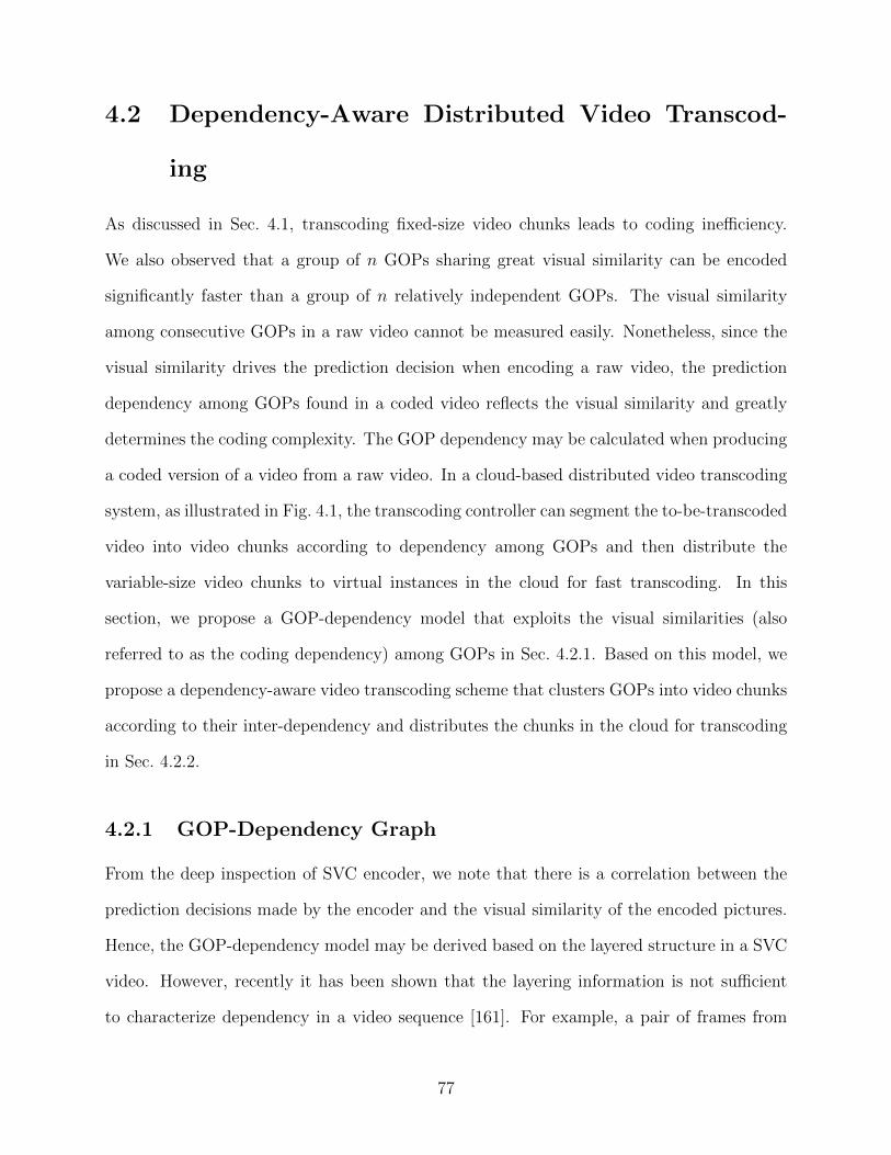
4.2 Dependency-Aware Distributed Video Transcod-
ing
As discussed in Sec. 4.1, transcoding fixed-size video chunks leads to coding inefficiency.
We also observed that a group of n GOPs sharing great visual similarity can be encoded
significantly faster than a group of n relatively independent GOPs. The visual similarity
among consecutive GOPs in a raw video cannot be measured easily. Nonetheless, since the
visual similarity drives the prediction decision when encoding a raw video, the prediction
dependency among GOPs found in a coded video reflects the visual similarity and greatly
determines the coding complexity. The GOP dependency may be calculated when producing
a coded version of a video from a raw video. In a cloud-based distributed video transcoding
system, as illustrated in Fig. 4.1, the transcoding controller can segment the to-be-transcoded
video into video chunks according to dependency among GOPs and then distribute the
variable-size video chunks to virtual instances in the cloud for fast transcoding. In this
section, we propose a GOP-dependency model that exploits the visual similarities (also
referred to as the coding dependency) among GOPs in Sec. 4.2.1. Based on this model, we
propose a dependency-aware video transcoding scheme that clusters GOPs into video chunks
according to their inter-dependency and distributes the chunks in the cloud for transcoding
in Sec. 4.2.2.
4.2.1 GOP-Dependency Graph
From the deep inspection of SVC encoder, we note that there is a correlation between the
prediction decisions made by the encoder and the visual similarity of the encoded pictures.
Hence, the GOP-dependency model may be derived based on the layered structure in a SVC
video. However, recently it has been shown that the layering information is not sufficient
to characterize dependency in a video sequence [161]. For example, a pair of frames from
77
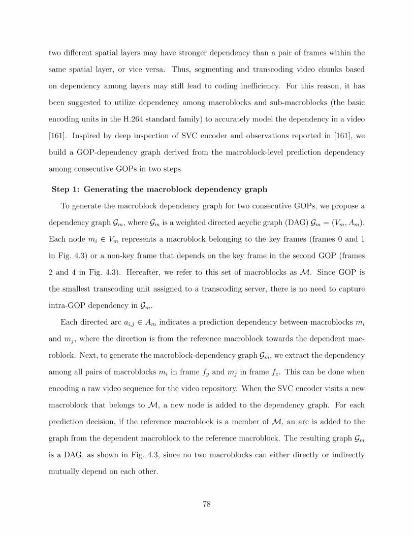
two different spatial layers may have stronger dependency than a pair of frames within the
same spatial layer, or vice versa. Thus, segmenting and transcoding video chunks based
on dependency among layers may still lead to coding inefficiency. For this reason, it has
been suggested to utilize dependency among macroblocks and sub-macroblocks (the basic
encoding units in the H.264 standard family) to accurately model the dependency in a video
[161]. Inspired by deep inspection of SVC encoder and observations reported in [161], we
build a GOP-dependency graph derived from the macroblock-level prediction dependency
among consecutive GOPs in two steps.
Step 1: Generating the macroblock dependency graph
To generate the macroblock dependency graph for two consecutive GOPs, we propose a
dependency graph Gm, where Gm is a weighted directed acyclic graph (DAG) Gm = (Vm, Am).
Each node mi ∈ Vm represents a macroblock belonging to the key frames (frames 0 and 1
in Fig. 4.3) or a non-key frame that depends on the key frame in the second GOP (frames
2 and 4 in Fig. 4.3). Hereafter, we refer to this set of macroblocks as M. Since GOP is
the smallest transcoding unit assigned to a transcoding server, there is no need to capture
intra-GOP dependency in Gm.
Each directed arc ai,j ∈ Am indicates a prediction dependency between macroblocks mi
and mj, where the direction is from the reference macroblock towards the dependent mac-
roblock. Next, to generate the macroblock-dependency graph Gm, we extract the dependency
among all pairs of macroblocks mi in frame fy and mj in frame fz. This can be done when
encoding a raw video sequence for the video repository. When the SVC encoder visits a new
macroblock that belongs to M, a new node is added to the dependency graph. For each
prediction decision, if the reference macroblock is a member of M, an arc is added to the
graph from the dependent macroblock to the reference macroblock. The resulting graph Gm
is a DAG, as shown in Fig. 4.3, since no two macroblocks can either directly or indirectly
mutually depend on each other.
78
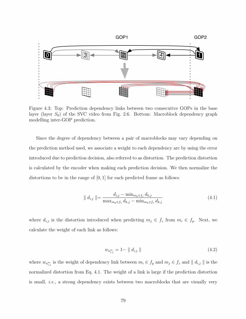
GOP1
0 123 4
GOP2
Figure 4.3: Top: Prediction dependency links between two consecutive GOPs in the baselayer (layer S0) of the SVC video from Fig. 2.6. Bottom: Macroblock dependency graphmodelling inter-GOP prediction.
Since the degree of dependency between a pair of macroblocks may vary depending on
the prediction method used, we associate a weight to each dependency arc by using the error
introduced due to prediction decision, also referred to as distortion. The prediction distortion
is calculated by the encoder when making each prediction decision. We then normalize the
distortions to be in the range of [0, 1] for each predicted frame as follows:
‖ di,j ‖=di,j −minmk∈fz dk,j
maxmk∈fz dk,j −minmk∈fz dk,j(4.1)
where di,j is the distortion introduced when predicting mj ∈ fz from mi ∈ fy. Next, we
calculate the weight of each link as follows:
wami,j = 1− ‖ di,j ‖ (4.2)
where wami,j is the weight of dependency link between mi ∈ fy and mj ∈ fz and ‖ di,j ‖ is the
normalized distortion from Eq. 4.1. The weight of a link is large if the prediction distortion
is small, i.e., a strong dependency exists between two macroblocks that are visually very
79
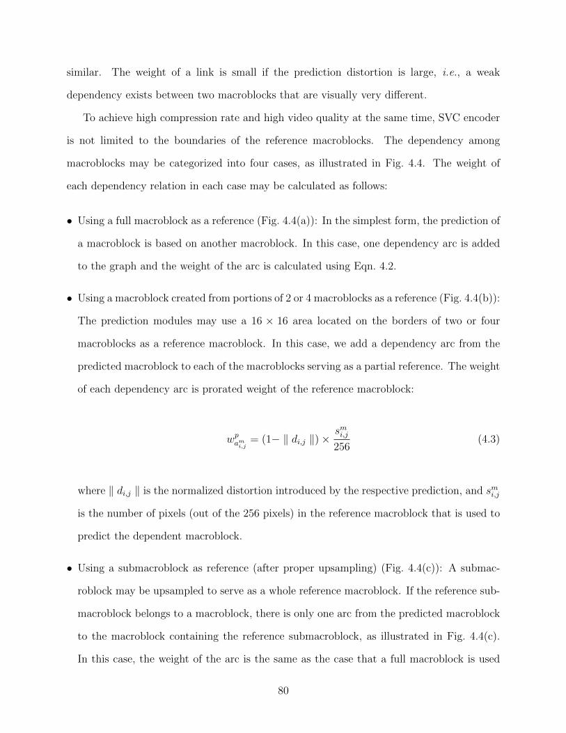
similar. The weight of a link is small if the prediction distortion is large, i.e., a weak
dependency exists between two macroblocks that are visually very different.
To achieve high compression rate and high video quality at the same time, SVC encoder
is not limited to the boundaries of the reference macroblocks. The dependency among
macroblocks may be categorized into four cases, as illustrated in Fig. 4.4. The weight of
each dependency relation in each case may be calculated as follows:
• Using a full macroblock as a reference (Fig. 4.4(a)): In the simplest form, the prediction of
a macroblock is based on another macroblock. In this case, one dependency arc is added
to the graph and the weight of the arc is calculated using Eqn. 4.2.
• Using a macroblock created from portions of 2 or 4 macroblocks as a reference (Fig. 4.4(b)):
The prediction modules may use a 16 × 16 area located on the borders of two or four
macroblocks as a reference macroblock. In this case, we add a dependency arc from the
predicted macroblock to each of the macroblocks serving as a partial reference. The weight
of each dependency arc is prorated weight of the reference macroblock:
wpami,j = (1− ‖ di,j ‖)×smi,j256
(4.3)
where ‖ di,j ‖ is the normalized distortion introduced by the respective prediction, and smi,j
is the number of pixels (out of the 256 pixels) in the reference macroblock that is used to
predict the dependent macroblock.
• Using a submacroblock as reference (after proper upsampling) (Fig. 4.4(c)): A submac-
roblock may be upsampled to serve as a whole reference macroblock. If the reference sub-
macroblock belongs to a macroblock, there is only one arc from the predicted macroblock
to the macroblock containing the reference submacroblock, as illustrated in Fig. 4.4(c).
In this case, the weight of the arc is the same as the case that a full macroblock is used
80
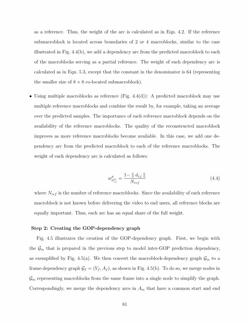
as a reference. Thus, the weight of the arc is calculated as in Eqn. 4.2. If the reference
submacroblock is located across boundaries of 2 or 4 macroblocks, similar to the case
illustrated in Fig. 4.4(b), we add a dependency arc from the predicted macroblock to each
of the macroblocks serving as a partial reference. The weight of each dependency arc is
calculated as in Eqn. 5.3, except that the constant in the denominator is 64 (representing
the smaller size of 8× 8 co-located submacroblock).
• Using multiple macroblocks as reference (Fig. 4.4(d)): A predicted macroblock may use
multiple reference macroblocks and combine the result by, for example, taking an average
over the predicted samples. The importance of each reference macroblock depends on the
availability of the reference macroblocks. The quality of the reconstructed macroblock
improves as more reference macroblocks become available. In this case, we add one de-
pendency arc from the predicted macroblock to each of the reference macroblocks. The
weight of each dependency arc is calculated as follows:
wpami,j =1− ‖ di,j ‖Nref
(4.4)
where Nref is the number of reference macroblocks. Since the availability of each reference
macroblock is not known before delivering the video to end users, all reference blocks are
equally important. Thus, each arc has an equal share of the full weight.
Step 2: Creating the GOP-dependency graph
Fig. 4.5 illustrates the creation of the GOP-dependency graph. First, we begin with
the Gm that is prepared in the previous step to model inter-GOP prediction dependency,
as exemplified by Fig. 4.5(a). We then convert the macroblock-dependency graph Gm to a
frame-dependency graph Gf = (Vf , Af ), as shown in Fig. 4.5(b). To do so, we merge nodes in
Gm representing macroblocks from the same frame into a single node to simplify the graph.
Correspondingly, we merge the dependency arcs in Am that have a common start and end
81
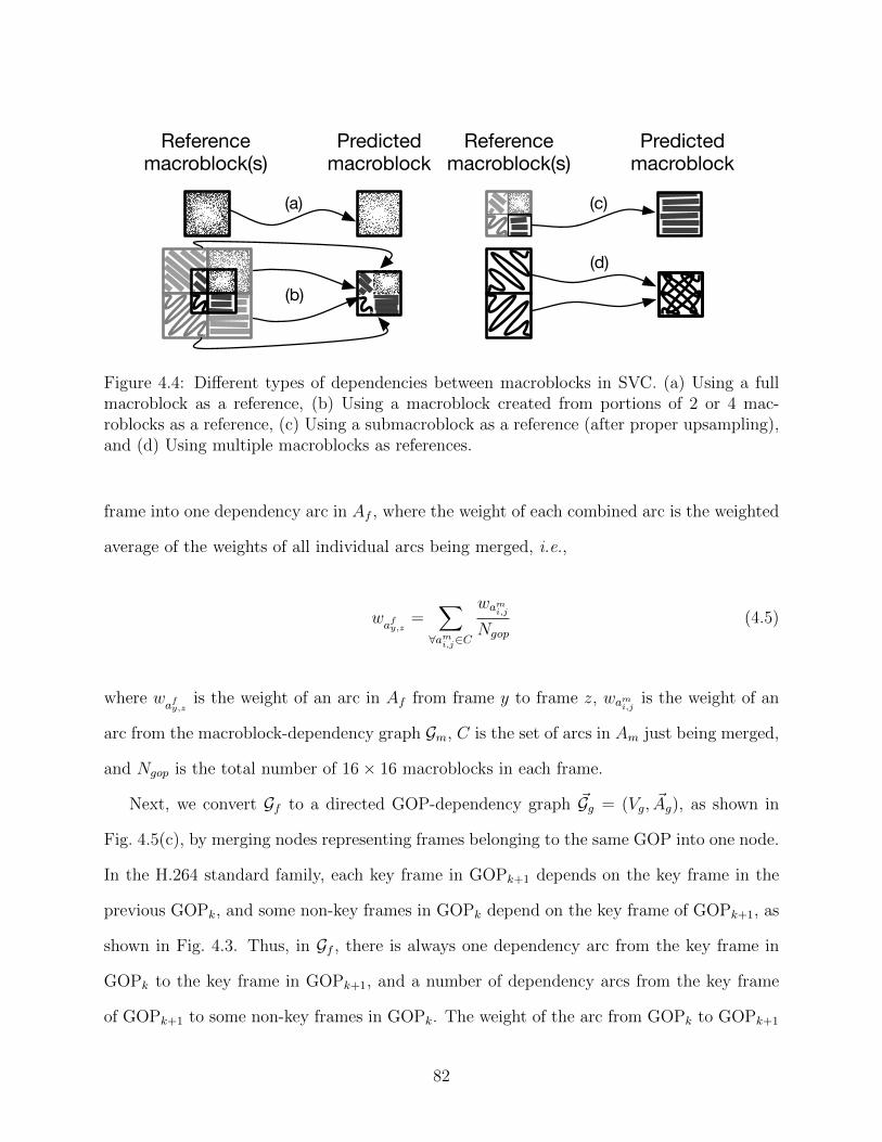
Reference macroblock(s)
Predicted macroblock
(a)
(b)
Reference macroblock(s)
Predicted macroblock
(c)
(d)
Figure 4.4: Different types of dependencies between macroblocks in SVC. (a) Using a fullmacroblock as a reference, (b) Using a macroblock created from portions of 2 or 4 mac-roblocks as a reference, (c) Using a submacroblock as a reference (after proper upsampling),and (d) Using multiple macroblocks as references.
frame into one dependency arc in Af , where the weight of each combined arc is the weighted
average of the weights of all individual arcs being merged, i.e.,
wafy,z =∑∀ami,j∈C
wami,jNgop
(4.5)
where wafy,z is the weight of an arc in Af from frame y to frame z, wami,j is the weight of an
arc from the macroblock-dependency graph Gm, C is the set of arcs in Am just being merged,
and Ngop is the total number of 16× 16 macroblocks in each frame.
Next, we convert Gf to a directed GOP-dependency graph ~Gg = (Vg, ~Ag), as shown in
Fig. 4.5(c), by merging nodes representing frames belonging to the same GOP into one node.
In the H.264 standard family, each key frame in GOPk+1 depends on the key frame in the
previous GOPk, and some non-key frames in GOPk depend on the key frame of GOPk+1, as
shown in Fig. 4.3. Thus, in Gf , there is always one dependency arc from the key frame in
GOPk to the key frame in GOPk+1, and a number of dependency arcs from the key frame
of GOPk+1 to some non-key frames in GOPk. The weight of the arc from GOPk to GOPk+1
82
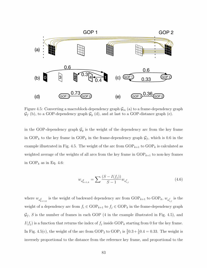
(a)
GOP 1 GOP 2
(c)
(d)
(b) 0 2 1
0.60.3
0.4
0.73GOP 1 GOP 2
0.60.33GOP 1 GOP 2
0.36GOP 1 GOP 2(e)
3 4
Figure 4.5: Converting a macroblock-dependency graph Gm (a) to a frame-dependency graphGf (b), to a GOP-dependency graph Gg (d), and at last to a GOP-distance graph (e).
in the GOP-dependency graph Gg is the weight of the dependency arc from the key frame
in GOPk to the key frame in GOPk in the frame-dependency graph Gf , which is 0.6 in the
example illustrated in Fig. 4.5. The weight of the arc from GOPk+1 to GOPk is calculated as
weighted average of the weights of all arcs from the key frame in GOPk+1 to non-key frames
in GOPk as in Eq. 4.6:
wa~gk+1,k
=∑ (S − I(fj))
S − 1wafi,j
(4.6)
where wa~gk+1,k
is the weight of backward dependency arc from GOPk+1 to GOPk, wafi,jis the
weight of a dependency arc from fi ∈ GOPk+1 to fj ∈ GOPk in the frame-dependency graph
Gf , S is the number of frames in each GOP (4 in the example illustrated in Fig. 4.5), and
I(fj) is a function that returns the index of fj inside GOPk starting from 0 for the key frame.
In Fig. 4.5(c), the weight of the arc from GOP2 to GOP1 is 230.3+ 1
30.4 = 0.33. The weight is
inversely proportional to the distance from the reference key frame, and proportional to the
83
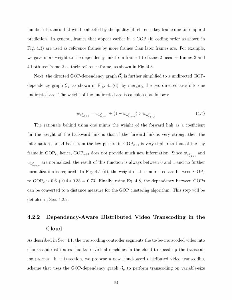
number of frames that will be affected by the quality of reference key frame due to temporal
prediction. In general, frames that appear earlier in a GOP (in coding order as shown in
Fig. 4.3) are used as reference frames by more frames than later frames are. For example,
we gave more weight to the dependency link from frame 1 to frame 2 because frames 3 and
4 both use frame 2 as their reference frame, as shown in Fig. 4.3.
Next, the directed GOP-dependency graph ~Gg is further simplified to a undirected GOP-
dependency graph Gg, as shown in Fig. 4.5(d), by merging the two directed arcs into one
undirected arc. The weight of the undirected arc is calculated as follows:
wagk,k+1= w
a~gk,k+1+ (1− w
a~gk,k+1)× w
a~gk+1,k(4.7)
The rationale behind using one minus the weight of the forward link as a coefficient
for the weight of the backward link is that if the forward link is very strong, then the
information spread back from the key picture in GOPk+1 is very similar to that of the key
frame in GOPk, hence, GOPk+1 does not provide much new information. Since wa~gk,k+1
and
wa~gk+1,k
are normalized, the result of this function is always between 0 and 1 and no further
normalization is required. In Fig. 4.5 (d), the weight of the undirected arc between GOP1
to GOP2 is 0.6 + 0.4 ∗ 0.33 = 0.73. Finally, using Eq. 4.8, the dependency between GOPs
can be converted to a distance measure for the GOP clustering algorithm. This step will be
detailed in Sec. 4.2.2.
4.2.2 Dependency-Aware Distributed Video Transcoding in the
Cloud
As described in Sec. 4.1, the transcoding controller segments the to-be-transcoded video into
chunks and distributes chunks to virtual machines in the cloud to speed up the transcod-
ing process. In this section, we propose a new cloud-based distributed video transcoding
scheme that uses the GOP-dependency graph Gg to perform transcoding on variable-size
84
video chunks. In other words, the new scheme assigns GOPs sharing great visual similarity
to the same machine for better coding efficiency and faster transcoding. We first present the
clustering algorithm for grouping GOPs to variable-size video chunks based on the GOP-
dependency graph Gg, and then present the algorithm that dispatches video chunks to virtual
machines for transcoding.
Preparing variable-size video chunks
In order to benefit from the visual similarity among pictures in a video sequence, we
propose to segment the video into variable-size video chunks so that GOPs are clustered ac-
cording to prediction dependency (hence, the visual similarity). Many clustering algorithms
have been proposed to group data into a fixed number of clusters [150] or any number of
clusters as needed [17, 45, 164]. Since the number of desired video chunks in the proposed
adaptive model is not known a priori when transcoding a video in real time, we adopt OP-
TICS (Ordering Points To Identify the Clustering Structure) [17] to cluster nodes in the
GOP-dependency graph Gg into as many video chunks as necessary.
Since OPTICS clusters a stream of data points according to distances between each
pair of points, we must convert the GOP-dependency graph Gg to a GOP-distance graph
Gd by converting the dependency weight of each arc to a distance measure between two
consecutive GOPs. Since highly dependent GOPs should be transcoded together, they should
be clustered into one video chunk. Thus, the distance between two consecutive GOPs dk,k+1
should be inversely proportional to the degree of dependency (the arc weight wagk,k+1in the
GOP-dependency graph Gg), as calculated in Eqn. 4.8.
dk,k+1 =1
wagk,k+1
− 1 (4.8)
We reduce one from the inverse of the weight of a GOP-dependency arc to make the
distance greater than or equal to zero. According to Eqn. 4.2–4.7, if two consecutive GOPs
are very similar, the weight of the corresponding dependency arc in Gg is close to 1 (due
85
to the low prediction distortion), which makes the distance between these two GOPs in Gd
approaching to zero according to Eqn. 4.8.
OPTICS has two parameters: ε – the maximum distance among nodes in a cluster, and
MinPts – the minimum number of nodes in a cluster. We set MinPts to one by default,
meaning that if there is no GOP with a strong visual similarity with a GOP, then the GOP
can be processed alone as a video chunk. The value of ε is set to 5 experimentally. The
computational complexity of OPTICS depends on the complexity of the ε-neighborhood
query function which is invoked exactly once for each GOP. Since the GOP-dependency
graph Gg is a chain of GOPs, the query function is invoked at most n times, where n is
the number of GOPs in the video sequence and the query function adds the distances of
the new GOPs together until the accumulated distance from the first GOP of the current
cluster exceeds the threshold ε. Since the computational complexity of the query function
(one addition and one comparison) is constant, the complexity of this algorithm is O(n).
Dispatching video chunks for distributed transcoding in the cloud
After segmenting the video into variable-size video chunks according to dependency
among GOPs, the transcoding controller dispatches video chunks to virtual machines in
the cloud for transcoding. Though it is an NP-hard problem to optimize the dispatching
algorithm for transcoding delay, number of virtual machines, or the energy consumed in the
cloud, heuristic solutions have been proposed [21]. For real-time streaming, video chunks
must be transcoded prior to their playback deadline. Thus, a simple FIFO dispatching algo-
rithm is suitable for our transcoding scheme since it preserves the time order of video chunks.
In other words, the transcoding controller dispatches the first job in the FIFO queue as soon
as a virtual machine becomes available.
86
4.3 Performance Evaluation
In order to evaluate the proposed dependency-aware distributed transcoding scheme, we
implement a prototype of the transcoding system in a private cloud with 10 computing
units. Each computing unit is equipped with 16 Intelr Xeonr E5640 CPU cores at 2.67
GHz. One machine is dedicated to serve as the transcoding controller, and the remaining
machines serve as transcoding servers. We used the most recent release of the reference
software package for scalable video coding, i.e. JSVM 9.19.15 [1]. As shown in Fig. 4.6
we modified the SVC encoder in JSVM by wiretapping a new module into the main video
coding modules of the encoder to generate the macroblock-dependency graph when encoding
a video, as described in Step 1 of generating the GOP-dependency graph in Sec. 4.2.1. The
macroblock-dependency graph is then converted to the GOP-dependency graph, as described
in Step 2 of generating the GOP-dependency graph in Sec. 4.2.1. The conversion can also
be performed in parallel to the encoding process on a different processor, since the encoder
produces consecutive GOPs. The GOP distances are calculated as described in Sec. 4.2.1,
and the results are stored as a list of n−1 distance measures in the video repository, where n
is the number of GOPs in the video sequence. Finally, the transcoding controller clusters the
GOPs into variable-size video chunks using the OPTICS algorithm according to the GOP
distances. The proposed algorithm needs to run only once for each raw video sequence prior
to being encoded and stored on the video repository. Once the distances are calculated and
stored, they can be used to serve any transcoding request received by the cloud transcoding
system.
We used the same set of seven full-HD raw video sequences as input to the transcoding
system as discussed in Sec. 3.1. As reported in Table 3.1, these videos are selected from
different genres. They exhibit diverse values of detail [99] and motion activity [67] visual
features. We encoded each video sequence using the modified SVC encoder with layering
configuration DTQ=(1, 3, 1), i.e., the SVC encoded video contains two dyadic spatial layers
87
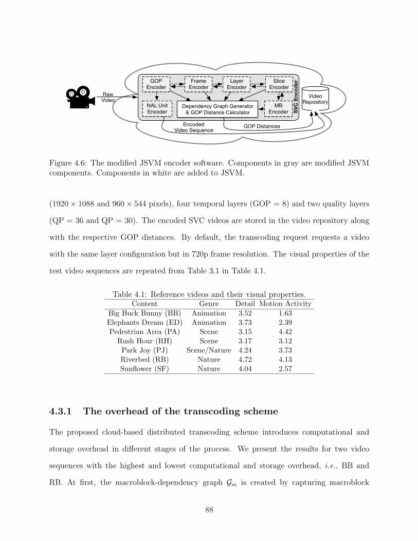
GOP Encoder
Frame Encoder
LayerEncoder
Slice Encoder
MB Encoder
Dependency Graph Generator & GOP Distance Calculator SV
C E
ncod
er
RawVideo
NAL Unit Encoder
EncodedVideo Sequence
GOP Distances
VideoRepository
Figure 4.6: The modified JSVM encoder software. Components in gray are modified JSVMcomponents. Components in white are added to JSVM.
(1920× 1088 and 960× 544 pixels), four temporal layers (GOP = 8) and two quality layers
(QP = 36 and QP = 30). The encoded SVC videos are stored in the video repository along
with the respective GOP distances. By default, the transcoding request requests a video
with the same layer configuration but in 720p frame resolution. The visual properties of the
test video sequences are repeated from Table 3.1 in Table 4.1.
Table 4.1: Reference videos and their visual properties.Content Genre Detail Motion Activity
Big Buck Bunny (BB) Animation 3.52 1.63Elephants Dream (ED) Animation 3.73 2.39Pedestrian Area (PA) Scene 3.15 4.42
Rush Hour (RH) Scene 3.17 3.12Park Joy (PJ) Scene/Nature 4.24 3.73Riverbed (RB) Nature 4.72 4.13Sunflower (SF) Nature 4.04 2.57
4.3.1 The overhead of the transcoding scheme
The proposed cloud-based distributed transcoding scheme introduces computational and
storage overhead in different stages of the process. We present the results for two video
sequences with the highest and lowest computational and storage overhead, i.e., BB and
RB. At first, the macroblock-dependency graph Gm is created by capturing macroblock
88
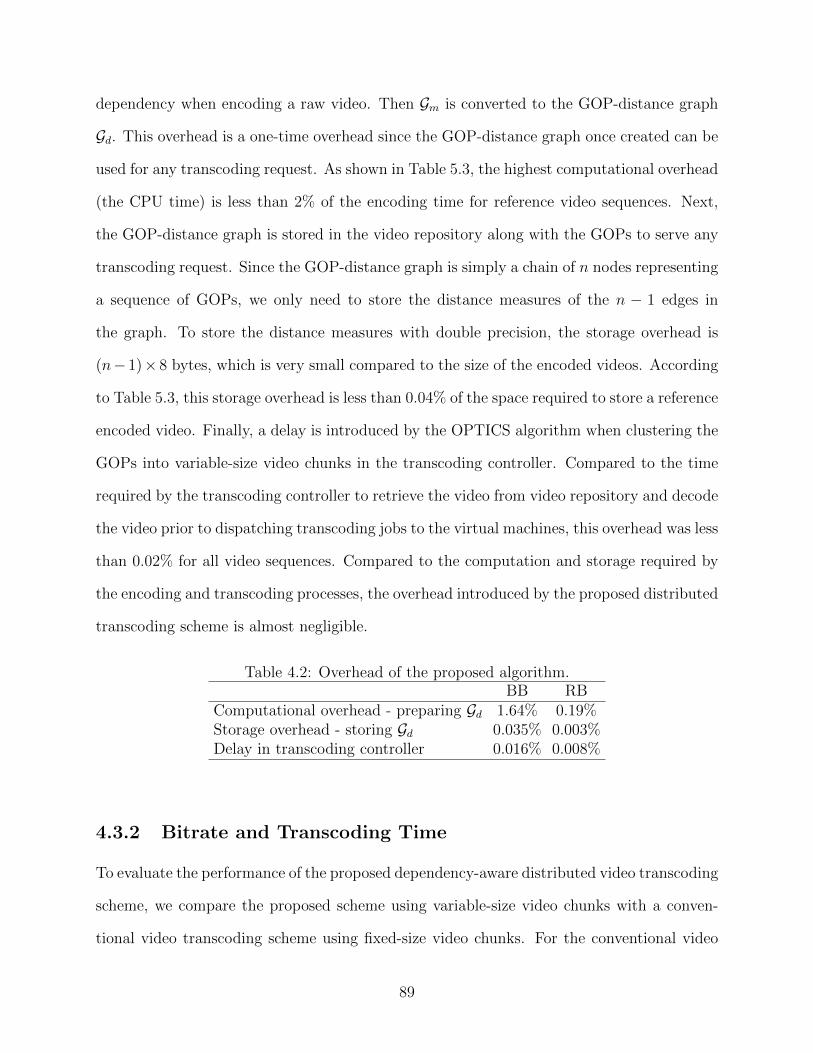
dependency when encoding a raw video. Then Gm is converted to the GOP-distance graph
Gd. This overhead is a one-time overhead since the GOP-distance graph once created can be
used for any transcoding request. As shown in Table 5.3, the highest computational overhead
(the CPU time) is less than 2% of the encoding time for reference video sequences. Next,
the GOP-distance graph is stored in the video repository along with the GOPs to serve any
transcoding request. Since the GOP-distance graph is simply a chain of n nodes representing
a sequence of GOPs, we only need to store the distance measures of the n − 1 edges in
the graph. To store the distance measures with double precision, the storage overhead is
(n− 1)× 8 bytes, which is very small compared to the size of the encoded videos. According
to Table 5.3, this storage overhead is less than 0.04% of the space required to store a reference
encoded video. Finally, a delay is introduced by the OPTICS algorithm when clustering the
GOPs into variable-size video chunks in the transcoding controller. Compared to the time
required by the transcoding controller to retrieve the video from video repository and decode
the video prior to dispatching transcoding jobs to the virtual machines, this overhead was less
than 0.02% for all video sequences. Compared to the computation and storage required by
the encoding and transcoding processes, the overhead introduced by the proposed distributed
transcoding scheme is almost negligible.
Table 4.2: Overhead of the proposed algorithm.BB RB
Computational overhead - preparing Gd 1.64% 0.19%Storage overhead - storing Gd 0.035% 0.003%Delay in transcoding controller 0.016% 0.008%
4.3.2 Bitrate and Transcoding Time
To evaluate the performance of the proposed dependency-aware distributed video transcoding
scheme, we compare the proposed scheme using variable-size video chunks with a conven-
tional video transcoding scheme using fixed-size video chunks. For the conventional video
89
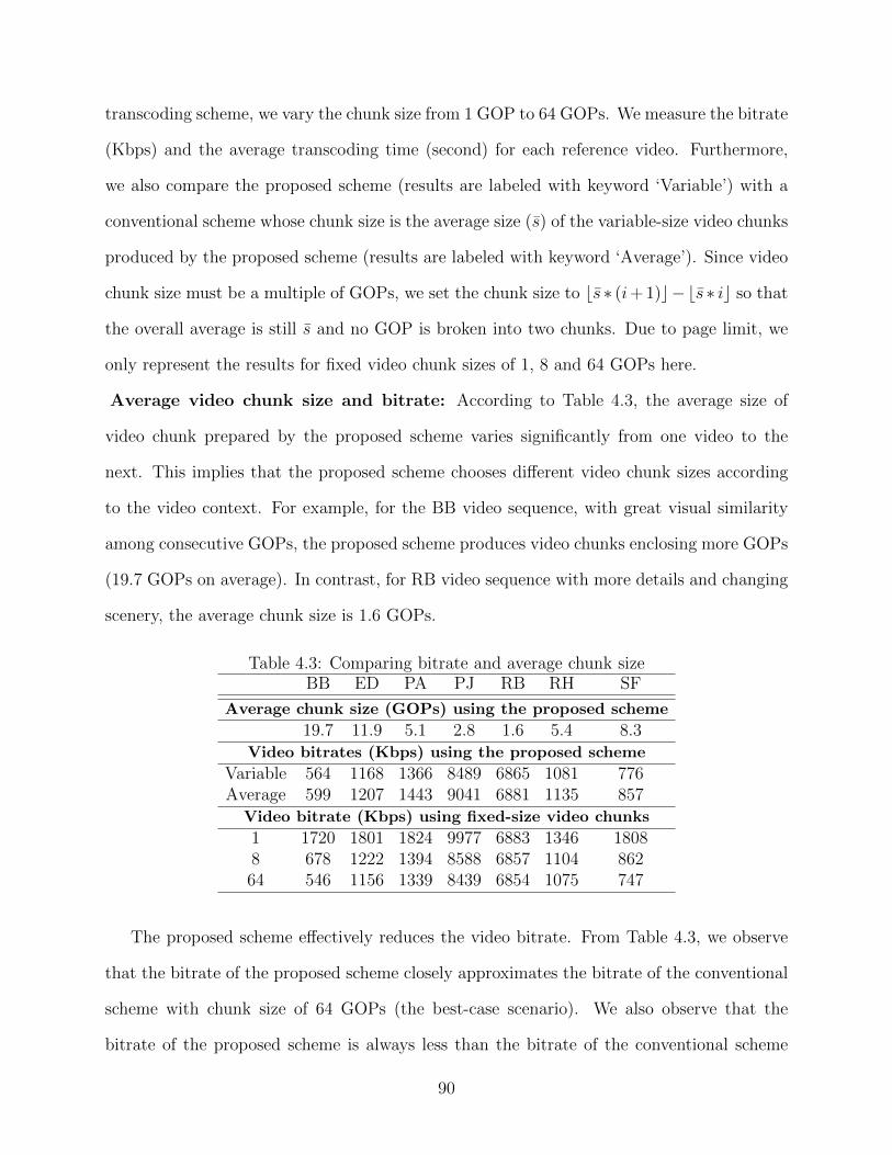
transcoding scheme, we vary the chunk size from 1 GOP to 64 GOPs. We measure the bitrate
(Kbps) and the average transcoding time (second) for each reference video. Furthermore,
we also compare the proposed scheme (results are labeled with keyword ‘Variable’) with a
conventional scheme whose chunk size is the average size (s) of the variable-size video chunks
produced by the proposed scheme (results are labeled with keyword ‘Average’). Since video
chunk size must be a multiple of GOPs, we set the chunk size to bs ∗ (i+ 1)c−bs ∗ ic so that
the overall average is still s and no GOP is broken into two chunks. Due to page limit, we
only represent the results for fixed video chunk sizes of 1, 8 and 64 GOPs here.
Average video chunk size and bitrate: According to Table 4.3, the average size of
video chunk prepared by the proposed scheme varies significantly from one video to the
next. This implies that the proposed scheme chooses different video chunk sizes according
to the video context. For example, for the BB video sequence, with great visual similarity
among consecutive GOPs, the proposed scheme produces video chunks enclosing more GOPs
(19.7 GOPs on average). In contrast, for RB video sequence with more details and changing
scenery, the average chunk size is 1.6 GOPs.
Table 4.3: Comparing bitrate and average chunk sizeBB ED PA PJ RB RH SF
Average chunk size (GOPs) using the proposed scheme
19.7 11.9 5.1 2.8 1.6 5.4 8.3Video bitrates (Kbps) using the proposed scheme
Variable 564 1168 1366 8489 6865 1081 776Average 599 1207 1443 9041 6881 1135 857
Video bitrate (Kbps) using fixed-size video chunks
1 1720 1801 1824 9977 6883 1346 18088 678 1222 1394 8588 6857 1104 86264 546 1156 1339 8439 6854 1075 747
The proposed scheme effectively reduces the video bitrate. From Table 4.3, we observe
that the bitrate of the proposed scheme closely approximates the bitrate of the conventional
scheme with chunk size of 64 GOPs (the best-case scenario). We also observe that the
bitrate of the proposed scheme is always less than the bitrate of the conventional scheme
90
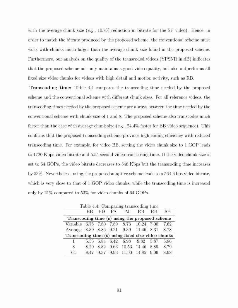
with the average chunk size (e.g., 10.8% reduction in bitrate for the SF video). Hence, in
order to match the bitrate produced by the proposed scheme, the conventional scheme must
work with chunks much larger than the average chunk size found in the proposed scheme.
Furthermore, our analysis on the quality of the transcoded videos (YPSNR in dB) indicates
that the proposed scheme not only maintains a good video quality, but also outperforms all
fixed size video chunks for videos with high detail and motion activity, such as RB.
Transcoding time: Table 4.4 compares the transcoding time needed by the proposed
scheme and the conventional scheme with different chunk sizes. For all reference videos, the
transcoding times needed by the proposed scheme are always between the time needed by the
conventional scheme with chunk size of 1 and 8. The proposed scheme also transcodes much
faster than the case with average chunk size (e.g., 24.4% faster for BB video sequence). This
confirms that the proposed transcoding scheme provides high coding efficiency with reduced
transcoding time. For example, for video BB, setting the video chunk size to 1 GOP leads
to 1720 Kbps video bitrate and 5.55 second video transcosing time. If the video chunk size is
set to 64 GOPs, the video bitrate decreases to 546 Kbps but the transcoding time increases
by 53%. Nevertheless, using the proposed adaptive scheme leads to a 564 Kbps video bitrate,
which is very close to that of 1 GOP video chunks, while the transcoding time is increased
only by 21% compared to 53% for video chunks of 64 GOPs.
Table 4.4: Comparing transcoding timeBB ED PA PJ RB RH SF
Transcoding time (s) using the proposed scheme
Variable 6.75 7.80 7.80 8.73 10.24 7.00 7.62Average 8.39 8.86 9.21 9.39 11.46 8.31 8.78Transcoding time (s) using fixed size video chunks
1 5.55 5.84 6.42 6.98 9.82 5.87 5.868 8.20 8.82 9.63 10.53 14.46 8.85 8.7964 8.47 9.37 9.93 11.00 14.85 9.09 8.98
91
4.4 Summary
In this chapter, we proposed a novel distributed video transcoding scheme. We note that
the existing proposals for cloud-assisted video transcoding, as listed in Sec. 2.2.2, treat the
encoded video no different from a raw video. A fixed number of consecutive frames or group
of pictures are grouped into a video chunk, the chunks are transcoded in parallel, and the
transcoded video chunks are then merged into a single video sequence to be delivered to
end users. On the contrary, in this research we proposed a dependency-aware distributed
video transcoding scheme that uses variable-size video chunks. The proposed model takes
advantage of visual similarity among macroblocks and GOPs in a video sequence.
As pioneering work in this research direction, we proposed an algorithm to extract the
dependency among macroblocks in an encoded video, based on which we determined the de-
pendency between successive GOPs. GOPs are then clustered according to their dependency
to create variable-size video chunks so that visually similar GOPs are put in one chunk. Our
experiments show that the proposed scheme improves resource efficiency by decreasing the
video bitrate and the computational resource consumption on the cloud. It also increases
the visual quality of the transcoded video for more complex video sequences. While the
proposed model was evaluated using layered video coding standard SVC, the same principle
applies to other video coding standards such as H.264/AVC or H.265/HEVC.
The suggested prediction dependency model between GOPs in an encoded video sequence
is a useful concept that can also be used in other multimedia streaming problems. In the
following chapter, this concept is re-engineered and a dependency model that considers the
fine grain dependencies between macroblocks and submacroblocks is presented. Furthermore,
a novel video packet importance model is built upon the proposed dependency model, and
the result is applied to the unequal error protection problem. This problem is part of the
service delivery phase in the life cycle of a video streaming episode, as illustrated in Fig. 1.1.
We discuss this further in the following chapter.
92
Chapter 5
Video Transmission in Wireless Networks
In Chapter 1, the life cycle of a video transmission session is illustrated. Dismissing the
details, such a life cycle starts from the raw video capture by the IP camera and concludes
with the video playback at the end user device. After the video is prepared by the video
streaming server, usually it must traverse through multiple transmission media to reach the
end user device. The current infrastructure of large IP networks such as the Internet or
the legacy IPTV networks, increasingly use high capacity cable connections for the entire
backhaul portion of the network. Nowadays, fiber-optic cables are used as the transmission
medium for the intermediate links between the core network and the small subnetworks at
the edge of the network. Furthermore, due to the increasing usage of FTTx architecture
in IP networks, the fiber-optic cables are also used as the transmission medium for the last
mile telecommunications. The most important benefits of such cable connections are the
high data transmission rate and the very low amount of physical noise leading to negligible
packet loss rate (unless the network is partially or fully congested). However, the lack of
support for mobility makes cable connections ineffectual for mobile communications.
For mobile communication, including mobile video streaming, the last mile of the telecom-
munication network uses wireless communication channels. The wireless connection can be
maintained using a mobile telecommunication technology (such as 3G or 4G networks) or
offloaded to a wireless LAN (such as WiFi networks)1. In contrast to the cable transmis-
sion mediums, wireless channels are intrinsically prone to interference and noise, resulting
in fluctuation in channel capacity. These features of wireless channels impose substantial
challenges for video streaming.
1Depending on the architecture, a wireless telecommunication network may use wireless data connectionsin part of the backhaul portion of the network besides the last mile.
93
In this chapter, we first look deeper into the coding and prediction mechanism of state-
of-the-art layered video coding standard, i.e., SVC. Next, toward smarter protection of video
packets over noisy communication channels and better quality of the transmitted video, we
exploit the prediction structure to propose a novel coding and dependency-aware unequal
error protection algorithm. The proposed algorithm calculates the importance of different
video packets and associates protection to each video packet, respectively. Experimental
results show that the proposed algorithm outperforms the state-of-the-art unequal error pro-
tection algorithms in terms of the quality of the transmitted video. Finally, we complete
the proposed UEP model by extending the UEP problem from unicast scenario to multi-
cast scenario, in which the full potential of layered video coding is utilized by allowing the
transmission network to multicast one copy of the layered video for groups of heterogeneous
mobile devices. We specifically propose a new technique to dynamically adjust and combine
the protection FEC packets for reference and dependent video layers for video multicast in
mobile communication networks.
5.1 Coding and Prediction in SVC
Before proposing the coding and dependency-aware UEP for layered video coding, we need
to have a deep understanding of layered video coding by inspecting a real layered video codec
standard. Moreover, while the concept of coding and dependency-aware UEP remains the
same, as will be shown in Sec. 5.2.1, modeling coding dependency and calculating importance
of video packets must be tailored for individual codec standards. In this section, we use SVC
[112] – the state-of-the-art layered video coding standard. The general design of SVC was
covered in Chapter 3. Therefore, we continue with the coding and prediction in SVC.
Fig. 5.1 schematically illustrates the prediction in SVC in a tree structure. In SVC,
enhancement macroblocks are created based on either temporal or spatial prediction. The
quality enhancement information may be included if it is available. Temporal prediction is
94
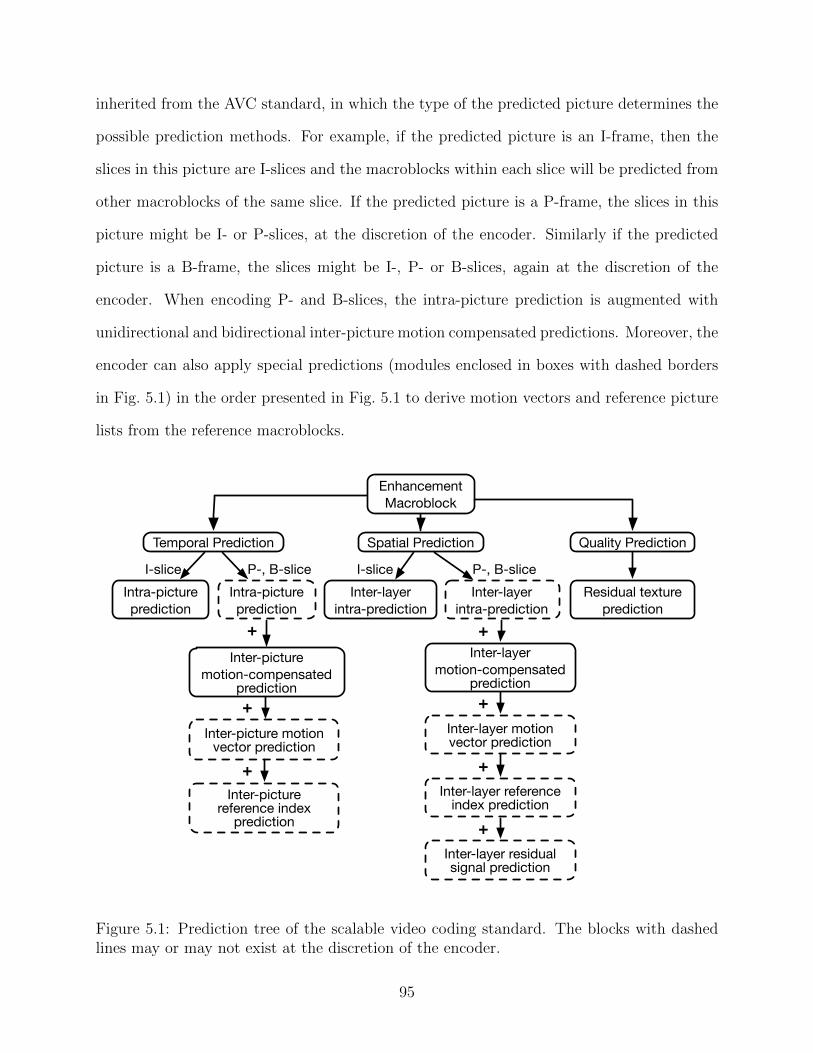
inherited from the AVC standard, in which the type of the predicted picture determines the
possible prediction methods. For example, if the predicted picture is an I-frame, then the
slices in this picture are I-slices and the macroblocks within each slice will be predicted from
other macroblocks of the same slice. If the predicted picture is a P-frame, the slices in this
picture might be I- or P-slices, at the discretion of the encoder. Similarly if the predicted
picture is a B-frame, the slices might be I-, P- or B-slices, again at the discretion of the
encoder. When encoding P- and B-slices, the intra-picture prediction is augmented with
unidirectional and bidirectional inter-picture motion compensated predictions. Moreover, the
encoder can also apply special predictions (modules enclosed in boxes with dashed borders
in Fig. 5.1) in the order presented in Fig. 5.1 to derive motion vectors and reference picture
lists from the reference macroblocks.
EnhancementMacroblock
Temporal Prediction Spatial Prediction Quality Prediction
Intra-picture prediction
Intra-picture prediction
Inter-picturemotion-compensated
prediction
Inter-picture motion vector prediction
Inter-layer intra-prediction
Inter-layerintra-prediction
Residual texture prediction
I-slice P-, B-slice I-slice P-, B-slice
+
+
Inter-picture reference index
prediction
+
Inter-layermotion-compensated
prediction
Inter-layer motion vector prediction
+
+
Inter-layer reference index prediction
+
Inter-layer residual signal prediction
+
Figure 5.1: Prediction tree of the scalable video coding standard. The blocks with dashedlines may or may not exist at the discretion of the encoder.
95
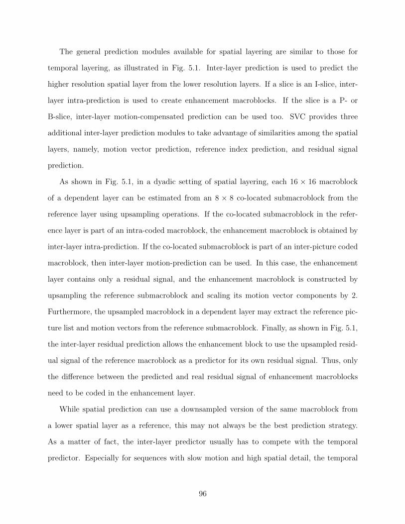
The general prediction modules available for spatial layering are similar to those for
temporal layering, as illustrated in Fig. 5.1. Inter-layer prediction is used to predict the
higher resolution spatial layer from the lower resolution layers. If a slice is an I-slice, inter-
layer intra-prediction is used to create enhancement macroblocks. If the slice is a P- or
B-slice, inter-layer motion-compensated prediction can be used too. SVC provides three
additional inter-layer prediction modules to take advantage of similarities among the spatial
layers, namely, motion vector prediction, reference index prediction, and residual signal
prediction.
As shown in Fig. 5.1, in a dyadic setting of spatial layering, each 16 × 16 macroblock
of a dependent layer can be estimated from an 8 × 8 co-located submacroblock from the
reference layer using upsampling operations. If the co-located submacroblock in the refer-
ence layer is part of an intra-coded macroblock, the enhancement macroblock is obtained by
inter-layer intra-prediction. If the co-located submacroblock is part of an inter-picture coded
macroblock, then inter-layer motion-prediction can be used. In this case, the enhancement
layer contains only a residual signal, and the enhancement macroblock is constructed by
upsampling the reference submacroblock and scaling its motion vector components by 2.
Furthermore, the upsampled macroblock in a dependent layer may extract the reference pic-
ture list and motion vectors from the reference submacroblock. Finally, as shown in Fig. 5.1,
the inter-layer residual prediction allows the enhancement block to use the upsampled resid-
ual signal of the reference macroblock as a predictor for its own residual signal. Thus, only
the difference between the predicted and real residual signal of enhancement macroblocks
need to be coded in the enhancement layer.
While spatial prediction can use a downsampled version of the same macroblock from
a lower spatial layer as a reference, this may not always be the best prediction strategy.
As a matter of fact, the inter-layer predictor usually has to compete with the temporal
predictor. Especially for sequences with slow motion and high spatial detail, the temporal
96
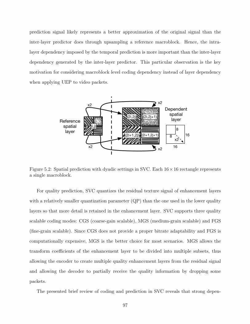
prediction signal likely represents a better approximation of the original signal than the
inter-layer predictor does through upsampling a reference macroblock. Hence, the intra-
layer dependency imposed by the temporal prediction is more important than the inter-layer
dependency generated by the inter-layer predictor. This particular observation is the key
motivation for considering macroblock level coding dependency instead of layer dependency
when applying UEP to video packets.
8
8 16
16
x2
Reference spatial layer
Dependent spatial layer
(i,j)
(2i,2j)
(2i+1,2j)
(2i,2j+1)
(2i+1,2j+1)
x2
x2
x2
x2
Figure 5.2: Spatial prediction with dyadic settings in SVC. Each 16×16 rectangle representsa single macroblock.
For quality prediction, SVC quantizes the residual texture signal of enhancement layers
with a relatively smaller quantization parameter (QP) than the one used in the lower quality
layers so that more detail is retained in the enhancement layer. SVC supports three quality
scalable coding modes: CGS (coarse-gain scalable), MGS (medium-grain scalable) and FGS
(fine-grain scalable). Since CGS does not provide a proper bitrate adaptability and FGS is
computationally expensive, MGS is the better choice for most scenarios. MGS allows the
transform coefficients of the enhancement layer to be divided into multiple subsets, thus
allowing the encoder to create multiple quality enhancement layers from the residual signal
and allowing the decoder to partially receive the quality information by dropping some
packets.
The presented brief review of coding and prediction in SVC reveals that strong depen-
97
dency exists among pictures within a layer and across layers. We argue that ignoring the
internal design of video codec standards leads to less effective UEP for three reasons. First,
temporal predictor and spatial predictor modules of SVC compete for the prediction of mac-
roblocks. Hence, not all macroblocks of a frame in the higher spatial layer depend on the
co-located submacroblocks in the reference spatial layer. The same dependency property
also holds across temporal layers. Second, while P- and B- frames are allowed to use past
and future pictures (in playback order) as references, the final coding decision is at the
discretion of the encoder. For example, to encode a video with very high motion activity
among consecutive frames, the encoder may use I- slices inside of a B-frame since the visual
information from past and future pictures are not as useful to predict the current picture.
Finally, when using inter-picture and inter-layer motion compensated prediction in temporal
and spatial prediction, the encoder may decide to use extra information (such as motion
vectors, reference picture lists and the residual signal) from the reference macroblock or sub-
macroblock. Though these observations are drawn from inspecting the SVC codec standard,
similar observations can be drawn for other codec standards.
The deep inspection of coding and prediction structure of SVC indicates that the large
scale dependency among video layers is not sufficient to determine the importance of video
packets for UEP. We will examine the correctness of this statement through experiments in
Sec. 5.2.2. By considering dependency at the submacroblock/macroblock level (the finest
processing unit of the H.264 video coding standard family), we propose a more effective UEP
model that provides better protection for more important video packets.
5.2 Coding-Aware UEP for Layered Video Streaming
As discussed in Chapter 3, video encoders exploit the redundancy of visual information in
time and scale domains. For example, when the camera pans slowly through the scene or
the scenery is stationary, the captured video sequence can be highly compressed without
98
noticeable loss of quality due to high visual similarity of consecutive frames. Encoded video
frames can be divided into reference and dependent pictures, where dependent pictures are
reconstructed using the reference pictures. However, in modern video coding standards, a
picture may be a reference picture for some pictures and may also be a dependent picture
depending on some other pictures at the same time. Furthermore, in a layered video coding
standard reference pictures and dependent pictures can be organized into reference layer(s)
and dependent layer(s), respectively. Video layers are separate substreams inside a video
bitstream for independent transmission. Similar to that of dependent pictures, the video
bitrate is reduced by storing the residual error of the predicted video signal in dependent
layers.
Dependent layers usually provide higher quality but rely on their respective reference
layers for successful reconstruction of the transmitted video frames. Since dependent layers
consist of pictures depending on those of the reference layers, any noise (lost or corrupted
video packets) in a reference layer may hinder the decodability of one ore more dependent
layers, even if the dependent layers were received correctly. In this case, the resources
consumed to transmit and decode the dependent layers are wasted. Such a decodability
dependency justifies the need for using stronger protection mechanism for reference layers,
i.e., unequal error protection (UEP). As discussed in Sec. 2.2, numerous UEP methods are
proposed to provide different level of protection according to the importance of the reference
and dependent video layers [14, 28, 53, 86, 134]. However, these proposals do not consider
the internal design of the video coding standards. In fact, they confront the problem as
a general unequal protection problem between reference and dependent layers where, for
example, data partitions in H.264/AVC [124] or multiple descriptions in MDC [23] can be
substituted by the concept of layers in scalable video coding (SVC) [112].
In fact, the importance of a piece of video content is determined by not only the lay-
ering structure, but also visual features and encoding decisions [162]. To accurately model
99
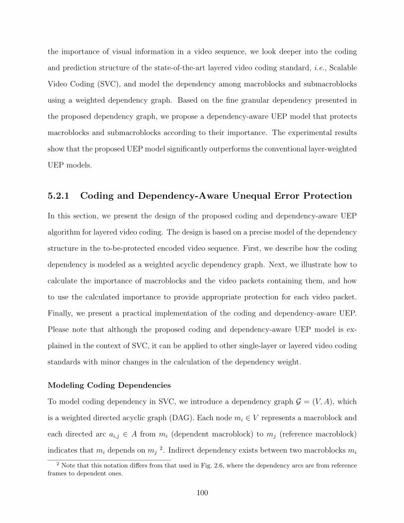
the importance of visual information in a video sequence, we look deeper into the coding
and prediction structure of the state-of-the-art layered video coding standard, i.e., Scalable
Video Coding (SVC), and model the dependency among macroblocks and submacroblocks
using a weighted dependency graph. Based on the fine granular dependency presented in
the proposed dependency graph, we propose a dependency-aware UEP model that protects
macroblocks and submacroblocks according to their importance. The experimental results
show that the proposed UEP model significantly outperforms the conventional layer-weighted
UEP models.
5.2.1 Coding and Dependency-Aware Unequal Error Protection
In this section, we present the design of the proposed coding and dependency-aware UEP
algorithm for layered video coding. The design is based on a precise model of the dependency
structure in the to-be-protected encoded video sequence. First, we describe how the coding
dependency is modeled as a weighted acyclic dependency graph. Next, we illustrate how to
calculate the importance of macroblocks and the video packets containing them, and how
to use the calculated importance to provide appropriate protection for each video packet.
Finally, we present a practical implementation of the coding and dependency-aware UEP.
Please note that although the proposed coding and dependency-aware UEP model is ex-
plained in the context of SVC, it can be applied to other single-layer or layered video coding
standards with minor changes in the calculation of the dependency weight.
Modeling Coding Dependencies
To model coding dependency in SVC, we introduce a dependency graph G = (V,A), which
is a weighted directed acyclic graph (DAG). Each node mi ∈ V represents a macroblock and
each directed arc ai,j ∈ A from mi (dependent macroblock) to mj (reference macroblock)
indicates that mi depends on mj2. Indirect dependency exists between two macroblocks mi
2 Note that this notation differs from that used in Fig. 2.6, where the dependency arcs are from referenceframes to dependent ones.
100
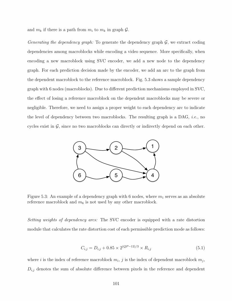
and mk if there is a path from mi to mk in graph G.
Generating the dependency graph: To generate the dependency graph G, we extract coding
dependencies among macroblocks while encoding a video sequence. More specifically, when
encoding a new macroblock using SVC encoder, we add a new node to the dependency
graph. For each prediction decision made by the encoder, we add an arc to the graph from
the dependent macroblock to the reference macroblock. Fig. 5.3 shows a sample dependency
graph with 6 nodes (macroblocks). Due to different prediction mechanisms employed in SVC,
the effect of losing a reference macroblock on the dependent macroblocks may be severe or
negligible. Therefore, we need to assign a proper weight to each dependency arc to indicate
the level of dependency between two macroblocks. The resulting graph is a DAG, i.e., no
cycles exist in G, since no two macroblocks can directly or indirectly depend on each other.
1
45
2
6
3
Figure 5.3: An example of a dependency graph with 6 nodes, where m1 serves as an absolutereference macroblock and m6 is not used by any other macroblock.
Setting weights of dependency arcs: The SVC encoder is equipped with a rate distortion
module that calculates the rate distortion cost of each permissible prediction mode as follows:
Ci,j = Di,j + 0.85× 2(QP−12)/3 ×Ri,j (5.1)
where i is the index of reference macroblock mi, j is the index of dependent macroblock mj,
Di,j denotes the sum of absolute difference between pixels in the reference and dependent
101
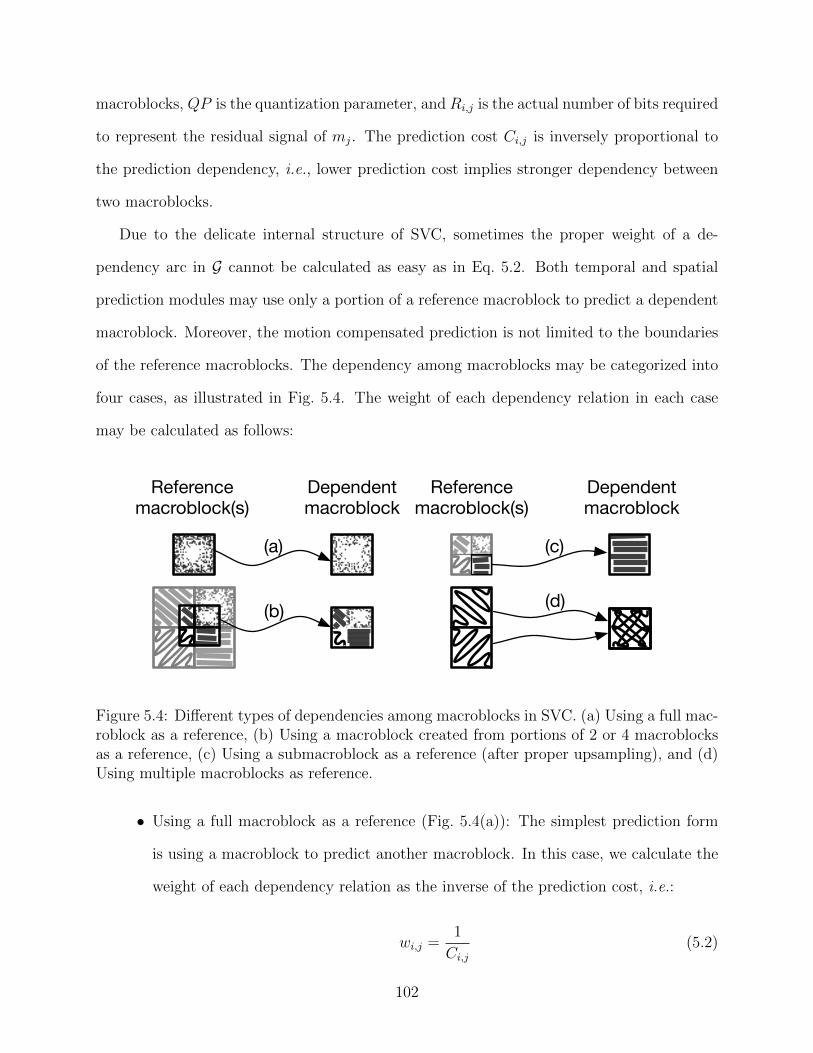
macroblocks, QP is the quantization parameter, and Ri,j is the actual number of bits required
to represent the residual signal of mj. The prediction cost Ci,j is inversely proportional to
the prediction dependency, i.e., lower prediction cost implies stronger dependency between
two macroblocks.
Due to the delicate internal structure of SVC, sometimes the proper weight of a de-
pendency arc in G cannot be calculated as easy as in Eq. 5.2. Both temporal and spatial
prediction modules may use only a portion of a reference macroblock to predict a dependent
macroblock. Moreover, the motion compensated prediction is not limited to the boundaries
of the reference macroblocks. The dependency among macroblocks may be categorized into
four cases, as illustrated in Fig. 5.4. The weight of each dependency relation in each case
may be calculated as follows:
Reference macroblock(s)
Dependentmacroblock
(a)
(b)
Reference macroblock(s)
Dependent macroblock
(c)
(d)
Figure 5.4: Different types of dependencies among macroblocks in SVC. (a) Using a full mac-roblock as a reference, (b) Using a macroblock created from portions of 2 or 4 macroblocksas a reference, (c) Using a submacroblock as a reference (after proper upsampling), and (d)Using multiple macroblocks as reference.
• Using a full macroblock as a reference (Fig. 5.4(a)): The simplest prediction form
is using a macroblock to predict another macroblock. In this case, we calculate the
weight of each dependency relation as the inverse of the prediction cost, i.e.:
wi,j =1
Ci,j(5.2)
102
• Using a macroblock created from portions of 2 or 4 macroblocks as a reference
(Fig. 5.4(b)): The prediction modules may use a 16 × 16 area located on the bor-
ders of two or four macroblocks as a reference macroblock. In this case, we add a
dependency arc from the dependent macroblock to each of the macroblocks serving
as a partial reference. The weight of each dependency arc is calculated as follows:
wi,j =1
Ci,j× Si,j
256(5.3)
where Si,j is the number of pixels of the reference macroblock that belongs to mi.
Compared to Eqn. 5.2, the weight of each arc representing a partial dependency is
scaled according to the amount of visual information in the dependent macroblock
predicted from the partial reference.
• Using a submacroblock as reference (after proper upsampling) (Fig. 5.4(c)): A sub-
macroblock may be upsampled to serve as a whole reference macroblock. If the
reference submacroblock belongs to a macroblock, there is only one arc from the
dependent macroblock to the macroblock containing the reference submacroblock,
as illustrated in Fig. 5.4(c). In this case, the weight of the arc is calculated the same
way as in the case that a full macroblock is used as a reference. Thus, the weight of
the arc is calculated as in Eqn. 5.2. If the reference submacroblock is located across
boundaries of 2 or 4 macroblocks, similar to the case illustrated in Fig. 5.4(b), we
add a dependency arc from the dependent macroblock to each of the macroblocks
serving as a partial reference. The weight of each dependency arc is calculated as
in Eqn. 5.3, except that the constant in the denominator is 64 (representing the
smaller size of 8× 8 co-located submacroblock).
• Using multiple macroblocks as reference (Fig. 5.4(d)): A dependent macroblock
may use multiple reference macroblocks and combine the result by, for example,
103
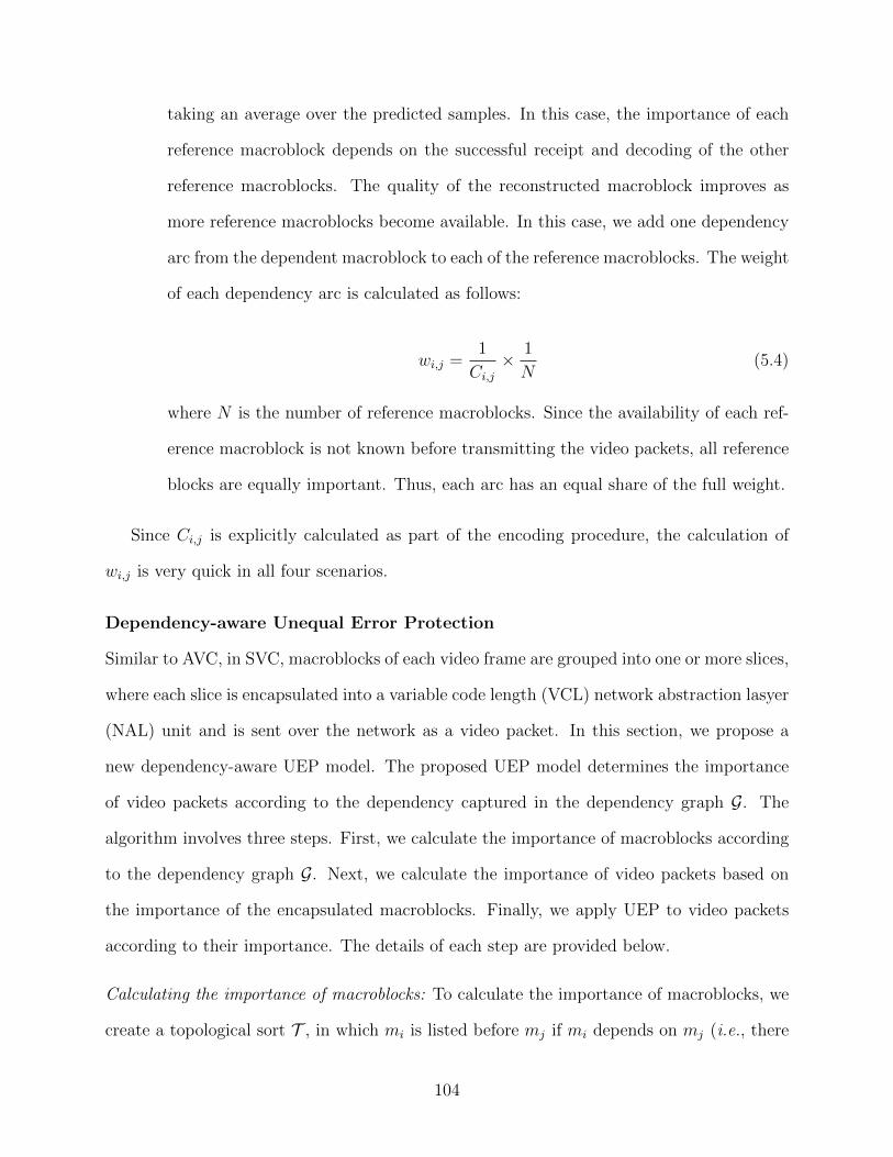
taking an average over the predicted samples. In this case, the importance of each
reference macroblock depends on the successful receipt and decoding of the other
reference macroblocks. The quality of the reconstructed macroblock improves as
more reference macroblocks become available. In this case, we add one dependency
arc from the dependent macroblock to each of the reference macroblocks. The weight
of each dependency arc is calculated as follows:
wi,j =1
Ci,j× 1
N(5.4)
where N is the number of reference macroblocks. Since the availability of each ref-
erence macroblock is not known before transmitting the video packets, all reference
blocks are equally important. Thus, each arc has an equal share of the full weight.
Since Ci,j is explicitly calculated as part of the encoding procedure, the calculation of
wi,j is very quick in all four scenarios.
Dependency-aware Unequal Error Protection
Similar to AVC, in SVC, macroblocks of each video frame are grouped into one or more slices,
where each slice is encapsulated into a variable code length (VCL) network abstraction lasyer
(NAL) unit and is sent over the network as a video packet. In this section, we propose a
new dependency-aware UEP model. The proposed UEP model determines the importance
of video packets according to the dependency captured in the dependency graph G. The
algorithm involves three steps. First, we calculate the importance of macroblocks according
to the dependency graph G. Next, we calculate the importance of video packets based on
the importance of the encapsulated macroblocks. Finally, we apply UEP to video packets
according to their importance. The details of each step are provided below.
Calculating the importance of macroblocks: To calculate the importance of macroblocks, we
create a topological sort T , in which mi is listed before mj if mi depends on mj (i.e., there
104
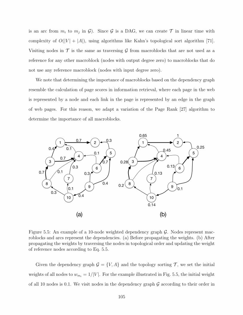
is an arc from mi to mj in G). Since G is a DAG, we can create T in linear time with
complexity of O(|V | + |A|), using algorithms like Kahn’s topological sort algorithm [71].
Visiting nodes in T is the same as traversing G from macroblocks that are not used as a
reference for any other macroblock (nodes with output degree zero) to macroblocks that do
not use any reference macroblock (nodes with input degree zero).
We note that determining the importance of macroblocks based on the dependency graph
resemble the calculation of page scores in information retrieval, where each page in the web
is represented by a node and each link in the page is represented by an edge in the graph
of web pages. For this reason, we adapt a variation of the Page Rank [27] algorithm to
determine the importance of all macroblocks.
21
4
6
7
9
3
5
10
8
0.65 1
0.28
0.45 0.25
0.130.13
0.20.1
0.14
21
4
6
7
9
3
5
10
8
0.4
0.4
0.7
0.7
0.7
0.7
0.4
0.3
0.3
0.3
0.1
0.1
0.1
0.1
0.3
(a) (b)
Figure 5.5: An example of a 10-node weighted dependency graph G. Nodes represent mac-roblocks and arcs represent the dependencies. (a) Before propagating the weights. (b) Afterpropagating the weights by traversing the nodes in topological order and updating the weightof reference nodes according to Eq. 5.5.
Given the dependency graph G = {V,A} and the topology sorting T , we set the initial
weights of all nodes to wmi= 1/|V |. For the example illustrated in Fig. 5.5, the initial weight
of all 10 nodes is 0.1. We visit nodes in the dependency graph G according to their order in
105
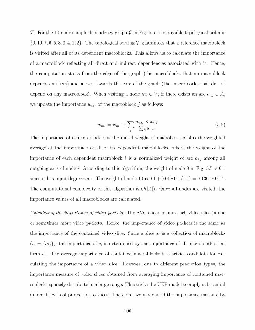
T . For the 10-node sample dependency graph G in Fig. 5.5, one possible topological order is
{9, 10, 7, 6, 5, 8, 3, 4, 1, 2}. The topological sorting T guarantees that a reference macroblock
is visited after all of its dependent macroblocks. This allows us to calculate the importance
of a macroblock reflecting all direct and indirect dependencies associated with it. Hence,
the computation starts from the edge of the graph (the macroblocks that no macroblock
depends on them) and moves towards the core of the graph (the macroblocks that do not
depend on any macroblock). When visiting a node mi ∈ V , if there exists an arc ai,j ∈ A,
we update the importance wmjof the macroblock j as follows:
wmj= wmj
+∑i
wmi× wi,j∑k wi,k
(5.5)
The importance of a macroblock j is the initial weight of macroblock j plus the weighted
average of the importance of all of its dependent macroblocks, where the weight of the
importance of each dependent macroblock i is a normalized weight of arc ai,j among all
outgoing arcs of node i. According to this algorithm, the weight of node 9 in Fig. 5.5 is 0.1
since it has input degree zero. The weight of node 10 is 0.1 + (0.4 ∗ 0.1/1.1) = 0.136 ' 0.14.
The computational complexity of this algorithm is O(|A|). Once all nodes are visited, the
importance values of all macroblocks are calculated.
Calculating the importance of video packets: The SVC encoder puts each video slice in one
or sometimes more video packets. Hence, the importance of video packets is the same as
the importance of the contained video slice. Since a slice si is a collection of macroblocks
(si = {mj}), the importance of si is determined by the importance of all macroblocks that
form si. The average importance of contained macroblocks is a trivial candidate for cal-
culating the importance of a video slice. However, due to different prediction types, the
importance measure of video slices obtained from averaging importance of contained mac-
roblocks sparsely distribute in a large range. This tricks the UEP model to apply substantial
different levels of protection to slices. Therefore, we moderated the importance measure by
106
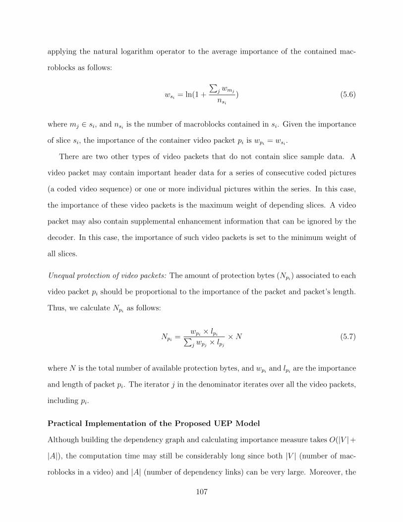
applying the natural logarithm operator to the average importance of the contained mac-
roblocks as follows:
wsi = ln(1 +
∑j wmj
nsi) (5.6)
where mj ∈ si, and nsi is the number of macroblocks contained in si. Given the importance
of slice si, the importance of the container video packet pi is wpi = wsi .
There are two other types of video packets that do not contain slice sample data. A
video packet may contain important header data for a series of consecutive coded pictures
(a coded video sequence) or one or more individual pictures within the series. In this case,
the importance of these video packets is the maximum weight of depending slices. A video
packet may also contain supplemental enhancement information that can be ignored by the
decoder. In this case, the importance of such video packets is set to the minimum weight of
all slices.
Unequal protection of video packets: The amount of protection bytes (Npi) associated to each
video packet pi should be proportional to the importance of the packet and packet’s length.
Thus, we calculate Npi as follows:
Npi =wpi × lpi∑j wpj × lpj
×N (5.7)
where N is the total number of available protection bytes, and wpi and lpi are the importance
and length of packet pi. The iterator j in the denominator iterates over all the video packets,
including pi.
Practical Implementation of the Proposed UEP Model
Although building the dependency graph and calculating importance measure takes O(|V |+
|A|), the computation time may still be considerably long since both |V | (number of mac-
roblocks in a video) and |A| (number of dependency links) can be very large. Moreover, the
107
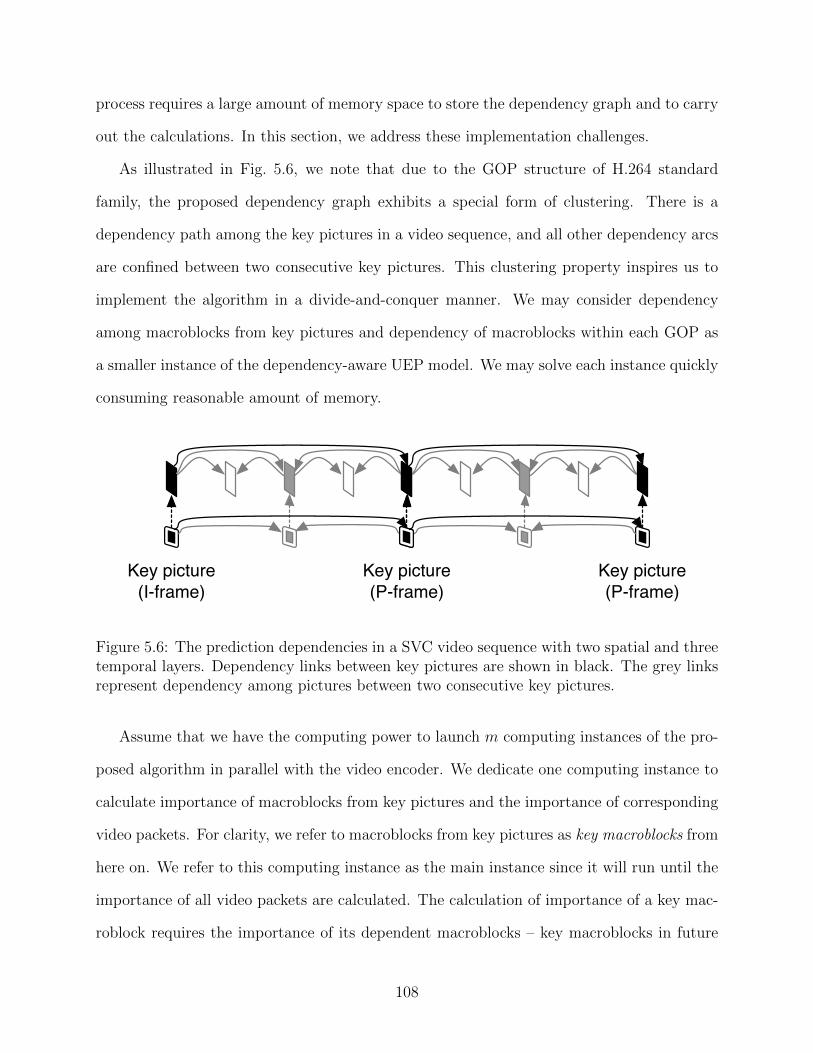
process requires a large amount of memory space to store the dependency graph and to carry
out the calculations. In this section, we address these implementation challenges.
As illustrated in Fig. 5.6, we note that due to the GOP structure of H.264 standard
family, the proposed dependency graph exhibits a special form of clustering. There is a
dependency path among the key pictures in a video sequence, and all other dependency arcs
are confined between two consecutive key pictures. This clustering property inspires us to
implement the algorithm in a divide-and-conquer manner. We may consider dependency
among macroblocks from key pictures and dependency of macroblocks within each GOP as
a smaller instance of the dependency-aware UEP model. We may solve each instance quickly
consuming reasonable amount of memory.
Key picture(I-frame)
Key picture(P-frame)
Key picture(P-frame)
Figure 5.6: The prediction dependencies in a SVC video sequence with two spatial and threetemporal layers. Dependency links between key pictures are shown in black. The grey linksrepresent dependency among pictures between two consecutive key pictures.
Assume that we have the computing power to launch m computing instances of the pro-
posed algorithm in parallel with the video encoder. We dedicate one computing instance to
calculate importance of macroblocks from key pictures and the importance of corresponding
video packets. For clarity, we refer to macroblocks from key pictures as key macroblocks from
here on. We refer to this computing instance as the main instance since it will run until the
importance of all video packets are calculated. The calculation of importance of a key mac-
roblock requires the importance of its dependent macroblocks – key macroblocks in future
108
GOPs and macroblocks within the same GOP. Recursively, the calculation of the importance
of a key macroblock in a future GOP also requires the importance of key macroblocks in
its future GOPs and macroblocks within the same GOP. The recursive relation still requires
the main instance to consider all macroblocks in a video sequence. Thus, this instance re-
quires large computing and memory resources. We note that the indirect dependencies decay
rapidly when the playback times of two key pictures are further apart. Therefore, when cal-
culating importance of macroblocks, the main instance can consider key macroblocks from n
future GOPs and ignore the subsequent ones. We refer to n as the key picture decay factor.
The value of n may be tuned according to visual features presented in the video sequence.
For example, when running the algorithm for high motion video sequences, n can be as small
as 4, because the visual similarity between consecutive video frames decays very fast.
When the video encoder proceeds with encoding the GOPs from the beginning of the
video, in parallel to the main instance of the proposed algorithm, each of the other m − 1
instances determines the importance of macroblocks within one GOP and the importance of
corresponding video packets. As soon as a computing instance has the importance of mac-
roblocks within one GOP, it passes the results to the main instance so that the importance
of key macroblocks of the GOP may be updated. Once the importance of key macroblocks
of GOPs 1 . . . n is updated, the main instance runs the algorithm on the key macroblocks of
GOPs 1 . . . n and finalizes the importance of key macroblocks and respective video packets
of GOP 1. GOP 1 is then removed from the graph. If n ≥ m − 1, the instance responsible
for GOP 1 is re-assigned to the next unprocessed GOP. The same process is repeated for
GOPs 2 . . . n + 1 and so on until all GOPs are removed from the graph. In this way, the
main instance always keeps track of macroblocks of at most n+1 key pictures, and the other
m− 1 instances always keep track of macroblocks of GOP size plus one pictures.
If n < m, when the importance of key macroblocks of GOP n is updated, the main
instance runs the algorithm on the key macroblocks of GOPs 1 . . . n and finalizes the impor-
109
tance of key macroblocks and respective video packets of GOP 1. Then it removes GOP 1
from the graph, frees the instance responsible for macroblocks of GOP 1, and associates the
next available GOP to this instance. In this way, the main instance always keeps track of
macroblocks of at most n + 1 key pictures and other m − 1 instances always keep track of
macroblocks of GOP size plus one pictures. When all GOPs are processed, the main instance
will also terminate.
Since the key picture decay factor truncates the continuity of the dependency in the
video sequence, the result is sub-optimal. In other words, we trade optimality for less com-
putational complexity and memory usage. For example, if we assume that each macroblock
has two outgoing links on average, the proposed algorithm needs 16 GB of memory to store
the dependency graph G for two hours of 24 fps HD video sequence. In comparison, the
divide-and-conquer implementation requires less than 7 MB of memory when the GOP size
and the parameter n are both equal to 8.
5.2.2 Performance Evaluation
To evaluate the performance of the proposed dependency-aware UEP model, we conduct a
series of experiments using JSVM 9.19.15 software package, which is the reference software
package for scalable video coding. As mentioned in Chapter 3, JSVM provides encoding,
decoding, and video analysis tools. As illustrated in Fig. 5.7, we added two modules (the
dependency logger module and the dependency graph module) to the SVC encoder provided
by JSVM. The dependency logger module is tapped into the main video coding modules of the
encoder, including GOP encoder, frame encoder, layer representation encoder, slice encoder,
and macroblock encoder. This module extracts all dependency information by monitoring
prediction and coding decisions during the encoding process. The dependency graph module
uses the macroblocks dependency information compiled by the dependency logger module to
generate the dependency graph as described in Sec. 5.2.1. This module also calculates the
importance of video packets using the algorithm we presented in the last section. We also
110
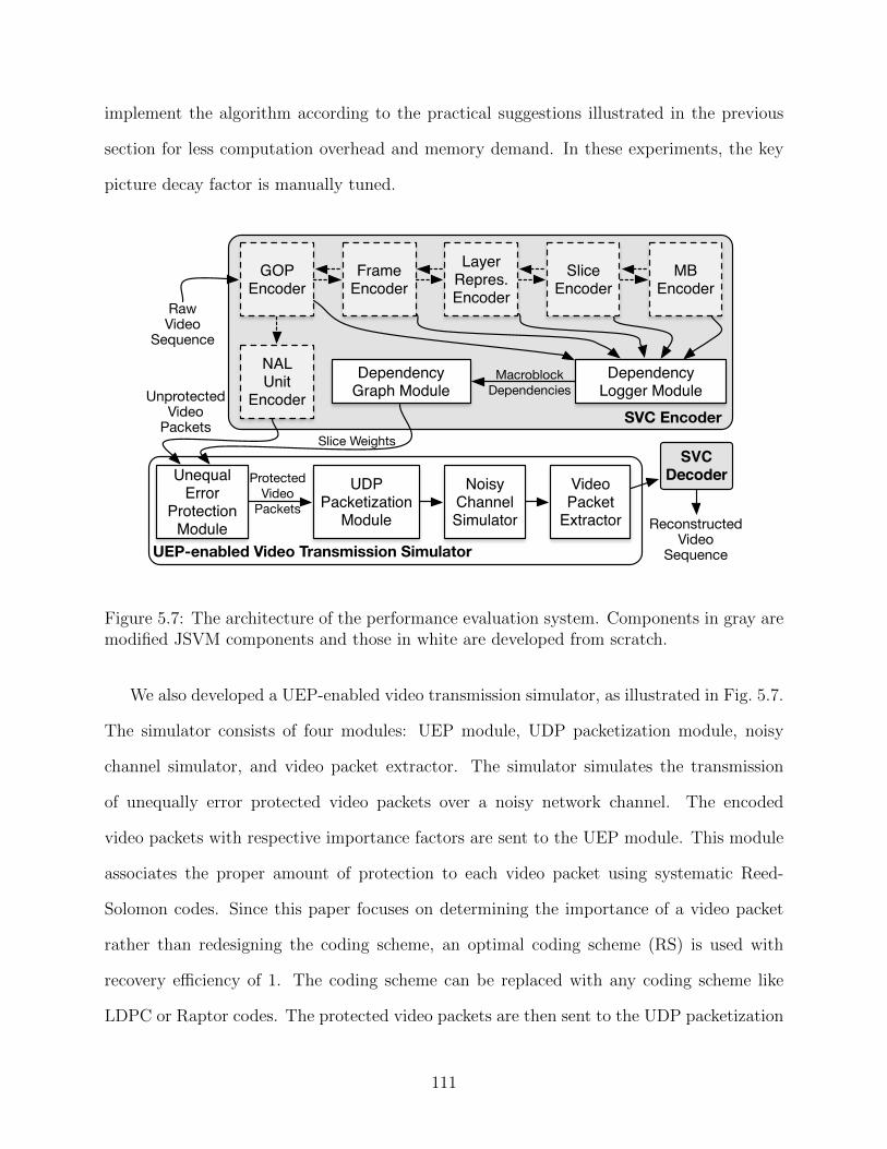
implement the algorithm according to the practical suggestions illustrated in the previous
section for less computation overhead and memory demand. In these experiments, the key
picture decay factor is manually tuned.
GOP Encoder
Frame Encoder
Layer Repres.Encoder
Slice Encoder
MB Encoder
Dependency Logger Module
SVC Encoder
Dependency Graph Module
Unequal Error
ProtectionModule
RawVideo
SequenceNAL Unit
Encoder
UEP-enabled Video Transmission Simulator
UnprotectedVideo
Packets
UDP Packetization
Module
Noisy Channel Simulator
ProtectedVideo
Packets
VideoPacket
Extractor
SVCDecoder
ReconstructedVideo
Sequence
MacroblockDependencies
Slice Weights
Figure 5.7: The architecture of the performance evaluation system. Components in gray aremodified JSVM components and those in white are developed from scratch.
We also developed a UEP-enabled video transmission simulator, as illustrated in Fig. 5.7.
The simulator consists of four modules: UEP module, UDP packetization module, noisy
channel simulator, and video packet extractor. The simulator simulates the transmission
of unequally error protected video packets over a noisy network channel. The encoded
video packets with respective importance factors are sent to the UEP module. This module
associates the proper amount of protection to each video packet using systematic Reed-
Solomon codes. Since this paper focuses on determining the importance of a video packet
rather than redesigning the coding scheme, an optimal coding scheme (RS) is used with
recovery efficiency of 1. The coding scheme can be replaced with any coding scheme like
LDPC or Raptor codes. The protected video packets are then sent to the UDP packetization
111
module. This module disperses each video packet in 512-byte UDP datagrams at a rate such
that the delay to the decoder is no more than 400 milliseconds [64]. The simulation can
be done in TCP as well. With TCP, although there is no end-to-end packet loss, a video
packet that arrives after its playback deadline (due to TCP flow or congestion control)
is considered lost by the decoder. Simulating the noisy channel in UDP gives us better
control on the packet loss rate. Next, UDP datagrams are virtually transmitted over a
packet erasure channel, where some packets are randomly dropped according to the channel’s
packet loss rate. We consider the error model an independent and identically distributed
random variable. On the receiver side, the video packets are extracted from the received
UDP datagrams, and the video stream is reconstructed using a SVC decoder. The decoder
is modified to calculate and report the peak signal-to-noise ratio of the reconstructed video.
The seven raw video sequences, as listed in Table 5.1, are selected from different genres.
They also exhibit diverse values of the detail and motion activity visual features [67]. As
described in Chapter 2, the detail feature provides a summary of the histogram descriptors in
the video sequence, and the motion activity feature primarily captures the degree or intensity
of scene changes. The reference raw video sequences are in YUV 4:2:0 format with frame
size of 1280×720 pixels and frame rate of 24 fps [3], the standard sampling scheme for H.26x
video coding standards. Since it takes hours to analyze a complete video and apply UEP,
we select 10 seconds (240 frames) of each video in order to conduct all experiments in a
reasonable amount of time. For video sequence that have movie titles at the beginning, i.e.,
BB and ED, the first 1000 frames are skipped. Otherwise, the frames are selected from the
beginning.
The modified JSVM package and the transmission simulator enabled us to conduct a
series of experiments to determine the effectiveness of the dependency-aware UEP model for
the seven reference videos. All experiments are conducted on a server cluster of 10 nodes.
Each server node is equipped with four Intelr Xeonr E5640 CPUs with four cores at 2.67
112
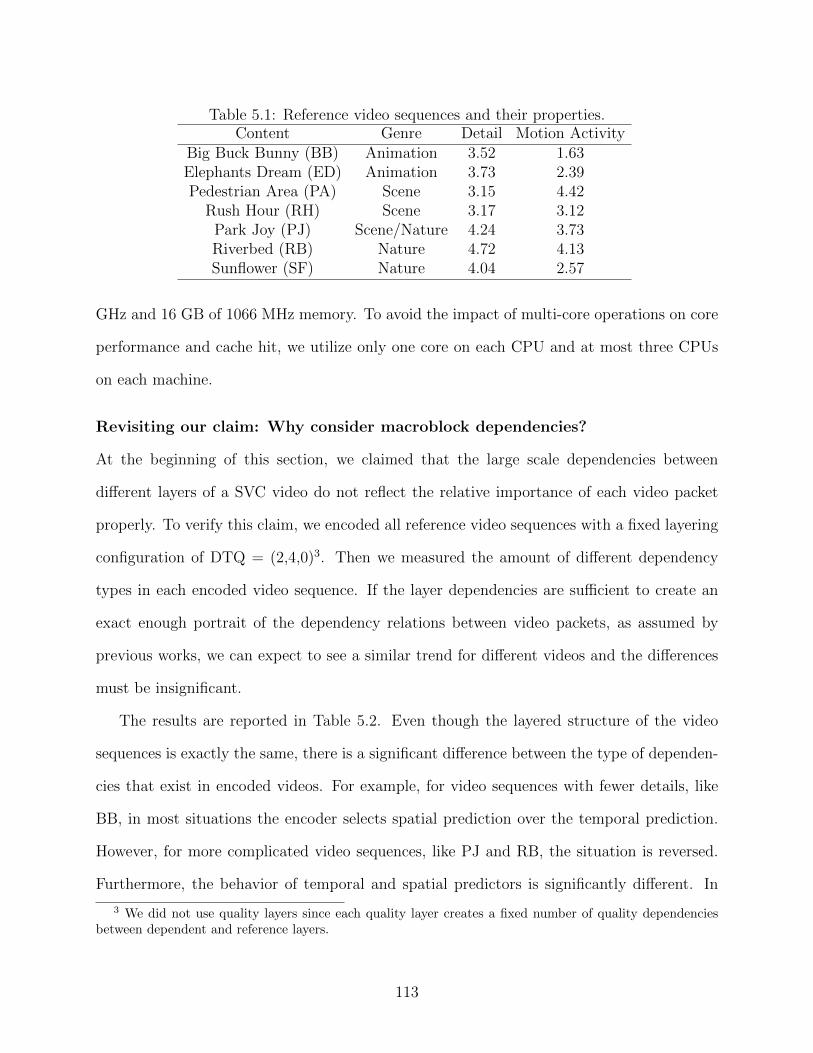
Table 5.1: Reference video sequences and their properties.Content Genre Detail Motion Activity
Big Buck Bunny (BB) Animation 3.52 1.63Elephants Dream (ED) Animation 3.73 2.39Pedestrian Area (PA) Scene 3.15 4.42
Rush Hour (RH) Scene 3.17 3.12Park Joy (PJ) Scene/Nature 4.24 3.73Riverbed (RB) Nature 4.72 4.13Sunflower (SF) Nature 4.04 2.57
GHz and 16 GB of 1066 MHz memory. To avoid the impact of multi-core operations on core
performance and cache hit, we utilize only one core on each CPU and at most three CPUs
on each machine.
Revisiting our claim: Why consider macroblock dependencies?
At the beginning of this section, we claimed that the large scale dependencies between
different layers of a SVC video do not reflect the relative importance of each video packet
properly. To verify this claim, we encoded all reference video sequences with a fixed layering
configuration of DTQ = (2,4,0)3. Then we measured the amount of different dependency
types in each encoded video sequence. If the layer dependencies are sufficient to create an
exact enough portrait of the dependency relations between video packets, as assumed by
previous works, we can expect to see a similar trend for different videos and the differences
must be insignificant.
The results are reported in Table 5.2. Even though the layered structure of the video
sequences is exactly the same, there is a significant difference between the type of dependen-
cies that exist in encoded videos. For example, for video sequences with fewer details, like
BB, in most situations the encoder selects spatial prediction over the temporal prediction.
However, for more complicated video sequences, like PJ and RB, the situation is reversed.
Furthermore, the behavior of temporal and spatial predictors is significantly different. In
3 We did not use quality layers since each quality layer creates a fixed number of quality dependenciesbetween dependent and reference layers.
113
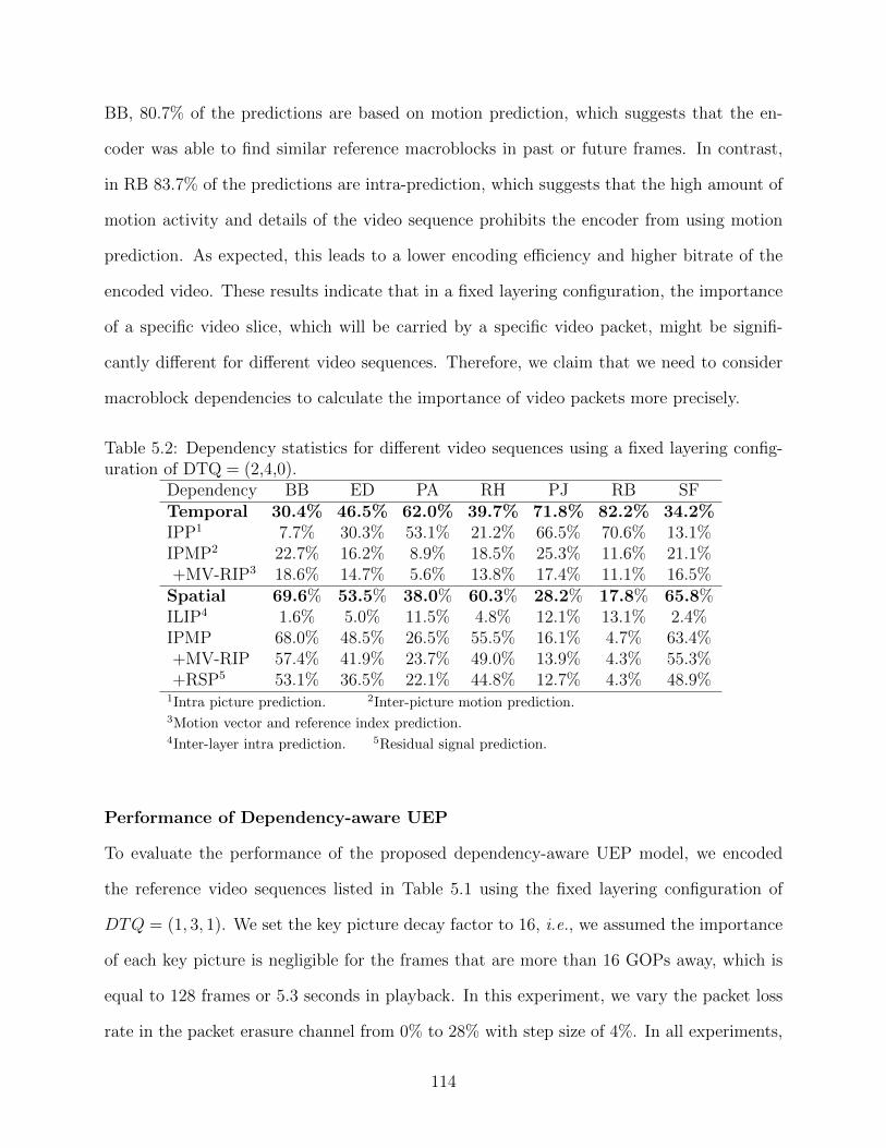
BB, 80.7% of the predictions are based on motion prediction, which suggests that the en-
coder was able to find similar reference macroblocks in past or future frames. In contrast,
in RB 83.7% of the predictions are intra-prediction, which suggests that the high amount of
motion activity and details of the video sequence prohibits the encoder from using motion
prediction. As expected, this leads to a lower encoding efficiency and higher bitrate of the
encoded video. These results indicate that in a fixed layering configuration, the importance
of a specific video slice, which will be carried by a specific video packet, might be signifi-
cantly different for different video sequences. Therefore, we claim that we need to consider
macroblock dependencies to calculate the importance of video packets more precisely.
Table 5.2: Dependency statistics for different video sequences using a fixed layering config-uration of DTQ = (2,4,0).
Dependency BB ED PA RH PJ RB SFTemporal 30.4% 46.5% 62.0% 39.7% 71.8% 82.2% 34.2%IPP1 7.7% 30.3% 53.1% 21.2% 66.5% 70.6% 13.1%IPMP2 22.7% 16.2% 8.9% 18.5% 25.3% 11.6% 21.1%+MV-RIP3 18.6% 14.7% 5.6% 13.8% 17.4% 11.1% 16.5%
Spatial 69.6% 53.5% 38.0% 60.3% 28.2% 17.8% 65.8%ILIP4 1.6% 5.0% 11.5% 4.8% 12.1% 13.1% 2.4%IPMP 68.0% 48.5% 26.5% 55.5% 16.1% 4.7% 63.4%+MV-RIP 57.4% 41.9% 23.7% 49.0% 13.9% 4.3% 55.3%+RSP5 53.1% 36.5% 22.1% 44.8% 12.7% 4.3% 48.9%
1Intra picture prediction. 2Inter-picture motion prediction.3Motion vector and reference index prediction.4Inter-layer intra prediction. 5Residual signal prediction.
Performance of Dependency-aware UEP
To evaluate the performance of the proposed dependency-aware UEP model, we encoded
the reference video sequences listed in Table 5.1 using the fixed layering configuration of
DTQ = (1, 3, 1). We set the key picture decay factor to 16, i.e., we assumed the importance
of each key picture is negligible for the frames that are more than 16 GOPs away, which is
equal to 128 frames or 5.3 seconds in playback. In this experiment, we vary the packet loss
rate in the packet erasure channel from 0% to 28% with step size of 4%. In all experiments,
114
the channel capacity is set to the video bitrate plus half of the expected packet loss rate
so that there is sufficient bandwidth to carry the video streaming and the corresponding
UEP data. To minimize vaiability in the results due to random packet drops, we virtually
transmitted each video sequence over the channel 10 times and report the average peak
signal-to-noise ratio (Y-PSNR) of the received video. In theory, due to better protection
of important video packets, the decoded videos should be in higher quality when using the
dependency-aware UEP model. For comparison purpose, we implement four other error
protection models:
• Equal error protection (EEP): All video packets are associated with the same im-
portance measure for equal protection.
• Packet-weighted UEP (PW-UEP): The importance of each video packet is propor-
tional to the number of bytes used to store the video packet [95, 96]. This model
also resembles similar models that use the number of bytes needed to represent a
slice or a frame as the importance measure of video packets.
• Layer-weighted UEP (LW-UEP): The importance of each layer is determined by
considering the layers that depend on it [53, 166]. This model also resembles the
UEP models based on error propagation zone as described in Sec. 2.2.
• Optimal model (Optimal UEP): The optimal UEP ensures that the most important
packets are always protected so that the distortion in playback is minimal. Hence,
only the least important packets are affected if losses occur during transmission. To
simulate the optimal model, we select and drop the video packets that cause the
least rate distortion. The number of packets to be dropped is determined by the
channel loss rate.
Implementation of EEP and PW-UEP is straight-forward. For LW-UEP, we use the
algorithm proposed in [53]. This algorithm involves solving the distortion optimization
115
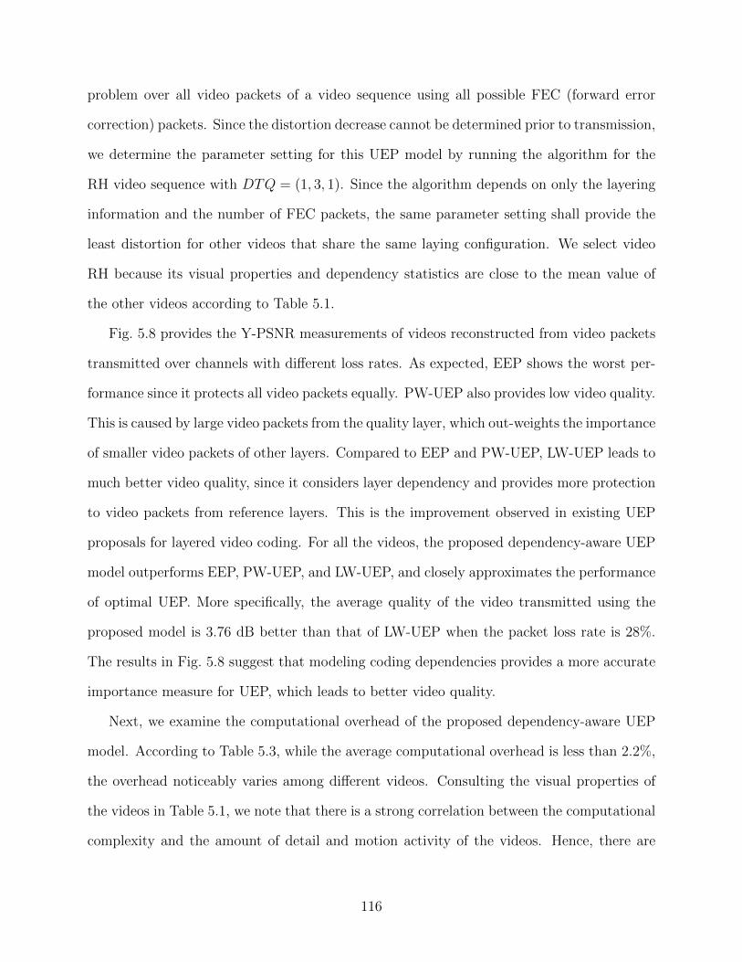
problem over all video packets of a video sequence using all possible FEC (forward error
correction) packets. Since the distortion decrease cannot be determined prior to transmission,
we determine the parameter setting for this UEP model by running the algorithm for the
RH video sequence with DTQ = (1, 3, 1). Since the algorithm depends on only the layering
information and the number of FEC packets, the same parameter setting shall provide the
least distortion for other videos that share the same laying configuration. We select video
RH because its visual properties and dependency statistics are close to the mean value of
the other videos according to Table 5.1.
Fig. 5.8 provides the Y-PSNR measurements of videos reconstructed from video packets
transmitted over channels with different loss rates. As expected, EEP shows the worst per-
formance since it protects all video packets equally. PW-UEP also provides low video quality.
This is caused by large video packets from the quality layer, which out-weights the importance
of smaller video packets of other layers. Compared to EEP and PW-UEP, LW-UEP leads to
much better video quality, since it considers layer dependency and provides more protection
to video packets from reference layers. This is the improvement observed in existing UEP
proposals for layered video coding. For all the videos, the proposed dependency-aware UEP
model outperforms EEP, PW-UEP, and LW-UEP, and closely approximates the performance
of optimal UEP. More specifically, the average quality of the video transmitted using the
proposed model is 3.76 dB better than that of LW-UEP when the packet loss rate is 28%.
The results in Fig. 5.8 suggest that modeling coding dependencies provides a more accurate
importance measure for UEP, which leads to better video quality.
Next, we examine the computational overhead of the proposed dependency-aware UEP
model. According to Table 5.3, while the average computational overhead is less than 2.2%,
the overhead noticeably varies among different videos. Consulting the visual properties of
the videos in Table 5.1, we note that there is a strong correlation between the computational
complexity and the amount of detail and motion activity of the videos. Hence, there are
116
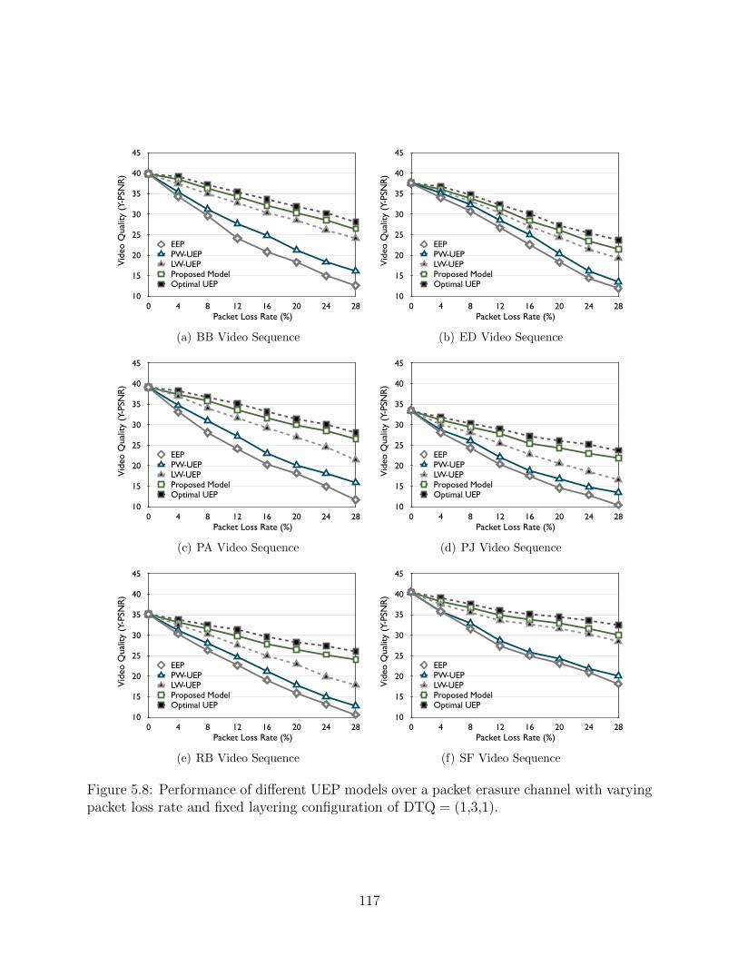
10
15
20
25
30
35
40
45
0 4 8 12 16 20 24 28
EEPPW-UEPLW-UEPProposed ModelOptimal UEP
Vid
eo Q
ualit
y (Y
-PSN
R)
Packet Loss Rate (%)
(a) BB Video Sequence
10
15
20
25
30
35
40
45
0 4 8 12 16 20 24 28
EEPPW-UEPLW-UEPProposed ModelOptimal UEP
Vid
eo Q
ualit
y (Y
-PSN
R)
Packet Loss Rate (%)
(b) ED Video Sequence
10
15
20
25
30
35
40
45
0 4 8 12 16 20 24 28
EEPPW-UEPLW-UEPProposed ModelOptimal UEP
Vid
eo Q
ualit
y (Y
-PSN
R)
Packet Loss Rate (%)
(c) PA Video Sequence
10
15
20
25
30
35
40
45
0 4 8 12 16 20 24 28
EEPPW-UEPLW-UEPProposed ModelOptimal UEP
Vid
eo Q
ualit
y (Y
-PSN
R)
Packet Loss Rate (%)
(d) PJ Video Sequence
10
15
20
25
30
35
40
45
0 4 8 12 16 20 24 28
EEPPW-UEPLW-UEPProposed ModelOptimal UEP
Vid
eo Q
ualit
y (Y
-PSN
R)
Packet Loss Rate (%)
(e) RB Video Sequence
10
15
20
25
30
35
40
45
0 4 8 12 16 20 24 28
EEPPW-UEPLW-UEPProposed ModelOptimal UEP
Vid
eo Q
ualit
y (Y
-PSN
R)
Packet Loss Rate (%)
(f) SF Video Sequence
Figure 5.8: Performance of different UEP models over a packet erasure channel with varyingpacket loss rate and fixed layering configuration of DTQ = (1,3,1).
117
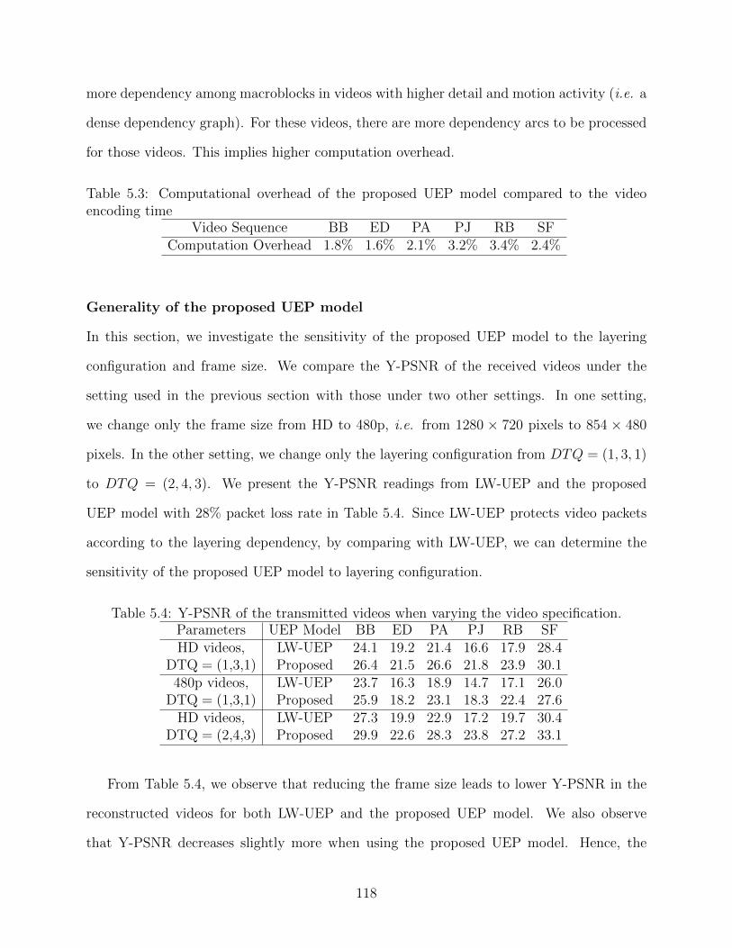
more dependency among macroblocks in videos with higher detail and motion activity (i.e. a
dense dependency graph). For these videos, there are more dependency arcs to be processed
for those videos. This implies higher computation overhead.
Table 5.3: Computational overhead of the proposed UEP model compared to the videoencoding time
Video Sequence BB ED PA PJ RB SFComputation Overhead 1.8% 1.6% 2.1% 3.2% 3.4% 2.4%
Generality of the proposed UEP model
In this section, we investigate the sensitivity of the proposed UEP model to the layering
configuration and frame size. We compare the Y-PSNR of the received videos under the
setting used in the previous section with those under two other settings. In one setting,
we change only the frame size from HD to 480p, i.e. from 1280 × 720 pixels to 854 × 480
pixels. In the other setting, we change only the layering configuration from DTQ = (1, 3, 1)
to DTQ = (2, 4, 3). We present the Y-PSNR readings from LW-UEP and the proposed
UEP model with 28% packet loss rate in Table 5.4. Since LW-UEP protects video packets
according to the layering dependency, by comparing with LW-UEP, we can determine the
sensitivity of the proposed UEP model to layering configuration.
Table 5.4: Y-PSNR of the transmitted videos when varying the video specification.Parameters UEP Model BB ED PA PJ RB SFHD videos, LW-UEP 24.1 19.2 21.4 16.6 17.9 28.4
DTQ = (1,3,1) Proposed 26.4 21.5 26.6 21.8 23.9 30.1480p videos, LW-UEP 23.7 16.3 18.9 14.7 17.1 26.0
DTQ = (1,3,1) Proposed 25.9 18.2 23.1 18.3 22.4 27.6HD videos, LW-UEP 27.3 19.9 22.9 17.2 19.7 30.4
DTQ = (2,4,3) Proposed 29.9 22.6 28.3 23.8 27.2 33.1
From Table 5.4, we observe that reducing the frame size leads to lower Y-PSNR in the
reconstructed videos for both LW-UEP and the proposed UEP model. We also observe
that Y-PSNR decreases slightly more when using the proposed UEP model. Hence, the
118
proposed UEP model is more sensitive to changes in frame size. When changing the layering
configuration from DTQ = (1, 3, 1) to DTQ = (2, 4, 3), the video bitrate increases, resulting
in higher video quality. According to Table 5.4, increasing the number of layers improves
the Y-PSNR by 1.61 dB and 2.43 dB on average for LW-UEP model and the proposed
model, respectively. The change also increases the gap between the average quality from
these two models, from 3.76 dB to 4.58 dB. This is because increasing the number of layers
introduces more macroblocks and more dependency relationships. In this case, the proposed
dependency-aware UEP model provides more precise UEP for video packets than LW-UEP
does.
5.3 Adaptive FEC for Layered Video Multicast
In Sec. 5.2, we proposed a novel method to calculate the importance of video packets of
different video layers more precisely. Through the experimental results, we also demonstrated
the better performance of the proposed model compared to other state-of-the-art UEP models
suggested for layered video coding. Layered video coding can be used in a video unicast
scenario (where the video is prepared and sent by the media server toward a specific end
user device) to address the fluctuation in channel bandwidth and packet loss rate. However,
the full capabilities of layered video coding can be used in a video multicast scenario, when a
single layered video is prepared by the media streamer and different groups of mobile devices
with similar connectivity, usually referred to as multicast groups, are receiving different
number of video layers according to their conditions. Again, the number of layers received
by each multicast group might change according to the connection quality.
In a mobile communication network, the last mile antenna uses heterogeneous wireless
channels with fluctuating capacity and packet loss rate for video multicast. Furthermore, the
mobile devices have different antenna, computation, display and battery capabilities. There-
fore, a proper video multicast solution must consider efficient use of the wireless channels
119
along with providing good quality of experience for the devices with heterogeneous capabili-
ties. Last but not least, the energy consumption of the devices connected to these networks
must be considered as a critical resource. In this section, we propose an adaptive video
multicast system that delivers layered video content to mobile devices through a mobile
communication network. The proposed system serves as an adaptive error protection layer
over the unequal error protection model suggested for video streaming unicast in Sec. 5.2.
To this end, a novel design is proposed to use the calculated importance of video packets
and prepare the redundant coded blocks needed for forward error correction in a multicast
video streaming scenario. Furthermore, this design makes the system flexible to dynamic
changes in channel loss rate with minimum coding overhead. Specifically, the employed
coding scheme is empowered by a novel structure for the coefficient matrix that decreases
the delay and the computational complexity of coding operations. The experimental results
show that the new system offers a flexible streaming service, decreases the computational
cost of preparing the FEC codes, significantly decreases the video transmission delay, and
conserves energy on mobile devices.
5.3.1 Adaptive FEC for Video Multicast
The proposed adaptive video streaming system utilizes three key enabling techniques: layered
video coding, erasure codes for forward error correction, and a novel mechanism to generate
the required coded blocks for forward error correction. Without loss of generality, we assume
that the multicast video is prepared in a number of layers, where the base layer is needed
to decode the video, and enhancement layers, if received successfully, improves the video
quality. Hence, the more layers a device receives, the higher the quality that the video is
played at. Mobile devices may determine the number of desired layers based on the network
connectivity, battery lifetime, other resources availability, or user preference. Since such an
algorithm is orthogonal to the proposed model, we assume that the desired number of layers
120
is known a priori in our system. Within each layer, a segment represents a time slice of the
video playback (say 1 second), which encompasses one or more video packets. Furthermore,
we assume that the proportional importance of each video packet is determined by the model
proposed in Sec. 5.2. Hence, the importance of the video segment can be calculated from
the contained video packets as shown in Eq. 5.6.
Similar to the existing proposals for using erasure codes in wireless communication [13,19],
we employ systematic erasure codes to cope with channel losses. This in turn also reduces
energy consumption and delay due to fewer decoding operations. However, the channel loss
may significantly vary over time. Unlike existing proposals, in order to dynamically ac-
commodate different loss rates, we adjust the level of coding according to the video stream
building blocks and the channel conditions. Towards this goal, an obvious solution is to
prepare coded packets for each loss rate at the source. The coded packets are then trans-
mitted according to the current loss rate in each channel. Such a solution is costly in terms
of computation needed to prepare the coded packets for each and every packet loss rate, let
aside the lateral problem of finding a proper step size for the packet loss rate. To address this
problem, our system generates the coded packets for each GOP in each layer in a progressive
manner that allows the streaming node to combine as few as possible video packets together
and serve the coded blocks according to the channel loss rate.
Adaptive Transmission of Protection Blocks
Given the sporadic losses in wireless channels, the media streaming server (or the edge media
server located at the edge of the network) is supposed to be capable of sending each layer of
the video with an arbitrary level of redundancy. For this reason, we propose a fine granular
coding scheme that adaptively produces data blocks and coded blocks for any loss rate. As
depicted in Fig. 5.9, each layer is divided into a sequence of segments, each consisting of
one or more GOPs. Each GOP is further divided into m blocks, denoted by white blocks
121
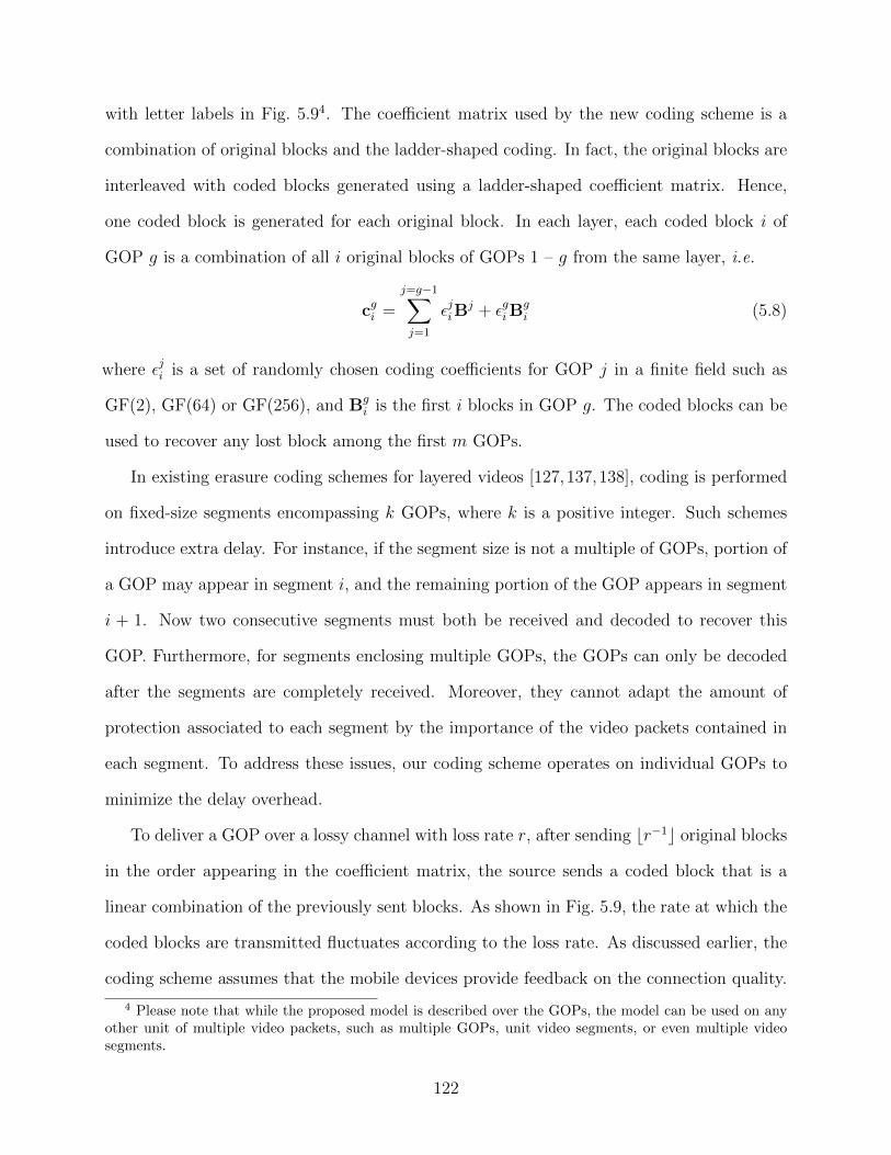
with letter labels in Fig. 5.94. The coefficient matrix used by the new coding scheme is a
combination of original blocks and the ladder-shaped coding. In fact, the original blocks are
interleaved with coded blocks generated using a ladder-shaped coefficient matrix. Hence,
one coded block is generated for each original block. In each layer, each coded block i of
GOP g is a combination of all i original blocks of GOPs 1 – g from the same layer, i.e.
cgi =
j=g−1∑j=1
εjiBj + εgiB
gi (5.8)
where εji is a set of randomly chosen coding coefficients for GOP j in a finite field such as
GF(2), GF(64) or GF(256), and Bgi is the first i blocks in GOP g. The coded blocks can be
used to recover any lost block among the first m GOPs.
In existing erasure coding schemes for layered videos [127,137,138], coding is performed
on fixed-size segments encompassing k GOPs, where k is a positive integer. Such schemes
introduce extra delay. For instance, if the segment size is not a multiple of GOPs, portion of
a GOP may appear in segment i, and the remaining portion of the GOP appears in segment
i + 1. Now two consecutive segments must both be received and decoded to recover this
GOP. Furthermore, for segments enclosing multiple GOPs, the GOPs can only be decoded
after the segments are completely received. Moreover, they cannot adapt the amount of
protection associated to each segment by the importance of the video packets contained in
each segment. To address these issues, our coding scheme operates on individual GOPs to
minimize the delay overhead.
To deliver a GOP over a lossy channel with loss rate r, after sending br−1c original blocks
in the order appearing in the coefficient matrix, the source sends a coded block that is a
linear combination of the previously sent blocks. As shown in Fig. 5.9, the rate at which the
coded blocks are transmitted fluctuates according to the loss rate. As discussed earlier, the
coding scheme assumes that the mobile devices provide feedback on the connection quality.
4 Please note that while the proposed model is described over the GOPs, the model can be used on anyother unit of multiple video packets, such as multiple GOPs, unit video segments, or even multiple videosegments.
122
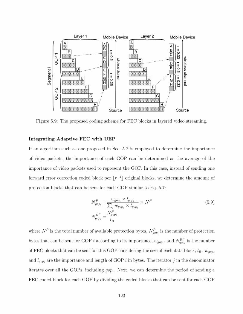
A
B
C
D
E
F
G
H
GO
P 1
Layer 1
GO
P 2
Segm
ent i
A
B
C
D
E
F
G
H
Layer 2
AB
CD
EFGH
ABC
DE
FGH
Mobile Device
Source
wireless channel
r = 0.5r = 0.25
Mobile Device
Source
wireless channelr = 0.33
r = 0.33r = 0.5
Figure 5.9: The proposed coding scheme for FEC blocks in layered video streaming.
Integrating Adaptive FEC with UEP
If an algorithm such as one proposed in Sec. 5.2 is employed to determine the importance
of video packets, the importance of each GOP can be determined as the average of the
importance of video packets used to represent the GOP. In this case, instead of sending one
forward error correction coded block per br−1c original blocks, we determine the amount of
protection blocks that can be sent for each GOP similar to Eq. 5.7:
NPgopi
=wgopi × lgopi∑j wgopj × lgopj
×NP (5.9)
NBP
gopi=NPgopi
lB
where NP is the total number of available protection bytes, NPgopi
is the number of protection
bytes that can be sent for GOP i according to its importance, wgopi , and NBP
gopiis the number
of FEC blocks that can be sent for this GOP considering the size of each data block, lB. wgopi
and lgopi are the importance and length of GOP i in bytes. The iterator j in the denominator
iterates over all the GOPs, including gopi. Next, we can determine the period of sending a
FEC coded block for each GOP by dividing the coded blocks that can be sent for each GOP
123
among its original blocks evenly, and sending the coded blocks interleaved with the original
blocks as described earlier.
The Choice of Coding Scheme
Reed-Solomon erasure codes perform coding operations in GF(256). However, due to the
field size, the encoding and decoding require matrix multiplication and inversion, which are
computationally expensive. To conserve energy on mobile devices while taking advantages
of erasure codes, we employ systematic Fountain codes in GF(2) in our coding scheme. The
encoding and decoding are simply XORing original blocks or coded blocks, respectively. The
coding coefficients are just 0’s and 1’s. For example, in Fig. 5.9, the coded block sent after
block A and block B for layer 1 is the XOR of the two blocks. If block B is lost during
transmission, it can be recovered by XORing block A and the coded block. Nonetheless, the
small field size increases the chance that the coded blocks are linearly dependent, making
the received coded blocks not decodable. For this reason, within each GOP, additional coded
blocks are produced by XORing a subset of blocks. It has been shown that for any number
of original data blocks k > 10, with α additional coded blocks the probability of decodability
of received k + α blocks is 1− 2−α [87].
In addition to the flexibility in adapting to loss rates over different wireless channels, the
proposed coding scheme has two other advantages over existing proposals. First, regardless
of the size of the finite field, the computational complexity is greatly reduced since the
main video content is delivered in its raw form. This means that decoding is only needed
when an original block is lost. More precisely, one decoding operation is needed for each
lost block. Second, the fine granular coding scheme is designed to minimize the delay due
to coding operations. Since a GOP is the smallest decodable unit that a media player
operates on, aligning the size of the decodable unit of the erasure codes to the same size
allows the GOPs to be delivered to the application as soon as possible. Hence, our proposed
coding scheme encourages progressive decoding by providing much more recovery points in
124
each video layer. This feature not only reduces the delay in decoding the video, but also
reduces energy consumed due to transmissions and computations, especially on resource-
scarce mobile devices.
5.3.2 Case Study: Application in a Mobile Network
In this section we tailor our streaming system to a state-of-the-art mobile communication
network. Specifically, the recent generations of mobile communication networks such as 4G
cellular networks use Orthogonal Frequency Division Multiple Access (OFDMA)-based multi-
carrier modulation in their downlinks. Hence, we apply our model to OFDMA to compare
its performance with other proposed FEC models for layered video multicast.
With OFDMA, the communication channel is divided into sub-channels. Sub-channels
with the same characteristics, including signal strength, loss rate, and coverage, are grouped
into a frequency range. Data packets are transmitted in sub-channels according to their
importance and the location of their destination [11]. In a live streaming session, the video
content is broadcast to all participating devices from the source, much like TV broadcasting.
Once the video content becomes available at the source, the coded blocks are computed and
stored. The original blocks and coded blocks are then pushed into the OFDMA network that
is responsible for delivering the blocks to mobile devices. Here, we explain how the blocks
are assigned to sub-channels in an OFDMA network for transmission.
In reality, an OFDMA network consists of thousands of sub-channels and many frequency
ranges. Without loss of generality and to keep the example illustrative, we assume that
there are eight 512 kbps sub-channels who are grouped into four frequency ranges. The area
covered by the OFDMA network is divided into four multicast groups with group 1 covered
by all four frequency ranges, group 2 covered by the first three frequency ranges, group 3
covered by the first two ranges, and group 4 covered by only the first range. The loss rate of
each range also varies from group to group. The group division and the corresponding loss
125
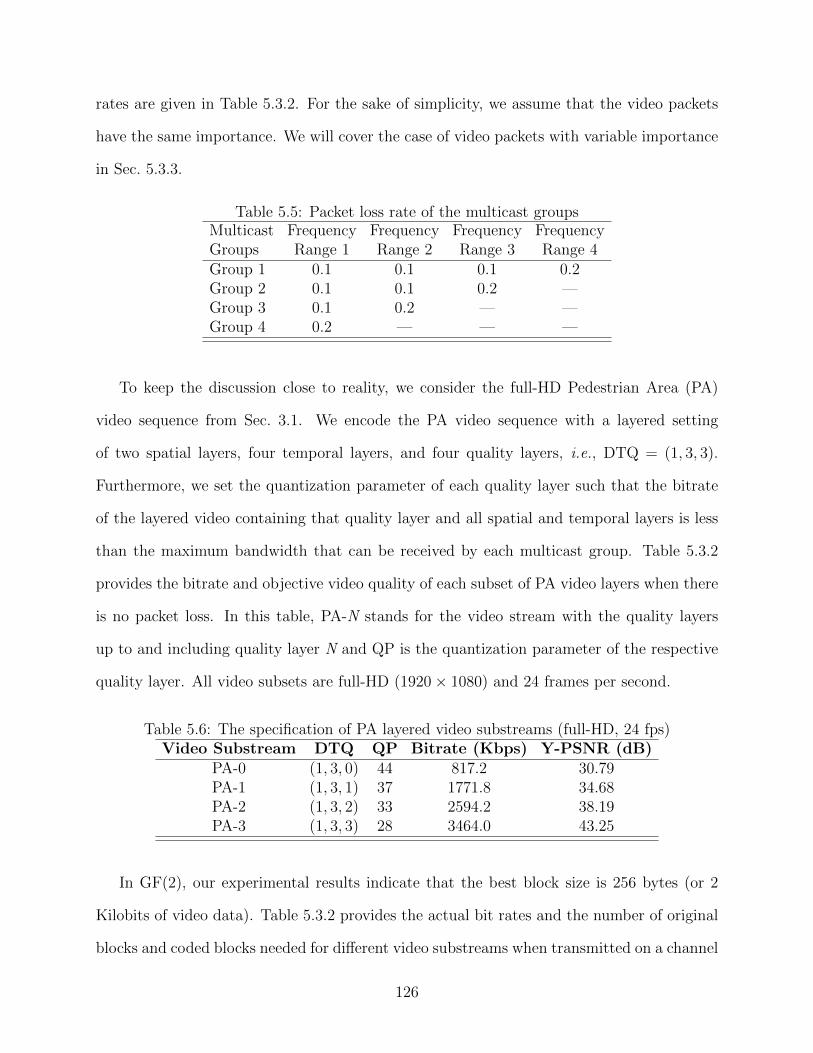
rates are given in Table 5.3.2. For the sake of simplicity, we assume that the video packets
have the same importance. We will cover the case of video packets with variable importance
in Sec. 5.3.3.
Table 5.5: Packet loss rate of the multicast groupsMulticast Frequency Frequency Frequency FrequencyGroups Range 1 Range 2 Range 3 Range 4Group 1 0.1 0.1 0.1 0.2Group 2 0.1 0.1 0.2 —Group 3 0.1 0.2 — —Group 4 0.2 — — —
To keep the discussion close to reality, we consider the full-HD Pedestrian Area (PA)
video sequence from Sec. 3.1. We encode the PA video sequence with a layered setting
of two spatial layers, four temporal layers, and four quality layers, i.e., DTQ = (1, 3, 3).
Furthermore, we set the quantization parameter of each quality layer such that the bitrate
of the layered video containing that quality layer and all spatial and temporal layers is less
than the maximum bandwidth that can be received by each multicast group. Table 5.3.2
provides the bitrate and objective video quality of each subset of PA video layers when there
is no packet loss. In this table, PA-N stands for the video stream with the quality layers
up to and including quality layer N and QP is the quantization parameter of the respective
quality layer. All video subsets are full-HD (1920× 1080) and 24 frames per second.
Table 5.6: The specification of PA layered video substreams (full-HD, 24 fps)Video Substream DTQ QP Bitrate (Kbps) Y-PSNR (dB)
PA-0 (1, 3, 0) 44 817.2 30.79PA-1 (1, 3, 1) 37 1771.8 34.68PA-2 (1, 3, 2) 33 2594.2 38.19PA-3 (1, 3, 3) 28 3464.0 43.25
In GF(2), our experimental results indicate that the best block size is 256 bytes (or 2
Kilobits of video data). Table 5.3.2 provides the actual bit rates and the number of original
blocks and coded blocks needed for different video substreams when transmitted on a channel
126
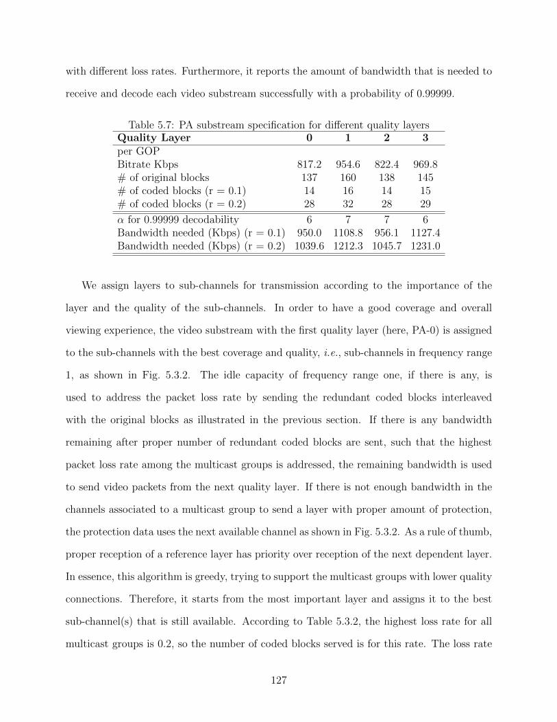
with different loss rates. Furthermore, it reports the amount of bandwidth that is needed to
receive and decode each video substream successfully with a probability of 0.99999.
Table 5.7: PA substream specification for different quality layersQuality Layer 0 1 2 3per GOPBitrate Kbps 817.2 954.6 822.4 969.8# of original blocks 137 160 138 145# of coded blocks (r = 0.1) 14 16 14 15# of coded blocks (r = 0.2) 28 32 28 29
α for 0.99999 decodability 6 7 7 6Bandwidth needed (Kbps) (r = 0.1) 950.0 1108.8 956.1 1127.4Bandwidth needed (Kbps) (r = 0.2) 1039.6 1212.3 1045.7 1231.0
We assign layers to sub-channels for transmission according to the importance of the
layer and the quality of the sub-channels. In order to have a good coverage and overall
viewing experience, the video substream with the first quality layer (here, PA-0) is assigned
to the sub-channels with the best coverage and quality, i.e., sub-channels in frequency range
1, as shown in Fig. 5.3.2. The idle capacity of frequency range one, if there is any, is
used to address the packet loss rate by sending the redundant coded blocks interleaved
with the original blocks as illustrated in the previous section. If there is any bandwidth
remaining after proper number of redundant coded blocks are sent, such that the highest
packet loss rate among the multicast groups is addressed, the remaining bandwidth is used
to send video packets from the next quality layer. If there is not enough bandwidth in the
channels associated to a multicast group to send a layer with proper amount of protection,
the protection data uses the next available channel as shown in Fig. 5.3.2. As a rule of thumb,
proper reception of a reference layer has priority over reception of the next dependent layer.
In essence, this algorithm is greedy, trying to support the multicast groups with lower quality
connections. Therefore, it starts from the most important layer and assigns it to the best
sub-channel(s) that is still available. According to Table 5.3.2, the highest loss rate for all
multicast groups is 0.2, so the number of coded blocks served is for this rate. The loss rate
127
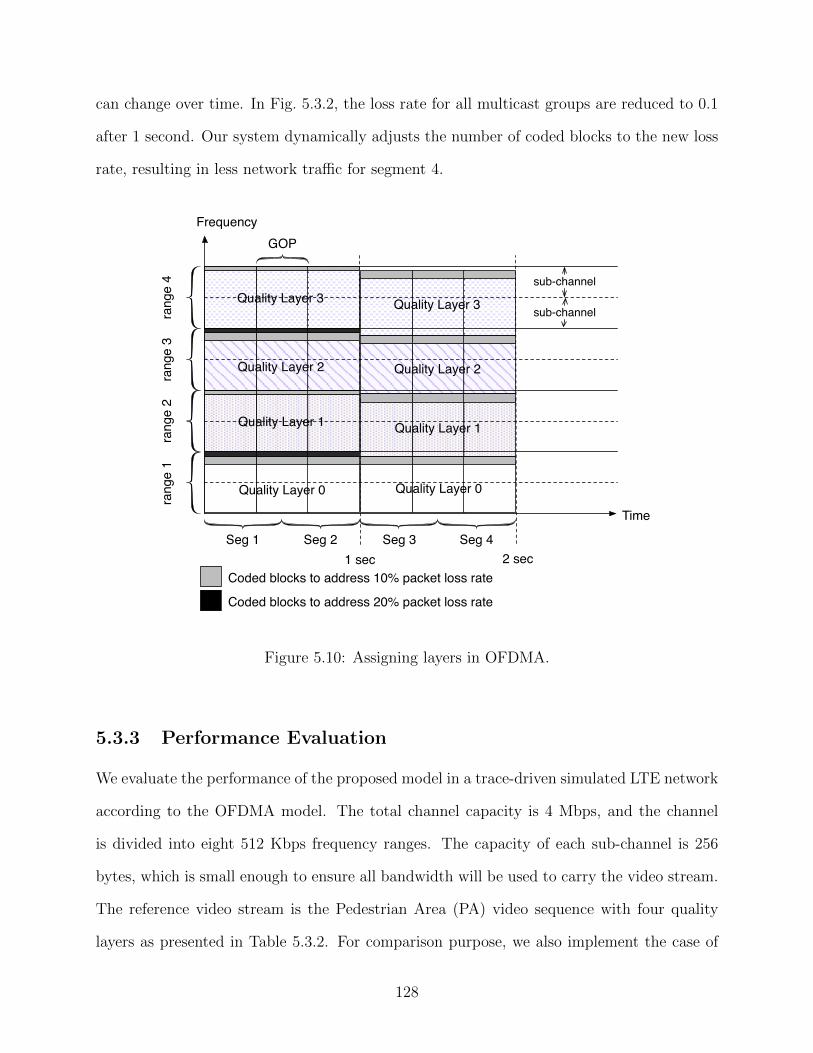
can change over time. In Fig. 5.3.2, the loss rate for all multicast groups are reduced to 0.1
after 1 second. Our system dynamically adjusts the number of coded blocks to the new loss
rate, resulting in less network traffic for segment 4.ra
nge
4
Frequency
rang
e 3
rang
e 2
rang
e 1
Seg 1
Time
1 sec 2 secSeg 2 Seg 4Seg 3
GOP
Quality Layer 0
Quality Layer 1
Quality Layer 2
Quality Layer 3
Quality Layer 0
Quality Layer 1
Quality Layer 2
Quality Layer 3sub-channel
sub-channel
Coded blocks to address 10% packet loss rate
Coded blocks to address 20% packet loss rate
Figure 5.10: Assigning layers in OFDMA.
5.3.3 Performance Evaluation
We evaluate the performance of the proposed model in a trace-driven simulated LTE network
according to the OFDMA model. The total channel capacity is 4 Mbps, and the channel
is divided into eight 512 Kbps frequency ranges. The capacity of each sub-channel is 256
bytes, which is small enough to ensure all bandwidth will be used to carry the video stream.
The reference video stream is the Pedestrian Area (PA) video sequence with four quality
layers as presented in Table 5.3.2. For comparison purpose, we also implement the case of
128
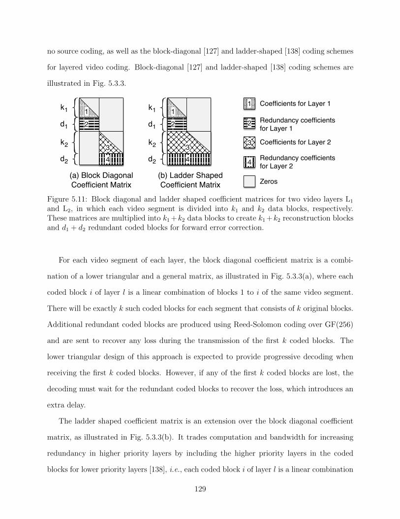
no source coding, as well as the block-diagonal [127] and ladder-shaped [138] coding schemes
for layered video coding. Block-diagonal [127] and ladder-shaped [138] coding schemes are
illustrated in Fig. 5.3.3.
(a) Block DiagonalCoefficient Matrix
k1
d1
k2
d2
12
34
(b) Ladder ShapedCoefficient Matrix
k1
d1
k2
d2
12
34
Coefficients for Layer 1
Coefficients for Layer 2
Redundancy coefficientsfor Layer 1
Zeros
Redundancy coefficientsfor Layer 2
1
2
3
4
Figure 5.11: Block diagonal and ladder shaped coefficient matrices for two video layers L1
and L2, in which each video segment is divided into k1 and k2 data blocks, respectively.These matrices are multiplied into k1 +k2 data blocks to create k1 +k2 reconstruction blocksand d1 + d2 redundant coded blocks for forward error correction.
For each video segment of each layer, the block diagonal coefficient matrix is a combi-
nation of a lower triangular and a general matrix, as illustrated in Fig. 5.3.3(a), where each
coded block i of layer l is a linear combination of blocks 1 to i of the same video segment.
There will be exactly k such coded blocks for each segment that consists of k original blocks.
Additional redundant coded blocks are produced using Reed-Solomon coding over GF(256)
and are sent to recover any loss during the transmission of the first k coded blocks. The
lower triangular design of this approach is expected to provide progressive decoding when
receiving the first k coded blocks. However, if any of the first k coded blocks are lost, the
decoding must wait for the redundant coded blocks to recover the loss, which introduces an
extra delay.
The ladder shaped coefficient matrix is an extension over the block diagonal coefficient
matrix, as illustrated in Fig. 5.3.3(b). It trades computation and bandwidth for increasing
redundancy in higher priority layers by including the higher priority layers in the coded
blocks for lower priority layers [138], i.e., each coded block i of layer l is a linear combination
129
of blocks from the same video segment in layers 1 to l−1 and blocks 1 to i in layer l. Hence,
the base layer of SVC is decodable with higher probability since it is included in every coded
block.
As can be seen in Fig. 5.3.3, the block-diagonal coding is applied across GOPs, and the
ladder-shaped coding is applied across GOPs and layers. To keep the comparison fair, we
use systematic random linear Fountain coding [87] over GF(2) for all the methods. The
block size is set to 256 byte and α for Fountain code is set to 16 for every 256 blocks for
99.999% of decodability, i.e., for each 16 blocks one block has been added to compensate
for probable linear dependent coded blocks. Each video segment represents 1 second of the
video playback and contains three GOPs, where according to Table 5.3.2 each GOP requires
137 — 160 original blocks for different quality layers.
In order to keep the simulation close to reality, we design the simulator to use traces of
packet loss rate from a real mobile network and the energy profile from a Samsung Galaxy
Nexus I9250 smartphone. We recorded the loss rate every second while driving around in a
car. The recorded packet loss rate trace is provided in Fig. 5.3.3. We use the same channel
division given in Table 5.3.2 of Sec. 4.2, in which the loss rate in the low-quality sub-channels
is twice that in the high-quality sub-channels. The reference smartphone was equipped with
a dual-core 1.2 GHz processor, 1 GB of memory, a 1750 mAh Li-Ion battery, and Android 4.2
(Jelly Bean) as the operating system. The measured energy profile is reported in Table 5.3.3.
Table 5.8: Energy profile of the reference mobile device.Energy Consumption (per GB)
4G Download 11.3297%GF(2) Decoding 0.0613%GF(256) Decoding 3.6193%
Video Quality Performance
We begin the evaluation with the objective quality of the transmitted video offered by each
coding scheme when varying the loss rate from 0 to 0.2 in all frequency ranges. We observe
130
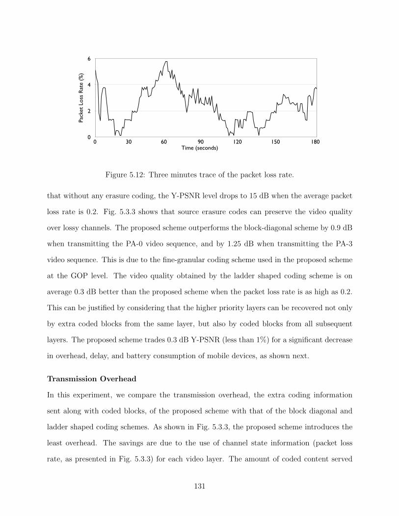
Pack
et L
oss
Rat
e (%
)
0
2
4
6
0 30 60 90 120 150 180Time (seconds)
Figure 5.12: Three minutes trace of the packet loss rate.
that without any erasure coding, the Y-PSNR level drops to 15 dB when the average packet
loss rate is 0.2. Fig. 5.3.3 shows that source erasure codes can preserve the video quality
over lossy channels. The proposed scheme outperforms the block-diagonal scheme by 0.9 dB
when transmitting the PA-0 video sequence, and by 1.25 dB when transmitting the PA-3
video sequence. This is due to the fine-granular coding scheme used in the proposed scheme
at the GOP level. The video quality obtained by the ladder shaped coding scheme is on
average 0.3 dB better than the proposed scheme when the packet loss rate is as high as 0.2.
This can be justified by considering that the higher priority layers can be recovered not only
by extra coded blocks from the same layer, but also by coded blocks from all subsequent
layers. The proposed scheme trades 0.3 dB Y-PSNR (less than 1%) for a significant decrease
in overhead, delay, and battery consumption of mobile devices, as shown next.
Transmission Overhead
In this experiment, we compare the transmission overhead, the extra coding information
sent along with coded blocks, of the proposed scheme with that of the block diagonal and
ladder shaped coding schemes. As shown in Fig. 5.3.3, the proposed scheme introduces the
least overhead. The savings are due to the use of channel state information (packet loss
rate, as presented in Fig. 5.3.3) for each video layer. The amount of coded content served
131
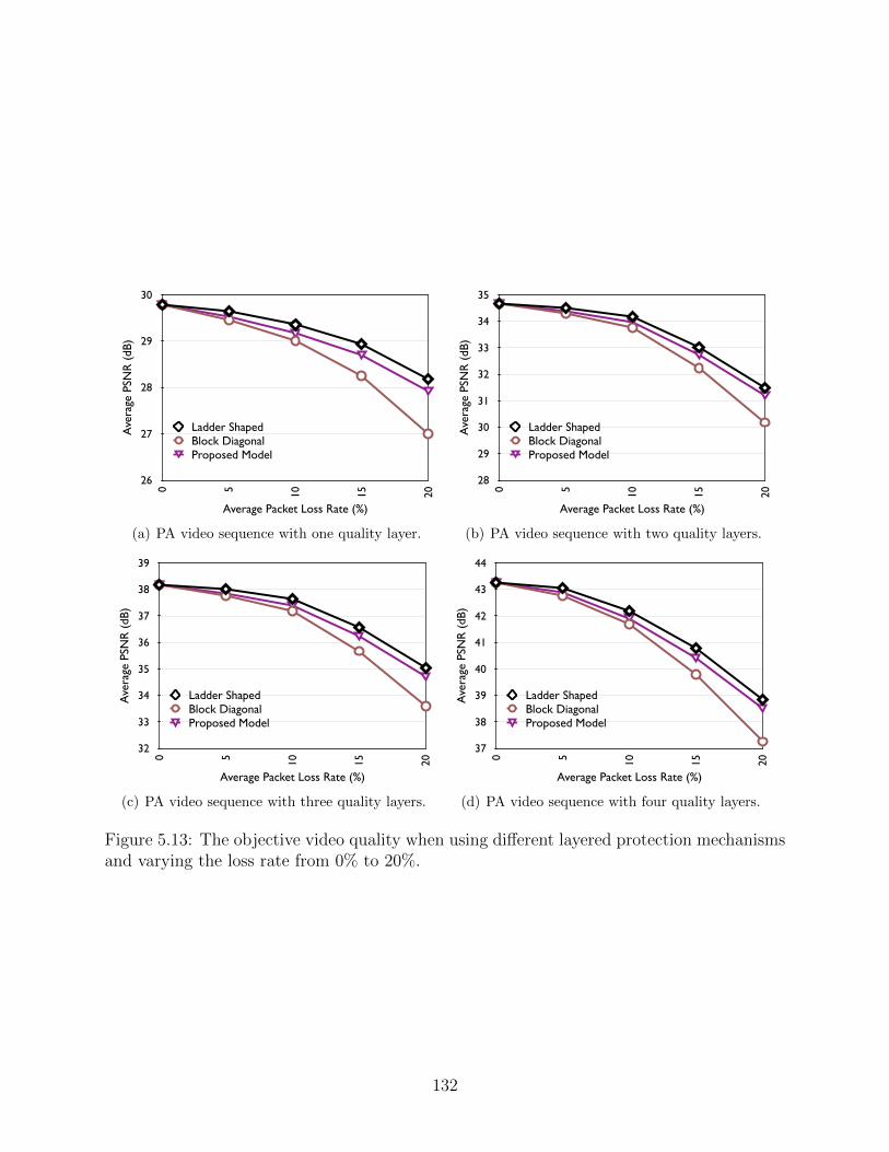
Ave
rage
PSN
R (
dB)
26
27
28
29
30
0 5 10 15 20Ladder ShapedBlock DiagonalProposed Model
Average Packet Loss Rate (%)
(a) PA video sequence with one quality layer.
Ave
rage
PSN
R (
dB)
28
29
30
31
32
33
34
35
0 5 10 15 20
Ladder ShapedBlock DiagonalProposed Model
Average Packet Loss Rate (%)
(b) PA video sequence with two quality layers.
Ave
rage
PSN
R (
dB)
32
33
34
35
36
37
38
39
0 5 10 15 20
Ladder ShapedBlock DiagonalProposed Model
Average Packet Loss Rate (%)
(c) PA video sequence with three quality layers.
Ave
rage
PSN
R (
dB)
37
38
39
40
41
42
43
44
0 5 10 15 20
Ladder ShapedBlock DiagonalProposed Model
Average Packet Loss Rate (%)
(d) PA video sequence with four quality layers.
Figure 5.13: The objective video quality when using different layered protection mechanismsand varying the loss rate from 0% to 20%.
132
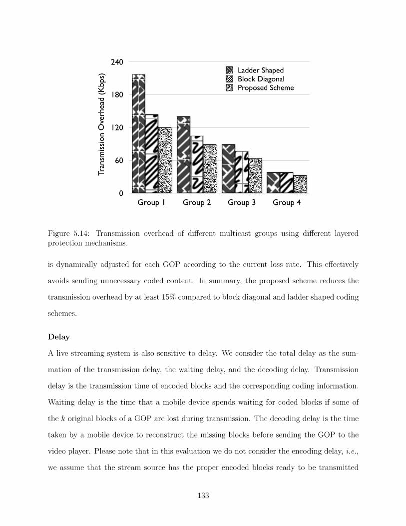
0
60
120
180
240
Group 1 Group 2 Group 3 Group 4
Ladder ShapedBlock DiagonalProposed Scheme
Tran
smis
sion
Ove
rhea
d (K
bps)
Figure 5.14: Transmission overhead of different multicast groups using different layeredprotection mechanisms.
is dynamically adjusted for each GOP according to the current loss rate. This effectively
avoids sending unnecessary coded content. In summary, the proposed scheme reduces the
transmission overhead by at least 15% compared to block diagonal and ladder shaped coding
schemes.
Delay
A live streaming system is also sensitive to delay. We consider the total delay as the sum-
mation of the transmission delay, the waiting delay, and the decoding delay. Transmission
delay is the transmission time of encoded blocks and the corresponding coding information.
Waiting delay is the time that a mobile device spends waiting for coded blocks if some of
the k original blocks of a GOP are lost during transmission. The decoding delay is the time
taken by a mobile device to reconstruct the missing blocks before sending the GOP to the
video player. Please note that in this evaluation we do not consider the encoding delay, i.e.,
we assume that the stream source has the proper encoded blocks ready to be transmitted
133
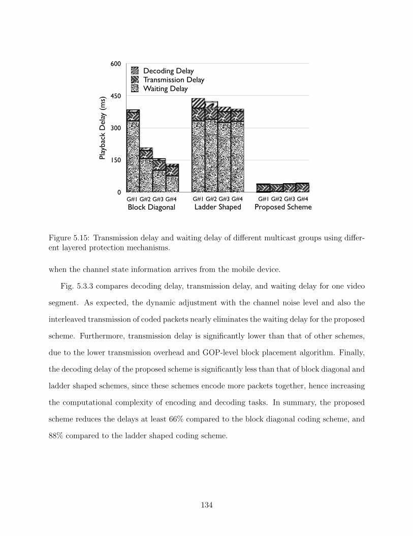
Play
back
Del
ay (
ms)
0
150
300
450
600
Waiting DelayTransmission DelayDecoding Delay
G#1 G#2 G#3 G#4Block Diagonal
G#1 G#2 G#3 G#4Ladder Shaped
G#1 G#2 G#3 G#4Proposed Scheme
Figure 5.15: Transmission delay and waiting delay of different multicast groups using differ-ent layered protection mechanisms.
when the channel state information arrives from the mobile device.
Fig. 5.3.3 compares decoding delay, transmission delay, and waiting delay for one video
segment. As expected, the dynamic adjustment with the channel noise level and also the
interleaved transmission of coded packets nearly eliminates the waiting delay for the proposed
scheme. Furthermore, transmission delay is significantly lower than that of other schemes,
due to the lower transmission overhead and GOP-level block placement algorithm. Finally,
the decoding delay of the proposed scheme is significantly less than that of block diagonal and
ladder shaped schemes, since these schemes encode more packets together, hence increasing
the computational complexity of encoding and decoding tasks. In summary, the proposed
scheme reduces the delays at least 66% compared to the block diagonal coding scheme, and
88% compared to the ladder shaped coding scheme.
134
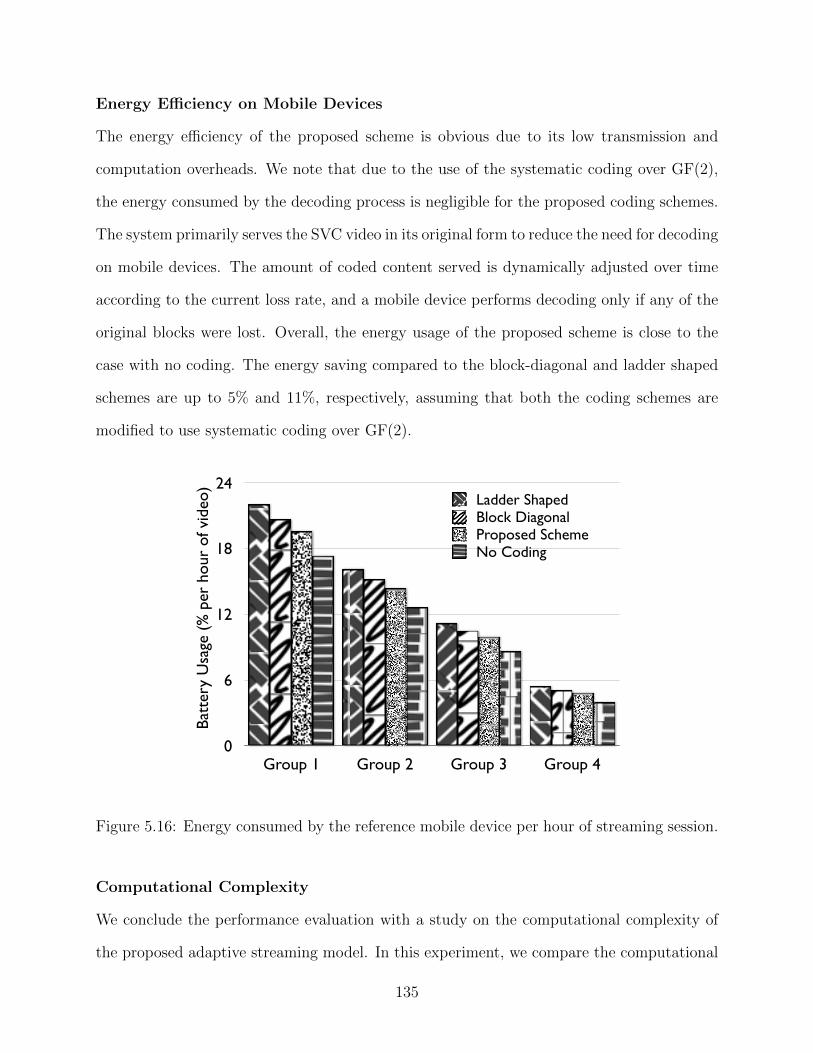
Energy Efficiency on Mobile Devices
The energy efficiency of the proposed scheme is obvious due to its low transmission and
computation overheads. We note that due to the use of the systematic coding over GF(2),
the energy consumed by the decoding process is negligible for the proposed coding schemes.
The system primarily serves the SVC video in its original form to reduce the need for decoding
on mobile devices. The amount of coded content served is dynamically adjusted over time
according to the current loss rate, and a mobile device performs decoding only if any of the
original blocks were lost. Overall, the energy usage of the proposed scheme is close to the
case with no coding. The energy saving compared to the block-diagonal and ladder shaped
schemes are up to 5% and 11%, respectively, assuming that both the coding schemes are
modified to use systematic coding over GF(2).
0
6
12
18
24
Group 1 Group 2 Group 3 Group 4
Ladder ShapedBlock DiagonalProposed SchemeNo Coding
Batt
ery
Usa
ge (
% p
er h
our
of v
ideo
)
Figure 5.16: Energy consumed by the reference mobile device per hour of streaming session.
Computational Complexity
We conclude the performance evaluation with a study on the computational complexity of
the proposed adaptive streaming model. In this experiment, we compare the computational
135
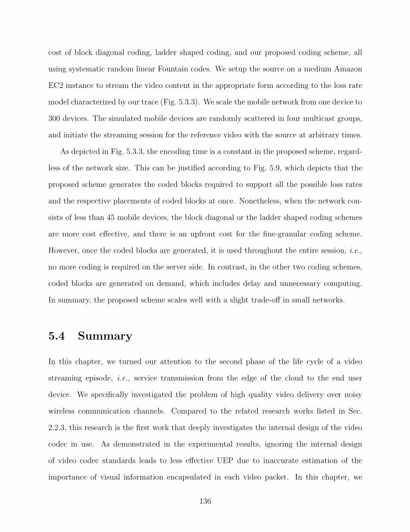
cost of block diagonal coding, ladder shaped coding, and our proposed coding scheme, all
using systematic random linear Fountain codes. We setup the source on a medium Amazon
EC2 instance to stream the video content in the appropriate form according to the loss rate
model characterized by our trace (Fig. 5.3.3). We scale the mobile network from one device to
300 devices. The simulated mobile devices are randomly scattered in four multicast groups,
and initiate the streaming session for the reference video with the source at arbitrary times.
As depicted in Fig. 5.3.3, the encoding time is a constant in the proposed scheme, regard-
less of the network size. This can be justified according to Fig. 5.9, which depicts that the
proposed scheme generates the coded blocks required to support all the possible loss rates
and the respective placements of coded blocks at once. Nonetheless, when the network con-
sists of less than 45 mobile devices, the block diagonal or the ladder shaped coding schemes
are more cost effective, and there is an upfront cost for the fine-granular coding scheme.
However, once the coded blocks are generated, it is used throughout the entire session, i.e.,
no more coding is required on the server side. In contrast, in the other two coding schemes,
coded blocks are generated on demand, which includes delay and unnecessary computing.
In summary, the proposed scheme scales well with a slight trade-off in small networks.
5.4 Summary
In this chapter, we turned our attention to the second phase of the life cycle of a video
streaming episode, i.e., service transmission from the edge of the cloud to the end user
device. We specifically investigated the problem of high quality video delivery over noisy
wireless communication channels. Compared to the related research works listed in Sec.
2.2.3, this research is the first work that deeply investigates the internal design of the video
codec in use. As demonstrated in the experimental results, ignoring the internal design
of video codec standards leads to less effective UEP due to inaccurate estimation of the
importance of visual information encapsulated in each video packet. In this chapter, we
136
0
5
10
15
20
1 40 80 120 160 200 240 300
Ladder ShapedBlock DiagonalProposed Scheme
Enco
ding
Tim
e ov
er G
F(2)
(s)
Number of Mobile Devices
Figure 5.17: Time needed to prepare all the redundant coded blocks.
tried to address this inefficiency.
Toward this goal, we first looked deeper into the coding and prediction mechanism of
state-of-the-art layered video coding standard, i.e., SVC. Next, towards high quality video
streaming over wireless networks and smarter protection of video packets over noisy commu-
nication channels, we proposed a novel coding and dependency aware unequal error protec-
tion algorithm. The proposed algorithm calculates the importance of different video packets
and associates proper protection to each video packet, respectively. Experimental results
show that the proposed algorithm outperforms the state-of-the-art unequal error protection
algorithms in terms of the visual quality of the transmitted video. Finally, we completed
the proposed UEP model by extending the UEP problem from unicast scenario to multi-
cast scenario, in which the full potential of layered video coding is utilized by allowing the
transmission network to multicast one copy of the layered video for groups of heterogeneous
mobile devices. To this end, we proposed a new technique to dynamically adjust and com-
bine the protection FEC packets for reference and dependent video layers for video multicast
137
in mobile communication networks. The experimental results show that the proposed model
improves the quality of the transmitted video and also reduces the energy consumption on
mobile phones.
In the following chapter, we investigate cooperative video streaming among adjacent
mobile phones. This problem is a part of service consumption phase in the life cycle of a
video streaming episode, as illustrated in Fig. 1.1.
138
Chapter 6
Video Reception in Smartphones
The final part of a video transmission session is reception and playback of the video on
the end user device. When it comes to mobile video streaming, the variable loss rate and
bandwidth fluctuation of cellular networks pose challenges to video streaming, since such
systems are very sensitive to delays and losses. On the one hand, an extensive body of
research is focused on improving the signal quality in cellular networks. On the other hand,
another domain of research is concentrated on utilizing short-range links such as WiFi and
Bluetooth to increase the overall link capacity around individual smartphones.
In this chapter, we are interested in the latter approach. The utilization of short-range
links leads to higher data rate and shorter delays, essential performance metrics for mul-
timedia streaming. Furthermore, such an arrangement improves the energy efficiency on
smartphones [48], since the energy per bit ratio of short-range links is less than that of cel-
lular links. Two main approaches are suggested to use short-range links: WiFi offloading
through Internet-connected WiFi routers, and using ad-hoc WiFi networks among collabo-
rating adjacent smartphones.
In this chapter, we investigate the utilization of ad-hoc WiFi networks of collaborating
smartphones. Such an ad-hoc network can be created when a group of smartphones in
proximity of each other are interested in playing the same video stream at the same time,
i.e., a sport match. This system utilizes cellular links to carry streaming content from
the Cloud to smartphones, and WiFi links to enable cooperation among smartphones. As
discussed in Sec. 2.2, this idea has been investigated in several research works to provide
short delays [16, 63], to share error recovery codes [80], to receive the content over multiple
paths [129], and to pre-fetch the content based on social ties [60]. Compared to past research
139
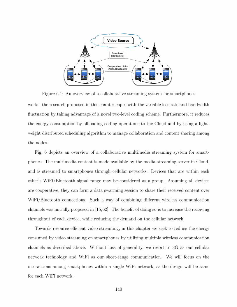
Downlinks (3G/4G/LTE)
Cooperation Links (WiFi, Bluetooth)
Video Source
Figure 6.1: An overview of a collaborative streaming system for smartphones
works, the research proposed in this chapter copes with the variable loss rate and bandwidth
fluctuation by taking advantage of a novel two-level coding scheme. Furthermore, it reduces
the energy consumption by offloading coding operations to the Cloud and by using a light-
weight distributed scheduling algorithm to manage collaboration and content sharing among
the nodes.
Fig. 6 depicts an overview of a collaborative multimedia streaming system for smart-
phones. The multimedia content is made available by the media streaming server in Cloud,
and is streamed to smartphones through cellular networks. Devices that are within each
other’s WiFi/Bluetooth signal range may be considered as a group. Assuming all devices
are cooperative, they can form a data swarming session to share their received content over
WiFi/Bluetooth connections. Such a way of combining different wireless communication
channels was initially proposed in [15,62]. The benefit of doing so is to increase the receiving
throughput of each device, while reducing the demand on the cellular network.
Towards resource efficient video streaming, in this chapter we seek to reduce the energy
consumed by video streaming on smartphones by utilizing multiple wireless communication
channels as described above. Without loss of generality, we resort to 3G as our cellular
network technology and WiFi as our short-range communication. We will focus on the
interactions among smartphones within a single WiFi network, as the design will be same
for each WiFi network.
140
There are two main challenges in designing an energy-efficient collaborative video stream-
ing system. First, all wireless connections are subject to channel fading and have considerably
higher loss rates than wired connections. For each lost packet, a retransmission has to be
performed, if the conventional forward error correction (FEC) cannot recover the distorted
packet. Many coding techniques have been proposed to cope with such losses, without im-
posing additional delays or retransmissions. In particular, network coding (NC) is known
for its advantage in maximizing the gain of each retransmission [101, 103] in wireless com-
munication, since it allows any retransmitted packet to be used to recover any lost packet.
Second, the effectiveness of bandwidth utilization, in such a collaborative network of
smartphones, is subject to segment scheduling among various links. Towards efficient band-
width utilization, Keller [72] proposed the MicroCast system, in which one specific phone
manages the scheduling of segment transmissions on all other phones in the network. The
design principle is to avoid using cellular links as much as possible, and to encourage data
swarming within the WiFi network.
Although MicroCast achieves good streaming rates by utilizing both cellular and WiFi
channels, as well as the overhearing feature in wireless communication, it suffers from two
main deficiencies. First, the scheduling algorithm is a centralized algorithm that introduces
unnecessary messaging and management overhead. Second, it is not energy efficient since it
imposes unnecessary computational burdens on the phones due to the large field size used
in NC operations.
In the proposed system, the energy saving is achieved through a two-level systematic NC
and transmission scheme. At the top level, the multimedia content is streamed from the
Cloud hosting the video source to a WiFi group formed by smartphones. At the bottom
level, received content is shared among smartphones within a WiFi network. The content is
transmitted in both verbatim form and coded form in Galois Field GF(2). Furthermore, to
manage collaboration and content sharing in the WiFi network, we propose a light-weight
141
distributed scheduling algorithm.
Finally, the proposed system is mathematically modeled as an optimization problem
for optimal resource allocation and scheduling. The optimal rate allocation and scheduling
(RAS) algorithm determines the amount of data and the data to be transmitted on each
link. Overall, the system minimizes both the streaming traffic in the cellular network and
the energy consumed by streaming applications on mobile devices. The experimental re-
sults show that significant energy saving is achieved in the proposed system. Moreover, the
proposed RAS algorithm prolongs the streaming session for the entire cooperative group.
6.1 Energy-Efficient Collaborative Streaming
In this section, we propose our energy-efficient streaming system for smartphones, hereafter
referred to as nodes. In this system, the energy saving is achieved through utilizing a two-
level systematic NC scheme and the computing power of the Cloud. Without making any
assumption regarding the video codec used to generate the video stream, our system sched-
ules the transmission at the segment level. Each video segment represents a small duration
(say 1 second) of the video playback. In a live streaming session, all nodes share the same
window of interest, i.e., the same set of segments. The remain of this section explains the
two levels of NC, the transmission scheme, and the heuristic scheduling algorithm in detail.
The optimized resource allocation and scheduling algorithm is discussed in the next section.
6.1.1 General transmission scheme
In this section, for the sake of simplicity, we assume a simple pull-based streaming scheme,
as shown in Fig. 6.1.1. Based on a scheduling algorithm, nodes explicitly request segments
that are due for playback soon from the video source, which is located in the Cloud. Since
transmissions over cellular links consume more energy than transmissions over WiFi links,
to conserve battery lifetime, nodes ideally should collectively download a single copy of
142
the video and exchange segments with each other over WiFi links. A heuristic scheduling
algorithm is detailed in Sec. 6.1.3. The optimized scheduling algorithm is covered in the next
section.
Upon receiving a request, the video source passes the segment to a network coding engine
in the Cloud, hereafter called NC coder. NC coder serves the segment using systematic code
in Galois Field GF(256) to minimize the transmission overhead and also the need for encoding
and decoding at both the sender side (the NC coder) and the receiver side (smartphones),
respectively. We assume that the link between the video source and the NC coders is a high
throughput and low delay link. More detail is provided in Sec. 6.1.2.
On the receiver side, the node can reconstruct the video segment as soon as k linearly
independent blocks are received over the cellular network. In a live streaming session, all
nodes play roughly the same segment and are interested in receiving the same set of segments
that are due for playback in the immediate future. Hence, nodes form a swarming session, in
which they exchange received segments with each other over the WiFi network. To cope with
losses in this network, each segment is served in both verbatim form and coded form. Similar
to the NC coder, a node divides a segment into k blocks of the same size and serves the
segment using systematic code. However, to minimize the encoding and decoding cost, the
coding operations are performed in GF(2). Receivers of the segment only need to perform
the decoding process if the first k blocks received are not all verbatim blocks. More detail is
provided in Sec. 6.1.2.
6.1.2 Two-Level Coding Scheme
Overall, nodes collaboratively request different segments from the Cloud and exchange with
each other in the WiFi network. A video segment is delivered in two phases. In the first
phase, blocks of the segment are transmitted in both verbatim form and coded form in
GF(256) over the cellular network. In the second phase, the node which receives sufficient
143
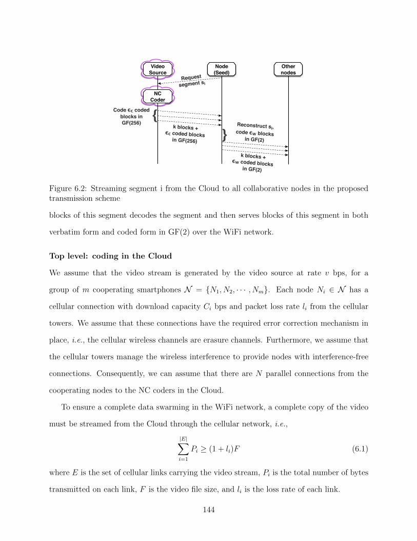
Video Source
Node (Seed)
Other nodes
Requestsegment si
{k blocks +ϵc coded blocksin GF(256)
Reconstruct si,code ϵw blocks
in GF(2)}k blocks +ϵw coded blocksin GF(2)
NC Coder
Code ϵc coded blocks in GF(256)
Figure 6.2: Streaming segment i from the Cloud to all collaborative nodes in the proposedtransmission scheme
blocks of this segment decodes the segment and then serves blocks of this segment in both
verbatim form and coded form in GF(2) over the WiFi network.
Top level: coding in the Cloud
We assume that the video stream is generated by the video source at rate v bps, for a
group of m cooperating smartphones N = {N1, N2, · · · , Nm}. Each node Ni ∈ N has a
cellular connection with download capacity Ci bps and packet loss rate li from the cellular
towers. We assume that these connections have the required error correction mechanism in
place, i.e., the cellular wireless channels are erasure channels. Furthermore, we assume that
the cellular towers manage the wireless interference to provide nodes with interference-free
connections. Consequently, we can assume that there are N parallel connections from the
cooperating nodes to the NC coders in the Cloud.
To ensure a complete data swarming in the WiFi network, a complete copy of the video
must be streamed from the Cloud through the cellular network, i.e.,
|E|∑i=1
Pi ≥ (1 + li)F (6.1)
where E is the set of cellular links carrying the video stream, Pi is the total number of bytes
transmitted on each link, F is the video file size, and li is the loss rate of each link.
144
Upon receiving a request for segment sj from node Ni ∈ N , the NC coder divides segment
sj into kj original blocks of the same size and serves nj = kj + εc systematic coded blocks
over the wireless downlink to the node. The value of εc is determined by the loss rate li. In
general, the expected number of blocks sent over a cellular link for a segment sj is:
E[nj] = kj + εc (6.2)
= kj +E[li]
1− E[li]kj
where E[li] is the expected loss rate from the NC coder to a node Ni. For example, if the
loss rate is 0.2, there should be 1.25 ∗ k blocks served by the source in order to ensure at
least k blocks are received. The first k blocks are served in their original form, and the
additional 0.25 ∗ k blocks will be served in coded form in order to recover any lost during
the transmission of the 1.25 ∗ k blocks. To generate coded blocks, the NC coder produces
each coded block as a linear combination of the k original blocks using random coefficients
from a finite field GF(2x).
Since each link i has a different loss rate 0 ≤ li ≤ 1 and the link quality varies over
time, the NC coder may have to generate and send different number of coded blocks for
each segment. To better utilize the bandwidth in cellular network, the coding is performed
in a larger field of GF(256) to ensure that with high probably the redundant coded blocks
received by a node are linearly independent. A node stops receiving and reconstructs the
video segment as soon as kj = k′j+ε′c linearly independent blocks are received over the cellular
network, where 0 ≤ k′j ≤ kj is the number of original blocks received and 0 ≤ ε′c ≤ εc is the
number of coded blocks received. Since RLNC is based on Reed-Solomon code, a maximum
distance separable code, the need for explicit retransmission of a lost packet is eliminated as
all transmitted blocks are equally important and useful in decoding the original segment.
Bottom level: coding in WiFi
Now, segment i is considered in the WiFi network. The node that receives this segment,
hereafter referred to as the seed for the segment, is now responsible for disseminating the
145
segments to other nodes in the WiFi network. In MicroCast [72], the seed broadcasts coded
blocks produced in GF(256) to all nodes in the WiFi network. If a node does not receive
enough coded blocks for decoding a segment, it explicitly requests the seed to serve more
coded blocks of the segment. We note that this system requires all nodes to perform the en-
coding and decoding operations in GF (256). However, since the system is taking advantage
of the overhearing feature in the WiFi network, and the network is formed by nearby nodes,
the loss rate is expected to be much lower than the cellular network. Our experiment on the
Galaxy Nexus phone indicates that encoding and decoding in GF(256) for every GB of data
consume 5.06% and 3.6% of the battery, respectively. Given the size of the WiFi network
and the lower loss rate, we believe that NC in GF(2) is sufficient. For this reason, we argue
that it is not necessary to perform NC in GF(256) in the WiFi network.
In our system, a seed of a segment sj first reconstructs the original segment. The seed then
sends the kj blocks from the segment over the WiFi network without encoding them. Nodes
that successfully receive these kj blocks can reconstruct the segment without performing any
decoding. Due to channel losses, some nodes may not receive the kj original blocks, and they
may miss different blocks. Reconciling the missing blocks for each node will be costly and
requires a direct communication between the node and the seed. Instead, the seed produces
and sends εw coded blocks in addition to the kj original blocks. The coded blocks at this
level are produced by simply XORing a random subset of the kj blocks, i.e., encoding in
GF(2). The value of εw is determined by the loss rate lw in the WiFi network. Hence, the
expected number of blocks sent in a WiFi network for a segment sj is:
E[mj] = kj + εw (6.3)
= kj +E[lw]
1− E[lw]kj
where E[lw] is the expected loss rate in the WiFi network. Here, we assume that an algorithm
for estimating the loss rate is in place. After a timeout period, if a node still does not have
sufficient blocks to reconstruct the original segment, it will ask the seed to send more coded
146
blocks.
Overall, with the two-level NC and transmission scheme, the encoding process is offloaded
to the Cloud, and the decoding process will take place just for the lost blocks of each segment
once in GF(256) at the seed and once in GF(2) at the other nodes. From our experiment
on the Galaxy Nexus phone, both encoding and decoding in GF(2) for every GB of data
consume approximately 0.06% of the battery, which is much more power efficient than that in
GF(256) on each node. In this system, to disseminate a segment sj to all smartphones, there
are E[nj] ∗ kj/(1 − li) blocks traveled from the Cloud to the seed, and E[mj] ∗ kj/(1 − lw)
blocks are shared in the WiFi network. This is very close to the minimum transmission
required to deliver a segment to all nodes, i.e., nj + mj, where nj is the number of blocks
sent over a cellular link with the minimum loss rate, and mj is the number of blocks shared
in a WiFi network with the minimum loss rate.
6.1.3 Distributed Scheduling Algorithm
In MicroCast [72], each node requests video segments from the Cloud according to the
segment assignment that is centrally managed by a specific node. If any node fails to retrieve
a particular segment, this node is informed and re-assigns the download task to another node.
However, given the overhearing feature in wireless communication, the segment download
scheduling can be managed in a distributed way among the nodes in the WiFi network.
Here, we propose such a distributed algorithm to coordinate the segment downloads.
Each node randomly picks a missing segment sj in the shared window of interest, with
preference toward segments that are due for playback immediately. Before pulling segment
sj from the Cloud, the node either broadcasts a message or unicasts the message to a random
node in the WiFi network. Upon receiving or overhearing the message, all nodes will avoid
scheduling segment i for transmission. As soon as the node that initiated the transmission
completely received the segment, it informs other nodes with another message. If such a
147
message is not received or overheard within a timeout period, all nodes will treat segment
i as a regular missing segment and proceed with regular segment transmission scheduling.
This distributed algorithm not only coordinates all nodes to collectively download a copy
of the video over time, but also allows load balancing among the nodes. The nodes with
longer battery lifetime or better cellular connections can be more active in pulling segments
from the Cloud, while nodes with low battery or poor cellular connections can benefit from
the data swarming in the WiFi network. However, this is based on the assumption that all
nodes are cooperative, and are not selfish or malicious in any form. The proposed distributed
scheduling algorithm is presented in Alg. 1.
In this algorithm, the Schedule() function decides whether a node should retrieve a
segment from the Cloud. The decision may be based on different heuristic criteria, or based
on a mathematical optimization model. In continue we propose the optimization model
and solve the optimization problem for resource allocation and scheduling as a centralized
algorithm. Later in Sec. 6.3 we compare the performance of the proposed optimal model
with three heuristic scheduling algorithms.
6.2 Optimal Resource Allocation and Scheduling
In this section, we present a mathematical model for the collaborative streaming system pro-
posed in the previous section. The proposed system is modeled as an optimization problem
for optimal resource allocation and scheduling. The optimal rate allocation and scheduling
(RAS) algorithm determines the amount of data and the data to be transmitted on each link.
Overall, using optimal RAS the proposed system minimizes both the streaming traffic in the
cellular network and the energy consumed by streaming applications on mobile devices.
148
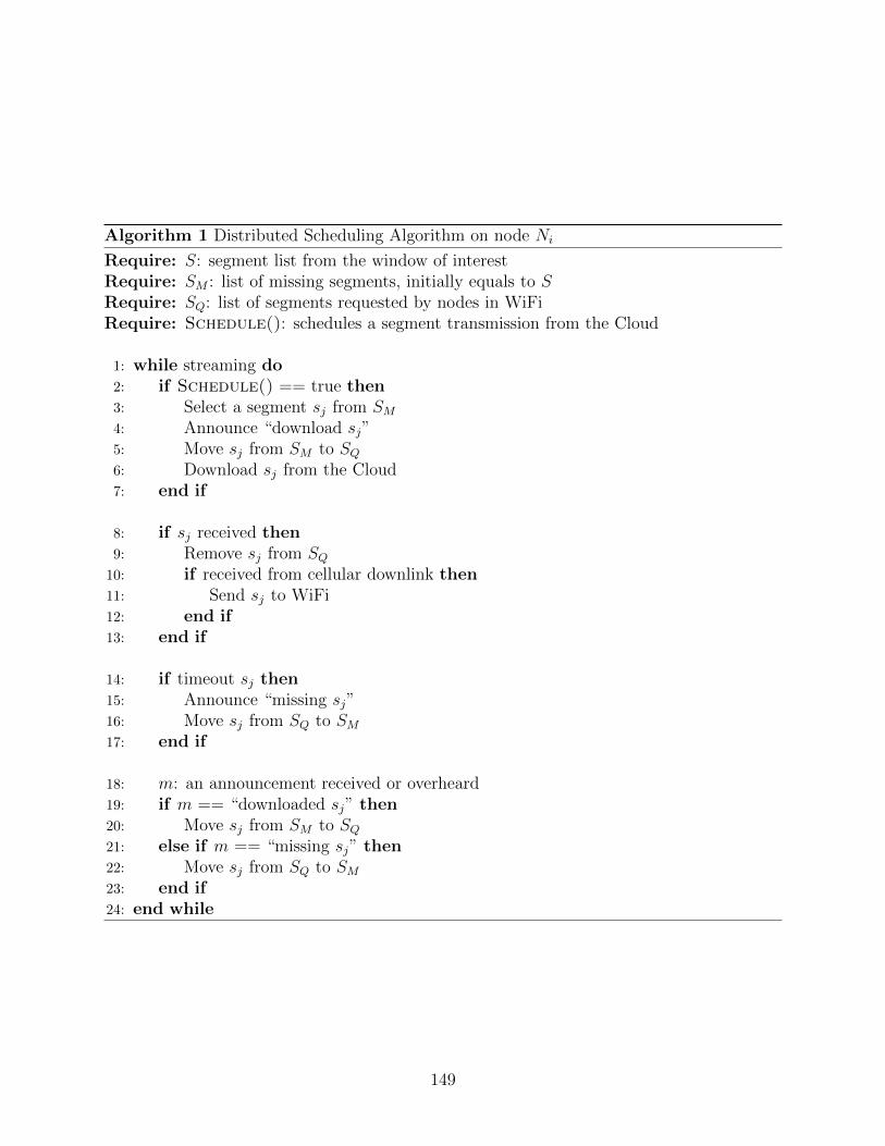
Algorithm 1 Distributed Scheduling Algorithm on node Ni
Require: S: segment list from the window of interestRequire: SM : list of missing segments, initially equals to SRequire: SQ: list of segments requested by nodes in WiFiRequire: Schedule(): schedules a segment transmission from the Cloud
1: while streaming do2: if Schedule() == true then3: Select a segment sj from SM4: Announce “download sj”5: Move sj from SM to SQ6: Download sj from the Cloud7: end if
8: if sj received then9: Remove sj from SQ
10: if received from cellular downlink then11: Send sj to WiFi12: end if13: end if
14: if timeout sj then15: Announce “missing sj”16: Move sj from SQ to SM17: end if
18: m: an announcement received or overheard19: if m == “downloaded sj” then20: Move sj from SM to SQ21: else if m == “missing sj” then22: Move sj from SQ to SM23: end if24: end while
149
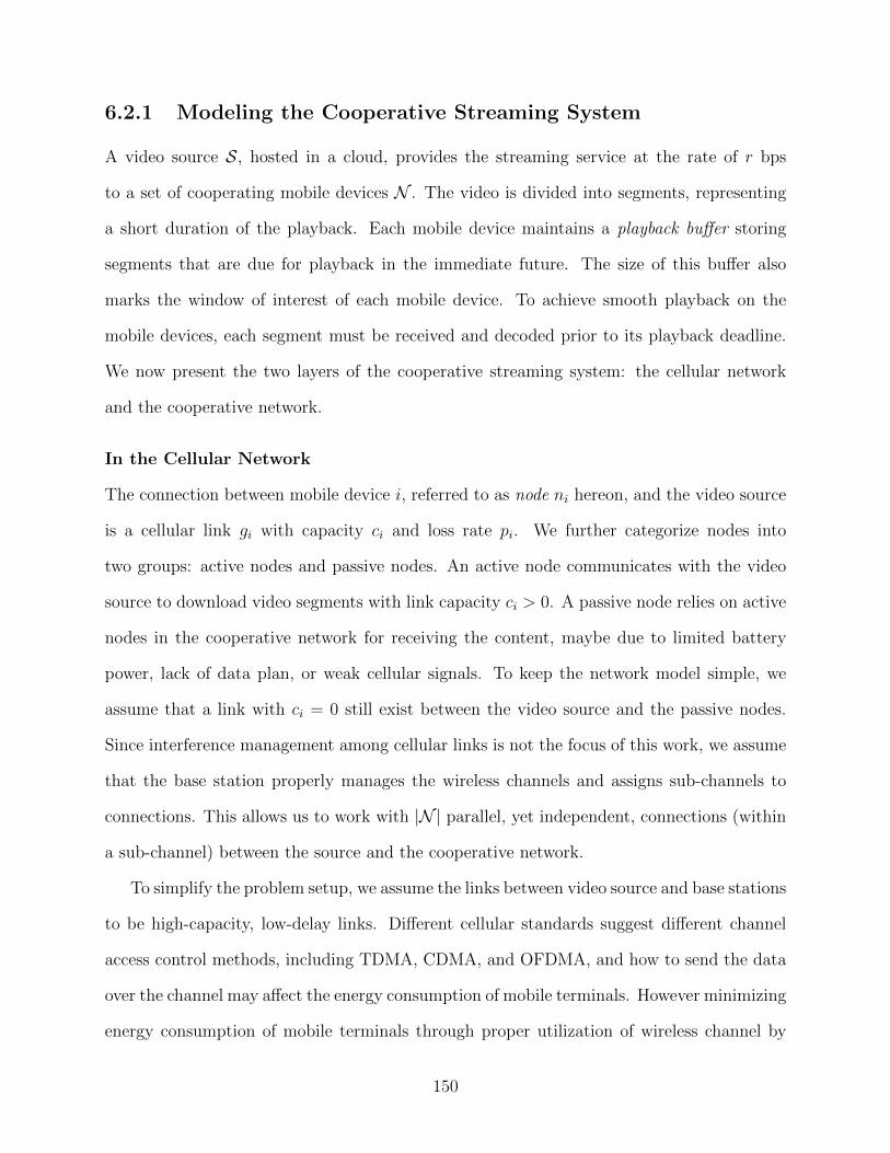
6.2.1 Modeling the Cooperative Streaming System
A video source S, hosted in a cloud, provides the streaming service at the rate of r bps
to a set of cooperating mobile devices N . The video is divided into segments, representing
a short duration of the playback. Each mobile device maintains a playback buffer storing
segments that are due for playback in the immediate future. The size of this buffer also
marks the window of interest of each mobile device. To achieve smooth playback on the
mobile devices, each segment must be received and decoded prior to its playback deadline.
We now present the two layers of the cooperative streaming system: the cellular network
and the cooperative network.
In the Cellular Network
The connection between mobile device i, referred to as node ni hereon, and the video source
is a cellular link gi with capacity ci and loss rate pi. We further categorize nodes into
two groups: active nodes and passive nodes. An active node communicates with the video
source to download video segments with link capacity ci > 0. A passive node relies on active
nodes in the cooperative network for receiving the content, maybe due to limited battery
power, lack of data plan, or weak cellular signals. To keep the network model simple, we
assume that a link with ci = 0 still exist between the video source and the passive nodes.
Since interference management among cellular links is not the focus of this work, we assume
that the base station properly manages the wireless channels and assigns sub-channels to
connections. This allows us to work with |N | parallel, yet independent, connections (within
a sub-channel) between the source and the cooperative network.
To simplify the problem setup, we assume the links between video source and base stations
to be high-capacity, low-delay links. Different cellular standards suggest different channel
access control methods, including TDMA, CDMA, and OFDMA, and how to send the data
over the channel may affect the energy consumption of mobile terminals. However minimizing
energy consumption of mobile terminals through proper utilization of wireless channel by
150
the base station is orthogonal to our discussion. Thus we assume that the base stations use
the channel efficiently.
Pass
ive
Activ
e
Activ
e
Activ
e
Video Source
active 3G link (ci > 0, pi > 0)passive 3G link (ci = 0, pi = 1)WiFi broadcast channel (ci,j > 0, pi,j > 0)
Figure 6.3: Network model.
In this system, the source serves only one copy of the video to active nodes, and the
nodes cooperatively exchange received segments in the network to deliver missing segments
on all devices. Hence, the source schedules the transmission of segments according to their
playback deadline and the rate allocation on each cellular link. As shown in Fig. 6.4, the
video source collects channel state and energy usage information from all active nodes, based
on which the RAS algorithm determines to which nodes the video segment will be pushed.
Hence each cellular link transmits different complete or partial segments within the current
window of interest. For clarity, we assume a segment represents one time unit of the playback.
Over time, exactly one copy of the video is streamed over the cellular network. Here, we
assume that an algorithm for estimating the next state of channel, based on the channel
state history, is in place.
Before pushing video segments, the source first divides a segment into k original blocks
of the same size and serves the segment using systematic code in Galois Field GF(256).
The coded blocks, a random linear combination of the original blocks, are sent along with
the original blocks to node ni that is selected by the source. Please note that there is an
151
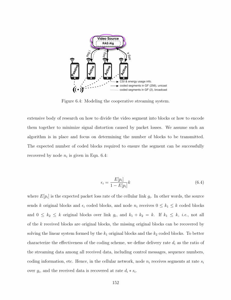
Pass
ive
Activ
e
Activ
e
Activ
e
Video SourceRAS Alg
seg
i
seg
j
seg
k
CSI & energy usage info.coded segments in GF (256), unicastcoded segments in GF (2), broadcast
Figure 6.4: Modeling the cooperative streaming system.
extensive body of research on how to divide the video segment into blocks or how to encode
them together to minimize signal distortion caused by packet losses. We assume such an
algorithm is in place and focus on determining the number of blocks to be transmitted.
The expected number of coded blocks required to ensure the segment can be successfully
recovered by node ni is given in Eqn. 6.4:
εi =E[pi]
1− E[pi]k (6.4)
where E[pi] is the expected packet loss rate of the cellular link gi. In other words, the source
sends k original blocks and εi coded blocks, and node ni receives 0 ≤ k1 ≤ k coded blocks
and 0 ≤ k2 ≤ k original blocks over link gi, and k1 + k2 = k. If k1 ≤ k, i.e., not all
of the k received blocks are original blocks, the missing original blocks can be recovered by
solving the linear system formed by the k1 original blocks and the k2 coded blocks. To better
characterize the effectiveness of the coding scheme, we define delivery rate di as the ratio of
the streaming data among all received data, including control messages, sequence numbers,
coding information, etc. Hence, in the cellular network, node ni receives segments at rate si
over gi, and the received data is recovered at rate di ∗ si.
152
In the Cooperative Network
In the cooperative network, each pair of nodes (ni, nj), ni, nj ∈ N , are reachable over a
WiFi link {wi,j}, with capacity ci,j > 0 and packet loss rate pi,j ≥ 0. Hence, the cooperative
network is a fully connected network. We assume that each WiFi link is bi-directional,
i.e., wi,j ' wj,i, with ci,j = cj,i and pi,j = pj,i. In the WiFi network, we consider the
time division multiple access (TDMA) model for the following reason. While IEEE 802.11
networks are based on orthogonal frequency-division multiplexing (OFDM), and can transmit
the information on multiple carrier frequencies, the usual smartphones are equipped with
just one cellular and one WiFi antenna. This means that when broadcasting in the WiFi
network, each smartphone is in either the sending mode or the receiving mode, but not both.
To avoid collision in the broadcast session, only one node can send at a time, while all other
nodes are in the receiving mode. Hence, the broadcasting node can use all the available
frequency range of the WiFi channel. Nodes in our system take advantage of this property
and employ a broadcast mechanism to share received segments.
Upon receiving a complete or partial segment, node ni becomes the seed of this segment in
the cooperative network, and is responsible to disseminate it to all other nodes. Before doing
so, node ni first reconstructs the k original blocks and serves the segment using systematic
code in Galois Field GF(2). The coded blocks, XOR of a random subset of the original
blocks, are broadcasted in the WiFi network. Our experiments on the Galaxy Nexus phone
indicate that encoding and decoding in GF(2) is almost 100 times more energy efficient than
that in GF(256). Since the loss rate in the WiFi network is expected to be much lower than
that in the cellular network, the field size of 2 is sufficient. The expected number of coded
blocks required to ensure the segment can be successfully recovered by all other nodes is
given in Eqn. 6.5.
εi =E[pwi ]
1− E[pwi ]k (6.5)
where E[pwi ] is the expected packet loss rate when node ni broadcasts. The loss rate pwi is
153
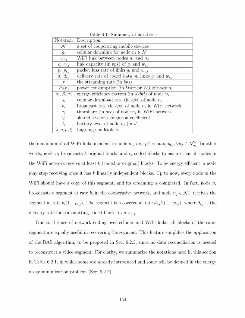
Table 6.1: Summary of notationsNotation DescriptionN a set of cooperating mobile devicesgi cellular downlink for node ni ∈ Nwi,j WiFi link between nodes ni and njci, ci,j link capacity (in bps) of gi and wi,jpi, pi,j packet loss rate of links gi and wi,jdi, di,j delivery rate of coded data on links gi and wi,jr the streaming rate (in bps)
Pi(r) power consumption (in Watt or W ) of node niαi, βi, γi energy efficiency factors (in J/bit) of node ni
si cellular download rate (in bps) of node nibi broadcast rate (in bps) of node ni in WiFi networkτi timeshare (in sec) of node ni in WiFi networkψ shared session elongation coefficientli battery level of node ni (in J)
λ, η, µ, ξ Lagrange multipliers
the maximum of all WiFi links incident to node ni, i.e., pwi = maxj pi,j,∀nj ∈ N−ni. In other
words, node ni broadcasts k original blocks and εi coded blocks to ensure that all nodes in
the WiFi network receive at least k (coded or original) blocks. To be energy efficient, a node
may stop receiving once it has k linearly independent blocks. Up to now, every node in the
WiFi should have a copy of this segment, and its streaming is completed. In fact, node ni
broadcasts a segment at rate bi in the cooperative network, and node nj ∈ N−nireceives the
segment at rate bi(1− pi,j). The segment is recovered at rate di,jbi(1− pi,j), where di,j is the
delivery rate for transmitting coded blocks over wi,j.
Due to the use of network coding over cellular and WiFi links, all blocks of the same
segment are equally useful in recovering the segment. This feature simplifies the application
of the RAS algorithm, to be proposed in Sec. 6.2.3, since no data reconciliation is needed
to reconstruct a video segment. For clarity, we summarize the notations used in this section
in Table 6.2.1, in which some are already introduced and some will be defined in the energy
usage minimization problem (Sec. 6.2.2).
154
6.2.2 The Power Consumption Minimization Problem
To minimize the energy consumption in the cooperative network described in Sec. 6.2.1, we
need an optimal rate allocation and segment scheduling algorithm in the cellular network
and the WiFi network. To do so, we first formulate the power consumption minimization
problem. We define Pi(r) (in Watt or W ) as the energy consumed by a cooperative node
ni ∈ N to receive the video stream at rate r, and P (r) =∑
ni∈N Pi(r) as the objective energy
function. According to [29], we consider the energy consumption of data transmission and
coding operations as a linear function of transmission and coding rate. The objective function
is defined as follows:
Pi(r) = αisi + βibi + γi∑
jdj,ibj(1− pj,i), (6.6)
∀ni ∈ N , nj ∈ N−ni
where αi, βi, and γi are energy efficiency factors (in J/bit) of node ni when receiving and
decoding each bit of data over a cellular link, encoding and broadcasting each bit over
the WiFi network, and receiving and decoding each bit in the WiFi network. Note that
the idle power is not included in this formula, since the objective here is to minimize the
power consumption due to data transmission. However, the idle power may affect lifetime
of mobile devices, and we will discuss this in Sec. 6.2.4. According to the setup in Sec. 6.2.1,
155
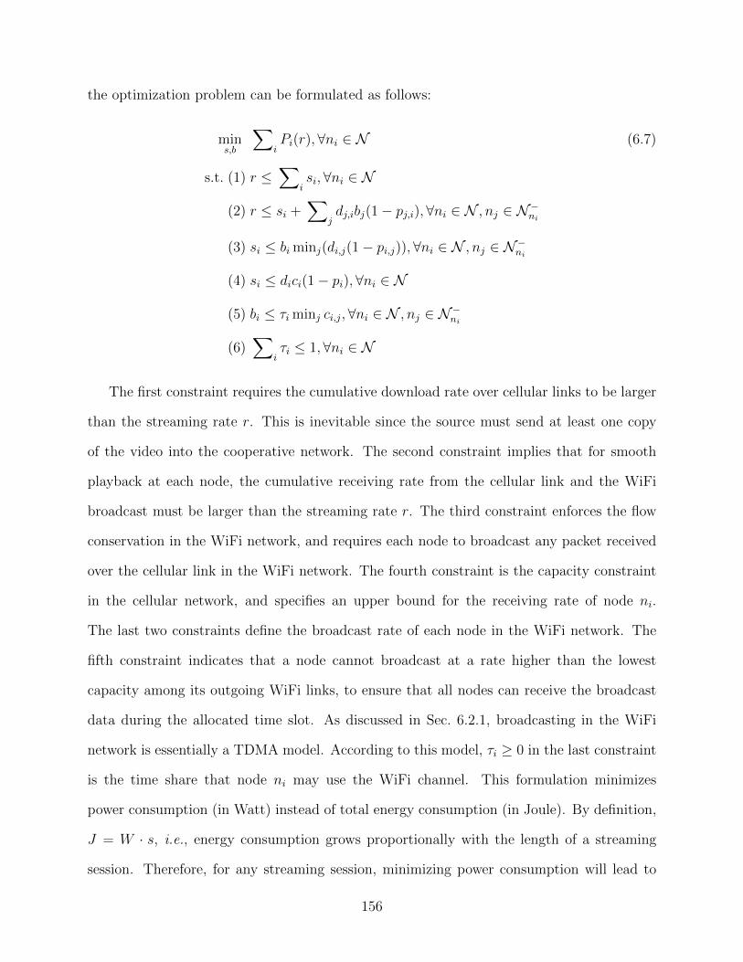
the optimization problem can be formulated as follows:
mins,b
∑iPi(r),∀ni ∈ N (6.7)
s.t. (1) r ≤∑
isi, ∀ni ∈ N
(2) r ≤ si +∑
jdj,ibj(1− pj,i),∀ni ∈ N , nj ∈ N−ni
(3) si ≤ bi minj(di,j(1− pi,j)),∀ni ∈ N , nj ∈ N−ni
(4) si ≤ dici(1− pi),∀ni ∈ N
(5) bi ≤ τi minj ci,j,∀ni ∈ N , nj ∈ N−ni
(6)∑
iτi ≤ 1,∀ni ∈ N
The first constraint requires the cumulative download rate over cellular links to be larger
than the streaming rate r. This is inevitable since the source must send at least one copy
of the video into the cooperative network. The second constraint implies that for smooth
playback at each node, the cumulative receiving rate from the cellular link and the WiFi
broadcast must be larger than the streaming rate r. The third constraint enforces the flow
conservation in the WiFi network, and requires each node to broadcast any packet received
over the cellular link in the WiFi network. The fourth constraint is the capacity constraint
in the cellular network, and specifies an upper bound for the receiving rate of node ni.
The last two constraints define the broadcast rate of each node in the WiFi network. The
fifth constraint indicates that a node cannot broadcast at a rate higher than the lowest
capacity among its outgoing WiFi links, to ensure that all nodes can receive the broadcast
data during the allocated time slot. As discussed in Sec. 6.2.1, broadcasting in the WiFi
network is essentially a TDMA model. According to this model, τi ≥ 0 in the last constraint
is the time share that node ni may use the WiFi channel. This formulation minimizes
power consumption (in Watt) instead of total energy consumption (in Joule). By definition,
J = W · s, i.e., energy consumption grows proportionally with the length of a streaming
session. Therefore, for any streaming session, minimizing power consumption will lead to
156
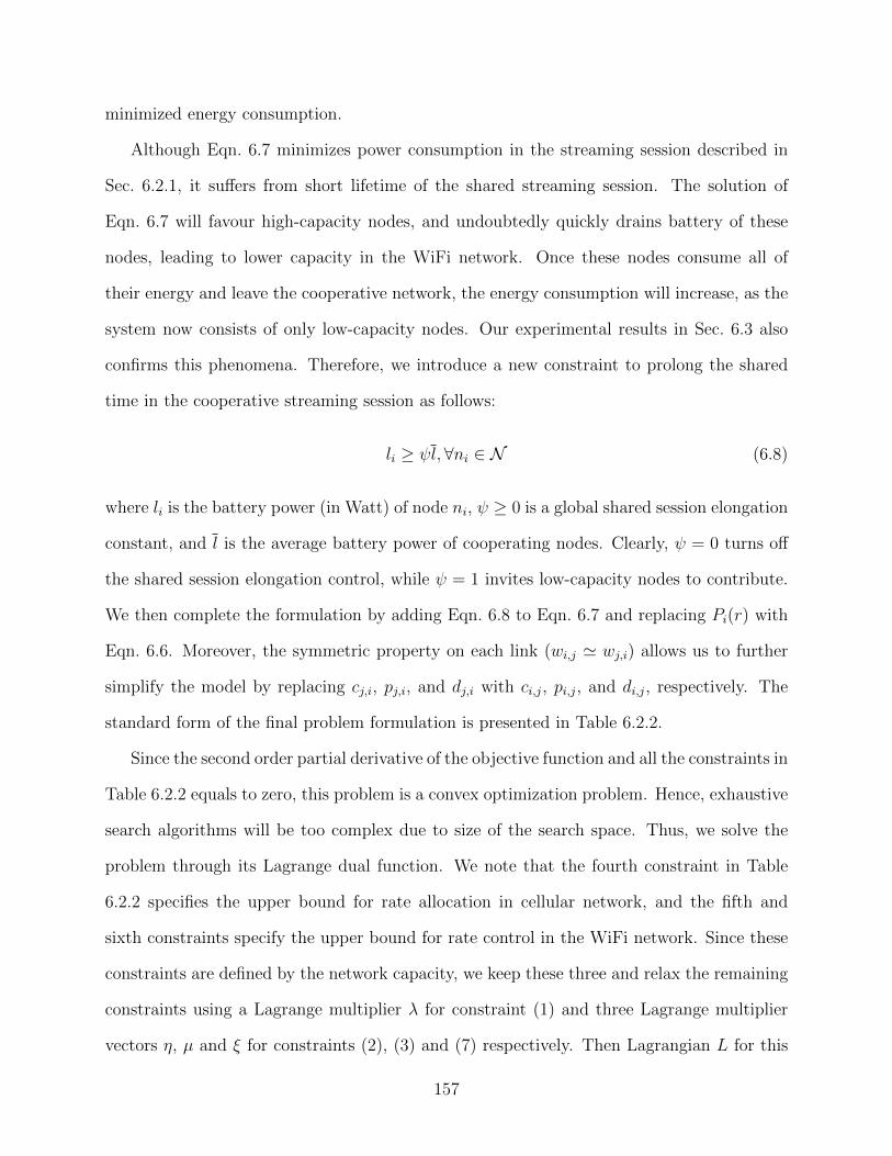
minimized energy consumption.
Although Eqn. 6.7 minimizes power consumption in the streaming session described in
Sec. 6.2.1, it suffers from short lifetime of the shared streaming session. The solution of
Eqn. 6.7 will favour high-capacity nodes, and undoubtedly quickly drains battery of these
nodes, leading to lower capacity in the WiFi network. Once these nodes consume all of
their energy and leave the cooperative network, the energy consumption will increase, as the
system now consists of only low-capacity nodes. Our experimental results in Sec. 6.3 also
confirms this phenomena. Therefore, we introduce a new constraint to prolong the shared
time in the cooperative streaming session as follows:
li ≥ ψl,∀ni ∈ N (6.8)
where li is the battery power (in Watt) of node ni, ψ ≥ 0 is a global shared session elongation
constant, and l is the average battery power of cooperating nodes. Clearly, ψ = 0 turns off
the shared session elongation control, while ψ = 1 invites low-capacity nodes to contribute.
We then complete the formulation by adding Eqn. 6.8 to Eqn. 6.7 and replacing Pi(r) with
Eqn. 6.6. Moreover, the symmetric property on each link (wi,j ' wj,i) allows us to further
simplify the model by replacing cj,i, pj,i, and dj,i with ci,j, pi,j, and di,j, respectively. The
standard form of the final problem formulation is presented in Table 6.2.2.
Since the second order partial derivative of the objective function and all the constraints in
Table 6.2.2 equals to zero, this problem is a convex optimization problem. Hence, exhaustive
search algorithms will be too complex due to size of the search space. Thus, we solve the
problem through its Lagrange dual function. We note that the fourth constraint in Table
6.2.2 specifies the upper bound for rate allocation in cellular network, and the fifth and
sixth constraints specify the upper bound for rate control in the WiFi network. Since these
constraints are defined by the network capacity, we keep these three and relax the remaining
constraints using a Lagrange multiplier λ for constraint (1) and three Lagrange multiplier
vectors η, µ and ξ for constraints (2), (3) and (7) respectively. Then Lagrangian L for this
157
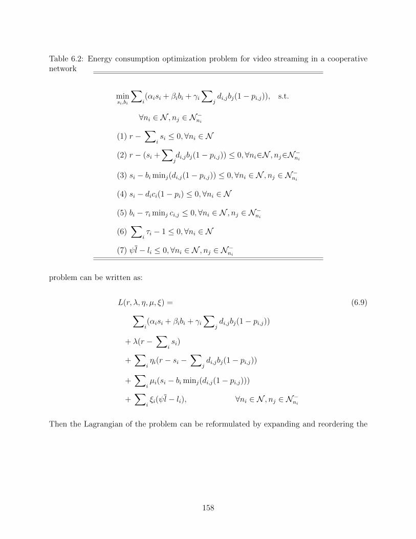
Table 6.2: Energy consumption optimization problem for video streaming in a cooperativenetwork
minsi,bi
∑i(αisi + βibi + γi
∑jdi,jbj(1− pi,j)), s.t.
∀ni ∈ N , nj ∈ N−ni
(1) r −∑
isi ≤ 0,∀ni ∈ N
(2) r − (si +∑
jdi,jbj(1− pi,j)) ≤ 0,∀ni∈N , nj∈N−ni
(3) si − bi minj(di,j(1− pi,j)) ≤ 0,∀ni ∈ N , nj ∈ N−ni
(4) si − dici(1− pi) ≤ 0,∀ni ∈ N
(5) bi − τi minj ci,j ≤ 0,∀ni ∈ N , nj ∈ N−ni
(6)∑
iτi − 1 ≤ 0,∀ni ∈ N
(7) ψl − li ≤ 0,∀ni ∈ N , nj ∈ N−ni
problem can be written as:
L(r, λ, η, µ, ξ) = (6.9)∑i(αisi + βibi + γi
∑jdi,jbj(1− pi,j))
+ λ(r −∑
isi)
+∑
iηi(r − si −
∑jdi,jbj(1− pi,j))
+∑
iµi(si − bi minj(di,j(1− pi,j)))
+∑
iξi(ψl − li), ∀ni ∈ N , nj ∈ N−ni
Then the Lagrangian of the problem can be reformulated by expanding and reordering the
158
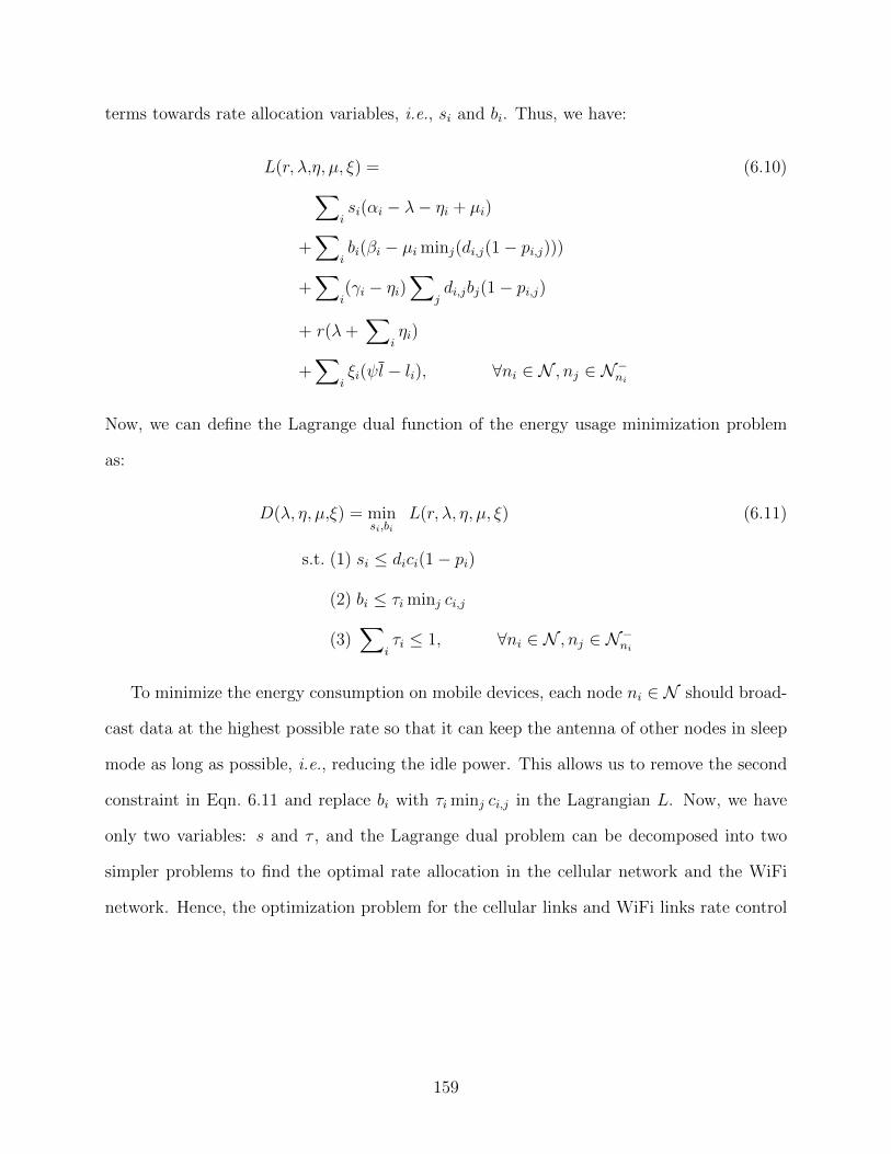
terms towards rate allocation variables, i.e., si and bi. Thus, we have:
L(r, λ,η, µ, ξ) = (6.10)∑isi(αi − λ− ηi + µi)
+∑
ibi(βi − µi minj(di,j(1− pi,j)))
+∑
i(γi − ηi)
∑jdi,jbj(1− pi,j)
+ r(λ+∑
iηi)
+∑
iξi(ψl − li), ∀ni ∈ N , nj ∈ N−ni
Now, we can define the Lagrange dual function of the energy usage minimization problem
as:
D(λ, η, µ,ξ) = minsi,bi
L(r, λ, η, µ, ξ) (6.11)
s.t. (1) si ≤ dici(1− pi)
(2) bi ≤ τi minj ci,j
(3)∑
iτi ≤ 1, ∀ni ∈ N , nj ∈ N−ni
To minimize the energy consumption on mobile devices, each node ni ∈ N should broad-
cast data at the highest possible rate so that it can keep the antenna of other nodes in sleep
mode as long as possible, i.e., reducing the idle power. This allows us to remove the second
constraint in Eqn. 6.11 and replace bi with τi minj ci,j in the Lagrangian L. Now, we have
only two variables: s and τ , and the Lagrange dual problem can be decomposed into two
simpler problems to find the optimal rate allocation in the cellular network and the WiFi
network. Hence, the optimization problem for the cellular links and WiFi links rate control
159
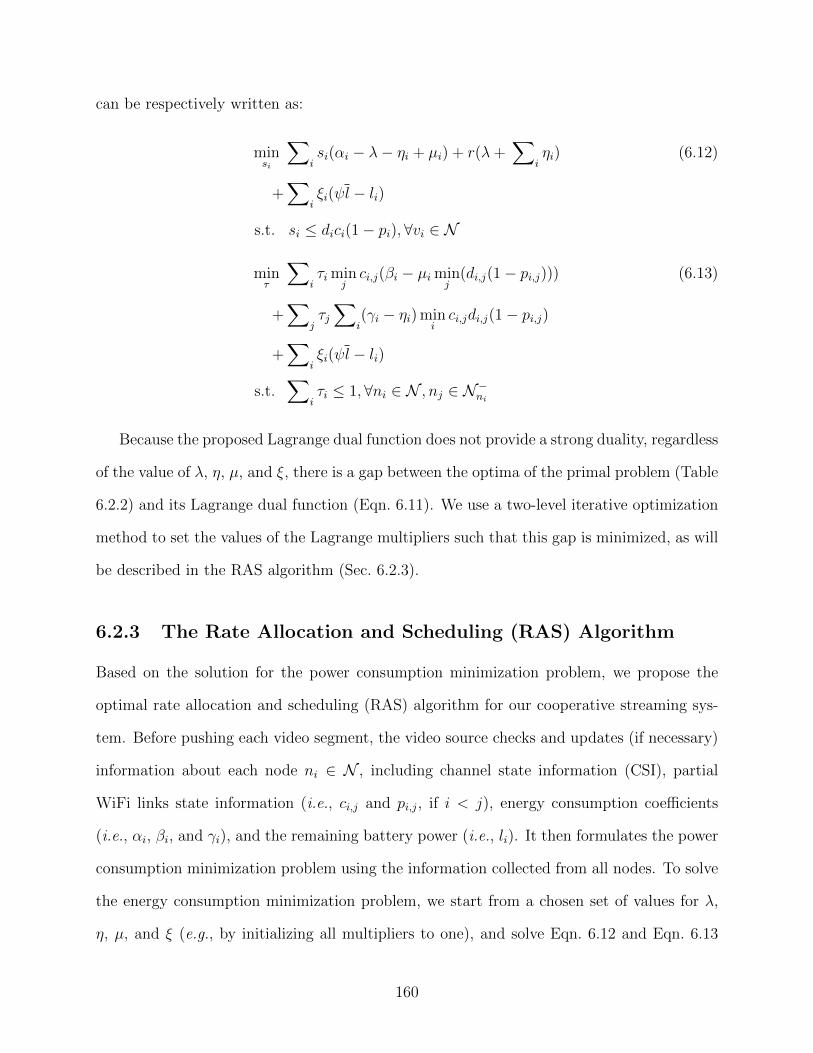
can be respectively written as:
minsi
∑isi(αi − λ− ηi + µi) + r(λ+
∑iηi) (6.12)
+∑
iξi(ψl − li)
s.t. si ≤ dici(1− pi),∀vi ∈ N
minτ
∑iτi min
jci,j(βi − µi min
j(di,j(1− pi,j))) (6.13)
+∑
jτj∑
i(γi − ηi) min
ici,jdi,j(1− pi,j)
+∑
iξi(ψl − li)
s.t.∑
iτi ≤ 1,∀ni ∈ N , nj ∈ N−ni
Because the proposed Lagrange dual function does not provide a strong duality, regardless
of the value of λ, η, µ, and ξ, there is a gap between the optima of the primal problem (Table
6.2.2) and its Lagrange dual function (Eqn. 6.11). We use a two-level iterative optimization
method to set the values of the Lagrange multipliers such that this gap is minimized, as will
be described in the RAS algorithm (Sec. 6.2.3).
6.2.3 The Rate Allocation and Scheduling (RAS) Algorithm
Based on the solution for the power consumption minimization problem, we propose the
optimal rate allocation and scheduling (RAS) algorithm for our cooperative streaming sys-
tem. Before pushing each video segment, the video source checks and updates (if necessary)
information about each node ni ∈ N , including channel state information (CSI), partial
WiFi links state information (i.e., ci,j and pi,j, if i < j), energy consumption coefficients
(i.e., αi, βi, and γi), and the remaining battery power (i.e., li). It then formulates the power
consumption minimization problem using the information collected from all nodes. To solve
the energy consumption minimization problem, we start from a chosen set of values for λ,
η, µ, and ξ (e.g., by initializing all multipliers to one), and solve Eqn. 6.12 and Eqn. 6.13
160
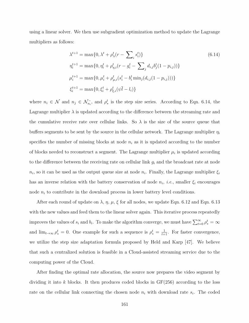
using a linear solver. We then use subgradient optimization method to update the Lagrange
multipliers as follows:
λt+1 = max{0, λt + ρtλ(r −∑
isti)} (6.14)
ηt+1i = max{0, ηti + ρtη,i(r − gti −
∑jdi,jb
tj(1− pi,j))}
µt+1i = max{0, µti + ρtµ,i(s
ti − bti minj(di,j(1− pi,j)))}
ξt+1i = max{0, ξti + ρtξ,i(ψl − li)}
where ni ∈ N and nj ∈ N−ni, and ρt∗ is the step size series. According to Eqn. 6.14, the
Lagrange multiplier λ is updated according to the difference between the streaming rate and
the cumulative receive rate over cellular links. So λ is the size of the source queue that
buffers segments to be sent by the source in the cellular network. The Lagrange multiplier ηi
specifies the number of missing blocks at node ni as it is updated according to the number
of blocks needed to reconstruct a segment. The Lagrange multiplier µi is updated according
to the difference between the receiving rate on cellular link gi and the broadcast rate at node
ni, so it can be used as the output queue size at node ni. Finally, the Lagrange multiplier ξi
has an inverse relation with the battery conservation of node ni, i.e., smaller ξi encourages
node ni to contribute in the download process in lower battery level conditions.
After each round of update on λ, η, µ, ξ for all nodes, we update Eqn. 6.12 and Eqn. 6.13
with the new values and feed them to the linear solver again. This iterative process repeatedly
improves the values of si and bi. To make the algorithm converge, we must have∑∞
t=0 ρt∗ =∞
and limt→∞ ρt∗ = 0. One example for such a sequence is ρt∗ = 1
t+1. For faster convergence,
we utilize the step size adaptation formula proposed by Held and Karp [47]. We believe
that such a centralized solution is feasible in a Cloud-assisted streaming service due to the
computing power of the Cloud.
After finding the optimal rate allocation, the source now prepares the video segment by
dividing it into k blocks. It then produces coded blocks in GF(256) according to the loss
rate on the cellular link connecting the chosen node ni with download rate si. The coded
161
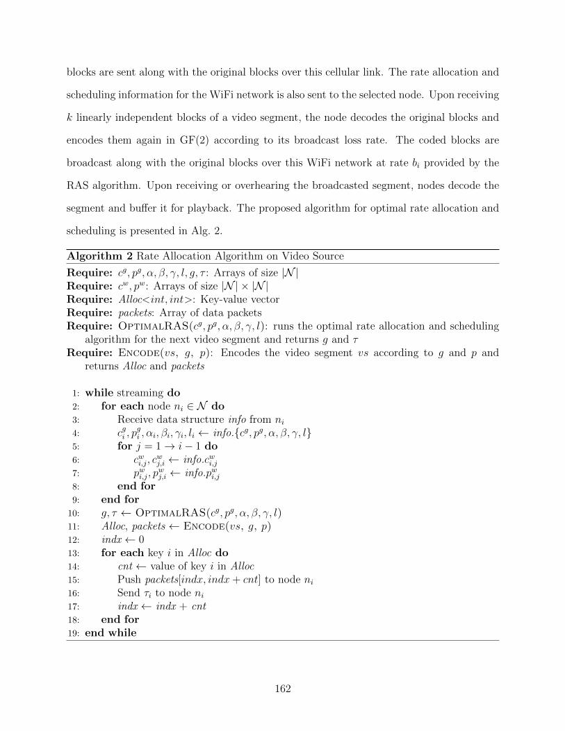
blocks are sent along with the original blocks over this cellular link. The rate allocation and
scheduling information for the WiFi network is also sent to the selected node. Upon receiving
k linearly independent blocks of a video segment, the node decodes the original blocks and
encodes them again in GF(2) according to its broadcast loss rate. The coded blocks are
broadcast along with the original blocks over this WiFi network at rate bi provided by the
RAS algorithm. Upon receiving or overhearing the broadcasted segment, nodes decode the
segment and buffer it for playback. The proposed algorithm for optimal rate allocation and
scheduling is presented in Alg. 2.
Algorithm 2 Rate Allocation Algorithm on Video Source
Require: cg, pg, α, β, γ, l, g, τ : Arrays of size |N |Require: cw, pw: Arrays of size |N | × |N |Require: Alloc<int, int>: Key-value vectorRequire: packets: Array of data packetsRequire: OptimalRAS(cg, pg, α, β, γ, l): runs the optimal rate allocation and scheduling
algorithm for the next video segment and returns g and τRequire: Encode(vs, g, p): Encodes the video segment vs according to g and p and
returns Alloc and packets
1: while streaming do2: for each node ni ∈ N do3: Receive data structure info from ni4: cgi , p
gi , αi, βi, γi, li ← info.{cg, pg, α, β, γ, l}
5: for j = 1→ i− 1 do6: cwi,j, c
wj,i ← info.cwi,j
7: pwi,j, pwj,i ← info.pwi,j
8: end for9: end for
10: g, τ ← OptimalRAS(cg, pg, α, β, γ, l)11: Alloc, packets ← Encode(vs, g, p)12: indx ← 013: for each key i in Alloc do14: cnt ← value of key i in Alloc15: Push packets[indx, indx+ cnt] to node ni16: Send τi to node ni17: indx ← indx + cnt18: end for19: end while
162
6.2.4 Overhead Analysis
The proposed RAS algorithm requires each active node to send battery usage and battery
information to the streaming source. This may be done periodically or just once. If this
information is provided to the source only once, the rate allocation on cellular links will not
consider power drained due to video decoding, rendering, and playback on the screen. If
this information is sent to the source periodically, the rate allocation will be dynamically
updated according to the current status of mobile devices. However, if bandwidth is scarce in
the network or signals are weak, the one-time update is preferred to reduce communication
overhead in the cellular network.
When providing update to the source, a node ni, in a cooperative network consisting
of N nodes, collects information (wi,j, ci,j, pi,j, and di,j) of WiFi links between itself and
each of the N − 1 nodes, the information (ci, pi, di, si) on the cellular link gi from the
source to itself, as well as its broadcast rate bi in the WiFi network and its battery level
li. Each of these values can be stored in 4 bytes. Hence, the size of an update message is
4 × (4(N − 1) + 6) bytes. For instance, in a cooperative network that consists of 10 nodes
and all nodes are active nodes, an update from a node is 168 bytes in size. Overall, there
are 1680 bytes flowing from the cooperative network to the source for each update period.
Assume that the update period is 10 seconds, which is frequent enough. The update shares
1680 Bps of the bandwidth. If we assume the bit rate for a typical streaming session 1 Mbps,
the communication overhead is 0.13% if the source serves only one copy of the video to the
cooperative network. Bear in mind that without the RAS algorithm, the source will stream
more than one copy of the video to the active nodes over the cellular network. Therefore, we
argue that this overhead is negligible. Furthermore, we note that the periodic update will
not lead to extra transmission delays, since the streaming source can use the previous RAS
results before receiving any new update.
Finally, we consider mobility of the mobile devices. Over time, the cooperative group
163
may move from one cell to another cell in the cellular network. For quick handover, the old
base station sends the new base station link information (wi,j, ci,j, pi,j, and di,j) for each of
the N2 WiFi links, the Lagrange multipliers (ηi, µi, ξi) for each of the N nodes and λ, as
well as the broadcast rate bi, the share time τi, and the battery level li of each node in the
WiFi network. Each of these values needs 4 bytes. Hence, the size of an update message is
4N2 + 6N + 1 bytes. For instance, in a cooperative network that consists of 10 nodes and
all nodes are active nodes, the old base station sends the new base station 1844 bytes during
the handover. Again, this overhead is considered negligible compared to the large volume of
the streaming traffic.
6.3 Performance Evaluation
In this section, we evaluate the performance of the proposed system, especially the effec-
tiveness of the RAS algorithm. In all experiments, unless specified otherwise, we assume
the packet loss rate of each cellular link and the WiFi broadcast channels are pi = 0.2 and
pw = 0.2, respectively. The average round trip time in the cellular network and the WiFi
network are 237 ms and 89 ms, respectively.
To evaluate our system in a close-to-reality setting, we use the energy profile from a real
smartphone. This phone is equipped with a dual-core 1.2 GHz processor, 1 GB of memory,
and a 3.7 V 1750 mAh Li-Ion battery that provides 23.31 KJ of energy. The operating
system is Android 4.2 (Jelly Bean). To collect the energy profile, we transmit (upload and
download) a large file using this phone in different network settings and monitor the energy
use. The energy consumption is measured three times using a fully charged phone, and
the average is reported in Table 6.3. For transmissions in cellular network, we control the
download rate of the phone using a software. We use the energy profile of the phone with
different download rates to simulate different types of nodes in the cooperative network.
According to Table 6.3, type I node achieves the maximum throughput, and the throughput
164
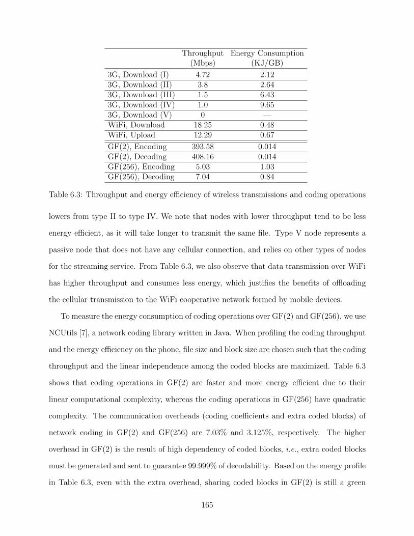
Throughput Energy Consumption(Mbps) (KJ/GB)
3G, Download (I) 4.72 2.123G, Download (II) 3.8 2.643G, Download (III) 1.5 6.433G, Download (IV) 1.0 9.653G, Download (V) 0 —WiFi, Download 18.25 0.48WiFi, Upload 12.29 0.67
GF(2), Encoding 393.58 0.014GF(2), Decoding 408.16 0.014GF(256), Encoding 5.03 1.03GF(256), Decoding 7.04 0.84
Table 6.3: Throughput and energy efficiency of wireless transmissions and coding operations
lowers from type II to type IV. We note that nodes with lower throughput tend to be less
energy efficient, as it will take longer to transmit the same file. Type V node represents a
passive node that does not have any cellular connection, and relies on other types of nodes
for the streaming service. From Table 6.3, we also observe that data transmission over WiFi
has higher throughput and consumes less energy, which justifies the benefits of offloading
the cellular transmission to the WiFi cooperative network formed by mobile devices.
To measure the energy consumption of coding operations over GF(2) and GF(256), we use
NCUtils [7], a network coding library written in Java. When profiling the coding throughput
and the energy efficiency on the phone, file size and block size are chosen such that the coding
throughput and the linear independence among the coded blocks are maximized. Table 6.3
shows that coding operations in GF(2) are faster and more energy efficient due to their
linear computational complexity, whereas the coding operations in GF(256) have quadratic
complexity. The communication overheads (coding coefficients and extra coded blocks) of
network coding in GF(2) and GF(256) are 7.03% and 3.125%, respectively. The higher
overhead in GF(2) is the result of high dependency of coded blocks, i.e., extra coded blocks
must be generated and sent to guarantee 99.999% of decodability. Based on the energy profile
in Table 6.3, even with the extra overhead, sharing coded blocks in GF(2) is still a green
165
choice as coding operations are significantly more energy efficient than that of GF(256).
In our simulation, we measure the energy consumption (in kJ) instead of power consump-
tion (in kW ), since it presents the total energy consumed throughout a streaming session.
To provide a clear view on the energy saving on mobile devices, we take the average of the
energy consumption consumed by each mobile device in the system. We also measure the
streaming delay (in ms), defined as the time it takes to deliver a specific segment to all the
collaborating nodes after it is scheduled by the RAS algorithm for transmission.
6.3.1 Cooperative Streaming using Different Coding Strategies
We begin the study with an investigation on the effect of different coding strategies on the
power consumption in a cooperative network of homogeneous devices, i.e., the cooperating
nodes are all from type I, as defined in Table 6.3. We turn off the shared session elongation
constraint (i.e., ψ = 0) in order to focus on the impact of different coding strategies and
cooperative arrangements. We feed the simulated source a high-definition video of length
6077 seconds with bitrate 4.36 Mbps. For comparison purpose, we implement four different
cooperation schemes listed below.
• Streaming over 3G: In this scheme, all mobile devices download the video directly over
cellular downlinks. There is no cooperation among mobile devices.
• Cooperation without network coding: In this scheme, mobile devices cooperate over
WiFi, but no coding is employed, i.e. di = di,j = 1,∀i ∈ N , j ∈ N−i . Without network
coding, all nodes must perform data reconciliation by contacting individual nodes for
particular missing segments.
• Cooperation using RLNC: In this scheme, random linear network coding is employed
over both cellular and WiFi links and coded blocks are always coded in GF(256). This
scheme is proposed in [72].
• Cooperation using two-level NC: In this scheme, as illustrated in Sec. 6.1, systematic
166
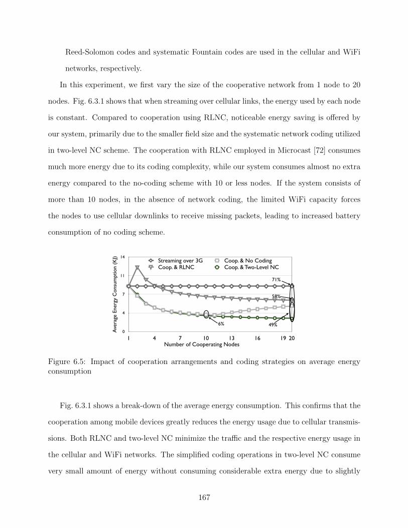
Reed-Solomon codes and systematic Fountain codes are used in the cellular and WiFi
networks, respectively.
In this experiment, we first vary the size of the cooperative network from 1 node to 20
nodes. Fig. 6.3.1 shows that when streaming over cellular links, the energy used by each node
is constant. Compared to cooperation using RLNC, noticeable energy saving is offered by
our system, primarily due to the smaller field size and the systematic network coding utilized
in two-level NC scheme. The cooperation with RLNC employed in Microcast [72] consumes
much more energy due to its coding complexity, while our system consumes almost no extra
energy compared to the no-coding scheme with 10 or less nodes. If the system consists of
more than 10 nodes, in the absence of network coding, the limited WiFi capacity forces
the nodes to use cellular downlinks to receive missing packets, leading to increased battery
consumption of no coding scheme.
0
4
7
11
14
1 4 7 10 13 16 19 20
Ave
rage
Ene
rgy
Con
sum
ptio
n (K
J) Streaming over 3G Coop. & No CodingCoop. & RLNC Coop. & Two-Level NC
Number of Cooperating Nodes
6% 49%
58%
71%
Figure 6.5: Impact of cooperation arrangements and coding strategies on average energyconsumption
Fig. 6.3.1 shows a break-down of the average energy consumption. This confirms that the
cooperation among mobile devices greatly reduces the energy usage due to cellular transmis-
sions. Both RLNC and two-level NC minimize the traffic and the respective energy usage in
the cellular and WiFi networks. The simplified coding operations in two-level NC consume
very small amount of energy without consuming considerable extra energy due to slightly
167
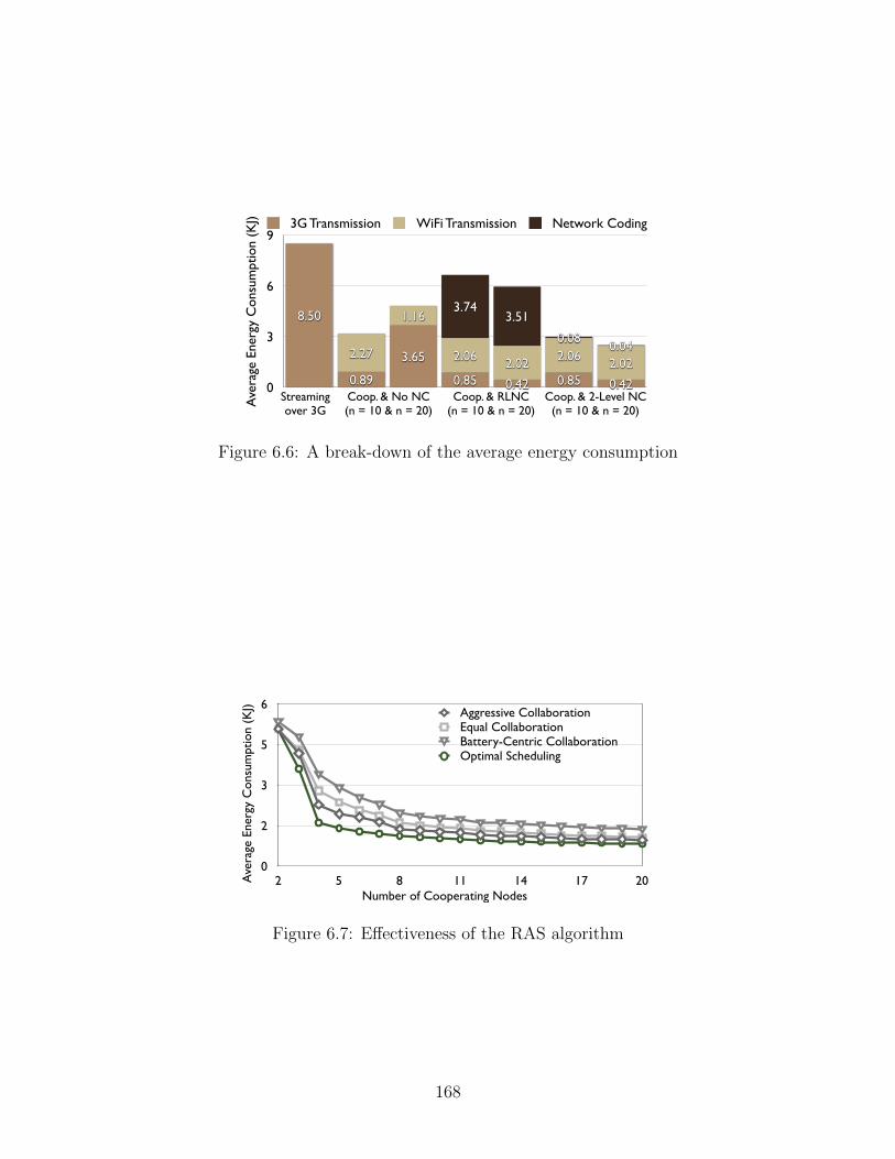
0
3
6
9
0.040.08
3.513.74
2.022.062.022.06
1.16
2.27
0.420.850.420.85
3.65
0.89
8.50
Ave
rage
Ene
rgy
Con
sum
ptio
n (K
J) 3G Transmission WiFi Transmission Network Coding
Streamingover 3G
Coop. & RLNC(n = 10 & n = 20)
Coop. & 2-Level NC (n = 10 & n = 20)
Coop. & No NC(n = 10 & n = 20)
Figure 6.6: A break-down of the average energy consumption
0
2
3
5
6
2 5 8 11 14 17 20
Aggressive CollaborationEqual CollaborationBattery-Centric CollaborationOptimal Scheduling
Number of Cooperating Nodes
Ave
rage
Ene
rgy
Con
sum
ptio
n (K
J)
Figure 6.7: Effectiveness of the RAS algorithm
168
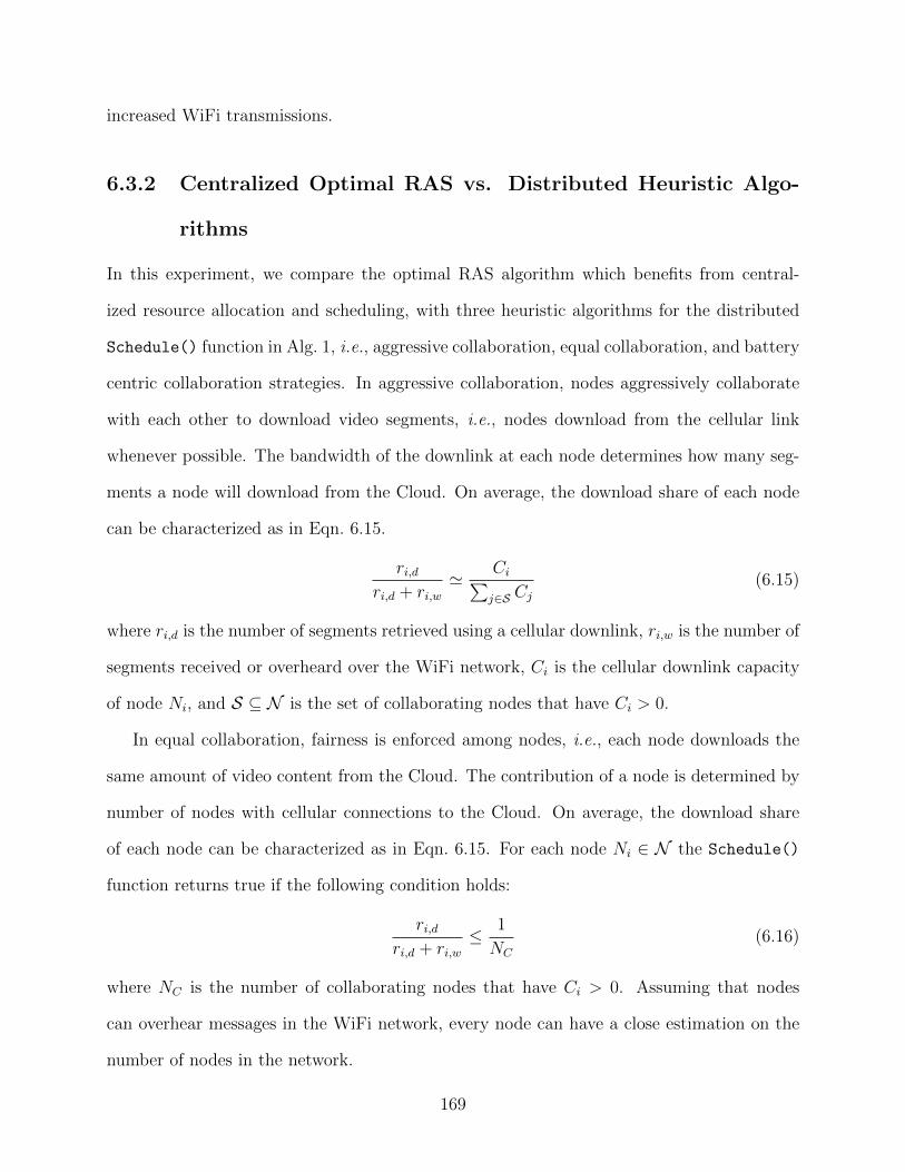
increased WiFi transmissions.
6.3.2 Centralized Optimal RAS vs. Distributed Heuristic Algo-
rithms
In this experiment, we compare the optimal RAS algorithm which benefits from central-
ized resource allocation and scheduling, with three heuristic algorithms for the distributed
Schedule() function in Alg. 1, i.e., aggressive collaboration, equal collaboration, and battery
centric collaboration strategies. In aggressive collaboration, nodes aggressively collaborate
with each other to download video segments, i.e., nodes download from the cellular link
whenever possible. The bandwidth of the downlink at each node determines how many seg-
ments a node will download from the Cloud. On average, the download share of each node
can be characterized as in Eqn. 6.15.
ri,dri,d + ri,w
' Ci∑j∈S Cj
(6.15)
where ri,d is the number of segments retrieved using a cellular downlink, ri,w is the number of
segments received or overheard over the WiFi network, Ci is the cellular downlink capacity
of node Ni, and S ⊆ N is the set of collaborating nodes that have Ci > 0.
In equal collaboration, fairness is enforced among nodes, i.e., each node downloads the
same amount of video content from the Cloud. The contribution of a node is determined by
number of nodes with cellular connections to the Cloud. On average, the download share
of each node can be characterized as in Eqn. 6.15. For each node Ni ∈ N the Schedule()
function returns true if the following condition holds:
ri,dri,d + ri,w
≤ 1
NC
(6.16)
where NC is the number of collaborating nodes that have Ci > 0. Assuming that nodes
can overhear messages in the WiFi network, every node can have a close estimation on the
number of nodes in the network.
169
Finally, in battery-centric collaboration, the objective is to maximize the overall battery
lifetime in the system. In other words, nodes with relatively low battery level will avoid
scheduling transmissions on their cellular links, while nodes with relatively longer remaining
battery lifetime will stream from the Cloud on behalf of the WiFi network. For each node
Ni ∈ N the Schedule() function returns true if the following condition holds:
Bi ≥ BC (6.17)
where Bi is the battery level of node i and BC is the approximate average of the battery
levels among nodes with Ci > 0. This scheduling algorithm requires each node to announce
its battery level, which can be piggybacked in any of the announcement messages.
The experiments are conducted in various heterogeneous cooperative networks consisting
of 20 nodes of types II—V defined in Table 6.3 with equal probability. To imitate the real-
world model of battery charges, we use a normal distribution with µ = 67 and σ2 = 10 [46]
to model the remaining battery lifetime. Again, we turn off the shared session elongation
constraint (i.e., ψ = 0) in order to focus on the impact of different rate allocation algorithms.
In order to ensure that almost all nodes have sufficient bandwidth on their cellular links to
sustain the streaming rate, we feed the simulated source a high-definition video of length
5482 seconds with a lower bitrate of 1.61 Mbps.
The specification of the nodes used in this experiment are summarized in Table 6.3.2.
Furthermore, we assume that the nodes join the system according to the order of node
identifiers, i.e., if the cooperative network contains 10 nodes, these nodes are nodes 1 to 10
from Table 6.3.2.
Fig. 6.3.1 shows that, compared to the aggressive, equal, and battery-centric collaboration
algorithms, our proposed RAS algorithm saves up to 15.0%, 22.4%, and 39.7% of energy,
respectively. It is interesting that the battery-centric collaboration algorithm, the most
intuitive heuristic approach to conserve battery, is the least energy-efficient solution.
Next, we compare the streaming delay offered by each scheduling algorithm. Fig. 6.3.2
170
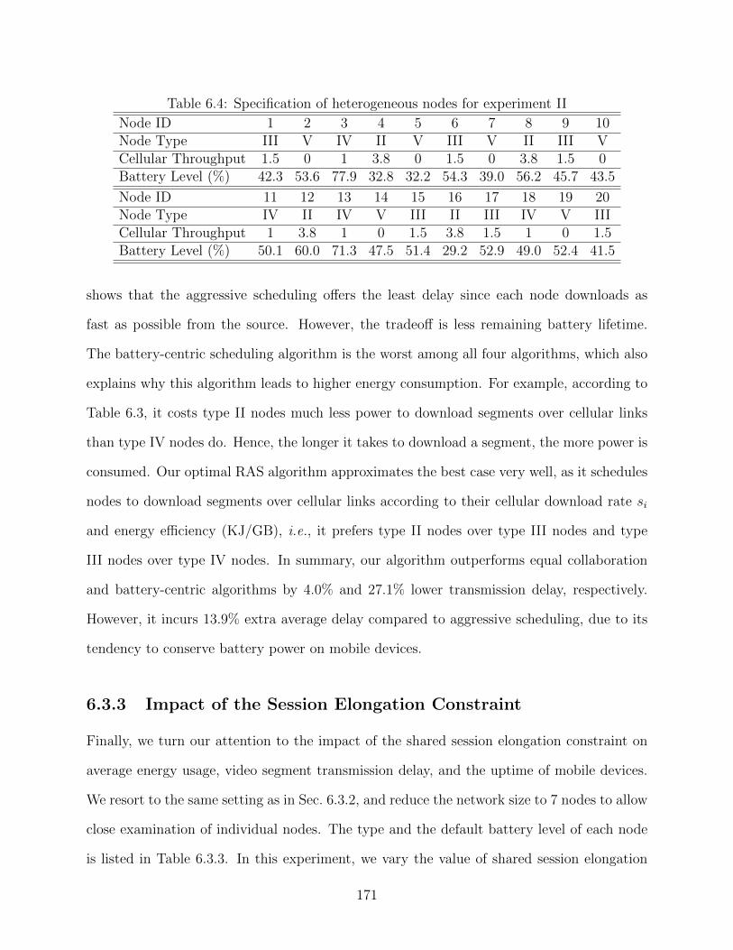
Table 6.4: Specification of heterogeneous nodes for experiment II
Node ID 1 2 3 4 5 6 7 8 9 10Node Type III V IV II V III V II III VCellular Throughput 1.5 0 1 3.8 0 1.5 0 3.8 1.5 0Battery Level (%) 42.3 53.6 77.9 32.8 32.2 54.3 39.0 56.2 45.7 43.5
Node ID 11 12 13 14 15 16 17 18 19 20Node Type IV II IV V III II III IV V IIICellular Throughput 1 3.8 1 0 1.5 3.8 1.5 1 0 1.5Battery Level (%) 50.1 60.0 71.3 47.5 51.4 29.2 52.9 49.0 52.4 41.5
shows that the aggressive scheduling offers the least delay since each node downloads as
fast as possible from the source. However, the tradeoff is less remaining battery lifetime.
The battery-centric scheduling algorithm is the worst among all four algorithms, which also
explains why this algorithm leads to higher energy consumption. For example, according to
Table 6.3, it costs type II nodes much less power to download segments over cellular links
than type IV nodes do. Hence, the longer it takes to download a segment, the more power is
consumed. Our optimal RAS algorithm approximates the best case very well, as it schedules
nodes to download segments over cellular links according to their cellular download rate si
and energy efficiency (KJ/GB), i.e., it prefers type II nodes over type III nodes and type
III nodes over type IV nodes. In summary, our algorithm outperforms equal collaboration
and battery-centric algorithms by 4.0% and 27.1% lower transmission delay, respectively.
However, it incurs 13.9% extra average delay compared to aggressive scheduling, due to its
tendency to conserve battery power on mobile devices.
6.3.3 Impact of the Session Elongation Constraint
Finally, we turn our attention to the impact of the shared session elongation constraint on
average energy usage, video segment transmission delay, and the uptime of mobile devices.
We resort to the same setting as in Sec. 6.3.2, and reduce the network size to 7 nodes to allow
close examination of individual nodes. The type and the default battery level of each node
is listed in Table 6.3.3. In this experiment, we vary the value of shared session elongation
171
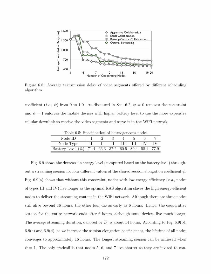
400
700
1,000
1,300
1,600
1 4 7 10 13 16 19 20
Aggressive CollaborationEqual CollaborationBattery-Centric CollaborationOptimal Scheduling
Number of Cooperating Nodes
Ave
rage
Tra
nsm
issi
on D
elay
(m
s)
Figure 6.8: Average transmission delay of video segments offered by different schedulingalgorithm
coefficient (i.e., ψ) from 0 to 1.0. As discussed in Sec. 6.2, ψ = 0 removes the constraint
and ψ = 1 enforces the mobile devices with higher battery level to use the more expensive
cellular downlink to receive the video segments and serve it in the WiFi network.
Table 6.5: Specification of heterogeneous nodes
Node ID 1 2 3 4 5 6 7Node Type I II II III III IV IV
Battery Level (%) 71.4 66.3 37.2 60.5 89.4 55.1 77.9
Fig. 6.9 shows the decrease in energy level (computed based on the battery level) through-
out a streaming session for four different values of the shared session elongation coefficient ψ.
Fig. 6.9(a) shows that without this constraint, nodes with low energy efficiency (e.g., nodes
of types III and IV) live longer as the optimal RAS algorithm slaves the high energy-efficient
nodes to deliver the streaming content in the WiFi network. Although there are three nodes
still alive beyond 16 hours, the other four die as early as 6 hours. Hence, the cooperative
session for the entire network ends after 6 hours, although some devices live much longer.
The average streaming duration, denoted by D, is about 14 hours. According to Fig. 6.9(b),
6.9(c) and 6.9(d), as we increase the session elongation coefficient ψ, the lifetime of all nodes
converges to approximately 16 hours. The longest streaming session can be achieved when
ψ = 1. The only tradeoff is that nodes 5, 6, and 7 live shorter as they are invited to con-
172
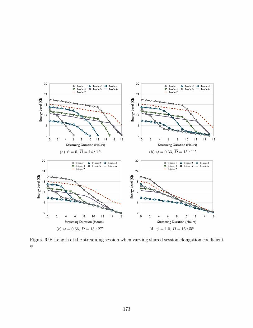
0
6
12
18
24
30
0 2 4 6 8 10 12 14 16 18
Ener
gy L
evel
(K
J)
Streaming Duration (Hours)
Node 1 Node 2 Node 3Node 4 Node 5 Node 6Node 7
(a) ψ = 0, D = 14 : 12′
0
6
12
18
24
30
0 2 4 6 8 10 12 14 16
Ener
gy L
evel
(K
J)
Streaming Duration (Hours)
Node 1 Node 2 Node 3Node 4 Node 5 Node 6Node 7
(b) ψ = 0.33, D = 15 : 11′
0
6
12
18
24
30
0 2 4 6 8 10 12 14 16
Ener
gy L
evel
(K
J)
Streaming Duration (Hours)
Node 1 Node 2 Node 3Node 4 Node 5 Node 6Node 7
(c) ψ = 0.66, D = 15 : 27′
0
6
12
18
24
30
0 2 4 6 8 10 12 14 16
Ener
gy L
evel
(K
J)
Streaming Duration (Hours)
Node 1 Node 2 Node 3Node 4 Node 5 Node 6Node 7
(d) ψ = 1.0, D = 15 : 55′
Figure 6.9: Length of the streaming session when varying shared session elongation coefficientψ
173
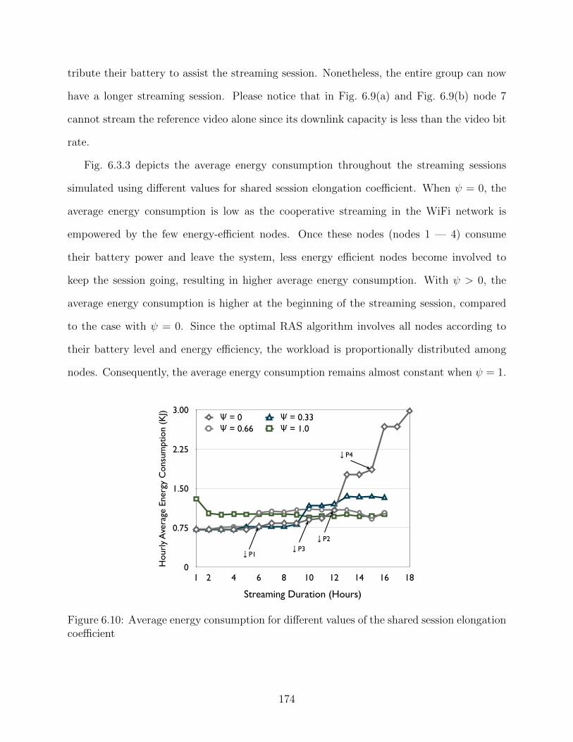
tribute their battery to assist the streaming session. Nonetheless, the entire group can now
have a longer streaming session. Please notice that in Fig. 6.9(a) and Fig. 6.9(b) node 7
cannot stream the reference video alone since its downlink capacity is less than the video bit
rate.
Fig. 6.3.3 depicts the average energy consumption throughout the streaming sessions
simulated using different values for shared session elongation coefficient. When ψ = 0, the
average energy consumption is low as the cooperative streaming in the WiFi network is
empowered by the few energy-efficient nodes. Once these nodes (nodes 1 — 4) consume
their battery power and leave the system, less energy efficient nodes become involved to
keep the session going, resulting in higher average energy consumption. With ψ > 0, the
average energy consumption is higher at the beginning of the streaming session, compared
to the case with ψ = 0. Since the optimal RAS algorithm involves all nodes according to
their battery level and energy efficiency, the workload is proportionally distributed among
nodes. Consequently, the average energy consumption remains almost constant when ψ = 1.
0
0.75
1.50
2.25
3.00
1 2 4 6 8 10 12 14 16 18
Hou
rly
Ave
rage
Ene
rgy
Con
sum
ptio
n (K
J)
Streaming Duration (Hours)
Ѱ = 0 Ѱ = 0.33Ѱ = 0.66 Ѱ = 1.0
⇣P1
⇣P2⇣P3
⇣P4
Figure 6.10: Average energy consumption for different values of the shared session elongationcoefficient
174
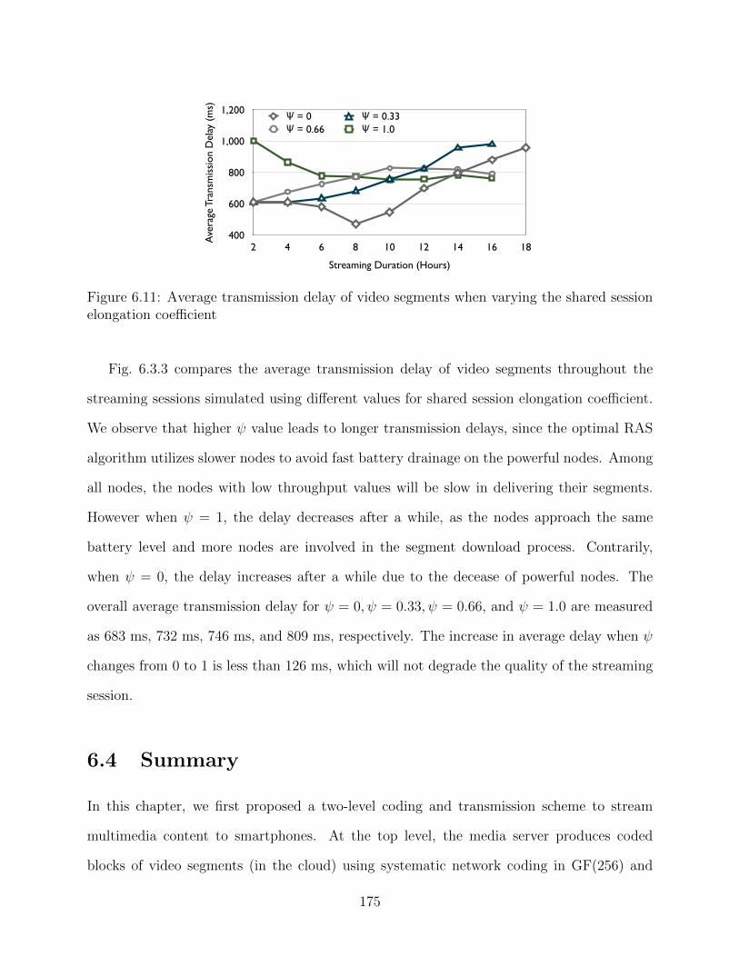
400
600
800
1,000
1,200
2 4 6 8 10 12 14 16 18
Ave
rage
Tra
nsm
issi
on D
elay
(m
s)
Streaming Duration (Hours)
Ѱ = 0 Ѱ = 0.33Ѱ = 0.66 Ѱ = 1.0
Figure 6.11: Average transmission delay of video segments when varying the shared sessionelongation coefficient
Fig. 6.3.3 compares the average transmission delay of video segments throughout the
streaming sessions simulated using different values for shared session elongation coefficient.
We observe that higher ψ value leads to longer transmission delays, since the optimal RAS
algorithm utilizes slower nodes to avoid fast battery drainage on the powerful nodes. Among
all nodes, the nodes with low throughput values will be slow in delivering their segments.
However when ψ = 1, the delay decreases after a while, as the nodes approach the same
battery level and more nodes are involved in the segment download process. Contrarily,
when ψ = 0, the delay increases after a while due to the decease of powerful nodes. The
overall average transmission delay for ψ = 0, ψ = 0.33, ψ = 0.66, and ψ = 1.0 are measured
as 683 ms, 732 ms, 746 ms, and 809 ms, respectively. The increase in average delay when ψ
changes from 0 to 1 is less than 126 ms, which will not degrade the quality of the streaming
session.
6.4 Summary
In this chapter, we first proposed a two-level coding and transmission scheme to stream
multimedia content to smartphones. At the top level, the media server produces coded
blocks of video segments (in the cloud) using systematic network coding in GF(256) and
175
serves coded blocks to the smartphones. At the bottom level, received content is shared
among smartphones within a WiFi network. The content is transmitted in both verbatim
form and coded form using systematic network coding in GF(2). Furthermore, we minimize
the network coding operations on smartphones by offloading the encoding process to the
server side (i.e., the cloud) and using XOR-only network coding in the WiFi network only
when necessary.
Furthermore, we proposed the optimal rate allocation and segment scheduling for mini-
mizing both the streaming traffic in the cellular network and the energy consumed by stream-
ing applications on mobile devices. More specifically, the proposed algorithm determines the
number of segments and the actual segments to be transmitted on each link. The actual
delivery of segments are achieved through the two-level coding scheme proposed in the first
section, ensuring an energy-efficient recovery of the streaming content on mobile devices. We
evaluate the system using a simulator driven by energy profile from real devices and com-
pare the performance of the proposed centralized optimal models with different distributed
heuristic scheduling models.
Our experimental results show that the proposed two level coding system saves up to
73% of battery usage on each phone compared to the current streaming mechanism over the
cellular network, and up to 52% compared to previous research works [72]. Due to the efficient
use of CPU time, the maximum achievable throughput in our system is approaching the
maximum capacity of the WiFi network, i.e., the system is capable to support higher quality
streaming. Furthermore, the proposed system provides short delay and long-lasting video
streaming by balancing the remaining battery lifetime among a group of cooperating nodes.
Moreover, compared to the proposed heuristic rate allocation and scheduling algorithms,
the proposed optimal RAS algorithm leads to significant energy saving on mobile devices.
Finally, our study on the impact of the session elongation constraint shows that enforcing
proportional contribution among all nodes effectively prolongs the streaming session for the
176

entire cooperative group.
While the proposed model significantly improves resource efficiency of video streaming
for collaborating smartphones, the provided bandwidth gain can also be traded for higher
video quality.
177
Chapter 7
Concluding Remarks and Future Works
Towards high quality and resource efficient video streaming service in mobile networks, in
this thesis we emphasized what can be brought from video coding and compression to differ-
ent parts of video streaming life cycle. This objective requires investigating the underlying
mechanisms and properties of the advanced video coding standards. Toward this goal, in
Chapter 3 we first introduced our carefully selected dataset of full-HD raw video sequences.
The dataset was assembled such that the selected video sequences represent a variety of con-
tent types that a video streaming server might need to encode and stream. Next, we looked
deeper into layered video coding and performed a systematic study on the use of advanced
video coding (H.264/AVC) and scalable video coding (SVC) for full HD video streaming.
We learned that in spite of the results reported in previous research works for using SVC for
low resolution videos (e.g., CIF and 4CIF), SVC requires less computational resources than
AVC in the encoding phase and also benefits from higher video quality in higher resolutions.
The main barriers for broad use of layered video coding in general and SVC in particular
are up to two times higher decoding time due to the more complex prediction loops and the
lack of embedded hardware decoders.
We notice that the results and observations reported in Chapter 3 can be generalized
to higher resolutions (such as 4K and 8K) for H.264/AVC and SVC. Even though these
standards do not support these resolutions, we tweaked the reference software to confirm
the findings in higher resolutions. However, it is not easy to generalize the reported ob-
servations to the new generation of video coding standards, i.e., H.265/HEVC and SHVC.
As discussed in Appendix A, many details have been modified in H.265/HEVC and SHVC.
Most importantly, the basic coding unit of video frames has changed from macroblocks and
178
sub-macroblocks to coding tree units (CTUs). CTUs can use larger block structures of up to
64× 64 samples and can better sub-partition the picture into variable sized structures. Such
a major change in the basic coding unit, along with other improvements and modifications,
may change the effect of layering and different video compression parameters and settings.
Looking into the application of internal dynamics of video coding standards in the life
cycle of a video streaming episode, in Chapter 4 we proposed a novel distributed video
transcoding scheme. The proposed scheme takes advantage of visual similarity among mac-
roblocks in a video sequence to reduce bitrate and transcoding time of the transcoded video.
As pioneering work in this research direction, we proposed an algorithm to extract the
dependency among macroblocks in an encoded video, based on which we determined the
dependency between successive GOPs. GOPs then were clustered according to their depen-
dency to create variable-size video chunks so that visually similar GOPs were put in one
chunk. Through experiments, we demonstrated that the proposed scheme reduces the video
bitrate and transcoding time. While the proposed model was evaluated using layered video
coding standard SVC, the same principle can be applied to other video coding standards such
as H.264/AVC or H.265/HEVC. The details of the model, however, needs to be adjusted to
the prediction mechanisms embedded in each video coding standard such that the similarity
between frames and GOPs are correctly calculated.
One related direction of future research is to determine the proper balance between video
transcoding and layered video coding. As discussed in details in Chapters 2 and 3, layered
video coding allows the edge media streamer to select a proper set of layers to match the
connection bandwidth and the hardware capabilities of the end user device. However, this
flexibility comes with a cost in terms of bitrate overhead for higher layers and computational
complexity of the coding tasks. The parallel solution to this problem is video transcoding that
transcodes the video either on the fly or using a set of predefined compression settings. Video
transcoding also comes with high computational cost along with more storage requirement
179
if it is offline. We need a model to wisely decide between adding or modifying a video layer,
adding a new encoding setting to the offline transcoding engine, or transcoding the video on
the fly to serve the specific end user. A straightforward solution toward this problem is using
a set of predefined parameters to create a constrained optimization problem and solve the
problem every time a decision needs to be made. As demonstrated in Chapter 4, considering
the video properties and the internal dynamics of the selected video coding standard might
strongly affect the cost function of the problem. The same statement can be made for a
heuristic solution.
In Chapter 5, we turned our attention to the video transmission phase of a video streaming
session. First, we precisely studied the coding and prediction mechanism of state-of-the-art
layered video coding standard, i.e., SVC. Next, toward smarter protection of video packets
over noisy communication channels and better quality of the transmitted video, we proposed
a novel coding and dependency aware unequal error protection algorithm. The proposed
algorithm calculates the importance of different video packets and associates protection to
each video packet, respectively. Experimental results show that the proposed algorithm
outperforms the state-of-the-art unequal error protection algorithms in terms of the quality
of the transmitted video. Finally, we completed the proposed UEP model by extending
the UEP problem from unicast scenario to multicast scenario, in which the full potential of
layered video coding is utilized by allowing the transmission network to multicast one copy
of the layered video for groups of heterogeneous mobile devices. To this end, we proposed a
new technique to dynamically adjust and combine the protection FEC packets for reference
and dependent video layers for video multicast in mobile communication networks.
The main idea proposed in Chapter 5, is utilizing the internal dependencies of compressed
video sequences to determine the importance of video packets. This idea can be applied
to any modern video coding standard, including H.265/HEVC and SHVC, as this idea is
extracted from video compression techniques. As expected, the new coding tree structure
180
and prediction mechanisms require the details of this method to be tailored again. Therefore,
a potential direction for future research can be the application of the same principle to the
new video coding standards. Furthermore, on the multicast problem, a deeper look into the
modulation schemes used in mobile wireless networks may bring more space to improve the
proposed solution.
Finally, in Chapter 6 we looked into the last part of the video streaming life cycle, i.e.,
video reception in smartphones. In this chapter, we first proposed a two-level coding and
transmission scheme to stream multimedia content to smartphones. At the top level, we used
systematic network coding in a Galois Field, i.e., GF(256). At the bottom level, the received
content is shared among smartphones within a WiFi network and systematic network coding
over GF(2) is utilized to augment the transmission process. Furthermore, we proposed the
optimal rate allocation and segment scheduling to minimize both the streaming traffic in
the cellular network and the energy consumed by streaming applications on mobile devices.
We also demonstrated that the proposed method outperforms similar works by reducing
the mobile traffic in the cellular network, reducing the battery usage on the smartphones,
reducing the transmission delay, and increasing the video quality.
181
Bibliography
[1] Joint Scalable Video Model (JSVM) software, version 9.19.15, Fraunhofer Heinrich-
Hertz-Institut, available online.
[2] Video Quality Measurement Tool, version 1.1, Multimedia Signal Processing Group,
Ecole Polytechnique Federale de Lausanne (EPFL), http://mmspg.epfl.ch.
[3] Xiph.org Test Media collection, http://media.xiph.org.
[4] Video System Characteristics of AVC, ATSC Standard A/72, Part 1:2008.
[5] Coding of audio-visual objects - part 2. ISO/IEC 14492-2 (MPEG-4 Visual), ISO/IEC
JTC 1, Version 3: May 2004.
[6] H.265/HEVC Reference Software (HM). https://hevc.hhi.fraunhofer.de/svn/svn-
HEVCSoftware/.
[7] NCUtils, Network Coding Utilities. http://code.google.com/p/ncutils.
[8] OpenHEVC, H.265/HEVC Encoder and Decoder Software.
https://github.com/OpenHEVC/ffmpeg.
[9] WiFi Direct, http://www.wi-fi.org/discover-and-learn/wi-fi-direct.
[10] x265, H.265/HEVC Encoder and Decoder Software. http://x265.org/.
[11] TS 22.146 V9.0.0 Technical Specification Group Services and System Aspects; Multi-
media Broadcast/Multicast Service; Stage 1, 2008.
[12] R. Ahlswede, N. Cai, S. Y. R. Li, and R. W. Yeung. Network Information Flow. IEEE
Transactions on Information Theory, 46(4):1204–1216, July 2000.
182
[13] S. Ahmad, R. Hamzaoui, and M. Al-Akaidi. Unequal Error Protection Using Foun-
tain Codes with Applications to Video Communication. in IEEE Transactions on
Multimedia, 13(1):92–101, February 2011.
[14] S. Ahmad, R. Hamzaoui, and M. Al-Akaidi. Unequal Error Protection Using Fountain
Codes with Applications to Video Communication. IEEE Transactions on Multimedia,
13(1):92–101, 2011.
[15] G. Ananthanarayanan, V. N. Padmanabhan, L. Ravindranath, and C. A. Thekkath.
Combine: Leveraging the Power of Wireless Peers Through Collaborative Download-
ing. In Proc. of 5th International Conference on Mobile Systems, Applications, and
Services (MobiSys), pages 286–298, San Juan, Puerto Rico, June 11-14, 2007.
[16] G. Ananthanarayanan, V. N. Padmanabhan, L. Ravindranath, and C. A. Thekkath.
Combine: Leveraging the Power of Wireless Peers Through Collaborative Download-
ing. In Proc. of 5th International Conference on Mobile Systems, Applications, and
Services (MobiSys), pages 286–298, San Juan, Puerto Rico, June 11-14 2007.
[17] M. Ankerst, M. M. Breunig, H.-P. Kriegel, and J. Sander. OPTICS: Ordering Points
to Identify the Clustering Structure. ACM Sigmod Record, 28(2):49–60, June 1999.
[18] R. Aparicio-Pardo, K. Pires, A. Blanc, and G. Simon. Transcoding Live Adaptive
Video Streams at a Massive Scale in the Cloud. In Proc. of the 6th ACM Multimedia
Systems Conference (MMSys 2015), pages 49–60. ACM, 2015.
[19] S. Arslan, P. Cosman, and L. Milstein. Generalized Unequal Error Protection LT
Codes for Progressive Data Transmission. in IEEE Transactions on Image Processing,
21(8):3586–3597, August 2012.
[20] A. Ashraf. Cost-Efficient Virtual Machine Provisioning for Multi-tier Web Applications
and Video Transcoding. In Proc. of 13th IEEE/ACM International Symposium on
183
Cluster, Cloud and Grid Computing (CCGrid), pages 66–69, Delft, Netherlands, May
13-16 2013.
[21] A. Ashraf, F. Jokhio, T. Deneke, S. Lafond, I. Porres, and J. Lilius. Stream-Based
Admission Control and Scheduling for Video Transcoding in Cloud Computing. In
Proc. of the 13th IEEE/ACM International Symposium on Cluster, Cloud and Grid
Computing (CCGrid), pages 482–489, Belfast, Northern Ireland, May 13-16 2013.
[22] Z. Avramova, D. De Vleeschauwer, P. Debevere, S. Wittevrongel, P. Lambert, R. Van
De Walle, and H. Bruneel. Performance of Scalable Video Coding for a TV broad-
cast network with constant video quality and heterogeneous receivers. In Proc. of
the10th International Conference on Telecommunications (ConTEL 2009), pages 435–
441, June 2009.
[23] E. Baccaglini, T. Tillo, and G. Olmo. Image and Video Transmission: A Comparison
Study of Using Unequal Loss Protection And Multiple Description Coding. Multimedia
Tools and Applications, 55(2):247–259, 2011.
[24] S. Bae, G. Nam, and K. Park. Effective Content-Based Video Caching with Cache-
Friendly Encoding and Media-Aware Chunking. In Proc. of the 5th ACM Multimedia
Systems Conference, pages 203–212, Singapore, Singapore, March 19-21 2014.
[25] M. Blestel and M. Raulet. Open SVC Decoder: A Flexible SVC Library. In Proc. of
the International Conference on Multimedia (MM 2010), pages 1463–1466, 2010.
[26] C. Boldrini, M. Conti, and A. Passarella. Exploiting Users’ Social Relations to For-
ward Data in Opportunistic Networks: The HiBOp Solution. Pervasive and Mobile
Computing, 4(15):633–657, October 2008.
[27] S. Brin and L. Page. The Anatomy of a Large-scale Hypertextual Web Search Engine.
Computer Networks and ISDN Systems, 30(1):107–117, 1998.
184

[28] H. Cai, B. Zeng, G. Shen, Z. Xiong, and S. Li. Error-Resilient Unequal Error Protection
of Fine Granularity Scalable Video Bitstreams. EURASIP Journal on Advances in
Signal Processing, 2006.
[29] A. Carroll and G. Heiser. An Analysis of Power Consumption in a Smartphone. In
Proc. of USENIX Annual Technical Conf. (ATC), pages 21–34, Boston, MA, June
23-25 2010.
[30] D. M. Chandler and S. S. Hemami. VSNR: A Wavelet-based Visual Signal-to-noise
Ratio for Natural Images. IEEE Transactions on Image Processing, 16(9):2284–2298,
2007.
[31] Z. H. Chang, B. F. Jong, W. J. Wong, and M. D. Wong. Distributed Video Transcoding
on a Heterogeneous Computing Platform. In Proc. of IEEE Asia Pacific Conference
on Circuits and Systems (APCCAS), pages 444–447. IEEE, 2016.
[32] M. Chen. AMVSC: A Framework of Adaptive Mobile Video Streaming in the Cloud. In
Proc. of IEEE Global Communications Conference (GLOBECOM), pages 2042–2047,
Anaheim, California, December 3-7 2012.
[33] R. Cheng, W. Wu, Y. Lou, and Y. Chen. A Cloud-Based Transcoding Framework for
Real-Time Mobile Video Conferencing System. In Proc. of 2nd IEEE International
Conference on Mobile Cloud Computing, Services, and Engineering (MobileCloud),
pages 236–245, London, UK, April 7-10 2014.
[34] J. Chesterfield, R. Chakravorty, I. Pratt, S. Banerjee, and P. Rodriguez. Exploiting
Diversity to Enhance Multimedia Streaming Over Cellular Links. In Proc. of 24th IEEE
Conference on Computer Communications (INFOCOM), pages 2020–2031, Miami, FL,
March 13-17, 2005.
185
[35] H. Choi, J. Nam, D. Sim, and I. V. Bajic. Scalable Video Coding Based on High Effi-
ciency Video Coding (HEVC). In IEEE Pacific Rim Conference on Communications,
Computers and Signal Processing (PacRim), pages 346–351, Aug 2011.
[36] Cisco. Cisco Visual Networking Index: Global Mobile Data Traffic Forecast Update,
2015—2020, February 2016.
[37] I. R. communication Standardization Sector (ITU-R). Recommendation ITU-R
BT.500-11: Methodology for the Subjective Assessment of the Quality of Television
Pictures, June 2002.
[38] N. Damera-Venkata, T. D. Kite, W. S. Geisler, B. L. Evans, and A. C. Bovik. Image
Quality Assessment Based on a Degradation Model. IEEE Transactions on Image
Processing, 9(4):636–650, 2000.
[39] J. Dean and S. Ghemawat. MapReduce: Simplified Data Processing on Large Clusters.
Communications of the ACM, 52(1):107–113, January 2008.
[40] C. Diaz, J. Cabrera, F. Jaureguizar, and N. Garcia. Adaptive Protection Scheme for
MVC-Encoded Stereoscopic Video Streaming in IP-Based Networks. In Proc. of IEEE
Visual Communications and Image Processing (VCIP), pages 1–6, San Diego, CA,
November 27-30 2012.
[41] a. Q. C. Digital Fountain Incorporated. Application Layer Forward Error Correction
for Mobile Multimedia Broadcasting Case Study, 2009.
[42] H. Dung and S. Vafi. An Adaptive Unequal Error Protection Based on Motion Energy
of H.264/AVC Video Frames. In IEEE Conference on Wireless Communications and
Networking Conference (WCNC’13), pages 4594–4599, 2013.
[43] M. Eberhard, L. Celetto, C. Timmerer, E. Quacchio, and H. Hellwagner. Performance
Analysis of Scalable Video Adaptation: Generic versus Specific Approach. In Proc. of
186
the 9th Int. Workshop on Image Analysis for Multimedia Interactive Services (WIAMIS
2008), pages 50–53, May 2008.
[44] A. Eichhorn and P. Ni. Pick your layers wisely-a quality assessment of h. 264 scal-
able video coding for mobile devices. In Proc. of IEEE International Conference on
Communications (ICC 2009), pages 1–6, Dresden, Germany, June 2009.
[45] M. Ester, H.-P. Kriegel, J. Sander, and X. Xu. A Density-Based Algorithm for Discov-
ering Clusters in Large Spatial Databases with Noise. In Proc. of the 2nd International
Conference on Knowledge Discovery and Data Mining (KDD-96), number 34, pages
226–231, Portland, Oregon, August 2-4 1996.
[46] D. Ferreira, A. K. Dey, and V. Kostakos. Understanding Human-Smartphone Con-
cerns: A Study of Battery Life. Lecture Notes in Computer Science, Pervasive Com-
puting, 6696:19–33, 2011.
[47] M. L. Fisher. An Applications Oriented Guide to Lagrangian Relaxation. in Interfaces,
15(2):10–21, March-April 1985.
[48] F. H. P. Fitzek, P. Kyritsi, and M. D. Katz. Cooperation in Wireless Networks: Prin-
ciples and Applications, chapter Power Consumption and Spectrum Usage Paradigms
in Cooperative Wireless Networks, pages 365–386. Springer, 2006.
[49] G. Gao, W. Zhang, Y. Wen, Z. Wang, W. Zhu, and Y. P. Tan. Cost Optimal Video
Transcoding in Media Cloud: Insights from User Viewing Pattern. In Proc. of IEEE In-
ternational Conference on Multimedia and Expo (ICME), pages 1–6, Chengdu, China,
July 14-18 2014.
[50] A. Garcia, H. Kalva, and B. Furht. A Study of Transcoding on Cloud Environments
for Video Content Delivery. In Proc. of 2010 ACM Multimedia Workshop on Mobile
Cloud Media Computing, pages 13–18. ACM, 2010.
187
[51] C. Gong, G. Yue, and X. Wang. Message-wise Unequal Error Protection Based on Low-
Density Parity-Check Codes. IEEE Transactions on Communications, 59(4):1019–
1030, 2011.
[52] R. Gupta, A. Pulipaka, P. Seeling, L. Karam, and M. Reisslein. H.264 Coarse Grain
Scalable (CGS) and Medium Grain Scalable (MGS) Encoded Video: A Trace Based
Traffic and Quality Evaluation. IEEE Transactions on Broadcasting, 58(3):428–439,
September 2012.
[53] H. Ha and C. Yim. Layer-weighted Unequal Error Protection for Scalable Video Coding
Extension of H. 264/AVC. IEEE Transactions on Consumer Electronics, 54(2):736–
744, 2008.
[54] B. Han, P. Hui, V. A. Kumar, M. V. Marathe, G. Pei, and A. Srinivasan. Cellular
Traffic Offloading through Opportunistic Communications: A Case Study. In Proc. of
5th ACM Workshop on Challenged Networks, pages 31–38, Chicago, IL, September
20-24, 2010.
[55] A. Heikkinen, J. Sarvanko, M. Rautiainen, and M. Ylianttila. Distributed Multi-
media Content Analysis with MapReduce. In Proc. of the 24th IEEE International
Symposium on Personal Indoor and Mobile Radio Communications (PIMRC), pages
3497–3501, London, UK, September 8-11 2013.
[56] T. Ho, R. Koetter, M. Medard, D. R. Karger, and M. Effros. The Benefits of Cod-
ing over Routing in a Randomized Setting. In Proc. of International Symposium on
Information Theory (ISIT 2003), page 442, Yokohama, Japan, June 29 - July 4, 2003.
[57] J.-C. Huang, C.-Y. Wu, and J.-J. Chen. On High Efficient Cloud Video Transcod-
ing. In Proc. of 2015 International Symposium on Intelligent Signal Processing and
Communication Systems (ISPACS), pages 170–173. IEEE, 2015.
188
[58] Z. Huang, C. Mei, L. Li, and T. Woo. CloudStream: Delivering High-Quality Stream-
ing Videos Through a Cloud-based SVC Proxy. In Proc. of IEEE Conference on
Computer Communications (INFOCOM), pages 201–205, Shanghai, China, April 10-
15 2011.
[59] P. Hui, J. Crowcroft, and E. Yoneki. Bubble Rap: Social-Based Forwarding in
Delay-Tolerant Networks. IEEE Transactions on Mobile Computing, 10(11):1576–
1589, November 2011.
[60] P. Hui, J. Crowcroft, and E. Yoneki. Bubble Rap: Social-Based Forwarding in
Delay-Tolerant Networks. IEEE Transactions on Mobile Computing, 10(11):1576–
1589, November 2011.
[61] Y. Huo, M. El-Hajjar, and L. Hanzo. Inter-Layer FEC Aided Unequal Error Protection
for Multilayer Video Transmission in Mobile TV. IEEE Transactions on Circuits and
Systems for Video Technology, 23(9):1622–1634, 2013.
[62] S. Ioannidis, A. Chaintreau, and L. Massoulie. Optimal and Scalable Distribution of
Content Updates Over a Mobile Social Network. In Proc. of 28th IEEE Conference
on Computer Communications (INFOCOM), pages 1422–1430, Rio de Janeiro, Brazil,
April 19-25, 2009.
[63] S. Ioannidis, A. Chaintreau, and L. Massoulie. Optimal and Scalable Distribution of
Content Updates Over a Mobile Social Network. In Proc. of 28th IEEE Conference
on Computer Communications (INFOCOM), pages 1422–1430, Rio de Janeiro, Brazil,
April 19-25 2009.
[64] ITU-T. Recommendation Y.1541 : Network Performance Objectives for IP-based
Services, 2011.
[65] ITU-T. H.264/AVC Reference Software, 2016.
189
[66] S. Jakubczak and D. Katabi. A Cross-layer Design for Scalable Mobile Video. In
Proc. of ACM Multimedia 2011 (MM 2011), pages 289–300, November 28-December
1 2011.
[67] S. Jeannin and A. Divakaran. MPEG-7 Visual Motion Descriptors. IEEE Transactions
on Circuits and Systems for Video Technology, 11(6):720–724, June 2001.
[68] F. Jokhio, A. Ashraf, S. Lafond, and J. Lilius. A Computation and Storage Trade-off
Strategy for Cost-Efficient Video Transcoding in the Cloud. In Proc. of 39th Con-
ference on Software Engineering and Advanced Applications (SEAA), pages 365–372,
Santander, Spain, September 4-6 2013.
[69] F. Jokhio, A. Ashraf, S. Lafond, I. Porres, and J. Lilius. Prediction-Based Dynamic Re-
source Allocation for Video Transcoding in Cloud Computing. In Proc. of the 21st In-
ternational Conference on Parallel, Distributed and Network-Based Processing (PDP),
pages 254–261, Belfast, Northern Ireland, February 27-March 1 2013.
[70] F. Jokhio, T. Deneke, S. Lafond, and J. Lilius. Bit Rate Reduction Video Transcoding
with Distributed Computing. In Proc. of the 20th International Conference on Parallel,
Distributed and Network-Based Processing (PDP), pages 206–212, Garching, Germany,
February 15-17 2012.
[71] A. B. Kahn. Topological Sorting of Large Networks. Communications of the ACM,
5(11):558–562, 1962.
[72] L. Keller, A. Le, B. Cici, H. Seferoglu, C. Fragouli, and A. Markopoulou. MicroCast:
Cooperative Video Streaming on Smartphones. In Proc. of 10th International Con-
ference on Mobile Systems, Applications, and Services (MobiSys), pages 57–70, Low
Wood Bay, United Kingdom, June 25-29, 2012.
[73] L. Keller, A. Le, B. Cici, H. Seferoglu, C. Fragouli, and A. Markopoulou. MicroCast:
190
Cooperative Video Streaming on Smartphones. In Proc. of 10th International Con-
ference on Mobile Systems, Applications, and Services (MobiSys), pages 57–70, Low
Wood Bay, United Kingdom, June 25-29 2012.
[74] J. Kim, R. M. Mersereau, and Y. Altunbasak. Error-Resilient Image and Video Trans-
mission over the Internet using Unequal Error Protection. IEEE Transactions on
Image Processing, 12(2):121–131, 2003.
[75] M. Kim, Y. Cui, S. Han, and H. Lee. Towards Efficient Design and Implementation of
a Hadoop-Based Distributed Video Transcoding System in Cloud Computing Environ-
ment. International Journal of Multimedia and Ubiquitous Engineering, 8(2):213–224,
2013.
[76] M. Kim, S. Han, Y. Cui, H. Lee, H. Cho, and S. Hwang. CloudDMSS: Robust Hadoop-
Based Multimedia Streaming Service Architecture for a Cloud Computing Environ-
ment. Cluster Computing, 17(3):605–628, September 2014.
[77] F. Lao, X. Zhang, and Z. Guo. Parallelizing Video Transcoding Using Map-Reduce-
Based Cloud Computing. In Proc. of IEEE International Symposium on Circuits and
Systems (ISCAS), pages 2905–2908, Seoul, Korea, May 20-23 2012.
[78] H. Y. Lee, H. K. Lee, and Y. H. Ha. Spatial Color Descriptor for Image Retrieval And
Video Segmentation. IEEE Transactions on Multimedia, 5(3):358–367, 2003.
[79] J.-S. Lee, F. De Simone, and T. Ebrahimi. Subjective Quality Assessment of Scalable
Video Coding: A Survey. In Proc. of the 3rd International Workshop on Quality of
Multimedia Experience (QoMEX 2011), pages 25–30, Mechelen, Belgium, September
2011.
[80] S. Li and S. G. Chan. BOPPER: Wireless Video Broadcasting With Peer-to-Peer
Error Recovery. In Proc. of IEEE International Conference on Multimedia and Expo
191
(ICME), pages 392–395, Beijing, China, July 2-5 2007.
[81] S. Li and S. H. G. Chan. BOPPER: Wireless Video Broadcasting With Peer-to-Peer
Error Recovery. In Proc. of IEEE International Conference on Multimedia and Expo
(ICME), pages 392–395, Beijing, China, July 2-5, 2007.
[82] X. Li, P. Amon, A. Hutter, and A. Kaup. Performance Analysis of Inter-Layer Pre-
diction in Scalable Video Coding Extension of H.264/AVC. IEEE Transactions on
Broadcasting, 57(1):66–74, March 2011.
[83] Z. Li, Y. Huang, G. Liu, F. Wang, Z.-L. Zhang, and Y. Dai. Cloud Transcoder:
Bridging the Format and Resolution Gap Between Internet Videos and Mobile Devices.
In Proc. of the 22nd International Workshop on Network and Operating System Support
for Digital Audio and Video (NOSSDAV), pages 33–38, June 7-8 2012.
[84] A. Limmanee and W. Henkel. UEP Network Coding for Scalable Data. In Proc. of
5th International Symposium on Turbo Codes and Related Topics, pages 333–337, Lau-
sanne, Switzerland, September 1-5 2008.
[85] Z. Liu, C. Wu, B. Li, and S. Zhao. UUSee: Large Scale Operational On Demand
Streaming with Random Network Coding. In Proc. of 29th Annual IEEE International
Conference on Computer Communications (INFOCOM), pages 1–9, San Diego, CA,
March 15-19 2010.
[86] E. Maani and A. K. Katsaggelos. Unequal Error Protection for Robust Streaming
of Scalable Video over Packet Lossy Networks. IEEE Transactions on Circuits and
Systems for Video Technology, 20(3):407–416, 2010.
[87] D. MacKay. Fountain Codes. in IEEE Proceedings of Communications, 152(6):1062–
1068, December 2005.
192
[88] V. Magoulianitis and I. Katsavounidis. HEVC Decoder Optimization in Low Power
Configurable Architecture for Wireless Devices. In IEEE 16th International Sympo-
sium on a World of Wireless, Mobile and Multimedia Networks (WoWMoM), pages
1–6. IEEE, 2015.
[89] J. L. Mannos and D. J. Sakrison. The Effects of a Visual Fidelity Criterion of the
Encoding of Images. IEEE Transactions on Information Theory, 20(4):525–536, 1974.
[90] B. Masnick and J. Wolf. On Linear Unequal Error Protection Codes. IEEE Transac-
tions on Information Theory, 13(4):600–607, 1967.
[91] L. Merritt and R. Vanam. x264: A High Performance H.264/AVC Encoder.
http://neuron.net/library/avc/overview, 2006.
[92] A. Moorthy, L. K. Choi, A. Bovik, and G. de Veciana. Video Quality Assessment
on Mobile Devices: Subjective, Behavioral and Objective Studies. IEEE Journal of
Selected Topics in Signal Processing, 6(6):652–671, Oct 2012.
[93] A. Nafaa, T. Taleb, and L. Murphy. Forward Error Correction Strategies for Media
Streaming over Wireless Networks. IEEE Communications Magazine, 46(1), 2008.
[94] S. Nazir, V. Stankovic, I. Andonovic, and D. Vukobratovic. Application Layer System-
atic Network Coding for Sliced H.264/AVC Video Streaming. Advances in Multimedia,
2012:1–9, 2012.
[95] S. Nazir, V. Stankovic, and D. Vukobratovic. Expanding Window Random Linear
Codes for Data Partitioned H.264 Video Transmission over DVB-H Network. In
18th IEEE International Conference on Image Processing (ICIP’11), pages 2205–2208,
2011.
[96] S. Nazir, V. Stankovic, and D. Vukobratovic. Unequal Error Protection for Data Parti-
tioned H.264/AVC Video Streaming with Raptor and Random Linear Codes for DVB-
193
H Networks. In IEEE International Conference on Multimedia and Expo (ICME),
pages 1–6, 2011.
[97] T. Oelbaum, H. Schwarz, M. Wien, and T. Wiegand. Subjective Performance Evalu-
ation of the SVC Extension of H.264/AVC. In Proc. of the 15th IEEE International
Conference on Image Processing (ICIP 2008), pages 2772–2775, October 2008.
[98] J.-R. Ohm, G. J. Sullivan, H. Schwarz, T. K. Tan, and T. Wiegand. Comparison of
the Coding Efficiency of Video Coding Standards — Including High Efficiency Video
Coding (HEVC). IEEE Transactions on Circuits and Systems for Video Technology,
22(12):1669–1684, 2012.
[99] D. K. Park, Y. S. Jeon, and C. S. Won. Efficient Use of Local Edge Histogram
Descriptor. In Proc. of the 2000 ACM Workshops on Multimedia, pages 51–54, 2000.
[100] V. Pavlushkov, R. Johannesson, and V. Zyablov. Unequal Error Protection for Con-
volutional Codes. IEEE Transactions on Information Theory, 52(2):700–708, 2006.
[101] M. V. Pedersen, F. H. P. Fitzek, and J. Heide. On-the-Fly Packet Error Recovery in a
Cooperative Cluster of Mobile Devices. In Proc. of IEEE Global Telecommunications
Conference (GLOBECOM), pages 1–6, Houston, TX, December 5-9, 2011.
[102] M. V. Pedersen, J. Heide, F. H. Fitzek, and T. Larsen. Pictureviewer: A Mobile
Application Using Network Coding. In Proc. of European Wireless Conference, pages
151–156, Aalborg, Denmark, May 17-20, 2009.
[103] V. Pedersen and F. H. P. Fitzek. Implementation and Performance Evaluation of
Network Coding for Cooperative Mobile Devices. In Proc. of IEEE International
Conference on Communications (ICC), pages 91–96, Beijing, China, May 19-23, 2008.
[104] H.-D. Pham and V. Sina. Unequal Error Protection of H. 264/AVC Video Bitstreams
Based on Data Partitioning and Motion Information of Slices. In IEEE International
194
Conference on Signal Processing, Communication and Computing (ICSPCC 2012),
pages 634–639, Hong Kong, China, August 2012.
[105] I. Politis, L. Dounis, and T. Dagiuklas. H.264/SVC vs. H.264/AVC Video Quality
Comparison under QoE-driven Seamless Handoff. Signal Processing: Image Commu-
nication, 27(8):814 – 826, 2012.
[106] A. Pulipaka, P. Seeling, M. Reisslein, and L. Karam. Overview and Traffic Characteri-
zation of Coarse-Grain Quality Scalable (CGS) H.264 SVC Encoded Video. In Proc. of
the 7th IEEE Consumer Communications and Networking Conference (CCNC 2010),
pages 1–5, Las Vegas, NV, January 2010.
[107] A. Ramasubramonian and J. Woods. Video Multicast Using Network Coding. In
Proc. of SPIE Conference on Visual Communications and Image Processing (VCIP),
pages 1–11, San Jose, CA, January 2009.
[108] R. Razavi, M. Fleury, M. Altaf, H. Sammak, and M. Ghanbari. H.264 Video Streaming
with Data-Partitioning and Growth Codes. In IEEE 16th International Conference on
Image Processing, pages 90–912, 2009.
[109] P. Rodriguez, R. Chakravorty, J. Chesterfield, I. Pratt, and S. Banerjee. MAR: A
Commuter Router Infrastructure for the Mobile Internet. In Proc. of 2nd International
Conference on Mobile Systems, Applications, and Services (MobiSys), pages 217–230,
Boston, MA, June 6-9, 2004.
[110] S. S. and R. J. AHG Report on Spatial Scalability Resampling. Technical report,
Report JVT-R006 of the 18th Meeting of the Joint Video Team, 2006.
[111] O. Salim and W. Xiang. A Novel Unequal Error Protection Scheme for 3D Video Trans-
mission over Cooperative MIMO-OFDM Systems. in EURASIP Journal on Wireless
Communications and Networking, (1):269–283, 2012.
195
[112] H. Schwarz, D. Marpe, and T. Wiegand. Overview of the Scalable Video Coding
Extension of the H. 264/AVC Standard. IEEE Transactions on Circuits and Systems
for Video Technology, 17(9):1103–1120, 2007.
[113] P. Seeling, F. H. P. Fitzek, G. Ertli, A. Pulipaka, and M. Reisslein. Video Network
Traffic and Quality Comparison of VP8 and H.264 SVC. In Proc. of the 3rd Workshop
on Mobile Video Delivery (MoViD 2010), pages 33–38, 2010.
[114] H. Seferoglu, L. Keller, B. Cici, A. Le, and A. Markopoulou. Cooperative Video
Streaming on Smartphones. In Proc. of 49th Annual Allerton Conference on Commu-
nication, Control, and Computing, pages 220–227, Urbana Champaign, IL, September
28-30, 2011.
[115] K. Seshadrinathan, R. Soundararajan, A. C. Bovik, and L. K. Cormack. Study of
Subjective and Objective Quality Assessment of Video. IEEE Transactions on Image
Processing, 19(6):1427–1441, 2010.
[116] H. Sheikh and A. Bovik. Image Information and Visual Quality. IEEE Transactions
on Image Processing, 15(2):430–444, February 2006.
[117] H. Shojania and B. Li. Random Network Coding on the iPhone: Fact or Fiction? In
Proc. of 18th International Workshop on Network and Operating Systems Support for
Digital Audio and Video (NOSSDAV), pages 37–42, Williamsburg, VA, June 3-5, 2009.
[118] T. Sikora. The MPEG-7 Visual Standard for Content Description - An Overview.
IEEE Transactions on Circuits and Systems for Video Technology, 11(6):696–702, June
2001.
[119] T. Sikora. The MPEG-7 Visual Standard for Content Description - An Overview.
IEEE Transactions on Circuits and Systems for Video Technology, 11(6):696–702,
2001.
196
[120] M. Slanina, M. Ries, and J. Vehkapera. Rate Distortion Performance of H.264/SVC
in Full HD with Constant Frame Rate and High Granularity. In Proc. of the 8th
International Conference on Digital Telecommunications (ICDT 2013), pages 7–13,
Venice, Italy, April 2013.
[121] H. Soroush, P. Gilbert, N. Banerjee, M. D. Corner, B. N. Levine, and L. Cox. Spider:
Improving Mobile Networking with Concurrent Wi-Fi Connections. ACM SIGCOMM
Computer Communication Review, 41(4):402–403, August 2011.
[122] Statista. Number of Mobile Applications Available in Leading App Stores as of July
2015, July 2015.
[123] M. Stiemerling and S. Kiesel. A System for Peer-to-Peer Video Streaming in Resource
Constrained Mobile Environments. In Proc. of 1st ACM Workshop on User-Provided
Networking (U-NET), pages 25–30, Rome, Italy, December 1-4, 2009.
[124] T. Stockhammer and M. Bystrom. H.264/AVC Data Partitioning for Mobile Video
Communication. In International Conference on Image Processing (ICIP’04), vol-
ume 1, pages 545–548, 2004.
[125] G. J. Sullivan, J.-R. Ohm, W.-J. Han, and T. Wiegand. Overview of the High Efficiency
Video Coding (HEVC) Standard. IEEE Transactions on Circuits and Systems for
Video Technology, 22(12):1649–1668, 2012.
[126] N. Thomos, S. Argyropoulos, N. V. Boulgouris, and M. G. Strintzis. Robust Trans-
mission of H.264/AVC Streams using Adaptive Group Slicing and Unequal Error Pro-
tection. EURASIP Journal on Applied Signal Processing, 2006:1–13, 2006.
[127] N. Thomos, J. Chakareski, and P. Frossard. Prioritized Distributed Video Delivery
With Randomized Network Coding. in IEEE Transactions on Multimedia, 13(4):776–
787, August 2011.
197
[128] C. L. Tsao and R. Sivakumar. On Effectively Exploiting Multiple Wireless Interfaces
in Mobile Hosts. In Proc. of 5th Int. Conf. on Emerging Networking Experiments and
Technologies (CoNEXT), pages 337–348, Rome, Italy, December 1-4 2009.
[129] C. L. Tsao and R. Sivakumar. On Effectively Exploiting Multiple Wireless Interfaces
in Mobile Hosts. In Proc. of 5th International Conference on Emerging Networking
Experiments and Technologies (CoNEXT), pages 337–348, Rome, Italy, December 1-4
2009.
[130] I. Unanue, I. Urteaga, R. Husemann, J. D. Ser, V. Roesler, A. Rodriguez, and
P. Sanchez. A Tutorial on H.264/SVC Scalable Video Coding and its Tradeoff between
Quality, Coding Efficiency and Performance. Recent Advances on Video Coding. In-
tech Open Access Publisher, 2011.
[131] G. Van der Auwera, P. David, and M. Reisslein. Traffic and Quality Characterization of
Single-Layer Video Streams Encoded with the H.264/MPEG-4 Advanced Video Coding
Standard and Scalable Video Coding Extension. IEEE Transactions on Broadcasting,
54(3):698–718, Sept 2008.
[132] A. Vetro. MPEG-21 Digital Item Adaptation: Enabling Universal Multimedia Access.
IEEE MultiMedia, 11(1):84–87, January 2004.
[133] P. F. H. P. F. Vingelmann, M. V. Pedersen, J. Heide, and H. Charaf. Synchronized
Multimedia Streaming on the iPhone Platform with Network Coding. in IEEE Com-
munications Magazine, 49(6):126–132, June 2011.
[134] D. Vukobratovic and V. Stankovic. Unequal Error Protection Random Linear Coding
for Multimedia Communications. In IEEE International Workshop on Multimedia
Signal Processing, pages 280–285, 2010.
198
[135] D. e. a. Vukobratovic. Unequal Error Protection Random Linear Coding Strategies for
Erasure Channels. IEEE Transactions on Communications, 60(5):1243–1252, 2012.
[136] F. Wang, J. Liu, and M. Chen. CALMS: Cloud-Assisted Live Media Streaming for
Globalized Demands with Time/Region Diversities. In Proc. of IEEE Conference on
Computer Communications (INFOCOM), pages 199–207, Orlando, Florida, March 25-
30 2012.
[137] H. Wang and C. Kuo. Robust Video Multicast With Joint Network Coding and AL-
FEC. In Proc. of IEEE International Symposium on Circuits and Systems (ISCAS
2008), pages 2062–2065, Seattle, Washington, May 18-21 2008.
[138] H. Wang, S. Xiao, and C. Kuo. Random Linear Network Coding With Ladder-Shaped
Global Coding Matrix for Robust Video Transmission. in Elsevier Journal of Visual
Communication and Image Representation, 22(3):203–212, April 2011.
[139] Z. Wang, A. Bovik, H. Sheikh, and E. Simoncelli. Image Quality Assessment: from
Error Visibility to Structural Similarity. IEEE Transactions on Image Processing,
13(4):600–612, April 2004.
[140] Z. Wang and A. C. Bovik. A Universal Image Quality Index. IEEE Signal Processing
Letters, 9(3):81–84, 2002.
[141] Z. Wang, E. Simoncelli, and A. Bovik. Multiscale Structural Similarity for Image
Quality Assessment. In Proc. of the 37th Asilomar Conference on Signals, Systems
and Computers, volume 2, pages 1398–1402, November 2003.
[142] WebM. VP9 Video Codec, June 2013.
[143] J. Whitbeck, M. Amorim, Y. Lopez, J. Leguay, and V. Conan. Relieving the Wireless
Infrastructure: When Opportunistic Networks Meet Guaranteed Delays. In Proc. of
199
IEEE International Symposium on a World of Wireless, Mobile and Multimedia Net-
works (WoWMoM), pages 1–10, Paris, France, June 20-24, 2011.
[144] S. Wicker and V. Bhargava. Reed-Solomon Codes and Their Applications. Wiley, 1999.
[145] T. Wiegand, G. J. Sullivan, G. Bjontegaard, and A. Luthra. Overview of the
H.264/AVC Video Coding Standard. IEEE Transactions on Circuits and Systems
for Video Technology, 13(7):560–576, 2003.
[146] M. Wien, H. Schwarz, and T. Oelbaum. Performance Analysis of SVC. IEEE Trans-
actions on Circuits and Systems for Video Technology, 17(9):1194–1203, September
2007.
[147] C. S. Won, D. K. Park, and S.-J. Park. Efficient Use of MPEG-7 Edge Histogram
Descriptor. ETRI journal, 24(1):23–30, 2002.
[148] J. W. Woods. Multidimensional Signal, Image, and Video Processing and Coding.
Academic Press, 2 edition, July 2011.
[149] Y. Wu, C. Wu, B. Li, and F. C. Lau. vSkyConf: Cloud-assisted Multi-party Mobile
Video Conferencing. In Proc. of the 2nd ACM SIGCOMM Workshop on Mobile Cloud
Computing, pages 33–38, Hong Kong, China, August 12 2013.
[150] R. Xu, D. Wunsch, et al. Survey of Clustering Algorithms. IEEE Transactions on
Neural Networks, 16(3):645–678, May 2005.
[151] M. Yang, J. Cai, W. Zhang, Y. Wen, and C. H. Foh. Adaptive Configuration of Cloud
Video Transcoding. In Proc. of 2015 IEEE International Symposium on Circuits and
Systems (ISCAS), pages 1658–1661. IEEE, 2015.
[152] YouTube. YouTube Live Encoder Settings, Bitrates and Resolutions, March 2016.
200
[153] M. R. Zakerinasab and M. Wang. An Update Model for Network Coding in Cloud
Storage Systems. In Proc. of 50th Annual Allerton Conference on Communication,
Control, and Computing (Allerton), pages 1–8, Monticello, IL, October 1-5 2012.
[154] M. R. Zakerinasab and M. Wang. A Cloud-Assisted Energy Efficient Video Streaming
System for Smartphones. In Proc. of IEEE/ACM International Symposium on Quality
of Service (IWQoS 2013), pages 1–10, Montreal, Canada, June 3-4 2013.
[155] M. R. Zakerinasab and M. Wang. DeltaNC: Efficient File Updates for Network-
Coding-Based Cloud Storage Systems. In Proc. of IEEE 21st International Symposium
on Modeling, Analysis and Simulation of Computer and Telecommunication Systems
(MASCOTS), pages 1–5, San Francisco, CA, August 14-16 2013.
[156] M. R. Zakerinasab and M. Wang. An Anatomy of H.264/SVC for Full HD Video
Streaming. In Proc. of IEEE 22nd International Symposium on Modeling, Analysis
and Simulation of Computer and Telecommunication Systems (MASCOTS), pages 1–
10, Paris, France, September 9-11 2014.
[157] M. R. Zakerinasab and M. Wang. Optimal Rate Allocation and Scheduling in Coop-
erative Streaming. In Proc. of IEEE 39th Conference on Local Computer Networks
(LCN 2014), pages 1–4, Edmonton, Canada, September 8-11 2014.
[158] M. R. Zakerinasab and M. Wang. Adaptive Video Streaming in Heterogeneous Mobile
Networks. In Proc. of IEEE Wireless Communications and Networking Conference
(WCNC 2015), pages 1–6, New Orleans, LA, March 9-12 2015.
[159] M. R. Zakerinasab and M. Wang. Dependency-Aware Distributed Video Transcoding
in the Cloud. In Proc. of IEEE 40th Conference on Local Computer Networks (LCN
2015), pages 1–8, Clearwater Beach, FL, October 26-29 2015.
[160] M. R. Zakerinasab and M. Wang. Dependency-Aware Unequal Error Protection for
201
Layered Video Coding. In Proc. of ACM Multimedia 2015 (MM 2015), pages 1–10,
Brisbane, Australia, October 26-30 2015.
[161] M. R. Zakerinasab and M. Wang. Does Chunk Size Matter in Distributed Video
Transcoding? In Proc. of IEEE/ACM International Symposium on Quality of Service
(IWQoS 2015), pages 1–2, Portland, OR, June 15-16 2015.
[162] M. R. Zakerinasab and M. Wang. Inspecting Coding Dependency in Layered Video
Coding for Efficient Unequal Error Protection. In Proc. of 35th IEEE International
Conference on Distributed Computing Systems (ICDCS 2015), pages 1–2, Columbus,
OH, June 29 - July 2 2015.
[163] M. R. Zakerinasab and M. Wang. Practical Network Coding for the Update Problem
in Cloud Storage Systems. In To appear in IEEE Transactions on Network and Service
Management (IEEE TNSM), pages 1–14, March 2017.
[164] T. Zhang, R. Ramakrishnan, and M. Livny. BIRCH: An Efficient Data Clustering
Method for Very Large Databases. ACM SIGMOD Record, 25(2):103–114, June 1996.
[165] W. Zhang, Y. Wen, and H.-H. Chen. Toward Transcoding as a Service: Energy-
Efficient Offloading Policy for Green Mobile Cloud. IEEE Network, 28(6):67–73,
November 2014.
[166] X. Zhang, X. Peng, D. Wu, T. Porter, and R. Haywood. A Hierarchical Unequal Packet
Loss Protection Scheme for Robust H.264/AVC Transmission. In 6th IEEE Consumer
Communications and Networking Conference (CCNC 2009), pages 1–5. IEEE, January
10-13 2009.
[167] Y. Zhao, H. Jiang, K. Zhou, Z. Huang, and P. Huang. Meeting Service Level Agreement
Cost-Effectively for Video-on-Demand Applications in the Cloud. In Proc. of IEEE
202

Conference on Computer Communications (INFOCOM), pages 298–306, Toronto,
Canada, April 27 - May 2 2014.
203
Appendix A
High Efficiency Video Coding
In this section we provide a brief review of H.265/HEVC video coding standard [125]. High
Efficiency Video Coding (HEVC) is the latest video coding standard developed by Joint
Collaborative Team on Video Coding (JCT-VC). The same standard is published by ITU-T
Study Group 16 Video Coding Experts Group (VCEG) as ITU-T H.265. Therefore, it is
common to refer to this standard as H.265/HEVC. The initial version of the H.265/HEVC
standard was ratified in 2013.
Similar to H.264/AVC, H.265/HEVC was developed with the goal of providing twice
the coding and compression efficiency of the previous standard. This means compared to
H.264/AVC, H.265/HEVC is expected to provide similar quality of the encoded video while
using half the bitrate. Although the performance analysis results vary depending on the type
of content and the encoder settings, HEVC is reported to decrease the bitrate of the encoded
video from 40% to 60%. From another perspective, if the video bitrate is constant, HEVC
is supposed to provide significantly better video quality. The higher coding efficiency comes
with the support of higher video resolutions and frame rates. The highest H.264/AVC level
(level 5.2) supports 4K videos at 60 fps frame rate with a maximum bitrate of 720 Mbps. In
comparison, the current highest level of H.265/HEVC (level 6.2) supports 4K videos at 300
fps frame rate and 8K videos at 120 fps frame rate with a maximum bitrate of 800 Mbps.
The cost of such a substantial performance improvement is the considerable increase in the
computational cost of encoding and decoding tasks.
Our measurements using the reference software for HEVC, called HM [6], shows 10 to
15 times increase in both encoding and decoding time compared to H.264/AVC. Optimized
HEVC encoder/decoders libraries such as x265 [10] and openhevc [8] tried to reduce this
204
gap to as low as two to three times of complexity, which is still very high as smartphones
are not equipped with processors as the decoding mostly happens on weaker devices such as
smartphones. This problem gets more significant when considering that as of end of 2016
only a few high end smartphones are equipped with H.265/HEVC hardware decoders, while
almost all the current smartphones have hardware decoders for H.264/AVC. The situation
is not that much better for H.265/HEVC rivals such as Google’s VP9 [142].
The block diagram of the HEVC encoder/decoder is illustrated in Fig. A.1. The basics
of video compression in HEVC, like other video coding standards, is a hybrid use of block-
based intra-picture prediction and block-based motion-compensated inter-picture prediction.
Compared to H.264/AVC, the higher coding performance of H.265/HEVC mainly roots in
utilizing larger and more flexible structure for coding blocks, encoding the motion vectors
with much higher precision, and adaptation of improved prediction tools, as briefly discussed
here. First, instead of using macroblocks of 16 × 16 luma samples as the coding blocks,
H.265/HEVC uses a quad-tree structured coding tree supporting coding blocks with up to
64 × 64 luma samples. Larger coding blocks increase the coding efficiency when higher
resolution video is encoded. The HEVC coding tree is illustrated in Fig. A.2:
• Coding tree units and coding tree block (CTB) structure: At the first level, each frame is
partitioned into multiple coding tree units (CTU), where each CTU covers a rectangular
area of N × N luma samples (N = 16, 32, 64)1. The size of the CTU is dynamically
selected according to the coding complexity of different areas of the picture. Typically,
larger CTUs provide better compression and can be used for low complexity areas of
the frame. Smaller CTUs can be used for high complexity areas or regions of interest.
Each CTU contains a coding tree block (CTB) for luma samples along with two chroma
CTBs and the associated syntax elements.
• Coding units (CU) and coding blocks (CB): On the next level, each CTU is divided into
1 The structure of the coding blocks in Google’s VP9 is also very similar.
205
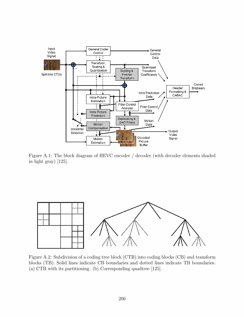
Figure A.1: The block diagram of HEVC encoder / decoder (with decoder elements shadedin light gray) [125].
Figure A.2: Subdivision of a coding tree block (CTB) into coding blocks (CB) and transformblocks (TB). Solid lines indicate CB boundaries and dotted lines indicate TB boundaries.(a) CTB with its partitioning. (b) Corresponding quadtree [125].
206
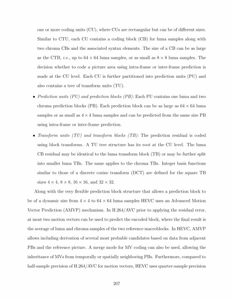
one or more coding units (CU), where CUs are rectangular but can be of different sizes.
Similar to CTU, each CU contains a coding block (CB) for luma samples along with
two chroma CBs and the associated syntax elements. The size of a CB can be as large
as the CTB, i.e., up to 64× 64 luma samples, or as small as 8× 8 luma samples. The
decision whether to code a picture area using intra-frame or inter-frame prediction is
made at the CU level. Each CU is further partitioned into prediction units (PU) and
also contains a tree of transform units (TU).
• Prediction units (PU) and prediction blocks (PB): Each PU contains one luma and two
chroma prediction blocks (PB). Each prediction block can be as large as 64× 64 luma
samples or as small as 4× 4 luma samples and can be predicted from the same size PB
using intra-frame or inter-frame prediction.
• Transform units (TU) and transform blocks (TB): The prediction residual is coded
using block transforms. A TU tree structure has its root at the CU level. The luma
CB residual may be identical to the luma transform block (TB) or may be further split
into smaller luma TBs. The same applies to the chroma TBs. Integer basis functions
similar to those of a discrete cosine transform (DCT) are defined for the square TB
sizes 4× 4, 8× 8, 16× 16, and 32× 32.
Along with the very flexible prediction block structure that allows a prediction block to
be of a dynamic size from 4× 4 to 64× 64 luma samples HEVC uses an Advanced Motion
Vector Prediction (AMVP) mechanism. In H.264/AVC prior to applying the residual error,
at most two motion vectors can be used to predict the encoded block, where the final result is
the average of luma and chroma samples of the two reference macroblocks. In HEVC, AMVP
allows including derivation of several most probable candidates based on data from adjacent
PBs and the reference picture. A merge mode for MV coding can also be used, allowing the
inheritance of MVs from temporally or spatially neighboring PBs. Furthermore, compared to
half-sample precision of H.264/AVC for motion vectors, HEVC uses quarter-sample precision
207
and stronger filters for interpolation of fractional-sample positions. Therefore, HEVC can
encode motion vectors with much greater precision, giving a better predicted block with less
residual error. Furthermore, compared to 9 intra-picture prediction directions of H.264/AVC,
HEVC provides 35 intra-prediction modes, allowing the reference coding unit for the intra-
frame prediction to be selected much more precisely. Finally, HEVC is equipped with a
new and advanced deblocking filter, called Sample Adaptive Offset (SAO), that reduces the
artifacts of the decoded video on the borders of CUs. These new capabilities altogether allow
HEVC to achieve the same video quality of H.264/AVC with a video bitrate 40% to 60%
less than that of H.264/AVC.
208