WP/04/98

Toward More Effective Redistribution: Reform Options for Intergovernmental

Transfers in China

Ehtisham Ahmad, Raju Singh, and Mario Fortuna

© 2004 International Monetary Fund WP/04/98

IMF Working Paper

Fiscal Affairs Department

Toward More Effective Redistribution: Reform Options for Intergovernmental Transfers in China

Prepared by Ehtisham Ahmad, Raju Singh, and Mario Fortuna1

June 2004

Abstract

This Working Paper should not be reported as representing the views of the IMF. The views expressed in this Working Paper are those of the author(s) and do not necessarily represent those of the IMF or IMF policy. Working Papers describe research in progress by the author(s) and are published to elicit comments and to further debate.

Full implementation of an intergovernmental transfer system based on revenue capacities andexpenditure needs could significantly improve both redistribution and equity objectives of the Chinese authorities. This was envisaged in the 1994 fiscal reforms, but the authorities were unable to implement the measures fully. This paper examines mechanisms that might facilitate effective implementation. JEL Classification Numbers: H70, H77 Keywords: Fiscal Policy, Intergovernmental Fiscal Relations, China Author’s E-Mail Address: eahmad@imf.org; rsingh2@imf.org; fortuna@notes.uac.pt

1 Ehtisham Ahmad and Raju Singh are Division Chief and Senior Economist, respectively, with the Fiscal Affairs Department at the IMF, and Mario Fortuna is Professor of Economics at the University of Azores. This paper is part of a larger project that also included Hana Brixi (World Bank) and Ben Lockwood (University of Warwick).

- 2 -

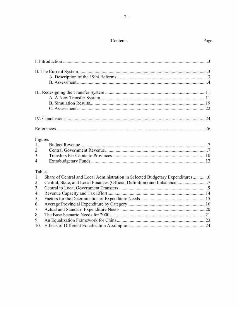
Contents Page

I. Introduction ............................................................................................................................3

II. The Current System...............................................................................................................3 A. Description of the 1994 Reforms ..............................................................................3 B. Assessment ................................................................................................................4

III. Redesigning the Transfer System ......................................................................................11 A. A New Transfer System..........................................................................................11 B. Simulation Results...................................................................................................19 C. Assessment ..............................................................................................................22

IV. Conclusions........................................................................................................................24

References................................................................................................................................26 Figures 1. Budget Revenue .............................................................................................................7 2. Central Government Revenue........................................................................................7 3. Transfers Per Capita to Provinces................................................................................10 4. Extrabudgetary Funds ..................................................................................................12 Tables 1. Share of Central and Local Administration in Selected Budgetary Expenditures.............6 2. Central, State, and Local Finances (Official Definition) and Imbalance...........................7 3. Central to Local Government Transfers ............................................................................9 4. Revenue Capacity and Tax Effort....................................................................................14 5. Factors for the Determination of Expenditure Needs........................................................15 6. Average Provincial Expenditure by Category...................................................................16 7. Actual and Standard Expenditure Needs .........................................................................20 8. The Base Scenario Needs for 2000..................................................................................21 9. An Equalization Framework for China............................................................................23 10. Effects of Different Equalization Assumptions ...............................................................24

- 3 -

I. INTRODUCTION In 1994, China carried out far-reaching fiscal reforms. Revenue bases were assigned to different levels of government, and a more transparent and rules-based transfer system was designed to replace the various ad hoc bilateral agreements that had defined intergovernmental fiscal relations up to then. However, while succeeding in improving the buoyancy of the tax system and providing the central government with additional resources, the reforms did not provide each province with sufficient resources to deliver a minimum standard of public services, leading to a proliferation of illegal fees and charges and to indirect borrowing. The scope of equalization and special purpose transfers was considerably limited by the revenue returns that provided resources to the areas where they were generated.2 This paper argues that effective and full implementation of the general transfers system included in the 1994 reforms, in which general purpose transfers were defined primarily on the basis of local revenue capacity, and expenditure needs would allow a better redistribution of resources among provinces than the framework that had evolved at the beginning of 2000. The simulations in this paper, based on information for 2000, indicate that, together with special purpose transfers, such a redesigned system could contribute also toward attainment of a minimum standard of public services in each province.

II. THE CURRENT SYSTEM

A. Description of the 1994 Reforms

The 1994 fiscal reforms were comprehensive on the revenue-sharing side, clearly assigning some taxes to the central or the local governments3 and introducing other taxes such as VAT, that would be shared between the center and lower levels. In carrying out this reform, the authorities had four main goals, namely to simplify the tax system, raise the revenue-to-GDP ratio, raise the share of the central government in total revenue, and achieve a more stable fiscal federal system by shifting from ad hoc, negotiated transfers to rule-based revenue assignments. There were no changes to the expenditure responsibilities, which remained consistent with the very broad guidelines under the constitution. Under the new revenue arrangements, tax revenue assigned to the central government included: 75 percent of the (newly introduced) VAT; excise and trade-related taxes; and the enterprise income tax collected from central state-owned enterprises (SOEs). Revenue assigned to local governments included: 25 percent of the VAT; the business tax; the enterprise; income taxes 2 See Ahmad, Ehtisham, Gao Qiang, and Vito Tanzi (1995) for the 1994 reforms, and Ahmad, E., Li Keping, R. Singh, and T. Richardson (2003).

3 The term local government in China is taken to refer to all four levels of subnational administration. At the second tier there are 22 provinces, five autonomous regions, and four municipalities (Beijing, Shanghai, Tienjin, Chongqing). The third tier consists of 331 prefectures. The fourth tier consists of 2,109 counties/cities. The fifth tier consists of 44,741 villages/townships.

- 4 -

levied on local SOEs, as well as on foreign financed enterprises; and the personal income tax. At the same time, a national tax service was established to administer the new central and shared revenue system. However, tax policy remained under the control of the center, and the subnational jurisdictions had very limited legal means of varying rates even for taxes for which revenues were entirely assigned to them. In addition, the system of transfers was redesigned, moving away from ad hoc, negotiated transfers toward a more rules-based mechanism. The new system of transfers from central to local governments comprised four main parts: • “fixed subsidies” were designed to ensure that every province would have total nominal

revenues no lower than in 1993;

• “revenue returned” provided each province with 30 percent of the increase in VAT and excise tax collection in its province over the 1993 base;

• “specific-purpose grants” or earmarked transfers were allocated on an ad hoc basis; and

• “subsidy transfers” or general purpose grants were meant to help equalize the resources of the provinces. These were rules-based and depend on variables such as provincial population or land area.

The spending assignments between the different levels of government were, however, not revised. They remained, as under the centrally planned system, where local governments provided a wide range of services as agents of the central government. There was an unclear expenditure assignment and the pressure to devolve expenditures to lower administrative units was inconsistent with the revenues available at these lower levels of government.4

B. Assessment

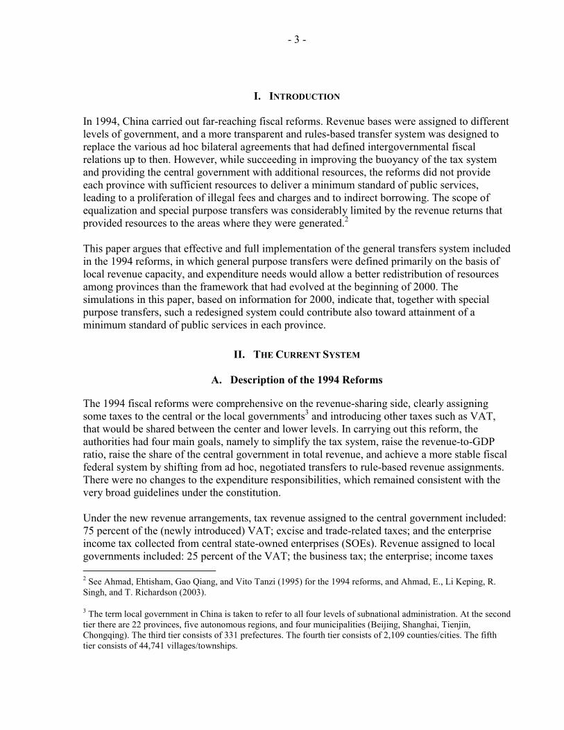
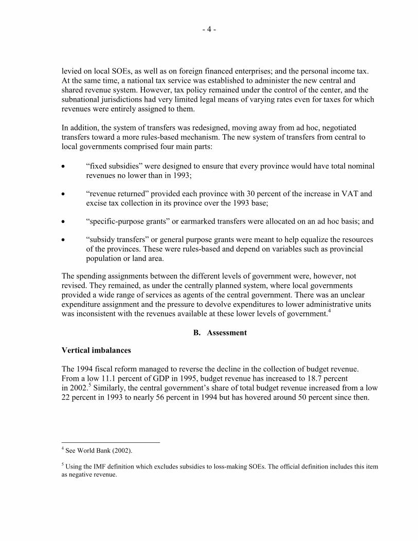
Vertical imbalances The 1994 fiscal reform managed to reverse the decline in the collection of budget revenue. From a low 11.1 percent of GDP in 1995, budget revenue has increased to 18.7 percent in 2002.5 Similarly, the central government’s share of total budget revenue increased from a low 22 percent in 1993 to nearly 56 percent in 1994 but has hovered around 50 percent since then.

4 See World Bank (2002).

5 Using the IMF definition which excludes subsidies to loss-making SOEs. The official definition includes this item as negative revenue.

- 5 -

Figure 1. Budget Revenue 1979-2002(In percent of GDP)

05

101520253035

1980

1982

1984

1986

1988

1990

1992

1994

1996

1998

2000

2002

While revenue was recentralized, spending responsibilities became increasingly decentralized. Local governments bear very heavy expenditure responsibilities. In 2001, the share of local governments in total budget revenue was 48 percent, but they accounted for 69 percent of total budget expenditure. Not only are local governments responsible for providing health and education, but they are also responsible for unemployment insurance, social security, and infrastructure. In 2001, provincial governments accounted for about 90 percent of total spending

Figure 2. Central Government Revenue Share1979-2002

(In percent of budget revenue)

0

10

20

30

40

50

60

1980

1982

1984

1986

1988

1990

1992

1994

1996

1998

2000

2002

- 6 -

in culture, education and health, and for practically all the social relief and welfare expenditure (Table 1). Table 1. Share of Central and Local Administration in Selected Budgetary Expenditures, 2001

(In percent)

Central Local

Total

31

69

Capital construction 34 66 Working capital 59 41 Technological upgrading and R&D 25 75 Geological prospecting 31 69 Industry, transport and commerce 28 72 Agriculture 11 89 Culture, education, science and health 11 89 Social relief and welfare 1 99 Defense 99 1 Government administration 3 97 Government debt service 100 0 Policy subsidies 40 60

Source: Ministry of finance data. The local expenditures include the earmarked transfers from the central government. During the 1990s, the vertical imbalance widened. The 1994 fiscal reform, by centralizing revenue, has provided the central government with a surplus (before transfers), but created a deficit at the subnational level. Such imbalances are not uncommon in large federations, such as Australia or India for instance, and allow the center to play a greater role in macroeconomic stabilization. The vertical imbalance also provides potential room for equalization transfers. In China, these imbalances have tended to widen, especially since the start of the pro-active fiscal policy in 1998 (see Table 2). However, the effective vertical imbalance in favor of the center has been negated by the revenue returned on a derivation basis. While the revenue-returns are treated in the formal Chinese budget as transfers, they effectively reduce the central government share in the main revenue sources. The central government is thus left with only limited untied resources. Adjusting for the returned revenue, the vertical imbalance between the central and local governments appears therefore significantly smaller, hampering the ability of the central government to carry out its stabilization and redistribution roles. Horizontal imbalances Local governments are assigned heavy spending responsibilities without the capacity to generate adequate own-revenue nor a transfer system that will provide them with the needed

- 7 -

resources to deliver minimum standards of public services. As a result, local governments have turned to off-budget sources of revenue and indirect borrowing to meet priority expenditures including unfunded mandates.

Table 2. Central, State, and Local Finances (Official Definition) and Imbalance, 1990–2001

(In percent of GDP)

1990 1994 1995 1996 1997 1998 1999 2000 2001

Central government Own revenue 5.4 6.2 5.5 5.4 5.7 6.2 7.1 7.8 8.9 Own expenditure 5.4 3.8 3.5 3.2 3.4 4.0 5.1 6.2 6.0 Own balance 0 2.4 2 2.2 2.3 2.3 2.1 1.6 2.9

Subnational governments Own local revenue 10.5 4.9 5 5.5 5.9 6.4 6.8 7.1 8.1 Own expenditure 11.2 8.6 8.2 8.5 9.0 9.8 11.0 11.6 13.6 Own balance -0.7 -3.7 -3.2 -3.1 -3.1 -3.4 -4.2 -4.4 -5.5

Total imbalance -0.7 -1.3 -1.2 -0.8 -0.8 -1.2 -2.1 -2.8 -2.6

Adjusted balances for revenue returned

Central government ... ... ... -0.7 -0.4 -0.5 -0.5 -1.0 0.7 Subnational government ... ... ... -0.1 -0.4 -0.7 -1.6 -1.8 -3.2

Pro memoria Revenue returned ... ... ... 2.9 2.7 2.7 2.6 2.6 2.3

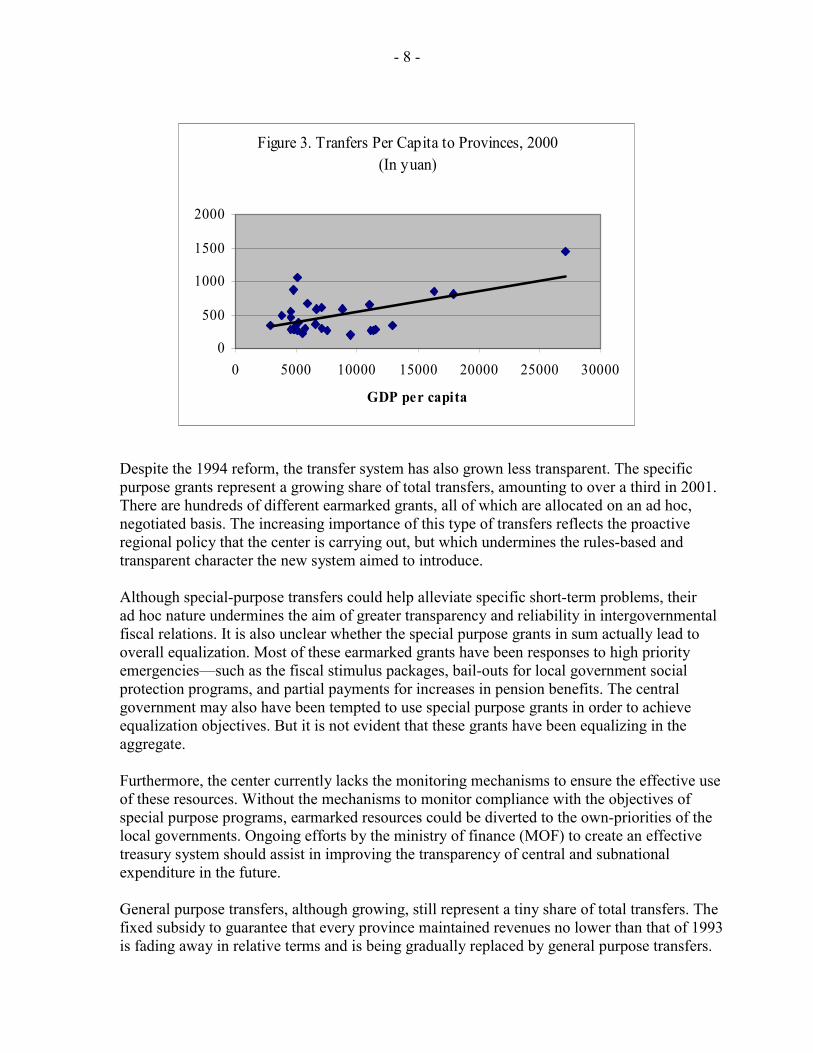
Sources: Ministry of finance; and IMF staff estimates. Subnational levels of government widely diverge with respect to their revenue generating capabilities. In 2000, the ratio between the highest and the lowest budgetary revenue collection in per capita terms among provinces was 12.8—with some of the coastal provinces far outstripping others. Although the transfer system helps to deal with these differences in revenue mobilization, it does not adequately distribute resources to allow all subnational levels of government to adequately deliver minimum standards in public services. The “revenue returned” principle has perpetuated a regressive character of the current system, whereby richer provinces receive most of the transfers (Figure 3)—the regressivity is due largely to the transfers to the richest coastal provinces. Although declining, the share of these transfers still represented in 2001 about 40 percent of the total transfers from the central to the local governments. The predominance of the revenue returned continues to hamper the system’s ability to redistribute fiscal revenues.

- 8 -

Despite the 1994 reform, the transfer system has also grown less transparent. The specific purpose grants represent a growing share of total transfers, amounting to over a third in 2001. There are hundreds of different earmarked grants, all of which are allocated on an ad hoc, negotiated basis. The increasing importance of this type of transfers reflects the proactive regional policy that the center is carrying out, but which undermines the rules-based and transparent character the new system aimed to introduce. Although special-purpose transfers could help alleviate specific short-term problems, their ad hoc nature undermines the aim of greater transparency and reliability in intergovernmental fiscal relations. It is also unclear whether the special purpose grants in sum actually lead to overall equalization. Most of these earmarked grants have been responses to high priority emergencies—such as the fiscal stimulus packages, bail-outs for local government social protection programs, and partial payments for increases in pension benefits. The central government may also have been tempted to use special purpose grants in order to achieve equalization objectives. But it is not evident that these grants have been equalizing in the aggregate. Furthermore, the center currently lacks the monitoring mechanisms to ensure the effective use of these resources. Without the mechanisms to monitor compliance with the objectives of special purpose programs, earmarked resources could be diverted to the own-priorities of the local governments. Ongoing efforts by the ministry of finance (MOF) to create an effective treasury system should assist in improving the transparency of central and subnational expenditure in the future. General purpose transfers, although growing, still represent a tiny share of total transfers. The fixed subsidy to guarantee that every province maintained revenues no lower than that of 1993 is fading away in relative terms and is being gradually replaced by general purpose transfers.

Figure 3. Tranfers Per Capita to Provinces, 2000(In yuan)

0

500

1000

1500

2000

0 5000 10000 15000 20000 25000 30000

GDP per capita

- 9 -

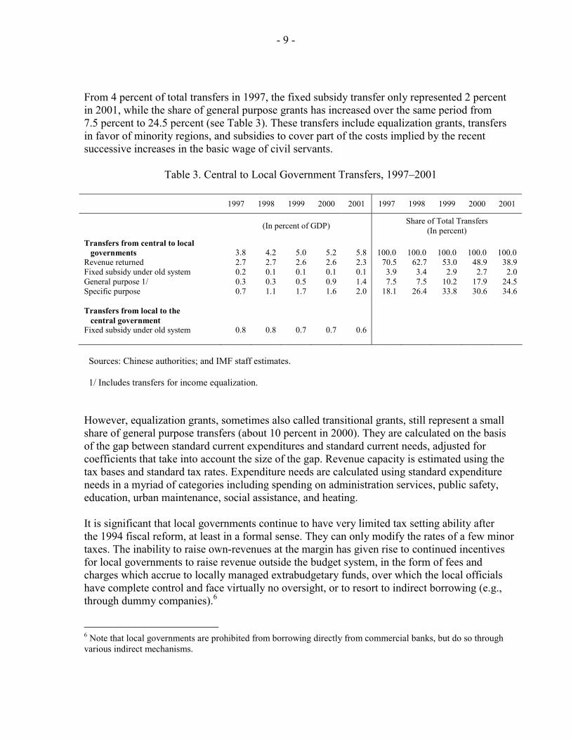
From 4 percent of total transfers in 1997, the fixed subsidy transfer only represented 2 percent in 2001, while the share of general purpose grants has increased over the same period from 7.5 percent to 24.5 percent (see Table 3). These transfers include equalization grants, transfers in favor of minority regions, and subsidies to cover part of the costs implied by the recent successive increases in the basic wage of civil servants.

Table 3. Central to Local Government Transfers, 1997–2001

1997 1998 1999 2000 2001 1997 1998 1999 2000 2001

(In percent of GDP) Share of Total Transfers (In percent)

Transfers from central to local governments 3.8 4.2 5.0 5.2 5.8 100.0 100.0 100.0 100.0 100.0 Revenue returned 2.7 2.7 2.6 2.6 2.3 70.5 62.7 53.0 48.9 38.9 Fixed subsidy under old system 0.2 0.1 0.1 0.1 0.1 3.9 3.4 2.9 2.7 2.0 General purpose 1/ 0.3 0.3 0.5 0.9 1.4 7.5 7.5 10.2 17.9 24.5 Specific purpose

0.7 1.1 1.7 1.6 2.0 18.1 26.4 33.8 30.6 34.6

Transfers from local to the central government

Fixed subsidy under old system

0.8 0.8 0.7 0.7 0.6

Sources: Chinese authorities; and IMF staff estimates. 1/ Includes transfers for income equalization. However, equalization grants, sometimes also called transitional grants, still represent a small share of general purpose transfers (about 10 percent in 2000). They are calculated on the basis of the gap between standard current expenditures and standard current needs, adjusted for coefficients that take into account the size of the gap. Revenue capacity is estimated using the tax bases and standard tax rates. Expenditure needs are calculated using standard expenditure needs in a myriad of categories including spending on administration services, public safety, education, urban maintenance, social assistance, and heating. It is significant that local governments continue to have very limited tax setting ability after the 1994 fiscal reform, at least in a formal sense. They can only modify the rates of a few minor taxes. The inability to raise own-revenues at the margin has given rise to continued incentives for local governments to raise revenue outside the budget system, in the form of fees and charges which accrue to locally managed extrabudgetary funds, over which the local officials have complete control and face virtually no oversight, or to resort to indirect borrowing (e.g., through dummy companies).6

6 Note that local governments are prohibited from borrowing directly from commercial banks, but do so through various indirect mechanisms.

- 10 -

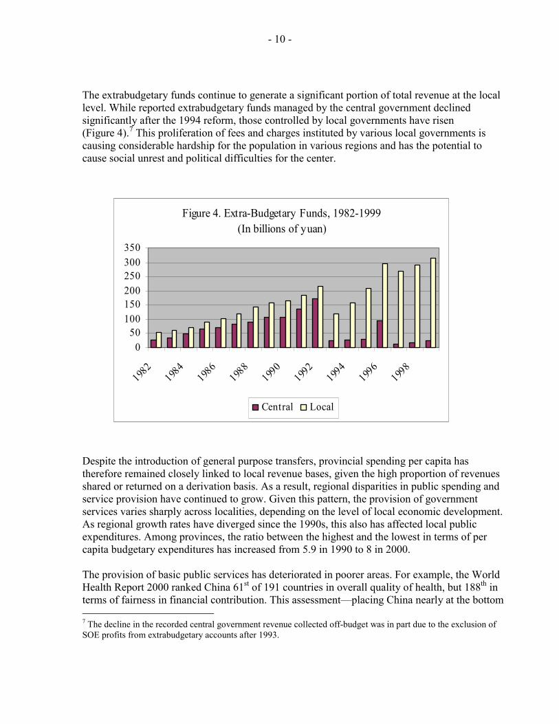
The extrabudgetary funds continue to generate a significant portion of total revenue at the local level. While reported extrabudgetary funds managed by the central government declined significantly after the 1994 reform, those controlled by local governments have risen (Figure 4).7 This proliferation of fees and charges instituted by various local governments is causing considerable hardship for the population in various regions and has the potential to cause social unrest and political difficulties for the center. Despite the introduction of general purpose transfers, provincial spending per capita has therefore remained closely linked to local revenue bases, given the high proportion of revenues shared or returned on a derivation basis. As a result, regional disparities in public spending and service provision have continued to grow. Given this pattern, the provision of government services varies sharply across localities, depending on the level of local economic development. As regional growth rates have diverged since the 1990s, this also has affected local public expenditures. Among provinces, the ratio between the highest and the lowest in terms of per capita budgetary expenditures has increased from 5.9 in 1990 to 8 in 2000. The provision of basic public services has deteriorated in poorer areas. For example, the World Health Report 2000 ranked China 61st of 191 countries in overall quality of health, but 188th in terms of fairness in financial contribution. This assessment—placing China nearly at the bottom 7 The decline in the recorded central government revenue collected off-budget was in part due to the exclusion of SOE profits from extrabudgetary accounts after 1993.

Figure 4. Extra-Budgetary Funds, 1982-1999(In billions of yuan)

050

100150200250300350

1982

1984

1986

1988

1990

1992

1994

1996

1998

Central Local

- 11 -

of all countries assessed—is an indication of the unequal access to public health care in China. A similar situation exists in education. China’s intergovernmental system has also led to indirect local borrowing, skirting a provision in the budget law that forbids direct borrowing or issuance of guarantees by local governments. However, local governments freely establish companies that then borrow from the banks. There is an expectation that the state would eventually bear responsibility for borrowing for public purposes by such companies. Such borrowing is also poorly monitored at both the provincial and central levels. This leads to a system in which any systematic design or redistribution of a well designed intergovernmental framework could be undermined.

III. REDESIGNING THE TRANSFER SYSTEM

A. A New Transfer System The method used to calculate the provincial revenue capacities and expenditure needs in this section is simplified and mainly illustrative, and the quality of data can certainly be improved. This provides an illustrative example of how to construct an equalization transfer formula (for general allocations to provinces), with a minimum data requirement, rather than to provide the exact model to be used for China. The following sections discuss the methodology and the results. Formulas for equalization transfers Roughly speaking, there are four possible types of formulas for equalization transfers: (1) those that consider revenue capacities, as well as the expenditure needs of different regions; (2) those that consider only the equalization of revenue capacities; (3) those that are based on some “needs” indicators; and (4) those that distribute untied transfers on an equal per capita basis.8 In the current exercise, we use a formula based on revenue capacities and expenditure needs of different regions. The 1994 reform also envisaged that such a formula would be the main mechanism to implement redistributive transfers, although full equalization was not foreseen in the short term.9

8 See Ehtisham Ahmad (ed) 1997, Financing Decentralized Expenditures: an international comparison of grants, Edward Elgar.

9 See Lou Jiwei, 1997.

- 12 -

A typical formula of this type could be written as follows: TRi = Ni - Ci - OTRi, (1) where Ni is the standard expenditure need of the ith region, and Ci is the standard revenue capacity of the ith region. Ni - Ci measures the gap between the standard expenditure need and revenue capacity. OTRi represents other transfers (e.g., specific purpose transfers) the ith region receives from the center that are used to meet part of the expenditure needs assessed by the model. This formula states that the central government transfer will cover the difference between each region’s standard expenditure needs and revenue capacity, to ensure that a region with standard tax effort will be able to provide a standard level of public services. There is a question of how to match the sum of the entitlements (ΣiTRi) calculated from the above formula with the available pool for transfers. In theory, the pool can either be larger or smaller than the total entitlement. A commonly used method is to adjust the size of the transfer proportionally according to the size of the pool. Let TT be the size of the pool for transfers. Then the actual transfer to the ith region is: ATRi = (TT/ΣiTRi)TRi (2) where ATRi stands for actual transfer to the ith region, and TRi is calculated using Equation 1. Measuring revenue capacity Revenue capacity (Ci) is defined as the ability of a government to raise revenues from its own sources and revenue-sharing arrangements. There are several ways to measure the revenue capacity of a subnational government. In many developed countries, revenue capacity is measured using data on major tax bases and standard (average) tax rates. This method measures the revenue capacity of a region by the revenue that could be raised in that region if the regional government taxes all the standard tax bases with a standard tax effort. The formula is as follows: Ci = ΣjBij*tj, (3) where Ci is the ith region’s tax capacity, Bij is the ith region’s jth tax base, and tj is the standard (e.g., national average effective) tax rate on the jth tax base. It is important to apply the standard tax rate to the region’s tax base rather than the region’s own effective tax rate, in order to ensure that the regions with a high tax effort are not penalized and regions with a low tax effort are not rewarded. In other words, if the region’s effective tax rates are higher than the national averages, the transfer it receives does not decrease as a result; and if the region’s effective tax rates are lower than the national average, the transfer it receives does not increase as a result. This method requires detailed and accurate information on major tax bases, which may not be readily available for all regions. Revenue capacities may be also measured indirectly by employing some income or output indicators. The frequently used indicators include: (a) the gross

- 13 -

domestic product (GDP) of the region; (b) personal income (sum of all incomes received by the residents) or disposable personal income of the region; (c) total retail sales of the region. In the current exercise, provincial GDP levels are used as a proxy of the tax bases. More elaborate models might be tried using additional variables.10 Revenue capacity, REVi , was estimated using the coefficients of the regression of own revenue11 on own GDP for region i. The results are the following:

REVi = 0.0651288 GDPi ; (4) R2

= 0.894 ; N=31; Df = 30

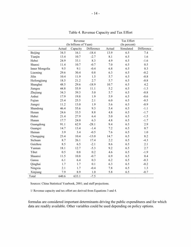
On the basis of this regression, the series presented in Table 4 were derived The simulated revenue capacity assumes that tax effort is based on a linear relationship linked to GDP.12 Caution should be taken, however, in using these results since a significant portion of contributions of residents are made in the form of fees instead of taxes. This could introduce a potential distortion in the estimates below if the pattern is not homogeneous across the country. Eliminating fees and converting these into taxes that are accounted as budget revenue sources will clarify this situation and should be subject to further analysis. Expenditure needs This section discusses a commonly used method to determine expenditure needs of subnational governments. It divides the total expenditures of a subnational government into many different categories and for each category estimates the corresponding needs. The total expenditure needs of a subnational government are the sum of the estimated needs for all these categories. In this exercise, the expenditure needs of each province are broken down into seven categories: education, health, social welfare, government administration, law and order, economic development and other. These seven categories are constructed by consolidating various expenditure items in the Chinese economic classification. For each category, a formula is developed to estimate the expenditure needs of the provinces. The variables used in these

10 For a discussion and an alternative approach to calculating revenue capacity, see World Bank Report No. 20342-CHA on “Managing Public Expenditures for Better Results,” April 25, 2000, p. 140.

11 Own revenue was obtained from the 2001 Statistical Yearbook. Revenue was adjusted by subtracting the negative value under transfers for SOEs. The same value was then added to expenditures on economic development.

12 One might test the hypothesis that the tax effort is not linear. Regressions with nonlinear forms of the regressor did not provide better explanation of the variation of the dependent variable. More work could, however, be carried out on this issue.

- 14 -

Table 4. Revenue Capacity and Tax Effort

Revenue

(In billions of Yuan) Tax Effort

(In percent) Actual Capacity Difference Actual Simulated Difference Beijing 34.5 16.1 -18.4 13.9 6.5 7.4 Tianjin 13.4 10.7 -2.7 8.1 6.5 1.6 Hebei 24.9 33.1 8.3 4.9 6.5 -1.6 Shanxi 11.4 10.7 -0.7 7.0 6.5 0.5 Inner Mongolia 9.5 9.1 -0.4 6.8 6.5 0.3 Liaoning 29.6 30.4 0.8 6.3 6.5 -0.2 Jilin 10.4 11.9 1.5 5.7 6.5 -0.8 Heilongjiang 18.5 21.2 2.7 5.7 6.5 -0.8 Shanghai 48.5 29.6 -18.9 10.7 6.5 4.2 Jiangsu 44.8 55.9 11.1 5.2 6.5 -1.3 Zhejiang 34.3 39.3 5.0 5.7 6.5 -0.8 Anhui 17.9 19.8 1.9 5.9 6.5 -0.6 Fujian 23.4 25.5 2.1 6.0 6.5 -0.5 Jiangxi 11.2 13.0 1.9 5.6 6.5 -0.9 Shandong 46.4 55.6 9.3 5.4 6.5 -1.1 Henan 24.6 33.5 8.8 4.8 6.5 -1.7 Hubei 21.4 27.9 6.4 5.0 6.5 -1.5 Hunan 17.7 24.0 6.3 4.8 6.5 -1.7 Guangdong 91.1 62.9 -28.1 9.4 6.5 2.9 Guangxi 14.7 13.4 -1.4 7.2 6.5 0.7 Hainan 3.9 3.4 -0.5 7.6 6.5 1.0 Chongqing 23.4 10.4 -13.0 14.7 6.5 8.2 Sichuan 8.7 26.1 17.4 2.2 6.5 -4.3 Guizhou 8.5 6.5 -2.1 8.6 6.5 2.1 Yunnan 18.1 12.7 -5.3 9.2 6.5 2.7 Tibet 0.5 0.8 0.2 4.6 6.5 -1.9 Shaanxi 11.5 10.8 -0.7 6.9 6.5 0.4 Gansu 6.1 6.4 0.3 6.2 6.5 -0.3 Qinghai 1.7 1.7 0.1 6.3 6.5 -0.2 Ningxia 2.1 1.7 -0.4 7.8 6.5 1.3 Xinjiang 7.9 8.9 1.0 5.8 6.5 -0.7 Total 640.6 633.1 -7.5

Sources: China Statistical Yearbook, 2001; and staff projections. 1/ Revenue capacity and tax effort are derived from Equations 3 and 4. formulas are considered important determinants driving the public expenditures and for which data are readily available. Other variables could be used depending on policy options.

- 15 -

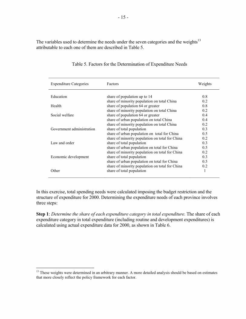
The variables used to determine the needs under the seven categories and the weights13 attributable to each one of them are described in Table 5.

Table 5. Factors for the Determination of Expenditure Needs

Expenditure Categories Factors Weights

Education

share of population up to 14 share of minority population on total China

0.8 0.2

Health share of population 64 or greater share of minority population on total China

0.8 0.2

Social welfare share of population 64 or greater share of urban population on total China share of minority population on total China

0.4 0.4 0.2

Government administration share of total population share of urban population on total for China share of minority population on total for China

0.3 0.5 0.2

Law and order share of total population share of urban population on total for China share of minority population on total for China

0.3 0.5 0.2

Economic development share of total population share of urban population on total for China share of minority population on total for China

0.3 0.5 0.2

Other

share of total population 1

In this exercise, total spending needs were calculated imposing the budget restriction and the structure of expenditure for 2000. Determining the expenditure needs of each province involves three steps: Step 1: Determine the share of each expenditure category in total expenditure. The share of each expenditure category in total expenditure (including routine and development expenditures) is calculated using actual expenditure data for 2000, as shown in Table 6.

13 These weights were determined in an arbitrary manner. A more detailed analysis should be based on estimates that more closely reflect the policy framework for each factor.

- 16 -

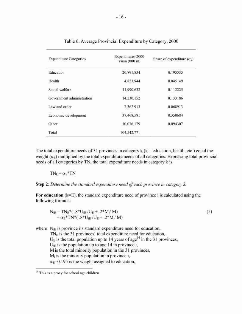
Table 6. Average Provincial Expenditure by Category, 2000

Expenditure Categories Expenditures 2000 Yuan (000 m) Share of expenditure (αk)

Education 20,891,834 0.195535

Health 4,823,944 0.045149

Social welfare 11,990,632 0.112225

Government administration 14,230,152 0.133186

Law and order 7,362,913 0.068913

Economic development 37,468,581 0.350684

Other 10,076,179 0.094307

Total 104,542,771

The total expenditure needs of 31 provinces in category k (k = education, health, etc.) equal the weight (αk) multiplied by the total expenditure needs of all categories. Expressing total provincial needs of all categories by TN, the total expenditure needs in category k is TNk = αk*TN Step 2: Determine the standard expenditure need of each province in category k. For education (k=E), the standard expenditure need of province i is calculated using the following formula: NiE = TNE*( .8*UiE /UE + .2*Mi/ M) (5) = αE*TN*( .8*UiE /UE + .2*Mi/ M) where NiE is province i’s standard expenditure need for education, TNE is the 31 provinces’ total expenditure need for education, UE is the total population up to 14 years of age14 in the 31 provinces, UiE is the population up to age 14 in province i, M is the total minority population in the 31 provinces, Mi is the minority population in province i, αE=0.195 is the weight assigned to education, 14 This is a proxy for school age children.

- 17 -

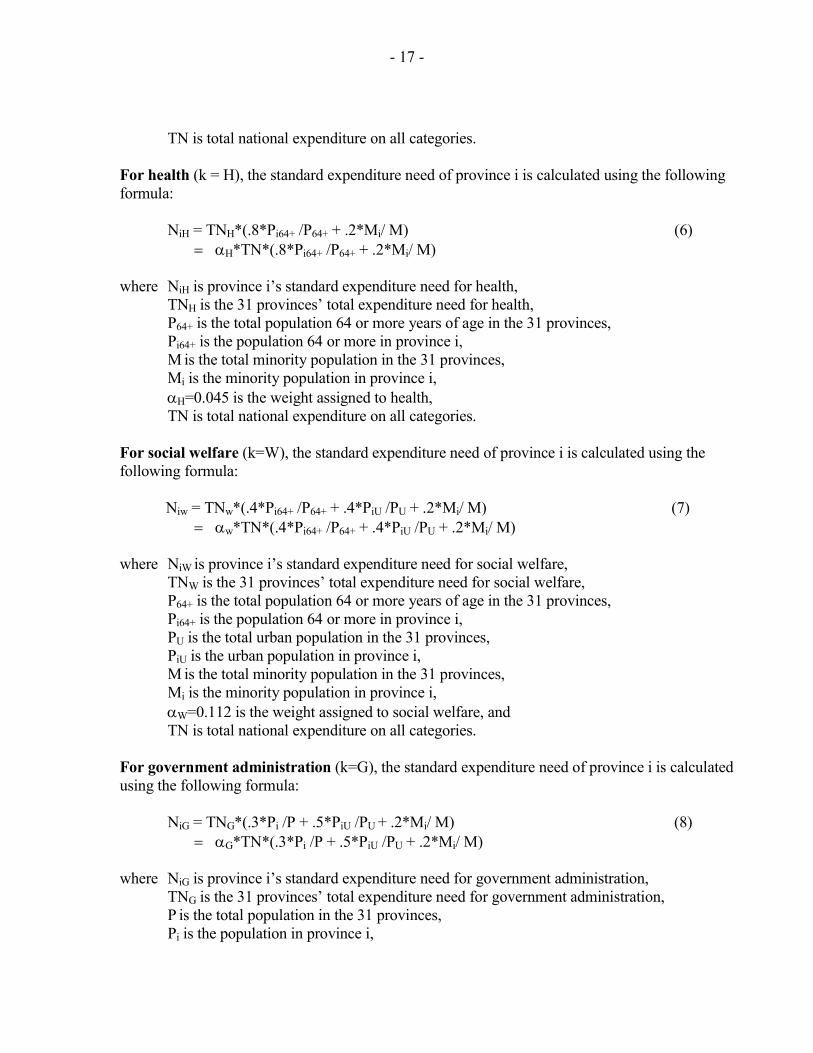
TN is total national expenditure on all categories. For health (k = H), the standard expenditure need of province i is calculated using the following formula: NiH = TNH*(.8*Pi64+ /P64+ + .2*Mi/ M) (6) = αH*TN*(.8*Pi64+ /P64+ + .2*Mi/ M) where NiH is province i’s standard expenditure need for health, TNH is the 31 provinces’ total expenditure need for health, P64+ is the total population 64 or more years of age in the 31 provinces, Pi64+ is the population 64 or more in province i, M is the total minority population in the 31 provinces, Mi is the minority population in province i, αH=0.045 is the weight assigned to health, TN is total national expenditure on all categories. For social welfare (k=W), the standard expenditure need of province i is calculated using the following formula: Niw = TNw*(.4*Pi64+ /P64+ + .4*PiU /PU + .2*Mi/ M) (7) = αw*TN*(.4*Pi64+ /P64+ + .4*PiU /PU + .2*Mi/ M) where NiW is province i’s standard expenditure need for social welfare, TNW is the 31 provinces’ total expenditure need for social welfare, P64+ is the total population 64 or more years of age in the 31 provinces, Pi64+ is the population 64 or more in province i, PU is the total urban population in the 31 provinces, PiU is the urban population in province i, M is the total minority population in the 31 provinces, Mi is the minority population in province i, αW=0.112 is the weight assigned to social welfare, and TN is total national expenditure on all categories. For government administration (k=G), the standard expenditure need of province i is calculated using the following formula: NiG = TNG*(.3*Pi /P + .5*PiU /PU + .2*Mi/ M) (8) = αG*TN*(.3*Pi /P + .5*PiU /PU + .2*Mi/ M) where NiG is province i’s standard expenditure need for government administration, TNG is the 31 provinces’ total expenditure need for government administration, P is the total population in the 31 provinces, Pi is the population in province i,

- 18 -

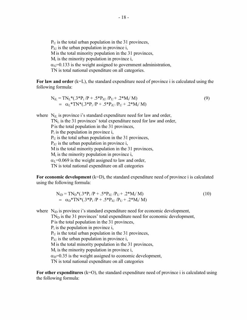
PU is the total urban population in the 31 provinces, PiU is the urban population in province i, M is the total minority population in the 31 provinces, Mi is the minority population in province i, αG=0.133 is the weight assigned to government administration, TN is total national expenditure on all categories. For law and order (k=L), the standard expenditure need of province i is calculated using the following formula: NiL = TNL*(.3*Pi /P + .5*PiU /PU + .2*Mi/ M) (9) = αL*TN*(.3*Pi /P + .5*PiU /PU + .2*Mi/ M) where NiL is province i’s standard expenditure need for law and order, TNL is the 31 provinces’ total expenditure need for law and order, P is the total population in the 31 provinces, Pi is the population in province i, PU is the total urban population in the 31 provinces, PiU is the urban population in province i, M is the total minority population in the 31 provinces, Mi is the minority population in province i, αL=0.069 is the weight assigned to law and order, TN is total national expenditure on all categories For economic development (k=D), the standard expenditure need of province i is calculated using the following formula: NiD = TND*(.3*Pi /P + .5*PiU /PU + .2*Mi/ M) (10) = αD*TN*(.3*Pi /P + .5*PiU /PU + .2*Mi/ M) where NiD is province i’s standard expenditure need for economic development, TND is the 31 provinces’ total expenditure need for economic development, P is the total population in the 31 provinces, Pi is the population in province i, PU is the total urban population in the 31 provinces, PiU is the urban population in province i, M is the total minority population in the 31 provinces, Mi is the minority population in province i, αD=0.35 is the weight assigned to economic development, TN is total national expenditure on all categories For other expenditures (k=O), the standard expenditure need of province i is calculated using the following formula:

- 19 -

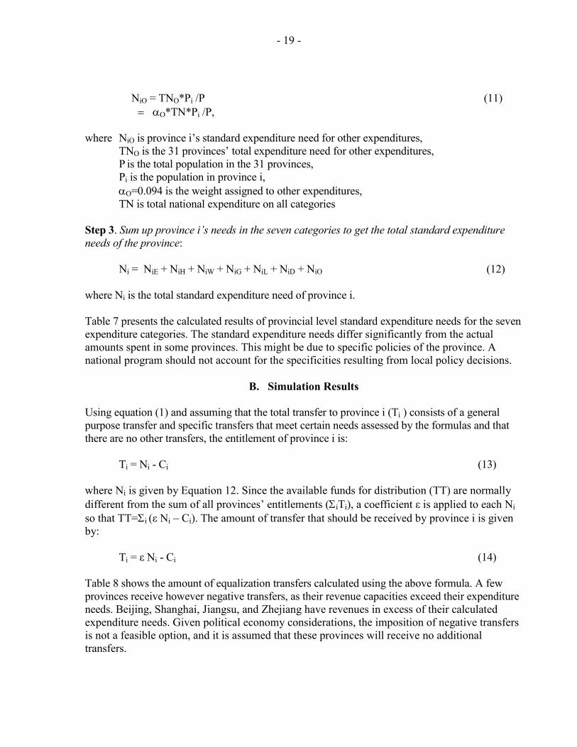
NiO = TNO*Pi /P (11) = αO*TN*Pi /P, where NiO is province i’s standard expenditure need for other expenditures, TNO is the 31 provinces’ total expenditure need for other expenditures, P is the total population in the 31 provinces, Pi is the population in province i, αO=0.094 is the weight assigned to other expenditures, TN is total national expenditure on all categories Step 3. Sum up province i’s needs in the seven categories to get the total standard expenditure needs of the province: Ni = NiE + NiH + NiW + NiG + NiL + NiD + NiO (12) where Ni is the total standard expenditure need of province i. Table 7 presents the calculated results of provincial level standard expenditure needs for the seven expenditure categories. The standard expenditure needs differ significantly from the actual amounts spent in some provinces. This might be due to specific policies of the province. A national program should not account for the specificities resulting from local policy decisions.

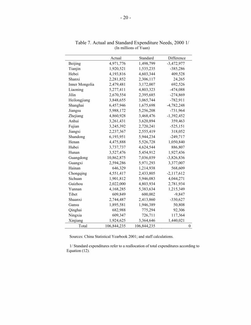
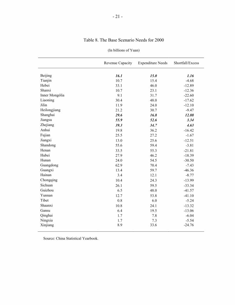
B. Simulation Results Using equation (1) and assuming that the total transfer to province i (Ti ) consists of a general purpose transfer and specific transfers that meet certain needs assessed by the formulas and that there are no other transfers, the entitlement of province i is: Ti = Ni - Ci (13) where Ni is given by Equation 12. Since the available funds for distribution (TT) are normally different from the sum of all provinces’ entitlements (ΣiTi), a coefficient ε is applied to each Ni so that TT=Σi (ε Ni – Ci). The amount of transfer that should be received by province i is given by: Ti = ε Ni - Ci (14) Table 8 shows the amount of equalization transfers calculated using the above formula. A few provinces receive however negative transfers, as their revenue capacities exceed their expenditure needs. Beijing, Shanghai, Jiangsu, and Zhejiang have revenues in excess of their calculated expenditure needs. Given political economy considerations, the imposition of negative transfers is not a feasible option, and it is assumed that these provinces will receive no additional transfers.

- 20 -

Table 7. Actual and Standard Expenditure Needs, 2000 1/ (In millions of Yuan)

Actual Standard Difference Beijing 4,971,776 1,498,799 -3,472,977 Tianjin 1,920,521 1,535,235 -385,286 Hebei 4,193,816 4,603,344 409,528 Shanxi 2,281,852 2,306,117 24,265 Inner Mongolia 2,479,481 3,172,007 692,526 Liaoning 5,277,411 4,803,323 -474,088 Jilin 2,670,554 2,395,685 -274,869 Heilongjiang 3,848,655 3,065,744 -782,911 Shanghai 6,457,946 1,675,698 -4,782,248 Jiangsu 5,988,172 5,256,208 -731,964 Zhejiang 4,860,928 3,468,476 -1,392,452 Anhui 3,261,431 3,620,894 359,463 Fujian 3,245,392 2,720,241 -525,151 Jiangxi 2,237,367 2,555,419 318,052 Shandong 6,193,951 5,944,234 -249,717 Henan 4,475,888 5,526,728 1,050,840 Hubei 3,737,737 4,624,544 886,807 Hunan 3,527,476 5,454,912 1,927,436 Guangdong 10,862,875 7,036,039 -3,826,836 Guangxi 2,594,286 5,971,293 3,377,007 Hainan 646,329 1,214,938 568,609 Chongqing 4,551,417 2,433,805 -2,117,612 Sichuan 1,901,812 5,946,083 4,044,271 Guizhou 2,022,000 4,803,934 2,781,934 Yunnan 4,168,285 5,383,634 1,215,349 Tibet 609,849 600,002 -9,847 Shaanxi 2,744,487 2,413,860 -330,627 Gansu 1,895,581 1,946,389 50,808 Qinghai 682,988 775,294 92,306 Ningxia 609,347 726,711 117,364 Xinjiang 1,924,625 3,364,646 1,440,021

Total 106,844,235 106,844,235 0

Sources: China Statistical Yearbook 2001; and staff calculations. 1/ Standard expenditures refer to a reallocation of total expenditures according to Equation (12).

- 21 -

Table 8. The Base Scenario Needs for 2000

(In billions of Yuan)

Revenue Capacity Expenditure Needs Shortfall/Excess

Beijing 16.1 15.0 1.16 Tianjin 10.7 15.4 -4.68 Hebei 33.1 46.0 -12.89 Shanxi 10.7 23.1 -12.36 Inner Mongólia 9.1 31.7 -22.60 Liaoning 30.4 48.0 -17.62 Jilin 11.9 24.0 -12.10 Heilongjiang 21.2 30.7 -9.47 Shanghai 29.6 16.8 12.88 Jiangsu 55.9 52.6 3.34 Zhejiang 39.3 34.7 4.63 Anhui 19.8 36.2 -16.42 Fujian 25.5 27.2 -1.67 Jiangxi 13.0 25.6 -12.51 Shandong 55.6 59.4 -3.81 Henan 33.5 55.3 -21.81 Hubei 27.9 46.2 -18.39 Hunan 24.0 54.5 -30.50 Guangdong 62.9 70.4 -7.43 Guangxi 13.4 59.7 -46.36 Hainan 3.4 12.1 -8.77 Chongqing 10.4 24.3 -13.99 Sichuan 26.1 59.5 -33.34 Guizhou 6.5 48.0 -41.57 Yunnan 12.7 53.8 -41.10 Tibet 0.8 6.0 -5.24 Shaanxi 10.8 24.1 -13.32 Gansu 6.4 19.5 -13.06 Qinghai 1.7 7.8 -6.04 Ningxia 1.7 7.3 -5.54 Xinjiang 8.9 33.6 -24.76

Source: China Statistical Yearbook.

- 22 -

C. Assessment In order to assess the new transfer design, three scenarios have been considered: • Base case equalization applies the entire amount of resources available for transfers in

2000 (Y 475 billion) to equalization, using the formula as designed, subject to zero transfers to the rich provinces. This implies the elimination of the revenue returned, and places all equalization transfers on a consistent basis.

• Partial equalization at 20 percent, the equalization is based on 20 percent of the total transfers, with 80 percent distributed according to the total transfer pattern observed in 2000. This closely approximates the current situation.

• Partial equalization at 60 percent, the equalization is based on 60 percent of the total transfers, with 40 percent distributed according to the transfer pattern in 2000. This is an intermediate case that simulates retention at the current level of the “revenue returned.”

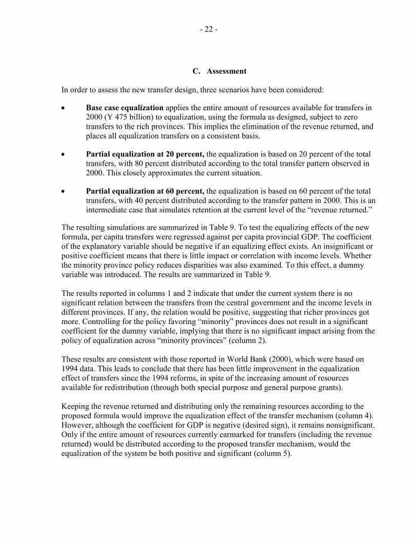
The resulting simulations are summarized in Table 9. To test the equalizing effects of the new formula, per capita transfers were regressed against per capita provincial GDP. The coefficient of the explanatory variable should be negative if an equalizing effect exists. An insignificant or positive coefficient means that there is little impact or correlation with income levels. Whether the minority province policy reduces disparities was also examined. To this effect, a dummy variable was introduced. The results are summarized in Table 9. The results reported in columns 1 and 2 indicate that under the current system there is no significant relation between the transfers from the central government and the income levels in different provinces. If any, the relation would be positive, suggesting that richer provinces got more. Controlling for the policy favoring “minority” provinces does not result in a significant coefficient for the dummy variable, implying that there is no significant impact arising from the policy of equalization across “minority provinces” (column 2). These results are consistent with those reported in World Bank (2000), which were based on 1994 data. This leads to conclude that there has been little improvement in the equalization effect of transfers since the 1994 reforms, in spite of the increasing amount of resources available for redistribution (through both special purpose and general purpose grants). Keeping the revenue returned and distributing only the remaining resources according to the proposed formula would improve the equalization effect of the transfer mechanism (column 4). However, although the coefficient for GDP is negative (desired sign), it remains nonsignificant. Only if the entire amount of resources currently earmarked for transfers (including the revenue returned) would be distributed according to the proposed transfer mechanism, would the equalization of the system be both positive and significant (column 5).

- 23 -

Table 9. An Equalization Framework for China

Actual

Transfers 2000

Base Case

20 percent Under

Equalization Formula

60 percent Under

Equalization Formula

Actual Transfers 2000 per

capita

Base Case per capita

1/

Equalization 20 percent per capita

Equalization 60 percent per capita

(In billions of Yuan) (In Yuan per capita)

Beijing 11.4 0.0 9.1 4.6 824.9 0.0 659.9 330.0 Tianjin 8.5 4.9 7.8 6.3 849.2 485.1 776.4 630.7 Hebei 18.2 13.4 17.2 15.3 269.9 198.5 255.6 227.1 Shanxi 11.4 12.8 11.7 12.3 345.8 389.2 354.5 371.9 Inner Mongolia 16.1 23.5 17.6 20.5 677.6 987.8 739.6 863.7 Liaoning 27.8 18.3 25.9 22.1 656.0 432.0 611.2 521.6 Jilin 16.3 12.6 15.6 14.1 597.5 460.5 570.1 515.3 Heilongjiang 21.5 9.8 19.2 14.5 582.8 266.7 519.6 393.1 Shanghai 24.3 0.0 19.4 9.7 1451.6 0.0 1161.3 580.6 Jiangsu 21.8 0.0 17.4 8.7 293.1 0.0 234.5 117.2 Zhejiang 16.2 0.0 13.0 6.5 346.4 0.0 277.1 138.6 Anhui 16.2 17.1 16.4 16.7 270.6 284.9 273.5 279.2 Fujian 9.2 1.7 7.7 4.7 265.1 50.0 222.0 136.0 Jiangxi 11.8 13.0 12.0 12.5 285.0 313.8 290.8 302.3 Shandong 19.1 4.0 16.1 10.0 210.4 43.5 177.0 110.3 Henan 20.6 22.7 21.0 21.8 222.6 244.7 227.0 235.8 Hubei 18.3 19.1 18.5 18.8 303.6 317.0 306.3 311.6 Hunan 19.1 31.7 21.6 26.7 296.6 492.0 335.7 413.8 Guangdong 22.9 7.7 19.9 13.8 265.0 89.3 229.9 159.6 Guangxi 12.5 48.2 19.6 33.9 278.5 1072.7 437.3 755.0 Hainan 2.9 9.1 4.1 6.6 368.5 1157.8 526.4 842.1 Chongqing 12.0 14.5 12.5 13.5 388.3 470.2 404.7 437.4 Sichuan 23.0 34.6 25.3 30.0 276.1 415.8 304.1 359.9 Guizhou 12.4 43.2 18.6 30.9 351.8 1224.9 526.4 875.6 Yunnan 23.2 42.7 27.1 34.9 541.0 995.7 632.0 813.8 Tibet 6.4 5.4 6.2 5.8 2442.7 2075.4 2369.3 2222.4 Shaanxi 16.9 13.8 16.3 15.1 468.8 383.8 451.8 417.8 Gansu 12.7 13.6 12.9 13.2 495.7 529.5 502.5 516.0 Qinghai 5.5 6.3 5.7 6.0 1061.8 1210.4 1091.5 1150.9 Ningxia 4.9 5.8 5.1 5.4 871.9 1023.5 902.2 962.8 Xinjiang 11.9 25.7 14.7 20.2 618.2 1336.0 761.8 1048.9

Total 475.0 475.0 475.0 475.0

Sources: Ministry of Finance; and staff calculations. 1/ Subject to the restriction of using Y 470 billion in total.

- 24 -

Table 10. Effects of Different Equalization Assumptions

Actual Actual 2/

w/Minority Dummy

Partial Equalization 20 percent

Partial Equalization 60 percent

Base Case Equalization

1 2 3 4 5 Intercept

379.87

(2.53) 1/

380.15

(2.04) 1/

491.90

(3.39) 2/

720.52

(5.08) 2/

947.00

(6.31) 2/

GDPpc

0.02 (1.37)

0.02 (1.34)

0.01 (0.49)

-0.02 (-0.142)

-0.05 (3.14) 2/

DumGDPminority provs

… …

- 0,00 (-0.00)

… …

… …

… …

R2 0.061 0.061 0.008 0.065 0.254

Note: t ratios in parentheses. 1/ Significant at the 5 percent. 2/ Significant at the 1 percent level.

IV. CONCLUSIONS The 1994 reforms correctly designed an equalization transfer system, based on expenditure needs and revenue capacities. However, the resources subsequently available were inadequate to make any significant equalization impact or allow provinces to deliver a minimum standard of public services. The “revenue returned” element still dominates the system, making the overall equalization effect of the transfer system by 2000 little different than in 1994. Coupled with the inability of lower level governments to raise own revenues at the margin, this situation has led to a proliferation of illegal fees and charges and widespread indirect borrowing. The revenues returned principle was designed to convince the richest provinces to adopt the 1994 reforms package and were premised on avoiding major disruptions to economic activity in the richer provinces. A more complete and effective solution might lie in a complete overhaul of the intergovernmental system—recall that the 1994 reforms did not address expenditure responsibilities. An alternative solution would lie in a joint reassessment of expenditure responsibilities together with a revamped revenue assignment and transfer system. Tax reforms, such as the provision of additional own source revenues, would be beneficial to the more developed provinces, and social security reforms would remove a potential liability that could be extremely detrimental to the coastal provinces in the not too distant future.15 15 For further details on this, see Ahmad, Lockwood, and Singh (forthcoming).

- 25 -

Currently, almost all rates and bases are nationally set, even for those taxes where revenue entirely goes to local governments. Tax reforms are needed to provide provinces and counties with some control over rates of assigned taxes at the margin. This is a key element of fiscal accountability. The choice of taxes, where some local control is envisaged, should be such as not to lead to excessive economic distortions and tax competition. There are strong arguments for standardizing the base for the personal income tax. However, bounded control over a number of percentage points for provinces (piggybacking) should provide them with much greater room for maneuver than at present. Such reforms will also provide significant revenues to the more advanced coastal provinces—also reducing the political pressures for revenue returned. More extensive use of property taxes at the county level, including enhanced valuation and recording mechanisms for leasehold properties, and basing annual taxes on the annual lease value equivalent should also be considered. On the spending side, subnational expenditure assignments are incommensurate with their available resources. Even some middle income counties face difficulties in meeting pension liabilities, and unfunded mandates from the center continue to pose difficulties, including for key priority issues such as basic education or health care. The recentralization of pension liabilities and unemployment insurance should be considered. Pensions should at a minimum be pooled at the provincial level. This would eliminate the need for central government “gap-filling” transfers to subprovincial administrations running pension deficits. However, provincial pooling would not address the higher burdens borne by the coastal provinces, which have adverse demographic characteristics (e.g., in Shanghai). Central pooling of pensions should reduce the political case for revenue returned made by influential provinces, such as Shanghai, while at the same time help in the standardization of contribution rates across China—needed to establish a level playing field for investment. The case for centralization of unemployment insurance is even stronger. Given the factors that give rise to unemployment, a wider pooling of risk is highly desirable. Moreover, unemployment benefits act as an automatic stabilizer and thus have a macroeconomic function that would be enhanced by centralization. In addition, the ability of local governments to bypass the existing constraints on bank borrowing need to be addressed. Without a more orderly allocation of overall borrowing limits, other reforms to ensure redistribution might be negated. While the redesigned transfer system has the potential to achieve more effective redistribution, it cannot do so in isolation of the other reforms highlighted. The reforms described above form part of an extensive and interlocking package of measures that will take several years to implement fully. China clearly cannot move on all these fronts simultaneously and rapidly. While the pace of the reforms may be gradual, the scope should be comprehensive. The design of the ultimate overall reform package should be consistent, and it will be important to keep this medium-term goal in sight.

- 26 -

REFERENCES Ahmad, Ehtisham, 1997, “China” in Fiscal Federalism in Theory and Practice, ed. by T. Ter-

Minassian (Washington: International Monetary Fund). _____, 1997, “Intergovernmental Transfers—An International Perspective,” in Financing

Decentralized Expenditures—An international Comparison of Grants, ed. by E. Ahmad, (Northampton, Massachusetts: Edward Elgar).

______, Gao Qiang, and Vito Tanzi, 1995, Reforming China’s Public Finances, (Washington:

International Monetary Fund). ______, Li Keping, and Thomas Richardson, 2002, “Recentralization in China?” in Managing

Fiscal Decentralization, ed. by Ahmad, E. and Vito Tanzi (London: Routledge). ______, and Raju Singh, 2002, “Recentralization in China?” IMF Working Paper 02/168

(Washington: International Monetary Fund). ______, Ben Lockwood, and Raju Singh, 2004, “Tax Reforms and Restructuring

Intergovernmental Fiscal Relations” IMF Working Paper, forthcoming (Washington: International Monetary Fund).

Arora, Vivek, and John Norregaard, 1997, “Intergovernmental Fiscal Relations: The Chinese

System in Perspective,” IMF Working Paper 97/129 (Washington: International Monetary Fund).

Dayal-Gulati, Anuradha, and Aasim Husain, 2000, “Centripetal Forces in China’s Economic

Take-Off,” IMF Working Paper 00/86 (Washington: International Monetary Fund). Li, Shi, 2000, “Efficiency and Redistribution in China’s Revenue Sharing System,” in

Governance, Decentralization, and Reform in China, India, and Russia, ed. by J.J. Dethier (The Hague: Kluwer).

Lou, Jiwei, 1997, “Constraints in Reforming the Transfer System in China,” in Financing

Decentralized Expenditures—An international Comparison of Grants, ed. by E. Ahmad (Northampton, Massachusetts: Edward Elgar)

Qiang, Gao, 1995, “Problems in Chinese Intergovernmental Fiscal Relations” in Reforming

China’s Public Finances, ed. by E. Ahmad, V. Tanzi, and G. Qiang (Washington: International Monetary Fund).

West, Loraine A., and Christine Wong, 1995, “Fiscal Decentralization and Growing Regional

Disparities in Rural China: Some Evidence in the Provision of Social Services,” Oxford Review of Economic Policy, Vol. 11 (Winter), pp. 70–84.

- 27 -

Wong, Christine P., 1997, ed., Financing Local Government in the People’s Republic of China, published for the Asian Development Bank by Oxford UP.

Wong, Christine P., Christopher Heady, and Wing T. Woo, 1995, Fiscal Management and

Economic Reform in the People’s Republic of China, published for the Asian Development Bank by Oxford UP.

Wong, Christine P., 1991, “Central-Local Relations in an Era of Fiscal Decline : the Paradox of

Fiscal Decentralization in Post-Mao China,” China Quarterly (December): 691–715. World Bank, 2000, Managing Public Expenditures for Better Results, Washington DC. World Bank, 2002, China—Provincial Expenditure Review, Washington DC (January). World Health Organization, 2000, World Health Report 2000, WHO, Geneva.