arX

iv:1

703.

0546

8v2

[cs

.DB

] 2

8 M

ar 2

017

Database Learning:Toward a Database that Becomes Smarter Every Time

∗

Yongjoo Park, Ahmad Shahab Tajik, Michael Cafarella, Barzan MozafariUniversity of Michigan, Ann Arbor

{pyongjoo, tajik, michjc, mozafari}@umich.edu

ABSTRACT

In today’s databases, previous query answers rarely benefit answer-

ing future queries. For the first time, to the best of our knowledge,

we change this paradigm in an approximate query processing (AQP)

context. We make the following observation: the answer to each

query reveals some degree of knowledge about the answer to another

query because their answers stem from the same underlying distri-

bution that has produced the entire dataset. Exploiting and refining

this knowledge should allow us to answer queries more analytically,

rather than by reading enormous amounts of raw data. Also, pro-

cessing more queries should continuously enhance our knowledge

of the underlying distribution, and hence lead to increasingly faster

response times for future queries.

We call this novel idea—learning from past query answers—

Database Learning. We exploit the principle of maximum entropy

to produce answers, which are in expectation guaranteed to be more

accurate than existing sample-based approximations. Empowered

by this idea, we build a query engine on top of Spark SQL, called

Verdict. We conduct extensive experiments on real-world query

traces from a large customer of a major database vendor. Our results

demonstrate that Verdict supports 73.7% of these queries, speeding

them up by up to 23.0× for the same accuracy level compared to

existing AQP systems.

1. INTRODUCTIONIn today’s databases, the answer to a previous query is rarely

useful for speeding up new queries. Besides a few limited ben-

efits (see Previous Approaches below), the work (both I/O and

computation) performed for answering past queries is often wasted

afterwards. However, in an approximate query processing con-

text (e.g., [6, 19, 34, 36, 66, 85]), one might be able to change this

paradigm and reuse much of the previous work done by the database

system based on the following observation:

∗This manuscript is an extended report of the work published in ACM SIGMOD

conference 2017.

Permission to make digital or hard copies of all or part of this work for personal orclassroom use is granted without fee provided that copies are not made or distributedfor profit or commercial advantage and that copies bear this notice and the full cita-tion on the first page. Copyrights for components of this work owned by others thanACM must be honored. Abstracting with credit is permitted. To copy otherwise, or re-publish, to post on servers or to redistribute to lists, requires prior specific permissionand/or a fee. Request permissions from permissions@acm.org.

SIGMOD’17, May 14-19, 2017, Chicago, IL, USA

© 2017 ACM. ISBN 978-1-4503-4197-4/17/05. . . $15.00

DOI: http://dx.doi.org/10.1145/3035918.3064013

The answer to each query reveals some fuzzy knowledge

about the answers to other queries, even if each query ac-

cesses a different subset of tuples and columns.

This is because the answers to different queries stem from the

same (unknown) underlying distribution that has generated the en-

tire dataset. In other words, each answer reveals a piece of infor-

mation about this underlying but unknown distribution. Note that

having a concise statistical model of the underlying data can have

significant performance benefits. In the ideal case, if we had access

to an incredibly precise model of the underlying data, we would

no longer have to access the data itself. In other words, we could

answer queries more efficiently by analytically evaluating them on

our concise model, which would mean reading and manipulating

a few kilobytes of model parameters rather than terabytes of raw

data. While we may never have a perfect model in practice, even

an imperfect model can be quite useful. Instead of using the entire

data (or even a large sample of it), one can use a small sample

of it to quickly produce a rough approximate answer, which can

then be calibrated and combined with the model to obtain a more

accurate approximate answer to the query. The more precise our

model, the less need for actual data, the smaller our sample,

and consequently, the faster our response time. In particular,

if we could somehow continuously improve our model—say, by

learning a bit of information from every query and its answer—we

should be able to answer new queries using increasingly smaller

portions of data, i.e., become smarter and faster as we process

more queries.

We call the above goal Database Learning (DBL), as it is rem-

iniscent of the inferential goal of Machine Leaning (ML) whereby

past observations are used to improve future predictions [17,18,70].

Likewise, our goal in DBL is to enable a similar principle by learn-

ing from past observations, but in a query processing setting.

Specifically, in DBL, we plan to treat approximate answers to past

queries as observations, and use them to refine our posterior knowl-

edge of the underlying data, which in turn can be used to speed up

future queries.

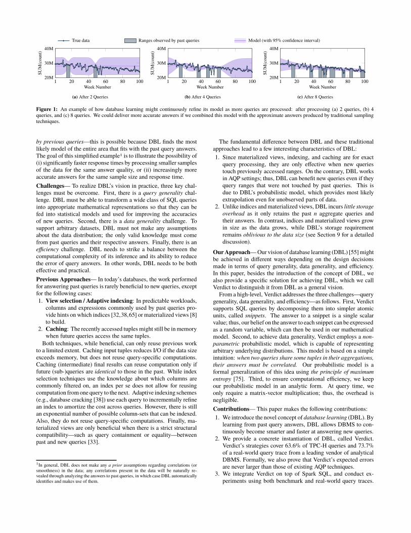
In Figure 1, we visualize this idea using a real-world Twitter

dataset [9,10]. Here, DBL learns a model for the number of occur-

rences of certain word patterns (known as n-grams, e.g., “bought

a car”) in tweets. Figure 1(a) shows this model (in purple) based

on the answers to the first two queries asking about the number

of occurrences of these patterns, each over a different time range.

Since the model is probabilistic, its 95% confidence interval is

also shown (the shaded area around the best current estimate). As

shown in Figure 1(b) and Figure 1(c), DBL further refines its model

as more new queries are answered. This approach would allow

a DBL-enabled query engine to provide increasingly more accu-

rate estimates, even for those ranges that have never been accessed

1 20 40 60 80 10020M

30M

40M

Week Number

SU

M(c

ount)

True data Ranges observed by past queries Model (with 95% confidence interval)

(a) After 2 Queries

1 20 40 60 80 10020M

30M

40M

Week Number

SU

M(c

ount)

(b) After 4 Queries

1 20 40 60 80 10020M

30M

40M

Week Number

SU

M(c

ount)

(c) After 8 Queries

Figure 1: An example of how database learning might continuously refine its model as more queries are processed: after processing (a) 2 queries, (b) 4queries, and (c) 8 queries. We could deliver more accurate answers if we combined this model with the approximate answers produced by traditional samplingtechniques.

by previous queries—this is possible because DBL finds the most

likely model of the entire area that fits with the past query answers.

The goal of this simplified example1 is to illustrate the possibility of

(i) significantly faster response times by processing smaller samples

of the data for the same answer quality, or (ii) increasingly more

accurate answers for the same sample size and response time.

Challenges— To realize DBL’s vision in practice, three key chal-

lenges must be overcome. First, there is a query generality chal-

lenge. DBL must be able to transform a wide class of SQL queries

into appropriate mathematical representations so that they can be

fed into statistical models and used for improving the accuracies

of new queries. Second, there is a data generality challenge. To

support arbitrary datasets, DBL must not make any assumptions

about the data distribution; the only valid knowledge must come

from past queries and their respective answers. Finally, there is an

efficiency challenge. DBL needs to strike a balance between the

computational complexity of its inference and its ability to reduce

the error of query answers. In other words, DBL needs to be both

effective and practical.

Previous Approaches— In today’s databases, the work performed

for answering past queries is rarely beneficial to new queries, except

for the following cases:

1. View selection / Adaptive indexing: In predictable workloads,

columns and expressions commonly used by past queries pro-

vide hints on which indices [32,38,65] or materialized views [8]

to build.

2. Caching: The recently accessed tuples might still be in memory

when future queries access the same tuples.

Both techniques, while beneficial, can only reuse previous work

to a limited extent. Caching input tuples reduces I/O if the data size

exceeds memory, but does not reuse query-specific computations.

Caching (intermediate) final results can reuse computation only if

future (sub-)queries are identical to those in the past. While index

selection techniques use the knowledge about which columns are

commonly filtered on, an index per se does not allow for reusing

computation from one query to the next. Adaptive indexing schemes

(e.g., database cracking [38]) use each query to incrementally refine

an index to amortize the cost across queries. However, there is still

an exponential number of possible column-sets that can be indexed.

Also, they do not reuse query-specific computations. Finally, ma-

terialized views are only beneficial when there is a strict structural

compatibility—such as query containment or equality—between

past and new queries [33].

1In general, DBL does not make any a prior assumptions regarding correlations (or

smoothness) in the data; any correlations present in the data will be naturally re-

vealed through analyzing the answers to past queries, in which case DBL automatically

identifies and makes use of them.

The fundamental difference between DBL and these traditional

approaches lead to a few interesting characteristics of DBL:

1. Since materialized views, indexing, and caching are for exact

query processing, they are only effective when new queries

touch previously accessed ranges. On the contrary, DBL works

in AQP settings; thus, DBL can benefit new queries even if they

query ranges that were not touched by past queries. This is

due to DBL’s probabilistic model, which provides most likely

extrapolation even for unobserved parts of data.

2. Unlike indices and materialized views, DBL incurs little storage

overhead as it only retains the past n aggregate queries and

their answers. In contrast, indices and materialized views grow

in size as the data grows, while DBL’s storage requirement

remains oblivious to the data size (see Section 9 for a detailed

discussion).

Our Approach— Our vision of database learning (DBL) [55] might

be achieved in different ways depending on the design decisions

made in terms of query generality, data generality, and efficiency.

In this paper, besides the introduction of the concept of DBL, we

also provide a specific solution for achieving DBL, which we call

Verdict to distinguish it from DBL as a general vision.

From a high-level, Verdict addresses the three challenges—query

generality, data generality, and efficiency—as follows. First, Verdict

supports SQL queries by decomposing them into simpler atomic

units, called snippets. The answer to a snippet is a single scalar

value; thus, our belief on the answer to each snippet can be expressed

as a random variable, which can then be used in our mathematical

model. Second, to achieve data generality, Verdict employs a non-

parametric probabilistic model, which is capable of representing

arbitrary underlying distributions. This model is based on a simple

intuition: when two queries share some tuples in their aggregations,

their answers must be correlated. Our probabilistic model is a

formal generalization of this idea using the principle of maximum

entropy [75]. Third, to ensure computational efficiency, we keep

our probabilistic model in an analytic form. At query time, we

only require a matrix-vector multiplication; thus, the overhead is

negligible.

Contributions— This paper makes the following contributions:

1. We introduce the novel concept of database learning (DBL). By

learning from past query answers, DBL allows DBMS to con-

tinuously become smarter and faster at answering new queries.

2. We provide a concrete instantiation of DBL, called Verdict.

Verdict’s strategies cover 63.6% of TPC-H queries and 73.7%

of a real-world query trace from a leading vendor of analytical

DBMS. Formally, we also prove that Verdict’s expected errors

are never larger than those of existing AQP techniques.

3. We integrate Verdict on top of Spark SQL, and conduct ex-

periments using both benchmark and real-world query traces.

Runtime query processing

Post-query

processing

SQL query

AQP

Engine

(raw ans, raw err)

Inference

(improved ans, improved err)

Query

Synopsis

Model Learning

Runtime dataflow

Post-query dataflow

Figure 2: Workflow in Verdict. At query time, the Inference module usesthe Query Synopsis and the Model to improve the query answer and errorcomputed by the underlying AQP engine (i.e., raw answer/error) beforereturning them to the user. Each time a query is processed, the raw answerand error are added to the Query Synopsis. The Learning module uses thisupdated Query Synopsis to refine the current Model accordingly.

Verdict delivers up to 23× speedup and 90% error reduction

compared to AQP engines that do not use DBL.

The rest of this paper is organized as follows. Section 2 overviews

Verdict’s workflow, supported query types, and internal query rep-

resentations. Sections 3 and 4 describe the internals of Verdict in

detail, and Section 5 presents Verdict’s formal guarantees. Section 6

summarizes Verdict’s online and offline processes, and Section 7

discusses Verdict’s deployment scenarios. Section 8 reports our

empirical results. Section 9 discusses related work, and Section 10

concludes the paper with future work.

2. VERDICT OVERVIEWIn this section, we overview the system we have built based

on database learning (DBL), called Verdict. Section 2.1 explains

Verdict’s architecture and overall workflow. Section 2.2 presents

the class of SQL queries currently supported by Verdict. Section 2.3

introduces Verdict’s query representation. Section 2.4 describes the

intuition behind Verdict’s inference. Lastly, Section 2.5 discusses

the limitations of Verdict’s approach.

2.1 Architecture and WorkflowVerdict consists of a query synopsis, a model, and three pro-

cessing modules: an inference module, a learning module, and an

off-the-shelf approximate query processing (AQP) engine. Figure 2

depicts the connection between these components.

We begin by defining query snippets, which serve as the basic

units of inference in Verdict.

Definition 1. (Query Snippet) A query snippet is a supported

SQL query whose answer is a single scalar value, where supported

queries are formally defined in Section 2.2.

Section 2.3 describes how a supported query (whose answer may

be a set) is decomposed into possibly multiple query snippets. For

simplicity, and without loss of generality, here we assume that every

incoming query is a query snippet.

For the i-th query snippet qi , the AQP engine’s answer includes

a pair of an approximate answer θi and a corresponding expected

error βi . θi and βi are formally defined in Section 3.1, and are

produced by most AQP systems [6, 34, 60, 84, 85, 87]. Now we can

formally define the first key component of our system, the query

synopsis.

Definition 2. (Query Synopsis) Let n be the number of query

snippets processed thus far by the AQP engine. The query synopsis

Qn is defined as the following set: {(qi, θi, βi) | i = 1, . . . , n}.

Term Definition

raw answer answer computed by the AQP engine

raw error expected error for raw answer

improved answer answer updated by Verdict

improved error expected error for improved answer (by Verdict)

past snippet supported query snippet processed in the past

new snippet incoming query snippeet

Table 1: Terminology.

We call the query snippets in the query synopsis past snippets,

and call the (n + 1)-th query snippet the new snippet.

The second key component is the model, which represents Ver-

dict’s statistical understanding of the underlying data. The model is

trained on the query synopsis, and is updated every time a query is

added to the synopsis (Section 4).

The query-time workflow of Verdict is as follows. Given an

incoming query snippet qn+1 , Verdict invokes the AQP engine to

compute a raw answer θn+1 and a raw error βn+1. Then, Verdict

combines this raw answer/error and the previously computed model

to infer an improved answer θ̂n+1 and an associated expected error

β̂n+1, called improved error. Theorem 1 shows that the improved

error is never larger than the raw error. After returning the improved

answer and the improved error to the user, (qn+1, θn+1, βn+1) is

added to the query synopsis.

A key objective in Verdict’s design is to treat the underlying AQP

engine as a black box. This allows Verdict to be used with many

of the existing engines without requiring any modifications. From

the user’s perspective, the benefit of using Verdict (compared to

using the AQP engine alone) is the error reduction and speedup, or

only the error reduction, depending on the type of AQP engine used

(Section 7).

Lastly, Verdict does not modify non-aggregate expressions or

unsupported queries, i.e., it simply returns their raw answers/errors

to the user. Table 1 summarizes the terminology defined above. In

Section 3, we will recap the mathematical notations defined above.

2.2 Supported QueriesVerdict supports aggregate queries that are flat (i.e., no derived

tables or sub-queries) with the following conditions:

1. Aggregates. Any number of SUM, COUNT, or AVG aggregates can

appear in the select clause. The arguments to these aggregates

can also be a derived attribute.

2. Joins. Verdict supports foreign-key joins between a fact table2

and any number of dimension tables, exploiting the fact that this

type of join does not introduce a sampling bias [3]. For sim-

plicity, our discussion in this paper is based on a denormalized

table.

3. Selections. Verdict currently supports equality and inequality

comparisons for categorical and numeric attributes (including

the in operator). Currently, Verdict does not support disjunc-

tions and textual filters (e.g., like ’%Apple%’) in the where

clause.

4. Grouping. groupby clauses are supported for both stored

and derived attributes. The query may also include a having

clause. Note that the underlying AQP engine may affect the

cardinality of the result set depending on the having clause

(e.g., subset/superset error). Verdict simply operates on the

result set returned by the AQP engine.

2Data warehouses typically record measurements (e.g., sales) into fact tables and

normalize commonly appearing attributes (e.g., seller information) into dimension

tables [74].

select A1, AVG(A2), SUM(A3)

from r

where A2 > a2

group by A1;select AVG(A2)

from r

where A2 > a2

and A1 = a11;

select SUM(A3)

from r

where A2 > a2

and A1 = a11;

select AVG(A2)

from r

where A2 > a2

and A1 = a12;

select SUM(A3)

from r

where A2 > a2

and A1 = a12;

groupby

valu

ea12

a11

AVG(A2) SUM(A3)

aggregate function

Query

Snippets

decompose

Figure 3: Example of a query’s decomposition into multiple snippets.

Nested Query Support— Although Verdict does not directly sup-

port nested queries, many queries can be flattened using joins [1]

or by creating intermediate views for sub-queries [33]. In fact, this

is the process used by Hive for supporting the nested queries of the

TPC-H benchmark [42]. We are currently working to automatically

process nested queries and to expand the class of supported queries

(see Section 10).

Unsupported Queries— Each query, upon its arrival, is inspected

by Verdict’s query type checker to determine whether it is supported,

and if not, Verdict bypasses the Inference module and simply returns

the raw answer to the user. The overhead of the query type checker is

negligible (Section 8.5) compared to the runtime of the AQP engine;

thus, Verdict does not incur any noticeable runtime overhead, even

when a query is not supported.

Only supported queries are stored in Verdict’s query synopsis and

used to improve the accuracy of answers to future supported queries.

That is, the class of queries that can be improved is equivalent to

the class of queries that can be used to improve other queries.

2.3 Internal Representation

Decomposing Queries into Snippets— As mentioned in Sec-

tion 2.1, each supported query is broken into (possibly) multiple

query snippets before being added to the query synopsis. Concep-

tually, each snippet corresponds to a supported SQL query with a

single aggregate function, with no other projected columns in its

select clause, and with no groupby clause; thus, the answer to

each snippet is a single scalar value. A SQL query with multiple

aggregate functions (e.g., AVG(A2), SUM(A3)) or a groupby clause

is converted to a set of multiple snippets for all combinations of each

aggregate function and each groupby column value. As shown in

the example of Figure 3, each groupby column value is added as

an equality predicate in the where clause. The number of generated

snippets can be extremely large, e.g., if a groupby clause includes a

primary key. To ensure that the number of snippets added per each

query is bounded, Verdict only generates snippets for Nmax (1,000

by default) groups in the answer set. Verdict computes improved

answers only for those snippets in order to bound the computational

overhead.3

For each aggregate function g, the query synopsis retains a maxi-

mum of Cg query snippets by following a least recently used snippet

replacement policy (by default, Cg=2, 000). This improves the ef-

ficiency of the inference process, while maintaining an accurate

model based on the recently processed snippet answers.

Aggregate Computation— Verdict uses two aggregate functions

to perform its internal computations: AVG(Ak) and FREQ(*). As

3Dynamically adjusting the value of Nmax (e.g., based on available resources and

workload characteristics) makes an interesting direction for future work.

stated earlier, the attribute Ak can be either a stored attribute (e.g.,

revenue) or a derived one (e.g., revenue * discount). At run-

time, Verdict combines these two types of aggregates to compute

its supported aggregate functions as follows:

• AVG(Ak) = AVG(Ak)

• COUNT(*) = round(FREQ(*) × (table cardinality))

• SUM(Ak) = AVG(Ak) × COUNT(*)

2.4 Why and When Verdict Offers BenefitIn this section, we provide the high level intuition behind Verdict’s

approach to improving the quality of new snippet answers. Verdict

exploits potential correlations between snippet answers to infer the

answer of a new snippet. Let Si and Sj be multisets of attribute

values such that, when aggregated, they output exact answers to

queries qi and qj , respectively. Then, the answers to qi and qj are

correlated, if:

1. Si and Sj include common values. Si ∩ Sj , φ implies the

existence of correlation between the two snippet answers. For

instance, computing the average revenue of the years 2014 and

2015 and the average revenue of the years 2015 and 2016 will be

correlated since these averages include some common values (here,

the 2015 revenue). In the TPC-H benchmark, 12 out of the 14

supported queries share common values in their aggregations.

2. Si and Sj include correlated values. For instance, the average

prices of a stock over two consecutive days are likely to be similar

even though they do not share common values. When the compared

days are farther apart, the similarity in their average stock prices

might be lower. Verdict captures the likelihood of such attribute

value similarities using a statistical measure called inter-tuple co-

variance, which will be formally defined in Section 4.2. In the

presence of non-zero inter-tuple covariances, the answers to qi and

qj could be correlated even when Si ∩ Sj , φ. In practice, most

real-life datasets tend to have non-zero inter-tuple covariances, i.e.,

correlated attribute values (see Appendix E for an empirical study).

Verdict formally captures the correlations between pairs of snip-

pets using a probabilistic distribution function. At query time, this

probabilistic distribution function is used to infer the most likely

answer to the new snippet given the answers to past snippets.

2.5 LimitationsVerdict’s model is the most likely explanation of the underly-

ing distribution given the limited information stored in the query

synopsis. Consequently, when a new snippet involves tuples that

have never been accessed by past snippets, it is possible that Ver-

dict’s model might incorrectly represent the underlying distribution,

and return incorrect error bounds. To guard against this limitation,

Verdict always validates its model-based answer against the (model-

free) answer of the AQP engine. We present this model validation

step in Appendix B.

Because Verdict relies on off-the-shelf AQP engines for obtaining

raw answers and raw errors, it is naturally bound by the limitations

of the underlying engine. For example, it is known that sample-

based engines are not apt at supporting arbitrary joins or MIN/MAX

aggregates. Similarly, the validity of Verdict’s error guarantees

are contingent upon the validity of the AQP engine’s raw errors.

Fortunately, there are also off-the-shelf diagnostic techniques to

verify the validity of such errors [5].

3. INFERENCEIn this section, we describe Verdict’s inference process for com-

puting an improved answer (and improved error) for the new snippet.

Verdict’s inference process follows the standard machine learning

Sym. Meaning

qi i-th (supported) query snippet

n + 1 index number for a new snippet

θi random variable representing our knowledge of the rawanswer to qi

θi (actual) raw answer computed by AQP engine for qi

βi expected error associated with θi

θ̄i random variable representing our knowledge of the exact

answer to qi

θ̄i exact answer to qi

θ̂n+1 improved answer to the new snippet

β̂n+1 improved error to the new snippet

Table 2: Mathematical Notations.

arguments: we can understand in part the true distribution by means

of observations, then we apply our understanding to predicting the

unobserved. To this end, Verdict applies well-established tech-

niques, such as the principle of maximum entropy and kernel-based

estimations, to an AQP setting.

To present our approach, we first formally state our problem in

Section 3.1. A mathematical interpretation of the problem and

the overview on Verdict’s approach is described in Section 3.2.

Sections 3.3 and 3.4 present the details of the Verdict’s approach

to solving the problem. Section 3.5 discusses some challenges in

applying Verdict’s approach.

3.1 Problem StatementLet r be a relation drawn from some unknown underlying distri-

bution. r can be a join or Cartesian product of multiple tables. Let

r’s attributes be A1, . . . , Am, where A1, . . . , Al are the dimension

attributes and Al+1, . . . , Am are the measure attributes. Dimension

attributes cannot appear inside aggregate functions while measure

attributes can. Dimension attributes can be numeric or categorical,

but measure attributes are numeric. Measure attributes can also be

derived attributes. Table 2 summarizes the notations we defined

earlier in Section 2.1.

Given a query snippet qi on r, an AQP engine returns a raw

answer θi along with an associated expected error βi . Formally, β2i

is the expectation of the squared deviation of θi from the (unknown)

exact answer θ̄i to qi .4 βi and βj are independent if i , j.

Suppose n query snippets have been processed, and therefore the

query synopsis Qn contains the raw answers and raw errors for the

past n query snippets. Without loss of generality, we assume all

queries have the same aggregate function g on Ak (e.g., AVG(Ak)),

where Ak is one of the measure attributes. Our problem is then

stated as follows: given Qn and (θn+1, βn+1), compute the most

likely answer to qn+1 with an associated expected error.

In our discussion, for simplicity, we assume static data, i.e., the

new snippet is issued against the same data that has been used

for answering past snippets in Qn . However, Verdict can also be

extended to situations where the relations are subject to new data

being added, i.e., each snippet is answered against a potentially

different version of the dataset. The generalization of Verdict under

data updates is presented in Appendix D.

3.2 Inference OverviewIn this section, we present our random variable interpretation

of query answers and a high-level overview of Verdict’s inference

process.

4Here, the expectation is made over θi since the value of θi depends on samples.

Our approach uses (probabilistic) random variables to represent

our knowledge of the query answers. The use of random variables

here is a natural choice as our knowledge itself of the query answers

is uncertain. Using random variables to represent degrees of belief

is a standard approach in Beyesian inference. Specifically, we de-

note our knowledge of the raw answer and the exact answer to the

i-th query snippet by random variables θi and θ̄i , respectively. At

this step, the only information available to us regarding θi and θ̄i is

that θi is an instance of θi ; no other assumptions are made.

Next, we represent the relationship between the set of random

variables θ1, . . . ,θn+1, θ̄n+1 using a joint probability distribution

function (pdf). Note that the first n + 1 random variables are for

the raw answers to past n snippets and the new snippet, and the last

random variable is for the exact answer to the new snippet. We are

interested in the relationship among those random variables because

our knowledge of the query answers is based on limited information:

the raw answers computed by the AQP engine, whereas we aim to

find the most likely value for the new snippet’s exact answer. This

joint pdf represents Verdict’s prior belief over the query answers.

We denote the joint pdf by f (θ1 = θ′1, . . . ,θn+1 = θ

′n+1, θ̄n+1 =

θ̄′n+1). For brevity, we also use f (θ′

1, . . . , θ′

n+1, θ̄′

n+1) when the

meaning is clear from the context. (Recall that θi refers to an actual

raw answer from the AQP engine, and θ̄n+1 refers to the exact answer

to the new snippet.) The joint pdf returns the probability that the

random variables θ1, . . . , θn+1, θ̄n+1 takes a particular combination

of the values, i.e., θ′1, . . . , θ′

n+1, θ̄′

n+1. In Section 3.3, we discuss

how to obtain this joint pdf from some statistics available on query

answers.

Then, we compute the most likely value for the new snippet’s exact

answer, namely the most likely value for θ̄n+1, by first conditionaliz-

ing the joint pdf on the actual observations (i.e., raw answers) from

the AQP engine, i.e., f (θ̄n+1 = θ̄′n+1| θ1 = θ1, . . . ,θn+1 = θn+1).

We then find the value of θ̄′n+1

that maximizes the conditional pdf.

We call this value the model-based answer and denote it by Üθn+1.

Section 3.4 provides more details of this process. Finally, Üθn+1

and its associated expected error Üβn+1 are returned as Verdict’s im-

proved answer and improved error if they pass the model validation

(described in Appendix B). Otherwise, the (original) raw answer

and error are taken as Verdict’s improved answer and error, respec-

tively. In other words, if the model validation fails, Verdict simply

returns the original raw results from the AQP engine without any

improvements.

3.3 Prior BeliefIn this section, we describe how Verdict obtains a joint pdf

f (θ′1, . . . , θ′

n+1, θ̄′

n+1) that represents its knowledge of the underly-

ing distribution. The intuition behind Verdict’s inference is to make

use of possible correlations between pairs of query answers. This

section applies such statistical information of query answers (i.e.,

means, covariances, and variances) for obtaining the most likely

joint pdf. Obtaining the query statistics is described in Section 4.

To obtain the joint pdf, Verdict relies on the principle of maxi-

mum entropy (ME) [15, 75], a simple but powerful statistical tool

for determining a pdf of random variables given some statistical

information available. According to the ME principle, given some

testable information on random variables associated with a pdf in

question, the pdf that best represents the current state of our knowl-

edge is the one that maximizes the following expression, called

entropy:

h( f ) = −∫

f ( ®θ) · log f ( ®θ) d ®θ (1)

where ®θ = (θ′1, . . . , θ′

n+1, θ̄′

n+1).

Note that the joint pdf maximizing the above entropy differs

depending on the kinds of given testable information, i.e., query

statistics in our context. For instance, the maximum entropy pdf

given means of random variables is different from the maximum

entropy pdf given means and (co)variances of random variables.

In fact, there are two conflicting considerations when applying this

principle. On one hand, the resulting pdf can be computed more

efficiently if the provided statistics are simple or few, i.e., sim-

ple statistics reduce the computational complexity. On the other

hand, the resulting pdf can describe the relationship among the ran-

dom variables more accurately if richer statistics are provided, i.e.,

the richer the statistics, the more accurate our improved answers.

Therefore, we need to choose an appropriate degree of statistical in-

formation to strike a balance between the computational efficiency

of pdf evaluation and its accuracy in describing the relationship

among query answers.

Among possible options, Verdict uses the first and the second

order statistics of the random variables, i.e., mean, variances, and

covariances. The use of second-order statistics enables us to capture

the relationship among the answers to different query snippets, while

the joint pdf that maximizes the entropy can be expressed in an

analytic form. The uses of analytic forms provides computational

efficiency. Specifically, the joint pdf that maximizes the entropy

while satisfying the given means, variances, and covariances is a

multivariate normal with the corresponding means, variances, and

covariances [75].

Lemma 1. Let θ = (θ1, . . . , θn+1, θ̄n+1)⊺ be a vector of n+2

random variables with mean values ®µ = (µ1, . . . , µn+1, µ̄n+1)⊺ and

a (n+2)×(n+2) covariance matrix Σ specifying their variances and

pairwise covariances. The joint pdf f over these random variables

that maximizes h( f )while satisfying the provided means, variances,

and covariances is the following function:

f ( ®θ) = 1√(2π)n+2 |Σ |

exp

(−1

2( ®θ − ®µ)⊺Σ−1( ®θ − ®µ)

), (2)

and this solution is unique.

In the following section, we describe how Verdict computes the

most likely answer to the new snippet using this joint pdf in Equa-

tion (2). We call the most likely answer a model-based answer.

In Appendix B, this model-based answer is chosen as an improved

answer if it passes a model validation. Finally, in Section 3.5, we

discuss the challenges involved in obtaining ®µ and Σ, i.e., the query

statistics required for deriving the joint pdf.

3.4 Model-based AnswerIn the previous section, we formalized the relationship among

query answers, namely (θ1, . . . , θn+1, θ̄n+1), using a joint pdf. In

this section, we exploit this joint pdf to infer the most likely answer to

the new snippet. In other words, we aim to find the most likely value

for θ̄n+1 (the random variable representing qn+1’s exact answer),

given the observed values for θ1, . . . , θn+1, i.e., the raw answers

from the AQP engine. We call the most likely value a model-

based answer and its associated expected error a model-based error.

Mathematically, Verdict’s model-based answer Üθn+1 to qn+1 can be

expressed as:

Üθn+1 = Arg Maxθ̄′n+1

f (θ̄′n+1 | θ1 = θ1, . . . ,θn+1 = θn+1). (3)

That is, Üθn+1 is the value at which the conditional pdf has its

maximum value. The conditional pdf, f (θ̄′n+1| θ1, . . . , θn+1),

is obtained by conditioning the joint pdf obtained in Section 3.3 on

the observed values, i.e., raw answers to the past snippets and the

new snippet.

Computing a conditional pdf may be a computationally expen-

sive task. However, a conditional pdf of a multivariate normal

distribution is analytically computable; it is another normal distri-

bution. Specifically, the conditional pdf in Equation (3) is a normal

distribution with the following mean µc and variance σ2c [16]:

µc = µ̄n+1 +®k⊺n+1Σ−1n+1( ®θn+1 − ®µn+1) (4)

σ2c = κ̄

2 − ®k⊺n+1Σ−1n+1®kn+1 (5)

where:

• ®kn+1 is a column vector of length n+ 1 whose i-th element is

(i, n + 2)-th entry of Σ;

• Σn+1 is a (n + 1) × (n + 1) submatrix of Σ consisting of Σ’s

first n + 1 rows and columns;

• ®θn+1=(θ1, . . . , θn+1)⊺;

• ®µn+1 = (µ1, . . . , µn+1)⊺; and

• κ̄2 is the (n + 2, n + 2)-th entry of Σ

Since the mean of a normal distribution is the value at which the

pdf takes a maximum value, we take µc as our model-based answerÜθn+1. Likewise, the expectation of the squared deviation of the

value θ̄′n+1

, which is distributed according to the conditional pdf

in Equation (3), from the model-based answer Üθn+1 coincides with

the variance σ2c of the conditional pdf. Thus, we take σc as our

model-based error Üβn+1 .

Computing each of Equations (4) and (5) requires O(n3) time

complexity at query time. However, Verdict uses alternative forms

of these equations that require only O(n2) time complexity at query

time (Section 5). As a future work, we plan to employ inferen-

tial techniques with sub-linear time complexity [49, 80] for a more

sophisticated eviction policy for past queries.

Note that, since the conditional pdf is a normal distribution, the

error bound at confidence δ is expressed as αδ · Üβn+1, where αδis a non-negative number such that a random number drawn from

a standard normal distribution would fall within (−αδ, αδ) with

probability δ. We call αδ the confidence interval multiplier for

probability δ. That is, the exact answer θ̄n+1 is within the range

( Üθn+1 − αδ · Üβn+1, Üθn+1 + αδ · Üβn+1) with probability δ, according

to Verdict’s model.

3.5 Key ChallengesAs mentioned in Section 3.3, obtaining the joint pdf in Lemma 1

(which represents Verdict’s prior belief on query answers) requires

the knowledge of means, variances, and covariances of the random

variables (θ1, . . . ,θn+1, θ̄n+1). However, acquiring these statistics

is a non-trivial task for two reasons. First, we have only observed one

value for each of the random values θ1, . . . , θn+1, namely θ1, . . . ,

θn+1. Estimating variances and covariances of random variables

from a single value is nearly impossible. Second, we do not have

any observation for the last random variable θ̄n+1 (recall that θ̄n+1

represents our knowledge of the exact answer to the new snippet,

i.e., θ̄n+1). In Section 4, we present Verdict’s approach to solving

these challenges.

4. ESTIMATING QUERY STATISTICSAs described in Section 3, Verdict expresses its prior belief on

the relationship among query answers as a joint pdf over a set of

random variables (θ1, . . . , θn+1, θ̄n+1). In this process, we need

to know the means, variances, and covariances of these random

variables.

Verdict uses the arithmetic mean of the past query answers for

the mean of each random variable, θ1, . . . , θn+1, θ̄n+1 . Note that

this only serves as a prior belief, and will be updated in the process

of conditioning the prior belief using the observed query answers.

In this section, without loss of generality, we assume the mean of

the past query answers is zero.

Thus, in the rest of this section, we focus on obtaining the vari-

ances and covariances of these random variables, which are the

elements of the (n + 2) × (n + 2) covariance matrix Σ in Lemma 1

(thus, we can obtain the elements of the column vector ®kn+1 and the

variance κ̄2 as well). Note that, due to the independence between

expected errors, we have:

cov(θi, θj ) = cov(θ̄i, θ̄j ) + δ(i, j) · β2icov(θi, θ̄j ) = cov(θ̄i, θ̄j )

(6)

where δ(i, j) returns 1 if i = j and 0 otherwise. Thus, computing

cov(θ̄i, θ̄j ) is sufficient for obtaining Σ.

Computing cov(θ̄i, θ̄j ) relies on a straightforward observation:

the covariance between two query snippet answers is computable

using the covariances between the attribute values involved in com-

puting those answers. For instance, we can easily compute the

covariance between (i) the average revenue of the years 2014 and

2015 and (ii) the average revenue of the years 2015 and 2016, as

long as we know the covariance between the average revenues of

every pair of days in 2014–2016.

In this work, we further extend the above observation. That

is, if we are able to compute the covariance between the average

revenues at an infinitesimal time t and another infinitesimal time t′,we will be able to compute the covariance between (i) the average

revenue of 2014–2015 and (ii) the average revenue of 2015–2016,

by integrating the covariances between the revenues at infinitesimal

times over appropriate ranges. Here, the covariance between the

average revenues at two infinitesimal times t and t′ is defined in

terms of the underlying data distribution that has generated the

relation r, where the past query answers help us discover the most-

likely underlying distribution. The rest of this section formalizes

this idea.

In Section 4.1, we present a decomposition of the (co)variances

between pairs of query snippet answers into inter-tuple covariance

terms. Then, in Section 4.2, we describe how inter-tuple covariances

can be estimated analytically using parameterized functions.

4.1 Covariance DecompositionTo compute the variances and covariances between query snippet

answers (i.e., θ1, . . . , θn+1, θ̄n+1), Verdict relies on our proposed

inter-tuple covariances, which express the statistical properties of

the underlying distribution. Before presenting the inter-tuple co-

variances, our discussion starts with the fact that the answer to a

supported snippet can be mathematically represented in terms of the

underlying distribution. This representation then naturally leads us

to the decomposition of the covariance between query answers into

smaller units, which we call inter-tuple covariances.

Let g be an aggregate function on attribute Ak , and t = (a1, . . . , al)be a vector of length l comprised of the values for r’s dimension at-

tributes A1, . . . , Al. To help simplify the mathematical descriptions

in this section, we assume that all dimension attributes are numeric

(not categorical), and the selection predicates in queries may contain

range constraints on some of those dimension attributes. Handling

categorical attributes is a straightforward extension of this process

(see Appendix F.2).

We define a continuous function νg(t) for every aggregate func-

tion g (e.g., AVG(Ak), FREQ(*)) such that, when integrated, it

produces answers to query snippets. That is (omitting possible

normalization and weight terms for simplicity):

θ̄i =

∫t∈Fi

νg(t) dt (7)

Formally, Fi is a subset of the Cartesian product of the domains of

the dimension attributes, A1, . . . , Al, such that t ∈ Fi satisfies the

selection predicates of qi . Let (si,k, ei,k ) be the range constraint for

Ak specified in qi . We set the range to (min(Ak), max(Ak)) if no

constraint is specified for Ak . Verdict simply represents Fi as the

product of those l per-attribute ranges. Thus, the above Equation (7)

can be expanded as:

θ̄i =

∫ ei, l

si, l

· · ·∫ ei,1

si,1

νg(t) da1 · · · dal

For brevity, we use the single integral representation using Fi unless

the explicit expression is needed.

Using Equation (7) and the linearity of covariance, we can de-

compose cov(θ̄i, θ̄j ) into:

cov(θ̄i, θ̄j ) = cov

(∫t∈Fi

νg(t) dt,

∫t′∈Fj

νg(t′) dt′)

=

∫t∈Fi

∫t′∈Fj

cov(νg(t), νg(t′)) dt dt′(8)

As a result, the covariance between query answers can be broken

into an integration of the covariances between tuple-level function

values, which we call inter-tuple covariances.

To use Equation (8), we must be able to compute the inter-tuple

covariance terms. However, computing these inter-tuple covari-

ances is challenging, as we only have a single observation for each

νg(t). Moreover, even if we had a way to compute the inter-tuple co-

variance for arbitrary t and t′, the exact computation of Equation (8)

would still require an infinite number of inter-tuple covariance com-

putations, which would be infeasible. In the next section, we present

an efficient alternative for estimating these inter-tuple covariances.

4.2 Analytic Inter-tuple CovariancesTo efficiently estimate the inter-tuple covariances, and thereby

compute Equation (8), we propose using analytical covariance

functions, a well-known technique in statistical literature for ap-

proximating covariances [16]. In particular, Verdict uses squared

exponential covariance functions, which is capable of approximat-

ing any continuous target function arbitrarily closely as the number

of observations (here, query answers) increases [54].5 Although

the underlying distribution may not be a continuous function, it is

sufficient for us to obtain νg(t) such that, when integrated (as in

Equation (7)), produces the same values as the integrations of the

underlying distribution.6 In our setting, the squared exponential

covariance function ρg(t, t′) is defined as:

cov(νg(t), νg(t′)) ≈ ρg(t, t′) = σ2g ·

l∏k=1

exp©­«−(ak − a′

k)2

l2g,k

ª®¬(9)

Here, lg,k for k=1 . . . l and σ2g are tunable correlation parameters

to be learned from past queries and their answers (Appendix A).

Intuitively, when t and t′ are similar, i.e., (ak − a′

k)2 is small

for most Ak , then ρg(t, t′) returns a larger value (closer to σ2g),

5 This property of the universal kernels is asymptotic (i.e., as the number of observations

goes to infinity).6The existence of such a continuous function is implied by the kernel density estimation

technique [79].

indicating that the expected values of g for t and t′ are highly

correlated.

With the analytic covariance function above, the cov(θ̄i, θ̄j ) terms

involving inter-tuple covariances can in turn be computed analyti-

cally. Note that Equation (9) involves the multiplication of l terms,

each of which containing variables related to a single attribute. As

a result, plugging Equation (9) into Equation (8) yields:

cov(θ̄i, θ̄j ) = σ2g

l∏k=1

∫ ei,k

si,k

∫ ej,k

sj,k

exp©­«−(ak − a′

k)2

l2g,k

ª®¬

da′k

ak

(10)

The order of integrals are interchangeable, since the terms includ-

ing no integration variables can be regarded as constants (and thus

can be factored out of the integrals). Note that the double-integral of

an exponential function can also be computed analytically (see Ap-

pendix F.1); thus, Verdict can efficiently compute cov(θ̄i, θ̄j ) in O(l)times by directly computing the integrals of inter-tuple covariances,

without explicitly computing individual inter-tuple covariances. Fi-

nally, we can compose the (n + 2) × (n + 2) matrix Σ in Lemma 1

using Equation (6).

5. FORMAL GUARANTEESNext, we formally show that the error bounds of Verdict’s im-

proved answers are never larger than the error bounds of the AQP

engine’s raw answers.

Theorem 1. Let Verdict’s improved answer and improved error to

the new snippet be (θ̂n+1, β̂n+1) and the AQP engine’s raw answer

and raw error to the new snippet be (θn+1, βn+1). Then,

β̂n+1 ≤ βn+1

and the equality occurs when the raw error is zero, or when Verdict’s

query synopsis is empty, or when Verdict’s model-based answer is

rejected by the model validation step.

Proof. Recall that (θ̂n+1, β̂n+1) is set either to Verdict’s model-

based answer/error, i.e., ( Üθn+1, Üβn+1), or to the AQP system’s raw

answer/error, i.e., (θn+1, βn+1), depending on the result of the model

validation. In the latter case, it is trivial that β̂n+1 ≤ βn+1 , and hence

it is enough to show that Üβn+1 ≤ βn+1.

Computing Üβn+1 involves an inversion of the covariance matrix

Σn+1 , where Σn+1 includes the βn+1 term on one of its diagonal

entries. We show Üβn+1 ≤ βn+1 by directly simplifying Üβn+1 into

the form that involves βn+1 and other terms.

We first define notations. Let Σ be the covariance matrix of the

vector of random variables (θ1, . . . , θn+1, θ̄n+1); ®kn be a column

vector of length n whose i-th element is the (i, n+1)-th entry of Σ; Σnbe an n× n submatrix of Σ that consists of Σ’s first n rows/columns;

κ̄2 be a scalar value at the (n + 2, n + 2)-th entry of Σ; and ®θn be a

column vector (θ1, . . . , θn)⊺.

Then, we can express ®kn+1 and Σn+1 in Equations (4) and (5) in

block forms as follows:

®kn+1 =

(®knκ̄2

), Σn+1 =

(Σn

®kn®k⊺n κ̄2 + β2

n+1

), ®θn+1 =

( ®θnθn+1

)

Here, it is important to note that ®kn+1 can be expressed in terms

of ®kn and κ̄2 because (i, n + 1)-th element of Σ and (i, n + 2)-thelement of Σ have the same values for i = 1, . . . , n. They have the

same values because the covariance between θi and θn+1 and the

covariance between θi and θ̄n+1 are same for i = 1, . . . , n due to

Equation (6).

Algorithm 1: Verdict offline process

Input: Qn including (qi, θi, βi ) for i = 1, . . . , n

Output: Qn with new model parameters and precomputed

matrices

1 foreach aggregate function g in Qn do

2 (lg,1, . . . , lg,l, σ2g) ← learn(Qn) // Appendix A

// Σ(i, j) indicates (i, j)-element of Σ3 for (i, j) ← (1, . . . , n) × (1, . . . , n) do

// Equation (6)

4 Σ(i, j) ← covariance(qi , qj ; lg,1, . . . , lg,l, σ2g)

5 end

6 Insert Σ and Σ−1 into Qn for g

7 end

8 return Qn

Using the formula of block matrix inversion [41], we can obtain

the following alternative forms of Equations (4) and (5) (here, we

assume zero means to simplify the expressions):

γ2= κ̄2 − ®k⊺n Σ−1

n®kn, θ = ®k⊺n Σ−1

n®θn (11)

Üθn+1 =β2n+1· θ + γ2 · θn+1

β2n+1+ γ2

, Üβ2n+1 =

β2n+1· γ2

β2n+1+ γ2

(12)

Note that Üβ2n+1< βn+1 for βn+1 > 0 and γ2 < ∞, and Üβ2

n+1=

βn+1 if βn+1 = 0 or γ2 →∞. �

Lemma 2. The time complexity of Verdict’s inference is O(Nmax ·l · n2) The space complexity of Verdict is O(n · Nmax

+ n2), where

n · Nmax is the size of the query snippets and n2 is the size of the

precomputed covariance matrix.

Proof. It is enough to prove that the computations of a model-based

answer and a model-based error can be performed in O(n2) time,

where n is the number of past query snippets. Note that this is clear

from Equations (11) and (12), because the computation of Σ−1n in-

volves only the past query snippets. For computing γ2, multiplying®kn , a precomputed Σ−1

n , and ®kn takes O(n2) time. Similarly for θ in

Equation (11) �

These results imply that the domain sizes of dimension attributes

do not affect Verdict’s computational overhead. This is because

Verdict analytically computes the covariances between pairs of

query answers without individually computing inter-tuple covari-

ances (Section 4.2).

6. VERDICT PROCESS SUMMARYIn this section, we summarize Verdict’s offline and online pro-

cesses. Suppose the query synopsis Qn contains a total of n query

snippets from past query processing, and a new query is decom-

posed into b query snippets; we denote the new query snippets in

the new query by qn+1, . . . , qn+b .

Offline processing— Algorithm 1 summarizes Verdict’s offline

process. It consists of learning correlation parameters and comput-

ing covariances between all pairs of past query snippets.

Online processing— Algorithm 2 summarizes Verdict’s runtime

process. Here, we assume the new query is a supported query;

otherwise, Verdict simply forwards the AQP engine’s query answer

to the user.

Algorithm 2: Verdict runtime process

Input: New query snippets qn+1, . . . , qn+b ,

Query synopsis Qn

Output: b number of improved answers and improved errors

{(θ̂n+1, β̂n+1), . . . , (θ̂n+b, β̂n+b)},Updated query synopsis Qn+b

1 fc← number of distinct aggregate functions in new queries

/* The new query (without decomposition) is

sent to the AQP engine in practice. */

2 {(θn+1, βn+1), . . . , (θn+b, βn+b )} ← AQP(qn+1, . . . , qn+b)

// improve up to Nmax rows

3 for i ← 1, . . . , (fc · Nmax) do

// model-based answer/error

// (Equations (4) and (5))

4 ( Üθn+i, Üβn+i ) ← inference(θn+i, βn+i,Qn)

// model validation (Appendix B)

5 (θ̂n+i, β̂n+i ) ← if valid( Üθn+i , Üβn+i) then ( Üθn+i, Üβn+i )else (θn+i, βn+i )

6 Insert (qn+i, θn+i, βn+i ) into Qn

7 end

8 for i ← (fc · Nmax+ 1), . . . , b do

9 (θ̂n+i, β̂n+i ) ← (θn+i, βn+i )10 end

// Verdict overhead ends

11 return {(θ̂n+1, β̂n+1), . . . , (θ̂n+b, β̂n+b)},Qn

7. DEPLOYMENT SCENARIOSVerdict is designed to support a large class of AQP engines.

However, depending on the type of AQP engine used, Verdict may

provide both speedup and error reduction, or only error reduction.

1. AQP engines that support online aggregation [34,60,84,85]:

Online aggregation continuously refines its approximate answer as

new tuples are processed, until users are satisfied with the current

accuracy or when the entire dataset is processed. In these types

of engines, every time the online aggregation provides an updated

answer (and error estimate), Verdict generates an improved answer

with a higher accuracy (by paying small runtime overhead). As soon

as this accuracy meets the user requirement, the online aggregation

can be stopped. With Verdict, the online aggregation’s continuous

processing will stop earlier than it would without Verdict. This

is because Verdict reaches a target error bound much earlier by

combining its model with the raw answer of the AQP engine.

2. AQP engines that support time-bounds [6, 19, 24, 36, 45, 66,

87]: Instead of continuously refining approximate answers and re-

porting them to the user, these engines simply take a time-bound

from the user, and then they predict the largest sample size that they

can process within the requested time-bound; thus, they minimize

error bounds within the allotted time. For these engines, Verdict

simply replaces the user’s original time bound t1 with a slightly

smaller value t1 − ǫ before passing it down to the AQP engine,

where ǫ is the time needed by Verdict for inferring the improved

answer and improved error. Thanks to the efficiency of Verdict’s

inference, ǫ is typically a small value, e.g., a few milliseconds (see

Section 8.5). Since Verdict’s inference brings larger accuracy im-

provements on average compared to the benefit of processing more

tuples within the ǫ time, Verdict achieves significant error reduc-

tions over traditional AQP engines.

In this paper, we use an online aggregation engine to demonstrate

Verdict’s both speedup and error reduction capabilities (Section 8).

However, for interested readers, we also provide evaluations on a

time-bound engine Appendix C.2.

Some AQP engines also support error-bound queries but do not

offer an online aggregation interface [?, 7, 68]. For these engine,

Verdict currently only benefits their time-bound queries, leaving

their answer to error-bound queries unchanged. Supporting the

latter would require either adding an online aggregation interface

to the AQP engine, or a tighter integration of Verdict and the AQP

engine itself. Such modifications are beyond the scope of this paper,

as one of our design goals is to treat the underlying AQP engine as a

black box (Figure 2), so that Verdict can be used alongside a larger

number of existing engines.

Note that Verdict’s inference mechanism is not affected by the

specific AQP engine used underneath, as long as the conditions in

Section 3 hold, namely the error estimate β2 is the expectation of the

squared deviation of the approximate answer from the exact answer.

However, the AQP engine’s runtime overhead (e.g., query parsing

and planning) may affect Verdict’s overall benefit in relative terms.

For example, if the query parsing amount to 90% of the overall query

processing time, even if Verdict completely eliminates the need for

processing any data, the relative speedup will only be 1.0/0.9 =

1.11×. However, Verdict is designed for data-intensive scenarios

where disk or network I/O is a sizable portion of the overall query

processing time.

8. EXPERIMENTSWe conducted experiments to (i) quantify the percentage of real-

world queries that benefit from Verdict (Section 8.2), (ii) study

Verdict’s average speedup and error reductions over an AQP en-

gine (Section 8.3), (iii) test the reliability of Verdict’s error bounds

(Section 8.4), (iv) measure Verdict’s computational overhead and

memory footprint (Section 8.5), and (v) study the impact of dif-

ferent workloads and data distributions on Verdict’s effectiveness

(Section 8.6). In summary, our results indicated the following:

• Verdict supported a large fraction (73.7%) of aggregate queries

in a real-world workload, and produced significant speedups

(up to 23.0×) compared to a sample-based AQP solution.

• Given the same processing time, Verdict reduces the baseline’s

approximation error on average by 75.8%–90.2%.

• Verdict’s runtime overhead was <10 milliseconds on average

(0.02%–0.48% of total time) and its memory footprint was neg-

ligible.

• Verdict’s approach was robust against various workloads and

data distributions.

We also have supplementary experiments in Appendix C. Ap-

pendix C.1 shows the benefits of model-based inference in compar-

ison to a strawman approach, which simply caches all past query

answers. Appendix C.2 demonstrates Verdict’s benefit for time-

bound AQP engines.

8.1 Experimental Setup

Datasets and Query Workloads— For our experiments, we used

the three datasets described below:

1. Customer1: This is a real-world query trace from one of the

largest customers (anonymized) of a leading vendor of analytic

DBMS. This dataset contains 310 tables and 15.5K timestamped

queries issued between March 2011 and April 2012, 3.3K of

which are analytical queries supported by Spark SQL. We did

not have the customer’s original dataset but had access to their

data distribution, which we used to generate a 536 GB dataset.

0 2 4 6 100

5

10

15

20

25

Runtime (sec)

Err

or

Bound

(%)

NoLearn Verdict

0 2 4 6 100

2

4

6

8

10

Runtime (sec)

Act

ual

Err

or

(%)

(a) Cached, Customer1

0 1 2 3 4 5 60

5

10

15

20

25

Runtime (min)

Err

or

Bound

(%)

0 1 2 3 4 5 60

2

4

6

8

10

Runtime (min)

Act

ual

Err

or

(%)

(b) Not Cached, Customer1

0 10 20 30 40 50 600

5

10

15

Runtime (sec)

Err

or

Bound

(%)

0 10 20 30 40 50 600

2

4

6

Runtime (sec)

Act

ual

Err

or

(%)

(c) Cached, TPC-H

0 6 12 18 24 300

5

10

15

Runtime (min)

Err

or

Bound

(%)

0 6 12 18 24 300

2

4

6

Runtime (min)

Act

ual

Err

or

(%)

(d) Not Cached, TPC-H

Figure 4: The relationship (i) between runtime and error bounds (top row), and (ii) between runtime and actual errors (bottom row), for both systems: NoLearnand Verdict.

2. TPC-H: This is a well-known analytical benchmark with 22

query types, 21 of which contain at least one aggregate function

(including 2 queries with min or max). We used a scale factor

of 100, i.e., the total data size was 100 GB. We generated a

total of 500 queries using TPC-H’s workload generator with its

default settings. The queries in this dataset include joins of up

to 6 tables.

3. Synthetic: For more controlled experiments, we also gener-

ated large-scale synthetic datasets with different distributions

(see Section 8.6 for details).

Implementation— For comparative analysis, we implemented two

systems on top of Spark SQL [12] (version 1.5.1):

1. NoLearn: This system is an online aggregation engine that

creates random samples of the original tables offline and splits

them into multiple batches of tuples. To compute increasingly

accurate answers to a new query, NoLearn first computes an

approximate answer and its associated error bound on the first

batch of tuples, and then continues to refine its answer and error

bound as it processes additional batches. NoLearn estimates its

errors and computes confidence intervals using closed-forms

(based on the central limit theorem). Error estimation based

on the central limit theorem has been one of the most popular

approaches in online aggregation systems [34, 46, 84, 85] and

other AQP engines [3, 6, 19].

2. Verdict: This system is an implementation of our proposed

approach, which uses NoLearn as its AQP engine. In other

words, each time NoLearn yields a raw answer and error, Ver-

dict computes an improved answer and error using our proposed

approach. Naturally, Verdict incurs a (negligible) runtime over-

head, due to supported query check, query decomposition, and

computation of improved answers; however, Verdict yields an-

swers that are much more accurate in general.

Experimental Environment— We used a Spark cluster (for both

NoLearn and Verdict) using 5 Amazon EC2 m4.2xlarge instances,

each with 2.4 GHz Intel Xeon E5 processors (8 cores) and 32GB

of memory. Our cluster also included SSD-backed HDFS [72] for

Spark’s data loading. For experiments with cached datasets, we

distributed Spark’s RDDs evenly across the nodes using Spark SQL

DataFrame repartition function.

DatasetTotal # of Queries # of Supported

Percentagewith Aggregates Queries

Customer1 3,342 2,463 73.7%

TPC-H 21 14 63.6%

Table 3: Generality of Verdict. Verdict supports a large fraction of real-world and benchmark queries.

8.2 Generality of VerdictTo quantify the generality of our approach, we measured the cov-

erage of our supported queries in practice. We analyzed the real-

world SQL queries in Customer1. From the original 15.5K queries,

Spark SQL was able to process 3.3K of the aggregate queries.

Among those 3.3K queries, Verdict supported 2.4K queries, i.e.,

73.7% of the analytical queries could benefit from Verdict. In ad-

dition, we analyzed the 21 TPC-H queries and found 14 queries

supported by Verdict. Others could not be supported due to textual

filters or disjunctions in the where clause. These statistics are sum-

marized in Table 3. This analysis proves that Verdict can support a

large class of analytical queries in practice. Next, we quantified the

extent to which these supported queries benefitted from Verdict.

8.3 Speedup and Error ReductionIn this section, we first study the relationship between the process-

ing time and the size of error bounds for both systems, i.e., NoLearn

and Verdict. Based on this study, we then analyze Verdict’s speedup

and error reductions over NoLearn.

In this experiment, we used each of Customer1 and TPC-H

datasets in two different settings. In one setting, all samples were

cached in the memories of the cluster, while in the second, the data

had to be read from SSD-backed HDFS.

We allowed both systems to process half of the queries (since

Customer1 queries were timestamped, we used the first half).

While processing those queries, NoLearn simply returned the query

answers, but Verdict also kept the queries and their answers in its

query synopsis. After processing those queries, Verdict (i) pre-

computed the matrix inversions and (ii) learned the correlation

parameters. The matrix inversions took 1.6 seconds in total; the

correlation parameter learning took 23.7 seconds for TPC-H and

8.04 seconds for Customer1. The learning process was relatively

faster for Customer1 since most of the queries included COUNT(*)

for which each attribute did not require a separate learning. This

Cached?Error Time Taken

SpeedupBound NoLearn Verdict

Customer1

Yes2.5% 4.34 sec 0.57 sec 7.7×1.0% 6.02 sec 2.45 sec 2.5×

No2.5% 140 sec 6.1 sec 23.0×1.0% 211 sec 37 sec 5.7×

TPC-H

Yes4.0% 26.7 sec 2.9 sec 9.3×2.0% 34.2 sec 12.9 sec 2.7×

No4.0% 456 sec 72 sec 6.3×2.0% 524 sec 265 sec 2.1×

Cached? RuntimeAchieved Error Bound Error

NoLearn Verdict Reduction

Customer1

Yes1.0 sec 21.0% 2.06% 90.2%

5.0 sec 1.98% 0.48% 75.8%

No10 sec 21.0% 2.06% 90.2%

60 sec 6.55% 0.87% 86.7%

TPC-H

Yes5.0 sec 13.5% 2.13% 84.2%

30 sec 4.87% 1.04% 78.6%

No3.0 min 11.8% 1.74% 85.2%

10 min 4.49% 0.92% 79.6%

Table 4: Speedup and error reductions by Verdict compared to NoLearn.

offline training time for both workloads was comparable to the time

needed for running only a single approximate query (Table 4).

For the second half of the queries, we recorded both systems’

query processing times (i.e., runtime), approximate query answers,

and error bounds. Since both NoLearn and Verdict are online aggre-

gation systems, and Verdict produces improved answers for every

answer returned from NoLearn, both systems naturally produced

more accurate answers (i.e., answers with smaller error bounds)

as query processing continued. Approximate query engines, in-

cluding both NoLearn and Verdict, are only capable of producing

expected errors in terms of error bounds. However, for analysis, we

also computed the actual errors by comparing those approximate

answers against the exact answers. In the following, we report their

relative errors.

Figure 4 shows the relationship between runtime and average

error bound (top row) and the relationship between runtime and

average actual error (bottom row). Here, we also considered two

cases: when the entire data is cached in memory and when it resides

on SSD. In all experiments, the runtime-error graphs exhibited a

consistent pattern: (i) Verdict produced smaller errors even when

runtime was very large, and (ii) Verdict showed faster runtime for the

same target errors. Due to the asymptotic nature of errors, achieving

extremely accurate answers (e.g., less than 0.5%) required relatively

long processing time even for Verdict.

Using these results, we also analyzed Verdict’s speedups and

error reduction over NoLearn. For speedup, we compared how long

each system took until it reached a target error bound. For error

reduction, we compared the lowest error bounds that each system

produced within a fixed allotted time. Table 4 reports the results for

each combination of dataset and location (in memory or on SSD).

For the Customer1 dataset, Verdict achieved a larger speedup

when the data was stored on SSD (up to 23.0×) compared to when

it was fully cached in memory (7.7×). The reason was that, for

cached data, the I/O time was no longer the dominant factor and

Spark SQL’s default overhead (e.g., parsing the query and reading

the catalog) accounted for a considerable portion of the total data

processing time. For TPC-H, on the contrary, the speedups were

smaller when the data was stored on SSD. This difference stems from

1% 2% 4% 8% 16% 32%05

1015202530

Verdict Error Bound

Act

ual

Err

or

(%)

Figure 5: The comparison between Verdict’s error bound at 95% confidenceand the actual error distribution (5th, 50th, and 95th percentiles are reportedfor actual error distributions).

the different query forms betweenCustomer1 andTPC-H. The TPC-

H dataset includes queries that join several tables, some of which

are large tables that were not sampled by NoLearn. (Similar to most

sample-based AQP engines, NoLearn only samples fact tables, not

dimension tables.) Consequently, those large tables had to be read

each time NoLearn processed such a query. When the data resided

on SSD, loading those tables became a major bottleneck that could

not be reduced by Verdict (since they were not sampled). However,

on average, Verdict still achieved an impressive 6.3× speedup over

NoLearn. In general, Verdict’s speedups over NoLearn reduced as

the target error bounds became smaller; however, even for 1% target

error bounds, Verdict achieved an average of up to 5.7× speedup

over NoLearn.

Table 4 also reports Verdict’s error reductions over NoLearn. For

all target runtime budgets we examined, Verdict achieved massive

error reductions compared to NoLearn.

The performance benefits of Verdict depends on several important

factors, such as the accuracy of past query answers and workload

characteristics. These factors are further studied in Section 8.6

and Appendix C.1.

8.4 Confidence Interval GuaranteesTo confirm the validity of Verdict’s error bounds, we configured

Verdict to produce error bounds at 95% confidence and compared

them to the actual errors. We ran Verdict for an amount of time

long enough to sufficiently collect error bounds of various sizes.

By definition, the error bounds at 95% confidence are probabilis-

tically correct if the actual errors are smaller than the error bounds

in at least 95% of the cases. Figure 5 shows the 5th percentile,

median, and 95th percentile of the actual errors for different sizes

of error bounds (from 1% to 32%). In all cases, the 95th percentile

of the actual errors were lower than the error bounds produced by

Verdict, which confirms the probabilistic correctness of Verdict’s

error bound guarantees.

8.5 Memory and Computational OverheadIn this section, we study Verdict’s additional memory footprint

(due to query synopsis) and its runtime overhead (due to inference).

The total memory footprint of the query synopsis was 5.79MB for

TPC-H and 18.5MB for Customer1workload (23.2KB per-query for

TPC-H and 15.8KB per-query for Customer1). This included past

queries in parsed forms, model parameters, covariance matrices,

and the inverses of those covariance matrices. The size of query

synopsis was small because Verdict does not retain any of the input

tuples.

To measure Verdict’s runtime overhead, we recorded the time

spent for its regular query processing (i.e., NoLearn) and the ad-

ditional time spent for the inference and updating the final answer.

As summarized in Table 5, the runtime overhead of Verdict was

negligible compared to the overall query processing time. This is

Latency Cached Not Cached

NoLearn 2.083 sec 52.50 sec

Verdict 2.093 sec 52.51 sec

Overhead 0.010 sec (0.48%) 0.010 sec (0.02%)

Table 5: The runtime overhead of Verdict.

because multiplying a vector by a Cg×Cg matrix does not take much

time compared to regular query planning, processing, and network

commutations among the distributed nodes. (Note that Cg=2, 000

by default; see Section 2.3.)

8.6 Impact of Different Data Distributions andWorkload Characteristics

In this section, we generated various synthetic datasets and queries

to fully understand how Verdict’s effectiveness changes for different

data distributions, query patterns, and number of past queries.

First, we studied the impact of having queries with a more diverse

set of columns in their selection predicates. We produced a table

of 50 columns and 5M rows, where 10% of the columns were

categorical. The domains of the numeric columns were the real

values between 0 and 10, and the domains of the categorical columns

were the integers between 0 and 100.

Also, we generated four different query workloads with varying

proportions of frequently accessed columns. The columns used for

the selection predicates were chosen according to a power-law dis-

tribution. Specifically, a fixed number of columns (called frequently

accessed columns) had the same probability of being accessed, but

the access probability of the remaining columns decayed according

to the power-law distribution. For instance, if the proportion of

frequently accessed columns was 20%, the first 20% of the columns

(i.e., 10 columns) appeared with equal probability in each query,

but the probability of appearance reduced by half for every remain-

ing column. Figure 6(a) shows that as the proportion of frequently

accessed columns increased, Verdict’s relative error reduction over

NoLearn gradually decreased (the number of past queries were fixed

to 100). This is expected as Verdict constructs its model based on

the columns appearing in the past. In other words, to cope with

the increased diversity, more past queries are needed to understand

the complex underlying distribution that generated the data. Note

that, according to the analytic queries in the Customer1 dataset,

most of the queries included less than 5 distinct selection predi-

cates. However, by processing more queries, Verdict continued to

learn more about the underlying distribution, and produced larger

error reductions even when the workload was extremely diverse

(Figure 6(c)).

Second, to study Verdict’s potential sensitivity, we generated

three tables using three different probability distributions: uniform,

Gaussian, and a log-normal (skewed) distribution. Figure 6(b)

shows Verdict’s error reductions when queries were run against each

table. Because of the power and generality of the maximum entropy

principle taken by Verdict, it delivered a consistent performance

irrespective of the underlying distribution.

Third, we varied the number of past queries observed by Verdict

before running our test queries. For this study, we used a highly

diverse query set (its proportion of frequently accessed columns was

20%). Figure 6(c) demonstrates that the error reduction continued

increasing as more queries were processed, but its increment slowed

down. This is because, after observing enough information, Verdict

already had a good knowledge of the underlying distribution, and

processing more queries barely improved its knowledge. This result

indicates that Verdict is able to deliver reasonable performance

without having to observe too many queries.

This is because, after observing enough information, Verdict

already has a good knowledge of the underlying distribution, and

processing more queries barely improves its knowledge. This result

indicates that Verdict is able to deliver reasonable performance

without having to observe too many queries.

Lastly, we studied the negative impact of increasing the number

of past queries on Verdict’s overhead. Since Verdict’s inference

consists of a small matrix multiplication, we did not observe a

noticeable increase in its runtime overhead even when the number

of queries in the query synopsis increased (Figure 6(d)).

Recall that the domain size of the attributes does not affect Ver-

dict’s computational cost since only the lower and upper bounds

of range constraints are needed for covariance computations (Sec-

tion 4.2).

9. RELATED WORK

Approximate Query Processing— There has been substantial

work on sampling-based approximate query processing [3, 4, 6, 13,

19,21,27,29,35,46,53,58,67,73,78]. Some of these systems differ

in their sample generation strategies. Some of these systems differ

in their sample generation strategies (see [57] and the references

within). For instance, STRAT [19] and AQUA [4] create a single

stratified sample, while BlinkDB creates samples based on column

sets. Online Aggregation (OLA) [20, 34, 60, 82] continuously re-

fines its answers during query execution. Others have focused on

obtaining faster or more reliable error estimates [5, 83]. These are

orthogonal to our work, as reliable error estimates from an under-

lying AQP engine will also benefit DBL. There is also AQP tech-

niques developed for specific domain, e.g., sequential data [11,64],

probabilistic data [30, 59], and RDF data [37, 76], and searching in

high-dimensional space [62]. However, our focus in this paper is

on general (SQL-based) AQP engines.

Adaptive Indexing, View Selection— Adaptive Indexing and data-

base cracking [38, 39, 65] has been proposed for a column-store

database as a means of incrementally updating indices as part of

query processing; then, it can speed up future queries that access

previously indexed ranges. While the adaptive indexing is an ef-

fective mechanism for exact analytic query processing in column-

store databases, answering queries that require accessing multiple

columns (e.g., selection predicates on multiple columns) is still

a challenging task: column-store databases have to join relevant

columns to reconstruct tuples. Although Idreos et al. [39] pre-join

some subsets of columns, the number of column combinations still

grows exponentially as the total number of columns in a table in-

creases. Verdict can easily handle queries with multiple columns

due to its analytic inference. Materialized views are another means

of speeding up future aggregate queries [25, 33, 44, 56]. Verdict

also speed up aggregate queries, but Verdict does not require strict

query containments as in materialized views.

Pre-computation— COSMOS [82] stores the results of past queries

as multi-dimensional cubes, which are then reused if they are con-

tained in the new query’s input range, while boundary tuples are

read from the database. This approach is not probabilistic and is

limited to low-dimensional data due to the exponential explosion

in the number of possible cubes. Also, similar to view selection,

COSMOS relies on strict query containment.

Model-based and Statistical Databases— Statistical approaches

have been used in databases for various goals. MauveDB [23]

constructs views that express a statistical model, hiding the possible

irregularities of the underlying data. MauveDB’s goal is to support

4% 10% 20% 40%0

20406080

100

ratio of frequently accessed columns

Err

or

Red

uct

ion

(%)

(a) Workload Diversity

Uniform

Gaussi

an

Skewed

020406080

100

Err

or

Red

uct

ion

(%)

(b) Data distribution

10 100 200 300 4000

20

40

60

80

# of past queries

Err

or

Red

uct

ion

(%)

(c) Learning Behavior

10 100 200 300 40002468

10

# of past queries

Over

hea

d(m

s)

(d) Overhead

Figure 6: The effectiveness of Verdict in reducing NoLearn’s error for different (a) levels of diversity in the queried columns, (b) data distributions, and (c)number of past queries observed. Figure (d) shows Verdict’s overhead for different number of past queries.

statistical modeling, such as regression or interpolation. , rather

than speeding up future query processing. BayesDB [52] provides

a SQL-like language that enables non-statisticians to declaratively

use various statistical models. Bayesian networks have been

used for succinctly capturing correlations among attributes [31].

Exploiting these correlations can be an interesting future direction

for DBL.

Maximum Entropy Principle— In the database community, the

principle of maximum entropy (ME) has been previously used for

determining the most surprising piece of information in a data ex-

ploration context [71], and for constructing histograms based on

cardinality assertions [47]. Verdict uses ME differently than these

previous approaches; they assign a unique variable to each non-

overlapping area to represent the number of tuples belonging to

that area. This approach poses two challenges when applied to an

AQP context. First, it requires a slow iterative numeric solver for

its inference. Thus, using this approach for DBL may eliminate

any potential speedup. Second, introducing a unique variable for

every non-overlapping area can be impractical as it requires O(2n)variables for n past queries. Finally, the previous approach cannot

express inter-tuple covariances in the underlying data. In contrast,

Verdict’s approach handles arbitrarily overlapping ranges in multi-

dimensional space with O(n) variables (and O(n2) space), and its

inference can be performed analytically.

10. CONCLUSION AND FUTURE WORKIn this paper, we presented database learning (DBL), a novel

approach to exploit past queries’ (approximate) answers in speeding

up new queries using a principled statistical methodology. We

presented a prototype of this vision, called Verdict, on top of Spark

SQL. Through extensive experiments on real-world and benchmark

query logs, we demonstrated that Verdict supported 73.7% of real-

world analytical queries, speeding them up by up to 23× compared

to an online aggregation AQP engine.

Exciting lines of future work include: (i) the study of other infer-

ential techniques for realizing DBL, (ii) the development of active

database learning [61], whereby the engine itself proactively exe-

cutes certain approximate queries that can best improve its internal

model, and (iii) the extension of Verdict to support visual analyt-

ics [14, 22, 26, 40, 43, 48, 63, 77, 81].

11. ACKNOWLEDGEMENTThis work was in part funded by NSF awards 1544844, 1629397,

and 1553169. The authors are grateful to Aditya Modi, Morgan

Lovay, and Shannon Riggins for their feedback on this manuscript.

12. REFERENCES[1]

https://db.apache.org/derby/docs/10.6/tuning/ctuntransform36368.html.

[2] S. Acharya, P. B. Gibbons, and V. Poosala. Aqua: A fast decisionsupport system using approximate query answers. In VLDB, 1999.

[3] S. Acharya, P. B. Gibbons, V. Poosala, and S. Ramaswamy. Joinsynopses for approximate query answering. In SIGMOD, 1999.

[4] S. Acharya, P. B. Gibbons, V. Poosala, and S. Ramaswamy. The AquaApproximate Query Answering System. In SIGMOD, 1999.

[5] S. Agarwal, H. Milner, A. Kleiner, A. Talwalkar, M. Jordan,S. Madden, B. Mozafari, and I. Stoica. Knowing when you’re wrong:Building fast and reliable approximate query processing systems. InSIGMOD, 2014.

[6] S. Agarwal, B. Mozafari, A. Panda, H. Milner, S. Madden, andI. Stoica. BlinkDB: queries with bounded errors and boundedresponse times on very large data. In EuroSys, 2013.

[7] S. Agarwal, A. Panda, B. Mozafari, A. P. Iyer, S. Madden, andI. Stoica. Blink and it’s done: Interactive queries on very large data.PVLDB, 2012.

[8] S. Agrawal, S. Chaudhuri, and V. R. Narasayya. Automated selectionof materialized views and indexes in sql databases. In VLDB, 2000.

[9] M. R. Anderson, D. Antenucci, V. Bittorf, M. Burgess, M. J.Cafarella, A. Kumar, F. Niu, Y. Park, C. Ré, and C. Zhang.Brainwash: A data system for feature engineering. In CIDR, 2013.

[10] D. Antenucci, M. R. Anderson, and M. Cafarella. A declarative queryprocessing system for nowcasting. PVLDB, 2016.

[11] A. Arasu and G. S. Manku. Approximate counts and quantiles oversliding windows. In PODS, 2004.

[12] M. Armbrust et al. Spark sql: Relational data processing in spark. InSIGMOD, 2015.

[13] B. Babcock, S. Chaudhuri, and G. Das. Dynamic sample selection forapproximate query processing. In VLDB, 2003.

[14] L. Battle, R. Chang, and M. Stonebraker. Dynamic prefetching ofdata tiles for interactive visualization. 2015.

[15] A. L. Berger, V. J. D. Pietra, and S. A. D. Pietra. A maximum entropyapproach to natural language processing. Computational linguistics,1996.

[16] C. M. Bishop. Pattern recognition. Machine Learning, 2006.

[17] J. G. Carbonell, R. S. Michalski, and T. M. Mitchell. An overview ofmachine learning. In Machine learning. 1983.

[18] A. Carlson, J. Betteridge, B. Kisiel, B. Settles, E. R. Hruschka Jr, andT. M. Mitchell. Toward an architecture for never-ending languagelearning. In AAAI, 2010.

[19] S. Chaudhuri, G. Das, and V. Narasayya. Optimized stratifiedsampling for approximate query processing. TODS, 2007.

[20] T. Condie, N. Conway, P. Alvaro, J. M. Hellerstein, K. Elmeleegy,and R. Sears. Mapreduce online. In NSDI, 2010.

[21] J. Considine, F. Li, G. Kollios, and J. Byers. Approximateaggregation techniques for sensor databases. In ICDE, 2004.

[22] A. Crotty, A. Galakatos, E. Zgraggen, C. Binnig, and T. Kraska.Vizdom: interactive analytics through pen and touch. VLDB, 2015.

[23] A. Deshpande and S. Madden. Mauvedb: supporting model-baseduser views in database systems. In SIGMOD, 2006.

[24] A. Dobra, C. Jermaine, F. Rusu, and F. Xu. Turbo-charging estimateconvergence in dbo. PVLDB, 2009.

[25] A. El-Helw, I. F. Ilyas, and C. Zuzarte. Statadvisor: Recommendingstatistical views. VLDB, 2009.

[26] M. El-Hindi, Z. Zhao, C. Binnig, and T. Kraska. Vistrees: fastindexes for interactive data exploration. In HILDA, 2016.

[27] W. Fan, F. Geerts, Y. Cao, T. Deng, and P. Lu. Querying big data byaccessing small data. In PODS, 2015.

[28] D. Freedman, R. Pisani, and R. Purves. Statistics. 2007.

[29] V. Ganti, M.-L. Lee, and R. Ramakrishnan. Icicles: Self-tuningsamples for approximate query answering. In VLDB, 2000.

[30] W. Gatterbauer and D. Suciu. Approximate lifted inference withprobabilistic databases. PVLDB, 2015.

[31] L. Getoor, B. Taskar, and D. Koller. Selectivity estimation usingprobabilistic models. In SIGMOD Record, 2001.

[32] G. Graefe and H. Kuno. Adaptive indexing for relational keys. InICDEW, 2010.

[33] A. Y. Halevy. Answering queries using views: A survey. VLDBJ,2001.

[34] J. M. Hellerstein, P. J. Haas, and H. J. Wang. Online aggregation. InSIGMOD, 1997.

[35] K. Hose, D. Klan, and K.-U. Sattler. Distributed data summaries forapproximate query processing in pdms. In IDEAS, 2006.

[36] Y. Hu, S. Sundara, and J. Srinivasan. Estimating Aggregates inTime-Constrained Approximate Queries in Oracle. In EDBT, 2009.

[37] H. Huang, C. Liu, and X. Zhou. Approximating query answering onrdf databases. WWW, 2012.

[38] S. Idreos, M. L. Kersten, and S. Manegold. Database cracking. InCIDR, 2007.

[39] S. Idreos, M. L. Kersten, and S. Manegold. Self-organizing tuplereconstruction in column-stores. In SIGMOD, 2009.

[40] S. Idreos, O. Papaemmanouil, and S. Chaudhuri. Overview of dataexploration techniques. In SIGMOD, 2015.

[41] J. S. R. Jang. General formula: Matrix inversion lemma.http://www.cs.nthu.edu.tw/~jang/book/addenda/matinv/matinv/ .

[42] Y. Jia. Running tpc-h queries on hive.https://issues.apache.org/jira/browse/HIVE-600.

[43] M. Joglekar, H. Garcia-Molina, and A. Parameswaran. Interactivedata exploration with smart drill-down. In ICDE, 2016.

[44] S. Joshi and C. Jermaine. Materialized sample views for databaseapproximation. TKDE, 2008.

[45] S. Joshi and C. Jermaine. Sampling-Based Estimators forSubset-Based Queries. VLDB J., 18(1), 2009.

[46] S. Kandula, A. Shanbhag, A. Vitorovic, M. Olma, R. Grandl,S. Chaudhuri, and B. Ding. Quickr: Lazily approximating complexadhoc queries in bigdata clusters. In SIGMOD, 2016.

[47] R. Kaushik, C. Ré, and D. Suciu. General database statistics usingentropy maximization. In DBPL, 2009.

[48] A. Kim, E. Blais, A. Parameswaran, P. Indyk, S. Madden, andR. Rubinfeld. Rapid sampling for visualizations with orderingguarantees. PVLDB, 2015.

[49] N. Lawrence, M. Seeger, R. Herbrich, et al. Fast sparse gaussianprocess methods: The informative vector machine. NIPS, 2003.

[50] M. Lichman. UCI machine learning repository, 2013.

[51] M. Lovric. International Encyclopedia of Statistical Science.

Springer, 2011.

[52] V. Mansinghka et al. Bayesdb: A probabilistic programming systemfor querying the probable implications of data. arXiv, 2015.

[53] A. Meliou, C. Guestrin, and J. M. Hellerstein. Approximating sensornetwork queries using in-network summaries. In IPSN, 2009.

[54] C. A. Micchelli, Y. Xu, and H. Zhang. Universal kernels. JMLR, 2006.

[55] B. Mozafari. Verdict: A system for stochastic query planning. InCIDR, Biennial Conference on Innovative Data Systems, 2015.

[56] B. Mozafari, E. Z. Y. Goh, and D. Y. Yoon. CliffGuard: A principledframework for finding robust database designs. In SIGMOD, 2015.

[57] B. Mozafari and N. Niu. A handbook for building an approximatequery engine. IEEE Data Eng. Bull., 2015.

[58] C. Olston, E. Bortnikov, K. Elmeleegy, F. Junqueira, and B. Reed.Interactive Analysis of Web-Scale Data. In CIDR, 2009.

[59] D. Olteanu, J. Huang, and C. Koch. Approximate confidencecomputation in probabilistic databases. In ICDE, 2010.

[60] N. Pansare, V. R. Borkar, C. Jermaine, and T. Condie. Onlineaggregation for large mapreduce jobs. PVLDB, 4, 2011.

[61] Y. Park. Active database learning. In CIDR, 2017.

[62] Y. Park, M. Cafarella, and B. Mozafari. Neighbor-sensitive hashing.PVLDB, 2015.

[63] Y. Park, M. Cafarella, and B. Mozafari. Visualization-aware samplingfor very large databases. In ICDE, 2016.

[64] K. S. Perera, M. Hahmann, W. Lehner, T. B. Pedersen, andC. Thomsen. Efficient approximate olap querying over time series. InIDEAS, 2016.

[65] E. Petraki, S. Idreos, and S. Manegold. Holistic indexing inmain-memory column-stores. In SIGMOD, 2015.

[66] A. Pol and C. Jermaine. Relational confidence bounds are easy withthe bootstrap. In SIGMOD, 2005.

[67] N. Potti and J. M. Patel. Daq: a new paradigm for approximate queryprocessing. PVLDB, 2015.

[68] J. Ramnarayan, B. Mozafari, S. Menon, S. Wale, N. Kumar,H. Bhanawat, S. Chakraborty, Y. Mahajan, R. Mishra, andK. Bachhav. Snappydata: A hybrid transactional analytical store builton spark. In SIGMOD, 2016.

[69] F. Rusu, C. Qin, and M. Torres. Scalable analytics model calibrationwith online aggregation. IEEE Data Eng. Bull., 2015.

[70] A. L. Samuel. Some studies in machine learning using the game ofcheckers. IBM Journal of research and development, 1959.

[71] S. Sarawagi. User-adaptive exploration of multidimensional data. InVLDB, 2000.

[72] K. Shvachko, H. Kuang, S. Radia, and R. Chansler. The hadoopdistributed file system. In MSST, 2010.

[73] L. Sidirourgos, M. L. Kersten, and P. A. Boncz. SciBORQ: Scientificdata management with Bounds On Runtime and Quality. In CIDR,2011.

[74] A. Silberschatz, H. F. Korth, S. Sudarshan, et al. Database system

concepts. 1997.

[75] J. Skilling. Data Analysis: A Bayesian Tutorial. Oxford UniversityPress, 2006.

[76] A. Souihli and P. Senellart. Optimizing approximations of dnf querylineage in probabilistic xml. In ICDE, 2013.

[77] M. Vartak, S. Rahman, S. Madden, A. G. Parameswaran, andN. Polyzotis. SEEDB: efficient data-driven visualizationrecommendations to support visual analytics. PVLDB, 2015.

[78] J. Wang, S. Krishnan, M. J. Franklin, K. Goldberg, T. Kraska, andT. Milo. A sample-and-clean framework for fast and accurate queryprocessing on dirty data. In SIGMOD, 2014.

[79] L. Wasserman. All of Nonparametric Statistics. Springer, 2006.

[80] C. K. Williams and M. Seeger. Using the nyström method to speed upkernel machines. In NIPS, 2000.

[81] E. Wu, L. Battle, and S. R. Madden. The case for data visualizationmanagement systems: vision paper. PVLDB, 2014.

[82] S. Wu, B. C. Ooi, and K.-L. Tan. Continuous Sampling for OnlineAggregation over Multiple Queries. In SIGMOD, pages 651–662,2010.

[83] F. Xu, C. Jermaine, and A. Dobra. Confidence bounds forsampling-based group by estimates. TODS, 2008.

[84] K. Zeng, S. Agarwal, A. Dave, M. Armbrust, and I. Stoica. G-OLA:Generalized on-line aggregation for interactive analysis on big data.In SIGMOD, 2015.

[85] K. Zeng, S. Agarwal, and I. Stoica. iolap: Managing uncertainty forefficient incremental olap. 2016.

[86] K. Zeng, S. Gao, J. Gu, B. Mozafari, and C. Zaniolo. Abs: a systemfor scalable approximate queries with accuracy guarantees. InSIGMOD, 2014.

[87] K. Zeng, S. Gao, B. Mozafari, and C. Zaniolo. The analyticalbootstrap: a new method for fast error estimation in approximatequery processing. In SIGMOD, 2014.

APPENDIX

Appendix is organized as follows. Appendices A and B provide Ver-

dict’s learning and model validation processes, respectively. Ap-

pendix C includes additional experiments for demonstrating the

effectiveness and accuracy of Verdict. Appendix D present the

generalization of Verdict’s approach to the databases into which

new tuples may be inserted. Appendix E studies the prevalence of

non-zero inter-tuple correlations in real-world datasets. Appendix F

0 0.2 0.4 0.6 0.8 10

0.2

0.4

0.6

0.8

1

True Correlation Parameter

Est

imat

ed

Corr

elat

ion

Par

amet

er

20 50 100# past queries:

Figure 7: Correlation Param Learning

describes technical details that we did not discuss in the main body

of the paper.

A. PARAMETER LEARNINGThis section describes Verdict’s correlation parameter learning.

In Appendix A.1, we presents mathematical description of the pro-

cess, and in Appendix A.2, we study its effectiveness with experi-

ments.

A.1 Optimal Correlation ParametersIn this section, we describe how to find the most likely values of

the correlation parameters defined in Section 4.2. In this process,

we exploit the joint pdf defined in Equation (2), as it allows us to

compute the likelihood of a certain combination of query answers

given relevant statistics. Let ®θpast denote a vector of raw answers to

past snippets. Then, by Bayes’ theorem:

Pr(Σn | ®θpast) ∝ Pr(Σn) · Pr( ®θpast | Σn)where Σn is an n × n submatrix of Σ consisting of Σ’s first n rows

and columns, i.e., (co)variances between pairs of past query an-

swers, and ∝ indicates that the two values are proportional, There-

fore, without any preference over parameter values, determining

the most likely correlation parameters (which determine Σn) given

past queries amounts to finding the values for lg,1, . . . , lg,l, σ2g that

maximize the below log-likelihood function:

log Pr( ®θpast | Σn) = log f ( ®θpast)

= −1

2®θ⊺pastΣ

−1n®θpast −

1

2log |Σn | −

n

2log 2π (13)

where f ( ®θpast) is the joint pdf from Equation (2).

Verdict finds the optimal values for lg,1, . . . , lg,l by solving the

above optimization problem with a numerical solver, while it esti-

mates the value for σ2g analytically from past query answers (see

Appendix F.3). Concretely, the current implementation of Verdict

uses the gradient-descent-based (quasi-newton) nonlinear program-

ming solver provided by Matlab’s fminuncon() function, without

providing explicit gradients. Although our current approach is typ-

ically slower than using closed-form solutions or than using the

solver with an explicit gradient (and a Hessian), they do not pose a

challenge in Verdict’s setting, since all these parameters are com-

puted offline, i.e., prior to the arrival of new queries. We plan

to improve the efficiency of this offline training by using explicit

gradient expressions.

Since Equation (13) is not a convex function, the solver of our

choice only returns a locally optimal point. A conventional strategy

to handle this issue is to obtain multiple locally optimal points by

solving the same problem with multiple random starting points, and

to take the one with the highest log-likelihood value as a final answer.

Still, this approach does not guarantee the correctness of the model.

In contrast, Verdict’s strategy is to find a locally-optimal point that

0 0.5 1012345

a1

νg(t)

True data Model (with 95% confidence interval)

(a) After three queries

0 0.5 1012345

a1

νg(t)

(b) After ten queries

Figure 8: An example of (a) overly optimistic confidence intervals due toincorrect estimation of the underlying distributon, and (b) its resolution withmore queries processed. Verdict relies on a model validation to avoid thesituation as in (a).

can capture potentially large inter-tuple covariances, and to vali-

date the correctness of the resulting model against a model-free

answer (Appendix B). We demonstrate empirically in the following

section that this strategy is effective for finding parameter values

that are close to true values. Verdict’s model validation process in

Appendix B provides robustness against the models that may differ

from the true distribution. Verdict uses lg,k = (max(Ak)−min(Ak))for the starting point of the optimization problem.

Lastly, our use of approximate answers as the constraints for the

ME principle is properly accounted for by including additive error

terms in their (co)variances (Equation (6)).

A.2 Accuracy of Parameter LearningIn this section, we demonstrate our empirical study on the effec-

tiveness of Verdict’s correlation parameter estimation process. For

this, we used the synthetic datasets generated from pre-determined

correlation parameters to see how close Verdict could estimate the

values of those correlation parameters. We let Verdict estimate

the correlation parameter values using three different numbers of

past snippets (20, 50, and 100) for various datasets with different

correlation parameter values.

Figure 7 shows the results. In general, the correlation parameter

values discovered by Verdict’s estimation process were consistent

with the true correlation parameter values. Also, the estimated

values tended to be closer to the true values when a larger number

of past snippets were used for the estimation process. This result

indicates that Verdict can effectively learn statistical characteristics

of the underlying distribution just based on the answers to the past

queries.

B. MODEL VALIDATIONVerdict aims to provide correct error bounds even when its model

differs significantly from the true data. In Appendix B.1, we de-

scribes its process, and in Appendix B.2, we empirically demon-

strate its effectiveness.

B.1 Model Validation ProcedureVerdict’d model validation rejects its model—the most likely

explanation of the underlying distribution given the answers to past

snippets—if there is evidence that its model-based error is likely

to be incorrect. Verdict’s model validation process addresses two

situations: (i) negative estimates for FREQ(*), and (ii) an unlikely

large discrepancy between a model-based answer and a raw answer.

Negative estimates for FREQ(*)— To obtain the prior distribution

of the random variables, Verdict uses the most-likely distribution

(based on the maximum entropy principle (Lemma 1)), given the

means, variances, and covariances of query answers. Although this

makes the inference analytically computable, the lack of explicit

non-negative constraints on the query answers may produce negative

estimates on FREQ(*). Verdict handles this situation with a simple

check; that is, Verdict rejects its model-based answer if Üθn+1 < 0

for FREQ(*), and uses the raw answer instead. Even if Üθn+1 ≥ 0,

the lower bound of the confidence interval is set to zero if the value

is less than zero.

Unlikely model-based answer— Verdict’s model learned from em-

pirical observations may be different from the true distribution.

Figure 8(a) illustrates such an example. Here, after the first three

queries, the model is consistent with past query answers (shown as

gray boxes); however, it incorrectly estimates the distribution of the

unobserved data, leading to overly optimistic confidence intervals.

Figure 8(b) shows that the model becomes more consistent with the

data as more queries are processed.

Verdict rejects (and does not use) its own model in situations

such as Figure 8(a) by validating its model-based answers against the

model-free answers obtained from the AQP engine. Specifically, we

define a likely region as the range in which the AQP engine’s answer

would fall with high probability (99% by default) if Verdict’s model

were to be correct. If the AQP’s raw answer θn+1 falls outside this

likely region, Verdict considers its model unlikely to be correct. In

such cases, Verdict drops its model-based answer/error, and simply

returns the raw answer to the user unchanged. This process is akin

to hypothesis testing in statistics literatures [28].

Although no improvements are made in such cases, we take this

conservative approach to ensure the correctness of our error guar-

antees. (See Section 5 and Appendix B.2 for formal guarantees and

empirical results, respectively).

Formally, let t ≥ 0 be the value for which the AQP engine’s

answer would fall within ( Üθn+1 − t, Üθn+1 + t) with probability δv(0.99 by default) if Üθn+1 were the exact answer. We call the ( Üθn+1 −t, Üθn+1 + t) range the likely region. To compute t, we must find the

value closest to Üθn+1 that satisfies the following expression:

Pr(|X − Üθn+1 | < t

)≥ δv (14)

where X is a random variable representing the AQP engine’s possi-

ble answer to the new snippet if the exact answer to the new snippet

was Üθn+1. The AQP engine’s answer can be treated as a random

variable since it may differ depending on the random samples used.

The probability in Equation (14) can be easily computed using ei-

ther the central limit theorem or the Chebyshev’s inequality [51].

Once the value of t is computed, Verdict rejects its model if θn+1

falls outside the likely region ( Üθn+1 − t, Üθn+1 + t).In summary, the pair of Verdict’s improved answer and improved

error, (θ̂n+1, β̂n+1), is set to ( Üθn+1, Üβn+1) if θn+1 is within the range

( Üθn+1 − t, Üθn+1 + t), and is set to (θn+1, βn+1) otherwise. In either

case, the error bound at confidence δ remains the same as αδ · β̂n+1,

where αδ is the confidence interval multiplier for probability δ.

B.2 Empirical Study on Model ValidationThis section studies the effect of Verdict’s model validation de-

scribed in Appendix B.1. For this study, we first generated synthetic

datasets with several predetermined correlation parameters values.

Note that one can generate such synthetic datasets by first determin-

ing a joint probabilistic distribution function with predetermined

correlation parameter values and sampling attribute values from

the joint probability distribution function. In usual usage scenario,

Verdict estimates those correlation parameters from past snippets;

however, in this section, we manually set the values for the correla-

tion parameters in Verdict’s model, to test the behavior of Verdict

running with possibly incorrect correlation parameter values.

Figure 9 reports the experiment results from when Verdict was

tested without a model validation step and with a model valida-

tion step, respectively. In the figure, the values on the X-axis are

0.1 0.2 0.5 1.0 2.0 5.0 10.00

1

2

3

4

Artificial Correlation Parameter Scale (×)

Rat

ioof

Act

ual

Err

or

to

Err

or

Bound

Median without model validation

5th, 95th percentile without model validation

Median with model validation

5th, 95th percentile with model validation

Figure 9: Effect of model validation. For Verdict’s error bounds to becorrect, the 95th percentile should be below 1.0. One can find that, withVerdict’s model validation, the improved answers and the improved errorswere probabilistically correct even when largely incorrect correlation pa-rameters were used.

artificial correlation parameter scales, i.e., the product of the true

correlation parameters and each of those scales are set in Verdict’s

model. For instance, if a true correlation parameter was 5.0, and

the “artificial correlation parameter scale” was 0.2, Verdict’s model

was set to 1.0 for the correlation parameter. Thus, the values of

the correlation parameters in Verdict’s model were set to the true

correlation parameters, when the “artificial correlation parameter

scale” was 1.0. Since the Y-axis reports the ratio of the actual error

to Verdict’s error bound, Verdict’s error bound was correct when

the value on the Y-axis was below 1.0.

In the figure, one can observe that, Verdict, used without the

model validation, produced incorrect error bounds when the corre-

lation parameters used for the model deviated largely from the true

correlation parameter values. However, Verdict’s model validation

could successfully identify incorrect model-based answers and pro-

vide correct error bounds by replacing those incorrect model-based

answers with the raw answers computed by the AQP system.

C. ADDITIONAL EXPERIMENTSThis section contains additional experiments we have not in-

cluded in the main part of our paper. First, we study the impact

of two factors that affect the performance benefits of Verdict (Ap-

pendix C.1). Second, we show that Verdict can achieve error reduc-

tions over time-bounded AQP engines (Appendix C.2).

C.1 Verdict vs. Simple Answer CachingTo study the benefits of Verdict’s model-based inference, we con-

sider another system Baseline2, and make comparisons between

Verdict and Baseline2, using the TPC-H dataset. Baseline2 is

similar to NoLearn but returns a cached answer if the new query is

identical to one of the past ones. When there are multiple instances

of the same query, Baseline2 caches the one with the lowest ex-

pected error.

Figure 10(a) reports the average actual error reductions of Verdict

and Baseline2 (over NoLearn), when different sample sizes were

used for past queries. Here, the same samples were used for new

queries. The result shows that both systems’ error reductions were

large when large sample sizes were used for the past queries. How-

ever, Verdict consistently achieved higher error reductions com-

pared to Baseline2, due to its ability to benefit novel queries as

well as repeated queries (i.e., the queries that have appeared in the

past).

0.01 0.05 0.1 0.5 1.00

20

40

60

80

100

Sample Size (%)

Act

ual

Err

or

Red

uct

ion

(%)

Baseline2 Verdict

(a) Sample Sizes for Past Queries

0 20 40 60 80 1000

20

40

60

80

100

Novel Query Ratio (%)

Act

ual

Err

or

Red

uct

ion

(%)

(b) Query Workload Composition

Figure 10: (a) Comparison of Verdict and Baseline2 for different samplesizes used by past queries and (b) comparison of Verdict and Baseline2 fordifferent ratios of novel queries in the workload.

Customer1 TPC-H0

20

40

60

80

100 80.6163.42

Err

or

Red

uct

ion

(%)

(a) Cached

Customer1 TPC-H0

20

40

60

80

100 88.9781.29

Err

or

Red

uct

ion

(%)

(b) Not Cached

Figure 11: Average error reduction by Verdict (compared to NoLearn) forthe same time budget.

Figure 10(b) compares Verdict and Baseline2 by changing the

ratio of novel queries in the workload. Understandably, both Verdict

and Baseline2 were more effective for workloads with fewer novel

queries (i.e., more repeated queries); however, Verdict was also

effective for workloads with many novel queries.

C.2 Error Reductions forTime-Bound AQP Engines

Recall that, in Section 8, we demonstrated Verdict’s speedup and

error reductions over an online aggregation system. In this section,

we show Verdict’s error reductions over a time-bound AQP system.

First, we describe our experiment setting. Next, we present our

experiment results.

Setup— Here, we describe two systems, NoLearn and Verdict,

which we compare in this section:

1. NoLearn: This system runs queries on samples of the original

tables to obtain fast but approximate query answers and their

associated estimated errors. This is the same approach taken

by existing AQP engines, such as [2, 6, 19, 66, 69, 86]. Specifi-

cally, NoLearn maintains uniform random samples created of-

fline (10% of the original tables), and it uses the largest samples

that are small enough to satisfy the requested time bounds.

2. Verdict: This system invokes NoLearn to obtain raw answer-

s/errors but modifies them to produce improved answers/errors

using our proposed inference process. Verdict translates the

user’s requested time bound into an appropriate time bound for

NoLearn.

Observe that we are using the term NoLearn here to indicate a time-

bound AQP system in this section. (In Section 8, we used NoLearn

for an online aggregation system.)

Experiment Results— This section presents the error reduction by

Verdict compared to NoLearn. For experiments, we ran the same set

of queries as in Section 8 with both Verdict and NoLearn described

above. For comparison, we used the identical time-bounds for both

Verdict and NoLearn. Specifically, we set the time-bounds as 2

seconds and 0.5 seconds for the Customer1 and TPC-H datasets

cached in memory, respectively; and we set the time-bounds as 5.0

seconds for both Customer1 and TPC-H datasets loaded from SSD.

Figure 11 reports Verdict’s error reductions over NoLearn for each

of four different combinations of a dataset and cache setting.

In Figure 11, one can observe that Verdict achieved large error

reductions (63%–86%) over NoLearn. These results indicate that

the users of Verdict can obtain much more precise answers compared

to the users of NoLearn within the same time-bounds.

D. GENERALIZATION OF VERDICT

UNDER DATA ADDITIONSThus far, we have discussed our approach based on the assumption

that the database is static, i.e., no tuples are deleted, added, or

updated. In this section, we suggest the possibility of using Verdict

even for the database that allows an important kind of data update:

data append. In Appendix D.1, we present the approach, and in

Appendix D.2, we show its effectivess with experiments.

D.1 Larger Expected Errors for Old QueriesA naïve strategy to supporting tuples insertions would be to re-

execute all past queries every time new tuples are added to the

database to obtain their updated answers. This solution is obviously

impractical.

Instead, Verdict still makes use of answers to past queries even

when new tuples have been added since computing their answers.

The basic idea is to simply lower our confidence in the raw answers

of those past queries.

Assume that qi (whose aggregate function is on Ak) is computed

on an old relation r, and a set of new tuples ra has since been added

to r to form an updated relation ru . Let θ̄ai

be a random variable

representing our knowledge of qi’s true answer on ra , and θ̄ui

be

qi ’s true answer on ru .

We represent the possible difference between Ak’s values in r

and those in ra by a random variable sk with mean µk and variance

η2k. Thus:

θ̄ai = θ̄i + sk

The values of µk and η2k

can be estimated using small samples of r

and ra . Verdict uses the following lemma to update the raw answer

and raw error for qi :

Lemma 3.

E[θ̄ui − θi] = µk ·|ra |

|r | + |ra |

E[(θ̄ui − θi −|ra | µk|r | + |ra | )

2] = β2i +( |ra | ηk|r | + |ra |

)2

where |r | and |ra | are the number of tuples in r and ra , respectively.

Proof. Since we represented a snippet answer on the appended

relation using a random variable θ̄ui

, we can also represent a snippet

5% 10% 15% 20%0

1.0

2.0

3.0

4.0

5.0

Proportion of the Number of Appended Tuples

Aver

age

Err

or

(%)

NoLearn error bound Verdict actual error

Verdict error bound (no adjustment)

Verdict error bound (with adjustment)

5% 10% 15% 20%0

20

40

60

80

100

Proportion of the Number of Appended Tuples

Err

or

bound

Vio

lations

(%)

no adjustment with adjustment

Figure 12: Data append technique (Appendix D) is highly effective indelivering correct error estimates in face of new data.

answer on the updated relation ru using a random variable. Let the

snipept answer on ru be θ̄ui

. Then,

E[θ̄ui − θi] = E

[ |r | θ̄i|r | + |ra | +

|ra | sk|r | + |ra |

]− θ̄i =

|ra | µk|r | + |ra |

Also,

E

[(θ̄ui − θi −

|ra | µk|r | + |ra | )

2

]

= E

[(θ̄i +

|ra | sk|r | + |ra | − θi −

|ra | µk|r | + |ra |

)]

= E

[(θ̄i − θi)2 +

( |ra ||r | + |ra |

)2

(sk − µk )2

+ 2

( |ra ||r | + |ra |

)(θ̄i − θi)(sk − µk )

]

= β2i +

( |ra | ηk|r | + |ra |

)2

where we used to independence between (θ̄i−θi) and (sk−µk). �

Once the raw answers and the raw errors of past query snippets are

updated using this lemma, the remaining inference process remains

the same.

D.2 Empirical Evaluation for Data AppendIn this section, we empirically study the impact of new data (i.e.,

tuple insertions) on Verdict’s effectiveness. We generated an initial

synthetic table with 5 million tuples and appended additional tuples

to generate different versions of the table. The newly inserted tuples

were generated such that their attribute values gradually diverged

from the attribute values of the original table. We distinguish

between these different versions by the ratio of their newly inserted

tuples, e.g., a 5% appended table means that 250K (5% of 5 million)

tuples were added. We then ran the queries and recorded the error

bounds of VerdictAdjust and VerdictNoAdjust (our approach

-0.1 0.0

0.1

0.2

0.3

0.4

0.5

0.6

0.7

0.8

0.9

1.0

0

20

40

60

-0.2

(Normalized) Inter-tuple Covariance

Per

centa

ge

(%)

Figure 13: Inter-tuple Covariances for 16 real-life UCI datasets.

with and without the technique introduced in Appendix D.1). We

also measured the error bounds of NoLearn and the actual error.

As shown in Figure 12(a), VerdictNoAdjust produced overly-

optimistic error bounds (i.e., lower than the actual error) for 15%

and 20% appends, whereas VerdictAdjust produced valid error

bounds in all cases. Since this figure shows the average error bounds

across all queries, we also computed the fraction of the individual

queries for which each method’s error bounds were violated. In Fig-

ure 12(b), the Y-axis indicates those cases where the actual error was

larger than the system-produced error bounds. This figure shows

more error violations for VerdictNoAdjust, which increased with

the number of new tuples. In contrast, VerdictAdjust produced

valid error bounds in most cases, while delivering substantial error

reductions compared to NoLearn.

E. PREVALENCE OF INTER-TUPLE CO-

VARIANCES IN REAL-WORLDIn this section, we demonstrate the existence of the inter-tuple

covariances in many real-world datasets by analyzing well-known

datasets from the UCI repository [50]. We analyzed the follow-

ing well-known 16 datasets: cancer, glass, haberman, ionosphere,

iris, mammographic-masses, optdigits, parkinsons, pima-indians-

diabetes, segmentation, spambase, steel-plates-faults, transfusion,

vehicle, vertebral-column, and yeast.

We extracted numeric attributes (or equivalently, columns) from

those datasets and composed each of the datasets into a relational

table. Suppose a dataset has m attributes. Then, we computed

the correlation between adjacent attribute values in the i-th column

when the column is sorted in order of another j-th column—i and

j are the values (inclusively) between 1 and m, and i , j. Note that

there are m(m− 1)/2 number of pairs of attributes for a dataset with

m attributes. We analyzed all of those pairs for each of 16 datasets

listed above.

Figure 13 shows the results of our analysis. The figure reports the

percentage of different levels of correlations (or equivalently, nor-

malized inter-tuple covariances) between adjacent attributes. One

can observe that there existed strong correlations in the datasets we

analyzed. Remember that the users of Verdict do not need to pro-

vide any information regarding the inter-tuple covariances; Verdict

automatically detects them as described in Appendix A, relying on

the past snippet answers stored in the query synopsis.

F. TECHNICAL DETAILSIn this section, we present the mathematical details we have omit-

ted in the main body of this paper. First, we describe the analytics

expression for the double-integrals in Equation (10). Second, we

extend the result of Section 4 to categorical attributes. Third, we

provides details on some correlation parameter computations.

F.1 Double-integration of Exp Function

For the analytic computation of Equation (10), we must be able

to analytically express the result of the following double integral:

f (x, y) =∫ b

a

∫ d

cexp

(−(x − y)2

z2

)dx dy (15)

To obtain its indefinite integral, we used the Symbolic Math Toolbox

in Matlab, which yielded:

f (x, y) = −1

2

(z2 exp

(−(x − y)2

z2

))−√π

2z(x − y) erf

(x − y

z

)

where erf(·) is the error function, available from most mathematics

libraries. Then, the definite integral in Equation (15) is obtained by

f (b, d) − f (b, c) − f (a, d) + f (a, c).

F.2 Handling Categorical AttributesThus far, we have assumed that all dimension attributes are nu-

meric. This section describes how to handle dimension attributes

that contain both numeric and categorical attributes. Let a tuple

t = (a1, . . . , ac, ac+1, . . . , al), where c is the number of categor-

ical attributes; the number of numeric attributes is l − c. Also

tc = (a1, . . . , ac) and tl = (ac+1, . . . , al). The covariance between

two query snippet answers in Equation (8) is extended as:∑tc ∈Fc

i

∑t′c ∈Fc

j

∫tl ∈F l

i

∫t′l∈F l

j

cov(νg(t), νg(t′)) dt dt′

where Fci

is the set of tc that satisfies qi ’s selection predicates

on categorical attributes, and Fli

is the set of tl that satisfies qi’s

selection predicates on numeric attributes. The first question, then,

is how to define the inter-tuple covariance, i.e., cov(νg(t), νg(t′)),when two arbitrary tuples t and t

′ follow the schema with both

categorical and numeric attributes. For this, Verdict extends the

previous inter-tuple covariance in Equation (9), which was defined

only for numeric attributes, as follows:

cov(νg(t), νg(t′)) ≈ σ2g ·

c∏k=1

δ(ak, a′k )l∏

k=c+1

exp©­«−(ak − a′

k)2

l2g,k

ª®¬

where δ(a, a′) returns 1 if a = a′ and 0 otherwise. The inter-tuple

covariance between two tuples become zero if they include different

categorical attribute values. Note that this is a natural choice, since

the covariance between the two random variables, independently

and identically drawn from the same distribution, is zero. With

the above definition of the inter-tuple covariance, cov(θ̄i, θ̄j ) is

expressed as:

σ2g

c∏k=1

|Fi,k ∩ Fj,k |

l∏k=c+1

∫ ei,k

si,k

∫ ej,k

sj,k

exp©­«−(ak − a′

k)2

l2g,k

ª®¬

da′k

ak

(16)

where Fi,k and Fj,k are the set of the Ak’s categorical attribute

values used for the in operator in i-th and j-th query snippet, re-

spectively. If qi includes a single equality constraint for a categorical

attribute Ak , e.g., Ak = 1, the equality constraint is conceptually

treated as the in operator with the list including only that particular

attribute value. If no constraints are specified in qi for a categorical

attribute Ak , Fi,k is conceptually treated as a universal set including

all attribute values in Ak . The above expression can be computed

efficiently, since counting the number of common elements between

two sets can be performed in a linear time using a hash set, and the

double integral of an exponential function can be computed analyt-

ically (Appendix F.1).

F.3 Analytically Computed Parameter ValuesWhile Verdict learns correlation parameters, i.e., lg,1, . . . , lg,l ,

by solving an optimization problem, the two other parameters, i.e.,

the expected values of query answers (namely ®µ) and the multiplier

for ρg(t, t′) (namely σg), are analytically computed as follows.

Recall that ®µ is used for computing model-based answers and errors

(Equation (12)), and σg is used for computing the covariances

between pairs of query answers (Equation (16)).

First, we use a single scalar value µ for the expected values of

the prior distribution; that is, every element of ®µ is set to µ once

we obtain the value. Note that it only serves as the means in the

prior distribution. We take different approaches for AVG(Ak) and

FREQ(*) as follows. For AVG(*), we simply set µ =∑n

i=1θi/n;

whereas, for FREQ(*), we set µ =∑ni=1θi/|Fi |where |Fi | is the area

of the hyper-rectangle∏l

k=c+1(si,k, ei,k ) specified as qi’s selection

predicates on numeric attributes.

Second, observe that σ2g is equivalent to the variance of νg(t).

For AVG(Ak), we use the variance of θ1, . . . , θn; for FREQ(*), we

use the variance of θ1/|Fi |, . . . , θn/|Fi |. We attempted to learn the

optimal value for σ2g in the course of solving the optimization prob-

lem (Equation (13)); however, the local optimum did not produce a

model close to the true distribution.