�����������������

Citation: Chen, X.; Du, W. Too Big or

Too Small? The Threshold Effects of

City Size on Regional Pollution in

China. Int. J. Environ. Res. Public

Health 2022, 19, 2184. https://

doi.org/10.3390/ijerph19042184

Academic Editors: Minjun Shi and

Ioar Rivas

Received: 28 December 2021

Accepted: 7 February 2022

Published: 15 February 2022

Publisher’s Note: MDPI stays neutral

with regard to jurisdictional claims in

published maps and institutional affil-

iations.

Copyright: © 2022 by the authors.

Licensee MDPI, Basel, Switzerland.

This article is an open access article

distributed under the terms and

conditions of the Creative Commons

Attribution (CC BY) license (https://

creativecommons.org/licenses/by/

4.0/).

International Journal of

Environmental Research

and Public Health

Article

Too Big or Too Small? The Threshold Effects of City Size onRegional Pollution in ChinaXiong Chen 1 and Wencui Du 2,*

1 College of Humanities and Social Sciences, Nanjing University of Aeronautics and Astronautics,Nanjing 211106, China; chenxiong@china-ceco.com

2 School of Economics, Capital University of Economics and Business, Beijing 100070, China* Correspondence: duwencui@cueb.edu.cn; Tel.: +86-138-1022-7719

Abstract: The relationship between urban agglomeration and environmental pollution was checkedusing the balanced panel data of 285 cities in China from 2003 to 2016 and applying the fixed-effectmodel and the threshold effect model. This showed that: (1) the relationship between urban agglom-eration (represented by city size) and environmental pollution is not linear but an inverted U-shape.As long as the GDP is less than 800,370 million RMB, the expansion of city size is not conduciveto reducing pollutant emissions. When GDP is less than 41,641 million RMB, the influence of cityexpansion on environmental pollution is relatively less. When GDP is higher than 800,370 millionRMB, the city expansion may reduce pollutant emission. (2) The city size is not too big but is infact too small. Only 18 cities experienced the inverted U-shape with the expansion of their city size,causing the gas and water pollutant emissions to decrease. (3) For cities in an urban agglomeration,environmental pollution can be reduced by expanding the city size through coordinated developmentof urban agglomeration. In conclusion, for most large cities in urban agglomerations in China, thecity size is not too large but too small.

Keywords: city size; environmental pollution; threshold effect model

1. Introduction

The history of city development stems from the history of the migration from the ruralarea to the urban area and a history of industrial agglomeration. Cities play a critical role inthe development of a country, as they are the gathering places of a country’s main economyand the living space for much of the population. Cities are also the growth poles of economicdevelopment. With the advancement of industrialization and urbanization, city sizescontinue to expand gradually, and megacities are continually emerging, therefore makingthe relationship between urban development and economic development inseparable.

In the case of China, since the reform and opening-up in 1978, China has enteredthe rapid urbanization stage, with a rapid increase in the number of cities and the urbanpopulation. Figure 1 depicts the historical changes in the urbanization rate and prefecture-level cities in China from 1978 to 2017. Between 1978 and 2017, China was the largestdeveloping country in the world, and there was a great migration in the population fromrural to urban areas. In 1978, the population living in cities and towns was 172.45 million.This had increased more than 4.7 times by 2017 to a population of 813.47 million living incities and towns. Approximately 52 million people migrated from the countryside to thecity each year, excluding individuals who already worked in the city. Notably, householdregistration remains, resulting in the existence of a registered rural population living incities. Considering these people, China’s urbanization rate increased dramatically.

The “space-time compression” effect is a consequence of the rapid urban developmentin China. This means that some big cities have completed the urbanization process of devel-oped countries in a relatively short period. However, the continuous expansion of cities has

Int. J. Environ. Res. Public Health 2022, 19, 2184. https://doi.org/10.3390/ijerph19042184 https://www.mdpi.com/journal/ijerph

Int. J. Environ. Res. Public Health 2022, 19, 2184 2 of 21

gradually exposed a number of problems. The excessive agglomeration of the population,industry, and transportation to cities, in combination with unscientific urban planning, hasmeant that urban expansions exceed the affordability of social resources. This has resultedin a series of economic and social problems, which have mainly manifested in populationexpansion, resource shortage, environmental deterioration, housing shortage, and trafficcongestion. Environmental degradation is one of the economic and social problems causedby the expansion of city size and is particularly prominent in developing countries.

Int. J. Environ. Res. Public Health 2022, 19, x FOR PEER REVIEW 2 of 24

Figure 1. Divisions of administrative areas and urbanization rate in China (1978–2017). Sources:

China Compendium of Statistics (1949–2008), China Statistical Yearbook (2010–2018).

The “space-time compression” effect is a consequence of the rapid urban develop-

ment in China. This means that some big cities have completed the urbanization process

of developed countries in a relatively short period. However, the continuous expansion

of cities has gradually exposed a number of problems. The excessive agglomeration of the

population, industry, and transportation to cities, in combination with unscientific urban

planning, has meant that urban expansions exceed the affordability of social resources.

This has resulted in a series of economic and social problems, which have mainly mani-

fested in population expansion, resource shortage, environmental deterioration, housing

shortage, and traffic congestion. Environmental degradation is one of the economic and

social problems caused by the expansion of city size and is particularly prominent in de-

veloping countries.

For example, when looking at urban air pollution in China, in 2017, 239 out of 338

cities exceeded the limits for air with acceptable quality (including municipalities directly

under the Central Government, prefecture-level cities, autonomous prefectures, and

leagues), accounting for 70.7% of all cities. Meanwhile, only 99 cities complied with the

environmental air quality standards, accounting for the other 29.3%. The average number

of days exceeding the standard in 338 cities was 22.0%, meaning there were 2,311 days of

severe pollution and 802 days of serious pollution, and 48 cities had more than 20 days of

severe pollution.

Furthermore, some people attribute “city diseases”, such as environmental pollution,

to the rapid growth of the urban population and city size expansion. The question to be

addressed is whether environmental pollution in big cities is caused by the increasing size

of the city. Researchers observe air and water pollution in big cities, and there is a common

belief that a larger population causes more pollution. However, the researchers assert that

it may only because the pollution of big cities is of greater concern. If city size is a critical

factor affecting environmental pollution, what city size is optimal for environmental pro-

tection? From the perspective of sustainable development, is there an optimal city size?

These questions are worthy of further study. However, according to our literature review,

there is currently no agreement of the answers to these questions.

The theoretical discussion of optimal city size in the literature began with Henderson

[1], who presented a general equilibrium model of an economy where production and

consumption occurred in cities and argued that the city size equilibrium is determined by

the location or investment decisions of laborers and capital owners. Consequently, a series

of studies expanded on this theory from different perspectives and discussed, in-depth,

what the optimal city size is, and whether a city can be too big or too small [2–4].

Figure 1. Divisions of administrative areas and urbanization rate in China (1978–2017). Sources:China Compendium of Statistics (1949–2008), China Statistical Yearbook (2010–2018).

For example, when looking at urban air pollution in China, in 2017, 239 out of 338 citiesexceeded the limits for air with acceptable quality (including municipalities directly underthe Central Government, prefecture-level cities, autonomous prefectures, and leagues),accounting for 70.7% of all cities. Meanwhile, only 99 cities complied with the environ-mental air quality standards, accounting for the other 29.3%. The average number ofdays exceeding the standard in 338 cities was 22.0%, meaning there were 2311 days ofsevere pollution and 802 days of serious pollution, and 48 cities had more than 20 days ofsevere pollution.

Furthermore, some people attribute “city diseases”, such as environmental pollution,to the rapid growth of the urban population and city size expansion. The question to beaddressed is whether environmental pollution in big cities is caused by the increasing sizeof the city. Researchers observe air and water pollution in big cities, and there is a commonbelief that a larger population causes more pollution. However, the researchers assertthat it may only because the pollution of big cities is of greater concern. If city size is acritical factor affecting environmental pollution, what city size is optimal for environmentalprotection? From the perspective of sustainable development, is there an optimal city size?These questions are worthy of further study. However, according to our literature review,there is currently no agreement of the answers to these questions.

The theoretical discussion of optimal city size in the literature began with Hender-son [1], who presented a general equilibrium model of an economy where production andconsumption occurred in cities and argued that the city size equilibrium is determined bythe location or investment decisions of laborers and capital owners. Consequently, a seriesof studies expanded on this theory from different perspectives and discussed, in-depth,what the optimal city size is, and whether a city can be too big or too small [2–4]. Moreover,studies have explored the impact of city size on employment [5–7] and on technologicalprogress [8].

This paper aims to make two main contributions. Notably, in the literature review, thelinear relationship between city size and environmental pollution has been assessed, but

Int. J. Environ. Res. Public Health 2022, 19, 2184 3 of 21

no decisive conclusion was reached. Thus, the first contribution of this paper is to test thenon-linear relationship. The second contribution is that policy suggestions are proposedaccording to the inflection points of the inverted U-shape.

Therefore, this paper is structured as follows. In Section 2, we present our regressionmodel and describe the data. The empirical results are discussed in Section 3, and furtheranalyses about the inflection point between city size and environmental pollution arepresented in Section 4, followed by the conclusions in Section 5 and suggestions in Section 6.

2. Literature Review

Research on the relationship between city size and environmental pollution has been re-lated to two research strands. One strand uses mathematical models to explore the optimalcity size in theory. Whilst the other focuses more on the historical data and uses empiricalresearch to find the appropriate relationship between city size and environmental pollution.

Regarding the theoretical literature, the effect of pollution on city size equilibrium wasnot debated until Borck and Tabuchi [9]. Borck and Tabuchi [9] studied the optimal sizeand the equilibrium size of cities in a monocentric city model with environmental pollutionbased on Henderson [1]. They considered that if pollution is local, the equilibrium citiesare too large. If pollution is global and per capita pollution declines with city size, theequilibrium cities may be too small. Based on Henderson [1], Pflüger and Michael [10]developed a micro-founded city systems model with an endogenous number of cities toexplore whether local governments establish optimal city size when production processesinvolve environmental pollution. The belief was that if pollution is local, the equilibriumcities are at the optimal size, and if pollution is global, the cities are too small. Thisconclusion is in opposition to the findings of Borck and Tabuchi [9].

Compared to the less theoretical studies, there are many empirical studies on city sizeand environmental pollution, and these studies can be split into two main groups based ontheir conclusions. The first group considers that the expansion of city size will enable largecities to have better pollution control equipment and stronger environmental governancecapacity than smaller cities, therefore helping to alleviate environmental pollution [11–15].

Satterthwaite [11] studied urban environmental problems in developing countries inAsia, Africa, and Latin America and found that because of the more advanced pollutioncontrol technology in big cities, as well as the higher pressure on them and their ability toconduct environmental governance, environmental pollution would be mitigated with theexpansion of city size and that the environmental problems in smaller cities were the mostserious. Kahn [12] considered the larger metropolitan areas as the primary income growthlocations, especially in developing countries, as these areas have more resources and moreeducated residents, both of which lead to a reduction in pollution levels. Glaeser [13]believed that less gasoline is consumed as more people commute using public transportand houses are smaller. All these factors mean that cities are, in fact, green, in the sense thatthey use less energy and have smaller carbon footprints than less dense living arrangements.Moreover, Gaigné et al. [14] argued that a higher population density makes cities moreenvironmentally friendly because the average commuting length is reduced. In addition,Kahn and Walsh [15] believed that big cities feature more high-tech companies instead ofheavy industries and employ workers who demand high-quality local amenities.

The second strand of research considers that the expansion of city size aggravatesthe consumption of resources and environmental pollution [16,17]. Li et al. [16] exploredthe impact of city size change and industrial structure change on CO2 emissions using50 Chinese cities of different sizes from 2005 to 2014. They found that increasing city sizeincreases CO2 emissions and the impacts on CO2 emissions in different sized cities canbe significant. Liu et al. [17] investigated how urban forms were related to different airpollution measures (PM2.5 and API) in 83 Chinese cities and found that urban air pollutionlevels increased consistently and substantially from small to medium to large and finallyto megacities.

Int. J. Environ. Res. Public Health 2022, 19, 2184 4 of 21

According to both the theoretical and empirical studies, no unified conclusion hasbeen reached regarding the relationship between city size and environmental pollution.Thus, with the expansion of city sizes, will environmental pollution increase in severityor gradually be alleviated? Why do empirical tests show both a negative and a positivecorrelation between city size and environmental pollution?

The non-linear relationship between city size and environmental pollution is tested inthis study for the reasons mentioned above. Environmental pollution was measured usingindustrial wastewater, industrial SO2, industrial dust discharge, and PM2.5. To measurecity size and environmental pollution from different aspects, we represent the city sizeusing the population, gross domestic product (GDP), and built-up area. According to the“Notice on Adjusting the Standards for Classifying Cities” issued by The State Council inChina, cities are classified according to population, and big cities usually have a largerbuilt-up area and higher GDP level. In order to fully measure the city size, we not only usethe population indicators in the empirical test, but also supplement the regression resultsfrom the perspectives of GDP and built-up area.

3. Methodology and Data3.1. Empirical Research Design3.1.1. Basic Model

To investigate the impact of city size on environmental pollution and whether there isa nonlinear effect, the empirical model was established based on the STIRPAT model, whichis a widely used model to investigate the level of environmental pollution and greenhousegas emissions. The STIRPAT model is based on the influence, population, affluence, andtechnology (IPAT) model proposed by Ehrlich and Holdren [18]. The econometric model isestablished as follows:

ln(POLLUit) = α0 + α1 ln(SIZEit) + α2 ln(SIZEit)2 + α3 ln(INDit) + α4 ln(FDIit)

+α5 ln(TECHit) + α6 ln(ENERGYit) + α7 ln(INVESTit) + µi + τt + εit(1)

where the dependent variable is POLLU, which represents the total pollutant emissions.In the regression, the pollutant emissions are measured using three indicators: industrialwastewater discharge, industrial SO2 discharge, and industrial dust discharge. The unit ofindustrial wastewater discharge is a million tons, the unit of industrial SO2 discharges is athousand tons, and the unit of industrial dust discharge is also a thousand tons.

The independent variable is SIZE, which represents the city size. Using the concepts ofphysics, Way [19] considered that city size could be measured from three aspects: the area,the population, and the volume. In accordance with this, we measured city size from threeperspectives: population, GDP, and built-up area. The unit of population is ten thousand,the unit of GDP is one billion RMB, and the unit of area is a square kilometer.

To investigate whether the city size has a nonlinear impact on environmental pollution,the quadratic term of SIZE was added to the empirical model. From the regression results,if α̂1 > 0, the larger the city size, the more pollution emissions, contrastingly if α̂1 < 0, thelarger the city size, the fewer pollution emissions. If α̂1 > 0, but α̂2 < 0, the relationshipbetween city size and environmental pollution is nonlinear. With the expansion of city size,environmental pollution presents an inverted U-shaped relationship, which first increasesand decreases at an inflection point. If α̂1 < 0, but α̂2 > 0, the nonlinear relationshipbetween city size and environmental pollution can also be proven. With the expansion ofcity size, environmental pollution presents a U-shaped relationship, decreasing and thenincreasing. If α̂1 and α̂2 are identical, or α̂2 is not significant, the relationship between citysize and environmental pollution is linear.

The control variables include IND, FDI, TECH, ENERGY, and INVEST. IND refers tothe proportion of industry value added to GDP, measured in units of 1%. The higher theproportion of industrial value added to GDP, the more pollution emissions from industrialproduction. FDI refers to foreign direct investment (FDI), measured in units of billiondollars. The research on the relationship between FDI and environmental pollution has

Int. J. Environ. Res. Public Health 2022, 19, 2184 5 of 21

not been uniform, with some studies asserting FDI aggravates environmental pollution,that is, the “Pollution Haven Hypothesis” [20]. TECH refers to the proportion of scien-tific expenditure in the general budget expenditure of local finance, measured in units of1%. According to the literature, technological progress may reduce resource consumptionper unit output, reduce pollution emissions [21], or increase total output and pollutionemissions [22]. ENERGY refers to annual electricity consumption, measured in units ofbillion-kilowatt hour. Energy use is closely related to the pollutant emissions in urban-ization [23,24]; thus, energy consumption was added as a control variable. The annualelectricity consumption data was selected instead of the energy consumption data basedon data availability. INVEST refers to the total fixed assets investment, measured in unitsof a billion RMB. Fixed assets investment is a critical factor affecting economic growth andone of the factors causing environmental pollution. Therefore, INVEST has been added tothe empirical model to control the influence of fixed asset investments.

Additionally, I = 1 . . . n identifies the city, t refers to the yearly observation, µ representsthe individual factors of the city that are not affected by time, τ represents the time factorsthat are not affected by the city’s individual factors and ε is the error term.

3.1.2. Threshold Model

The threshold model, introduced by Hansen [25], describes the jumping characteror structural break in the relationship between variables. Hansen [25] provided the leastsquares estimation method for threshold fixed effect regression. Then, the threshold regres-sion for panel data was complemented by Wang [26]. Considering the single-thresholdmodel, the equation is

yit =

{µi + β′1xit + εit,µi + β′2xit + εit,

i fi f

qit ≤ γqit > γ

(2)

yit is the dependent variable, xit is the independent variable, qit is the thresholdvariable, and γ is the threshold. Here, the observations are divided into two regimes, withcoefficients β1 and β2 depending on whether the threshold variable qit is either smaller orlarger than the threshold γ. Their differing regression slopes distinguish the regimes.

Using the indicator function I(·), a simple alternative of Equation (2) is

yit = µi + β′1xit · I(qit ≤ γ) + β′2xit · I(qit > γ) + εit (3)

Defining β =

(β1β2

)and xit(γ) =

(xit · I(qit ≤ γ)xit · I(qit > γ)

), Equation (3) can be further

simplified as follows:yit = µi + β′xit(γ) + εit (4)

By averaging the time on both sides of Equation (4) simultaneously, Equation (4) canbe rewritten as follows:

yi = µi + β′xi(γ) + εi (5)

Subtracting Equation (5) from Equation (4), the deviation form of the equation is

y∗it = µi + β′x∗it(γ) + ε∗it (6)

where y∗it ≡ yit − yi, x∗it(γ) ≡ xit(γ) − xi(γ), and ε∗it ≡ εit − εi. Using the two-stepregression method, first, given γ, the ordinary least-squares estimator of β is

β̂(γ) ={

x∗(γ)′x∗(γ)}−1{

x∗(γ)′y∗}

(7)

Second, γ̂ is the value that minimizes the residual sum of squares (SSR). Finally, theestimated coefficient is β̂(γ̂).

Int. J. Environ. Res. Public Health 2022, 19, 2184 6 of 21

Next, we assess whether H0: β1 = β2. Hansen [25] proposed using the likelihood ratiotest (LR):

LR(γ) ≡ [SSR∗ − SSR(γ̂)]/σ̂2 (8)

where σ̂2 ≡ SSR(γ̂)n(T−1) . If “H0: β1 = β2” is rejected, the threshold effect is considered, and the

threshold value can be further tested. Defining LR statistics:

LR(γ) ≡ [SSR(γ)− SSR(γ̂)]/σ̂2 (9)

Here, we identify the threshold effect using a bootstrap method designed by Hansen [25].Above is the estimated scheme search for any single threshold. The method for searchingdouble or triple thresholds is similar.

To investigate the threshold effect of city size on pollutant emissions, the econometricmodel is as follows:

ln(POLLUit)= β0 + β1 I(SIZEit ≤ γ) ln(SIZEit) + β2 I(SIZEit > γ) ln(SIZEit)+β3 ln(INDit) + β4 ln(FDIit) + β5 ln(TECHit)+β6 ln(ENERGYit) + β7 ln(INVESTit) + µi + τt + εit

(10)where the variable definitions are similar to Equation (1) (Section 3.1).

3.2. Sample Selection

Our objective was to identify the relationship between city size and pollutant emissions.A cross-city panel data set was selected. The data for all variables were obtained from theChina City Statistical Yearbook (2004–2017). The sample list, which included 285 Chinesecities from 2003 to 2016, and the total observations were 3990.

From 2003 to 2016, the number of cities at prefecture level and above in China wasconstantly changing. To obtain balanced panel data, we made fine adjustments to thesample cities: (1) Because of the lack of data, Lhasa was deleted. (2) In 2013, Chaohu wasmerged into Hefei, Wuhu, and Ma’anshan; thus, the data after 2013 were missing, andChaohu was deleted. (3) In 2013, four new prefecture level cities—Sansha, Bijie, Tongren,and Haidong—were established in China. Due to the lack of data before 2013, the four citieswere deleted. (4) In 2015, Danzhou was established. Due to the lack of data before 2015,Danzhou was deleted.

3.3. Summary Statistics

The summary statistics of the key variables are presented in Table 1. In Table 1, themean of the variable population is 431.85. This result indicates that the average populationin a Chinese city is 431.85 ten thousand. The maximum population is 3392 ten thousand(Chongqing in 2016). The minimum value is 16.37 ten thousand (Jiayuguan in 2003). Itshows the great differences in the size of Chinese cities. The maximum is 207 times theminimum. In terms of GDP, the maximum value of gdp is 28178.650 billion RMB (Shanghaiin 2016), and the minimum value is 31.773 billion RMB (Jiayuguan in 2003). From the urbanland area perspective, the maximum value of area is 1420 square kilometers (Beijing in 2016),and the minimum value is 5 square kilometers (Dingxi in 2003). From the perspective ofpopulation, economic development, and urban land area, great differences are observedin city size and development in Chinese cities. The scale gap between big cities and smallcities is large.

Int. J. Environ. Res. Public Health 2022, 19, 2184 7 of 21

Table 1. Summary statistics of the key variables.

Variable Unit Obs Mean Std Dev Min Max

POLLU

wastewater thousand tons 3990 74.396 95.795 0.070 912.600

so2 thousand tons 3990 58.475 58.754 0.002 683.162

dust thousand tons 3990 32.976 120.421 0.034 5168.812

SIZE

population ten thousand 3990 431.85 305.23 16.37 3392

gdp billion RMB 3990 1496.699 2303.817 31.773 28,178.650

area square kilometers 3990 113.134 162.450 5 1420

IND % 3990 48.646 11.05 9 90.97

FDI billion dollars 3990 6.375 16.504 0 308.256

TECH % 3990 2.52 5.04 0 36.81

ENERGY billion-kilowatt hour 3990 72.650 127.435 0.225 1486.020

INVEST billion RMB 3990 924.874 1267.146 16.567 17,245.760

4. Results4.1. Basic Regression Results

The regression results are presented in Table 2. The fixed effect regressions usingindustrial wastewater to represent environmental pollution are presented in Column (1).The regressions using industrial SO2 to represent environmental pollution are presented inColumn (2). The regressions using industrial dust to represent environmental pollution arepresented in Column (3).

In Table 2, Column (1), (2), and (3), SIZE has a positive and significant coefficient,suggesting the positive relationship between population and environmental pollution,while in Column (1), (2), and (3), SIZE2 has a negative and significant coefficient. Thecoefficients of SIZE and SIZE2 together prove that the relationship between environmentalpollution and city size represented by population is an inverted U-shape, suggesting thatwhen the city’s population increases gradually, the pollution emissions first increase andthen decrease after the inflection point.

When the urban population is small, it is suggested that the expansion of city size,industry, and the population is concentrated in urban areas. The city attracts labor force,and the inflow of labor force further promotes the city’s development. Then, the further citydevelopment again attracts more people. When the economic development and populationinflow in cities show a spiral escalation trend, the city size can be further expanded.However, with the expansion of city size, environmental problems caused by agglomerationstill emerge. First, industrial production requires skilled industrial workers, and mostindustrial workers live in cities. Thus, industrial production must be concentrated in citiesduring the early stage of economic and social development. Industrial agglomerationresults in increased production and consumption of resources and energy. Second, with theinteractive development of urbanization and industrialization, the population is constantlygathering in cities, especially in large cities. When people migrate from rural areas to thecity, they have changed their household registration status and living habits, resultingin increased consumer demand. Therefore, as the city size expands, the environmentalpollution increases and environmental problems become increasingly prominent.

However, the relationship between city size and environmental pollution is not un-changed. When the city size expands to a certain extent, urban development will producean agglomeration economy.

On the one hand, industrial agglomeration can promote the centralized utilization ofresources. The externality of knowledge and technology will accelerate the diffusion, and

Int. J. Environ. Res. Public Health 2022, 19, 2184 8 of 21

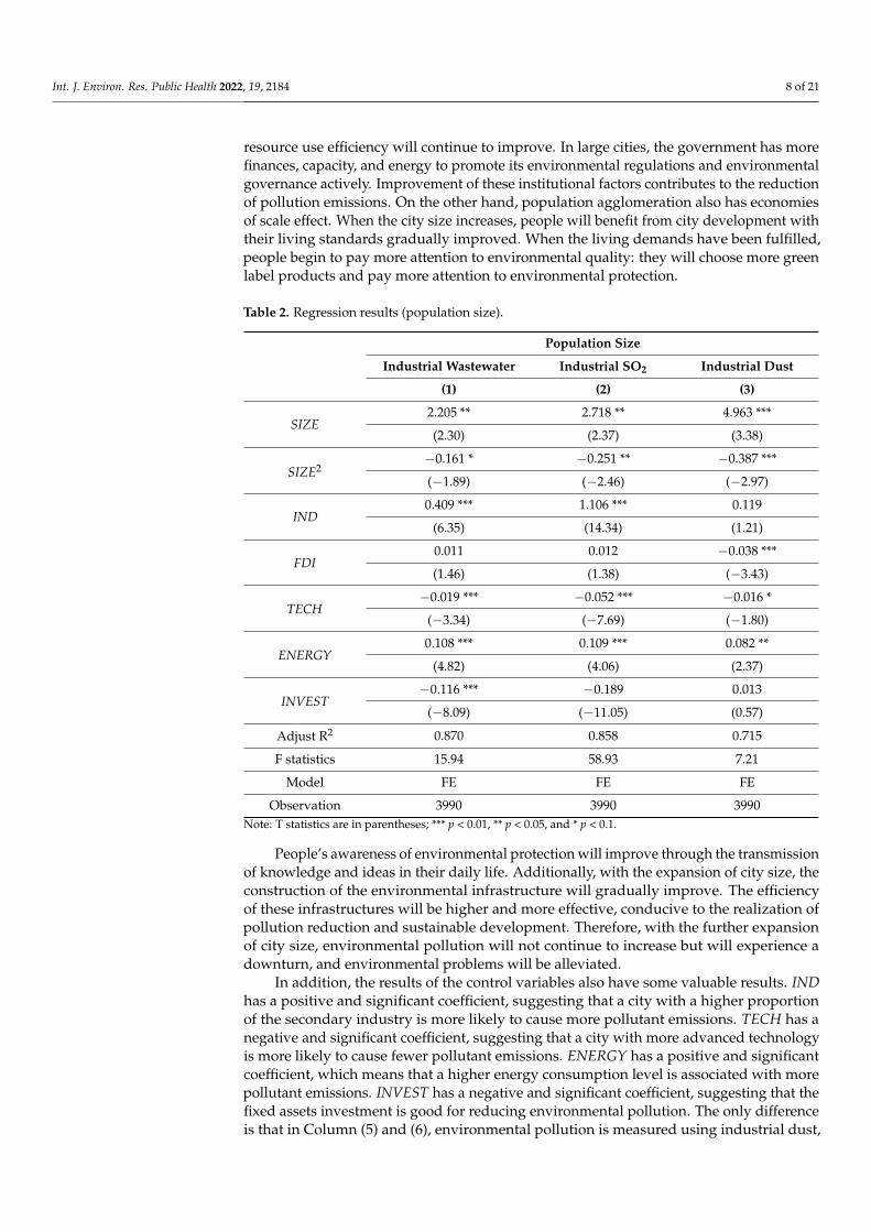
resource use efficiency will continue to improve. In large cities, the government has morefinances, capacity, and energy to promote its environmental regulations and environmentalgovernance actively. Improvement of these institutional factors contributes to the reductionof pollution emissions. On the other hand, population agglomeration also has economiesof scale effect. When the city size increases, people will benefit from city development withtheir living standards gradually improved. When the living demands have been fulfilled,people begin to pay more attention to environmental quality: they will choose more greenlabel products and pay more attention to environmental protection.

Table 2. Regression results (population size).

Population Size

Industrial Wastewater Industrial SO2 Industrial Dust

(1) (2) (3)

SIZE2.205 ** 2.718 ** 4.963 ***

(2.30) (2.37) (3.38)

SIZE2−0.161 * −0.251 ** −0.387 ***

(−1.89) (−2.46) (−2.97)

IND0.409 *** 1.106 *** 0.119

(6.35) (14.34) (1.21)

FDI0.011 0.012 −0.038 ***

(1.46) (1.38) (−3.43)

TECH−0.019 *** −0.052 *** −0.016 *

(−3.34) (−7.69) (−1.80)

ENERGY0.108 *** 0.109 *** 0.082 **

(4.82) (4.06) (2.37)

INVEST−0.116 *** −0.189 0.013

(−8.09) (−11.05) (0.57)

Adjust R2 0.870 0.858 0.715

F statistics 15.94 58.93 7.21

Model FE FE FE

Observation 3990 3990 3990Note: T statistics are in parentheses; *** p < 0.01, ** p < 0.05, and * p < 0.1.

People’s awareness of environmental protection will improve through the transmissionof knowledge and ideas in their daily life. Additionally, with the expansion of city size, theconstruction of the environmental infrastructure will gradually improve. The efficiencyof these infrastructures will be higher and more effective, conducive to the realization ofpollution reduction and sustainable development. Therefore, with the further expansionof city size, environmental pollution will not continue to increase but will experience adownturn, and environmental problems will be alleviated.

In addition, the results of the control variables also have some valuable results. INDhas a positive and significant coefficient, suggesting that a city with a higher proportionof the secondary industry is more likely to cause more pollutant emissions. TECH has anegative and significant coefficient, suggesting that a city with more advanced technologyis more likely to cause fewer pollutant emissions. ENERGY has a positive and significantcoefficient, which means that a higher energy consumption level is associated with morepollutant emissions. INVEST has a negative and significant coefficient, suggesting that thefixed assets investment is good for reducing environmental pollution. The only differenceis that in Column (5) and (6), environmental pollution is measured using industrial dust,

Int. J. Environ. Res. Public Health 2022, 19, 2184 9 of 21

and IND’s estimated coefficient is not significant. The estimated coefficient of FDI issignificantly negative. Thus, the industrial dust discharge in Chinese cities is related to FDI,and the introduction of FDI is good for pollution control. However, this conclusion is notprominent in the other regressions.

To assess the robustness of the regression results presented in Table 2, we repeatedthe regression in Table 2 using GDP and built-up area to represent city size instead ofpopulation. The regression results are presented in Table 3. The regressions using GDPto represent city size are presented in Column (1), (2), and (3), and the regressions usingthe built-up area to represent city size are presented in Column (4), (5), and (6). In Table 3,except for the regression in Column (4), all the other regressions are robust. The estimatedcoefficient of SIZE is significantly positive, and the estimated coefficient of SIZE2 is nega-tive, suggesting that the relationship between city size and environmental pollution is aninverted U-shape. The estimated results of the control variables are almost the same as theresults in Table 2.

Table 3. Regression results (GDP and built-up area).

Gdp Built-Up Area

IndustrialWastewater Industrial SO2 Industrial Dust Industrial

Wastewater Industrial SO2 Industrial Dust

(1) (2) (3) (4) (5) (6)

SIZE0.490 ** 2.707 *** 1.424 *** −0.028 1.088 *** 0.984 ***

(1.99) (9.32) (3.79) (−0.20) (6.49) (4.57)

SIZE2−0.012 * −0.086 *** −0.033 *** −0.008 −0.124 *** −0.090 ***

(−1.69) (−9.90) (−2.93) (−0.55) (−6.80) (−3.82)

IND0.373 *** 0.856 *** 0.058 0.371 *** 0.991 *** 0.046

(5.51) (10.72) (0.57) (5.61) (12.62) (0.46)

FDI0.010 0.015 −0.040 *** 0.009 0.014 * −0.035 ***

(1.39) (1.70) (−3.60) (1.26) (1.67) (−3.18)

TECH−0.017 *** −0.037 *** −0.012 −0.016 *** −0.046 *** −0.011

(−2.85) (−5.47) (−1.39) (−2.80) (−6.74) (−1.24)

ENERGY0.099 *** 0.115 *** 0.022 0.131 *** 0.103 *** 0.066 *

(4.10) (4.05) (0.60) (5.75) (3.79) (1.89)

INVEST−0.161 *** −0.182 *** −0.190 *** −0.088 *** −0.201 *** −0.020

(−5.37) (−5.15) (−4.17) (−5.79) (−11.12) (−0.84)

Adjust R2 0.870 0.830 0.717 0.870 0.827 0.716

F statistics 15.06 74.40 9.23 15.55 65.38 8.53

Model FE FE FE FE FE FE

Observation 3990 3990 3990 3990 3990 3990

Note: T statistics are in parentheses; *** p < 0.01, ** p < 0.05, and * p < 0.1.

According to the regression results in Tables 2 and 3, we calculated the inflectionpoints of an inverted U-shaped relationship. The inflection points calculated are presentedin Table 4.

In Table 4, the population’s inflection points are 9.42 million when environmentalpollution is represented by industrial wastewater discharge, 2.25 million when environ-mental pollution is represented by industrial SO2 discharge, and 6.09 million when theenvironmental pollution is represented by industrial dust discharge.

According to the three different inflection points represented by different pollutantemissions, the samples can be divided into four groups. Samples in the first group are

Int. J. Environ. Res. Public Health 2022, 19, 2184 10 of 21

62 cities with a population within 2.25 million, for example, Xiamen, Xining, and Zhuhai.With the expansion of their city size, the three kinds of pollutants gradually increase.Because the urban population is too small to utilize centralized population-based pollutiontreatment facilities, the scale effect has not yet been achieved. Samples in the secondgroup are 158 cities with a population between 6.09 million and 2.25 million, for example,Dalian, Nanchang, and Taiyuan. With the expansion of their city size, the industrial SO2emissions gradually decrease, but the amount of industrial wastewater and dust continueto increase. The third group samples are 47 cities with a population between 9.42 millionand 6.09 million, for example, Nanjing, Suzhou, Hangzhou, and Qingdao. For them, withthe expansion of city size, the industrial SO2 and dust emissions gradually decrease, butthe industrial waste water discharge continues to increase. Thus, for the third group ofcities, the gas pollutant emissions are efficiently controlled because of the scale effect. Moreattention should be paid to the treatment of water pollutant. Samples in the fourth groupare 18 cities with a population larger than 9.42 million, including Beijing, Shanghai, andChongqing, etc. With the expansion of their city size, the gas and water pollutants decrease.Thus, for most of the large cities in China, the city size is not too large but too small.The environmental problems, the so-called “city disease”, are indeed not caused by theexpansion of city size but due to the city’s insufficient size.

Table 4. Inflection points calculated from the regressions.

City Size Unit Industrial Wastewater IndustrialSO2

IndustrialDust

Population Million 9.42 2.25 6.09

GDP Billion Yuan RMB 7362 68 23,461

Built-up area Square kilometer Inverted U-shape isnot invalid 80.40 236.75

The inflection points of GDP are 7362 billion RMB when the environmental pollutionis represented by industrial wastewater discharge, 68 billion RMB when the environmentalpollution is represented by industrial SO2 discharge, and 23,461 billion RMB when theenvironmental pollution is represented by industrial dust discharge. In 2016, the largestGDP appeared in Shanghai and was approximately 2818 billion RMB. Thus, no city achievedthe GDP inflection points when environmental pollution is represented by industrialwastewater and dust discharge. For the inflection point of 68 billion RMB, there areonly 44 cities with a GDP of less than 68 billion RMB. Thus, with the expansion of mostcities’ economic scale, environmental pollution is aggravated in the short term until theinflection point.

The built-up area’ inflection points are 80.40 square kilometers when environmentalpollution is represented by industrial SO2 and 236.75 square kilometers when environmen-tal pollution is represented by industrial dust. Thus, the sample cities can be divided intothree groups.

The first group has 136 cities with their built-up area less than 80.40 square kilometers,for example, Lvliang, Tonghua, and Huangshan. Due to their limitations of a uniquegeographical location or construction planning, the built-up areas of these cities are notvery large, which is not conducive to attracting more people and industries, formingan agglomeration effect, and therefore, the scale effect of pollution reduction cannot beachieved. With the expansion of the built-up area, air pollutants continue to increase. Thesecond group has 105 cities with a built-up area of less than 236.75 square kilometers andmore than 80.40 square kilometers, for example, Quanzhou, Weihai, and Jiujiang. For thesecities, the enlarging of city size is good for industrial SO2 reduction but bad for industrialdust reduction. Only for 44 cities in the third group, including the main large cities ofBeijing, Shanghai, and Shenzhen, the expansion of city size reduces air pollutant emission.

Int. J. Environ. Res. Public Health 2022, 19, 2184 11 of 21

4.2. Threshold Regression Results

Table 5 presents the threshold regression results with SIZE represented by population.And the LR test result is presented in Figure 2. As can be seen from Table 5, in the regressionwhere the city size is represented by population, SIZE has a positive and significant impact onindustrial wastewater only if the population is bigger than 2,160,000. This suggests that if thecity population is smaller than 2,160,000, the expansion of city size will not lead to increasesin industrial wastewater discharge. However, SIZE has a negative and significant impacton industrial SO2 discharge when the population is larger than 570,000, indicating that theincreasing population may reduce industrial SO2 discharge, especially when the populationis more than 570,000 and less than 1,040,000. Additionally, SIZE has a positive and significantimpact on industrial dust discharge when the population is larger than 570,000, suggesting thatincreases in the population would cause increases in the industrial dust discharge. Therefore,the threshold impact of population on urban environmental pollution is complex. When thepopulation exceeds 570,000, urban size expansion leads to the reduction of industrial SO2emissions but will not reduce industrial dust emissions. The results show that when thepopulation is larger than 570,000, a trade-off should be made for environmental policy betweenindustrial SO2 and dust emissions. Additionally, as long as the population is smaller than2,160,000, the impact of urban expansion on industrial wastewater can be ignored.

Table 5. Threshold regression results (population).

Threshold Point Industrial Wastewater Industrial SO2 Industrial Dust

γ1 1,320,000 570,000 570,000

γ2 1,840,000 1,040,000 3,300,000

γ3 2,160,000 3,340,000 11,470,000

SIZE (thr ≤ γ1)0.258 0.167 −0.001

(1.56) (0.76) (−0.00)

SIZE (γ1 < thr ≤ γ2)0.159 −0.702 *** 0.381 *

(1.03) (−3.80) (1.75)

SIZE (γ2 < thr ≤ γ3)0.231 −0.544 *** 0.504 **

(1.57) (−3.09) (2.37)

SIZE (thr > γ3)0.033 ** −0.469 *** 0.399 *

(2.70) (−2.72) (1.87)

IND0.370 *** 1.083 *** 0.175 *

(5.98) (14.75) (1.90)

FDI0.011 * 0.0101 −0.029 ***

(1.68) (1.26) (−2.89)

TECH−0.016 *** −0.042 *** −0.015 *

(−2.79) (−6.03) (−1.69)

ENERGY0.131 *** 0.143 *** 0.130 ***

(6.15) (5.61) (4.06)

INVEST−0.099 *** −0.141 *** 0.031

(−7.45) (−8.86) (1.53)

Adjust R2 0.864 0.819 0.718

F statistics 12.89 45.79 22.97

Method FE FE FE

Observation 3990 3990 3990Note: T statistics are in parentheses; *** p < 0.01, ** p < 0.05, and * p < 0.1.

Int. J. Environ. Res. Public Health 2022, 19, 2184 12 of 21Int. J. Environ. Res. Public Health 2022, 19, x FOR PEER REVIEW 13 of 24

First threshold Second threshold Third threshold

Ind

ust

ria

l w

ast

ewa

ter

Ind

ust

ria

l S

O2

Ind

ust

ria

l d

ust

Figure 2. LR test results (threshold: population).

The threshold regression results with GDP represented by population are presented

in Table 6, and the LR test result is presented in Figure 3. As presented in Table 6, in the

regression where GDP represents the city size, a threshold effect was observed on indus-

trial wastewater discharge, and the threshold is 544,068 million RMB. When the GDP is

lower than 544,068 million RMB, the influence of city size on industrial wastewater dis-

charge is not prominent. When the GDP exceeds 544,068 million RMB, the effect of city

size on industrial waste water discharge is significantly negative. Additionally, there is a

threshold effect with GDP when the city pollutant emissions are represented by industrial

SO2, and the first and second thresholds are 12,355 million RMB and 850,713 million RMB.

When the GDP is less than 12,355 million RMB or more than 850,713 million RMB, the

influence of city size on industrial SO2 emissions is negative. When the GDP exceeds

12,355 million RMB and is lower than 850,713 million RMB, the effect of city size on in-

dustrial SO2 is negative, suggesting that the expansion of city size is good for pollutant

reduction and the scale effect of city size is prominent.

Figure 2. LR test results (threshold: population).

The threshold regression results with GDP represented by population are presentedin Table 6, and the LR test result is presented in Figure 3. As presented in Table 6, in theregression where GDP represents the city size, a threshold effect was observed on industrialwastewater discharge, and the threshold is 544,068 million RMB. When the GDP is lowerthan 544,068 million RMB, the influence of city size on industrial wastewater dischargeis not prominent. When the GDP exceeds 544,068 million RMB, the effect of city size onindustrial waste water discharge is significantly negative. Additionally, there is a thresholdeffect with GDP when the city pollutant emissions are represented by industrial SO2, andthe first and second thresholds are 12,355 million RMB and 850,713 million RMB. When theGDP is less than 12,355 million RMB or more than 850,713 million RMB, the influence ofcity size on industrial SO2 emissions is negative. When the GDP exceeds 12,355 millionRMB and is lower than 850,713 million RMB, the effect of city size on industrial SO2 isnegative, suggesting that the expansion of city size is good for pollutant reduction and thescale effect of city size is prominent.

There is also a threshold effect with GDP if the city pollutant emissions are repre-sented by industrial dust. The first and second thresholds are 41,641 million RMB and800,370 million RMB. As long as the GDP is less than 800,370 million RMB, the expansionof city size is not conducive to reducing pollutant emissions. However, when GDP is less

Int. J. Environ. Res. Public Health 2022, 19, 2184 13 of 21

than 41,641 million RMB, the influence of city expansion on environmental pollution isrelatively less. When GDP is higher than 800,370 million RMB, the city expansion increasesurban investment for environmental protection, improves pollutant treatment facilities’efficiency, optimizes resource allocation, and reduces pollutant emission.

The threshold regression results with GDP represented by population are presentedin Table 7, and the LR test result is presented in Figure 4. As presented in Table 7, in theregression where the built-up area represents the city size, a threshold effect is observed onindustrial wastewater discharge. The threshold is 500 square kilometers. If the built-uparea is less than 500 square kilometers, the influence of city size on industrial wastewaterdischarge is positive, suggesting that city expansion harms the environment. However,if the built-up area exceeds 500 square kilometers, the industrial wastewater dischargedecreases following the increasing expansion of city size. Thus, the city size is not too largebut too small.

Table 6. Threshold regression results (GDP).

Threshold Point Industrial Wastewater Industrial SO2 Industrial Dust

γ1 544,068 12,355 41,641

γ2 850,713 800,370

SIZE (thr ≤ γ1)0.013 −0.034 *** 0.013 ***

(0.41) (−8.86) (4.94)

SIZE (γ1 < thr ≤ γ2)−0.111 *** −0.048 0.459 ***

(−6.60) (−0.89) (6.67)

SIZE (γ2 < thr)−0.026 *** −0.024 ***

(−5.82) (−4.49)

IND0.372 *** 1.001 *** 0.176 *

(6.07) (13.51) (1.85)

FDI0.010 0.009 −0.034 ***

(1.55) (1.15) (−3.20)

TECH−0.017 ** −0.036 *** −0.017 *

(−2.89) (−5.18) (−1.91)

ENERGY0.139 *** 0.132 *** 0.062 *

(6.59) (4.83) (1.79)

INVEST−0.090 *** −0.129 *** −0.155 ***

(−7.00) (−3.82) (−3.64)

Adjust R2 0.865 0.820 0.253

F statistics 20.23 55.23 499.23

Method FE FE FE

Observation 3990 3990 3990Note: T statistics are in parentheses; *** p < 0.01, ** p < 0.05, and * p < 0.1.

Table 7. Threshold regression results (built-up area).

Threshold Point Industrial Wastewater Industrial SO2 Industrial Dust

γ1 500 15 15

γ2 830 496

SIZE (thr ≤ γ1)0.067 *** −0.344 *** −0.190 ***

(4.75) (−9.97) (−4.36)

Int. J. Environ. Res. Public Health 2022, 19, 2184 14 of 21

Table 7. Cont.

Threshold Point Industrial Wastewater Industrial SO2 Industrial Dust

SIZE (γ1 < thr ≤ γ2) −0.124 *** −0.035 0.249 ***

(−3.63) (−0.87) (4.88)

SIZE (γ2 < thr)−0.093 *** −0.110 ***

(−5.26) (−5.17)

IND0.337 *** 1.007 *** 0.081

(5.48) (13.68) (0.87)

FDI0.0109 0.012 −0.028 ***

(1.62) (1.49) (−2.72)

TECH−0.014 ** −0.039 *** −0.011

(−2.48) (−5.65) (−1.29)

ENERGY0.151 *** 0.136 *** 0.100 ***

(6.96) (5.29) (3.08)

INVEST−0.077 *** −0.146 *** 0.009

(−5.41) (−8.62) (0.42)

Adjust R2 0.865 0.820 0.715

F statistics 17.22 56.53 21.27

Method FE FE FE

Observation 3990 3990 3990Note: T statistics are in parentheses; *** p < 0.01, ** p < 0.05.

Additionally, a threshold effect is observed for the built-up area when the city pollutantemissions are represented by industrial SO2. The first and second thresholds are 15 squarekilometers and 830 square kilometers, respectively. When the built-up area is smaller than15 square kilometers or exceeds 830 square kilometers, the expansion of city size is good forindustrial SO2 reduction. But when the built-up area is bigger than 15 square kilometersand smaller than 830 square kilometers, there is no significant relationship between citysize and industrial SO2 emissions.

Moreover, the threshold effect of built-up area on industrial dust emissions is sig-nificant. When the built-up area is less than 15 square kilometers or exceeds 496 squarekilometers, an apparent negative relationship is observed between city size and industrialdust emission, suggesting that the expansion of city size benefits the emission reduction. Bycontrast, if the built-up area is larger than 15 square kilometers and smaller than 496 squarekilometers, the relationship between city size and industrial dust emissions is positive,indicating that the city is too large.

The regression results summary is presented in Table 8. In Table 8, only 54 Chinesecities have a population of less than 2,160,000, such as Fushun in Liaoning, Dongguan inGuangdong, and Dongying Shandong; thus, for most Chinese cities, the population is nottoo large but too small.

In 2016, the city with the highest GDP was Shanghai with a volume of 2,817,865 millionRMB, while the lowest municipal GDP (15,341 Million RMB) occurs in Jiayuguan City. Only33 cities have a GDP exceeding 544,068 million RMB. Thus, for most cities, the scale effectsof GDP have not been achieved, and no relationship is observed between city size andpollutant emission.

In 2016, only in Longnan was the built-up area less than 15 square kilometers. In13 cities—Beijing, Chongqing, Guangzhou, Tianjin, Shanghai, Dongguan, Shenzhen,Chengdu, Nanjing, Qingdao, Hangzhou, Changchun, and Xi’an—the built-up areaswere larger than 496 square kilometers. Thus, for most cities, the expansion of city size

Int. J. Environ. Res. Public Health 2022, 19, 2184 15 of 21

harms pollutant emission reduction because the built-up areas in most cities are notlarge enough.

In summary, according to the thresholds and the Chinese city size in 2016, Chinesecities are not too large but too small. Cities are too small to effectively use pollutiontreatment facilities, invest sufficient funds in environmental protection, and take advantageof pollution treatment’s scale effect.

Table 8. Results summary.

Industrial Wastewater Industrial SO2 Industrial Dust

Population [0, 2,160,000] #

(2,160,000, ∞) +[0, 570,000] #

(570,000, ∞) -[0, 570,000] #

(570,000, ∞) +

GDP [0, 544,068] #

(544,068, ∞) -[0, 12,355] or (850,713, ∞) -

(12,355, 850,713] #[0, 800,370] +

(800,370, ∞) -

Built-up area [0, 500] +

(500, ∞) -[0, 15] or (830, ∞) -

(15, 830] #[0, 15] or (496, ∞) -

(15, 496] +

Note: # no relationship between city size and pollutant emission, + positive relationship between city size andpollutant emission, - negative relationship between city size and pollutant emission.

Int. J. Environ. Res. Public Health 2022, 19, x FOR PEER REVIEW 15 of 24

First threshold Second threshold

Ind

ust

ria

l w

ast

ewa

ter

Ind

ust

ria

l S

O2

Ind

ust

ria

l d

ust

Figure 3. LR test results (threshold: GDP).

There is also a threshold effect with GDP if the city pollutant emissions are repre-

sented by industrial dust. The first and second thresholds are 41,641 million RMB and

800,370 million RMB. As long as the GDP is less than 800,370 million RMB, the expansion

of city size is not conducive to reducing pollutant emissions. However, when GDP is less

than 41,641 million RMB, the influence of city expansion on environmental pollution is

relatively less. When GDP is higher than 800,370 million RMB, the city expansion in-

creases urban investment for environmental protection, improves pollutant treatment fa-

cilities’ efficiency, optimizes resource allocation, and reduces pollutant emission.

The threshold regression results with GDP represented by population are presented

in Table 7, and the LR test result is presented in Figure 4. As presented in Table 7, in the

regression where the built-up area represents the city size, a threshold effect is observed

on industrial wastewater discharge. The threshold is 500 square kilometers. If the built-

up area is less than 500 square kilometers, the influence of city size on industrial

wastewater discharge is positive, suggesting that city expansion harms the environment.

However, if the built-up area exceeds 500 square kilometers, the industrial wastewater

discharge decreases following the increasing expansion of city size. Thus, the city size is

not too large but too small.

Figure 3. LR test results (threshold: GDP).

Int. J. Environ. Res. Public Health 2022, 19, 2184 16 of 21Int. J. Environ. Res. Public Health 2022, 19, x FOR PEER REVIEW 17 of 24

First threshold Second threshold

Ind

ust

ria

l w

ast

ewa

ter

Ind

ust

ria

l S

O2

Ind

ust

ria

l d

ust

Figure 4. LR test results (threshold: built-up area).

Additionally, a threshold effect is observed for the built-up area when the city pollu-

tant emissions are represented by industrial SO2. The first and second thresholds are 15

square kilometers and 830 square kilometers, respectively. When the built-up area is

smaller than 15 square kilometers or exceeds 830 square kilometers, the expansion of city

size is good for industrial SO2 reduction. But when the built-up area is bigger than 15

square kilometers and smaller than 830 square kilometers, there is no significant relation-

ship between city size and industrial SO2 emissions.

Moreover, the threshold effect of built-up area on industrial dust emissions is signif-

icant. When the built-up area is less than 15 square kilometers or exceeds 496 square kilo-

meters, an apparent negative relationship is observed between city size and industrial

dust emission, suggesting that the expansion of city size benefits the emission reduction.

By contrast, if the built-up area is larger than 15 square kilometers and smaller than 496

square kilometers, the relationship between city size and industrial dust emissions is pos-

itive, indicating that the city is too large.

The regression results summary is presented in Table 8. In Table 8, only 54 Chinese

cities have a population of less than 2,160,000, such as Fushun in Liaoning, Dongguan in

Guangdong, and Dongying Shandong; thus, for most Chinese cities, the population is not

too large but too small.

Figure 4. LR test results (threshold: built-up area).

4.3. Regressions inside and outside an Urban Agglomeration

An urban agglomeration is the highest structural form of organization when urbandevelopment occurs rapidly. An urban agglomeration is huge, multi-core, and multi-level,formed by many cities centrally distributed in the region. An urban agglomeration is alsoa combination of metropolitan areas and has the function of convergence and diffusionof various production factors. Urban agglomeration has become the most dynamic andpotential economic development area and the productivity distribution’s growth pole.

By 2018, China had formally formed seven major metropolitan agglomerations:Yangtze River Delta Urban Agglomeration, Beijing-Tianjin-Hebei Urban Agglomeration,Guangdong-HongKong-Macao Greater Bay Area, Chengdu-Chongqing Urban Agglom-eration, Middle Reaches of Yangtze River Urban Agglomeration, Central Plains UrbanAgglomeration, and Guanzhong Plain Urban Agglomeration.

Compared with small cities, urban agglomerations have different characteristics oftheir environmental pollution and pollutant emission reduction. When industrializationenters the middle and late phases, population and industry constantly shift to a single-coreurban agglomeration centered on a large city or multi-core urban agglomeration centeredon multiple large cities, resulting in the agglomeration of population and industry.

Spatial agglomeration may have two impacts on environmental pollution. On theone hand, urban agglomeration strengthens the economies of scale effect. In an urbanagglomeration, due to the clustering of the population, economy, and various treatmentfacilities, the efficiency of environmental infrastructure utilization will be improved greatly

Int. J. Environ. Res. Public Health 2022, 19, 2184 17 of 21

with increased efficiency of centralized treatment of pollution and a decrease of the averagecost for pollution control. From this perspective, an urban agglomeration is more conduciveto sustainable development. On the other hand, although urban agglomerations haveadvantages in controlling pollution due to economies of scale, environmental problemspersist and are caused by a high-density population and industrial agglomeration, includingwater pollution caused by urban agglomeration and the superposition effect, the heat islandeffect of urban agglomeration, and the solid waste problem of urban agglomeration [27].

To examine the different relationship between city size and environmental pollutionin cities in an urban agglomeration and cities not in an urban agglomeration, we splitthe sample into two groups. One group contains cities in urban agglomeration, and theother group contains cities not in urban agglomeration. Taking industrial dust dischargeas the dependent variable and city size as the independent variable measured by the totalurban population, GDP, and the built-up area, the regression is repeated for the two samplegroups, respectively.

The regression results are presented in Table 9, the regressions for cities in an urbanagglomeration are shown in Column (1), (2), and (3), and the regressions for cities notin an urban agglomeration are presented in Column (4), (5), and (6). In Table 9, theestimated coefficients of SIZE in cities in an urban agglomeration are all significantlypositive, and the estimated coefficients of SIZE2 in cities in an urban agglomeration are allsignificantly negative, suggesting that the inverted U-shaped relationship between city sizeand environmental pollution is valid for cities in an urban agglomeration. By contrast, forthe regression of cities not in an urban agglomeration, the estimated coefficients of SIZE2

are not significant in all columns. The estimated coefficients of SIZE are significant in onlyColumn (6). Thus, the inverted U-shaped relationship between city size and environmentalpollution is not valid for cities not in an urban agglomeration.

Table 9. Results summary (cities in and not in an urban agglomeration).

Cities in an Urban Agglomeration Cities Not in an Urban Agglomeration

Population GDP Built-Up Area Population GDP Built-Up Area

(1) (2) (3) (4) (5) (6)

SIZE6.982 *** 2.832 *** 0.974 *** 0.964 −0.059 0.678 **

(3.62) (4.61) (3.09) (0.41) (−0.10) (2.11)

SIZE2−0.532 *** −0.068 *** −0.091 *** −0.092 0.010 −0.048

(−3.14) (−3.87) (−2.81) (−0.41) (0.55) (−1.28)

IND−0.034 −0.362 ** −0.222 0.243 * 0.291 ** 0.262 **

(−0.21) (−2.02) (−1.37) (1.90) (2.23) (2.00)

FDI−0.077 *** −0.087 *** −0.076 *** −0.024 * −0.024 * −0.021

(−3.31) (3.73) (−3.24) (−1.91) (−1.91) (−1.61)

TECH−0.006 −0.005 −0.002 −0.020 −0.023 * −0.018

(−0.49) (−0.44) (−0.13) (−1.52) (−1.73) (−1.42)

ENERGY0.117 ** 0.022 0.116 ** 0.070 0.028 0.037

(2.06) (0.35) (2.00) (1.59) (0.61) (0.85)

INVEST−0.057 * −0.394 *** −0.070 0.111 *** −0.034 0.052

(−1.72) (−5.55) (−1.99) (3.47) (−0.55) (1.62)

Adjust R2 0.685 0.687 0.682 0.739 0.740 0.741

F statistics 7.14 8.50 4.86 8.29 9.35 10.43

Model FE FE FE FE FE FE

Observation 2030 2030 2030 1960 1960 1960Note: T statistics are in parentheses; *** p < 0.01, ** p < 0.05, and * p < 0.1.

Int. J. Environ. Res. Public Health 2022, 19, 2184 18 of 21

The different regression results indicate that when a city is in an urban agglomeration,with the expansion of the city size, it is possible to reach the inflection point of the invertedU-shaped curve because of the cooperation and synergy among the cities in the urbanagglomeration. However, if a city is not in an urban agglomeration, the inverted U-shapedrelationship between city size and environmental pollution is no longer significant. There-fore, for cities in an urban agglomeration, environmental pollution can be reduced byexpanding the city size through the coordinated development of an urban agglomeration.However, for cities not in an urban agglomeration, the relationship between city size andenvironmental pollution is not prominent.

4.4. Further Regressions

The environmental pollution in a city is not only from production, but also from living.However, the cities’ environmental pollution data is from “China City Statistical Yearbook”,which is published by the National Bureau of Statistics in China. This yearbook disclosesdata on the discharge of pollutants such as industrial wastewater and industrial wastegas in Chinese cities at prefecture level and above but has no data on living pollution. Wecollected the PM2.5 average annual concentration data of sample cities, which is monitoredby the Ministry of Ecology and Environment of the People’s Republic of China, and checkedthe regression results using this data. The results shown in Table 10 are robust.

Table 10. Regression results (PM2.5).

Population Size GDP Built-Up Area

(1) (2) (3)

SIZE0.051 *** 0.002 *** −0.003

(30.48) (3.26) (−0.49)

SIZE2−0.000 *** −0.000 *** −0.000 ***

(−19.05) (−3.42) (−2.66)

IND0.495 *** 0.323 *** 0.302 ***

(20.25) (11.97) (11.04)

FDI−0.027 −0.122 *** −0.149 ***

(−0.83) (−3.23) (−4.18)

TECH0.292 ** 0.163 0.201

(2.01) (1.00) (1.26)

ENERGY−0.009 ** −0.014 ** 0.005

(−2.55) (−2.51) (1.12)

INVEST−0.000 0.004 *** 0.006 ***

(−0.06) (6.18) (11.95)

Adjust R2 0.266 0.090 0.092

F statistics 205.58 56.11 57.25

Model FE FE FE

Observation 3990 3990 3990Note: T statistics are in parentheses; *** p < 0.01, ** p < 0.05.

5. Discussion

In 2020, the Chinese government proposed that “China aims to peak its carbon dioxideemissions by 2030 and achieve carbon neutrality by 2060” (named “double carbon target”)at the general debate of the 75th United Nations General Assembly. To achieve this goal,more attention should be paid to the relationship between city size and environmentalpollution under the “double carbon target” according to the above conclusions.

Int. J. Environ. Res. Public Health 2022, 19, 2184 19 of 21

First of all, we need a comprehensive assessment of urban environmental infrastructureand pollution. Due to the improvement of environmental infrastructure construction andthe strengthening of environmental investment, some large cities have formed a systemof urban environmental governance, and the pollutant emission and GDP in these citiesare not commensurate, such as Xi’an in Shanxi Province, Fuzhou in Fujian Province, andChangchun in Jilin Province. However, although the population and GDP are small insome small cities, environmental pollution is huge, such as Liaoyang in Liaoning Province,Tongling in Anhui Province, and Jiujiang in Jiangxi Province, and this finding is particularlynoteworthy. Thus, for some cities, environmental infrastructure should be strengthened,while for others, urban production and living activities could be further expanded to makefull use of existing environmental infrastructure.

Secondly, we should have a scientific understanding of the “big city disease”. Theenvironmental problems in some large cities are not due to the large scale of the city, but tothe incomplete construction of the corresponding environmental infrastructure. Cities aretoo small to make effective use of pollution treatment facilities, make sufficient investmentsin environmental protection, and use the scale effect of pollution treatment. For most of thelarge cities in China, the city size is not too large but too small.

Finally, for cities in an urban agglomeration, environmental pollution can be reducedby expanding city size through the coordinated development of urban agglomeration.However, for cities not in an urban agglomeration, the relationship between city size andenvironmental pollution is not apparent.

Despite our valuable conclusions, this paper has several limitations. First, becauseof the limitations of the data, we could not obtain more data before 2003. Thus, we couldnot analyze the dynamic relationship between city size and pollutant emissions over along period. Second, environmental pollution in cities is caused by production and living.However, we did not carry out intensive analysis into the relationship between city sizeand environmental pollution caused by living because of the missing data, which would benecessary to understand the mechanism between city size and environmental pollution,especially for large cities.

6. Conclusions

As complex environments comprising people and economic activities, cities constantlygather where goods and services are produced and consumed [1]. With the continuousdevelopment of the economy and society, cities are expanding at an alarming rate, andthis phenomenon is particularly prominent in developing countries. With the rapid urbandevelopment, many factors, such as industry, population, and capital, are constantlygathering in cities, and environmental pollution problems caused by agglomeration occur.Urban diseases such as traffic, smog, and inefficiency are emerging in large cities. A criticalpractical question that requires an urgent answer is whether a city is too big or too small.

With a balanced panel data of 285 Chinese cities from 2003 to 2016, the relationshipbetween city size in an urban agglomeration and environmental pollution was assessed inthis research. The empirical findings and policy suggestions are as follows:

(1) From the spatial distribution of population, the economy, and pollutant emissionsof Chinese cities, we observe three asymmetries in urban development.

The first asymmetry refers to the asymmetry between population and GDP. Somecities have a large population, but the GDP is not high, reflecting low efficiencies, suchas Fuyang in Anhui, Zhumadian in Henan, and Lvliang in Shanxi. Some cities have ahigh economic development level. However, their population is small, indicating a largepopulation expansion space in these cities, such as Dongguan in Guangdong, Dongying inShandong, and Zhenjiang in Jiangsu.

The second asymmetry refers to the asymmetry of water pollution and air pollution.From the spatial part of pollutants in Chinese cities, water pollution is mainly distributedin the eastern coastal areas and the Yangtze River Economic Belt. At the same time,

Int. J. Environ. Res. Public Health 2022, 19, 2184 20 of 21

air pollution is mainly distributed in North China and Northwest China. Therefore, adifferentiation policy should be adopted for different pollutants and different regions.

The third asymmetry refers to the asymmetry between city size and environmentalpollution. Large cities may have better environmental performance, while small cities mayhave worse environmental quality.

(2) The relationship between city size and environmental pollution is not linear butan inverted U-shape. When the city’s population size gradually expands, the pollutionemissions first increase and then decrease after the inflection point. Whether GDP orbuilt-up area is used as a measure of city size, the inverted U-shape remains. When the citysize enlarges to the inflection point, the environmental pollution decreases following theexpansion of city size.

(3) The inflection points of the population are 9.42 million when the environmentalpollution is represented by industrial wastewater discharge, 2.25 million when the envi-ronmental pollution is represented by industrial SO2 discharge, and 6.09 million when theenvironmental pollution is represented by industrial dust discharge. According to the threedifferent inflection points represented by the different pollutant emissions, the sampleswere divided into four groups. The first group has 62 cities with a population smaller than2.25 million; the second group has 158 cities with a population smaller than 6.09 millionand larger than 2.25 million; the third group samples are 47 cities with a population smallerthan 9.42 million and larger than 6.09 million; the fourth group samples are 18 cities with apopulation larger than 9.42 million. Only for the fourth group, with the expansion of citysize, the gas and water pollutant emissions decrease.

Most existing studies believe that city size and environmental pollution have a linearrelationship and ascribe environmental problems in big cities to the oversize of cities, whichignores the inflection point between urban scale and environmental pollution. From thispoint of view, the conclusion of this study theoretically supplements and expands theexisting research on urbanization and environmental pollution.

Author Contributions: Conceptualization, X.C. and W.D.; methodology, W.D.; software, W.D.; vali-dation, X.C. and W.D.; formal analysis, X.C.; investigation, X.C.; data curation, X.C.; writing—originaldraft preparation, W.D.; writing—review and editing, W.D. All authors have read and agreed to thepublished version of the manuscript.

Funding: This study was funded by a grant from the National Natural Science Foundation ofChina (72003131) and MOE (Ministry of Education in China) Project of Humanities and SocialSciences (20YJA790009).

Institutional Review Board Statement: Not applicable.

Informed Consent Statement: Not applicable.

Data Availability Statement: The data can be made available upon request.

Acknowledgments: The authors are grateful for the financial support provided by the NationalNatural Science Foundation of China (grant no. 72003131) and the Ministry of Education in ChinaProject of Humanities and Social Sciences (grant no. 20YJA790009).

Conflicts of Interest: The authors declare no conflict of interest.

References1. Henderson, J.V. The Sizes and Types of Cities. Am. Econ. Rev. 1974, 64, 640–656.2. Albouy, D.; Behrens, K.; Robert-Nicoud Fr Seegert, N. The Optimal Distribution of Population across Cities. J. Urban Econ.

2019, 110, 102–113. [CrossRef]3. Au, C.C.; Henderson, J.V. Are Chinese Cities Too Small? Rev. Econ. Stud. 2006, 73, 549–576. [CrossRef]4. Desmet, K.; Rossi-Hansberg, E. Urban Accounting and Welfare. Am. Econ. Rev. 2013, 103, 2296–2327. [CrossRef]5. Sveikauskas, L. The Productivity of Cities. Q. J. Econ. 1975, 89, 393–413. [CrossRef]6. Ciccone, A. Agglomeration-effects in Europe. Eur. Econ. Rev. 2002, 46, 213–227. [CrossRef]7. Ciccone, A.; Hall, R.E. Productivity and Density of Economic Activity. Am. Econ. Rev. 1996, 86, 54–70.8. Black, D.; Henderson, J.V. A Theory of Urban Growth. J. Political Econ. 1999, 107, 252–284. [CrossRef]

Int. J. Environ. Res. Public Health 2022, 19, 2184 21 of 21

9. Borck, R.; Tabuchi, T. Pollution and City Size: Can Cities be Too Small? J. Econ. Geogr. 2019, 19, 995–1020. [CrossRef]10. Pflüger, M.P. City Size, Pollution and Emission Policies; IZA Discussion Papers, No. 11354; Institute of Labor Economics (IZA): Bonn,

Germany, 2018.11. Satterthwaite, D. Environmental Transformations in Cities as They Get Larger, Wealthier and Better Managed. Geogr. J.

1997, 163, 216–224. [CrossRef]12. Kahn, M.E. Green Cities: Urban Growth and the Environment; Brookings Institution Press: Washington, DC, USA, 2006.13. Glaeser, E. Triumph of the City: How Our Greatest Invention Makes Us Richer, Smarter, Greener, Healthier, and Happier; PenguinGroup,

Penguin Press: New York, NY, USA, 2011.14. Gaigné, C.; Riou, S.; Thisse, J.F. Are Compact Cities Environmentally Friendly? J. Urban Econ. 2012, 72, 123–136. [CrossRef]15. Kahn, M.E.; Walsh, R. Cities and the Environment. In Handbook of Regional and Urban Economics; Duranton, G., Henderson, J.V.,

Strange, W.C., Eds.; North-Holland: New York, NY, USA, 2015; Volume 5, pp. 405–465.16. Li, L.; Lei, Y.; Wu, S.; He, C.; Chen, J.; Yan, D. Impacts of City Size Change and Industrial Structure Change on CO2, Emissions in

Chinese Cities. J. Clean. Prod. 2018, 195, 831–838. [CrossRef]17. Liu, Y.; Wu, J.; Yu, D.; Ma, Q. The Relationship between Urban form and Air Pollution depends on Seasonality and City Size.

Environ. Sci. Pollut. Res. 2018, 25, 15554–15567. [CrossRef] [PubMed]18. Ehrlich, P.R.; Holdren, J.P. Impact of Population Growth. Science 1971, 171, 1212–1217. [CrossRef]19. Way, H. Beyond the Big City: The Question of Size in Planning for Urban Sustainability. Procedia Environ. Sci. 2016, 36, 138–145.

[CrossRef]20. Eskeland, G.S.; Harrison, A.E. Moving to Greener Pastures? Multinationals and the Pollution Haven Hypothesis. J. Dev. Econ.

2003, 70, 1–23. [CrossRef]21. Levinson, A. Technology, International Trade, and Pollution from US Manufacturing. Am. Econ. Rev. 2009, 99, 2177–2192.

[CrossRef]22. Jaffe, A.B.; Newell, R.G.; Stavins, R.N. Environmental Policy and Technological Change. Environ. Resour. Econ. 2002, 22, 41–70.

[CrossRef]23. Hu, Y.; Yin, Z.; Ma, J.; Du, W.; Liu, D.; Sun, L. Determinants of GHG Emissions for a Municipal Economy: Structural Decomposition

Analysis of Chongqing. Appl. Energy 2017, 196, 162–169. [CrossRef]24. Xu, X.; González, J.E.; Shen, S.; Miao, S.; Dou, J. Impacts of Urbanization and Air Pollution on Building Energy Demands: Beijing

Case Study. Appl. Energy 2018, 225, 98–109. [CrossRef]25. Hansen, B.E. Threshold effects in non-dynamic panels: Estimation, testing, and inference. J. Econom. 1999, 93, 345–368. [CrossRef]26. Wang, Q. Fixed-effect panel threshold model using Stata. Stata J. 2015, 15, 121–134. [CrossRef]27. Du, W.C.; Xia, X.H. How does Urbanization Affect GHG Emissions? A Cross-country Panel Data Analysis Based on the Threshold

Model. Appl. Energy 2018, 229, 872–883. [CrossRef]