
Timed Automata for Security of Real-Time Systems
173
General rights Copyright and moral rights for the publications made accessible in the public portal are retained by the authors and/or other copyright owners and it is a condition of accessing publications that users recognise and abide by the legal requirements associated with these rights. Users may download and print one copy of any publication from the public portal for the purpose of private study or research. You may not further distribute the material or use it for any profit-making activity or commercial gain You may freely distribute the URL identifying the publication in the public portal If you believe that this document breaches copyright please contact us providing details, and we will remove access to the work immediately and investigate your claim. Downloaded from orbit.dtu.dk on: Aug 21, 2022 Timed Automata for Security of Real-Time Systems Vasilikos, Panagiotis Publication date: 2019 Document Version Publisher's PDF, also known as Version of record Link back to DTU Orbit Citation (APA): Vasilikos, P. (2019). Timed Automata for Security of Real-Time Systems. Technical University of Denmark.
-
Upload
khangminh22 -
Category
Documents
-
view
3 -
download
0
Transcript of Timed Automata for Security of Real-Time Systems
General rights Copyright and moral rights for the publications made accessible in the public portal are retained by the authors and/or other copyright owners and it is a condition of accessing publications that users recognise and abide by the legal requirements associated with these rights.
Users may download and print one copy of any publication from the public portal for the purpose of private study or research.
You may not further distribute the material or use it for any profit-making activity or commercial gain
You may freely distribute the URL identifying the publication in the public portal If you believe that this document breaches copyright please contact us providing details, and we will remove access to the work immediately and investigate your claim.
Downloaded from orbit.dtu.dk on: Aug 21, 2022
Timed Automata for Security of Real-Time Systems
Vasilikos, Panagiotis
Publication date:2019
Document VersionPublisher's PDF, also known as Version of record
Link back to DTU Orbit
Citation (APA):Vasilikos, P. (2019). Timed Automata for Security of Real-Time Systems. Technical University of Denmark.
Timed Automata for Security ofReal-Time Systems
Panagiotis Vasilikos
Kongens Lyngby 2019ISSN 0909-3192

Technical University of DenmarkDepartment of Applied Mathematics and Computer ScienceMatematiktorvet, building 303B,2800 Kongens Lyngby, DenmarkPhone +45 4525 [email protected]

Summary (English)
Ensuring information security is a fundamental problem in computing environments ofmodern society. Information flow theory provides key techniques for guaranteeing thatcertain information security goals are met by a computing system. However, the fo-cus of the researchers has been mainly around the security of programming languages,whereas, little effort has been put in the security analysis of cyber-physical systems(CPS) and internet of things (IoT) devices. CPS and IoT involve computations whichhave unstructured control flow and can be both data- and continuous time-dependent,making the programming language approaches inadequate. This thesis makes a break-through to the problem of information security in such systems.
To this end, we model systems using timed automata, a formalism that has establisheditself for analyzing safety properties of CPS and IoT devices. We then leverage ap-proaches from the theory of information flow, and we develop novel techniques forboth the qualitative, and the quantitative security analysis of our models.
Our main contributions include
• the development of a language, whose semantics is given using timed automata,and a sound type system, which enforces a non-interference security conditionon programs written in our language.
• a sound algorithm which traverses a timed automaton and enforces a non-interferencecondition, which permits locality-based information release.
• a logic for the specification of time- and data-dependent access control policiesfor networks of timed automata, and techniques for translating policies in our

ii
logic to a logic which can be handled by standard model-checkers for timed au-tomata such as UPPAAL. We also provide an implementation of our translation.
• the first principled information-flow analysis of information leakage on systemsthat implement the countermeasure clocks with reduced resolution. Our analysisrelies on a novel translation of timed automata to information-theoretic channels,which we then use to derive insights into the effectiveness of this countermeasureand the existing attacks that can bypass it.

Summary (Danish)
At sikre informationssikkerhed er et grundlæggende problem i computermiljøer i detmoderne samfund. Informationsteorien indeholder nøgleteknikker til at garantere, atvisse informationssikkerhedsmål opfyldes af et computersystem. Forskernes fokus hardog primært været omkring sikkerheden ved programmeringssprog, hvorimod der ergjort en lille indsats i sikkerhedsanalysen af cyber-fysiske systemer (CPS) og inter-net of things- (IoT) enheder. CPS og IoT involverer beregninger, der har ustruktureretkontrolstruktur og kan være både afhængig af data og kontinuerlig tid, hvilket gør pro-grammeringssprogtilgangene utilstrækkelige. Denne afhandling gør et gennembrud iproblemet med informationssikkerhed i sådanne systemer.
Med henblik herpå modellerer vi systemer ved hjælp af tidsautomater, en formalisme,der er etableret til at analysere sikkerhedsegenskaber for CPS og IoT-enheder. Vi ud-nytter derefter tilgange fra informationsteorien, og vi udvikler nye teknikker til bådeden kvalitative og den kvantitative sikkerhedsanalyse af vores modeller.
Vores vigtigste bidrag inkluderer
• udviklingen af et sprog, hvis semantik er givet ved hjælp af tidsautomater, og etkorrekt typesystem, der håndhæver en ikke-interferens-sikkerhedsbetingelse påprogrammer skrevet i vores sprog.
• en korrekt algoritme, der gennemløber en tidsautomat og håndhæver en ikke-interferensbetingelse, som tillader lokalitetsbaseret informationsfrigivelse.
• en logik til specifikation af tids- og datafhængige adgangskontrolpolitikker fornetværk med tidsautomater, og teknikker til at oversætte politikker i vores logik

iv
til en logik, der kan håndteres af standardmodeltjekkere for tidsautomater somUPPAAL. Vi leverer også en implementering af vores oversættelse.
• den første systematiske information flow-analyse af informationslækage på sy-stemer, der implementerer modforanstaltningsurene med reduceret opløsning.Vores analyse er afhængig af en ny oversættelse af tidsautomater til informa-tionsteoretiske kanaler, som vi derefter bruger til at udlede indsigt i effektivitetenaf denne modforanstaltning og de eksisterende angreb, der kan omgå den.

Preface
This thesis was prepared at the department of Applied Mathematics and ComputerScience at the Technical University of Denmark in fulfillment of the requirements foracquiring a PhD degree in Computer Science.
The research has been performed under the supervision of Professor Hanne Riis Niel-son and Professor Flemming Nielson in the period from September 2016 to August2019.
The core of the developments presented in this thesis are based on four published pa-pers. In particular, Chapter 3, Chapter 4, Chapter 5 and Chapter 6 are based on thepublications of [NNV17], [VNN18], [VNN17] and [VNNK] respectively.
Lyngby, 31-August-2019
Panagiotis Vasilikos

vi

Acknowledgements
I am especially grateful to my supervisors Hanne Riis Nielson and Flemming Nielsonfor their constant support, guidance and teaching through those years. Thanks to them,I am the researcher who I am today, and without them, this thesis would have not beenpossible. I would also like to thank Boris Köpf for being my supervisor during myexternal research stay at IMDEA Software. His work on quantitative information flowhas been really inspiring, and our collaboration has been beneficial for my career.
I would also like to thank my assessment committee Michael Reichhardt Hansen, LucaVigano and Luca Aceto for their valuable comments on this work.
Being part of the formal methods section at DTU has been a rewarding and fun experi-ence. I am thankful to all the people who shared the office, had lunches and discussionswith me. My special thanks go to Alberto Lluch Lafuente for his priceless support.
On a personal note, I want to thank all of my friends in Copenhagen, and especiallymy girlfriend Sonia for our special moments, which made me forget and overcome myresearch frustrations. Most importantly, I want to thank my sister Sofia and my parentsPantazis and Kariofyllia, for their love, constant support and always believing in me.

viii

Contents
Summary (English) i
Summary (Danish) iii
Preface v
Acknowledgements vii
1 Introduction 1
2 Information Flow Theory 52.1 Access Control . . . . . . . . . . . . . . . . . . . . . . . . . . . . . 62.2 Non-Interference . . . . . . . . . . . . . . . . . . . . . . . . . . . . 92.3 Declassification . . . . . . . . . . . . . . . . . . . . . . . . . . . . . 132.4 Quantitative Information Flow . . . . . . . . . . . . . . . . . . . . . 15
3 A Type System for Non-Interference 193.1 Timed Automata . . . . . . . . . . . . . . . . . . . . . . . . . . . . 20
3.1.1 Timed Automata Semantics . . . . . . . . . . . . . . . . . . 233.2 Non-Interference in Timed Automata . . . . . . . . . . . . . . . . . . 253.3 Timed Commands . . . . . . . . . . . . . . . . . . . . . . . . . . . . 273.4 Type System . . . . . . . . . . . . . . . . . . . . . . . . . . . . . . . 303.5 Adequacy . . . . . . . . . . . . . . . . . . . . . . . . . . . . . . . . 363.6 Related Work . . . . . . . . . . . . . . . . . . . . . . . . . . . . . . 373.7 Conclusions . . . . . . . . . . . . . . . . . . . . . . . . . . . . . . . 38
4 Secure Locality-Based Declassification 394.1 Modelling the Smart Grid System . . . . . . . . . . . . . . . . . . . 404.2 Y -Bisimulation Security . . . . . . . . . . . . . . . . . . . . . . . . 43

x CONTENTS
4.3 Post-Dominators . . . . . . . . . . . . . . . . . . . . . . . . . . . . 464.4 Algorithm for Secure Declassification . . . . . . . . . . . . . . . . . 484.5 Related Work . . . . . . . . . . . . . . . . . . . . . . . . . . . . . . 544.6 Conclusions . . . . . . . . . . . . . . . . . . . . . . . . . . . . . . . 55
5 Data- and Time- Dependent Policy-Based Access Control 575.1 Networks of Timed Automata . . . . . . . . . . . . . . . . . . . . . 595.2 Information Flow Instrumented Semantics . . . . . . . . . . . . . . . 61
5.2.1 Behaviours . . . . . . . . . . . . . . . . . . . . . . . . . . . 615.2.2 Operational Semantics . . . . . . . . . . . . . . . . . . . . . 62
5.3 Access Control in BTCTL . . . . . . . . . . . . . . . . . . . . . . . 645.3.1 The Syntax . . . . . . . . . . . . . . . . . . . . . . . . . . . 655.3.2 Semantics of the BTCTL Formulas . . . . . . . . . . . . . . 66
5.4 Reduction of BTCTL to TCTL+ . . . . . . . . . . . . . . . . . . . 685.4.1 Behaviour Automata . . . . . . . . . . . . . . . . . . . . . . 705.4.2 Trace Equivalence . . . . . . . . . . . . . . . . . . . . . . . 715.4.3 TCTL+ . . . . . . . . . . . . . . . . . . . . . . . . . . . . . 745.4.4 Reduction Complexity . . . . . . . . . . . . . . . . . . . . . 76
5.5 The Translator . . . . . . . . . . . . . . . . . . . . . . . . . . . . . . 775.6 Related Work . . . . . . . . . . . . . . . . . . . . . . . . . . . . . . 805.7 Conclusions . . . . . . . . . . . . . . . . . . . . . . . . . . . . . . . 81
6 Timing Leaks and Coarse-Grained Clocks 836.1 Coarse-Grained Clocks . . . . . . . . . . . . . . . . . . . . . . . . . 856.2 (Stochastic) Timed Automata . . . . . . . . . . . . . . . . . . . . . . 876.3 Timed Systems and Adversaries with Clocks . . . . . . . . . . . . . . 89
6.3.1 Timed Systems . . . . . . . . . . . . . . . . . . . . . . . . . 906.3.2 Clocks . . . . . . . . . . . . . . . . . . . . . . . . . . . . . 906.3.3 Adversaries with Clocks . . . . . . . . . . . . . . . . . . . . 92
6.4 Quantifying Leakage in Timed Systems . . . . . . . . . . . . . . . . 936.4.1 Timing Channels and Min-Leakage . . . . . . . . . . . . . . 936.4.2 Timing Channels of Deterministic Systems . . . . . . . . . . 956.4.3 Probability Measure for Stochastic Timed Automata . . . . . 956.4.4 Timing Channels of Stochastic Systems . . . . . . . . . . . . 98
6.5 Analysis of Timing Channels in Deterministic Systems . . . . . . . . 1016.5.1 Relating Clock Grain and Leakage . . . . . . . . . . . . . . . 1016.5.2 Timing Techniques . . . . . . . . . . . . . . . . . . . . . . . 1036.5.3 Modelling Timing Techniques . . . . . . . . . . . . . . . . . 1046.5.4 A Hierarchy of Timing Techniques . . . . . . . . . . . . . . . 106
6.6 Analysis of Timing Channels in Stochastic Systems: A Case Study . . 1096.6.1 Modelling the Case Study . . . . . . . . . . . . . . . . . . . 1096.6.2 Analysing the Leakage in the Case Study . . . . . . . . . . . 111
6.7 Related Work . . . . . . . . . . . . . . . . . . . . . . . . . . . . . . 1116.8 Conclusions . . . . . . . . . . . . . . . . . . . . . . . . . . . . . . . 112

CONTENTS xi
7 Conclusions 115
A Proofs of Chapter 3 117A.1 Lemma 3.2 . . . . . . . . . . . . . . . . . . . . . . . . . . . . . . . 117A.2 Theorem 3.3 . . . . . . . . . . . . . . . . . . . . . . . . . . . . . . . 117
B Proofs of Chapter 4 121B.1 Proposition 4.1 . . . . . . . . . . . . . . . . . . . . . . . . . . . . . 121B.2 Fact 4 . . . . . . . . . . . . . . . . . . . . . . . . . . . . . . . . . . 122B.3 Fact 5 . . . . . . . . . . . . . . . . . . . . . . . . . . . . . . . . . . 122B.4 Theorem 4.6 . . . . . . . . . . . . . . . . . . . . . . . . . . . . . . . 123B.5 Theorem 4.7 . . . . . . . . . . . . . . . . . . . . . . . . . . . . . . . 129B.6 Corollary 4.8 . . . . . . . . . . . . . . . . . . . . . . . . . . . . . . 132
C Proofs of Chapter 5 133C.1 Proof of Theorem 5.2 . . . . . . . . . . . . . . . . . . . . . . . . . . 133
D Proofs of Chapter 6 135D.1 Proof of Fact 8 . . . . . . . . . . . . . . . . . . . . . . . . . . . . . 135D.2 Proof of Fact 9 . . . . . . . . . . . . . . . . . . . . . . . . . . . . . 136D.3 Proof of Theorem 6.11 . . . . . . . . . . . . . . . . . . . . . . . . . 136D.4 Proof of Theorem 6.12 . . . . . . . . . . . . . . . . . . . . . . . . . 137
E Details of the Case Study 6.6 141
Bibliography 147

xii CONTENTS

CHAPTER 1
Introduction
Information security is essential to the privacy and safety of modern society. Over thelast few years, cyber-attacks have successfully compromised information such as creditcard numbers, login credentials, and personal data, leading to significant financial lossand privacy violations of companies and individuals [ATT19]. More importantly, othercyber-attacks have demonstrated that information can be manipulated in such a waythat could result in catastrophic explosions at a petrochemical plant [SAU19], or bringdown the power and heat in a war-torn country, during winter [LJC16].
Although the task of information security is vital, the exponential growth of technol-ogy makes it complicated and daunting. In particular, latest technology trends haveintroduced the internet of things (IoT) and cyber-physical systems (CPS) to automatemany commercial and industrial applications respectively. Both IoT and CPS involveincreasingly distributed and interconnected devices, such as sensors, actuators, con-trollers and processors, whose functionality is complex, and highly dependent on bothdiscrete and continuous variables, such as data and time.
Those variables may introduce information channels that could allow an adversary tocompromise sensitive information. For instance, consider a scenario of a distributedsystem that consists of a sensor and a controller. The sensor continually computessome data and communicates it to the controller. For ensuring data integrity, the sensoralways encrypts (signs) the data with its private key. Consider also an adversary whois able to sniff messages sent on the link used by the sensor and the controller, and can

2 Introduction
also measure the delay between the captured messages. A faulty implementation of theencryption algorithm could introduce vast information flows from the sensor’s privatekey to the observations of the adversary, that is the time of the sniffed messages andthe data in them. Consequently, the adversary could infer the private key of the sensor,impersonate it, and then deliver false information to the controller, taking full controlof the entire system.
Information flow theory [Sha01, VSI96, CT06] studies the way information flows be-tween different variables of a system. There exist two main approaches in informationflow theory, the qualitative and the quantitative ones.
In the qualitative approach, information flow security policies are used to specify thedesired information flows in a system. For instance, for the example of the sensor andthe controller, a security policy could specify that there should be no flow of infor-mation between the private key of the sensor and the observations of the adversary.Next, a security condition describes formally when a system fulfills the security policy,and an information flow control mechanism enforces the security policy on the system,proving that the security condition is satisfied.
In the quantitative approach, mathematical techniques are used to calculate the exactamount of information flowing between the variables of the system. Going back tothe example of the sensor and the controller, if the sensor’s key is 1024-bit long, thenone could calculate the information leaked from the key to the observations of theadversary. For instance, a 2-bit leak is tolerable; however, if 1000 bits are leaked, thenthe implementation of the encryption should be refined. The amount of informationleakage is often calculated with the use of an information-theoretic measure calledentropy [Sha01, ACPS12, CT06, Smi09].
In the field of programming languages, information flow theory has been a funda-mental approach to ensure the confidentiality and integrity of information. In par-ticular, for the qualitative approach, there is a significant body of work from the lit-erature that allows one to express complex information security policies, which canbe data-dependent [LNN15, LNNF15], and permit intentional information leakage[SS09, AS07, GLMS14, MSZ04, MSZ06, ML97, ZM01]. One approach to enforcesecurity policies is access control, which however, only protects against explicit flowsbetween variables (e.g reading or writing to a variable). Another approach is with theuse of non-interference [VSI96, SM03] style security conditions, which requires theabsence of flows between the sensitive variables of the system and the ones that couldbe manipulated by or observed from the adversary. Finally, a common information flowmechanism for enforcing non-interference is via a type-system [VSI96, SM03, Aga00].The quantitative approach has found many applications in measuring the amount of in-formation leaked through the timing behaviour of a program [DFK+13, KB07, BK15,MKP+18], and also in evaluating the effectiveness of countermeasures deployed tolimit such information leaks [CRS83, KD09, ZAM11].
3
Unfortunately, many of those approaches are not suitable for the security analysis ofIoT and CPS. In particular, most of the programming language approaches [Aga00,KD09, KB07, PHW08, BK15] model time as a discrete variable. On the one hand,this simplification makes the analysis of information flow easier, since time is treatedas any other discrete data variable of the system. However, as illustrated recently in[BP18], this simplification can introduce some false sense of security, allowing forsome information flows to be undetected. Another limitation of most programminglanguage approaches is that they allow only structured control flow, which is not alwayssuited for the modelling of systems such as IoT and CPS. We show the latter with anexample in Chapter 4.
Contributions This thesis contributes to the problem of information security in sys-tems such as IoT and CPS. To this end, we model systems as timed automata [AILS07,AD94], a formalism that has established itself for analyzing safety properties of sys-tems with hard real-time constraints. We then study the problem of information secu-rity in the following contexts: (a) detection of information leakage through informationchannels, constructed using both the data and the timing properties of the system, (b)specification and enforcement of security policies which permit intentional informationrelease, (c) specification and enforcement of data- and time-dependent security poli-cies, and (d) quantification of the effectiveness of countermeasures against informationleakage through information channels constructed by measuring the timing propertiesof the system.
In addressing (a), we take a language-based approach by defining the language of timedcommands, whose semantics is given using timed automata. We then develop a typesystem, and we prove that type-checked commands leak no information under adver-saries that can observe both some of the data and the execution time of the command.The latter result is formulated via a non-interference theorem.
In addressing (b), we define locality-based security policies, which allow intentional in-formation release at specific locations of the automaton. We then develop an algorithmwhich certifies a timed automaton with respect to a security policy. Certified automataare proved to satisfy the security policy, and we formulate this via a bisimulation-basedrelaxed non-interference.
In addressing (c), we present a logic in which one can express data- and time-dependentsecurity policies for access control on networks of timed automata. We show how afragment of our logic can be reduced to a logic that current model checkers for timedautomata such as UPPAAL [UPP] can handle, and we implement a translator that per-forms this reduction. We then show how the enforcement of the policies can be ex-pressed as a reachability problem, and consequently checked by UPPAAL [UPP].
4 Introduction
In addressing (d), we present the first information flow analysis of the countermeasureof reducing clock resolution. Our analysis is based on translations of timed automatamodels to information-theoretic channels, and using it we achieve the following: (1) weshow that contrary to the popular belief a coarse-grained clock might leak more than afine-grained one, (2) we give sufficient conditions for when increasing the granularityof the clock we achieve less information leakage, and (3) we show that the attacktechniques used to bypass this countermeasure form a strict hierarchy in terms of theinformation an adversary can extract using them.
Our main contributions to (a), (b), (c), and (d) have been published in the followingpapers
• (a) Information flow for timed automata by Flemming Nielson, Hanne Riis Niel-son and Panagiotis Vasilikos. Appeared in Models, Algorithms, Logics and Tools- Essays Dedicated to Kim Guldstrand Larsen on the Occasion of His 60th Birth-day. [NNV17]
• (b) Secure information release in timed automata by Panagiotis Vasilikos, Flem-ming Nielson and Hanne Riis Nielson. Appeared in Principles of Security andTrust - 7th International Conference, POST 2018. [VNN18]
• (c) Time dependent policy-based access control by Panagiotis Vasilikos, Flem-ming Nielson and Hanne Riis Nielson. Appeared in 24th International Sympo-sium on Temporal Representation and Reasoning, TIME 2017. [VNN17]
• (d) Timing leaks and coarse-grained clocks by Panagiotis Vasilikos, FlemmingNielson, Hanne Riis Nielson and Boris Köepf. Appeared in 32nd IEEE Com-puter Security Foundations Symposium, CSF 2019. [VNNK]
Thesis Organization In Chapter 2, we recall information security notions from thetheory of information flow, which we later extend to our developments for timed au-tomata. We also present some motivating examples which will be analysed in fol-lowing chapters. Next, Chapters 3, 4, 5, and 6 present our contributions to theabove-mentioned problems (a), (b), (c) and (d) respectively. Chapter 7 discusses ourconclusions, and Appendix A, B, C and D include proofs of the results presentedin the Chapters 3, 4, 5 and 6 respectively. Finally, in Appendix E we give detailedcalculations for a case study presented in Chapter 6.

CHAPTER 2
Information Flow Theory
Formalisms of information security developed in this dissertation build on certain no-tions of information flow theory, which have been widely studied in language-basedsettings. Information flow theory studies the way information flows between the vari-ables in a system. There exist two main approaches of information flow theory – thequalitative and the quantitative.
The qualitative approach consists of three main steps: (1) the specification of securitypolicies, which precisely describe the desired flows in a system, (2) a security condi-tion that defines when a system respects a security policy, and (3) an information flowcontrol mechanism that checks the system against the security condition. Main devel-opments of the qualitative approach include (a) access control, which protects againstdirect flows in a system (e.g reading or writing on a file), (b) non-interference, whichrequires no flow of information from sensitive to public variables of the system, andhas been the standard approach to the defeat of covert channels, and finally, (c) de-classification, which is a relaxed version of non-interference, permitting conditionalinformation flows.
On the other hand, in the quantitative approach, mathematical techniques are used tocalculate the exact amount of information flowing between the variables of the sys-tem. Those techniques are usually based on a measure called entropy. Main entropydefinitions include Shannon-entropy, Min-entropy, and g-entropy.

6 Information Flow Theory
InformationFlow Theory
The QualitativeApproach
The QuantitativeApproach
Access Control
Non-Interference
Declassification
Shannon-entropy
Min-entropy
g-entropy
Figure 2.1: Main approaches of information flow theory.
In this Chapter, we describe and compare the qualitative and quantitative approachesin more detail. We also give motivating examples that will be analysed later using ourdevelopments.
Chapter organization We start with the qualitative approach and in Section 2.1, 2.2,and 2.3 we discuss the access control, non-interference, and declassification develop-ments respectively. Finally, in Section 2.4 we discuss the quantitative approach.
2.1 Access Control
Historically, access control policies [dVSS14] have been the standard way for definingthe desired information flows in a system. They do that by specifying who and how onecan access data and resources. The security condition in access control specifies thata direct access or an explicit flow of information should occur only when it is allowedby the access control policy. Access requests to resources or data by users or processesare then either denied, or authorized by a monitor [Fag78] that enforces the policies.
The literature offers a vast number of access control models, where among all, themost used in practice are the discretionary access control (DAC) [Lam74, BSJ93],mandatory access control (MAC) [Thu09], and role-based access control (RBAC)[OSM00], while lately, great attention has been given to the attribute-based accesscontrol (ABAC) model.
Discretionary access control is one of the oldest forms of access control and was first

2.1 Access Control 7
defined by Lampson [Lam74] in 1970. The core idea in DAC is that a system is definedby a set of subjects S (e.g the users of the system or the processes which run on behalfof them) a set of objects O (e.g files, sockets etc.) and a set of permissions R (e.g read,write etc.). An access control policy L : S ×O → P(R) defines the set of permissionsa subject has on an object. For example, if u is a user of the system, and f a file of thesystem, then a policy L such that L(u, f) = {read} specifies that the user u can onlyread the file f . Any other type of action on f by u will be denied. DAC policies areknown for their simplicity and flexibility, which has made them applicable to a varietyof systems, both commercial and industrial. However, they are also known to be weakon the information flow constraints that they put in a system. In particular, once accesshas been granted, they do not impose any restrictions on subsequent use of an object bya subject. For example, a trojan-horse process p running on behalf of a fully privilegeduser u could maliciously copy contents from a restricted-read permission file f1 (e.gonly u can read f1) to another file f2, which could be read by any other user. Thisproblem raised the need for a new model of access control policies, and a solution wasgiven by the mandatory access control (MAC) model.
Mandatory access control policies [Thu09] constrain also manipulations of objects thatcan occur inside the execution of a process. Those constraints are expressed with theuse of a security lattice (L,⊑), whose elements are security clearance levels, and theordering ⊑ represents the desired flows between them. This lattice-based access controlmodel was first introduced by Denning [Den76]. A security policy L : S ∪ O → Lis a mapping that assigns a security level to each one of the subjects and objects ofthe system. For instance, going back to our trojan-horse example, let L = {L, H} bethe set of security clearances, with only two elements, low L, and high H, and withL ⊑ H. The latter means that a flow of information is allowed only from the low tothe high security level. The security policy L = [p 7→ H, f1 7→ H, f2 7→ L] wouldhave disallowed p to copy the files of f1 to f2, since L(f1) = H ̸⊑ L = L(f2). MACpolicies have found their way in military systems and intelligence agencies; however,they are not so appealing for commercial applications, since under certain conditions auser may desire to declassify his data to a lower security level.
Role-based access control (RBAC) is a much broader model of access control, allowingone to express both DAC and MAC policies [OSM00]. The core of this model is basedon a set of roles which are assigned to a set of permissions. Users are then assigned toa particular role. This simple model implements DAC policies on the role’s level usingthe set of permissions, while by defining a hierarchy on the roles, one can also specifyMAC policies. In the context of an organization, roles describe job-specific functions,and role permissions determine the permitted actions or tasks a role should have inorder to do its job. For example, a doctor in a hospital will be assigned to the role Doc-tor, and this role may have permissions such as writing, modifying prescriptions andreading patient’s medical records. If now there exists another role for the nurses of thehospital, and assume that this role is Nurse, we can define a hierarchy between them,by allowing the role Nurse only to read patients prescriptions and nothing more. Stan-

8 Information Flow Theory
p1 in1
**UUUUUUU
UU c1
mch // d
out1 44jjjjjjjjj
out2 **TTTTTTT
TT
p2 in2
44iiiiiiiii c2
Figure 2.2: The processes and channels of the gateway example.
dard RBAC models are very intuitive and flexible when it comes to role administrator,and thus they have been widely accepted by many commercial organizations; however,they are not suitable for specifying dynamic policies.
Attribute-based access control (ABAC) [MS08, BBF01, MSA11, JBLG05, GBO12,CWW+10, PSL+15] is a broader policy model that offers the flexibility of data de-classification and dynamic policy specification. Policies in ABAC are specified withthe use of conditions which talk about attributes of the system’s environment. Such at-tributes are the current time, the location of the subject that tries to perform an access,the contents of the object the subject is trying to have access etc. Going back to theexample of the hospital, with the use of an ABAC model one can express that doctorscan have access to the medical history of a patient only during a certain period of thepatient’s treatment and not after (i.e here, the attribute of interest is time). In addition tothat, a doctor may have no access to any resource when it is not in the hospital (i.e here,the attribute of interest is location). The expressive power of ABAC models allows forthe specification of real-world policies; ABAC is more general and flexible than DAC,MAC, and RBAC.
The work presented in Chapter 5 deals with the problem of expressing and enforcingABAC policies in distributed real-time systems of processes. In particular, in our con-text, the subjects will be processes, objects will be data variables, while the attributesof interest are the content of the data that is communicated between the processes andthe current system’s time.
This work is motivated by the world of avionics software in distributed real-time com-puter networks consisting of processing modules [MPTB12]. Every processing modulehosts different software functions that share computing resources (e.g. I/O, executiontime) that need to be partitioned based on the content of some variables or the timeof the system. The separation of the resources is essential in order to ensure that un-trusted processes such as passenger devices can have access to on-board communica-tion systems, without alerting the safe operation of the aircraft. The separation is thenimplemented by a kernel which is used as a monitor that authorizes the accesses of theprocesses based on data- and time-dependent security policies.
EXAMPLE 2.1 Such a system is depicted in Figure 2.2. A gateway with two processesp1, p2 called the producers, each of them producing data for different targets c1 and c2

2.2 Non-Interference 9
resp., called the consumers. The gateway uses a multiplexer m, and a demultiplexerd to successfully deliver the data to the intended target. The data is communicatedthrough channels whose names label the edges in Figure 2.2.
The security goal of the gateway is that the producers p1, p2 talk only with the con-sumers c1, c2 resp., and this happen only within certain time intervals. We will seemore details of the example in Chapter 5.
As we have seen, access control offers a variety of models, which allow one to express,and enforce rich security policies, meeting the needs of industry, military and any mod-ern organization of today. However, poor system implementations allow for unintendedtransfer of information. This could happen even without the use of common operationssuch as read or write, resulting in violation of security policies, which becomes unde-tected by the access control monitor. This leads to the development of new ways andmethods of enforcing security policies which we explore in the next section.
2.2 Non-Interference
Unintended information flows can occur whenever a system builds a covert channel.Covert channels are mechanisms used to transfer information via the control-flow of asystem, its termination behaviour, its execution time, power consumption, temperatureetc. Information flows arising from covert channels are called implicit flows. Covertchannels are not intended by the design of the system, and thus, they are hard to detect.We now give some examples of covert channels which are investigated in this thesis.
Control-flow covert channels are one of the most common types of covert channels.They occur whenever a system’s control flow depends on secret data. For example,consider the program if y > 0 x := 1 else x := 0. If an adversary observes thefinal value of x he deduces partial information (i.e that y is positive when x is 1 andthat y is not positive when x is 0) of the variable y without explicitly reading it. Thiskind of covert channel has been extensively studied in the literature, with Denning[DD77] being the first to formally specify when a program is free of control-flow covertchannels.
Systems with non-deterministic semantics give rise to new control-flow covert chan-nels. Such covert channels are particularly interesting for the kind of systems we studyin this thesis.
EXAMPLE 2.2 To see an example of such a covert channel consider a Dijkstra’sGuarded Command [Dij75] like language, which allows for statements of the form

10 Information Flow Theory
g → C, where the command C can be executed when the guard g evaluates to true.Next, consider the program x := 0; ( y > 0 → skip [] tt → x := 1), which firstsets the value of x to 0 and then makes a non-deterministic choice which may modifythe value of x. Notice that, even if the variable x does not appear in the branch whichdepends on the guard y > 0, the value of x is still dependent on y. In particular,observing that the final value of x is not 1 allows the adversary to deduce that y ispositive.
This kind of implicit flow cannot be detected with the approach of [BBM94], whichdeals with information flows in a guarded command-like language. In Chapter 3, weshow how we can detect those kind of flows.
Another common type of a covert channel is a timing channel. A timing channeltransfers secret information through the execution-time of the system. In particular,the information conveyed by timing channels has been used by adversaries to recovercryptographic keys, where the timing channel is built by measuring cryptographic orcache-dependent operations, and by malicious websites which correlate this informa-tion with the internal state of a victim who visits the website [Koc96, SWT01, BT11,VK17, OKSK15, FS00, AKM+15].
EXAMPLE 2.3 As an example of a system that builds a timing channel consider a pro-gram that implements the RSA encryption algorithm using the modular exponentiation,which computes xk mod n for the secret key k, the plaintext x and the constant modulusn. The implementation of xk mod n is given by the following piece of code
m := (1 ∗ 1) mod n;for (j = 0; j < len(k); j++) {
m := (m ∗ m) mod n;if (k[j] == 1) thenm := (m ∗ x) mod n;
}
where the secret bits of the key are stored in the array k[]. Next, consider an abstractmodel of this program, whose execution time t is given based on the number of modularmultiplications it performs. Now if an adversary observes t, we have a timing channelsince the conditional execution (if k[j] == 1) of the modular multiplication operationm = (m ∗ x) mod n reveals information about the entries of k (i.e one extra modularmultiplication is performed when k[j] is 1).
Non-interference is the prevailing security condition that defeats completely covertchannels, and was first introduced by Goguen and Meseguer [GM82]. The non-interference

2.2 Non-Interference 11
definition of [GM82] is fundamentally about higher-level processes not interfering withlower-level processes of the system. In a more general context, non-interference is usu-ally expressed with a lattice-based access control policy, (as we saw in the mandatoryaccess control policies model), and requires that entities of the system that have secu-rity classification that appears higher in the lattice do not interfere with the ones thathave a lower security classification.
To give a better understanding of the non-interference condition, we consider a programP which takes as input some secret from the set I and produces a public output from theset O. Consider also the security lattice L = {L, H} from the MAC policies example,and let all the elements from the set I have H security level, and all the ones from Ohave L security level. We want to ensure that running the program P on some secretinput does not produce an information flow from the secret input to its correspondingoutput, or to put it otherwise, we want that the set of inputs does not interfere with theset of outputs.
If now the program P is deterministic it can be seen as a function P : I 7→ O mappinginputs to outputs. The non-interference property is formally expressed as
∀i1, i2 ∈ I : P(i1) = P(i2)
that is that independently of the secret input, the observation to the adversary is thesame, and thus there is no interference between the secret inputs and the public outputs.
EXAMPLE 2.4 Consider now the modular exponentiation program from Example 2.3.If we fix the message x then the program can be seen as a function P : K 7→ T whichmaps a secret key k ∈ K to its execution time t ∈ T . In particular, assume that Kcontains all the possible keys of size 1024-bits, and for a key k ∈ K we have thatits execution time is P (k) = 1025 + Ham(k), where Ham(k) is the Hamming weightof the key (i.e the number of non-zero bits). This program does not satisfy the non-interference property between the secret input set of keys K, and the output set ofexecution times T . To see this, take the key k0 with all bits equal to 0, and we have thatP(k0) = 1025 ̸= 2049 = P(k1), where k1 is the key with all bits equal to 1.
If now the program P is non-deterministic, the program is not a function from inputs tooutputs anymore. To define the non-interference condition, let P(i) ⊆ O be the set ofpossible outputs of the input i ∈ I . In this case, the non-interference condition can bedescribed by the following condition
∀i1, i2 ∈ I : P(i1) ⊆ P(i2)
which by symmetry implies that P(i1) = P(i2) as above.
EXAMPLE 2.5 Let now P be the program of the non-deterministic guarded commandprogram of Example 2.2. Let also Y = Z be the input set of the program and let
12 Information Flow Theory
V A SA C
• vote, credentials // •
•identity, vote // •
• oo voted already•
signed vote // •
• oo vote counted •
• oo vote counted
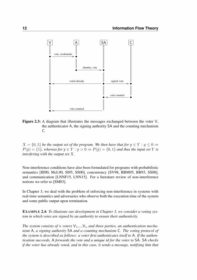
Figure 2.3: A diagram that illustrates the messages exchanged between the voter V,the authenticator A, the signing authority SA and the counting mechanismC.
X = {0, 1} be the output set of the program. We then have that for y ∈ Y : y ≤ 0 ⇒P (y) = {1}, whereas for y ∈ Y : y > 0 ⇒ P (y) = {0, 1} and thus the input set Y isinterfering with the output set X .
Non-interference conditions have also been formulated for programs with probabilisticsemantics [III90, McL90, SI95, SS00], concurrency [SV98, BBM95, BB93, SS00],and communication [LNNF15, LNN15]. For a literature review of non-interferencenotions we refer to [SM03].
In Chapter 3, we deal with the problem of enforcing non-interference in systems withreal-time semantics and adversaries who observe both the execution time of the systemand some public output upon termination.
EXAMPLE 2.6 To illustrate our development in Chapter 3, we consider a voting sys-tem in which votes are signed by an authority to ensure their authenticity.
The system consists of n voters V1,...,Vn and three parties, an authentication mecha-nism A, a signing authority SA and a counting mechanism C. The voting protocol ofthe system is described as follows: a voter first authenticates itself to A. If the authen-tication succeeds, A forwards the vote and a unique id for the voter to SA. SA checksif the voter has already voted, and in this case, it sends a message, notifying him that
2.3 Declassification 13
he has already voted; otherwise, it signs the vote and forwards it to C. C then countsthe vote, informs SA about it, and subsequently SA notifies the voter about it. Themessages exchanged by the different parties of the system are depicted in Figure 2.3.
For signing the votes, the signing authority SA uses an implementation of the RSAalgorithm similar to the one given in the Example 2.3. The security goal of the systemis to ensure that whenever a voter observes the messages received from SA, and theirarrival time, he cannot infer anything about the RSA key used by SA.
Non-interference provide strong guarantees that no information is leaked in case of con-fidentiality, and that untrusted data does not influence trusted data in case of integrity.However, many real systems need to allow some interference in order to achieve theirpurposes. This need leads to the development of relaxed notions of non-interferencewhich permit data declassification.
2.3 Declassification
Without the possibility of leaking some information some systems would have not beenuseful. For example, at the end of an election a voting protocol reveals the sum of allvotes, a password authentication mechanism reveals some information of the passwordin case of a failed log-in attempt, and the medical history of the patient will becomepublic to the doctor in case of the patient getting a disease. Systems with intentionalleak lead to the development of security policies which allow data declassification. Se-curity policies for data declassification are partitioned in three main categories basedon what data can be declassified, who can declassify data, and where data can be de-classified. We explain those categories in the context of confidentiality.
What data can be declassified? Property-based information flow policies [SS09, AS07,GLMS14] control what information or property of the secret can be deduced by anadversary. One way of expressing property-based information flow policies is withthe use of equivalence relations [SS09]. This approach generalizes non-interferencethat requires that any two secrets must be indistinguishable to the adversary, and onlydemands that two secrets are indistinguishable to the adversary if they have the sameproperty specified by the security policy.
EXAMPLE 2.7 For instance, for the RSA program P : K 7→ T of the Example 2.4, aproperty-based policy could be defined by the equivalence relation
≡Ham= {(k1, k2) | k1, k2 ∈ K : Ham(k1) = Ham(k2)}
which specifies that two keys should be indistinguishable to the adversary if and onlyif they have the same Hamming weight. Next, notice that equivalent keys under ≡Ham

14 Information Flow Theory
d
d = 1
¬(d = 1)
Figure 2.4: The part of the smart grid system, where it receives the declassificationdecision d and based on that decides if it should declassify data or not.Information should be declassified only when the red state is reached.
result in the same execution time in P and thus they are indistinguishable to the adver-sary. Therefore P satisfies the security policy ≡Ham.
Who can declassify data? Ownership-based information flow policies [SS09, MSZ04,MSZ06, ML97] are essential in many applications that require control over who candeclassify data. The most widely accepted framework that allows expressing such poli-cies is the decentralized label model [ML97], where data is annotated with ownershiplabels. Declassification of some data is then only allowed if it is performed from theowner indicated in the label. The decentralized label model has been implemented inthe Jif compiler [MZZ+06], which is used to enforce information flow policies for Javaprograms. One open issue with this formalism was that there was no formalization ofa semantic condition that proves that an adversary cannot influence the declassifica-tion. Later work of [MSZ06, ZM01] solved this issue by introducing the notion ofrobust-declassification.
Where can data be declassified? Locality-based information flow policies [AS07,GLMS14, MS04, Pin95, RG99] describe wherein the system (or program) data de-classification is allowed. In particular, components of the system, or code fragmentsof the program are annotated with declassification labels. Then, the security policyspecifies that reaching such a labelled component, or executing a labelled code frag-ment may result in some information leakage. The most standard semantic notionfor enforcing locality-based information flow policies is the one of intransitive non-interference [MS04, Pin95, RG99]. For a system or program that satisfies intransitivenon-interference, it is guaranteed that only labelled components or code fragments de-classify data.
The work in Chapter 4 considers the problem of enforcing locality-based policies onreal-time systems. The work is motivated by data declassification problems in smartpower grid systems. In its very basic form, a smart grid system consists of a meterthat measures the electricity consumption in a customer’s C house, and then sends this

2.4 Quantitative Information Flow 15
data to the utility company UC. The detailed measurements of the meter provide moreaccurate billings for UC, while C receives energy management plans that optimize hisenergy consumption. Although this setting seems to be beneficial for both UC and C, ithas been shown that high-frequent monitoring of the power flow poses a major threatto the privacy of C [SF15, GA17, MR17]. To deal with this problem many smart gridsystems introduce a trusted third-party TTP, on which both UC and C agree on [SF15].Now, the data of the meter is collected by the TTP, and by the end of each month, theTTP charges C depending on the tariff prices defined by UC. In this protocol, UC trustsTTP for the accurate billing of C, while C trusts TTP with its sensitive data. However,in some cases, C may desire an energy management plan by UC, and consequently, hemakes a clear statement to TTP, allowing the latter to release its private data to UC.
EXAMPLE 2.8 Figure 2.4 illustrates part of the smart grid system that we will seelater in Chapter 4. In particular, Figure 2.4 depicts the part of the system where thetrusted party TTP receives the decision d of the client C, and based on that it moveson its next location, deciding if data should be declassified.
The locality-based policy that we wish to enforce here is that information is releasedonly when the system reaches the red location in Figure 2.4.
Security policies that allow data declassification offer a flexible way to overcome thestrictness of non-interference conditions, and for this reason they are more appealingin real-world applications. However, their drawback is that sometimes it is difficultto understand the implication of a declassification for the security of a system. Forexample, a declassification may reveal some property of the secret, but this does not sayif the leakage is big or small with respect to the size of the secret, resulting in a situationwhere an adversary could infer the entire secret based on its property. Quantitativeinformation flow provides mathematical mechanisms for dealing with such cases.
2.4 Quantitative Information Flow
Quantitative information flow studies the problem of measuring the correlation betweenthe secret components and the observable ones in a system. The quantity of correla-tion is usually calculated based on a mathematical measure called entropy. Informationentropy measures are used to describe the initial uncertainty the adversary has regard-ing the secret, and his posterior uncertainty or remaining uncertainty after making hisobservations. In particular, the initial uncertainty is calculated based on a probabilitydistribution on the secret, while the posterior uncertainty is calculated based on the in-formation channel of the adversary. Formally, the information channel is defined as amatrix, and for each secret and observation it contains the probability of the observation

16 Information Flow Theory
encryption noise communicationK T Y Z
Figure 2.5: The functionality of the sensor.
conditioned on the secret. Whenever the observations of the adversary are based onlyon the timing of the system then the information channel is called a timing channel.
EXAMPLE 2.9 The timing channel TC : K × T 7→ [0, 1] of the program P : K 7→ Tfrom the Example 2.4 is
TC(k, t) =
{1 if t = P(k)
0 otherwise
Since the program P is deterministic, then for a key k ∈ K, the probability of a timingobservation t ∈ T conditioned on k is 1, if and only if, t = P(k), otherwise it is 0.
The leakage of the system is then defined as the difference between the initial uncer-tainty and the remaining uncertainty of the adversary i.e
Leakage = Initial Uncertainty - Remaining Uncertainty
The literature offers a large body of information entropy measures [CT06, Smi09,Sha01, Rn61]. We briefly discuss three of them, Shannon-entropy, Min-entropy, andg-entropy.
Shannon-entropy is a foundational concept of information theory, introduced by theAmerican mathematician Shannon [Sha01]. It is a measure that explains the averageuncertainty of the adversary about the secret variable of the system. In particular, it rep-resents the optimal number of bits needed on average to describe the secret. Similarly,the conditional Shannon-entropy is used to describe the remaining average uncertaintyof the secret when making some observations of the system’s state. Denning’s book[Den82] gives the first attempt to use Shannon’s measures of entropy to quantify leak-age in programs written in an imperative language, while later work of Clark et al.[CHM05] provided a static analysis that could compute Shannon-leakage in programs.Although Shannon-entropy was one of the first measures used in order to quantify leak-age in programs, Smith noticed that it is not an appropriate security measure when anadversary has a high probability of guessing the secret with one try, and consequently,he suggested Min-entropy [Smi09].

2.4 Quantitative Information Flow 17
Min-entropy is a special case of Rényi’s Entropy [Rn61]. It expresses precisely thesecret’s vulnerability to being guessed correctly after one try, while the conditionalmin-entropy gives the expected min-entropy of the secret after observing some out-put [Smi09]. This entropy measure has been in particular interesting for computingleakage in information channels of deterministic programs. For example, the informa-tion leaked from a deterministic program P : I 7→ O that maps secrets inputs from Ito public outputs in O is equal to log2|O|, whenever the secret is uniformly distributed[Smi09]. Therefore any over-approximation of the set of outputsO can be used directlyto over-approximate the leakage of the program.
EXAMPLE 2.10 For the program P : K 7→ T from the Example 2.4, we have that
|T | = | {1025 + Ham(k) | k is a 1024-bit key} | = 1025
and, if we assume a uniform distribution on the set of the keys K, then the min-leakageis log2|T | ≈ 10 bits.
Later on, Alvin et al. [ACPS12] showed that min-entropy is not enough to capture theadversary’s threat in all applications. For example, an adversary may benefit if he canguess some property of the secret and not the entire secret. For this reason, Alvin et al.[ACPS12] introduced g-entropy.
g-entropy [ACPS12] is a generalization of min-entropy. The core mechanism of thisentropy measure is the use of gain functions that describe the benefit the adversary getsafter guessing a specific part of the secret. Similarly to the previous entropy measures,conditional g-entropy is the expected benefit an adversary gains after making his obser-vation. Although, g-entropy can be seen as a rich framework for expressing differentattack scenarios, it hasn’t received a lot of attention in practice yet.
Quantitative information flow has found many applications in measuring informationleakage conveyed by timing channels [DFK+13, KB07, BK15, MKP+18], and in eval-uating the effectiveness of countermeasures against timing channels [CRS83, KD09,ZAM11].
In Chapter 6, we investigate the effectiveness of a widely deployed countermeasureagainst timing channels, that is the countermeasure of reducing the accuracy of thesystem’s clocks provided to the adversary. In particular, we use min-entropy to measurethe information leakage of timing channels in real-time systems with reduced accuracyclocks.
EXAMPLE 2.11 As an example, consider a scenario of a distributed system that con-sists of a sensor and a controller. In particular, the sensor continually computes somedata and communicates it to the controller. For ensuring data integrity, the sensor

18 Information Flow Theory
always encrypts (signs) the data with his RSA private key. The RSA encryption is im-plemented using the modular exponentiation algorithm which is given in Example 2.3.To decrease the correlation between the encryption time and the secret bits of the key,the sensor adds noise to the encryption time by delaying for some additional periodafter each encryption, and then it communicates the data to the controller. Finally, onthe side of the controller, we assume an adversary who runs malicious code and mea-sures the time needed for the sensor to send its data, trying to infer bits of the sensor’sprivate key. The measurements of the adversary are affected from the countermeasureof reducing clock resolution.
What we are interested here is to measure how much information about the secret keyk ∈ K is leaked, when the adversary observes the time z ∈ Z. This functionality of thesensor is given in Figure 2.5.

CHAPTER 3
A Type System forNon-Interference
In this chapter, we take a language-based approach to enforce a non-interference stylesecurity property for timed automata. In particular, we adapt the guarded commandlanguage of Dijkstra [Dij75] to more closely correspond to the primitives of the timedautomata formalism – resulting in the timed command language – and we show how toobtain timed automata from programs in timed commands. We use mandatory accesscontrol policies (MAC) to specify which components of the timed automaton are secret,and which are public. We then, develop a type system for enforcing non-interferenceon programs in timed commands. In particular, the type system generates a set ofconstraints, which over-approximate the possible flows between the components of theautomaton. We prove the soundness of the type system, that is that, type-checkedprograms imply non-interference. Our approach is illustrated In Figure 3.1.
Chapter Organisation In Section 3.1, we give the model and the semantics of timedautomata. Next, in Section 3.2, we define our non-interference condition for timedautomata. In Section 3.3, we present the timed command language and we show howa timed command results in a timed automaton. In Section 3.4, we give our type sys-tem, and in Section 3.5 our soundness result. We finish with related work and ourconclusions in Section 3.6, and Section 3.7 respectively.

20 A Type System for Non-Interference
The Problem
Our Approach
q◦
Timed Automaton (1)
q•
Security Policy (2): x is a secret variable andr is a public clock.
Challenge (3): Is there a flow of informationfrom the initial value of x to the final value of r?
TC = begin[tt] do r ≤ 10→ x:=x+ 1: r ;[tt]
x < 0 → x:=x+ 2: [] ¬(x < 0)→ skip: ;[tt]
→ x:=x+ 1: od [] r > 10 → skip:[tt]end
{r, q◦} ; {x, r}...L(q•) = L
Flows (3)
MAC Policy (2) Type System
Timed Command (1)
r ≤ 10→ x:=x+ 1: r
x < 0 → x:=x+ 2:
¬(x < 0)→ skip:
→ x:=x+ 1:
r > 10→ skip:
L = [x 7→ H, r 7→ L, ...] ⊢[q•:tt][q◦:tt]
TC : E, I& {q•}
Figure 3.1: The idea of our development in Chapter 3.
3.1 Timed Automata
In this section, we give the model and semantics of timed automata. We describe timewith the set of non-negative real numbers R≥0. Timed automata [AILS07, AD94]are finite automata extended with real-valued variables called dense clocks or simplyclocks, that are used to record the elapse of time, and integer data variables, which we
3.1 Timed Automata 21
simply call variables.
Dense clocks are being increased at the same rate, have infinite precision, and can reset.The transitions of the automaton are guarded with constraints over dense clocks and/orvariables, restricting in that way the possible timing behaviour of the automaton.
Formally now, let Clocks be a finite set of dense clocks taking values from R≥0, andVar a finite set of variables taking values from Z. A timed automaton [AD94, AILS07]TA = (Q,E, I, q◦, q•) consists of a set of nodes Q, a set of annotated edges E, and alabelling function I on nodes. The node q◦ ∈ Q will be the initial node and the node q•is a final node. The mapping I maps each node in Q to a guard (to be introduced below)that will be imposed as an invariant at the node. Finally, we sometimes write (E, I) forTA.
The edges are annotated with actions and take the form (qs, g → x :=a: r, qt), whereqs ∈ Q is the source node, qt ∈ Q is the target node, and x, a and r are finite sequencesof variables, arithmetic expressions, and clocks respectively. The action g→ x :=a: rconsists of a guard g that has to be satisfied in order for the multiple assignments x :=ato be performed and the clock variables r to reset. We shall assume that the sequencesx and a of program variables and expressions, respectively, have the same length andthat x does not contain any repetitions. To cater for special cases we shall allow towrite skip for the assignments of g→ x :=a: r when x (and hence a) is empty; alsowe shall omit the guard g when it equals tt, and omit the clock resets when r is empty.
The arithmetic expressions a, the boolean expressions b, and guards g are defined asfollows:
a ::= a1 opa a2 | x | nb ::= tt | ff | a1 opr a2 | b1 ∧ b2 | b1 ∨ b2 | ¬bg ::= b | r opr n | g1 ∧ g2
where n is an integer, x is a data variable, r is a clock, opa is a finite set of totalarithmetic operators (as usual), and we also have the relational operators opr ∈ {<,≤,=,≥, >}.
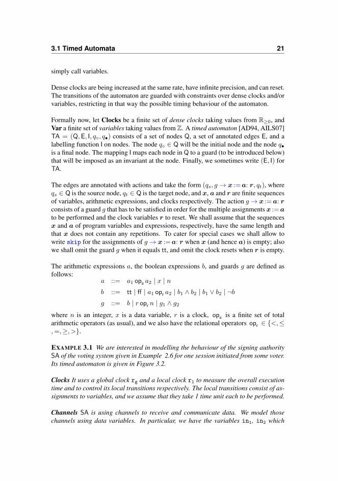
EXAMPLE 3.1 We are interested in modelling the behaviour of the signing authoritySA of the voting system given in Example 2.6 for one session initiated from some voter.Its timed automaton is given in Figure 3.2.
Clocks It uses a global clock rg and a local clock rl to measure the overall executiontime and to control its local transitions respectively. The local transitions consist of as-signments to variables, and we assume that they take 1 time unit each to be performed.
Channels SA is using channels to receive and communicate data. We model thosechannels using data variables. In particular, we have the variables in1, in2 which

22 A Type System for Non-Interference
1
[rg ≤ tend]
2
[rl ≤ tlookup]
3 [rl ≤ 1]
4
[rl ≤ 2]
5
[tt]
6
[rl ≤ treply]
7
[rl ≤ 1]
8
[rl ≤ 1]
9
[rl ≤ 3]
...
vote_req init_sign
mult
reply_has_voted
end
vote_counted
req_count
update_db1
update_dbn
extra_mult
dummy_mult
inc_counter
reply_has_counted
Casting Phasevote_req rl ≥ 2 → (id, v):=(in1, in2): rlinit_sign rl ≥ 3 ∧
∨nj=1(id = j ∧ dj = 0) → (i, s, y):=(1, 1, 1): rl
reply_has_voted rl ≥ 1 ∧ ¬∨n
j=1(id = j ∧ dj = 0) → out2:=0: rl
Signing Phasemult rl ≥ 1 ∧ i < 1025 → s:=s · s:extra_mult rl ≥ 2 ∧
∨1024j=1 (i = j ∧ kj = 1) → s:=s · v:
dummy_mult rl ≥ 2 ∧ ¬∨1024
j=1 (i = j ∧ kj = 1) → y:=y · v:inc_counter rl ≥ 3 → i:=i+ 1: rl
Counting Phasereq_count rl ≥ 1 ∧ ¬(i < 1025)→ out1:=s: rlvote_counted rl ≥ 1 → x:=in3: rlupdate_vote_dbj rl ≥ 1 ∧ id = j → dj :=1: rlreply_has_counted rl ≥ 1 → out2:=1: rl
Ending Phaseend rg ≥ tend → : rl
Figure 3.2: The timed automaton of the signing authority SA, and the abbreviationsof its actions grouped up based on the different phases (casting, signing,counting, ending) of the voting system.
store the unique identity of a user, and its vote, whenever the authenticator A writesto them. The channel out1 is used to send the signed vote from SA to the countingmechanism C, while the channel in3 stores the reply from C when the vote of the voterhas been counted. Finally, the channel out2 is used to send the messages of the signing

3.1 Timed Automata 23
authority SA to the voter.
Variables The variables id and v are used to store the identity and the vote of a voter,received from the channels in1 and in2 respectively. In particular, if the voter Vj
wants to vote then the authenticator will send the identity j through the channel in1.The variables d1,...,dn are used to record if a voter has not voted yet by holding thevalue 0, or any other value otherwise. For the RSA signature the automaton is using animplementation of the algorithm given in Example 2.3, introducing a dummy variabley for eliminating the timing channel created due to the extra multiplication. The bits ofthe 1024-bit RSA key are represented by the variables k1,...,k1024, the signature of thevote v is stored in the variable s, and i is the index variable used for the loop iteration.Finally, the variable x is used to store the reply from the counting mechanism C.
Transitions The signing authority SA starts at the initial location 1, and waits for votesfrom the authenticator A until the end of the voting period denoted by the invariantrg ≤ tend (tend is a constant greater than 2). If the value of rg becomes equal to tend theautomaton terminates by moving to its final location 5 (the ending phase). The edgefrom 1 to 2 is taken whenever a vote request occurs (the casting phase begins).
Next, at location 2, the authority checks if the user has already voted (this could takeup to tlookup ≥ 3). If the check fails, it replies to the voter with the constant 0 using thechannel out2. Otherwise, it moves to location 3 by performing an initialization of thevariables needed for the signature (the signing phase begins).
The loop transition starting at 3, moving to 4, 9 and back to 3 is the loop of the RSAencryption algorithm. Once it has been completed the automaton moves to the location6 by sending the signature s to C using the channel out1 (the counting phase begins).Next, it waits (up to treply > 1) for a reply from C, and once it receives it, it reads itfrom channel in3, stores the reply in variable x, and moves to location 7. Finally, itupdates the variable dj to 1 (if the voter has id=j) since now the voter has voted, andnotifies him by sending the constant 1 through the channel out2.
Finally, the · operator is the modulo n multiplication.
3.1.1 Timed Automata Semantics
To specify the semantics of timed automata let σ be a state mapping variables to theirinteger values, and let δ be a clock assignment mapping clocks to non-negative reals.We then have total semantic functions [[·]] for evaluating the arithmetic expressions,boolean tests, and guards; the values of the arithmetic expressions and boolean ex-pressions only depend on the states, whereas that of guards also depend on the clockassignments.

24 A Type System for Non-Interference
The semantics of timed automata is given by a transition system whose configurationshave the form ⟨q, σ, δ⟩ ∈ Config, where [[I(q)]](σ, δ) is true, and the transitions aredescribed by an initial delay (possibly none) that increases the values of all the clocksfollowed by an action. Therefore, whenever (qs, g→ x :=a: r, qt) is in E we have therule:
⟨qs, σ, δ⟩t−→ ⟨qt, σ′, δ′⟩
t ≥ 0[[I(qs)]](σ, δ + t) = tt,[[g]](σ, δ + t) = tt,σ′ = σ[x 7→ [[a]]σ], δ′ = (δ + t)[r 7→ 0],[[I(qt)]](σ
′, δ′) = tt
where t corresponds to the initial delay. The rule ensures that after the initial delaythe invariant and the guard are satisfied in the starting configuration, and updates themappings σ and δ. Here δ + t abbreviates λr. δ(r) + t. Finally, it ensures that theinvariant is satisfied in the resulting configuration. Initial configurations are the ones ofthe node q◦.
We define a trace from ⟨qs, σ, δ⟩ to qt in a timed automaton TA to have one of threeforms. It may be a finite “successful” sequence
⟨qs, σ, δ⟩ = ⟨q′0, σ′0, δ
′0⟩
t1−→ · · · tn−→ ⟨q′n, σ′n, δ
′n⟩ (n > 0)
such that {n} = {i | q′i = qt ∧ 0 < i ≤ n}.
in which case at least one step is performed. It may be a finite “unsuccessful” sequence
⟨qs, σ, δ⟩ = ⟨q′0, σ′0, δ
′0⟩
t1−→ · · · tn−→ ⟨q′n, σ′n, δ
′n⟩ (n ≥ 0)
such that ⟨q′n, σ′n, δ
′n⟩ is stuck and qt ̸∈ {q′1, · · · , q′n}
where ⟨q′n, σ′n, δ
′n⟩ is stuck when there is no transition starting from ⟨q′n, σ′
n, δ′n⟩. Fi-
nally, it may be an infinite “unsuccessful” sequence
⟨qs, σ, δ⟩ = ⟨q′0, σ′0, δ
′0⟩
t1−→ · · · tn−→ ⟨q′n, σ′n, δ
′n⟩
tn+1−→ · · ·such that qt ̸∈ {q′1, · · · , q′n, · · · }.
Finally, for a configuration ⟨qs, σ, δ⟩ and the node qt we define the trace behaviourFinal[[TA : qs 7→ qt]](σ, δ) as
Final[[TA : qs 7→ qt]](σ, δ) =
{(σ′, δ′) | a successful trace from ⟨qs, σ, δ⟩ in TA ends in ⟨qt, σ′, δ′⟩}∪ {⊥ | there is an unsuccessful trace from ⟨qs, σ, δ⟩ in TA to qt }
In particular, it is the set that contains all the final pairs of states of successful tracesthat end at qt, or the ⊥ element in case of the existence of an unsuccessful trace.

3.2 Non-Interference in Timed Automata 25
3.2 Non-Interference in Timed Automata
In this section, we give our non-interference semantic notion for security in timed au-tomata. In particular, we assume a victim which is modelled as a timed automaton,operating under some secret input information. For the adversary we assume that itknows (1) the timed automaton (i.e the system of the victim), (2) some public inputinformation, and (3) it observes some public output information at the final node of theautomaton. The goal of the adversary is to deduce information about the initial secretinformation. Security is then defined by a non-interference condition between the ini-tial secret and the final public information i.e that there is no flow of information fromthe initial secret to the final public information.
EXAMPLE 3.2 Returning to the voting system of Example 3.1 we shall assume that thevariables k1, ..., k1024 that store the bits of the secret key, the variables s and y (i.e thedummy variable) which store the signature of the vote, and the channel variable out1which communicates the signed vote to the counting authority are secret, whereas therest of the variables and clocks are public.
To this end, we envisage that there is a security lattice expressing the permissible flows[DD77]. Formally, this is a complete lattice and the permitted flows go in the directionof the partial order. In our development it will contain just two elements, L (for low orpublic) and H (for high or secret), and we set L ⊑ H so that only the flow from H to L isdisallowed.
A security policy is then expressed by a mapping L that assigns an element of thesecurity lattice to each program variable, clock, and node. An entity is called high orsecret, if it is mapped to H by L, and it is said to be low or public if it is mapped to L
by L.
EXAMPLE 3.3 Returning to the voting system of Examples 3.1 and 3.2 we shall letthe security policy L map the variables k1, ..., k1024, s, y, and out1 to the high securitylevel (H), whereas the remaining variables, and all the clocks and nodes to the lowsecurity level (L).
To express adherence to the security policy we use the binary operation ; defined onsets χ and χ′ (of variables, clocks and nodes):
χ; χ′ ⇔ ∀u ∈ χ : ∀u′ ∈ χ′ : L(u) ⊑ L(u′)
This expresses that all the entities of χ may flow into those of χ′; note that if one of theentities of χ has a high security level then it must be the case that all the entities of χ′
have high security level. Note also that ; is transitive but not reflexive.
26 A Type System for Non-Interference
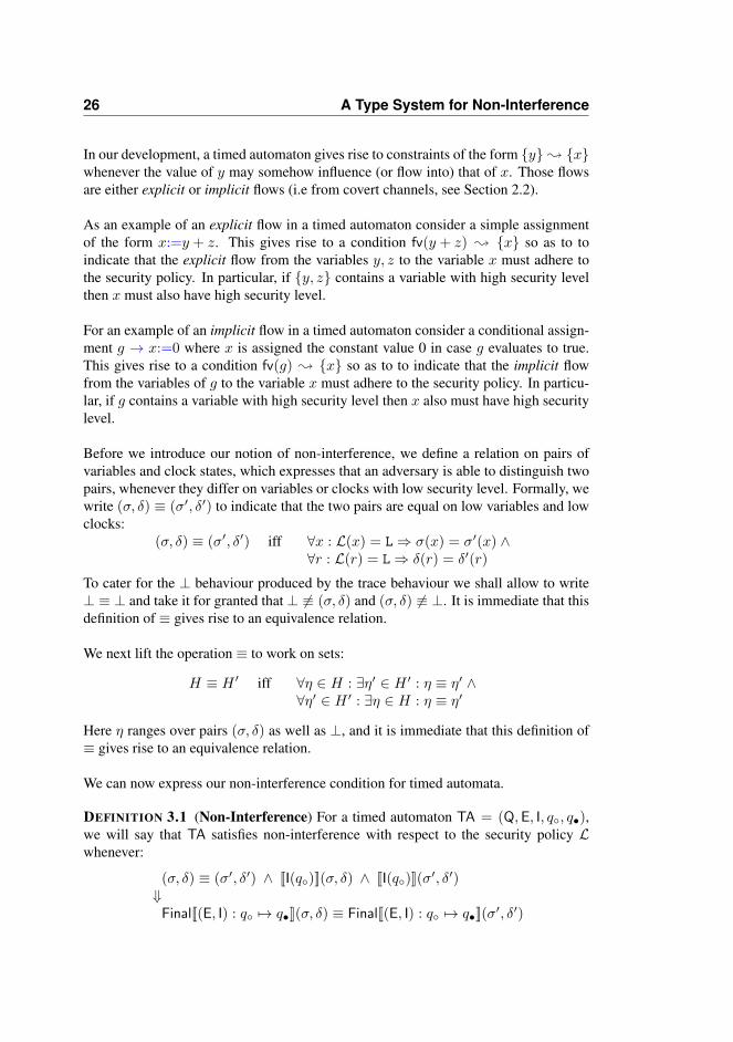
In our development, a timed automaton gives rise to constraints of the form {y} ; {x}whenever the value of y may somehow influence (or flow into) that of x. Those flowsare either explicit or implicit flows (i.e from covert channels, see Section 2.2).
As an example of an explicit flow in a timed automaton consider a simple assignmentof the form x:=y + z. This gives rise to a condition fv(y + z) ; {x} so as to toindicate that the explicit flow from the variables y, z to the variable x must adhere tothe security policy. In particular, if {y, z} contains a variable with high security levelthen x must also have high security level.
For an example of an implicit flow in a timed automaton consider a conditional assign-ment g → x:=0 where x is assigned the constant value 0 in case g evaluates to true.This gives rise to a condition fv(g) ; {x} so as to to indicate that the implicit flowfrom the variables of g to the variable x must adhere to the security policy. In particu-lar, if g contains a variable with high security level then x also must have high securitylevel.
Before we introduce our notion of non-interference, we define a relation on pairs ofvariables and clock states, which expresses that an adversary is able to distinguish twopairs, whenever they differ on variables or clocks with low security level. Formally, wewrite (σ, δ) ≡ (σ′, δ′) to indicate that the two pairs are equal on low variables and lowclocks:
(σ, δ) ≡ (σ′, δ′) iff ∀x : L(x) = L ⇒ σ(x) = σ′(x) ∧∀r : L(r) = L ⇒ δ(r) = δ′(r)
To cater for the ⊥ behaviour produced by the trace behaviour we shall allow to write⊥ ≡ ⊥ and take it for granted that ⊥ ̸≡ (σ, δ) and (σ, δ) ̸≡ ⊥. It is immediate that thisdefinition of ≡ gives rise to an equivalence relation.
We next lift the operation ≡ to work on sets:
H ≡ H ′ iff ∀η ∈ H : ∃η′ ∈ H ′ : η ≡ η′ ∧∀η′ ∈ H ′ : ∃η ∈ H : η ≡ η′
Here η ranges over pairs (σ, δ) as well as ⊥, and it is immediate that this definition of≡ gives rise to an equivalence relation.
We can now express our non-interference condition for timed automata.
DEFINITION 3.1 (Non-Interference) For a timed automaton TA = (Q,E, I, q◦, q•),we will say that TA satisfies non-interference with respect to the security policy Lwhenever:
(σ, δ) ≡ (σ′, δ′) ∧ [[I(q◦)]](σ, δ) ∧ [[I(q◦)]](σ′, δ′)
⇓Final[[(E, I) : q◦ 7→ q•]](σ, δ) ≡ Final[[(E, I) : q◦ 7→ q•]](σ
′, δ′)
3.3 Timed Commands 27
This condition caters for a passive adversary that observes the public part of final con-figurations, and tries to deduce secret information of the initial configurations. In par-ticular, it says that if we consider two initial configurations that only differ on highvariables and clocks then the final configurations are also only allowed to differ onhigh variables and clocks. Otherwise an adversary observing the final configurationscould infer information about the initial secret variables or clocks. In other words, thereis no information flow from the initial values of high variables and clocks to the finalvalues of low variables and clocks.
The fact that the trace behaviour produces a set of configurations means that we takedue care of non-determinism, and the fact that the trace behaviour may contain ⊥ meansthat we take due care of non-termination (because of looping or because of gettingstuck). In addition to that, because we allow the adversary to observe the final valuesof low clocks, it also means that we take care of potential timing channels. Finally,our semantic condition is more involved than in classical papers like [VSI96] whichconsider only deterministic programs, due to the highly non-deterministic nature oftimed automata (i.e our notion also caters for covert channels as the one given in Ex-ample 2.2).
3.3 Timed Commands
The semantic condition for non-interference is undecidable in general [Cas09]. Toobtain a sound and decidable enforcement mechanism, the traditional approach is todevelop a type system for a suitable programming language or process calculus.
To this end we introduce the language TC of timed commands. It is strongly motivatedby Dijkstra’s language of guarded commands [Dij75] but is designed so that it com-bines guards and assignments in the manner of timed automata. The syntax is givenby:
TC ::= begin[g◦] C [g•]end
C ::= g→ x :=a: r | C1;[g]C2 | doT1 [] · · · []Tn od []Tn+1 [] · · · []Tm
T ::= g→ x :=a: r | T ;[g]C
A timed command TC specifies a guard condition g◦ that must hold initially and acondition g• that must hold if the command terminates. The command C itself canhave one of three forms. One possibility is that it is an action of the form g→ x :=a: r.Another possibility is that it is a sequence of commands and then the condition g mustbe satisfied when moving from the first command to the second. The third possibility isthat it is a looping construct with a number of branches T1, · · · , Tn that will loop anda number of branches Tn+1, · · · , Tm that will terminate the looping behaviour. In case

28 A Type System for Non-Interference
⊢qtqs g→ x :=a: r : {(qs, g→ x :=a: r, qt)}, [ ]
⊢qqs C1 : E1, I1 ⊢qt
q C2 : E2, I2
⊢qtqs C1;
[g]C2 : E1 ∪ E2, I1 ∪ I2 ∪ [q 7→ g]where q is fresh
∧ni=1 ⊢qs
qs Ti : Ei, Ii∧m
i=n+1 ⊢qtqs Ti : Ei, Ii
⊢qtqs doT1 [] · · · []Tn od []Tn+1 [] · · · []Tm :
∪i Ei,
∪i Ii
⊢q•q◦ C : E, I
⊢ begin[g◦] C [g•]end : E, I′, q◦, q•where
{I′ = I[q◦ 7→ g◦; q• 7→ g•]q◦, q• are fresh
Table 3.1: From Timed Commands to Timed Automata.
n = 0 and m > 1 we dispense with the do od. Here T is a special form of commandthat starts with an action and potentially is followed by a number of commands. Guardsand expressions are defined as in Section 3.1.
EXAMPLE 3.4 The automaton of the signing authority SA of Example 3.1 is given bythe following timed command
begin[rg≤tend] Tcasting [] Tending[tt] end
where the command Tending=end describes the ending phase of the voting system, thecommand
Tcasting= vote_req;[rl≤tlookup]
( init_sign;[rl≤1] doTsigning od [] Tcounting) [] ( reply_has_voted)
describes the casting phase, while
Tsigning= mult;[rl≤2] ( extra_mult [] dummy_mult );[rl≤3] inc_counter
corresponds to the signing phase, and finally,
Tcounting= req_count;[rl≤treply] vote_counted;[rl≤1]
( update_db1 [] ... [] update_dbn);[rl≤1] reply_has_counted
describes the counting phase.

3.3 Timed Commands 29
Transformational Semantics We shall define the semantics of a timed commandby mapping it into a timed automaton. Consider begin[g◦] C [g•]end and let q◦ andq• be two distinct nodes; they will be the initial and final node of the resulting timedautomaton and we shall ensure that I(q◦) = g◦ and I(q•) = g•. Additional nodes willbe created during the construction using a judgment of the form:
⊢qtqs C : E, I
Here C is a timed command, qs and qt are nodes, E is a set of edges, and the judgmentwill introduce additional nodes whose invariants are given by the labelling functionI. This defines a timed automaton with initial node qs, final node qt, edges E, andlabelling function I.
The judgment is specified by the axioms and rules of Table 3.1. In the axiom we simplycreate the edge (qs, g→ x :=a: r, qt) starting in qs and ending in qt and indicating theaction to be performed; the resulting labelling function is empty as no new nodes arecreated in the construct.
In the first rule we create a fresh node q to be used to glue the timed automata for C1
and C2 together; the node q has the invariant g and is used as target node for C1 aswell as source node for C2. The resulting set of edges is the union of the two sets; thetwo branches will create disjoint sets of nodes so the two mappings I1 and I2 will havedisjoint domains and we write union for their combination.
In the rule for the looping construct we achieve the looping of the branches T1, · · · , Tnby using qs as source as well as target node, whereas for Tn+1, · · · , Tm we use qt astarget node. The overall set of edges is obtained as the union of the edges Ei and as inthe previous case the domains of the mappings Ii will be disjoint so the mappings areeasily combined.
Recall that T is a special form of timed command and hence timed automata can beconstructed using the judgments of Table 3.1. The timed automata constructed fromT always have exactly one edge leaving the initial node and do not contain any edgeback to the initial node unless the initial and final nodes coincide. The timed automataconstructed from C may have more than one edge leaving the initial node and maycontain edges back to the initial node even when the initial and final nodes are distinct.
For the overall timed command begin[g◦] C [g•]end we can now obtain a timed au-tomaton with initial node q◦, final node q•, edges E, and labelling function I′ given bythe last inference rule of Table 3.1.
EXAMPLE 3.5 The transformation applied to the timed command of Example 3.4gives rise to the timed automaton of Figure 3.2.
30 A Type System for Non-Interference
3.4 Type System
The information flow type system is specified using judgments of the form
⊢[qt:gt][qs:gs]
C : E, I&χ
This is an extension of the judgments ⊢qtqs C : E, I of the previous section for con-
structing timed automata from commands. The new judgments maintain informationabout the invariants gs and gt associated with the nodes qs and qt and a set χ of latentvariables and nodes that influence the termination of the command; the influence of χon qt remains to be enforced. The type system is specified in Table 3.2 and explainedbelow.
Assignment Consider the first axiom of Table 3.2. The second line of the side condi-tion expresses all the explicit flows from components of the sequence of expressions tocorresponding components of the sequence of variables. The first line of the side condi-tion expresses that the modifications of variables and clocks as well as the terminationrelies on having started the action. The third line of the side condition expresses ourknowledge that gs holds and the implicit flows arising from testing the guard g in thepre-state and the condition gt in the post-state before performing the modifications ofvariables and clocks. (We are using the insight from Hoare logic [Apt81] that evaluat-ing gt in the post-state is the same as evaluating gt[a/x][0/r] in the pre-state.) Ratherthan also expressing the implicit flow for termination (in the form of a side conditionfv(gs ∧ g ∧ gt[a/x][0/r]) ; {qt}) we produce the latent set of variables and nodes{qs}∪ fv(gs ∧ g ∧ gt[a/x][0/r]) as listed after the ampersand in the axiom. (We shallsee the flexibility offered by this approach shortly.)
EXAMPLE 3.6 Consider the command
extra_mult = rl ≥ 2 ∧1024∨j=1
(i = j ∧ kj = 1) → s:=s · v:
appearing in the timed command Tsigning in Example 3.4, and the automaton fromFigure 3.2. It is the case that qs = 4, qt = 9, gs = rl ≤ 2, and gt = rl ≤ 3. The typesystem imposes the following constraints on the flows:
{4} ; {9, s}, {s, v} ; {s}, {rl, i, k1, ..., k1024} ; {s}
It is easy to check that they are fulfilled for the security assignment of Example 3.3. Thelatent set of variables is {4, rl, i, k1, ..., k1024}.

3.4 Type System 31
⊢[qt:gt][qs:gs]
g→ x :=a: r : {(qs, g→ x :=a: r, qt)}, [ ] &{qs} ∪ fv(gs ∧ g ∧ gt[a/x][0/r])
if {qs} ; {qt,x, r}∧i fv(ai) ; {xi}
fv(gs ∧ g ∧ gt[a/x][0/r]) ; {x, r}
⊢[q:g][qs:gs]
C1 : E1, I1 &χ1 ⊢[qt:gt][q:g] C2 : E2, I2 &χ2
⊢[qt:gt][qs:gs]
C1;[g]C2 : E1 ∪ E2, I1 ∪ I2 ∪ [q 7→ g] &χ2
if q is freshfv(g) ∪ {q} ; Clocks ∪ {q}χ1 ; {q}∧n
i=1 ⊢[qs:gs][qs:gs]
Ti : Ei, Ii &χi
∧mi=n+1 ⊢[qt:gt]
[qs:gs]Ti : Ei, Ii &χi
⊢[qt:gt][qs:gs]
doT1 [] · · · []Tn od []Tn+1 [] · · · []Tm :∪
i Ei,∪
i Ii & {qt}if {qs} ; {qt}∧n
i=1 χi ; {qs}ΦT1,··· ,Tn
Tn+1,··· ,Tm[qt:gtqs:gs ] ⇒
∧mi=n+1 χi ; {qt}∧
i,j|i ̸=j,sat(fstζigs (Ti)∧fst
ζjgs (Tj))
χi ; ass(Tj)
where ζl is gs if l ≤ n and ζl is gt if l > n∧mi=n+1
(∀r ∈ fv(fstgtgs(Ti)) ∩ Clocks : L(r) = L) ∧(∧m
j=n+1 (fstgtgs(Ti) ⇔ fstgtgs(Tj)) ∨ (∀x ∈ fv(fstgtgs(Ti)) ∩ Var : L(x) = L)
)
⊢[q•:g•][q◦:g◦]
C : E, I&χ
⊢ begin[g◦] C [g•]end : E, I′, q◦, q•where
I′ = I[q◦ 7→ g◦; q• 7→ g•]fv(g◦) ∪ {q◦} ; Clocks ∪ {q◦}fv(g•) ∪ {q•} ; Clocks ∪ {q•}χ; {q•}L(q•) = L
q◦, q• are fresh
Table 3.2: Type System for Timed Commands.

32 A Type System for Non-Interference
Sequence The first inference rule of Table 3.2 deals with the sequential compositionof two commands. The second line of the side condition expresses the explicit flowpossible due to the delay at the node q separating the two commands. Recall thatClocks is the set of all clock variables and it is included to mimic the effect of thepotential delay. The third line of the side condition takes care of imposing the latenteffect of the first command on the node q following immediately after it.
EXAMPLE 3.7 Let us consider the sequence of commands
(extra_mult [] dummy_mult);[rl≤3] inc_counter
from Example 3.4, and the automaton from Figure 3.2. The latent set of variables fromthe first non-deterministic command will simply be {9}, and the two constraints willamount to {rl, 9} ; {rl, rg, 9}, and {9} ; {9}, which are satisfied for the securityassignment of Example 3.3.
Auxiliary Operations Before approaching the last inference rule in Table 3.2 weshall introduce three auxiliary operations.
The auxiliary operation ass(C) over-approximates the set of variables and clocks mod-ified by the command (ignoring any initial and final delays):
ass(g→ x :=a: r) = {x, r}ass(C1;
[g]C2) = ass(C1) ∪ ass(C2) ∪ Clocks
ass(
(doT1 [] · · · []Tn od[]Tn+1 [] · · · []Tm
)) =
{ass(T1) ∪ · · · ∪ ass(Tm) ∪ Clocks if n > 0ass(T1) ∪ · · · ∪ ass(Tm) if n = 0
where recall that Clocks is the set of all clocks, and it is included to mimic the effectof the potential (internal) delays of the sequence and loop command. The correctnessof our ass(.) is given with the following fact
FACT 1 If ⊢qtqs C : E, I and if (σ′, δ′) ∈ Final[[(E, I[qs 7→ gs][qt 7→ gt] : qs 7→ qt]](σ, δ)
then ∃t ≥ 0 : {x | σ(x) ̸= σ′(x)} ∪ {r | δ(r) + t ̸= δ′(r)} ⊆ ass(C), where tcorresponds to the initial delay.
Next, the auxiliary operation fstgtgs(T ) determines the initial guard and the invariantimmediately following it (in the manner of the rule for assignment):
fstgtgs(g→ x :=a: r) = gs ∧ g ∧ gt[a/x][0/r]fstgtgs(T ;
[g]C) = fstggs(T )
The inclusion of gs is so as to get the strongest information for use in the rule for thelooping construct in Table 3.2.

3.4 Type System 33
We shall need the auxiliary predicate ΦT1,··· ,Tn
Tn+1,··· ,Tm[qt:gtqs:gs ] that must be true whenever it
is possible that the construct doT1 [] · · · []Tn od []Tn+1 [] · · · []Tm does not terminatefrom a state satisfying gs; we return to this below.
Looping We can now explain the inference rule in Table 3.2 for looping. The firstline in the side condition expresses that the termination relies on having started theaction as we saw in the axiom for assignment. The second line in the side conditiontakes care of imposing the latent effect χi of the looping commands on the loop headerqs.
The third line in the side condition takes care of imposing the latent effect of the termi-nating commands on the final node qt. However, by using the predicate ΦT1,··· ,Tn
Tn+1,··· ,Tm[qt:gtqs:gs ]
we dispense with imposing this latent effect in case termination of the looping constructis guaranteed. As an example this means that the type system will allow the followingtimed command(
(h = 0→ h:=h: ) [] (h ̸= 0→ h:=h: ));[tt]tt → l:=l:
that would otherwise be disallowed (assuming that h is a high variable and l is a lowvariable). Indeed it is in order to accommodate this kind of behaviour that the typesystem makes use of latent variables and nodes. This is essential for preventing unnec-essary timing channels created from non-termination which depends on high variables.
Using the notation of Table 3.2 we can now clarify our demands on the auxiliary nota-tion ΦT1,··· ,Tn
Tn+1,··· ,Tm[qt:gtqs:gs ] used in the third line:
⊥ ∈∪
(σ,δ)|[[gs]](σ,δ) Final[[(∪iEi,∪iIi[qs 7→ gs][qt 7→ gt]) : qs 7→ qt]](σ, δ)
⇓ΦT1,··· ,Tn
Tn+1,··· ,Tm[qt:gtqs:gs ]
The subscript (σ, δ) | [[gs]](σ, δ) is intended to let (σ, δ) range over all possibilities thatsatisfy [[gs]](σ, δ). Note that we do not require to capture non-termination precisely butwill allow any over-approximation.
Before explaining the fourth line in the side condition it is helpful to establish thefollowing property of the type system as stated in Table 3.2.
LEMMA 3.2 If ⊢[qt:gt][qs:gs]
C : E, I&χ then we have that {qs} ; ass(C) ∪ {qt} and∀χ′ : (χ; χ′) ⇒ ({qs} ; χ′).
If ⊢[qt:gt][qs:gs]
T : E, I&χ then ∀χ′ : (χ ; χ′) ⇒ ({qs} ∪ fv(fstgtgs(T )) ; χ′) and{qs} ∪ fv(fstgtgs(T )) ; ass(T ), and {qs} ; {qt}.

34 A Type System for Non-Interference
(Note that the lack of reflexivity of ; means that we need to write slightly complexformula like ∀χ′ : (χ ; χ′) ⇒ ((· · · ) ; χ′) because the formula ((· · · ) ; χ is ingeneral incorrect.)
This lemma shows that we have already taken care of the so-called block labels of[DD77] and thereby take care of the implicit flows due to testing guards in the mannerof [VSI96]. However, the language considered in [VSI96] is deterministic and as wehave already showed in Example 2.2 the presence of non-determinism poses a com-plication, giving rise to new information flows. For another example of such a flow,consider the following command:
tt → l:=0: ;[tt]((h = 0→ h:=h: ) [] (tt → l:=1: )
)where l is a low variable and h is a high variable. Here the final value of l will be 1if h ̸= 0, however if h = 0, the final value of l may be either 0 or 1. This presents aviolation for adherence to the non-interference condition.
The purpose of the fourth line in the side condition is to take care of this possibilityand this is a novel contribution with respect to [DD77, VSI96, BBM94]. The notationsat(· · · ) is intended to express the satisfiability of the · · · formula. We are consideringall terminating branches in the looping construct and whenever there are two branchesthat are not mutually exclusive (that is, where sat(fstζigs(Ti)∧ fstζjgs(Tj))) we make sureto record the information flow arising from bypassing the branch that would otherwiseperform an assignment. This is essential for dealing with non-determinism.
Before explaining the fifth condition let us consider the following command operatingon a low clock rl, a high clock rh and a high variable h:
rh ≥ 50 ∧ h = 1 → skip: [] rh ≥ 100 ∧ ¬(h = 1) → skip:
Take arbitrary σ, δ. Here we have that (σ[h 7→ 1], δ[rh 7→ 50]) ≡ (σ[h 7→ 0], δ[rh 7→60]) but running the command from (σ[h 7→ 1], δ[rh 7→ 50]) might produce (σ[h 7→1], δ[rh 7→ 50]) itself (and the initial and final value of rl are equal), whereas runningthe command from (σ[h 7→ 0], δ[rh 7→ 60]) can only produce (σ[h 7→ 0], δ[rh 7→60] + t) for t ≥ 40 (the initial and the final value of rl differ by at least 40 time units)in which case (σ[h 7→ 1], δ[rh 7→ 50]) ̸≡ (σ[h 7→ 0], δ[rh 7→ 60] + t).
The purpose of the fifth line in the side condition is to take care of this possibility byenforcing that the terminating branches only test on low clocks, and that the conditionson clocks are the same whenever we test on high variables. This is essential to dealwith timing channels (see Section 2.2).

3.4 Type System 35
To this end we define g as follows
b = ttr opr n = r opr ng1 ∧ g2 = g1 ∧ g2
and we write g ⇔ g′ to express the equivalence of the guards g and g′.
EXAMPLE 3.8 Returning to Example 3.4 and the timed automaton of Figure 3.2, letus consider the command
extra_mult [] dummy_mult
From the first line we get the constraint {4} ; {9}. We have no contribution from thesecond line since there is no looping, and we also have no contribution from the thirdand forth line since the termination of the command is guaranteed and there is no pairof states satisfying the guards of both commands resp. Finally, from the fifth conditionwe get only that L(rl) = L, since rl ≥ 2 ⇔ rl ≥ 2 and thus
rl ≥ 2 ∧1024∨j=1
(i = j ∧ kj = 1) ⇔ rl ≥ 2 ∧ ¬1024∨j=1
(i = j ∧ kj = 1)
It is easy to check that the above conditions are fulfilled with the security assignmentof Example 3.3.
Timed Commands Consider the last inference rule in Table 3.2. The first and lastlines of the side condition are as in Table 3.1. The second and third lines of the sidecondition express the explicit flow possible due to the delay at the node q◦ and q• andis analogous to our treatment of sequencing. The fourth line of the side condition takescare of imposing the latent effect of the command on the final node q• and is analogousto our treatment of sequencing. The fifth line will allow us to invoke Theorem 3.3 ofthe next section.
EXAMPLE 3.9 Consider the timed command
begin[rg≤tend] Tcasting [] Tending[tt] end
from Example 3.4 and its automaton of Figure 3.2. It is the case that q◦ = 1, q• = 5,g◦ = rg ≤ tend and g• = tt. The type system imposes the following constraints on theflows:
{rg, 1} ; {rg, rl, 1}, {5} ; {rg, rl, 5}, {5} ; {5}, L(q•) = L
It is easy to check that they are fulfilled for the security assignment of Example 3.3.Finally, using Example 3.6, Example 3.7 and Example 3.8 we can easily check that thebody of the time command type checks.

36 A Type System for Non-Interference
3.5 Adequacy
To prove the adequacy of the type system we shall establish some terminology. Afunction like Final[[TA : qs 7→ qt]] mapping a pair of state and clock assignment to aset of pairs of states and clock assignments, and possibly the symbol ⊥ will be called asemantic function. Whenever F is a semantic function we define
F |= gs 7→ gt iff ∀(σ, δ), (σ′, δ′) : (σ, δ) ≡gs (σ′, δ′)⇓F (σ, δ) ≡gt F (σ′, δ′)
where (using ≡ as defined in Section 3.2)
(σ, δ) ≡g (σ′, δ′) abbreviates (σ, δ) ≡ (σ′, δ′) ∧ [[g]](σ, δ) ∧ [[g]](σ′, δ′)
H ≡g H ′ abbreviates H ≡ H ′ ∧∀(σ, δ) ∈ H : [[g]](σ, δ) ∧ ∀(σ′, δ′) ∈ H ′ : [[g]](σ′, δ′)
The semantic condition for when a timed automaton TA = (Q,E, I, q◦, q•) satisfiesnon-interference with respect to a security policy L (see Definition 3.1) then amountsto Final[[(E, I) : q◦ 7→ q•]] |= I(q◦) 7→ I(q•).
Finally, let us define the composition of two semantic functions F1 and F2 as follows:
F1 ⋄ F2 = λ(σ0, δ0). (F1(σ0, δ0) ∩ {⊥}) ∪∪(σ1,δ1)∈F (σ0,δ0)\{⊥} F2(σ1, δ1)
FACT 2 If F1 |= g0 7→ g1 and F2 |= g1 7→ g2 then F1 ⋄ F2 |= g0 7→ g2.
We are then ready to state a non-interference result in the manner of Definition 3.1:
THEOREM 3.3 (ADEQUACY OF COMMANDS) If ⊢[qt:gt][qs:gs]
C : E, I&χ and χ; {qt}and L(qt) = L and fv(gs) ; {qs} then we have Final[[(E, I[qs 7→ gs][qt 7→ gt]) : qs 7→qt]] |= gs 7→ gt.
We can now establish our main result that the type system enforces a sufficient condi-tion for the absence of information flows violating the security policy.
COROLLARY 3.4 (ADEQUACY) If ⊢ begin[g◦] C [g•]end : E, I, q◦, q• then we havethat Final[[(E, I) : q◦ 7→ q•]] |= I(q◦) 7→ I(q•).

3.6 Related Work 37
3.6 Related Work
There are many works dealing with information flow on systems with a notion of dis-crete time. The work of [FGM03] develops a non-interference property based on bisim-ulations of processes from a discrete-time process algebra. The works of [BMP19] and[ATM10] introduce a calculus as a semantic framework for dealing with informationsecurity in IoT devices and cyber-physical systems respectively. A language-based ap-proach is taken in [Aga00], where a transformational type system is used to removediscrete timing as a covert channel for deterministic programs. However, as has al-ready been noted in [BP18] discrete time may allow for some information flows to beundetected.
There are several papers that deal with information flow on systems with a notion ofdense time. The work of [BFST02] and [BT03] define a notion of non-interference fortimed automata with high-level (secret) and low-level (public) actions. Their notion ofsecurity is expressed as a non-interference property and it depends on a natural numberm, representing a minimum delay between high-level actions such that the low-levelbehaviors are not affected by the high-level ones. The authors of [LMST10] definea notion of timed non-interference based on bisimulations for probabilistic timed au-tomata which again is based on high-level and low-level actions. Similarly, the workof [GSB18] defines an action-based non-interference and uses model-checking tech-niques in order to enforce it on timed automata models. A somewhat different ap-proach is taken in [GMR07] that studies the synthesis of controllers for achievingnon-interference between high- and low-level actions. Our work differs from thoseworks since we are concerned with timed automata that use data-variables and ournon-interference notion is state-based instead.
There are other works that define security of timed-systems based on notions eitherdifferent or somehow different from non-interference style conditions. The work of[LMMV19] propose a hybrid process calculus for the modelling of cyber-physical sys-tems, and the security analysis of integrity and denial of service attacks. The work of[Cas09] presents timed-opacity as a generalization of non-interference in timed sys-tems, and shows that verifying timed-opacity is in general undecidable; however theauthors of [Cas09] do not consider approaches for enforcing timed-opacity. The workof [AS19] studies the following problem: given a timed automaton with timing param-eters, a secret state and a final public state, synthesize the timing parameters and theexecution times for which one cannot infer whether the system’s execution has passedthrough the secret state. Finally, the work of [BP18] introduces a hybrid logic for veri-fying information flow security properties that depend both on discrete and continuousvariables.

38 A Type System for Non-Interference
3.7 Conclusions
We have shown how to successfully merge timed automata with information flow andlanguage-based security through the introduction of the timed commands language pat-terned after Dijkstra’s guarded commands. This has facilitated developing a type sys-tem that prevents unnecessary covert channels and that deals with non-determinism,non-termination and continuous real-time. The type system has been proved adequateby means of a non-interference result.

CHAPTER 4
Secure Locality-BasedDeclassification
In this chapter, we develop a static analysis which allows one to enforce a securitycondition that permits locality-based declassification in timed automata. In particu-lar, our security condition is a bisimulation relation on the configurations of the timedautomaton, it captures adversaries that can make multiple observations, and permitsthe bypassing of a security policy whenever an execution reaches particular nodes. Tocheck our security condition, we first define a general notion of the post-dominator re-lation [LT79], which allows us to determine the points (i.e the nodes) in the automatonwhere the propagation of an implicit flow should stop. We then develop a static anal-ysis that is an algorithm which traverses a timed automaton and imposes informationflow constraints using the post-dominator relation. Finally, we prove that whenever atimed automaton is certified by our algorithm then it satisfies our security condition.The idea of our approach is illustrated in Figure 4.1.
Chapter Organisation In Section 4.1, we model the smart grid system from Exam-ple 2.8 as a timed automaton, while we also introduce some auxiliary definitions forthe traces of timed automata. In Section 4.2, we give our security condition, and inSection 4.3, we define our post-dominator relation. In Section 4.4, we give our staticanalysis. Finally, in Section 4.5 and Section 4.6, we finish with our related work andconclusions respectively.

40 Secure Locality-Based Declassification
The Problem
Our Approach
q◦
Timed Automaton TA
q q′
Adversary: It observes low variables and clocks at q andq′.
Security Condition: Observations at q should not interferewith sensitive information. However, observations at q′
may be correlated with sensitive information.
Challenge: Is there an information flow that violates thesecurity condition?
Step 1 (Post-Dominator): Compute the post-dominator relation, and determine the points, wherethe control-flow implicit flows from the guards should stop e.g
q◦ q The flows from g1, g2stop here
Step 2 (The Algorithm): Use the information from Step 1 and generate the possible informationflows. The algorithm omits some of the flows that occur at the node q′.
fv(g1) ; {...}fv(g2) ; {...}...
g1→... g2→...
g4→...
g3→...
g1→...
g2→...
Figure 4.1: The idea of our development in Chapter 4.
4.1 Modelling the Smart Grid System
In Section 3.1 we introduced the model of a timed automaton, and we required that ithas a final location q•. In this chapter, we drop this restriction, and a timed automatonis now given as quadruple TA = (Q,E, I, q◦), where all of its components are definedas in Section 3.1.
We are now ready to give the timed automaton model of the smart grid system given

4.1 Modelling the Smart Grid System 41
1
[rm ≤ 720]
2 [rm = 720]
4 [rm = 720]
3 [rm = 720]
bill_analytics
data_am
data_pm
data_mid
data_req
data
release_no
price
release_yes
price_analytics
Data Aggregationdata_am: rd ≤ 12 ∧ rf = 1 → edam:=edam + ed: rfdata_pm: rd > 12 ∧ rd < 24 ∧ rf = 1 → edpm:=edpm + ed: rfdata_mid: rd = 24 ∧ rf = 1 → edpm:=edpm + ed: (rf, rd)data_req: rm = 720 → (d, cam, cpm):=(1, edam, edpm):data: rm = 720 → (d, cam, cpm):=(0, edam, edpm):
Billing and Analyticsrelease_no d = 0 → skip:release_yes d = 1 → (yam, ypm):=(cam, cpm):price_analytics → (pam, ppm, a, f):=(vam, vpm, z, 1):price → (pam, ppm, a, f):=(vam, vpm, 0, 1):bill_analytics f = 1 → (b, x, edam, edpm, f):=(pam · cam + ppm · cpm, a, 0, 0, 0): (rm, rd, rf)
Figure 4.2: The timed automaton SG of the smart grid system, and the abbreviationsof its actions during the data aggregation phase, and during the billing andanalytics phase.
in Example 2.8. Recall that it consists of a customer C, a utility company UC and atrusted third party TTP which is used for controlling the way UC is making use of C’sdata, in order to achieve data privacy.
EXAMPLE 4.1 The timed automaton SG of the smart grid system is given in Fig-ure 4.2
Clocks. The automaton uses three clocks. The clocks rm and rd measure the elapse oftime within one month and one day respectively, while the clock rf is used to regulatethe frequency of the electricity measurements performed by the sensor, by allowing onemeasurement every full hour.
Variables. The variable ed contains the electricity data of the customer C, while thevariables edam and edpm aggregate the data from ed between midnight and noon, andfrom noon to midnight respectively. The collectors cam and cpm are used by the trustedparty TTP to collect the electricity data from edam and edpm respectively, while thevariable d is used to hold the decision of the customer C with regards the analytics ofhis data. Whenever C decides for his data to be declassified to the utility UC, then the

42 Secure Locality-Based Declassification
latter receives C’s data (i.e cam and cpm) from TTP, and stores it in the variables yamand ypm (resp.). The bill for the customer is stored in the b variable, and it is calculatedbased on the electricity tariff values vam and vpm which are collected from the TTP inthe price variables pam and ppm respectively. Finally, the flag f is used from the TTP todetermine if it has collected all the information about the bill and the data analytics aof C, while a is stored in the variable z from TTP and in x from C.
Transitions. We begin at the initial location 1 with the data aggregation phase dur-ing the period of a month (rm ≤ 720). Here we have three different transitions thatcorrespond to the two different time periods, midnight to noon (rd ≤ 12), noon to mid-night (rd > 12), and the exact moment of the end of a day (rd = 24). Within a day,a measurement is performed every one hour (rf = 1). By the end of the day the lastmeasurement is calculated, and the clock rd is reset indicating the start of a new day.The aggregation phase ends at the end of the month (rm = 720), and the trusted partyTTP collects the electricity data from C together with his decision about analysing it.Next the automaton moves to location 2.
At location 2, the billing and analytics phase starts. The TTP requests from the UC theprices of the electricity tariffs for the two time periods of interest moving to location4. Otherwise, if C has made a request for his data to be analysed (d = 1), TTPalso reveals the collected data to UC moving to location 3. Once the TTP receiveseverything (f = 1) from UC, he calculates the bill for C, sends it to him together withthe analysis result, the clocks and the variables of the meter are reset, the automatonmoves to location 1, and a new month starts. For simplicity here we assume that all thecalculations done by the TTP and the UC by the end of the month are being completedin zero time.
The semantics of timed automata is the same as the ones defined in Section 3.1.1,while now we introduce some extra definitions that we will use in later sections of ourdevelopment.
For a configuration ⟨qs, σ, δ⟩ and a node qt, we write Traces[[TA : qs 7→ qt]](σ, δ) forthe set of traces from ⟨qs, σ, δ⟩ to qt. Let now the length of a trace be the numberof transitions appearing in it (possibly this number could be ∞) we then make use ofLemma 1 of [HSW12] and we obtain the following
PROPOSITION 4.1 For a pair (σ, δ) whenever Traces[[TA : qs 7→ qt]](σ, δ) containsonly successful traces, then there exists a trace tr ∈ Traces[[TA : qs 7→ qt]](σ, δ) withmaximal length.
Proposition 4.1 shows that whenever a configuration ⟨qs, σ, δ⟩ is guaranteed to reach aconfiguration at the node qt, then the number of transitions it takes is bounded.
4.2 Y -Bisimulation Security 43
Next, we define the delay ∆(tr) of a trace tr from ⟨qs, σ, δ⟩ to qt, and we have that iftr is a successful trace
⟨qs, σ, δ⟩ = ⟨q′0, σ′0, δ
′0⟩
t1−→ · · · tn−→ ⟨q′n, σ′n, δ
′n⟩ = ⟨qt, σ′, δ′⟩
then∆(tr) =
∑ni=1 ti
In the case of tr being an unsuccessful (finite or infinite) trace we have that
∆(tr) = ∞
One may think here that the delay of an unsuccessful finite trace from ⟨qs, σ, δ⟩ to qtshouldn’t be ∞, since we have a finite number of transitions, and we could have insteadtaken the sum of the times appearing in the transition arrows of the trace. However, ourintention here is to capture that qt is never reached, and thus "waiting" to reach qt takes∞ time.
Finally, for two pairs (σ1, δ1), (σ2, δ2), and two nodes qs, qt, whenever
∀tr1 ∈ Traces[[TA : qs 7→ qt]](σ1, δ1) :∀tr2 ∈ Traces[[TA : qs 7→ qt]](σ2, δ2) : ∆(tr1) = ∆(tr2) (and vice versa)
we say that (σ1, δ1) and (σ2, δ2) have the same termination behaviour with respectto qs and qt. Note that it is not necessarily the case that a pair (σ, δ) has the sametermination behaviour as itself.
4.2 Y -Bisimulation Security
In this section, we define our security notion based on a bisimulation relation on theconfigurations of the timed automaton.
In particular, as in Section 3.2 we model the victim as an automaton that runs on somesecret input. We assume the same adversary model as in Section 3.2, but with onecore difference. In contrast to the adversary model from Section 3.2, the adversarynow is able to observe information at intermediate nodes of the automaton, and notonly at final nodes. Moreover, computations of the victim leading to some of thosenodes are allowed to leak secret information, permitting in that way locality-baseddata declassification. Our security via bisimulation then says that computations of theautomaton under two configurations that are indistinguishable to the adversary (i.e theyare equal on the their public part) lead to distinguishable configurations only at nodeswhere declassification is allowed.

44 Secure Locality-Based Declassification
To this end, as in Section 3.2, for a timed automaton TA = (Q,E, I, q◦) we assumea security mapping L associating clocks and variables1 to a high H or low L securitylevel.
EXAMPLE 4.2 Returning to Example 4.1 of our smart grid system, we have that Lmaps the program variable ed of the electricity data, the variables eam, epm that storethis data, the collectors cam, cpm and the bill b to the security level H, while the rest ofthe program variables and clocks are mapped to L.
We also assume that there exists a set of observable nodes Y ⊆ Q, which are the nodeswhere the values of program variables and clocks with low security are observable bythe adversary. The observable nodes will be described by the union of two disjoint setsYs and Yw, where a node q in Ys (Yw resp.) will be called strongly observable (weaklyobservable resp.). Computations leading to weakly observable nodes, are allowed tobypass the security policy L, whereas this is not the case for the ones leading to stronglyobservable nodes.
EXAMPLE 4.3 For the smart grid automaton SG from Example 4.1 , we have the setof observable nodes Y = {2, 3, 4}, with the strongly observable ones being the nodes2 and 4 (Ys = {2, 4}), and the weakly one is the node 3 (Yw = {3}). Node 3 is weaklyobservable because that’s the place in the automaton where TTP is allowed to releasethe secret information of C. The only non-observable node here is the initial node 1,which describes the data aggregation phase that takes place at the customer’s side C.
Observable steps Since the values of low program variables and clocks are onlyobservable at the nodes in Y , we collapse the transitions of the automaton that lead tonon-observable nodes into one. Thus we have an observable successful step
⟨qs, σ, δ⟩D=⇒Y ⟨qt, σ′, δ′⟩
whenever there exists a successful trace tr
⟨qs, σ, δ⟩ = ⟨q0, σ0, δ0⟩t1−→ · · · tn−→ ⟨qn, σn, δn⟩ = ⟨qt, σ′, δ′⟩ (n > 0)
from ⟨qs, σ, δ⟩ to qt in TA and qt ∈ Y , D = ∆(tr) and ∀i ∈ {1, ..., n− 1} : qi ̸∈ Y .
And we have an observable unsuccessful trace
⟨qs, σ, δ⟩∞=⇒Y ⊥
1Recall that, in Section 3.2, L was mapping also nodes to a security level, however this is not needed inthis setting.
4.2 Y -Bisimulation Security 45
whenever there exists an unsuccessful finite trace
⟨qs, σ, δ⟩ = ⟨q0, σ0, δ0⟩t1−→ · · · tn−→ ⟨qn, σn, δn⟩ (n ≥ 0)
or an unsuccessful infinite trace
⟨qs, σ, δ⟩ = ⟨q0, σ0, δ0⟩t1−→ · · · tn−→ ⟨qn, σn, δn⟩
tn+1−→ · · ·
from ⟨qs, σ, δ⟩ to any of the nodes in Y and ∀i > 0 : qi ̸∈ Y . From now on aconfiguration γ will range over Config ∪ {⊥}.
Next, as in Section 3.2 we write (σ, δ) ≡ (σ′, δ′) to indicate that the two pairs are equalon low variables and low clocks, and our bisimulation relation is defined as follows
DEFINITION 4.2 (Y -Bisimulation) For a timed automaton TA = (Q,E, I, q◦), and aset of observable nodes Y = Ys∪Yw, a relation ≃Y ⊆ (Config∪{⊥})×(Config∪{⊥})will be called a Y−bisimulation relation if ≃Y is symmetric, and we have that if γ1 =⟨q1, σ1, δ1⟩ ≃Y ⟨q2, σ2, δ2⟩ = γ2 then
(σ1, δ1) ≡ (σ2, δ2) ⇒ if γ1D1=⇒Y γ′1 then ∃γ′2, D2 :
γ2D2=⇒Y γ′2 ∧ γ′1 ≃Y γ′2∧
(γ′1 ̸= ⊥ ∧ γ′2 ̸= ⊥) ⇒ ((node(γ′1) ∈ Yw ∧ node(γ′2) ∈ Yw)∨pair(γ′1) ≡ pair(γ′2))
where node(⟨q, σ, δ⟩) = q, pair(⟨q, σ, δ⟩) = (σ, δ). In addition to that, if γ1 ≃Y γ2then
(γ1 = ⊥ ⇔ γ2 = ⊥)
We write ∼Y for the union of all the Y -bisimulations and it is immediate that this def-inition of ∼Y is both a Y -bisimulation and an equivalence relation. Intuitively, whentwo configurations are related in ∼Y , and they are low equivalent then they producedistinguishable pairs of states only at the weakly observable nodes. Otherwise, obser-vations made at strongly observable nodes should be still indistinguishable. In bothcases, the resulting configurations of two Y -bisimilar configurations should also beY -bisimilar, meaning that even if we declassify data, later computations leading tostrongly observable nodes should respect the security policy L. Making use of ∼Y oursecurity condition is then defined as
DEFINITION 4.3 (Y−Bisimulation Security) For a timed automaton TA = (Q,E, I, q◦),a set Y = Ys∪Yw of observable nodes, and a security policy L, we say that TA satisfiesY -bisimulation security whenever:
∀q ∈ {q◦} ∪ Y : ∀(σ, δ), (σ′, δ′) :([[I(q)]](σ, δ) ∧ [[I(q)]](σ′, δ′)) ⇒ ⟨q, σ, δ⟩ ∼Y ⟨q, σ′, δ′⟩

46 Secure Locality-Based Declassification
This condition ensures that the initial configurations and the ones with nodes in Y ,where the adversary can make observations are related in ∼Y . In addition, wheneverthe set of observable nodes Yw is empty our notion of security coincides with standarddefinitions of non-interference where information does not flow from secret to public,and in particular, whenever there is only one strongly observable node, and there are noedges leaving from it, then we have the non-interference notion given in Definition 3.1.
4.3 Post-Dominators
The lack of having a structured language as the one of timed commands from Sec-tion 3.3 (but instead we have an arbitrary timed automaton graph) poses a challengeon determining the information flows between low and high entities. In particular, forthe implicit flows arising from testing guards, it is challenging to find their end points(nodes), that are the points where the control flow is not dependent on the variablesappearing in the guard anymore. To this end, we define a generalized version of thepost-dominator relation, and the immediate post-dominator relation [LT79], which willhelp us to solve this problem.
A path π in a timed automaton TA = (Q,E, I, q◦) is a finite π = q0act1q1...qn−1actnqn(n ≥ 0), or infinite π = q0act1q1...qn−1actnqn... sequence of alternating nodes andactions, such that ∀i > 0 : (qi−1, acti, qi) ∈ E. We say that a path is trivial if π = q0and we say that a node q belongs to the path π, or π contains q, and we will write q ∈ π,if there exists some i such that qi = q. For a finite path π = q0act1q1...qn−1actnqn wewrite π(i) = qiacti+1qi+1...qn−1actnqn (i ≤ n) for the suffix of π that starts at thei-th position and we usually refer to it as the i-th suffix of π. Finally, for a node q anda set of nodes Y ⊆ Q we write
Π(q,Y ) = {π | π = q0act1q1...qn−1actnqn : n > 0 ∧ q0 = q ∧ qn ∈ Y ∧∀i ∈ {1, ..., n− 1} : qi ̸∈ Y }
for the set of all the non-trivial finite paths that start at q, end at a node y in Y and allthe intermediate nodes of the path do not belong to Y . Our post-dominator definitionis then the following
DEFINITION 4.4 (Y Post-Dominators) For a node q and a set of nodes Y ⊆ Q wedefine the set
pdomY (q) ={q′ | ∀π ∈ Π(q,Y ) : q′ ∈ π(1) }
and whenever q′ ∈ pdomY (q), we will say that q′ is a Y post-dominator of q.
4.3 Post-Dominators 47
Intuitively, whenever a node q′ is a Y post-dominator of a node q, it means that everynon-trivial path that starts at q has to visit q′ before it visits one of the nodes in Y . Wewrite pdomy(q) whenever Y = {y} is a singleton and we have the following facts
FACT 3 For a set of nodes Y ⊆ Q and for a node q we have that
pdomY (q) =∩y∈Y
pdomy(q)
FACT 4 The post-dominator set for a singleton set {y} can be computed by finding thegreatest solution of the following data-flow equations:
pdomy(q)=Q if Π(q,{y}) = ∅pdomy(q)={y} if y ∈ succ(q)pdomy(q)=
∩q′∈succ(q)
({q′} ∪ pdomy(q
′))
otherwise
where succ(q) is the set of the immediate successors of q.
For a node q, we are interested in finding the Y post-dominator “closest" to it. For this,we give the definition of an immediate post-dominator as follows
DEFINITION 4.5 (Immediate Y Post-Dominator) For a node q and a set of nodes Ywe define the set
ipdomY (q) = {q′ ∈ pdomY (q) | pdomY (q) = {q′}∨q′ ̸∈ Y ∧ (∀q′′ ∈ pdomY (q) : q
′′ ̸= q′ ⇒q′′ ∈ pdomY (q
′))}
and a node q′ ∈ ipdomY (q) will be called an immediate Y post-dominator of q.
The following fact gives us a unique immediate Y post-dominator for the nodes thatcan reach Y (Π(q,Y ) ̸= ∅). Intuitively this unique immediate Y post-dominator of anode q is the node that is the “closest" Y post-dominator of q, meaning that in anynon-trivial path starting from q and ending in Y , the Y immediate post-dominator of qwill always be visited first before any other Y post-dominator of q.
FACT 5 For a set of nodes Y and a node q, whenever Π(q,Y ) ̸= ∅, and pdomY (q) ̸= ∅,then there exists node q′ such that ipdomY (q) = {q′}.
For simplicity, whenever a node q′ is the unique immediate Y post-dominator of anode q and Π(q,Y ) ̸= ∅ we shall write ipdY (q) for q′ and we will say that the unique

48 Secure Locality-Based Declassification
immediate Y post-dominator of q is defined. For any other case where q can eithernot reach Y (Π(q,Y ) = ∅) or pdomY (q) = ∅ we will say that the unique immediatepost-dominator of q is not defined.
EXAMPLE 4.4 For the timed automaton SG from Example 4.1 and for the set of ob-servable nodes Y = {2, 3, 4} from Example 4.3, we have that pdomY (q) = ipdY (q) ={2} for q being 1, 3 and 4, while pdomY (2) = ∅. Therefore for the nodes 1,3 and 4their unique immediate Y post-dominator is defined, and it is the node 2, while theunique immediate Y post-dominator of the node 2 is not defined.
4.4 Algorithm for Secure Declassification
We develop an algorithm (given in Table 4.1) that traverses the graph of a timed au-tomaton TA, and imposes information flow constraints (of the form χ ; χ′ as inSection 3.2) on the program variables and clocks of the automaton, with respect to asecurity policy L, and a Y post-dominator relation, where Y = Ys ∪ Yw is the set ofobservable nodes. Before we explain the algorithm we start by defining some auxiliaryoperators.
Auxiliary Operators For an edge (qs, g→ x :=a: r, qt) ∈ E we define the auxiliaryoperator ass(.), expr(.) and con(.) as
ass((qs, g→ x :=a: r, qt)) = {x, r}expr((qs, g→ x :=a: r, qt)) = {a}con((qs, g→ x :=a: r, qt)) = I(qs) ∧ g ∧ I(qt)[a/x][0/r]
where ass(.) gives the modified variables and clocks of the assignment performed byTA using that edge, expr(.) gives the expressions used for the assignment, and theoperator con(.) returns the condition that has to hold in order for the assignment to beperformed. We lift the ass(.) operator to operate on finite paths, and thus for a pathπ = q0act1q1...qn−1actnqn we define the auxiliary operator Ass(.) as
Ass(q0act1q1...qn−1actnqn) =∪n
i=1 ass((qi−1, acti, qi))
Next, we writeQ;w = {q | ∀π = q..q′ ∈ Π(q,Y ) : q
′ ∈ Yw}
for the set of nodes, where whenever the automaton performs a successful observablestep starting from a node q ∈ Q;w, and ending in an observable node q′ ∈ Y , it isalways the case that q′ is weakly observable.

4.4 Algorithm for Secure Declassification 49
C1. For all q ∈ Q;w :(a)
∧e∈Eq
∀y ∈ fv(con(e)) : L(y) = L ∧ (Ψe ∨Ae)
C2. For all q ∈ Qc;w such that their unique immediate Y post-dominator is defined :
(a)∧
e∈Eq
∪π∈Π(e,{ipdY (q)})
fv(con(e)) ; Ass(π) ∧Ae
(b)∧
e ̸=e′:e∈Eq, e′∈Eq, sat(con(ϵ)∧con(e′)) fv(con(e)) ;∪
π∈Π(e′,{ipdY (q)})Ass(π)
(c) Φq ⇒∧
e∈Eq∀y ∈ fv(con(e)) : L(y) = L
C3. For all q ∈ Qc;w such that their unique immediate Y post-dominator is not defined :
(a)∧
e∈Eq∀y ∈ fv(con(e)) : L(y) = L∧
(b) ((e; w ∧Ψe) ∨Ae)
Table 4.1: Security of TA = (Q,E, I, q◦) with respect to L and the Y post-dominatorrelation.
Condition C1 We start by looking at the nodes in Q;w. According to our securitynotion (given in Definition 4.3), for two low equivalent configurations at a node q,whenever the first one performs a successful (or unsuccessful) observable step thatends at a weakly observable node, then also the second should be able to perform anobservable step that ends at a weakly observable node (or an unsuccessful one resp.).For that, the condition C1 (a) first requires that the guards of the outgoing edges in Eq ,where
Eq = {(q, act, q′) | (q, act, q′) ∈ E}contain only low variables. However, this is not enough.
To explain the rest of the constraints imposed by the condition C1 (a), consider thefollowing automaton
1 2
3
→ l:=h:
l > 0 → skip:
l ≤ 0 → skip:
where the node 3 is weakly observable, h and l are a high and a low variable respec-

50 Secure Locality-Based Declassification
tively, and all the invariants of the nodes are set to tt. This automaton is not secure withrespect to Definition 4.3. To see this, we have ([l 7→ 0, h 7→ 1], δ) ≡ ([l 7→ 0, h 7→ 0], δ)(for some clock state δ) but the pair ([l 7→ 0, h 7→ 1], δ) always produces ⊥ since wewill have an infinite loop at the node 2, whereas ([l 7→ 0, h 7→ 0], δ) always terminatesat the node 3. This is because even if both edges of the node 2 contain only the lowvariable l in their condition, the assignment l:=h bypasses the policy L and thus, rightafter it, the two pairs stop being low equivalent.
As another example, consider the automaton
1 2
34
→ l:=h:
→ l′:=l:
l′ > 0 → skip:
l′ ≤ 0 → skip:
Here the node 4 is weakly observable, h is a high variable, l, l′ are two low variables,and all the invariants of nodes are set to tt again. We have ([l 7→ 0, l′ 7→ 0, h 7→1], δ) ≡ ([l 7→ 0, l′ 7→ 0, h 7→ 0], δ) (for some clock state δ) and again the firstpair produces ⊥ by looping at the node 3, whereas the second pair always terminates.Here even if the variable l is not used in any condition after the assignment l:=h, itinfluences the value of l′ and consequently, since l′ appears on the condition of theedges of the node 3 we get this behavior.
To cater for such cases, for an edge e = (qs, g → x :=a: r, qt) we first define thepredicate
Ae =∧i
fv(ai) ; {xi}
that takes care of the explicit flows arising from the assignments. We then define
Π(e,Y ) = {π | e = (q0, act1, q1) : π = q0act1q1...qn−1actnqn ∈ Π(q0,Y )}
to be the set of paths (the ones defined in Section 4.3) that start with e and end in Y ,and all the intermediate nodes do not belong to Y . Finally, whenever an assignment
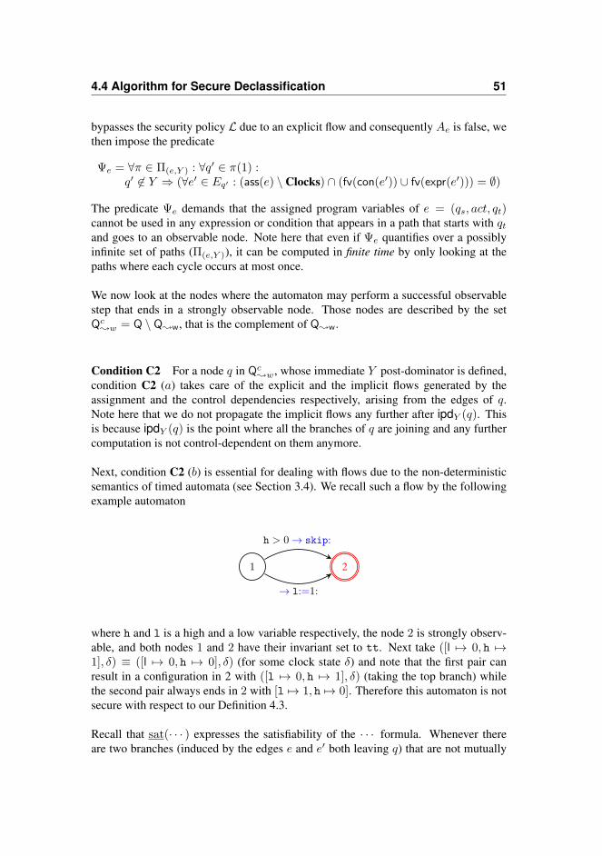
4.4 Algorithm for Secure Declassification 51
bypasses the security policy L due to an explicit flow and consequently Ae is false, wethen impose the predicate
Ψe = ∀π ∈ Π(e,Y ) : ∀q′ ∈ π(1) :q′ ̸∈ Y ⇒ (∀e′ ∈ Eq′ : (ass(e) \ Clocks) ∩ (fv(con(e′)) ∪ fv(expr(e′))) = ∅)
The predicate Ψe demands that the assigned program variables of e = (qs, act, qt)cannot be used in any expression or condition that appears in a path that starts with qtand goes to an observable node. Note here that even if Ψe quantifies over a possiblyinfinite set of paths (Π(e,Y )), it can be computed in finite time by only looking at thepaths where each cycle occurs at most once.
We now look at the nodes where the automaton may perform a successful observablestep that ends in a strongly observable node. Those nodes are described by the setQc
;w = Q \ Q;w, that is the complement of Q;w.
Condition C2 For a node q in Qc;w, whose immediate Y post-dominator is defined,
condition C2 (a) takes care of the explicit and the implicit flows generated by theassignment and the control dependencies respectively, arising from the edges of q.Note here that we do not propagate the implicit flows any further after ipdY (q). Thisis because ipdY (q) is the point where all the branches of q are joining and any furthercomputation is not control-dependent on them anymore.
Next, condition C2 (b) is essential for dealing with flows due to the non-deterministicsemantics of timed automata (see Section 3.4). We recall such a flow by the followingexample automaton
1 2
h > 0 → skip:
→ l:=1:
where h and l is a high and a low variable respectively, the node 2 is strongly observ-able, and both nodes 1 and 2 have their invariant set to tt. Next take ([l 7→ 0, h 7→1], δ) ≡ ([l 7→ 0, h 7→ 0], δ) (for some clock state δ) and note that the first pair canresult in a configuration in 2 with ([l 7→ 0, h 7→ 1], δ) (taking the top branch) whilethe second pair always ends in 2 with [l 7→ 1, h 7→ 0]. Therefore this automaton is notsecure with respect to our Definition 4.3.
Recall that sat(· · · ) expresses the satisfiability of the · · · formula. Whenever thereare two branches (induced by the edges e and e′ both leaving q) that are not mutually

52 Secure Locality-Based Declassification
exclusive, that is that sat(con(e) ∧ con(e′)), we make sure to record the informationflow arising from bypassing the branch that would otherwise perform an assignment.
Next, the following fact shows that our Ass(.) operator used in condition C2, correctlyapproximates the modified clocks and variables along a path.
FACT 6 For a timed automaton TA = (Q,E, I, q◦), we have that if
⟨q, σ, δ⟩ D=⇒{q′} ⟨q′, σ′, δ′⟩
then{x | σ(x) ̸= σ′(x)} ∪ {r | δ′(r) ̸= δ(r) +D} ⊆
∪π∈Π(e,{q′})
Ass(π)
where e corresponds to the initial edge of this observable step.
Finally, condition C2 (c) takes care of cases where a timing covert channel (see Sec-tion 3.4) could have occurred. We recall such a case with the following automaton
1 2
h > 0 ∧ r > 30 → skip:
h ≤ 0 → skip:
where h and r is a high program variable and a low clock respectively, node 2 isstrongly observable and both 1 and 2 have their invariant set to tt. Next, for ([h 7→1], [r 7→ 0]) ≡ ([h 7→ 0], [r 7→ 0]) we have that the first pair always delays at least 30units and ends in 2 with a clock state that has r > 30, whereas the second pair can go to2 taking the lower branch immediately without any delay, and thus the resulting pairswill not be low equivalent. To take care of such behaviours, we stipulate a predicate Φq
such that
∃tr1, tr2 ∈∪
(σ,δ):[[I(q)]](σ,δ) Traces[[TA : q 7→ ipdY (q)]](σ, δ) : ∆(tr1) ̸= ∆(tr2)
⇓Φq
Using this predicate we demand that whenever the TA does not have a “constant” ter-mination behavior from the node q to the node ipdY (q), then variables that influencethe termination behavior should not be of high security level.2
2In Section 3.4, the predicate Φ was used only for detection of timing channels, which were created dueto non-termination. Here we refine the predicate Φ to Φq , so it caters for any timing channel.

4.4 Algorithm for Secure Declassification 53
Condition C3 We are now left with the nodes in Qc;w, whose immediate Y post-
dominator is not defined. Since for such a node q, we cannot find a point (the uniqueimmediate Y post-dominator) where the control dependencies from the branches ofq end, condition C3 (a) requires that the conditions of the edges of q should not bedependent on high security variables.
Condition C3 (b) caters for the explicit flows, of an edge e using the predicate Ae.However we are allowed to dispense Ae, whenever further computations after takingthe edge e may lead only to weakly observable nodes and Ψe holds. To express this,for an edge e = (qs, g→ x :=a: r, qt) we write
e; w
whenever qt ∈ Yw or qt ∈ Q;w.
EXAMPLE 4.5 Consider now the automaton SG of Example 4.1, and the Y post-dominator relation of Example 4.4.
We have that the nodes 1, 3 and 4 are in Qc;w and also that their immediate unique
Y post-dominator is defined. Condition C2 (a) and C2 (b) impose the following con-straints
{rm, rd, rf} ; {ed, eam, epm, cam, cpm, d, rd, rf}, {ed, eam} ; {eam},{ed, epm} ; {epm}, {eam} ; {cam}, {epm} ; {cpm}, {vam} ; {pam}, {vpm} ; {ppm},{rm} ; {pam, ppm, a, f}, {z} ; {a}, {} ; {d, f, a}
Finally, for the node 1, because Φ1 (condition C2 (c)) all the clocks need to be of lowsecurity level.
Next, the node 2 is in Qc;w and since its unique immediate Y post-dominator is not
defined, condition C3 (b) impose the constraints
{pam, ppm, cam, cpm} ; {b}, {a} ; {x}, {} ; {eam, epm, f}
and condition C3 (a) imposes that rm, d and f should be of low security level. Noticehere that since for the edge e = (2, d = 1 → (yam, ypm):=(cam, cpm): , 3) that releasesthe sensitive information ofC we have that e; w, we are not imposing the constraints{cam} ; {yam} and {cpm} ; {ypm}. All those constraints are easy to verify for thesecurity assignment of Example 4.2.
Now if we were to change the node 3 from being a weakly observable to a stronglyobservable node, the automaton SG will not be secure with respect to Definition 4.3. Inthat case our algorithm will reject it, since for the edge e we would have that e ̸; wand the predicate Ae would have resulted in false.

54 Secure Locality-Based Declassification
Finally, we write secY,L(TA) whenever the constraints arising from our algorithm(given in Table 4.1) are satisfied, and we then have the following theorems, whichare the building stones for establishing the soundness of our algorithm.
THEOREM 4.6 For a timed automaton TA = (Q,E, I, q◦), if secY,L(TA) then for(σ1, δ1), (σ2, δ2) such that [[I(q)]](σ1, δ1) and [[I(q)]](σ2, δ2) and (σ1, δ1) ≡ (σ2, δ2) wehave that
if ⟨q, σ1, δ1⟩D1=⇒Y ⟨q′, σ′
1, δ′1⟩ then ∃(σ′
2, δ′2), D2 : ⟨q, σ2, δ2⟩
D2=⇒Y ⟨q′, σ′2, δ
′2⟩∧
(q′ ∈ Yw ∨ (σ′1, δ
′1) ≡ (σ′
2, δ′2))
THEOREM 4.7 For a timed automaton TA = (Q,E, I, q◦), if secY,L(TA) then for(σ1, δ1), (σ2, δ2) such that [[I(q)]](σ1, δ1) and [[I(q)]](σ2, δ2) and (σ1, δ1) ≡ (σ2, δ2) wehave that
if ⟨q, σ1, δ1⟩∞=⇒Y ⊥ then also ⟨q, σ2, δ2⟩
∞=⇒Y ⊥
The following corollary concludes the two theorems from above to establish the sound-ness of our algorithm with respect to the notion of security of Definition 4.3.
COROLLARY 4.8 For a timed automaton TA = (Q,E, I, q◦), if secY,L(TA) then TAsatisfies Y -bisimulation security.
4.5 Related Work
The work of this chapter can be seen as an extension of the work presented in Chap-ter 3. We are now capable of dealing with any timed automaton, and with adversariesthat can make multiple observations at any node in the timed automaton. Whereas,in Chapter 3, we were restricted by the timed automata expressed from the constructsof the timed commands, while we were only concerned with adversaries that couldmake observations only at the final node of the timed automaton. Finally, the work inChapter 3 does not support declassification of data.
Having said that, the related work presented in Section 3.6 also applies here with thesame comparison, while there is one substantial difference, that is that, none of theworks discussed in Section 3.6 considers policies that permit data declassification. Toour knowledge, we are the first who considered the problem of locality-based declassi-fication in a setting with systems of real-time semantics, such as timed automata.
Our notion of security is based on intransitive non-interference [LMP12, MS04, Pin95,RG99]. Whenever certain conditions are met, intransitive non-interference permitssome flows which would have been otherwise disallowed from standard non-interference
4.6 Conclusions 55
notions. In particular, our notion shares some ideas from [MS04, LMP12], where abisimulation-based security is defined for a programming language with threads. Intheir approach, the bypassing of the security policy is localized on the actions of theprogram. An attacker is able to observe the low variables of a program at any of itscomputation steps (e.g in a timed automaton all of the nodes would have been observ-able). Moreover, discrete time is considered in [MS04, LMP12], and it is defined as thenumber of transitions a program takes. It is also considered that time is observed bythe adversary. In contrast to [MS04, LMP12], we localize bypassing of policies at thelevel of the nodes, while we also define a more flexible notion of security with respectto the adversary’s observability, since we allow for choosing on which nodes of theautomaton the adversary makes observations. Finally, our semantics for time differs,since we are concerned with dense time.
Papers that deal with other dimensions of declassification e.g what data can be de-classified, and who can declassify data are also relevant, and have been discussed inSection 2.3.
4.6 Conclusions
We have shown how to successfully enforce information flow policies, that permit con-trolled locality-based declassification on timed automata. For this, we developed analgorithm that prevents unnecessary covert channels and deals with non-determinism,non-termination, continuous real-time, and with adversaries that are allowed to observecomputations on several locations in the timed automaton. Our algorithm makes use ofa novel definition of post-dominators, which allows us to deal with the implicit flowsarising from the unstructured control flow in timed automata. Finally, our algorithmhas been proved sound by means of a bisimulation result.
Automation Our work lacks full automation mainly because of the predicate Φq andthe sat(· · · ) operation.
In particular, recall that the predicate Φq is used for the detection of timing channels, byrequiring that the time needed getting from the node q to its immediate post-dominatoripdY (q) should be constant. There has been a lot of research [ARF17, ARF16] done fordetermining the maximum (maxt), or minimum (mint) execution time that a timedautomaton needs to move from a location qs to a location qt. One possibility for over-approximating Φq is to make use of this work [ARF17, ARF16] and thus the predicateΦq would amount to checking if the execution time between the two nodes of interest(q and ipdY (q)) is constant (i.e maxt = mint). Next, to reduce the complexity of ouralgorithm, we could also relax our requirements on when to check the predicate Φq .

56 Secure Locality-Based Declassification
In particular, checking Φq only on nodes whose edges contain high variables (at leastone) is sufficient, since if all the variables are low we get no contribution from Φq .
Finally, recall that the sat(· · · ) operation expresses the satisfiability of the · · · formula,and it is used to detect implicit flows arising from the non-deterministic semanticsof timed automata. Already the work of [NN19] considers an algorithm that over-approximates sat(...), and has been implemented at http://www.formalmethods.dk/if4fun/ for detecting flows in a guarded-command style language. Another di-rection could be rephrase the problem as an SMT problem (Satisfaction Modulo Theo-ries) and use one of the available solvers such as Z3 [dMB08].

CHAPTER 5
Data- and Time- DependentPolicy-Based Access Control
In this chapter, we develop a logic which can be used to enforce data- and time- de-pendent policy based access control on systems of distributed real-time processes. Inparticular, we model systems of distributed real-time processes as networks of timedautomata, and we define an information flow instrumented operational semantics forthem. The semantics make use of labels called behaviours, in order to record the differ-ent explicit flows, arising whenever a process is trying to read, or write to a variable, ora channel of the network. Our logic is called BTCTL (behaviour timed computationaltree logic), and it is based on those behaviours. Moreover, we illustrate how we cansuccessfully express and enforce security policies for our gateway example presentedin Example 2.1.
We then show that the model-checking problem N |= Φ of a network N and a BTCTLformula Φ, can be reduced to the model-checking problem BA |= T [[Φ]]. Here, BA is atimed automaton, raising from a product automaton-like construction of the network N,while, T [[Φ]] is a formula produced by a transformation on Φ. The transformed formulaT [[Φ]] results to a formula in a logic called TCTL+, that is a variation of the TCTL[ACD93] (timed computational tree logic). Finally, we implement this reduction, andwe show how the enforcement of policies can be fully automated using the model-checker UPPAAL. Our approach is depicted in Figure 5.1.

58 Data- and Time- Dependent Policy-Based Access Control
The Problem
Our Approach
1p1 :
Network N
2p2 :
3p3 :
Processes: The processes p1, p2 and p3 communicate viathe channels ch1 and ch2. The clock r is used to measurethe execution time of the network.
Security Condition Φ: The process p1 can communicatewith p3 until the time becomes 10, whereas after that onlyp2 can communicate with p3. The condition Φ isaction-based.
Challenge: How to check that N |= Φ?
Step 1 (Network Transformation) BA: Perform a product automaton-like construction, andintroduce two new nodes which use the labels l1 and l2 resp. to record the communicationactions. The new automaton is the BA.
l1 l2
p2 : ch2(x, x2) : p3p1 : ch1(x, x1) : p3
Step 2 (Condition Transformation) T [[Φ]]: The transformed condition is state-based. It saysthat whenever the automaton reaches the node labeled with l1, then the time should be at most 10,whereas, whenever it reaches the node with label l2, the time should be above 10.
Step 3: Check if BA |= T [[Φ]].
→ ch1!x1:
→ ch2!x2:
r ≤ 10 → ch1?x:
r > 10 → ch2?x:
r ≤ 10 → skip: ...
→ x:=x1:
r > 10 → skip: ...
→ x:=x2:
Figure 5.1: The idea of our approach in Chapter 5.
Chapter Organisation In Section 5.1, we give the model of networks of timed au-tomata, and in Section 5.2 we give the semantics for them. Next, in Section 5.3, wepresent the syntax and the semantics of BTCTL , and in Section 5.4 we present the re-duction of the model-checking problem from BTCTL to TCTL+. In Section 5.5, wediscuss an implementation of this reduction, and we show how we can use the model-checker UPPAAL to fully automate our enforcement of security policies. Finally, inSection 5.6 and Section 5.7, we give our related work and conclusions respectively.
5.1 Networks of Timed Automata 59
5.1 Networks of Timed Automata
We start by giving the model of a network of timed automata, which can be seen as anabstraction of systems of distributed real-time processes. In particular, the processesin the network have isolated memories and the only way to communicate is throughpolyadic channels. In addition, communications may be constrained from the currenttime of the network and from the content of some of the variables.
Networks Formally, a network of timed automata N
p1 : TA1 || ... || pn : TAn (n ≥ 1)
which sometimes, we simply call it network, is the parallel composition of n timedautomata called processes, written as the family N=(TAi)i≤n.
The processes are able to exchange information via synchronous message passing, us-ing polyadic channels from the finite set Chan. Each of the processes in the net-work, is labelled with a unique identifier p ∈ P={p1, ..., pn} and we write Varp andClocksp for the data variables and clocks appearing in the process p. We also re-quire that the sets of data variables and clocks for the processes are mutually disjoint(∀i ̸= j : Varpi
∩Varpj= ∅∧Clockspi
∩Clockspj= ∅) and we write Var=
∪i Varpi
and Clocks=∪
i Clockspifor the overall data variables and clocks appearing in the net-
work. Finally, we also require that the sets of nodes of the processes are mutuallydisjoint (i.e ∀i ̸= j : Qi ∩ Qj = ∅).
Processes Each process is modelled as a timed automaton [AD94, AILS07] TA =(Q,E, I, q◦) which is defined as in Section 3.1. However, the edges are now labelledwith actions g→ act: r, where the syntax of the action act is given by
act ::= x :=a | ch!a | ch?x
The assignment action g → x :=a: r is as in the previous chapters, while the actiong→ ch!a: r is used to communicate the data of the expressions in a using the channelch ∈ Chan, and the action g → ch?x: r is used to receive data and store it in thevariables of the sequence x.
Recall that we assume that the sequences x and a of data variables and expressions,respectively, have the same length and that in addition x does not contain any repeti-tions.

60 Data- and Time- Dependent Policy-Based Access Control
1[tt]
2[tt]
→ in1!x1:
→ in2!x2:
(a) The processes of the producers p1 (top) andp2 (bottom).
5 [r ≤ 10]
6[rm=0]
7
[rm=0]
0 ≤ r ∧ r ≤ 7 → in1?x: rm
r=10 → skip: r
→ ch!(1, x):
5 ≤ r ∧ r ≤ 10 → in2?x: rm
→ ch!(2, x):
(b) The process of the multiplexer m.
8
[tt]
9
[rd=0]→ ch?(y, z): rd
y = 1 → out1!z:
y = 2 → out2!z:
(c) The process of the demultiplexer d.
3[tt]
4[tt]
→ out1?z1:
→ out2?z2:
(d) The processes of the consumers c1 (top) andc2 (bottom).
Figure 5.2: The network of the gateway Example 2.1.
Finally, we write x(i) (and also a(i)) for the i-th element of the sequence x (and arespectively). Recall also that for special cases of the assignment action, we shall writeg→ skip: r when x (and hence a) is empty; also for any kind of action we shall omitthe guard g when it is equal to tt, and omit the clock resets when r is empty. If it is thecase that all of the above take place together we omit the whole action.
EXAMPLE 5.1 The network of our gateway from Example 2.1 is given in Figure 5.2.
Processes and Channels The network consists of six processes given from the set P= {p1, p2,m, d, c1, c2}. Two producers p1 and p2 send their data via the channels in1and in2 respectively. The multiplexer m collects the data from the producers using thechannel ch and then forwards it to the demultiplexer d, who then distributes it to theconsumers c1 and c2 via the channels out1 and out2 respectively.

5.2 Information Flow Instrumented Semantics 61
Clocks We use two clocks rm (in the multiplexer) and rd (in the demultiplexer) tomodel instantaneous transitions, i.e in this model actions (assignments and channelcommunication) take no time. The multiplexer makes use of an additional clock r (inthe multiplexer) in order to regulate the communication requests from the two produc-ers p1 and p2. The clock r is reset every 10 time units, splitting in this way the overallexecution of the automaton in intervals of 10 time units.
Variables The variables x1 and x2 carry the data the producers p1 and p2 wish tocommunicate respectively. Upon communication between one of the producers and themultiplexer, the multiplexer stores the data of the producers in the variable x. Next, atthe side of the demultiplexer the value of x is stored in the variable z and the variabley is used from the multiplexer to identify the origin of the data. Finally, the consumersc1 and c2 use the variables z1 and z2 respectively to store the value of z.
Transitions In each period the multiplexer m reads data from the channel in1 onlywhenever the time t ∈ [0, 7], expressed by the guard 0 ≤ r∧ r ≤ 7, while it reads datafrom the channel in2 only whenever t ∈ [5, 10], expressed by the guard 5 ≤ r∧r ≤ 10.Whenever t ∈ [5, 7] the multiplexer chooses non-deterministically to read either fromin1 or in2. Next, the multiplexer transfers the data together with a constant, using thedyadic channel ch to the demultiplexer d; the constant is used as a mark to indicatethe source of the data. In case of p1 being the source, then this constant is 1, otherwiseit is 2. Finally, the demultiplexer delivers the data to the right consumer according tothe constant, expressed by the guards y = 1 and y = 2. Finally, whenever a period of10 time units has been completed (r = 10) the multiplexer resets the clock r.
5.2 Information Flow Instrumented Semantics
In this section, we develop an information flow instrumented semantics for networks.The instrumentation makes use of labels which we call behaviours. The behavioursallow us to monitor the accesses on variables and channels performed by the processes,and they will be one of the main ingredients for the enforcement of our security policiesin later sections.
5.2.1 Behaviours
The transitions of networks are labeled with behaviours. In particular, a behaviourrecords information relevant to the action that has occurred and also information about
62 Data- and Time- Dependent Policy-Based Access Control
the processes which were involved in the action. Formally a behavior takes the form
b ∈ Blocal ∪ Bcom ∪ {ϵ}
whereBlocal = P ×
−−→Var ×
−−→Exp
are the behaviours that occur due to assignments and
Bcom = P × Chan ×−−→Var ×
−−→Exp × P
are the behaviours that occur due to the communication between two processes. Wewrite
−−→Var and
−−→Exp for the sets of sequences with elements over the data variables and
arithmetic expressions respectively.
For instance, the local behaviour p : (x,a) records that the process p has performedan assignment in which the sequence a is used to modify the variables of the sequencex. As another example, consider the behaviour p : ch(x,a) : p′, which records that acommunication between the processes p (the sender) and p′ (the receiver) has occurred,using the channel ch, and the sequence a is the sequence of expressions whose valueshave been communicated and have been bound to the variables of the sequence x.
Finally, in all of the behaviours, the sequences that are being used must have the samelength, while for the delay action we will write the empty behaviour ϵ.
5.2.2 Operational Semantics
To specify the semantics of networks, let σ be a state mapping data variables to integers,let δ be a clock assignment mapping clocks to non-negative reals and let κ be a mappingfrom data variables to a set of processes which we call writers. The mapping κ is usedto monitor the explicit flows that occur from the assignments and the communicationbetween two processes in the network. We will explain the use of κ in more detail in awhile.
We then have total semantic functions [[.]] for evaluating the expressions, boolean testsand guards. We evaluate expressions either with a state σ, or the mapping κ, where forthe first case the evaluation returns a value, and in the second it returns the writers ofthe expression.
The configurations of a network N = (TAi)i≤n are of the form ⟨q, σ, δ, κ⟩, whereq ∈ Q1 × ...× Qn is an n-tuple of nodes, we write q(i) for the i-th element of q, andwe have that
∧ni=1[[Ii(q(i))]](σ, δ). Finally, we write q [q′/q] to substitute the node q
with the node q′ in q.

5.2 Information Flow Instrumented Semantics 63
⟨qs, σ, δ, κ⟩pj :(x,a)=⇒ ⟨qt, σ′, δ′, κ′⟩ if
(q, g→ x :=a: r, q′) is in Ej
[[g]](σ, δ) = tt
σ′ = σ[x 7→ [[a]]σ]
δ′ = δ[r 7→ 0]
κ′ = κ[x 7→ [[a]]κ]
qt = qs[q′/q]∧n
i=1[[Ii(qt(i))]](σ′, δ′) = tt
⟨qs, σ, δ, κ⟩ph:ch(x,a):pl
=⇒ ⟨qt, σ′, δ′, κ′⟩ if
h ̸= l(q1, g1 → ch!a: r1, q
′1) is in Eh
(q2, g2 → ch?x: r2, q′2) is in El
σ′ = σ[x 7→ [[a]]σ]δ′ = (δ[r1 7→ 0])[r2 7→ 0]κ′ = κ[x 7→ [[a]]κ]qt = qs[q
′1/q1][q
′2/q2]∧n
i=1[[Ii(qt(i))]](σ′, δ′) = tt
⟨q, σ, δ, κ⟩ ϵ=⇒ ⟨q, σ, δ′, κ⟩ if
{∃ t > 0 : δ′ = λr. δ(r) + t,∧n
i=1[[Ii(q(i))]](σ, δ′) = tt
Table 5.1: Instrumented semantics of networks.
The transitions of a network take the form
⟨qs, σ, δ, κ⟩b
=⇒ ⟨qt, σ′, δ′, κ′⟩
and the initial configurations are of the form ⟨q◦, σ, λr.0, κ◦⟩ where q◦ is the sequence,whose elements are the initial nodes of the timed automata in the network, and κ◦ mapseach variable to the process that it belongs to (i.e κ◦(x) = {p} iff x ∈ Varp). Thetransition relation is given in Table 5.1.
The rule for the assignment, ensures that the guard is satisfied in the starting config-uration and updates the mappings σ, δ, κ and the location of the process pj . Finally,it ensures that the invariant is satisfied in the resulting configuration. The behaviourpj : (x,a) records that the process pj is performing an assignment to the sequence xusing the sequence a, and the mapping κ′ records the information flow that occurs dueto this behaviour, by updating the writers of each variable x(i) with the writers of theexpression a(i). Here, for a single expression a′, we have that [[a′]]κ =
∪y∈fv(a′) κ(y),
and recall that fv(a′) is the set of free variables occurring in a′.
To understand the rule for the communication one could see it as an assignment of the

64 Data- and Time- Dependent Policy-Based Access Control
form x :=a, where a are the expressions which are used at the channel output action,and x are the variables that are used in the channel input action.
Finally, the delay rule only modifies the clock assignment with a delay t, ensuring thatthe invariant is satisfied in the resulting configuration. The mapping κ remains the samesince the delay action produces the empty behaviour ϵ.
DEFINITION 5.1 (Runs) A run of a configuration γ is a (possibly infinite) sequence
⟨q0, σ0, δ0, κ0⟩b1=⇒ ...
bn=⇒ ⟨qn, σn, δn, κn⟩bn+1=⇒ ...
where γ = ⟨q0, σ0, δ0, κ0⟩ and we write Runs(γ) for the set of runs of γ.
EXAMPLE 5.2 To understand better how the semantics work, return to Example 5.1and consider the configuration ⟨q, σ, δ, κ⟩ where q = (1, 2, 5, 8, 3, 4), and let σ =λx.0, δ = λr.0 and
κ = [x1 7→ {p1} , x2 7→ {p2} , x 7→ {m} , y 7→ {d} , z 7→ {d} , z1 7→ {c1} , z2 7→ {c2}]
A possible transition of the network is the following
⟨q, σ, δ, κ⟩ p1:in1(x,x1):m=⇒ ⟨q[6/5], σ[x 7→ σ(x1)], δ[rm 7→ 0], κ[x 7→ {p1}]⟩
which corresponds to the communication between the producer p1 and the multiplexerm. The resulting mapping κ[x 7→ {p1}] records that p1 has written its value into thevariable x, since there is an explicit flow from the variable x1 to the variable x and x1has previously been written by p1.
5.3 Access Control in BTCTL
In this section, we present our behaviour based logic BTCTL which serves to specifydata- and time-dependent security policies for access control, based on the behavioursof the network. In particular, each of the variables of the network will be associatedwith a security policy that expresses under which content of the network’s variables andclocks one may influence the value of this particular variable. The goal of the policieshere is to ensure data integrity. We will then specify a security condition as a formula,in order to specify when a network satisfies the security policies. However, recall thataccess control protects only from explicit flows of information and not from implicitones.
5.3 Access Control in BTCTL 65
5.3.1 The Syntax
The syntax of the BTCTL formulas ϕ is given by
ϕ ::= g | set1 rel set2 | ∀2b(ϕ1, ϕ2) | ϕ1 ∧ ϕ2 | ¬ϕ
whereset ::= a |W
We have basic formulas which can be either a guard g, or relations between two sets ofwriters, set1 rel set2, where rel = {⊆,⊇}. The underlined set expression a denotesthe set of writers of the expression a and W ∈ P(P) is a set of writers. For example,let x be a variable and p1, p2 two processes. One example policy could be x ⊆ {p1},which specifies that only p1 can influence the value of x and not p2.
We use the box operator ∀2b(ϕ1, ϕ2) to speak about pre- and post-conditions wheneverthe non-empty behaviour b ̸= ϵ happens. Informally speaking, a configuration γ willsatisfy the ∀2b(ϕ1, ϕ2) formula whenever for all of the network runs starting at γ, if atransition labelled with the behaviour b occurs, then ϕ1 should hold at the configurationbefore the transition and ϕ2 at the configuration after it. As we will see shortly, the boxoperator will be the key formula to enforce access control policies. The ¬ϕ and ϕ1 ∧ ϕ2cases are the usual ones. Finally, we sometimes write ϕ1 ⇒ ϕ2 for ¬(ϕ1 ∧ ¬ϕ2).
EXAMPLE 5.3 Let’s now go back to our gateway network given in Example 5.1.
Security Policies Each of the variables has a policy which specifies the maximum setof permitted writers of the variable. We are interested in the policies of the variablesof the multiplexer, the demultiplexer and the two consumers. Therefore we have thefollowing policies
Px = (0 ≤ r ∧ r < 5 ⇒ x ⊆ {p1})∧(5 ≤ r ∧ r ≤ 7 ⇒ x ⊆ {p1, p2})∧(7 < r ∧ r ≤ 10 ⇒ x ⊆ {p2})
Py = y ⊆ {m}Pz = (0 ≤ r ∧ r ≤ 7 ∧ y = 1 ⇒ z ⊆ {p1})∧
(5 ≤ r ∧ r ≤ 10 ∧ y = 2 ⇒ z ⊆ {p2})Pz1 = z1 ⊆ {p1}Pz2 = z2 ⊆ {p2}
The first line of the policy for the variable x, expresses that whenever the clock r ∈[0, 5), only the process p1 is allowed to write data to x, while both p1 and p2 may writeto x if r ∈ [5, 7]. Finally, the last line expresses that whenever r ∈ (7, 10], then only

66 Data- and Time- Dependent Policy-Based Access Control
p2 can write to x. Next, looking at the policy for the variable y, a write action to it isallowed only by the multiplexer.
The policy of the variable z is both a time- and data-dependent policy. In particular,it specifies that whenever r ∈ [0, 7], and y contains the value 1, then the value of zcan be influenced by p1, whereas whenever r ∈ [5, 10] and y is 2, p2 may influence thevalue of z.
Finally, the policies for z1 and z2, express that only p1 can influence z1, and only p2can influence z2 respectively.
Security Condition Next, we need to specify our semantic security condition thatdefines when the network satisfies the given security policies. In particular, we needto ensure that the policies are enforced, whenever an action that writes data to thevariables of interest occurs. To this end, we define the following formulas
Φx = ∀2p1:in1(x,x1):m(tt, Px) ∧ ∀2p2:in2(x,x2):m(tt, Px)Φy,z = ∀2m:ch((y,z),(1,x)):d(tt, Py ∧ Pz) ∧ ∀2m:ch((y,z),(2,x)):d(tt, Py ∧ Pz)Φz1 = ∀2d:out1(z1,z):c1(tt, Pz1)Φz2 = ∀2d:out2(z2,z):c2(tt, Pz2)
Each of the formulas expresses that whenever someone is writing to the variable (orvariables) appearing as a subscript, then the policy of the variable (or variables) isimposed as a post condition. The variable x is accessed (someone is writing datato x) whenever p1 and p2 communicates with the multiplexer, and thus we have toimpose the policy of the variable x for both of those actions. The variables y and z arebeing accessed whenever the multiplexer communicates with the demultiplexer, andthat happens with two communication actions. Similarly, we define the formulas forthe variables z1 and z2.
5.3.2 Semantics of the BTCTL Formulas
The formal semantics for when a configuration γ satisfies a BTCTL formula ϕ is givenbelow

5.3 Access Control in BTCTL 67
γ |= g iff γ = ⟨q, σ, δ, κ⟩ ⇒ [[g]](σ, δ)γ |= set1 rel set2 iff γ = ⟨q, σ, δ, κ⟩ ⇒ [[set1]]κ rel [[set2]]κ
γ |= ∀2b(ϕ1, ϕ2) iff ∀γ0b1=⇒ γ1
b2=⇒ .. ∈ Runs(γ) :∀i ≥ 1 : bi = b ⇒ γi−1 |= ϕ1 and γi |= ϕ2
γ |= ϕ1 ∧ ϕ2 iff γ |= ϕ1 and γ |= ϕ2γ |= ¬ϕ iff γ ̸|= ϕ
A guard g is then satisfied by a configuration γ whenever g holds in γ. For the case ofthe set relation rel, γ satisfies it whenever set1 rel set2 evaluates to true, and we do thatcheck by lifting the definition of [[.]]κ to set of expressions, by defining [[a]]κ = [[a]]κ,and [[W ]]κ = W . A configuration γ satisfies the box formula ∀2b(ϕ1, ϕ2) wheneverfor all the execution paths that start from γ, if a behaviour b′ occurs and b′ is syntac-tically equal to b, then the pre-condition ϕ1 has to hold at the configuration before thebehaviour and the post-condition ϕ2 at the configuration after it. The rest of the casesare the usual ones.
EXAMPLE 5.4 We now give an example to illustrate how the box operator semanticswork. For this, consider the prefix
pr = γ0p1:in1(x,x1):m
=⇒ γ1m:ch((y,z),(1,x)):d
=⇒ γ2d:out1(z1,z):c1
=⇒ γ3
of an execution trace of the network given in Example 5.1, where for the initial con-figuration γ0 = ⟨q0, σ0, δ0, κ0⟩, we have that q0 = (1, 2, 5, 8, 3, 4), σ0 is arbitrary,δ0 = λr.0 and
κ0 = [x1 7→ {p1} , x2 7→ {p2} , x 7→{m }, y 7→ {d} , z 7→ {d} , z1 7→{ c1 }, z2 7→ {c2}]
In addition, for the rest of the configurations we have that γ1 = ⟨q1, σ1, δ1, κ1⟩, γ2 =⟨q2, σ2, δ2, κ2⟩ and γ3 = ⟨q3, σ3, δ3, κ3⟩ where
q1 = q0[6/5], σ1 = σ0[x 7→ σ0(x1)], δ1 = δ0[rm 7→ 0], κ1 = κ0[x 7→ {p1}]
q2 = q1[5/6][9/8], σ2 = σ1[y 7→ 1, z 7→ σ1(x)], δ2 = δ1[rd 7→ 0],κ2 = κ1[y 7→ ∅, z 7→ {p1}]
q3 = q1[8/9], σ3 = σ2[z1 7→ σ2(z)], δ3 = δ2, κ3 = κ2[z1 7→ {p1}].
Next, consider the formulas Φx, Φy,z, Φz1 given in Example 5.3, and we will now dothe appropriate checks for those formulas on the prefix pr.
The formula Φx is the conjunction of two box operators, where for the first one because
of the behaviour p1 : in1(x, x1) : m of the transition γ0p1:in1(x,x1):m
=⇒ γ1, we have tocheck that γ1 |= Px. Recall that

68 Data- and Time- Dependent Policy-Based Access Control
Px = (0 ≤ r ∧ r < 5 ⇒ x ⊆ {p1})∧(5 ≤ r ∧ r ≤ 7 ⇒ x ⊆ {p1, p2})∧(7 < r ∧ r ≤ 10 ⇒ x ⊆ {p2})
This check evaluates to true, since γ1 satisfies only the guard of the first line of the
policy and κ1(x) = {p1}. For the transition γ1m:ch((y,z),(1,x)):d
=⇒ γ2, because of theformula Φy,z we have to check that γ2 |= Py ∧ Pz, and recall that
Py = y ⊆ {m}Pz = (0 ≤ r ∧ r ≤ 7 ∧ y = 1 ⇒ z ⊆ {p1})∧
(5 ≤ r ∧ r ≤ 10 ∧ y = 2 ⇒ z ⊆ {p2})
This check evaluates to true, since κ2(y) = ∅, and thus γ2 |= Py, while for the policyPz we have that γ2 satisfies only the condition at the first line of the policy, and κ2(z) ={p1}, which give us that γ2 |= Pz as required.
Finally, for the last transition γ2d:out1(z1,z):c1
=⇒ γ3, because of the Φz1 formula, wehave to check that γ3 |= Pz. This check evaluates to true, since κ3(z1) = {p1} andPz1 = z1 ⊆ {p1}.
5.4 Reduction of BTCTL to TCTL+
In this section, we perform a transformation of the original network, and the securityconditions which are expressed as BTCTL formulas. The transformation results ina timed automaton, whose nodes carry extra information with regards to the actionsperformed in the original network. We call this automaton a behaviour automaton. Thetransformed security conditions are formulas in a new logic which we call TCTL+.TCTL+ is a logic based on TCTL (timed computational tree logic) [ACD93].
In the next section, we will show how a fragment of TCTL+ can be handled by themodel checker UPPAAL [UPP]. This will allows to fully automate our static enforce-ment of access control policies. Both the transformation of the network, and the secu-rity conditions are inspired by the work done in [JW02], where the action-based logicATCTL (action-TCTL) is being reduced to TCTL [ACD93].

5.4 Reduction of BTCTL to TCTL+ 69
1 [r ≤ 10]
2
[ru=0]
3
[rm=0]
4
[ru=0 ∧ r ≤ 10]
5[r ≤ 10 ∧ rd=0]
6
[ru=0]
7[rm=0]
8
[ru=0 ∧ r ≤ 10]
9[ru=0 ∧ rd=0]
10
[ru=0 ∧ r ≤ 10]
11
[ru=0 ∧ r ≤ 10]
12[ru=0 ∧ rd=0]
13[ru=0 ∧ rd=0]14 [ru=0]
15
[rm=0 ∧ rd=0]
16 [ru=0 ∧ rm=0]
17
[rm=0 ∧ rd=0]
18 [ru=0 ∧ rm=0]
19
[ru=0 ∧ rm=0]
20
[ru=0 ∧ rm=0]
g_read_in1
read_in1 g_read_ch1
read_ch1
g_read_in2
read_in1 g_read_ch2
read_ch2
g_round_reset
round_reset g_round_reset
round_resetg_read_in2
read_in2
g_read_out2
read_out2
g_read_in1
read_in1
g_read_out1
read_out1
g_read_out2
g_read_out1
read_out1
read_out2
read_out2 g_read_out2
g_read_out1read_out1
Genuine Verticesv L(v)1 (1,2,5,8,3,4)3 (1,2,6,8,3,4)5 (1,2,5,9,3,4)7 (1,2,7,8,3,4)15 (1,2,7,9,3,4)17 (1,2,6,9,3,4)
Auxiliary Verticesv L(v) v L(v)2 p1 : in1(x, x1) : m 10 d : out2(z2, z) : c24 m : ch((y, z), (1, x)) : d 11 d : out1(z1, z) : c16 p2 : in2(x, x2) : m 12 p1 : in1(x, x1) : m8 m : ch((y, z), (2, x)) : d 13 m : (ϵ, ϵ)9 p2 : in2(x, x2) : m 14 m : (ϵ, ϵ)16 d : out2(z2, z) : c2 18 d : out1(z1, z) : c119 d : out1(z1, z) : c1 20 d : out2(z2, z) : c2
Actionsread_in1 → x:=x1: rm g_read_in1 0 ≤ r ≤ 7 → skip: ruread_in2 → x:=x2: rm g_read_in2 5 ≤ r ≤ 10→ skip: ruread_ch1 → (y, z):=(1, x): rd g_read_ch1 → skip: ruread_ch2 → (y, z):=(2, x): rd g_read_ch2 → skip: ruread_out1 → z1:=z: g_read_out1 y = 1 → skip: ruread_out2 → z2:=z: g_read_out2 y = 2 → skip: ruround_reset → skip: r g_round_reset r = 10 → skip: ru
Figure 5.3: The behaviour automaton of the gateway’s network, its vertices togetherwith their labels, and the abbreviations for the actions used. The auxiliaryvertices are colored with purple.

70 Data- and Time- Dependent Policy-Based Access Control
Step 1. let Qgen = ∅; let Qaux = ∅;for all q: create fresh v; let L(v) = q; let I(v) =
∧ni=1 Ii(q(i)); insert v in Qgen
Step 2. for all (qi, g→ x :=a: r, q′i) ∈ Ei:
for all vs ∈ Qgen, vt ∈ Qgen such that
L(vs)(i) = qi
L(vt)(i) = q′i∀j : j ̸= i : L(vs)(j) = L(vt)(j)
:
create fresh v;insert (vs, g→ skip: ru, v) in E; insert (v,x :=a: r, vt) in E ;let L(v) = pi : (x,a); let I(v) = (ru = 0) ∧ I(vt)[a/x][0/r]; insert v in Qaux
Step 3. for all (qi, g1 → ch!a: r1, q′i) ∈ Ei and (qj , g2 → ch?x: r2, q
′j) ∈ Ej such that i ̸= j:
for all vs ∈ Qgen, vt ∈ Qgen such that
L(vs)(i) = qi ∧ L(vs)(j) = qj
L(vt)(i) = q′i ∧ L(vt)(j) = q′j∀l : l ̸= i ∧ l ̸= j : L(vs)(l) = L(vt)(l)
:
create fresh v; let g = g1 ∧ g2; let r = r1r2;insert (vs, g→ skip: ru, v) in E; insert (v,x :=a: r, vt) in E;let L(v) = pi : ch(x,a) : pj ; let I(v) = (ru = 0) ∧ I(vt)[a/x][0/r]; insert v in Qaux
Step 4. let Q = Qgen ∪Qaux
Table 5.2: The algorithm for constructing the edges E, the invariant function I, thevertices Q and the labelling function L of the behaviour automaton BA.
5.4.1 Behaviour Automata
A network N = (TAi)i≤n yields a behaviour automaton BA = (Q,E, I, L, v◦), which isa kind of timed automaton in that it is the product automaton of the network, extendedto contain auxiliary vertices that represent the actions of the network, and a labellingfunction L that assigns to each vertex a property.
A property is either a behaviour or a location vector of the original network N. Auxil-iary vertices will be labeled with the behaviour that corresponds to the particular actionof the vertex, while genuine vertices which represent locations of the network N arelabeled with a location vector. The initial vertex v◦ will be labeled with the initiallocation vector of the network q◦.
The behaviour automaton BA has the same set of variables as the network N, whilefor the clock variables it has an extra clock ru, which is used to model instantaneoustransitions. Similarly to the timed automata, E is a finite set of edges, the mapping Iimposes an invariant on each vertex, and Q is the finite set of vertices.

5.4 Reduction of BTCTL to TCTL+ 71
vs v vtg→ skip: ru x :=a: r
Figure 5.4: Edge construction of the behaviour automaton BA.
The algorithm for constructing the edges E, the labelling functions I and L, and the setof vertices Q = Qgen ∪ Qaux (and notice that Qgen ∩ Qaux = ∅) where Qgen andQaux contain the genuine and auxiliary vertices respectively, is given in Table 5.2.
In the first step, we create the genuine vertices and we label them with the invariantof the location vector that they represent. Each of those vertices is inserted in Qgen,which will be used in the next steps to create the auxiliary vertices.
In step 2, we create the auxiliary vertices, and the edges that correspond to the as-signment actions of the network. For each process pi, we start looking at all of itsassignment edges (qi, g → x :=a: r, q′i) ∈ Ei. For each one of those edges and forall the vertices vs ∈ Qgen and vt ∈ Qgen, where the label of vs, L(vs) corresponds toa vector location where this assignment could have been performed, and would havemoved the network to the location L(vt), we create the edges (vs, g→ skip: ru, v) and(v,x :=a: r, vt). Notice here that v is a fresh auxiliary vertex, whereas in the construc-tion of the product automaton one would have constructed only the edge (vs, g→x :=a: r, vt).
The auxiliary vertex v is labelled with the assignment behaviour pi : (x,a) and itsinvariant is being set to (ru = 0) ∧ I(vt)[a/x][0/r], to first ensure that the action ofthe edge leaving v will be performed instantaneous, and secondly that we can not getstuck at an auxiliary vertex. Figure 5.4 illustrates the construction. Finally, note thateach auxiliary vertex v has exactly one predecessor and exactly one successor.
Similarly to step 2, in step 3 we construct the auxiliary vertices for the communicationactions of the network, and finally, in step 4, we define the set Q.
EXAMPLE 5.5 The behaviour automaton of the our gateway network from Exam-ple 5.1 is given in Figure 5.3. It has 20 vertices, with vertex 1 being its initial vertexand 27 edges.
5.4.2 Trace Equivalence
We will now show that the runs of the original network N can be simulated by thebehaviour automaton BA and vice versa.
Particularly, each transition in the network N is equivalent to a single step transition (in

72 Data- and Time- Dependent Policy-Based Access Control
⟨vs, σ, δ, κ⟩ −→ ⟨vt, σ′, δ′, κ′⟩ if
(vs, g→ x :=a: r, vt) is in E
[[g]](σ, δ) = tt
σ′ = σ[x 7→ [[a]]σ]
δ′ = δ[r 7→ 0]
κ′ = κ[x 7→ [[a]]κ]
[[I(vt)]](σ′, δ′) = tt
⟨v, σ, δ, κ⟩ −→ ⟨v, σ, δ′, κ⟩ if{
∃ t > 0 : δ′ = λr. δ(r) + t,[[I(v)]](σ, δ′) = tt
Table 5.3: Semantics for Behaviour Automata.
the case of a delay) or a two-step transition (in the case of an action) in its behaviourautomaton BA. To overcome the vagueness of this explanation we will define a relationbetween runs of the network N, and the runs of the behaviour automaton BA.
To this end, we start by giving the operational semantics of behaviour automata in Ta-ble 5.3. The semantics is similar to the semantics of the timed automata networks,however now, the transitions are not labelled with behaviours, and there is no com-munication. Also for a configuration γ′ of the behaviour automaton BA we writeRunsBA(γ
′) for the set of runs it produces. Moreover, we now write RunsN(γ) forthe runs of a configuration γ in the network N.
Now let γ, and γ′ be two configurations of a network N, and its behaviour automatonBA respectively. We define the relation ∼=: ConfigN × ConfigBA → {tt,ff} to be
⟨q, σ, δ, κ⟩ ∼= ⟨v, σ′, δ′, κ′⟩ iff
q = L(v)σ = σ′
∀r ∈ Clocks : δ(r) = δ′(r)κ = κ′
where recall that Clocks is the set of the clocks appearing in the network N, and thusthe clock ru of the behaviour automaton BA is not included in it. It is straightforward(from the first condition) by the definition of ∼= that configurations of the network N canonly be related with configurations that correspond to genuine vertices in the behaviourautomaton BA.
Next, for the behaviour automata BA, we define a macro transition t′ to be a single stepdelay transition γ′s −→ γ′t or a two-step transition γ′s −→ γaux −→ γ′t, where γauxis an auxiliary configuration (a configuration that corresponds to an auxiliary vertex)

5.4 Reduction of BTCTL to TCTL+ 73
and γ′s and γ′t are genuine configurations (configurations that correspond to genuinevertices). We then lift the definition of ∼= to single step transitions of the network Nand macro transitions of the behaviour automaton BA as
(γsϵ
=⇒ γt) ∼= (γ′s −→ γ′t) iff
{γs ∼= γ′sγt ∼= γ′t
(γsb
=⇒ γt) ∼= (γ′s −→ γaux −→ γ′t) iff
γs ∼= γ′sγt ∼= γ′tγaux = ⟨v, σ, δ, κ⟩ ⇒ b = L(v)
Next for each genuine configuration γ′ of BA, we have that every run ρ′ = γ′0 −→γ′1.... ∈ RunsBA(γ
′) of γ′, with length greater than 0, can be parsed as a macro tran-sition run MTR(ρ′) = t′1t
′2t
′3..... where each t′j is a macro transition. For example the
finite runγ′0 −→ γ′1 −→ γaux1
−→ γ′2 −→ γ′3 −→ γaux2−→ γ′4
which is a sequence of a delay, action (two-step), delay, action (two-step) will producethe macro transition trace t′1t
′2t
′3t
′4 where t′1 = γ′0 −→ γ′1, t′2 = γ′1 −→ γaux1 −→ γ′2,
t′3 = γ′2 −→ γ′3 and t′4 = γ′3 −→ γaux2 −→ γ′4.
Similarly to the macro transition runs, for each configuration γ of the network N, wecan write each nonzero-length run, ρ = γ0
b1=⇒ γ1b2=⇒ γ2... ∈ RunsN(γ) of γ, as a
transition run TR(ρ) = t1t2... where ti = γi−1bi=⇒ γi (for all i ≥ 1).
Finally we lift the definition of ∼= to runs (of length n > 0). For a run ρ of the network,and a run ρ′ which starts in a genuine configuration in the behaviour automaton wehave that
ρ ∼= ρ′ iff
{TR(ρ) and MTR(ρ′) have the same length∀i ≥ 1 : TR(ρ)(i) ∼= MTR(ρ′)(i)
Therefore, ρ ∼= ρ′, if and only if, the transition run TR(ρ) of ρ and the macro transitionrun MTR(ρ′) of ρ′ have the same length and they are equivalent stepwise.
The following fact follows from the method of constructing a behaviour automaton andstates that equivalent configurations in the network N and its behaviour automaton BAproduce equivalent execution traces.
FACT 7 For a network N, its behaviour automaton BA and two configurations γ ∈ConfigN and γ′ ∈ ConfigBA such that γ ∼= γ′ we have that :
• ∀ρ ∈ RunsN(γ) : ∃ρ′ ∈ RunsBA(γ′) : ρ ∼= ρ′
• ∀ρ′ ∈ RunsBA(γ′) : ∃ρ ∈ RunsN(γ) : ρ ∼= ρ′
74 Data- and Time- Dependent Policy-Based Access Control
EXAMPLE 5.6 Now consider the prefix
pr = γ0p1:in1(x,x1):m
=⇒ γ1m:ch((y,z),(1,x)):d
=⇒ γ2d:out1(z1,z):c1
=⇒ γ3
from our gateway’s network from Example 5.4. An equivalent prefix in the behaviourautomaton from Example 5.5 is
pr′ = γ′0 −→ γaux1 −→ γ′1 −→ γaux2 −→ γ′2 −→ γaux3 −→ γ′3
where γ0 = ⟨q0, σ0, δ0, κ0⟩, and γ′0 = ⟨1, σ0, δ0[ru 7→ 0], κ0⟩, and notice here thatL(1) = q0. Next, γaux1
= ⟨2, σ0, δ0[ru 7→ 0], κ0⟩ with L(2) = p1 : in1(x, x1) : m. Wethen have that, γ1 = ⟨q1, σ1, δ1, κ1⟩, and γ′1 = ⟨3, σ1, δ1[ru 7→ 0], κ1⟩ with L(3) = q1.Next, γaux2 = ⟨4, σ1, δ1[ru 7→ 0], κ1⟩ with L(4) = m : ch((y, z), (1, x)) : d. Wecontinue and we have that,γ2 = ⟨q2, σ2, δ2, κ2⟩, and γ′2 = ⟨5, σ2, δ2[ru 7→ 0], κ2⟩ withL(5) = q2. Next, γaux3
= ⟨11, σ2, δ2[ru 7→ 0], κ2⟩ with L(11) = d : out1(z1, z) : c1.Finally, γ3 = ⟨q3, σ3, δ3, κ3⟩, and γ′3 = ⟨1, σ3, δ3[ru 7→ 0], κ3⟩ with L(1) = q3.
5.4.3 TCTL+
For the behaviour automata, we define a new logic called TCTL+ patterned after TCTL[ACD93]. The syntax of a TCTL+ formula ψ is given by
ψ ::= prop | g | set1 rel set2 | ∀2ψ | ∃(ψ1Uψ2) | ¬ψ | ψ1 ∧ ψ2
The basic formula prop is a proposition, which is either a behaviour, or a location vec-tor, and it holds in a configuration if its vertex is labelled with prop. The set formulasare the same as in BTCTL . The ∀2ψ formula holds in a configuration if for all of itsexecution traces, ψ holds in all the configurations of the trace, while for the ∃(ψ1Uψ2)to hold, it is sufficient that there exists an execution trace where ψ1 holds for a prefixof the trace until ψ2 holds at some configuration. The rest of the operators are the sameas in BTCTL . The formal semantics of the TCTL+ formulas is given by
γ′ |= prop iff γ′ = ⟨v, σ, δ, κ⟩ ⇒ L(v) = propγ′ |= g iff γ′ = ⟨v, σ, δ, κ⟩ ⇒ [[g]](σ, δ)γ′ |= set1 rel set2 iff γ′ = ⟨v, σ, δ, κ⟩ ⇒ [[set1]]κ rel [[set2]]κγ′ |= ∀2ψ iff ∀γ′0 −→ γ′1 −→ γ′2.... ∈ RunsBA(γ
′) : ∀i ≥ 0 : γ′i |= ψγ′ |= ∃(ψ1Uψ2) iff ∃γ′0 −→ γ′1 −→ γ′2.... ∈ RunsBA(γ
′) : ∃i : γ′i |= ψ2 and∀j < i : γ′j |= ψ1
γ′ |= ψ1 ∧ ψ2 iff γ′ |= ψ1 and γ′ |= ψ2
γ′ |= ¬ψ iff γ′ ̸|= ψ

5.4 Reduction of BTCTL to TCTL+ 75
1
2
3
→ x:=1:
→ x:=2:
(a) The timed automaton of the process p.
1
b1
b2 3
2→ skip: ru
→ skip: ru → x:=2:
→ x:=1:
(b) The behaviour automaton of p.
Figure 5.5: An example of a timed automaton and its behaviour automaton.
Our goal is to transform a BTCTL formula ϕ into a TCTL+ formula ψ, and then showthat: for two equivalent configurations γ, and γ′ of a network N, and its behaviourautomaton BA respectively, the problem of checking the formula ϕ in γ can be reducedto the problem of checking the transformed formula ψ in γ′, and vice versa.
We perform the transformation of the formulas using a function T [[.]] as follows
T [[g]] = gT [[set1 rel set2]] = set1 rel set2T [[∀2b(ϕ1, ϕ2)]] = ∀2(b ⇒ (T [[ϕ1]] ∧ ∃(b U(¬b ∧ T [[ϕ2]]))))T [[ϕ1 ∧ ϕ2]] = T [[ϕ1]] ∧ T [[ϕ2]]T [[¬ϕ]] = ¬T [[ϕ]]
The only non-trivial case here is the one of the formula ∀2b(ϕ1, ϕ2). To understandthe translation recall that the satisfaction of the ∀2b(ϕ1, ϕ2) requires that whenever thebehaviour b appears in a networks’s run, then ϕ1 should hold in the pre- configurationand ϕ2 in the post-configuration.
In the behaviour automaton BA, auxiliary configurations that are labelled with the be-haviour b are equal with the pre-configurations on the variable state, clock assignmentand the writers state, and thus it is sufficient to check the precondition on them (i.e tocheck that T [[ϕ1]]). Next, we make use of the b U(¬b ∧ T [[ϕ2]]) formula to check theformula T [[ϕ2]] exactly at the successor of the auxiliary configuration (since the suc-cessor will not satisfy the behaviour b), which is again equal to the post-configuration.
Next, for the special cases ∀2b(tt, ϕ2) (ϕ2 is not tt) and ∀2b(ϕ1, tt) (ϕ1 is not tt) weshall omit the transformed formula that corresponds to the trivial formula tt, by writingT [[∀2b(tt, ϕ2)]] = ∀2(b ⇒ b U(¬b∧T [[ϕ2]])) for the first case and T [[∀2b(ϕ1, tt)]] =∀2(b ⇒ T [[ϕ1]]) for the second case.
EXAMPLE 5.7 Take the security condition
Φx = ∀2b1(tt, Px) ∧ ∀2b2
(tt, Px)

76 Data- and Time- Dependent Policy-Based Access Control
for the x variable from Example 5.3, where b1 = p1 : in1(x, x1) : m and b2 = p2 :in2(x, x2) : m. We apply our transformation and we get
T [[Φx]] = T [[∀2b1(tt, Px) ∧ ∀2b2(tt, Px)]]= T [[∀2b1(tt, Px)]] ∧ T [[∀2b2(tt, Px)]]= ∀2(b1 ⇒ b1 U(¬b1 ∧ T [[Px]])) ∧ ∀2(b2 ⇒ b2 U(¬b2 ∧ T [[Px]]))= ∀2(b1 ⇒ b1 U(¬b1 ∧ Px)) ∧ ∀2(b2 ⇒ b2 U(¬b2 ∧ Px))
Finally, we shall assume that formulas in the pre-condition of the ∀2b(ϕ1, ϕ2) arenot nested. This assumption is essential for proving the correctness of our translation.The following example illustrates the problem if we allow nested formulas in the pre-condition.
EXAMPLE 5.8 Consider the timed automaton of a process p (given in Figure 5.5a)with a variable x and a clock r, and its behaviour automaton BA (given in Figure 5.5b),where b1 = p : (x, 1) and b2 = p : (x, 2) are the behaviours of the actions x:=1 andx:=2 respectively, and all the location invariants in the timed automaton of p are tt.
Now let ϕ = ∀2b1(∀2b2
(tt, x = 1), tt) and observe that every initial configurationof the process p does not satisfy ϕ, whereas every initial configuration of the be-haviour automaton does satisfy the transformed formula T [[ϕ]] = ∀2(b1 ⇒ (∀2(b2 ⇒∃(b2 U(¬b2 ∧ x = 1))))).
Although, we do not allow nested formulas in the pre-condition of the box operator,note that the proposed formula transformation is sufficient to express the access controlpolicies of our interest.
Finally, we state the correctness of the function T [[.]] with the following theorem
THEOREM 5.2 For a network N, its behaviour automaton BA, a BTCTL formula ϕand for every configuration γ and γ′ of N and BA respectively, we have that if γ ∼= γ′
thenγ |= ϕ iff γ′ |= T [[ϕ]]
5.4.4 Reduction Complexity
We give a computation bound for the algorithm of Table 5.2, that given a networkN = (TAi)i≤n constructs the behaviour automaton BA = (Q,E, I, L, v◦). Assumingthat the computation time of all the simple operations (creation of fresh vertices, settingof invariants e.t.c) is constant, we have that : let K = |Q1| + ... + |Qn| and E =

5.5 The Translator 77
UPPAAL ts.xmlphi.text
ba.xmlT_phi.q
translator UPPAALts.xml
phi.textphi.text
Figure 5.6: The architecture of the translator.
|E1|+ ...+ |En| then the first part of the algorithm is bounded by Kn. The second partiterates over the assignment edges and all the pairs of the auxiliary vertices and that isbounded by E×K2n×n, where n corresponds to the computation bound of checkingthe third condition of the branch of the for-loop. Similarly to the second part of thealgorithm the third part is bounded by E2 ×K2n × n and therefore for the total sumof those bounds we obtain a complexity of O(E2 ×K2n × n) . Finally, for a BTCTLformula ϕ the complexity of the transformation T [[ϕ]] is linear to the size of ϕ.
5.5 The Translator
We have implemented a translator in Java that works together with the model checkerUPPAAL version 4.0 [UPP]. Figure 5.6 depicts the architecture of the translator.
UPPAAL is using a graphical interface in which one can model (draw) a network oftimed automata. We first do this, and next UPPAAL saves it as a file in the eXtensibleMarkup Language (XML) [XML]; the xml file together with a text file that containsthe desired property ϕ that we want to check are then being passed to the translator.
The translator parses the two files and produces an xml file which contains the be-haviour automaton of the network together with a UPPAAL query file that includes theproperty T [[ϕ]]. The two files are imported to UPPAAL and then one can check if thedesired property holds.
Since UPPALL does not allow nested formulas nor supports the operator ∃ϕ1Uϕ2, wehad to find a workaround for some of the transformed formulas. The guards g aretranslated directly; for the set1 rel set2, we model a set as a bit array since UPPAALsupports multidimensional integer arrays and then we check the bit version of the rela-tion rel . In case of the T [[∀2b(ϕ1, ϕ2)]] = ∀2(b ⇒ (T [[ϕ1]] ∧∃(b U(¬b∧T [[ϕ2]])))),UPPAAL allows labelling a vertex with a string (the name of the vertex) and thus aux-iliary vertices with label b have as a name a string that corresponds to the behaviourb. For the part b U(¬b ∧ T [[ϕ2]]) we annotate the outgoing edges of the auxiliary ver-tices with an assignment to a fresh variable a that works as a switch. We switch on bya := 1, only when we leave the auxiliary vertex, and we switch off by a := 0, when-ever we leave the successor of the auxiliary vertex. Thus the formula b U(¬b∧T [[ϕ2]])
78 Data- and Time- Dependent Policy-Based Access Control
is transformed into the formula a = 1 ⇒ T [[ϕ2]].
Finally, since the mapping κ is not part of the timed automata of UPPAAL, we hadto find a way to encode it with our translator. To achieve this, we first associate eachvariable and each process of the network with a number, and next we model κ as atwo-dimensional array, whose first index corresponds to a variable and its second toa process. For instance, assume that we want to model the state κ with κ(x) = {p}.If now x is associated with the number 1 and p is associated with the number 2, thenκ[1][2] = 1, while for any other index j ̸= 2, κ[1][j] = 0, modelling in that waythat only p has written data in x. The edges of the automaton are also annotated withassignments to κ to capture the updates to it whenever the network performs an action.
EXAMPLE 5.9 We used our translator and verified the security conditions from Ex-ample 5.3, for our gateway Example 5.1.
In Figure 5.7 (a), you can see the declarations of the various components of the be-haviour automaton generated by our translator. In particular, the first two lines de-scribe the way the enumeration has been done for creating the κ states, and on thethird line the initial state κ◦ is being declared. Next, we have the declarations of thevariables and clocks used by the automaton. Finally, we finish with the two variablesa1 and a0, that will be used as switches in order to encode our formula, and the writersset appearing in our formula (to be explained shortly).
In Figure 5.7 (b), you can see the behaviour automaton generated from our gateway.Here, we have hided the actions, the labels of the vertices, and their invariants forreadability issues.
Next, in Figure 5.7 (c), we see the formula Φx. The < x > notation is used to describethe x expression.
In Figure 5.7 (d), we see how the translation of Φx looks. UPPAAL requires the nodes tohave different names. Because of this, on the first line, you see that instead of having theformula ba.P1in1xx1M imply true which encodes the formula p1 : in1(x, x1) : m ⇒tt, we need to enumerate all the vertices that come with the property p1 : in1(x, x1),and use them before the implication. In our case, there are only two such vertices withlabels P1in1xx1M0 and P1in1xx1M1. Next, the a0 variable is used as a switch forthe first box formula. To understand the rest of the formula, take for example the partforall (i: int[0,5]) ba.k[2][i] <=ba.w5[i] which encodes the formula x ⊆ {p1}. Thewriters set x is described from the set k[2], and the set {p1} is described from the setw5 (see the declarations in Figure 5.7 (a)). The rest of the translation can be describedsimilarly.

5.5 The Translator 79
(a) The declarations of the behaviour automaton.
(b) The behaviour automaton.
(c) The formula Φx
(d) The translated formula T [[Φx]].
Figure 5.7: An illustration of the translator on the Example 5.1.

80 Data- and Time- Dependent Policy-Based Access Control
5.6 Related Work
There are many other papers dealing with access control [RZFG01, KS16a, HLH14,HHD08, ZYL14, XAC], however without considering time-dependent security poli-cies. A survey of access control models is available at [dVSS14].
A rich logic that allows reasoning about time-dependent policies, together with a proofchecker for the logic is considered in [DGP08], while SecPAL [BFG10] is another logicthat supports time-dependent policies, as well as the encoding of many well-knownpolicy idioms such as DAC, MAC, RBAC, and ABAC. A somewhat different approachhas been taken in [BHKZ11], where a (offline or online) monitor is used to enforcetime-dependent access control, by checking a system’s logs that records the differentactions of the users in a database system. Our contribution focuses on the challengesof time- and data-dependent access control for embedded systems modeled as timedautomata.
The work of [MS08] presents a formal specification and verification of the temporalrole-based access control (TRBAC) model [BBF01], a flexible model in which the rolesof the users of the system are enabled or disabled depending on the time of the system.They then use UPPAAL [UPP] to model a TRBAC system and verify the desired secu-rity policies. The same authors of this paper, present in [MSA11], an extension of thismodel which is based on the generalized-TRBAC (GTRBAC) model [JBLG05]. Thework of [GBO12] considers spatial-TRBAC (STRBAC) models [CWW+10] in whichthe rights of the user may depend on the time as well as on the location of the user;again the different roles of the system are modeled as timed automata and verifiedin UPPAAL. Although all of those models deal with an important number of accesscontrol policies at the subject-object level considering time dependencies, there are noinformation flow considerations that occur at the application level of the system.
The work of [PSL+15] formalizes the timed decentralised label model (TDLM) an ex-tension of the traditional and well-established decentralised label model (DLM) [ML97],which deals with both information flow and time-dependent security policies. How-ever, their work does not consider an enforcement mechanism for the policies. Our keycontribution is to develop a logic that allows the specification of time, data’s contentand information flow dependent policies for access control, and to make use of currentmodel checkers such as UPPAAL [UPP] for the enforcement of the policies.
5.7 Conclusions 81
5.7 Conclusions
We have successfully shown how to enforce access control policies on networks oftimed automata using a behaviour-based logic. The logic allows specification of data-and time-dependent security policies, an essential need in the modern world of cy-berphysical systems. We have developed a sound reduction of a substantial fragmentof our logic to a logic based on TCTL [ACD93], so that the model checking of theformulas can be performed by existing model checkers such as UPPAAL [UPP]. Weimplemented a translator which performs the reduction and together with UPPAALit enforces access control policies. Finally, we illustrated our development using anexample from the aerospace industry, where ensuring data’s integrity is a life criticalgoal.
82 Data- and Time- Dependent Policy-Based Access Control

CHAPTER 6
Timing Leaks andCoarse-Grained Clocks
A widely deployed countermeasure against timing channel attacks is to reduce the ac-curacy of the clocks that are available to adversaries. While a number of high-profileattacks show that this mitigation can be side-stepped, there has not been a principledanalysis of the degree of security it provides until now.
In this chapter, we perform the first information-flow analysis w.r.t. adversaries withlow-resolution clocks.
We define clock resolution based on the period of the clock, which we call grain.Our analysis relies on a notion of adversaries with clocks that is parametric in theclock’s grain and on the number of timing observations they can make. We connectthis adversary to a victim modeled as a timed automata [AILS07, AD94] system witheither deterministic or stochastic time semantics. We show that the resulting model isexpressive enough to capture the essential aspects of state-of-the-art attacks [SWT01,KS16b, SMGM17, Wra91], such as the clock-edge, and the one-pad, and we presenta novel timing technique, which we call the co-prime technique. In order to facilitatean information-flow analysis of the model, we present a novel algorithm that, given asystem of timed automata and an adversary with a clock, constructs a timing channelthat represents the information that the adversary can extract from the system. Themain challenge of the construction is computing the probabilities of the adversary’stiming observations, since (stochastic) timed automata semantics are defined based on

84 Timing Leaks and Coarse-Grained Clocks
The Problem
Our Approach
i ∈ I TAi
i1
···
···
in
Timed System TS
Victim: It runs the system TS, whose timing behaviour on inputi ∈ I , is described by the timed automaton TAi.
Adversary: Whenever a red edge is taken by the victim, theadversary observes the time of the system using a clock, tryingto infer the input i.
Challenge: How much information is leaked after kobservations?
Step 1 (Algorithm): Construct the timing channel TC(...) by enumerating the observations of theadversary and compute their probabilities
TC(...)(i, o) =
1 if i = i1
and o = 012 if i = i2
and o = 3
... ...
0 otherwise
Step 2 (Quantitative Information Flow): Use min-leakage on the timing channel from Step 1 tocalculate the leakage.
Figure 6.1: The idea of our development in Chapter 6.
general probability measures.
The construction enables us to leverage state-of-the-art techniques for quantitativeinformation-flow analysis for formalizing and computing leakage to adversaries withfine-grained clocks.
Using this approach, we derive the following insights:
• While it is well-known that coarse-grained clocks can be bypassed using attack tech-niques such as the clock-edge and the one-pad, we show here that a coarse-grained

6.1 Coarse-Grained Clocks 85
clock might leak even more than a fine-grained clock without using any attack tech-nique.
• We provide sufficient conditions for when a coarse-grained clock leaks less than afine-grained one. In particular, we show that when the system is deterministic and weincrease the grain of the clock by a multiple, the corresponding timing channel leaksless information.
• We show that the different techniques to construct fine-grained clocks, namely theone-pad technique, the clock-edge technique, and the co-prime technique, form a stricthierarchy in terms of the amount of information the adversary can extract.
Finally, we illustrate our approach on the distributed system of Example 2.11. The ideaof our approach is depicted in Figure 6.1.
Chapter Organisation In Section 6.1, we describe the countermeasure of reducingclock resolution. In Section 6.2, we give semantics of (stochastic) timed automata, andin Section 6.3 we give the models of timed automata systems, and adversaries withclocks. In Section 6.4, we recall the basics of quantitative information flow, and wepresent our algorithm for constructing timing channels of systems. In Section 6.5, wepresent our theoretical insights for the case of timing channels of deterministic systems,and the timing techniques one-pad, clock-edge and co-prime. In Section 6.6, we applyour techniques on the Example 2.11. Section 6.7, and Section 6.8 discusses relatedwork and conclusions respectively.
6.1 Coarse-Grained Clocks
Recall that a timing channel is a mechanism which reveals information through thetiming behaviour of a system. Information conveyed by timing channels has beenused by adversaries to recover cryptographic keys, where the timing channel is builtby measuring cryptographic or cache-dependent operations, and by malicious websiteswhich correlate this information with the internal state of a victim who visits the web-site [Koc96, SWT01, BT11, VK17, OKSK15, FS00, AKM+15]. There are two mainapproaches to defeating timing channels. The first approach relies on closing or miti-gating the channel. Examples of this approach include:
• Constant-time software [ABB+16], which is a coding discipline that forbids thatbranching decisions, memory access patterns, and variable-latency instructions depend

86 Timing Leaks and Coarse-Grained Clocks
t1
t2
t1
t2
time
g
3 · g
Figure 6.2: The countermeasure of decreasing clock resolution.
on secrets. Constant-time defeats completely timing channels. However, it is very dif-ficult to achieve due to the complexity of modern software, and hardware architecture,and the efficiency constraints which are essential in certain cases.
• Input blinding, which decorrelates the payload of cryptographic algorithms from theexecution time, making it provably difficult for the adversary to recover the crypto-graphic key [CRS83, KD09]. The guarantees of this countermeasure have been studiedformally [CRS83, KD09]. However, it is limited to cryptographic applications only.
• Predictive mitigation techniques, which group timing observations into epochs of in-creasing duration, thereby provably reducing the amount of leaked information [ZAM11].This countermeasure has been shown [BDK13] to be effective against timing channelattacks created due to packet delays in web-applications. However, it can still createperformance overhead.
The other approach relies on reducing the adversary’s ability to make precise timingobservations, e.g., by decreasing an adversary’s clock resolution or removing the clockentirely. A clock is a counter that is being increased every after a fixed period. In-creasing this period results in a clock with lower resolution, changing the perception ofthe adversary regarding the timing behaviour of the system, and hence making it moredifficult for it to build a timing channel.
This countermeasure is attractive because it does not imply performance overhead,while it works for adversaries that run on the same platform (i.e. not for remote at-tackers where one cannot control the clock). In particular, it has been proposed inthe literature for mitigation of interrupt-related timing channels [MS07] and deployedin all major browser implementations after the first browser-based side-channel at-tacks [OKSK15].
Figure 6.2 shows an example of the countermeasure. The clock on the top is beingincreased with a period of g, and it is able to distinguish between two events that arriveat times t1 and t2 resp. since at time t1 the clock has been increased 4 times, while

6.2 (Stochastic) Timed Automata 87
at t2, 5 times. By increasing this period by a factor of 2 · g (Figure 6.2 bottom) thetimes of the two events become indistinguishable since in both cases the clock will beincreased only once.
Unfortunately, low-resolution clocks are not an effective defense against many kindsof attacks. Several authors have successfully side-stepped this defense by buildingtheir own high-resolution clocks from primitives such as low-resolution clocks andsimple counter processes [SWT01, KS16b, SMGM17, Wra91]. Therefore a principledanalysis of this countermeasure and its security guarantees is needed.
6.2 (Stochastic) Timed Automata
In this section we give our models of (stochastic) timed automata. We make sure to saydense clocks when we talk about timed automata, whereas we say clocks when we talkabout the adversary.
We use the same model of a timed automaton TA = (Q,E, I, q◦), as described in Sec-tion 3.1, however, we now drop the data variables, and our automaton uses only denseclocks described by the set Clocks. The edges in E take the form (qs, g→ r, qt) whereqs ∈ Q is the source location and qt ∈ Q is the target location, the guard g now includesconstraints over dense clock variables only, and r is the sequence of dense clocks toreset. Finally, q◦ is the initial node and I imposes an invariant (i.e a guard) on eachnode.
The semantics of a timed automaton is given by a transition system whose configu-rations have the form γ = ⟨q, δ⟩ ∈ Config with γ |= I(q) and the transitions aredescribed by an initial delay that increases the values of all the dense clocks followedby an action. Therefore, whenever e = (qs, g→ r, qt) is in E we have the transition :
⟨qs, δ⟩t,e−→ ⟨qt, δ′⟩ if
t ≥ 0,δ + t |= I(qs) ∧ g,δ′ = (δ + t)[r 7→ 0],δ′ |= I(qt)
where t corresponds to the initial delay. The rule ensures that after the delay t theinvariant and the guard are satisfied (|=) with the valuation δ + t, and then updatesthe valuation δ + t to δ′ by resetting the dense clocks in r. Finally, it ensures that theinvariant is satisfied in the resulting configuration that uses the valuation δ′. The initialconfiguration of the automaton have all the dense clocks initialised to 0, and has theform ⟨q◦, λr.0⟩ where λr.0 |= I(q◦), and we write γq◦ for ⟨q◦, λr.0⟩.
DEFINITION 6.1 (Run). A run of a configuration γ = ⟨q, δ⟩ ∈ Config is a (possibly

88 Timing Leaks and Coarse-Grained Clocks
q◦
[tt]
q
[r ≤ 10]
r = 7 → r
r ≥ 5 → r
r = 5 → r
5
15
105
23
7
13
Figure 6.3: An example of a (stochastic) timed automaton.
infinite) sequence
⟨q0, δ0⟩t1,e1−→ ...
tn,en−→ ⟨qn, δn⟩tn+1,en+1−→ ...
where ⟨q0, δ0⟩ = ⟨q, δ⟩ and we write Runs(γ) for the set of runs of γ.
Finally, a run of a timed automaton is described by a run ρ ∈ Runs(γq◦) of the initialconfiguration γq◦ and we write Runs(TA) for Runs(γq◦).
We now give our notion of determinism for timed automata
DEFINITION 6.2 (Deterministic timed automaton). A timed automaton TA is de-terministic whenever Runs(TA) = {ρ} (for some run ρ).
EXAMPLE 6.1 Figure 6.3 depicts a timed automaton with two locations q◦ (the ini-tial), q and a dense clock r. The automaton moves from q◦ to q after delaying 5 or7 time units, and from q to q◦ after delaying for a time between 5 and 10. The denseclock r is reset after each move. Formally, we have that TA = (Q,E, I, q◦), where Q ={q◦, q}, E = {e1, e2, e3} where e1 = (q◦, r = 5 → r, q), e2 = (q◦, r = 7 → r, q),e3 = (q, r ≥ 5 → r, q◦) and the invariant mapping is I = [q◦ 7→ tt, q 7→ r ≤ 10]. Aprefix of an example run of the automaton is
⟨q◦, [r 7→ 0]⟩ 5,e1−→ ⟨q, [r 7→ 0]⟩ 5.5,e3−→⟨q◦, [r 7→ 0]⟩ 7,e2−→ ⟨q, [r 7→ 0]⟩ 7.97,e3−→ ⟨q◦, [r 7→ 0]⟩...
We define stochastic semantics for timed automata based on [Car17, BBB+14]. Stochas-tic timed automata are stochastic processes, where at each transition the automaton firstchooses randomly a delay and then an edge. We start by defining some auxiliary opera-tors. Let TA = (Q,E, I, q◦) be a timed automaton, then for a configuration γ ∈ Configand an edge e ∈ E we define
Int(γ, e)={t ∈ R≥0 | ∃γ′ ∈ Config : γ
t,e−→ γ′}

6.3 Timed Systems and Adversaries with Clocks 89
to be the set of delays such that the edge e can be taken from γ after such a delay, andwe write
Int(γ) =∪e∈E
Int(γ, e)
for the set of all possible delays that γ can perform.1 Finally, for a configuration γ ∈Config we write
Enab(γ) = {e | e ∈ E : Int(γ, e) ̸= ∅}for the set of enabled edges of γ (i.e the ones that at least one transition is possible bytaking them). We are now ready to give the definition of stochastic timed automaton.
DEFINITION 6.3 (Stochastic Timed Automata.) Given a timed automaton TA =(Q,E, I, q◦), a stochastic timed automaton STA = (TA, (µγ)γ∈Config, (κγ)γ∈Config) is atimed automaton equipped with the families (µγ)γ∈Config, (κγ)γ∈Config where
• for each configuration γ ∈ Config, µγ : B(R≥0) 7→ [0, 1] is a probability mea-sure over the Borel2 σ-algebra B(R≥0) such that µγ(Int(γ)) = 1;
• for each configuration γ ∈ Config, κγ : E 7→ [0, 1] is a probability distributionover the set of edges such that for all e ∈ E : κγ(e) > 0 iff e ∈ Enab(γ), and wealso have that
∑e∈Enab(γ) κ(e) = 1
For a run of the automaton now, at each transition (in the run) from a configuration⟨q, δ⟩, first, a delay t is chosen according to µ⟨q,δ⟩ and then an edge according toκ⟨q,δ+t⟩.
EXAMPLE 6.2 Back to Example 6.1, a stochastic version of the automaton is depictedin Figure 6.3, where for configurations of the initial location q◦ the delay is chosenaccording to a (discrete) probability distribution that is expressed with a probabilitymass function (Figure 6.3 left) that assigns 2
3 and 13 to the delays 5 and 7 resp., while
for the configurations of the location q the delay is chosen according to a (continuous)uniform probability distribution that is expressed using the density function (Figure 6.3right) over the interval [5, 10]. In both cases after the delay has been chosen, there isexactly one enabled edge, that is chosen with probability 1.
6.3 Timed Systems and Adversaries with Clocks
In this section, we give our models of systems of timed automata and adversaries withclocks. Systems of timed automata, or simply timed systems, will be used to model the
1As in [Car17, BBB+14] we shall assume that for all γ ∈ Config, Int(γ) ̸= ∅, that is that the automatonis deadlock-free.
2The Borel set B(R≥0) is the smallest σ-algebra generated by the open sets of R≥0.

90 Timing Leaks and Coarse-Grained Clocks
timing behaviour of a system that operates on some secret provided by a victim. Anadversary then tries to infer information of the victim’s secret by measuring the timingbehaviour of the system using a clock.
6.3.1 Timed Systems
Let I be a finite set of secret inputs of the victim. A timed system S is either a fam-ily of deterministic timed automata (Qi,Ei, Ii, q
i◦)i∈I , or a family of stochastic timed
automata ((Qi,Ei, Ii, qi◦), (µγ)
iγ∈Config, (κγ)iγ∈Config)i∈I , where for each i ∈ I , the au-
tomaton TAi = (Qi,Ei, Ii, qi◦) describes the timing behaviour of the system on input
i ∈ I . In the first case the system will be called deterministic and in the second stochas-tic. We will also write Q =
∪i∈I Qi, E =
∪i∈I Ei and Runs(S) =
∪i∈I Runs(TAi).
EXAMPLE 6.3 Consider the input set I = {i1, i2} and the stochastic system S, wherefor the input i1 the behaviour of S is described by the stochastic timed automaton fromExample 2. For input i2 the behaviour of S is given by a variation of the stochastictimed automaton of Example 6.2, where now the probability measure over the delaysfor the configurations of the initial location is given by a discrete uniform distributionthat is described by a probability mass function that assigns 1
2 to both delays 5 and 7.
6.3.2 Clocks
The main tool of the adversary for building a timing channel from a timed system is aclock. A clock is a counter that is being increased after a constant period g, discretizingin this way the time domain R≥0 in buckets of size g.
This fixed period g between two consecutive increments of the clock is called its grainor granularity. The grain of the clock is the smallest time unit that it can measure.A point in time where a clock is being incremented is called a clock-edge, and thisincrement is equal to the clock’s grain g.
Formally, a clock is given by the following definition
DEFINITION 6.4 (Clock.) A clock c : R≥0 7→ N with granularity or grain g ∈ N>0
is a step function over the time domain R≥0, where at time t ∈ R≥0 the value of c is
c(t) =
⌊t
g
⌋· g
and ⌊.⌋ is the floor function.

6.3 Timed Systems and Adversaries with Clocks 91
0 2 4 6 8 100
2
4
6
8
t
c1(t) = ⌊t⌋c2(t) =
⌊t2
⌋· 2
Figure 6.4: Two clocks c1 and c2 with grains 1 and 2 respectively.
A fine-grained clock gives more precise measurements, and intuitively one could thinkthat an adversary with such a clock is a bigger threat in comparison to one with acoarse-grained clock; however, we will show later that this is not always the case.
EXAMPLE 6.4 Consider the clocks c1 and c2 of grain 1 and 2 respectively, given inFigure 6.4. For the time points 0, 1.3, 2.5, 3.6... the value of c1 is 0, 1, 2, 3... ,while forc2 we have 0, 0, 2, 2,... For every clock-edge of c2 we have two clock-edges of c1. Theclock-edges of c1 happen at the time points 1, 2, 3,... while the ones of c2 at the timepoints 2, 4, 6,...
We now give two facts, which will be later used in the proofs of our two main theorems(Theorem 6.11 and Theorem 6.12 resp.).
FACT 8 Let c1 and c2 be two clocks with grains g1 and g2 respectively. If g2 is amultiple of g1 then ∀t1, t2 ∈ R≥0 : (c1(t1) = c1(t2) ⇒ c2(t1) = c2(t2))
FACT 9 Let c be a clock with grain g and n ∈ N, then for t1, t2 ∈ R≥0: c(t1 + n) =c(t2 + n) ⇔ c(t1 + (n mod g)) = c(t2 + (n mod g)).
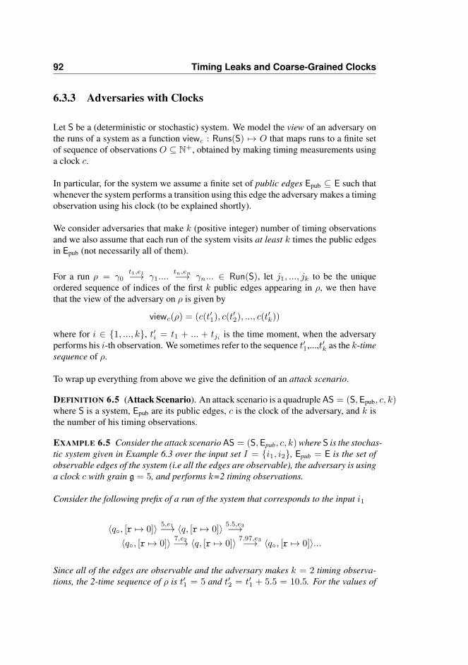
92 Timing Leaks and Coarse-Grained Clocks
6.3.3 Adversaries with Clocks
Let S be a (deterministic or stochastic) system. We model the view of an adversary onthe runs of a system as a function viewc : Runs(S) 7→ O that maps runs to a finite setof sequence of observations O ⊆ N+, obtained by making timing measurements usinga clock c.
In particular, for the system we assume a finite set of public edges Epub ⊆ E such thatwhenever the system performs a transition using this edge the adversary makes a timingobservation using his clock (to be explained shortly).
We consider adversaries that make k (positive integer) number of timing observationsand we also assume that each run of the system visits at least k times the public edgesin Epub (not necessarily all of them).
For a run ρ = γ0t1,e1−→ γ1....
tn,en−→ γn... ∈ Run(S), let j1, ..., jk to be the uniqueordered sequence of indices of the first k public edges appearing in ρ, we then havethat the view of the adversary on ρ is given by
viewc(ρ) = (c(t′1), c(t′2), ..., c(t
′k))
where for i ∈ {1, ..., k}, t′i = t1 + ... + tji is the time moment, when the adversaryperforms his i-th observation. We sometimes refer to the sequence t′1,...,t′k as the k-timesequence of ρ.
To wrap up everything from above we give the definition of an attack scenario.
DEFINITION 6.5 (Attack Scenario). An attack scenario is a quadruple AS = (S,Epub, c, k)where S is a system, Epub are its public edges, c is the clock of the adversary, and k isthe number of his timing observations.
EXAMPLE 6.5 Consider the attack scenario AS = (S,Epub, c, k) where S is the stochas-tic system given in Example 6.3 over the input set I = {i1, i2}, Epub = E is the set ofobservable edges of the system (i.e all the edges are observable), the adversary is usinga clock c with grain g = 5, and performs k=2 timing observations.
Consider the following prefix of a run of the system that corresponds to the input i1
⟨q◦, [r 7→ 0]⟩ 5,e1−→ ⟨q, [r 7→ 0]⟩ 5.5,e3−→⟨q◦, [r 7→ 0]⟩ 7,e2−→ ⟨q, [r 7→ 0]⟩ 7.97,e3−→ ⟨q◦, [r 7→ 0]⟩...
Since all of the edges are observable and the adversary makes k = 2 timing observa-tions, the 2-time sequence of ρ is t′1 = 5 and t′2 = t′1 + 5.5 = 10.5. For the values of

6.4 Quantifying Leakage in Timed Systems 93
the clock c at those two time points we have c(t′1) = 5 and c(t′2) = 10, and thereforethe view of the adversary on ρ is
viewc(ρ) = (c(t′1), c(t′2)) = (5, 10)
6.4 Quantifying Leakage in Timed Systems
In this section, we give an algorithm that given an attack scenario constructs the cor-responding timing channel. Based on the timing channel, one can then quantify theleakage of the timed system using standard measures from quantitative information-flow. We start by recalling some basics of quantitative information-flow.
6.4.1 Timing Channels and Min-Leakage
For the rest of this subsection we assume a random variable I with range the secretinput space I of a timed system, a probability distribution pI on I , and a randomvariable O with range the public set of timing observations O of the adversary. Ourdefinitions are based on [ACPS12, Smi09] and all the logarithms have base two.
The threat of the adversary guessing the secret input with one try, before making anytiming observation, is given by the min-vulnerability of I defined as
V(pI) = maxi∈IpI(i)
Min-vulnerability expresses that the adversary will choose for his guess the input thatis more probable.
The relationship between the input space and the observations of the adversary is givenby a timing channel TC : I ×O 7→ [0, 1], that is a probability transition matrix, wherefor i ∈ I and o ∈ O, TC(i, o) is the probability of O = o conditioned on I = i (i.e theconditional probability).
The expected probability of the adversary guessing the secret input, given his timingchannel, is given by the conditional min-vulnerability of I and the timing channel TC,by
V(pI ,TC) =∑o∈O
maxi∈IpI(i) · TC(i, o)
The min-vulnerability and the conditional min-vulnerability, can be turned into en-tropies by taking their negative logarithm [Smi09].

94 Timing Leaks and Coarse-Grained Clocks
For measuring the leakage of a timing channel we have the min-leakage [Smi09]
Lmin(pI ,TC) = logV(pI,TC)
V(pI)
and the min-capacityCmin(TC) = suppI
Lmin(pI ,TC)
The min-capacity is the worst-case leakage and it is realised over a uniform prior pI[ACPS12]. Based on min-leakage we can order timing channels as
DEFINITION 6.6 (Ordering on Channels) Given a random variable I with range I ,two random variables O1, O2 with range O1 and O2 resp., and the timing channelsTC1 : I ×O1 7→ [0, 1] and TC2 : I ×O2 7→ [0, 1], we write
TC1 ⪯ TC2 if ∀pI : Lmin(pI ,TC1) ≤ Lmin(pI ,TC2)
A special case of a timing channel is a deterministic timing channel. A timing channelTC : I × O 7→ [0, 1] is deterministic whenever ∀i ∈ I : ∃o ∈ O : TC(i, o) = 1 (i.eeach row of the channel contains exactly one 1).
Recall [ACPS12, Smi09] that a deterministic channel TC : I × O 7→ [0, 1] gives riseto an equivalence relation (or partition) on I , given by
i1 ≡TC i2 iff ∃o ∈ O : TC(i1, o) = 1 = TC(i2, o)
Two secrets are indistinguishable to the the adversary if and only if they give the sameobservation through the timing channel TC. For example if ≡TC is equal to ⊤ = I × Ithen ≡TC describes no leakage since all the secrets are related. On the other hand if≡TC is equal to the identity relation ⊥ = {(i, i) | i ∈ I} we have that everything isleaked since each secret produces a unique observable. In any other case where theequivalence relation ≡TC is such that ⊥ ⊂≡TC⊂ ⊤, we have partial information aboutthe secret.
Deterministic channels can be ordered based on their equivalence relation by partitionrefinement.
DEFINITION 6.7 (Partition Refinement). Given deterministic channels TC1 : I ×O1 7→ [0, 1] and TC2 : I ×O2 7→ [0, 1] we write TC1 ⊑ TC2 if the partition of TC1 isrefined by the partition of TC2.
The following theorem from [ACPS12, Smi09] shows that the leakage ordering corre-sponds to the partition refinement ordering.

6.4 Quantifying Leakage in Timed Systems 95
Step 1. For each i ∈ I let Oi = {viewc(ρ) | ρ ∈ Runs(TAi)}.
Step 2. Let I to be a random variable with range the input set I and
O to be a random variable with range O =∪
iOi. For the timing
channel TC(AS) : I ×O 7→ [0, 1], and for i ∈ I , and o ∈ O :
if S is deterministic and o ∈ Oi, then set TC(AS)(i, o) = 1.
if S is stochastic and o ∈ Oi, then set TC(AS)(i, o) = Pγqi◦(view−1
c (o)).
Otherwise, set TC(AS)(i, o) = 0.
Table 6.1: The algorithm for constructing the timing channel TC(AS) of an attack sce-nario AS = (S,Epub, c, k).
THEOREM 6.8 Given deterministic channels TC1 : I × O1 7→ [0, 1] and TC2 : I ×O2 7→ [0, 1] we have
TC1 ⊑ TC2 iff TC1 ⪯ TC2
6.4.2 Timing Channels of Deterministic Systems
We now show how one can construct the timing channel of an attack scenario wherethe system is deterministic.
Let AS = (S,Epub, c, k) be an attack scenario where S = (TAi)i∈I is a deterministicsystem. We construct the timing channel TC(AS) of AS using the algorithm givenin Table 6.1. The first step of the algorithm computes for each input i ∈ I , the setof its possible observations Oi. Since S is deterministic, Oi = {o} is a singleton.All the observations of the system are described by the set O =
∪i∈I Oi and taking
random variables I and O over the input set I and the observations O (resp.), we havethe deterministic timing channel TC(AS) : I × O 7→ [0, 1], that for input i and itsunique observation o it returns 1, otherwise it returns 0. Notice that our algorithm isindependent of our choice of min-leakage to be used as the measure for quantifyingleakage.
6.4.3 Probability Measure for Stochastic Timed Automata
To explain the construction for the case of S being stochastic we need to define a proba-bility measure on the runs of stochastic timed automata. We will then use this measureto compute the probabilities of the timing observations of an adversary.
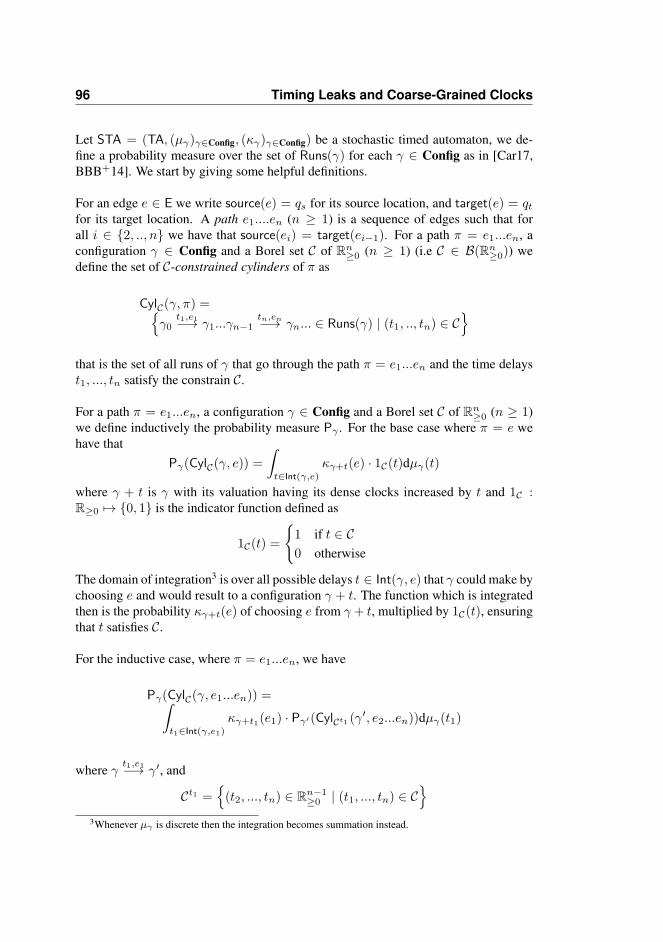
96 Timing Leaks and Coarse-Grained Clocks
Let STA = (TA, (µγ)γ∈Config, (κγ)γ∈Config) be a stochastic timed automaton, we de-fine a probability measure over the set of Runs(γ) for each γ ∈ Config as in [Car17,BBB+14]. We start by giving some helpful definitions.
For an edge e ∈ E we write source(e) = qs for its source location, and target(e) = qtfor its target location. A path e1....en (n ≥ 1) is a sequence of edges such that forall i ∈ {2, .., n} we have that source(ei) = target(ei−1). For a path π = e1...en, aconfiguration γ ∈ Config and a Borel set C of Rn
≥0 (n ≥ 1) (i.e C ∈ B(Rn≥0)) we
define the set of C-constrained cylinders of π as
CylC(γ, π) ={γ0
t1,e1−→ γ1...γn−1tn,en−→ γn... ∈ Runs(γ) | (t1, .., tn) ∈ C
}that is the set of all runs of γ that go through the path π = e1...en and the time delayst1, ..., tn satisfy the constrain C.
For a path π = e1...en, a configuration γ ∈ Config and a Borel set C of Rn≥0 (n ≥ 1)
we define inductively the probability measure Pγ . For the base case where π = e wehave that
Pγ(CylC(γ, e)) =
∫t∈Int(γ,e)
κγ+t(e) · 1C(t)dµγ(t)
where γ + t is γ with its valuation having its dense clocks increased by t and 1C :R≥0 7→ {0, 1} is the indicator function defined as
1C(t) =
{1 if t ∈ C0 otherwise
The domain of integration3 is over all possible delays t ∈ Int(γ, e) that γ could make bychoosing e and would result to a configuration γ + t. The function which is integratedthen is the probability κγ+t(e) of choosing e from γ + t, multiplied by 1C(t), ensuringthat t satisfies C.
For the inductive case, where π = e1...en, we have
Pγ(CylC(γ, e1...en)) =∫t1∈Int(γ,e1)
κγ+t1(e1) · Pγ′(CylCt1 (γ′, e2...en))dµγ(t1)
where γt1,e1−→ γ′, and
Ct1 ={(t2, ..., tn) ∈ Rn−1
≥0 | (t1, ..., tn) ∈ C}
3Whenever µγ is discrete then the integration becomes summation instead.
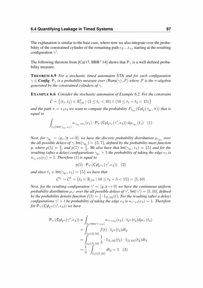
6.4 Quantifying Leakage in Timed Systems 97
The explanation is similar to the base case, where now we also integrate over the proba-bility of the constrained cylinder of the remaining path e2....en, starting at the resultingconfiguration γ′.
The following theorem from [Car17, BBB+14] shows that Pγ is a well-defined proba-bility measure.
THEOREM 6.9 For a stochastic timed automaton STA and for each configurationγ ∈ Config, Pγ is a probability measure over (Runs(γ),F) where F is the σ-algebragenerated by the constrained cylinders of γ.
EXAMPLE 6.6 Consider the stochastic automaton of Example 6.2. For the constraint
C ={(t1, t2) ∈ R2
≥0 | (5 ≤ t1 < 10) ∧ (10 ≤ t1 + t2 < 15)}
and the path π = e1e3 we want to compute the probability Pγq◦(CylC(γq◦ , π)) that is
equal to ∫t1∈Int(γq◦ ,e1)
κγq◦+t1(e1) · Pγ′(CylCt1 (γ′, e3)) dµγq◦
(t1) (1)
Next, for γq◦ = ⟨q◦, [r 7→ 0]⟩ we have the discrete probability distribution µγq◦over
the all possible delays of γ, Int(γq◦) = {5, 7}, defined by the probability mass functionp, where p(5) = 2
3 , and p(7) = 13 . We also have that Int(γq◦ , e1) = {5} and for the
resulting (after a delay) configurations γq◦ + 5 the probability of taking the edge e1 isκγ◦+5(e1) = 1. Therefore (1) is equal to
p(5) · Pγ′(CylCt1 (γ′, e3)) (2)
and since t1 ∈ Int(γq◦ , e1) = {5} we have that
Ct1 = C5 = {t2 ∈ R≥0 | 10 ≤ t2 + 5 < 15} = [5, 10)
Next, for the resulting configuration γ′ = ⟨q, r 7→ 0⟩ we have the continuous uniformprobability distribution µγ′ over the all possible delays of γ′, Int(γ′) = [5, 10], definedby the probability density function f(t) = 1
5 ·1[5,10](t). For the resulting (after a delay)configurations γ′ + t he probability of taking the edge e3 is κγ′+t(e3) = 1. Thereforefor Pγ′(CylC5(γ′, e3)) we have
Pγ′(CylC5(γ′, e3)) =∫t2∈Int(γ′,e3)
κγ′+t2(e3) · 1C5(t2)dµγ′(t2)
=
∫t2∈[5,10]
f(t) · 1C5(t2)dt2
=
∫t2∈[5,10]
1
5· 1[5,10](t2) · 1[5,10)(t2)dt2
=1
5·∫t2∈[5,10)
dt2 = 1 (3)

98 Timing Leaks and Coarse-Grained Clocks
and thus using (1), (2) and (3) we have
Pγq◦(CylC(γq◦ , e1e3)) =
2
3· 1 =
2
3
6.4.4 Timing Channels of Stochastic Systems
We now show how one can construct the timing channel of an attack scenario wherethe system is stochastic.
For an attack scenario AS = (S,Epub, c, k) of a stochastic system
S = (TAi, (µγ)iγ∈Config(κγ)
iγ∈Config)i∈I
we construct the corresponding timing channel using Table 6.1. The construction fol-lows the same logic as the one for deterministic systems, where for each input i ∈ I weneed to enumerate all the possible observations (Step 1 of Table 6.1) of the adversaryand then compute its probabilities (Step 2 of Table 6.1).
For deterministic systems, this process is straightforward, since each input is associ-ated with exactly one observation, and consequently this observation has probability 1.However, this is not the case for stochastic systems.
Starting with Step 1, for an input i ∈ I , the set of possible observations Oi ={viewc(ρ) | ρ ∈ Runs(TAi)} could turn to be infinite. To deal with this case (whenneeded) we assume that the clock c of the adversary has a limit (i.e this models thatthe clock has finite capacity). Now let g be the grain of c and l = m.g (m is a naturalnumber) its capacity. The modified clock cl : R≥0 7→ N is given by
cl(t) = min{l,
⌊t
g
⌋· g
}The modified clock cl now behaves as the clock c for time points t < l, whereas forvalues greater or equal to l its value becomes constant. Here notice that the algorithmfrom Table 6.1 remains unchanged, but only the definition of the clock changes, so wecan bound the set Oi.
Next, for Step 2 we compute the probability of an observation o. First, we have that theruns which can result in the observation o, are described by the preimage view−1
c (o),and consequently the probability of the observation o is equal to Pγqi◦
(view−1c (o)). To
show that view−1c (o) is measurable our goal is to express it as a union of disjoint con-
strained cylinders. This will also give us a more algorithmic approach for computingthe probability of o. We start by providing some auxiliary sets and operators.

6.4 Quantifying Leakage in Timed Systems 99
For the rest, we fix an input i ∈ I and let TA be its corresponding timed automatonwhere we omit the subscript i. Let
Paths =∪∞
i=k {e1...ei | | {j | ej ∈ Epub} | = k ∧source(e1) = q◦ ∧ ei ∈ Epub}
be the set of paths that start at the initial location q◦, contain exactly k public edges andthe last edge is public. Each path in this set represents one or more (prefixes of) runsthat could result to a k-sequence of timing observations.
EXAMPLE 6.7 For the attack scenario of Example 6.5, we have that k = 2 andPaths = {e1e3, e2e3}
Now for a sequence of observations o = (z1, ..., zk) ∈ Oi and a path π = e1, ..., en ∈Paths we want to specify a constraint that describes the set of possible delays that couldresult to this particular sequence of observations taking this path. We thus define
Ce1...en(z1, ..., zk) =∩ki=1
{(t1, ..., tn) ∈ Rn
≥0 | {j | ej ∈ Epub} = {j1..., jk}⇒ t1 + ...+ tji ∈ c−1(zi)
}and notice here that c−1(z) (for z ∈ {z1, ..., zk}) is an interval.4
EXAMPLE 6.8 For the path π = e1e3 ∈ Paths from Example 6.7 and the observationo = (5, 10) ∈ O we have the constraint
Cπ(o) ={(t1, t2) ∈ R2
≥0 | t1 ∈ c−1(5)}∩{
(t1, t2) ∈ R2≥0 | t1 + t2 ∈ c−1(10)
}and since c−1(5) = [5, 10) and c−1(10) = [10, 15) we have that
Cπ(o) ={(t1, t2) ∈ R2
≥0 | (5 ≤ t1 < 10)∧(10 ≤ t1 + t2 < 15)}
Finally, this allows us to express view−1c (o) as a union of disjoint constrained cylinders
asview−1
c (o) =∪
π∈Paths
CylCπ(o)(γq◦ , π)
4The same holds whenever we have a clock cl with limit l.

100 Timing Leaks and Coarse-Grained Clocks
and thus the probability of the observation o ∈ Oi is
Pγq◦(view−1
c (o)) =∑
π∈Paths
Pγq◦(CylCπ(o)(γq◦ , π))
The next example illustrates the construction of a timing channel for the case of thesystem being stochastic.
EXAMPLE 6.9 We will now compute the timing channel of the attack scenario fromExample 6.5.
The set of possible observations of the adversary is O = {(5, 10), (5, 15)} = Oi1 =Oi2 and from Example 6.7, we have that Paths={e1e3, e2e3}.
Next, let π1 = e1e3, and π2 = e2e3. For the input i1 and the observation o = (5, 10)we have that
view−1c ((5, 10)) = CylCπ1
(5,10)(γqi1◦, π1)∪
CylCπ2 (5,10)(γ
qi1◦, π2)
and thus
Pγqi1◦(view−1
c ((5, 10))) = Pγqi1◦(CylCπ1
(5,10)(γqi1◦, π1))+
Pγqi1◦(CylCπ2 (5,10)
(γqi1◦, π2))
Note that in Example 6.6, we calculated the probability Pγqi1◦(CylCπ1
(5,10)(γqi1◦, π1)) =
23 and working similarly we can show that Pγ
qi1◦(CylCπ2 (5,10)
(γqi1◦, π2)) =
15 and there-
fore we get that
Pγqi1◦(view−1
c ((5, 10))) =2
3+
1
5=
13
15
We work similarly for the observation o = (5, 15) and we get
Pγqi1◦(view−1
c ((5, 15))) = Pγqi1◦(CylCπ1
(5,15)(γqi1◦, π1))+
Pγqi1◦(CylCπ2
(5,15)(γqi1◦, π2))
= 0 +2
15=
2
15

6.5 Analysis of Timing Channels in Deterministic Systems 101
We repeat the process for the input i2, and we obtain the following timing channel
TC(AS)(i, o) =
13
15if i = i1 and o = (5, 10)
2
15if i = i1 and o = (5, 15)
8
10if i = i2 and o = (5, 10)
2
10otherwise
6.5 Analysis of Timing Channels in Deterministic Sys-tems
In this section, we start by analyzing the relationship between clock grain and leakagefor deterministic systems. Next, we present timing techniques that have been used tobypass a low-resolution clock, we present a new timing technique, and we show howthose techniques can be modelled in our framework. We finish by showing a result onthe hierarchy of those techniques in terms of how much information can be extractedfrom the adversary.
6.5.1 Relating Clock Grain and Leakage
In our first result, we show that, contrary to popular belief a coarse-grained clock mightleak more information than a fine-grained clock.
PROPOSITION 6.10 There exist deterministic system S and attack scenarios AS1,AS2 of S with clocks c1, c2 resp., and grains g1, g2 with g1 < g2 and TC(AS1) ⪯TC(AS2).
Note that Proposition 6.10 does not talk about the well-known bypassing techniques[SWT01, KS16b, SMGM17, Wra91] that have been used to side-step the defense ofa coarse-grained clock; instead it shows that the security offered by a coarse-grainedclock could be worse than the one offered by a fine-grained clock, even when bypassingtechniques are not in use.
Proposition 6.10 follows from the following example

102 Timing Leaks and Coarse-Grained Clocks
EXAMPLE 6.10 Consider a deterministic system S, whose input set is I = {i1, i2}and the system is given by two automata TAi1 and TAi2 who both have a single edgeleaving their initial location e1 = (q◦, r = 2 → , q) (for TAi1 ), and e2 = (q′◦, r =3 → , q′) (for TAi2 ) controlled by a dense clock r.
For TAi1 we have the run ρ1 = γq◦2,e1−→ γ1... and for TAi2 we have the run ρ2 =
γq′◦3,e2−→ γ′1.... Next consider the two attack scenarios AS1 = (S, {e1, e2} , c1, 1)
and AS2 = (S, {e1, e2} , c2, 1) where the edges of interest are observable, the clockc1 has grain g1 = 2, the clock c2 has grain g2 = 3, and the adversary makes onetiming observation. Following the algorithm from Table 6.1, for AS1 we have Oi1 ={viewc1(ρ1)} = {c1(2)} = {2} and Oi2 = {viewc1(ρ2)} = {c1(3)} = {2}, whereasfor AS2 we have Oi1 = {viewc2(ρ1)} = {c2(2)} = {0} and Oi2 = {viewc2(ρ2)} ={c2(3)} = {3} and thus we get the timing channels
TC(AS1)(i, o) = 1 TC(AS2)(i, o) =
1 if i = i1
and o = 0
1 if i = i2
and o = 3
0 otherwise
We then have that ≡TC(AS1)= ⊤, whereas ≡TC(AS2)= ⊥, and thus TC(AS1) ⊑ TC(AS2).Next, using Theorem 6.8 we get that TC(AS1) ⪯ TC(AS2) showing that the attack sce-nario where the clock has grain g2 = 3 leaks more than the scenario where the clockhas grain g1 = 2.
Although, we showed that, in general, increasing the grain of the clock does not in-crease security, with our next theorem we provide sufficient conditions for when thisactually happens.
THEOREM 6.11 (Multiple-g security.) Let AS1 = (S,Epub, c1, k) and AS2 = (S,Epub, c2, k)be two attack scenarios such that S is deterministic and the clocks c1, c2 have grainsg1, g2 (resp.) and g1 is a multiple of g2. We then have that
TC(AS1) ⪯ TC(AS2)
In particular, Theorem 6.11 shows that whenever the system is deterministic and weincrease the grain of the clock to a multiple of it, the new low-resolution clock givesbetter (or at least the same) security.

6.5 Analysis of Timing Channels in Deterministic Systems 103
tslow tslow + tpad
tfast tfast + tpad
time
(a) The one-pad technique.
Learning phase:tpad = g4
Attack phase:tf = c(tf ) + g− 3 · tpad
tfc(tf ) tf + 3 · tpad
4 · tpad
g
g
time
(b) The clock-edge technique.
Figure 6.5: Padding timing techniques.
6.5.2 Timing Techniques
Several timing techniques have successfully side-stepped the defence provided by acoarse-grained clock, by building their own fine-grained clocks from primitives suchas coarse-grained clocks and simple counter processes [SWT01, KS16b, SMGM17].We now explain how techniques such as the one-pad and the clock-edge [SMGM17,KS16b] work, and we present a new timing technique called the co-prime. We studythose techniques in a setting as in [SMGM17, KS16b], where the adversary tries tomeasure the timing of a function f that is sent to the victim in a piece of maliciouscode where he performs his timing technique.
The One-Pad Technique In many cases the adversary wants only to distinguish be-tween two different executions of f , tslow and tfast, where tfast is smaller than tslow.Using the one-pad technique the adversary exploits the fact that the time between twoclock-edges is constant and equal to g. He then chooses to perform a constant timeoperation called padding.
If now tpad is the time of the padding operation, the padding is chosen in such a waysuch that the short duration tslow plus the duration of the padding tpad always crossesthe next clock-edge i.e tslow + tpad ≥ c(tslow) + g, while tfast + tpad < c(tfast) + g.
After the end of the padding operation, if the value of the adversary’s clock is abovethe next clock-edge, he infers that the slow event has happened, otherwise it is the caseof the fast event. Figure 6.5 (a) depicts a scenario of the one-pad technique.

104 Timing Leaks and Coarse-Grained Clocks
The Clock-Edge Technique The one-pad technique is good enough for distinguish-ing between two different execution times, however, sometimes an adversary requiresa mechanism that gives more precise measurements. For those cases, the clock-edgetechnique can be used. The fact that a clock c with grain g is being increased witha constant rate i.e every g, gives the attacker the ability to express the duration of asequence of his operations as a portion to g. In particular, similarly to the one-padtechnique the adversary here adds a padding for one or more times.
The technique begins with a learning phase (Figure 6.5 (b) top), where the adversaryperforms his padding operation between two consecutive clock-edges. Assuming thata number of m operations have occurred between the two edges, and using that theduration of m padding operations is equal to g, the attacker derives that the duration ofhis padding operation is tpad = g
m .
The attack phase (Figure 6.5 (b) bottom) of the technique then begins with the adver-sary aligning the operation f that he wants to measure to a clock-edge and right afterthe execution of f completes, he inspects the value of his clock c(tf ). Immediatelyafter, he starts performing his padding operator until he observes the next clock-edge.If at this point he observes n paddings the duration tf of f can be approximated by thenumber c(tf ) + g− n · tpad ≈ tf .5
The Co-Prime Technique Looking at the one-pad and the clock-edge technique onecould think of the following questions: Do we always need a padding operation withduration less than g in order to perform fine-grained measurements? What happens ifwe do not stop at the next clock-edge and we continue performing the padding operatorfor a couple of more times?
For the co-prime technique, the adversary may not necessarily use a padding with tim-ing less than the grain of the clock, and he may also not stop at the next clock-edge. Inparticular, in the co-prime technique, the adversary performs a padding operation forg (the grain of the clock) times, and the timing of his padding tpad is co-prime with g.Why this technique works becomes clear in the next two subsections.
6.5.3 Modelling Timing Techniques
We use the algorithm in Table 6.2 to model the essential aspects of the timing tech-niques: one-pad, clock-edge and co-prime.
5In the clock-edge techniques presented in [KS16b, SMGM17] the padding operation corresponds to theincrement of a counter.
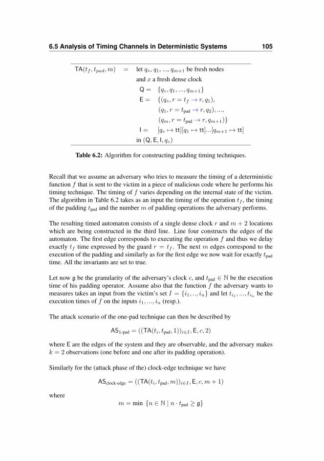
6.5 Analysis of Timing Channels in Deterministic Systems 105
TA(tf , tpad,m) = let q◦, q1, ..., qm+1 be fresh nodes
and x a fresh dense clock
Q = {q◦, q1, ..., qm+1}E = {(q◦, r = tf → r, q1),
(q1, r = tpad → r, q2), ...,
(qm, r = tpad → r, qm+1)}I = [q◦ 7→ tt][q1 7→ tt]...[qm+1 7→ tt]
in (Q,E, I, q◦)
Table 6.2: Algorithm for constructing padding timing techniques.
Recall that we assume an adversary who tries to measure the timing of a deterministicfunction f that is sent to the victim in a piece of malicious code where he performs histiming technique. The timing of f varies depending on the internal state of the victim.The algorithm in Table 6.2 takes as an input the timing of the operation tf , the timingof the padding tpad and the number m of padding operations the adversary performs.
The resulting timed automaton consists of a single dense clock r and m + 2 locationswhich are being constructed in the third line. Line four constructs the edges of theautomaton. The first edge corresponds to executing the operation f and thus we delayexactly tf time expressed by the guard r = tf . The next m edges correspond to theexecution of the padding and similarly as for the first edge we now wait for exactly tpadtime. All the invariants are set to true.
Let now g be the granularity of the adversary’s clock c, and tpad ∈ N be the executiontime of his padding operator. Assume also that the function f the adversary wants tomeasures takes an input from the victim’s set I = {i1, .., in} and let ti1 , ..., tin be theexecution times of f on the inputs i1, ..., in (resp.).
The attack scenario of the one-pad technique can then be described by
AS1-pad = ((TA(ti, tpad, 1))i∈I ,E, c, 2)
where E are the edges of the system and they are observable, and the adversary makesk = 2 observations (one before and one after its padding operation).
Similarly for the (attack phase of the) clock-edge technique we have
ASclock-edge = ((TA(ti, tpad,m))i∈I ,E, c,m+ 1)
wherem = min {n ∈ N | n · tpad ≥ g}

106 Timing Leaks and Coarse-Grained Clocks
Again E are the edges of the system and they are all observable. The number m ofpaddings is ensuring that independently of f ’s timing, the padding will cross the nextclock-edge.
Finally, if g is co-prime with tpad, the attack scenario of the co-prime technique is
ASco-prime = ((TA(ti, tpad, g))i∈I ,E, c, g+ 1)
6.5.4 A Hierarchy of Timing Techniques
We now compare the power of the timing techniques, one-pad, clock-edge and co-prime in terms of how much information the adversary can extract using them, and weexplain in more details why the co-prime technique works. We start with an examplethat illustrates the construction (Table 6.2) of the attack scenarios of the clock-edge andthe co-prime technique and shows that the co-prime technique can distinguish more.
EXAMPLE 6.11 Assume that we want to distinguish between two timing behavioursof an operation f that takes the inputs i1 and i2 and runs for time ti1 = 8 and ti2 = 9respectively. Assume also that we have a clock c with grain g = 10 and a padding withtiming tpad=2.
For the clock-edge technique we need to add our padding for
m = min {n ∈ N | n · tpad ≥ g}= min {n ∈ N | n · 2 ≥ 10}= 5
Using the algorithm of Table 6.2 we get the system S = (TA(ti, 2, 5))i∈I and for eachi ∈ I we have a timed automaton TA(ti, 2, 5) = (Q,E, I, q◦) where Q = {q◦, q1, ..., q6}and E contains the edges e1 = (q◦, r = ti → r, q1), e2 = (q1, r = 2 → r, q2),...,e6 =(q5, r = 2 → r, q6), and I = λq.tt.
We then have two runs
ρ1 = γ18,e1−→ γ2
2,e2−→ ...2,e6−→ γ7
andρ2 = γ′1
9,e′1−→ γ′22,e′2−→ ...
2,e′6−→ γ′7
for i1 and i2 respectively.
The view of the adversary on ρ1 is
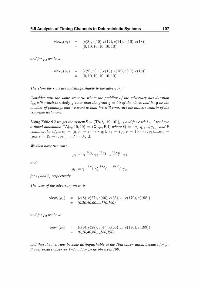
6.5 Analysis of Timing Channels in Deterministic Systems 107
viewc(ρ1) = (c(8), c(10), c(12), c(14), c(16), c(18))= (0, 10, 10, 10, 10, 10)
and for ρ2 we have
viewc(ρ2) = (c(9), c(11), c(13), c(15), c(17), c(19))= (0, 10, 10, 10, 10, 10)
Therefore the runs are indistinguishable to the adversary.
Consider now the same scenario where the padding of the adversary has durationtpad=19 which is strictly greater than the grain g = 10 of the clock, and let g be thenumber of paddings that we want to add. We will construct the attack scenario of theco-prime technique.
Using Table 6.2 we get the system S = (TA(ti, 19, 10))i∈I and for each i ∈ I we havea timed automaton TA(ti, 19, 10) = (Q, q◦,E, I) where Q = {q◦, q1, ..., q11} and Econtains the edges e1 = (q◦, r = ti → r, q1), e2 = (q1, r = 19 → r, q2),...,e11 =(q10, r = 19 → r, q11), and I = λq.tt.
We then have two runs
ρ1 = γ18,e1−→ γ2
19,e2−→ ...19,e11−→ γ12
andρi2 = γ′1
9,e′1−→ γ′219,e′2−→ ...
19,e′11−→ γ′12
for i1 and i2 respectively.
The view of the adversary on ρ1 is
viewc(ρ1) = (c(8), c(27), c(46), c(65), ..., c(179), c(198))= (0,20,40,60,...,170,190)
and for ρ2 we have
viewc(ρ2) = (c(9), c(28), c(47), c(66), ..., c(180), c(199))= (0,20,40,60...,180,190)
and thus the two runs become distinguishable at the 10th observation, because for ρ1the adversary observes 170 and for ρ2 he observes 180.

108 Timing Leaks and Coarse-Grained Clocks
To understand better why the co-prime technique works observe that in general a tim-ing technique is distinguishing two timings t1, t2, when observing differences in thesequences
(c(t1), c(t1 + tpad), ..., c(t1 +m · tpad))
and
(c(t2), c(t2 + tpad), ..., c(t2 +m · tpad))
The question therefore is how to choose the appropriate number m of paddings formaking the two sequences distinguishable.
However, Fact 9 shows that the two sequences are distinguishable if and only if
(c(t1), c(t1 + (tpad mod g)), ..., c(t1 + (m · tpad mod g)))
and
(c(t2), c(t2 + (tpad mod g)), ..., c(t2 + (m · tpad mod g)))
are different.
The co-prime technique exploits this fact and rephrases the question of the paddingtechniques to: (1) what padding is needed, and (2) how many times I need to add it soby the end of the timing technique the padding times generate the entire Zg set (answer:(1) tpad needs to be co-prime with g, and (2) it needs to be added g times).
We finish by showing that the timing-techniques of the one-pad, clock-edge and theco-prime form a strict hierarchy in terms of the amount of information the adversarycan extract. In particular, we show that the co-prime technique achieves the most in-formation leakage among the other techniques, whereas the one-pad achieves the leastleakage.
THEOREM 6.12 Let f be a function that runs on the input set I and its timing be-haviour is described by the family (ti)i∈I . Let also c be a clock with grain g, a paddingwith time tpad, and AS1-pad, and ASclock-edge the corresponding attack scenarios of theone-pad and the clock-edge techniques. Consider also another padding with durationt′pad that is co-prime with g, and let ASco-prime be the corresponding co-prime attackscenario. We then have that
TC(AS1-pad) ⪯ TC(ASclock-edge) ⪯ TC(ASco-prime)

6.6 Analysis of Timing Channels in Stochastic Systems: A Case Study109
q◦
encryption
noise
communication
q
q′
r = 10 →r = 1 →
→ r
r = tenc(k) →
tenc
1
1
110
10
(a) The stochastic timed automaton of the sensorwhen it operates on key k.
200 400 600 800 1,0001
2
3
4
5
6
g
(b) The effect of increasing the grain gon the min-capacity.
Figure 6.6: Case Study:RSA
6.6 Analysis of Timing Channels in Stochastic Systems:A Case Study
In this section, we analyse timing channels of stochastic systems. In particular, weperform a case study, based on the Example 2.11. It consists of two parts. The firstpart is the modelling of our case study as a system of timed automata. In the secondpart, we consider different adversaries (with respect to their clock), we compute theirtiming channels, and we derive our insights about the relation between clock grain andleakage in stochastic systems.
6.6.1 Modelling the Case Study
We now recall the Example 2.11, and we give more details about it, while we leavesome calculations needed in Appendix E. We consider a scenario of a distributed sys-tem that consists of a sensor and a controller. We are interested in modelling the be-haviour of the sensor.
In particular, the sensor constantly computes some data and communicates it to thecontroller. For ensuring data integrity, the sensor always encrypts (signs) the data with

110 Timing Leaks and Coarse-Grained Clocks
his RSA private key. The RSA encryption is implemented using the modular exponen-tiation algorithm which computes xk mod n for the secret key k, some data x and theconstant modulus n. The implementation is the same as the one from Example 2.3 andit is given by the following piece of code
m := (1 ∗ 1) mod n;for (j = 0; j < len(k); j++) {
m := (m ∗ m) mod n;if (k[j] == 1) thenm := (m ∗ x) mod n;
}
Here the secret bits of the key are stored in the array k[]. Due to the conditional execu-tion of the modular multiplication operation m = m ∗ x mod n the running time of thisprogram reveals information about the entries of k.
To decrease the correlation between the encryption time and the secret bits of the key,the sensor adds noise to the encryption time by delaying for some additional periodafter each encryption, and then it communicates the data to the controller.
In our model, we assume that the sensor performs each modular multiplication in 1time unit. We also assume that the size of the secret key k is 1024-bits, and thus thetimed needed for one encryption is
tenc(k) = 1025 + Ham(k)
where Ham(k) is the Hamming weight of k (i.e the number of non-zero bits).
For the noise added by the sensor, we assume that the sensor chooses randomly to waitfor t ∈ {1, 2, ..., 10}, with respect to a uniform distribution.
We model the timing behaviour of the sensor as a stochastic timed system with inputspace the 21024 keys and for each key, we have a stochastic timed automaton as depictedin Figure 6.6 (a).
The automaton consists of three locations and one dense clock x that is used to controlthe transitions between them. Starting at the initial location q◦, the automaton performsan encryption with respect to a Dirac’s distribution on the time point tenc(k), model-ing in that way that an encryption takes exactly tenc(k) time units. Next, it moves tolocation q, where we have 10 different edges leaving q, one for each possible delay,modelling the additional noise added by the sensor. A delay is chosen uniformly andthe automaton moves to location q′. At location q′ the automaton communicates themessage to the controller with respect to an exponential distribution of parameter λ = 6time units.

6.7 Related Work 111
Finally, on the side of the controller, we assume an adversary who runs malicious codethat uses the clock of the controller and measures the time needed for the sensor to sendits data, trying to infer bits of the sensor’s private key.
6.6.2 Analysing the Leakage in the Case Study
Using Table 6.1, we constructed the timing channel for 1000 different attack scenar-ios (for different clocks), where we have as observable edges the ones that model thecommunication of the message. We assumed an adversary that performs one timing ob-servation and uses a clock with grain g = 1, 2, ..., 1000 and with some limit l > 15000.The details of the construction can be found in the Appendix E.
We then computed the min-capacity for each one of those channels. The graph inFigure 6.6 (b) shows the effect of increasing the grain of the clock on the informationleaked by the channel. The maximum leakage is around 6.7-bits for grain g = 1,whereas we have 1-bit leakage for the attack scenarios where the grain is above 678.We can also see from the graph that increasing the grain of the clock does not alwaysgive us less information leakage. In particular, for g = 514, we have around 1.43-bitsleaked, whereas for g = 520 we have around 1.58-bits, which leads to the followingproposition
PROPOSITION 6.13 There exists stochastic system S and attack scenarios AS1, AS2of S with clocks c1, c2 resp., and grains g1, g2 with g1 < g2, and
Cmin(TC(AS1)) < Cmin(TC(AS2))
Proposition 6.13 shows also for the case of stochastic systems that the security offeredby a coarse-grained clock could be worse than the one offered by a fine-grained clock,even when bypassing timing techniques are not used.
Finally, our experiment shows that increasing the grain of the clock to a multiple ofit results to a channel with less (or equal) leakage, however a proof that this holds forgeneral stochastic systems (i.e Theorem 6.11 generalizes to stochastic systems) is stillelusive.
6.7 Related Work
There is an extensive work on formally quantifying and providing bounds on the leak-age of timing channels for cryptographic implementations [CRS83, KD09, KB07, BK15],

112 Timing Leaks and Coarse-Grained Clocks
remote network adversaries [ZAM11, GH02] and language-based settings [PHW08,MKP+18, DFK+13]. The main novelty of our approach compared to those is the mod-elling of coarse-grained clock adversaries, and the novel algorithms that we give forconstructing timing channels for systems of timed automata.
Clocks of certain granularity and their defence power have been studied a lot in practiceusing empirical ways. Schwarz et al. [SMGM17] provided a wide range of techniquesthat can be used to build fine-grained clocks in Javascript, including similar techniquesto the one-pad and the clock-edge. Wei-Ming Hu [Hu91, Hu92] proposed the conceptof fuzzy time. Instead of increasing the grain of the clock, fuzzy time modifies itsfunctionality by randomly changing its grain within a certain period. Vattikonda et al.[VDS11] proposed fuzzy time for mitigating timing channels in hypervisors, and alsoevaluated the impact of this countermeasure on the usability of the system. Fuzzy timehas also been proposed and implemented in Firefox by Kohlbrenner et al. [KS16b]for defeating timing channels in browsers. They also showed that this mitigation iseffective against timing techniques such as the clock-edge.
Mantel et al. [MS07] proposed an information-theoretic framework for comparing theeffectiveness of different countermeasures on the bandwidth of interrupt-related chan-nels, that is a special case of timing channels. In their analysis, they include the coun-termeasure of coarse-grained clocks and fuzzy time. For coarse-grained clocks, theyperform a case-study where they show how increasing the grain of the clock reducesthe capacity of the channel. Our approach is more general, while we also showed thatincreasing the grain of a clock might result in more leakage, and we provided formalproofs for when this is not the case.
6.8 Conclusions
We performed the first principled information-flow analysis of timing leaks w.r.t. ad-versaries with clocks of reduced resolution, where we derived novel insights into theeffectiveness of existing attacks and countermeasures.
In particular, we introduced a model of timed automata systems which is generalenough to cater for scenarios where the victim’s timing behaviour is stochastic or de-terministic, and a model of adversary that is parametric on the clock’s granularity andthe number of timing observations.
We provided novel algorithms for transforming such a model into an information-theoretic channel, allowing us to measure the leakage conveyed by it using existingtechniques from quantitative information-flow.

6.8 Conclusions 113
Based on that, we showed that a coarse-grained clock might leak more than a fine-grained clock, and we provided sufficient conditions for when one can achieve bettersecurity by increasing the grain of the clock. For the techniques that have bypassed thiscountermeasure, we showed that they form a strict hierarchy in terms of the informationan adversary can extract using them, and we introduced a new timing technique.
Scalability and Automation The rich expressiveness offered from the stochastictimed automata, and our adversary model, comes with the cost of scalability issues,while it also puts obstacles for automating our work. In particular, we have the follow-ing issues
• our approach relies on enumeration of the adversary’s set of outputs O, whichcan be very large.
• the number k of the adversary’s observations can be very long in realistic attacks.
• the construction of the timing channel in the stochastic case involves calculationsof the form
Pγ(...) =
∫t1∈C1
...
∫tn∈Cn
dµn(tn)...dµ1(t1)
which makes it difficult, or even impossible to calculate them sometimes.
As a first step, to overcome those difficulties, we could limit ourselves to deterministicsystems. In this case, we know that min-capacity only depends on the cardinality |O| ofthe output set O. In particular, we have that min-capacity=log|O| [ACPS12], and thusany over-approximation O# ⊇ O gives us a direct upper bound on the min-capacity i.elog|O| ≤ log|O#|.
For dealing with the arbitrary number k of the adversary’s observations we can useresults from quantitative information flow [KD09, SS17]. In particular, for (stochastic)systems with independent observations, calculating the channel for a single observationcan be used to give us bounds on the leakage for k observations [KD09, SS17].
As another approach, we could approximate the security offered by a coarse-grainedclock using techniques from statistical model checking, and automate our analysis us-ing the model-checker for (stochastic) timed automata UPPAAL [DLL+15]. This ap-proach is particularly interesting. since it can allow for estimating the trade-off betweensecurity and safety properties of a system.

114 Timing Leaks and Coarse-Grained Clocks

CHAPTER 7
Conclusions
In this thesis, we leveraged approaches from the theory of information flow and devel-oped novel techniques for the qualitative and quantitative security analysis of real-timesystems, which we modelled using timed automata.
Qualitative developments In Chapter 3, we started by defining a non-interferencecondition, which requires independence between the initial secret components and thefinal public components of a timed automaton. Our condition caters for adversaries thatcan infer secret information through timing and control-flow channels, upon the termi-nation of the automaton. As a first step for checking our non-interference conditionwe developed the language timed commands, whose semantics is given using timedautomata. We then developed a type system for our language, and we proved that type-checked programs satisfy non-interference. The prime intention of this work was toidentify and solve core information security problems in timed automata, however, dueto its language-based nature it cannot deal with every timed automaton.
Our work in Chapter 4 extended the work of Chapter 3 in various ways. First, wedefined a bisimulation-based security condition. Our condition caters for (a) timedautomata that need to protect not only secret initial information, but also fresh infor-mation computed during the execution of the automaton, (b) adversaries observinginformation at various locations of the automaton, and not only the final ones, and (c)scenarios where computations leading to certain locations of the automaton may release

116 Conclusions
secret information. We then developed an algorithm that traverses a timed automatonand generates information flow constraints. In particular, our algorithm makes use of anovel post-dominator relation in order to deal with information flows created from theunstructured control flow in timed automata. Finally, we proved that whenever the con-straints generated from our algorithm are satisfied, then the timed automaton satisfiesour security condition.
In Chapter 5, we presented the BTCL logic, which can be used for enforcing data- andtime-dependent access control on networks of timed automata. We started by defin-ing information flow instrumented semantics for networks. Specifically, our semanticsmake use of labels, called behaviours, that capture the different explicit informationflows in the network. Our logic is based on those behaviours and access control con-ditions are formulated as formulas in our logic. We then presented techniques fortranslating our networks and formulas into models of timed automata and TCTL-likeformulas (resp.), that can be handled by standard model-checkers such as UPPAAL[UPP]. Finally, we implemented our translations and we illustrated how our approachcan be fully automated.
Quantitative developments In Chapter 6, we presented the first information flowanalysis of the countermeasure reducing clock resolution. Our development considersattack scenarios which are described by a victim and an adversary. In particular, wedefined a (stochastic) timed automata-based system, which describes the victim whocomputes on some secret input. The system provides a clock of a certain granularity,which can be accessed by an adversary. The adversary observes the time of the systemmaking queries to the system’s clock during certain computations and tries to infer thesystem’s secret.
We then presented novel algorithms for constructing the information theoretic timingchannel of an attack scenario. Any information theoretic measure can then be used tocalculate the leakage of the timing channel, allowing one to evaluate the effectivenessof this countermeasure.
We then used our techniques and we achieved the following: (1) we showed that con-trary to the popular-belief a coarse-grained clock might leak more than a fine-grainedone, (2) we gave sufficient conditions for when increasing the grain of the clock weachieve less information leakage, and (3) we showed that the attack techniques usedto bypass this countermeasure form a strict hierarchy in terms of the information anadversary can extract using them.

APPENDIX A
Proofs of Chapter 3
A.1 Lemma 3.2
PROOF. We prove the first statement by induction on ⊢[qt:gt][qs:gs]
C : E, I&χ using that ;is transitive.
We prove the second statement by induction on ⊢[qt:gt][qs:gs]
T : E, I&χ. It is immediate forthe two axioms for actions because {qs}∪fv(fstgtgs(T )) = χ. In the rule for compositionfor T ;[g]C observe that {qs} ∪ fv(fstgtgs(T ;
[g]C)) = {qs} ∪ fv(fstggs(T )) and that theinduction hypothesis gives that {qs} ∪ fv(fstggs(T )) ; {q} because χ1 ; {q}.
We have {qs} ∪ fv(fstggs(T )) ; ass(T ) from the induction hypothesis, {q} ; Clocksfrom the rule, and {q} ; ass(C) from the previous result, and then get {qs} ∪fv(fstgtgs(T ;
[g]C)) ; ass(T ;[g]C). Next suppose χ = χ2 ; χ′; from the previousresult we have {q} ; χ′ and hence {qs} ∪ fv(fstgtgs(T ;
[g]C)) ; χ′.
A.2 Theorem 3.3
PROOF. We proceed by induction on ⊢[qt:gt][qs:gs]
C : E, I&χ.

118 Proofs of Chapter 3
Case: Assignment Assume that (σ0, δ0) ≡gs (σ′0, δ
′0) and that
η ∈ Final[[({(qs, g→ x :=a: r, qt)}), [qs 7→ gs][qt 7→ gt]) : qs 7→ qt]](σ0, δ0)
In case η = (σ1, δ1) it follows that there exists t ≥ 0 such that σ1 = [[x :=a]]σ0 andδ1 = (δ0 + t)[r 7→ 0], and such that [[g]](σ0, (δ0 + t)) = tt, [[gs]](σ0, δ0 + t) = tt and[[gt]](σ1, δ1) = tt. Defining η′ = (σ′
1, δ′1) = ([[x :=a]]σ′
0, (δ′0 + t)[r 7→ 0]) ensures
that [[g]](σ′0, (δ
′0 + t)) = tt, [[gs]](σ′
0, δ′0 + t) = tt and [[gt]](σ
′1, δ
′1) = tt because all
variables and clocks tested are low and hence
η ≡gt η′ ∈ Final[[({(qs, g→ x :=a: r, qt)}), [qs 7→ gs][qt 7→ gt]) : qs 7→ qt]](σ
′0, δ
′0)
In case η = ⊥ it follows that there is no value of t ≥ 0 such that [[g]](σ0, (δ0+ t)) = tt,[[gs]](σ0, δ0 + t) = tt and [[gt]](σ1, δ1) = tt. Then there also is no value of t ≥ 0 suchthat [[g]](σ′
0, (δ′0 + t)) = tt, [[gs]](σ′
0, δ′0 + t) = tt and [[gt]](σ
′1, δ
′1) = tt because all
variables and clocks tested are low and hence setting η′ = ⊥ establishes that
η ≡ η′ ∈ Final[[({(qs, g→ x :=a: r, qt)}), [qs 7→ gs][qt 7→ gt]) : qs 7→ qt]](σ′0, δ
′0)
The other direction is similar and this completes the assignment case.
Case: Sequence We shall write
F = Final[[(E1 ∪ E2, I1 ∪ I2[qs 7→ gs][q 7→ g][qt 7→ gt]) : qs 7→ qt]]
F1 = Final[[(E1, I1[qs 7→ gs][q 7→ g]) : qs 7→ q]]
F2 = Final[[(E2, I2[q 7→ g][qt 7→ gt]) : q 7→ qt]]
and observe that F = F1 ⋄ F2. The result then follows from the induction hypothesesand Fact 2.
Case: Looping We shall write
F = Final[[(∪
i Ei,∪
i Ii[qs 7→ gs][qt 7→ gt]) : qs 7→ qt]]
Fi =
{Final[[(Ei, Ii[qs 7→ gs]) : qs 7→ qs]] whenever i ≤ nFinal[[(Ei, Ii[qs 7→ gs][qt 7→ gt]) : qs 7→ qt]] whenever i > n
and this gives rise to the equation
F = (
n∪i=1
Fi ⋄ F ) ∪m∪
i=n+1
Fi
We shall consider two subcases, one where the condition ΦT1,··· ,Tn
Tn+1,··· ,Tm[qt:gtqs:gs ] is true and
one where it is false.

A.2 Theorem 3.3 119
Subcase: Looping when ΦT1,··· ,Tn
Tn+1,··· ,Tm[qt:gtqs:gs ] is true In this case (using the notation
of Table 3.2) all the variables and clocks in∪m
i=1 fv(fstgigs(Ti)) are low. Assume that
(σ0, δ0) ≡gs (σ′0, δ
′0) and that η ∈ F (σ0, δ0). This must be because of a trace as
considered in Section 3.1.
If this trace visits qs infinitely often we will be able to construct a sequence k1, k2, · · · , ki, · · ·such that each ki ≤ n and
∀i > 0 : (σi, δi) ∈ Fki(σi−1, δi−1)
and η = ⊥. By the induction hypothesis we can find (σ′i, δ
′i) such that
∀i > 0 : (σi, δi) ≡gs (σ′i, δ
′i) ∈ Fki
(σ′i−1, δ
′i−1)
and this establishes that ⊥ ∈ F (σ′0, δ
′0).
If the trace visits qs only finitely often we will be able to construct a sequence k1, k2, · · · , kjsuch that ∀i < j : ki ≤ n and kj ≤ m and
∀i ∈ {1, · · · , j − 1} : (σi, δi) ∈ Fki(σi−1, δi−1)
η ∈ Fkj(σj−1, δj−1)
By the induction hypothesis we can find (σ′i, δ
′i) and η′ such that
∀i ∈ {1, · · · , j − 1} : (σi, δi) ≡gs (σ′i, δ
′i) ∈ Fki
(σ′i−1, δ
′i−1)
η ≡ η′ ∈ Fkj(σ′
j−1, δ′j−1)
and this establishes that η′ ∈ F (σ′0, δ
′0).
The other direction is similar and this completes the subcase.
Subcase: Looping when ΦT1,··· ,Tn
Tn+1,··· ,Tm[qt:gtqs:gs ] is false In this case all the variables and
clocks in∪n
i=1 fv(fstgigs(Ti)) are low but this is not necessarily the case for those in∪m
i=n+1 fv(fstgigs(Ti)); however, we do know that [[gs]](σ, δ) ⇒ ⊥ ̸∈ F (σ, δ). Assume
that (σ0, δ0) ≡gs (σ′0, δ
′0) and that η ∈ F (σ0, δ0). The assumptions of the subcase
ensure that η ̸= ⊥.
We will be able to construct a sequence k1, k2, · · · , kj such that ∀i < j : ki ≤ n andkj > n and
∀i ∈ {1, · · · , j − 1} : (σi, δi) ∈ Fki(σi−1, δi−1)
η ∈ Fkj(σj−1, δj−1)
By the induction hypothesis we can find (σ′i, δ
′i) such that
∀i ∈ {1, · · · , j − 1} : (σi, δi) ≡gs (σ′i, δ
′i) ∈ Fki(σ
′i−1, δ
′i−1)
There are now two scenarios for how to proceed.

120 Proofs of Chapter 3
Subcase scenario where all variables and clocks in fv(fstgtgs(Tkj)) are low In this
case we can find η′ ∈ Fkj(σ′
j−1, δ′j−1) such that η ≡ η′.
Subcase scenario where at least one variable or clock in fv(fstgtgs(Tkj)) is high
Then ass(Tkj) cannot contain any low variable or clock and hence there is t ≥ 0
such that η ≡ (σj−1, δj−1 + t) where the addition of t takes care of the poten-tial delay in qs. Next we use that ⊥ ̸∈ F (σ′
j−1, δ′j−1) to obtain k′j , σ
′j , δ
′j such that
(σ′j , δ
′j) ∈ Fk′
j(σ′
j−1, δ′j−1).
It cannot be the case that k′j ≤ n. To see this, assume by way of contradiction thatk′j ≤ n. Then (σj−1, δj−1) would be a witness for sat(fstgtgs(Tkj
)∧fstgsgs(Tk′j)) ensuring
that fstgtgs(Tkj ) ; ass(Tk′j) so that ass(Tk′
j) could not contain a low variable or clock. It
would follow that there would be t′ ≥ 0 such that (σ′j , δ
′j) ≡gs (σj−1, δj−1+ t
′) wherethe addition of t′ is due to the possibility of delay in qs. But then we would be ableto construct an infinite sequence (σ′
l, δ′l) for l > j such that (σ′
l, δ′l) ∈ Fk′
j(σ′
l−1, δ′l−1)
and (σ′l, δ
′l) ≡gs (σ′
j−1, δ′j−1 + t′ would hold for l ≥ j. But this would contradict the
fact that ⊥ ̸∈ F (σ′j , δ
′j).
We are left with the case where k′j > n. We must have that ass(Tk′j) cannot contain any
low variable or clock: either one variable or clock in fstgtgs(Tk′j) is high and it follows as
in a case above, or all variables and clocks in fstgtgs(Tk′j) are low and it follows because
(σj−1, δj−1 + t) is a witness for sat(fstgtgs(Tkj) ∧ fstgtgs(Tk′
j)) and we could proceed as
in a case above. Hence (σ′j , δ
′j) = (σ′
j−1, δ′j−1 + t′) for some t′ ≥ 0.
It remains to show that t′ can be chosen to be t. For this we use that all clocks infstgtgs(Tkj ) and fstgtgs(Tk′
j) are low and that fstgtgs(Tkj ) = fstgtgs(Tk′
j).
The other direction is similar and this completes the subcase.

APPENDIX B
Proofs of Chapter 4
B.1 Proposition 4.1
Assume that all the traces in Traces[[TA : qs 7→ qt]](σ, δ) are successful and we wantto show that there exists tr ∈ Traces[[TA : qs 7→ qt]](σ, δ) with a maximal length m.
We use results from model-checking for timed automata [HSW12]. We define theregion graph RG(TA) of TA, that is a finite graph where nodes of the region graph areof the form (q, reg) where reg is a clock region, that is an equivalence class definedon the clock states (for details we refer to [HSW12]). Configurations of RG(TA) areof the form ⟨(q, reg), σ⟩ and we have that ⟨(q, reg), σ⟩ =⇒ ⟨(q′, reg′), σ′⟩ if there areδ ∈ reg, δ′ ∈ reg′, t ≥ 0, σ′ such that the automaton TA performs the transition⟨q, σ, δ⟩ t−→ ⟨q′, σ′, δ′⟩.
Lemma 1 of [HSW12] then states that each abstract run (finite or infinite) in the regiongraph RG(TA) can be instantiated by a run (finite or infinite resp.) in TA and viceversa. This is based on the property of the region graph of being pre-stable that is that⟨(q, reg), σ⟩ =⇒ ⟨(q′, reg′), σ′⟩ if ∀δ ∈ reg there are δ′ ∈ reg′, t ≥ 0, σ′ such that⟨q, σ, δ⟩ t−→ ⟨q′, σ′, δ′⟩.
Therefore, the computation tree T of ⟨q, σ, δ⟩ in TA has the same depth as the computa-
122 Proofs of Chapter 4
tion tree T ′ of ⟨(q, [δ]), σ⟩ inRG(TA) where [δ] is the region that contains all the clockstates that are equivalent to δ. We then recall König’s infinity lemma as it applies totrees – that every tree who has infinitely-many vertices but is locally finite (each vertexhas finitely-many successor vertices), has at least one infinite path [Fra97]. It is imme-diate that T ′ is a locally finite tree. Now if T ′ is infinite then by König’s infinity lemmawe have that T ′ has an infinite path and thus using Lemma 1 of [HSW12] we have alsothat T has an infinite path that corresponds to a trace ⟨q, σ, δ⟩ in TA which contradictsour assumptions that all the traces of ⟨q, σ, δ⟩ are finite. Therefore we can concludethat T ′ has a finite depth, and thus also T , and that they are equal to the number m.
B.2 Fact 4
PROOF. The first equation is straightforward by the definition of the post-dominatorrelation.
For the second one, that is when y is a successor (an immediate one) of q, then theonly post-dominators of q is the node y. This is because there exists a non-trivial pathπ = qacty ∈ Π(q,y) (for some action act) such that the trivial path π(1) = y containsonly y, and therefore for any other path π′ ∈ Π(q,y) in which a node q′ different fromy is contained in π′(1), q′ can not be a post-dominator of q since it is not contained inthe trivial path π(1).
To understand the last equation notice that if a node q′′ post-dominates all of the suc-cessors of q, or it is a successor of q that post-dominates all the other successors of qthen all the non-trivial paths from q to y will always visit q′′ and thus q′′ ∈ ipdomy(q).Similarly, if q′′ ̸∈
∩q′∈succ(q)
({q′} ∪ ipdomy(q
′))
then there exists a successor of q,q′ ̸= q′′ such that q′′ does not post-dominate q′ and thus we can find a non-trivial pathπ ∈ Π(q,Y ) that starts with qactq′ (for some action act) and does not contain q′′ andthus q′′ is not a post-dominator of q.
B.3 Fact 5
PROOF. To prove that ipdomY (q) is singleton we consider two cases. In the case thatipdomY (q) = {q′} then the proof is trivial.
Assume now that ipdomY (q) = {q1, ..., qn} (n ≥ 2), take an arbitrary non-trivial pathπ ∈ Π(q,Y ), and find the closest to q (the one that appears first in the path) Y post-dominator qj ∈ ipdomY (q) in that path. Next, note that qj ̸∈ Y , since if qj ∈ Y , we

B.4 Theorem 4.6 123
could shorten that path to the point that we meet qj for the first time, and thus we havefound a non trivial path π′ ∈ Π(q,Y ) (since qj ∈ Y ) in which ∀i ̸= j : qi ̸∈ π′(1), andthus ∀i ̸= j : qi ̸∈ ipdomY (q), which contradicts our assumption.
Next, to prove that ∀i ̸= j : qi ∈ ipdomY (qj), assume that this is not the case, and thuswe can find ql ̸= qj : ql ̸∈ ipdomY (qj). Therefore, we can find a path π′′ ∈ Π(qj ,Y )
such that ql ̸∈ π′′(1), but this means that if we concatenate the paths π′ and π′′, wehave a path in Π(q,Y ) in which ql does not belong to it, and thus ql does not belong in its1- suffix either. Therefore ql ̸∈ ipdomY (q), which again contradicts our assumption.
Finally, to prove that ipdomY (q) is singleton, assume that there exists another Y post-dominator of q, ql, such that ql ̸= qj , and ql ̸∈ Y , and qj ∈ ipdom(ql). Then thismeans that qj belongs in all the 1-suffixes of the paths in the set Π(ql,Y ). Thereforetake π = ql...qj ...y ∈ Π(ql,Y ) (for some y ∈ Y ) such that π contains no cycles (e.geach node occurs exactly once in the path), but then there exists a path π′ = qj ...y (thesuffix of the path π) such that ql ̸∈ π′, and thus ql ̸∈ pdomY (qj), which contradictsour assumption. Therefore, we have proved that qj is the unique immediate Y post-dominator of q.
B.4 Theorem 4.6
PROOF. Assume that ⟨q, σ1, δ1⟩D1=⇒Y ⟨q′, σ′
1, δ′1⟩ because of the trace
⟨q, σ1, δ1⟩ = ⟨q, σ01, δ01⟩t1−→ ...
tk−→ ⟨qk1, σk1, δk1⟩ = ⟨q′, σ′1, δ
′1⟩ (∗)
where k > 0 and ∀i ∈ {1, .., k − 1} : qi1 ̸∈ Y and D1 =∑k
j=1 tj and the firsttransition of the trace has happened because of the edge e ∈ Eq .
We shall consider two main cases. The one where q is in Q;w and one where it is not.
Main Case 1: q is in Q;w In that case q′ ∈ Yw and thus we only have to prove that(σ2, δ2) can reach q′. We start by proving a small fact.
First for a set of variables and clocks Z , and two pairs (σ, δ), (σ′, δ′) we write
(σ, δ) ≡Z (σ′, δ′) iff ∀x : (x ∈ Z ∧ L(x) = L) ⇒ σ(x) = σ′(x) ∧∀r : (r ∈ Z ∧ L(r) = L) ⇒ δ(r) = δ′(r)
Next, for a finite path π = q0act1q1...qn−1actnqn we define the auxiliary operator

124 Proofs of Chapter 4
Z(.) as
Z(π) =
n−1∪i=0
(∪
e′∈Eqi
fv(con(e′)) ∪ fv(expr(e′)))
Now we will prove that for a path π = q′01act′1q
′11...q
′(n−1)1act
′nq
′n ∈ Π(e,Y ), if
⟨q, σ1, δ1⟩ = ⟨q′01, σ′01, δ
′01⟩
t′1−→ ...t′l−→ ⟨q′l1, σ′
l1, δ′l1⟩ (l ≤ n) (1)
using the edges (q′01, act′1, q
′11), ..., (q
′(l−1)1, act
′l, q
′l) and (σ1, δ1) ≡Z(π) (σ2, δ2) then
∃(σ′l2, δ
′l2) :
⟨q, σ2, δ2⟩ = ⟨q′01, σ′02, δ
′02⟩
t′1−→ ...t′l−→ ⟨q′l1, σ′
l2, δ′l2⟩ (a)
andl < n⇒ (σ′
l1, δ′l1) ≡Z(π(l)) (σ′
l2, δ′l2) (b)
where recall that π(l) is the l-suffix of π. The proof proceeds by induction on l.
Base case: l = 1 To prove (a), let e = (q′01, g → x :=a: r, q′11) and note thatbecause (σ1, δ1) ≡Z(π) (σ2, δ2) and con(e) contains only low variables (since q′01 =q ∈ Q;w and C1 (a)) it is immediate that there exists σ′
12 = σ2[x 7→ [[a]]σ2], δ′12 =(δ2 + t′1)[r 7→ 0] such that [[I(q′01)]](σ2, δ2 + t′1) = tt and [[I(q′11)]](σ
′12, δ
′12) = tt, and
⟨q′01, σ2, δ2⟩t′1−→ ⟨q′11, σ′
12, δ′12⟩.
Now if l < n, to prove (b) we consider two cases. One where Ae is true and onewhere it is false. If Ae is true we note that (σ′
11, δ′11) ≡Z(π) (σ′
12, δ′12), and then it
is immediate that also (σ′11, δ
′11) ≡Z(π(1)) (σ′
12, δ′12) as required. Otherwise, if Ae is
false then Ψe is true and thus (σ′11, δ
′11) ≡Z(π(1)) (σ′
12, δ′12), because the two pairs are
still low equivalent for the variables that are not used in the assignment of e, while theones used in the assignment of e they do not appear in any condition (or expression) ofan edge of a node q that belongs in π(1).
Inductive case: l = l0 + 1 (l0 > 0) Because of the trace in (1) we have that
tr1 = ⟨q′01, σ′01, δ
′01⟩
t′1−→ ⟨q′11, σ′11, δ
′11⟩
and
tr2 = ⟨q′11, σ′11, δ
′11⟩
t′2−→ ...t′l−→ ⟨q′l1, σ′
l1, δ′l1⟩

B.4 Theorem 4.6 125
Using our induction hypothesis on tr1 we have that there exists (σ′12, δ
′12) such that
⟨q′01, σ2, δ2⟩t′1−→ ⟨q′11, σ′
12, δ′12⟩ and (σ′
11, δ′11) ≡Z(π(1)) (σ′
12, δ′12) and the proof is
completed using our induction hypothesis on tr2.
The proof of Main Case 1 follows by the result (a) of the fact from above, taking thepath π that corresponds to the trace (∗) and using that (σ1, δ1) ≡Z(π) (σ2, δ2) (since(σ1, δ1) ≡ (σ2, δ2) and all the nodes in π except qk1 have edges whose conditionscontain only low variables). Therefore, since (σ1, δ1) creates the trace (*) we also havethat ∃(σ′
2, δ′2) :
⟨q, σ2, δ2⟩ = ⟨q01, σ02, δ02⟩t1−→ ...
tk−→ ⟨qk1, σk2, δk2⟩ = ⟨q′, σ′2, δ
′2⟩
and thus for D2 = t1 + ...+ tk we have that
⟨q, σ2, δ2⟩D2=⇒Y ⟨q′, σ′
2, δ′2⟩
where q′ ∈ Yw and this completes the proof for this case.
Main Case 2: When q is not in Q;w The proof proceeds by induction on the lengthk of the trace (∗).
Base case: k=1 We have that
⟨q, σ1, δ1⟩t1−→ ⟨q′, σ′
1, δ′1⟩
and let e = (q, g → x :=a: r, q′), then it is immediate that D1 = t1, σ′1 = σ1[x 7→
[[a]]σ1], δ′1 = (δ1 + t1)[r 7→ 0] and [[I(q)]](σ1, δ1 + t1) = tt and [[I(q′)]](σ′1, δ
′1) = tt.
We shall consider two subcases one where the unique immediate Y post-dominator ofq is defined and one where it is not.
Subcase 1: When the unique immediate Y post-dominator ipdY (q) is defined Ithas to be the case then that q′=ipdY (q) since q′ ∈ Y and in particular, we have thatq′ ∈ Ys. We will proceed by considering two other subcases of the Subcase 1, onewhere the condition Φq is true and one which it is false.
Subcase 1 (a): When Φq is true Then it is the case that all the variables of the condi-tion con(e) are low and thus it is immediate that there exists t2 = t1 and σ′
2 = σ2[x 7→
126 Proofs of Chapter 4
[[a]]σ2], δ′2 = (δ2 + t2)[r 7→ 0] and [[I(q)]](σ2, δ2 + t2) = tt and [[I(q′)]](σ′2, δ
′2) = tt
such that ⟨q, σ2, δ2⟩t2−→ ⟨q′, σ′
2, δ′2⟩ which implies that for D2 = t2
⟨q, σ2, δ2⟩D2=⇒Y ⟨q′, σ′
2, δ′2⟩
Finally, because secY,L(TA), condition C2 (a) gives us that Ae is true, and thus all theexplicit flows arising from the assignments x :=a are permissible and thus (σ′
1, δ′1) ≡
(σ′2, δ
′2) as required.
Subcase 1 (b): When Φq is false If it is the case that all the variables in the conditioncon(e) are low then the proof proceeds as in Subcase 1(a).
For the case now that at least one variable in the condition con(e) is high then becausesecY,L(TA), condition C2 (a) and Fact 6 ensure that
∀x : L(x) = L⇒ σ′1(x) = σ1(x)
and∀r : L(r) = L⇒ δ′1(r) = δ1(r) + t1
Since Φq is false (σ1, δ1) and (σ2, δ2) have the same termination behaviour and thusthere exists t2 = t1 and (σ′
2, δ′2) such that ⟨q, σ2, δ2⟩
t2−→ ⟨q′, σ′2, δ
′2⟩ and therefore for
D2 = t2 we have that⟨q, σ2, δ2⟩
D2=⇒Y ⟨q′, σ′2, δ
′2⟩
We just showed that (σ′1, δ
′1) ≡ (σ1, δ1 + t1) ≡ (σ2, δ2 + t2) and we will now show
that (σ′2, δ
′2) ≡ (σ2, δ2 + t2).
Now if⟨q, σ2, δ2⟩
t2−→ ⟨q′, σ′2, δ
′2⟩
using the edge e or an edge e′ ̸= e such that con(e′) contains a high variable, sincesecY,L(TA), condition C2 (a) and Fact 6 gives that
∀x : L(x) = L⇒ σ′2(x) = σ2(x)
and∀r : L(r) = L⇒ δ′2(r) = δ2(r) + t2
and therefore (σ′2, δ
′2) ≡ (σ2, δ2 + t2) as required.
If now con(e′) contains only low variables, (σ1, δ1) is a witness of sat(con(e) ∧con(e′)) and therefore because secY,L(TA), using the condition C2 (b) and Fact 6 wework as before and we obtain that (σ′
2, δ′2) ≡ (σ2, δ2 + t2).

B.4 Theorem 4.6 127
Subcase 2: When the unique immediate Y post-dominator of q is not defined Inthat case, all the variables in con(e) are low. If q′ is in Yw we have that e; w and weproceed as in Main Case 1. Otherwise, we proceed as in Subcase 1(a).
This completes the case for k = 1.
Inductive case: (k = k0 + 1) We have that
⟨q, σ1, δ1⟩ = ⟨q, σ01, δ01⟩t1−→ ...
tk−→ ⟨qk1, σk1, δk1⟩ = ⟨q′, σ′1, δ
′1⟩
and recall that the first transition happened because of the edge e and that q is not inQ;w.
We shall consider two cases again, one where the unique immediate Y post-dominatorof q is defined and one where it is not.
Subcase 1: When the unique immediate-post dominator ipdY (q) is defined Wewill procceed by considering two subcases of Subcase 1, one where Φq is true and onewhere Φq is false.
Subcase 1 (a): When Φq is true Since Φq is true we have that all the variables incon(e) are low and thus ∃t′1 = t1 and (σ12, δ12) ≡ (σ11, δ11) (this is ensured by ourassumptions that secY,L(TA) and the predicate Ae of the condition C2 (a) that takescare of the explicit flows arising from the assignment in the edge e) such that
⟨q, σ2, δ2⟩ = ⟨q01, σ02, δ02⟩t′1−→ ⟨q11, σ12, δ12⟩ (1)
Since q is not in Q;w, note that it is also the case that q11 is not in Q;w and thus usingthat (σ12, δ12) ≡ (σ11, δ11) and our induction hypothesis on the trace
⟨q11, σ11, δ11⟩t2−→ ...
tk−→ ⟨qk1, σk1, δk1⟩
we have that ∃(σ′2, δ
′2) and D′
2 = t2 + ...+ tk such that
⟨q11, σ12, δ12⟩D′
2=⇒Y ⟨q′, σ′2, δ
′2⟩ (2)
and therefore by (1) and (2) and for D2 = t′1 +D′2 we have that
⟨q, σ2, δ2⟩D2=⇒Y ⟨q′, σ′
2, δ′2⟩
and (σ′1, δ
′1) ≡ (σ′
2, δ′2) ∨ q′ ∈ Yw as required.

128 Proofs of Chapter 4
Subcase 1 (b): When Φq is false In the case that all the variables in con(e) are lowthen the proof proceeds as in Subcase 1(a).
Assume now that at least one variable in con(e) is high. Since ipdY (q) is definedthen there exists j ∈ {1, ..., k} such that qj1=ipdY (q) and ∀i ∈ {1, .., j − 1} : qi1 ̸=ipdY (q). Therefore we have that
⟨q01, σ01, δ01⟩t1−→ ...
tj−→ ⟨qj1, σj1, δj1⟩tj+1−→ ...
tk−→ ⟨qk1, σk1, δk1⟩
Next, using that secY,L(TA), condition C2 (a) and Fact 6 gives us that
∀x : L(x) = L⇒ σj1(x) = σ01(x)
and∀r : L(r) = L⇒ δj1(r) = δ01(r) + t1 + ...+ tj
Since Φq is false, (σ1, δ1) and (σ2, δ2) have the same termination behaviour and thusthere exists trace tr′ ∈ Traces[[TA : q 7→ ipdY (q)]](σ2, δ2) and t′1, ..., t
′l such that
t1 + ...+ tj = t′1 + ...+ t′l and (σl2, δl2) such that tr′ is
⟨q, σ2, δ2⟩ = ⟨q, σ02, δ02⟩t′1−→ ...
t′l−→ ⟨ql2, σl2, δl2⟩ (3)
and ql2=ipdY (q).
It is immediate that∀x : L(x) = L⇒ σl2(x) = σ02(x)
and∀r : L(r) = L⇒ δl2(r) = δ02(r) + t′1 + ...+ t′l
To see how we obtain this result, we have that if tr′ has started using the edge e or anedge e′ ̸= e, where con(e′) contains at least one high variable, then this result followsby our assumptions that secY,L(TA), condition C2 (a) and Fact 6. Now if the tr′ hasstarted using an edge e′ ̸= e and con(e′) contains only low variables then (σ1, δ1)is a witness of sat(con(e) ∧ con(e′)) and the result follows by our assumptions thatsecY,L(TA), condition C2 (b) and Fact 6. Therefore in any case (σj1, δj1) ≡ (σl2, δl2).
Now if ipdY (q)=qk1 the proof has been completed. Otherwise, we have that ipdY (q)is not in Q;w and the proof follows by an induction on the trace
⟨qj1, σj1, δj1⟩tj−→ ...
tk−→ ⟨qk1, σk1, δk1⟩
using that (σj1, δj1) ≡ (σl2, δl2)
B.5 Theorem 4.7 129
Subcase 2: When the unique immediate Y post-dominator of q is not defined Inthat case, all the variables in con(e) are low. Therefore, if e ; w we proceed similarto Main Case 1, otherwise we proceed as in Subcase 1(a).
This completes our proof.
B.5 Theorem 4.7
PROOF. Assume that ⟨q, σ1, δ1⟩∞=⇒Y ⊥ and thus either there exists a finite unsuccess-
ful trace tr
⟨q, σ1, δ1⟩ = ⟨q01, σ01, δ01⟩t1−→ ...
tn−→ ⟨qn1, σn1, δn1⟩ (n ≥ 0)
such that ∀i ∈ {1, ..., n} : qi1 ̸∈ Y and ⟨qn1, σn1, δn1⟩ is stuck, or there exists aninfinite unsuccessful trace tr
⟨q, σ1, δ1⟩ = ⟨q01, σ01, δ01⟩t1−→ ...
tn−→ ⟨qn1, σn1, δn1⟩tn+1−→ ...
such that ∀i > 0 : qi1 ̸∈ Y .
Assume now that all the traces from ⟨q, σ2, δ2⟩ to a node q′ ∈ Y are successful, whichmeans that ⟨q, σ2, δ2⟩ ̸
∞=⇒Y ⊥ and thus by Proposition 4.1 the set
{k | ⟨q′0, σ′0, δ
′0⟩
t′1−→ ...t′k−→ ⟨q′k, σ′
k, δ′k⟩ : ⟨q′0, σ′
0, δ′0⟩ = ⟨q, σ2, δ2⟩ ∧ q′k ∈ Y ∧
∀i ∈ {1, ..., k − 1} : q′i ̸∈ Y }
has a maximum m.
The proof proceeds by contradiction where we show that we can either construct anunsuccessful trace of ⟨q, σ2, δ2⟩ or a “long" trace tr′
⟨q, σ2, δ2⟩ = ⟨q02, σ02, δ02⟩t′1−→ ...
t′l−→ ⟨ql2, σl2, δl2⟩ (l > 0)
where ∀i ∈ {1, ..., l} : qi2 ̸∈ Y and m ≤ l and that would mean that this trace willeither terminate later (at a node in Y ) and thus it will have a length greater than m, orit will result into an unsuccessful trace.
We consider two main cases one where q is in Q;w and one where it isn’t.
Main Case 1: When q is in Q;w If the trace tr of ⟨q, σ1, δ1⟩ visits only nodes thatcan reach Y (∀i : Πqi1 ̸= ∅) then we proceed similar to the proof of Main Case 1

130 Proofs of Chapter 4
of Theorem 4.6, using the result (a) and (b) of the fact proven there. Therefore if tr isinfinite we can show that (σ2, δ2) can simulate the firstm steps of (σ1, δ1) and this giveus the desired trace tr′. Similarly, in case of tr being a finite unsuccessful trace thatstops at the node qn1, and ⟨qn1, σn1, δn1⟩ is a stuck, we can also show that (σ2, δ2) canreach the node qn1 (using the result (a)) and the resulting configuration will be stuck(using the result (b)).
Now if the first j > 0 nodes q01...qj1 (visited by tr) can reach Y and then for the nodeq(j+1)1 we have that Π(q(j+1)1,Y ) = ∅, we can show similarly as before that (σ2, δ2) canreach the node q(j+1)1 (using the results (a) and (b)), and thus any further computationwill lead to an unsuccessful trace since Π(q(j+1)1,Y ) = ∅.
Finally if tr visits only nodes that cannot reach Y (∀i : Πqi1 = ∅) and thus also q cannotreach Y , the proof is trivial since all the traces of ⟨q, σ2, δ2⟩ will be unsuccessful withrespect to Y . This completes the proof of Main Case 1.
Main Case 2: When q is not in Q;w We will now present a finite constructionstrategy for the desired trace tr′.
Construction We start by looking at the configurations ⟨q, σ1, δ1⟩, ⟨q, σ2, δ2⟩ theunsuccessful trace tr of (σ1, δ1), and we remember that so far we have created a tracetr′ = ⟨q, σ2, δ2⟩ of length l = 0. We proceed according to the following cases:
Case 1: When the unique immediate Y post-dominator ipdY (q) of q is definedWe then consider two subcases, one where Φq is false and one where Φq is true.
Subcase (a): Φq is false Now if the trace tr does not visit ipdY (q), we have that(σ1, δ1) and (σ2, δ2) have the same termination behaviour (using that Φq is false) andthus there exists a trace tr′ of (σ2, δ2) that never visits ipdY (q). However, then wewould have the case that tr′ is an unsuccessful trace with respect to q and the set Ywhich contradicts our assumptions.
If the trace tr does visit ipdY (q), then it has to be the case that ipdY (q) is not in Y .Assume now that tr starts with an edge e ∈ Eq . If con(e) contains only low variablesthen ∃t′1 = t1 and (σ12, δ12) ≡ (σ11, δ11) (this is ensured by our assumptions thatsecY,L(TA) and the predicate Ae of condition C2 (a) that takes care of the explicitflows arising from the assignment in the edge e) such that
⟨q, σ2, δ2⟩ = ⟨q02, σ02, δ02⟩t′1−→ ⟨q12, σ12, δ12⟩

B.5 Theorem 4.7 131
where q12 = q11. If now m ≤ l + 1 then we have our desired trace tr′ and we stop.
Otherwise, notice that also q11 is not in Q;w and we repeat the Construction by look-ing at the configurations ⟨q11, σ11, δ11⟩, ⟨q11, σ12, δ12⟩, the suffix of tr that starts with⟨q11, σ11, δ11⟩ and we remember that so far we have created the trace
tr′ = ⟨q02, σ02, δ02⟩t′1−→ ⟨q12, σ12, δ12⟩ (⟨q, σ2, δ2⟩ = ⟨q02, σ02, δ02⟩)
that has length equal to l+1.
Now if con(e) contains at least one high variable then we look at the first occurrenceof ipdY (q) in tr and let that to be the configuration ⟨qh1, σh1, δh1⟩ for some h > 0.Therefore, since secY,L(TA), using the condition C2 (a) and Fact 6 we have that that
∀x : L(x) = L⇒ σh1(x) = σ01(x)
and∀r : L(r) = L⇒ δh1(r) = δ01(r) + t1 + ...+ th
Since Φq is false (σ1, δ1) and (σ2, δ2) have the same termination behaviour and thusthere exists trace tr′ ∈ Traces[[TA : q 7→ ipdY (q)]](σ2, δ2) and t′1, ..., t
′j such that
t1 + ...+ th = t′1 + ...+ t′j and (σj2, δj2) such that tr′ is
⟨q, σ2, δ2⟩ = ⟨q02, σ02, δ02⟩t′1−→ ...
t′j−→ ⟨qj2, σj2, δj2⟩where qj2 =ipdY (q).
Now if j + l ≥ m we have constructed the required trace tr′.
Otherwise, we have that
∀x : L(x) = L⇒ σj2(x) = σ02(x)
and∀r : L(r) = L⇒ δj2(r) = δ02(r) + t′1 + ...+ t′j
To see how we obtain this result, we have that if tr′ has started using the edge e or anedge e′ ̸= e, where con(e′) contains at least one high variable, then this result followsby our assumptions that secY,L(TA), condition C2 (a) and Fact 6. Now if the tr′ hasstarted using an edge e′ ̸= e and con(e′) has only low variables then (σ1, δ1) is awitness of sat(con(e) ∧ con(e′)) and the result follows again by our assumptions thatsecY,L(TA), condition C2 (b) and Fact 6. Therefore in any case (σh1, δh1) ≡ (σj2, δj2)and thus we repeat the Construction by looking at the configurations ⟨qh1, σh1, δh1⟩,⟨qj2, σj2, δj2⟩ the suffix of tr that starts with ⟨qh1, σh1, δh1⟩ and we remember that sofar we have created the trace tr′
⟨q, σ2, δ2⟩ = ⟨q02, σ02, δ02⟩t′1−→ ...
t′j−→ ⟨qj2, σj2, δj2⟩of length equal to l + j.

132 Proofs of Chapter 4
Subcase (b): Φq is true Then if tr starts with the edge e, because secY,L(TA), con(e)contains only low variables and we proceed as in Subcase (a).
Case 2: When the unique immediate Y post-dominator ipdY (q) of q is not definedIn this case, if tr starts with the edge e, because secY,L(TA) we have that con(e)contains only low variables. Now if e ; w working as in Main Case 1 we can get anunsuccessful trace tr′, otherwise we proceed as in Subcase (a).
B.6 Corollary 4.8
PROOF. Let
Z = {(⟨q, σ, δ⟩, ⟨q, σ′, δ′⟩) | [[I(q)]](σ, δ) ∧ [[I(q)]](σ′, δ′)}∪{(⊥,⊥)}
It is immediate by Theorem 4.6, and Theorem 4.7 that Z is a Y−bisimulation and that
∀q ∈ {q◦} ∪ Y : ∀(σ, δ), (σ′, δ′) :[[I(q)]](σ, δ) ∧ [[I(q)]](σ′, δ′)⇓(⟨q, σ, δ⟩, ⟨q, σ′, δ′⟩) ∈ Z
Therefore since ∼Y is the largest Y−bisimulation we have that Z ⊆∼Y and thus TAsatisfies Y -bisimulation security.

APPENDIX C
Proofs of Chapter 5
C.1 Proof of Theorem 5.2
PROOF. The proof proceeds by structural induction on ϕ.
The base cases are trivial since T [[ϕ]] = ϕ, the formula ϕ does not include any constraintabout the clock ru, and γ ∼= γ′.
For the ∀2b(ϕ1, ϕ2) case, assume that γ |= ∀2b(ϕ1, ϕ2) and thus by definition
∀γ0b1=⇒ γ1
b2=⇒ .. ∈ RunsN(γ) :∀i ≥ 1 : bi = b ⇒ γi−1 |= ϕ1 and γi |= ϕ2 (1)
Now take arbritary run ρ′ = γ′0 −→ γ′1 −→ ... ∈ RunsBA(γ′), where γ′ = γ′0 and
prove that∀j ≥ 0 : γ′j |= b ⇒ (T [[ϕ1]] ∧ ∃(b U(¬b ∧ T [[ϕ2]])))
Now if ρ′ has length 0 then ρ′ = γ′ and the proof is trivial since γ′ is a genuineconfiguration and thus γ′ ̸|= b. Similarly, if ρ′ has length greater than 0 and γ′j is agenuine configuration then the proof holds. Now if γ′j is an auxiliary configuration,consider the macro tranistion run MTR(ρ) = t′1t
′2... of the run ρ′ and let t′i be the
macro tranistion which corresponds to the transition in which γ′j is being involved and
134 Proofs of Chapter 5
thus we have that MTR(ρ′)(i) = γ′j−1 −→ γ′j −→ γ′j+1. Next, let γ′j = ⟨v, σ, δ, κ⟩and using Fact 7 we have that ∃ρ ∈ RunsN(γ) : ρ ∼= ρ′ and thus
∀h ≥ 1 : TR(ρ)(h) ∼= MTR(ρ′)(h)⇒ TR(ρ)(i) ∼= MTR(ρ′)(i)
⇔ γi−1bi=⇒ γi ∼= γ′j−1 −→ γ′j −→ γ′j+1
⇔ γi−1∼= γ′j−1 and γi ∼= γ′j+1 and L(v) = bi (2)
Now if γ′j ̸|= b then the proof is trivial. Otherwise, because of (2) (L(v) = bi) wehave that also bi = b and using (1) we have that γi−1 |= ϕ1 and γi |= ϕ2. Next, using(2) (γi−1
∼= γ′j−1) and our induction hypothesis we have also that γ′j−1 |= T [[ϕ1]]and since ϕ1 does not contain any nested formulas we also have that γ′j |= T [[ϕ1]] asrequired. Finally, using (2) ( γi ∼= γ′j+1) and our induction hypothesis we have alsothat γ′j+1 |= T [[ϕ2]] and thus γ′j |= ∃(b U (¬b ∧ T [[ϕ2]])) as required.
For the other direction now assume that
γ′ |= ∀2b ⇒ (T [[ϕ1]] ∧ ∃(b U(¬b ∧ T [[ϕ2]])))
and thus
∀γ′0 −→ γ′1 −→ γ′2.... ∈ RunsBA(γ′) :
∀i ≥ 0 : γ′i |= b ⇒ (T [[ϕ1]] ∧ ∃(b U(¬b ∧ T [[ϕ2]]))) (3)
and take arbitrary run ρ = γ0b1=⇒ γ1
b2=⇒ ... ∈ RunsN(γ), where γ0 = γ and provethat
∀j ≥ 1 : bj = b ⇒ γj−1 |= ϕ1 and γj |= ϕ2
For the cases where the length of ρ is 0 or bj ̸= b then the proof is trivial. Thereforetake j such that bj = b and consider the transition run TR(ρ) = t1t2.... of the run ρand thus, using Fact 7 we have that ∃ρ′ ∈ RunsBA(γ
′) : ρ ∼= ρ′ and consequently
∀h ≥ 1 : TR(ρ)(h) ∼= MTR(ρ′)(h)⇒ TR(ρ)(j) ∼= MTR(ρ′)(j)
⇔ γj−1bj=⇒ γj ∼= γ′s −→ γaux −→ γ′t
⇔ γj−1∼= γ′s and γj ∼= γ′t and if γaux = ⟨v, σ, δ, κ⟩ then L(v) = bj (4)
Therefore because of (4) (L(v) = bj) and (3) we have that
γaux |= T [[ϕ1]] ∧ ∃(b U (¬b ∧ T [[ϕ2]]))
and thus since ϕ1 does not contain any nested formulas, γ′s |= T [[ϕ1]] and γ′t |= T [[ϕ2]];but then using (4) ( γj−1
∼= γ′s and γj ∼= γ′t) and our induction hypothesis we get therequired result.
Finally, the cases ϕ1 ∧ ϕ2 and ¬ϕ can be proved straightforwardly using structuralinduction on ϕ1, ϕ2 and ϕ.

APPENDIX D
Proofs of Chapter 6
D.1 Proof of Fact 8
PROOF. A clock c with grain g, defines an equivalence relation on R≥0 by for t1,t2 ∈ R≥0 we have that
t1 ≡g t2 iff c(t1) = c(t2)
and observe that the equivalence classes of ≡g are then described by the intervals [0, g),[g, 2 · g), [2 · g, 3 · g).....
Now for two clocks c1 and c2 with grains g1 and g2 (resp.) where g2 = n · g1 (forn being a positive integer) we have that ≡g1
refines every equivalence class of ≡g2in
exactly n equivalence classes (e.g for the first equivalence class [0, g2) of ≡g2we have
the n equivalence classes [0, g1), ..., [(n − 1) · g1, n · g1) of ≡g1). Therefore for t1,
t2 ∈ R≥0 we have that
t1 ≡g1t2 ⇒ t1 ≡g2
t2
which give us that
c1(t1) = c1(t2) ⇒ c2(t1) = c2(t2)
as required.

136 Proofs of Chapter 6
D.2 Proof of Fact 9
PROOF. Since n ∈ N is a natural number we have that n = m · g + (n mod g) forsome integer m. We then have that c(t1 + n) = c(t2 + n) iff
⌊t1+ng
⌋· g =
⌊t2+ng
⌋· g
⇔⌊t1+m·g+(n mod g)
g
⌋· g =
⌊t2+m·g+(n mod g)
g
⌋· g
⇔⌊t1+(n mod g)
g +m⌋· g =
⌊t2+(n mod g)
g +m⌋· g
⇔ (⌊t1+(n mod g)
g
⌋+m) · g = (
⌊t2+(n mod g)
g
⌋+m) · g
⇔⌊t1+(n mod g)
g
⌋· g+ g ·m =
⌊t2+(n mod g)
g
⌋· g+ g ·m
⇔⌊t1+(n mod g)
g
⌋· g =
⌊t2+(n mod g)
g
⌋· g
⇔ c(t1 + (n mod g))=c(t2 + (n mod g))
and thus we have proved the required result.
D.3 Proof of Theorem 6.11
PROOF. Let AS1 = (S,Epub, c1, k) and AS2 = (S,Epub, c2, k) be two attack scenariossuch that S is deterministic and the clocks c1, c2 have grains g1, g2 (resp.), and g1 is amultiple of g2. We will prove that
TC(AS1) ⪯ TC(AS2)
Since S is deterministic then also TC(AS1) and TC(AS2) are, and thus by Theorem 6.8in order to prove that TC(AS1) ⪯ TC(AS2) it is sufficient to show that TC(AS1) ⊑TC(AS2).
Let i1, i2 ∈ I , with i1 ≡TC(AS2) i2. Let also ρ1, ρ2 ∈ Runs(S) be their correspond-ing runs, and t′1,...,t′k and t′′1 ,...,t′′k be the k-time sequence of ρ1 and ρ2 resp. Since,i1 ≡TC(AS2) i2 we have that the view of the adversary on the runs of them is the same,that is
viewc2(ρ1) = (c2(t′1), c2(t
′2), ..., c2(t
′k))
= viewc2(ρ2)= (c2(t
′′1), c2(t
′′2), ..., c2(t
′′k)) (1)

D.4 Proof of Theorem 6.12 137
Next, using that the grain g1 of the clock c1, is a multiple of the grain g2, of the clockc2, Fact 8 and (1) we get that
viewc1(ρ1) = (c1(t′1), c1(t
′2), ..., c1(t
′k))
= viewc1(ρ2)= (c1(t
′′1), c1(t
′′2), ..., c1(t
′′k))
and this give us that i1 ≡TC(AS1) i2 and thus we showed that TC(AS1) ⊑ TC(AS2) asrequired.
D.4 Proof of Theorem 6.12
PROOF. Let S1-pad, Sclock-edge and Sco-prime be the deterministic systems that corre-spond to the three scenarios AS1-pad, ASclock-edge and ASco-prime (resp.) Since S1-pad,Sclock-edge, Sco-prime are deterministic, we also have that TC(AS1-pad) : I ×O1 7→ [0, 1],TC(ASclock-edge) : I ×O2 7→ [0, 1] and TC(ASco-prime) : I ×O3 7→ [0, 1] are determin-istic. Therefore, using Theorem 6.8, in order to prove that
TC(AS1-pad) ⪯ TC(ASclock-edge) ⪯ TC(ASco-prime)
it is sufficient to show that
TC(AS1-pad) ⊑ TC(ASclock-edge) ⊑ TC(ASco-prime)
that is that the partition of TC(AS1-pad) is refined by the one of TC(ASclock-edge), andthe partition of TC(ASclock-edge) is refined by the one of TC(ASco-prime).
We will start by showing that
TC(ASclock-edge) ⊑ TC(ASco-prime)
Let i1, i2 ∈ I , with their timings ti1 , ti2 , such that
i1 ≡TC(ASco-prime) i2
which means that there exists o ∈ O3 such that
TC(ASco-prime)(i1, o) = 1 = TC(ASco-prime)(i2, o) (1)
Next, let ρi1 and ρi2 to be the runs of the automata of the system Sco-prime which corre-spond to i1 and i2 (resp.). Expanding (1) we have that

138 Proofs of Chapter 6
viewc(ρi1) = (c(ti1), c(ti1 + t′pad), ..., c(ti1 + g · t′pad))
= o= viewc(ρi2)= (c(ti2), c(ti2 + t′pad), ..., c(ti2 + g · t′pad)) (2)
Now since t′pad is co-prime with g, t′pad is a generator of the group (Zg,+) and thus
Zg = {0, 1, .., g− 1}={0 mod g, t′pad mod g, ..., (g− 1) · t′pad mod g
}(3)
Therefore using (3) and (2) we have that
∀z ∈ Zg : c(ti1 + z) = c(ti2 + z) (4)
Now using (4) we will show that i1 ≡TC(ASclock-edge) i2. Let ρ′i1 and ρ′i2 to be the runs ofthe automata of the system Sclock-edge that correspond to i1 and i2 (resp.). We then havethat
viewc(ρ′i1) = (c(ti1), c(ti1 + tpad), ..., c(ti1 +m · tpad))
and
viewc(ρ′i1) = (c(ti2), c(ti2 + tpad), ..., c(ti2 +m · tpad))
where m is the number of paddings needed for the clock-edge technique. Using Fact 9,we have that for proving viewc(ρ
′i1) = viewc(ρ
′i1) it is sufficient to show that
∀z ∈ {0 mod g, tpad mod g, ..., (m · tpad) mod g} :c(ti1 + z) = c(ti2 + z) (6)
However, since
{0 mod g, tpad mod g, ..., (m · tpad) mod g} ⊆ Zg
and by (4), we have that (6) holds and we have proved that
TC(ASclock-edge) ⊑ TC(ASco-prime)

D.4 Proof of Theorem 6.12 139
Finally, we will show that TC(AS1-pad) ⊑ TC(ASclock-edge). Let i1, i2 ∈ I , with timesti1 and ti2 (resp.), such that i1 ≡TC(AS2) i2, which means that there exists o ∈ O2 suchthat TC(ASclock-edge)(i1, o) = 1 = TC(ASclock-edge)(i2, o). Next let ρi1 , ρi2 to be theruns of the automata of the system Sclock-edge that correspond to i1 and i2 (resp.), andρ′i1 , ρ′i2 to be the runs of the automata of the system S1-pad that correspond to i1 and i2(resp.). By our assumptions we have that
viewc(ρi1) = (c(ti1), c(ti1 + tpad), ..., c(ti1 +m · tpad))= o= viewc(ρi2)= (c(ti2), c(ti2 + tpad), ..., c(ti2 +m · tpad))
for m being the padding needed for the clock-edge technique, and thus we also havethat
viewc(ρ′i1) = (c(ti1), c(ti1 + tpad))
= (c(ti2), c(ti2 + tpad))= viewc(ρ
′i2)
which give us that i1 ≡TC(AS1-pad) i2.
Therefore we can conclude that
TC(AS1-pad) ⊑ TC(ASclock-edge)
and this completes the proof.

140 Proofs of Chapter 6

APPENDIX E
Details of the Case Study 6.6
We provide some more details with regards to the calculations presented in Section 6.6.
In particular, we show Step 1, and Step 2 of the algorithm in Table 6.1 for an arbitrarykey k, a clock cl with g ∈ [1, 1000] and limit l > 15000.
Let e1 = (q◦, r = tenc(k) → , q) be the edge that corresponds to the encryption,e2 = (q, r = 1 → , q′),...,e11 = (q, r = 10 → , q′) the edges that correspond to thenoise, and e12 = (q′, → r, q◦) to be the edge of the communication.
For the initial configuration γq◦ we have the Dirac’s distribution µγq◦, where for a Borel
set A we have
µγq◦(A) = δtenc(k)(A) =
{1 if tenc(k) ∈ A
0 otherwise
For a configuration γq of the location q, we have a discrete uniform probability µγq
over the set 1, ..., 10 given by the probability mass function
p(t) =1
10· 1{1,...,10}(t)
Finally, for the configuration γq′ of the location q′ we have an exponential distributionµγq′ given by the density function
f(t) = 6 · exp(−6 · t) · 1[0,+∞)(t)

142 Details of the Case Study 6.6
Next, for any t1 ∈ Int(γ◦) ={tenc(k)
}, t2 ∈ Int(γq, ) = {1, ..., 10}, and t3 ∈
Int(γq′) = [0,+∞) we have κγq◦+t1(e1) = 1, κγq+t2(e) = 1 (if t2 = z and e = ez+1)and κγq′+t3(e12) = 1 respectively.
Regarding Step 1, we have that the possible observations of the adversary for the inputk, is given by the set
Ok ={c(tenc(k) + 1), c(tenc(k) + 1) + g, ..., l
}Next, we need to compute the probabilities of those outputs (Step 2). We start bycomputing the 1-observable (i.e k = 1) paths of the automaton and we get
Paths = {e1e2e12, e1e3e12, ..., e1e11e12}
Therefore for an observation o ∈ Ok we have that
viewcl(o) =∪
π∈Paths
CylCπ(o)(γq◦ , π)
and thusPγq◦
(view−1cl
(o)) =∑
π∈Paths
Pγq◦(CylCπ(o)(γq◦ , π))
For an observation o ∈ Ok, and a path π ∈ Paths we will show how we compute theprobability
Pγq◦(CylCπ(o)(γq◦ , π))
We distinguish the following cases o < l and o = l.
Case (a) For o < l, and π = e1eze12 ∈ Paths, where z ∈ {2, ..., 11}, we have that
Cπ(o) ={(t1, t2, t3) ∈ R3
≥0 | o ≤ t1 + t2 + t3 < o+ g}
andPγq◦
(CylCπ(o)(γq◦ , π))
is equal to ∫t1∈Int(γq◦ ,e1)
κγq◦+t1(e1) · Pγq(CylCt1
π (o)(γq, π(1)))dµγq◦
(t1)
where π(1) = eze12. Since we integrate with respect to a Dirac’s distribution overtenc(k), we have that the previous integral is equal to
Pγq(Cyl
Ctenc(k)π (o)
(γq, π(1))) (1)
Next let Ctenc(k)π (o) = C1 and then (1) is equal to

143
∫t2∈Int(γq,ez)
κγq+t(ez) · Pγq′ (CylCt21(γq′ , e12))dµγq
(t2)
= p(z − 1) · Pγq′ (CylCz−11
(γq′ , e12))
=1
10· Pγq′ (CylCz−1
1(γq′ , e12))
=1
10·∫t∈Int(γq′ ,e12)
κγq′+t(e12) · 1Cz−11
(t)dµγq′ (t)
=1
10·∫t∈[0,+∞)
6 · exp(−6 · t) · 1[0,+∞)(t) · 1Cz−11
(t)dt (2)
We next distinguish between three subcases based on the constraint
Cz−11 = [o− (tenc(k) + z − 1), o+ g − (tenc(k) + z − 1))
First, letL = o− (tenc(k) + z − 1)
andU = o+ g − (tenc(k) + z − 1)
Now if L < 0, and U > 0, (2) is
1
10·∫t∈[0,U)
6 · exp(−6 · t)dt
=1
10· (−exp(−6 · U) + 1)
Next, if L ≥ 0, and U > 0, (2) is
1
10·∫t∈[L,U)
6 · exp(−6 · t)dt
=1
10· (−exp(−6 · U) + exp(−6 · L))
Otherwise, when U ≤ 0 (2) is equal to 0.
Case (b) For o = l, and π = e1eze12 ∈ Paths where z ∈ {2, ..., 11} we have that
Cπ(l) ={(t1, t2, t3) ∈ R3
≥0 | t1 + t2 + t3 ≥ l}
andPγq◦
(CylCπ(l)(γq◦ , π))

144 Details of the Case Study 6.6
is equal to ∫t1∈Int(γq◦ ,e1)
κγq◦+t1(e1) · Pγq (CylCt1π (l)
(γq, π(1)))dµγq◦(t1)
where π(1) = eze12. Since we integrate with respect to a Dirac’s distribution overtenc(k), we have that the previous integral is equal to
Pγq (CylCtenc(k)π (l)
(γq, π(1))) (1)
Next, let Ctenc(k)π (l) = C1 and then (1) is equal to
∫t2∈Int(γq,ez)
κγq+t(ez) · Pγq′ (CylCt21(γq′ , e12))dµγq (t2)
= p(z − 1) · Pγq′ (CylCz−11
(γq′ , e12))
=1
10· Pγq′ (CylCz−1
1(γq′ , e12))
=1
10·∫t∈Int(γq′ ,e12)
κγq′+t(e12) · 1Cz−11
(t)dµγq′ (t)
=1
10·∫t∈[0,+∞)
6 · exp(−6 · t) · 1[0,+∞)(t) · 1Cz−11
(t)dt (2)
Next, we distinguish between two subcases based on the constraint
Cz−11 = [l − (tenc(k) + z − 1),+∞)
First, let
L = l − (tenc(k) + z − 1)
Now if L < 0, (2) is
1
10·∫t∈[0,+∞)
6 · exp(−6 · t)dt
=1
10
Otherwise, if L ≥ 0, (2) is

145
1
10·∫t∈[L,+∞)
6 · exp(−6 · t)dt
=1
10· limn→∞
[−exp(−6 · t)]nL
=1
10· limn→∞
−exp(−6 · n) + exp(−6 · L)
=1
10· exp(−6 · L)

146 Details of the Case Study 6.6

Bibliography
[ABB+16] José Bacelar Almeida, Manuel Barbosa, Gilles Barthe, François Dupres-soir, and Michael Emmi. Verifying constant-time implementations. In25th USENIX Security Symposium, USENIX Security 16, Austin, TX,USA, August 10-12, 2016., pages 53–70, 2016.
[ACD93] Rajeev Alur, Costas Courcoubetis, and David L. Dill. Model-checking indense real-time. Inf. Comput., 104(1):2–34, 1993.
[ACPS12] Mário S. Alvim, Konstantinos Chatzikokolakis, Catuscia Palamidessi,and Geoffrey Smith. Measuring information leakage using generalizedgain functions. In 25th IEEE Computer Security Foundations Sympo-sium, CSF 2012, Cambridge, MA, USA, June 25-27, 2012, pages 265–279, 2012.
[AD94] Rajeev Alur and David L. Dill. A theory of timed automata. Theor.Comput. Sci., 126(2):183–235, 1994.
[Aga00] Johan Agat. Transforming out timing leaks. In Proc. POPL, pages 40–53,2000.
[AILS07] Luca Aceto, Anna Ingolfsdottir, Kim Guldstrand Larsen, and Jiri Srba.Reactive Systems: Modelling, Specification and Verification. CambridgeUniversity Press, 2007.
[AKM+15] Marc Andrysco, David Kohlbrenner, Keaton Mowery, Ranjit Jhala, SorinLerner, and Hovav Shacham. On subnormal floating point and abnormaltiming. In 2015 IEEE Symposium on Security and Privacy, SP 2015, SanJose, CA, USA, May 17-21, 2015, pages 623–639, 2015.

148 BIBLIOGRAPHY
[Apt81] Krzysztof R. Apt. Ten years of Hoare’s logic: A survey – part 1. ACMTrans. Program. Lang. Syst., 3(4):431–483, 1981.
[ARF16] Omar I. Al-Bataineh, Mark Reynolds, and Tim French. Finding minimumand maximum termination time of timed automata models with cyclicbehaviour. CoRR, abs/1610.09795, 2016.
[ARF17] Omar I. Al-Bataineh, Mark Reynolds, and Tim French. Finding minimumand maximum termination time of timed automata models with cyclicbehaviour. Theor. Comput. Sci., 665:87–104, 2017.
[AS07] Aslan Askarov and Andrei Sabelfeld. Localized delimited release: com-bining the what and where dimensions of information release. In Proceed-ings of the 2007 Workshop on Programming Languages and Analysis forSecurity, PLAS 2007, San Diego, California, USA, June 14, 2007, pages53–60, 2007.
[AS19] Étienne André and Jun Sun. Parametric timed model checking for guar-anteeing timed opacity. CoRR, abs/1907.00537, 2019.
[ATM10] Ravi Akella, Han Tang, and Bruce M. McMillin. Analysis of informationflow security in cyber-physical systems. IJCIP, 3(3-4):157–173, 2010.
[ATT19] Cyber attack trends analysis. 1, 2019.
[BB93] Jean-Pierre Banâtre and Ciarán Bryce. Information flow control in a par-allel language framework. In 6th IEEE Computer Security FoundationsWorkshop - CSFW’93, Franconia, New Hampshire, USA, June 15-17,1993, Proceedings, pages 39–52, 1993.
[BBB+14] Nathalie Bertrand, Patricia Bouyer, Thomas Brihaye, Quentin Menet,Christel Baier, Marcus Größer, and Marcin Jurdzinski. Stochastic timedautomata. Logical Methods in Computer Science, 10(4), 2014.
[BBF01] Elisa Bertino, Piero A. Bonatti, and Elena Ferrari. Trbac: A temporalrole-based access control model. ACM Trans. Inf. Syst. Secur., 4(3):191–233, 2001.
[BBM94] Jean-Pierre Banatre, Ciaran Bryce, and Daniel Le Metayer. Compile-timedetection of information flow in sequential programs. In Proc. ESORICS,pages 55–73, 1994.
[BBM95] Ciarán Bryce, Jean-Pierre Banâtre, and Daniel Le Métayer. An approachto information security in distributed systems. In 5th IEEE Workshop onFuture Trends of Distributed Computing Systems (FTDCS 1995), August28-30, 1995, Chenju, Korea, Proceedings, pages 384–394, 1995.

BIBLIOGRAPHY 149
[BDK13] Michael Backes, Goran Doychev, and Boris Köpf. Preventing side-channel leaks in web traffic: A formal approach. In 20th Annual Networkand Distributed System Security Symposium, NDSS 2013, San Diego,California, USA, February 24-27, 2013, 2013.
[BFG10] Moritz Y. Becker, Cédric Fournet, and Andrew D. Gordon. Secpal: De-sign and semantics of a decentralized authorization language. Journal ofComputer Security, 18(4):619–665, 2010.
[BFST02] Roberto Barbuti, Nicoletta De Francesco, Antonella Santone, and LucaTesei. A notion of non-interference for timed automata. Fundam. Inform.,51(1-2):1–11, 2002.
[BHKZ11] David A. Basin, Matús Harvan, Felix Klaedtke, and Eugen Zalinescu.Monitoring usage-control policies in distributed systems. TIME, pages88–95, 2011.
[BK15] Michael Backes and Boris Köpf. Quantifying information flow incryptographic systems. Mathematical Structures in Computer Science,25(2):457–479, 2015.
[BMP19] M Balliu, Merro M., and M. Pasqua. Securing cross-app interactions iniot platforms. IEEE Computer Security Foundations Symposium., 2019.
[BP18] Brandon Bohrer and André Platzer. A hybrid, dynamic logic for hybrid-dynamic information flow. In Proceedings of the 33rd Annual ACM/IEEESymposium on Logic in Computer Science, LICS 2018, Oxford, UK, July09-12, 2018, pages 115–124, 2018.
[BSJ93] Elisa Bertino, Pierangela Samarati, and Sushil Jajodia. Authorizationsin relational database management systems. In CCS ’93, Proceedingsof the 1st ACM Conference on Computer and Communications Security,Fairfax, Virginia, USA, November 3-5, 1993., pages 130–139, 1993.
[BT03] Roberto Barbuti and Luca Tesei. A decidable notion of timed non-interference. Fundam. Inform., 54(2-3):137–150, 2003.
[BT11] Billy Bob Brumley and Nicola Tuveri. Remote timing attacks are stillpractical. In Computer Security - ESORICS 2011 - 16th European Sym-posium on Research in Computer Security, Leuven, Belgium, September12-14, 2011. Proceedings, pages 355–371, 2011.
[Car17] Pierre Carlier. Verification of Stochastic Timed Automata. (Vérificationdes automates temporisés et stochastiques). PhD thesis, University ofParis-Saclay, France, 2017.

150 BIBLIOGRAPHY
[Cas09] Franck Cassez. The dark side of timed opacity. In Advances in Informa-tion Security and Assurance, Third International Conference and Work-shops, ISA 2009, Seoul, Korea, June 25-27, 2009. Proceedings, pages21–30, 2009.
[CHM05] David Clark, Sebastian Hunt, and Pasquale Malacaria. Quantified inter-ference for a while language. Electr. Notes Theor. Comput. Sci., 112:149–166, 2005.
[CRS83] David Chaum, Ronald L. Rivest, and Alan T. Sherman, editors. Advancesin Cryptology: Proceedings of CRYPTO ’82, Santa Barbara, California,USA, August 23-25, 1982. Plenum Press, New York, 1983.
[CT06] Thomas M. Cover and Joy A. Thomas. Elements of information theory(2. ed.). Wiley, 2006.
[CWW+10] Hsing-Chung Chen, Shiuh-Jeng Wang, Jyh-Horng Wen, Yung-Fa Huang,and Chung-Wei Chen. A generalized temporal and spatial role-based ac-cess control model. JNW, 5(8):912–920, 2010.
[DD77] Dorothy E. Denning and Peter J. Denning. Certification of programs forsecure information flow. Commun. ACM, 20(7):504–513, 1977.
[Den76] Dorothy E. Denning. A lattice model of secure information flow. Com-mun. ACM, 19(5):236–243, 1976.
[Den82] Dorothy E. Denning. Cryptography and Data Security. Addison-Wesley,1982.
[DFK+13] Goran Doychev, Dominik Feld, Boris Köpf, Laurent Mauborgne, and JanReineke. Cacheaudit: A tool for the static analysis of cache side channels.In Proceedings of the 22th USENIX Security Symposium, Washington,DC, USA, August 14-16, 2013, pages 431–446, 2013.
[DGP08] Henry DeYoung, Deepak Garg, and Frank Pfenning. An authorizationlogic with explicit time. CSF, pages 143–165, 2008.
[Dij75] Edsger W. Dijkstra. Guarded commands, nondeterminacy and formalderivation of programs. Commun. ACM, 18(8):453–457, 1975.
[DLL+15] Alexandre David, Kim G. Larsen, Axel Legay, Marius Mikucionis, andDanny Bøgsted Poulsen. Uppaal SMC tutorial. STTT, 17(4):397–415,2015.
[dMB08] Leonardo Mendonça de Moura and Nikolaj Bjørner. Z3: an efficientSMT solver. In Tools and Algorithms for the Construction and Analysisof Systems, 14th International Conference, TACAS 2008, Held as Partof the Joint European Conferences on Theory and Practice of Software,

BIBLIOGRAPHY 151
ETAPS 2008, Budapest, Hungary, March 29-April 6, 2008. Proceedings,pages 337–340, 2008.
[dVSS14] Sabrina De Capitani di Vimercati, Pierangela Samarati, and Ravi Sandhu.Access control. Computing Handbook, 3rd ed., 1:47:1–25, 2014.
[Fag78] Ronald Fagin. On an authorization mechanism. ACM Trans. DatabaseSyst., 3(3):310–319, 1978.
[FGM03] Riccardo Focardi, Roberto Gorrieri, and Fabio Martinelli. Real-time in-formation flow analysis. IEEE Journal on Selected Areas in Communica-tions, 21(1):20–35, 2003.
[Fra97] M. Franchella. On the origins of Dénes König’s infinity lemma. Archivefor History of Exact Sciences, 51:3–27, 1997.
[FS00] Edward W. Felten and Michael A. Schneider. Timing attacks on web pri-vacy. In CCS 2000, Proceedings of the 7th ACM Conference on Computerand Communications Security, Athens, Greece, November 1-4, 2000.,pages 25–32, 2000.
[GA17] B. B. Gupta and Tafseer Akhtar. A survey on smart power grid: frame-works, tools, security issues, and solutions. Annales des Télécommunica-tions, 72(9-10):517–549, 2017.
[GBO12] Emsaieb Geepalla, Behzad Bordbar, and Kozo Okano. Verification ofspatio-temporal role based access control using timed automata. NESEA,pages 1–6, 2012.
[GH02] James Giles and Bruce E. Hajek. An information-theoretic and game-theoretic study of timing channels. IEEE Trans. Information Theory,48(9):2455–2477, 2002.
[GLMS14] Sylvia Grewe, Alexander Lux, Heiko Mantel, and Jens Sauer. A for-malization of declassification with what-and-where-security. Archive ofFormal Proofs, 2014, 2014.
[GM82] Joseph A. Goguen and José Meseguer. Security policies and securitymodels. In 1982 IEEE Symposium on Security and Privacy, Oakland,CA, USA, April 26-28, 1982, pages 11–20, 1982.
[GMR07] Guillaume Gardey, John Mullins, and Olivier H. Roux. Non-interferencecontrol synthesis for security timed automata. Electr. Notes Theor. Com-put. Sci., 180(1):35–53, 2007.
[GSB18] Christopher Gerking, David Schubert, and Eric Bodden. Model checkingthe information flow security of real-time systems. In Engineering Se-cure Software and Systems - 10th International Symposium, ESSoS 2018,Paris, France, June 26-27, 2018, Proceedings, pages 27–43, 2018.

152 BIBLIOGRAPHY
[HHD08] Yong-Zhong He, Zhen Han, and Ye Du. Context active rbac and its ap-plications. ISECS, pages 1041–1044, 2008.
[HLH14] Xuezhen Huang, Jiqiang Liu, and Zhen Han. A privacy-aware accessmodel on anonymized data. INTRUST, pages 201–212, 2014.
[HSW12] Frédéric Herbreteau, B. Srivathsan, and Igor Walukiewicz. Efficientemptiness check for timed büchi automata. Formal Methods in SystemDesign, 40(2):122–146, 2012.
[Hu91] Wei-Ming Hu. Reducing timing channels with fuzzy time. In IEEE Sym-posium on Security and Privacy, pages 8–20, 1991.
[Hu92] Wei-Ming Hu. Reducing timing channels with fuzzy time. Journal ofComputer Security, 1(3-4):233–254, 1992.
[III90] James W. Gray III. Probabilistic interference. In Proceedings of the 1990IEEE Symposium on Security and Privacy, Oakland, California, USA,May 7-9, 1990, pages 170–179, 1990.
[JBLG05] James Joshi, Elisa Bertino, Usman Latif, and Arif Ghafoor. A general-ized temporal role-based access control model. IEEE Trans. Knowl. DataEng., 17(1):4–23, 2005.
[JW02] David N. Jansen and Roel Wieringa. Extending ctl with actions and realtime. J. Log. Comput., 12(4):607–621, 2002.
[KB07] Boris Köpf and David A. Basin. An information-theoretic model foradaptive side-channel attacks. In Proceedings of the 2007 ACM Confer-ence on Computer and Communications Security, CCS 2007, Alexandria,Virginia, USA, October 28-31, 2007, pages 286–296, 2007.
[KD09] Boris Köpf and Markus Dürmuth. A provably secure and efficient coun-termeasure against timing attacks. IACR Cryptology ePrint Archive,2009:89, 2009.
[Koc96] Paul C. Kocher. Timing attacks on implementations of diffie-hellman, rsa,dss, and other systems. In Advances in Cryptology - CRYPTO ’96, 16thAnnual International Cryptology Conference, Santa Barbara, California,USA, August 18-22, 1996, Proceedings, pages 104–113, 1996.
[KS16a] M. Fahim Ferdous Khan and Ken Sakamura. A discretionary delegationframework for access control systems. OTM Conferences, pages 865–882, 2016.
[KS16b] David Kohlbrenner and Hovav Shacham. Trusted browsers for uncertaintimes. In 25th USENIX Security Symposium, USENIX Security 16, Austin,TX, USA, August 10-12, 2016., pages 463–480, 2016.

BIBLIOGRAPHY 153
[Lam74] Butler W. Lampson. Protection. Operating Systems Review, 8(1):18–24,1974.
[LJC16] Robert M. Lee, Michael J., and Tim Conway. Analysis of the cyber attackon the ukrainian power grid. defense use case. E-ISAC., 2016.
[LMMV19] Ruggero Lanotte, Massimo Merro, Andrei Munteanu, and Luca Viganò.A formal approach to physics-based attacks in cyber-physical systems(extended version). CoRR, abs/1902.04572, 2019.
[LMP12] Alexander Lux, Heiko Mantel, and Matthias Perner. Scheduler-independent declassification. In Mathematics of Program Construction- 11th International Conference, MPC 2012, Madrid, Spain, June 25-27,2012. Proceedings, pages 25–47, 2012.
[LMST10] Ruggero Lanotte, Andrea Maggiolo-Schettini, and Angelo Troina. Timeand probability-based information flow analysis. IEEE Trans. SoftwareEng., 36(5):719–734, 2010.
[LNN15] Ximeng Li, Flemming Nielson, and Hanne Riis Nielson. Factorizationof behavioral integrity. In Computer Security - ESORICS 2015 - 20thEuropean Symposium on Research in Computer Security, Vienna, Austria,September 21-25, 2015, Proceedings, Part II, pages 500–519, 2015.
[LNNF15] Ximeng Li, Flemming Nielson, Hanne Riis Nielson, and Xinyu Feng.Disjunctive information flow for communicating processes. In Trust-worthy Global Computing - 10th International Symposium, TGC 2015,Madrid, Spain, August 31 - September 1, 2015 Revised Selected Papers,pages 95–111, 2015.
[LT79] Thomas Lengauer and Robert Endre Tarjan. A fast algorithm for findingdominators in a flowgraph. ACM Trans. Program. Lang. Syst., 1(1):121–141, 1979.
[McL90] John McLean. Security models and information flow. In Proceedings ofthe 1990 IEEE Symposium on Security and Privacy, Oakland, California,USA, May 7-9, 1990, pages 180–189, 1990.
[MKP+18] Pasquale Malacaria, M. H. R. Khouzani, Corina S. Pasareanu, Quoc-SangPhan, and Kasper Søe Luckow. Symbolic side-channel analysis for prob-abilistic programs. In 31st IEEE Computer Security Foundations Sympo-sium, CSF 2018, Oxford, United Kingdom, July 9-12, 2018, pages 313–327, 2018.
[ML97] Andrew C. Myers and Barbara Liskov. A decentralized model for infor-mation flow control. In ACM Symposium on Operating System Principles,SOSP 1997, pages 129–142. ACM, 1997.
154 BIBLIOGRAPHY
[MPTB12] Kevin Mueller, Michael Paulitsch, Sergey Tverdyshev, and Holger Bla-sum. Mils-related information flow control in the avionic domain: Aview on security-enhancing software architectures. In IEEE/IFIP Inter-national Conference on Dependable Systems and Networks Workshops,DSN 2012, Boston, MA, USA, June 25-28, 2012, pages 1–6, 2012.
[MR17] Bruce M. McMillin and Thomas P. Roth. Cyber-Physical Security andPrivacy in the Electric Smart Grid. Synthesis Lectures on InformationSecurity, Privacy, and Trust. Morgan & Claypool Publishers, 2017.
[MS04] Heiko Mantel and David Sands. Controlled declassification based onintransitive noninterference. In Programming Languages and Systems:Second Asian Symposium, APLAS 2004, Taipei, Taiwan, November 4-6,2004. Proceedings, pages 129–145, 2004.
[MS07] Heiko Mantel and Henning Sudbrock. Comparing countermeasuresagainst interrupt-related covert channels in an information-theoreticframework. In 20th IEEE Computer Security Foundations Symposium,CSF 2007, 6-8 July 2007, Venice, Italy, pages 326–340, 2007.
[MS08] Samrat Mondal and Shamik Sural. Security analysis of temporal-rbacusing timed automata. IAS, pages 37–40, 2008.
[MSA11] Samrat Mondal, Shamik Sural, and Vijayalakshmi Atluri. Security anal-ysis of gtrbac and its variants using model checking. Computers andSecurity, 30(2-3):128–147, 2011.
[MSZ04] Andrew C. Myers, Andrei Sabelfeld, and Steve Zdancewic. Enforcing ro-bust declassification. In 17th IEEE Computer Security Foundations Work-shop, (CSFW-17 2004), 28-30 June 2004, Pacific Grove, CA, USA, pages172–186, 2004.
[MSZ06] Andrew C. Myers, Andrei Sabelfeld, and Steve Zdancewic. Enforcingrobust declassification and qualified robustness. Journal of ComputerSecurity, 14(2):157–196, 2006.
[MZZ+06] Andrew C. Myers, Lantian Zheng, Steve Zdancewic, Stephen Chong, andNathaniel Nystrom. Jif 3.0: Java information flow, July 2006.
[NN19] Flemming Nielson and Hanne Riis Nielson. Lightweight informationflow. In Models, Languages, and Tools for Concurrent and DistributedProgramming - Essays Dedicated to Rocco De Nicola on the Occasion ofHis 65th Birthday, pages 455–470, 2019.
[NNV17] Flemming Nielson, Hanne Riis Nielson, and Panagiotis Vasilikos. In-formation flow for timed automata. In Models, Algorithms, Logics andTools - Essays Dedicated to Kim Guldstrand Larsen on the Occasion ofHis 60th Birthday, pages 3–21, 2017.
BIBLIOGRAPHY 155
[OKSK15] Yossef Oren, Vasileios P. Kemerlis, Simha Sethumadhavan, and Ange-los D. Keromytis. The spy in the sandbox: Practical cache attacksin javascript and their implications. In Proceedings of the 22nd ACMSIGSAC Conference on Computer and Communications Security, Den-ver, CO, USA, October 12-16, 2015, pages 1406–1418, 2015.
[OSM00] Sylvia L. Osborn, Ravi S. Sandhu, and Qamar Munawer. Configuringrole-based access control to enforce mandatory and discretionary accesscontrol policies. ACM Trans. Inf. Syst. Secur., 3(2):85–106, 2000.
[PHW08] Alessandra Di Pierro, Chris Hankin, and Herbert Wiklicky. Quantifyingtiming leaks and cost optimisation. In Information and CommunicationsSecurity, 10th International Conference, ICICS 2008, Birmingham, UK,October 20-22, 2008, Proceedings, pages 81–96, 2008.
[Pin95] Sylvan Pinsky. Absorbing covers and intransitive non-interference. InProceedings of the 1995 IEEE Symposium on Security and Privacy, Oak-land, California, USA, May 8-10, 1995, pages 102–113, 1995.
[PSL+15] Martin Leth Pedersen, Michael Hedegaard Sørensen, Daniel Lux, UlrikNyman, and René Rydhof Hansen. The timed decentralised label model.NordSec, pages 27–43, 2015.
[RG99] A. W. Roscoe and M. H. Goldsmith. What is intransitive noninterference?In Proceedings of the 12th IEEE Computer Security Foundations Work-shop, CSFW 1999, Mordano, Italy, June 28-30, 1999, pages 228–238,1999.
[RZFG01] Carlos Ribeiro, Andre Zuquete, Paulo Ferreira, and Paulo Guedes. Spl:An access control language for security policies and complex constraints.NDSS, 2001.
[Rn61] Alfrd Rnyi. On measures of entropy and information. In Proceedings ofthe Fourth Berkeley Symposium on Mathematical Statistics and Probabil-ity, Volume 1: Contributions to the Theory of Statistics, pages 547–561,Berkeley, Calif., 1961. University of California Press.
[SAU19] A cyberattack in saudi arabia had a deadly goal. experts fear another try.2019.
[SF15] Ingmar Baumgart Sören Finster. Privacy-aware smart metering: A survey.IEEE Communications Surveys and Tutorials, 17(2):1088–1101, 2015.
[Sha01] Claude E. Shannon. A mathematical theory of communication. MobileComputing and Communications Review, 5(1):3–55, 2001.

156 BIBLIOGRAPHY
[SI95] Paul F. Syverson and James W. Gray III. The epistemic representation ofinformation flow security in probabilistic systems. In The Eighth IEEEComputer Security Foundations Workshop (CSFW ’95), March 13-15,1995, Kenmare, County Kerry, Ireland, pages 152–166, 1995.
[SM03] Andrei Sabelfeld and Andrew C. Myers. Language-based information-flow security. IEEE Journal on Selected Areas in Communications,21(1):5–19, 2003.
[SMGM17] Michael Schwarz, Clémentine Maurice, Daniel Gruss, and Stefan Man-gard. Fantastic timers and where to find them: High-resolution microar-chitectural attacks in javascript. In Financial Cryptography and DataSecurity - 21st International Conference, FC 2017, Sliema, Malta, April3-7, 2017, Revised Selected Papers, pages 247–267, 2017.
[Smi09] Geoffrey Smith. On the foundations of quantitative information flow.In Foundations of Software Science and Computational Structures, 12thInternational Conference, FOSSACS 2009, Held as Part of the Joint Eu-ropean Conferences on Theory and Practice of Software, ETAPS 2009,York, UK, March 22-29, 2009. Proceedings, pages 288–302, 2009.
[SS00] Andrei Sabelfeld and David Sands. Probabilistic noninterference formulti-threaded programs. In Proceedings of the 13th IEEE ComputerSecurity Foundations Workshop, CSFW ’00, Cambridge, England, UK,July 3-5, 2000, pages 200–214, 2000.
[SS09] Andrei Sabelfeld and David Sands. Declassification: Dimensions andprinciples. Journal of Computer Security, 17(5):517–548, 2009.
[SS17] David M. Smith and Geoffrey Smith. Tight bounds on information leak-age from repeated independent runs. In 30th IEEE Computer SecurityFoundations Symposium, CSF 2017, Santa Barbara, CA, USA, August21-25, 2017, pages 318–327, 2017.
[SV98] Geoffrey Smith and Dennis M. Volpano. Secure information flow in amulti-threaded imperative language. In POPL ’98, Proceedings of the25th ACM SIGPLAN-SIGACT Symposium on Principles of ProgrammingLanguages, San Diego, CA, USA, January 19-21, 1998, pages 355–364,1998.
[SWT01] Dawn Xiaodong Song, David A. Wagner, and Xuqing Tian. Timing anal-ysis of keystrokes and timing attacks on SSH. In 10th USENIX SecuritySymposium, August 13-17, 2001, Washington, D.C., USA, 2001.
[Thu09] Bhavani Thuraisingham. Mandatory Access Control, pages 1684–1685.Springer US, Boston, MA, 2009.
BIBLIOGRAPHY 157
[UPP] UPPALL. http://www.uppaal.com/index.php?sida=200&rubrik=95.
[VDS11] Bhanu C. Vattikonda, Sambit Das, and Hovav Shacham. Eliminating finegrained timers in xen. In Proceedings of the 3rd ACM Cloud ComputingSecurity Workshop, CCSW 2011, Chicago, IL, USA, October 21, 2011,pages 41–46, 2011.
[VK17] Pepe Vila and Boris Köpf. Loophole: Timing attacks on shared eventloops in chrome. In 26th USENIX Security Symposium, USENIX Secu-rity 2017, Vancouver, BC, Canada, August 16-18, 2017., pages 849–864,2017.
[VNN17] Panagiotis Vasilikos, Flemming Nielson, and Hanne Riis Nielson. Timedependent policy-based access control. In 24th International Symposiumon Temporal Representation and Reasoning, TIME 2017, October 16-18,2017, Mons, Belgium, pages 21:1–21:18, 2017.
[VNN18] Panagiotis Vasilikos, Flemming Nielson, and Hanne Riis Nielson. Se-cure information release in timed automata. In Principles of Security andTrust - 7th International Conference, POST 2018, Held as Part of theEuropean Joint Conferences on Theory and Practice of Software, ETAPS2018, Thessaloniki, Greece, April 14-20, 2018, Proceedings, pages 28–52, 2018.
[VNNK] Panagiotis Vasilikos, Flemming Nielson, Hanne Riis Nielson, and BorisKoepf. Timing leaks and coarse-grained clocks. In 32nd IEEE ComputerSecurity Foundations Symposium, CSF 2019.
[VSI96] Dennis M. Volpano, Geoffrey Smith, and Cynthia E. Irvine. A soundtype system for secure flow analysis. Journal of Computer Security,4(2/3):167–188, 1996.
[Wra91] John C. Wray. An analysis of covert timing channels. In IEEE Symposiumon Security and Privacy, pages 2–7, 1991.
[XAC] OASIS eXtensible Access Control Markup Language. https://www.oasis-open.org/committees/tc_home.php?wg_abbrev=xacml.
[XML] eXtensible Markup Language(XML) . https://www.w3.org/XML/.
[ZAM11] Danfeng Zhang, Aslan Askarov, and Andrew C. Myers. Predictive mit-igation of timing channels in interactive systems. In Proceedings ofthe 18th ACM Conference on Computer and Communications Security,CCS 2011, Chicago, Illinois, USA, October 17-21, 2011, pages 563–574,2011.

158 BIBLIOGRAPHY
[ZM01] Steve Zdancewic and Andrew C. Myers. Robust declassification. In 14thIEEE Computer Security Foundations Workshop (CSFW-14 2001), 11-13June 2001, Cape Breton, Nova Scotia, Canada, pages 15–23, 2001.
[ZYL14] Wenrong Zeng, Yuhao Yang, and Bo Luo. Content-based access control:Use data content to assist access control for large-scale content-centricdatabases. BigData Conference, pages 701–710, 2014.