This paper was produced as part of the Centre's Globalisation Programme. The Centre for Economic...
38
CEP Discussion Paper No 812 July 2007 The Effect of Information and Communication Technologies on Urban Structure Yannis M. Ioannides, Henry G. Overman, Esteban Rossi-Hansberg and Kurt Schmidheiny
-
Upload
independent -
Category
Documents
-
view
1 -
download
0
Transcript of This paper was produced as part of the Centre's Globalisation Programme. The Centre for Economic...

CEP Discussion Paper No 812
July 2007
The Effect of Information and Communication
Technologies on Urban Structure
Yannis M. Ioannides, Henry G. Overman, Esteban Rossi-Hansberg and Kurt Schmidheiny
Abstract The geographic concentration of economic activity occurs because transport costs for goods, people and ideas give individuals and organisations incentives to locate close to each other. Historically, all of these costs have been falling. Such changes could lead us to predict the death of distance. This paper is concerned with one aspect of this prediction: the impact that less costly communication and transmission of information might have on cities and the urban structure. We develop a model which suggests that improvements in ICT will increase the dispersion of economic activity across cities making city sizes more uniform. We test this prediction using cross country data and find empirical support for this conclusion. Keywords: ICT, urban structure, cross country data JEL Classifications: O3, R1 Data: City Population project (http://www.citypopulation.de); World Bank World Development Indicators (online); International Road Federation World Road Statistics This paper was produced as part of the Centre’s Globalisation Programme. The Centre for Economic Performance is financed by the Economic and Social Research Council. Acknowledgements Thanks go to Kwok Song Too for data, and to Filipe Lage de Sousa, Kay Shan and Stefanie Sieber for research assistance. Comments by Marcus Berliant, Antonio Ciccone, Anna Hardman, Vernon Henderson, Soks Kim, Jed Kolko, Diego Puga, Will Strange and Ping Wang and other participants at presentations at Athens University of Economics and Business, University of Helsinki, University College London, Washington University in Saint Louis, Universitat Pompeu Fabra and the International Workshop on “Agglomeration and Growth in Knowledge-based Societies” are gratefully acknowledged. Last but not least, Philippe Martin made unusually generous and very perceptive comments on all aspects of the paper. Yannis M. Ioannides is a Professor in the Economics Department at Tufts University, USA. Henry G. Overman is Deputy Director of the Globalisation Programme at the Centre for Economic Performance and Reader in Economic Geography in the Department of Geography and Environment, London School of Economics. Esteban Rossi-Hansberg is a Professor in the Economics Department at Princeton University, USA. Kurt Schmidheiny is an Assistant Professor in the Economics Department at Universitat Pompeu Fabra, Spain. Published by Centre for Economic Performance London School of Economics and Political Science Houghton Street London WC2A 2AE All rights reserved. No part of this publication may be reproduced, stored in a retrieval system or transmitted in any form or by any means without the prior permission in writing of the publisher nor be issued to the public or circulated in any form other than that in which it is published. Requests for permission to reproduce any article or part of the Working Paper should be sent to the editor at the above address. © Y. M. Ioannides, H. G. Overman, E. Rossi-Hansberg and K. Schmidheiny, submitted 2007 ISBN 978 0 85328 025 5

THE EFFECT OF ICT ON URBAN STRUCTURE
1
The Effect of Information and Communication Technologies on Urban Structure
Yannis M. Ioannides, Henry G. Overman,
Esteban Rossi-Hansberg, and Kurt Schmidheiny
1. Introduction
The geographic concentration of economic activity occurs because transport costs for
goods, people and ideas give individuals and organisations incentives to locate close to
each other. If such costs did not exist, then economic activity would tend to spread evenly
over space. Historically, all of these transport costs have been falling. For example, steam,
the railways, the combustion engine and the use of containers for transportation have all
worked to reduce the cost of shipping goods, while the automobile, commuter railways
THE EFFECT OF ICT ON URBAN STRUCTURE
2
and the airplane have performed a similar role for the cost of moving people. More re-
cently, new information and communication technologies (ICT) have also significantly
reduced the cost of transmitting and communicating information over both long and short
distances. Such changes could lead us to predict the death of distance. That is, to suggest
that location will no longer matter and that economic activity will, in the near future, be
evenly distributed across space. This paper is concerned with one particular aspect of this
prediction: the impact that less costly communication and transmission of information
might have on cities, the urban structure and the spatial distribution of economic activity.
Two innovations in the last century have changed dramatically the cost of communicat-
ing and transmitting information. The first is the widespread adoption of telephony (first
fixed line, then mobile), which made possible oral communication over long distances.
The second main innovation is the internet and E-mail which has played a similar role for
written documents, voice and images. Both these technologies may require substantial up-
front fixed investments, but once made they essentially eliminate the link between the cost
of communication and the distance between locations.
What are the implications of these changes in ICT for urban structure and the distribu-
tion of economic activity in space? This paper provides a partial answer to this question.
We begin with a brief description of the adoption path for a number of recent ICT innova-
tions before turning to consider in more detail the ways in which ICT might affect urban
structure. We next present a formal model which helps clarify our thinking. Our model
suggests that improvements in ICT will increase the dispersion of economic activity
across cities. That is, it will make city sizes more uniform. In the empirical section, we
test this prediction using cross country data and find empirical support for this conclusion.
A concluding section spells out a number of policy implications.
2. ICT and urban structure
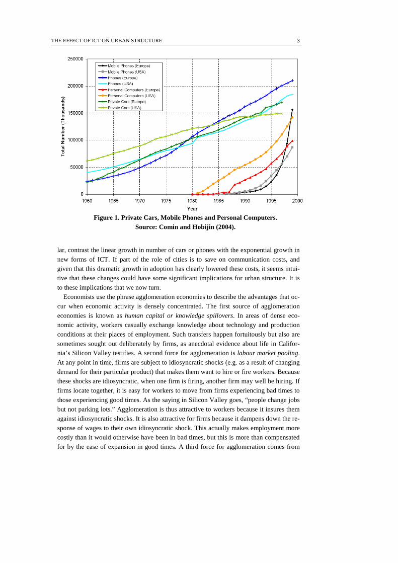
Changes in ICT are very clear in the data, especially if we focus on technology adoption.
Figure 1 presents the number of cars, phone lines, mobile phones, and personal computers
during the last five decades, using Comin and Hobijin’s “Historical Cross-Country Tech-
nological Adoption Dataset” [Comin and Hobijin (2004)]. The adoption of the telephone
was well under way by the 1950's. By the end of the 1990's, the number of telephone lines
exceeds 150 million in both Europe and the US. In contrast, changes in personal com-
puters are all concentrated in the 1980's and 1990's. The US went from less than 5 million
computers in the early 1980's to more than 140 million computers in the late 1990's. This
is a remarkable change that is likely to have very important effects. The data show a simi-
lar pattern for the EU that went from less than 5 million personal computers to 100 mil-
lion in the late 1990's. The EU and the US have also experienced similar dramatic changes
in the use of cell phones, but with the growth occurring even later than for personal com-
puters. Mobile telephones technology was practically unused in 1985, but more than 150
million people owned a mobile phone in the 1990's in the EU, and more than 85 million in
the US. Of course, these numbers alone do not reflect the costs associated with implemen-
tation of these technologies but they do show the dramatic growth in adoption. In particu-
THE EFFECT OF ICT ON URBAN STRUCTURE
3
lar, contrast the linear growth in number of cars or phones with the exponential growth in
new forms of ICT. If part of the role of cities is to save on communication costs, and
given that this dramatic growth in adoption has clearly lowered these costs, it seems intui-
tive that these changes could have some significant implications for urban structure. It is
to these implications that we now turn.
Economists use the phrase agglomeration economies to describe the advantages that oc-
cur when economic activity is densely concentrated. The first source of agglomeration
economies is known as human capital or knowledge spillovers. In areas of dense eco-
nomic activity, workers casually exchange knowledge about technology and production
conditions at their places of employment. Such transfers happen fortuitously but also are
sometimes sought out deliberately by firms, as anecdotal evidence about life in Califor-
nia’s Silicon Valley testifies. A second force for agglomeration is labour market pooling.
At any point in time, firms are subject to idiosyncratic shocks (e.g. as a result of changing
demand for their particular product) that makes them want to hire or fire workers. Because
these shocks are idiosyncratic, when one firm is firing, another firm may well be hiring. If
firms locate together, it is easy for workers to move from firms experiencing bad times to
those experiencing good times. As the saying in Silicon Valley goes, “people change jobs
but not parking lots.” Agglomeration is thus attractive to workers because it insures them
against idiosyncratic shocks. It is also attractive for firms because it dampens down the re-
sponse of wages to their own idiosyncratic shock. This actually makes employment more
costly than it would otherwise have been in bad times, but this is more than compensated
for by the ease of expansion in good times. A third force for agglomeration comes from
Figure 1. Private Cars, Mobile Phones and Personal Computers.
Source: Comin and Hobijin (2004).
THE EFFECT OF ICT ON URBAN STRUCTURE
4
the greater variety of intermediate products and richer mix of labour skills and expertise
that are available in larger urban areas. Greater variety of goods and services lowers prices
and wages and also enhances firms’ options in choosing technologies for production and
distribution of their products. The associated effects on firms are known as pecuniary ex-
ternalities (as distinct from real externalities, the latter term being reserved for non-market
interactions among economic agents’ output decisions). Finally, local amenities due to
weather, physical attractiveness, culture or tradition are an important factor in enhancing
the appeal of particular urban agglomerations. These mechanisms, which essentially go
back to Alfred Marshall’s Principles of Economics, explain at least some of the spatial
concentration that we observe throughout the world.
Of course, if these agglomeration economies were the only forces driving the location
of economic activity then we would expect to observe extreme spatial concentration. In
reality, we do not, because these agglomeration economies are offset by costs (dispersion
or congestion forces) as activity becomes increasingly concentrated. These costs take
many forms but all arise from the fact that competition for local resources, broadly de-
fined, increases with spatial concentration. For example, congestion occurs as a result of
increased competition for space, firms pay higher rents and wages as result of increased
competition for land and workers, while they receive lower prices for their output as a re-
sult of increased competition in goods markets. The balance between these agglomeration
and dispersion forces determines the spatial structure of the economy.
The strength and importance of these agglomeration and dispersion forces depend on
many things, including the cost of communicating information across space. Knowledge
spillovers, for example, depend on the role that distance plays in inhibiting efficient
communication of ideas. The importance of face to face communication shows just how
dramatic can be these distance effects. But the telephone, the email and video conferenc-
ing, for example, are all reducing these costs of communicating ideas at a distance.
Changing communication costs may also affect the benefits from labour market pool-
ing. Remember, these benefits require works to move from firm to firm. ICT may increase
the efficiency of this process as news about vacancies in one firm are more easily com-
municated to workers who may be looking for work. A similar story could be told about
the benefits of pecuniary externalities. For example, falling information costs allow firms
to more easily identify potential suppliers of intermediate goods or skills. Turning to dis-
persions forces, ICT may facilitate e-working, allowing individuals to avoid the high costs
of commuting in congested cities. Alternatively, it may increase the competition faced by
firms as consumers find it easier to identify alternative sources of supply.
Thus, new ways to transport ideas and communicate information are, in general, likely
to affect all of the agglomeration and dispersion forces that urban and regional economists
have identified as key determinants of the concentration of economic activity in space.
Thus, independently of the sources of agglomeration forces, ICT will likely have an im-
pact on spatial concentration. In what follows, we illustrate the potential impact of ICT by
focusing on production externalities as the main source of agglomeration. This gives us a
prediction about the impact of ICT that we then confirm using real world data. These ef-
fects may also be consistent with other models where ICT has a similar effect on different
THE EFFECT OF ICT ON URBAN STRUCTURE
5
agglomeration economies. So, our exercise does not allow us to discriminate between dif-
ferent models which predict that ICT will disperse economic activity across cities. It does,
however, suggest that models that predict the opposite changes to city structure (i.e. in-
creasing concentration) are not consistent with the data.
ICT can, in principle, have many distinct effects on the distribution of economic activ-
ity in space. On one hand, it can increase the spatial scope of knowledge spillovers —it is
easier for any professional to acquire context that helps her assess information she casu-
ally receives from counterparts in other firms. Therefore, fewer person-to-person interac-
tions may suffice to obtain a better understanding of what other firms are up to. To the ex-
tent that knowledge spillovers, whether deliberate (as among employees of the same firm)
or fortuitous, are productive, we would expect that ITC would make them more effective
among individuals who are located further apart. Local increasing returns are thus less lo-
calized when a wider set of people across a whole country or across countries can interact
with each other by using new technologies and while economizing on commuting costs.
In this sense, improvements in ICT reduce the importance of the quantities of productive
factors employed in a city on that city’s productivity. This is the stand we take on the the-
ory we present in the next section.
This implies that local urban agglomeration effects become less important and lead to
less concentration of people and jobs in a few successful (and larger cities) or urban ag-
glomerations. Agents and firms obtain smaller benefits from locating close to each other
and so they locate more evenly in space in order to economize on land rents (and other
congestion costs). ICT, in particular, can help businesses create opportunities by improv-
ing their communications with other firms, suppliers and clients worldwide. For example,
real estate, tourism and hotel operators may market their products directly, without relying
on city-based intermediaries. This is important, as most of recent urban growth worldwide
has been fuelled by growth in service sectors, while manufacturing has been relocating to
smaller urban centres with good transportation links [Henderson (1997)] and often out-
sourced to lower cost countries.
These arguments associate ICT with greater dispersion in economic activity. This
would, in turn, imply larger concentration of the city size distribution. That is, it would be
associated with a reduction in the variance of city sizes. Arguably, this potential advan-
tage may not be fully realized if the interurban transportation system does not develop
sufficiently to serve a greater network of urban centres. However, at any given level of
development, improvements in ICT increase the incentives for economic activity to relo-
cate to smaller urban centres.
On the other hand, ICT may also make certain local public goods more important as a
share of consumption or as a share of inputs. Also, changes in the industrial composition
of cities, which have been favouring services, may on balance foster concentration of cer-
tain services due to increasing returns at the plant level. London, New York or Paris are
attractive in part because there are certain products and services that can only be found
there. Similarly, urban living affords better consumption prospects. As individuals spend
more on amenities, such as theatres and other artistic activities, certain large cities would
become relatively more attractive and therefore likely to grow relative to smaller or me-
THE EFFECT OF ICT ON URBAN STRUCTURE
6
dium cities. On top of increasing the share of some of these goods and services in con-
sumption, better ICT may make these goods and services more readily available and
cheaper to consume. Clearly, to the extent that public goods (and other forces of urban
concentration) become effective and far reaching with ICT, we should observe a more
dispersed distribution of cities and a more concentrated distribution of economic activity.
From this verbal discussion it should be clear that there are two key paths through
which ICT may affect the urban structure. But it is still not clear which effect is likely to
dominate. Our next step is thus to develop a theoretical model which will make all these
connections clear. In particular, it will connect changes in ICT with changes in the size
distribution of cities. As we will show, the effect on urban structure generated by the
model will depend on the particular assumption made on how ICT affects agglomeration
forces. This relationship is monotonic and so it helps us design an empirical exercise that
is informative on which of these different effects dominates in reality.
3. A Model of ICT and Urban Evolution
As discussed above, any reasonable model of urban structure or of the role of space in
economic activity, more generally, would predict that improvements in ICT should have
effects on the distribution of economic activity in space. However, no model of urban sys-
tems seems to have explicitly incorporated the effects of ICT. We use the theory in Rossi-
Hansberg and Wright (2007), from now on RHW, to illustrate how ICT may lead to more
urban dispersion. As one may see in more detail in Appendix A, this is a dynamic model
that allows for investment in both physical and human capital and yields very specific re-
sults about the properties of an urban economy in the long run. We incorporate ICT as a
determinant of the agglomeration forces that drive productivity for each industry in each
city. Each industry is assumed to be served by several cities and cities specialize com-
pletely. Therefore, changes in ICT can influence the typical sizes of cities specialized in
an industry, which in turn will determine the concentration of economic activity is space.
To reiterate, the trade-off between agglomeration effects —the benefits that firms and
individuals obtain from being close to each other— and congestion costs determines the
size of cities. Most of these agglomeration effects are related to interactions of different
types among individuals. These interactions will be affected by the communication and
information technology used by these agents. But how will ICT affect agglomeration
forces? And how will these changes in agglomeration forces change the distribution of
economic activity in space?
The potential effect of ICT on the dispersion of the size distribution of cities is not ob-
vious. Essentially, we need to understand whether the consequences of productivity
shocks, or of other shocks that cities may experience, will be more or less persistent, and
will have larger or smaller effects, the larger agglomeration forces. The model in RHW
views the connection between agglomeration effects and productivity as mediated by in-
dustry specific physical and human capital. Agglomeration effects are the result of an ex-
ternality generated by the amount of human capital and labour employed in the city.
THE EFFECT OF ICT ON URBAN STRUCTURE
7
To illustrate this mechanism, suppose that an industry receives a positive and persistent
productivity shock. Naturally, firms in the cities that produce in those industries will want
to produce more. This implies that they want to use more of the industry specific factors.
But the total availability of those factors is given in the current period. So the price of the
industry specific physical and human capital increases. The positive productivity shock
also implies that cities specialized in that industry will grow as firms employ more work-
ers. The higher price of the industry specific human and physical capital will create incen-
tives to accumulate more of these factors. So next period the industry will have more in-
dustry specific factors. Because of the agglomeration effects (and this is the key) having
more of these factors will imply more workers being hired and higher productivity, which
in turn will elicit further accumulation of factors and induce larger cities, even if next pe-
riod’s productivity shock is lower. That is, the effect of the original productivity shock on
city size will be persistent through its effect on the accumulation of industry specific fac-
tors. The stocks of these factors are determined by the accumulated history of the indus-
try’s productivity shocks and, therefore, the size distribution of cities is determined by the
history of these shocks. It is the distribution of these factors across industries which then
determines the size distribution of cities.
The mechanism described above relies crucially on the impact that the level of human
and physical capital has on the level of productivity in a city — that is, on the strength of
the agglomeration effects. The stronger these effects, the larger the impact of past produc-
tivity and the larger the reaction of city size and industry specific factors to an idiosyn-
cratic productivity shock. If agglomeration forces are very small and the productivity of
an industry producing in a given city is essentially independent of the level of human
capital and employment in the city (and therefore the level of physical capital), today’s
productivity shock will have only a temporary effect on city size and no effect on the long
term stock of these factors. Hence, cities will not grow and may even decline substantially
depending on the history of shocks to an industry. This implies that all cities will have
similar sizes and so the distribution of city sizes will be extremely concentrated. If all cit-
ies are of similar sizes, the distribution of economic activity in space will exhibit a lot of
dispersion. Note that the more concentrated the size distribution of cities the more dis-
persed the distribution of economic activity in space.
In contrast, if agglomeration effects depend heavily on the amount of factors employed
in a city, the effect of past shocks on the stock of industry specific factors will be very im-
portant. Cities specialized in industries that received a history of good shocks will be very
large, and cities that received a history of bad shocks will be small. Hence, the size distri-
bution of cities will be very dispersed and the distribution of economic activity in space
will be very concentrated.
Our focus then is on the effect that ICT has on the relationship between the levels of
human capital and employment in a city and the productivity of firms operating in that
city. If improvements in ICT decreases the externality generated by human capital and
employment in an industry it will lead to a more concentrated distribution of city sizes
and more dispersion in the distribution of economic activity in space. If the reverse is true,
so that improvements in ICT lead to larger externalities from employment and human
THE EFFECT OF ICT ON URBAN STRUCTURE
8
capital, we should observe a more dispersed distribution of cities and a more concentrated
distribution of economic activity in space. The model in RHW helps us link the effect of
changes in ICT on urban agglomeration forces with the dispersion —or more precisely the
variance— of the distribution of city sizes.
We now present more details of the formal model in RHW (all derivations are relegated
to Appendix A). Our choice of model is influenced by the fact that this framework allows
for several important productivity effects in a dynamic setting that are key elements of the
economic phenomena we wish to address. First, it allows for an industry-specific technol-
ogy shock for each industry over and above all variable inputs which may vary over time.
This industry specific total factor productivity growth implies that output increases even
while input quantities are constant. Second, it contains spillover effects in urban produc-
tion that are specific to each city. And third, it includes commuting costs which them-
selves may be affected by technological improvements. It follows Henderson (1974) in
some of its features and proposes a theory of the size distribution of cities where the size
of a city is determined by the city's core industry (cities specialize), the amount of indus-
try specific human and physical capital, production externalities in labour and human
capital, and commuting costs. Each industry’s technology, that is its total factor produc-
tivity, is defined as a weighted geometric mean of the industry’s total employment and in-
dustry-specific human capital in the city, and an additional factor that is random and is an
independent and identically distributed (i.i.d.) productivity shock with constant mean and
variance.
We measure the importance of knowledge spillovers from total industry employment
via the elasticity jγ and from industry specific human capital in the economy via the elas-
ticity jε . These elasticities depend on the weight each receives in the determination of in-
dustry j total factor productivity. These parameters are external to individual firms in the
industry (that is, beyond those firms’ control), but internal to the urban economy due to
the presence of city developers. City developers arbitrage across city sizes.
Ideally one would model explicitly the decision of agents in a city to adopt ICT. This
has not been done in the literature in a way that may be readily adopted for our purposes.
Here we only study the effect on urban structure given exogenous technology adoption
decisions. A very simple way to introduce the effect of ICT is to let those two elasticities
vary with the quality of information technology, .ι The nature of the dependence repre-
sents two alternative effects of ICT. We may assume that ICT weakens the importance of
agglomeration effects, if the parameters ( )j tγ ι and ( )j tε ι decrease as ICT improves.
Since people located far away can now interact at a smaller cost, and thus people do not
have to be close together to be productive, agglomeration effects attenuate at a slower rate
with distance, and so people living in a city are less important in determining that city's
productivity level. Conversely, assuming that both ( )j tγ ι and ( )j tε ι increase with the
quality of ICT would be consistent with a greater importance of city specific factors (like
public goods) as a result of changes in ICT. In such a case, the larger both of these pa-
rameters the more important are a city's total human capital and employment in determin-
ing city-specific total factor productivity for industry j. Which effect dominates is, ulti-
mately, an empirical question that we try to settle in this paper.
THE EFFECT OF ICT ON URBAN STRUCTURE
9
In modelling an economy’s urban structure, the theory recognizes an important trade-
off that is generated by city geometry. Cities consist of a central business district, where
all agents work and all production is located, and residential areas surrounding it. Each
agent consumes the services of one unit of land per period. In a spatial equilibrium within
each city, agents should be indifferent over where to live. Therefore, equilibrium rents
should vary with location so as to compensate agents for increased commuting costs, with
rents at the city edge assumed to be equal to zero. In the model these costs per person in-
crease with city population capturing increasing congestion. On the other hand, any given
amount of employment and human capital in a city is not only directly productive, but
also indirectly through the spillover effects.
With a given national population, as the number of cities varies, the total congestion
costs and the output of the city’s industry, which reflects both effects of employment and
human capital, change at different rates. Therefore, a trade-off emerges which, with a
given national population, implies a specific number of cities. Cities exhibit optimal sizes
as city developers internalize the external effects at the city level. Since the knowledge
spillovers are city- and industry-specific, it pays for cities to specialize. That is, a city’s
silk industry should not be burdened by extra congestion costs imposed by a semiconduc-
tors industry and the developer ensures that this is the case.
The process of city formation resembles free entry equilibrium in the textbook case of
an industry with firms that have U-shaped cost curves. In equilibrium, with free entry, all
cities produce at the average cost minimizing quantity of output and the industry is served
by an appropriate number of cities. Thus, aggregate industry output effectively exhibits
constant returns to scale. RHW attribute urban growth to the outcome of the trade-off be-
tween commuting costs and knowledge spillovers, which reconciles increasing returns to
scale at the local level and constant returns to scale at the aggregate level.
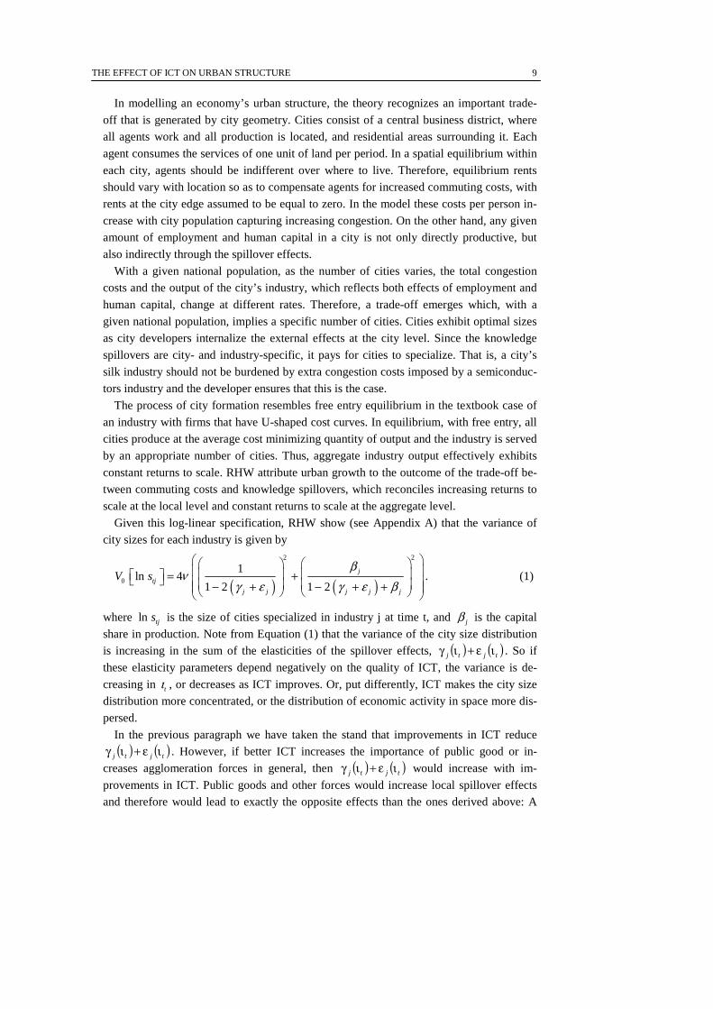
Given this log-linear specification, RHW show (see Appendix A) that the variance of
city sizes for each industry is given by
( ) ( )
2 2
0
1ln 4
1 2 1 2
j
tj
j j j j j
V sβ
νγ ε γ ε β
= + − + − + +
. (1)
where ln tjs is the size of cities specialized in industry j at time t, and jβ is the capital
share in production. Note from Equation (1) that the variance of the city size distribution
is increasing in the sum of the elasticities of the spillover effects, ( ) ( )tjtj ιε+ιγ . So if
these elasticity parameters depend negatively on the quality of ICT, the variance is de-
creasing in tι , or decreases as ICT improves. Or, put differently, ICT makes the city size
distribution more concentrated, or the distribution of economic activity in space more dis-
persed.
In the previous paragraph we have taken the stand that improvements in ICT reduce
( ) ( )tjtj ιε+ιγ . However, if better ICT increases the importance of public good or in-
creases agglomeration forces in general, then ( ) ( )tjtj ιε+ιγ would increase with im-
provements in ICT. Public goods and other forces would increase local spillover effects
and therefore would lead to exactly the opposite effects than the ones derived above: A
THE EFFECT OF ICT ON URBAN STRUCTURE
10
less concentrated size distribution of cities and a more concentrated distribution of eco-
nomic activity. The data can potentially help us distinguish the role played by changes in
the quality of ICT on urban structure, and through the theory, the effect of better ICT on
the elasticity of technology to urban factors. In the next section we turn to study this rela-
tionship empirically.
The model above incorporates ICT only in reduced form. One could also go deeper into
the specification of the spillover functions( )j tγ ι , and ( )j tε ι by trying to model the ef-
fect of lower communication costs on total factor productivity. We refrain from doing so
because it is unlikely that in view of our data we would be able to distinguish between al-
ternative theories of the precise role of ICT in affecting the elasticities of the spillover ef-
fects.
Finally, one can also incorporate the impact of ICT on commuting costs (as in the nota-
ble increase in the use of personal vehicles documented above, or because of telecommut-
ing) by letting commuting costs depend on ICT. The effect of ICT on commuting costs af-
fects city growth rates independently of their scale. As shown in Appendix A, lower
commuting costs as a result of improvements in ICT result in all cities’ growing at a faster
rate. Thus, declining commuting costs change the mean of the distribution of city sizes but
not its shape or variance. As the prediction concerning the variance is the one we take to
the data this justifies our focus in the preceding discussion of the model.
4. Empirical Methodology
Our theoretical model predicts that ICT should make the distribution of city sizes in the
long run more concentrated if it weakens agglomeration effects. We study this prediction
empirically by looking at the effect of ICT on the distribution of city sizes across different
countries.
Unfortunately, as will be clear when we discuss our data in Section 5 below, the avail-
able data only tend to cover the larger cities in each country. This is a problem for our
empirical implementation because such truncated data (i.e. data that do not cover the
smaller cities) do not allow us to calculate the mean and variance of the entire city size
distribution directly. To get around this problem, we proceed as follows. First, we assume
that the city size distribution is Pareto (alternatively referred to as following a power law).
Given this assumption we can express the log of the proportion of cities that are larger
than S, that is the log of the counter-cumulative of the size distribution of cities, as a linear
function of log city size:
ln ( ) ln lnoP s S S Sζ ζ> = − + , (2)
where oS denotes the minimum city size and ζ the elasticity of the proportion of cities
larger than S with respect to S, a negative number that is commonly referred to as the Zipf
coefficient. See Box 1 for details. Given a set of cities, an estimate of the Zipf coefficient
is provided by running a regression of log rank on log city size. How does this help us?
First, because when the distribution is Pareto the Zipf coefficient can be consistently esti-
mated by running the regression only on the largest (i.e. truncated) sample of cities. Sec-
THE EFFECT OF ICT ON URBAN STRUCTURE
11
BOX 1: Zipf’s law and the Pareto distribution Zipf’s law for cities [Zipf (1949)] is an empirical regularity that has attracted consider-
able interest by researchers. In its strict version, which is also known as the rank-size rule, the law is a deterministic rule that states that the second largest city is half the size
of the largest, the third largest city is a third of the size of the largest city, etc. To illus-
trate, let us take a country (for instance the US), and order its cities by population: New York as the largest has rank 1, Los Angeles as the second largest has rank 2, etc. We then
draw a graph, known as Zipf’s plot (see Fig. B.1): on the y-axis, we place the log of the
rank (New York has log rank ln1, Los Angeles log rank ln2); on the x-axis, the log of the population of the corresponding city (which will be called the size of the city). If the
rank-size rule holds, this produces a downwards sloping line with slope equal to -1.
Generally, and to a remarkable extent, statistical analyses for many different countries,
as Gabaix and Ioannides (2004) discuss in detail, obtain estimated coefficients that are
concentrated often around one. This indicates that the size distribution of cities is well
approximated by Zipf's law with coefficient one. Nevertheless, there is substantial varia-
tion in Zipf's coefficients across time and across countries, a fact that ought to cause
some doubts as to full validity of the law.
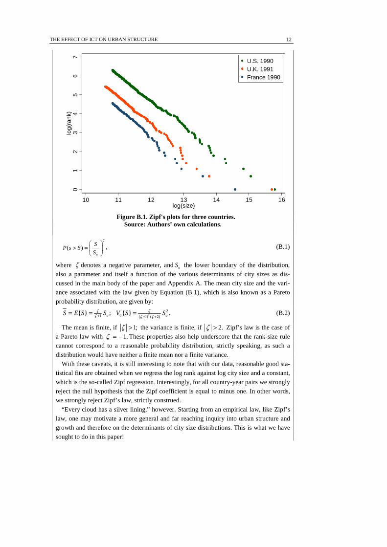
Consider the three Zipf plots on Fig. B.1. They look quite similar to one another, yet
the slopes of ordinary least squares lines fitted to them are not equal to -1. Note that the
plot for France is steeper than that for UK which in turn is steeper than that of the US; the
respective estimates are -1.55, -1.46, and -1.37, are all estimated with very high precision
and using 96, 232 and 552 observations, respectively. Note also that the plot for the US is
furthest to the right because its cities are larger than those of the UK with the same rank,
whose plot in turn is further out than that of France, for the same reason. The techniques
employed in the main part of the paper are aimed at backing out from such differences
the effect of ICT across countries and over time.
Can we obtain Zipf’s law by means of theoretical arguments? The simplest direct theo-
retical argument one could make would be by invoking Gibrat’s law. If different cities
grow randomly with the same expected growth rate and the same variance (Gibrat’s Law
for means and variances of growth rate), then the limit distribution of city sizes con-
verges to Zipf ’s law. See Gabaix and Ioannides (2004) for an extensive discussion of
this issue. Empirically, on the other hand, Zipf’s law for cities is an instance of a power
law (see further below for details). Power laws are attractive in various sciences, espe-
cially in physics, because they are “scale free”, in that they do not depend on the defini-
tions of units of measurement. Naturally, this is an important concern in physics. Rossi-
Hansberg and Wright (2007) provide a rigorous justification for a power law that is di-
rectly rooted in economic theory. It follows as a special case of the model outlined in
Appendix A.
A power law of cities states that the proportion of cities that are greater than a particu-
lar city of sizeS , the counter-cumulative of the size distribution of cities, is of the form:
THE EFFECT OF ICT ON URBAN STRUCTURE
12
01
23
45
67
log(
rank
)
10 11 12 13 14 15 16log(size)
U.S. 1990U.K. 1991France 1990
Figure B.1. Zipf's plots for three countries.
Source: Authors’ own calculations.
( )o
SP s S
S
ζ
> =
, (B.1)
where ζ denotes a negative parameter, andoS the lower boundary of the distribution,
also a parameter and itself a function of the various determinants of city sizes as dis-
cussed in the main body of the paper and Appendix A. The mean city size and the vari-
ance associated with the law given by Equation (B.1), which is also known as a Pareto
probability distribution, are given by:
2
201 ( 1) ( 2)
{ } ; { } .o oS E S S V S Sζ ζζ ζ ζ+ + +
= = = (B.2)
The mean is finite, if 1;ζ > the variance is finite, if 2.ζ > Zipf’s law is the case of
a Pareto law with 1.ζ = − These properties also help underscore that the rank-size rule
cannot correspond to a reasonable probability distribution, strictly speaking, as such a
distribution would have neither a finite mean nor a finite variance.
With these caveats, it is still interesting to note that with our data, reasonable good sta-
tistical fits are obtained when we regress the log rank against log city size and a constant,
which is the so-called Zipf regression. Interestingly, for all country-year pairs we strongly
reject the null hypothesis that the Zipf coefficient is equal to minus one. In other words,
we strongly reject Zipf’s law, strictly construed.
“Every cloud has a silver lining,” however. Starting from an empirical law, like Zipf’s
law, one may motivate a more general and far reaching inquiry into urban structure and
growth and therefore on the determinants of city size distributions. This is what we have
sought to do in this paper!
THE EFFECT OF ICT ON URBAN STRUCTURE
13
We think that rigorous research along the lines of our paper helps caution economists,
sociologists, urban scientists and econophysicists against undue predictions. E.g., as
groups of countries integrate, like the EU, economic forces are unleashed which reshape
their urban systems. What is likely to happen to the sizes of their larger cities and their
ranks? Zipf’s law offers a straightforward prediction. But is it reliable? We think not, and
have instead proposed a way to make predictions that rely on underlying determinants of
city sizes in a dynamic world.
ond, because for a Pareto distribution changes in the Zipf coefficient map one to one to
changes in the variance of the city size distribution.
We have underscored the model’s prediction that improvements in ICT will decrease
the variance of the cross-sectional distribution of cities. In Appendix A we show that this
leads to a higher absolute value of the Zipf coefficient, ( )Sζ . Hence, the absolute value
of the Zipf coefficient increases with improvements in ICT, at least when attention is re-
stricted to the upper tail of city sizes. In other words, improvements in the quality of ICT
decrease the variance of the size distribution while they increase the absolute value of the
Zipf coefficient. Since the Zipf coefficient is negative, they decrease its algebraic value.
This result holds independently of whether the size distribution is Pareto. Of course, if it
is not Pareto, the Zipf coefficient will not be a constant, but the model predicts that its
value will change in the same direction for all, large enough, city sizes. It is important to
note that even though the theory in the previous section implies a Pareto distribution of
city sizes only for particular cases (see RHW for details), we approach the data using Zipf
coefficients that are specified as independent of city size. That is, we assume that the size
distribution is always Pareto.
So our assumption of a particular distribution for city sizes gives us a specification that
can be estimated given the data that we have at our disposal and that allows us to directly
test our theory on the impact of ICT on the city size distribution. The crucial question is
then, of course, whether this is an appropriate assumption. It turns out that empirical evi-
dence give us good reason to think that the Pareto distribution is a reasonable fit for real
world city size distributions across a large numbers of countries and at many different
points in time. Even if the distribution is not Pareto, it is likely that reductions in variance
will be associated with the same direction of change for the Zipf coefficient (as discussed
above). In the empirical section, we also address this concern by presenting robustness
checks using other measures of dispersion in the upper tail.
Once we have the estimated Zipf coefficient, we may use it as a summary of the city
size distribution for different countries and examine how variations in the city size distri-
bution may be attributed to the observed changes in ICT. Clearly a large number of other
factors will determine the city size distribution and we will need to control for these if we
want to isolate the effect of ICT. We discuss and motivate these additional controls in the
results section below.
To capture the effects of ICT we use data on the number of telephone lines and on ac-
cess to the internet. Our main focus is on the number of telephone lines for several rea-
THE EFFECT OF ICT ON URBAN STRUCTURE
14
sons. First, because we have more data. Second, because the impact on the urban structure
will take time and, as Figure 1 shows, the rapid adoption of internet technology has only
occurred relatively recently. Third, because for telephone lines we have a way to deal with
the endogeneity problem for ICT. That is, we have a way to control for the fact that the
number of telephone lines or internet connections may be driven by the urban structure,
rather than the other way round. To allow for this, we need to find a suitable instrumental
variable that is correlated with the number of telephone lines, does not independently af-
fect the urban structure and is unlikely to be affected by changes to that urban structure.
Information on the industrial organization of telecommunications sector provides such a
variable because it is related to the number of telephone lines, but should not independ-
ently affect urban concentration. We believe this is a natural way to proceed, since it is
hard to argue that urban concentration directly influences the competition status of the
telecommunication sector in a country or vice versa. As no such instrumental variable is
available for the internet, our results there are necessarily more speculative (although both
sets of results point in the same direction).
The Zipf coefficient for a country c in year t is obtained from the following regres-
sion:
ict ct ct ict ictR P eλ ζ= + + , (3)
where ln(rank )ict ictR = is the log of the rank of city i in country c in year t , ictP is the
log population of that city, ctλ is a country-year specific intercept, and ctζ is a country-
year specific Zipf coefficient.
To analyze what factors explain the city size distribution Rosen and Resnick (1980),
with that work subsequently having been updated by Soo (2005), take the estimated Zipf
coefficients ctζ from a regression like (3) and seek to understand its determinants in terms
of generally time-varying country-level characteristics. This is accomplished by means of
a (so-called second step) regression of the estimated Zipf coefficients for each country and
year, ˆctζ , against ctX , a collection of explanatory variables that are thought to determine
the city size distribution. That is:
ˆct ct ctXζ θ η ε= + + , (4)
where θ is a constant and η is a vector of coefficients. From among the explanatory vari-
ables we include telephones per capita, density of roads, volatility of growth of GDP per
capita and other variables.
We implement a similar approach, but make three modifications. The first deals with a
potential bias in the estimation of the Zipf coefficient. The second increases the efficiency
of the estimators by implementing a one-step procedure rather than the two-step proce-
dure just described. The third exploits the fact that we have panel data and thus may con-
trol for unobserved country specific determinants of differences in the city size distribu-
tion. We describe each of these three modifications in turn.
In a recent paper, Gabaix and Ibragimov (2006) return to a known bias of the estimate
of the Zipf coefficient from Equation (3). This bias arises from the fact that ranks and
sizes are obviously correlated. The bias is strong in small samples and their proposed cor-
THE EFFECT OF ICT ON URBAN STRUCTURE
15
rection is to use ln(rank 0.5)ict ictR∗ = − in place of the log rank in the left hand side of
Equation (3). We implement that correction here and run a regression like (3),
,ict ct ct ict ictR P eλ ζ∗ = + +
where ictP , ctλ and ctζ are defined as before. Our second change is to recognise that in-
stead of adopting the two-step procedure found in the existing literature, we can get more
efficient estimators if we substitute for ctζ̂ from Equation (4) into equation (3) and esti-
mate instead:
[ ]ict ct ict ct ict ictR P X P eλ θ η∗ ∗= + + + , (5)
where ∗icte is now composed of an i.i.d. error plus the interaction between rank and error
from the first step, while all other coefficients and variables are as defined before.
Both the two-step and one-step procedures —Equations (3)-(4) and (5), respectively—
control for observable country characteristics that may affect the city size distribution.
However, as we have ranks of cities and explanatory variables for several years, we can
also control for unobserved country characteristics that may affect the distribution. Con-
tinuing to implement the Gabaix-Ibragimov we work with the following modification of
Equation (6):
[ ] .ict ct c ict ct ict ictR P X P eλ θ η∗ ∗= + + + (6)
The only difference from Equation (5) is that the log population of city i , country c ,
time t is allowed to have an effect which is country specific, cθ . Of course, as one would
expect, if ctX contains time invariant observed characteristics then their coefficients can-
not be separately identified via econometric procedures that allow for unobservable coun-
try-specific effects.
Before turning to the implementation of our approach, we re-iterate that, although we
rely on Zipf’s law to motivate our econometric approach, our estimations should generally
capture the impact upon the entire distribution of city sizes that emanate from changes in
underlying determinants of interest.
5. Data
We use the same city data as that used in Soo (2005), which were taken from Thomas
Brinkhoff's City Population project (http://www.citypopulation.de). Soo's paper provides
a fairly extensive discussion of the nature of the data, particularly with regard to the issue
of the definition of cities.1 Data on population, GDP per capita in 2000 Purchasing Power
Parity (PPP), trade and government expenditure as a percentage of GDP, non-agricultural
economic activity and land area come from the World Bank World Development Indica-
tors (online). Data on kilometres of roads come from the International Road Federation
1 We use data on cities as opposed to urban agglomerations because they are more con-
sistently available internationally.
THE EFFECT OF ICT ON URBAN STRUCTURE
16
World Road Statistics.2 GDP growth is calculated as log difference of GDP in 2000 PPP;
its volatility is measured as the empirical standard deviation over the observed time pe-
riod.
We use two different measures to evaluate the role of ICT in determining the city size
distribution: telephones and the internet. As already discussed, our main focus is on tele-
phones, because we have data for a longer time period. Data on the number of telephone
land lines and internet users per 1000 also come from the World Bank World Develop-
ment Indicators. We multiply these numbers by 1000 and use per capita measure of phone
lines and internet users in the estimations.
We also use two sets of variables as instruments to purge two explanatory variables of
their endogeneity. The first set, and the most crucial, provides information on the market
structure of the telecommunications sector (private or public monopoly versus competi-
tive provision) and is used to instrument the number of telephone lines. The telecommuni-
cations data are taken from the OECD International Regulation Database.3 We use these
variables to instrument the number of phone lines, as discussed further below. A second
set of variables are used to instrument for trade as a percentage of GDP and are derived
from information on membership of the two most important regional preferential trade
agreements for several of the countries that we consider, that is, the North American Free
Trade Agreement (NAFTA) and the European Economic Community and the European
Union, as appropriate in the respective years (EEC/EU). The membership variables were
constructed by the authors based on the year in which countries joined the respective trad-
ing area.4
We start with city-level data for 73 countries covering 7,530 different cities recorded at
various time periods between 1972 and 2001. There are 197 country-year pairs meaning
that, on average, we observe each country 2.7 times. Detailed inspection of the data re-
veals that the relevant explanatory variables are missing for many countries. Fortunately,
the variables are available for three blocks of countries -- North America, Europe and
some of the former countries of the Soviet Union.5 Deleting countries with missing data
2 Further details on all these variables are provided in Soo (2005). A large number of
our explanatory variables were also kindly provided by Kwok Tong Soo. 3 See the Indicators of Product Market Regulation Homepage at:
http://www.oecd.org/eco/pmr and described in Conway (2006). Missing data points for
Eastern European countries were filled by the authors based on media coverage. 4 Other variables may also, of course, be endogenous, but these are the two for which
we have been able to construct reasonable instruments. 5 Specifically, we use data on Austria, Belarus, Belgium, Bulgaria, Canada, Denmark,
Finland, France, Greece, Hungary, Italy, Mexico, the Netherlands, Norway, Poland, Por-
tugal, Romania, the Russian Federation, the Slovak Republic, Spain, Sweden, Switzer-
land, the United Kingdom and the United States. We have to drop Germany because of
the reunification of 1990 and the ensuing adoption of Federal Republic of Germany in-
stitutions in former German Democratic Republic territory causes definitional problems.
THE EFFECT OF ICT ON URBAN STRUCTURE
17
leaves us with 24 countries covering 2,955 cities recorded at various time periods between
1980 and 2000. There are now 63 country-year pairs meaning that, on average, we ob-
serve each country 2.6 times. For the internet regressions we have to drop Mexico and re-
strict the time period to 1990 to 2000. This gives us 23 countries and 41-country year
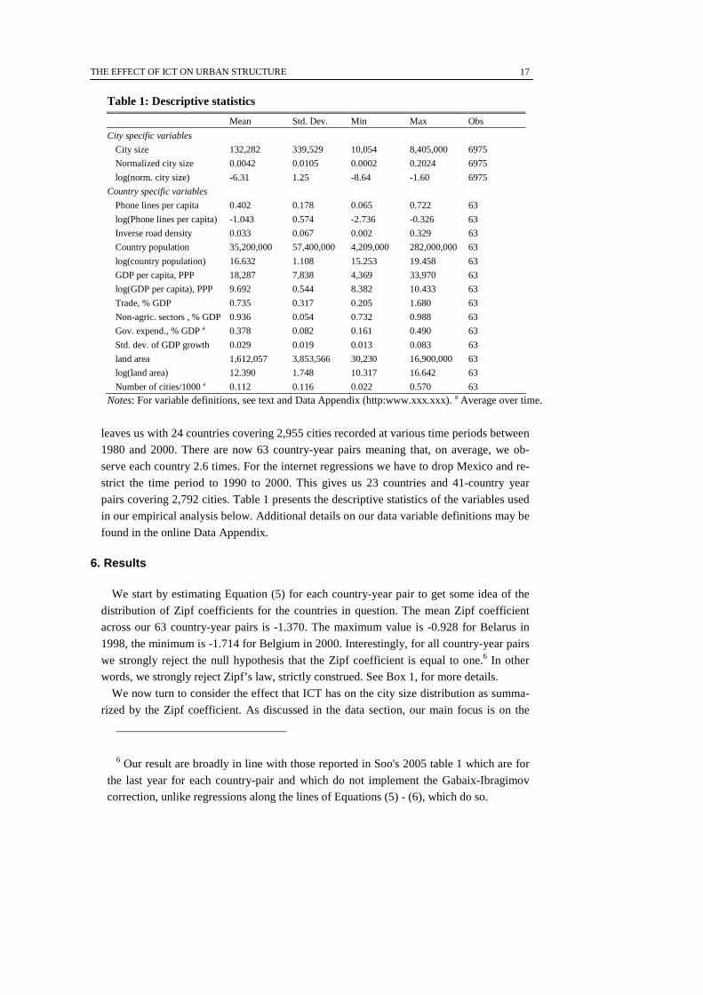
pairs covering 2,792 cities. Table 1 presents the descriptive statistics of the variables used
in our empirical analysis below. Additional details on our data variable definitions may be
found in the online Data Appendix.
6. Results
We start by estimating Equation (5) for each country-year pair to get some idea of the
distribution of Zipf coefficients for the countries in question. The mean Zipf coefficient
across our 63 country-year pairs is -1.370. The maximum value is -0.928 for Belarus in
1998, the minimum is -1.714 for Belgium in 2000. Interestingly, for all country-year pairs
we strongly reject the null hypothesis that the Zipf coefficient is equal to one.6 In other
words, we strongly reject Zipf’s law, strictly construed. See Box 1, for more details.
We now turn to consider the effect that ICT has on the city size distribution as summa-
rized by the Zipf coefficient. As discussed in the data section, our main focus is on the
6 Our result are broadly in line with those reported in Soo's 2005 table 1 which are for
the last year for each country-pair and which do not implement the Gabaix-Ibragimov
correction, unlike regressions along the lines of Equations (5) - (6), which do so.
Table 1: Descriptive statistics
Mean Std. Dev. Min Max Obs
City specific variables
City size 132,282 339,529 10,054 8,405,000 6975
Normalized city size 0.0042 0.0105 0.0002 0.2024 6975
log(norm. city size) -6.31 1.25 -8.64 -1.60 6975
Country specific variables
Phone lines per capita 0.402 0.178 0.065 0.722 63
log(Phone lines per capita) -1.043 0.574 -2.736 -0.326 63
Inverse road density 0.033 0.067 0.002 0.329 63
Country population 35,200,000 57,400,000 4,209,000 282,000,000 63
log(country population) 16.632 1.108 15.253 19.458 63
GDP per capita, PPP 18,287 7,838 4,369 33,970 63
log(GDP per capita), PPP 9.692 0.544 8.382 10.433 63
Trade, % GDP 0.735 0.317 0.205 1.680 63
Non-agric. sectors , % GDP 0.936 0.054 0.732 0.988 63
Gov. expend., % GDP a 0.378 0.082 0.161 0.490 63
Std. dev. of GDP growth 0.029 0.019 0.013 0.083 63
land area 1,612,057 3,853,566 30,230 16,900,000 63
log(land area) 12.390 1.748 10.317 16.642 63
Number of cities/1000 a 0.112 0.116 0.022 0.570 63
Notes: For variable definitions, see text and Data Appendix (http:www.xxx.xxx). a Average over time.
THE EFFECT OF ICT ON URBAN STRUCTURE
18
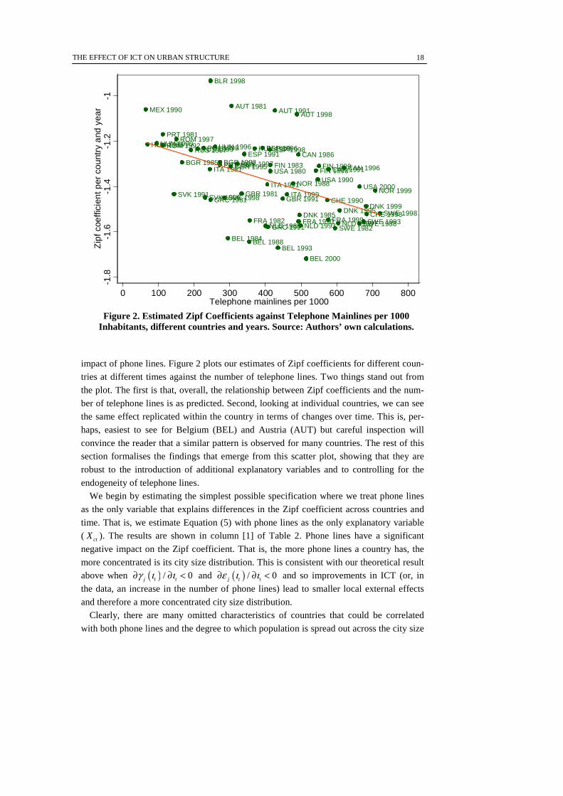
impact of phone lines. Figure 2 plots our estimates of Zipf coefficients for different coun-
tries at different times against the number of telephone lines. Two things stand out from
the plot. The first is that, overall, the relationship between Zipf coefficients and the num-
ber of telephone lines is as predicted. Second, looking at individual countries, we can see
the same effect replicated within the country in terms of changes over time. This is, per-
haps, easiest to see for Belgium (BEL) and Austria (AUT) but careful inspection will
convince the reader that a similar pattern is observed for many countries. The rest of this
section formalises the findings that emerge from this scatter plot, showing that they are
robust to the introduction of additional explanatory variables and to controlling for the
endogeneity of telephone lines.
We begin by estimating the simplest possible specification where we treat phone lines
as the only variable that explains differences in the Zipf coefficient across countries and
time. That is, we estimate Equation (5) with phone lines as the only explanatory variable
( ctX ). The results are shown in column [1] of Table 2. Phone lines have a significant
negative impact on the Zipf coefficient. That is, the more phone lines a country has, the
more concentrated is its city size distribution. This is consistent with our theoretical result
above when ( ) / 0j t tγ ι ι∂ ∂ < and ( ) / 0j t tε ι ι∂ ∂ < and so improvements in ICT (or, in
the data, an increase in the number of phone lines) lead to smaller local external effects
and therefore a more concentrated city size distribution.
Clearly, there are many omitted characteristics of countries that could be correlated
with both phone lines and the degree to which population is spread out across the city size
AUT 1981AUT 1991AUT 1998
BLR 1998
BEL 1984BEL 1988BEL 1993
BEL 2000
BGR 1985 BGR 1992BGR 1995BGR 1997
CAN 1986
CAN 1991CAN 1996
DNK 1985DNK 1995
DNK 1999
FIN 1983FIN 1993FIN 1999
FRA 1982 FRA 1990FRA 1999
GRC 1981
GRC 1991
HUN 1985HUN 1990 HUN 1996 HUN 1999
ITA 1981
ITA 1991ITA 1999
MEX 1990
NLD 1985 NLD 1993 NLD 1999
NOR 1988NOR 1999
POL 1998
PRT 1981
PRT 1991
ROM 1992ROM 1997
RUS 1997RUS 1999
SVK 1991SVK 1996SVK 1998
ESP 1991ESP 1996ESP 1998
SWE 1982SWE 1988SWE 1993
SWE 1998
CHE 1990
CHE 1998
GBR 1981GBR 1991
USA 1980USA 1990
USA 2000
-1.8
-1.6
-1.4
-1.2
-1Z
ipf c
oeffi
cien
t per
cou
ntry
and
yea
r
0 100 200 300 400 500 600 700 800Telephone mainlines per 1000
Figure 2. Estimated Zipf Coefficients against Telephone Mainlines per 1000
Inhabitants, different countries and years. Source: Authors’ own calculations.
THE EFFECT OF ICT ON URBAN STRUCTURE
19
distribution. Column [2] begins to address this problem by including several additional
explanatory variables. Before turning to discussing the empirical results, we briefly moti-
vate each of the additional control variables.
We include the inverse of road density as a proxy for transport costs within the country.
Countries with a low road density are likely to have high transport costs encouraging
population to concentrate in just a few cities. Thus, we expect the coefficient on inverse
road density to be positive (fewer roads imply higher inverse road density, higher trans-
port costs and urban population that is more concentrated in fewer cities).
We include three variables to control for the economic and geographic size of the coun-
try: population, income and land area. More densely populated countries are likely to have
Table 2: Phone lines and the city size distribution
OLS IV
Dep. variable log(rank-0.5) [1] [2] [3] [4] [5] [6] [7] [8]
log(city size)
× log(Phone lines per capita) -0.152*** -0.129*** -0.074*** -0.089*** -0.137*** -0.127*** -0.099*** -0.097**
(0.005) (0.010) (0.010) (0.029) (0.007) (0.029) (0.017) (0.041)
× Inverse road density -0.290*** 0.181 -0.224** 0.177
(0.088) (0.113) (0.096) (0.114)
× log(country population) -0.047*** -0.156 -0.073*** -0.160
(0.007) (0.096) (0.011) (0.106)
× log(GDP per capita), PPP -0.083*** -0.065 -0.057 -0.039
(0.023) (0.068) (0.039) (0.085)
× Trade, % GDP -0.090*** 0.083** -0.381*** 0.139
(0.017) (0.033) (0.070) (0.086)
× Non-agric. sectors, % GDP -0.100 0.269 0.370* 0.247
(0.117) (0.238) (0.198) (0.323)
× Gov. expend., % GDP -0.674*** -0.517***
(0.053) (0.081)
× Std. dev. of GDP growth -1.320** 1.532
(0.618) (1.051)
× log(land area) 0.017*** 0.000
(0.004) (0.007)
× Number of cities/1000 -0.040 -0.041
(0.060) (0.061)
× Year 0.004*** 0.001 0.004*** 0.001
(0.001) (0.002) (0.001) (0.003)
× Constant -1.179*** -1.127*** country spec. -1.195*** -1.153*** country spec.
(0.006) (0.008) (0.008) (0.010)
Constant country-year spec. country-year spec. country-year spec. country-year spec.
R2 0.975 0.977 0.982 0.982
Obs cities 6975 6975 6975 6975 6975 6975 6975 6975
Obs country-year 63 63 63 63 63 63 63 63
Obs countries 24 24 24 24 24 24 24 24
Notes: Standard errors in brackets. *** , ** , and * indicate significance at the 1%, 5% and 10% level, respectively. Interacted variables are mean-shifted. Instruments are dummy variables for public and private telephony monop-oly, EU/EEC-, NAFTA-membership.
THE EFFECT OF ICT ON URBAN STRUCTURE
20
more equal city size distribution, so we expect the coefficient on population to be negative
while that on land area should be positive. Although we do not constrain the coefficients
to be equal, these two variables could pick up other effects, thus introducing some ambi-
guity about the expected signs on their coefficients. Given our focus on more developed
countries we have no strong prior on the sign of the coefficient on GDP. Models in the
New Economic Geography tradition predict that our measure of trade openness (trade as a
percentage of GDP) should have a negative effect on spatial concentration and hence on
the Zipf coefficient because international trade weakens agglomeration forces (See Chap-
ter 18 of Fujita et al., 1999). Similarly, we would expect higher agricultural production to
lead to less concentration and a flatter city size distribution. That is, we expect the coeffi-
cient on non-agricultural sectors as a percentage of GDP to be positive. A measure of the
size of government (government expenditure as a share of GDP) allows for the possibility
that larger governments may imply higher population concentration. That would indeed
be the case if (as Ades and Glaeser (1995) emphasize) rent seeking behaviour encourages
citizens to locate close to policy makers in the capital city. Conversely, large governments
have more means to work against agglomeration forces and support peripheral regions
through regional policies. Thus we have no strong priors on the sign of the coefficient on
government expenditure.
Finally, we include the standard deviation of the rate of growth of real GDP since the
theory underlying our approach (discussed in Appendix A) indicates that a higher volatil-
ity of total factor productivity shocks should lead to a larger variance of the size distribu-
tion and therefore larger Zipf coefficients. We also include a time trend to capture system-
atic changes in the Zipf coefficient across time and the number of cities as a convenient
way of allowing for non-linearities in the Zipf regression.7
Results reported in column [2] are in line with our expectations for all variables except
the inverse of road density, trade as a percentage of GDP, and the volatility of GDP. In-
troducing country fixed effects and instrumenting for phone lines per capita alters these
findings so we consider the issue no further for now. Instead, we draw attention to the fact
that introducing all of these controls does not change our conclusion on the role of phone
lines. The coefficient is somewhat smaller in absolute value, but still negative and highly
significant. Thus, introducing a large number of additional controls does not change our
conclusion that telephone lines are associated with more concentrated city size distribu-
tions.
Columns [3] and [4] of Table 2 report results after introducing a country-specific fixed
effect, that is, from estimating Equation (6) rather than Equation (5). Column [3] reports
results when phone lines are the only explanatory variable in ctX . Column [4] reports re-
7 Several recent studies, e.g. Black and Henderson (2003), have emphasised that the
log rank - log population relationship is often concave. The relationship therefore exhib-
its a steep (negative) slope for the highest ranked cities and a flatter (still negative) slope
for lower rank cities. Increasing the number of cities may therefore have a positive im-
pact on the coefficient.
THE EFFECT OF ICT ON URBAN STRUCTURE
21
sults when we include the additional control variables. Note that the coefficients for four
time invariant variables cannot be identified in the fixed effect specification. These vari-
ables are time invariant either because of data availability (government expenditure as a
percentage of GDP, standard deviation of GDP growth) or because they show very little
time series variation (land area and number of cities). Moving from column [2] to column
[3] we see that introducing unobservable country-specific effects further decreases the ab-
solute value of the coefficient on phone lines, although the coefficient remains negative
and highly significant. Introducing additional controls in column [4] leaves the effect of
telephone lines per capita essentially unchanged. As mentioned above, the introduction of
fixed effects now gives us signs on inverse road density and on trade as a percentage of
GDP (even if the former is just insignificant) that are consistent with our theory, given a
country’s economic fundamentals as measured here. Thus, our finding that telephone lines
are associated with more dispersed city size distributions is robust to controlling for other
country characteristics both observed and unobserved.
Of course, one may still worry that the relationship is being driven by time varying un-
observed characteristics of countries and that it is changes in these unobserved character-
istics that drive changes in urban structure which, in turn drive changes in our explanatory
variables. For example, increasing car ownership may lead to the dispersion of population
and telephone lines then respond to that dispersion (rather than vice versa). To control for
this, we adopt the standard solution of looking for an instrumental variable that is (i) cor-
related with the number of telephone lines and (ii) not in itself a determinant of the city
size distribution. We construct two such variables based on the market structure in the
telecommunications sector. We can identify three broad market structures for the coun-
tries in our sample: competitive, public or private monopoly. The instruments that we use
are dummies for whether the country has a public monopoly or a private monopoly with a
competitive structure as the excluded category. Clearly, market structure will affect the
number of phone lines but it is very unlikely to be driven by the city size distribution thus
satisfying the first condition for a valid instrument. In addition, we expect it to play no in-
dependent role in determining the city size distribution thus satisfying the second condi-
tion for a valid instrument.
One might have similar concerns about inverse road density as a proxy for transport
costs. That is, more dispersed population leads to more roads and lower transport costs
rather than transport costs driving population dispersion. We have experimented with
lagged road density as an instrument but this resulted in considerable reductions in sample
size and little change in the coefficient on road density. As our main interest is in the ICT
variables, which we are able to instrument, we do not worry about this further other than
to note that the coefficients on inverse road density should be interpreted with caution.
We have had more success with finding an instrument for trade as a percentage of GDP.
Here, we use the fact that the decision to join regional trade agreements is associated with
large changes in trade volumes, but surely uncorrelated with the city size distribution.
Given the particular sample of countries that we consider we define two dummies, one for
membership in NAFTA and a second for the membership in the EU (or EEC depending

THE EFFECT OF ICT ON URBAN STRUCTURE
22
on time period) and use these as an instrument for trade. Finally, we assume that all other
right hand side variables are exogenous.
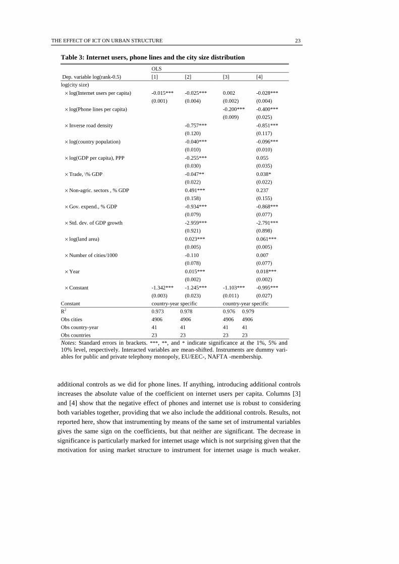
First stage regression results are reported in Table 4. In the cross section, public mo-
nopolies decrease the number of telephone lines while private sector monopolies increase
them. Once we have included a fixed effect we see that both are positively associated with
the number of phone lines. Some of the time series variation in these variables comes
from liberalization that moved countries from private monopolies to competition. Most of
the variation, however, comes from privatization coupled with liberalization which moved
countries from public monopolies to competition.8 Our results may be explained as fol-
lows. At least in terms of the number of phone lines, the efficiency effects of liberalization
were outweighed by changes to public service agreements and the tendency for newly pri-
vatized firms to reduce the cross-subsidisation of residential lines by business users. In
terms of the instruments for trade, entering into preferential trade agreements increases
trade as expected.
Columns [5]-[8] in Table 2 show what happens when we use these variables to instru-
ment for the number of phone lines and for trade as a percentage of GDP. Column [5] ig-
nores country fixed effects and includes instrumented phone lines as the only explanatory
variable. Comparing to column [1] we see that our results are essentially unchanged. The
same is true as we introduce more explanatory variables (compare column [6] to column
[2]), if we introduce fixed effects with phone lines on their own (column [7] versus col-
umn [3]) and if we introduce fixed effects and time-varying explanatory variables (col-
umn [8]).9 Comparing columns [2] and [6] illustrates that instrumenting for phone lines
per capita seems to be important in assessing the effect of GDP volatility on urban struc-
ture. In column [6] we obtain that GDP volatility has a positive coefficient as the theory
above predicts. The effect is very large, although very imprecisely measured since it is not
significant at the 10% level.
In sum, we find a robust negative significant effect of the number of phone lines per
capita on the Zipf coefficient. Over our study period, increasing phone lines per capita
have tended to cause the dispersion of population resulting in a more concentrated city
size distribution.
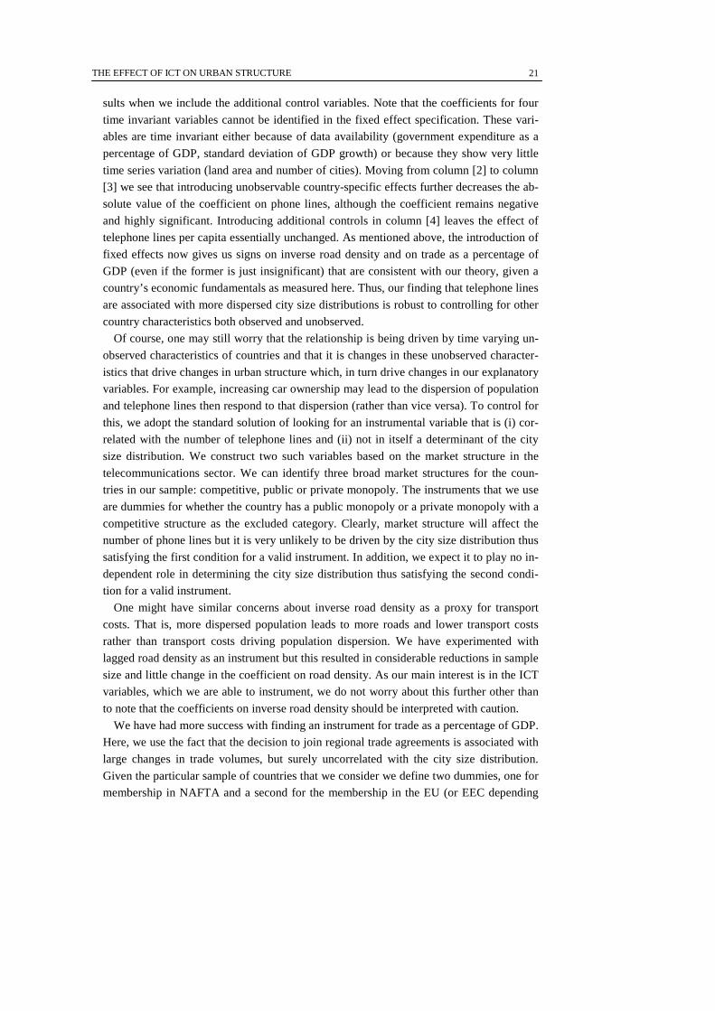
Columns [1] and [2] in Table 3 show that we reach a similar conclusion for the impact
of the internet on the city size distribution. Column [1] presents results from a regression
of Zipf coefficients on the number of internet users per capita. That is, from estimating
equation (6) with internet users per capita as the only explanatory variable ( ctX ). We see
a negative significant effect on the Zipf coefficient, although the effect is much smaller
than that of phone lines. Column [2] shows what happens when we introduce the same
8 During the time period we consider there were no privatisations that replace a public
monopoly with a private monopoly, although this had certainly happened in earlier peri-
ods (e.g. in the United Kingdom). 9 The only change is that trade as a percentage of GDP is just insignificant in the final
specification (it is significant at the 10.5% level).
THE EFFECT OF ICT ON URBAN STRUCTURE
23
additional controls as we did for phone lines. If anything, introducing additional controls
increases the absolute value of the coefficient on internet users per capita. Columns [3]
and [4] show that the negative effect of phones and internet use is robust to considering
both variables together, providing that we also include the additional controls. Results, not
reported here, show that instrumenting by means of the same set of instrumental variables
gives the same sign on the coefficients, but that neither are significant. The decrease in
significance is particularly marked for internet usage which is not surprising given that the
motivation for using market structure to instrument for internet usage is much weaker.
Table 3: Internet users, phone lines and the city size distribution
OLS
Dep. variable log(rank-0.5) [1] [2] [3] [4]
log(city size)
× log(Internet users per capita) -0.015*** -0.025*** 0.002 -0.028***
(0.001) (0.004) (0.002) (0.004)
× log(Phone lines per capita) -0.200*** -0.400***
(0.009) (0.025)
× Inverse road density -0.757*** -0.851***
(0.120) (0.117)
× log(country population) -0.040*** -0.096***
(0.010) (0.010)
× log(GDP per capita), PPP -0.255*** 0.055
(0.030) (0.035)
× Trade, \% GDP -0.047** 0.038*
(0.022) (0.022)
× Non-agric. sectors , % GDP 0.491*** 0.237
(0.158) (0.155)
× Gov. expend., % GDP -0.934*** -0.868***
(0.079) (0.077)
× Std. dev. of GDP growth -2.959*** -2.791***
(0.921) (0.898)
× log(land area) 0.023*** 0.061***
(0.005) (0.005)
× Number of cities/1000 -0.110 0.007
(0.078) (0.077)
× Year 0.015*** 0.018***
(0.002) (0.002)
× Constant -1.342*** -1.245*** -1.103*** -0.995***
(0.003) (0.023) (0.011) (0.027)
Constant country-year specific country-year specific
R2 0.973 0.978 0.976 0.979
Obs cities 4906 4906 4906 4906
Obs country-year 41 41 41 41
Obs countries 23 23 23 23
Notes: Standard errors in brackets. *** , ** , and * indicate significance at the 1%, 5% and 10% level, respectively. Interacted variables are mean-shifted. Instruments are dummy vari-ables for public and private telephony monopoly, EU/EEC-, NAFTA -membership.
THE EFFECT OF ICT ON URBAN STRUCTURE
24
That is, in many countries internet access services are provided by firms that may be unre-
lated to the traditional telecommunications providers. Only 16 countries have more than
one year of data for internet usage so, not surprisingly, implementing the fixed effects
specification gives insignificant results. We do still get the same signs for the coefficients,
however. Finally, introducing fixed effects and instrumenting leads to coefficients that are
essentially zero.10 This is hardly surprising given the limited number of observations and
the fact that market structure in the telecommunications sector does not provide good in-
struments for the number of internet connections.
6.1. Some details on instrumentation and additional robustness checks
A careful inspection of our auxiliary results, the first-stage regressions reported in Table
4, suggests that abolishing of public monopolies increases phone lines in the cross-section
(specification [6], Table 2 and 4) and reduces phone lines in the fixed effects estimation
(specification [8], Table 2 and 4). In principle there are theoretical arguments for both.
However, in both cases the predicted phone lines from the first stage regressions are in-
creasing over time. The general increase of telephone mainlines is explained by the time
trend as well as increases in population, road density, and GDP. The positive sign of pub-
lic and private monopolies means that abolishing these monopolies lowered the number of
phones lines when it occurred (in a jump). This jump may be an extreme prediction. We
therefore investigated this further by using as an additional instrument the dummy vari-
able whether there is a public or private monopoly interacted with the time trend. This ad-
ditional analysis shows that abolishing monopolies generally reduces phone lines signifi-
cantly in a jump, and then is followed by slightly (but not significant) faster growth there-
after. In the respective second stage for specification [8], the effect of phone lines is even
stronger, -0.106, and now significant at 1%. The trade variable now also becomes signifi-
cant, although with a sign opposite to what the New Economic Geography theory would
predict.
A second question concerning the nature of our instrumental variables strategy arises
from considering the literature on the political economy of urbanization. This literature
raises the possibility that urban concentration may be driven by the general degree of
competition in the economic and political spheres. This raises the possibility that some
measure of the degree of competition in the economy should be included directly in the
regression, violating the second requirement for the validity of an instrument (that it
should have no direct effect on urban structure). Using this line of reasoning, one could
argue, for example, that the industrial organization of the telecommunications sector is ac-
tually just proxying for an overly centralized public sector which favours larger cities. To
summarise, if industrial organization of the telecommunications sector is capturing other
factors that have a direct effect on urban concentration, then it is inappropriate as an in-
10 These results are available on request.
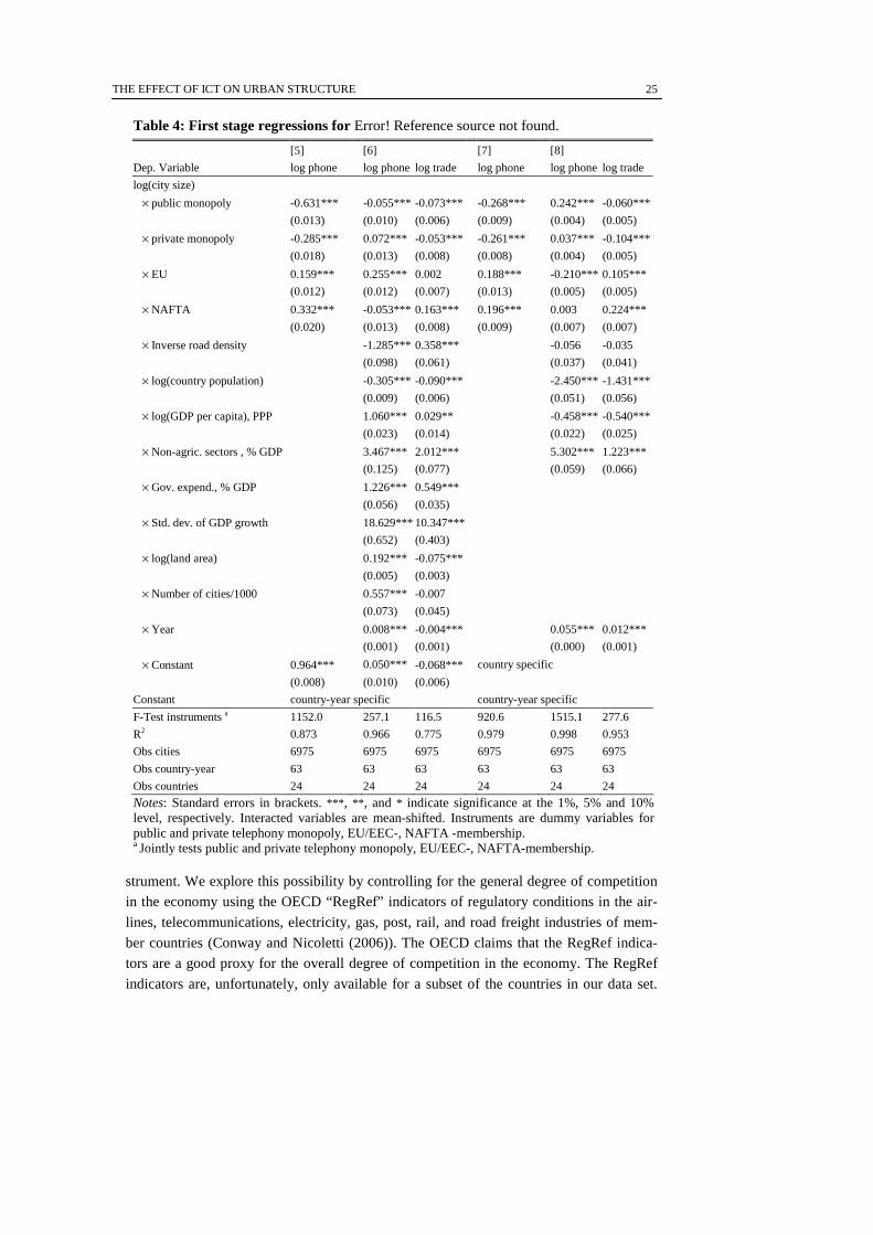
THE EFFECT OF ICT ON URBAN STRUCTURE
25
strument. We explore this possibility by controlling for the general degree of competition
in the economy using the OECD “RegRef” indicators of regulatory conditions in the air-
lines, telecommunications, electricity, gas, post, rail, and road freight industries of mem-
ber countries (Conway and Nicoletti (2006)). The OECD claims that the RegRef indica-
tors are a good proxy for the overall degree of competition in the economy. The RegRef
indicators are, unfortunately, only available for a subset of the countries in our data set.
Table 4: First stage regressions for Error! Reference source not found.
[5] [6] [7] [8]
Dep. Variable log phone log phone log trade log phone log phone log trade
log(city size)
× public monopoly -0.631*** -0.055*** -0.073*** -0.268*** 0.242*** -0.060***
(0.013) (0.010) (0.006) (0.009) (0.004) (0.005)
× private monopoly -0.285*** 0.072*** -0.053*** -0.261*** 0.037*** -0.104***
(0.018) (0.013) (0.008) (0.008) (0.004) (0.005)
× EU 0.159*** 0.255*** 0.002 0.188*** -0.210*** 0.105***
(0.012) (0.012) (0.007) (0.013) (0.005) (0.005)
× NAFTA 0.332*** -0.053*** 0.163*** 0.196*** 0.003 0.224***
(0.020) (0.013) (0.008) (0.009) (0.007) (0.007)
× Inverse road density -1.285*** 0.358*** -0.056 -0.035
(0.098) (0.061) (0.037) (0.041)
× log(country population) -0.305*** -0.090*** -2.450*** -1.431***
(0.009) (0.006) (0.051) (0.056)
× log(GDP per capita), PPP 1.060*** 0.029** -0.458*** -0.540***
(0.023) (0.014) (0.022) (0.025)
× Non-agric. sectors , % GDP 3.467*** 2.012*** 5.302*** 1.223***
(0.125) (0.077) (0.059) (0.066)
× Gov. expend., % GDP 1.226*** 0.549***
(0.056) (0.035)
× Std. dev. of GDP growth 18.629*** 10.347***
(0.652) (0.403)
× log(land area) 0.192*** -0.075***
(0.005) (0.003)
× Number of cities/1000 0.557*** -0.007
(0.073) (0.045)
× Year 0.008*** -0.004*** 0.055*** 0.012***
(0.001) (0.001) (0.000) (0.001)
× Constant 0.964*** 0.050*** -0.068*** country specific
(0.008) (0.010) (0.006)
Constant country-year specific country-year specific
F-Test instruments a 1152.0 257.1 116.5 920.6 1515.1 277.6
R2 0.873 0.966 0.775 0.979 0.998 0.953
Obs cities 6975 6975 6975 6975 6975 6975
Obs country-year 63 63 63 63 63 63
Obs countries 24 24 24 24 24 24
Notes: Standard errors in brackets. *** , ** , and * indicate significance at the 1%, 5% and 10% level, respectively. Interacted variables are mean-shifted. Instruments are dummy variables for public and private telephony monopoly, EU/EEC-, NAFTA -membership. a Jointly tests public and private telephony monopoly, EU/EEC-, NAFTA-membership.
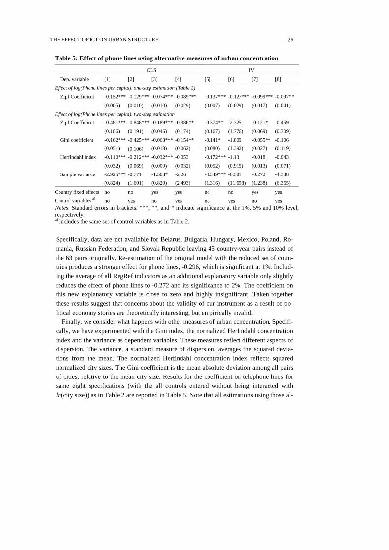
THE EFFECT OF ICT ON URBAN STRUCTURE
26
Specifically, data are not available for Belarus, Bulgaria, Hungary, Mexico, Poland, Ro-
mania, Russian Federation, and Slovak Republic leaving 45 country-year pairs instead of
the 63 pairs originally. Re-estimation of the original model with the reduced set of coun-
tries produces a stronger effect for phone lines, -0.296, which is significant at 1%. Includ-
ing the average of all RegRef indicators as an additional explanatory variable only slightly
reduces the effect of phone lines to -0.272 and its significance to 2%. The coefficient on
this new explanatory variable is close to zero and highly insignificant. Taken together
these results suggest that concerns about the validity of our instrument as a result of po-
litical economy stories are theoretically interesting, but empirically invalid.
Finally, we consider what happens with other measures of urban concentration. Specifi-
cally, we have experimented with the Gini index, the normalized Herfindahl concentration
index and the variance as dependent variables. These measures reflect different aspects of
dispersion. The variance, a standard measure of dispersion, averages the squared devia-
tions from the mean. The normalized Herfindahl concentration index reflects squared
normalized city sizes. The Gini coefficient is the mean absolute deviation among all pairs
of cities, relative to the mean city size. Results for the coefficient on telephone lines for
same eight specifications (with the all controls entered without being interacted with
ln(city size)) as in Table 2 are reported in Table 5. Note that all estimations using those al-
Table 5: Effect of phone lines using alternative measures of urban concentration
OLS IV
Dep. variable [1] [2] [3] [4] [5] [6] [7] [8]
Effect of log(Phone lines per capita), one-step estimation (Table 2)
Zipf Coefficient -0.152*** -0.129*** -0.074*** -0.089*** -0.137*** -0.127*** -0.099*** -0.097**
(0.005) (0.010) (0.010) (0.029) (0.007) (0.029) (0.017) (0.041)
Effect of log(Phone lines per capita), two-step estimation
Zipf Coefficient -0.481*** -0.848*** -0.189*** -0.386** -0.374** -2.325 -0.121* -0.459
(0.106) (0.191) (0.046) (0.174) (0.167) (1.776) (0.069) (0.309)
Gini coefficient -0.162*** -0.425*** -0.068*** -0.154** -0.141* -1.809 -0.055** -0.106
(0.051) (0.106) (0.018) (0.062) (0.080) (1.392) (0.027) (0.119)
Herfindahl index -0.110*** -0.212*** -0.032*** -0.053 -0.172*** -1.13 -0.018 -0.043
(0.032) (0.069) (0.009) (0.032) (0.052) (0.915) (0.013) (0.071)
Sample variance -2.925*** -0.771 -1.508* -2.26 -4.349*** -6.581 -0.272 -4.388
(0.824) (1.601) (0.820) (2.493) (1.316) (11.698) (1.238) (6.365)
Country fixed effects no no yes yes no no yes yes
Control variables a) no yes no yes no yes no yes
Notes: Standard errors in brackets. ***, **, and * indicate significance at the 1%, 5% and 10% level, respectively. a) Includes the same set of control variables as in Table 2.
THE EFFECT OF ICT ON URBAN STRUCTURE
27
ternative measures are based on a two-step procedure11 and therefore are less efficient
than the one-step estimation in Table 2. For comparison, we therefore also report the two-
step estimation using the Zipf coefficient as dependent variable. The results for the two-
step using Zipf are qualitatively identical to the one-step results. Due to the loss of effi-
ciency, they are not always significant.
Remarkably for such different measures of dispersion, the results for the coefficients of
telephones line per capita with the Gini and Herfindahl indices as dependent variables are
– up to a scale factor – very similar to the two-step using Zipf. The coefficients with the
sample variance as a dependent variable are also negative and thus consistent with our
findings using the Zipf coefficient. It is worth emphasising, however, that our choice of
Zipf coefficient as a measure for urban concentration is not arbitrary, being driven instead
by a desire to link our empirical results firmly with our theoretical model of urban struc-
ture. In contrast, while all three of these alternative measures of urban concentration ap-
pear intuitive, when estimated on the truncated sample of larger cities they are not consis-
tent estimators of the population variables and cannot be linked to our theoretical predic-
tion of decreasing variance for all cities. For this reason, the Zipf coefficient results repre-
sent our preferred specification and we take these robustness checks as broadly consistent
with our overall findings.
7. Policy Discussion and Conclusion
We find robust evidence that increases in the number of telephone lines per capita lead to
a more concentrated distribution of city sizes and so correspondingly to more dispersion
in the distribution of economic activity in space. The model we presented in Section 2 ra-
tionalizes this empirical result. As access to telephones improves, the ensuing changes in
city size distributions imply that local production externalities decrease. That results in an
urban structure that is less dependent on past shocks and hence a size distribution of cities
with smaller variance. This smaller variance is reflected in Zipf coefficients that are larger
in absolute value.
Figure 3 illustrates the magnitude of our empirical results. It assumes that the size dis-
tribution of city sizes is Pareto and plots the distribution we estimate (labelled ‘actual’ in
the figure) and the distribution we would expect if the mean of the log of phone lines per
capita increases by one standard deviation. The figure also compares these two distribu-
tions with the one associated with Zipf’s law, that is, a Pareto distribution with coefficient
minus one, according to Equation (2). The increase in phone lines per capita concentrates
the distribution, by making the Zipf relationship steeper. If ICT improves, cities are not as
large. For example, the share of cities with more than a million inhabitants is reduced by
two percentage points. Since the share of cities with populations larger than 1 million is
11 In the first step, the measure (Zipf coefficient, Gini coefficient, Herfindahl index,
sample variance) is estimated for every country and year from observed city sizes. In the
second step, the measure is regressed on ln(Phone lines per capita) and control variables.
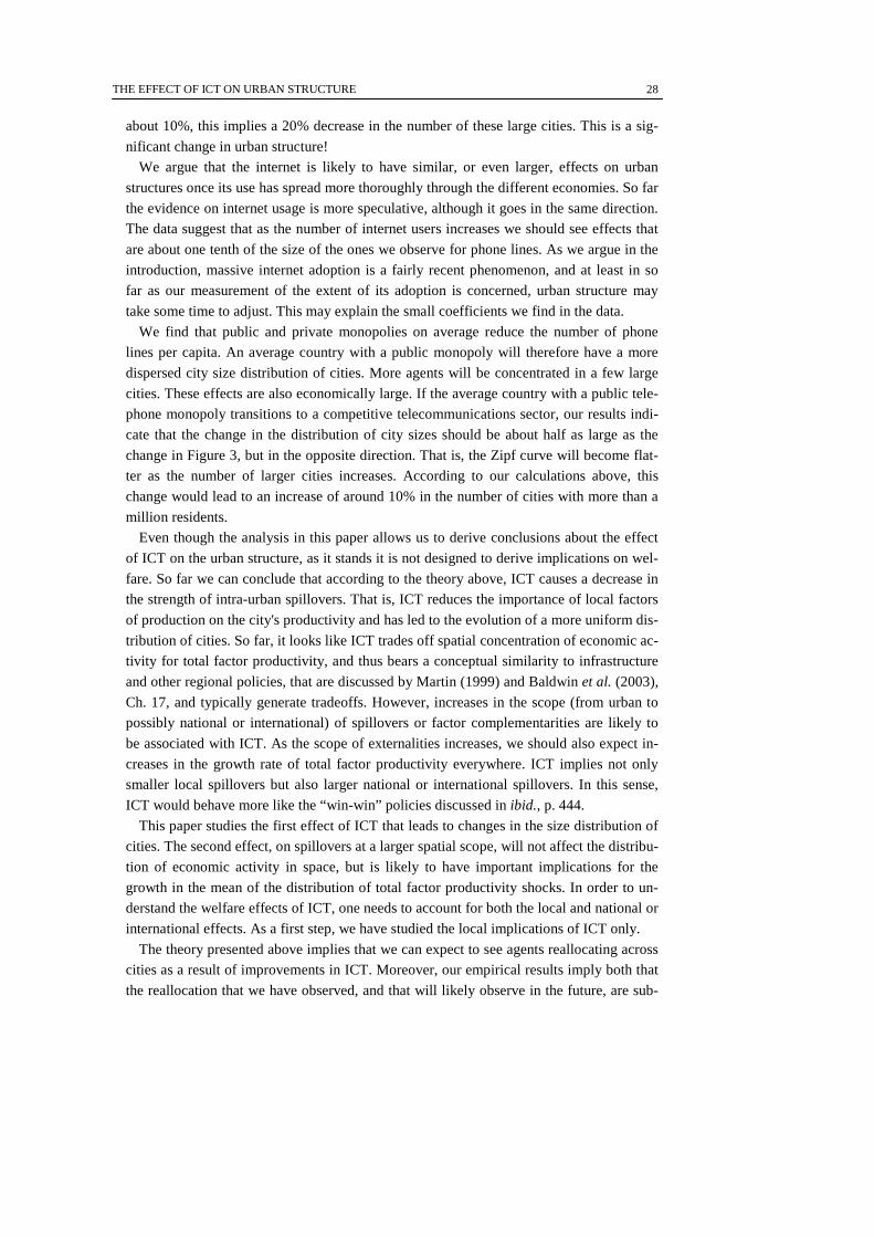
THE EFFECT OF ICT ON URBAN STRUCTURE
28
about 10%, this implies a 20% decrease in the number of these large cities. This is a sig-
nificant change in urban structure!
We argue that the internet is likely to have similar, or even larger, effects on urban
structures once its use has spread more thoroughly through the different economies. So far
the evidence on internet usage is more speculative, although it goes in the same direction.
The data suggest that as the number of internet users increases we should see effects that
are about one tenth of the size of the ones we observe for phone lines. As we argue in the
introduction, massive internet adoption is a fairly recent phenomenon, and at least in so
far as our measurement of the extent of its adoption is concerned, urban structure may
take some time to adjust. This may explain the small coefficients we find in the data.
We find that public and private monopolies on average reduce the number of phone
lines per capita. An average country with a public monopoly will therefore have a more
dispersed city size distribution of cities. More agents will be concentrated in a few large
cities. These effects are also economically large. If the average country with a public tele-
phone monopoly transitions to a competitive telecommunications sector, our results indi-
cate that the change in the distribution of city sizes should be about half as large as the
change in Figure 3, but in the opposite direction. That is, the Zipf curve will become flat-
ter as the number of larger cities increases. According to our calculations above, this
change would lead to an increase of around 10% in the number of cities with more than a
million residents.
Even though the analysis in this paper allows us to derive conclusions about the effect
of ICT on the urban structure, as it stands it is not designed to derive implications on wel-
fare. So far we can conclude that according to the theory above, ICT causes a decrease in
the strength of intra-urban spillovers. That is, ICT reduces the importance of local factors
of production on the city's productivity and has led to the evolution of a more uniform dis-
tribution of cities. So far, it looks like ICT trades off spatial concentration of economic ac-
tivity for total factor productivity, and thus bears a conceptual similarity to infrastructure
and other regional policies, that are discussed by Martin (1999) and Baldwin et al. (2003),
Ch. 17, and typically generate tradeoffs. However, increases in the scope (from urban to
possibly national or international) of spillovers or factor complementarities are likely to
be associated with ICT. As the scope of externalities increases, we should also expect in-
creases in the growth rate of total factor productivity everywhere. ICT implies not only
smaller local spillovers but also larger national or international spillovers. In this sense,
ICT would behave more like the “win-win” policies discussed in ibid., p. 444.
This paper studies the first effect of ICT that leads to changes in the size distribution of
cities. The second effect, on spillovers at a larger spatial scope, will not affect the distribu-
tion of economic activity in space, but is likely to have important implications for the
growth in the mean of the distribution of total factor productivity shocks. In order to un-
derstand the welfare effects of ICT, one needs to account for both the local and national or
international effects. As a first step, we have studied the local implications of ICT only.
The theory presented above implies that we can expect to see agents reallocating across
cities as a result of improvements in ICT. Moreover, our empirical results imply both that
the reallocation that we have observed, and that will likely observe in the future, are sub-

THE EFFECT OF ICT ON URBAN STRUCTURE
29
stantial. Moving costs are also important and we have not commented on them so far in
this paper. Some of these costs are due to regulation and lack of flexibility in labour mar-
kets. Others reflect frictions in the adjustment of urban public infrastructure. Yet other
costs are due to the cost of selling and buying homes, and the actual transport and organ-
izational costs involved in moving across cities. Our results highlight the importance of
government policy in reducing this type of costs. If moving costs are artificially high, be-
cause of government regulation and interference, economies will not be able to take ad-
vantage of the gains associated with the ICT improvements, since agents will not respond
by redistributing themselves accordingly in space.
It is imperative to allow for the natural reallocation that will result from further im-
provements in ICT. After all, this reallocation across space is the adjustment by the indi-
viduals and by firms to an economic environment where physical location is becoming
less important.
THE EFFECT OF ICT ON URBAN STRUCTURE
30
REFERENCES
Ades, Alberto F., and Edward L. Glaeser (1995), “Trade and Circuses: Explaining Urban Giants”, Quarterly Journal of Economics, 110, February, 195-227.
Baldwin, Richard, Rikard Forslid, Philippe Martin, Gianmarco Ottaviano, and Frederic Robert-Nicoud (2003), Economic Geography and Public Policy, Princeton, NJ: Princeton University Press.
Black, Duncan and Vernon Henderson (2003), “Urban Evolution in the USA”, Journal of Economic Geography 3(4), 343-372.
Comin, Diego A., and Bart Hobijin (2004), “Cross-Country Technological Adoption: Mak-ing the Theories Face the Facts,” Journal of Monetary Economics, 39—83. Data accessible at: http://www.nber.org/hccta/.
Conway Paul and Giuseppe Nicoletti (2006), “Product Market Regulation in Non-manufacturing Sectors in OECD Countries: Measurement and Highlights”, OECD Economics Department working paper 58; data accessible at: http://www.oecd.org/eco/pmr/.
Fujita, Masahisa, Paul R. Krugman and Anthony J. Venables (1999), The Spatial Economy: Cities, Regions, and International Trade, Cambridge, MA: MIT Press.
Gabaix, Xavier and Rustam Ibragimov (2006), “Log(Rank-1/2): A Simple Way to Improve the OLS Estimation of Tail Exponents”, Harvard Institute of Economic Research Working Papers No. 2106.
Gabaix, Xavier and Yannis M. Ioannides (2004), ‘The Evolution of City Size Distributions,’ pp. 2341-2378, in Henderson, J. V., and J.-F. Thisse, eds., Handbook of Regional and Urban Economics, Vol. IV, Cities and Geography, Amsterdam: North-Holland.
Henderson, Vernon (1974), ‘The Sizes and Types of Cities’, American Economic Review, 64, March, 640-656.
Henderson, Vernon (1997), ‘Medium Size Cities’, Regional Science and Urban Economics, 27, 449-470.
Martin, Philippe (1999), ‘Public Policies, Regional Inequalities, and Growth”, Journal of Public Economics, 73, 85-105.
Rosen, K. T. and M. Resnick (1980), “The Size Distribution of Cities: an Examination of the Pareto Law and Primacy”, Journal of Urban Economics 8(2), 156-186.
Rossi-Hansberg, Esteban and Mark Wright (2007), “Urban Structure and Growth”, Review of Economic Studies 74, April, 597-624.
Soo, Kwok Tong (2005), “Zipf's Law for Cities: a Cross-country Investigation”, Regional Science and Urban Economics 35(3), 239-263.
Zipf, George K. (1949). Human Behavior and the Principle of Least Effort. Addison–Wesley, Cam-bridge, MA.
THE EFFECT OF ICT ON URBAN STRUCTURE
31
APPENDIX A: A Model of ICT, Urban Evolution and Ci ty Size Distributions
We illustrate how to study the role of ICT on the urban hierarchy by considering the basic
theoretical model in RHW. Total factor productivity, that is the level of technology, in in-
dustry j at time t is given by
j j
tj tj tj tjA A H Nγ ε=% % % ,
where tjN% and tjH% denote the city's total employment and industry j specific human
capital, and ln tjA is an independent and identically distributed (i.i.d.) productivity shock
with mean zero and variance ν . Thus parameters jγ and jε determine the importance of
knowledge spillovers from total employment in industry j and industry j-specific human
capital in the economy, which are external to individual firms in the industry but internal
to the urban economy due to the presence of city developers. If both parameters jγ and
jε are equal to zero there are no external effects and economic activity has no incentive to
agglomerate in cities. The larger both of these parameters the more important are a city's
total human capital and employment in determining tjA% city-specific total factor productiv-
ity industry j.
A very simple way to introduce the effect of ICT is therefore to let these two parameters
vary with the quality of information technology, .ι Namely, let ( )j tγ ι where
( ) / 0j t tγ ι ι∂ ∂ < and, similarly, let ( )j tε ι be such that ( ) / 0j t tε ι ι∂ ∂ < . Essentially, this
assumption amounts to ICT’s increasing the importance of agglomeration effects since
people located far away can now interact at a smaller cost and so people living in the city
are less important in determining the city's productivity level. Conversely, we could as-
sume that both ( )j tγ ι and ( )j tε ι depend positively on the quality of ICT, which would
be consistent with arguments that emphasize the greater importance of public goods as a
result of changes in ICT. Which effect dominates is, ultimately, an empirical question that
we try to settle in this paper.
In order for city sizes to be well defined, it will be clarified shortly below that we need
to guarantee that the knowledge spillover parameters jγ and jε satisfy
( ) ( ) 1 / 2j jγ ι ε ι+ < for all ι . Otherwise, cities would, in a sense, be too productive and
therefore would grow unboundedly since agglomeration effects would dominate conges-
tion costs at all population levels. As long as this condition is satisfied, as a city grows
eventually congestion costs become more important than agglomeration costs and so city
sizes are finite.
Cities consist of a central business centre, where all agents work and all production is
located, and residential areas surrounding it. Each agent consumes the services of one unit
of land per period. For spatial equilibrium within each city agents should be indifferent
about where to live in the city. Therefore, equilibrium rents at a distance z from the centre
should obey ( )( )R z z zτ= − , where z denotes a city’s radius, where rent is equal to 0.
Hence, total rents in a city of radius z are given by
323
02 ( )
3 2
z bTR zR z dz z N
πτπ= = =∫ % .
THE EFFECT OF ICT ON URBAN STRUCTURE
32
since everyone in the city lives in one unit of land, a city of population N~
and
.3/2 21
τπ≡ −b Total commuting costs are given by 32
02
zTCC z zdz bNπ τ= =∫ % .
Assuming the presence of city developers or governments that internalize city-wide ex-
ternalities, RHW show that in this framework the unique equilibrium allocation may be
obtained as a solution to the following planning problem: Choose state contingent se-
quences { } ,
0, 1, , , , , ,
J
tj tj tj tj tj tj tj t jC X N u K Hµ
∞
= = to maximize
00 1
(1 ) ln /J
tt ti t
t i
E N C Nδ δ∞
= =
−
∑ ∑ (A.1)
subject to, for all t and j , 32
1
1j j j j j j
j jtj tj tj tj
tj tj tj tj tj tjtj tj tj tj
N K H NC X b A u
β α γ α β εα βµ µ
µ µ µ µ
+ − − +
− − + + ≤
, (A.2)
1
J
t tjj
N N=
=∑ , (A.3)
1
1j j
t j tj tjK K Xω ω−
+ = , (A.4)
0 11 (1 )t j tj j tj jH H B u B+ = + − , (A.5)
where: , ,tj tj tjN K X and tjH denote total employment, total physical capital, physical capi-
tal investment, and total human capital in industry j in the economy and jα and jβ are
positive parameters satisfying 0 1j jα β< + < ; tjC denotes total consumption of repre-
sentative household i, and tjµ the number of cities producing goods in industry j ; tju
denotes the fraction of time agent i devotes to work. Thus, the maximization problem
above amounts to maximizing the sum total of households’ lifetime utilities, (A.1), sub-
ject to: a resource constraint, Equation (A.2), which expresses that the use of resources for
consumption, investment, and commuting costs may not exceed current output (and pre-
supposes that rents are redistributed back to the city residents); a labour market equilib-
rium condition, Equation (A.3), according to which the total labour force is allocated to all
industries; and the two factor accumulation equations, for physical and human capital.
That is, respectively, Equation (A.4), according to which current investment and the exist-
ing capital stock produce capital stock in the next period (with jω being a parameter satis-
fying 0 1jω< < ), and Equation (A.5), where human capital is augmented at a rate that
depends on the portion of each individual’s endowment of leisure not allocated for work.
The problem of maximizing with respect to the number of cities tjµ is a static problem
with first order condition
( ) 2
12j j j j j j j j j jj jtj
tj tj tj tj tj tj tjtj
Ns A K H N u
bβ α γ α β ε α β γ εγ ε
µµ
+ − − + − − − − + = =
.
So the size of a city, tjs , with core industry j is then given by

THE EFFECT OF ICT ON URBAN STRUCTURE
33
( ) ( )1
1 2
2
ˆ ˆ ˆˆ ˆ2ˆ
j j
j j j j jj j
tj j tj tj tj tj tjs F A H K N ub
γ ε
α β α β φγ ε − +
− − + =
, (A.6)
where the auxiliary variables ˆtjA , ˆjα , ˆ
jβ ,and ˆjφ are defined as:
( )1
1 2ˆ j j
tj tjA A γ ε− += , ( )ˆ
1 2
j jj
j j
α γα
γ ε+
=− +
,
( )ˆ
1 2
jj
j j
ββ
γ ε=
− +, and ( )
1ˆ1 2
j jj
j j
α βφ
γ ε− −
=− +
.
Given this log-linear specification, RHW show that capital investments and consump-
tion in each industry are constant fractions of output net of commuting costs, and the frac-
tion of time devoted to work tju is constant across time. Taking natural logarithms of both
sides of Equation (6) that defines city size, we get
( )( )
( )21 1 ˆln 2 ln ln ln
1 2 1 2
j j
tj tj tj j tj
j j j j
s A Kb
γ εψ β
γ ε γ ε
+ = + + + − + − +
(A.7)
where the auxiliary variable tjψ includes all non-stochastic variables that enter the plan-
ning problem, including tjN and tjH .
If ln tjA and tjK are the sole stochastic variables in Equation (A.7), then the mean and
variance of city sizes are easily obtained and given, respectively, by
( )( ) ( )21 ˆln 2 ln ln
1 2
j j
tj tj j tj
j j
s E Kb
γ εψ β
γ ε
+ = + + − +
, (A.8)
( ) ( ) ( ) ( )2
2
0
1 ˆln 4 4 ln1 2
tj j tj
j j
V s V Kν βγ ε
= + − +
.
It is now clear why condition ( ) ( ) 1 / 2j jγ ι ε ι+ < must hold. They are to ensure that
the mean and variance of the city size distribution are mathematically well defined. RHW
show that as ∞→t the variance of the log of physical capital in industry j is:
( )0 2ln
ˆ1tj
j
V Kν
β =
+,
so that the variance of the long run log-city size distribution may be obtained from (A.8)
and given by
( ) ( )
2 2
0
1ln 4
1 2 1 2j
tj
j j j j j
V sβ
νγ ε γ ε β
= + − + − + +
.(A.9)
Note that the variance of the city size distribution is then increasing in ( ) ( )j t j tγ ι ε ι+ .
Therefore, any assumption that we make about the dependence of these elasticities on ICT
is reflected on changes on the invariant distribution of city sizes.

THE EFFECT OF ICT ON URBAN STRUCTURE
34
We would also like to connect the variance of the distribution of city sizes to the Zipf's
coefficient, in order to be able to connect our theoretical results with the data through this
coefficient. The local Zipf coefficient is given by the elasticity of the counter-cumulative
of the city size distribution, ( )P s S> , with respect to city size,
( ) ( )( )
0P s SS
SP s S S
ζ∂ >
= <> ∂
.
Given the mean of the distribution of city sizes, as we increase the variance we are
shifting mass to the tails of the distribution. This implies that for S high enough (large
enough city sizes) the term ( )Sζ will be smaller the larger the variance. As the vari-
ance goes to infinity, ( ) 2,Sζ > − ( )limS Sζ→∞ converges to the Pareto coefficient.

CENTRE FOR ECONOMIC PERFORMANCE Recent Discussion Papers
811 Guy Michaels The Division of Labor, Coordination, and the Demand for Information Processing
810 Maia Güell Jose V. Rodriguez Mora Chris Telmer
Intergenerational Mobility and the Informative Content of Surnames
809 Stephen J. Redding Daniel M. Sturm Nikolaus Wolf
History and Industry Location: Evidence from German Airports
808 Anna Lipinska The Maastricht Convergence Criteria and Optimal Monetary Policy for the EMU Accession Countries
807 Eran Yashiv The Beveridge Curve
806 Ghazala Azmat Alan Manning John Van Reenen
Privatization, Entry Regulation and the Decline of Labor’s Share of GDP: A Cross-Country Analysis of the Network Industries
805 Henry G. Overman Patricia Rice Anthony J. Venables
Economic Linkages Across Space
804 Benjamin Aleman-Castilla The Returns to Temporary Migration to the United States: Evidence from the Mexican Urban Employment Survey
803 Eran Yashiv Labor Search and Matching in Macroeconomics
802 Nicholas Oulton Jeremy Greenwood and Per Krusell, “Growth Accounting with Investment-Specific Technological Progress: A Discussion of Two Approaches” A Rejoinder
801 Mirabelle Muûls Mauro Pisu
Imports and Exports at the Level of the Firm: Evidence from Belgium
800 Richard E. Baldwin Frédéric Robert-Nicoud
Protection for Sale Made Easy
799 Alejandro Cuñat Marc J. Melitz
Volatility, Labor Market Flexibility, and the Pattern of Comparative Advantage
798 Giulia Faggio Job Destruction, Job Creation and Unemployment in Transition Countries: What Can We Learn?
797 Nicholas Oulton Chain Indices of the Cost of Living and the Path-Dependence Problem: an Empirical Solution

796 David Marsden Richard Belfield Salima Benhamou
Inventive Pay Systems and the Management of Human Resources in France and Great Britain
795 Andrew B. Bernard J. Bradford Jensen Stephen Redding Peter K. Schott
Firms in International Trade
794 Richard E. Baldwin Frédéric Robert-Nicoud
Offshoring: General Equilibrium Effects on Wages, Production and Trade
793 Alan Manning Respect
792 Nick Bloom Uncertainty and the Dynamics of R&D
791 Richard E. Baldwin Frédéric Robert-Nicoud
Entry and Asymmetric Lobbying: Why Governments Pick Losers
790 Alan Manning Sanchari Roy
Culture Clash or Culture Club? The Identity and Attitudes of Immigrants in Britain
789 Giorgio Gobbi Roberta Zizza
Does the Underground Economy Hold Back Financial Deepening? Evidence from the Italian Credit Market
788 Nick Bloom Raffaella Sadun John Van Reenen
Americans do I.T. better: US Multinationals and the Productivity Miracle
787 Elizabeth O. Ananat Guy Michaels
The Effect of Marital Breakup on the Income Distribution of Women with Children
786 Willem H. Buiter Seigniorage
785 Gustavo Crespi Chiara Criscuolo Jonathan E. Haskel Matthew Slaughter
Productivity Growth, Knowledge Flows and Spillovers
784 Richard Layard Guy Mayraz Stephen Nickell
The Marginal Utility of Income
783 Gustavo Crespi Chiara Criscuolo Jonathan E. Haskel
Information Technology, Organisational Change and Productivity Growth: Evidence from UK Firms
782 Paul Castillo Carlos Montoro Vicente Tuesta
Inflation Premium and Oil Price Volatility
The Centre for Economic Performance Publications Unit Tel 020 7955 7673 Fax 020 7955 7595 Email [email protected]
Web site http://cep.lse.ac.uk