THESIS

AUTOMATIC QUESTION DETECTION FROM PROSODIC SPEECH ANALYSIS

Submitted by

Rachel Hirsch

Department of Computer Science

In partial fulfillment of the requirements

For the Degree of Master of Science

Colorado State University

Fort Collins, Colorado

Summer 2019

Master’s Committee:

Advisor: Bruce DraperCo-Advisor: Darrell Whitley

Michael Kirby

Copyright by Rachel Hirsch 2019

All Rights Reserved

ABSTRACT

AUTOMATIC QUESTION DETECTION FROM PROSODIC SPEECH ANALYSIS

Human-agent spoken communication has become ubiquitous over the last decade, with assis-

tants such as Siri and Alexa being used more every day. An AI agent needs to understand exactly

what the user says to it and respond accurately. To correctly respond, the agent has to know whether

it is being given a command or asked a question.

In Standard American English (SAE), both word choice and intonation of the speaker are nec-

essary to discern the true sentiment of an utterance. Much Natural Language Processing (NLP)

research has been done into automatically determining these sentence types using word choice

alone. However, intonation is ultimately the key to understanding the sentiment of a spoken sen-

tence. This thesis uses a series of attributes to characterize vocal prosody of utterances to train

classifiers to detect questions. The dataset used to train these classifiers is a series of hearings by

the Supreme Court of the United States (SCOTUS). Prosody-trained classifier results are compared

against a text-based classifier, using Google Speech-to-Text transcriptions of the same dataset.

ii

ACKNOWLEDGEMENTS

First and foremost, I want to thank Dr. Bruce Draper for helping me flesh out my thesis topic,

despite not being as fully versed in natural language processing as in computer vision, and putting

up with my initial bumps in the road.

I also want to thank the Computer Science department for funding my research with a research

assistantship with Dr. Darrell Whitley and a teaching assistantship for introductory Python work-

ing with Professor Dave Matthews. I learned much more than I expected about both the Python

language and how to best communicate with and teach new concepts to newbie programmers.

Finally, I want to add a special shoutout to my family, my girlfriend, and my friends for always

being there for me when I needed a rubber duck or a shoulder to cry on. Thank you for believing

in me and keeping me focused on finishing my work. I couldn’t have done it without you all.

iii

DEDICATION

This thesis is dedicated to all the people who helped me get through this program,

and also my cat.

iv

TABLE OF CONTENTS

ABSTRACT . . . . . . . . . . . . . . . . . . . . . . . . . . . . . . . . . . . . . . . . . . . iiACKNOWLEDGEMENTS . . . . . . . . . . . . . . . . . . . . . . . . . . . . . . . . . . . iiiDEDICATION . . . . . . . . . . . . . . . . . . . . . . . . . . . . . . . . . . . . . . . . . ivLIST OF TABLES . . . . . . . . . . . . . . . . . . . . . . . . . . . . . . . . . . . . . . . viiLIST OF FIGURES . . . . . . . . . . . . . . . . . . . . . . . . . . . . . . . . . . . . . . . viii

Chapter 1 Introduction . . . . . . . . . . . . . . . . . . . . . . . . . . . . . . . . . . . 11.1 What Is Prosody? . . . . . . . . . . . . . . . . . . . . . . . . . . . . . . . 11.2 Why Is Prosody Useful? . . . . . . . . . . . . . . . . . . . . . . . . . . . 21.3 Why Is Lexicon Useful? . . . . . . . . . . . . . . . . . . . . . . . . . . . 3

Chapter 2 Related Work . . . . . . . . . . . . . . . . . . . . . . . . . . . . . . . . . . 42.1 Speech - Lexical Classification . . . . . . . . . . . . . . . . . . . . . . . 42.2 Speech - Prosodic Classification . . . . . . . . . . . . . . . . . . . . . . . 5

Chapter 3 Classifiers Used . . . . . . . . . . . . . . . . . . . . . . . . . . . . . . . . . 83.1 Decision Tree . . . . . . . . . . . . . . . . . . . . . . . . . . . . . . . . . 83.2 K-Neighbors . . . . . . . . . . . . . . . . . . . . . . . . . . . . . . . . . 93.3 Maximum Entropy . . . . . . . . . . . . . . . . . . . . . . . . . . . . . . 93.4 Naive Bayes . . . . . . . . . . . . . . . . . . . . . . . . . . . . . . . . . 103.5 Gaussian Naive Bayes . . . . . . . . . . . . . . . . . . . . . . . . . . . . 103.6 Logistic Regression . . . . . . . . . . . . . . . . . . . . . . . . . . . . . 113.7 Random Forest . . . . . . . . . . . . . . . . . . . . . . . . . . . . . . . . 113.8 Stochastic Gradient Descent . . . . . . . . . . . . . . . . . . . . . . . . . 12

Chapter 4 Methodology . . . . . . . . . . . . . . . . . . . . . . . . . . . . . . . . . . 134.1 Data Collection . . . . . . . . . . . . . . . . . . . . . . . . . . . . . . . . 134.2 Dataset Contents . . . . . . . . . . . . . . . . . . . . . . . . . . . . . . . 144.3 Text Classifier . . . . . . . . . . . . . . . . . . . . . . . . . . . . . . . . 15

4.3.1 Data Parsing . . . . . . . . . . . . . . . . . . . . . . . . . . . . . . . . 154.3.2 Training Text Classifier . . . . . . . . . . . . . . . . . . . . . . . . . . 17

4.4 Prosody Classifier . . . . . . . . . . . . . . . . . . . . . . . . . . . . . . 174.4.1 Data Parsing . . . . . . . . . . . . . . . . . . . . . . . . . . . . . . . . 174.4.2 Chosen Prosody Classifiers . . . . . . . . . . . . . . . . . . . . . . . . 184.4.3 Training & Testing Prosody Classifiers . . . . . . . . . . . . . . . . . . 20

Chapter 5 Results & Discussion . . . . . . . . . . . . . . . . . . . . . . . . . . . . . . 215.1 Principal Components Analysis . . . . . . . . . . . . . . . . . . . . . . . 215.2 Text Classifier Accuracy . . . . . . . . . . . . . . . . . . . . . . . . . . . 235.3 Prosody Classifier Accuracy . . . . . . . . . . . . . . . . . . . . . . . . . 235.4 Classifier Comparison . . . . . . . . . . . . . . . . . . . . . . . . . . . . 265.5 Attribute Dropping Tests . . . . . . . . . . . . . . . . . . . . . . . . . . . 26

v

5.6 Speech-to-Text-to-Speech-to-Text Tests . . . . . . . . . . . . . . . . . . . 28

Chapter 6 Conclusions . . . . . . . . . . . . . . . . . . . . . . . . . . . . . . . . . . . 296.1 Overall Conclusions . . . . . . . . . . . . . . . . . . . . . . . . . . . . . 296.2 Future Work . . . . . . . . . . . . . . . . . . . . . . . . . . . . . . . . . 30

Bibliography . . . . . . . . . . . . . . . . . . . . . . . . . . . . . . . . . . . . . . . . . . 32

vi

LIST OF TABLES

2.1 Crosslingual results for automatic question detection using only lexical features . . . . 52.2 Crosslingual results for automatic question detection using only prosodic features [1] . 62.3 Crosslingual classification results for purely prosodic features, purely lexical features,

and combination of all features [1] . . . . . . . . . . . . . . . . . . . . . . . . . . . . 6

4.1 Number of samples in full SCOTUS dataset . . . . . . . . . . . . . . . . . . . . . . . 144.2 Number of samples in training and testing SCOTUS dataset . . . . . . . . . . . . . . . 144.3 12-dimensional feature vector extracted from the fundamental frequency (F0) curve of

each utterance . . . . . . . . . . . . . . . . . . . . . . . . . . . . . . . . . . . . . . . 18

5.1 Accuracy of text classifiers on SCOTUS transcriptions . . . . . . . . . . . . . . . . . 235.2 Accuracy of prosody classifiers on SCOTUS audio, 30 trials each . . . . . . . . . . . . 255.3 Average true negative and positive and false positive and negative predictions by prosody

classifiers on SCOTUS audio, 30 trials each . . . . . . . . . . . . . . . . . . . . . . . 255.4 High-Greater-Than-Low sample distribution . . . . . . . . . . . . . . . . . . . . . . . 265.5 Accuracy of Random Forest Classifier, dropping attributes 1 through 6 . . . . . . . . . 275.6 Accuracy of Random Forest Classifier, dropping attributes 7 through 12 . . . . . . . . 285.7 Correctly and incorrectly transcribed Speech-to-Text-to-Speech-to-Text sentences. . . . 28

vii

LIST OF FIGURES

1.1 Example contours for WH-question, YN-question, and AL-question [2] . . . . . . . . 2

5.1 2D and 3D principal components graphs . . . . . . . . . . . . . . . . . . . . . . . . . 215.2 2D principal components graph from Figure 5.1 at various zoom levels . . . . . . . . . 225.3 Min, Max, Avg accuracy for each classifier - data from Table 5.2 . . . . . . . . . . . . 245.4 Min, Max, Avg accuracy for RFC classifier, dropping out each attribute before training

- data from Tables 5.5 and 5.6 . . . . . . . . . . . . . . . . . . . . . . . . . . . . . . . 27

viii

Chapter 1

Introduction

Alexa. Siri. Cortana. Google Assistant. What do these AI assistants all have in common? The

answer is Natural Language Processing (NLP) [3]. Each of these assistants is meant to listen to

what the user wants and respond accordingly. This could be something as simple as asking an AI

assistant to remotely turn off a device or as complex as managing email or text correspondences [4].

Most of English natural language processing focuses on the spoken word domain and does not

typically include prosodic features of speech. However, prosody changes dramatically in English

to indicate intended meaning such as sarcasm [5], questions [6], and other sentiment [7]. In fact,

intonation is considered the main mediator of the relation between sentence prosody and meaning

[8].

This thesis considers the prosodic side of English and seeks to determine if it is possible to

detect interrogative sentences from prosody alone, using traditional prosodic features. A prosody-

based sentence classifier is compared against a solely lexicon-based classifier on spoken sentences

(utterances) taken from audio of hearings by the Supreme Court of the United States (SCOTUS)

[9].

1.1 What Is Prosody?

Before discussing prior NLP research, precisely what prosody is and how important it is in the

English language must be made clear. Prosody is defined as “a level of linguistic representation at

which the acoustic-phonetic properties of an utterance vary independently of its lexical items" [10].

This includes attributes of speech such as [8]:

• Emphasis

• Pitch accenting

• Rhythm

• Rhythmic patterning

• Intonation

• Intonational breaks

1

English prosody is broken into two categories: pitch accents and boundaries. Both of these

categories are marked by a combination of high or low pitch targets, represented in fundamental

frequency (F0) measurements in Hertz and duration. [11]

1.2 Why Is Prosody Useful?

Prosody affects the interpretation and comprehension of spoken sentences by listeners. The

tune, emphasis, and rhythm of utterances impact how sentences are understood. Prosody reflects

syntactic structure and thus is influential in resolving syntactic ambiguity [11]. For instance, the

sentence “I never said she stole my money" [12] means something different depending on which

word or words are stressed and whether or not the sentence has an overall rising or falling contour.

For instance, “I never said she stole my money" means “someone said she stole my money, but it

wasn’t me", but “I never said she stole my money" means “I said someone stole my money, but it

wasn’t her."

In most cases, yes-no questions end in a rising contour in both Standard American English

(SAE) and British English. In the SAE corpus used by Hedberg et al. [13], 90.5% of yes-no

questions had a rising contour (designated low-rise or high-rise), 5.6% had a falling contour (low-

fall, rise-fall, or high-fall), and 0.5% had a level contour. However, there is a lack of agreement as

to exactly which type of rising contour is most often used by SAE speakers.

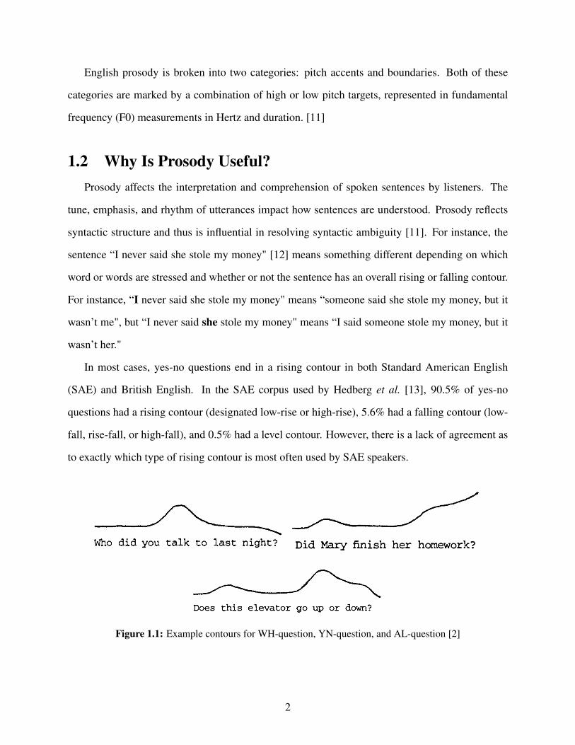
Figure 1.1: Example contours for WH-question, YN-question, and AL-question [2]

2

Questions can be categorized into three types: Wh-Questions (WH), yes/no-questions (YN)

and alternative questions (AL) [2]. WH, YN, and AL. WH-questions typically begin with a ques-

tion word, i.e. who/what/when/where/why. WH-question contours typically rise at the middle

of the sentence, then trend back down (upper left of Figure 1.1). YN-questions are those which

specifically require a yes or no answer, for example “did I do that?". YN-questions more com-

monly have a rise at the end of the sentence (upper right of Figure 1.1). AL-questions encompass

all other types of questions, e.g. declarative or rhetorical. AL-questions typically do not have an

obvious average up or down contour (bottom of Figure 1.1).

1.3 Why Is Lexicon Useful?

Two ways to approach lexical analysis are (1) bag-of-words approach, and (2) location-based

approach. The difference between the two can be demonstrated with the sentences “this is a state-

ment" versus the question "is this a statement?". The word set for both these sentences is:[

“a", “is",

“this", “statement"]

. Thus, a bag of words approach is not always the best option, and a location-

based word vector could do better. Furthermore, adding a prosodic component to a lexicon-based

classifier can further increase accuracy [1]. An example of this will be discussed in Section 2.2.

That said, this thesis focuses on a bag-of-words lexicon-based classifier to compare to a prosody-

based classifier as this is what prior research has indicated leads to best results.

3

Chapter 2

Related Work

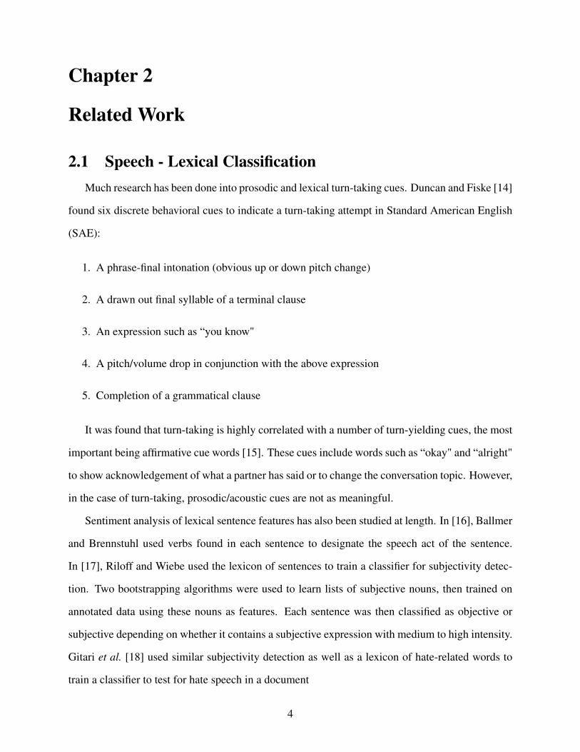
2.1 Speech - Lexical Classification

Much research has been done into prosodic and lexical turn-taking cues. Duncan and Fiske [14]

found six discrete behavioral cues to indicate a turn-taking attempt in Standard American English

(SAE):

1. A phrase-final intonation (obvious up or down pitch change)

2. A drawn out final syllable of a terminal clause

3. An expression such as “you know"

4. A pitch/volume drop in conjunction with the above expression

5. Completion of a grammatical clause

It was found that turn-taking is highly correlated with a number of turn-yielding cues, the most

important being affirmative cue words [15]. These cues include words such as “okay" and “alright"

to show acknowledgement of what a partner has said or to change the conversation topic. However,

in the case of turn-taking, prosodic/acoustic cues are not as meaningful.

Sentiment analysis of lexical sentence features has also been studied at length. In [16], Ballmer

and Brennstuhl used verbs found in each sentence to designate the speech act of the sentence.

In [17], Riloff and Wiebe used the lexicon of sentences to train a classifier for subjectivity detec-

tion. Two bootstrapping algorithms were used to learn lists of subjective nouns, then trained on

annotated data using these nouns as features. Each sentence was then classified as objective or

subjective depending on whether it contains a subjective expression with medium to high intensity.

Gitari et al. [18] used similar subjectivity detection as well as a lexicon of hate-related words to

train a classifier to test for hate speech in a document

4

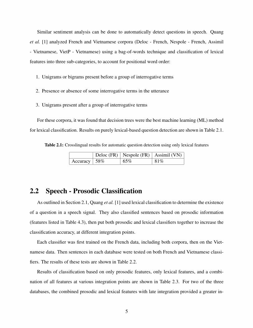
Similar sentiment analysis can be done to automatically detect questions in speech. Quang

et al. [1] analyzed French and Vietnamese corpora (Deloc - French, Nespole - French, Assimil

- Vietnamese, VietP - Vietnamese) using a bag-of-words technique and classification of lexical

features into three sub-categories, to account for positional word order:

1. Unigrams or bigrams present before a group of interrogative terms

2. Presence or absence of some interrogative terms in the utterance

3. Unigrams present after a group of interrogative terms

For these corpora, it was found that decision trees were the best machine learning (ML) method

for lexical classification. Results on purely lexical-based question detection are shown in Table 2.1.

Table 2.1: Crosslingual results for automatic question detection using only lexical features

Deloc (FR) Nespole (FR) Assimil (VN)Accuracy 58% 65% 81%

2.2 Speech - Prosodic Classification

As outlined in Section 2.1, Quang et al. [1] used lexical classification to determine the existence

of a question in a speech signal. They also classified sentences based on prosodic information

(features listed in Table 4.3), then put both prosodic and lexical classifiers together to increase the

classification accuracy, at different integration points.

Each classifier was first trained on the French data, including both corpora, then on the Viet-

namese data. Then sentences in each database were tested on both French and Vietnamese classi-

fiers. The results of these tests are shown in Table 2.2.

Results of classification based on only prosodic features, only lexical features, and a combi-

nation of all features at various integration points are shown in Table 2.3. For two of the three

databases, the combined prosodic and lexical features with late integration provided a greater in-

5

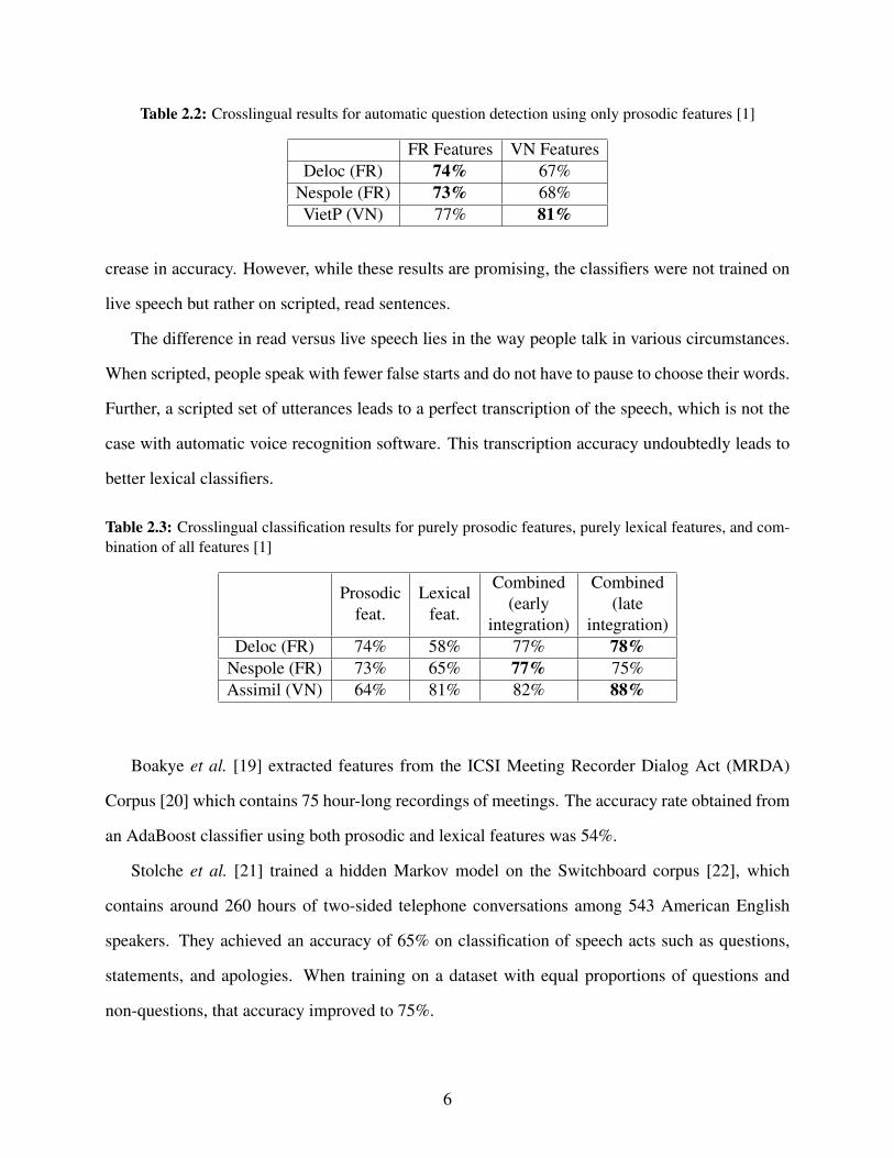
Table 2.2: Crosslingual results for automatic question detection using only prosodic features [1]

FR Features VN FeaturesDeloc (FR) 74% 67%

Nespole (FR) 73% 68%VietP (VN) 77% 81%

crease in accuracy. However, while these results are promising, the classifiers were not trained on

live speech but rather on scripted, read sentences.

The difference in read versus live speech lies in the way people talk in various circumstances.

When scripted, people speak with fewer false starts and do not have to pause to choose their words.

Further, a scripted set of utterances leads to a perfect transcription of the speech, which is not the

case with automatic voice recognition software. This transcription accuracy undoubtedly leads to

better lexical classifiers.

Table 2.3: Crosslingual classification results for purely prosodic features, purely lexical features, and com-bination of all features [1]

Prosodicfeat.

Lexicalfeat.

Combined(early

integration)

Combined(late

integration)Deloc (FR) 74% 58% 77% 78%

Nespole (FR) 73% 65% 77% 75%Assimil (VN) 64% 81% 82% 88%

Boakye et al. [19] extracted features from the ICSI Meeting Recorder Dialog Act (MRDA)

Corpus [20] which contains 75 hour-long recordings of meetings. The accuracy rate obtained from

an AdaBoost classifier using both prosodic and lexical features was 54%.

Stolche et al. [21] trained a hidden Markov model on the Switchboard corpus [22], which

contains around 260 hours of two-sided telephone conversations among 543 American English

speakers. They achieved an accuracy of 65% on classification of speech acts such as questions,

statements, and apologies. When training on a dataset with equal proportions of questions and

non-questions, that accuracy improved to 75%.

6

Donnelly et al. [6] trained a model on live classroom audio, focusing on questions asked by

teachers. When using this live speech dataset, the accuracy rate was 69%, only improving 5%

when combining lexical and prosodic features.

7

Chapter 3

Classifiers Used

The classifiers tested were all chosen based on their use in previous prosody- and lexicon-

based speech classification research. Three of these classifiers were used in lexical classification,

and seven were used in prosodic classification, with some overlap. Classifiers trained and tested

on text data are:

1. Decision Tree (DTC)

2. Maximum Entropy (MaxEnt)

3. Naive Bayes (NB)

Classifiers trained and tested on prosody data are:

1. Decision Tree (DTC)

2. K-Neighbors (KNC)

3. Gaussian Naive Bayes (GNB)

4. Logistic Regression (LogReg)

5. Random Forest (RFC)

6. Stochastic Gradient Descent (SGD)

3.1 Decision Tree

A decision tree classifier (DTC) is based on a hierarchical decomposition of the training space

wherein some condition is used to divide the space [23]. In the context of SCOTUS transcriptions,

these conditions are existence or absence of words in each sentence, as shown in the NLTK example

in Section 4.3.1.

Advantages of using a decision tree are numerous. Decision trees require little data preparation

and can be easily visualized. They are able to handle numerical and categorical data, which is

especially helpful in the case of the SCOTUS audio, as approximately half of the prosodic attributes

are numerical values and the rest are boolean conditions (see Table 4.3 for the full list).

8

Disadvantages of a decision tree classifier include the possibility of overfitting and instability

due to small variations in data. Creation of an optimal decision tree is an NP-complete problem, so

practical DTC algorithms rely on various heuristic algorithms to make tree creation decisions [24].

3.2 K-Neighbors

A K-Neighbors classifier (KNC) uses instance-based learning to build a model based on the k

nearest neighbors of each data point. A larger k value typically suppresses noise effects but can

make boundaries between classes less distinct. Thus, this parameter is highly dependent on the

type and nature of the training data. Classification predictions are done using a majority vote of all

a data point’s k nearest neighbors [25].

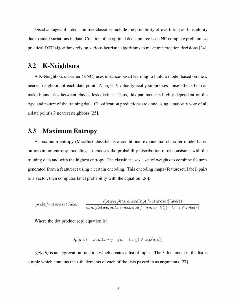
3.3 Maximum Entropy

A maximum entropy (MaxEnt) classifier is a conditional exponential classifier model based

on maximum entropy modeling. It chooses the probability distribution most consistent with the

training data and with the highest entropy. The classifier uses a set of weights to combine features

generated from a featureset using a certain encoding. This encoding maps (featureset, label) pairs

to a vector, then computes label probability with the equation [26]:

prob(featureset|label) =dp(weights, encoding(featureset|label))

sum(dp(weights, encoding(featureset|l)) ∀ l ∈ labels)

Where the dot product (dp) equation is:

dp(a, b) = sum(x ∗ y for (x, y) ∈ zip(a, b))

zip(a,b) is an aggregation function which creates a list of tuples. The i-th element in the list is

a tuple which contains the i-th elements of each of the lists passed in as arguments [27].

9

MaxEnt is essentially a multi-class logistic regression model which uses the concept of entropy

to converge to a solution [28, 29].

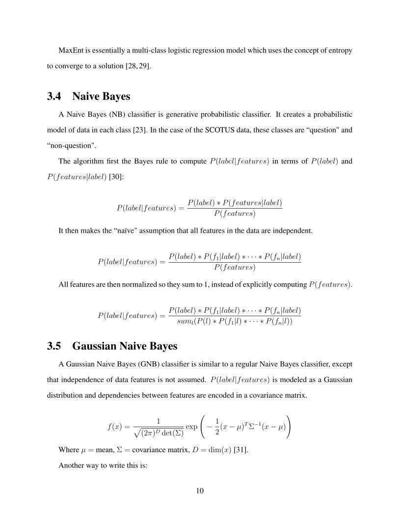
3.4 Naive Bayes

A Naive Bayes (NB) classifier is generative probabilistic classifier. It creates a probabilistic

model of data in each class [23]. In the case of the SCOTUS data, these classes are “question" and

“non-question".

The algorithm first the Bayes rule to compute P (label|features) in terms of P (label) and

P (features|label) [30]:

P (label|features) =P (label) ∗ P (features|label)

P (features)

It then makes the “naïve" assumption that all features in the data are independent.

P (label|features) =P (label) ∗ P (f1|label) ∗ · · · ∗ P (fn|label)

P (features)

All features are then normalized so they sum to 1, instead of explicitly computing P (features).

P (label|features) =P (label) ∗ P (f1|label) ∗ · · · ∗ P (fn|label)

suml(P (l) ∗ P (f1|l) ∗ · · · ∗ P (fn|l))

3.5 Gaussian Naive Bayes

A Gaussian Naive Bayes (GNB) classifier is similar to a regular Naive Bayes classifier, except

that independence of data features is not assumed. P (label|features) is modeled as a Gaussian

distribution and dependencies between features are encoded in a covariance matrix.

f(x) =1

√

(2π)D det(Σ)exp

(

−1

2(x− µ)TΣ−1(x− µ)

)

Where µ = mean, Σ = covariance matrix, D = dim(x) [31].

Another way to write this is:

10

P (xi|y) =1

√

(2πσ2y)

exp

(

−(xi − µy)

2

2σ2y

)

Where σy and µy are estimated using maximum likelihood [32].

3.6 Logistic Regression

A Logistic Regression (LogReg) classifier attempts to fit a logistic model with coefficients

w = (w1, . . . , wp) to minimize the sum of squares between data points with binary labels. It uses

a sigmoid function on the linear regression algorithm to solve a problem of the form:

minw||Xw − y||22

The linear regression (LinReg) equation is:

y = β0 + β1X1 + β2X2 + · · ·+ βnXn

With the sigmoid function:

p =1

1 + e−y

When applying the Sigmoid function to the LinReg equation, that gives:

p =1

1 + e−(β0+β1X1+β2X2+···+βnXn)

Like the MaxEnt classifier, label estimation is calculated via maximum likelihood [33].

3.7 Random Forest

A Random Forest classifier (RFC) fits multiple decision tree classifiers (DTCs) trained on sub-

sets of the training data, then averages the output of those DTCs to improve accuracy of predictions

and lessen the effects of over-fitting [34]. Because samples are randomly drawn from the dataset

11

with replacement (i.e. a bootstrap sample) to create the initial decision trees, it can lead to bias

in the forest. However, because the final output is averaged and nodes are randomly split during

tree construction, the variance and bias decreases, leading to a better overall model than a single

decision tree [35].

3.8 Stochastic Gradient Descent

A Stochastic Gradient Descent (SGD) classifier uses a “one versus all" (OVA) approach to

compute a binary classification of each of K classes versus all other K − 1 classes. It tends to

work best on scaled, or normalized, data. This classifier uses a first-order SGD learning algorithm

to iterate over the training data and update model parameters using the following equation:

w ←− w − η

(

α∂R(w)

∂w+

∂L(wTxi + b, yi)

∂w

)

Where the learning rate (η) is constant or decaying gradually for each time step t [36]:

η(t) =1

α(t0 + t)

This SGD algorithm is simple for the prosodic data that the SGD classifier was tested on, as

the classes in the data are already binary.

12

Chapter 4

Methodology

4.1 Data Collection

For these experiments, the corpus used was approximately 28 hours of audio files downloaded

from the Supreme Court of the United States (SCOTUS) Argument Audio website [9]. Trials were

chosen at random so as not to create bias. Case numbers used are as follows:

• 16-1498

• 17-204

• 17-290

• 17-532

• 17-571

• 17-647

• 17-1091

• 17-1094

• 17-1107

• 17-1174

• 17-1184

• 17-1201

• 17-1299

• 17-1307

• 17-1471

• 17-1484

• 17-1594

• 17-1606

• 17-1625

• 18-96

• 18-302

• 18-389

• 18-431

• 18-457

• 18-459

• 18-481

• 18-485

• 18-525

This corpus was chosen for a number of reasons, the most important being the ability to quickly

gather the data and the amount of audio already in existence. Furthermore, it presented an interest-

ing challenge of analyzing prosody of live speech in a controlled environment where all speakers

are measured and composed. There are no vocal outbursts and all words are carefully chosen.

Since there is rarely more than one person talking at one time, and the audio was recorded in an

indoor venue, there is little background noise.

13

4.2 Dataset Contents

Each sentence in the SCOTUS hearings was transcribed using Google’s Speech-to-Text API

[37]. Sentences were initially labeled as questions or non-questions based on the presence of a

question mark at the end of the sentence, then rechecked by hand. This dataset includes over

eleven times as many non-questions as questions, so preprocessing was necessary before training

classifier models. Exact sample amounts can be seen in Table 4.1.

Table 4.1: Number of samples in full SCOTUS dataset

# SamplesQuestions 696

Non-Questions 8114Total 8810

Each classifier tested was trained on a dataset containing equal amounts of question and non-

question data samples. This meant the questions in the smaller dataset were always the same

utterances, however the non-questions were not, as a random sampling of non-question utterances

were chosen for each training set. A random set of question and non-question utterances were

chosen for testing, so the same questions were not always used for training. The amount of training

and testing samples can be seen in Table 4.2.

Table 4.2: Number of samples in training and testing SCOTUS dataset

Training Testing TotalQuestions 557 139 696

Non-Questions 557 139 696Total 1114 278 1392

Utterances marked as questions were then analyzed for accuracy. Only a handful of sentences

were labeled incorrectly. One of the most inaccurately labeled sentences was the opening statement

by Chief Justice Roberts. For example, from the official transcript of Case 17-290, this sentence is

a statement:

14

“We’ll hear argument first this morning in Case 17-290, Merck Sharp & Dohme versus

Albrecht. Mr. Dvoretzky."

And from the Speech-to-Text transcript, it is marked as a question:

“Will your argument first this morning in case 17290 Berkshire Pandora versus Al-

brecht Rhapsody?"

A similar statement is issued at the start of each hearing and was often misclassified by the

Speech-to-Text transcription. This is likely due to the phrase “we’ll hear" being recognized as

“will your", making this sentence seem like a WH-question. This was not the only often incorrectly

transcribed phrase, a point which is addressed in Section 6.2.

4.3 Text Classifier

4.3.1 Data Parsing

Audio data gathered from the SCOTUS audio website [9] was transcribed into text via Google

Cloud Speech-to-Text API, then separated into JSON files containing lists of separate sentences, or

“utterances" in each audio file. Timing of the beginning and end of each utterance was also saved

for ease of splitting audio for later prosody attribute gathering. [37]

Each utterance was then classified as a question or non-question based on whether or not the

transcript ended with a question mark. Each utterance marked with a question mark was then

double checked manually, though very few had to be changed. For an example of an incorrectly

transcribed sentence leading to the wrong label, see the end of Section 4.2.

Each utterance was first passed through the Python NLTK library [38] to extract a bag of words

for each sentence and remove punctuation. For example, the sentence:

"Why do we have this case at all?"

This sentence would be marked as a question because the original transcript ended with ‘?’.

The sentence then becomes this word set, if punctuation is left in the transcript:

15

{‘contains(why)’: True, ‘contains(do)’: True, ‘contains(we)’: True, ‘contains(have)’:

True, ‘contains(this)’: True, ‘contains(case)’: True, ‘contains(at)’: True, ‘contains(all)’:

True, ‘contains(?)’: True}

or this set, if punctuation is removed:

{‘contains(why)’: True, ‘contains(do)’: True, ‘contains(we)’: True, ‘contains(have)’:

True, ‘contains(this)’: True, ‘contains(case)’: True, ‘contains(at)’: True, ‘contains(all)’:

True}

Because a bag of words is a set, word duplicates are removed. For instance, the sentence:

“Because justice justice justice courses that’s the whole point of impossibility from

the only presidential the appointed person at the FDA."

becomes this set, with punctuation included:

‘contains(because)’: True, ‘contains(justice)’: True, ‘contains(courses)’: True, ‘con-

tains(’s)’: True, ‘contains(the)’: True, ‘contains(whole)’: True, ‘contains(point)’: True,

‘contains(of)’: True, ‘contains(impossibility)’: True, ’contains(from)’: True, ’con-

tains(only)’: True, ‘contains(presidential)’: True, ‘contains(appointed)’: True, ‘con-

tains(person)’: True, ‘contains(at)’: True, ‘contains(fda)’: True, ‘contains(.)’: True

This sentence also shows the limitations of the Speech-to-Text software. The original quote,

from the transcript of the trial, was:

“Because, Justice – Justice – Justice Gorsuch, that’s the whole point of impossibility

preemption. Are we going to let Dr. Monroe, who is five layers down from the only

Presidentially-appointed person at the FDA"

Incorrect transcription aside, this sentence was originally a statement, and was correctly marked

as such by the punctuation.

16

Because this classifier is meant to work on-the-fly, the transcriptions from the Speech-to-Text

software were used for text classification rather than the original text of the hearings. This often

leads to entire words or phrases being dropped in the transcription, and incorrect words being

included, like “courses" being heard instead of “Gorsuch".

Datasets of punctuated and non-punctuated sentences were then tested separately on a number

of classifiers.

4.3.2 Training Text Classifier

The majority of research in the field of text classification without neural networks points to

Decision Tree (DT) [23,39], Maximum Entropy (MaxEnt) [40–44], and Naive Bayes (NB) [23,44,

45] classifiers as resulting in the best accuracy for sentence type classification. These classifiers

are described in Sections 3.1, 3.3, 3.4, and respectively.

Once all transcriptions were parsed, with or without punctuation in two separate datasets, each

of three classifiers (MaxEnt, NB, and DT) from the NLTK [38] library were trained and tested on

a 50/50 split of positive (questions) and negative (non-questions) examples. This resulted in a full

set of 1392 samples, split into 80% for training, 20% for testing. Exact amounts of training and

testing examples can be seen in Table 4.2. Results of these tests are in Table 5.1.

4.4 Prosody Classifier

4.4.1 Data Parsing

For each utterance transcribed in the text data, the file was split into a short clip using the start

and end times listed alongside the Speech-to-Text transcription. This single-sentence audio file

was then turned into a list of fundamental frequency (F0) values at every millisecond in the file

using the Praat Parselmouth Python library [46]. Finally, a series of attributes were computed using

this frequency list.

17

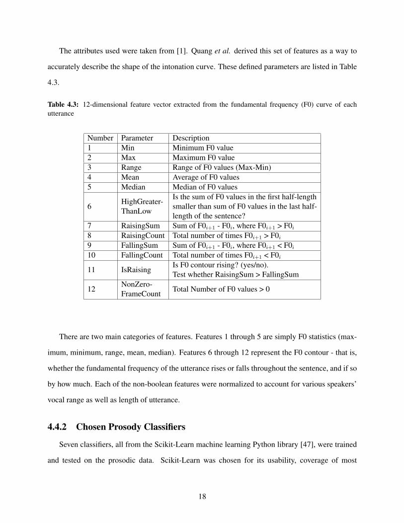
The attributes used were taken from [1]. Quang et al. derived this set of features as a way to

accurately describe the shape of the intonation curve. These defined parameters are listed in Table

4.3.

Table 4.3: 12-dimensional feature vector extracted from the fundamental frequency (F0) curve of eachutterance

Number Parameter Description1 Min Minimum F0 value2 Max Maximum F0 value3 Range Range of F0 values (Max-Min)4 Mean Average of F0 values5 Median Median of F0 values

6HighGreater-ThanLow

Is the sum of F0 values in the first half-lengthsmaller than sum of F0 values in the last half-length of the sentence?

7 RaisingSum Sum of F0i+1 - F0i, where F0i+1 > F0i

8 RaisingCount Total number of times F0i+1 > F0i

9 FallingSum Sum of F0i+1 - F0i, where F0i+1 < F0i

10 FallingCount Total number of times F0i+1 < F0i

11 IsRaisingIs F0 contour rising? (yes/no).Test whether RaisingSum > FallingSum

12NonZero-FrameCount

Total Number of F0 values > 0

There are two main categories of features. Features 1 through 5 are simply F0 statistics (max-

imum, minimum, range, mean, median). Features 6 through 12 represent the F0 contour - that is,

whether the fundamental frequency of the utterance rises or falls throughout the sentence, and if so

by how much. Each of the non-boolean features were normalized to account for various speakers’

vocal range as well as length of utterance.

4.4.2 Chosen Prosody Classifiers

Seven classifiers, all from the Scikit-Learn machine learning Python library [47], were trained

and tested on the prosodic data. Scikit-Learn was chosen for its usability, coverage of most

18

machine-learning tasks, and implementation by machine learning experts. The classifiers tested

are in the list below. Classifiers are ordered by accuracy, and includes the section number in which

the classifier is described.

1. Stochastic Gradient Descent (SGD, 3.8)

2. Gaussian Naive Bayes (GNB, 3.5)

3. Decision Tree (DTC, 3.1)

4. Logistic Regression (LogReg, 3.6)

5. K-Neighbors (KNC, 3.2)

6. Random Forest (RFC, 3.7)

The LogReg classifier was tested to get a feel for how the data truly looked, and to decide

whether or not it could be easily separated. The LinReg classifier did not perform with high

accuracy, though it was above random chance, meaning the data could not be easily classified.

This will be discussed more in depth in Section 5.1.

A Bayesian model has been shown to work well for prosodic data classification [21, 48]. A

GNB classifier was tested on the prosodic data for this reason as well as a comparison to the NB

classifier tested on the transcription corpus. The Gaussian version was used as prosodic features

are not independent and should not be assumed as such.

The DTC was chosen to test as Quang et al. had such success with one in their French prosody

question classification experiments [1] and Boakye et al. also recommend it be used for prosody-

based predictions [19]. The RFC was thus tested because it uses multiple DTCs to make predictions

and hence was expected to outperform the DTC.

Finally, a K neighbors classifier (KNC) was tested as it is often used in emotion classification

based on prosody analysis [49, 50]. In all cases, the training data had to be high-dimensional with

empirically chosen features [51]. The prosodic data used to train the classifier fits this description,

so a KNC was chosen.

19

4.4.3 Training & Testing Prosody Classifiers

For each run of a classifier, training and testing data was randomly sampled to retrieve a set of

50/50 positive (questions) and negative (non-questions) examples. The amount of data used in the

training and testing data for each class is given in Table 4.2.

Each classifier was run 30 times, for each run using a different subset of training and test-

ing samples to account for bias. Results were then averaged to get an overall view of how each

classifier performed. Final results of these tests are in Table 5.2.

Classifier parameters were updated in order to maximize performance. The parameters used

are listed below, in order of lowest to highest average accuracy:

1. SGD: max_iter=1000, tol=1e-3, loss=‘squared_hinge’

2. DTC: max_depth=8, splitter=‘random’

3. GNB: priors=None, var_smoothing=1e-9

4. LogReg: solver=‘liblinear’, max_iter=1500

5. KNC: n_neighbors=25

6. RFC: max_depth=5, n_estimators=90

20

Chapter 5

Results & Discussion

5.1 Principal Components Analysis

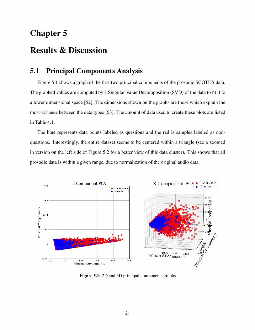
Figure 5.1 shows a graph of the first two principal components of the prosodic SCOTUS data.

The graphed values are computed by a Singular Value Decomposition (SVD) of the data to fit it to

a lower dimensional space [52]. The dimensions shown on the graphs are those which explain the

most variance between the data types [53]. The amount of data used to create these plots are listed

in Table 4.1.

The blue represents data points labeled as questions and the red is samples labeled as non-

questions. Interestingly, the entire dataset seems to be centered within a triangle (see a zoomed

in version on the left side of Figure 5.2 for a better view of this data cluster). This shows that all

prosodic data is within a given range, due to normalization of the original audio data.

Figure 5.1: 2D and 3D principal components graphs

21

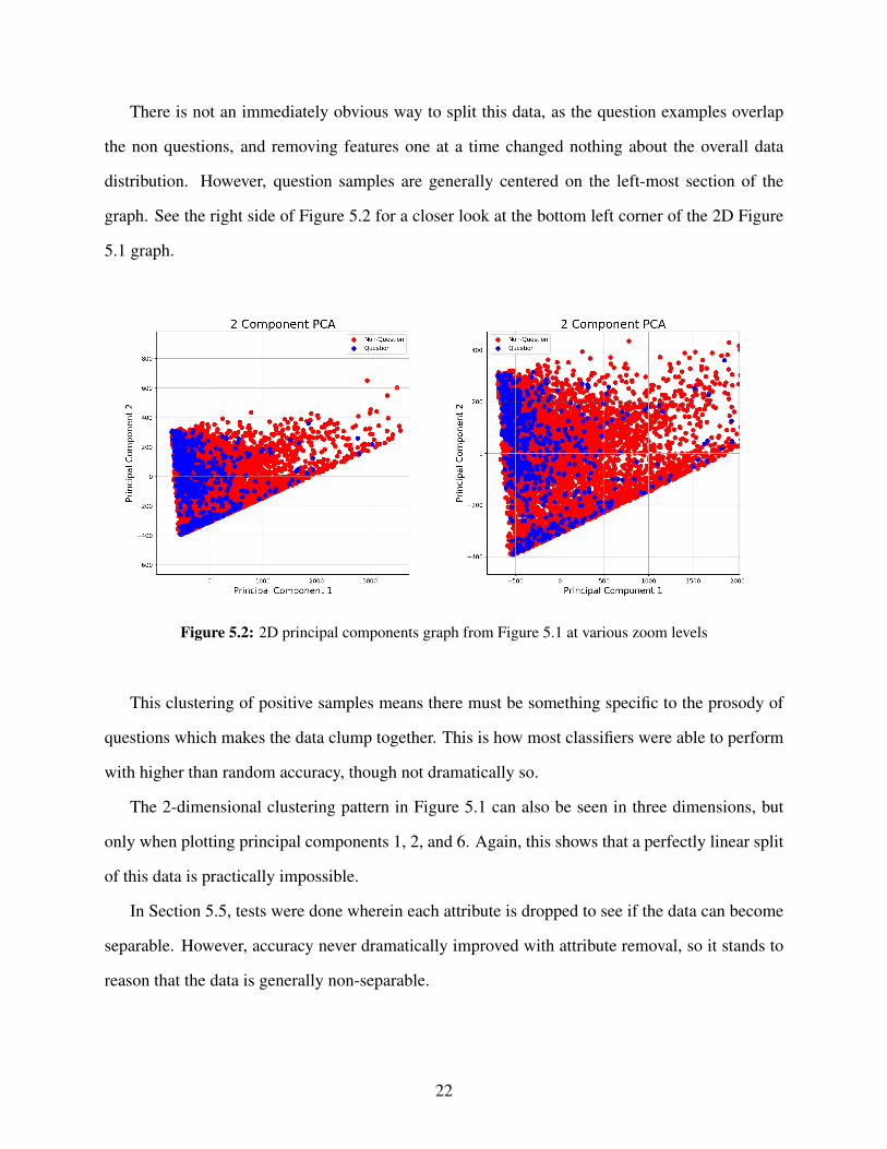
There is not an immediately obvious way to split this data, as the question examples overlap

the non questions, and removing features one at a time changed nothing about the overall data

distribution. However, question samples are generally centered on the left-most section of the

graph. See the right side of Figure 5.2 for a closer look at the bottom left corner of the 2D Figure

5.1 graph.

Figure 5.2: 2D principal components graph from Figure 5.1 at various zoom levels

This clustering of positive samples means there must be something specific to the prosody of

questions which makes the data clump together. This is how most classifiers were able to perform

with higher than random accuracy, though not dramatically so.

The 2-dimensional clustering pattern in Figure 5.1 can also be seen in three dimensions, but

only when plotting principal components 1, 2, and 6. Again, this shows that a perfectly linear split

of this data is practically impossible.

In Section 5.5, tests were done wherein each attribute is dropped to see if the data can become

separable. However, accuracy never dramatically improved with attribute removal, so it stands to

reason that the data is generally non-separable.

22

5.2 Text Classifier Accuracy

Three different Natural Language Toolkit (NLTK) [38] classifiers were chosen to be compared

to the prosody classifiers. Classifiers trained and tested on the text data were (in order of least to

most change between punctuated and non-punctuated datasets):

1. Maximum Entropy (MaxEnt)

2. Naive Bayes (NB)

3. Decision Tree (DTC)

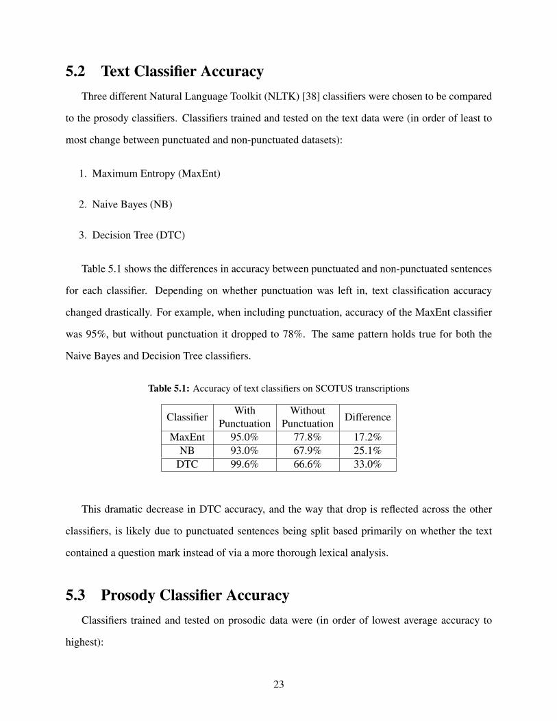
Table 5.1 shows the differences in accuracy between punctuated and non-punctuated sentences

for each classifier. Depending on whether punctuation was left in, text classification accuracy

changed drastically. For example, when including punctuation, accuracy of the MaxEnt classifier

was 95%, but without punctuation it dropped to 78%. The same pattern holds true for both the

Naive Bayes and Decision Tree classifiers.

Table 5.1: Accuracy of text classifiers on SCOTUS transcriptions

ClassifierWith

PunctuationWithout

PunctuationDifference

MaxEnt 95.0% 77.8% 17.2%NB 93.0% 67.9% 25.1%

DTC 99.6% 66.6% 33.0%

This dramatic decrease in DTC accuracy, and the way that drop is reflected across the other

classifiers, is likely due to punctuated sentences being split based primarily on whether the text

contained a question mark instead of via a more thorough lexical analysis.

5.3 Prosody Classifier Accuracy

Classifiers trained and tested on prosodic data were (in order of lowest average accuracy to

highest):

23

1. Stochastic Gradient Descent (SGD)

2. Gaussian Naive Bayes (GNB)

3. Decision Tree (DTC)

4. Logistic Regression (LogReg)

5. K-Neighbors (KNC)

6. Random Forest (RFC)

Figure 5.4 shows the minimum, maximum, and average accuracy when training and testing

these seven different classifiers (explained in Section 4.4.2) on a 50/50 split of positive and negative

examples. Exact numbers are given in Table 5.2.

Figure 5.3: Min, Max, Avg accuracy for each classifier - data from Table 5.2

The SGD classifier performed the worst, with an average of 55.4% accuracy over 30 test runs.

Meanwhile, the best performance was the Random Forest Classifier, reaching 63% average accu-

racy. All classifiers performed above 50% accuracy on average, and all but SGD performed above

24

60%. This implies that some pattern was found in the prosodic data to make classifier predictions

not solely a proverbial coin flip.

Table 5.2: Accuracy of prosody classifiers on SCOTUS audio, 30 trials each

Classifier SGD GNB DTC LogReg KNC RFCMin Accuracy 46.2% 55.5% 55.5% 57.3% 53.0% 57.7%Max Accuracy 63.1% 66.3% 66.3% 65.9% 65.9% 68.1%Avg Accuracy 55.4% 60.1% 60.3% 61.0% 62.0% 63.0%

Std Dev 4.5% 2.4% 3.4% 2.2% 2.6% 2.3%

Table 5.3 shows the number of true negative, true positive, false negative, and false positive

predictions made by each classifier, with 278 data points tested for each of 30 runs. While both the

SGD and KNC classifiers have approximately equal amounts of both true and false negative and

positive values, this does not hold across all classifiers. This is especially obvious for the GNB

classifier, which predicted over twice as many true positives as true negatives, and approximately

three times as many false positives and false negatives. The most striking difference, however, is

that the only classifier with a larger true negative than true positive value is SGD. SGD is also the

only classifier with a higher number of false negatives than false positives.

Table 5.3: Average true negative and positive and false positive and negative predictions by prosody classi-fiers on SCOTUS audio, 30 trials each

Classifier SGD GNB DTC LogReg KNC RFCTrue Neg 77.2 55.1 79.8 73.6 84.7 80.7True Pos 74.4 113.0 87.7 95.4 86.1 91.0False Pos 62.9 83.5 60.9 65.8 54.9 57.2False Neg 64.5 27.4 50.6 44.2 53.3 50.0

Distributions of parameter 6 (HighGreaterThanLow) in Table 4.3 are seen in Table 5.4. Inter-

estingly, these distributions are nearly mirrored in both question types. This may account for part

of the difficulty in accurately categorizing the sentence types. Even worse, there were no samples

that were negative for parameter 11 (IsRaising). However, taking out this parameter did not greatly

increase classifier accuracy.

25

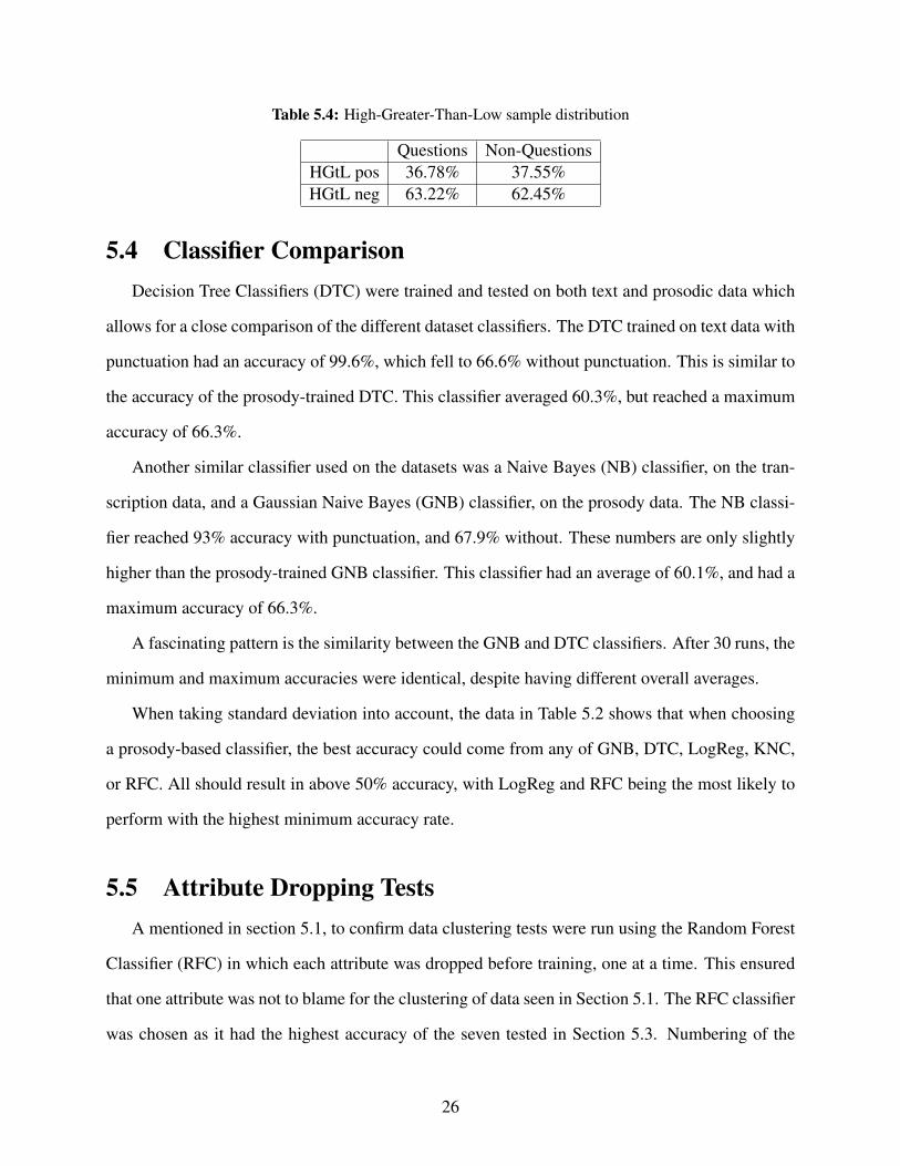
Table 5.4: High-Greater-Than-Low sample distribution

Questions Non-QuestionsHGtL pos 36.78% 37.55%HGtL neg 63.22% 62.45%

5.4 Classifier Comparison

Decision Tree Classifiers (DTC) were trained and tested on both text and prosodic data which

allows for a close comparison of the different dataset classifiers. The DTC trained on text data with

punctuation had an accuracy of 99.6%, which fell to 66.6% without punctuation. This is similar to

the accuracy of the prosody-trained DTC. This classifier averaged 60.3%, but reached a maximum

accuracy of 66.3%.

Another similar classifier used on the datasets was a Naive Bayes (NB) classifier, on the tran-

scription data, and a Gaussian Naive Bayes (GNB) classifier, on the prosody data. The NB classi-

fier reached 93% accuracy with punctuation, and 67.9% without. These numbers are only slightly

higher than the prosody-trained GNB classifier. This classifier had an average of 60.1%, and had a

maximum accuracy of 66.3%.

A fascinating pattern is the similarity between the GNB and DTC classifiers. After 30 runs, the

minimum and maximum accuracies were identical, despite having different overall averages.

When taking standard deviation into account, the data in Table 5.2 shows that when choosing

a prosody-based classifier, the best accuracy could come from any of GNB, DTC, LogReg, KNC,

or RFC. All should result in above 50% accuracy, with LogReg and RFC being the most likely to

perform with the highest minimum accuracy rate.

5.5 Attribute Dropping Tests

A mentioned in section 5.1, to confirm data clustering tests were run using the Random Forest

Classifier (RFC) in which each attribute was dropped before training, one at a time. This ensured

that one attribute was not to blame for the clustering of data seen in Section 5.1. The RFC classifier

was chosen as it had the highest accuracy of the seven tested in Section 5.3. Numbering of the

26

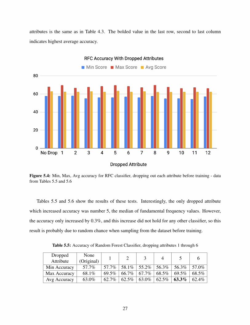
attributes is the same as in Table 4.3. The bolded value in the last row, second to last column

indicates highest average accuracy.

Figure 5.4: Min, Max, Avg accuracy for RFC classifier, dropping out each attribute before training - datafrom Tables 5.5 and 5.6

Tables 5.5 and 5.6 show the results of these tests. Interestingly, the only dropped attribute

which increased accuracy was number 5, the median of fundamental frequency values. However,

the accuracy only increased by 0.3%, and this increase did not hold for any other classifier, so this

result is probably due to random chance when sampling from the dataset before training.

Table 5.5: Accuracy of Random Forest Classifier, dropping attributes 1 through 6

DroppedAttribute

None(Original)

1 2 3 4 5 6

Min Accuracy 57.7% 57.7% 58.1% 55.2% 56.3% 56.3% 57.0%Max Accuracy 68.1% 69.5% 66.7% 67.7% 68.5% 69.5% 68.5%Avg Accuracy 63.0% 62.7% 62.5% 63.0% 62.5% 63.3% 62.4%

27

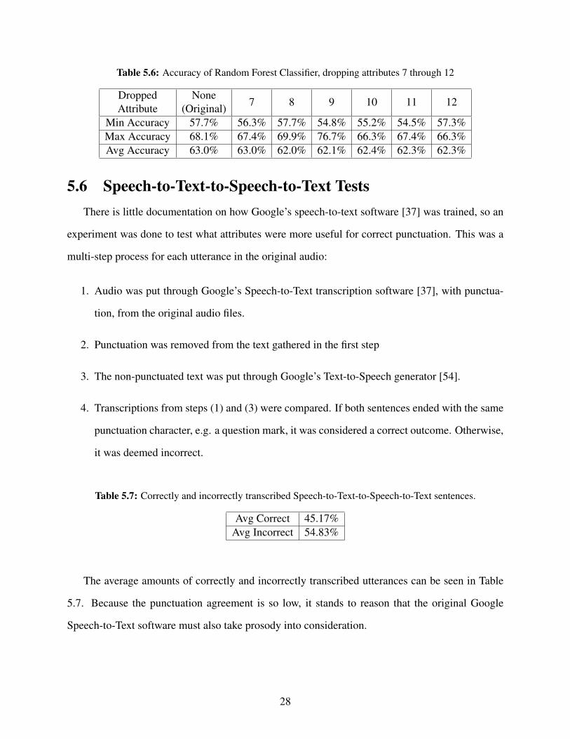
Table 5.6: Accuracy of Random Forest Classifier, dropping attributes 7 through 12

DroppedAttribute

None(Original)

7 8 9 10 11 12

Min Accuracy 57.7% 56.3% 57.7% 54.8% 55.2% 54.5% 57.3%Max Accuracy 68.1% 67.4% 69.9% 76.7% 66.3% 67.4% 66.3%Avg Accuracy 63.0% 63.0% 62.0% 62.1% 62.4% 62.3% 62.3%

5.6 Speech-to-Text-to-Speech-to-Text Tests

There is little documentation on how Google’s speech-to-text software [37] was trained, so an

experiment was done to test what attributes were more useful for correct punctuation. This was a

multi-step process for each utterance in the original audio:

1. Audio was put through Google’s Speech-to-Text transcription software [37], with punctua-

tion, from the original audio files.

2. Punctuation was removed from the text gathered in the first step

3. The non-punctuated text was put through Google’s Text-to-Speech generator [54].

4. Transcriptions from steps (1) and (3) were compared. If both sentences ended with the same

punctuation character, e.g. a question mark, it was considered a correct outcome. Otherwise,

it was deemed incorrect.

Table 5.7: Correctly and incorrectly transcribed Speech-to-Text-to-Speech-to-Text sentences.

Avg Correct 45.17%Avg Incorrect 54.83%

The average amounts of correctly and incorrectly transcribed utterances can be seen in Table

5.7. Because the punctuation agreement is so low, it stands to reason that the original Google

Speech-to-Text software must also take prosody into consideration.

28

Chapter 6

Conclusions

6.1 Overall Conclusions

“Prosody" refers to patterns of accents and intonation in spoken language, as opposed to “lex-

icon" which describes only words used within an utterance. When considering only recordings

from the Supreme Court of the United States (SCOTUS), classifiers trained to recognize interrog-

ative utterances solely on lexical features perform with considerably higher accuracy than those

trained on prosody alone.

The classifiers trained on transcriptions of SCOTUS data were Maximum Entropy (MaxEnt),

Naive Bayes (NB), and Decision Tree (DTC). When including punctuation in lexicon-based clas-

sifiers, the DTC was able to recognize questions at 99.6% accuracy. Yet, when punctuation was

removed, that fell to 66.6%. Without punctuation included, the highest performing classifier was

MaxEnt, at 77.8% accuracy. The classifier with the least difference between punctuated and non-

punctuated training and testing sets was MaxEnt, with accuracies of 95% and 77.8% accuracy,

respectively.

Seven classifiers were trained on prosodic data - the same utterances used for the transcription

dataset. These classifiers were (lowest to highest average accuracy) Linear Regression (LinReg),

Stochastic Gradient Descent (SGD), Gaussian Naive Bayes (GNB), Decision Tree (DTC), Logistic

Regression (LogReg), K-Neighbors (KNC), and Random Forest (RFC).

Prosody-based classifiers performed better than random, i.e. 50% accuracy, but not nearly as

well as lexical classifiers. The highest accuracy obtained was an average of 63.0% by the RFC

classifier. The lowest was LinReg with a 5.8% average. All but LinReg and SGD performed with

higher than 60% accuracy.

Looking at the principle components of the prosodic data, it was discovered that the data is

mostly non-separable (see Figure 5.1). To check if certain attributes could be removed for better

29

class separability, and thus higher accuracy, tests performed dropping out each attribute. The RFC

classifier was averaged over 30 runs, dropping one attribute at a time for each of these 30-run

tests. This test was done twelve times, once for each attribute. However, these experiments were

ultimately for naught as there was no significant increase in accuracy when removing any of the

attributes.

6.2 Future Work

Quang et al. [1] showed that integration of text and prosody of speech can increase accuracy of

sentence type classification in French and Vietnamese, whereas the research in this thesis focused

primarily on prosodic analysis of English speech. Future research in this area would thus include

more integration of prosodic features and lexical analysis. This includes not only discovery and

creation of better lexical classifiers, but also further linguistic research into prosodic features which

differ between types of sentences, as well as between languages.

Classifiers using the same attributes should be trained and tested on other datasets, such as au-

dio from television interviews. It is conceivable that some of the non-separability of the SCOTUS

data was due to the measured way in which the participants speak. Tensions running rampant may

lead to greater separability of classes.

It remains to be seen whether a better speech-to-text generator would result in higher text

classification accuracy. Take the example sentence in Section 4.3.1:

“Because justice justice justice courses that’s the whole point of impossibility from

the only presidential the appointed person at the FDA."

This sentence should have been transcribed closer to the original court transcript:

“Because, Justice – Justice – Justice Gorsuch, that’s the whole point of impossibility

preemption. Are we going to let Dr. Monroe, who is five layers down from the only

Presidentially-appointed person at the FDA"

30

Furthermore, more accurate transcription of court proceedings could also dramatically increase

text classification accuracy. The common courtroom phrase “your honor" was regularly transcribed

from the SCOTUS audio as “your own or". And as seen above, the name “Gorsuch" often became

“courses". It is thus foreseeable that more accurate speech transcripts would lead to more accurate

sentence classification in the case of SCOTUS hearings, even without punctuation included.

31

Bibliography

[1] Vu Minh Quang, Laurent Besacier, and Eric Castelli. Automatic question detection:

Prosodic-lexical features and crosslingual experiments. INTERSPEECH-2007, pages 2257–

2260, 2007.

[2] Christine Bartels. The Intonation of English Statements and Questions: A Compositional

Interpretation. PhD thesis, University of Massachusetts Amherst, 2015.

[3] Gustavo LÃspez, Luis Quesada, and Luis Guerrero. Alexa vs. siri vs. cortana vs. google

assistant: A comparison of speech-based natural user interfaces. pages 241–250, 01 2018.

[4] Matthew Hoy. Alexa, siri, cortana, and more: An introduction to voice assistants. Medical

Reference Services Quarterly, 37:81–88, 01 2018.

[5] Joshi Aditya, Pushpak Bhattacharyya, and Mark J. Carman. Automatic sarcasm detection: A

survey. ACM Computing Surveys, 50(5):1–22, November 2017.

[6] Patrick J. Donnelly, Nathaniel Blanchard, Andrew M. Olney, Sean Kelly, Martin Nystrand,

and Sidney K. D’Mello. Words matter: automatic detection of teacher questions in live

classroom discourse using linguistics, acoustics, and context. pages 218–227, March 2017.

[7] Amir Zadeh, Minghai Chen, Soujanya Poria, Erik Cambria, and Louis-Philippe Morency.

Tensor fusion network for multimodal sentiment analysis. In Proceedings of the 2017 Confer-

ence on Empirical Methods in Natural Language Processing, pages 1103–1114, September

2017.

[8] Elisabeth Selkirk. Sentence prosody: Intonation, stress, and phrasing. The handbook of

phonological theory, 1:550–569, 1995.

[9] Supreme court of the united states: Argument audio. https://www.supremecourt.gov/oral_

arguments/argument_audio/2018.

32

[10] Michael Wagner and Duane G. Watson. Experimental and theoretical advances in prosody:

A review. Lang Cogn Process, 25:7–9, January 2010.

[11] Katy Carlson. How prosody influences sentence comprehension. Language and Linguistics

Compass, pages 1188–1200, January 2009.

[12] Gretchen McCulloch. One sentence with 7 meanings unlocks a mystery of human speech.

All Things Linguistic, June 2018.

[13] Nancy Hedberg, Juan M. Sosa, and Emrah Görgülü. The meaning of intonation in yes-no

questions in american english: A corpus study. Corpus Linguistics and Linguistic Theory,

2014.

[14] S. Duncan and D. W. Fiske. Face-To-Face Interaction: Research, Methods, and Theory.

Lawrence Erlbaum Associates, 1977.

[15] Agustín Gravano. Turn-Taking and Affirmative Cue Words in Task-Oriented Dialogue. PhD

thesis, Graduate School of Arts and Sciences, Columbia University, New York, NY, 2009.

[16] T. Ballmer and W. Brennstuhl. Speech Act Classification: A Study in the Lexical Analysis of

English Speech Activity Verbs. Springer Science Business Media, 2013.

[17] E. Riloff and J. Wiebe. Learning extraction patterns for subjective expressions. Proceedings

of Conference on Empirical Methods in Natural Language Processing (EMNLP), 2003.

[18] Njagi Dennis Gitari, Zhang Zuping, Hanyurwimfura Damien, and Jun Long. A lexicon-based

approach for hate speech detection. International Journal of Multimedia and Ubiquitous

Engineering, 10(4):215–230, 2015.

[19] Kofi Boakye, Benoît Favre, and Dilek Z. Hakkani-Tür. Any questions? automatic question

detection in meetings. 2009 IEEE Workshop on Automatic Speech Recognition Understand-

ing, pages 485–489, 2009.

33

[20] Sonali Bhagat Jeremy Ang Elizabeth Shriberg, Raj Dhillon and Hannah Carvey. The icsi

meeting recorder dialog act (mrda) corpus. 2004.

[21] Andreas Stolcke, Noah Coccaro, Rebecca Bates, Paul Taylor, Carol Van Ess-Dykema, Klaus

Ries, Elizabeth Shriberg, Daniel Jurafsky, Rachel Martin, and Marie Meteer. Dialogue act

modeling for automatic tagging and recognition of conversational speech. Computational

Linguistics, 26(3):339–373, September 2000.

[22] J. Godfrey, E. Holliman, and J. McDaniel. Switchboard: telephone speech corpus for research

and development . acoustics,. In IEEE International Conference on Speech, and Signal Pro-

cessing, ICASSP-92, volume 1, pages 517–520, 1992.

[23] Charu C Aggarwal and Cheng Xiang Zhai. Mining text data. Springer, 2012.

[24] 1.10. decision trees. https://scikit-learn.org/stable/modules/tree.html, 2019.

[25] 1.6.2. nearest neighbors classification. https://scikit-learn.org/stable/modules/neighbors.

html, 2019.

[26] Source code for nltk.classify.maxent. https://www.nltk.org/_modules/nltk/classify/maxent.

html.

[27] 2. built-in functions - zip(). https://docs.python.org/3.3/library/functions.html#zip, 2019.

[28] Christopher Manning. Maxent models and discriminative estimation: Generative vs. discrim-

inative models. https://web.stanford.edu/class/cs124/lec/Maximum_Entropy_Classifiers.pdf.

[29] Ronald Rosenfeld. A maximum entropy approach to adaptive statistical language modelling.

Computer Speech Language, 10:187–228, 1996.

[30] Source code for nltk.classify.naivebayes. https://www.nltk.org/_modules/nltk/classify/

naivebayes.html.

34

[31] Mengye Ren. Naive bayes and gaussian bayes classifier. https://www.cs.toronto.edu/

~urtasun/courses/CSC411/tutorial4.pdf, October 2015.

[32] 1.9.1. gaussian naive bayes. https://scikit-learn.org/stable/modules/naive_bayes.html, 2019.

[33] Avinash Navlani. Understanding logistic regression in python. https://www.datacamp.com/

community/tutorials/understanding-logistic-regression-python, September 2018.

[34] 3.2.4.3.1. sklearn.ensemble.randomforestclassifier. https://scikit-learn.org/stable/modules/

generated/sklearn.ensemble.RandomForestClassifier.html, 2019.

[35] 1.11.2.1. random forests. https://scikit-learn.org/stable/modules/ensemble.html, 2019.

[36] 1.5. stochastic gradient descent. https://scikit-learn.org/stable/modules/sgd.html, 2019.

[37] Google cloud speech-to-text api. https://cloud.google.com/speech-to-text/.

[38] Edward Loper and Steven Bird. Nltk: The natural language toolkit. In In Proceedings of the

ACL Workshop on Effective Tools and Methodologies for Teaching Natural Language Pro-

cessing and Computational Linguistics. Philadelphia: Association for Computational Lin-

guistics, 2002.

[39] Y. H. Li and A. K. Jain. Classification of text documents. The Computer Journal, 41(8):537–

546, January 1998.

[40] Kamal Nigam. Using maximum entropy for text classification. In In IJCAI-99 Workshop on

Machine Learning for Information Filtering, pages 61–67, 1999.

[41] Hai Leong Chieu and Hwee Tou Ng. A maximum entropy approach to information extraction

from semi-structured and free text. In Eighteenth National Conference on Artificial Intelli-

gence, pages 786–791, 2002.

[42] Na rae Han, Martin Chodorow, and Claudia Leacock. Detecting errors in english article usage

with a maximum entropy classifier trained on a large, diverse corpus. In Paper presented at

the 4th International Conference on Language Resources and Evaluation, 2004.

35

[43] Christopher Potts. Sentiment symposium tutorial: Classifiers. http://sentiment.

christopherpotts.net/classifiers.html#nb, 2011.

[44] Monali Bordoloi, Saroj Biswas, and Ph D Candidate. Sentiment analysis of product using

machine learning technique: A comparison among nb, svm and maxent. International Jour-

nal of Pure and Applied Mathematics, 118:71–83, 07 2018.

[45] Steven Bird, Ewan Klein, and Edward Loper. Natural Language Processing with Python -

Analyzing Text with the Natural Language Toolkit. O’Reilly Media, 2019.

[46] Yannick Jadoul, Bill Thompson, and Bart de Boer. Introducing parselmouth: A python inter-

face to praat. Journal of Phonetics, 91:1–15, November 2018.

[47] F. Pedregosa, G. Varoquaux, A. Gramfort, V. Michel, B. Thirion, O. Grisel, M. Blondel,

P. Prettenhofer, R. Weiss, V. Dubourg, J. Vanderplas, A. Passos, D. Cournapeau, M. Brucher,

M. Perrot, and E. Duchesnay. Scikit-learn: Machine learning in python. Journal of Machine

Learning Research, 12:2825–2830, 2011.

[48] Nathaniel Blanchard, Patrick Donnelly, Andrew M. Olney, Samei Borhan, Brooke Ward, Xi-

aoyi Sun, Sean Kelly, Martin Nystrand, and Sidney K. D’Mello. Identifying teacher questions

using automatic speech recognition in classrooms. pages 191–201, January 2016.

[49] Gulnaz Nasir Peerzade, Ratnadeep Deshmukh, and S.D. Waghmare. A review: Speech emo-

tion recognition. International Journal of Computer Sciences and Engineering, 6:400–402,

March 2018.

[50] Y. Kim and E. M. Provost. Emotion classification via utterance-level dynamics: A pattern-

based approach to characterizing affective expressions. In 2013 IEEE International Confer-

ence on Acoustics, Speech and Signal Processing, pages 3677–3681, May 2013.

[51] L. Kerkeni, Y. Serrestou, M. Mbarki, K. Raoof, and M. A. Mahjoub. A review on speech

emotion recognition: Case of pedagogical interaction in classroom. In 2017 International

36

Conference on Advanced Technologies for Signal and Image Processing (ATSIP), pages 1–7,

May 2017.

[52] sklearn.decomposition.pca. https://scikit-learn.org/stable/modules/generated/sklearn.

decomposition.PCA.html, 2019.

[53] 2.5.1.1. exact pca and probabilistic interpretation. https://scikit-learn.org/stable/modules/

decomposition.html#pca, 2019.

[54] Google cloud text-to-speech api. https://cloud.google.com/text-to-speech/.

37