Modeling prosodic feature sequences for speaker recognition

Modeling Prosodic Feature Sequences for Speaker Recognition

E. Shriberg a,b

L. Ferrer a,c

S. Kajarekar a

A. Venkataraman a

A. Stolckea,b

a SRI International

333 Ravenswood Ave, Menlo Park, CA 94025, USA

b International Computer Science Institute

1947 Center Street, Berkeley, CA 94704, USA

c EE Department, Stanford University

Stanford, CA 94305, USA

Corresponding author: Dr. Elizabeth Shriberg EJ 196 SRI International 333 Ravenswood Ave., Menlo Park, CA 94025, USA [email protected] (510) 666-2918; fax: (510) 666-2956 Abstract: We describe a novel approach to modeling idiosyncratic prosodic behavior for automatic speaker recognition. The approach computes various duration, pitch, and energy features for each estimated syllable in speech recognition output, quantizes the features, forms N-grams of the quantized values, and models normalized counts for each feature N-gram using support vector machines (SVMs). We refer to these features as “SNERF-grams” (N-grams of Syllable-based Nonuniform Extraction Region Features). Evaluation of SNERF-gram performance is conducted on two-party spontaneous English conversational telephone data from the Fisher corpus, using one conversation side in both training and testing. Results show that SNERF-grams provide significant performance gains when combined with a state-of-the-art baseline system, as well as with two highly successful long-range feature systems that capture word usage and lexically constrained duration patterns. Further experiments examine the relative contributions of features by quantization resolution, N-gram length, and feature type. Results show that the optimal number of bins depends on both feature type and N-gram length, but is roughly in the range of 5 to 10 bins. We find that longer N-grams are better than shorter ones, and that pitch features are most useful, followed by duration and energy features. The most important pitch features are those capturing pitch level, whereas the most important energy features reflect patterns of rising and falling. For duration features, nucleus duration is more important for speaker recognition than are durations from the onset or coda of a syllable. Overall, we find that SVM modeling of prosodic feature sequences yields valuable information for automatic speaker recognition. It also offers rich new opportunities for exploring how speakers differ from each other in voluntary but habitual ways. Keywords: prosody, automatic speaker recognition, speaker verification, support vector machines

Modeling Prosody for Speaker Recognition 2

1 Introduction

Conventional speaker recognition1 systems rely on spectral features extracted from very short time segments of speech. This approach, while highly successful in clean or matched acoustic conditions, suffers significant performance degradation in the presence of handset variability. Futhermore, because spectral slices are not modeled in sequence, the approach fails to capture longer-range stylistic features of a person’s speaking behavior, such as lexical, prosodic, and discourse-related habits. Modeling such long-range features in automatic speaker recognition is motivated for at least three reasons. First, of course, such features can increase performance beyond that of cepstral features. Progress in this area has already been made in a small number of studies (Adami et al., 2003; Doddington, 2001; Ferrer et al., 2003; Kajarekar et al., 2003; Kajarekar et al., 2004; Reynolds et al., 2003; Shriberg et al., 2004; Weber et al., 2002). It has also been found that adding long-range features can provide a larger relative gain in performance when larger amounts of training data are available (e.g., Ferrer et al., 2003). Second, unlike frame-based features, longer-range features reflect voluntary behavior, and as such could potentially be useful not only for recognizing speakers, but also for recognizing characteristics of the speech, such as the speaking style (e.g., casual chit-chat versus argumentation versus event planning). Finally, regardless of the applied task, research on long-range features should be of fundamental scientific interest to researchers interested in understanding speaking behavior. This should be the case in particular when the speech studied is spontaneous (as it is here), since individual variation is greater and reflects more contributing factors in spontaneous than in read or laboratory speech (Blaauw, 1994; Laan, 1997). A large literature in linguistics has described individual variation in articulation and acoustics (e.g., Hawkins, 1997; Millar et al., 1980, Perkell et al., 1997). Much of this work focuses on variation in the spectral domain, such as the location of formants. In general, this is the type of variation that we normalize out as listeners (Johnson and Mullenix, 1997), and thus do not perceive as variation in style. Stylistic variation in the temporal domain has been reported by researchers in other subdisciplines, particularly in descriptive studies of speech prosody. Such work has shown that individual speakers show significant differences in prosodic patterns, including intonation, phrasing, accentuation, pitch range, and speaking rate (Barlow and Wagner, 1988; Blaauw, 1994; Dahan and Bernard, 1996; Tajima and Port, 1998; Van Donzel and Koopmans-van Beinum, 1997). With few exceptions the research has focused on fairly small sets of features, and not on discerning feature relationships; however, it has provided a useful starting point for the development of potential features in this work. Previous work in linguistics (Sussman et al., 1998) as well as in automatic speech recognition (Adda-Decker and Lamel, 1999; Weintraub et al., 1996) has also examined what happens to pronunciation patterns under different speaking conditions (e.g., reading versus speaking spontaneously). Again, the focus has not been on discerning feature relations or uncovering speaker-specific styles, but the studies provide information relevant to features at the level of pronunciation that might show individual differences. Finally, a small number of additional studies have revealed other interesting ways in which speakers differ, including variation in disfluency production (Lickley, 1994; Strangert, 1993). In this paper we describe a new approach to modeling idiosyncratic stylistic prosodic behaviors for automatic speaker recognition, first introduced in a more limited study (Shriberg et al., 2004). The approach bears most similarity to past work by Adami et al. (2003), who modeled a small set of pitch, energy, and duration patterns using a bigram language model. In this work, we compute a much larger set of prosodic features associated with each syllable (syllable-based nonuniform extraction region features, or “SNERFs”), and then

1 In the literature, the term “speaker recognition” is used to refer to both (open-set) speaker verification and (closed-set) speaker identification. In this paper, we use “speaker recognition” to refer to “speaker verification”.


model counts of syllable-feature sequences (“SNERF-grams”) using support vector machines (SVMs). We evaluate the approach on development data for a system submitted to the NIST 2004 Speaker Recognition Evaluation (SRE). The task is a speaker verification task, in which one side of a short telephone conversation is provided for training the speaker model, and a side from a different conversation is used in testing. The outline of the paper is as follows. Section 2 describes the speech data ( 2.1), the automatic speech recognizer used ( 2.2), support vector machines ( 2.3), a state-of-the art cepstral system ( 2.4), the SNERF-gram system ( 2.5), and two other state-of-the art systems with which the SNERF system is combined—an SVM-based word N-gram system ( 2.6) and a GMM-based lexically constrained duration system ( 2.7). Section 2.8 describes system combination. Section 3 presents results, including results by quantization resolution ( 3.1), by N-gram order ( 3.2), by feature type and subtype ( 3.3), and finally for combinations of the SNERF system with the cepstral baseline system and two other noncepstral systems ( 3.4). Section 4 discusses future work and conclusions.

2 Method

2.1 Speech Data We used 2564 5-minute conversation sides from the Fisher corpus of two-party telephone conversations on various topics. We divided the Fisher data set into three independent subsets without overlapping speakers, as shown in Table 1. The data set was designed as follows. We separated the speakers into two sets: 1) speakers with only one recording, and 2) speakers with more than one recording. The first set was used to create the background model. The second set was used as test data. The test data set was further split into two gender-balanced sets, which we also refer to as “splits”. We use one split to train TNORM (see Section 2.3.2) and to train the combiner (see Section 2.8), when testing on the other split. Test sets for the one conversation side training condition were designed as follows. Given a set of conversations (n) from one speaker, each conversation was used to create a separate speaker model. Thus the number of models estimated for that speaker is n. Each model was tested against all the conversation sides excluding the one that was used for training that model. Thus the total number of possible target trials is n(n-1). We used only a subset of the possible trials in our experiments. The subset was selected in order to create a test set similar in composition to NIST evaluation sets in terms of the ratio of imposter to target trials, and to include a mix of channel and handset conditions. As indicated, we used only half of the original conversation side length in our development sets, in an attempt to match the average duration of a conversation side in the NIST 2004 evaluation data (about two and a half minutes).

Background Model

Test Set 1

Test Set 2

Conversation sides 1128 734 702 Unique speakers 1128 249 249 Imposter trials - 13130 9153 True speaker trials - 1508 1328 Average original side length (minutes) ~5 ~5 ~5 Average side length used (minutes) ~5 ~2.5 ~2.5

Table 1: Statistics on Fisher data sets.

We chose to use data from the Fisher corpus, rather than data from either the Switchboard (NIST 2001 and 2002 Extended Speaker Recognition Evaluation data) corpus or Mixer (NIST 2004 SRE data) corpus, for the


following reasons. First, the Fisher set contains a mixture of land-line and cellular phone data, unlike the Switchboard data used in previous evaluations. Second, the Fisher corpus is more than twice the size of the Mixer data used in the 2004 evaluation. Third, there has been significant development on Switchboard (both Switchboard 1 and Switchboard 2) in past work, whereas the Fisher data is less familiar and therefore more challenging. To illustrate the relatively high difficulty of the Fisher data, we provide in Table 2 a comparison of equal error rates (EERs) for different data sets, using a roughly comparable (but not our latest) baseline system across corpora.

Datasets Drawn From Number of Training Conversation Sides

Equal Error Rate (%)

Switchboard 1 8 0.9 Switchboard 2 8 2.3 Switchboard 2 1 6.3

Fisher 1 8.4 Mixer 1 11.3

Table 2: Comparison of performance of a similar baseline-only system across corpora, to illustrate the relative difficulty of the Fisher data set used here.

As shown, Switchboard 2 is more difficult than Switchboard 1; this is generally thought to be attributable to greater dialect variation in the former. The Fisher dataset is even more difficult than Switchboard 2; in addition to dialect variation, it also contains more telephone channel variations. In our experiments, results on Fisher have tended to generalize to the NIST 2004 SRE data, in spite of the fact that the latter set is considerably more difficult than Fisher (Kajarekar et al., 2005).

2.2 Automatic Speech Recognition

Our features make reference to the time marks associated with a speech transcription. Some features, such as duration features, which are normalized by their expected values given segmental information, also use the word hypothesis information itself. Since our systems must be fully automatic, we use the output of an automatic speech recognition system to obtain hypothesized words and their associated sub-word-level time marks. Note that an interesting issue here is that the best speech recognition system as measured in terms of word error rate (WER), may or may not be the best system to use for obtaining hypothesized words and time marks for the task of speaker recognition. We have found in different work using Gaussian mixture models (GMMs) to model word-, phone-, and state-level duration modeling, for example, that in some cases, more errorful speech recognition results in better speaker recognition performance--presumably because the patterns of speech recognition errors themselves may correlate with speakers. For this work, all of our higher-level features are based on a decoding that uses a version of SRI's five times real time conversational telephone speech recognition system (Stolcke et al., 2000). The system uses models developed for the NIST RT-03F evaluation. It is trained on Switchboard 1, some Switchboard 2, and CallHome English data, as well as on Broadcast News and web data for the language model. No Fisher data was used in training the ASR system. A speech-nonspeech hidden Markov model (HMM) was used first to detect regions of speech; the speech regions thus detected form the basis of all processing, including that of the baseline speaker ID system. The system then performed one forward/backward decoding pass with a bigram language model (LM) over a 37k word and 3k multiword vocabulary, and gender-dependent within-word triphone genonic (bottom-up state-clustered) acoustic models trained with the MMIE criterion, to generate word lattices. Front-end processing at this stage used Mel cepstral processing, vocal tract length normalization, and model-based HLDA. The model means were adapted to each conversation side using MLLR without prior recognition, based on a phone-loop model. Following the first recognition pass, lattices were expanded and rescored with a 4-gram LM to generate adaptation hypotheses. These were then used to


adapt a second set of models based on PLP analysis, LDA and MLLT transformed features, and using cross-word triphones. The adapted models and a trigram multiword LM were used to generate N-best lists. These were then rescored with a 4-gram LM, pronunciation models, a pause-LM, and a phone-in-word duration model. All scores were combined and the 1-best hypothesis was obtained by decoding confusion networks built from the N-best lists. Two different versions of the ASR hypotheses and alignments were produced. The first version corresponds to the output of the first decoding pass, which used within-word MFCC triphones and a bigram language model. It had a word error rate of about 29% on the data used here. The second version was the final-pass recognition output, which uses cross-word PLP triphones rescored with a 4-gram language model as well as other knowledge sources. This version had a word error rate of roughly 21%.

2.3 SVM Modeling

2.3.1 General description

SVMs, which are now widely used, were first introduced by Vapnik (1995). They are a class of binary classifiers that have been shown to have good generalization performance and robustness to increasing input feature vector size. Features in text categorization tasks tend to be vectors of statistics, typically N-gram statistics such as raw or scaled relative frequencies. Since the number of N-grams for even modest tasks tends to be enormous, SVMs have been found to be particularly well suited to text categorization tasks (Joachims, 1998). In fact, Yang and Liu (1999) compared a number of text categorization methods and verified the claim in Joachims (1998) that SVMs are competitive, if not better, than other classifiers they considered. The other classifiers included kNN (k-nearest neighbors), Naïve Bayes, and artificial neural networks. Further motivation for the use of SVMs comes from work by Campbell et al. (2004), who recently applied the approach to phone-based speaker verification. Since a significant amount of work in the field uses SVMs for speaker verification, we expect our choice of this classification paradigm to also make our work easier to compare and contrast with other published experiments. A unique and desirable feature of SVMs, which sets them apart from conventional hyperplane-based classifiers, is that they seek to find the hyperplane that has the maximum margin (distance from either of the convex hulls that enclose the positive and negative training instances). Vapnik (1995) showed that when the classifying hyperplane is defined this way, the upper bound of the expected value of the error on an identically distributed test corpus is minimized. An excellent tutorial on SVMs can be found in Burges (1998), to which we refer the reader for further details. However, we provide below a very brief overview of the theory behind SVMs, as a motivation for the framework used in this research. Suppose that our instances consist of feature vectors x, with their associated classes y ∈{+1,-1}. Then a hyperplane classifier is defined by

f(x) = sgn(w·x + b)

where w is a weight vector and b is a scalar bias that allows the hyperplane to be offset from the origin. The optimal hyperplane has the maximal margin of separation between the two classes of y, and it can be found by solving a constrained quadratic optimization problem using any of a number of standard numerical toolkits. The remarkable extension to this basic framework offered by SVMs is that it is possible to map the input feature vector to a possibly higher dimensional space via some potentially nonlinear transformation, perform the linear classification therein, and still retain the mathematical validity of the correctness results and bounds that hold in the input space. The transformed space, which is often referred to as the feature space (in contrast to the input space), can be infinite dimensional and yet be tractably used by manipulating variables in the lower and finite dimensional input space. We note however that because we ended up using a linear kernel in this work, as described in the next section, our classification happens in the input space itself; the significant feature of SVMs that we exploit here is thus simply the maximization of the classification margin.


2.3.2 Application to our noncepstral systems

As noted earlier, our task is to classify a given speech sample as coming from either a target speaker or an imposter. We do this by taking the value of the decision function output by the SVM classifier for each sample, which is the distance of the sample from the classifying hyperplane. The actual decision (target/imposter) is made by choosing a threshold over the range of the SVM outputs, using a held-out development data set and determining on which side of the threshold a given sample’s decision function mapping lies. We could have chosen instead to generate probabilities, which are intuitively more appealing. There was no clear evidence, however, that such a method outperforms the baseline. Indeed, maximum a posteriori classification using a sigmoid after the SVM is equivalent to classifying using a threshold as we have done.2 Alternately we could have used SVMs in regression mode to fit output values of -1 and +1 for imposters and targets, respectively. Again, we found no convincing experimental evidence that such an approach outperforms one in which the decision function is used directly. For a similar reason, we also decided to use a linear kernel over more complex kernels, after several exploratory experiments showed no clear advantage of the latter.

In our experimental setup, each training or test conversation side was assumed to provide a single point in the hyperspace. The coordinates of the point were assumed to be given by the feature vector given by our noncepstral system. For practical reasons, we do not use the complete set of features. Instead, we select the most frequent N-grams occurring in the background model training data. Subsetting the set of features in this way is not uncommon in the field. For example, Doddington (2001) used a subset of the all word-bigrams that occurred at least 200 times in order to implement a word-bigram-based speaker verification system. Subsetting has the dual advantage of making the problem tractable and simultaneously allowing us to filter out information that we intuitively feel to be useless to the problem at hand. During training, each true speaker vector is assigned to the class "+1", and each imposter is assigned to the class "-1". The score assigned by the SVM to any particular test trial was the Euclidean distance from the separating hyperplane to the point that represented the particular trial, with negative values indicating imposters. Finally, scores were normalized using TNORM (Aukenthaler et al., 2000) before being thresholded. TNORM is an impostor-centric score normalization method. The assumption is that the variation in the test duration introduces a bias and a variance in the scores. To get a better estimate of the score distribution, the score of each trial is normalized by a mean and a variance, which are estimated by scoring the same test file against a set of impostor models. Note that these impostor models are estimated for each test split from the speakers in the other split. We used the SVMLite toolkit (Joachims, 1998) to induce SVMs and classify instances. In view of the extreme skew in the distribution of classes in the training data (1128 imposter samples versus only one target sample) we also used a bias of 500 against misclassification of positive examples, a number that we initially set to be the ratio between the number of positive and negative examples, subsequently refined through experimentation. We tried to ameliorate the relative paucity of positive examples by creating pseudo instances through sampling from subsets of conversation sides belonging to the positive class. That is, we divided each conversation side into several subconversation sections and thus obtained multiple positive instances where previously a single instance only would have been available. We gained no significant improvement, however, from that approach, and thus did not use it in the experiments reported here.

2.4 Baseline System

Our baseline cepstral Gaussian mixture model (GMM) system (after Reynolds, 1995) uses a 300-3300 Hz bandwidth front end consisting of 19 MEL filters. It computes 13 cepstral coefficients (C1-C13) with cepstral mean subtraction, and their first- and second-order differences, producing a 39-dimensional feature

2 We thank an anonymous reviewer for this point.


vector. The feature vectors are modeled by a 2048-component GMM. The background GMM is trained using gender- and handset- (electret, carbon and cell phone) balanced data. Target GMMs are adapted from the background GMM using MAP adaptation of the means of the Gaussian components. For channel normalization, the feature transformation described in Reynolds (2003) is applied using gender- and handset-dependent models that are adapted from the background model. Verification is performed using 5-best Gaussian components per frame, selected with respect to the background model scores.

2.5 SNERF-Gram System

The SNERF-gram system employs a novel approach to model prosodic information, and thus for clarity we provide an overview of the approach in Figure 1. Steps in the figure are further explained in the sections below. It is of particular importance to note that the final features provided to the classifier are based on counts (of specific prosodic feature sequences), rather than on the values of prosodic features themselves. We will use the term “feature” to refer both to prosodic features and to the final values (based on counts of N-grams of discretized prosodic values) input to the SVM; the distinction should be clear from context.

Figure 1: Overview of SNERF-gram modeling

2.5.1 Syllable-level features

M odel Features Using SVM

Section 2.3.2.

Apply TNO RM to Scores

Section 2.3.2.

Com bine Scores

Section 2.8.

Com pute Syllable-Level Prosodic Features

Syllabify recognizer output; extract duration, pitch, energy measures w ithin each syllable; compute various features. See Section 2.5.1.

Discretize Features

Create X equally-filled bins; X = 2, 3, 5, 10, 30, 60. Section 2.5.1.4.

Obtain Conversation-Level N -Gram Frequencies

W ithin each conversation side, obtain count for each specific N-gram; divide by total num ber of syllables in conversation side. Section 2.5.2.

Create N-Gram s

For each syllable-level feature, concatenate discretized values for N consecutive syllables (counting pause as a syllable); N = 1, 2, 3. Section 2.5.2.

Rank-Norm alize N-G ram Frequencies

Use background data distributions to map N-gram frequencies to a uniform distribution and obtain comparable dynam ic ranges across features input to SVM . Section 2.5.3.

Prune Feature List

Prune based on overall feature frequency or other criteria. Sections 2.3.2 and 3.1.


To obtain estimated syllable regions, we syllabified the output of the speech recognizer using ‘tsylb2’ (Fisher, 1995), a program that uses a set of human-created rules that operate on the best-matched dictionary pronunciation for each word. For each resulting syllable region, as illustrated in Figure 2 , we obtain phone-level alignment information from the speech recognizer, and then extract a large number of features related to the duration, pitch, and energy values in the syllable.

Figure 2: Illustration of syllabification based on recognizer output. The smallest units indicated are 10-millisecond frames. The minimum frame count for all phone models is 3.

The duration features are obtained from recognizer alignments. Pitch is estimated using the get_f0 function in ESPS/Waves (Entropic, 1993), and then post-processed using an approach adapted from Sönmez et al. (1998). The post-processing median-filters the pitch, and then fits linear splines, and produces the posterior probability of pitch halving and pitch doubling for each frame using a log-normal tied-mixture model of pitch. The model also estimates speaker pitch range parameters used for normalization. Energy features are obtained using the RMS energy values from ESPS/Waves, and post-processed to fit one spline for each segment obtained from the pitch stylization. We note that while we used this approach to energy stylization for convenience, we are aware that the approach is suboptimal, since the stylization assumptions are based on characteristics of F0 rather than of energy. Thus, we expect that if there is any benefit to such crudely stylized energy features, a better-fitting algorithm would only yield improved results. After extraction and stylization of these features, we created a number of duration, pitch, and energy features aimed at capturing basic prosodic patterns at the syllable level. The motivation for computing features that are highly correlated (differing, for example, only in normalization, binning, or N-gram length, as described below) is that we do not know ahead of time which versions of a feature are best given robustness issues, or how those features interact with other features.

2.5.1.1 Duration features

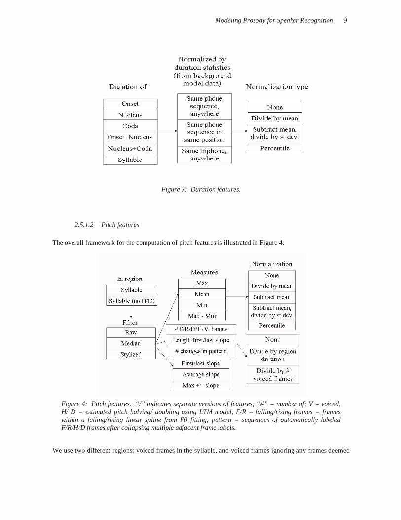
For duration features, we use five different regions in the syllable: onset, nucleus, coda, onset+nucleus, nucleus+coda, and the full syllable. We obtain the duration for that region, and normalize it using three different approaches for computing normalization statistics based on data from speakers in the background model. We use instances of the same sequence of phones appearing in the same syllable position, the same sequence of phones appearing anywhere, and instances of the same triphones anywhere. We cross these alternatives with four different types of normalization: no normalization, division by the distribution mean, Z-score normalization ((value-mean)/st.dev), and percentile, as shown in Figure 3. Note that Figure 3 (as well as Figure 4 and Figure 5 to follow) is meant only as a convenient schematic to illustrate the possible features. Not all combinations of region, measure, and normalization are used, because some combinations are ill defined or do not make sense.


Figure 3: Duration features.

2.5.1.2 Pitch features

The overall framework for the computation of pitch features is illustrated in Figure 4.

Figure 4: Pitch features. “/” indicates separate versions of features; “#” = number of; V = voiced, H/ D = estimated pitch halving/ doubling using LTM model, F/R = falling/rising frames = frames within a falling/rising linear spline from F0 fitting; pattern = sequences of automatically labeled F/R/H/D frames after collapsing multiple adjacent frame labels.

We use two different regions: voiced frames in the syllable, and voiced frames ignoring any frames deemed


to be halved or doubled by the pitch post-processing described earlier. The pitch output in these regions is then used in one of three forms: raw, median-filtered, or stylized using the linear spline approach mentioned earlier. For each of these pitch value sequences, we compute a large set of features: maximum pitch, mean pitch, minimum pitch, maximum minus minimum pitch, number of frames that are rising/falling/doubled/halved/voiced, length of the first/last slope, number of changes from fall to rise, value of first/last/average slope, and the maximum positive/negative slope. The first four features are normalized by five different approaches using data over the whole conversation side: no normalization, divide by mean, subtract mean, Z-score normalization, and percentile value. The features involving frame counts are normalized by both the total duration of the region and the duration of the region counting only voiced frames.

2.5.1.3 Energy features

For energy features, we used four different regions: the nucleus, the nucleus minus any unvoiced frames, the whole syllable, and the whole syllable minus any unvoiced frames. These values were then used to compute features in a manner similar to that described for pitch features, and as shown in Figure 5. Note however that unlike the case for pitch, we did not include unnormalized values for energy, since raw energy magnitudes tend to reflect characteristics of the channel rather than of the speaker.

Figure 5: Energy features.

2.5.1.4 Syllable-level feature discretization

Because we use count-based features in the SVM modeling, it is necessary to discretize the duration, pitch, and energy features just described. Since we do not know a priori where to place thresholds for binning the data, we try a small number of different total bin counts (2, 3, 5, 10, 30, 60), creating several binned versions for each feature. In each case, we attempt to discretize evenly on the rank distribution of values for the particular feature, so that resulting bins contain roughly equal amounts of data. For some features, for example discrete features having a small number of different values, we use a smaller number of bins to avoid having bins with no data. In the case of an unusually frequent value, we allow that value to have more mass (i.e., we do not split identical values across bins). We assign a separate bin for any inherently missing values, for example, values for pitch features during syllables without any detected voicing.


2.5.2 Sequences of discretized syllable-level features (N-grams)

Each resulting syllable-level feature, for each bin resolution, is then also modeled in three ways: unigram (current syllable only), bigram (current syllable and previous syllable or pause), and trigram (current syllable and previous two syllables or pauses). Pauses present an interesting case in this approach. Although they do not contain pitch or energy information, we do not want to ignore them. They provide useful conditioning information when present in the longer N-grams, and provide the priors for pause occurrence when used as unigrams. We thus needed to come up with a binning approach for pauses. Currently we simply bin pauses into short and long pauses, with a threshold at 15 frames, across all features. Clearly this is an area where future work on threshold tuning is likely to be helpful; it may also be the case that different approaches to the binning of pauses should be used for different types of features. The resulting number of different observed N-grams (where an N-gram is a sequence of specific bin values for a specific feature) is large—on the order of one million. For each N-gram, we count the number of appearances of that N-gram and normalize that count by the total number of syllables in the conversation side. After pruning of the N-gram list according to frequency and other criteria (see Section 3.1), the resulting values are provided to the SVM.

2.5.3 Rank-normalization of normalized counts

In order to map the N-gram frequencies to a uniform distribution and obtain comparable dynamic ranges for all feature dimensions we apply a slightly modified version of a technique known as rank normalization. The feature value distribution for each feature in the background data is recorded. In testing, a feature value is replaced by its rank, i.e., the total number of background data instances that fall below the given value on that dimension. The rank is then divided by the total number of background instances (1128 in our case, the number of speakers in the background set). The resulting normalized value lies in the closed interval from 0 to 1. Zero values, which correspond to instances in which a speaker has no occurrences of a particular prosodic feature sequence, are each mapped to zero. This preserves the sparseness of the feature vectors, an important consideration for efficient processing of high-dimensional feature vectors. More important, to the extent that the test samples conform to the distribution of background values, the resulting normalized distribution will be uniform. Another intuitive way to understand rank normalization is that the difference between any two normalized feature values corresponds to the percentage of background speakers who fall between the two values. Thus, feature value differences are amplified in regions of high population density and compressed in those of low density.

2.6 Word N-gram SVM System

The true test of the utility of the SNERF system is to see whether it provides complementary information beyond that already modeled by effective systems developed in past work. Here we present two additional systems, each of which has consistently improved performance under a variety of conditions (differences in data sets, amount of data, and other models with which they were combined). The first of these is a word N-gram system. The word N-gram-based SVM system is a recent extension of work on idiosyncratic word N-gram usage, which was first explored in a language modeling approach by Doddington (2001). These earlier language models, however, were not optimized for discrimination among speakers, since they were trained with the maximum likelihood criterion. Following the same approach as used for the SNERF system, we constructed speaker-specific word N-gram models using SVMs.


The word N-gram SVM operates in a feature space given by the relative frequencies of word N-grams in the recognition output for a conversation side. Each N-gram corresponds to one feature dimension. We considered all N-grams up to length three as potential input features, and selected those that occurred more than once in the background training set. This resulted in roughly 150 000 N-grams. The 150 000-dimensional feature space is feasible since it is very sparse: only a few N-grams occur in any given conversation side. As was done for the SNERF-gram system, the N-gram frequencies are rank-normalized and modeled in an SVM with a linear kernel, with a bias of 500 against misclassification of positive examples. These scores were also TNORMed.

2.7 GMM Duration System

The second noncepstral system we include here is a highly successful prosodic system, described in more detail in Ferrer et al. (2003). This system, which is actually a combination of three individual duration systems, uses Gaussian mixtures to model a speaker's idiosyncratic temporal patterns in the pronunciation of individual words, phones, and subphones (states). It was inspired by previous work on similar features used for improving automatic word recognition (Gadde, 2000). Three different types of features are created:

1. Word features that contain the sequence of phone durations in the word, and have varying numbers of components depending on the number of phones in their pronunciation. Each pronunciation gives rise to a different feature space.

2. Phone features that contain the duration of context-independent phones; these

are one-dimensional vectors. 3. State-in-phone features that contain the sequence of HMM state durations in

the phones. Since our recognition system uses three-state phone HMMs throughout, all feature vectors are three-dimensional.

For the extraction of these features we used state-level alignments from the recognizer described earlier. For each feature type, a model is built using the background model data for each occurring word or phone. Speaker models for each word and phone are then obtained through MAP adaptation of means and weights of the corresponding background model. During testing, three scores are obtained, one for each feature type. Each of these scores is computed as the sum of the log likelihoods of the feature vectors in the test utterance, given its models. This number is then divided by the number of components that were scored. The final score for each feature type is obtained from the difference between the speaker-specific model score and the background model score. This score is further normalized using TNORM. The three resulting scores can be used in the final system combination either independently, or after a simple summation of the three scores. Since results are similar using either approach, we use the single summed version here.

2.8 System Combination

We used split 1 of the data to train the combiner for split 2, and split 2 to train it for split 1. For a given trial, our GMM-based systems output the logarithm of the likelihood ratio between the corresponding speaker and background model, and our SVM-based systems output the discriminant function value for a given test vector and speaker model. This output, or score, is a real-valued number. Our final decision is made by combining the scores from individual systems. The goal of the system combination procedure is to combine the N individual score vectors (where N = total number of trials) from the M different component systems, while minimizing the overall error. In our system combination, we minimize equal error rate (EER), or the error rate at which the number of false alarms is equal to the number of false rejections.


We experimented with different approaches to model combination, including majority voting, simple weighted sums, error-correcting codes, decision trees, SVMs, and maximum entropy models. We found that a simple neural network combiner with no hidden layer and sigmoid output nonlinearity, a common combination approach in the field, yielded results that were as good as results obtained using the other approaches just mentioned. Therefore, we report results here for the neural network combiner only. We note, however, that there are known suboptimalities when using this approach under certain conditions, and that further research in this area is certainly warranted.

3 Results and Discussion

We present results based on a pooling of results from both test splits. In all cases, we use EER as a metric. It is worth noting that another metric, the detection cost function (DCF) is also used by NIST in speaker recognition evaluations. Because the DCF assigns a cost to the different error types, and is specific to a particular application, we focus only on the EER here, and accordingly optimize our results for that metric.

3.1 Results Relevant to Pruning: Effects of Binning and N-gram Order by Feature Type

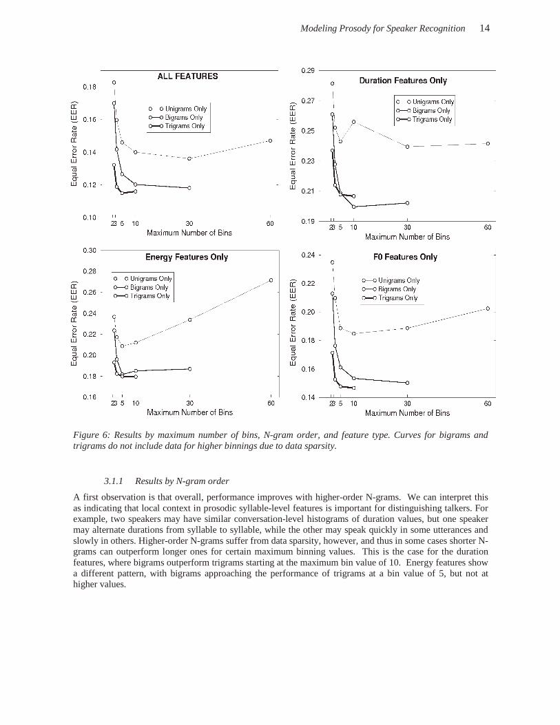
As noted earlier, a goal before supplying features to the SVM is to prune the large feature list to minimize computational load. It is also useful to prune features that add noise or may be detrimental to performance. As a first (albeit heuristic) pruning, we considered only the 100 000 most frequent features, discarding the rest. This pruning corresponds to an average minimum of six occurrences of each feature in each conversation side in the background model. In experiments not shown here, we found that we did not lose performance if we removed the divide-by-mean normalization for duration features, and if we removed the non-percentile-based normalizations for all features (kept only raw and percentile-based values). All experiments reported here thus omit these specific features. We were particularly interested in the issue of quantization level. Alternative binnings of the same feature are obviously highly correlated, and it is likely that each feature type has a “sweet spot” in terms of this factor. We should thus be able to considerably prune the list of features by omitting binnings that are too detailed, since having large bin counts combined with higher-order N-grams dramatically increases the number of final features. Through experimentation, we found that rather than use only a particular number of bins, or that number of bins plus all coarser binnings, it is better to use the following approach: For a given feature N-gram and a given maximum bin count, include next-coarser binnings only until reaching the point at which about 90% of the feature sequences for that binning value are present in our list of the 100 000 most frequently occurring N-grams. Once this constraint is satisfied, omit the remaining coarser binnings. Using this approach, we ran experiments breaking down the set of features input to the SVM by maximum number of bins, by N-gram order, and by feature type (duration, energy, or pitch). Results are shown in Figure 6. Each data point corresponds to an experiment that contains a particular subset of the full set of features computed. All results have had TNORM applied.


Figure 6: Results by maximum number of bins, N-gram order, and feature type. Curves for bigrams and trigrams do not include data for higher binnings due to data sparsity.

3.1.1 Results by N-gram order

A first observation is that overall, performance improves with higher-order N-grams. We can interpret this as indicating that local context in prosodic syllable-level features is important for distinguishing talkers. For example, two speakers may have similar conversation-level histograms of duration values, but one speaker may alternate durations from syllable to syllable, while the other may speak quickly in some utterances and slowly in others. Higher-order N-grams suffer from data sparsity, however, and thus in some cases shorter N-grams can outperform longer ones for certain maximum binning values. This is the case for the duration features, where bigrams outperform trigrams starting at the maximum bin value of 10. Energy features show a different pattern, with bigrams approaching the performance of trigrams at a bin value of 5, but not at higher values.


3.1.2 Results by quantization level

Results show that across the board, moving from only 2 to 5 bins results in sharp gains in performance; clearly, 2 or 3 bins is too crude. In the case of the all-features condition, the optimum maximum binning resolution (given the bin values we ran here) is about 30 for unigrams and bigrams, and about 5 for trigrams. If we look at individual feature types, however, the picture is quite different. Duration features show a leveling off in performance at about 5 or 10 bins, with the exception of a poor result at the value of 10 bins for unigrams (yet unexplained, but apparently a true effect). Energy features, however, show marked degradation in performance for unigrams after a binning of 5; pitch features show a similar behavior after a binning of about 30. Both of these features are inherently noisier and more variable than is duration, as seen in particular in the case of the unigram results. Based on these observations, we chose to use the following maximum number of bins by type and N-gram order (unigrams, bigrams, and trigrams, respectively): 30, 10, and 5 for duration; 5, 5, and 5 for energy; and 10, 10, and 5 for pitch. After applying the various pruning methods just described, we ran the overall SNERF-gram system. The resulting EER was 11.18%.

3.2 Results by N-gram Order for Pruned System

A careful reader will notice that in Figure 6, performance for the trigrams-only system approaches the result just reported for the pruned system using all N-gram lengths (11.18%). Thus, we may ask whether it is important to include lower order N-grams in the system at all. To address this question, we started with the pruned system, and selectively removed particular N-gram lengths (collapsed over type and binning values) to produce results for the complete set of possible combinations. Results are shown in Table 3.

Feature Length(s) Included EER (%) Significantly Different From

(a) Unigrams 13.68 b, c, d, e, f, g (b) Bigrams 11.64 a, d, e, f, g (c) Trigrams 11.50 a, e, f, g (d) Unigrams + Bigrams 11.32 a, b (e) Unigrams + Trigrams 11.32 a, b, c (f) Bigrams + Trigrams 11.28 a, b, c, g (g) Unigrams + Bigrams + Trigrams 11.18 a, b, c, f

Table 3: Results for pruned system for different N-gram order combinations. Significance is evaluated in a McNemar matched pairs test, at 95% confidence. Score-level combination results are for best found combination of systems (a) through (g), using combiner in Section 2.8.

As shown, unigrams alone perform significantly worse than all other conditions; this is expected given the trends seen earlier for the unpruned system results in Figure 6. Also as expected from the earlier results, longer N-grams are better than shorter ones. What is interesting about these results is that in terms of EERs, all other conditions peform fairly similarly—which might lead one to just choose a condition with fewer lengths—and yet many of the differences in EER are significant. For example, the system including all lengths (g) differs from that including only bigrams and trigrams (f) by only 0.1% EER, and yet the former is a significantly better system. Even systems with the same EER (d and e) differ in terms of which other systems they significantly surpass. Although it is of course easier to reach significance in a matched pairs test when the systems compared are highly correlated, these results demonstrate that different N-gram lengths make systematically different errors. This suggests that some gain might be obtained by creating


separate SNERF subsystems based on different N-gram length combinations, and then combining outputs at the score level. We ran this experiment, and indeed the approach leads to an improvement. A score-level combination of systems (b), (c), (e), (f), and (g) results in 10.90% EER. Clearly more work can be done along these lines, but to keep things simple, for all further analyses in this paper we use the best-performing system from Table 3, i.e. the system that includes all N-gram orders (g).

3.3 Results by Feature Type and Subtype

A main interest in our analyses of results is to understand which feature types contribute most to overall performance. Such analysis can lead to the design of better features, as well as to new hypotheses in basic science about how speakers differ stylistically. In this section we again start with the pruned list of features described in 3.1, but this time selectively include or remove certain types and subtypes of prosodic features. For each main prosodic feature type (duration, energy, and f0), we ran an experiment including only that feature type. In addition, within each feature type, we defined subtypes of features. For example, for pitch features we created groups such as pitch “level” (maximum, mean, and minimum pitch in the syllable), pitch “slopes” (determined by the fitted splines described earlier), “voicing” features, and so on. A complete list of the subtypes is given in the caption of Figure 7, which shows results for each of the three main feature types alone, followed by numbered experiments in which each of the subtypes is selectively removed from that main feature type.

Figure 7: Performance of systems by feature type and subtype. “Dur”= include duration features only, “Energy”=include energy features only, “Pitch”=include pitch features only. Numbered conditions refer to removal of subtypes of features within each category, as follow. D1=remove whole-syllable duration features, D2=remove nucleus-related features, D3=remove onset and coda features. E1=remove energy level features, E2=remove slope features, E3=remove fall-rise pattern features. P1=remove pitch level features, P2=remove slope features, P3=remove slopes at syllable edges only, P4=remove halving/doubling features, P5=remove fall-rise pattern features, P6=remove features related to ratio of voiced to unvoiced frames. Significance results are provided in the text.

A first observation from Figure 7 is that experiments that include features from only one main feature type (duration, energy, or pitch) all perform significantly worse (as verified in a McNemar matched pairs test at 95% confidence) than the all-features system (EER = 11.18%) described earlier. Pitch features provide the


most information, since pitch alone achieves the lowest EER of any feature type alone. The importance of pitch is further supported by additional experiments (not shown in Figure 7), in which a main feature type is removed from the all-features system. Removing energy features degrades performance to 11.53%, removing duration features degrades it to 12.94%, and removing pitch degrades it to 13.72%. Figure 7 also shows that after pitch, duration is the next most useful feature type. The numbered subtype experiments reveal further interesting details on feature importance. In the case of duration, all three conditions (“D1”, “D2”, and “D3”) differ significantly from the all-duration condition. The most important duration features for distinguishing speakers involve the duration of the syllable nucleus. This is followed by features reflecting durations of onsets and codas, and finally by features consisting of the whole syllable. It is not surprising that vowels show more absolute variation, since this is predicted phonetically, but it is interesting that this is the information that is most discriminative among speakers. The pattern also suggests that the durational information captured is more robust when using less phonetic context. This may be due in part to the fact that whole syllables occur less frequently than do syllable parts (allowing the former to be more robustly estimated), and also to some relationship between unit size and N-gram length. In considering the latter, it is worth noting that in Section 3.1.1 we found that duration features are at their best when modeled as bigrams. It may well be that speaker-specific patterns for consecutive syllables are most robust when considering only the nucleus in two consecutive syllables, rather than the complete syllable lengths. In the case of energy, removal of any of the subtypes from the all-energy condition leads to significant degradation. The most severe degradation is seen in “E3”, in which features related to the rising and falling pattern features have been removed. These rises and falls are independent of the absolute energy level a speaker is in, and thus form a rather striking contrast to results for pitch (below) in which just the opposite result pertains (what is most useful there is range, not rises and falls). It is also worth noting that the pattern-based rise and fall features come from the admittedly crude spline-fitting algorithm described earlier. The approach nevertheless seems to capture useful discriminative information about energy patterns; better techniques for fitting energy patterns are likely to only improve results. Perhaps the most interesting results are those for pitch features. As shown, results for pitch are much better overall than those for the other two features. Given the extreme degradation in condition “P1”, most of the effect for pitch seems to come from features related to a speaker’s pitch level. This is not surprising, since pitch level is determined to some extent by physiology. Pitch is also captured by the cepstral baseline system, however, so an important question is whether the SNERF-gram system can contribute information after combination. This question is addressed in the following section. There is also significant degradation from the all-pitch condition to conditions “P5” and “P6”, suggesting that there is some contribution from the patterns of falling and rising pitch (although not as great a contribution as seen in the case of energy) and from the speaker’s ratio of voiced to unvoiced speech frames.

3.4 Combination Results

Since the applied goal of this work is to use long-range features to improve on the state of the art, we investigated performance after combination with our baseline system as well as with the two long-range feature systems described earlier. Results are shown in Table 4.


Includes

ID # of

Systems Baseline Word

N-grams

3 Duration Systems

SNERFs EER (%)

Significantly Better than All Systems from

a to <ID>

a 1 x 27.362 - b 1 x 12.271 a c 2 x x 11.741 b d 1 x 11.177 c e 2 x x 11.037 c f 2 x x 8.181 e g 3 x x x 7.969 e h 1 x 7.687 f i 2 x x 7.405 h j 2 x x 6.664 i k 2 x x 6.594 i l 3 x x x 6.418 j m 3 x x x 6.382 i n 3 x x x 6.065 l o 4 x x x x 5.783 m

Table 4: Equal error rates for system combinations, ordered from highest to lowest resulting EER. Significance is evaluated in a McNemar test, at 95% confidence.

Of the three individual noncepstral systems (a, b, d), the SNERF system alone significantly outperforms both the word N-grams system alone (the weakest of the systems) and the duration system (itself a combination of three subsystems) alone. Of the two-way combinations of noncepstral systems (c, e, f), the best result (f) combines the SNERF and duration systems. This combination is significantly better than using either individual system alone, and demonstrates that while the duration and SNERF systems both model duration features, they nevertheless provide complementary information. Next in performance is a three-way combination of all noncepstral systems (g). Although the noncepstral systems are not intended to be used on their own, together they achieve performance that is not far from (and not significantly worse than) that of the cepstral system (h).

If the baseline system is allowed to combine with only one other system, best performance is achieved by choosing the SNERF system (k). If the baseline can combine with two other systems, best results include the SNERF system as one of those two systems. We note that for many of these later comparisons, it is difficult to reach significance given the amount of data available. Also, in some cases significance results can show a reversal in direction; this is the case for combination (m), which has a lower EER than does (l), but which differs significantly from only (i) rather than from (j). Such cases can occur because the matched pairs test removes matched decisions, making it easier to reach significance when the two overall systems compared are highly correlated than when they differ on many decisions. In general, combination systems that share the same component systems are more likely to be correlated; this explains the reversal seen in (m), which differs, more than does (l), from the components used in (j).

Perhaps the most important observation to note, however, is the overall result from the four-way combination. Without the SNERF system, the best result is combination (l), with an EER of 6.418. By adding the SNERF system (o), we reach an EER of 5.783, a significant improvement.


4 Future Work and Conclusions

This work has important potential extensions, some of which have been alluded to earlier. One of these is that the system should be more powerful if it is conditioned in some way on word information. Speakers clearly have distinct ways of pronouncing certain words and N-grams. The challenge in such work is to learn which words or word groups to condition on, and which to collapse over (since unmotivated conditioning merely splits the data and decreases robustness). Obvious candidates for idiosyncratic behavior are discourse-related forms, such as filled pauses, discourse markers, and backchannels, some of which have been explored from the perspective of usage statistics in previous work (e.g., Reynolds et al., 2003). Note that word-based conditioning could limit some of our bigram and trigram features, since features would no longer necessarily be contiguous. A second issue is the choice of our unit, the syllable. While this was an obvious choice for the modeling of properties like duration, there is no reason to restrict the framework to syllables. Other larger or smaller units could certainly be used. In fact, because our features are counts, it should also be possible to combine features at different levels of resolution in the same SVM. This would allow for the use of different feature extraction regions by feature, depending on what the feature’s “natural” unit appears to be. Third, since we find in general that longer N-grams perform better than shorter ones, it is worthwhile to move beyond trigrams. Fourth, although preliminary work has shown conflicting results, it is possible that a nonlinear kernel could better model features or feature interactions in this type of system. Finally, SNERF-gram modeling and modeling of noncepstral features in general, should investigate the relationship between the contribution of individual systems (and their component features), and the amount of training data used. Systems that use longer-range features are likely to show relatively more benefit over cepstral-based systems when more training data is available. Overall, we find that SVM modeling of prosodic feature sequences provides useful information for automatic speaker recognition. It performs well on its own, and combines successfully with three other state-of-the-art systems (a cepstral system, word N-gram model, and a lexically constrained duration model). On the theoretical side, unlike most conventional systems used in speaker recognition, the general framework used in modeling SNERFs supports analyses that can lead to a better understanding of how speakers differ prosodically in largely voluntary ways. Although our current prosodic features are admittedly crude, we hope that in the longer term, such efforts can help to shed light on basic individual differences in prosodic speaking behavior.

5 Acknowledgments

We thank Kemal Sönmez, Jing Zheng, and our colleagues at ICSI for collaboration and many useful discussions. We are also grateful to two anonymous reviewers for insightful comments that helped to significantly improve the content of this paper. This work was supported by interagency KDD funding through SRI NSF Award IRI-9619921, and by NSF IIS-0329258 through a subcontract to the International Computer Science Institute (ICSI). The views herein are those of the authors and do not reflect the views of the funding agencies.

6 References

Adda-Decker, M. and Lamel, L., 1999. Pronunciation Variants across Systems, Languages, and Speaking Styles. Speech Communication 29, 83-99.


Adami, A., Mihaescu, R., Reynolds, D. A., and Godfrey, J. J., 2003. Modeling Prosodic Dynamics for Speaker Recognition. Proceedings of the IEEE International Conference on Acoustics, Speech, and Signal Processing, Hong Kong. Auckenthaler, R., Carey, M., and Lloyd-Thomas, H., 2000. Score Normalization for Text-Independent Speaker Verification Systems. Digital Signal Processing 10, pp. 42–54. Barlow, M. and Wagner, M., 1988. Prosody as a Basis for Determining Speaker Characteristics. Proceedings of the Australian International Conference on Speech Science and Technology, pp. 80-85. Blaauw, E., 1994. The Contribution of Prosodic Boundary Markers to the Perceptual Difference between Read and Spontaneous Speech. Speech Communication, vol. 14, pp. 359-375. Burges, C. J. C., 1998. A Tutorial on Support Vector Machines for Pattern Recognition. Data Mining and Knowledge Discovery, vol. 2, no. 2, pp. 121-167. Campbell, W., Campbell, J, Reynolds, D., Jones, D., and Leek, T., 2004. Phonetic Speaker Recognition with Support Vector Machines. In Advances in Neural Information Processing Systems 16, Morgan Kaufmann.

Dahan, D. and Bernard, J.-M., 1996. Interspeaker Variability in Emphatic Accent Production in French. Language and Speech, vol. 39, no. 4, pp. 341-374.

Doddington, G., 2001. Speaker Recognition Based on Idiolectal Differences between Speakers. Proceedings of Eurospeech, Aalborg, Denmark, pp. 2521-2524.

Entropic, 1993. ESPS Version 5.0 Programs Manual, Entropic Research Laboratory, Washington, D.C.

Fisher, W., 1995. tsylb2. Source code available through FTP from NIST.

Ferrer, L., Bratt, H., Gadde, V. R. R., Kajarekar, S., Shriberg, E., Sönmez, K., Stolcke, A., and Venkataraman, A., 2003. Modeling Duration Patterns for Speaker Recognition. Proceedings of the IEEE International Conference on Acoustics, Speech, and Signal Processing, Geneva, pp. 2017-2020,

Gadde, V. R. R., 2000. Modeling Word Duration. In Proceedings of the International Conference on Spoken Language Processing, vol. 1, pp. 601-604.

Hawkins, S. R., 1997. Vocalic Structure in Speech Space: A Study of Individual Differences. Ph.D. thesis, Australian National University.

Joachims, T., 1998. Text Categorization with Support Vector Machines: Learning with Many Relevant Features. Proceedings of the European Conference on Machine Learning.

Johnson, K. and Mullennix, J., editors, 1997. Talker Variability in Speech Processing. San Diego: Academic Press.

Kajarekar, S., Ferrer, L., Venkataraman, A., Sönmez, K., Shriberg, E., Stolcke, A., Bratt, H., and Gadde, V. R. R., 2003. Speaker Recognition Using Prosodic and Lexical Features. In: Proceedings of the IEEE Speech


Recognition and Understanding Workshop, St. Thomas, U. S. Virgin Islands, pp. 19-24.

Kajarekar, S., Ferrer, L., Sönmez, K., Zheng, J., Shriberg, E., and Stolcke, A., 2004. Modeling NERFs for Speaker Recognition. Proceedings of the Odyssey-04 Speaker and Language Recognition Workshop, Toledo, Spain, pp. 51-56.

Kajarekar, S., Ferrer, L., Shriberg, E., Sönmez, K., Stolcke, A., Venkataraman, A., and Zheng, J., 2005. SRI’s 2004 NIST Speaker Recognition Evaluation System. Proceedings of the IEEE International Conference on Acoustics, Speech, and Signal Processing, Philadelphia, pp. 173-176.

Laan, G. P. M., 1997. The Contribution of Intonation, Segmental Durations, and Spectral Features to the Perception of a Spontaneous and a Read Speaking Style. Speech Communication, vol. 22, pp. 43-65.

Lickley, R. J., 1994. Detecting Disfluency in Spontaneous Speech. Ph.D. thesis, University of Edinburgh.

Millar, J., Oasa-Stoycheff, H., and Wagner, M., 1980. Towards Modelling of Speaker Characteristics. Journal of the Acoustical Society of America, 67 Supplement 1:94.

Perkell, J., Zandipour, M., and Matthies, M., 1997. Individual Differences in Cyclical and Speech Movement. Proceedings of the 134th Meeting of the Acoustical Society of America, San Diego.

Reynolds, D., Andrews, W., Campbell, J., Navratil, J., Peskin, B., Adami, A., Jin, Q., Klusacek, D., Abramson, J., Mihaescu, R., Godfrey, J., Jones, D., Xiang, B., 2003. The SuperSID Project: Exploiting High-level Information for High-accuracy Speaker Recognition. In Proceedings of the IEEE International Conference on Acoustics, Speech, and Signal Processing, vol. 4, pp. 784-787, Hong Kong.

Reynolds, D., 1995. Speaker Identification and Verification Using Gaussian Mixture Speaker Models. Speech Communication, vol. 17, no. 1-2, pp. 91-108.

Reynolds, D., 2003. Channel Robust Speaker Verification via Channel Mapping. Proceedings of the IEEE International Conference on Acoustics, Speech, and Signal Processing, vol. 2, pp. 53-56, Hong Kong. Strangert, E., 1993. Speaking Style and Pausing. Phonum, vol. 2, pp. 121-137. Shriberg, E., Ferrer, L., Kajareker, S., and Venkataraman, A., 2004. SVM Modeling of SNERF-grams for Speaker Recognition. Proceedings of Interspeech 2004: International Conference on Spoken Language Processing, Jeju Island, Korea. Stolcke, A., Bratt, H., Butzberger, J., Franco, H., Gadde, V. R. R., Plauche, M., Richey, C., Shriberg, E., Sönmez, E., Weng, F., and Zheng, J., 2000. The SRI March 2000 Hub-5 Conversational Speech Transcription System. Proceedings of the NIST Speech Transcription Workshop, College Park, MD.

Sussman, J., Dalston, E., and Gumbert, S., 1998. The Effect of Speaking Style on a Locus Equation Characterization of Stop Place Articulation. Phonetica, vol, 55, no. 4, pp. 204-225.


Sönmez, K., Shriberg, E., Heck, L. and Weintraub, M., 1998. Modeling Dynamic Prosodic Variation for Speaker Verification. Proceedings of the International Conference on Spoken Language Processing, vol. 7, Sydney, Australia, pp. 3189-3192.

Tajima, K. and Port, R., 1998. Speech Rhythm in English and Japanese. Proceedings of the Sixth Conference on Laboratory Phonology, York, United Kingdom.

Vapnik, V., 1995. The Nature of Statistical Learning Theory. Springer.

van Donzel, M. and Koopmans-van Beinum, F., 1997. Evaluation of prosodic characteristics in retold stories in Dutch. In G. Kokkinakis, N. Fakotakis, and E. Dermatas, editors, Proceedings of the 5th European Conference on Speech Communication and Technology, Rhodes, Greece.

Weber, F., Manganaro, L., Peskin, B., and Shriberg, E. E., 2002. Using Prosodic and Lexical Information for Speaker Identification. Proceedings of the IEEE International Conference on Acoustics, Speech, and Signal Processing, vol. 1, pp. 141-144, Orlando.

Weintraub, M., Taussig, K., Hunicke-Smith, K., and Snodgras, A., 1996. Effect of Speaking Style on LVCSR Performance. Proceedings of the International Conference on Spoken Language Processing, Addendum, pp. 16-19, Philadelphia.

Yang, Y. and Liu, X., 1999. A Re-examination of Text Categorization Methods. In Proceedings of the 22th Ann. Int. ACM SIGIR Conference on Research and Development in Information Retrieval (SIGIR'99), pp. 42-49.

Modeling prosodic feature sequences for speaker recognition

Documents

Transcript of Modeling prosodic feature sequences for speaker recognition