THEORY OF MACHINES AND MECHANISMS
526
Theory of Machines and Mechanisms, 4e Uicker et al. © Oxford University Press 2015. All rights reserved. Solutions Manual to accompany THEORY OF MACHINES AND MECHANISMS Fourth Edition International Version John J. Uicker, Jr. Professor Emeritus of Mechanical Engineering University of Wisconsin – Madison Gordon R. Pennock Associate Professor of Mechanical Engineering Purdue University Joseph E. Shigley Late Professor Emeritus of Mechanical Engineering The University of Michigan
-
Upload
khangminh22 -
Category
Documents
-
view
2 -
download
0
Transcript of THEORY OF MACHINES AND MECHANISMS

Theory of Machines and Mechanisms, 4e Uicker et al.
© Oxford University Press 2015. All rights reserved.
Solutions Manual to accompany
THEORY OF MACHINES
AND MECHANISMS Fourth Edition
International Version
John J. Uicker, Jr. Professor Emeritus of Mechanical Engineering
University of Wisconsin – Madison
Gordon R. Pennock Associate Professor of Mechanical Engineering
Purdue University
Joseph E. Shigley Late Professor Emeritus of Mechanical Engineering
The University of Michigan

Theory of Machines and Mechanisms, 4e Uicker et al.
© Oxford University Press 2015. All rights reserved.
PART 1
KINEMATICS AND MECHANISMS

Theory of Machines and Mechanisms, 4e Uicker et al.
© Oxford University Press 2015. All rights reserved.
Chapter 1
The World of Mechanisms
1.1 Sketch at least six different examples of the use of a planar four-bar linkage in practice.
They can be found in the workshop, in domestic appliances, on vehicles, on agricultural
machines, and so on.
Since the variety is unbounded no standard solutions are shown here.
1.2 The link lengths of a planar four-bar linkage are 0.2, 0.4, 0.6 and 0.6 m. Assemble the
links in all possible combinations and sketch the four inversions of each. Do these
linkages satisfy Grashof's law? Describe each inversion by name, for example, a crank-
rocker mechanism or a drag-link mechanism.
0.2, 0.6, 0.4, 0.6s l p q ; these linkages all satisfy Grashof’s law
since 0.2 0.6 0.4 0.6 . Ans.
Drag-link mechanism Drag-link mechanism Ans.
Crank-rocker mechanism Crank-rocker mechanism Ans.
Double-rocker mechanism Crank-rocker mechanism Ans.
1.3 A crank-rocker linkage has a 250 mm frame, a 62.5 mm crank, a 225 mm coupler, and a
187.5 mm rocker. Draw the linkage and find the maximum and minimum values of the
transmission angle. Locate both toggle positions and record the corresponding crank
angles and transmission angles.

Theory of Machines and Mechanisms, 4e Uicker et al.
© Oxford University Press 2015. All rights reserved.
Extremum transmission angles: min 1 max 353.1 98.1 Ans.
Toggle positions: 2 2 4 440.1 59.1 228.6 90.9 Ans.
1.4 In Fig. P1.4, point C is attached to the coupler; plot its complete path.
1.5 Find the mobility of each mechanism illustrated in Fig. P1.5.

Theory of Machines and Mechanisms, 4e Uicker et al.
© Oxford University Press 2015. All rights reserved.
(a) 1 26, 7, 0;n j j 3 6 1 2 7 1 0 1m Ans.
(b) 1 28, 10, 0;n j j 3 8 1 2 10 1 0 1m Ans.
(c) 1 27, 9, 0;n j j 3 7 1 2 9 1 0 0m Ans.
Note that the Kutzbach criterion fails in this case; the true mobility is m=1. The
exception is due to a redundant constraint. The assumption that the rolling contact
joint does not allow links 2 and 3 to separate duplicates the constraint of the fixed
link length 2 3O O .
(d) 1 24, 3, 2;n j j 3 4 1 2 3 1 2 1m Ans.
Notice that each coaxial pair of sliding ground joints is counted as only a single
prismatic pair.
1.6 Use the Kutzbach criterion to determine the mobility of the mechanism illustrated in Fig.
P1.6.
1 25, 5, 1;n j j 3 5 1 2 5 1 1 1m Ans.
Notice that the double pin is counted as two single j1 pins.
1.7 Find a planar mechanism with a mobility of one that contains a moving quaternary link.

Theory of Machines and Mechanisms, 4e Uicker et al.
© Oxford University Press 2015. All rights reserved.
How many distinct variations of this mechanism can you find?
To have at least one quaternary link, a planar mechanism must have at least eight links.
The Grübler criterion then indicates that ten single-freedom joints are required for
mobility of m = 1. According to H. Alt, “Die Analyse und Synthese der achtgleidrigen
Gelenkgetriebe”, VDI-Berichte, vol. 5, 1955, pp. 81-93, there are a total of sixteen
distinct eight-link planar linkages having ten revolute joints, seven of which contain a
quaternary link. These seven are shown below: Ans.
1.8 Use the Kutzbach criterion to detemine the mobility of the planar mechanism illustrated
in Fig. P1.8. Clearly number each link and label the lower pairs (j1) and higher pairs (j2)
on Fig. P1.8.
1 25, 5, 1;n j j 3 5 1 2 5 1 1 1m Ans.

Theory of Machines and Mechanisms, 4e Uicker et al.
© Oxford University Press 2015. All rights reserved.
1.9 For the mechanism illustrated in Fig. P1.9, determine the number of links, the number of
lower pairs, and the number of higher pairs. Using the Kutzbach criterion determine the
mobility. Is the answer correct? Briefly explain.
1 24, 3, 2;n j j 3 4 1 2 3 1 2 1m Ans.
If it is not evident that the input shown will increment this device in the direction shown,
then consider incrementing link 3 downward. Since it seems intuitive that this
determines the position of all other links, this verifies that mobility of one is correct.
1.10 Use the Kutzbach criterion to detemine the mobility of the planar mechanism illustrated
in Fig. P1.10. Clearly number each link and label the lower pairs (j1) and higher pairs (j2)
on Fig. P1.10. Treat rolling contact to mean rolling with no slipping.
1 25, 5, 1;n j j 3 5 1 2 5 1 1 1m Ans.

Theory of Machines and Mechanisms, 4e Uicker et al.
© Oxford University Press 2015. All rights reserved.
1.11 For the mechanism illustrated in Fig. P1.11 treat rolling contact to mean rolling with no
slipping. Determine the number of links, the number of lower pairs, and the number of
higher pairs. Using the Kutzbach criterion determine the mobility. Is the answer correct?
Briefly explain.
1 27, 8, 1;n j j 3 7 1 2 8 1 1 1m Ans.
This result appears to be correct. If all parts remain assembled and within the limits of
travel of the joints shown, then it appears that when any one member is locked the total
system becomes a structure.
1.12 Does the Kutzbach criterion provide the correct result for the planar mechanism
illustrated in Fig. P1.12? Briefly explain why or why not.
1 24, 2, 3;n j j 3 4 1 2 2 1 3 2m Ans.
This result appears to be correct. If any part except the wheel is moved, other parts are
required to follow. However, after all other parts are in a set position, the wheel is still
able to rotate because of slipping against the frame at A.

Theory of Machines and Mechanisms, 4e Uicker et al.
© Oxford University Press 2015. All rights reserved.
1.13 The mobility of the mechanism illustrated in Fig. P1.13 is m = 1. Use the Kutzbach
criterion to determine the number of lower pairs and the number of higher pairs. Is the
wheel rolling without slipping, or rolling and slipping, at point A on the wall?
Suppose that we identify the number of constraints at A by the symbol k. Then if we
account for all links and all other joints as follows, the Kutzbach criterion gives
1 25; 4; 1; 1;kn j j j 3 5 1 2 4 1 1 1 3 ;m k k
Therefore, to have mobility of 1m , we must have 2k constraints at A. The wheel
must be rolling without slipping. Ans.
1.14 Devise a practical working model of the drag-link mechanism.

Theory of Machines and Mechanisms, 4e Uicker et al.
© Oxford University Press 2015. All rights reserved.
1.15 Find the time ratio of the linkage of Problem 1.3.
From the values of 2 and 4 we find 188.5 and 171.5 .
Then, from Eq. (1.5), 1.099Q . Ans.
1.16 Plot the complete coupler curve of the Roberts' mechanism illustrated in Fig. 1.24b. Use
AB = CD = AD = 62.5 mm and BC = 31.25 mm.
1.17 If the crank of Fig. 1.11 is turned 25 revolutions counterclockwise, how far and in what
direction does the carriage move?
Screw and carriage move by (25 rev)/(6 rev/mm) = 4.17 mm to the right.
Carriage moves (7 rev)/(18 rev/mm) = 3.57 mm to the left with respect to the screw.
Net motion of carriage = 25/6 – 25/7 = 25/42 = 0.59 mm to the right. Ans.
More in-depth study of such devices is covered in Chapter 9.

Theory of Machines and Mechanisms, 4e Uicker et al.
© Oxford University Press 2015. All rights reserved.
1.18 Show how the mechanism of Fig. 1.15b can be used to generate a sine wave.
With the length and angle of crank 2 designated as R and 2, respectively, the horizontal
motion of link 4 is 4 2 2cos sin 90x R R .
1.19 Devise a crank-and-rocker linkage, as in Fig. 1.14c, having a rocker angle of 60. The
rocker length is to be 0.50 m.
Theory of Machines and Mechanisms, 4e Uicker et al.
© Oxford University Press 2015. All rights reserved.
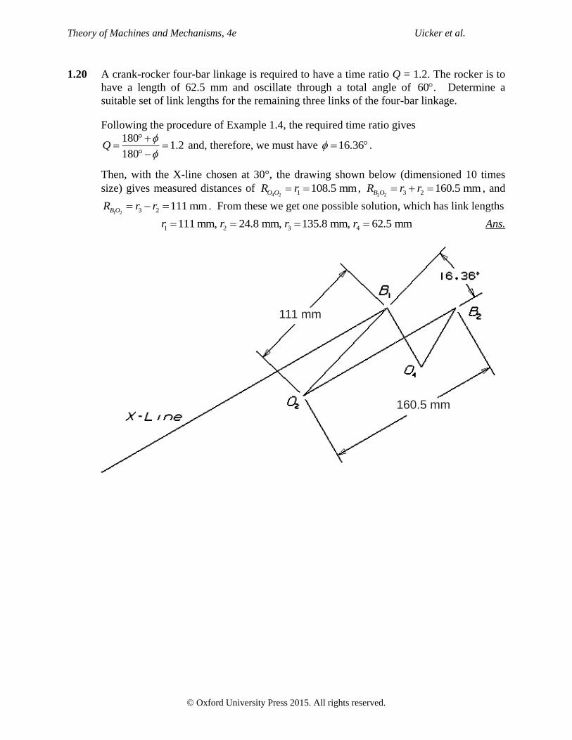
1.20 A crank-rocker four-bar linkage is required to have a time ratio Q = 1.2. The rocker is to
have a length of 62.5 mm and oscillate through a total angle of 60 . Determine a
suitable set of link lengths for the remaining three links of the four-bar linkage.
Following the procedure of Example 1.4, the required time ratio gives
1801.2
180Q
and, therefore, we must have 16.36 .
Then, with the X-line chosen at 30°, the drawing shown below (dimensioned 10 times
size) gives measured distances of 4 2 1 108.5 mmO OR r ,
2 2 3 2 160.5 mmB OR r r , and
1 2 3 2 111 mmB OR r r . From these we get one possible solution, which has link lengths
1 2 3 4111 mm, 24.8 mm, 135.8 mm, 62.5 mmr r r r Ans.
111 mm
160.5 mm

Theory of Machines and Mechanisms, 4e Uicker et al.
© Oxford University Press 2015. All rights reserved.
Chapter 2
Position and Displacement
2.1 Describe and sketch the locus of a point A that moves according to the equations
cos 2xAR at t , sin 2
yA
R at t , and 0zAR .
The locus is the spiral shown. Ans.
2.2 Find the position difference to point P from point Q on the curve 2 16y x x , where 2x
PR and 4xQ
R .
2
2 2 16 10y
PR ; ˆ ˆ2 10P R i j
2
4 4 16 4y
QR ; ˆ ˆ4 4Q R i j
ˆ ˆ2 14 14.142 98.1PQ P Q R R R i j Ans.

Theory of Machines and Mechanisms, 4e Uicker et al.
© Oxford University Press 2015. All rights reserved.
2.3 The path of a moving point is defined by the equation 22 28y x .
Find the position difference to point P from point Q if 4xPR and
3xQ
R .
2
2 4 28 4y
PR ; ˆ ˆ4 4P R i j
2
2 3 28 10y
QR ; ˆ ˆ3 10Q R i j
ˆ ˆ7 14 15.652 63.4PQ P Q R R R i j Ans.
2.4 The path of a moving point P is defined by the equation 360 / 3y x . What is the displacement of the point if its motion
begins when 0xPR and ends when 3x
PR ?
3
0 60 0 / 3 60y
PR ; ˆ0 60P R j
3
3 60 3 / 3 51y
PR ;
ˆ ˆ3 3 51P R i j
ˆ ˆ(3) (0) 3 9 9.487 71.57P P P R R R i j Ans.
2.5 If point A moves on the locus of Problem 2.1, find its displacement from t = 1.5 to t = 2.
ˆ ˆ ˆ1.5 1.5 cos3 1.5 sin3 1.5A a a a R i j i
ˆ ˆ ˆ2.0 2.0 cos4 2.0 sin 4 2.0A a a a R i j i
ˆ2.0 1.5 3.5A A A a ΔR R R i Ans.
2.6 The position of a point is given by the equation 2100 j te R . What is the path of the
point? Determine the displacement of the point from t = 0.10 to t = 0.60.
The point moves in a circle of radius 100 with center at the origin. Ans.
0.628 ˆ ˆ0.10 100 80.902 58.779je R i j
3.770 ˆ ˆ0.60 100 80.902 58.779je R i j
ˆ ˆ0.60 0.10 161.804 117.557 200.0 216 ΔR R R i j Ans.

Theory of Machines and Mechanisms, 4e Uicker et al.
© Oxford University Press 2015. All rights reserved.
2.7 The equation 2 /104 j tt e R defines the position of a point. In which direction is
the position vector rotating? Where is the point located when t = 0? What is the next
value t can have if the orientation of the position vector is to be the same as it is when t =
0? What is the displacement from the first position of the point to the second?
Since the polar angle for the position vector is
/10t , then /d dt is negative and therefore
the position vector is rotating clockwise. Ans.
2 00 0 4 4 0je R Ans.
The position vector will next have the same
direction when /10 2t , that is, when t=20. Ans.
2 220 20 4 404 0je R
20 0 400 0 R R R Ans.
2.8 The location of a point is defined by the equation 2 / 304 2 j tt e R , where t is time in
seconds. Motion of the point is initiated when t = 0. What is the displacement during the
first 3 s? Find the change in angular orientation of the position vector during the same
time interval.
0 ˆ0 0 2 2 0 2je R i
9/ 30 ˆ ˆ3 12 2 14 54 8.229 11.326je R i j
ˆ ˆ3 0 6.229 11.326 12.926 61.19 ΔR R R i j Ans.
54 0 54 ccw Ans.

Theory of Machines and Mechanisms, 4e Uicker et al.
© Oxford University Press 2015. All rights reserved.
2.9 Link 2 in Fig. P2.9 rotates according to the equation / 4t . Block 3 slides outward
on link 2 according to the equation 2 2r t . What is the absolute displacement
3PR from t = 1 to t = 3? What is the apparent displacement 3/ 2PR ?
3
2 / 42j j t
P re t e R
3
ˆ ˆ1 3 45 2.121 2.121P R i j
3
ˆ ˆ3 11 135 7.778 7.778P R i j
3 3 3
ˆ ˆ3 1 9.899 5.657 11.402 150.26P P P ΔR R R i j Ans.
3
0 2
/ 2 2ˆ2j
P re t R i
3 / 2 2
ˆ1 3P R i
3 /2 2
ˆ3 11P R i
3 3 3/2 /2 /2 2
ˆ3 1 8P P P ΔR R R i Ans.
2.10 A wheel with center at O rolls without slipping so that its center is displaced 250 mm to
the right. What is the displacement of point P on the periphery during this interval?
Since the wheel rolls without slipping,
O POR R .
/
250 mm /150 mm 1.667 rad 95.51O POR R
For POR ,
270 95.51 174.49 ˆ ˆ150 mm 174.49 149.3 14.4 mmPO
R i j
ˆ ˆ ˆ ˆ250 149.3 14.4 150 mm
P O PO PO
ΔR ΔR R R
i i j j
6 inPO
R ˆ ˆ100.7 164.4 mm 192.8 mm 58.51P R i j Ans.
2.11 A point Q moves from A to B along link 3 whereas link 2 rotates from 2 30 to
2 120 . Find the absolute displacement of Q.
3
ˆ ˆ0.3 m 30 259.8 150.0 mmQ R i j
3
ˆ ˆ0.3 m 120 150.0 259.8 mmQ R i j
3 3 3
ˆ ˆ409.8 109.8 mmQ Q Q ΔR R R i j
5 /3ˆ600.0 mmQ BA ΔR R i

Theory of Machines and Mechanisms, 4e Uicker et al.
© Oxford University Press 2015. All rights reserved.
2 4
0.3 mAO BO
R R ;4 2
0.6 mBA O O
R R 5 3 5 /3Q Q Q ΔR ΔR ΔR
5
ˆ ˆ190.2 109.8 mm 219.6 mm 30Q ΔR i j Ans.
2.12 The linkage is driven by moving the sliding block 2. Write the loop-closure equation.
Solve analytically for the position of sliding block 4. Check the result graphically for the
position where 45 .
The loop-closure equation is
A B AB R R R Ans.
/12 jj
A B AB
j
B AB
R e R R e
R R e
500 mm, 15AB
R
Taking the imaginary components of this, we get
sin15 sinA ABR R
sin sin 45500 mm 1365 mm
sin15 sin15A ABR R
Ans.
2.13 The offset slider-crank mechanism is driven by the rotating crank 2. Write the loop-
closure equation. Solve for the position of the slider 4 as a function of 2 .
20 mm
AOR , 50 mm
BAR , and 140 mm
CBR
C A BA CB R R R R
32/ 2 jjj
C A BA CBR R e R e R e
Taking real and imaginary parts,
2 3cos cosC BA CBR R R and 2 30 sin sinA BA CBR R R
and, solving simultaneously, we get
1 23
sinsin A BA
CB
R R
R
with 390 90

Theory of Machines and Mechanisms, 4e Uicker et al.
© Oxford University Press 2015. All rights reserved.
22
2 2
2
2 2 2
cos sin
50cos 19 200 1 000sin 2 500sin
C BA CB A BAR R R R R
Ans.
2.14 For the mechanism illustrated in Fig. P2.14, define a set of vectors that is suitable for a
complete kinematic analysis of the mechanism. Label and show the sense and orientation
of each vector on Fig. P2.14. Write the vector loop equation(s) for the mechanism.
Identify suitable input(s) for the mechanism. Identify the known quantities, the unknown
variables, and any constraints. If you have identified constraints then write the constraint
equation(s).
One suitable set of two vector loop equations is
? ? ?
2 3 4 5 1
R R R R R 0 and ? 1 2 3
2 3 44 24 22
I C C C
R R R R R 0 Ans.
The angle 2 is a reasonable input. Three constraint equations are required.
44 4 (C1) 24 4 (C2) 22 2 (C3) Ans.
There are four unknowns 3 4 5 24, , , and R .

Theory of Machines and Mechanisms, 4e Uicker et al.
© Oxford University Press 2015. All rights reserved.
2.15 Assume rolling with no slip between pinion 5 and rack 4 in the mechanism illustrated in
Fig. P2.15. Define a set of vectors that is suitable for a complete kinematic analysis of
the mechanism. Label and show the sense and orientation of each vector on Fig. P2.15.
Write the vector loop equation(s) for the mechanism. Identify suitable input(s) for the
mechanism. Identify the known quantities, the unknown variables, and any constraints.
If you have identified constraints then write the constraint equation(s).
One suitable set of vectors is as shown. The vector loop equation is
? ?
2 3 6 4 15 1 R R R R R R 0ÖI Ö Ö ÖÖ ÖÖ ÖÖ
with 5 5 6R Ans.
The angle 2 is a suitable input. Ans.
There are two unknown variables, 3
and R6. Ans.

Theory of Machines and Mechanisms, 4e Uicker et al.
© Oxford University Press 2015. All rights reserved.
2.16 For the geared five-bar mechanism illustrated in Fig. P2.16, there is rolling with no
slipping between gears 2 and 5. Define a set of vectors that is suitable for a complete
kinematic analysis of the mechanism. Label and show the sense and orientation of each
vector on Fig. P2.16. Write the vector loop equation(s) for the mechanism. Identify
suitable input(s) for the mechanism. Identify the known quantities, the unknown
variables, and any constraints. If you have identified constraints then write the constraint
equation(s).
One suitable set of vectors is as shown. The vector loop equation is
? C
2 3 4 5 1 R R R R R 0ÖI Ö Ö? Ö ÖÖ
with 2 2 5 5 0 Ans.
The angle 2 is a suitable input.

Theory of Machines and Mechanisms, 4e Uicker et al.
© Oxford University Press 2015. All rights reserved.
2.17 For the mechanism illustrated in Fig. P2.17, gear 3 is pinned to link 4 at point B, and is
rolling without slipping on the semi-circular ground link 1. The radius of the semi-
circular ground link is 1 and the radius of gear 3 is 3. Define a set of vectors that is
suitable for a complete kinematic analysis of the mechanism shown. Label and show the
sense and orientation of each vector in Fig. P2.17. Write the vector loop equation(s) for
the mechanism. Identify suitable input(s) for the mechanism. Identify the known
quantities, the unknown variables, and any constraints. If you have identified constraints
then write the constraint equation(s).
One suitable set of vectors is as shown. The vector loop equation is
?
2 4 5 1 R R R R 0ÖI Ö Ö? ÖÖ
with 2 2 3 3R Ans.
The angle 2 is a suitable input.

Theory of Machines and Mechanisms, 4e Uicker et al.
© Oxford University Press 2015. All rights reserved.
2.18 For the mechanism illustrated in Fig. P1.6, define a set of vectors that is suitable for a
complete kinematic analysis of the mechanism. Label and show the sense and orientation
of each vector in Fig. P1.6. Write the vector loop equation(s) for the mechanism.
Identify suitable input(s) for the mechanism. Identify the known quantities, the unknown
variables, and any constraints. If you have identified constraints then write the constraint
equation(s).
One set of vectors suitable for a kinematic analysis of the mechanism is shown below.
The corresponding vector loop equations are
? ?
1 2 3 13
I
a
R R R R 0 and ? ? ?
3 4 15 13
C
b
R R R R 0 Ans.
with the constraint equation 13 13 constant.a bR R Ans.

Theory of Machines and Mechanisms, 4e Uicker et al.
© Oxford University Press 2015. All rights reserved.
2.19 For the mechanism illustrated in Fig. P1.8, define a set of vectors that is suitable for a
complete kinematic analysis of the mechanism. Label and show the sense and orientation
of each vector in Fig. P1.8. Write the vector loop equation(s) for the mechanism.
Identify suitable input(s) for the mechanism. Identify the known quantities, the unknown
variables, and any constraints. If you have identified constraints then write the constraint
equation(s).
One set of vectors suitable for a kinematic analysis of the mechanism is shown here.
The corresponding set of vector loop equations is
? ?
1 2 4 5
I
R R R R 0 and ? ?
1 22 3 35
C
R R R R 0 Ans.
with the constraint equation 22 2 . Ans.

Theory of Machines and Mechanisms, 4e Uicker et al.
© Oxford University Press 2015. All rights reserved.
2.20 For the mechanism illustrated in Fig. P1.9, define a set of vectors that is suitable for a
complete kinematic analysis of the mechanism. Label and show the sense and orientation
of each vector in Fig. P1.9. Write the vector loop equation(s) for the mechanism.
Identify suitable input(s) for the mechanism. Identify the known quantities, the unknown
variables, and any constraints. If you have identified constraints then write the constraint
equation(s).
One set of vectors suitable for a complete kinematic analysis of this mechanism is as
shown.
The corresponding set of vector loop equations is
?
1 3 32 2
I
R R R R 0 and ? ? 1 2 ?
11 4 34 33 32 2
C C I
R R R R R R 0 Ans.
with the two constraint equations
34 4 90° C1 and 33 4 180° C2. Ans.

Theory of Machines and Mechanisms, 4e Uicker et al.
© Oxford University Press 2015. All rights reserved.
2.21 For the mechanism illustrated in Fig. P1.10, define a set of vectors that is suitable for a
complete kinematic analysis of the mechanism. Label and show the sense and orientation
of each vector in Fig. P1.10. Write the vector loop equation(s) for the mechanism.
Identify suitable input(s) for the mechanism. Identify the known quantities, the unknown
variables, and any constraints. If you have identified constraints then write the constraint
equation(s).
One set of vectors suitable for a kinematic analysis of the mechanism is shown.
The corresponding set of vector loop equations is
1 11 2 3
I
R R R R 0 and 1 ? ?
11 2 34 4 9
I C
R R R R R 0 Ans.
with the constraint equation
34 3 C1 Ans.
However, these equations do not analyze the angular displacement of the small wheel,
body 5. In order to do this, we might consider the apparent angular displacement as seen
by an observer fixed on vector 9 and viewing the point of contact between bodies 5 and
1. The non-slip condition would provide the constraint
1 1/9 5 5/9
1 1 9 5 5 9
5 5 1 5 9
5 5 9 9
0
0R
.Ans
where 5 is the radius of wheel 5 and 5 is the angular displacement of body 5.
2.22 Write a calculator program to find the sum of any number of two-dimensional vectors
expressed in mixed rectangular or polar forms. The result should be obtainable in either
form with the magnitude and angle of the polar form having only positive values.
Because the variety of makes and models of calculators is vast and no standards exist for
programming them, no solution is shown here.

Theory of Machines and Mechanisms, 4e Uicker et al.
© Oxford University Press 2015. All rights reserved.
2.23 Write a computer program to plot the coupler curve of any crank-rocker or double-crank
form of the four-bar linkage. The program should accept four link lengths and either
rectangular or polar coordinates of the coupler point relative to the coupler.
Again the variety of programming languages makes it difficult to provide a standard
solution. However, one version, written in ANSI/ISO FORTRAN 77, is supplied here as
an example. There are also no universally accepted standards for programming graphics.
Therefore the Tektronix PLOT10 subroutine library, for display on Tektronix 4010 series
displays, is chosen as an older but somewhat recognized alternative. The symbols in the
program correspond to the notation shown in Figure 2.19 of the text. The required input
data are:
X5, Y5, -1R1, R2, R3, R4,
R5, θ5, 1
The program can be verified using the data of Example 2.7 and checking the results
against those of Table 2.3.
PROGRAM CCURVE
C
C A FORTRAN 77 PROGRAM TO PLOT THE COUPLER CURVE OF ANY CRANK-ROCKER
C OR DOUBLE-CRANK FOUR-BAR LINKAGE, GIVEN ITS DIMESNIONS.
C ORIGINALLY WRITTEN USING SUBROUTINES FROM TEKTRONIX PLOT10 FOR
C DISPLAY ON 4010 SERIES DISPLAYS.
C REF:J.J.UICKER,JR, G.R.PENNOCK, & J.E.SHIGLEY, ‘THEORY OF MACHINES
C AND MECHANISMS,’ FOURTH EDITION, OXFORD UNIVERSITY PRESS, 2009.
C EXAMPLE 2.6
C
C WRITTEN BY: JOHN J. UICKER, JR.
C ON: 01 JANUARY 1980
C
C READ IN THE DIMENSIONS OF THE LINKAGE.
READ(5,1000)R1,R2,R3,R4,X5,Y5,IFORM
1000 FORMAT(6F10.0,I2)
C
C FIND R5 AND ALPHA.
IF(IFORM.LE.0)THEN
R5=SQRT(X5*X5+Y5*Y5)
ALPHA=ATAN2(Y5,X5)
ELSE
R5=X5
ALPHA=Y5/57.29578
END IF
Y5=AMAX1(0.0,R5*SIN(ALPHA))
C
C INITIALIZE FOR PLOTTING AT 120 CHARACTERS PER SECOND.
CALL INITT(1200)
C
C SET THE WINDOW FOR THE PLOTTING AREA.
CALL DWINDO(-R2,R1+R2+R4,-R4,R4+R4+Y5)
C
C CYCLE THROUGH ONE CRANK ROTATION IN FIVE DEGREE INCREMENTS.
TH2=0.0
DTH2=5.0/57.29578
IPEN=-1
DO 2 I=1,73

Theory of Machines and Mechanisms, 4e Uicker et al.
© Oxford University Press 2015. All rights reserved.
CTH2=COS(TH2)
STH2=SIN(TH2)
C
C CALCULATE THE TRANSMISSION ANGLE.
CGAM=(R3*R3+R4*R4-R1*R1-R2*R2+2.0*R1*R2*CTH2)/(2.0*R3*R4)
IF(ABS(CGAM).GT.0.99)THEN
CALL MOVABS(100,100)
CALL ANMODE
WRITE(7,1001)
1001 FORMAT(//’ *** THE TRANSMISSION ANGLE IS TOO SMALL. ***’)
GO TO 1
END IF
SGAM=SQRT(1.0-CGAM*CGAM)
GAM=ATAN2(SGAM,CGAM)
C
C CALCULATE THETA 3.
STH3=-R2*STH2+R4*SIN(GAM)
CTH3=R3+R1-R2*CTH2-R4*COS(GAM)
TH3=2.0*ATAN2(STH3,CTH3)
C
C CALCULATE THE COUPLER POINT POSITION.
TH6=TH3+ALPHA
XP=R2*CTH2+R5*COS(TH6)
YP=R2*STH2+R5*SIN(TH6)
C
C PLOT THIS SEGMENT OF THE COUPLER CURVE.
IF(IPEN.LT.0)THEN
IPEN=1
CALL MOVEA(XP,YP)
ELSE
IPEN=-1
CALL DRAWA(XP,YP)
END IF
TH2=TH2+DTH2
2 CONTINUE
C
C DRAW THE LINKAGE.
CALL MOVEA(0.0,0.0)
CALL DRAWA(R2,0.0)
XC=R2+R3*COS(TH3)
YC=R3*SIN(TH3)
CALL DRAWA(XC,YC)
CALL DRAWA(XP,YP)
CALL DRAWA(R2,0.0)
CALL MOVEA(XC,YC)
CALL DRAWA(R1,0.0)
1 CALL FINITT(0,0)
CALL EXIT
STOP
END

Theory of Machines and Mechanisms, 4e Uicker et al.
© Oxford University Press 2015. All rights reserved.
2.24 For each linkage illustrated in Fig. P2.24, find the path of point P: (a) inverted slider-
crank mechanism; (b) second inversion of the slider-crank mechanism; (c) Scott-Russell
straight-line mechanism; and (d) drag-link mechanism.
(a) (b)
(c) (d)
(a) 40 mmCA
R , 70 mmBA
R , 80 mmPC
R ; (b) 100 mmCA
R , 50 mmBA
R ,
162.5 mmPB
R ; (c) 125 mmBA CB PB
R R R ; (d) 10 mmDA
R , 20 mmBA
R ,
30 mmCC DC
R R , 40 mmPB
R .

Theory of Machines and Mechanisms, 4e Uicker et al.
© Oxford University Press 2015. All rights reserved.
2.25 Using the offset slider-crank mechanism in Fig. P2.13, find the crank angles
corresponding to the extreme values of the transmission angle.
As shown, 390 .
Also from the figure
2 2 3sin cose r r .
Differentiating with
respect to 2 ,
2 2 3
2
cos sind
r rd
;
2 2
2 3
cos
sin
rd
d r
.
Now, setting 2/ 0d d , we get 2cos 0 .
Therefore, we conclude that 2 2 1 / 2 90 , 270 ,k Ans.
2.26 In Section 1.10 it is pointed out that the transmission angle reaches an extreme value for
the four-bar linkage when the crank lies on the line between the fixed pivots. Referring
to Fig. 2.19, this means that reaches a maximum or minimum when crank 2 is colinear
with the line 2 4O O . Show, analytically, that this statement is true.
From 4 2 :O O A
2 2 2
1 2 1 2 22 coss r r rr .
Also, from 4 :ABO 2 2 2
3 4 3 42 coss r r r r .
Equating these we
differentiate with respect to 2
to obtain
1 2 2 3 4
2
2 sin 2 sind
r r r rd
or
1 2 2
2 3 4
sin
sin
r rd
d r r
.
Now, for 2
0d
d
, we have 2sin 0 . Thus, 2 0, 180 , 360 , Q.E.D.

Theory of Machines and Mechanisms, 4e Uicker et al.
© Oxford University Press 2015. All rights reserved.
2.27 Figure P2.27 illustrates a crank-and-rocker four-bar linkage in the first of its two limit
positions. In a limit position, points 2 , , and BO A lie on a straight line; that is, links 2
and 3 form a straight line. The two limit positions of a crank-rocker describe the extreme
positions of the rocking angle. Suppose that such a linkage has 1 100 mmr ,
2 50 mmr , 3 125 mmr , and 4 100 mmr .
(a) Find 2 4 and corresponding to each limit position.
(b) What is the total rocking angle of link 4?
(c) What are the transmission angles at the extremes?
(a) From isosceles triangle 4 2O O B we
can calculate or measure 2 29 ,
4 58 and 2 248 , 4 136 .
Ans.
(b) Then 4 4 4 78 Ans.
(c) Finally, from isosceles triangle
4 2O O B , 29 and 68 . Ans.
2.28 A double-rocker four-bar linkage has a dead-center position and may also have a limit
position (see Prob. 2.27). These positions occur when links 3 and 4 in Fig. P2.28 lie
along a straight line. In the dead-center position the transmission angle is 180 and the
mechanism is locked. The designer must either avoid such positions or provide the
external force, such as a spring, to unlock the linkage. Suppose, for the linkage
illustrated in Fig. P2.28, that 1
140 mmr , 2
55 mmr , 3
50 mmr , and 4 120 mmr .
Find 2 and 4 corresponding to the dead-center position. Is there a limit position?
For the given dimensions, there are two
dead-center positions, and they
correspond to the two extreme travel
positions of crank 2O A . From 4 2O AO
using the law of cosines, we can find
2 114.0 , 4 162.8 and, symmetrically,
2 114.0 , 4 162.8 . There are
also two limit positions; these occur at
2 56.5 , 4 133.1 and, symmetrically,
at 2 56.5 , 4 133.1 . Ans.

Theory of Machines and Mechanisms, 4e Uicker et al.
© Oxford University Press 2015. All rights reserved.
2.29 Figure P2.29 illustrates a slider-crank linkage that has an offset e and that is placed in one
of its limiting positions. By changing the offset e, it is possible to cause the angle that
crank 2 makes in traversing between the two limiting positions to vary in such a manner
that the driving or forward stroke of the slider takes place over a larger angle than the
angle used for the return stroke. Such a linkage is then called a quick-return mechanism.
The problem here is to develop a formula for the crank angle traversed during the
forward stroke and also develop a similar formula for the angle traversed during the
return stroke. The ratio of these two angles would then constitute a time ratio of the drive
to return strokes. Also determine which direction the crank should rotate.
From the figure we can see that 3 2 2 3 2 2sin sin 180e r r r r or
1
2
3 2
sine
r r
, 1
2
3 2
180 sine
r r
1 1
2 2
3 2 3 2
180 sin sindrive
e e
r r r r
Ans.
1 1
2 2
3 2 3 2
360 180 sin sinreturn
e e
r r r r
Ans.
Assuming driving is when B is sliding to the right, the crank should rotate clockwise. Ans.

Theory of Machines and Mechanisms, 4e Uicker et al.
© Oxford University Press 2015. All rights reserved.
Chapter 3
Velocity
3.1 The position vector of a point is given by the equation 100 j te R , where R is in meters.
Find the velocity of the point at 0.40 s.t
100 mj tt e R
100 m/sj tt j e R
0.400.40s 100 m/s
100 cos0.40 sin 0.40 m/s
100 sin 72 100 cos72 m/s
jj e
j j
j
R
0.40s 298.783 97.080 m/s 314.159 m/s 162j R Ans.
3.3 If automobile A is traveling south at 70.4 km/h and automobile B north 60 east at 51.2
km/h, what is the velocity difference between B and A? What is the apparent velocity of
B to the driver of A?
ˆ70.4 km/h 90 70.4 km/hA V j
ˆ ˆ51.2 km/h 30 44.34 25.6 km/hB V i j
ˆ ˆ44.34 96 km/hBA B A V V V i j
105.74 km/h 65.2 =105.74 km/h N 24.8 EBA V Ans
Naming B as car 3 and A as car 2, we have2B AV V since 2 is
translating. Then 3 3 2/ 2B B B BA V V V V
3 /2 105.74 km/h 65.2 =105.74 km/h N 24.8 EB V Ans.
3.4 In Fig. P3.4, wheel 2 rotates at 450 rev/min and drives wheel 3 without slipping. Find
the velocity difference between points B and A.

Theory of Machines and Mechanisms, 4e Uicker et al.
© Oxford University Press 2015. All rights reserved.
2
450 rev/min 2 rad/rev
60 s/min
15 rad/s cw
2 22 1500 4710 mm/sAO AOV R
4200 mm/s 90B V
ˆ ˆ4710 4200
6300 mm/s 138.4
BA B A
V V V
i j Ans.
3.5 Two points A and B, located along the radius of a wheel (see Fig. P3.5), have speeds of
80 and 140 in/s, respectively. The distance between the points is .75 mmBA
R .
(a) What is the diameter of the wheel?
(b) Find ,
,AB BA
V V and the angular velocity of the wheel.
ˆ ˆ ˆ3.5 2 1.5 m/sBA B A V V V j j j Ans.
ˆ ˆ ˆ2 3.5 1.5 m/sAB A B V V V j j j Ans.
2
1.5 m/s20 rad/s cw
0.075 m
BA
BA
V
R Ans.
2
2
2
3.5 m/s175 mm
20 rad/s
BO
BO
VR
2
2 2 17.5 mm 350 mmBOD R Ans.

Theory of Machines and Mechanisms, 4e Uicker et al.
© Oxford University Press 2015. All rights reserved.
3.6 A plane leaves point B and flies east at 448 km/h. Simultaneously, at point A, 320 km
southeast (see Fig. P3.6), a plane leaves and flies northeast at 499.2 km/h.
(a) How close will the planes come to each other if they fly at the same altitude?
(b) If they both leave at 6:00 p.m., at what time will this occur?
ˆ ˆ499.2 45 km/h 352.96 352.96 km/hA V i j ;
ˆ448 km/hB V i
ˆ ˆ95 352.96 km/hBA B A V V V i j
At initial time ˆ ˆ0 320 120 160 276.8 kmBA R i j
Later ˆ ˆ( ) 0 160 95 276.8 352.96 kmBA BA BAt t t t R R V i j
To find the minimum of this:
2 22 160 95 276.8 352.96BAR t t
2 2 160 95 95 2 276.8 352.96 352.96 0BAdR dt t t
269211 225 798 0t 0.838 h 51 mint or 6:51p.m. Ans.
320 kmAB
R ˆ ˆ0.845 h 79.68 21.44 82.56 km 165BA R i j Ans.
3.7 To the data of Problem 3.6, add a wind of 48 km/h from the west.
(a) If A flies the same heading, what is its new path?
(b) What change does the wind make in the results of Problem 3.6?
With the added wind ˆ ˆ400.96 352.96 km/h 534.24 km/h 41.4A V i j
Since the velocity is constant, the new path is a straight line at N 48.6º E. Ans.
Since the velocities of both planes change by the same amount, the velocity difference
BAV does not change. Therefore the results of Problem 3.6 do not change. Ans.
3.8 The velocity of point B on the linkage illustrated in Fig. P3.8 is 1 m/s. Find the velocity
of point A and the angular velocity of link 3.
0.1 mAB
R
A B AB V V V
1.24 m/s 165A V Ans.
0.37 m/s 120AB V

Theory of Machines and Mechanisms, 4e Uicker et al.
© Oxford University Press 2015. All rights reserved.
3
0.37 m/s3.7 rad/s ccw
0.1 m
AB
AB
V
R Ans.

Theory of Machines and Mechanisms, 4e Uicker et al.
© Oxford University Press 2015. All rights reserved.
3.9 The mechanism illustrated in Fig. P3.9 is driven by link 2 at 2
45 rad/s ccw. Find the
angular velocities of links 3 and 4.
100 mm,
2AO
R 250 mm,BA
R 2
250 mm,4
O OR and 300 mm.
4BO
R
2 22 45 rad/s 100 mm 4 500 mm/sAO AOV R
4 4B A BA O BO V V V V V
358.5 mm/sBAV ; 4
4 619 mm/sBOV .
3
358.5 in/s1.43 rad/s ccw
250 in
BA
BA
V
R Ans.
4
4
4
4 619 mm/s15.40 rad/s ccw
300 mm
BO
BO
V
R Ans.

Theory of Machines and Mechanisms, 4e Uicker et al.
© Oxford University Press 2015. All rights reserved.
3.10 Crank 2 of the push-link mechanism illustrated in Fig. P3.10 is driven at
260 rad / s cw. Find the velocities of points B and C and the angular velocities of
links 3 and 4.
2
6 in,AO
R 12 in,BA
R 4 2
3 in,O O
R 12 in,4
BOR 6 in,
DAR and 4 in.
CDR
2 22 60 rad/s 6 in 360 in/sAO AOV R
4 4B A BA O BO V V V V V
520.8 in/sBAV ; 454.4 in/s 41B V Ans.
C A CA B CB V V V V V
153.2 in/s 60C V Ans.
3
520.8 in/s43.40 rad/s cw
12 in
BA
BA
V
R ; 4
4
4
454.4 in/s37.87 rad/s cw
12 in
BO
BO
V
R Ans.
3.11 Find the velocity of point C on link 4 of the mechanism illustrated in Fig. P3.11 if crank
2 is driven at 2
48 rad / s ccw. What is the angular velocity of link 3?
2 22 48 rad/s 200 mm 9 600.0 mm/sAO AOV R
4 4B A BA O BO V V V V V
2
200 mm,AO
R 800 mm,BA
R 4 2
400 mm,O O
R 4
400 mm,BO
R and 4
300 mm.CO
R
268 mm/sBAV ; 3
268 mm/s0.335 rad/s ccw
800 mm
BA
BA
V
R Ans.
4 4C O CO B CB V V V V V ; 7 118 mm/s 75.8C V Ans.

Theory of Machines and Mechanisms, 4e Uicker et al.
© Oxford University Press 2015. All rights reserved.
3.12 Figure P3.12 illustrates a parallel-bar linkage, in which opposite links have equal lengths.
For this linkage, demonstrate that 3
is always zero and that 4 2
. How would you
describe the motion of link 4 with respect to link 2?
Referring to Fig. 2.19 and using 1 3r r and 2 4r r , we compare Eqs. (2.26) and (2.27) to
see that . Then Eq. (2.29) gives 3 0 and its derivative is 3 0 . Ans.
Next we substitute Eq. (2.25) into Eq. (2.33) to see that 2 . Then Fig. 2.19 shows
that, since link 3 is parallel to link 1 3 0 , then 4 2 . Finally, the derivative of
this gives 4 2 . Ans.
Since 4/ 2 4 2 0 , link 4 is in curvilinear translation with respect to link 2. Ans.

Theory of Machines and Mechanisms, 4e Uicker et al.
© Oxford University Press 2015. All rights reserved.
3.13 Figure P3.13 illustrates the antiparallel or crossed-bar linkage. If link 2 is driven at
21 rad/s ccw, find the velocities of points C and D.
2 4
300 mmAO BO
R R , 4 2
150 mmBA O O
R R , and 75 mmCA DBR R
2 22 1 rad/s 300 mm 300 m/sAO AOV R
4 4B A BA O BO V V V V V
Construct the velocity image of link 3.
402.5 mm/s 151C V Ans.
290 mm/s 249D V Ans.
3.14 Find the velocity of point C of the linkage illustrated in Fig. P3.14 assuming that link 2
has an angular velocity of 60 rad/s ccw. Also find the angular velocities of links 3 and 4.
2
150 mm,AO BA
R R 4 2 4
250 mm,O O BO
R R and 200 mm.CA
R
2 22 60 rad/s 150 mm 9 000 mm/sAO AOV R
4 4B A BA O BO V V V V V
4 235 mm/sBAV ; 4
7 940 mm/sBOV
3
4 235 mm/s28.23 rad/s cw
150 in
BA
BA
V
R Ans.
4
4
4
7 940 mm/s31.76 rad/s cw
250 mm
BO
BO
V
R Ans.
Construct the velocity image of link 3:
12 680 mm/s 156.9C V Ans.

Theory of Machines and Mechanisms, 4e Uicker et al.
© Oxford University Press 2015. All rights reserved.
3.15 The inversion of the slider-crank mechanism illustrated in Fig. P3.15 is driven by link 2
at 2
60 rad/s ccw. Find the velocity of point B and the angular velocities of links 3 and
4.
2
75 mm,AO
R 400 mm,BA
R and 2
125 mm.4
O OR
2 22 60 rad/s 75 mm 4500 mm/sAO AOV R
3 3 4 3 / 4P A P A P P V V V V V
3
3
4 3
4260 mm/s22.0 rad/s ccw
194 mm
P A
P A
V
R Ans.
Construct the velocity image of link 3:
4790 mm/s 96.5B V Ans.
3.16 Find the velocity of the coupler point C and the angular velocities of links 3 and 4 of the
mechanism illustrated if crank 2 has an angular velocity of 30 rad/s cw.
2
75 mm,AO
R 125 mm,BA CB
R R 2
250 mm,4
O OR and
4
150 mm.BO
R
2 22 30 rad/s 75 mm 2 250.0 mm/sAO AOV R
4 4B A BA O BO V V V V V
Construct the velocity image of link 3:
2 250.0 mm/s 126.9C V Ans.
3
2 250.0 mm/s18.00 rad/s ccw
125 mm
BA
BA
V
R ; 4
4
4
00
200.0 mm
BO
BO
V
R Ans.

Theory of Machines and Mechanisms, 4e Uicker et al.
© Oxford University Press 2015. All rights reserved.
3.17 Link 2 of the linkage illustrated in Fig. P3.17 has an angular velocity of 10 rad/s ccw.
Find the angular velocity of link 6 and the velocities of points B, C, and D.
2
62.5 mm,AO
R 250 mm,BA
R 200 mm,CB
R 100 mm,CA DC
R R
2
200 mm,6
O OR and
6
150 mm.DO
R
2 22 10 rad/s 62.5 mm 625.0 mm/sAO AOV R
B A BA V V V
289.25 mm/s 180B V Ans.
Construct velocity image of link 3:
C A CA B CB V V V V V 605.5 mm/s 207.6C V Ans.
6 6D C DC O DO V V V V V 604.5 mm/s 206.2D V Ans.
6
6
6
604.5 mm/s4.03 rad/s ccw
150 mm
DO
DO
V
R Ans.
3.18 The angular velocity of link 2 of the drag-link mechanism illustrated in Fig. P3.18 is 16
rad/s cw. Plot a polar velocity diagram for the velocity of point B for all crank positions.
Check the positions of maximum and minimum velocities by using Freudenstein’s
theorem. 2
350 mm,AO
R 425 mm,BA
R 2
100 mm,4
O OR and 400 mm.
4BO
R
The graphical construction is shown in the position where
2 135 , where the result is 5760 mm/s 7.2B V .
It is repeated at increments of 2 15 . The maximum
and minimum velocities are
9130 mm/s 146.6B,max V at 2 15 and
4590 mm/s 63.7B,min V at 2 225 , respectively.
Within graphical accuracy these two positions
approximately verify Freudenstein’s theorem.
A numeric solution for the same problem can be found from Eq. (3.22) using Eqs. (2.25)
through (2.33) for position values. The accuracy of the values reported above have been

Theory of Machines and Mechanisms, 4e Uicker et al.
© Oxford University Press 2015. All rights reserved.
verified in this way.
3.19 Link 2 of the mechanism illustrated in Fig. P3.19 is driven at 2
36 rad/s cw. Find the
angular velocity of link 3 and the velocity of point B.
2
125 mm,AO
R 200 mm,4
BA BOR R and
2
175 mm.4
O OR
2 22 36 rad/s 125 mm 4 500 mm/sAO AOV R
4 4B A BA O BO V V V V V
5 070 mm/s 56.3B V Ans.
3
647 mm/s3.23 rad/s ccw
200 mm
BA
BA
V
R Ans.
3.20 Find the velocity of point C and the angular velocity of link 3 of the push-link mechanism
illustrated in Fig. P3.20. Link 2 is the driver and rotates at 8 rad/s ccw.
2
150 mm,AO
R 250 mm,4
BA BOR R
2
75 mm,4
O OR 300 mm,
CAR and 100 mm.
CBR
2 22 8 rad/s 150 mm 1200 mm/sAO AOV R
4 4B A BA O BO V V V V V
Construct velocity image of link 3:
C A CA B CB V V V V V
3847.5 mm/s 136.8C V Ans.

Theory of Machines and Mechanisms, 4e Uicker et al.
© Oxford University Press 2015. All rights reserved.
3
3785 mm/s15.14 rad/s ccw
250 mm
BA
BA
V
R Ans.
3.21 Link 2 of the mechanism illustrated in Fig. P3.21 has an angular velocity of 56 rad/s ccw.
Find the velocity of point C.
2150 in,AOR 250 mm,
4BA BO
R R 2
100 mm,4
O OR and 300 mm.
CAR
2 22 56 rad/s 150 mm 8400 mm/sAO AOV R
4 4B A BA O BO V V V V V
Construct the velocity image of link3:
C A CA B CB V V V V V 927.5 mm/s 137.8C V Ans.
3.22 Find the velocities of points B, C, and D of the double-slider mechanism illustrated in
Fig. P3.22 if crank 2 rotates at 42 rad/s cw.
2
50 mm,AO
R 250 mm,BA
R 100 mm,CA
R 175 mm,CB
R 200 mm.DC
R
2 22
42 rad/s 50 mm 2100 mm/s
AO AOV R
B A BA V V V 1635 mm/s 180B V Ans.

Theory of Machines and Mechanisms, 4e Uicker et al.
© Oxford University Press 2015. All rights reserved.
Construct velocity image of link 3:
C A CA B CB V V V V V 1695 mm/s 154.2C V Ans.
530 mm/s 90D C DC V V V Ans.
3.23 Figure P3.23 illustrates the mechanism used in a two-cylinder 60 V engine consisting,
in part, of an articulated connecting rod. Crank 2 rotates at 2000 rev/min cw. Find the
velocities of points B, C, and D.
2
50 mm,AO
R 150 mm,BA CB
R R 50 mm,CA
R 125 mm.DC
R
2
2000 rev/min 2 rad/rev209.4 rad/s
60 s/min
2 22
209.4 rad/s 50 mm 10 470 mm/s
AO AOV R
10 648 mm/s 120B A BA V V V Ans.
Construct velocity image of link 3:
12 180 mm/s 93C V Ans.
9 468 mm/s 60D C DC V V V Ans.

Theory of Machines and Mechanisms, 4e Uicker et al.
© Oxford University Press 2015. All rights reserved.
3.24 Make a complete velocity analysis of the linkage illustrated in Fig. P3.24 given that
224 rad/s cw. What is the absolute velocity of point B? What is its apparent velocity
to an observer moving with link 4?
2
200 mm,AO
R 2
500 mm.4
O OR
2 22 24 rad/s 200 mm 4800 mm/sAO AOV R
Using the path of P3 on link 4, we write
3 3 4 3 / 4P A P A P P V V V V V
3
3
3
4045 mm/s6.16 rad/s cw
656.75 mm
P A
P A
V
R
From this, or graphically, we complete the velocity image of link 3, from which
33945 mm/s 39.7B V Ans.
Then, since link 4 remains perpendicular to link 3, we have 4 3 and we find the
velocity image of link 4:
3 /4 2582.5 mm/s 12.4B V Ans.
3.25 Find B
V for the linkage illustrated in Fig. P3.25 if 300 mm/s.A
V
300 mm/sAV
Using the path of P3 on link 4, we write
3 3 4 3 / 4P A P A P P V V V V V
Next construct the velocity image of link 3 [or 3 3B P BP A BA V V V V V ]:
312.5 mm/s 23.0B V Ans.

Theory of Machines and Mechanisms, 4e Uicker et al.
© Oxford University Press 2015. All rights reserved.
3.26 Figure P3.26 illustrates a variation of the Scotch-yoke mechanism. The mechanism is
driven by crank 2 at 2
36 rad/s ccw. Find the velocity of the crosshead, link 4.
2
250 mm.AO
R
2 22 36 rad/s 250 mm 9000 mm/sAO AOV R
Using the path of A2 on link 4, we write
2 4 2 / 4A A A V V V
(Note that the path is unknown for4 / 2AV !)
44657.5 m/s 180A V Ans.
All other points of link 4 have this same velocity; it is in translation.
3.27 Make a complete velocity analysis of the linkage illustrated in Fig. P3.27 for 2
72
rad/s ccw.
2
37.5 mm,AO DC
R R 262.5 mm,BA
R 2
150 mm,4
O OR 125 mm,
4BO
R 2
175 mm,6
O OR
and 6
200 mm.EO
R
2 22 72 rad/s 37.5 mm 2700 mm/sAO AOV R
4 4B A BA O BO V V V V V
Construct velocity image of link 3: 3C A CA B CB V V V V V
31908 mm/s 203.2C V Ans.
Using the path of C3 on link 6, we next write
3 6 3 6 6 6/ 6 and C C C C C O V V V V V , from which 6
1076.75 mm/s 241.4C V Ans.
From this, graphically, we can complete the velocity image of link 6, from which
1934.75 mm/s 98.9E V Ans.
Since link 5 remains perpendicular to link 6, 6 6
6 6
5 6 9.67 rad/s cwC O
C O
V
R Ans.

Theory of Machines and Mechanisms, 4e Uicker et al.
© Oxford University Press 2015. All rights reserved.
From these we can get 5 5 5 5
1612.25 mm/s 210.1D C D C V V V Ans.
3.28 The mechanism illustrated in Fig. P3.28 is driven such that VC = 250 mm/s to the right.
Rolling contact is assumed between links 1 and 2, but slip is possible between links 2 and
3. Determine the angular velocity of link 3.
Using the path of C2 on link 3, we write
2 3 2 /3C C C V V V and 3 3 3 3C D C D V V V
3 3
3 3
3
105.65 mm/s1.569 rad/s cw
67.25 mm
C D
C D
V
R Ans.
3.29 The circular cam illustrated in Fig. P3.29 is driven at an angular velocity of 2
15 rad/s
ccw. There is rolling contact between the cam and the roller, link 3. Find the angular
velocity of the oscillating follower, link 4.
2 15 rad/s 31.25 mm 468.75 mm/sBA BAV R
4 2 4 / 2D D D V V V and 4 4D E D E V V V
4
4
4
381 mm/s4.355 rad/s ccw
87.5 mm
D E
D E
V
R Ans.

Theory of Machines and Mechanisms, 4e Uicker et al.
© Oxford University Press 2015. All rights reserved.
3.30 The mechanism illustrated in Fig. P3.30 is driven by link 2 at 10 rad/s ccw. There is
rolling contact at point F. Determine the velocity of points E and G and the angular
velocities of links 3, 4, 5, and 6.
2 10 rad/s 25 mm 250 mm/sBA BAV R
C B CB D CD V V V V V
3
333.25 mm/s3.333 rad/s ccw
100 mm
CB
CB
V
R Ans.
4
166.75 mm/s3.333 rad/s ccw
50 mm
CD
CD
V
R Ans.
Construct velocity image of link 3: 3 3 3
251.5 mm/s 220.9E B E B C E C V V V V V Ans.
Using the path of E3 on link 6, we write 3 6 3 / 6E E E V V V and
6 6E H E H V V V
6
6
6
121.45 mm/s3.774 rad/s cw
32.2 mm
E H
E H
V
R Ans.
Construct velocity image of link 6: 6 6
298.25 mm/s 57.1G E GE H GH V V V V V Ans.
5 6F FV V ; 5 3E EV V ; 5
5
5
319.5 mm/s25.56 rad/s cw
12.5 mm
F E
F E
V
R Ans.

Theory of Machines and Mechanisms, 4e Uicker et al.
© Oxford University Press 2015. All rights reserved.
3.31 Figure P3.31 is a schematic diagram for a two-piston pump. The pump is driven by a
circular eccentric, link 2, at 2
25 rad/s ccw. Find the velocities of the two pistons,
links 6 and 7.
2 2 2 25 rad/s 25 mm 625 mm/sF F E FEV V R
Using the path of F2 on link 3, we write
2 3 2 /3F F F V V V and 3 3F G F G V V V
Construct velocity image of link 3:
3 3C F CF G CG V V V V V and
3 3D F DF G DG V V V V V . Then
32.55 mm/s 180A C AC V V V Ans.
144.42 mm/s 180B D BD V V V Ans.

Theory of Machines and Mechanisms, 4e Uicker et al.
© Oxford University Press 2015. All rights reserved.
3.32 The epicyclic gear train illustrated in Fig. P3.32 is driven by the arm, link 2, at 2
10
rad/s cw. Determine the angular velocity of the output shaft, attached to gear 3.
2 10 rad/s 75 mm 750 mm/sB BA BAV V R
Using 0D V construct the velocity image of link 4 from which 1500 mm/s 0C V .
3
1500 mm/s30.00 rad/s cw
50 mm
CA
CA
V
R Ans.

Theory of Machines and Mechanisms, 4e Uicker et al.
© Oxford University Press 2015. All rights reserved.
3.33 The diagram in Fig. P3.33 illustrates a planar schematic approximation of an automotive
front suspension. The roll center is the term used by the industry to describe the point
about which the auto body seems to rotate with respect to the ground. The assumption is
made that there is pivoting but no slip between the tires and the road. After making a
sketch, use the concepts of instant centers to find a technique to locate the roll center.
By definition, the “roll center” (of the vehicle body, link 2, with respect to the road, link
1,) is the instant center I12. It can be found by the repeated application of Kennedy’s
theorem as shown.
In the automotive industry it has become common practice to use only half of this
construction, assuming by symmetry that I12 must lie on the vertical centerline of the
vehicle. Notice that this is true only when the right and left suspension arms are
symmetrically positioned. It is not true once the vehicle begins to roll as in a turn.
Having lost sight of the relationship to instant centers and Kennedy’s theorem, and
remembering only the shortened graphical construction on one side of the vehicle, many
in the industry are now confused about the movement of the roll center along the
centerline of the vehicle (called the “jacking coefficient”!). They should be thinking
about the fixed and moving centrodes (Section 3.21), which are more horizontal than
vertical!

Theory of Machines and Mechanisms, 4e Uicker et al.
© Oxford University Press 2015. All rights reserved.
3.34 Locate all instant centers for the linkage of Problem 3.22.
Instant centers 12I , 23I ,
34I , 14I (at infinity), 35I ,
56I , and 16I (at infinity)
are found by inspection.
All others are found by
repeated applications of
Kennedy’s theorem except
46I .
One line can be found for
46I ; however, no second
line can be found by
Kennedy’s theorem since
no line can be drawn (in
finite space) between 14I
and 16I . Now it must be
seen that 46I must be
infinitely remote because
the relative motion
between links 4 and 6 is
translation; that is, the
angle between lines on
links 4 and 6 remains
constant.

Theory of Machines and Mechanisms, 4e Uicker et al.
© Oxford University Press 2015. All rights reserved.
3.35 Locate all instant centers for the mechanism of Problem 3.25.
Instant centers 12I (at infinity), 23I ,
34I (at infinity), and 14I are found
by inspection. All others are found
by repeated applications of
Kennedy’s theorem.
3.36 Locate all instant centers for the mechanism of Problem 3.26.
Instant centers 12I , 23I , 34I (at
infinity), and 14I (at infinity) are
found by inspection. All others
are found by repeated applications
of Kennedy’s theorem except 13I .
One line ( 12 23 I I ) can be found for
13I ; however, no second line can
be found by Kennedy’s theorem
since no line can be drawn (in
finite space) between 14I and 34I .
Now it must be seen that 13I must
be infinitely remote because the
relative motion between links 1
and 3 is translation; the angle
between links 1 and 3 remains
constant.

Theory of Machines and Mechanisms, 4e Uicker et al.
© Oxford University Press 2015. All rights reserved.
3.37 Locate all instant centers for the mechanism of Problem 3.27.
Instant centers 12I , 23I ,
34I , 14I , 35I , 56I (at
infinity), and 16I are
found by inspection. All
others are found by
repeated applications of
Kennedy’s theorem.
3.38 Locate all instant centers for the mechanism of Problem 3.28.
Instant centers 12I and 13I are
found by inspection.
One line for 23I is found by
Kennedy’s theorem. The other is
found by drawing perpendicular
to the relative velocity of slipping
at the point of contact between
links 2 and 3.

Theory of Machines and Mechanisms, 4e Uicker et al.
© Oxford University Press 2015. All rights reserved.
3.39 Locate all instant centers for the mechanism of Problem 3.29.
Instant centers 12I , 23I , 34I , and 14I are found by inspection. The other two are found by
use of Kennedy’s theorem.

Theory of Machines and Mechanisms, 4e Uicker et al.
© Oxford University Press 2015. All rights reserved.
3.40 For the mechanism illustrated in Fig. P3.40, the input link 2 is in the position
4150 mmAOR and is moving to the right at a velocity of 18.75 mm/sAV . Determine
the first-order kinematic coefficients for the mechanism in the given position, and
determine the angular velocities of links 3 and 4.
4150 mmBO BAR R
Let the following vectors be defined: 42
j
AOR e r , 3
3
j
BAR e
r , and 4
44
j
BOR e
r . Then
the loop-closure equation is 2 3 4 r r r 0 . The two scalar position equations are
2 3 3 4 4
3 3 4 4
cos cos 0
sin sin 0
r r r
r r
With the given data, at the position 2 150 mmr , the solution is 3 60 and 4 120 .
Taking the derivative of the position equations with respect to input 2r gives
3 3 3 4 4 4
3 3 3 4 4 4
1 sin sin 0
cos cos 0
r r
r r
or, in matrix format,
3 3 4 4 3
3 3 4 4 4
sin sin 1
cos cos 0
r r
r r
The determinant of the Jacobian is 3 4 4 3sinr r and goes to zero when 3 4 or
when 3 4 180 .
The solutions for the first-order kinematic coefficients are 3
3 4 4cos 3.85 10 rad/mmr and 3
4 3 3cos 3.85 10 rad/mmr Ans.
The input velocity is given as 2 15.0 m/sr .
3 3 2 72.17 rad/s (ccw)r and 4 4 2 72.17 rad/s (cw)r Ans.

Theory of Machines and Mechanisms, 4e Uicker et al.
© Oxford University Press 2015. All rights reserved.
3.41 For the mechanism illustrated in Fig. P3.41 pinion 3 is rolling without slipping on rack 4
at point D. Input link 2 is in the position 4
250 mmGOR , and the input velocity is ˆ75 mm/sG V i . Determine the first-order kinematic coefficients of the mechanism.
Find the angular velocities of both the rack 4 and the pinion 3.
Rack and pinion mechanism. 3 125 mmDGR .
Let the following vectors be defined as 4
0
2
j
GOR er , 4
44
j
DOR e
r , and 4
3 3
jj e ρ .
Then the loop-closure equation is 2 3 4 r ρ r 0 . The two scalar position equations are
2 3 4 4 4
3 4 4 4
sin cos 0
cos sin 0
r r
r
At the position 2 250 mmr , the solution is 4 150 and 4 3 4tan 216.5 mmr .
Taking the derivative of the position equations with respect to input 2r gives
3 4 4 4 4 4 4 4
3 4 4 4 4 4 4 4
1 cos sin cos 0
sin cos sin 0
r r
r r
or, simplifying by use of the position equations and putting into matrix format,
4 4
2 4 4
0 cos 1
sin 0r r
The determinant of the Jacobian is 2 4cosr and goes to zero when 4 90 or 2 0r .
The solutions for the first-order kinematic coefficients are
4 4sin 0.002 309 rad/mm and 4 2 1.154 7 mm/mmr r Ans.
The input velocity is given as 2 1875 mm/sr . From this we can get
4 4 2 0.173 2 rad/s (cw)r Ans.
However, we must notice that vector 3ρ is not attached to link 3. To find 3 we start
with the constraint for rolling with no slip. If we designate rotation of link 3 by the angle
3 then 3 3 4 4r . Dividing this by t and taking the limit, we get the
angular velocity of the pinion, link 3
3 3 4 4 3 0.519 6 rad/s (ccw)r Ans.

Theory of Machines and Mechanisms, 4e Uicker et al.
© Oxford University Press 2015. All rights reserved.
3.42 For the mechanism of Example 2.9, see Fig. 2.34, the dimensions are 1 800 mmR ,
9 550 mmR , and 3 500 mm . In the position where 2 750 mmR , the input link 2 has
a velocity of ˆ150 mm/sA V j . Determine the first-order kinematic coefficients for this
mechanism. Find the velocity of rack 4, and the angular velocity of pinion 3.
Using the vectors defined in Example 2.9, the complex algebra loop-closure equation is 34 34
2 9 34 1 4 0j j
jR jR e R e jR R
and the two scalar position equations are
9 34 34 34 4
2 9 34 34 34 1
sin cos 0
cos sin 0
R R R
R R R R
At 2 750 mmR with the given dimensions these give 34 259.8 mmR and 4 606.2 mmR
with the no-slip condition that 34 3 3R .
Taking the derivative of the position equations with respect to input 2R gives
34 34 4
34 34
cos 0
1 sin 0
R R
R
with the condition that 34 3 3R .
From these, the first-order kinematic coefficients are
34 1.154 7 mm/mmR , 3
3 2.3 10 rad/mm , and 4 0.577 35 mm/mmR Ans.
The velocity of the rack is 4 4 2ˆ ˆ86.6 mm/sR R V i i Ans.
The angular velocity of the pinion is 3 3 2 0.3464 rad/s ccw.R Ans.

Theory of Machines and Mechanisms, 4e Uicker et al.
© Oxford University Press 2015. All rights reserved.
3.43 For the mechanism illustrated in Fig. P3.43, in the current position 4
250 mmAOR , and
the input velocity is ˆ125 mm/sA V i . Determine the first-order kinematic coefficients
of the mechanism. Find the angular velocity of link 3 and the slipping velocity between
links 3 and 4.
125 mmPAR and
490 .APO
Let the following vectors be defined as 4
0
2
j
AO r eR , 3
3
j
PA r e
R , 3
4 4
j
PO jr e
R . Then
the loop-closure equation is 3 3
2 3 4 0j j
r r e jr e
The two scalar equations are
2 3 3 4 3
3 3 4 3
cos sin 0
sin cos 0
r r r
r r
which, at the input position 2 250 mmr , has the solution 1
3 3 2cos 240r r and
4 3 3tan 216.5 mmr r .
Taking the derivative of the position equations with respect to input 2r gives
3 3 3 4 3 3 3 4
3 3 3 4 3 3 3 4
1 sin cos sin 0
cos sin cos 0
r r r
r r r
or, simplifying by use of the position equations and putting into matrix format,
3 3
2 3 4
0 sin 1
cos 0r r
The determinant of the Jacobian is 2 3sinr and goes to zero when 3 0 at 2 125 mmr .
From the solution of these equations, the first-order kinematic coefficients are
3 3cos 0.002 309 rad/mm and 4 2 1.1547 mm/mmr r Ans.
For the given input velocity of 2 125 mm/sr ,
the angular velocity of link 3 is 3 3 3 2 0.289 rad/s (cw)r Ans.
and the slipping velocity is 3/4 4 4 2 144.34 mm/sV r r r . Ans.

Theory of Machines and Mechanisms, 4e Uicker et al.
© Oxford University Press 2015. All rights reserved.
3.44 For the mechanism illustrated in Fig. 3.30 there is rolling contact at point F. The input
has an angular velocity of 2 10 rad/s ccw and there is rolling contact between links 5
and 6 at point F. Determine the first-order kinematic coefficients for links 3, 4, 5, and 6.
Find the angular velocities for links 3, 4, 5, and 6 and the velocities of points E and G.
Let the following vectors be defined: 2
2 ,j
BA r e R 3
3 ,j
CB r e
R 0
1 ,j
DA reR
4
4 ,j
CD r e
R 3 3
312.5 37.5 mm,j j
EB r e j e R
25 37.5 mm,HA j R and
6 6
612.5 .j j
EH j e r e R
Then there are two loop-closure equations
BA CB CD DA
BA EB EH HA
R R R R 0
R R R R 0
and four corresponding scalar equations
2 2 3 3 4 4 1
2 2 3 3 4 4
2 2 3 3 3 6 6 6
2 2 3 3 3 6 6 6
cos cos cos 0
sin sin sin 0
cos ½ cos 1.5sin 0.5sin cos 25 0
sin ½ sin 1.5cos 0.5cos sin 37.5 0
r r r r
r r r
r r r
r r r
Numerical solution of these with the dimensions specified at the position 2 180 gives
the current position as 3 28.955 , 4 75.522 , 6 14.478 , 6 29.65 mm.r
Taking derivatives of these four equations with respect to input 2 gives
2 2 3 3 3 4 4 4
2 2 3 3 3 4 4 4
2 2 3 3 3 3 3 6 6 6 6 6 6 6
2 2 3 3 3 3 3 6 6 6 6 6 6 6
sin sin sin 0
cos cos cos 0
sin ½ sin 1.5cos 0.5cos sin cos 0
cos ½ cos 1.5sin 0.5sin cos sin 0
r r r
r r r
r r r r
r r r r
Numerical solution gives the solution as 3 0.33334 rad/rad, 4 0.33334 rad/rad,
6 0.37751 rad/rad, and 6 27.24 mm/rad.r
The no-slip condition gives the displacement constraint 6 5 5 6r from which
we find 6 5 5 6r , which gives 5 6 6 5 2.55663 rad/rad.r

Theory of Machines and Mechanisms, 4e Uicker et al.
© Oxford University Press 2015. All rights reserved.
Therefore the first-order kinematic coefficients are
3 0.3333 rad/rad, 4 0.3333 rad/rad,
5 2.5566 rad/rad, 6 0.3775 rad/rad. Ans.
The angular velocities are
3 3 2 3.333 rad/s ccw, 4 4 2 3.333 rad/s ccw, 5 5 2 25.566 rad/s (cw),
and 6 6 2 3.775 rad/s (cw). Ans.
The positions of point E and G are
2 2 3 3 3
2 2 3 3 3
6 6
6 6
cos ½ cos 37.5sin
sin ½ sin 37.5cos
25 25sin 75cos
37.5 25cos 75sin
E
E
G
G
x r r
y r r
x
y
The derivatives of these give the first-order kinematic coefficients
2 2 3 3 3 3 3
2 2 3 3 3 3 3
6 6 6 6
6 6 6 6
sin ½ sin 37.5cos 19 mm/rad
cos ½ cos 37.5sin 16.468 mm/rad
25cos 75sin 16.22 mm/rad
25sin 75cos 25.05 mm/rad
E
E
G
G
x r r
y r r
x
y
And the velocities are
2 2ˆ ˆ+ y 190 164.67 251.47mm / s 139.09
ˆ ˆ2 6.487 10.022 298.45mm / s 57.09
E E E
G G G
x
x y
V î j î j
V î j î j
&
& & Ans.

Theory of Machines and Mechanisms, 4e Uicker et al.
© Oxford University Press 2015. All rights reserved.
3.45 For the mechanism illustrated in Fig. P3.45, input link 2 is moving vertically upwards
with a velocity of 187.5 mm/sAV . Pinion 4 has a radius of 25 mm and is rolling without
slipping on rack 3 at point B. The distance from point E to point B is equal to the
distance from point B to pin A. The distance from O4 to A is 50 mm. Determine the first-
order kinematic coefficients for the rack 3 and the pinion 4, and find the angular velocity
of rack 3 and pinion 4 and the velocity of point E. Also find the velocity along rack 3 of
the point of contact between links 3 and 4 (that is, point B).
Let the following vectors be defined: 4 2 ,AO jrR
3
3 ,j
BA r e
R and 34
4 4 4 .jj
BO r e jr e
R
Then the loop-closure equation is 4 4AO BA BO R R R 0
and the scalar equations are
3 3 4 3
2 3 3 4 3
cos sin 0
sin cos 0
r r
r r r
The position solution for the given data at 2 50 mmr is
3 120 , 3 43.3 mmr .
Taking derivatives of these equations with respect to input 2r gives
3 3 3 3 3 4 3 3
3 3 3 3 3 4 3 3
cos sin cos 0
25 sin cos sin 0
r r r
r r r
or, simplifying by use of the position equations and putting into matrix format,
3 2 3
3 3
cos 0
sin 0 25
r r
The determinant of the Jacobian is 2 3sinr and goes to zero when 3 0 or 180 .
From these, the first-order kinematic coefficients are 3 31 sinr and 3 2 31 tanr
The no-slip condition gives the displacement constraint 3 4 4 3r from
which we find 3 4 4 3r , which gives 4 3 3 4r .
Therefore the first-order kinematic coefficients are
3 15470 mm/mm,r 3 0.0115 rad/mm, 4 0.0346 rad/mm. Ans.
For 2 187.5 mm/sr , the angular velocities of links 3 and 4 are
3 3 2 2.165 rad/s ccwr and 4 4 2 6.495 rad/s (cw)r . Ans.
Given that REA = 2r3 = 86.6 mm, the position of point E is 3
2 86.6j
E E Ex jy jr e R
386.6cos 43.3 mmEx and 2 386.6sin 25 mmEy r
The derivative with respect to input 2r gives
3 386.6sin 0.866 03 mm/mmEx and
3 31 3.464cos 0.500 mm/mmEy
2 162.38 mm/sE Ex x r and 2 93.75 mm/sE Ey y r
The velocity of point E is 187.5 mm/s 150EV Ans.
The velocity along rack 3 of the point of contact between links 3 and 4 is
4 /3 3 3 2 1.154 70 mm/mm 187.5 mm/s 216.5 mm/sBV r r r

Theory of Machines and Mechanisms, 4e Uicker et al.
© Oxford University Press 2015. All rights reserved.
4 /3 216.5 mm/s 60BV Ans.
3.46 For the mechanism illustrated in Fig. P3.46, the dimensions are 2
250 mmAOR and
4 500 mmPOR . At the position illustrated, where 4 2 30O O A ,
4PA AOR R , and
PB BAR R , the angular velocity of the input link 2 is ω2 = 5 rad/s cw. Determine the
first-order kinematic coefficients for links 3, 4, and 5. Then find: (i) the angular
velocities of links 3 and 4; (ii) the velocity of link 5; and (iii) the velocity of point P fixed
in link 4.
Using instant centers, the first-order kinematic coefficients for link 3 and link 4 are
23 12
23 13
3
250.00 mm0.500 rad/rad
500.00 mm
I I
I I
R
R
Ans.
24 12
24 14
4
144.35 mm0.500 rad/rad
288.70 mm
I I
I I
R
R
Ans.
For link 5
0,Bx 25 12
216.50 mm/radB B I Ir y R Ans.
From these, with 2 5 rad/s (cw),
(i) 3 3 2 2.50 rad/s ccw, 4 4 2 2.50 rad/s ccw Ans.
(ii) 2ˆ1 082.5 mm/sB Br V j Ans.
(iii) 144 0.500 rad/rad 500.00 mm 250.00 mm/radP PIr R
2 1 250.0 in/s 120P Pr V Ans.

Theory of Machines and Mechanisms, 4e Uicker et al.
© Oxford University Press 2015. All rights reserved.
3.47 For the mechanism illustrated in Fig. P3.47, the input link 2 is moving parallel to the X-
axis with a constant velocity 375 mm/sBV to the right. At the instant indicated, the
angle θ4 = 60º. (i) Determine the first-order kinematic coefficients for links 3 and 4, and
find the angular velocities of links 3 and 4. (ii) Determine the conditions for the
determinant of the coefficient matrix of part (i) to be zero; then sketch the mechanism in
the position where the determinant is zero.
4100 mm.BA AOR R
The two scalar loop-closure equations are
4
4
2 3 4
2 3 4
cos cos 0
sin sin 0
BA AO
BA AO
r R R
y R R
The solution at the current geometry, with 2 50 mm,r 2 86.6 mm,y is 4 60 and 3 90 .
(i) Taking the derivative with respect to input 2r gives
4
4
3 3 4 4
3 3 4 4
1 sin sin 0
cos cos 0
BA AO
BA AO
R R
R R
which in matrix format becomes
4
4
3 4 3
43 4
sin sin 1
cos cos 0
BA AO
BA AO
R R
R R
The determinant of the Jacobian matrix is 4
2
4 3sin 5 000 mBA AOR R .
The first-order kinematic coefficients for links 3 and 4 are
43 4cos 0.010 rad/mmAOR and 4 3cos 0BAR Ans.
The angular velocities are
3 3 2 3.75 rad/s (cw)r and 4 4 2 0r Ans.
(ii) The conditions for which 0 are that 3 4 or 3 4 180 ; e.g., this will
happen when 3 4 68.907 and 2 71.975 mmr as shown below.

Theory of Machines and Mechanisms, 4e Uicker et al.
© Oxford University Press 2015. All rights reserved.
3.48 For the mechanism illustrated in Fig. P2.15, the dimensions are 2
50 mmAOR ,
150 mmBAR , and 5
62.5 mmCOR . In the position indicated, the angle 2BAO is 150°
and the distance 80 mmBCR . The input link 2 is vertical and the angular velocity is
2 10 rad/s cw . (i) Show the locations of all instant centers. (ii) Using instant centers,
determine the first-order kinematic coefficients of link 3, rack 4, and pinion 5. (iii)
Determine the angular velocity of link 3, the velocity of rack 4, and the angular velocity
of pinion 5.
(ii) The first-order kinematic coefficients are
23 12
23 13
3
50 mm0.385 rad/rad
130 mm
I I
I I
R
R
Ans.
24 124 29 mm/radI Ir R Ans.
25 12
25 15
5
146 mm0.462 rad/rad
316 mm
I I
I I
R
R Ans.
(iii) The requested velocities are
3 3 2 0.385 rad/rad 10 rad/s 3.85 rad/s (ccw) Ans.
4 4 2 29 mm/rad 10rad/s 290 mm/s 90V r Ans.
4 4 2 0.462 rad/rad 10 rad/s 4.62 rad/s (cw) Ans.

Theory of Machines and Mechanisms, 4e Uicker et al.
© Oxford University Press 2015. All rights reserved.
3.49 For the mechanism illustrated in Fig. P2.16, the dimensions are 177 mmBAR and
150 mmBCR . The radius of gear 2 is 2 25 mm and the radius of gear 5 is
5 50 mm . In the position indicated, the angular velocity 2 5 rad/s ccw .
Determine the first-order kinematic coefficients of links 3, 4, and 5. Find the angular
velocities of links 3, 4, and 5.
The two scalar loop closure equations are
5 2 5 5 4 3 2 2
5 5 4 3 2 2
cos cos cos cos 0
sin sin sin sin 0
O O BC BA
BC BA
R R R
R R
with the rolling contact constraint equation 5 5 2 2 .
At the position 2 90 with the given dimensions the solution is 3 45 ,
4 90 , 5 0 .
The derivatives of these equations with respect to input 2 are
5 5 5 4 4 3 3 2 2
5 5 5 4 4 3 3 2 2
sin sin sin sin 0
cos cos cos cos 0
BC BA
BC BA
R R
R R
with the constraint 5 5 2 .
In matrix form, these appear as
3 4 5 5 5 2 2 2 5 23
3 4 5 5 5 2 2 2 5 24
sin sin sin sin sin sin
cos cos cos cos cos cos
BA BC
BA BC
R R
R R
The determinant is 2
3 4sin 18 750 mBA BCR R .
At 2 90 with the given dimensions the first-order kinematic coefficients are
3 2 4 5 4 2sin ( sin 0.200 rad/radBCR Ans.
4 2 3 5 3 2sin ( sin 0BCR Ans.
5 2 5 0.500 rad/rad Ans.
The angular velocities are
3 3 2 0.200 rad/rad 5 rad/s 1.00 rad/s (cw) Ans.
4 4 2 0 Ans.
5 5 2 0.500 rad/rad 5 rad/s 2.50 rad/s (cw) Ans.

Theory of Machines and Mechanisms, 4e Uicker et al.
© Oxford University Press 2015. All rights reserved.
3.50 For the mechanism illustrated in Fig. P2.17, the radius of wheel 3 is 3 15 mm and the
other dimensions are 2 5
140 mmO OR , 110 mmBAR and 5
52 mmAOR . For the given
position, link 4 is parallel to the X-axis and link 5 is coincident with the Y-axis. Also, the
input link 2 has an angular velocity of 2 15 rad/s cw . Determine the first-order
kinematic coefficients for links 3, 4, and 5. Find the angular velocities of links 3, 4, and
5.
The two scalar loop closure equations are
2 5 2 5
2 5
2 4 5
2 4 5
cos cos cos 0
sin sin sin 0
O O BO BA AO
BO BA AO
R R R R
R R R
with the rolling contact constraint equation 3 3 2 1 1 2 , which,
since 1 0 , reduces to 3 3 1 3 2 .
At the position 2 120 with 2
60 mm,BOR 1 45 mm, and the given dimensions,
the solution is 4 0,
5 90 .
The derivatives of the loop-closure equations with respect to input 2 are
2 5
2 5
2 4 4 5 5
2 4 4 5 5
sin sin sin 0
cos cos cos 0
BO BA AO
BO BA AO
R R R
R R R
and the constraint equation derivative gives 3 3 1 3 .
In matrix form, these appear as
5 2
5 2
4 5 24
54 5 2
sin sin sin
cos cos cos
BA AO BO
BA AO BO
R R R
R R R
The determinant is 5
2
5 4sin 5 720 mBA AOR R .
At 2 120 with the given dimensions the first-order kinematic coefficients are
3 1 3 3 4.000 rad/rad Ans.
2 54 5 2sin 0.273 rad/radBO AOR R Ans.
25 2 4sin 1.000 rad/radBA BOR R Ans.
The angular velocities are
3 3 2 4.000 rad/rad 15 rad/s 60.00 rad/s (cw) Ans.
4 4 2 0.273 rad/rad 15 rad/s 4.09 rad/s (ccw) Ans.
5 5 2 1.000 rad/rad 15 rad/s 15.00 rad/s (cw) Ans.

Theory of Machines and Mechanisms, 4e Uicker et al.
© Oxford University Press 2015. All rights reserved.
Chapter 4
Acceleration
4.1 The position vector of a point is defined by the equation 3 ˆ ˆ4 3 10t t R i j where R is
in meters and t is in seconds. Find the acceleration of the point at 3 st .
3 ˆ ˆ4 3 10t t t R i j
2 ˆ4t t R i
ˆ2t t R i 2ˆ ˆ3 s 2 3 6 m/s R i i Ans.
4.2 Find the acceleration at 2t s of a point that moves according to the equation
2 3 3ˆ ˆ= 6 3t t t R i j . The units are mm and seconds.
2 3 3ˆ ˆ= 6 3t t t t R i j
2 2ˆ ˆ= 2 2t t t t R i j
ˆ ˆ= 2 2t t t R i j 2ˆ ˆ ˆ2 s = 2 2 2 2 4 mm/s R i j j Ans.

Theory of Machines and Mechanisms, 4e Uicker et al.
© Oxford University Press 2015. All rights reserved.
4.3 The path of a point is described by the equation 2 /10= ( 4) j tt e R where R is in
metre and t is in seconds. For t = 15 s, find the unit tangent vector for the path, the
normal and tangential components of the point’s absolute acceleration, and the radius of
curvature of the path.
2 /10= ( 4) j tt t e R
/10 2 /10= 2 ( 4)10
j t j tjt te t e R
2
/10 /10 2 /10= 2 ( 4)5 5 100
j t j t j tj t j tt e e t e
R
Noticing, at t = 15 s, that /10 1.5j t je e j , we find that
215 s = (15 4) 229 m R
220 s = 2 15 (15 4) 71.94 30.00 77.95 m/s 22.610
jj j j R
2
2 215 1520 s = 2 (15 4) 18.850 20.601 m/s
5 5 100
j jj j j j
R
From the direction of the velocity we find the unit tangent and unit normal vectors
ˆ ˆ ˆ ˆˆ 1.0 22.6 cos 22.6 sin 22.6 0.92296 0.38489t u i j i j Ans.
ˆ ˆ ˆ ˆˆˆ ˆ sin 22.6 cos 22.6 0.38489 0.92296n t u k u i j i j
From these, the components of the point’s absolute acceleration are
2 2ˆ ˆ ˆ ˆˆ 0.38489 0.92296 18.850 20.601 ft/s 26.269 m/sn nA u R i j i j Ans.
2 2ˆ ˆ ˆ ˆˆ 0.92296 0.38489 18.850 20.601 ft/s 9.468 m/st tA u R i j i j Ans.
Then, from Eq. (4.2) or Eq. (4.14), the radius of curvature is
2 2
2
77.95 m/s231.3 m
26.269 m/snA
R Ans.
where the negative sign indicates that the center of curvature is in the negative ˆ nu
direction from the point.
4.4 The motion of a point is described by the equations 34 cos x t t and 3 6 sin 2y t t
where x and y are in meters and t is in seconds. Find the acceleration of the point at
1.26 st .
3 3ˆ ˆ4 cos 6 sin 2t t t t t R i j
3 3 3 2 3ˆ ˆ4 cos 12 sin 2 sin 2 3 cos2t t t t t t + t t R i j
2 3 2 5 3 2 2 2ˆ ˆ48 sin 36 cos 1 2 3 sin 2 cos2t t t t t t t t +2 t t R i j
2ˆ ˆ1.26 s 1 128.379 10.626 1 128.429 m/s 180.54 R i j Ans.

Theory of Machines and Mechanisms, 4e Uicker et al.
© Oxford University Press 2015. All rights reserved.
4.5 Link 2 in Fig. P4.5 has an angular velocity of 2 120 rad/s ccw and an angular
acceleration of 4 800 rad/s2 ccw at the instant indicated. Determine the absolute
acceleration of point A.
2500 mmAOR
2 2 2
2 2
2
2 2
2 2
ˆ
ˆ ˆˆ120 rad/s 500 mm mm 4 800 rad/s 500 mm
n t
A O AO AO
AO AO
A A A A
R k R
i k i
2 2ˆ ˆ7200 m 2400 m m/s 7589.5 m/s 161.6A A i j Ans.
4.6 Link 2 is rotating clockwise as illustrated in Fig. P4.6. Find its angular velocity and
acceleration and the acceleration of its midpoint C.
500 mm BAR
n t
B A BA BA A A A A
Construct the acceleration polygon. 2
2
178.4 m/s18.9 rad/s cw
0.5 m
n
BA
BA
A
R Ans.
Note the ambiguous sign of this square root. The sense of cannot be determined from
the accelerations, but here is found from the problem statement. 2
2
2
51 m/s102 rad/s cw
0.5 m
t
BA
BA
A
R Ans.
292.76m/s 44.0C A Ans.

Theory of Machines and Mechanisms, 4e Uicker et al.
© Oxford University Press 2015. All rights reserved.
4.7 For the data given in Fig. P4.7, find the velocity and acceleration of points B and C.
400 mm, 250 mm, 200 mmBA CA CBR R R
B A BA V V V
2 24 rad/s 400 mm 9600 mm/sBA BAV R
Construct the velocity polygon.
3600 mm/s 270B V Ans.
2510 mm/s 12.1C V Ans.
n t
B A BA BA A A A A
22 2
2 24 rad/s 400 mm 230.4m/sn
BA BAA R
2 2
2 160 rad/s 400 mm 63.99 m/st
BA BAA R
Construct the acceleration polygon. 2118.53 m/s 165B A Ans.
263.06 m/s 240.3C A Ans.

Theory of Machines and Mechanisms, 4e Uicker et al.
© Oxford University Press 2015. All rights reserved.
4.8 For the straight-line mechanism illustrated in Fig. P4.8, 2 20 rad/s cw and
2
2 140 rad/s cw . Determine the velocity and acceleration of point B and the angular
acceleration of link 3.
2100 mmAO CA BAR R R
2 2A O AO V V V
2 22 20 rad/s 100 mm 2000 mm/sAO AOV R
C A CA V V V
Construct the velocity image of link 3.
3864mm/s 270B V Ans.
2 2 2
n t
A O AO AO A A A A
2 2
22 2
2 20 rad/s 100 mm 40,000 mm/sn
AO AOA R
2 2
2 2
2 140 rad/s 100 m 14,000 mm/st
AO AOA R
n t
C A CA CA A A A A
22 22000 mm/s 100 mm 40,000.0 mm/sn
CA CA CAA V R
Construct the acceleration image of link 3. 26340mm/s 90B A Ans.
22
3
14000 mm/s140 rad/s cw
100 mm
t
BA
BA
A
R Ans.

Theory of Machines and Mechanisms, 4e Uicker et al.
© Oxford University Press 2015. All rights reserved.
4.9 In Fig. P4.8, the slider 4 is moving to the left with a constant velocity of 200 mm/s. Find
the angular velocity and angular acceleration of link 2.
2 2A C AC O AO V V V V V .
Construct the velocity image of link 3.
2
2
2
386.4 mm/s3.864 rad/s ccw
100 mm
AO
AO
V
R Ans.
2 2 2AO AO
n t n t
A C AC AC O A A A A A A A
22 2/ 386.4 mm/s / 100 mm 1493 mm/sn
AC AC ACA V R
2 2 2
22 2/ 386.4 mm/s / 100 mm 1493 mm/sn
AO AO AOA V R
2
2
22
2
5572 mm/s55.72 rad/s cw
100 mm
t
AO
AO
A
R Ans.
4.10 Solve Problem 3.8 using constant input velocity, for the acceleration of point A and the
angular acceleration of link 3.
n t
A B AB AB A A A A
22
2366 mm/s
1339.5 mm/s100 mm
n ABAB
AB
VA
R
275.78 in/s 15A A Ans.
22
3
1339.5mm/s13.39 rad/s cw
100 mm
t
AB
AB
A
R Ans.

Theory of Machines and Mechanisms, 4e Uicker et al.
© Oxford University Press 2015. All rights reserved.
4.11 For Problem 3.9, using constant input velocity, find the angular accelerations of links 3
and 4.
2 2 2AO AO
n t
A O A A A A
2 2
22 2
2 45 rad/s 100 mm 202 500 mm/sn
AO AOA R
4 4 4BO BO
n t n t
B A BA BA O A A A A A A A
22 2/ 358.5 mm/s / 250.0 mm 514.09 mm/sn
BA BA BAA V R (Ignore compared to other
parts.)
4 4 4
22 2/ 4 619 mm/s / 300 mm 71 117 mm/sn
BO BO BOA V R
22
3
140 818 mm/s563.3 rad/s ccw
250 mm
t
BA
BA
A
R Ans.
4
4
22
4
37 103 mm/s123.7 rad/s ccw
300 mm
t
BO
BO
A
R Ans.

Theory of Machines and Mechanisms, 4e Uicker et al.
© Oxford University Press 2015. All rights reserved.
4.12 For Problem 3.10, using constant input velocity, find the acceleration of point C and the
angular accelerations of links 3 and 4.
2 2 2AO AO
n t
A O A A A A
2 2
22 2
2 60 rad/s 150 mm 21 600 in/sn
AO AOA R
4 4 4BO BO
n t n t
B A BA BA O A A A A A A A
22 2/ 13,020 mm/s / 300 mm 540,000 mm/sn
BA BA BAA V R
4 4 4
22 2/ 11,360 mm/s / 300 mm 430,75 mm/sn
BO BO BOA V R
Construct the acceleration image of link 3. 2209,615 mm/s 10.6C A Ans.
22
3
136,500 mm/s455.0 rad/s ccw
300 mm
t
BA
BA
A
R Ans.
4
4
22
4
46,050 mm/s153.5 rad/s cw
300 mm
t
BO
BO
A
R Ans.

Theory of Machines and Mechanisms, 4e Uicker et al.
© Oxford University Press 2015. All rights reserved.
4.13 For Problem 3.11, using constant input velocity, find the acceleration of point C and the
angular accelerations of links 3 and 4.
2 2 2AO AO
n t
A O A A A A
2 2
22 2
2 48 rad/s 200 mm 460 800 mm/sn
AO AOA R
4 4 4BO BO
n t n t
B A BA BA O A A A A A A A
22 2/ 268 mm/s / 800 mm 89.78 mm/sn
BA BA BAA V R (Ignore compared to other parts.)
4 4 4
22 2/ 9 365 mm/s / 400 mm 219 258 mm/sn
BO BO BOA V R
Construct the acceleration image of link 4. 2931 350 mm/s 114.4C A Ans.
22
3
1 393 250 mm/s1 741.6 rad/s ccw
800 mm
t
BA
BA
A
R Ans.
4
4
22
4
1 222 300 mm/s3 055.8 rad/s ccw
400 mm
t
BO
BO
A
R Ans.

Theory of Machines and Mechanisms, 4e Uicker et al.
© Oxford University Press 2015. All rights reserved.
4.14 Using the data of Problem 3.13 and assuming constant input velocity, solve for the
accelerations of points C and D and the angular acceleration of link 4.
2 2 2AO AO
n t
A O A A A A
2 2
22 2
2 1 rad/s 300 mm 300 mm/sn
AO AOA R
4 4 4BO BO
n t n t
B A BA BA O A A A A A A A
22 2/ 263.5 mm/s / 150 mm 462.87 mm/sn
BA BA BAA V R
4 4 4
22 2/ 227 mm/s / 300 mm 171.77 mm/sn
BO BO BOA V R
Construct the acceleration image of link 3. 2515.4 mm/s 119.8C A Ans. 2492.5 mm/s 21.8D A Ans.
4
4
22
4
221.2 mm/s0.737 3 rad/s cw
300 mm
t
BO
BO
A
R Ans.

Theory of Machines and Mechanisms, 4e Uicker et al.
© Oxford University Press 2015. All rights reserved.
4.15 For Problem 3.14, using constant input velocity, find the acceleration of point C and the
angular acceleration of link 4.
2 2 2AO AO
n t
A O A A A A
2 2
22 2
2 60.0 rad/s 150 mm 540 000 mm/sn
AO AOA R
4 4 4BO BO
n t n t
B A BA BA O A A A A A A A
22 2/ 4 235 mm/s / 150 mm 119 570 mm/sn
BA BA BAA V R
4 4 4
22 2/ 7 940 mm/s / 250.0 mm 252 170 mm/sn
BO BO BOA V R
Construct the acceleration image of link 3.
2781 250 mm/s 68.9C A Ans.
4
4
22
4
373 750 mm/s1 495 rad/s ccw
250.0 mm
t
BO
BO
A
R Ans.

Theory of Machines and Mechanisms, 4e Uicker et al.
© Oxford University Press 2015. All rights reserved.
4.16 Solve Problem 3.16, using constant input velocity, for the acceleration of point C and the
angular acceleration of link 4.
2 2 2AO AO
n t
A O A A A A
2 2
22 2
2 30.0 rad/s 75 mm 67 500 mm/sn
AO AOA R
4 4 4BO BO
n t n t
B A BA BA O A A A A A A A
22 2/ 2 250.0 mm/s / 125 mm 40 500 mm/sn
BA BA BAA V R
4 4 4
22 2/ 0.0 mm/s / 125.0 mm 0.0 mm/sn
BO BO BOA V R
Construct the acceleration image of link 3. 2148 500 mm/s 216.9C A Ans.
4
4
22
4
108 000 mm/s720 rad/s ccw
150 mm
t
BO
BO
A
R Ans.

Theory of Machines and Mechanisms, 4e Uicker et al.
© Oxford University Press 2015. All rights reserved.
4.17 For Problem 3.17 using constant input velocity, find the acceleration of point B and the
angular accelerations of links 3 and 6.
2 2 2AO AO
n t
A O A A A A
2 2
22 2
2 10.0 rad/s 62.5 mm 6250 mm/sn
AO AOA R
n t
B A BA BA A A A A
22 2/ 467.5 mm/s / 250 mm 874.75 mm/sn
BA BA BAA V R
25022.5 mm/s 0B A Ans.
22
3
4372.5 mm/s17.49 rad/s ccw
250 mm
t
BA
BA
A
R Ans.
Construct the acceleration image of link 3, or CB CB
n t n t
C A CA CA B A A A A A A A
6 6 6DO DO
n t n t
D C DC DC O A A A A A A A
22 2/ 15 mm/s / 100 mm 2.25 mm/sn
DC DC DCA V R (Ignore compared to other
parts.)
6 6 6
22 2/ 604.5 mm/s / 150 mm 2436.14 mm/sn
DO DO DOA V R
6
6
22
6
1621.9 mm/s10.81 rad/s cw
150 mm
t
DO
DO
A
R Ans.

Theory of Machines and Mechanisms, 4e Uicker et al.
© Oxford University Press 2015. All rights reserved.
4.18 For the data of Problem 3.18, what angular acceleration must be given to link 2 for the
position indicated to make the angular acceleration of link 4 zero?
4 4 4BO BO
n t
B O A A A A
4 4 4
22 2/ 5760 mm/s / 400 mm 3 317.8 in/sn
BO BO BOA V R
2 2 2AO AO
n t n t
A B AB AB O A A A A A A A
22 2/ 5005 mm/s / 425 mm 58940 mm/sn
AB AB ABA V R
2 2 2
22 2/ 5600 mm/s / 350 mm 89600 mm/sn
AO AO AOA V R
2
2
22
2
18540 mm/s52.97 rad/s ccw
350 mm
t
AO
AO
A
R Ans.
4.19 For the data of Problem 3.19, what angular acceleration must be given to link 2 for the
angular acceleration of link 4 to be 100 rad/ 2s cw at the instant indicated?
4 4 4BO BO
n t
B O A A A A
4 4 4
22 2/ 5 070 mm/s / 200 mm 128 525 mm/sn
BO BO BOA V R
4 4
2 2
4 100 rad/s 200 in 20 000 mm/st
BO BOA R
2 2 2AO AO
n t n t
A B AB AB O A A A A A A A
22 2/ 647 mm/s / 200 mm 2 093 mm/sn
AB AB ABA V R (Ignore compared to other parts.)
2 2 2
22 2/ 4 500 mm/s / 125 mm 162 000 mm/sn
AO AO AOA V R
2
2
22
2
522 575 mm/s4 180.6 rad/s ccw
125 mm
t
AO
AO
A
R Ans.

Theory of Machines and Mechanisms, 4e Uicker et al.
© Oxford University Press 2015. All rights reserved.
4.20 Solve Problem 3.20 using constant input velocity for the acceleration of point C and the
angular acceleration of link 3.
2 2 2AO AO
n t
A O A A A A
2 2
22 2
2 8.0 rad/s 150 mm 9600 mm/sn
AO AOA R
4 4 4BO BO
n t n t
B A BA BA O A A A A A A A
22 2/ 3785 mm/s / 250 mm 57305 mm/sn
BA BA BAA V R
4 4 4
22 2/ 3483.75 mm/s / 250 mm 48545 mm/sn
BO BO BOA V R
Construct the acceleration image of link 3. 263410 mm/s 22.9C A Ans.
22
3
15,647.5 mm/s62.59 rad/s cw
250 mm
t
BA
BA
A
R Ans.
4.21 For Problem 3.21, using constant input velocity, find the acceleration of point C and the
angular acceleration of link 3.
2 2 2AO AO
n t
A O A A A A
2 2
22 2
2 56.0 rad/s 150 mm 470400 mm/sn
AO AOA R
4 4 4BO BO
n t n t
B A BA BA O A A A A A A A
22 2/ 6965 mm/s / 250 mm 194045 mm/sn
BA BA BAA V R
4 4 4
22 2/ 11380 mm/s / 250 mm 518017.5 mm/sn
BO BO BOA V R
Construct the acceleration image of link 3. 2450600 mm/s 255.6C A Ans.
22
3
18520 mm/s74.08 rad/s cw
250 mm
t
BA
BA
A
R Ans.

Theory of Machines and Mechanisms, 4e Uicker et al.
© Oxford University Press 2015. All rights reserved.
4.22 Find the accelerations of points B and D of Problem 3.22 using constant input velocity.
2 2 2AO AO
n t
A O A A A A
2 2
22 2
2 42.0 rad/s 50 mm 88200 mm/sn
AO AOA R
22 2/ 1066 mm/s / 250 mm 4547.5 mm/sn
BA BA BAA V R
22117 in/s 0B A Ans.
Construct the acceleration image of link 3, or CB CB
n t n t
C A CA CA B A A A A A A A
n t
D C DC DC A A A A
22 2/ 1541.5 mm/s / 200 mm 11880 mm/sn
DC DC DCA V R
249400 mm/s 90D A Ans.
n t
B A BA BA A A A A

Theory of Machines and Mechanisms, 4e Uicker et al.
© Oxford University Press 2015. All rights reserved.
4.23 Find the accelerations of points B and D of Problem 3.23 using constant input velocity.
2 2 2AO AO
n t
A O A A A A
2 2
22 2
2 209.4 rad/s 50 mm 2 192 420 mm/sn
AO AOA R
22 2/ 5469 mm/s / 150 mm 199 400 mm/sn
BA BA BAA V R
2732 180 mm/s 240B A Ans.
Construct the acceleration image of link 3, or CB CB
n t n t
C A CA CA B A A A A A A A
n t
D C DC DC A A A A
22 2/ 6 725 mm/s / 125 mm 361 805 mm/sn
DC DC DCA V R
21 209 300 mm/s 120D A Ans.
4.24 to 4.30 The nomenclature for this group of problems is illustrated in Fig. P4.24, and the
dimensions and data are given in Table P4.24 to P4.30. For each problem,
determine 3 4 3 4 3 4, , , , , and . The angular velocity 2 is constant for each
problem, and a negative sign is used to indicate the clockwise direction. The dimensions
of even-numbered problems are given in inches and odd-numbered problems are given in
millimeters.
This group of problems was solved on a programmable calculator. The position solution
values were found from Eqs. (2.25) through (2.32). The velocity values were found from
Eqs. (3.22). The acceleration values were found from Eqs. (4.31) and (4.32).
Prob. 3, deg 4 , deg 3, rad/s 4 , rad/s 2
3, rad/s 2
4 , rad/s
4.24 105.29 159.60 0.809 3 0.525 0 0.230 28 0.008 09
4.25 171.01 195.54 70.452 7 47.566 8 3 196.657 49 3 330.841 37
4.26 45.57 91.15 -4.000 0 -4.000 0 -1.120 22 54.890 98
4.27 28.32 55.88 -0.632 6 -2.155 7 7.822 40 6.704 18
4.28 24.17 63.73 -1.516 7 1.712 9 41.414 93 74.975 93
4.29 38.42 155.60 -6.855 2 -1.234 5 62.500 44 -96.514 21
4.30 73.16 138.51 -0.505 1 7.275 3 -206.384 28 -94.122 01
n t
B A BA BA A A A A

Theory of Machines and Mechanisms, 4e Uicker et al.
© Oxford University Press 2015. All rights reserved.
4.31 Crank 2 of the system illustrated in Fig. P4.31 has a constant speed of 60 rev/min ccw.
Find the velocity and acceleration of point B and the angular velocity and acceleration of
link 4.
4 2 2 4300 mm, 175 mm, 700 mmO O AO BOR R R
2
rev rad 1 min60 2 6.283 rad/s
min rev 60 s
2 2 2 2 4 2 / 4A O A O A A V V V V V
2 2 2 22 6.283 rad/s 175 mm 1 099.5 mm/sA O A OV R
Construct the velocity polygon.
4 4
4 4
4
910.75 mm/s6.571 rad/s cw
138.6 mm
A O
A O
V
R Ans.
4 4B O BO V V V
4 44 6.571 rad/s 700 mm 4 600 mm/sBO BOV R
4 600 mm/s 19.1B V Ans.
Since we know the path of A2 on link 4, we write
2 2 2 2 2 2 4 2 4 2 2/ 4 / 4
n t c n t
A O A O A O A A A A A A A Α Α A A A A ; 4 4 4 4 4 4
n t
A O A O A O A A Α Α
2 2 2 2
22 2
2 6.283 rad/s 175 mm 6 908.3 mm/sn
A O A OA R
2 4 2
2
/42 2 6.571 rad/s 616 mm/s 8 095.5 mm/s 19.1c
A A A 4A V×
2
2
2
22
/4
/4
/4
616 mm/s0
An
A
A
VA
Construct the acceleration polygon.
4 4
4 4
22
4
11 970 mm/s86.36 rad/s ccw
138.6 mm
t
A O
A O
A
R Ans.
Construct the acceleration image of link 4. 267 568 mm/s 187.5B A Ans.

Theory of Machines and Mechanisms, 4e Uicker et al.
© Oxford University Press 2015. All rights reserved.
4.32 Determine the acceleration of link 4 of Problem 3.26 assuming constant input velocity.
Since we know the path of A2 on link 4, we write
2 2 2 2 2 2 4 2 4 2 2/ 4 / 4
n t c n t
A O A O A O A A A A A A A Α Α A A A A
2 2 2 2
22 2
2 36.0 rad/s 250 mm 324000 mm/sn
A O A OA R
4 2 24 /42 2 0.0 rad/s 6587.5 mm/s 0c
A A A A V × ;
2
4
2
22
/4
/2
/4
6587.5 mm/s0
An
A
A
VA
Next we construct the acceleration polygon.
4
22905000 mm/s 180.0A A Ans.

Theory of Machines and Mechanisms, 4e Uicker et al.
© Oxford University Press 2015. All rights reserved.
4.33 For Problem 3.27 using constant input velocity, find the acceleration of point E.
2 2 2AO AO
n t
A O A A A A
2 2
22 2
2 72.0 rad/s 37.5 mm 194400 mm/sn
AO AOA R
4 4 4BO BO
n t n t
B A BA BA O A A A A A A A
22 2/ 3780 mm/s / 262.5 mm 54432.5 mm/sn
BA BA BAA V R
4 4 4
22 2/ 1800 mm/s / 125 mm 25920 mm/sn
BO BO BOA V R
Construct the acceleration image of link 3.
Since we know the path of C3 on link 6, we write
3 6 3 6 3 3/ 6 /6
c n t
C C C C C C A A A A A and 6 6 6 6 6 6
n t
C O C O C O A A Α Α
3 6 3
2
6 /62 2 9.673 rad/s 1253.75 mm/s 24254 mm/sc
C C C A V ×
3
3
3
22
/6
/6
/6
1253.75 mm/s0
Cn
C
C
VA
6 6
6 6
6 6
22
21046.75 mm/s
10415 mm/s111.325 mm
C On
C O
C O
VA
R
Construct the acceleration image of link 6. 2180822.5 mm/s 252.8E A Ans.

Theory of Machines and Mechanisms, 4e Uicker et al.
© Oxford University Press 2015. All rights reserved.
4.34 Find the acceleration of point B and the angular acceleration of link 4 of Problem 3.24
using constant input velocity.
2 2
22 2
2 24.0 rad/s 200 mm 115200 mm/sn
AO AOA R
Since we know the path of P3 on link 4, we write
3 3 3 3 3 3 4 3 4 3 3/ 4 / 4
n t c n t
P A P A P A P P P P P A A Α Α A A A A
3 3 3 3 3 3
22 2/ 4045 mm/s / 656.75 mm 24915 mm/sn
P A P A P AA V R
3 4 3
2
/42 2 6.159 rad/s 2592.5 mm/s 31937.5 in/s 102.4c
P P P 4A V ×
3
3
3
22
/4
/4
/4
2592.5 mm/s0
Pn
P
P
VA
Construct the acceleration image of link 3. 2123765 mm/s 25.7B A Ans.
Since links 3 and 4 remain perpendicular,
3 3
3 3
22
4 3
30070 mm/s45.78 rad/s ccw
656.75 mm
t
P A
P A
A
R Ans.

Theory of Machines and Mechanisms, 4e Uicker et al.
© Oxford University Press 2015. All rights reserved.
4.35 For Problem 3.25, using constant input velocity, find the acceleration of point B and the
angular acceleration of link 3.
Since we know the path of P3 on link 4, we write
3 3 3 3 3 3 4 3 4 3 3/ 4 / 4
n t c n t
P A P A P A P P P P P A A Α Α A A A A
3 3 3 3 3 3
22 2/ 68.375 mm/s / 225 mm 20.775 mm/sn
P A P A P AA V R
3 4 3
2
/42 2 0.3039 rad/s 307.75 mm/s 187 mm/s 102.8c
P P P 4A V ×
3
3
3
22
/4
/4
/4
307.75 mm/s0
Pn
P
P
VA
Construct the acceleration image of link 3. 2505.75 mm/s 102.1B A Ans.
3 3
3 3
22
3
280.5 mm/s1.247 rad/s cw
225 mm
t
P A
P A
A
R Ans.

Theory of Machines and Mechanisms, 4e Uicker et al.
© Oxford University Press 2015. All rights reserved.
4.36 Solve Problem 3.31 for the accelerations of points A and B assuming constant input
velocity.
Since we know the path of F2 on link 3, we write
2 2 2 2 2 2 3 2 3 2 2/3 /3
n t c n t
F E F E F E F F F F F A A Α Α A A A A and 3 3 3 3 3 3
n t
F G F G F G A A A A
2 2 2 2
22 2
2 25.0 rad/s 25 mm 15625 mm/sn
F E F EA R
3 3
3 3
3 3
22
2102.75 mm/s
69.45 mm/s152 mm
F Gn
F G
F G
VA
R
2 3 2
2
3 /32 2 0.676 rad/s 616.5 mm/s 833.5 mm/s 80.5c
F F F A V ×
2
2
2
22
/3
/3
/3
616.5 mm/s0
Fn
F
F
VA
Construct the acceleration image of link 3. n t
A C AC AC A A A A and n t
B D BD BD A A A A
22 2/ 195.175 mm/s / 150 mm 254 mm/sn
AC AC ACA V R
2169.2 in/s 0A A Ans.
22 2/ 190.55 mm/s / 150 mm 242 mm/sn
BD BD BDA V R
220152.5 mm/s 0B A Ans.

Theory of Machines and Mechanisms, 4e Uicker et al.
© Oxford University Press 2015. All rights reserved.
4.37 For Problem 3.32, determine the acceleration of point 4C and the angular acceleration of
link 3 if crank 2 is given an angular acceleration of 2 rad/ 2s ccw.
n t
B A BA BA A A A A
22 2
2 10.0 rad/s 75 mm 7500 mm/sn
BA BAA R
2 2
2 2.0 rad/s 75 mm 150 mm/st
BA BAA R
4 4 /1
r n t
D D B DB DB A A A A A
22 2/ 750 mm/s / 25 mm 22500 mm/sn
DB DB DBA V R
Draw the acceleration image of link 4.
4
215002.5 mm/s 91.1C A Ans.
3 4 3 / 4
r n t
C C C A CA CA A A A A A A
22 2/ 1500 mm/s / 50 mm 45000 mm/sn
CA CA CAA V R
Draw the acceleration image of link 3.
3 3
3 3
22
3
300 mm/s6.0 rad/s ccw
50 m
t
C A
C A
A
R Ans.

Theory of Machines and Mechanisms, 4e Uicker et al.
© Oxford University Press 2015. All rights reserved.
4.38 Determine the angular accelerations of links 3 and 4 of Problem 3.29 assuming constant
input velocity.
Since we know the path of D4 on link 2, we write
2 2 2 2 2 2
n t
D A D A D A A A A A
2 2 2 2
22 2
2 15.0 rad/s 31.25 mm 7031.25 mm/sn
D A D AA R
4 2 4 2 4 4 4 4 4 4 4/ 2 / 2
c n t n t
D D D D D D E D E D E A A A A A A A A
4 2 4
2
2 /22 2 15.0 rad/s 1235.25 mm/s 37057.5 mm/s 80.8c
D D D A V ×
4 4 4
22 2
/2 /2 /2 1235.25 mm/s 62.5 mm 24414.5 mm/sn
D D DA V
4 4 4 4 4 4
22 2381 mm/s 87.5 mm 1659.75 mm/sn
D E D E D EA V R
Draw the acceleration images of links 2 and 4.
4 4
4 4
22
4
8810 mm/s100.7 rad/s ccw
87.5 mm
t
D E
D E
A
R Ans.
3 2 3 3 3 3 3 3/ 2
r n t
C C C D C D C D A A A A A A
3 3 3 3 3 3
22 21047.75 mm/s 12.5 mm 87825 mm/sn
C D C D C DA V R
3 3
3 3
22
3
5792.5 mm/s463.4 rad/s ccw
12.5 mm
t
C D
C D
A
R Ans.

Theory of Machines and Mechanisms, 4e Uicker et al.
© Oxford University Press 2015. All rights reserved.
4.39 For Problem 3.30 using constant input velocity, determine the acceleration of point G and
the angular accelerations of links 5 and 6.
BA BA
n t
B A A A A A
22 2
2 10 rad/s 25 mm 2500 mm/sn
BA BAA R
n t n t
C B CB CB D CD CD A A A A A A A
22 2/ 333.25 mm/s / 100 mm 1111 mm/sn
CB CB CBA V R
22 2/ 166.5 mm/s / 50 mm 555.5 mm/sn
CD CD CDA V R
Construct the acceleration image of link 3.
Since we know the path of E3 on link 6, we write
3 6 3 6 3 3/6 /6
c n t
E E E E E E A A A A A and 6 6 6 6 6 6
n t
E H E H E H A A Α Α
3 6 3
2
6 /62 2 3.774 rad/s 272.25 mm/s 2055.75 mm/s 104.5c
E E E A V ×
3 3 3
22
/6 /6 /6/ 292.75 mm/s / 0n
E E EA V
6 6 6 6 6 6
22 2121.5 mm/s 32.25 mm 458.25 mm/sn
E H E H E HA V R
Construct the acceleration image of link 6. 28785 mm/s 64.5G A Ans.
6 6
6 6
22
6
3547.5 mm/s110.2 rad/s cw
32.25 in
t
E H
E H
A
R Ans.
5 6 5 5 5 5 5 5/ 6
r n t
F F F E F E F E A A A A A A
5 5 5 5 5 5
22 2319.5 mm/s 12.5 mm 8167.5 mm/sn
F E F E F EA V R
5 5
5 5
2
5
0 mm/s0
12.5 mm
t
F E
F E
A
R Ans

Theory of Machines and Mechanisms, 4e Uicker et al.
© Oxford University Press 2015. All rights reserved.
4.40 Continue with Problem 3.40 and find the second-order kinematic coefficients of links 3
and 4. Assuming an input acceleration of 2
218750 mm/sAA find the angular
accelerations of links 3 and 4.
4150 mmBO BAR R
From the solution of Problem 3.40 we have the derivative of the loop-closure equations
with respect to the input r2. In matrix form this is
3 3 4 4 3
3 3 4 4 4
sin sin 1
cos cos 0
r r
r r
From these we found the determinant of the Jacobian and the first-order kinematic
derivatives. At the position shown these are 2
3 4 4 3sin 19485.625 mmr r ,
3
3 4 4cos 3.849 10 rad/mmr , and 3
4 3 3cos 3.849 10 rad/mmr .
The next derivative of the above equations with respect to input r2, in matrix form, gives
2 23 3 4 4 3 3 3 3 4 4 4
2 23 3 4 4 4 3 3 3 4 4 4
sin sin cos cos
cos cos sin sin
r r r r
r r r r
The solution to this set of equations is
24 4 4 4 3 3 4 43 3
23 3 3 3 3 3 4 44 4
2 2
3 4 3 4 4 3
2 2
3 3 4 3 4 4
cos sin cos cos1
cos sin sin sin
cos1
cos
r r r r
r r r r
r r r
r r r
For the specified position these give values of 6 2
3 8.5536 10 rad/mm Ans.
and 6 2
4 8.5536 10 rad/mm . Ans.
From these we find angular accelerations of
2 2
3 3 2 3 2 2 934.9 rad/s (cw)r r Ans.
and 2 2
4 4 2 4 2 2 934.9 rad/s ccwr r Ans.

Theory of Machines and Mechanisms, 4e Uicker et al.
© Oxford University Press 2015. All rights reserved.
4.41 Continue with Problem 3.49 and find the second-order kinematic coefficients of links 3,
4, and 5. Assuming constant angular velocity for link 2 find the angular accelerations of
links 3, 4, and 5.
From the solution of Problem 3.49 we have the
derivative of the loop-closure equations with respect to
the input 2 . In matrix form this is
3 4 2 5 23
3 4 2 5 24
sin sin sin sin
cos cos cos cos
BA BC
BA BC
R R
R R
with the constraint 5 5 2 and the determinant
3 4sinBA BCR R .
At the position shown these give values of 218 750 m
3 2 4 5 4 2sin ( sin 0.200 rad/radBCR
4 2 3 5 3 2sin ( sin 0BCR
5 2 5 0.500 rad/rad
The next derivative of these equations gives
23 4 3 43 3
23 4 3 44 4
2 5 2 2 5
2 5 2 2
sin sin cos cos
cos cos sin sin
cos cos
sin sin 1
BA BC BA BC
BA BC BA BC
R R R R
R R R R
with the derivative of the constraint giving 5 0 . The solution of the above equations
gives
2 23 3 4 3
2 24 3 4 4
4 5 2 4 52
3 5 2 3
cos1
cos
cos cos
cos cos 1
BA BC BC
BA BA BC
BC BC
BA BA
R R R
R R R
R R
R R
At the position shown the values of the second-order kinematic derivatives are 2
3 0.240 rad/rad , 2
4 0.150 rad/rad , and 5 0 . Ans.
With 2 5 rad/s const , the requested angular accelerations are 2 2
3 3 2 6.0 rad/s ccw , 2 2
4 4 2 3.75 rad/s ccw , 2
5 5 2 0 . Ans.

Theory of Machines and Mechanisms, 4e Uicker et al.
© Oxford University Press 2015. All rights reserved.
4.42 Continue with Problem 3.50 and find the second-order kinematic coefficients of links 3,
4, and 5. Assuming constant angular velocity for link 2 find the angular accelerations of
links 3, 4, and 5.
From the solution of Problem 3.50 we have the derivative of the loop-closure equations
with respect to the input 2 . In matrix form this is
5 2
5 2
4 5 24
54 5 2
sin sin sin
cos cos cos
BA AO BO
BA AO BO
R R R
R R R
with the constraint 3 3 1 3 and the determinant 5 5 4sinBA AOR R .
At the position shown these give values of 25 720 m
3 1 3 3 4.000 rad/rad
2 54 5 2sin 0.273 rad/radBO AOR R
25 2 4sin ( 1.000 rad/radBA BOR R
The next derivative of these equations gives
5 5 2
5 5 2
24 5 4 5 24 4
254 5 4 5 25
sin sin cos cos cos
cos cos sin sin sin
BA AO BA AO BO
BA AO BA AO BO
R R R R R
R R R R R
with the derivative of the constraint giving 3 0 . The solution of the above equations
gives
5 25 5
25
2 22 54 54 4
225 2 454 5
coscos1 1
coscos
AO BOBA AO AO
BA BOBA BA AO
R RR R R
R RR R R
At the position shown the values of the second-order kinematic derivatives are
3 0 , 2
4 0.000 35 rad/rad , and 2
5 0.420 rad/rad . Ans.
With 2 15 rad/s const , the requested angular accelerations are 2
3 3 2 0 , 2 2
4 4 2 0.078 8 rad/s ccw , 2 2
5 5 2 94.41 rad/s (cw) . Ans.

Theory of Machines and Mechanisms, 4e Uicker et al.
© Oxford University Press 2015. All rights reserved.
4.43 Find the inflection circle for motion of the coupler of the double-slider mechanism
illustrated in Fig. P4.43. Select several points on the centrode normal and find their
conjugate points. Plot portions of the paths of these points to demonstrate for yourself
that the conjugates are indeed the centers of curvature.
125 mmBAR

Theory of Machines and Mechanisms, 4e Uicker et al.
© Oxford University Press 2015. All rights reserved.
4.44 Find the inflection circle for motion of the coupler relative to the frame of the linkage
illustrated in Fig. P4.44. Find the center of curvature of the coupler curve of point C and
generate a portion of the path of C to verify your findings.
2 4 462.5 mm, 22.5 mm, 87.5 mm, 29.25 mmcA AO BO POR R R R
Since point C is on the inflection circle, its center of curvature is at infinity and its point
path is a straight line in the vicinity of the position shown. Ans.

Theory of Machines and Mechanisms, 4e Uicker et al.
© Oxford University Press 2015. All rights reserved.
4.45 For the motion of the coupler relative to the frame, find the inflection circle, the centrode
normal, the centrode tangent, and the centers of curvature of points C and D of the
linkage of Problem 3.13. Choose points on the coupler coincident with the instant center
and inflection pole and plot nearby portions of their paths.

Theory of Machines and Mechanisms, 4e Uicker et al.
© Oxford University Press 2015. All rights reserved.
4.46 The planar four-bar linkage illustrated in Fig. P4.46 has link dimensions 4 2
50 mmO OR ,
220 mmAOR , 63 mmBAR , and
430 mmBOR . For the position indicated, link 2 is
30 counterclockwise from the ground link 2 4O O and the angular velocity and angular
acceleration of the coupler link AB are 3 5 rad/s ccw and 2
3 20 rad/s cw ,
respectively. For the instantaneous motion of the coupler link AB show: (a) the velocity
pole I, the pole tangent T, and the pole normal N; (b) the inflection circle and the Bresse
circle; (c) the acceleration center of the coupler link AB. Then determine; (d) the radius
of curvature of the path of coupler point C where 25 mmCBR , (e) the magnitude and
direction of the velocity of coupler point C, (f) the magnitude and direction of the angular
velocity of link 2, (g) the magnitude and direction of the velocity of the pole, (h) the
magnitude and direction of the acceleration of coupler point C, and (i) the magnitude and
direction of the acceleration of the velocity pole.
(a) The pole I is coincident with the instant center 13I shown in the figure below. The
instant center 24I and the collineation axis are as shown in the figure. From Bobillier's
theorem, the angle from the collineation axis to the first ray (say link 2) is measured as
84° cw. This is equal to the angle from the second ray (link 4) to the pole tangent T; that
is, 84° cw. Therefore, the pole tangent T is as shown in the figure and the pole normal N,
which is perpendicular to the pole tangent T, is also shown.
(b) The inflection point AJ for point A on link 3 can be obtained from the Euler-Savary
equation; that is,
22 13.8 mm9.5 mm
20 mmA
A
AIAJ
AO
RR
R
The location of the inflection point AJ is shown in the figure.
Similarly, the inflection point BJ for point B on link 3 can be obtained from the Euler-
Savary equation; that is,
22 56.2 mm105.3 mm
30 mmB
B
BIBJ
BO
RR
R
The location of the inflection point BJ is shown on the figure.
Knowing the pole normal and the two inflection points, the inflection circle can be
drawn. The inflection circle for the motion of link 3 with respect to 1, the inflection pole
J, and the center of the inflection circle (denoted as point O) are shown on the figure.
Note that the pole normal N points from the pole I toward the inflection pole J and the
pole tangent T is 90 clockwise from the pole normal. The diameter of the inflection
circle for the motion 3/1 is measured as
49.2 mmJIR Ans.
The diameter of the Bresse circle is

Theory of Machines and Mechanisms, 4e Uicker et al.
© Oxford University Press 2015. All rights reserved.
22
3
2
3
5 rad/s49.2 mm 61.5 mm
20 rad/sJIb R
Ans.
Since the angular acceleration of the coupler link is clockwise (that is, negative), the
Bresse circle must lie on the positive side of the pole tangent, as shown on the figure.
(c) The point of intersection of the inflection circle and the Bresse circle (other than pole I) is the
acceleration center of the coupler link; see the figure.
(d) From the Euler-Savary equation, the radius of curvature of the coupler point C is
22 37.4 mm16.4 mm
85.2 mmC
C
CIC CO
CJ
RR
R Ans.
The location of the center of curvature of the path of point C (that is, CO ) is as shown on
the figure.
(e) The velocity of coupler point C is
3 5 rad/s 37.4 mm 187 mm/sC CIV R Ans.
The direction of the velocity vector of point C is as shown on the figure.
(f) The angular velocity of link 2 can be written as
23 13
23 12
2 3
13.7 mm5 rad/s 3.43 rad/s (cw)
20 mm
I I
I I
R
R
Ans.
(g) The velocity of the pole I is
3 5 rad/s 49.2 mm 246 mm/sJIv R Ans.
Since the angular velocity of the coupler link is positive (counterclockwise) the velocity
of the pole must be negative; that is, in the direction opposite to the pole tangent T (as
shown on the figure).
(h) The acceleration of coupler point C can be written as
4 2
3 3
24 273.6 mm 5 rad/s 20 rad/s
C CA R
22 356 mm/s Ans.
The angle from the line I to the pole normal N is measured as 38.25 ccw, as shown
in the figure. Therefore, the direction of the acceleration vector of point C is 38.25 ccw
from the line connecting to C, as shown in the figure.
(i) The acceleration of the pole I can be written as
22 2
3 3 5 rad/s 49.2 mm 1 230 mm/sI JIA v R
The acceleration of the pole is directed along the pole normal N as shown on the figure.
The angle from the horizontal axis to the pole normal N is measured as 33.0 .

Theory of Machines and Mechanisms, 4e Uicker et al.
© Oxford University Press 2015. All rights reserved.
As a check, the acceleration of the pole can be written as
4 2
3 3
24 238 mm 5 rad/s 20 rad/s
I IA R
=1 217 mm/s2
Ans.

Theory of Machines and Mechanisms, 4e Uicker et al.
© Oxford University Press 2015. All rights reserved.
4.47 Consider the double-slider mechanism in the position given in Problem 3.8. Point B
moves with a constant velocity 1000 mm/sBV to the left as illustrated in the figure.
The angular velocity and angular acceleration of coupler link AB are 3 3.66 rad/s ccw
and 2
3 13.40 rad/s cw , respectively. For the absolute motion of coupler link AB in
the specified position, draw the inflection circle and the Bresse circle. Then determine:
(a) the radius of curvature of the path of point C, which is a point in link 3 midway
between points A and B; and
(b) the magnitude and direction of the velocity of the velocity pole I. Using the
acceleration pole determine:
(c) the magnitude and direction of the acceleration of the pole I;
(d) the magnitude and direction of the velocity of points A and C; and
(e) the magnitude and direction of the acceleration of points A and C.
The pole I is the point coincident with the instant center 13I at the intersection of the
vertical line through point B and the line perpendicular to the direction of motion of
slider 2 through point A. Since point A moves on a straight line, the center of curvature
for point A is at infinity. Hence, the inflection point AJ is coincident with point A.
Similarly, the inflection point BJ is coincident with point B since point B also moves on
a straight line and the center of curvature of point B is at infinity. Knowing the two
inflection points AJ and BJ and the pole I, the center O of the inflection circle is
obtained as the intersection of the perpendicular bisectors of AIJ and BIJ as shown in the
figure below. The centrode normal passes through I and O and intersects the inflection
circle at inflection point J. The diameter of the inflection circle is measured as
386.25 mmJIR .

Theory of Machines and Mechanisms, 4e Uicker et al.
© Oxford University Press 2015. All rights reserved.
We keep in mind that the centrode normal N points from I toward J and the centrode
tangent is 90 clockwise from the centrode normal. The diameter of the Bresse circle is
22
3
2
3
3.66 rad/s (386.25 mm) 1386.25 mm
13.40 rad/sJIb R
Since the angular acceleration of link 3 (that is, 3 ) is clockwise (negative), the Bresse
circle must lie on the positive side of the centrode tangent. The Bresse circle is
positioned as shown in the figure.
As a check, note that point B, fixed in link 3, moves on a straight line with a constant
velocity. Hence point B must be the acceleration center for the absolute motion of link 3.
With the above construction of the inflection circle and the Bresse circle, the acceleration
center (the point of intersection of the inflection circle and the Bresse circle)
coincides with point B.
The angle from the line I to the centrode normal N is measured as 45 ccw . To
check, in Eq. (4.48),
21 13
22
3
13.40 rad/stan tan 45 ccw
3.66 rad/s
(a) The radius of curvature of point C, from the Euler-Savary equation, is
2 2(301.325 mm)
10939.25 mm8.3 mm
C
CIC CC
CJ
RR
R Ans.
Since the center of curvature C for point C does not lie on the paper, the direction is
indicated by an arrow on the figure.
(b) The magnitude of the velocity of the pole I is
3 (386.25 mm) 3.66 rad/s 1413.75 mm/sJIR Ans.
Since the angular velocity of link 3 is positive (counterclockwise) the pole velocity is
in the negative pole tangent direction as shown in the figure.
(c) The magnitude of the acceleration of the pole I is
2
3 (1413.75 mm/s) 3.66 rad/s 51.75 mm/sIA Ans.
The acceleration of the pole points along the positive pole normal as shown in the figure.
(d) The magnitude and direction of the velocity of points A and C are found as follows.
Since point A is fixed in link 3 the velocity of point A is
3 3.66 rad/s (334.5 mm) 1224.275 mm/sA AIV R Ans.
The direction of the velocity of A is perpendicular to the line AIR as shown in the figure.
Since point C is fixed in link 3 the velocity of point C is
3 3.66 rad/s (301.25 mm) 1102.575 mm/sC CIV R Ans.
The direction of the velocity of C is perpendicular to the line CIR as shown in the figure.
(e) The magnitude and direction of the acceleration of points A and C are found as
follows:
From Eq. (4.49), the acceleration of point A is given by

Theory of Machines and Mechanisms, 4e Uicker et al.
© Oxford University Press 2015. All rights reserved.
4 2
3 3
4 2 2
2
100 mm (3.66 rad/s) (13.40 rad/s )
1894.75 mm/s
A AA R
.Ans
The angle between the line I and the centrode normal is 45 ccw. Therefore, the
acceleration of point A is directed at an angle of 45 ccw from the line A as shown in
the figure.
The acceleration of point C can be written as
4 2
3 3
4 2 2
2
50 mm (36.6 rad/s) (1 340 rad/s )
947.5 mm/s
C CA R
.Ans
The acceleration of point C is at an angle of 45 ccw from line C as shown in the
figure.

Theory of Machines and Mechanisms, 4e Uicker et al.
© Oxford University Press 2015. All rights reserved.
4.48 For the mechanism of Problem 3.17, the input link 2 is rotating with an angular velocity
2 15 rad/s ccw and an angular acceleration 2
2 320.93 rad/s cw . For the
instantaneous motion of the connecting rod 3, find:
(a) the inflection circle and the Bresse circle;
(b) the location of the acceleration pole;
(c) the center of curvature of the path traced by the coupler point C fixed in link 3;
(d) the magnitude and direction of the velocity and acceleration of points A, B, and C;
(e) the magnitude and direction of the velocity and acceleration of the inflection pole J.
(a) The velocity pole I for the connecting rod 3 is coincident with the instant center 13I .
Since point B on link 3 travels on a straight line, it is an inflection point; that is, JB
coincides with point B (the inflection circle for the motion 3/1 has to pass through point
B). The inflection point for point A on link 3 can be obtained from the Euler-Savary
equation; that is,
22 334.25 mm1787.5 mm
62.5 mmA
A
AIAJ
AO
RR
R
The inflection circle is drawn through points I, JA, and JB as shown in the figure below.

Theory of Machines and Mechanisms, 4e Uicker et al.
© Oxford University Press 2015. All rights reserved.
The diameter of the inflection circle is measured as
2213.75 mmJIR Ans.
The centrode tangent T and the centrode normal N are also shown in the figure. Note that
the centrode normal passes through the pole I and the center of the inflection circle O and
intersects the inflection circle at the inflection pole J. The centrode normal points from I
to J and the centrode tangent is 90° clockwise from the centrode normal.
In order to draw the Bresse circle, the angular velocity and angular acceleration of link 3
must be known. The method of kinematic coefficients (see Sections 3.12 and 4.12) is
used here to determine 3
and 3
.
The vectors for the slider-crank portion of the mechanism are shown in the figure. The
vector loop equation can be written as
2 3 4 1 R R R R 0
The X and Y components can be written as
2 2 3 3 4cos cos 0R R R
2 2 3 3 1sin sin 0R R R
Differentiating these with respect to the input 2
gives
2 2 3 3 3 4sin sin 0R R R
2 2 3 3 3cos sin 0R R
where 3 3 2
d d and 4 4 2
R dR d are the first-order kinematic coefficients of links
3 and 4, respectively. Writing these equations in matrix form gives
3 3 3 2 2
3 3 2 24
sin 1 sin
cos 0 cos
R R
R RR
The determinant of the coefficient matrix is 3 3cosR . The length of the input link is
262.5 mmR and the length of the coupler link is
3250 mm.R The slider offset is
1 37.5 mmR . For the given input position o
2135 , the coupler angle (found from
trigonometry) is 3
19.07 . Substituting the known data gives
3
4
3.267 1 1.768
9.451 0 1.768R
Therefore, the first-order kinematic coefficients of link 3 and link 4 are
3
0.187 1 rad/rad and 4
28.925 mm/radR
The angular velocity of link 3 is
3 3 2
(0.187 1 rad/rad)(15 rad/s) 2.81 rad/s (ccw)
Differentiating the above matrix equation with respect to the input variable 2
gives

Theory of Machines and Mechanisms, 4e Uicker et al.
© Oxford University Press 2015. All rights reserved.
2
3 3 3 2 2 3 3 3
2
3 3 4 2 2 3 3 3
sin 1 cos cos
cos 0 sin sin
R R R
R R R R
Then substituting the numerical data gives
3
4
3.267 1 1.437
9.451 0 1.653R
Using Cramer's rule, the second-order kinematic coefficients of the mechanism are
2
30.175 rad/rad and 2
450.25 mm/rad R
The angular acceleration of link 3 can be written (see Table 4.2) as
2
3 3 2 3 2
2 2 2
2
(0.187 1 rad/rad)( 320.93 rad/s ) (0.175 rad/rad )(15 rad/s)
20.67 rad/s (cw)
The negative sign indicates that the angular acceleration of link 3 is clockwise.
The diameter of the Bresse circle for the motion 3/1 can now be written as
22
3
2
3
2.81 rad/s2213.75 mm 845.75 mm
20.67 rad/sJIb R
Ans.
Since the angular acceleration of link 3 is clockwise (negative) the Bresse circle must lie
on the positive side of the centrode tangent as shown in the figure.
(b) The acceleration center for the absolute motion of link 3 is the point of
intersection of the inflection circle and the Bresse circle. The angle from the line I to
the centrode normal N is measured as 69.09 ccw . As a check, from Eq. (4.48), the
angle is given by
2
1 13
22
3
20.67 rad/stan tan 69.09 ccw
2.81 rad/s
(c) From the Euler-Savary equation, the radius of curvature of point C can be written as
2 2(323.75 mm)
86.5 mm1210.25 mmC
C
CIC CO
CJ
RR
R
The center of curvature OC of point C is as shown in the figure.
(d) The velocity of point A is
3 (2.81 rad/s)(334.25 mm) 937.75 mm/sA AIV R Ans.
As a cross-check, the velocity of point A can also be found as
22 (15 rad/s)(62.5 mm) 937.55 mm/s.A AOV R
The direction of velocity of point A is 135° as shown in the figure.
The velocity of point B is
3 (2.81 rad/s)(154.5 mm) 433.75 mm/sB BIV R Ans.
The direction of velocity of point B is 180° as shown in the figure.
The velocity of point C is
3 (2.81 rad/s)(323.75 mm) 908.5 mm/sC CIV R Ans.

Theory of Machines and Mechanisms, 4e Uicker et al.
© Oxford University Press 2015. All rights reserved.
The direction of velocity of point C is 152.39° as shown in the figure.
From Eq. (4.49), the acceleration of point A can be written as
44 2 2 2 2
3 3 1109.75 mm 2.81 rad/s ( 20.67 rad/s ) 24550 mm/sA AA R Ans.
With o69.09 ccw, the direction of the acceleration of point A is 9.94° as shown in the
figure. The acceleration of point B can be written as
44 2 2 2 2
3 3 932.5 mm 2.81 rad/s ( 20.67 rad/s ) 20628.5 mm/sB BA R Ans.
The direction of the acceleration of point B is as shown in the figure. The acceleration of
point C can be written as
44 2 2 2 2
3 3 1113.5 mm 2.81 rad/s ( 20.67 rad/s ) 24632 mm/sC CA R Ans.
The direction of the acceleration of point C is 4.79° as shown in the figure.
(e) The velocity of the inflection pole J is the same as the velocity of the pole I.
Therefore, the velocity of the inflection pole J is
3 2.81 rad/s 2213.95 in 6212.75 mm/sJIv R Ans.
The direction of the velocity of inflection pole J is perpendicular to line IJ as shown in
the figure.
The acceleration of the inflection pole J is
44 2 2 2 2
3 3 2068 mm 2.81 rad/s ( 20.67 rad/s ) 45747.5 mm/sJ JA R Ans.
The acceleration of the inflection pole J makes an angle of 69.09 with the line J .

Theory of Machines and Mechanisms, 4e Uicker et al.
© Oxford University Press 2015. All rights reserved.
4.49 Figure P3.32 illustrates an epicyclic gear train driven by the arm, link 2, with an angular
velocity 2 3.33 rad/s cw and an angular acceleration 2
2 15 rad/s ccw . Define
point E as a point on the circumference of the planet gear 4 horizontal to the right of
point B such that the angle 90 . DBE For the absolute motion of the planet gear 4,
draw the inflection circle and the Bresse circle on a scaled drawing of the epicyclic gear
train. Then determine:
(a) The location of the acceleration center of the planet gear.
(b) The radii of curvature of the paths of points B and E.
(c) The locations of the centers of curvature of the paths of points B and E.
(d) The magnitudes and the directions of the velocities of points B and E and the pole I.
(e) The magnitudes and the directions of the accelerations of points B and E and the pole I.
Since the problem is for the motion 4/1 where 4 is the planet gear which is in internal
rolling contact with the fixed ring gear 1 then the pole I is coincident with the instant
center 14I which is the point of contact between the two gears. Note that the fixed
centrode is gear 1 and the moving centrode is gear 4. Recall that the centrode normal N
points from the fixed centrode toward the moving centrode (in the neighborhood of the
pole I). Therefore, the centrode normal N points vertically downward. Also, recall that
the Euler-Savary equation can be written as
1 1 1
F MJI IO IOR R R
The center of curvature of the fixed centrode FO is coincident with the center of the
fixed gear, that is, point A, and the center of curvature of the moving centrode MO is
coincident with the center of the planet gear; that is, point B. Recall that I with respect to
FO and I with respect to MO are both vertically upward; therefore, the radii of curvature
of the fixed and the moving centrodes, respectively, are
1 4100 mm and 25 mmF MIO IOR R
Substituting into the Euler-Savary equation gives
1 1 1 3
100 mm 25 mm 100 mmJIR
Therefore, the diameter of the inflection circle is
100 3 33.33 mmJIR
The inflection circle is shown in the figure below. Recall that the centrode tangent T is
90 clockwise from the centrode normal N and is, therefore, horizontal and is positive to
the left.
As a check: The inflection point for point C is coincident with the inflection pole J;
therefore, the radius of curvature of the path of point C, from the Euler-Savary equation,
is
2 2(50 mm)
150 mm16.66 mmC
C
CIC CO
CJ
RR
R
To determine the angular velocity and the angular acceleration of the planet gear 4, the
rolling contact equation between the planet gear 4 and the fixed ring gear 1 (see Chapter

Theory of Machines and Mechanisms, 4e Uicker et al.
© Oxford University Press 2015. All rights reserved.
3, Example 3.9) can be written as
4 2
1 2
1
4
100 mm 4
25
We use the positive sign here since there is internal rolling contact between the planet
gear 4 and the ring gear 1. Differentiating this equation with respect to the input position,
the rolling contact equation, in terms of first-order kinematic coefficients, is written as
4 2
1 2
1
4
4
Since the input is the arm (link 2) then 2
1 , and since the ring gear 1 is fixed then
10 . Therefore, the first- and second-order kinematic coefficients of the planet gear 4
from the above equation are
4
3 rad/rad and 4
0
The angular velocity of the planet gear 4 is
4 4 2 ( 3 rad/rad)( 3.33 rad/s) 10 rad/s (ccw)
The angular acceleration of the planet gear 4 is
2 2
4 4 2 4 2 ( 3 rad/rad) 15 rad/s 0 45 rad/s (cw)
Therefore, the diameter of the Bresse circle for the motion 4/1 is
22
4
2
4
10 rad/s33.33 mm 74 mm
45 rad/sJIb R
Since the angular acceleration of planet gear 4 is clockwise (negative), the Bresse circle
lies on the positive side of the centrode tangent T. The Bresse circle is as shown in the
figure.

Theory of Machines and Mechanisms, 4e Uicker et al.
© Oxford University Press 2015. All rights reserved.
(a) The acceleration center for the absolute motion of planet gear is the intersection
of the inflection circle and the Bresse circle. The acceleration center is shown in the
figure. The angle from the line I to the centrode normal N is measured as
24.23 ccw
Check: The angle is given by the relation
21 1 o4
22
4
45 rad/stan tan 24.23 ccw
10 rad/s
(b) and (c) The radius of curvature of the path of point B, from the Euler-Savary
equation, is
22 25 mm75.75 mm
8.25 mmB
B
BIB BO
BJ
RR
R Ans.
Note that the center of curvature BO of point B is coincident with point A and the
inflection point BJ is coincident with the inflection pole J. The radius of curvature of the
path of point E, from the Euler-Savary equation, is
22 35.25 mm105.75 mm
11.75 mmE
E
EIE EO
EJ
RR
R Ans.
The center of curvature EO of point E is shown on the figure.
(d) The magnitude and direction of the velocity of points B, E and the pole I.
The velocity of point B is
4 10 rad/s 25 mm 25 mm/sB BIV R Ans.
The direction of the velocity of point B is horizontal to the right as shown in the figure.
The velocity of point E is
4 10 rad/s 35.25 mm 352.5 mm/sE EIV R Ans.
The direction of the velocity of point E is perpendicular to line IE and is inclined at an
angle of 45° from the horizontal.
The velocity of the pole I can be written as
4 10 rad/s 33.25 mm 332.5 mm/sJIR Ans.
The direction of the velocity of the pole I is along the negative centrode tangent T since
the angular velocity of link 4 is counterclockwise; that is, positive.
(e) The acceleration of point B can be written as
44 2 2 2 2
4 4 12.75 mm 10 rad/s ( 45 rad/s ) 1400 mm/sB BA R Ans.
With 24.23o ccw the direction of the acceleration of point B is as shown in the figure.
The acceleration of point E can be written as
44 2 2 2 2
4 4 37.75 mm 10 rad/s ( 45 rad/s ) 4139.5 mm/sE EA R Ans.
With 24.23 ccw the direction of the acceleration of point E is as shown in the
figure. The acceleration of the pole I is
2
4 (333.25 mm/s) 10 rad/s 3332.5 mm/sIA Ans.

Theory of Machines and Mechanisms, 4e Uicker et al.
© Oxford University Press 2015. All rights reserved.
The acceleration of the pole is directed along the positive pole normal as shown in the
figure.
Check: The acceleration of the pole I can also be obtained from the equation
44 2 2 2 2
4 4 30.4 mm 10 rad/s ( 45 rad/s ) 3332.5 mm/sI IA R

Theory of Machines and Mechanisms, 4e Uicker et al.
© Oxford University Press 2015. All rights reserved.
4.50 On 450 by 600 mm paper, draw the linkage illustrated in Fig. P4.50 in full size, placing A at 150 mm from the lower edge and 175 mm from the right edge. Better utilization of
the paper is obtained by tilting the frame through about 15 as indicated.
(a) Find the inflection circle.
(b) Draw the cubic of stationary curvature.
(c) Choose a coupler point C coincident with the cubic and plot a portion of its
coupler curve in the vicinity of the cubic.
(d) Find the conjugate point C . Draw a circle through C with center at C and
compare this circle with the actual path of C.
(e) Find Ball’s point. Locate a point D on the coupler at Ball’s point and plot a
portion of its path. Compare the result with a straight line.
25 mm, 125 mm, 43.75 mm, 81.25 mmAA BA B A BBR R R R
Drawn with a precise CAD system above, the circle around center C matches the
coupler curve near C to better than visual comparison can detect for the 30 of crank
rotation shown. Similarly, Ball’s point D follows an almost perfect straight line over the
same range as shown.

Theory of Machines and Mechanisms, 4e Uicker et al.
© Oxford University Press 2015. All rights reserved.
Chapter 5
Multi-Degree-of-Freedom Planar Linkages
5.1 The slotted links 2 and 3 are driven independently at constant speeds of 2
30 rad/s cw
and 3
20 rad/s cw, respectively. Find the absolute velocity and acceleration of the
center of the pin 4
P carried in the two slots.
XB = 100 mm; YB = 25 mm.
Identifying the pin as separate body 4 and, noticing the two paths it travels on bodies 2
and 3, we write
2 22 30 rad/s 54.9 mm 1647 mm/sP P AV R
3 33 20 rad/s 102.6 mm 2052 mm/sP P BV R
4 2 4 3 4/2 /3P P P P P V V V V V
Construct the velocity polygon
42355 mm/s 15.6P V Ans.
2 2 2 2 2 2P O P O
n t
P O A A A A ; 3 3 3 3 3 3P O P O
n t
P O A A A A
2 2 2 2
22 2
2 30.0 rad/s 54.9 mm 49410 mm/sn
P O P OA R .
3 3 3 3
22 2
3 20.0 rad/s 102.6 mm 41040 mm/sn
P O P OA R
4 2 4 2 4 4 3 4 3 4 4/ 2 / 2 /3 /3
c n t c n t
P P P P P P P P P P P A A A A A A A A A
4 2 4
2
2 /22 2 30.0 rad/s 1683 mm/s 100980 mm/s 30.0c
P P P A V ×

Theory of Machines and Mechanisms, 4e Uicker et al.
© Oxford University Press 2015. All rights reserved.
4 3 4
2
3 /32 2 20.0 rad/s 1155 mm/s 46200 mm/s 225.0c
P P P A V ×
4
4
4
22
/2
/2
/2
1683 mm/s0
Pn
P
P
VA
;
4
4
4
22
/2
/2
/2
1155 mm/s0
Pn
P
P
VA
Construct the acceleration polygon.
4
2125730 mm/s 66.6P A Ans.
For comparison, let us now solve the same problem by use of kinematic coefficients. The
loop-closure constraint equations can be written as
2 2 3 3
2 2 3 3
cos cos 0
sin sin 0
B
B
r r x
r r y
Recognizing that 2 and 3 are the two independent degrees of freedom, and that r2 and
r3 are dependent position unknowns. Since these appear linearly (which is not true in
other problems), the loop-closure equations can be written in matrix form as follows:
2 3 2
2 3 3
cos cos
sin sin
B
B
r X
r Y
For the given position 2 60 and 3 135 , and the dimensions are 100 mmBX and
25 mm.BY The determinant of this set is 3 2sin 0.966 , and the solutions
for the two unknown position values are 2 54.9 mmr and 3 102.6 mmr . The position
coordinates of the center of the pin are
2 2 3 3
2 2 3 3
cos cos 27.45 mm
sin sin 47.55 mm
P B
P B
x r x r
y r y r
Taking the derivatives of the loop-closure equations with respect to both 2 and 3 , in
turn, we find the following two sets of equations for the first-order kinematic coefficients.
2 3 22 23 2 2 3 3
2 3 32 33 2 2 3 3
cos cos sin sin
sin sin cos cos
r r r r
r r r r
and the solutions for these are
22 23 2 3 2 3
32 33 2 3 3 2
cos1
cos
r r r r
r r r r
At the current position, the numeric values of the first-order kinematic coefficients are
22 23
32 33
14.71 mm/rad 106.2 mm/rad
56.84 mm/rad 27.49 mm/rad
r r
r r
Using these, the first-order kinematic coefficients for the center of the pin are
2 22 2 2 2 32 3
2 22 2 2 2 32 3
cos sin cos 40.19 mm/rad
y sin cos sin 40.19 mm/rad
P
P
x r r r
r r r
3 23 2 33 3 3 3
3 23 2 33 3 3 3
cos cos sin 53.11 mm/rad
sin sin cos 91.98 mm/rad
P
P
x r r r
y r r r
With the given independent input velocities of 2
30 rad/s cw and 3
20 rad/s cw,

Theory of Machines and Mechanisms, 4e Uicker et al.
© Oxford University Press 2015. All rights reserved.
the velocity of the pin P4 is
2 2 3 3
2 2 3 3
2268 mm/s
634 mm/s
P P P
P P P
x x x
y y y
ˆ ˆ ˆ ˆV 2268 634 mm/s 2355 mm/s 15.62P P Px y i j i j Ans.
Taking the second derivatives of the loop-closure equations with respect to both 2 and
3 , in turn, we find the following three sets of equations for the second-order kinematic
coefficients:
2 3 222 223 233
2 3 322 323 333
22 2 2 2 23 2 32 3 33 3 3 3
22 2 2 2 23 2 32 3 33 3 3 3
cos cos
sin sin
2 sin cos sin sin 2 sin cos
2 cos sin cos cos 2 cos sin
r r r
r r r
r r r r r r
r r r r r r
and the solutions for these are
222 223 233 22 3 2 2 3 2 23 3 2 32 33
322 323 333 22 23 32 3 2 33 3 2 3 3 2
2 cos sin cos 21
2 cos 2 cos sin
r r r r r r r r
r r r r r r r r
At the current position, the numeric values of the second-order kinematic coefficients are 2 2 2
222 223 233
2 2 2322 323 333
62.787 mm/rad 87.307 mm/rad 56.92 mm/rad
30.46 mm/rad 125.195 mm/rad 117.31 mm/rad
r r r
r r r
The second-order kinematic coefficients for the center of the pin are 2
22 222 2 22 2 2 2 322 3
2
22 222 2 22 2 2 2 322 3
2
23 223 2 23 2 323 3 32 3
cos 2 sin cos cos 21.538 mm/rad
sin 2 cos sin sin 21.538 mm/rad
cos sin cos sin 48.334 mm/rad
y
P
P
P
P
x r r r r
y r r r r
x r r r r
2
23 223 2 23 2 323 3 32 3
2
33 233 2 333 3 33 3 3 3
2
33 233 2 333 3 33 3 3 3
sin cos sin cos 128.719 mm/rad
cos cos 2 sin cos 28.461 mm/rad
sin sin 2 cos sin 49.296 mm/rad
P
P
r r r r
x r r r r
y r r r r
With the given independent input velocities and accelerations of 2
30 rad/s cw,
320 rad/s cw, and 2 3 0 , the acceleration of the pin P4 is
2 2 2
2 2 3 3 22 2 23 2 3 33 3
2 2
2 2 3 3 22 2 23 2 3 33 3
2 50 mm/s
2 115360 mm/s
P P P P P P
P P P P P P
x x x x x x
y y y y y y
2 2ˆ ˆ ˆ ˆ50 115360 mm/s 125730 mm/s 66.6P P Px y A i j i j Ans.
It should be noted that the exact match between the graphic and the analytic solutions
achieved for this problem is not at all typical, nor can such matches be expected. Graphic
results are usually far less accurate than analytic ones. The reason for the agreement
achieved here is that a very precise CAD system was used for the graphic constructions.

Theory of Machines and Mechanisms, 4e Uicker et al.
© Oxford University Press 2015. All rights reserved.
5.2 For the five-bar linkage in the position illustrated in Fig. P5.2, the angular velocity of
link 2 is 15 rad/s cw and the angular velocity of link 5 is 15 rad/s cw. Determine the
angular velocity of link 3 and the apparent velocity 4 /5BV .
2 5200 mm 23.1O O R ,
2300 mmAOR , and 200 mmBAR
Let us define 2 51 200 mm,O Or R 1 23.1 ,
22 300 mm,AOr R 3 200 mm,BAr R
and 54 .BOr R Then the loop-closure equation can be written as
1 1 2 2 3 3 4 5 0r r r r
with horizontal and vertical components of
1 1 2 2 3 3 4 5
1 1 2 2 3 3 4 5
cos cos cos cos 0
sin sin sin sin 0
r r r r
r r r r
Solution of these position equations give two unknowns, 4 300 mmr and 3 203.1 .
Derivatives of the loop-closure equations with respect to each of the independent degrees
of freedom, 2 and 5 , give the first-order kinematic coefficients
3 3 5 32 35 2 2 4 5
3 3 5 42 45 2 2 4 5
sin cos sin sin
cos sin cos cos
r r r
r r r r r
The determinant of the Jacobian is 3 3 5cosr and this will go to zero whenever
3 5 2 1 2k ; that is, whenever link 3 is perpendicular to link 5. At the current
position, 159.94 mm. The solutions for the first-order kinematic coefficients are
32 35 2 5 2 4
42 45 2 3 3 2 3 4 3 5
cos1
sin sin
r r
r r r r r r
At the current position, with the given data, the values for the first-order kinematic
coefficients are
32 35
42 45
1.875 74 rad/rad 1.875 74 rad/rad
225.25 mm/rad 225.25 mm/radr r
Therefore, with 2 5 15 rad/s, we have
43 32 2 35 5 /5 42 2 45 50 and 0BV r r Ans.

Theory of Machines and Mechanisms, 4e Uicker et al.
© Oxford University Press 2015. All rights reserved.
5.3 For the five-bar linkage in the position illustrated in Fig. P5.2, the angular velocity of
link 2 is 2 25 rad/s ccw and the apparent velocity 4 /5BV is 5000 mm/s upward along
link 5. Determine the angular velocities of links 3 and 5.
Here we can continue the solution of Problem 5.2. However, the problem is now
expressed in terms of two different input variables, 2 and 4r , as independent degrees of
freedom. Therefore, we can use the same vectors and the same loop-closure equations.
However, we must now take derivatives with respect to 2 and 4r to find the first-order
kinematic coefficients. The result, in matrix form, is
3 3 4 5 32 34 2 2 5
3 3 4 5 52 54 2 2 5
sin sin sin cos
cos cos cos sin
r r r
r r r
The determinant of the Jacobian is now 3 4 3 5sinr r , which goes to zero whenever
link 3 is aligned with link 5. The solutions for the first-order kinematic coefficients are
332 34 2 4 5 2 4
352 54 2 3 3 2 3 3 5
sin 0 8.3276 10 rad/mm1
sin cos 1.000 00 rad/rad 4.4396 10 rad/mm
r r r
r r r
With the given input velocities, 2 25 rad/s and 4 5000 mm/sr , the requested
velocities are
3 32 2 34 4 41.64 rad/s (cw)r and 5 52 2 54 4 47.20 rad/s ccwr Ans.

Theory of Machines and Mechanisms, 4e Uicker et al.
© Oxford University Press 2015. All rights reserved.
5.4 For Problem 5.2, assuming that the two given input velocities are constant, determine the
angular acceleration of link3 at the instant indicated.
Starting with the equations of Problem 5.2 for the first-order kinematic coefficients,
3 3 5 32 35 2 2 4 5
3 3 5 42 45 2 2 4 5
sin cos sin sin
cos sin cos cos
r r r
r r r r r
we can take derivatives with respect to each independent variable to find equations for
the second-order kinematic derivatives
3 3 5 322 325 355
3 3 5 422 425 455
2 2
3 3 32 2 2 3 3 32 35 5 42 3 3 35 5 45 4 5
2
3 3 32 2 2 3 3 32 35
sin cos
cos sin
cos cos cos sin cos 2sin cos
sin sin sin co
r
r r r r
r r r r r r r
r r r
2
5 42 3 3 35 5 45 4 5s sin 2cos sinr r r r
With satisfaction, we notice that the Jacobian is identical with that of Problem 5.2. The
solution to these equations gives
2 2
3 3 5 32 2 5 2 3 3 5 32 35 42 3 3 5 35 45
2 2 2 2 2
3 32 2 3 3 2 3 3 5 32 35 3 3 5 42 3 35 3 3 5 45 3
322 325 355
422 425 455
1 sin sin sin sin 2
cos cos sin 2 sin
r r r r r r
r r r r r r r r r r
r r r
4 3 5cosr
Substituting the numeric data, including results of Problem 5.2, we get
2 2 2
322 325 355
2 2 2422 425 455
2.641 69 rad/rad 4.050 06 rad/rad 5.458 43 rad/rad
579.95 mm/rad 534.56 mm/rad 1518.19 mm/radr r r
Therefore, given that 2 5 15 rad/s (cw) and 2 5 0, the angular acceleration
of link 3 is
2 2
3 32 2 35 5 322 2 325 2 5 355 52 0 Ans.

Theory of Machines and Mechanisms, 4e Uicker et al.
© Oxford University Press 2015. All rights reserved.
5.5 Figure P5.5 illustrates link 2 rotating at a constant angular velocity of 10 rad/s ccw while
the sliding block 3 slides toward point A at the constant rate of 125 mm/s. At the instant
indicated RPA = 100 mm. Find the absolute velocity and absolute acceleration of point P
of block 3.
275 mmAOR and 150 mmBAR
With the dimensions given, O2AP is a 3-4-5 right triangle and 2
ˆ125 mmPO R j .
For velocity, we write
3 2 3
2 2 2 2
/2
2
ˆ ˆˆ10 rad/s 125 mm 1 250 mm/s
P P P
P O P O
V V V
V V ω R
k j i
Also, we are given 3 /2 125 mm/sPV . From these we construct the velocity polygon
shown in the figure, and from this we measure
3
1 179.25 mm/s 175.13P V Ans.
For acceleration, we write
3 2 3 2 3 3
2 2 2 2 2 2
2 2
/2 /2
2 2ˆ ˆ10 rad/s 125 mm 12 500 mm/s
c n t
P P P P P P
n t
P O P O P O
n
P OA
A A A A A
A A A A
j j
3 2 3
3 3 3
3
2
2 /2
2 2
/2 /2 /2
/2
2 2 10 rad/s 125 mm/s 2 500 mm/s
0
0
c
P P P
n
P P P
t
P
A V
A V V
A
From these we construct the acceleration polygon shown in the figure, and from this we
measure
3
211 180 in/s 79.70P A Ans.

Theory of Machines and Mechanisms, 4e Uicker et al.
© Oxford University Press 2015. All rights reserved.
5.6 For Problem 5.5, determine the value of the sliding velocity 3 /2PV that minimizes the
absolute velocity of point P of block 3. Find the value of 3 /2PV that minimizes the
absolute acceleration of point P of block 3.
By careful inspection of the velocity polygon of Problem 5.5 we can see that the absolute
velocity is minimized when it becomes perpendicular to 3 /2PV . Reconstructing the
velocity polygon in this condition, as shown in the figure, we find
3
1 000.0 mm/s 143.13P V and 3 /2 750.0 mm/s 53.13P V Ans.
Similarly, the absolute acceleration of P3 is minimized when it becomes perpendicular to
3 2
c
P PA . Reconstructing the acceleration polygon in this condition, as shown in the figure,
we find 3
210 000 mm/s 53.13P A and 3 2
27 500 mm/s 143.13c
P P A . Then, from
this, we can calculate
3 2
3
2
/2
2
7 500 mm/s375.0 mm/s
2 2 10.00 rad/s
c
P P
P
AV
Ans.
Notice how the visualization of the inherent geometry has dramatically simplified this
problem, compared to a totally mathematical approach. Notice also that 3 /2PV must
increase in both cases.

Theory of Machines and Mechanisms, 4e Uicker et al.
© Oxford University Press 2015. All rights reserved.
5.7 The two-link planar robots illustrated in Fig. P5.7 have the link lengths
2 4300 mmAO BOR R and 400 mmPA PBR R . The two robots are carrying a small
object labeled P. At the instant indicated the angular positions are 2 45 and
3/2 15 . (Notice that the angle 3/2 3 2 is given because that is the angle
controlled by the motor in joint A.) A second robot having identical dimensions is
stationed at position O4, 1000 mm to the right. What angular positions must the two
joints 4 and 5/4 of the second robot have at this moment to allow it to take over
possession of the object P?
Dimensions are:
2300 mmAOR , 400 mmPAR .
The loop-closure constraint equations at this instant allow us to write
4 5
4 5
1000 300cos 400cos 400cos30 300cos 45 0
300sin 400sin 400sin30 300sin 45 0
These can be rearranged to read
5 4
5 4
cos 0.750cos 1.10364
sin 0.750sin 1.03033
Now, by squaring and adding, we eliminate the variable 5.
4 41.0 0.562 5 1.655 47cos 1.545 50sin 2.279 60
or 4 41.655 47cos 1.545 50sin 1.842 10 0
Next, by defining 4tan 2x , and by use of the standard identities, this becomes
2 21.65547 1 1.545 50 2 1.842 10 1 0x x x
or 20.18663 3.09100 3.49757 0x x
The roots of this equation give
15.340 54x and 1.221 64x
and from the definition of x these give two values of 4
4 172.54 and 4 101.39
Now, returning these to the above equations, we can solve for values of 5
5 111.10 and 5 162.84
Of these, the second value of each pair fits our figure. Therefore,

Theory of Machines and Mechanisms, 4e Uicker et al.
© Oxford University Press 2015. All rights reserved.
4 101.39 and 5/4 61.45 Ans.
5.8 For the transfer of the object described in Problem 5.7 it is necessary that the velocities of
point P of the two robots match. If the two input velocities of the first robot are
2 10 rad/s cw and 3/2 15 rad/s ccw, what angular velocities must be used for 4
and 5/4 ?
First we find
3 2 3/2 10 rad/s (cw) 15 rad/s (ccw) 5 rad/s (ccw)
Then, the velocity of point P is given by
2 2 4 4
2 22
3
10 rad/s 300 mm 3000 mm/s
5 rad/s 400 mm 2000 mm/s
P O AO PA O BO PB
AO AO
PA PA
V R
V R
V V V V V V V
From these data and equations, we can construct the velocity polygon shown in the
figure. This allows us to find data for the following calculations:
4
4
4
1350.5 mm/s4.502 rad/s cw
300 mm
BO
BO
V
R Ans.
5
686.5 mm/s1.716 rad/s ccw
400 mm
PB
PB
V
R

Theory of Machines and Mechanisms, 4e Uicker et al.
© Oxford University Press 2015. All rights reserved.
5/4 5 4 1.716 rad/s 4.502 rad/s 6.218 rad/s (ccw) Ans.
If an analytical solution is preferred, we start with the robot on the left, where we find
3 2 3/2 10 rad/s (cw) 15 rad/s (ccw) 5 rad/s (ccw)
22
3
ˆ ˆ ˆ ˆˆ10.0 rad/s 300cos 45 300sin 45 mm 2121.32 2121.32 mm/s
ˆ ˆ ˆ ˆˆ5.0 rad/s 400cos30 400sin 30 mm 1000 1732.05 mm/s
ˆ ˆ1121.32 389.27 mm/s
A AO
PA PA
P A PA
V ω ×R k × i j i j
V ω ×R k × i j i j
V V V i j
Similarly, for the robot on the right, we have
44 4
5 5
4 5
ˆ ˆˆ rad/s 300cos101.39 300sin101.39 mm
ˆ ˆˆ rad/s 400cos162.84 400sin162.84 mm
294.09 59.25 mm 118.02 382.18 mm
B BO
PB PB
P B PB
V ω ×R k × i j
V ω ×R k × i j
V V V i j i j
Next, by setting the two equations for PV equal to each other, and then separating the i
and j components, we obtain a set of two equations for 4 and 5
4
5
294.09 mm 118.02 mm 1121.32 mm/s
59.25 mm 382.18 mm 389.27 mm/s
The solutions to these equations give
4
5
4.502 rad/s (cw)
1.716 rad/s (ccw)
Ans.
5/4 5 4 1.716 rad/s 4.502 rad/s 6.218 rad/s (ccw) Ans
We see that these results agree precisely with those obtained above by the graphical
approach. It must be pointed out that this is not usual for graphic solutions, but is the
result of the high-precision CAD system used here.
As yet a third approach to the solution of this problem, we can find the instant centers of
velocity. In doing this we follow exactly the approach shown in Example 5.5 in the text.
Since we are given velocities for 2 and 3 , the location of instant center 13I is defined
by
23 13
23 13 23 12
23 12
2
3
10.0 rad/s2.0 or 2.0
5.0 rad/s
I I
I I I I
I I
RR R
R
Therefore 13I takes the position shown in the figure below. When the other instant
centers are found through the Aronhold-Kennedy theorem, this results in the instant
centers shown for 24 34,I I and for 25 35,I I .
Once the remaining instant centers are found, we may find the information requested in
the problem. We find

Theory of Machines and Mechanisms, 4e Uicker et al.
© Oxford University Press 2015. All rights reserved.
24 12
24 14
4 2
818.84 mm10 rad/s 4.502 rad/s (cw)
1818.84 mm
I I
I I
R
R Ans.
25 12
25 15
5 2
193.87 mm10 rad/s 1.716 rad/s (ccw)
1129.51 mm
I I
I I
R
R
5/4 5 4 1.716 rad/s 4.502 rad/s 6.218 rad/s (ccw) Ans.
Again, the very high degree of agreement is a consequence of the precision of the CAD
system used in finding the distances between instant centers.

Theory of Machines and Mechanisms, 4e Uicker et al.
© Oxford University Press 2015. All rights reserved.
5.9 For the transfer of the object described in Problem 5.7 it is necessary that the velocities of
point P of the two robots match. If the two input velocities of the first robot are
2 10 rad/s cw and 3/2 10 rad/s ccw, what angular velocities must be used for 4
and 5/4 ?
First we find
3 2 3/2 10 rad/s (cw) 10 rad/s (ccw) 0 rad/s
Notice that this implies that link 3 is in translation relative to the ground.
Then, the velocity of point P is given by
2 2 4 4
2 22
3
10 rad/s 300 mm 3000 mm/s
0 rad/s 400 mm 0.0 in/s
P O AO PA O BO PB
AO AO
PA PA
V R
V R
V V V V V V V
From these data and equations, we can construct the velocity polygon shown in the
figure. This allows us to find data for the following calculations:
4
4
4
3020 mm/s10.067 rad/s cw
300 mm
BO
BO
V
R Ans.
5
2844.5 mm/s7.111 rad/s ccw
400 mm
PB
PB
V
R
5/4 5 4 7.111 rad/s 10.067 rad/s 17.178 rad/s (ccw) Ans.

Theory of Machines and Mechanisms, 4e Uicker et al.
© Oxford University Press 2015. All rights reserved.
If an analytical solution is preferred, we start with the robot on the left, where we find
3 2 3/2 10 rad/s (cw) 10 rad/s (ccw) 0 rad/s
22
3
ˆ ˆ ˆ ˆˆ10.0 rad/s 300cos 45 300sin 45 in 2121.32 2121.32 mm/s
ˆ ˆ ˆ ˆˆ0 rad/s 400cos30 400sin 30 in 0.000 00 0.000 00 mm/s
ˆ ˆ2.121 32 2.121 32 mm/s
A AO
PA PA
P A PA
V ω ×R k × i j i j
V ω ×R k × i j i j
V V V i j
Similarly, for the robot on the right, we have
44 4
5 5
4 5
ˆ ˆˆ rad/s 300cos101.39 300sin101.39 mm
ˆ ˆˆ rad/s 400cos162.84 400sin162.84 mm
294.09 59.25 mm 118.02 382.18 mm
B BO
PB PB
P B PB
V ω ×R k × i j
V ω ×R k × i j
V V V i j i j
Next, by setting the two equations for PV equal to each other, and then separating the i
and j components, we obtain a set of two equations for 4 and 5
4
5
294.09 mm 118.02 mm 2121.32 mm/s
59.25 mm 382.18 mm 2121.32 mm/s
The solutions to these equations give
4
5
10.067 rad/s (cw)
7.111 rad/s (ccw)
Ans.
5/4 5 4 7.111 rad/s 10.067 rad/s 17.178 rad/s (ccw) Ans
We see that these results agree precisely with those obtained above by the graphical
approach. It must be pointed out that this is not usual for graphic solutions, but is the
result of the high-precision CAD system used here.
As yet a third approach to the solution of this problem, we can find the instant centers of
velocity. In doing this we follow exactly the approach shown in Example 5.5 in the text.
Since we are given velocities for 2 and 3 , the location of instant center 13I is defined
by
23 13
23 13
23 12
2
3
10.0 rad/s or
0.0 rad/s
I I
I I
I I
RR
R
Therefore 13I goes to infinity in the direction shown in the figure below. This indicates
that link 3 is in translation with respect to the ground, which we could see when we found
that 3 0 . When the other instant centers are found through the Aronhold-Kennedy
theorem, this results in the instant centers shown for 24 34,I I and for 25 35,I I . However,
we find that the lines toward instant center 24I are essentially parallel, and that instant
center 24I appears to also be at infinity. This implies that link 4 is in translation with
respect to link 2, which means that 4 2 10 rad/s (cw) .

Theory of Machines and Mechanisms, 4e Uicker et al.
© Oxford University Press 2015. All rights reserved.
Once the remaining instant centers are found, we may find the information requested in
the problem. We find
24 12
24 14
4 2 10.000 rad/s (cw)I I
I I
R
R Ans.
25 12
25 15
5 2
18.503 60 in10 rad/s 7.112 rad/s (ccw)
26.017 20 in
I I
I I
R
R
5/4 5 4 7.112 rad/s 10.000 rad/s 17.112 rad/s (ccw) Ans.
Notice that the precision is not perfect this time, in spite of the use of a high-precision
CAD system. However, this probably stems from the possibility that the apparent
parallelism and intersections at infinity were likely not perfect. Still, the precision is
amazing for a graphical solution.
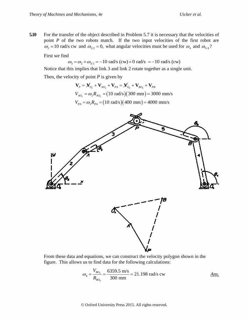
Theory of Machines and Mechanisms, 4e Uicker et al.
© Oxford University Press 2015. All rights reserved.
5.10 For the transfer of the object described in Problem 5.7 it is necessary that the velocities of
point P of the two robots match. If the two input velocities of the first robot are
2 10 rad/s cw and 3/2 0, what angular velocities must be used for 4 and 5/4 ?
First we find
3 2 3/2 10 rad/s (cw) 0 rad/s 10 rad/s (cw)
Notice that this implies that link 3 and link 2 rotate together as a single unit.
Then, the velocity of point P is given by
2 2 4 4
2 22
3
10 rad/s 300 mm 3000 mm/s
10 rad/s 400 mm 4000 mm/s
P O AO PA O BO PB
AO AO
PA PA
V R
V R
V V V V V V V
From these data and equations, we can construct the velocity polygon shown in the
figure. This allows us to find data for the following calculations:
4
4
4
6359.5 m/s21.198 rad/s cw
300 mm
BO
BO
V
R Ans.

Theory of Machines and Mechanisms, 4e Uicker et al.
© Oxford University Press 2015. All rights reserved.
5
7160.5 mm/s17.901 rad/s ccw
400 mm
PB
PB
V
R
5/4 5 4 17.901 rad/s 21.198 rad/s 39.099 rad/s ccw Ans.
If an analytical solution is preferred, we start with the robot on the left, where we find
22
3
ˆ ˆ ˆ ˆˆ10.0 rad/s 300cos 45 300sin 45 in 2121.32 2121.32 mm/s
ˆ ˆ ˆ ˆˆ10.0 rad/s 400cos30 400sin 30 in 80.000 00 138 56 mm/s
ˆ ˆ164.852 80 223.416 80 in/s
A AO
PA PA
P A PA
V ω ×R k × i j i j
V ω ×R k × i j i j
V V V i j
Similarly, for the robot on the right, we have
44 4
5 5
4 5
ˆ ˆˆ rad/s 12cos101.39 12sin101.39 in
ˆ ˆˆ rad/s 16cos162.84 16sin162.84 in
11.763 60 2.370 00 in 4.720 80 15.287 20 in
B BO
PB PB
P B PB
V ω ×R k × i j
V ω ×R k × i j
V V V i j i j
Next, by setting the two equations for PV equal to each other, and then separating the i
and j components, we obtain a set of two equations for 4 and 5
4
5
294.09 mm 118.02 mm 4121.3 mm/s
59.25 mm 382.18 mm 5585.42 mm/s
The solutions to these equations give
4
5
21.198 rad/s (cw)
17.901 rad/s ccw
Ans.
5/4 5 4 17.901 rad/s 21.198 rad/s 39.099 rad/s ccw Ans
We see that these results agree precisely with those obtained above by the graphical
approach. It must be pointed out that this is not usual for graphic solutions, but is the
result of the high-precision CAD system used here.
As yet a third approach to the solution of this problem, we can find the instant centers of
velocity. In doing this we follow exactly the approach shown in Example 5.5. However,
since we have equal velocities for 2 and 3 , the location of instant center 13I is defined
by
23 13
23 12
2
3
10.0 rad/s1.0
10.0 rad/s
I I
I I
R
R
and therefore 13I becomes coincident with 12I as shown in the figure below. When the
other instant centers are found through the Kennedy-Aronhold theorem, this also results
in coincident instant centers for 24 34,I I and for 25 35,I I as shown in the figure. Under
these input velocity conditions, links 2 and 3 act as a single solid unit.

Theory of Machines and Mechanisms, 4e Uicker et al.
© Oxford University Press 2015. All rights reserved.
Once the remaining instant centers are found, however, we may still find the information
requested in the problem. We find
24 12
24 14
4 2
1892.675 mm10 rad/s 21.198 rad/s (cw)
892.85 mm
I I
I I
R
R Ans.
25 12
25 15
5 2
694.075 mm10 rad/s 17.901 rad/s (ccw)
387.725 mm
I I
I I
R
R
Ans.
Again, the perfect agreement results from the precision of the CAD system used in
finding the distances between instant centers.

Theory of Machines and Mechanisms, 4e Uicker et al.
© Oxford University Press 2015. All rights reserved.
5.11 To successfully transfer an object between two robots, as described in Problems 5.7 and
5.8, it is helpful if the accelerations are also matched at point P. Assuming that the two
input accelerations are 2 3 0 at this instant for the robot on the left, what angular
accelerations must be given to the two input joints of the robot on the right to achieve
this?
Starting after the solutions of Problem 5.8 (the velocity analysis) is completed, the
condition for the acceleration of point P is written as
2 2 2 4 4 4
2 4
2 4
2 4
2 22 2
2 2
222
3000 mm/s 1350.6 mm/s30000 mm/s 6080.5 mm/s
300 mm 300 mm
2000 mm/s1000 mm/s
400 mm
n t n t n t n t
P O AO AO PA PA O BO BO PB PB
AO BOn n
AO BO
AO BO
n PAPA
PA
V VA A
R R
VA
R
A A A A A A A A A A A
22
2686.5 mm/s
1178.25 mm/s400 mm
n PBPB
PB
VA
R
Notice that a difficulty arises in the graphic solution of the above acceleration equation in
that the two unknowns do not arise consecutively in the equation. Nevertheless, recalling
that vector addition is commutative (independent of order), we can proceed with the
vectors appearing out of order, as is shown in the dotted lines in the figure above. Once

Theory of Machines and Mechanisms, 4e Uicker et al.
© Oxford University Press 2015. All rights reserved.
the solution with the dotted lines is completed, we have obtained the correct magnitudes
and directions of the two unknown tangential components. However, we do not have a
valid acceleration polygon unless we now arrange the components in their correct order,
according to the original acceleration equation, as is shown in the dashed lines in the
figure. If this is not done, the acceleration image point B cannot be labeled, and the
absolute acceleration of B and acceleration images of links 4 and 5 cannot be correctly
shown.
Whether or not the vectors are arranged in their correct order, however, we can proceed
with the solution for the two unknown angular accelerations as follows:
4
4
22
4
27583 mm/s91.943 rad/s ccw
300 mm
t
BO
BO
A
R Ans.
22
4
15127 mm/s37.818 rad/s ccw
400 mm
t
PB
PB
A
R Ans.

Theory of Machines and Mechanisms, 4e Uicker et al.
© Oxford University Press 2015. All rights reserved.
PART 2
DESIGN OF MECHANISMS

Theory of Machines and Mechanisms, 4e Uicker et al.
© Oxford University Press 2015. All rights reserved.
Chapter 6
Cam Design
6.1 The reciprocating radial roller follower of a plate cam is to rise 40 mm with simple
harmonic motion in 180 of cam rotation and return with simple harmonic motion in the
remaining 180 . If the roller radius is 7.5 mm and the prime-circle radius is 40 mm,
construct the displacement diagram, the pitch curve, and the cam profile for clockwise
cam rotation.
6.2 A plate cam with a reciprocating flat-face follower has the same motion as in Problem
6.1. The prime-circle radius is 40 mm, and the cam rotates counterclockwise. Construct
the displacement diagram and the cam profile, offsetting the follower stem by 15 mm in
the direction that reduces the bending stress in the follower during rise.

Theory of Machines and Mechanisms, 4e Uicker et al.
© Oxford University Press 2015. All rights reserved.
6.3 Construct the displacement diagram and the cam profile for a plate cam with an
oscillating radial flat-face follower that rises through 30 with cycloidal motion in 150
of counterclockwise cam rotation, then dwells for 30 , returns with cycloidal motion in
120 , and dwells for 60 . Determine the necessary length for the follower face, allowing
6.25 mm clearance at the free end. The prime-circle radius is 37.5 mm, and the follower
pivot is 150 mm to the right.
Notice that, with the prime circle radius given, the cam is undercut and the follower will
not reach positions 7 and 8. The follower face length shown is 250 mm but can be made
as short as 243.75 mm (position 9) from the follower pivot. Ans.

Theory of Machines and Mechanisms, 4e Uicker et al.
© Oxford University Press 2015. All rights reserved.
6.4 A plate cam with an oscillating roller follower is to produce the same motion as in
Problem 6.3. The prime-circle radius is 75 mm, the roller radius is 12.5 mm, the length
of the follower is 125 mm, and it is pivoted at 156.25 mm to the right of the cam rotation
axis. The cam rotation is clockwise. Determine the maximum pressure angle.
From a graphical analysis, max 39 Ans.
6.5 For a full-rise simple harmonic motion, write the equations for the velocity and the jerk at
the midpoint of the motion. Also, determine the acceleration at the beginning and the end
of the motion.
Using Eqs. (6.12) and (6.11) we find
1sin
2 2 2 2
L Ly
1
2 2
Ly
Ans.
3 3
3 3
1sin
2 2 2 2
L Ly
3
3
3
1
2 2
Ly
Ans.
2 2
2 20 cos0
2 2
L Ly
2
2
20
2
Ly
Ans.
2 2
2 21 cos
2 2
L Ly
2
2
21
2
Ly
Ans.

Theory of Machines and Mechanisms, 4e Uicker et al.
© Oxford University Press 2015. All rights reserved.
6.6 For a full-rise cycloidal motion, determine the values of for which the acceleration is
maximum and minimum. What is the formula for the acceleration at these points? Find
the equations for the velocity and the jerk at the midpoint of the motion.
Using Eqs. (6.13), we know that acceleration is an extremum when jerk is zero. This
occurs when cos2 0 ; that is, when 1 4 or when 3 4 ,
max2 2
1 2 2sin
4 2
L Ly y
Ans.
min2 2
3 2 3 2sin
4 2
L Ly y
Ans.
1 2
1 cos2
L Ly
Ans.
2 2
3 3
1 4 4cos
2
L Ly
Ans.
6.7 A plate cam with a reciprocating follower is to rotate clockwise at 400 rev/min. The
follower is to dwell for 60 of cam rotation, after which it is to rise to a lift of 50 mm.
During 20 mm of its return stroke, it must have a constant velocity of 800 mm/s.
Recommend standard cam motions from Section 6.7 to be used for high-speed operation
and determine the corresponding lifts and cam rotation angles for each segment of the
cam.

Theory of Machines and Mechanisms, 4e Uicker et al.
© Oxford University Press 2015. All rights reserved.
The curves shown are initially only sketches and not drawn to scale. They suggest the
standard curve types that might be chosen. The actual choices are shown in the table
below.
400 rev/min 2 rad/rev41.888 rad/s cw
60 s/min
To match the required velocity condition in Seg. DE we must have
4 4
4
4 4 4 4
4
800.000 mm/s 41.888 rad/s
19.098 600 mm/rad 20.000 mm
1.047 198 rad 60.000
y y
y
y L
Matching the first derivatives at D and E we find
5 5 42 19.098 593 mm/radL y 5 59.549 297 mm/radL (1)
3 3 42 19.098 593 mm/radL y 3 312.158 542 mm/radL (2)
Matching the second derivatives at C we find
2 2 2
2 3 35.26830 2.5000 4L 2 2
2 3 3 3106.758 078 8.780 500L (3)
For geometric continuity, we have
1 2 3 4 5L L L L L or 3 5 30.000 000 mmL L (4)
1 2 3 4 5 2 or 2 3 5 4.188 790 rad (5)
Equations (1) through (5) are now solved simultaneously for 2 , 3L , 3 , 5L , and 5 .
The results are summarized in the following table:
Seg. Type Eq. L, mm rad , deg
AB dwell --- 0 1.047 198 60.000
BC 8th
order poly. (6.14) 50.000 1.089 824 62.442
CD half harmonic (6.20) 1.648 0.135 268 7.750
DE constant velocity --- 20.000 1.047 198 60.000
EA half cycloidal (6.25) 28.352 2.963 698 169.808
6.8 Repeat Problem 6.7 except with a dwell for 20 of cam rotation.
The procedure is the same as for Problem 6.7. The results are:
Seg. Type Eq. L, mm rad , deg
AB dwell --- 0 0.349 066 20.000
BC 8th
order poly. (6.14) 50.000 1.870 958 107.198
CD half harmonic (6.20) 4.872 0.398 667 22.842
DE constant velocity --- 20.000 1.047 198 60.000
EA half cycloidal (6.25) 25.128 2.617 296 149.960

Theory of Machines and Mechanisms, 4e Uicker et al.
© Oxford University Press 2015. All rights reserved.
6.9 If the cam of Problem 6.7 is driven at constant speed, determine the time of the dwell and
the maximum and minimum velocity and acceleration of the follower for the cam cycle.
The time duration of the dwell is 1 1.047 198 rad 41.888 rad/s 0.025 st Ans.
Working from the equations listed, the maximum and minimum values of the kinematic
coefficients in each segment of the cam are as follows:
Seg. Eq. maxy mm/rad miny mm/rad maxy mm/rad
2 miny mm/rad
2
AB --- 0 0 0 0
BC (6.14) 241.704 0 221.783 221.783
CD (6.20) 0 19.137 0 221.783
DE --- 19.099 19.099 0 0
EA (6.25) 0 19.133 10.141 0
max max 241.704 mm/rad 41.888 rad/s 10 124 mm/sy y Ans.
min min 19.137 mm/rad 41.888 rad/s 800.0 mm/sy y Ans.
22 2
max max 221.783 mm/rad 41.888 rad/s 389 141 mm/sy y Ans.
22 2
min min 221.783 mm/rad 41.888 rad/s 389 141 mm/sy y Ans.

Theory of Machines and Mechanisms, 4e Uicker et al.
© Oxford University Press 2015. All rights reserved.
6.10 A plate cam with an oscillating follower is to rise through 20 in 60 of cam rotation,
dwell for 45 , then rise through an additional 20 , return, and dwell for 60 of cam
rotation. Assuming high-speed operation, recommend standard cam motions from
Section 6.7 to be used, and determine the lifts and cam-rotation angles for each segment
of the cam.
From the sketches shown (not drawn to scale), the curve types identified in the table
below were chosen.
Next, equating the second derivatives at D, the remaining entries in the table were found.
3 4
2 2
3 4
5.26830 5.26830L L
2
4 4
2
3 3
2.000L
L
4 32
3 4 31 2 195
3 80.772
4 114.228
Seg. Type Eq. L, deg rad , deg
AB cycloidal (6.13) 20.000 1.047 198 60.000
BC dwell --- 0 0.785 399 45.000
CD 8th
order poly. (6.14) 20.000 1.409 731 80.772
DE 8th
order poly. (6.17) 40.000 1.993 661 114.228
EA dwell --- 0 1.047 198 60.000

Theory of Machines and Mechanisms, 4e Uicker et al.
© Oxford University Press 2015. All rights reserved.
6.11 Determine the maximum velocity and acceleration of the follower for Problem 6.10,
assuming that the cam is driven at a constant speed of 600 rev/min.
Working from the equations listed, the maximum and minimum values of the kinematic
coefficients in each segment of the cam are as follows:
Seg. Eq. maxy miny maxy miny
AB (6.13) 0.666 667 0 2.000 000 2.000 000
BC --- 0 0 0 0
CD (6.14) 0.440 004 0 0.925 344 0.924 344
DE (6.17) 0 0.622 264 0.925 402 0.925 402
EA --- 0 0 0 0
600 rev/min 2 rad/rev 60 s/min 62.832 rad/s
max max 0.666 667 rad/rad 62.832 rad/s 41.888 rad/sy y Ans.
22 2
max max 2.000 rad/rad 62.832 rad/s 7 896 rad/sy y Ans.

Theory of Machines and Mechanisms, 4e Uicker et al.
© Oxford University Press 2015. All rights reserved.
6.12 The boundary conditions for a polynomial cam motion are as follows: for 0 , 0y ,
and 0 y ; for , , and 0y L y . Determine the appropriate displacement
equation and the first three derivatives of this equation with respect to the cam rotation
angle. Sketch the corresponding diagrams.
Since there are four boundary conditions, we choose a cubic polynomial
2 3
0 1 2 3y C C C C
2
31 232 CC C
y
Then from the boundary conditions:
00 0y C 0 0C
10 0C
y
1 0C
2 31.0y C C L 2 3C L
3232
1.0 0CC
y
3 2C L
Therefore the equation and its three derivatives are:
2 3 2 3
3 2 3 2y L L L
Ans.
2 2
6 6 6L L Ly
Ans.
2 2 26 612 1 2L LLy
Ans.
312Ly
Ans.

Theory of Machines and Mechanisms, 4e Uicker et al.
© Oxford University Press 2015. All rights reserved.
6.13 Determine the minimum face width using 2-mm allowances at each end and determine
the minimum radius of curvature for the cam of Problem 6.2.
Referring to Problem 6.2 for the data and figure,
40.000 mmL 180 rad 0 40.0 mmR
From Eqs. (6.12) and (6.15) for simple harmonic motion,
max 2 20.000 mm/rady L min 2 20.000 mm/rady L
From Eq. (6.30)
max minFace width y allowancesy
Face width 20.000 mm 20.000 mm 2 2 mm 44.0 mm Ans.
From Eq. (6.28):
0
0 01 cos cos (constant)2 2 2
R y y
L L LR R
40.0 mm 40.000 mm 2 60.0 mm Ans.
6.14 Determine the maximum pressure angle and the minimum radius of curvature for the cam
of Problem 6.1.
Referring to Problem 6.1 for the figure and data,
40.000 mmL 180 rad 0 40.000 mmR 7.500 mmrR
For simple harmonic motion, Eq. (6.12) can be substituted into Eq. (6.33) to give
sintan
3 cos
. This can be differentiated and d d set to zero to find the angle
70.53 at which max 19.47 . However, it is much simpler to use the nomogram of
Fig. 6.28 to find max 20 directly. For the accuracy needed, the nomogram is
considered sufficient. Ans.
From Fig. 6.30a, using 0 1.0R L , we get 0min1.43rR R . This gives
0min1.43 1.43 40 mm 7.50 mm 49.7 mmrR R Ans.

Theory of Machines and Mechanisms, 4e Uicker et al.
© Oxford University Press 2015. All rights reserved.
6.15 A radial reciprocating flat-face follower is to have the motion described in Problem 6.7.
Determine the minimum prime-circle radius if the radius of curvature of the cam is not to
be less than 10 mm. Using this prime-circle radius, what is the minimum length of the
follower face using allowances of 3 mm on each side?
From Problem 6.9, max 241.704 mm/rady , min 19.137 mm/rady ,
2
min 221.783 in/rady
Therefore, from Eq. (6.29),
0 min min 10.000 mm 221.783 mm 50.000 mm 181.783 mmR y y Ans.
Also, from Eq. (6.30),
max minFace width allowances 241.704 mm 19.137 mm 2 3.0 mm 266.84 mmy y Ans.
6.16 Graphically construct the cam profile of Problem 6.15 for clockwise cam rotation.

Theory of Machines and Mechanisms, 4e Uicker et al.
© Oxford University Press 2015. All rights reserved.
6.17 A radial reciprocating roller follower is to have the motion described in Problem 6.7.
Using a prime-circle radius of 400 mm, determine the maximum pressure angle and the
maximum roller radius that can be used without producing undercutting.
We will use the nomogram of Fig. 6.28 to find the maximum pressure angle in each
segment of the cam. Calculations are shown in the following table. Asterisks are used to
signify values used with the nomogram to adjust half-return curves to equivalent full-
return curves, and to adjust the prime-circle baseline.
Seg. *
0R , mm *L , mm * *
0R L * , deg max , deg
BC 400.000 50.000 8.0 62.4 12
CD 446.704 3.296 135.5 15.5 1
EA 400.000 56.704 7.0 339.6 3
For the total cam, max 12 . Ans.
Also we use Figs. 6.32 and 6.33 to check for undercutting. Again, asterisks are used to
denote values that are adjusted for use with the charts. Note that doubling as was done
for use of the nomogram is not necessary since we have figures for half-harmonic and
half-cycloidal cam segments. Note also that segment EA need not be checked since
undercutting occurs only in segments with negative acceleration.
Seg. *
0R , mm L, in *
0R L , deg *
0min rR R max
rR mm
BC 400.000 50.000 8.0 62.1 0.725 290
CD 448.352 1.648 272.1 7.7 0.680 304
To avoid undercutting for the entire cam, 290 mmrR . Ans.
6.18 Graphically construct the cam profile of Problem 6.17 using a roller radius of 15 mm.
The cam rotation is to be clockwise.

Theory of Machines and Mechanisms, 4e Uicker et al.
© Oxford University Press 2015. All rights reserved.
6.19 A plate cam rotates at 300 rev/min and drives a reciprocating radial roller follower
through a full rise of 75 mm in 180° of cam rotation. Find the minimum radius of the
prime-circle if simple harmonic motion is used and the pressure angle is not to exceed
25 . Find the maximum acceleration of the follower.
Using max 25 and 180 , Fig. 6.28 gives 0 0.75R L . Therefore
0 0.75 0.75 75 mm 56.25 mmR L Ans.
300 rev/min 2 rad/rev31.416 rad/s
60 s/min
222
max 22
75 mm37.5 mm/rad
2 2 rad
Ly
22 2 2
max max 37.5 mm/rad 31.416 rad/s 37000 mm/sy y Ans.
6.20 Repeat Problem 6.19 except that the motion is cycloidal.
Figure 6.28 gives 0 0.95R L . Therefore 0 0.95 0.95 75 mm 71.25 mmR L Ans.
2
max 22
2 75 mm247.7475 mm/rad
rad
Ly
22 2 2
max max 47.7475 mm/rad 31.416 rad/s 47125 mm/sy y Ans.
6.21 Repeat Problem 6.19 except that the motion is eighth-order polynomial.
Figure 6.28 gives 0 0.95R L . Therefore 0 0.95 0.95 75 mm 71.25 mmR L Ans.
2
max 22
5.2683 75 mm5.268340.025 mm/rad
rad
Ly
22 2 2
max max 40.025 mm/rad 31.416 rad/s 39500 mm/sy y Ans.
6.22 Using a roller diameter of 0.80 in, determine whether the cam of Problem 6.19 will be
undercut.
Using 0 0.75R L and 180 , Fig. 6.30a gives min 0 1.55rR R .
min 1.55 2.25 in 0.80 in 2.688 in 0 ; thus, this cam is not undercut. Ans.

Theory of Machines and Mechanisms, 4e Uicker et al.
© Oxford University Press 2015. All rights reserved.
6.23 Equations (6.30) and (6.31) describe the profile of a plate cam with a reciprocating flat-
face follower. If such a cam is to be cut on a milling machine with cutter radius cR ,
determine similar equations for the center of the cutter.
In complex polar notation, using Eq. (6.27) and using u and v to denote the local
rectangular part coordinates of the cam shape, the loop-closure equation is
0
j j
cue jve jR jy y jR
Dividing this by je
0
j j
cu jv j R R y e y e
Now separating this into real and imaginary parts we find
0 sin coscu R R y y
0 cos sincv R R y y Ans.

Theory of Machines and Mechanisms, 4e Uicker et al.
© Oxford University Press 2015. All rights reserved.
6.24 & 6.25 Since programming languages vary so much, particularly with the use of
graphics, no attempt is made to show a “standard” solution for these problems.
6.26 A plate cam with an offset reciprocating roller follower is to have a dwell of 60° and then
rise in 90° to another dwell of 120°, after which it is to return in 90° of cam rotation. The
radius of the base circle is 40 mm, the radius of the roller follower is 15 mm, and the
follower offset is 20 mm. For the rise motion 60 150 , the equation of the
displacement (the lift) is to be
40( sin )y
where y is in millimeters and is the cam rotation angle in radians. (i) Find equations
for the first- and second-order kinematic coefficients of the lift y for this rise motion. (ii)
Sketch the displacement diagram and the first- and second-order kinematic coefficients
for the follower motion described. Comment on the suitability of this rise motion in the
context of the other displacements specified. At the cam angle θ = 120°, determine the
following: (iii) the location of the point of contact between the cam and follower,
expressed in the moving Cartesian coordinate system attached to the cam; (iv) the radius
of the curvature of the pitch curve and the radius of curvature of the cam surface; and (v)
the pressure angle of the cam. Is this pressure angle acceptable?
(i) From the equation given for the lift, the first- and second-order kinematic
coefficients are
1
40 cos mm/rady
and 240sin mm/rady
(ii) Sketches of the first-order and the second-order kinematic coefficients of the
displacement diagram are shown here.
0
1
2
3
4
5
6
60 80 100 120 140
θ (degree)
y' (c
m/r
ad)
-4.5
-4
-3.5
-3
-2.5
-2
-1.5
-1
-0.5
0
60 80 100 120 140
θ (degree)
y''
(cm
/ra
ds)
The rise motion specified is not suitable between dwells on either side since the first- and
second-order kinematic coefficients are not zero at the beginning and end of the rise. A
cycloidal rise curve would be preferable, but would have higher values of acceleration
and would lead to higher forces.
At the cam angle θ = 120º, we have 60 60 3 rad .
340( sin ) 40 sin 60 48.0 mmy

Theory of Machines and Mechanisms, 4e Uicker et al.
© Oxford University Press 2015. All rights reserved.
1 140 cos 40 cos60 32.7 mm/rady
240sin 40sin60 34.6 mm/rady
The absolute coordinates of the trace point are
0 20 mm,X 2 2 22
0 40 mm 15 mm 20 mm 51.2 mmrY R R
0 20 mm,X X 0 51.2 mm 48.0 mm 99.2 mmY Y y
The cam coordinates of the trace point (the pitch curve) and derivatives are
cos sin 20 mm cos120 99.2 mm sin120 75.9 mmu X Y
sin cos 20 mm sin120 99.2 mm cos120 66.9 mmv X Y
sin cos sin 38.6 mm/radu X Y y
cos sin cos 92.3 mm/radv X Y y
2 2 100.0 mm/radw u v 2cos sin 2 cos sin 13.87 mm/radu X Y y y 2sin cos 2 sin cos 2.76 mm/radv X Y y y
(iii) From Eq. (6.38), the cam coordinates of the point of contact (the cam surface) are
62.1 mmcam r
vu u R
w
61.1 mmcam r
uv v R
w
Ans.
(iv) From Eq. (6.39), the radius of curvature of the pitch curve is 3
72.2 mmw
u v v u
Ans.
(v) From Eq. (6.39) the pressure angle is
cos sin cos 0.9919v u
w w
7.3 Ans.
This pressure angle is less than 30° and is acceptable.

Theory of Machines and Mechanisms, 4e Uicker et al.
© Oxford University Press 2015. All rights reserved.
6.27 A plate cam with an offset reciprocating roller follower is to be designed using the input,
the rise and fall, and the output motion shown in Table P6.27. The radius of the base circle
is to be 30 mm, the radius of the roller follower is 12.5 mm, and the follower offset (or
eccentricity) is to be 15 mm.
Table P6.27 Displacement Information for Plate Cam With Reciprocating Roller Follower
Cam angle range Rise or Fall (mm) Follower motion
0° - 20° 0 Dwell
20° - 110° +25 Full-rise simple harmonic motion
110° - 120° 0 Dwell
120° - 200° +5 Full-rise cycloidal motion
200° - 270° 0 Dwell
270° - 360° -30 Full-return cycloidal motion
Comment on the suitability of the motions specified. At the cam angle 50 ,
determine the following: (i) the first-, second-, and third-order kinematic coefficients of
the lift curve, (ii) the coordinates of the point of contact between the roller follower and
the cam surface, expressed in the Cartesian coordinate system rotating with the cam, (iii)
the radius of curvature of the pitch curve, (iv) the unit tangent and the unit normal vectors
to the pitch curve, and (v) the pressure angle of the cam.
The portion of the motions which specifies simple harmonic motion is not suitable for
high-speed operation since there will be discontinuities in the second derivatives at both
ends of that segment where it interfaces with dwells. Cycloidal motion would correct
this problem but would give a higher peak acceleration. Still, simple harmonic motion is
specified.
(i) Eqs. (6.12), with 50 20 30 , 25 mm, 90 2 rad,L gives
25 mm1 cos 1 cos 6.25 mm
2 2 3
Ly
sin 25 mm sin 21.65 mm/rad2 3
Ly
Ans.
2
2
2cos 2 25 mm cos 25.0 mm/rad
2 3
Ly
Ans.
3
3
3sin 4 25 mm sin 86.60 mm/rad
2 3
Ly
Ans.
Therefore the fixed coordinates of the tracepoint are
0 30 mm 12.5 mm 42.5 mm,rR R R 2 22 2
0 0 42.5 mm 15 mm 39.76 mmY R
15 mm,X 0 39.76 mm 6.25 mm 46.01 mmY Y y
The cam coordinates of the trace point (the pitch curve) and derivatives are
cos sin 15 mm cos50 46.01 mm sin50 44.89 mmu X Y
sin cos 15 mm sin50 46.01 mm cos50 18.08 mmv X Y
sin cos sin 34.67 mm/radu X Y y

Theory of Machines and Mechanisms, 4e Uicker et al.
© Oxford University Press 2015. All rights reserved.
cos sin cos 30.97 mm/radv X Y y
2 2 46.49 mm/radw u v 2cos sin 2 cos sin 2.10 mm/radu X Y y y
2sin cos 2 sin cos 35.18 mm/radv X Y y y
(ii) From Eq. (6.38), the cam coordinates of the point of contact (the cam surface) are
36.56 mmcam r
vu u R
w
8.76 mmcam r
uv v R
w
Ans.
(iii) From Eq. (6.39), the radius of curvature of the pitch curve is
3 87.02 mmw u v v u Ans.
(iv) The unit tangent and the unit normal vectors to the pitch curve are
ˆ ˆ ˆ ˆˆ 0.746 0.666t u w v w u i j i j Ans.
ˆ ˆ ˆ ˆˆ 0.666 0.746n v w u w u i j i j Ans.
(v) From Eq. (6.39) the pressure angle is
cos sin cos 0.9897v w u w 8.2 Ans.
This pressure angle is less than 30° and is acceptable for the specified cam angle 50 .

Theory of Machines and Mechanisms, 4e Uicker et al.
© Oxford University Press 2015. All rights reserved.
6.28 A plate cam with a radial reciprocating roller follower is to be designed using the input,
the rise and fall, and the output motion shown in Table P6.28. The base circle diameter is
3 in and the diameter of the roller is 1 in. Displacements are specified as follows.
Table P6.28 Displacement Information for Plate Cam With Reciprocating Roller Follower Input (deg) Lift L (in) Output y
0 90 3.0 Cycloidal Rise
90 105 0 Dwell
105 195 -3.0 Cycloidal Fall
195 210 0 Dwell
210 270 2.0 Simple Harmonic Rise
270 285 0 Dwell
285 345 -2.0 Simple Harmonic Fall
345 360 0 Dwell
Plot the lift curve (the displacement diagram), and the profile of the cam. (i) Comment
on the lift curves at appropriate positions of the cam, (for example, when the cam angle is
0 , 45 , 180 , 210 , 225 , and 300 ). (ii) Identify on your
cam profile the location(s) and the value of the largest pressure angle. Would this
pressure angle cause difficulties for a practical cam-follower system? (iii) Identify on
your cam profile the location(s) of discontinuities in position, velocity, acceleration,
and/or jerk. Are these discontinuities acceptable (why or why not)? (iv) Identify on your
cam profile any regions of positive radius of curvature of the cam profile. Are these
regions acceptable (why or why not)? (v) For the values given in Table P6.28, what
design changes would you suggest to improve the cam design?
The lift curve (displacement diagram is shown in Fig. 1.
Figure 1. The lift curve or displacement diagram.
The cam profile is plotted in Fig. 2.

Theory of Machines and Mechanisms, 4e Uicker et al.
© Oxford University Press 2015. All rights reserved.
Figure 2. The cam profile.
(i) Because of the choice of harmonic motion rise and return curves, there are
discontinuities in acceleration at 210 , 270 , 285 , and 345 . Because
of adjacent dwells, cycloidal motion would be preferable, although it would lead to
slightly higher peak acceleration in these segments.
(ii) The pressure angle, see Sec. 6.10, should be less than 30 . In this design, the
pressure angle is more than the accepted value at the cam angles
16 64 , 131 180 , 216 256 , and 299 341
Therefore, this cam profile is not a good design. The high values of the pressure angle
may be due to the selection of the displacement curves and the diameter of the base circle
and the diameter of the follower.
(iii) Position discontinuities never occur. Discontinuities in the derivatives will occur
only at transitions between dwell segments and lifting/returning segments of motion.
Discontinuities in the derivatives are undesirable. There is an acceleration discontinuity
at the beginning and end of the simple harmonic motions, both rise and return. There is a
jerk discontinuity at the beginning and end of the cycloidal motions, both rise and return.
Whether these discontinuities are acceptable depends on the intended speed of operation,
and on the masses and stiffnesses involved.

Theory of Machines and Mechanisms, 4e Uicker et al.
© Oxford University Press 2015. All rights reserved.
(iv) The radius of curvature of a cam profile should always be negative for a good
cam design. Positive curvature means that the cam has a concave surface and there is the
possibility that the follower may lose contact with the cam. If the radius of curvature of
the cam profile is positive then the radius of curvature of the cam must be greater than the
radius of the follower. In the proposed design, the positive values of the radius of
curvature of the cam are always greater than 0.5 in (i.e., the radius of the follower). The
radius of curvature of the cam is positive for the cam angles
3 25 , 170 192 , 215 220 , and 261 270
The radius of curvature is positive, and smaller than the radius of the roller follower, for
the cam angles
9 13 , 181 187 , and 215 216
Note that the radius of curvature of the cam is zero between the cam angles 214 and 215
degrees, meaning that pointing has occurred. Also, it could imply that undercutting has
occurred. Also, with the exception of where the radius of curvature of the cam goes to
zero, there is an inflection point at the boundary of each range of angles for which the
radius of curvature is positive.
(v) Possible design changes to the cam-follower system. (a) Increasing the radius of
the prime circle (with the same lift curve) in general would reduce the pressure angle. (b)
Change the profiles to match acceleration at the transistion (blend) points to eliminate
acceleration discontinuities. (c) Changing both SHM profiles to cycloidal would make
accelerations continuous but would also increase accelerations (and the pressure angle) in
the middle parts of the rise and the return profiles. (d) We may want to increase the
diameter of the roller if the contact stresses are high. (e) We could explore numerically
the effects on forces of changing the offset (or the eccentricity) . These are not obvious
from observation.

Theory of Machines and Mechanisms, 4e Uicker et al.
© Oxford University Press 2015. All rights reserved.
6.29 Continue using the same displacement information and the same design parameters as in
Problem 6.28. Use a spreadsheet to determine and plot the following for a complete
rotation of the cam: (i) the first-order kinematic coefficients of the follower center; (ii)
the second-order kinematic coefficients of the follower center; (iii) the third-order
kinematic coefficients of the follower center; (iv) the lift curve (displacement diagram);
(v) the radius of curvature of the cam surface; and (vi) the pressure angle of the cam-
follower system. Is the pressure angle suitable for a practical cam-follower system?
(i) The first-order kinematic coefficients for the cam design are shown in Fig. 3.
0 50 100 150 200 250 300 350 400-6
-4
-2
0
2
4
6First order Kinematics Coeeficients
(Cam angle) - degrees
First
order
KC - i
n
xfc
'
yfc
'
Figure 3. The first-order kinematic coefficients.
(ii) The second-order kinematic coefficients for the cam design are shown in Fig. 4.
0 50 100 150 200 250 300 350 400-15
-10
-5
0
5
10
15Second order Kinematics Coeeficients
(Cam angle) - degrees
Secon
d orde
r KC -
in
xfc
pp"
yfc
"
Figure 4. The second-order kinematic coefficients.

Theory of Machines and Mechanisms, 4e Uicker et al.
© Oxford University Press 2015. All rights reserved.
(iii) The third-order kinematic coefficients for the cam design are shown in Fig. 5.
0 50 100 150 200 250 300 350 400-40
-30
-20
-10
0
10
20
30
40Third order Kinematics Coeeficients
(Cam angle) - degrees
Third
order
KC - i
n
xfc
p"'
yfc
"'
Figure 5. The third-order kinematic coefficients.
(iv) The lift curve (displacement diagram) for the cam design is shown in Fig. 6.
0 50 100 150 200 250 300 350 4000
0.5
1
1.5
2
2.5
3Position Profile
(Cam angle) - degrees
Lift - i
n
Figure 6. The lift curve (displacement diagram).
Theory of Machines and Mechanisms, 4e Uicker et al.
© Oxford University Press 2015. All rights reserved.
(v) The radius of curvature of the cam surface is shown in Fig. 7.
Figure 7. The radius of curvature of the cam surface.
The radius of curvature of a cam profile should always be negative for a good cam
design. The positive curvature means that the cam has a concave surface and there is the
possibility that the follower may lose contact with the cam. If the radius of curvature of
the cam profile is positive then the radius of curvature of the cam must be greater than the
radius of the follower. In the proposed design, the positive values of the radius of
curvature of the cam are always greater than 0.5 in (i.e., the radius of the follower).
Note that the radius of curvature of the cam surface goes to infinity when the cam angle
is 4°, 26°, 168°, 191°, 225°, and 330°; i.e., there are six inflection points on the cam
surface. Also, note the discontinuity at the start and the end of the simple harmonic
profile at 210°, 270°, 285°, and 345°. This discontinuity is due to the simple harmonic
profiles and for this reason simple harmonic profiles are not generally recommended for
high-speed cam-follower systems.
(vi) The pressure angle for the cam-follower system is shown in Fig. 8.
0 50 100 150 200 250 300 350 4000
5
10
15
20
25
30
35
40
45
50Pressure Angle
(Cam angle) - degrees
Pres
sure a
ngle -
degre
es
Figure 8. The pressure angle of the cam-follower system.
The recommended value of the pressure angle is less than 30 degrees. In this design, the
pressure angle is more than the accepted value at the cam angles 2 18 62 ,
134 178 , 220 256 , and 302 336 . Therefore, this cam profile is not a good
design. The high values of the pressure angle may be due to the selection of the
displacement curves and the dimensions of the cam and the diameter of the roller.

Theory of Machines and Mechanisms, 4e Uicker et al.
© Oxford University Press 2015. All rights reserved.
Chapter 7
Spur Gears
7.1 Find the module of a pair of gears having 32 and 84 teeth, respectively, whose center distance is 87 mm.
322 3
mm m 32 84 87 mm2 2 2
NNR R
2 87 mmm 1.5 mm/tooth116 teeth
Ans.
7.2 Find the number of teeth and the circular pitch of a 150-mm pitch diameter gear whose module is 2.5 mm/tooth.
2 m 60 teeth150 mm 2.5 mm/toothN R Ans. m 7.854 mm/tooth2.5 mm/toothp Ans.
7.3 Determine the module pitch of a pair of gears having 18 and 40 teeth, respectively, whose center distance is 90.625 mm.
2 32 3 m
2
5890.625 m
2
2 90.625 m =
583.125 mm/tooth
N NR R
Ans.
7.4 Find the number of teeth and the circular pitch of a gear whose pitch diameter is 10.5 mm in if module is 3.125 mm/tooth.
2125 mm / 3.125 mm per tooth
m
RN Ans.
= 3.14 3.125 = 9.8125 mm/toothp m Ans.

Theory of Machines and Mechanisms, 4e Uicker et al.
© Oxford University Press 2015. All rights reserved.
7.5 Find the module and the pitch diameter of a 40-tooth gear whose circular pitch is 37.7 mm/tooth.
m 12 mm/tooth37.7 mm/toothp Ans. 2 480 mm12 mm/tooth 40 teethD R mN Ans.
7.6 The pitch diameters of a pair of mating gears are 42 mm and 102 mm, respectively. If the module is 1.5 mm/tooth how many teeth are there on each gear?
2 2 22 m m 28 teeth1.5 mm/tooth42 mmN R D Ans.
3 3 32 m 68 teeth102 mm 1.5 mm/toothN R D m Ans.
7.7 Find the module and the pitch diameter of a gear whose circular pitch is 9.815 mm/tooth if the gear has 36 teeth.
m is circular pitch
9.815=
3.14= 3.125 mm/tooth
pwhere P
Ans.
36 3.125 = 35.83mm
3.14
NMD
Ans.
7.8 The pitch diameters of a pair of gears are 62 mm and 100 mm, respectively. If their module is 2 mm per/tooth, how many teeth are there on each gear?
2 2 22 / m / m 62 mm / 2 mm per tooth 31 teethN R D Ans.
3 3 32 / m / m 100 mm / 2 mm per tooth 50 teethN R D Ans.
7.9 What is the diameter of a 33-tooth gear if its module is 2 mm/tooth?
2 2 mm/tooth 33 teeth 66 mmD R mN Ans.
7.10 A shaft carries a 30-tooth, 3-mm/tooth module gear that drives another gear at a speed of 480 rev/min. How fast does the 30-tooth gear rotate if the shaft center distance is 105 mm?
2 2 2 30 teeth 2 45 mm3 mm/toothR mN
3 2 3 2 105 mm 45 mm 60 mmR R R R
32 3
2
60 mm480 rev/min 640 rev/min
45 mm
R
R Ans.

Theory of Machines and Mechanisms, 4e Uicker et al.
© Oxford University Press 2015. All rights reserved.
7.11 Two gears having an angular velocity ratio of 3:1 are mounted on shafts whose centers are 150 mm apart. If the module of the gears is 3 mm/tooth, how many teeth are there on each gear?
22 3 2 2 2
3
3150 mm 1 1 4
1R R R R R
2 37.5 mm inR
2 22 / m 2 25 teeth37.5 mm / 3 mm / toothN R Ans.
3 3 2 2 112.5 mmR R R R
3 32 / m 2 75 teeth112.5 mm/ 3 mm/ toothN R Ans.
7.12 A gear having a module of 4 mm/tooth and 21 teeth drives another gear at a speed of 240 rev/min. How fast is the 21-tooth gear rotating if the shaft center distance is 170 mm?
2 2m 2 4 21/ 2 42 mmR N
3 2 3 2 170 mm 42 mm 128 mmR R R R
32 3
2
128 mm240 rev/min 731.4 rev/min
42 mm
R
R Ans.
7.13 A 6.35 mm/tooth module, 24-tooth pinion is to drive a 36-tooth gear. The gears are cut on the 20° full-depth involute system. Find and tabulate the addendum, dedendum, clearance, circular pitch, base pitch, tooth thickness, pitch circle radii, base circle radii, length of paths of approach and recess, and contact ratio.
m 6.35 mm / tooth 6.35 mma Ans. 1.25 m 1.25 6.35 mm / tooth 7.9375 mmd Ans.
7.9375 mm 6.35 mm 1.5875 mm c d a Ans.
πm =(π 6.35mm / tooth) 19.94 mm/toothp Ans.
cos 19.94 mm/tooth cos 20 18.737mm/toothbp p Ans.
2 19.94 mm/tooth 2 9.97 mmt p Ans.
2 2
6.35 mm/tooth 24 teethmN 2 76.2 mm
2R
3 3
6.35 mm/tooth 36 teethmN 2 114.3 mm
2R
Ans.

Theory of Machines and Mechanisms, 4e Uicker et al.
© Oxford University Press 2015. All rights reserved.
2 2 cos 76.2 mm cos 20 71.6 mmr R ; 3 3 cos 114.3 mm cos 20 107.4 mmr R Ans.
15.875 mmCP [measured or by Eq. (7.10)] Ans. 15 mmPD [measured or by Eq. (7.11)] Ans.
15.875 mm 15 mm1.647 teeth avg.
18.737 mm/toothcb
CP PDm
p
Ans.

Theory of Machines and Mechanisms, 4e Uicker et al.
© Oxford University Press 2015. All rights reserved.
7.14 A 5 mm/tooth module, 15-tooth pinion is to mate with a 30-tooth internal gear. The gears are 20° full-depth involute. Make a drawing of the gears showing several teeth on each gear. Can these gears be assembled in a radial direction? If not, what remedy should be used?
Since the addendum circle of internal gear 3 is of lesser radius (71.12 mm) than its base circle (70.475 mm), contact is initiated to the left of point A before proper involute contact is possible. This is similar to undercutting but on an internal gear it is called fouling.
With this condition the involute curves of the internal gear are extended radially to meet the addendum circle and this results in converging radii; therefore the gears cannot be assembled in the radial direction. Ans.
One remedy is to reduce the internal gear addendum to match the base circle radius. However, the internal gear is then non-standard. A better remedy is to increase the module to 6.35 mm/tooth so that the addendum circle of the internal gear is 63.5 mm.

Theory of Machines and Mechanisms, 4e Uicker et al.
© Oxford University Press 2015. All rights reserved.
7.15 A 10 mm/tooth module, pitch 17-tooth pinion and a 50-tooth gear are paired. The gears are cut on the 20° full-depth involute system. Find the angles of approach and recess of each gear and the contact ratio.
m 10 mm/tooth = 10 mma πm 10 mm/tooth = 31.4 mmp
cos 31.4 mm/tooth cos 20 29.5 mm/toothbp p
2 2
10 mm/tooth 17 teethm 2 85 mm
2R N
3 3
10 mm/tooth 50 teethm 2 250 mm
2R N
2 2 cos 85 mm cos 20 79.87 mmr R
3 3 cos 250 mm cos 20 234.923 mmr R
26.314 mmCP [Eq. (7.10)] 22.707 mmPD [Eq. (7.11)]
22
26.314 mm0.324 rad 18.58
79.87 mm
CP
r 3
3
26.314 mm0.110 rad 6.32
234.923 mm
CP
r Ans.
22
22.707 mm0.280 rad 16.04
79.87 mm
PD
r 3
3
22.707 mm0.095 rad 5.45
234.973 mm
PD
r Ans.
26.314 mm 22.707 mm1.66 teeth avg.
29.5 mm/toothcb
CP PDm
p
Ans.
7.16 A gearset with a module of 5 mm/tooth has involute teeth with 22½° pressure angle, and has 19 and 31 teeth, respectively. They have 1.0m for the addendum and 1.25m for the dedendum.* Tabulate the addendum, dedendum, clearance, circular pitch, base pitch, tooth thickness, base circle radius, and contact ratio.
1.0 5.0 mma m Ans.
1.35 1.35 5 mm 6.75 mmd m Ans. 1.75 mmc d a Ans.
5 mm/tooth 15.708 mm/toothp m Ans.
cos 15.708 mm/tooth cos 22.5 14.512 mm/toothbp p Ans. 2 7.854 mmt p Ans.
2 2 2 19 teeth 5 mm/tooth 2 47.500 mmR N m
3 3 2 31 teeth 5 mm/tooth 2 77.500 mmR N m
2 2 cos 47.500 mm cos 22.5 43.884 mmr R Ans.
3 3 cos 77.500 mm cos 22.5 71.601 mmr R Ans. 11.325 mmCP [Eq. (7.10)] 10.640 mmPD [Eq. (7.11)]
11.325 mm 10.640 mm1.51 teeth avg.
14.512 mm/toothcb
CP PDm
p
Ans.
* In SI, tooth sizes are given in modules, m, and a = 1.0m means 1 module, not 1 meter.

Theory of Machines and Mechanisms, 4e Uicker et al.
© Oxford University Press 2015. All rights reserved.
7.17 A gear with a module of 8 mm/tooth and 22 teeth is in mesh with a rack; the pressure angle is 25°. The addendum and dedendum are 1.0m and 1.25m, respectively.* Find the lengths of the paths of approach and recess and determine the contact ratio.
1.0 8.0 mma m
8 mm/tooth 25.133 mm/toothp m
cos 25.133 mm/tooth cos 25 22.778 mm/toothbp p
2 2 2 22 teeth 8 mm/tooth 2 88.0 mmR N m
sin 18.930 mmCP a [Fig. 7.10] Ans. 16.243 mmPD [Eq. (7.11)] Ans.
18.930 mm 16.243 mm1.54 teeth avg.
22.778 mm/toothcb
CDm
p
Ans.
7.18 Repeat Problem 7.15 using the 25° full-depth system.
m 10 mm/tooth = 10 mma m 10 mm/tooth = 31.4 mm/toothp
cos 31.4 mm/tooth cos 25 28.458 mm/toothbp p
2 2
10 mm/tooth 17 teethm / 2 85 mm
2R N
3 3
10 mm/tooth 50 teethm / 2 250 mm
2R N
2 2 cos 85 mm cos 25 77 mmr R 3 3 cos 250 mm cos 25 226.576 mmr R
22.225 mmCP [Eq. (7.10)] 19.989 mmPD [Eq. (7.11)]
22
22.225 mm0.288 rad 16.50
77 mm
CP
r 3
3
22.225 mm0.098 rad 5.61
226.576 mm
CP
r Ans.
22
19.989 mm0.259 rad 14.85
77 mm
PD
r 3
3
19.989 mm0.088 rad 5.04
226.576 mm
PD
r Ans.
22.225 mm 19.989 mm1.48 teeth avg.
28.458 mm/toothcb
CDm
p
Ans.

Theory of Machines and Mechanisms, 4e Uicker et al.
© Oxford University Press 2015. All rights reserved.
7.19 Draw a 12.7 mm/tooth module, 26-tooth, 20° full-depth involute gear in mesh with a rack. (a) Find the lengths of the paths of approach and recess and the contact ratio. (b) Draw a second rack in mesh with the same gear but offset 3.175 mm in further
away from the gear center. Determine the new contact ratio. Has the pressure angle changed?
12.7 mm
3.175 mm
(a) sin 12.7 mm sin 20 37.132 mmCP a [see figure] Ans. 30.3784 mmPD [Eq. (7.11)] Ans.
37.132 mm 30.3784 mm1.80 teeth avg.
37.49 mm/toothcb
CDm
p
Ans.
(b) Since the pressure angle is a property that has determined the shapes of the teeth on both the rack and the pinion, moving the rack by 3.175 mm does not change the tooth shapes or the pressure angle. The modified contact ratio is:
sin 9.525 mm sin 20 27.849 mmC P a [see figure] Ans. 30.378 mmP D [Eq. (7.11)] Ans.
27.849 mm 30.378 mm1.55 teeth avg.
37.49 mm/toothcb
C Dm
p
Ans.

Theory of Machines and Mechanisms, 4e Uicker et al.
© Oxford University Press 2015. All rights reserved.
7.20 through 7.24 Shaper gear cutters have the advantage that they can be used for either
external or internal gears and also that only a small amount of runout is necessary at the end of the stroke. The generating action of a pinion shaper cutter can easily be simulated by employing a sheet of clear plastic. The figure illustrates one tooth of a 16-tooth pinion cutter with 20° pressure angle as it can be cut from a plastic sheet. To construct the cutter, lay out the tooth on a sheet of drawing paper. Be sure to include the clearance at the top of the tooth. Draw radial lines through the pitch circle spaced at distances equal to one fourth of the tooth thickness as shown in the figure. Next, fasten the sheet of plastic to the drawing and scribe the cutout, the pitch circle, and the radial lines onto the sheet. Then remove the sheet and trim the tooth outline with a razor blade. Then use a small piece of fine sandpaper to remove any burrs.
To generate a gear with the cutter, only the pitch circle and the addendum circle need be drawn. Divide the pitch circle into spaces equal to those used on the template and construct radial lines through them. The tooth outlines are then obtained by rolling the template pitch circle upon that of the gear and drawing the cutter tooth lightly for each position. The resulting generated tooth upon the gear will be evident. The following problems all employ a standard 1-tooth/in diametral pitch 20 full-depth template constructed as described above. In each case you should generate a few teeth and estimate the amount of undercutting
Problem No. 7.20 7.21 7.22 7.23 7.24
No. of Teeth 10 12 14 20 36
The diagram used to make the plastic template for Problems 7.20 through 7.24 is shown at the left.
The drawing generated for Problem 7.20 is also shown at left. Note how the tip(s) of the shaper cutter slightly cut away the material at the flank of the tooth so that the tooth is a small amount narrower here than at its thickest radius. This is the meaning of the term undercut.
Problems 7.21 to 7.24 are similar.

Theory of Machines and Mechanisms, 4e Uicker et al.
© Oxford University Press 2015. All rights reserved.
7.25 A 10-mm/tooth module gear has 17 teeth, a 20° pressure angle, an addendum of 1.0m, and a dedendum of 1.25m.* Find the thickness of the teeth at the base circle and at the addendum circle. What is the pressure angle corresponding to the addendum circle?
At the pitch circle:
2 10 mm/tooth 17 teeth 2 85.0 mmpr R mN
85.0 mm 17 15.708 mmpt R N
inv inv 20 0.014 904 At the base circle:
cos 85.0 mm cos 20 79.874 mmbr r R
inv inv0 0.0 From Eq. (7.16)
2 inv inv2
ptt r
R
15.708 mm
2 79.874 mm 0.014 904 0.0 17.142 mm2 85.0 mm
t
Ans.
At the addendum circle: 85.0 mm 10.0 mm 95.0 mmar R a
1 1cos cos 79.874 mm 95.0 mm 32.78a b ar r Ans.
15.708 mm
2 95.0 mm 0.014 904 0.071 844 6.737 mm2 85.0 mmat
Ans.
* In SI, tooth sizes are given in modules, m, and a = 1.0m means 1 module, not 1 meter.

Theory of Machines and Mechanisms, 4e Uicker et al.
© Oxford University Press 2015. All rights reserved.
7.26 A 15-tooth pinion has 16.9 mm/tooth module, 20° full-depth involute teeth. Calculate the thickness of the teeth at the base circle. What are the tooth thickness and the pressure angle at the addendum circle?
At the pitch circle: MN 2 16.9 mm/tooth 15 teeth 2 126.75 mmpr R
126.75 mm 15 teeth 26.533 mmpt R N
inv inv 20 0.014 904 At the base circle:
cos 126.75 mm cos 20 119.1 mmbr r R
inv inv0 0.0 From Eq. (7.16)
2 inv inv2
ptt r
R
26.533 mm
2 119.1 mm 0.014 904 0.0 28.48 mm2 126.75 mm
t
Ans.
At the addendum circle: 126.75 mm 16.9 mm 143.65 mmar R a
1 1cos cos 119.1 mm 143.65 mm 33.99b ar r Ans.
26.533 mm
2 143.65 mm 0.014 904 0.081 018 11.076 mm2 126.75 mm
t
Ans.
7.27 A tooth is 19.9 mm thick at a pitch circle radius of 200 mm in and a pressure angle of 25°. What is the thickness at the base circle?
At the base circle: cos 200 mm cos 25 181.26 mmbr r R
inv inv0 0.0 From Eq. (7.16)
2 inv inv2
ptt r
R
19.9 mm
2 181.26 mm 0.029 975 0.0 28.9 mm2 200 mm
t
Ans.

Theory of Machines and Mechanisms, 4e Uicker et al.
© Oxford University Press 2015. All rights reserved.
7.28 A tooth is 39.9 mm thick at the pitch radius of 400 mm and has a pressure angle of 20°. At what radius does the tooth become pointed?
2 inv inv 02
ptt r
R
inv 2 inv 39.9 mm 2 400 mm 0.014 904 0.064779pt R
cos 400 mm cos 20 cos31.647 441.53 mmbr r Ans.
7.29 A 25˚ full-depth involute, 2.1 mm/tooth module pinion has 18 teeth. Calculate the tooth thickness at the base circle. What are the tooth thickness and pressure angle at the addendum circle?
At the pitch circle:
m / 2 2.1 mm/tooth 18 teeth 2 18.9 mmpr R N
18.9 mm 18 teeth 3.297 mmpt R N
inv inv 25 0.029 975 At the base circle:
cos 18.9 mm cos 25 17.129 mmbr r R
inv inv0 0.0
2 inv inv2
ptt r
R
3.297 mm
2 17.129 mm 0.029 975 0.0 4 mm2 18.9 mm
t
Ans.
At the addendum circle: 18.9 mm 2.1 mm 21 mmar R a
1 1cos cos 17.129 mm 21 mm 35.35b ar r Ans.
3.297 mm
2 21 mm 0.029 975 0.092 339 1.04 mm2 18.9 mm
t
Ans.

Theory of Machines and Mechanisms, 4e Uicker et al.
© Oxford University Press 2015. All rights reserved.
7.30 A nonstandard 10-tooth 3.1 mm/tooth module involute pinion is to be cut with a 22½° pressure angle. What maximum addendum can be used before the teeth become pointed?
At the pitch circle:
2 3.1 mm/tooth 10 teeth 2 15.5 mmpr R MN
15.5 mm 10 teeth 4.867 mmpt R N
At the addendum circle:
2 inv inv 02
ptt r
R
inv 2 inv 4.867 mm 2 15.5 mm 0.021 514 0.18214pt R ; 42.772
cos 15.5 mm cos 22.5 cos 42.772 19.5 mmbr r
19.5 mm 15.5 mm 4 mma r R Ans.
7.31 The accuracy of cutting gear teeth can be measured by fitting hardened and ground pins in diametrically opposite tooth spaces and measuring the distance over the pins. For a 2.5 mm/tooth module 20° full-depth involute system 96-tooth gear: (a) Calculate the pin diameter that will contact the teeth at the pitch lines if there is to
be no backlash. (b) What should be the distance measured over the pins if the gears are cut
accurately?
(a) 2 2.5 mm/tooth 96 teeth 2 120 mmR MN
cos 120 mm cos 20 112.76 mmbr R
tan 112.76 mm tan 20 41 mmbr
2 2 96 teeth 0.016362 rad 0.937 5N
tan 112.76 mm tan 20.937 5 41 mm 2.14 mmbs r
2 2 2.14 mm 4.28 mmd s Ans.
(b) cos 112.76 mm cos20.9375 =120.73 mms br r
distance over pins 2 2 120.73 mm 2.14 mm 245.74 mmsr s Ans.

Theory of Machines and Mechanisms, 4e Uicker et al.
© Oxford University Press 2015. All rights reserved.
7.32 A set of interchangeable gears with 6.35 mm/tooth module is cut on the 20° full-depth involute system. The gears have tooth numbers of 24, 32, 48, and 96. For each gear, calculate the radius of curvature of the tooth profile at the pitch circle and at the addendum circle.
, teethN 2 mmR MN
cos , mmbr R tan , mmp br
24 76.2 71.6 26.06 32 101.6 95.47 34.74 48 152.4 143.2 52.12 96 304.8 286.4 104.24
, teethN , mmar b ar r 1cos , dega b ar r tan , mma b ar
24 82.55 0.86741 29.84 41.07 32 107.95 0.88442 27.82 50.36 48 158.75 0.90211 25.56 68.50 96 311.15 0.92052 23.00 121.56
7.33 Calculate the contact ratio of a 17-tooth pinion that drives a 73-tooth gear. The gears are 0.26 mm/tooth module and cut on the 20° fine pitch system.
m 0.26 mm/tooth 0.26 mma
m cos 0.26 mm/tooth cos 20 0.767 mm/toothbp
22
0.26 17 teeth2.21 mm
2 2
MNR
3
3
0.26 73 teeth9.49 mm
2 2
MNR
0.708 mmCP [measured or by Eq. (7.10)] 0.591 mmPD [measured or by Eq. (7.11)]
0.708 mm 0.591 mm1.693 teeth avg.
0.767 mm/toothcb
CDm
p
Ans.
7.34 A 25° pressure angle 11-tooth pinion is to drive a 23-tooth gear. The gears have a module of 3.175 mm/tooth and have stub teeth. What is the contact ratio?
0.8 m 0.8 3.175 mm/tooth = 2.54 mma (Notice the stub teeth.)
πm cos 3.175 mm/tooth cos 25 9 mm/toothbp
22
3.175 11 17.4625 mm
2 2
MNR
3
3
3.175 23 teeth36.5125 mm
2 2
MNR
5.3 mmCP [measured or by Eq. (7.10)] 4.85 mmPD [measured or by Eq. (7.11)]
5.3 mm 4.85 mm1.127 teeth avg.
9 mm/toothcb
CDm
p
Ans.

Theory of Machines and Mechanisms, 4e Uicker et al.
© Oxford University Press 2015. All rights reserved.
7.35 A 22-tooth pinion mates with a 42-tooth gear. The gears have full-depth involute teeth, have a module of 1.5 mm/teeth, and are cut with a 17½° pressure angle.* Find the contact ratio.
1.5 mm/tooth 1.5 mma M
m cos 1.5 mm/tooth cos17.5 4.49 mm/toothbp
22
1.5 22 teeth16.5 mm
2 2
MNR
3
3
1.5 42 teeth31.5 mm
2 2
MNR
4.43 mmCP [measured or by Eq. (7.10)] 3.997 mmPD [measured or by Eq. (7.11)]
4.43 mm 3.997 mm1.877 teeth avg.
4.49 mm/toothcb
CDm
p
Ans.
7.36 The center distance of two 24-tooth, 20 pressure angle, full-depth involute spur gears with module of 12.7 mm/tooth is increased by 3.17 mm over the standard distance. At what pressure angle do the gears operate?
The original two gears are identical.
2 3
m
212.7 24 teeth
2152.4 mm
NR R
When the gear centers are separated to a non-standard distance, the base circles do not change. The line of contact adjusts to remain tangent to the new locations of the two base circles. The pressure angle changes. Since the two base circles do not change,
2 3 152.4 mm cos 20
143.2 mm
r r
From the figure we can see that the shaft center distance is related to the new pressure angle as follows
3 2 322 3 cos cos cos
r r rrR R
1 12 3
2 3
143.2 mm 143.2 mmcos cos 21.56
307.96 mm
r r
R R
Ans.
* Such gears came from an older standard and are now obsolete.

Theory of Machines and Mechanisms, 4e Uicker et al.
© Oxford University Press 2015. All rights reserved.
7.37 The center distance of two 18-tooth, 25 pressure angle, full-depth involute spur gears with module of 8.5 mm/tooth is increased by 1.5875 mm in over the standard distance. At what pressure angle do the gears operate?
Consult the figure and the discussion with the solution of Problem 7.36.
2 3
8.5 mm/tooth 18 teeth76.5 mm
2 2
MNR R
2 3 76.5 mm cos 25 69.3 mmr r
1 12 3
2 3
69.3 mm 69.3 mmcos cos 25.82
153.98 mm
r r
R R
Ans.
7.38 A pair of mating gears have 1 mm/tooth module and are generated on the 20° full-depth involute system. If the tooth numbers are 15 and 50, what maximum addendums may they have if interference is not to occur?
22
1 mm/tooth 15 teeth7.5 mm
2 2
MNR
3
3
1 mm/tooth 50 teeth25 mm
2 2
MNR
2 2 cos 7.5 mm cos 20 7 mmr R
3 3 cos 25 mm cos 20 23.5 mmr R
From Eq. (7.12), using Eqs. (7.10) and (7.11),
22 22 2 2 3 2sin 5.99 mma r R R R Ans.
22 23 3 2 3 3sin 1.1 mma r R R R Ans.
7.39 A set of gears is cut with a 114 mm/tooth circular pitch and a 17½° pressure angle.* The pinion has 20 full-depth teeth. If the gear has 240 teeth, what maximum addendum may it have in order to avoid interference?
114 mm/tooth / 36.3 mm/toothM P
22
36.3 mm/tooth 20 teeth363 mm
2 2
MNR
3
3
36.3 mm/tooth 240 teeth4356 mm
2 2
MNR
3 3 cos 4356 mm cos17.5 4154.39 mmr R
22 23 3 2 3 3sin 34.272 mma r R R R Ans.
* Such gears came from an older standard and are now obsolete.

Theory of Machines and Mechanisms, 4e Uicker et al.
© Oxford University Press 2015. All rights reserved.
7.40 Using the method described for Problems 7.20 through 7.24, cut a 25 mm/tooth module 20° pressure angle full-depth involute rack tooth from a sheet of clear plastic. Use a nonstandard clearance of 0.35 m in order to obtain a stronger fillet. This template can be used to simulate the generating action of a hob. Now, using the variable-center-distance system, generate an 11-tooth pinion to mesh with a 25-tooth gear without interference. Record the values found for center distance, pitch radii, pressure angle, gear blank diameters, cutter offset, and contact ratio. Note that more than one satisfactory solution exists.
One solution may be found by the procedure shown in the numeric example in Section 7.11 under the title of Center-Distance Modification. It proceeds as follows:
20 , 25 mm/toothM , πm 78.5 mm/toothp , m 25 mma , 1.35 m 33.75 mmd , 0.35 m 8.75 mmc ,
2 11 teethN , 3 25 teethN ,
22
25 mm/tooth 11 teeth137.5 mm
2 2
MNR
3
3
25 mm/tooth 25 teeth312.5 mm
2 2
MNR
2 2 cos 129.2 mmr R 3 3 cos 293.65 mmr R
2
2 sin 9 mme a R Ans.
2 2 tan 2 46.67 mmt e p 3 2 39.25 mmt p
2 2 3 2
2 2 3
2inv inv 0.022 115 rad
2
N t t R
R N N
, 22.70 Ans.
22
cos142.85 mm
cos
RR
3
3
cos324.67 mm
cos
RR
Ans.
2 3 467.52 mmR R Ans.
Working depth 50.2 mm
2 2 174.28 mmR a 3 3 343.69 mmR a Ans.
43.1 mmCP 58.68 mmPD 1.36 teeth avg.c bm CD p Ans.

Theory of Machines and Mechanisms, 4e Uicker et al.
© Oxford University Press 2015. All rights reserved.
7.41 Using the template cut in Problem 7.40 generate an 11-tooth pinion to mesh with a 44-tooth gear with the long-and-short-addendum system. Determine and record suitable values for gear and pinion addendum and dedendum and for the cutter offset and contact ratio. Compare the contact ratio with that of standard gears.
20 , m 25 mm/tooth , m 78.5 mm/toothp , m 25 mma , 1.35 m 33.75 mmd , 0.35 m 8.75 mmc ,
2 11 teethN , 3 44 teethN ,
22
25 mm/tooth 11 teeth137.5 mm
2 2
MNR
3
3
25 mm/tooth 44 teeth550 mm
2 2
MNR
2 2 cos 129.2 mmr R 3 3 cos 516.83 mmr R
4159
18.1
26.98
32.7
41.59
Since, with standard gears, point C is to the left of point A, there is interference and undercutting. This problem can be eliminated using the long-and-short-addendum system as shown in the figure at the left. Since the interference is near point C, we reduce the addendum of the gear until point C is coincident with point A. Combining Eqs. (7.10) and (7.12) we can show that
22 23 3 2 3 3sin 18.1 mma r R R R Ans.
Since the working depth of standard gears is retained, the new dedendum of the gear is
3 3m 1.35 m 41.59 mm ind a Ans.
Then, retaining the same clearance and pitch point P,
2 3 0.85 32.7 mma d P , 2 2m 1.35 m 26.98 mmd a Ans.
Assuming a standard rack cutter with m 25 mma , Fig. 7.26 shows the offset is
2 2 1.582 mm e a d , 3 3 16.197 mme a d Ans.
From Eqs. (7.9), (7.10), and (7.11) the contact ratio is 47.779 mmCP 63.982 mmPD
1.49 teeth avg.c bm CD p Ans. It is not easy to find a “contact ratio” for standard gears since these would have undercutting over the range CC . The distance C D is slightly less than the distance CD, but has eliminated the interference.
7.42 A pair of involute spur gears with 9 and 36 teeth are to be cut with a 20 full-depth cutter with module of 8.5 mm/tooth.

Theory of Machines and Mechanisms, 4e Uicker et al.
© Oxford University Press 2015. All rights reserved.
(a) Determine the amount that the addendum of the gear must be decreased in order to avoid interference.
(b) If the addendum of the pinion is increased by the same amount, determine the contact ratio.
20 , 8.5 mm/toothM , m 26.69 mm/toothp ,
2 9 teethN , 3 36 teethN ,
22
m 8.5 mm/tooth 9 teeth38.25 mm
2 2
NR
3
3
m 8.5 mm/tooth 36 teeth153 mm
2 2
NR
2 2 cos 35.94 mmr R 3 3 cos 143.77 mmr R
(a) From Eqs. (7.10) and (7.12)
22 23 3 2 3 3sin 4.935 mma r R R R
3m - 3.565 mma Ans.
(b) 2 m 12.065 mma 3 m 4.935 mma
From Eqs. (7.9), (7.10), and (7.11) the contact ratio is 13 mmCP 22 mmPD
cos 1.40 teeth avg.cm CD p Ans.
7.43 A standard 20° pressure angle full-depth involute 25 mm/tooth module 20-tooth pinion drives a 48-tooth gear. The speed of the pinion is 500 rev/min. Using the position of the point of contact along the line of action as the abscissa, plot a curve indicating the sliding velocity at all points of contact. Notice that the sliding velocity changes sign when the point of contact passes through the pitch point.
20 , m 25 mm/tooth , m 25 mma , 2 500 rev/min 52.360 rad/s ,
2 20 teethN , 3 48 teethN ,
2 2m 2 250mmR N 3 3m 2 600 mmR N
2 2 cos 234.92 mmr R 3 3 cos 563.82 mmr R
Defining X to be the distance from the point of contact to the pitch point along the line of action, then, since this is the distance to the instant center, the sliding velocity at the point of contact is
3 /2 3 2 2 3 21 1854.4 mm/sXV X X R R X
and, using Eqs. (7.9) and (7.10), X varies between 65.5 mminitX CP and
58.37 mmfinalX PD .

Theory of Machines and Mechanisms, 4e Uicker et al.
© Oxford University Press 2015. All rights reserved.
mm/s
5000
2500
-2500
-5000
-25-50-75 25 50 75-mm

Theory of Machines and Mechanisms, 4e Uicker et al.
© Oxford University Press 2015. All rights reserved.
Chapter 8
Helical Gears, Bevel Gears, Worms, and Worm Gears
8.1 A pair of parallel-axis helical gears has 14½° normal pressure angle, module of
3mm/teeth, and 45° helix angle. The pinion has 15 teeth, and the gear has 24 teeth.
Calculate the transverse and normal circular pitch, the normal module of 3 mm/teeth, the
pitch radii, and the equivalent tooth numbers.
2 15 teethN , 3 24 teethN ,
m 3 mm/teeth , Ans.
m 9.43 mm/toothtp , cos 6.668 mm/toothn tp p , Ans.
2 2m 2 22.5 mmR N , 3 3m 2 36 mmR N , Ans.
3
2 2 cos 42.43 teetheN N , 3
3 3 cos 67.88 teetheN N Ans.
8.2 A set of parallel-axis helical gears are cut with a 20° normal pressure angle and a 30°
helix angle. They have module of 1.8 mm/tooth and have 16 and 40 teeth, respectively.
Find the transverse pressure angle, the normal circular pitch, the axial pitch, and the pitch
radii of the equivalent spur gears.
2 16 teethN , 3 40 teethN ,
1tan tan cos 22.796t n , m = 1.8 mm/tooth
m 5.657 mm/toothtp , Ans.
cos 4.899 mm/toothn tp p , tan 9.798 mm/toothx tp p , Ans.
2 2m 2 14.4 mmR N , 3 3m 2 36 mmR N ,
2
2 2 cos 19 mmeR R , 2
3 3 cos 47.62 mmeR R Ans.
8.3 A parallel-axis helical gearset is made with a 20° transverse pressure angle and a 35°
helix angle.The gears have module of 2mm/tooth and have 15 and 25 teeth, respectively.
If the face width is 19 mm, calculate the base helix angle and the axial contact ratio.
1tan tan cos 33.34b t , Ans.
m 2 mm/tooth , m 6.2857 mm/toothtp ,
tan 2.006 teeth avgx tm F p Ans.

Theory of Machines and Mechanisms, 4e Uicker et al.
© Oxford University Press 2015. All rights reserved.
8.4 A set of helical gears is to be cut for parallel shafts whose center distance is to be about
88.9 mm in to give a velocity ratio of approximately 1.80. The gears are to be cut with a
standard 20° pressure angle hob whose module is 2.1 mm/teeth. Using a helix angle of
30°, determine the transverse values of the diametral and circular pitches and the tooth
numbers, pitch radii, and center distance.
2 3 3 2 1.8R R , 3 21.8R R ,
2 3 2 2 21.8 2.8 88.9 mmR R R R R , 2 331.75 mm, 57.15 mmR R ,
m = 2.1 mm/tooth ,
m 2.1mt = 2.425 mm/tooth
cos cos 20
, m 7.85 mm/toothtp Ans.
22
2 2 31.75 mm26.18 say 26
mt 2.425 mm/tooth
RN
, 3
3
2 2 31.75 mmNow, N 47.15 say 47
mt 2.425 mm/tooth
R ,
Therefore we will use 2 26 teethN and 3 47 teethN Ans.
22
mt 2.425 2631.525 mm
2 2
NR
, 3
3
mt 2.425 4756.987 mm
2 2
NR
, Ans.
2 3 88.512 mmR R Ans.
8.5 A 16-tooth helical pinion is to run at 1800 rev/min and drive a helical gear on a parallel
shaft at 400 rev/min. The centers of the shafts are to be spaced 275 mm apart. Using a
helix angle of 25° and a pressure angle of 20°, determine the values for the tooth
numbers, pitch radii, normal circular and module as well as and face width.
2 3 3 2 1800 400 4.5R R 3 24.5R R
2 3 2 2 24.5 5.5 275 mmR R R R R , 2 350 mm, 225 mm R R , Ans.
2 16 teethN , 3 3 2 2 24.5 72 teethN R R N N Ans.
2 2 2
2 50m 2R / 6.25 mm/tooth
16N
, nmt = m / cos 6.25 / cos25 6.896 mm/tooth , Ans.
π mn = 3.14 6.25 19.625 mm/toothtp , 0.711 8 in/toothn np P , Ans.
tan 19.625 / tan 25 42.08 mm/toothx tp p 2 teeth 2 42.08 84.16 mmxF p
Therefore, we may choose 84 mmF . Ans.

Theory of Machines and Mechanisms, 4e Uicker et al.
© Oxford University Press 2015. All rights reserved.
8.6 The catalog description of a pair of helical gears is as follows: 14½° normal pressure
angle, 45° helix angle, module of 3.175 mm/tooth, 25 mm in face width, and normal
module of 2.24 mm/tooth. The pinion has 12 teeth and a 37.5 mm pitch diameter, and the
gear has 32 teeth and a 100 mm pitch diameter. Both gears have full-depth teeth, and
they may be purchased either right- or left-handed. If a right-hand pinion and left-hand
gear are placed in mesh, find the transverse contact ratio, the normal contact ratio, the
axial contact ratio, and the total contact ratio.
2 37.5 mm 2 18.75 mmR , 3 100 mm 2 50 mmR ,
m 3.175 mma , πm = 9.9695 mm/toothtp ,
tan tan cos 0.365 7t n , 1tan 0.365 7 20.09 20.00t ,
cos 9.9695 cos14.5 9.36819 mm/toothb t tp p ,
2 2 cos 7.69 mmtr R , 3 3 cos 46.98 mmtr R
7.69 mmCP [Eq. (7.10)], 6.55 mmPD [Eq. (7.11)],
1.54 teeth avgt bm CD p , Ans.
1tan tan cos 43.22b t , 2cos 2.91 teeth avgn t bm m Ans.
tan 2.55 teeth avgx tm p , 4.09 teeth avgx tm m m Ans.
8.7 In a medium-sized truck transmission a 22-tooth clutch-stem gear meshes continuously
with a 41-tooth countershaft gear. The data indicate normal module of 3.34 mm/tooth,
18½° normal pressure angle, 23½° helix angle, and a 28 mm face width. The clutch-stem
gear is cut with a left-hand helix, and the countershaft gear is cut with a right-hand helix.
Determine the normal and total contact ratio if the teeth are cut full-depth with respect to
the normal diametral pitch.
tan tan cos 0.364 9t n , 1tan 0.364 9 20.04 20.00t
7.600 teeth/innP , mn 3.34 mma ,
mt mncos 3.64 mm/tooth , πm 11.429 mm/tootht tm ,
2 2m 2 40 mmR N , 3 3m 2 74.62 mmR N ,
2 2 cos 37.58 mmtr R , 3 3 cos 70.12 mmtr R
8.55 mmCP [Eq. (7.10)], 6.657 mmPD [Eq. (7.11)],
cos 9.85 mm/toothb t tp p , 1.53 teeth avgt bm CD p ,
1tan tan cos 22.22b t , 2cos 1.79 teeth avgn t bm m Ans.
tan 1.08 teeth avgx tm F p , 2.87 teeth avgx tm m m Ans.

Theory of Machines and Mechanisms, 4e Uicker et al.
© Oxford University Press 2015. All rights reserved.
8.8 A helical pinion is right-handed, has 12 teeth, has a 60° helix angle, and is to drive
another gear at a velocity ratio of 3.0. The shafts are at a 90° angle, and the normal
module of the gears is 2.5 mm/tooth. Find the helix angle and the number of teeth on the
mating gear. What is the shaft center distance?
3 2 30 RH , 3 2 3 2 36 teethN N Ans.
2 2 2m 2cos 30 mm R N , 3 3 3m 2cos 51.96 mmR N
2 3 81.96 mmR R Ans.
8.9 A right-hand helical pinion is to drive a gear at a shaft angle of 90°. The pinion has 6
teeth and a 75° helix angle and is to drive the gear at a velocity ratio of 6.5. The normal
module of the gear is 2.5 mm/tooth. Calculate the helix angle and the number of teeth on
the mating gear. Also determine the pitch radius of each gear.
3 2 15 RH , 3 2 3 2 39 teethN N Ans.
2 2 2m 2cos 28.97 mmR N , 3 3 3m 2cos 50.47 mmR N Ans.
8.10 Gear 2 in Fig P8.10 is to rotate clockwise and drive gear 3 counterclockwise at a velocity
ratio of 2. Use a normal module of 4.25mm/tooth, a shaft center distance of about 250
mm, and the same helix angle for both gears. Find the tooth numbers, the helix angles,
and the exact shaft center distance.
2 3 2 25 , Ans.
2 3 3 2 2.0R R , 3 22.0R R ,
2 3 2 2 22.0 3.0 250 mmR R R R R ,
2 383.33 mm, 166.66 mmR R ,
2 2 22cos / mn 35.5 teethN R ,
3 3 32cos / mn 71.1 teethN R
Therefore we choose
2 36 teethN , Ans.
3 72 teethN , Ans.
2 2 2m 2cos 84.4 mmR N ,
3 3 3m 2cos 168.8 mmR N ,
2 3 253.2 mmR R Ans.

Theory of Machines and Mechanisms, 4e Uicker et al.
© Oxford University Press 2015. All rights reserved.
8.11 A pair of straight-tooth bevel gears are to be manufactured for a shaft angle of 90°. If the
driver is to have 16 teeth and the velocity ratio is to be 3:1, what are the pitch angles?
2 16 teethN , 3 2 3 2 23 48 teethN N N ,
1
2 2 3tan 18.43N N , 3 290 71.57 Ans.
8.12 A pair of straight-tooth bevel gears has a velocity ratio of 1.5 and a shaft angle of 60°.
What are the pitch angles?
1
2
2 3
sintan 23.41
cos
, 3 260 36.59 Ans.
8.13 A pair of straight-tooth bevel gears is to be mounted at a shaft angle of 120°. The pinion
and gear are to have 16 and 36 teeth, respectively. What are the pitch angles?
1
2
3 2
sintan 26.33
cosN N
, 3 2120 93.67 Ans.
8.14 A pair of straight-tooth bevel gears with module of 12.7mm/tooth have 19 teeth and 28
teeth, respectively. The shaft angle is 90°. Determine the pitch diameters, pitch angles,
addendum, dedendum, face width, and pitch radii of the equivalent spur gears.
2 2m 2 120.65 mmR N , 3 3m 2 177.8 mmR N , Ans.
1
2 2 3tan 34.16N N , 3 290 55.84 , Ans.
Using Table 8.2: 90 3 2 1.474Gm m N N , 3 9.55 mma , Ans.
Whole depth 55.58 2 27.79 mm , 3 3Whole depth 18.24 mm d a Ans.
Working depth 2 m 25.4 mm , 0.122 m 0.05 mm 2.43 mmc
2 3Working depth 15.85 mm a a 2 2Whole depth 64.5 mmd a Ans.
Cone distance, 2 2sin 214.8 mmR Let 0.3 4.465 mmF , say F = 64.5mm Ans.
2 2 2cos 145.8 mmeR R 3 3 3cos 316.7 mmeR R Ans.

Theory of Machines and Mechanisms, 4e Uicker et al.
© Oxford University Press 2015. All rights reserved.
8.15 A pair of straight-tooth bevel gears with module of 3.2 mm/tooth have 18 teeth and 30
teeth, respectively, and a shaft angle of 105°. For each gear, calculate the pitch radius,
pitch angle, addendum, dedendum, face width, and equivalent number of teeth. Make a
sketch of the two gears in mesh. Use standard tooth proportions as for a 90° shaft angle.
2 2m 2 28.8 mmR N , 3 3m 2 48 mmR N , Ans.
1
2
3 2
sintan 34.45
cosN N
, 3 2105 70.55 Ans.
Using Table 8.2: 3 2 901.667, 2.032Gm N N m , 3 2.0675 mma , Ans.
Whole depth 6.9469 mm , 3 3Whole depth 4.8793 mmd a Ans.
Working depth 2.188 3.2 6.4 mm , 0.188 m 0.05 mm 0.6516 mmc
2 3Working depth 4.3325 mma a 2 2Whole depth 2.6219 mmd a Ans.
Cone distance, 2 2sin 50.52 mmR Let 0.3 15.16 mmF , say F = 15 mm Ans.
2 2 2cos 34.64 mmeR R 3 3 3cos 143 mmeR R
2 22m 21.65 teethe eN R , 3 32m 89.375 teethe eN R Ans.
8.16 A worm having 4 teeth and a lead of 25 mm drives a worm gear at a velocity ratio of 7.5.
Determine the pitch diameters of the worm and worm gear for a center distance of 44.5
mm.
2 25 mm 4 teeth 6.25 mm/toothxp N
3 2 3 2 7.5 4 teeth 30 teethN N
3 3 2 29.86 mmxR N p 2 344.5 14.64 mmR R Ans.

Theory of Machines and Mechanisms, 4e Uicker et al.
© Oxford University Press 2015. All rights reserved.
8.17 Specify a suitable worm and worm gear combination for a velocity ratio of 50 and a
center distance of 150 mm. Use an axial pitch of 12.5 mm/tooth.
Use 2 1 toothN , 3 2 3 2 50 1 teeth 50 teethN N
3 3 2 99.52 mmxR N p 2 3150 mm 50.48 mmR R Ans.
8.18 A double-threaded worm drives a worm gear having 40 teeth. The axial pitch is 31.75
mm and the pitch diameter of the worm is 44.45mm. Calculate the lead and lead angle of
the worm. Find the helix angle and pitch diameter of the worm gear.
2 2 teeth 31.75 mm/tooth 63.5 mmxN p Ans.
1 1
2tan 2 tan 63.5 mm 44.45 mm 24.453R Ans.
24.453 Ans.
3 3 2 40 teeth 31.75 mm/tooth 2 202.23 mmxR N p Ans.
8.19 A double-threaded worm with a lead angle of 20° and an axial pitch of 12.7 mm/tooth
drives a worm gear with a velocity reduction of 16 to 1. Determine the following for the
worm gear: (a) the number of teeth, (b) the pitch radius, and (c) the helix angle. (d)
Determine the pitch radius of the worm. (e) Compute the center distance.
2 2 teeth 12.7 mm/tooth 25.4 mmxN p
2 2 tan 25.4 mm 2 tan 20 11.11 mmR Ans.
3 2 3 2 16 11.11 mm 177.76 mmR R Ans.
3 32 87.9 teethxN R p Ans.
20.0 Ans.
2 3 11.11 mm 177.76 mm 188.87 mmR R Ans.

Theory of Machines and Mechanisms, 4e Uicker et al.
© Oxford University Press 2015. All rights reserved.
Chapter 9
Mechanism Trains
9.1 Find the speed and direction of gear 8 in Fig. P9.1. What is the first-order kinematic
coefficient of the train?
5 72 482
3 5 6 8
18 15 33 16 5
44 33 36 48 88
N NN N
N N N N Ans.
8 82 2 5 88 1 200 rev/min ccw 68.18 rev/min ccw Ans.

Theory of Machines and Mechanisms, 4e Uicker et al.
© Oxford University Press 2015. All rights reserved.
9.2 Figure P9.2 gives the pitch diameters of a set of spur gears forming a train. Compute the
first-order kinematic coefficient of the train. Determine the speed and direction of
rotation of gears 5 and 7.
175mm
375mm 225mm
750mm
225mm
400mm
2 452
3 5
175 mm 225 mm 7
375 mm 750 mm 50
R R
R R 5 6
72 52
6 7
7 750 mm 225 mm 21
50 225 mm 400 mm 80
R R
R R Ans.
5 52 2 7 50 120 rev/min cw 16.80 rev/min cw Ans.
7 72 2 21 80 120 rev/min cw 31.50 rev/min cw Ans.

Theory of Machines and Mechanisms, 4e Uicker et al.
© Oxford University Press 2015. All rights reserved.
9.3 Figure P9.3 illustrates a gear train consisting of bevel gears, spur gears, and a worm and
worm gear. The bevel pinion is mounted on a shaft that is driven by a V-belt on pulleys.
If pulley 2 rotates at 1200 rev/min in the direction indicated, find the speed and direction
of rotation of gear 9.
6 82 492
3 5 7 9
6 in 18 20 3 3
10 in 38 48 36 304
N NR N
R N N N
9 92 2 3 304 1 200 rev/min 11.84 rev/min cw Ans.

Theory of Machines and Mechanisms, 4e Uicker et al.
© Oxford University Press 2015. All rights reserved.
9.4 Use the truck transmission of Fig. 9.2 and an input speed of 4 000 rev/min to find the
drive shaft speed for each forward gear and for the reverse gear.
First gear: 6292
3 9
17 17 289
43 43 1 849
NN
N N
9 92 2 289 1 849 4 000 rev/min 625.2 rev/min Ans.
Second gear: 5282
3 8
17 27 153
43 33 473
NN
N N
8 82 2 153 473 4 000 rev/min 1 293.9 rev/min Ans.
Third gear: 2 472
3 7
17 36 51
43 24 86
N N
N N
7 72 2 51 86 4 000 rev/min 2 372.1 rev/min Ans.
Fourth gear: 22 1.0
2 22 2 1.0 4 000 rev/min 4 000 rev/min Ans.
Reverse gear: 62 1192
3 10 9
17 17 22 3 179
43 18 43 16 641
NN N
N N N
9 92 2 3 179 16 641 4 000 rev/min 764.1 rev/min Ans.

Theory of Machines and Mechanisms, 4e Uicker et al.
© Oxford University Press 2015. All rights reserved.
9.5 Figure P9.5 illustrates the gears in a speed-change gearbox used in machine tool
applications. By sliding the cluster gears on shafts B and C, nine speed changes can be
obtained. The problem of the machine tool designer is to select tooth numbers for the
various gears so as to produce a reasonable distribution of speeds for the output shaft.
The smallest and largest gears are gears 2 and 9, respectively. Using 20 and 45 teeth for
these gears, determine a set of suitable tooth numbers for the remaining gears. What are
the corresponding speeds of the output shaft? Note that the problem has many solutions.
We also set 6 20 teethN (minimum). Ans.
Since the largest speed reduction will be obtained with gears 2-5-6-9,
62,min
5 9 5
20 20450 rev/min 137 rev/min
45C A
NN
N N N
From this we get 5 29.197N , and we choose 5 30 teeth.N Ans.
Next, using distance units of circular pitch, the distance between shafts B and C is
5 8 6 9 7 10 65 teethBC N N N N N N . 8 5 35 teethN BC N . Ans.
Similarly the distance between shafts A and B is
2 5 3 6 4 7 50 teethAB N N N N N N . 3 6 30 teeth.N AB N Ans.
Since the minimum is 20 teeth and since 4 7 50 teethAB N N we see that
4 720 , 30N N and we choose 4 7 25 teethN N Ans.
and, finally, 10 7 40 teethN BC N . Ans.
With all tooth numbers known, we can now find the output shaft speed for each gear
arrangement. These are:
Arrangement First-order kinematic coefficient, CA Output shaft speed, C , rev/min
2-5-5-8 0.571 257.1
2-5-6-9 0.296 133.3
2-5-7-10 0.416 187.5
3-6-5-8 1.285 578.6
3-6-6-9 0.667 300.0
3-6-7-10 0.938 421.9
4-7-5-8 0.857 385.7
4-7-6-9 0.444 200.0
4-7-7-10 0.625 281.3

Theory of Machines and Mechanisms, 4e Uicker et al.
© Oxford University Press 2015. All rights reserved.
9.6 The internal gear (gear 7) in Fig. P9.6 turns at 60 rev/min ccw. What are the speed and
direction of rotation of arm 3?
62 472
4 5 7
20 teeth 40 teeth 36 teeth 20
40 teeth 18 teeth 154 teeth 77
NN N
N N N
7 3 372/3
2 3 3
60 rev/min 20
0 77
; 3 81.1 rev/min ccw Ans.
9.7 If the arm in Fig. P9.6 rotates at 400 rev/min ccw, find the speed and direction of rotation
of internal gear 7.
62 472
4 5 7
20 teeth 40 teeth 36 teeth 20
40 teeth 18 teeth 154 teeth 77
NN N
N N N
7 3 772/3
2 3
400 rev/min 20
0 400 rev/min 77
; 7 296.1 rev/min ccw Ans.

Theory of Machines and Mechanisms, 4e Uicker et al.
© Oxford University Press 2015. All rights reserved.
9.8 In Fig. P9.8a, shaft C is stationary. If gear 2 rotates at 600 rev/min ccw, what are the
speed and direction of rotation of shaft B?
232
3
18 teeth 3
24 teeth 4
N
N 3 32 2
3600 rev/min ccw 450 rev/min cw
4
5 785
6 8
18 teeth 20 teeth 3
42 teeth 40 teeth 14
N N
N N
8 385/3
5 3 5
0 450 rev/min 3
450 rev/min 14
; 5 1 650 rev/min ccw Ans.
9.9 In Fig. P9.8a, consider shaft B as stationary. If shaft C is driven at 450 rev/min ccw,
what are the speed and direction of rotation of shaft A?
5 785
6 8
18 teeth 20 teeth 3
42 teeth 40 teeth 14
N N
N N
8 3 385/3
5 3 3
450 rev/min 3
0 14
; 3 572.7 rev/min ccw
32 3
2
24 teeth572.7 rev/min ccw 763.6 rev/min cw
18 teethA
N
N Ans.
9.10 In Fig. P9.8a, determine the speed and direction of rotation of shaft C under the
following conditions:
(a) Shafts A and B both rotate at 450 rev/min ccw; and
(b) Shaft A rotates at 450 rev/min cw and shaft B rotates at 450 rev/min ccw.
5 785
6 8
18 teeth 20 teeth 3
42 teeth 40 teeth 14
N N
N N
(a) 23 2
3
18 teeth450 rev/min ccw 337.5 rev/min cw
24 teeth
N
N
8 3 885/3
5 3
337.5 rev/min 3
450 rev/min 337.5 rev/min 14
; 8 168.8 rev/min cw Ans.
(b) 23 2
3
18 teeth450 rev/min cw 337.5 rev/min ccw
24 teeth
N
N
8 3 885/3
5 3
337.5 rev/min 3
450 rev/min 337.5 rev/min 14
; 8 361.6 rev/min ccw Ans.

Theory of Machines and Mechanisms, 4e Uicker et al.
© Oxford University Press 2015. All rights reserved.
9.11 In Fig. P9.8b, gear 2 is connected to the input shaft. If arm 3 is connected to the output
shaft, what speed reduction can be obtained? What is the sense of rotation of the output
shaft? What changes could be made in the train to produce the opposite sense of rotation
for the output shaft?
52 462
4 5 6
20 teeth 28 teeth 16 teeth 5
28 teeth 16 teeth 108 teeth 27
NN N
N N N
6 3 362/3
2 3 2 3
0 5
27
3 2
5
22
The speed reduction is 17 22 77.3 Ans.
The sense of the output rotation is opposite to the input sense. Ans.
The opposite sense of rotation for the output shaft can be produced by replacing gears 4
and 5 by a single 44-tooth gear. Ans.

Theory of Machines and Mechanisms, 4e Uicker et al.
© Oxford University Press 2015. All rights reserved.
9.12 The Lévai type-L train illustrated in Fig. 9.10 has N2 = 16T, N4 = 19T, N5 = 17T, N6 =
24T, and N7 = 95T. Internal gear 7 is fixed. Find the speed and direction of rotation of
the arm if gear 2 is driven at 150 rev/min cw.
62 472
4 5 7
16 teeth 19 teeth 24 teeth 384
19 teeth 17 teeth 95 teeth 1 615
NN N
N N N
7 3 372/3
2 3 3
0 384
150 rev/min 1 615
; 3 46.79 rev/min ccw Ans.
9.13 The Lévai type-A train of Fig. 9.10 has N2 = 20T and N4 = 32T.
(a) If the module is m = 8 mm/tooth, find the number of teeth on gear 5 and the crank
arm radius.
(b) If gear 2 is fixed and internal gear 5 rotates at 15 rev/min ccw, find the speed and
direction of rotation of the arm.
(a) 5 2 42 20 teeth 2 32 teeth 84 teethN N N Ans.
3 2 4 2 8 mm/tooth 20 teeth 32 teeth 2 208 mmR m N N Ans.
(b) 2 452
4 5
20 teeth 32 teeth 5
32 teeth 84 teeth 21
N N
N N
5 3 352/3
2 3 3
15 rev/min 5
0 21
3 12.12 rev/min ccw Ans.

Theory of Machines and Mechanisms, 4e Uicker et al.
© Oxford University Press 2015. All rights reserved.
9.14 The tooth numbers for the automotive differential illustrated in Fig. 9.22 are N2 = 17T, N3
= 54T, N4 = 11T, and N5 = N6 = 16T. The drive shaft turns at 1200 rev/min. What is the
speed of the right wheel if it is jacked up and the left wheel is resting on the road surface?
23 2
3
17 teeth1 200 rev/min 377.8 rev/min
54 teeth
N
N
5 465
4 6
16 teeth 11 teeth1
11 teeth 16 teeth
N N
N N
6 3 665/3
5 3
377.8 rev/min1
0 377.8 rev/min
6 755.6 rev/min Ans.
9.15 A vehicle using the differential illustrated in Fig. 9.22 turns to the right at a speed of 48
km/h on a curve of 24-m radius. Use the same tooth numbers as in Problem 9.14. The
tire diameter is 375 mm. Use 1500 mm as the distance between treads.
(a) Calculate the speed of each rear wheel.
(b) Find the rotational speed of the ring gear.
(a)
48 km/h 1000 m/km 60 min/h33.33 rad/min
24 m
carcar
v
For the right and left wheels, respectively:
6
33.33 rad/min 24 m 1000 mm/m 750 mm658.108 rev/min
2 rad/rev 375 / 2 mm
Rv
r
Ans.
5
33.33 rad/min 24 m 1000 mm/m 750 mm700.566 rev/min
2 rad/rev 375/2 mm
Lv
r
Ans.
5 465
4 6
16 teeth 11 teeth1
11 teeth 16 teeth
N N
N N
(b) 6 3 365/3
5 3 3
658.108 rev/min1
700.566 rev/min
3 679.34 rev/min Ans.

Theory of Machines and Mechanisms, 4e Uicker et al.
© Oxford University Press 2015. All rights reserved.
9.16 Figure P9.16 illustrates a possible arrangement of gears in a lathe headstock. Shaft A is
driven by a motor at a speed of 720 rev/min. The three pinions can slide along shaft A so
as to yield the meshes 2 with 5, 3 with 6, or 4 with 8. The gears on shaft C can also slide
so as to mesh either 7 with 9 or 8 with 10. Shaft C is the mandrel shaft.
(a) Make a table demonstrating all possible gear arrangements, beginning with the
slowest speed for shaft C and ending with the highest, and enter in this table the
speeds of shafts B and C.
(b) If the gears all have a module of 5 mm/tooth, what must be the shaft center
distances?
N2 = 16T, N3 = 36T, N4 = 25T, N5 = 64T, N6 = 66T, N7 = 17T, N8 = 55T, N9 =
79T, N10 = 41T
(a)
Gears , rev/minB , rev/minC
2-5-7-9 180.0 38.7
4-8-7-9 327.3 70.4
3-6-7-9 589.1 126.8
2-5-8-10 180.0 241.5
4-8-8-10 327.3 439.0
3-6-8-10 589.1 790.2
(b) 2 5 2 5 mm/tooth 16 teeth 64 teeth 2 200 mmAB m N N Ans.
7 9 2 5 mm/tooth 17 teeth 79 teeth 2 240 mmBC m N N Ans.

Theory of Machines and Mechanisms, 4e Uicker et al.
© Oxford University Press 2015. All rights reserved.
9.17 Shaft A in Fig. P9.17 is the output and is connected to the arm. If shaft B is the input and
drives gear 2, what is the speed ratio? Can you identify the Lévai type for this train?
N2 = 16T, N3 = 18T, N4 = 16T, N5 = 18T, N6 = 50T
3 5262
3 4 6
16 teeth 18 teeth 18 teeth 9
18 teeth 16 teeth 50 teeth 25
N NN
N N N
662/
2 2
0 9
25
A AA
A A
; 29 34A Ans.
This train is Lévai type F. Ans.
9.18 In Problem 9.17, shaft B rotates at 150 rev/min cw. Find the speed of shaft A and of
gears 3 and 4 about their own axes.
Step Arm 2 3 4 5 6
Locked +1 +1 +1 +1 +1 +1
Arm fixed 0 +16/9 -128/81 +16/9 +16/9 -1
Total +1 +25/9 -47/81 +25/9 +25/9 0
29 25 9 25 150 rev/min cw 54.0 rev/min cwA Ans.
3 247 81 9 25 47 225 150 rev/min cw 31.3 rev/min ccw Ans.
4 225 9 9 25 1.0 150 rev/min cw 150.0 rev/min cw Ans.

Theory of Machines and Mechanisms, 4e Uicker et al.
© Oxford University Press 2015. All rights reserved.
9.19 Bevel gear 2 is driven by the engine in the reduction unit illustrated in Fig. P9.19. Bevel
planets 3 mesh with crown gear 4 and are pivoted on the spider (arm), which is connected
to propeller shaft B. Find the percentage speed reduction.
N2 = 36T, N3 = 21T, N4 = 52T; crown gear 4 is fixed
3242
3 4
36 teeth 21 teeth 9
21 teeth 52 teeth 13
NN
N N
442/
2 2
0 9
13
B BB
B B
; 29 22B
Speed reduction to 9/22 = 40.9% is speed reduction of 59.1%. Ans.

Theory of Machines and Mechanisms, 4e Uicker et al.
© Oxford University Press 2015. All rights reserved.
9.20 In the clock mechanism illustrated in the Fig. P9.20, a pendulum on shaft A drives an
anchor (see Fig. 1.12c). The pendulum period is such that one tooth of the 30T
escapement wheel on shaft B is released every 2 s, causing shaft B to rotate once every
minute. In the figure, note that the second (to the right) 64T gear is pivoted loosely on
shaft D and is connected by a tubular shaft to the hour hand.
(a) Show that the train values are such that the minute hand rotates once every hour
and that the hour hand rotates once every 12 hours.
(b) How many turns does the drum on shaft F make every day?
(a) 1.0 rev/minB
8 teeth 8 teeth 1
60 teeth 64 teeth 60
CBDB
C D
NN
N N
1 60 rev/minD DB B 60 min/revDt Ans.
1 28 teeth 8 teeth 1
60 42 teeth 64 teeth 720
D EHB DB
E H
N N
N N
1 720 rev/minH HB B 720 min/rev
12 hr/rev60 min/hr
Ht Ans.
(b) 1 8 teeth 1
60 96 teeth 720
DFB DB
F
N
N
1 720 rev/min 60 min/hr 24 hr/day 2 rev/dayF FB B Ans.

Theory of Machines and Mechanisms, 4e Uicker et al.
© Oxford University Press 2015. All rights reserved.
Chapter 10
Synthesis of Linkages
10.1 A function varies from 0 to 1. Find the Chebychev spacing for two, three, four, five, and
six precision positions.
With 0 0.0x and 1 10.0Nx , Eq. (10.5) becomes:
(2 1)5.0 5.0cos 1,2,...,
2j
jx j N
N
j \ N 2 3 4 5 6
1 0.146447 0.066987 0.038060 0.024472 0.017037
2 0.853553 0.500000 0.308658 0.206107 0.146447
3 0.933013 0.691342 0.500000 0.370591
4 0.961940 0.793893 0.629409
5 0.975528 0.853553
6 0.982963

Theory of Machines and Mechanisms, 4e Uicker et al.
© Oxford University Press 2015. All rights reserved.
10.2 Determine the link lengths of a slider-crank linkage to have a stroke of 600 mm and a
time ratio of 1.20.
After laying out the distance B1B2 = 600 mm, we see that the time ratio is
180 180 1.20Q
and, from this, our design must have 16.40 . Therefore we construct the point C
such that the central angle 1 2 2 32.80 .B CB Using this point C as the center of a
circle ensures that any point O2 on this circle will have the angle
1 2 2 16.40B O B and thus will be a possible solution point. One typical solution
uses the point O2 shown.
Choosing the point O2 shown we measure the two distances
2 1 3 2 1 324.956 mmO B r r and 2 2 3 2 801.946 mmO B r r and from these we find
2 261.50 mmr Ans.
3 1 063.45 mmr Ans.

Theory of Machines and Mechanisms, 4e Uicker et al.
© Oxford University Press 2015. All rights reserved.
10.3 Determine a set of link lengths for a slider-crank linkage such that the stroke is 400 mm
and the time ratio is 1.25.
After laying out the distance B1B2 = 400 mm, we see that the time ratio is
180 180 1.25Q and, from this, our design must have 20.00 .
Therefore we construct the point C such that the central angle 1 2 2 40.00 .B CB
Using this point C as the center of a circle ensures that any point O2 on this circle will
have the angle 1 2 2 20.00B O B and thus will be a possible solution point. One
typical solution uses the point O2 shown.
400
392.25
740.5
Choosing the point O2 shown we measure the two distances 2 1 3 2 740.5 mmO B r r
and 2 2 3 2 392.25 mmO B r r and from these we find
2 176.5 mmr Ans.
3 568.75 mmr Ans.

Theory of Machines and Mechanisms, 4e Uicker et al.
© Oxford University Press 2015. All rights reserved.
10.4 The rocker of a crank-rocker linkage is to have a length of 500 mm and swing through a
total angle of 45 with a time radio of 1.25. Determine a suitable set of dimensions for
1 2 3, , and r r r .
After laying out the angle 1 4 2 45B O B with BO4 = 500 mm, we see that the time
ratio is 180 180 1.25Q and, from this, we find that 20.00 .
Therefore we construct the point C such that the central angle 1 2 2 40.00 .B CB
Then, using this point C as the center of a circle ensures that any point O2 on this circle
will have the angle 1 2 2 20.00B O B and thus will be a possible solution point. One
typical solution uses the point O2 shown.
Choosing the point O2 shown we measure the three distances 2 4 556 mmO O ,
2 1 3 2 878 mmO B r r , and 2 2 3 2 588 mmO B r r and from these we find
1 556 mmr Ans.
2 145 mmr Ans.
3 733 mmr Ans.

Theory of Machines and Mechanisms, 4e Uicker et al.
© Oxford University Press 2015. All rights reserved.
10.5 A crank-and-rocker mechanism is to have a rocker of 1800 mm length and a rocking
angle of 75 . If the time ratio is to be 1.32, what are a suitable set of link lengths for the
remaining three links?
After laying out the angle 1 4 2 75B O B with BO4 = 1800 mm, we see that the time
ratio is 180 180 1.32Q and, from this, we find that 24.83 .
Therefore we construct the point C such that the central angle 1 2 2 49.66 .B CB
Then, using this point C as the center of a circle ensures that any point O2 on this circle
will have the angle 1 2 2 24.83B O B and thus will be a possible solution point. One
typical solution uses the point O2 shown.
1907.25
3807.85
2434.25
Choosing the point O2 shown we measure the three distances 2 4 2434.25 mmO O ,
2 1 3 2 3807.85 mmO B r r , and 2 2 3 2 1907.25 mmO B r r and from these we find
1 2434.25 mmr Ans.
2 950.25 mmr Ans.
3 2857.5 mmr Ans.

Theory of Machines and Mechanisms, 4e Uicker et al.
© Oxford University Press 2015. All rights reserved.
10.6 Design a crank and coupler to drive rocker 4 in Fig. P10.6 such that slider 6 will
reciprocate through a distance of 400 mm with a time radio of 1.20. Use
4 400mma r and 5 600mmr with 4r vertical at midstroke. Record the location of
2O and dimensions 2 3 and r r .
After laying out the angle 1 4 2 60B O B with BO4 = 400 mm, we see that the time
ratio is 180 180 1.20Q and, from this, we find that 16.36 .
Therefore we construct the point D such that the central angle 1 2 2 32.72 .B DB
Then, using this point D as the center of a circle ensures that any point O2 on this circle
will have the angle 1 2 2 16.36B O B and thus will be a possible solution point. One
typical solution uses the point O2 shown.
549
895.75
895.75
626
Choosing the point O2 shown we measure the three distances 2 4 626 mmO O ,
2 1 3 2 895.75 mmO B r r , and 2 2 3 2 549 mmO B r r and from these we find
1 626 mmr Ans.
2 173.25 mmr Ans.
3 722.5 mmr Ans.

Theory of Machines and Mechanisms, 4e Uicker et al.
© Oxford University Press 2015. All rights reserved.
10.7 Design a crank and rocker for a six-link mechanism such that the slider in Fig. P10.6 for
Problem 10.6 reciprocates through a distance of 800 mm with a time ratio of 1.12; use
4 1 200a r mm and 5 1 800r mm. Locate 4O such that rocker 4 is vertical when the
slider is at midstroke. Find suitable coordinates for 2O and lengths for 2 3 and r r .
After laying out the angle 1
1 4 2 2sin 400 1200 38.94B O B with BO4 = 1 200
mm, we see that the time ratio is 180 180 1.12Q and, from this, we find
that 10.19 .
Therefore we construct the point D such that the central angle 1 2 2 20.38 .B DB
Then, using this point D as the center of a circle ensures that any point O2 on this circle
will have the angle 1 2 2 10.19B O B and thus will be a possible solution point. One
typical solution uses the point O2 shown.
Choosing the point O2 shown we measure the three distances 2 4 1 979 mmO O ,
2 1 3 2 2 634 mmO B r r , and 2 2 3 2 1 942 mmO B r r and from these we find
1 1 979 mmr Ans.
2 346 mmr Ans.
3 2 288 mmr Ans.

Theory of Machines and Mechanisms, 4e Uicker et al.
© Oxford University Press 2015. All rights reserved.
10.8 Figure P10.8 illustrates two positions of a folding seat used in the aisles of buses to
accommodate extra passengers. Design a four-bar linkage to support the seat so that it
will lock in the open position and fold to a stable closing position along the side of the
aisle.
The open position is a toggle position with no force tending to open or close the 3-4-5 tri-
angle. Thus a small catch only allowing joint A to rotate very slightly past the 180°
position at A2 will keep the seat open.
10.9 Design a spring-operated four-bar linkage to support a heavy lid like the trunk lid of an
automobile. The lid is to swing through an angle of 80 from the closed to the open
position. The springs are to be mounted so that the lid will be held closed against a stop,
and they should also hold the lid in a stable open position without the use of a stop.
One typical solution has
2 4 2 4O A AB O B O O . A stop
for the closed position may be
provided with point B slightly
below the line 4O A . The open
position is held stable by the
choice of the spring free length.

Theory of Machines and Mechanisms, 4e Uicker et al.
© Oxford University Press 2015. All rights reserved.
10.10 For Fig. P10.10, synthesize a linkage to move AB from position 1 to position 2 and
return.
10.11 Synthesize a mechanism to move AB successively through positions 1, 2, and 3 of Fig.
P10.11.

Theory of Machines and Mechanisms, 4e Uicker et al.
© Oxford University Press 2015. All rights reserved.
10.12 through 10.21* Figure P10.12 illustrates a function-generator linkage in which the
motion of rocker 2 corresponds to x and the motion of rocker 4 to the function y = f (x).
Use four precision points and Chebychev spacing and synthesize a linkage to generate
the functions illustrated in Table P10.12 to P10.31. Plot a curve of the desired function
and a curve of the actual function that the linkage generates. Compute the maximum
error between them in percent.
Problem
number
Function,
y f x
Range
0 0x ,
deg
0 0y ,
deg
2 1r r 3 1r r 4 1r r Max.
Error, deg
10.12, 10.22 10log x 1 2x 52.628 259.077 -3.352 0.845 3.485 0.0037
10.13, 10.23 sin x 0 2x -62.263 75.606 1.834 2.238 -0.693 0.1900
10.14, 10.24 tan x 0 4x 269.709 124.189 -2.660 7.430 8.685 0.0380
10.15, 10.25 xe 0 1x 241.644 40.422 -3.499 0.878 3.399 0.0258
10.16, 10.26 1 x 1 2x 33.804 120.213 -0.385 1.030 0.384 0.0161
10.17, 10.27 1.5x 0 1x -5.171 211.689 0.625 1.309 -0.401 0.1460
10.18, 10.28 2x 0 1x -29.321 233.836 2.523 3.329 -0.556 0.0673
10.19, 10.29 2.5x 0 1x -88.313 44.492 -1.801 0.908 1.274 0.4120
10.20, 10.30 3x 0 1x -85.921 37.637 -1.606 0.925 1.107 0.5095
10.21, 10.31 2x 1 1x -21.180 -53.670 -0.610 0.565 0.380 2.3400
10.22 through 10.31 Repeat Problems 10.12 through 10.21 using the overlay method.
The overlay method can be used to confirm the above solutions. Other nearby solutions
are also possible but are too numerous to display here.
* Solutions for these problems were among the earliest computer work in kinematic synthesis and results are
shown in F. Freudenstein, “Four-bar Function Generators,” Machine Design, vol. 30, no. 24, pp. 119-123, 1958.

Theory of Machines and Mechanisms, 4e Uicker et al.
© Oxford University Press 2015. All rights reserved.
10.32 Figure P10.32 illustrates a coupler curve that can be generated by a four-bar linkage (not
illustrated). Link 5 is to be attached to the coupler point, and link 6 is to be a rotating
member with 6O as the frame connection. In this problem we wish to find a coupler
curve from the Hrones and Nelson atlas or by precision positions, such that, for an
appreciable distance, point C moves through an arc of a circle. Link 5 is then
proportioned so that D lies at the center of curvature of this arc. The result is then called
a hesitation motion because link 6 will hesitate in its rotation for the period during which
point C traverses the approximate circular arc. Make a drawing of the complete linkage
and plot the velocity-displacement diagram for 360 of displacement of the input link.
This coupler curve for point C was found from the Hrones and Nelson atlas, page 150.
The hesitation is shown by the following plot of the first-order kinematic coefficient 6 .

Theory of Machines and Mechanisms, 4e Uicker et al.
© Oxford University Press 2015. All rights reserved.
10.33 Synthesize a four-bar linkage to obtain a coupler curve having an approximate straight-
line segment. Then, using the suggestion included in Fig. 10.42b or Fig. 10.44b,
synthesize a dwell motion. Using an input crank angular velocity of unity, plot the
velocity of rocker 6 versus the input crank displacement.
The Hrones and Nelson atlas contains a wide variety of coupler curves similar to the one
shown; this one is from page 93.
The dwell in the rotation of link 6 is shown by the following plot of the first-order
kinematic coefficient 6 .

Theory of Machines and Mechanisms, 4e Uicker et al.
© Oxford University Press 2015. All rights reserved.
10.34 Synthesize a dwell mechanism using the idea suggested in Fig. 10.42a and the Hrones
and Nelson atlas. Rocker 6 is to have a total angular displacement of 60 . Using this
displacement as the abscissa, plot a velocity diagram of the motion of the rocker to
illustrate the dwell motion.
The Hrones and Nelson atlas contains a wide variety of coupler curves similar to the one
shown here; this one is from page 93.
The dwell in the rotation of link 6 is shown by the following plot of the first-order
kinematic coefficient 6 .

Theory of Machines and Mechanisms, 4e Uicker et al.
© Oxford University Press 2015. All rights reserved.
Chapter 11
Spatial Mechanisms
11.1 Use the Kutzbach criterion to determine the mobility of the SSC linkage illustrated in Fig.
P11.1. Identify any idle freedoms and state how they can be removed. What is the
nature of the path described by point B?
375BA O OR R
mm, 3
150BOR mm, and 2 = 30
3n , 2 3j , 3 1j , 1 4 5 0j j j
6 3 1 4 1 3 2 2m Ans.
There is one idle freedom, the rotation of link 3 about its own axis. This idle freedom may
be eliminated by employing a two-freedom pair, such as a universal joint, in place of one of
the two spheric pairs, either at B or at O3. Ans.
The path described by point B is the curve of intersection of a cylinder of radius BA about
the y axis and a sphere of radius BO3 centered at O3. Ans.

Theory of Machines and Mechanisms, 4e Uicker et al.
© Oxford University Press 2015. All rights reserved.
11.2 For the SSC linkage illustrated in Fig. P11.1 express the position of each link in vector
form.
3
ˆ75 mmO O R i , 2 2ˆ ˆˆ ˆ75cos 75sin 64.952 08 37.5 mmBA R i k i k , Ans.
ˆ mmAO AORR j , 3
150 mmBOR .
Substituting these into 3 3O O BO AO BA R R R R gives
2ˆ ˆ450 cos 1 144.899 mmAO R j j , Ans.
3 2 2 2ˆ ˆ ˆ75 cos 1 450 cos 1 75sin
ˆ ˆ ˆ10.048 144.889 37.5 mm
BO
R i j k
i j k
Ans.
11.3 For the linkage of Fig. P11.1 with ˆ50 mm/sA V j , use vector analysis to find the
angular velocities of links 2 and 3 and the velocity of point B at the position specified.
The velocity of point B is given by 3B BO A BA V V V V , or
33 2ˆ2B BO BA V ω ×R j ω ×R
Assuming that the idle freedom is not active we can set 33 0BO ω R , where
3 3 3 3ˆ ˆ ˆx y z ω i j k and 2 2
ˆω j. Expanding these and using the position data from
Problem 11.2 gives four simultaneous equations:
2
3
3
3
0 10.048 144.889 37.5 0
37.5 0 37.5 144.899 0
0 37.5 0 10.048 50
64.952 144.889 10.048 0 0
x
y
z
Solving these gives 2ˆ2.570 rad/s ω j Ans.
3ˆ ˆ ˆ1.158 0.086 0.643 rad/s ω i j k , 3 1.327 rad/s Ans.
ˆ ˆ ˆ96.35 50 166.9 mm/sB V i j k , 199 mm/sBV Ans.

Theory of Machines and Mechanisms, 4e Uicker et al.
© Oxford University Press 2015. All rights reserved.
11.4 Solve Problem 11.3 using graphic techniques.
The position and velocity solutions are shown in the figure below. After the top and
front views are drawn to scale, first and second auxiliary views are drawn to view rod
O3B in true length and end views, respectively.
Next a velocity polygon is drawn with origin at point B. The velocity VA is drawn true
length, downward in the front view. The direction of VBA is added horizontal in the front
view and perpendicular to link 2 in the top view. This direction is projected to the first
auxiliary view where it intersects the line of VB, which is perpendicular to rod 3 in this
view. This completes the velocity polygon for the equation B A BA V V V . Projecting
this to all other views, we can measure the true lengths of VB from the second auxiliary
view, and VBA from the top view.
The angular velocities are then found from
2
305 mm/s4.067 rad/s
75 mm
BA
BA
V
R Ans.
3
3
3
222 mm/s1.480 rad/s
150 mm
BO
BO
V
R Ans.
222 mm/sBV Ans.
The results show typical graphical error when compared with the analytical solution in
Problem 11.3.

Theory of Machines and Mechanisms, 4e Uicker et al.
© Oxford University Press 2015. All rights reserved.
11.5 For the spherical RRRR illustrated in Fig. P11.5, use vector algebra to make complete
velocity and acceleration analyses at the position given.
2
ˆ175O O R k mm, 4
ˆ50O O R i mm, 2
ˆ75AO R i mm, 4
ˆ225BO R jmm, ˆ ˆ ˆ125 225 175BA R i j k mm,
2ˆ60 ω k rad/s.
2
ˆ75 mmAO R i , 4 2
ˆ ˆ50 175 mmO O R i k , 4
ˆ225 mmBO R j .
Substituting these into 2 4 2 4AO BA O O BO R R R R gives
ˆ ˆ ˆ125 225 175 mmBA R i j k , 311.25 mmBAR
The velocity analysis proceeds as follows:
2 22
ˆ ˆˆ60 rad/s 75 mm 4 500 mm/sA AO AO V V ω ×R k × i j Ans.
4 44 4 4
ˆ ˆ ˆ225 mm 225B BO BO V V ω ×R i × j k
Since the two revolutes at A and B have axes that intersect at O, this is a spherical
linkage; therefore triangle AOB rotates about O as a rigid link with point O stationary.
From this we see that the axis of rotation of link 3 passes through O and is perpendicular
to both AV and BV . Therefore 3 3ˆω i and
3 3 3 3ˆ ˆ ˆ ˆˆ ˆ125 225 175 175 225BA BA V ω ×R i × i j k j k

Theory of Machines and Mechanisms, 4e Uicker et al.
© Oxford University Press 2015. All rights reserved.
Substituting these into B A BA V V V or 4 3 3ˆ ˆˆ ˆ225 4 500 175 225 k j j k , and
equating components gives
3 4ˆ4 500 175 25.714 rad/s ω ω i , Ans.
ˆ ˆ4 500 5 785 mm/sBA V j k , and ˆ5 785 mm/sB V k . Ans.
To find accelerations we first calculate
2 2
2 2
2ˆ270 000 mm/sn
AO AO A R i , 2 22
t
AO AO A α ×R 0 Ans.
4 4
2 2
4ˆ148 775 mm/sn
BO BO A R j , 4 44 4
ˆ225t
BO BO A α ×R k
Remembering that link 3 rotates about point O we also find
2
3 3ˆ115 725 mm/sn
AO AO A × ×R k ,
3 3 3 3ˆ ˆ ˆ175 175 75 75t y z y
AO AO x
3A α ×R i j k
2
3 3ˆ148 775 mm/sn
BO BO A × ×R j ,
3 3 3 3ˆ ˆ ˆ225 50 225 50t z z y
BO BO x
3A α ×R i j k
Substituting these into 2
n n t
A AO AO AO A A A A and 4
n n t
B BO BO BO A A A A , and
equating components gives y
3270 000 175 , 3 0 225 z ,
3 3 0 175 75x z , 3148 775 148 775 50 z ,
30 115 725 75 y , and 4 3 3225 225 50 x y .
From these we solve for 2ˆ1 543 rad/s3α j and 2
4ˆ343 rad/s α i . Ans.
ˆ ˆ148 775 77 175B A j k mm/s2 Ans.

Theory of Machines and Mechanisms, 4e Uicker et al.
© Oxford University Press 2015. All rights reserved.
11.6 Solve Problem 11.5 using graphic techniques.
To avoid confusion, the position and velocity solutions are shown in a separate figure
above. The acceleration solution is shown below. The results agree with those of the
previous analytic solution of Problem 11.5.

Theory of Machines and Mechanisms, 4e Uicker et al.
© Oxford University Press 2015. All rights reserved.
11.7 Solve Problem 11.5 using transformation matrix techniques.
Following the conventions of Sec. 11.6 and Fig. 11.11, the Denavit-Hartenberg parameter
values are:
i,j ,i ja ,i j ,i j ,i js
1,2 0 23.20° 1 0 0
2,3 0 94.90° 2 101.54º 0
3,4 0 77.47° 3 67.30º 0
4,1 0 90.00° 4 90.00º 0
Using Eqs. (11.12) and (11.15) we find
12
1 0 0 0
0 0.91914 0.39394 0
0 0.39394 0.91914 0
0 0 0 1
T
23
0.20005 0.08369 0.97620 0
0.97979 0.01709 0.19932 0
0 0.99635 0.08542 0
0 0 0 1
T
, 13
0.20005 0.08369 0.97620 0
0.90056 0.37679 0.21685 0
0.38598 0.92252 0 0
0 0 0 1
T
,
34
0.38591 0.20015 0.90057 0
0.92254 0.08372 0.37671 0
0 0.97618 0.21695 0
0 0 0 1
T
, 14
0 1 0 0
0 0 1 0
1 0 0 0
0 0 0 1
T
.
Next, from Eqs. (11.22) and (11.25),
1
0 1 0 0
1 0 0 0
0 0 0 0
0 0 0 0
D
, 2
0 0.91914 0.39394 0
0.91914 0 0 0
0.39394 0 0 0
0 0 0 0
D
,
3
0 0 0.21685 0
0 0 0.97620 0
0.21685 0.97620 0 0
0 0 0 0
D
, 4
0 0 1 0
0 0 0 0
1 0 0 0
0 0 0 0
D
.
Now, from Eq. (11.26), 1 1 2 2 3 3 4 4 0D D D D , we get the following set of
equations:
2
3 1
4
0 0.97620 0 0 0
0.39394 0.21685 1 0 0 rad/s
0.91914 0 0 1 60
From these we find 2 65.275 rad/s , 3 0 , and 4 25.714 rad/s . From these and

Theory of Machines and Mechanisms, 4e Uicker et al.
© Oxford University Press 2015. All rights reserved.
Eq. (11.27) we find the velocity matrices
2
0 60 0 0
60 0 0 0
0 0 0 0
0 0 0 0
rad/s, 3
0 0 25.714 0
0 0 0 0
25.714 0 0 0
0 0 0 0
rad/s, 4
0 0 25.714 0
0 0 0 0
25.714 0 0 0
0 0 0 0
rad/s.
These can be used with Eq. (11.28) to find the velocities of all moving points.
Acceleration analysis follows similar steps. From Eq. (11.29) we get the following set of
equations:
2
2
3
4
0 0.97620 0 1 543
0.39394 0.21685 1 0 rad/s
0.91914 0 0 0
From these we find 2 0 , 2
3 1 580 rad/s , and 2
4 343 rad/s . From these and Eq.
(11.30) we find the acceleration matrices
2
0 0 0 0
0 0 0 0
0 0 0 0
0 0 0 0
, 3
0 0 0 0
0 0 1 543 0
0 1 543 0 0
0 0 0 0
rad/s2, 4
0 0 343 0
0 0 0 0
343 0 0 0
0 0 0 0
rad/s2.
These can be used with Eq. (11.31) to find the accelerations of all moving points.

Theory of Machines and Mechanisms, 4e Uicker et al.
© Oxford University Press 2015. All rights reserved.
11.8 Solve Problem 11.5 except with 90 .
The position vectors for this new position are:
2
ˆ75 mmAO R j , ˆ ˆ ˆx y z
BA BA BA BAR R R R i j k , 4 2
ˆ ˆ50 175 mmO O R i k , 4 4 4
ˆ ˆ225sin 225cosBO R j k .
Substituting these into 2 4 2 4AO BA O O BO R R R R and separating components gives
50x
BAR , 4225sin 75y
BAR , 4225cos 175z
BAR , and squaring and adding these gives
2 2 2 2 2
4 450 225 78 750cos 175 33 750sin 75 96 875BAR
If we now define 4tan 2 and use the identities 2 2
4cos 1 1 and
2
4sin 2 1 , then the above equation can be reduced to 219 18 23 0 .
The root of interest here is 0.72419 , which corresponds to 4 71.823 . With this
the four position vectors are
2
ˆ75 mmAO R j , ˆ ˆ ˆ50 288.772 104.810 mmBA R i j k , 4 2
ˆ ˆ50 175 mmO O R i k , 4
ˆ ˆ213.772 70.189 mmBO R j k
The velocity analysis proceeds as in Problem 11.5:
2 22
ˆ ˆˆ60 rad/s 75 mm 4 500 mm/sA AO AO V V ω ×R k × j i
4 44 4 4 4
ˆ ˆ ˆˆ ˆ213.772 70.189 mm 70.189 213.772B BO BO V V ω ×R i × j k j k
Since the two revolutes at A and B have axes which intersect at O, this is a spherical
linkage; therefore triangle AOB rotates about O as a rigid link with point O stationary.
From this we see that the axis of rotation of link 3 passes through O and is perpendicular
to both AV and BV . Therefore 3 3 3ˆ ˆ0.95010 0.31195 ω j k and
3 3 3 3ˆ ˆ ˆ189.650 15.600 47.500BA BA V ω ×R i j k
Substituting these into B A BA V V V and equating components gives
3 23.726 rad/s and 4 5.273 rad/s , and from these we get
3ˆ ˆ22.542 7.401 rad/s ω j k , 4
ˆ5.273 rad/sω i , Ans. ˆ ˆ ˆ4 500 370 1 127 mm/sBA V i j k , and ˆ ˆ370 1 127 mm/sB V j k . Ans.
To find accelerations we first calculate
2 2
2 2
2ˆ270 000 mm/sn
AO AO A R j , 2 22
t
AO AO A α ×R 0 ,
4 4
2 2
4ˆ ˆ5 943 1 951 mm/sn
BO BO A R j k , 4 44 4 4
ˆ ˆ70.20 213.78t
BO BO A α ×R j k
Remembering that link 3 rotates about point O we also find
2
3 3ˆ ˆ33 300 101 450 mm/sn
AO AO A × R j k ,
3 3 3ˆ ˆ ˆ175 75 175 75t y z
AO AO x x
3 3A α ×R i j k ,
2
3 3ˆ28 150 mm/sn
BO BO A × ×R i ,
3 3 3 3ˆ ˆ ˆ70.20 213.78 70.20 50 213.78 50t y z x z y
BO BO x
3 3 3A α ×R i j k
Substituting these into 2
n n t
A AO AO AO A A A A and4
n n t
B BO BO BO A A A A , and equating
components gives
3 30 175 75y z , 3 30 28 150 70.20 213.78y z ,
3270 000 33 300 175 x
, x
4 3 35 943 70.20 70.20 50 z , 30 101 450 75 x ,
4 3 31 951 213.78 213.78 50x y .
From these we solve for 2
3ˆ ˆ ˆ1 302 49 115 rad/s α i j k and 2
4ˆ1 304 rad/s α i . Ans.
2ˆ270 000 mm/sA A j , 2ˆ ˆ85 750 280 750 mm/st
BO A j k Ans.

Theory of Machines and Mechanisms, 4e Uicker et al.
© Oxford University Press 2015. All rights reserved.
11.9 Determine the advance-to-return time ratio for Problem 11.5. What is the total angle of
oscillation of link 4?
Time ratio = 181.1/178.9 = 1.012, 4 46.5 Ans.

Theory of Machines and Mechanisms, 4e Uicker et al.
© Oxford University Press 2015. All rights reserved.
11.10 For the spherical RRRR linkage illustrated in Fig. P11.10, determine whether the crank is
free to turn through a complete revolution. If so, find the angle of oscillation of link 4
and the advance-to-return time ratio.
2150O OR mm,
4225O OR mm,
237.5AOR mm,
4262.5BOR mm, 412.5BAR mm,
2 120 , and ˆ30 ω k rad/s.
Time ratio = 187/173 = 1.081, 4 38 Ans.

Theory of Machines and Mechanisms, 4e Uicker et al.
© Oxford University Press 2015. All rights reserved.
11.11 Use vector algebra to make complete velocity and acceleration analyses of the linkage of
Fig. P11.10 at the position specified.
The position vectors were found from a graphical analysis done on a CAD software
system (see Problem 11.12). For the position 2 120 they are as follows:
4 2
ˆ ˆ225 150 mmO O R i k , 4
ˆ ˆ236.975 111.75 mmBO R j k ,
2
ˆ ˆ18.75 32.475 mmAO R i j , ˆ ˆ ˆ243.75 204.5 261.75 mmBA R i j k .
The velocity analysis for this position, with 2ˆ30 rad/sω k , proceeds as follows:
22ˆ ˆ974.275 562.5 mm/sA AO V ω ×R i j ,
44 4 4ˆ ˆ ˆ111.75 236.975B BO V i ×R j k .
Since all revolute axes intersect at O, this is a spherical mechanism and triangle AOB
(link 3) rotates about O. Thus the axis of rotation of link 3 passes through O and is
perpendicular to AV and BV . Calling this axis 3 3ˆ ˆ, u u ,
ˆ ˆ ˆˆ 11.5733 20.0432 9.45121B A B A u V ×V V ×V i j k
3 3 3 3ˆ ˆ ˆ132.525 213.325 290.1BA BA V ×R i j k
Substituting these into B A BA V V V , equating components, and solving gives
3 8.820 rad/s and 4 10.797 rad/s . From these
3ˆ ˆ ˆ4.083 7.071 3.334 rad/s i j k , and 4
ˆ10.797 rad/s i . Ans.
For acceleration analysis we first calculate
2 2
2
2 2ˆ ˆ25300 42089 mm/sn
AO AO A × ×R i j , 2 22
t
AO AO A ×R 0 ,
4 4
2
4 4ˆ ˆ25126 13027 mm/sn
BO BO A × ×R j k ,
4 44 4 4ˆ ˆ ˆ111.75 236.975t
BO BO A i ×R j k
Remembering that link 3 rotates about point O we also find
2
3 3ˆ ˆ ˆ2251 3898 11023 mm/sn
AO AO A × ×R i j k ,
2
3 3ˆ ˆ ˆ22117 10447 4926 mm/sn
BO BO A × ×R i j k ,
3 3 3 3 3 3 3ˆ ˆ ˆ150 32 19 150 32 19t y z z x x y
AO AO A ×R i j k ,
3 3 3 3 3 3 3ˆ ˆ ˆ112 237 225 112 237 225t y z z x x y
BO BO A ×R i j k
Next, from 2 2
n t n t
A AO AO AO AO A A A A A and 4 4
n t n t
B BO BO BO BO A A A A A , we
separate components and obtain
3 3 24300 2251 150 32y z ; 3 30 22117 112 237y z ;
3 342089 3898 150 19x z ; 4 3 327626 112 10447 112 225x z ;
3 3 0 11023 32 19x y ; 4 3 313027 237 4926 237 225x y ;
From these 2
3ˆ ˆ ˆ273 115 148 rad/s α i j k and 2
4ˆ130 rad/sα i . Ans.

Theory of Machines and Mechanisms, 4e Uicker et al.
© Oxford University Press 2015. All rights reserved.
11.12 Solve Problem 11.11 using graphic techniques.
The position and velocity solutions are shown first with the acceleration solution on the
next diagram. The results verify those of the analytical solution in Problem 11.11.

Theory of Machines and Mechanisms, 4e Uicker et al.
© Oxford University Press 2015. All rights reserved.
11.13 Solve Problem 11.11 using transformation matrix techniques.
The Denavit-Hartenberg parameters are:
12 12 12 1 12
23 23 23 2 23
34 34 34 3 34
41 41 41 4 41
0, 14.04 , 60.00 , 0,
0, 104.41 , 69.52 , 0,
0, 49.34 , 93.18 , 0,
0, 90.00 64.75 0.
a s
a s
a s
a s
From Eqs. (11.12) and (11.15) the transformation matrices are:
12
0.50000 0.84015 0.21005 0
0.86603 0.48506 0.12127 0
0 0.24260 0.97014 0
0 0 0 1
T
13
0.61206 0.39312 0.68618 0
0.75747 0.04214 0.65151 0
0.22720 0.91852 0.32356 0
0 0 0 1
T
14
0.42650 0.90449 0 0
0 0 1 0
0.90449 0.42650 0 0
0 0 0 1
T
Next, from Eqs. (11.22) and (11.25),
1
0 1 0 0
1 0 0 0
0 0 0 0
0 0 0 0
D
2
0 0.97015 0.12127 0
0.97015 0 0.21005 0
0.12127 0.21005 0 0
0 0 0 0
D
3
0 0.32357 0.65151 0
0.32357 0 0.68618 0
0.65151 0.68618 0 0
0 0 0 0
D
4
0 0 1 0
0 0 0 0
1 0 0 0
0 0 0 0
D
and from Eq. (11.26) we get the following set of equations
2
3 1
4
0.21005 0.68618 0 0 0
0.12127 0.65151 1 0 0 rad/s
0.97015 0.32357 0 1 36
from which we find 2 33.670 rad/s , 3 10.307 rad/s , and 4 10.798 rad/s .

Theory of Machines and Mechanisms, 4e Uicker et al.
© Oxford University Press 2015. All rights reserved.
With these values and Eqs. (11.27) we find the velocity matrices
2
0 36 0 0
36 0 0 0
0 0 0 0
0 0 0 0
, 3
0 3.335 4.083 0
3.335 0 7.072 0
4.083 7.072 0 0
0 0 0 0
, 4
0 0 10.798 0
0 0 0 0
10.798 0 0 0
0 0 0 0
.Ans.
These can be used with Eq. (11.28) to find the velocities of all moving points. Ans.
The acceleration analysis follows parallel steps using Eqs. (11.29) and (11.30)
2
2
3
41
0.21005 0.68618 0 183.0
0.12127 0.65151 1 254.6 m/s
0.97015 0.32357 0 76.4
;
2
2
2
3
2
4
152 rad/s
220 rad/s
130 rad/s
2
0 0 0 0
0 0 0 0
0 0 0 0
0 0 0 0
, 3
0 148 273 0
148 0 115 0
273 115 0 0
0 0 0 0
, 4
0 0 130 0
0 0 0 0
130 0 0 0
0 0 0 0
. Ans.
Although the global axes have changed because of the Denavit-Hartenberg conventions,
these results correlate with and verify those of Problems 11.11 and 11.12. Ans.

Theory of Machines and Mechanisms, 4e Uicker et al.
© Oxford University Press 2015. All rights reserved.
11.14 Figure P11.14 illustrates the top, front, and auxiliary views of a spatial slider-crank RSSP
linkage. In the construction of many such mechanisms provision is made to vary the
angle ; thus the stroke of slider 4 becomes adjustable from zero, when = 0, to twice
the crank length, when = 90. With = 30, use vector algebra to make a complete
velocity analysis of the linkage at the given position.
50AOR mm, 150BAR mm, 240 , ˆ24 ω i rad/s
The position vectors were found from a graphical analysis done on a CAD software
system (see Problem 11.15). For the position 2 240 they are as follows:
ˆ ˆ ˆ21.651 37.500 25.000 mmAO R i j k , ˆ164.720 mmBO R i ,
ˆ ˆ ˆ143.069 37.500 25.000 mmBA R i j k .
The velocity analysis for this position, with 2 24 rad/s , proceeds as follows:
2ˆ ˆ20.785 12.000 rad/s ω i j , 2
ˆ ˆ ˆ300.000 519.615 1 039.230 mm/sA AO V ω ×R i j k ,
3 3 3 3 3 3 3ˆ ˆ ˆ25.000 37.500 143.069 25.000 37,500 143.069y z z x x y
BA BA V ω ×R i j k , ˆB BVV i .
Substituting these into B A BA V V V and separating into components,
3 3
3 3
3 3
300.000 25.000 37.500
0.0 519.615 25.000 143.069
0.0 1 039.230 37.500 143.069
y z
B
x z
x y
V
However, this is a set of only three equations and there are four unknown variables. This
results from the fact that the linkage has two degrees of freedom and the connecting rod
is free to rotate about the axis AB. If we assume that this second “idle freedom” is
inactive, then we can set 3 0BA R to get a fourth equation:
3 3 30.0 143.069 37.500 25.000x y z
The four equations can now be solved to give
3ˆ ˆ ˆ2.309 6.659 3.228 rad/s ω i j k and ˆ345.400 mm/sB V i Ans.

Theory of Machines and Mechanisms, 4e Uicker et al.
© Oxford University Press 2015. All rights reserved.
11.15 Solve Problem 11.14 using graphical techniques.
The graphic solution is shown in the figure above. The results verify those found in
Problem 11.14. They are
3
1 159.6 mm/s7.731 rad/s
150 mm
BA
BA
V
R , and 345.5 mm/sBV Ans.
11.16 Solve Problem 11.14 using transformation matrix techniques.
One choice for the Denavit-Hartenberg parameters gives:
12 0a , 12 90 , 12 1 30 , 12 0s ,
14 0a , 14 30 , 14 0 , 14 4s .
From Eqs. (11.12) and (11.11) we obtain
1 1
1 1
12
cos 0 sin 0
sin 0 cos 0
0 1 0 0
0 0 0 1
T
,
1
1
12
0 2sin
0 2cos
2 0
1 1
AR T
;

Theory of Machines and Mechanisms, 4e Uicker et al.
© Oxford University Press 2015. All rights reserved.
4
14
4
1 0 0 0
0 cos sin sin
0 sin cos cos
0 0 0 1
T
, 4
14
4
0 0
0 sin
0 cos
1 1
BR T
.
From these and the length of the connecting rod we write
2 2 22 2
1 1 4 42sin 2cos sin cos 6t
BA B A B AR R R R R
This reduces to 2
4 4 14 sin cos 32 0 , which has a solution
2 2
4 1 12sin cos 4sin cos 32
By differentiating the above equation with respect to time we obtain
4 4 4 1 1 4 12 4 sin cos 4 sin sin 0
which has for a solution
4 1
4 1
1 4
2 sin sin
2sin cos
and, from Eqs. (11.22), (11.23), (11.25), and (11.27),
1
0 1 0 0
1 0 0 0
0 0 0 0
0 0 0 0
D
, 4
0 0 0 0
0 0 0 sin
0 0 0 cos
0 0 0 0
D
;
1
1
2
0 0 0
0 0 0
0 0 0 0
0 0 0 0
,
4
4
4
0 0 0 sin
0 0 0 cos
0 0 0
0 0 0 0
.
Now, with 30 , 1 30 , and 1 24 rad/s , the above formulae give
4 164.7 mm , 4 345.4 mm/s , and Ans.
25.000 mm
43.300 mm
0
1
AR
,
0
82.350 mm
142.650 mm
1
BR
,
1 039.225 mm/s
600.000 mm/s
0
0
AR
,
0
172.700 mm/s
299.125 mm/s
0
BR
. Ans.
These results agree with those of Problems 11.14 and 11.15 once the Denavit-Hartenberg
coordinate directions are considered. Note, however, that the loop-closure equation was
never used. No coordinate system was fixed to link 3 and no velocity of link 3 was
found. This is because of our lack of information about the degree of freedom
representing the spin of link 3 about the line AB.

Theory of Machines and Mechanisms, 4e Uicker et al.
© Oxford University Press 2015. All rights reserved.
11.17 Solve Problem 11.14 with = 60 using vector algebra.
The position vectors were found from a graphical analysis done on a CAD software
system (see Problem 11.18). For the position 2 240 they are as follows:
ˆ ˆ ˆ37.500 21.650 25.000 mmAO R i j k , ˆ183.809 mmBO R i ,
ˆ ˆ ˆ146.309 21.651 25.000 mmBA R i j k .
The velocity analysis for this position, with 2 24 rad/s , proceeds as follows:
2ˆ ˆ12.000 20.784 rad/s ω i j ,
2ˆ ˆ ˆ519.615 300.000 1 039.230 mm/sA AO V ω ×R i j k , Ans.
3 3 3 3 3 3 3ˆ ˆ ˆ25.000 21.651 146.309 25.000 21.651 146.309y z z x x y
BA BA V ω ×R i j k , ˆB BVV i .
Substituting these into B A BA V V V and separating into components we get
3 3
3 3
3 3
519.615 25.000 21.650
0.0 300.000 25.000 146.309
0.0 1 039.230 21.651 146.309
y z
B
x z
x y
V
However, this is a set of only three equations and there are four unknown variables. This
results from the fact that the linkage has two degrees of freedom and the connecting rod
is free to rotate about the axis AB. If we assume that this second “idle freedom” is
inactive, then 3 0BA ω R .
3 3 30.0 146.309 21.651 25.000x y z
The four equations can now be solved to give
3ˆ ˆ ˆ1.333 6.905 1.823 rad/s ω i j k and ˆ652.821 mm/sB V i Ans.

Theory of Machines and Mechanisms, 4e Uicker et al.
© Oxford University Press 2015. All rights reserved.
11.18 Solve Problem 11.14 with = 60 using graphical techniques.
The graphic solution is shown in the figure above. The results verify those found in
Problem 11.17. They are
3
1 089.75 mm/s7.265 rad/s
150 mm
BA
BA
V
R , and 652.851 mm/sBV Ans.

Theory of Machines and Mechanisms, 4e Uicker et al.
© Oxford University Press 2015. All rights reserved.
11.19 Solve Problem 11.14 with = 60 using transformation matrix techniques.
One choice for the Denavit-Hartenberg parameters gives:
12 0a , 12 90 , 12 1 30 , 12 0s ,
14 0a , 14 60 , 14 0 , 14 4s .
From Eqs. (11.13) and (11.12) we obtain
1 1
1 1
12
cos 0 sin 0
sin 0 cos 0
0 1 0 0
0 0 0 1
T
,
1
1
12
0 2sin
0 2cos
2 0
1 1
AR T
;
4
14
4
1 0 0 0
0 cos sin sin
0 sin cos cos
0 0 0 1
T
, 4
14
4
0 0
0 sin
0 cos
1 1
BR T
.
From these and the length of the connecting rod we write
2 2 22 2
1 1 4 42sin 2cos sin cos 6t
BA B A B AR R R R R
This reduces to 2
4 4 14 sin cos 32 0 , which has a solution
2 2
4 1 12sin cos 4sin cos 32
By differentiating the above equation with respect to time we obtain
4 4 4 1 1 4 12 4 sin cos 4 sin sin 0
which has for a solution
4 1
4 1
1 4
2 sin sin
2sin cos
and, from Eqs. (11.22), (11.23), (11.25), and (11.27),
1
0 1 0 0
1 0 0 0
0 0 0 0
0 0 0 0
D
, 4
0 0 0 0
0 0 0 sin
0 0 0 cos
0 0 0 0
D
;
1
1
2
0 0 0
0 0 0
0 0 0 0
0 0 0 0
,
4
4
4
0 0 0 sin
0 0 0 cos
0 0 0
0 0 0 0
.
Now, with 60 , 1 30 , and 1 24 rad/s , the above formulae give
4 183.800 mm , 4 652.800 mm/s , and

Theory of Machines and Mechanisms, 4e Uicker et al.
© Oxford University Press 2015. All rights reserved.
25.0 mm
43.3 mm
0
1
AR
,
0
159.175 mm
91.900 mm
1
BR
,
1 039.225 mm/s
600.0 mm/s
0
0
AR
,
0
565.35 mm/s
326.40 mm/s
0
BR
.
These results agree with those of Problems 11.17 and 11.18 once the Denavit-Hartenberg
coordinate directions are considered.

Theory of Machines and Mechanisms, 4e Uicker et al.
© Oxford University Press 2015. All rights reserved.
11.20 Figure P11.20 illustrates the top, front, and profile views of an RSRC crank and
oscillating-slider linkage. Link 4, the oscillating slider, is rigidly attached to a round rod
that rotates and slides in the two bearings. (a) Use the Kutzbach criterion to find the
mobility of this linkage. (b) With crank 2 as the driver, find the total angular and linear
travel of link 4. (c) Write the loop-closure equation for this mechanism and use vector
algebra to solve it for all unknown position data.

Theory of Machines and Mechanisms, 4e Uicker et al.
© Oxford University Press 2015. All rights reserved.
100
100 AOR mm in, 300 BAR mm in, 2 40 , and ˆ48 ω i rad/s.
(a) The RSRC linkage has n = 4, j1 = 2, j2 = 1, j3 = 1. The Kutzbach criterion gives

Theory of Machines and Mechanisms, 4e Uicker et al.
© Oxford University Press 2015. All rights reserved.
1 2 36 1 5 4 3 6(4 1) 5(2) 4(1) 3(1) 1m n j j j Ans.
(b) Since vectors do not show the rotation , matrix methods were necessary and are
shown in Problem 11.23. See (c) for the vector solution. Together, they show:
4135 45 ; 4 90 . Ans.
182.85 mm 382.85 mmBy ; 400 mmBy . Ans.
(c) B AB Q AQ R R R R
2 2ˆ ˆ ˆ ˆ ˆˆ ˆ100 100sin 100cosB AB AB ABy x y z j i j k i j k
Separating components,
100ABx , 2100sinB ABy y , 2100cosABz
and, from the length of link 3,
2 2 2 2
ABAB AB ABx y z R
2 2 2 2
2 2100 100sin 100cos (300)By
2
2200sin 2800 0B By y
2
2 2100sin 100 175 sinBy Ans.
2
2 2ˆ ˆ ˆ100 100 175 sin 100cosAB R i j k Ans.
For 2 40 , ˆ ˆ208 mmB By R j j , ˆ ˆ ˆ100 272.275 76.6 mmAB R i j k . Ans.

Theory of Machines and Mechanisms, 4e Uicker et al.
© Oxford University Press 2015. All rights reserved.
11.21 Use vector algebra to find VB, 3, and 4 for Problem 11.20.
First we identify, for 2 40 , that ˆ100 mmQ R i , ˆ ˆ64.275 76.6 mmAQ R j k ,
ˆ208 mmB R j , and ˆ ˆ ˆ100 272.275 76.6 mmAB R i j k .
Next we note that the rotation axis of the revolute at B is ˆ ˆ76.6 100AB j×R i k and,
normalizing this, we can express the apparent angular velocity 3/ 4ω axis as
3/ 4ˆ ˆˆ 0.608 0.794 ω i k . Then the angular velocity of link 3 can be written as
3 4 3/ 4 3/ 4 4 3/ 4ˆ ˆ ˆ0.608 0.794 ω ω ω i j k . With this done, we can find
2ˆ ˆ3677 3085.375 mm/sA AQ V ω ×R j k , ˆ
B BVV j , and
3 4 3/4 3/4 4 3/4ˆ ˆ ˆ(76.6 216.15 ) 125.975 100 165.575AB AB V ω ×R i j k . Now,
setting B AB A V V V and equating components, we get the following equations:
4 3/4
3/4
4 3/4
76.6 216.15 0
125.975 147.081
100 165.575 123.415
BV
which can be solved to give 4 19.444 rad/s , 3/ 4 6.891 rad/s , 2808.95 mm/sBV .
3ˆ ˆ ˆ4.190 19.444 5.471 rad/s ω i j k ,
4ˆ19.444 rad/sω j , ˆ2808.95 mm/sB V j . Ans.
Note that if 3ω were written as 3 3 3 3ˆ ˆ ˆx y z ω i j k , then the above set of simultaneous
equations would have four unknowns and could not be solved.

Theory of Machines and Mechanisms, 4e Uicker et al.
© Oxford University Press 2015. All rights reserved.
11.22 Solve Problem 11.21 using graphical techniques.
The graphic solution is shown in the figure above. The results verify those found in
Problem 11.21. 3 and 4 are not apparent in the graphic method, but
2807.5 mm/sBV . Ans.

Theory of Machines and Mechanisms, 4e Uicker et al.
© Oxford University Press 2015. All rights reserved.
11.23 Solve Problem 11.21 using transformation matrix techniques.
The Denavit-Hartenberg parameters from the global coordinate system to joint A are:
12 0a , 12 0 , 12 2 40 , 12 100 mms ,
and, proceeding in the other direction around the loop, to joint A, they are:
16 0a , 16 90 , 16 0 , 16 0s ,
65 0a , 65 0 , 65 0 , 65 Bs y ,
54 0a , 54 0 , 54 4 , 54 0s ,
43 0a , 43 90 , 43 0 , 43 0s ,
3 0Ba , 3 0B , 3 3B , 3 0Bs ,
300 mmBAa , 0BA , 90BA , 0BAs .

Theory of Machines and Mechanisms, 4e Uicker et al.
© Oxford University Press 2015. All rights reserved.
From Eqs. (11.12) we obtain for a first path to A:
2 2
2 2
12
cos sin 0 0
sin cos 0 0
0 0 1 100
0 0 0 1
T
,
and along the other path to joint A, from Eqs. (11.12) and (11.15), we get:
16
1 0 0 0
0 0 1 0
0 1 0 0
0 0 0 1
T
,
65
1 0 0 0
0 1 0 0
0 0 1
0 0 0 1
B
Ty
, 15
1 0 0 0
0 0 1
0 1 0 0
0 0 0 1
ByT
,
4 4
4 4
54
cos sin 0 0
sin cos 0 0
0 0 1 0
0 0 0 1
T
,
4 4
14
4 4
cos sin 0 0
0 0 1
sin cos 0 0
0 0 0 1
ByT
,
43
1 0 0 0
0 0 1 0
0 1 0 0
0 0 0 1
T
,
4 4
13
4 4
cos 0 sin 0
0 1 0
sin 0 cos 0
0 0 0 1
ByT
,
3 3
3 3
3
cos sin 0 0
sin cos 0 0
0 0 1 0
0 0 0 1
BT
,
3 4 3 4 4
3 3
1
3 4 3 4 4
cos cos sin cos sin 0
sin cos 0
cos sin sin sin cos 0
0 0 0 1
B
B
yT
,
0 1 0 0
1 0 0 300
0 0 1 0
0 0 0 1
BAT
,
3 4 3 4 4 3 4
3 3 3
1
3 4 3 4 4 3 4
sin cos cos cos sin 300sin cos
cos sin 0 300cos
sin sin cos sin cos 300sin sin
0 0 0 1
B
A
yT
.

Theory of Machines and Mechanisms, 4e Uicker et al.
© Oxford University Press 2015. All rights reserved.
At the terminations of these two paths, the position of point A must agree. Therefore,
2 2 3 4 3 4 4 3 4
2 2 3 3 3
3 4 3 4 4 3 4
cos sin 0 0 100 sin cos cos cos sin 300sin cos 0
sin cos 0 0 0 cos sin 0 300cos 0
0 0 1 100 0 sin sin cos sin cos 300sin sin 0
0 0 0 1 1 0 0 0 1 1
By
2 3 4
2 3
3 4
100cos 300sin cos
100sin 300cos
100 300sin sin
1 1
By
Noting from the figure that 390 0 and 4180 0 , we can solve these three
equations for the position results
1 2
3 2sin 1 cos 3
1
4 2tan 1 cos
2
2 2100 7 sin 100sinBy
and, at 2 40 , these give 3 24.83 , 4 52.55 , and 208 mmBy .
For velocity analysis we begin by using Eqs. (11.22) and (11.25) to find
1
0 1 0 0
1 0 0 0
0 0 0 0
0 0 0 0
Q
, 1 1
0 1 0 0
1 0 0 0
0 0 0 0
0 0 0 0
D Q
,
3
0 1 0 0
1 0 0 0
0 0 0 0
0 0 0 0
Q
,
4 4
4 41
3 13 3 13
4 4
0 cos 0 cos
cos 0 sin 0
0 sin 0 sin
0 0 0 0
B
B
y
D T Q Ty
,
4
0 1 0 0
1 0 0 0
0 0 0 0
0 0 0 0
Q
, 1
4 14 4 14
0 0 1 0
0 0 0 0
1 0 0 0
0 0 0 0
D T Q T
,
6
0 150 0 0
0 0 0 0
0 0 0 1
0 0 0 0
Q
, 1
6 16 6 16
0 0 0 0
0 0 0 1
0 0 0 0
0 0 0 0
D T Q T
.

Theory of Machines and Mechanisms, 4e Uicker et al.
© Oxford University Press 2015. All rights reserved.
Next we write from Eq. (11.27)
2
2
2 2 2
0 0 0
0 0 0
0 0 0 0
0 0 0 0
D
and, along the other path,
4 3 4 4 3
4 3 4 3
3 6 4 4 3 3
4 4 3 4 3
0 cos cos
cos 0 sin
sin 0 sin
0 0 0 0
B
B
B
B
y
yD y D D
y
4
4 6 4 4
4
0 0 0
0 0 0
0 0 0
0 0 0 0
B
B
yD y D
Since the velocity of point A must agree along the two paths
2 2
2 2
2 3
100cos 100cos
100sin 100sin
100 100
1 1
2 2 2 4 3 4 3 4
2 2 2 4 3 4 3
2 4 2 4 3 4 3
100sin 100sin cos cos 4
100cos 100cos cos 100sin
0 100cos 100sin sin sin
0 0
B
B
B
y
y
y
At the position where 2 40 , 3 24.83 , 4 52.55 , 208 mmBy , and
2 48.0 rad/s , these equations can be solved for 3 6.891 rad/s , 4 19.444 rad/s ,
and 112.357 in/sBy . With these values we can evaluate
3
0 4.191 19.444 34.865
4.191 0 5.471 112.357
19.444 5.471 0 45.513
0 0 0 0
and 4
0 0 19.444 0
0 0 0 112.357
19.444 0 0 0
0 0 0 0
from which we write the vector forms of the results: ˆ2808 mm/sB V j , 3
ˆ ˆ ˆ5.471 19.444 4.191 rad/s ω i j k , and 4ˆ19.444 rad/sω j . Ans.
Note that the global x1 and z1 axis orientations in this solution differ from those of
Problem 11.21 because of the conventions of the Denavit-Hartenberg parameters. This is
also the reason that the components of 3 seem switched.

Theory of Machines and Mechanisms, 4e Uicker et al.
© Oxford University Press 2015. All rights reserved.
Chapter 12
Robotics
12.1 For the SCARA robot shown in Fig. P12.1, find the transformation matrix T15 relating the
position of the tool coordinate system to the ground coordinate system when the joint
actuators are set to the values 1
30 , 2
60 , 3
50 mm , and 4
0 . Also find
the absolute position of the tool point that has coordinates x5 = y5 = 0, z5 = 35 mm.
12 23250 mma a ,
34 450a a ,
12 34 450 ,
23180 ,
12 1 ,
23 2 ,
340 ,
45 4 ,
12300 mms ,
230s ,
34 3s , and
4550 mms .
See the solution to Problem 12.2 for the formulae before numerical evaluation.
1 15 5
0.866 0.500 0 433 0 433 mm
0.500 0.866 0 0 0 0
0 0 1 200 35 mm 165 mm
0 0 0 1 1 1
R T R
Ans.

Theory of Machines and Mechanisms, 4e Uicker et al.
© Oxford University Press 2015. All rights reserved.
12.2 Repeat Problem 12.1 using arbitrary (symbolic) values for the joint variables.
12 23250 mma a ,
34 450a a ,
12 34 450 ,
23180 ,
12 1 ,
23 2 ,
340 ,
45 4 ,
12300 mms ,
230s ,
34 3s ,
4550 mms
1 1 1
1 1 1
12
cos sin 0 250cos mm
sin cos 0 250sin mm
0 0 1 300 mm
0 0 0 1
T
2 2 1
2 2 1
23
cos sin 0 250cos mm
sin cos 0 250sin mm
0 0 1 0
0 0 0 1
T
34
3
1 0 0 0
0 1 0 0
0 0 1
0 0 0 1
T
4 4
4 4
45
cos sin 0 0
sin cos 0 0
0 0 1 50 mm
0 0 0 1
T
1 2 1 2 1 1 2
1 2 1 2 1 1 2
13 12 23
cos sin 0 250cos 250cos mm
sin cos 0 250sin 250sin mm
0 0 1 300 mm
0 0 0 1
T T T
1 2 1 2 1 1 2
1 2 1 2 1 1 2
14 13 34
3
cos sin 0 250cos 250cos mm
sin cos 0 250sin 250sin mm
0 0 1 300 mm
0 0 0 1
T T T
1 2 4 1 2 4 1 1 2
1 2 4 1 2 4 1 1 2
15 14 45
3
cos sin 0 250cos 250cos mm
sin cos 0 250sin 250sin mm
0 0 1 250 mm
0 0 0 1
T T T
Ans.
5
0
0
35 mm
1
R
1 1 2
1 1 2
1 15 5
3
250cos 250cos mm
250sin 250sin mm
215 mm
1
R T R
Ans.

Theory of Machines and Mechanisms, 4e Uicker et al.
© Oxford University Press 2015. All rights reserved.
12.3 For the gantry robot shown in Fig. P12.3, find the transformation matrix T15 relating the
position of the tool coordinate system to the ground coordinate system when the joint
actuators are set to the values 1
450 mm , 2
181.25 mm , 3
50 mm , and 4
0 .
Also find the absolute position of the tool point that has coordinates x5 = y5 = 0, z5 =
43.75 mm.
12 23 34 450a a a a ,
1290 ,
2390 ,
34 450 ,
12 2390 ,
340 ,
45 4 ,
12 1s ,
23 2s ,
34 3s , and 45
50 mms .
See the solution to Problem 12.4 for the formulae before numerical evaluation.
15
0 1 0 181.25 mm
0 0 1 100 mm
1 0 0 450 mm
0 0 0 1
T
1
181.25 mm
143.75 mm
450 mm
1
R
Ans.

Theory of Machines and Mechanisms, 4e Uicker et al.
© Oxford University Press 2015. All rights reserved.
12.4 Repeat Problem 12.3 using arbitrary (symbolic) values for the joint variables.
12 23 34 450a a a a
, 1290
, 2390
, 34 450
, 12 2390
, 340
,
45 4
, 12 1s
, 23 2s
, 34 3s
, 45
50 mms
12
1
0 0 1 0
1 0 0 0
0 1 0
0 0 0 1
T
23
2
0 0 1 0
1 0 0 0
0 1 0
0 0 0 1
T
34
3
1 0 0 0
0 1 0 0
0 0 1
0 0 0 1
T
4 4
4 4
45
cos sin 0 0
sin cos 0 0
0 0 1 50 mm
0 0 0 1
T
2
13 12 23
1
0 1 0
0 0 1 0
1 0 0
0 0 0 1
T T T
2
3
14 13 34
1
0 1 0
0 0 1
1 0 0
0 0 0 1
T T T
4 4 2
3
15 14 45
4 4 1
sin cos 0
0 0 1 50 mm
cos sin 0
0 0 0 1
T T T
Ans.
5
0
0
43.75 mm
1
R
2
3
1 15 5
1
93.75 mm
1
R T R
Ans.

Theory of Machines and Mechanisms, 4e Uicker et al.
© Oxford University Press 2015. All rights reserved.
12.5 For the SCARA robot of Problem 12.1 in the position described, find the instantaneous
velocity and acceleration of the same tool point, x5 = y5 = 0, z5 = 35 mm, if the actuators
have (constant) velocities of 1
0.20 rad/s , 2
0.35 rad/s , and 3 4
0 .
1 1
0 1 0 0
1 0 0 0
0 0 0 0
0 0 0 0
D Q
1
2 12 2 12
0 1 0 125 mm/rad
1 0 0 216.5 mm/rad
0 0 0 0
0 0 0 0
D T Q T
1
3 13 3 13
0 0 0 0
0 0 0 0
0 0 0 1
0 0 0 0
D T Q T
1
4 14 4 14
0 1 0 0
1 0 0 433 mm/rad
0 0 0 0
0 0 0 0
D T Q T
2 1 1 1
0 0.200 0 0
0.200 0 0 0
0 0 0 0
0 0 0 0
D
3 2 2 2
0 0.150 0 43.75 mm/s
0.150 0 0 75.78 mm/s
0 0 0 0
0 0 0 0
D
4 3 3 3
0 0.150 0 45.75 mm/s
0.150 0 0 75.78 mm/s
0 0 0 0
0 0 0 0
D
5 4 4 4
0 0.150 0 45.75 mm/s
0.150 0 0 75.78 mm/s
0 0 0 0
0 0 0 0
D
2 1 1 1 1 1 1 1 1
0 0 0 0
0 0 0 0
0 0 0 0
0 0 0 0
D D D
3 2 2 2 2 2 2 2 2
2
2
0 0 0 15.16 mm/s
0 0 0 8.75 mm/s
0 0 0 0
0 0 0 0
D D D
4 3 3 3 3 3 3 3 3
2
2
0 0 0 15.16 mm/s
0 0 0 8.75 mm/s
0 0 0 0
0 0 0 0
D D D
5 4 4 4 4 4 4 4 4
2
2
0 0 0 15.16 mm/s
0 0 0 8.75 mm/s
0 0 0 0
0 0 0 0
D D D
5 5 1
43.75 mm/s
10.83 mm/s
0
0
R R
2
2
5 5 5 5 1
13.5 mm/s
2.2 mm/s
0
0
R R
Ans.

Theory of Machines and Mechanisms, 4e Uicker et al.
© Oxford University Press 2015. All rights reserved.
12.6 For the gantry robot of Problem 12.3 in the position described, find the instantaneous
velocity and acceleration of the same tool point, x5 = y5 = 0, z5 = 43.75 mm, if the
actuators have (constant) velocities of 1 2 0 , 3 40 mm/s , and 4 20 rad/s .
1 1
0 0 0 0
0 0 0 0
0 0 0 1
0 0 0 0
D Q
1
2 12 2 12
0 0 0 1
0 0 0 0
0 0 0 0
0 0 0 0
D T Q T
1
3 13 3 13
0 0 0 0
0 0 0 1
0 0 0 0
0 0 0 0
D T Q T
1
4 14 4 14
0 0 1 450
0 0 0 0
1 0 0 180
0 0 0 0
D T Q T
2 1 1 1 0D 3 2 2 2 0D
4 3 3 3
0 0 0 0
0 0 0 40
0 0 0 0
0 0 0 0
D
5 4 4 4
0 0 500 9000
0 0 0 40
500 0 0 3600
0 0 0 0
D
2 1 1 1 1 1 1 1 1 0D D D 3 2 2 2 2 2 2 2 2 0D D D
4 3 3 3 3 3 3 3 3 0D D D 5 4 4 4 4 4 4 4 4 0D D D
5 5 1
0
40 mm/s
0
0
R R
5 5 5 5 1
0
0
0
0
R R
Ans.

Theory of Machines and Mechanisms, 4e Uicker et al.
© Oxford University Press 2015. All rights reserved.
12.7 The SCARA robot of Problem 12.1 is to be guided along a path for which the origin of
the end effector O5 follows the straight line given by
5
1 1 1
ˆ ˆ ˆ( ) 40 100 30 75 50 mmO
t t t R i j k
with t varying from 0.0 to 5.0 s; the orientation of the end effector is to remain constant
with 5 1
ˆ ˆ k k (vertically downward) and 5
i radially outward from the base of the robot.
Find expressions for how each of the actuators must be driven, as functions of time, to
achieve this motion.
From the problem statement we construct the figure shown for the path described.
From this we write the transformation T15.
15
0.800 0.600 0 100 40
0.600 0.800 0 75 30
0 0 1 50
0 0 0 1
t
tT
However, as shown in the solution for Problem 12.2,
1 2 4 1 2 4 1 1 2
1 2 4 1 2 4 1 1 2
15 14 45
3
cos sin 0 250cos 250cos
sin cos 0 250sin 250sin
0 0 1 250
0 0 0 1
T T T
.
Equating these gives
1 1 2
1 1 2
3
1 2 4
250cos 250cos 100 40 100 1.000 0.400
250sin 250sin 75 30 75 1.000 0.400
250 50
36.87
t t
t t
( )
( )
( )
( )
a
b
c
d

Theory of Machines and Mechanisms, 4e Uicker et al.
© Oxford University Press 2015. All rights reserved.
Squaring and adding Eqs. (a) and (b) gives
2
2125 000 62 500cos 15 625 1.000 0.800 0.160t t
1 2
2 cos 0.04 0.20 1.75t t 2180 0 Ans.
where the quadrant was found from the figure of the robot.
Expanding the trigonometric functions and recognizing that 2 is now known, Eqs. (a)
and (b) become
2 1 2 1
2 1 2 1
250 1 cos cos 250 sin sin 100 1.000 0.400
250 sin cos 250 1 cos sin 75 1.000 0.400
t
t
which can be solved for 1sin and 1cos
1 2 2sin 3 1 cos 4sin
1 2 2cos 4 1 cos 3sin
where 220 1 cos 1.000 0.400t
From the ratio of these we get
2 21
1
2 2
3 1 cos 4sintan
4 1 cos 3sin
Ans.
where the quadrant of 1 is found by considering the signs of the numerator and
denominator separately.
With both 1 and 2 known, Eqs. (c) and (d) give
3 200 mm Ans.
4 1 2 36.87 Ans.

Theory of Machines and Mechanisms, 4e Uicker et al.
© Oxford University Press 2015. All rights reserved.
12.8 The gantry robot of Problem 12.3 is to travel a path for which the origin of the end
effector O5 follows the straight line given by
5
1 1 1
ˆ ˆ ˆ( ) 120 300 150 90 225 mmO
t t t R i j k
with t varying from 0.0 to 4.0 s; the orientation of the end effector is to remain constant
with 5 1
ˆˆ k j (vertically downward) and 5 1
ˆ ˆi i . Find expressions for the positions of
each of the actuators, as functions of time, for this motion.
From Problem 12.4 and the problem statement we can write
4 4 2
3
15
4 4 1
sin cos 0 1 0 0 120 300
0 0 1 50 0 0 1 150
cos sin 0 0 1 0 90 225
0 0 0 1 0 0 0 1
t
Tt
Equating individual elements and solving, we get
1 90 225 mmt Ans.
2 120 300 mmt Ans.
3 100 mm Ans.
4 90 Ans.

Theory of Machines and Mechanisms, 4e Uicker et al.
© Oxford University Press 2015. All rights reserved.
12.9 The end effector of the SCARA robot of Problem 12.1 is working against a force loading
of 1 1
ˆ ˆ10 5 Nti k and a constant torque loading of 1
ˆ25 mm Nk as it follows the trajectory
described in Problem 12.7. Find the torques required at the actuators, as functions of
time, to achieve the motion described.
Using the 1 , 2 , 3 , and 4 values from Problem 12.7 and formulae from Problems 12.2
and 12.5,
1 1
0 1 0 0
1 0 0 0
0 0 0 0
0 0 0 0
D Q
1
11
2 12 2 12
0 1 0 250sin
1 0 0 250cos
0 0 0 0
0 0 0 0
D T Q T
1
3 13 3 13
0 0 0 0
0 0 0 0
0 0 0 1
0 0 0 0
D T Q T
1 1 2
1 1 1 2
4 14 4 14
0 1 0 250sin 250sin
1 0 0 250cos 250cos
0 0 0 0
0 0 0 0
D T Q T
From these the Jacobian and loads are
1 1 1 2
1 1 1 2
0 0 0 0
0 0 0 0
1 1 0 1
0 250sin 0 250sin 250sin
0 250cos 0 250cos 250cos
0 0 1 0
J
0
0
25 mm N
10 N
0
5 N
F
Now, from Eq. (12.19), we get
1 25 mm N Ans.
2 125 2500sin mm N Ans.
3 5 N Ans.
4 1 1 225 2500sin 2500sin mm N Ans.

Theory of Machines and Mechanisms, 4e Uicker et al.
© Oxford University Press 2015. All rights reserved.
12.10 The end effector of the gantry robot of Problem 12.3 is working against a force loading of
1 1
ˆ ˆ20 10 lbti j and a constant torque loading of 1
ˆ22.5 NMj as it follows the trajectory
described in Problem 12.8. Find the torques required at the actuators, as functions of time,
to achieve the motion described.
Using the 1 , 2 , 3 , and 4 values from Problem 12.8 and formulae from Problems 12.4
and 12.6,
1 1
0 0 0 0
0 0 0 0
0 0 0 1
0 0 0 0
D Q
1
2 12 2 12
0 0 0 1
0 0 0 0
0 0 0 0
0 0 0 0
D T Q T
1
3 13 3 13
0 0 0 0
0 0 0 1
0 0 0 0
0 0 0 0
D T Q T
1
4 14 4 14
0 0 1 1.107 0.406
0 0 0 1.356 0.542
1 0 0 0
0 0 0 0
D T Q T
From these, the Jacobian and loads are
0 0 0 0
0 0 0 1
0 0 0 0
0 1 0 1.107 0.406
0 0 1 1.356 0.542
1 0 0 0
Jt
t
0
22.6 N M
0
89 N
44.5 N
0
F
t
Now, from Eq. (12.19), we get
1 0 Ans.
2 89 N Ans.
3 44.5 Nt Ans. 2
4 2.26 5.424 54.24 Mt t N Ans.

Theory of Machines and Mechanisms, 4e Uicker et al.
© Oxford University Press 2015. All rights reserved.
PART 3
DYNAMICS OF MACHINES

Theory of Machines and Mechanisms, 4e Uicker et al.
© Oxford University Press 2015. All rights reserved.
Chapter 13
Static Force Analysis
13.1 Figure P13.1 illustrates four mechanisms and the external forces and torques exerted on
or by the mechanisms. Sketch the free-body diagram of each part of each mechanism.
Do not attempt to show the magnitudes of the forces, except roughly, but do sketch them
in their proper locations and orientations.

Theory of Machines and Mechanisms, 4e Uicker et al.
© Oxford University Press 2015. All rights reserved.

Theory of Machines and Mechanisms, 4e Uicker et al.
© Oxford University Press 2015. All rights reserved.
13.2 What moment 12M must be applied to the crank of the mechanism illustrated in Fig.
P13.2 if 4005 NP ?
275 mm, 350 mm.AO BAR R
Kinematic analysis:
1 1sin sin sin 75 mmsin105 350 mm 11.95r
Force analysis: ˆ4005 N P i
14 34 14 34ˆ ˆ ˆ ˆ ˆ ˆ ˆcos sin 4005 N 0.978 0.207 0F F F F F P j i j i j i j
344005 N 0.978 0F 34 4005 N 0.978 4094 NF
14 340.207 0F F 14 0.207 4094 N 845.5 NF
32 34ˆ ˆ ˆ ˆ4094 N 0.978 0.207 4005 845.5 N F F i j i j
12 2 32 12ˆ ˆ ˆ ˆ75 mm cos105 sin105 4005 845.5 N M M r F M i j × i j 0
12 277.98 N.M M 0 12ˆ277.98 N.M M k Ans.

Theory of Machines and Mechanisms, 4e Uicker et al.
© Oxford University Press 2015. All rights reserved.
13.3 If 12 452 N mM for the mechanism illustrated in Fig. P13.2, what force P is required to
maintain static equilibrium?
275 mm, 350 mmAO BAR R
Kinematic analysis:
Recall 11.95 from Problem 13.2.
cos cos 75 mmcos105 350 mmcos11.95 323 mmx r
Force analysis:
14 12 0z
O xF M M
14 12 452 N.M 323 mm 139938 NF M x
Recall the force polygon on link 4 from Problem 13.2.
14 tan 1399.38 N tan11.95 6510.35 NP F Ans.

Theory of Machines and Mechanisms, 4e Uicker et al.
© Oxford University Press 2015. All rights reserved.
13.4 Find the frame reactions and torque 12M necessary to maintain equilibrium of the four-
bar linkage shown in Fig. P13.4a.
Kinematic analysis:
2
ˆ ˆ87.5 mm 210 75.775 43.75 mmAO R i j4
ˆ ˆ150 mm 135.53 107.05 105.075 mmBO R i j
ˆ ˆ150 mm 82.83 18.725 148.825 mmBA R i j4
ˆ ˆ100 mm 135.53 71.375 70.05 mmCO R i j
445 N
445 N
Force analysis:
4 4 4 34
34
34
ˆ ˆ ˆ ˆ71.375 70.05 mm 311.732 317.574 N
ˆ ˆ ˆ ˆ 107.05 105.075 in cos82.83 sin82.83
ˆ45.203 N M 119.325 in
O CO BO
F
F
M R × P R ×F 0
i j × i j
i j × i j 0
k 0
34 9.4702 N mF 34ˆ ˆ372.941 N 82.83 46.569 370.022 N F i j
4 34 14i F P F F 0 14ˆ ˆ265.153 52.447 N 270.288 N 168.81 F i j
Ans.
2 32 12i F F F 0 12ˆ ˆ46.569 370.022 N 372.941 N 82.83 F i j
Ans.

Theory of Machines and Mechanisms, 4e Uicker et al.
© Oxford University Press 2015. All rights reserved.
2 212 32
12ˆ ˆ ˆ ˆˆ 75.75 43.75 mm 46.569 370.021 N
O AO
M
M M R ×F 0
k i j × i j 0
12 26.408 N MM 12ˆ26.408 N M M k Ans.
13.5 What torque must be applied to link 2 of the linkage illustrated in Fig. P13.4b to maintain
static equilibrium?
22.5 N
2 4 4 2 4 487.5 mm; 150 mm; 100 mm; 50 mm; 175 mmAO BA BO CO O O DOR R R R R R
Kinematic analysis:
2
ˆ ˆ87.5 mm 240 43.75 75.75 mmAO R i j4
ˆ ˆ150 mm 152.64 133.225 68.925 mmBO R i j
ˆ ˆ150 mm 105.26 39.475 144.7 mmBA R i j4
ˆ ˆ175 mm 152.64 155.425 80.425 mmDO R i j
222.5 N
222.5 N
Force analysis:
4 4 4 34
34
34
ˆ ˆ ˆ ˆ ˆ ˆ ˆ155.425 80.425 in 222.5 N 133.225 68.925 mm cos105.26 sin105.26
ˆ18.176 N M 110.375 in
O DO BO
F
F
M R P R F 0
i j × i i j × i j 0
k 0
34 4.116 N MF
34ˆ ˆ162.109 N 105.26 42.66 156.391 N F i j

Theory of Machines and Mechanisms, 4e Uicker et al.
© Oxford University Press 2015. All rights reserved.
2 212 32
12ˆ ˆ ˆ ˆˆ 43.75 75.751 mm 42.66 156.39 N
O AO
M
M M R ×F 0
k i j × i j 0
12 10.23 N MM 12ˆ10.23 N M M k Ans.

Theory of Machines and Mechanisms, 4e Uicker et al.
© Oxford University Press 2015. All rights reserved.
13.6 Sketch a complete free-body diagram of each link of the linkage illustrated in Fig. P13.6.
What force P is necessary for equilibrium?
2 4 4100 mm, 150 mm, 125 mm, 200 mm, 400 mm, AO BA BO CO CDR R R R R and
2 460 mm.O OR
Kinematic analysis:
2
ˆ100 mm 90 100 mmAO R j 4
ˆ ˆ125 mm 44.3 89 87 mmBO R i j
ˆ ˆ150 mm 4.86 149 13 mmBA R i j 4
ˆ ˆ200 mm 44.3 143 140 mmCO R i j
ˆ ˆ400 mm 20.44 375 140 mmDC R i j
Force analysis:
2 212 32
32
32 32
ˆ ˆ ˆˆ90 N m 100 mm cos 4.86 sin 4.86
ˆ90 N m 99.640 mm 903 N 4.86
O AO
F
F
M M R ×F 0
k j × i j 0
k 0 F
4 4 434 54
54
54 54
ˆ ˆ ˆ ˆ89 87 mm cos175.14 sin175.14 903 N
ˆ ˆ ˆ ˆ 143 140 mm cos 20.44 sin 20.44
ˆ ˆˆ86 N m 181 mm 472 N 20.44 =44 165 N
O BO CO
F
F
M R ×F R ×F 0
i j × i j
i j × i j 0
k 0 F i j
16ˆ ˆ ˆ ˆ443 N 165 N =P F F i i j j 0 ˆ443 NP i Ans.

Theory of Machines and Mechanisms, 4e Uicker et al.
© Oxford University Press 2015. All rights reserved.
13.7 Determine the torque 12M required to drive slider 6 of Fig. P13.7 against a load of
112.5 NP at a crank angle of 30 , or as specified by your instructor.
250 mm
150 mm
2 462.5 mm; 400 mm; 200 mm.AO BO BCR R R
Kinematic analysis:
2
ˆ ˆ62.5 mm 30 54.125 31.25 mmAO R i j
4
ˆ ˆ7.466 in 73.37 2.136 7.154 inAO R i j
4
ˆ ˆ400 mm 73.37 114.45 383.275 mmBO R i j ˆ ˆ200 mm 175.20 199.3 16.725 mmCB R i j
Force analysis:
16 56ˆ ˆ ˆ ˆcos175.20 sin175.20P F F F i j i j 0
56 cos175.20 1112.5 N 0.996 1116.416 NF P
56ˆ ˆ1116.416 N 175.20 112.5 93.419 N F i j
4 4 454 34
34
34 34
ˆ ˆ ˆ ˆ ˆ ˆ ˆ ˆ114.45 383.275 mm 12.5 93.419 N 53.4 178.85 mm cos163.37 sin163.37
ˆ4439.954 N M 186.65 mm 2341.679 N 163.37 = 2243.
O BO AO
F
F
M R ×F R ×F 0
i j × i j + i j × i j 0
k 0 F ˆ ˆ735 670.165 Ni j
2 212 32
12ˆ ˆ ˆ ˆˆ 54.125 31.25 mm 2243.73 670.165 N
O AO
M
M M R F 0
k i j i j 0
12 106.38 N MM 12ˆ106.38 N M M k Ans.
13.8 Sketch complete free-body diagrams for the four-bar linkage illustrated in Fig. P13.8.
What torque M12 must be applied to link 2 to maintain static equilibrium at the position
shown?

Theory of Machines and Mechanisms, 4e Uicker et al.
© Oxford University Press 2015. All rights reserved.
Kinematic analysis:
2
ˆ ˆ200 mm 60 100 173 mmAO R i j 4
ˆ ˆ350 mm 109.05 114 331 mmCO R i j
ˆ ˆ400 mm 46.06 278 288 mmBA R i j , ˆ ˆ700 mm 46.06 486 504 mmCA R i j
Force analysis:
Since the lines of action of all constraint forces cannot be found from two- and three-
force members, the force 34F is resolved into radial and transverse components,
34 34 and r F F . Then
4 414 34 34
ˆ ˆ ˆ ˆˆ45 N m 114 331 mm cos 19.05 sin 19.05O CO F M M + R ×F k + i j × i j 0
34ˆ ˆ45 N m 350 mmF k + k 0 34
ˆ ˆ129 N 19.05 =122 42 N F i j
43 43
43
ˆ ˆ ˆ ˆ ˆ ˆ ˆ278 288 mm 350 N 486 504 mm 122 42 N
ˆ ˆ ˆ ˆ + 486 504 mm cos70.95 sin 70.95
r
A BA CA CA
rF
M R P R ×F + R ×F 0
i j × i + i j × i j
i j × i j 0
43ˆ ˆ ˆ101 N m 41 N m+624 mm rF k k k 0 , 43
ˆ ˆ228 N 70.95 =74 215 Nr F i j
43 43 43ˆ ˆ48 257 N 261 N 100.58r F F F i j
Now the lines of action for other forces may be found as shown.
43 43 23
r F F F P F 0
23ˆ ˆ ˆ ˆ ˆ74 215 N 122 42 N 350 N i j i j i F 0 , 23
ˆ ˆ=398 257 N 474 N 32.85 F i j
2 212 32 12
ˆ ˆ ˆ ˆˆ 100 173 mm 398 257 NO AO M M M R ×F k i j × i j 0
12 94.55 N mM 12ˆ94.55 N m M k Ans.
13.9 Sketch free-body diagrams of each link and show in Fig. P13.9 all the forces acting. Find
the magnitude and direction of the moment that must be applied to link 2 to drive the

Theory of Machines and Mechanisms, 4e Uicker et al.
© Oxford University Press 2015. All rights reserved.
linkage against the forces shown.
Kinematic analysis:
2
ˆ ˆ200 mm 30 173.2 100 mmAO R i j4
ˆ ˆ500 mm 84.34 1.973 19.902 inCO R i j
ˆ ˆ700 mm 67.81 264.375 648.15 mmBA R i j ˆ ˆ700 mm 34.61 23.045 15.903 inCA R i j
4
ˆ ˆ350 mm 84.34 34.525 348.3 mmDO R i j
445 N
890 N
445 N
890 N
Force analysis:
Since the lines of action of all constraint forces cannot be found from two- and three-
force members, the force 34F is resolved into radial and transverse components,
34 34 and r F F . Then
4 4 4 34
34ˆ ˆ ˆ ˆ ˆ ˆ ˆ ˆ34.5251 348.3 mm 858.85 231.4 N 49.325 497.55 mm cos 5.66 sin 5.66
O DO D CO
F
M R ×P R ×F 0
i j × i j + i j × i j 0
34ˆ ˆ307 N M 499.95 mmF k k 0
34ˆ ˆ614 lN 5.66 =609.65 62.3 N F i j
43 43
43
ˆ ˆ ˆ ˆ ˆ ˆ ˆ264.375 648.15 mm 445 N 576.125 397.5755 mm 609.65 62.3 N
ˆ ˆ ˆ ˆ + 576.125 397.575 mm cos 95.66 sin 95.66
r
A BA B CA CA
rF
M R ×P R ×F R ×F 0
i j × i + i j × i j
i j × i j 0
43ˆ ˆ ˆ288.36 N M 278.347 N M 534.15 mm rF k k k 0 ,
43ˆ ˆ1059.1N 95.66 = 102.35 1054.65 Nr F i j
43 43 43ˆ ˆ712 992.35 N 1219.3 N 125.66r F F F i j
Now the lines of action for other forces may be found as shown.
43 43 23
r
B
F F F P F 0
23ˆ ˆ ˆ ˆ ˆ102.35 1054.65 N 609.65 62.3 N 445 N i j i j i F 0 ,

Theory of Machines and Mechanisms, 4e Uicker et al.
© Oxford University Press 2015. All rights reserved.
23ˆ ˆ=1157 992.35 N 1526.35 N 40.62 F i j
2 212 32 12
ˆ ˆ ˆ ˆˆ; 173.2 100 mm 1157 992.35 NO AO M M M R ×F 0 k i j × i j 0
12 56 N MM 12ˆ56 N M M k Ans.
13.10 Figure P13.10 illustrates a four-bar linkage with external forces applied at points B and C.
Draw a free-body diagram of each link and show all the forces acting on each. Find the
torque that must be applied to link 2 to maintain equilibrium.
2 4 2150 mm, 600 mm, 600 mm,AO CA O OR R R
4400 mm,CO BAR R and
300 mm.BCR
Kinematic analysis:
2
ˆ ˆ150 mm 30 130 75 mmAO R i j 4
ˆ ˆ400 mm 124.56 227 329 mmCO R i j
ˆ ˆ400 mm 16.00 385 110 mmBA R i j ˆ ˆ600 mm 42.38 443 404 mmCA R i j
Force analysis:
43
43
ˆ ˆ ˆ ˆ ˆ ˆ ˆ ˆ ˆ ˆ ˆ385 110 mm 354 354 N + 443 404 mm 1 800 N + 443 404 mm cos124.56 sin124.56
A BA B CA C CA
F
i j × i j i j × i i j × i j 0
M R ×P R ×P R ×F 0
43ˆ ˆ ˆ174.876 N m 726.000 N m 594 mm rF k k k 0 ,
43ˆ ˆ927 124.56 N= 526 763 N F i j
43 23B C F F P P F 0

Theory of Machines and Mechanisms, 4e Uicker et al.
© Oxford University Press 2015. All rights reserved.
23ˆ ˆ ˆ ˆ ˆ526 763 N 354 354 N+1 800 N i j i j i F 0 ,
23ˆ ˆ= 920 1 117 N 1 447 N 129.48 F i j
2 212 32 12
ˆ ˆ ˆ ˆˆ; 130 75 mm 920 1 117 NO AO M M M R ×F 0 k i j × i j 0
12 214.21 N mM 12ˆ214.21 N m M k Ans.
13.11 Draw a free-body diagram of each of the members of the mechanism illustrated in Fig.
P13.11 and find the magnitudes and the directions of all the forces and moments.
Compute the magnitude and direction of the torque that must be applied to link 2 to
maintain static equilibrium. 534 N
801 N
2 4 2 4 450 mm; 125 mm; 100 mm; 75 mm; 50 mm; 175 mm;AO CA O O CO DO DC BAR R R R R R R
62.5 mm.BCR
Kinematic analysis:
2
ˆ50 mm 180 50 mmAO R i
ˆ ˆ175 mm 55.98 97.9 145 mmBA R i j
4
ˆ ˆ100 mm 124.23 56.25 82.675 mmCO R i j
ˆ ˆ125 mm 41.41 93.75 82.675 mmCA R i j
4
ˆ ˆ75 mm 95.27 6.9 74.675 mmDO R i j
534 N534 N
801 N
Force analysis:
Since the lines of action of all constraint forces cannot be found from two- and three-
force members, the force 34F is resolved into radial and transverse components,

Theory of Machines and Mechanisms, 4e Uicker et al.
© Oxford University Press 2015. All rights reserved.
34 34 and r F F . Then
4 4 4 34
34ˆ ˆ ˆ ˆ ˆ ˆ ˆ ˆ6.9 74.675 mm 694.2 400.5 N 56.25 82.675 mm cos34.23 sin34.23
O DO D CO
F
M R ×P R ×F 0
i j × i j + i j × i j = 0
34ˆ ˆ49 N M 100 mmF k k 0
34ˆ ˆ489.5 N 34.23 =404.95 275.9 N F i j
43 43
43
ˆ ˆ ˆ ˆ ˆ ˆ ˆ97.9 145 mm 534 N 93.75 82.675 mm 405 276 N
ˆ ˆ ˆ ˆ + 93.75 82.675 mm cos 55.77 sin 55.77
r
A BA B CA CA
rF
M R ×P + R ×F R ×F 0
i j × i + i j × i j
i j × i j 0
43ˆ ˆ ˆ77.43 N M 7.565 N M 124 mm rF k k k 0 , 43
ˆ ˆ685.3 N 55.77 =387.15 565.15 Nr F i j
43 43 43ˆ ˆ17.8 841 N 841 N 91.21r F F F i j
, 34 43ˆ ˆ17.8 841 N 841 N 88.79 F F i j
Ans.
Now the lines of action for other forces may be found as shown.
43 23B F F P F 0 , 23ˆ ˆ ˆ17.8 841 N 534 N i j i F 0 ,
23ˆ ˆ=53.4 841 N 1005.7 N 56.73 F i j , 32 23
ˆ ˆ124 189 lb 226 lb 123.27 F F i j Ans.
34 14D F F P F 0 , 14ˆ ˆ ˆ ˆ4 189 lb 156 90 lb i j i j F 0 ,
14ˆ ˆ=676.4 1241.55 N 1415.1 N 61.42 F i j , 12 32
ˆ ˆ534 841 N 1005.7 N 56.73 F F i j Ans.
2 212 32 12
ˆ ˆ ˆˆ; 50 mm 534 841 NO AO M M M R ×F 0 k i × i j = 0
12 42 N MM 12ˆ42 N M M k Ans.
13.12 Determine the magnitude and direction of the torque that must be applied to link 2 to
maintain static equilibrium.
445 N
222.5 N
275 mm; 350 mm; 175 mm; 200 mm.AO CA BA BCR R R R
Kinematic analysis:
2
ˆ75 mm 90 75 mmAO R j ˆ ˆ350 mm 12.37 341.275 75 mmCA R i j
ˆ ˆ175 mm 34.93 143.475 100.225 mmBA R i j

Theory of Machines and Mechanisms, 4e Uicker et al.
© Oxford University Press 2015. All rights reserved.
445 N
222.5 N
Force analysis:
14
14ˆ ˆ ˆ ˆ ˆ ˆ ˆ ˆ ˆ143.475 100.225 mm 222.5 N 341.875 75 mm 445 N 341.875 75 in
A BA B CA C CA
F
M R ×P R ×P R ×F 0
i j × j + i j × i + i j × j = 0
14ˆ ˆ ˆ31.927 N M 33.375 N M 350 mmF k k k 0 14
ˆ4.45 N 90 =4.45 N F j
14 23B C F P P F F 0
23ˆ ˆ ˆ222.5 N 445 N 4.45 N j i j F 0 , 23
ˆ ˆ=445 226.95 N 498.4 N 27.02 F i j
2 212 32O AO M M R F 0 12ˆ ˆ ˆˆ 75 mm 445 226.95 NM k + j × i j 0
12 33.375 N MM 12ˆ33.375 N M M k Ans.

Theory of Machines and Mechanisms, 4e Uicker et al.
© Oxford University Press 2015. All rights reserved.
13.13 Figure P13.13 shows a Figee floating crane with leminscate boom configuration. Also
shown is a schematic diagram of the crane. The lifting capacity is 16 T (with 1 T = 1
metric ton =1 000 kg) including the grab, which is about 10 T. The maximum outreach is
30 m, which corresponds to the position 2 49 . Minimum outreach is 10.5 m at
2 132 . Other dimensions are given in the legend to Fig. P13.13. For the maximum
outreach position and a grab load of 10 T (under standard gravity), find the bearing
reactions at A, B, 2 4, and ,O O as well as the moment 12M required. Notice that the
photograph shows a counterweight on link 2; neglect this weight and also the weights of
the members.
214.7 m;AOR 6.5 m;BAR
419.3 m;BOR 22.3 m;CAR 16 m.CBR (Photograph and
dimensions by permission from B.V. Machinefabriek Figee, Haarlem, Holland)

Theory of Machines and Mechanisms, 4e Uicker et al.
© Oxford University Press 2015. All rights reserved.
Kinematic analysis:
2
ˆ ˆ14.700 m 49.00 9.644 11.094 mAO R i j , 4
ˆ ˆ19.300 m 59.70 9.739 16.663 mBO R i j
ˆ ˆ6.500 m 2.37 6.494 0.269 mBA R i j , ˆ ˆ22.300 m 14.39 21.600 5.543 mCA R i j
Force analysis:
Note that a metric ton is a unit of mass whereas a more appropriate unit for rating a crane
would be force capacity. Nevertheless, the weight of a metric ton in standard gravity is
21 000 kg 9.81 m/s 9.810 kNW mg . Therefore, the stated load on the crane is 98.100 kNF .
43
43ˆ ˆ ˆ ˆ ˆ ˆ ˆ6.494 0.269 m cos59.70 sin 59.70 21.600 5.543 m 98.100 kN
A BA CA
F
M R ×F R ×F 0
i j × i j + i j × j 0
43ˆ ˆ5.471 m 2 119 kN mF k k 0 ,
43ˆ ˆ387 59.70 kN=195 334 kN F i j , 14 34
ˆ ˆ387 kN 59.70 =195 334 kN F F i j , Ans.
43 23 F F F F 0
23ˆ ˆ ˆ195 334 kN 98.1 kN i j j F 0 ,
23ˆ ˆ= 195 236 kN 307 kN 129.59 F i j , 12 32
ˆ ˆ= = 195 236 kN 307 kN 129.59 F F i j , Ans.
2 212 32O AO M M R ×F 0 ; 12ˆ ˆ ˆ ˆˆ 9.644 11.094 m 195 236 kNM k i j × i j 0
12 113 kN mM 12ˆ113 kN m M k Ans.

Theory of Machines and Mechanisms, 4e Uicker et al.
© Oxford University Press 2015. All rights reserved.
13.14 Repeat Problem 13.13 for the minimum outreach position.
Kinematic analysis:
2
ˆ ˆ14.700 m 132.00 9.836 10.924 mAO R i j , 4
ˆ ˆ19.300 m 120.35 9.751 16.656 mBO R i j
ˆ ˆ6.500 m 3.81 6.486 0.432 mBA R i j , ˆ ˆ22.300 m 15.83 21.454 6.083 mCA R i j
Force analysis:
Note that a metric ton is a unit of mass whereas a more appropriate unit for rating a crane
would be force capacity. Nevertheless, the weight of a metric ton in standard gravity is
21 000 kg 9.81 m/s 9.810 kNW mg . Therefore, the stated load on the crane is 98.100 kNF .
43
43ˆ ˆ ˆ ˆ ˆ ˆ ˆ6.486 0.432 m cos120.35 sin120.35 + 21.454 6.083 m 98.1 kN
A BA CA
F
M R ×F R ×F 0
i j × i j i j × j = 0
43ˆ ˆ5.815 m 2 105 kN mF k k 0 ,
43ˆ ˆ362 kN 120.35 = 183 312 kN F i j , 14 34
ˆ ˆ362 kN 120.35 = 183 312 kN F F i j Ans.
43 23 F F F F 0 23ˆ ˆ ˆ183 312 kN 98.1 kN i j j F 0
23ˆ ˆ=183 214 kN 282 kN 49.51 F i j , 12 32
ˆ ˆ= =183 214 kN 282 kN 49.51 F F i j , Ans.
2 212 32 12
ˆ ˆ ˆ ˆˆ, 9.836 10.924 m 183 214 kNO AO M M M R ×F 0 k i j × i j 0
12 109 kN mM 12ˆ109 kN m M k Ans.

Theory of Machines and Mechanisms, 4e Uicker et al.
© Oxford University Press 2015. All rights reserved.
13.15 Repeat Problem 13.7 assuming coefficients of Coulomb friction 0.20c between links
1 and 6 and 0.10c between links 3 and 4. Determine the torque 12M necessary to
drive the system, including friction, against the load P.
250 mm
150 mm
2 462.5 mm; 400 mm; 200 mm.AO BO BCR R R
See the figure and solution for Problem 13.7 for the kinematic and frictionless solutions.
For friction between links 1 and 6, the friction angle is 1tan 0.20 11.31 . Since
the impending motion 6 /1CV is to the left the friction force 16 16
n
cf F is toward the right.
Also, since the non-friction normal force 16
nF is downward (from the solution for Problem
13.7), the total force 16F acts at the angle 90 11.31 78.69 . Therefore,
16 56ˆ ˆ ˆ ˆ ˆ ˆcos 78.69 sin 78.69 cos175.20 sin175.20P F F F i i j j i j 0
16 561112.5 N cos 78.69 cos175.20 0F F , 16 56sin 78.69 sin175.20 0F F
16 96.89 NF , 56 1135.484 NF , 56ˆ ˆ1135.484 N 175.20 1131.5 95 N F i j . For friction
between links 3 and 4, the friction angle is 1tan 0.10 5.71 . Since the impending
motion 3 / 4AV is upward the friction force 34 34
n
cf F is upward. Also, since the non-
friction normal force 34
nF is toward the left (from the solution for Problem 13.7), the total
force 34F acts at the angle 163.37 5.71 157.66 . Therefore,
4 4 454 34
34
ˆ ˆ ˆ ˆ ˆ ˆ ˆ ˆ114.45 383.275 mm 1131.5 95 N 53.4 178.85 mm cos157.66 sin157.66
O BO AO
F
M R ×F R ×F 0
i j × i j i j × i j 0
34ˆ444.55 N M 185.725 mmF k 0 , 34
ˆ ˆ2393.6 N 157.66 = 2213.95 909.815 N F i j
2 212 32O AO M M R ×F 0 , 12ˆ ˆ ˆ ˆˆ 54.125 31.25 mm 2213.95 909.815 NM k i j × i j 0
12 118.22 N MM 12ˆ118.22 N M M k Ans.

Theory of Machines and Mechanisms, 4e Uicker et al.
© Oxford University Press 2015. All rights reserved.
13.16 Repeat Problem 13.12 assuming a coefficient of static friction 0.20 between links 1
and 4. Determine the torque 12M necessary to overcome friction.
445 N
222.5 N
275 mm; 350 mm; 175 mm; 200 mm.AO CA BA BCR R R R
See the figure and solution for Problem 13.12 for the kinematic and frictionless solution.
For friction between links 1 and 4, the friction angle is 1tan 0.20 11.31 . Since
the impending motion 4 /1CV is to the right the friction force 14 14
n
cf F is toward the left.
Also, since the non-friction normal force 14
nF is upward (from the solution for Problem
13.12), the total force 14F acts at the angle 90 11.31 101.31 . Therefore,
14
14
ˆ ˆ ˆ ˆ ˆ ˆ143.475 100.225 mm 222.5 N + 341.875 75 mm 445 N
ˆ ˆ ˆ ˆ + 341.875 75 mm cos101.31 sin101.31
A BA B CA C CA
F
M R P R ×P R ×F 0
i j × j i j × i
i j × i j 0
14ˆ ˆ ˆ31.923 N M 33.375 N M 349.95 mmF k k k 0 14
ˆ ˆ4.147 N 101.31 = 0.814 3.964 N F i j
14 23B C F P P F F 0
23ˆ ˆ ˆ ˆ222.5 N 445 N 0.814 3.964 N j i i j F 0 , 23
ˆ ˆ=445.8 226.54 N 500 N 26.94 F i j
2 212 32O AO M M R F 0 , 12ˆ ˆ ˆˆ 75 mm 445.8 226.54 NM k j i j 0
12 33.435 NM 12ˆ33.435 N M M k Ans.

Theory of Machines and Mechanisms, 4e Uicker et al.
© Oxford University Press 2015. All rights reserved.
13.17 In each case shown, pinion 2 is the driver, gear 3 is an idler, and the gears have module of
4.20 mm/tooth and 20 pressure angle. For each case, sketch the free-body diagram of
gear 3 and show all forces acting. For (a) pinion 2 rotates at 600 rev/min and transmits
18 hp to the gearset. For (b) and (c), pinion 2 rotates at 900 rev/min and transmits 25 hp
to the gearset.
(a) 22
m 4.20 18 teeth37.8 mm
2 2
NR
3
3
m 4.20 34 teeth71.4 mm
2 2
NR
2
600 rev/min 262.832 rad/s cw
60 s/min
, 2
3 2
3
37.8 mm62.832 rad/s 33.264 rad/s ccw
71.4 mm
R
R
23 3
3 3
18 hp 734.25 N M/s/hp5565 N
71.4 mm 10 m 33.264 rad/s
t PF
R
23 23 cos 5565 N cos20 5922.15 NtF F , 43 23 5922.15 NF F Ans.
23 43 13 F F F F 0 13 23 43 5565 N 5565 N 11130 Nt tF F F Ans.

Theory of Machines and Mechanisms, 4e Uicker et al.
© Oxford University Press 2015. All rights reserved.
(b) 22
m 4.20 mm/tooth 18 teeth37.8 mm
2 2
NR
3
3
m 4.20 mm/tooth36 teeth75.6 mm
2 2
NR
2
900 rev/min 294.248 rad/s ccw
60 s/min
, 2
3 2
3
37.8 mm94.248 rad/s 47.124 rad/s cw
75.6 mm
R
R
23
3 3
25 hp 734.25 N M/s/hp5152.5 N
75.6 mm 10.3 m 47.124 rad/s
t PF
R
23 23 cos 5152.5 N cos20 5483 NtF F , 43 23 5483 NF F Ans.
23 43 13 F F F F 0
13 23 43
5483 N 20 5483 110
F F F
4634.7 N 225 Ans.
(c) 22
m 4.20 18 37.8 mm
2 2
NR
3
3
m 4.20 36 75.6 mm
2 2
NR
2
900 rev/min 294.248 rad/s ccw
60 s/min
, 2
3 2
3
37.8 mm94.248 rad/s 47.124 rad/s cw
75.6 mm
R
R
23
3 3
25 hp 734.25 N M/s/hp5152.5 N
75.6 mm 47.124 rad/s
t PF
R
23 23 cos 5152.5 N cos20 5483 NtF F , 43 23 5483 NF F Ans.
23 43 13 F F F F 0
13 23 43
5483 N 20 5483 N 70
F F F
9931.5 N 135 Ans.

Theory of Machines and Mechanisms, 4e Uicker et al.
© Oxford University Press 2015. All rights reserved.
13.18 A 15-tooth spur pinion with module of 5 mm/tooth and 20 pressure angle, rotates at 600
rev/min, and drives a 60-tooth gear. The drive transmits 18 kW. Construct a free-body
diagram of each gear showing upon it the tangential and radial components of the forces
and their proper directions.
22
15 teeth5 mm/tooth37.500 mm
2 2
mNR
33
60 teeth5 mm/tooth150 mm
2 2
mNR
2
600 rev/min 262.832 rad/s
60 s/min
2
3 2
3
1.500 in62.832 rad/s 15.708 rad/s
6.000 in
R
R
32
3 3
18 kW 1000 N m/s/kW 1000 mm/m1 910 N
150 mm 62.832 rad/s
t PF
R
, 32 32 tan 695 Nr tF F
23 32 1 910 Nt tF F 23 32 695 Nr rF F

Theory of Machines and Mechanisms, 4e Uicker et al.
© Oxford University Press 2015. All rights reserved.
13.19 A 16-tooth pinion on shaft 2 rotates at 1 720 rev/min and transmits 5 hp to the double-
reduction gear train. All gears have 20 pressure angle. The distances between centers
of the bearings and gears for shaft 3 are shown in Fig. P13.19. Find the magnitude and
direction of the radial force that each bearing exerts against the shaft.
4.20 m,
3.175 mm,
50 mm 200 mm 50 mm
22
m 3.175 mm/teeth 16 teeth25.4 mm
2 2
NR
m 3.175 mm/teeth 64 teeth
101.6 mm2 2
AA
NR
m 4.20mm/teeth 24 teeth50.4 mm
2 2
BB
NR
4
m 4.20 mm/teeth 36 teeth75.6 mm
2 2
ANR
2
1 720 rev/min 2180.118 rad/s
60 s/min
2
3 2
25.4 mm180.118 rad/s 45.029 rad/s
101.6 mmA
R
R
4 3
4
50.4 mm45.029 rad/s 30.020 rad/s
75.6 mm
BR
R
23
3
5 hp 734.25 NM/s/hp802.47 N
101.6 mm 45.029 rad/s
t
A
PF
R
, 23 23 cos 855 NtF F
43 23
101.6 mm802.47 N 1617.67 N
50.4 mm
t tA
B
RF F
R 43 43 cos 1721.49 NtF F

Theory of Machines and Mechanisms, 4e Uicker et al.
© Oxford University Press 2015. All rights reserved.
Choosing a coordinate system with origin at C as shown we have
23ˆ ˆ855 N 20 802.47 293.79 NA F F i j ˆ ˆ101.6 50.4 mmA R j k
43ˆ ˆ1721.49 N 20 1617.67 527.64 NB F F i j ˆ ˆ50.4 254 mmB R j k
ˆ ˆx y
C C CF F F i j C R 0
ˆ ˆx y
D D DF F F i j ˆ304.8 mmD R k
C A A B B D D M R ×F R ×F R ×F 0
ˆ ˆ ˆ ˆ ˆ ˆ ˆ ˆˆ ˆ ˆ101.6 50.4 mm 803.47 293.79 N 50.4 254 mm 1617.67 587.84 N 304.8 mm x y
D DF F j k × i j j k × i j k × i j 0
ˆ ˆ ˆ ˆ ˆ ˆˆ ˆ14.79 40.72 81.43 N M 148.4 407.6 81.43 N M 304.8 304.8 mmy x
D DF F i j k i j k i j 0
1495.2 N, 445 Nx y
D DF F ˆ ˆ350 lb 163.42 1495.2 445 ND F i j Ans.
A B C D F F F F F 0
ˆ ˆ ˆ ˆ ˆ ˆ803.47 293.79 N 1617.67 587.84 N 1495.2 445 NC i j i j F i j 0,
ˆ ˆ961.2 N 188.86 952.3 146.85 NC F i j Ans.

Theory of Machines and Mechanisms, 4e Uicker et al.
© Oxford University Press 2015. All rights reserved.
13.20 Solve Problem 13.17 if each pinion has right-hand helical teeth with a 30 helix angle
and a 20 pressure angle. All gears in the train are helical, and, of course, the module is
4.20 mm/teeth for each case.
Since the pressure angles and the helix angle are related by cos tan tann t ,
1 1tan tan cos tan tan 20 cos30 22.80t n
(a) 22
m 4.20 mm/teeth 18 teeth37.8 mm
2 2
NR
3
3
m 4.20 mm/teeth 34 teeth71.4 mm
2 2
NR
2
600 rev/min 262.832 rad/s cw
60 s/min
, 2
3 2
3
37.8 mm62.832 rad/s 33.264 rad/s ccw
71.4 mm
R
R
23
3 3
18 hp 734.25 N M/s/hp5607 N
71.4 mm 33.264 rad/s
t PF
R
23 23 tan 5607 N tan 22.80 2358.5 Nr t
tF F ,
23 23 tan 5607 N tan30 3235.15 Na tF F
23ˆ ˆ ˆ5607 2358.5 3235.15 N F i j k 43
ˆ ˆ ˆ5607 2358.5 3235.15 N F i j k
23 43 13 F F F F 0 13ˆ11218.45 N F i Ans.
3 23 3 43 13ˆ ˆR R M j×F j F M 0
13ˆ ˆ ˆ ˆ ˆ ˆˆ ˆ71.4 mm 5607 2358.5 3235.15 N 71.4 mm 5607 2358.5 3235.15 lb j × i j k j × i j k M 0
13ˆ ˆ ˆ ˆ ˆ ˆˆ ˆ71.4 mm 5607 2358.5 3235.15 N 71.4 mm 5607 2358.5 3235.15 N j × i j k j × i j k M 0
13ˆ458.238 N M M i This moment must be supplied by the shaft bearings. Ans.

Theory of Machines and Mechanisms, 4e Uicker et al.
© Oxford University Press 2015. All rights reserved.
(b) 22
m 4.20 mm/teeth 18 teeth37.8 mm
2 2
NR
3
3
m 4.20 mm/teeth 36 teeth75.6 mm
2 2
NR
2
900 rev/min 294.248 rad/s ccw
60 s/min
, 2
3 2
3
37.8 mm94.248 rad/s 47.124 rad/s cw
75.6 mm
R
R
23
3 3
25 hp 734.25 N M/s/hp5152.5 N
75.6 mm 47.124 rad/s
t PF
R
23 23 tan 5152.5 N tan 22.80 2184.95 Nr t
tF F ,
23 23 tan 5152.5 N tan30 2999.3 Na tF F
23ˆ ˆ ˆ5152.5 2184.95 2999.3 N F i j k 43
ˆ ˆ ˆ2184.95 5152.5 2999.3 N F i j k
23 43 13 F F F F 0 13ˆ ˆ3 3 N F i j Ans.
3 23 3 43 13ˆ ˆR R M j×F i ×F M 0
13ˆ ˆ ˆ ˆ ˆ ˆˆ ˆ75.6 mm 5152.5 2184.95 2999.3 N 756 mm 2184.95 5152.5 2999.3 N j × i j k i × i j k M 0
13ˆ ˆ224.95 224.95 N M M i j This moment must be supplied by the shaft bearings. Ans.
(c) 22
m 4.20 mm/teeth 18 teeth37.8 mm
2 2
NR
3
3
m 4.20 mm/teeth 36 teeth75.6 mm
2 2
NR
2
900 rev/min 294.248 rad/s ccw
60 s/min
, 2
3 2
3
37.8 mm94.248 rad/s 47.124 rad/s cw
75.6 mm
R
R

Theory of Machines and Mechanisms, 4e Uicker et al.
© Oxford University Press 2015. All rights reserved.
23
3 3
25 hp 734.25 N M/s/hp5152.5 N
75.6 mm 47.124 rad/s
t PF
R
23 23 tan 5152.5 N tan 22.80 2184.95 Nr t
tF F ,
23 23 tan 5607 N tan30 2999.3 Na tF F
23ˆ ˆ ˆ5152.5 2184.95 2999.3 N F i j k 43
ˆ ˆ ˆ2184.95 5152.5 2999.3 N F i j k
23 43 13 F F F F 0 13ˆ ˆ7378.1 7378.1 N F i j Ans.
3 23 3 43 13ˆ ˆR R M j×F i ×F M 0
13ˆ ˆ ˆ ˆ ˆ ˆˆ ˆ75.6 mm 5152.5 2184.95 2999.3 N 75.6 mm 2184.95 5152.5 2999.3 N j × i j k i × i j k M 0
13ˆ ˆ224.95 224.95 N M M i j This moment must be supplied by the shaft bearings. Ans.
13.21 Analyze the gear shaft of Example 13.8 and find the bearing reactions andC DF F .
The solution is shown in Fig. 13.20c.
623 N
1223.75N
207 N623 N
1806.7 N
761 N
316 N
690 N525 N
58.3 N
1117 N 98
.5m
m
94.82 mm
525 623 1171 N
316 6901 N
C
D
F i j k
F i k
ˆ ˆ ˆ
ˆ ˆ Ans.

Theory of Machines and Mechanisms, 4e Uicker et al.
© Oxford University Press 2015. All rights reserved.
13.22 In each of the bevel gear drives illustrated in Fig. P13.22, bearing A takes both thrust load
and radial load, whereas bearing B takes only radial load. The teeth are cut with a 20
pressure angle. For (a) 2ˆ20 N M T i and for (b) 2
ˆ26.7 N M T k . Compute the
bearing loads for each case.
17.25 mm
34.5 mm2.5 mm
50 mm 26.25 mm
32 mm
42.5 mm62.5 mm
4.2 mm50 mm
(a) 1tan 32 teeth 16 teeth 63.43
32 2 2 20 N M 17.25 mm 1161.45 NtF T R
32 32 tan cos 189.12 Nr tF F 32 32 tan sin 377.8 Na tF F
23ˆ ˆ ˆ189.1 1161.45 377.8 N F i j k
23 3A BA B PA M R ×F R ×F T 0
3ˆ ˆ ˆ ˆ ˆˆ ˆ ˆ ˆ50 mm 34.5 59 mm 189.12.5 1161.45 377.8 Nx y
B BF F T k × i j i k × i j k k 0
3ˆ ˆ ˆ ˆ ˆ ˆ50 mm 50 mm 68.49 1.889 40 N My x
B BF F T i j i j k k 0
3ˆ40 N M T k ˆ ˆ37.825 1370.6 NB F i j Ans.
23A B F F F F 0 ˆ ˆ ˆ226.95 209.15 378.25 NA F i j k Ans.
(b) 1tan 18 teeth 24 teeth 36.87
32 2 2 26.7 N M 32 mm 834.375 NtF T R
32 32 tan cos 242.97 Nr tF F 32 32 tan sin 182 Na tF F
32ˆ ˆ ˆ242.97 834.375 182 N F i j k
32 2A BA B PA M R ×F R ×F T 0
ˆ ˆ ˆ ˆ ˆˆ ˆ ˆ ˆ50 mm 32 20 mm 242.97 834.375 182 N 26.7 N Mx y
B BF F k × i j i k × i j k k 0
ˆ ˆ ˆ ˆ ˆ ˆ50 mm 50 mm 16.687 0.89 26.7 N M 26.7 N My x
B BF F i j i j k k 0
ˆ ˆ17.8 333.75 lbB F i j Ans.

Theory of Machines and Mechanisms, 4e Uicker et al.
© Oxford University Press 2015. All rights reserved.
23A B F F F F 0 ˆ ˆ ˆ222.5 1170.35 182.45 NA F i j k Ans.

Theory of Machines and Mechanisms, 4e Uicker et al.
© Oxford University Press 2015. All rights reserved.
13.23 Figure P13.23 illustrates a gear train composed of a pair of helical gears and a pair of
straight-tooth bevel gears. Shaft 4 is the output of the train and delivers 6 hp to the load
at a speed of 370 rev/min. All gears have pressure angles of 20 . If bearing E is to take
both thrust load and radial load, whereas bearing F is to take only radial load, determine
the force that each bearing exerts against shaft 4.
43.7
5 m
m
18.
75 m
m
2m,
12.5 mm,
21.875 mm,
21.875 mm,
3m,
The diameters of the bevel gears at their large faces are
4 4m 2 3 mm/tooth×2 teeth 60 mmR N 3 3m 2 3 mm/tooth 2 teeth 30 mmR N
1
4 3tan 63.43R R 1
3 4tan 26.57R R
The average pitch radii are
4,avg 4 12.5sin 51.3 mmR R 3,avg 3 12.5sin 25.65 mmR R
4
370 rev/min 238.746 rad/s
60 s/min
34
4,avg 4
6 hp 734.25 N M/s/hp2216 N
51.3 mm 38.746 rad/s
t PF
R
34 34 tan cos 360.45 Nr tF F 34 34 tan sin 720.9 Na tF F
34ˆ ˆ ˆ720.9 360.45 2216 N F i j k
34 4E FE F PE M R ×F R ×F T 0
ˆ ˆ ˆ ˆ ˆ ˆ ˆˆ ˆ60 mm 18 51.3 mm 720.9 360.45 2216 N 113.69 N My z
F FF F i × j k i j × i j k i 0
ˆ ˆ ˆ ˆˆ ˆ60 mm 60 mm 113.69 40 30.48 in lb 113.69 N Mz y
F FF F j k i j k i 0
ˆ ˆ489.5 640.8 NF F j k Ans.
34E F F F F F 0 ˆ ˆ ˆ720.9 849.95 1575.3 NE F i j k Ans.

Theory of Machines and Mechanisms, 4e Uicker et al.
© Oxford University Press 2015. All rights reserved.
13.24 Using the data of Problem 13.23, find the forces exerted by bearings C and D onto shaft
3. Which of these bearings should take the thrust load if the shaft is to be loaded in
compression?
The pitch radius of the helical gear S is
m 2 2 mm/teeth 35 teeth 2 35 mmS SR N
23 43 3,avg 2216 N 25.65 mm 36.45 mm 1559.4 Nt t
SF F R R
23 23 tan 1559.4 N tan 20 567.575 Nr tF F
23 23 tan 1559.4 N tan30 900.32 Na tF F
23ˆ ˆ ˆ567.575 900.32 1559.4 N F i j k
43 23C DC D PC RC M R ×F R ×F R ×F 0
ˆ ˆ ˆ ˆ ˆ ˆˆ ˆ43.75 mm 25.65 67.425 mm 720.9 360.45 2216 N
ˆ ˆ ˆ ˆ ˆ36.45 21.875 in 567.575 900.32 1559.4 N
x z
D DF F
j × i k i j × i j k
i j × i j k 0
ˆ ˆ ˆ ˆ ˆˆ ˆ ˆ43.75 mm 43.75 mm 149.4 56.85 39.38 N m 34 56.85 45.278 N mz x
D DF F i k i j k i j k 0
ˆ ˆ133.5 4191.9 ND F i k Ans.
23 43C D F F F F F 0 ˆ ˆ ˆ284.8 538.45 418.3 NC F i j k Ans.
Since the thrust force is in the ˆj direction, C should be a thrust bearing.

Theory of Machines and Mechanisms, 4e Uicker et al.
© Oxford University Press 2015. All rights reserved.
13.25 Use the method of virtual work to solve the slider-crank mechanism of Problem 13.2.
1 1sin sin sin 75 mm sin105 350 mm 11.95r
cos cos 75 mmcos105 350 mmcos11.95 342.4 mmx r
The first-order kinematic coefficient is
24 12tan 342.4 mmtan11.95 72.467 mmI Ix dx d R x
12 4005 N 72.467 mm 290.23 N M cwM Px Ans.
13.26 Use the method of virtual work to solve the four-bar linkage of Problem 13.5.
222.5 N
2 4 4 2 4 487.5 mm; 150 mm; 100 mm; 50 mm; 175 mm.AO BA BO CO O O DOR R R R R R
The first-order kinematic coefficient is
24 12 24 144 4 2 64.420 mm 114.425 mm 0.563I I I Id d R R
414 sin152.64 175 mm 222.5 N sin152.64 17.89 N M cwDOM R P
12 14 4 2 14 4 17.89 N M cw 0.563 10.072 N M ccwM M d d M Ans.

Theory of Machines and Mechanisms, 4e Uicker et al.
© Oxford University Press 2015. All rights reserved.
13.27 Use the method of virtual work to analyze the crank-shaper linkage of Problem 13.7.
Given that the load remains constant at ˆ100 lb,P i find and plot a graph of the crank
torque 12M for all positions in the cycle using increments of 30 for the input crank.
4 4 4 2cos 2.5cosAO AOx R 4 4 4 2sin 6 2.5sinAO AOy R
1 24
2
6 2.5sintan
2.5cos
4 242.25 30sinAOR
24 14 4 4sinI I AOy R 24 14
4
24 14
44 4
2
61 6sin
I I
AO
I I
ydR
d y
5 48sin 16 16sinBCy 1
5 4sin 2 2sin
46
5 5 4 5
5 4 5
8sin 8cos 16cos 8cos
8 sin 2cos tan
I C BC C CBy y x x
46 144 5 4 516 8sin 16cos tanC I Idx d y
12 4 4 2CM dx d d d P
Theory of Machines and Mechanisms, 4e Uicker et al.
© Oxford University Press 2015. All rights reserved.
Values for one cycle are shown in the following table.
2 (deg.) 4 (deg.) 4(mm)AOR 4 2d d 5(deg.) 4 (mm)Cdx d 12 (N m)M
0 67.38 162.5 0.147 93 8.85 393.175 25.88
30 73.37 189.15 0.240 15 4.80 392.875 41.98
60 81.30 206.5 0.281 97 1.32 396.775 49.78
90 90.00 212.5 0.294 12 0.00 400 52.35
120 98.70 206.5 0.281 97 1.32 394 49.43
150 106.63 189.15 0.240 15 4.80 373.65 39.93
180 112.62 162.5 0.147 93 8.85 345.275 22.73
210 114.50 130.5 0.04593 10.37 333.65
240 108.05 100.85 0.41416 5.65 368.05 67.83
270 90.00 87.5 0.71429 0.00 400 127.143
300 71.95 100.85 0.41416 5.65 392.575 72.35
330 65.50 130.5 0.04593 10.37 394.35 8.06
360 67.38 162.5 0.147 93 8.85 393.75 25.88
The values of 12M from this table are graphed as follows:
100
50
-50
-100
-150

Theory of Machines and Mechanisms, 4e Uicker et al.
© Oxford University Press 2015. All rights reserved.
13.28 Use the method of virtual work to solve the four-bar linkage of Problem 13.10.
23 12 23 133 3 2 75 mm 688 mm 0.1089I I I Id d R R
132 3
ˆ ˆ0.1089 568 mm 135.33 61.881 mm 45.33B B BId d R R k R k
132 3
ˆ ˆ0.1089 662 mm 124.56 72.153 mm 34.56C C CId d R R k R k
12
500 N 135 61.881 mm 45.33 1 800 N 0 72.153 mm 34.56
30.940cos89.67 N m+129.876cos34.56 N m
B B C CM
P R P R
12 107 N m cwM Ans.
Theory of Machines and Mechanisms, 4e Uicker et al.
© Oxford University Press 2015. All rights reserved.
13.29 A car (link 2) that weighs 8900 N is slowly backing a 4450 N trailer (link 3) up a 30
inclined ramp as illustrated in Fig. P13.29. The car wheels are of 325 mm radius, and the
trailer wheels have 250 mm radius; the center of the hitch ball is also 13 in above the
roadway. The centers of mass of the car and trailer are located at 2G and 3,G
respectively, and gravity acts vertically downward in Fig. 13.29. The weights of the
wheels and friction in the bearings are considered negligible. Assume that there are no
brakes applied on the car or on the trailer, and that the car has front-wheel drive.
Determine the loads on each of the wheels and the minimum coefficient of static friction
between the driving wheels and the road to avoid slipping.
1250 m
m
600 mm
800 mm
1200 mm
2000 mm
900 mm
8900 N
4450 N
For the trailer:
3
ˆ ˆ945 863.15 mm 1279.9 mm 42.41G B R i j
313 3ˆ1250 mmB G BF M k R W 0
13ˆ ˆ3364.2 N 120 1682 2914.75 N F i j Ans.
13 23 3 F F F W 0
23ˆ ˆ2278.49 N 42.41 1682 1535.25 N F i j
For the car:
12 32ˆ ˆˆ ˆ2000 mm 800 mm 8900 N 2900 325 mmR
P F M k k i j F 0
12ˆ5513.55 NR F j Ans.
12 12 3212
ˆF Rf F F i F F 0 12ˆ4921.7 NF F j Ans.

Theory of Machines and Mechanisms, 4e Uicker et al.
© Oxford University Press 2015. All rights reserved.
12ˆ1682 Nf i Ans.
12 12 1682 N 4921.7 NFf F 0.34 Ans.
13.30 Repeat Problem 13.29 assuming that the car has rear-wheel drive rather than front-wheel
drive.
The entire solution is identical with that of Problem 13.29 except that friction force 12f
acts on the rear wheel of the car instead of on the front wheel. The solution process and
all values are the same until the final step. Then
12 12 1682 N 5513.5 NRf F 0.31 Ans.

Theory of Machines and Mechanisms, 4e Uicker et al.
© Oxford University Press 2015. All rights reserved.
13.31 The low-speed disk cam with oscillating flat-faced follower illustrated in Fig. P13.31 is
driven at a constant shaft speed. The displacement curve for the cam has a full-rise
cycloidal motion, defined by Eq. (6.13), with parameters 30L , 30 , and a prime-
circle radius 30 mmoR ; the instant pictured is at 2 112.5 . A force of 8 NCF is
applied at point C and remains at 45 from the face of the follower as demonstrated. Use
the virtual work approach to determine the moment 12M required on the crankshaft at
the instant shown to produce this motion.
2 350 mm; 42 mm; 150 mm.O O B CR R R
The moment on link 3 caused by the output load is
313
ˆ ˆ150 mm 8 N sin 135 0.849 N mCO C M R ×F k k
From Eq. (6.13b),
2 30 112.51 cos 1 cos 2 0.200
150 150
Ly
From virtual work
12 3 2 13 13ˆ ˆ0.200 0.849 N m 0.170 N md d y M M M k k Ans.
13.32 Repeat Problem 13.31 for the entire lift portion of the cycle, finding 12M as a function of
2.
From Problem 13.31
313
ˆ ˆ150 mm 8 N sin 135 0.849 N mCO C M R F k k
22
3602 301 cos 1 cos 0.200 1 cos 2.4
150 150
Ly
12 13 2 2ˆ ˆ0.200 1 cos2.4 0.849 N m 0.170 1 cos2.4 N my M M k k Ans.

Theory of Machines and Mechanisms, 4e Uicker et al.
© Oxford University Press 2015. All rights reserved.
13.33 A disk 3 of radius R is being slowly rolled under a pivoted bar 2 driven by an applied
torque T as illustrated in Fig. P13.33. Assume that a coefficient of static friction of
exists between the disk and ground and that all other joints are frictionless. A force F is
acting vertically downward on the bar at a distance d from the pivot 2.O Assume that the
weights of the links are negligible in comparison to F. Find an equation for the torque T
required as a function of the distance 2COx R , and an equation for the final distance x
that is reached when friction no longer allows further movement.
20O M 32
cos
cosB B
d dF F F
x x
0C M 23 sin sinB
RdT F R F
X
But, for geometric compatibility, sinR x . Therefore,
22sinB BT F d F d R x Ans.
Also, 2
2
sec 1 tan 11
sin tan tan tan
Rx R R R
Motion is still possible as long as tan , or as long as
21 1x R Ans.

Theory of Machines and Mechanisms, 4e Uicker et al.
© Oxford University Press 2015. All rights reserved.
13.34 Links 2 and 3 are pinned together at B and a constant vertical load 800 kNP is applied
at B as illustrated in Fig. P13.34. Link 2 is fixed in the ground at A and link 3 is pinned to
the ground at C. The length of link 2 is 8 m and it has a 150 mm solid square cross-
section. The length of link 3 is 0.5 m and it has a solid circular cross-section with
diameter D. Both links are made from a steel with a modulus of elasticity 207 GPaE
and a compressive yield strength yc 200 MPa.S Using the theoretical values for the end
condition constants of each link, determine: (i) the slenderness ratio, the critical load, and
the factor of safety guarding against buckling of link 2; and (ii) the minimum diameter
minD of link 3 if the static factor of safety guarding against buckling is to be 2N .
(i) The area moment of inertia and the radius of gyration of link 2, respectively, are
33
44
2
150 mm 150 mm0.421 88 10 m
12 12
bhI
4
22 2
2
/12 0.150 m0.043 30 m
12 12
I b bk
A b
Therefore, the slenderness ratio of link 2 is
2
2r
2
8 m184.75
0.043 30 m
LS
k Ans.
The end-condition constant for link 2 (with fixed-pinned ends) is 2 2.C Therefore, the
slenderness ratio at the point of tangency is
2
9
2r 6
yc
2 2 207 10 Pa2202.14
200 10 PaD
C ES
S
Comparing these gives 2 2
r r DS S . Therefore, the Johnson parabolic equation must be
used to determine the critical load of link 2.
The critical unit load of link 2 is
2
2
cr yc r2yc
2 2
1
2
P S SS
A C E

Theory of Machines and Mechanisms, 4e Uicker et al.
© Oxford University Press 2015. All rights reserved.
Substituting the given information into this equation, the critical load of link 2 is
2
6
cr 2.62 10 NP Ans.
The axial compressive load 2F is the component of the vertical load P acting along the
central axis of the link 2 as shown in this figure:
F2
F3
P
30°
60°
Therefore, the axial compressive load in link 2 is
2
ocos30 692.8 kNF P
Similarly, the axial compressive load in link 3 is
3
osin30 400 kNF P
The factor of safety guarding against buckling for link 2 is
2
6cr
2 3
2
2.62 10 N3.782
692.8 10 N
PN
F
Ans.
Therefore, link 2 is safe against this axial compressive load.
(ii) The end condition constant for link 3 (with pinned-pinned ends) is 3 1C . The
slenderness ratio at the point of tangency for link 3 is
3
9
3r 6
yc
2 2 1 207 10 Pa142.93
200 10 PaD
C ES
S
(1)
The cross-sectional area and the area moment of inertia of link 3 are 2
34
DA
and
4
364
DI
Therefore, the radius of gyration for the link 3, in terms of the diameter D, is
33
3 4
I Dk
A
Therefore, the slenderness ratio for link 3, in terms of diameter D, is
3
3
3
0.5 m
4
2 mr
D
LS
k D
To determine the minimum diameter of link 3 to prevent buckling, the critical load must
be derived in terms of the diameter D for both the Euler column formula and the Johnson
parabolic equation. The critical load can be written as
3cr 3 3P N F
Substituting 3 2N and 3F from above, the critical load is

Theory of Machines and Mechanisms, 4e Uicker et al.
© Oxford University Press 2015. All rights reserved.
3cr 2 400 kN 800 kNP
CASE (1). The critical load in terms of the diameter D from the Euler column formula is
3
3
211 43
cr 3 2 4
r
N4.011 44 10
m
C EP A D
S
Equating with the load F3 gives
3
11 4 4 cr 4.011 44 10 N m 800 kNP D
Therefore, the minimum diameter from the Euler column formula is
Euler 0.038 mD (2)
CASE (2). The critical load can be written in terms of the diameter D from the Johnson
parabolic equation as
3
3
2
r
cr 3
3
1
2yc
yc
S SP A S
C E
or as
3
8 2 cr 1.570 8 10 Pa 15 377.3 NP D
Equating with the load F3 gives
3
8 2 cr 1.570 8 10 Pa 15 377.3 N 800 kNP D
Therefore, the minimum diameter of the link 3 from the Johnson parabolic equation is
Johnson 0.072 mD (3)
Note that the diameter given by the Euler column formula, Eq.(2), is smaller than the
diameter from the Johnson parabolic equation, Eq. (3), i.e., ( Euler JohnsonD D ).
In certain cases, the claim that the bigger of the two diameters is the correct answer
may not be true. Therefore, to determine the minimum diameter of the column we need
to decide which of the two criteria is valid. The slenderness ratio must be compared with
the slenderness ratio at the point of tangency for both diameters.
Tthe slenderness ratio of link 3 is
3r E
Euler
2 m52.63S
D
Comparing with Eq. (1), the conclusion is
33E Dr rS S
Therefore, the Euler column formula is not appropriate. So min 0.038 m.D From Eq.
(3), the slenderness ratio of link 3 can be written as
3r J
Johnson
2 m27.78S
D
The conclusion is
3 3r J r D
S S
Therefore, the Johnson parabolic equation is the valid equation. The minimum diameter
of the column 3 from the Johnson parabolic equation is
min Johnson 0.072 m 72 mmD D Ans.

Theory of Machines and Mechanisms, 4e Uicker et al.
© Oxford University Press 2015. All rights reserved.
13.35 The horizontal link 2 is subjected to the load 150 kNF at C as illustrated in Fig.
P13.35. The link is supported by the solid circular aluminum link 3. The lengths of the
links are 2 5 m,CAL R 3 m,BAR and
3 3 m.BDL R The end D of link 3 is fixed in
the ground and the opposite end B is pinned to link 2 (that is, the effective length of the
link is EFF 30.5L L ). For aluminum, the yield strength is Syc = 370 MPa and the
modulus of elasticity is E = 207 GPa. Determine the diameter d of the solid circular
cross-section of link 3 to ensure that the static factor of safety is N = 2.5.
The cross-sectional area and the area moment of inertia of link 3, respectively, are
A = π d 2
/ 4 and I = π d 4
/ 64
Therefore, the radius of gyration of the link is 4
2
64
4 4
I d dk
A d
Using the effective length EFF 30.5L L , the slenderness ratio of the link is
r EFF 0.5 3 m / 4 6 mS L k d d (1)
The slenderness ratio at the point of tangency is
9 6
r yc2 2 207 10 Pa 370 10 Pa 105.09D
S E S (2)
Taking moments about A gives
3 m 5 m cos60P F
where P is the compressive load acting at B on link 3. Solving this equation, the
compressive load is
5 m 150 000 N 0.5125 000
3 mP N
The factor of safety guarding against buckling of link 3 is defined as
crN P P
Substituting N = 2.5, the critical unit load is
cr 2.5 125 000 N 312 500 NP
Using the Euler column formula, the critical unit load can be written as 2
cr2
r
P EA S

Theory of Machines and Mechanisms, 4e Uicker et al.
© Oxford University Press 2015. All rights reserved.
Which, with the available data and Eq. (1), can be written as
2 9
22
207 10 Pa312 500 N
4 6 md d
Rearranging this equation gives 4 8 4701.12 10 md
Therefore, the diameter of link 3 is
0.0515 m 51.5 mmd (3)
Using the Johnson parabolic equation, the critical unit load can be written as 2
y rcry
12
S SPS
A E
which can be written as 2
66
2 9
312 500 N 1 370 10 10 m370 10 Pa
4 207 10 Pa 2
d
d
Rearranging this equation gives 2 3 25.60 10 m d
Therefore, the diameter of link 3 is
0.074 8 m 74.8 mmd (4)
To check which answer is valid, that is, Eq. (3) or Eq. (4), recall that the slenderness
ratio, from Eq. (1), is
Sr = 6 m/ d
To check the Euler column formula, the slenderness ratio is
(Sr)EULER = 6 m / (0.0515 m) = 116.5
Comparing this answer with Eq. (2) indicates that
(Sr)EULER > (Sr)D that is 116.5 > 105.09
Therefore, the Euler column formula is a valid equation. The correct diameter of link 3 is
d = 51.5 mm Ans.
Next we check the validity of the Johnson parabolic equation. The slenderness ratio is
(Sr)JOHNSON = 6 m / (0.0748 m) = 80.21
Therefore
(Sr)JOHNSON < (Sr)D; that is, whether 80.21 < 105.09, which is not possible. Therefore, the
Johnson parabolic equation is not valid.

Theory of Machines and Mechanisms, 4e Uicker et al.
© Oxford University Press 2015. All rights reserved.
13.36 The horizontal link 2 is subjected to the inclined load 8 000 NF at C as illustrated in
Fig. P13.36. The link is supported by a solid circular cross-section link 3 whose length
35 m L BD . The end D of the vertical link 3 is fixed in the ground link and the end B
supports link 2 (that is, the effective length of the link is 30.5EFFL L ). Link 3 is a steel
with a compressive yield strength yc 370 MPaS and a modulus of elasticity
207 GPaE . Determine the diameter d of link 3 to ensure that the factor of safety
guarding against buckling is 2.5.N Also, answer the following statements true or false
and briefly give your reasons. (i) The slenderness ratio at the point of tangency between
the Euler column formula and the Johnson parabolic equation does not depend on the
geometry of the column. (ii) Under the same loading conditions, a link with pinned-
pinned ends will give a higher factor of safety against buckling than an identical link with
fixed-fixed ends. (iii) If the slenderness ratio ( )r r DS S at the point of tangency then the
critical unit load does not depend on the yield strength of the column material.
The cross-sectional area and the area moment of inertia of link 3, respectively, are
A = π d 2
/ 4 and I = π d 4
/ 64
Therefore, the radius of gyration of the link is
4
2
64
4 4
I d dk
A d
Taking moments about A gives

Theory of Machines and Mechanisms, 4e Uicker et al.
© Oxford University Press 2015. All rights reserved.
4 m 5 m cos60P F
where P is the compressive load acting at B on link 3. Rearranging this equation, the
compressive load P is
5 m 8 000 N 0.5 4 m 5 000 NP
Using the effective length EFF 30.5L L , the slenderness ratio of the link is
r EFF / 0.5 5 m 4 10 mS L k d d (1)
The slenderness ratio at the point of tangency is
1 21 2
9 6
r 2 2 207 10 Pa 370 10 Pa 105.087ycDS E S
The factor of safety guarding against buckling can be written as
N = Pcr / P
Therefore, the critical unit load is
cr 2.5 5 000 N 12 500 NP NP
and the critical unit load for this factor of safety is
2
12 500 Ncr
4
P
A d (2)
From the Euler column formula, the critical unit load can be written as 2
cr
2
r
P E
A S
(3)
Equating Eqs. (2) and (3) gives
2 9
22
12 500 N 207 10 Pa
4 10 m
d d
Rearranging and solving, the diameter of the link using the Euler formula is
0.0297 m 29.7 mmd (4)
From the Johnson parabolic equation, the critical unit load can be written as 2
y rcry
1
2
S SPS
A E
Substituting the known data gives 2
66
2 9
12 500 N 1 370 10 Pa 10 m370 10 Pa
4 207 10 Pa 2
d
d
Rearranging and solving, the diameter of the link using the Johnson parabolic equation is
0.0676 m 67.6 mmd (5)
To determine the correct diameter, that is, Eq. (4) or Eq. (5), the slenderness ratio from
Eq. (1) is
r 10 mS d
Using Eq. (4), the slenderness ratio, from the Euler column formula, is
(Sr)EULER = 10 m / 0.0297 m = 336.7
Since 336.7 > 105.087, (Sr)EULER > (Sr)D is valid. Therefore, the diameter of link 3 is
d = 29.7 mm Ans.

Theory of Machines and Mechanisms, 4e Uicker et al.
© Oxford University Press 2015. All rights reserved.
To check the Johnson parabolic equation: Using Eq. (5), the slenderness ratio, from the
Johnson parabolic equation, is
(Sr)JOHNSON = 10 m / 0.0676 m = 147.93
Since 147.93 > 105.087, (Sr)JOHNSON > (Sr)D, which is not possible. Therefore, the
Johnson parabolic equation is not valid.
Statement (i) is true. Ans.
The reason is that the slenderness ratio at the point of tangency is defined as
1 2
r yc( ) 2 /DS E S
which is a function of only the material properties of the link (and does not depend on the
geometry of the link).
Statement (ii) is false. Ans.
The factor of safety is defined as N = Pcr / P. Therefore, a higher value for the critical
load Pcr will give a higher value for the factor of safety. The critical load Pcr is greater for
fixed-fixed ends (C = 4) than for pinned-pinned ends (C = 1) from both the Euler column
formula and the Johnson parabolic equation.
Statement (iii) is true. Ans.
When Sr > (Sr)D, then we must use the Euler column formula; that is, 2
cr
2
r
P E
A S
, which
does not depend on the yield strength of the material.

Theory of Machines and Mechanisms, 4e Uicker et al.
© Oxford University Press 2015. All rights reserved.
13.37 A load AP is acting at A and a load BP is acting at B of the horizontal link 3, as illustrated
in Fig. P13.37. Link 3 is pinned to the vertical link 2 at O and link 2 is fixed in the
ground link 1 at D. The lengths are 1200 mm,AO 600 mm,OB and
1800 mm.DO Both links have solid circular cross-sections with diameter 50 mmD
and are made from a steel alloy with a compressive yield strength yc 585.65 mPa,S a
tensile yield strength yt 516.75 mPa,S and modulus of elasticity
3206.7 10 mPa.E
Assuming that links 2 and 3 are in static equilibrium and using the theoretical value for
the end-condition constant for link 2, determine: (i) the magnitude of the force BP that is
acting as shown at B if 133.5 RN,AP (ii) the critical load, critical unit load, and the
factor of safety to guard against buckling for link 2, and (iii) the diameter of a solid
circular cross-section for link 2 that will ensure the factor of safety guarding against
buckling of the link is N = 4.
(i) The free body diagram of link 3 is as shown in the figure below.
Taking moments about O gives 1200 mm 600 mm 0y y
O A BM P P which can be
written as
1200 mm cos30 600 mm cos30A BP P
Therefore, the reaction force at B is

Theory of Machines and Mechanisms, 4e Uicker et al.
© Oxford University Press 2015. All rights reserved.
2B AP P (1)
Substituting the given data into this equation, the reaction force at B is
133 5 RN 267 RNBP Ans.
Taking the sum of the forces in the y-direction on link 3 gives
23 0y y y y
A BF P P F
which can be written as
23 cos30 cos30y
A BF P P
Substituting Eq. (1) gives
23 3 cos30 3 133.5 RN cos30 346.84 RNy
AF P (2)
Taking the sum of the forces in the x-direction gives
23 0x x x x
A BF P P F
which can be written as
12 sin30 sin30x
A BF P P
Substituting Eq. (1), the x-component of the reaction force at O is
23 200.25 RNxF
(ii) The cross-sectional area and the area moment of inertia of link 2, respectively, are
2 2 2(50 mm) 1963.5 mm4 4
A D
and
4 4 4(50 mm) 306796.875 mm64 64
I D
The radius of gyration of link 2 is 4
2
306796.875 mm12.5 mm
1963.5 mm
Ik
A
The slenderness ratio of link 2 can be definded as
r
1800 mm150
12.5 mm
LS
k (3)
and the slenderness ratio of link 2 at the point of tangency can be written as
r
yc
2D
CES
S
where the end condition constant for fixed-pinned end conditions (using the theoretical
value) is C = 2; that is, the effective length for fixed-pinned ends is EFF 0.5L L .
Therefore, the slenderness ratio of link 2 at the point of tangency is
32 2 206.7 10 mPa
118.04585.65 mPa
r DS
(4)
In order to determine the critical load on link 2, we must first determine if this link is an
Euler column or a Johnson column. The criterion for using the Johnson parabolic
equation is
r r DS S

Theory of Machines and Mechanisms, 4e Uicker et al.
© Oxford University Press 2015. All rights reserved.
From Eqs. (3) and (4) this implies that 150 118.04 , which is a contradiction. Therefore,
link 2 is an Euler column. The critical load on link 2 from the Euler column equation can
be written as 2
cr 2
r
C EP A
S
(5)
Substituting the known values into this equation, the critical load on link 2 is
3
2 3
cr 2
206.7 10 mPa1963.5 mm 335.695 10 RN or 355.695 RN
150P
Ans.
The critical unit load on link 2 is 3
cr
2
355.695 10 N181.15 mPa
1963.5 mm
P
A
Ans.
Link 2 is in compression as shown in the figure.
The definition of the factor of safety for link 2 is
cr
32
y
PN
F
where, from Eq. (2), 32 77 942 lbyF is the compressive load at point O on link 2.
Therefore, the factor of safety for link 2 is
355.695 N1.025
346840 NN Ans.
(iii) For the circular cross-section of link 2 and a factor of safety N = 4, the critical
load for buckling can be written as
cr 4346840 N
PN
Therefore, the required critical load for the buckling is
cr 346840 N 1387.36 RNP (6)
The cross-section area and the area moment of inertia of the solid circular link 2,
respectively, are 2 4A D and
4 64I D
Therefore, the radius of gyration of the link is

Theory of Machines and Mechanisms, 4e Uicker et al.
© Oxford University Press 2015. All rights reserved.
4
2
64
4 4
I D Dk
A D
The slenderness ratio of link 2 is
r
1800 mm 7200 mm
4
LS
k D D (7)
First consider the Euler column formula. Substituting Eqs. (6) and (7) into Eq. (5), the
critical load is
2 2 2 3
cr 22
r
2 206.7 10 mPa1387.36 RN
4 7200 mm
C E DP A
S D
Rearranging this equation gives 2
4 2
3
4 1387360 N(7200 mm)9556506.65 mm
2 206700 mPaD
Therefore, the diameter of the cross-section of the link 2 is 68.25 mmD ,
Substituting this into Eq. (7), the slenderness ratio of link 2 is
r
7200 mm 7200 mm105.5
68.25 mmS
D (8)
Compaing Eq. (8) with Eq. (4) gives that r r DS S ; that is,105.5 118.04 . Therefore,
the condition for link 2 to be an Euler column is not satisfied; that is, the assumption that
the link is an Euler column is not correct.
Now we assume that link 2 is a Johnson column; the Johnson parabolic equation is 2
y r
cr y
1
2
S SP A S
CE
Substituting Eq. (7) into this equation gives 2
yc2
cr yc
7200 mm1
4 2 206760 mPa 2
S DP D S
Rearranging this equation gives 2
yc2 cr
yc
7200 mm4 1 1
2 206760 mPa 2
SPD
S
Substituting the known values into this equation gives 2
2 24.1387.36 RN 1 585.65 mPa 7200 mm 14781.25 mm
2 206760 mPa 2 585.65 mPaD
Therefore, the diameter of link 2 from the Johnson parabolic equation is 69.146 mmD .
Substituting this into Eq. (7), the slenderness ratio of link 2 is
r
7200 mm 7200 mm104.1
69.146 S
D

Theory of Machines and Mechanisms, 4e Uicker et al.
© Oxford University Press 2015. All rights reserved.
Comparing with Eq. (4) now shows that r r DS S ; that is, that 104.1 118.04 .
Therefore, the assertion that the column is a Johnson column is valid. The diameter of
link 2 to guard against buckling is 2.77 inD . Ans.

Theory of Machines and Mechanisms, 4e Uicker et al.
© Oxford University Press 2015. All rights reserved.
13.38 The horizontal link 2 is subjected to the load P = 5 000 N as illustrated in Fig. P13.38.
This link is supported by the vertical link 3, which has a constant circular cross-section.
The lengths are 5 m,AC 4 m,AB and 3 5 m.DB L For the vertical link 3, the end
D is fixed in the ground link and the end B supports link 2 (that is, the effective length of
link 3 is 30.5EFFL L ). The yield strength and the modulus of elasticity for the aluminum
link 3 are Sy = 370 MPa and E = 207 GPa, respectively. Determine the diameter d of link
3 to ensure that the static factor of safety guarding against buckling is N = 2.5.
The cross-sectional area and the second moment of area of link 3 can be written as
A = π d 2
/ 4 and I = π d 4
/ 64
Therefore, the radius of gyration of the link is
4
2
64
4 4
I d dk
A d
Using the effective length 30.5EFFL L , the slenderness ratio of the link is
r EFF 0.5 5 m 4 10 mS L k d d
The slenderness ratio at the point of tangency is
1 21 2
9 62 2 207 10 Pa 370 10 Pa 105.09r yDS E S
Taking moments about A of all forces on link 2 we find
324 m 5 m sin53.13 0y
AM F P
And therefore the vertical load on link 3 is
32 sin53.13 5 m 4 m 5 000 NyF P
The factor of safety guarding against buckling of link 3 can be written as

Theory of Machines and Mechanisms, 4e Uicker et al.
© Oxford University Press 2015. All rights reserved.
2.5crN P P
Therefore, the critical unit load is
2.5 5 000 N=12 500 NcrP NP
(i) Using the Euler column formula, the critical unit load can be written as 2
cr
2
r
P E
A S
which can be written as
2 9
22
207 10 Pa12 500 N
4 10 md d
Rearranging this equation gives 4 7 47.79 10 m d
Therefore, the diameter of link 3 is
0.0297 m 29.7 mmd (1)
(ii) Using the Johnson parabolic equation, the critical unit load can be written as 2
y rcry
1
2
S SPS
A E
which can be written as 2
66
2 9
12 500 N 1 370 10 Pa 10 m370 10 Pa
4 207 10 Pa 2
d
d
Rearranging this equation gives 2 3 24.57 10 m d
Therefore, the diameter of link 3 is
0.0676 m 67.6 mmd (2)
To check which answer is valid, that is, Eq. (1) or Eq. (2), recall that the slenderness ratio
is defined as
Sr = 10 m/ d
To check the Euler column formula: The slenderness ratio is
(Sr)EULER = 10 m/ (0.0297 m) = 336.7
or (Sr)EULER > (Sr)D since the values are 336.7 > 105.09. Therefore, the Euler column
formula is the valid equation. The correct diameter of the link is
d = 29.7 mm Ans.
Using the Johnson parabolic equation, the slenderness ratio is (Sr)JOHNSON = 10 / 0.0676 =
147.93 or (Sr)JOHNSON > (Sr)D. Since 147.93 < 105.09 is not possible, therefore the
Johnson parabolic equation is not valid.

Theory of Machines and Mechanisms, 4e Uicker et al.
© Oxford University Press 2015. All rights reserved.
13.39 The horizontal link 2 is pinned to the vertical wall at A and pinned to link 3 at B as
illustrated in Fig. P13.39. The opposite end of link 3 is pinned to the wall at C. A
vertical force 25 kNP is acting on link 2 at B. Link 2 has a 20 × 30 mm solid
rectangular cross-section and link 3 has a 40 × 40 mm solid square cross-section. The
length of link 3 is 1.2 mBC and the angle 30ABC . The two links are made from
a steel alloy with a tensile yield strength yt 190 MPaS , a compressive yield strength
yc 205 MPaS , and a modulus of elasticity GPa207E . Using the theoretical value for
the end-condition constant for link 3, determine: (i) the value of the slenderness ratio at
the point of tangency between the Euler column formula and the Johnson parabolic
formula; (ii) the critical load and the factor of safety guarding against buckling of link 3;
and (iii) the minimum width of the square cross-section of link 3 for the factor of safety to
guard against buckling to be N = 1.
The free-body diagram of link 2 is as shown below.
2
F12Y
F12X
F32Y
F32XA
B
P

Theory of Machines and Mechanisms, 4e Uicker et al.
© Oxford University Press 2015. All rights reserved.
Taking moments about A gives
32 0y
A BA BAM R F R P
Therefore, the y-component of the reaction force at B is
32 25 kNyF P
The free-body diagram of link 3 is as shown in the next figure.
F13X
F13Y
F23X
F23Y
A
3
B
C Taking moments about C gives
23 23 0y x
C BA ACM R F R F
or
23 23 23tan 60x y yBA
AC
RF F F
R
Therefore, the x- and y-components of the reaction force at B are
23 tan 60 25 kN 43.3 kNxF
and
23 32 25 kNy yF F
The magnitude of the tensile load T on link 2 at B is
32 23 43.3 kNx xT F F (1)
The magnitude of the compressive load appP on link 3 at B is
2 2
app 23 23 23 50 kNx yP F F F (2)
Link 2 is subjected to the tensile load T, which creates a tensile stress in the link. The
factor of safety guarding against yielding for the link is defined as
ytN S (3)
where the tensile stress can be written as
T A (4)

Theory of Machines and Mechanisms, 4e Uicker et al.
© Oxford University Press 2015. All rights reserved.
and the cross-sectional area of the link is 4 2(0.02 m)(0.03 m) 6 10 mA (5)
Substituting Eqs. (1) and (5) into Eq. (4), the tensile stress is 3
4 2
43.3 10 N72.17 MPa
6 10 m
(6)
Substituting Eq. (6) and the tensile yield strength into Eq. (3), the factor of safety
guarding against yielding for link 2 is
190 MPa2.63
72.17 MPaN
(i) The slenderness ratio of link 3, at the point of tangency, can be written as
r
yc
2D
CES
S
Using the theoretical value (for pinned-pinned ends), the end-condition constant for the
link is
1C (7)
Substituting 207 GPaE , yc 205 MPaS , and Eq. (7) into Eq. (6), the slenderness
ratio, at the point of tangency, is
9
r 6
2 1 207 10 Pa141.18
205 10 PaDS
Ans. (8)
(ii) The cross-sectional area of link 3 is 2 2 3 2(0.040 m) 1.6 10 mA b (9)
The second moment of area of the link is 4 4
7 4(0.040 m)2.13 10 m
12 12
bI (10)
and the radius of gyration of the link is 7 4
2
3 2
2.13 10 m1.155 10 m
1.6 10 m
Ik
A
Therefore, the slenderness ratio is
r 2
1.2 m103.92
1.155 10 m
LS
k
(11)
In order to determine the critical load for link 3, we must first determine if this column is
an Euler column or a Johnson column. The criterion for using the Johnson parabolic
equation is
r r DS S
From Eqs. (8) and (11) we have r r DS S that is, 18.14192.103 . Therefore, link 3 is
a Johnson column. The critical load for link 3 (that is, the Johnson parabolic equation)
can be written as 2
yc r
cr yc
1
2
S SP A S
CE
(12)

Theory of Machines and Mechanisms, 4e Uicker et al.
© Oxford University Press 2015. All rights reserved.
Substituting the known values into this equation, the critical load is 2
63 2 6
cr 9
1 205 10 Pa 103.921.6 10 m 205 10 Pa
1 207 10 Pa 2P
Therefore, the critical load is
cr 239.14 kNP Ans. (13)
The definition of the factor of safety guarding against buckling is
cr
app
PN
P (14)
where appP is the compressive load on column 3 at B and is given by Eq. (2). Substituting
Eqs. (2) and (13) into Eq. (14), the factor of safety guarding against buckling is
239.14 kN4.78
50 kNN Ans.
(iii) The critical load for a factor of safety 1N is cr app 1 50 kN 50 kNP NP .
If we assume that link 3 is an Euler column, then the critical load on link 3 (that is, the
Euler column equation) can be written as 2
cr 2
r
C EAP
S
(15)
From Eqs. (9) and (10), the radius of gyration of link 3 is 4
2
/12
12
I b bk
A b
and from Eq. (11), the slenderness ratio of link 3 is
r 12 /L
S L bk
(16)
Substituting Eqs. (9) and (16) into Eq. (15), the critical load on link 3 can be written as 2 2
cr 2 212 /
C EbP
L b
Rearranging this equation, the minimum width of the link can be written as 1/4
2
cr
2
12L Pb
C E
Substituting the known values into this equation gives
1/4
2 3
9
12 1.2 m 50 10 N0.025 5 m 25.5 mm
21 207 10 Pab
To check whether the assumption of an Euler column is correct, from Eq. (16), the new
slenderness ratio of link 3 is
3
r 12 / 12 1.2 m / (25.5 10 m) 163.02S L b
Comparing this result with Eq. (8) we have r r DS S ; that is, 18.14101.163 . So this
verifies that link 3 is indeed an Euler column.

Theory of Machines and Mechanisms, 4e Uicker et al.
© Oxford University Press 2015. All rights reserved.
If we assume that link 3 is a Johnson column, then substituting Eqs. (9) and (16) into
Eq. (12), the critical load can be written as 2
yc2
cr yc
( 12 / )1
2
S L bP b S
CE
or as 2
2yc2
cr yc
12
2
SLP S b
CE
Rearranging this equation, the new width of the link can be written as
22
yc
cr yc
12
2
SLb P S
CE
Substituting the known values into this equation, the width is
2 2
63 6
9
Pa N Pa
Pa
12 1.2 m 205 1050 10 (205 10 ) 26 mm
21 207 10b
Now we must check if the assertion that the link is a Johnson column is correct. From
Eq. (16), the new slenderness ratio of link 3 is
2
r 12 / 12 1.2 m / (2.60 10 m) 159.88S L b
Comparing this result with Eq. (8) we have r r DS S ; that is, 159.88 141.18 . This
means that the assumption that link 3 is a Johnson column is invalid. Link 3 is an Euler
column and the minimum width of the square cross-section (in order for the factor of
safety to guard against buckling to be N = 1) is b = 25.5 mm. Ans.

Theory of Machines and Mechanisms, 4e Uicker et al.
© Oxford University Press 2015. All rights reserved.
13.40 The link BC = 1.2 m and 25 mm square cross-section is fixed in the vertical wall at C and
pinned at B to a circular steel cable AB with diameter d = 20 mm as illustrated in Fig.
P13.40. The distance AC = 0.7 m. The mass m of a container, suspended from pin B,
produces a gravitational load at B that results in the moment at point C in the wall
C 8 000 NmM ccw. The yield strength and modulus of elasticity of the steel cable AB
and the steel link BC are y 370 MPaS and 207 GPa,E respectively. Given that m =
2 000 kg, determine: (i) the tension in the cable AB and the factor of safety guarding
against tensile failure; (ii) the compressive load acting in link BC; (iii) the factor of safety
guarding against buckling of link BC. (Use the theoretical value of the end-condition
constant assuming that the link has fixed-pinned ends.) If C 10 000 NmM ccw, then
determine the maximum mass of a container that can be suspended from pin B before
buckling of link BC will begin (that is, the factor of safety guarding against buckling
failure is 1N ).
(i) The angle between the cable and the link is
1 0.7tan 30.256
1.2

Theory of Machines and Mechanisms, 4e Uicker et al.
© Oxford University Press 2015. All rights reserved.
The cable AB and the link BC are in static equilibrium. The free body diagram of link BC
is as shown in the following figure.
Summing moments about C at the wall gives
sin30.256 0C CM M L P Lmg (1)
where P is the tension in the cable AB. Rearranging Eq. (1), the tension can be written as
sin 30.256
Cmg M LP
Substituting the given data into this equation, the tension is 22 000 kg 9.81 m/s 8 000 Nm 1.2 m
25 708 Nsin30.256
P
Ans.
The axial stress in the cable can be written as
2 4A
P P
A d
Substituting the given data into this equation, the axial stress in the cable is
2
25 708 N81.83 MPa
0.020 m 4A
The factor of safety guarding against tensile failure in the cable can be written as
y 370 MPa4.52
81.83 MPaA
SN
Ans. (2)
(ii) The compressive load in link BC can be obtained by summing forces in the x-
direction; that is,
cos30.256 0x
cF P P
where cP is the compressive load in the link. Therefore, the compressive load is
cos30.256 22 206 NcP P Ans.
(iii) To determine whether the link is an Euler column or a Johnson column, we first
find the slenderness ratio at the point of tangency between the Euler column formula and
the Johnson parabolic equation
r
y
2D
ECS
S

Theory of Machines and Mechanisms, 4e Uicker et al.
© Oxford University Press 2015. All rights reserved.
where the theoretical value of the end-condition constant corresponding to fixed-pinned
end conditions is 2C . Therefore, the slenderness ratio at the point of tangency D is
9
r 6
2 207 10 Pa 2148.62
370 10 PaDS
The radius of gyration of the link can be written as 3 12
12
I bh hk
A bh
Which, for the given data, is
0.025 m0.007 22 m
12k
The slenderness ratio of the link can be written as
r
1.2 m166.2
0.007 22 m
LS
k
Since r r DS S , therefore the link is an Euler column. The critical load using the Euler
column formula can be written as 2 2 2 9
cr 2 2
r
2 (0.025 m) (207 10 Pa)92 452 N
(166.2)
C AEP
S
Therefore, the factor of safety guarding against buckling of the link is
cr
c
92 367 N4.16
22 206 N
PN
P Ans.
Combining Eqs. (1) and (2), the compressive load exerted on the link, as a function of
the mass of the container, is
c cos30.256 cos30.256sin30.256 tan30.256
C Cmg M L mg M LP P
(3)
For a factor of safety guarding against buckling N = 1, the critical load must be equal to
the compressive load; that is,
cr ctan30.256
Cmg M LP P
Rearranging this equation, the mass of the container can be written as
crtan 30.256 CP M Lm
g
Substituting the given data into this equation, the mass of the container is
2
tan30.256 (92 367 N) 10 000 Nm 1.2 m6 342 kg
9.81 m/sm
Ans. (4)
Substituting Eq. (4) into Eq. (3), the compressive load is 2
c
(6 342 kg)(9.81 m/s ) 10 000 Nm 1.2 m92 370 N
tan30.256 tan30.256
Cmg M LP
Note that the compressive load in the link is equal to the critical load. Also, note that it is
important to show that this answer cannot be obtained using the factor of safety found in
part (iii) because the moment has changed; that is, new 2 000 kg 4.16 8 320 kg.m

Theory of Machines and Mechanisms, 4e Uicker et al.
© Oxford University Press 2015. All rights reserved.
13.41 A vertically upward force F is applied at C of the horizontal link 4 as illustrated in Fig.
P13.41. The link is pinned to the ground at B and pinned to the vertical link 2 at A. The
lengths 600 mm and 1500 mmAB AC and links 2 and 4 are made from a steel alloy
with a compressive yield strength yc 413.4 mPaS and a modulus of elasticity
3206.7 10 mPa.E Link 2 has a hollow circular cross-section with an outside diameter
50 mm,D wall thickness 6.25 mm,t and length 1500 mm.L Using the theoretical
value for the end-condition constant for link 2, determine: (i) the value of the slenderness
ratio at the point of tangency between Euler’s column formula and Johnson’s parabolic
formula; (ii) the critical load acting on link 2; and (iii) the force F for the factor of safety
of link 2 to guard against buckling to be 1N . (iv) If link 2 has a solid circular cross-
section with diameter 75 mmD and 89 RNF then determine the maximum length
of link 2 for the factor of safety to guard against buckling to be 2N .
(i) The cross-sectional area and the second moment of area for the hollow circular
link 2, respectively, are
2 22 2 24 50 mm 37.5 mm 4 859 mmA D d
and

Theory of Machines and Mechanisms, 4e Uicker et al.
© Oxford University Press 2015. All rights reserved.
4 44 4 464 50 mm 37.5 mm 64 209.73 mmI D d
Therefore, the radius of gyration for the link is 4
2
209.73 mm15.62 mm
859 mm
Ik
A
and the slenderness ratio of the link is
r
1500 mm96
15.62 mm
LS
k
The slenderness ratio at the point of tangency can be written as
r
y
2D
CES
S
where the theoretical value for the end-condition constant for link 2 is C = 2 . Therefore,
the slenderness ratio at the point of tangency is
3
r
2 2 206.7 10 mPa140.50
413.4 mPaDS
Ans.
(ii) The critical load is determined by first finding if the link is to be considered an
Euler column or a Johnson column. The criterion for using the Johnson parabolic
equation is r r DS S . In this example, we have 96 < 140.50. Therefore, the link is
regarded as a Johnson column. The critical load from the Johnson parabolic equation is 2
y r
cr y
1
2
S SP A S
CE
Substituting the known values into this equation gives the critical load as
2
2
cr 3
1 413.4 mPa 96859 mm 413.4 mPa 281.297 RN
2 206.7 10 mPa 2P
Ans.
(iii) The definition of the factor of safety of the link is
cr APPN P P
From the given factor of safety for the link, this equation can be written as
cr APP 1N P P
Therefore, the applied force at point A can be written as
APP cr 1 281297 NP P
To determine the force F acting at C in link 4, we take moments about B, which gives
APP900 mm 600 mm 0BM F P
Therefore, the force F acting at point C is
APP600 mm 600 mm 281297 N187531.9 N or 187.53 RN
900 mm 900 mm
PF
Ans.
(iv) Link 2 is a solid circular column with factor of safety of N = 2. To determine the
applied force we take moments about B; that is,

Theory of Machines and Mechanisms, 4e Uicker et al.
© Oxford University Press 2015. All rights reserved.
0BM
Therefore, the applied force is
APP
900 mm 900 mm 89 RN133.5 RN
600 mm 600 mm
FP
From the definition of the factor of safety
cr APP 2N P P
Therefore, the critical load is
cr APP2 2 133.5 RN 267 RNP P
The cross-sectional area is
22 24 75 mm 4 4418.75 mmA D
The second moment of area is
44 464 75 mm 64 1554687.5 mmI D
The radius of gyration is 4
2
15546875 mm18.75 mm
4418.75 mm
Ik
A
First, the critical unit load from the Johnson parabolic equation is 2
y rcry
1
2
S SPS
A CE
With known values, this equation can be written as 22
r
2 3
267 RN 413.4 mpa413.4 mPa
4418.75 mm 2.206.7 10 mPa 2
S
Solving this equation gives the slenderness ratio from the Johnson parabolic formula as
r 184.10S
Second, the critical unit load from the Euler column formula is 2
cr
2
r
P C E
A S
Substituting the known values into this equation gives 2 3
2 2
r
267 RN 2 206.7 10 mPa
4418.75 mm S
Therefore, the slenderness ratio from the Euler formula is
264.14rS
A comparison of the two slenderness ratios shows that
264.14 184.10
In other words
(Sr)EULER > (Sr)JOHNSON
The length of link 2 can be written as
rL k S
where the slenderness ratio that is used in this equation is for the Euler column formula.
Therefore, the length of the link is

Theory of Machines and Mechanisms, 4e Uicker et al.
© Oxford University Press 2015. All rights reserved.
18.75 mm 264.14 4952.625 mm 4.952 mL Ans.
As an alternative method to determine the critical load, consider the effective length of
the link; that is, LEFF. From the end-condition constant
C = (1/α)2
This defines α = 0.707. Therefore, the effective length of the link can be written as
EFF 0.707 1500 mm 1060.5 mmL L
The slenderness ratio of the link is
EFFr
1060.5 mm67.88
15.625 mm
LS
k
The slenderness ratio at the point of tangency is
3
r
y
2 206.7 10 mPa99.32
413.4 mPaD
ES
S
The critical load is determined by first finding if the link is an Euler column or a Johnson
column. The criterion for the Johnson column is
r r DS S
In this example, we have
67.88 < 99.32
Therefore, the Johnson parabolic equation must be applied. The equation can be written
as 2
y r
cr y
1
2
S SP A S
E
Substituting the known values into this equation, the critical load is 2
2
cr 3
1 413.4 mPa 67.88859 mm 413.4 mPa 281.3 N
206.7 10 mPa 2P
Note that this answer is in good agreement with Eq. (1).

Theory of Machines and Mechanisms, 4e Uicker et al.
© Oxford University Press 2015. All rights reserved.
13.42 A force F is acting at C perpendicular to link 2 as illustrated in Fig. P13.42. The end A is
pinned to the ground and the supporting link 3 is pinned to link 2 at B and pinned to the
ground at D. The lengths are 200 mmAC and 150 mm.AD Link 3 has a circular
cross-section with diameter 5 mm.D Both links are a steel alloy with a compressive
yield strength yc 420 MPaS and modulus of elasticity 206 GPa.E Using the
theoretical value for the end-condition constant for link 3, determine: (i) the slenderness
ratio at the point of tangency between Euler’s column formula and Johnson’s parabolic
formula; (ii) the critical load and the critical unit load acting on the link; and (iii) the
force F for the factor of safety to guard against buckling to be 1N . If the force
3 000 NF then for link 3 determine: (a) the critical load for the factor of safety to
guard against buckling to be 1N ; and (b) the slenderness ratio.
(i) From the pinned-pinned end conditions, the end-condition constant for link 3 is
C = 1. (1)
Therefore, the slenderness ratio of link 3 at the point of tangency is
9
r 6
yc
2 2 1 206 10 Pa98.4
420 10 PaD
CES
S
Ans. (2)
(ii) In order to determine the critical load on link 3, we first determine if this link is an
Euler column or a Johnson column. The Euler and Johnson criterion, respectively, are
r r DS S and r r D
S S (3)

Theory of Machines and Mechanisms, 4e Uicker et al.
© Oxford University Press 2015. All rights reserved.
The cross-sectional area of link 3 is 2 2 5 2A 4 (0.005 m) 4 1.963 10 mD (4)
and the second moment of area of link 3 is 4 4 11 464 (0.005 m) 64 3.068 10 mI D
The radius of gyration of link 3 is 11 4
3
5 2
3.068 10 m1.25 10 m
1.963 10 m
Ik
A
The slenderness ratio of link 3 is
r 3
0.15 m120
1.25 10 m
LS
k
(5)
Substituting Eqs. (2) and (5) into Eq. (3) gives
r r DS S ; that is, 120 98.4
Therefore, link 3 is an Euler column. The critical load on link 3 from the Euler column
equation can be written as 2
cr 2
r
C EP A
S
(6)
Substituting the known values into this equation, the critical load on link 3 is 2 9
5 2
cr 2
1 206 10 Pa1.963 10 m 2 772 N
120P
Ans.
Therefore, the critical unit load on link 3 is
6cr
5 2
2 772 N141.2 10 Pa
1.963 10 m
P
A
Ans.
(iii) The free body diagram of link 2 is shown in the figure. Taking moments about pin
A can be written as
32 32( ) ( ) 0x y y x x y y x
A CA CA BA BAM R F R F R F R F
or as

Theory of Machines and Mechanisms, 4e Uicker et al.
© Oxford University Press 2015. All rights reserved.
2 2 2 32 3 2 32 3( cos )( sin ) ( sin )( cos ) ( cos )( sin ) ( sin )( cos ) 0CA F CA F BA BAR F R F R F R F
or as
2 32 3 2sin( ) sin( ) 0CA F BAR F R F
Rearranging this equation, the force is
32 2 3
2
sin( )
sin( )
BA
CA F
R FF
R
(7)
The free-body diagram of link 3 is shown in the following figure. Note that link 3 is in
compression.
The reaction force 23 32BF F F ; therefore, the magnitude of the reaction force BF is
equal to the magnitude of the internal force 32F ; that is, Eq. (7) can be written as
2 3
2
sin ( )
sin( )
BA B
CA F
R FF
R
(8)
The factor of safety guarding against buckling for link 3 can be written as
cr
B
PN
F (9)
Rearranging Eq. (9), the compressive load on link 3 can be written as
cr 2 772 N2 772 N
1B
PF
N (10)
Substituting 2 120 , 3 60 , 210 ,F 0.2 m,CAR 0.15 m,BAR and putting Eq.
(10) into Eq. (8), the force is
0.15 m 2 772 N sin(120 60 )1 800.6 N
0.2 m sin(210 120 )F
Ans.
(a) Rearranging Eq. (7) gives

Theory of Machines and Mechanisms, 4e Uicker et al.
© Oxford University Press 2015. All rights reserved.
232
2 3
sin( )
sin( )
CA F
BA
R FF
R
Substituting 3 000 NF and the given data into this equation gives
32
0.2 m 3 000 N sin(210 120 )4 618.8 N
0.15 m sin(120 60 )BF F
(11)
Rearranging Eq. (9) and substituting Eq. (11) and the factor of safety N = 1 into the
resulting equation, the critical load applied on link 3 is
cr 1 4 618.8 N 4 618.8 NBP NF Ans. (12)
(b) If we assume that the link is an Euler column: Rearranging Eq. (6), the
slenderness ratio of link 3 can be written as
2
r Eulercr
C EAS
P
(13)
Substituting Eqs. (1), (4), and (12) into Eq. (13), the slenderness ratio of link 3 is
2 9 5 2
r Euler
1 206 10 Pa 1.963 10 m92.97
4 618.8 NS
Next, if we assume that the link is a Johnson column, the Johnson parabolic equation is 2
y rcry
1
2
S SPS
A CE
Rearranging this equation, the slenderness ratio can be written as
crr yJohnson
y
2 PS S CE
S A
or as
6 9
r 6 5 2Johnson
2 4 618.8 N420 10 Pa 1 206 10 Pa 92.3
420 10 Pa 1.963 10 mS
(14)
From Eq. (2), the slenderness ratio of link 3 at the point of tangency is r 98.4D
S .
Note that
r rJohnson DS S ; that is, 92.3 98.4
which is the correct answer. Therefore, the link must be a Johnson column. The correct
value for the slenderness ratio is given by Eq. (14); that is,
r r Johnson92.3S S Ans.
As a check, we note that
r rEuler DS S ; that is, 92.97 98.4 , which is not possible. Therefore, the link must be
a Johnson column. So again the correct value for the slenderness ratio is
r r Johnson92.3S S .

Theory of Machines and Mechanisms, 4e Uicker et al.
© Oxford University Press 2015. All rights reserved.
Chapter 14
Dynamic Force Analysis*
14.1 The steel bell crank illustrated in Fig. P14.1 is used as an oscillating cam follower. Using
76.42 RN/ 3m for the density of steel, find the mass moment of inertia of the lever about
an axis through O.
75 mm
150 mm
9.375 mm
18.75 mm
25 mm12.5 mm
For the vertical arm, using Appendix A, Table 5,
318.75 mm 93.75 mm 9.375 mm 76.42 RN/m 1.32 Nm wht
2 22 2 2 2
12 1.32 N 9804 mm/s 18.75 mm 93.75 mm 12 0.10446 N mm sG m a cI
22 2 22
0.10446 N mm s 1.32 N 9804 mm/s 37.5 mm 0.29726 N mm sO GI I md
For the horizontal arm, using Appendix A, Table 5,
318.75 mm 150 mm 9.375 mm 76.42 KN/m 2.12 Nm wht
2 22 2 22
12 2.12 N / 9804 mm/s 18.75 mm 150 mm 12 0.41774 N mm sG m a cI
22 22 2
0.41774 N mm s 2.12 N / 9804 mm / s 93.75 mm 1.98002 N mm sO GI I md
For the roller, using Appendix A, Table 5,
* Unless instructed otherwise, solve all problems without friction and without gravitational loads.

Theory of Machines and Mechanisms, 4e Uicker et al.
© Oxford University Press 2015. All rights reserved.
22 312.5 mm 12.5 mm 76.42 RN/m 0.493 Nm r t
22 2 3 22 0.493 N 9804 mm/s 12.5 mm 2 4 10 N mm sGI mr
22 2 22 3
4 N mm s 0.493 N 9804 mm/s 150 mm 1.1529 N mm s10O GI I md
For the composite lever
1.32 N 2.12 N 0.493 N 3.933 Nm
2 2 2 20.29726 N mm s 1.98002 N mm s 1.1529 N mm s 3.4302 N mm sOI
Ans.

Theory of Machines and Mechanisms, 4e Uicker et al.
© Oxford University Press 2015. All rights reserved.
14.2 A 5- by 50- by 300-mm steel bar has two round steel disks, each 50 mm in diameter and
20 mm long, welded to one end as shown. A small hole is drilled 25 mm from the other
end. The density of steel is 7.80 Mg/ 3m . Find the mass moment of inertia of this
weldment about an axis through the hole.
Dimensions are in millimeters.
For the rectangular bar, using Appendix A, Table 5,
30.050 m 0.300 m 0.005 m 7.80 Mg/m 0.585 kgm wht
2 22 2 212 0.585 kg 0.050 m 0.300 m 12 0.004 509 kg mGI m a c
22 2 20.004 509 kg m 0.585 kg 0.125 m 0.013 650 kg mO GI I md
For the two circular disks, using Appendix A, Table 5,
22 32 2 0.025 m 0.020 m 7.80 Mg/m 0.613 kgm r t
22 22 0.613 kg 0.025 m 2 0.000 191 kg mGI mr
22 2 20.000 191 kg m 0.613 kg 0.250 m 0.038 480 kg mO GI I md
For the composite lever
0.585 kg 0.613 kg 1.198 kgm
2 2 20.013 650 kg m 0.038 480 kg m 0.052 130 kg mOI Ans.

Theory of Machines and Mechanisms, 4e Uicker et al.
© Oxford University Press 2015. All rights reserved.
14.3 Find the external torque that must be applied to link 2 of the four-bar linkage shown to
drive it at the given velocity.
2 4 275 mm, 175 mm,AO A OR R 200 mm, 150 mm,BA BOR R
3100 mm,G AR
3 475 mm,G oR
3 4 43.15 N, 3.47 N,w o w
2 3
2 22.8702 N mm s , 1.7132 N mm s ,G GI I
4
21.246 N mm s ,GI 2ˆ180 rad/s,ω k 2 , 0 2
2ˆ4 950 rad/s , k 2
4ˆ8 900 rad/s , k
3
2ˆ ˆ1896 225 m/s ,G i + j 4
2ˆ ˆ684 225 m/s ,G i + j .
The D’Alembert inertia forces and offsets are:
22 2 Gm f A 0 22 2GI t α 0
2 2 2 0h t f
3
2 2
3 3
ˆ ˆ3.15 N 9.66 m/s 1896 +225 m/s
ˆ ˆ618.5 71.2 N 623 N 186.77
Gm
i j
f A
i j
4
2 2
4 4
ˆ ˆ3.47 N 9.66 m/s 684 +225 m/s
ˆ ˆ244.75 80.1 N 258.1 N 198.21
Gm
i j
f A
i j
33 3
2 2ˆ1.7132 N mm s 4 950 rad/s
ˆ8455 N mm
GI
t α
k
k
44 4
2 2ˆ1.242 N mm s 8 900 rad/s
ˆ11125 N mm
GI
t α
k
k
3 3 3 14240 N mm 623 N 13.625 mmh t f ,
4 4 4 1125 N mm 258.1 N 42.85 mmh t f
Next, the free-body diagrams are drawn with the inertia forces applied. Since the lines of
action for the forces on the free-body diagrams cannot be discovered from two- and three-
force member concepts, the force 34F is divided into radial and transverse components.
(Notice that it is totally coincidental that the reaction components are also exactly aligned

Theory of Machines and Mechanisms, 4e Uicker et al.
© Oxford University Press 2015. All rights reserved.
with the radial and transverse axes of link 3. This results from the perpendicularity of
links 3 and 4.)
4 4 4 44 4 34
t
O G O BO M R ×f t R ×F 0
34
ˆ ˆ ˆ ˆ ˆ ˆ ˆ ˆˆ45 60 mm 244.75 80.1 N 1125 N mm 90 120 mm 0.800 0.600t
F i j × i j k i j i j 0×
34ˆ ˆ ˆ182895 N mm 11125 N mm 150 mm tF 0k k k
34 44 lbtF
3 3 3 43
r
A G A BA M R ×f t R ×F 0
43ˆ ˆ ˆ ˆ ˆ ˆ ˆ ˆˆ80 60 in 618.55 71.2 lb 8455 N mm 160 120 mm 0.600 0.800
rF i j × i j k i j × i j 0
43ˆ ˆ ˆ31.417 N mm 8455 N mm 200 mm rF 0k k k
43 115.7 NrF 34ˆ ˆ89 209.15 N 226.95 N 67.26 F i j
43 3 23 F F f F 0
23ˆ ˆ707.55 284.8 N 760.95 N 21.82 F i j
2 2 32 12O AO M R ×F M 0 12ˆ854.4 N mm M k Ans.

Theory of Machines and Mechanisms, 4e Uicker et al.
© Oxford University Press 2015. All rights reserved.
14.4 Crank 2 of the four-bar linkage illustrated in Fig. P14.4 is balanced. For the given
angular velocity of link 2, find the forces acting at each joint and the external torque that
must be applied to link 2.
2 4 250 mm, 325 mm,AO O OR R
4425 mm, 200 mm,BA BOR R
3212.5 mm,G AR
4 4100 mm,G oR
3 4 411.79 N, 29.9 N,w o w
2 3
2 22.66 N mm s , 6.74 N mm s ,G GI I
4
259.07 N mm s ,GI 2ˆ200 rad/s,ω k 2 , 0 2
3ˆ6 500 rad/s , k 2
4ˆ240 rad/ s , k
3
2ˆ ˆ948 78.3 m/s ,G i + j 4
2ˆ ˆ240 633 m/s ,G i + j
The D’Alembert inertia forces and offsets are:
22 2 Gm f A 0 22 2GI t α 0
2 2 2 0h t f
3
2 2
3 3
ˆ ˆ11.79 N 9.66 m/s 948 +78.6 m/s
ˆ ˆ1157 97.9 N 1161.45 N 4.74
Gm
i j
f A
i j
4
2 2
4 4
ˆ ˆ29.9 N 9.66 m/s 240 633 m/s
ˆ ˆ743.15 1958 N 2096 N 69.24
Gm
i j
f A
i j
33 3
2 2ˆ6.7417 N mm s 6 500 rad/s
ˆ43832.5 N mm
GI
t α
k
k
44 4
2 2ˆ59.1 N mm s 240 rad/s
ˆ14128.75 N mm
GI
t α
k
k
3 3 3 43832.5 N mm 1161.45 N 37.725 mmh t f ,
4 4 4 141228.75 N mm 2096 N 6.775 mmh t f
Next, the free-body diagrams with inertia forces are drawn. Since the lines of action for
the forces on the free-body diagrams cannot be discovered from two- and three-force
member concepts, the force 34F is divided into radial and transverse components.

Theory of Machines and Mechanisms, 4e Uicker et al.
© Oxford University Press 2015. All rights reserved.
4 4 4 44 4 34
t
O G O BO M R ×f t R ×F 0
34
ˆ ˆ ˆ ˆ ˆ ˆ ˆ ˆˆ36.6 93.1 mm 747.15 1958 N 14128.75 N mm 73 186.175 mm 0.931 0.365t
F i j × i j k i j i j 0×
34ˆ ˆ ˆ2407.451 N mm 14128.75 N mm 200 mm tF 0k k k
34 84.55 NtF
3 3 3 43 43
t r
A G A BA BA M R ×f t R ×F R ×F 0
43
ˆ ˆ ˆ ˆ ˆ ˆ ˆ ˆˆ181.35 110.77 mm 1157 97.9 N 43832.5 N mm 362.7 221.55 mm 75.65 31.15 N
ˆ ˆ ˆ ˆ 362.7 221.55 mm 0.365 0.931 rF
i j × i j k i j × i j
i j × i j 0
43ˆ ˆ ˆ ˆ145.913 N m 43.83 N m 18.37 N m 0.29717 m rF 0k k k k
43 280.35 NrF 34ˆ ˆ26.7 293.7 N 293.7 N 95.06 F i j Ans.
34 4 14 F F f F 0
14ˆ ˆ720.9 1668.7 N 1815.6 N 113.27 F i j Ans.
43 3 23 F F f F 0
23ˆ ˆ1183.7 195.8 N 1201.5 N 170.57 F i j Ans.
32 12 F F F 0 12ˆ ˆ1183.7 195.8 N 1201.5 N 9.43 F i j Ans.

Theory of Machines and Mechanisms, 4e Uicker et al.
© Oxford University Press 2015. All rights reserved.
2 2 32 12 0O AO M R F M 12ˆ54.846 N m M k Ans.

Theory of Machines and Mechanisms, 4e Uicker et al.
© Oxford University Press 2015. All rights reserved.
14.5 For the angular velocity of crank 2 given in Fig. P14.5, find the reactions at each joint and
the external torque applied to the crank.
275 mm,AOR 300 mm,BAR
3112 mm,G AR 3 1.54 kg,m 4 1.30 kg,m
2
20.039 8 kg m ,GI 3
20.012 2 kg m ,GI 2ˆ2 1 0 r a d / s ,ω k
2 0,α
2
3ˆ7.670 rad/s , α k
3
2ˆ ˆ2 384 1 486 m/s ,G A i j 4
2ˆ2 393 m/s .G A i
The D’Alembert inertia forces and offsets are:
22 2 Gm f A 0 22 2GI t α 0
2 2 2 0h t f
2
33 3
ˆ ˆ1.54 kg 2 384 1 486 m/s
ˆ ˆ3 671 2 288 N 4 326 N 31.94
Gm
i j
f A
i j
4
2
4 4
ˆ1.30 kg 2 393 m/s
ˆ3 111 N 3 111 N 0.00
Gm
i
f A
i
33 3
2 2ˆ0.012 2 kg m 7 670 rad/s
ˆ85 904 mm N
GI
t α
k
k
44 4GI t α 0
3 33 85 904 mm N 4 326 lb 19.86 mmt fh , 4 4 4 0h t f
Next, the free-body diagrams with inertia forces are drawn and the solution proceeds.
3 3 3 4 14A G A BA BA M R ×f t R ×f R ×F 0
14
ˆ ˆ ˆ ˆ ˆ ˆ ˆˆ110.2 19.8 mm 3 671 2 288 N 85 904 mm N 295.3 53.0 mm 3 111 N
ˆ ˆ ˆ 295.3 53.0 mm F
i j × i j k i j × i
i j × j 0
14ˆ ˆ ˆ ˆ324 902 mm N 85 904 mm N 164 985 mm N 295.3 mm F 0k k k k
14 1 273 NF 14ˆ1 273 N 1 273 N 90 F j Ans.
4 14 34 F f F F 0 34ˆ ˆ3 111 1 273 N 3 361 N 157.75 F i j Ans.
43 3 23 F F f F 0 23ˆ ˆ6 782 1 015 N 6 858 N 171.49 F i j Ans.
32 12 F F F 0 12ˆ ˆ6 782 1 015 N 6 858 N 171.49 F i j Ans.
2 2 32 12O AO M R ×F M 0 12ˆ305.84 N m M k Ans.

Theory of Machines and Mechanisms, 4e Uicker et al.
© Oxford University Press 2015. All rights reserved.
14.6 Figure P14.6 illustrates a slider-crank mechanism with an external force BF applied to the
piston. For the given crank velocity, find the reaction forces in the joints and the crank
torque.
275 mm,AOR 300 mm,BAR
2 231.25 mm,G oR
387.5 mm,G AR 2 4.22 N,w
3 15.575 N,w 4 11.125 N,w 2
20.4105 N mm s ,GI 3
212.2375 N mm s ,GI
2ˆ160 rad/s,ω k
2 0,α2
3ˆ3 090 rad/s , α k
2
2 0792 m/s 150 ,G A
3
2 01839 m/s 158.3 ,G A4
2 01.884 m/s 180 ,G A03560 180 ,B N F
The D’Alembert inertia forces and offsets are:
2 2
22 2
ˆ ˆ4.2 N 9804 mm/s 685.8 396 m/s
ˆ ˆ298.15 173.55 N 347 N 30.00
Gm
i j
f A
i j
22 2GI t α 0
2 2 2 0h t f
2
33 3
2 ˆ ˆ1708 680 m/s9804 mm/s
ˆ ˆ2754.5 1094.7 N 2963.7 N 21.70
Gm
i j
f A
i j
4
2 2
4 4
ˆ11.125 N 9804 mm/s 1.884 mm/s
ˆ2171.6 N 2171.6 N 0.00
Gm
i
f A
i
33 3
2 2ˆ12.2375 N mm s 3 090 rad/s
ˆ37.83 N m
GI
t α
k
k
44 4GI t α 0
3 33 37825 N mm 2963.7 N 12.9 mmt fh , 4 4 4 0h t f
Next, the free-body diagrams are drawn with inertia forces and the solution proceeds.
3 3 3 4 14A G A BA BA B BA M R ×f t R ×f R ×F R ×F 0

Theory of Machines and Mechanisms, 4e Uicker et al.
© Oxford University Press 2015. All rights reserved.
14
ˆ ˆ ˆ ˆ ˆ ˆ ˆˆ86.82 11.12 mm 2754.5 1094.7 N 37825 N mm 297.65 375 mm 2171.6 N
ˆ ˆ ˆ ˆ ˆ ˆ 297.65 37.5 mm 3560 N 297.65 375 mm F
i j × i j k i j × i
i j × i i j × j 0
14ˆ ˆ ˆ ˆ ˆ125.16 N m 37.82 N m 81.43 N m 133.5 N m 297.65 mm F 0k k k k k
14 120.15 NF 14ˆ120.15 N 120.15 N 90 F j Ans.
4 14 34B F f F F F 0
34ˆ ˆ1388.4 120.15 N 1392.85 N 4.95 F i j Ans.
43 3 23 F F f F 0
23ˆ ˆ1366.15 974.5 N 1677.65 N 144.50 i jF Ans.
32 12 F F F 0 12ˆ ˆ1664.3 1148.1 N 2020.3 n 145.40 i jF Ans.
2 2 32 12 0O AO M R F M 12ˆ12015 N mm M k Ans.

Theory of Machines and Mechanisms, 4e Uicker et al.
© Oxford University Press 2015. All rights reserved.
14.7 The following data apply to the four-bar linkage illustrated in Fig. P14.7: 2
0.3 mAOR ,
4 20.9 mO OR , 1.5 mBAR ,
40.8 mBOR , 0.85 mCAR , 33C ,
40.4 mDOR ,
53 ,D 2 2
0,G OR 3
0.65 m,G AR 16 , 4 4
0.45 m,G OR 17 , 2 5.2 kg,m
3 65.8 kg,m 4 21.8 kg,m 2
22.3 kg m ,GI 3
24.2 kg m ,GI 4
20.51 kg m .GI A
kinematic analysis at 2 60 , 2ˆ12 rad/s ccw kω , and 2 0α , gives 3 0.7 ,
4 20.4 , 23 85.6 rad/s cw , 2
4 172 rad/s cw , 3
296.4 259 m/sG A , and
4
297.8 270 m/sG A . Find all pin reactions and the torque applied to link 2.
The D’Alembert inertia forces and offsets are:
22 2 Gm f A 0 22 2GI t α 0
2 2 2 0h t f
3
2
3 3
ˆ ˆ65.8 kg 18.394 94.629 m/s
ˆ ˆ1 210 6 227 N 6 343 N 79
Gm
i j
f A
i j
4
2
4 4
ˆ21.8 kg 97.800 m/s
ˆ2 132 N 2 132 N 90
Gm
j
f A
j
33 3
2 2ˆ4.200 kg m 85.6 rad/s
ˆ360 N m
GI
t α
k
k
44 4
2 2ˆ0.51 kg m 172 rad/s
ˆ88 N m
GI
t α
k
k
3 33 360 N m 6 343 N 0.057 mt fh , 4 4 4 88 N m 2 132 N 0.041 mh t f

Theory of Machines and Mechanisms, 4e Uicker et al.
© Oxford University Press 2015. All rights reserved.
Next, the free-body diagrams are drawn with inertia forces. Since the lines of action for
the forces on the free-body diagrams cannot be discovered from two- and three-force
member concepts, the force 34F is divided into radial and transverse components.
4 4 4 44 4 34
t
O G O BO M R ×f t R ×F 0
34
ˆ ˆ ˆ ˆ ˆ ˆ ˆˆ0.357 0.273 m 2 132 N 88 N m 0.750 0.279 m 0.348 0.937t
F i j × j k i j i j 0×
34ˆ ˆ ˆ761 N m 88 N m 0.800 m tF 0k k k
34 1 061 NtF
3 3 3 43 43
t r
A G A BA BA M R ×f t R ×F R ×F 0
43
ˆ ˆ ˆ ˆ ˆ ˆ ˆ ˆˆ0.622 0.187 m 1 210 6 227 N 360 N m 1.499 0.019 m 370 996 N
ˆ ˆ ˆ ˆ 1.499 0.019 m 0.937 0.348 rF
i j × i j k i j × i j
i j × i j 0
43ˆ ˆ ˆ ˆ3 650 N m 360 N m 1 501 N m 0.505 m rF 0k k k k
43 10 913 NrF 34 ˆ ˆ10 600 2 800 N 10 964 N 14.8 F i j Ans.
34 4 14 F F f F 0 14ˆ ˆ10 600 4 932 N 11 691 N 155.0 F i j Ans.
43 3 23 F F f F 0 23ˆ ˆ9 390 3 427 N 9 996 N 20.0 i jF Ans.
32 12 F F F 0 12ˆ ˆ9 390 3 427 N 9 996 N 20.0 i jF Ans.
2 2 32 12O AO M R ×F M 0 12ˆ2 954 N m M k Ans.

Theory of Machines and Mechanisms, 4e Uicker et al.
© Oxford University Press 2015. All rights reserved.
14.8 Solve Problem 14.7 with an additional external force 12 kN 0D F acting at point D.
Here, the method of superposition is used for the solution. The force components of
Problem 14.7 are denoted with primes and the additional force increments with double
primes. The figures here show the incremental forces only.
4 4 4 34O DO D BO M R ×F R ×F 0
34ˆ ˆ ˆ ˆ ˆ ˆ ˆ0.114 0.383 m 12 000 N 0.750 0.279 m 0.999 0.013 F i j × i i j i j 0×
34ˆ ˆ4 600 N m 0.269 m F 0k k 34 17 081 NF
34ˆ ˆ17 079 217 N 17 081 N 179.3 i jF
34ˆ ˆ6 479 2 584 N 6 975 N 158.3 i jF Ans.
14ˆ ˆ5 079 217 N 5 084 N 2.4 F i j
14ˆ ˆ5 521 4 715 N 7 260 N 139.5 i jF Ans.
23ˆ ˆ17 079 217 N 17 081 N 179.3 i jF 23
ˆ ˆ7 689 3 644 N 8 509 N 154.6 i jF Ans.
12ˆ ˆ17 079 217 N 17 087 N 179.3 i jF 12
ˆ ˆ7 689 3 644 N 8 509 N 154.6 i jF Ans.
12ˆ4 405 N m M k 12
ˆ1 451 N m M k Ans.

Theory of Machines and Mechanisms, 4e Uicker et al.
© Oxford University Press 2015. All rights reserved.
14.9 Make a complete kinematic and dynamic analysis of the four-bar linkage of Problem 14.7
using the same data, but with 2 2 2170 , 12 rad/s ccw, 0, and an external
force D 8.94 64.3 kN F acting at point D.
Kinematic Analysis:
22
ˆ ˆˆ12 rad/s 0.295 0.052 m
ˆ ˆ0.625 3.545 m/s 3.600 m/s 100
A AO
V ω ×R k × i j
i j
4
3 4
3 3 4 4
3 4
ˆ ˆ ˆ ˆ ˆ ˆˆ ˆ0.625 3.545 m/s rad/s 1.304 0.740 m rad/s 0.109 0.793 m
ˆ ˆ ˆ ˆ ˆ ˆ0.625 3.545 m/s 0.740 1.304 m 0.793 0.109 m
B A BA BO
i j k × i j k × i j
i j i j i j
V V ω ×R ω ×R
3ˆ3.020 rad/sω k 4
ˆ3.607 rad/sω k Ans.
ˆ ˆ2.859 0.393 m/s 2.886 m/s 172.16B V i j
2 2 2
22
2
2 2
ˆ ˆ12 rad/s 0.295 0.052 m
ˆ ˆ42.543 7.502 m/s 43.200 m/s 10
A AO AO
A R α ×R × i j
i j

Theory of Machines and Mechanisms, 4e Uicker et al.
© Oxford University Press 2015. All rights reserved.
4 4
2 23 3 4 4
2 2 23
2 24
23
ˆ ˆ ˆ ˆ ˆ ˆˆ42.543 7.502 m/s 11.893 6.749 m/s rad/s 1.304 0.740 m
ˆ ˆ ˆ ˆˆ1.419 10.311 m/s rad/s 0.109 0.793 m
ˆ ˆ ˆ32.069 3.940 m/s 0.740 1.
B A BA BA BO BO
A A R α ×R R α ×R
i j i j k × i j
i j k × i j
i j i 3 4 4ˆ ˆ ˆ304 m 0.793 0.109 m j i j
2
3ˆ0.390 rad/s α k 2
4ˆ40.816 rad/s α k Ans.
3 3 3
23 3
2 2 2ˆ ˆ ˆ ˆ ˆ ˆˆ42.543 7.502 m/s 4.149 4.234 m/s 0.390 rad/s 0.455 0.464 m
G A G A G A
A A R α ×R
i j i j k × i j
3
2 2ˆ ˆ38.575 11.913 m/s 40.373 m/s 17.16G A i j Ans.
4 4 4 4 4
24 4
2 2ˆ ˆ ˆ ˆˆ0.932 5.780 m/s 40.816 rad/s 0.072 0.444 m
O OG G G
A R α ×R
i j k × i j
4
2 2ˆ ˆ19.054 2.841 m/s 19.265 m/s 8.48G A i j Ans.
Dynamic Analysis:
The D’Alembert inertia forces and offsets are:
22 2 Gm f A 0 22 2GI t α 0
2 2 2 0h t f
3
2
3 3
ˆ ˆ65.8 kg 38.575 11.913 m/s
ˆ ˆ2 538 784 N 2 657 N 162.84
Gm
i j
f A
i j
4
2
4 4
ˆ ˆ21.8 kg 19.054 2.841 m/s
ˆ ˆ415 62 N 420 N 171.52
Gm
i j
f A
i j
33 3
2 2ˆ4.200 kg m 0.390 rad/s
ˆ1.638 N m
GI
t α
k
k
44 4
2 2ˆ0.51 kg m 40.816 rad/s
ˆ21 N m
GI
t α
k
k
3 33 1.638 N m 2 657 N 0.001 mt fh , 4 4 4 21 N m 420 N 0.050 mh t f
Next, the free-body diagrams with inertia forces are drawn. Since the lines of action for
the forces on the free-body diagrams cannot be discovered from two- and three-force
member concepts, the force 34F is divided into radial and transverse components.

Theory of Machines and Mechanisms, 4e Uicker et al.
© Oxford University Press 2015. All rights reserved.
4 4 4 4 44 4 34
t
O G O DO D BO M R ×f t R ×F R ×F 0
34
ˆ ˆ ˆ ˆ ˆ ˆ ˆ ˆˆ0.072 0.444 m 415 62 N 21 N m 0.284 0.282 m 3 877 8 056 N
ˆ ˆ ˆ ˆ0.109 0.793 m 0.991 0.136 tF
i j × i j k i j × i j
i j i j 0×
34ˆ ˆ ˆ ˆ180 N m 21 N m 3 379 N m 0.800 m tF 0k k k k
34 3 972 NtF
3 3 3 43 43
t r
A G A BA BA M R ×f t R ×F R ×F 0
43
ˆ ˆ ˆ ˆ ˆ ˆ ˆ ˆˆ0.455 0.464 m 2 538 784 N 1.638 N m 1.304 0.740 m 3 935 542 N
ˆ ˆ ˆ ˆ 1.304 0.740 m 0.136 0.991r
F
i j × i j k i j × i j
i j × i j 0
43ˆ ˆ ˆ ˆ1 534 N m 2 N m 3 618 N m 1.192 in rF 0k k k k
43 1 747 NrF 34
ˆ ˆ4 173 1 189 N 4 339 N 164.10 i jF Ans.
34 4 14D F F f F F 0 14ˆ ˆ711 6 929 N 6 966 N 84.14 F i j Ans.
43 3 23 F F f F 0 23
ˆ1 635 1 972 N 2 562 N 129.65 iF Ans.
32 12 F F F 0 12
ˆ1 635 1 972 N 2 562 N 129.65 iF Ans.
2 2 32 12O AO M R ×F M 0 12ˆ668 N m M k Ans.

Theory of Machines and Mechanisms, 4e Uicker et al.
© Oxford University Press 2015. All rights reserved.
14.10 Repeat Problem 14.9 using 2 2 2200 , 12 rad/s ccw, 0, and an external force
8.49 45 kNC F acting at point C.
Kinematic Analysis:
22
ˆ ˆˆ12 rad/s 0.282 0.103 m
ˆ ˆ1.231 3.383 m/s 3.600 m/s 70
A AO
V ω ×R k × i j
i j
4
3 4
3 3 4 4
3 4
ˆ ˆ ˆ ˆ ˆ ˆˆ ˆ1.231 3.383 m/s rad/s 1.198 0.902 m rad/s 0.016 0.799 m
ˆ ˆ ˆ ˆ ˆ ˆ1.231 3.383 m/s 0.902 1.198 m 0.799 0.016 m
B A BA BO
i j k × i j k × i j
i j i j i j
V V ω ×R ω ×R
3ˆ2.846 rad/sω k 4
ˆ1.671 rad/sω k Ans.
ˆ ˆ1.336 0.027 m/s 1.337 m/s 178.84B V i j
2 2 2
22
2
2 2
ˆ ˆ12 rad/s 0.282 0.103 m
ˆ ˆ40.595 14.775 m/s 43.200 m/s 20
A AO AO
A R α ×R × i j
i j
4 4
2 23 3 4 4
2 2 23
2 24
23
ˆ ˆ ˆ ˆ ˆ ˆˆ40.595 14.775 m/s 9.703 7.306 m/s rad/s 1.198 0.902 m
ˆ ˆ ˆ ˆˆ0.045 2.233 m/s rad/s 0.016 0.799 m
ˆ ˆ ˆ30.937 9.702 m/s 0.902 1.1
B A BA BA BO BO
A A R α ×R R α ×R
i j i j k × i j
i j k × i j
i j i 3 4 4ˆ ˆ ˆ98 m 0.799 0.016 m j i j
2
3ˆ8.760 rad/s α k
2
4ˆ48.558 rad/s α k Ans.

Theory of Machines and Mechanisms, 4e Uicker et al.
© Oxford University Press 2015. All rights reserved.
3 3 3
2
3 3
2 2 2ˆ ˆ ˆ ˆ ˆ ˆˆ40.595 14.775 m/s 3.169 4.204 m/s 8.760 rad/s 0.391 0.519 m
G A G A G A
A A R α ×R
i j i j k × i j
3
2 2ˆ ˆ41.972 7.146 m/s 42.576 m/s 9.66G A i j Ans.
4 4 4 4 4
2
4 4
2 2ˆ ˆ ˆ ˆˆ0.343 1.209 m/s 48.558 rad/s 0.123 0.433 m
G G O G O
A R α ×R
i j k × i j
4
2 2ˆ ˆ21.365 4.754 m/s 21.887 m/s 12.54G A i j Ans.
Dynamic Analysis:
The D’Alembert inertia forces and offsets are:
22 2 Gm f A 0 22 2GI t α 0
2 2 2 0h t f
3
2
3 3
ˆ ˆ65.8 kg 41.972 7.146 m/s
ˆ ˆ2 762 470 N 2 802 N 170.34
Gm
i j
f A
i j
4
2
4 4
ˆ ˆ21.8 kg 21.365 4.754 m/s
ˆ ˆ466 104 N 477 N 167.46
Gm
i j
f A
i j
33 3
2 2ˆ4.200 kg m 8.760 rad/s
ˆ37 N m
GI
t α
k
k
44 4
2 2ˆ0.51 kg m 48.558 rad/s
ˆ25 N m
GI
t α
k
k
3 33 37 N m 2 802 N 0.013 mt fh , 4 4 4 25 N m 477 N 0.052 mh t f
Next, the free-body diagrams with inertia forces are drawn. Since the lines of action for
the forces on the free-body diagrams cannot be discovered from two- and three-force
member concepts, the force 34F is divided into radial and transverse components.
4 4 4 44 4 34
t
O G O BO M R ×f t R ×F 0
34
ˆ ˆ ˆ ˆ ˆ ˆ ˆ ˆˆ0.123 0.433 m 466 104 N 25 N m 0.016 0.799 m 0.999 0.020t
F i j i j k i j i j 0

Theory of Machines and Mechanisms, 4e Uicker et al.
© Oxford University Press 2015. All rights reserved.
34ˆ ˆ ˆ214 N m 25 N m 0.800 m tF 0k k k
34 299 NtF
3 3 3 43 43
t r
A G A CA C BA BA M R ×f t R ×F R ×F R ×F 0
43
ˆ ˆ ˆ ˆ ˆ ˆ ˆ ˆˆ0.391 0.519 m 2 762 470 N 37 N m 0.291 0.799 m 6 003 6 003 N
ˆ ˆ ˆ ˆ ˆ ˆ ˆ ˆ 1.198 0.902 m 299 6 N 1.198 0.902 m 0.020 0.999r
F
i j × i j k i j × i j
i j × i j i j × i j 0
43ˆ ˆ ˆ ˆ ˆ1 250 N m 37 N m 3 050 N m 277 N m 1.179 in rF 0k k k k k
43 1 260 NrF 34ˆ ˆ274 1 266 N 1 295 N 77.80 F i j Ans.
34 4 14 F F f F 0 14ˆ ˆ192 1 370 N 1 383 N 82.01 F i j Ans.
43 3 23C F F f F F 0 23
ˆ2 968 6 799 N 7 419 N 113.58 iF Ans.
32 12 F F F 0 12
ˆ2 968 6 799 N 7 419 N 113.58 iF Ans.
2 2 32 12O AO M R ×F M 0 12ˆ1 612 N m M k Ans.

Theory of Machines and Mechanisms, 4e Uicker et al.
© Oxford University Press 2015. All rights reserved.
14.11 At 2 270 , 2 18 rad/s ccw , 2 0 , a kinematic analysis of the linkage whose
geometry is given in Problem 14.7 gives 3 46.6 , 4 80.5 , 23 178 rad/s cw ,
24 256 rad/s cw ,
3
2112 m/s 22.7G A , 4
2119 m/s 352.5G A . An external force
8.94 kN 64.3D F acts at point D. Make a complete dynamic analysis of the linkage.
The D’Alembert inertia forces and offsets are:
22 2 Gm f A 0 22 2GI t α 0
2 2 2 0h t f
3
2
3 3
ˆ ˆ65.8 kg 103.324 43.221 m/s
ˆ ˆ6 799 2 844 N 7 370 N 157.30
Gm
i j
i j
f A
4
2
4 4
ˆ ˆ21.8 kg 117.982 15.533 m/s
ˆ ˆ2 572 339 N 2 594 N 172.50
Gm
i j
f A
i j
33 3
2 2ˆ4.200 kg m 178 rad/s
ˆ748 N m
GI
t α
k
k
44 4
2 2ˆ0.51 kg m 256 rad/s
ˆ131 N m
GI
t α
k
k
3 33 748 N m 7 370 N 0.101 mt fh , 4 4 4 131 N m 2 594 N 0.050 mh t f

Theory of Machines and Mechanisms, 4e Uicker et al.
© Oxford University Press 2015. All rights reserved.
Next, the free-body diagrams with inertia forces are drawn. Since the lines of action for
the forces on the free-body diagrams cannot be discovered from two- and three-force
member concepts, the force 34F is divided into radial and transverse components.
4 4 4 4 44 4 34
t
O G O DO D BO M R ×f t R ×F R ×F 0
34
ˆ ˆ ˆ ˆ ˆ ˆ ˆ ˆˆ0.059 0.446 m 2 572 339 N 131 N m 0.276 0.290 m 3 877 8 056 N
ˆ ˆ ˆ ˆ0.131 0.789 m 0.986 0.164 tF
i j × i j k i j × i j
i j i j 0×
34ˆ ˆ ˆ ˆ1 127 N m 131 N m 3 348 N m 0.800 m tF 0k k k k
34 2 613 NtF
3 3 3 43 43
t r
A G A BA BA M R ×f t R ×F R ×F 0
43
ˆ ˆ ˆ ˆ ˆ ˆ ˆ ˆˆ0.300 0.577 m 6 799 2 844 N 748 N m 1.031 1.089 m 2 578 429 N
ˆ ˆ ˆ ˆ1.031 1.089 m 0.164 0.986 rF
i j × i j k i j × i j
i j × i j 0
43ˆ ˆ ˆ ˆ3 070 N m 748 N m 3 250 N m 0.839 in rF 0k k k k
43 677 NrF 34ˆ ˆ2 466 1 097 N 2 699 N 156.01 i jF Ans.
34 4 14D F F f F F 0 14ˆ ˆ1 411 9 153 N 9 261 N 98.76 i jF Ans.
43 3 23 F F f F 0 23
ˆ9 265 1 747 lb 9 428 N 10.68 iF Ans.
32 12 F F F 0 12
ˆ9 265 1 747 lb 9 428 N 10.68 iF Ans.
2 2 32 12O AO M R ×F M 0 12ˆ2 780 N m M k Ans.

Theory of Machines and Mechanisms, 4e Uicker et al.
© Oxford University Press 2015. All rights reserved.
14.12 The following data apply to a four-bar linkage similar to the one illustrated in Fig. P14.7:
2120 mmAOR ,
4 2300 mmO OR , 320 mmBAR ,
4250 mmBOR , 360 mmCAR ,
15C , 4
0DOR , 0D , 2 2
0G OR , 3
200 mmG AR , 8 , 4 4
125 mmG OR ,
0 , 2 0.5 kg,m 3 4 kg,m 4 1.5 kg,m 2
20.005 N m s ,GI 3
20.011 N m s ,GI
4
20.002 3 N m s .GI A kinematic analysis at 2 90 and 2 32 rad/s ccw with 2 0
gave 3 23.9 . 4 91.7 , 2
3 221 rad/s ccw, 2
4 122 rad/s ccw, 3
288.6 m/s 255 ,G A
and 4
232.6 m/s 244 .G A Using an external force 632 N 342C F acting at point C,
make a complete dynamic analysis of the linkage.
The D’Alembert inertia forces and offsets are:
22 2 Gm f A 0 22 2GI t α 0
2 2 2 0h t f
3
2
3 3
ˆ ˆ4.0 kg 22.931 85.581 m/s
ˆ ˆ92 342 N 354 N 75
Gm
i j
i j
f A
4
2
4 4
ˆ ˆ1.5 kg 14.291 29.301 m/s
ˆ ˆ21 44 N 49 N 64
Gm
i j
f A
i j
33 3
2 2ˆ0.011 kg m 221 rad/s
ˆ2.431 N m
GI
t α
k
k
44 4
2 2ˆ0.002 3 kg m 122 rad/s
ˆ0.281 N m
GI
t α
k
k

Theory of Machines and Mechanisms, 4e Uicker et al.
© Oxford University Press 2015. All rights reserved.
3 33 2.431 N m 354 N 0.007 mt fh , 4 4 4 0.281 N m 49 N 0.006 mh t f
Next, the free-body diagrams with inertia forces are drawn. Since the lines of action for
the forces on the free-body diagrams cannot be discovered from two- and three-force
member concepts, the force 34F is divided into radial and transverse components.
4 4 4 44 4 34
t
O G O BO M R ×f t R ×F 0
34
ˆ ˆ ˆ ˆ ˆ ˆ ˆ ˆˆ0.004 0.125 m 21 44 N 0.281 N m 0.008 0.249 m 0.999 0.030t
F i j × i j k i j i j 0×
34ˆ ˆ ˆ2.844 N m 0.281 N m 0.250 m tF 0k k k
34 13 NtF
3 3 3 43 43
t r
A G A CA C BA BA M R ×f t R ×F R ×F R ×F 0
43
ˆ ˆ ˆ ˆ ˆ ˆ ˆ ˆˆ0.170 0.106 m 92 342 N 2.431 N m 0.280 0.226 m 601 195 N
ˆ ˆ ˆ ˆ ˆ ˆ ˆ0.292 0.130 m 12.5 N 0.292 0.130 m 0.030 0.999 rF
i j × i j k i j × i j
i j × i i j × i j 0
43ˆ ˆ ˆ ˆ ˆ48 N m 2.431 N m 191 N m 1.623 N m 0.296 in rF 0k k k k k
43 496 NrF 34ˆ ˆ2 496 N 496 N 89.71 i jF Ans.
34 4 14 F F f F 0 14ˆ ˆ24 452 N 453 N 93.02 i jF Ans.
43 3 23C F F f F F 0 23
ˆ690 643 lb 944 N 137 iF Ans.
32 12 F F F 0 12
ˆ690 643 lb 944 N 137 iF Ans.
2 2 32 12O AO M R ×F M 0 12ˆ82.83 N m M k Ans.

Theory of Machines and Mechanisms, 4e Uicker et al.
© Oxford University Press 2015. All rights reserved.
14.13 Repeat Problem 14.12 at 2 260 . Analyze both the kinematics and the dynamics of
the system at this position.
Kinematic Analysis:
22
ˆ ˆˆ32 rad/s 0.021 0.118 m
ˆ ˆ3.782 0.667 m/s 3.840 m/s 10
A AO
V ω ×R k × i j
i j
4
3 4
3 3 4 4
3 4
ˆ ˆ ˆ ˆ ˆ ˆˆ ˆ3.782 0.667 m/s rad/s 0.138 0.289 m rad/s 0.183 0.171 m
ˆ ˆ ˆ ˆ ˆ ˆ3.782 0.667 m/s 0.289 0.138 m 0.171 0.183 m
B A BA BO
i j k × i j k × i j
i j i j i j
V V ω ×R ω ×R
3ˆ10.554 rad/sω k 4
ˆ4.314 rad/s ω k Ans.
ˆ ˆ0.736 0.789 m/s 1.079 m/s 46.99B V i j
2 2 2
22
2
2 2
ˆ ˆ32 rad/s 0.021 0.118 m
ˆ ˆ21.338 121.013 m/s 122.880 m/s 80
A AO AO
A R α ×R × i j
i j
4 4
2 23 3 4 4
2 2 23
2 24
ˆ ˆ ˆ ˆ ˆ ˆˆ21.338 121.013 m/s 15.374 32.158 m/s rad/s 0.138 0.289 m
ˆ ˆ ˆ ˆˆ3.402 3.174 m/s rad/s 0.183 0.171 m
B A BA BA BO BO
A A R α ×R R α ×R
i j i j k × i j
i j k × i j
23 3 4 4
ˆ ˆ ˆ ˆ ˆ ˆ2.562 92.029 m/s 0.289 0.138 m 0.171 0.183 m i j i j i j
2
3ˆ199.622 rad/s α k 2
4ˆ352.356 rad/s α k Ans.
3 3 3
2
3 3
2 2 2ˆ ˆ ˆ ˆ ˆ ˆˆ21.338 121.013 m/s 6.718 21.240 m/s 199.622 rad/s 0.060 0.191 m
G A G A G A
A A R α ×R
i j i j k × i j
3
2 2ˆ ˆ52.748 87.796 m/s 102.423 m/s 59.00G A i j Ans.
4 4 4 4 4
2
4 4
2 2ˆ ˆ ˆ ˆˆ1.701 1.587 m/s 352.356 rad/s 0.091 0.085 m
G G O G O
A R α ×R
i j k × i j
4
2 2ˆ ˆ31.651 30.477 m/s 43.939 m/s 43.92G A i j Ans.

Theory of Machines and Mechanisms, 4e Uicker et al.
© Oxford University Press 2015. All rights reserved.
Dynamic Analysis:
The D’Alembert inertia forces and offsets are:
22 2 Gm f A 0 22 2GI t α 0
2 2 2 0h t f
3
2
3 3
ˆ ˆ4.0 kg 52.748 87.796 m/s
ˆ ˆ211 351 N 410 N 121.00
Gm
i j
f A
i j
4
2
4 4
ˆ ˆ1.5 kg 31.651 30.477 m/s
ˆ ˆ47 46 N 66 N 136.08
Gm
i j
f A
i j
33 3
2 2ˆ0.011 N m s 199.622 rad/s
ˆ2.196 N m
GI
t α
k
k
44 4
2 2ˆ0.002 3 N m s 352.356 rad/s
ˆ0.810 N m
GI
t α
k
k
3 3 32.196 N m 410 N 0.005 mh t f , 4 4 4
0.810 N m 66 N 0.012 mh t f
Next, the free-body diagrams with inertia forces are drawn. Since the lines of action for
the forces on the free-body diagrams cannot be discovered from two- and three-force
member concepts, the force 34F is divided into radial and transverse components.
4 4 4 44 4 34
t
O G O BO M R ×f t R ×F 0
34
ˆ ˆ ˆ ˆ ˆ ˆ ˆ ˆˆ0.091 0.085 m 47 46 N 0.810 N m 0.183 0.170 m 0.682 0.731t
F i j × i j k i j i j 0×
34ˆ ˆ ˆ8.212 N m 0.810 N m 0.250 m tF 0k k k
34 36 NtF
3 3 3 43 43
t r
A G A CA C BA BA M R ×f t R ×F R ×F R ×F 0
43
ˆ ˆ ˆ ˆ ˆ ˆ ˆ ˆˆ0.060 0.191 m 211 351 N 2.196 N m 0.066 0.354 m 601 195 N
ˆ ˆ ˆ ˆ ˆ ˆ ˆ ˆ0.138 0.289 m 25 26 N 0.138 0.289 m 0.731 0.682 rF
i j × i j k i j × i j
i j × i j i j × i j 0
43ˆ ˆ ˆ ˆ ˆ19 N m 2.196 N m 226 N m 3.629 N m 0.305 in rF 0k k k k k
43 658 NrF 34ˆ ˆ505 422 N 659 N 39.88 i jF Ans.
34 4 14 F F f F 0 14ˆ ˆ458 468 N 655 N 134.39 i jF Ans.
43 3 23C F F f F F 0 23
ˆ115 124 N 169 N 46.97 iF Ans.
32 12 F F F 0 12
ˆ115 124 N 169 N 46.97 iF Ans.
2 2 32 12O AO M R ×F M 0 12ˆ11.03 N m M k Ans.

Theory of Machines and Mechanisms, 4e Uicker et al.
© Oxford University Press 2015. All rights reserved.
14.14 Repeat Problem 14.13 at 2 300 .
Kinematic Analysis:
22
ˆ ˆˆ32 rad/s 0.060 0.104 m
ˆ ˆ3.326 1.920 m/s 3.840 m/s 30
A AO
V ω ×R k × i j
i j
4
3 4
3 3 4 4
3 4
ˆ ˆ ˆ ˆ ˆ ˆˆ ˆ3.326 1.920 m/s rad/s 0.093 0.306 m rad/s 0.147 0.202 m
ˆ ˆ ˆ ˆ ˆ ˆ3.326 1.920 m/s 0.306 0.093 m 0.202 0.147 m
B A BA BO
i j k × i j k × i j
i j i j i j
V V ω ×R ω ×R
3ˆ1.597 rad/sω k 4
ˆ14.071 rad/s ω k Ans.
ˆ ˆ2.844 2.066 m/s 3.515 m/s 36.04B V i j
2 2 2
22
2
2 2
ˆ ˆ32 rad/s 0.060 0.104 m
ˆ ˆ61.440 106.417 m/s 122.880 m/s 120
A AO AO
A R α ×R × i j
i j
4 4
2 23 3 4 4
2 2 23
2 24
ˆ ˆ ˆ ˆ ˆ ˆˆ61.440 106.417 m/s 0.237 0.780 m/s rad/s 0.093 0.306 m
ˆ ˆ ˆ ˆˆ29.105 39.995 m/s rad/s 0.147 0.202 m
B A BA BA BO BO
A A R α ×R R α ×R
i j i j k × i j
i j k × i j
23 3 4 4
ˆ ˆ ˆ ˆ ˆ ˆ90.782 145.632 m/s 0.306 0.093 m 0.202 0.147 m i j i j i j
2
3ˆ671.302 rad/s α k
2
4ˆ567.507 rad/s α k Ans.
3 3 3
2
3 3
2 2 2ˆ ˆ ˆ ˆ ˆ ˆˆ61.440 106.417 m/s 0.079 0.504 m/s 671.302 rad/s 0.031 0.198 m
G A G A G A
A A R α ×R
i j i j k × i j
3
2 2ˆ ˆ71.399 85.103 m/s 111.087 m/s 50.00G A i j Ans.
4 4 4 4 4
2
4 4
2 2ˆ ˆ ˆ ˆˆ14.547 20.022 m/s 567.507 rad/s 0.073 0.101 m
G G O G O
A R α ×R
i j k × i j
4
2 2ˆ ˆ71.865 21.406 m/s 74.986 m/s 16.59G A i j Ans.
Dynamic Analysis:
The D’Alembert inertia forces and offsets are:
22 2 Gm f A 0 22 2GI t α 0

Theory of Machines and Mechanisms, 4e Uicker et al.
© Oxford University Press 2015. All rights reserved.
2 2 2 0h t f
3
2
3 3
ˆ ˆ4.0 kg 71.399 85.103 m/s
ˆ ˆ286 340 N 444 N 130.00
Gm
i j
f A
i j
4
2
4 4
ˆ ˆ1.5 kg 71.865 21.406 m/s
ˆ ˆ108 32 N 112 N 163.41
Gm
i j
f A
i j
33 3
2 2ˆ0.011 N m s 671.302 rad/s
ˆ7.384 N m
GI
t α
k
k
44 4
2 2ˆ0.002 3 N m s 567.507 rad/s
ˆ1.305 N m
GI
t α
k
k
3 3 37.384 N m 444 N 0.017 mh t f , 4 4 4
1.305 N m 112 N 0.012 mh t f
Next, the free-body diagrams with inertia forces are drawn. Since the lines of action for
the forces on the free-body diagrams cannot be discovered from two- and three-force
member concepts, the force 34F is divided into radial and transverse components.
4 4 4 44 4 34
t
O G O BO M R ×f t R ×F 0
34
ˆ ˆ ˆ ˆ ˆ ˆ ˆ ˆˆ0.073 0.101 m 108 32 N 1.305 N m 0.147 0.202 m 0.809 0.588t
F i j × i j k i j i j 0×
34ˆ ˆ ˆ13.273 N m 1.305 N m 0.250 m tF 0k k k
34 58 NtF
3 3 3 43 43
t r
A G A CA C BA BA M R ×f t R ×F R ×F R ×F 0
43
ˆ ˆ ˆ ˆ ˆ ˆ ˆ ˆˆ0.032 0.197 m 286 340 N 7.384 N m 0.013 0.360 m 601 195 N
ˆ ˆ ˆ ˆ ˆ ˆ ˆ ˆ0.094 0.306 m 47 34 N 0.094 0.306 m 0.588 0.809 rF
i j × i j k i j × i j
i j × i j i j × i j 0
43ˆ ˆ ˆ ˆ ˆ46 N m 7.384 N m 219 N m 11.170 N m 0.256 in rF 0k k k k k
43 603 NrF 34ˆ ˆ401 453 N 606 N 48.50 i jF Ans.
34 4 14 F F f F 0 14ˆ ˆ293 486 N 567 N 121.13 i jF Ans.
43 3 23C F F f F F 0 23
ˆ86 81 N 119 N 43.26 iF Ans.
32 12 F F F 0 12
ˆ86 81 N 119 N 43.26 iF Ans.
2 2 32 12O AO M R ×F M 0 12ˆ13.85 N m M k Ans.

Theory of Machines and Mechanisms, 4e Uicker et al.
© Oxford University Press 2015. All rights reserved.
14.15 Analyze the dynamics of the offset slider-crank mechanism illustrated in Fig. P14.15
using the following data: 0.06 ma , 2
0.1 m,AOR 0.38 m,ABR 0.4 m,CAR
32 ,C 3
0.26 m,G AR 22 , 2 2.5 kg,m 3 7.4 kg,m 4 2.5 kg,m
2
20.005 N m s ,GI 3
20.013 6 N m s ,GI 2 120 , and 2 18 rad/s cw, with 2 0,
ˆ2 000 N,B F i ˆ1 000 N.C F i . Assume a balanced crank and no friction forces.
Kinematic Analysis:
22
ˆ ˆˆ18 rad/s 0.050 0.087 m
ˆ ˆ1.559 0.900 m/s 1.800 m/s 30
A AO
V ω ×R k × i j
i j
3
3 3
3
ˆ ˆ ˆ ˆˆ1.559 0.900 m/s rad/s 0.351 0.147 m
ˆ ˆ ˆ ˆ1.559 0.900 m/s 0.147 0.351 m
ˆ
B A BA
BV
i j k × i j
i j i j
V V ω × R
i
3ˆ2.567 rad/s ω k ˆ1.182 m/sB V i Ans.
2 2 2
22
2
2 2
ˆ ˆ18 rad/s 0.050 0.087 m
ˆ ˆ16.200 28.059 m/s 32.400 m/s 60
A AO AO
A R α ×R × i j
i j
23 3
2 2 23
ˆ ˆ ˆ ˆ ˆ ˆ ˆˆ16.200 28.059 m/s 2.310 0.966 m/s rad/s 0.351 0.147 mB
B A BA BA
A
i
A A R α ×R
i j i j k × i j
23 3
ˆ ˆ ˆ ˆ ˆ13.890 27.093 m/s 0.147 0.351 mBA i i j i j
2
3ˆ77.188 rad/sα k 2ˆ25.156 m/sB A i Ans.
3 3 3
2
3 3
2 2 2ˆ ˆ ˆ ˆ ˆ ˆˆ16.200 28.059 m/s 1.713 0.021 m/s 77.188 rad/s 0.260 0.003 m
G A G A G A
A A R α ×R
i j i j k i j
3
2 2ˆ ˆ14.466 7.969 m/s 16.516 m/s 28.85G A i j Ans.

Theory of Machines and Mechanisms, 4e Uicker et al.
© Oxford University Press 2015. All rights reserved.
Dynamic Analysis:
The D’Alembert inertia forces and offsets are:
22 2 Gm f A 0 22 2GI t α 0
2 2 2 0h t f
3
2
3 3
ˆ ˆ7.4 kg 14.466 7.969 m/s
ˆ ˆ107 59 N 122 N 151.15
Gm
i j
f A
i j
2
4 4
ˆ2.5 kg 25.156 m/s
ˆ63 N 63 N 180
Bm
i
f A
i
33 3
2 2ˆ0.013 6 N m s 77.188 rad/s
ˆ1.050 N m
GI
t α
k
k
44 4GI t α 0
3 3 31.050 N m 122 N 0.009 mh t f ,
4 4 40h t f
Next, the free-body diagrams with inertia forces are drawn. Here the lines of action for the
forces on the free-body diagrams can all be discovered from two- and three-force member
concepts.
3 3 3 4 14A G A CA C BA BA B BA M R ×f t R ×F R ×f R ×F R ×F 0
14
ˆ ˆ ˆ ˆ ˆ ˆ ˆˆ0.260 0.003 m 107 59 N 1.050 N m 0.395 0.065 m 1 000 N
ˆ ˆ ˆ ˆ ˆ ˆ ˆ ˆ ˆ 0.351 0.147 m 63 N 0.351 0.147 m 2 000 N 0.351 0.147 m 1.000 F
i j × i j k i j × i
i j × i i j × i i j × j 0
14ˆ ˆ ˆ ˆ ˆ ˆ15 N m 1.050 N m 65 N m 9.261 N m 294 N m 0.351 in F k k k k k k 0
14 639 NF 14ˆ639 N 639 N 90.00 jF Ans.
14 4 34B F F f F F 0 34ˆ ˆ2 063 639 N 2 160 N 17.21 i jF Ans.
43 3 23C F F f F F 0 23
ˆ3 170 698 N 3 246 N 12.42ˆ iF j Ans.
32 12 F F F 0 12
ˆ3 170 698 N 3 246 N 12.42ˆ iF j Ans.
2 2 32 12O AO M R ×F M 0 12ˆ241 N m M k Ans.

Theory of Machines and Mechanisms, 4e Uicker et al.
© Oxford University Press 2015. All rights reserved.
14.16 Analyze the system of Problem 14.15 for a complete rotation of the crank. Use C F 0
and ˆ1 000 NB F i when BV is toward the right, but use B F 0 when BV is toward the
left. Plot a graph of 12M versus 2 .
Kinematic Analysis: 32
1 2 3 4
jjjR R e R e R
320.060 0.100 0.380jj
Bj e e R
2 30.060 0.100sin 0.380sin 0 1
3 2sin 0.158 0.263sin
2 30.100cos 0.380cosBR
32
3 31 2
jj
G G AjR R e R e
R 32
3
220.060 0.100 0.260
jj
G j e e
R
3 2 3 2 30.100cos 0.260cos 22 0.060 0.100sin 0.260sin 22G j R
The first-order kinematic coefficients are found as follows: 32
3 40.100 0.380jjj e j e R
2 3 30.100cos 0.380cos 0 2 3 3 40.100sin 0.380sin R
3 2 30.263cos cos 2 2 30.100 sin cos tanBR
32
3
22
30.100 0.260jj
G j e j e R
3 2 3 3 2 3 30.100sin 0.260sin 22 0.100cos 0.260cos 22G j R
Similarly, the second-order kinematic coefficients are as follows: 3 32 2
3 30.100 0.380 0.380j jj
Be j e e R
2
2 3 3 3 30.100sin 0.380cos 0.380sin 0 2
2 3 3 3 30.100cos 0.380sin 0.380cos BR
2
3 2 3 3 30.263sin cos tan , 2
3 2 3 30.100cos 0.380 cosBR
3 32
3
22 22 2
3 30.100 0.260 0.260j jj
G e j e e R
3
2
2 3 3 3 3
2
2 3 3 3 3
0.100cos 0.260sin 22 0.260cos 22
0.100sin 0.260cos 22 0.260sin 22
G
j
R
Dynamic Analysis:
By virtual work we can formulate the dynamic input torque requirement as:
312 3 3 3 4ˆ
G B B B M f R t k f R F R
The individual elements of this equation are:
3 3 3
2 2
3 3 3 2 2 397.6 kg/sG G Gm m f A R R
2
3 2 3 3 3 3
2
2 3 3 3 3
240cos 623sin 22 623cos 22
240sin 623cos 22 623sin 22j
f

Theory of Machines and Mechanisms, 4e Uicker et al.
© Oxford University Press 2015. All rights reserved.
3
2
3 2 3 3 3 3 2 3 3
2
2 3 3 3 3 2 3 3
240 cos 623sin 22 623cos 22 0.100sin 0.260sin 22
240sin 623cos 22 623sin 22 0.100 cos 0.260 cos 22
G
f R
33 3 2 3 3 3 2 3 3 362sin 22 1 62cos 22 162G f R
3 3
2
3 3 3 2 3ˆ ˆ4.406 N mG GI I t α k k
3 3 3 3ˆ 4.406 N m t k
2 2
4 4 4 2 810 kg/sB B Bm m f A R R
2
4 3 2 3 3ˆ81cos 308 N cos f i
2 2
4 3 2 3 2 3 3sin 8.1cos 30.8 N m cosB f R
2 3 2 3 2 3ˆ ˆ500 1 sgn cos tan sin N=500 1+sgn sin cos NB F i i
3 2 3 3 2 350 1+sgn sin cos sin cos N mB B F R
Finally, putting these pieces together, we obtain:
12 3 2 3 3 3 2 3 3 3
2 2
3 2 3 2 3 3
3 2 3 3 2 3
62sin 22 1 62cos 22 158
sin 8.1cos 30.8 cos
50 1+sgn sin cos sin cos N m
M
The plot of this torque requirement is shown below. The sinusoidal curve in the first half
of the cycle is caused primarily by the mass of the connecting rod; the mass of the piston
is included also. The applied force FB causes the rise in the second half of the cycle.
Note that the mass of link 3 causes dynamic torque, which helps to overcome up to one
third of the applied force effect.

Theory of Machines and Mechanisms, 4e Uicker et al.
© Oxford University Press 2015. All rights reserved.
14.17 A slider-crank mechanism similar to that of Problem 14.15 has 0,a 2
100 mm,AOR
450 mm,BAR 0,CBR 0,C 3
200 mm,G AR 0 , 2 14.68 N,w 3 34.26 N,w
4 11.57 N,w 2
29.79 N mm s ,GI 3
258.96 N mm s ,GI and 600.75 N mm.
Corresponding to 2 120 and 2 24 rad/s cw with 2 0, a kinematic analysis
gives 3 10.9 , 392 mm,BR 2
3 89.3 rad/s ccw, 2ˆ40600 mm/s ,B A i and
3
2ˆ ˆ40600 22600 mm/s .G A i j Assume link 2 is balanced and find 14F and 23F .
The D’Alembert inertia forces and offsets are:
22 2 Gm f A 0 22 2GI t α 0
2 2 2 0h t f
3
2
3 3
2 ˆ ˆ40600 22600 mm / s34.26 N 9650 mm/s
ˆ ˆ144.18 80.23 N 165 N 150.90
Gm
i j
f A
i j
2
4 4
2 ˆ40600 mm / s11.57 N 9650 mm/s
ˆ48.68 N 48.68 N 180
Bm
i
f A
i
33 3
2 2ˆ58.96 N mm s 89.3 rad/s
ˆ5265.46 N mm
GI
t α
k
k
44 4GI t α 0
3 3 3ˆ5265.5 in lb 165 N 31.9 mmh t f k ,
4 4 40h t f
3 3 3 4 14A G A BA BA M R ×f t R ×f R ×F 0
14
ˆ ˆ ˆ ˆ ˆ ˆ ˆˆ220.9 42.5 mm 144.2 802 N 52655 N mm 441.9 85 mm 48.68 N
ˆ ˆ ˆ441.9 85 mm 1.000 F
i j × i j k i j × i
i j × j 0

Theory of Machines and Mechanisms, 4e Uicker et al.
© Oxford University Press 2015. All rights reserved.
14ˆ ˆ ˆ ˆ11596.7 N mm 5265.5 N mm 4139.6 N mm 441.9 mm F k k k k 0
14 4.94 NF 14ˆ4.94 N 4.94 N 90.00 jF Ans.
14 4 3 23 F F f f F 0 23
ˆ192.86 85.2 N 210.8 N 23.83 iF Ans.
14.18 Repeat Problem 14.17 for 2 240 . The results of a kinematic analysis are 3 10.9 ,
392 mm,BR 2
3 112 rad/s ccw, 2ˆ35200 mm/s ,B A i and
3
2ˆ ˆ31600 27700 mm/s .G A i j
The D’Alembert inertia forces and offsets are:
22 2 Gm f A 0 22 2GI t α 0
2 2 2 0h t f
3
2
3 3
2 ˆ ˆ3160 27700 mm/s34.26 N 9650 mm/s
ˆ ˆ112.21 98.34 N 158.1 N 138.76
Gm
i j
f A
i j
2
4 4
2 ˆ11.57 N / 9650 mm / s 35200 mm / s
ˆ42.2 N 42.2 N 180
Bm
i
f A
i
33 3
2 2ˆ58.96 N mm s 112 rad/s
ˆ6603.8 N mm
GI
t α
k
k
44 4GI t α 0
3 3 3ˆ6603.8 N mm 149.21 N 44.25 mmh t f k ,
4 4 40h t f

Theory of Machines and Mechanisms, 4e Uicker et al.
© Oxford University Press 2015. All rights reserved.
3 3 3 4 14A G A BA BA M R ×f t R ×f R ×F 0
14
ˆ ˆ ˆ ˆ ˆ ˆˆ220.95 42.52 mm 112.2 142.84 N 6603.8 N mm 441.9 85.1 mm 42.2 N
ˆ ˆ ˆ441.9 85.1 mm 1.000 F
i j × i j k i j ×
i j × j 0
14ˆ ˆ ˆ ˆ16958.95 N mm 6603.8 N mm 3587.8 N mm 441.9 mm F k k k k 0
14 15.3 NF 14ˆ15.3 N 15.3 N 90.00 jF Ans.
14 4 3 23 F F f f F 0 23
ˆ154.37 113.65 N 191.7 N 36.36 iF Ans.
14.19 A slider-crank mechanism, as in Problem 14.15, has 0.008 m,a 2
0.25 m,AOR
1.25 m,BAR 1.0 m,CAR , 38 ,C 3
0.75 m,G AR 18 , 2 10 kg,m
3 140 kg,m 4 50 kg,m 2
22.0 N m s ,GI and 3
28.42 N m s ,GI and has a balanced
crank. Make a complete kinematic and dynamic analysis of this system at 2 120 with
2 6 rad/s ccw and 2 0 , using 50 kN 180B F and 80 kN 60 .C F
Kinematic Analysis:
22
ˆ ˆˆ6 rad/s 0.125 0.217 m
ˆ ˆ1.299 0.750 m/s 1.500 m/s 150
A AO
V ω ×R k × i j
i j
3
3 3
3
ˆ ˆ ˆ ˆˆ1.299 0.750 m/s rad/s 1.227 0.225 m
ˆ ˆ ˆ ˆ1.299 0.750 m/s 0.225 1.227 m
ˆ
B A BA
BV
i j k × i j
i j i j
V V ω ×R
i
3ˆ0.611 rad/sω k ˆ1.162 m/sB V i Ans.

Theory of Machines and Mechanisms, 4e Uicker et al.
© Oxford University Press 2015. All rights reserved.
2 2 2
22
2
2 2
ˆ ˆ6 rad/s 0.125 0.217 m
ˆ ˆ4.500 7.794 m/s 9.000 m/s 60
A AO AO
A R α ×R × i j
i j
23 3
2 2 23
ˆ ˆ ˆ ˆ ˆ ˆ ˆˆ4.500 7.794 m/s 0.459 0.084 m/s rad/s 1.227 0.225 mB
B A BA BA
A
i
A A R α ×R
i j i j k × i j
23 3
ˆ ˆ ˆ ˆ ˆ4.041 7.710 m/s 0.225 1.227 mBA i i j i j
2
3ˆ6.284 rad/sα k 2ˆ5.455 m/sB A i Ans.
3 3 3
2
3 3
2 2 2ˆ ˆ ˆ ˆ ˆ ˆˆ4.500 7.794 m/s 0.247 0.133 m/s 6.284 rad/s 0.660 0.357 m
G A G A G A
A A R α ×R
i j i j k × i j
3
2 2ˆ ˆ6.496 3.514 m/s 16.516 m/s 28.41G A i j Ans.
Dynamic Analysis:
The D’Alembert inertia forces and offsets are:
22 2 Gm f A 0 22 2GI t α 0
2 2 2 0h t f
3
2
3 3
ˆ ˆ140 kg 6.496 3.514 m/s
ˆ ˆ909 492 N 1 034 N 151.59
Gm
i j
f A
i j
2
4 4
ˆ50 kg 5.455 m/s
ˆ273 N 273 N 180
Bm
i
f A
i
33 3
2 2ˆ8.42 N m s 6.284 rad/s
ˆ52.911 N m
GI
t α
k
k
44 4GI t α 0
3 3 352.911 N m 1 034 N 0.051 mh t f ,
4 4 40h t f

Theory of Machines and Mechanisms, 4e Uicker et al.
© Oxford University Press 2015. All rights reserved.
3 3 3 4 14A G A CA C BA BA B BA M R ×f t R ×F R ×f R ×F R ×F 0
14
ˆ ˆ ˆ ˆ ˆ ˆ ˆ ˆˆ0.660 0.357 m 909 492 N 52.911 N m 0.263 0.301 m 40 000 69 282 N
ˆ ˆ ˆ ˆ ˆ ˆ ˆ ˆ ˆ 1.227 0.225 m 273 N 1.227 0.225 m 50 000 N 1.227 0.225 m 1.000 F
i j × i j k i j × i j
i j × i i j × i i j × j 0
14
ˆ ˆ ˆ ˆ ˆ ˆ0.207 N m 52.911 N m 6 157 N m 61.425 N m 11 250 N m 1.227 in F k k k k k k 0
14 14 280 NF 14ˆ14 280 N 14 280 N 90.00 jF Ans.
14 4 34B F F f F F 0 34
ˆ ˆ50 273 14280 N 52 262 N 15.86 F i j Ans.
43 3 23C F F f F F 0 23
ˆ ˆ11 182 54 510 N 55 645 N 78.41 i jF Ans.
32 12 F F F 0 12
ˆ ˆ11 182 54 510 N 55 645 N 78.41 i jF Ans.
2 2 32 12O AO M R ×F M 0 12ˆ9 240 N m M k Ans.

Theory of Machines and Mechanisms, 4e Uicker et al.
© Oxford University Press 2015. All rights reserved.
14.20 Cranks 2 and 4 of the cross-linkage illustrated in Fig. P14.20 are balanced. The
dimensions of the linkage are 2
150 mm,AOR 4 2
450 mm,O OR 450 mm,BAR 4
150 mm,BoR
600 mm,CAR and 3
300 mm.G AR Also, 3 17.8 N,w 2 4
27 N mm s ,G GI I and
3
255.29 N mm s .GI Corresponding to the position shown, and with 2 10 rad/s ccw and
2 0, a kinematic analysis gives results of 3 1.43 rad/s cw, 4 11.43 rad/s cw,
23 4 84.8 rad/s ccw, and
3
2ˆ ˆ7.776 7.374 m/s .G A i j Find the driving torque
and the pin reactions with ˆ133.5 N.C F j
The D’Alembert inertia forces and offsets are:
22 2 Gm f A 0 22 2GI t α 0
2 2 2 0h t f
3
2 2
3 3
ˆ ˆ17.8 N 7.776 7.374 mm/s 9.65 m/s
ˆ ˆ14.33 13.58 N 19.74 N 136.52
Gm
i j
i j
f A
44 4 Gm f A 0
33 3
2 2ˆ55.29 N mm s 84.8 rad/s
ˆ4688.74 N mm
GI
t α
k
k
44 4
2 2ˆ7 N mm s 84.8 rad/s
ˆ594.3 N mm
GI
t α
k
k
3 3 34688.74 N mm 19.74 N 237.48 mmh t f ,
40h

Theory of Machines and Mechanisms, 4e Uicker et al.
© Oxford University Press 2015. All rights reserved.
Next, the free-body diagrams with inertia forces are drawn. Since the lines of action for
the forces on the free-body diagrams cannot be discovered from two- and three-force
member concepts, the force 34F is divided into radial and transverse components.
4 44 34
t
O BO M t R ×F 0
34
ˆ ˆ ˆ ˆˆ594.3 N mm 21.42 148.45 mm 0.990 0.143t
F k i j i j 0×
34 4.99 NtF
3 3 3 43 43
t r
A G A CA C BA BA M R ×f t R ×F R ×F R ×F 0
43
ˆ ˆ ˆ ˆ ˆ ˆ ˆˆ235.72 185.57 m 14.32 13.59 N 4690.6 N mm 471.4 371.15 in 133.5 lb
ˆ ˆ ˆ ˆ ˆ ˆ ˆ ˆ353.57 278.375 mm 4.49 0.716 N 353.57 278.375 mm 0.143 0.990 rF
i j × i j k i j × j
i j × i j i j × i j 0
43ˆ ˆ ˆ ˆ ˆ5861.7 N mm 4690.3 N mm 62935.2 N mm 999 N mm 389.75 mm rF 0k k k k k
43 191.13 NrF 34ˆ ˆ22.38 189.92 N 191.26 N 96.7 F i j Ans.
34 14 F F F 0 14ˆ ˆ22.38 189.92 N 191.26 N 83.3 F i j Ans.
43 3 23C F F f F F 0 23ˆ ˆ8.05 42.8 N 43.56 N 100.67 F i j Ans.
32 12 F F F 0 12ˆ ˆ8.05 42.8 N 43.56 N 100.67 F i j Ans.

Theory of Machines and Mechanisms, 4e Uicker et al.
© Oxford University Press 2015. All rights reserved.
2 2 32 12O AO M R ×F M 0 12ˆ2163.8 N mm M k Ans.

Theory of Machines and Mechanisms, 4e Uicker et al.
© Oxford University Press 2015. All rights reserved.
14.21 Find the driving torque and the pin reactions for the mechanism of Problem 14.20 under
the same dynamic conditions, but with crank 4 as the driver.
Given the same dynamic conditions, the D’Alembert forces and torques are the same as in
Problem 14.20. However, crank 2 is now a two-force member with no applied moment.
Therefore the free-body diagrams appear as:
The solution now proceeds as follows:
3 3 3 23B G B CB C AB M R ×f t R ×F R ×F 0
ˆ133.5 Nˆ ˆ ˆ ˆ ˆ ˆ117.85 92.8 mm 14.32 13.59 N 4690.6 N.mm 117.85 92.8 mm ji + j i j i j
23ˆ ˆ ˆ ˆ353.575 278.37 mm 0.500 0.866 F 0i j i j
23ˆ ˆ ˆ ˆ2931.2 N mm 4690.6 N mm 15733.97 N mm 445.37 mm F 0k k k k
23 39.275 NF 23ˆ ˆ19.64 34 N 39.27 N 120 F i j Ans.
32 12 F F F 0 12ˆ ˆ19.64 34 N 39.27 N 120 F i j Ans.
23 3 43C F F f F F 0 43ˆ ˆ33.95 181.1 N 184.27 N 79.38 F i j Ans.
34 14 F F F 0 43ˆ ˆ33.951 181.1 N 184.27 N 79.38 F i j Ans.

Theory of Machines and Mechanisms, 4e Uicker et al.
© Oxford University Press 2015. All rights reserved.
4 4 34 4 14O BO M R ×F t M 0 14ˆ1754.4 N mm M k Ans.
14.22 A kinematic analysis of the mechanism of Problem 14.20 at 2 210 with
2 10 rad/s ccw and 2 0 gave 3 14.7 , 4 164.7 , 3 4.73 rad/s ccw,
4 5.27 rad/s cw, 3 4 10.39 rad/s cw, and 3
27.8 20.85 m / s .G A Compute the crank
torque and the pin reactions for this posture using the same force CF as in Problem 14.20.
The D’Alembert inertia forces and offsets are:
22 2 Gm f A 0 22 2GI t α 0
2 2 2 0h t f
3
2 2
3 3
ˆ ˆ17.8 N 7.29 2.77 m/s 9.65 m/s
ˆ ˆ13.43 5.12 N 14.37 N 159.15
Gm
i j
i j
f A
44 4 Gm f A 0
33 3
2 2ˆ7 N mm s 10.39 rad/s
ˆ72.8 N mm
GI
t α
k
k
44 4
2 2ˆ7 N mm s 10.39 rad/s
ˆ72.8 N mm
GI
t α
k
k
3 3 372.86 N mm 14.37 N 5.1 mmh t f ,
40h
Next, the free-body diagrams are drawn. Since the lines of action for the forces on the
free-body diagrams cannot be discovered from two- and three-force member concepts, the
force 34F is divided into radial and transverse components.
4 44 34
t
O BO M t R ×F 0
34
ˆ ˆ ˆ ˆˆ72.86 N mm 144.7 39.47 mm 0.263 0.965t
F k i j i j 0×
34 0.485 NtF
3 3 3 43 43
t r
A G A CA C BA BA M R ×f t R ×F R ×F R ×F 0
43
ˆ ˆ ˆ ˆ ˆ ˆ ˆˆ290.12 76.32 mm 13.83 5.12 N 72.86 N mm 580.25 152.65 mm 133.5
ˆ ˆ ˆ ˆ ˆ ˆ ˆ ˆ435.2 114.48 mm 0.129 0.467 N 435.2 114.48 mm 0.965 0.263 rF
i j × i j k i j × j
i j × i j i j × i j 0
43ˆ ˆ ˆ ˆ ˆ459.685 N mm 72.86 N mm 77430 N mm 188.57 N mm 224.92 mm
rF k k k k k 0
43 347 NrF 34ˆ ˆ333.75 89 N 347 N 15.20 F i j Ans.
43 3 23C F F f F F 0 23ˆ ˆ347 48.95 N 351.5 N 8.02 F i j Ans.

Theory of Machines and Mechanisms, 4e Uicker et al.
© Oxford University Press 2015. All rights reserved.
2 2 32 12O AO M R ×F M 0 12ˆ19691.25 N mm M k Ans.
14.23 Figure P14.23 illustrates a linkage with an extended coupler having an external force of
CF acting during a portion of the cycle. The dimensions of the linkage are
2400 mm,AOR
4 21000 mm,O O BAR R
41400 mm,BOR
3800 mm,G AR and
4 4500 mm.G OR Also 3 987.9 N,w 4 925.6 N,w
3
225142.5 N mm s ,GI and
4
229370 N mm s ,GI and the crank is balanced. Make a kinematic and dynamic
analysis for a complete rotation of the crank using 2 10 rad/s ccw,
ˆ ˆ222.5 3942.7 NC F i j for 290 300 and C F 0 otherwise. 1
00
mm
400 mm
Kinematic Analysis 32 4
2 3 1 4
jj jR e R e R R e
32 4400 1000 1000 1400jj je e e
2 3 4400cos 1000cos 1000 1400cos 2 3 4400sin 1000sin 1400sin
Eliminating 3 we find 4 from the roots of the quadratic
2
2 4 2 4 2425 200cos tan 2 1400sin tan 2 1200cos 3075 0 Ans.
Then 1
3 4 2 4 2tan 175sin 50sin 175cos 125 50cos Ans.

Theory of Machines and Mechanisms, 4e Uicker et al.
© Oxford University Press 2015. All rights reserved.
32
3400 800
jj
G e e R
4
41000 500
j
G e R
Ans.
324.086
400 1403.5jj
C e e
R Ans.
The first-order kinematic coefficients are: 32 4
3 4400 1000 1400jj jj e j e j e
2 3 3 4 4400sin 1000sin 1400sin 2 3 3 4 4400cos 1000cos 1400cos
3 4 2 4 3350sin 875sin 4 2 3 4 3250sin 875sin Ans.
32
3 3 2 3 3 2 3 3400 800 400 sin 50sin 400 cos 50cosjj
G j e j e j R Ans.
4
4 4 4 4 4 4500 500sin 500cosj
G j e j R Ans.
32
2 3 3 2 3 3
4.086
3
400sin 1403.57sin 4.086 400cos 1403.57 cos 4.086
400 1403.57jj
C
j
j e j e
R
Ans.
The second-order kinematic coefficients are: 3 32 4 42 2
3 3 4 4400 1000 1000 1400 1400j jj j je j e e j e e
2 2
2 3 3 3 3 4 4 4 4400cos 1000sin 1000cos 1400sin 1400cos 2 2
2 3 3 3 3 4 4 4 4400cos 1000sin 1000cos 1400sin 1400cos
2 2
3 4 2 4 3 3 4 4 3350cos 875cos 1225 875sin Ans.
2 2
4 4 2 3 4 3 4 4 3250cos 625 875cos 875sin Ans.
3 32
3
2 2
3
2
3 3
2 3 3 3 3 2 3 3 3 3400cos 800sin 800cos 400sin 800cos 800sin
400 800 800j jj
G
j
e j e e
R
Ans.
4 4
4
2 2 2
4 4 4 4 4 4 4 4 4 4500 500 500sin 500cos 500cos 500sin
j j
G j e e j R Ans.
Dynamic Analysis
By virtual work we can formulate the dynamic input torque requirement as:
3 412 3 3 3 4 4 4ˆ ˆ
G G C CM f R t k f R t k F R
The individual elements of this equation are:
2 2
3
3 3 3 3
22 2
3 3 3 2
2 3 3 3 3 2 3 3 3 34094 cos 8188sin 8188cos 4094sin 8188cos 8188sin N
987.9 9804 mm/s 10 rad/s 10 N/mmG G G G
j
m m
f A R R R
3
2
3 2 3 3 3 33 2 3 3
2
2 3 3 3 3 2 3 3
4094cos 8188sin 8188cos 400sin 800sin N mm
4094sin 8188cos 8188sin 400cos 800cos N mm
G
f R
33 3 2 3 3 3 2 3 3 332575.97 N m sin 1 cos 2G f R
3 3
2
3 3 3 2 3ˆ ˆ2514.25 N mG GI I t α k k
3 3 3 3ˆ 2514.25 N m t k
4 4 4 4
22 2
4 4 4 2
2 2
4 4 4 4 4 4 4 4
925.6 N 9804 mm/s 10 rad/s 9.44 N/in
4797sin 4797cos 4797cos 4797sin N
G G G Gm m
j
f A R R R

Theory of Machines and Mechanisms, 4e Uicker et al.
© Oxford University Press 2015. All rights reserved.
4
2
4 4 4 4 4 4 4
2
4 4 4 4 4 4
4797sin 4797cos 500sin N mm
4797cos 4797sin 500cos N mm
G
f R
44 4 42298.55 N mG f R
4 4
2
4 4 4 2 4ˆ ˆ2937 N mG GI I t α k k
4 4 4 4ˆ 2937 N m t k
2 3 3
2 3 3
4450 N cos120 400sin 1403.57sin 4.086 mm
4450 N sin120 400cos 1403.57cos 4.086 mm
C C
F R
2 3 31780sin 120 6245.9sin 124.086 N mC C F R
Reassembling the elements we must remember that force FC is nonzero for only a portion
of the cycle. Therefore,
3 2 3 3 3 2 3 3 3 3 3 4 4 4 4
3 3 4 43 2 3 3 2 3 3
12 3275.9 sin 1 cos 2 2514.2 2298.55 2937 N m
N m53353275.9cos 3275.9sin 1 9066=
M
for the entire cycle and, for 290 300 , an additional increment is added:
2 3 312 1780sin 120 6245.9n 124.086 N mM Ans.
This input torque requirement is shown in the following plot. Notice the small
discontinuities in the curve when force FC begins and ends its effect.
11,000
5,500
5,500

Theory of Machines and Mechanisms, 4e Uicker et al.
© Oxford University Press 2015. All rights reserved.
14.24 Figure P14.24 illustrates a motor geared to a shaft on which a flywheel is mounted. The
mass moments of inertia of the parts are as follows: flywheel, 2303.7 N mm s ;I
flywheel shaft, 21.724 N mm s ;I gear, 219.135 N mm s ;I pinion, 20.388 N mm s ;I motor, 29.612 N mm s .I If the motor has a starting torque of
8343.75 N mm, what is the angular acceleration of the flywheel shaft at the instant the
motor is turned on ?
225 mm
50 mm
If we identify the motor shaft as 2 and the flywheel shaft as 3 then 2 2 2
2 9.612 N mm s 0.388 N mm s 10 N mm sI 2 2 2 2
3 303.7 N mm s 1.724 N mm s 19.135 N mm s 324.559 N mm sI
3 2 3 2R R 3 2 3 2R R
3 3 23 3 3M R F I 2
23 2 3 3 2F R R I
2 12 2 32 2 2M M R F I 2
12 2 2 2 32 2 2 3 3 2M I R F I R R I
Now, substituting the numeric values,
22 2 2
2 28343.75 N mm 10 N mm s 25 mm 112.5 mm 324.559 N mm s 26.028 N mm s
2 2
2 8343.75 N mm 26.028 N mm s 320.56 rad/s
2 2
3 2 3 2 25 mm 112.5 mm 320.56 rad/s 71.24 rad/sR R Ans.

Theory of Machines and Mechanisms, 4e Uicker et al.
© Oxford University Press 2015. All rights reserved.
14.25 The disk cam of Problem 13.31 is driven at a constant input shaft speed of
2 25 rad/s ccw. Both the cam and the follower have been balanced so that the centers
of mass of each are located at their respective fixed pivots. The mass of the cam is 0.075
kg with radius of gyration of 30 mm, and for the follower the mass is 0.030 kg with
radius of gyration of 35 mm. Determine the moment 12M required on the camshaft at the
instant shown in the figure to produce this motion.
3
22
3 3 0.030 0.035 0.000 036 75 2
GI m k kg m kg m
For full-rise cycloidal cam motion, Eq. (5.19),
2 30 112.51 cos 1 cos 2 0.200
150 150
Ly
2 2
360 302 2 112.5sin sin 2 0.480
150150
Ly
22 2
3 2 0.480 25 rad/s 300 rad/sy
3
2 2
3 3 0.000 036 75 kg m 300 rad/s 0.011 025 N mGt I
By virtual work,
312 3ˆ
0.200 0.011 025 N m 0.150 m 8 N sin 45 0.168 N m ccw
CO CM y t
R ×F k
Ans.

Theory of Machines and Mechanisms, 4e Uicker et al.
© Oxford University Press 2015. All rights reserved.
14.26 Repeat Problem 14.25 with a shaft speed of 2 50 rad/s ccw.
3
22 2
3 3 0.030 kg 0.035 m 0.000 036 75 kg mGI m k
For full-rise cycloidal cam motion, Eq. (5.19),
2 30 112.51 cos 1 cos 2 0.200
150 150
Ly
2 2
360 302 2 112.5sin sin 2 0.480
150150
Ly
22 2
3 2 0.480 50 rad/s 1 200 rad/sy
3
2 2
3 3 0.000 036 75 kg m 1 200 rad/s 0.044 1 N mGt I
By virtual work,
312 3ˆ
0.200 0.044 1 N m 0.150 m 8 N sin 45 0.161 N m ccw
CO CM y t
R ×F k
Ans.

Theory of Machines and Mechanisms, 4e Uicker et al.
© Oxford University Press 2015. All rights reserved.
14.27 A rotating drum is pivoted at 2O and is decelerated by the double-shoe brake mechanism
illustrated in Fig. P14.27. The mass of the drum is 1023.5 N and its radius of gyration is
1414.5 mm. The brake is actuated by force ˆ445 N P j , and it is assumed that the
contacts between the two shoes and the drum act at points C and D, where the
coefficients of Coulomb friction are 0.350. Determine the angular acceleration of
the drum and the reaction force at the fixed pivot 12.F
5 65ˆ ˆ ˆ ˆ300 mm 75 mmP F M i × j j × i 0 65 445 1780 NF P
5 65 35 F P F F 0 35ˆ ˆ1780 445 N 1833.4 N 14.04 F i j
The friction angle is 1tan 0.350 19.29 .
3 53 23ˆ ˆ ˆ ˆ ˆ550 mm 125 225 mm cos sin F M j ×F i j × i j 0
23 3858 NF 32ˆ ˆ3644.5 1277 N 3858 N 19.29F i j
4 64 24ˆ ˆ ˆ ˆ ˆ625 mm 125 225 mm cos sin F M j ×F i j × i j 0
24 6501.45 NF 42ˆ ˆ6136.5 2149.35 N 6501.45b 160.71F i j
2
22 2 2
2 2 1023.5 N 9804.4 mm/s 141.5 mm 2123.1 N mm sGI m k
2 2 2
ˆ ˆ ˆ ˆ ˆ ˆ200 mm 3644.5 1277.2 N 200 mm 6136.5 2149.4 NO GI M i × i j i × i j α
2
2ˆ322 rad/s α k Ans.
2 12 32 42 F F F F 0
12ˆ ˆ2496.45 872.2 N 2643.3 N 19.29F i j Ans.
Note that gravitational effects are not yet included. If gravity acts in the ˆj direction then
the j component is 410 lb. Since the main bearing at O2 supports this weight, it does not
affect the friction forces and can be added by superposition. If weights of the other parts

Theory of Machines and Mechanisms, 4e Uicker et al.
© Oxford University Press 2015. All rights reserved.
were known, however, these weights might have some small effect on the friction forces
and the braking forces, and would have to be included simultaneously. Superposition
could not be applied.

Theory of Machines and Mechanisms, 4e Uicker et al.
© Oxford University Press 2015. All rights reserved.
14.28 For the mechanism illustrated in Fig. P14.28, the dimensions are 2 4
0.15 m,G OR
20.20 m,EGR and the length of link 4 is 0.20 m, symmetric about O4. The ground
bearing is midway between E and G2. There is a torque 2T acting on the input link 2, and
a torque 4T acting on link 4. Link 2 is in translation with a velocity of
2ˆ0.114 8 m/sV j and an acceleration of 2
2ˆ0.35 m/s A j and the line connecting
mass centers 2G and
3G is horizontal. The kinematic coefficients are 3 11.5 rad/m ,
2
3 380 rad/m , 43 2 m/mR , and 2
43 40 m/mR (where 43R is the vector from
3G
to 4G ). The acceleration of the mass center of link 3 is
3
2ˆ ˆ1.053 0.432 m/sG A i j . The
masses and second moments of mass of the moving links are 2 4m m 0.5 kg,
3m 1 kg, 2 4
22 kg m ,G GI I and 3
2I 5 kg m .G Assume that gravity acts in the
negative Z direction, and that the effects of friction can be neglected. Determine the
unknown internal reaction forces, and the unknown torques 2T and 4T .
The free-body diagram for link 2 is shown in Figure 1. Recall that gravity acts in the
negative Z-direction and the effects of friction can be neglected.
Since the center of mass 2G is translating in the Y-direction, the sum of the external
forces in the X-direction acting on link 2 shows
212 32 2 0X X X X
GF F P m A (1)

Theory of Machines and Mechanisms, 4e Uicker et al.
© Oxford University Press 2015. All rights reserved.
Figure 1. Free-body diagram of link 2.
Since friction can be neglected, the sum of the external forces in the Y-direction acting on
link 2 gives
232 2
Y Y Y
GF P m A
Substituting the given information, the Y-component of the reaction force between links 2
and 3 is
2
32 0.5 kg ( 0.35 m/s ) 40 N sin120 34.816 NYF Ans. (2)
Since link 2 is not rotating then the angular acceleration 2 0 . Therefore, the sum of the
external moments on link 2 acting about 2G can be written as
7 12 9 2 0X XR F R P T (3)
Therefore, there are still 4 unknowns for link 2, namely the forces 12 ,XF 32 ,XF and 32
YF and
the torque 2T .
The free-body diagram for link 3 is shown in Figure 2.
Figure 2. Free-body diagram of link 3.
The sum of the external forces in the X-direction acting on link 3 can be written as

Theory of Machines and Mechanisms, 4e Uicker et al.
© Oxford University Press 2015. All rights reserved.
323 43 3
X X X
GF F m A (4)
The sum of the external forces in the Y-direction acting on link 3 can be written as
323 43 3
Y Y Y
GF F m A (5)
The sum of the external moments acting about the center of mass G3 can be written as
2 3 343 43 23 3
Y
G G GR F R F I (6)
The vector 43R points from the center of mass of link 3 to the location of the reaction
force F43, and the vector 2 3G GR points from the center of mass of link 3 to the center of
mass of link 2.
Equations (4), (5), and (6) contain two new unknown variables, namely the internal
reaction force F43 and the location of this force (i.e., R43). Note that the force F43 is
perpendicular to the slot since friction is neglected. Therefore, 43
XF and 43
YF are not
independent unknowns (the angle is known). Therefore, there are 6 equations and 6
unknown variables, namely the forces 12 ,XF 32 ,XF 32 ,YF 43 ,F the torque T2, and the distance
R43.
These six unknowns can now be solved for by inspection. Substituting Eq. (2) and
the given acceleration of the center of mass 2G into Eq. (5), the Y-component of the
internal reaction force between links 3 and 4 is
2
43 43 sin 60 1 kg ( 0.432 m/s ) (34.816 N) 34.384 NYF F Ans.
Therefore, the force between links 3 and 4 is
43
34.384 N39.70 N
sin 60F
Ans.
Substituting known values into Eq. (4), the internal reaction force between links 2 and
3 is
2
23 ( 39.70 N)cos60 1 kg 1.053 m/s 20.91 NXF Ans.
Substituting known values into Eq. (6) gives
2 2
34( 39.70 N) (0.259 81 m)(34.816 N) 5 kg m ( 0.983 rad/s )R
Rearranging this equation, the unknown distance is
43
13.961 N m0.351 66 m
39.70 NR
Therefore, the distance from the ground pin O4 to the line of action of the internal
reaction force F43 is
43 0.300 m 0.351 66 0.300 m 51.7 mmZ R
Since the distance Z is less than the length of link 4 then link 3 is sliding along link 4 (i.e.,
there is sliding contact and not tipping). The internal reaction force between links 3 and 4
acts within the physical limits of link 4.
Substituting known values into Eq. (1) gives
12 20.91 N 40 N cos60 0XF Ans.
Rearranging this equation, the unknown force is
12 40.91 NXF Ans.

Theory of Machines and Mechanisms, 4e Uicker et al.
© Oxford University Press 2015. All rights reserved.
Substituting known values into Eq. (3) gives
20.1 m (40.91 N) 0.2 m (40 N)cos120 0T
Rearranging this equation, the unknown torque acting on link 2 is
2 0.091 NmT Ans.
The free-body diagram for link 4 is shown in Figure 3.
Figure 3. Free-body diagram of link 4.
Since 4G is coincident with the ground pivot 4O , the sum of the external forces in the X-
direction acting on link 4 can be written as
434 14 4cos60 0X X
GF F m A (7)
The sum of the external forces in the Y-direction acting on link 4 can be written as
34 14sin 60 0YF F (8)
The sum of the external moments acting about the center of mass of link 4 can be written
as
434 4 4GZF T I (9)
Equations (7), (8), and (9) contain three new unknown variables, namely the internal
reaction forces 14 ,XF 14 ,YF and the torque T4. These three unknown variables can now be
solved for as follows. Substituting known values into Eq. (7), the X-component of the
force between links 1 and 4 is
14 19.85 NXF Ans.
Substituting known values into Eq. (8), the Y-component of the internal reaction force
between links 1 and 4 is
14 34.38 NYF Ans.
Substituting known values into Eq. (9), the torque acting on link 4 is
2 2
4 2 kg m ( 0.983 rad/s ) (0.051 7 m)(39.70 N) 4.018 NmT Ans.
The negative sign indicates that the torque acting on link 4 is clockwise.

Theory of Machines and Mechanisms, 4e Uicker et al.
© Oxford University Press 2015. All rights reserved.
14.29 For the mechanism illustrated in Fig. P14.29, the kinematic coefficients are
3 2 rad/m, 2
3 6.928 rad/m , 4 1.732 m/m,R and 2
4 8 m/m .R The
velocity and the acceleration of the input link 2 are 2
ˆ5 m/s V j and 2
2ˆ20 m/s A j
and the force acting on link 2 is ˆ200 N. F j The length of link 3 is 1 mBAR and the
distance 3 2
0.5 m.G GR A linear spring is attached between points O and A with a free
length 0.5 mL and a spring constant 2 500 N/m.K A viscous damper with a
damping coefficient 45 N s/mC is connected between the ground and link 4. The
masses and mass moments of inertia of the links are 2 0.75 kg,m
3 2.0 kg,m
4 1.5 kg,m 2
20.25 N m s ,GI 3
21.0 N m sGI and 4
20.35 N m s .GI Assume
that gravity acts in the negative Y-direction (as illustrated in Fig. P14.29) and the effects
of friction in the mechanism can be neglected.
(i) Determine the first-order kinematic coefficients of the linear spring and the viscous
damper.
(ii) Determine the equivalent mass of the mechanism.
(iii) Determine the magnitude and direction of the horizontal force P that is acting on link
4.
A double-slider mechanism.

Theory of Machines and Mechanisms, 4e Uicker et al.
© Oxford University Press 2015. All rights reserved.
(i) The vectors for the linear spring are shown in Fig. 2a.
Figure 2a. Vectors for the linear spring.
The vector loop for the linear spring can be written as
?
2S
I
R R 0
From which, the magnitudes can be written as the scalar equation
2SR R
Differentiating this with respect to the input position 2R , the first-order kinematic
coefficient of the spring is
1 m/mSR Ans. (1)
Note that the sign is positive because, for a negative input, the length of the linear spring
is decreasing. Also, note that the first-order kinematic coefficient of the mass center of
input link 2 is
21 m/mG SY R
The vectors for the viscous damper are shown in Fig. 2b.
Fig. 2b. Vectors for the viscous damper.
The vector loop for the damper can be written as
4
?
9 C
R R R 0
Since all components of this equation are horizontal, this gives
9 4 0CR R R
Differentiating with respect to the input position 2R gives
4 0CR R
Rearranging and substituting the given data, the first-order kinematic coefficient of the
viscous damper is
4 1.732 m/mCR R Ans. (2)
The positive sign agrees with our intuition since, for a positive input, the length of the
viscous damper is increasing.
(ii) The equivalent mass of the mechanism can be written as
4
EQ
2
j
j
m A
(3)
For link 2: 2 2 2
2 2 2
2 2 2G G GA m X Y I
(4)
The vector loop for the center of mass of the input link can be written as
2
??
2
I
G
R R 0

Theory of Machines and Mechanisms, 4e Uicker et al.
© Oxford University Press 2015. All rights reserved.
The X and Y components of this equation give
20GX
and 2 2GY R
Differentiating these with respect to the input position 2R give
20GX
and
2 2R 1 m/mGY
Substituting these values into Eq. (4) gives
22 2 2
2 0.75 kg 0 1 0.25 kg m 0 0.75 kgA
(5)
For link 3: 2
33
2
3
2
333 GGG IYXmA
(6)
The vector loop for the center of mass of link 3 can be written as
3 3 2
??
2
I
G G G
R R R
The X and Y components are
3 3 2 3cos 0.25 mG G GX R
and 3 3 22 3sin 0.433 mG G GY R R
Differentiating these with respect to the input position 2R give
3 3 2 3 3sin 0.866 m/mG G GX R
and 3 3 2 3 31 cos 0.5 m/mG G GY R
Substituting these and other known data into Eq. (6) gives
22 2 2
3 2.0 kg ( 0.866 m/m) 0.5 m/m 1.0 kg m ( 2 rad/m) 6 kgA
(7)
For link 4: 2
44
2
4
2
444 GGG IYXmA
(8)
Note from given data that 4 4 1.732 m/m;GX R therefore, Eq. (8) can be written as
2 22 2
4 1.5 kg [ 1.732 m/m 0 ] 0.35 kg m 0 4.5 kgA
(9)
Therefore, substituting Eqs. (5), (7), and (9) into Eq. (3), the equivalent mass of the
mechanism is
EQ 0.75 kg 6 kg 4.5 kg 11.25 kgm Ans. (10)
(iii) The power equation for the mechanism can be written as
2 4
fdWdT dU
dt dt dt F V P V
Substituting the time rate of change of energy terms into the right-hand side gives
4 4 4
3 2 2
2 4 2 2 2 2 0 22
2 2 2jj j j G s S S S C
j j j
A R R B R m gY R K R R R R CR R
F V P V
The linear velocity of link 2 and the force acting on link 2 are both in the same direction
(that is, both downward). Assuming that the force P is in the same direction as the
velocity of link 4 (that is, to the right), then the above equation can be written as
4 4 4
3 2 2
2 4 2 2 2 2 0 22
2 2 2jj j j G s S S S C
j j j
FV PV A R R B R m gY R K R R R R CR R
The velocity of the input link 2 is 2 2V R and the velocity of link 4 is 4 4;V R therefore,
this can be written as

Theory of Machines and Mechanisms, 4e Uicker et al.
© Oxford University Press 2015. All rights reserved.
4 4 43 2 2
2 4 2 2 2 2 0 22
2 2 2jj j j G s S S S C
j j j
FR PR A R R B R m gY R K R R R R CR R
Dividing by the input velocity 2R throughout gives the equation of motion for the
mechanism, that is
4 4 42 2
4 2 2 0 2
2 2 2jj j j G s S S S C
j j j
F PR A R B R m gY K R R R CR R
(11)
where the first-order kinematic coefficient of link 4 is given as 4 1.732 m/mR . The
sum of the Bj terms can be written as
4 4
2 2 2
1
2
j
j
j j
dAB
d
(12)
For link 2: 2 2 2 2 22 2 2 2( )G G G G GB m X X Y Y I
and this has a value of
2
2 0.75 kg 0 0 0.25 kg m 0 0B
(13)
For link 3: 3 3 3 3 33 3 3 3G G G G GB m X X Y Y I
which has a value of
2 2 2
3 2 kg [( 0.866 m/m)( 4 m/m ) (0.5 m/m)(0)] 1 kg m ( 2 rad/m)( 0.928 rad/m ) 20.78 kg/mB (14)
For link 4: 4 4 4 4 44 4 4 4G G G G GB m X X Y Y I
which has a value of
2 2
4 1.5 kg [( 1.732 m/m)( 8 m/m ) (0)(0)] 0.35 kg m 0 0 20.78kg/mB (15)
Substituting Eqs. (13), (14), and (15) into Eq. (12) gives
4
2 3 4
2
0 20.78 kg/m 20.78 kg/m 41.56 kg/mj
j
B B B B
(16)
The change in potential energy due to gravity is
4
2jj G
j
m gY
For link 2: 2
2
2 (0.75 kg)(9.81 m/s ) 1 m/m 7.36 NGm gY
For link 3: 3
2
3 (2 kg)(9.81 m/s )( 2 m/m) 39.24 NGm gY
For link 4: 4
2
4 (1.5 kg)(9.81 m/s )(0) 0Gm gY
Summing these three values gives
4
2
7.36 N 39.24 N 0 31.80 Njj G
j
m gY
(17)
Then substituting Eqs. (1), (2), (10), (16), and (17) into Eq. (11) gives
2 2
4 2 2 0 211.25 kg 41.56 kg/m 31.80 N (1 m/m) (1.732 m/m)S S SF PR R R K R R C R
Rearranging this equation, the force acting on link 4 can be written as
2
2 2 0 2
4
111.25 kg 41.56 kg/m 31.80 N 3S S SP F R R K R R CR
R

Theory of Machines and Mechanisms, 4e Uicker et al.
© Oxford University Press 2015. All rights reserved.
The input velocity is 2 5 m/sR , the input acceleration is 2
2 20 m/s ,R and the force
is 200 N.F Substituting these values and the known data into this equation, the force
acting on link 4 can be written as
2 2200 N 11.25 kg ( 20 m/s ) 41.56 kg/m ( 5 m/s) 31.80 N1
1.732 m/m 2500 N/m 0.866 m 0.5 m 3 45 Ns/m ( 5 m/s)P
or as
1200 N 225 N 1 039 N 31.80 N 915.0 N 675.0 N
1.732P
Therefore, the force acting on link 4 is
705.66 NP Ans.
The negative sign indicates that the force P (acting on link 4) is acting to the left; that is,
in the opposite direction to the velocity of the output link 4. Recall that the force P was
originally assumed to be acting to the right.

Theory of Machines and Mechanisms, 4e Uicker et al.
© Oxford University Press 2015. All rights reserved.
14.30 Consider the four-bar linkage of Problem P14.20 modified as illustrated in Fig. P14.30.
The linkage includes a spring and a viscous damper as shown. The spring has a stiffness
2.14 N/mmk and a free length 0 112.5 mm.R The viscous damper has a damping
coefficient 0.04.45 N /mm.C The external force acting at point C of coupler link 3 is
556.25 NCF vertically downward (that is, in the negative Y-direction). The input
crank is rotating with a constant angular velocity ω2 = 10 rad/s ccw and the angular
acceleration of link 3 is 2
3 84.8 rad/s ccw; the acceleration of the mass center of
coupler link 3 is 3
2
Gˆ ˆ7750 7375 mm/s A i j . Use the masses and the second moments of
mass as specified in Problem 14.20 with the exception that the weight of link 3 is w3 =
445 N. Assume that the locations of the centers of mass of links 2 and 4 are coincident
with the ground pivots 2O and
4 ,O respectively, and the center of mass of link 3 is as
indicated by 3G in Fig. P14.30. Also, assume that gravity acts vertically downward (that
is, in the negative Y-direction) and the effects of friction in the mechanism can be
neglected.
1. Write the equation of motion for the mechanism.
2. Determine the equivalent mass moment of inertia of the mechanism.
3. Determine the driving torque 2T on the input crank 2 from the equation of motion.
The mechanism modified from Problem 14.20.

Theory of Machines and Mechanisms, 4e Uicker et al.
© Oxford University Press 2015. All rights reserved.
From Problem 14.20, the given data are
2
4 2
4
150 mm
450 mm
450 mm
150 mm
600 mm
AO
O O
AB
BO
AC
R
R
R
R
R
3
3
2 4
3
2
2
300 mm
445 N
55.29 N mm s
7 N mm s
G A
G
G G
R
w
I
I I
2
3
4
2
10 rad/s ccw
1.43 rad/s cw
11.43 rad/s cw
9660 mm/sg
2
2
3
2
4
0
84.8 rad/s ccw
84.8 rad/s ccw
ˆ556.25 NC
F j
0 shows vectors that are used throughout the solution.
The first-order kinematic coefficient of link 3 can be written as
33 33
2
1.43 rad/s0.143 rad/rad
10 rad/s
The first-order kinematic coefficient of link 4 can be written as
44
2
11.43 rad/s1.143 rad/rad
10 rad/s
The angular acceleration of link 3 can be written as
2
3 3 2 3 2
Rearranging this, the second-order kinematic coefficient for link 3 can be written as
223 3 2
3 33 22
2
84.8 rad/s ( 0.143 rad/rad)(0)0.84 rad/rad
10 rad/s
Similarly, the second-order kinematic coefficient of link 4 is
224 4 2
4 22
2
84.8 rad/s ( 0.143 rad/rad)(0)0.84 rad/rad
10 rad/s
Since the mass centers G2 and G4 are located at the fixed pivots O2 and O4, respectively,
the first- and second-order kinematic coefficients of these mass centers are
20Gx
20Gx
20Gx
20Gy
20Gy
20Gy
418 inGx
40Gx
40Gx
40Gy
40Gy
40Gy
To find the first- and second-order kinematic coefficients for the center of mass G3, the
vector loop for the center of mass of link 3 can be written as
3 2 33G R R R
where R2 = 150 mm, θ2 = 60º, R33 = 300 mm, and θ33 = θ3 = 321.8º. The X and Y
components of the vector equation for the center of mass of link 3 are

Theory of Machines and Mechanisms, 4e Uicker et al.
© Oxford University Press 2015. All rights reserved.
3 2 2 33 3cos cos 150 mm cos60 300 mm cos321.8 310.75 mmGx R R
3 2 2 33 3sin sin 150 mm sin 60 300 mm sin321.8 55.62 mmGy R R
The first-order kinematic coefficients for the center of mass of link 3 are
3 2 2 33 3 3sin sin 150 mm sin60 300 mm sin321.8 ( 0.143 rad/rad) 156.43 mm/radGx R R
3 2 2 33 3 3cos cos 150 mm cos60 300 mm cos321.8 ( 0.143 rad/rad) 41.29 mm/radGy R R
The second-order kinematic coefficients for the center of mass of link 3 can be written as
3
2
2 2 33 3 3 33 3 3cos cos sinGx R R R
3
2
2 2 33 3 3 33 3 3sin sin cosGy R R R
Therefore,
3
2 2 2150 mm cos60 300 in cos321.8 ( 0.143 rad/rad) 300 mm sin321.8 (0.848 rad/rad ) 77.5 mm/radGx
3
2 2150 mm sin60 300 mm sin321.8 ( 0.143 rad/rad) 300 mm cos321.8 (0.848 rad/rad) 73.8 mm/radGy
To determine 4
2
j
j
A
, note that 4
EQ
2
j
j
A I
(that is, the equivalent mass moment of
inertia). Therefore, the units must be 2in lb s .
For link 2:
2 2 2
2 2 2 2 2 2
2 2 2 2( ) (0 0) 7 N mm s (1 rad/rad) 7 N mm sG G GA m x y I m
For link 3:
2 2 2
3 3 3 3 3 3
22 2 2 2
2
( )
445 N[( 156.43 mm/rad) 41.29 mm/rad ] 55.29 N mm s ( 0.143 rad/rad) 121.7 N mm s
9653 mm/s
G G GA m x y I
For link 4:
4 4 4
2 2 2 2 2 2
4 4 4 4( ) (0 0) 7 N mm s ( 1.143 rad/rad) 9.15 N mm sG G GA m x y I m
Therefore, the equivalent mass moment of inertia of the mechanism is 4
2 2 2 2
EQ 2 3 4
2
7 N mm s 121.1 N mm s 9.15 N mm s 137.85 N mm sj
j
I A A A A
Ans.
To determine
4
2j
jB , note that 4 4
2 2 2
1
2
j
j
j j
dAB
d
; therefore, the units must be 2 in lb s .
For link 2:
2
2 2 2 2 2 2 2 2 2 2( ) (0 0) 7 N mm s (1 rad/rad)(0) 0G G G G GB m x x y y I m
For link 3:

Theory of Machines and Mechanisms, 4e Uicker et al.
© Oxford University Press 2015. All rights reserved.
3 3 3 3 3 3 3 3 3
2 2
2
2 2
2
( )
445 N[( 156.43 mm/rad)(77.5 mm/rad ) (41.29 mm/rad)(73.8mm/rad )]
9653 mm/s
55.29 N mm s ( 0.143 rad/rad)(0.848 rad/rad )
48.505 N mm s
G G G G GB m x x y y I
For link 4:
4 4 4 4 4 4 4 4 4
2 2 2
4
( )
(0 0) 7 N mm s ( 1.143 rad/rad)(0.848 rad/rad ) 6.786 N mm s
G G G G GB m x x y y I
m
Therefore, the sum of these coefficients is 4
2 2 2
2 3 4
2
0 48.505 N mm s 6.786 N mm s 55.291 N mm sj
j
B B B B
The power equation can be written as
fdWdT dU
Pdt dt dt
(1)
The left-hand side of the power equation can be written
2 2 C CP T F V (2)
The unknown torque 2T is taken to be positive in the same direction as the input angular
velocity (that is, counterclockwise). The velocity of point C can be written as
2ˆ ˆ( )C C Cx y V i j (3)
The first-order kinematic coefficients for the path of point C can be obtained from the
vector equation
2 3C R R R
The X and Y components of this vector equation are
2 2 3 3cos cosCx R R
2 2 3 3cos sinCy R R
Therefore, the first-order kinematic coefficients for point C are
2 2 3 3 3sin sin 150 mm sin60 600 mm sin321.8 ( 0.143 rad/rad) 182.963 mm/radCx R R (4a)
2 2 3 3 3cos cos 150 mm cos60 600 mm cos321.8 ( 0.143 rad/rad) 7.5735 mm/radCy R R (4b)
Substituting Eqs. (4) into Eq. (3), the velocity of point C can be written as
2ˆ ˆ182.963 mm/rad 7.5735 mm/radC
V i j
Therefore, the power due to the vertically downward force at point C is
2 2
2 2
ˆ ˆ ˆ556.25 N ( ) 556.25 N
556.25 N (7.5735 mm/rad) 4213 N mm/rad
C C C C Cx y y
F V j i j
(5)
The negative sign indicates that the vertical force and the vertical component of the
velocity of point C are in opposite directions (that is, that the vertical component of the
velocity of point C is upwards).
Substituting Eq. (5) into Eq. (2), the net power is

Theory of Machines and Mechanisms, 4e Uicker et al.
© Oxford University Press 2015. All rights reserved.
2 2 24213 N mm/radP T (6)
Now consider the right-hand side of the power equation, see Eq. (1). In general, the time
rate of change of kinetic energy can be written as
4 4
3
2 2
j j
j j
dTA B
dt
However, the generalized inputs for this problem are 2 , 2 2 , and
2 2. Therefore, this equation can be written as
4 4
3
2 2 2
2 2
j j
j j
dTA B
dt
The constant angular velocity of the input link is 2 10 rad/s ccw. Therefore, the time
rate of change of the kinetic energy is
2 2 2
2 2[ 137.838 N mm s (0) 55.291 N mm s (10 rad/s) ] 5529.1 N mmdT
dt
(7)
The time rate of change of the potential energy due to gravity is
3
4
3 2 2 2
2
445 N 41.2875 mm/rad 1837.293 N mmj
g
j G G
j
dUm gy m gy
dt
(8)
The vector loop equation for the spring can be written as
2 10S R R R 0
The X and Y components are
2 2cos cos 0S SR R (9a)
2 2 10sin sin 0S SR R R (9b)
From Eq. (9a) the stretched length of the spring (for this position of the mechanism) is
2 2cos 150 mm cos60 75 mmAsR x R
Differentiating Eqs. (9) with respect to the input position gives
2 2sin cos sin 0S S S S SR R R
2 2cos sin cos 0S S S S SR R R
Substituting the known information gives
150 mm sin 60 0o
SR
Therefore, the first-order kinematic coefficient for the spring is
150 mm sin 60 129.75 mm/radsR
The time rate of change of the potential energy in the spring is
2 2 2( ) 2.136 N/mm (75 mm 112.5 mm)( 129.75 mm/rad) 10.392 N mm/rads so ssdU
k R R Rdt
(10)
The vector loop equation for the viscous damper can be written as
4 11C R R R 0

Theory of Machines and Mechanisms, 4e Uicker et al.
© Oxford University Press 2015. All rights reserved.
The X and Y components of this equation are
4 4 11 11cos cos cos 0C CR R R
4 4 11 11sin sin sin 0C CR R R
Differentiating these with respect to the input position gives
4 4 4sin cos sin 0C C C C CR R R
4 4 4cos sin cos 0C C C C CR R R
Substituting the known information (with the angle 4 261.8 , and the first-order
kinematic coefficient 4 1.143 rad/rad ) gives
150 mm sin 261.8 ( 1.143 rad/rad) cos180 0CR
Therefore, the first-order kinematic coefficient for the damper is
150 mm sin 261.8 ( 1.143 rad/rad) 169.75 mm/radCR
The positive sign indicates that the length of the vector CR is increasing for positive
input. The velocity of point B at the end of the damper is
2 169.75 mm/rad (10 rad/s) 1697.5 mm/sB CV R
The time rate of change of the dissipative effect of the damper is
2 2 2
2 2 20.0445 N s/mm (169.75 mm/rad) 10 rad/s 12.784 N mm/radf
c
dWCR
dt
(11)
Therefore, from Eqs. (7), (8), (10), and (11), the right hand side of the power equation,
Eq. (1), can be written as
2 2 2 2
2
5.5291 N m/rad 1.8373 N m/rad 10.392 N m/rad 12.784 N m/rad
30.5424 N m/rad
fdWdT dU
dt dt dt
(12)
Substituting Eqs. (6) and (12) into Eq. (1) gives
2 2 2 24.213 N m/rad 30.5424 N m/radT (13)
The equation of motion is obtained by dividing both sides of Eq. (13) by the input ngular
velocity ω2. Therefore, the equation of motion for this problem can be written as
2 4.213 N m 30.5424 N mT Ans.
The driving torque acting on the input crank is
2 34.755 N mT
The positive sense indicates that the driving torque acting on the input crank is in the
same direction as the input angular velocity. Therefore, the driving torque acting on the
input crank is
2 34.7554 N m ccwT Ans.

Theory of Machines and Mechanisms, 4e Uicker et al.
© Oxford University Press 2015. All rights reserved.
14.31 For the Scotch-yoke mechanism in the position illustrated in Fig. P14.31, an external
force ˆ125 NP j is acting on link 4, and an unknown torque 2T is acting on the input
link 2. The length 2 1 mR , the angle 30 , and the angular velocity and acceleration
of link 2 are 2
ˆ15 rad/sω k and 2
2ˆ2 rad/sα k , respectively. The accelerations of the
centers of mass of the links are 2
2ˆ ˆ5.4 11.3 m/sG A i j , 3
2ˆ ˆ10.8 22.6 m/sG A i j , and
4
2ˆ22.6j m/sG A . The centers of mass of links 2 and 3 are at the geometric centers of
links 2 and 3, respectively. The masses and mass moments of inertia of the links are
2 5 kgm , 3 5 kgm , 4 15 kgm , 2
20.02 N m sGI , 3
20.12 N m sGI , and
4
20.08 N m sGI . Gravity is acting vertically downwards (that is, 29.81 m/sg in the
negative Y-direction). Assume that friction in the mechanism can be neglected. (i) Draw
free-body diagrams of all moving links of the mechanism. (ii) Write the governing
equations for all moving links. List all unknown variables. (iii) Determine the
magnitudes and directions of all internal reaction forces. (iv) Determine the magnitude
and the direction of the torque 2T . (v) Indicate the point(s) of contact of link 4 with
ground link 1.
A Scotch-yoke mechanism.

Theory of Machines and Mechanisms, 4e Uicker et al.
© Oxford University Press 2015. All rights reserved.
(i) The free-body diagram for link 2 is shown in Fig. 1.
G2
T2
G3
O2
W2
F12X
F12Y
F32X
F32Y
R5
R2
Figure 1. The free-body diagram for link 2. Ans.
The sum of the forces acting on link 2 in the X-direction can be written as
2
12 32 2
X X X X
GF F F m A (1)
The sum of the forces acting on link 2 in the Y-direction can be written as
212 32 2 2 .Y Y Y Y
GF F F W m A (2)
The sum of the moments acting on link 2 about point 2O can be written as
2 2 2 22 32 2 32 5 2 2 2 2 5 5( )X Y Y X X X Y Y X
O G G GM R F R F R W T I m R A R A (3)
Therefore, there are three equations and five unknowns for the free-body diagram of link
2. The unknowns are the four reaction forces 12
XF , 12
YF , 32
XF , 32
YF and the crank torque 2T .
The free-body diagram for link 3 is shown is Fig. 2.
G3F23X
F23Y
W3F43
R7 Figure 2. The free-body diagram for link 3. Ans.
The sum of the forces acting on link 3 in the X-direction can be written as
323 3
X X X
GF F m A (4)
The sum of the forces acting on link 3 in the Y-direction can be written as
323 3
Y Y Y
GF F m A (5)
The sum of the moments acting on link 3 about the center of mass 3G can be written as
3 37 43 3G GM R F I
Since link 3 cannot rotate, the angular acceleration is 03 . Therefore, this equation
can be written as
0437 FR
(6)
Equations (4), (5), and (6) contain two new unknowns, 43F and 7R . Therefore, there are
now a total of six equations and seven unknowns.

Theory of Machines and Mechanisms, 4e Uicker et al.
© Oxford University Press 2015. All rights reserved.
If we assume that link 4 is only sliding on ground link 1, then the free-body diagram for
link 4 is as shown in Fig. 3.
F34R8
W4
G4
P
F14
R9
Figure 3. The free-body diagram for link 4 when sliding only.
The sum of the forces acting on link 4 in the X-direction can be written as
414 4
X X
GF F m A
Since link 4 can only accelerate in the Y-direction, that is, since 4
0X
GA , this becomes
14 0F Ans. (7)
The sum of the forces acting on link 4 in the Y-direction can be written as
434 4 4
Y Y
GF F P W m A (8)
The sum of the moments acting on link 4 about the center of mass 4G can be written as
4 8 34 9 14 4 4G GM R F R F I
Since link 4 can not rotate, that is, since 04 , this becomes
0149348 FRFR
(9)
From Equations (7) and (9), the distance 9R , which means that link 4 attempts to tip.
For tipping, the free body diagram of link 4 is modified as shown in Figure 4.
F34R8
W4
F14B
R11
G4
P
F14T
R10
Figure 4. The free-body diagram for link 4 with tipping. Ans.

Theory of Machines and Mechanisms, 4e Uicker et al.
© Oxford University Press 2015. All rights reserved.
The sum of the forces acting on link 4 in the X-direction can be written as
414 14 4 0X X
T B GF F F m A (10)
The sum of the forces acting on link 4 in the Y-direction can be written as
434 4 4
Y Y
GF F P W m A (11)
Note that Eq. (11) is the same as Eq. (8).
The sum of the moments acting on link 4 about the center of mas 4G can be written as
014111410348 BT FRFRFR
(12)
Equations (10), (11) and (12) contain two new unknowns TF14 and BF14 . Therefore, there
are a total of nine equations and nine unknowns.
(iii) We will solve this problem by the method of inspection.
Substituting kg53 m and3
210.8 m/sX
GA into Eq.(4), we have
2
23 (5 kg)( 10.8 m/s ) 54 NXF Ans. (13)
Substituting kg52 m , 2
25.4 m/sX
GA , and N5423 XF into Eq.(1), we have
2
12 (5kg)( 5.4 m/s ) ( 54 N) 81 NXF Ans. (14)
Equation (6) implies that either 07 R or 043 F . Since there is contact between links 3
and 4, the internal reaction force 43F cannot be zero. Therefore
07 R
(15)
Substituting kg154 m , 4
222.6 m/sY
GA , 2
4 4 (15 kg)(9.81 m/s ) 147 NW m g , and
N125P into Eq. (11) we have
2
34 (15 kg)(22.6 m/s ) 147 N 125 N 361 NF Ans. (16)
Substituting kg53 m , 2
3 m/s6.22YGA , N49m/skg)8.9)(5( 2
33 gmW , and
N36134 F into Eq. (5), we have
2
23 (5 kg)(22.6 m/s ) 49 N 361 N 523 NYF Ans. (17)
Substituting kg52 m , 2
211.3 m/sY
GA , 2
2 2 (5 kg)(9.81 m/s ) 49 NW m g , and
N52323 YF into Eq. (2), we have
2
12 (5 kg)(11.3 m/s ) 49 N 523 N 628.5 NYF Ans. (18)
From Eq. (12), we have
34814111410 FRFRFR BT (19)
Using Eqs. (10) and (19), we have
1011
348
14RR
FRF T
, and
1011
348
14RR
FRF B
(20)
Substituting 8 2 7 2 2 sin30 0.5 mX XR R R R R , m4.010 R , m9.011 R and
N36134 F into Eq. (20), we have
14
(0.5 m)(361 N)361 N
0.9 m 0.4 mTF
Ans. (21a)
and

Theory of Machines and Mechanisms, 4e Uicker et al.
© Oxford University Press 2015. All rights reserved.
14
(0.5 m)(361 N)361 N
0.9 m 0.4 mBF
Ans. (21b)
(iv) From Eq. (3), we have
2 2 22 2 2 5 5 5 2 2 23 2 23( )X Y Y X X X Y Y X
G G GT I m R A R A R W R F R F (22a)
Substituting 2 49 N,W 2
20.02 N m s ,GI 2
2 rad/s2 , kg52 m , 5 2
1sin30 0.25 m
2
XR R ,
5 2
1cos30 0.433 m
2
YR R , 2
25.4 m/sX
GA , 2
211.3 m/sY
GA , 2 2 sin30 0.5 mXR R ,
2 2 cos30 0.866 mYR R , 23 54 NXF , and 23 523 NYF into Eq. (22a), we have
2 2 2 2
2 (0.02 N m s )(2 rad/s ) (5 kg) (0.25 m)(11.3 m/s ) ( 0.433 m)( 5.4 m/s )
(0.25 m)(49 N) (0.5 m)(523 N) ( 0.866 m)( 54 N) N m
229.46 N.
T
Ans. (22b)
(v) Since N36114 TF , therefore N36141 TF ; this means that link 4 is pushing to the
right on ground link 1 at the upper-right corner of the slot. Also, since N36114 BF ,
therefore N36141 BF ; this means that link 4 is pushing to the left on ground link 1 at
the lower-left corner of the slot. Ans.

Theory of Machines and Mechanisms, 4e Uicker et al.
© Oxford University Press 2015. All rights reserved.
14.32 For the parallelogram four-bar linkage in the position illustrated in Fig. P14.32, the
angular velocity and acceleration of the input link 2 are 2 2 rad / s ccw and 2
2 1 rad / s ccw, respectively. The distances 2 4
0.2 m,BO AOR R 2 4
0.3 m,BA O OR R
and 0.1 m.CBR The force 100 NCF acts at point C on link 3 in the X-direction and a
counterclockwise torque 4 10 N mT acts on link 4. The masses and the second
moments of mass are 2 4 0.5 kg,m m 2 4
22 kg m ,G GI I 3 1 kg,m and
3
25 kg m .GI The mass centers of links 2 and 4 are coincident with pins O2 and O4 and
the mass center of link 3 is coincident with pin A. Gravity acts into the page (in the
negative Z-direction) and friction can be neglected. The first and second–order kinematic
coefficients of the mass center of link 3 are 3
0.141 m/rad,GX 3
0.141 m/rad,GY
3
20.141 m/rad ,GX and 3
20.141 m/rad .GY (i) Determine the acceleration of the
mass center of link 3. (ii) Draw the free-body diagrams for links 2, 3, and 4. List all
unknown variables. (iii) Determine the magnitudes and the directions of the internal reaction
forces 23F and 43F . (iv) Determine the magnitude and the direction of the input torque 2.T
Figure P14.32 A parallelogram four-bar linkage.
(i) The acceleration of the mass center G3 can be written as
3 3 3
22 2 2
2 2 0.141 m 2 rad/s 0.141 m 1 rad/s 0.423 m/sX
G G GA X X
Ans.
3 3 3
22 2 2
2 2 0.141 m 2 rad/s 0.141 m 1 rad/s 0.705 m/sY
G G GA Y Y
Ans.
(ii) The free-body diagram of link 2 is shown in Fig. 1.
Figure 1. Free-body diagram of link 2. Ans.
The sum of the forces in the X-direction acting on link 2 can be written as

Theory of Machines and Mechanisms, 4e Uicker et al.
© Oxford University Press 2015. All rights reserved.
12 32 0X X XF F F (1)
The sum of the forces in the Y-direction can be written as
12 32 0Y Y YF F F (2)
The sum of the moments acting about the mass center G2 can be written as
2 232 32 2 2cos sinY X
G B B B B GM R F R F T I (3)
The unknown variables in Eqs. (1), (2), and (3) are 12 12 32 32 2, , , , and .X Y X YF F F F T Therefore,
the total number of unknown variables is five and there are only three equations.
The free body diagram of Link 3 is shown in Fig. 2.
Figure 2. Free-body diagram of link 3. Ans.
The sum of the forces in the X-direction acting on link 3 can be written as
323 43 3
X X X X
C GF F F F m A (4)
The sum of the forces in the Y-direction acting on link 3 can be written as
323 43 3
Y Y Y Y
GF F F m A (5)
The sum of the external moments acting about the mass center 3G can be written as
3 23 23cos sin 0Y X
G BB BB BB BBM R F R F (6a)
The new unknown variables in Eqs. (4), (5), and (6a) are 43 43 and .X YF F Therefore, the
total number of equations is six and the total number of unknown variables is seven; that
is, 12 12, ,X YF F 32 32 2, , ,X YF F T 43
XF and 43.YF Note that 0;BB therefore, Eq. (6a) can be
written as
23 0Y
BBR F (6b)
Therefore, either
0BBR or 23 0YF (6c)
The free body diagram of link 4 is shown in Fig. 3.
Figure 3. Free-body diagram of link 4. Ans.
The sum of the forces in the X-direction acting on link 4 can be written as

Theory of Machines and Mechanisms, 4e Uicker et al.
© Oxford University Press 2015. All rights reserved.
14 34 0X X XF F F (7)
The sum of the forces in the Y-direction acting on link 4 can be written as
34 14 0Y Y YF F F (8)
The sum of the moments acting on link 4 about the mass center 4G can be written as
4 434 34 4 4cos sinY X
G A A A A GM R F R F T I (9)
The new unknown variables in Eqs. (7), (8), and (9) are 14 14 and .X YF F Therefore, there are
a total of nine equations and nine unknown variables; that is, 12 12 32 32 2 43 43, , , , , , ,X Y X Y X YF F F F T F F
14 14 and .X YF F Ans.
(iii) The solution procedure will be the method of inspection. From Eq. (6c), the
reaction force
23 0 YF (10)
Substituting Eq. (10) into Eq. (5), the reaction force
3
2
43 3 23 1 kg( 0.705 m/s ) 0 0.705 Y Y Y
GF m A F N (11)
Rearranging Eq. (9), the reaction force 34
XF can be written as
4 4 4 4 34
34
4
2 2
cos
sin
2kg m (1 rad/s ) 10 N m 0.2 m 0.707 0.705 N55.87 N
0.2 m 0.707
Y
G AX
A
I T R FF
R
(12)
Therefore, the total reaction force is
0
43 55.87 N 180.72 F Ans. (13)
Solving Eq. (7), the reaction force 23
XF can be written as
323 3 43
21 kg 0.423 m/s 55.87 N 100 N 43.71 N
X X X
G CF m A F F
(14)
Therefore, the total reaction force is
0
23 43.71 N 180 F Ans. (15)
(iv) Rearranging Eq. (3), the input torque 2T can be written as
22 2 2 32 2 32
2 2
sin cos
2 kg m 1 rad/s 0.2 m 0.707 43.71 N 0.2 m 0.707 0 8.18 N m
X Y
G B BT I R F R F
Ans. (16)
The positive sign indicates that the input torque is counterclockwise. Ans.

Theory of Machines and Mechanisms, 4e Uicker et al.
© Oxford University Press 2015. All rights reserved.
14.33 For the mechanism in the position shown, the velocity and acceleration of link 2 are
2ˆ10 m/s V i and 2
2ˆ10 m/s ,A i respectively. The length of link 3 is
33.5 mCGR and
the distance 3
2.5 m.OGR The first- and second-order kinematic coefficients of link 3
are 3 0.200 rad/m and 2
3 0.1386 rad/m . The force 10 NCF acts in the
negative Y direction at point C on link 3 and the line of action of an unknown force P
acting on link 2 is parallel to the X-axis as illustrated in Fig. P14.33. The masses and the
second moments of mass of links 2 and 3 are 2 3 kg,m 3 5 kg,m 2
2
G 1.5 kg m ,I
and 3
2
G 7.5 kg m .I Gravity acts in the negative Y-direction and there is no friction in
the mechanism. (i) Draw the free-body diagrams of links 2 and 3. (ii) Write the
governing equations for links 2 and 3. List all unknown variables. (iii) Determine the
magnitudes and directions of all internal reaction forces. (iv) Determine the magnitude
and direction of the force P acting on link 2. (v) Indicate the point(s) of contact of link 2
with ground link 1.
Figure P14.33 A planar mechanism.
(i) The free-body diagram of link 2 is shown in Fig. 1.
Figure 1. Free-body diagram of link 2. Ans.
(ii) The sum of the forces acting on link 2 in the X-direction can be written as
232 2
X X X
GF F P m A Ans. (1)
Note that the direction of the external force P is assumed to be in the positive X-direction.
The sum of the forces acting on link 2 in the Y-direction can be written as

Theory of Machines and Mechanisms, 4e Uicker et al.
© Oxford University Press 2015. All rights reserved.
212 32 2 2
Y Y Y Y
GF F F W m A Ans. (2)
Note that 2
210 m/sX
GA and 2
0Y
GA .
The sum of the moments acting on link 2 about the mass center 2G can be written as
2 3 2 3 23 2 3 2 2
12 12 2 2 2( )G G G G G
X Y X Y Y X
G G G G GM R F R W I m R A R A Ans. (3)
Therefore, there are three equations and five unknowns for the free-body diagram of link
2. The unknowns are the three reaction forces 32 32 12, ,X Y YF F F , the distance 12
XR (that is, the
location of 12
YF ), and the external force P.
The free-body diagram of link3 is shown is Fig. 2.
Figure 2. Free-body diagram of link 3. Ans.
The sum of the forces acting on link 3 in the X-direction can be written as
323 13 3
X X X X
GF F F m A Ans. (4)
The sum of the forces acting on link 3 in the Y-direction can be written as
323 13 3 3
Y Y Y Y
C GF F F F W m A Ans. (5)
Note that the acceleration of the center of gravity of link 3 is the same as the acceleration
of link 2 (that is, 3
2
2 10 m/sX
GA A and 3
0Y
GA ).
The sum of the moments acting on link 3 about the center of mass 3G can be written as
3 332 3 13 32 3 13 3 3cos sin cosY X
G C C GM R F R F R F I Ans. (6)
Equations (4), (5) and (6) contain two new unknowns, 13
XF and 13
YF . Therefore, there are
a total of six equations and seven unknowns.
Since links 1 and 3 have contact at a pin in a slot, the direction of the reaction force must
be perpendicular to the slot. This means only the magnitude of the reaction force 13F is
unknown.
The X and Y components of this reaction force can be written as
13 13 3cos( 90 )XF F and 13 13 3sin( 90 )YF F (7a)
This provides a seventh equation allowing the seven unknowns to be solved. Also, since
the internal reaction force 13F is perpendicular to the slot then Eq. (6) can be written as
332 13 3 3cosC C GR F R F I (7b)
The angular acceleration of link 3 can be written as

Theory of Machines and Mechanisms, 4e Uicker et al.
© Oxford University Press 2015. All rights reserved.
2
3 3 2 3 2 R R (8a)
where 2 2 10 m/sR V and 2
2 2 10 m/s .R A This agrees with the observation that
the input velocity 2R must be positive; that is, the vector
2R is increasing in length for
this position. Substituting this information and the known kinematic coefficients for link
3 (that is, 3 0.200 rad/m and 2
3 0.1386 rad/m ) into Eq. (8a), the angular
acceleration of link 3 is
2 2 2 2
3 (0.200 rad/m)( 10 m/s ) ( 0.1386 rad/m )(10 m/s) 15.86 rad/s (8b)
Note that the angular acceleration of link 3 has a negative value; that is, the angular
acceleration of link 3 is clockwise. Also, note that the angular velocity of link 3 is
counterclockwise for this position.
(iii) Substituting the known values into Eq. (7b) gives
2 2
13(2.5 m) (3.5 m)cos( 30 )10 N (7.5 kg m )( 15.86 rad/s )F (9a)
Therefore, the reaction force is
13 35.46 N F Ans. (9b)
The negative sign indicates that the internal reaction force 13F is acting downward; that
is, in the opposite direction to the assumed direction shown in Fig. 2. Therefore, the
point of contact between link 3 and link 1 is on the top side of the ground pin O.
Substituting the known values into Eq. (5) gives
2
23 35.46 N sin(60 ) 10 N (5 kg)(9.81 m/s ) 0YF (10a)
Therefore, the reaction force is
23 89.76 NYF Ans. (10b)
Substituting the known values into Eq. (4) gives
2
23 35.46 N cos(60 ) (5 kg)(10 m/s )XF (11a)
Therefore, the reaction force is
23 67.73 NXF Ans. (11b)
(iv) Substituting the known values into Eq. (1) gives
267.73 N (3 kg)(10 m/s )P (12a)
Therefore, the applied force is
97.73 NP Ans. (12b)
Substituting the known values into Eq. (2) gives
2
12 89.76 N (3 kg)(9.81 m/s ) 0YF (13a)
Therefore, the reaction force is
12 119.19 NYF Ans. (13b)
Substituting the known values into Eq. (3) gives
3 2
2
12 (119.19 N) (3 kg)(9.81 m/s ) 0X
G GR R (14a)
(v) Therefore, the distance is
3 212 0.25X
G GR R (14b)
The negative sign indicates that the location of the internal reaction force 12
YF is to the left
of the mass center of link 3. Given that the distance

Theory of Machines and Mechanisms, 4e Uicker et al.
© Oxford University Press 2015. All rights reserved.
3 2
0.5 mG GR (15)
Then the distance from the mass center of link 3 to the point of application of the normal
force is
12 0.25 0.5 m 0.125 mXR Ans. (16)

Theory of Machines and Mechanisms, 4e Uicker et al.
© Oxford University Press 2015. All rights reserved.
14.34 Consider the slider-crank mechanism of Problem 14.5. The designer proposes to modify
this mechanism by including a linear spring and a viscous damper as illustrated in Fig.
P14.34. The spring, with a stiffness 3.5 kN/mSk and an unstretched length 0 75 mm,r
is attached from the ground to point E on the input link 2. In the given position, the
spring is parallel to the X-axis. The damper with coefficient 1.25 kN s/mC is attached
between the ground pivot 2O and pin B on link 4. At the input position 2 45 , the
motor driving input link 2 is applying a torque 2 6.7 N mT ccw, causing the link to
rotate with an angular velocity 2 100 rad/sω ccw and an angular acceleration 2
2 10 rad/sα ccw. An external horizontal force BF is acting at pin B on link 4, as
illustrated in Fig. P14.34. The variable positions, velocities, and accelerations of the
mechanism have been determined and are provided in Table P14.34.
Table P14.34
2 3 2AOR
BAR 2EOR
3 4V 3 4A
deg deg mm mm mm rad/s m/s 2rad/s 2m/s
45 10.18 75 300 125 17.96 -6.25 1736.20 -534
Assume: (i) Gravity acts vertically downward (that is, in the negative Y-direction). (ii)
The location of the center of mass of link 2 is coincident with the ground pivot 2O and
the center of mass of link 4 is coincident with pin B. The location of the center of mass
of link 3 is as indicated in Fig. P14.5. (iii) The effects of friction in the mechanism can
be neglected. (iv) The weight and mass moment of inertia of each link are as given in
Fig. P14.5. Determine: (i) the first- and second-order kinematic coefficients of the
mechanism that are necessary for the power equation. (ii) the equivalent mass moment of
inertia of the mechanism. (iii) the equation of motion for the mechanism. (iv) the
magnitude and direction of the external force BF acting on link 4 when the mechanism is
in the given position.
Figure P14.34. The mechanism modified from Problem 14.5.

Theory of Machines and Mechanisms, 4e Uicker et al.
© Oxford University Press 2015. All rights reserved.
The vectors for a kinematic analysis of the mechanism are shown in Fig. 1.
Figure 1. The vectors for analysis of the mechanism.
(i) The first-order kinematic coefficient of link 3 can be written as
33
2
17.96 rad/s0.179 6 rad/rad
100 rad/s
The first-order kinematic coefficient of link 4 can be written as
44
2
6.25 m/s62.5 mm/rad
100 rad/s
VR
(1)
The angular acceleration of link 3 can be written as
2
3 3 2 3 2
Rearranging this equation, the second-order kinematic coefficient of link 3 can be written
as 2 2
23 3 23 2 2
2
(1 736.20 rad/s ) ( 0.1796 rad/rad)(10 rad/s )0.173 8 rad/rad
(100 rad/s)
Similarly, the linear acceleration of link 4 can be written as
2
4 4 2 4 2A R R
Therefore, the second-order kinematic coefficient of link 4 is
2 2
24 4 24 2 2
2
534 000 mm/s ( 625 mm/rad)(10 rad/s )54 mm/rad
(100 rad/s)
A RR
Since the mass center of link 2, G2, is located at the fixed pivot O2, their first- and
second-order kinematic coefficients are
2
0Gx , 2
0Gx
2
0Gy , and 2
0Gy .
To determine the first- and second-order kinematic coefficients for the center of mass of
link 3: The vector loop for point G3, see Fig. 1, can be written as
3
??
2 33
I C
G
R R R
where the magnitude of the vector 33R is given as 112.5 mm and the angle 33 3 . This
implies that the first-order kinematic coefficient 33 3 and the second-order kinematic
coefficient 33 3 . The X and Y components of the above equation are
3 2 2 33 3cos cos =163.76 mmGX R R
3 2 2 33 3sin sin 33.145 mmGY R R

Theory of Machines and Mechanisms, 4e Uicker et al.
© Oxford University Press 2015. All rights reserved.
The first-order kinematic coefficients of the center of mass of link 3 are
3 2 2 33 3 3sin sin 56.605 mm/radGX R R
3 2 2 33 3 3cos cos 33.145 mm/radGY R R
The second-order kinematic coefficients of the center of mass of link 3 are
3
2 2
2 2 33 3 3 33 3 3cos cos sin 53.148 mm/radGX R R R
3
2 2
2 2 33 3 3 33 3 3sin sin cos 33.145 mm/radGY R R R
The first- and second-order kinematic coefficients of the center of mass of link 4 are
4 4 62.558 mm/radGx R
4
2
4 53.340 mm/radGx R
4
0Gy 4
0Gy
The first-order kinematic coefficient for the damper is
4 62.558 mm/radCR R
The first-order kinematic coefficient for the spring can be obtained from the vector loop
for point E, see Fig. 1; that is,
??
22
C
E
R R
where the magnitude of the vector 22R is given as 5 in and the angle
22 2 180 225 .
This implies that the first-order kinematic coefficient 22 1 rad/rad . The X component
of point E is
22 22cos = 88.388 mmEX R
Therefore, the first-order kinematic coefficient of point E is
22 22 2sin 88.388 mm/radEX R
Note that the first-order kinematic coefficient for the spring is
88.388 mm/radS ER X
(ii) To determine 4
2
j
j
A
: Note that 4
EQ
2
j
j
A I
; (that is, the equivalent mass moment of
inertia) therefore, the units must be 2mm N s .
For link 2:
2 2 2
2 2 2
2 2 2
2 2 2 2
2
( )
(0 0) 0.039 kg m (1 rad/rad) 0.039 kg m 39.0 mm N s
G G GA m x y I
m
For link 3:
3 3 3
2 2 2
3 3 3
2 2 2 2
2 2
( )
[( 0.056 605 m/rad) (0.033 145 m/rad) ] 0.012 kg m ( 0.179 6 rad/rad)1.54 kg
0.007 013 kg m 7.013 mm N s
G G GA m x y I
For link 4:
4 4 4
2 2 2
4 4 4
2 2 2 2
( )
[( 0.062 558 mm/rad) (0) ] 0 0.005 088 kg m 5.088 mm N s1.30 kg
G G GA m x y I
Therefore, the sum of the coefficients is

Theory of Machines and Mechanisms, 4e Uicker et al.
© Oxford University Press 2015. All rights reserved.
42 2 2 2
2 3 4
2
39.0 mm N s 7.013 mm N s 5.088 mm N s 51.101 mm N sj
j
A A A A
Ans.
To determine
4
2j
jB : Note that 4 4
2 2 2
1
2
j
j
j j
dAB
d
; therefore, the units must be 2 mm N s .
For link 2:
2 2 2 2 2
2
2 2 2 2 2( ) (0 0) 0.039 kg m (1 rad/rad)(0) 0G G G G GB m x x y y I m
For link 3:
3 3 3 3 33 3 3 3
2 2
2 2
( )
[( 0.056 605 m/rad)( 0.053 148 m/rad) (0.033 145 m/rad)( 0.033 145 m/rad)]1.54 kg
0.012 2 kg m ( 0.179 6 rad/rad)(0.173 8 rad/rad )
0.002 560 kg m 2.560 mm N s
G G G G GB m x x y y I
For link 4:
4 4 4 4 44 4 4 4
2
2 2
( )
[( 0.062 558 m/rad)( 0.053 340 in/rad ) 0] 01.30 kg
0.004 338 kg m 4.338 mm N s
G G G G GB m x x y y I
Therefore, the sum of the coefficients is
4
2 2 2
2 3 4
2
0 2.560 mm N s 4.338 mm N s 6.898 mm N sj
j
B B B B
Ans.
(iii) The power equation can be written as
fdWdT dU
Pdt dt dt
(2)
The time rate of change of the kinetic energy can be written as
4 4
3
2 2
j j
j j
dTA B
dt
where the generalized inputs for this problem are 2 2 2 2 2, , and .
Therefore, the time rate of change of the kinetic energy is 4 4
3 2 2 2 2
2 2 2 2
2 2
[51.101 mm N s (10 rad/s ) 6.898 mm N s (100 rad/s) ]j j
j j
dTA B
dt
That is,
269.491 N mdT
dt
The time rate of change of the potential energy can be written as
4
3 2 2
23
( ) ( )jj G S S O S G S S O S
j
dUm gy K R R R m gy K R R R
dt
The time rate of change of the potential energy due to gravity is

Theory of Machines and Mechanisms, 4e Uicker et al.
© Oxford University Press 2015. All rights reserved.
3 2 3 2
22 2
3 3
1.54 kg (0.033 145 m/rad) 0.500 7 N m9.81 m/s
g
G G
dUm gy w y
dt
The time rate of change of the potential energy due to the linear spring can be written as
0 2
2 2
( )
3.500 N/mm[ 125 mm cos 45 75 mm]( 0.088 388 m/rad) 4.141 8 N m
SS S S S
dUK R R R
dt
Therefore, the time rate of change of the total potential energy is
2 2 20.500 7 N m 4.141 8 N m 3.641 1 N m
g SdU dUdU
dt dt dt
The time rate of change of the dissipative effects due to the viscous damper is
2 2 2
2 21.25 N s/mm( 62.558 mm/rad) (100 rad/s) 489.188 N mf
C
dWCR
dt
Note that the time rate of change of the dissipative effects due to the viscous damper is a
positive value. This must always be true for this term on the right-hand side of the power
equation.
Therefore, the right-hand side of the power equation, see Eq. (2), can be written as
2 2 2
2
69.491 N m 3.641 1 N m 489.188 N m
555.038 N m
fdWdT dU
dt dt dt
(3)
Note that the most influential term is the time rate of change of the dissipative effects due
to the viscous damper. This implies that the damping coefficient 7 lb s/inC is a very
large value.
The left-hand side of the power equation, see Eq. (2), can be written as
2 2 2 26.7 N m ( )X
B B B BP F x T ω F V (4)
Note that the torque 2T is acting in the same direction as the angular velocity of link 2
(that is, counterclockwise) and the external force acting on the piston BF is assumed
positive when acting in the same direction as the velocity of the piston (link 4) (that is, in
the negative X-direction). The first-order kinematic coefficient of point B can be
obtained from the point path vector equation, or by noting that 4Bx R . From Eq. (1),
the first-order kinematic coefficient of link 4 is 4 62.5 mm/radR . Therefore, the first-
order kinematic coefficient of point B is
62.5 mm/radBx (5)
Substituting Eq. (5) into Eq. (4) gives
2 26.7 N m ( 0.062 5 m)X
BP F (6)
Finally, equating the two equations, Eqs. (3) and (6), the power equation can be written as
2 2 26.7 N m (0.062 5 m) 555.038 N mX
BF (7)

Theory of Machines and Mechanisms, 4e Uicker et al.
© Oxford University Press 2015. All rights reserved.
The equation of motion is obtained by dividing both sides of the power equation, Eq. (7),
by the input angular velocity 2 . Therefore, the equation of motion can be written as
6.7 N m (0.062 5 m) 555.038 N mX
BF Ans. (8)
(iv) Rearranging Eq. (8), the external force acting on the piston is
8 773.4 NX
BF Ans.
The negative sign indicates that the external force acting on the piston (link 4) is acting to
the left, that is, in the negative X-direction. Therefore, the assumption made in Eq. (4)
was correct; that is, the force is acting in the same direction as the velocity of the piston
(link 4).

Theory of Machines and Mechanisms, 4e Uicker et al.
© Oxford University Press 2015. All rights reserved.
14.35 For the mechanism in the position illustrated in Fig. P14.35, the velocity and acceleration
of the input link 2 are 2
ˆ7 m/sV i and 2
2ˆ2 m/s , A i respectively. The first- and
second-order kinematic coefficients of links 3 and 4 are 3 0, 4 1.0 rad/m,
2
3 1.0 rad/m , and 2
4 3.0 rad/m . The radius of massless link 4, which is rolling on
the ground link, is 4 1 m,R the length of link 3 is 2
6 m,G AR and the radius of the
ground link is 1 2 m.R The free length and spring rate of the spring, the damping
constant of the viscous damper, the masses, and the mass moments of inertia of links 2
and 3 (about their mass centers) are as shown in Table P14.35. Assume that gravity acts
in the negative Y direction and the effects of friction can be neglected. Determine: (i) the
kinematic coefficients ,Sr ,Cr 3,Gx
3,Gy
3,Gx and
3.Gy ; (ii) the equivalent mass of the
mechanism; (iii) the equation of motion for the mechanism in symbolic form; (iv) the
magnitude and direction of the horizontal external force P that is acting on link 2.
Table P14.35
Ro K C 2m 3m 2GI
3GI
m N/m Ns/m kg kg 2kg-m 2kg-m
3 25 15 1.20 0.80 0.25 0.10
Figure P14.35 A planar mechanism.

Theory of Machines and Mechanisms, 4e Uicker et al.
© Oxford University Press 2015. All rights reserved.
The vectors for kinematic analysis of the mechanism are shown in Fig. 1.
Figure 1. Vectors for a kinematic analysis of the mechanism.
The vector loop equation for the mechanism can be written as
2 3 7 R R R 0
where link 7 is an arm connecting the ground link to the center of the wheel, link 4. The
X and Y components of this equation are
2 2 3 3 7 7cos cos cos 0R R R
2 2 3 3 7 7sin sin sin 0R R R
(i) Differentiating these equations with respect to the input position gives
2 3 3 3 7 7 7cos sin sin 0R R
2 3 3 3 7 7 7sin cos cos 0R R
Differentiating again with respect to the input position gives
2 2
3 3 3 3 3 3 7 7 7 7 7 7sin cos sin cos 0R R R R
2 2
3 3 3 3 3 3 7 7 7 7 7 7cos sin cos sin 0R R R R
Solving for the first-order kinematic coefficients we get
3 0 and 7 0.333 rad/m
Solving for the second-order kinematic coefficients, they are
2
3 1 rad/m and 2
7 1 rad/m
The rolling contact equation between the wheel, link 4, and the ground link can be written
as
4 71
4 1 7
R
R
The correct sign is negative because there is external contact between link 4 and the
ground link. Differentiating this equation with respect to the input position gives
4 71
4 1 7
R
R

Theory of Machines and Mechanisms, 4e Uicker et al.
© Oxford University Press 2015. All rights reserved.
Substituting the known values into this equation, the first-order kinematic coefficient for
link 4 is
4 1 rad/m
Differentiating the above equation with respect to the input position gives
4 71
4 1 7
R
R
Substituting the known values into this equation, the second-order kinematic coefficient
for link 4 is
2
4 3 rad/m
The first-order kinematic coefficient of the spring is
2 1 m/mSR R Ans.
Note that the answer is positive because the length of the spring increases for a positive
change in the input position. The first-order kinematic coefficient of the damper can be
written as
2 1 m/mCR R Ans. (1)
Note that the answer is negative because the change in the length of the vector 1C AOR R
decreases for positive change in the input position.
Check: Since link 4 is rolling on the ground link at point E then point E is the instant
center 14I . Therefore, the velocity of point A (which is directed in the positive X-
direction) can be written as
14 144 4 2( ) ( 1 rad/m 7 m/s)( 1 m) 7 m/sA I A I AV R R R (2)
The first-order kinematic coefficient of the damper is defined as
2
7 m/s1 m/m
7 m/s
AC
VR
R
The correct sign is negative because the change in length of the vector 1C AOR R
decreases as the change in length of the input vector 2R increases.
The vector equation for the center of mass of link 3 can be written as
3 2 33G R R R
The X and Y components of this equation are
3 2 2 33 3cos cosGx R R and
3 2 2 33 3sin sinGy R R
Differentiating these equations with respect to the input position, the first-order kinematic
coefficients for the center of mass of link 3 are
3 2 33 3 3cos sinGx R and
3 2 33 3 3sin cosGy R (3)
Substituting the known data into this equation, the first-order kinematic coefficients for
the center of mass of link 3 are
3
1 m/mGx and 3
0Gy Ans.
Differentiating Eq. (3) with respect to the input position, the second-order kinematic
coefficients of the center of mass of link 3 can be written as
3
2
33 3 3 33 3 33sin cosGx R R and 3
2
33 3 3 33 3 33cos sinGy R R

Theory of Machines and Mechanisms, 4e Uicker et al.
© Oxford University Press 2015. All rights reserved.
Substituting the known data into this equation, the second-order kinematic coefficients
for the center of mass of link 3 are
3
21.5 m/mGx and 3
22.598 m/mGy Ans.
The X and Y components of the acceleration of the mass center of link 3 are
3 3 3
2 2 2 2 2
2 2A ( 1.5 m/m )(7m/s) (1 m/m)( 2 m/s ) 75.5 m/sX
G G Gx R x R
3 3 3
2 2 2 2 2
2 2A ( 2.598 m/m )(7 m/s) (0)( 2 m/s ) 127.302 m/sY
G G Gy R y R
Note that the mass center of link 3 has X and Y components, therefore, the path of the
mass center of link 3 is not a horizontal straight line. The magnitude and direction of the
acceleration of the mass center of link 3 are
3
2148.0 m/s 239.33G A
(ii) The equivalent mass of the mechanism can be written as
2 2 2
EQ
2 2
( )j j j
n n
j j G G G j
j j
m A m x y I
(4)
Substituting known data into Eq. (4) gives
2 2 2 2
2 1.2 kg[(1 m/m) 0 ] 0.25 kg m (0) 1.2 kgA
Substituting known data into Eq. (4) gives
2 2 2 2
3 0.8 kg[(1 m/m) 0 ] 0.10 kg m (0) 0.8 kgA
Since link 4 is massless then
4 0A
Therefore, the equivalent mass of the mechanism is
EQ 1.20 kg 0.80 kg 0 2.00 kgm Ans.
(iii) The power equation for the mechanism can be written as
4 4 4
2 2 2
2 j 2 2 2 2 0 2 2
j=2 2 2
[ ] ( )jj j G S S C
j j
A R B R R m gy R K R R R R CR R
P V
Assume that the force P acting on link 2 is positive in the same direction as the positive
input velocity. Canceling the input velocity 2 2 ,V R the equation of motion for the
mechanism can be written as
4 4
2 2
2 2 0 2
2 2 2
(R )j
n
j j j G S s C
j j j
P A R B R m gy K R R CR R
Ans. (5)
The coefficients jB can be written as
( ) j j j jj j G G G G G j jj
B m x x y y I (6)
Substituting known data into Eq. (6) gives
2
2 1.20 kg[(1 m/m)(0) (0)(0)] (0.25 kg m )(0)(0) 0B
Substituting known data into Eq. (6) gives 2 2 2
3 0.80 kg[(1 m/m)( 1.5 m/m) (0)( 2.598 m/m )] 0.10 kg m (0)( 1 rad/m ) 1.20 kg/mB
Since link 4 is massless,
4 0B
Therefore, the sum of the coefficients jB is

Theory of Machines and Mechanisms, 4e Uicker et al.
© Oxford University Press 2015. All rights reserved.
4
2
0 1.20 kg/m 0 1.20 kg/mj
j
B
(7)
The effects of gravity can be written as
2 3 4
42
2 3 4
2
[ ] 9.81 m/s [(1.20 kg)(0) (0)(0) (4 kg)(0)] 0jj G G G G
j
m gy g m y m y m y
The terms for the spring and the damper in Eq. (5) are
0( )R 25 N/m(5.196 m 3 m)(1 m/m) 54.9 N m/mS sK R R (8a)
2 2
2 (15 N s/m)( 1 m/m) (7 m/s) 105 N m/mCCR R (8b)
(iv) The external force P acting on link 2 can be written from Eq. (5) as
4 4
2 2
EQ 2 2 0 2
2 2
(R )jj j G S s c
j j
P m R B R m gy K R R CR R
Substituting the given data and Eqs. (1), (2), (7), and (8) into this equation, the magnitude
of the external force P acting on link 2 can be written as
2 2(2.0 kg)( 2 m/s ) ( 1.2 kg/m)(7 m/s) 0 54.9 N 105 N 97.1 NP Ans.
The positive sign indicates that the assumption that the external force P is acting to the
right (that is, in the same direction as the input velocity) is correct. Therefore, the external
force P is acting to the right.

Theory of Machines and Mechanisms, 4e Uicker et al.
© Oxford University Press 2015. All rights reserved.
14.36 For the mechanism in the position illustrated in Fig. P14.36, link 3 is horizontal. The
constant angular velocity of the input link 2, which rolls without slipping on the inclined
plane, is 2 20 rad/s cw. The first- and second-order kinematic coefficients of links 3
and 4 are 3 0.125 rad/rad, 4 1.299 m/rad,R 3 0, and 2
4 0.094 m/rad .R The
radius of link 2 is 1.5 m,R the length of link 3 is 4 2
6 m,BA G GR R and 2.5 m.SAOR
The free length of the spring is 3 m, the spring rate is 25 N/m,k and the damping
constant of the viscous damper is 15 N s/m.C · The masses and mass moments of
inertia of links 2 and 4 are 2 7 kg,m 4 4 kg,m 2
218 kg m ,GI · and
4
222 kg m .GI ·
Assume that the mass of link 3 is negligible compared with the masses of links 2 and 4,
the effects of friction can be neglected, and gravity acts vertically downward as illustrated
in Fig. P14.36. Determine: (i) the first- and second-order kinematic coefficients of the
mass centers of links 2 and 4, (ii) the equivalent mass moment of inertia of the
mechanism, and (iii) the magnitude and direction of the input torque acting on link 2.
Figure P14.36 A planar mechanism.
Vectors for the mass centers of links 2 and 4 are shown in Fig. 1.
Figure 1. Vectors for the mass centers of links 2 and 4.

Theory of Machines and Mechanisms, 4e Uicker et al.
© Oxford University Press 2015. All rights reserved.
The vector equation for the mass center of link 2, see Fig. 1, can be written as
2
?
9 7G
R R R
The X and Y components of this equation are
2 9 9 7 7cos cosGX R R and
2 9 9 7 7sin sinGY R R
Differentiating with respect to the input position 2 gives
2 9 9cosGX R and
2 9 9sinGY R (1)
Substituting 9 150 and 9 1.5 m/radR gives
2
1.5cos150 1.299 mo
GX and 2 9 9sin 1.5sin150 0.75 mo
GY R Ans.
The rolling contact equation between link 2 and the inclined plane (link 1) can be written
in terms of the first-order kinematic coefficients as
9 2 2 2 1.5 mR
Therefore, the second-order kinematic coefficient is
9 0R
Differentiating Eqs. (1) with respect to the input position 2 gives
2 9 9cos 0GX R and
2 9 9sin 0GY R Ans. (2)
The vectors for the mass center of link 4 are shown in Fig. 1. The first-order kinematic
coefficients of the mass center of link 4 can be written as
4 24 1.299 mG GX R X and
40GY Ans.
The second-order kinematic coefficients of the mass center of link 4 can be written as
4 4 0.094 mGX R and
40GY Ans.
(ii) The power equation for the mechanism can be written as
4 4
2 2 2
2 2 2 2 2 2 0 2 2
2 2
[ ] ( )jEQ j j G s s c
j j
I B m gy K r r r Cr
T ω
The input torque is taken positive in the same direction as the given input angular velocity
(that is, clockwise). Then canceling the input angular velocity, the equation of motion for
the mechanism can be written as
4 4
2 2
2 2 2 0 2
2 2
( )jEQ j j G s s c
j j
T I B m gy K r r r Cr
(3)
The equivalent mass moment of inertia of the mechanism can be written as
2 2 2
EQ ( )j j j jj G G Gj
I A m x y I (4)
Substituting known data for link 2 into this equation gives 2 2 2 2 2 2
2 (7 kg)(( 1.299 m/rad) (0.75 m/rad) ) 18 kg m (1 rad/rad) 33.75 kg m /radA
Substituting known data for link 3 into Eq. (4) gives
3 0A
Substituting known data for link 4 into Equation (4) gives
2 2 2 2 2 2
4 (4 kg)(( 1.299 m/rad) 0 ) 22 kg m (0) 6.75 kg m /radA
Therefore, the equivalent mass moment of inertia of the mechanism is

Theory of Machines and Mechanisms, 4e Uicker et al.
© Oxford University Press 2015. All rights reserved.
4
2 2 2
EQ
2
33.75 kg m 0 6.75 kg m 40.5 kg mj
j
I A
Ans.
(iii) The coefficient jB can be written as
( )j j j j jj j G G G G G j jB m x x y y I (5)
Substituting known data for link 2 into Eq. (5) gives
2
2 7 kg(( 1.299 m/rad)(0) (0.75 m/rad)(0)) (18 kg m )(1 rad/rad)(0) 0B
Substituting known values for link 3 into Eq. (5) gives
3 0B
Substituting known data for link 4 into Eq. (5) gives
2 2 2
4 4 kg(( 1.299 m/rad)( 0.094 m/rad ) (0)(0)) (22 kg m )(0)(0) 0.488 kg mB
Therefore, the coefficient is
4
2 2
2
0 0 0.488 kg m 0.488 kg mj
j
B
The effects of gravity can be written as
2 3 4
3
4
2 3 4
2
2
[ ]
9.81 m/s [(7 kg)(0.75 m/rad) (0)( ) (4 kg)(0)] 51.5 N m/rad
jj G G G G
j
G
m gy m gy m gy m gy
y
The velocity of the mass center of link 2 down the inclined plane is
2 2 20 rad/s 1.5 m 30 m/sGV R
which agrees with the first-order kinematic coefficients in Eq. (2); that is,
2
2 2
2 21.299 m/rad 0.75 m/rad 1.5 m/rad 30 m/sGV
Therefore, the first-order kinematic coefficient of the spring is
Sr R 1 5 m rad. /
and is negative because the length of the spring is decreasing for positive input motion.
Therefore
0( ) 25 N/m(2.5 m 3 m)( 1.5 m/rad) 18.75 N m/radS SK r r r
The first-order kinematic coefficient of the damper can be written as
4 1.299 m/radCr r
Therefore
2 2
2 (15 N s/m)(1.299 m/rad) ( 20 rad/s) 506.22 N m/radcCr
From Eq. (3). the input torque can be written as 4 4
2 2
2 2 2 0 2
2 2
2 2 2
( )
(40.5 kg m )(0) (0.488 kg m )( 20 rad/s) 51.5 N m 18.75 N m 506.22 N m
240.77 N m
jEQ j j G S S C
j j
T I B m gy K r r r Cr
Ans.
The negative sign indicates that the torque is in the opposite direction to the input angular
velocity (which is specified as clockwise). Therefore, the input torque must be acting
counterclockwise.

Theory of Machines and Mechanisms, 4e Uicker et al.
© Oxford University Press 2015. All rights reserved.
14.37 Figure P14.37 illustrates a two-throw opposed-crank crankshaft mounted in bearings at A
and G. Each crank has an eccentric weight of 26.7 N, which may be considered as
located at a radius of 50 mm from the axis of rotation, and at the center of each throw
(points C and E). It is proposed to locate weights at B and F to reduce the bearing
reactions, caused by the rotating eccentric cranks, to zero. If these weights are to be
mounted 75 mm from the axis of rotation, how much must they weigh?
150 mm
150 mm
150 mm
50 mm
50 mm
150 mm
45 mm
50 mm
50 mm
75 mm
75 mm
2 2 2 2 2 2 2 250 mm 200 mm 500 mm 650 mm 700 mm 0y
A B B C C E E F F GM m r m r m r m r F
2 2 2 2 2 2 2 2700 mm 650 mm 500 mm 200 mm 50 mm 0y
G A B B C C E E F FM F m r m r m r m r
Dividing by 250 mm and substituting numeric values gives
2 2 25625 mm 400500 mm N 73125 mm 0B Fm m
2 2 273125 mm 400500 mm N 5625 mm 0B Fm m
Solving simultaneously gives
5.932 NB F Bw w m Ans.

Theory of Machines and Mechanisms, 4e Uicker et al.
© Oxford University Press 2015. All rights reserved.
14.38 Figure P14.38 illustrates a two-throw crankshaft, mounted in bearings at A and F, with
the cranks spaced 90 apart. Each crank may be considered to have an eccentric weight
of 26.7 N at the center of the throw and 50 mm from the axis of rotation. It is proposed
to eliminate the rotating bearing reactions, which the crank would cause, by mounting
additional correction weights on 75 mm arms at points B and E. Calculate the magnitudes
and angular locations of these weights.
50 mm
150 mm
300 mm
150 mm
50 mm
50 mm
50 mm
2 2 2 2
2 2 2 2
ˆ ˆ ˆ ˆˆ50 mm sin cos 200 mm
ˆ ˆ ˆˆ ˆ 500 mm 650 mm sin cos
y
A B B B B C C
D D E E E E
m r m r
m r m r
M i × j k i × j
i × k i × j k 0
2 2 2 2
2 2 2 2
ˆ ˆ ˆ ˆˆ650 mm sin cos 500 mm
ˆ ˆ ˆˆ ˆ 200 mm 50 mm sin cos
y
F B B B B C C
D D E E E E
m r m r
m r m r
M i × j k i × j
i × k i × j k 0
Dividing by 250 mm , substituting numeric values, and equating vector components
gives
2 2 2 5625 mm cos 667500 N mm 73125 mm cos 0B B E Em m
2 2 2 5625 mm sin 267000 N mm 73125 mm sin 0B B E Em m
2 2 2 73125 mm cos 267000 N mm 5625 mm cos 0B B E Em m
2 2 273125 mm sin 667500 N mm 5625 mm sin 0B B E Em m
Solving simultaneously gives
cos 2.968 NB Bm , sin 8.9 NB Bm , cos 8.9 NE Em , sin 2.968 NE Em
9.38 NBm , 108.43B , 9.38 NEm , 161.57E Ans.

Theory of Machines and Mechanisms, 4e Uicker et al.
© Oxford University Press 2015. All rights reserved.
14.39 Solve Problem 14.38 with the angle between the two throws reduced from 90 to 0 .
2 2 2 2
2 2 2 2
ˆ ˆ ˆˆ ˆ50 mm sin cos 200 mm
ˆ ˆ ˆˆ ˆ 500 mm 650 mm sin cos
y
A B B B B C C
D D E E E E
m r m r
m r m r
M i × j k i × k
i × k i × j k 0
2 2 2 2
2 2 2 2
ˆ ˆ ˆˆ ˆ650 mm sin cos 500 mm
ˆ ˆ ˆˆ ˆ 200 mm 50 mm sin cos
y
F B B B B C C
D D E E E E
m r m r
m r m r
M i × j k i × k
i × k i × j k 0
Dividing by 250 mm , substituting numeric values, and equating vector components
gives
2 2 2 5625 mm cos 934500 N mm 73125 mm cos 0B B E Em m
2 2 5625 mm sin 73125 mm sin 0B B E Em m
2 2 2 73125 mm cos 934500 N in 5625 mm cos 0B B E Em m
2 273125 mm sin 5625 mm sin 0B B E Em m
Solving simultaneously gives
cos 11.868 NB Bm , sin 0.000 NB Bm , cos 11.868 NE Em ,
sin 0.000 lbE Em
11.868 NBm , 180.00B , 11.868 NEm , 180.00E Ans.

Theory of Machines and Mechanisms, 4e Uicker et al.
© Oxford University Press 2015. All rights reserved.
14.40 The connecting rod illustrated in Fig. P14.40 weighs 35.155 N and is pivoted on a knife
edge and caused to oscillate as a pendulum. The rod is observed to complete 54.5
oscillations in 1 min. Determine the mass moment of inertia of the rod about its own
center of mass.
43.75 mm
56.25 mm
350 mm
100 mmGr , 35.155 Nw , 60 s 54.5 cycles 1.101 s/cycle
From Eq. (14.101),
2 2 22 35.155 N 100 mm 1.101 s/cycle 2 rad/cycle 107.91 N mm sO GI mgr
22 2 2 2107.91 N mm s 35.155 N 9650 mm/s 100 mm 71.53 N mm sG O GI I mr
Ans.
14.41 A gear is suspended on a knife edge at the rim as illustrated in Fig. P14.41 and caused to
oscillate as a pendulum. Its period of oscillation is observed to be 1.08 s. Assume that
the center of mass and the axis of rotation are coincident. If the weight of the gear is 178
N, find the mass moment of inertia and the radius of gyration of the gear.
200 mm

Theory of Machines and Mechanisms, 4e Uicker et al.
© Oxford University Press 2015. All rights reserved.
From Eq. (14.101),
2 2 22 178 N 200 mm 1.08 s/cycle 2 rad/cycle 10515.75 N mm sO GI mgr
22 2 2 21051.75 N mm s 178 N 9650 mm/s 200 mm 313.95 N mm sG O GI I mr
Ans.
2 2313.95 N mm s 178 N 9650 mm/s 130.45 mmG Gk I m Ans.

Theory of Machines and Mechanisms, 4e Uicker et al.
© Oxford University Press 2015. All rights reserved.
14.42 Figure P14.42 illustrates a wheel whose mass moment of inertia I is to be determined.
The wheel is mounted on a shaft in bearings with very low frictional resistance to
rotation. At one end of the shaft and on the outboard side of the bearings is connected a
rod with a weight bW secured to its end. It is possible to measure the mass moment of
inertia of the wheel by displacing the weight bW from its equilibrium and permitting the
assembly to oscillate. If the weight of the pendulum arm is neglected, show that the mass
moment of inertia of the wheel can be obtained from the equation
2
24b
lI W l
g
Using W for the weight of the wheel, the location of the center of mass of the assembly is
rG where G b GWr W l r or b b GW l W W r and the mass moment of inertia is
2
O bI I W l g . Now, using Eq. (14.101)
22 2
22 4
bb bG
W WW l W lI gr
g g
Rearranging this we get
2
24b
lI W l
g
Q.E.D.

Theory of Machines and Mechanisms, 4e Uicker et al.
© Oxford University Press 2015. All rights reserved.
14.43 If the weight of the pendulum arm is not neglected in Problem 14.42, but is assumed to be
uniformly distributed over the length l, show that the mass moment of inertia of the wheel
can be obtained from the equation
2
2 2 34
a ab b
W WlI l W W
g
where aW is the weight of the arm.
Using W for the weight of the wheel and rG for the location of the center of mass of the
assembly,
2G b G a GWr W l r W l r or 2b a G b aW W W r W l W l
The total mass moment of inertia is 22 2 2 2
12 2 3
b a a b aO
W l W l W W l W llI I I
g g g g g
Using Eq. (14.101) 22 2
3 2 2
b a ab
W l W l W lI W l
g g
which can now be rearranged to read 2
24 2 3
a ab b
W WlI l W W
g
Q.E.D.

Theory of Machines and Mechanisms, 4e Uicker et al.
© Oxford University Press 2015. All rights reserved.
14.44 Wheel 2 in Fig. P14.44 is a round disk that rotates about a vertical axis z through its
center. The wheel carries a pin B at a distance R from the axis of rotation of the wheel,
about which link 3 is free to rotate. Link 3 has its center of mass G located at a distance r
from the vertical axis through B, and it has a weight 3W and a mass moment of inertia GI
about its own mass center. The wheel rotates at an angular velocity 2 with link 3 fully
extended. Develop an expression for the angular velocity 3 that link 3 would acquire if
the wheel were suddenly stopped.
Consider link 3 alone. The momentum before and after are
3 2ˆm R r L i 3 3
ˆm r L i
The angular momentum before and after about point G are
2
3 2ˆ3G m r H k 2
3 3ˆ3G m r H k
The angular momentum before and after about point B are
2 2
3 2 3 2
2
3 2
ˆ
ˆ ˆ3
ˆ4 3
B G r
m r m Rr r
m Rr r
H H j×L
k k
k
2 2
3 3 3 3
2
3 3
ˆ
ˆ ˆ3
ˆ4 3
B G r
m r m r
m r
H H j×L
k k
k
Since there is no angular impulse on link 3 about point B, B B H H
3 21 3 4R r Ans.

Theory of Machines and Mechanisms, 4e Uicker et al.
© Oxford University Press 2015. All rights reserved.
14.45 Repeat Problem 14.44, except assume that the wheel rotates with link 3 radially inward.
Under these conditions, is there a value for the distance r for which the resulting angular
velocity 3 is zero?
Consider link 3 alone. The momentum before and after are
3 2ˆm R r L i 3 3
ˆm r L i
The angular momentum before and after about point G are
2
3 2ˆ3G m r H k 2
3 3ˆ3G m r H k
The angular momentum before and after about point B are
1 1
2 2
3 2 3 2
2
3 2
ˆ
ˆ ˆ3
ˆ4 3
B G r
m r m Rr r
m Rr r
H H j×L
k k
k
2
2 2
3 3 3 3
2
3 3
ˆ
ˆ ˆ3
ˆ4 3
B G r
m r m r
m r
H H j×L
k k
k
Since there is no angular impulse on link 3 about point B, B B H H
3 21 3 4R r
3 0 for 3 4r R Ans.

Theory of Machines and Mechanisms, 4e Uicker et al.
© Oxford University Press 2015. All rights reserved.
14.46 Figure P14.46 illustrates a planetary gear-reduction unit that utilizes 3.63mm/tooth spur
gears cut on the 20 full-depth system. All parts are steel with density 38 10 N/mm .
The arm is rectangular and is 100 mm wide by 350 mm long with a 100 mm diameter
central hub and two 75 mm diameter planetary hubs. The segment separating the planet
gears is a 0.5 × 100 mm diameter cylinder. The inertia of the gears can be obtained by
treating them as cylinders equal in diameter to their respective pitch circles. The input to
the reducer is driven with 25 with a torque of 297 N-m at 600 rev/min. The mass
moment of inertia of the resisting load is 2648.5875 N mm s . Calculate the bearing
reactions on the input, output, and planetary shafts. As a designer, what forces would you
use in designing the mounting bolts? Why?
37.5 mm
37.5 mm
40.625 mm
25
mm
50
mm
337.5 mm
37.
5m
m
34.375 mm
12.5 mm
31.25
50
mm
40
.625
mm 268.75 mm
200 mm 200 mm
34.375 mm
25
mm
34.375 mm

Theory of Machines and Mechanisms, 4e Uicker et al.
© Oxford University Press 2015. All rights reserved.
400 mm
11
m 3.63 mm/tooth 104 teeth188.76 mm
2 2
NR
2
2
m 3.63mm/tooth 35 teeth63.525 mm
2 2
NR
33
m 3.63 mm/tooth 52 teeth94.38 mm
2 2
NR
4
4
m 3.63 mm/tooth 17 teeth30.85 mm
2 2
NR
1 297 N mout AT T
Assume a symmetric arrangement of (typically = 3) planets, symmetrically arranged on
an pronged planet carrier. Then the tangential component of the force 2 AF for each planet
is
2
297 N m2371.8 N
125.23 mm
t outA
A
TF
R
For equilibrium of each planet
2 3 43 2 12cos20 cos20 0M R F R F 3 43 2 12R F R F
2 12 43 2cos20 cos20 0t t
AF F F F
12 43 2 3 12 21 cos20t
AF F R R F F
3
12 2
2 3 cos 20
t
A
RF F
R R
12 1508.5 / NF
43 2 3 12F R R F 43 1014.6 NF

Theory of Machines and Mechanisms, 4e Uicker et al.
© Oxford University Press 2015. All rights reserved.
2 12 43 2sin 20 sin 20 0r r
AF F F F
2 12 43 sin 20r
AF F F 2 169.1 Nr
AF
2 2
2 2 2
t r
A A AF F F 2 2376.3 NAF Ans.
Assuming that the m-pronged planet carrier is arranged symmetrically, there is no net
force on the input or output shafts; 14 1 0AF F Ans.
The input torque is
4 4 34 14cos20 0M R F T 14 28.92 N minT T Ans.
Balancing the moments on the casing
1 2 21 11cos20 400 0M R F mm F 11 222.5 NF Ans.
This force F11 must be absorbed by the mounting bolts.

Theory of Machines and Mechanisms, 4e Uicker et al.
© Oxford University Press 2015. All rights reserved.
14.47 It frequently happens in motor-driven machinery that the greatest torque is exerted when
the motor is first turned on, because of the fact that some motors are capable of delivering
more starting torque than running torque. Analyze the bearing reactions of Problem
14.46 again, but this time use a starting torque equal to 250% of the full-load torque.
Assume a normal-load torque and a speed of zero. How does this starting condition
affect the forces on the mounting bolts?
Note that data are given for m = 2 planets. The masses of the moving elements are:
5 3 2 2 28 10 N/mm 35037.5 2 12.5 2 37.5 12.5 2 15.75 87.5 133 NAm
5 3 2 2 2 2
2 8 10 N/mm 62.5 34.5 92.75 34.5 50 12.5 18.75 81.25 109.47 Nm
5 3 2
4 8 10 N/mm 30.25 34.5 8 Nm
The centroidal mass moments of inertia are:
5 3 2 2 4 4
2 2 4 2 2 2
8 10 N/mm [4 350 375 350 100 12 50 12.5 2 2 37.5 12.5 2
2 37.5 12.5 123.25 2 15.75 87.5 2 2 15.75 87.5 123.5 ] 1.479 N m
AI
5 3 4 4 4 4 2
2 8 10 N/mm 62.5 34.5 2 92.75 34.5 2 50 12.5 2 18.75 81.25 2 0.3949 N mI
5 3 4 3 2
4 8 10 N/mm 30.25 34.5 2 3.6434 10 N mI
The angular accelerations are found by the tabular method (see Section 9.7):
Step Number Frame 1 Arm A Planets 2, 3 Sun 4
1. Gears fixed to arm
2. Arm fixed 0 104 35 104 35 52 17
3. Total 0 69 35 6 003 595
The output torque is 292.14 N moutT .
The input torque is 2.5 28.92 N m 72.31 N minT .
Balancing the sun gear and input shaft:
4 4 34 4 42 t
inM R F T I
3 2 2
342 30.35 mm 72.31 N m 3.6434 10 N m 9650 mm/s 6003 595tF
34 1190.8 0.0627tF
Balancing the arm and output shaft:
22 t
A out A A A AM T R F I
2 2
2292.14 N m 2 123.2 mm = 1.479 N m 9650 mm/st
AF
2 1185.48 0.6225t
AF

Theory of Machines and Mechanisms, 4e Uicker et al.
© Oxford University Press 2015. All rights reserved.
Balancing a typical planet:
2 3 43 2 12 2 2
t tM R F R F I
1292.85 mm 1190.8 0.0627 62.5 in 0.3949 m 9650 mm / s 69 35t 2 2 F N
12 1769.3 1.3839tF
22 12 43 2 2
t t t t
A GF F F F m A
21769.3 1.3839 1190.8 0.0627 1185.48 0.6225 109.47 N 9650 mm/s 21.93
2512 rad/s
Now, reassembling the above results,
34 1190.8 0.6274 1158.78 NtF 34 34 tan 20 421.86 Nr tF F
12 1769.3 1.3839 1060.88 NtF 12 12 tan 20 386.26 Nr tF F
2 1158.78 0.6225 1504 Nt
AF 2 386.26 421.86 35.6 Nr
AF
The input and output bearing reactions are zero. Ans.
The load on the planet shaft is 2 2
2 2 2 1504.5 Nt r
A A AF F F Ans.
The forces in the mounting bolts to restrain the unbalanced frame moment are:
11 1 212 400 mm 985.23 NtF R F Ans.

Theory of Machines and Mechanisms, 4e Uicker et al.
© Oxford University Press 2015. All rights reserved.
14.48 The gear-reduction unit of Problem 14.46 is running at 600 rev/min when the motor is
suddenly turned off, without changing the resisting-load torque. Solve Problem 14.46 for
this condition.
Here we can use the free-body diagrams from Problem 14.46 and the mass data and
angular motion relationships from Problem 14.47. Then, proceeding as in Problem 14.47,
but with Tin = 0, we balance the sun gear and input shaft:
4 4 34 4 42 t
inM R F T I
3 2 2
3460.7 mm 3.6434 10 N m 9650 mm/s 6003 595tF
34 0.6274tF
Balancing the arm and output shaft:
22 t
A out A A A AM T R F I
2 2
20.2921 N m 2 123.2 mm = 1.4796 N m 9650 mm/st
AF
2 1185.48 0.6225t
AF
Balancing a typical planet:
2 3 43 2 12 2 2
t tM R F R F I
2 2
1292.84 mm 0.6274 62.5 mm 0.3949 N m 9650 mm/s 69 35tF
12 1.3839tF
22 12 43 2 2
t t t t t
A GF F F F m A
21.3839 0.6274 1185.48 0.6225 109.47 N 9650 mm/s 123.2
2342 rad/s
600 rev/min 62.8 rad/sA 2
2 2486425 mm/sr
G A AA R
2
2 2
2 12 43 2 2 109.47 N 9650 mm/s 486425 mm/s 5518 Nr r r r r
A GF F F F m A
Reassembling the above results,
34 0.6279 21.36 NtF 34 34 tan 20 8 Nr tF F
12 1.3839 473.48 NtF 12 12 tan 20 172.215 Nr tF F
2 1185.48 0.6225 972.77 Nt
AF 2 172.21 8 5682.65 Nr
AF
The input and output bearing reactions are zero. Ans.
The load on the planet shaft is 2 2
2 2 2 5762.75 Nt r
A A AF F F Ans.
The forces in the mounting bolts to restrain the unbalanced frame moment are:
11 1 212 400 mm 439.66 NtF R F Ans.

Theory of Machines and Mechanisms, 4e Uicker et al.
© Oxford University Press 2015. All rights reserved.
14.49 The differential gear train illustrated in Fig. P14.49 has gear 1 fixed and is driven by
rotating shaft 5 at 500 rev/min in the direction shown. Gear 2 has fixed bearings
constraining it to rotate about the positive y axis, which remains vertical; this is the output
shaft. Gears 3 and 4 have bearings connecting them to the ends of the carrier arm, which
is integral with shaft 5. The module of gears 1 and 5 are both 3.175 mm/tooth, while the
module of gears 3 and 4 are both 4.23 mm/tooth. All gears have the 20 pressure angles
and are each 18.75 mm thick, and all are made of steel with density 3 37.9 10 g / mm .
The mass of shaft 5 and all gravitational loads are negligible. The output shaft torque
loading is ˆ133.5 N m T j as shown. Note that the coordinate axes shown rotate with
the input shaft 5. Determine the driving torque required, and the forces and moments in
each of the bearings. (Hint: It is reasonable to assume through symmetry that 13 14t tF F .
It is also necessary to recognize that only compressive loads, not tension, can be
transmitted between gear teeth.)
3 3 2
2 7.98 10 g/mm 100 18.75 47.97 Nm 2
2 247.97 N 4 2 0.2399 N myy
GI
3 3 2
3 7.92 10 g/mm 75 18.75 26.96 Nm 3
2 226.96 N 3 2 0.0759 N mxx
GI
3
2 226.96 N 75 4 0.0379 N myy
GI 3 3
20.0379 N mzz yy
G GI I
4 3 26.96 Nm m 4 3
20.0759 N mxx xx
G GI I
4 3
20.0379 N myy yy
G GI I 4 4
20.0379 N mzz yy
G GI I

Theory of Machines and Mechanisms, 4e Uicker et al.
© Oxford University Press 2015. All rights reserved.
5 0m
5ˆ ˆ500 rev/min 52.36 rad/s ω j j 2 5
ˆ2 104.72 rad/s ω ω j
Noting that the primary xyz axes rotate at an angular velocity of 5ω
3ˆ ˆ69.81 52.36 rad/s ω i j 4
ˆ ˆ69.81 52.36 rad/s ω i j
Recognizing that 5ˆ ˆ ˆ52.36 rad/sd dt i ω ×i k , the absolute accelerations are 2 0α ,
2
3ˆ ˆ69.81 52.36 3 655 rad/s α k k , 2
4ˆ ˆ69.81 52.36 3 655 rad/s α k k , 5 0α .
Link 5: Note that we assume the mass of link 5 is negligible. Also, assuming no thrust
bearing at the fixed pivot, 15 35 45 0y y yF F F .
5 15 35 45 0x x x xF F F F
5 15 35 45 0z z z zF F F F
5 15 5 15 0x x zM M d F
5 15 35 454 4 0y y z zM M F F
5 15 35 45 5 15 0z z z z xM M M M d F

Theory of Machines and Mechanisms, 4e Uicker et al.
© Oxford University Press 2015. All rights reserved.
7.275
5. 45
7. 275
7.275
5. 45
5. 45
7.275
5.45
Link 4: Note that the forces on bevel gear teeth are related by Eq. (13.20) where, in this
case, 4cos 0.8 , 4sin 0.6 , and 20 . Noting that
4
2 2
5 5 5ˆ ˆ ˆ100 mm 100 mm 274150 mm/sG A ω × ω × i i i
4
2 2
4 14 24 54 45.45 5.45 26.96 N 9650 mm/s 274150 mm/s 765.4 Nx z z x x
GF F F F m A
4 14 247.275 7.275 0y z zF F F 24 14
z zF F
4 14 24 54 0z z z zF F F F
Using Eqs. (14.110) for the moment equations,
4 14 2475 75 0x z zM F F
4 0yM
4 4 4
2
4 14 24 54 4 4 45.45 5.45 ( ) 6460 mm/sz z z z zz z xx yy x y
G G GM F F M I I I
2
54 6460 mm/szM
Link 3: Again 3cos 0.8 , 3sin 0.6 , and 20 and using Eqs. (14.110) we get
similar results
3
2 2
5 5 5ˆ ˆ ˆ100 in 100 mm 274150 mm/sG A ω × ω × i i i
3
2 2
3 13 23 53 35.45 5.45 26.96 N 9650 mm/s 274150 mm/s 765.845 Nx z z x x
GF F F F m A
3 13 237.275 7.275 0y z zF F F 23 13
z zF F
3 13 23 53 0z z z zF F F F
3 13 2375 75 0x z zM F F
3 0yM
3 3 3
2
3 13 23 53 3 3 35.45 5.45 ( ) 6460 mm/sz z z z zz z xx yy x y
G G GM F F M I I I
53 6460 mmz 2M /s

Theory of Machines and Mechanisms, 4e Uicker et al.
© Oxford University Press 2015. All rights reserved.
7.275
5.45
7.275
5.45
Link 2: This time 2cos 0.6 , 2sin 0.8 , and 20 .
2 12 32 425.45 5.45 0x x z zF F F F
2 12 32 427.275 7.275 0y y z zF F F F
2 12 32 42 0z z z zF F F F
2 2 12 0x zM d F 12 0zF
2 12 32 42100 100 0y y z zM M F F 32 42 133.5 N m 100 mm 1335 Nz zF F
2 32 42 2 12100 7.275 100 7.275 0z z z xM F F d F
Reviewing these again shows
32 42 667.5 Nz zF F 12 0xF , 12 388.7 NyF
Finally, collecting all results, we have:
12ˆ388.7 N F j 12
ˆ133.5 N m M j Ans.
15 F 0 15ˆ267 N m M j Ans.
35ˆ ˆ1057.3 1335 N F i k 35
ˆ28.74 N m M k Ans.
45ˆ ˆ1057.3 1335 N F i k 45
ˆ28.749 N m M k Ans.

Theory of Machines and Mechanisms, 4e Uicker et al.
© Oxford University Press 2015. All rights reserved.
14.50 Figure P14.50 illustrates a flyball governor. Arms 2 and 3 are pivoted to block 6, which
remains at the height shown but is free to rotate around the y axis. Block 7 also rotates
about and is free to slide along the y axis. Links 4 and 5 are pivoted at both ends between
the two arms and block 7. The two balls at the ends of links 2 and 3 weigh 15.575 N
each, and all other masses are negligible in comparison; gravity acts in the ˆj direction.
The spring between links 6 and 7 has a stiffness of 0.178 N/mm and would be unloaded if
block 7 were at a height of ˆ275 mm.D R j All moving links rotate about the y axis with
angular velocities of ˆ j . Make a graph of the height DR versus the rotational speed
rev/min, assuming that changes in speed are slow.
150 m
m
400 m
m
150 mm
400 mm
The free-body diagram below shows only one of the arms, body 2, containing one of the
two flyballs. Force F42 comes from body 4, which is a two-force member, thus defining
its line of action. The force FA comes from the spring. The position of the bottom of the
spring is
400 2 150cos 400 300cos mmDR
The total force in the spring is
0 1 lb/in 400 mm 300cos mm 275 mm 22.25 53.4cos ND Dk R R
Since this total force must balance two flyball arms, force FA of the free-body diagram is
11.17 26.7cos NAF

Theory of Machines and Mechanisms, 4e Uicker et al.
© Oxford University Press 2015. All rights reserved.
Taking moments about point B,
2
2 2150cos mm 300sin 150sin mm 150sin mm 11.125 26.7cos N 0m m g
Dividing by 150sin mm
2
2 253.4cos 11.125 N 26.7cos N 0m m g
Substituting values and rearranging we get
2 20.484 N s cos 26.7 26.7cos 6 1 cos N , 2 2 2cos 55.155 1 cos rad /s
1 cos 1 cos7.427 rad/s 70.919 rev/min
cos cos
, 400 300cos mmDR Ans.
400
mm
300
200
100

Theory of Machines and Mechanisms, 4e Uicker et al.
© Oxford University Press 2015. All rights reserved.
Chapter 15
Vibration Analysis
15.1 Derive the differential equation of motion for each of the systems illustrated in Fig. P15.1
and write the formula for the natural frequency n for each system.
(a) F k x y mx n
mx kx ky
k m
Ans.
(b) F F cx kx mx n
mx cx kx F
k m
Ans.
(c) 1 2F cx k x k x mx
1 2
1 2
0
n
mx cx k k x
k k m
Ans.

Theory of Machines and Mechanisms, 4e Uicker et al.
© Oxford University Press 2015. All rights reserved.
(d) 1 2F k x k x y mx
1 2 2
1 2n
mx k k x k y
k k m
Ans.
(e) F c x y kx mx n
mx cx kx cy
k m
Ans.
(f) Both springs 3 and 4 experience the same spring force F34, and each is deflected
by an amount consistent with its own rate, F34/k3 or F34/k4, respectively. The total
deflection is 34 3 34 4x F k F k or 34 3 4 3 4F k k x k k
3 41 2
3 4
k kF k x k x x mx
k k
3 41 2
3 4
3 41 2
3 4
0
n
k kmx k k x
k k
k kk k
k k
m
Ans.

Theory of Machines and Mechanisms, 4e Uicker et al.
© Oxford University Press 2015. All rights reserved.
15.2 Evaluate the constants of integration of the solution to the differential equation for an
undamped free system, using the following sets of starting conditions:
(a) 0 , 0x x x
(b) 00, x x v
(c) 0 0, x x x a
(d) 0 0, x x x b
For each case, transform the solution to a form containing a single trigonometric term.
For each case we use a trial solution of: with initial value of:
sin cosn nx A t B t (0)x B (1)
cos sinn n n nx A t B t 0 nx A (2)
2 2sin cosn n n nx A t B t 20 nx B (3)
3 3cos sinn n n nx A t B t 30 nx A (4)
(a) 0 , 0x x x . Use Eqs. (1) and (2); 00,A B x
0 cos nx x t Ans.
(b) 00, x x v . Use Eqs. (1) and (2); 0 , 0nA v B
0 sinn nx v t Ans.
(c) 0 0, x x x a . Use Eqs. (1) and (3); 2
0 0, nB x B a
These are inconsistent unless 2
0 0na x . Second given condition is not useful.
One more initial condition required, such as 00x v from which
0 nA v .
0 0sin cosn n nx v t x t
22
0 0 sinn nx x v t where 1
0 0tan nx v Ans.
(d) 0 0, x x x b . Use Eqs. (1) and (4); 3
0 0, nB x A b
3
0 0sin cosn n nx b t x t
2
2 3
0 0 sinn nx x b t where 1 3
0 0tan nx b Ans.

Theory of Machines and Mechanisms, 4e Uicker et al.
© Oxford University Press 2015. All rights reserved.
15.3 A system like Fig. 15.5 has m = 1 kg and an equation of motion
20cos 8 / 4 mm.x t Determine the following:
(a) The spring constant k
(b) The static deflection st
(c) The period
(d) The frequency in hertz
(e) The velocity and acceleration at the instant t = 0.20 s
(f) The spring force at t = 0.20 s
Plot a phase diagram to scale showing the displacement, velocity, acceleration, and
spring-force phasors at the instant t = 0.20 s.
(a) 8 rad/sn k m
22 8 rad/s 1 kg 631.65 N/mnk m Ans.
(b) 21 kg 9.81 m/s
0.015 53 m 15.53 mm631.65 N/m
st
F mg
k k Ans.
(c) 2 2 rad/rev 8 rad/s 0.250 s/revn Ans.
(d) 1 4 rev/s 4 Hzf Ans.
(e) 8 4 8 0.25 8 0.20 0.25 1.35 rad 243t t
8 rad/s 0.020 m sin 8 4 0.503sin 243 m/s 0.448 m/sx t Ans.
2 2 28 rad/s 0.020 m cos 8 4 12.633cos 243 m/s 5.735 m/sx t Ans.
(f) 631.65 N/m 0.020 m cos243 12.633cos243 N 5.735 NF kx Ans.
0.020cos243 mx , 0.503sin 243 m/sx , 212.633cos243 m/sx
12.633cos243 NF

Theory of Machines and Mechanisms, 4e Uicker et al.
© Oxford University Press 2015. All rights reserved.
15.4 The weight 1W in Fig. P15.4 drops through the distance h and collides with 2W with
plastic impact (a coefficient of restitution of zero). Derive the differential equation of
motion of the system, and determine the amplitude of the resulting motion of 2W .
Define 0t at the instant of impact. At the beginning of impact we have 1 2v gh .
By conservation of momentum, 1 1 1 2 2m v m m v . Thus 1 1 2 22W g gh W W v g
or 2 1 1 22v ghW W W . Therefore, at 0t , 0x , 2x v .
Note that, at 0x , the spring force includes a reaction to 2W . And so,
1F kx W W g x where, for convenience, we have defined 1 2W W W . From
the force balance we get the differential equation of motion
1W g x kx W Ans.
with natural frequency of n kg W . Then
1cos sinn nx A t B t W k
sin cosn n n nx A t B t
and with the initial conditions stated above 1A W k and 2 nB v . Therefore
1 2 1cos sinn n nx W k t v t W k
Transforming to a single transient term we get
1sin nx X t W k where
2 2
1 2 nX W k v Ans.
and 1 1
2
tann
W k
v

Theory of Machines and Mechanisms, 4e Uicker et al.
© Oxford University Press 2015. All rights reserved.
15.5 The vibrating system illustrated in Fig. P15.5 has 1 3 850 N/mk k , 2 1 850 N/mk ,
and 40 NW . What is the natural frequency in hertz?
Springs 1 and 2 both experience the same spring force F12, and each is deflected by an
amount consistent with its own rate, F12/k1 or F12/k2, respectively. The total deflection is
12 1 12 2x F k F k or 12 1 2 1 2F k k x k k
12 3F F k x mx 1 23
1 2
0k k
mx k xk k
The natural frequency is
1 23
1 2
2
850 N/m 1850 N/m850 N/m
850 N/m 1850 N/m 18.74 rad/s 2.983 Hz40 N 9.81 m/s
n
k kk
k k
W g
Ans.

Theory of Machines and Mechanisms, 4e Uicker et al.
© Oxford University Press 2015. All rights reserved.
15.6 Figure P15.6 illustrates a weight W = 80.1 N connected to a pivoted rod which is
assumed to be weightless and very rigid. A spring having a rate of k =13.35 N/M is
connected to the center of the rod and holds the system in static equilibrium at the
position shown. Assuming that the rod can vibrate with a small amplitude, determine the
period of the motion.
150 mm
300 mm
2M a ka W W g 2 2W g ka W
22
2
13.35 N/M 9650 mm/s150 mm20.05 rad/s
300 mm 80.1 Nn
ka a kg
W g W
2 2 rad/rev0.313 s/rev
20.05 rad/sn
Ans.

Theory of Machines and Mechanisms, 4e Uicker et al.
© Oxford University Press 2015. All rights reserved.
15.7 Figure P15.7 illustrates an upside-down pendulum of length l retained by two springs
connected a distance a from the pivot. The springs have been positioned such that the
pendulum is in static equilibrium when it is in the vertical position.
(a) For small amplitudes, find the natural frequency of this system.
(b) Find the ratio l/a at which the system becomes unstable.
(a) 2
1 2M W a k a a k a W g
2 2
1 2 0W g k k a W
2
1 21 0
k k ag
W
2
1 21n
k k ag
W
Ans.
(b) The system becomes unstable whenever the natural frequency becomes the square
root of a negative number (imaginary). At such values the system is not oscillatory.
This happens whenever
1 2a k k a W Ans.
15.8 (a) Write the differential equation for the system illustrated in Fig. P15.8 and find
the natural frequency.
(b) Find the response x if y is a step input of height 0y .
(c) Find the relative response z x y to the step input of part (b).

Theory of Machines and Mechanisms, 4e Uicker et al.
© Oxford University Press 2015. All rights reserved.
(a) 1 2F k x k x y mx
1 2 2mx k k x k y 1 2n k k m Ans.
(b) The complementary solution is
cos sinn nx A t B t
For a particular solution, arrange the equation to the form
2
2nx x k m y
Since, for a step input the right-hand side is constant, try x C , 0x .
2
2nC k m y 2 1 2C k y k k
The complete solution is x x x
2 1 2cos sinn nx A t B t k y k k
At 0t , 0x and 0y y .
2 0 1 20 1 0A B k y k k 2 0 1 2A k y k k
sin cosn n n nx A t B t
At 0t , 0x
0 0 1n nA B 0B
Therefore, the complete response is
2 0 1 2 2 0 1 2cos nx k y k k t k y k k
2 0
1 2
1 cos n
k yx t
k k
Ans.
(c) 1 2 02 0
1 2 1 2
1 cos n
k k yk yz x y t
k k k k
1 0 2 0
1 2
cos nk y k y tz
k k
Ans.

Theory of Machines and Mechanisms, 4e Uicker et al.
© Oxford University Press 2015. All rights reserved.
15.9 An undamped vibrating system consists of a spring whose scale is 35 kN/m and a mass of
1.2 kg. A step force F = 50 N is exerted on the mass for 0.040 s.
(a) Write the equations of motion of the system for the era in which the force acts and
for the era that follows.
(b) What are the amplitudes in each era?
(c) Sketch a time plot of the displacement.
(a) 35 000 N/m 1.2 kg 171 rad/sn
First era: 0 0.040 st : 1.2 kg 35 000 N/m 50 Nx x
From Eq. (15.21)
1 cos 50 N 35 000 N/m 1 cos171nx F k t t
0.001 429 m 1 cos171x t 1.429 mm 1 cos171x t Ans.
Also 0.244 m/s sin171 244 mm/s sin171x t t
At the end of the first era 0.040 st , 6.831 rad 391.4nt
0.000 209 m 0.209 mmx , 0.127 m/s 127 mm/sx
Second era: 0.040 st : 1.2 35 000 0x x
From Eqs. (15.16) and (15.17)
2 2 22
0 0 0 0.209 mm 127 mm/s 171 rad/s 0.773 mmnX x v
1 10 0tan tan 127 mm/s 171 rad/s 0.209 mm 74.3nv x
0 cos 0.773 mm cos 171 74.3nx X t t Ans.
(b) First era; 0 0.040 st : 1.429 mmX Ans.
Second era; 0.040 st : 0.773 mmX Ans.
(c)

Theory of Machines and Mechanisms, 4e Uicker et al.
© Oxford University Press 2015. All rights reserved.
15.10 Figure P15.10 illustrates a round shaft whose torsional spring constant is in lb/radtk
connecting two wheels having mass moments of inertia 1 2andI I . Show that the system
is likely to vibrate torsionally with a frequency of
1 2
1 2
t
n
k I I
I I
Designating the angular positions of the two wheels by 1 and 2 , respectively, and
summing moments on each, we get
1 1 2 1 1tM k I 1 1 1 2 0t tI k k
2 1 2 2 2tM k I 2 2 1 2 0t tI k k
Next, we assume a solution of the form
cosj j nC t
for each inertia with j = 1, 2.
Substituting these gives
2
1 1 1 2cos cos cos 0n n t n t nI C t k C t k C t
2
2 2 1 2cos cos cos 0n n t n t nI C t k C t k C t
Dividing each by cos nt and writing these in matrix form they become
211
222
0n t t
t n t
CI k k
Ck I k
For this set of equations to have a non-trivial solution for C1 and C2, the determinant of
the coefficient matrix must vanish. Therefore,
2 2
1 2 0n t n t t tI k I k k k
This expands to a quadratic equation in 2
n
2
2 2
1 2 1 2 0n t nI I k I I
Solving this, we get four roots:
0n 1 2
1 2
t
n
k I I
I I
Q.E.D.
Note that the other frequency of 0n shows the capability for rigid body rotation
since the entire shaft with wheels is free to rotate.

Theory of Machines and Mechanisms, 4e Uicker et al.
© Oxford University Press 2015. All rights reserved.
15.11 A motor is connected to a flywheel by a 15.625 mm diameter steel shaft 900 mm long, as
shown. Using the methods of Chapter 15, it can be demonstrated that the torsional spring
constant of the shaft is 531.1 N M/rad. The mass moments of inertia of the motor and
flywheel are 2.712 and 6.328 2N M s , respectively. The motor is turned on for 2 s,
and during this period it exerts a constant torque of 22.6 N M on the shaft.
(a) What speed in revolutions per minute does the shaft attain?
(b) What is the natural circular frequency of vibration o f the system?
(c) Assuming no damping, what is the amplitude of the vibration of the system in
degrees during the first era? During the second era?
This is a difficult problem, but too interesting and challenging not to include.
(a) The angular impulse equation is
00
t
H H Tdt
Since the motor starts from rest, its initial angular momentum is 0 0H . We also
see that 1 2H I I , 22.6 NMT , and 2 st . Substituting,
1 2 00
22.6 NMt
I I H dt
29.04 NM s 22.6 NM t
22.5 rad/s t for 0 2 st At t = 2 s 5.0 rad/s 47.75 rev/min Ans.
(b) From Problem 15.10
2 2
1 2
2 2
1 2
531.1 NM/rad 2.712 NMs 6.328 NMs16.726 rad/s
2.712 NMs 6.328 NMs
t
n
k I I
I I
Ans.
(c) First era; 0 2 st :
The differential equations are:
1 1 1 2t tI k k T
2 2 1 2 0t tI k k
After using the conditions that, at t = 0, 1 2 0 the solutions become
2
2 21
1 1 2
cos2
n
t
I IT tA B t
I I I k
2
2
1 2
cos2
n
TtA B t
I I
Then using the conditions that, at t = 0, 1 2 0 , we find

Theory of Machines and Mechanisms, 4e Uicker et al.
© Oxford University Press 2015. All rights reserved.
1 2
2
1 2t
I ITB A
k I I
and the solutions become
2
2 21 1 22
1 21 2
cos2
n
t t
I IT T tI I t
k I I kI I
2
1 22 2
1 21 2
1 cos2
n
t
I IT Ttt
k I II I
But we are interested in the relative motion, the twist in the shaft, which is
2
1 2
1 2
1 cos n
t
I tT
k I I
So the amplitude during the first era is
2
2
21 2
6.328 NMs22.6 NM0.029 rad 1.707
531.1 NM/rad 9.04 NMst
IT
k I I
Ans.
For the completion of the first era we can compute that, at t = 2.0 s,
16.7 rad/s 2.0 s 33.45 rad 1 916.7nt and cos 0.449nt . Thus,
1 5.0302 rad , and 1 5.0302 rad . These are the initial displacements for the
second era.
Second era; 2 st :
The differential equations now become:
1 1 1 2 0t tI k k
2 2 1 2 0t tI k k
Following a similar procedure to that above, we eventually obtain
1 2 0.0555cos 19.6nt
Therefore the amplitude of the second era is
0.0555 rad 3.180 Ans.

Theory of Machines and Mechanisms, 4e Uicker et al.
© Oxford University Press 2015. All rights reserved.
15.12 The weight of the mass of a vibrating system is 44.5 N, and it has a natural frequency of
1 Hz. Using the phase-plane method, plot the response of the system to the force
function illustrated in Fig. P15.12. What is the final amplitude of the motion?
22 244.5 n 9650 mm/s 2 rad/s 4.552 n/25 mm 0.182n/mmnk m
1 53.4 n 0.182 n/mm 293.4 mmF k 2 26.7 n 0.182 n/mm 146.7 mmF k
12 rad/s 0.25 s 1.571 rad 90.0
nt , 2
2 rad/s 0.25 s 1.571 rad 90.0n
t
The final amplitude is X = 464 mm. Ans.

Theory of Machines and Mechanisms, 4e Uicker et al.
© Oxford University Press 2015. All rights reserved.
15.13 An undamped vibrating system has a spring scale of 35.6 N/mm and a weight of 222.5 N.
Find the response and the final amplitude of vibration of the system if it is acted upon by
the forcing function illustrated in Fig. P15.13. Use the phase-plane method.
235.6 n/mm 50 lb 9650 mm/s 39.298 rad/sn k m
39.298 rad/s 0.040 s 1.572 rad 90n t ,
55.625 n 35.6 n/mm 1.5625 mmF k
The final amplitude is 4.42 mm. Ans.

Theory of Machines and Mechanisms, 4e Uicker et al.
© Oxford University Press 2015. All rights reserved.
15.14 A vibrating system has a spring k = 3 936 N/m and a weight of W = 20 N. Plot the
response of this system to the forcing function illustrated in Fig. P15.14:
(a) Using three steps
(b) Using six steps
max 200 NF
23 936 N/m 20 N 9.81 m/s 43.937 rad/sn k m
(a) Three-step solution: 43.937 rad/s 0.1 s 3 1.465 rad 83.91n t
1 0.083 mF k , 2 0.250 mF k , 3 0.417 mF k , 0.500 mF k
(b) Six-step solution: 43.937 rad/s 0.1 s 6 0.732 rad 41.96n t
1 0.042 mF k , 2 0.125 mF k , 3 0.208 mF k , 4 0.292 mF k ,
5 0.375 mF k , 6 0.458 mF k , 0.500 mF k

Theory of Machines and Mechanisms, 4e Uicker et al.
© Oxford University Press 2015. All rights reserved.
15.15 (a) What is the value of the coefficient of critical damping for a spring-mass-damper
system in which k = 64 kN/m and m = 36 kg?
(b) If the actual damping is 20% of critical, what is the natural frequency of the
system?
(c) What is the period of the damped system?
(d) What is the value of the logarithmic decrement?
(a) 64 000 N/m 36 kg 42.164 rad/sn k m
2 2 36 kg 42.164 rad/s 3 035.8 N s/mc nc m Ans.
(b) 2 21 42.164 rad/s 1 0.20 41.312 rad/sd n Ans.
(c) 2 2 41.312 rad/s 0.152 s/cycled Ans.
(d) 2 22 1 2 0.2 1 0.20 1.283 Ans.
15.16 A vibrating system has a spring k = 3.6 kN/m and a mass m = 16 kg. When disturbed, it
was observed that the amplitude decayed to one-fourth of its original value in 4.80 s.
Find the damping coefficient and the damping factor.
3 600 N/m 16 kg 15.0 rad/sn k m
Using Eq. (15.32) with ln 1.0 0.25 1.386N and 4.80 sN
1.386 4.80 s 15.0 rad/s 0.019 25N nN Ans.
2 0.01925 2 15 kg 15.0 rad/s 8.663 N s/mnc m Ans.
15.17 A vibrating system has k = 53.44 N/mm, W = 445 N, and damping equal to 20% of
critical.
(a) What is the damped natural frequency d of the system?
(b) What are the period and the logarithmic decrement?
253.4 N/mm 445 N 9650 mm/s 34.03 rad/sn k m
(a) 2 21 34.03 rad/s 1 0.20 33.34 rad/sd n Ans.
(b) 2 2 33.34 rad/s 0.188 s/cycled Ans.
2 22 1 2 0.20 1 0.20 1.283 Ans.

Theory of Machines and Mechanisms, 4e Uicker et al.
© Oxford University Press 2015. All rights reserved.
15.18 Solve Problem 15.14 using damping equal to 15% of critical.
23 936 N/m 20 N 9.81 m/s 43.937 rad/sn k m
2 21 43.937 rad/s 1 0.15 43.440 rad/sd n
Six-step solution: 43.440 rad/s 0.10 s 6 0.724 rad 41.48d t
1 0.042 mF k , 2 0.125 mF k , 3 0.208 mF k , 4 0.292 mF k ,
5 0.375 mF k , 6 0.458 mF k , 0.500 mF k
In each step of 0.724 radd t the reduction in amplitude is
20.724 rad 1
41.48 0.896n nX X e
. Therefore,
0 0.0417 mx , 0 90 1 0.896 0.0417 m 0.0376 mx
1 0.1138 mx , 1 77.34 2 0.896 0.1138 m 0.1020 mx
2 0.1653 mx , 2 59.98 3 0.896 0.1653 m 0.1481 mx
3 0.1916 mx , 3 42.86 4 0.896 0.1916 m 0.1716 mx
4 0.1926 mx , 4 27.01 5 0.896 0.1926 m 0.1726 mx
5 0.1719 mx , 5 13.53 6 0.896 0.1719 m 0.1539 mx
6 0.1394 mx , 6 12.64

Theory of Machines and Mechanisms, 4e Uicker et al.
© Oxford University Press 2015. All rights reserved.
15.19 A damped vibrating system has an undamped natural frequency of 10 Hz and a weight of
3560 N. The damping ratio is 0.15. Using the phase-plane method, determine the response
of the system to the forcing function illustrated in Fig. P15.19.
10 revs/s 2 rad/rev 62.832 rad/sn
2 21 62.832 rad/s 1 0.15 62.121 rad/sd n
62.121 rad/s 0.01 s 0.621 rad 35.59d t
22 23560 N 9650 mm/s 62.832 rad/s 339.1 N/mmnk m
1 26.25 mmF k , 2 39.375 mmF k , 3 13.125 mmF k , 4 13.125 mmF k ,
In each step of 0.621 radd t the reduction in amplitude is
20.621 rad 1
35.59 0.910n nX X e
. Therefore,
0 26.25 mmx , 0 90 1 23.875 mmx 1 22.75 mmx
1 29.7 mmx , 1 43.53 2 27.025 mmx 2 24.6 mmx
2 43.5 mmx , 2 59.95 3 39.6 mmx 3 36.025 mmx
3 58.5 mmx , 3 113.94 4 53.15 mmx 4 48.375 mmx
4 51.25 mmx , 4 199.90

Theory of Machines and Mechanisms, 4e Uicker et al.
© Oxford University Press 2015. All rights reserved.
15.20 A vibrating system has a spring rate of 3 000 N/m, a damping coefficient of 100 N s/m ,
and a weight of 800 N. It is excited by a harmonically varying force 0
50 NF at a
frequency of 60 cycles per minute.
(a) Calculate the amplitude of the forced vibration and the phase angle between the
vibration and the force.
(b) Plot several cycles of the displacement-time and force-time diagrams.
(a) 2 81.549 kg800 N 9.81 m/sm W g
3 000 N/m
6.065 rad/s81.549 kg
n
k
m
100 N s/m0.101
2 2 81.549 kg 6.065 rad/sn
c
m
60 cycles/min 2 rad/cycle 60 s/min1.036
6.065 rad/sn
0
2 22 21 2n n
F kX
2 22
50 N 3 000 N/m0.075 m 75 mm
1 1.036 2 0.101 1.036
X
Ans.
1 1
2 2 2
2 2 0.101 1.036tan tan 109.25
1 1 1.036
n
n
Ans.
15.21 A spring-mounted mass has k = 44.5 N/mm, c = 1.424 / NS/mm, and weighs 1557.5 N.
This system is excited by a force having an amplitude of 890 N at a frequency of 2 Hz.
Find the amplitude and phase angle of the resulting vibration and plot several cycles of
the force-time and displacement-time diagrams.
22 0.161 Ns /mm1557.5 n. 9650 mm/sm w g
244.5 N/mm 16.605 rad/s0.161 ns /mmn k m
22 1.424 Ns/mm 2 0.16 Ns /mm 16.605 rad/s 0.266nc m
2 Hz 2 rad/cycle 16.605 rad/s 0.757n
0
2 22 21 2n n
F kX
2 22
890 N 44.5 N/mm34.075 mm
1 0.757 2 0.266 0.757
X
Ans.
1 1
2 2 2
2 2 0.266 0.757tan tan 43.26
1 1 0.757
n
n
Ans.

Theory of Machines and Mechanisms, 4e Uicker et al.
© Oxford University Press 2015. All rights reserved.
15.22 When a 26700-N press is mounted upon structural-steel floor beams, it causes them to
deflect18.75 mm. If the press has a reciprocating unbalance of 2002.5. N and it operates
at a speed of 72 rev/min, how much of the force will be transmitted from the floor beams
to other parts of the building? Assume no damping. Can this mounting be improved?
26700 N 18.75 mm 1.424 N/mmk 2 226700 N 9650 mm/s 2.767 Ns /mmm
21424 N/mm 2.76 Ns /mm 22.714 rad/sn k m
72 rev/min 2 rad/rev 60 s/min 22.689 rad/s 0.332n
Assuming no damping, Eq. (15.62) gives
2 2 22
2 2
1 1 11.124
1 1 0.3321 n
n
T
0 1.124 2002.5 N 2250.8 NtrF TF
Fig. 15.37 shows that, with 0.332n , small changes in either damping or n will do
little to reduce transmissibility. Therefore the mounting cannot be improved. The
primary opportunity for improvement would be to reduce the unbalance.

Theory of Machines and Mechanisms, 4e Uicker et al.
© Oxford University Press 2015. All rights reserved.
15.23 Four vibration mounts are used to support a 450-kg machine that has a rotating unbalance
of 0.35 kg m and runs at 250 rev/min. The vibration mounts have damping equal to 36
percent of critical. What must the spring constant of the mounting be if 20 percent of the
exciting force is transmitted to the foundation? What is the resulting amplitude of motion
of the machine?
From Eq. (15.63)
2 2 22 2
2 22 2 22 2
/ 1 2 0.30 / / 1 0.36 /0.20
1 / 2 0.30 / 1 / 0.36 /
n n n n
n n n n
T
2
2 2 2 20.20 1 / 0.36 / / 1 0.36 /n n n n
2
2 2 4 20.04 1 / 0.36 / / 1 0.36 /n n n n
6 4 2
0.36 / 0.96 / 0.0656 / 0.04 0n n n
Numerically searching for the root we find
2
/ 0.168 423n / 0.410 39n
250 rev/min 26.180 rad/s 63.792 83 rad/sn
22 450 kg 63.792 83 rad/s 1 831 286 N/mnk m Ans.
Now, from Eq. (15.56)
2
2 2 22 2
/ 0.168 4230.186 81
1 0.168 423 0.72 0.168 4231 / 0.36 /
n
un n
mX
m e
0.186 81 0.35 kg m 450 kg 0.145 mmX Ans.

Theory of Machines and Mechanisms, 4e Uicker et al.
© Oxford University Press 2015. All rights reserved.
15.24 A 600-mm long steel shaft is simply supported by two bearings at A and C as illustrated
in Fig. P15.24. Flywheels 1 and 2 are attached to the shaft at locations B and D,
respectively. Flywheel 1 at location B weighs 50 N, flywheel 2 at location D weighs 20
N, and the weight of the shaft can be neglected. The known stiffness coefficients are
11 20 000 N/m,k 12 50 000 N/m,k and
22 40 000 N/m.k Determine: (i) the first
and second critical speeds of the shaft using the exact solution and the first critical speed
using (ii) the Dunkerley and (iii) Rayleigh-Ritz approximations. (iv) If flywheel 2 is then
placed at location B and flywheel 1 is placed at location D, determine the first critical
speed of the new system using the Dunkerley approximation.
(i) The exact solutions for the first and second critical speeds of the shaft are 2
11 1 22 2 11 1 22 2 1 2 11 22 12 21
2 2
1 2
( ) ( ) 4 ( )1 1,
2
a m a m a m a m m m a a a a
(1)
The influence coefficients are the reciprocals of the stiffness coefficients; that is,
1ii iia k and 1jk kj jka a k (2)
Therefore, the influence coefficients are
4 5
11 1 2 10 N/m 5 10 m/Na , 4 5
22 1 4 10 N/m 2.5 10 m/Na (3a)
and 4 5
12 1 5 10 N/m 2 10 m/Na (3b)
The masses of the two flywheels are
1 2
50 N5.10 kg
9.81 m/sm and 2 2
20 N2.04 kg
9.81 m/sm (4)
Substituting Eqs. (3) and (4) into Eq. (1) gives 5 2 2 4 4 10
5 2
2 2
1 2
30.6 10 s (30.6 s 208.080 s ) 101 1, (15.3 13.49) 10 s
2
Using the positive sign for the first critical speed and the negative sign for the second
critical speed gives
1 86.10 rad/s and 2 235.05 rad/s Ans.

Theory of Machines and Mechanisms, 4e Uicker et al.
© Oxford University Press 2015. All rights reserved.
(ii) Using the Dunkerley approximation, the first critical speed of the shaft with the
two flywheels can be written as
2221112
1
1mama
(5)
Substituting Eqs. (3) and the masses into Eq. (5) gives
5 5 4 2
2
1
15 10 m/N 5.10 kg 2.5 10 m/N 2.04 kg 3.06 10 s
Therefore, the first critical speed of the shaft is
157.17 rad / s Ans.
(iii) Using the Rayleigh-Ritz approximation, the first critical speed of the shaft with
the two flywheels can be written as
2 1 1 2 21 2 2
1 1 2 2
( )
( )
g W x W x
W x W x
(6)
The total deflections of the shaft at the mass particles can be written as
1 11 1 12 2x a W a W and 2 12 1 22 2x a W a W (7)
Substituting the known values and Eq. (2) into Eqs. (7) the total deflections are 3
1 2.9 10 mx and 3
2 1.5 10 mx (8)
Substituting Eqs. (8) and the known values into Eq. (6) gives 2 3 3
2
1 3 2 3 2
9.81 m/s [(50 N)(2.9 10 m) (20 N)(1.5 10 m)]
[(50 N)(2.9 10 m) (20 N)(1.5 10 m) ]
or 2
2 2 2
1 6
1.72 m/s3 688 rad /s
466 10 m
Therefore, the first critical speed of the shaft is
1 60.72 rad/s Ans.
(iv) When the two flywheels are interchanged then the Dunkerley approximation, see
Eq. (5), can be written as
newnew mama 2221112
1
1
(9)
Note that the influence coefficients of the shaft do not change (even though the two
flywheels were interchanged). Therefore, substituting these values into Eq. (9) gives
5 5 4 2
2
1
15 10 m/N 2.04 kg 2.5 10 m/N 5.10 kg 2.30 10 s
Therefore, the first critical speed of the shaft is
1 66.01 rad/s Ans.

Theory of Machines and Mechanisms, 4e Uicker et al.
© Oxford University Press 2015. All rights reserved.
15.25 The first critical speeds of a rotating shaft with two mass disks, obtained from three
different mathematical techniques, are 110 rad/s, 112 rad/s, and 100 rad/s, respectively.
(i) Which values correspond to the first critical speed of the shaft from the exact solution,
the Dunkerley approximation, and the Rayleigh-Ritz approximation? (ii) If the influence
coefficients are 4
11 22 10 m/Na a and the masses of the two disks are the same, that is,
m1 = m2 = m, then use the Dunkerley approximation to calculate the mass m. (iii) If the
influence coefficients are 4
11 22 10 m/Na a and the masses of the two disks are
specified as m1 = m2 = m = 0.5 kg, use the Rayleigh-Ritz approximation to calculate the
influence coefficient a12.
(i) The first critical speed from the Rayleigh-Ritz approximation is an upper bound;
therefore, the value 1 112 rad/s corresponds to the answer from the Rayleigh-Ritz
approximation. The Dunkerley approximation gives a lower limit to the first critical
speed; therefore, the value 1 100 rad/s corresponds to the answer from the Dunkerley
approximation. The value of the first critical speed from the exact method is
110 rad/s1
. Ans.
(ii) Since the first critical speed and the influence coefficients are given then the
Dunkerley approximation can be used to calculate the two masses; that is, 2
1 11 1 22 21 a m a m (1)
Substituting the given information and the first critical speed from the table into Eq. (1)
gives
2 4 41 100 rad/s 10 m/N 10 m/Nm m
Therefore, the mass is
24
10.5 kg
2 10 m/N 100 rad/sm
Ans.
(iii) The Rayleigh-Ritz equation can be written as
2 1 1 2 21 2 2
1 1 2 2
( )
( )
g W x W x
W x W x
Since the two masses are the same then this equation can be written as
2 2 2
1 1 2 1 2( )g x x x x (2)
The total deflections of the shaft at locations 1 and 2 can be written as
1 11 1 12 2x a W a W and 2 12 1 22 2x a W a W (3)
Since the influence coefficients 11 22a a and 12 21a a and the masses m1 = m2 = m then
the deflections 1 2x x x . Therefore, Eq. (2) can be written as 2
1 g x (4)
Substituting the known data and Eqs. (3) into Eq. (4) gives
2
2
2 4
12
9.81 m/s112 rad/s
(0.5 kg)(9.81 m/s )(10 m/N )a
Solving for the influence coefficient gives 5
12 5.94 10 m/Na Ans.

Theory of Machines and Mechanisms, 4e Uicker et al.
© Oxford University Press 2015. All rights reserved.
15.26 A steel shaft is simply supported by two rolling element bearings at A and B as illustrated
in Fig. P15.26. The length of the shaft is 1.45 m and two flywheels with weight 300 N
are attached to the shaft at the locations shown. One flywheel is 0.35 m to the right of
the left bearing at A and the other flywheel is 0.35 m to the left of the right bearing at B.
The weight of the shaft can be neglected. The influence coefficients are specified as 5
11 126 10 mm/Na and 5
21 92.5 10 mm/N.a (i) Determine the first and second
critical speeds of the shaft using the exact solution. Determine the first critical speed of
the shaft using: (ii) the Dunkerley approximation and (iii) the Rayleigh-Ritz equation.
(i) The exact solutions for the first and second critical speeds of the shaft can be written 2
11 1 22 2 11 1 22 2 11 22 12 21 1 2
2 2
1 2
( ) ( ) 4( )1 1,
2
a m a m a m a m a a a a m m
(1)
From the symmetry of the loading, we find the influence coefficients 6
11 22 1.26 10 m/Na a (2)
From Maxwell's reciprocity theorem, we get the influence coefficients 6
21 12 0.925 10 m/Na a (3)
The mass of the flywheels are
2
1 2 2
300 N30.581 N s /m
9.81 m/sm m m (4)
Substituting Eqs. (2), (3), and (4) into Eq. (1), the exact solutions can be written as
11 212 2
1 2
1 1, a a m
(5)
Equation (5) can be written as
2 2
1 2
11 21
1,
a a m
(6)
Substituting the numerical values into Eq. (6), the exact solutions can be written as
62 2
1 2 2
10,
(1.26 m/N 0.925 m/N) 30.581 N s /m
(7)
Using the positive sign in the denominator of Eq. (7), the first critical speed of the shaft is
obtained from the relation
6 62 4 2 2
1 22
10 101.4966 10 rad / s
66.819 s2.185 m/N 30.581 N s /m
Therefore, the first critical speed of the shaft is
1ω 122.3 rad / s Ans. (8)

Theory of Machines and Mechanisms, 4e Uicker et al.
© Oxford University Press 2015. All rights reserved.
Similarly, using the negative sign in the denominator of Eq. (7), the second critical speed
of the shaft can be obtained from the relation
6 62 4 2 2
1 22
10 109.761 10 rad / s
10.245 s0.335 m/N 30.581 N s /m
Therefore, the second critical speed of the shaft is
2 312.4 rad/s Ans.
Note that the second critical speed is about three times the first critical speed.
(ii) The Dunkerley approximation to the first critical speed of the shaft can be written as
11 22 112
1
12a a m a m
(9)
Substituting the numerical values into Eq. (9), the Dunkerley approximation to the first
critical speed of the shaft is
6 2 6 2
2
1
12 1.26 10 m/N 30.581 N s /m 77.064 10 s
Therefore, the Dunkerley approximation to the first critical speed of the shaft is
1 113.9 rad/s Ans.
Note that the the Dunkerley approximation to the first critical speed of the shaft is less
than the exact answer, see Eq. (8); that is, the Dunkerley approximation always gives a
lower bound.
(iii) The Rayleigh-Ritz equation can be written as
2 1 1 2 21 2 2
1 1 2 2
W x W xg
W x W x
(10)
where the deflections are 6 6
1 11 1 12 2 300 N(1.260 0.925) 10 m/N 655.5 10 mx a W a W
and 6 6
2 21 1 22 2 300 N(0.925 1.260) 10 m/N 655.5 10 mx a W a W
Substituting these values into Eq. (10), the Rayleigh-Ritz equation can be written as 2
2 4 2 2
1 2 6
2Wx 1 9.81 m/sω g g 1.4966 10 rad /s
2Wx x 655.5 10 m
Therefore, the Rayleigh-Ritz equation to the first critical speed of the shaft is
1 122.3 rad/s Ans.
Note that the Rayleigh-Ritz approximation to the first critical speed of the shaft gives the
same as the exact answer, see Eq. (8). In general, the Rayleigh-Ritz equation will give a
slightly greater value than the exact answer; that is, the Rayleigh-Ritz equation will give
an upper bound.

Theory of Machines and Mechanisms, 4e Uicker et al.
© Oxford University Press 2015. All rights reserved.
15.27 A steel shaft is simply supported by two rolling element bearings at A and C as illustrated
in Fig. P15.27. The length of the shaft is 0.6 m and two flywheels are attached to the
shaft at the locations B and D as shown. The flywheel at location B weighs 200 N and the
flywheel at location D weighs 90 N. The weight of the shaft can be neglected. It was
found that with flywheel 1 alone, the first critical speed of the shaft is 800 rad/s and with
flywheel 2 alone, the first critical speed of the shaft is 1 200 rad/s. (i) Determine the first
critical speed for the two mass system. (ii) If the two flywheels are interchanged (that is,
flywheel 2 is placed at location B and flywheel 1 is placed at location D), determine the
first critical speed of the new system using the Dunkerley approximation.
(i) Using the Dunkerley approximation, the first critical speed of the shaft with the two
flywheels can be written as 2
1 11 1 22 21 ω a m a m
(1)
or as
2 2 2
1 11 22
1 1 1
(2)
From the given data, the critical speeds are 11 800 rad/s and 22 1200 rad/s.
Therefore, Eq. (2) can be written as
4 2
2 22
1
1 1 1 1 110 s
64 144800 rad/s 1 200 rad/s
(3a)
or as 2 4 2 2
1 44.308 10 rad /s (3b)
Therefore, the first critical speed of the shaft is
1 665.6 rad/s Ans. (4)
(ii) When the two flywheels are interchanged then Eq. (1) can be written as 2
1 11 1 22 21 new newa m a m (5)
Note that the influence coefficients of the shaft (by definition) do not change (even
though the two flywheels were interchanged). Therefore, the influence coefficient
2
11 11 11a m (6a)
which can be written as
8
11 2 2
17.6641 10 m/N
800 rad/s (200 N / 9.81 m/s )a
(6b)

Theory of Machines and Mechanisms, 4e Uicker et al.
© Oxford University Press 2015. All rights reserved.
Similarly, the influence coefficient
2
22 22 21a m (7a)
which can be written as
8
22 2 2
17.5694 10 m/N
1 200 rad/s (90 N / 9.81 m/s )a (7b)
Substituting Eqs. (6b) and (7b) into Eq. (5) gives
8 8
2 2 2
1
1 90 N 200 N(7.6641 10 m/N) (7.5694 10 m/N)
ω 9.81 m/s 9.81 m/s
(8)
From this equation, the first critical speed of the shaft is 1 667.2 rad/s. Ans.

Theory of Machines and Mechanisms, 4e Uicker et al.
© Oxford University Press 2015. All rights reserved.
15.28 A steel shaft, which is 1250 mm in length, is simply supported by two bearings at B and
D as illustrated in Fig. P15.28. Flywheels 1 and 2 are attached to the shaft at A and C,
respectively. The flywheel at location A weighs 66.75 N the flywheel at location C
weighs 133.5 N, and the weight of the shaft can be neglected. The stiffness coefficients
are specified as 11 3560 N/mmk and
22 720 m/mmk . (i) Determine the first critical
speed for the two-mass system using the Dunkerley approximation. (ii) If the two
flywheels are interchanged (that is, flywheel 2 is placed at location A and flywheel 1 is
placed at location C), determine the first critical speed of the new system.
(i) Using the Dunkerley approximation, the first critical speed of the shaft with the two
flywheels can be written as 2
1 11 1 22 21 a m a m (1)
The influence coefficients are the inverse of the spring stiffness coefficients.
1ii iia k
Therefore, the influence coefficients are 4
11 2.8 10 mm/Na and 4
22 1.4 10 mm/Na
Substituting these values and the masses into Eq. (1) gives
4 4 6 2
2 2 2
1
1 66.75 N 135.5 N2.8 10 mm/N 1.4 10 mm/N 3.9 10 s
9650 mm/s 9650 mm/s
which gives
1 507.3 rad/s Ans.
(ii) When the two flywheels are interchanged then Eq. (1) becomes 2 new new
1 11 1 22 21 a m a m (2)
Note that the influence coefficients of the shaft do not change (even though the two
flywheels are interchanged). Therefore, substituting values into Eq. (2) gives
4 4 6 2
2 2 2
1
1 133.5 N 66.75 N2.8 10 mm/N 1.4 10 mm/N 4.08 10 s
9650 mm/s 9650 mm/s
which gives
1 453.7 rad/s Ans.

Theory of Machines and Mechanisms, 4e Uicker et al.
© Oxford University Press 2015. All rights reserved.
Chapter 16
Dynamics of Reciprocating Engines
16.1 A one-cylinder, four-stroke engine has a compression ratio of 7.6 and develops brake
power of 2.25 kW at 3 000 rev/min. The crank length is 22 mm with a 60-mm bore.
Develop and plot a rounded indicator diagram using a card factor of 0.90, a mechanical
efficiency of 72%, a suction pressure of 100 kPa and a polytropic exponent of 1.30.
22 24 0.060 m 4 0.002 827 mA D
2 32 2 0.022 m 0.002 827 m 1 000 L/m 0.124 4 L 124.4 mLv rA
1 1 124.4 mL 7.6 7.6 1 143.2 mLv v R R
2 1 143.2 mL 124.4 mL 18.8 mLv v v
2 18.8 mL 124.4 mL 0.1511 15.11%C v v
2
2
2.25 kW 60 s/min 1 000 N m/ kW s 0.001 kPa m / N724 kPa
0.044 m 0.002 827 m 3 000 rev/min 2 rev/work strokebp
724 kPa 0.72 1 005 kPai b mp p e
1 100 kPap
4 1 1.3
1 7.6 1 1005 kPa1 1.30 1 100 kPa 447 kPa
7.6 7.6 0.90
i
k
c
pRp k p
R R f
As in Example 16.1, we calculate the values:
X(%) v(mL) pc(kPa) pe(kPa)
0 18.8 1401 6266
5 25.0 966 4321
10 31.2 724 3238
15 37.5 572 2557
20 43.7 468 2094
25 49.9 394 1761
30 56.1 338 1512
35 62.3 295 1319
40 68.6 261 1165
45 74.8 233 1041
50 81.0 210 938
55 87.2 191 852
60 93.4 174 779
65 99.7 160 717

Theory of Machines and Mechanisms, 4e Uicker et al.
© Oxford University Press 2015. All rights reserved.
70 105.9 148 662
75 112.1 138 615
80 118.3 128 573
85 124.5 120 536
90 130.8 113 503
95 137.0 106 474
100 143.2 100 447
Then we sketch and round the following diagram:
0
500
1000
1500
2000
2500
3000
3500
4000
4500
0 20 40 60 80 100 120
Displacement X , %
Pre
ssu
re p
, kP
a

Theory of Machines and Mechanisms, 4e Uicker et al.
© Oxford University Press 2015. All rights reserved.
16.2 Construct a rounded indicator diagram for a four-cylinder, four-stroke gasoline engine
having a 85-mm bore, a 90-mm stroke, and a compression ratio of 6.25. The operating
conditions to be used are 22.4 kW at 1 900 rev/min. Use a mechanical efficiency of 72%,
a card factor of 0.90, a suction pressure of 100 kPa, and a polytropic exponent of 1.30.
22 24 0.085 m 4 0.001 806 mA D
2 30.090 m 0.001 806 m 1 000 L/m 0.162 54 L 162.54 mLv A
1 1 162.54 mL 6.25 6.25 1 193.5 mLv v R R
2 1 193.5 mL 162.54 mL 30.96 mLv v v
2 30.96 mL 162.54 mL 0.1905 19.05%C v v
2
2
22.4 kW 60 s/min 1 000 N m/ kW s 0.001 kPa m / N8 704 kPa
0.090 m 0.001 806 m 1 900 rev/min 2 rev/work strokebp
8 704 kPa 0.72 12 090 kPai b mp p e
1 100 kPap
4 1 1.3
1 6.25 1 12 090 kPa1 1.30 1 100 kPa 4 719 kPa
6.25 6.25 0.90
i
k
c
pRp k p
R R f
As in Example 16.1, we calculate the values:
X(%) v(mL) pc(kPa) pe(kPa)
0 31.0 1 083 51 102
5 39.1 800 37 744
10 47.2 626 29 526
15 55.3 509 24 019
20 63.5 426 20 100
25 71.6 364 17 186
30 79.7 317 14 944
35 87.8 279 13 172
40 96.0 249 11 741
45 104.1 224 10 564
50 112.2 203 9 580
55 120.4 185 8 748
60 128.5 170 8 036
65 136.6 157 7 420
70 144.7 146 6 883
75 152.9 136 6 411
80 161.0 127 5 994
85 169.1 119 5 622
90 177.2 112 5 289
95 185.4 106 4 990
100 193.5 100 4 719

Theory of Machines and Mechanisms, 4e Uicker et al.
© Oxford University Press 2015. All rights reserved.
Then we sketch and round the following diagram:
0
5000
10000
15000
20000
25000
30000
35000
40000
0 10 20 30 40 50 60 70 80 90 100
Displacement X , %
Pre
ssu
re p
, kP
a

Theory of Machines and Mechanisms, 4e Uicker et al.
© Oxford University Press 2015. All rights reserved.
16.3 Construct an indicator diagram for a V6 four-stroke gasoline engine having a 100-mm
bore, a 90-mm stroke, and a compression ratio of 8.40. The engine develops 150 kW at
4 400 rev/min. Use a mechanical efficiency of 72%, a card factor of 0.88, a suction
pressure of 100 kPa, and a polytropic exponent of 1.30.
22 24 0.100 m 4 0.007 854 mA D
2 30.090 m 0.007 854 m 1 000 L/m 0.707 L 707 mLv A
1 1 707 mL 8.40 8.40 1 803 mLv v R R
2 1 803 mL 707 mL 96 mLv v v
2 96 mL 707 mL 0.1358 13.58%C v v
2
2
150 000 W 6 cyl 60 s/min 0.001 kPa m / N965 kPa
0.090 m 0.007 854 m 4 400 rev/min 2 rev/work strokebp
965 kPa 0.72 1 340 kPai b mp p e
1 100 kPap
4 1 1.3
1 8.40 1 1 340 kPa1 1.30 1 100 kPa 550 kPa
8.40 8.40 0.88
i
k
c
pRp k p
R R f
As in Example 16.1, we calculate the values:
X(%) v(mL) pc(kPa) pe(kPa)
0 96 1 590 8 751
5 131 1 056 5 812
10 167 774 4 259
15 202 603 3 315
20 237 488 2 687
25 272 408 2 243
30 308 348 1 914
35 343 302 1 661
40 378 266 1 462
45 414 237 1 302
50 449 213 1 170
55 484 193 1 061
60 520 176 968
65 555 161 888
70 590 149 820
75 626 138 760
80 661 129 708
85 696 120 661
90 732 113 620
95 767 106 583
100 802 100 550

Theory of Machines and Mechanisms, 4e Uicker et al.
© Oxford University Press 2015. All rights reserved.
Then we sketch and round the following diagram:

Theory of Machines and Mechanisms, 4e Uicker et al.
© Oxford University Press 2015. All rights reserved.
16.4 A single-cylinder, two-stroke gasoline engine develops 30 kW at 4 500 rev/min. The
engine has an 80-mm bore, a stroke of 70 mm, and a compression ratio of 7.0. Develop a
rounded indicator diagram for this engine using a card factor of 0.990, a mechanical
efficiency of 65%, a suction pressure of 100 kPa, and a polytropic exponent of 1.30.
22 24 0.080 m 4 0.005 027 mA D
2 30.070 m 0.005 027 m 1 000 L/m 0.352 L 352 mLv A
1 1 352 mL 7.0 7.0 1 411 mLv v R R
2 1 411 mL 352 mL 59 mLv v v
2 59 mL 352 mL 0.1662 16.62%C v v
2
2
30 000 W 60 s/min 0.001 kPa m / N1 137 kPa
0.070 m 0.005 027 m 4 500 rev/min 1 rev/work strokebp
1 137 kPa 0.65 1 749 kPai b mp p e
1 100 kPap
4 1 1.3
1 7.0 1 1 749 kPa1 1.30 1 100 kPa 673 kPa
7.0 7.0 0.990
i
k
c
pRp k p
R R f
As in Example 16.1, we calculate the values:
x(%) v(mL) pc(kPa) pe(kPa)
0 59 1 259 8 473
5 76 894 6019
10 94 682 4 592
15 111 546 3 672
20 129 451 3 034
25 147 382 2 569
30 164 329 2 217
35 182 288 1 942
40 199 256 1 722
45 217 229 1 542
50 235 207 1 394
55 252 188 1 268
60 270 173 1 162
65 287 159 1 070
70 305 147 991
75 323 137 921
80 340 128 860
85 358 120 805
90 375 112 756
95 393 106 712
100 411 100 673

Theory of Machines and Mechanisms, 4e Uicker et al.
© Oxford University Press 2015. All rights reserved.
Then we sketch and round the following diagram:

Theory of Machines and Mechanisms, 4e Uicker et al.
© Oxford University Press 2015. All rights reserved.
16.5 The engine of Problem 16.1 has a connecting rod 80 mm long and a mass of 0.100 kg,
with the mass center 15 mm from the crankpin end. Piston mass is 0.175 kg. Find the
bearing reactions and the crankshaft torque during the expansion stroke corresponding to
a piston displacement of X = 30% ( 60t ). To find ,ep see the answer to Problem
16.1 in Appendix B.
0.080 m , 3 0.100 kgm , 4 0.175 kgm , 0.015 mA , 0.065 mB A ,
3 3 0.100 kg 0.065 m 0.080 m 0.081 25 kgA Bm m ,
3 3 0.100 kg 0.015 m 0.080 m 0.018 75 kgB Am m ,
3 000 rev/min 2 rad/rev 60s/min 314.16 rad/s , 0.022 mr ,
0.022 m 0.080 m 0.275r , 22 20.022 m 314.16 rad/s 2 171 m/sr ,
60t ,
2 2 2
cos 1 sin 0.022 m cos60 0.080 m 1 0.275sin 60 0.088 7 mx r r ,
30%X , 1 512 kPaep (from Prob. 16.1), 2 20.060 m 4 0.002 827 mA ,
21 512 kPa 0.002 827 m 4 274 NeP p A
2 2 2(cos cos 2 171 m/s cos60 0.275cos120 787 m/s2 )r
x r t t
2 22 2
2
0.275tan sin 1 sin 0.275sin 60 1 sin 60 0.244 9
2 2
r rt t
41 3 4
2
ˆtan
ˆ0.018 75 kg 0.175 kg 787 m/s 4 274 N 0.244 9
Bm m x P
F j
j
ˆ 1 013 N j Ans.
34 4 3 4
2
ˆ ˆtan
ˆ ˆ0.175 kg 787 m/s 4 274 N 1 013 N
Bm x P m m x P
F i j
i j
ˆ ˆ 4 136 1 013 N 4 258 N 13.8 i j Ans.
2 232 3 3 4 3 3 4
2
ˆ ˆ[ cos ] sin tan
ˆ ˆ0.081 25 kg 2 171 m/s cos60 4 274 N N153 1 013
A B A Bm r t m m x P m r t m m x P
F i j
i j
ˆ ˆ 4 186 1 166 N 4 345 N 164.4 i j Ans.
21 3 4ˆ ˆ ˆtan 0.088 7 m 1 013 N 89.82 N mBx m m x P T k k k Ans.

Theory of Machines and Mechanisms, 4e Uicker et al.
© Oxford University Press 2015. All rights reserved.
16.6 Repeat Problem 16.5, but do the computations for the compression cycle ( 660ωt ).
0.080 m , 3 0.100 kgm , 4 0.180 kgm , 0.010 mA , 0.070 mB A ,
3 3 0.100 kg 0.065 m 0.080 m 0.081 25 kgA Bm m ,
3 3 0.100 kg 0.015 m 0.080 m 0.018 75 kgB Am m ,
3 000 rev/min 2 rad/rev 60s/min 314.16 rad/s , 0.022 mr ,
0.022 m 0.080 m 0.275r , 22 20.022 m 314.16 rad/s 2 171 m/sr ,
660t ,
2 2 2
cos 1 sin 0.022 m cos660 0.080 m 1 0.275sin 660 0.088 7 mx r r ,
30%X , 338 kPacp (from Prob. 16.1), 2 20.060 m 4 0.002 827 mA ,
2338 kPa 0.002 827 m 956 NcP p A
2 2 2(cos cos 2 171 m/s cos660 0.275cos1320 787 m/s2 )r
x r t t
2 22 2
2
0.275tan sin 1 sin 0.275sin 660 1 sin 660 0.230 36
2 2
r rt t
41 3 4
2
ˆtan
ˆ0.012 5 0.175 kg 787 m/s 956 N 0.230 36
Bm m x P
kg
F j
j
ˆ 186 N j Ans.
34 4 3 4
2
ˆ ˆtan
ˆ ˆ0.175 kg 787 m/s 956 N 186 N
Bm x P m m x P
F i j
i j
ˆ ˆ 818 186 N 839 N 12.8 i j Ans.
2 232 3 3 4 3 3 4
2
ˆ ˆ[ cos ] sin tan
ˆ ˆ0.081 25 kg 2 171 m/s cos660 1 105 N N153 186
A B A Bm r t m m x P m r t m m x P
F i j
i j
ˆ ˆ 1 017 339 N 1 071 N 161.5 i j Ans.
21 3 4ˆ ˆ ˆtan 0.088 7 m 3.02 N m34 NBx m m x P T k k k Ans.

Theory of Machines and Mechanisms, 4e Uicker et al.
© Oxford University Press 2015. All rights reserved.
16.7 Make a complete force analysis of the engine of Problem 16.5. Plot a graph of the
crankshaft torque versus crank angle for 720 of crank rotation.
0.080 m , 3 0.100 kgm , 4 0.175 kgm , 0.010 mA , 0.070 mB A ,
3 3 0.100 kg 0.065 m 0.080 m 0.081 25 kgA Bm m ,
3 3 0.100 kg 0.015 m 0.080 m 0.018 75 kgB Am m ,
3 000 rev/min 2 rad/rev 60s/min 314.16 rad/s , 0.022 mr ,
0.022 m 0.080 m 0.275r , 22 20.022 m 314.16 rad/s 2 171 m/sr ,
2 20.060 m 4 0.002 827 mA , and/or e cp p p as taken from Prob. 16.1,
20.002 827 mP Ap p ,
2
2cos 1 sin 0.022 m cos 0.080 m 1 0.275sin
rx r t t
,
2 2(cos cos 2 171 m/s cos 0.275cos 22 )r
x r t t
2
2 2
2tan sin 1 sin 0.275sin 1 0.037 8sin
2
r rt t
14 3 4 tan
0.193 75 kg tan
BF m m x P
x P
21 3 4 14tanBT m m x P x F x
t, x, m X,% P, N 2, m/sx tan
14F , N 21T , N·m
0 0.102 0 14 276 -2 768 0 0 0
15 0.101 2.27 15 218 -2 614 0.071 36 1 048 106
30 0.098 8.43 10 115 -2 179 0.138 80 1 345 132
45 0.094 18.12 6 412 -1 535 0.198 13 1 211 114
60 0.089 30.23 4 249 -787 0.244 91 1 003 89
75 0.083 43.59 3 042 -45 0.275 00 834 69
90 0.077 57.01 2 326 597 0.285 40 697 54
105 0.071 69.47 1 888 1 078 0.275 00 577 41
120 0.067 80.23 1 615 1 384 0.244 91 461 31
135 0.063 88.83 1 444 1 535 0.198 13 345 22
150 0.060 95.03 1 340 1 582 0.138 80 229 14
165 0.059 98.76 1 283 1 580 0.071 36 113 7
180 0.058 100.00 1 264 1 574 0 0 0
195 0.059 98.76 1 264 1 580 -0.071 36 -112 -7
210 0.060 95.03 1 264 1 582 -0.138 80 -218 -13
225 0.063 88.83 1 264 1 535 -0.198 13 -309 -19
240 0.067 80.23 1 264 1 384 -0.244 91 -375 -25
255 0.071 69.47 1 264 1 078 -0.275 00 -405 -29

Theory of Machines and Mechanisms, 4e Uicker et al.
© Oxford University Press 2015. All rights reserved.
270 0.077 57.01 1 264 597 -0.285 40 -394 -30
285 0.083 43.59 1 264 -45 -0.275 00 -345 -29
300 0.089 30.23 1 264 -787 -0.244 91 -272 -24
315 0.094 18.12 1 264 -1 535 -0.198 13 -192 -18
330 0.098 8.43 1 264 -2 179 -0.138 80 -117 -11
345 0.101 2.27 1 264 -2 614 -0.071 36 -54 -5
360 0.102 0 774 -2 768 0 0 0
375 0.101 2.27 283 -2 614 0.071 36 -16 -2
390 0.098 8.43 283 -2 179 0.138 80 -19 -2
405 0.094 18.12 283 -1 535 0.198 13 -2 0
420 0.089 30.23 283 -787 0.244 91 32 3
435 0.083 43.59 283 -45 0.275 00 75 6
450 0.077 57.01 283 597 0.285 40 114 9
465 0.071 69.47 283 1 078 0.275 00 135 10
480 0.067 80.23 283 1 384 0.244 91 135 9
495 0.063 88.83 283 1 535 0.198 13 115 7
510 0.060 95.03 283 1 582 0.138 80 82 5
525 0.059 98.76 283 1 580 0.071 36 42 2
540 0.058 100.00 283 1 574 0 0 0
555 0.059 98.76 287 1 580 -0.071 36 -42 -2
570 0.060 95.03 300 1 582 -0.138 80 -84 -5
585 0.063 88.83 324 1 535 -0.198 13 -123 -8
600 0.067 80.23 361 1 384 -0.244 91 -154 -10
615 0.071 69.47 422 1 078 -0.275 00 -173 -12
630 0.077 57.01 521 597 -0.285 40 -181 -14
645 0.083 43.59 681 -45 -0.275 00 -185 -15
660 0.089 30.23 950 -787 -0.244 91 -196 -17
675 0.094 18.12 1 434 -1 535 -0.198 13 -226 -21
690 0.098 8.43 2 262 -2 179 -0.138 80 -256 -25
705 0.101 2.27 3 402 -2 614 -0.071 36 -207 -21
720 0.102 0 3 961 -2 768 0 0 0
T21 (N∙m) vs. ωt (deg.)

Theory of Machines and Mechanisms, 4e Uicker et al.
© Oxford University Press 2015. All rights reserved.
16.8 The engine of Problem 16.3 uses a connecting rod 300 mm long. The masses are
3 0.90Am kg, 3 0.30Bm kg, and 4 1.64m kg. Find all the bearing reactions and the
crankshaft torque for one cylinder of the engine during the expansion stroke at a piston
displacement of X = 30% ( 63.2t ). The pressure should be obtained from the
indicator diagram, Fig. AP16.3 in Appendix B.
0.300 m , 3 0.80 kgAm , 3 0.30 kgBm , 4 1.64 m kg ,
4 400 rev/min 2 rad/rev 60s/min 460.8 rad/s , 0.045 mr ,
0.045 m 0.300 m 0.150r , 22 20.045 m 460.8 rad/s 9 554 m/sr ,
63.2t ,
2 2 2
cos 1 sin 0.045 m cos63.2 0.300 m 1 0.15sin 63.2 0.317 6 mx r r ,
30.0%X , 1 914 kPaep (from Prob. 16.3), 2 20.100 m 4 0.007 854 mA ,
21 914 kPa 0.007 854 m 15 033 NeP p A
2 2 2(cos cos 9 554 m/s cos63.2 0.150cos126.4 3 457 m/s2 )r
x r t t
2 22 2
2
0.15tan sin 1 sin 0.15sin 63.2 1 sin 63.2 0.135
2 2
r rt t
41 3 4
2
ˆtan
ˆ0.30 kg 1.64 3 457 m/s 15 033 N 0.135
Bm m x P
kg
F j
j
ˆ 1 124 N j Ans.
34 4 3 4
2
ˆ ˆtan
ˆ ˆ1.64 3 457 m/s 15 033 N 1 124 N
Bm x P m m x P
kg
F i j
i j
ˆ ˆ 9 364 1 124 N 9 431 N 6.8 i j Ans.
2 2
2 232 3 3 4 3 3 4
ˆ ˆ0.80 kg 9 554 m/s cos 63.2 8 326 N 0.80 kg 9 554 m/s sin 63.2 1 124 N
ˆ ˆ[ cos ] sin tanA B A Bm r t m m x P m r t m m x P
i j
F i j
ˆ ˆ 4 880 7 946 N 9 325 N 121.6 i j Ans.
21 3 4ˆ ˆ ˆtan 0.317 6 m 1 124 N 357 N mBx m m x P T k k k Ans.

Theory of Machines and Mechanisms, 4e Uicker et al.
© Oxford University Press 2015. All rights reserved.
16.9 Repeat Problem 16.8, but do the computations for the same position in the compression
cycle ( 656.8t ).
0.300 m , 3 0.90 Am kg , 3 0.30 Bm kg , 4 1.64 m kg ,
4 400 rev/min 2 rad/rev 60s/min 460.8 rad/s , 0.045 mr ,
0.045 m 0.300 m 0.150r , 22 20.045 m 460.8 rad/s 9 554 m/sr ,
656.8t ,
2 2 2
cos 1 sin 0.045 m cos656.8 0.300 m 1 0.15sin 656.8 0.317 6 mx r r ,
30.0%X , 348 kPacp (from Prob. 16.3), 2 20.100 m 4 0.007 854 mA ,
2348 kPa 0.007 854 m 2 733 NcP p A
2 2 2(cos cos 9 554 m/s cos 656.8 0.150cos1313.62 ) 3 457 m/s
rrx t t
2 22 2
2
0.15tan sin 1 sin 0.15sin 656.8 1 sin 656.8 0.135
2 2
r rt t
41 3 4
2
ˆtan
ˆ0.30 kg 1.64 kg 3 457 m/s 2 733 N 0.135
Bm m x P
F j
j
ˆ 536 N j Ans.
34 4 3 4
2
ˆ ˆtan
ˆ ˆ1.64 kg 3 457 m/s 2 733 N 536 N
Bm x P m m x P
F i j
i j
ˆ ˆ 2 936 536 N 2 985 N 169.6 i j Ans.
2 2
2 232 3 3 4 3 3 4
ˆ ˆ0.90 kg 9 554 m/s cos 656.8 4 250 N 0.90 kg 9 554 m/s sin 656.8 536 N
ˆ ˆ[ cos ] sin tanA B A Bm r t m m x P m r t m m x P
i j
F i j
ˆ ˆ 7 850 7 139 N 10 611 N 42.3 i j Ans.
21 3 4ˆ ˆ ˆtan 0.317 6 m 536 N 170 N mBx m m x P T k k k Ans.

Theory of Machines and Mechanisms, 4e Uicker et al.
© Oxford University Press 2015. All rights reserved.
16.10 Additional data for the engine of Problem 16.4 are 3 110l mm, 3 15G AR mm,
4 0.24m kg, and 0.133m kg. Make a complete force analysis of the engine and plot
a graph of the crankshaft torque versus crank angle for 360 of crank rotation.
0.110 m , 3 0.13 m kg , 4 0.24 m kg , 0.015 mA , 0.095 mB A ,
3 3 0.13 0.095 m 0.110 m 0.112 A Bm m kg kg ,
3 3 0.13 0.015 m 0.110 m 0.018 B Am m kg kg ,
4 500 rev/min 2 rad/rev 60 s/min 471.24 rad/s , 0.035 mr ,
0.035 m 0.110 m 0.318r , 22 20.035 m 471.24 rad/s 7 772 m/sr ,
22 24 0.080 m 4 0.005 027 mA D , or e cp p p as taken from Prob. 16.4,
20.005 027 mP Ap p ,
2 22cos 1 sin 0.035 m cos 0.110 m 1 0.318sinx r rt t ,
2 2(cos cos 7 772 m/s cos 0.318cos 22 )r
x r t t
2
2 2
2tan sin 1 sin 0.318sin 1 0.050 62sin
2
r rt t
14 3 4 tanBF m m x P
21 3 4
2
tan
0.005 027 m 2005 N cos 0.318cos 2 tan
BT m m x P x
p x

Theory of Machines and Mechanisms, 4e Uicker et al.
© Oxford University Press 2015. All rights reserved.
t, P, N 2, m/sx x, m tan
14F , N 21T , N·m
0 31 945 -10 245 0.145 00 0 0 0
15 35 849 -9 649 0.143 43 0.082 63 2 757 395.4
30 24 949 -7 968 0.138 91 0.161 10 3 688 512.3
45 16 102 -5 496 0.131 93 0.230 68 3 387 446.9
60 10 845 -2 650 0.123 24 0.286 02 2 906 358.2
75 7 812 130 0.113 74 0.321 86 2 525 287.2
90 6 022 2 473 0.104 28 0.334 29 2 226 232.2
105 4 943 4 153 0.095 62 0.321 86 1 936 185.1
120 4 263 5 123 0.088 24 0.286 02 1 597 140.9
135 3 831 5 496 0.082 43 0.230 68 1 211 99.8
150 3 567 5 495 0.078 29 0.161 10 803 62.9
165 3 429 5 366 0.075 82 0.082 63 398 30.2
180 1 943 5 299 0.075 00 0 0 0
195 510 5 366 0.075 82 -0.082 63 -157 -11.9
210 531 5 495 0.078 29 -0.161 10 -314 -24.6
225 568 5 496 0.082 43 -0.230 68 -458 -37.8
240 635 5 123 0.088 24 -0.286 02 -560 -49.4
255 733 4 153 0.095 62 -0.321 86 -581 -55.5
270 897 2 473 0.104 28 -0.334 29 -513 -53.5
285 1 160 130 0.113 74 -0.321 86 -384 -43.7
300 1 609 -2 650 0.123 24 -0.286 02 -265 -32.6
315 2 394 -5 496 0.131 93 -0.230 68 -225 -29.7
330 3 706 -7 968 0.138 91 -0.161 10 -266 -36.9
345 5 508 -9 649 0.143 43 -0.082 63 -249 -33.8
360 31 945 -10 245 0.145 00 0 0 0
-100
0
100
200
300
400
500
600
0 90 180 270 360 450
wt, deg
T2
1, N
.m
T21 (N∙m) vs. ωt (deg)

Theory of Machines and Mechanisms, 4e Uicker et al.
© Oxford University Press 2015. All rights reserved.
16.11 The four-stroke engine of Problem 16.1 has a stroke of 66 mm and a connecting rod
length of 183 mm. The mass of the rod is 0.386 kg, and the center of mass center is 42
mm from the crankpin. The piston assembly has mass of 0.576 kg. Make a complete
force analysis for one cylinder of this engine for 720 of crank rotation. Use 110 kPa for
the exhaust pressure and 70 kPa for the suction pressure. Plot a graph to show the
variation of the crankshaft torque with the crank angle. Use Fig. 16.23 for the pressures.
0.183 m , 3 0.386 kgm , 4 0.576 kgm , 0.042 mA , 0.141 mB A ,
3 3 0.386 kg 0.141 m 0.183 m 0.297 4 kgA Bm m ,
3 3 0.386 kg 0.042 m 0.183 m 0.088 6 kgB Am m ,
3 000 rev/min 2 rad/rev 60s/min 314.16 rad/s , 0.033 mr ,
0.033 m 0.183 m 0.180r , 22 20.033 m 314.16 rad/s 3 257 m/sr ,
2 20.060 m 4 0.002 83 mA , or e cp p p as taken from Example 16.1,
20.002 83 mP Ap p ,
2
2cos 1 sin 0.033 m cos 0.183 m 1 0.180sin
rx r t t
,
2 2(cos cos 3 257 m/s cos 0.180cos 22 )r
x r t t
2
2 2
2tan sin 1 sin 0.180sin 1 0.016 2sin
2
r rt t
14 3 4 tanBF m m x P
21 3 4 tanBT m m x P x
t, P, N 2, m/sx x, m tan
14F , N 21T ,N·m
0 14 279 -3 843 0.216 0 0 0
15 16 066 -3 654 0.215 0.046 64 636 136.8
30 10 688 -3 114 0.211 0.090 36 778 164.3
45 6 792 -2 303 0.205 0.128 31 675 138.4
60 4 445 -1 335 0.197 0.157 78 561 110.6
75 3 230 -335 0.189 0.176 49 531 100.3
90 2 432 586 0.180 0.182 92 516 92.9
105 1 976 1 351 0.172 0.176 49 507 87.2
120 1 649 1 922 0.164 0.157 78 462 75.7
135 1 461 2 303 0.158 0.128 31 384 60.6
150 1 357 2 528 0.154 0.090 36 274 42.3
165 1 288 2 638 0.151 0.046 64 142 21.4
180 1 263 2 671 0.150 0 0 0
195 1 263 2 638 0.151 -0.046 64 -137 -20.7
210 1 263 2 528 0.154 -0.090 36 -266 -40.9

Theory of Machines and Mechanisms, 4e Uicker et al.
© Oxford University Press 2015. All rights reserved.
225 1 263 2 303 0.158 -0.128 31 -358 -56.6
240 1 263 1 922 0.164 -0.157 78 -401 -65.7
255 1 263 1 351 0.172 -0.176 49 -381 -65.6
270 1 263 586 0.180 -0.182 92 -302 -54.4
285 1 263 -335 0.189 -0.176 49 -184 -34. 7
300 1 263 -1 335 0.197 -0.157 78 -59 -11.7
315 1 263 -2 303 0.205 -0.128 31 34 7.0
330 1 263 -3 114 0.211 -0.090 36 73 15.4
345 1 263 -3 654 0.215 -0.046 64 54 11.7
360 773 -3 843 0.216 0 0 0
375 283 -3 654 0.215 0.046 64 -100 -21.5
390 283 -3 114 0.211 0.090 36 -161 -34.1
405 283 -2 303 0.205 0.128 31 -160 -32.8
420 283 -1 335 0.197 0.157 78 -95 -18.8
435 283 -335 0.189 0.176 49 11 2.0
450 283 586 0.180 0.182 92 123 22.1
465 283 1 351 0.172 0.176 49 208 35.8
480 283 1 922 0.164 0.157 78 246 40.4
495 283 2 303 0.158 0.128 31 233 36.8
510 283 2 528 0.154 0.090 36 177 27.3
525 283 2 638 0.151 0.046 64 95 14.3
540 283 2 671 0.150 0 0 0
555 289 2 638 0.151 -0.046 64 -95 -14.4
570 305 2 528 0.154 -0.090 36 -179 -27.6
585 327 2 303 0.158 -0.128 31 -238 -37.6
600 371 1 922 0.164 -0.157 78 -260 -42.6
615 440 1 351 0.172 -0.176 49 -236 -40.6
630 543 586 0.180 -0.182 92 -171 -30.7
645 723 -335 0.189 -0.176 49 -88 -16.7
660 993 -1 335 0.197 -0.157 78 -17 -3.3
675 1 521 -2 303 0.205 -0.128 31 1 0.3
690 2 378 -3 114 0.211 -0.090 36 -28 -5.9
705 3 588 -3 654 0.215 -0.046 64 -54 -11.6
720 3 962 -3 843 0.216 0 0 0
-100
-50
0
50
100
150
200
0 90 180 270 360 450 540 630 720 810
T21, N
.m
wt, deg
T21 (N∙m) vs. ωt (deg)

Theory of Machines and Mechanisms, 4e Uicker et al.
© Oxford University Press 2015. All rights reserved.
Chapter 17
Balancing
17.1 Determine the bearing reactions at A and B for the system illustrated in Fig. P17.1 if the
speed is 350 rev/min. Determine the magnitude and the angular orientation of the
balancing mass if it is located at a radius of 50 mm.
1 25 mm,R 2 35 mm,R 3 40 mm,R 1 2 kg,m 2 1.5 kg,m 3 3 kg.m
350 rev/min 2 rad/rev 60 s/min 36.652 rad/s
22
1 1 1 2 kg 0.025 m 36.652 rad/s 67.168 NF m R
22
2 2 2 1.5 kg 0.035 m 31.416 rad/s 70.527 NF m R
22
3 3 3 3 kg 0.040 m 31.416 rad/s 161.204 NF m R
1ˆ67.168 N 90 67.168 N F j
2ˆ ˆ70.527 N 165 68.123 18.254 N F i j
3ˆ ˆ161.204 N 75 41.723 155.711 N F i j
1 2 3ˆ ˆ26.401 106.796 N 110.011 N 103.9 F F F F i j
Since all rotating masses are in a single plane, the correction mass must be in that plane.

Theory of Machines and Mechanisms, 4e Uicker et al.
© Oxford University Press 2015. All rights reserved.
ˆ ˆ0.200 m 110.011 N 103.9 1.000 mA B M k × k ×F 0
22.002 76.1 NB F Ans.
ˆ ˆ0.800 m 110.011 N 103.9 1.000 mA A M k × k ×F 0
88.008 76.1 NA F Ans.
110.011 N 76.1C F F
22 0.050 m 31.416 rad/s 110.011 NC C C CF m R m
22 110.011 N 0.050 m 31.416 rad/s 1.638 kgC C Cm F R
Ans.
76.1C Ans.

Theory of Machines and Mechanisms, 4e Uicker et al.
© Oxford University Press 2015. All rights reserved.
17.2 Figure P17.2 illustrates three weights connected to a shaft that rotates in bearings at A
and B. Determine the magnitude of the bearing reactions if the shaft speed is 350 rev/min.
A counterweight is to be located at a radius of 250 mm. Find the value of the weight and
its angular orientation.
150 mm 300 mm
1 200 mm,R 2 300 mm,R 3 150 mm,R
1 0.556 N,w 2 0.417 N,w 3 0.834 N.w
350 rev/min 2 rad/rev 60 s/min 36.652 rad/s
2
2
1 1 1 2
0.556 N 200 mm 36.652 rad/s15.486 N
9650 mm /F m R
s
2
2
2 2 2 2
0.417 N 300 mm 36.652 rad/s17.42 N
9650 mm/sF m R
2
2
3 3 3 2
0.834 N 150 mm 36.652 rad/s17.42 N
9650 mmF m R
1ˆ15.486 N 90 15.486 N F j
2ˆ ˆ17.42 N 135 12.317 12.317 N F i j
3ˆ ˆ17.42 N 30 15.0891 8.713 N F i j
1 2 3ˆ ˆ2.767 5.544 N 6.198 N 63.5 F F F F i j
Since all rotating masses are in a single plane, the correction mass must be in that plane.
6.198 lb 116.5C F F
22 250 mm 36.652 rad/s 6.198 NC C C CF m R m
2
22
6.198 N 9650 mm/s0.178 N
250 N 31.416 rad/s
CC
C
Fm
R Ans.
116.5C Ans.
Without the correction mass ˆ ˆ450 mm 300 mm A B M k ×F k × F 0
4.134 N 116.5B F Ans.
ˆ ˆ450 mm 150 mm B A M k F k F 0
2.064 N 116.5A F Ans.

Theory of Machines and Mechanisms, 4e Uicker et al.
© Oxford University Press 2015. All rights reserved.
17.3 Figure P17.3 illustrates two weights connected to a rotating shaft and mounted outboard
of bearings A and B. If the shaft rotates at 150 rev/min, what are the magnitudes of the
bearing reactions at A and B? Suppose the system is to be balanced by reducing a weight
at a radius of 125 mm. Determine the amount and the angular orientation of the weight
to be removed.
100 mm 50 mm
1 100 mm,R 2 150 mm,R 1 17.8 N,w 2 13.35 N.w
150 rev/min 2 rad/rev 60 s/min 15.708 rad/s
2
2
1 1 1 2
17.8 mm 100 mm 15.709 rad/s45.514 N
9650 mm/sF m R
2
2
2 2 2 2
17.8 N 150 mm 15.708 rad/s51.201 N
9650 mm/sF m R
1ˆ45.514 N 90 45.514 N F j
2ˆ ˆ51.201 N 135 36.205 36.205 N F i j
1 2ˆ ˆ36.205 9.309 N 37.384 N 165.6 F F F i j
ˆ ˆ150 mm 100 mm
ˆ ˆ ˆ ˆˆ1396.187 mm N 5430.78 mm N 100 mm
B A
x y
A AF F
M k × F k ×F
i j k × i j 0
ˆ ˆ54.307 13.959 lb 56.074 N 14.4A F i j Ans.
ˆ ˆ18.102 4.65 N 18.690 N 165.6B A F F F i j Ans.
The correction should be
37.384 N 165.6C F F
This can be done by mass removal at a radius of 125 mm of
2
22
37.384 N 9650 mm/s11.699 N
125 mm 15.708 rad/s
CC
C
Fm
R
Ans.
14.4C Ans.

Theory of Machines and Mechanisms, 4e Uicker et al.
© Oxford University Press 2015. All rights reserved.
17.4 For a speed of 250 rev/min, calculate the magnitudes and relative angular orientations of
the bearing reactions at A and B for the two-mass system illustrated in Fig. P17.4.
1 60 mm,R 2 40 mm,R 1 2 kg,m 2 1.5 kg.m
250 rev/min 2 rad/rev 60 s/min 26.180 rad/s
22
1 1 1 2 kg 0.060 m 26.180 rad/s 82.247 NF m R
22
2 2 2 1.5 kg 0.040 m 26.180 rad/s 41.123 NF m R
1ˆ82.247 N 90 82.247 N F j
2ˆ41.123 N 90 41.123 N F j
ˆ ˆˆ ˆ ˆ0.250 m 82.246 N 0.550 m 41.123 N 0.500 mB A M k × j k × j k ×F 0

Theory of Machines and Mechanisms, 4e Uicker et al.
© Oxford University Press 2015. All rights reserved.
17.5 The rotating system illustrated in Fig. P17.5 has 1 2 60 mm,R R 300 mm,a c
600 mm,b 1 21 kg, and 3 kg.m m Find the bearing reactions at A and B and their
angular orientations measured from a rotating reference mark if the shaft speed is 150
rev/min.
150 rev/min 2 rad/rev 60 s/min 15.708 rad/s
22
1 1 1 1 kg 0.060 m 15.708 rad/s 14.804 NF m R
22
2 2 2 3 kg 0.060 m 15.708 44.413 NF m R
1ˆ14.804 N 90 14.804 N F j
2ˆ44.413 N 90 44.413 N F j
ˆ ˆˆ ˆ ˆ0.300 m 14.804 N 0.900 m 44.413 N 1.200 mB A M k × j k × j k ×F 0
ˆ29.609 N 29.609 N 90.0A F j
1 2B A F F F F 0 Ans.

Theory of Machines and Mechanisms, 4e Uicker et al.
© Oxford University Press 2015. All rights reserved.
17.6 The rotating shaft illustrated in Fig. P15.5 supports two masses 1 2 and m m whose weights
are 17.8 N and 22.25 N, respectively. The dimensions are 1 100 mm,R 2 75 mm,R
50 mm,a 200 mm,b and 75 .c mm Find the magnitudes of the rotating-bearing
reactions at A and B and their angular orientations measured from a rotating reference
mark if the shaft speed is 350 rev/min.
350 rev/min 2 rad/rev 60 s/min 36.652 rad/s
2
2
1 1 1 2
17.8 N 100 mm 36.683 rad/s247.789 lb
9650 mm/sF m R
2
2
2 2 2 2
22.25 N 75 mm 36.683 rad/s232.303 N
9650 in/sF m R
1ˆ247.789 N 90 247.789 N F j
2ˆ232.303 N 90 232.303 N F j
1 2
ˆ ˆ ˆ50 mm 250 mm 325 mm
ˆ ˆ ˆ ˆˆ12389.57 mm N 58076.06 mm N 325 in
B A
x y
A AF F
M k ×F k ×F k ×F
i i k × i j 0
ˆ140.575 N 140.575 N 90A F j Ans.
1 2ˆ156.061 N 156.061 lb 90B A F F F F j Ans.

Theory of Machines and Mechanisms, 4e Uicker et al.
© Oxford University Press 2015. All rights reserved.
17.7 The shaft illustrated in Fig. P17.7 is to be balanced by placing masses in the correction
planes L and R. The weights of the three masses 1 2 3, , and m m m are 1.1125 N, 0.834 N,
and 1.39 N, respectively. The dimensions are 1 125 mm,R 2 100 mm,R 3 125 mm,R
25 mm,a 200 mm,b e 250 mm,c and 225 mm.d Calculate the magnitudes
of the corrections in N mm and their angular orientations.
1 1ˆ ˆ1.1125 N 125 in 139.062 N mmm R j j
2 2ˆ ˆ0.834 N 100 mm 150 83.437 N mm 150 72.256 41.718 N mmm R i j
3 3ˆ ˆ1.39 N 125 mm 60 173.828 N mm 60 86.914 150.542 N mmm R i j
Using Eqs. (17.6) and (17.7),
1 1ˆ450 mm 875 mm 71.519 N mmm R j
2 2ˆ ˆ675 mm 875 mm 55.743 32.186 N mmm R i j
3 3ˆ ˆ200 mm 875 mm 19.865 34.411 N mmm R i j
ˆ ˆ35.878 4.922 N mm 36.211 N mm 7.8L Lm R i j Ans.
ˆ ˆ50.535 58.121 N mm 77.019 N mm 131.0R Rm R i j Ans.

Theory of Machines and Mechanisms, 4e Uicker et al.
© Oxford University Press 2015. All rights reserved.
17.8 The shaft of Problem 17.7 is to be balanced by removing weight from the two correction
planes. Determine the corrections to be subtracted in ounce-inches and their angular
orientations.
36.211 N mm 172.2L Lm R Ans.
77.019 N mm 49.0R Rm R Ans.

Theory of Machines and Mechanisms, 4e Uicker et al.
© Oxford University Press 2015. All rights reserved.
17.9 The shaft illustrated in Fig. P17.7 is to be balanced by subtracting masses in the two
correction planes L and R. The three masses are 1 2 36 g, 8 g, and 5 gm m m . The
dimensions are 1 125 mm,R 2 150 mm,R 3 100 mm,R 25 mm,a 300 mm,b
600 mm,c 150 mm,d and 75 mm.e Calculate the magnitudes and angular
locations of the corrections.
1 1ˆ ˆ6 g 125 mm 750.000 g mmm R j j
2 2ˆ ˆ8 g 150 mm 150 1 200 g mm 150 1 039.230 600.000 g mmm R i j
3 3ˆ ˆ5 g 100 mm 60 500 g mm 60 250.000 433.013 g mmm R i j
Using Eqs. (17.6) and (17.7),
1 1ˆ900 mm 1 125 mm 600.000 g mmm R j
2 2ˆ ˆ1 050 mm 1 125 mm 969.948 560.000 g mmm R i j
3 3ˆ ˆ300 mm 1 125 mm 66.667 115.470 g mmm R i j
The masses to be removed are: ˆ ˆ903.281 75.470 g mm 906.428 g mm 175.2L Lm R i j Ans.
ˆ ˆ114.051 207.543 g mm 236.816 g mm 61.2R Rm R i j Ans.

Theory of Machines and Mechanisms, 4e Uicker et al.
© Oxford University Press 2015. All rights reserved.
17.10 Repeat Problem 17.9 if masses are to be added in the two correction planes.
ˆ ˆ903.281 75.470 g mm 906.428 g mm 4.8L Lm R i j Ans.
ˆ ˆ114.051 207.543 g mm 236.816 g mm 118.8R Rm R i j Ans.

Theory of Machines and Mechanisms, 4e Uicker et al.
© Oxford University Press 2015. All rights reserved.
17.11 Solve the two-plane balancing problem as stated in Section 17.8.
This is an experimental procedure and is explained in Section 17.8; no further solution
process is shown here.
17.12 A rotor to be balanced in the field yielded an amplitude of 5 at an angle of 142 at the
left-hand bearing and an amplitude of 3 at an angle of 22 at the right-hand bearing
because of unbalance. To correct this, a trial mass of 12 was added to the left-hand
correction plane at an angle of 210 from the rotating reference. A second run then gave
left-hand and right-hand responses of 8 160 and 4 260 , respectively. The first trial
mass was then removed and a second mass of 6 added to the right-hand correction plane
at an angle of 70 . The responses to this were 2 74 and 4.5 80 for the left- and
right-hand bearings, respectively. Determine the original unbalances.
5 142A X , 3 22B X ,
12 210L m , 8 160AL X , 4 260BL X ,
6 70R m , 2 74AR X , 4.5 80BR X .
These gave the following results from a programmable calculator run:
6.05 234L M , 5.98 65.2R M Ans.

Theory of Machines and Mechanisms, 4e Uicker et al.
© Oxford University Press 2015. All rights reserved.
Chapter 18
Cam Dynamics
18.1 In Fig. P18.1a, the mass m is constrained to move only in the vertical direction. The
circular cam has an eccentricity of 50 mm, a speed of 25 rad/s, and the weight of the
mass is 26.7 N. Neglecting friction, find the angle t at the instant the cam jumps.
F W F my
my mg F
0 1 cosy y t 2
0 cosy y t 2
0 cosF m y t mg
Jump begins when F = 0; that is, when 2
0 cos 0m y t mg
2
22
0
9650 mm/scos 0.308 8
25 rad/s 50 mm
mgt
m y
1cos 0.308 8 107.99t Ans.

Theory of Machines and Mechanisms, 4e Uicker et al.
© Oxford University Press 2015. All rights reserved.
18.2 In Fig. P18.1a, the mass m is driven up and down by the eccentric cam and it has a
weight of 8 lb. The cam eccentricity is 0.75 in. Assume no friction.
(a) Derive the equation for the contact force.
(b) Find the cam velocity corresponding to the beginning of the cam jump.
(a) From the solution to Problem 18.1, we have for the contact force 2
0 cosF m y t mg Ans.
(b) Jump begins when cos 1t and F = 0: that is, when 2
0 0m y mg
2
0
386 in/s22.69 rad/s
0.75 in
g
y Ans.

Theory of Machines and Mechanisms, 4e Uicker et al.
© Oxford University Press 2015. All rights reserved.
18.3 In Fig. P18.1a, the slider has a mass of 2.5 kg. The cam is a simple eccentric and causes
the slider to rise 30 mm with no friction. At what cam speed in revolutions per minute
will the slider first lose contact with the cam? Sketch a graph of the contact force at this
speed for 360 of cam rotation.
From Problem 18.1, we have for the contact force 2
0 cosF m y t mg
Jump begins when cos 1t and F = 0; that is, when 2
0 0m y mg
2
0
9.81 m/s18.08 rad/s 172.7 rev/min
0.030 m
g
y Ans.

Theory of Machines and Mechanisms, 4e Uicker et al.
© Oxford University Press 2015. All rights reserved.
18.4 The cam-and-follower system illustrated in Fig. P18.1b has 0.9 kN / mk ,
0.80 kg,m 15 15 cos mm,y t and 60 rad / .s The retaining
spring is assembled with a preload of 2.4 N.
(a) Compute the maximum and minimum values of the contact force.
(b) If the follower is found to jump off the cam, compute the angle t corresponding
to the very beginning of jump.
(a) Let Fc = contact force, and P = preload.
cF F ky P my cmy ky P F
0.015 0.015cos 60 my t , 254cos60 m/sy t
20.80 kg 54cos60 m/s 900 N/m 0.015 0.015cos60 m 2.4 N
15.9 29.7cos60 N
cF t t
t
,max 15.9 29.7 N 45.6 NcF , ,min 0cF Ans.
(b) Jump begins when Fc = 0; that is, when
160 cos 15.9 N 29.7 N 122.37t Ans.

Theory of Machines and Mechanisms, 4e Uicker et al.
© Oxford University Press 2015. All rights reserved.
18.5 Figure P18.1b illustrates the mathematical model of a cam-and-follower system.
The motion machined into the cam is to move the mass to the right through a
distance of 50 mm with parabolic motion in 150 of cam rotation, dwell for 30 ,
return to the starting position with simple harmonic motion, and dwell for the
remaining 30 of cam angle. There is no friction or damping. The spring rate is
7.12 N/mm, and the spring preload is 26.7 N corresponding to the 0y position.
The weight of the mass is 160.2 N.
(a) Sketch a displacement diagram showing the follower motion for the entire 360
of cam rotation. Without computing numerical values, superimpose graphs of the
acceleration and cam contact force onto the same axes. Show where jump is most
likely to begin.
(b) At what speed in revolutions per minute would jump begin?
(a) Just as in Problem 18.4, if we let Fc = contact force and P = preload:
cF F ky P my cmy ky P F
Using first-order kinematic coefficients and assuming that the input shaft speed is
constant, then 2y y and
2 2160.2 9650 mm/s 7.12 N/mm 26.7 NcF N y y
Going through the different phases of the motion defined above, we can sketch
the approximate curve shown for the cam contact force
This sketch shows that jump is very possible at point A 75t or point B
180t or point C 330t , the three points where the contact
force drops discontinuously, depending on whether is large enough for the
contact force to indicate a negative value.
(b) For point A 75t , 50 mmL , 150 2.618 rad . From Eq. (6.6a),
25y mm and, from Eq. (6.6c), 21.167 in/rady . Therefore,

Theory of Machines and Mechanisms, 4e Uicker et al.
© Oxford University Press 2015. All rights reserved.
2 2
,
2 2
160.2 N 9650 mm/s 7.12 N/mm 26.7 N
0.485 N s 204.7 N
c AF y y
Thus, , 0c AF for 20.559 rad/s
For point B 180t , 50 mmL , 150 2.618 rad . From Eq.
(6.12a), 50 mmy and, from Eq. (6.21c), 236 mm/rady . Therefore,
2 2
,
2 2
160.2 N 9650 mm/s 7.12 N/mm 26.7 N
0.485 N s 382.7 N
c BF y y
Thus, , 0c BF for 25.308 rad/s
For point C 330t , 0y y , and , 26.7 Nc CF for all values of .
Of these cases, jump begins at A when 20.559 rad/s 196.3 rev/min . Ans.

Theory of Machines and Mechanisms, 4e Uicker et al.
© Oxford University Press 2015. All rights reserved.
18.6 A cam-and-follower mechanism is illustrated in abstract form in Fig. P18.1b. The cam is
cut so that it causes the mass to move to the right a distance of 25 mm with harmonic
motion in 150 of cam rotation, dwell for 30 , and then return to the starting position in
the remaining 180 of cam rotation, also with harmonic motion. The spring is assembled
with a 20-N preload and it has a rate of 4.25 kN/m. The follower mass is 18 kg.
Compute the cam speed in revolutions per minute at which jump would begin.
Just as in Problem 18.4, if we let Fc = contact force and P = preload:
cF F ky P my cmy ky P F
Using first-order kinematic coefficients and assuming that the input shaft speed is
constant, then 2y y and
218 kg 4 250 N/m 20 NcF y y
Going through the different phases of the motion defined above shows that jump is most
likely at the transition from the dwell to the full-return simple-harmonic motion since, at
that position, y and Fc suddenly drop. For that position 180t , 0.025 mL ,
180 3.1416 rad . From Eq. (6.15c), 0.025 my and 20.0125 m/rady .
Therefore,
2
2 2
18 kg 4 250 N/m 20 N
0.630 N s 132 N
cF y y
Thus, 0cF for 23.688 rad/s 226.2 rev/min. Ans.

Theory of Machines and Mechanisms, 4e Uicker et al.
© Oxford University Press 2015. All rights reserved.
18.7 Figure P18.7 illustrates a lever OAB driven by a cam cut to give the roller a rise of 37.5
mm with parabolic motion and a parabolic return with no dwells. The lever and roller are
to be assumed weightless, and there is no friction. Calculate the jump speed if
125 l mm
Taking moments about the fixed pivot
2
2 2O AM F mg m
4 2AF m mg 500 mmAF m mg
Going through the different phases of the motion defined above shows that jump is most
likely at the transition from the concave to the convex parabolic rise motion since, at that
position, y and Fc suddenly drop. For that position 90t , 37.5 mmL ,
180 3.1416 rad . From Eqs. (6.6a) and (6.6c), 18.75 mmy and 215.2 mm/rady . Therefore,
2 2 2 215.2 mm/rad 125 mm 0.121 6y
2 2
2 2
500 mm 0.1216 9650 mm/s
60.8 mm 9650 mm/s
AF m m
m m
Thus, 0AF for 12.6 rad/s 120.3 rev/min. Ans.

Theory of Machines and Mechanisms, 4e Uicker et al.
© Oxford University Press 2015. All rights reserved.
18.8 A cam-and-follower system similar to the one in Fig. 18.6 uses a plate cam driven at a
speed of 600 rev/min and employs simple harmonic rise and parabolic return motions.
The events are rise in 150 , dwell for 30 , and return in 180 . The retaining spring has
a rate k = 14 kN/m with a precompression of 12.5 mm. The follower has a mass of 1.6
kg. The external load is related to the follower motion y by the equation
0.325 10.75 ,F y where y is in meters and F is in kilonewtons. Dimensions
corresponding to Fig. 18.6 are R = 20 mm, r = 5 mm, 60 mm,Bl and 90 mm.Cl
Using a rise of L = 20 mm and assuming no friction, plot the displacement, cam-shaft
torque, and radial component of the cam force for one complete revolution of the cam.
600 rev/min 62.832 rad/s
For simple harmonic rise motion, we use Eqs. (6.12) with 0.020 mL and 150 .
For the first part of the parabolic return motion, following Example 6.1,
2
0.020 1 2 my
, 0.080 my , 20.080 0.008 106 my
For the second part of the parabolic return motion,
2
0.040 1 my , 0.080 1 my , 20.080 0.008 106 my
Then we can use Eq. (18.11)
2
23 325 10 750 14 000 0.0125 1.6 N
500 3 250 6 317 N
yF y y y
y y
and Eqs. (18.9) and (18.13)
tana y y
12 23 23tan y yT a F y F

Theory of Machines and Mechanisms, 4e Uicker et al.
© Oxford University Press 2015. All rights reserved.
t , deg y, m y , m/s y , m/s2
23
yF , N 12T , N·m
0 0 0 0.008 106
0.014 400
551.2
591.0
0
15 0.000 489 0.003 708 0.013 695 588.1 -2.181
30 0.001 910 0.007 053 0.011 650 579.8 -4.089
45 0.004 122 0.009 708 0.008 464 566.9 -5.503
60 0.006 910 0.011 413 0.004 450 550.6 -6.284
75 0.010 000 0.012 000 0 532.5 -6.390
90 0.013 090 0.011 413 -0.004 450 514.4 -5.871
105 0.015 878 0.009 708 -0.008 464 498.1 -4.836
120 0.018 090 0.007 053 -0.011 650 485.2 -3.422
135 0.019 511 0.003 708 -0.013 695 476.9 -1.768
150 0.020 000 0 -0.014 400
0
474.0
565.0
0
165 0.020 000 0 0 565.0 0
180 0.020 000 0 0
-0.008 106
565.0
513.8
0
195 0.019 722 -0.002 122 -0.008 106 512.9 1.088
210 0.018 889 -0.004 244 -0.008 106 510.2 2.165
225 0.017 500 -0.006 366 -0.008 106 505.7 3.219
240 0.015 556 -0.008 488 -0.008 106 499.4 4.239
255 0.013 056 -0.010 610 -0.008 106 491.2 5.212
270 0.010 000 -0.012 732 -0.008 106
0.008 106
481.3
583.7
6.128
7.430
285 0.006 944 -0.010 610 0.008 106 573.8 6.088
300 0.004 444 -0.008 488 0.008 106 565.6 4.801
315 0.002 500 -0.006 366 0.008 106 559.3 3.561
330 0.001 111 -0.004 244 0.008 106 554.8 2.355
345 0.000 278 -0.002 122 0.008 106 552.1 1.172
360 0 0 0.008 106
0.014 400
551.2
591.0
0

Theory of Machines and Mechanisms, 4e Uicker et al.
© Oxford University Press 2015. All rights reserved.
18.9 Repeat Problem 18.8 with the speed of 900 rev/min, 0.110 10.75 kN,F y where y is
in meters, and the coefficient of sliding friction is 0.025.
900 rev/min 94.248 rad/s
For simple harmonic rise motion, we use Eqs. (6.12) with 0.020 mL and 150 .
For the first part of the parabolic return motion, following Example 6.1,
2
0.020 1 2 my
, 0.080 my , 20.080 0.008 106 my
For the second part of the parabolic return motion,
2
0.040 1 my , 0.080 1 my , 20.080 0.008 106 my
Then we can use Eq. (18.11)
2
23
110 10 750 14 000 0.0125 1.6 N
1 1.666 667 0.033 333 tan sgn
285 24 750 14 212 N
1 1.666 667 0.033 333 tan sgn
yy y y
Fy y
y y
y y
and Eqs. (18.9) and (18.13)
tana y y
12 23 23tan y yT a F y F

Theory of Machines and Mechanisms, 4e Uicker et al.
© Oxford University Press 2015. All rights reserved.
t , deg y, m y , m/s y , m/s2
23
yF , N 12T , N·m
0 0 0 0.008 106
0.014 400
400
490
0
15 0.000 489 0.003 708 0.013 695 498 -1.85
30 0.001 910 0.007 053 0.011 650 509 -3.59
45 0.004 122 0.009 708 0.008 464 521 -5.05
60 0.006 910 0.011 413 0.004 450 533 -6.08
75 0.010 000 0.012 000 0 545 -6.54
90 0.013 090 0.011 413 -0.004 450 556 -6.35
105 0.015 878 0.009 708 -0.008 464 565 -5.49
120 0.018 090 0.007 053 -0.011 650 572 -4.04
135 0.019 511 0.003 708 -0.013 695 576 -2.13
150 0.020 000 0 -0.014 400
0
575
780
0
165 0.020 000 0 0 780 0
180 0.020 000 0 0
-0.008 106
780
665
0
195 0.019 722 -0.002 122 -0.008 106 660 1.40
210 0.018 889 -0.004 244 -0.008 106 641 2.72
225 0.017 500 -0.006 366 -0.008 106 608 3.87
240 0.015 556 -0.008 488 -0.008 106 562 4.77
255 0.013 056 -0.010 610 -0.008 106 529 5.61
270 0.010 000 -0.012 732 -0.008 106
0.008 106
428
664
5.45
8.45
285 0.006 944 -0.010 610 0.008 106 586 6.22
300 0.004 444 -0.008 488 0.008 106 522 4.43
315 0.002 500 -0.006 366 0.008 106 471 3.00
330 0.001 111 -0.004 244 0.008 106 433 1.84
345 0.000 278 -0.002 122 0.008 106 410 0.87
360 0 0 0.008 106
0.014 400
400
490
0

Theory of Machines and Mechanisms, 4e Uicker et al.
© Oxford University Press 2015. All rights reserved.
18.10 A plate cam drives a reciprocating roller follower through the distance L = 31.25 mm
with parabolic motion in 120 of cam rotation, dwells for 30 , and returns with cycloidal
motion in 120 , followed by a dwell for the remaining cam angle. The external load on
the follower is 14 160.2F N during the rise and zero during the dwells and the return.
In the notation of Fig. 18.6, R = 75 mm, r = 25 mm, 150 mm,Bl
200 mm, andCl 26.7 N/mm.k The spring is assembled with a preload of 166.875 N
when the follower is at the bottom of its stroke. The weight of the follower is 8 N, and
the cam velocity is 140 rad/s. Assuming no friction, plot the displacement, the torque
exerted on the cam by the shaft, and the radial component of the contact force exerted by
the roller against the cam surface for one complete cycle of motion.
For 0 60 , we use Eqs. (6.5a) (6.5c) with 31.25 mmL and 120 .
2
62.5 mmy , 59.675 mmy , 28.5 mmy
For 60 120 , we use Eqs. (6.6a) – (6.6c) with 31.25 mmL and 120 .
2
31.25 1 2 1 mmy
, 59.675 1 mmy , 28.5 mmy
For 150 270 , we use Eqs. (6.13) with 31.25 mmL and 120 .
Then we can use Eq. (18.11)
23 14 166.875 687.5 406.63 NyF F y y
and Eqs. (18.9) and (18.13)
tana y y
12 23 23tan y yT a F y F

Theory of Machines and Mechanisms, 4e Uicker et al.
© Oxford University Press 2015. All rights reserved.
t , deg y, m y , m/s y , m/s2
23
yF , N 12T , N·m
0 0 0 0
1.139 863
37.5
177.7
0
15 0.039 063 0.298 416 1.139 863 183.5 54.8
30 0.156 250 0.596 831 1.139 863 201.1 120.0
45 0.351 563 0.895 247 1.139 863 230.4 206.3
60 0.625 000 1.193 662 1.139 863
-1.139 863
271.4
63.1
324.0
75.3
75 0.898 438 0.895 247 -1.139 863 104.1 93.2
90 1.093 750 0.596 831 -1.139 863 133.4 79.6
105 1.210 938 0.298 416 -1.139 863 151.0 45.1
120 1.250 000 0 -1.139 863
0
156.8
225.0
0
135 1.250 000 0 0 225.0 0
150 1.250 000 0 0 225.0 0
165 1.234 424 -0.174 808 -1.266 070 107.0 -18.7
180 1.136 444 -0.596 831 -1.790 493 44.4 -26.5
195 0.921 924 -1.018 854 -1.266 070 60.1 -61.2
210 0.625 000 -1.193 662 0 131.3 -156.7
225 0.328 076 -1.018 854 1.266 070 202.4 -206.2
240 0.113 556 -0.596 831 1.790 493 218.1 -130.2
255 0.015 576 -0.174 808 1.266 070 155.5 -27.2
270 0 0 0 37.5 0
285 0 0 0 37.5 0
300 0 0 0 37.5 0
315 0 0 0 37.5 0
330 0 0 0 37.5 0
345 0 0 0 37.5 0
360 0 0 0
1.139 863
37.5
177.7
0

Theory of Machines and Mechanisms, 4e Uicker et al.
© Oxford University Press 2015. All rights reserved.
18.11 Repeat Problem 18.10 if friction exists with 0.04 and the cycloidal return takes place
in 180 .
For 0 60 , we use Eqs. (6.6a) – (6.6c) with 31.25 mmL and 120 .
2
62.5 mmy , 59.675 mmy , 28.5 mmy
For 60 120 , we use Eqs. (6.6a) – (6.6c) with 28.5 mmL and 120 .
2
31.25 1 2 1 mmy
, 59.675 1 mmy , 28.5 mmy
For 150 330 , we use Eqs. (6.13) with 31.25 mmL and 180 .
Then we can use Eq. (18.11)
14
23
166.875 667.5 406.63 N
1 5.6 16.8 tan sgn
y F y yF
y y
and Eqs. (18.9) and (18.13)
tana y y
12 23 23tan y yT a F y F

Theory of Machines and Mechanisms, 4e Uicker et al.
© Oxford University Press 2015. All rights reserved.
t , deg y, m y , m/s y , m/s2
23
yF , N 12T , N·m
0 0 0 0
1.139 863
38
178
0
15 0.039 063 0.298 416 1.139 863 185 55
30 0.156 250 0.596 831 1.139 863 204 122
45 0.351 563 0.895 247 1.139 863 235 211
60 0.625 000 1.193 662 1.139 863
-1.139 863
278
65
332
77
75 0.898 438 0.895 247 -1.139 863 135 95
90 1.093 750 0.596 831 -1.139 863 152 80
105 1.210 938 0.298 416 -1.139 863 152 45
120 1.250 000 0 -1.139 863
0
157
225
0
135 1.250 000 0 0 225 0
150 1.250 000 0 0 188 0
165 1.245 305 -0.053 307 -0.397 887 188 -10
180 1.213 957 -0.198 944 -0.689 161 157 -31
195 1.136 444 -0.397 887 -0.795 775 136 -54
210 1.005 624 -0.596 831 -0.689 161 127 -76
225 0.828 639 -0.742 468 -0.397 887 127 -94
240 0.625 000 -0.795 775 0 133 -106
255 0.421 361 -0.742 468 0.397 887 139 -104
270 0.244 376 -0.596 831 0.689 161 139 -83
285 0.113 556 -0.397 887 0.795 775 129 -51
300 0.036 043 -0.198 944 0.689 161 106 -21
315 0.004 695 -0.053 307 0.397 887 75 -4
330 0 0 0 38 0
345 0 0 0 38 0
360 0 0 0
1.139 863
38
178
0

Theory of Machines and Mechanisms, 4e Uicker et al.
© Oxford University Press 2015. All rights reserved.
Chapter 19
Flywheels, Governors, and Gyroscopes
19.1 Table P19.1 lists the output torque for a one-cylinder engine running at 4 500 rev/min.
(a) Find the mean output torque.
(b) Determine the mass moment of inertia of an appropriate flywheel using
0.018s
C .
Table P19.1 Torque data for Problem 19.1
degi
N mi
T
degi
N mi
T
degi
N mi
T
degi
N mi
T
0 0 180 0 360 0 540 0
10 17 190 -344 370 -145 550 -344
20 812 200 -540 380 -150 560 -540
30 963 210 -576 390 7 570 -577
40 1 016 220 -570 400 164 580 -572
50 937 230 -638 410 235 590 -643
60 774 240 -785 420 203 600 -793
70 641 250 -879 430 490 610 -893
80 697 260 -814 440 424 620 -836
90 849 270 -571 450 571 630 -605
100 1 031 280 -324 460 814 640 -379
110 1 027 290 -190 470 879 650 -264
120 902 300 -203 480 785 660 -300
130 712 310 -235 490 638 670 -368
140 607 320 -164 500 570 680 -334
150 594 330 -7 510 576 690 -198
160 544 340 150 520 540 700 -56
170 345 350 145 530 344 710 -2
(a) Using n = 72 and h = 4π/72, we enter the data from Table P19.1 into Simpson’s
rule to find 2 1 890.7 N mU U .
2 1 4 890.7 N m 4 rad 70.88 N mmT U U Ans.
(b) 4 500 rev/min 471.24 rad/s
22
2 1
2890.7 N m 0.018 471.24 rad/s 0.223 N m s
sU U CI
Ans.

Theory of Machines and Mechanisms, 4e Uicker et al.
© Oxford University Press 2015. All rights reserved.
19.2 Using the data of Table 19.2, determine the moment of inertia for a flywheel for a two-
cylinder 90 V engine having a single crank. Use Cs = 0.010 and a nominal speed of
4 600 rev/min. If a cylindrical or disk-type flywheel is to be used, what should be the
thickness if it is made of steel and has an outside diameter of 250 mm? Use = 7.8
Mg/m3 as the density of steel.
Table 19.2 Torque data for a four-cylinder, four-cycle internal combustion engine
degi
T
m 180
T
m
+360
N
T
m 540
N
T
m
Ntotal
T
m
0 0 0 0 0 0
15 311.5 -11.9 -9.5 -11.9 278.2
30 232.52 -22.9 -13.9 -22.9 172.7
45 270.3 -31.1 -9.9 -32.5 196.8
60 240.3 -35.9 0.9 -39.5 165.8
75 204.7 -34.5 14 -41.3 142.9
90 176.8 -26.9 26.9 -40.3 136.6
105 134.6 -14 34.5 -34.7 120.4
120 118.6 -0.9 35.9 -30.3 123.4
135 89.3 9.9 31.1 -30.5 99.9
150 59.2 13.9 22.9 -60.9 35
165 20.5 9.5 11.9 -84.5 -42.7
Using n = 48 and h = 4π/48, we integrate the data from columns 2-5 of Table 19.2 by
Simpson’s rule to find 2 1 394.32 N mU U .
4 600 rev/min 481.71 rad/s
22
2 1
2394.32 N m 0.0100 481.71 rad/s 0.1699 kg m
sU U CI
22 22 2 0.1699 kg m 0.350 m 2.7744 kgm I R
3 3/ 2.7744 kg 7 800 kg/m 0.000 356 mV m
230.000 356 m 0.350 m 0.000924 m 0.924 mmt V A
Ans.
19.3 Using the data of Table 19.1, find the mean output torque and the flywheel inertia
required for a three-cylinder in-line engine corresponding to a nominal speed of 2 400
rev/min. Use Cs = 0.03.
. Table 19.1 Example 19.1: Torque data for Fig. 19.3
degi
N.i
T
m
degi
N.i
T
m
degi
.i
T
N m
degi
.i
T
N m
degi
.i
T
N m
0 0 150 59.2 300 -0.9 450 26.9 600 -39.5
15 311.5 165 20.5 315 9.9 465 34.5 615 -41.3
30 232.5 180 0 330 13.9 480 35.9 630 -40.3
45 270.3 195 -11.9 345 9.5 495 31.1 645 -34.7
60 240.32 210 -22.9 360 0 510 22.9 660 -30.3
75 204.7 225 -31.1 375 -9.5 525 11.9 675 - 30.5
90 176.8 240 -35.9 390 -13.9 540 0 690 -60.9

Theory of Machines and Mechanisms, 4e Uicker et al.
© Oxford University Press 2015. All rights reserved.
105 134.6 255 -34.5 405 -9.9 555 -11.9 705 -84.5
120 118.6 270 -26.9 420 0.9 570 -22.9
135 89.3 285 -14 435 14 585 -32.5
Using n = 48 and h = 4π/48, we integrate the data from Table 19.1 by Simpson’s rule to
find 2 1 388.27 NmU U .
2 1 4 388.27 N 4 rad 30.89 NmT U U m m Ans.
2 400 rev/min 251.3 rad/s
22
2 1
2388.27 N.m 0.03 251.3 rad/s 0.2 m s
sU U CI
Ans.

Theory of Machines and Mechanisms, 4e Uicker et al.
© Oxford University Press 2015. All rights reserved.
19.4 The load torque required by a 200-tonne punch press is displayed in Table P19.4 for one
revolution of the flywheel. The flywheel is to have a nominal angular velocity of 2 400
rev/min and to be designed for a coefficient of speed fluctuation of 0.075.
(a) Determine the mean motor torque required at the flywheel shaft and the motor
horsepower needed, assuming a constant torque-speed characteristic for the
motor.
(b) Find the moment of inertia needed for the flywheel.
Table P19.4 Torque data for Problem 19.4
degi
mi
T
degi
mi
T
degi
N mi
T
degi
mi
T
0 95.3 90 877.5 180 200.3 270 95.3
10 95.3 100 925.3 190 181.2 280 95.3
20 95.3 110 944.3 200 162.2 290 95.3
30 95.3 120 953.8 210 152.6 300 95.3
40 95.3 130 934.8 220 124 310 95.3
50 143.2 140 858.5 230 114.5 320 95.3
60 286.1 150 391 240 104.9 330 95.3
70 572.3 160 238.5 250 95.3 340 95.3
80 763 170 219.4 260 95.3 350 95.3
(a) Using n = 36 and h = 2π/36, we integrate the data from Table P19.4 by Simpson’s
rule to find 1857.875 N mU .
2 1857.875 N m 2 rad 295.7mT U Nm Ans.
2 400 rev/min 251.3 rad/s
295.7 N m 2 400 rev/min 2 rad/rev6 073 HP
734.25 N m/min/HPP T
Ans.
(b) The torque data show a constant requirement of 95.34 N·m, probably friction, in
addition to the torque for the punching operation. If this constant torque is
subtracted from the data in the table (for speed fluctuation), and the integration
repeated, then we get 1658.18 N mU
2 2 21658.18 N 0.075 251.3 rad/s 0.349 N ss
U CI m
Ans.

Theory of Machines and Mechanisms, 4e Uicker et al.
© Oxford University Press 2015. All rights reserved.
19.5 Find Tm for the four-cylinder engine whose torque displacement is that of Fig. 19.4.
N M
333.75
222.5
111.25
Table 19.2 Torque data for a four-cylinder, four-cycle internal combustion engine
degi
m
T
180
N m
T
+360
N m
T
540
N m
T
mtotal
T
0 0 0 0 0
15 311.5 -11.9 -9.5 -11.9 278.2
30 232.5 -22.9 -13.9 -22.9 172.7
45 270.3 -31.1 -9.9 -32.5 196.8
60 240.3 -35.9 0.9 -39.5 165.7
75 204.7 -34.5 14 -41.3 142.9
90 176.8 -26.9 26.9 -40.3 136.6
105 134.6 -14 34.5 -34.7 120.4
120 118.6 -0.9 35.9 -30.3 123.4
135 89.3 9.9 31.1 -30.5 99.9
150 59.2 13.9 22.9 -60.9 35
165 20.5 9.5 11.9 -84.5 -42.7
Using n = 12 and h = π/12, we integrate the data from column 6 of Table 19.2 by
Simpson’s rule to find 2 1 388.3 N mU U .
2 1 388.3 N m rad 123.6 NmT U U m Ans.

Theory of Machines and Mechanisms, 4e Uicker et al.
© Oxford University Press 2015. All rights reserved.
19.6 A pendulum mill is illustrated schematically in Fig. P19.6. In such a mill, grinding is
done by a conical muller that is free to spin about a pendulous axle that, in turn, is
connected to a powered vertical shaft by a Hooke universal joint. The muller presses
against the inner wall of a heavy steel pan, and it rolls around the inside of the pan
without slipping. The weight of the muller is W = 436 N; its principal mass moments of
inertia are 213.46 m ssI N and 29.79 N m sI . The length of the muller axle is
1
1000 mmn
GA i ii
l R X Y
and the radius of the muller at its center of mass is
250 mmGB
R . Assuming that the vertical shaft is to be inclined at 30 and will be
driven at a constant angular velocity of 240 rev/minp
, find the crushing force
between the muller and the pan. Also determine the minimum angular velocity p
required to ensure contact between the muller and the pan.
240 rev/min 25.133 rad/sp 4/3ˆ ˆsin coss s ω ω i j
3ˆ ˆ25.133 rad/sp ω j j 4 3 4/3
ˆ ˆsin coss p s ω ω ω i j
3
ˆ ˆ ˆ1000sin 1000cos
ˆ1000sin
G GA
p
p
V ω R
j i j
k
4
ˆ ˆ ˆ ˆsin cos 10cos 10sin
ˆ250 250cos
s p s
G GB
s p
i j i j
V ω R
k
Equating these with 30 we find 4sin cos 2.866s p p . Then

Theory of Machines and Mechanisms, 4e Uicker et al.
© Oxford University Press 2015. All rights reserved.
2 2 2ˆ ˆ ˆ ˆ ˆsin cos sin 4sin sin cos ˆ1.433p s p sp s p p j× i j k kω ×ω k
22 2 22 4361 N 9650 mm/s 250 mm 2 564.7 N m sSI mr
2 22 2 2 24 4361 9650 mm/s 250 4 1000 444.755 sI mr ml N mm mm Nm
Now Eq. (19.36) shows
cosps s
p ss
I I I
M
2 2 2 ˆ4sin sin cos
cos14.12 430.64 N m s
4sin cos
p
pp
kM
2 2 ˆ4sin cos14.12sin 430.64sin cos N s p
m kM
2 2 ˆ ˆ10946.555173.29 N m s N m p
k kM
Now formulating the externally applied moments,
ˆ ˆGA c BAW F M j×R i ×R
ˆ ˆ ˆ ˆ ˆ ˆ ˆ ˆ4361 N sin cos 1000 mm sin cos 1000 mm cos sin 250 mmcF M j× i j i × i j i j
ˆ ˆ4361 200sin N m 4cos sin 250 nn cF M k k
1ˆ ˆ2180.5 N m 741 mm cFn
M k k
and setting the two expressions equal
ˆ10946.555ˆ ˆ2180.5 N m 741 mm N m cF kM k k
we can now solve for the crushing force
14769.55 kNcF Ans.
If we start before setting the angular velocity, then we have 2 2 ˆ ˆ ˆ173.29 N m s 2180.5 N m 741.025 mm p cF kM k k
Now by setting Fc to zero we can determine the minimum angular velocity p required to
ensure contact between the muller and the pan: 22180.5 N m 173.29 N m s 3.547 rad/s 33.87 rev/minp Ans.

Theory of Machines and Mechanisms, 4e Uicker et al.
© Oxford University Press 2015. All rights reserved.
19.7 Use the gyroscopic formulae of this chapter to solve again the problem presented in
Example 14.9 of Chapter 14.
From the given data we can identify
2ˆ5 rad/sp ω ω k 3
ˆ ˆ350 5 rad/ss ω ω i k
22 24.5 kg 0.050 m 0.011 3 kg msI mk
From Eq. (19.37)
2 ˆ ˆˆ ˆ0.011 3 kg m 5 rad/s 350 5 rad/s 19.8 N ms
p sI M ω ×ω k i k j
This brings us precisely to the formulation of Eq. (2) of Example 14.9. From there on the
solution procedure, and the results, are identical. Notice how much more simply this
approach can be accomplished. Q.E.D.

Theory of Machines and Mechanisms, 4e Uicker et al.
© Oxford University Press 2015. All rights reserved.
19.8 The oscillating fan illustrated in Fig. P19.8 precesses sinusoidally according to the
equation sin1.5p
t , where 30 ; the fan blade spins at ˆ1800 rev/mins i . The
weight of the fan and motor armature is 23.36 N, and other masses can be assumed
negligible; gravity acts in the ˆj direction. The principal mass moments of inertia are
27.23 N mm ssI and 22.78 N mm sI ; the center of mass is located at
100 mmGC
R to the front of the precession axis. Determine the maximum moment
zM that must be accounted for in the clamped tilting pivot at C.
ˆ ˆ1.5 sin cos rad/sp ω i j ˆ ˆ1800 rev/min 188.5 rad/ss i i
2 2ˆ ˆ ˆ ˆ1.5 sin cos rad/s 188.5 rad/s 282.7cos rad/s ˆ244.9 rad/sp s i j i kω ω k
cosps s
p ss
I I I
M
2 2 21.5 rad/s ˆ7.23 mm s 4.45 N mm s cos 244.9 rad/s188.5 rad/s
1.77 NN m
kM
On the other side of the equation, the external moments are
ˆ ˆˆ ˆ ˆ ˆ ˆsin cos 100 mm cos 2.02 N z z z
GCM W M W M m M k R i j k k k k
Now, equating the two we can solve for the moment zM .
ˆ ˆ ˆ2.02 N m 1.77 NzM m k k k ˆ0.24 N mz M k Ans.
Here we see that the gyroscopic moment is almost large enough to support the weight of

Theory of Machines and Mechanisms, 4e Uicker et al.
© Oxford University Press 2015. All rights reserved.
the fan motor.
19.9 The propeller of an outboard motorboat is spinning at high speed and is caused to precess
by steering to the right or left. Do the gyroscopic effects tend to raise or lower the rear of
the boat? What is the effect and is it of noticeable size?
In this case sω refers to the angular velocity of the propeller and is directed fore or aft
depending on the direction of rotation. pω is vertical and refers to the angular velocity
of the turn. The moment required to maintain the turn is proportional to p sω ω as
shown in Eq. (19.36) or (19.37) and this axis is lateral on the boat. Therefore the moment
(or its reaction) can tend to raise or lower the rear of the boat. The direction depends on
both the direction of rotation of the engine and the direction of the turn. Eq. (19.37)
shows that the effect is likely to be very small since, for any reasonable rate of turn,
p sω ω will be at least an order of magnitude smaller than 2
s , which is the order of
the usual accelerations of the engine. In a very extreme case, a knowledgeable person
might be able to detect this moment, but most would not. It would never be a danger.

Theory of Machines and Mechanisms, 4e Uicker et al.
© Oxford University Press 2015. All rights reserved.
19.10 A large and very high-speed turbine is to operate at an angular velocity of
18 000 rev/min and will have a rotor with a principal mass moment of inertia of 225 N m ssI . It has been suggested that because this turbine will be installed at the
North Pole with its axis horizontal, perhaps the rotation of the earth will cause gyroscopic
loads on its bearings. Estimate the size of these additional loads.
ˆ ˆ18 000 rev/min 1885 rad/ss ω i i
ˆ ˆ1.0 rev/day 0.0000115 rad/sp ω j j
2ˆ ˆ ˆ0.0000115 rad/s 1885 rad/s 0.022 rad/sp s ω ω j i k
2 2ˆ ˆ25 N m s 0.022 rad/s 0.5461 N ms
p sI ω ω k k Ans.
Thus, if the bearings were separated by only 125es, they would experience less than one
additional pound of loading. This is totally negligible.