THEORETICAL CONSIDERATIONS OF

DRAWING A ROJND TUBE THROUGH A

CCNICAL DIE AND A POLYGONAL PLUG

By

STEPHEN PHARES ^NG'ANG'A

B.Sc. Mechanical Engineering

A thesis submitted in partial fulfilment

for the award of the degree of Master of

Science in Engineering in the

University of Nairobi

Mechanical Engineering Department

1988

ii

This thesis is my original work and has not

been presented for a degree in any other

University.

Stephen Phares

This thesis has been submitted for examination

with my approval as University Supervisor

Dr. S.M. Maranga

iii

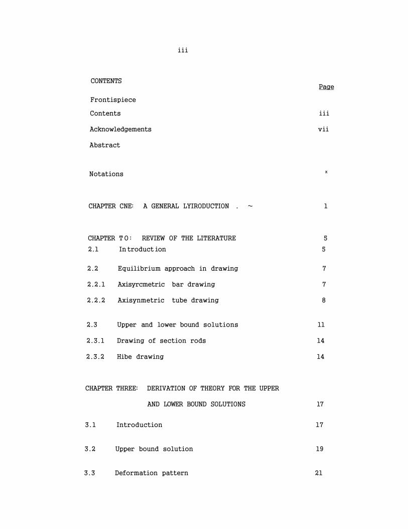
CONTENTS Page

Frontispiece

Contents iii

Acknowledgements vii

Abstract

Notations x

CHAPTER CNE: A GENERAL LYIRODUCTION . ~ 1

CHAPTER TO : REVIEW OF THE LITERATURE 5

2.1 In troduct ion 5

2.2 Equilibrium approach in drawing 7

2.2.1 Axisyrcmetric bar drawing 7

2.2.2 Axisynmetric tube drawing 8

2.3 Upper and lower bound solutions 11

2.3.1 Drawing of section rods 14

2.3.2 Hibe drawing 14

CHAPTER THREE: DERIVATION OF THEORY FOR THE UPPER

AND LOWER BOUND SOLUTIONS 17

3.1 Introduction 17

3.2 Upper bound solution 19

3.3 Deformation pattern 21

iv

Page

3.4 Velocity field 25

3.5 Strain rates 30

3.6 Total pcwer required for deformation 33

3.6.1 Internal power of deformation 33

3.6.2 Pcwer loss in shearing material at inlet and

exit shear surfaces 38

3.6.3 Frictional losses at the tool-workpiece

interfaces 42

3.6 .3 .1 Apparent strain method 43

3 .6 .3 .2 The mean equivalent strain 50

3.6 .3 .3 Work hardening factor B 52

3.6.3.4 Evaluation of and I2 53

3.7 Lower bound solution 55

3.7.1 Deformation pattern of' the lower bound

solution 55

3.7.2 Derivation of the lower bound solution 56

3.8 Computer program g2

Flow chart for the upper bound solution

for polygonal drawing 67

Flow chart for the lower bound solution for

polygonal drawing 72

Flow chart for the upper bound solution for

axisyrrmetric drawing

Flow chart for the lower bound solution for

axisyrrmetric drawing

CHAPTER FOUR: RESULTS 77

CHAPTER FIVE: DISCUSSION OF RESULTS 90

5.1 Introduction 90

5.2 Upper bound 90

5.3 Lower bound 93

5.4 Limitation of achievable reduction of area 96

CHAPTER SIX: CONCLUSIONS 98

CHAPTER SEVEN: SUGGESTIONS FOR FURTHER WORK 100

REFERENCES 102

vi

APPENDICES

Page

A-l Upper bound solution

A-l.l Detailed deformation pattern A1

A-l.2 Derivation of the flow path parameters A15

A-l.3 Equivalent plug semi-angle and cross-sectional

area of tube material A23

A-l.4 Derivation of velocity discontinuity suffered

by an element entering the deformation zone A29

A34

A-2 Lower bound solution - 33

A-2.1 Lower bound numerical integration A33

A-2.1.1 Gecmetrical derivations

A-2.1.2 Development of the recursive equations to

evaluate the draw stress and the mean

pressure A34

A-3 Canputer programmes

A-4 Tabulated sample solutions of the upper and

lower bound for polygonal and axisynmetric

drawing A57

A-5 Equations for equivalent axisynmetric

drawing A72

vii

ACKNOWLEDGEMENTS

I express my appreciation to rry supervisor

Dr. S.M. Maranga who has given me valuable guidance, advice

and encouragement in the preparation of the thesis.

Prof J.K Musuva deserves special thanks for the encouragement

he has given me during the preparation of the thesis.

I thank the staff of the mechanical engineering

workshops and particularly the chief technician Mr. Paul Ndegwa

for the assistance he has given during the final stages of the

project.

I wish to thank the DAAD Secretariat for the

financial assistance they gave throughout the research period.

Finally, special thanks go to Ms F. Kollikho for

typing the manuscript to very high standards.

viii

ABSTRACT

Theoretical and practical investigations in the

drawing of the following sections directly from an entirely

round stock have been reported: polygonal bars, polygonal

tubes with the outside and bore surfaces geometrically similar,

and tubes with the outside polygonal surface and circular

bore. The derived theoretical solutions enabled the

industrialists to design tools to manufacture tubing or bar

stocks directly from round with minimum amount of energy being

dissipated in the drawing process; the resulting optimal

tools also produced relatively superior polygonal stocks.

This thesis extends the theoretical analysis to the manufacture

of a polygonal tube by drawing an entirely round stock through

a deformation passage formed by a conical die and a polygonal

plug.

Using a prescribed shape of the plug and a regular

conical die, two solutions of the drawing loads were derived:

the lower bound and the upper bound. The lower bound load

considered the homogeneous deformation and the friction work

and thus ignored the redundant work. The upper bound value

of the drawing force was derived from the minimum energy

associated with the velocity pattern obtained by con formal

napping. Unlike the axisynmetric drawing on a mandrel, the

ix

plug profile was corrplex; an equivalent plug semi-angle was

therefore used to enable comparisons to be made between

deformation passages formed by a known die profile and the

polygonal plugs and also to facilitate the optimization of

the process parameters.

The graphs of the drawing forces drawn against the

various parameterrs such as the die angle, the equivalent plug

angle, the reduction of area as well as friction snowed trends

similar to those tried practically and reported in the

literature of polygonal tube drawing directly from round stock.

X

NOTATION

Diameter of the inlet circular section

D0(=2R ) Diameter of the outlet circular section a. a.

H Diagonal length of the drawing plug equal to the a

diameter circumscribing the polygon

L Die length measured along the draw axis

Ns Nurrber of sides of the drawn polygonal tube

t. Inlet tube wall thickness

d^(=2rb) Plug diameter equal to the bore of input stock

Ak . Cross-sectional area at entry

A Cross-sectional area at exit a

Af Ratio of cross-sectional area at entry to that at

the exit

red, ' r' Reduction of area

t Minimum tube wall thickness along the diagonal a

of the drawn tube

K Factor (0«<i ) expressing the tube wall thickness

at the diagonals in terms of Da i .e. ta = <Da

de Diameter of an equivalent circular section of the

plug at the exit

a Die semi-angle of the conical surface

ct The equivalent plug semi-angle; it is the semi-angle

of a conical plug corresponding to the polygonal

tube drawing plug through a conical die for the same

xi

reduction of area and the same die length

ac Plug semi-angle of the conical surface of a polygonal

section drawing plug

as Plug semi-angle of the flat surface of a polygaial

section drawing plug

Xc Angle subtended by the conical surface of a symmetric

section of the plug at the draw axis

A3 Angle subtended by the flat surface of a symnetric

section of the plug at the draw axis

3 Included angle of a syrrmetric section of the plug

p,9,<p General spherical co-ordinates

p Radial distance frcm the virtual apex of the conical

surface of die to the centroid of the assumed shape

element at the inlet section

9 Inclination of the radius to the tube axis

4> Inclination of a particle measured in a plane

perpendicular to the draw axis

f Relative angular deflection of an element measured

in the p-Q plane

n Relative lateral displacement of the assumed shape

element referred to the inlet

u Velocities in the p, 9 and 4> directions P O <J>

u , u The mean coefficient of friction at the die-tube m'

and plug-tube interfaces

xii

p , p Mean pressure at the die-tube and the plug tube

interfaces

a Mean draw stress za

k Mean yield stress in shear

Y Mean yield stress in tension m

W Work dene per unit volume of material

VOL Volumetric rate

J* Actual externally supplied power

V Volume of deforming material

i. . Strain rate ij

T Shear stress at the sliding surface

|Au| Velocity discontinuities along the sliding surfaces

Sp Surface of velocity discontinuities

TV Predetermined body tractions

S Surfaoe area subjected to pre-determined body

tractions

S^ Surface of prescribed velocity

u^ Velocity at entry and exit surfaces having

predetermined body tractions

a. . Stress tensor component ij

a Generalised stress or t^rta. .a. .}*

2 i i Generalised strsiin or ^ e ' e' }

j-j

t Factor (-l<t<l) selected to cptlmise the inlet and

exit shear surfaces by minimizing the plastic work

xiii

dene

N Nunber of hyperbolic curves banding the exit

section

M Nianber of sectors into which the inlet section is

divided.

General subscripts

a exit parameter

b entry parameter

p plug surface

d die surface

c conical

s straight or flat

m mean

5. . Kronecker delta ij

V Poisson's ratio

1

1. A GENERAL INTOCDUCTICN

The prevailing economic factors such as manpower,

equipment and energy facing the world today force industry to

be en the look-out for alternative ways of manufacturing

products for exajrple the manufacture of polygonal products by

drawing or extrusion.

Hie project undertook to investigate the mechanics of

drawing polygonal tube from round through a cylindrical die on

a polygonal plug. This is a process whereby the bore of the

tube changes from round to the polygonal shape whilst the

external surface remains circular. The process would be

Important to industry in for exanple the manufacture of

spanners and locking devioes. Such a process would bring

significant savings in the cost of raw materials, tooling,

pcwer and labour. In addition the process would inpart improved

mechanical properties on the final product.

The aim of the investigation was to establish a theore

solution. The solution provides an estimate of the forces on

the drawing tools, the optimum design of the tools and an

understanding of the flow of the deforming metal. This leads to

an efficient utilization of material and selection of a draw

2

bench.

The project is an extension of the work in polygonal-

bar and -tube drawing. The drawing of regular polygonal bars

was investigated experimentally and theoretically by Basily {3};

the drawing of regular polygonal tube from round through a

polygonal die on a polygonal plug by Kariyawasam {4}; and the

drawing of regular polygonal tube from round on a cylindrical

plug by Muriuki {5}. In each of the forementicned drawing

processes, the theoretical predictions agreed reasonably with

the actual data. There is havever, no known literature on the

drawing of regular polygonal tube from round through a cylindrical

die on a polygonal plug. This project therefore undertakes to

study the drawing process and establish a theoretical model to

predict the drawing- and plug- forces for a range of the process

parameters.

In the works of the three forementioned authors (3, 4 & 5) on

polygonal drawing, the workpiece of initially circular section

had to transform to a polygonal section in a single pass.

The passage through which the workpiece deformed into the final

product combined both conical and plane surfaces of different

inclinations to the draw axis to allow for gradual deformation.

The shapes of the dies and the plugs in case of tubing included

3

the pyramidical plane surfaces, the elliptical plane/conical

surfaces, the triangular plane/conical surfaces and the inverted

parabolic plane/conical surfaces. In this project, the elliptical

plane/conical surface profile of the plug and a straight conical

surface for the die were selected for the theoretical analysis.

In chapter (2), a review of the drawing theories is

presented. Unlike the case of axisyrrmetf'ic drawing, in the

polygonal drawing processes, the flow pattern is very complicated

and the resulting theoretical models are solved numerically using

a computer. Two solutions are established in this project: the

first is based on the equilibrium of forces and predicts a lcwer

bound solution; and the second predicts an upper bound solution

and is based on a velocity field that minimises the energy required

for the process and incorporates an apparent strain method and

Coulomb friction. The actual draw load is bracketed by the two

solutions.

The corresponding axisyrrmetric tube drawing solutions

are also analysed with the aid of a computer to facilitate

comparison between polygonal tube drawing and axisyrrmetric tube

drawing.

Details of the derivations are in chapters (3) and the

appendix. The oamputer programs developed to solve the solutions

are in the appendix.

5

2. REVIEW OF THE LITERATURE

2.1 INTRODUCTION

Drawing of metal is an ancient craft, dating back to

ancient Egypt where the process was used to draw ornamental

wires. Today, large quantities of rods, tubes, wires and

special sections are finished by cold drawing {6}.

Cold drawing gives a good dimensional control, a good

surface finish and irrproved strength of the drawn metal {6}.

However, a limit on the reduction of area possible in

a single pass is determined by the condition that the longitudinal

stress at tte exit cannot exceed the strength of the drawn metal.

It is important, therefore to have the tensile stress on the

drawn metal as lew as possible.

A lot of literature, both theoretical and experimental

has been published on the drawing process. The factors

considered in the various theories include the die geometry,

mechanical properties of the work material, the coefficient of

friction, etc. A wide review of the drawing process is given

by Wistreich {1}.

6

Recently, investigators have been mainly working on the

drawing of non-circular sections e.g. polygonal rods and tubes,

channels, etc. which had not received attention in the past.

In these cases, the flow is either syirmetric or asynmetric as

opposed to plane strain deformation for drawing sheets or

axisyrrmetric drawing of bars and tubes. Among recent

investigators on polygonal drawing include Juneja and Prakash

{2}, Basily {3}, Kariyawasam {4} and Muriuki {5}. There is

however, no known literature, experimental or theoretical on

the direct drawing of round tube to a tubular section having

an external circular surface and a polygonal bore inspite of

the importance of this type of shape in engineering works such

as manufacture of spanners and locking devices. This project

therefore undertakes to establish a general theoretical solution

on the direct drawing of such a tube.

Metal working theories can be grouped broadly under

the following headings:-

( i ) equilibrium approach,

( i i ) slipline field approach/

( i i i ) upper and lower bound solution,

(iv) energy approach where the total work consists of

homogeneous, redundant and friction components,

(v) visioplasticity, and

7

(vi) finite element method.

A comprehensive review for the equilibrium approach is

presented in the next section and that for the upper and lower

bound solution in section 2.3. These two theories formed the

basis of the theoretical analysis presented in chapter (3) .

2.2 EQUILIBRIUM APPROACH IN DRAWING

This method is based on the equilibrium of forces.

It therefore takes into account only that distorsion necessary

for the shape change and neglects any redundant deformation.

When using the theoretical models derived by this method, the

errors involved for exairple in the drawing forces may be large

especially for large die angles with small reductions.

However, the loads determined by this method have been found to

agree closely with experimental results in seme processes

especially wire drawing {1}.

2.2.1 AXISYMMFIBIC BAR DRAWING

One of the first useful equations in wire drawing was

proposed by Sachs {6} in 1927. It was assumed that plane

cross-sections of the workpiece remain plane as they pass through

the die; the stress distribution on such planes is uniform;

8

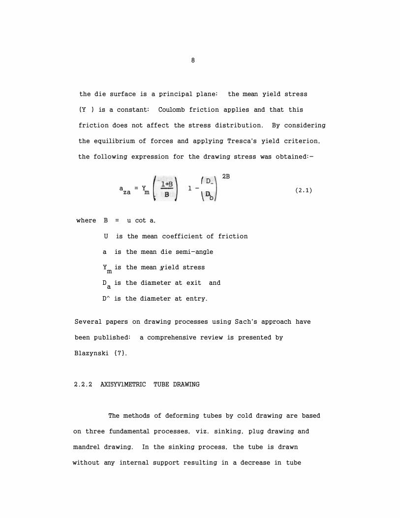
the die surface is a principal plane; the mean yield stress

(Y ) is a constant; Coulomb friction applies and that this

friction does not affect the stress distribution. By considering

the equilibrium of forces and applying Tresca's yield criterion,

the following expression for the drawing stress was obtained:-

a = Y za m

1 -

2B

(2.1)

where B = u cot a,

U is the mean coefficient of friction

a is the mean die semi-angle

Y is the mean yield stress m J

D is the diameter at exit and a

D^ is the diameter at entry.

Several papers on drawing processes using Sach's approach have

been published; a comprehensive review is presented by

Blazynski {7}.

2 .2 .2 AXI5YV1METRIC TUBE DRAWING

The methods of deforming tubes by cold drawing are based

on three fundamental processes, viz. sinking, plug drawing and

mandrel drawing. In the sinking process, the tube is drawn

without any internal support resulting in a decrease in tube

9

diameter with ideally no change in wall thickness. Wall

thickening may take place but it rarely exoeeds 7%. In the

plug drawing process, the tube is drawn over a fixed or

floating plug positioned in the die throat. In practice, a

small amount of sinking is present in the process using a

plug; there is a reduction in both the diameter and the wall

thickness. In the mandrel drawing process, the internal tool

moves with respect to both the tube and the die.

In 1946, Sachs and Baldwin {11} derived a formula for

the draw stress in the sinking of thin walled-tubing: -

where B = u cot oi

Da and D^ are the mean diameters at exit and entry

respectively and

Y' ^1-1 Y is the modified mean yield stress from m m

the von Mises yield criterion.

The solution was based on the following assumptions: -

A pressure normal to the working tool-metal interface

exists on the interface of tube and die and is a principal

stress; a shear stress exists on the interface because of

fricticn; transverse sections are free of shear stresses; the

(2.2)

10

normal stress acting on the transverse sections is uniformly

distributed over the cross-section and is a principal stress;

the wall thickness is small in corrparison to the tube diameter;

the wall thickness of the tube remains constant throughout the

process.

Oie of the limitations on the application of the

equilibrium solutions is that they only account for homogeneous

work and friction work and no account is taken for the redundant

work. Hcwever, various investigators have proposed the

incorporation of a redundancy factor in the theories and a

carprehensive review is presented by Blazynski {7}. A more

general method of accounting for the effect of redundancy on

the parameters and mechanics of various processes was proposed

by Blazynski and Cole {11}. The authors extended Baldwin and

Sachs { 17} theory to account for redundant work by obtaining

the difference between the loads of the total and useful

deformation. An upper bound solution for the sinking process

incorporating the effect of redundancy has been extensively

treated by Avitzur {12}. Avitzur assumed the deforming zone

to be bounded by spherical shear surfaoes with their centres

at the virtual apex of the die. The flew through the die was

thus expressed by kinematically admissible velocity field.

11

2.3 UPPER AND LOWER BOUND SOLUTIONS

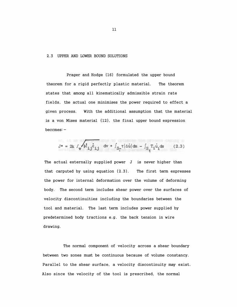
Prager and Hodge (16) formulated the upper bound

theorem for a rigid perfectly plastic material. The theorem

states that among all kinematically admissible strain rate

fields, the actual one minimises the power required to effect a

given process. With the additional assumption that the material

is a von Mises material {12}, the final upper bound expression

beccmes: -

The actual externally supplied power J is never higher than

that carputed by using equation (2.3). The first term expresses

the power for internal deformation over the volume of deforming

body. The second term includes shear power over the surfaces of

velocity discontinuities including the boundaries between the

tool and material. The last term includes power supplied by

predetermined body tractions e.g. the back tension in wire

drawing.

The normal component of velocity across a shear boundary

between two zones must be continuous because of volume constancy.

Parallel to the shear surface, a velocity discontinuity may exist.

Also since the velocity of the tool is prescribed, the normal

12

ccmpcnent of the postulated velocity field for the deforming

material should be equal to the normal caipcnent of the velocity

of the tool over the surface of contact. When the postulated

velocity field satisfies the relaxed continuity requirements,

i .e . permitting velocity discontinuities parallel to the shear

boundary, it is called a kinematically adnissible velocity

field {12}.

Kinematically actnissible solutions are useful in that

in addition to predicting the loads required for a certain

process, it is also possible to optimise the process taking into

consideration the effects of various parameters. Also the

proportion of the redundant deformation and the defects such as

shaving, central burst, dead metal zone, etc. can be predicted.

The approach also unveils information to eliminate the various

defects.

The lower bound theorem states that among all

statically admissible stress fields, the actual one maximizes

the expression

I = / T.u.ds (2 .4)

v 1 1

where I is the computed power supplied by the tool over

surfaces over which the velocity is prescribed, T^ is the

normal component of traction over the prescribed surfaces and

13

iii is the relative velocity between the tool and workpiece.

The stress field describing the stress distribution

within the deforming zone should satisfy the following

requirements:- It should be a smooth function; it should

obey the equilibrium equations; it should satisfy the surface

conditions when surface tractions are prescribed and the state

of stress does not violate the yield criterion. Such a stress

field is called a statically admissible stress field.

Different kinematically admissible velocity fields can

be assumed to determine a value of J*. For the lowest value of

J*, it is presumed that the velocity field that led to it is

approaching the actual velocity field.

Several statically admissible stress fields can be

assumed with a view to obtaining a value for I. For the highest

value of I, it is presumed that the stress field that led to it

is closer to the actual stress field. For actual stress and

strain rate fields, J* = I = actual power.

A nurrber of investigators have developed the upper

bound technique and applied it to specific problems. A brief

recount of the more recent work relevant to the current

research is presented in the next two subsections.

2.3.1 DRAWING OF SECTION RODS

In 1975, Juneja and Prakash {2} obtained an upper bound

solution for the symmetric drawing of polygonal sections. The

solution predicted the cptimum convergent angles of the die

surfaces for the minimum drawing stress and the critical

convergent angles for the formation of a dead metal zone. The

draw stress was observed to decrease rapidly to that of the axi-

symnetric solution by Avitzur {12} as the nunber of sides of

section increases.

Concurrently but independently, Basily {3} obtained

an upper and lover bound solution for the asynmetric drawing of

regular polygonal bars from round bar. It was shown that the

equivalent die angle can be optimised for every relevant

combination of the coefficient of friction and reduction of

area. It was further shewn that as the number of sides of the

drawn section rod increases, results of both the upper and lower

bound solutions approach those of the corresponding axisyrrmetric

case.

2.3.2 TUBE DRAWING

A general upper bound solution was derived for axi-

symnetric contained plastic flow occuring in processes like

drawing and extrusion of tubes and wires by Juneja and Prakash

{13}. The solution was extended to particular cases for

instance plastic flow through conical dies using a plug or a

mandrel.

Kariyawasam & Sansome {4} investigated the process of direct

drawing of round tube to any regular polygonal shape both

experimentally and theoretically. In addition to designing

draw tools optimised to give the least work of deformation, the

effect of diameter to thickness ratio of the undrawn tube and

the effect of reduction of area on the draw force was also

investigated.

wa Muriuki {5} investigated the direct drawing of

regular polygonal tube from round on a cylindrical plug both

experimentally and theoretically. The derived theoretical

solutions were based on a method of conformally mapping

triangular elements in the inlet plane to corresponding

triangular elements in the exit plane. Several sets of the

die profiles shown in Figure 3.2 on page (20) were tested

experimentally. The elliptical plane/conical surface die

produced results which agreed fairly well with the predicted

values. Hie reports by Basily & Sansome {3} and Kariyawasam

& Sansome {4} also recommended this type of the

die profile to be the optimal

This project therefore selected the elliptical plane/

surfaces to be the profile of the plug to be investigated.

17

3 DERIVATION OF'THEORY FOR THE UPPER AND LOWER BOUND SOLUTION

3.1 INTRODUCTION

Equations for the upper and lower bound solution in

the drawing of regular polygonal tube from round through a

cylindrical die on a polygonal plug are developed in this

chapter (See Figure 3 .1 ) . Close pass drawing is assumed in

the derivations.

The deformation passage is complex and numerical

integration was used to obtain the solutions for any given set

of drawing parameters. The deformation pattern was selected

such that the difference between the two bounding loads is as

small as possible since the actual load lies between the two

limits.

The upper bound solution was obtained by equating the

total power derived for the prescribed deformation pattern to

the applied power. The development of the velocity field for

the upper bound solution is described in section 3.4 and

Coulomb friction was incorporated by an apparent strain method

presented in section 3 .6 .3 .1 on page (43).

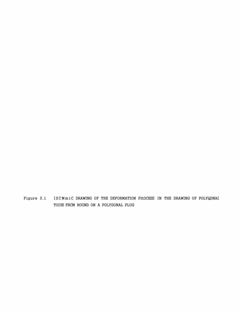
Figure 3.1 ISCMmiC DRAWING OF THE DEFORMATION PltOCESS IN THE DRAWING OF POLYQDNAI

TOI3E FRCM ROUND ON A POLYGONAL PLUG

19

The derivation for the lcwer bound solution was based

on the equilibrium of forces and Tresca's yield criterion. The

solution was developed for the elliptical plane/conical surface

plug (Figure 3.2) and a cylindrical die.

Equations for the lower and upper bound solution for

axisyrrmetric drawing are presented in appendix A-5 on page (A72)

The computer programmes presented in Section 3.3

provides the results for the upper and lower bound solution

for polygonal drawing and also for axisyrrmetric irawing for

the purpose of comparison.

3.2 UPPER BOUND SOLUTION

In the upper bound solution, the minimum energy

required to deform the material is calculated. In addition

to the homogenous deformation, relative shearing at the inlet

and outlet regions of the deformation zone is considered.

FUrther relative shearing of the material elonents in the

deformation zone is also considered and finally, friction

between the deforming metal and the tools is accounted for

using Coulomb's relationship.

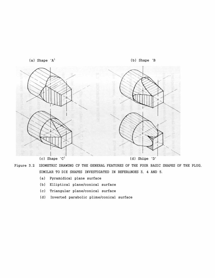
(a) Shape 'A1 (b) Shape 'B

(c) Shape 'C1 (d) Shiipe 'D'

Figure 3.2 ISOMETRIC DRAWING CF THE GENERAL FEATURES OF THE FOUR BASIC SHAPES OF THE PLUG,

SIMILAR TO DIE SHAPES INVESTIGATED IN REFERiiNOES 3, 4 AND 5.

(a) Pyramidical plane surface

(b) Elliptical plane/conical surface

(c) Triangular plane/conical surface

(d) Inverted parabolic plime/conical surface

21

A velocity field is assumed and if the deforming metal

obeys von Mises yield criterion and the Levy-Mises flow rule,

the upper bound solution described in section 2.3 of Chapter 2

indicates that the actual strain rate field e^ is the one that

minimises the expression given by equation (2 .3 ) on page 11

The velocity field is derived from a ccnformally mapped

deformation pattern described in section 3.3. Having derived

the velocity field, the minimum value of J*, the power to effect

the process, is obtained for the given set of drawing parameters.

3.3 DEFORMATION PATTERN

The entry plane (X^ (see Figure 3.3) is defined

as the plane normal to the die axis through the point where the

outermost tube elements (D = D^) first contact the die and

start to deform.

Similarly the exit plane (X , Y ) (Figure 3.3) is the cl 2L

plane normal to the draw axis through the point where the

outermost material (D = D a ) starts to flew parallel to the draw

axis and deformation ceases.

FIOTRE 3 .3 DEFORMATION PATITSRN TOR THE DRAWING OF REGUUR

POLYGONAL TUBE FRCM ROUND

23

The method applied for obtaining the deformation

pattern is based on conformally mapping each triangular element

in the inlet plane to the corresponding triangular element at

the exit plane (Figure 3 .3) .

At the exit plane, the cross-sectional area of the

polygonal tube is banded by (N—2) hyperbolae, in each of which

the focal distance a^ is adjusted to suit the asymptotes such

that the hyperbola corresponding to the inner surface is almost

coincident with the flat surface of the polygonal tube. The

outermost curve remains circular corresponding to the die

surface. The area between consecutive curves is calculated.

Assuming a constant reduction in area, the corresponding cross-

sectional area at the inlet plane is determined and hence

the radii bounding it (see Figure 3 .4) .

The banded area at the inlet cross-section of the

tube is divided into (M-l) equal sectors. Each sector, say

ABCD, is further divided into two triangles, the large triangle

ADB and the small triangle DCB. The area of each triangle can

be determined and frcm the known co-ordinates of the vertices,

the centroid is located.

Assuming a constant reduction in a_rea of the large

triangle ADB on the inlet plane, the corresponding area of the

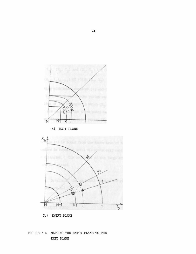
24

(b) ENTRY PLANE

(a) EXIT PLANE

FIGURE 3.4 MAPPING THE ENTOY PLANE TO THE

EXIT PLANE

25

l*irge triangle A'D'B' on the exit plane can be determined. Let

this triangle at the exit plane be defined by the co-ordinates

( X r Y x ) . (Xg, Y 2 ) and (X3, Y3) (or (Xa> Y J ^

and (Xa , Y & ) i j + 1 ) of which (X^, Y^) lies on the hyperbola i.

Starting with kncwn vertices (1) and (2) (or (X^, Y^) and

(X2, Y 2)) ,the third unknown vertex can be found by solving the

equation of the triangle in which (X^, Y^), (X2> Y2) and the

area are kncwn and the third point satifies the hyperbola i.

Having determined the third vertex (X„, YJ (or (X , Y ). . , ) »

d o a a i , j+i

the point is then substituted for (X2 , Y 9 ) of the small

triangle D'C'B' and the third unknown vertex which satifies the

hyperbola i+1 is found from the known area of triangle. The

procedure is repeated until the whole exit section is mapped

into triangles. The centroids of the large and small triangles

can now be located.

Details of the conformal mapping are given in Appendix

A-l, section A-l.l.

3.4 VELOCITY FIELD

It is assumed that before meeting the die, all

particles of the tube material travel parallel to the draw axis

towards the die entry. Within the die, the velocity of a

26

particle is expressed 3-dimensionally by a spherical co-ordinate

system, li = u(up, uQ , u^) and changes as the deformation proceeds.

Beyond the exit plane, the particle travels parallel to the draw

axis without further plastic deformation. A boundary therefore

exists which separates the undeformed metal zone to the zone

where relative deformation occurs. A particle cn reaching this

surface shears and changes direction.

A similar distortion occurs at the exit except that the

particles pass through the boundary from the deforming zone into

a region subject to elastic distortion cnly.

There is no general theoretical method to determine the

shape and position of these boundaries. It is usual to

assume that the boundaries are plane, spherical or conical.

In the current problem, the deformation mode is ccmplex.

A general shear surface was defined such that a particle on

any streamline cn entry was assumed to shear at an angle (—-10) to th

draw axis where -l<t<l (see Figures 3 . 5 and A-1 .6 ) . The

position of the particle was defined on the general spherica

surface (pb,0,4>). The parameter t was used to optimise the

shear surface by minimizing the shear work. A general

pyramidical shear surface was defined at the exit of the

deformation zone.

27

Once a shear surface has been defined, a plane parallel to

•exit' or 'entry' planes and passing through the centroid of the

particle on the respective shear surfaces can be drawn. Such

planes are denoted by (X^, Y^) and (X^, Y£) for the exit and

entry shear surfaces respectively. Let the centroid of the

triangular elonent at entry be denoted by (X^, Y.^Ki.j) and

that of the corresponding triangular element at the exit by

(X\ Y ' ) ( i , j ) . By joining the centroids of the corresponding a a

triangular elements, the drawn vector was assumed to define

the path followed by the element. Detailed derivations of the

flew path parameters are in Appendix A-l, section A-1.2.

Having defined the flew path, the velocity field

u(p,9,4>) is established and therefore the strain rates (see Figure

A - l . 1 2 ) .

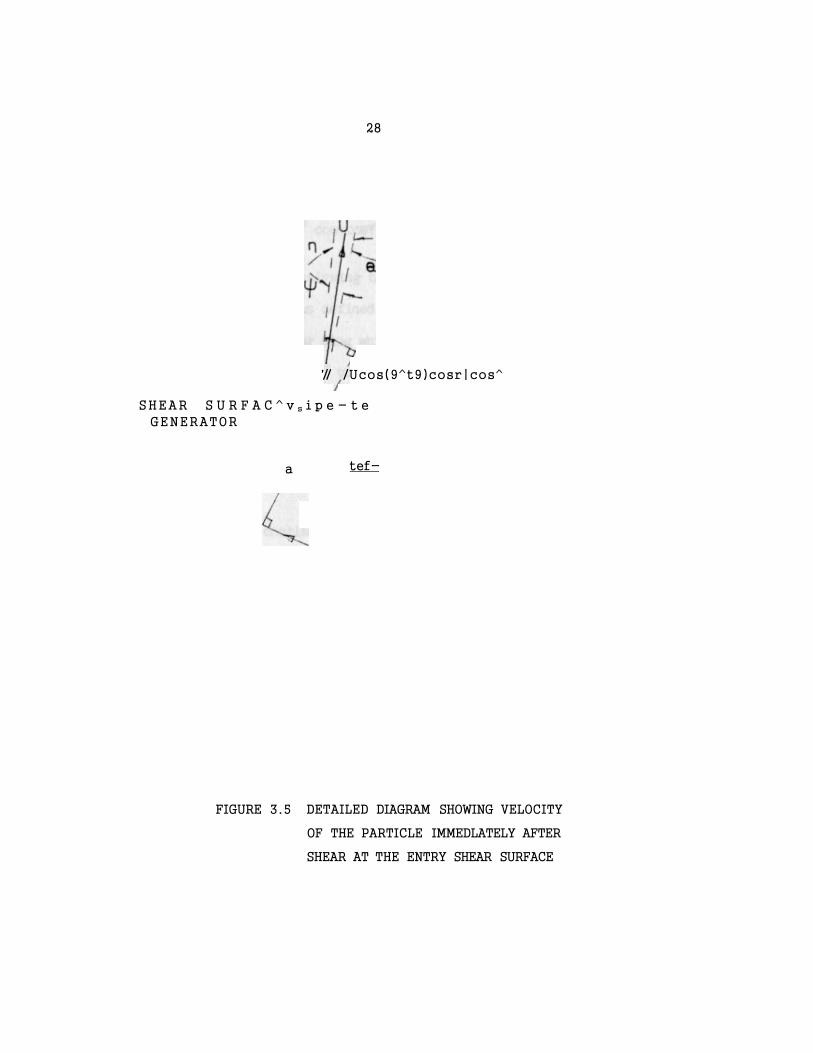
Let li be the velocity of an element before shear at

the assumed velocity discontinuity surface and u(p,9,4>) the

velocity immediately after shear. The component of velocity

normal to the shear surface must be of the same magnitude on

both sides of the shear surface for continuity of flew

(Figure 3.5) i .e .

ll ccstQ = ucosncosf cos (1-t )9

28

SHEAR S U R F A C ^ v s i p e - t e

GENERATOR

'// /Ucos(9^t9)cosr|cos^

a tef-

FIGURE 3.5 DETAILED DIAGRAM SHOWING VELOCITY

OF THE PARTICLE IMMEDLATELY AFTER

SHEAR AT THE ENTRY SHEAR SURFACE

29

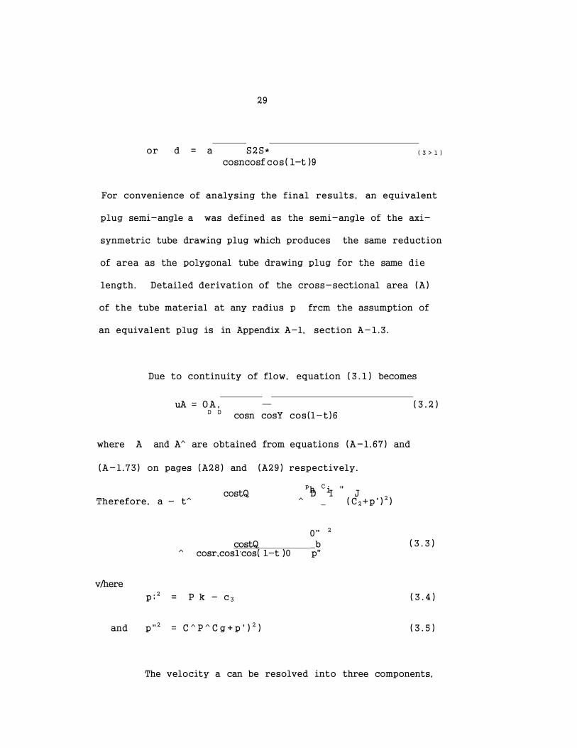
or d = a S2S* ( 3 > 1 )

cosncosf cos( 1-t )9

For convenience of analysing the final results, an equivalent

plug semi-angle a was defined as the semi-angle of the axi-

synmetric tube drawing plug which produces the same reduction

of area as the polygonal tube drawing plug for the same die

length. Detailed derivation of the cross-sectional area (A)

of the tube material at any radius p frcm the assumption of

an equivalent plug is in Appendix A-l, section A-1.3.

Due to continuity of flow, equation (3.1) becomes

uA = OA , — (3 .2) D D cosn cosY cos(l-t)6

where A and A^ are obtained from equations (A-l.67) and

(A-l.73) on pages (A28) and (A29) respectively.

ph C i " costQ D I J Therefore, a - t^ ^ _ (C 2+p') 2)

0" 2

costQ _b ^ cosr,cos1,cos( 1-t )0 p"

(3 .3 )

v/here

p; 2 = P k - c 3 (3 .4 )

and p" 2 = C ^ P ^ C g + p ' ) 2 ) (3 .5)

The velocity a can be resolved into three components,

30

namely up, u^ and u^ in the p, 8 and <p directicns. Considering

the geometry of Figure A-1.4 on page (A16) and substituting

for u from equation (3.3), the velocity ccnponents of the

particle thus become:

iip = u cosncos^

P'7

costQ

cos(l-t)0 (3.6)

Uq = u cosncosT

2 (Pbl

"b pni

cos t6 tanY

cos(l-t)9 (3.7)

u = u smn

% costQ tann

cos (l-t)9 cosy

(3.8)

3 .5 STRAIN RATES

i. a

The general expressions for strain rates as functions

of velocity components up, Uq and in the directions p, 0

and $ respectively, in the general spherical polar co-ordinate

system (15) are as follows:-

31

EP =

3u

3p

u

y p 30 p

( 3 . 9 )

(3.10)

^ 3u, u Uq

3ue ue i 3UQ Y P 0 = 3 O ~ " O - + P 3 E _ ( 3 - 1 2 )

]. 9U9 1 9U. U,

'9* = 5 5 9 3T + p 99 " p c o t 9 (3 .13)

' , 1 Y<J>p 3p p psin9 90 (3 .14)

Equations (3.9) to (3.14) were applied to the derived velocity

expressions (equations (3 .6) to (3 .8) )to yield the strain rates.

The final expressions for the strain rates become:

_ = 2 C L "b. C C 6 t 9 [fb\ {p-(C2+p»)/Pl_| }p (3 .15)

P "2 p os(l-t)e \p"/ ' p~pbl

where C^, and p' are given in Appendix (A-1.3) by the

equations (A-1.68), (A-1.59) and (A-1.70) respectively, while

2 2 p" and p" are evaluated using equations (3.4) and (3.5) on b

32

on page (29).

li / p bl 2 ocstQ £9 = " p p77/ cos( l-t)9 (1+tanY(-t tant9+(l-t)tan(l-t)9

+ — — ) ) (3.16) os'f

• ^ ( f b f coste . {1 + tan* + \ 0 0 t f 0 Q B ( ^ A ) t (3.17)

P \P'7 Cos(l-t)9 t a n Q Zgoosf '

where 0 and Z are given by equations (A-1.53) and (A-1.44) A S

on pages (A22) and (A15) respectively.

Ob YP6 " p

, A „ I 2

%) coste { t a r t f _ 1 tartf {p-(C9+p')

P 1 cos(l-t)9 p" 2 2

(-£—) }p-t tantQ + (1-t)tan(l-t)9} (3.13) P-Pb

• - ^ Y94> P

bl ccst9tann { < z l _ _ t t a n t 9

PI cos(l-t)6coslF tan9

+ tanQ +(l-t)tan(l-t)6+tan*}

= Jb Y *P p

Ui_ /Pu 2

b ) cost9tann ( " l { p _ ( c + p , ) ( _ g _ ) } }

[p"l cos( 1-t )9cos4/ P"2 2 P-Pb

33

3.6 TOTAL POWER REQUIRED FOR DEFORMATION

3.6.1 INTERNAL POWER OF DEFORMATION

The following assumptions were made when deriving the

rate of internal work to deform the material in the deforming zone:

(i) The material obeys von Mises yield criterion,

a ' j a' . = 2k2 (3.23)

where a< . = a. . - . (3 .21)

and k is the yield stress of the material in shear.

(ii) The flow obeys the Levy-'lises stress-strain relationship

. = a' dX where dA is a constant (3.22) ij ij

of proportionality. *

( i i i ) The material is rigid perfectly plastic and non work-

hardening.

(iv) The inccmpressibility condition is satisfied

i .e . ^ = = 0 (3 .23)

The rate of work required to deform an elemental

volixne dV is

34

dWj = a i j 6 i J dV .

Therefore power to deform material of volume V is

W_ = / o. i . ,dV I Jv ij ij

Multiplying each side of the Levy-Mises expression

by gives

e, .e. . = dAa 'e . . (3 .24) ij ij ij iJ

Also multiplying the equation by a! . gives J

a! i. . = dAa! .a'. . (3.25) ij ij ij iJ

Therefore, o ! .e . . = 2dAk2 (3 .26) J " J

from von Mises equation (3.20).

Equation (3.21) can be rewritten as

a ' i y - Catj - i a ^ j i y

= a. i . . (3 .27) ij ij

and from equations (3.24) and (3.25),

(3 .28)

Substituting equations (3.27) and (3.28) into equation

(3.25) gives

35

By substituting equation (3.29) into the expression for Wr

gives

W x = Ik A e. j e i j dV (3 .30)

If k is assumed constant,

Wj =k /2 . /v dV (3 .31)

If the mean yield stress is Y , then for the von Mises m

condition,

Y k - J

/3

Therefore, W, = /| y J i, . dV ( 3 3 2) ^ 3 m v ij ij

Substituting for the strain rates frcm equations

(3.9) to (3.19).

e. i, » e? + t* + ei? + 2(e?0 + A + fe2 } IJ LJ 1 2 3 12 23 31

36

Therefore, the expression for the internal power of deformation

becomes

wi = j 2 'v / { 2 ( £ p + + + 4 * * ^ V d v

Y ••• 2 Y or _ m r D , b. costs Ar .v

where

2C,o p'

2C1P . -- -- _Pl 2

P"" " ^ b

K = 2 { ^ (p - (C2+P') ) )} „2 ^ 2

2 +2 {-(l+tanYC-ttante +(l-t)tan(l-t)9 + —) ) }

oosY

+2 {l+ + } tanB tan(^-^A)cos4'sin9

2

(3.34)

+ {-(tan f-2CTtan¥(p-(C0+p')(—£—))—~ - ttant9+( l-t)tan( 1-t )Q )} 1 2 p-p^ p"2

+. (.(tanr^jJ. t t a n t 9 +tan8+( 1-t) tan( 1-t )9 +tan*)})

tan^ tanQ

2

'tan? ' ^ ^ I J ^ ^ > 2 ^ (3.35)

2

The elemental spherical volume is

2 dV = p sin8dpd9ckj> (3.36)

37

Therefore,

Y_ A _ ^ u o" 2

I " W„ » -IS f V " r271" r^K ^ ^ costs ^ 2 .

• 3 e ^ J ^ ^ ^ smedodec^

a (3.37)

Y ' , ,2

- IT- J27r (/pb £,,2 * dp} costesinede^ ( 3 b 3 8 )

e <,=0 P=p P cos(l-t)0 a

The elemental spherical surface area at entry-

is 2 dA^ = Pbsin6d9cfc> (3.39)

Equation (3.38) becomes:-

* r J s % fb 2 / 9 2 - F { / P b 0 ^ d o } coste ^ (3.40)

3 pb 9=cte 4>=0 P=Pa oos(l-t)9

Equation (3.4) can be rewritten as

p»» ^ Q

c—) = c - — 0 1 2

Pb

Substituting for C^ and C3 from equations (A-l.68) and (A-l.74)

on pages (A28) and (A29) respectively and rearranging,

D" 2 A,

(-£) = (3.41) pb P,2

38

Therefore,

W - f % fb f 2 n ;p costa 1 /3 p^ 9«a • i o o 0»2 cos( l-t)9 " "b

b e "a. "

= Y m V V ( s ) <3-42>

where

f(s) = / 3 2 = a J27T { |P b _£_ /K do) dA (3 .43)

b

f(s) is evaluated numerically by dividing the inlet section

into N x(M-l)x(N-2) elemental areas which are themselves O

subdivided into large and small triangles i.e.

f ( s ) = V ^ 1 ( A dA.} (3 .44)

E B/ 3 M- 1 = 1 J=1 Pa P" 2 cos(l-t)6

3 .6 .2 POWER LOSS IN SHEARING MATERIAL AT INLET AND EXIT

SHEAR SURFACES

The internal power Wj derived in the last section

is required to overcome the homogeneous deformation and the

necessary relative shearing within the material itself as it

progresses through the deforming zone. Power is also

required to corrpensate for the losses due to the shearing

39

of material on both the inlet and exit shear surfaces.

The rate of work on crossing a. shear boundary of

elemental area dA is given by 3

dWR = ku*dAg (3 .45)

where

u* is the velocity discontinuity along the surface,

k is the yield stress of the material in shear equal

Y

to __m by the von Mises yield criterion.

/3

The velocity discontinuities at the entry and exit

shear boundaries are derived in Appendix A-1.4, equations

(A-1.78) and (A-1.79) respectively. The rate of work

dissipation at the entry shear surface is

= / ( 3 - 4 6 )

= / k V S S I ? < 3 - 4 7 )

The rate of work dissipation at the exit shear surface is

WD = / k'u dA! (3 .48) Ra . ra s

a

40

where

k' = k for a non work-hardening material and

dA' is the elemental area on the shear boundary at s

exit.

. <*A Therefore, W^ = / k u r a ^ f t 9 (3 .49)

a

Assuming a passage formed by an equivalent conical plug and a

conical die,

2 dA. p"

—^ = (-£) (3.50) dA p"

a a

2 pr

and u r a =(—) u^ (3 .51)

2 • pa 2 ^ Therefore, WDo - / k (-2) u . ( — )

^ A p" **> 01* ccste T) a b

= { k u r b S t 9 - < 3 ' 5 2 >

D

The total rate of work of shear at the inlet and exit surfaces

of velocity discontinuity is

WD = WD + WD, R Ra Rb

. dA

= 2/ k u . Ab rb cost6

41

Y u . dA , 2 J 2 n A. / — - 1

/3 costQ ^

- ; 3 Y m V b R ( s > ( 3 - 5 3 >

where

B(8) - T- / i2 • {-sin* • Afa ' cos( 1—t )9tan4/

cost9 tanf + cost9 tan(l-t)6}2) * (3.54)

frcm equation (A-1.78) on page (32).

R(s) is evaluated numerically by dividing the inlet

section into N x(M-l)x(N-2) elemental areas which are s

themselves subdivided into large and small triangles.

Therefore,

N N-2 M-l ^

R(s) = — lim 2 I ( {ccstetann }2 + A, j=l cos(l-t)8taM

2 * b {-sint9+cost9tan4,+cost9tan( l-t)9} ) * — ^ (3.55)

Values of -l<t<l are used to select the shear surface that

gives the minimum value of R(s). This if. then the optimum

shear surface for the given draw conditions.

42

3.6.3 FRICTICNAL LOSSES AT THE TOOL-WORKPIECE INTERFACES

Besides the internal paver W^ and the shear power

additional power is required to overccme the frictional

losses which occur as the tube slides between the die and the

plug.

In the case of Coulomb friction, a mean coefficient

of friction y is usually assumed for the given relative

sliding surfaces. The rate of work loss is given by:-

» F = V W s ^ s + f A , W s ^ s ( 3' 5 6 )

SI S<5

where the first term on the right calculates the loss at the

die-tube interface and the second term calculates the loss

at the plug-tube interface.

The die and plug pressures and the coefficients of

friction are unknown. A mean pressure at both interfaces

can be assumed and if the distribution of pressure and the

mean coefficient of friction axe known, the frictional loss

can be calculated. The values are however unknown. To

avoid this difficulty, can be obtained indirectly by the r

apparent strain method. The method .allows the calculation

of the draw load in the case of Coulcrrb friction without

43

obtaining the distributicn of pressure at the tube-tool

interfaces.

3 . 6 . 3 . 1 APPARENT STRAIN METHOD

This is an energy method where the work done 6er

unit volume is divided into the plastic work and the surface

frictional energy {14}.

Friction produces shear stresses and strains at the

interface and these have two major effects on the work done.

Energy is dissipated at the interface as a result of the

relative motion and when the surface shear stress is

significant compared with the yield shear stress, additional

internal distortion results within the deformation zone.

The two effects increase the work done.

The total work done per unit volume of the material

is equated to an area under the equivalent stress-strain

curve (see Figure 3 .6) . The strains i and e corresponding cL

to the total work and plastic work per unit volume are known as

the apparent and mean.equivalent strains, respectively.

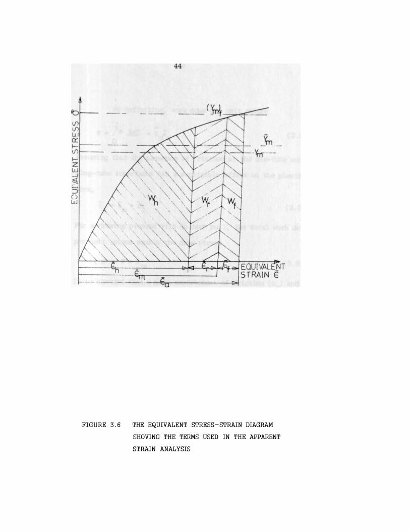
FIGURE 3.6 THE EQUIVALENT STRESS-STRAIN DIAGRAM

SHOVING THE TERMS USED IN THE APPARENT

STRAIN ANALYSIS

45

By definition, work dene per unit volime

z — W = / a adi = Y e (3 .57)

0 m a

Assuming that the presence of friction at the die-tube and

plug-tube interfaces has a negligible effect on the plastic

work,

ea = em + sf • (3 .58 )

For a drawing process with no back pull, the total work done

per unit volume equals the draw stress.

i .e . w = az a (3 .59)

It is assured that a mean coefficient of friction (y ) and m

a mean pressure (pm) occur at both the die-tube and the plug-

tube interfaces during the drawing process.

Using subscripts s^, c^ and c9 to denote the straight,

conical plug and die surfaces respectively:-

From Figure 3.7 for steady draw, the equilibrium of horizontal

forces gives,

azaAa = Pm < E « W » » + s i m ) + ( 3 ' 3 3 >

£(Umcosas - si«xs) dA s l • I(PmC06ac - S i m , ) dAc l

From equations (3.57) and (3.59),

46

° z a U a

FIGURE 3.7 STRESS AND THE DEFORMATION PATTERN IN THE

DRAWING OF POLYGONAL TUBE FROM ROUND

THROUGH A CYLINDRICAL DIE

47

a za

e = — Y m

a = T " (3.61)

Substituting for a in (3.60) gives, za

cr p , - _ za m l J v ,A ea - V- = r I f ^ V 0 8 0 + s l n B ) c2

m m a

+ ^(umcosas - sinas)dAs l +£(Umcos>c - s i roJdA^}

P_ or e • I. (3.32)

a V 1 m

where

I1 = - {Z(umcosa + sim)dA c 2 (3 .63) A

a

+E(Mmcosas - sir»s)dAs l + £(umCQsac - s inaJdA^}

= Apparent strain factor .

Frcm the definition of friction strain work done against

friction per unit volume of material

W. = (Y ) £ (3.64) f m ^ f

The friction work Wf can also be determined by the energy

dissipated as the material slides between the die and the

plug surfaces as follows:-

Using u s l , uQ l and u c 2 to represent the respective surface

48

velocities, equation (3.66) gives,

' W f X " V m V s l + V A A l

+ UnPaF%2 < i Ac2 (3-05)

By expressing the elemental surface velocities in terms of

the input velocity u^ gives

V 0 1 = dAsl + > dAcl

Uc2 + E ( t ~ ) d A J (3.66)

%

Substituting for

( V / f V o 1 = <*8i +

dAcl + £(^£2) dAc2}

^ "b

P_ or E . • — I9 (3.67)

(Y ) nrf

where

•p Umllb slv , r /u cl .

2 = T - { i : ( — > ^ s i + £ ( r-> ^ d Vol "b

49

+ ) d AC 2 } (3 .68)

= Friction strain factor .

Dividing equation (3 .62) by (3.67),

i a _ ( V h 1 h

T ' 12 B r2 m

where B = — (3 69}

< V f

Therefore e„ = B — £ f 2 " a

= He (3 .70) cL

I,

where f = B — (3 .71)

X2

Substituting equation (3.58) into (3.70) and rearranging,

e = e + Ye a m a

e - _ m

or £a 1 -V (3 .72)

From equations (3.62) and (3.72),

i ^ _ v a

p m~ Ym T 7

= y (3.73) m

I L ( " )

50

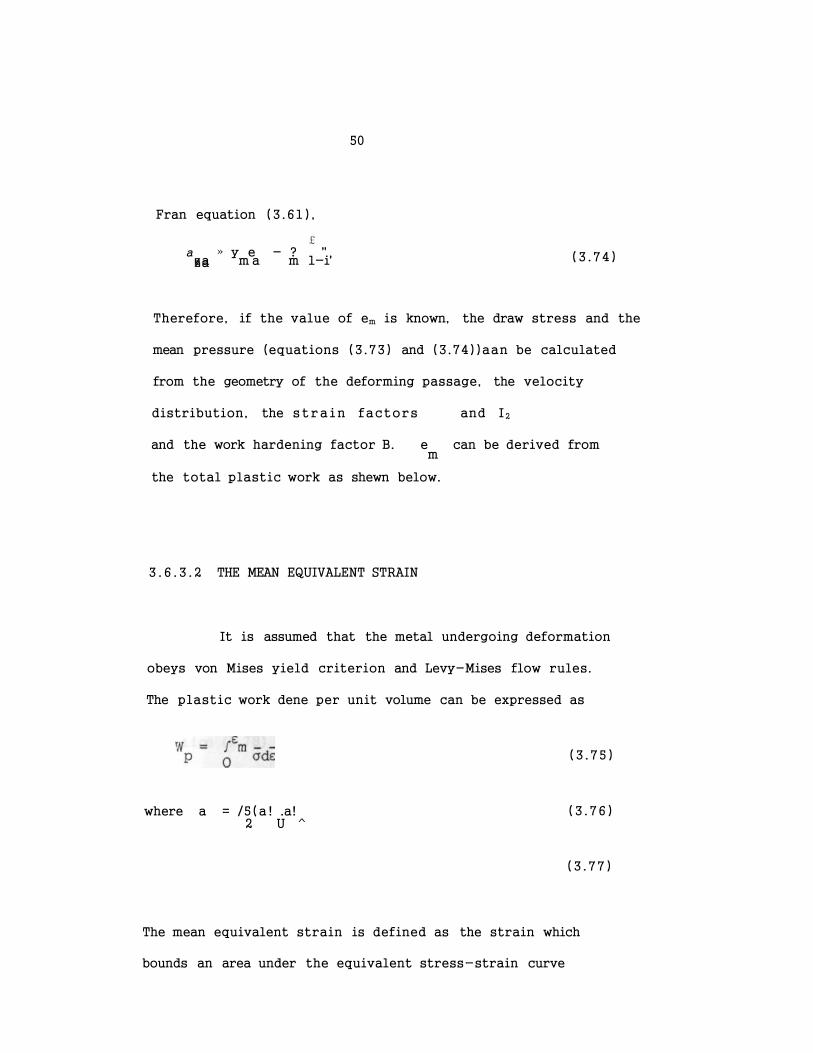
Fran equation (3.61),

£ a » y e - ? " za m a m 1-i' za (3.74)

Therefore, if the value of em is known, the draw stress and the

mean pressure (equations (3.73) and (3.74))aan be calculated

from the geometry of the deforming passage, the velocity

distribution, the strain factors and I2

and the work hardening factor B. e can be derived from

the total plastic work as shewn below.

3 .6 .3 .2 THE MEAN EQUIVALENT STRAIN

It is assumed that the metal undergoing deformation

obeys von Mises yield criterion and Levy-Mises flow rules.

The plastic work dene per unit volume can be expressed as

m

(3.75)

where a = /5(a! .a! 2 U ^

(3 .76)

(3 .77)

The mean equivalent strain is defined as the strain which

bounds an area under the equivalent stress-strain curve

51

(Figure 3.6) equal to the total plastic work done per unit

volume of the material.

i o w - f^

p 0 5 d e " <3-78>

The plastic work W^ consists of the internal work of

deformation (VT) and the redundant work (W ) of shearing the

material at the assumed surfaces of discontinuity at both the

inlet and outlet boundaries.

i .e . W = W. + W (3 .79) p l r

In terms of pcwer,

W x Vol = tATt + WD (3.3Q)

P 1 rv

From equations (3.42) and (3.53),

" i = Y m V V < s )

Y

and W = ^ ^ ( s ) /3

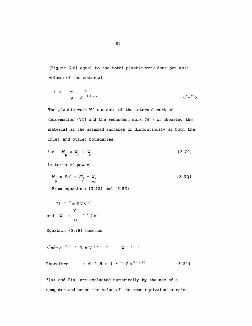
Equation (3.78) beccmes

<YmSm> V o 1 " V b V ( s ) + W s )

Therefore, = ± ^ H s ) * ^ V b R t s ) } (3 .31)

f(s) and R(s) are evaluated numerically by the use of a

computer and hence the value of the mean equivalent strain.

52

3.6.3 .3 WORK HARDEN DC FACTOR B

This is the ratio of the mean flow stress over the

whole strain range ) to the mean flow stress over the cL

strain range em ^ e . The value will therefore depend on

not only the material characteristics but also on the

process and the friction.

If the coefficient of friction is anall, the strain

range e ^ I is also small. The mean flow stress over this m a

range can therefore be approximated as,

<Ym) = ^ (3.82)

f a

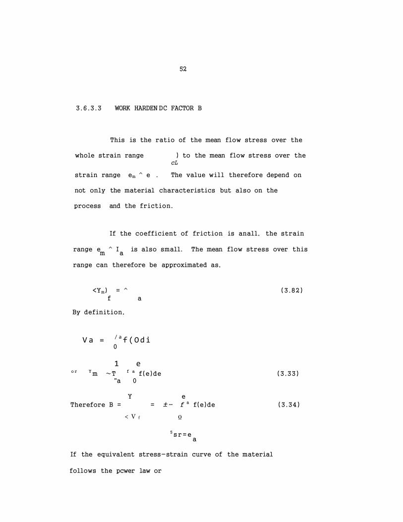
By definition,

V a = / af(Odi 0

1 e o r Y m ~T f a f(e)de (3.33)

"a 0

Y e

Therefore B = = ±- f a f(e)de (3.34)

< V f 0

5 sr=e a

If the equivalent stress-strain curve of the material

follows the pcwer law or

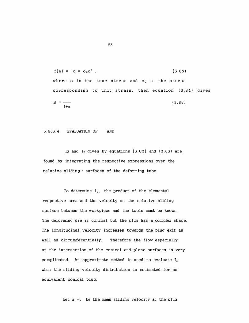
53

f(e) = o = oQcn , (3.85)

where o is the true stress and oQ is the stress

corresponding to unit strain , then equation ( 3 . 8 4 ) gives

B = —— (3.86) 1+n

3.G.3.4 EVALUATION OF AND

Ij and I2 given by equations (3.C3) and (3.63) are

found by integrating the respective expressions over the

relative sliding • surfaces of the deforming tube.

To determine I 2 , the product of the elemental

respective area and the velocity on the relative sliding

surface between the workpiece and the tools must be known.

The deforming die is conical but the plug has a corrplex shape.

The longitudinal velocity increases towards the plug exit as

well as circumferentially. Therefore the flow especially

at the intersection of the conical and plane surfaces is very

complicated. An approximate method is used to evaluate I2

when the sliding velocity distribution is estimated for an

equivalent conical plug.

Let u -, be the mean sliding velocity at the plug

54

surface; then

f\ udA asl = 3 (3 .87)

/ . dA As s

For a convergent plug and conical die passage and the

continuity of flow,

u = ~ ubcosote (3 .38)

and dAg = 2Tr(rb-(p.-p)cosa tanae)dp (3.39)

Therefore,

P" 2

b

u , = si

f % ( 7 7 ) c o s ae

2 7 r ( r b" ( p b" p ) c o s o t t a x i ae ) d p

P

/ 2rr(r.-(p.-p)cosa tana )dp 0 D O e

(3 .90)

2nA

% ^ e f " < 3 ' 9 1 >

r

For the die-tube interface, the mean sliding velocity

u g 9 is given by:-

(u^ + ua)cosa

us2

55

3.7 LOVER BOUND SOLUTION

The upper bound solution developed in the previous

sections is an overestimate of the load required to effect

the process. The value overestimates the load. A lower

bound solution which neglects the effect of redundant work is

thus necessary; the actual load lies within the two limits.

By considering the equilibrium of forces on an

elemental volume and applying Tresca's yield criterion, an

expression for the draw stress is obtained. A computer

prograirme is developed to solve the problem numerically.

3.7.1 DEFORMATION PATTERN OF THE LOWER BOUND SOLLTICN

The four basic tool profiles in the deforming zone

are the pyramidical plane surface, the elliptical plane/conical

surface, the inverted parabolic plane/conical surface and the

triangular plane/conical surface (see Figure 3.2). The lower

bound solution is developed for a conical die and the

elliptical, plane/conical surface plug. This type of plug

allows a gradual deformation in the die-plug deforming

passage and the surface equation is readily derived.

56

The conical surface of the plug is inclined at an

angle to the draw axis while the elliptical plane surface

is inclined at an angle a to the draw axis. s

3 .7 .2 DERIVATION OF THE LOWER BOUND SOLUTION

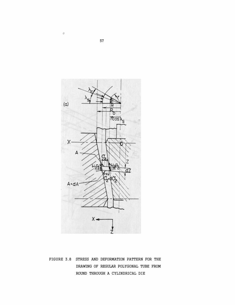
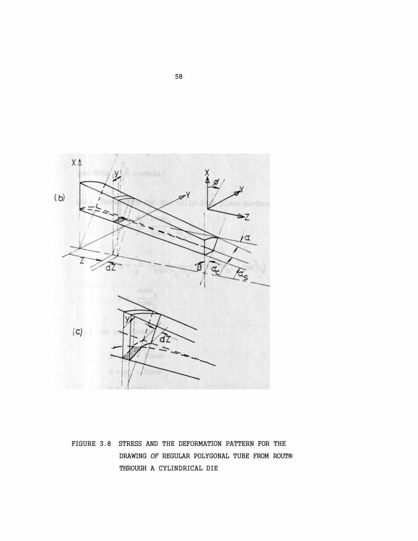
The lower bound solution is derived by considering

the equilibrium of forces acting on an element at a distance

Z from the selected origin (see Figure 3 .8 ) . Figure 3.3

shows a round tube deforming through a conical die on an

elliptical plane/conical surface plug to produce a polygonal

tube. The following geometrical relations are derived:-

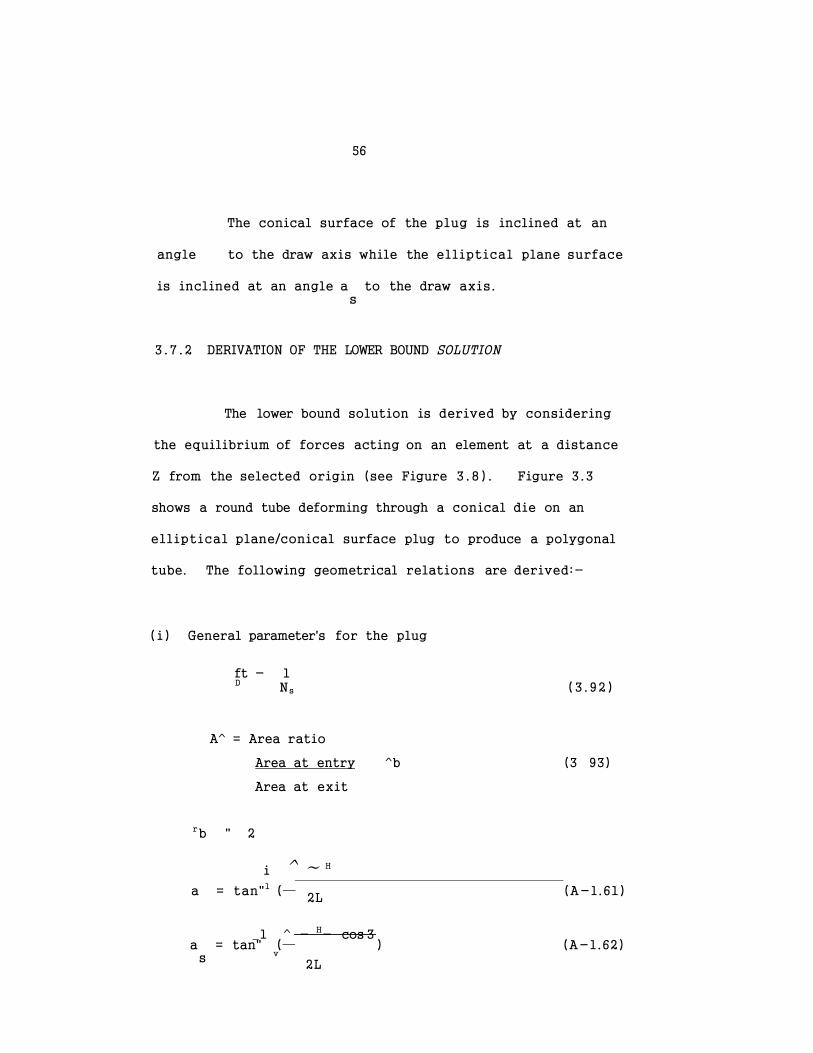
(i) General parameter's for the plug

ft - 1 D Ns (3 .92)

A^ = Area ratio

Area at entry ^b (3 93)

Area at exit

rb " 2

i ^ ~ H

a = tan"1 (— (A-l.61) 2L

_1 ^ - H- cos 3

2L

a = tan" (— ) (A-l.62) s v

0

57

FIGURE 3.8 STRESS AND DEFORMATION PATTERN FOR THE

DRAWING OF REGULAR POLYGONAL TUBE FROM

ROUND THROUGH A CYLINDRICAL DIE

58

FIGURE 3.8 STRESS AND THE DEFORMATION PATTERN FOR THE

DRAWING OF REGULAR POLYGONAL TUBE FROM ROUT®

THROUGH A CYLINDRICAL DIE

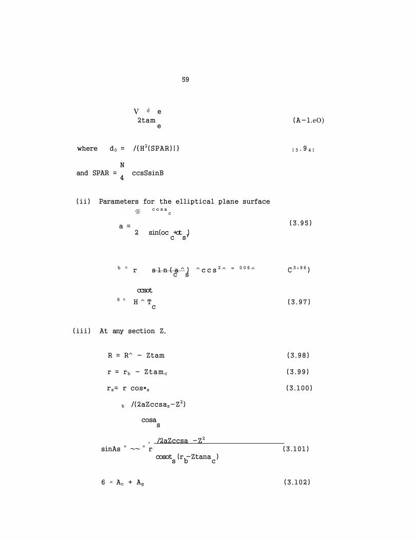
59

V d e

2tam (A-l.eO) e

where d0 = /{H2(SPAR)|} ( 3 . 9 4 )

N and SPAR = ccsSsinB

4

(ii) Parameters for the elliptical plane surface

% c o s ac

a = 2 sin(oc +ot )

c sy

b = r s l n ( a ^ ) ^ c c s 2 ^ " 0 0 6 C 3 ' 9 6 ) c s

ccsot

c

(iii) At any section Z,

b /(2aZccsas-Z2)

cosa s

(3.95)

6 = H ^ T (3.97)

R = R^ - Ztam (3.98)

r = rb - Ztamc (3.99)

rs= r cos*s (3.100)

, /2aZccsa -Z2

sinAs = ~~ = r (3.101) cosot (r.-Ztana )

s b c

6 « Ac + Ag (3.102)

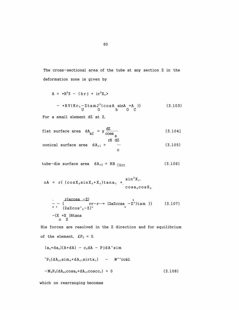
60

The cross-sectional area of the tube at any section Z in the

deformation zone is given by

A = *R23 - ( h r j + ir2Xc>

- *RV(Kr h -ZtamJ 2 (cosA sinA +A )} (3.103) U O b O C

For a small element dZ at Z,

dZ flat surface area dA , = y ——— (3.104)

si cosa ' s

rX dZ

oonical surface area dAcl = — (3.105)

c

tube-die surface area dAc2 = RB C Q s a (3.106)

sin 2 X c ; oA = r{ ( cosX s s inX s +X c ) tana c +

cosa s cosX s

. r(acosa -Z) 9

- - { rr-r—+ (2aZccsa -Z")tam }} (3.107) a r (2aZcos^s-Z)" s

-(X +X )Rtana o S

Hie forces are resolved in the Z direction and for equilibrium

of the element, £FZ = 0.

(az+daz)(A+dA) - czdA - PjdA^sim

+P2(dAslsims+dAclsirtxc) - W^^cc&L

-M2P2(dAslcosas+dAclcosccc) = 0 (3.108)

which on rearranging becomes

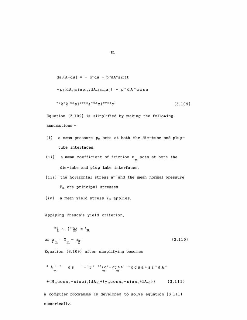
61

daz(A+dA) = - o^dA + p^dA^sirtt

-p2(dAslsinpts+dAclsinac) + p ^ d A ^ c o s a

+ p 2 y 2 ( d A s l c o s a s + d A c l c o s a c ) (3 .109)

Equation (3.109) is siirplified by making the following

assumptions:-

( i ) a mean pressure pm acts at both the die-tube and plug-

tube interfaces,

( i i ) a mean coefficient of friction u acts at both the m

die-tube and plug tube interfaces,

( i i i ) the horizcntal stress a^ and the mean normal pressure

Pm are principal stresses

(iv) a mean yield stress Ym applies.

Applying Tresca's yield criterion,

a 7 ~ ( " P j = Ym L m m

or o = Y - a„ (3 .110) * m m Z

Equation (3.109) after simplifying beccmes

d § } = d s { - ( r 5 dA*<1-<T>> ^ c c s a + s i ^ d A ^ m m m

+(Mmcosa s-sinoi s )dA s l+(ymcosa c-sina c )dA c l}} ( 3 . 1 1 1 )

A computer programme is developed to solve equation (3.111)

numericallv.

62

3.8 COMPUTER P ROCRAMME

The four sub-programmes consist of:-

( i ) the development of the deformation pattern and hence

the velocity field,

( i i ) the upper bound solution for the polygonal tube

drawing ,

( i ii ) the lower bound solution for the polygonal tube

drawing , and

(iv) the upper and lower bound solutions for the

corresponding axisyrrmetric drawing of tube cn a

conical or cylindrical plug.

In each of the sub-progranmes are the following

four main components of the flow chart:

( i ) the input statement,

(ii) three major Do loops,

(iii) the main programme , and

(iv) print out statements.

The input statement consists mainly of the incoming

and outgoing tube dimensions and the stress-strain properties

of the material. The three major Do loops generate the

nurrber of sides of the bore of drawn section, the die semi-angle

63

and the coefficient of friction.

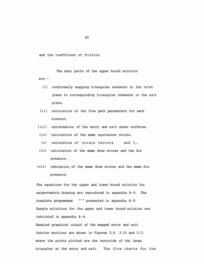
The main parts of the upper bound solution

are: -

( i ) conformally mapping triangular elements in the inlet

plane to corresponding triangular elements in the exit

plane,

( i i ) calculation of the flow path parameters for each

element,

( iii ) optimization of the entry and exit shear surfaces ,

(iv) calculation of the mean equivalent strain,

(v) calculation of strain factors and I 2 ,

(vi) calculation of the mean draw stress and the die

pressure ,

(vii) tabulation of the mean draw stress and the mean die

pressure.

The equations for the upper and lower bound solution for

axisyrrmetric drawing are reproduced in appendix A-5. The

complete programmes a r e presented in appendix A-3.

Sample solutions for the upper and lower bound solution are

tabulated in appendix A-4.

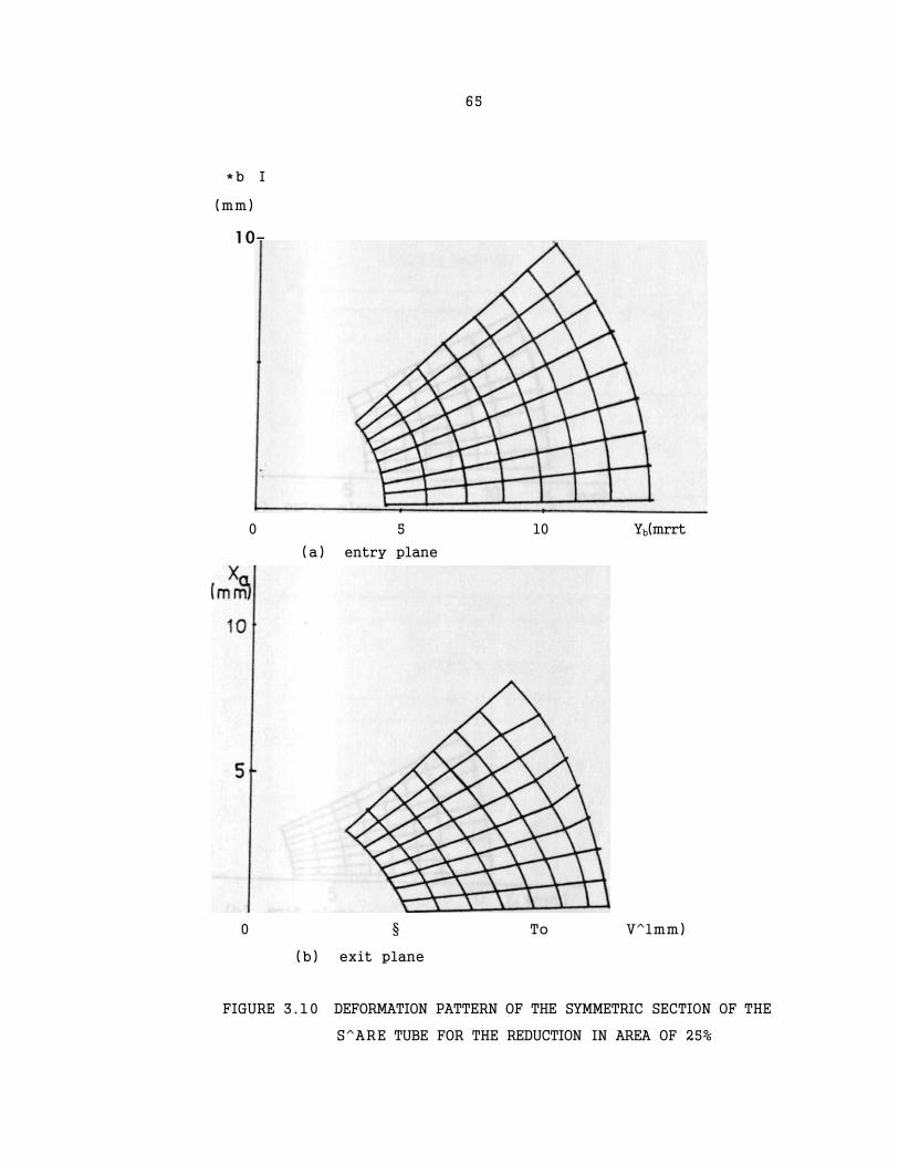
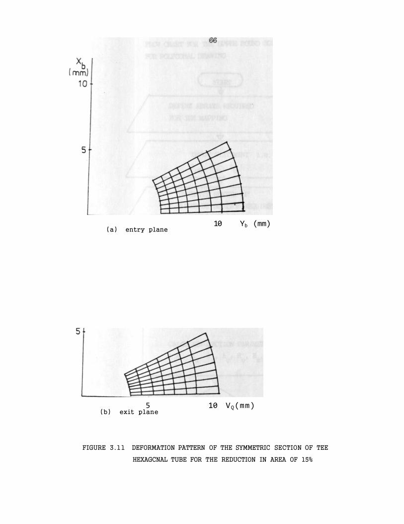
Sampled graphical output of the mapped entry and exit

tabular sections are shown in Figures 3.9, 3.10 and 3.11

where the points plotted are the centroids of the large

triangles at the entry and exit. The flow charts for the

64

10 Yb (mmJ

^a) entry plane

(mm)

b) exit plane

JRE 3.9 DEFORMATION PATTERN OF THE SYMMETRIC SECTION OF THE

SQUARE TUBE FOR THE REDUCTION IN AREA OF 9%

65

*b I

(mm)

10-

0 5 10 Yb(mrrt

(a) entry plane

0 § To V^lmm)

(b) exit plane

FIGURE 3 .10 DEFORMATION PATTERN OF THE SYMMETRIC SECTION OF THE

S^ARE TUBE FOR THE REDUCTION IN AREA OF 25%

(a) entry plane 10 Yb (mm)

(b) exit plane 5 10 VQ(mm)

FIGURE 3.11 DEFORMATION PATTERN OF THE SYMMETRIC SECTION OF TEE

HEXAGCNAL TUBE FOR THE REDUCTION IN AREA OF 15%

67

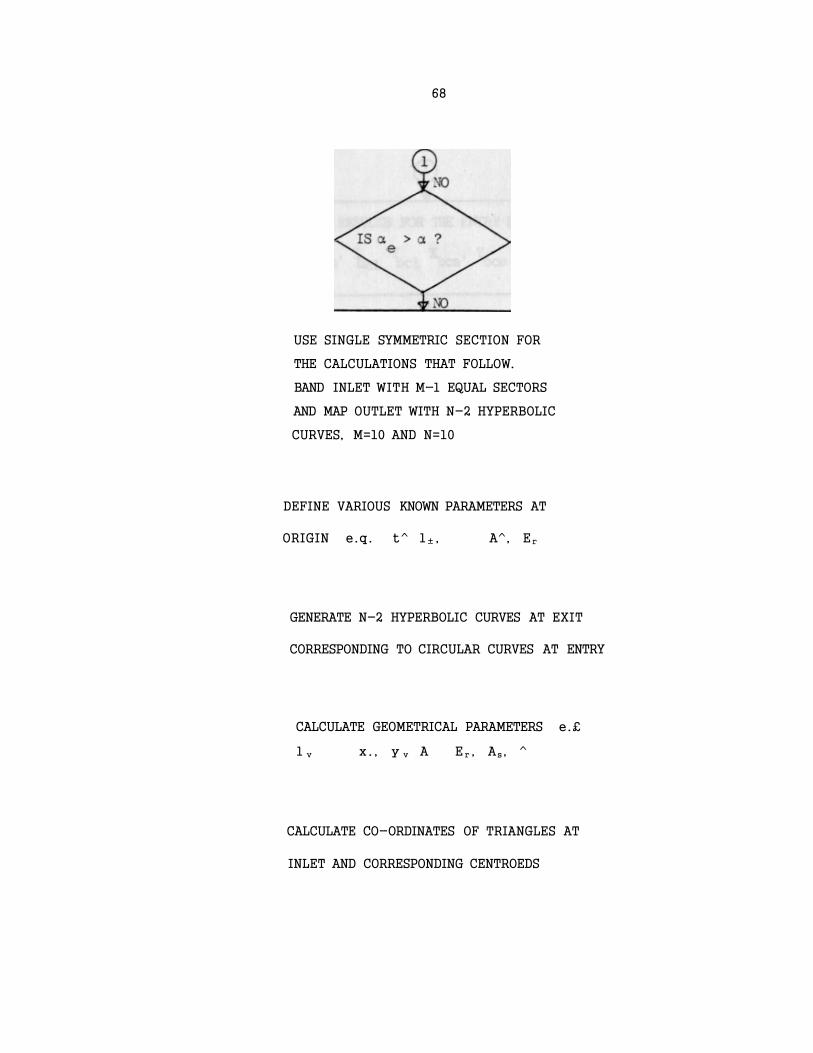
FLOW CHART FDR THE UPPER BOUND SOLUTION

FOR POLYGONAL DRAWING

CALCULATE SECTION PARAMETERS

i .e . Aa, Ab, Ar, Re , Ha,

68

USE SINGLE SYMMETRIC SECTION FOR

THE CALCULATIONS THAT FOLLOW.

BAND INLET WITH M-l EQUAL SECTORS

AND MAP OUTLET WITH N-2 HYPERBOLIC

CURVES, M=10 AND N=10

DEFINE VARIOUS KNOWN PARAMETERS AT

ORIGIN e.q. t^ l± , A^, Er

GENERATE N-2 HYPERBOLIC CURVES AT EXIT

CORRESPONDING TO CIRCULAR CURVES AT ENTRY

CALCULATE GEOMETRICAL PARAMETERS e.£

l v x. , y v A E r , As, ^

CALCULATE CO-ORDINATES OF TRIANGLES AT

INLET AND CORRESPONDING CENTROEDS

69

i PRINT RESULTS FOR THE ENTRY PLANE i.e.

V V ^ W *bcs' Ybcs ^ Er

TO MAP CORRESPONDING TRIANGLES AT EXIT

PLANE, BEGIN WITH TWO KNOWN

CO-ORDINATES. BEGIN WITH LARGE TRIANGLES

CALCULATE THIRD CO-ORDINATE FROM KNOWN

AREA OF TRIANGLE AND EQUATION OF CURVE

i.e. A CIRCLE

CALCULATE THIRD CO-ORDINATE BY

SUBSTITUTING X AND SOLVING FOR Y

CALCULATE THIRD CO-ORDINATE FROM KNOWN

AREA OF TRIANGLE AND EQUATION OF CURVE

i.e. HYPERBOLA

70

0 —

MAP SMALL TRIANGLES AT EXIT BY BEGINNING WITH

TWO KNCWN CO-ORDINATES, AREA AND EQUATION OF

CURVE i.e. HYPERBOLA

CALCULATE THE CENTROIDS OF THE LARGE AND

SMALL TRIANGLES AT EXIT

PRINT RESULTS FOR TIE EXIT PLANE i.e.

X , Y , X , Y i X _ i X a a acs acs acl acl

CALCULATE PERCENTAGE ERROR IN AREA

OBTAINED FROM MAPPING AND ACTUAL VALUE A

PRINT THE RESULT

CALCULATE RADIAL DISTANCE OF PARTICLES Ra> R^

DEFLECTICN ANGLES n» <P AND LENGTH OF

FLOW PATH Z FOR ALL (i, j)

OPTIMIZE THE SHEAR SURFACES i .e .

MINIMIZE R(s) FOR 0<t<+l

CALCULATE INTERNAL POWER OF DEFORMATION

FACTOR f(s) FOR OPTIMAL VALUE OF t

TABULATE THE RESULTS

85

FLOH CHART FOR THE LOWER BOUND SOLUTION FOR

POLYGONAL DRAWING

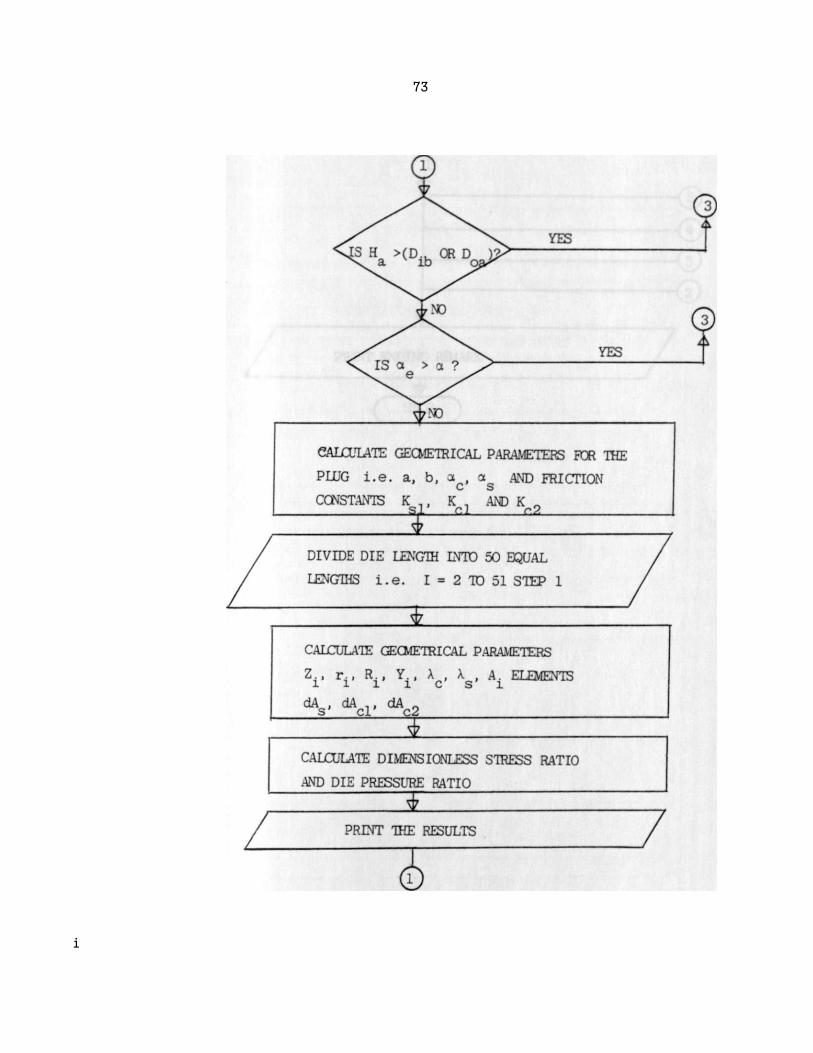
73

i

74

G

PRINT ENDING REMARK

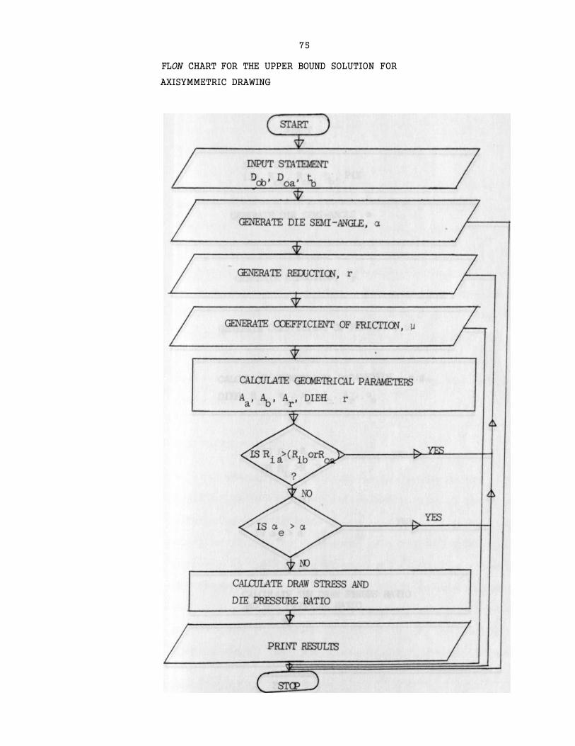
75

FLON CHART FOR THE UPPER BOUND SOLUTION FOR

AXISYMMETRIC DRAWING

76

FLOW CHART FOR THE LOWER BOUND SOLUTION FOR

AXISYMMETRIC DRAWING

( STCP )

77

4 RESULTS AND DISCUSSION

4 . 1 INTRODUCTION

The theoretical account deals with the effect of

the following parameters on the drawing process; namely,

the draw force, the mean coefficient of friction, the die

semi-angle, the equivalent semi-angle of the plug as well

as the limitation of the achievable reduction of area.

In both the upper and lower bound solutions, the influence

of the forementioned drawing parameters in the design of

the draw tools i . e . the die and the polygonal plug are

presented. The results of axisymmetric drawing are

presented for the purpose of comparing the mode of

analysis .

4 . 2 THE LOWER BOUND SOLUTION

The lower bound analysis was based on the

equilibrium of forces of an elemental slug of the material

undergoing plastic deformation leading to a differential

equation (3.111) on page (61) . The method neglects the

increase in the drawing stress produced by the onset of

the redundant shearing and as a result it underestimates

the magnitude of the draw forces especially at large die

angles where the redundant work is at its greatest (for

a fixed plug) . The draw load obtained by the integration

78

of the basic d i f ferential equation (3 .111) can be shown,

for the case of Ng = ® to comprise approximately of a

constant term and a second term which incorporates the mean

coefficient of friction and the die semi-angle (7) . The

former term represents the homogeneous component which is

virtually a constant for a given reduction of area. The

later term represents the frictional component and decreases

with die semi-angle ( i . e . shorter contact lengths) , for a

given input-output tubing.

Although the lower bound analysis oversimplifies

the mechanics of the process by ignoring the effect of the

pattern of flow, the analysis involved is usually straight-

forward and forms an important conjugate in the upper bound

analysis.

Figures 4 . 1 to 4 .5 show the effect of different

parameters on the draw force for the axisymmetric tube

drawing.

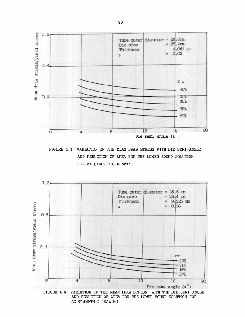
Figures (4 .3) and (4 .4 ) show that for a particular

reduction, the total draw stress decreases as the die semi-

angle increases. The explanation for this is that increasir

the die angle implies decreasing the die length and hence

surface area of tool-workpiece contact. This results in

lower friction work. The homogenous work remains constant

79

f-> CO

•H •—

01

Jo . . <H 'Ji

1

Tube o

Die si

Thickn

U

uter diameter

;se

ss

= 28.6 am

= 25.4 rim

= 4.064 rrm

= 0.06

0 0

FIGURE 4 .1 VARIATION CF THE MEAN DRAW STRESS WITH THE DIE SEMI-

ANGLE AND THE EQUIVALENT PLUG SEMI-ANGLE FOR THE

LOWER BOUND SOLUTION FOR AXISY\METKIC DRAWING

7) 73 —<

• H

N 3

0.8

•3 0.4

3

£

o 10 20 Reduction cf 30 area (rt)

FIGURE 4.2 VARIATION OF THE MEAN DRAW STRESS WITH THE REDUCTION

OF AREA AND THE DIE SEMI-ANGLE FOR THE L3VER BOUND

SOLUTION FOR AXISYfcMETRIC DRAWING

80

Die semi-angle (a )

FIGURE 4 .3 VARIATION OF THE MEAN DRAW STRESS WITH DIE SEMI-ANGLE

AND REDUCTION OF AREA FOR THE LCWER BOUND SOLUTION

FOR AXISYMETRIC DRAWING

FIGURE 4.4 VARIATION OF THE MEAN DRAW STRESS -WITH THE DIE SEMI-ANGLE

AND REDUCTION OF AREA FOR THE LOWER BOUND SOLUTION FOR

AXISYMMETRIC DRAWING

81

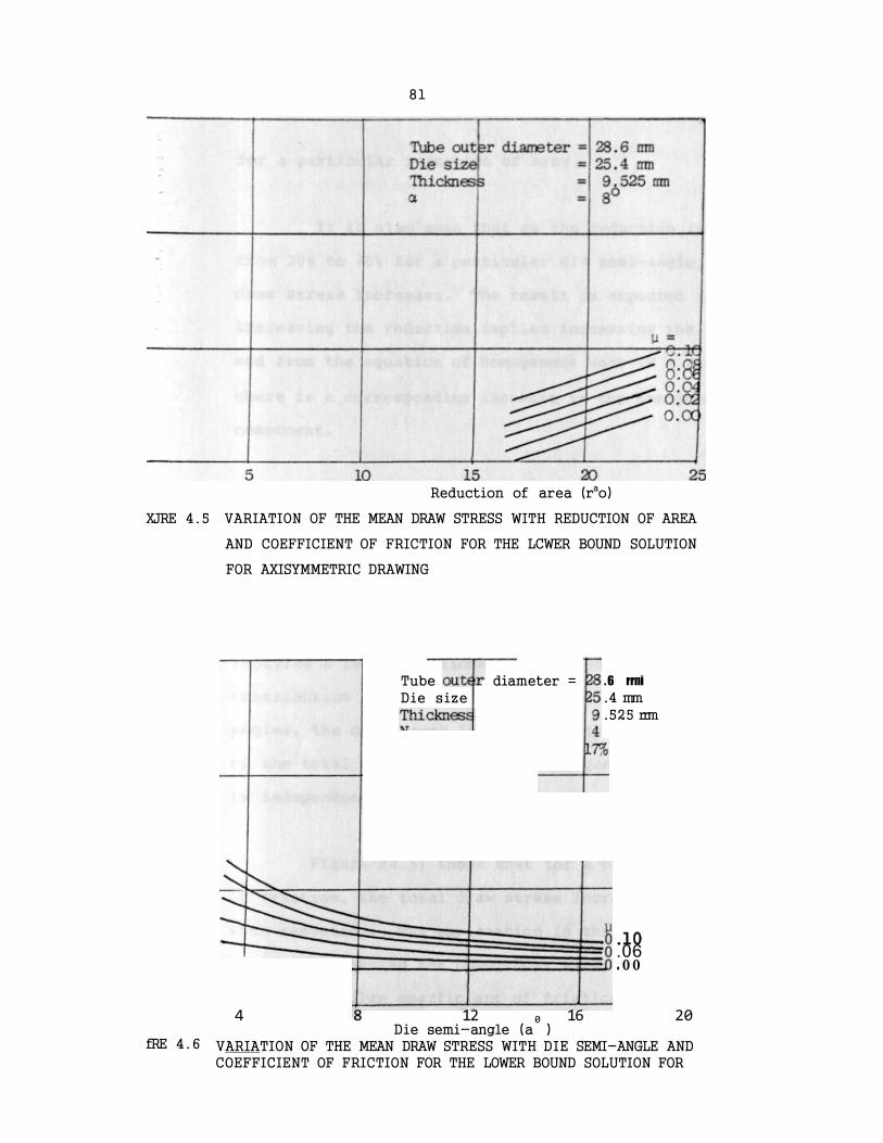
Reduction of area (rao)

XJRE 4.5 VARIATION OF THE MEAN DRAW STRESS WITH REDUCTION OF AREA

AND COEFFICIENT OF FRICTION FOR THE LCWER BOUND SOLUTION

FOR AXISYMMETRIC DRAWING

fRE 4 .6

.10

.06

. 0 0

4 8 12 0 16 20 Die semi-angle (a )

VARIATION OF THE MEAN DRAW STRESS WITH DIE SEMI-ANGLE AND COEFFICIENT OF FRICTION FOR THE LOWER BOUND SOLUTION FOR

. 6 rrni

.4 mm

.525 rrm

Tube

Die size

diameter =

82

for a particular reduction of area.

It is also seen that as the reduction increases

from 20% to 40% for a particular die semi-angle, the tot

draw stress increases. The result is expected since

increasing the reduction implies increasing the area rat

and from the equation of homogenous work (W • Yfcn

there is a corresponding increase in the homogenous work

component.

Another feature that is observed from the graphs

that when the die semi-angle is small (about 4°) , the cu

are very steep but when the die semi-angle is large (abc

2 0 ° ) , the curves are almost horizontal. The explanation

that at very low die semi-angles, the die length is larg

implying a large frictional work component as the main

contribution to the total draw stress. For large die se

angles , the die length is small and the main contributio

of the total draw stress is the homogenous component whi

is independent of the die angle.

Figure (4 .5) shows that for a particular coeffic

of friction , the total draw stress increases almost line

with reduction. The explanation is that increasing redu

implies increasing the homogenous work component. Furth

for a particular coefficient of friction, e .g . u « 0, th.

jUNAL, iUBfc DRAWING

83

curve crosses the abscissa at a reduction of about 16.5%.

This is the minimum possible reduction for the given set o]

draw parameters. A smaller reduction implies a smaller an

ratio which would occur if the plug semi-angle is less thar

0° which is inadmissible.

It is further observed that as the coefficient of

friction increases from 0 . 0 to 0 . 1 for a particular reducti

the total draw stress increases since the frictional work i

directly proportional to the coefficient of friction .

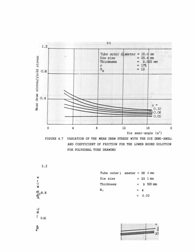
In the case of polygonal drawing, figures (4.6) and

( 4 . 7 ) show that for any coefficient of friction not equal t

zero, the total draw stress decreases as the die semi-angle

increases. This result is expected since as the die semi-

angle increases the frictional work component decreases whi

the homogenous work component remains constant for constant

reduction of area. When u = 0, the frictional work

component is zero and the graph is a straight horizontal

line representing the homogenous work component.

Figure ( 4 . 8 ) shows that for any particular die , the

total draw stress increases with reduction since the

homogenous work component increases with reduction.

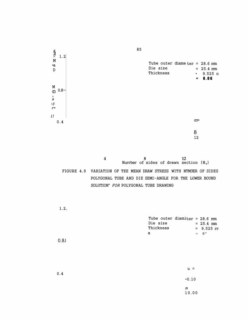
Figures ( 4 . 9 ) , (4 .10) and (4 .11) show the variation

of the total draw stress with the number of sides of drawn

0 4 8 12 16 2

Die semi-angle (a0)

FIGURE 4.7 VARIATION OF THE MEAN DRAW STRESS WITH THE DIE SEMI-ANGLi

AND COEFFICIENT OF FRICTION FOR THE LOWER BOUND SOLUTION

FOR POLYGONAL TUBE DRAWING

1.2

w 1 - j W

rH <D •H >i

-J M

I

a a) s

0.8

0.4l

Tube outer

Die size

Thickness

N0

i ameter = 28

= 25

= 9

= 4

0 mn

1 mn

525 mm

= 0. 02

§ 85

U —) 1.2 M •a D

M

CO 0.8-

* a

•3 r*

i!

Tube outer diame

Die size

Thickness

ter = 28.6 rrm

= 25.4 rrm

• 9.525 n

= 0 . 0 6

0.4 cc=

8 12

4 8 12 Nurrber of sides of drawn section (Ns)

FIGURE 4.9 VARIATION OF TEE MEAN DRAW STRESS WITH NTM3ER OF SIDES

POLYGONAL TUBE AND DIE SEMI-ANGLE FOR THE LOWER BOUND

SOLUTION" FOR POLYGONAL TUBE DRAWING

1.2,

Tube outer diami

Die size

Thickness

a

ter = 28.6 rrm

= 25.4 mm

= 9.525 rr

= 8 °

0.8J

0.4

u =

•0.10

m

10 . 00

86

0 . 2 5

co

T3 r—i cd •H

«T

5 0 . 2 43

co

i

0.24

0

Tube outer diameter

Die size

Thickness

28.6 rrm

25.4 mn

9.525 nm

0.06

8 12 Number of sides of drawn section (N )

s

FIGURE 4.11 VARIATION OF THE MEAN DRAW STRESS WITH NUMBER OF SIDES

OF POLYGONAL PLUG FOR THE LOWER BOUND SOLUTION FOR

POLYGONAL TUBE DRAWING

1.2

0.8

0 .4

Tube outei Product d] Thickness ct = 8°

3 diameter 28.

ameter = 25.4

= 9.52

xrm mm 5 mn

U = 0 Y

n in In 9f) 9n

87

section for a given tube using the concept of close {

drawing. For a given input tube and drawing d ie , and

constant coefficient of friction , the draw stress dec

s l ightly with the number of sides. Although the surfc

increases with consequential increase in the frictior

component, there is a decrease in the homogeneous wor

component because of the decrease in reduction of are

4 . 3 THE UPPER BOUND SOLUTION

The upper bound solution was obtained from a

velocity field that minimizes the energy to effect th

deformation and incorporates an apparent strain metho<

include Coulomb fr ict ion . The velocity pattern was

developed by conformal mapping of triangular elements

entry plane to the positions at the exit plane. The

solution therefore accounts for the mode of deformatic

Figure (4 .12) shows that for a given die semj

angle and coefficient of friction, the total draw stre

increases with the reduction of area for the case of o

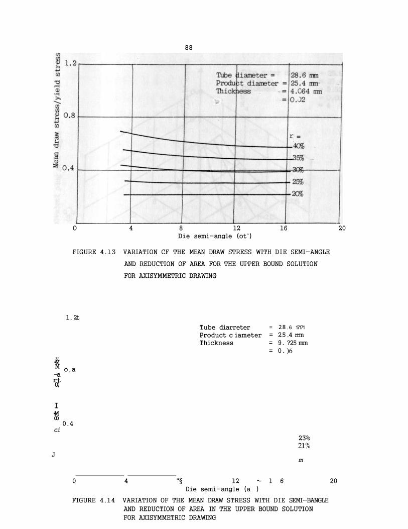
symmetric drawing. Figures (4 .13) and (4 .14) show the

variation of the total draw stress with the die semi-a

for axisymmetric drawing.

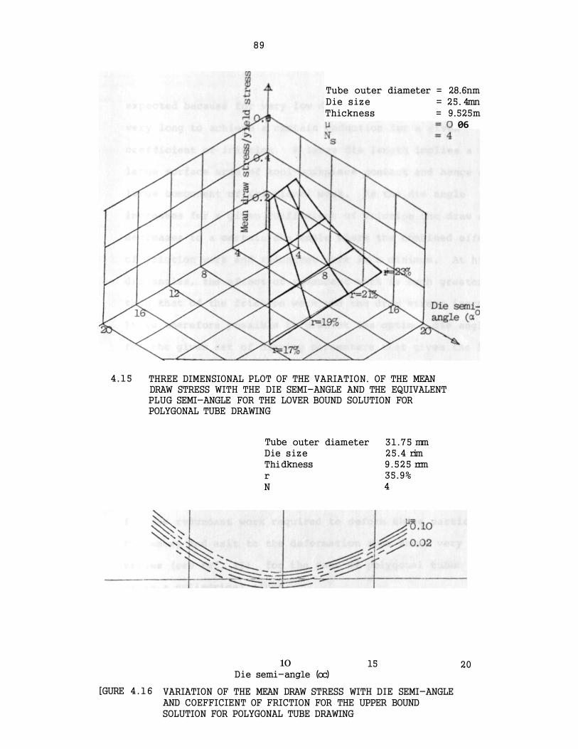
Figure (4 .16) shows the variation of the draw

ratio against the die semi-angle in the upper bound so

for drawing a square tube directly from round. At ver

die angles the draw stress ratio tends to in f in ity . T

88

O 4 8 12 16 20

Die semi-angle (ot°)

FIGURE 4.13 VARIATION CF THE MEAN DRAW STRESS WITH DIE SEMI-ANGLE

AND REDUCTION OF AREA FOR THE UPPER BOUND SOLUTION

FOR AXISYMMETRIC DRAWING

1. 2t

u •M M

-a r-t 0)

I •M CO

ci

J

o.a

Tube diarreter Product c Thickness

iameter

= 28 = 25

= 9.

= 0 .

. 6 17171

.4 rrm

?25 mm

)6

0.4

23%

21%

m

0 4 "§ 12 ~ 1 6 20

Die semi-angle (a )

FIGURE 4.14 VARIATION OF THE MEAN DRAW STRESS WITH DIE SEMI-BANGLE

AND REDUCTION OF AREA IN THE UPPER BOUND SOLUTION

FOR AXISYMMETRIC DRAWING

89

Tube outer diameter = 28.6nm Die size = 25. 4mn Thickness = 9.525m

06

4.15 THREE DIMENSIONAL PLOT OF THE VARIATION. OF THE MEAN DRAW STRESS WITH THE DIE SEMI-ANGLE AND THE EQUIVALENT PLUG SEMI-ANGLE FOR THE LOVER BOUND SOLUTION FOR POLYGONAL TUBE DRAWING

Tube Die Thi r N

outer diameter size

dkness

31.75 mm 25.4 rim 9.525 rrm 35.9% 4

10 Die semi-angle (oc)

15 20

[GURE 4.16 VARIATION OF THE MEAN DRAW STRESS WITH DIE SEMI-ANGLE AND COEFFICIENT OF FRICTION FOR THE UPPER BOUND SOLUTION FOR POLYGONAL TUBE DRAWING

90

expected because for very low die angles, the die must be

very long to achieve a certain reduction for a given

coefficient of fr ict ion . A large die length implies a

large surface area of tool-workpiece contact and hence a

large component of frictional work. As the die angle

increases for a given coefficient of friction the draw stre

decreases to a certain die angle where the combined effect

of friction work and redundant work is a minimum. At highe

die angles, the e f fect of redundant work is much greater

than that of the friction work and the draw stress increase

It is therefore possible to predict the optimum die angle

for the given set of drawing parameters that gives the leas

work of deformation.

Figures ( 4 . 17 ) and (4 .18) show a comparison of the

upper and lower bound solution for drawing a square tube.

In the case of square drawing, the particles of the tube

undergo severe distortion as they pass through the deformat

passage. Therefore, the upper bound analysis which account

for the redundant work required to deform these particles a

the entry and exit to the deformation zone shows very high

values (see ref. (5) for the case of polygonal tube drawi

using a cylindrical plug) .

Figures ( 4 . 1 9 ) and (4.20) shows the values of the

upper and lower bound solution for the hexagon and octagon

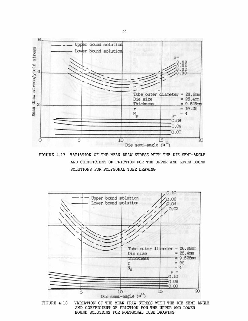
91

FIGURE 4.17 VARIATION OF THE MEAN DRAW STRESS WITH THE DIE SEMI-ANGLE

AND COEFFICIENT OF FRICTION FOR THE UPPER AND LOVER BOUND

SOLUTIONS FOR POLYGONAL TUBE DRAWING

FIGURE 4.18 VARIATION OF THE MEAN DRAW STRESS WITH THE DIE SEMI-ANGLE AMD COEFFICIENT OF FRICTION FOR THE UPPER AND LOWER BOUND SOLUTIONS FOR POLYGONAL TUBE DRAWING

0.08

0.06

— 0.04

I 0 - 8

c 4-i cn

Utiper bound soluti Lqwer bound solutipn f -.1°/ oN

Die semi-angle (a )

0.02

0.00

FIGURE 4.19 VARIATICN OF THE MEAN DRAW STRESS WITH THE DIE SEMI-ANGLE

AND COEFFICIENT OF FRICTION FOR THE UPPER AND LOWER BOUND

SOLUTIONS FOR POLYGONAL TUBE DRAWING

w

I -M M

I—I

•r-»

co

I J-t (Q

= V s

0

FIGURE 4.20

5 1 0 o 1 5 2 0

Die semi-angle (ot )

VARIATICN OF THE MEAN DRAW STOESS WITH THE DIE SEMI-ANGLE AM) COEFFICIENT OF FRICTION FOR THE UPPER AND LOVER BCIJND

SOLUTIONS FOR POLYGONAL TUBE DRAWING

0.02

0.00

bound soluti

= 26.99rrm 25.4frm

U-0.10

0.06

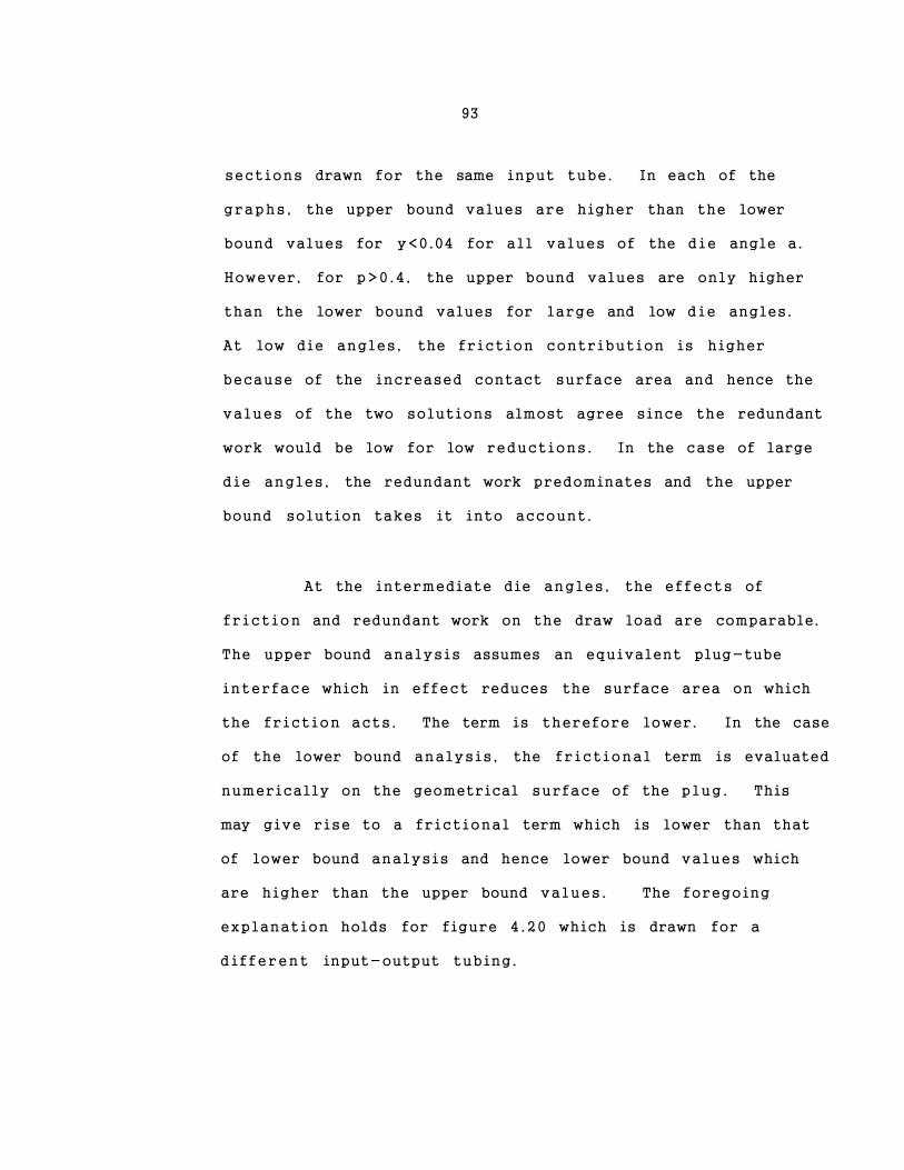
93

sections drawn for the same input tube. In each of the

graphs, the upper bound values are higher than the lower

bound values for y<0.04 for all values of the die angle a.

However, for p>0.4 , the upper bound values are only higher

than the lower bound values for large and low die angles.

At low die angles, the friction contribution is higher

because of the increased contact surface area and hence the

values of the two solutions almost agree since the redundant

work would be low for low reductions. In the case of large

die angles, the redundant work predominates and the upper

bound solution takes it into account.

At the intermediate die angles, the effects of

friction and redundant work on the draw load are comparable.

The upper bound analysis assumes an equivalent plug-tube

interface which in effect reduces the surface area on which

the friction acts. The term is therefore lower. In the case

of the lower bound analysis, the frictional term is evaluated

numerically on the geometrical surface of the plug. This

may give rise to a frictional term which is lower than that

of lower bound analysis and hence lower bound values which

are higher than the upper bound values. The foregoing

explanation holds for figure 4 .20 which is drawn for a

different input-output tubing.

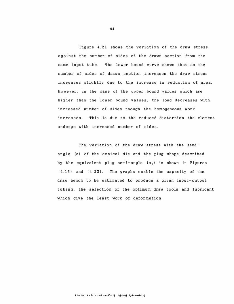
94

Figure 4 . 2 1 shows the variation of the draw stress

against the number of sides of the drawn section from the

same input tube. The lower bound curve shows that as the

number of sides of drawn section increases the draw stress

increases slightly due to the increase in reduction of area.

However, in the case of the upper bound values which are

higher than the lower bound values, the load decreases with

increased number of sides though the homogeneous work

increases. This is due to the reduced distortion the element

undergo with increased number of sides.

The variation of the draw stress with the semi-

angle (a) of the conical die and the plug shape described

by the equivalent plug semi-angle (a e ) is shown in Figures

( 4 . 1 5 ) and ( 4 . 2 3 ) . The graphs enable the capacity of the

draw bench to be estimated to produce a given input-output

tubing, the selection of the optimum draw tools and lubricant

which give the least work of deformation.

i i u i u 1 v h ruuiva-i 'ni j ivjulmj iyivnni-ivj

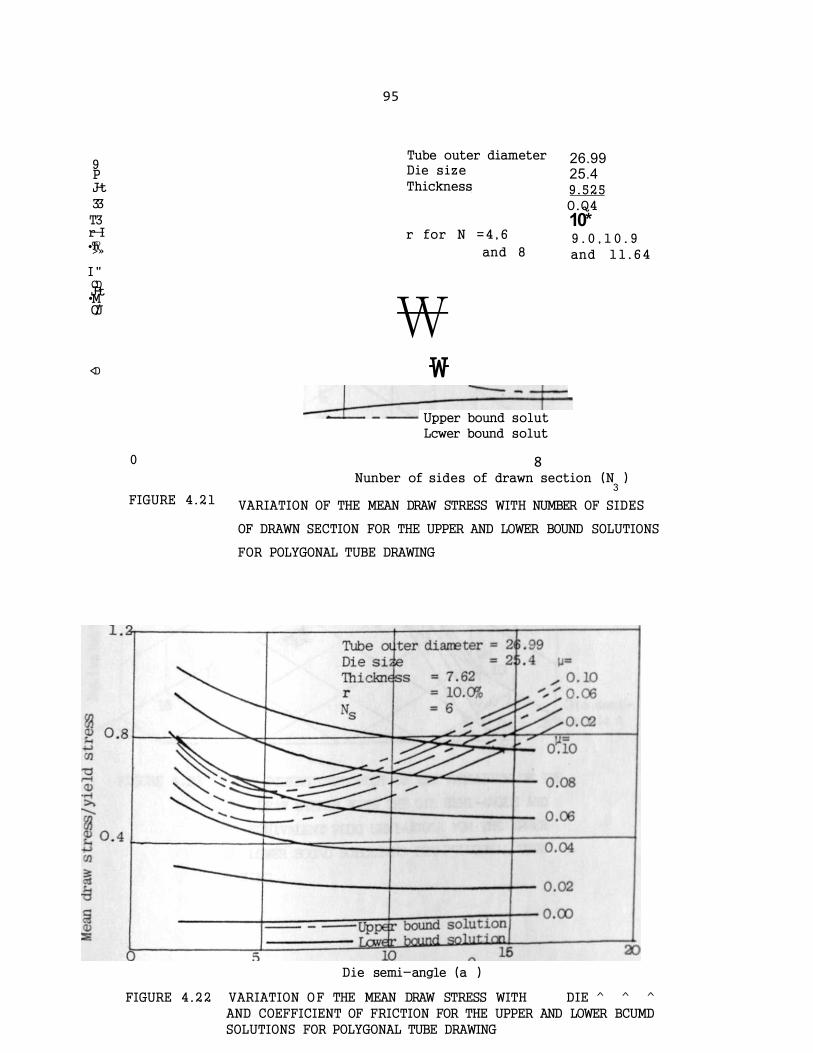
95

9 P J-t

33

T3 r—I CD •h >»

I " CD J-t •M C/J

<D

Tube outer diameter Die size

Thickness

r for N =4,6

and 8

\ \

0

FIGURE 4.21

Upper bound solut Lcwer bound solut

26.99 25.4 9.525

O.Q4

10* 9 . 0 , 1 0 . 9

and 11 .64

8 Nunber of sides of drawn section (N ) 3

VARIATION OF THE MEAN DRAW STRESS WITH NUMBER OF SIDES

OF DRAWN SECTION FOR THE UPPER AND LOWER BOUND SOLUTIONS

FOR POLYGONAL TUBE DRAWING

Die semi-angle (a )

FIGURE 4.22 VARIATION OF THE MEAN DRAW STRESS WITH DIE ^ ^ ^

AND COEFFICIENT OF FRICTION FOR THE UPPER AND LOWER BCUMD

SOLUTIONS FOR POLYGONAL TUBE DRAWING

96

Tube outer diametei*=31.75fnn Die s i ze =25.4rrm Thickness =9.525mn

FIGURE 4.23 THREE DIMENSIONAL PLOT OF THE VARIATION* OF THE

MEAN DRAW STRESS WITH THE DIE SEMI-ANGLE AND

THE EQUIVALENT PLUG SEMI-ANGLE FOR THE UPPER

AND LOWER BOUND SOLUTIONS FOR POLYGONAL TUBE

DRAWING

97

5 . 4 LIMITATION OF ACHIEVABLE REDUCTION OF AREA

The expressions for the cross-sectional area of the

tube material at entry and exit are:-

A b = ^ b " ( 5 . 1 )

Aa = -D2 - H2 (SPAR), respectively, ( 5 . 2 ) 4 a a

Where SPAR is a shape parameter equal to

cos|3sin8 (N s)

Therefore the reduction is given by:

I D 2 - H 2 ( S P A R )

r = 1 - i — - ( 5 . 4 )

- 1 1

For close pass drawing, Ha = db and the reduction of area

is given by

I D 2 - d?(SPAR) r = 1 * b } ( 5 . 5 )

* t 2 a > - 1 ) b t b

In practice , H a<d b to allow for sinking .

i

The maximum reduction of area possible occurs when

Ha = db = Da and tb = Db - Da and is given by:

4D2(tt/4 - SPAR) x r = 1 - ^ a 1

M D * - D2)

98

5 CONCLUSIONS

An extensive investigation of the mechanics of

drawing polygonal tube from round stock through a

cylindrical die and a polygonal plug has been accomplished

theoretically to enable the following conclusions to be

drawn.

1. In general for any given set of draw parameters, the

derived upper bound solution predicts a higher value

of draw stress due to the account taken for redundant

work whilst the simpler lower bound solution under-

estimates the draw stress as it neglects the redundant

effect .

2. Unlike the axisymmetric tube drawing problem, the shape

of the die deforming passage forms an integral part of

the analysis of drawing polygonal tube directly from

round stock through a cylindrical die.

3. The predicted loads in the drawing of a square section

proved to be the severest of all polygonal sections

implying that it may be very diff icult to draw the

section (Figures 4 . 16 , 4.17 and 4 . 1 8 ) . This is

because the material suffers the greatest lateral

displacement as the bore of the workpiece transforms

99

from round to square with the external surface

remaining circular for a particular reduction of area.

4. The upper bound solution predicts the optimum die semi-

angle a and the corresponding plug semi-angle a e . The

predicted values form a useful guide in the design of

draw tools that would dissipate the least amount of

energy.

5. The developed theory and accompanying computer program

form a useful guide when producing draw schedules and

in the design of draw tools for any given set of draw

parameters.

100

6 SUGGESTIONS FOR FURTHER WORK

On the basis of the present study of mechanics of

drawing regular polygonal tube directly from round stock

through a cylindrical die and a polygonal plug, further work

is suggested as follows:-

1. Experimental investigation of the process:

Because of the unavailability of a draw bench, the

experimentation was not part of the project study. It

it suggested that experimental investigations be carried

out using dies and plugs designed according to the

proposed theory. The study would provide the actual data

for the drawing process and hence the verification of the

theoretical solutions. It is expected that the actual

draw loads would lie between the upper and lower bound

values.

2. Irregular polygonal tube drawing:

The derived theoretical solution was limited to regular

polygonal sections. The solution could be extended to

include irregular polygonal sections.

101

Other plug profiles:

The theoretical solutions were confined to the drawing

on plug made of elliptical plane/conical surfaces. The

study could be extended to other profiles such as those

shown in Figure 3.2.

Equivalent plug semi-angle cc :

In the present study, the theory was developed for

a conical die with a semi-angle a and a plug with

an equivalent semi-angle . The results however were

obtained for close pass drawing where H^ = d^. It is

suggested that adjustments be made for the case where

H <<± by taking account of the prior sinking.

102

REFERENCES

Wistreich, J.G. Investigation of the mechanics of wire

drawing, Proc. Instn. Mech. Engrs., 1955, Vol. 169,

pp 654-665

Juneja, B.L. & An analysis for drawing and extrusion of

PraJkash, R polygonal sections, Int. J. Mach. Tool.

Des. Res., 1975, Vol. 15, pp 1-18

Basily, B.B. & Some theoretical considerations for the

Sans one, D.H. direct drawing of section rod from round

bar, Int. J. Mech. Sci . , 1976, Vol. 18,

pp 201-208

Kariyawasam, V.P. An experimental study of the direct

& Sansome, D.H. drawing of round tube to any regular

polygonal section pp 1-14

wa Muriuki, M The mechanics of drawing polygonal tube

frcm round on a cylindrical plug. PhD

thesis (1980) University of .Aston in

Birmingham

103

Rove, G.W. An introduction to the principles of metal

working, Edvard Arnold (publishers) Ltd., 1965.

Blazynski, T.Z. Metal forming, tool profiles and flow,

The Maanillan Press Ltd., 1976

Swift, H.W. Stresses and strains in tube drawing,

SER. 7, No. 308, 1949, Vol. 40, pp 882-903

Chung, S.Y. Theory of hollow sinking of thin walled tubes,

Metallurgia, 1951 pp 215-218

Moore, G.G. Theories and experiments on tube sinking

& Wallace, J.F. through conical dies, Proc. Instn. Mech.

Engrs., 1967-68, Vol. 182, pp 19-27

Blazynski, T.Z. An investigation of sinking and mandrel

& Cole , I .M . drawing processes, Proc. Instn. Mech.

Engrs., 1963-64, Vol. 178.

Avitzur, B. Metal forming: Processes and analysis,

Mcgraw-Hill book carp any, 1968

104

13. Juneja, B.L. & A general solution to axi-symnetric

Prakash, R. contained plastic flow processes, Proc.

Indo Brit. Conf. Engg. Prod., 1976,

pp C93-C107

14. Thonpson, P.J. & Apparent strain method for analysis of

Sansome, D.H. steady-state metal-working operations,

Metals Technology, November 1976

pp 497-5C2

15. Ford, H. & Advanced mechanics of materials

Alexander, J.il. Ellis Horwood Ltd., 1977.

16 . Prager, W. & Theory of perfectly plastic sol ids ,

Hodge, P . G . Chapman & Hall , London, 1951.

17 . Sachs, J. & Stress analysis of tube sinking , Trans.

Baldwin, W.M. A . S . M . E . 68 , 1946 pp 655-662.

1

APPENDIX

A-L UPPER BOUND SOLUTION

A-L.L DETAILED DEFORMATION PATTERN

The general equation of a hyperbola with respect

to the x i , y i axis (Figure 3.3 on page 22) is

2 2 x. y.

- i - 4 = i (A-i.i) a. b

The equation with respect to the Xa> Y a x i s beccmes

(X sin£+Y ccsZ-l. ) 2 (XQCOS5-Y s i n S ) 2

— 2~ = 1 (A-l.2) a. b.

The orientation of the X , Y axis is selected such that a a

5 = 0(=0).

The equation of the line inclined at 25 to the Y axis is a

y. = -x.tan<f> + I. tan$ (A-l.3) J l l l

and its intersection with the hyperbola i (equation A-l.l) is

9 2 x. (l.tanti - x.tan{>) 4 - 1 1 = i o 2

u 2 1

a b i i

which yields

2

1 , . 2 2 2. N (b.-a. tan $)

i i

(A-l.4)

Equation (A-l.l) can be re-written in the form

2 2 , 2,, 2. a i

X i = ( W ^

i

2 2 ai

U r n . = y. -2

i b.x.

Therefore, y^ = ± * 1 is the equation of the asynptotes

of the hyperbola i.

Also from Figure A-l.l, the slope of the asynptotes with

respect to the x^, y. axis is tan(Tr/2^>).

The foregoing analysis yields

b. = (A-l.5) I taitp

Referring to equation (A-l.4) let (v,w) = ( x i , y i ) the point

of intersection; then

-Zitan 4 *±/U 2 tanV( 1-tan4* K a f t a n 4 * ) }

v = x = t ^ 1 1-tan<P ( B<I

4

and w = y = taixK-v+iL) ' (A-l.7)

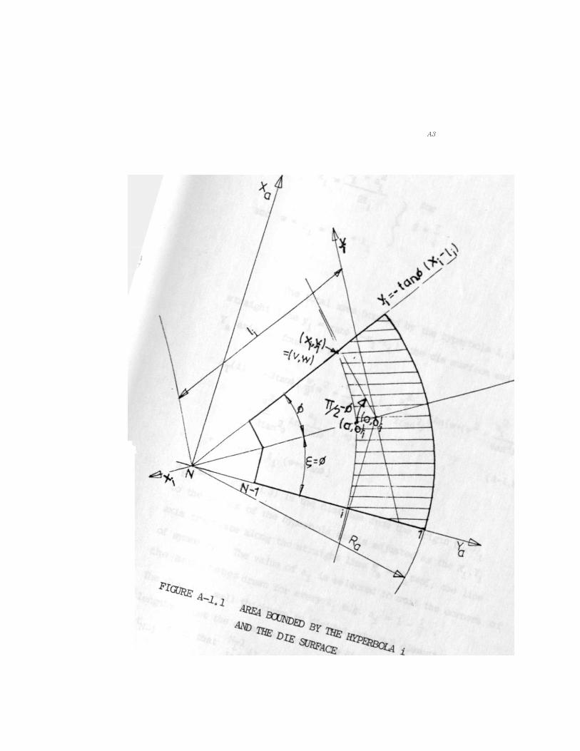
A3

4

or v = x. = 1

I. + a2

_i i_

2Z. l

for

8 = —

and w = y. = -x. + I. Ji l l

Hie total area bounded by the hyperbola i, the

straight line y^ = tanp O-x^H^), the die surface and the

Y axis is found to be a

a 2 a 2 a 2

AT(i) = -2tan$ { + + Un{w+(w2 + )*}) T 2 tan 9 2tan $ tan $

a 2 a . D 2

" i a n 2 / " ^ } ^

2 + v tanp - JL (w+vtan0)

a (see Figure 3.3) is the distance frcm the origin ( 0 , 0 ^

to the vertex of the hyperbola and is adjusted as the X^,Y^

axis translate along the straight line Xa = Yatan;, the line

of symmetry. The value of ai is selected to suit the corners o

the asymptotes drawn for every ljL e.g. a.L = 1 - ^ .

The diagonal wall thickness is divided into N-2 elemental

lengths. Let the elemental lengths be At2, At3> At4

N-l At. , such that Z At. = t

3-1 i = 2 1 a

5

D Then A. « ~ - £ At , (2<i<N-l)

1 2 n=2 .

Let At 2 = At3 = AtN_1 = At

D H a a

Then At = —

1

N-2

Dr

~2 i± = - (i-l)At (A-l.9)

Assuming a constant reduction in area, the inner

radius u ( i ) (Figure A-l. 2) of the cross-sectional area at

the entry plane corresponding to the area A^,(i) can be

deteirnined.

Let A = Area ratio r

_ Area at entry

Area at exit

fb

A a

Then, -J § - mi2 ( ! ) ( § ) -

(A-l. 10)

which simplifies to

Db * u r ( i ) = { T ~ r Y i } > (A-l.II)

A 6

The area banded by the radii u r(i+l) and ur(i)

(Figure A-1.2) tis divided into M-l equal sectors each

subtending an angle dtt> . where j refers to the element j

between the radial lines j and j+1. Let the inclination of

the radial line j to the axis be # then ctt . = 4> - $ .. J J J J

Let + d<$>2 + + c t t ^ = Zdfr = 2J>

and d01 = ctf>2 = d s p ^ = dp ,

then dp = — (A-l. 12) M-l

Frcm Figure (A-l.2), + . , 6 J J-l J-l

= + dt>2 + + ^ j - l

= (j-l)<#

= (j-l) — (A-l.13) M-l

The elemental area enclosed by the radial lines and

circular bands, say ABCD is divided into two triangles; a

large triangle ADB and a small triangle DBC. Let the angle

subtended at the centre . = dy and the radial increment J

AD = <5R, where u (i ) = R.

The approximate area of the large triangle ADB is

AL - &R6R5Y (A-l.14)

FIGURE A-1.2 (a) DIVIDING THE ENTRY PLANE INTO (N-2)

BANDS X(M-l) SECTORS

(b) EACH ELEMENTAL AREA IS FURTHER

SUBDIVIDED INTO A LARGE AND

SMALL TRIANGLE

8

and that of the small triangle DBC is

As = £RcR5y - *6R26y (A-1.15)

The difference between the two areas

A . = At - A d L s

= *6R26y (A-1.16)

and the sum of the two areas

Al + As = R6R6y - i<5R25y (=ABCD) (A-1.17)

Therefore,

Al = KABCD + Ad) (A-1.18)

and As = *(ABCD - Ad) (A-1.19)

Substituting for A^ and area ABCD,

Al = J (u r(i){u r(i) - ur<i+l)}) (A-1.20)

and As = i f^ ({(u r(i) - u r ( i + l » ur(i)}-{ur(i)-ur(i+l)}2)

(A-1.21)

Equations (A-1.20) and (A-1.21) are the expressions for the

elemental areas of the large and small triangles.

The co-ordinates of the vertices A, B, C and D are

obtained as follows;

9

At A, j) = u (i ) sin<J> (A-1.22) J

Y b ( i , j ) = u r ( i ) cos0^

At B, y i , j + l ) = u r ( i ) siat>.+1 (A-1.23)

Y b ( i , j+1) = u r ( i ) cos0 j + 1

At C, y i + l j + l ) = u .U+1 ) sir*J)j+1 (A-1.24)

Y b (i+l fj+1) = u r(i+l) ccs$ j+1

At D, X b ( i+l , j ) = u r(i+l) sin? . (A-1.25)

Y b ( i+l , j ) = ur(i+l) cast.

The centroids of the large and small triangles are located

as follows:-

The centroid of the large triangle ABD

x^cLCi, j) = cy i, j) + - y i + i , j) + y i. j+i ) ) /3 CA-I.26)

YbCL(i, j) = (Y b ( i , j ) + Y b ( i+l , j ) + Y b ( i , j+l ) ) /3

and the centroid of the small triangle DCB,

^ C S d J ) = ( y i + l j ) + y i + l , j + l ) * y i , j + l ) ) / 3 (A-1.27)

YbCS(i,j) = c y i + l , j ) + Yb(i+l,j+l) + Y b ( i , j+l ) ) /3

Assuming the same constant reduction A^, each

triangle at the entry plane is transformed into a corresponding

triangle at the exit plane where

AlO

r

and As = ^ (A-1.28)

r

Considering the Y axis and its intersection with the hyperbola a

i and i+1, the vertices © and (2) (or (X ,Y ). .and a a 1, j

( xa » Y

a ) j + l j w h e r e J=l) of the large triangle are known.

is known and the third vertex must lie on hyperbola i.

To determine the third vertex, consider the triangle A' B' D'

(Figure A-1.3a). Let the co-ordinates of the triangle be

A , (X 1 , Y 1 ) , B ' (X 2 ,Y 2 ) and D' (X 3 ,Y 3 ) . Applying the trapezium

rule,

AL = i ( X l ( Y 3 - V + X 2 ( Y l " Y 3 ) + X 3 ( V Y 1 ) } ( A " 1 - 2 9 )

Vertex (I) lies on the intersection of the outer curve

(a circle) and the Y axis (Figure A-1.3b). a

Therefore, X (=X,) =0 a 1 D (A-1.30)

and Y (=Y,) = ± — a 1 2

where the appropriate value of Y^ is the positive value.

Vertex © lies on the intersection of the hyperbola i and

the Y axis, a '

i .e . X (=X0) = 0 (A-1.31a) a ct

Y (=Y9) is obtained frcm equations (A-1.2) and (A-1.3) as a ^

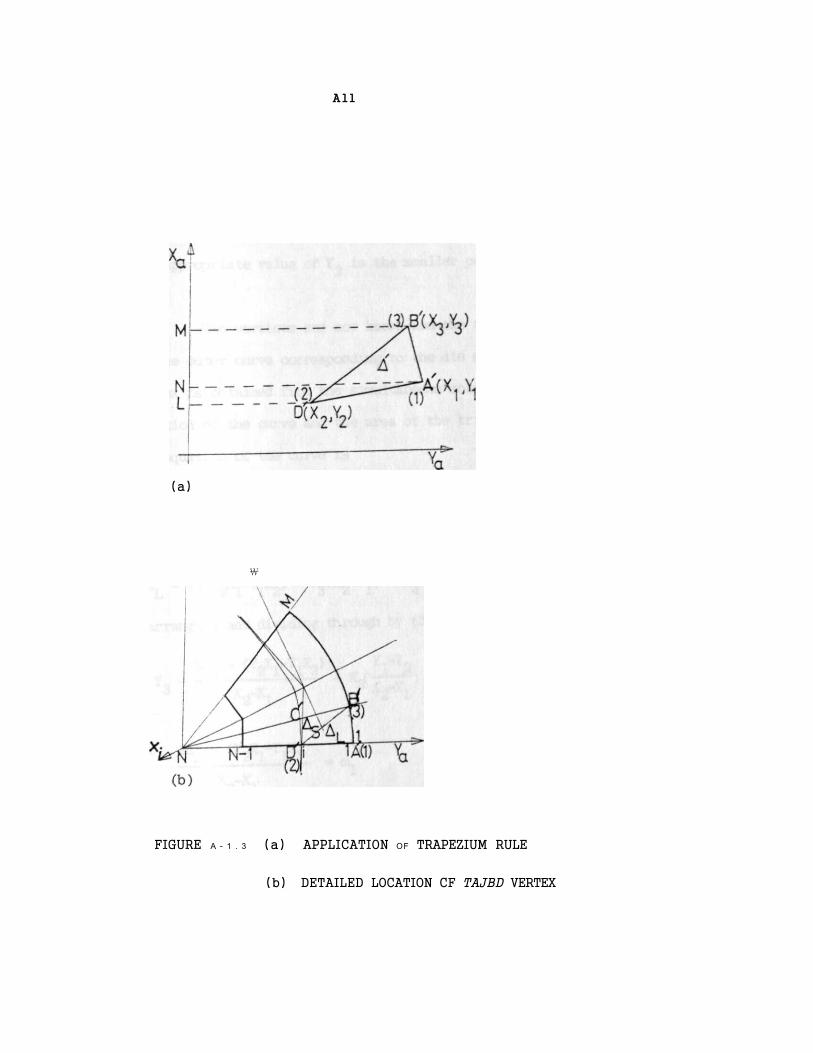
A l l

(a)

\

FIGURE A - 1 . 3 (a) APPLICATION OF TRAPEZIUM RULE

(b) DETAILED LOCATION CF TAJBD VERTEX

A12

v = ig 4

cos£( 1-tan £)

(A-1.31b)

The appropriate value of Y9 is the smaller positive value.

TWo vertices are new known and the third vertex lies

on the outer curve corresponding to the die surface. The

vertex is obtained fran the simultaneous solution of the

equation of the curve and the area of the triangle.

The equation of the curve is

2 2 D a 2

X 3 + Y 3 - ^

and equation (A-1.29) is re-written in the form

(A-1.32)

A L = * « W Y 1 X 2 ) + Y 3 ( X 2 " X 1 ) + W V >

rearranging and dividing through by (Xg-X^) gives

" ( W Y 1 X 2 )

Y 3 X 2 " X 1

Y -Y 1 2

(A-1.33)

Let 2A£ - ( Y ^ - Y ^ )

V X 1

(A-1.34)

and V Y 2

V X 1

= K-, (A-1.35)

Then Y3 = ~ (A-1.36)

A13

Substituting for Y3 in equation (A-1.32), expanding and

rearranging yields

X = W ^ W 2 - ( l ^ X m ^ - C ^ ) 2 ) } (A-1.37)

3 1+K2

1

The appropriate value of Xg is the larger positive value.

Having determined vertex (3) (X^.Y^) of the large

triangle, vertex (2) (X 2 ,Y 2 ) of the large triangle becomes

vertex @ of ^ 3 n a 1 1 triangle and vertex (D

(X3>Y3) of the large triangle becomes vertex (2) of the small

triangle.

Two vertices of the small triangle are known and the

third one lies on the hyperbola i, i .e.

(XgS in£ +Y3COS£ -I ± ) 2 (X^ccsC -YgS in£)2

2 72 = 1

a. b. i l

(A-1.38)

and Y3 = (m^ -K^X^) (A-1.39)

2A' - (YJC,-Y

where m' = —^ Z 1 1 - (A-1.40)

X 2 " X 1

Equations (A-1.39), (A-1.38) and (A-1.5) are solved

simultaneously to yield X^ as

A14

4 C3 + *3 C2 + C1 " 4*3 -V2 " dl " ai " 0

which on factorizing gives

-(C2-d2)±/{(C2-d2)2-4(C3^2)(C1-d1-af)}

3 " 2(C3-d3)

where

9 2 2-C^ = sin C-^sin^+k^ccs *

2 C9 = rn^sin2^-2£isin^-a7i^k1coswC+2k1ilicosC

C1 = m^2ccs2C-2m^ilicosC^i

2 2 2 2 d3 = tan 0 (cos C+kjSii^+kjSin £)

2 2 d2 = tan"J$(-HnJsin2£-2m^k^sin S)

_ 9 2 d i = m i £

The appropriate value of X^ is the smaller positive value,

The centroids of the triangles at the exit plane

can now be obtained.

For the large triangle,

X CL(i, j) = (X (i , j) + X ( i , j + 1 ) • X Ci+l.j)>/3 (A-1.42) a a a a

Y a ( i , j ) = {Y ( i . j ) * Y (i,j+1) * Y (i+1,j)} /3

A15

For the small triangle,

X C S ( i J ) = (X a ( i+lJ ) + Xa(i+l,j+l) + X a ( i , jfl)>/3 (A-l.

Y aCS(i , j ) = (Ya(i+l,j) + Y^Ci+l,j+1) + Y a ( i , j+l)} /3

A-l.2 DERIVATION OF THE FL£W PATH PARAMETERS

6 b ( i , j ) is the horizontal distance a particle travels

after shearing at the assumed discontinuity boundary, .neasured

relative to the entry plane (see Figures A-l.4 and A-l.5).

<5a(i,j) is the horizontal distance the particle travels after

shear at the assumed discontinuity boundary, measured relative

to the exit plane.

Therefore the total distance covered by the particle

in the deforming zone is

Z s ( i , j) = L + 5 b (i , j) - 5 a ( i , j) (Figures A-l.6 and A-l.7)

(A-l.44)

The length of the flow path Zt for each element and the

relative angular diflections n and V as the element flews

through the deformation zone are determined from geometry as

follows;

R u C U ) K Sin0(i, j) = or 6 ( i , j ) = sin ( — ) (A-1.45)

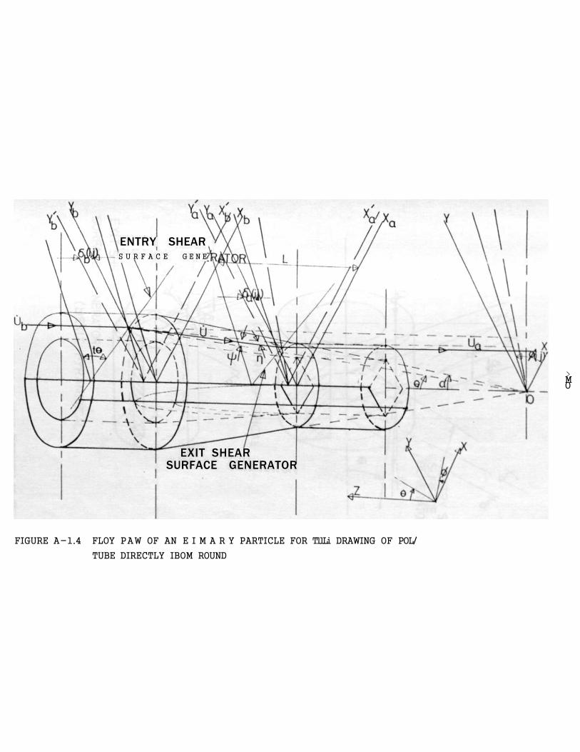
ENTRY SHEAR S U R F A C E G E N E

EXIT SHEAR SURFACE GENERATOR

> M O

FIGURE A-1.4 FLOY PAW OF AN E I M A R Y PARTICLE FOR TllLi DRAWING OF POL/

TUBE DIRECTLY IBOM ROUND

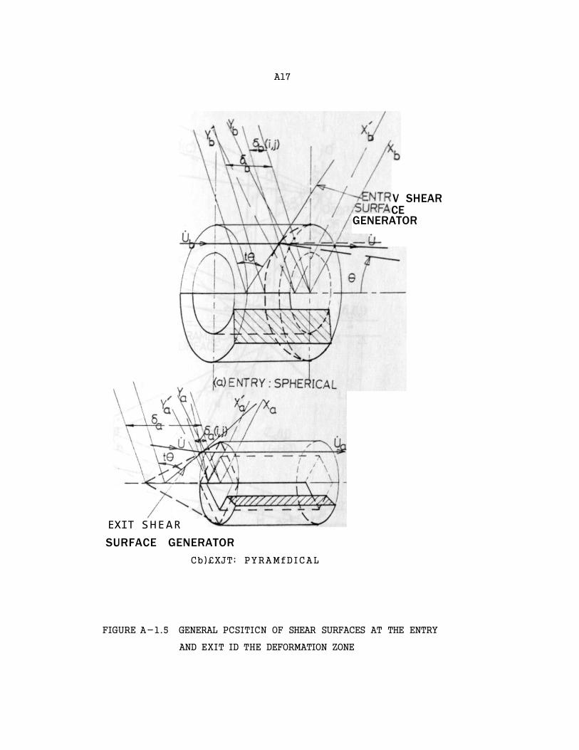
A17

V SHEAR CE

GENERATOR

EXIT SHEAR SURFACE GENERATOR

Cb)£XJT; PYRAMfDICAL

FIGURE A-1.5 GENERAL PCSITICN OF SHEAR SURFACES AT THE ENTRY

AND EXIT ID THE DEFORMATION ZONE

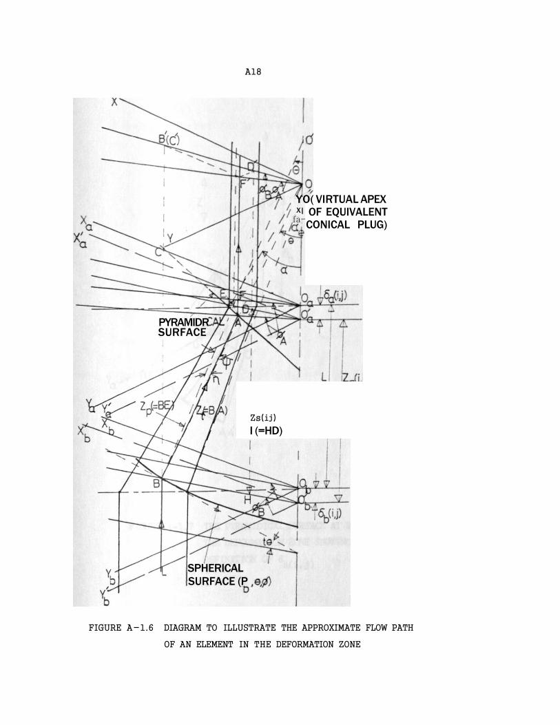
A18

PYRAMIDR SURFACE

SPHERICAL SURFACE (P

YO( VIRTUAL APEX X| OF EQUIVALENT

CONICAL PLUG) fa-

Zs(ij)

I (=HD)

FIGURE A-1.6 DIAGRAM TO ILLUSTRATE THE APPROXIMATE FLOW PATH

OF AN ELEMENT IN THE DEFORMATION ZONE

A19

FIGURE A-1.7 THE PYRAMIDICAL SURFACE AT THE EXIT TO

THE DEFORMATION ZONE SHOWING THE

DEFINITION OF <S ,. . N a(i,J)

A20

where p^ is derived frcm gecmetry as

La

Pb = — 2 (A-l .46)

( ^ o o w

<$b(i,j) = Pb{cos9(i,j) - ccsa} (A-l.47)

X j i j ) + Y 2 ( i , j ) = R^(i,j)

where X ^ i , j) and Y ^ d . j ) are defined by equation (A-l.22)

on page

Therefore R b ( i , j ) = AX^U.j) + Y2(i, j)} (A-l.48)

Similarly R ( i , j ) = /{xf(i ,j ) + Y f ( i J ) } (A-l.49)

a. a a

Considering the geometry of Figures A-l.5 and A-l.6,

6 ( i | j ) = 6 { — - 1} (A-l.50) a a 2Ra(i,j)Cos4)A(i,j)

i X ( i, j ) where tan"1 {— •} > for * <6

Y (i , j) • A U . J ) - A (A"1-51)

-1 X a ( i J )

20-tan {-= } , for <J>A>0

Y a ( i J )

Considering Figure A-l.3a,

Z t ( i J ) = ( C y i J ) - X a ( i , j ) } Z + { Y b ( i , j ) - Y a ( i , j ) } ^ ( i , j ) )

(A-l.52)

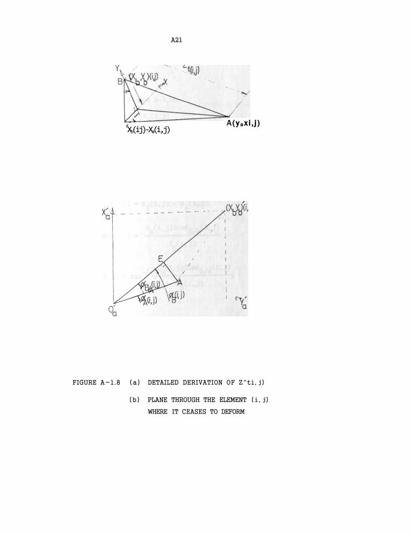
A21

A (yaxi , j ) fXb(ij)-Xa(i,j)

FIGURE A-l.8 (a) DETAILED DERIVATION OF Z^ti, j)

(b) PLANE THROUGH THE ELEMENT (i , j)

WHERE IT CEASES TO DEFORM

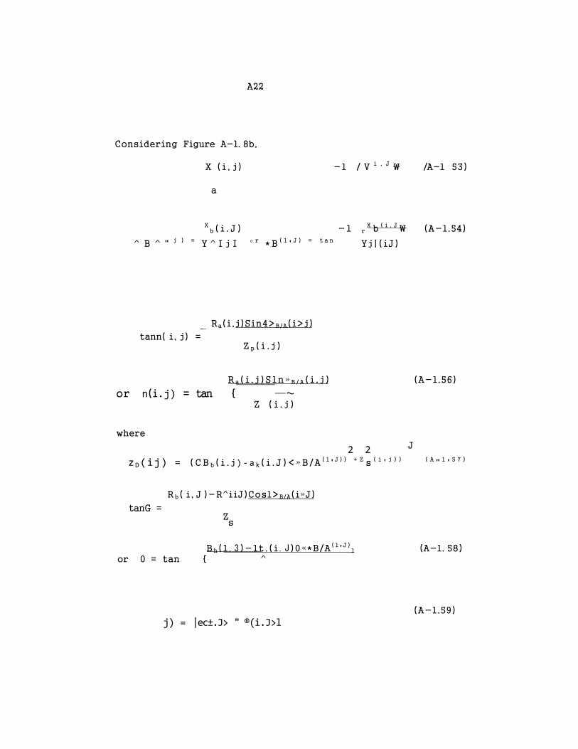
A22

Considering Figure A-l. 8b,

X (i , j) -l / V i , J \ /A-l 53)

a

Xb ( i . J ) -1 r

X b ( i , J \ (A-l.54)

^ B ^ " j ) = Y ^ I j I ° r * B ( 1 ' J ) = t a n Yj|(iJ)

Ra(i,j)Sin4>B/A(i>j)

tann( i, j) = Z p ( i . j )

R a ( i . j )Sln» B / A ( i . j ) (A-l.56)

or n(i.j) = tan { —~ Z ( i . j )

where

2 2 J

z D(ij) = (CB b ( i . j)-a k ( i . J )<»B /A ( 1 ' J ) } + Z s ( i ' j ) ) ( A " 1 ' 5 7 )

Rb( i, J )-R^iiJ)Cosl>B/A(i»J)

tanG = Z s

Bh(l,3)-lt.(i.J)0«*B/A ( 1 ' J )1 (A-l. 58)

or 0 = tan { ^

j) = |ec±.J> " ®(i.J>l (A-l.59)

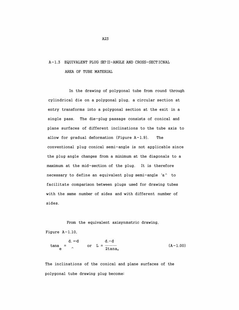
A23

A-1.3 EQUIVALENT PLUG SE? II-ANGLE AND CROSS-SECT ICNAL

AREA OF TUBE MATERIAL

In the drawing of polygonal tube from round through

cylindrical die on a polygonal plug, a circular section at

entry transforms into a polygonal section at the exit in a

single pass. The die-plug passage consists of conical and

plane surfaces of different inclinations to the tube axis to

allow for gradual deformation (Figure A-1.9). The

conventional plug conical semi-angle is not applicable since

the plug angle changes from a minimum at the diagonals to a

maximum at the mid-section of the plug. It is therefore

necessary to define an equivalent plug semi-angle 'a to

facilitate comparison between plugs used for drawing tubes

with the same number of sides and with different number of

sides.

From the equivalent axisynmstric drawing,

Figure A-1.10,

d. •-d d.-d tana = or L = ——— (A-1.00)

e ^ 2tanae

The inclinations of the conical and plane surfaces of the

polygonal tube drawing plug become;

A24

I

FIGURE A-1.9 SKETCH SHOWING THE DRAWING OF REGULAR

POLYGONAL TUBE FRCM ROUND THRGjGH A

CYLINDRICAL DIE

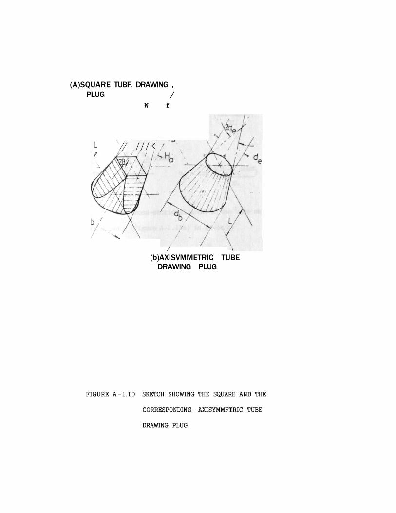
(A)SQUARE TUBF. DRAWING , PLUG /

\ f

// / / / <

/ \

(b)AXISVMMETRIC TUBE DRAWING PLUG

FIGURE A-l.IO SKETCH SHOWING THE SQUARE AND THE

CORRESPONDING AXISYMMFTRIC TUBE

DRAWING PLUG

A26

"b H

2 ? l ^h ~ ^ tan* = — or a = tan {— — } (A-1.S1)

L c 2L

^b _ Ha co60

. 2 2 _ -lrcL-H cos8, /A , tanpc = ot = tan { o a } (A-1.62)

s T s L 2L

The cross-sectional area of the tube material at

any radius p (Figure A-l.lla) is given by

Ap= 7r(R2-r2) (A-1.63)

where

R = psinct (A-1.64)

and r Is obtained from the expression

r.-r tana =

e (pb-p)ccsa

as r = - (pb-p)cosatanae (A-1.65)

Substituting for r and R into equation (A-1.63) and

factorizing,

j* 2 A = Tr3in23(p2-{~r—-- + (p-PK)cotatam } ) (A-1.66)

p sine d "

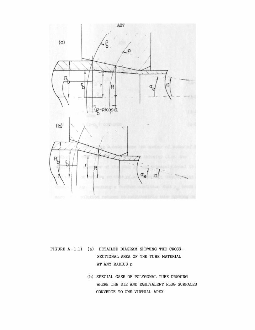
FIGURE A-l.ll (a) DETAILED DIAGRAM SHOWING THE CROSS-

SECTIONAL AREA OF THE TUBE MATERIAL

AT ANY RADIUS p

(b) SPECIAL CASE OF POLYGONAL TUBE DRAWING

WHERE THE DIE AND EQUIVALENT PLUG SURFACES

CONVERGE TO ONE VIRTUAL APEX

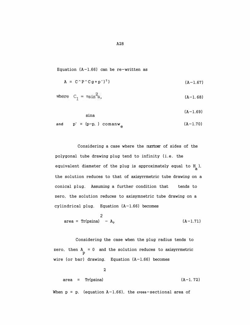
A28

Equation (A-l.66) can be re-written as

A = C ^ P ^ C g + p ' ) 2 ) (A-l.67)

(A-l. 68)

sina (A-l.69)

and p' = (p-p, ) comanw e

(A-l.70)

Considering a case where the nurrtoer of sides of the

polygonal tube drawing plug tend to infinity (i.e. the

equivalent diameter of the plug is approximately equal to H ), a

the solution reduces to that of axisyrrmetric tube drawing on a

conical plug. Assuming a further condition that tends to

zero, the solution reduces to axisymnetric tube drawing on a

cylindrical plug. Equation (A-l.66) becomes

2 area = Tr(psina) - Ap (A-l.71)

Considering the case when the plug radius tends to

zero, then A = 0 and the solution reduces to axisyrrmetric P

wire (or bar) drawing. Equation (A-l.66) becomes

2

area = Tr(psina) (A-l. 72)

When p = p. (equation A-l.66), the cross-sectional area of

A29

the tube material at entry is obtained as

2 0

\ = Tr{(pbsiflcO - r£}

This expression can be re-written in the form

, _ 2r r (A-1.73)

~ PbCl " 3

_ 2 (A-1.74) where C3 = Trrfa

v

and C, is equation (A-1.38).

A-1.4 DERIVATION OF VELOCITY DISCONTINUITY SUFFERED BY AN

ELEMENT ENTERING THE DEFORMATION ZONE (Figures

A-1.12 and A-1.13)

Referring to Figure A-1.13a,

(A-1.75) ^rsl = -%sint9^cos(e-t9)+upsin(6-t9)

Referring to Figure A-1.13b,

u is the corponent of velocity nonral to the p-8 plane and

$

, .2-2 * (A-1.76) urb = rsl

2, i = {u^C-i^sintS+UgCOsCe-tfi )nipsin(9-t9)) >

The resultant velocity (of the tangential carponents) on b o *

sides of the shear surface gives the velocity discontinuity.

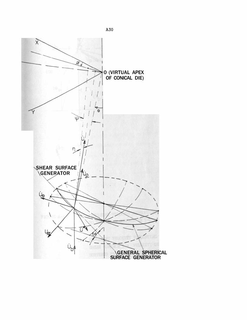
A30

SHEAR SURFACE \GENERATOR

0 (VIRTUAL APEX OF CONICAL DIE)

\GENERAL SPHERICAL SURFACE GENERATOR

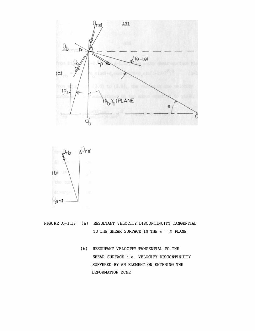
FIGURE A-1.13 (a) RESULTANT VELOCITY DISCONTINUITY TANGENTIAL

TO THE SHEAR SURFACE IN THE p - & PLANE

(b) RESULTANT VELOCITY TANGENTIAL TO THE

SHEAR SURFACE i .e . VELOCITY DISCONTINUITY

SUFFERED BY AN ELEMENT ON ENTERING THE

DEFORMATION ZCNE

A32

From Figures A-1.12 and A-l. 13, the entry shear surface yields

u r b = Cu2+{-ubsint9+u9cos(l-t)9^psin(l-t)e}2)i (A-l.77)

From equations C3.6) to (3 .8 ) , the values of the velocity

components are substituted in the above equation to yield,

a = a ((ccstetann 2 +

rb o cos(l-t)9tanf

+ ccst9tan(l-t)6}2)i (A-l.78)

Any particle with initial velocity u^ before deformation,

travels through the deformation zone with a velocity LI=U(U2,Uq ).

At the exit boundary, the velocity of a particle just before shear

is u=d(up ,UQ^). After shear, the particle travels parallel to

the tube axis with a velocity il . Assuming an equivalent a

divergent deformation passage,

p» 2 u = u w C—) (A-l.79)

ra rb D " ^a

where p" 2 is equation (3 .4) and P"2 is obtained from b a

equation C3.5).

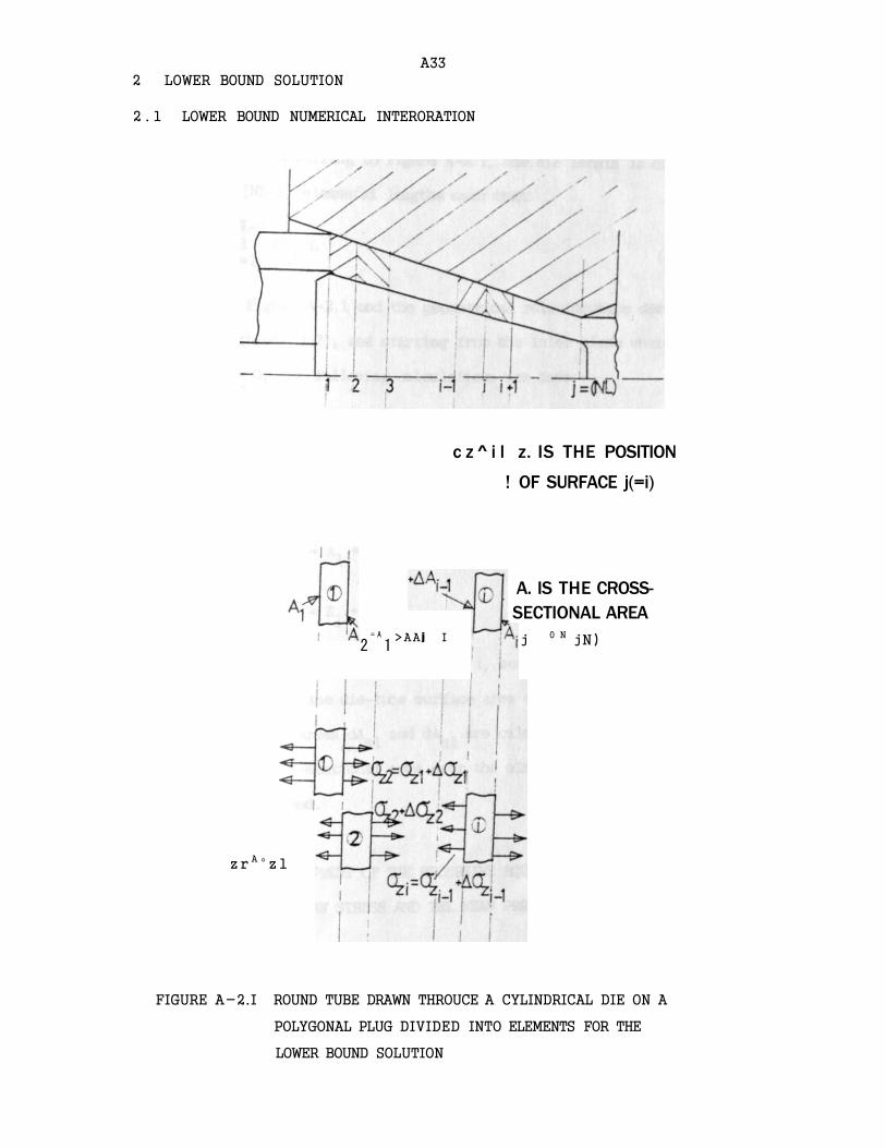
A33 2 LOWER BOUND SOLUTION

2 . 1 LOWER BOUND NUMERICAL INTERORATION

c z ^ i l z. IS THE POSITION

! OF SURFACE j(=i)

z r A ° z 1

2= A

1 >AA j I

A. IS THE CROSS-SECTIONAL AREA j 0 N jN)

FIGURE A-2.I ROUND TUBE DRAWN THROUCE A CYLINDRICAL DIE ON A

POLYGONAL PLUG DIVIDED INTO ELEMENTS FOR THE

LOWER BOUND SOLUTION

A34

A-2.1.1 GEOMETRICAL DERIVATIONS

Referring to Figure A-2.1, the die length is divided

into (NL-1) elemental lengths such that

NL-1

£ AZ.=L i = 1 i (A-2.1)

Using Figure A-2.1 and the geometrical relationships derived

in section (3.7), and starting frcm the inlet plane where

= O, the following calculations are done:-

(a) At any section Zi> calculate R(i), r(i ) ,

and A^. From Figure A-2.1, the following relationship

is developed:-

A. = A, + i AA._ (A-2.2) i 1 j . 2 J-l

i and Z. = Z. + Z AZ . . (A-2.3)

1 1 j=2 3

(b) Considering the tube element i, between the surfaces i

and i+1, the die-tube surface area dAc9 and the plug-tube

surface areas dA , and dA , are calculated. The change si el

in cross-sectional area over the element i, AAi is also

determined.

A-2.1.2 DEVELOPMENT OF THE RECURSIVE EQUATIONS TO EVALUATE

THE DRAW STRESS AND THE MEAN PRESSURE

Starting frcm the inlet plane surface i = 1, and

assuming no backpull (a =0), the stress on the surface i=2

A35

can be determined from the equilibrium equation (3.11). The

calculated value of is used to determine a ^ , etc.

From Figure A-2.1, a .=a , + L Aa . , (A-2.4) ' zi zl j=2 zj-1 v

The equilibrium equation (3.111) applied to the element i can

be conveniently re-written as

A( I { - (!zi) AA. + (1 -{-£}) Y A.+AA. Y 1 Y

l l

( K c 2 M c 2 ( i ) + K s i a A s l ( i ) + K c l A A c l ( i ) ) } ( A " 2 ' 5 )

vhere

K = (\i cosa -sim ) = constant 1 (A-2.6) si m s s

K = (p cosa -sim ) = constant 2 (A-2.7) cl m c c

K ~ = (u cosot+sim) = constant 3 (A-2.8) c2 m

Example:

Starting at Z± = l = 0 where the conditions of stress are

known f z l = 0 ) , the change of stress over element i=l Y

can be determined;

A3 6

A ( ! f i ) = { ' ( 0 ) A A i + ( 1 - ( 0 ) )

^ s ^ + K cl A A cl ( 1 ) + K C2 A A C2 ( 1 »

°zl which yields A (-—).

But a 0 a . a , 0-, ( rf) = (J5i) + = A ( ^ )

Y Y Y Y

Therefore,

^ (A^AA 2 ) { - Z f < > +

( K s l M s l ( 2 ) + K c l A A c l ( 2 ) + K C 2 M C 2 ( 2 ) )

az2 which yields A( ) etc.

Y

The mean pressure at the die-tube (or plug-tube)

interface can be calculated from the total normal force for

elements i=l, 2, NL divided by the total die-tube

surface area. For the element (i), the normal force NF^Ci)

at the die-tube interface is given by;

NF, ( i ) = P .(AA 9 ( i ) ) (A-2.9) 1 mi c^

= { 1 _ ( ! 5 i ) } « « , (A-2.10) V Y c2

A37

Therefore, the total normal force for elements i=l, 2, 3,

NL is

NF, NL-1 . a .

£ ^ ( " f )> A A ^ i ) (A-2.il)

The dimensionless pressure ratio becomes

& = ! V Y

E4Ao2(i)

a ,

E (1 - H | i ) } M c 2 ( i )

ZAAc2(i)

a ,

Z (-f±) AA 2 ( i ) = 1 _ { 1 9£ ; (A-2.12)

ZAAc2(i)

The expression for the mean pressure at the plug-tube

interface is

3 . , E ( A . 2 1 3 )

Z(AAcl(i)+AAsl(i))

A38

A-3 COMPUTER PROGRAMMES

A-3.1 UPPER BOUND SOLUTION FOR POLYOONAL DRAWING

1 TRACE 2 2 MASTER IJBFPTD 3 C UPPER BOUND SOLUTION PQR POLYGONAL TUBE DRAWING 4 DIMENSION PL(IO),A(10),AT(!0),ER(10),X(10),Y(IQ),XA(ll,ll), 5 lYAdl, 11) ,ARLT3(10) ,ARSTB(10),ARLTACilO),ARSTA(lO),XBCL(11,11), 6 2Y8CL(11,11),X3CS(11,11),YBCS(11,11),KACL(11,11),fACL(11,11), 7 3XAC5(11,11), YACS (11,11), KB(11,11),YB(11,11),RAS(11,11), 3 4R8S (11,11), THETAS(11,11),DAS(11,11),PHISBA(11,11),ZS(11,11), 9 5ZTS(11,11),ETAS(11,11) ,HETALC (11,11) ,RAL11,11),

10 6RBL(ll,ll),0BL(ll,ll) ,DAL(U,11),PHILBA(U,11) ,ZL(llfll),

11 7ZTL(11,11) ,PSIS( 11,11) ,HETASC(11,11),PSIL(11,11), 12 IDBS(11,U) ,THETAL( 11,11),ETAL( 11,11)

13 4RITE(2.10) 14 10 FORMAT<//5X,'UPPER BOUND SOLUTION FOR POLYGONAL TUBE DRAWING ) 15 t»RITE(2,20) 16 20 FORMAT(5X,'SOLUTION FOR SQUARE HEXAGON AND OUODECASON) 17 C STOCK OUTER QIAMETER=90B,PfiQ0UCT OUTER OIAMETER=DOA GAUSE=TB 18 C FRICTION COEFFICIENT=MU 19 #RITE(2,30) 20 30 FORMAT(5X, DOB,DOA AND TB ARE FIXED') 21 C INPUT STATEMENTS

22 READ(1,31)DOB,OOA,TB

23 31 FORMAT(3F0.0) 24 DI3=QGB-(2.0*T8)

25 ROB-OOB/2.0 26 R0A=D0A/2.0 27 RIB=0tB/2.0 28 PI=3.1415927 29 C GENERATE NUMBER OF SIDES OF SECTION REQUIRED BY GENERATING BETA 30 DO 100 I3ETA=15,45,15 31 *RITE(2,40) IBETA 32 40 F0RMAT(5X, 'BETA5',14)

33 BETA=PI*BETA/130.0

34 C8ETA=C0S(BETA)

35 SBETA=SIN(BETA)

36 T8ETA=TAN(BETA)

37 TB2=T8ETA**2

38 T84=T82»2

39 TB8=TB4«2 40 T828=l.0/TB2 41 TB18=1.0/TBETA

42 SPAR=CBETA*SBETA*P I / < 4.0*6ET A)

43 C CALCULATE SECTION PARAMETERS I.E.AA,A8,AR,ETC 44 HA=0i3

A39

45 AB=PIt|(R0B**2MRI8"2))

46 AA*Pl *RQA*t2-HA**2*SPAR

47 R£3SQRT (R0ft**2-(AA/PI)) 48 AR-AB/AA

49 RED-1.0-1.0/AR

50 RA=HA/2.0

51 ¥RITE(2,42> HA,RE,TB,ftED

52 42 FORMAT(21,4F10.5)

53 C RADIUS OF INSCRIBED CIRCLE AT E W ( R A I )

54 RAI=HA»CBETA/2.0

55 C SINGLE SYHHETRIC SECTION USED TO SAVE COMPUTER TI*E,DENOTED

56 C HEREAFTER BY 'DOUBLE! SYMMETRIC

57 C BAND THE INLET (DOUBLE)SYHIIETRIC INTO .1-1 EQUAL

58 C SECTORS AND MP OUTLET rflTH N-2 HYPERBOLIC CURVES,(I,J)

59 C DEFINES GENERAL INTERSECTION AND (l.DDENOTES THE ORIGIN

60 M=10

61 M=10 62 C FIRST CURVE OF OUTLET CIRCULAR SECTION CORRESPONDS TO THE

63 C DIE ,PL!I) REFERS TO THE POSITION OF HYPERBOLA VIRTUAL ORIGIN

64 C ALONG LINE OF SYMMETRY AND A(I) IS THE FOCAL LENGTH

65 TA=ROH-RA

66 PL(l>=D0A/2

67 PL(10)=0.0

68 C TA IS THE THICKNESS OF SECTION ALONG TUBE DIAGONAL AND IS

69 C DIVIDED INTO N-2 EQUAL LENGTHS

70 DT=(TA*\ROA* (<1.0/CBETA)-1.0 >))/(N-2)

71 C INCLUDED AREA OF THE DIE AT(l),ATilO) CORRESPONDS TO THE

72 C ORIGIN

73 AT(1)=0.0

74 AT(10)=PI*(R0A«2)/(2.0*PI/BETA)

75 ER(1)=ROB

76 ER(10)=0.0

77 C DETAILED HAPPIN6 STARTS HERE i t t U U M t t

79 DO 305 1=2,N-l

79 PL (I) =(ROA/CBETA)-((I-1)*DT)

90 A(l)~(i.0-I.0*l/N)*5.00

81 C CALCULATE CO-ORDINATES AT INTERSECTION OF HYPERBOLA AND

32 C LINE INCLINED TO(DOUBLE) BETA BY THE YA-AIIS

83 IF(IBETA,EQ,45) GO TO 55

34 T(I)=(-PL <I) »T84*SQRT(PL (I) **2»T88* (1.0-T84) *(A( I) **2*PL (I)*»2

35 l*TB4) M/U.0-TB4)

36 GO TO 56

37 55 X(I) = (PHI)«2+A(I>**2)/I2.0*PL(I))

38 56 Y (I) =TBETA*< -X i I > <-PL H))

A40

89 C CO-ORDINATES OF INTERSECTION TO 5L3AL IA-YA AXES

90 V=X(I)

91 K»Y(I) 92 *A<l,H)=« 93 YA(I,N)=-VfPL(I)

94 C AREA ENCLOSED 3Y HYPERBOLA 1 AND THE DIE I=DENOTED 3Y AT CI)

95 A T U ) = i2.0»T3£TAf((K/2.0US8RT(yu2*Am«2»T328)<-A(l)«2

96 1 *Q. 5*T828*(AL06(W+SflRT(H*»2*A (I)f*2»TB2B))) -A( I) "2*0.5*TB2B

97 2*ALQ6(A(I) tRBIB) )MBETA*D0A**2/4.0)*(VH2fT3ETA) -(PL( I)

98 3TBETA))) 99 C AREA ENCLOSED BY THE DIE AND THE CURVE REFERRED TO THE INLET

100 A8T=AT(I)*AR

101 C EQUIVALENT RADIUS AT INLET ER(I)

102 ER(I)=SGRT(D08»*2/4.0-ABT/BETA)

103 C AREA OF THE BAND AT INLET ENCLOSED BY THE CIRCULAR ARC I t i-l

104 ABAND=(ER(I-l)»2-ER(l>**2HBETA/2.0

105 C DIVIDE THE AREA OF THE 3AN0 INTO fl-1 EQUAL SECTORS AND ALSO

106 C CALCULATE THE RADIAL MIDTH OF SAND

107 A8CD=ABAND/(M-1)

108 DR=€R(I-l)-£R(n

109 DPHIJ=BETA/(H-1)

110 C CALCULATE AREAS OF LARGE AND SHALL TRIANGLES AT INLET PLANE

111 DD=O.5*0R«2*DPHlJ

112 ARLT8(11 =0.5*(ABCD*DD)

113 AfiSTB (I) =0.5*(A8C0-0D)

114 C EQUIVALENT TRIANGULAR AREAS AT EXIT PLANE

115 ARLTA(l)=ARLT8(I)/AR

116 AfiSTA(I)=ARSTB(I)/AS

117 C INTERSECTION OF HYPERBOLA I AND YA-AIIS

118 <A(lf l)=0.0

119 IF(I3ETA.E9.45) GO TO 107

120 YAR3= (PL (I) +SQRT (PL(I) " 2 - (1.0-TB4) * (PL i IJ "2-A(I) «2))) /

121 HCBETAM1.0-TB4))

122 YAR4=(PL(I)-SQRT(PL(I)**2-(1.0-TB4)*(PL (I)**2-A(1)»*2I))/

123 • 1(C8£TA*(1.0-TB4))

124" IF <YAfi3.LT.VAR4) SO TO 103

125 YA(I,1)=YAR4

126 GO TO 305

127 103 YA(I,l)=YAR3 128 60 TO 305

129 107 YA(l,t)=PL(l)*A(l)

130 305 CONTINUE

131 C CURVE 1=1 IS A CIRCLE AND CO-ORDINATES OF INTERSECTION HITH

132 C LINE INCLINED AT SETA TO YA-AHS CAN 3E FOUND

A41

133 YAU,M)=(D0A/2)«SSRTIl.0/U.0fTB2)>

134 KA(l,l1>*fAU,ft)*T9£TA

135 YA(1,1)=R0A

136 XAtl,l)=0.0

137 XAilO,10)=0.0

138 YAUO,10)=0.0

139 HRITE(2,70>

140 70 FORMAT(SXr LIHITIN6 CO-QftOIMATES AT EXIT PLANE ,11)

141 iiRITE(2,7l) (XA(I,N), 1=1,N)

142 *RITE<2,71) <YAC1,H>,1*1VM> 143 71 F0RNAT(2X,10(2X^,6),/)

144 C CO-ORDINATES OF TRIANGLES AT INLET

145 00 310 I=l,N-l

14b DO 315 .3=1,11

147 PH1J*(J-1)*BETA/(H-1)

148 X8!l,J)=ER(I)*SIN(PHiJ)

149 YB(I,J)=ER(D*COS(PHIJ)

150 315 CONTINUE

151 310 CONTINUE

152 C LOCATE CENTRGIOS OF LARGE AND SHALL TRIANGLES AT INLET

153 DO 320 1*1,(1-2

154 DO 325 .j=l,H-l

155 XBCL(Ifl,Jfl)a(X8(I,J)fX8(Ifl,J)fXB(I,Jfl))/3.0 156 YBCL(lfl,Jfl)=<YB(I,J)fYB(IflfJ)fYB(I,Jfl))/3.0 157 XBCSi!fl,Jfl> = aBU*l,J)*<B(Ifl,JM>«-XBiI,Jfl))/3.0

158 Y3C3( l+t, Jfl)=(YB( If l . J W B d M , M I fYB(I,Jft)>/3.0

159 325 CONTINUE

160 320 CONTINUE

161 80 TO 503

162 C CALL FOR A FRESH PAGE TO PRINT RESULTS

163 WRITE(2,350)

164 350 FORMAT<1HI)

165 C PRINT CO-ORDINATES OF INLET TRIANGLES AND EQUIVALENT RADIUS

166 WRITE(2,352)

167 352 FORMAT(5X, VALUES OF XB,YB AT INLET PLANE AND EQUIVALENT

168 IRADIUS ER'/)

169 «RITE(2,353>

170 353 FORMAT(2X, 1=',5X,'J=l',7X,'J=2',7X, Js

3',7X,'J=4',7X, 3=5 ,

171 17X,'J=6',7X, J=7',7X,'J=8',7X,'J=9',7X, J=10',2X,'E9 RADIUS',

172 2/)

173 DO 370 1=1, N

174 *RITE(2,355) K I , (XBiI,J),J=t«M) ,ERU)>)

175 JjRITE(2,356)(YB(I,J),J=l,i1)

A42

176 355 F0RNAT(2X,I2,10(2X,F8.4),2X,F9.4)

177 356 FORHAT(7Xf10(2X

yF9.4>>

173 370 CONTINUE

179 C CENTftOIDS OF TRIANGLES AT INLET AND RESPECTIVE AREAS

130 MR ITE (2,3591

131 359 FORMAT(//5X,'VALUES OF IBCS,YBCSVXBCL,Y8CL AND AREAS OF

132 ITRIAN6LES',/)

183 DO 375 1=2,N-l

184 *RITE(2,3560> (I, (XBCS(IJ) ,J=2,?I) ,ARST8(H))

135 MRITE(2,3561)(YBCS(I,J),J*2l!f)

136 #RITE(2,3560) (I, (KBCL(IJ) ,Js

2,i1) ,ARLTI(I)))

1S7 WRITE (2,3561) t YBCL (I, J), J=2, M)

133 3560 F0R«AT(5X,I2,8Xf?(2X,F8.4),2X,F8.4)

139 3561 FQRf!ATil5X,9t2X,F8.4))

190 375 CONTINUE

191 C NAPPING CORRESPONDING TRIANGLES AT EXIT PLANE

192 503 AZER0=0.0

193 DO 330 1=1,N-2

194 DO 335 J=1,N-1

195 C NAPPING LARGE TRIANGLES

196 AREAL=AftLTA(IH)

197 Xl«A(I,J)

193 YI—YA(I,J)

199 X2S

XA(I+1,J)

200 Y2*YA(H-l,J)

201 IF(I.ST.l) SO TO 97

202 IF(J.EQ.i) GO TO 72

203 Df11s

(2.0*AREAL-(Xl*Y2-YUX2) )/(X2-Xl)

204 DK1=(Y1-Y2)/(X2-X1)

205 X3R1»(COW 1 «DK1) *SQRT ((SH t *0K 11 " 2 - U 1 . O^Wtl« *2) t tDHl **2

206 1-R0A«2) )))/<!. 0*DKt«2)

207 X3R2S

((DM frDKl) -SfiRT ((DM *DK 1) «2- € € I - O+DK1 «2) * (DM »2

208 l-ROA**2))))/lt.O*OKlH2)

209 Y3RI=CM-DK1*X3R1

210 Y3R2=0M-DKi*X3R2

211 C SELECT CO-ORDINATE OF THIRD VERTEX

212 IFU3Ri.6T.X3R2) GO TO 75

213 YA(I,J+1)=Y3R2

214 (A(I,Jft)=X3R2

215 30 TO 76

216 75 YA(I,JH)*Y3Rl

217 XA(I,JM)=X3Ri

218 76 GO TO 77

219 C NAPPING THE INITIAL LARGE TRIANGLES BY SUBSTITUTING (

A43

220 C AND SOLVING FOR Y

221 72 DHI=(2.0*AR£AL-(Y2«1-YUX2)>/(Y1-Y2)

222 DKl»(X2-n>/m-Y2>

223 Y3R13

(OH 1 *0K 1) *SQR T {(DHI fOK I /1 «-2- U 1 . 0*0K U*2) * (DH1 »*2

224 1-R0A«2)))>/(1.<W)K1M2)

225 Y3R23

((OHI*0KI) -SQRT ((OH I *DK I) **2- < (I. O+DK1 **2) * < OH I *«2

226 i-RQA«2)>})/(1.0*0KI«2)

227 X 3R1 =0« I -OK 1 »Y3« 1

228 X3R2=DH1-DKUY3R2

229 C THIRD VERTEX OF TRIANGLE

230 IFIY3R1.ST.Y3R2) 50 TO 78

231 XA(I,.M)=X3R2

232 YA(I,J+1)S

Y3R2

233 SO TO 77

324 73 XA<I,J+l)s

X3Rl

235 YAiI,Jfl)»Y3Rl

236 30 TO 77

237 C HAPPING LARSE TRIANGLES HEftE THE THIRD VERTEX LIES ON

239 C HYPERBOLA I

239 C NAPPING LARGE TRIANGLES SY SUBSTITUTING < AND SOLVE FOR 1

240 97 HH1=(2.0*AREAL-(X1*Y2-YI*X2))/(YI-Y2)

241 HK1=(X2-X1)/(Y1-Y2)

242 HCls

PL(l) «2-T8l*HNt»*2

243 HC2=-2.0*PL (I) +2.0*HK1 *HHUTB2

244 HC33

1.0-HK1»2»T82

245 3QT=SQRT(HC2«*2-4.0*HC3(HC1-A(I)«2))

246 Y3Ll=(-HC2tSQT)/I2.0fHC3)

247 Y3L2=(-HC2-SST)/(2.0*HC3)

248 X3Ll=ttHl-HKl*Y3Ll

249 X3L2=HN1-HK1*Y3L2

250 C SELECT THE THIRD VERTEX

251 IF(Y3Ll.LT.Y3L2.AND.X3Li.5T. AZERO) SO TO 112

252 XA(I,JH)*X312

253 YAiI,J+l)=Y3L2

254 50 TO 77

255 112 XA(l,J+l)s

X3U

256 YAU,J+l)s

Y3Ll

257 GO TO 77

253 C HAPPIN6 SHALL TRIANGLES AT INLET

259 ' 11 XU=XAIIH,J>

260 YU*YAU*I,J>

261 X22=XA(I,J+1)

262 Y22=<A(L,JH>

263 AREAS=ARSTA(I+1)

A44

264 FNls(2.0AREAS-(YlUX22-Y22»Xl t) I / (X! i-X22>

265 FK1=(Y22-Y11)/ (X11-X22)

266 C3=FK1«2=TB2

267 C2--2.0*FH1*FK I +2.0*FK I *PL( IH>

268 Cl=FMl»*2*PL (I+l) «2-2.0*PL ( I ) »FM

269 SQT»SSRT(C2»2-4.0tf3*(Ct-A(!*l)**2l)

270 X3SI—(-C2+SQT)/(2.0#C3)

271 X3S2= < —C2-3QT>/(2.0+C3)

272 Y3Sls

FNl-FKl*X3Sl

273 Y3S2=FIU-FKlfX3S2

274 C SELECT THIRD VERTEX

275 IF(X3S2.LT.X3S1.QR.X3S2.6T.AZER0) 80 TO 91

276 XftU+t,J+l)=X3St

277 YA(l*l,J+l)s

Y3Sl

278 50 TO 335

279 91 XAU*l,JM)*X3S2

230 YA(U*l,J*l)*Y3S2

291 335 CONTINUE

282 330 CONTINUE

293 C LOCATING THE CENT ROI OS OF THE HAPPED TRIANGLES AT EXIT PLANE

234 DO 340 1=1,N-2

285 DO 345 J=1,K-1

236 XACL(I+M+l)=<XA(IfJ)*XA(I,J+lKXA<IM,J)>/3.0

237 YACLUM J*l)=(*A<I,J)*YA(I,JM>*YA(I*M)>/3.0

288 XACS(IMfJMMXA(M,J)*XA(I*l,J*l>*XA(I,J*l))/3.0

239 YACSiM,Jfl)=(YA(IMlJ)+YA(Ifi

lJfl)<'YA(I,Jfl)>/3.0

290 345 CONTINUE

291 340 CONTINUE

292 SO TO 504

293 C CALL FOR A FRESH PASE TO PRINT RESULTS

294 *RITE(2,349)

295 349 FORMAT(1 Hi)

296 C PRINTOUT FOR EXIT PLANE

297 *RITE(2,3565)

298 3565 F0PNAT(//5X,'VALUES OF XA,YA AND FOCAL DISTANCE A(I) OF

299 IHYPERBOIA I',/)

300 *RITE(2,353)

301 A(10)=0.0

302 A t U *ROA*(1.0/CBETA-i.0)

303 DO 380 1=1,N

304 *R!TE<2,355M(I,(XA(I,J=M>,A<1))>

305 *RITE(2f356)(YA(M»,J

s

M>

306 380 CONTINUE

307 «RITE(2,3570)

A 45

308 3570 FORMAT(//5X, VALUES OF lACS.YACS.XAClJACl AMD AREAS OF

309 ITRIN6ALE3',/)

310 D0 385 1=2, N-l

311 *ftITE(2,3560()U,UCASU,J)fJ»2,H)

fARSTAU)>>

312 WfiITE(2,356lMYACS(I,J),J=2,M)

313 KRtTE(2,3560)((I,(XACL(l,J),J=2,M),ARLTA(l)))

314 HRITE(2,356l) (YAClil,J),J=2,R)

315 385 CONTINUE

316 C PER CENTA6E ERROR IN AREA OBTAINED FROM MAPPING AND ACTUAL

317 C VALUE AA

318 AS8=AA/(PI/BETA)

319 ERRCR=((ASB-AT(N-l)I/ASB)*100.0

320 WRITE(2,3571)ERROR

321 3571 FORMAT (//5X, 'PERCENTAGE DIFFERENCE OF TOTAL (-SECTIONAL AREA

322 ls',f8.4,//>

323 C «*$*$**$ END OF CONFORilAL MAPPING *$$W$ms

324 C ttttt&ttt UPPER BOUND SOLUTION NO* BEGINS MfcttttM

325 504 WRITE(2,400)

326 400 FORMAT I//,5X,'i*ttfc UPPER 30UND SOLUTION BEGINS HERE Itttit')

327 C GENERATE THE DIE SEMI ANGLE

328 DO 200 IALPHA=2,13,4

329 ALPHA= <Pf /180.0)H ALPHA

330 TAD»TAN(ALPHA)

331 DIEH-(RQB-ROA)/TAD

332 ALPHAE=ATAN(RIB-ftE) /DIEH)

333 ALFAEM180.0/P I) ALPHAS

334 C CALCULATIONS OF THE RADIAL DISTANCE OF THE PARTICLES AND

335 C DIFLECTIQN ANGLES PSIaXI

fETA

f...ETC AND LENGTH OF FLOW PATH

336 CAD=COS(ALPHA)

337 SAD=SIN«ALPHA)

338 TAE=TAN(ALPHAE)

339 CAE=COS(ALPHAE?

340 SAE=SIN(ALPHAE)

34! RH08=OIEH»ROB/ICAD*(RGB-ROA)

342 C CALCULATIONS FOR THE SHALL TRIANGLES AT EIIT(A) AND ENTRY(8)

343 DO 405 I=2,N-l

344 DO 410 d=2,M

345 RAS (I, J i =SQftT( KACS (I, J) »»2*YACS (I, J) " 2 ) 346 RBSii.J) =SQRT (I8CS (I, J) "2+YBCS (I, JI "2)

347 THETAS(I,J)s

ASIN(R8S(I,J)/RHQ8)

348 PHlA=ATAN()(ACS(IfJ>/YACS<l

fJ>>

349 DB=RH08Mi.O-CAO)

350 BET2=2.0*BETA

351 DBS(I,J)=RHOB*(COS(THETAS(I, J))-CAD i

352 DA=DB

A46

353 IF(PHIA.ST.BETA) 50 TO 402

354 DAS(IfJ)=0AHQ0A/(2.0*RAS(U)*CQ3<PHIA) 1-1.0)

355 80 TO 403

356 403 I DAS (I, J) 'Oft* (DOA/ (2. 0*RAS (I, J) *C0S (BET2-PHI A)) -1.0)

357 i PHI8=ATAN(X8CS(I,j)/Y5CS(l,J))

358 PHISBA(I,J i =PHIB-PHIA

359 ZSIt,J)=D[EH*D8SiI,J)-DAS(IfJ)

360 C TOTAL LENGTH OF PLOW PATH IN DEFORMING ZONE

361 ZT3 (I, J) =S6R T C (XBC5 (I f J) -XACS (1, J) > YBC3 C t, J) -

362 lYACSfI,J))*»2+ZS(I,J)**2)

363 ZPS=SQRT( (R3S (I,J) -RAS ! I, J) *CQS <PHISBA (l,J)))§*2*

364 IZS(!,J)»2)

365 ETASil,J)=ATAN(RA3(I,J)*SIM(PH1S8A(I,J)I/ZPS)

366 HETASC (I, J) =ATAN ((RBS (IT J > -RAS (I. J) *CGS (PHISBA ([, J)

367 l))/ZS(I,J)>

368 PSIS(I,J)=A8S(HETALC(I,J)-THETAS11,J)>

369 410 CONTINUE

370 405 CONTINUE

371 C CALCULATIONS FOR THE LARGE TRIAN6LE3 AT EKIT(A) AND ENTRY(8)

372 •00 415 1=2,N-l

373 DO 420 J=2,.i

374 RAL(I,J i=SQRT(KACL(I,J)**2+YACL(I,J)**2)

375 R8L (I, J) =SfiRT( XBCL (I, J)«2+YBCL (I, J) « 2 )

376 THETAL(I,J)=ASIN(RBL(I,J)/RH08)

377 DBL (I, J )=ROB*(COS(THETAL i I, J))-CAD)

378 PHIA=ATAN(XACL(I,J)/YACL(I,J) I

379 IF <PHI A.ST.BETA) 50 TO 406

380 DAL'.I, J)=DA*(00A/(2.O*RAL(I, J)*C0S(PHIft))-1.0)

381 SO TO 407

382 406 DAL (I, J)=DA*<DOA/(2.0*RAL(I,J)*COS i8ET2-PHI A) -1.0)

383 407 PHIB-ATAN (XBCL (£, J>/Y8CL( I, J) >

384 PHILBA(I,J)=PHI8-PHIA

385 ZL'I,J)=DlEH*D3L!I,J)-DALiJ.I,J)

336 ( TOTAL LENGTH OF FLOW PATH IN DEFORMING ZONE

C-4

CO —1

ZTL(I,J)=S8RT((X8CL(I,J)-J(ACL(I,J) )**2Mf8CL(l,J)-

388 IYACLU,J))«2*ZL(I,J>«2)

389 ZPL=SQRT{ (RBL'I,J) -RAL(I,J)*CGSiPHILBA(l,J)l )*»2*

390 IZL(I,J)**2)

391 ETAL(I,J)=ATAN(RALU,J)«SlN{PHILBA(l,J>)/ZPL>

392 HETALC (E, J > =ATAN(RBL i £ f J> -RAL (I

f J > »COS (PHILBA (E«J)))

393 l/ZL(I,J)>

394 PS IL < I, J >s

A8S(HETALC 11, J)-THETAL(I,J))

395 420 CONTINUE

396 415 CONTINUE

397 SO TO 18

A47

398 WRITE(2,408> 39? 408 FORMAT(5X

t "LENGTH OF FLOW PATH IN THE DEFQMIIN6 ZONE ITS

400 l,ZTL',/)

401 rfRITE(2,353)

402 DO 425 l»2,N-l

403 NRITE(2,411) (I, (ZTSU,J),Js

2,H))

404 WRITE(2,4t2)(ZTL(I,J),J=2,M)

405 411 FORMAT *5XtI2,3X,?<3X,F8. *))

406 412 F0RMAT(15X,9(3X,F9.4>)

407 425 CONTINUE

408 C OPTIMIZATION OF SHEAR WORK IE VALUE OF T THAT MINIMIZES

409 C SHEAR WORK FACTOR R(S)

410 18 MR1TE(2,413)

411 413 FORMAT(51,'PARAMETER T SHEAR FACTOR R(S)',/I

412 C GENERATE T BETWEEN 0 AND 1

413 DO 430 IT=1,10

414 MTifl.l

415 TP=l.O-T

416 RS=0.0

417 DO 460 I=2fN-l

418 DO 465 j=2,H

419 C VALUE OF RS FOR SMALL TRIANGULAR ELEMENTS

420 AR£AS=ARST8-:n

421 THETA=THETAS(I,J)

422 ETA=ETAS(I,J)

423 P3I=PSI5(I,J)

424 RSSF=SQRT ((COS < WHETA*TAN (ETA) / (COS (TPHHETA) HAN (PSI

425 I)))**2+(-SIN (T *THETA)*COS(T*THETA)*TAN(PSI)«-CGS(T*TKETA

426 2> *TAN(TP*THETA> > **2>

427 RSS-(RSSF*(2.0»PI/8ETA)/A8)*AAftEAS/C0S(T*THETA)

423 C VALUE OF RS FOR SMALL TRIANGULAR ELEMENTS

429 AREAL=ARLT9(li

430 THETA=THETAL(IfJ)

431 ETA=ETAL!I,J)

432 PSI=PSIL(I,J)

433 RSIF=SQRT(ICOS(T*TKETA)tTAN(ETA)/(CQS(TP*TH£TA)*TAN(PSI 434 l)))«2M-SINiT*THETA) C0S(T*THETA)»TAN(PSI) C0S(T*THETA

435 2)<TAN(TP*THETA>)**2)

436 RSL*(RSLF*(2.0*P I /BETA) /AB) *AREAl/CQS (T*TH£TA)

437 RS=RS*RSL*RSS

438 465 CONTINUE

439 460 CONTINUE

440 HRITE(2,414)T,RS

441 414 F0RMAT(9X|F5.,3,8X,F10.6)

442 S5V-RS

A48

443 IF(IT.EQ.1) 60 TO 416

444 C 1 SELECT MINIMUM SHEAR FACTOR

445 IF(RSV.LT.RSH) 60 TO 416

44b 60 TO 430

447 416 RSNs

RSV

443 TM=T

449 430 CONTINUE

450 *RITE(2,4t7)TM,RSM

451 417 FORMAT 1//,5)(, OPTIMAL T= F5.3,5X, AND MINIMUM RS='f

452 IF10.6//)

453 T=TM

454 RS=RSM

455 TP=l.O-T

456 C CALCULATE SHAPE FACTOR FS US IMS OPTIMAL T FOR INTERNAL

457 C PGNER OF DEFORMATION

458 C1=PI*SAD**2

459 C2=RI8/SA0

440 C3-PI*RIB**2

461 RH08DO=RHOB**2Cl-C3

4e2 RHOA=RHOB*RQA/ROB

463 FS=0.0

464 00 435 1=2,N-l

465 DO 440 J=2,M

466 C VALUE OF FS FOR SMALL TRIANGULAR ELEMENTS

467 AREAS=ARST8(I)

468 THETA=THETAS(I,J)

469 HETA=HETA3C(I,J)

470 ETA=ETAS(I,J)

471 ZDIE=ZS(I,J >

472 PS1=PSIS(I,J)

473 RAD=RAS(I,J)

474 PHl=PHISBA<ItJ)

475 RHOE=(RHOB-ZS(I,J)}*COS(THETA)

476 C DIVIDE (RHOB-RHOA) INTO 10 ELEMENTAL LENGTHS

477 ORHG='RHOA)/lO.O

478 DO 445 IRH0=1,9

479 RHO=RHOA*(DRHO *IRHO!

430 RH0D='RH0-RH08)*TAE/TAD

481 RHOOD=Cl*(RHQ«2-(C2*RHOD)«2)

482 ft 1=(2 *C I *fiHO / RHO DD) * (RHO- (C2 +RHO D) * i RHQO / (RHO-RHOB) >)

433 R2=2.0*RU*2

484 R3=(-(1.0+TAN(PSI)»(-T»TAN(T»THETA)tTP*TAK(TP«THETfl)

485 l + (1.0/(C0S(PSI))))))«2

486 R4= (1. 0*RAD*COS(PHI)/((RHOB-RHOE)•COS(THETA)fSIN(THETA)

487 I •COS (PSI>) H A N !PSI)/TANUHETA)) «2

A49

483 R5= (-T AW <PSI) -ft I *TAN (PSI)-TtTAII (T*THETA) (TP* 439 ITHETA)) )**2

490 R6S

(- U TAN(ETA)/TAN(PSI))* 1-1 J)/TAN(THETA) -T *TAN I T» 491 ITHETA) +TAN(THETA) «-TPHANHP»THETA) *TAN(PST)))) " 2

492 R7=(<TAN(ETA)/TAN(PSI))tll.0*Rl))»2 493 R0QTK=S9RT(R2fR3+R4*R5*R6*R7> 494 ROQTKS=ROQTK*RHO*ORHO/RHODD 495 FSS=RQGTKS*AREAS>CQS! THHETA) / COS (TP»THETA) 49a C VALUE OF FS FOR LAPSE TRIANGULAR ELEMENTS 497 AREAL=ARLT6(I)

498 THETA=THETALtI,J)

499 HETA=HETALC(l,J)

500 ETA=£TAL(I,J)

501 PSI=PSIL(I,J)

502 ZDIE=ZL(I,J)

503 PHI=PHIL3A(I,J)

504 RAD=RAL(J,J)

505 RHOE=( RHG8-ZL(I, J)) *CQS (THETA)

506 S3= (=(1.0+TAN(PSI/•(-T »TAN1T *THE TA)+TP*THETA) 507 l*(t.0/<CQS(PSI>)>))>«2

508 S4= (1.0*RAD+COS(PHI)/((RHOB-RHQE)«CQSTITHETA)*SIN(THETA)

509 I *COS (PS I)) *TAN (PS I) / TAN (THET A)) **2

510 55*((-TAN(PSI)-R1*TAN(PSI)-T*TAN(T*THETA)*TP*TAN(TP*

511 ITHETA)))«2

512 S6=((TAN(ETA)/TAN(PSI))*(-1.0/TAN(THETA)-T*TAN(T»

513 ITHETA) * TAN(THETA) *TP*TAN(TP«THETA)+TANIPSI)) ))«2

514 S7s

((TAN (ETA) / TAN (PS I)) * (1.0+fil )•) *»2

515 RQGTK=SQRT (S2fS3<-S4*S5*S6*S7)

516 RQQTKL=RGQTK*RHC*DRHO/RHODD

517 FSL=ROOTKL*COS (T »THETA) *AR£AL/COS (TP »THETA)

J13 FS=FS+-FSL+F3S

519 445 CONTINUE

520 440 CONTINUE

521 4 CONTINUE

522 *RITE(2,441)FS

523 441 FORMAT(5)1,'VALUE OF F(S)= \F10.6,//)

524 FS=FS*(PI/8ETA)/(RH08t*2»S6RT(3.0))

525 C CALCULATE THE MEAN EQUIVALENT STRAIN(E3STH)

526 E9STH=FS> (2.0/SfiRT (3.0)) *RS

527 *RITE(2,442)E3STN

528 442 FORMAT<51, VALUE OF HEAN EQUIVALENT STRAIN* ',flO.S»

529 C PRINT HEADING FOR FINAL TABLE OF RESULTS

530 *RITE(2,443)

531 443 FORMAT(7X,'ALPHA',2X,'AL?HAE',5X, RED',, 'NU',3K,'0SR'

532 l,7X,'OPR')

A50

533 MITE(2,444)

534 444 format(2x, $ $ $ st $mm*t$m*m$sfmtmm*$t f $ $s$ )

535 UA«3.0*25.4

536 UB=UA/AR

537 V0L=UB*A8

538 C TO FIND FRICTION FACTORS II AND 12

53? USBARI =UB »CAE«AL08 (AR) / RED

540 USBAR2s

<UB+UAJ»CAD/2.0

541 D£S

R18*8ETA/(IH)

542 0A32= iBETA/2.0) *CAD* (R08*RH0B-R0A*RHCA)

543 C GENERATE COEFFICIENT OF FRICTI0N(0,0.02, O.ll

544 DO 450 ICOEFF=0.10,2

545 CMU=IC0EFF*0.01

546 Fli-O.0

547 FI2=0.0

548 C INTEGRATE EXPRESSIONS OVER PLUS-TUBE INTERFACE

54? DO 455 J=l, 11-1

550 THETA=THE TAL•N-1, J+1 >

551 D0Eu=Sfi?.T(ilA(N-l,jH)-j(A(N-l,J))«2MYA':N-l,JH)-

552 1YA(N-1,J))«2)

553 OASl=0.5*(DE*DDE!)lfZTL(N-l,J*i>

554 FIl=FIl+DASlKCf!U*COS(THETA)-SIN!THETA) J

J J J FI2=FIH-DAS1

55o 455 CONTINUE

557 FACT 1 D= (<C«U*CA0+5AD) «DAS2MF I1)) / AA

558 FACT20= ((USBAR 1 /UB) *F 12*(US8AR2/U8) *0AS2) *CNU/ AB

55? NS=PI/BETA

560 FACT1=FACT1D*NS*2.0

561 FACT2=FACT2D*NS*2.0

562 C ASSUME A TYPICAL VALUE FOR THE *GRK HARDENING FACTOR

563 YN=0.232i

564 BFACT31.0/(i.O*YNI

565 C HENCE DRAW STRESS RATIO AND DIE PRESSURE RATIO CAN

566 C BE FOUND

567 DSR=EQSTM/(l,0-BFACT*FACT2/FACTli)

568 DPR=EQS TH/ iFAC r I * U. 0-8FACT*FACT2/FACTt))

56? HRITE (2,456 > I ALPHA, ALFAE,KRED, CNLI, DSR, DPR

570 456 FORMAT(2X,I8,F10.4,I3f3FI0.4i

571 450 CONTINUE

572 300 CONTINUE

573 200 CONTINUE

574 100 CONTINUE

575 STOP

576 END

577 FINISH

A51

A-3.2 LOWER BOUND SOLUTION FOR POLYGONAL DRAWING

1 TRACE 2

2 MASTER LBFPTD

3 C LOWER BOUND SOLUTION FOR POLYGONAL TUBE DRAHIK6

4 C PRCGRAM CALCULATES LOfcER BOUND BY NUMERICAL INTEGRATION

5 KRITE(2,10)

6 10 FORMAT(//,5K,'LONER BOUND SOLUTION FOR POLYGONAL TUBE DRAHIN6',//)

7 «RITE(2.20

8 20 FORMATl//,5Xf 'SOLUTION FOR SQUARE HE(A60N AND DUODECAGON',//>

9 C STOCK OUTER 01AMETER=0G3 PRODUCT OUTER OIAMETER=OOA 3AU6E=TB

t COEFF=MU

10 WRITE(2,30)

11 30 FORMAT(2X,'DOB,DOA AND TB ARE FIXED')

12 C INPUT STATEMENTS

13 READ(1,33)DOB,DOA,TB

t4 33 FORMAT(3F0.0)

15 0IB=DOB-(2.O*TB)

16 R0B=D0B/2.0

17 R0A=DQA/2.0

18 RIB=DI8/2.0

19 C DIE ANGLE=ALPKA PLU6 EQUIVALENT AN6LE=ALPHAE DIMENSIONLESS STRESS

I RATIO=DSR DIE PRESSURE RATIO=')Pfi

20 Pl=3.1415927

21 C GENERATE NUMBER OF SIDES OF SECTION REQUIRED BY GENERATING BETA

22 DO 100 18£TAS

15,45,15

23 WRITE(2,40)2BETA

24 40 F0FMAr(2X,'BETA=',I6)

25 BE TA=P1^I BETA/100.0

26 CBETA=COS(BETA)

27 S8ETA=SIN(BETA)

29 C CALCULATE SECTION PARAMETERS I.E.AA,AB,AR,HA,5PAfi,ETC

29 HA=0I8

30 A B = P H M ( R Q B » 2 H R i B * * 2 ) )

31 SPAR»C8ETA*S6ETA*Pi/(4.0tBETA)

32 AA=PI*R0A**2-HA«2*SPAR

33 Aft-AB/AA

34 RED-1.0-1.O/Aft

35 RE=SfiflT(RQA**2-(AA/PI))

36 *RITE(2,43)HA,RE,TB,RED

37 43 FGRMAT2X,4F 10.5

38 C PRINT HEADING FOR FINAL TABLE OF RESULTS

39 *RITE(2,50)

40 50 FORMAT(7X,' ALPHA',2X,'ALPHAE',6X,'MU',IX,'DSR',

41 17X,'DPR')

42 «RITE(2,70)

43 70 FORMAT (2X, tt$$$t$f$$Sti$$U$ti$S$$$$ft$99t*$$iitSS$$$$tS$tf$$ >

A52

44 C GENERATE THE DIE SEMI-ANGLE

45 DO 225 IALPHA=2,22,4

46 ALPHA* (PI/180.0) HALPHA

47 TAD=TAN(ALPHA)

49 CAD=COS(ALPHA)

49 5AD=SIN(ALPHA)

50 DIEH=(RQ8-RQA)/TA0

51 ALPHAE=TAN((RI9-RE)/DIEH)

52 ALFAE=(130.0/PIi *ALPHAE

53 TAE=ThN(ALPHAE>

54 C CALCULATE CONICAL ANO FLAT SURFACE ANGLES

55 ALPHAC=ATAN(DI3-HA)/(2.')*DIEH))

56 ALPHAS=ATAN( iOI9-(HA»C&ETA)) /(2.0*DIEH))

57 C CONSTANTS FOR THE ELLIPSE

53 CAC=COSlALPHAC) '

59 CAS=COS(ALPHAS)

60 SAC=SIN(ALPHAC)

61 SAS=SIM<ALPHAS)

62 TAC=TAN(ALPHAC)

*3 TAS=TAN(ALPHAS)

64 8=RIB* (1.0/SIN (ALPHAC+ALPHAS)) *S&RT( (CAC) **2-<CAS) «2

65 A-RIB* <CAC/SIN( ALPHAO ALPHAS))

66 C NUMERICAL INTEGRATION OF THE DRAW STRESS

67 C ACCUMULATIVE SURFACE AREA OF DIE 13 9SURFA

68 DSURFA=0.0

69 C FOR NO BACKPULL THE NORMAL STRESS AT INLET PLANE IS ZERO

70 DSR=0.0

71 C EVALUATE FRICTION CONSTANTS KS1,KC1 AND KC2

72 DO 425 KCQEFF=0,t0,2

73 COEFF=KCOEFF/100.0

74 S1=(C0EFF*CAS)-3AS

75 Cl=(COEFFtCAC)-SAC

76 C2*(C0EFF«CA0)*3A0

77 C DIVIDE DIE LENGTH INTO 50 E3UAL LENGTHS

78 NL=5l

79 C ACCUMULATE PRODUCT OF DSRI AND DIE SURFACE AREA

80 DSRSF=0.0

31 DZ=DIEH/(NL-1)

32 A11=0.5*8ETAMR08-R18)KRQ8*-RI&)

33 DO 500 I=2,NL,1

34 Z I = ( M ) * O Z

35 RIL=RQ8-(ZItTAD)

36 RIS=RI8-(ZI*TAC)

37 C Y VALUE ON THE ELLIPSE

33 YI=8*S6RT(2.0*A*ZI*CAS-(Zl**2))/(A*CAS)

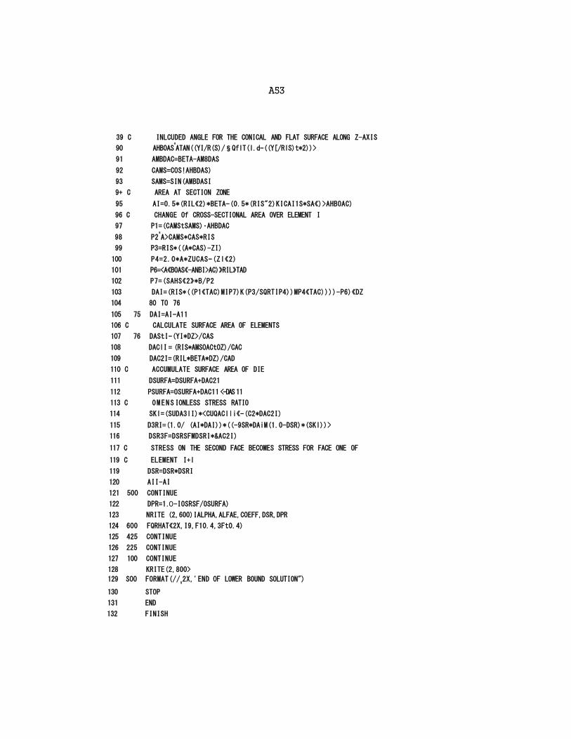
A53

39 C INLCUDED ANGLE FOR THE CONICAL AND FLAT SURFACE ALONG Z-AXIS

90 AHB0ASs

ATAN((YI/R(S)/§QflT(l.d-((Y[/RlS)t*2))>

91 AMBDAC=BETA-AM8DAS

92 CAMS=COS!AHBDAS)

93 SAMS=SIN(AMBDASI

9+ C AREA AT SECTION ZONE

95 AI=0.5*(RIL«2)*BETA-(0.5*(RIS"2)KICAI1S*SA«)>AHBOAC)

96 C CHANGE Of CROSS-SECTIONAL AREA OVER ELEMENT I

97 P1=(CAMStSAMS)•AHBDAC

98 P2s

A>CAMS*CAS*RIS

99 P3=RIS*((A*CAS)-ZI)

100 P4=2.0*A*ZUCAS-(Zl«2)

101 P6=<A«B0AS«-ANBI>AC)»RIL»TAD

102 P7=(SAHS«2»*B/P2

103 DAI=(RIS*((P1«TAC)MIP7)K(P3/SQRTIP4))MP4«TAC))))-P6)«DZ

104 80 TO 76

105 75 DAI=AI-A11

106 C CALCULATE SURFACE AREA OF ELEMENTS

107 76 DAStI-(YI*DZ>/CAS

108 DAClI = (RIS*AMSOACtOZ)/CAC

109 DAC2I=(RIL*BETA*DZ)/CAD

110 C ACCUMULATE SURFACE AREA OF DIE

111 DSURFA=DSURFA+DAC21

112 PSURFA=OSURFA+DAC11 <-DAS 11

113 C 0MENS IONLESS STRESS RATIO

114 SKl=(SUDA3lI)*<CUQAClli«-(C2*DAC2I)

115 D3RI=(1.0/ (AI*DAI))*((-9SR*DAiM(1.0-DSR)*(SKl))>

116 DSR3F=DSRSFMDSRI*&AC2I)

117 C STRESS ON THE SECOND FACE BECOMES STRESS FOR FACE ONE OF

119 C ELEMENT I+l

119 DSR=DSR*DSRI

120 AII-AI

121 500 CONTINUE

122 DPR=1.O-IOSRSF/OSURFA)

123 NRITE (2,600)IALPHA,ALFAE,COEFF,DSR,DPR

124 600 FQRHAT«2X,I9,F10.4,3Ft0.4)

125 425 CONTINUE

126 225 CONTINUE

127 100 CONTINUE

128 KRITE(2,800>

129 SOO FORMAT(//V2X,'END OF LOWER BOUND SOLUTION")

130 STOP

131 END

132 FINISH

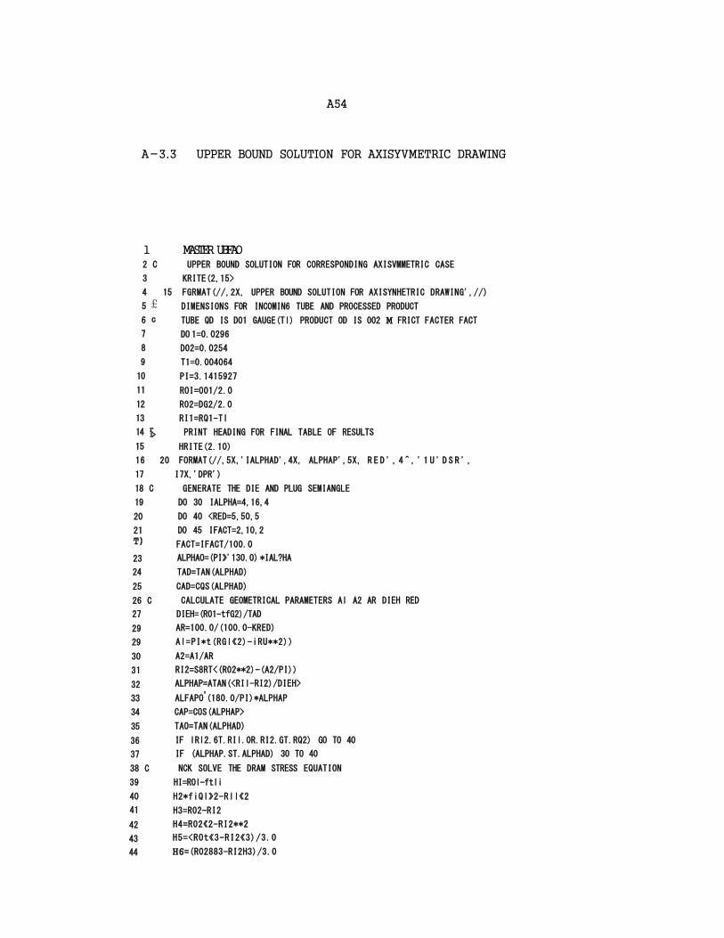
A54

A-3.3 UPPER BOUND SOLUTION FOR AXISYVMETRIC DRAWING

1 MASTER UBFAO 2 C UPPER BOUND SOLUTION FOR CORRESPONDING AXISVMMETRIC CASE

3 KRITE(2,15>

4 15 FGRMAT(//,2X, UPPER BOUND SOLUTION FOR AXISYNHETRIC DRAWING',//)

5 £ DIMENSIONS FOR INC0MIN6 TUBE AND PROCESSED PRODUCT

6 c TUBE QD IS D01 GAUGE(Tl) PRODUCT OD IS 002 M FRICT FACTER FACT

7 DO 1=0.0296

8 D02=0.0254

9 T1=0.004064

10 PI=3.1415927

11 ROI=001/2.0

12 R02=DG2/2.0

13 RI1=RQ1-Tl

14 r i> PRINT HEADING FOR FINAL TABLE OF RESULTS

15 HRITE(2.10)

16 20 FORMAT(//,5X,'IALPHAD',4X, ALPHAP',5X, R E D ' , 4 ^ , ' 1 U ' D S R ' ,

17 I7X,'DPR')

18 C GENERATE THE DIE AND PLUG SEMIANGLE

19 DO 30 IALPHA=4,16,4

20 DO 40 <RED=5,50,5

21 DO 45 IFACT=2,10,2 T) FACT=IFACT/100.0

23 ALPHAO=(PI»'130.0) *IAL?HA

24 TAD=TAN(ALPHAD)

25 CAD=CQS(ALPHAD)

26 C CALCULATE GEOMETRICAL PARAMETERS Al A2 AR DIEH RED

27 DIEH=(R01-tfG2)/TAD

29 AR=100.0/(100.0-KRED)

29 Al=PI*t(RGl«2)-iRU**2))

30 A2=A1/AR

31 RI2=S8RT<(R02**2)-(A2/PI))

32 ALPHAP=ATAN(<RIl-RI2)/DIEH>

33 ALFAPOs

(180.0/PI)*ALPHAP

34 CAP=COS(ALPHAP>

35 TAO=TAN(ALPHAD)

36 IF lRl2.6T.RIl.0R.RI2.GT.RQ2) GO TO 40

37 IF (ALPHAP.ST.ALPHAD) 30 TO 40

38 C NCK SOLVE THE DRAM STRESS EQUATION

39 HI=ROl-ftli

40 H2*fiQl»2-Rll«2

41 H3=R02-RI2

42 H4=R02«2-RI2**2

43 H5=<ROt«3-RI2«3)/3.0

44 H6=(R02883-RI2H3)/3.0

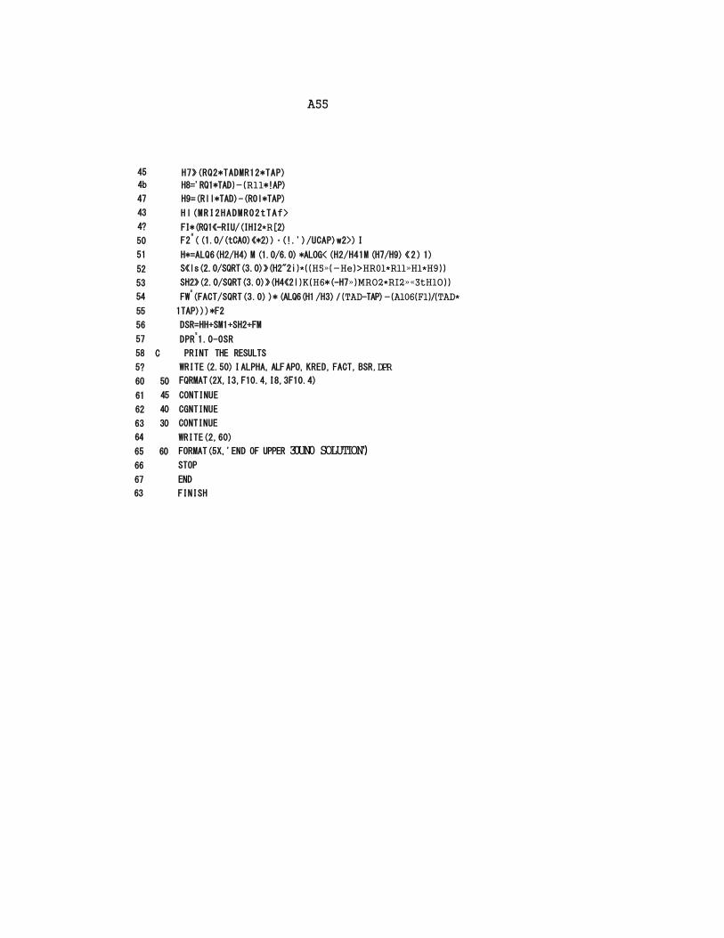
A55

45 H7»(RQ2*TADMR12*TAP)

4b H8='RQ1*TAD)-(R11*!AP)

47 H9=(Rll*TAD)-(R0l*TAP)

43 Hl(MRI2HADMR02tTAf>

4? FI*(RQ1«-RIU/(IHI2*R[2)

50 F2a

( (1.0/(tCA0)«*2)) •(!.')/UCAP)w2>) I

51 H*=ALQ6(H2/H4) M (1.0/6.0) *ALOG< (H2/H41M (H7/H9) « 2 ) 1)

52 S«ls(2.0/SQRT(3.0)»(H2"2i)*((H5»(-He)>HR0l*Rll»Hl*H9))

53 SH2»(2.0/SQRT(3.0)»(H4«2l)K(H6*(-H7»)MRO2*RI2»«3tHlO))

54 FWs

(FACT/SQRT(3.0) )* (ALQ6(H1 /H3) / (TAD-TAP)-(Al06(Fl)/(TAD*

55 1TAP)))*F2

56 DSR=HH+SM1+SH2+FM

57 DPRs

1.0-0SR

58 C PRINT THE RESULTS

5? WRITE (2.50) I ALPHA, ALF APO, KRED, FACT, BSR, DPR

60 50 FQRMAT(2X,I3,F10.4,I8,3F10.4)

61 45 CONTINUE

62 40 CGNTINUE

63 30 CONTINUE

64 WRITE(2,60)

65 60 FORMAT(5X,'END OF UPPER 30UN0 SOLUTION')

66 STOP

67 END

63 FINISH

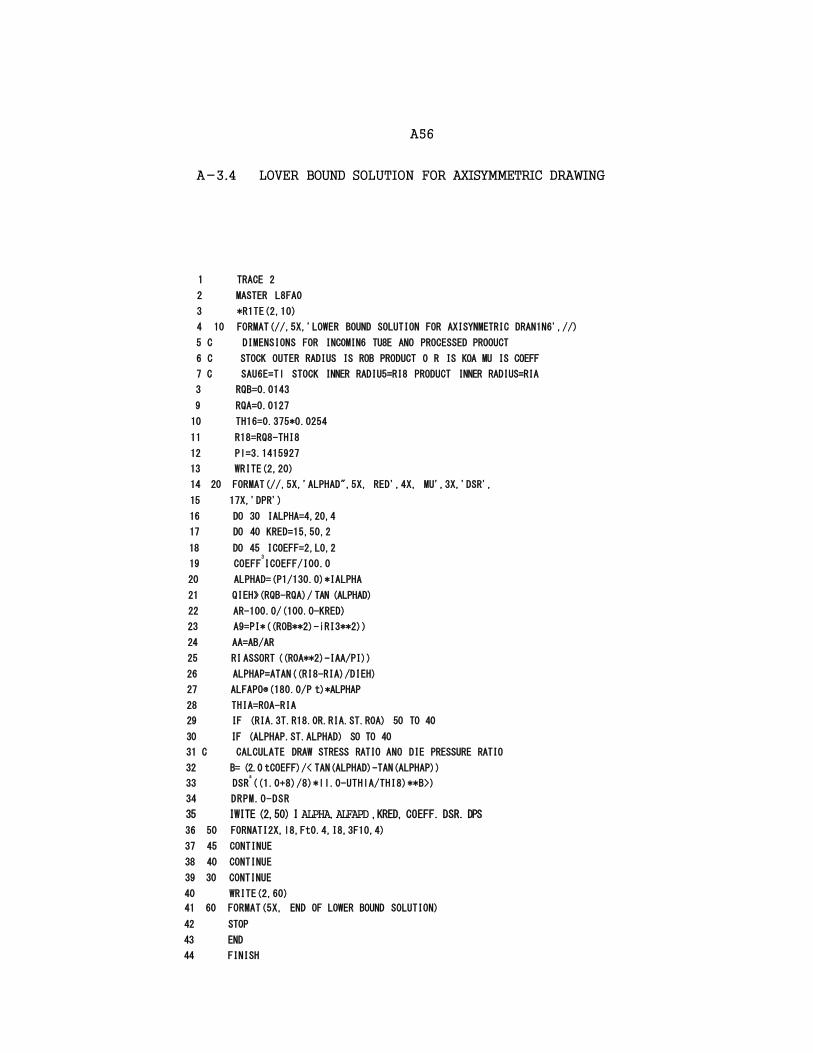
A56

A-3.4 LOVER BOUND SOLUTION FOR AXISYMMETRIC DRAWING

1 TRACE 2

2 MASTER L8FA0

3 *R1TE(2,10)

4 10 FORMAT(//,5X,'LOWER BOUND SOLUTION FOR AXISYNMETRIC DRAN1N6',//)

5 C DIMENSIONS FOR INC0MIN6 TU8E ANO PROCESSED PROOUCT

6 C STOCK OUTER RADIUS IS ROB PRODUCT 0 R IS KOA MU IS COEFF

7 C SAU6E=Tl STOCK INNER RADIU5=RI8 PRODUCT INNER RADIUS=RIA

3 RQB=0.0143

9 RQA=0.0127

10 TH16=0.375*0.0254

11 R18=RQ8-THI8

12 Pl=3.1415927

13 WRITE(2,20)

14 20 FORMAT(//,5X,'ALPHAD",5X, RED',4X, MU',3X,'DSR',

15 17X,'DPR')

16 DO 30 IALPHA=4,20,4

17 DO 40 KRED=15,50,2

18 DO 45 IC0EFF=2,L0,2

19 COEFF3

ICOEFF/I00.0

20 ALPHAD=(P1/130.0)*IALPHA

21 QIEH»(RQB-RQA)/ TAN (ALPHAD)

22 AR-100.0/(100.O-KRED)

23 A9=PI*((ROB**2)-iRI3**2))

24 AA=AB/AR

25 RI ASSORT ((R0A**2)-IAA/PI))

26 ALPHAP=ATAN((RI8-RIA)/DIEH)

27 ALFAPO®(180.0/P t)*ALPHAP

28 THIA=ROA-RIA

29 IF (RIA.3T.R18.0R.RIA.ST.R0A) 50 TO 40

30 IF (ALPHAP.ST.ALPHAD) SO TO 40

31 C CALCULATE DRAW STRESS RATIO ANO DIE PRESSURE RATIO

32 B= (2.0 tCOEFF)/< TAN(ALPHAD)-TAN(ALPHAP))

33 DSRs

((1.0+8)/8)*ll.0-UTHlA/THI8)**B>)

34 DRPM.O-DSR

35 IWITE (2,50) I ALPHA, ALFAPD ,KRED, COEFF. DSR. DPS

36 50 F0RNATI2X,l8,Ft0.4,I8,3F10,4)

37 45 CONTINUE

38 40 CONTINUE

39 30 CONTINUE

40 WRITE(2,60)

41 60 FORMAT(5X, END OF LOWER BOUND SOLUTION)

42 STOP

43 END

44 FINISH

A57

TABULATED SAMPLE SOLUTIONS OF THE UPPER AND

LOWER BOUND FOR POLYGONAL AND AXISYiWETRIC

DRAWING

A58

TABLE A-4.1.1 THE CPPER AND LOWER BOUND SOLUTIONS FOR THE

DRAWING OF HEXAGONAL TUBE FROM ROUND THROUGH A CYLINDRICAL DIE ON A POLYGONAL PLUG

INPUT TUBE SIZE: 28.6 rrm O.D. x 9.52 rrm THICKNESS REDUCTION OF AREA: 21.61% OUTPUT TUBE SIZE 25.4 rrm O.D.

/-v Upper bound Lower bound

0) M-d 3 w

a (V Mean draw .Vfean die Mean draw Mean die

r—t rH (J) a. a ;d a stress/yielc i pressure/ stress/yiel d pressure/ r—t

stress yield stress stress yield stress 1 I)

•r-t UJ Sbi MO

C t—i V hO 3 § > 1

-H 1) -U o a

(a /Y ) za' m

(p/Y) tn

(o /Y ) v za' nr

c

a 3 ffl

i ^

£ O

2 0.54 0.02 2.0661 3.9779 0.6077 0.9964 0.04 2.3101 2.8578 0.9416 0.9978 0.06 2.4587 2.2407 1.1501 0.9990 0.08 2.5648 1.8501 1.2298 0.9997 0.10 2.6484 1.5809 1.2309 1.0000

6 1.63 0.02 1.0401 3.1860 0.5314 0.9971 0.04 1.1411 2.7135 0.8204 0.9981 0.06 1.2194 2.3696 1.0749 0.9987

0.08 1.2833 2.1083 1.2701 0.9992

0.10 1.3374 1.9031 1.3971 0.9996

LO 2.73 0.02 0.3062 2.9125 0.5147 0.9973

0.04 0.8531 2.7252 0.7879 0.9982

0.06 0.3936 2.5635 1.0426 0.9987

0.08 0.9306 2.4226 1.2614 0.9991

0.10 0.9647 2.2987 1.4333 0.9994

L4 3.86 0.02 2.1694 7.4811 0.5073 0.9974

0.04 2.3269 6.7690 0.7728 0.9982

0.06 2.4614 6.1917 1.0260 0.9987

0.08 2.5789 5.7145 1.2538 0.9991

0.10 2.6837 5.3137 1.4467 0.9994

18 5.02 0.02 2.4043 8.7732 0.5031 0.9974

0.04 2.5088 8.3968 0.7641 0.9983

0.06 2.6064 8.0570 1.0159 0.9987

0.08 2.6983 7.7488 1.2484 0.9991

0.10 2.7853 7.4681 1.4533 0.9993

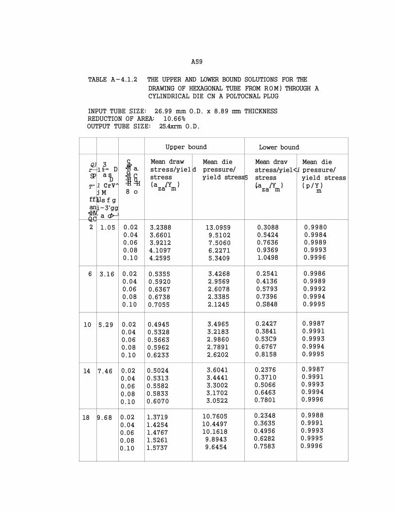
A59

TABLE A-4.1.2 THE UPPER AND LOWER BOUND SOLUTIONS FOR THE

DRAWING OF HEXAGONAL TUBE FROM ROM) THROUGH A CYLINDRICAL DIE CN A POLTOCNAL PLUG

INPUT TUBE SIZE: 26.99 mm O.D. x 8.89 rrm THICKNESS REDUCTION OF AREA: 10.66% OUTPUT TUBE SIZE: 25.4xrm O.D.

Upper bound Lower bound

Q) r—1 SP

T"

ffll an •iHV. QC

3 i—» D a s

D 1 CrV^

j M i s f g i-3'gg a c/>—'

c a> •H a. o •H C «H 0 «H -H

8 o

Mean draw

stress/yiel stress (a /Y )

za' m

Mean die d pressure/

yield stress

Mean drav

stress/yiel< 5 stress

(a /Y ) v za' m

Mean die

i pressure/

yield stress

( p / Y ) m

2 1.05 0.02 0.04 0.06 0.08 0.10

3.2388 3.6601 3.9212 4.1097 4.2595

13.0959 9.5102 7.5060 6.2271 5.3409

0.3088 0.5424 0.7636 0.9369 1.0498

0.9980 0.9984 0.9989 0.9993 0.9996

6 3.16 0.02 0.04 0.06 0.08 0.10

0.5355 0.5920 0.6367 0.6738 0.7055

3.4268 2.9569 2.6078 2.3385 2.1245

0.2541 0.4136 0.5793 0.7396 O.S848

0.9986 0.9989 0.9992 0.9994 0.9995

10 5.29 0.02 0.04 0.06 0.08 0.10

0.4945 0.5328 0.5663 0.5962 0.6233

3.4965 3.2183 2.9860 2.7891 2.6202

0.2427 0.3841 0.53C9 0.6767 0.8158

0.9987 0.9991 0.9993 0.9994 0.9995

14 7.46 0.02 0.04 0.06 0.08 0.10

0.5024 0.5313 0.5582 0.5833 0.6070

3.6041 3.4441 3.3002 3.1702 3.0522

0.2376 0.3710 0.5066 0.6463 0.7801

0.9987 0.9991 0.9993 0.9994 0.9996

18 9.68 0.02 0.04 0.06 0.08 0.10

1.3719 1.4254 1.4767 1.5261 1.5737

10.7605 10.4497 10.1618 9.8943 9.6454

0.2348 0.3635 0.4956 0.6282 0.7583

0.9988 0.9991 0.9993 0.9995 0.9996

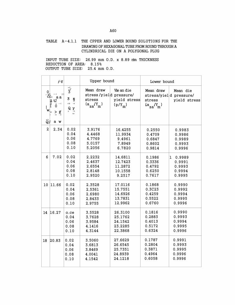
A60

TABLE A-4.1.1 THE CPPER AND LOWER BOUND SOLUTIONS FOR THE

DRAWING OF HEXAGONAL TUBE FROM ROUND THROUGH A CYLINDRICAL DIE ON A POLYGONAL PLUG

INPUT TUBE SIZE: 26.99 mm O.D. x 8.89 rim THICKNESS REDUCTION OF AREA: 8.15% OUTPUT TUBE SIZE: 25.4 mm O.D.

/—V Upper bound Lower bound

0 r - t &

| w.

• H

Qi

r - t (1)

- a a ii tJ 1 C — t

I 0

> f « i I - H - H

: a w

• P rf 3

3 = ^ § « M - H

Q y 0 - H

tn

Mean draw

stress /yiel

stress (a /Y )

za' m

Vie an die

d pressure/

yield stress

(p/Y ) m

Mean draw

stress/yiel stress (a /Y ) v za' m

Mean die

d pressure/

yield stress

2 2.34 0.02 0.04 0.06 0.08 0.10

3.9176 4.4468 4.7769 5.0157 5.2056

16.4255 11.9934 9.4961 7.8949 6.7820

0.2550 0.4709 0.6847 0.8602 0.9814

0.9983 0.9986 0.9989 0.9993 0.9996

6 7.02 0.02 0.04 0.06 0.08 0.10

2.2232 2.4637 2.6554 2.8148 2.9520

14.6811 12.7423 11.2872 10.1558 9.2517

0.1986 0.3336 0.4792 0.6250 0.7617

1 0.9989 0.9991 0.9993 0.9994 0.9995

10 11.66 0.02 0.04 0.06 0.08 0.10

2.3528 2.5361 2.6980 2.8433 2.9755

17.0116 15.7551 14.6926 13.7831 12.9962

0.1868 0.3C23 0.4259 0.5522 0.6760

0.9990 0.9992 0.9994 0.9995 0.9996

14 16.27 o.ce 0.04 0.06 0.08 0.10

3.5528 3.7628 3.9584 4.1416 4.3144

26.3100 25.1762 24.1542 23.2285 22.3868

0.1816 0.2883 0.4013 0.5172 0.6324

0.9990 0.9993 0.9994 0.9995 0.9996

18 20.83 0.02 0.04 0.06 0.08 0.10

3.5060 3.6813 3.8469 4.0041 4.1542

27.6629 26.6545 25.7351 24.8939 24.1218

0.1787 0.2804 0.3871 0.4964 0.6058

0.9991 0.9993 0.9995 0.9996 0.9996

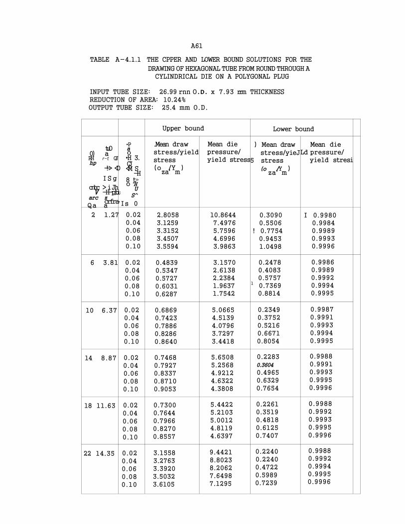
A61

TABLE A-4.1.1 THE CPPER AND LOWER BOUND SOLUTIONS FOR THE

DRAWING OF HEXAGONAL TUBE FROM ROUND THROUGH A CYLINDRICAL DIE ON A POLYGONAL PLUG

INPUT TUBE SIZE: 26.99 rnn O . D . x 7.93 rrm THICKNESS REDUCTION OF AREA: 10.24% OUTPUT TUBE SIZE: 25.4 mm O.D.

Upper bound Lower bound

tuO 0) a RH r-t OJ hp

-!-> <D

I S g

cnbc > i Jh V -H-pjbi

arc z crfra

Qa a

•P a o •H 3. CJ <M S

-H 8 t» o 'H

U 3 S^

' Is 0

.Mean draw stress/yield stress (o /Y )

za' m

Mean die pressure/ yield stress

) Mean draw

stress/yieJ 5 stress

(o /Y ) za' m

Mean die Ld pressure/

yield stresi

2 1.27 0.02 0.04 0.06 0.08 0.10

2.8058 3.1259 3.3152 3.4507 3.5594

10.8644 7.4976 5.7596 4.6996 3.9863

0.3090 0.5506

! 0.7754 0.9453 1.0498

I 0.9980 0.9984 0.9989 0.9993 0.9996

6 3.81 0.02 0.04 0.06 0.08 0.10

0.4839 0.5347 0.5727 0.6031 0.6287

3.1570 2.6138 2.2384 1.9637 1.7542

0.2478 0.4083 0.5757

1 0.7369 0.8814

0.9986 0.9989 0.9992 0.9994 0.9995

10 6.37 0.02 0.04 0.06 0.08 0.10

0.6869 0.7423 0.7886 0.8286 0.8640

5.0665 4.5139 4.0796 3.7297 3.4418

0.2349 0.3752 0.5216 0.6671 0.8054

0.9987 0.9991 0.9993 0.9994 0.9995

14 8.87 0.02 0.04 0.06 0.08 0.10

0.7468 0.7927 0.8337 0.8710 0.9053

5.6508 5.2568 4.9212 4.6322 4.3808

0.2283 0.3604

0.4965 0.6329 0.7654

0.9988 0.9991 0.9993 0.9995 0.9996

18 11.63 0.02 0.04 0.06 0.08 0.10

0.7300 0.7644 0.7966 0.8270 0.8557

5.4422 5.2103 5.0012 4.8119 4.6397

0.2261 0.3519 0.4818 0.6125 0.7407

0.9988 0.9992 0.9993 0.9995 0.9996

22 14.35 0.02 0.04 0.06 0.08 0.10

3.1558 3.2763 3.3920 3.5032 3.6105

9.4421 8.8023 8.2062 7.6498 7.1295

0.2240 0.2240 0.4722 0.5989 0.7239

0.9988 0.9992 0.9994 0.9995 0.9996

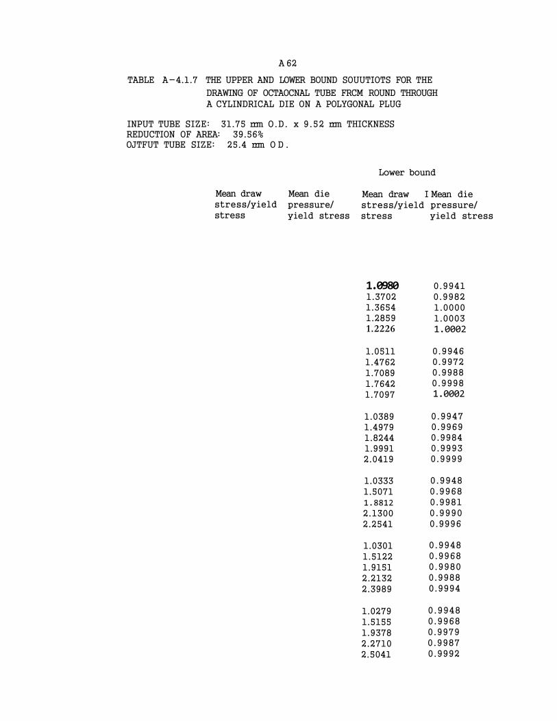
A 62

TABLE A-4.1.7 THE UPPER AND LOWER BOUND SOUUTIOTS FOR THE

DRAWING OF OCTAOCNAL TUBE FRCM ROUND THROUGH

A CYLINDRICAL DIE ON A POLYGONAL PLUG

INPUT TUBE SIZE: 31.75 rrm O.D. x 9.52 rrm THICKNESS REDUCTION OF AREA: 39.56% OJTFUT TUBE SIZE: 25.4 rrm O D .

Mean draw stress/yield stress

Mean die pressure/ yield stress

Lower bound

Mean draw I Mean die stress/yield pressure/ stress yield stress

1.0980 1.3702 1.3654 1.2859 1.2226

0.9941 0.9982 1.0000 1.0003 1.0002

1.0511 1.4762 1.7089 1.7642 1.7097

0.9946 0.9972 0.9988 0.9998 1.0002

1.0389 1.4979 1.8244 1.9991 2.0419

0.9947 0.9969 0.9984 0.9993 0.9999

1.0333 1.5071 1.8812 2.1300 2.2541

0.9948 0.9968 0.9981 0.9990 0.9996

1.0301 1.5122 1.9151 2.2132 2.3989

0.9948 0.9968 0.9980 0.9988 0.9994

1.0279 1.5155 1.9378 2.2710 2.5041

0.9948 0.9968 0.9979 0.9987 0.9992

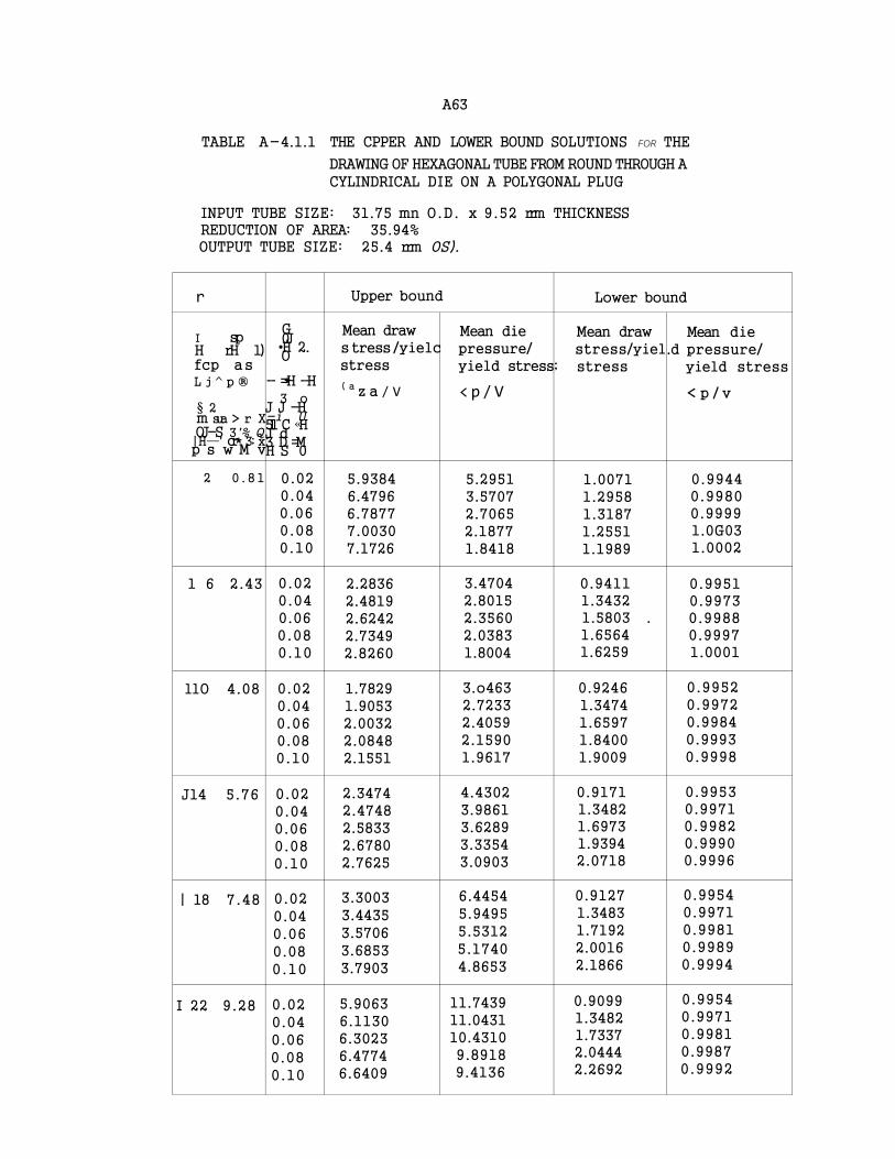
A63

TABLE A-4.1.1 THE CPPER AND LOWER BOUND SOLUTIONS FOR THE

DRAWING OF HEXAGONAL TUBE FROM ROUND THROUGH A CYLINDRICAL DIE ON A POLYGONAL PLUG

INPUT TUBE SIZE: 31.75 mn O.D. x 9.52 rrm THICKNESS REDUCTION OF AREA: 35.94% OUTPUT TUBE SIZE: 25.4 rrm OS).

r Upper bound Lower bound

I sp H rH 1) fcp as L j ^ p ®

§ 2 m sua > r X OJ-S 3'% Q |H—' cr* 3; x p s w M v

G 0J •H 2. O

- =*H -H 3 o

J J -H -i U 5ll C «H J d 3 D =M H S 0

Mean draw s tress /yielc stress

( a z a / V

Mean die pressure/ yield stress

<p/V

Mean draw stress/yiel

; stress

Mean die .d pressure/

yield stress

< p / v

2 0 . 8 1 0.02 0.04 0.06 0.08 0.10

5.9384 6.4796 6.7877 7.0030 7.1726

5.2951 3.5707 2.7065 2.1877 1.8418

1.0071 1.2958 1.3187 1.2551 1.1989

0.9944 0.9980 0.9999 1.0G03 1.0002

1 6 2.43 0.02 0.04 0.06 0.08 0.10

2.2836 2.4819 2.6242 2.7349 2.8260

3.4704 2.8015 2.3560 2.0383 1.8004

0.9411 1.3432 1.5803 . 1.6564 1.6259

0.9951 0.9973 0.9988 0.9997 1.0001

llO 4.08 0.02 0.04 0.06 0.08 0.10

1.7829 1.9053 2.0032 2.0848 2.1551

3.o463 2.7233 2.4059 2.1590 1.9617

0.9246 1.3474 1.6597 1.8400 1.9009

0.9952 0.9972 0.9984 0.9993 0.9998

J14 5.76 0.02 0.04 0.06 0.08 0.10

2.3474 2.4748 2.5833 2.6780 2.7625

4.4302 3.9861 3.6289 3.3354 3.0903

0.9171 1.3482 1.6973 1.9394 2.0718

0.9953 0.9971 0.9982 0.9990 0.9996

| 18 7.48 0.02 0.04 0.06 0.08 0.10

3.3003 3.4435 3.5706 3.6853 3.7903

6.4454 5.9495 5.5312 5.1740 4.8653

0.9127 1.3483 1.7192 2.0016 2.1866

0.9954 0.9971 0.9981 0.9989 0.9994

I 22 9.28 0.02 0.04 0.06 0.08 0.10

5.9063 6.1130 6.3023 6.4774 6.6409

11.7439 11.0431 10.4310 9.8918 9.4136

0.9099 1.3482 1.7337 2.0444 2.2692

0.9954 0.9971 0.9981 0.9987 0.9992

A 64

TABLE A-4.1.7 THE UPPER AND LOWER BOUND SOUUTIOTS FOR THE

DRAWING OF OCTAOCNAL TUBE FRCM ROUND THROUGH A CYLINDRICAL DIE ON A POLYGONAL PLUG

INPUT TUBE SIZE: 37.75 rrm O.D. x 9.52 am THICKNESS REDUCTION OF AREA: 40.96% OUTPUT TUEE SIZE: 25.4 rrm O.D.

-

•M C

Upper bound Lower bound

0 l—l sp

1 0 •H '

l t :

•Hv. Q fi

d rH U a a

N JJ (J)

13M (i^Q

I > i S •H -H b

;d a

«M S VH IH Q O 0 -H

in

i1-<U =M

- S 0

Mean draw

stress/yield stress (a /Y )

za' nr

Mean die pressure/ yield stress

( p / V m

Mean draw s tress/yiel< stress (a /Y )

za' m

Mean die i pressure/

yield stress (p/Y )

m

2 0.20 0.02 0.04 0.06 0.08 0.10

2.4639 2.6750 2.7946 2.8780 2.9436

1.9868 1.3357 1.0107 0.8159 0.6862

1.1341 1.3992 1.3834 1.2977 1.2319

0.9940 0.9982 1.00C1 1.0003 1.0002

6 0.62 0.02 0.04 0.06 0.08 0.10

0.8747 0.9463 0.9974 1.0370 1.0695

1.2001 0.9650 0.8094 0.6988 0.6162

1.0951 1.5290 1.7594 1.8062 1.7420

0.9944 0.9971 0.9988 0.9998 1.0002

10 1.03 0.02 0.04 0.06 0.08 0.10

0.7882 0.8306

0.8805 0.9143 0.9434

1.2627 1.0871 0.9565 0.8556 0.7753

1.0848 1.5581 1.8897 2.0617 2.0969

0.9945 0.9968 0.9983 0.9993 0.9999

14 1.46 0.02 0.04 0.06 0.08 0.10

0.7574 0.7971 0.8305 0.8595 0.8852

1.3125 1.1725 1.0612 0.9708 0.8959

1.0800 1.5708 1.9545 2.2055 2.3258

0.9946 0.9967 0.9981 0.9990 0.9996

18 1.90 0.02 0.04 0.06 0.08 0.10

0.7445 0.7763 0.8042 0.8291 0.8518

1.3567 1.2410 1.1451 1.G643 0.9953

1.0772 1.5779 1.9933 2.2973 2.4828

0.9946 0.9967 0.9979 0.9988 0.9994

22 2.37 0.02 0.04 0.06 0.08 0.10

0.7388 0.7648 0.7883 O.8C09 0.8298

1.3976 1.3002 1.2168 1.1447 1.0817

1.0754 1.5826 2.0194 2.3613 2.5972

0.9946 0.9966 0.9978 0.9986 0.9992

A65

TABLE A-4 .1.8 THE tPPER AND LOWER BOUND SOLUTIONS FOR THE

DRAWING OF OCTAGONAL TUBE FRCM ROUND THROUGH A CYLINDRICAL DIE ON A POLYGONAL PLUG

INPUT TUBE SIZE: 26.99 inn O.D. x 8.89 rrm THICKNESS REDUCTION OF AREA: 11.63% CUIPUT TUBE SIZE: 25.4 run O.D.

<D % a co

a 3 33 tuo

ICQ a; TJ

<D •ni 2 3

<D tbOTJ 3 rH a a -uj 0) S -I

3 SP

2 f •H -H

I I

C 0)

• H 3 . y :H S a-, O

-H 8tS O -H

U

CD « h s o

Upper bound

Mean draw stress/yield stress

« W V

Mean die pressure/ yield stress

<P/*m> m

Lower bound

Mean dray/ LMean die stress/yield pressure/ stress yield stress

« W < p / V

0.59 0.02 0.04 0.06 0.08 0.10

1.9488 2.2017 2.3587 2.4721 2.5621

7.7633 5.0491 4.4634 3.7053 3.1793

0.3300 0.5704 0.7942 0.9666 1.0762

0.9979 0.9984 0.9989 0.9993 0.9996

1.78 0.02 0.04 0.06 0.08 0.10

0.5471 0.6044 0.6498 0.6874 0.7196

3.4408 2.9708 2.6214 2.3515 2.1369

0.2760 0.4451 0.6185 0.7844 0.9329

0.9985 0.9989 0.9991 0.9993 0.9995

10 2.99 0.02 0.04 0.06 0.08 0.10

0.4234 0.4560 0.4845 0.5100 0.5330

2.9498 2.7135 2.5163 2.3493 2.2063

0.2646 0.4163 0.5721 0.7255 0.8705

0.9986 0.9990 0.9992 0.9994 0.9995

14 4.22 0.02 0.04 0.06 0.08 0.10

0.4928 0.5211 0.5475 0.5721 0.5952

3.4992 3.3397 3.1966 3.0676 2.9509

0.2597 0.4035 0.5507 0.6969 0.8380

0.9986 0.9990 0.9993 0.9994 0.9995

18 5.501 0.02 0.04 0.06 0.08 0.10

0.7526

0.7856

0.8174

0.8480

0.8776

5.2569 5.1423 5.0336 4.9306 4.8327

0.2569 0.3961 0.5383 0.6800 0.8181

0.9987 0.9991 0.9993 0.9994 0.9995

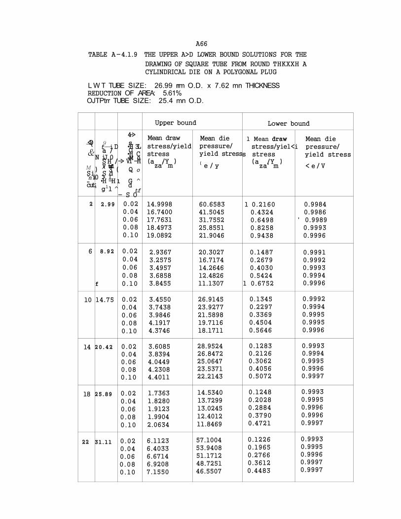
A66

TABLE A-4.1.9 THE UPPER A>D LOWER BOUND SOLUTIONS FOR THE

DRAWING OF SQUARE TUBE FROM ROUND THKXXH A CYLINDRICAL DIE ON A POLYGONAL PLUG

L W T TUBE SIZE: 26.99 rrm O.D. x 7.62 mn THICKNESS REDUCTION OF .AREA: 5.61% OJTPtrr TUBE SIZE: 25.4 mn O.D.

Upper bound Lower bound

<D —(

&

M Si 'n i „ 1

cut:

9 t—i D a /

N iJ 0 S H / V tsfl

) ^ 3 ( S d

0 > 1 •H -H 1

' g11 ^

4->

s •H 3L O •H C «M 0

-> Vi -H

Q o

G ^ d

tf - S O

Mean draw

stress/yield stress (a /Y )

za/ m

Mean die pressure/ yield stress

( e / y

1 Mean draw

stress/yiel< s stress

(a /Y ) za' m

Mean die i pressure/

yield stress

< e / V

2 2 . 9 9 0.02 0.04 0.06 0.08 0.10

14.9998 16.7400 17.7631 18.4973 19.0892

60.6583 41.5045 31.7552 25.8551 21.9046

1 0.2160 0.4324 0.6498 0.8258 0.9438

0.9984 0.9986

' 0.9989 0.9993 0.9996

6 8 . 9 2

f

0.02

0.04

0.06

0.08

0 .10

2.9367 3.2575 3.4957 3.6858 3.8455

20.3027 16.7174 14.2646 12.4826 11.1307

0.1487 0.2679 0.4030 0.5424

1 0.6752

0.9991 0.9992 0.9993 0.9994 0.9996

10 14.75 0.02 0.04 0.06 0.08 0.10

3.4550 3.7438 3.9846 4.1917 4.3746

26.9145 23.9277 21.5898 19.7116 18.1711

0.1345 0.2297 0.3369 0.4504 0.5646

0.9992 0.9994 0.9995 0.9995 0.9996

14 2 0 . 4 2 0.02 0.04 0.06 0.08 0.10

3.6085 3.8394 4.0449 4.2308 4.4011

28.9524 26.8472 25.0647 23.5371 22.2143

0.1283 0.2126 0.3062 0.4056 0.5072

0.9993 0.9994 0.9995 0.9996 0.9997

18 25 . 89 0.02 0.04 0.06 0.08 0.10

1.7363 1.8280 1.9123 1.9904 2.0634

14.5340 13.7299 13.0245 12.4012 11.8469

0.1248 0.2028 0.2884 0.3790 0.4721

0.9993 0.9995 0.9996 0.9996 0.9997

22 31 .11 0.02 0.04 0.06 0.08 0.10

6.1123 6.4033 6.6714 6.9208 7.1550

57.1004 53.9408 51.1712 48.7251 46.5507

0.1226 0.1965 0.2766 0.3612 0.4483

0.9993 0.9995 0.9996 0.9997 0.9997

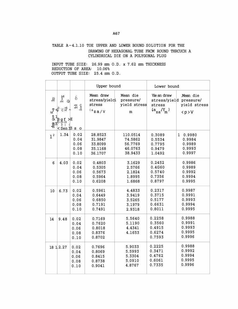
A67

TABLE A-4.1.10 TOE UPPER AND LOWER BOUND SOLUTION FOR THE

DRAWING OF HEXAGONAL TUBE FRCM ROUND THRCUCH A CYLINDRICAL DIE ON A POLYGONAL PLUG

INPUT TUBE SIZE: 26.99 rrm O.D. x 7.62 rrm THICKNESS REDUCTION OF AREA: 10.06% OUTPUT TUBE SIZE: 25.4 rrm O.D.

Upper bound Lower bound

0) rH

T < M 5 1 CA ®3 •H

bfl 3 . „ rH QJ .0 ->-> <1) p C H ^

B g f > D-H-H - 3 | ( < Sen 3

c ©

•H C «H 0 - -H

E

3 s o

Mean draw stress/yielc stress

( a z a / V

Mean die i pressure/

yield stress

m

Vie an draw

stress/yiel stress (a /Y ) v za' m

.Mean die d pressure/

yield stress

<p>V

l 2 1.34 0.02 0.04 0.06 0.08 0.10

28.8523 31.9847 33.8099 35.1168 36.1707

110.0514 74.5862 56.7769 46.0763 38.9433

0.3089 0.5534 0.7795 0.9479 1.0492

1 0.9980 0.9984 0.9989 0.9993 0.9997

6 4.03 0.02 0.04 0.06 0.08 0.10

0.4803 0.5305 0.5673 0.5964 0.6208

3.1629 2.5766 2.1824 1.8995 1.6868

0.2452 0.4G60 0.5740 0.7356 0.8797

0.9986 0.9989 0.9992 0.9994 0.9995

10 6.73 0.02 0.04 0.06 0.08 0.10

0.5961 0.6449 0.6850 0.7191 0.7491

4.4833 3.9419 3.5265 3.1979 2.9318

0.2317 0.3715 0.5177 0.6631 0.8011

0.9987 0.9991 0.9993 0.9994 0.9995

14 9.48 0.02 0.04 0.06 0.08 0.10

0.7169 0.7620 0.8018 0.8376 0.8702

5.5640 5.1190 4.4341 4.1653

0.2258 0.3560 0.4915 0.6274 0.7593

0.9988 0.9991 0.9993 0.9995 0.9996

18 1 .2.27 0.02 0.04 0.06 0.08 0.10

0.7696 0.8069 0.8415 0.8738 0.9041

5.9033 5.5993 5.3304 5.0910 4.8767

0.2225 0.3471 0.4762 0.6061 0.7335

0.9988 0.9992 0.9994 0.9995 0.9996

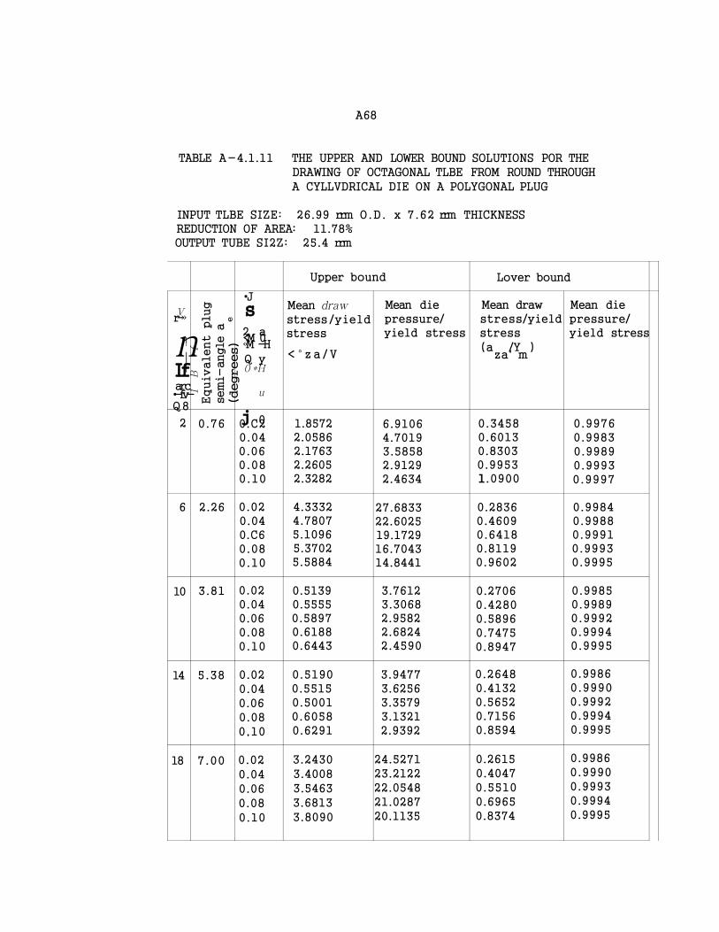
A68

TABLE A-4.1.11 THE UPPER AND LOWER BOUND SOLUTIONS POR THE DRAWING OF OCTAGONAL TLBE FROM ROUND THROUGH

A CYLLVDRICAL DIE ON A POLYGONAL PLUG

INPUT TLBE SIZE: 26.99 rrm O.D. x 7.62 rrm THICKNESS REDUCTION OF AREA: 11.78% OUTPUT TUBE SI2Z: 25.4 rrm

Upper bound Lover bound

V r-»

n If arc •-fv-Q8

1

B

f Equiv

alent plu

g

sem

i-angle

a

(degrees)

e

•J

s 2 a <M 0 «M -H

Q y 0 *H

u

j 0

Mean draw stress /yield stress

< ° z a / V

Mean die pressure/ yield stress

Mean draw stress/yield stress

(a /Y ) za' m

Mean die pressure/ yield stress

2 0.76 0.C2 0.04 0.06 0.08 0.10

1.8572 2.0586 2.1763 2.2605 2.3282

6.9106 4.7019 3.5858 2.9129 2.4634

0.3458 0.6013 0.8303 0.9953 1.0900

0.9976 0.9983 0.9989 0.9993 0.9997

6 2.26 0.02 0.04 0.C6 0.08 0.10

4.3332 4.7807 5.1096 5.3702 5.5884

27.6833 22.6025 19.1729 16.7043 14.8441

0.2836 0.4609 0.6418 0.8119 0.9602

0.9984 0.9988 0.9991 0.9993 0.9995

10 3.81 0.02 0.04 0.06 0.08 0.10

0.5139 0.5555 0.5897 0.6188 0.6443

3.7612 3.3068 2.9582 2.6824 2.4590

0.2706 0.4280 0.5896 0.7475 0.8947

0.9985 0.9989 0.9992 0.9994 0.9995

14 5.38 0.02 0.04 0.06 0.08 0,10

0.5190 0.5515 0.5001 0.6058 0.6291

3.9477 3.6256 3.3579 3.1321 2.9392

0.2648 0.4132 0.5652 0.7156 0.8594

0.9986 0.9990 0.9992 0.9994 0.9995

18 7.00 0.02

0.04

0.06

0.08

0.10

3.2430

3.4008

3.5463

3.6813

3.8090

24.5271 23.2122 22.0548 21.0287 20.1135

0.2615 0.4047 0.5510 0.6965 0.8374

0.9986 0.9990 0.9993 0.9994 0.9995

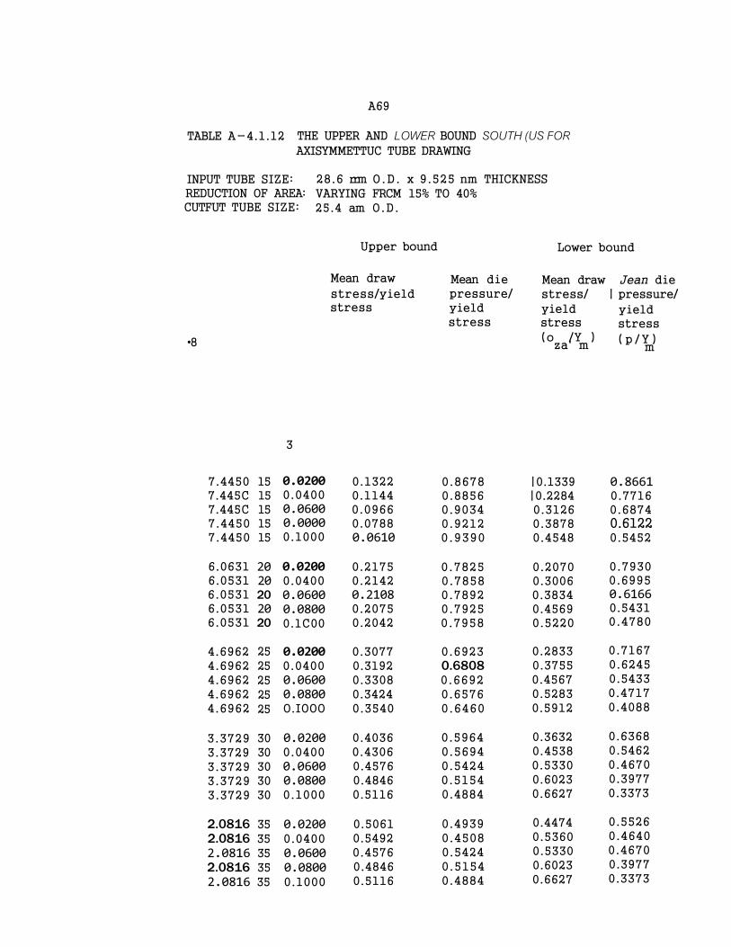
A69

TABLE A-4.1.12 THE UPPER AND LOWER BOUND SOUTH (US FOR AXISYMMETTUC TUBE DRAWING

INPUT TUBE SIZE: REDUCTION OF AREA: CUTFUT TUBE SIZE:

28.6 rrm O.D. x 9.525 nm THICKNESS VARYING FRCM 15% TO 40% 25.4 am O.D.

Upper bound Lower bound

•8

Mean draw

stress/yield stress

Mean die pressure/ yield stress

Mean draw Jean die stress/ | pressure/

yield stress

(o /Y ) za' m

yield stress

( p / Y ) m

3

7.4450 7.445C 7.445C 7.4450 7.4450

15 15 15 15 15

0.0200 0.0400 0.0600 0.0000 0.1000

0.1322 0.1144 0.0966 0.0788 0.0610

0.8678 0.8856 0.9034 0.9212 0.9390

|0.1339 |0.2284 0.3126 0.3878 0.4548

0.8661 0.7716 0.6874 0.6122 0.5452

6.0631 6.0531 6.0531 6.0531 6.0531

20 20 20 20 20

0.0200 0.0400 0.0600 0.0800 0.1C00

0.2175 0.2142 0.2108 0.2075 0.2042

0.7825 0.7858 0.7892 0.7925 0.7958

0.2070 0.3006 0.3834 0.4569 0.5220

0.7930 0.6995 0.6166 0.5431 0.4780

4.6962 4.6962 4.6962 4.6962 4.6962

25 25 25 25 25

0.0200 0.0400 0.0600 0.0800 O.IOOO

0.3077 0.3192 0.3308 0.3424 0.3540

0.6923 0.6808 0.6692 0.6576 0.6460

0.2833 0.3755 0.4567 0.5283 0.5912

0.7167 0.6245 0.5433 0.4717 0.4088

3.3729 3.3729 3.3729 3.3729 3.3729

30 30 30 30 30

0.0200 0.0400 0.0600 0.0800 0.1000

0.4036 0.4306 0.4576 0.4846 0.5116

0.5964 0.5694 0.5424 0.5154 0.4884

0.3632 0.4538 0.5330 0.6023 0.6627

0.6368 0.5462 0.4670 0.3977 0.3373

2.0816 2.0816 2.0816 2.0816 2.0816

35 35 35 35 35

0.0200 0.0400 0.0600 0.0800 0.1000

0.5061 0.5492 0.4576 0.4846 0.5116

0.4939 0.4508 0.5424 0.5154 0.4884

0.4474 0.5360 0.5330 0.6023 0.6627

0.5526 0.4640 0.4670 0.3977 0.3373

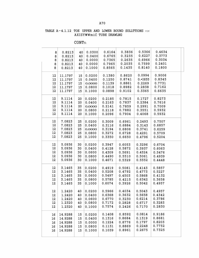
A70

TABLE A-4.1.12 TOE UPPER AND LOWER BOUND SOLLTTIONS FOR AXISY\WmiC TUBE DRAWLNG

CONT'D.

8 0.8213 40 0.0300 0.6164 0.3836 0.5366 0.4634

8 0.8213 40 0.0400 0.6765 0.3235 0.6227 0.3773

8 0.8213 40 0.0000 0.7365 0.2635 0.6966 0.3034

8 0.8213 40 0.0000 0.7965 0.2035 0.7599 0.2401

8 0.8213 40 0.1000 0.8565 0.1435 0.8140 0.1800

12 11.1797 15 0.0200 0.1380 0.8620 0.0994 0.9006

12 11.1797 15 0.0400 0.1250 0.8741 0.*I655 0.8345

12 11.1797 15 0.0000 0.1139 0.8861 0.2269 0.7731 12 11.1797 15 0.0800 0.1018 0.8982 0.2838 0.7162

12 11.1797 15 0.1000 0.0898 0.9102 0.3365 0.6635

12 9.1114 20 0.0200 0.2185 0.7815 0.1727 0.8273 12 9.1114 20 0.0400 0.2163 0.7837 0.2384 0.7616 12 9.1114 20 0.0000 0.2141 0.7859 0.2991 0.7009 12 9.1114 20 0.0800 0.2118 0.7882 0.3551 0.5932 12 9.1114 20 0.1000 0.2096 0.7904 0.4068 0.5932

12 7.0823 25 0.0200 0.3009 0.6961 0.2493 0.7507 12 7.0823 25 0.0400 0.3116 0.6884 0.3143 0.6857 12 7.0823 25 0.0000 0.3194 0.6806 0.3741 0.6259 12 7.0823 25 0.0800 0.3272 0.6728 0.4291 0.5709 12 7.0823 25 0.1000 0.3350 0.6650 0.4796 0.5204

12 5.0936 30 0.0200 0.3947 0.6053 0.3296 0.6704 12 5.0936 30 0.0400 0.4128 0.5872 0.3937 0.6063 12 5.0936 30 0.0600 0.4309 0.5691 0.4524 0.5476 12 5.0936 30 0.0800 0.4490 0.5510 0.5061 0.4939 12 5.0936 30 0.1000 0.4671 0.5329 0.5552 0.4448

12 3.1465 35 0.0200 0.4919 0.5081 0.4143 0.5857 12 3.1465 35 0.0400 0.5208 0.4792 0.4773 0.5227 12 3.1465 35 0.0600 0.5497 0.4503 0.5868 0.4132 12 3.1465 35 0.0800 0.5785 0.4215 0.6342 0.3658 12 3.1465 35 0.1000 0.6074 0.3926 0.5042 0.4957

12 1.2420 40 0.0200 0.5966 0.4034 0.5043 0.4957

12 1.2420 40 0.0400 0.6368 0.3632 0.5658 0.4342

12 1.2420 40 0.0600 0.6770 0.3230 0.6214 0.3786

12 1.2320 40 0.0800 0.7172 0.2828 0.6717 0.3283

12 1.2320 40 0.1000 0.7574 0.2426 0.7170 0.2830

16 14.9288 15 0.0200 0.1408 0.8592 0.0814 0.9186

16 14.9288 15 0.0400 0.1316 0.8684 0.1319 0.8681

16 14.9288 15 0.0000 0.1224 0.8776 0.1797 0.8203

16 14.9288 15 0.0800 0.1131 0.8869 0.2248 0.7752

16 14.9288 15 0.1000 0.1039 0.8961 0.2675 0.7325

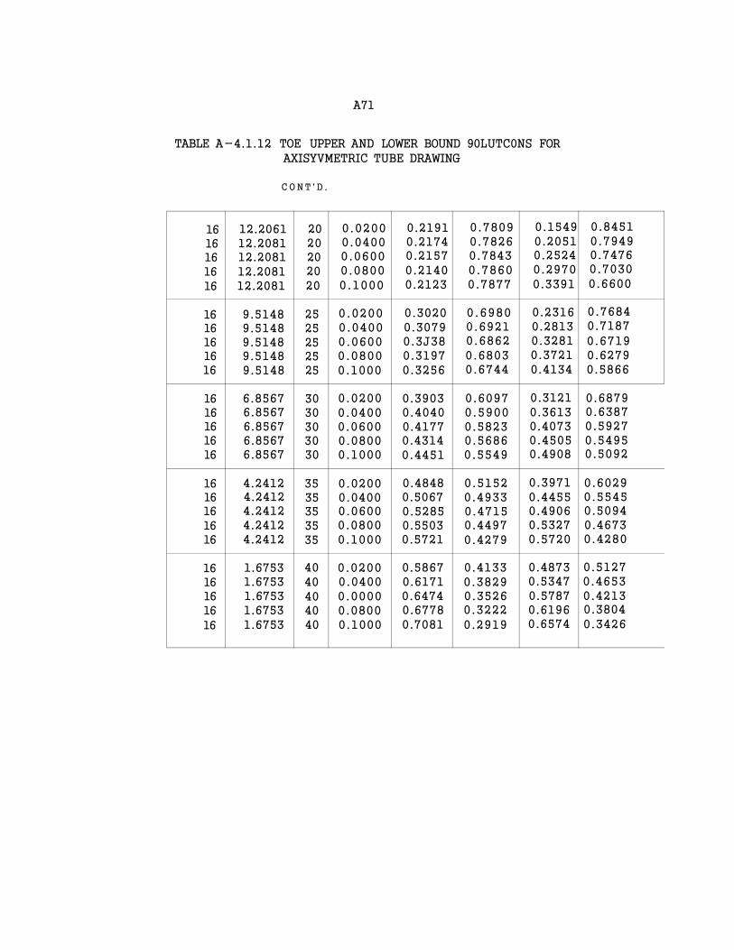
A71

TABLE A-4.1.12 TOE UPPER AND LOWER BOUND 90LUTC0NS FOR

AXISYVMETRIC TUBE DRAWING

C O N T ' D .

16 12.2061 20 0.0200 0.2191 0.7809 0.1549 0.8451

16 12.2081 20 0.0400 0.2174 0.7826 0.2051 0.7949

16 12.2081 20 0.0600 0.2157 0.7843 0.2524 0.7476

16 12.2081 20 0.0800 0.2140 0.7860 0.2970 0.7030

16 12.2081 20 0.1000 0.2123 0.7877 0.3391 0.6600

16 9.5148 25 0.0200 0.3020 0.6980 0.2316 0.7684

16 9.5148 25 0.0400 0.3079 0.6921 0.2813 0.7187

16 9.5148 25 0.0600 0.3J38 0.6862 0.3281 0.6719

16 9.5148 25 0.0800 0.3197 0.6803 0.3721 0.6279

16 9.5148 25 0.1000 0.3256 0.6744 0.4134 0.5866

16 6.8567 30 0.0200 0.3903 0.6097 0.3121 0.6879

16 6.8567 30 0.0400 0.4040 0.5900 0.3613 0.6387

16 6.8567 30 0.0600 0.4177 0.5823 0.4073 0.5927 16 6.8567 30 0.0800 0.4314 0.5686 0.4505 0.5495 16 6.8567 30 0.1000 0.4451 0.5549 0.4908 0.5092

16 4.2412 35 0.0200 0.4848 0.5152 0.3971 0.6029 16 4.2412 35 0.0400 0.5067 0.4933 0.4455 0.5545 16 4.2412 35 0.0600 0.5285 0.4715 0.4906 0.5094

16 4.2412 35 0.0800 0.5503 0.4497 0.5327 0.4673

16 4.2412 35 0.1000 0.5721 0.4279 0.5720 0.4280

16 1.6753 40 0.0200 0.5867 0.4133 0.4873 0.5127

16 1.6753 40 0.0400 0.6171 0.3829 0.5347 0.4653

16 1.6753 40 0.0000 0.6474 0.3526 0.5787 0.4213

16 1.6753 40 0.0800 0.6778 0.3222 0.6196 0.3804

16 1.6753 40 0.1000 0.7081 0.2919 0.6574 0.3426

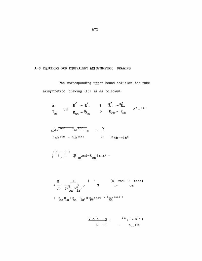
A72

A-5 EQUATIONS FOR EQUIVALENT AXI SYMMETRIC DRAWING

The corresponding upper bound solution for tube

axisymnetrtc drawing {13} is as follows:-

2 2 D2 02 a R - R . i R . - R..

U n < 3 - U 2 )

Y o _ R o K - K. m R - R. u aoa " ia oa ia

R tana - R. tan8 o (_J* ia ) } + 1

R ob t a m - Rib t a n B / 3 iRdb-*lb)2

(R^ -R^ ) { & ib (R tan8-R . tana) • 1 3 v ib ob

2 1 { ° (R. tan0-R tana)

+ — —o f) o 3 i* oa /3 (R2 -R? )

oa ia

+ R R. (R -R.n)(Riatax» " R oa t a n 6 ) }

oa ia oa ia ia oa

V o b - y , l n( ! * 3 b )

R -R. - a__+R.

A73

In R , •-R.. In ^ ob ib^ ( O b lb^

nu 0 R -R. R +R + -2 Sec 8 { <» i a o a o a }

/3 tana-tan 8 tam+tan8

where m^ and m2 are constant friction factors on the die-tube

and plug-tube interfaces respectively.

a is the mean die semi-angle

8 is the mean plug semi-angle

R . is inlet tube external radius ob

R., is inlet tube bore radius lb

R is outlet tube external radius oa

R. is outlet tube bore radius ia

The corresponding lower bound solution for tube

axi-symnetric drawing (6) is as follcws:-

t B * Ha = 1 * 1 (l - (-*) } (3.113)

Y B* m

U i n , 2 where B* =

tarn-tang

u and u„ are the mean coefficients of friction on the 1 2

die-tube and plug-tube interfaces respectively,

A74

a is the mean die semi-angle,

8 is the mean plug semi-angle,

t^ is inlet tube wall thickness,

t is outlet tube wall thickness. a

The die or plug pressure in both cases is

o a (3.114)

Y m