The TME-EMT Project — The PDF Notes — - Olivier Ramaré

The TME-EMT Project—

The PDF Notes

—

Theorie Multiplicative Explicite desnombres

—

Explicit Multiplicative number Theory

—

Contributors:Olivier Bordelles, Pierre Dusart, Charles Greathouse

Harald Helfgott, Pieter Moree, Akhilesh P., Olivier Ramare& Enrique Trevino

December 11, 2021

ii

December 11, 2021

Introduction

Fully explicit results in multiplicative number theory are often scattered throughthe litterature. The aim of this site is to present an annoted bibliography inorder to keep track of the current knowledge. By the way, the acronym TME-EMT stands for

Theorie Multiplicative Explicite des nombres—

Explicit Multiplicative number Theory

Being up-to date is a difficulty, so please do not consider this site as present-ing the best available, but as a first line on which to strengthen more specializedinquiries.

2

December 11, 2021

Contents

I Averages of arithmetical functions 7

1 Explicit bounds on primes 9

1.1 Bounds on primes, in special ranges . . . . . . . . . . . . . . . . . . . 9

1.2 Bounds on primes, without any congruence condition . . . . . . . . . . 10

1.3 Bounds on the n-th prime . . . . . . . . . . . . . . . . . . . . . . . . . 13

1.4 Bounds on primes in arithmetic progressions . . . . . . . . . . . . . . . 14

1.5 Least prime verifying a condition . . . . . . . . . . . . . . . . . . . . . 15

2 Explicit bounds on the Moebius function 17

2.1 Bounds on M(D) =∑d≤D µ(d) . . . . . . . . . . . . . . . . . . . . . . 17

2.2 Bounds on m(D) =∑d≤D µ(d)/d . . . . . . . . . . . . . . . . . . . . . 19

2.3 Bounds on m(D) =∑d≤D µ(d) log(D/d)/d . . . . . . . . . . . . . . . 20

2.4 Miscellanae . . . . . . . . . . . . . . . . . . . . . . . . . . . . . . . . . 21

2.5 The Moebius function and arithmetic progressions . . . . . . . . . . . 21

3 Averages of non-negative multiplicative functions 23

3.1 Asymptotic estimates . . . . . . . . . . . . . . . . . . . . . . . . . . . 23

3.2 Upper bounds . . . . . . . . . . . . . . . . . . . . . . . . . . . . . . . . 26

3.3 Estimates of some special functions . . . . . . . . . . . . . . . . . . . . 27

3.4 Euler products . . . . . . . . . . . . . . . . . . . . . . . . . . . . . . . 31

4 Explicit pointwise upper bounds for some arithmetic functions 33

II Exact computations 35

5 Exact computations of the number of primes 37

6 Computations of arithmetical constants 39

6.1 Euler products of rational functions . . . . . . . . . . . . . . . . . . . 39

6.2 Some special sums over prime values that are derivatives . . . . . . . . 39

III General analytical tools 41

7 Tools on Fourier transforms 43

7.1 The large sieve inequality . . . . . . . . . . . . . . . . . . . . . . . . . 43

4 CONTENTS

8 Tools on Mellin transforms 45

8.1 Explicit truncated Perron formula . . . . . . . . . . . . . . . . . . . . 45

8.2 L2-means . . . . . . . . . . . . . . . . . . . . . . . . . . . . . . . . . . 45

IV Exponential sums / points close to curves 47

9 Explicit results on exponential sums 49

10 Integer Points near Smooth Plane Curves 51

10.1 Bounds using elementary methods . . . . . . . . . . . . . . . . . . . . 52

10.2 Bounds using exponential sums techniques . . . . . . . . . . . . . . . . 53

10.3 Integer points on curves . . . . . . . . . . . . . . . . . . . . . . . . . . 53

V Size of L(1, χ) and character sums 55

11 Size of L(1, χ) 57

11.1 Upper bounds for |L(1, χ)| . . . . . . . . . . . . . . . . . . . . . . . . . 57

11.2 Lower bounds for |L(1, χ)| . . . . . . . . . . . . . . . . . . . . . . . . . 57

12 Character sums 59

12.1 Explicit Polya-Vinogradov inequalities . . . . . . . . . . . . . . . . . . 59

12.2 Burgess type estimates . . . . . . . . . . . . . . . . . . . . . . . . . . . 60

VI Zeros and zero-free regions 65

13 Bounds for |ζ(s)|, |L(s, χ)| and related questions 67

13.1 Size of |ζ(s)| and of L-series . . . . . . . . . . . . . . . . . . . . . . . . 67

13.2 On the total number of zeroes . . . . . . . . . . . . . . . . . . . . . . . 69

13.3 L2-averages . . . . . . . . . . . . . . . . . . . . . . . . . . . . . . . . . 70

13.4 Bounds on the real line . . . . . . . . . . . . . . . . . . . . . . . . . . 71

14 Explicit zero-free regions for the ζ and L functions 73

14.1 Numerical verifications of the Generalized Riemann Hypothesis . . . . 73

14.2 Asymptotical zero-free regions . . . . . . . . . . . . . . . . . . . . . . . 75

14.3 Real zeros . . . . . . . . . . . . . . . . . . . . . . . . . . . . . . . . . . 76

14.4 Density estimates . . . . . . . . . . . . . . . . . . . . . . . . . . . . . . 76

14.5 Miscellanae . . . . . . . . . . . . . . . . . . . . . . . . . . . . . . . . . 77

VII Sieve and short interval results 79

15 Short intervals containing primes 81

15.1 Interval with primes, without any congruence condition . . . . . . . . 81

15.2 Interval with primes under RH, without any congruence condition . . 84

15.3 Interval with primes, with congruence condition . . . . . . . . . . . . . 85

December 11, 2021

CONTENTS 5

16 Sieve bounds 8716.1 Some upper bounds . . . . . . . . . . . . . . . . . . . . . . . . . . . . 8716.2 Combinatorial sieve estimates . . . . . . . . . . . . . . . . . . . . . . . 88

VIII Analytic Number Theory in Number Fields 89

17 Bounds on the Dedekind zeta-function 9117.1 Size . . . . . . . . . . . . . . . . . . . . . . . . . . . . . . . . . . . . . 9117.2 Zeroes and zero-free regions . . . . . . . . . . . . . . . . . . . . . . . . 91

IX Applications 93

18 Explicit bounds for class numbers 9518.1 Majorising hKRK . . . . . . . . . . . . . . . . . . . . . . . . . . . . . 9518.2 Majorising hK . . . . . . . . . . . . . . . . . . . . . . . . . . . . . . . 9618.3 Using the influence of small primes . . . . . . . . . . . . . . . . . . . . 9618.4 The h−

K of CM-fields . . . . . . . . . . . . . . . . . . . . . . . . . . . . 97

19 Primitive Roots 99

X Development 101

20 README 10320.1 How to write . . . . . . . . . . . . . . . . . . . . . . . . . . . . . . . . 10320.2 How to contribute . . . . . . . . . . . . . . . . . . . . . . . . . . . . . 10420.3 Adding a part or a chapter . . . . . . . . . . . . . . . . . . . . . . . . 104

Bibliography 105

Notation

Notation is standard, except maybe for the following one: we write f = O∗(g) tosay that |f | ≤ g. This is simply a Landau-bigO symbol with an implied constantequal to one. Furthermore, the letter p always denotes a prime variable.

The TME-EMT project, 2021 December 11, 2021

6 CONTENTS

December 11, 2021

Part I

Averages of arithmeticalfunctions

Chapter 1

Explicit bounds on primes

Corresponding html file: ../Articles/Art01.htmlCollecting references: [P. Dusart, 59], [P. Dusart, 64],

1.1 Bounds on primes, in special ranges

The paper [J. Rosser and L. Schoenfeld, 185], contains several bounds valid onlywhen the variable is small enough.

In [J. Buthe, 25], the author proves the next theorem.

Theorem (2016) Assume the Riemann Hypothesis has been checked up toheight H0. Then when x satisfies

√x/ log x ≤ H0/4.92, we have

� |ψ(x)− x| ≤√x

8π log2 x when x > 59,

� |θ(x)− x| ≤√x

8π log2 x when x > 599,

� |π(x)− li(x)| ≤√x

8π log x when x > 2657.

If we use the value H0 = 30 610 046 000 obtained by D. Platt in [D. J. Platt,156], these bounds are thus valid for x ≤ 1.8 · 1021.

In [J. Buthe, 24], the following bounds are also obtained.

Theorem (2018) We have

� |ψ(x)− x| ≤ 0.94√x when 11 < x ≤ 1019,

� 0 < li(x)− π(x) ≤√x

log x

(1.95 + 3.9

log x + 19.5log2 x

)when 2 ≤ x ≤ 1019.

[59] P. Dusart, 1998, “Autour de la fonction qui compte le nombre de nombres premiers”.[64] P. Dusart, 2016, “Estimates of ψ, θ for large values of x without the Riemann hypothesis”.[185] J. Rosser and L. Schoenfeld, 1962, “Approximate formulas for some functions of primenumbers”.[25] J. Buthe, 2016, “Estimating π(x) and related functions under partial RH assumptions”.[156] D. J. Platt, 2017, “Isolating some non-trivial zeros of zeta”.[24] J. Buthe, 2018, “An analytic method for bounding ψ(x)”.

10 CHAPTER 1. EXPLICIT BOUNDS ON PRIMES

1.2 Bounds on primes, without any congruencecondition

The subject really started with the four papers [J. Rosser, 181], [J. Rosser andL. Schoenfeld, 185], [J. Rosser and L. Schoenfeld, 186] and [L. Schoenfeld, 191].We recall the usual notation: π(x) is the number of primes up to x (so thatπ(3) = 2), the function ψ(x) is the summatory function of the van Mangoldfunction Λ, i.e. ψ(x) =

∑n≤x Λ(n), while we also define ϑ(x) =

∑p≤x log p.

Here are some elegant bounds that one can find in these papers.

Theorem (1962) � For x > 0, we have ψ(x) ≤ 1.03883x and the maximumof ψ(x)/x is attained at x = 113.

� When x ≥ 17, we have π(x) > x/ log x.

� When x > 1, we have∑p≤x

1/p > log log x.

� When x > 1, we have∑p≤x

(log p)/p < log x.

There are many other results in these papers. In [P. Dusart, 62], on can findamong other things the inequality

When x ≥ 17, we have π(x) >x

log x− 1.

And also

Theorem (1999) � When x ≥ e22, we have ψ(x) = x+O∗(

0.006409x

log x

).

� When x ≥ 10 544 111, we have ϑ(x) = x+O∗(

0.006788x

log x

).

� When x ≥ 3 594 641, we have ϑ(x) = x+O∗(

0.2x

log2 x

).

� When x > 1, we have ϑ(x) = x+O∗(

515x

log3 x

).

[181] J. Rosser, 1941, “Explicit bounds for some functions of prime numbers”.[185] J. Rosser and L. Schoenfeld, 1962, “Approximate formulas for some functions of primenumbers”.[186] J. Rosser and L. Schoenfeld, 1975, “Sharper bounds for the Chebyshev Functions ϑ(X)and ψ(X)”.[191] L. Schoenfeld, 1976, “Sharper bounds for the Chebyshev Functions ϑ(X) and ψ(X)II”..[62] P. Dusart, 1999, “Inegalites explicites pour ψ(X), θ(X), π(X) et les nombres premiers”.

December 11, 2021

1.2 Bounds on primes, without any congruence condition 11

This is improved in [P. Dusart, 61], and in particular, it is shown that the515 above can be replaced by 20.83 and also that

When x ≥ 89 967 803, we have ϑ(x) = x+O∗( x

log3 x

).

Bounds of the shape |ψ(x) − x| ≤ εx have started appearing in [J. Rosserand L. Schoenfeld, 185]. The latest paper is [L. Faber and H. Kadiri, 68] withits corrigendum [Kadiri-Faber*18], where the explicit density estimate from[H. Kadiri, 97] is put to contribution, even for moderate values of the variable.In particular

When x ≥ 485 165 196, we have ψ(x) = x+O∗(0.00053699x).

In [D. J. Platt and T. S. Trudgian, 157], one find the following estimate

Theorem (2021) When x ≥ e2000, we have

∣∣∣∣ψ(x)−xx

∣∣∣∣ ≤ 235 (log x)0.52 exp−√

log x5.573412 .

Refined bounds for π(x) are to be found in [L. Panaitopol, 151] and in [C.Axler, 2].

By comparing in an efficient manner with ψ(x) − x, [O. Ramare, 168], ob-tained the next two results.

Theorem (2013)

For x > 1, we have∑n≤x Λ(n)/n = log x − γ + O∗(1.833/ log2 x). When

x ≥ 23, we can replace the error term by O∗(0.0067/ log x). Furthermore, when1 ≤ x ≤ 1010, this error term can be replaced by O∗(1.31/

√x).

Theorem (2013) For x ≥ 8950, we have

∑n≤x

Λ(n)/n = log x− γ +ψ(x)− x

x+O∗

( 1

2√x

+ 1.75 · 10−12)

.

[R. Mawia, 131] developed the method to incorporate more functions (andcorrected the initial work), extending results of [J. Rosser and L. Schoenfeld,185].

Here are some of his results.

[61] P. Dusart, 2018, “Estimates of some functions over primes”.[68] L. Faber and H. Kadiri, 2015, “New bounds for ψ(x)”.[97] H. Kadiri, 2013, “A zero density result for the Riemann zeta function”.[157] D. J. Platt and T. S. Trudgian, 2021, “The error term in the prime number theorem”.[151] L. Panaitopol, 2000, “A formula for π(x) applied to a result of Koninck-Ivic”.[2] C. Axler, 2016, “New bounds for the prime counting function”.[168] O. Ramare, 2013, “Explicit estimates for the summatory function of Λ(n)/n from theone of Λ(n)”.[131] R. Mawia, 2017, “Explicit estimates for some summatory functions of primes”.



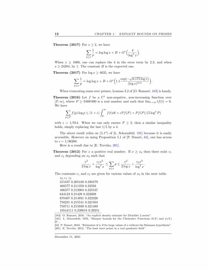
Theorem (2017) For x ≥ 2, we have∑p≤x

1

p= log log x+B +O∗

( 4

log3 x

).

When x ≥ 1000, one can replace the 4 in the error term by 2.3, and whenx ≥ 24284, by 1. The constant B is the expected one.

Theorem (2017) For log x ≥ 4635, we have∑p≤x

1

p= log log x+B +O∗

(1.1

exp(−√

0.175 log x)

(log x)3/4

).

When truncating sums over primes, Lemma 3.2 of [O. Ramare, 163] is handy.

Theorem (2016) Let f be a C1 non-negative, non-increasing function over[P,∞[, where P ≥ 3 600 000 is a real number and such that limt→∞ tf(t) = 0.We have∑

p≥P

f(p) log p ≤ (1 + ε)

∫ ∞P

f(t)dt+ εPf(P ) + Pf(P )/(5 log2 P )

with ε = 1/914. When we can only ensure P ≥ 2, then a similar inequalityholds, simply replacing the last 1/5 by a 4.

The above result relies on (5.1*) of [L. Schoenfeld, 191] because it is easilyaccessible. However on using Proposition 5.1 of [P. Dusart, 64], one has accessto ε = 1/36260.

Here is a result due to [E. Trevino, 201].

Theorem (2012) For x a positive real number. If x ≥ x0 then there exist c1and c2 depending on x0 such that

x2

2 log x+

c1x2

log2 x≤∑p≤x

p ≤ x2

2 log x+

c2x2

log2 x.

The constants c1 and c2 are given for various values of x0 in the next table.x0 c1 c2315437 0.205448 0.330479468577 0.211359 0.32593486377 0.212904 0.325537644123 0.21429 0.322609678407 0.214931 0.322326758231 0.215541 0.321504758711 0.215939 0.32148910544111 0.239818 0.29251

[163] O. Ramare, 2016, “An explicit density estimate for Dirichlet L-series”.[191] L. Schoenfeld, 1976, “Sharper bounds for the Chebyshev Functions ϑ(X) and ψ(X)II”..[64] P. Dusart, 2016, “Estimates of ψ, θ for large values of x without the Riemann hypothesis”.[201] E. Trevino, 2012, “The least inert prime in a real quadratic field”.

December 11, 2021

1.3 Bounds on the n-th prime 13

1.3 Bounds on the n-th prime

Denote by pn the n-th prime. Thus p1 = 2, p2 = 3, p4 = 5, · · · .The classical form of prime number theorem yields easily pn ∼ n log n.[J. Rosser, 184] shows that this equivalence does not oscillate by proving

that pn is greater than n log n for n ≥ 2.The asymptotic formula for pn can be developped as shown in [M. Cipolla,

31]:

pn ∼ n(

log n+ log log n− 1 +log log n− 2

log n− (ln lnn)2 − 6 log log n+ 11

2 log2 n+ · · ·

).

This asymptotic expansion is the inverse of the logarithmic integral Li(x)obtained by series reversion.

But [J. Rosser, 184] also proved that for every n > 1:

n(log n+ log log n− 10) < pn < n(log n+ log log n+ 8).

He improves these results in [J. Rosser, 181] : for every n ≥ 55,

n(log n+ log log n− 4) < pn < n(log n+ log log n+ 2).

This result was subsequently improved by Rosser and Schoenfeld [J. Rosserand L. Schoenfeld, 185] in 1962 to

n(log n+ log log n− 3/2) < pn < n(log n+ log log n− 1/2),

for n > 1 and n > 19 respectively.The constants were subsequently reduced by [G. Robin, 179]. In particular,

the lower boundn(log n+ log log n− 1.0072629) < pn

is valid for n > 1 and the constant 1.0072629 can be replaced by 1 for pk ≤ 1011.Then [J.-P. Massias and G. Robin, 129] showed that the lower bound constantequals to 1 was admissible for pk < e598 and pk > e1800. Finally, [P. Dusart, 63]showed that

n(log n− log log n− 1) < pn

for all n > 1, and also that

pn < n(log n+ log log n− 0.9484)

[184] J. Rosser, 1938, “The n-th prime is greater than n logn”.[31] M. Cipolla, 1902, “La determinatzione assintotica dell‘nimo numero primo”.[181] J. Rosser, 1941, “Explicit bounds for some functions of prime numbers”.[185] J. Rosser and L. Schoenfeld, 1962, “Approximate formulas for some functions of primenumbers”.[179] G. Robin, 1983, “Estimation de la fonction de Tchebychef θ sur le k-ieme nombrespremiers et grandes valeurs de la fonction ω(n) nombre de diviseurs premiers de n”.[129] J.-P. Massias and G. Robin, 1996, “Bornes effectives pour certaines fonctions concernantles nombres premiers”.[63] P. Dusart, 1999, “The kth prime is greater than k(ln k + ln ln k − 1) for k ≥ 2”.



for n > 39017 i.e. pn > 467 473.

In [E. Carneiro, M. Milinovich, and K. Soundararajan, 26], the authors provethe next result.

Theorem (2019) Under the Riemann Hypothesis we have pn+1 − p − n ≤2225

√pn log pn.

1.4 Bounds on primes in arithmetic progressions

Collecting references: [K. McCurley, 133], [K. McCurley, 132], [O. Ramare andR. Rumely, 177], [P. Dusart, 60], Lemma 10 of [P. Moree, 140], section 4 of [P.Moree and H. te Riele, 141].

A consequence of Theorem 1.1 and 1.2 of [M. A. Bennett et al., 11] statesthat

Theorem (2018) We have max3≤q≤104

maxx≥8·109

max1≤a≤q,(a,q)=1

log x

x

∣∣∣ ∑n≤x,n≡a[q]

Λ(n) − x

ϕ(q)

∣∣∣ ≤1/840.

When q ∈ (104, 105], we may replace 1/840 by 1/160 and when q ≥ 105, wemay replace 1/840 by exp(0.03

√q log3 q).

Furthermore, we may replace∑

n≤x,n≡a[q]

Λ(n) by∑

p≤x,p≡a[q]

log p with no changes

in the constants.

Similarly, as a consequence of Theorem 1.3 of [M. A. Bennett et al., 11]states that

Theorem (2018) We have max3≤q≤104

maxx≥8·109


log2 x

x

∣∣∣ ∑p≤x,p≡a[q]

1−Li(x)

ϕ(q)

∣∣∣ ≤ 1/840.

When q ∈ (104, 105], we may replace 1/840 by 1/160 and when q ≥ 105, wemay replace 1/840 by exp(0.03

√q log3 q).

Concerning estimates with a logarithmic density, in [O. Ramare, 176] and

[26] E. Carneiro, M. Milinovich, and K. Soundararajan, 2019, Fourier optimization and primegaps.[133] K. McCurley, 1984, “Explicit estimates for the error term in the prime number theoremfor arithmetic progressions”.[132] K. McCurley, 1984, “Explicit estimates for θ(x; 3, `) and ψ(x; 3, `)”.[177] O. Ramare and R. Rumely, 1996, “Primes in arithmetic progressions”.[60] P. Dusart, 2002, “Estimates for θ(x; k, `) for large values of x”.[140] P. Moree, 2004, “Chebyshev’s bias for composite numbers with restricted prime divi-sors”.[141] P. Moree and H. te Riele, 2004, “The hexagonal versus the square lattice”.[11] M. A. Bennett et al., 2018, “Explicit bounds for primes in arithmetic progressions”.[176] O. Ramare, 2002, “Sur un theoreme de Mertens”.

December 11, 2021

1.5 Least prime verifying a condition 15

in [D. Platt and O. Ramare, 154], estimates for the functions∑n≤x,n≡a[q]

Λ(n)/n are

considered. Extending computations from the former, the latter paper Theorem8.1 reads as follows.

Theorem (2016) We have maxq≤1000

maxq≤x≤105


√x∣∣∣ ∑n≤x,n≡a[q]

Λ(n)

n− log x

ϕ(q)−C(q, a)

∣∣∣ ∈(0.8533, 0.8534) and the maximum is attained with q = 17, x = 606 and a = 2.

The constant C(q, a) is the one expected, i.e. such that∑

n≤x,n≡a[q]

Λ(n)n −

log xϕ(q)−

C(q, a) goes to zero when x goes to infinity.When q belongs to ”Rumely’s list”, i.e. in one of the following set:

� {k ≤ 72}

� {k ≤ 112, k non premier}

�

{116, 117,120, 121, 124, 125, 128, 132, 140, 143, 144, 156, 163,

169, 180, 216, 243, 256, 360, 420, 432}

Theorem 2 of [O. Ramare, 176] gives the following.

Theorem (2002) When q belongs to Rumely’s list and a is prime to q, we have∑n≤x,n≡a[q]

Λ(n)

n=

log x

ϕ(q)+ C(q, a) +O∗(1) as soon as x ≥ 1.

More precise bounds are given.

1.5 Least prime verifying a condition

[E. Bach and J. Sorenson, 3], [H. Kadiri, 100],

Last updated on January 1rst, 2019, by Olivier Ramare

[154] D. Platt and O. Ramare, 2017, “Explicit estimates: from Λ(n) in arithmetic progressionsto Λ(n)/n”.[3] E. Bach and J. Sorenson, 1996, “Explicit bounds for primes in residue classes”.[100] H. Kadiri, 2008, “Short effective intervals containing primes in arithmetic progressionsand the seven cube problem”.



December 11, 2021

Chapter 2

Explicit bounds on theMoebius function

Corresponding html file: ../Articles/Art02.htmlCollecting references: [H. Diamond and P. Erdos, 50], [M. Deleglise and J.

Rivat, 47], [P. Borwein, R. Ferguson, and M. Mossinghoff, 21].

2.1 Bounds on M(D) =∑

d≤D µ(d)

The first explicit estimate for M(D) is due to [R. von Sterneck, 210] where theauthor proved that |M(D)| ≤ 1

9D+ 8 for any D ≥ 0. A popular estimate is theone of [R. Mac Leod, 127].

Theorem (1967) When D ≥ 0, we have |M(D)| ≤ 180D + 5. When D ≥ 1119,

we have |M(D)| ≤ D/80.

We mention at this level the annoted bibliography contained at the end of[F. Dress, 53]. [N. Costa Pereira, 37] shows that

Theorem (1993) When D ≥ 120 727, we have |M(D)| ≤ D/1036.

On elaborating on this method, [F. Dress and M. El Marraki, 54] showedthat

[50] H. Diamond and P. Erdos, 1980, “On sharp elementary prime number estimates”.[47] M. Deleglise and J. Rivat, 1996, “Computing the summation of the Mobius function”.[21] P. Borwein, R. Ferguson, and M. Mossinghoff, 2008, “Sign changes in sums of the Liouvillefunction”.[210] R. von Sterneck, 1898, “Bemerkung uber die Summierung einiger zahlentheorischenFunktionen”.[127] R. Mac Leod, 1967, “A new estimate for the sum M(x) =

∑n≤x µ(n)”.

[53] F. Dress, 1983/84, “Theoremes d’oscillations et fonction de Mobius”.[37] N. Costa Pereira, 1989, “Elementary estimates for the Chebyshev function ψ(X) and forthe Mobius function M(X)”.[54] F. Dress and M. El Marraki, 1993, “Fonction sommatoire de la fonction de Mobius 2.Majorations asymptotiques elementaires”.

18 CHAPTER 2. EXPLICIT BOUNDS ON THE MOEBIUS FUNCTION

Theorem (1993) When D ≥ 617 973, we have |M(D)| ≤ D/2360.

One of the argument is the estimate from [F. Dress, 52]

Theorem (1993) When 33 ≤ D ≤ 1012, we have |M(D)| ≤ 0.571√D.

This has been extended by [T. Kotnik and J. van de Lune, 105] to 1014 andrecently in [G. Hurst, 87] to 1016, i.e.

Theorem (2018) When 33 ≤ D ≤ 1016, we have |M(D)| ≤ 0.571√D.

Another tool is [H. Cohen and F. Dress, 34] where refined explicit estimatesfor the remainder term of the counting functions of the squarefree numbers inintervals are obtained.

The latest best estimate of this shape comes from [H. Cohen, F. Dress, andM. El Marraki, 35]. This preprint being difficult to get, it has been republishedin [H. Cohen, F. Dress, and M. El Marraki, 36].

Theorem (1996) When D ≥ 2 160 535, we have |M(D)| ≤ D/4345.

These results are used in [F. Dress, 51] to study the discrepancy of the Fareyseries.

Concerning upper bounds that tend to 0, [L. Schoenfeld, 190] is the pioneerand shows among other estimates that

Theorem (1969) When D > 0, we have |M(D)|/D ≤ 2.9/ logD.

[M. El Marraki, 65] improves that into

Theorem (1995) When D ≥ 685, we have |M(D)|/D ≤ 0.10917/ logD.

The latest bound coming from [O. Ramare, 171] improves that:

Theorem (2012) When D ≥ 1 100 000, we have |M(D)|/D ≤ 0.013/ logD.

[52] F. Dress, 1993, “Fonction sommatoire de la fonction de Mobius 1. Majorationsexperimentales”.[105] T. Kotnik and J. van de Lune, 2004, “On the order of the Mertens function”.[87] G. Hurst, 2018, “Computations of the Mertens function and improved bounds on theMertens conjecture”.[34] H. Cohen and F. Dress, 1988, “Estimations numeriques du reste de la fonction sommatoirerelative aux entiers sans facteur carre”.[35] H. Cohen, F. Dress, and M. El Marraki, 1996, “Explicit estimates for summatory functionslinked to the Mobius µ-function”.[36] H. Cohen, F. Dress, and M. El Marraki, 2007, “Explicit estimates for summatory functionslinked to the Mobius µ-function”.[51] F. Dress, 1999, “Discrepance des suites de Farey”.[190] L. Schoenfeld, 1969, “An improved estimate for the summatory function of the Mobiusfunction”.[65] M. El Marraki, 1995, “Fonction sommatoire de la fonction µ de Mobius, majorationsasymptotiques effectives fortes”.[171] O. Ramare, 2013, “From explicit estimates for the primes to explicit estimates for theMoebius function”.

December 11, 2021

2.2 Bounds on m(D) =∑d≤D µ(d)/d 19

In [O. Ramare, 169], bounds including coprimality conditions are proved andhere is a typical example.

Theorem (2013) When 1 ≤ q < D, we have∣∣∣∑ d≤D,

(d,q)=1

µ(d)∣∣∣/D ≤ q

ϕ(q)/(1 +

log(D/q)).

2.2 Bounds on m(D) =∑

d≤D µ(d)/d

[R. Mac Leod, 127] shows that the sum m(D) takes its minimal value at D = 13.A folklore result is generalized in [A. Granville and O. Ramare, 79] and reads

Theorem (1996) WhenD ≥ 0 and for any integer r ≥ 1, we have∣∣∣∑ d≤D,

(d,r)=1

µ(d)/d∣∣∣ ≤

1.

In fact, Lemma 1 of [H. Davenport, 43] already contains the requisite mate-rial.

The next result is proved in [O. Ramare, 169].

Theorem (2013) When D ≥ 7, we have |∑d≤D µ(d)/d| ≤ 1/10. We can re-

place the couple (7, 1/10) by (41, 1/20) or (694, 1/100).

This is further extended in [O. Ramare, 175] where it is shown that

Theorem (2012) When D ≥ 0 and for any integer r ≥ 1 and any real number

ε ≥ 0, we have∣∣∣∑ d≤D,

(d,r)=1

µ(d)/d1+ε∣∣∣ ≤ 1 + ε.

Concerning upper bounds that tend to 0, [M. El Marraki, 66] is the first toget such an estimate.

Theorem (1996) When D ≥ 33 we have |m(D)| ≤ 0.2185/ logD.

When D > 1 we have |m(D)| ≤ 726/(logD)2.

This second bound is improved in [O. Bordelles, 20].

Theorem (2015) When D > 1 we have |m(D)| ≤ 546/(logD)2.

[169] O. Ramare, 2015, “Explicit estimates on several summatory functions involving theMoebius function”.[127] R. Mac Leod, 1967, “A new estimate for the sum M(x) =

∑n≤x µ(n)”.

[79] A. Granville and O. Ramare, 1996, “Explicit bounds on exponential sums and the scarcityof squarefree binomial coefficients”.[43] H. Davenport, 1937, “On some infinite series involving arithmetical functions”.[175] O. Ramare, 2013, “Some elementary explicit bounds for two mollifications of the Moebiusfunction”.

[66] M. El Marraki, 1996, “Majorations de la fonction sommatoire de la fonctionµ(n)n

”.[20] O. Bordelles, 2015, “Some explicit estimates for the Mobius function”.



[O. Ramare, 171] proves several bounds of the shape m(D)� 1/ logD. Thisis improved in [O. Ramare, 169] by using [M. Balazard, 8]. which provides uswith a better manner to convert bounds on M(D) into bounds for m(D). Hereis one result obtained.

Theorem (2015) When D ≥ 463 421 we have |m(D)| ≤ 0.0144/ logD.

We can for instance replace the couple (463 421, 0.0144)by any of (96 955,1/69), (60 298, 1/65), (1426, 1/20) or (687, 1/12).

In [O. Ramare, 170] and [O. Ramare, 169], the problem of adding coprimalityconditions is further addressed. Here is one of the results obtained.

Theorem (2015) When 1 ≤ q < D we have∣∣∣∑ d≤D,

(d,q)=1

µ(d)/d∣∣∣ ≤ q

ϕ(q)0.78/ log(D/q).

When D/q ≥ 24233, we can replace 0.78 by 17/125.

2.3 Bounds on m(D) =∑

d≤D µ(d) log(D/d)/d

The initial investigations on this function go back to [R. Daublebsky von Ster-neck, 42]. In [O. Ramare, 169] it is proved that

Theorem (2015) When 3846 ≤ D we have |m(D)−1| ≤ 0.00257/ logD. WhenD > 1, we have |m(D)− 1| ≤ 0.213/ logD.

This implies in particular that

Theorem (2015) When 222 ≤ D we have |m(D)− 1| ≤ 1/1250. When D > 1,the optimal bound 1 holds.

These bounds are a consequence of the identity:

|m(D)− 1| ≤74 − γD2

∫ D

1

|M(t)|dt+2

D.

It is also proved that, for any D ≥ 1, we have

0 ≤∑d≤D,

(d,q)=1

µ(d) log(D/d)/d ≤ 1.00303q/ϕ(q).

[171] O. Ramare, 2013, “From explicit estimates for the primes to explicit estimates for theMoebius function”.[169] O. Ramare, 2015, “Explicit estimates on several summatory functions involving theMoebius function”.[8] M. Balazard, 2012, “Elementary Remarks on Mobius’ Function”.[170] O. Ramare, 2014, “Explicit estimates on the summatory functions of the Moebiusfunction with coprimality restrictions”.[42] R. Daublebsky von Sterneck, 1902, “Ein Analogon zur additiven Zahlentheorie.”

December 11, 2021

2.4 Miscellanae 21

2.4 Miscellanae

Here is an elegant wide ranging estimate, taken from Claim 3.1 of [E. Trevino,200].

Theorem (2015) When D ≥ 1 we have |∑d>D µ(d)/d2| ≤ 1/D.

2.5 The Moebius function and arithmetic pro-gressions

The results in this section are scarce. We mention a Theorem of [O. Bordelles,20].

Theorem (2015) Let χ be a non-principal Dirichlet character mmodulo q ≥ 37and let k ≥ 1 be some integer. Then∣∣∣∣ ∑

n≤x,(n,k)=1

µ(n)χ(n)

n

∣∣∣∣ ≤ k

ϕ(k)

2√q log q

L(1, χ).

Last updated on February 18th, 2018, by Olivier Ramare

[200] E. Trevino, 2015, “The least k-th power non-residue”.[20] O. Bordelles, 2015, “Some explicit estimates for the Mobius function”.



December 11, 2021

Chapter 3

Averages of non-negativemultiplicative functions

Corresponding html file: ../Articles/Art10.html

3.1 Asymptotic estimates

When looking for averages of functions that look like 1 or like the divisor func-tion, Lemma 3.2 of [O. Ramare, 174] offers an efficient easy path. The techniqueof comparison of two arithmetical function via their Dirichlet series is known asthe Convolution method and is for instance decribed at length in [P. Bermentand O. Ramare, 13], and in the course that can be found here1.

Theorem (1995) Let (gn)n≥1, (hn)n≥1 and (kn)n≥1 be three complex sequences.Let H(s) =

∑n hnn

−s, and H(s) =∑n |hn|n−s. We assume that g = h?k, that

H(s) is convergent for <(s) ≥ −1/3 and further that there exist four constantsA, B, C and D such that∑

n≤t

kn = A log2 t+B log t+ C +O∗(Dt−1/3) for t > 0.

Then we have for all t > 0 :∑n≤t

gn = u log2 t+ v log t+ w +O∗(Dt−1/3H(−1/3))

with u = AH(0), v = 2AH ′(0) + BH(0) and w = AH ′′(0) + BH ′(0) + CH(0).We have also∑

n≤t

ngn = Ut log t+ V t+W +O∗(2.5Dt2/3H(−1/3))

[174] O. Ramare, 1995, “On Snirel’man’s constant”.[13] P. Berment and O. Ramare, 2012, “Ordre moyen d’une fonction arithmetique par lamethode de convolution”.

1https://ramare-olivier.github.io/CoursNouakchott/index.html

https://ramare-olivier.github.io/CoursNouakchott/index.html

24CHAPTER 3. AVERAGES OF NON-NEGATIVE MULTIPLICATIVE

FUNCTIONS

with

U =2AH(0), V = −2AH(0) + 2AH ′(0) +BH(0),

W =A(H ′′(0)− 2H ′(0) + 2H(0)) +B(H ′(0)−H(0)) + CH(0).

This Lemma says that one derives information from gn from informationson the model kn. When this model is kn = 1, the values concerning A, B andC are given by the first half of Lemma 3.3 of [O. Ramare, 174]:

Lemma (1995)∑n≤t 1/n = log t+ γ +O∗(0.9105t−1/3).

When this model is kn = τ(n), the number of divisors of n, the valuesconcerning A, B and C are given by Corollary 2.2 of [D. Berkane, O. Bordelles,and O. Ramare, 12]. Please note the ”γ2 − 2γ1” which is wrongly typed as”γ2−γ1” in the aforementioned paper (and thanks to Tim Trudgian and DavidPlatt for spotting this typo):

Lemma (2011)∑n≤t τ(n)/n = 1

2 log2 t + 2γ log t + γ2 − 2γ1 + O∗(1.16/t1/3)where γ1 is the second Laurent-Stieljes constant – for instance [R. Kreminski,106] and [M. Coffey, 33]. In particular, we have γ1 = −0.0728158454836767248605863758749013191377+O∗(10−40).

The constants H(0), H ′(0) and H ′′(0) are to be computed. In most cases,the Dirichlet series has an Euler product, in which case, (see section 3 of [O.Ramare, 174]) we have

H(0) =∏p(1 +

∑m hpm), then

H ′(0)

H(0)=∑p

∑mmhpm

1 +∑m hpm

(− log p), and also

H ′′(0)

H(0)=

(H ′(0)

H(0)

)2

+∑p

{ ∑mm

2hpm

1 +∑m hpm

−[ ∑

mmhpm

1 +∑m hpm

]2}

log2 p.

It is sometimes more expedient to use the same convolution method but bycomparing the function to the function q 7→ q. In such a case, the next lemma,Lemma 4.3 from [O. Ramare, 163], is handy.

Theorem (2015) We have, for any real number x ≥ 0 and any real number

c ∈ [1, 2],∑q≤x

q = 12x

2 +O∗(xc/2).

This leads to the next theorem.

[174] O. Ramare, 1995, “On Snirel’man’s constant”.[12] D. Berkane, O. Bordelles, and O. Ramare, 2012, “Explicit upper bounds for the remainderterm in the divisor problem”.[106] R. Kreminski, 2003, “Newton-Cotes integration for approximating Stieltjes (generalizedEuler) constants”.[33] M. Coffey, 2006, “New results on the Stieltjes constants: asymptotic and exact evalua-tion”.[163] O. Ramare, 2016, “An explicit density estimate for Dirichlet L-series”.

December 11, 2021

3.1 Asymptotic estimates 25

Theorem Let (hn)n≥1 be a complex sequences. Let H(s) =∑n hnn

−s, andH(s) =

∑n |hn|n−s. We assume that H(s) is convergent for <(s) ≥ c, for some

c ∈ [1, 2]. Then we have for all t > 0 :

∑n≤t

∑d|n

n

dh(d) =

t2

2H(2) +O∗(tcH(c)/2).

A typical usage is to evaluate∑n≤t φ(n), with h(d) = µ(d).

The convolution method has been brought one step further in [A. P. andO. Ramare, 150] where the following theorem is proved.

Theorem (2017) Let (g(m))m≥1 be a sequence of complex numbers such thatboth series

∑m≥1 g(m)/m and

∑m≥1 g(m)(logm)/m converge. We define

G](x) =∑m>x g(m)/m and assume that

∫∞1|G](t)|dt/t converges. Let A0 ≥ 1

be a real parameter. We have∑n≤D

(g ? 11)(n)

n=∑m≥1

g(m)

m

(log

D

m+ γ)

+

∫ ∞D/A0

G](t)dt

t+O∗(R)

where R is defined by

R =

∣∣∣∣∣∣∑

1≤a≤A0

1

aG](D

a

)+G]

(D

A0

)(log

A0

[A0]−R([A0])

)∣∣∣∣∣∣+6/11

D

∑m≤D/A0

|g(m)|

where [A0] is the integer part of A0, while the remainder R is defined by R(X) =∑n≤X 1/n− logX − γ.

The remainder R(X) is shown in Lemma to verify |R(X)| ≤ γ/X for everyX > 0, and |R(X)| ≤ (6/11)/X when X ≥ 1.

Theorem 21.1 of [O. Ramare, 166] offers a fully explicit estimate for the aver-age of a general non-negative multiplicative function, but it is often numericallyrather poor. It relies on the technique developped by [B. Levin and A. Fainleib,114].

Theorem (2009) Let g be a non-negative multiplicative function. Let A and κbe three positive real parameters such that, for any Q ≥ 1, one has∑

p≥2,ν≥1pν≤Q

g(pν)

log(pν)

= κ logQ+O∗(L)

[150] A. P. and O. Ramare, 2017, “Explicit averages of non-negative multiplicative functions:going beyond the main term”.[166] O. Ramare, 2009, Arithmetical aspects of the large sieve inequality.[114] B. Levin and A. Fainleib, 1967, “Application of some integral equations to problems ofnumber theory”.



FUNCTIONS

and∑p≥2

∑ν,k≥1 g

(pk)g(pν)

log(pν)≤ A. Then, when D ≥ exp(2(L+A)), we

have ∑d≤D

g(d) = C (logD)κ (

1 +O∗(B/ logD

))where B = 2(L+A)

(1 + 2(κ+ 1)eκ+1

)and

C =1

Γ(κ+ 1)

∏p≥2

{(∑ν≥0

g(pν))(

1− 1

p

)κ}.

3.2 Upper bounds

When looking for an upper bound, it is common to compare sums to an Eulerproduct, via,

∑n≤y

f(n)/n ≤∏p≤y

1 +∑

1≤m≤log y/ log p

f(pm)

valid when f is non-negative and multiplicative. Lemma 4 of [H. Daboussi andJ. Rivat, 41] extends this. Let z be a parameter and vz(n) be the characteristicfunction of those integers that have all their prime factors p ≤ z.

Theorem (2000) Let z ≥ 2, f a multiplicative function with f ≥ 0 and S =∑p≤z

f(p)1+f(p) log p. We assume that S > 0 and write K(t) = log t − 1 − (1/t).

For any y such that log y ≥ S, we have∑n>y

vz(n)µ2(n)f(n) ≤∏p≤z

(1 + f(p)) exp

(− log y

log zK

(log y

S

))∑n≤y

vz(n)µ2(n)f(n) ≥∏p≤z

(1 + f(p))

{1− exp

(− log y

log zK

(log y

S

))}and in particular, when log y ≥ 7S, we have∑

n>y

vz(n)µ2(n)f(n) ≤∏p≤z

(1 + f(p)) exp

(− log y

log z

)∑n≤y

vz(n)µ2(n)f(n) ≥∏p≤z

(1 + f(p))

{1− exp

(− log y

log z

)}.

It is sometimes required to compare a function close to 1 (or more generallyto the divisor function τk) to a function close to 1/n or τk(n)/n. Theorem 01of [R. Hall and G. Tenenbaum, 83] offers a fast way of doing so.

[41] H. Daboussi and J. Rivat, 2001, “Explicit upper bounds for exponential sums overprimes”.[83] R. Hall and G. Tenenbaum, 1988, Divisors.

December 11, 2021

3.3 Estimates of some special functions 27

Theorem (1988) Let f be a non-negative multiplicative function such that, forsome A and B,∑

p≤y

f(p) log p ≤ Ay (y ≥ 0),∑p

∑ν≥2

f(pν)

pνlog pν ≤ B.

Then, for x > 1, ∑n≤x

f(n) ≤ (A+B + 1)x

log x

∑n≤x

f(n)

n

See also Section 4.6, and for instance Theorem 4.22, of [O. Bordelles, 18].In particular, in case a further condition is assumed, we have Theorem 4.28 of[O. Bordelles, 18] at our disposal.

Theorem (2012) Let f be a non-negative multiplicative function such that, forevery prime p and every non-negative power a the condition f(pa+1) ≥ f(pa)holds, we have for x ≥ 1∑

n≤x

f(n) ≤ x∏p≤x

(1− 1

p

)(1 +

∑a≥1

f(pa)

pa

).

The next lemma is handy to remove coprimality conditions. It originatesfrom [J. van Lint and H. Richert, 115].

Theorem (1965) Let f be a non-negative multiplicative function and let d bea positive integer. We have for x ≥ 0∑

n≤x

µ2(n)f(n) ≤∏p|d

(1 + f(p))∑n≤x,

(n,d)=1

µ2(n)f(n) ≤∑n≤xd

µ2(n)f(n).

Though it is somewhat difficult to get, this lemma has been further gener-alized in Lemma 4.1 of [O. Ramare, 173].

3.3 Estimates of some special functions

[H. Cohen and F. Dress, 34] contains the following Theorem.

Theorem (1988) Let R(x) =∑n≤x µ

2(n)−6x/π2. We have |R(x+y)−R(x)| ≤1.6749

√y + 0.6212x/y and |R(x + y) − R(x)| ≤ 0.7343y/x1/3 + 1.4327x1/3 for

x, y ≥ 1.

[18] O. Bordelles, 2012, Arithmetic Tales.[115] J. van Lint and H. Richert, 1965, “On primes in arithmetic progressions”.[173] O. Ramare, 2012, “On long κ-tuples with few prime factors”.[34] H. Cohen and F. Dress, 1988, “Estimations numeriques du reste de la fonction sommatoirerelative aux entiers sans facteur carre”.



FUNCTIONS

See also [N. Costa Pereira, 37]. [L. Moser and R. A. MacLeod, 142] and [H.Cohen, F. Dress, and M. El Marraki, 36] contains:

Theorem (2008) We have |∑n≤x µ

2(n)−6x/π2| ≤ 0.02767√x for x ≥ 438653.

One can replace (0.02767, 438653) by (0.036438, 82005), by (0.1333, 1004), by(1/2, 8) or by (1, 1).

Lemma 3.4 of [O. Ramare, 163] gives us:

Theorem (2013) We have 6π2 log x+ 0.578 ≤

∑n≤x µ

2(n)/n ≤ 6π2 log x+ 1.166

for x ≥ 1When x ≥ 1000, one can also replace the couple (0.578, 1.166) by (1.040, 1.048).

In fact, in the same paper, the asymptotic∑n≤x

µ2(n)

n=

6

π2

(log x+ 2

∑p≥2

log p

p2 − 1+ γ)

+O∗(3/x1/3)

valid for x ≥ 1 is proved. A script using SAGE and another one using GP/PARIare then displayed to explain how to cover the initial range in x. See also Lemma1 of [L. Schoenfeld, 190] for an earlier version.

The main result [D. Berkane, O. Bordelles, and O. Ramare, 12] reads asfollows.

Theorem (2012) We define ∆(x) =∑n≤x τ(n)− x(log x+ 2γ − 1). We have

� When x ≥ 1, we have |∆(x)| ≤ 0.961x1/2.

� When x ≥ 1 981, we have |∆(x)| ≤ 0.482x1/2.

� When x ≥ 5 560, we have |∆(x)| ≤ 0.397x1/2.

� When x ≥ 5, we have |∆(x)| ≤ 0.764x1/3 log x.

For evaluation of the average of the divisor function on integers belongingto a fixed residue class modulo 6, see Corollary to Proposition 3.2 of [J.-M.Deshouillers and F. Dress, 48].

For more complicated sums and when x is large with respect to k, one canuse [C. Mardjanichvili, 128].

[37] N. Costa Pereira, 1989, “Elementary estimates for the Chebyshev function ψ(X) and forthe Mobius function M(X)”.[142] L. Moser and R. A. MacLeod, 1966, “The error term for the squarefree integers”.[36] H. Cohen, F. Dress, and M. El Marraki, 2007, “Explicit estimates for summatory functionslinked to the Mobius µ-function”.[163] O. Ramare, 2016, “An explicit density estimate for Dirichlet L-series”.[190] L. Schoenfeld, 1969, “An improved estimate for the summatory function of the Mobiusfunction”.[12] D. Berkane, O. Bordelles, and O. Ramare, 2012, “Explicit upper bounds for the remainderterm in the divisor problem”.[48] J.-M. Deshouillers and F. Dress, 1988, “Sommes de diviseurs et structure multiplicativedes entiers”.[128] C. Mardjanichvili, 1939, “Estimation d’une somme arithmetique”.

December 11, 2021

3.3 Estimates of some special functions 29

Theorem (1939) Let k and ` be two positive integers. We have for any realnumber x ≥ 1 ∑

m≤x

τ `k(m) ≤ x k`

(k!)k`−1k−1

(log x+ k` − 1)k`−1.

See [J.-M. Deshouillers and F. Dress, 48] for some upper bounds linked withτ3.

[O. Bordelles, 19] contains the following bounds, better than the above whenx is small with respect to k.

Theorem (2002) Let k ≥ 1 be a positive integer.

� When x ≥ 1 is a real number, we have∑m≤x τk(m) ≤ x(log x + γ +

(1/x))k−1.

� When x ≥ 6 is a real number, we have∑m≤x τk(m) ≤ 2x(log x)k−1.

In [M. Cully-Hugill and T. Trudgian, 40], we find the next result.

Theorem (2021) For x ≥ 2, we have∑n≤x

d4(n) = C1x(log x)3 + C2x(log x)2 + C3x(log x+ C4x+O∗(4.48x3/4 log x)

where the constants C1 = 1/6, C2 = 2γ − 1/2, and C3 and C4 are the expectedones and may be expressed in terms of the Stieltjes constants γi.

They deduce for instance from this that∑n≤x d4(n) ≤ (1/3)x(log x)3 when

x ≥ 193.In the same paper, these authors also establish the next estimate.

Theorem (2021) For x ≥ 2, we have∑n≤x

d(n)2 = D1x(log x)3+D2x(log x)2+D3x(log x+D4x+O∗(9.73 4.48x3/4 log x+0.73√x)

where the constants D1 = 1/π2, and D2, D3 and D4 are the expected ones andmay be expressed in terms of usual constants.

They deduce for instance from this that∑n≤x d(n)2 ≤ (1/4)x(log x)3 when

x ≥ 433 and that∑n≤x d(n)2 ≤ x(log x)3 when x ≥ 7.

In [K. Lapkova, 109], we find the next result.

[19] O. Bordelles, 2002, “Explicit upper bounds for the average order of dn(m) and applicationto class number”.[40] M. Cully-Hugill and T. Trudgian, 2021, “Two explicit divisor sums”.[109] K. Lapkova, 2016, “Explicit upper bound for an average number of divisors of quadraticpolynomials”.



FUNCTIONS

Theorem (2015) Let b and c be two integers such that δ = b2 − c is non-zero,square-free and not congruent to 1 modulo 4. Assume further that the functionn2 + 2bn + c is positive and non-decreasing when n ≥ 1.Then, for N ≥ 1, wehave ∑

n≤N

τ(n2 + 2bn+ c) ≤ C1N logN + C2 + C3

where the constants C1, C2 and C3 are defined as follows. We first defineξ =

√1 + 2|b|+ |c| and κ = 4

π2

√4|δ|(log(4|δ|) + 0.648). Then

C1 =12

π2(log κ+1), C2 = 2

[κ+(log κ+1)

( 6

π2log ξ+1.166

)], C3 = 2κ(max(|b|, |c|1/2)+1).

See [K. Lapkova, 110] for the number of divisors of a reducible quadraticpolynomial.

Evaluations of Lemma 4.3 of [M. Cipu, 32] are improved in Lemma 12 of [T.Trudgian, 205]. Only upper bounds are given, but the proof given there givesthe lower bounds as well. This gives the first two estimates, while the third onecomes from Lemma 4.3 of [M. Cipu, 32].

Theorem (2015) Let x ≥ 1 be a real number. We have

� 0.786x − 0.3761 − 8.14x2/3 ≤∑n≤x

2ω(n) − 6

π2x log x ≤ 0.787x − 0.3762 +

8.14x2/3

� 1.3947 log x+0.4106−3.253x−1/3 ≤∑n≤x

2ω(n)

n− 3

π2(log x)2 ≤ 1.3948 log x+

0.4107 + 3.253x−1/3,

�

∑n≤x

2ω(2n−1)

2n− 1≤ 3

2π2(log x)2 + 3.123 log x+ 3.569 +

0.525

x.

We take the next lemma from [E. Trevino, 199], Lemma 2.

Theorem (2015) Let x ≥ 1 be a real number. We have∑n≤x φ(n)/n ≤ 6

π2x+log x+ 1.

Lemma 3 of the same paper is as follows.

Theorem (2015) Let x ≥ 1 be a real number. We have∑n≤x nφ(n) ≤ 2

π2x3 +

12x

2 log x+ x2.

[110] K. Lapkova, 2017, “On the average number of divisors of reducible quadratic polyno-mials”.[32] M. Cipu, 2015, “Further remarks on Diophantine quintuples”.[205] T. Trudgian, 2015, “Bounds on the number of Diophantine quintuples”.[199] E. Trevino, 2015, “The Burgess inequality and the least kth power non-residue”.

December 11, 2021

3.4 Euler products 31

Several estimates are proved in [A. P. and O. Ramare, 150]. For instanceTheorem 1.2 gives the following.

Theorem (2017) Let x ≥ 1 be a real number. We have∑n≤x µ

2(n)/φ(n) =

log x + c0 + O∗(3.95/√x) where c0 = γ +

∑p≥2

log p

p(p− 1). When x > 1, this O∗

can be replaced by O∗(21/√x log x).

The function∑n≤x µ

2(n)/φ(n) has been the subject of several estimates,see for instance Lemma 7 of [H. Montgomery and R. Vaughan, 138], Lemma3.4-3.5 of [O. Ramare, 174], the earlier paper [D. R. Ward, 211] and Lemma 4.5of [J. Buthe, 23] where the error term O∗(58/

√x) is achieved. The constant c0

is evaluated precisely in (2.11) of [J. Rosser and L. Schoenfeld, 185].

3.4 Euler products

[J. Rosser and L. Schoenfeld, 185] contains estimates regarding∏p(1−1/p) and

its inverse. In particular we find the next results therein.

Theorem (1962) � When x > 1, we have 1 − 1

log2 x≤ eγ(log x)

∏p≤x

(1 −

1

p

)≤ 1 +

1

2 log2 x.

� When x > 1, we have 1− 1

2 log2 x≤ e−γ

∏p≤x

(1− 1

p

)−1

/ log x ≤ 1+1

log2 x.

Several other estimates are proven. In [P. Dusart, 61], it is proved that

Theorem (2016) � When x > 2 278 382, we have 1− 1

5 log3 x≤ eγ(log x)

∏p≤x

(1−

1

p

)≤ 1 +

1

5 log3 x.

� When x > 2 278 382, we have 1 − 1

5 log3 x≤ e−γ

∏p≤x

(1 − 1

p

)−1

/ log x ≤

1 +1

5 log3 x.

[150] A. P. and O. Ramare, 2017, “Explicit averages of non-negative multiplicative functions:going beyond the main term”.[138] H. Montgomery and R. Vaughan, 1973, “The large sieve”.[174] O. Ramare, 1995, “On Snirel’man’s constant”.[211] D. R. Ward, 1927, “Some Series Involving Euler’s Function”.[23] J. Buthe, 2014, “A Brun-Titchmarsh inequality for weighted sums over prime numbers”.[185] J. Rosser and L. Schoenfeld, 1962, “Approximate formulas for some functions of primenumbers”.[61] P. Dusart, 2018, “Estimates of some functions over primes”.



FUNCTIONS

In [O. Bordelles, 16], the reader will find explicit upper bounds for∏p≤x,p≡a[q]

(1−

1

p

)−1

Theorem 5 of [R. Mawia, 131] contains the next result.

Theorem (2017) Let ε be a complex number such that |ε| ≤ 2. When x ≥

exp(22), we have∏p≤x

(1+

ε

p

)= eγ(ε)+εB(log x)ε

{1+O∗

( 0.841

log3 x

)}where γ(ε) =

∑p≥2

∑n≥2

(−1)n+1 εn

npnand B = γ +

∑p≥2

(log(1− 1/p) + (1/p)

).

Equation (2.2) of [J. Rosser and L. Schoenfeld, 185] gives an approximatevalue for B.

Last updated on June 10th, 2019, by Olivier Ramare

[16] O. Bordelles, 2005, “An explicit Mertens’ type inequality for arithmetic progressions”.[131] R. Mawia, 2017, “Explicit estimates for some summatory functions of primes”.[185] J. Rosser and L. Schoenfeld, 1962, “Approximate formulas for some functions of primenumbers”.

December 11, 2021

Chapter 4

Explicit pointwise upperbounds for some arithmeticfunctions

Corresponding html file: ../Articles/Art12.htmlThe following bounds may be useful is applications.From [G. Robin, 179]:

Theorem (1983) For any integer n ≥ 3, the number of prime divisors ω(n) ofn satisfies:

ω(n) ≤ 1.3841log n

log log n.

From [J.-L. Nicolas and G. Robin, 147]:

Theorem (1983) For any integer n ≥ 3, the number τ(n) of divisors of nsatisfies:

τ(n) ≤ n1.538 log 2/ log logn.

From page 51 of [G. Robin, 180]:

Theorem (1983) For any integer n ≥ 3, we have

τ3(n) ≤ n1.59141 log 3/ log logn

where τ3(n) is the number of triples (d1, d2, d3) such that d1d2d3 = n.

[179] G. Robin, 1983, “Estimation de la fonction de Tchebychef θ sur le k-ieme nombrespremiers et grandes valeurs de la fonction ω(n) nombre de diviseurs premiers de n”.[147] J.-L. Nicolas and G. Robin, 1983, “Majorations explicites pour le nombre de diviseursde n”.[180] G. Robin, 1983, “Grandes valeurs de fonctions arithmetiques et problemes d’optimisationen nombres entiers”.

34CHAPTER 4. EXPLICIT POINTWISE UPPER BOUNDS FOR SOME

ARITHMETIC FUNCTIONS

The PhD memoir [J.-L. Duras, 57] contains result concerning the maximumof τk(n), i.e. the number of k-tuples (d1, d2, . . . , dk) such that d1d2 · · · dk = n,when 3 ≤ k ≤ 25.

From [J.-L. Duras, J.-L. Nicolas, and G. Robin, 58]:

Theorem (1999) For any integer n ≥ 1, any real number s > 1 and any integerk ≥ 1, we have

τk(n) ≤ nsζ(s)k−1

where τk(n) is the number of k-tuples (d1, d2, · · · , dk) such that d1d2 · · · dk = n.

The same paper also announces the bound for n ≥ 3 and k ≥ 2

τk(n) ≤ nak log k/ log log k

where ak = 1.53797 log k/ log 2 but the proof never appeared.From [J.-L. Nicolas, 146]:


σ(n) ≤ 2.59791n log log(3τ(n)),

σ(n) ≤ n{eγ log log(eτ(n)) + log log log(eeτ(n)) + 0.9415}.

The first estimate above is a slight improvement of the bound

σ(n) ≤ 2.59n log log n (n ≥ 7)

obtained in [A. Ivic, 92]. In this same paper, the author proves that

σ∗(n) ≤ 28

15n log log n (n ≥ 31)

where σ∗(n) is the sum of the unitary divisors of n, i.e. divisors d of n that aresuch that d and n/d are coprime.

In [I. S. Eum and J. K. Koo, 67] we find the next estimate


σ(n) ≤ 34eγn log log n.

Further estimates restricted to some sets of integers may be found in thispaper as well as in [L. C. Washington and A. Yang, 212].

On this subject, the readers may consult the web siteThe sum of divisors function and the Riemann hypothesis. .

Last updated on September 19th, 2021, by Olivier Ramare

[57] J.-L. Duras, 1993, “Etude de la fonction nombre de facons de representer un entier commeproduit de k facteurs”.[58] J.-L. Duras, J.-L. Nicolas, and G. Robin, 1999, “Grandes valeurs de la fonction dk”.[146] J.-L. Nicolas, 2008, “Quelques inegalites effectives entre des fonctions arithmetiques”.[92] A. Ivic, 1977, “Two inequalities for the sum of the divisors functions”.[67] I. S. Eum and J. K. Koo, 2015, “The Riemann hypothesis and an upper bound of thedivisor function for odd integers”.[212] L. C. Washington and A. Yang, 2021, “Analogues of the Robin-Lagarias criteria for theRiemann hypothesis”.

December 11, 2021

Part II

Exact computations

Chapter 5

Exact computations of thenumber of primes

Corresponding html file: ../Articles/Art03.htmlCollecting references: [M. Deleglise and J. Rivat, 45], [M. Deleglise and J.

Rivat, 46], [D. Platt, 152].

Last updated on July 14th, 2012, by Olivier Ramare

[45] M. Deleglise and J. Rivat, 1996, “Computing π(x) : The Meissel, Lehmer, Lagarias,Miller, Odlyzko method”.[46] M. Deleglise and J. Rivat, 1998, “Computing ψ(x)”.[152] D. Platt, 2011, “Computing degree 1 L-function rigorously”.

38CHAPTER 5. EXACT COMPUTATIONS OF THE NUMBER OF PRIMES

December 11, 2021

Chapter 6

Computations ofarithmetical constants

Corresponding html file: ../Articles/Art04.htmlCollecting references: [J. Cazaran and P. Moree, 27].

6.1 Euler products of rational functions

The computation of Euler product of rational function is dealt with in [P. Moree,139]. The reader may also consult the following web page1.

6.2 Some special sums over prime values thatare derivatives


[27] J. Cazaran and P. Moree, 1999, “On a claim of Ramanujan in his first letter to Hardy”.[139] P. Moree, 2000, “Approximation of singular series constant and automata. With anappendix by Gerhard Niklasch.”

1http://guests.mpim-bonn.mpg.de/moree/Moree.en.html

http://guests.mpim-bonn.mpg.de/moree/Moree.en.html

40 CHAPTER 6. COMPUTATIONS OF ARITHMETICAL CONSTANTS

December 11, 2021

Part III

General analytical tools

Chapter 7

Tools on Fourier transforms


7.1 The large sieve inequality

The best version of the large sieve inequality from [H. Montgomery and R.Vaughan, 137] and [H. Montgomery and R. Vaughan, 138] (obtained at thesame time by A. Selberg) is as follows.

Theorem (1974) Let M and N ≥ 1 be two real numbers. Let X be a set ofpoints of [0, 1) such that

minx,y∈X

mink∈Z|x− y + k| ≥ δ > 0.

Then, for any sequence of complex numbers (an)M<n≤M+N , we have

∑x∈X

∣∣∣∣∣∣∑

M<n≤M+N

an exp(2iπnx)

∣∣∣∣∣∣2

≤∑

M<n≤M+N

|an|2(N − 1 + δ−1).

It is very often used with part of the Farey dissection.

Theorem (1974) Let M and N ≥ 1 be two real numbers. Let Q ≥ 1 be a realparameter. For any sequence of complex numbers (an)M<n≤M+N , we have

∑q∈Q

∑a mod q,

(a,q)=1

∣∣∣∣∣∣∑

M<n≤M+N

an exp(2iπna/q)

∣∣∣∣∣∣2

≤∑

M<n≤M+N

|an|2(N − 1 +Q2).

The summation over a runs over all invertible classes a modulo q.


[137] H. Montgomery and R. Vaughan, 1974, “Hilbert’s inequality”.[138] H. Montgomery and R. Vaughan, 1973, “The large sieve”.

44 CHAPTER 7. TOOLS ON FOURIER TRANSFORMS

December 11, 2021

Chapter 8

Tools on Mellin transforms


8.1 Explicit truncated Perron formula

Here is Theorem 7.1 of [O. Ramare, 167].

Theorem (2007) Let F (z) =∑n an/n

z be a Dirichlet series that convergesabsolutely for <z > κa, and let κ > 0 be strictly larger than κa. For x ≥ 1 andT ≥ 1, we have

∑n≤x

an =1

2iπ

∫ κ+iT

κ−iTF (z)

xzdz

z+O∗

∫ ∞1/T

∑| log(x/n)|≤u

|an|nκ

2xκdu

Tu2

.

See [O. Ramare, 172] for different versions.

8.2 L2-means

We start with a majorant principle taken for instance from [H. Montgomery,136], chapter 7, Theorem 3.

Theorem Let λ1, · · · , λN be N real numbers, and suppose that |an| ≤ An forall n. Then ∫ T

−T

∣∣∣ ∑1≤n≤N

ane(λnt)∣∣∣2dt ≤ 3

∫ T

−T

∣∣∣ ∑1≤n≤N

Ane(λnt)∣∣∣2dt

.

[167] O. Ramare, 2007, “Eigenvalues in the large sieve inequality”.[172] O. Ramare, 2016, “Modified truncated Perron formulae”.[136] H. Montgomery, 1994, Ten lectures on the interface between analytic number theoryand harmonic analysis.

46 CHAPTER 8. TOOLS ON MELLIN TRANSFORMS

The constant 3 has furthermore been shown to be optimal in [B. F. Logan,117] where the reader will find an intensive discussion on this question. Thenext lower estimate is also proved there:

Theorem Let λ1, · · · , λN be N be real numbers, and suppose that an ≥ 0 forall n. Then ∫ T

−T

∣∣∣ ∑1≤n≤N

ane(λnt)∣∣∣2dt ≥ T ∑

n≤N

a2n.

.

We follow the idea of Corollary 3 of [H. Montgomery and R. Vaughan, 137]but rely on [E. Preissmann, 160] to get the following.

Theorem (2013) Let (an)n≥1 be a series of complex numbers that are suchthat

∑n n|an|2 <∞ and

∑n |an| <∞. We have, for T ≥ 0,∫ T

0

∣∣∣∑n≥1

annit∣∣∣2dt =

∑n≤N

|an|2(T +O∗(2πc0(n+ 1))

),

where c0 =

√1 + 2

3

√65 . Moreover, when an is real-valued, the constant 2πc0

may be reduced to πc0.

This is Lemma 6.2 from [O. Ramare, 163].Corollary 6.3 and 6.4 of [O. Ramare, 163] contain explicit versions of a

Theorem of [P. Gallagher, 76]



∑n |an| <∞. We have, for T ≥ 0,

∑q≤Q

q

ϕ(q)

∑χ mod q,χ primitive

∫ T

−T

∣∣∣∣∑n

anχ(n)nit∣∣∣∣2dt ≤ 7

∑n

|an|2(n+Q2 max(T, 3)).



∑n |an| <∞. We have, for T ≥ 0,

∑q≤Q

q

ϕ(q)

∑χ mod q,χ primitive

∫ T

−T

∣∣∣∣∑n

anχ(n)nit∣∣∣∣2dt ≤∑

n

|an|2(43n+ 338 Q

2 max(T, 70)).


[117] B. F. Logan, 1988, “An interference problem for exponentials”.[137] H. Montgomery and R. Vaughan, 1974, “Hilbert’s inequality”.[160] E. Preissmann, 1984, “Sur une inegalite de Montgomery et Vaughan”.[163] O. Ramare, 2016, “An explicit density estimate for Dirichlet L-series”.[76] P. Gallagher, 1970, “A large sieve density estimate near σ = 1.”

December 11, 2021

Part IV

Exponential sums / pointsclose to curves

Chapter 9

Explicit results onexponential sums

Corresponding html file: ../Articles/Art05.htmlCollecting references: [A. Granville and O. Ramare, 79], [H. Daboussi and

J. Rivat, 41].


[79] A. Granville and O. Ramare, 1996, “Explicit bounds on exponential sums and the scarcityof squarefree binomial coefficients”.[41] H. Daboussi and J. Rivat, 2001, “Explicit upper bounds for exponential sums overprimes”.

50 CHAPTER 9. EXPLICIT RESULTS ON EXPONENTIAL SUMS

December 11, 2021

Chapter 10

Integer Points near SmoothPlane Curves


In what follows, N > 1 is an arbitrary large integer, δ ∈(0, 1

2

)and if

f : [N, 2N ] −→ R is any positive function, then let R(f,N, δ) be the numberof integers n ∈ [N, 2N ] such that ‖f(n)‖ < δ, where as usual ‖x‖ denotesthe distance from x ∈ R to its nearest integer. Note that, since δ is verysmall, R(f,N, δ) roughly counts the number of integer points very close tothe arc y = f(x) with N 6 x 6 2N . Hence the trivial estimate is given byR(f,N, δ) 6 N + 1.

The numberR(f,N, δ) arises fairly naturally in a large collection of problemsin number theory, e.g. [M. Filaseta, 69], [M. Filaseta and O. Trifonov, 70], [M.Huxley, 88], [M. Huxley and P. Sargos, 89], [M. Huxley and P. Sargos, 90], [M.Huxley and O. Trifonov, 91] and bibref(”Huxley*07””). We deal with eithergetting an asymptotic formula of the shape

R(f,N, δ) = Nδ + Error terms

where the remainder terms depend on the derivatives of f but not on δ, orfinding an upper bound for R(f,N, δ) as accurate as possible.

[69] M. Filaseta, 1990, “Short interval results for squarefree numbers”.[70] M. Filaseta and O. Trifonov, 1996, “The distribution of fractional parts with applicationsto gap results in number theory.”[88] M. Huxley, 1996, Area, Lattice Points and Exponential Sums.[89] M. Huxley and P. Sargos, 1995, “Integer points close to a plane curve of class Cn. (Pointsentiers au voisinage d’une courbe plane de classe Cn.)”[90] M. Huxley and P. Sargos, 2006, “Integer points in the neighborhood of a plane curve ofclass Cn. II. (Points entiers au voisinage d’une courbe plane de classe Cn. II.)”.[91] M. Huxley and O. Trifonov, 1996, “The square-full numbers in an interval”.

52 CHAPTER 10. INTEGER POINTS NEAR SMOOTH PLANE CURVES

10.1 Bounds using elementary methods

The basic result of the theory is well-known and may be found in [I. Vino-gradov, 209]. The proof follows from a clever use of the mean-value theorem(see Theorem 5.6 of [O. Bordelles, 18] for instance).

Theorem (First derivative test) Let f ∈ C1[N, 2N ] such that there existλ1 > 0 and c1 > 1 such that, for all x ∈ [N, 2N ], we have

λ1 6∣∣f ′(x)

∣∣ 6 c1λ1.

Then

R(f,N, δ) 6 2c1Nλ1 + 4c1Nδ +2δ

λ1+ 1.

This result is useful when λ1 is very small, so that the condition is in generaltoo restrictive in the applications. Using a rather neat combinatorial trick,[M. Huxley, 88] succeeded in passing from the first derivative to the secondderivative. This reduction step enables him to apply this theorem to a functionbeing approximatively of the same order of magnitude as f ′. This provides thefollowing useful result.

Theorem (Second derivative test) Let f ∈ C2[N, 2N ] such that there existλ2 > 0 and c2 > 1 such that, for all x ∈ [N, 2N ], we have

λ2 6∣∣f ′′(x)

∣∣ 6 c2λ2 and Nλ2 > c−12 .

ThenR(f,N, δ) 6 6

{(3c2)

1/3Nλ

1/32 + (12c2)

1/2Nδ1/2 + 1

}.

Both hypotheses above are often satisfied in practice, so that this result maybe considered as the first useful tool of the theory. A proof of this Theorem maybe found in Theorem 5.8 of [O. Bordelles, 18].

Using a kth version of Huxley’s reduction principle may allow us to generalizethe above results. A better way is to split the integer points into two classes,namely the major arcs in which the points belong to a same algebraic curve ofdegree ≤ k − 1, and the minor arcs. The points coming from the minor arcsare treated by divided differences techniques, generalizing the proof of boththeorems above and, by a careful analysis of the points belonging to major arcs,[M. Huxley and P. Sargos, 89] and [M. Huxley and P. Sargos, 90] succeeded inproving the following fundamental result. A proof of an explicit version may befound in Theorem 5.12 of [O. Bordelles, 18].

[209] I. Vinogradov, 2004, The method of trigonometrical sums in the theory of numbers.[18] O. Bordelles, 2012, Arithmetic Tales.[88] M. Huxley, 1996, Area, Lattice Points and Exponential Sums.[89] M. Huxley and P. Sargos, 1995, “Integer points close to a plane curve of class Cn. (Pointsentiers au voisinage d’une courbe plane de classe Cn.)”[90] M. Huxley and P. Sargos, 2006, “Integer points in the neighborhood of a plane curve ofclass Cn. II. (Points entiers au voisinage d’une courbe plane de classe Cn. II.)”.

December 11, 2021

10.2 Bounds using exponential sums techniques 53

Theorem (kth derivative test) Let k > 3 be an integer and f ∈ Ck[N, 2N ]such that there exist λk > 0 and ck > 1 such that, for all x ∈ [N, 2N ], we have

λk 6∣∣f (k)(x)

∣∣ 6 ckλk.

Let δ ∈(0, 1

4

). Then

R(f,N, δ) 6 αkNλ2

k(k+1)

k + βkNδ2

k(k−1) + 8k3

(δ

λk

)1/k

+ 2k2(5e3 + 1

)where

αk = 2k2c2

k(k+1)

k and βk = 4k2

(5e3c

2k(k−1)

k + 1

).

10.2 Bounds using exponential sums techniques

The next result leads us to estimate R(f,N, δ) with the help of exponentialsums (see [S. W. Graham and G. Kolesnik, 78] for instance), which have beenextensively studied in the 20th century by many specialists, such as van derCorput, Weyl or Vinogradov. Nevertheless, even using the finest exponent pairsto date, the result generally does not significantly improve on the previousestimates seen above. A simple proof of the following inequality may be foundin [M. Filaseta, 69].

Theorem (kth derivative test) Let f : [N, 2N ] −→ R be any function andδ ∈

(0, 1

4

). Set K =

⌊(8δ)−1

⌋+ 1. Then, for any positive integer H 6 K, we

have

R(f,N, δ) 64N

H+

4

H

H∑h=1

∣∣∣∣∣∣∑

N6n62N

e(hf(n))

∣∣∣∣∣∣ .10.3 Integer points on curves

This last part is somewhat out of the scope of the TME-EMT project, but mayhelp the reader in orienting him/herself in the litterature.

When δ −→ 0, we are led to counting the number of integer points lyingon curves, and we denote this number by R(f,N, 0). This problem goes backto Jarnık [V. Jarnık, 96] who proved that a strictly convex arc y = f(x) withlength L has at most

63

(2π)1/3L2/3 +O

(L1/3

)integer points and this is a nearly best possible result under the sole hypothesisof convexity. However, [H. Swinnerton-Dyer, 197] proved that if f ∈ C3[0, N ]

[78] S. W. Graham and G. Kolesnik, 1991, Van der Corput’s Method of Exponential Sums.[69] M. Filaseta, 1990, “Short interval results for squarefree numbers”.

[96] V. Jarnık, 1925, “Uber die Gitterpunkte auf konvexen Kurven”.[197] H. Swinnerton-Dyer, 1974, “The number of lattice points on a convex curve”.


54 CHAPTER 10. INTEGER POINTS NEAR SMOOTH PLANE CURVES

is such that |f(x)| 6 N and f ′′′(x) 6= 0 for all x ∈ [0, N ], then the number ofinteger points on the arc y = f(x) with 0 6 x 6 N is � N3/5+ε. This resultwas later generalized by [E. Bombieri and J. Pila, 14] who showed among otherthings the following estimate.

Theorem (1989) Let N > 1, k > 4 be integers and define K =(k+2

2

). Let I be

an interval with length N and f ∈ CK(I) satisfying |f ′(x)| 6 1, f ′′(x) > 0 andsuch that the number of solutions of the equation f (K)(x) = 0 is 6 m. Thenthere exists a constant c0 = c0(k) > 0 such that

R(f,N, 0) 6 c0(m+ 1)N1/2+3/(k+3).

Last updated on July 23rd, 2012, by Olivier Bordelles

[14] E. Bombieri and J. Pila, 1989, “The number of integral points on arcs and ovals”.

December 11, 2021

Part V

Size of L(1, χ) and charactersums

Chapter 11

Size of L(1, χ)

Corresponding html file: ../Articles/Art07.htmlCollecting references: [S. Louboutin, 122],

11.1 Upper bounds for |L(1, χ)|[S. Louboutin, 123], [A. Granville and K. Soundararajan, 82], [A. Granville andK. Soundararajan, 80]. [O. Ramare, 164], [O. Ramare, 165], [S. Louboutin, 124],

11.2 Lower bounds for |L(1, χ)|[S. Louboutin, 118] announces the following lower bound proved in [S. R. Louboutin,126] .

Theorem (2013) For any non-quadratic primitive Dirichlet character χ of con-ductor f , we have |L(1, χ)| ≥ 1/(10 log(f/π)).


[122] S. Louboutin, 1993, “Majorations explicites de |L(1, χ)|”.[123] S. Louboutin, 1996, “Majorations explicites de |L(1, χ)| (suite)”.[82] A. Granville and K. Soundararajan, 2003, “The distribution of values of L(1, χ)”.[80] A. Granville and K. Soundararajan, 2004, “Errata to: The distribution of values ofL(1, χ), in GAFA 13:5 (2003).”[164] O. Ramare, 2001, “Approximate Formulae for L(1, χ)”.[165] O. Ramare, 2004, “Approximate Formulae for L(1, χ), II”..[124] S. Louboutin, 1998, “Majorations explicites du residu au point 1 des fonctions zeta”.[118] S. Louboutin, 2013, “An explicit lower bound on moduli of Dichlet L-functions ats = 1”.[126] S. R. Louboutin, 2015, “An explicit lower bound on moduli of Dirichlet L-functions ats = 1”.

58 CHAPTER 11. SIZE OF L(1, χ)

December 11, 2021

Chapter 12

Character sums


12.1 Explicit Polya-Vinogradov inequalities

The main Theorem of [Z. M. Qiu, 161] implies the following result.

Theorem (1991) For χ a primitive character to the modulus q > 1, we have∣∣∣∣ M+N∑a=M+1

χ(a)

∣∣∣∣ ≤ 4π2

√q log q + 0.38

√q + 0.637√

q .

When χ is not especially primitive, but is still non-principal, we have

∣∣∣∣ M+N∑a=M+1

χ(a)

∣∣∣∣ ≤8√

63π2

√q log q + 0.63

√q + 1.05√

q .

This was improved later by [G. Bachman and L. Rachakonda, 4] into thefollowing.

Theorem (2001) For χ a non-principal character to the modulus q > 1, we

have

∣∣∣∣ M+N∑a=M+1

χ(a)

∣∣∣∣ ≤ 13 log 3

√q log q + 6.5

√q.

These results are superseded by [D. Frolenkov, 73] and more recently by[D. A. Frolenkov and K. Soundararajan, 74] into the following.

Theorem (2013) For χ a non-principal character to the modulus q ≥ 1000, we

have

∣∣∣∣ M+N∑a=M+1

χ(a)

∣∣∣∣ ≤ 1π√

2

√q(log q + 6) +

√q.

[161] Z. M. Qiu, 1991, “An inequality of Vinogradov for character sums”.[4] G. Bachman and L. Rachakonda, 2001, “On a problem of Dobrowolski and Williams andthe Polya-Vinogradov inequality”.[73] D. Frolenkov, 2011, “A numerically explicit version of the Polya-Vinogradov inequality”.[74] D. A. Frolenkov and K. Soundararajan, 2013, “A generalization of the Polya–Vinogradovinequality”.

60 CHAPTER 12. CHARACTER SUMS

In the same paper they improve upon estimates of [C. Pomerance, 159] andget the following.

Theorem (2013) For χ a primitive character to the modulus q ≥ 1200, we have

maxM,N

∣∣∣∣∣M+N∑a=M+1

χ(a)

∣∣∣∣∣ ≤{

2π2

√q log q +

√q, χ even,

12π

√q log q +

√q, χ odd.

This latter estimates holds as soon as q ≥ 40.

In case χ odd, the constant 1/(2π) has already been asymptotically obtainedin [E. Landau, 108] and is still unsurpassed. When χ is odd and M = 1, thebest asymptotical constant up to now is 1/(3π) from Theorem 7 of [A. Granvilleand K. Soundararajan, 81],

In case χ even, we have

maxM,N

∣∣∣∣∣N∑

a=M

χ(a)

∣∣∣∣∣ = 2 maxN

∣∣∣∣∣N∑a=1

χ(a)

∣∣∣∣∣ .(The LHS is always less than the RHS. Equality is then easily proved). Theasymptotical best constant is 23/(35π

√3) from Theorem 7 of [A. Granville and

K. Soundararajan, 81].

12.2 Burgess type estimates

The following from [E. Trevino, 199] is an explicit version of Burgess with theonly restriction being p ≥ 107.

Theorem (2015) Let p be a prime such that p ≥ 107. Let χ be a non-principalcharacter mod p. Let r be a positive integer, and let M and N be non-negativeintegers with N ≥ 1. Then∣∣∣∣∣

M+N∑a=M+1

χ(a)

∣∣∣∣∣ ≤ 2.74N1− 1r p

r+1

4r2 (log p)1r .

From the same paper, we get the following more specific result.

Theorem (2015) Let p be a prime. Let χ be a non-principal character mod p.Let M and N be non-negative integers with N ≥ 1, let 2 ≤ r ≤ 10 be a positive

[159] C. Pomerance, 2011, “Remarks on the Polya-Vinogradov inequality”.[108] E. Landau, 1918, “Abschatzungen von Charaktersummen, Einheiten und Klassen-zahlen”.[81] A. Granville and K. Soundararajan, 2007, “Large character sums: pretentious charactersand the Polya-Vinogradov theorem”.[199] E. Trevino, 2015, “The Burgess inequality and the least kth power non-residue”.

December 11, 2021

12.2 Burgess type estimates 61

integer, and let p0 be a positive real number. Then for p ≥ p0, there existsc1(r), a constant depending on r and p0 such that∣∣∣∣∣

M+N∑a=M+1

χ(a)

∣∣∣∣∣ ≤ c1(r)N1− 1r p

r+1

4r2 (log p)1r

where c1(r) is given byr p0 = 107 p0 = 1010 p0 = 1020

2 2.7381 2.5173 2.35493 2.0197 1.7385 1.36954 1.7308 1.5151 1.31045 1.6107 1.4572 1.29876 1.5482 1.4274 1.29017 1.5052 1.4042 1.28138 1.4703 1.3846 1.27299 1.4411 1.3662 1.264110 1.4160 1.3495 1.2562

We can get a smaller exponent on log if we restrict the range of N or if wehave r ≥ 3.

Theorem (2015) Let p be a prime. Let χ be a non-principal character mod p.

Let M and N be non-negative integers with 1 ≤ N ≤ 2p12 + 1

4r or r ≥ 3. Letr ≤ 10 be a positive integer, and let p0 be a positive real number. Then forp ≥ p0, there exists c2(r), a constant depending on r and p0 such that∣∣∣∣∣

M+N∑a=M+1

χ(a)

∣∣∣∣∣ ≤ c2(r)N1− 1r p

r+1

4r2 (log p)12r ,

where c2(r) is given byr p0 = 107 p0 = 1010 p0 = 1020

2 3.7451 3.5700 3.53413 2.7436 2.5814 2.49364 2.3200 2.1901 2.10715 2.0881 1.9831 1.90376 1.9373 1.8504 1.77487 1.8293 1.7559 1.68438 1.7461 1.6836 1.61679 1.6802 1.6262 1.563810 1.6260 1.5786 1.5210

Kevin McGown in [K. J. McGown, 135] has slightly worse constants in aslightly larger range of N for smaller values of p.

[135] K. J. McGown, 2012, “Norm-Euclidean cyclic fields of prime degree”.



Theorem (2012) Let p ≥ 2 · 104 be a prime number. Let M and N be non-

negative integers with 1 ≤ N ≤ 4p12 + 1

4r . Suppose χ is a non-principal charactermod p. Then there exists a computable constant C(r) such that∣∣∣∣∣

M+N∑a=M+1

χ(a)

∣∣∣∣∣ ≤ C(r)N1− 1r p

r+1

4r2 (log p)12r ,

where C(r) is given byr C(r) r C(r)2 10.0366 9 2.14673 4.9539 10 2.04924 3.6493 11 1.97125 3.0356 12 1.90736 2.6765 13 1.85407 2.4400 14 1.80888 2.2721 15 1.7700

If the character is quadratic (and with a more restrictive range), we haveslightly stronger results due to Booker in [A. Booker, 15].

Theorem (2006) Let p > 1020 be a prime number with p ≡ 1 (mod 4). Letr ∈ {2, 3, 4, . . . , 15}. Let M and N be real numbers such that 0 < M,N ≤ 2

√p.

Let χ be a non-principal quadratic character mod p. Then∣∣∣∣∣M+N∑a=M+1

χ(a)

∣∣∣∣∣ ≤ α(r)N1− 1r p

r+1

4r2 (log p+ β(r))12r ,

where α(r) and β(r) are given byr α(r) β(r) r α(r) β(r)2 1.8221 8.9077 9 1.4548 0.00853 1.8000 5.3948 10 1.4231 -0.41064 1.7263 3.6658 11 1.3958 -0.78485 1.6526 2.5405 12 1.3721 -1.12326 1.5892 1.7059 13 1.3512 -1.43237 1.5363 1.0405 14 1.3328 -1.71698 1.4921 0.4856 15 1.3164 -1.9808

Concerning composite moduli, we have the next result in [N. Jain-Sharma,T. Khale, and M. Liu, 94] .

Theorem (2021) Let χ be a primitive character with modulus q ≥ ee9.594 . Thenfor N ≤ q5/8, we have∣∣∣∣∣

M+N∑a=M+1

χ(a)

∣∣∣∣∣ ≤ 9.07√Nq3/16(log q)1/4

(2ω(q)d(q)

)3/4√ q

ϕ(q).

[15] A. Booker, 2006, “Quadratic class numbers and character sums”.[94] N. Jain-Sharma, T. Khale, and M. Liu, 2021, “Explicit Burgess bound for compositemoduli”.

December 11, 2021

12.2 Burgess type estimates 63

Last updated on December 11th, 2021, by Olivier Ramare



December 11, 2021

Part VI

Zeros and zero-free regions

Chapter 13

Bounds for |ζ(s)|, |L(s, χ)|and related questions

Corresponding html file: ../Articles/Art06.htmlCollecting references: [T. Trudgian, 204], [H. Kadiri and N. Ng, 103],

13.1 Size of |ζ(s)| and of L-series

Theorem 4 of [H. Rademacher, 162] gives the convexity bound. See also section4.1 of [T. S. Trudgian, 207].

Theorem (1959) In the strip −η ≤ σ ≤ 1 + η, 0 < η ≤ 1/2, the Dedekindzeta function ζK(s) belonging to the algebraic number field K of degree n anddiscriminant d satisfies the inequality

|ζK(s)| ≤ 3

∣∣∣∣1 + s

1− s

∣∣∣∣ ( |d||1 + s|2π

) 1+η−σ2

ζ(1 + η)n.

On the line <s = 1/2, Lemma 2 of [R. Lehman, 112] gives a better result,namely

Theorem (1970) If t ≥ 1/5, we have |ζ( 12 + it)| ≤ 4(t/(2π))1/4.

In fact, Lehman states this Theorem for t ≥ 64/(2π), but modern means ofcomputations makes it easy to check that it holds as soon as t ≥ 0.2. See alsoequation (56) of [R. J. Backlund, 5] reproduced below.

[204] T. Trudgian, 2011, “Improvements to Turing’s method”.[103] H. Kadiri and N. Ng, 2012, “Explicit zero density theorems for Dedekind zeta functions”.[162] H. Rademacher, 1959, “On the Phragmen-Lindelof theorem and some applications”.[207] T. S. Trudgian, 2014, “An improved upper bound for the argument of the Riemannzeta-function on the critical line II”..[112] R. Lehman, 1970, “On the distribution of zeros of the Riemann zeta-function”.

[5] R. J. Backlund, 1918, “Uber die Nullstellen der Riemannschen Zetafunktion.”

68CHAPTER 13. BOUNDS FOR |ζ(S)|, |L(S, χ)| AND RELATED

QUESTIONS

For Dirichlet L-series, Theorem 3 of [H. Rademacher, 162] gives the corre-sponding convexity bound.

Theorem (1959) In the strip −η ≤ σ ≤ 1 + η, 0 < η ≤ 1/2, for all moduliq > 1 and all primitive characters χ modulo q, the inequality

|L(s, χ)| ≤(q|1 + s|

2π

) 1+η−σ2

ζ(1 + η)

holds.

This paper contains other similar convexity bounds.

Corollary to Theorem 3 of [Y. Cheng and S. Graham, 29] goes beyond con-vexity.

Theorem (2001) For 0 ≤ t ≤ e, we have |ζ( 12 + it)| ≤ 2.657. For t ≥ e, we have

|ζ( 12 + it)| ≤ 3t1/6 log t. Section 5 of [T. S. Trudgian, 207] shows that one can

replace the constant 3 by 2.38.

This is improved in [G. A. Hiary, 86].

Theorem (2016) When t ≥ 3, we have |ζ( 12 + it)| ≤ 0.63t1/6 log t.

Concerning L-series, the situation is more difficult but [G. A. Hiary, 85]manages, among other and more precise results, to prove the following.

Theorem (2016) Assume χ is a primitive Dirichlet character modulo q > 1.Assume further that q is a sixth power. Then, when |t| ≥ 200, we have

|L( 12 + it, χ)| ≤ 9.05d(q)(q|t|)1/6(log q|t|)3/2

where d(q) is the number of divisors of q.

It is often useful to have a representation of the Riemann zeta function or ofL-series inside the critical strip. In the case of L-series, [R. Spira, 194] and [R.Rumely, 187] proceed via decomposition in Hurwitz zeta function which theycompute through an Euler-MacLaurin development. We have a more efficientapproximation of the Riemann zeta function provided by the Riemann Siegel

[162] H. Rademacher, 1959, “On the Phragmen-Lindelof theorem and some applications”.[29] Y. Cheng and S. Graham, 2004, “Explicit estimates for the Riemann zeta function”.[207] T. S. Trudgian, 2014, “An improved upper bound for the argument of the Riemannzeta-function on the critical line II”..[86] G. A. Hiary, 2016, “An explicit van der Corput estimate for ζ(1/2 + it)”.[85] G. A. Hiary, 2016, “An explicit hybrid estimate for L(1/2 + it, χ)”.[194] R. Spira, 1969, “Calculation of Dirichlet L-functions”.[187] R. Rumely, 1993, “Numerical Computations Concerning the ERH”..

December 11, 2021

13.2 On the total number of zeroes 69

formula, see for instance equations (3-2)–(3.3) of [A. Odlyzko, 148]. This ex-pression is due to [W. Gabcke, 75]. See also equations (2.4)-(2.5) of [R. Lehman,113], a corrected version of Theorem 2 of [E. Titchmarsh, 198].

In general, we have the following estimate taken from equations (53)-(54),(56) and (76) of [R. J. Backlund, 5] (see also [R. Backlund, 6]).

Theorem (1918) � When t ≥ 50 and σ ≥ 1, we have |ζ(σ + it)| ≤ log t −0.048.

� When t ≥ 50 and 0 ≤ σ ≤ 1, we have |ζ(σ + it)| ≤ t2

t2−4

(t

2π

) 1−σ2 log t.

� When t ≥ 50 and −1/2 ≤ σ ≤ 0, we have |ζ(σ + it)| ≤(t

2π

) 12−σ log t.

On the line <s = 1, one can rely on [T. Trudgian, 202].

Theorem (2012) When t ≥ 3, we have |ζ(1 + it)| ≤ 34 log t.

Asymptotically better bounds are available since the huge work of [K. Ford,71].

Theorem (2002) When t ≥ 3 and 1/2 ≤ σ ≤ 1, we have |ζ(σ + it)| ≤76.2t4.45(1−σ)3/2(log t)2/3.

The constants are still too large for this result to be of use in any decentregion. See [M. Kulas, 107] for an earlier estimate.

13.2 On the total number of zeroes

The first explicit estimate for the number of zeros of the Riemann ζ-functiongoes back to [R. Backlund, 6]. An elegant consequence of the result of Backlundis the following easy estimate taken from Lemma 1 of [R. S. Lehman, 111].

Theorem (1966) If ϕ is a continuous function which is positive and monotonedecreasing for 2πe ≤ T1 ≤ t ≤ T2, then∑T1<γ≤T2

ϕ(γ) =1

2π

∫ T2

T1

ϕ(t) logt

2πdt+O∗

(4ϕ(T1) log T1 + 2

∫ T2

T1

ϕ(t)

tdt

)where the summation is over all zeros of the Riemann ζ-function of imaginarypart between T1 and T2, with multiplicity.

[148] A. Odlyzko, 1987, “On the distribution of spacings between zeros of the zeta function”.[75] W. Gabcke, 1979, “Neue Herleitung und explizite Restabschaetzung der Riemann-Siegel-Formel”.[113] R. Lehman, 1966, “Separation of zeros of the Riemann zeta-function”.[198] E. Titchmarsh, 1947, “On the zeros of the Riemann zeta function”.

[5] R. J. Backlund, 1918, “Uber die Nullstellen der Riemannschen Zetafunktion.”[6] R. Backlund, 1914, “Sur les zeros de la fonction ζ(s) de Riemann”.[202] T. Trudgian, 2012, “A new upper bound for |ζ(1 + it)|”.[71] K. Ford, 2002, “Vinogradov’s integral and bounds for the Riemannn zeta function”.[107] M. Kulas, 1994, “Some effective estimation in the theory of the Hurwitz-zeta function”.[111] R. S. Lehman, 1966, “On the difference π(x)− li(x)”.



QUESTIONS

Theorem 19 of [J. Rosser, 181] gives a bound for the total number of zeroes.

Theorem (1941) For T ≥ 2, we have

N(T ) =∑ρ,

0<γ≤T

1 =T

2πlog

T

2π− T

2π+

7

8+O∗

(0.137 log T+0.443 log log T+1.588

)

where the summation is over all zeros of the Riemann ζ-function of imaginarypart between 0 and T , with multiplicity.

It is noted in Lemma 1 of [O. Ramare and Y. Saouter, 178] that the O-termcan be replaced by the simpler O∗(0.67 log T

2π ) when T ≥ 103.This is improved in Corollary 1 of [T. S. Trudgian, 207] into

Theorem (1941) For T ≥ e, we have

N(T ) =∑ρ,

0<γ≤T

1 =T

2πlog

T

2π− T

2π+

7

8+O∗

(0.112 log T+0.278 log log T+2.510+

1

5T

)where the summation is over all zeros of the Riemann ζ-function of imaginarypart between 0 and T , with multiplicity.

13.3 L2-averages

We can find in [H. Helfgott, 84] the proof of the following estimate. Though itis unpublished yet, the full proof is available.

Theorem (1941) Let 0 < σ ≤ 1 and T ≥ 3. Then

1

2π

(∫ σ−iT

σ−i∞+

∫ σ+i∞

σ+iT

)|ζ(s)|2

|s|2ds ≤ κσ,T

c1,σT +

c[1,σT 2σ when σ > 1/2,

log T2T +

c[2,σT when σ = 1/2,

c3,σ/T2σ when σ < 1/2.

where

c1,σ = ζ(2σ)/2, c[1,σ = c232σ

2σ, c[2,σ = 3c2 +

1− log 3

2, c = 9/16,

c3,σ =( c2

2σ+

1/6

1− 2σ

)(1 +

1

σ

)2σ

, κσ,T =

9/4

(1− 9/2

T2 )2 when 1/2 ≤ σ ≤ 1,

(1+σ)2(1− (1+σ)2

σT2

)2 when 0 < σ < 1/2.

[181] J. Rosser, 1941, “Explicit bounds for some functions of prime numbers”.[178] O. Ramare and Y. Saouter, 2003, “Short effective intervals containing primes”.[207] T. S. Trudgian, 2014, “An improved upper bound for the argument of the Riemannzeta-function on the critical line II”..[84] H. Helfgott, 2017, “L2 bounds for tails of ζ(s) on a vertical line”.

December 11, 2021

13.4 Bounds on the real line 71

13.4 Bounds on the real line

After some estimates from [G. Bastien and M. Rogalski, 9], Lemma 5.1 of [O.Ramare, 163] shows the following.

Theorem (2013) When σ > 1 and t is any real number, we have |ζ(σ + it)| ≤eγ(σ−1)/(σ − 1).

Here is the Theorem of [H. Delange, 44]. See also Lemma 2.3 of [K. Ford,72] for a slightly weaker version.

Theorem (1987) When σ > 1 and t is any real number, we have

−<ζ′

ζ(σ + it) ≤ 1

σ − 1− 1

2σ2.

Last updated on June 18th, 2019, by Olivier Ramare

[9] G. Bastien and M. Rogalski, 2002, “Convexite, complete monotonie et inegalites sur lesfonctions zeta et gamma, sur les fonctions des operateurs de Baskakov et sur des fonctionsarithmetiques”.[163] O. Ramare, 2016, “An explicit density estimate for Dirichlet L-series”.[44] H. Delange, 1987, “Une remarque sur la derivee logarithmique de la fonction zeta deRiemann”.[72] K. Ford, 2000, “Zero-free regions for the Riemann zeta function”.



QUESTIONS

December 11, 2021

Chapter 14

Explicit zero-free regionsfor the ζ and L functions


14.1 Numerical verifications of the GeneralizedRiemann Hypothesis

Numerical verifications of the Riemann hypothesis for the Riemann ζ-functionhave been pushed extremely far. B. Riemann himself computed the first zeros.Concerning more recent published papers, we mention [J. Van de Lune, H. teRiele, and D.T.Winter, 208] who proved that

Theorem (1986) Every zero ρ of ζ that have a real part between 0 and 1 andan imaginary part not more, in absolute value, than ≤ T0 = 545 439 823 are infact on the critical line, i.e. satisfy <ρ = 1/2.

The bound 545 439 823 is increased to 1 000 000 000 in [D. Platt, 152]. In[D. J. Platt, 156], this bound is further increased to 30 610 046 000. Betweenthese results, [S. Wedeniwski, 188] announced that, he and many collaboratorsproved, using a network method:

Theorem (2002) T0 = 29 538 618 432 is admissible in the theorem above.

[X. Gourdon and P. Demichel, 77] went one step further

[208] J. Van de Lune, H. te Riele, and D.T.Winter, 1986, “On the zeros of the Riemannzeta-function in the critical strip. IV”..[152] D. Platt, 2011, “Computing degree 1 L-function rigorously”.[156] D. J. Platt, 2017, “Isolating some non-trivial zeros of zeta”.[188] S. Wedeniwski, 2002, “On the Riemann hypothesis”.[77] X. Gourdon and P. Demichel, 2004, “The 1013 first zeros of the Riemann Zeta Functionand zeros computations at very large height”.

74CHAPTER 14. EXPLICIT ZERO-FREE REGIONS FOR THE ζ AND L

FUNCTIONS

Theorem (2004) T0 = 2.445 · 1012 is admissible in the theorem above.

These two last announcements have not been subject to any academic pa-pers.

We now have [D. Platt and T. Trudgian, 155]

Theorem (2021) T0 = 3 · 1012 is admissible in the theorem above.

One of the key ingredient is an explicit Riemann-Siegel formula due to[W. Gabcke, 75] (the preprint of Gourdon mentionned above gives a versionof Gabcke’s result) and such a formula is missing in the case of Dirichlet L-function.

Let us introduce some terminology. We say that a modulus q ≥ 1 (i.e. aninteger!) satisfies GRH(H) for some numerical value H when every zero ρ ofthe L-function associated to a primitive Dirichlet character of conductor q andwhose real part lies within the critical line (i.e. has a real part lying inside theopen interval (0, 1)) and whose imaginary part is below, in absolute value, H,in fact satisfies <ρ = 1/2.

By employing an Euler-McLaurin formula, [R. Rumely, 187] has proved that

Theorem (1993) � Every q ≤ 13 satisfies GRH(10 000).

� Every q belonging to one of the sets

– {k ≤ 72}– {k ≤ 112, k non premier}

–{116, 117,120, 121, 124, 125, 128, 132, 140, 143, 144, 156, 163,

169, 180, 216, 243, 256, 360, 420, 432}

satisfies GRH(2 500).

These computations have been extended by [M. Bennett, 10] by using Rumely’sprogramm. All these computations have been superseded by the work of D.Platt. [D. Platt, 152] and [D. Platt, 153] use two fast Fourier transforms, onein the t-aspect and one in the q-aspect, as well as an approximate functionnalequation to prove via extremely rigorous computations that

Theorem (2011-2013) Every modulus q ≤ 400 000 satisfiesGRH(100 000 000/q).

[155] D. Platt and T. Trudgian, 2021, “The Riemann hypothesis is true up to 3 · 1012”.[75] W. Gabcke, 1979, “Neue Herleitung und explizite Restabschaetzung der Riemann-Siegel-Formel”.[187] R. Rumely, 1993, “Numerical Computations Concerning the ERH”..[10] M. Bennett, 2001, “Rational approximation to algebraic numbers of small height: theDiophantine equation |axn − byn| = 1”.[152] D. Platt, 2011, “Computing degree 1 L-function rigorously”.[153] D. Platt, 2013, “Numerical computations concerning the GRH”..

December 11, 2021

14.2 Asymptotical zero-free regions 75

We mention here the algorithm of [S. Omar, 149] that enables one to proveefficiently that some L-functions have no zero within the rectangle 1/2 ≤ σ ≤ 1et 2σ − |t| = 1 though this algorithm has not been put in practice.

There are much better results concerning real zeros of Dirichlet L-functionsassociated to real characters.

14.2 Asymptotical zero-free regions

The first fully explicit zero free region for the Riemann zeta-function is due to[J. Rosser, 184] in Lemma 19 (essentially with R0 = 19 in the notations below).This is next imporved upon in Theorem 1 of [J. Rosser and L. Schoenfeld, 186]by using a device of [S. Stechkin, 196] (getting essentially R0 = 9.646). Thenext step is in [O. Ramare and R. Rumely, 177] where the second order term isimproved upon, relying on [S. Stechkin, 195].

Next, in [H. Kadiri, 102] and later in [H. Kadiri, 101], the following result isproven.

Theorem (2002) The Riemann ζ-function has no zeros in the region

<s ≥ 1− 1

R0 log(|=s|+ 2)with R0 = 5.70175.

[W.-J. Jang and S.-H. Kwon, 95] improved the value of R0 by showing thatR0 = 5.68371 is admissible. By plugging a better trigonometric polynomial inthe same method, it is proved in [M. J. Mossinghoff and T. S. Trudgian, 143]that


<s ≥ 1− 1

R0 log(|=s|+ 2)with R0 = 5.573412.

Concerning Dirichlet L-function, the first explicit zero-free region has beenobtained in [K. McCurley, 134] by adaptating [J. Rosser and L. Schoenfeld,186]. [H. Kadiri, 102] (cf also [H. Kadiri, 98]) improves that into:

[149] S. Omar, 2001, “Localization of the first zero of the Dedekind zeta function”.[184] J. Rosser, 1938, “The n-th prime is greater than n logn”.[186] J. Rosser and L. Schoenfeld, 1975, “Sharper bounds for the Chebyshev Functions ϑ(X)and ψ(X)”.[196] S. Stechkin, 1970, “Zeros of Riemann zeta-function”.[177] O. Ramare and R. Rumely, 1996, “Primes in arithmetic progressions”.[195] S. Stechkin, 1989, “Rational inequalities and zeros of the Riemann zeta-function”.[102] H. Kadiri, 2002, “Une region explicite sans zeros pour les fonctions L de Dirichlet”.[101] H. Kadiri, 2005, “Une region explicite sans zeros pour la fonction ζ de Riemann”.[95] W.-J. Jang and S.-H. Kwon, 2014, “A note on Kadiri’s explicit zero free region forRiemann zeta function”.[143] M. J. Mossinghoff and T. S. Trudgian, 2015, “Nonnegative trigonometric polynomialsand a zero-free region for the Riemann zeta-function”.[134] K. McCurley, 1984, “Explicit zero-free regions for Dirichlet L-functions”.[98] H. Kadiri, 2009, “An explicit zero-free region for the Dirichlet L-functions”.



FUNCTIONS

Theorem (2002) The Dirichlet L-functions associated to a character of con-ductor q has no zero in the region:

<s ≥ 1− 1

R1 log(qmax(1, |=s|))with R1 = 6.4355,

to the exception of at most one of them which would hence be attached to areal-valued character. This exceptional one would have at most one zero insidethe forbidden region (and which is loosely called a ”Siegel zero”).

In [Kadiri*18], the next theorem is proved.

Theorem (2016) The Dirichlet L-functions associated to a character of con-ductor q ∈ [3, 400 000] has no zero in the region:

<s ≥ 1− 1

R2 log(qmax(1, |=s|))with R1 = 5.60.

Concerning the Vinogradov-Korobov zero-free region, [K. Ford, 72] showsthat


<s ≥ 1− 1

58(log |=s|)2/3(log log |=s|)1/3(|=s| ≥ 3).

Concerning the Dedekind ζ-function, see [H. Kadiri, 99].

14.3 Real zeros

[J. Rosser, 182], [J. Rosser, 183], [K. S. Chua, 30], [M. Watkins, 213],

14.4 Density estimates

After initial work of [J. Chen and T. Wang, 28] and [M. Liu and T. Wang, 116],here are the latest two best results. We first define

N(σ, T, χ) =∑

ρ=β+iγ,L(ρ,χ)=0,σ≤β,|γ|≤T

1

[72] K. Ford, 2000, “Zero-free regions for the Riemann zeta function”.[99] H. Kadiri, 2012, “Explicit zero-free regions for Dedekind zeta functions”.[182] J. Rosser, 1949, “Real roots of Dirichlet L-series”.[183] J. Rosser, 1950, “Real roots of Dirichlet L-series”.[30] K. S. Chua, 2005, “Real zeros of Dedekind zeta functions of real quadratic field”.[213] M. Watkins, 2004, “Real zeros of real odd Dirichlet L-functions”.[28] J. Chen and T. Wang, 1989, “On the distribution of zeros of Dirichlet L-functions”.[116] M. Liu and T. Wang, 2002, “Distribution of zeros of Dirichlet L-functions and an explicitformula for ψ(t, χ)”.

December 11, 2021

14.5 Miscellanae 77

which thus counts the number of zeroes ρ of L(s, χ), zeroes whose real part isdenoted by β (and assumed to be larger than σ), and whose imaginary part inabsolute value γ is assumed to be not more than T . For the Riemann ζ-function(i.e. when χ = χ0 the principal character modulo 1), it is customary to countonly the zeroes with positive imaginary part. The relevant number is usuallydenoted by N(σ, T ). We have 2N(σ, T ) = N(σ, T, χ0).

For low values, we start with the main Theorem of [H. Kadiri and N. Ng,103]. We reproduce only a special case.

Theorem (2013) Let T ≥ 3.061 · 1010. We have 2N(17/20, T, χ0) ≤ 0.5561T +0.7586 log T − 268658 where χ0 is the principal character modulo 1.

See also [H. Kadiri, 97]. Otherwise, here is the result of [O. Ramare, 163].

Theorem (2016) For T ≥ 2 000 and T ≥ Q ≥ 10, as well as σ ≥ 0.52, we have∑q≤Q

q

ϕ(q)

∑χ mod ∗q

N(σ, T, χ) ≤ 20(56Q5T 3

)1−σlog5−2σ(Q2T )+32Q2 log2(Q2T )

where χ mod ∗q denotes a sum over all primitive Dirichlet character χ to themodulus q. Furthermore, we have

N(σ, T, χ0) ≤ 6T log T log

(1 +

6.87

2T(3T )8(1−σ)/3 log4−2σ(T )

)+ 103(log T )2

where χ0 is the principal character modulo 1.

In [H. Kadiri, A. Lumley, and N. Ng, 104]. this result is improved upon, werefer to their paper for their result by quote a corollary.

For T ≥ 1, we have N(0.9, T ) ≤ 11.5T 4/14 log16/5(T ) + 3.2 log2(T ) whereN(σ, T ) = N(σ, T, χ0) and χ0 is the principal character modulo 1.

14.5 Miscellanae

The LMFDB1 database contains the first zeros of many L-functions. A part ofAndrew Odlyzko’s website2 contains extensive tables concerning zeroes of theRiemann zeta function.


[103] H. Kadiri and N. Ng, 2012, “Explicit zero density theorems for Dedekind zeta functions”.[97] H. Kadiri, 2013, “A zero density result for the Riemann zeta function”.[163] O. Ramare, 2016, “An explicit density estimate for Dirichlet L-series”.[104] H. Kadiri, A. Lumley, and N. Ng, 2018, “Explicit zero density for the Riemann zetafunction”.

1http://www.lmfdb.org2http://www.dtc.umn.edu/~odlyzko/zeta_tables/index.html


http://www.lmfdb.org

http://www.dtc.umn.edu/~odlyzko/zeta_tables/index.html


FUNCTIONS

December 11, 2021

Part VII

Sieve and short intervalresults

Chapter 15

Short intervals containingprimes


15.1 Interval with primes, without any congru-ence condition

The story seems to start in 1845 when Bertrand conjectured after numericaltrials that the interval ]n, 2n − 3] contains a prime as soon as n ≥ 4. Thiswas proved by Cebysev in 1852 in a famous work where he got the first goodquantitative estimates for the number of primes less than a given bound, sayx. By now, analytical means combined with sieve methods (see [R. Baker, G.Harman, and J. Pintz, 7] ) ensures us that each of the intervals [x, x + x0.525]for x ≥ x0 contains at least one prime. This statement concerns only for the(very) large integers.

It falls very close to what we can get under the assumption of the RiemannHypothesis: the interval [x − K

√x log x, x] contains a prime, where K is an

effective large constant and x is sufficiently large (cf [D. Wolke, 214] for anaccount on this subject). A theorem of Schoenfeld [L. Schoenfeld, 191] also tellsus that the interval

[x−√x log2 x/(4π), x]

contains a prime for x ≥ 599 under the Riemann Hypothesis. These results arestill far from the conjecture in [H. Cramer, 38] on probabilistic grounds: the

[7] R. Baker, G. Harman, and J. Pintz, 2001, “The difference between consecutive primes,III”..[214] D. Wolke, 1983, “On the explicit formula of Riemann-von Mangoldt, II”..[191] L. Schoenfeld, 1976, “Sharper bounds for the Chebyshev Functions ϑ(X) and ψ(X)II”..[38] H. Cramer, 1936, “On the order of magnitude of the difference between consecutive primenumbers”.

82 CHAPTER 15. SHORT INTERVALS CONTAINING PRIMES

interval [x−K log2 x, x] contains a prime for any K > 1 and x ≥ x0(K). Notethat this statement has been proved for almost all intervals in a quadratic aver-age sense in [A. Selberg, 192] assuming the Riemann Hypothesis and replacingK by a function K(x) tending arbitrarily slowly to infinity.

[L. Schoenfeld, 191] proved the following.

Theorem (1976) Let x be a real number larger than 2 010 760. Then the in-terval ]

x(

1− 1

16 597

), x]

contains at least one prime.

The main ingredient is the explicit formula and a numerical verification ofthe Riemann hypothesis.

From a numerical point of view, the Riemann Hypothesis is known to holdup to a very large height (and larger than in 1976). [S. Wedeniwski, 188] andthe Zeta grid project verified this hypothesis till height T0 = 2.41 · 1011 and[X. Gourdon and P. Demichel, 77] till height T0 = 2.44 · 1012 thus extending thework [J. Van de Lune, H. te Riele, and D.T.Winter, 208] who had conductedsuch a verification in 1986 till height 5.45 × 108. This latter computations hasappeared in a refereed journal, but this is not the case so far concerning theother computations; section 4 of the paper [Y. Saouter and P. Demichel, 189]casts some doubts on whether all the zeros where checked. Discussions in 2012with Dave Platt from the university of Bristol led me to believe that the resultsof [S. Wedeniwski, 188] can be replicated in a very rigorous setting, but that itmay be difficult to do so with the results of [X. Gourdon and P. Demichel, 77]with the hardware at our disposal.

In [O. Ramare and Y. Saouter, 178], we used the value T0 = 3.3 · 109 andobtained the following.

Theorem (2002) Let x be a real number larger than 10 726 905 041. Then theinterval ]

x(

1− 1

28 314 000

), x]


If one is interested in somewhat larger value, the paper [O. Ramare and Y.Saouter, 178] also contains the following.

[192] A. Selberg, 1943, “On the normal density of primes in small intervals, and the differencebetween consecutive primes”.[191] L. Schoenfeld, 1976, “Sharper bounds for the Chebyshev Functions ϑ(X) and ψ(X)II”..[188] S. Wedeniwski, 2002, “On the Riemann hypothesis”.[77] X. Gourdon and P. Demichel, 2004, “The 1013 first zeros of the Riemann Zeta Functionand zeros computations at very large height”.[208] J. Van de Lune, H. te Riele, and D.T.Winter, 1986, “On the zeros of the Riemannzeta-function in the critical strip. IV”..[189] Y. Saouter and P. Demichel, 2010, “A sharp region where π(x)− li(x) is positive”.[178] O. Ramare and Y. Saouter, 2003, “Short effective intervals containing primes”.

December 11, 2021

15.1 Interval with primes, without any congruence condition 83

Theorem (2002) Let x be a real number larger than exp(53). Then the interval]x(

1− 1

204 879 661

), x]


Increasing the lower bound in x only improves the constant by less than 5percent. If we rely on [X. Gourdon and P. Demichel, 77], we can prove that

Theorem (2004, conditional) Let x be a real number larger than exp(60).Then the interval ]

x(

1− 1

14 500 755 538

), x]


Note that all prime gaps have been computed up to 1015 in [T. Nicely, 145],extending a result of [A. Young and J. Potler, 215].

In [T. Trudgian, 206], we find

Theorem (2016) Let x be a real number larger than 2 898 242. The interval[x, x

(1 +

1

111(log x)2

)]contains at least one prime.

In [P. Dusart, 61], we find

Theorem (2016) Let x be a real number larger than 468 991 632. The interval[x, x

(1 +

1

5000(log x)2

), x]

contains at least one prime.Let x be a real number larger than 89 693. The interval[

x, x(

1 +1

log3 x

)]contains at least one prime.

The proof of these latter results has an asymptotical part, for x ≥ 1020

where we used the numerical verification of the Riemann hypothesis togetherwith two other arguments: a (very strong) smoothing argument and a use ofthe Brun-Titchmarsh inequality.

[145] T. Nicely, 1999, “New maximal primes gaps and first occurences”.[215] A. Young and J. Potler, 1989, “First occurence prime gaps”.[206] T. Trudgian, 2016, “Updating the error term in the prime number theorem”.[61] P. Dusart, 2018, “Estimates of some functions over primes”.



The second part is of algorithmic nature and covers the range 1010 ≤ x ≤1020 and uses prime generation techniques [U. Maurer, 130]: we only look atfamilies of numbers whose primality can be established with one or two Fermat-like or Pocklington’s congruences. This kind of technique has been already usedin a quite similar problem in [J.-M. Deshouillers, H. te Riele, and Y. Saouter, 49].The generation technique we use relies on a theorem proven in [J. Brillhart, D.Lehmer, and J. Selfridge, 22] and enables us to generate dense enough familiesfor the upper part of the range to be investigated. For the remaining (smaller)range, we use theorems of [G. Jaeschke, 93] that yield a fast primality test (forthis limited range).

Let us recall here that a second line of approach following the original workof Cebysev is still under examination though it does not give results as good asanalytical means (see [N. Costa Pereira, 37] for the latest result).

For very large numbers [A. W. Dudek, 55] proved the following.

Theorem (2014) The interval (x, x+3x2/3] contains a prime for x ≥ exp(exp(34.32)).

This is improved in [M. Cully-Hugill, 39] as follows.

Theorem (2021) The interval (x, x+3x2/3] contains a prime for x ≥ exp(exp(33.99)).

15.2 Interval with primes under RH, withoutany congruence condition

Theorem (2002) Under the Riemann Hypothesis, the interval]x− 8

5

√x log x, x

]contains a prime for x ≥ 2.

This is improved upon in [A. W. Dudek, 56] into:


π

√x log x, x


In [E. Carneiro, M. Milinovich, and K. Soundararajan, 26], the authors goone step further and prove the next result.


25

√x log x, x


[130] U. Maurer, 1995, “Fast Generation of Prime Numbers and Secure Public-Key Crypto-graphic Parameters”.[49] J.-M. Deshouillers, H. te Riele, and Y. Saouter, 1998, “New experimental results con-cerning the Goldbach conjecture”.[22] J. Brillhart, D. Lehmer, and J. Selfridge, 1975, “New primality crietria and factorizationsfor 2m ± 1”.[93] G. Jaeschke, 1993, “On strong pseudoprimes to several bases”.[37] N. Costa Pereira, 1989, “Elementary estimates for the Chebyshev function ψ(X) and forthe Mobius function M(X)”.[55] A. W. Dudek, 2016, “An explicit result for primes between cubes”.[39] M. Cully-Hugill, 2021, “Primes between consecutive powers”.[56] A. W. Dudek, 2015, “On the Riemann hypothesis and the difference between primes”.[26] E. Carneiro, M. Milinovich, and K. Soundararajan, 2019, Fourier optimization and primegaps.

December 11, 2021

15.3 Interval with primes, with congruence condition 85

15.3 Interval with primes, with congruence con-dition

Collecting references: [K. McCurley, 133], [K. McCurley, 132], [H. Kadiri, 100].

Last updated on September 1rst, 2021, by Charles Greathouse.

[133] K. McCurley, 1984, “Explicit estimates for the error term in the prime number theoremfor arithmetic progressions”.[132] K. McCurley, 1984, “Explicit estimates for θ(x; 3, `) and ψ(x; 3, `)”.[100] H. Kadiri, 2008, “Short effective intervals containing primes in arithmetic progressionsand the seven cube problem”.



December 11, 2021

Chapter 16

Sieve bounds


16.1 Some upper bounds

Theorem 2 of [H. Montgomery and R. Vaughan, 138] contains the followingexplicit version of the Brun-Tichmarsh Theorem.

Theorem (1973) Let x and y be positive real numbers, and let k and ` berelatively prime positive integers. Then π(x+ y; k, `)− π(x; k, `) < 2y

φ(k) log(y/k)

provided only that y > k.

Here as usual, we have used the notation

π(z; k, `) =∑p≤z,p≡`[k]

1,

i.e. the number of primes up to z that are coprime to ` modulo k. See [J. Buthe,23] for a generic weighted version of this inequality.

Here is a bound concerning a sieve of dimension 2 proved by [H. Siebert,193].

Theorem (1976) Let a and b be coprime integers with 2|ab. Then we have, forx > 1, ∑

p≤x,ap+ b prime

1 ≤ 16ωx

(log x)2

∏p|ab,p>2

p− 1

p− 2ω =

∏p>2

(1− (p− 1)−2).

[138] H. Montgomery and R. Vaughan, 1973, “The large sieve”.[23] J. Buthe, 2014, “A Brun-Titchmarsh inequality for weighted sums over prime numbers”.[193] H. Siebert, 1976, “Montgomery’s weighted sieve for dimension two”.

88 CHAPTER 16. SIEVE BOUNDS

16.2 Combinatorial sieve estimates

The combinatorial sieve is known to be difficult from an explicit viewpoint. Forthe linear sieve, the reader may look at Chapter 9, Theorem 9.7 and 9.8 from[M. B. Nathanson, 144].


[144] M. B. Nathanson, 1996, Additive number theory – The classical bases.

December 11, 2021

Part VIII

Analytic Number Theory inNumber Fields

Chapter 17

Bounds on the Dedekindzeta-function


17.1 Size

The knowledge on the general Dedekind zeta is less accomplished than the oneof the Riemann zeta-function, but we still have interesting results. Theorem4 of [H. Rademacher, 162] gives the convexity bound. See also section 4.1 of[T. S. Trudgian, 207].

Theorem (1959) In the strip −η ≤ σ ≤ 1 + η, 0 < η ≤ 1/2, the Dedekindzeta function ζK(s) belonging to the algebraic number field K of degree n anddiscriminant d satisfies the inequality

|ζK(s)| ≤ 3

∣∣∣∣1 + s

1− s

∣∣∣∣ ( |d||1 + s|2π

) 1+η−σ2

ζ(1 + η)n.

17.2 Zeroes and zero-free regions

We denote by NK(T ) the number of zeros ρ, of the Dedekind zeta-function ofthe number field K of degree n and discriminant dK , zeros that lie in the criticalstrip 0 < <ρ = σ < 1 and which verify |=ρ| ≤ T . After a first result in [H.Kadiri and N. Ng, 103], we find in [T. Trudgian, 203] The following result.

[162] H. Rademacher, 1959, “On the Phragmen-Lindelof theorem and some applications”.[207] T. S. Trudgian, 2014, “An improved upper bound for the argument of the Riemannzeta-function on the critical line II”..[103] H. Kadiri and N. Ng, 2012, “Explicit zero density theorems for Dedekind zeta functions”.[203] T. Trudgian, 2015, “An improved upper bound for the error in the zero-counting for-mulae for Dirichlet L-function and Dedekind zeta-function on the critical line”.

92 CHAPTER 17. BOUNDS ON THE DEDEKIND ZETA-FUNCTION

Theorem (1959) When T ≥ 1, we haveNK(T ) = Tπ log

(|dK |

(T

2πe

)n)+O∗

(0.316(log |dK |+

n log T ) + 5.872n+ 3.655)

.

In [H. Kadiri, 99], a zero-free region is proved.

Theorem (1959) Let K be a number field of degree n over Q and of discrim-inant d ≥ 2. The associated Dedekind zeta-function ζK has no zeros in theregion

σ ≥ 1− 1

12.55 log |dK |+ n(9.69 log |t|+ 3.03) + 58.63, |t| ≥ 1

and at most one zero in the region

σ ≥ 1− 1

12.74 log |dK |, |t| ≤ 1.

The exceptional zero, if it exists, is simple and real.

See [J.-H. Ahn and S.-H. Kwon, 1] for a result for Hecke L-series.

Last updated on February 14th, 2017, by Olivier Ramare

[99] H. Kadiri, 2012, “Explicit zero-free regions for Dedekind zeta functions”.[1] J.-H. Ahn and S.-H. Kwon, 2014, “Some explicit zero-free regions for Hecke L-functions”.

December 11, 2021

Part IX

Applications

Chapter 18

Explicit bounds for classnumbers

Corresponding html file: ../Articles/Art13.htmlLet K be a number field of degree n ≥ 2, signature (r1, r2), absolute value of

discriminant dK , class number hK , regulator RK and wK the number of rootsof unity in K. We further denote by κK the residue at s = 1 of the Dedekindzeta-function ζK(s) attached to K.

Estimating hK is a long-standing problem in algebraic number theory.

18.1 Majorising hKRK

One of the classic way is the use of the so-called analytic class number formulastating that

hKRK =wK√dK

2r1(2π)r2κK

and to use Hecke’s integral representation of the Dedekind zeta function tobound κK . This is done in [S. Louboutin, 119] and in [S. Louboutin, 121]with additional properties of log-convexity of some functions related to ζK andenabled Louboutin to reach the following bound:

hKRK ≤wK2

(2

π

)r2 (e log dK4n− 4

)n−1√dK .

Furthermore, if ζK(β) = 0 for some 12 ≤ β < 1, then we have

hKRK ≤ (1− β)wK

(2

π

)r2 (e log dK4n

)n√dK .

[119] S. Louboutin, 2000, “Explicit bounds for residues of Dedekind zeta functions, values ofL-functions at s = 1, and relative class numbers”.[121] S. Louboutin, 2001, “Explicit upper bounds for residues of Dedekind zeta functionsand values of L-functions at s = 1, and explicit lower bounds for relative class numbers ofCM-fields”.

96 CHAPTER 18. EXPLICIT BOUNDS FOR CLASS NUMBERS

When K is abelian, then the residue κK may be expressed as a product of valuesat s = 1 of L-functions associated to primitive Dirichlet characters attached toK. On using estimates for such L-functions from [O. Ramare, 164], we get forinstance

hKRK ≤wK2

(2

π

)r2 ( log dK4n− 4

+5− log 36

4

)n−1√dK .

Note that the constant 14 (5− log 36) = 0.354 · · · can be improved upon in many

cases. For instance, when K is abelian and totally real (i.e. r2 = 0), a resultfrom [O. Ramare, 164] implies that the constant may be replaced by 0, so that

hKRK ≤(

log dK4n− 4

)n−1√dK .

18.2 Majorising hK

One may also estimate hK alone, without any contamination by the regula-tor since this contamination is often difficult to control, see [M. Pohst and H.Zassenhaus, 158].

In this case, one rather uses explicit bounds for the Piltz-Dirichlet divisorfunctions τn (see [O. Bordelles, 19] and [O. Bordelles, 17]) and get

hK ≤MK

(n− 1)!

(log(M2KdK

)2

+ n− 2

)n−1√dK

as soon as

n ≥ 3, dK ≥ 139M−2K where MK = (4/π)r2n!/nn.

The constant MK is known as the Minkowski constant of K.In [M. Cully-Hugill and T. Trudgian, 40] we find the following.

Theorem (2021) Ler K be a quartic number field with class number hK andMinkowski bound b. Then if b ≥ 193, we have hK ≤ (1/3)x(log x)3.

18.3 Using the influence of small primes

It is explained in [S. Louboutin, 125] how the behavior of certain small primesmay subtantially improve on the previous bounds. To make things more signif-

[164] O. Ramare, 2001, “Approximate Formulae for L(1, χ)”.[158] M. Pohst and H. Zassenhaus, 1989, Algorithmic algebraic number theory.[19] O. Bordelles, 2002, “Explicit upper bounds for the average order of dn(m) and applicationto class number”.[17] O. Bordelles, 2006, “An inequality for the class number”.[40] M. Cully-Hugill and T. Trudgian, 2021, “Two explicit divisor sums”.[125] S. Louboutin, 2005, “On the use of explicit bounds on residues of Dedekind zeta functionstaking into account the behavior of small primes”.

December 11, 2021

18.4 The h−K of CM-fields 97

icant, define, for a rational prime p,

ΠK(p) =∏p|p

(1− 1

NK(p)

)−1

.

From [S. Louboutin, 125], we have among other things

hKRK ≤wK2

(2

π

)r2 ΠK(2)

ΠQ(2)n

(e log dK4n− 4

× en log 4/ log dK

)n−1√dK

where K is any number field of degree n ≥ 3. In particular, when 2 is inert inK, then

hKRK ≤wK

2(2n − 1)

(2

π

)r2 (e log dK4n− 4

× en log 4/ log dK

)n−1√dK .

18.4 The h−K of CM-fields

Let K be here a CM-field of degree 2n > 2, i.e. a totally complex quadraticextension K of its maximal totally real subfield K+. it is well known thathK+ divides hK . The quotient is denoted by h−K and is called the relative classnumber of K. The analytic class number formula yields

h−K =QKwK(2π)n

(dKdK+

)1/2κKκK+

=QKwK(2π)n

(dKdK+

)1/2

L(1, χ)

where χ is the quadratic character of degree 1 attached to the extension K/K+

and QK ∈ {1, 2} is the Hasse unit index of K. Here are three results originatingin this formula.

From [S. Louboutin, 119]:

Theorem (2000) We have

h−K ≤ 2QKwK

(dKdK+

)1/2(e log(dK/dK+)

4πn

)n.

From [S. Louboutin, 120]:

Theorem (2003) Assume that (ζK/ζK+)(σ) ≥ 0 whenever 0 < σ < 1. Thenwe have

h−K ≥QKwKπe log dK

(dKdK+

)1/2(n− 1

πe log dK

)n−1

.

[119] S. Louboutin, 2000, “Explicit bounds for residues of Dedekind zeta functions, values ofL-functions at s = 1, and relative class numbers”.[120] S. Louboutin, 2003, “Explicit lower bounds for residues at s = 1 of Dedekind zetafunctions and relative class numbers of CM-fields”.


98 CHAPTER 18. EXPLICIT BOUNDS FOR CLASS NUMBERS

Again from [S. Louboutin, 120]:

Theorem (2003) Let c = 6− 4√

2 = 0.3431 · · · . Assume that dK ≥ 2800n andthat either K does not contain any imaginary quadratic subfield, or that thereal zeros in the range 1 − c

log dN≤ σ < 1 of the Dedekind zeta-functions of

the imaginary quadratic subfields of K are nor zeros of ζK(s), where N is thenormal closure of K. Then we have

h−K ≥cQKwK

4nec/2[N : Q]

(dKdK+

)1/2(n

πe log dK

)n.

And a third result from [S. Louboutin, 120]:

Theorem (2003) Assume n > 2, dK > 2800n and that K contains an imagi-nary quadratic subfield F such that ζF (β) = ζK(β) = 0 for some β satisfying1− 2

log dK≤ β < 1. Then we have

h−K ≥6

(πe)2

(dKdK+

)1/2−1/n(n

πe log dK

)n−1

.

Last updated on August 23rd, 2012, by Olivier Bordelles

[120] S. Louboutin, 2003, “Explicit lower bounds for residues at s = 1 of Dedekind zetafunctions and relative class numbers of CM-fields”.

December 11, 2021

Chapter 19

Primitive Roots



100 CHAPTER 19. PRIMITIVE ROOTS

December 11, 2021

Part X

Development

Chapter 20

README

20.1 How to write

This part is technical and destined at the development team only.

1. Sections are coded via <div class="section">1. Title</div>. Thenumbering is done by hand.

2. Theorems, Lemmas, Propositions are coded via

<span class="THM">Theorem (1986)</span>

<blockquote class="outer-thm">

<div class="thm">

Every zero $\rho$ of $\zeta$ that have a

real part between 0 and 1 and an imaginary part not more,

in absolute value, than $T_0=545439823$ are in fact on

the critical line, i.e. satisfy $\Re \rho=1/2$.

</div></blockquote>

Note that the part </div></blockquote> should be on a single line.

3. Mathematics are entered latex style and processed via MathJax. Macrosare to be avoided, of course.

4. A reference is introduced on one line in the form<script language="javascript">bibref("Ramare*12")</script>

where Ramare*12 is the key of the bibtex entry, which has to be introducedin the Local-TME-EMT.bib file.

The file Latex/booklet.tex is the master file of the PDF booklet and hasto be edited by hand. The Perl script Biblio/UpDateBiblio.pl will createtex-files that are to be used as chapter for each html-file found in Articles/,save the file Template Article.html of course.

104 CHAPTER 20. README

20.2 How to contribute

Everyone is most welcome to help us keep track of the results. You can do soby simply sending to the development team a mail with the proper information(in bibtex format for the relevant part). You may also propose a new annotedbibliography, for instance for ”Explicit results in the combinatorial sieve”, orany other missing entry. There are other ways to contribute, like modifyingthe CSS so that this site would be readable under windows, a fact we do notguarantee. Or by proposing a rewrite of some already present bibliography. Oranything else we did not think about.

20.3 Adding a part or a chapter

Adding a chapter requires several steps.

� Modify the file accueil.html.

� Modify in the file ../MiseEnPage.js the variable Architecture TME EMT.This modification changes the numbers and each file Articles/Art**.htmlhas to be subsequently modified at the level of the command BandeauGeneral(2,

"../../", [0, 2]).

� Modify accordingly the file Latex/booklet.tex.

December 11, 2021

Bibliography

[1] J.-H. Ahn and S.-H. Kwon. “Some explicit zero-free regions for HeckeL-functions”. In: J. Number Theory 145 (2014), pp. 433–473. issn: 0022-314X. doi: 10.1016/j.jnt.2014.06.008. url: http://dx.doi.org/10.1016/j.jnt.2014.06.008 (cit. on p. 92).

[2] C. Axler. “New bounds for the prime counting function”. In: Integers 16(2016), Paper No. A22, 15. issn: 1553-1732 (cit. on p. 11).

[3] E. Bach and J. Sorenson. “Explicit bounds for primes in residue classes”.In: Math. Comp. 65.216 (1996), pp. 1717–1735. issn: 0025-5718. doi:10.1090/S0025-5718-96-00763-6. url: http://dx.doi.org/10.1090/S0025-5718-96-00763-6 (cit. on p. 15).

[4] G. Bachman and L. Rachakonda. “On a problem of Dobrowolski andWilliams and the Polya-Vinogradov inequality”. In: Ramanujan J. 5.1(2001), pp. 65–71. issn: 1382-4090. doi: 10.1023/A:1011445212478.url: %5Curl%7Bhttp://dx.doi.org/10.1023/A:1011445212478%7D(cit. on p. 59).

[5] R. J. Backlund. “Uber die Nullstellen der Riemannschen Zetafunktion.”Swedish. In: Acta Math. 41 (1918), pp. 345–375. issn: 0001-5962; 1871-2509/e. doi: 10.1007/BF02422950 (cit. on pp. 67, 69).

[6] R. Backlund. “Sur les zeros de la fonction ζ(s) de Riemann”. In: C. R.Acad. Sci. 158 (1914), pp. 1979–1981 (cit. on p. 69).

[7] R. Baker, G. Harman, and J. Pintz. “The difference between consecutiveprimes, III”. In: Proc. London Math. Soc. 83.3 (2001), pp. 532–562 (cit.on p. 81).

[8] M. Balazard. “Elementary Remarks on Mobius’ Function”. In: Proceed-ings of the Steklov Intitute of Mathematics 276 (2012), pp. 33–39 (cit. onp. 20).

[9] G. Bastien and M. Rogalski. “Convexite, complete monotonie et inegalitessur les fonctions zeta et gamma, sur les fonctions des operateurs deBaskakov et sur des fonctions arithmetiques”. In: Canad. J. Math. 54.5(2002), pp. 916–944 (cit. on p. 71).

https://doi.org/10.1016/j.jnt.2014.06.008

http://dx.doi.org/10.1016/j.jnt.2014.06.008


https://doi.org/10.1090/S0025-5718-96-00763-6

http://dx.doi.org/10.1090/S0025-5718-96-00763-6

http://dx.doi.org/10.1090/S0025-5718-96-00763-6

https://doi.org/10.1023/A:1011445212478

%5Curl%7Bhttp://dx.doi.org/10.1023/A:1011445212478%7D

https://doi.org/10.1007/BF02422950

106 BIBLIOGRAPHY

[10] M. Bennett. “Rational approximation to algebraic numbers of smallheight: the Diophantine equation |axn − byn| = 1”. In: J. reine angew.Math. 535 (2001), pp. 1–49 (cit. on p. 74).

[11] M. A. Bennett et al. “Explicit bounds for primes in arithmetic progres-sions”. In: Illinois J. Math. 62.1-4 (2018), pp. 427–532. issn: 0019-2082.doi: 10.1215/ijm/1552442669 (cit. on p. 14).

[12] D. Berkane, O. Bordelles, and O. Ramare. “Explicit upper bounds forthe remainder term in the divisor problem”. In: Math. of Comp. 81.278(2012), pp. 1025–1051 (cit. on pp. 24, 28).

[13] P. Berment and O. Ramare. “Ordre moyen d’une fonction arithmetiquepar la methode de convolution”. In: Revue de la filiere mathematiques(RMS) 122.1 (2012), pp. 1–15 (cit. on p. 23).

[14] E. Bombieri and J. Pila. “The number of integral points on arcs andovals”. In: Duke Math. J. 59 (1989), pp. 337–357 (cit. on p. 54).

[15] A. Booker. “Quadratic class numbers and character sums”. In: Math.Comp. 75.255 (2006), 1481–1492 (electronic). issn: 0025-5718. doi: 10.1090/S0025-5718-06-01850-3. url: http://dx.doi.org/10.1090/S0025-5718-06-01850-3 (cit. on p. 62).

[16] O. Bordelles. “An explicit Mertens’ type inequality for arithmetic pro-gressions”. In: J. Inequal. Pure Appl. Math. 6.3 (2005), paper no 67 (10p)(cit. on p. 32).

[17] O. Bordelles. “An inequality for the class number”. In: JIPAM. J. In-equal. Pure Appl. Math. 7.3 (2006), Article 87, 8 pp. (electronic). issn:1443-5756 (cit. on p. 96).

[18] O. Bordelles. Arithmetic Tales. Universitext. Springer London HeidelbergNew York Dordrecht, 2012 (cit. on pp. 27, 52).

[19] O. Bordelles. “Explicit upper bounds for the average order of dn(m) andapplication to class number”. In: JIPAM. J. Inequal. Pure Appl. Math.3.3 (2002), Article 38, 15 pp. (electronic). issn: 1443-5756 (cit. on pp. 29,96).

[20] O. Bordelles. “Some explicit estimates for the Mobius function”. In: J.Integer Seq. 18.11 (2015), Article 15.11.1, 13. issn: 1530-7638 (cit. onpp. 19, 21).

[21] P. Borwein, R. Ferguson, and M. Mossinghoff. “Sign changes in sumsof the Liouville function”. In: Math. Comp. 77.263 (2008), pp. 1681–1694. issn: 0025-5718. doi: 10.1090/S0025-5718-08-02036-X. url:http://dx.doi.org/10.1090/S0025-5718-08-02036-X (cit. on p. 17).

[22] J. Brillhart, D. Lehmer, and J. Selfridge. “New primality crietria andfactorizations for 2m ± 1”. In: Math. Comp. 29.130 (1975), pp. 620–647(cit. on p. 84).

[23] J. Buthe. “A Brun-Titchmarsh inequality for weighted sums over primenumbers”. In: Acta Arith. 166.3 (2014), pp. 289–299 (cit. on pp. 31, 87).

December 11, 2021

https://doi.org/10.1215/ijm/1552442669

https://doi.org/10.1090/S0025-5718-06-01850-3

https://doi.org/10.1090/S0025-5718-06-01850-3

http://dx.doi.org/10.1090/S0025-5718-06-01850-3

http://dx.doi.org/10.1090/S0025-5718-06-01850-3

https://doi.org/10.1090/S0025-5718-08-02036-X

http://dx.doi.org/10.1090/S0025-5718-08-02036-X

BIBLIOGRAPHY 107

[24] J. Buthe. “An analytic method for bounding ψ(x)”. In: Math. Comp.87.312 (2018), pp. 1991–2009. issn: 0025-5718. doi: 10.1090/mcom/3264(cit. on p. 9).

[25] J. Buthe. “Estimating π(x) and related functions under partial RH as-sumptions”. In: Math. Comp. 85.301 (2016), pp. 2483–2498. issn: 0025-5718. doi: 10.1090/mcom/3060 (cit. on p. 9).

[26] E. Carneiro, M. Milinovich, and K. Soundararajan. Fourier optimizationand prime gaps. 2019. doi: 10.4171/CMH/467 (cit. on pp. 14, 84).

[27] J. Cazaran and P. Moree. “On a claim of Ramanujan in his first letterto Hardy”. In: Expositiones Mathematicae 17 (1999). based on a lecturegiven 01-12-1997 by J. Cazaran at the Hardy symposium in Sydney,pp. 289–312 (cit. on p. 39).

[28] J. Chen and T. Wang. “On the distribution of zeros of Dirichlet L-functions”. In: J. Sichuan Univ., Nat. Sci. Ed. 26 (1989) (cit. on p. 76).

[29] Y. Cheng and S. Graham. “Explicit estimates for the Riemann zeta func-tion”. In: Rocky Mountain J. Math. 34.4 (2004), pp. 1261–1280 (cit. onp. 68).

[30] K. S. Chua. “Real zeros of Dedekind zeta functions of real quadraticfield”. In: Math. Comput. 74.251 (2005), pp. 1457–1470 (cit. on p. 76).

[31] M. Cipolla. “La determinatzione assintotica dell‘nimo numero primo”.In: Matematiche Napoli 3 (1902), pp. 132–166 (cit. on p. 13).

[32] M. Cipu. “Further remarks on Diophantine quintuples”. In: Acta Arith.168.3 (2015), pp. 201–219. issn: 0065-1036. doi: 10.4064/aa168-3-1(cit. on p. 30).

[33] M. Coffey. “New results on the Stieltjes constants: asymptotic and exactevaluation”. In: J. Math. Anal. Appl. 317.2 (2006), pp. 603–612. issn:0022-247X. doi: 10.1016/j.jmaa.2005.06.048. url: http://dx.doi.org/10.1016/j.jmaa.2005.06.048 (cit. on p. 24).

[34] H. Cohen and F. Dress. “Estimations numeriques du reste de la fonctionsommatoire relative aux entiers sans facteur carre”. In: Prepublicationsmathematiques d’Orsay : Colloque de theorie analytique des nombres,Marseille (1988), pp. 73–76 (cit. on pp. 18, 27).

[35] H. Cohen, F. Dress, and M. El Marraki. “Explicit estimates for summa-tory functions linked to the Mobius µ-function”. In: Univ. Bordeaux 1Pre-publication.96-7 (1996) (cit. on p. 18).

[36] H. Cohen, F. Dress, and M. El Marraki. “Explicit estimates for sum-matory functions linked to the Mobius µ-function”. In: Funct. Approx.Comment. Math. 37 (2007), pp. 51–63. issn: 0208-6573 (cit. on pp. 18,28).

[37] N. Costa Pereira. “Elementary estimates for the Chebyshev functionψ(X) and for the Mobius function M(X)”. In: Acta Arith. 52 (1989),pp. 307–337 (cit. on pp. 17, 28, 84).


https://doi.org/10.1090/mcom/3264


https://doi.org/10.4171/CMH/467

https://doi.org/10.4064/aa168-3-1

https://doi.org/10.1016/j.jmaa.2005.06.048

http://dx.doi.org/10.1016/j.jmaa.2005.06.048

http://dx.doi.org/10.1016/j.jmaa.2005.06.048

108 BIBLIOGRAPHY

[38] H. Cramer. “On the order of magnitude of the difference between con-secutive prime numbers”. In: Acta Arith. 2 (1936), pp. 23–46 (cit. onp. 81).

[39] M. Cully-Hugill. “Primes between consecutive powers”. In: arXiv preprintarXiv:2107.14468 (2021) (cit. on p. 84).

[40] M. Cully-Hugill and T. Trudgian. “Two explicit divisor sums”. In: Ra-manujan J. 56.1 (2021), pp. 141–149. issn: 1382-4090. doi: 10.1007/s11139-020-00333-3 (cit. on pp. 29, 96).

[41] H. Daboussi and J. Rivat. “Explicit upper bounds for exponential sumsover primes”. In: Math. Comp. 70.233 (2001), pp. 431–447 (cit. on pp. 26,49).

[42] R. Daublebsky von Sterneck. “Ein Analogon zur additiven Zahlentheo-rie.” German. In: Wien. Ber. 111 (1902), pp. 1567–1601 (cit. on p. 20).

[43] H. Davenport. “On some infinite series involving arithmetical functions”.In: Quart. J. Math., Oxf. Ser. 8 (1937), pp. 8–13 (cit. on p. 19).

[44] H. Delange. “Une remarque sur la derivee logarithmique de la fonctionzeta de Riemann”. In: Colloq. Math. 53.2 (1987), pp. 333–335. issn: 0010-1354 (cit. on p. 71).

[45] M. Deleglise and J. Rivat. “Computing π(x) : The Meissel, Lehmer, La-garias, Miller, Odlyzko method”. In: Math. Comp. 65.213 (1996), pp. 235–245 (cit. on p. 37).

[46] M. Deleglise and J. Rivat. “Computing ψ(x)”. In: Math. Comp. 67.224(1998), pp. 1691–1696 (cit. on p. 37).

[47] M. Deleglise and J. Rivat. “Computing the summation of the Mobiusfunction”. In: Exp. Math. 5.4 (1996), pp. 291–295 (cit. on p. 17).

[48] J.-M. Deshouillers and F. Dress. “Sommes de diviseurs et structure mul-tiplicative des entiers”. In: Acta Arith. 49.4 (1988), pp. 341–375 (cit. onpp. 28, 29).

[49] J.-M. Deshouillers, H. te Riele, and Y. Saouter. “New experimental re-sults concerning the Goldbach conjecture”. In: Algorithmic number the-ory. Ed. by J. Buhler. Lect. Notes Comput. Sci. 1423. 3rd internationalsymposium, ANTS-III, Portland, OR, USA, June 21-25, 1998 (cit. onp. 84).

[50] H. Diamond and P. Erdos. “On sharp elementary prime number esti-mates”. In: Enseign. Math. 26.3-4 (1980), pp. 313–321 (cit. on p. 17).

[51] F. Dress. “Discrepance des suites de Farey”. In: J. Theor. NombresBordx. 11.2 (1999), pp. 345–367 (cit. on p. 18).

[52] F. Dress. “Fonction sommatoire de la fonction de Mobius 1. Majorationsexperimentales”. In: Exp. Math. 2.2 (1993) (cit. on p. 18).

December 11, 2021

https://doi.org/10.1007/s11139-020-00333-3

https://doi.org/10.1007/s11139-020-00333-3

BIBLIOGRAPHY 109

[53] F. Dress. “Theoremes d’oscillations et fonction de Mobius”. In: Semin.Theor. Nombres, Univ. Bordeaux I Exp. No 33 (1983/84). https://

gdz.sub.uni-goettingen.de/id/PPN320141322_0013, 33pp (cit. onp. 17).

[54] F. Dress and M. El Marraki. “Fonction sommatoire de la fonction deMobius 2. Majorations asymptotiques elementaires”. In: Exp. Math. 2.2(1993), pp. 99–112 (cit. on p. 17).

[55] A. W. Dudek. “An explicit result for primes between cubes”. In: Func-tiones et Approximatio Commentarii Mathematici 55.2 (2016), pp. 177–197 (cit. on p. 84).

[56] A. W. Dudek. “On the Riemann hypothesis and the difference betweenprimes”. English. In: Int. J. Number Theory 11.3 (2015), pp. 771–778.issn: 1793-0421; 1793-7310/e. doi: 10.1142/S1793042115500426 (cit.on p. 84).

[57] J.-L. Duras. “Etude de la fonction nombre de facons de representer unentier comme produit de k facteurs”. http://math.univ-lyon1.fr/

~nicolas/theseduras.pdf. PhD thesis. Universite de Limoges, 1993(cit. on p. 34).

[58] J.-L. Duras, J.-L. Nicolas, and G. Robin. “Grandes valeurs de la fonctiondk”. In: Number theory in progress, Vol. 2 (Zakopane-Koscielisko, 1997).Berlin: de Gruyter, 1999, pp. 743–770 (cit. on p. 34).

[59] P. Dusart. “Autour de la fonction qui compte le nombre de nombrespremiers”. 173 pp. PhD thesis. http://www.unilim.fr/laco/theses/1998/T1998_01.pdf: Limoges, 1998 (cit. on p. 9).

[60] P. Dusart. “Estimates for θ(x; k, `) for large values of x”. In: Math. Comp.71.239 (2002), pp. 1137–1168 (cit. on p. 14).

[61] P. Dusart. “Estimates of some functions over primes”. In: Ramanujan J.45.1 (2018), pp. 227–251. doi: 10.1007/s11139-016-9839-4 (cit. onpp. 11, 31, 83).

[62] P. Dusart. “Inegalites explicites pour ψ(X), θ(X), π(X) et les nombrespremiers”. In: C. R. Math. Acad. Sci., Soc. R. Can. 21.2 (1999), pp. 53–59 (cit. on p. 10).

[63] P. Dusart. “The kth prime is greater than k(ln k+ ln ln k−1) for k ≥ 2”.In: Math. Comp. 68.225 (1999), pp. 411–415 (cit. on p. 13).

[64] P. Dusart. “Estimates of ψ, θ for large values of x without the Riemannhypothesis”. In: Math. Comp. 85.298 (2016), pp. 875–888. issn: 0025-5718. doi: 10.1090/mcom/3005 (cit. on pp. 9, 12).

[65] M. El Marraki. “Fonction sommatoire de la fonction µ de Mobius, majo-rations asymptotiques effectives fortes”. In: J. Theor. Nombres Bordeaux7.2 (1995), pp. 407–433 (cit. on p. 18).

[66] M. El Marraki. “Majorations de la fonction sommatoire de la fonctionµ(n)n ”. In: Univ. Bordeaux 1 Pre-publication.96-8 (1996) (cit. on p. 19).


https://gdz.sub.uni-goettingen.de/id/PPN320141322_0013

https://gdz.sub.uni-goettingen.de/id/PPN320141322_0013

https://doi.org/10.1142/S1793042115500426

http://math.univ-lyon1.fr/~nicolas/theseduras.pdf

http://math.univ-lyon1.fr/~nicolas/theseduras.pdf

http://www.unilim.fr/laco/theses/1998/T1998_01.pdf

http://www.unilim.fr/laco/theses/1998/T1998_01.pdf

https://doi.org/10.1007/s11139-016-9839-4


110 BIBLIOGRAPHY

[67] I. S. Eum and J. K. Koo. “The Riemann hypothesis and an upper boundof the divisor function for odd integers”. In: J. Math. Anal. Appl. 421.1(2015), pp. 917–924. issn: 0022-247X. doi: 10.1016/j.jmaa.2014.07.063 (cit. on p. 34).

[68] L. Faber and H. Kadiri. “New bounds for ψ(x)”. In: Math. Comp. 84.293(2015), pp. 1339–1357. issn: 0025-5718. doi: 10.1090/S0025- 5718-

2014-02886-X. url: http://dx.doi.org/10.1090/S0025-5718-2014-02886-X (cit. on p. 11).

[69] M. Filaseta. “Short interval results for squarefree numbers”. In: J. Num-ber Theory 35 (1990), pp. 128–149 (cit. on pp. 51, 53).

[70] M. Filaseta and O. Trifonov. “The distribution of fractional parts withapplications to gap results in number theory.” English. In: Proc. Lond.Math. Soc., III. Ser. 73.2 (1996), pp. 241–278 (cit. on p. 51).

[71] K. Ford. “Vinogradov’s integral and bounds for the Riemannn zeta func-tion”. In: Proc. London Math. Soc. 85 (2002), pp. 565–633 (cit. on p. 69).

[72] K. Ford. “Zero-free regions for the Riemann zeta function”. In: Proceed-ings of the Millenial Conference on Number Theory Urbana, IL (2000)(cit. on pp. 71, 76).

[73] D. Frolenkov. “A numerically explicit version of the Polya-Vinogradovinequality”. In: Mosc. J. Comb. Number Theory 1.3 (2011), pp. 25–41.issn: 2220-5438 (cit. on p. 59).

[74] D. A. Frolenkov and K. Soundararajan. “A generalization of the Polya–Vinogradov inequality”. In: Ramanujan J. 31.3 (2013), pp. 271–279. issn:1382-4090. doi: 10.1007/s11139-012-9462-y. url: %5Curl%7Bhttp://dx.doi.org/10.1007/s11139-012-9462-y%7D (cit. on p. 59).

[75] W. Gabcke. “Neue Herleitung und explizite Restabschaetzung der Riemann-Siegel-Formel”. PhD thesis. Mathematisch-Naturwissenschaftliche Fakultatder Georg-August-Universitat zu Gottingen, 1979 (cit. on pp. 69, 74).

[76] P. Gallagher. “A large sieve density estimate near σ = 1.” In: Invent.Math. 11 (1970), pp. 329–339 (cit. on p. 46).

[77] X. Gourdon and P. Demichel. “The 1013 first zeros of the RiemannZeta Function and zeros computations at very large height”. In: http:// numbers. computation. free. fr/ Constants/ Miscellaneous/

zetazeros1e13-1e24. pdf (2004) (cit. on pp. 73, 82, 83).

[78] S. W. Graham and G. Kolesnik. Van der Corput’s Method of ExponentialSums. London Math. Soc. Lect. Note 126. Cambridge University Press,1991 (cit. on p. 53).

[79] A. Granville and O. Ramare. “Explicit bounds on exponential sums andthe scarcity of squarefree binomial coefficients”. In: Mathematika 43.1(1996), pp. 73–107 (cit. on pp. 19, 49).

December 11, 2021



https://doi.org/10.1090/S0025-5718-2014-02886-X

https://doi.org/10.1090/S0025-5718-2014-02886-X

http://dx.doi.org/10.1090/S0025-5718-2014-02886-X

http://dx.doi.org/10.1090/S0025-5718-2014-02886-X

https://doi.org/10.1007/s11139-012-9462-y

%5Curl%7Bhttp://dx.doi.org/10.1007/s11139-012-9462-y%7D

%5Curl%7Bhttp://dx.doi.org/10.1007/s11139-012-9462-y%7D

http://numbers.computation.free.fr/Constants/Miscellaneous/zetazeros1e13-1e24.pdf



BIBLIOGRAPHY 111

[80] A. Granville and K. Soundararajan. “Errata to: The distribution of valuesof L(1, χ), in GAFA 13:5 (2003).” In: Geom. Func. Anal. 14.1 (2004),pp. 245–246 (cit. on p. 57).

[81] A. Granville and K. Soundararajan. “Large character sums: pretentiouscharacters and the Polya-Vinogradov theorem”. In: J. Amer. Math. Soc.20.2 (2007), 357–384 (electronic). issn: 0894-0347. doi: 10.1090/S0894-0347-06-00536-4. url: http://dx.doi.org/10.1090/S0894-0347-06-00536-4 (cit. on p. 60).

[82] A. Granville and K. Soundararajan. “The distribution of values of L(1, χ)”.In: Geom. Func. Anal. 13.5 (2003). http : / / www . math . uga . edu /

~andrew/Postscript/L1chi.ps, pp. 992–1028 (cit. on p. 57).

[83] R. Hall and G. Tenenbaum. Divisors. Vol. 90. Cambridge Tracts in Math-ematics. Cambridge: Cambridge University Press, 1988, pp. xvi+167 (cit.on p. 26).

[84] H. Helfgott. “L2 bounds for tails of ζ(s) on a vertical line”. https:

//mathoverflow.net/questions/285197/l-2-bounds-for-tails-

of-zetas-on-a-vertical-line/285338. 2017 (cit. on p. 70).

[85] G. A. Hiary. “An explicit hybrid estimate for L(1/2 + it, χ)”. In: ActaArith. 176.3 (2016), pp. 211–239. issn: 0065-1036. doi: 10.4064/aa8433-7-2016 (cit. on p. 68).

[86] G. A. Hiary. “An explicit van der Corput estimate for ζ(1/2 + it)”. In:Indag. Math. (N.S.) 27.2 (2016), pp. 524–533. issn: 0019-3577. doi: 10.1016/j.indag.2015.10.011 (cit. on p. 68).

[87] G. Hurst. “Computations of the Mertens function and improved boundson the Mertens conjecture”. In: Math. Comp. 87.310 (2018), pp. 1013–1028. issn: 0025-5718. url: https://doi.org/10.1090/mcom/3275(cit. on p. 18).

[88] M. Huxley. Area, Lattice Points and Exponential Sums. Oxford SciencePub., 1996 (cit. on pp. 51, 52).

[89] M. Huxley and P. Sargos. “Integer points close to a plane curve of classCn. (Points entiers au voisinage d’une courbe plane de classe Cn.)”French. In: Acta Arith. 69.4 (1995), pp. 359–366 (cit. on pp. 51, 52).

[90] M. Huxley and P. Sargos. “Integer points in the neighborhood of a planecurve of class Cn. II. (Points entiers au voisinage d’une courbe planede classe Cn. II.)” French. English summary. In: Funct. Approximatio,Comment. Math. 35 (2006), pp. 91–115 (cit. on pp. 51, 52).

[91] M. Huxley and O. Trifonov. “The square-full numbers in an interval”.In: Math. Proc. Camb. Phil. Soc. 119 (1996), pp. 201–208 (cit. on p. 51).

[92] A. Ivic. “Two inequalities for the sum of the divisors functions”. In: Univ.u Novom Sadu Zb. Rad. Prirod.-Mat. Fak. 7 (1977), pp. 17–21 (cit. onp. 34).


https://doi.org/10.1090/S0894-0347-06-00536-4

https://doi.org/10.1090/S0894-0347-06-00536-4

http://dx.doi.org/10.1090/S0894-0347-06-00536-4

http://dx.doi.org/10.1090/S0894-0347-06-00536-4

http://www.math.uga.edu/~andrew/Postscript/L1chi.ps

http://www.math.uga.edu/~andrew/Postscript/L1chi.ps

https://mathoverflow.net/questions/285197/l-2-bounds-for-tails-of-zetas-on-a-vertical-line/285338



https://doi.org/10.4064/aa8433-7-2016

https://doi.org/10.4064/aa8433-7-2016

https://doi.org/10.1016/j.indag.2015.10.011

https://doi.org/10.1016/j.indag.2015.10.011


112 BIBLIOGRAPHY

[93] G. Jaeschke. “On strong pseudoprimes to several bases”. In: Math. Comp.61.204 (1993), pp. 915–926 (cit. on p. 84).

[94] N. Jain-Sharma, T. Khale, and M. Liu. “Explicit Burgess bound forcomposite moduli”. In: Int. J. Number Theory 17.10 (2021), pp. 2207–2219. issn: 1793-0421. doi: 10.1142/S1793042121500834 (cit. on p. 62).

[95] W.-J. Jang and S.-H. Kwon. “A note on Kadiri’s explicit zero free re-gion for Riemann zeta function”. In: J. Korean Math. Soc. 51.6 (2014),pp. 1291–1304. issn: 0304-9914. doi: 10.4134/JKMS.2014.51.6.1291.url: http://dx.doi.org/10.4134/JKMS.2014.51.6.1291 (cit. onp. 75).

[96] V. Jarnık. “Uber die Gitterpunkte auf konvexen Kurven”. In: Math. Z.24 (1925), pp. 500–518 (cit. on p. 53).

[97] H. Kadiri. “A zero density result for the Riemann zeta function”. In:Acta Arith. 160.2 (2013), pp. 185–200 (cit. on pp. 11, 77).

[98] H. Kadiri. “An explicit zero-free region for the Dirichlet L-functions”. In:Being processed... (2009). http://arxiv.org/pdf/math.NT/0510570(cit. on p. 75).

[99] H. Kadiri. “Explicit zero-free regions for Dedekind zeta functions”. In:Int. J. Number Theory 8.1 (2012). http://dx.doi.org/10.1142/

S1793042112500078, pp. 125–147. issn: 1793-0421. doi: 10.1142/S1793042112500078(cit. on pp. 76, 92).

[100] H. Kadiri. “Short effective intervals containing primes in arithmetic pro-gressions and the seven cube problem”. In: Math. Comp. 77.263 (2008),pp. 1733–1748 (cit. on pp. 15, 85).

[101] H. Kadiri. “Une region explicite sans zeros pour la fonction ζ de Rie-mann”. In: Acta Arith. 117.4 (2005), pp. 303–339 (cit. on p. 75).

[102] H. Kadiri. “Une region explicite sans zeros pour les fonctions L de Dirich-let”. http://tel.archives-ouvertes.fr/tel-00002695. PhD thesis.Universite Lille 1, 2002 (cit. on p. 75).

[103] H. Kadiri and N. Ng. “Explicit zero density theorems for Dedekind zetafunctions”. In: J. Number Theory 132.4 (2012), pp. 748–775. issn: 0022-314X. doi: 10.1016/j.jnt.2011.09.002 (cit. on pp. 67, 77, 91).

[104] H. Kadiri, A. Lumley, and N. Ng. “Explicit zero density for the Riemannzeta function”. In: J. Math. Anal. Appl. 465.1 (2018), pp. 22–46. issn:0022-247X. doi: 10.1016/j.jmaa.2018.04.071 (cit. on p. 77).

[105] T. Kotnik and J. van de Lune. “On the order of the Mertens function”.In: Experiment. Math. 13.4 (2004), pp. 473–481. issn: 1058-6458. url:http://projecteuclid.org/euclid.em/1109106439 (cit. on p. 18).

December 11, 2021

https://doi.org/10.1142/S1793042121500834

https://doi.org/10.4134/JKMS.2014.51.6.1291

http://dx.doi.org/10.4134/JKMS.2014.51.6.1291

http://arxiv.org/pdf/math.NT/0510570

http://dx.doi.org/10.1142/S1793042112500078

http://dx.doi.org/10.1142/S1793042112500078

https://doi.org/10.1142/S1793042112500078

http://tel.archives-ouvertes.fr/tel-00002695



http://projecteuclid.org/euclid.em/1109106439

BIBLIOGRAPHY 113

[106] R. Kreminski. “Newton-Cotes integration for approximating Stieltjes(generalized Euler) constants”. In: Math. Comp. 72.243 (2003), 1379–1397 (electronic). issn: 0025-5718. doi: 10 . 1090 / S0025 - 5718 - 02 -

01483-7. url: http://dx.doi.org/10.1090/S0025-5718-02-01483-7(cit. on p. 24).

[107] M. Kulas. “Some effective estimation in the theory of the Hurwitz-zetafunction”. In: Funct. Approx. Comment. Math. 23 (1994), 123–134 (1995).issn: 0208-6573 (cit. on p. 69).

[108] E. Landau. “Abschatzungen von Charaktersummen, Einheiten und Klassen-zahlen”. In: Gott. Nachr. 2 (1918), pp. 79–97 (cit. on p. 60).

[109] K. Lapkova. “Explicit upper bound for an average number of divisors ofquadratic polynomials”. In: Arch. Math. (Basel) 106.3 (2016), pp. 247–256. issn: 0003-889X. url: https://doi.org/10.1007/s00013-015-0862-2 (cit. on p. 29).

[110] K. Lapkova. “On the average number of divisors of reducible quadraticpolynomials”. In: J. Number Theory 180 (2017), pp. 710–729. issn: 0022-314X. url: https://doi.org/10.1016/j.jnt.2017.05.002 (cit. onp. 30).

[111] R. S. Lehman. “On the difference π(x)− li(x)”. In: Acta Arith. 11 (1966),pp. 397–410. issn: 0065-1036 (cit. on p. 69).

[112] R. Lehman. “On the distribution of zeros of the Riemann zeta-function”.In: Proc. London Math. Soc. (3) 20 (1970), pp. 303–320. issn: 0024-6115(cit. on p. 67).

[113] R. Lehman. “Separation of zeros of the Riemann zeta-function”. In:Math. Comp. 20 (1966), pp. 523–541. issn: 0025-5718 (cit. on p. 69).

[114] B. Levin and A. Fainleib. “Application of some integral equations toproblems of number theory”. In: Russian Math. Surveys 22 (1967), pp. 119–204 (cit. on p. 25).

[115] J. van Lint and H. Richert. “On primes in arithmetic progressions”. In:Acta Arith. 11 (1965), pp. 209–216 (cit. on p. 27).

[116] M. Liu and T. Wang. “Distribution of zeros of Dirichlet L-functions andan explicit formula for ψ(t, χ)”. In: Acta Arith. 102.3 (2002), pp. 261–293(cit. on p. 76).

[117] B. F. Logan. “An interference problem for exponentials”. In: MichiganMath. J. 35.3 (1988), pp. 369–393. issn: 0026-2285. doi: 10.1307/mmj/1029003818. url: http://dx.doi.org/10.1307/mmj/1029003818 (cit.on p. 46).

[118] S. Louboutin. “An explicit lower bound on moduli of Dichlet L-functionsat s = 1”. In: preprint (2013) (cit. on p. 57).


https://doi.org/10.1090/S0025-5718-02-01483-7

https://doi.org/10.1090/S0025-5718-02-01483-7

http://dx.doi.org/10.1090/S0025-5718-02-01483-7

https://doi.org/10.1007/s00013-015-0862-2

https://doi.org/10.1007/s00013-015-0862-2


https://doi.org/10.1307/mmj/1029003818

https://doi.org/10.1307/mmj/1029003818

http://dx.doi.org/10.1307/mmj/1029003818

114 BIBLIOGRAPHY

[119] S. Louboutin. “Explicit bounds for residues of Dedekind zeta functions,values of L-functions at s = 1, and relative class numbers”. In: J. NumberTheory 85.2 (2000), pp. 263–282. issn: 0022-314X. doi: 10.1006/jnth.2000.2545. url: http://dx.doi.org/10.1006/jnth.2000.2545 (cit.on pp. 95, 97).

[120] S. Louboutin. “Explicit lower bounds for residues at s = 1 of Dedekindzeta functions and relative class numbers of CM-fields”. In: Trans. Amer.Math. Soc. 355.8 (2003), 3079–3098 (electronic). issn: 0002-9947. doi:10.1090/S0002-9947-03-03313-0. url: http://dx.doi.org/10.1090/S0002-9947-03-03313-0 (cit. on pp. 97, 98).

[121] S. Louboutin. “Explicit upper bounds for residues of Dedekind zeta func-tions and values of L-functions at s = 1, and explicit lower bounds forrelative class numbers of CM-fields”. In: Canad. J. Math. 53.6 (2001),pp. 1194–1222. issn: 0008-414X. doi: 10.4153/CJM-2001-045-5. url:http://dx.doi.org/10.4153/CJM-2001-045-5 (cit. on p. 95).

[122] S. Louboutin. “Majorations explicites de |L(1, χ)|”. In: C. R. Acad. Sci.Paris 316 (1993), pp. 11–14 (cit. on p. 57).

[123] S. Louboutin. “Majorations explicites de |L(1, χ)| (suite)”. In: C. R.Acad. Sci. Paris 323 (1996), pp. 443–446 (cit. on p. 57).

[124] S. Louboutin. “Majorations explicites du residu au point 1 des fonctionszeta”. In: J. Math. Soc. Japan 50 (1998), pp. 57–69 (cit. on p. 57).

[125] S. Louboutin. “On the use of explicit bounds on residues of Dedekindzeta functions taking into account the behavior of small primes”. In:J. Theor. Nombres Bordeaux 17.2 (2005), pp. 559–573. issn: 1246-7405.url: http://jtnb.cedram.org/item?id=JTNB_2005__17_2_559_0(cit. on pp. 96, 97).

[126] S. R. Louboutin. “An explicit lower bound on moduli of Dirichlet L-functions at s = 1”. In: J. Ramanujan Math. Soc. 30.1 (2015), pp. 101–113. issn: 0970-1249 (cit. on p. 57).

[127] R. Mac Leod. “A new estimate for the sum M(x) =∑n≤x µ(n)”. In:

Acta Arith. 13 (1967). Erratum, ibid. 16 (1969), 99-100 (cit. on pp. 17,19).

[128] C. Mardjanichvili. “Estimation d’une somme arithmetique”. In: ComptesRendus Acad. Sciences URSS N. s. 22 (1939), pp. 387–389 (cit. on p. 28).

[129] J.-P. Massias and G. Robin. “Bornes effectives pour certaines fonctionsconcernant les nombres premiers”. In: J. Theor. Nombres Bordeaux 8.1(1996), pp. 215–242. issn: 1246-7405. url: http://jtnb.cedram.org/item?id=JTNB_1996__8_1_215_0 (cit. on p. 13).

[130] U. Maurer. “Fast Generation of Prime Numbers and Secure Public-Key Cryptographic Parameters”. In: Journal of Cryptology 8.3 (1995),pp. 123–156 (cit. on p. 84).

December 11, 2021

https://doi.org/10.1006/jnth.2000.2545

https://doi.org/10.1006/jnth.2000.2545

http://dx.doi.org/10.1006/jnth.2000.2545

https://doi.org/10.1090/S0002-9947-03-03313-0

http://dx.doi.org/10.1090/S0002-9947-03-03313-0

http://dx.doi.org/10.1090/S0002-9947-03-03313-0

https://doi.org/10.4153/CJM-2001-045-5

http://dx.doi.org/10.4153/CJM-2001-045-5

http://jtnb.cedram.org/item?id=JTNB_2005__17_2_559_0



BIBLIOGRAPHY 115

[131] R. Mawia. “Explicit estimates for some summatory functions of primes”.In: Integers 17 (2017). A11, 18pp (cit. on pp. 11, 32).

[132] K. McCurley. “Explicit estimates for θ(x; 3, `) and ψ(x; 3, `)”. In: Math.Comp. 42 (1984), pp. 287–296 (cit. on pp. 14, 85).

[133] K. McCurley. “Explicit estimates for the error term in the prime num-ber theorem for arithmetic progressions”. In: Math. Comp. 42 (1984),pp. 265–285 (cit. on pp. 14, 85).

[134] K. McCurley. “Explicit zero-free regions for Dirichlet L-functions”. In:J. Number Theory 19 (1984), pp. 7–32 (cit. on p. 75).

[135] K. J. McGown. “Norm-Euclidean cyclic fields of prime degree”. In: Int.J. Number Theory 8.1 (2012), pp. 227–254. issn: 1793-0421. doi: 10.1142 / S1793042112500133. url: http : / / dx . doi . org / 10 . 1142 /

S1793042112500133 (cit. on p. 61).

[136] H. Montgomery. Ten lectures on the interface between analytic numbertheory and harmonic analysis. Vol. 84. CBMS Regional Conference Seriesin Mathematics. Published for the Conference Board of the MathematicalSciences, Washington, DC, 1994, pp. xiv+220. isbn: 0-8218-0737-4 (cit.on p. 45).

[137] H. Montgomery and R. Vaughan. “Hilbert’s inequality”. In: J. Lond.Math. Soc., II Ser. 8 (1974), pp. 73–82 (cit. on pp. 43, 46).

[138] H. Montgomery and R. Vaughan. “The large sieve”. In: Mathematika20.2 (1973), pp. 119–133 (cit. on pp. 31, 43, 87).

[139] P. Moree. “Approximation of singular series constant and automata.With an appendix by Gerhard Niklasch.” In: Manuscripta Matematica101.3 (2000), pp. 385–399 (cit. on p. 39).

[140] P. Moree. “Chebyshev’s bias for composite numbers with restricted primedivisors”. In: Math. Comp. 73.245 (2004), pp. 425–449 (cit. on p. 14).

[141] P. Moree and H. te Riele. “The hexagonal versus the square lattice”. In:Math. Comp. 73.245 (2004), pp. 451–473 (cit. on p. 14).

[142] L. Moser and R. A. MacLeod. “The error term for the squarefree inte-gers”. In: Canad. Math. Bull. 9 (1966), pp. 303–306. issn: 0008-4395.doi: 10.4153/CMB-1966-039-4 (cit. on p. 28).

[143] M. J. Mossinghoff and T. S. Trudgian. “Nonnegative trigonometric poly-nomials and a zero-free region for the Riemann zeta-function”. In: J.Number Theory 157 (2015), pp. 329–349. issn: 0022-314X. doi: 10.1016/j.jnt.2015.05.010. url: http://dx.doi.org/10.1016/j.jnt.2015.05.010 (cit. on p. 75).

[144] M. B. Nathanson. Additive number theory – The classical bases. Vol. 164.Graduate Texts in Mathematics. Springer-Verlag, New York, 1996, pp. xiv+342.isbn: 0-387-94656-X. url: https://doi.org/10.1007/978-1-4757-3845-2 (cit. on p. 88).


https://doi.org/10.1142/S1793042112500133

https://doi.org/10.1142/S1793042112500133

http://dx.doi.org/10.1142/S1793042112500133

http://dx.doi.org/10.1142/S1793042112500133

https://doi.org/10.4153/CMB-1966-039-4





https://doi.org/10.1007/978-1-4757-3845-2

https://doi.org/10.1007/978-1-4757-3845-2

116 BIBLIOGRAPHY

[145] T. Nicely. “New maximal primes gaps and first occurences”. In: Math.Comp. 68.227 (1999), pp. 1311–1315 (cit. on p. 83).

[146] J.-L. Nicolas. “Quelques inegalites effectives entre des fonctions arithmetiques”.In: Functiones et Approximatio 39 (2008), pp. 315–334 (cit. on p. 34).

[147] J.-L. Nicolas and G. Robin. “Majorations explicites pour le nombre dediviseurs de n”. In: Canad. Math. Bull. 39 (1983), pp. 485–492 (cit. onp. 33).

[148] A. Odlyzko. “On the distribution of spacings between zeros of the zetafunction”. In: Math. Comp. 48.177 (1987), pp. 273–308. issn: 0025-5718.doi: 10.2307/2007890. url: %5Curl%7Bhttp://dx.doi.org/10.2307/2007890%7D (cit. on p. 69).

[149] S. Omar. “Localization of the first zero of the Dedekind zeta function”.In: Math. Comp. 70.236 (2001), pp. 1607–1616 (cit. on p. 75).

[150] A. P. and O. Ramare. “Explicit averages of non-negative multiplicativefunctions: going beyond the main term”. In: Coll. Math. 147 (2017),pp. 275–313 (cit. on pp. 25, 31).

[151] L. Panaitopol. “A formula for π(x) applied to a result of Koninck-Ivic”.In: Nieuw Arch. Wiskd. (5) 1.1 (2000), pp. 55–56. issn: 0028-9825 (cit.on p. 11).

[152] D. Platt. “Computing degree 1 L-function rigorously”. arXiv:1305.3087.PhD thesis. Mathematics, 2011 (cit. on pp. 37, 73, 74).

[153] D. Platt. “Numerical computations concerning the GRH”. http : / /

arxiv.org/abs/1305.3087. PhD thesis. 2013 (cit. on p. 74).

[154] D. Platt and O. Ramare. “Explicit estimates: from Λ(n) in arithmeticprogressions to Λ(n)/n”. In: Exp. Math. 26 (2017), pp. 77–92 (cit. onp. 15).

[155] D. Platt and T. Trudgian. “The Riemann hypothesis is true up to 3·1012”.In: Bull. Lond. Math. Soc. 53.3 (2021), pp. 792–797. issn: 0024-6093. doi:10.1112/blms.12460 (cit. on p. 74).

[156] D. J. Platt. “Isolating some non-trivial zeros of zeta”. In: Math. Comp.86.307 (2017), pp. 2449–2467. issn: 0025-5718. url: https://doi.org/10.1090/mcom/3198 (cit. on pp. 9, 73).

[157] D. J. Platt and T. S. Trudgian. “The error term in the prime numbertheorem”. In: Math. Comp. 90.328 (2021), pp. 871–881. issn: 0025-5718.doi: 10.1090/mcom/3583 (cit. on p. 11).

[158] M. Pohst and H. Zassenhaus. Algorithmic algebraic number theory. Vol. 30.Encyclopedia of Mathematics and its Applications. Cambridge: Cam-bridge University Press, 1989, pp. xiv+465. isbn: 0-521-33060-2. doi:10.1017/CBO9780511661952. url: http://dx.doi.org/10.1017/

CBO9780511661952 (cit. on p. 96).

December 11, 2021

https://doi.org/10.2307/2007890

%5Curl%7Bhttp://dx.doi.org/10.2307/2007890%7D

%5Curl%7Bhttp://dx.doi.org/10.2307/2007890%7D

http://arxiv.org/abs/1305.3087


https://doi.org/10.1112/blms.12460




https://doi.org/10.1017/CBO9780511661952

http://dx.doi.org/10.1017/CBO9780511661952

http://dx.doi.org/10.1017/CBO9780511661952

BIBLIOGRAPHY 117

[159] C. Pomerance. “Remarks on the Polya-Vinogradov inequality”. In: Inte-gers (Proceedings of the Integers Conference, October 2009) 11A (2011),Article 19, 11pp (cit. on p. 60).

[160] E. Preissmann. “Sur une inegalite de Montgomery et Vaughan”. In: En-seign. Math. 30 (1984), pp. 95–113 (cit. on p. 46).

[161] Z. M. Qiu. “An inequality of Vinogradov for character sums”. In: Shan-dong Daxue Xuebao Ziran Kexue Ban 26.1 (1991), pp. 125–128. issn:0559-7234 (cit. on p. 59).

[162] H. Rademacher. “On the Phragmen-Lindelof theorem and some applica-tions”. In: Math. Z. 72 (1959), pp. 192–204 (cit. on pp. 67, 68, 91).

[163] O. Ramare. “An explicit density estimate for Dirichlet L-series”. In:Math. Comp. 85.297 (2016), pp. 335–356 (cit. on pp. 12, 24, 28, 46, 71,77).

[164] O. Ramare. “Approximate Formulae for L(1, χ)”. In: Acta Arith. 100(2001), pp. 245–266 (cit. on pp. 57, 96).

[165] O. Ramare. “Approximate Formulae for L(1, χ), II”. In: Acta Arith. 112(2004), pp. 141–149 (cit. on p. 57).

[166] O. Ramare. Arithmetical aspects of the large sieve inequality. Vol. 1.Harish-Chandra Research Institute Lecture Notes. With the collabo-ration of D. S. Ramana. New Delhi: Hindustan Book Agency, 2009,pp. x+201. isbn: 978-81-85931-90-6 (cit. on p. 25).

[167] O. Ramare. “Eigenvalues in the large sieve inequality”. In: Funct. Ap-proximatio, Comment. Math. 37 (2007), pp. 7–35 (cit. on p. 45).

[168] O. Ramare. “Explicit estimates for the summatory function of Λ(n)/nfrom the one of Λ(n)”. In: Acta Arith. 159.2 (2013), pp. 113–122 (cit. onp. 11).

[169] O. Ramare. “Explicit estimates on several summatory functions involvingthe Moebius function”. In: Math. Comp. 84.293 (2015), pp. 1359–1387(cit. on pp. 19, 20).

[170] O. Ramare. “Explicit estimates on the summatory functions of the Moe-bius function with coprimality restrictions”. In: Acta Arith. 165.1 (2014),pp. 1–10 (cit. on p. 20).

[171] O. Ramare. “From explicit estimates for the primes to explicit estimatesfor the Moebius function”. In: Acta Arith. 157.4 (2013), pp. 365–379 (cit.on pp. 18, 20).

[172] O. Ramare. “Modified truncated Perron formulae”. In: Ann. Blaise Pas-cal 23.1 (2016), pp. 109–128 (cit. on p. 45).

[173] O. Ramare. “On long κ-tuples with few prime factors”. In: Proc. of theLondon Math. Soc. 104.1 (2012), pp. 158–196. doi: doi:10.1112/plms/pdr026. url: http://dx.doi.org/10.1112/plms/pdr026 (cit. onp. 27).


https://doi.org/doi:10.1112/plms/pdr026

https://doi.org/doi:10.1112/plms/pdr026

http://dx.doi.org/10.1112/plms/pdr026

118 BIBLIOGRAPHY

[174] O. Ramare. “On Snirel’man’s constant”. In: Ann. Scu. Norm. Pisa 21(1995), pp. 645–706 (cit. on pp. 23, 24, 31).

[175] O. Ramare. “Some elementary explicit bounds for two mollificationsof the Moebius function”. In: Functiones et Approximatio 49.2 (2013),pp. 229–240 (cit. on p. 19).

[176] O. Ramare. “Sur un theoreme de Mertens”. In: Manuscripta Math. 108(2002), pp. 483–494 (cit. on pp. 14, 15).

[177] O. Ramare and R. Rumely. “Primes in arithmetic progressions”. In:Math. Comp. 65 (1996), pp. 397–425 (cit. on pp. 14, 75).

[178] O. Ramare and Y. Saouter. “Short effective intervals containing primes”.In: J. Number Theory 98 (2003), pp. 10–33 (cit. on pp. 70, 82).

[179] G. Robin. “Estimation de la fonction de Tchebychef θ sur le k-ieme nom-bres premiers et grandes valeurs de la fonction ω(n) nombre de diviseurspremiers de n”. In: Acta Arith. 42 (1983), pp. 367–389 (cit. on pp. 13,33).

[180] G. Robin. “Grandes valeurs de fonctions arithmetiques et problemesd’optimisation en nombres entiers”. PhD thesis. Universite de Limoges,1983 (cit. on p. 33).

[181] J. Rosser. “Explicit bounds for some functions of prime numbers”. In:Amer. J. Math. 63 (1941), pp. 211–232 (cit. on pp. 10, 13, 70).

[182] J. Rosser. “Real roots of Dirichlet L-series”. In: Bull. Amer. Math. Soc.55 (1949), pp. 906–913 (cit. on p. 76).

[183] J. Rosser. “Real roots of Dirichlet L-series”. In: J. Res. Nat. Bur. Stan-dards (1950), pp. 505–514 (cit. on p. 76).

[184] J. Rosser. “The n-th prime is greater than n log n”. In: Proc. Lond. Math.Soc., II. Ser. 45 (1938), pp. 21–44 (cit. on pp. 13, 75).

[185] J. Rosser and L. Schoenfeld. “Approximate formulas for some functionsof prime numbers”. In: Illinois J. Math. 6 (1962), pp. 64–94 (cit. onpp. 9–11, 13, 31, 32).

[186] J. Rosser and L. Schoenfeld. “Sharper bounds for the Chebyshev Func-tions ϑ(X) and ψ(X)”. In: Math. Comp. 29.129 (1975), pp. 243–269 (cit.on pp. 10, 75).

[187] R. Rumely. “Numerical Computations Concerning the ERH”. In: Math.Comp. 61 (1993), pp. 415–440 (cit. on pp. 68, 74).

[188] S. Wedeniwski. “On the Riemann hypothesis”. In: (2002) (cit. on pp. 73,82).

[189] Y. Saouter and P. Demichel. “A sharp region where π(x)− li(x) is pos-itive”. In: Math. Comp. 79.272 (2010), pp. 2395–2405. issn: 0025-5718.doi: 10.1090/S0025-5718-10-02351-3. url: http://dx.doi.org/10.1090/S0025-5718-10-02351-3 (cit. on p. 82).

December 11, 2021

https://doi.org/10.1090/S0025-5718-10-02351-3

http://dx.doi.org/10.1090/S0025-5718-10-02351-3

http://dx.doi.org/10.1090/S0025-5718-10-02351-3

BIBLIOGRAPHY 119

[190] L. Schoenfeld. “An improved estimate for the summatory function of theMobius function”. In: Acta Arith. 15 (1969), pp. 223–233 (cit. on pp. 18,28).

[191] L. Schoenfeld. “Sharper bounds for the Chebyshev Functions ϑ(X) andψ(X) II”. In: Math. Comp. 30.134 (1976), pp. 337–360 (cit. on pp. 10,12, 81, 82).

[192] A. Selberg. “On the normal density of primes in small intervals, and thedifference between consecutive primes”. In: Archiv Math. Naturv. B.47.6(1943), pp. 82–105 (cit. on p. 82).

[193] H. Siebert. “Montgomery’s weighted sieve for dimension two”. In: Monatsh.Math. 82.4 (1976), pp. 327–336 (cit. on p. 87).

[194] R. Spira. “Calculation of Dirichlet L-functions”. In: Math. Comp. 23(1969), pp. 489–497. issn: 0025-5718 (cit. on p. 68).

[195] S. Stechkin. “Rational inequalities and zeros of the Riemann zeta-function”.In: Trudy Mat. Inst. Steklov (english translation: in Proc. Steklov Inst.Math. 189 (1990)) 189 (1989), pp. 127–134 (cit. on p. 75).

[196] S. Stechkin. “Zeros of Riemann zeta-function”. In: Math. Notes 8 (1970),pp. 706–711 (cit. on p. 75).

[197] H. Swinnerton-Dyer. “The number of lattice points on a convex curve”.In: J. Number Theory 6 (1974), pp. 128–135 (cit. on p. 53).

[198] E. Titchmarsh. “On the zeros of the Riemann zeta function”. In: Quart.J. Math., Oxford Ser. 18 (1947), pp. 4–16. issn: 0033-5606 (cit. on p. 69).

[199] E. Trevino. “The Burgess inequality and the least kth power non-residue”.In: Int. J. Number Theory 11.5 (2015), pp. 1653–1678. issn: 1793-0421.doi: 10.1142/S1793042115400163. url: http://dx.doi.org/10.

1142/S1793042115400163 (cit. on pp. 30, 60).

[200] E. Trevino. “The least k-th power non-residue”. In: J. Number Theory149 (2015), pp. 201–224. issn: 0022-314X. doi: 10.1016/j.jnt.2014.10.019 (cit. on p. 21).

[201] E. Trevino. “The least inert prime in a real quadratic field”. In: Math.Comp. 81.279 (2012), pp. 1777–1797. issn: 0025-5718. doi: 10.1090/S0025-5718-2012-02579-8 (cit. on p. 12).

[202] T. Trudgian. “A new upper bound for |ζ(1 + it)|”. In: (2012). http:

//arxiv.org/abs/1210.6743 (cit. on p. 69).

[203] T. Trudgian. “An improved upper bound for the error in the zero-countingformulae for Dirichlet L-function and Dedekind zeta-function on the criti-cal line”. In: Math. Comp. 84.293 (2015), pp. 1439–1450. issn: 0025-5718.doi: 10.1090/S0025-5718-2014-02898-6. url: http://dx.doi.org/10.1090/S0025-5718-2014-02898-6 (cit. on p. 91).


https://doi.org/10.1142/S1793042115400163

http://dx.doi.org/10.1142/S1793042115400163

http://dx.doi.org/10.1142/S1793042115400163



https://doi.org/10.1090/S0025-5718-2012-02579-8

https://doi.org/10.1090/S0025-5718-2012-02579-8



https://doi.org/10.1090/S0025-5718-2014-02898-6

http://dx.doi.org/10.1090/S0025-5718-2014-02898-6

http://dx.doi.org/10.1090/S0025-5718-2014-02898-6

120 BIBLIOGRAPHY

[204] T. Trudgian. “Improvements to Turing’s method”. In: Math. Comp. 80.276(2011), pp. 2259–2279. issn: 0025-5718. doi: 10.1090/S0025- 5718-

2011-02470-1. url: %5Curl%7Bhttp://dx.doi.org/10.1090/S0025-5718-2011-02470-1%7D (cit. on p. 67).

[205] T. Trudgian. “Bounds on the number of Diophantine quintuples”. In:J. Number Theory 157 (2015), pp. 233–249. issn: 0022-314X. doi: 10.1016/j.jnt.2015.05.004 (cit. on p. 30).

[206] T. Trudgian. “Updating the error term in the prime number theorem”. In:Ramanujan J. 39.2 (2016), pp. 225–234. issn: 1382-4090. doi: 10.1007/s11139-014-9656-6. url: http://dx.doi.org/10.1007/s11139-014-9656-6 (cit. on p. 83).

[207] T. S. Trudgian. “An improved upper bound for the argument of theRiemann zeta-function on the critical line II”. In: J. Number Theory 134(2014), pp. 280–292. issn: 0022-314X. doi: 10.1016/j.jnt.2013.07.017 (cit. on pp. 67, 68, 70, 91).

[208] J. Van de Lune, H. te Riele, and D.T.Winter. “On the zeros of the Rie-mann zeta-function in the critical strip. IV”. In: Math. Comp. 46.174(1986), pp. 667–681 (cit. on pp. 73, 82).

[209] I. Vinogradov. The method of trigonometrical sums in the theory of num-bers. Translated from the Russian, revised and annotated by K. F. Rothand Anne Davenport, Reprint of the 1954 translation. Mineola, NY:Dover Publications Inc., 2004, pp. x+180. isbn: 0-486-43878-3 (cit. onp. 52).

[210] R. von Sterneck. “Bemerkung uber die Summierung einiger zahlentheo-rischen Funktionen”. In: Monatsh. Math. Phys. 9 (1898), pp. 43–45. doi:10.1007/BF01707854 (cit. on p. 17).

[211] D. R. Ward. “Some Series Involving Euler’s Function”. In: J. LondonMath. Soc. S1-2.4 (1927), pp. 210–214. doi: 10.1112/jlms/s1-2.4.210(cit. on p. 31).

[212] L. C. Washington and A. Yang. “Analogues of the Robin-Lagarias criteriafor the Riemann hypothesis”. In: Int. J. Number Theory 17.4 (2021),pp. 843–870. issn: 1793-0421. doi: 10.1142/S1793042121500111 (cit.on p. 34).

[213] M. Watkins. “Real zeros of real odd Dirichlet L-functions”. In: Math.Comp. 73.245 (2004), pp. 415–423 (cit. on p. 76).

[214] D. Wolke. “On the explicit formula of Riemann-von Mangoldt, II”. In:J. London Math. Soc. 2.28 (1983) (cit. on p. 81).

[215] A. Young and J. Potler. “First occurence prime gaps”. In: Math. Comp.52.185 (1989), pp. 221–224 (cit. on p. 83).

December 11, 2021

https://doi.org/10.1090/S0025-5718-2011-02470-1

https://doi.org/10.1090/S0025-5718-2011-02470-1

%5Curl%7Bhttp://dx.doi.org/10.1090/S0025-5718-2011-02470-1%7D

%5Curl%7Bhttp://dx.doi.org/10.1090/S0025-5718-2011-02470-1%7D



https://doi.org/10.1007/s11139-014-9656-6

https://doi.org/10.1007/s11139-014-9656-6

http://dx.doi.org/10.1007/s11139-014-9656-6

http://dx.doi.org/10.1007/s11139-014-9656-6



https://doi.org/10.1007/BF01707854

https://doi.org/10.1112/jlms/s1-2.4.210

https://doi.org/10.1142/S1793042121500111

The TME-EMT Project — The PDF Notes — - Olivier Ramaré

Documents

Transcript of The TME-EMT Project — The PDF Notes — - Olivier Ramaré