The Stricter Standard: An Empirical Assessment of Daubert’s Effect on Civil Defendants
58
675 THE STRICTER STANDARD: AN EMPIRICAL ASSESSMENT OF DAUBERT’S EFFECT ON CIVIL DEFENDANTS Andrew Jurs + Scott DeVito ++ I. GATEKEEPING EXPERT EVIDENCE, DAUBERT, AND CURRENT RESEARCH ON DAUBERT’S EFFECT.......................................681 A. The Frye Decision and Expert Admissibility ...................................... 682 B. The Daubert Revolution and Its Aftermath ......................................... 685 C. Prior Studies on Daubert: Surveys and Case Review Analysis ....................................................................... 687 1. Studies Relying on Survey Methodology ...................................... 687 2. Quantitative Analysis of Reported Cases ..................................... 689 3. Prior Survey and Case Study Research—Conclusion ............................................................. 690 II. REMOVAL RATE APPROACH TO ANALYZING DAUBERT .............................690 A. The Cheng and Yoon Study: Basic Method and Result ............................................................................ 690 B. The Promise of Removal Rate Analysis.............................................. 692 C. Our Analysis of Removal Rates Shows That a State’s Adoption of Daubert Does Effect the Rate of Removal ................................................................ 693 1. Two Thought Experiments and the Expected Consequences of Daubert’s Adoption: Flight-from-Frye and Flight-to-State-Court ................................................................ 693 2. Analysis of Removal Rate Data Demonstrates Litigants Act in the Same Way as the Flight-from-Frye Thought Experiment ..................................... 696 3. Analysis of Removal Rate Data Also Demonstrates Litigants Act in the Same Way as the Flight-to-State-Court Thought Experiment ................................................................. 700 + Associate Professor of Law, Drake University Law School; J.D., 2000, University of California, Berkeley, School of Law; B.A., 1997, Stanford University. ++ Associate Professor of Law, Florida Coastal School of Law; Ph.D., 1996, University of Rochester, Department of Philosophy; J.D., 2003, University of Connecticut; B.A., 1991, Queens College. The authors wish to thank Mack Shelley, Ph.D., Miguel Schor, and Mark Kende for their review and comments on an earlier draft of this work, and Jagdeep Bhandari for his encouragement on the early stages of the project.
Transcript of The Stricter Standard: An Empirical Assessment of Daubert’s Effect on Civil Defendants

675
THE STRICTER STANDARD: AN EMPIRICAL ASSESSMENT OF DAUBERT’S EFFECT ON CIVIL
DEFENDANTS
Andrew Jurs+ Scott DeVito++
I. GATEKEEPING EXPERT EVIDENCE, DAUBERT, AND
CURRENT RESEARCH ON DAUBERT’S EFFECT ....................................... 681 A. The Frye Decision and Expert Admissibility ...................................... 682 B. The Daubert Revolution and Its Aftermath ......................................... 685 C. Prior Studies on Daubert: Surveys and
Case Review Analysis ....................................................................... 687 1. Studies Relying on Survey Methodology ...................................... 687 2. Quantitative Analysis of Reported Cases ..................................... 689 3. Prior Survey and Case Study
Research—Conclusion ............................................................. 690 II. REMOVAL RATE APPROACH TO ANALYZING DAUBERT ............................. 690
A. The Cheng and Yoon Study: Basic Method and Result ............................................................................ 690
B. The Promise of Removal Rate Analysis .............................................. 692 C. Our Analysis of Removal Rates Shows
That a State’s Adoption of Daubert Does Effect the Rate of Removal ................................................................ 693 1. Two Thought Experiments and the
Expected Consequences of Daubert’s Adoption: Flight-from-Frye and Flight-to-State-Court ................................................................ 693
2. Analysis of Removal Rate Data Demonstrates Litigants Act in the Same Way as the Flight-from-Frye Thought Experiment ..................................... 696
3. Analysis of Removal Rate Data Also Demonstrates Litigants Act in the Same Way as the Flight-to-State-Court Thought Experiment ................................................................. 700
+ Associate Professor of Law, Drake University Law School; J.D., 2000, University of California, Berkeley, School of Law; B.A., 1997, Stanford University. ++ Associate Professor of Law, Florida Coastal School of Law; Ph.D., 1996, University of Rochester, Department of Philosophy; J.D., 2003, University of Connecticut; B.A., 1991, Queens College. The authors wish to thank Mack Shelley, Ph.D., Miguel Schor, and Mark Kende for their review and comments on an earlier draft of this work, and Jagdeep Bhandari for his encouragement on the early stages of the project.

676 Catholic University Law Review [Vol. 62:675
4. The Empirical Evidence of Actual Removal Rates Demonstrates Litigants Behavior After the Adoption of Daubert Mirrored Our Thought Experiments ........................................ 702
D. Removal Rates Studies: Squaring the Circle ..................................... 702 1. Cheng & Yoon—Review of Data Aggregation ............................. 703
a. The Preliminary and National Studies ................................ 703 b. The Target Data: Rate of Removal ...................................... 704 c. Calculating the Preliminary Study’s
Rate of Removal ................................................................. 704 d. Recreating Rate of Removal for the
Preliminary Study .............................................................. 706 i. The First Problem: Calculating the
Number of Removals to Federal Court .......................... 706 ii. Calculating the Number of Torts
in State Court .................................................................. 710 iii. Because of Errors in Their Process,
It Is Not Possible to Recreate Cheng and Yoon’s Preliminary Study ........................................ 711
e. Recreating the Data for the National Study ......................... 711 f. Summary and Data Aggregation Conclusions ..................... 715
2. Recreating the Preliminary Study: A Statistically Significant Result Found Once the Proper Study Population Is Used .............................. 716 a. An Intuitive Explanation of the
Difference-in-Differences Analysis .................................... 716 b. A Mathematically Formal Description of the
Difference-in-Differences Analysis .................................... 718 c. Difference-in-Differences as
Fixed-Effects Analysis ....................................................... 720 d. Using the Proper Study Population,
the Preliminary Study Demonstrates That Connecticut’s Adoption of Daubert Decreased Removal Rates .................................................................................. 723
3. Recreating the National Study: Statistical Insignificance Caused by Inclusion of Confounding Data and a Small Effect Hidden by the Kind of Study Population Used ........................ 723
III. DAUBERT IS THE STRICTER STANDARD FOR EXPERT WITNESS ADMISSIBILITY ........................................................ 728
A. Implications of the Daubert Effect Conclusions ................................. 728 B. Potential Areas of Future Research ................................................... 729
IV. CONCLUSION ............................................................................................ 731
2013] Daubert's Effect on Civil Defendants 677
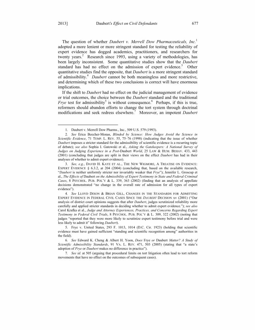
The question of whether Daubert v. Merrell Dow Pharmaceuticals, Inc.1 adopted a more lenient or more stringent standard for testing the reliability of expert evidence has dogged academics, practitioners, and researchers for twenty years.2 Research since 1993, using a variety of methodologies, has been largely inconsistent. Some quantitative studies show that the Daubert standard has had no effect on the admission of expert evidence.3 Other quantitative studies find the opposite, that Daubert is a more stringent standard of admissibility.4 Daubert cannot be both meaningless and more restrictive, and determining which of these two conclusions is correct will have enormous implications.
If the shift to Daubert had no effect on the judicial management of evidence or trial outcomes, the choice between the Daubert standard and the traditional Frye test for admissibility5 is without consequence.6 Perhaps, if this is true, reformers should abandon efforts to change the tort system through doctrinal modifications and seek redress elsewhere.7 Moreover, an impotent Daubert
1. Daubert v. Merrell Dow Pharms., Inc., 509 U.S. 579 (1993). 2. See Erica Beecher-Monas, Blinded by Science: How Judges Avoid the Science in Scientific Evidence, 71 TEMP. L. REV. 55, 75–76 (1998) (indicating that the issue of whether Daubert imposes a stricter standard for the admissibility of scientific evidence is a recurring topic of debate); see also Sophia I. Gatowski et al., Asking the Gatekeepers: A National Survey of Judges on Judging Experience in a Post-Daubert World, 25 LAW & HUM. BEHAV. 433, 443 (2001) (concluding that judges are split in their views on the effect Daubert has had in their analyses of whether to admit expert evidence). 3. See, e.g., DAVID H. KAYE ET AL., THE NEW WIGMORE, A TREATISE ON EVIDENCE: EXPERT EVIDENCE § 6.3.2, at 204 (2004) (concluding that, based on the available research, “Daubert is neither uniformly stricter nor invariably weaker that Frye”); Jennifer L. Groscup et al., The Effects of Daubert on the Admissibility of Expert Testimony in State and Federal Criminal Cases, 8 PSYCHOL. PUB. POL’Y & L. 339, 363 (2002) (finding that an analysis of appellate decisions demonstrated “no change in the overall rate of admission for all types of expert evidence”). 4. See LLOYD DIXON & BRIAN GILL, CHANGES IN THE STANDARDS FOR ADMITTING
EXPERT EVIDENCE IN FEDERAL CIVIL CASES SINCE THE DAUBERT DECISION xv (2001) (“Our analysis of district court opinions suggests that after Daubert, judges scrutinized reliability more carefully and applied stricter standards in deciding whether to admit expert evidence.”); see also Carol Krafka et al., Judge and Attorney Experiences, Practices, and Concerns Regarding Expert Testimony in Federal Civil Trials, 8 PSYCHOL. PUB. POL’Y & L. 309, 322 (2002) (noting that judges “reported that they were more likely to scrutinize expert testimony before trial and were less likely to admit it” following Daubert). 5. Frye v. United States, 293 F. 1013, 1014 (D.C. Cir. 1923) (holding that scientific evidence must have gained sufficient “standing and scientific recognition among” authorities in the field). 6. See Edward K. Cheng & Albert H. Yoon, Does Frye or Daubert Matter? A Study of Scientific Admissibility Standards, 91 VA. L. REV. 471, 503 (2005) (stating that “a state’s adoption of Frye or Daubert makes no difference in practice”). 7. See id. at 505 (arguing that procedural limits on tort litigation often lead to tort reform movements that have no effect on the outcomes of subsequent cases).

678 Catholic University Law Review [Vol. 62:675
would also indicate that the controversy in evidence law about expert admissibility has been much ado about nothing.
However, if Daubert is a more stringent standard, the implications are enormous. It would indicate that—at the time of its decision—the Supreme Court badly misjudged what effect Daubert would have on the admissibility of scientific evidence. At the time, the Court believed that the decision would be consistent with “the liberal thrust of the Federal Rules [of Evidence] and their general approach of relaxing the traditional barriers to opinion testimony.”8 If this were not true, the Court would need to revisit expert reliability standards, to clarify the standard by either affirming the new reality or insisting upon the lenient standard initially envisioned. A stricter Daubert standard would also have an enormous effect on substantive tort law by procedural modification.9 Finally, a stricter standard for admissibility affects the market for expert witness services, because only those experts who can provide a sound empirical basis for their opinions will be permitted to testify.10 Therefore, the interpretation of the Daubert standard is important, especially in an era when expert witness testimony is as prevalent as it is today.11
In this Article, we answer the question: Did Daubert have a measurable effect on expert admissibility, and if so, did it adopt a stricter or more lenient standard for admissibility? To make this determination, this Article builds on a
8. Daubert v. Merrell Dow Pharms., Inc., 509 U.S. 579, 588 (1993) (internal quotation marks omitted) (citing Beech Aircraft Corp. v. Rainey, 488 U.S. 153, 169 (1988)). Four years after Daubert, the Court reiterated its understanding that Daubert lowered the admissibility standard. See Gen. Electric v. Joiner, 522 U.S. 136, 142 (1997) (acknowledging that “the Federal Rules of Evidence allow district courts to admit a somewhat broader range of scientific testimony than would have been admissible under Frye”); see also infra notes 46–52 and accompanying text (detailing the Court’s perception of the role of the Daubert decision). 9. See infra Part III.A (discussing in detail the implications of a stricter Daubert standard). 10. Michael J. Saks, The Aftermath of Daubert: An Evolving Jurisprudence of Expert Evidence, 40 JURIMETRICS J. 229, 239 (2000) (“Testimony from those fields that could, but do not, provide adequate data . . . should be excluded until they can provide adequate empirical support for what the experts are claiming for their field in general, or for themselves individually.”). 11. The percentage of cases involving experts remains an area with surprisingly few definitive statistics. One oft-cited study concluded that experts are involved in as many as 86% of all civil jury cases. Samuel R. Gross, Expert Evidence, 1991 WISC. L. REV. 1113, 1119 (reporting data from all civil jury cases tried in California Superior Court between 1985 and 1986). Other studies returned an expert witness rate between 63% and 71%. Anthony Champagne et al., An Empirical Examination of the Use of Expert Witnesses in American Courts, 31 JURIMETRICS J. 375, 380 (1991) (finding that 57 out of 90 civil cases tried in the Dallas County District Court in Texas in 1988 utilized expert witness testimony); Daniel Shuman et al., An Empirical Examination of the Use of Expert Witnesses in the Courts—Part II: A Three City Study, 34 JURIMETRICS J. 193, 197 (1994) (reporting that 131 cases out of 183 included expert testimony, a rate of 73%). Regardless of the exact rate, experts are a permanent and enormous part of modern litigation.

2013] Daubert's Effect on Civil Defendants 679
methodology used in a 2005 study by Edward Cheng and Albert Yoon.12 In certain cases, removal allows a civil defendant the option of transferring a case from state to federal court.13 By removing the case, however, the defendant may also be changing the scientific admissibility standard from the state court’s Frye standard to the federal Daubert standard.14 Cheng and Yoon first suggested that the effect of Daubert could be measured across the judicial system by reviewing removal rates from state to federal court in multiple jurisdictions.15 We also believe that removal rates offer a very accurate method of measuring the systematic effect of Daubert because these rates test litigants’ opinions in the context of real cases.16
To this end, we created a database of approximately 4 million cases and calculated removal rates during the period from 1990 to 2000. Based on our two-step analysis of that data, we conclude that Daubert is a stricter standard than Frye for the admissibility of expert testimony.17 First, by properly identifying, isolating, and removing other possible confounding variables, we were able to isolate and then measure the effect of the federal courts’ adoption
12. Cheng & Yoon, supra note 6, at 482–84 (describing the removal-rate metric). 13. See 28 U.S.C. § 1446 (2006) (articulating the requirements to remove a case from state court to federal court); see also Cheng & Yoon, supra note 6, at 482–83 (explaining that a litigant may remove a tort action—normally restricted to state court—to federal court under diversity jurisdiction). 14. The central premise allowing for this comparison is that evidence rules are generally considered to be procedural, and thus a state’s evidentiary rules on expert admissibility will not transfer upon removal. Instead, the Federal Rules of Evidence will usually apply to the action, even if state substantive tort law remains. See Cheng & Yoon, supra note 6, at 483 (explaining that, although state substantive law is retained in tort cases because of diversity jurisdiction and the Erie doctrine, the procedural rules of the new forum are applied (citing Erie R.R. Co. v. Tompkins, 304 U.S. 64, 78 (1938))); see also, e.g., Robin Kundis Craig, When Daubert Gets Erie: Medical Certainty and Medical Expert Testimony in Federal Court, 77 DENV. U. L. REV. 69, 82 (1999) (asserting that “[m]ost federal courts apply the Federal Rules of Evidence rather than state rules to all evidentiary questions in diversity cases”); Abbe R. Gluck, Intersystemic Statutory Interpretation: Methodology as “Law” and the Erie Doctrine, 120 YALE L.J. 1898, 1979 & n.279 (2011) (explaining that the Federal Rules of Evidence are generally considered to be procedural and are applied in cases removed from state courts); Alex Stein, Constitutional Evidence Law, 61 VAND. L. REV. 65, 98–99 (2008) (noting that all evidence rules, except burdens of proof, privileges, presumptions, and the competency of witnesses, are procedural). 15. See Cheng & Yoon, supra note 6, at 482 (using the rate at which cases were removed to federal court to measure the effect of the Daubert decision on the admission of expert evidence). 16. See infra Part II.B (explaining the merits of using removal rate as a measuring tool). 17. See infra Part II.C.2 (demonstrating that the rate of removal to federal court in Frye states increased following the adoption of Daubert in federal courts); see also infra Part II.C.3 (demonstrating that the rate of removal to federal court decreased once Frye states adopted Daubert); infra Part II.C.4 (concluding that the rates of removal to federal court in relation to a jurisdiction’s adoption of Daubert indicate that Daubert is a stricter standard for admissibility than Frye).

680 Catholic University Law Review [Vol. 62:675
of Daubert on removal rates to federal court.18 These results demonstrate that, absent other countervailing effects, the adoption of Daubert by federal courts results in an increase in civil defendants removing the case to federal courts to benefit from the courts’ restriction of expert testimony under that standard.19 Second, by using the same process, we were able to measure the counter-effect on removals when a state court adopted Daubert after the federal courts had already done so.20 These results demonstrate that a state court’s adoption of Daubert after federal adoption decreases the rate of removals to federal court.21 This is consistent with our initial result because, after the state court adopts Daubert, litigants gain no procedural benefit from shifting court systems when both apply the same reliability standard. Combined, these results demonstrate unequivocally that, when measured in the aggregate and based on actual behavior in real cases, civil defendants believe the Daubert standard is more restrictive to expert testimony and act accordingly.22
We begin in Part I of this Article by briefly outlining the Daubert standard and the impact the case has had on gatekeeping expert testimony. Additionally, Part I introduces prior empirical studies on Daubert, and addresses those studies’ contradictory results. We then begin our empirical analysis in Part II. First, we briefly review the Cheng and Yoon study and its counterintuitive finding that a state’s choice between Daubert and Frye “makes no difference in practice.”23 We then explain in more detail why the removal rate metric is the key to determining Daubert’s true effect. Next, we then used the removal rate metric to analyze our database of civil case data in order to measure the aggregate effect of Daubert on litigant behavior. Our analysis demonstrates that the adoption of Daubert in federal court did, in a statistically significant manner, increase removal rates from Frye states. Furthermore, we will also demonstrate that in the period after the federal adoption of Daubert, a state’s adoption of a Daubert-type standard for state court reduced the removal rates, thereby reversing the post-Daubert increase in removals. Both findings demonstrate, for the first time and using actual case data, that civil defendants believe Daubert is a stricter admissibility standard.
18. See infra Part II.C.2 (explaining the methodology by which we analyzed the impact of Daubert on removal rates in Frye states). 19. See infra Part II.C.2 (noting our conclusion that the rate of removal to federal court in Frye states increased after the adoption of Daubert in federal courts). 20. See infra Part II.C.3 (explaining the methodology by which we analyzed the subsequent adoption of Daubert in state courts on removal rates). 21. See infra Part II.C.4 (noting our conclusion that the rate of removal to federal court following a state’s adoption of Daubert reverted to pre-federal-court-adoption levels). 22. See infra Part II.C.4 (summarizing our conclusion that Daubert is a stricter standard because of the preceding analysis of litigant behavior in relation to a jurisdiction’s adoption of that standard). 23. Cheng & Yoon, supra note 6, at 503.

2013] Daubert's Effect on Civil Defendants 681
Because our results so clearly contrast with Cheng and Yoon, who used the same data, we then revisit the Cheng and Yoon study and evaluate its methodology in detail. In so doing, we found that Cheng and Yoon appear to have made three kinds of errors in their analysis that explain why they failed to identify the true nature of adoption of Daubert. First, there seem to be errors in how they determined the removal rates that form their study population. Second, they failed to recognize that state adoption of Daubert after federal adoption of Daubert will have a different effect than state adoption of Daubert before federal adoption of Daubert. Consequently, their data is internally inconsistent with regard to their analysis of state adoption of Daubert. Third, the small size of the study population they directly use (removal rates) combined with the enormous size of the population they derive the study population from (torts filed in state court) minimized the chances of finding an effect from state adoption of Daubert.
Finally, we will finish in Part III with some comments on the significance of a stricter Daubert standard. We also suggest areas for future empirical consideration that would build upon our research.
By measuring the actual behavior of civil litigants, this Study can answer the question whether Daubert is a stricter standard for expert admissibility. Based on our analysis of the behavior of civil defendants in actual cases, the answer is yes.
I. GATEKEEPING EXPERT EVIDENCE, DAUBERT, AND CURRENT RESEARCH ON
DAUBERT’S EFFECT
As many as 86% of all cases involve expert evidence and, consequently, this evidence is of central importance to modern civil and criminal litigation.24 With certain civil causes of action—such as products liability or medical malpractice—the percentage of cases utilizing expert evidence can be even higher.25 In this context, any changes in the rules governing expert evidence have the potential to greatly affect case management.26 Before analyzing the data on Daubert’s effect, we will first review the issue of admissibility
24. See supra note 11 and accompanying text (discussing the prevalence of expert evidence in modern litigation). 25. See Gross, supra note 11, at 1119 (finding that over 90% of products liability and medical malpractice cases relied on expert testimony); see also Joseph Sanders, From Science to Evidence: The Testimony on Causation in the Benedectin Cases, 46 STAN. L. REV. 1, 31–32 (1993) (noting the particular importance of expert witnesses in products liability cases). 26. See Krafka et al., supra note 4, at 328 (reporting that approximately 69% of judges surveyed changed their procedures for considering the admissibility of expert evidence following their jurisdictions’ shift to Daubert and that, generally, judges view themselves as more active in the admissibility process following Daubert); see also The Changing Role of Judges in the Admissibility of Expert Evidence, CIV. ACTION (Nat’l Ctr. for State Courts), Spring 2006, at 3 [hereinafter Changing Role of Judges].

682 Catholic University Law Review [Vol. 62:675
standards for scientific evidence, and review prior interesting but inconclusive studies on their effect.
A. The Frye Decision and Expert Admissibility
Concern over the admissibility of expert witness testimony did not originate with the Daubert debate of the late twentieth century. In fact, the admissibility standard articulated in Frye v. United States grew out of dissatisfaction with preexisting common law standards. Eventually the Frye standard became the admissibility test in federal and many state courts, when litigants raised the issue of admissibility of scientific testimony. Frye required that—before admission—a method be generally accepted in the relevant field.27 However, throughout the twentieth century, critics exposed many weaknesses of the Frye general acceptance formula.28
Before 1923, judges used two common law tests to determine the admissibility of expert evidence. Some courts simply evaluated the helpfulness of the evidence to a lay jury, and admitted the evidence if it was relevant.29 Others would consider the qualifications of the expert under what Professor David Faigman and his coauthors call “the commercial marketplace test,” whereby any expert who succeeds in a chosen profession must do so based on expertise.30
By 1923, the problems with relying on relevance or the reputation of the expert led the D.C. Circuit to reconsider the standard for admissibility of expert evidence.31 In Frye, the court shifted the focus away from the prior
27. Frye v. United States, 293 F. 1013, 1014 (D.C. Cir. 1923). 28. See infra notes 36–41 and accompanying text (tracking the evolution of the Frye standard and its shortcomings). 29. KAYE ET AL., supra note 3, § 1.2.1, at 6–7 (noting that expert testimony must have been “particularly important to aiding the trier of fact” in order to be admitted); David L. Faigman et al., Check Your Crystal Ball at the Courthouse Door, Please: Exploring the Past, Understanding the Present, and Worrying About the Future of Scientific Evidence, 15 CARDOZO L. REV. 1799, 1803 (1994) (explaining that the relevant inquiry was whether the testimony was from an area beyond the knowledge of the average juror). 30. Faigman et al., supra note 29, at 1804 & n.13 (noting that judges would evaluate the qualifications and expertise of the expert through “the expert’s success in an occupation or profession which embraced” the subject matter in question); Michael J. Saks, Judging Admissibility, 35 J. CORP. L. 135, 136 (2009) (explaining that judges often inferred expertise from the expert’s commercial success). 31. Frye, 293 F. at 1013; see also Faigman et al., supra note 29, at 1805 (arguing that Frye was a response to the failure of the commercial marketplace test); Saks, supra note 30, at 137 (noting that “commercial value is not a measure of scientific or any other kind of validity”); Michael J. Saks, Merlin and Solomon: Lessons from the Law’s Formative Encounters with Forensic Identification Science, 49 HASTINGS L.J. 1069, 1074 (1998) (explaining that the flaws of the commercial marketplace test necessitated the Frye standard).

2013] Daubert's Effect on Civil Defendants 683
common law standard to a “general acceptance test.”32 The court concluded that expert testimony cannot be considered at trial unless it has become “sufficiently established as to have gained general acceptance in the particular field to which it belongs.”33 Applying this standard, the Frye court affirmed the exclusion of the expert testimony because the testing in question remained experimental.34
With the holding in Frye, the D.C. Circuit developed a standard by which a court could assess whether a scientific principle had gained sufficient recognition as to be appropriate to consider in court. Yet, for all its controversy, particularly later, the standard appears to have been applied sparingly for decades. Professor Michael Saks notes that the case was not cited for over 10 years following the decision; it received fewer than 15 citations in its first 25 years, and fewer than 100 citations in the next 25-year span.35 By the late twentieth century, however, the trend shifted.
The Frye test was used primarily in criminal cases until the late 1980s36 when courts began to apply it to complex scientific causation in toxic tort cases.37 The application of the Frye test to complicated civil cases intensified the existing controversy over the standard, and commentators noted the unworkability of the vague “general acceptance” test.38 Critics argued that the
32. Frye, 293 F. at 1013–14 (considering the admissibility of expert testimony explaining the systolic blood pressure deception test); see also Faigman et al., supra note 29, at 1806 (arguing that, although Frye is inherently a marketplace test, the standard shifts the emphasis from the credentials of the expert and the commercial marketplace, requiring an evaluation of the body of knowledge rather than the expert himself). 33. Frye, 293 F. at 1014. 34. Id. (holding that “the systolic blood pressure deception test ha[d] not yet gained such standing and scientific recognition” to justify admitting the expert testimony). 35. Saks, supra note 30, at 139; see also Faigman et al., supra note 29, at 1808 (describing Frye as “barely noticed” and “of little importance” in the decades after it was decided). Professor David Bernstein noted that, despite the dearth of federal court citations to Frye, state courts may have used the standard more often in deciding cases. David E. Bernstein, Frye, Frye, Again: The Past, Present, and Future of the General Acceptance Test, 41 JURIMETRICS J. 385, 388–90 (2001). However, that theory cannot be tested because state trial court opinions generally remain unpublished. Id. 36. Bernstein, supra note 35, at 390 (asserting that Frye was applied only in criminal cases until 1988); Kenneth J. Chesebro, Galileo’s Retort: Peter Huber’s Junk Scholarship, 42 AM. U. L. REV. 1637, 1693–95 (1993) (indicating that 64 of 67 federal appellate decisions applying Frye were criminal decisions); Susan Haack, An Epistemologist in the Bramble-Bush: At the Supreme Court with Mr. Joiner, 26 J. HEALTH POL. POL’Y & L. 217, 227 (2001) (noting that Frye was the standard for the admissibility of expert evidence first in criminal cases, but later became the standard in civil cases); cf. KAYE ET AL., supra note 3, § 5.3.2, at 159–60 (detailing the several types of evidence the Frye test has been used to exclude). 37. Bernstein, supra note 35, at 390–92 (explaining that Frye was applied to toxic tort cases starting in 1988). 38. See, e.g., Bert Black, A Unified Theory of Scientific Evidence, 56 FORDHAM L. REV. 595, 628 (1988) (arguing that the Frye test is too incoherent to be applied effectively by the

684 Catholic University Law Review [Vol. 62:675
test provided little guidance on what evidence demonstrated general acceptance, and then what level of proof was required.39 They also noted Frye’s failure to exclude “scientific” evidence that later proved to be unfounded.40 In his exhaustive study of toxic tort litigation, Professor Joseph Sanders analyzed the judicial decision making process in case law and examined in detail how the system failed to properly manage complex expert testimony.41
Criticism of the Frye standard left many with an impression of judicial incompetence in the management of scientific evidence,42 and commentators showed increasing dismay with courts’ inability to sift away “junk science.”43 In the context of this debate over the courts’ ability to properly manage complex science, the U.S. Supreme Court granted certiorari in a toxic tort case from the Ninth Circuit: Daubert v. Merrell Dow Pharmaceuticals, Inc.44
courts); Paul C. Giannelli, The Admissibility of Novel Scientific Evidence: Frye v. United States, A Half-Century Later, 80 COLUM. L. REV. 1197, 1207–08, 1223 (1980) (arguing that the Frye test is too vague and leads to inconsistent results). 39. See KAYE ET AL., supra note 3, § 5.3.3, at 164 (noting that the Frye decision was unclear in its standard); Giannelli, supra note 41, at 1219 (finding that courts are unsure as to the appropriate scenarios to which to apply the Frye standard). 40. See PETER W. HUBER, GALILEO’S REVENGE (1991); see also KAYE ET AL., supra note 3, § 5.3.2, at 163–64 (providing examples of cases in which the Frye standard allowed for the admission of “worthless and potentially misleading” scientific evidence); Giannelli, supra note 38, at 1224–25 (pointing to the admission of evidence collected from paraffin tests as proof of Frye’s shortcomings). 41. Sanders, supra note 25, at 27–28 (arguing that scientific data “fails to provide the lay fact finder with the resources necessary to assess properly the quality of experts or the weight and relative importance of the scientific findings”). 42. See Andre A. Moenssens, Admissibility of Scientific Evidence—An Alternative to the Frye Rule, 25 WM. & MARY L. REV. 545, 551–52 (1984) (asserting that judges often admitted evidence under Frye because of their failure to understand the relevant scientific principles). 43. See, e.g., CARL F. CRANOR, TOXIC TORTS 46–47 (2006) (arguing that expert testimony can be used to mislead judges and juries unfamiliar with the scientific evidence); MICHAEL D. GREEN, BENDECTIN AND BIRTH DEFECTS: THE CHALLENGES OF MASS TOXIC SUBSTANCES
LITIGATION 20 (1996) (articulating concern about the use of invalid scientific evidence); HUBER, supra note 40, at 14–17; David E. Bernstein, Junk Science in the United States and the Commonwealth, 21 YALE J. INT’L L. 123, 123 (1996) (alleging misuse of scientific evidence in toxic tort cases); Gary Edmond & David Mercer, Trashing “Junk Science”, 1998 STAN. TECH. L. REV. 3, ¶¶ 52, 57 (noting tensions regarding the use of junk science); Barry M. Epstein & Marc S. Klein, The Use and Abuse of Expert Testimony in Product Liability Actions, 17 SETON HALL L. REV. 656, 660–62 (1987) (acknowledging the concern over the use of bad science in product liability cases). 44. Daubert v. Merrell Dow Pharms., Inc., 43 F.3d 1311 (9th Cir. 1991), cert. granted, 506 U.S. 214 (1992).

2013] Daubert's Effect on Civil Defendants 685
B. The Daubert Revolution and Its Aftermath
The Federal Rules of Evidence became effective in 1975,45 and while the rules contained a specific section on expert admission, the effect of Rule 702 on the Frye standard was unclear.46 The Daubert Court definitively resolved the dispute.
In Daubert, Justice Harold Blackmun—writing for the majority—stated unequivocally “[t]hat [the] austere [Frye] standard, absent from, and incompatible with, the Federal Rules of Evidence, should not be applied in federal trials.”47 Beyond that initial labeling of Frye as austere, there are additional reasons to believe that the Daubert Court consciously lowered the standard for admissibility. Instead of Frye’s “general acceptance” test, the Daubert test depends on the twin standards of Rule 702: relevance and reliability.48 The Court specifically stated that a Rule 702 approach is consistent with the Federal Rules’ purpose “of relaxing the traditional barriers to opinion testimony.”49 In addition, under the new standard, the Court specifically endorsed the idea that shaky expert evidence should be admitted, subject to vigorous cross-examination.50 Four years later in General Electric Co. v. Joiner, the Court expressly stated what had been implied in Daubert: “the Federal Rules of Evidence allow district courts to admit a somewhat broader range of scientific testimony than would have been admissible under Frye.”51 The intent of the Daubert standard, the Court later explained, was to ensure that any expert “employs in the courtroom the same level of intellectual rigor that characterizes the practice of an expert in the relevant field.”52
45. Act of Jan. 2, 1975, Pub. L. No. 93-595, 88 Stat. 1926 (enacting the Federal Rules of Evidence). 46. See Giannelli, supra note 38, at 1228–29 (“The adoption of the Federal Rules of Evidence has not resolved the uncertain status of the Frye test. Indeed, the Federal Rules, which became effective in 1975 and have been adopted in various forms by twenty-two jurisdictions, have contributed to the confusion.” (citation omitted)); see also Faigman et al., supra note 29, at 1809–10 (noting that, even though Rule 702 and the Advisory Committee Notes made no reference to Frye, courts incorporated the “general acceptance” standard into the Rule 702 test). 47. Daubert v. Merrell Dow Pharms., Inc., 509 U.S. 579, 582, 589 (1993). 48. See id. at 589 (explaining that Rule 702 is “[t]he primary locus” of the trial judge’s duty to ensure that expert evidence is both relevant and reliable); see also FED. R. EVID. 702 (requiring expert evidence to be both helpful to the trier of fact and reliable in both its methodology and the expert’s execution of that methodology). 49. Id. at 588 (internal quotation marks omitted) (citing Beech Aircraft Corp. v. Rainey, 488 U.S. 153, 169 (1988)). 50. Id. at 596 (citing Rock v. Arkansas, 483 U.S. 44, 61 (1987)) (explaining that inconsistencies or inaccuracies in expert testimony can be challenged by cross-examination). 51. Gen. Electric Co. v. Joiner, 522 U.S. 136, 142 (1997). 52. Kumho Tire Co. v. Carmichael, 526 U.S. 137, 152 (1999).

686 Catholic University Law Review [Vol. 62:675
After Daubert, federal courts began to apply the Rule 702 standard to many different forms of scientific evidence.53 Daubert empowered judges to act as gatekeepers of expert evidence, a role that requires detailed assessment of complex scientific principles.54 Even though the Daubert majority expressed confidence in the judiciary’s ability to handle this gatekeeping role, Chief Justice William Rehnquist expressed apprehension in converting judges into “amateur scientists.”55 Certainly many commentators, scholars, and even federal judges shared his concern.56
After 20 years, Daubert’s influence in state courts remains mixed. Many states decided, even after Daubert, that their courts would continue to use the Frye test to evaluate expert evidence.57 Other states concluded that Daubert recognized the judicial role already present in their jurisdictions.58 Finally, a large group of states followed the lead of the Supreme Court and abandoned Frye in favor of Daubert’s rules-based reliability approach.59 In these states, the Daubert decision directed judges to become more involved in gatekeeping decisions and screening scientific evidence for methodological soundness.60 Indeed, even in those states that retained Frye, the debate over the 53. See generally Saks, supra note 30, at 147–55 (discussing the application of the Daubert standard to several types of forensic evidence). 54. Daubert, 509 U.S. at 592–94, 597 (requiring the trial judge to assess the scientific validity of proffered expert evidence and urging judges to engage in the evaluation of such factors as the peer reception and margin of error of the scientific technique or methodology in question); see also Gatowski et al., supra note 2, at 436–37 (discussing the factors Daubert provided to judges for assessing scientific validity, but also noting that the Court did not provide specific guidance for evaluating these principles). 55. Daubert, 509 U.S. at 600–01 (Rehnquist, C.J., concurring in part and dissenting in part). Justice Blackmun and the majority did not share this concern. Id. at 592–93 (majority opinion) (“We are confident that federal judges possess the capacity to undertake this review.”). 56. See, e.g., Saks, supra note 30, at 144 (recognizing that some judges are unwilling or unable to apply Daubert in cases with complex scientific evidence); see also Daubert v. Merrell Dow Pharms., 43 F.3d 1311, 1315 (9th Cir. 1995) (noting that federal judges “face a far more complex and daunting task in a post-Daubert world than before”). 57. KAYE ET AL., supra note 3, § 6.4.2, at 225–26 & n.17. This group of states includes: Pennsylvania, see Grady v. Frito-Lay, 839 A.2d 1038, 1039 (Pa. 2003) (retaining Frye); Illinois, see Donaldson v. Cent. Ill. Pub. Serv. Co., 767 N.E.2d 314, 323 (Ill. 2002) (same); California, see People v. Leahy, 882 P.2d 321, 324 (Cal. 1994) (same); New York, see People v. Wesley, 633 N.E.2d 451, 454 (N.Y. 1994) (same); and Florida, see Flanagan v. State, 625 So. 2d 827, 828 (Fla. 1993) (same). For a complete list of those states that retained the Frye standard after Daubert, see David E. Bernstein & Jeffrey D. Jackson, The Daubert Trilogy in the States, 44 JURIMETRICS J. 351, 355 n.25 (2004). 58. See KAYE ET AL., supra note 3, § 6.4.2, at 225 & n.14 (listing the courts that applied a Daubert-like standard before the decision). 59. See id. at 225 & n.16 (listing the courts that followed the Supreme Court and adopted the Daubert standard). 60. See supra note 54 and accompanying text (describing the judge’s role as gatekeeper under Daubert and the type of analysis performed by a judge in assessing the scientific validity of expert evidence).

2013] Daubert's Effect on Civil Defendants 687
admissibility standard for experts appears to have increased judicial scrutiny of scientific evidence.61
C. Prior Studies on Daubert: Surveys and Case Review Analysis
Even if judges in both Daubert and Frye jurisdictions have examined scientific evidence more closely after Daubert, many scholars question if the shift in standards had a major effect on the handling of cases. To help answer this question, researchers have both surveyed judges and performed quantitative analysis of reported cases.
1. Studies Relying on Survey Methodology
Survey instruments since Daubert have attempted to measure the effect of the Rule 702 standard on judicial practices. For example, a 2001 study by Sophia Gatowski and her coauthors analyzed state court judges’ perceptions of the gatekeeping function and the effect of Daubert.62 Judges surveyed supported the gatekeeping role by a wide margin (91%), and over 60% of judges saw themselves taking an active role in admissibility analysis.63 When asked about the effect of Daubert on the gatekeeping process, the judges’ responses did not show a clear consensus.64 The largest group of judges in the survey (36%) believed Daubert was not intended to raise or lower the threshold for admissibility, and an additional 11% were unsure of Daubert’s intent.65 Even among those who believed Daubert did change the admissibility standard, the result was mixed. Twenty-three percent of respondents stated that the Court’s intent was to lower the threshold, while 32% indicated that the court’s intent was to raise the standard.66 In that 2001 survey, then, judges lacked consensus on the effect of Daubert on gatekeeping, even if many supported an active judicial role.
61. See KAYE ET AL., supra note 3, at 186 (noting that Frye jurisdictions apply the test with “enhanced vigor”); see also Bernstein, supra note 35, at 393 (asserting that Frye is “slowly converging with Daubert jurisprudence”). 62. Gatowski et al., supra note 2, at 433. The participating judges were from both Daubert and Frye jurisdictions. Id. at 442 (surveying 400 judges: 205 from Daubert jurisdictions and 195 from Frye jurisdictions). 63. Id. at 443 (noting that judges support the gatekeeping function regardless of which admissibility standard is applied). 64. Id. at 444 (finding a 14% difference between judges who believed Daubert changed their roles as gatekeeper and those who believed that their roles remained the same following the Daubert decision). 65. Id. at 443 (stating that those who believed that Daubert had no intent to change the standard for admissibility instead believed that Daubert’s intent was to give judges the discretion to apply the admissibility framework themselves). 66. Id.
688 Catholic University Law Review [Vol. 62:675
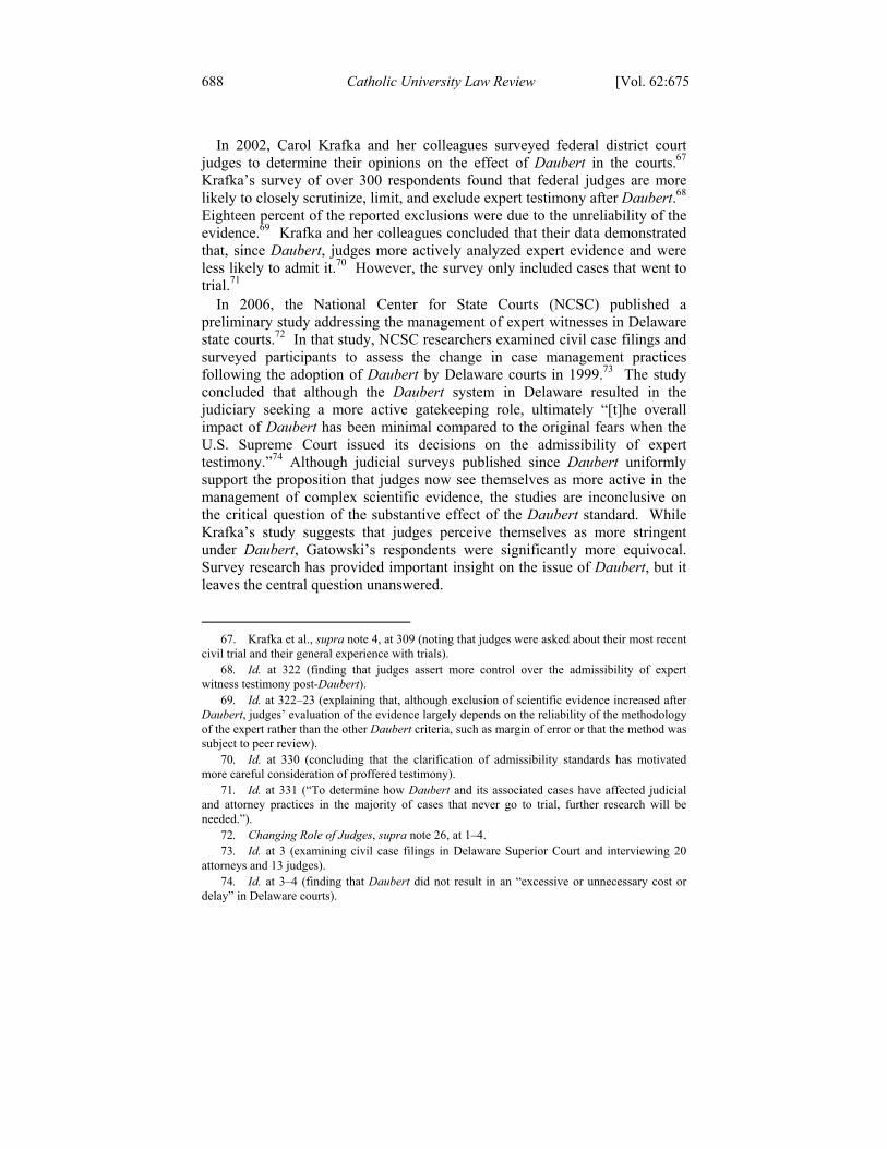
In 2002, Carol Krafka and her colleagues surveyed federal district court judges to determine their opinions on the effect of Daubert in the courts.67 Krafka’s survey of over 300 respondents found that federal judges are more likely to closely scrutinize, limit, and exclude expert testimony after Daubert.68 Eighteen percent of the reported exclusions were due to the unreliability of the evidence.69 Krafka and her colleagues concluded that their data demonstrated that, since Daubert, judges more actively analyzed expert evidence and were less likely to admit it.70 However, the survey only included cases that went to trial.71
In 2006, the National Center for State Courts (NCSC) published a preliminary study addressing the management of expert witnesses in Delaware state courts.72 In that study, NCSC researchers examined civil case filings and surveyed participants to assess the change in case management practices following the adoption of Daubert by Delaware courts in 1999.73 The study concluded that although the Daubert system in Delaware resulted in the judiciary seeking a more active gatekeeping role, ultimately “[t]he overall impact of Daubert has been minimal compared to the original fears when the U.S. Supreme Court issued its decisions on the admissibility of expert testimony.”74 Although judicial surveys published since Daubert uniformly support the proposition that judges now see themselves as more active in the management of complex scientific evidence, the studies are inconclusive on the critical question of the substantive effect of the Daubert standard. While Krafka’s study suggests that judges perceive themselves as more stringent under Daubert, Gatowski’s respondents were significantly more equivocal. Survey research has provided important insight on the issue of Daubert, but it leaves the central question unanswered.
67. Krafka et al., supra note 4, at 309 (noting that judges were asked about their most recent civil trial and their general experience with trials). 68. Id. at 322 (finding that judges assert more control over the admissibility of expert witness testimony post-Daubert). 69. Id. at 322–23 (explaining that, although exclusion of scientific evidence increased after Daubert, judges’ evaluation of the evidence largely depends on the reliability of the methodology of the expert rather than the other Daubert criteria, such as margin of error or that the method was subject to peer review). 70. Id. at 330 (concluding that the clarification of admissibility standards has motivated more careful consideration of proffered testimony). 71. Id. at 331 (“To determine how Daubert and its associated cases have affected judicial and attorney practices in the majority of cases that never go to trial, further research will be needed.”). 72. Changing Role of Judges, supra note 26, at 1–4. 73. Id. at 3 (examining civil case filings in Delaware Superior Court and interviewing 20 attorneys and 13 judges). 74. Id. at 3–4 (finding that Daubert did not result in an “excessive or unnecessary cost or delay” in Delaware courts).

2013] Daubert's Effect on Civil Defendants 689
2. Quantitative Analysis of Reported Cases
Researchers studying the effect of Daubert have also used non-survey methodologies, by analyzing reported court decisions to measure changes since 1993. Just as with the survey research, these studies are also largely inconclusive.
A 2001 study by Lloyd Dixon and Brian Gill examined the substantive effect of the Daubert decision in federal civil cases by analyzing challenges to expert evidence in federal district courts.75 Their methodology evaluated the number of reported decisions in Westlaw’s database that dealt with challenges to expert evidence and the results of reliability determinations in those decisions.76 Dixon and Gill concluded that the data “suggest that the standards for reliability tightened in the years after the Daubert decision.”77 However, the researchers noted that their study had two important limitations: (1) their findings did not address whether greater judicial scrutiny resulted in better outcomes in the affected cases; and (2) the study was not conclusive in determining whether Daubert’s effect was uniform across the judiciary.78 Even with the limitations, Dixon and Gill concluded that their “analysis of district court opinions suggests that following Daubert, judges scrutinized reliability more carefully and applied stricter standards in deciding whether to admit expert evidence.”79
In 2002, Jennifer Groscup and her colleagues published an empirical study on the effect of Daubert on expert testimony in federal criminal cases.80 Using a methodology similar to Dixon and Gill’s analysis, Groscup used search terms in a computer database to see what trends or changes could be measured over time.81 In evaluating trends in both state and federal courts, Groscup found that “the basic rates of admission at the trial and the appellate court levels did not change significantly after Daubert in criminal cases on appeal.”82 Groscup suggested that the party offering the evidence, the type of counsel for the defense, and the standard of review may all play a part in the static rates of admission of expert evidence.83 Groscup concluded that, although there may be increased scrutiny of scientific evidence in criminal
75. DIXON & GILL, supra note 4, at xii–xiv. 76. Id. at 15–19 (explaining the methodology by which the data was collected). 77. Id. at 28 fig.4.1, 29 (reporting that the success rate for the challenge of expert evidence increased following Daubert). 78. Id. at 30–31 (noting that additional data is needed to address the study’s limitations). 79. Id. at 61. 80. Groscup et al., supra note 3, at 342 (examining appellate court decisions). 81. Id. at 342–44 (using specific terms and connectors and date restrictions in the Westlaw database). 82. Id. at 345 (noting that this conclusion was contrary to the prediction of most commentators). 83. Id. at 346–47.

690 Catholic University Law Review [Vol. 62:675
cases, “no change in the overall rate of admission for all types of expert evidence was observed.”84
3. Prior Survey and Case Study Research—Conclusion
In assessing the results of prior research in the field, both survey instruments and case review studies remain largely inconclusive on the effect of the Daubert ruling. Clearly, the Krafka survey responses and the Dixon and Gill case review study demonstrate support for the conclusion that Daubert has raised the standard for admission of expert testimony. Conversely, Gatowski’s survey and the Groscup case review study demonstrate little to no difference between Frye and Daubert jurisdictions, suggesting the change is much ado about nothing.
Without a clear finding from prior research, and without more guidance from the Supreme Court, the question of Daubert’s effect remained open. To find out more, researchers Edward Cheng and Albert Yoon turned to a new tool of analysis.
II. REMOVAL RATE APPROACH TO ANALYZING DAUBERT
To answer the question of whether Daubert adopted a stricter standard for admitting scientific evidence, Cheng and Yoon adopted a new approach by analyzing a new metric and a large amount of case data to measure Daubert’s effect.85 Their study concluded that the adoption of the Daubert standard did not have a statistically significant effect.86
We found this conclusion counterintuitive and sought to re-examine the data Cheng and Yoon used, in order to try to explain their result. Surprisingly, our analysis, using the exact same datasets as Cheng and Yoon, returned the opposite result. We found that the adoption of Daubert did have a statistically significant effect when measured by the removal rate metric.87
A. The Cheng and Yoon Study: Basic Method and Result
In their 2005 study, Cheng and Yoon’s innovation was to analyze state and federal aggregate civil case data, by isolating and then measuring the effect of the shift from the Frye standard to the Daubert standard by calculating the rate at which litigants remove cases with diversity jurisdiction from state court to federal court.88 After calculating this removal rate across several jurisdictions,
84. Id. at 363. 85. See infra Part II.A (describing the Cheng and Yoon research study). 86. See Cheng & Yoon, supra note 6, at 503. 87. See infra Part II.C (reaching the opposite conclusion of Cheng and Yoon). 88. Cheng & Yoon, supra note 6, at 482. If a case meets the requirements for removal, a defendant must file a notice of removal with the appropriate federal court within thirty days of being served with the complaint. 28 U.S.C. § 1446(b) (2006). When a case is removed from state

2013] Daubert's Effect on Civil Defendants 691
the study could then compare removal rates in Frye jurisdictions with removal rates in Daubert jurisdictions.89
Because rate of removal is not reported by any given jurisdiction, Cheng and Yoon needed to calculate it themselves.90 To do so, they divided the number of tort cases removed from a jurisdiction’s state court and subsequently filed in that jurisdiction’s federal court by the number of tort cases in that state’s state court:91
EQUATION 1 The numerator was calculated using data from the Federal Court Cases:
Integrated Data Base (Federal Database) created by the Federal Judicial Center.92 The denominator was calculated using the State Court Statistics, 1985–2001 Dataset, which collected data from various state court databases (State Databases).93
The central premise allowing for this comparison is that federal courts must use the Federal Rules of Evidence and, therefore, the Daubert standard is the only standard used in federal trials, including cases that originated in states using the Frye standard.94 As a result, a litigant in a Frye state can remove a case from the state court to the federal court, which is required to apply the Daubert standard, thus gaining the advantage of the different test for admissibility.95 Of course, litigants will only choose to remove their case if it
court to federal court, it should be filed in the federal district court where the initial action is pending. Id. § 1446(a). 89. See Cheng & Yoon, supra note 6, at 482–84. 90. See id. at 488. Unfortunately, Cheng and Yoon’s method of aggregating the data to calculate the removal rate has a number of flaws and produced data that could only be reproduced in an ad hoc fashion or could not be reproduced at all, which we discuss infra in Part II.D. 91. See Cheng & Yoon, supra note 6, at 487 & fig.4 (describing the method by which Cheng and Yoon calculated the removal rate). 92. Id. at 488 (describing the method by which Cheng and Yoon gathered their data). 93. Id. at 488, 492. Cheng and Yoon engaged in two related studies: the Preliminary Study and the National Study. The Preliminary Study utilized two state-specific databases: the New York data came from the Technology Division of the New York State Unified Court System database (New York Database), and the Connecticut data came from the Judicial information Systems division of the Connecticut Judicial Branch (Connecticut Database). Id. at 488. The National Study utilized a database created by the National Center for State Courts called State Court Statistics, 1985 to 2001 (State Database). Id. at 492. 94. See id. at 482–83 (discussing how admissibility standards are procedural and, therefore, do not have to be followed in federal court under the well-established Erie Railroad Co. v. Tompkins standard). 95. See id. (noting that the admissibility standard plays a major role in a litigant’s decision to remove a case to federal court).
Rate of removal =# of tort cases removed to federal court
# of tort cases filed in state court

692 Catholic University Law Review [Vol. 62:675
is in their best interest.96 This innovative study design captured the effect of Daubert on a larger body of cases, not just those that went to trial or resulted in appellate decisions, as in previous studies.97 The new metric also avoided filtering the results through survey responses, allowing Cheng and Yoon to measure the real-world effect of the Daubert standard.98
Cheng and Yoon compared the removal rate of 16 states—8 Daubert states and 8 Frye states—from 1994 to 2000.99 Using a fixed effects statistical model,100 the study found that “a state’s choice of scientific admissibility standard does not have a statistically significant effect on removal rates.”101 Because there is no effect of the standard on removal rates, Cheng and Yoon concluded that “a state’s adoption of Frye or Daubert makes no difference in practice”102 and that the power of Daubert lies solely in a judge’s scrutiny of expert evidence.103
B. The Promise of Removal Rate Analysis
We believe that the removal rate metric is the most important innovation of the Cheng and Yoon study and that it offers significant benefits over alternative methods, such as survey work or case studies.104 The power of the removal rate approach lies in the scope of cases included in the analysis. Under the removal rate approach, we can capture Daubert’s effect on a larger body of cases, not just those that went to trial or resulted in appellate decisions.105 In our analysis infra, we could include an aggregate total of 3,997,970 cases.106 Case study research could never hope to individually
96. See id. at 508 (arguing that the study’s validity depends on defense counsel’s capacity to make decisions that are in their client’s best interest). 97. See id. at 484 (noting that the removal metric captures more cases because it considers an earlier stage of the litigation process, eliminating the role that confounding variables, such as selection bias and sealed settlements, play in the process). 98. Id. (arguing that the removal rate reduces the problem of inaccurate recall often encountered by survey research). 99. Id. at 492–94 (discussing the criteria for exclusion from the study, such as states that did not clearly adopt either Frye or Daubert or states with incomplete data). 100. For a detailed discussion of this procedure and the results, see infra Part II.D.2.a–d. 101. Cheng & Yoon, supra note 6, at 503. 102. Id. (emphasis added). 103. Id. at 503, 505 (suggesting that Daubert’s influence resulted in greater awareness of junk science). 104. Id. at 506 (“The removal rate metric offers an important, useful, and much-needed alternative.”); see also supra Part I.C (reviewing the inconclusive results achieved by alternative methods of evaluating Daubert’s effect). 105. See DIXON & GILL, supra note 4, at xiii (analyzing only 399 district court opinions); see also Groscup et al., supra note 3, at 344 (analyzing only 693 appellate opinions). 106. This total refers to the cases collected from the State Database for the period from 1990 to 2000, which we analyzed in the National Study, infra Part II.D, the Flight-from-Frye analysis, infra Part II.C.2, and the Flight-to-State-Court analysis, infra Part II.C.3.

2013] Daubert's Effect on Civil Defendants 693
analyze such numbers, and we believe this larger sample improves the validity and reliability of our results.
Additionally, the removal rate approach avoids the potential shortcomings of quantitative survey research. Namely, the removal rate analysis measures the true test of litigants’ opinions—their actions when their self-interest is in play—rather than simply measuring survey responses.107
Finally, as Cheng and Yoon noted in their work, the removal rate metric also removes one potential distorting factor from consideration.108 Because removal occurs early in the litigation process, the strength of the evidence in a specific case is likely unknown at the time of removal.109 As such, a litigant’s removal decision usually cannot be based on case-specific evidentiary concerns, but rather represents a general opinion of the relative merits of state or federal court approaches.110
With these benefits, we are convinced that the removal rate metric offers the best opportunity to measure the true effect of the Daubert decision.
C. Our Analysis of Removal Rates Shows That a State’s Adoption of Daubert Does Effect the Rate of Removal
Using a fixed-effects approach to removal-rate analysis, Cheng and Yoon concluded that a state’s adoption of Daubert or Frye does not affect removal rates in a statistically significant manner.111 Because this result was so counterintuitive, we set out to determine whether their conclusion could be confirmed. Our own statistical analysis demonstrates that defendants respond to a state’s adoption of Daubert or Frye in precisely the way one would intuitively expect if defendants think that the Daubert standard is stricter than the Frye standard.112
1. Two Thought Experiments and the Expected Consequences of Daubert’s Adoption: Flight-from-Frye and Flight-to-State-Court
To understand the true effect of Daubert on removal rates, we must focus on what removal rates were intended to measure—defense attorneys’ views as to the relative strictness of the Daubert and Frye standards—and ask what the world would be like if defense attorneys believe that Daubert is a stricter
107. See Cheng & Yoon, supra note 6, at 508 (assuming that attorneys remove cases to federal court when removal is in their client’s best interest). 108. Id. at 484. 109. See 28 U.S.C. § 1446(b) (2006) (requiring that the removal decision be made within thirty days of receipt of the complaint). 110. Cheng & Yoon, supra note 6, at 484 (arguing that litigants make the choice to remove to federal court when it is a more favorable forum, regardless of the relative strength of the underlying merits of the case). 111. Id. at 503; see also supra notes 101–03 and accompanying text. 112. See infra Part II.C.1–4 (detailing our analysis, methodology, and conclusion).

694 Catholic University Law Review [Vol. 62:675
standard. In engaging in this process we used two thought experiments. The first thought experiment, “Flight-from-Frye,” is based on two assumptions. First, if defense attorneys believe that Daubert is a stricter standard than Frye, then, in cases where the admissibility standard matters, they should remove the case from a Frye jurisdiction to a Daubert jurisdiction.113 Second, although there is a cost to remove a case from state court to federal court, it is not excessive.114
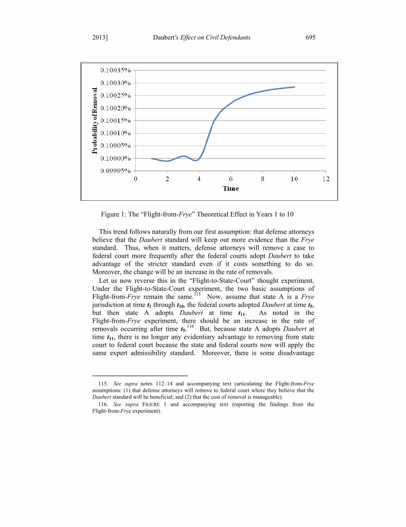
If these assumptions are true, then we should expect to see the following: if state A is a Frye jurisdiction at time t1 through t10 and if the federal courts adopt Daubert at time t5, then the rate of removals from state court to federal court should increase after time t5, with a steep increase initially followed by gradual tapering. Graphically, this should look something like:
113. See Cheng & Yoon, supra note 6, at 508 (arguing that removal rate analysis “depends on defense counsel’s judgment” of the “practical ramifications” of the admissibility standard in his or her jurisdiction); see also Henry G. Miller, The Daubert Debacle, N.Y. ST. B.A. J., Mar./Apr. 2005, at 24, 28 (asserting that “[t]hose representing corporate defendants accused of manufacturing dangerous products will, of course, try to go to federal court and make as many Daubert motions as they can,” and that a defense attorney can subsequently win a case based on a Daubert motion alone); cf. David Paul Horowitz, “Will the Gatekeeper Let Daubert In?”, N.Y. ST. B.J., June 2006, at 18, 18 (observing that defense attorneys in New York not only prefer to apply Daubert but have also advocated for its adoption in New York, a Frye state). 114. See 28 U.S.C. § 1914(a) (2006) (“The clerk of each district court shall require the parties instituting any civil action, suit or proceeding in such court, whether by original process, removal or otherwise, to pay a filing fee of $350.”).
2013] Daubert's Effect on Civil Defendants 695
Figure 1: The “Flight-from-Frye” Theoretical Effect in Years 1 to 10
This trend follows naturally from our first assumption: that defense attorneys believe that the Daubert standard will keep out more evidence than the Frye standard. Thus, when it matters, defense attorneys will remove a case to federal court more frequently after the federal courts adopt Daubert to take advantage of the stricter standard even if it costs something to do so. Moreover, the change will be an increase in the rate of removals.
Let us now reverse this in the “Flight-to-State-Court” thought experiment. Under the Flight-to-State-Court experiment, the two basic assumptions of Flight-from-Frye remain the same.115 Now, assume that state A is a Frye jurisdiction at time t1 through t10, the federal courts adopted Daubert at time t5, but then state A adopts Daubert at time t11. As noted in the Flight-from-Frye experiment, there should be an increase in the rate of removals occurring after time t5.
116 But, because state A adopts Daubert at time t11, there is no longer any evidentiary advantage to removing from state court to federal court because the state and federal courts now will apply the same expert admissibility standard. Moreover, there is some disadvantage
115. See supra notes 112–14 and accompanying text (articulating the Flight-from-Frye assumptions: (1) that defense attorneys will remove to federal court where they believe that the Daubert standard will be beneficial; and (2) that the cost of removal is manageable). 116. See supra FIGURE 1 and accompanying text (reporting the findings from the Flight-from-Frye experiment).
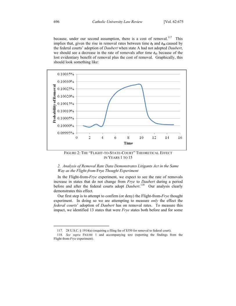
696 Catholic University Law Review [Vol. 62:675
because, under our second assumption, there is a cost of removal.117 This implies that, given the rise in removal rates between time t5 and t10 caused by the federal courts’ adoption of Daubert when state A had not adopted Daubert, we should see a decrease in the rate of removals after time t11 because of the lost evidentiary benefit of removal plus the cost of removal. Graphically, this should look something like:
FIGURE 2: THE “FLIGHT-TO-STATE-COURT” THEORETICAL EFFECT
IN YEARS 1 TO 15
2. Analysis of Removal Rate Data Demonstrates Litigants Act in the Same Way as the Flight-from-Frye Thought Experiment
In the Flight-from-Frye experiment, we expect to see the rate of removals increase in states that do not change from Frye to Daubert during a period before and after the federal courts adopt Daubert.118 Our analysis clearly demonstrates this effect.
Our first step is to attempt to confirm (or deny) the Flight-from-Frye thought experiment. In doing so we are attempting to measure only the effect the federal courts’ adoption of Daubert has on removal rates. To measure this impact, we identified 13 states that were Frye states both before and for some
117. 28 U.S.C. § 1914(a) (requiring a filing fee of $350 for removal to federal court). 118. See supra FIGURE 1 and accompanying text (reporting the findings from the Flight-from-Frye experiment).
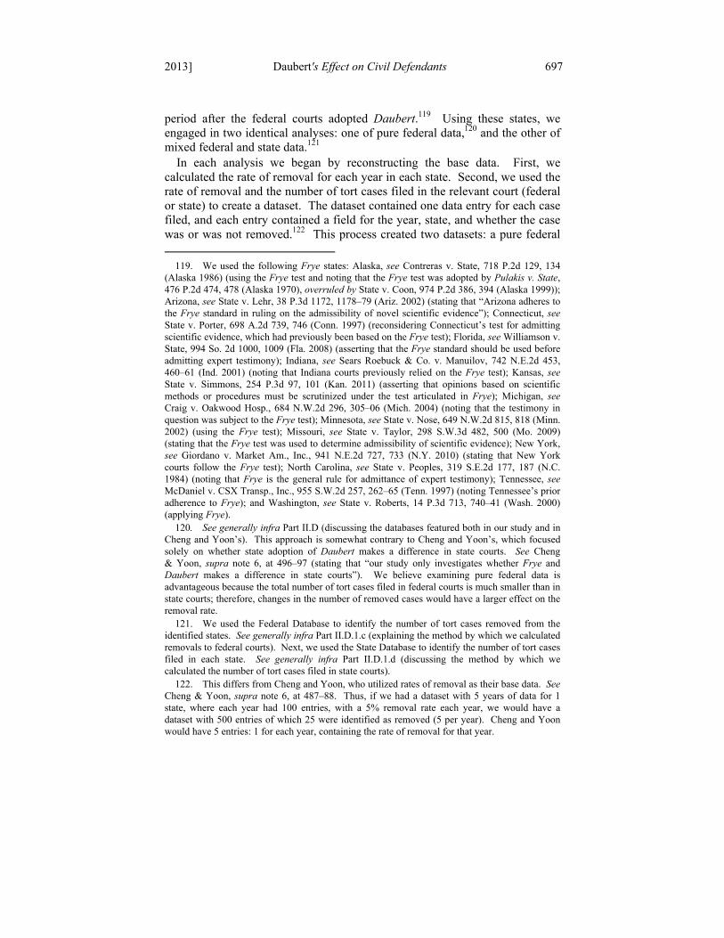
2013] Daubert's Effect on Civil Defendants 697
period after the federal courts adopted Daubert.119 Using these states, we engaged in two identical analyses: one of pure federal data,120 and the other of mixed federal and state data.121
In each analysis we began by reconstructing the base data. First, we calculated the rate of removal for each year in each state. Second, we used the rate of removal and the number of tort cases filed in the relevant court (federal or state) to create a dataset. The dataset contained one data entry for each case filed, and each entry contained a field for the year, state, and whether the case was or was not removed.122 This process created two datasets: a pure federal 119. We used the following Frye states: Alaska, see Contreras v. State, 718 P.2d 129, 134 (Alaska 1986) (using the Frye test and noting that the Frye test was adopted by Pulakis v. State, 476 P.2d 474, 478 (Alaska 1970), overruled by State v. Coon, 974 P.2d 386, 394 (Alaska 1999)); Arizona, see State v. Lehr, 38 P.3d 1172, 1178–79 (Ariz. 2002) (stating that “Arizona adheres to the Frye standard in ruling on the admissibility of novel scientific evidence”); Connecticut, see State v. Porter, 698 A.2d 739, 746 (Conn. 1997) (reconsidering Connecticut’s test for admitting scientific evidence, which had previously been based on the Frye test); Florida, see Williamson v. State, 994 So. 2d 1000, 1009 (Fla. 2008) (asserting that the Frye standard should be used before admitting expert testimony); Indiana, see Sears Roebuck & Co. v. Manuilov, 742 N.E.2d 453, 460–61 (Ind. 2001) (noting that Indiana courts previously relied on the Frye test); Kansas, see State v. Simmons, 254 P.3d 97, 101 (Kan. 2011) (asserting that opinions based on scientific methods or procedures must be scrutinized under the test articulated in Frye); Michigan, see Craig v. Oakwood Hosp., 684 N.W.2d 296, 305–06 (Mich. 2004) (noting that the testimony in question was subject to the Frye test); Minnesota, see State v. Nose, 649 N.W.2d 815, 818 (Minn. 2002) (using the Frye test); Missouri, see State v. Taylor, 298 S.W.3d 482, 500 (Mo. 2009) (stating that the Frye test was used to determine admissibility of scientific evidence); New York, see Giordano v. Market Am., Inc., 941 N.E.2d 727, 733 (N.Y. 2010) (stating that New York courts follow the Frye test); North Carolina, see State v. Peoples, 319 S.E.2d 177, 187 (N.C. 1984) (noting that Frye is the general rule for admittance of expert testimony); Tennessee, see McDaniel v. CSX Transp., Inc., 955 S.W.2d 257, 262–65 (Tenn. 1997) (noting Tennessee’s prior adherence to Frye); and Washington, see State v. Roberts, 14 P.3d 713, 740–41 (Wash. 2000) (applying Frye). 120. See generally infra Part II.D (discussing the databases featured both in our study and in Cheng and Yoon’s). This approach is somewhat contrary to Cheng and Yoon’s, which focused solely on whether state adoption of Daubert makes a difference in state courts. See Cheng & Yoon, supra note 6, at 496–97 (stating that “our study only investigates whether Frye and Daubert makes a difference in state courts”). We believe examining pure federal data is advantageous because the total number of tort cases filed in federal courts is much smaller than in state courts; therefore, changes in the number of removed cases would have a larger effect on the removal rate. 121. We used the Federal Database to identify the number of tort cases removed from the identified states. See generally infra Part II.D.1.c (explaining the method by which we calculated removals to federal courts). Next, we used the State Database to identify the number of tort cases filed in each state. See generally infra Part II.D.1.d (discussing the method by which we calculated the number of tort cases filed in state courts). 122. This differs from Cheng and Yoon, who utilized rates of removal as their base data. See Cheng & Yoon, supra note 6, at 487–88. Thus, if we had a dataset with 5 years of data for 1 state, where each year had 100 entries, with a 5% removal rate each year, we would have a dataset with 500 entries of which 25 were identified as removed (5 per year). Cheng and Yoon would have 5 entries: 1 for each year, containing the rate of removal for that year.

698 Catholic University Law Review [Vol. 62:675
dataset and a mixed federal and state dataset. The pure federal dataset contained entries using the Federal Database to calculate the number of cases removed, the number of tort cases filed, and the removal rate. The mixed dataset contained entries using the State Database to calculate the number of tort cases filed, the Federal Database to calculate the number of cases removed, and both of those numbers to calculate the removal rate.123
Starting with the pure federal dataset, we limited the data to include just those cases in the 13 states that were the appropriate kind of tort action from 1990 to 2000.124 Next, we limited the dataset to include only those tort cases that had been removed from state court to federal court.125 We excluded data from the specific states during certain periods of time where that data was excluded by Cheng and Yoon.126
It is important to note that we have assumed that state adoption of Daubert will result in a decrease in removal rates from the point in time when the state adopts Daubert—presuming the federal courts have already adopted Daubert.127 Therefore, to eliminate confusion that this counter-effect could have, we removed data associated with it by excluding data for each state starting from the year the state adopted Daubert.128 We also eliminated the year Daubert was adopted by the federal courts (1993) because the confusion of the transition year would likely disrupt the analysis.129
123. This second dataset is the same one used by Cheng and Yoon. See Cheng & Yoon, supra note 6, at 491–94 (noting that in the National Study, Cheng and Yoon used the same methodology for calculating removal rates as in the Preliminary Study). 124. See infra Part II.D.1.d.i (discussing in detail the method by which we chose the appropriate type of tort cases). 125. Because there are far fewer federal tort cases, the denominator (number of tort cases) is substantially smaller than the corresponding number of tort cases filed in state court. 126. Cheng and Yoon’s Appendix A does not include data for Florida in 1999 and 2000, New Mexico before 1994, and Oregon in 1990. See Cheng & Yoon, supra note 6, app. at 512–13. 127. See supra FIGURE 2 and accompanying text (explaining the Flight-to-State-Court experiment). 128. We excluded data for Alaska from 1999 onward, see State v. Coon, 974 P.2d 386, 394 (Alaska 1999) (holding that Alaska no longer applies the Frye test); Connecticut from 1997 onward see State v. Porter, 698 A.2d 739, 746 (Conn. 1997) (adopting Daubert); Indiana from 1995 onward, see Steward v. State, 652 N.E.2d 490, 498–99 (Ind. 1995) (assessing the admissibility of expert evidence based on the Indiana Rules of Evidence and the principles of Daubert); and Tennessee from 1997 onward, see McDaniel v. CSX Transp., Inc., 955 S.W.2d 257, 265 (Tenn. 1997) (adopting certain aspects of Daubert and allowing expert evidence only where it will “substantially assist the trier of fact” and does not “indicate a lack of trustworthiness”). Because Arizona, Florida, Kansas, Michigan, Minnesota, Missouri, New York, and Washington did not adopt Daubert in the relevant period, we used data from the entire relevant period for those states. See supra note 119 (detailing the standards for the states in question). 129. See Daubert v. Merrell Dow Pharms., Inc., 509 U.S. 579 (1993).

2013] Daubert's Effect on Civil Defendants 699
Using this data, we performed a fixed-effects130 analysis using logistic regression.131 This provided statistically significant132 results showing that the probability that a case in federal court was removed from state court increased after Daubert was adopted.133
Daubert Adopted
in U.S. Court Probability of Removal
No 0.259268 Yes 0.327401
FIGURE 3: FIXED-EFFECTS ANALYSIS ON REMOVAL RATE USING FEDERAL DATA ONLY
Next, we reproduced this analysis using the mixed Federal and State Database. This analysis also produced statistically significant results demonstrating that the adoption of Daubert increases the probability of removal to federal court.134
Daubert Adopted in U.S. Court
Probability of Removal
No 0.004517 Yes 0.005297
FIGURE 4: FIXED-EFFECTS ANALYSIS ON REMOVAL RATE USING STATE AND FEDERAL DATA
The difference between the probability of removal in Figure 3 and Figure 4—the probability of removal in Figure 3 is approximately 61.8 times larger
130. See infra Part II.D.2.a–d (explaining in detail our fixed-effects model). 131. We used a logistic regression because this method is generally preferred when the independent variable is categorical/binary. See, e.g., ALAN AGRESTI & CHRISTINE FRANKLIN, STATISTICS 610 (2007); DAMODAR N. GUJARATI & DAWN C. PORTER, ESSENTIALS OF
ECONOMETRICS 387–89 (2010). 132. All measures of statistical significance discussed in this Article relate to the p-value of a statistical hypothesis. We will consider a result to be statistically significant if its corresponding p-value is less than or equal to 0.05. This means that there is no more than a 1 in 20 chance (5% chance) that our result is due to chance. DAVID HENSHER, JOHN M. ROSE & WILLIAM H. GREENE, APPLIED CHOICE ANALYSIS: A PRIMER 46–47 (2005). In addition, a p-value of ≤ 0.05 is consistent with general practice. See, e.g., id; SCOTT E. MAXWELL & HAROLD D. DELANY, DESIGNING EXPERIMENTS AND ANALYZING DATA: A MODEL COMPARISON PERSPECTIVE 47 (2d ed. 2004). 133. Using only federal data, the p-value was less than 0.0005. The results of the logistic regression are fairly robust and supported by the results of a linear regression, which provided a regression coefficient of 0.0595772, with a p-value of less than 0.0005. 134. Using both federal and state data, the p-value was less than 0.0005. Once again, the linear regression also supports the conclusion that the removal rate following the adoption of Daubert in federal courts is statistically significant. Using linear regression in the fixed-effects analysis, we achieved a correlation coefficient of 0.0014486, with a p-value of less than 0.0005.

700 Catholic University Law Review [Vol. 62:675
than the probability of removal in Figure 4—is likely due to the difference in the method by which we calculated the rate of removal using the pure Federal Database and the mixed Federal and State Database. In both cases, we used the same removal rate formula (Equation 1), the same numerator (number of tort cases listed in the Federal Database as having been removed from state court), but different denominators (number of tort cases filed in state court versus number of tort cases filed in federal court in a given state). In the pure federal dataset, the denominator is the number of tort cases filed in federal court in a given state. In the mixed federal and state dataset, the denominator is the number of tort cases filed in a given state court. On average, there is only 1 tort case filed in federal court for every 30 tort cases filed in the relevant state court.135 Given this 30:1 ratio of filings, we should expect to find a comparable difference in probability of removal, which we did.136 These results unequivocally demonstrate that in states using the Frye standard, the adoption of Daubert by the federal courts results in an increased rate of removals to the federal courts.
3. Analysis of Removal Rate Data Also Demonstrates Litigants Act in the Same Way as the Flight-to-State-Court Thought Experiment
The Flight-to-State-Court thought experiment proposed that, if the state court was initially a Frye state, remained a Frye state for a period of time after the federal courts adopted Daubert, but eventually adopted Daubert, the rate of removals should decrease.137 Looking at actual case data, litigants’ actual behavior mirrored this result.138
We used 5 states that adopted Daubert from 1994 to 2000139—a period after the federal courts adopted Daubert—and 8 states that did not adopt Daubert
135. This ratio (30:1) was calculated using the 16 states used by Cheng & Yoon during the period from 1990 to 2000. See Cheng & Yoon, supra note 6, at 493 fig.7 (listing the states used by Cheng and Yoon during their National Study). 136. Compare supra FIGURE 3 and accompanying text (reporting the probability of removal using only federal data), with supra FIGURE 4 and accompanying text (reporting the probability of removal using both federal and state data). 137. See supra text accompanying notes 115–17. 138. See infra text accompanying notes 139–44; see also infra FIGURE 5. 139. The five states are Alaska, Connecticut, Indiana, North Carolina, and Tennessee. See State v. Coon, 974 P.2d 386, 394–95 (Alaska 1999) (adopting Daubert and rejecting Frye as inconsistent with the Alaska Rules of Evidence); see also State v. Porter, 698 A.2d 739, 746 (Conn. 1997) (holding that Daubert should be the new standard for accepting expert scientific evidence in the state); Steward v. State, 652 N.E.2d 490, 498 (Ind. 1995) (holding that, although the Daubert standard is not binding, it is helpful in applying the Indiana Rules of Evidence); State v. Goode, 461 S.E.2d 631, 639 (N.C. 1995) (holding that the test of whether to admit expert evidence requires analyzing the test adopted by the Supreme Court in Daubert); McDaniel v. CSX Transp., Inc., 955 S.W.2d 257, 262–65 (Tenn. 1997) (noting Tennessee’s prior adherence to Frye and holding that a partial acceptance of Daubert is appropriate). We ignore Arizona, Florida, Kansas, Michigan, Minnesota, Missouri, New York and Washington because they did not
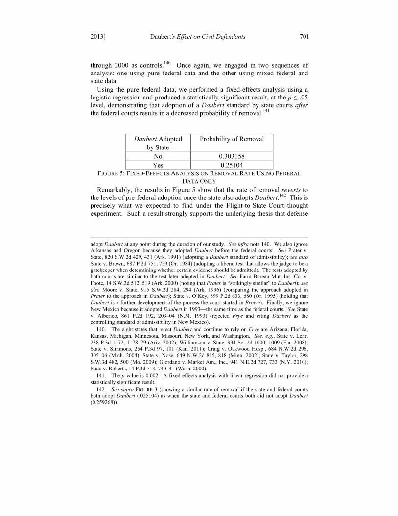
2013] Daubert's Effect on Civil Defendants 701
through 2000 as controls.140 Once again, we engaged in two sequences of analysis: one using pure federal data and the other using mixed federal and state data.
Using the pure federal data, we performed a fixed-effects analysis using a logistic regression and produced a statistically significant result, at the p ≤ .05 level, demonstrating that adoption of a Daubert standard by state courts after the federal courts results in a decreased probability of removal.141
Daubert Adopted by State
Probability of Removal
No 0.303158 Yes 0.25104
FIGURE 5: FIXED-EFFECTS ANALYSIS ON REMOVAL RATE USING FEDERAL
DATA ONLY Remarkably, the results in Figure 5 show that the rate of removal reverts to
the levels of pre-federal adoption once the state also adopts Daubert.142 This is precisely what we expected to find under the Flight-to-State-Court thought experiment. Such a result strongly supports the underlying thesis that defense
adopt Daubert at any point during the duration of our study. See infra note 140. We also ignore Arkansas and Oregon because they adopted Daubert before the federal courts. See Prater v. State, 820 S.W.2d 429, 431 (Ark. 1991) (adopting a Daubert standard of admissibility); see also State v. Brown, 687 P.2d 751, 759 (Or. 1984) (adopting a liberal test that allows the judge to be a gatekeeper when determining whether certain evidence should be admitted). The tests adopted by both courts are similar to the test later adopted in Daubert. See Farm Bureau Mut. Ins. Co. v. Foote, 14 S.W.3d 512, 519 (Ark. 2000) (noting that Prater is “strikingly similar” to Daubert); see also Moore v. State, 915 S.W.2d 284, 294 (Ark. 1996) (comparing the approach adopted in Prater to the approach in Daubert); State v. O’Key, 899 P.2d 633, 680 (Or. 1995) (holding that Daubert is a further development of the process the court started in Brown). Finally, we ignore New Mexico because it adopted Daubert in 1993—the same time as the federal courts. See State v. Alberico, 861 P.2d 192, 203–04 (N.M. 1993) (rejected Frye and citing Daubert as the controlling standard of admissibility in New Mexico). 140. The eight states that reject Daubert and continue to rely on Frye are Arizona, Florida, Kansas, Michigan, Minnesota, Missouri, New York, and Washington. See, e.g., State v. Lehr, 238 P.3d 1172, 1178–79 (Ariz. 2002); Williamson v. State, 994 So. 2d 1000, 1009 (Fla. 2008); State v. Simmons, 254 P.3d 97, 101 (Kan. 2011); Craig v. Oakwood Hosp., 684 N.W.2d 296, 305–06 (Mich. 2004); State v. Nose, 649 N.W.2d 815, 818 (Minn. 2002); State v. Taylor, 298 S.W.3d 482, 500 (Mo. 2009); Giordano v. Market Am., Inc., 941 N.E.2d 727, 733 (N.Y. 2010); State v. Roberts, 14 P.3d 713, 740–41 (Wash. 2000). 141. The p-value is 0.002. A fixed-effects analysis with linear regression did not provide a statistically significant result. 142. See supra FIGURE 3 (showing a similar rate of removal if the state and federal courts both adopt Daubert (.025104) as when the state and federal courts both did not adopt Daubert (0.259268)).

702 Catholic University Law Review [Vol. 62:675
attorneys believe Daubert is the stricter standard.143 Next, we reproduced this analysis using the combined federal and state dataset but found no statistically significant relationships.144
4. The Empirical Evidence of Actual Removal Rates Demonstrates Litigants Behavior After the Adoption of Daubert Mirrored Our Thought Experiments
By analyzing the removals from 1990 to 2000, we can demonstrate that those litigants in the dataset acted in the manner predicted by the Flight-from-Frye and Flight-to-State-Court thought experiments.145 This result strongly supports the conclusion that litigants themselves believe that the Daubert standard is stricter than the Frye standard.146
D. Removal Rates Studies: Squaring the Circle
We began our project with the counterintuitive results from Cheng and Yoon’s work—that Daubert had no real effect on litigants and was much ado about nothing.147 Having run our analysis, the opposite seems to be true—litigants perceive Daubert to be a stricter standard.148 Both of these results, using the same data, cannot be correct. Therefore, it became necessary
143. See, e.g., Miller, supra note 113, at 24, 28 (explaining that defense attorneys remove cases to federal court when planning to file Daubert motions because Daubert employs a higher evidentiary standard than Frye). 144. Our suspicion is that the failure to find an effect is due to three factors. First, the number of torts filed in state court compared to the number of torts removed to federal courts is extremely small. See supra FIGURE 4 (noting that the rate of removal for torts filed in state courts is less than 0.53%, likely whether or not Daubert is adopted in federal courts). Second, the number of torts in which scientific evidence is involved is also very small. In this context, any change in the number of removals is likely to be very small compared to the total number of torts filed. Third, in this context, Indiana and North Carolina both adopted Daubert in 1995 and Alaska adopted Daubert in 1999. See State v. Coon, 974 P.2d 386, 394–95 (Alaska 1999); see also Steward v. State, 652 N.E.2d 490, 498 (Ind. 1995); State v. Goode, 461 S.E.2d 631, 639 (N.C. 1995). This means that for Indiana and North Carolina there is only one year where the trend can begin to be established before it is expected to reverse. Similarly, for Alaska there is only one year where the reversal would be measured. In such a context, it would almost be a miracle to find the effect. 145. See supra Part II.C.1–3. 146. After all, defense attorneys should remove their client’s case to federal court when it is in their client’s best interest. Cheng & Yoon, supra note 6, at 508. Therefore, the change in removal rates outlined in the previous sections supports the belief that Daubert is a stricter standard than Frye. See Miller, supra note 113, at 24, 28. 147. See Cheng & Yoon, supra note 6, at 503. For example, Cheng and Yoon suggest that, because the change in standard had no effect, state courts should consider uniformly adopting Daubert as the admissibility standard. Id. In addition, they suggest that advocates for reform should focus not on doctrinal tests, but on efforts to improve judicial outcomes. Id. at 504. 148. See supra note 112; supra Part II.C.1–4 and accompanying text (discussing how our study led to statistically significant results at the p ≤ .05 level, demonstrating that whether a state court adopts Daubert significantly affects the removal rate to federal court).

2013] Daubert's Effect on Civil Defendants 703
so as to unpack the analysis Cheng and Yoon performed to find an explanation for the varying results. In so doing, we found three errors: (1) a miscalculation of removal rates;149 (2) a failure to account for the difference in effect between state adoption of Daubert before federal adoption and state adoption of Daubert after federal adoption;150 and (3) a utilization of a study population that was too small to identify the effect of state adoption of Daubert.151 Combined, these three errors suggest that our results, rather than Cheng and Yoon’s, are correct; Daubert is the stricter standard.
1. Cheng & Yoon—Review of Data Aggregation
Before running a data analysis, a researcher must collect the underlying data to ensure its validity.152 Looking at the underlying data aggregation for the Cheng and Yoon study, we found what appear to be several errors.153 If their data is fundamentally flawed, any conclusions drawn from it will be undermined.
a. The Preliminary and National Studies
Cheng and Yoon’s removal rate analysis (the “Analysis”) occurred in two stages. In the first stage (the “Preliminary Study”), Cheng and Yoon compared Connecticut’s rate of removal in tort cases from state to federal court with removal rates154 from New York state court to the Eastern District of New York (EDNY) during the period 1994 to 2000.155 The Preliminary Study relied on a statistical model called “difference-in-differences,”156 a special case of fixed effect analysis.157 After engaging in a difference-in-differences analysis, Cheng and Yoon concluded that the 1997 adoption of Daubert by Connecticut did not have a statistically significant effect upon removal rates.158
149. See infra Part II.D.1.c.i. 150. See infra Part II.D.3. 151. See infra text accompanying notes 258–64, 269–70. 152. See, e.g., Responsible Conduct in Data Management, U.S. DEP’T OF HEALTH & HUM. SERVS., http://ori.dhhs.gov/education/products/n_illinois_u/datamanagement/dctopic.html (last visited Mar. 25, 2013). 153. See supra text accompanying notes 149–51. 154. Cheng & Yoon, supra note 6, at 485 (comparing the Eastern District of New York and the District of Connecticut). 155. The EDNY includes the counties of Kings (the Bronx), Nassau, Queens, Richmond (Staten Island), and Suffolk. See EDNY, http://www.nyed.uscourts.gov/ (last visited Mar. 25, 2013) (stating “[t]he district comprises the counties of Kings, Nassau, Queens, Richmond, and Suffolk and concurrently with the Southern District, the waters within the counties of Bronx and New York”). 156. Cheng & Yoon, supra note 6, at 485–86 n.43. 157. See infra Part II.D.2.c (describing the difference-in-differences approach). 158. Cheng & Yoon, supra note 6, at 489–90. Cheng and Yoon fail to provide the result of the difference-in-differences analysis of the Preliminary Study and, instead, merely conclude that
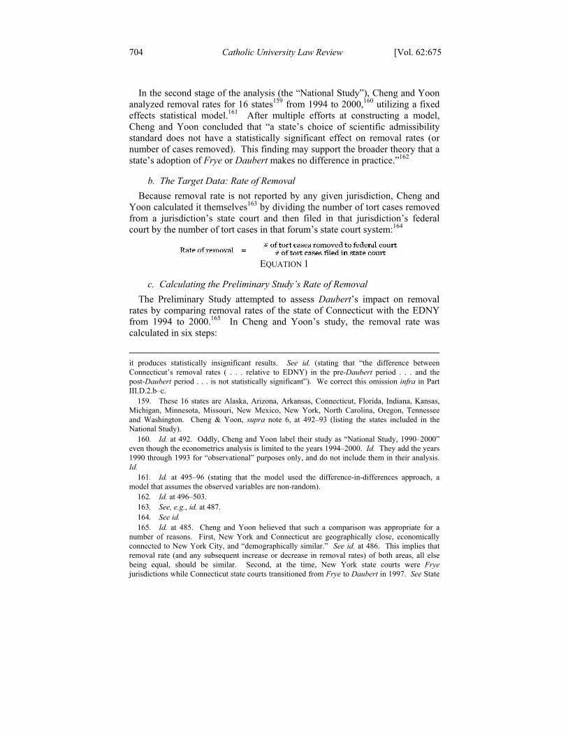
704 Catholic University Law Review [Vol. 62:675
In the second stage of the analysis (the “National Study”), Cheng and Yoon analyzed removal rates for 16 states159 from 1994 to 2000,160 utilizing a fixed effects statistical model.161 After multiple efforts at constructing a model, Cheng and Yoon concluded that “a state’s choice of scientific admissibility standard does not have a statistically significant effect on removal rates (or number of cases removed). This finding may support the broader theory that a state’s adoption of Frye or Daubert makes no difference in practice.”162
b. The Target Data: Rate of Removal
Because removal rate is not reported by any given jurisdiction, Cheng and Yoon calculated it themselves163 by dividing the number of tort cases removed from a jurisdiction’s state court and then filed in that jurisdiction’s federal court by the number of tort cases in that forum’s state court system:164
EQUATION 1
c. Calculating the Preliminary Study’s Rate of Removal
The Preliminary Study attempted to assess Daubert’s impact on removal rates by comparing removal rates of the state of Connecticut with the EDNY from 1994 to 2000.165 In Cheng and Yoon’s study, the removal rate was calculated in six steps:
it produces statistically insignificant results. See id. (stating that “the difference between Connecticut’s removal rates ( . . . relative to EDNY) in the pre-Daubert period . . . and the post-Daubert period . . . is not statistically significant”). We correct this omission infra in Part III.D.2.b–c. 159. These 16 states are Alaska, Arizona, Arkansas, Connecticut, Florida, Indiana, Kansas, Michigan, Minnesota, Missouri, New Mexico, New York, North Carolina, Oregon, Tennessee and Washington. Cheng & Yoon, supra note 6, at 492–93 (listing the states included in the National Study). 160. Id. at 492. Oddly, Cheng and Yoon label their study as “National Study, 1990–2000” even though the econometrics analysis is limited to the years 1994–2000. Id. They add the years 1990 through 1993 for “observational” purposes only, and do not include them in their analysis. Id. 161. Id. at 495–96 (stating that the model used the difference-in-differences approach, a model that assumes the observed variables are non-random). 162. Id. at 496–503. 163. See, e.g., id. at 487. 164. See id. 165. Id. at 485. Cheng and Yoon believed that such a comparison was appropriate for a number of reasons. First, New York and Connecticut are geographically close, economically connected to New York City, and “demographically similar.” See id. at 486. This implies that removal rate (and any subsequent increase or decrease in removal rates) of both areas, all else being equal, should be similar. Second, at the time, New York state courts were Frye jurisdictions while Connecticut state courts transitioned from Frye to Daubert in 1997. See State

2013] Daubert's Effect on Civil Defendants 705
1. Calculate the number of torts in Connecticut state court using the Connecticut database;166 2. Calculate the number of torts in New York state court for the geographic area coextensive with the EDNY using the New York database;167 3. Calculate the number of removals from the Connecticut state courts to federal court that were filed in the United States District Court for the District of Connecticut;168 4. Calculate the number of removals from the relevant New York state courts to the United States District Court for the EDNY;169 5. Use Equation 1 to calculate removal rate for New York;170 and 6. Use Equation 1 to calculate removal rate for Connecticut.171
According to Cheng and Yoon, these steps produce the following results:172
v. Porter, 698 A.2d 737, 746 (Conn. 1997). Consequently, Cheng and Yoon believed that, if there is a statistically significant change in the removal rates between the two states after 1997, that would be evidence that the choice of admissibility standard for scientific evidence affects removal rates. Cheng & Yoon, supra note 6, at 486. 166. Cheng & Yoon, supra note 6, at 485–86. 167. See id. 168. See id. 169. See id. 170. See id. at 487–88. 171. See id. 172. Id. at 489.

706 Catholic University Law Review [Vol. 62:675
Connecticut New York (limited to EDNY)
Year # of torts filed
# of cases removed to federal
court
% Rate-of-Removal173
# of torts filed
# of cases removed to federal
court
% Rate-of-Removal
1994 16,172 56 0.35 42,120 207 0.49 1995 18,417 64 0.35 46,199 237 0.51 1996 20,165 48 0.24 47,711 333 0.70 1997 20,295 49 0.24 47,235 263 0.56 1998 20,054 63 0.31 46,808 288 0.62 1999 18,845 52 0.28 45,838 310 0.68 2000 18,201 56 0.31 43,964 362 0.82
TABLE 1
d. Recreating Rate of Removal for the Preliminary Study
i. The First Problem: Calculating the Number of Removals to Federal Court
The first step in our review of Cheng and Yoon’s work was to attempt to confirm the results of the Preliminary Study. First, we recreated Table 1 using the same data as Cheng and Yoon.174 The Federal Database came with a set of codebooks that explained what fields were included in the data and what each meant.175 The first field of interest in the Federal Database is the “nature of
173. Because the number of removed cases is generally much smaller than the number of filed cases, we will report rate of removal as a percentage removal rate. Thus, a removal rate of 0.35% corresponds to a removal rate of 0.0035. 174. See infra Part II.D.1.d.iii. Cheng and Yoon graciously provided us with a copy of the data used in the study. When we were unable to recreate Cheng and Yoon’s aggregation numbers from that data, the authors obtained a copy of the Federal Database directly from the Federal Judicial Center. That database matched the one Cheng and Yoon provided. 175. Codebooks were provided for various periods of time. See FED. JUDICIAL CTR., FEDERAL COURT CASES: INTEGRATED DATA BASE, 1970–2000 pt. 117 [hereinafter FED. JUDICIAL CTR. DATA BASE], available at http://www.icpsr.umich.edu/icpsrweb/NACJD/studies /08429/ascii (covering 2000); see also id. at pt. 116 (covering 1999); id. at pt. 115 (covering 1998); id. at pt. 104 (covering 1997); id. at pt. 103 (covering 1996); id. at pt. 98 (covering 1995); id. at pt. 88 (covering 1994); id. at pt. 87 (covering 1993); id. at pt. 86 (covering 1992); id. at pt. 74 (covering 1991); id. at pt. 73 (covering 1990); id. at pt. 65 (covering 1989); id. at pt. 64 (covering 1988). All codebooks are on file with the authors.
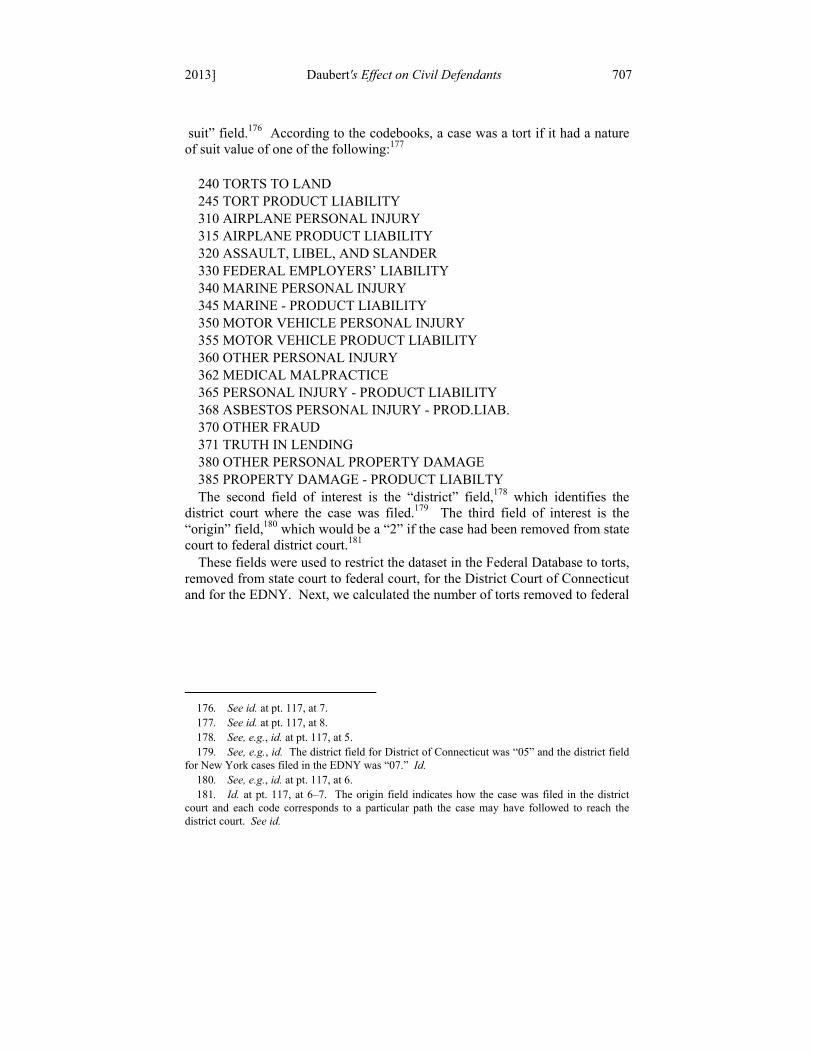
2013] Daubert's Effect on Civil Defendants 707
suit” field.176 According to the codebooks, a case was a tort if it had a nature of suit value of one of the following:177
240 TORTS TO LAND 245 TORT PRODUCT LIABILITY 310 AIRPLANE PERSONAL INJURY 315 AIRPLANE PRODUCT LIABILITY 320 ASSAULT, LIBEL, AND SLANDER 330 FEDERAL EMPLOYERS’ LIABILITY 340 MARINE PERSONAL INJURY 345 MARINE - PRODUCT LIABILITY 350 MOTOR VEHICLE PERSONAL INJURY 355 MOTOR VEHICLE PRODUCT LIABILITY 360 OTHER PERSONAL INJURY 362 MEDICAL MALPRACTICE 365 PERSONAL INJURY - PRODUCT LIABILITY 368 ASBESTOS PERSONAL INJURY - PROD.LIAB. 370 OTHER FRAUD 371 TRUTH IN LENDING 380 OTHER PERSONAL PROPERTY DAMAGE 385 PROPERTY DAMAGE - PRODUCT LIABILTY The second field of interest is the “district” field,178 which identifies the
district court where the case was filed.179 The third field of interest is the “origin” field,180 which would be a “2” if the case had been removed from state court to federal district court.181
These fields were used to restrict the dataset in the Federal Database to torts, removed from state court to federal court, for the District Court of Connecticut and for the EDNY. Next, we calculated the number of torts removed to federal
176. See id. at pt. 117, at 7. 177. See id. at pt. 117, at 8. 178. See, e.g., id. at pt. 117, at 5. 179. See, e.g., id. The district field for District of Connecticut was “05” and the district field for New York cases filed in the EDNY was “07.” Id. 180. See, e.g., id. at pt. 117, at 6. 181. Id. at pt. 117, at 6–7. The origin field indicates how the case was filed in the district court and each code corresponds to a particular path the case may have followed to reach the district court. See id.

708 Catholic University Law Review [Vol. 62:675
court in the EDNY and District Court for Connecticut, producing results that differed significantly from those provided by Cheng and Yoon:182
Connecticut New York (limited to EDNY)
Year Cheng & Yoon
removals
Authors’ # of removals
Difference Cheng & Yoon
removals
Authors’ # of removals
Difference
1994 56 73 -17 207 259 -52 1995 64 260 -196 237 358 -121 1996 48 71 -23 333 414 -81 1997 49 68 -19 263 319 -56 1998 63 87 -24 288 340 -52 1999 52 74 -22 310 363 -53 2000 56 73 -17 362 413 -51
TABLE 2 Because of the significant differences in results, we reviewed the data to
identify where Cheng and Yoon may have reasonably further limited the data to arrive at their results. Eventually, we determined it was the jurisdiction field, which states:183
1 -US government plaintiff 2 -US government defendant 3 -federal question 4 -diversity of citizenship 5 -local question
We determined that Cheng and Yoon must have limited jurisdiction to only
diversity of citizenship184 because doing so eliminates many of the differences between our results and their results:
182. See Cheng & Yoon, supra note 6, at 489 fig.5. 183. See, e.g., FED. JUDICIAL CTR. DATA BASE, supra note 175, at pt. 117, at 7. 184. Id. Cheng and Yoon likely ignored the “1,” “2,” and “3” field values because such cases were likely to be removed for reasons other than scientific evidence admissibility standards. We also assume the “local question” cases, field value of “5,” were automatically ignored because there were no cases that fit into category “5” in the relevant period.

2013] Daubert's Effect on Civil Defendants 709
Connecticut New York (limited to EDNY)
Year C&Y # of removals
Authors’ # of removals
Difference C&Y # of removals
Authors’ # of removals
Difference
1994 56 60 -4 207 212 -5 1995 64 67 -3 237 240 -3 1996 48 49 -1 333 338 -5 1997 49 53 -4 263 265 -2 1998 63 68 -5 288 289 -1 1999 52 56 -4 310 314 -4 2000 56 58 -2 362 363 -1
TABLE 3 Although the differences in results were smaller after adjusting for the
jurisdiction limitation, they still did not match.185 Through trial and error, we were able to (mostly) conform our results to Cheng and Yoon’s results by eliminating three categories of torts: products liability, torts to land, and assault, libel, and slander:186
Connecticut New York (limited to EDNY)
Year C&Y # of removals
Authors’ # of removals
Difference C&Y # of removals
Authors’ # of removals
Difference
1994 56 56 0 207 207 0 1995 64 64 0 237 237 0 1996 48 48 0 333 333 0 1997 49 49 0 263 263 0 1998 63 63 0 288 288 0 1999 52 52 0 310 310 0 2000 56 56 0 362 357 5
TABLE 4 Removing these three tort categories was an ad hoc measure, but it did
produce results that conformed to almost all of Cheng and Yoon’s reported results.187 The only remaining difference was New York, in 2000, where we
185. See supra TABLE 3 (showing a disparity in the results even after the jurisdictional limitation was adjusted). 186. The “nature of suit” field was restricted to values between 300 and 400, excluding cases with the following values: 240 (torts to land), 245 (tort product liability), and 320 (assault, libel, and slander). See, e.g., FED. JUDICIAL CTR. DATA BASE, supra note 175, pt. 117, at 7–8. 187. See supra TABLE 4 (showing more comparable results than in TABLE 3).

710 Catholic University Law Review [Vol. 62:675
found 5 fewer torts.188 That result would match but only if we reintroduced assault, libel, and slander torts for just New York in 2000.189
Our attempt to recreate Cheng and Yoon’s removals count to federal court identified a substantial methodological flaw in their calculations. We could only reproduce their results by adopting two different ad hoc approaches.190 Moreover, removing product liability torts from the analysis is of grave concern in a study on the effect of a change in scientific evidence admissibility standards because product liability cases are the torts where scientific evidence is most likely to be present and contested.191 Further, there is no rational basis for removing assault, libel, and slander, or torts to land (or reintroducing assault, libel, and slander for just New York in 2000).192
ii. Calculating the Number of Torts in State Court
Although Cheng and Yoon’s data aggregation from the Federal Database did not match our aggregation without ad hoc data manipulation, we were able to replicate Cheng and Yoon’s data aggregation of the Connecticut database and New York database to calculate the number of torts filed in each state.193
188. See supra TABLE 4. 189. However, if we reintroduced assault, libel, and slander to match Cheng and Yoon’s results, the only data points that would match would be New York in 2000. 190. See supra notes 184, 186 and accompanying text (explaining that we limited the data by jurisdiction and removed three “nature of suit” categories to match over 92% of Cheng and Yoon’s results). Cheng and Yoon do not provide any explanation for their data aggregation methods that would account for or explain these differences. Rather they simply stated that “we extracted only tort cases filed in the EDNY and the District of Connecticut for the period of 1994 to 2000” and that they report this data in raw form in their Figure 5. Cheng & Yoon, supra note 6, at 488–89 & fig.5 (“Figure 5 shows the raw numbers and the calculated removal rates for Connecticut and the EDNY.” (emphasis added)). 191. See Cheng & Yoon, supra note 6, at 483–84 (discussing the importance of scientific evidence in products liability tort cases); see also Margaret A. Berger, Upsetting the Balance Between Adverse Interests: The Impact of the Supreme Court’s Trilogy on Expert Testimony in Toxic Tort Litigation, 64 LAW & CONTEMP. PROBS. 289, 289–90 (2001) (explaining the contested nature of scientific evidence in toxic tort cases and how those cases led the fight for a reformed standard). 192. See Cheng & Yoon, supra note 6, at 485–91 (failing to provide any explanation for their methods for aggregating data). 193. There were two minor differences. First, in 1997, we counted 20,294 torts filed in Connecticut while Cheng and Yoon counted 20,295 torts filed in Connecticut. See id. at 489 fig.5; see also supra TABLE 1. Second, in 1999, we counted 18,844 torts filed in Connecticut while Cheng and Yoon counted 18,845 torts filed in Connecticut. See Cheng & Yoon, supra note 6, at 489 fig.5; see also supra TABLE 1. We presume that this is a reporting or typographical error.

2013] Daubert's Effect on Civil Defendants 711
iii. Because of Errors in Their Process, It Is Not Possible to Recreate Cheng and Yoon’s Preliminary Study
Although we were able to essentially recreate Cheng and Yoon’s calculation of the number of torts filed in Connecticut and New York, we could not match Cheng and Yoon’s calculation of the number of removals to federal district court.194 Consequently, we reject Cheng and Yoon’s calculation of the removal rate from 1994 to 2000 in Connecticut and the EDNY.
e. Recreating the Data for the National Study
Cheng and Yoon’s National Study examined the removal rate in 16 states195 from 1994 to 2000.196 Their calculation of those rates of removal for that period are provided below:197
194. See supra Part II.D.1.d.i (discussing the difficulty in determining how Cheng and Yoon calculated the number of removals from state to federal court during the Preliminary Study). 195. See Cheng & Yoon, supra note 6, at 492–93 (including Alaska, Arizona, Arkansas, Connecticut, Florida, Indiana, Kansas, Michigan, Minnesota, Missouri, New Mexico, New York, North Carolina, Oregon, Tennessee, and Washington). 196. Id. at 491–92 (noting the econometrics analysis was from 1994 to 2000). 197. Id. at app. a at 512–13; see also infra TABLE 5.
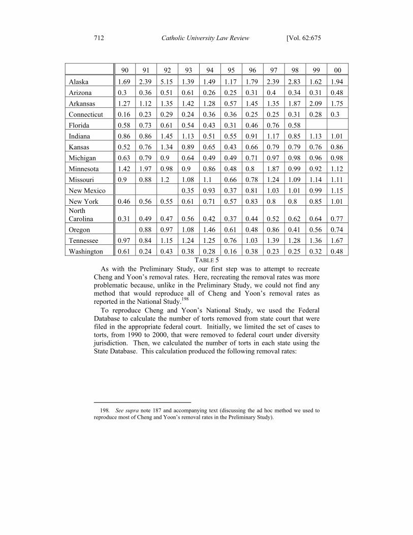
712 Catholic University Law Review [Vol. 62:675
90 91 92 93 94 95 96 97 98 99 00
Alaska 1.69 2.39 5.15 1.39 1.49 1.17 1.79 2.39 2.83 1.62 1.94
Arizona 0.3 0.36 0.51 0.61 0.26 0.25 0.31 0.4 0.34 0.31 0.48
Arkansas 1.27 1.12 1.35 1.42 1.28 0.57 1.45 1.35 1.87 2.09 1.75
Connecticut 0.16 0.23 0.29 0.24 0.36 0.36 0.25 0.25 0.31 0.28 0.3
Florida 0.58 0.73 0.61 0.54 0.43 0.31 0.46 0.76 0.58
Indiana 0.86 0.86 1.45 1.13 0.51 0.55 0.91 1.17 0.85 1.13 1.01
Kansas 0.52 0.76 1.34 0.89 0.65 0.43 0.66 0.79 0.79 0.76 0.86
Michigan 0.63 0.79 0.9 0.64 0.49 0.49 0.71 0.97 0.98 0.96 0.98
Minnesota 1.42 1.97 0.98 0.9 0.86 0.48 0.8 1.87 0.99 0.92 1.12
Missouri 0.9 0.88 1.2 1.08 1.1 0.66 0.78 1.24 1.09 1.14 1.11
New Mexico 0.35 0.93 0.37 0.81 1.03 1.01 0.99 1.15
New York 0.46 0.56 0.55 0.61 0.71 0.57 0.83 0.8 0.8 0.85 1.01 North Carolina 0.31 0.49 0.47 0.56 0.42 0.37 0.44 0.52 0.62 0.64 0.77
Oregon 0.88 0.97 1.08 1.46 0.61 0.48 0.86 0.41 0.56 0.74
Tennessee 0.97 0.84 1.15 1.24 1.25 0.76 1.03 1.39 1.28 1.36 1.67
Washington 0.61 0.24 0.43 0.38 0.28 0.16 0.38 0.23 0.25 0.32 0.48 TABLE 5
As with the Preliminary Study, our first step was to attempt to recreate Cheng and Yoon’s removal rates. Here, recreating the removal rates was more problematic because, unlike in the Preliminary Study, we could not find any method that would reproduce all of Cheng and Yoon’s removal rates as reported in the National Study.198
To reproduce Cheng and Yoon’s National Study, we used the Federal Database to calculate the number of torts removed from state court that were filed in the appropriate federal court. Initially, we limited the set of cases to torts, from 1990 to 2000, that were removed to federal court under diversity jurisdiction. Then, we calculated the number of torts in each state using the State Database. This calculation produced the following removal rates:
198. See supra note 187 and accompanying text (discussing the ad hoc method we used to reproduce most of Cheng and Yoon’s removal rates in the Preliminary Study).

2013] Daubert's Effect on Civil Defendants 713
90 91 92 93 94 95 96 97 98 99 00
Alaska 1.37 1.92 3.65 1.10 1.85 1.41 1.51 2.39 3.02 1.62 2.05
Arizona 0.32 0.38 0.55 0.65 0.34 0.41 0.36 0.42 0.37 0.31 0.48
Arkansas 1.33 1.24 1.39 1.51 1.77 1.41 1.66 1.44 1.96 2.19 1.89
Connecticut 0.18 0.23 0.33 0.24 0.38 0.37 0.26 0.27 0.34 0.30 0.31
Florida 0.27 0.28 0.23 0.20 0.19 0.20 0.22 0.30 0.23
Indiana 0.61 0.85 1.44 1.13 0.67 1.14 1.07 1.25 0.88 1.13 1.03
Kansas 0.57 0.83 1.38 0.93 0.79 1.02 0.87 0.84 0.80 0.80 0.99
Michigan 0.70 0.83 0.91 0.67 0.65 1.01 0.97 1.02 1.00 0.99 1.02
Minnesota 1.65 2.07 1.06 0.98 1.11 1.08 1.00 1.91 1.01 0.97 1.19
Missouri 1.05 0.92 1.24 1.18 1.40 1.26 1.06 1.30 1.13 1.17 1.14
New Mexico 0.35 1.03 1.65 1.25 1.08 1.01 0.99 1.20
New York 0.48 0.59 0.59 0.69 0.86 0.80 0.90 0.80 0.80 0.86 1.01
North Carolina 0.35 0.67 0.51 0.63 0.60 0.75 0.72 0.56 0.68 0.67 0.80
Oregon 0.67 0.73 0.87 1.22 1.06 1.14 0.72 0.42 0.60 0.71
Tennessee 1.09 0.87 1.19 1.34 1.67 1.67 1.37 1.46 1.32 1.40 1.72
Washington 0.65 0.25 0.43 0.44 0.35 0.32 0.46 0.24 0.27 0.33 0.50 TABLE 6

714 Catholic University Law Review [Vol. 62:675
Once again, our results differed from Cheng and Yoon’s:199
90 91 92 93 94 95 96 97 98 99 00
Alaska -0.32 -0.47 -1.50 -0.29 0.36 0.24 -0.28 0.00 0.19 0.00 0.11
Arizona 0.02 0.02 0.04 0.04 0.08 0.16 0.05 0.02 0.03 0.00 0.00
Arkansas 0.06 0.12 0.04 0.09 0.49 0.84 0.21 0.09 0.09 0.10 0.14
Connecticut 0.02 0.00 0.04 0.00 0.02 0.01 0.01 0.02 0.03 0.02 0.01
Florida -0.31 -0.45 -0.38 -0.34 -0.24 -0.11 -0.24 -0.46 -0.35
Indiana -0.25 -0.01 -0.01 0.00 0.16 0.59 0.16 0.08 0.03 0.00 0.02
Kansas 0.05 0.07 0.04 0.04 0.14 0.59 0.21 0.05 0.01 0.04 0.13
Michigan 0.07 0.04 0.01 0.03 0.16 0.52 0.26 0.05 0.02 0.03 0.04
Minnesota 0.23 0.10 0.08 0.08 0.25 0.60 0.20 0.04 0.02 0.05 0.07
Missouri 0.15 0.04 0.04 0.10 0.30 0.60 0.28 0.06 0.04 0.03 0.03
New Mexico 0.00 0.10 1.28 0.44 0.05 0.00 0.00 0.05
New York 0.02 0.03 0.04 0.08 0.15 0.23 0.07 0.00 0.00 0.01 0.00
North Carolina
0.04 0.18 0.04 0.07 0.18 0.38 0.28 0.04 0.06 0.03 0.03
Oregon -0.21 -0.24 -0.21 -0.24 0.45 0.66 -0.14 0.01 0.04 -0.03
Tennessee 0.12 0.03 0.04 0.10 0.42 0.91 0.34 0.07 0.04 0.04 0.05
Washington 0.04 0.01 0.00 0.06 0.07 0.16 0.08 0.01 0.02 0.01 0.02 TABLE 7
We were only able to find 15 data points (state-by-year) out of the 170 total200 where our results align with Cheng and Yoon’s results—a 9% success rate. Then, we attempted to locate a method for counting that enabled us to more closely reproduce the results of Cheng and Yoon’s calculation of removal
199. See infra TABLE 7. TABLE 7 was compiled by subtracting the values Cheng and Yoon found from the values we found. 200. See supra TABLE 7. TABLE 7 has a total of 176 entries (16 states by 11 years). Of these, we leave 6 blank (Florida in 1999 and 2000; New Mexico in 1990, 1991, and 1992; Oregon in 1990) because Cheng and Yoon also left those dates blank. Cheng & Yoon, supra note 6, app. a, at 512–13; see also supra TABLE 7. Cheng and Yoon did not explain why those entries were left blank. Cheng & Yoon, supra note 6, at 491–513 (failing to account for blank entries). Although they did indicate that the databases used to calculate these results may have been either inaccurate or incomplete. Id. at 492.

2013] Daubert's Effect on Civil Defendants 715
rate. Using the same ad hoc measures used in the Preliminary Study,201 we were able to produce results that were closer to Cheng and Yoon’s:
90 91 92 93 94 95 96 97 98 99 00
Alaska -0.40 -0.70 -1.65 -0.36 0.22 0.24 -0.28 0.00 0.09 0.00 0.00
Arizona 0.02 0.01 0.02 0.03 0.07 0.14 0.05 0.00 0.00 0.00 -0.01
Arkansas 0.04 0.00 0.00 0.03 0.48 0.80 0.15 0.00 0.00 -0.02 0.05
Connecticut 0.00 0.00 0.00 0.00 0.00 0.00 0.00 0.00 0.00 0.00 0.00
Florida -0.32 -0.46 -0.39 -0.34 -0.26 -0.11 -0.25 -0.47 -0.36
Indiana -0.29 -0.05 -0.03 -0.07 0.11 0.58 0.13 -0.01 -0.01 0.00 -0.01
Kansas 0.03 0.00 0.00 0.02 0.10 0.49 0.14 0.00 0.00 0.00 0.00
Michigan 0.05 0.00 0.00 0.02 0.14 0.49 0.25 0.00 0.00 0.00 0.00
Minnesota 0.19 0.00 0.00 0.06 0.22 0.50 0.16 0.00 0.00 0.00 0.00
Missouri 0.13 0.00 0.00 0.05 0.24 0.56 0.25 0.00 0.00 -0.01 0.00
New Mexico 0.00 0.02 1.22 0.39 0.00 0.00 0.00 0.03
New York 0.01 0.01 0.02 0.06 0.13 0.22 0.05 -0.01 -0.02 -0.01 -0.02 North Carolina 0.02 0.00 0.00 0.04 0.18 0.36 0.26 0.00 0.00 0.00 0.00
Oregon -0.23 -0.25 -0.22 -0.25 0.39 0.61 -0.14 0.00 0.00 -0.09
Tennessee 0.09 0.00 0.03 0.06 0.34 0.85 0.30 0.00 -0.01 0.00 0.00
Washington 0.04 0.00 0.00 0.02 0.06 0.15 0.07 0.00 -0.01 0.00 0.00 TABLE 8
Although this analysis does allow us to align 66 data points with Cheng and Yoon, that only comprises 39% of the entries.202 Ultimately, we were not able to find a method of calculating removal rates that produced results that matched Cheng and Yoon’s table of removal rates. Thus, we can only conclude that a set of errors crept into their data calculation techniques.
f. Summary and Data Aggregation Conclusions
In order to perform a useful statistical analysis, one must input data that is consistent and understandable. Unfortunately, the data aggregation that Cheng and Yoon used to create the inputs to their statistical analysis is fundamentally flawed. Thus, any conclusions drawn from their data is suspect.
201. See supra notes 184–86 and accompanying text. 202. See supra TABLE 8.

716 Catholic University Law Review [Vol. 62:675
2. Recreating the Preliminary Study: A Statistically Significant Result Found Once the Proper Study Population Is Used
As previously noted, Cheng and Yoon’s calculation of removal rates either miscalculates the rate of removal or utilizes an unknown, unidentified, and non-systematic method of calculation.203 Recreating the Preliminary Study using our own methods and our rates of removal allows us to conclude that there is a statistically significant effect from Connecticut’s adoption of Daubert in 1997.204 Cheng and Yoon’s failure to find a statistically significant result was likely due to the use of removal rates as the study population. We find statistical significance by using properly calculated removal rates, counts of torts filed, and counts of torts removed to create a dataset in which there is one entry for each tort filed in the respective court and each data entry is identified as either removed or not based on the removal rate.205
a. An Intuitive Explanation of the Difference-in-Differences Analysis
Cheng & Yoon attempt to analyze whether the rate of removal is correlated in a meaningful way with state adoption of Daubert by utilizing a difference-in-differences approach.206 A difference-in-differences analysis can be seen as combining two comparison techniques: before-after analysis and matching.207 In a before-after analysis, we measure the effect a treatment208 has on a population by comparing the tested variable209 before and after the treatment is given,210 for example, comparing the removal rate in Connecticut before it adopts Daubert (pre-1997) with the removal rate after it adopts Daubert (post-1997). Thus, the before-after analysis measures change over time within the same group, presuming that any change in the tested variable is due solely to the treatment.211 The problem with the before-after analysis is that there may be some unknown covariate within the population that alters the measured variable and thereby produces potentially incorrect results.212
203. See supra Part II.D.1.e (discussing Cheng and Yoon’s errors). 204. See infra text accompanying notes 246–50. 205. See infra Part II.D.2.d. 206. Cheng & Yoon, supra note 6, at 485–86 n.43. 207. MYOUNG-JAE LEE, MICRO-ECONOMETRICS FOR POLICY, PROGRAM, AND TREATMENT
EFFECTS 99 (2005) (describing the technique of difference-in-differences). 208. The “treatment” at issue is a state’s adoption of the Daubert standard. 209. The “tested variable” is rate of removal to federal court. 210. See LEE, supra note 207, at 64–65 (describing the before-after design). 211. See id. at 65. 212. See id. at 65, 99 (recognizing the danger posed by the “time effect” when using before-after analysis).
2013] Daubert's Effect on Civil Defendants 717
To avoid that problem, the difference-in-differences (DID) analysis combines before-after analysis with matching analysis.213 In matching, we compare two populations over the same period where one population receives the treatment and the other does not.214 Importantly, we must pick two populations that are comparable215 and are presumed to have the same covariate values.216 In the Preliminary Study, Cheng and Yoon carefully argued that Connecticut and the EDNY are comparable in this way.217
By adding matching to before-after analysis, we can eliminate the effects of any unseen covariate in the treated population.218 In essence, if an unknown covariate is acting to decrease the rate of removals in the treated state (Connecticut), that same covariate should be acting in the same manner in the comparable state (New York).
The process for performing a DID analysis is very simple. First, calculate the mean rate of removal for Connecticut and the EDNY, separately, during the pre-treatment period (pre-1997) and the post-treatment period (post-1997).219 This provides four mean removal rates: (1) Connecticut pre-1997; (2) Connecticut post-1997; (3) EDNY pre-1997; and (4) EDNY post-1997. Next, calculate the difference within each time period between the treatment group and the non-treatment group.220 Thus, we calculate the difference between Connecticut pre-1997 and New York pre-1997, and between Connecticut post-1997 and New York post-1997. This results in the 213. See id. (explaining how matching controls the undesirable effect that results from using a before-after design exclusively). 214. See id. at 79, 99 (stating how matching allows researchers to measure two tested variables, where only one of the tested variables receives the “treatment” at issue). 215. See James J. Heckman et al., Matching as an Econometric Estimator, 65 REV. ECON. STUD. 261, 261 (1998). Two populations are “comparable” if both populations “would have experienced the same outcomes . . . had they participated in the programme.” Id. at 262. A central difficulty with matching is ensuring that the two groups are comparable. See id. (explaining that it is difficult to determine whether two groups, having their “tested variable” measured, are truly comparable). 216. See LEE, supra note 207, at 99 (explaining that, if the effect of the treatment takes a long time to manifest itself, the changes observed between two control groups may be due to changes in other variables). If both groups have similar covariate variables, it becomes more likely that the observed differences between the two groups are due to the treatment. See id. 217. See Cheng & Yoon, supra note 6, at 486–87 (explaining the choice of Connecticut and the EDNY). 218. See LEE, supra note 207, at 99. 219. The difference-in-differences method starts by selecting two tested variables with similar environmental conditions. Id. Once the tested variables are chosen, the researcher must compare the subjects’ response variables before and after one of the variables received the treatment. Id. 220. See JOSHUA D. ANGRIST & JORN-STEFFEN PISCHKE, MOSTLY HARMLESS
ECONOMETRICS: AN EMPIRICIST’S COMPANION 227, 229–30 (2009) (discussing the requirements of a fixed-effects difference-in-differences analysis); see also LEE, supra note 207, at 99 (noting that the subjects’ response variables must be measured before and after treatment).

718 Catholic University Law Review [Vol. 62:675
“differences” in difference-in-differences. Finally, calculate the difference between the post-treatment period differences and the pre-treatment period differences.221 For instance, in this case, take the post-1997 result and subtract it from the pre-1997 result. This results in the “difference” in the difference-in-differences.
b. A Mathematically Formal Description of the Difference-in-Differences Analysis
Intuitively, the idea of the DID analysis is easy to grasp, but examining the method in a formal mathematical notation reveals the kind of phenomena the DID approach is meant to analyze. To mathematically explain the DID analysis, we describe an algebraic method for doing a DID analysis that corresponds to the intuitive method.222 Then, we describe a method for doing the DID analysis using a fixed-effects analysis.223
The algebraic explanation necessarily begins with the introduction of mathematical notation.
Let:
μi,t= the mean of the study variable224 in state i at time t. i = 0 for the non-treatment group225 and i = 1 for the treatment group.226
221. See ANGRIST & PISCHKE, supra note 220, at 230 tbl. 5.2.3 (illustrating how to calculate the difference-in-differences using the average employment in fast-food chains as an example); see also LEE, supra note 207, at 100 (discussing how the difference-in-differences rate was calculated to measure the effect immigration has on unemployment). 222. See ANGRIST & PISCHKE, supra note 220, at 228–29 (explaining an algebraic model of difference-in-differences analysis); see also David Card & Alan B. Krueger, Minimum Wages and Employment: A Case Study of the Fast-Food Industry in New Jersey and Pennsylvania, 84 AM. ECON. REV. 772, 778–79 (1994) (applying the algebraic difference-in-differences method intuitively to study the effect of minimum wage changes on employment in the fast food industry); Daniel S. Hamermesh, Comment, What a Wonderful World This Would Be, 48 INDUS. & LAB. REL. REV. 835, 835 (1995) (specifying the algebraic formula for the difference-in-differences methods and critiquing the work of Card and Krueger). 223. See ANGRIST & PISCHKE, supra note 220, at 233–41 (discussing difference-in-differences as fixed effects); see also MARNO VERBEEK, A GUIDE TO MODERN
ECONOMETRICS 345 (2d ed. 2004) (noting that “[t]he fixed effects model is simply a linear regression model in which the intercept terms vary over the individual units i . . . . We can write this in the usual regression framework by including a dummy variable for each unit i in the model”); Marianne Bertrand et al., How Much Should We Trust Differences-in-Differences Estimates?, 119 Q. J. ECON. 249, 250–51 (2004) (discussing difference-in-differences estimation and the fixed-effects regression formula); Card & Krueger, supra note 222, at 779–81 (utilizing a least-squares dummy variable model to discuss the effect of minimum wage changes on employment). 224. In this case, the study variable is the average removal rate. 225. In this case, the non-treatment group is the EDNY. 226. The treatment group is Connecticut because it adopted Daubert in 1997. See State v. Porter, 698 A.2d 739, 746 (Conn. 1997).

2013] Daubert's Effect on Civil Defendants 719
t = 0 for the pre-treatment period227 and t = 1 for the post-treatment period.228
A DID analysis is performed by calculating the study variable mean for each population at specified time periods.229 In the Preliminary Study, the treatment group is Connecticut, the non-treatment group is the EDNY, the pre-treatment period is before 1997, and the post-treatment group is after 1997. Excluding 1997, the year Connecticut adopted Daubert, in terms of the variable μ would give us:230
μ0,o = EDNY from 1994 to 1996 = 0.5771
μ0,1 = EDNY from 1998 to 2000 = 0.7094
μ1,o = Connecticut from 1994 to 1996 = 0.3259
μ1,1 = Connecticut from 1998 to 2000 = 0.3183 The difference-in-differences estimator is found by calculating the
difference within each time period between the treatment group and the non-treatment group:231
μ1,o – μ0,o = 0.3259 – 0.5771 = –0.2510
μ1,1 – μ0,1 = 0.3183 – 0.7069 = –0.3910 Finally, we calculate the difference between the post-treatment period
differences and the pre-treatment period differences:232
( μ1,1 – μ0,1) – (μ1,o – μ0,o)
= –0.3910 – –0.2510
= –0.1400. This gives us a difference-in-differences estimator of – 0.14% (or -0.0014),
which means that Connecticut’s adoption of Daubert decreased the removal rate by 0.14%.
This number, standing alone, is not entirely helpful. It is important to know if it captures a statistically significant correlation between removal rate and
227. The pre-treatment period is pre-1997 because Connecticut adopted Daubert in 1997. Id. 228. The post-treatment period is post-1997. 229. See supra note 219 and accompanying text (outlining the periods that our study needs to break the study variables into in order to perform a difference-in-differences analysis). 230. All values are shown in percentages. We ignore the year of transition throughout the analyses because it is highly likely that the data will be confused, owing a part of the year to the Frye standard and a part to the Daubert standard. Moreover, unless stated otherwise, the numbers used are based on our aggregation of the data, not Cheng and Yoon’s. 231. See supra note 220 and accompanying text. 232. See supra note 221 and accompanying text.

720 Catholic University Law Review [Vol. 62:675
adoption of Daubert. This question is answered by recognizing that the DID approach is simply a special case of the fixed-effects method used by Cheng and Yoon in the National Study.233
c. Difference-in-Differences as Fixed-Effects Analysis
Outside the context of a fixed-effects analysis, we would attempt, statistically, to capture the relationship between a state’s adoption of Daubert and removal rate by identifying a state where Daubert was adopted and then regressing the removal rate against years. If there was an effect of adopting Daubert on removal rate, then, after the first year of adoption, the rate of removal would change in a (hopefully) statistically significant way. Our discussion of the DID analysis should make us concerned that such a simple regression might fail because it does not take into account unknown covariates that could influence the removal rate in an unmeasured way and thereby interfere with finding a correlation between removal rate and the year. This problem arises because the study populations are likely to be heterogeneous.234
In this case, heterogeneity may be apparent at both the state and year level. In other words, despite the assumption of comparability between the EDNY and Connecticut, each state might have its own unique set of characteristics that affect the way Daubert is correlated with removal rate. Similarly, each year might have its own unique characteristics that could affect the way Daubert is correlated with removal rates.
One way to capture this heterogeneity is to create a regression formula that contains a set of dummy variables235 to capture the state-specific and year-specific heterogeneity:236
Ratei,t = α1 + β1S1,i + β2 S 2,i + γ1Y1,t + γ2Y2,t + . . . + γ6Y6,t + δD1,t+μi,t
EQUATION 2
233. See supra note 222 and accompanying text. 234. See Heckman et al., supra note 215, at 262 (explaining how difficult it is to tell whether two groups are homogeneous). Ideally, if comparing data from two different subjects, we would prefer to assume that the statistical properties of the data for each subject are overall the same for the other subject. When this occurs, we have homogeneity. When this does not occur, we have heterogeneity; there may be unobserved relevant variables that are correlated with the observed variables and the value of those variables may differ from subject to subject. See LEE, supra note 207, at 64–65, 99 (discussing how changes that take place over time make it difficult to separate the “treatment effect from the ‘time effect’”). A heterogeneous population has unique or individual characteristics as compared to another population. See DAMODAR GUJARATI, ECONOMETRICS BY EXAMPLE 282 (2011). 235. Dummy variables are variables that have a value of 1 if a condition is met and a value of 0 otherwise. GUJARATI, supra note 234, at 47. 236. See id. at 283 (noting that equation 17.2 is the operation form of the “fixed effects regression model,” which accounts for heterogeneity).

2013] Daubert's Effect on Civil Defendants 721
Where the subscript i identifies the state (i = 1 when the state is Connecticut and 2 if the state is New York); the subscript t identifies the year (t = 1 for 1994, 2 for 1995, . . . 7 for 2000);237 Ratei,t is the removal rate at time t in state i; Sn,i is a set of two binary variables such that S1,i is set to 1 when i is 1 (the state is Connecticut) and to 0 when i is 2 (the state is New York), and S2,i is set to 0 when i is 1 (the state is Connecticut) and to 1 when i is 2 (the state is New York); Yn,t is a set of six binary variables each of which is set to 1 when n equals t;238 Di,t is a binary variable that is set to 1 if state i at time t has adopted Daubert and 0 otherwise; α1 is the y intercept; βi is the regression coefficient for state i; γi is the regression coefficient for year i; δ is the regression coefficient for the Daubert variable and corresponds to the difference-in-differences estimator; and μi,t is the standard error term.
At this point, any heterogeneity in the state or the year should be captured by the model.239 The equation can be solved through a regression analysis by using removal rates. This method produces data that appears as follows:240
237. See Cheng & Yoon, supra note 6, at 489 (excluding 1997, the year of treatment). 238. Y1,t =1 when t = 1, which corresponds to 1994, and Y6,t = 1 when t = 6, which corresponds to 2000. 239. This depiction of the data may be somewhat misleading because, generally, we do not use all of the dummy variables in a fixed-effects analysis because of the “dummy variable trap.” See GUJARATI, supra note 234, at 283. To calculate our Daubert estimator, we used a least-squares dummy variable model and performed a linear regression on that model. Because there was one dummy variable for each state and one for each year, we encountered perfect collinearity between one state dummy variable and one year dummy variable and the rate of removal intercept. See id. at 48, 283 (explaining how a perfect collinearity will lead to a common interval of 1). To avoid this problem, we dropped one state dummy variable and one year dummy variable. Id. 240. S1 is a dummy variable for Connecticut, S2 is a dummy variable for the EDNY, Y1 to Y3 are dummy variables for 1994 to 1996 respectively, Y4 to Y6 are dummy variables for 1998 to 2000 respectively, and D is a dummy variable for state adoption of Daubert. The year 1997 was dropped because it was the transition year.

722 Catholic University Law Review [Vol. 62:675
Removal Rate S1 S2 Y1 Y2 Y3 Y4 Y5 Y6 D
0.0037 1 0 1 0 0 0 0 0 0
0.0036 1 0 0 1 0 0 0 0 0
0.0024 1 0 0 0 1 0 0 0 0
0.0034 1 0 0 0 0 1 0 0 1
0.0030 1 0 0 0 0 0 1 0 1
0.0032 1 0 0 0 0 0 0 1 1
0.0050 0 1 1 0 0 0 0 0 0
0.0053 0 1 0 1 0 0 0 0 0
0.0071 0 1 0 0 1 0 0 0 0
0.0062 0 1 0 0 0 1 0 0 0
0.0069 0 1 0 0 0 0 1 0 0
0.0084 0 1 0 0 0 0 0 1 0 TABLE 9
The linear regression,241 using Equation 2242 and this dataset, produces a value for the Daubert coefficient δ of –0.0013991, which is extremely close to the result calculated using the algebraic method (-0.001400). Consistent with Cheng and Yoon’s conclusion,243 this result is statistically insignificant with a p-value of 0.329 and a 95% confidence interval of -0.0048985 and 0.0021003.
At this point, given the lack of statistical significance, Cheng and Yoon concluded that there was no measurable effect.244 That conclusion is incorrect. Evidence of statistical insignificance does not mean the underlying effect is zero; rather, it means that the data and the analysis provide insufficient evidence to determine the effect.245 If, instead of using a pure rates dataset, we 241. In this instance we used the same linear regression as Cheng and Yoon because it was consistent with our dual goals of explaining the statistical methods and demonstrating the problems with Cheng and Yoon’s methodology. 242. Importantly, the regression analysis will result in some of the dummy variables being omitted to avoid the problem of collinearity. See GUJARATI, supra note 234, at 48, 283. In this case, the dummy variables for Connecticut and 1994 were omitted. 243. Interestingly, Cheng and Yoon do not provide any of the results from their DID analysis—neither the value of the Daubert coefficient nor the p-value. Instead, they merely conclude that the result is not statistically significant. See Cheng & Yoon, supra note 6, at 489–90. 244. See id. 245. See SIU L. CHOW, STATISTICAL SIGNIFICANCE: RATIONALE, VALIDITY AND UTILITY 8 (1996) (noting that “an important real-life effect may be ignored simply because it does not reach
2013] Daubert's Effect on Civil Defendants 723
create a dataset that has one entry for each case filed in federal court, with each entry identified by state, year, and whether or not it was removed,246 we find a statistically significant correlation, at the p ≤ .05 level, between the adoption of Daubert and removal rate: δ = -0.0012657 with a p-value of 0.006. This result is well within the 95% confidence interval calculated both in Cheng and Yoon’s linear regression on rates and in our own. Thus, the fact that regression using rates proves to be statistically insignificant does not, by itself, prove that there was no effect. Rather, it demonstrates a failure of the methodology to find the effect.
d. Using the Proper Study Population, the Preliminary Study Demonstrates That Connecticut’s Adoption of Daubert Decreased Removal Rates
Using the proper removal rates, number of torts, number of removals, and an expanded dataset (the right study population), we were able to find that adoption of Daubert by Connecticut in 1997 decreased the removal rates in a statistically significant manner.247 Further, our result is compatible with the 95% confidence interval provided by Cheng and Yoon.248 Thus, we can conclude that Cheng and Yoon were incorrect in their conclusion that Daubert cannot be shown to have an effect on removals.249 Instead, the opposite is true—Daubert does have an effect on removal rates and that effect is precisely what is expected if it is the stricter standard.250
3. Recreating the National Study: Statistical Insignificance Caused by Inclusion of Confounding Data and a Small Effect Hidden by the Kind of Study Population Used
Having failed to find a statistically significant result in the Preliminary Study, Cheng and Yoon turned to the National Study where they used a fixed effects analysis on 16 states over 7 years to determine whether there was a statistically significant correlation between removal rate and state adoption of Daubert.251 Here, we will also be unable to find a statistically significant
the arbitrarily chosen level of statistical significance”). Adam Narkiewicz brought this point to our attention. 246. If, in New York in 1998, there is a removal rate of 5% and there were 1,000 torts, the dataset will have 1,000 data points, of which 50 will be identified as removed and 950 will be identified as not removed, but all of which will be identified as “New York” and “1998.” 247. See supra Part II.D.1.a–b; see also supra Part II.D.2. 248. See Cheng & Yoon, supra note 6, at 498, 500–01 (measuring regression at the 95% confidence interval level). 249. Our data found a statistically significant correlation between adoption of Daubert and removal. See supra Part II.D.2.d. 250. See supra Part II.D.2.d. 251. See Cheng & Yoon, supra note 6, at 491–94.

724 Catholic University Law Review [Vol. 62:675
effect. But this failure is instructive because it unveils another error in Cheng and Yoon’s analysis: a failure to account for the fact that state adoption of Daubert before federal adoption differs in effect from state adoption of Daubert after federal adoption, leading to the inclusion of data from states that are not comparable.252 Once that error is eliminated, we find a statistically significant correlation between state adoption of Daubert and removal rate.253
Similar to the fixed-effects version of the Preliminary Study, to engage in a fixed-effects analysis we must create two sets of dummy variables: one for the states and one for the years.254 Because we have 16 states, we will need 16 dummy variables:
S1,i is 1 when i = 1 (the state is Alaska) and 0 otherwise; S2,i is 1 when i = 2 (the state is Arkansas) and 0 otherwise; S3,i is 1 when i = 3 (the state is Arizona) and 0 otherwise; S4,i is 1 when i = 4 (the state is Connecticut) and 0 otherwise; S5,i is 1 when i = 5 (the state is Florida) and 0 otherwise; S6,i is 1 when i = 6 (the state is Indiana) and 0 otherwise; S7,i is 1 when i = 7 (the state is Kansas) and 0 otherwise; S8,i is 1 when i = 8 (the state is Michigan) and 0 otherwise; S9,i is 1 when i = 9 (the state is Minnesota) and 0 otherwise; S10,i is 1 when i = 10 (the state is Missouri) and 0 otherwise; S11,i is 1 when i = 11 (the state is New Mexico) and 0 otherwise; S12,i is 1 when i = 12 (the state is New York) and 0 otherwise; S13,i is 1 when i = 13 (the state is North Carolina) and 0 otherwise; S14,i is 1 when i = 14 (the state is Oregon) and 0 otherwise; S15,i is 1 when i = 15 (the state is Tennessee) and 0 otherwise; and S16,i is 1 when i = 16 (the state is Washington) and 0 otherwise.
We will also need 7 year variables:
Y1,t is 1 when t = 1 (the year is 1994) and 0 otherwise; Y2,t is 1 when t = 2 (the year is 1995) and 0 otherwise; Y3,t is 1 when t = 3 (the year is 1996) and 0 otherwise; Y4,t is 1 when t = 4 (the year is 1997) and 0 otherwise;
252. Cheng and Yoon included two states, Oregon and Arkansas, that adopted a liberal standard for admitting expert testimony similar to Daubert years before Daubert was decided by the Supreme Court. See id. at 493 fig.7. 253. See infra note 277 and accompanying text; see also infra FIGURES 6 & 7. 254. The inclusion of these dummy variables will help capture the heterogeneity between the study groups used in the data. See supra Part II.D.2.d.
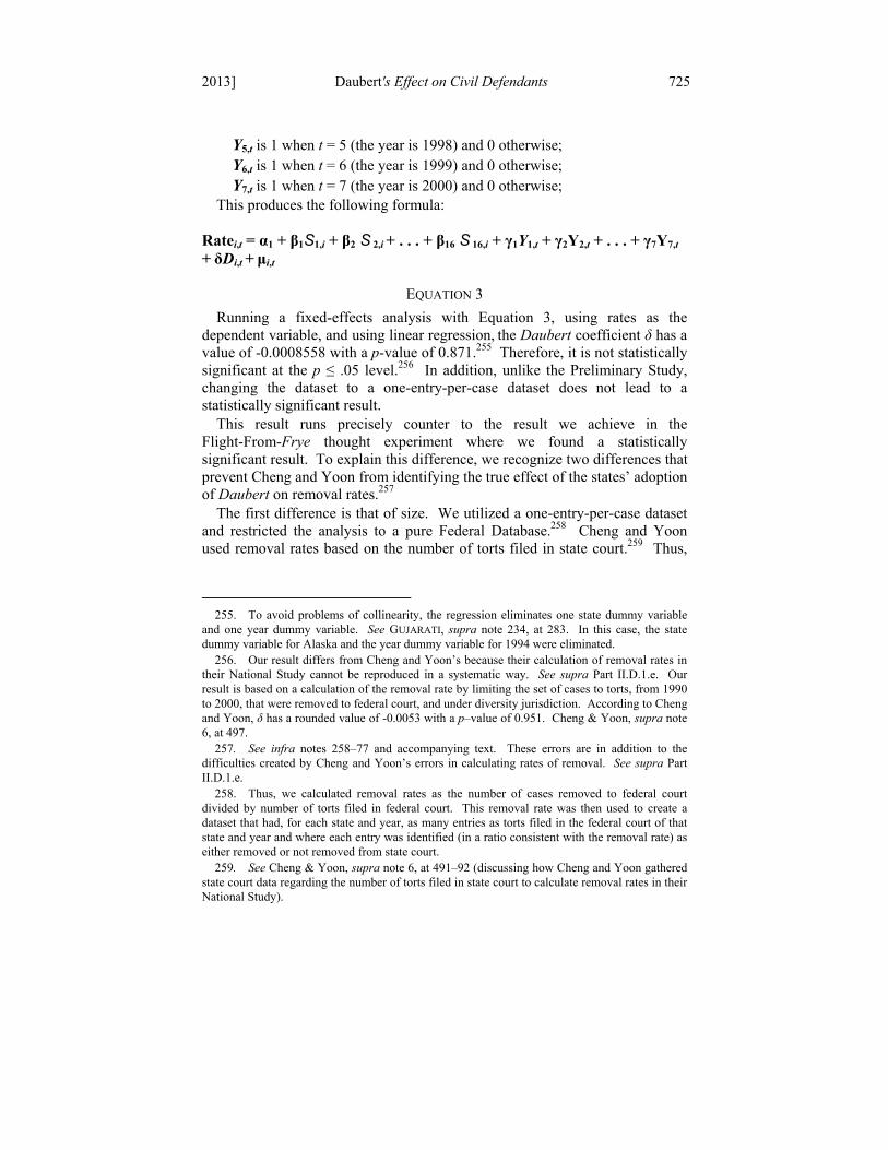
2013] Daubert's Effect on Civil Defendants 725
Y5,t is 1 when t = 5 (the year is 1998) and 0 otherwise; Y6,t is 1 when t = 6 (the year is 1999) and 0 otherwise; Y7,t is 1 when t = 7 (the year is 2000) and 0 otherwise;
This produces the following formula:
Ratei,t = α1 + β1S1,i + β2 S 2,i + . . . + β16 S 16,i + γ1Y1,t + γ2Y2,t + . . . + γ7Y7,t + δDi,t + μi,t
EQUATION 3
Running a fixed-effects analysis with Equation 3, using rates as the dependent variable, and using linear regression, the Daubert coefficient δ has a value of -0.0008558 with a p-value of 0.871.255 Therefore, it is not statistically significant at the p ≤ .05 level.256 In addition, unlike the Preliminary Study, changing the dataset to a one-entry-per-case dataset does not lead to a statistically significant result.
This result runs precisely counter to the result we achieve in the Flight-From-Frye thought experiment where we found a statistically significant result. To explain this difference, we recognize two differences that prevent Cheng and Yoon from identifying the true effect of the states’ adoption of Daubert on removal rates.257
The first difference is that of size. We utilized a one-entry-per-case dataset and restricted the analysis to a pure Federal Database.258 Cheng and Yoon used removal rates based on the number of torts filed in state court.259 Thus,
255. To avoid problems of collinearity, the regression eliminates one state dummy variable and one year dummy variable. See GUJARATI, supra note 234, at 283. In this case, the state dummy variable for Alaska and the year dummy variable for 1994 were eliminated. 256. Our result differs from Cheng and Yoon’s because their calculation of removal rates in their National Study cannot be reproduced in a systematic way. See supra Part II.D.1.e. Our result is based on a calculation of the removal rate by limiting the set of cases to torts, from 1990 to 2000, that were removed to federal court, and under diversity jurisdiction. According to Cheng and Yoon, δ has a rounded value of -0.0053 with a p–value of 0.951. Cheng & Yoon, supra note 6, at 497. 257. See infra notes 258–77 and accompanying text. These errors are in addition to the difficulties created by Cheng and Yoon’s errors in calculating rates of removal. See supra Part II.D.1.e. 258. Thus, we calculated removal rates as the number of cases removed to federal court divided by number of torts filed in federal court. This removal rate was then used to create a dataset that had, for each state and year, as many entries as torts filed in the federal court of that state and year and where each entry was identified (in a ratio consistent with the removal rate) as either removed or not removed from state court. 259. See Cheng & Yoon, supra note 6, at 491–92 (discussing how Cheng and Yoon gathered state court data regarding the number of torts filed in state court to calculate removal rates in their National Study).

726 Catholic University Law Review [Vol. 62:675
our database is both larger and smaller than Cheng and Yoon’s.260 It is larger because we have 57,640 entries, while Cheng and Yoon have only 112 (a difference of 514.6-to-1).261 But, it is also smaller because Cheng and Yoon’s removal rates are calculated with a denominator based on tort filings in state court. Thus, their removal rates summarize 2,956,439 cases while ours correspond to only 57,640 (a difference of 51.3-to-1).262 Both of these size differences work to our advantage and Cheng and Yoon’s disadvantage.263
The large size of our federal dataset compared to Cheng and Yoon’s plays an important role. Assuming the Daubert effect is small, it is more likely that a statistically significant result will be found in the larger dataset.264 Thus, our 57,640 data entries enable us to more easily identify a statistically significant result.265 Similarly, Cheng and Yoon summarized a vastly larger dataset,266 which will likely introduce many torts for which Daubert is not relevant.267 Once again, if we assume that the Daubert effect is small, then it will be harder to find the effect if the data includes cases for which Daubert adoption is irrelevant because those cases will create a noise—masking the effect.268 Thus, our 57,640 data entries work to our advantage.
The second difference is the set of state Cheng and Yoon examined. They analyzed 16 states269 while we look only at the 13 states that adopted Daubert after the federal courts.270 This difference matters because, if defense attorneys see Daubert as a stricter standard, then those attorneys will tend to stay in state court if they are in a state that adopted Daubert before the federal courts to
260. See infra notes 261–62 and accompanying text. 261. See Cheng & Yoon, supra note 6, at 497, 500–02 & fig.9 (showing that Cheng and Yoon had 110 entries after the 2 dummy variables were removed to avoid collinearity). 262. These numbers were calculated using Cheng and Yoon’s data and reviewing the number of cases filed per state and year. 263. See infra notes 264–69 and accompanying text (explaining our method used). 264. See CHOW, supra note 245, at 90–91 (discussing the sample-size dependence problem: whether or not statistical significance is obtained often depends on the sample size of the data). 265. Cf. id. (discussing how statistical significance is easier to find when there are larger numbers of entries tested). 266. See Cheng & Yoon, supra note 6, at 491–93; see also supra note 262 and accompanying text. 267. Cf. Gross, supra note 11, at 1119 (noting that there are certain torts in which the rate of expert witness testimony is much higher). 268. This could be a covariate in the data because distinct states are likely to have a separate ratio of tort cases based on their location. See LEE, supra note 207, at 64–65, 99 (discussing the problems covariates cause when comparing tested variables that take a long time to feel the effects stemming from a “treatment”). 269. Cheng & Yoon, supra note 6, at 493. 270. Arkansas and Oregon adopted tests similar to Daubert as a state evidentiary standard before the federal courts adopted Daubert in 1993, and New Mexico adopted the standard in the same year. See State v. Alberico, 861 P.2d 193, 203–04 (N.M. 1993); see also Prater v. State, 820 S.W.2d 429, 431 (Ark. 1991); State v. Brown, 687 P.2d 751, 759 (Or. 1984); supra note 139.

2013] Daubert's Effect on Civil Defendants 727
gain the evidentiary advantage in state court.271 Once the federal courts adopt Daubert, there is a leveling of evidentiary standards.272 We would expect this to result in an increase in the rate of removals because defense attorneys would no longer use the evidentiary difference as a basis for staying in state court.273 This is precisely what we find.274
We engaged in two sets of logistic-fixed-effects analyses from 1990 to 1996,275 one on pure federal data and the other using mixed federal and state data, using 10 states: Arizona, Arkansas, Florida, Kansas, Michigan, Minnesota, Missouri, New York, Oregon, and Washington. Arkansas and Oregon both adopted a Daubert standard before 1993 while the 8 other states did not adopt Daubert during the study period (and stand in as controls in our analysis).276
Both sets of analyses yielded statistically significant results at the p ≤ .05 level,277 demonstrating that the probability of removal increased after the federal courts adopted Daubert:
Daubert Adopted By
Federal Courts Probability of
Removal No 0.287348 Yes 0.330554
FIGURE 6: FIXED-EFFECTS ANALYSIS ON REMOVAL RATE USING FEDERAL
DATA ONLY
271. See Horowitz, supra note 113, at 18 (arguing that defense attorneys should remove the case when it is in their clients’ best interest); see also Miller, supra note 113, at 24, 28 (arguing that a defense attorney can win a case with a successful Daubert motion). 272. There is a leveling of standards because, in our hypothetical, both the state and federal courts apply the same evidentiary standard: Daubert. 273. See supra note 271 and accompanying text. 274. See infra note 277 and accompanying text; see also supra FIGURES 6 & 7 (showing the results of the calculated removal rates). 275. We excluded 1993 because that is the year the federal courts adopted Daubert. Daubert v. Merrell Down Pharms., Inc., 509 U.S. 579 (1993). 276. See supra notes 140, 270 and accompanying text. We eliminated New Mexico, which adopted Daubert in 1993, although it is unlikely that the adoption of Daubert by the federal courts would have any effect on removal rates in New Mexico because, before 1993, the federal and state courts used the same evidentiary standard, and, in this case, even after 1993, they both used the same standard. See State v. Alberico, 861 P.3d 192, 203–04 (N.M. 1993). Thus, its inclusion in the analysis would only create the same error found in Cheng and Yoon’s analysis. 277. The p-value for both logistic analyses was < 0.0005. Both analyses also produced statistically significant results using linear regression showing that the correlation was positive between federal court adoption of Daubert and removal rate.

728 Catholic University Law Review [Vol. 62:675
Daubert Adopted By
Federal Courts Probability of
Removal No 0.004431 Yes 0.004801
FIGURE 7: FIXED-EFFECTS ANALYSIS ON REMOVAL RATE USING FEDERAL AND
STATE DATA Cheng and Yoon’s analysis uses one variable, the Daubert dummy variable,
to account for two very different effects: (1) the effect of state adoption of Daubert where the state adopts after federal adoption and (2) the effect of state adoption where the state adopts Daubert before federal adoption.278 Because the two different effects work in opposite directions (increasing removal rate and decreasing removal rate, respectively), combining them is likely to result in one cancelling the other out and making it nearly impossible to find any statistically significant effect.279
III. DAUBERT IS THE STRICTER STANDARD FOR EXPERT WITNESS
ADMISSIBILITY
A. Implications of the Daubert Effect Conclusions
Our analysis demonstrates that the choice between Frye and Daubert does
matter, and matters quite significantly.280 Courts addressing the substantive scientific admissibility standard must consider the effect of choosing between two different substantive standards.281 If a court chooses Daubert, the ramifications will be that litigants will perceive the standard as strictly assessing expert evidence.282
The difference in scientific admissibility standards also has considerable effects on substantive tort law.283 Of course, the burden of proof in civil cases generally falls on the claimant, usually by a preponderance of the evidence standard.284 But, if the claimant must also prove issues that require expert
278. See supra notes 269–76 and accompanying text. 279. See supra notes 132, 277 and accompanying text (discussing the statistically significant results found in our study). 280. See supra notes 133, 141, 277 and accompanying text. 281. Cf. Krafka et al., supra note 4, at 22–23 (explaining how judges’ actions in the post-Daubert era are indicative of the fact that the change in evidentiary standards has affected how they approach scientific evidence). 282. See id. at 22–24. 283. See infra notes 284–91 and accompanying text (expressing the significance of an expert testimony admissibility standard). 284. See Stein, supra note 14, at 81 (“For civil trials, the default proof standard is a preponderance of the evidence. Under this standard, adjudicators must deem a factual allegation

2013] Daubert's Effect on Civil Defendants 729
testimony, the shift to Daubert will raise the requirements for the claimant to prove his or her case.285 Whether this shift is good or appropriate is not part of our analysis, except that any choice must be done knowing the full effect of the decision.
Further, our study raises an issue that relates back to the origins of the Daubert standard itself. In Daubert, Justice Blackmun, writing for the majority, rejected the Frye standard because it was so inconsistent with “the liberal thrust of the Federal Rules.”286 Despite this proclamation, we now see that the Daubert standard has tightened scrutiny beyond the Frye limits that troubled Blackmun and the majority.287 If so, the Court badly misjudged the effect Daubert would have on expert testimony, and the Court must now revisit the issue to clarify the standard, either affirming the new reality or reanimating the lenient standard originally intended.288
Lastly, the results of this study also have an effect on litigants in court. The effect of stricter scrutiny will change the marketplace for expert services because only those experts that can provide a sound empirical basis for their opinions will be admitted.289 In a world of strict expert review, empirical testing will be the lynchpin of admissibility.290 Therefore, litigants encourage and support specific fields when they choose to hire fields that satisfy the criteria of empirical science, while other fields will be forced to adapt to the new reality or fade away.291
B. Potential Areas of Future Research
There are several areas of further research that would build upon our analysis. One method would be to apply the same approach to a different, but
proven when it is more probable than not.” (footnote omitted) (citing Grogan v. Gartner, 498 U.S. 279, 286 (1991))). 285. See supra Part II.D.2.d (explaining that Daubert is a stricter standard on litigants because it results in a higher rate of removals). 286. See supra text accompanying notes 47–56; see also Daubert v. Merrell Dow Pharms., Inc., 509 U.S. 579, 588 (1993) (quoting Beech Aircraft Corp. v. Rainey, 488 U.S. 153, 169 (1988)). 287. See supra Part II.E (concluding, instead, that Daubert has resulted in a stricter standard). 288. See Faigman et al., supra note 29, at 1810 & n.34 (describing the widely shared view that the Frye standard would prove to be a stricter standard for admissibility than Daubert as “an erroneous one”). 289. See Saks, supra note 10, at 239 (“Testimony from those fields that could, but do not, provide adequate data . . . should be excluded until they can provide adequate empirical support for what the experts are claiming for their field in general, or for themselves individually.”). 290. See id. at 238–39 (“For those fields that can answer essential questions about themselves with sufficient completeness . . . the decision whether to admit or exclude can be made with relative ease.”). 291. See id. at 240 (observing that Daubert created a difficult situation for sciences that cannot satisfy the empirical data criteria).
730 Catholic University Law Review [Vol. 62:675
similar, set of data. As mentioned previously, the success of the analysis necessarily depends on the underlying data quality.292 The analysis here relies, in whole or in part, on the federal dataset.293 The same analysis, utilizing exclusively state-level data, may be useful to confirm or rebut these findings.
A second area of further research evolves from a limitation of this study. In removal rate analyses, the choice for removal lies with the defendant.294 Although the removal rate analysis is a powerful tool to measure these litigants’ behavior, it can only capture about half of civil case actors.295 The other half, the plaintiffs/claimants, must be studied using other metrics.296 Use of these alternative metrics would result in a more complete picture of Daubert’s effects.
A third potential study builds on the innovation of aggregate case data in a more general sense. The removal rate metric is capable of capturing a considerably larger number of cases than a case study approach.297 For example, this study used data on nearly 4 million cases, as compared to the several hundred used in other studies.298 Just as our study applies the removal rate metric to civil case data, expanding on case review studies such as Dixon and Gill, a researcher could apply an aggregate case data metric to criminal case data as well, expanding on the case review approach of the Groscup study.299 This type of study could measure the aggregate effect of Daubert on criminal cases and compare it to the effect on civil litigation. Additionally, aggregate case data methodologies can thoughtfully be applied to other substantive areas beyond Daubert.300
Finally, because Daubert is a more restrictive test, one might start to wonder if it has become synonymous with, or at least subsumed within the sphere of, 292. See supra Part II.D.1 (arguing that working with data that is fundamentally flawed will lead to inaccurate conclusions). 293. See supra Part II.C.2 (relying on the federal dataset). 294. See supra note 88 and accompanying text (describing the process for removal to federal court). 295. See supra text accompanying note 294 (noting that it is the defendant’s choice to remove to federal court and, consequently, this rate will only capture the defendant’s actions). 296. See supra notes 294–95 and accompanying text (noting the limitations of this study). 297. See infra note 298 and accompanying text (providing an example of this difference because the cited removal rate data approach was able to capture approximately 4 million cases when the cited case study approach was only able to capture 399). 298. See DIXON & GILL, supra note 4, at xiii (analyzing 399 district court opinions); see also supra note 106 and accompanying text. 299. Groscup et al., supra note 3, at 344 (analyzing 693 appellate opinions). 300. Cheng and Yoon cite one example of aggregate case data methodologies being applied to an area other than to Daubert. For example, they credit a 2002 Federal Judicial Center study on class action lawsuits for the origin of removals as an aggregate measure of procedural change. See Cheng & Yoon, supra note 6, at 482 n.32 (citing BOB NIEMIC & TOM WILLGING, FED. JUDICIAL CTR., EFFECTS OF AMCHEM/ORTIZ ON THE FILING OF FEDERAL CLASS ACTIONS: REPORT TO THE ADVISORY COMMITTEE ON CIVIL RULES 12–13 (2002)).

2013] Daubert's Effect on Civil Defendants 731
summary judgment. A very strict admissibility standard could have the same effect, in practice, as summary judgment by limiting the evidence available to claimants. Daubert may have not reached that level, but it is important to consider the interrelationship of the two issues.
IV. CONCLUSION
Since 1993, the effect of Daubert on expert admissibility has been hotly contested. In Daubert, the Supreme Court indicated strongly that this test would be more lenient for admissibility of expert evidence. Yet the initial perception of the effect was not overwhelmingly consistent with that result, so researchers began to investigate whether and how the scientific admissibility standard had changed. Some survey data indicated that judges saw Daubert as a stricter standard, while some did not. Some case review analysis found that Daubert was a stricter standard, while some did not. Despite utilizing several different empirical methodologies, the final determination of Daubert’s true effect remained inconclusive.
Finally, in 2005, Edward Cheng and Albert Yoon offered a fresh approach, utilizing removal rates to measure actual litigant behavior based on Daubert. Their approach captured several advantages over other approaches by: (1) aggregating large amounts of case data; (2) measuring real-world behavior without reporting a bias; and (3) isolating the scientific admissibility standard variable.
We also believe removal rate analysis is the best tool for assessing the aggregate effect of Daubert, so we recreated Cheng and Yoon’s underlying removal rate data to conduct additional studies. The results of this analysis demonstrated that, based on actual behavior in millions of real cases, civil defendants believe the Daubert standard to be a stricter one. Not only does the removal rate increase in the years after Daubert, as one would expect if the standard for admissibility is tighter, but we can also show that if the state adopts Daubert, and in so doing returns the state and federal court to the same admissibility standard, the removal rate then drops in response. Both of these effects support the conclusion that defendants perceive Daubert as an advantageous, stricter standard.
Because the results discussed in this Article so clearly contrast with Cheng and Yoon’s study, we then revisited the analysis Cheng and Yoon performed, looking for an explanation for the different results. When we did so, we found methodological problems with both the underlying data aggregation and the mathematical analysis of those data. Consequently, these errors undermine the validity of their study and their conclusions cannot be supported. When using our methods, the answer is clear: Daubert is the stricter standard of admissibility.

732 Catholic University Law Review [Vol. 62:675