The Storey-Based Stability of Steel Frames

Subjected to Variable Gravity and Fire Loading

by

Terence Ma

A thesis

presented to the University of Waterloo

in the fulfillment

of the thesis requirement for the degree of

Doctor of Philosophy (Ph.D.)

in

Civil Engineering

Waterloo, Ontario, Canada, 2020

c© Terence Ma 2020

Examining Committee Membership

The following served on the Examining Committee for this thesis. The decision of the Examining Commit-

tee is by majority vote.

External Examiner Dr. Ronald D. ZiemianProfessor, Department of Civil and Environmental EngineeringBucknell University

Supervisor Dr. Lei XuProfessor, Department of Civil and Environmental EngineeringUniversity of Waterloo

Internal Member Dr. Wei-Chau XieProfessor, Department of Civil and Environmental EngineeringUniversity of Waterloo

Internal Member Dr. Scott WalbridgeAssociate Professor, Department of Civil and Environmental EngineeringUniversity of Waterloo

Internal-External Member Dr. Elizabeth WeckmanProfessor, Department of Mechanical and Mechatronics EngineeringUniversity of Waterloo

ii

Author’s Declaration

This thesis consists of material all of which I authored or co-authored: see Statement of Contributions

included in the thesis. This is a true copy of the thesis, including any required final revisions, as accepted by

my examiners. I understand that my thesis may be made electronically available to the public.

iii

Statement of Contributions

The works presented herein, unless otherwise noted, have been accomplished solely by the author, with

guidance from the supervising professor, Lei Xu. The content covered in Chapter 3 with regards to the

effects of shear and axial deformations in the steel frames is contained in Ma and Xu (2019c) and Ma

et al. (2019), respectively. Note that a part of the derivation in Section 3.3 with regards to the stability

of steel frames with considering the axial stiffness of beams and the associated finite element validation

was completed in collaboration with a colleague in the same research group, Linbo Zhang. The effects of

column imperfections and lateral loads on the deformations of steel frames in Chapter 4 are published in Ma

and Xu (2019b). The stability of steel frames with members in uniform elevated temperatures in Chapter

5 is published in Xu et al. (2018) and Ma and Xu (2018, 2019d,g). Note that the research conducted in

Chapter 5 with regards to the proposed minimization problem based on the worst case scenario of elevated

temperatures resulting in the instability of a steel frame in Xu et al. (2018) was initiated by a former Ph.D.

student, Yi Zhuang (Zhuang, 2013), belonging in the same research group. Chapter 6 extends the notion of

elevated temperatures to include segmented members and post-earthquake conditions, and is published in

Ma and Xu (2019h), Ma and Xu (2019a), Ma and Xu (2019f), and Ma et al. (2020). The outcomes in Ma

et al. (2020) were accomplished with minimal guidance from Dr. Weiyong Wang of Chongqing University.

Finally, the work on multistorey steel frame stability in Chapter 7 is proposed in Ma and Xu (2019e).

iv

Abstract

The concept of storey-based stability has been developed over the past several decades, and includes power-

ful methods to holistically assess the structural integrity of unbraced and semi-braced steel frames. Recently,

it has also been applied in variable loading analysis, which unlike traditional proportional loading analysis,

aims to determine the worst and best case scenarios of loading which will cause the instability of any such

frame. Presented in this thesis are a number of theoretical and analytical methods which extend the field

of applicability of the storey-based stability and variable loading analysis concepts, particularly towards the

direction of performance-based fire-structural analysis. As building fires commonly occur and are responsi-

ble for significant losses of property and life across the world, it is of fundamental importance for structural

engineers to understand and design against the instability of a structure subjected to fire conditions.

In this study, the concept of storey-based stability analysis is first extended to account for shear and axial

deformations in members of the frames. Although these effects are often neglected in traditional structural

stability analysis, they may become significant in some cases. The effects of column initial imperfections

and lateral loads on the deformations and related failure criteria of a frames are also considered. With these

concepts in mind, the storey-based analysis approach is then extended to account for elevated temperatures

and various fire scenarios, and the concept of variable loading is extended to consider variable fire and

temperature loading instead of gravity loading. The complexity of the problem is then further heightened

by considering the presence of stepped members in a frame resulting from longitudinal temperature gradi-

ents. Most especially, the post-earthquake fire situation is considered by modelling the damages to both the

structure and insulation before applying the appropriate stability analysis equations. The post-earthquake

fire scenario deserves special attention since large-scale conflagrations can potentially follow earthquakes

during which extinguishing measures are rendered unavailable. Finally, the extension of the storey-based

stability and variable gravity loading concepts towards multiple storey frames is achieved in this study, with

the capabilities of considering all of the aforementioned conditions.

The proposed methods contained in this study provide a comprehensive and robust toolset for holistically

evaluating the stability and deformations of structures by considering them as structural systems rather than

individual members. As necessary, the use of finite element modelling is used to validate the theoretical

accuracy of all of the proposed methods. Finally, some recommendations for further research are proposed

with aims to further extend the fields of storey-based stability and variable loading.

v

Acknowledgments

As the author of this thesis I wish to hereby acknowledge several parties that have been imperative to the

success of the thesis research.

• First, the physical and spiritual support and care of my loving parents, Joseph and Carol, has been the

best that I could ever ask for and has enabled me to work productively.

• Secondly I would like to thank my supervisor, Dr. Lei Xu, who has always been supportive and

available throughout my degree. He also fulfills the role of a career mentor.

• I am grateful to the friends in Grad Cell Fellowship who have always been there to pray with me,

listen and share in my struggles both in terms of research, emotional well-being and faith.

• The rest of the examining committee have contributed significant time and provided valuable insight

towards improvement of the thesis research, including revisions to the final version of this thesis.

• This research has been funded through the CGS-M and CGS-D scholarships provided by the Na-

tional Sciences and Engineering Research Council of Canada (NSERC), as well as the Engineering

Excellence Fellowship sponsored by the University of Waterloo.

• Finally and most importantly, I give praise and thanks to my Creator who sent Jesus Christ to perish on

the cross to cleanse me from my sins and grant eternal life despite my shortcomings, and has provided

me with everything necessary for the completion of this degree and onward since the date of my birth.

I wish that anyone reading this thesis will come to repentance and saving faith in Jesus Christ.

vi

TO

Joseph & Carol, My Parents

vii

Table of ContentsExamining Committee Membership . . . . . . . . . . . . . . . . . . . . . . . . . . . . . . . . . iiAuthor’s Declaration . . . . . . . . . . . . . . . . . . . . . . . . . . . . . . . . . . . . . . . . . iiiAbstract . . . . . . . . . . . . . . . . . . . . . . . . . . . . . . . . . . . . . . . . . . . . . . . . vAcknowledgments . . . . . . . . . . . . . . . . . . . . . . . . . . . . . . . . . . . . . . . . . . . viDedication . . . . . . . . . . . . . . . . . . . . . . . . . . . . . . . . . . . . . . . . . . . . . . . viiList of Figures . . . . . . . . . . . . . . . . . . . . . . . . . . . . . . . . . . . . . . . . . . . . . xivList of Tables . . . . . . . . . . . . . . . . . . . . . . . . . . . . . . . . . . . . . . . . . . . . . xviii

1 Introduction 11.1 Background . . . . . . . . . . . . . . . . . . . . . . . . . . . . . . . . . . . . . . . . . . . 11.2 Scope and Objectives . . . . . . . . . . . . . . . . . . . . . . . . . . . . . . . . . . . . . . 21.3 Thesis Organization . . . . . . . . . . . . . . . . . . . . . . . . . . . . . . . . . . . . . . . 4

2 Literature Review 62.1 Storey-Based Stability . . . . . . . . . . . . . . . . . . . . . . . . . . . . . . . . . . . . . 6

2.1.1 Rotational Buckling of Columns . . . . . . . . . . . . . . . . . . . . . . . . . . . . 102.1.2 Behaviour of β . . . . . . . . . . . . . . . . . . . . . . . . . . . . . . . . . . . . . 122.1.3 Inelastic Buckling of Columns . . . . . . . . . . . . . . . . . . . . . . . . . . . . . 132.1.4 Effects of Shear Deformations . . . . . . . . . . . . . . . . . . . . . . . . . . . . . 142.1.5 Effects of Axial Deformations . . . . . . . . . . . . . . . . . . . . . . . . . . . . . 162.1.6 Columns in Tension . . . . . . . . . . . . . . . . . . . . . . . . . . . . . . . . . . 16

2.2 Variable Loading . . . . . . . . . . . . . . . . . . . . . . . . . . . . . . . . . . . . . . . . 172.3 Multistorey Frame Stability . . . . . . . . . . . . . . . . . . . . . . . . . . . . . . . . . . . 182.4 Column Imperfections and Notional Loading . . . . . . . . . . . . . . . . . . . . . . . . . 222.5 Fire-Structural Analysis . . . . . . . . . . . . . . . . . . . . . . . . . . . . . . . . . . . . . 24

2.5.1 Prescriptive versus Rational Approach . . . . . . . . . . . . . . . . . . . . . . . . . 242.5.2 Material Properties of Steel in Elevated Temperatures . . . . . . . . . . . . . . . . . 252.5.3 Estimation of Member Temperatures . . . . . . . . . . . . . . . . . . . . . . . . . . 262.5.4 Behaviour of Semi-Rigid Connections in Elevated Temperatures . . . . . . . . . . . 282.5.5 Storey-Based Fire Resistance of Steel Frames . . . . . . . . . . . . . . . . . . . . . 292.5.6 Non-Linear Temperature Distributions in Framing Members . . . . . . . . . . . . . 302.5.7 Post-Earthquake Fire Effects on Structures . . . . . . . . . . . . . . . . . . . . . . 31

3 Stability of Frames with Considering Shear and Beam Axial Deformations 333.1 Introduction . . . . . . . . . . . . . . . . . . . . . . . . . . . . . . . . . . . . . . . . . . . 333.2 Lateral Stiffness of a Frame with Timoshenko Members . . . . . . . . . . . . . . . . . . . . 33

3.2.1 Shear Angle Controversy . . . . . . . . . . . . . . . . . . . . . . . . . . . . . . . . 343.2.2 Solution to the Governing Differential Equations . . . . . . . . . . . . . . . . . . . 353.2.3 Columns in Tension . . . . . . . . . . . . . . . . . . . . . . . . . . . . . . . . . . 383.2.4 Rotational Buckling . . . . . . . . . . . . . . . . . . . . . . . . . . . . . . . . . . 383.2.5 Behaviour of Lateral Stiffness Equation . . . . . . . . . . . . . . . . . . . . . . . . 403.2.6 Frame Lateral Stiffness without Considering Axial Beam Deformations . . . . . . . 413.2.7 Effect of Shear Deformations on Rotational Stiffness of Beams . . . . . . . . . . . . 423.2.8 True End Fixity Factor . . . . . . . . . . . . . . . . . . . . . . . . . . . . . . . . . 453.2.9 FEA Validation . . . . . . . . . . . . . . . . . . . . . . . . . . . . . . . . . . . . . 47

viii

3.3 Lateral Stiffness of a Frame with Axially Deforming Beams . . . . . . . . . . . . . . . . . 483.3.1 Column Upper End Displacements . . . . . . . . . . . . . . . . . . . . . . . . . . . 493.3.2 Frame Stability with Axially Deforming Beams . . . . . . . . . . . . . . . . . . . . 513.3.3 Behaviour of the Series Spring Stiffness Operator . . . . . . . . . . . . . . . . . . . 553.3.4 Local Stiffness Reduction Factor . . . . . . . . . . . . . . . . . . . . . . . . . . . . 563.3.5 Numerical Example #1 on the Effect of Lateral Bracing . . . . . . . . . . . . . . . . 573.3.6 Numerical Example #2 on the Effect of Lateral Bracing . . . . . . . . . . . . . . . . 62

3.4 Lean-On Frame Example . . . . . . . . . . . . . . . . . . . . . . . . . . . . . . . . . . . . 663.4.1 Parametric Study - Effect of Shear Deformations . . . . . . . . . . . . . . . . . . . 683.4.2 Parametric Study - Effect of Axial Deformations . . . . . . . . . . . . . . . . . . . 71

3.5 Variable Loading . . . . . . . . . . . . . . . . . . . . . . . . . . . . . . . . . . . . . . . . 733.5.1 Numerical Example for Variable Loading . . . . . . . . . . . . . . . . . . . . . . . 743.5.2 Worst Case Variable Loading . . . . . . . . . . . . . . . . . . . . . . . . . . . . . . 753.5.3 Best Case Variable Loading . . . . . . . . . . . . . . . . . . . . . . . . . . . . . . 783.5.4 FEA Validation . . . . . . . . . . . . . . . . . . . . . . . . . . . . . . . . . . . . . 80

3.6 Conclusion . . . . . . . . . . . . . . . . . . . . . . . . . . . . . . . . . . . . . . . . . . . 81

4 Capacity of Frames Subjected to Column Imperfections and Lateral Loads 834.1 Introduction . . . . . . . . . . . . . . . . . . . . . . . . . . . . . . . . . . . . . . . . . . . 834.2 Lateral Stiffness of Frame subjected to Column Imperfections and Lateral Loads . . . . . . 83

4.2.1 Column Lateral Stiffness . . . . . . . . . . . . . . . . . . . . . . . . . . . . . . . . 844.2.2 Calculation of Inter-Storey Drift . . . . . . . . . . . . . . . . . . . . . . . . . . . . 884.2.3 Definition of Frame Capacity . . . . . . . . . . . . . . . . . . . . . . . . . . . . . . 894.2.4 Effect of Lateral Loads . . . . . . . . . . . . . . . . . . . . . . . . . . . . . . . . . 894.2.5 Effect of Shear Deformations . . . . . . . . . . . . . . . . . . . . . . . . . . . . . 904.2.6 Effect of Axial Beam Deformations . . . . . . . . . . . . . . . . . . . . . . . . . . 90

4.3 Variable Loading Anlaysis . . . . . . . . . . . . . . . . . . . . . . . . . . . . . . . . . . . 914.3.1 Failure Criterion of Instability . . . . . . . . . . . . . . . . . . . . . . . . . . . . . 924.3.2 Failure Criteria related to Deformations . . . . . . . . . . . . . . . . . . . . . . . . 924.3.3 Computational Procedure . . . . . . . . . . . . . . . . . . . . . . . . . . . . . . . . 94

4.4 Numerical Example for Column Imperfections . . . . . . . . . . . . . . . . . . . . . . . . 944.4.1 Effect of Out-of-Plumbness, ∆0 . . . . . . . . . . . . . . . . . . . . . . . . . . . . 964.4.2 Effect of Out-of-Straightness, δ0 . . . . . . . . . . . . . . . . . . . . . . . . . . . . 974.4.3 Effect of Bracing Stiffness . . . . . . . . . . . . . . . . . . . . . . . . . . . . . . . 984.4.4 FEA Validation . . . . . . . . . . . . . . . . . . . . . . . . . . . . . . . . . . . . . 994.4.5 Variable Loading Analysis - Problem Setup . . . . . . . . . . . . . . . . . . . . . . 1004.4.6 Variable Loading Analysis - Instability Criterion . . . . . . . . . . . . . . . . . . . 1014.4.7 Variable Loading Analysis - Excessive Inter-Storey Displacement Criterion . . . . . 1024.4.8 Variable Loading Analysis - Excessive Deflection Criterion . . . . . . . . . . . . . . 1044.4.9 Variable Loading Analysis - Onset of Yielding Criterion . . . . . . . . . . . . . . . 1054.4.10 Effects of Increasing the Column Imperfections . . . . . . . . . . . . . . . . . . . . 106

4.5 Numerical Example with Lateral Loads . . . . . . . . . . . . . . . . . . . . . . . . . . . . 1074.6 Conclusion . . . . . . . . . . . . . . . . . . . . . . . . . . . . . . . . . . . . . . . . . . . 107

5 Stability Analysis of Frames Subjected to Variable Fire Loading 1095.1 Introduction . . . . . . . . . . . . . . . . . . . . . . . . . . . . . . . . . . . . . . . . . . . 109

ix

5.2 Lateral Stiffness of a Frame with Heated Members . . . . . . . . . . . . . . . . . . . . . . 1095.2.1 Frame Stability based on Member Temperatures . . . . . . . . . . . . . . . . . . . 1115.2.2 Frame Stability based on Locality Factor . . . . . . . . . . . . . . . . . . . . . . . 1145.2.3 Computational Procedure . . . . . . . . . . . . . . . . . . . . . . . . . . . . . . . . 1155.2.4 Discussion of the Shear Modulus at Elevated Temperatures . . . . . . . . . . . . . . 1165.2.5 The Effects of Shear and Axial Deformations in Elevated Temperatures . . . . . . . 118

5.3 Numerical Examples for Frame Stability in Elevated Temperatures . . . . . . . . . . . . . . 1195.3.1 Two Bay Example . . . . . . . . . . . . . . . . . . . . . . . . . . . . . . . . . . . 1205.3.2 Four Bay Example . . . . . . . . . . . . . . . . . . . . . . . . . . . . . . . . . . . 1235.3.3 Parametric study on kC/B . . . . . . . . . . . . . . . . . . . . . . . . . . . . . . . . 127

5.4 Extension for Variable Fire Duration . . . . . . . . . . . . . . . . . . . . . . . . . . . . . . 1285.4.1 Frame Stability Accounting for Fire Duration . . . . . . . . . . . . . . . . . . . . . 1295.4.2 Computational Procedure . . . . . . . . . . . . . . . . . . . . . . . . . . . . . . . . 1315.4.3 Discussion of the Solution . . . . . . . . . . . . . . . . . . . . . . . . . . . . . . . 132

5.5 Numerical Examples for Fire Duration . . . . . . . . . . . . . . . . . . . . . . . . . . . . . 1335.5.1 Asymmetrical Two Bay Frame subjected to Standard Fire . . . . . . . . . . . . . . 1335.5.2 Four Bay Frame subjected to Parametric Fire . . . . . . . . . . . . . . . . . . . . . 138

5.6 Stochastic Fire Resistance Approach . . . . . . . . . . . . . . . . . . . . . . . . . . . . . . 1415.6.1 Random Variables . . . . . . . . . . . . . . . . . . . . . . . . . . . . . . . . . . . 1415.6.2 Computational Procedure . . . . . . . . . . . . . . . . . . . . . . . . . . . . . . . . 1435.6.3 Numerical Example . . . . . . . . . . . . . . . . . . . . . . . . . . . . . . . . . . 1435.6.4 Parametric Study . . . . . . . . . . . . . . . . . . . . . . . . . . . . . . . . . . . . 1455.6.5 Simulation Results . . . . . . . . . . . . . . . . . . . . . . . . . . . . . . . . . . . 150

5.7 Conclusion . . . . . . . . . . . . . . . . . . . . . . . . . . . . . . . . . . . . . . . . . . . 155

6 Stability of Frames with Segmented Members 1576.1 Introduction . . . . . . . . . . . . . . . . . . . . . . . . . . . . . . . . . . . . . . . . . . . 1576.2 Stability and Deformation of Frames with Three-Segment Members . . . . . . . . . . . . . 157

6.2.1 End Fixity Factors for Three-Segment Members . . . . . . . . . . . . . . . . . . . 1586.2.2 Calculation of Column End Fixity Factors with Three Segments . . . . . . . . . . . 1606.2.3 Thermal Restraints for Three-Segment Members . . . . . . . . . . . . . . . . . . . 1656.2.4 Frame Stability with Three-Segment Members . . . . . . . . . . . . . . . . . . . . 1676.2.5 Vertical Stiffness of a Column Restraint . . . . . . . . . . . . . . . . . . . . . . . . 1706.2.6 Rotational Buckling Load of a Three-Segment Column . . . . . . . . . . . . . . . . 1726.2.7 Effect of Axial Beam Deformations . . . . . . . . . . . . . . . . . . . . . . . . . . 1766.2.8 Modelling Applications . . . . . . . . . . . . . . . . . . . . . . . . . . . . . . . . 176

6.3 Numerical Examples for Three-Segment Members . . . . . . . . . . . . . . . . . . . . . . 1786.3.1 Two Bay Frame subjected to Localized Fire . . . . . . . . . . . . . . . . . . . . . . 1786.3.2 Two Bay Frame subjected to Blast Damage . . . . . . . . . . . . . . . . . . . . . . 183

6.4 Application of Three-segment Members towards Post-Earthquake Fire . . . . . . . . . . . . 1886.4.1 Modelling of Structural Damage . . . . . . . . . . . . . . . . . . . . . . . . . . . . 1886.4.2 Modelling of Damage to Insulation . . . . . . . . . . . . . . . . . . . . . . . . . . 189

6.5 Numerical Example for Post-Earthquake Fire . . . . . . . . . . . . . . . . . . . . . . . . . 1906.5.1 Effect of Inter-storey Drift, ∆0 . . . . . . . . . . . . . . . . . . . . . . . . . . . . . 1926.5.2 FEA Validation . . . . . . . . . . . . . . . . . . . . . . . . . . . . . . . . . . . . . 1936.5.3 Effect of Delamination Length, Ld . . . . . . . . . . . . . . . . . . . . . . . . . . . 194

x

6.5.4 Probabilistic Post-Earthquake Analysis . . . . . . . . . . . . . . . . . . . . . . . . 1956.6 Generalization for n-segment Members . . . . . . . . . . . . . . . . . . . . . . . . . . . . 1986.7 Conclusion . . . . . . . . . . . . . . . . . . . . . . . . . . . . . . . . . . . . . . . . . . . 199

7 Storey-Based Stability for Multistorey Frames 2007.1 Introduction . . . . . . . . . . . . . . . . . . . . . . . . . . . . . . . . . . . . . . . . . . . 2007.2 Proposed Frame Decomposition Method . . . . . . . . . . . . . . . . . . . . . . . . . . . . 201

7.2.1 End Fixity Factors . . . . . . . . . . . . . . . . . . . . . . . . . . . . . . . . . . . 2027.2.2 Storey-Based Stability in Multistorey Frames . . . . . . . . . . . . . . . . . . . . . 2057.2.3 Discussion of Shape Coefficients . . . . . . . . . . . . . . . . . . . . . . . . . . . . 2067.2.4 Effects of Axial Beam Deformations . . . . . . . . . . . . . . . . . . . . . . . . . . 2087.2.5 Computational Procedure of the Decomposition Method . . . . . . . . . . . . . . . 209

7.3 Matrix Analysis Method of Multistorey Frames . . . . . . . . . . . . . . . . . . . . . . . . 2097.4 Validation . . . . . . . . . . . . . . . . . . . . . . . . . . . . . . . . . . . . . . . . . . . . 210

7.4.1 Elastic Analysis Example . . . . . . . . . . . . . . . . . . . . . . . . . . . . . . . 2107.4.2 Inelastic Analysis Example . . . . . . . . . . . . . . . . . . . . . . . . . . . . . . . 2157.4.3 Effects of Axial Beam Deformations . . . . . . . . . . . . . . . . . . . . . . . . . . 220

7.5 Parametric Analyses . . . . . . . . . . . . . . . . . . . . . . . . . . . . . . . . . . . . . . 2207.5.1 Sensitivity of Shape Parameters in Asymmetric Buckling Analysis . . . . . . . . . . 2217.5.2 Stochastic Error Analysis . . . . . . . . . . . . . . . . . . . . . . . . . . . . . . . . 222

7.6 Variable Loading of Multistorey Frames . . . . . . . . . . . . . . . . . . . . . . . . . . . . 2247.6.1 Minimization Problem . . . . . . . . . . . . . . . . . . . . . . . . . . . . . . . . . 2247.6.2 Shape Parameters . . . . . . . . . . . . . . . . . . . . . . . . . . . . . . . . . . . . 2257.6.3 Rotational Buckling . . . . . . . . . . . . . . . . . . . . . . . . . . . . . . . . . . 2257.6.4 Solving the Objective Function . . . . . . . . . . . . . . . . . . . . . . . . . . . . . 2267.6.5 Elastic Analysis Example in Variable Loading . . . . . . . . . . . . . . . . . . . . . 2277.6.6 Inelastic Analysis Example in Variable Loading . . . . . . . . . . . . . . . . . . . . 228

7.7 Other Considerations for Multistorey Frames . . . . . . . . . . . . . . . . . . . . . . . . . 2297.7.1 Initial Imperfections in Multistorey Frames . . . . . . . . . . . . . . . . . . . . . . 2307.7.2 Elevated Temperatures in Multistorey Frames . . . . . . . . . . . . . . . . . . . . . 230

7.8 Numerical Example - Putting it All Together . . . . . . . . . . . . . . . . . . . . . . . . . . 2337.8.1 Variable Fire Analysis . . . . . . . . . . . . . . . . . . . . . . . . . . . . . . . . . 2367.8.2 Post-Earthquake Fire Analysis . . . . . . . . . . . . . . . . . . . . . . . . . . . . . 241

7.9 Conclusion . . . . . . . . . . . . . . . . . . . . . . . . . . . . . . . . . . . . . . . . . . . 243

8 Conclusion 2458.1 Summary . . . . . . . . . . . . . . . . . . . . . . . . . . . . . . . . . . . . . . . . . . . . 2458.2 Effects of Shear and Axial Deformations on the Stability of Frames . . . . . . . . . . . . . 2458.3 Frame Capacity with Column Imperfections and Lateral Loading . . . . . . . . . . . . . . . 2468.4 Frame Stability in Variable Fire Loading . . . . . . . . . . . . . . . . . . . . . . . . . . . . 2468.5 Frame Stability with Segmented Members . . . . . . . . . . . . . . . . . . . . . . . . . . . 2478.6 Stability of Multistorey Frames . . . . . . . . . . . . . . . . . . . . . . . . . . . . . . . . . 248

9 Recommendations for Future Research 2499.1 Overview of Recommendations . . . . . . . . . . . . . . . . . . . . . . . . . . . . . . . . . 2499.2 Fire-Structural Modelling . . . . . . . . . . . . . . . . . . . . . . . . . . . . . . . . . . . . 249

xi

9.2.1 Variable Fuel Loading . . . . . . . . . . . . . . . . . . . . . . . . . . . . . . . . . 2499.2.2 Independent Fire Curve Assumption . . . . . . . . . . . . . . . . . . . . . . . . . . 2509.2.3 Thermal Gradients of Columns . . . . . . . . . . . . . . . . . . . . . . . . . . . . . 2509.2.4 Thermal Expansion of Beams . . . . . . . . . . . . . . . . . . . . . . . . . . . . . 2519.2.5 Refinement of Seismic Structural Damage Assumptions . . . . . . . . . . . . . . . 251

9.3 Storey-Based Stability and Capacity Analysis . . . . . . . . . . . . . . . . . . . . . . . . . 2519.3.1 Progressive Collapse . . . . . . . . . . . . . . . . . . . . . . . . . . . . . . . . . . 2519.3.2 Frame Capacity Defined by Residual Lateral Stiffness . . . . . . . . . . . . . . . . 2529.3.3 Consideration of Transverse Loads . . . . . . . . . . . . . . . . . . . . . . . . . . . 2539.3.4 Robustness of Variable Loading Problem . . . . . . . . . . . . . . . . . . . . . . . 2539.3.5 Stochastic Analysis of Non-Fire Scenarios . . . . . . . . . . . . . . . . . . . . . . . 2549.3.6 Advanced Inelastic Deformation Analysis . . . . . . . . . . . . . . . . . . . . . . . 254

9.4 Experimental Validation . . . . . . . . . . . . . . . . . . . . . . . . . . . . . . . . . . . . 255

References 256

Appendices 270

A2 Appendix for the Literature Review 270A2.3 Deficiencies of the Liu and Xu (2005) Decomposition Method . . . . . . . . . . . . . . . . 270

A2.3.1 Background of the Alignment Chart Method . . . . . . . . . . . . . . . . . . . . . 270A2.3.2 Inconsistency of the Liu and Xu (2005) Method . . . . . . . . . . . . . . . . . . . . 274A2.3.3 Validation Example . . . . . . . . . . . . . . . . . . . . . . . . . . . . . . . . . . . 274

A3 Appendix for Shear and Beam Axial Deformations 279A3.2 Behaviour of Columns in Tension . . . . . . . . . . . . . . . . . . . . . . . . . . . . . . . 279

A3.2.3 Solution to the Governing Differential Equations for Columns in Tension . . . . . . 279A3.2.5 Behaviour of the Lateral Stiffness Equation for Columns in Tension . . . . . . . . . 282

A4 Appendix for Column Imperfections and Lateral Loads 285A4.2 Derivations with Considering Shear Deformations . . . . . . . . . . . . . . . . . . . . . . . 285

A4.2.5 Timoshenko Column with Initial Imperfections and Lateral Loads . . . . . . . . . . 285A4.5 Numerical Example with Lateral Loads . . . . . . . . . . . . . . . . . . . . . . . . . . . . 288

A4.5.1 Proportional Loading Analysis . . . . . . . . . . . . . . . . . . . . . . . . . . . . . 289A4.5.2 Effect of Lateral Bracing . . . . . . . . . . . . . . . . . . . . . . . . . . . . . . . . 291A4.5.3 Variable Loading Analysis - Instability Criterion . . . . . . . . . . . . . . . . . . . 292A4.5.4 Variable Loading Analysis - Other Criteria . . . . . . . . . . . . . . . . . . . . . . 293

A5 Appendix for Frames in Elevated Temperatures 296A5.2 Shear and Beam Axial Deformations in Elevated Temperatures . . . . . . . . . . . . . . . . 296

A5.2.1 Parametric Study of Lean-On Frame in Elevated Temperatures . . . . . . . . . . . . 296A5.3 Shear and Axial Beam Deformations in Variable Loading Examples . . . . . . . . . . . . . 300

A5.3.1 Two Bay Example in Variable Temperature Loading . . . . . . . . . . . . . . . . . 300A5.3.2 Four Bay Example in Variable Temperature Loading . . . . . . . . . . . . . . . . . 302

A6 Appendix for Frames Containing Segmented Members 304A6.2 Derivations for Three-Segment Members . . . . . . . . . . . . . . . . . . . . . . . . . . . 304

xii

A6.2.1 True End Fixity Factors for Three-Segment Timoshenko Members . . . . . . . . . . 304A6.2.2 Rotational Stiffness Contribution at Connection of a Three-Segment Beam . . . . . 305A6.2.4 Frame Stability with Three-Segment Timoshenko Members . . . . . . . . . . . . . 307A6.2.5 Rotational Buckling Load of a Three-Segment Timoshenko Column . . . . . . . . . 308

A6.6 Derivations for n-segment Members . . . . . . . . . . . . . . . . . . . . . . . . . . . . . . 310A6.6.1 End Fixity Factors for n-segment Members . . . . . . . . . . . . . . . . . . . . . . 310A6.6.2 Calculation of Column End Fixity Factors with n Segments . . . . . . . . . . . . . . 311A6.6.3 Thermal Restraints for n-segment Members . . . . . . . . . . . . . . . . . . . . . . 313A6.6.4 Frame Stability with n-segment Members . . . . . . . . . . . . . . . . . . . . . . . 314A6.6.5 Individual n-segment Column Rotational Buckling Load . . . . . . . . . . . . . . . 316

A7 Appendix for Multistorey Frame Stability 319A7.2 Derivations for Member in Multistorey Frames . . . . . . . . . . . . . . . . . . . . . . . . 319

A7.2.1 Rotational Stiffness Contribution with Second-Order Effects . . . . . . . . . . . . . 319A7.2.3 Derivation of Shape Coefficients . . . . . . . . . . . . . . . . . . . . . . . . . . . . 320

A7.3 Matrix Analysis Method of Multistorey Frames . . . . . . . . . . . . . . . . . . . . . . . . 323A7.3.1 Column Stiffness Matrix . . . . . . . . . . . . . . . . . . . . . . . . . . . . . . . . 323A7.3.2 Frame-based Stability via the Matrix Method . . . . . . . . . . . . . . . . . . . . . 326A7.3.3 Lateral Bracing via the Matrix Method . . . . . . . . . . . . . . . . . . . . . . . . 328A7.3.4 Computational Procedure of the Matrix Method . . . . . . . . . . . . . . . . . . . . 330A7.3.5 Advantages and Limitations of the Matrix Method . . . . . . . . . . . . . . . . . . 331

A7.4 Validation of Multistorey Examples . . . . . . . . . . . . . . . . . . . . . . . . . . . . . . 332A7.4.1 Elastic Analysis Example with Considering Shear Deformations . . . . . . . . . . . 332A7.4.2 Inelastic Analysis Example with Considering Shear Deformations . . . . . . . . . . 333A7.4.3 Elastic Analysis Example with Considering Axial Beam Deformations . . . . . . . . 334

A7.6 Further Results of Multistorey Variable Loading Examples . . . . . . . . . . . . . . . . . . 336A7.6.5 Elastic Analysis Example in Variable Loading . . . . . . . . . . . . . . . . . . . . . 336A7.6.6 Inelastic Analysis Example in Variable Loading . . . . . . . . . . . . . . . . . . . . 338

A7.7 Derivations Relating to Other Considerations . . . . . . . . . . . . . . . . . . . . . . . . . 339A7.7.2 Rotational Stiffness Contribution of an Axially Loaded Three-Segment Member . . 339

xiii

List of Figures2.1 Generalized semi-rigidly connected semi-braced storey frame analyzed by Xu and Liu (2002b) 72.2 Generalized plot of column lateral stiffness S versus axial load N . . . . . . . . . . . . . . . 112.3 Generalized plot of β with respect to φ and ru, with rl = 1 . . . . . . . . . . . . . . . . . . 122.4 Generalized plot of β with respect to φ and ru, with rl = 0 . . . . . . . . . . . . . . . . . . 132.5 Illustration of decomposition model for general multistorey frame . . . . . . . . . . . . . . 192.6 Column imperfection functions (Zhuang, 2013) . . . . . . . . . . . . . . . . . . . . . . . . 232.7 Steel stress-strain curve at elevated temperature in Eurocode 3 (BSI, 2005) . . . . . . . . . . 25

3.1 Axially loaded semi-rigidly connected Timoshenko column in Compression . . . . . . . . . 343.2 Comparison of the Engesser (1891) and Haringx (1948) assumptions on ω . . . . . . . . . . 363.3 Effect of η on the lateral stiffness with respect to φ for rl = 0.75, ru = 0.5, Engesser (1891)

assumption . . . . . . . . . . . . . . . . . . . . . . . . . . . . . . . . . . . . . . . . . . . 403.4 Effect of η on the lateral stiffness with respect to φ for rl = 0.75, ru = 0.5, Haringx (1948)

assumption . . . . . . . . . . . . . . . . . . . . . . . . . . . . . . . . . . . . . . . . . . . 413.5 Deformation of a typical semi-rigidly connected member . . . . . . . . . . . . . . . . . . . 423.6 Definition of end fixity factor for a member . . . . . . . . . . . . . . . . . . . . . . . . . . 453.7 Critical sway loads versus slenderness ratio for single column . . . . . . . . . . . . . . . . . 473.8 General semi-braced storey frame subjected to gravity loading . . . . . . . . . . . . . . . . 483.9 Equivalent spring system for storey frame in Fig. (3.8) . . . . . . . . . . . . . . . . . . . . 523.10 Deformed state of the equivalent spring system in Fig. (3.9) . . . . . . . . . . . . . . . . . . 533.11 Replacement of a column and its brace in parallel with an equivalent spring . . . . . . . . . 533.12 Replacement of a beam and column-brace system in series with an equivalent spring . . . . 543.13 Using an equivalent spring stiffness, Seq,1, to represent the entire storey frame . . . . . . . . 543.14 Pseudo-algorithm for calculating storey-based equivalent spring stiffness . . . . . . . . . . . 543.15 Lateral stiffness reduction factor versus beam-to-column-brace stiffness ratio . . . . . . . . 573.16 Four-bay frame subjected to proportional gravity loading . . . . . . . . . . . . . . . . . . . 573.17 Critical load of four-bay frame with varying lateral bracing stiffness . . . . . . . . . . . . . 593.18 Buckled shape of four-bay frame with Kbr = 0 kN/m (unbraced) . . . . . . . . . . . . . . . 613.19 Buckled shape of four-bay frame with Kbr = 454 kN/m (semi-braced) . . . . . . . . . . . . 623.20 Buckled shape of four-bay frame with Kbr = 10,000 kN/m (fully braced) . . . . . . . . . . . 623.21 Eleven-bay frame subjected to proportional gravity loading . . . . . . . . . . . . . . . . . . 633.22 Critical gravity loads of the eleven-bay frame with varying lateral bracing stiffness . . . . . 633.23 Reductions of critical gravity loads for the eleven-bay frame with varying bracing stiffness . 643.24 Buckled shape of eleven-bay frame with Kbr = 0 kN/m (unbraced) . . . . . . . . . . . . . . 663.25 Buckled shape of eleven-bay frame with Kbr = 220 kN/m (semi-braced) . . . . . . . . . . . 663.26 Buckled shape of eleven-bay frame with Kbr = 10,000 kN/m (fully braced) . . . . . . . . . 663.27 Generalized lean-on frame consisting of n bays . . . . . . . . . . . . . . . . . . . . . . . . 673.28 Difference in Psw from using the Haringx (1948) and Engesser (1891) assumptions . . . . . 693.29 Effect of shear deformations on Sn+1 with varying L/r and loading levels . . . . . . . . . . 693.30 Effect of shear deformations on Pcr with varying KL/r and loading levels . . . . . . . . . . 703.31 Effect of beam axial deformations on Pcr with varying beam size and number of bays . . . . 723.32 Four-bay frame subjected to variable gravity loading . . . . . . . . . . . . . . . . . . . . . 743.33 Buckled shape of modified four-bay frame in best case loading example obtained in ABAQUS

(Simulia, 2012) . . . . . . . . . . . . . . . . . . . . . . . . . . . . . . . . . . . . . . . . . 81

xiv

4.1 General semi-braced storey frame subjected to column imperfections and lateral load . . . . 844.2 Column subjected to column imperfections and second-order effects (Zhuang, 2013) . . . . 854.3 Four-bay frame subjected to column imperfections ∆0 and δ0 . . . . . . . . . . . . . . . . . 954.4 Effect of ∆0 on the inter-storey displacement of the example frame . . . . . . . . . . . . . . 964.5 Effect of δ0 on the maximum deflection in the example frame . . . . . . . . . . . . . . . . . 974.6 Effect of δ0 on the inter-storey drift in the example frame . . . . . . . . . . . . . . . . . . . 984.7 Effect of Kbr on the buckling load, Psw . . . . . . . . . . . . . . . . . . . . . . . . . . . . . 994.8 Comparison of inter-storey displacement and maximum deflection obtained with the pro-

posed method and FEA . . . . . . . . . . . . . . . . . . . . . . . . . . . . . . . . . . . . . 100

5.1 General semi-braced storey frame subjected to elevated member temperatures . . . . . . . . 1105.2 Assumed Poisson’s ratio with respect to temperature . . . . . . . . . . . . . . . . . . . . . 1185.3 Comparison of methods used to estimate the tangent shear modulus at elevated temperatures 1195.4 Example two-bay frame subjected to heated members . . . . . . . . . . . . . . . . . . . . . 1205.5 Example four-bay frame subjected to heated members . . . . . . . . . . . . . . . . . . . . . 1245.6 Parametric study of worst case heating scenario with respect to kC/B . . . . . . . . . . . . . 1275.7 General semi-braced storey frame subjected to time-based heating in fire . . . . . . . . . . . 1295.8 Example two-bay frame with standard fire curves for variable fire duration analysis . . . . . 1335.9 Example four-bay frame with parametric fire curves for variable fire duration analysis . . . . 1385.10 Example four-bay frame with parametric fire curves for variable fire duration analysis . . . . 1395.11 Example four-bay frame for stochastic variable fire analysis . . . . . . . . . . . . . . . . . . 1445.12 Variation of fire curves with fuel load for four-bay frame stochastic analysis example . . . . 1465.13 Temperature-time curves of Column 2 with varying origin location and fuel load for four-

bay frame stochastic analysis example . . . . . . . . . . . . . . . . . . . . . . . . . . . . . 1475.14 Temperature-time curves of Column 1 with varying origin location and fuel load for four-

bay frame stochastic analysis example . . . . . . . . . . . . . . . . . . . . . . . . . . . . . 1475.15 Temperature-time curves of Column 4 with varying origin location and fuel load for four-

bay frame stochastic analysis example . . . . . . . . . . . . . . . . . . . . . . . . . . . . . 1485.16 Temperature-time curves of Column 2 with varying fire separation resistance for four-bay

frame stochastic analysis example . . . . . . . . . . . . . . . . . . . . . . . . . . . . . . . 1485.17 Lateral stiffness versus time with varying origin location and fuel loads for four-bay frame

stochastic analysis example . . . . . . . . . . . . . . . . . . . . . . . . . . . . . . . . . . . 1495.18 Lateral stiffness versus time with varying origin location and gravity load intensity for four-

bay frame stochastic analysis example . . . . . . . . . . . . . . . . . . . . . . . . . . . . . 1505.19 Histogram plot of fire resistance in Monte Carlo simulation . . . . . . . . . . . . . . . . . . 1515.20 Frame lateral stiffness versus fire event duration in worst case scenario . . . . . . . . . . . . 153

6.1 General semi-braced storey frame with three-segment members . . . . . . . . . . . . . . . . 1586.2 Definition of end fixity factor for a three-segment beam . . . . . . . . . . . . . . . . . . . . 1596.3 Equivalent simply-supported three-segment member subjected to end moment . . . . . . . . 1596.4 Equivalent simply-supported three-segment member subjected to end moment . . . . . . . . 1616.5 Free-body diagram of a three-segment column with initial out-of-plumbness . . . . . . . . . 1676.6 Buckled shape of a three-segment column . . . . . . . . . . . . . . . . . . . . . . . . . . . 1736.7 Two-bay frame with three-segment members subjected to localized heating scenarios . . . . 1786.8 Lateral stiffness versus base temperature load in two-bay frame subjected to localized fire . . 1806.9 Buckled shape of frame in Case 1 (left end fire) . . . . . . . . . . . . . . . . . . . . . . . . 182

xv

6.10 Buckled shape of frame in Case 2 (left bay fire) . . . . . . . . . . . . . . . . . . . . . . . . 1826.11 Buckled shape of frame in Case 3 (central fire) . . . . . . . . . . . . . . . . . . . . . . . . 1826.12 Buckled shape of frame in Case 4 (right bay fire) . . . . . . . . . . . . . . . . . . . . . . . 1826.13 Buckled shape of frame in Case 5 (left end fire) . . . . . . . . . . . . . . . . . . . . . . . . 1826.14 Example two-bay frame with numbered blast location scenarios . . . . . . . . . . . . . . . 1836.15 Cross-sections of segments with damaged insulation (DI) and undamaged insulation (UI) . . 1846.16 Time-temperature results from finite element analysis of segment cross-sections for blast

damage example . . . . . . . . . . . . . . . . . . . . . . . . . . . . . . . . . . . . . . . . 1856.17 Buckled shape of frame in Scenario U (no insulation damage) . . . . . . . . . . . . . . . . 1866.18 Buckled shape of frame in Scenario 2 (worst case delamination in Column 1) . . . . . . . . 1876.19 Buckled shape of frame in Scenario 7 (worst case delamination in Column 2) . . . . . . . . 1876.20 Buckled shape of frame in Scenario 13 (worst case delamination in Column 3) . . . . . . . . 1876.21 Example four-bay frame with subjected to post-earthquake fire scenarios . . . . . . . . . . . 1906.22 Effect of inter-storey drift and insulation damage on storey lateral deflection . . . . . . . . . 1926.23 Theoretical versus FEA deflection for post-earthquake fire example . . . . . . . . . . . . . . 1946.24 Lateral stiffness of frame versus fire duration for varying lengths of delamination . . . . . . 1946.25 Weibull distribution assumed for the interstorey drift ratio in probabilistic analysis of exam-

ple frame . . . . . . . . . . . . . . . . . . . . . . . . . . . . . . . . . . . . . . . . . . . . 1966.26 CDF corresponding to CP1 condition in probabilistic analysis of example frame . . . . . . . 198

7.1 Schematic of a typical column in an m-storey, (n−1)-bay frame . . . . . . . . . . . . . . . 2017.2 Deformation of a typical member with considering axial load effects . . . . . . . . . . . . . 2027.3 Buckled shape of a continually spliced column in the asymmetrical buckling mode . . . . . 2077.4 Two-bay, two-storey rigidly connected frame for elastic analysis example . . . . . . . . . . 2117.5 Buckled shape obtained from FEA of example two-bay, two-storey frame under proportional

loading . . . . . . . . . . . . . . . . . . . . . . . . . . . . . . . . . . . . . . . . . . . . . 2127.6 Decomposition method results for two-bay, two-storey frame with calibrated shape param-

eters held constant . . . . . . . . . . . . . . . . . . . . . . . . . . . . . . . . . . . . . . . . 2137.7 Matrix method results for two-bay, two-storey frame with calibrated shape parameters held

constant . . . . . . . . . . . . . . . . . . . . . . . . . . . . . . . . . . . . . . . . . . . . . 2147.8 Three-bay, one-storey semi-rigidly connected frame for inelastic analysis example . . . . . . 2157.9 Buckled shape obtained from FEA of example one-bay, three-storey frame under propor-

tional loading . . . . . . . . . . . . . . . . . . . . . . . . . . . . . . . . . . . . . . . . . . 2167.10 Buckled shape obtained from FEA for varying lateral bracing stiffness, Kbr . . . . . . . . . 2177.11 Matrix method results for one-bay, three-storey frame with shape parameters constant in

proportional loading . . . . . . . . . . . . . . . . . . . . . . . . . . . . . . . . . . . . . . . 2187.12 Decomposition method results for one-bay, three-storey frame with shape parameters con-

stant in proportional loading . . . . . . . . . . . . . . . . . . . . . . . . . . . . . . . . . . 2187.13 Un-calibrated analysis results of decomposition method for one-bay, three-storey example . 2207.14 Product of storey lateral stiffness versus total load with varying w0 in two-bay, two-storey

frame . . . . . . . . . . . . . . . . . . . . . . . . . . . . . . . . . . . . . . . . . . . . . . 2217.15 Difference between critical loads under the most conservative asymmetrical buckling as-

sumption versus FEA . . . . . . . . . . . . . . . . . . . . . . . . . . . . . . . . . . . . . . 2237.16 Buckling modes of minimum (left) and maximum (right) variable loading cases . . . . . . . 2297.17 Multistorey frame subjected to variable fire and post-earthquake fire conditions . . . . . . . 2347.18 Parametric fire curves in each bay for three-bay, two-storey example in variable fire loading . 236

xvi

7.19 Buckled shape corresponding to the worst case fire scenario with all constraints activated . . 2407.20 Buckled shape corresponding to the worst case fire scenario with single fire and floor sepa-

ration constraints deactivated . . . . . . . . . . . . . . . . . . . . . . . . . . . . . . . . . . 2407.21 Buckled shape corresponding to Case 1 of the post-earthquake fire analysis . . . . . . . . . 2427.22 Buckled shape corresponding to Case 2 of the post-earthquake fire analysis . . . . . . . . . 242

9.1 A weak column added to an otherwise structurally adequate frame . . . . . . . . . . . . . . 252

xvii

List of Tables2.1 Eurocode 3 (BSI, 2005) temperature-dependent variables . . . . . . . . . . . . . . . . . . . 27

3.1 Validation of critical loads, Pcr (kN), obtained from proposed method using FEA for four-bay frame . . . . . . . . . . . . . . . . . . . . . . . . . . . . . . . . . . . . . . . . . . . . 61

3.2 Validation of critical loads, Pcr (kN), obtained from proposed method using FEA for eleven-bay frame . . . . . . . . . . . . . . . . . . . . . . . . . . . . . . . . . . . . . . . . . . . . 65

3.3 Rotational buckling loads of columns in numerical example . . . . . . . . . . . . . . . . . . 743.4 First-order lateral stiffness of columns in numerical example . . . . . . . . . . . . . . . . . 753.5 Effect of shear deformations on the rotational stiffness of beams in four-bay example . . . . 753.6 Worst case scenario of gravity loading for four-bay frame example . . . . . . . . . . . . . . 763.7 Best case scenario of gravity loading for four-bay frame example . . . . . . . . . . . . . . . 783.8 Rotational buckling loads of columns in modified numerical example . . . . . . . . . . . . . 793.9 Best case scenario of gravity loading for modified four-bay frame example . . . . . . . . . . 793.10 Comparison between results of FEA and proposed method on buckling loads in best case

scenarios for modified four-bay frame example . . . . . . . . . . . . . . . . . . . . . . . . 80

4.1 Column properties in variable gravity loading for four-bay frame example . . . . . . . . . . 1014.2 Worst case gravity loading scenario causing instability, as obtained by solving Eqs. (4.18) . . 1014.3 Corrected worst case gravity loading scenario causing instability . . . . . . . . . . . . . . . 1024.4 Best case gravity loading scenario causing instability for four-bay frame example . . . . . . 1024.5 Worst case gravity loading scenario causing excessive inter-storey displacement as obtained

by solving Eqs. (4.20) . . . . . . . . . . . . . . . . . . . . . . . . . . . . . . . . . . . . . . 1034.6 Best case gravity loading scenario causing excessive inter-storey displacement . . . . . . . . 1034.7 Worst case gravity loading scenario causing excessive deflections . . . . . . . . . . . . . . . 1044.8 Best case gravity loading scenario causing excessive deflections . . . . . . . . . . . . . . . 1044.9 Worst case gravity loading scenario causing onset of yielding . . . . . . . . . . . . . . . . . 1054.10 Best case gravity loading scenario causing onset of yielding . . . . . . . . . . . . . . . . . . 1064.11 Variable loading results (expressed in total loads, kN) with varying column imperfections . . 106

5.1 Ambient lateral stiffness of columns, S0,i for pinned two-bay frame example . . . . . . . . . 1215.2 Worst case variable heating analysis for two-bay frame . . . . . . . . . . . . . . . . . . . . 1215.3 Best case variable heating analysis for two-bay frame . . . . . . . . . . . . . . . . . . . . . 1225.4 Most localized variable heating analysis for two-bay frame . . . . . . . . . . . . . . . . . . 1235.5 Uniform heating analysis for two-bay frame . . . . . . . . . . . . . . . . . . . . . . . . . . 1235.6 Ambient lateral stiffness of columns for four-bay frame example . . . . . . . . . . . . . . . 1245.7 Worst case variable elevated temperature distribution of the four-bay frame . . . . . . . . . 1255.8 Best case variable elevated temperature distribution of the four-bay frame . . . . . . . . . . 1255.9 Most localized variable heating analysis for four-bay frame . . . . . . . . . . . . . . . . . . 1265.10 Uniform heating analysis for four-bay frame . . . . . . . . . . . . . . . . . . . . . . . . . . 1265.11 Member section properties in two-bay frame example . . . . . . . . . . . . . . . . . . . . . 1345.12 Ambient lateral stiffness of columns, S0,i for modified two-bay frame example . . . . . . . . 1345.13 Material properties used in calculations of member temperatures for two-bay frame . . . . . 1355.14 Worst case fire duration scenario for two-bay frame example . . . . . . . . . . . . . . . . . 135

xviii

5.15 Effect of varying insulation thickness on individual columns on minimum fire duration, F ,causing instability . . . . . . . . . . . . . . . . . . . . . . . . . . . . . . . . . . . . . . . . 136

5.16 Effects of shear and axial deformations on results of worst case fire resistance in two-bayframe . . . . . . . . . . . . . . . . . . . . . . . . . . . . . . . . . . . . . . . . . . . . . . 137

5.17 Parameters for compartment fire curves in four-bay example . . . . . . . . . . . . . . . . . 1395.18 Member section properties in four-bay frame example . . . . . . . . . . . . . . . . . . . . . 1395.19 Worst case fire duration scenario for four-bay frame . . . . . . . . . . . . . . . . . . . . . . 1405.20 Member section properties in four-bay frame stochastic analysis example . . . . . . . . . . 1445.21 Insulation thickness for four-bay frame stochastic analysis example . . . . . . . . . . . . . . 1455.22 Random variable parameters for four-bay frame stochastic analysis example . . . . . . . . . 1455.23 Random variable distribution for instances corresponding to Fire Scenario 1 . . . . . . . . . 1515.24 Random variables in worst case scenario of stochastic variable analysis . . . . . . . . . . . 1535.25 Random variable distribution for instances corresponding to Fire Scenario 2 . . . . . . . . . 1545.26 Design fire resistance results of simulation of stochastic variable fire analysis . . . . . . . . 155

6.1 Prescribed ω factors in two-bay frame in localized fire example . . . . . . . . . . . . . . . . 1796.2 Critical reference temperature, Tcr, in analyses of two-bay frame subjected to localized fires . 1816.3 Member section properties in two-bay frame example . . . . . . . . . . . . . . . . . . . . . 186

7.1 Calibrated beam shape parameters for Example 1 . . . . . . . . . . . . . . . . . . . . . . . 2127.2 Calibrated column shape parameters for Example 1 . . . . . . . . . . . . . . . . . . . . . . 2127.3 Worst and best case gravity loading scenario causing instability for two-bay, two-storey frame2287.4 Worst and best case gravity loading scenario causing instability for one-bay, three-storey frame2297.5 Cross-sectional properties for members in three-bay, two-storey example . . . . . . . . . . . 2357.6 Parameters for compartment fire curves in three-bay, two-storey example . . . . . . . . . . . 2367.7 Fire durations in each bay for worst case fire causing instability based on duration; all con-

straints active . . . . . . . . . . . . . . . . . . . . . . . . . . . . . . . . . . . . . . . . . . 2387.8 Fire durations in each bay for worst case fire causing instability based on duration; single

fire and floor separation constraints deactivated . . . . . . . . . . . . . . . . . . . . . . . . 2387.9 Fire resistance of three-bay, two-storey frame with 60 minutes of passive fire resistance

provided by insulation subject to post-earthquake fire scenarios . . . . . . . . . . . . . . . . 2427.10 Fire resistance of three-bay, two-storey frame with 120 minutes of passive fire resistance

provided by insulation subject to post-earthquake fire scenarios . . . . . . . . . . . . . . . . 243

xix

John 3:16 (KJV)

"For God so loved the world, that he gave his only begotten Son, that whosoever believed in him shouldnot perish, but have everlasting life."

xx

Chapter 1

Introduction

1.1 Background

Stability is one of the most important considerations in the design of structures, as the instability of a struc-

ture may lead to structural collapse. However, the effects of fires are seldom regarded in a comprehensive

manner when stability is concerned. The collapses of the World Trade Centers during the September 11,

2001 terrorist attacks are examples of structural instability failures caused by the degradation of steel in fire

(Kodur, 2003a). In fact, the World Trade Center 7 collapsed solely as a result of degradation due to fire as

it was not physically impacted by the planes during the attack (Kodur, 2004). Moreover, fires commonly

succeed seismic events due to the toppling of ignition sources, and many of the deadliest fires throughout

history have resulted from such post-earthquake fires (Mousavi et al., 2008). Due to its variable nature,

the development of fire and its subsequent effects on structures can be difficult to predict. Nevertheless, a

demand exists for the provision of design tools to assess the stability of different types of structures under

various fire scenarios. Concomitantly, it is also well known that the presence of column initial imperfections

arising during fabrication and erection can significantly increase deflections and reduce column capacity

(Xu and Wang, 2008). However, the presence of column initial imperfections is difficult to address theo-

retically when evaluating the loading capacity in structural frames. Moreover, the effects of shear and axial

deformations in members can sometimes significantly reduce the capacity of a frame but are neglected in

most stability-based calculation procedures and consequently not well understood by designers. Presented

in this study are several novel computational methods that can be used to assess the storey-based stability of

steel frames with the above considerations in mind. More specifically, the frames are subjected to various

conditions including applied gravity and lateral loading, the presence of column initial imperfections, and

fire loading, including the case of post-earthquake fire conditions upon which the structure has been dam-

aged previously through seismic loading. The generalized condition of a frame containing members with

non-linear elevated temperature distributions is also considered. The proposed methods are presented in the

form of storey-based lateral stiffness equations for semi-rigidly connected, semi-braced steel frames, ex-

tending the one originally proposed by Xu (2001). The use of semi-rigid connections is useful and practical

since ideal connections such as purely pinned or fixed connections rarely exist in reality, and the modelling

of semi-rigid connections can be used to simulate any connection between and including these extremes.

1

The concept of storey-based stability is also extended to account for frames containing multiple storeys and

with considering the effects of shear and beam axial deformations on the lateral stiffness of the frames.

Although the proposed methods assume the use of structural steel, the concepts may be similarly extended

towards other construction materials such as concrete and timber. The concept of storey-based stability is

useful as the structural behaviour and stability of a frame is more precisely evaluated as a whole, rather

than as individual members. Storey-based buckling occurs when the lateral stiffness of a storey diminishes

to zero (Xu, 2001). In addition to presenting the lateral stiffness equation, it is understood that some of

the aforementioned loading conditions, such as fire, are highly variable in nature. As such, the variable

loading approach introduced in Xu (2001) is also adapted in this study towards fire loads. The concept of

variable loading is different from the traditional proportional loading approach, whereby a load multiplier

corresponding to buckling is determined, but does not account for all possible cases of loading patterns and

combinations (Xu, 2001). Since many different loading scenarios can similarly occur that would all result

in the instability of a given frame, the variable loading approach involves using minimization problems to

determine the worst case loading scenario that would lead to instability. Both the lateral stiffness equations

and minimization problems proposed in this study are extensions to the original method for assessing sta-

bility of steel frames in Xu (2001), which only considered variable gravity loading but is extended herein

to consider variable fire loading as well. Finally, a stochastic analysis method is also proposed to assess the

risk of instability occurring during fires and to determine the design fire resistance duration of a frame with

using random variables for the properties of the thermal analysis. Overall, the proposed equations are useful

for conducting simplified analyses of frame stability, with results that are easy to interpret. The analyses

relating to variable loading and stochastic models are convenient to program using the proposed methods

compared to using traditional eigenvalue stability analysis.

1.2 Scope and Objectives

The purpose of this study is to develop a comprehensive, analytical design methodology for assessing the

storey-based lateral stability of steel frames susceptible to side-sway under a robust spectrum of consid-

erations including variable gravity and fire loading. The focus of the research presented in this study is

on semi-braced and unbraced, semi-rigidly and ideally connected steel frames subjected to various loading

conditions. A frame that is semi-braced contains diagonal bracing or other means of providing additional

lateral stiffness to the main structural members but may be subjected to significant lateral deformations in

the form of side-sway. Of course, the proposed methods can be applied towards unbraced frames by setting

2

the lateral bracing stiffness to zero. Frames containing multiple storeys can also be decomposed into indi-

vidual storeys (Liu and Xu, 2005) and analyzed using the proposed methods. Given these definitions, the

specific objectives of the research are outlined as follows:

• To investigate the effects of shear and axial deformations in members towards the storey-based sta-

bility analysis of such frames. These effects are not considered in previous storey-based stability

methods, which employ the Euler-Bernoulli beam assumption.

• To investigate the effects of column initial imperfections directly towards the stability and deforma-

tions of columns in such frames.

• To investigate the effects of lateral loads on the stability and deformations of columns in such frames,

including the effects of notional loads, which simulate the effects of column initial imperfections.

• To propose a minimization problem which, under variable elevated temperature loading conditions,

identifies the worst and best case distributions of member temperatures in a frame causing instability

in fire.

• To extend the concept of variable elevated temperature loading towards realistic fire scenarios, in-

cluding the revision of the proposed minimization problem to determine the minimum fire duration

causing instability of a frame. In such an analysis, the member temperatures will be made dependent

on the duration and fire temperature-time relationships of fire events.

• To propose a stochastic analysis approach which assesses the risk of a frame becoming unstable

and calculates the associated fire resistance during a variable fire event via the storey-based stability

approach.

• To identify the effects of earthquakes toward structural and insulation damage, and model these effects

in the derivation of the lateral stiffness equation for frames undergoing post-earthquake fire conditions.

• To propose a method for evaluating the storey-based lateral stability of a frame with members contain-

ing non-linear temperature distributions by modelling the members as containing multiple segments

of constant elasticity, such as in the cases of localized fires or post-earthquake fires.

• To extend the storey-based stability and variable loading approaches to apply towards frames contain-

3

ing multiple storeys via decomposition into individual storeys.

The scope of research work presented in this study is purely analytical and involves a number of theoretical

derivations. It does not involve the conducting of laboratory experiments, although such work is recom-

mended for future research in this field for the purposes of validation in the real world. Numerical examples

and parametric studies are provided in each chapter to demonstrate the behaviour of the lateral stiffness

equation and minimization problems in each loading case, where applicable. Where necessary, finite el-

ement analyses (FEA) were conducted to verify the theoretical accuracy of the proposed methods. Note

that the methods presented apply towards the design of planar frames only. There is sufficient information

available in the literature to extend all of these concepts towards the assessment of three-dimensional frame

stability, but such work is out of the scope of the research contained in this study. Overall, the proposed

methods are useful when compared to alternative methods of analysis such as finite element analysis as the

results of the proposed methods are easy to interpret and understand given the simplicity of the derived,

closed-form equations. Moreover, the variable loading and probabilistic analyses can easily be conducted

via the proposed methods in spreadsheet form without requiring extensive coding into other analysis soft-

ware packages.

1.3 Thesis Organization

The contents of each section in this thesis are outlined as follows:

• Chapter 2 outlines the literature pertaining to all concepts introduced in the proposed methods, in

addition to identifying the needs in the pertinent research field.

• Chapter 3 investigates the effects of shear and axial deformations towards storey-based lateral stiffness

and stability of frames, with comparison to the results obtained when they are neglected.

• Chapter 4 discusses the effects of column imperfections towards the stability of steel frames, including

the application of the notional load method to simulate the effect of column initial imperfections in

the storey-based stability method. As notional loads are applied laterally, the effects of generalized

lateral loads towards frame stability are also briefly investigated.

• Chapter 5 presents methods for assessing the lateral stability of frames subjected to heating from

fires. The direct effects of elevated member temperatures on the lateral stability of a frame are first

4

considered. Then, the relationships between fire curves and member temperatures are adopted and a

minimization problem is established for determining the worst case fire causing instability. A stochas-

tic approach for predicting the fire resistance of a frame is also proposed.

• Chapter 6 extends the concept of fire loading towards the stability of frames subjected to fire fol-

lowing earthquakes. The post-earthquake fire condition is a special case in the proposed generalized

procedure for evaluating the lateral stiffness of frames containing three-segment members due to lon-

gitudinally non-uniform heating, which is also presented.

• Chapter 7 extends the storey-based stability method to account for multistorey frames. Two separate

analysis methods are derived and compared, and the proposed method can be utilized under elevated

temperature conditions. The application of variable gravity and fire loading is also demonstrated for

multistorey frames.

All of the methods proposed in this thesis are presented in similar ways. After reviewing the background

information, a derivation for the lateral stiffness of the frame is presented first, followed by numerical

examples, validation via FEA, parametric studies, and a conclusion. Where variable loading is considered,

minimization problems and the corresponding computational procedures are also presented.

5

Chapter 2

Literature Review

2.1 Storey-Based Stability

The concept of storey-based stability was first developed in the works of Higgins (1965), Zweig (1968),

Salem (1969) and Yura (1971), under the notion that frame instability must occur with all columns in a

storey buckling at the same time, and that columns in a frame can be supported by other columns as long

as the capacity of the overall frame is not exceeded. Because of the nature of structural redundancy and

capability of redistribution of loads in frame structures, it is no surprise that the overall loading capacity

of a frame is usually higher than when the capacity is evaluated based on its individual members. Such a

conclusion is not only true for framed structures in the environment of ambient temperatures, but also for

steel frames subjected to elevated temperatures. The need for holistic structural assessment methodologies

such as those developed within the field of storey-based stability also arises as the consideration of overall

stability in a structure can be overlooked when its members are considered individually. The interactions

among the members in a storey are often neglected in current analysis methods of individual member capac-

ity such as the alignment chart method (Duan and Chen, 1999; CSA, 2014; AISC, 2017). Following Yura

(1971), LeMesurrier (1977), Lui (1992) and Aristizabal-Ochoa (1997) all derived matrix-based methods

for computing the storey-based stability of a frame subjected to gravity loads. Xu (2001) derived a lateral

stiffness equation for evaluating the lateral stiffness of an unbraced planar storey frame with semi-rigid con-

nections, and shortly thereafter extended the equation to consider semi-braced frames (Xu and Liu, 2002b).

Semi-braced frames are defined as those with limited amounts of lateral bracing present but still experience

significant lateral sway in the buckling mode. Semi-braced frames can perform significantly better than

unbraced frames, as they reflect a transition between the fully unbraced and fully braced cases (Ziemian,

2010). The concept of semi-rigid connections in the derivation of the lateral stiffness equation is robust in

dealing with generalized member connections, which include but are by no means limited to pinned and

fixed end connections. According to Bahaz et al. (2017), the research on the rotational stiffness behaviour of

semi-rigid connections has increased in popularity over the past few decades (Ivanyi, 2000; Al-Jabri et al.,

2005; Bayo et al., 2006; Valipour and Bradford, 2012; Meghezz-Larafi and Tati, 2016). A generalized visu-

alization of the semi-braced, semi-rigidly connected storey frame analyzed by Xu and Liu (2002b) can be

seen in Fig. (2.1).

6

Figure 2.1: Generalized semi-rigidly connected semi-braced storey frame analyzed by Xu and Liu (2002b)

The frame consists of n beams and n+1 columns arranged as shown. Out-of-plane effects are ignored and

the frames are two-dimensional. The members are assumed to deform according to the Euler-Bernoulli beam

theory. As such, only flexural deformations are considered in Xu (2001) and Xu and Liu (2002b), while the

effects of shear deformations on the lateral stiffness are neglected. Moreover, the floor or roof diaphragm

located on top of the storey is assumed to be rigid. As such, if lateral loads are applied to the frame, the

columns are all assumed to deflect by the same distance. As such, the effects of axial deformations of the

beams are also neglected. Furthermore, the beams are assumed to be laterally braced (otherwise, lateral-

torsional buckling may occur) and the members are assumed to consist of compact sections not subjected to

local buckling. Where symbols are common to both the columns and beams of the frame, let the subscripts c

and b correspond to columns and beams, respectively. Similarly, let the subscript indices i and j correspond

to the numbering, from left to right, of the columns and beams, respectively. Then Pi is the applied gravity

load on column i. Let E, I and L be the Young’s modulus of elasticity, in-plane moment of inertia and

lengths of the members, respectively. The total bracing stiffness in the storey is Kbr, which can simply be

set to zero when analyzing unbraced frames. Based on Xu and Liu (2002b), the lateral stiffness of diagonal

bracing can be calculated via Eq. (2.1).

Kbr =nk

∑k=1

[EkAk

Lk

(1

1+(Ak/Ac,k)sin3θk

)cos2

θk

](2.1)

Where nk is the number of diagonal braces in the frame and θk is the angle of the brace with respect to the

horizontal plane. Ak and Ac,k are the cross-sectional areas of the brace and column connecting the bracing

at the top end of brace k, respectively. Note that if Ac Ak then the sine term in Eq. (2.1) can be ne-

glected. Note that the applicability of Kbr in both the Xu and Liu (2002b) method and the proposed methods

throughout this study is limited to tension-only bracing. Additionally, where typical lateral deformations

7

occur in the frames considered, the vertical component of the reaction of a diagonal brace is assumed to

be negligible. Finally, the end fixity factors, ru,i and rl,i shown in Fig. (2.1) correspond to the upper and

lower connections of column i, respectively. The end fixity factors were introduced by Monforton and Wu

(1963) to model generalized semi-rigid connections at the ends of members. The end fixity factors can be

calculated using Eq. (2.2).

ru,i =1

1+ 3Ec,iIc,iRu,iLc,i

; rl,i =1

1+ 3Ec,iIc,iRl,iLc,i

(2.2)

where Ru,i and Rl,i are the effective values of rotational stiffness at the upper and lower end connections,

respectively. Note that Eq. (2.2) can be rearranged to express Ru and Rl explicitly in Eq. (2.3).

Ru,i =3Ec,iIc,iru,i

L(1− ru,i); Rl,i =

3Ec,iIc,irl,i

L(1− rl,i)(2.3)

The value of the end fixity factor ranges between zero and unity, where zero represents an idealized pin con-

nection and unity represents an idealized fixed connection. Conversely, rotational stiffness can range from

zero for pin connections to infinity for fixed connections. Thus, the end fixity factors are more convenient to

use as the mathematical issues arising from substituting R = ∞ can be avoided. For connections where the

ends of columns are connected to other members, such as in the case of the upper ends of the columns in

Fig. (2.1), the effective rotational stiffness is the sum of contributions R′ from each of the members attached

to the corresponding end of the column, given in Eq. (2.4) (Xu, 2001). In using Eq. (2.4), the attached

members are replaced with an equivalent rotational spring of stiffness, Ru,i, at the upper end of the column.

Ru,i =mu

∑ju=1

R′i, ju Rl,i =ml

∑jl=1

R′i, jl (2.4)

where mu and ml are the number of members connected to the upper or lower end of the column, respectively.

R′i, ju and R′i, jl are the values of rotational stiffness provided by the jthu and jthl member connected to the

corresponding end, respectively. An expression for R′i, j was derived by Xu (2001) in Eq. (2.5), and is based

on the work of (Monforton and Wu, 1963).

R′i, j =6Eb, jIb, jzN, j

Lb, j

[2+ vzF, j

4− zN, jzF, j

](2.5)

where zN, j and zF, j are the member-connection fixity factors corresponding to the near- and far-end connec-

tions of member j, respectively, calculated via Eq. (2.6).

zN, j =1

1+ 3Eb, jIb, jZN, jLb, j

; zF, j =1

1+ 3Eb, jIb, jZF, jLb, j

(2.6)

where ZN, j and ZF, j are the values of rotational stiffness of the near and far end connections on the attaching

8

member, respectively. Note that Z is different from R in that Z refers to the rotation of the actual connection

whereas R refers to the rotation of the member end. However, both range from zero to infinity and are

similarly transformed into the fixity factors r and z, respectively. vFN is the ratio of the far-end to near-end

rotations of the semi-rigid member (which comprises of the flexural portion as well as the rotational springs

on each end). Xu and Liu (2002a) showed that sufficiently accurate results can be obtained by assuming

asymmetric buckling of the frame, i.e. vFN = 1. It is important to note that Eq. (2.5) is only applicable if

the attached member j is not axially loaded since Eq. (2.5) is based on the derivation of Monforton and Wu

(1963). As such, Eq. (2.5) only applies for beam-to-column connections, as in the case of the single-storey

frame in Fig. (2.1). If the method proposed by Xu and Liu (2002b) is used to analyze individual storeys

located in multistorey frames, then neglecting the contributions of the column-to-column connections to

the effective rotational stiffness altogether will generally produce conservative results. Liu and Xu (2005)

and Xu and Wang (2007) attempted to apply Eq. (2.5) to consider the contribution of column-to-column

connections to the effective rotational stiffness in multistorey frames, but in doing so neglected a portion of

the beam-to-column contribution towards the rotational stiffness. A review of the literature pertaining to the

application of storey-based stabiilty towards multistorey frames is provided in Section 2.3, and a corrected

expression for R′i, j in multistorey frames is derived as part of Chapter 7. In any case, the lateral stiffness

equation that was proposed by Xu and Liu (2002b) is given in Eq. (2.7).

ΣS =

( n+1

∑i=1

Si

)+Kbr =

n+1

∑i=1

12Ec,iIc,i

L3c,i

βi +Kbr (2.7)

where ΣS is the lateral stiffness of the frame, taken as the sum of contributions to the lateral stiffness from

individual columns in the frame, Si, plus the bracing stiffness Kbr. By definition, the lateral stiffness corre-

sponds to the magnitude of a lateral force required in order to produce a unit lateral deflection in the same

direction. The modification factor β is given in Eqs. (2.8) (Xu, 2001).

βi =φ 3

12a1φ cosφ +a2 sinφ

18rlru−a3 cosφ +(a1−a2)φ sinφ(2.8a)

φi = π√

N/Ne =

√NEI

L (2.8b)

a1 = 3[rl(1− ru)+ ru(1− rl)] (2.8c)

a2 = 9rlru− (1− rl)(1− ru)φ2 (2.8d)

a3 = 18rlru +a1φ2 (2.8e)

where φ is the axial load coefficient, N is the compressive axial force in the column, and Ne is the Euler

9

buckling load of the column. The frame is stable when ΣS > 0. For each column, if βi > 0 then the column

has sufficient reserve capacity to bear the axial load by itself, and can provide lateral support to other weaker

columns in the same storey. However, if βi ≤ 0 then the column must rely on the stiffness provided by other

columns in the frame in order to maintain stability (Xu, 2001). Note that βi is a non-linear function of the

axial load, but decreases monotonically with increasing axial loads until rotational buckling occurs, which is

a phenomenon explained in the following section. In other words, an increase of axial loads can only reduce

the lateral stiffness of the frame, and a decrease of axial loads can only increase the lateral stiffness of the

frame. Finally, in the absence of axial loads (φ = 0), Eq. (2.8a) is undefined and the alternative expression

for β in Eq. (2.9) should be used instead. (Chen, 2000).

limφ→0

β = β0 =rl + ru + rlru

4− rlru(2.9)

The case where no axial loads exist and β0 is used to calculate the lateral stiffness corresponds to first-order

analysis. It can also be shown that for lean-on columns (ru = rl = 0), the lateral stiffness Si converges to

−N/L.

2.1.1 Rotational Buckling of Columns

It was shown in the previous section that the lateral stiffness of a column is the product of a constant

12EI/L3, and the β factor, which is a non-linear function of φ , ru and rl . The expression of β in Eq. (2.8a)

is applicable as long as columns are in compression within the elastic range and do not experience rotational

buckling. Rotational buckling refers to the case whereby a column with infinite lateral bracing on both ends

reaches its buckling load. As such, instability occurs when the rotational buckling load, Nu, is reached,

regardless of the bracing provided by other columns or lateral bracing in the frame. In fact, a discontinuity

in β , and subsequently Si in Eq. (2.7), exists at N = Nu for semi-braced and unbraced columns. A general

plot of the lateral stiffness of a column versus its compressive axial load is illustrated in Fig. (2.2).

As shown in Fig. (2.2), for columns where ru 6= rl , the lateral stiffness S decreases towards negative infinity

as the axial load approaches the rotational buckling load. For columns where ru = rl , a removable disconti-

nuity exists at N = Nu. For N > Nu, Eq. (2.7) may return a positive value of S but is invalid since instability

has already occurred. In other words, beyond Nu, the mathematical value of the lateral stiffness equation

is plotted in Fig. (2.2) but does not bear any physical meaning. Note that the value of the intercept on the

vertical axis can vary, with a minimum value of zero corresponding to ru = rl = 0. The range of applicability

10

Figure 2.2: Generalized plot of column lateral stiffness S versus axial load N

of Eq. (2.7) for each column is therefore given in Eq. (2.10).

0≤ Ni < Nu,i =π2Ec,iIc,i

(KiLc,i)2 (2.10)

where Nu,i is the individual buckling load of column i and Ki is its effective length factor. Newmark (1949)

showed that Ki can be estimated via Eq. (2.11) with errors within 4% for values of the end fixity factors

between zero and unity.

Ki ≈ Kapp =

√ [π2 + ru,i(6−π2)

]×[π2 + rl,i(6−π2)

][π2 + ru,i(12−π2)

]×[π2 + rl,i(12−π2)

] (2.11)

Despite the relative accuracy of Eq. (2.11), the exact value of Ki needs to be determined in some of the

computational procedures presented in this study. The exact value of K can be obtained by expressing the

right-most term in Eq. (2.10) in terms of φ via application of Eq. (2.8b), and then setting the denominator

of β to zero via Eq. (2.8a). As such, the value of φu, the value of φ corresponding to the rotational buckling

load Nu, can be expressed via Eq. (2.12).

Nu =φ 2

u EIL2 ; 18rlru−a3 cosφu +(a1−a2)φu sinφu = 0; φu > 0 (2.12)

Due to the non-linearity of the expression, root-finding methods are required to solve Eq. (2.12). The

Newton-Raphson method (Ypma, 1995) converges well when an initial guess of φu = π/Kapp is employed.

Also, multiple roots exist in Eq. (2.12) and correspond to higher buckling modes. Only the minimum

non-zero value of φu satisfying Eq. (2.12) shall be taken when computing Nu. These other roots will not

typically be encountered when using the initial guess of φu = π/Kapp, since such a guess already very closely

approximates the value of φu.

11

2.1.2 Behaviour of β

To visualize the actual behaviour of β with respect to its variables, plots of β versus φ with varying ru while

rl = 1 and rl = 0 are shown in Figs. (2.3) and (2.4), respectively. Note that a plot similar to Fig. (2.3) was

Figure 2.3: Generalized plot of β with respect to φ and ru, with rl = 1

presented in Zhuang (2013) whereby β was plotted versus P and it was shown that β is approximately lin-

early related to P at the beginning of the curve, but becomes non-linear as the load approaches the rotational

buckling load, Nu. In fact, the initial portion of the curve appears so linear that Xu (2001) and Liu and Xu

(2005) originally proposed a simplification to the function of β in Eq. (2.8a) via a Taylor series expansion.

However, such an approximation fails to produce accurate results for loads near the rotational buckling load

and is not recommended in this study. In the case of Fig. (2.3), it is demonstrated that for rl = ru = 1, a

removable discontinuity exists at φ = 2π , corresponding to rotational buckling with K = 0.5 (fixed-fixed

column). For rl 6= ru, the plots tend to negative infinity at the rotational buckling load. For visualization

purposes, although Eq. (2.8a) has numerical values past Nu, the values are not shown. Refer to Fig. (2.2) for

a generalized plot of the function past Nu. In any case, the values of the function past the rotational buckling

load are not valid because rotational buckling has already occurred. Finally, note the value of β0 = 1 for

rl = ru = 1, indicating the lateral stiffness of 12EI/L3 for a fixed-fixed column subjected to lateral sway.

In Fig. (2.4), it is first noted that rl = ru = 0 results in a removable discontinuity at φ = π , corresponding

to K = 1 (pin-pin column). All of the other curves intercept this point and tend towards negative infinity at

their respective rotational buckling loads. In general, the rotational buckling load and β increase as the end

12

Figure 2.4: Generalized plot of β with respect to φ and ru, with rl = 0

fixity factors (i.e., the rotational stiffness at the ends) increases. Also, the value of β0 for a lean-on column

is rl = ru = 0, indicating that lean-on columns do not provide lateral stiffness on their own but rely on the

lateral stiffness of other columns to maintain stability.

2.1.3 Inelastic Buckling of Columns

Previous storey-based stability formulations have assumed that the columns in the frame will be sufficiently

slender such that the inelastic buckling and yielding failure modes will not govern for the individual columns

of the frame. However, many cases exist in practice whereby columns are designed with slenderness ratios

within the inelastic buckling or yielding ranges. Inelastic buckling is caused by the partial yielding of steel

in columns with high axial stresses due to residual stresses and imperfections (CSA, 2014). If the axial

stresses in a column reach the yield stress before elastic buckling occurs, then inelastic buckling may govern

the failure of the column. As such, elastic buckling may not always govern the failure of the frame and

Eq. (2.7) may not always be applicable, especially in the presence of high axial stresses. Yura and Helwig

(1995) proposed a tangent modulus equation to account for inelastic buckling by empirically reducing the

elastic modulus for stability problems via Eq. (2.13).

E = τEE0 (2.13a)

13

τE =

1 N/Ny <

13

−7.38 NNy

log10( N

φcNy

) 13 ≤ N/Ny < φc

0 N/Ny ≥ φc

(2.13b)

where E0 is the un-reduced elastic modulus of steel. Owing to the difficulty in predicting the actual behaviour

of a column during inelastic buckling due to non-uniform material properties and stresses throughout the

cross-sections, Eq. (2.13) is adopted in the column buckling equations presented in the American standard

(AISC, 2017) for the design of steel structures. It is also adopted in this study wherever the consideration

of inelastic buckling is required. The strength reduction factor φc empirically adjusts the column strength and

has been assumed to be 0.85 as consistent with LFRD (Yura and Helwig, 1995; Paul et al., 2000; AISC, 2017).

Note that a limitation of the Yura and Helwig (1995) model exists where columns are oriented for minor-axis

bending and subjected to significant compressive loads, resulting in further partial yielding not accounted

for in Eq. (2.13). For the purposes of this study, this effect will be neglected but further investigation on its

significance to the results especially at elevated temperatures is recommended.

2.1.4 Effects of Shear Deformations

Until now, the storey-based stability formulations have neglected the effects of shear deformations in the

members of the frames via invoking the Euler-Bernoulli beam theory. This assumption is valid for members

that are sufficiently slender, since the effect of shear deformations is negligible in such cases (Wang et al.,

1991; McGuire et al., 2000). However, studies have shown that shear deformations can have significant

effects on the critical loads in columns with low slenderness ratios (Lin et al., 1970; McGuire et al., 2000).

The consideration of shear deformations is best accomplished by replacing the Euler-Bernoulli beam equa-

tion with the Timoshenko beam equations (Timoshenko, 1916) in all relevant derivational procedures. The

Euler-Bernoulli beam equation was developed in the eighteenth century and neglects the effects of shear

deformations, presented in Eq. (2.14) (Truesdell and Euler, 1960).

d2

dx2

(EI

d2ydx2

)= q (2.14)

where x is the longitudinal coordinate of a member, y is the transverse deflection and q is the transverse

distributed load. Timoshenko (1916) subsequently developed the governing system of differential equations

for the deformation of a member with accounting for shear deformations via Eq. (2.15).

d2

dx2

(EI

dϕ

dx

)= q (2.15a)

14

dydx

= ϕ− 1κAG

ddx

(EI

dϕ

dx

)(2.15b)

where ϕ is the rotation of the normal to the beam section and G is the shear modulus given in Eq. (2.16)

with Poisson’s ratio ν .

G =E

2(1+ν)(2.16)

The Timoshenko shear coefficient of the section, κ , is the ratio of effective shearing area to the total area

of the section, and is based on its geometry. Theoretically, κ is the value satisfying Eq. (2.17), but cannot

easily be solved and is often approximated using equations from Cowper (1966) for various cross-section

shapes (Simulia, 2012). ∫A

τdA = κAGϕ (2.17)

where τ is the shear stress in the cross section with area A. Fundamentally, the difference between the

Timoshenko (1916) and Euler-Bernoulli (Truesdell and Euler, 1960) assumptions is that the Euler-Bernoulli

beam theory assumes that ϕ is equal to the slope of the beam via Eq. (2.18).

ϕ =dydx

(2.18)

In other words, the second term of Eq. (2.15b) is neglected in the Euler-Bernoulli assumption. The Timo-

shenko (Timoshenko, 1916) model has been validated experimentally (Méndez-Sánchez et al., 2005; Díaz-

de Anda et al., 2012) and is widely accepted in modern analysis procedures relating to the calculation of

deformations with consideration for shear deformations (Thomas et al., 1973; Dawe, 1978; Friedman and

Kosmatka, 1993; Simulia, 2012). According to Wang et al. (1991), the effect of shear deformations is

therefore related to the shear flexibility factor, η , in Eq. (2.19) .

η =EI/L2

κAG=

EGκ

[1

(L/r)2

](2.19)

The effect of shearing on the deformation of the member increases with η (Wang et al., 1991), which is

inversely proportional to the square of the slenderness L/r. As such, for columns of low slenderness the

effect of shear deformations may also need to be considered in addition to inelastic buckling, as discussed

in the previous section. A derivation of the storey-based lateral stiffness equation along with the associated

demonstration of stability analysis with considering shear deformations is presented in the current study in

Chapter 3.

15

2.1.5 Effects of Axial Deformations

The storey-based stability approach was developed based on the consideration of rigid floor or roof di-

aphragms, which mimics the reality of practical building construction. When applying the storey-based

stability approach to the cases with non-rigid (flexible) diaphragms or with no diaphragm present, the ap-

proach may not be conservative due to neglect the axial deformation of the beam. The use of Eq. (2.7) to

evaluate the lateral stiffness of a storey requires the assumption that all columns deflect by the same distance

in the presence of lateral loads. In other words, the floor or roof system including the beams on top of the

storey must be sufficiently rigid. While this assumption is appropriate and widely accepted for many cases

such as when concrete diaphragms are present, there remains some structures with flexible or no diaphragms,

such as single storey frames for warehouses and other industrial buildings, and storage racks. In such cases,

the columns in the storeys will not deflect by the same distances and the lateral stiffness of the frames are

reduced. Presented in Chapter 3 is a method for reducing the lateral stiffness to account for the effects of

axial deformations in the beams of a frame, which have not been considered in previous storey-based sta-

bility analysis methods. Note that in contrast, the axial deformations in columns would serve to shorten the

columns, thus increasing the capacity and lateral stiffness by negligible amounts. As such, the effects of

column axial deformations are conservatively neglected in traditional design and analysis. Likewise, only

the effects of beam axial deformations on the lateral stiffness are considered in the current study.

2.1.6 Columns in Tension

None of the previous storey-based stability formulations have considered the lateral stiffness of a column

subjected to tensile axial loading. It will be demonstrated in the current study that tensile loads increase

the lateral stiffness of members. Until now, the compressive axial loads in columns have been assumed to

be greater or equal to zero, with columns in tension conservatively assigned N = 0. The lateral stiffness

equation for a column in tension is derived in Appendix A3.2.3 and discussed in Section 3.2.3. However,

columns in tension are seldom considered in stability analysis as they do not often occur in reality and the

tensile loads are even less commonly sustained for long durations. As such, it is conservative to neglect

any tensile loads present in the columns and the investigation of columns loaded in tension is only briefly

included within scope of this study.

16

2.2 Variable Loading

Owing to the variable nature of applied loads, Xu (2001) devised a minimization problem that would de-

termine the minimum and maximum possible axial loading capacity of the frame. Xu (2001) defined the

minimum possible axial loading scenario causing instability of the frame as the worst case scenario of grav-

ity loads for the frame. Similarly, the maximum possible axial loading scenario causing instability could

be defined as the best case scenario. This concept of variable loading abandons the traditional approach

of proportional loading, which limits stability analyses to only consider certain loading scenarios, and as

such, may not always adequately represent those possible in reality. The minimum and maximum buckling

capacities associated with variable loading provide the envelope of buckling capacity of the frame. The

minimization problem is shown in Eqs. (2.20) (Xu, 2001) and modified to include semi-braced frames via

Xu and Liu (2002b).

Minimize or Maximize:n+1

∑i=1

Pi (2.20a)

subject to:

ΣS =n+1

∑i=1

12Ec,iIc,i

L3c,i

βi +Kbr = 0 (2.20b)

Pl,i ≤ Pi < Nu,i ∀i ∈ 1,2, ...,n+1 (2.20c)

where Pl,i ≥ 0 is a user-specified lower bound for the applied gravity load resulting from non-varying (per-

manent or long-term) loads in the analysis. For the single-storey frame, it is assumed that the axial load

Ni is equal to the applied gravity load Pi for all columns. The solution to Eqs. (2.20) can be accomplished

by using non-linear constrained optimization algorithms. The objective function in Eq. (2.20a) minimizes

or maximizes the total gravity load while constraining the individual applied gravity loads within the ap-

plicable limits in Eq. (2.20c) and setting the instability of the frame as a constraint in Eq. (2.20b). Xu

(2003) proposed a reformulation of the constraints as penalty functions to solve an equivalent optimization

problem, although with penalty functions it can still be difficult to converge to the globally optimal solution

unless a robust searching algorithm is employed. Ma and Xu (2018) and Xu et al. (2018) have since suc-

cessfully employed the use of the GRG Nonlinear algorithm (Lasdon et al., 1973) to solve more complex

forms of similar minimization problems. The GRG Nonlinear algorithm is generally successful for global

minimization or maximization solutions when multi-start searching is enabled. Multi-start searching in-

volves simultaneously initiating multiple instances of a local searching algorithm in different regions of the

searching domain, and is explained in György and Kocsis (2011). Finally, the concept of variable loading is

17

extended from variable gravity loading to variable fire loading in Chapter 5.

Note that due to the existence of the hole disconuity in the lateral stiffness function for columns with ru = rl

shown in Fig. (2.2), the minimization problem presented in Xu (2001) via Eq. (2.20) is actually incomplete

because it does not consider the cases where rotational buckling of any single column occurs. In such a case,

Pi = Nu,i results in an instability whereby ΣS is discontinuous, and the corresponding value of the objective

function in Eq. (2.20a) may be lower than that obtained from solving the minimization problem. To address

this issue, the variable loading problems presented in this study will mandate that the user also compare the

final results with the rotational buckling loads when solving the minimum problem in Eq. (2.20a). If the

minimum rotational buckling load of a column in the frame is less than the value of the objective function

solved via the minimization problem, then the worst case scenario corresponding to the instability of the

frame is governed by rotational buckling.

2.3 Multistorey Frame Stability

Since Xu and Liu (2002a), the field of storey-based stability has evolved towards use in multistorey struc-

tures (Liu and Xu, 2005; Xu and Wang, 2008; Kim and Choi, 2015; Li et al., 2016). The analysis of mul-

tistorey structures is commonly completed in design by assessing the capacity of the individual members

(CSA, 2014; AISC, 2017). However, in reality the members often interact especially when semi-rigid or

rigid connections exist. These interactions have been shown to have significant effects, both beneficial and

detrimental to the buckling loads of members (Bridge and Fraser, 1987; Hellesland and Bjorhovde, 1996;

Webber et al., 2015; Meghezz-Larafi and Tati, 2016; Li et al., 2016). The holistic consideration of individual

storeys within multistorey buildings as entire structural systems of framing members is more realistic as it

accounts for these interactions between members and may result in more cost-effective design solutions. The

extension of the storey-based stability method towards multistorey frames was first attempted for unbraced

frames by Liu and Xu (2005), who proposed the inclusion of the column-to-column rotational stiffness

contribution to the rotational stiffness experienced at the end of a column. The columns of the frame are as-

sumed to be continuously spliced, and the frames are decomposed into single-storey frames, each analyzed

individually. The process of decomposition is visualized in Fig (2.5) whereby all of the members attached

to the ends of each column in the storey (shown with dashed lines) are replaced with equivalent rotational

springs of rotational stiffness Ru and Rl . The values of Ru and Rl can subsequently be transformed into the

end fixity factors, ru and rl via Eq. (2.2). The decomposition procedure can be completed for each storey,

and instability occurs when the lateral stiffness, ΣS, for any single storey diminishes to zero (Liu and Xu,

18

Figure 2.5: Illustration of decomposition model for general multistorey frame

2005). The original expression proposed in Liu and Xu (2005) used to calculate the equivalent rotational

stiffness R at the end of a column (Ru,i or Rl,i) is given in Eq. (2.21).

R =nconn

∑j=1

µ jR′j (2.21a)

R′j =6E jI jrN, j

L j(4− zN, jzF, j)

(2+ zN, jvFN, j

)(2.21b)

where nconn is the number of members (beams and columns) connected at the corresponding end of the

column for which R is being calculated, and R′j is the equivalent rotational stiffness provided by member j

at the corresponding connection. zN, j and zF, j are the near- and far-end connection fixity factors of the jth

connected member calculated via Eq. (2.6), and vFN, j is defined in Section 2.1. According to Liu and Xu

(2005), if member j is a beam, then µ j is a distribution factor that supposedly partitions R′j to the two column

ends joined at their connection with the beam. If member j is a column, then µ j = 1 since partitioning is

only applicable for the beams (Liu and Xu, 2005). For beams, µ j is expressed in Eq. (2.22).

µ j =R′c

R′c +R′c′(2.22)

where R′c is the rotational stiffness of column for which R is being calculated and R′c′ is the rotational stiffness

of the other connecting column at the joint, both obtainable via Eq. (2.21b). However, Eq. (2.21b) neglects

the effect of column axial loads towards reducing the rotational stiffness of the contributing column, and

thus over-estimates the end rotational stiffness contribution of columns. Moreover, the derivation for Eq.

(2.21b) neglects the differential lateral displacement (DLD) between the ends of member j (Monforton and

19

Wu, 1963). In the sway buckling mode, which generally governs in semi-braced and unbraced frames and

corresponds to the failure mode detected in the storey-based stability method (Xu, 2001), this differential

lateral displacement of the columns cannot be neglected, as the analysis would otherwise correspond to that

of a braced frame. That is, DLD occurs in the columns of unbraced and semi-braced frames, but not in braced

frames. Finally, the use of the distribution factor, µ j, in Liu and Xu (2005) results only in an approximate

analysis as it is based on an assumption that all columns reach their individual buckling loads simultaneously

with the ends of the members in the frame rotating by the same magnitude (Duan and Chen, 1999). In fact,

the Liu and Xu (2005) method is not realistic as it adopts this simultaneous buckling assumption (implying

that there is no restraining interaction between columns) but then proceeds to add the column-to-column

contribution of rotational stiffness back to the calculations without also including the (1-µ j) portion of the

rotational stiffness provided by the beams originally partitioned to the other connected column. As such, the

Liu and Xu (2005) method neglects part of the beam contribution to the rotational stiffness at the column

ends. A detailed explanation of this shortcoming is provided in Appendix A2.3. As the decomposition of

a frame into individual storeys requires replacing the members immediately connected to the columns in a

given storey with equivalent rotational springs, the full rotational stiffness of the members being replaced

should be considered rather than just a portion (i.e. µ j), thereof. In Chapter 7, all of these issues are

addressed in a re-derivation of the term R′ in multistorey frames. Unlike the original Liu and Xu (2005)

method, the proposed method presented Chapter 7 also applies to semi-braced frames. Since Liu and Xu

(2005) completed their study, a number of other studies related to the stability of multistorey steel frames

have been conducted. Several methods (Georgios and Gantes, 2006; Webber et al., 2015; Meghezz-Larafi

and Tati, 2016; Gunaydin and Aydin, 2019) have been proposed to isolate columns in multistorey frames

for individual effective length analysis, with accounting for rotational stiffness interactions with connecting

members. However, the determination of the effective length of separate columns in these studies does

not consider the lateral stiffness interactions between columns of the same storey and often requires very

complicated solutions. Finite element analysis and matrix methods have also been proposed (Kim and Choi,

2015; Li et al., 2016) for the storey-based analysis of frames, but require matrix-based solutions instead of

providing closed-form, explicit solutions. Overall, the idea of decomposing a frame into individual storeys

to be analyzed explicitly for instability corresponding to zero lateral stiffness is easy to understand but

has only been addressed by Liu and Xu (2005), in which the aforementioned shortcomings result in only

approximate equations unlike the equations in the proposed method.

The concept of variable loading is also addressed in the current study for multistorey frames, and is based on

20

the minimization problems originally developed by Xu and Wang (2007) for unbraced frames. Given that

the instability of any individual storey in a multistorey frame occurs when its lateral stiffness diminishes

to zero, the maximization problem for determining the best case of applied loading causing instability is

expressed via Eq. (2.23) for unbraced frames in Xu and Wang (2007).

Maximize:m

∑i=1

n

∑j=1

Pi, j (2.23a)

subject to:

Si =n

∑j=1

12Ec,i, jIc,i, j

L3c,i, j

βi, j ≥ 0 ∀i ∈ 1,2, ...,m (2.23b)

0≤ Ni, j < Nu,i, j ∀i ∈ 1,2, ...,m , j ∈ 1,2, ...,n (2.23c)

where i is the storey index, m is the number of storeys, j is the column index, n is the number of columns,

and Si is the storey-based lateral stiffness of storey i. Note that the indexing convention used for multistorey

frames will be different from the indexing convention used throughout the rest of the thesis. In the case of

Eq. (2.23), the sum of applied loads is maximized with the constraint of instability occurring in at most one

storey in the frame, while ensuring that rotational buckling does not occur in any single column. Similarly,

the minimization problem for variable loading in multistorey frames is presented in Eq. (2.24).

Minimize:m

∑i=1

n

∑j=1

Pi, j (2.24a)

subject to:

Si∗ =n

∑j=1

12Ec,i∗, jIc,i∗, j

L3c,i∗, j

βi∗, j = 0 (2.24b)

Si =n

∑j=1

12Ec,i, jIc,i, j

L3c,i, j

βi, j ≥ 0 ∀i ∈ 1,2, ...,m ; i 6= i∗ (2.24c)

0≤ Ni, j < Nu,i, j ∀i ∈ 1,2, ...,m , j ∈ 1,2, ...,n (2.24d)

In the minimization problem, at least one storey, i∗, must be constrained to be unstable. Otherwise, if the

same constraints used in the maximization problem are used then the solution to the minimization problem

will be a stable frame. Although not included in Xu and Wang (2007), the maximum and minimization

problems can easily be extended for semi-braced frames to include the lateral bracing term Kbr in Eqs.

(2.23b), (2.24b), and Eqs. (2.24c) for each storey. The issues presented regarding the Liu and Xu (2005) are

also present in the methodology of Xu and Wang (2007). Moreover, Xu and Wang (2007) could not solve

either of the minimization or maximization problems without introducing a Taylor series approximation of

the lateral stiffness in each storey. Consequently, the results of the Xu and Wang (2007) may not be accurate.

21

In Chapter 7, a more robust and rigorous computational procedure for determining the worst and best cases

of applied gravity loading in a multistorey, semi-braced frame is presented with the associated minimization

and maximization problems re-written. The proposed procedure utilizes methods of global optimization,

preventing the need for any Taylor series simplifications of the lateral stiffness equations, and rectifies the

issues discussed previously regarding the Liu and Xu (2005) method.

2.4 Column Imperfections and Notional Loading

Column initial imperfections, hereafter referred to simply as column imperfections, are deviances in the

constructed columns from the perfectly plumb and straight configuration, which arise during the fabrication

and erection process, respectively. The presence of column imperfections can increase the lateral deflection

of a frame when it is subjected to axial loads and amplify so-called second-order effects (Xu and Wang,

2008). As such, columns will deform excessively, potentially yield, and collapse before the theoretical

bifurcation load is reached (Xu and Wang, 2008). As it is theoretically very difficult to precisely predict the

load at which a column will fail in this manner, the capacity of a column or frame can alternatively be defined

as the load corresponding to which a maximum allowable deflection is reached. Column imperfections may

be considered in analysis by either directly modelling the imperfections in the columns or by applying

an equivalent notional load at the top of the frame (Schmidt, 1999). Notional loads are commonly used

in structural steel design codes around the world (SA, 1990; CEN, 1992; CSA, 2014; AISC, 2017) as an

alternative against directly modelling column imperfections in structural analysis. Xu and Wang (2008) and

Zhuang (2013) attempted to directly model the column imperfections by deriving lateral stiffness equations

for an unbraced storey frame with assumed shapes for the column imperfections. Hellesland (2009) also

proposed an approximate storey-based method to estimate the deformations in a frame with considering

initial imperfections. In Chapter 4 of this study, explicit closed-form equations are derived to evaluate

the storey-based stability and deformations of steel frames with accounting for the presence of column

imperfections. To model the column imperfections, the initial imperfections can be represented by using the

two deformed shape functions introduced by Clarke and Bridge (1992). The first function is a sinusoidal

out-of-straightness function shown in Fig. (2.6a). Out-of-straightness of members commonly occurs during

the fabrication process of hot-rolled steel. The second function is an out-of-plumbness function shown in

Fig. (2.6b), in which the deformation is assumed to vary linearly along the length of the column. Out-

of-plumbness of columns generally occurs during the erection process. Tolerance limits for both out-of-

straightness and out-of-plumbness are commonly specified in design codes such as CSA-S16: Design of

22

(a) Out of straightness (b) Out-of-plumbness

Figure 2.6: Column imperfection functions (Zhuang, 2013)

Steel Structures (CSA, 2014).

Furthermore, the concept of notional loading to simulate the effects of column imperfections has not pre-

viously been addressed in the study of storey-based stability for steel frames. To simulate the effects of

out-of-plumbness on an unbraced frame, a notional load, Q, calculated using Eq. (2.25), is applied laterally

at the top of the storey (Schmidt, 1999).

Q =∆0

HΣP (2.25)

where ∆0 is the lateral offset between the top and bottom of the columns in the storey due to out-of-

plumbness imperfections, H is the height of the storey, and ΣP is the sum of gravity loads on the columns of

the storey. In Chapter 4 an investigation of the lateral stiffness and deflection of a frame containing column

imperfections is conducted. It will be shown that in terms of both stability and deflection of storey frames,

the column imperfections can be replaced by notional loads without compromising the accuracy of the anal-

ysis. Minimization problems are also introduced for assessing the worst-case failure of a frame based on

various failure modes, as they were absent in Xu and Wang (2008) and Zhuang (2013).

Finally, since notional loads are applied laterally, the derived equations of lateral deformation are briefly

extended to consider the application of any lateral loads at the top of the frame. The difference between

notional loads and other lateral loads is that notional loads are fictitious and small, which means that the

axial forces in columns induced by notional loads can be ignored. However, in the general case of lateral

loads being applied on storey frames, the induced axial forces should be considered unless they are small.

23

2.5 Fire-Structural Analysis

2.5.1 Prescriptive versus Rational Approach

There are two general philosophies related to the design of structures in fire. The first, and the conven-

tional one, is the prescriptive approach, which involves the correlation of experimental data from fire tests

to estimate the fire resistance of members or structural apparatus. The fire resistance of a structural or

building component can be expressed as the duration of time that the component is able to withstand the

onset of a predefined fire scenario (Buchanan, 2001). The experimental procedures to be undertaken for

the estimation of fire resistance under the prescriptive approach are outlined in applicable standards (ISO,

1999; ECS, 2002; ASTM, 2016; ULC Standards, 2014). Building codes often mandate the use of struc-

tural and building components satisfying specified minimum requirements for tested fire resistance under

the prescriptive approach. However, as demonstrated by the British Research Establishment (1996) via the

Cardington Tests, the fire performance of an entire structural system will be more realistic than the perfor-

mance of its individual components tested separately due to the presence of load redistribution mechanisms

(Wang and Kodur, 2000). The ability for a structural system to redistribute loads under fire conditions is the

reality of structural redundancy. Moreover, the testing of large structural apparatus is very expensive and the

fire resistance of an assembly cannot easily be extrapolated using the fire resistances of its individual com-

ponents. As such, the prescriptive approach is disadvantageous when compared to the rational approach,

which is an alternative approach emerged in recent years. In the rational approach for the design of struc-

tures subjected to fire, theoretical calculations are used to evaluate the performance of a structure against

established performance-based design criteria. If it can be shown via rational engineering calculations that a

structural system satisfies specified fire-performance criteria, then that design may be deemed acceptable in

many modern design codes (Buchanan, 2001). Many such calculation methods have been made available by

researchers over the past few decades and adopted in current standards such as in Annex K of S16: Design

of Steel Structures (CSA, 2014). Of particular note, although it does not accurately represent the develop-

ment of a real fire, the ASTM E119 (ASTM, 2016) standard fire curve is commonly used as a benchmark

for calculating the fire resistance of structural members and apparatus (Buchanan, 2001). In such a case, if

a structure can be shown via calculations to maintain its strength and stability requirements when subjected

to a required duration of the ASTM E119 fire, it is said to be adequate from a fire performance standpoint.

The focus of the current study is to develop rational, performance-based calculation methods for estimating

the fire resistance of steel structures.

24

2.5.2 Material Properties of Steel in Elevated Temperatures

For steel members, the degradation of steel as a result of elevated temperatures can be modelled by reducing

the elastic modulus and yield stress (Culver et al., 1973; Lie, 1992; CEN, 1992; BSI, 2005; CSA, 2014)

based on the results of various experiments conducted by past researchers, such as Hamarthy and Stanzak

(1970) and Outinen and Mäkeläinen (2002). Simplistic empirical relations of the elastic modulus and yield

stress have been proposed by researchers in the past (Lie and Hamarthy, 1972; Lie and Stanzak, 1974;

Lie, 1992) and adopted in the field of storey-based stability (Zhuang, 2013; Xu and Zhuang, 2014), but

these models are not realistic because the elastic modulus is assumed to be independent of the stress in the

steel. In reality, Hamarthy and Stanzak (1970) showed that the stress-strain relationship of structural steel

in elevated temperatures above 400C is non-linear and does not exhibit a sharp yielding point. Currently,

a widely accepted and rigorous model of the stress-strain curve of steel is available in the Eurocode 3 (BSI,

2005), which considers the tangent elastic modulus as a function of both the temperature and stress, and is

based on the experiments conducted by Outinen and Mäkeläinen (2002). A plot of the Eurocode 3 (BSI,

2005) stress-strain curve is shown in Fig. (2.7). The symbols f and ε are used to denote the stress and

Figure 2.7: Steel stress-strain curve at elevated temperature in Eurocode 3 (BSI, 2005)

strain at points of interest in the figure, respectively. The stress-strain curve is subdivided into four portions,

numbered in Fig. (2.7). The first portion is linearly elastic, with slope Ea, which is the proportional elastic

modulus. This portion ends at the proportional limit (εp, fp). As such, the strain of the proportional limit

can be calculated via Eq. (2.26).

εp(T ) = fp(T )/Ea(T ) (2.26)

25

The second portion involves non-linear deformation and the calculation of a tangent elastic modulus. For

the purpose of this study, a member is assumed to fail once the yield stress is reached, shown in the third

portion of the plot in Fig. (2.7) whereby E = 0 and σ = fy(T ). The final portion of the graph represents

ultimate failure, with εt = 0.15 and εu = 0.20. The elastic modulus can therefore by represented via Eq.

(2.27).

E(σ ,T ) = µE0; µ =1

E0

Ea(T ), σ ≤ fp(T ).

ba

(εy(T )− ε

)[a2− (εy(T )− ε

)2]−0.5 fp(T )< σ < fy(T ).

0, σ ≥ fy(T ).

(2.27)

where εy(T ) = 0.02 is the assumed yield strain, and a and b are coefficients defined in the Eurocode 3 (BSI,

2005) and given in Eqs. (2.28).

a2 =(εy(T )− εp(T )

)(εy(T )− εp(T )+ c/Ea(T )

)(2.28a)

b2 = c(εy(T )− εp(T )

)Ea(T )+ c2 (2.28b)

c =( fy(T )− fp(T ))2

(εy(T )− εp)Ea(T )−2( fy(T )− fp(T ))(2.28c)

Finally, the strain in the second portion of the plot is expressed in Eq. (2.29) (BSI, 2005).

ε = εy(T )−[a2− (a/b)2(σ + c− fp(T ))2]0.5 (2.29)

The temperature-dependent values of Ea(T ), fp(T ), and fy(T ) are shown in Table 2.1. The use of linear in-

terpolation for intermediate values in these tables is stipulated in the Eurocode 3 (BSI, 2005). The Eurocode

3 model (BSI, 2005) was adopted for the calculation of steel material properties in this study due to its ro-

bustness in considering the non-linear stress-strain behaviour of steel at elevated temperatures, in addition to

its widely accepted use in European practice. However, it should be noted that the non-linear portion of the

stress-strain diagram of steel at elevated temperatures can also be affected by the heating and strain history

(Sinaie et al., 2014a). Although the heating and strain history are not considered in this study, alternative

methods of analysis are available for estimating the stress-strain relationship (Sinaie et al., 2014b).

2.5.3 Estimation of Member Temperatures

Since the material properties of steel degrade with elevated temperatures, thermal protection is almost always

required in practice in order to slow down the heating effects of steel in fires. Rational calculation methods

have been proposed for estimating the temperatures of insulated steel members. Pettersson et al. (1976)

26

Table 2.1: Eurocode 3 (BSI, 2005) temperature-dependent variables

T Ea(T )/E0 fp(T )/ fy,0 fp(T )/ fy,0

20C 1.000 1.000 1.000100C 1.000 1.000 1.000200C 1.000 0.807 0.900300C 1.000 0.613 0.800400C 1.000 0.420 0.700500C 0.780 0.360 0.600600C 0.470 0.180 0.310700C 0.230 0.075 0.130800C 0.110 0.050 0.090900C 0.060 0.0375 0.06751000C 0.040 0.0250 0.04501100C 0.020 0.0125 0.02251200C 0.000 0.0000 0.0000

derived an incremental time step method for computing member temperatures in compartment fires. The

approach involved first solving a heat balance equation for a given fire compartment, shown in Eq. (2.30),

over increment time steps during a fire.

IC = IL + IW + IR + IB (2.30)

where IC is the heat released during combustion of fuel, IL is the heat removed due to the replacement

of hot gases by cold air through openings, IW is the heat dissipated to and through the boundary wall of

the compartment, IR is the heat dissipated by radiation through windows and/or openings, and IB is the

quantity of heat stored in the gas volume within the fire compartment (Pettersson et al., 1976). After the fire

temperature, Tf , is determined as a function of the duration of the fire via Eq. (2.30), the temperature of a

steel member, Ts can be estimated via Eq. (2.31) over sequential time steps ∆t (Buchanan, 2001).

Ts(t +∆t) = Ts(t)+λI(Tf (t +∆t)−Ts(t))cslI(W/D)+ cIρIlI/2

∆t (2.31)

where the subscripts I and s refer to the material properties of insulation and steel, respectively. λ , c

and ρ correspond to the thermal conductivity, specific heat capacity, and density, respectively. lI is the

thickness of insulation, W is the unit weight of the steel section, and D is the heated perimeter of the steel

section. Although the method is robust, it requires many calculations and the step sizes must be refined in

order to increase the accuracy of solutions. Dwaikat and Kodur (2013) proposed a simplified method for

27

calculating member temperatures subjected to standard fire curves, which does not require the use of time

step integration. Although the simplified method proposed by Dwaikat and Kodur (2013) is easy to use and

accounts for both insulated and un-insulated steel members, it does not apply for the case of parametric (or

natural) fires. Parametric fires are more representative of realistic fire scenarios since they decay, whereas

standard fire curves are monotonically increasing in temperature. Thus, in order to model the effects of a

real compartment fire, the incremental method is preferred. In this study, both the Pettersson et al. (1976)

and Dwaikat and Kodur (2013) methods for estimating member temperatures are used, where applicable.

Of course, more advanced techniques can be used to estimate member temperatures, such as the use of finite

element heat transfer analysis.

2.5.4 Behaviour of Semi-Rigid Connections in Elevated Temperatures

It is important to realize that the degradation of steel material properties in fires not only affects the strength

and stiffness of steel members, but also the effectiveness of connections (Chen, 2010). Al-Jabri et al. (2005)

studied the effects of elevated steel temperature on the rotational stiffness of various types of semi-rigid

steel connections, and conducted experiments to plot the corresponding moment-rotation curves for each

connection type. The moment-rotation curves can be accurately fitted to the Ramberg and Osgood (1943)

model shown in Eq. (2.32).

Φ =MA+0.01

(MB

)n(2.32)

where M is the applied moment at the joint, Φ is the rotation of the connection, and the parameters A, B

and n determine the shape of the moment-rotation curve and are temperature-dependent. The Ramberg and

Osgood (1943) model can be simplified for small rotations to the linear spring model with rotational stiffness

A from Eq. (2.32). The linear spring model is commonly adopted in stability calculation methods for semi-

rigid frames (Hoblit, 1951; Monforton and Wu, 1963; Xu, 1994; Chen, 2010; Xu and Zhuang, 2014). It can

also be shown from the data obtained in Al-Jabri et al. (2005) that the parameter A is linearly negatively

correlated with temperature, indicating that the temperature-dependent rotational stiffness of a connection,

Z(T ), can be modelled to linearly degrade with increasing temperature. This relationship can be expressed

via Eq. (2.33).

Z(T ) = kZZ0 (2.33a)

kZ = 1− mZ

Z0T ≥ 0 (2.33b)

28

Where kZ is the reduction factor of the connection rotational stiffness and mZ is the linear stiffness reduction

slope, ranging from between 1× 104 to 1× 106 Nm/rad/C. The corresponding values of Z may then be

substituted into Eq. (2.6) when calculating zN and zF . Note that for idealized connections (Z = 0 or Z = ∞,

corresponding to z = 0 and z = 1, respectively), the rotational stiffness is unaffected by temperature when

using Eq. (2.33b). Similarly, the member-connection fixity factors for idealized connections also remain

unaffected at elevated temperatures. The member-connection fixity factor of a connection with elevated

temperature can therefore be expressed as a function of its ambient value via Eq. (2.34).

z =z0kZ

1− z0(1− kZ)(2.34)

where z is the end fixity factor of the connection and z0 is its end fixity factor under ambient temperature

conditions and can be calculated via Eq. (2.35).

z0 =1

1+ 3EIZ0L

(2.35)

where Z0 is the ambient rotational stiffness of the connection, and the properties E, I and L relate to the

corresponding properties of the member for which the ambient end fixity factor z0 is being calculated.

2.5.5 Storey-Based Fire Resistance of Steel Frames

As previously discussed, the evaluation of fire performance on an entire structure will often be better than

that of its individual members and sub-assemblies (Wang and Kodur, 2000). Steel frames are examples of

structural systems that can be considered in whole rather than as individual members. Methods for assessing

the fire-structural response of steel frames have been developed over the past twenty years (Toh et al., 2001;

Couto et al., 2013; Wang et al., 2013; Rackauskaite et al., 2017). The concept of storey-based stability

discussed in Section 2.1 was recently extended by Xu and Zhuang (2012) and Xu and Zhuang (2014) to

account for the effects of fire on unbraced steel frames, who proposed lateral stiffness equations for unbraced

steel storey frames subjected to elevated temperature loading but did not address the issue of variable fire

loading, the presence of lateral bracing, nor the effect of elevated temperatures on the rotational stiffness

of connections. As a part of the current study, Xu et al. (2018) developed a new lateral stiffness equation

for storey frames subjected to elevated temperatures, in addition to a minimization problem for determining

the worst case member temperatures causing instability of the storey frames. The minimization problem,

however, is based on the average member temperatures resulting in instability. A more meaningful approach

for assessing the worst case fire scenario would be to establish relationships between the fire duration and

member temperatures, and define the worst case scenario based on the minimum fire duration rather than

29

the member temperatures. Additionally, it is desirable to also assess the fire resistance of a frame from

a probabilistic perspective and determine a design-level fire resistance associated with some probability

of exceedance. Still further, the issues of stability in semi-braced frames and the reduction of connection

rotational stiffness in elevated temperatures have not yet been addressed. All of these issues are addressed

Chapter 5 of the current study.

2.5.6 Non-Linear Temperature Distributions in Framing Members

Many of the previous fire resistance calculation methods for steel frames assume that uniform temperatures

occur in the members (Toh et al., 2001; Couto et al., 2013; Xu and Zhuang, 2012), which is not always

realistic. For instance, fires in large compartments can move from one end of the compartment to the other

in what is referred to as the travelling fire phenomena (Rackauskaite et al., 2017). As the fire moves, the

temperature distributions in the beams will be non-uniform, with portions directly above the fire being heated

more than others. Since the elastic modulus of steel varies significantly depending on its temperature, the

beams cannot realistically be modelled using uniform temperatures. Moreover, warm air rises, causing non-

uniform vertical temperature distributions in columns (Thomas et al., 1963). To model this behaviour, Xu

and Zhuang (2014) proposed a method for evaluating the lateral stiffness of unbraced semi-rigid steel frames

containing two-segmented columns. The two-segmented column contains two zones of temperatures, which

is consistent with the two-zone model proposed by Thomas et al. (1963). However, the beams were still

assigned uniform temperatures in Xu and Zhuang (2014), and the method cannot be applied towards more

complicated thermal distributions in the frame members, such as in the case of a localized or travelling fire

(Rackauskaite et al., 2017), or when considering the effects of insulation delamination due to explosions

(Arablouei and Kodur, 2016) or at plastic hinges caused by seismic loading (Tomecek and Milke, 1993;

Braxtan and Pessiki, 2011; Wang et al., 2013). In such cases, both the beams and columns may contain non-

linear temperature distributions and should be modelled as such. In an effort to increase the robustness of

the Xu and Zhuang (2014) two-segment formulation towards modelling non-linear temperature distributions

in both beams and columns, the stability of a storey frame with both its beams and columns containing

up to three or more segments is derived in Chapter 6. Additionally, the rotational buckling limit for two-

segment columns was not presented in Xu and Zhuang (2014), rendering the formulation incomplete. Hoblit

(1951) devised a method for evaluating the buckling load of a column containing multiple segments of

constant elastic modulus and moment of inertia, which is followed in the current study to derive the rotational

buckling load of a column containing multiple segments of constant elasticity in Section 6.2.6.

30

2.5.7 Post-Earthquake Fire Effects on Structures

Post-earthquake fires are known for devastating entire communities. The conflagrations following the 1906

San Francisco, 1923 Tokyo, and 1995 Kobe earthquakes are all examples of post-earthquake fires (Mousavi

et al., 2008). Fires following earthquakes are significantly more dangerous than their non-seismically-related

counterparts, due to the permanent deformations in structures resulting from the earthquakes, damage to fire

protection, damage to utilities and loss of access for firefighters (Mousavi et al., 2008). The risk of fires

following earthquakes is high due to the possibility of toppled ignition sources resulting from the earth-

quakes (Mousavi et al., 2008). Thus, it is important to account for the possibility of post-earthquake fires in

structural design.

The analysis of a structure subjected to post-earthquake fire conditions requires consideration of two com-

ponents: structural damage and thermal damage (Della Corte et al., 2003). Regarding structural damage,

steel structures often deform permanently during earthquakes due to the formation of plastic hinges (Brax-

tan and Pessiki, 2011). The resulting deformed structure, rather than the original structure, must then be

analyzed under the further degrading effects of fire in a post-earthquake scenario. Owing to the difficulty of

predicting and obtaining detailed information about earthquake-induced structural damage, the modelling

of a deformed structure can be simplified by assuming an inter-storey drift angle and a corresponding col-

umn imperfection (Della Corte et al., 2003). The inter-storey drift angle is an assumed ratio of the relative

earthquake-induced displacement between storeys and the storey height (Della Corte et al., 2003). The inter-

storey drift is a commonly accepted indicator of the structural damage during earthquakes adopted by many

experimental and analytical researchers (Della Corte and Landolfo, 2001; Della Corte and Mazzolani, 2002;

Della Corte et al., 2003; Faggiano et al., 2010; Yazgan and Dazio, 2012; Memari et al., 2014). In particular,

Faggiano et al. (2010) defined performance levels of structures in fires following earthquakes based on the

inter-storey drift experienced during various fire scenarios, with inter-storey drifts of 0.7%, 2.5% and 5.0%

corresponding to the Immediate Occupancy, Life Safety, and Collapse Prevention performance levels. An-

other structural damage mechanism is the degrading of material properties as a result of plastic deformation

induced by earthquakes, mainly involving the degradation of the tangent modulus (Sinaie et al., 2014a,b)

while the elastic modulus in the linear portion of the stress-strain plot and yield stress remain largely unaf-

fected. However, this effect may be neglected for some cases, including well-engineered frames satisfying

the serviceability requirement of seismic design (Della Corte et al., 2003), such as critical infrastructure

designed to resist severe loadings such as post-earthquake fires. Additionally, lateral bracing systems can

31

fail during earthquakes (Clough and Jenschke, 1963; Matsumoto et al., 2012) and may not be available to

provide lateral support during a post-earthquake fire.

In terms of thermal damage, debonding and delamination occurs between insulating materials and steel

member surfaces at plastic hinges, resulting in portions of steel members being exposed directly to fire

(Braxtan and Pessiki, 2011; Keller and Pessiki, 2012). As these exposed portions of steel members become

heated relatively quickly compared to the protected portions, the resulting temperature distributions in the

members become non-uniform (Arablouei and Kodur, 2016). Past researchers (Braxtan and Pessiki, 2011;

Wang et al., 2013; Kodur and Arablouei, 2014; Arablouei and Kodur, 2016) have commonly modelled insu-

lation damage on structural members using a delamination length parameter. The delamination length is the

length of damage to the insulation at the location of a plastic hinge along the member, whereby the transfer

of heat from the compartment fire is more severe. Complex studies on the mechanics of insulation damage

have been conducted, from both experimental (Wang et al., 2013) and numerical (Kodur and Arablouei,

2014) perspectives. Typically, the delamination of insulation at plastic hinges occurs near connections or at

midspans of beams (Kodur and Arablouei, 2014). As such, the post-earthquake fire condition represents a

special case of analysis whereby members consist of up to three segments of differing material properties

mentioned in the previous section.

Despite the high risk of fires occurring in buildings after earthquakes, the post-earthquake fire resistance of

steel frames has been researched by few. Della Corte et al. (2003) presented a structural analysis procedure

for moment-resisting steel frames subjected to the structural and thermal damage mechanisms discussed

above. Kondo et al. (2009) used finite element analysis to determine the ultimate temperature of members in

a steel frame, but increased the temperatures of all members uniformly. Both studies utilized the inter-storey

drift angle concept in their assumptions about the structural damage of the frame. The field of storey-based

frame stability and lateral stiffness has not yet been extended to account for frames subjected to fire fol-

lowing earthquakes. Section 6.4 presents a new methodology for evaluating the lateral stiffness of a frames

subjected to post-earthquake fire conditions, with accounting for both the structural and thermal damage to a

frame in an earthquake. The concepts of inter-storey drift and delamination length are directly applied in the

assumptions of this study by treating the inter-storey drifts as column initial imperfections and partitioning

the members into three segments of differing temperatures based on delamination lengths.

32

Chapter 3

Stability of Frames with Considering Shear and Beam Axial De-formations

3.1 Introduction

This chapter investigates the effects of shear deformations and beam axial deformations discussed in Sec-

tion 2.1.4 and 2.1.5, respectively, on the lateral stiffness and stability of steel frames. First, derivations and

calculation procedures of the storey-based stability are presented with considering these effects. Then, the

proposed equations are demonstrated via numerical examples along with theoretical validation of the results

via FEA as necessary. It is emphasized that the proposed equations are explicit closed-form solutions to

the governing differential equations, which can conveniently be computed in spreadsheets and are computa-

tionally efficient compared to other methods such as eigenvalue buckling analysis as it does not require the

construction of a stiffness matrix nor the solution to an eigenvalue problem.

3.2 Lateral Stiffness of a Frame with Timoshenko Members

To begin, the frame shown in Fig. (2.1) will again be considered. This time, the columns of the frame

are assumed to deform as Timoshenko members (Timoshenko, 1916) according to the governing system

of differential equations in Eq. (2.15), instead of Euler-Bernoulli members. Combining Eqs. (2.15a) and

(2.15b) results in Eq. (3.1) below.

EId4ydx4 = q(x)− EI

κAGd2qdx2 (3.1)

Taking subsequent derivatives of Eq. (3.1) corresponding to the internal moment and shear functions results

in Eq. (3.2).

M(x) =−EIdϕ

dx(3.2a)

V (x) = κAG(−ϕ(x)+

dydx

)(3.2b)

Now, consider the axially loaded column with semi-rigid connections at both ends shown in Fig. (3.1). In

Fig. (3.1), the axial load is N and an arbitrary lateral load Q is applied at the ends of the column. The

displacement of the upper end relative to the lower end is ∆. The effective shear area of the column is

commonly expressed as the product κA (Ziemian, 2010; Simulia, 2012). The rotation of the normal to the

column section is ϕ(x) with values at the upper and lower ends ϕu and ϕl , respectively. y is the transverse

33

Figure 3.1: Axially loaded semi-rigidly connected Timoshenko column in Compression

coordinate and x is the longitudinal coordinate measured from the bottom end of the column. Only the

internal shear and bending moment functions are illustrated, although internal axial forces exist as well. To

determine the lateral stiffness of the column, an expression for dQ/d∆ is derived herein via solution of the

governing differential equation with the necessary boundary conditions. Note that plane sections still remain

plane under the Timoshenko (1916) formulations.

3.2.1 Shear Angle Controversy

As indicated in Fig. (3.1), ϕ is not necessarily the same as the rotation of the centerline in the deformed

member (dy/dx). Special attention should be devoted to the the internal shear force V (x), which is debated to

be either acting perpendicular to the normal of the section (ϕ) according to Engesser (1891), or perpendicular

to the centerline (dy/dx) according to Haringx (1948). As there is considerable disagreement in the literature

over which is more accurate for the purposes of the structural applications in this study (Timoshenko and

Gere, 1961; Nanni, 1971; Ziegler, 1982; Cheng and Pentelides, 1988a,b; Williams, 1990; Wang et al., 1991),

solutions with accommodating both of these assumptions are presented and compared in this study. It

will be shown that using either of these conflicting theories will not significantly affect the results of the

corresponding lateral stiffness equations. It is noted that Timoshenko himself (Timoshenko and Gere, 1961)

34

adopted the assumption of Haringx (1948).

3.2.2 Solution to the Governing Differential Equations

As consistent with the previous storey-based stability methods, the rotational springs at the ends of the

column are assumed to behave linearly.

Mu = Ruϕu (3.3a)

Ml = Rlϕl (3.3b)

Where Mu and Ml are the upper and lower end moments and Ru and Rl are the upper and lower effective

rotational stiffness, respectively. The rotational stiffness R in this context should be specified based on the

relation between the moment and the shear angle of the section rather than the centerline via Eq. (3.3).

Note that the end moments in Fig. (3.1) are shown in the positive counter-clockwise convention but act

in the opposite direction. With assuming that only small deformations occur, the internal bending moment

function of the column can be expressed in Eq. (3.4).

M(x) =−EIdϕ

dx=−Rlϕl +Qx+Ny (3.4)

The internal shear function depends on the assumed shear angle, and is presented in Eqs. (3.5a) and (3.5b)

corresponding to the Engesser (1891) and Haringx (1948) assumptions, respectively.

V (x) = κAG(−ϕ(x)+

dydx

)= Q+Nϕ (3.5a)

V (x) = κAG(−ϕ(x)+

dydx

)= Q+N

dydx

(3.5b)

In any case, taking external moments about the base of the column thus gives the following equilibrium

equation.

ϕlRl +ϕuRu = QL+N∆ (3.6)

Regardless of which assumption is taken regarding the shear angle, solving the system of differential equa-

tions formed by Eq. (3.4) and either of Eq. (3.5a) or Eq. (3.5b) results in Eq. (3.7).

y(x) =C1 cos(

φω

Lx)+C2 sin

(φω

Lx)+

ϕlRl

N− Q

Nx (3.7a)

ϕ(x) =1

ω2

[C2

φω

Lcos(

φω

Lx)−C1

φω

Lsin(

φω

Lx)]− Q

N(3.7b)

where φ is the axial load coefficient presented in Eq. (2.8b), C1 and C2 are integration coefficients that

depend on the boundary conditions, and ω is the axial shear modifier coefficient given in Eq. (3.8). By the

35

assumption of Engesser (1891), ω will take the form of Eq. (3.8a), while ω will take the form of Eq. (3.8b)

by the assumption of Haringx (1948).

ω =

√1+

NκAG

=√

1+ηφ 2 (3.8a)

ω =1√

1− NκAG

=1√

1−ηφ 2(3.8b)

It is reinforced by observing Eq. (3.8) that the influence of shear deformation is related to η from Eq. (2.19).

It can also be seen in Eq. (3.7) that the axial shear modifier coefficient, ω , serves as a modification factor to

the axial load coefficient with values greater or equal to unity for η ≥ 0. If the Haringx (1948) assumption

is used, it is apparent that Eq. (3.8b) is valid in the range N < κAG. Since κAG is typically very large,

it is unlikely that this limit will be exceeded. Also, it is noted that the difference between the values of ω

obtained in Eqs. (3.8) increases with ηφ 2. A plot of ω versus ηφ 2 is shown in Fig. (3.2), showing that

the Haringx (1948) assumption produces more conservative results by effectively amplifying the φ value to

higher values.

Figure 3.2: Comparison of the Engesser (1891) and Haringx (1948) assumptions on ω

There are four boundary conditions to this problem, listed in Eq. (3.9).

y(0) = 0 (3.9a)

y(L) = ∆ (3.9b)

ϕ(0) = ϕl (3.9c)

ϕ(L) = ϕu (3.9d)

36

Solving the system of five equations comprising of Eqs. (3.6) and (3.9) and isolating for the term Q/∆

results in the lateral stiffness equation for the column expressed in Eq. (3.10).

S =Q∆=

[12EI

L3 β′]( 1

1+ζ ′

)(3.10)

where β ′ is a modified form of Eq. (2.8a) containing the axial shear modified coefficient given in Eq.

(3.11a), and ζ ′ is a factor given in Eq. (3.11b). To be clear, the axial force N affects the terms φ and ω .

β′ =

φ 3ω

12a′1φ ′ cosφ ′+a′2 sinφ ′

18rlru−a′3 cosφ ′+(a′1−a′2)φ ′ sinφ ′(3.11a)

ζ′ = (ω2−1)

[18rlru(1− cosφ ′)+a′1φ ′ sinφ ′

18rlru−a′3 cosφ ′+(a′1−a′2)φ ′ sinφ ′

](3.11b)

φ′ = ωφ (3.11c)

a′1 = 3[rl(1− ru)+ ru(1− rl)] (3.11d)

a′2 = 9rlru− (1− rl)(1− ru)(φ′)2 (3.11e)

a′3 = 18rlru +a′1(φ′)2 (3.11f)

where φ ′ is a shear-modified axial load coefficient and ω is selected from either of Eqs. (3.8a) and (3.8b).

By comparison of the resulting lateral stiffness equations with considering shear in Eq. (3.10) and without

considering shear via the expression for Si in Eq. (2.7), it is clear that the effect of shear on the lateral

stiffness is accounted for via the axial shear modifier coefficient ω and the factor 1/(1+ζ ′), both of which

become unity if η = 0. As such, the solution once again reinforces the notion that the effect of shear

deformations scales with η . Moreover, the expression of Si in Eq. (2.7) is a special case of Eq. (3.10)

whereby η = 0. Note that in the absence of axial loading (φ = 0), Eq. (3.11a) and Eq. (3.11b) are undefined

and should be replaced with the expressions in Eq. (3.12) below.

limφ→0

β′ = β0 =

rl + ru + rlru

4− rlru(3.12a)

limφ→0

ζ′ = ζ

′0 = 12ηβ0 (3.12b)

It can also be shown that if both ends of the column are pin-connected (rl = ru = 0) then ζ ′0 = 0 and S

converges to −N/L, which means that the lateral stiffness demand of a lean-on column is unaffected by

shear deformations.

37

3.2.3 Columns in Tension

The effect of tensile axial loads on the lateral stiffness of columns has not been addressed in the previous

storey-based stability methods. An equivalent derivation and functional analysis for the lateral stiffness of

the column in the previous section subjected to tensile loads instead of compressive loads is provided in

Appendix A3.2.3. In summary it is shown that tensile loads increase the lateral stiffness contribution of a

column.

3.2.4 Rotational Buckling

Similar to the case of the lateral stiffness without considering shear deformations and presented in Xu (2001),

the lateral stiffness equation with considering shear deformations is applicable for a range of loading with

an upper bound in compression corresponding to the rotational buckling load. The rotational buckling

load corresponds to the first discontinuity in β ′, obtained by setting the denominator of the lateral stiffness

equation to zero and solving for the minimum non-zero value of φu satisfying Eq. (3.13).

Nu =φ 2

u EIL2 (3.13a)

0 = 9rurl[2ω

2(1− cosφ′u)−φ

′u sinφ

′u]+a′1

[ω

2φ′u sinφ

′u− (φ ′u)

2 cosφ′u]+ ...

(1− ru)(1− rl)(φ′u)

3 sinφ′u

(3.13b)

φ′u = φuω|φ=φu ; φu > 0 (3.13c)

Once again, no closed form solution can be derived, and root finding methods are required to solve the

non-linear equation. If the effect of shear deformations is small, an initial trial guess of φu = π/Kapp will

converge well via the Newton-Raphson method (Ypma, 1995). Note that it is the value of φu, not φ ′u, that

needs to be solved in Eq. (3.13) since ω is dependent on φ . An approximate value of Nu with accounting for

shear deformation can also be obtained by applying the reduction factor in Eq. (3.14) to the buckling load

obtained for Euler-Bernoulli columns, Nu,EB (Timoshenko and Gere, 1961).

Nu = Nu,EB

[ 11+Nu,EB/κAG

](3.14a)

Nu,EB ≈π2EI

(KappL)2 (3.14b)

Other approximate methods for calculating Nu have been proposed by various researchers (Wang et al.,

1991; Ziegler, 1982; Benergee and Williams, 1994). Note that if inelastic buckling is considered then the

tangent modulus theory (Yura and Helwig, 1995) may be applied in lieu of more accurate analysis methods.

38

In such a case, the value of E can be conservatively reduced via Eq. (2.13) when solving for the critical

inelastic buckling load (Yura and Helwig, 1995). The inelastic rotational buckling load can therefore be

estimated by substituting N = Nu in Eqs. (2.13) and solving with Eqs. (3.13) to obtain Eq. (3.15).

Nu = φcNy

[0.732 fy/ fE,0

](3.15a)

fE,0 =π2E0

(KL/r)2 =

φu(E)2 E0

(L/r)2 (3.15b)

Eqs. (3.15) is similar to the buckling equations presented in the AISC (2017) manual, which include further

adjustments (such as a 0.877 reduction factor) in consideration for residual stresses and column imperfec-

tions. In Eq. (3.15b), φu is a function of E due to its dependency on ru and rl . as such, Nu can be obtained via

iteration of Eqs. (2.13) and (3.15), with Eq. (3.15a) replacing the right-hand term of Eq. (3.13a) if inelastic

buckling is considered. Note that since E is adjusted by a reduction factor, it must be addressed whether or

not the shear modulus, G, should be adjusted accordingly. This has been investigated by Lau and Hancock

(1989), who proposed the following equation for G with considering plastic deformations.

G =E0

2(1+ν)+3e(3.16)

where e may be taken as zero according to the incremental theory of plasticity, or Es/E0− 1 according to

the deformation theory of plasticity (Lau and Hancock, 1989), and Es is the secant modulus calculated by

dividing the stress by the total strain. According to Hanson (1958), the deformation theory assumes that the

plastic strain is influenced by the current state of stress, whereas the incremental theory assumes that the

plastic strain is dependent on the time history of loading from the onset of plasticity (i.e. the incremental

strain occurring between two states of stress). Before buckling occurs, e = 0 regardless of which theory

is used, due to the assumptions of small transverse deformations and concentric columns in this chapter.

During buckling, however, it is shown in Becque (2016) that e may be taken as Eq. (3.17).

e =12

(E0

E−1)

(3.17)

Eq. (3.17) represents a refinement to the incremental theory in that it considers the relationship between

shear strain and stress increments during the onset of buckling in the absence of column initial imperfections

(Becque, 2016). As Eq. (3.17) is only applicable during the onset of buckling, it may only be used to obtain

critical loads.

39

3.2.5 Behaviour of Lateral Stiffness Equation

The purpose of this section is to provide visualizations of the behaviours of the respective lateral stiffness

equations. In general, the lateral stiffness of a column with accounting for shear deformations has been

shown via Eq. (3.10) to be a product of 12EI/L3 and some form of β/(1+ ζ ). When expanded fully, the

expressions of β and ζ are functions of the axial load coefficient, φ , the end fixity factors ru and rl , and

η when accounting for shear deformations. As η is related to the slenderness ratio via Eq. (2.19), typical

values of η for structural steel columns range from the orders of 10−4 for very slender columns to 10−2 for

stocky columns. First, the effect of shear deformations towards the lateral stiffness and rotational buckling

load of a typical semi-rigidly connected column in compression with ru = 0.75 and rl = 0.5 is visualized in

Fig. (3.3) with adopting the shear angle assumption of Engesser (1891).

Figure 3.3: Effect of η on the lateral stiffness with respect to φ for rl = 0.75, ru = 0.5, Engesser (1891)assumption

As observed in Fig. (3.3), the reduction to the lateral stiffness becomes more significant as η increases. The

rotational buckling load is also reduced due to the effect of shear deformations, as indicated where the curves

tend towards negative infinity. As consistent with the discussion in Section 2.1.2, the lateral stiffness and

rotational buckling loads Fig. (3.3) will generally increase if the end fixity factors are increased (and vice

versa), and a removable discontinuity occurs at the rotational buckling load if ru = rl . The effect of shear

deformations to decrease the lateral stiffness and rotational buckling load remains consistent for all cases

except for that of a lean-on column (ru = rl = 0) whereby it can be shown that neither the lateral stiffness

nor rotational buckling load are affected by shear deformations. Also plotting the same curves but under the

40

shear angle assumption proposed by Haringx (1948) results in Fig. (3.4).

Figure 3.4: Effect of η on the lateral stiffness with respect to φ for rl = 0.75, ru = 0.5, Haringx (1948)assumption

There is little difference between Fig. (3.3) and (3.4) except in that as η increases, Haringx (1948) provides

slightly more conservative results of both the lateral stiffness and rotational buckling loads. This can be

explained with reference to Fig. (3.2) whereby it is shown that the Haringx (1948) assumption results in

a higher value of ω , thus increasing the shear-modified axial load coefficient φ ′ faster than in using the

Engesser (1891). Note that the behaviour of the lateral stiffness equation for the column subjected to tensile

loads is studied in Appendix A3.2.5.

3.2.6 Frame Lateral Stiffness without Considering Axial Beam Deformations

Now that the lateral stiffness of a column has been derived and its behaviour has been investigated, the lateral

stiffness of a frame containing a series of these columns such as the one in Fig. (2.1) is derived. In emulating

the derivational procedure of Xu (2001), it is first assumed that all columns of the frame experience the same

upper end lateral displacement, ∆. This assumption is valid for rigid floors or roof systems located at the

upper beam line of the storey, and will be re-examined in Section 3.3. Now, assume that an externally

applied lateral load Q exists on the upper end of one side of the frame in Fig. (2.1). By equilibrium of forces

in the horizontal direction, Q will be distributed between the columns via Eq. (3.18).

Q =n+1

∑i=1

Qi (3.18)

where Qi is the portion of the external load experienced by column i. By definition of the lateral stiffness,

the upper end displacement experienced at each column end can therefore be expressed in terms of Si via

41

Eq. (3.19).

∆ = Qi/Si ∀i ∈ 1,2, ...,n+1 (3.19)

Substituting Eq. (3.19) into Eq. (3.18) results in the lateral stiffness of the frame, ΣS, in Eq. (3.20)

ΣS =Q∆=

n+1

∑i=1

Si (3.20)

If the frame is semi-braced, then according to Xu and Liu (2002b), the stiffness of bracing, Kbr, can be added

to the lateral stiffness of the frame via Eq. (3.21).

ΣS =Q∆=

( n+1

∑i=1

Si

)+Kbr (3.21)

The relation holds true regardless of whether or not shear deformations are considered. However, it will

demonstrated in Section 3.3 that if the beams of the frame are assumed to axially deform, then Eq. (3.20)

will not be conservative.

3.2.7 Effect of Shear Deformations on Rotational Stiffness of Beams

Shear deformations not only affect the lateral stiffness of columns directly, but also the effective rotational

stiffness of beams connected at the ends of columns, and thus subsequently also the end fixity factors of the

columns. A more generalized form of Eq. (2.5) for calculating the effective rotational stiffness provided by

a connecting beam with accounting for shear deformations in the connected beams is derived in this section.

Consider first the member with ends A and B in Fig. (3.5).

Figure 3.5: Deformation of a typical semi-rigidly connected member

where Ω is the chord rotation, θ is the rotation of the semi-rigid member end, and Φ is the connection

rotation. To be clear, a semi-rigid member is defined as consisting of the flexurally-deformable portion with

42

EI and κAG as well as the connections shown in Fig. (3.5) (Xu, 2001). As such, the rotations at the ends

of the flexurally-deformable portion are θ −Ω. y(x) is the transverse displacement, or deflection, of the

member. The transverse reactions YA and YB are also present at the ends. The connections on either end of

the member have rotational stiffness ZA and ZB, and the corresponding member-connection fixity factors, zA

and zB, respectively, can be expressed via Eq. (3.22).

zA =1

1+ 3EIZAL

zB =1

1+ 3EIZBL

(3.22)

As such, the end moments MA and MB are expressed via Eqs. (3.23) as functions of the connection rotations,

Φ, in the positive clockwise direction. Note that this is conceptually different from the end moments in

the columns given in Eqs. (3.3), which are functions of the member rotations rather than the connection

rotations.

MA = ZAΦA (3.23a)

MB = ZBΦB (3.23b)

The equation of external moment equilibrium for Fig. (3.5) is expressed in Eq. (3.24).

ZAΦA +ZBΦB +YBL = 0 (3.24)

Likewise, the expressions of internal moment and shear are given in Eqs. (3.25a) and (3.25b), respectively,

and are equated to the governing differential equations associated with the Timoshenko (1916) beam theory.

M(x) =−EIdϕ

dx= ZAΦA +YBx (3.25a)

V (x) = κAG(−ϕ +

dydx

)= YB (3.25b)

The system of two differential equations in Eqs. (3.25) is then solved for the deflected shape, y(x), and the

shear angle normal to the cross section of the member, ϕ(x). The solution is given in Eqs. (3.26).

y(x) =C1 +C2x+YB

κAGx− ZAΦA

2EIx2− YB

6EIx3 (3.26a)

ϕ(x) =C2−ZAΦA

EIx− YB

2EIx2 (3.26b)

As part of the process required to solve for the integration coefficients C1 and C2, the four boundary condi-

tions listed in Eqs. (3.27) are substituted into Eqs. (3.26).

y(0) = yA (3.27a)

43

y(L) = yB (3.27b)

ϕ(0) = θA−ΦA (3.27c)

ϕ(L) = θB−ΦB (3.27d)

The system of five equations comprising of Eqs. (3.27) and (3.24) can be linearly solved by expressing the

unknowns C1, C2, YB, ΦA and ΦB as functions of all other variables. Substituting the resulting solutions for

ΦA and ΦB into Eqs. (3.23) results in Eq. (3.28).

[MA

MB

]=

[ZA 0

0 ZB

][ΦA

ΦB

]=CCC2×4

θA

θB

yA

yB

(3.28)

where CCC2×4 is a rotational stiffness coefficient matrix. Rearranging Eq. (3.28) and applying Eq. (3.22) yields

the following result for R′A = MA/θA, which is the equivalent rotational stiffness provided to the connecting

member at end A.

R′A =6EIzA

L

(2+6ηzB + zB(1−6η)vBA− (2+ zB)wBA

4− zAzB +12η(zA + zB + zAzB)

)(3.29)

where vBA and wBA are shape coefficients shown in Eqs. (3.30). vBA is the ratio of end connection rotations

investigated by Xu and Liu (2002a), who concluded that vBA has little influence on the accuracy of the results

of the storey-based stability method.

vBA = θB/θA (3.30a)

wBA =Ω

θA=

yB− yA

θAL(3.30b)

At this point of the study, the beams used to calculate R′A are assumed to experience no chord rotation, i.e.

wBA = 0. Note that the equivalent rotational stiffness provided to the connected member at end B can be

similarly obtained by swapping the subscripts A and B in Eqs. (3.29) and (3.30). It is easy to see that when

shear deformations are neglected (η = 0), Eq. (3.29) converges to the expression given by Xu (2001) in Eq.

(2.5), which neglects shear deformations. As such, Eq. (3.29) is the generalized expression of the equivalent

rotational stiffness of a connected beam to the end of a column with accounting for shear deformations. In

any case, the resulting value of RA can be used in Eqs. (2.4) and (2.6) to calculate the end fixity factor of the

connected column end.

44

3.2.8 True End Fixity Factor

Although it does not affect the results of the column lateral stiffness calculations, it is further noted that

the general expressions of the end fixity factors in Eqs. (2.6) were originally defined based on flexural

deformations only (Zhuang, 2013). The end fixity factor is originally defined as the ratio between the

rotation at the end of the flexural portion of the member, α , and the rotation, φ , at the end of the semi-rigid

member on the outer side of the connection due to a unit end-moment, as shown in Fig. (3.6) (Xu, 1994). It

Figure 3.6: Definition of end fixity factor for a member

is also shown in Zhuang (2013) that r can be expressed in an alternative form shown in Eq. (3.31).

r =α

φ=

1/(R+RSS)

1/R=

RR+RSS

=1

1+RSS/R(3.31)

where R is the rotational stiffness of the semi-rigid connection, and RSS is the rotational stiffness of the

member if it is simply-supported. For members with uniform cross sections, RSS may be taken as 3EI/L3

when only flexural deformations are considered, resulting in the end fixity factors derived in (Monforton

and Wu, 1963) and expressed in Eq (2.2). RSS can be derived using the virtual work method (Zhuang, 2013),

and is re-derived with consideration for the effects of shear deformations as shown in Eq. (3.32).

1×θ =∫ L

0

x2

L2EIdx+

∫ L

0

1L2κAG

dx (3.32)

Integrating Eq.(3.32) and rearranging to determine RSS yields the following result.

RSS =1θ=

3EIL

(1

1+3η

)(3.33)

Note that the second term in Eq. (3.32) relates to the shear deformations, and if neglected, results in RSS =

3EI/L. This can also be seen in Eq. (3.33) whereby neglecting shear deformations via η = 0 results in the

term in brackets becoming unity. Substituting Eq. (3.33) into Eq. (3.31) yields the true end fixity factor, r′,

45

shown in Eq. (3.34).

r′ =1

1+ 3EIRL(1+3η)

(3.34)

Although it is more accurate to the original definition of the end fixity factor intended to parameterize the

rotational stiffness of a connection between zero and unity, the use of the true end fixity factor is inconve-

nient and unnecessary within the scope of storey-based stability analysis covered in this study for several

reasons. First, all of the original derivations of the lateral stiffness of columns, rotational buckling loads,

and rotational stiffness of beams presented thus far in Sections 2.1, 2.1.1, 2.3, 2.5.4, 3.2.2, 3.2.3, 3.2.4 and

3.2.7 employ substitutions of the original end fixity factor in Eq. (2.2). As such, all of the final equations in

the derivations are expressed in terms of the original end fixity factors. Consequently, using the original end

fixity factors in the equations associated with the above sections does not compromise the accuracy of the

results of the lateral stiffness of columns, rotational buckling loads, and rotational stiffness of connecting

beams since r is a dimensionless quantifying parameter rather than an intrinsic property. In fact, substitut-

ing the true end fixity factors in the original equations without re-deriving the corresponding expressions to

reflect the new definition of the end fixity factors would lead to inaccurate results. As such, it is useful to

express the original end fixity factors as functions of the true end fixity factors via the following substitution,

obtained by rearranging Eq. (3.34) and applying Eq. (2.2).

r = r′[

1+3η + 3EIRL

(1+3η)(1+ 3EIRL )

](3.35)

Therefore, if the true end fixity factors are calculated, then the corresponding expressions of the lateral

stiffness of columns, rotational buckling loads, and rotational stiffness of connecting beams can be used via

the substitution in Eq. (3.35) in order to produce the correct results. It is further noted that for the inherent

purpose of parameterizing the rotational stiffness of a connection between zero and unity, the differences

between the true and original end fixity factors will generally be negligible. It is also much simpler to use

the original end fixity factors. As such, using the original end fixity factors without the need to make the

substitution in Eq. (3.35) will not only provide the exact results in the storey-based stability analysis but also

yield accurate estimates of the true end fixity factors, which are only secondary to the intended purposes of

analysis. Therefore, for the remainder of the thesis only the original end fixity factors will be used in the

derivations. The only exception to this will be in Section 6.2.1 whereby the expression of the true end

fixity factor for a member containing three segments of uniform elastic modulus is presented for informative

purposes only. Finally, the expression of the rotational stiffness R with respect to the true end fixity factor

46

may be useful and is thus presented in Eq. (3.36), which results from the rearrangement of Eq. (3.34).

R =3EIr′

L(1− r′)(1+3η)(3.36)

3.2.9 FEA Validation

A finite element analysis was conducted in ABAQUS (Simulia, 2012) to verify the critical axial load of a

single semi-rigidly connected column. A W310×60 column is buckling about its strong axis (I = 125.1×

106 mm4, A = 7,394.6 mm2). The lower end is pinned (rl = 0), while the upper end has a rotational stiffness

of Ru = 3.98×107 Nm/rad. Its length is varied in a parametric study. As the single column is not laterally

braced, its critical load will be the sway load, Psw, obtained by setting the lateral stiffness in Eq. (3.10) to

zero. Quadratic Timoshenko beam elements (B22) were used to account for shear deformation, while cubic

Euler-Bernoulli beam elements (B23), which neglect shear deformation, were used as a comparison. Note

that ABAQUS (Simulia, 2012) employs the Haringx (1948) assumption in its calculations related to the B22

elements. To investigate the effect of the differing assumptions on the shear function, the theoretical results

of applying the assumption of Engesser (1891) via Eq. (3.8a) were also obtained. The Yura and Helwig

(1995) model of tangent modulus in Eq. (2.13) to simulate inelastic behaviour was adopted. For very stocky

columns, the values of Nu and Psw approach 0.85Ny = 2,200 kN as the slenderness ratio approaches zero. The

critical sway loads, obtained from FEA and by setting Eq. (3.10) to zero, are plotted against the slenderness

ratio of the column in Fig. (3.7).

Figure 3.7: Critical sway loads versus slenderness ratio for single column

In Fig. (3.7), the obtained values of Psw with both the proposed method and FEA are identical when using

Eq. (3.8b), as well as when shear deformation is neglected (η = 0). The theoretical value of Psw obtained

47

from Engesser’s assumption via Eq. (3.8a) is also plotted in Fig. (3.7). The difference between using the

assumptions of Engesser (1891) and Haringx (1948) is within 0.003% for L/r > 40 and decreases with

increasing slenderness ratio, but increases up to 0.2% as the slenderness ratio approaches zero. As such,

accurate results can be obtained with using either assumption for the shear angle for steel columns regardless

of the slenderness ratio. For the single column in this example, the differences in critical load with and

without considering shear deformations is negligible (up to only 0.2%). For this single column, the effects

of shear deformations on the critical load are negligible because the empirical tangent modulus, τE , in Eq.

(2.13) decreases very quickly with applied loading near the critical load, causing much larger decreases

to the lateral stiffness over small increments of loading than that caused due to shear deformations alone.

However, it will be demonstrated in the examples in Sections 3.4 and 3.5 that the shear deformations can

have a significant influence on the results in other cases.

3.3 Lateral Stiffness of a Frame with Axially Deforming Beams

In the case where rigid floor or roof systems are not present at the upper beam line of a storey, the effect

of axial deformation in the beams of a storey frame may affect the lateral stiffness, and subsequently the

critical loads of the frame. To demonstrate this, the frame in Fig. (3.8) is first considered. As with before,

the columns are indexed with subscript i and numbered from 1 to n+1. The location of the lateral bracing

in the frame also matters in this case, so the lateral bracing provided to the upper end of each column is

denoted Kbr,i.

Figure 3.8: General semi-braced storey frame subjected to gravity loading

An arbitrary lateral load, Q, is applied at the top of the frame, and is distributed to the columns via Eq. (3.18)

with assuming that no transverse loads act in between the ends of the columns. The reaction experienced in

each column is therefore Qi. Note that even if Q is not present, based on the buckling shape of the frame there

48

may still be axial forces in the beams related to the reactions Qi. Also, the induction of column axial loads

associated with the lateral load is assumed to be negligible. The reasons for this are: (1) Q is typically small

in magnitude compared to the applied gravity loads; and (2) Q will induce varying magnitudes compressive

and tensile forces in the columns, all of which sum to zero in the vertical direction. Compressive and tensile

forces in the columns will both decrease and increase the lateral stiffness, respectively, resulting in very little

change to the overall lateral stiffness of the frame. As such, the axial forces, N, in the beams of the frame

are shown in Fig. (3.8) and expressed generally in Eq. (3.37).

Nb,i = Q−i

∑j=1

Q j; i = 1,2, ...,n (3.37)

Let the axial stiffness of the beams be expressed as B via Eq. (3.38).

Bi =Eb,iAb,i

Lb,i; i = 1,2, ...,n (3.38)

In this derivation, the beams are assumed to deform axially rather than being rigid. As such, the difference

in lateral displacement between the upper ends of adjacent columns is expressed via Eq. (3.39).

∆i+1−∆i =

(Q−

i

∑j=1

Q j

)/Bi; i = 1,2, ...,n (3.39)

Also, by Hooke’s law the upper end displacement of each column is given in Eq. (3.40).

∆i =Qi

Si +Kbr,i; i = 1,2, ...,n+1 (3.40)

Note that the upper end of the column and the upper end of the brace are assumed to deform congruently

(i.e. in parallel). As such, the lateral stiffness of the column and brace are additive in Eq. (3.40).

3.3.1 Column Upper End Displacements

A system of 2(n+1) equations can be formed using Eqs. (3.18), (3.39) and (3.40). If the properties of the

members and bracing in the frame are known, then there are 2(n+1) unknowns in this system comprising

of all the values of ∆i and Qi, which can therefore be solved linearly using the system of equations (Ziemian,

2010). The resulting solution will vary depending on the number of columns in the frame, but can always

be expressed in the form of Eq. (3.41).

∆i =Q

Seq,i(3.41a)

Seq,i =SNUM

SDEN,i(3.41b)

49

where Seq,i is the effective lateral stiffness of column i with accounting for the interactions within the frame

system, based on the lateral load being applied on the left-most column in Fig. (3.8), and obtained by solving

the aforementioned system of 2(n+1) equations. In this way, the upper end displacement of each column

as a result of the lateral force Q can be evaluated. It will be shown in the following text that the numerator

SNUM is an indicator of the stability in the frame whereas the denominator SDEN,i relates to the relative

deformations of the columns. As such, the numerator SNUM can be called the stability-related stiffness

product, while the denominator SDEN is called the deformation-related stiffness product. As an example, the

solution to the system of equations for an n = 1 bay frame is given in Eqs. (3.42).

∆1 = Q(

B1 +(S2 +Kbr,2)

(S1 +Kbr,1)(S2 +Kbr,2)+B1(S1 +Kbr,1)+B1(S2 +Kbr,2)

)= Q

(SDEN,1

SNUM

)(3.42a)

∆2 = Q(

B1

(S1 +Kbr,1)(S2 +Kbr,2)+B1(S1 +Kbr,1)+B1(S2 +Kbr,2)

)= Q

(SDEN,2

SNUM

)(3.42b)

where ∆1 is the lateral deflection of the first column and ∆2 is the lateral deflection of the second column

when Q is applied on the first column. Conversely, if Q is instead applied to the second column instead of

the first, then the deflections take the form of Eqs. (3.43).

∆1 = Q(

B1

(S1 +Kbr,1)(S2 +Kbr,2)+B1(S1 +Kbr,1)+B1(S2 +Kbr,2)

)= Q

(SDEN,1

SNUM

)(3.43a)

∆2 = Q(

B1 +(S1 +Kbr,1)

(S1 +Kbr,1)(S2 +Kbr,2)+B1(S1 +Kbr,1)+B1(S2 +Kbr,2)

)= Q

(SDEN,2

SNUM

)(3.43b)

It is important to make the distinction between the numerator and denominator of Seq,i as they can be used

to evaluate the stability and deformation of the members of the frame, respectively. First, it is noted that

SNUM = 0 results in Seq,i = 0, which corresponds to the instability of the frame. In fact, SNUM is constant

for all columns and therefore does not require use of the subscript i. As such, the instability of the frame

occurs when SNUM = 0 with all columns buckling in the lateral side-sway mode. As with Xu (2001) and

Xu and Liu (2002b), Q does not have to be present for instability to occur because an infinitesimally small

value of Q would still result in ∆i = ∞ if Seq,i = 0. On the other hand, SDEN,i depends on the location of the

column and corresponds to the relative displacements experienced at the upper ends of each column. One

can visualize that the further away a column is from the lateral load, the less it will laterally deflect since the

beams in between the column and the load act as springs in series. For instance, if the lateral load is applied

on the left end of the frame, then the right end will experience the least displacement, and the displacements

of the columns in between will gradually increase from right to left. By this explanation, the location of the

lateral load Q therefore also affects the relative upper end lateral displacements of the columns and therefore

50

SDEN,i. As shown between Eqs. (3.42) and (3.43), if instead the location of Q is moved to the upper end

of any other column in Fig (3.8), the relations in Eq. (3.37) would change slightly. Not surprisingly, it was

found that the solution of SDEN is sensitive to the location of Q, whereas SNUM is independent of the location

of the applied lateral load. Finally, as a special case, it can be shown that if Q is applied on one end of the

frame (say, Column 1), then the lateral deflection of the column on the opposite end of the frame can be

expressed via Eq. (3.44).

∆n+1 = Q[ n

∏j=1

Sb, j

]/SNUM (3.44)

As such, the value of SDEN at the opposite end column is the product sum of the beam stiffness. The lateral

deflections of the intermediate columns cannot be expressed in simple terms but are readily obtainable by

solving the corresponding set of 2(n+1) equations. The deflections of the intermediate columns gradually

decrease towards the far end of the frame.

3.3.2 Frame Stability with Axially Deforming Beams

Since the upper end displacements of the columns in the storey frame are no longer equivalent, the definition

of lateral stiffness in a storey needs to be revisited. In this study, the lateral stiffness of a storey is hereby

defined with respect to the upper end displacement of a column when the applied lateral load is located at its

upper end. For instance, if Q is applied at Column 1, then the lateral stiffness of the storey is Seq,1 = Q/∆1.

Unless the frame is unstable, the answer will vary depending on which column is being considered. As

such, performing such a calculation on column i will be referred to as calculating the lateral stiffness of the

storey relative to column i. However, for stability calculations it is recalled that when a frame is unstable,

the lateral stiffness of the storey frame will conveniently be equal to zero when evaluated relative to any

column. Equivalently, if the lateral stiffness of the storey relative to any column is found to be a positive

value, then the frame is stable. Therefore, with regards to stability analysis it does not matter which column

the lateral stiffness is calculated relative to. For simplicity, let Seq,1 be taken where Q is applied on Column

1 (i.e. the storey-based lateral stiffness relative to Column 1). In calculating Seq,1, the equivalent spring

stiffness concept (Weggle et al., 2007) can be applied rather than solving the system of 2(n+ 1) equations

mentioned in the previous section. In doing so, the frame is decomposed into a system of springs in parallel

and in series, as shown in Fig. (3.9) for the frame in Fig. (3.8).

The equivalent spring stiffness of the storey is evaluated by continually replacing pairs of springs with single

springs of equivalent stiffness starting from the right end of the frame and moving towards the left end, where

51

Figure 3.9: Equivalent spring system for storey frame in Fig. (3.8)

Q is applied. Note that in general the lateral stiffness of a storey relative to any column can be calculated

by replacing the furthermost members from the location of the applied lateral load with equivalent springs,

and progressing towards the location of the lateral load. Also, the springs representing the diagonal braces

are technically grounded to the bottom of the storey but behave in the same manner as shown in the system

on Fig. (3.9). For the purpose of this study, the tilde symbol (∼) is hereby used to denote the series spring

stiffness operation shown in Eq. (3.45).

a∼ b =1

1/a+1/b(3.45)

The equivalent spring stiffness of a system of springs in series can be calculated using the operation in Eq.

(3.45) in which the total displacement experienced by the springs is equal to the sum of the displacements

experienced by the two springs in the system. Note that this operation is commutative and associative but

not distributive, as demonstrated in Eq. (3.46) below.

a∼ b = b∼ a (3.46a)

(a∼ b)∼ c = a∼ (b∼ c) (3.46b)

a∼ (b+ c) 6= a∼ b+a∼ c (3.46c)

Conversely, the values of stiffness are simply additive if springs are arranged in parallel, whereby the two

springs deform by the same distance. To demonstrate the proposed approach, Fig. (3.9) is repeated in

Fig. (3.10) but in its exaggerated deformed state resulting from the lateral load, Q. Note that the upper end

column displacements closest to the applied load are purposely shown to be greater than those furthest away,

to reflect how a system with axially deforming beams would normally behave.

Starting at the right end of the frame in Fig. (3.10), the right-most column deforms in parallel with the

52

Figure 3.10: Deformed state of the equivalent spring system in Fig. (3.9)

upper end of the brace connected at its upper end (with the same deflection of ∆n+1). The equivalent lateral

stiffness of this column-brace system is therefore the sum of the lateral stiffness of the column and the brace,

shown via the equivalent spring in Fig. (3.11).

Figure 3.11: Replacement of a column and its brace in parallel with an equivalent spring

Then, the beam connected to this column (beam n) deforms by (∆n - ∆n+1). As such, the (n+1)th column-

brace system acts in series with the end beam, since the sum of their displacements is equal to the displace-

ment experienced at the left end of beam n, ∆n. The equivalent spring stiffness of this beam-column-brace

system is therefore obtained by using the operator in Eq. (3.45) on the lateral stiffness of the column-brace

system and the lateral stiffness of the beam. The equivalent spring stiffness of this system is shown in Fig.

(3.12), and is attached to the upper end of column n.

This resulting system acts in parallel with the nth column-brace system, which together acts in series with

beam n−1, and so forth. The process of calculating the equivalent lateral stiffness in each step and replacing

the springs is repeated until the equivalent stiffness of all of the members in the storey (the last one being

Column 1) is lumped into a single effective value, Seq,1, shown in Fig. (3.13).

53

Figure 3.12: Replacement of a beam and column-brace system in series with an equivalent spring

Figure 3.13: Using an equivalent spring stiffness, Seq,1, to represent the entire storey frame

By doing this, Seq,1 can generally be expressed via Eq. (3.47).

Seq,1 =

[[[(Sn+1 +Kbr,n+1)∼ Bn +Sn +Kbr,n

]∼ Bn−1 +Sn−1 +Kbr,n−1

]∼ ...∼ B1 +S1 +Kbr,1

](3.47)

As seen in Eq. (3.47), it is difficult to write the equivalent lateral stiffness as an equation. Rather, the

equivalent pseudo-algorithm in Fig. (3.14) is relatively easier to understand and implement.

Figure 3.14: Pseudo-algorithm for calculating storey-based equivalent spring stiffness

Note that if tension-only lateral bracing exists, then some braces may only provide lateral resistance when

the lateral load is applied in a certain direction. As such, the analysis in Fig. (3.14) may need to be

repeated separately in the opposite direction, with only accounting for the applicable lateral bracing in either

direction. In terms of stability analysis, the lateral stiffness of the frame would be taken as the minimum

value from either case. Furthermore, whenever the column lateral stiffness equation is used, the compressive

axial load is limited to within the applicable rotational buckling load given in either Eq. (3.13) or Eq. (2.10).

54

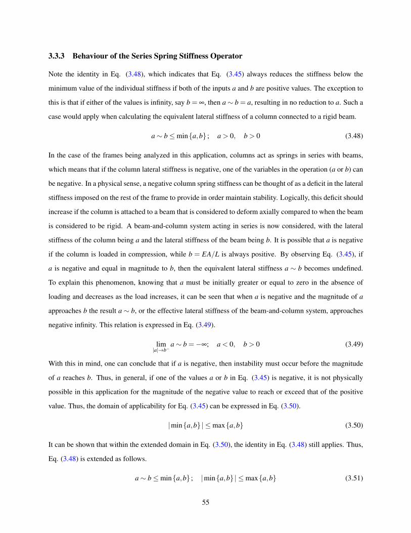
3.3.3 Behaviour of the Series Spring Stiffness Operator

Note the identity in Eq. (3.48), which indicates that Eq. (3.45) always reduces the stiffness below the

minimum value of the individual stiffness if both of the inputs a and b are positive values. The exception to

this is that if either of the values is infinity, say b = ∞, then a∼ b = a, resulting in no reduction to a. Such a

case would apply when calculating the equivalent lateral stiffness of a column connected to a rigid beam.

a∼ b≤mina,b ; a > 0, b > 0 (3.48)

In the case of the frames being analyzed in this application, columns act as springs in series with beams,

which means that if the column lateral stiffness is negative, one of the variables in the operation (a or b) can

be negative. In a physical sense, a negative column spring stiffness can be thought of as a deficit in the lateral

stiffness imposed on the rest of the frame to provide in order maintain stability. Logically, this deficit should

increase if the column is attached to a beam that is considered to deform axially compared to when the beam

is considered to be rigid. A beam-and-column system acting in series is now considered, with the lateral

stiffness of the column being a and the lateral stiffness of the beam being b. It is possible that a is negative

if the column is loaded in compression, while b = EA/L is always positive. By observing Eq. (3.45), if

a is negative and equal in magnitude to b, then the equivalent lateral stiffness a ∼ b becomes undefined.

To explain this phenomenon, knowing that a must be initially greater or equal to zero in the absence of

loading and decreases as the load increases, it can be seen that when a is negative and the magnitude of a

approaches b the result a ∼ b, or the effective lateral stiffness of the beam-and-column system, approaches

negative infinity. This relation is expressed in Eq. (3.49).

lim|a|→b−

a∼ b =−∞; a < 0, b > 0 (3.49)

With this in mind, one can conclude that if a is negative, then instability must occur before the magnitude

of a reaches b. Thus, in general, if one of the values a or b in Eq. (3.45) is negative, it is not physically

possible in this application for the magnitude of the negative value to reach or exceed that of the positive

value. Thus, the domain of applicability for Eq. (3.45) can be expressed in Eq. (3.50).

|mina,b| ≤maxa,b (3.50)

It can be shown that within the extended domain in Eq. (3.50), the identity in Eq. (3.48) still applies. Thus,

Eq. (3.48) is extended as follows.

a∼ b≤mina,b ; |mina,b| ≤maxa,b (3.51)

55

Therefore, for the application of the proposed equivalent spring stiffness operator in Eq. (3.48) towards

storey-based stability, it is demonstrated that the resulting equivalent series stiffness will always be less than

or equal to the minimum of the lateral stiffness terms in the operation. As a corollary, the consideration

of beam axial deformations in a storey frame will always reduce its lateral stiffness compared to when the

beam axial deformations are neglected via assumption of a rigid floor or roof system. Care should be taken

to ensure that the domain in Eq. (3.50) is satisfied whenever the series spring operator in Eq. (3.45) is used.

It is also worth mentioning that the series stiffness operation in Eq. (3.45) is called in Fig. (3.14) the same

number of times as the number of bays in the frame. In other words, adding more bays has the effect of

adding more springs in series. As such, the more bays a frame contains, the more significant the reduction

to the lateral stiffness will become as a result of considering beam axial deformations.

3.3.4 Local Stiffness Reduction Factor

Let ς be defined as the ratio of the axial stiffness of a beam, B, to the lateral stiffness of an immediately

connected column-brace system (S + Kbr) acting in series with B, via Eq. (3.52).

ς = B/(S+Kbr) (3.52)

Then it can be shown via substitution of Eq. (3.52) into Eq. (3.45) that the equivalent stiffness of this local

system is equal to ς/(1+ς) times the stiffness of the adjacent column-brace system. As such, the consider-

ation of beam axial deformations results in a reduction factor of ς/(1+ς) to the lateral stiffness of the local

system. The reduction factor can thus be used to estimate the relative effect of beam axial deformations on

the lateral stiffness of a frame, and is plotted in Fig. (3.15). However, it should be understood that the ac-

tual reduction to the lateral stiffness of the frame involves taking the series equivalent stiffness of B with an

equivalent spring system potentially comprised of many members, not limited to just that of the immediately

connected column-brace system. Nevertheless, it is demonstrated in the following numerical examples that

if ς is significantly high throughout a frame, then the effect of beam axial deformations on the critical loads

of the frame is negligible. However, if for any beam ς is small - say in the order of 101 - then beam axial

deformations will have much a greater effect on the lateral stiffness and should not be neglected. Thus, the

minimum value of ς in the frame can be used as an indicator to predict the significance of the effect of the

beam axial deformations on its lateral stiffness. It is also noted that if the column lateral stiffness becomes

negative (i.e. it relies on the other columns in the frame to maintain stability), then the corresponding value

of ς will become negative since the resulting equivalent lateral stiffness of the beam-column-brace system

will be negative and less than that of the column itself. In such a case, the relative effect of beam axial de-

56

Figure 3.15: Lateral stiffness reduction factor versus beam-to-column-brace stiffness ratio

formations on the lateral stiffness results in a reduction to the equivalent lateral stiffness comparable to that

taken if ς were positive and the same magnitude, as long as |ς | is sufficiently large. Moreover, when finding

the minimum value of ς in a frame, the values of ς for each beam should be evaluated with considering both

columns connected on the left and right ends of the beams.

3.3.5 Numerical Example #1 on the Effect of Lateral Bracing

A numerical example is herein presented to investigate the effect of lateral bracing and beam axial deforma-

tions on a four-bay frame, and provide validation of the results via a finite element model. Some discussion

is also provided with regards to the effect of beam axial deformations (or lack thereof) on the critical load

of a frame governed by the rotational buckling mode. Consider the four-bay frame adapted from Xu (2003)

and shown in Fig. (3.16).

Figure 3.16: Four-bay frame subjected to proportional gravity loading

57

The beam-to-column connections are pinned (zL = zR = 0 for all beams, ru = 0 for all columns), the interior

columns are fixed at the base (rl = 1), and the exterior columns are pinned at the base (rl = 0). The exterior

columns are therefore lean-on and rely on the lateral stiffness provided by the interior columns and lateral

bracing in order to maintain stability and sustain the applied gravity loads. Diagonal bracing of magnitude

Kbr, varying from zero to 10,000 kN/m, is provided at each of the exterior bays and are assumed to be

tension-only. Note that the maximum value of 10,000 kN/m can be provided by a 28 mm diameter steel bar

via Eq. (2.1). As such, if sway occurs in the right direction then Kbr,2 = Kbr,5 = Kbr and Kbr,1 = Kbr,4 = 0.

Conversely, if sway occurs in the left direction then Kbr,1 = Kbr,4 = Kbr and Kbr,2 = Kbr,5 = 0. Although

the critical gravity load will be the minimum of the critical gravity loads obtained in the sway analysis

of both directions separately, the frame and loading are symmetrical so both directions will produce the

same results. The lengths of the members are shown in millimeters on Fig. (3.16). The moments of

inertia and cross-sectional areas of the beams are Ib = 245× 106 mm4 and Ab = 7,610 mm2. For the

exterior columns, Ic,1 = Ic,5 = 129× 106 mm4 and Ac,1 = Ac,5 = 7,610 mm2. For the interior columns,

Ic,2 = Ic,3 = Ic,4 = 34.1×106 mm4 and Ac,2 = Ac,3 = Ac,4 = 4,570 mm2. The slenderness ratios (L/r) of the

interior and exterior members are 39.5 and 56.5, respectively. As such, the columns will buckle inelastically

at high loading levels. To account for this, the tangent modulus method is adopted via Eq. (2.13) at high

loading levels with E0 = 200 GPa and fy,0 = 350 MPa. The critical load, Pcr, corresponding to the instability

of the frame, was obtained with and without considering the effects of beam axial deformations (via the

proposed method of equivalent springs) and shown in Fig. (3.17) for varying amounts of the diagonal

bracing, Kbr. Note that the analysis for this example is independent of the assumed values of vFN since the

beams are simply supported (in Eq. (2.5), vFN is multiplied by zF = 0).

From Fig. (3.17) it can be seen that there is virtually no difference in this example between the critical loads

obtained with and without considering the effects of beam axial deformations. As the amount of lateral

bracing increases, the critical load increases from the unbraced case (Pcr = 277 kN) towards the fully braced

case (Pcr = 624 kN). The value of Pcr = 278 kN corresponding to the unbraced case matches the value

reported in the original example (Xu, 2003). The critical load in the fully braced case corresponds to the

imminent rotational buckling of the interior columns (Pcr ≈ Pu = 624 kN, where Pu is the value of P that

causes rotational buckling to occur in any of the interior columns). A maximum difference between the two

curves of 0.024% occurs at Kbr = 4.54×102 = 454 kN/m, with a reduction to the critical load of only 0.134

kN when beam axial deformations are considered. The reason for the small difference is explained in the

58

Figure 3.17: Critical load of four-bay frame with varying lateral bracing stiffness

following paragraph.

The first-order elastic lateral stiffness is the lateral stiffness of a column in the absence of axial loading

(Pi = 0). For the exterior columns, the first-order lateral stiffness is zero since they are lean-on columns. For

the interior columns, the first-order lateral stiffness is 176 kN/m. However, B = EA/L = 2.35×105 kN/m

for all beams, which is ς = 1,335 times the stiffness of the interior columns in the absence of bracing and

loading via Eq. (3.52), and ς = ∞ times the stiffness of the exterior columns in the absence of bracing

and loading. Although ς will change as loading of the columns begins to occur, using the value of ς with

considering just the first-order lateral stiffness will provide a conservative prediction of the relative effect of

beam axial deformations on the critical load. This is because ς generally increases as the values of lateral

stiffness in the columns are decreased with gravity loading. As such, even the minimum value of the local

stiffness reduction factor, ς/(1+ς), achieved using ς = 1,335, is very close to unity (0.9993). As such, the

reduction of the lateral stiffness of the frame when accounting for beam axial deformations will be negligible

in the absence of bracing. In fact, the difference in critical loads is only 0.014 kN (0.005%) for Kbr = 0.

Now, as the lateral stiffness of the bracing is increased, the value of ς in Eq. (3.52) will be reduced, and it

would follow that the effect of beam axial deformations increases as Kbr increases. However, as the lateral

bracing increases past 500 kN/m in Fig. (3.17), the critical load asymptotically approaches the rotational

buckling load, Pu = 624 kN corresponding to braced frames. The imminent rotational buckling of the interior

columns thus governs the failure of the frame for high values of Kbr and for design purposes the frame can

59

be treated as being fully braced. The rotational buckling loads of the columns are not functions of the

axial stiffness of the connecting beams. As such, the difference between the critical load with and without

considering beam axial deformations becomes less significant as the critical loads approach the rotational

buckling load (for Kbr > 454 kN/m). Thus, even at Kbr = 10,000 kN/m, despite a resulting low minimum

value of ς = 23 occurring in the frame, the difference in critical loads with and without considering the

effects of beam axial deformations is negligible due to the imminence of rotational buckling occurring at the

critical load. Note, however, that with ς = 23, the lateral stiffness of the frame will be significantly reduced

for loads below the rotational buckling load. For instance, the first-order lateral stiffness of the entire frame

with Kbr = 10,000 kN/m is 20,530 kN/m with neglecting beam axial deformations, but is reduced to 17,880

kN/m when beam axial deformations are considered (a 13% decrease). Regardless, the maximum difference

of 0.024% between critical loads with and without consideration of beam axial deformations thus occurs at

an intermediate value of Kbr = 454 kN/m whereby the value of ς is relatively low and the rotational buckling

is not imminent (Pcr = 543 kN Pu). Note that this intermediate value of bracing stiffness corresponds

to the semi-braced case for the frame, since the critical gravity loads are well within the limiting values

corresponding to the unbraced and fully braced cases. The lateral stiffness of 454 kN/m is comparable to

that which would be provided by 6 mm diameter steel tension cables at each of the locations shown in Fig.

(3.16). In such a case, the total first-order elastic lateral stiffness of the frame is 1,437 kN/m, which is 2.72

times the stiffness of the frame without diagonal bracing (529 kN/m). As a comparison, the CSA (2014)

standard suggests that a frame be considered fully braced only when its total lateral stiffness is at least five

times greater than its own stiffness without lateral bracing, corresponding to Kbr ≥ 1,058 kN/m for this

example. For this reason, the frame is a semi-braced frame.

Finally, a finite element analysis was conducted via ABAQUS (Simulia, 2012) to verify the theoretical

accuracy of the critical loads of the frame obtained via the proposed method for the cases with Kbr =

0.0 N/m (unbraced), Kbr = 454 kN/m (semi-braced), and Kbr = 10,000 kN/m (fully braced). Note that

Kbr = 454 kN/m corresponds to the maximum difference of 0.024% between the critical loads obtained

with and without considering beam axial deformations. Cubic Euler-Bernoulli beam elements (B23), which

neglect shear deformations, were used in all members. To simulate the effect of neglecting the beam axial

deformations, the linking interaction constraint was toggled on to constrain the ends of the columns to

deflect horizontally by the same distance. To realize the effect of the beam axial deformations, the linking

constraint was toggled off. The diagonal braces were modelled via Cartesian spring connectors-to-ground.

The Cartesian springs provide user-specified values of lateral stiffness against the horizontal translation of

60

the respective nodes. The members were joined via "Join + Rotation" connector sections, which were set to

have free rotation and joined translation. Since the buckling analysis is ABAQUS requires linear material

behaviour, the elastic moduli of the members in the model were calculated using Eq. (2.13) and manually

updated in ABAQUS as necessary. Furthermore, the effect of column axial shortening (different from beam

axial shortening) was neglected by manually changing the cross-sectional areas of the columns to high values

while manually specifying the transverse stiffness κAG for the calculations as applicable. In terms of the

validation of the FEA model itself, a verification package has been provided by ABAQUS (Simulia, 2014)

whereby the elements used in the current study have been verified against a variety of validation examples.

Additionally, the use of the finite element analysis procedure in ABAQUS (Xu and Zhuang, 2014) or other

similar finite element software (Georgios and Gantes, 2006; Li et al., 2016) has commonly been adopted for

the purposes of validation in previous storey-based stability methods. The sway buckling load of the frame

obtained from FEA analysis was found to be exact to the results of the example. The results of the critical

loads, Pcr, are shown in Table 3.1, obtained using the Xu and Liu (2002b) storey-based stability method

with neglecting the beam axial deformations, the proposed storey-based stability method with considering

the beam axial deformations, and FEA with and without toggling the linking constraint.

Table 3.1: Validation of critical loads, Pcr (kN), obtained from proposed method using FEA for four-bayframe

Calculation method Xu and Liu(2002b)

FEAProposedMethod

FEA

Considers beam axial deformations? No No Yes Yes

Kbr = 0.0 kN/m 277.317 277.317 277.303 277.303Kbr = 454 kN/m 564.507 564.506 564.372 564.372Kbr = 10,000 kN/m 623.427 623.428 623.422 623.423

As seen from Table 3.1, the differences between the results of the critical loads obtained between the storey-

based stability methods and FEA are at most 0.001 kN (0.004%). Therefore, the proposed method is shown

to be virtually exact to the theoretical governing Euler-Bernoulli equation. The buckling shapes of the frame

obtained from the FEA model for each case are also shown in Figs. (3.18) through (3.20).

Figure 3.18: Buckled shape of four-bay frame with Kbr = 0 kN/m (unbraced)

It is clear from observing Figs. (3.18) through (3.20) that the lateral sway mode governs the buckling for the

61

Figure 3.19: Buckled shape of four-bay frame with Kbr = 454 kN/m (semi-braced)

Figure 3.20: Buckled shape of four-bay frame with Kbr = 10,000 kN/m (fully braced)

first two cases (Kbr ≤ 454 kN/m), indicated by the large lateral deflections of the columns in the buckling

shapes. For Kbr = 10,000 kN/m, Fig. (3.20) confirms that the simultaneous rotational buckling of the interior

columns is imminent during the critical load of Pcr = 623.4 kN ≈ Pu = 624 kN. This is apparent by noting

that the lateral deflections of the upper ends of the columns are small compared to mid-height deflections of

the interior columns. In general, as the amount of lateral bracing increases, the curvature experienced by the

individual columns relative to the magnitude of lateral sway in the buckling shape increases.

3.3.6 Numerical Example #2 on the Effect of Lateral Bracing

Thus far, the previous example in Section 3.3.5 demonstrates negligible effects of axial deformations on

the critical gravity loads. It will also be demonstrated in an example shown in Section 3.4.2 that in an

extreme case, the effect of axial deformations can reduce the critical gravity loads of a lean-on frame by up

to 64.5%. The purpose of this example is to highlight a case where the critical gravity loads are shown to

be moderately affected by axial deformations. The frame in this example consists of a single storey with

semi-rigid connections (unlike the aforementioned examples), and is subjected to proportional loading. The

first four bays of the frame are shown in Fig. (3.21), but the frame is symmetrical and contains a total of

eleven bays (11 beams and 12 columns). All of the interior bays are identical except for the two containing

diagonal bracing shown. The exterior bays are fixed at the base (rl = 1), while the interior bays are pinned

at the base (rl = 0).

The planar frame is located in a rectangular plan frame and the direction of analysis is such that the columns

buckle about their weak axis (for W310×122, I = 61.5×106 mm4 and A = 15500 mm2; for W250×39,

I = 5.94×106 mm4 and A = 4920 mm2). Note that the proposed method can simply be repeated for the

other direction, corresponding to strong axis buckling related to the opposite plan dimension. The column

slenderness ratios are 73 and 132 for the exterior and interior columns, respectively. The roof rafters are

lightweight steel trusses (LWT) with moment of inertia I = 257×106 mm4 and total top-and-bottom chord

62

Figure 3.21: Eleven-bay frame subjected to proportional gravity loading

cross-sectional area A = 4360 mm2. The truss-to-column connections are all semi-rigid with zN = zF = 0.25.

The values of the elastic modulus for the members are calculated via the tangent modulus assumption in Eq.

(2.13). The end connection rotation ratios are assumed to be vFN = 1 in correspondence to the asymmetrical

buckling assumption recommended in Xu and Liu (2002a). The lateral stiffness provided by the tension-

only diagonal bracing, Kbr, was once again varied from zero to 10,000 kN/m (which can be provided by a 33

mm diameter bar). The critical loads, Pcr, of the planar frame computed via the proposed method are plotted

with those obtained with neglecting the effects of axial deformations via the Xu and Liu (2002b) method in

Fig. (3.22).

Figure 3.22: Critical gravity loads of the eleven-bay frame with varying lateral bracing stiffness

Unlike the plot for the previous example shown in Fig. (3.17), there is a noticeable difference in the results

of the critical gravity loads when axial deformations are considered. To show the difference more clearly,

63

Fig. (3.23) plots the percentage difference between the two curves from Fig. (3.22).

Figure 3.23: Reductions of critical gravity loads for the eleven-bay frame with varying bracing stiffness

As seen in Fig. (3.23), the percentage reduction to the critical load due to beam axial deformations is up to

1.29% in this example. Of course, the effect of beam axial deformations on the critical gravity loads can

be increased by various means, such as by adding to the number of bays in the frame or further reducing

the cross-sectional areas of the LWT. As with the previous example, the effect of axial truss deformations

becomes negligible as the frame approaches the fully braced condition because rotational buckling is not

related to axial beam deformations. Note that based on Fig. (3.22), the frame can be considered in this case

to be semi-braced when Kbr is between 102 and 103 kN/m. Below this range, the critical load approaches

the unbraced case (Pcr = 264.2 kN with considering beam axial deformations; Pcr = 267.7 kN with neglect-

ing beam axial deformations). Above this range, the critical load approaches the rotational buckling case

corresponding to a fully braced frame (Pcr = 442 kN).

As with the previous examples, a finite element model of the eleven-bay frame was constructed to verify

the theoretical accuracy of the proposed method and derived equations. A model similar to that established

in the previous example (Section 3.3.5) but with eleven bays and semi-rigid connections via the "Join +

Rotation" constraint was established in ABAQUS. This time, the rotational stiffness of the beam-to-column

joints was specified in the "Join + Rotation" constraint based on the end fixity factors. The data points on

Fig. (3.22) corresponding to three different values of Kbr were verified: (a) the unbraced case, Kbr = 0

kN/m, (b) the semi-braced case, Kbr = 220 kN/m corresponding to diagonal steel tension cable braces with

3/16" diameter, and (c) the fully braced case, Kbr = 10,000 kN/m. In this example, the values of the end

rotational stiffness of the columns Ru,i and Rl,i in Eq. (1) are dependent on the assumed values of vFN via

Eq. (2). As such, the verification was completed by first comparing the results of Fig. (3.22), obtained via

64

assuming vFN = 1, with the critical gravity loads obtained in FEA. In all cases, as predicted in Xu and Liu

(2002a), the errors to the critical gravity loads obtained via assumption of vFN = 1 the proposed method

were not significant. Following this comparison, the buckling shapes of the frames obtained via the FEA

solutions of critical gravity loads were obtained, and the joint rotations at the upper ends of each column

were recorded. Based on these joint rotations, calibrated values of vFN corresponding to the buckling shape

and critical gravity loads were obtained by dividing the far end rotations by the near end rotations for each

beam. The calibrated values of vFN were then re-substituted back to the proposed equations, with which the

critical gravity loads were re-calculated and compared with the FEA solution. The results of this analysis

are summarized in Table 3.2.

Table 3.2: Validation of critical loads, Pcr (kN), obtained from proposed method using FEA for eleven-bayframe

No axial deformations considered Axial deformations considered

Diag. bracing stiffness FEAXu and Liu

(2002a)(vFN=1)

Xu and Liu(2002a)

(vFN calib.)FEA

ProposedMethod(vFN=1)

ProposedMethod

(vFN calib.)

Kbr = 0.0 kN/m 260.764 267.642 260.745 257.545 264.179 257.528Kbr = 220 kN/m 319.192 325.178 319.175 315.858 321.668 315.842Kbr = 10,000 kN/m 439.768 441.358 439.760 439.568 440.959 439.639Column reference 1 2 3 4 5 6

When comparing the uncalibrated results (vFN = 1) with the corresponding FEA results in Table 3.2 (between

columns 1 and 2, and between columns 4 and 5), the maximum error is within 3%, which is expected given

that the assumption of vFN = 1 does not correspond to the actual buckling shape of the frame. When

comparing the calibrated results in Table 3.2 with the corresponding FEA results (between columns 1 and

3, and between columns 4 and 6), the error is within 0.02%, indicating that the proposed equations are

accurate to the theoretical solutions. In terms of the effect of beam axial deformations on the critical gravity

loads of the frame, the corresponding reductions to the critical gravity loads obtained in FEA (comparing

columns 1 and 4) are 1.23%, 1.04%, and 0.03% for the unbraced, semi-braced and fully braced cases,

respectively. These values are considerably accurate to those shown in Fig. (3.23). For the unbraced case,

during the failure at 257.5 kN with considering axial deformations, the minimum value of ς in the frame

is 108. Similarly, during the failure at 315.8 kN for the semi-braced case, the minimum value of ς in the

frame is 111. Based on Fig. (3.15), these values can be correctly used to predict that the effect of axial

deformations has approximately 1% influence on the critical gravity loads in the unbraced and semi-braced

65

cases. However, for the fully-braced case, axial deformations do not significantly affect the critical gravity

loads because rotational buckling is imminent, regardless of the values of ς . Finally, the buckling shapes

obtained from the finite element analyses for the unbraced, semi-braced, and fully braced cases are shown

in Figs. (3.24), (3.25) and (3.26), respectively.

Figure 3.24: Buckled shape of eleven-bay frame with Kbr = 0 kN/m (unbraced)

Figure 3.25: Buckled shape of eleven-bay frame with Kbr = 220 kN/m (semi-braced)

Figure 3.26: Buckled shape of eleven-bay frame with Kbr = 10,000 kN/m (fully braced)

The buckling shapes are extracted directly from the output of ABAQUS. The bracing bays are located on

the second and tenth bays, but are not shown in the figures. Similar to the previous example in Section

3.3.5, the lateral sway mode is experienced by the frame in the unbraced and semi-braced cases, whereas

the rotational buckling of the individual columns governs in the fully braced case. Note that the relative

magnitudes of column curvature corresponding to the semi-braced case are greater than those observed in

the unbraced case. Finally, it is noted that if the values of the end connection fixity factors were increased

to zF = zN = 0.75, the effect of axial beam deformations would account for up to a 1.64% difference to the

critical load, experienced during the unbraced case (Kbr = 0) and obtained using the assumption of vFN = 1

under the proposed method. The critical loads obtained with and without considering the axial deformations

would be 352.5 kN and 358.4 kN, respectively.

3.4 Lean-On Frame Example

The analysis of a generalized lean-on frame system to highlight the potential effects of both shear and beam

axial deformations on storey-based stability analysis is exemplified in this section. Consider the n-bay frame

in Fig. (3.27).

All connections are pinned, except for the base connection of Column n+ 1 (rl,n+1 = 1). As such, the

flexural stiffness of the beams have no effect on lateral stiffness of the columns. This supporting column

provides lateral support for all of the other lean-on columns in the frame, which are loaded with applied

gravity loads Pi. The height of the storey is H. No additional lateral bracing exists, but if considered, then

66

Figure 3.27: Generalized lean-on frame consisting of n bays

the corresponding stiffness can simply be added to the lateral stiffness of the supporting column. It can be

shown that for lean-on columns (ru = rl = 0), the lateral stiffness equation in Eq. (3.10) simplifies to Eq.

(3.53).

Si =−Pi/H; i ∈ 1,2, ...,n (3.53)

where Pi is the applied gravity load (positive in compression). Note that Si is independent of shear de-

formations. Even in the absence of gravity loading (Pi = 0), a lean-on column has no contribution to the

storey-based lateral stiffness (Si = 0). When a lean-on column is axially loaded, it relies on the supporting

columns of a frame to maintain stability (Si < 0). As such, no matter the lateral stiffness of the supporting

column, the lateral stiffness of the frame can be diminished to zero via supporting a series of loaded lean-on

columns, as long as the gravity loads in each lean-on column do not exceed their respective rotational buck-

ling loads (Pi < Nu,i). Otherwise, local instability via rotational buckling will occur. Note that the purpose

of this example is to demonstrate the full potential of the shear and beam axial deformations to reduce the

critical gravity loads when compared with ignoring them. It is presented as simply as possible in order

to maintain clarity and to show that the shear and beam axial deformations are solely responsible for the

reductions to the critical loads observed in each case. It may not be a realistic representation of frames in

practice.

67

3.4.1 Parametric Study - Effect of Shear Deformations

In order to assess the influence of the slenderness ratio, L/r, on the effect of shear deformations on the critical

loads, the slenderness ratio of the supporting column is varied in this study from 5 to 100 by changing its

length, H. A W460×97 section (I = 445×106 mm4, A= 12,300 mm2) is chosen for the supporting column.

Assume that the yield stress of steel is 350 MPa and the elastic modulus of steel is 200 GPa. The tangent

modulus model in Eq. (2.13) is employed to account for the effects of partial yielding in the presence of high

axial loads. With neglecting the effect of beam axial deformations, the storey-based instability condition of

the frame in Fig. (3.27) can be expressed by setting the storey-based lateral stiffness in Eq. (3.20) to zero,

resulting in Eq. (3.54).

Sn+1 =n

∑i=1

Pi

H; Pi < Nu,i =

π2EiIi

L2i

i ∈ 1,2, ...,n (3.54)

where Sn+1 is the lateral stiffness of the supporting column. Assuming that none of the lean-on columns

rotationally buckle, the critical total load applied on the lean-on column system, Pcr, is defined via Eq.

(3.55).

Pcr =n

∑i=1

Pi = HSn+1 (3.55)

Therefore, the critical total load of the frame is proportional to the lateral stiffness of the supporting column.

In other words, a percentage reduction to the lateral stiffness of the supporting column will result in the

same percentage reduction to the critical total load. Define Psw as the sway buckling load of the supporting

column, which is the value of Pn+1 that diminishes the lateral stiffness of the supporting column to zero

(Sn+1 = 0) calculated with considering shear deformations. If Pn+1 = Psw then Pcr = 0 since the lean-on

columns provide no contribution to the lateral stiffness even in the absence of loading. In this study, Pn+1

is varied between zero (unloaded) and Psw (fully loaded) to assess the effect of increasing axial loads in the

supporting column on Pcr. The lateral stiffness of the supporting column, Sn+1, was calculated with and

without considering the effects of shear deformations. At first, where the effects of shear deformations were

considered, both the Haringx (1948) and Engesser (1891) assumptions were compared via Eqs. (3.8b) and

(3.8a), respectively. However, it was found that the difference in Psw obtained between both assumptions

was below 0.06% for L/r = 5, and decreases for higher slenderness ratios, as shown in Fig. (3.28).

Similar to the conclusion of the finite element validation in Section 3.2.9, it was concluded that the use of

either assumption produces virtually identical results. As such, only the results via using the Haringx (1948)

assumption via Eq. (3.8b) are reported where shear deformations are considered. A value of κ = 0.44 for

68

Figure 3.28: Difference in Psw from using the Haringx (1948) and Engesser (1891) assumptions

wide flange sections (Cowper, 1966) is assumed. The reduction in lateral stiffness of the supporting column

due to considering shear deformations is plotted for varying slenderness ratios and load levels in Fig. (3.29).

Figure 3.29: Effect of shear deformations on Sn+1 with varying L/r and loading levels

From Fig. (3.29), it can be seen that the magnitude of the reduction in lateral stiffness due to accounting

for shear deformation increases exponentially as the slenderness ratio decreases for low slenderness ratios.

If the supporting column is unloaded (Pn+1 = 0), then the difference can be as high as 1,000 kN/m for a

slenderness ratio of 15, but is reduced below 1.0 kN/m for a slenderness ratio of 60. Above the L/r = 60,

the lateral stiffness is reduced by a negligible amount (below 1.0 kN/m). Note that for the unloaded column

69

with L/r = 15, the value of Sn+1 is 11,496 kN/m without considering shear deformations, and corresponds

to a 7% decrease to the lateral stiffness when considering shear deformations (reduced to 10,657 kN/m).

Similarly, for a slenderness ratio of 60, the value of Sn+1 is 179.6 kN/m with neglecting shear deformations,

corresponding to only a 0.5% decrease in the lateral stiffness with considering shear deformations (reduced

to 178.8 kN/m). The effect of increasing the axial load Pn+1 on the supporting column significantly decreases

the magnitude of the reduction of lateral stiffness due to shear deformations at low slenderness ratios (-93%

for L/r = 15). However, note that as the magnitude of Pn+1 increases, the critical total load Pcr will also

be reduced. The percentage reduction to the critical load of the frame, Pcr, as a result of considering shear

deformations compared to when neglecting them, is plotted in Fig. (3.30) for varying slenderness ratios

and supporting column load levels. To be clear, a zero percent reduction corresponds to no change in the

calculated critical load between considering and neglecting the shear deformations via the Haringx (1948)

assumption, whereas a 100% reduction corresponds to a zero lateral stiffness when shear deformations are

considered and an arbitrarily positive lateral stiffness when shear deformations are neglected.

Figure 3.30: Effect of shear deformations on Pcr with varying KL/r and loading levels

In the absence of loading (Pn+1 = 0), the reduction of Pcr due to shear deformation can be significant for

low slenderness ratios (-41% for L/r = 5). For slenderness ratios below 20, the reduction is at least 4.2%,

and for slenderness ratios above 40 the reduction is at least 1%. As such, if a 1% reduction to the critical

load is considered to be significant, it is recommended that shear deformations be considered for this frame

70

if the supporting column has a slenderness ratio below 40. By comparison, the threshold of significance

with regards material reliability coefficients in standards is generally on the order of 0.05, or 5% (CSA,

2014). However, the consideration for shear deformations always results in equal or lesser values of the

lateral stiffness and critical loads in structural members compared to when they are neglected. As such,

the threshold of significance for an error which is never conservative should typically be more stringent. A

threshold of 1% has been adopted simply as a benchmark for the current study. Note that as Pn+1 increases,

the percentage reduction of Pcr due to shear deformation decreases slightly but increases to 100% at Pn+1 =

Psw for every curve. This is because at Pn+1 = Psw, the lateral stiffness of the supporting column is zero

when considering shear deformations, so Pcr = 0. However, if shear deformations are neglected then Pcr

will still be a positive value. It is not recommended in lean-on systems to load supporting columns near

their sway capacities as that could result in the complete collapse of the frame. Based on the results of this

analysis, shear deformations can have a significant influence on the critical sway loads in frames containing

columns with low slenderness ratios. For this example, the effect of shear deformation on the critical load

is significant (above 1%) when the slenderness ratio of the supporting column is below 40, provided that

rotational buckling does not occur elsewhere in the lean-on system. It is also shown that the lateral stiffness

of a supporting column with slenderness ratio of 15 can be reduced by as much as 1,000 kN/m. Furthermore,

if the supporting column is loaded near its sway load, ignoring the shear deformations can be dangerous as

the calculations can show positive values of the lateral stiffness much higher than in reality.

3.4.2 Parametric Study - Effect of Axial Deformations

The effect of varying the number of bays and the beam axial stiffness in the lean-on frame was also investi-

gated. As increasing the number of bays would increase the number of times the series stiffness operation

is called in computing the effective spring stiffness approach, it is anticipated that the lateral stiffness of the

frame will decrease when considering the effects of beam axial deformations. For the purpose of this sec-

tion, all of the columns are assumed to have the same cross-section properties (W760×582, I = 8,600×106

mm4, A = 74,300 mm2), and all of the beams have the same cross-sectional properties which will be varied.

The height of the storey is H = 7.315 m, and the length of each beam is also 7.315 m. Similar to the previous

section, the lean-on columns are each subjected to an axial load Pi, and the frame critical load, Pcr, is defined

as the total gravity load in the frame during which the lateral stiffness of the frame diminishes to zero. As

such, the lateral stiffness of each lean-on column is given in Eq. (3.53) and the critical total load, Pcr, is

given in Eq. (3.55). The lean-on columns are individually stable as long as Pi < Nu,i = 21,519 kN, obtained

71

via Eq. (2.10) with K = 1, being supported by the cantilever, but will rotationally buckle if Nu is reached.

The supporting column is not loaded (Pn+1 = 0) and provides lateral support with Sn+1 = 13,213 kN/m. As

its slenderness ratio is L/r = 21.5, shear deformations would be expected to affect the results. However, to

isolate the effect of axial beam deformations, the effects of shear deformations are now neglected. As such,

Pcr = HSn+1 = 96,700 kN via Eq. (3.55), which is independent of the number of bays and assumes that none

of the axial loads in the lean-on columns exceed the rotational buckling load (only possible for n ≥ 5, and

rotational buckling governs the failure for n < 5). In this study, the number of bays was varied from n = 5 to

15, and the critical total load with accounting for beam axial deformations via the equivalent spring stiffness

approach was calculated for each case. The sizes of the beams were also varied using the sizes W100×19,

W410×67, W610×174, W840×392 and W920×784. These beam sizes correspond to cross-sectional areas

of 1,630 mm2, 8,600 mm2, 22,200 mm2, 50,000 mm2 and 99,800 mm2, respectively. Note that the critical

total load is independent of the moment of inertia and corresponding flexural deformations in the beams

since the beam-to-column connections are all pinned. The reduction in the critical total load as a percentage

below 96,700 kN, the value without considering beam axial deformations, for each scenario is plotted in

Fig. (3.31).

Figure 3.31: Effect of beam axial deformations on Pcr with varying beam size and number of bays

Based on Fig. (3.31), the percentage reduction to the critical total load increases as more bays with lean-on

columns are added to the frame. Note that a zero percent reduction corresponds to Pcr = 96,700 kN, while a

72

100% reduction corresponds to Pcr = 0 as a result of considering beam axial deformations. A decrease to the

beam area, and consequently the beam axial lateral stiffness, also results in a reduction to Pcr. In each case,

the ς values of the supporting column with respect to the nth beam are 3.4, 17.8, 45.9, 103.5 and 206.5 in

increasing order of beam area. The ς values of the lean-on columns vary and are negative when loaded, but

do not govern as the minimum ς values in the frame when considered based on their absolute values. Notice

that in the case of ς = 206.5 the reduction varies from only 1.1% to 2.6% depending on the number of bays.

In contrast, for the case of ς = 3.4 the reduction varies from 40.6% to 64.5%. Based on the example, the

ς factor has the greatest influence on the critical total load, and the number of bays has a lesser but still

significant influence. Finally, similar to the previous example in Section 3.3.5 a finite element model was

constructed using B23 elements to verify the critical load for the data point corresponding to n = 5 and A =

1,630 mm2 corresponding to W100×19 beams. The corresponding critical load obtained in FEA was 57,447

kN whereas the critical load obtained from the proposed method was 54,445 kN (a 0.004% difference). Both

of these values correspond to the 40.6% reduction to the critical load as a result of considering the beam

axial deformations shown in Fig. (3.31).

3.5 Variable Loading

To generalize the variable loading approach of Xu (2001) to account for both shear and beam axial deforma-

tions, a generalized minimization problem for determining the worst and best case distributions of applied

gravity loads resulting in the instability of a semi-braced frame is formulated in Eq. (3.56).

Minimize or Maximize:n+1

∑i=1

Pi (3.56a)

subject to:

Seq = 0 (3.56b)

Pl,i ≤ Pi < Nu,i ∀i ∈ 1,2, ...,n+1 (3.56c)

where Seq is the lateral stiffness of the storey obtained using the equivalent spring stiffness algorithm shown

in Fig. (3.14), with the column lateral stiffness Si calculated using Eq. (3.10) to account for shear defor-

mations. Also, Nu,i is calculated via the procedures discussed in Section 3.2.4. Of course, the problem

converges to Eqs. (2.20) if both shear and beam axial deformations are neglected. As with previously,

the problem can be solved using mathematical programming methods such as the GRG Nonlinear method

(Lasdon et al., 1973) used in combination with Multi-Start (György and Kocsis, 2011).

73

3.5.1 Numerical Example for Variable Loading

The results of the variable loading minimization problem in Eqs. (3.56) are herein compared for a four-bay

frame example with and without considering the effects of shear and axial deformations. The frame shown

in Fig. (3.32) is subjected to variable gravity loads, P1 through P5, with subscripts indicating the numbering

of the columns.

Figure 3.32: Four-bay frame subjected to variable gravity loading

All of the connections are semi-rigid, with rl = 0.2 for all columns and zN = zF = 0.8 for all beams, ap-

plicable when E = E0 = 200 GPa for all members. Note that the column end fixity factors will change as

the tangent modulus equation in Eq. (2.13) will be used to adjust E. For the columns, Ic,1 = 177× 106

mm4, Ic,2 = Ic,4 = Ic,5 = 145× 106 mm4, and Ic,3 = 198× 106 mm4. For all beams, Ib = 411× 106 mm4.

The areas of the columns are required when considering shear deformations, given as Ac,1 = 10,100 mm2,

Ac,2 = Ac,4 = Ac,5 = 8,450 mm2 and Ac,3 = 11,000 mm2. The lengths of the beams in order from left to right

are 6.096 m, 7.620 m, 4.572 m and 6.096 m. The slenderness ratios of the columns (L/r) range from 34

to 35, indicating that the columns are within the inelastic range of slenderness. Once again, κ = 0.44 for

wide-flange sections (Cowper, 1966). The yield stress is assumed to be 350 MPa and Poisson’s ratio is taken

as 0.3 for all members. The asymmetrical buckling mode is assumed (vFN = 1 for all beams) in accordance

with the recommendation of Xu (2001). The rotational buckling loads for each column in the frame were

calculated using Eqs. (3.15) and are shown in Table 3.3.

Table 3.3: Rotational buckling loads of columns in numerical example

Rotational buckling load (kN) Nu,1 Nu,2 Nu,3 Nu,4 Nu,5

Without shear deformations 2,948 2,466 3,213 2,466 2,466With shear deformations 2,942 2,461 3,206 2,461 2,461

Based on Table 3.3, the rotational buckling loads of the columns differ by less than 0.25% between neglect-

74

ing and considering shear deformations. The reason for such a small difference is that when N = Nu, the

tangent modulus reduction factor in Eq. (2.13) is low (τE ≈ 0.05 for each column), reducing the value of

η significantly and thus reducing the influence of shear deformations on the rotational buckling load. In

contrast, the first-order elastic lateral stiffness of the frame and its individual columns are shown in Table

3.4 with and without considering shear deformations. The values correspond to the values of lateral stiffness

in the absense of gravity loading (N = 0).

Table 3.4: First-order lateral stiffness of columns in numerical example

First-order lateral stiffness (kN/m) Col. 1 Col. 2 Col. 3 Col. 4 Col. 5 TotalWithout shear deformations 1,196 1,143 1,528 1,182 1,027 666,,,000777777With shear deformations 1,161 1,115 1,483 1,150 998.9 555,,,999000888

The values in Table 3.4 correspond to a reduction of 2.8% to the total lateral stiffness of the frame resulting

from the consideration of shear deformations. Note that the results throughout this example obtained with

considering shear deformations were once again virtually identical using either of the Engesser (1891) or

Haringx (1948) assumptions. Only the results obtained using the Engesser (1891) assumption are thus

reported. Additionally, the difference in the obtained values of connected member rotational stiffness, R′,

from Eq. (3.29) with and without neglecting the effects of shear deformations are tabulated in Table 3.5

for each beam along with its slenderness. R′s is the rotational stiffness provided at both ends of the beam to

the adjoining column with considering shear deformations, whereas R′n is the same quantity with neglecting

shear deformations.

Table 3.5: Effect of shear deformations on the rotational stiffness of beams in four-bay example

Beam 1 2 3 4

L/r 29 37 22 29R′s/R′n 0.95 0.97 0.91 0.95

As seen in Table 3.5, the reduction to the effective rotational stiffness due to shear deformations becomes

more significant as the slenderness ratios of the beams decrease.

3.5.2 Worst Case Variable Loading

The worst case loading scenario is obtained by minimizing the objective function in Eq. (3.56a). From a

design perspective, the results of the minimization problem can be used to identify the weakest columns

of a frame, which can be fortified to increase the worst case loading capacity. The results for the worst

75

case loading analyses for the numerical example are shown in Table 3.6. The column lateral stiffness, Si, is

calculated using Eq. (3.10), with substituting η = 0 for the cases where shear deformations are neglected.

Where axial deformations are considered, the equivalent spring stiffness method in Fig. (3.14) is used to

calculate Seq. Otherwise, ΣS in Eq. (2.20b) is taken as Seq.

Table 3.6: Worst case scenario of gravity loading for four-bay frame example

Applied gravity loads (kN) P1 P2 P3 P4 P5 Total

Neglecting shear and axial deformations 0 0 0 0 2,466∗ 222,,,444666666Considering axial deformations only 0 0 0 0 2,466∗ 222,,,444666666Considering shear deformations only 0 0 0 0 2,461∗ 222,,,444666111Considering shear and axial deformations 0 0 0 0 2,461∗ 222,,,444666111

* Denotes a column on the verge of rotational buckling, loaded just slightlybelow the rotational buckling load

Rotational buckling of Column 5 is imminent and governs the worst case scenario for this example, regard-

less of whether shear deformations are considered. Moreover since the rotational buckling loads are not

functions of the axial stiffness of beams in the frame, the effects of beam axial deformations on the mini-

mum solution are virtually non-existent. Note that Column 5 has a marginally lower rotational buckling load

than those of Columns 2 and 4 due to the varying lengths of the connecting beams, and as such, governs the

minimum solution. In fact, contrary to what is suggested in Xu (2001), it can be shown that the minimum

solution to Eqs. (2.20) and (3.56) always consists of loading in only one column. The reason for this is that

as Pi approaches Nu,i, the lateral stiffness of a column generally decreases asymptotically towards negative

infinity, as shown in Fig. (2.2). Thus, instability of the frame will occur as the lateral stiffness of the frame,

which will be less than or equal to the sum of the column lateral stiffness, diminishes to zero for some value

of Pi < Nu,i. An exception to this behaviour occurs when ru = rl , whereby instability occurs in the form of a

removable discontinuity in the lateral stiffness equation at Pi = Nu,i. Based on this rationale, the solution to

the minimization problems in Eqs. (2.20) and (3.56) must satisfy Eq. (3.57).

n+1

∑i=1

Pi ≤ mini∈[1,n+1]

Nu,i (3.57)

In many cases, such as in this example, the minimum case will consist of a single column being loaded until

Pi = Nu,i− ε , where ε is a very small value. However, in reality such an instability may take the form of

a local failure at the location of the column which is loaded near its rotational buckling load, rather than

failure of the entire storey. If load redistribution measures are in place, a progressive collapse analysis can

be conducted to determine if the rest of the frame can maintain stability after the buckling column is deleted

76

from the analysis and its load is redistributed to other columns. Such an analysis would be out of the scope

of this study and is elaborated on in the recommendations of Section 9.3.1. Regardless of whether or not

the failure occurring when a column approaches its rotational buckling load is local or global, an instability

will occur to some degree, and can be detected via the minimization problem.

To assess whether or not shear deformations will influence the minimum case loading solution when ro-

tational buckling is not imminent, the slenderness ratios of the columns in the frame were increased until

rotational buckling was no longer imminent in the minimum solution result (i.e. Pi ≤ 0.95Nu,i for all i during

sway instability). It was found that a length of Lc = 16.2 m for all the columns was required in order for

Pi = 0.95Nu,i to occur, corresponding to slenderness ratios of the columns between 121 to 124. Since the

lengths of the columns were changed proportionally, Column 5 remained the weakest and only column to

be loaded in the minimum case solution (P1 = P2 = P3 = P4 = 0). The rotational buckling load of Column

5 was Nu,5 = 1,718 kN and 1,725 kN with and without considering shear deformations, respectively. In

the minimum solution, instability occurred when P5 = 1,637 kN with neglecting both shear and beam axial

deformations. When considering shear deformations only, the minimum case was P5 = 1,630 kN, corre-

sponding to only a 0.43% decrease in the total load. As demonstrated previously, if the slenderness ratio

is further increased (in this case, to around 120), the effect of shear deformations on the result will only

diminish. As such, it is shown that for this example the minimum case solution is not significantly affected

by shear deformations since either rotational buckling will govern the minimum solution or the columns

will be too slender for shear deformations to significantly affect the results. Moreover, when beam axial de-

formations were included in the re-analysis with modified column lengths, the critical loads from both with

and without considering shear deformations (value of P5 in the minimum solution) were further decreased

by only 0.2 kN, indicating that axial deformations in the beams once again were virtually negligible. How-

ever, this occurred for a reason different from before, which was the imminence of rotational buckling. This

time, as the slenderness of the columns was increased, the overall magnitudes of the lateral stiffness in the

columns decreased, while the axial stiffness of the beams remained very high. In other words, the beams

became relatively rigid compared to the lateral stiffness of the columns, and the minimum value of ς in the

frame during instability was 2,406. As such, the effects of axial deformations on the lateral stiffness of the

frame are once again negligible. Overall, neither shear nor axial deformations were found to have significant

effects on the minimum solution for this example.

77

3.5.3 Best Case Variable Loading

The best case loading scenario is obtained by maximizing the objective function in Eq. (3.56a). The results

of the maximization problem indicate the relative proportions of loads that can be applied when assigning

occupancies to the corresponding locations of the building in order to maximize the efficiency of the design.

The results for the best case loading analyses for the numerical example are shown in Table 3.7. Note that

the lengths of the columns were changed back to 4.572 m.

Table 3.7: Best case scenario of gravity loading for four-bay frame example

Applied gravity loads (kN) P1 P2 P3 P4 P5 Total

Neglecting shear and axial deformations 2,699 2,226 2,880 2,215 2,254 111222,,,222777444Considering axial deformations only 2,699 2,226 2,880 2,215 2,254 111222,,,222777444Considering shear deformations only 2,691 2,216 2,869 2,206 2,246 111222,,,222222888Considering shear and axial deformations 2,691 2,216 2,869 2,206 2,246 111222,,,222222888

Between neglecting and considering shear deformations, the best case total load was affected by only 0.4%

in this example. The effect of shear deformations has a negligible influence on the best case solution due

to the fact that in the loading scenarios tabulated in Table 3.7, the columns are all loaded within 89% to

92% of their corresponding rotational buckling loads, Nu. As discussed previously, the lateral stiffness

of a column begins to decrease very sharply as the axial loads approach Nu defined in Section 3.2.4. In

this case, a difference of only 41 kN to the total load of the frame is enough to account for the decrease in

lateral stiffness that results from considering the effect of shear deformation while maintaining the instability

condition. Once again, the beam axial deformations have virtually no effect on the best case solution because

of the imminence of rotational buckling, which is not a function of the axial stiffness of the beams. This

time, since the gravity loads are well distributed between all the columns, the magnitudes of the column

lateral stiffness have all decreased to within 104 while the values of beam axial stiffness remain in the order

to 108. As such, during instability the minimum value of ς in the frame is 3,798, indicating that beam

axial deformations have little effect on the lateral stiffness of the frame. However, the effects of beam

axial deformations can be significant if the loads were less evenly distributed between the columns and the

residual lateral stiffness of one or more columns remained in order of 106 (ς would decrease to the order of

102), which occurs when any of the columns is not loaded.

Upon further investigation, it was found that if the three interior columns were changed to lean-on columns

(rl = ru = 0) and the same maximization problem was solved for the modified frame, the effect of shear and

78

axial deformations would more significantly affect the best case scenario. The updated rotational buckling

loads of the columns are shown in Table 3.8, while the results of the best case solutions in Table 3.9.

Table 3.8: Rotational buckling loads of columns in modified numerical example

Rotational Buckling Load (kN) Nu,1 Nu,2 Nu,3 Nu,4 Nu,5

Without shear deformations 2,948 2,350 3,069 2,350 2,465With shear deformations 2,942 2,345 3,063 2,345 2,460

Table 3.9: Best case scenario of gravity loading for modified four-bay frame example

Applied gravity loads (kN) P1 P2 P3 P4 P5 Total

Neglecting shear and axial deformations 1,142 2,348 3,062 2,192 17.5 888,,,777666111Considering axial deformations only 975.9 2,350∗ 2,847 2,251 308.0 888,,,777333111Considering shear deformations only 803.6 2,345∗ 2,998 2,251 203.1 888,,,666000111Considering shear and axial deformations 356.1 2,342 2,823 2,333 716.5 888,,,555777000

* Denotes a column on the verge of rotational buckling, loaded just slightly below the rota-tional buckling load

Note that the best case solutions presented in Table 3.9 are not unique as the interior column loads can be

re-distributed between the interior columns without changing the total lateral stiffness of the frame, based

on Eq. (3.53), as long as the loads are below the respective rotational buckling loads. The difference be-

tween the best case loads with and without considering shear deformations is 1.8%, while the difference

with and without considering beam axial deformations is 0.3%. Combined, the shear and beam axial de-

formations account for a 2.1% reduction to the best case total load. Note that the slenderness ratios of the

exterior columns in this example are between 34 and 35, which is within the range of significance for shear

deformations. As such, shear deformations have the potential to significantly influence the best case loading

scenario where supporting columns have low slenderness ratios and are not loaded to exceed their rotational

buckling limits. In this example, axial deformations have a small effect (0.3%) on the best case total loads,

with the minimum value of ς being 349 during the instabilities. If the beams are made longer or more

lean-on columns are added, such as in the case of the lean-on frame example in Section 3.4, then the effect

of beam axial deformations may increase. Finally, unlike the case of the worst case solution, despite the

interior lean-on columns being loaded close to their rotational buckling loads, the effects of shear and beam

axial deformations on the best case solutions can still be significant.

79

3.5.4 FEA Validation

A finite element model was constructed in ABAQUS (Simulia, 2012) to verify the results of the four cases

in Table 3.9. The two-dimensional model comprises of wireframe elements. Similar to the model in Section

3.2.9, Cubic Euler-Bernoulli (B23) were used where shear deformations were neglected, whereas quadratic

Timoshenko (B22) were used where shear deformations were considered. The semi-rigid connections were

modelled using "Join + Rotation" connector sections. The eigenvalue buckling analysis feature was em-

ployed to determine the critical loads of the frame in each case. Since the eigenvalue buckling analysis is

conducted using linear perturbations, the tangent elastic moduli and transverse shear stiffness (κAG) of the

columns and beams were inputted manually based on the values obtained in Eq. (2.13) during the appli-

cation of the critical loads in Table 3.9 for each case. The effect of column axial shortening was neglected

by manually changing the cross-sectional areas of the columns to high values (the actual values of κAG

were still inputted). The applied gravity loads in the FEA were assigned proportionally based on the relative

magnitudes of the loads shown in Table 3.9 for each case. The resulting total loads during instability are

compared between the eigenvalue buckling analyses and the results of the proposed method from Table 3.9

in Table 3.10.

Table 3.10: Comparison between results of FEA and proposed method on buckling loads in best casescenarios for modified four-bay frame example

Total loads during instability (kN) Proposed Method FEA

Neglecting shear and axial deformations 8,761.13 8,761.14Considering axial deformations only 8,731.46 8,731.44Considering shear deformations only 8,600.97 8,600.75Considering shear and axial deformations 8,570.06 8,569.80

As shown in Table 3.10, the proposed method is virtually exact (within 0.003%) to the results of the FEA.

The differences may be due to convergence tolerances in either of the solvers used in FEA or the proposed

method. Note that for this modified frame the results of the proposed method are completely independent of

the buckling shape (vFN). Otherwise, the results of the proposed method using the calibrated values of vFN

obtained from the buckling shape outputted in the FEA would have had to be verified as well. The buckling

shape is included in Fig. (3.33) and is visually identical for all four cases.

From observing the figure, it is clear that the lateral sway buckling mode governs the instability of the frame,

rather than rotational buckling, which would occur if any of the interior columns reach their respective

80

Figure 3.33: Buckled shape of modified four-bay frame in best case loading example obtained in ABAQUS(Simulia, 2012)

rotational buckling loads. Since the interior columns are lean-on, they are represented by straight lines in

the buckling shape diagram. A form of asymmetric buckling exists in the exterior bays.

3.6 Conclusion

This chapter has studied the effects of shear and beam axial deformations on the stability of semi-braced

steel frames. First, the lateral stiffness equation for a semi-rigidly connected column with considering

shear deformation was derived using the Timoshenko (1916) beam assumption. The consideration of shear

deformation can conveniently be accomplished by employing the shear flexibility coefficient (Wang et al.,

1991), η , in the lateral stiffness equation. With assuming that all of the columns in an unbraced frame

experience equal lateral displacements, the lateral stiffness equation of a storey frame is also presented.

Instability of the frame occurs when its lateral stiffness diminishes to zero as a result of axial loads. It is

noted that the lateral stiffness equations proposed by Xu and Liu (2002b) are a special case of the proposed

equations whereby ω = 1 or η = 0. The lateral stiffness equation of a semi-rigidly connected semi-braced

frame with considering the effects of beam axial deformations was also derived, and can be obtained either

by solving a system of equilibrium and compatibility equations, or by using the equivalent spring stiffness

concept, both methods of which are presented in this paper. Based on the results of this study, in certain

cases, shear deformations and beam axial deformations can significantly reduce the buckling loads of steel

frames, and should not always be neglected in storey-based stability analyses. Moreover, the effects of shear

deformations and beam axial deformations always reduce the lateral stiffness, and consequently, the critical

loads of a frame subjected to gravity loading. It is recommended that the critical loads of lean-on frames with

supporting columns with slenderness ratios below 40 may be significantly influenced by shear deformation.

A reduction factor, ς/(1+ ς), is also presented to predict the relative effect of the beam axial deformations

on the lateral stiffness of the frame, and indicate whether or not the beam axial deformations can be neglected

in stability analysis. It was found that if ς is in the order of 101 or less in any bay of the frame, then the

effect of beam axial deformations on the lateral stiffness will be significant, except if rotational buckling is

imminent. The reduction to the lateral stiffness and critical load may possibly be significant if ς is on the

81

order of 102, depending on other variables such as the number of bays and the member sizes in the frame.

Conversely, if ς exceeds the order of 102 for all bays in the frame then the effect of beam axial deformations

can safely be neglected in the analysis. The theoretical accuracy of the proposed methods was verified using

finite element analysis, whereby the results of the proposed methods were found to be virtually exact to

finite element models. The results of using the competing assumptions of the shearing angle proposed in the

literature by Engesser (1891) and Haringx (1948) are also compared and were found to be virtually identical

for the structural applications covered within the scope of this study. Finally, the variable loading approach

originally proposed by Xu and Liu (2002b) can similarly be extended to account for shear and beam axial

deformations by replacing the corresponding storey-based lateral stiffness equations with the ones presented

in this study, and a numerical example was provided to further reinforce the presented conclusions.

82

Chapter 4

Capacity of Frames Subjected to Column Imperfections and Lat-eral Loads

4.1 Introduction

This chapter addresses the effects of column imperfections and lateral loads on the storey-based lateral

stiffness and deformation of steel frames. Column imperfections and lateral loads are related since out-of-

plumbness imperfections can be simulated using equivalent lateral loads, called notional loads (Schmidt,

1999). The presence of both gravity and lateral loads and/or column imperfections on a frame causes

the P-∆ effect, which amplifies deformations and reduces the load-carrying capacity. Expressions of the

inter-storey lateral displacement, deflected shapes and internal bending moment functions in columns of

a semi-braced, semi-rigidly connected frame containing column initial imperfections and/or subjected to

lateral loads applied on its upper beam line are first derived. Note that the effect of lateral loads acting at

intermediate heights of storeys is not within the scope of this study. The use of notional loads to simulate

the effects of column imperfections is also investigated, and is found to produce identical results to directly

modelling the imperfections. However, neither the presence of lateral loads or column initial imperfections

influence the theoretical bifurcation loads of a frame. Rather, the deflections increase until various failure

criteria are met prior to the buckling load. A minimization problem is presented for determining the worst

case variable gravity loads resulting in failure as defined via the various deformation-based criteria of the

frame. The minimization problem is demonstrated via numerical examples to determine the best and worst

case scenarios of applied gravity loading for failure to occur. The results show that the consideration of

failure via the defined capacity criteria can significantly reduce the variable loading capacity of an example

frame constructed within allowable tolerances of the imperfections, or subjected to lateral loads. Validation

of the results of the proposed equations was also completed via FEA.

4.2 Lateral Stiffness of Frame subjected to Column Imperfections and Lat-

eral Loads

The deformation mechanics of a frame subjected to column imperfections and lateral loads applied on the

upper beam line are derived in this subsection. Note that Wang (2008) and Zhuang (2013) attempted to

derive the lateral stiffness of such a frame, but the resulting equations were found to be erroneous. Consider

83

the case of an n-bay storey frame with semi-rigid connections and axial loads shown in Fig. (4.1). The

columns in the frame contain out-of-straightness and out-of-plumbness imperfections corresponding to the

symbols δ0 and ∆0, respectively.

Figure 4.1: General semi-braced storey frame subjected to column imperfections and lateral load

4.2.1 Column Lateral Stiffness

All other properties shown in the figure are defined in Section 2.1. Once again, the lateral stiffness of an

individual column in the frame is first derived to determine its contribution to the frame lateral stiffness.

Consider the single column depicted by Fig. (4.2).

The dashed lines in Fig. (4.2) represent the out-of-straightness and out-of-plumbness functions that can be

expressed using Eqs. (4.1a) and (4.1b), respectively. Let y(x) be the additional deflection of the column

resulting from the axial load N, and y(L) = ∆.

y1(x) = δ0 sin(

π

Lx)

(4.1a)

y2(x) =∆0

Lx (4.1b)

where δ0 and ∆0 are the maximum out-of-straightness and out-of-plumbness deflections for the column,

respectively. δ0 and ∆0 are positive when the directions of the respective imperfections are towards the

positive y direction. The presence of semi-rigid connections causes end moments Mu and Ml , assumed to be

linearly related to the end rotations and given in Eq. (4.2).

Mu = Ruθu (4.2a)

Ml = Rlθl (4.2b)

84

Figure 4.2: Column subjected to column imperfections and second-order effects (Zhuang, 2013)

Based on external moment equilibrium, the end moments can be related using Eq. (4.3).

Ruθu +Rlθl = QL+N(∆+∆0) (4.3)

The governing Euler-Bernoulli differential equation for the flexural deformation of the column in Fig. (4.2)

is given in Eq. (4.4), which neglects shear deformations. Note that the same derivation but with considering

shear deformations via use of the Timoshenko (1916) system of governing differential equations is included

in Appendix A4.2.5.

EId2ydx2 = θlRl−N(y+ y1 + y2)−Qx (4.4)

Solving the differential equation results in the final deformed shape expressions and internal bending mo-

ment function in Eqs. (4.5). Note that Eqs. (4.5) are applicable for a compressive axial force N > 0.

Otherwise, if N = 0 then a different result will be obtained, as discussed later.

y(x) =C1 cos(

φxL

)+C2 sin

(φxL

)+

θlRl

N+

φ 2δ0 sin(πxL )

π2−φ 2 − ∆0

Lx− Q

Nx (4.5a)

y′(x) =C2φ

Lcos(

φxL

)−C1

φ

Lsin(

φxL

)+

φ 2δ0(π

L )cos(πxL )

π2−φ 2 − ∆0

L− Q

N(4.5b)

M(x) =−N

[C1 cos

(φ

Lx)+C2 sin

(φ

Lx)+

δ0π2 sin(π

L x)π2−φ 2

](4.5c)

85

where φ is the axial load coefficient of the column expressed in Eq. (2.8b), and C1 and C2 are integration

coefficients. The boundary conditions to the differential equation in Eq. (4.4) are given in Eqs. (4.6).

y(0) = 0 (4.6a)

y′(0) = θl (4.6b)

y(L) = ∆ (4.6c)

y′(L) = θu (4.6d)

The system of five equations obtained by substituting the four boundary conditions into Eqs. (4.5a) together

with Eq. (4.3) are then solved linearly for ∆, C1, C2, θl and θu. The upper end lateral displacement, also

known as the inter-storey drift, ∆, is therefore given in Eq. (4.7).

∆ =Q+ N∆0

L + Nδ0L χ

12EIL3 β

(4.7)

Where β is the same modification factor derived in Xu (2001) given in Eq. (2.8a), and χ is the out-of-

straightness influence coefficient given in Eq. (4.8).

χ =3φ 3π sinφ(ru− rl)

(π2−φ 2)(18rurl−a3 cosφ +(a1−a2)φ sinφ)(4.8)

Expressions of the integration coefficients, C1 and C2, are presented in Eqs. (4.9).[C1

C2

]=

L3

φ 3EI

(1

a1φ sinφ +a2 sinφ

)[γ∆,1 γδ ,1

γ∆,2 γδ ,2

][Q+ N∆0

LNδ0

L

](4.9a)

γ∆,1 = 9rurl(cosφ −1)−3rl(1− ru)φ sinφ (4.9b)

γ∆,2 = 9rurl sinφ −3ru(1− rl)φ +3rl(1− ru)φ cosφ (4.9c)

γδ ,1 = 3rlφ sinφ −9rurl(1+ cosφ) (4.9d)

γδ ,2 = 3ru(1− rl)φ −3rl(1− ru)φ cosφ −9rurl sinφ (4.9e)

Expressions of the end rotations can also be obtained by substituting the values of C1 and C2 into Eq. (4.5b),

or directly from the linear solution of applying the boundary conditions. These quantities are given in Eqs

(4.10). [θu

θl

]=

L2

φEI

(1

a1φ sinφ +a2 sinφ

)[γ∆,u γδ ,u

γ∆,l γδ ,l

][Q+ N∆0

LNδ0

L

](4.10a)

γ∆,u = 3rl(1− ru)(1− cosφ)+(1− ru)(1− rl)φ sinφ (4.10b)

γ∆,l = 3ru(1− rl)(1− cosφ)+(1− ru)(1− rl)φ sinφ (4.10c)

86

γδ ,u =−3rl(1− ru)(1+ cosφ)+(1− ru)(1− rl)φ sinφ (4.10d)

γδ ,l = 3rl(1− ru)(1+ cosφ)− (1− ru)(1− rl)φ sinφ (4.10e)

The denominator of Eq. (4.7) is independent of the imperfections, and is in fact identical to the lateral

stiffness of the column derived by Xu (2001). It also represents the tangent lateral stiffness of the column

(∂∆/∂Q), hereafter denoted as ST via Eq. (4.11).

ST =∂∆

∂Q=

12EIL3 β (4.11)

As such, the lateral stiffness of the column is unaffected by the presence of column imperfections and lat-

eral loads. However, the deflection of the column in Eq. (4.5a) including the inter-storey displacement in

Eq. (4.7) are functions of both the lateral load and the column imperfections. In fact, the numerator in

Eq. (4.7) shows the relative effect of the lateral load Q, imperfections ∆0 and δ0 on the inter-storey dis-

placement. Of special note, the N∆0/L term is equivalent to the notional load (Schmidt, 1999) if N is equal

to the applied gravity load, P, on the column. It is easy to see that if the out-of-plumbness imperfection

was replaced in the derivation by an equivalent notional load Q0 = N∆0/L acting coincidentally with Q,

then the resulting expression in Eq. (4.7) would remain unchanged. As such, the application of the no-

tional load method (Schmidt, 1999) for the out-of-plumbness imperfections produces identical results for

calculating the inter-storey displacement of a single column. A similar statement can be made regarding the

displacement function, y in Eq. (4.5a) when the out-of-plumbness imperfection is replaced with the notional

load. The term containing δ0 acts in a similar manner as the ∆0 term but is related to the out-of-straightness

rather than the out-of-plumbness. As such, it is hereafter referred to as the notional load accounting for

out-of-straightness imperfections. It can be positive or negative depending on whether the column bows in

the same direction as y, as well as the relative values of the end fixity factors, which affect the value of χ .

The maximum deflection can be obtained by evaluating the deflected shape via summing y1, y2 and y in Eq.

(4.12), and then discretizing over the lengths of the columns.

δ (x) = y(x)+ y1(x)+ y2(x) (4.12)

Note that in the absence of out-of-straightness imperfections, the maximum deflection of the columns will

be located at the upper end. As consistent with the discussion in Section 2.1.1, rotational buckling can occur

and Eq. (4.7) is applicable as long as the rotational buckling load is not exceeded in compression. Also, to

account for partial yielding and inelastic buckling of the column associated with large axial loads, the elastic

modulus may be empirically adjusted using the tangent modulus approach via Eq. (2.13). Finally, note that

87

if the above derivation is repeated for N = 0 it can be shown that the lateral stiffness of the column can still

be expressed via Eq. (4.11) but with β = β0 via Eq. (2.9).

4.2.2 Calculation of Inter-Storey Drift

As consistent with the concept of storey-based stability originally defined in Xu (2001), let it be assumed

that the upper ends of the columns of the frame deform by the same amount, ∆. With following the same

derivational procedure in Section 3.2.6, it can be shown that the inter-storey displacement of the storey is

expressed in Eq. (4.13).

∆ =

Q+n+1∑

i=1

Ni∆0,iL +

n+1∑

i=1

Niδ0,iL χi

n+1∑

i=1

12Ec,iIc,i

L3c,i

βi +Kbr

(4.13)

If the directions of the column imperfections are not known for the individual columns, a conservative esti-

mation of the inter-storey displacement can be attained by summing the absolute values of the imperfections,

resulting in the inequality in Eq. (4.14).

∆ =

Q+n+1∑

i=1

NiLc,i|∆0,i|+

n+1∑

i=1

NiLc,i|δ0,iχi|

n+1∑

i=1

12Ec,iIc,i

L3c,i

β +Kbr

(4.14)

Note that the axial loads, Ni are equal to the applied gravity loads, Pi, if the lateral load Q is absent or

neglected. Otherwise, the axial loads may be adjusted based on the induced axial loads as a result of Q,

discussed in Section 4.2.4. The storey-based lateral stiffness of the frame, ΣS, is therefore the sum of

contributions from the columns, given in Eq. (4.15), and is identical to Eq. (2.7).

ΣS =n+1

∑i=1

ST,i (4.15)

As such, Eq. (4.15) reinforces the notion that theoretical bifurcation load of a frame containing columns

with imperfections is not affected by the imperfections (Yura and Helwig, 1995; Ziemian, 2010). However,

the presence of the imperfections influences the magnitudes of deflections and the amount of bending prior

to buckling. Additionally, an imperfect column will not reach the elastic buckling load corresponding to

ΣS = 0 because ∆ increases asymptotically towards infinity as the denominator of Eq. (4.13) approaches

zero with the increase of applied loading. In contrast, for perfect columns, bifurcation of the load-deflection

plot occurs when ΣS = 0 and ∆ becomes undefined.

88

4.2.3 Definition of Frame Capacity

As the theoretical bifurcation load cannot physically be reached when considering the presence of column

imperfections and/or lateral loads, the capacity of a frame can be alternatively defined. In reality, the point

at which collapse of the column or frame occurs cannot theoretically be determined, since the equations

of deformation presented herein assume small deflections and are not accurate in the case of excessive

deformations. Furthermore, inelastic buckling can occur due to the combination of residual stresses and

large bending moments caused by the second-order effects. Only empirical models, such as the tangent

modulus equation proposed by Yura and Helwig (1995), exist to predict the buckling loads with considering

this behaviour. In practice, the permissible inter-storey displacement, as one of the important design criterion

concerning safety, is often stipulated in design codes and standards, such as the National Building Code of

Canada (NBCC) (NRC, 2015), whereby the inter-storey displacement must not exceed 1.0% to 2.5% of the

storey height, depending on the classification of the building. In the testing of steel structures subjected to

elevated temperatures, British and Chinese standards (BSI, 1987; ISO, 1990; CSBTS, 1999) have adopted a

deflection failure criterion of L/20 (5%). Reaching the permissible inter-storey displacement may therefore

be considered as a mode of failure. Alternatively, the capacity can be considered to be reached when yielding

in the columns begins to occur under elastic analysis. The condition during which onset of yielding occurs

in a column is given in Eq. (4.16). ∣∣∣∣∣NA +Mmax(N)

Sx

∣∣∣∣∣= fy (4.16)

where Sx is the section modulus and Mmax is the maximum internal bending moment defined in Eq. (4.5c)

and is typically a function of the axial load, N. Although, no closed form solution can be obtained to solve

for Mmax, good approximates to Mmax can be obtained by simply discretizing Eq. (4.5c) over x. Finally, note

that the maximum column deflection may occur at an intermediate height in a column if out-of-straightness

imperfections are present. In cases where the maximum deflection of a column is concerned, such as in

the design of columns in elevator shafts, the entire deflected shape of each column can be checked via Eq.

(4.12) to ensure that the maximum deflection does not exceed the permissible limit.

4.2.4 Effect of Lateral Loads

It has been demonstrated that the column initial imperfections can be replaced with fictitious notional loads

in the proposed equations. However, real lateral loads will also induce vertical reactions in frames, inducing

additional axial loads in the columns. The gravity load in each column may therefore be adjusted according

89

to Eq. (4.17).

Ni = Pi +HQ,i (4.17)

where HQ,i is the additional axial load on column i induced by overturning when applying the frame lateral

load, and can be estimated via first-order frame analysis. As the magnitude of HQ,i is typically small com-

pared to Pi, it can be neglected in many cases. Moreover, as Q is applied laterally, the net loading in the

vertical direction will not change as a result of Q. Thus, in general, some columns will experience increased

axial loading and reduced lateral stiffness while other columns will experience decreased axial loading and

increased lateral stiffness.

4.2.5 Effect of Shear Deformations

The derivation of the deformation behaviour of a single column in the frame in Section 4.2.1 is repeated in

Appendix A4.2.5 but with considering shear deformations via the Timoshenko (1916) system of governing

differential equations instead of the Euler-Bernoulli differential equation. It is shown that the tangent lateral

stiffness of a column, ST , is simply replaced with Eq. (3.10) when considering shear deformations in

the presence of column initial imperfections and lateral loads. Similarly, the out-of-straightness influence

coefficient, χ , is replaced with χ ′. As the focus of this chapter is on the effects of initial imperfections and

lateral loads on the stability and deformation of steel frames, shear deformations are henceforth neglected

in the subsequent examples in this chapter.

4.2.6 Effect of Axial Beam Deformations

If beam axial deformations are considered, then the stability analysis of the frame can be conducted using

the equivalent springs method presented in Section 3.3.2. The lateral stiffness of the columns, S, may be

taken as ST from Eq. (4.15) remain the same since it is neither affected by column imperfections nor lateral

loads. The same applies for the lateral bracing provided at each column node and the stiffness of the beams.

Note that if the out-of-plumbness imperfections in a frame are not equivalent for the columns, there may be

some initial stress imposed on the beams as they would become compressed or stretched from their initial

shapes. However, this effect is assumed to be negligible. In fact, column imperfections can be the result of

beams and connections being fabricated with imperfect dimensions related to fabrication and construction

tolerances. In such a case, no initial stresses exist in the beams. In any case, the stability analysis procedure

of a frame containing column imperfections and subjected to lateral loads remains identical to the method

presented in Section 3.3.2.

90

In terms of the deflection analysis, if the beams are not axially rigid then the upper end displacements of the

columns will not be uniform. However, the maximum additional deflection of the storey resulting from a

lateral load will occur at the column subjected to the lateral load. The equivalent spring stiffness of the storey

relative to the column subjected to the lateral load can be calculated, and the upper end displacement taken

as Q/Seq,i∗ , where i∗ is the index of the column subjected to the lateral load. Moreover, the effect of column

imperfections can be approximated via replacement with fictitious lateral loads applied concurrently with

Q using the notional load approach. In reality, these notional loads should be applied at the upper ends of

each individual column which complicates the analysis under the equivalent spring concept. However, it is

conservative to combine all of these notional loads to the single column whereby Q is applied, since it results

in a higher load experienced at the location of maximum deflection. This simplification is also accepted in

practice in the Canadian standard (CSA, 2014). Nevertheless, as the primary purpose of the chapter is to

investigate the relative effects of column imperfections and lateral loads on the deformation behaviour of a

frame, the effect of beam axial deformations will not be investigated in the numerical examples.

4.3 Variable Loading Anlaysis

The concept of variable loading focuses on identifying the worst or best case scenarios of applied loads

causing failure of a structure, and abandons the traditional assumption of proportional loading (Xu, 2001).

There are many different combinations of gravity loads that can similarly result in the various failure criteria

discussed previously being reached. The assessment of the worst- or best-case scenarios can be formulated

as minimization and maximization problems that solve for the minimum and maximum total applied loads,

respectively, that would cause the capacity of the frame to be reached. The capacity of a frame can be

defined in the following ways:

a) Instability, i.e. ΣS = 0 corresponding to ∆ = ∞ or rotational buckling corresponding to Ni = Nu,i, as

in the case of Xu (2001);

b) Excessive inter-storey drift, i.e. ∆ = ∆∗, where ∆∗ is the permissible inter-storey drift;

c) Excessive deflection at any height between and including column ends, i.e. δmax = δ ∗, where δ ∗ is

the permissible deflection based on design requirements;

d) Onset of yielding in any column as per Eq. (4.16); and

e) Any other related failure criterion.

91

4.3.1 Failure Criterion of Instability

Using criterion (a) related to the instability of the frame (ΣS = 0 corresponding to ∆ = ∞) results in a

minimization problem identical to that proposed in Xu (2001), shown in Eqs. (4.18), which is independent

of the imperfections. However, unlike in Xu (2001), Eqs. (4.18) can now also be used when considering

inelastic buckling as the instability criterion via the use of the empirical tangent modulus in Eq. (2.13).

Moreover, the presence of lateral loading may have an effect on the lateral stiffness of the columns via the

induction of axial loads in the columns.

Minimize or maximize:n+1

∑i=1

Pi (4.18a)

subject to:

ΣS =n+1

∑i=1

[12Ec,iIc,i

L3c,i

βi

]+Kbr = 0 (4.18b)

Ni ≤ Nu,i ∀i ∈ 1,2, ...,n+1 (4.18c)

Pi ≥ Pl,i ∀i ∈ 1,2, ...,n+1 (4.18d)

where Pi are the variable gravity loads, Ni are the axial loads of the columns, Nu,i are the rotational buckling

loads, and Pl,i is the lower bound gravity load which may either be taken as zero or prescribed by the user

to account for dead loads. Of course, Eq. (4.18b) may be replaced with the appropriate expressions of

the storey-based lateral stiffness with considering shear and beam axial deformations as necessary. When

considering the column imperfections, however, the excessive inter-storey drift, excessive deflection and

onset of yielding criteria will normally be reached before instability occurs, and are therefore generally

more conservative. The only exception to this is the case of a frame containing columns with ru = rl (most

commonly, ru = rl = 0 for lean-on columns), whereby instability can occur suddenly via rotational buckling

(as the lateral stiffness of such a column does not asymptotically decrease with applied loading due to the

removal discontinuity in Fig. (2.2), the deflections also do not asymptotically approach infinity).

4.3.2 Failure Criteria related to Deformations

When considering the alternative criteria, the failure constraint in Eq. (4.18b) can be replaced by any one of

the capacity criteria, (b) through (d), in Eqs. (4.19a) through (4.19c), respectively.

∆ =

Q+n+1∑

i=1

Ni∆0,iL +

n+1∑

i=1

Niδ0,iL χi

n+1∑

i=1ST,i +Kbr

= ∆∗ (4.19a)

92

δmax = maxx,i

∣∣∣δi(x)∣∣∣= δ

∗; i ∈ [1,n+1],x ∈ [0,Lc,i] (4.19b)

max

(∣∣∣∣∣Ni

Ai+

Mmax,i(Ni)

Sx,i

∣∣∣∣∣− fy,i

)= 0; i ∈ [1,n+1] (4.19c)

where ∆∗ and δ ∗ are chosen based on code requirements. To be conservative, if the magnitudes of the

imperfections are not known then the notional load terms in Eq. (4.19a) can be replaced with their absolute

values. Note that in this case, ∆ is the inter-storey displacement, and if out-of-straightness imperfections

are considered, ∆ may not be the maximum deflection in the storey. In Eq. (4.19b), δmax is the maximum

column deflection and δ ∗ is the permissible column deflection. δmax can be calculated via discretization of

the columns in Eq. (4.12). In Eq. (4.19c), the constraint detects the instance where onset of yielding occurs

in at least one column in the frame. Note that if Eq. (4.19c) is adopted, then the elastic modulus should

not be reduced via the tangent modulus model since elastic behaviour is assumed. The left-hand term in

Eq. (4.19c) may also be reduced to account for the presence of residual stresses, but the failure condition

represented by the equation is already very conservative as is. An additional constraint, ΣS > 0, may also

be added to ensure the elimination of the cases where lateral instability has already occurred. The resulting

formulation with considering the alternative failure constraints are presented in Eqs. (4.20).

Minimize or maximize:n+1

∑i=1

Pi (4.20a)

subject to:

Γ = Γ∗ (4.20b)

ΣS =n+1

∑i=1

[12Ec,iIc,i

L3c,i

βi

]+Kbr > 0 (4.20c)

Ni ≤ Nu,i ∀i ∈ 1,2, ...,n+1 (4.20d)

Pi ≥ Pl,i ∀i ∈ 1,2, ...,n+1 (4.20e)

where Γ is the general deformation-related quantity being evaluated against the corresponding limit, Γ∗. Eq.

(4.20b) can take the form of the conditions in Eqs. (4.19a) through (4.19c), which correspond to criteria (b)

through (d), respectively, or other criteria. Eqs. (4.18) and (4.20) can be solved using nonlinear constrained

optimization algorithms, such as the GRG Nonlinear algorithm (Lasdon et al., 1973). For complicated

minimization problems, the performance of the GRG Nonlinear algorithm can be further improved when

multi-start searching is enabled, described by György and Kocsis (2011). Finally, it is important to note that

in solving Eqs. (4.18) and (4.20) for the minimum total loads causing the capacity criteria to be reached, the

93

designer should verify that the total load in the final solution does not exceed the rotational buckling limit of

any column. Otherwise, the minimum solution shall be appropriately replaced with the case of loading the

column with the lowest rotational buckling load until rotational buckling occurs (Ni = Nu,i). Such a check is

required since the minimization problem cannot in itself identify the rotational buckling scenario.

4.3.3 Computational Procedure

A summary of the procedure that can be followed to analyze the frames with considering lateral loads and

column imperfections using the proposed method of variable gravity loading is provided as follows.

1. Determine the basic properties (Lc, Lb, Eb, Ic and Ib) and known or assumed end conditions (ru, rl , zN ,

zF ). In lieu of better predictions, specify vFN = 1 in beams for simplicity. Input the bracing stiffness,

Kbr.

2. Establish tangent modulus relations for the columns, Ec, or use other empirical models to estimate it.

3. Specify and calculate the values of Pl and Nu, respectively, for each column. Note that the solution for

Nu may be iterative if the tangent modulus approach is adopted.

4. Specify values for the initial imperfections (∆0 and δ0) and applied lateral load, Q, if present.

5. Select a capacity criterion from Eq. (4.18b) or Eqs. (4.19) and solve the minimization problem defined

by Eqs. (4.18) or (4.20) using a non-linear solver program. The solver should output the worst- or

best-case combination of loads resulting in the corresponding failure by minimizing or maximizing

the objective functions, respectively.

6. If solving for the worst-case combination of loads via minimizing the objective function, verify that

the total applied gravity load in the final solution does not exceed the rotational buckling limit of any

column. Otherwise, replace the minimum solution with the case of rotational buckling in the column

with the lowest rotational buckling load.

4.4 Numerical Example for Column Imperfections

A numerical example is provided to demonstrate the use of the proposed equations and variable gravity

loading method, as well as to illustrate the effect of column imperfections on the deformation-related be-

haviour of the frame. Consider the semi-braced four-bay storey frame shown in Fig. (4.3) and adapted from

Xu (2003), which contains out-of-plumbness and out-of-straightness imperfections.

The undeformed shape of the frame without column imperfections is shown in dashed lines, while the out-

of-straightness and out-of-plumbness deformations, ∆0 and δ0 respectively, are exaggerated in the figure.

94

Figure 4.3: Four-bay frame subjected to column imperfections ∆0 and δ0

No lateral load is applied to the frame in this example. The gravity loads are proportional, with the interior

columns experiencing twice the gravity loads compared to those of the exterior columns based on tributary

width. The exterior columns are fixed to the base of the frame (rl = 1), while the interior columns are pinned

to the base of the frame (rl = 0). The exterior beam-to-column connections are semi-rigid (zN = zF = 0.9)

and the interior beam-to-column connections are pinned (zN or zF = 0), meaning that the three interior

columns are lean-on. All of the columns have a length of Lc,i = 7.315 m, also equal to the storey height,

H. With assuming small deformations, the height of the storey between column ends is assumed to remain

constant with regards to the deformed shape of the column. The moments of inertia of the exterior and

interior columns are 129× 106 mm4 and 54.7× 106 mm4, respectively. The cross-sectional areas of the

exterior and interior columns are 7,610 mm2 and 9,280 mm2, respectively. As such, the slenderness ratios

of the columns are 56.2 and 95.3 for the exterior and interior columns, respectively. At these values, shear

deformations are unlikely to have a significant effect on the results. The floor on top of the storey is assumed

to be rigid, so the upper ends of the columns are assumed to deflect by the same distance. For all beams,

Lb = 7.315 m, Ib = 245×106mm4, and vFN = 1. Upon investigation, the results of the numerical example

are independent of vFN for this example. For the purpose of this example, elastic behaviour is assumed so

E = 200 GPa for all members and is not adjusted based on the tangent modulus approach. Since interior

columns are lean-on they possess zero lateral stiffness in the absence of axial loads. The lateral stiffness

of the interior columns with axial loads applied will become negative which signifies that they rely on the

lateral support provided by other columns to sustain the applied gravity loads. Three parametric analyses

were conducted, and the corresponding elastic load-deflection curves of the frame obtained from Eqs. (4.5a)

95

and (4.13) are plotted. Descriptions of these analyses are provided as follows:

1. Variation of the initial out-of-plumbness, ∆0, for each column between Lc/100 to Lc/500;

2. Variation of the initial out-of-straightness, δ0, for each column between −Lc/100 to Lc/100; and

3. Variation of the bracing stiffness, Kbr between zero and infinity.

In each of the analyses, the values of the imperfections not being varied were zero, and the bracing stiffness

was taken as 104 N/m for the first two analyses. Each column was assigned the same value of the imper-

fections in each case. Note that positive values of ∆0 and δ0 indicate that the direction of the respective

imperfection is towards the left, as shown in Fig. (4.3). Also, as some of the values of the imperfec-

tions selected in the analysis exceed the typical values specified in design standards, this investigation also

demonstrates what can happen if the imperfections exceed the design limits.

4.4.1 Effect of Out-of-Plumbness, ∆0

First, the effect of out-of-plumbness imperfections on the inter-storey displacement of the frame is investi-

gated under the given proportional loading scheme. As out-of straightness imperfections are not considered

here (δ0 = 0), the maximum deflection of each column will be equal to ∆. Since no lateral loads are present,

Ni = Pi. The total inter-storey displacement, ∆+∆0, is plotted on the abscissa of Fig. (4.4). For each load-

deflection curve, the magnitude of P is increased until instability occurs. The load-deflection curve of the

frame without considering out-of-plumbness imperfections is also plotted for the reason of comparison.

Figure 4.4: Effect of ∆0 on the inter-storey displacement of the example frame

In Fig. (4.4), Psw is the elastic critical sway load of the frame, obtained by solving for the value of P that

96

satisfies ΣS= 0 with E = 200 GPa. For this example, Psw = 949.7 kN and is independent of the imperfections.

In the absence of out-of-plumbness imperfections, the deflection is zero until elastic buckling occurs at

P = Psw. As the out-of-plumbness imperfections are introduced and increased, the deflection increases

for the same applied load and asymptotically approaches infinity as P approaches Psw. This asymptotic

behaviour is similar to that which would be expected of a single column as reported in (Ziemian, 2010).

4.4.2 Effect of Out-of-Straightness, δ0

The effect of out-of-straightness on the deformation of the frame was also investigated under the given

proportional loading scheme. This time, no out-of-plumbness imperfections are considered (∆0 = 0). The

resulting elastic load-deflection curves are plotted for varying values of δ0 between −H/100 and +H/100

in Fig. (4.5). As the inter-storey displacement does not necessarily correspond to the maximum deflection

in the columns, the maximum magnitude of deflection in each column, δmax, was obtained by evaluating Eq.

(4.12) and plotted on the abscissa, rather than the inter-storey displacement.

Figure 4.5: Effect of δ0 on the maximum deflection in the example frame

Based on the figure, the maximum deflection is increased as the magnitude of the out-of-straightness im-

perfection is increased. The plot is symmetrical because the frame is symmetrical. However, this will not

necessarily be the case for an asymmetrical frame. For each of the curves, the maximum deflection is ini-

tially in the same direction as the initial bowing direction. At these low load levels, the maximum deflection

97

in the frame is governed by the deflection at mid-height of the lean-on columns. However, as the load in-

creases, the upper end of the column begins to move in the opposite direction. Although the column initially

bows outwards it begins to move towards the opposite direction, as indicated by the rounded corners in the

curves associated with δ0 =±H/500 just before the curves cross the ordinate near P/Psw≈ 0.98. The curves

cross the ordinate when the deflection of the upper ends of the columns in the opposite direction begin to

govern the maximum deflection of the frame. The same behaviour occurs for the δ0 =±H/100 curves but

at much higher deflections near P/Psw ≈ 1. The inter-storey displacement, ∆, is also plotted in Fig. (4.6).

Figure 4.6: Effect of δ0 on the inter-storey drift in the example frame

As more clearly shown in Fig. (4.6), the direction of ∆ is in the opposite direction to the bowing direction

of the out-of-straightness imperfection. Overall, the out-of-straightness imperfections appear to have a

comparable effect on the maximum deflection in this example when the values in Fig. (4.5) are compared

to those corresponding to the out-of-plumbness imperfections of the same magnitude from Fig. (4.4). Also,

it is clear from comparing Fig. (4.5) with Fig. (4.6) that the maximum deflection may not necessarily occur

at the upper end of the columns when out-of-straightness imperfections are present.

4.4.3 Effect of Bracing Stiffness

The value of Kbr affects the value of Psw, which is independent of the imperfections and is plotted in Fig.

(4.7). Kbr also affects the magnitude of deflection for P < Psw, according to Eq. (4.13).

From Fig. (4.7), the elastic sway load varies between a minimum value of Psw = 941 kN to a maximum

value of Pu = 1,009 kN, attained with Kbr ≥ 77 kN/m, which represents the ideal bracing stiffness defined in

98

Figure 4.7: Effect of Kbr on the buckling load, Psw

Ziemian (2010). Thus, for this example if lateral bracing of at least 77 kN/m is provided then the frame can

be treated as fully braced. Pu = 1,009 kN corresponds to the rotational buckling loads of the three identical

interior lean-on columns (since the load factor is 2, the rotational buckling loads of the interior columns

are each 2,018 kN). Note that if the interior columns were semi-rigidly or rigidly connected then Psw would

asymptotically approach Pu with increasing Kbr, rather than reaching Pu at a finite value of Kbr (Ziemian,

2010). An example of this behaviour is shown in Appendix A4.5.2.

4.4.4 FEA Validation

A finite element model (FEM) was created in ABAQUS (Simulia, 2012) to validate the above results using

cubic wireframe B23 Euler-Bernoulli (non-shear-deformable) elements in all members. Note that the effect

of axial load on reducing the lateral stiffness is considered in using the B23 elements. In all cases, the elastic

sway loads (Psw) obtained in ABAQUS converged to the results of the out-of-plumbness, out-of-straightness

and lateral bracing parametric studies, with a maximum difference of only 0.5%. The differences in the

results are attributed to the use of linear piece-wise segments in ABAQUS to approximate the sine curve in

Eq. (4.1a) and the length of the imperfect column being assumed to be equal to the height of the storey in

the proposed method. The inter-storey displacements obtained in Fig. (4.4) and maximum deflections (less

the imperfections) in Fig. (4.5) were also checked in the model via the Nlgeom feature (Simulia, 2012) for

several cases, shown in Fig. (4.8). The Nlgeom feature in ABAQUS incorporates the effects of axial loads

when computing displacements (Simulia, 2012). Note that only the values of y(x), rather than the deflection

δ (x) were obtained from the ABAQUS output. In any case, the assessment of accuracy with comparing

y(x) between the proposed method and ABAQUS is analogous to comparing the deflections. Curves I, II

and III correspond to the inter-storey displacement with ∆0 = H/100, H/200 and H/400, respectively (with

99

δ0 = 0). Curve IV corresponds to the maximum deflection (less imperfections) with δ0 =H/100 and ∆0 = 0.

Figure 4.8: Comparison of inter-storey displacement and maximum deflection obtained with the proposedmethod and FEA

The differences between the maximum deflections computed by the proposed method and FEA were within

1% when the maximum deflection of the frame was below 0.1 m = L/73. The errors increase as the dis-

placement quantities increase, as a result of the small deformations assumption (theoretically, the error tends

to infinity at the buckling load as one model will return a finite deflection whereas the other will become

unstable). Additional but negligible errors arise due to the axial deformations of the columns in the finite

element model, which are neglected in the proposed method. As such, the proposed method yields accurate

results of the maximum deflection.

4.4.5 Variable Loading Analysis - Problem Setup

The frame in Fig. (4.3) was re-analyzed under the variable loading scheme in place of the proportional load-

ing scheme. For this analysis, ∆0 = H/500 and δ0 =−H/1000 for all columns except for in Section 4.4.10,

and Kbr = 105 N/m. Note that the chosen magnitudes of the imperfections correspond to the construction

tolerances stipulated in the Canadian standard (CSA, 2014). The constraints in the minimization problem

corresponding to each of the failure criteria (a) through (d) discussed in Section 4.3 were substituted in four

100

separate variable loading analyses. The solutions to the minimization problems in Eqs. (4.18) and (4.20) are

presented in the subsequent sections. This time, the inelastic behaviour of the columns was also modelled

using the tangent modulus equation in Eq. (2.13) (Yura and Helwig, 1995). The first-order stiffness of each

column, which is the value of ST,i when in the absence of axial loads, and values for Nu,i are given in Table

4.1. The columns are numbered from left to right. The lower bound load Pl = 0 for all columns (note that

an alternative value may be set to account for dead loads).

Table 4.1: Column properties in variable gravity loading for four-bay frame example

Scenario Col. 1 Col. 2 Col. 3 Col. 4 Col. 5 Kbr Storey

First-order lateral stiffness (kN/m) 530.9 0.0 0.0 0.0 530.9 100.0 111,,,111666222Rotational buckling load, Nu,i (kN) 2,215 1,671 1,671 1,671 2,215 - -

The properties of the frame to this point are consistent throughout each of the analyses in Sections 4.4.6

through 4.4.9. Note that as the interior columns are lean-on, the rotational buckling case needs to be checked

when solving for the minimum total load in each of the analyses as it may not be detected by the minimiza-

tion problem.

4.4.6 Variable Loading Analysis - Instability Criterion

The worst case gravity loading scenario causing instability was obtained by first solving Eqs. (4.18) and

tabulating the results in Table 4.2. Note that the analysis in this case is independent of the column imperfec-

tions since none of the terms in Eqs. (4.18) nor the rotational buckling loads of the columns are functions of

the column imperfections.

Table 4.2: Worst case gravity loading scenario causing instability, as obtained by solving Eqs. (4.18)

Col. 1 Col. 2 Col. 3 Col. 4 Col. 5 Kbr Total

Gravity load, Pi (kN) 2,210 0.0 0.0 0.0 0.0 - 222,,,222111000Ni/Nu,i 99.8% 0.0% 0.0% 0.0% 0.0% - -Lateral stiffness, ST,i (kN/m) -630.9 0.0 0.0 0.0 530.9 100.0 000...000

Apparently, based on the results of Table 4.2, the worst case loading scenario occurs when Column 1 is

loaded until sway buckling of the frame occurs. However, since the interior columns are lean-on (ru = rl =

0), the case of rotational buckling must also be checked. The total load of 2,210 kN exceeds the rotational

buckling loads of 1,671 kN for the interior columns. As such, the minimum solution is replaced by the case

of rotational buckling shown in Table 4.3.

101

Table 4.3: Corrected worst case gravity loading scenario causing instability

Col. 1 Col. 2 Col. 3 Col. 4 Col. 5 Kbr Total

Gravity load, Pi (kN) 0.0 1,671 0.0 0.0 0.0 - 111,,,666777111Ni/Nu,i 0.0% 100.0% 0.0% 0.0% 0.0% - -Lateral stiffness, ST,i (kN/m) 530.9 N/A∗ 0.0 0.0 530.9 100.0 NNN///AAA∗

* Denotes discontinuity in the lateral stiffness equation (4.18b) detected when the rotational bucklingload is reached

Note that if the load on Column 2 is applied to either of the identical Columns 3 or 4 instead, an equivalent

scenario is produced. Therefore, the minimum loading solution in Table 4.3 is not unique. Similarly, the

solution to Table 4.2 is not unique since Columns 1 and 5 are identical and the frame is symmetrical.

The maximization problem was also solved to determine the best case loading scenario that would result

in instability via Eqs. (4.18). Once again, the solution to the Eqs. (4.18) is independent of the column

imperfections. The resulting best case scenario is shown in Table 4.4.

Table 4.4: Best case gravity loading scenario causing instability for four-bay frame example

Col. 1 Col. 2 Col. 3 Col. 4 Col. 5 Kbr Total

Gravity load, Pi (kN) 1,259 1,671 1,671 1,671 1,259 - 777,,,555333000Ni/Nu,i 56.8% 100.0%∗∗100.0%∗∗100.0%∗∗56.8% - -Lateral stiffness, ST,i (kN/m) 292.6 -228.4 -228.4 -228.4 292.6 100.0 000...000

** Denotes a column on the verge of rotational buckling, loaded just slightly below the rotational buck-ling load

Based on the results, the frame has a maximum capacity of 7,530 kN if loaded in the given configuration.

The interior lean-on columns are on the verge of rotational buckling, with a demand on lateral stiffness of

228.4 kN/m each, meaning that they rely on the stiffness of the end columns and brace to maintain stability.

As such, the total axial capacity of the frame ranges largely between 1,671 kN for the worst case and 7,530

kN for the best case when variable loading is considered (for this frame, more than a fourfold increase).

This knowledge can be useful for design in that occupancies can be assigned to the bays of the frame in

proportion to the loads given in the best case scenario to maximize the capacity.

4.4.7 Variable Loading Analysis - Excessive Inter-Storey Displacement Criterion

Eqs. (4.20) were applied to determine the worst and best case loading scenarios resulting in the excessive

inter-storey displacement criterion in Eq. (4.19a) being reached. An excessive inter-storey displacement

criterion of ∆∗ = H/100 was specified, based on the requirements of the National Building Code of Canada

102

(NRC, 2015). Once again, the Yura and Helwig (1995) tangent modulus model in Eq. (2.13) was used to

account for the reduction in elastic modulus associated with high axial stresses. The corresponding worst

case scenario determined by the analysis is shown in Table 4.5.

Table 4.5: Worst case gravity loading scenario causing excessive inter-storey displacement as obtained bysolving Eqs. (4.20)

Col. 1 Col. 2 Col. 3 Col. 4 Col. 5 Kbr Total

Gravity load, Pi (kN) 2,209 0.0 0.0 0.0 0.0 - 222,,,222000999Ni/Nu,i 99.7% 0.0% 0.0% 0.0% 0.0% - -Lateral stiffness, ST,i (kN/m) -564.8 0.0 0.0 0.0 530.9 100.0 666666...111

Similar to that of the stability analysis, the loading of an exterior column was initially found to govern the

worst case failure of the frame via solving the minimization problem. However, the rotational buckling

loads of the interior columns need to be checked and are once again lower than the total load of 2,209 kN.

In this case, a minimum load of 2,209 kN is required to achieve the inter-storey displacement of H/100, but

instability can occur much earlier via rotational buckling of any of the interior columns at Nu = 1,671 kN. As

such, the results in Table 4.5 can be replaced with the rotational buckling scenario in Table 4.3, as rotational

buckling governs the capacity of the frame in this case. Note that if a lower value of ∆∗ was selected then

the solution the minimization problem would simply correspond to the same loading pattern with a lower

load on either of the external columns. The maximization problem was also solved to determine the best

case loading scenario that would result in excessive inter-storey displacement via Eq. (4.19a). The resulting

best case scenario is shown in Table 4.6.

Table 4.6: Best case gravity loading scenario causing excessive inter-storey displacement

Col. 1 Col. 2 Col. 3 Col. 4 Col. 5 Kbr Total

Gravity load, Pi (kN) 903.3 1,671 1,671 1,671 903.3 - 666,,,888111999Ni/Nu,i 40.8% 100.0%∗∗100.0%∗∗100.0%∗∗40.8% - -Lateral stiffness, ST,i (kN/m) 391.2 -228.4 -228.4 -228.4 391.2 100.0 111999777...111

** Denotes a column on the verge of rotational buckling, loaded just slightly below the rotational buck-ling load

Based on the results, the frame has a maximum capacity of 6,819 kN if the maximum permissible inter-storey

displacement of H/100 is introduced. This is lower (-9.4%) than the maximum capacity if only stability

is concerned. In this scenario, the frame is still stable with a limited lateral stiffness of 197.1 kN/m. The

exterior columns provide lateral stiffness such that the interior columns can sustain the applied loads while

103

maintaining the stability of the frame. Similar to the case of Table 4.4, the interior columns are loaded to

the verge of rotational buckling. Upon investigation, loading of the interior columns was found to generally

result in a smaller decrease to the lateral stiffness than the loading of the exterior columns. As such, the

best case scenario involves loading the interior columns as much as possible without causing failure, and

then loading onto the exterior columns as well until the permissible inter-storey displacement is reached.

Overall, the maximum capacity of the frame has been moderately reduced as a result of considering the

imperfections along with the maximum deflection criterion.

4.4.8 Variable Loading Analysis - Excessive Deflection Criterion

The minimization and maximization problems in Eqs. (4.20) were also solved using the permissible maxi-

mum deflection constraint in Eq. (4.19b) with a permissible deflection of δ ∗ = H/100. The corresponding

worst case scenario determined by the analysis is shown in Table 4.7.

Table 4.7: Worst case gravity loading scenario causing excessive deflections

Col. 1 Col. 2 Col. 3 Col. 4 Col. 5 Kbr Total

Gravity load, Pi (kN) 0.0 0.0 0.0 1,591 0.0 - 111,,,555999111δmax 18.0 18.0 18.0 73.2 18.0 - -Lateral stiffness, ST,i (kN/m) 530.9 0.0 0.0 -217.5 530.9 100.0 999555777...111

Based on the results, Column 4 deflects excessively when only P4 = 1,591 kN of load is applied, but the frame

is still stable. Since the interior columns are identical, the same deflection occurs when either Columns 2 or

3 are loaded by the same amount instead. This failure criterion corresponds to a lower minimum capacity

of the frame compared to the instability criterion (a reduction of 4.8%). Note that rotational buckling is not

imminent, since the total load does not exceed any of the rotational buckling loads of the columns. The

maximization problem was also solved, and the results are presented in Table 4.8.

Table 4.8: Best case gravity loading scenario causing excessive deflections

Col. 1 Col. 2 Col. 3 Col. 4 Col. 5 Kbr Total

Gravity load, Pi (kN) 859.8 1,611 1,611 1,611 859.8 - 666,,,555555222δmax 73.2 73.2 73.2 73.2 73.2 - -Lateral stiffness, ST,i (kN/m) 398.4 -220.2 -220.2 -220.2 398.4 100.0 222444666...888

Based on the results, the maximum case consists of all columns at the permissible deflection limit of H/100,

and the frame is still stable. The total load is 6,552 kN and corresponds to a 13.0% reduction in the total load

corresponding to the permissible deflection compared to the instability problem. Note that in this scenario

104

the upper end deflection, ∆+∆0, equals the maximum deflections of the exterior columns. The load causing

this is lower than that reported in Table 4.6, which does not satisfy the maximum permissible deflection

criterion.

4.4.9 Variable Loading Analysis - Onset of Yielding Criterion

The minimization and maximization problems in Eqs. (4.20) were also solved using the onset of yielding

constraint in Eq. (4.19c). In this case, since the onset of yielding defines the capacity, elastic analysis is

assumed with E = E0 = 200 GPa for all members. As such, the empirical tangent modulus model no longer

applies and the elastic rotational buckling loads of the columns become Nu = 14,368 kN for the exterior

columns and Nu = 2,018 kN for the interior columns. The solution to the minimization problem is given in

Table 4.9.

Table 4.9: Worst case gravity loading scenario causing onset of yielding

Col. 1 Col. 2 Col. 3 Col. 4 Col. 5 Kbr Total

Gravity load, Pi (kN) 0.0 0.0 1,729 0.0 0.0 - 111,,,777222999f/ fy 2.8% 0.0% 100.0% 0.0% 2.8% - -Lateral stiffness, ST,i (kN/m) 530.9 0.0 -236.3 0.0 530.9 100.0 999222555...666

In Table 4.9, f/ fy is the stress utilization ratio, where f is the maximum stress in the column and fy is the

yield stress of 350 MPa. Based on the solution in Table 4.9, the onset of yielding via Eq. (4.19c) occurs if

one of the interior columns is loaded to 1,729 kN. Note that this load is slightly higher than the rotational

buckling load obtained using the tangent modulus model with considering inelastic buckling, which is con-

servative. In any case, a further investigation reveals that for lean-on columns, the integration coefficients

C1 and C2 in Eq. (4.9) respectively become zero, and the corresponding bending moment functions there-

fore become independent of the inter-storey displacement. As such, the stresses in the interior columns are

independent of the loads in the other columns. The solution is not unique, since the loading of any inte-

rior column to 1,729 kN will therefore cause the onset of yielding. Meanwhile, the stresses in the exterior

columns are affected by the load in Column 3, resulting in a 2.8% stress utilization ratio, corresponding to a

maximum of 9.8 MPa stress in the columns. Nevertheless, the minimum solution is largely governed by the

loading of any single interior column, and a total load of 1,729 kN. Although this value is higher than that

obtained via the more conservative inelastic analysis, it is still 13.3% lower than the load required to cause

instability via rotational buckling (Nu = 2,018 kN) in the elastic analysis. The solution to the maximization

problem is given in Table 4.10.

105

Table 4.10: Best case gravity loading scenario causing onset of yielding

Col. 1 Col. 2 Col. 3 Col. 4 Col. 5 Kbr Total

Gravity load, Pi (kN) 941.0 1,729 1,729 1,729 941.0 - 777,,,000666888f/ fy 100.0% 100.0% 100.0% 100.0% 100.0% - -Lateral stiffness, ST,i (kN/m) 385.8 -236.3 -236.3 -236.3 385.8 100.0 111666222...666

In the maximum solution, three of the columns yield simultaneously. The solution is the most efficient

in terms of maximizing the applied loading, since all of the columns are at their yielding capacities. As

the stresses in the interior columns are independent of the loads on the other columns, they are loaded

until they yield, and then the exterior columns are also additionally loaded until yielding occurs in the

exterior columns. The solution to the maximization problem has a total applied gravity load of 7,068 kN

and corresponds to a decrease of 6.2% compared even to the more conservative inelastic analysis with

instability as the constraint in variable loading (the total applied load in the maximum case in the instability

analysis was 7,530 kN).

4.4.10 Effects of Increasing the Column Imperfections

In addition to the variable loading results obtained from Sections 4.4.7 through 4.4.9, the effects of varying

the magnitudes of the column imperfections on the results of the corresponding variable loading analyses

were investigated. Of course, the results in Section 4.4.6 corresponding to the instability failure criterion

are independent of the column imperfections. Table 4.11 summarizes the results obtained from the variable

loading analysis corresponding to three cases: (1) ∆0 = H/500 and δ0 = −H/1000 for all columns, corre-

sponding to the previous results; (2) ∆0 = H/500 and δ0 = −H/500 for all columns; and (3) ∆0 = H/200

and δ0 =−H/200 for all columns. From Cases 1 through 3, the values of the column imperfections become

more extreme. Note that all of the analyses correspond to negative values of the out-of-straightness, δ0, since

upon further investigation of this example the negative values correspond to the worst case when compared

to the same analysis computed with positive δ0 of the same magnitude.

Table 4.11: Variable loading results (expressed in total loads, kN) with varying column imperfections

Criteria ∆∗ = H/100 δ ∗ = H/100 Onset of yieldingMin. Max. Min. Max. Min. Max.

Case 1 1,671 6,819 1,591 6,552 1,729 7,068Case 2 1,671 6,769 1,498 6,450 1,552 6,893Case 3 1,671 5,548 1,210 4,172 1,237 5,778

106

As demonstrated in Table 4.11, the loading capacities in both the minimum and maximum variable loading

solutions generally decrease as the magnitudes of the column imperfections increase. In all of the columns

of Table 4.11, the loading patterns in the solutions are common to all three cases. Note that for the minimum

case corresponding to excessive inter-storey displacement (∆∗), the rotational buckling of an interior column

always occurs before the permissible inter-storey displacement is reached. Overall, it is demonstrated that

an increase to the magnitude of the columns imperfections further decreases the loading capacities achieved

in the variable loading analysis.

4.5 Numerical Example with Lateral Loads

A numerical example is presented in Appendix A4.5 to demonstrate the load-deformation behaviour and

variable loading analysis of a two-bay frame subjected to combined gravity and lateral loading. The conclu-

sions of the study are similar to those for column imperfections, which are that lateral loads applied at the

upper end of a storey only affect the deformations, but not elastic stability related to bifurcation. As the mag-

nitudes of the lateral loads are relatively small compared to those of the applied gravity loads, the associated

changes to the column axial loads induced by the presence of the lateral loads have negligible effects on the

results. When calculating the lateral displacements of the storeys, the lateral load has the same effect as the

notional load, as shown in Eq. (4.7). As with column imperfections, the lateral loads have the potential to

significantly reduce the variable load carrying capacity of a frame based on the deformation-related criteria

discussed in Section 4.3.

4.6 Conclusion

This chapter has addressed the effects of column imperfections and lateral loads towards the storey-based

stability of steel frames. A methodology was proposed to evaluate the capacity of a frame subjected to

the imperfections and lateral loads applied at the top of the storey, as well as in variable gravity loading.

It is demonstrated that the stability analysis approach for such frames is identical to that proposed by Xu

(2001). Moreover, the column imperfections can be simulated using the notional load approach (Schmidt,

1999). A new notional load term to account for the effect of out-of-straightness imperfections on the inter-

storey displacement is also proposed. To account for variable loading, a minimization problem can also

be solved to determine the worst- and best-case gravity loading distributions that would cause the capacity

of the frame to be reached. The capacity can be related to instability, excessive inter-storey-displacement,

excessive deflections, or the onset of yielding in the columns. A numerical example is presented to compare

107

the effects of the imperfection functions on the inter-storey displacement and maximum deflection of a

frame, and to demonstrate the use of the variable loading method. The results were compared against those

obtained via a finite element model and found to be accurate when the maximum deflection of the frame is

within typical magnitudes. Based on the results of the variable loading analysis, the maximum capacity of a

frame constructed according to the construction tolerances stipulated in the Canadian standard (CSA, 2014)

can be reduced by up to 13.0% for the given example when excessive inter-storey displacement, excessive

deflections or the onset of yielding of columns are considered as failure criteria, compared to when only the

stability of the frame is considered. The minimum capacity of the frame was also reduced by up to 4.8%

when considering the excessive deflection criterion. It was further demonstrated that either the rotational

buckling of a column in a frame or the excessive deflections occurring when column imperfections are

introduced can govern its variable loading capacity. Overall, the presence of initial column imperfections

can significantly reduce the capacity of a semi-braced or unbraced steel frame when the effects of axial loads

are considered, even if it is constructed within permissible tolerances. The influence of lateral loads applied

at the upper beam line of a storey frame on the results of the variable loading analysis was also investigated

via a numerical example, which yielded similar conclusions. Based on the results, a designer may be able

to determine the optimal proportional loading scheme to maximize the efficiency of a frame.

108

Chapter 5

Stability Analysis of Frames Subjected to Variable Fire Loading

5.1 Introduction

This chapter addresses the effect of fire on the lateral stiffness of a steel storey frame. The structural ef-

fects of fire are represented by the degradation of material properties of steel at elevated temperatures. The

lateral stiffness of a storey frame subjected to elevated temperatures is first presented. The concept of vari-

able loading (Xu, 2001) is particularly useful in the case of structural fires because the temperature loads

resulting from fires are highly variable and cannot easily be predicted. In applying the concept of variable

loading towards structural fire, a new minimization problem is presented for establishing the worst and best

case combinations of member temperatures causing instability of a frame. Additionally, the mechanics of

heat transfer are applied to establish temperature-time relationships of members heated by both standard and

parametric fires, and a revised minimization problem is presented for determining the worst case fire dura-

tion causing instability of a frame. Both minimization problems are demonstrated via numerical examples.

Finally, it is noted that the worst case fire duration scenario represents only one of many possible fire scenar-

ios that could lead to the instability of a steel frame. As such, a new stochastic analysis approach is presented

to capture the probability distribution of fire resistance of the frames, which will also be demonstrated via

numerical example.

5.2 Lateral Stiffness of a Frame with Heated Members

In determining the lateral stiffness of a frame with members subjected to elevated temperatures, reductions

must first be applied to the elastic moduli of heated members. The temperatures of the members are also as-

sumed to be uniform in this chapter. Where analyses show that temperature gradients will occur through the

cross-section of a member, the temperature of the member may be assumed to be the maximum temperature

in the gradient. This is generally conservative except that it neglects the effect of thermal bowing, which is

recommended for investigation and discussed further in Section 9.2.3. Unless the frame is thermally unre-

strained, the induced axial forces on columns as a result of restraints to thermal expansion should also be

considered. Consider the semi-braced, semi-rigidly connected steel n-bay frame shown in Fig. (5.1).

The temperatures of the beams and columns are denoted by Tb and Tc, respectively. The elastic modulus

109

Figure 5.1: General semi-braced storey frame subjected to elevated member temperatures

of each member is adjusted based on its temperature via Fig. (2.7). The columns are subjected to applied

gravity loads, Pi. All other properties shown in the figure are defined in Section 2.1. The axial load on each

column, Ni, can be calculated using Eq. (5.1).

Ni = Pi +HT,i (5.1)

where HT,i is the axial load induced on column i as a result of restraints to thermal expansion. If the column

is thermally unrestrained, HT,i may be taken as zero. In the case of an unrestrained frame, the forces resulting

from differential thermal expansion between columns are neglected. The magnitude of HT,i in considering

thermal restraints was derived by Zhuang (2013) and is given in Eq. (5.2).

HT,i =Pi +S⊥,iLc,i

∫ Tc,iT0

α(T )dT

1+ S⊥,iLc,i(E0−Ec,i)E0Ec,iAc,i

−Pi (5.2)

where α(T ) is the coefficient of thermal expansion of steel at elevated temperature, T0 is the ambient tem-

perature, and S⊥,i is the vertical spring stiffness of the column, and may conservatively be taken as the

vertical stiffness of the beam-column connection given in Zhuang (2013) but modified to account for shear

deformations via Eq. (5.3).

S⊥,i =mu

∑ju=1

12Eb, juIb, ju

L3b, ju

β0, ju

(1

1+ζ ′0, ju

)(5.3)

where β0 is given in Eq. (2.9) with substituting the end fixity factors of the beam end connections, ζ0 is

given in Eq. (3.12b) and equals zero if shear deformations are neglected, while mu is the number of beams

connected at the upper end of the column. Note that the end fixity factors of the beams, r, may need to be

approximated by substituting r = z since the end fixity factors are transcendental functions of the column

rotational stiffness. Eq. (5.3) assumes that the column is rigid compared to the beam, which results in

conservative values for S⊥,i. Note that Eq. (5.3) represents the sum of first-order vertical stiffness of the

110

beams connected at the upper end of the column. In lieu of more detailed numerical models, the coefficient

of thermal expansion of steel may be taken based on the relationship proposed by Kodur and Hamarthy

(2002) and given in Eq. (5.4).

α(T ) = (0.004T +12)×10−6 [C−1] (5.4)

Note that the integration of Eq. (5.4) in Eq. (5.2) is simple and can explicitly be expressed in terms of Tc,i in

Eq. (5.5). ∫ Tc,i

T0

α(T )dT =

(0.002(T 2

c,i−T 20 )+12(Tc,i−T0)

)×10−6 (5.5)

The lateral stiffness of the frame is therefore expressed as a function of the temperatures of the members and

axial load factor, φ , in Eq. (5.6) , which is modified from Zhuang (2013) to consider for shear deformations.

ΣS =n+1

∑i=1

Si +Kbr =n+1

∑i=1

12Ec,i(Tc,i)Ic,i

L3c,i

β′i (Tc,i)

( 11+ζ ′i (Tc,i)

)+Kbr (5.6)

where Ec,i(Tc,i) is the reduced elastic modulus of column i and βi(Tc,i) is calculated via Eq. (2.8a) but with

the values of φi the axial loads adjusted to account for restraints to thermal expansion in Eq. (5.1) where

necessary. ζi(Tc,i) is also a function of temperature. If axial deformations in beams are being considered,

then the equivalent springs procedure in Section 3.3.2 can still be utilized to calculate the lateral stiffness

of the storey, Seq(T ), with the values of stiffness in the columns and beams adjusted based on the elevated

temperatures. In any case, it is worth mentioning that the values of the end fixity factors in β and ζ via Eqs.

(2.8a) and (3.11b) will not only change based on the temperature-dependent elastic modulus of the columns

and beams, but are also affected by the temperatures of the connections via Eq. (2.33). The temperature of a

connection can be assumed to be equal to that of the connecting beam. Also, the lateral bracing stiffness may

also vary with its temperature or the temperature of its components. Due to the many forms of lateral bracing

that can exist, the effect of elevated temperature on lateral bracing stiffness is not extensively covered in this

study. Finally, it is noted that if Ec,i is dependent on the axial load, i.e. with using the Eurocode 3 (BSI,

2005) model, then the exact value of HT,i can be obtained via iteration of the elastic modulus. However,

since the magnitude HT,i is relatively small compared to Pi, HT,i can reasonably be approximated using the

value of Ec,i evaluated with an axial load of Pi.

5.2.1 Frame Stability based on Member Temperatures

A new minimization problem is presented which determines the worst or best case distribution of member

temperatures that would result in instability of the storey frame in Fig. (5.1). Unlike the minimization

problem for variable gravity loading originally introduced in Xu (2001), the worst case scenario of member

111

temperatures resulting in instability is defined as the case where the average temperature of the beams in

the frame is minimized, with the problem constrained such that ΣS = 0. Conversely, the best case scenario

of member temperatures resulting in instability is defined as the case where the average temperature of the

beams in the frame is maximized while satisfying ΣS = 0. The proposed minimization problem is presented

in Eqs. (5.7). Some new constraints are also introduced specifically in the application towards frames in

fire.

Minimize or Maximize: Tb,avg =1n

[n

∑j=1

Tb, j

](5.7a)

subject to:

ΣS =n+1

∑i=1

12Ec,i(Tc,i)Ic,i

L3c,i

βi(Tc,i,TTT b,i)( 1

1+ζ ′i (Tc,i,TTT b,i)

)= 0 (5.7b)

Ni < Nu,i(Tc,i,TTT b,i); ∀i ∈ 1,2, ...,n+1 (5.7c)

T0 ≤ Tb, j ≤ Tu; ∀ j ∈ 1,2, ...,n (5.7d)

Tb, j−median

Tb,r,Tb, j,Tb,s≥ 0; ∀(r,s) ∈ 1≤ r < j < s≤ n ∀2≤ j ≤ n−1 (5.7e)

The stability constraint in Eq. (5.7b) and individual column buckling limit in Eq. (5.7c) are common

between the proposed minimization problem and the one in Xu (2001), except that both ΣS and Nu,i are now

functions of the member temperatures. Note that in place of Eq. (5.7b) the appropriate expressions for the

storey lateral stiffness corresponding to whether or not shear and/or beam axial deformations are considered

can be used as necessary. Particularly, Ec,i, βi and ζi are now functions of the column temperature. βi, ζi

and Nu,i are also affected by the temperatures of any connecting beams, denoted by the vector TTT b,i, since

they influence the end fixity factors of the column in Eq. (2.8a). Nu,i may be estimated via Eq. (2.10) or

determined exactly via Eq. (2.12) or Eq. (3.13) with the adjusted value of Ec,i. Note that after solving

the minimization problem, the cases where Ni = Nu,i resulting in local instability via rotational buckling

should also be checked and compared with the obtained solution (ΣS is undefined at Ni = Nu,i and will not

be captured in Eq. (5.7)). In using the proposed method, a degradation model of the elastic modulus should

be selected. Commonly used models include the ones proposed by Lie (1992) and the Eurocode 3 model

(BSI, 2005) in Eq. (2.27). Eq. (5.7d) reflects the applicability range of temperatures for corresponding

the elastic modulus degradation models from 0C to Tu = 1,200C in the Eurocode 3 model (BSI, 2005),

and T0 ≥ 0 is the ambient temperature commonly taken as 20C. Note that an assumption about the column

temperatures of the frame is required. Given that there will be some correlation between the temperatures of

the columns and the beams in the same bay, it is preferential to treat the column temperatures as being related

112

to the beam temperatures rather than as independent variables. This will reduce the dimensionality of the

minimization problem, resulting in faster convergence of results. Zhuang (2013) and Xu et al. (2018) first

considered only heating of the temperatures of the beams in the frame while assuming that the temperatures

of the columns remained at ambient temperature. However, despite columns usually having more stringent

fire protection requirements than those of beams, the heating of the columns through the insulation during

a fire can be significant and should not be ignored. In this section, the heating of columns is modelled

using a constant ratio, kC/B, between the temperatures of columns and the connecting beams in adjacent

compartments, expressed in Eq. (5.8). The purpose of kC/B is to approximate the effects of the relative

differences in the provided insulation thicknesses between the columns and beams.

Tc,i = kC/B×max j∈Ci(Tb, j)≥ T0; 0≤ k ≤ 1 (5.8)

In Eq. (5.8), Ci is the set of all indices of beams connected to column i. The temperature of the column is

taken as the factor kC/B times the temperature of the hottest beam connected to column i. Since columns

usually have more stringent fire protection requirements than those of beams, 0≤ kC/B ≤ 1 unless the effects

of thermal lag during the cooling phase of a parametric fire need to be accounted for. Although this ratio

depends on many factors such as the duration of fire, fire curve, and the relative amount of insulation

applied to the members, a parametric analysis of the simplified method for predicting member temperatures

proposed by Dwaikat and Kodur (2013) suggested that kC/B < 0.9 in standard fires. Finally, an optional

constraint, named the "single-fire constraint", is shown in Eq. (5.7e). Assuming that the fire in the frame

that is being modelled has a single origin location and spreads via adjacent compartments over time, it is

unlikely for the members in compartments downstream from the origin to be hotter than those in upstream

compartments. Thus, the temperatures of the beams may be constrained to satisfy Eq. (5.9).

Tb,1 ≤ ...≤ Tb,O−1 ≤ Tb,O ≥ Tb,O+1 ≥ ...≥ Tb,n (5.9)

where O is the index of the compartment where the fire originates. Eq. (5.9) cannot easily be facilitated in

solver algorithms since O has to be determined for every scenario. However, Eq. (5.9) is equivalently satis-

fied if the temperature of each interior beam in the frame is not less than any two beams selected on either

side, formulated via the constraint in Eq. (5.7e). By satisfying Eq. (5.7e) for all applicable combinations

of the indices (r, j,s), Eq. (5.9) is automatically satisfied without searching for the location of O for every

scenario. Furthermore, the magnitude of the left-hand side of Eq. (5.7e) provides a measure of slack in the

constraint for each combination of (r, j,s), which is valuable information for aiding solving algorithms in

113

finding global minimums. As such, the use of Eq. (5.7e) is recommended as it can easily be facilitated in a

solver algorithm. Note that in cases where multiple originating fires are considered, or if compartments are

arranged such that fires can spread to non-adjacent compartments by any means, Eq. (5.7e) may be waived.

The use of this constraint to model single-origin fire scenarios requires further assuming that the members

in compartments that have ignited sooner will be hotter than members in compartments that ignite later,

which may not always be the case if the fuel loads, insulation and compartment properties are different. Of

course, if there are less than three compartments in the frame, the single-fire constraint does not need to be

considered and is automatically satisfied. Although clearly more complex than the minimization problem

in Xu (2001), the solution to Eqs. (5.7) can similarly be obtained using constrained non-linear optimization

techniques such as GRG Nonlinear (Lasdon et al., 1973) in combination with multi-start searching (György

and Kocsis, 2011).

5.2.2 Frame Stability based on Locality Factor

An alternative objective function for the minimization problem relating to beam temperatures is presented

in this subsection. Compartmentalization is a commonly applied concept in the design of structures in

fire, involving the use of barriers to prevent flame passage between adjacent compartments. In a well-

compartmentalized building, fires tend to be contained and seldom spread across entire floors. In poorly

compartmentalized buildings, especially those with "open-concept" plans, fires can easily engulf entire

storeys during the post-flashover stage due to the lack of barriers provided. Thus, for well-compartmentalized

buildings, the possibility of a contained fire that can still cause instability of its structure would be a signifi-

cant concern to its designers. For poorly compartmentalized buildings, the consideration of a post-flashover

fire scenario throughout a storey should also be investigated. To investigate these corresponding scenarios

under variable fire loading, the objective function in Eq. (5.7a) can be replaced by the locality factor, ψ in

Eq. (5.10).

Minimize or Maximize: ψ =Tmax

Tavg=

max j∈[1,n]

Tb, j

1n

n∑j=1

Tb, j

(5.10)

The value of ψ is analogous to the peaking factor used in traffic flow (TRB, 2010) and water demand

theory (Chin, 2013). It increases as localized temperatures become more severe relative to those in the other

compartments of the frame. In contrast, ψ decreases as the temperatures of the members become more

uniform throughout the frame. Thus, a frame containing a local but severe fire is expected to have a high

ψ value, whereas a frame containing a fire that has spread over large regions will have a lower ψ value.

114

The lowest possible value of ψ is unity, where all of the beam temperatures are the uniform. To determine

the most localized fire causing instability of the frame, the objective function in Eq. (5.10) is therefore

maximized. Conversely, the objective function in Eq. (5.7) can be minimized to yield the critical uniform

beam temperature in the frame causing instability. All of the constraints in the modified minimization

problem remain the same as in Eqs. (5.7).

5.2.3 Computational Procedure

A step-by-step process for solving the proposed minimization problem is provided below (Xu et al., 2018).

1. Input the problem constants, such as the basic member properties (Lc,i, Lb, j, Ic,i, Ib, j), the ambient

modulus of elasticity, yield stress and connection rotational stiffness values (E0, fy,0 and Z0). The

gravity loads on each column, Pi, are to be prescribed. Specify Pl,i for each column and vFN = 1 as

necessary. Select a value for the ratio, kC/B, between beam and column temperatures.

2. Select the minimization problem either entirely from Eqs. (5.7) or with replacing the objective func-

tion with Eq. (5.10), and determine whether or minimize or maximize the objective function. Choose

a non-linear constrained solver algorithm that varies the temperatures of the beams while minimizing

or maximizing the selected objective function and satisfying the constraints. In general the subroutine

should iterate Steps 3 through 7 in some form.

3. Assign a trial set of beam temperatures, and then calculate the resulting column temperatures based

on the ratio kC/B. The trial set may be determined based on information from previous iterations of

the solver algorithm.

4. Calculate the resulting temperature-dependent properties of the members in the frame (Ni, Ec,i, Eb, j,

zN,i, zF,i, Ru,i, Rl,i, ru,i, rl,i).

5. Check that the rotational buckling limits in Eq. (5.7c) have not been exceeded. If they have been

exceeded, reject the trial set and return to Step 3.

6. Evaluate the lateral stiffness of the frame according to Eq. (5.6). If ΣS 6= 0 then vary the temperatures

until instability occurs via ΣS = 0 by iterating Steps 3 through 5.

7. When a set of beam temperatures is found that satisfies all of the constraints, evaluate the optimality

of the solution according to the value of the objective function and store necessary information about

the solution. Return to Step 3 to find other feasible solutions.

8. When the convergence criteria for the solver algorithm is satisfied, output the optimal solution.

9. If multi-start algorithms are used, perform Steps 3 through 8 in parallel for different initial trial sets

115

within the domain of the problem, and return the optimal solution found by all sub-processes. Post-

process the optimal solution.

5.2.4 Discussion of the Shear Modulus at Elevated Temperatures

As this study also investigates the effects of shear deformations in steel members, the value of the shear

modulus, G, is also of interest. The shear modulus of steel subjected to elevated temperatures in the non-

linear portion of the stress-strain plot has not been measured in any experiments found within the literature,

which although are not within the scope of the current study, are recommended in future research in Section

9.4. It is generally well understood that for an isotropic material such as steel regardless of its temperature,

the value of the shear modulus can be expressed via Eq. (5.11) (Landau and Lifshitz, 1970).

G =E

2(1+ν)(5.11)

where ν is the Poisson’s ratio. According to the derivation of Eq. (5.11) in Landau and Lifshitz (1970),

however, Eq. (5.11) is only applicable when the material is linearly elastic. It may therefore not be fully

accurate to assume that the same relation can be extrapolated to apply towards calculating the shear modulus

in the non-linear portion of the stress-strain (σ−ε) curve of steel at elevated temperatures in Fig. (2.7). The

relation in question relates the tangent elastic modulus, Et = ∂σ/∂ε , to the tangent shear modulus, Gt ,

shown in Eq. (5.12).

Gt =Et

2(1+ν)(5.12)

The use of the tangent elastic modulus was first proposed by Engesser (1889) and is based on the assump-

tion that the incremental deformation of an element subjected to stresses in the non-linear portion of the

stress-strain plot is proportional to the tangent elastic modulus. As such, the material is effectively and

instantaneously linearly elastic with E = Et for the stress state with which the tangent elastic modulus is

calculated. The use of the tangent modulus is also adopted in the Eurocode 3 (BSI, 2005) model discussed

in Section 2.5.2. However, the use of a uniform tangent modulus throughout the entire cross section of a

member may not be entirely accurate since in reality the intensity and distribution of stress is seldom uni-

form throughout the cross-sections due to residual stresses and various imperfections, or during buckling

(Considère, 1891). According to Slavin (1962), the actual value of E should be taken between Et and E0,

where E0 is the Young’s modulus corresponding to the linear elastic portion of the stress-strain plot. Et

therefore provides a conservative estimation of the deformation behaviour. Since the use of Et is also based

the assumption that the material is effectively linearly elastic during some instance of the stress state, it

116

would therefore be plausible and conservative, without introducing any new assumptions, to use Eq. (5.12)

for estimating the tangent shear modulus as well. Eq. (5.12) has also been adopted in the practice of soil

mechanics (Plaxis, 2019). In addition to this, a more rigorous, alternative approach was derived by Becque

(2016) based on the incremental theory of plasticity to calculate the tangent shear modulus of material in

the non-linear portion of the stress-strain plot, shown in Eq. (5.13).

Gt =Ea

2(1+ν)+3e(5.13)

where Ea is the initial slope of the stress-strain plot (i.e. in the elastic region) and e is a coefficient that

depends on the assumptions of the analysis. Becque (2016) first describes what is known as the "plastic

buckling paradox", which refers to the general disagreement within the literature as to whether or not the

presence of axial stresses actually affects the tangent shear modulus. Some theoretically based derivations

(Hutchinson, 1974; Lubliner, 1990; Bazant and Cedolin, 1991) suggest that axial stresses do not affect the

value of Gt (i.e. e = 0). Experimental results (Batdorf, 1949; Onat and Drucker, 1953; Hutchinson, 1974;

Lubliner, 1990; Bazant and Cedolin, 1991), however, show the opposite, i.e. e as a function of the tan-

gent modulus. Becque (2016) apparently resolves this paradox, stating that the aforementioned theoretical

derivations are based on "incorrect applications" of the principles of plastic flow theory, and proposing that

e may be taken via Eq. (3.17) via use of the incremental theory of plasticity. However, Eq. (5.13) is only

accurate during the instance of buckling and for perfect columns in the absence of imperfections. The results

of both Eqs. (5.12) and (5.13) are herein compared with application towards steel at elevated temperatures,

but first a discussion on the effect of temperature on the Poisson’s ratio of steel is also necessary. Although

the literature data in this area is relatively scarce (National Institute of Standards and Technology, 2005), a

polynomial fit for the Poisson’s ratio of steel up to 725C was obtained by the National Institute of Standards

and Technology (2005) and is based on the research of Dever (1972) and Clark (1953).

ν(T ) = ν0 +ν1T +ν2T 2 +ν3T 3 +ν4T 4

ν0 = 0.2874

ν1 = 2.5302×10−5

ν2 = 2.6333×10−8

ν3 =−9.9420×10−11

ν4 = 1.2618×10−13

(5.14)

117

where T is the temperature in degrees Celsius and the equation is applicable for temperatures between 0C

and 725C. The Poisson’s ratio of austenite past the phase change that occurs the upper end of this range has

not yet been reported in literature. Since the temperatures in this study range up to 1,200C, the value of ν

at T = 725C is assumed at higher temperatures for this study. Since the values of Ea at these temperatures

are very low, the results of the analyses in this study are not sensitive to the value of ν at these temperatures.

Nevertheless, further research is recommended to determine the value of ν for austenite if the need arises.

The assumed Poisson’s ratio for this study is shown in Fig. (5.2). The values of Gt calculated by directly

Figure 5.2: Assumed Poisson’s ratio with respect to temperature

using Eq. (5.12) are compared with those proposed by Becque (2016) in Eq. (5.13) with the value of e

calculated via Eq. (3.17) in Fig. (5.3). The curves depend on the stress level, f/ fy,0, which is the ratio of

axial stress to the yield stress at ambient temperatures ( fy,0 = 350 MPa). The values with assuming e = 0 are

also shown for reference, and are independent of the stress level. It is shown in Fig. (5.3) that the Becque

(2016) results are in relatively close agreement with the direct application of Eq. (5.12). In fact, Eq. (5.12) is

more conservative. Meanwhile, assuming e = 0 is is not conservative and represents an upper bound for Gt .

As discussed previously, past experimental studies do not agree well with the assumption of e = 0 (Becque,

2016). Eq. (5.12) is henceforth used to calculate the tangent shear modulus in this study. Even so, it is

recommended that the results be validated experimentally in future research to confirm the accuracy of this

equation.

5.2.5 The Effects of Shear and Axial Deformations in Elevated Temperatures

A parametric study was also conducted to investigate the effects of shear and beam axial deformations on the

lateral stability of steel frames subjected to elevated temperatures. In Appendix A5.2.1, the generalized lean-

118

Figure 5.3: Comparison of methods used to estimate the tangent shear modulus at elevated temperatures

on frame from Section 3.4 is subjected to elevated temperature conditions and the critical loads are evaluated

with varying the column slenderness, beam size and number of bays in the frame. The findings of the study

are similar to those at ambient temperatures discussed in Chapter 3. That is, the same guidelines suggested

in Chapter 3 regarding the significance of shear deformations for columns with low slenderness ratios can

be applied at elevated temperatures. However, axial deformations may significantly affect the results of

the stability analysis at elevated temperatures even if they are insignificant during ambient temperature

conditions. To predict this, similar to the ambient case, the minimum value of ς in a frame can be used to

predict whether axial deformations will have an effect on the critical loads, with a threshold of about 102,

and should be checked at elevated temperatures. Finally, if rotational buckling governs the failure mode then

only shear deformations will affect the results, as in the case of ambient temperatures.

5.3 Numerical Examples for Frame Stability in Elevated Temperatures

A two-bay frame and a four-bay frame are analyzed using the two proposed minimization problems ac-

counting for the effect of elevated member temperatures. The obtained results from the worst case heating,

best case heating, most localized and uniform member temperature scenarios are compared in each frame.

Also, the effects of the parameter kC/B in Eq. (5.8) on the results of the minimization problem are examined

in a parametric study. First, however, to assess the relative effects of heating on the lateral stiffness of each

119

column in the numerical examples, a degradation contribution factor, Di, is introduced in Eqs. (5.15).

Di =∆Si

n+1∑

k=1∆Sk

×100% (5.15a)

∆Si = S0,i−Si (5.15b)

where S0,i is the lateral stiffness of the column under ambient conditions (T = 20C for all members) and

∆Si is the loss of lateral stiffness experienced by the column due to heating in the given scenario. The

degradation contribution factor measures the percentage contribution of the loss of lateral stiffness to a

single column against the total loss of lateral stiffness in the frame, and the sum of Di over all columns in

the frame is 100%.

5.3.1 Two Bay Example

Consider the unbraced (Kbr = 0) two-bay frame adapted from Zhuang (2013) and shown in Fig. (5.4) below.

All of its columns are pinned at the base (rl,i = 0 for all i) and the beam-to-column connections are rigid

(z = 1). The frame is assumed to be thermally restrained, and the additional axial loads caused by thermal

Figure 5.4: Example two-bay frame subjected to heated members

restraints are also considered in the analysis (HT 6= 0). Shear and axial deformations are first neglected in

this example, but their separate effects on the results of the variable loading analysis will then be examined in

Appendix A5.3.1. The cross-sectional areas of the columns are Ac,1 = Ac,3 = 7,610 mm2 and Ac,2 = 11,200

120

mm2. The moments of inertia of the members are Ic,1 = Ic,3 = 129×106 mm4, Ic,2 = 63.8×106 mm4, and

Ib = 245× 106 mm4. To model the elastic modulus of the columns, the Eurocode 3 model (BSI, 2005) in

Fig. (2.7) is used with E0 = 200 GPa and fy,0 = 350 MPa. For reference, the lateral stiffness of each column

under ambient temperature conditions, S0,i, when subjected to the prescribed gravity loading is presented in

Table (5.1).

Table 5.1: Ambient lateral stiffness of columns, S0,i for pinned two-bay frame example

Property Column 1 Column 2 Column 3 Total

First-order lateral stiffness, S0,i 251.3 kN/m -63.7 kN/m 251.3 kN/m 438.8 kN/m

Under ambient conditions, the interior column is already loaded so severely that its lateral stiffness contri-

bution is negative, which means it relies on the other columns of the frame to maintain stability. However,

the overall lateral stiffness of the frame is still positive, which means that it is still stable. The minimiza-

tion problems corresponding to the average temperature and locality objective functions were solved for the

two-bay frame, both in maximization and minimization. The single-fire constraint does not apply for frames

with only two bays. The ratio between beam and column temperatures is assumed to be kC/B = 0.8 in this

example. First, the worst case heating scenario was solved by minimizing the average temperature objective

function in Eq. (5.7a). The resulting fire scenario with beam temperatures, column lateral stiffness and

degradation contribution values are tabulated in Table 5.2.

Table 5.2: Worst case variable heating analysis for two-bay frame

Minimize Tb,avg Beam 1 Beam 2 Tb,avg ψ

Column 1 Column 2 Column 3

Beam temperatures, Tb, j 601C 20C 311C 1.93Column temperatures, Tc,i 481C 481C 20CLateral stiffness, Si -7.2 kN/m -245.4 kN/m 251.3 kN/mDegradation contribution, Di 58.7% 41.3% 0.0%

From the results, the worst case fire scenario involves heating on one compartment, while maintaining

the other compartment at ambient temperature. If the two bays are adequately compartmentalized, such

a scenario is not uncommon in reality, because barriers would prevent passage of flame into the adjacent

compartment. Note that since the frame is symmetrical, heating Bay 2 while maintaining Bay 1 at ambient

temperatures results in the same solution. As such, the solution to the minimization problem is not always

unique. An average beam temperature of only 311C is required to cause instability of the frame due to

121

the high magnitudes of the gravity loads. Also, the majority (58.7%) of the reduction to the frame lateral

stiffness as a result of heating is attributed to loss of lateral stiffness in Column 1. The effect of heating

therefore has a greater effect on the lateral stiffness of Column 1 than Column 2, since their temperatures

are the same and Column 1 experiences a greater loss in lateral stiffness. The best case member heating

scenario was also obtained by solving Eqs. (5.7) with maximizing the objective function. The resulting

scenario is tabulated in Table 5.3.

Table 5.3: Best case variable heating analysis for two-bay frame

Maximize Tb,avg Beam 1 Beam 2 Tb,avg ψ

Column 1 Column 2 Column 3

Beam temperatures, Tb, j 506C 506C 506C 1.00Column temperatures, Tc,i 405C 405C 405CLateral stiffness, Si 85.1 kN/m -170.3 kN/m 85.1 kN/mDegradation contribution, Di 37.9% 24.3% 37.9%

From the results, the best case fire scenario involves equal heating in both compartments to beam tempera-

tures of 506C. Such a case is representative of a situation where fire has passed through the barrier between

the two bays, or if no barrier exists in the first place and a flashover fire burns in the whole storey. This

time, the degradation contribution of the interior column is low (24.3%), which reinforces the observation

that heating of the interior column has a lesser effect on the lateral stiffness of the frame than heating of the

exterior columns. Note that any and all scenarios with an average member temperature greater than 506C

will therefore definitely result in instability of the frame. Furthermore, it is noted that if the thermal restraints

were ignored or if the storey frame was thermally unrestrained (HT = 0), the solution to the minimization

problem would have yielded an average beam temperature of 517C in the worst-case scenario instead of

506C. This result is 2.2% higher, which shows that the effects of thermal restraints can be significant and

should not be ignored.

Next the locality factor in Eq. (5.10) was maximized to yield the most concentrated heating scenario causing

instability. The resulting scenario is tabulated in Table 5.4.

The most localized fire scenario is identical to the worst case member heating scenario, and has a locality

factor of ψ = 1.94. This is often the case, as demonstrated via further examples in Ma and Xu (2018) and Xu

et al. (2018), since the worst-case heating scenarios often involve severe, localized heating until instability

occurs. Note that the most localized fire scenario may not always be identical to the worst-case scenario,

but will often be similar or identical to it (Ma and Xu, 2018). Finally, the locality factor was minimized to

122

Table 5.4: Most localized variable heating analysis for two-bay frame

Maximize ψ Beam 1 Beam 2 ψ Tb,avg

Column 1 Column 2 Column 3

Beam temperatures, Tb, j 601C 20C 1.94 311CColumn temperatures, Tc,i 481C 481C 20CLateral stiffness, Si -7.2 kN/m -245.4 kN/m 251.3 kN/mDegradation contribution, Di 58.7% 41.3% 0.0%

produce the uniform heating case, which is tabulated in Table 5.5.

Table 5.5: Uniform heating analysis for two-bay frame

Minimize ψ Beam 1 Beam 2 ψ Tb,avg

Column 1 Column 2 Column 3

Beam temperatures, Tb, j 506C 506C 1.00 506CColumn temperatures, Tc,i 405C 405C 405CLateral stiffness, Si 85.1 kN/m -170.3 kN/m 85.1 kN/mDegradation contribution, Di 37.9% 24.3% 37.9%

The distributed fire scenario case with ψ = 1 results from minimizing the objective function in Eq. (5.10),

and is identical to the best case scenario. Again, the best case heating scenario does not always contain

equal temperatures in all beams. Finally, it is shown in Appendix A5.3.1 that shear deformations have a

small influence on the results of this example, while beam axial deformations do not unless the beams are

heated more severely. Together, these effects account for up to 1.5% in further reductions to the critical

temperatures in the obtained solutions to the minimization problems.

5.3.2 Four Bay Example

To investigate the effects of member heating on the stability analysis of larger frames, an unbraced (Kbr = 0)

four-bay frame shown in Fig. (5.5) was analyzed using both the minimization problems corresponding to

the average beam temperatures and the locality factors. As with the two-bay example, the results are first

obtained with neglecting shear and axial deformations, which are examined later in Appendix A5.3.2.

Assume E0 = 200 GPa and vFN = 1 for all beams. The lengths of the beams are all 7.315 m, and the height

of the storey is 4.877 m. The interior columns are rigidly connected at the base (rl,2 = rl,3 = rl,4 = 1) while

the exterior columns are pinned at the base (rl,1 = rl,5 = 0). Column 1 is a lean-on column, which means

that with no loads at ambient temperatures its contribution to the lateral stiffness of the frame is zero. As

123

Figure 5.5: Example four-bay frame subjected to heated members

loads are increased on Column 1, the lateral stiffness contribution of Column 1 becomes more negative as

it relies on the lateral support provided by other columns in the frame to sustain the load. To achieve this

effect, the member-connection fixity factors of Beam 1 are set to zero (zL,1 = zR,1 = 0) while all of the other

member-connection fixity factors of the beams are set to unity. For the beams, Ib = 245×106mm4 and for

the columns, Ic,1 = Ic,5 = 177×106 mm4 and Ic,2 = Ic,3 = Ic,4 = 28.6×106 mm4. The areas of the sections

are Ab = 8,580 mm2, Ac,1 = Ac,5 = 10,100 mm2 and Ab,2 = Ab,3 = Ab,4 = 6,180 mm2. The ambient lateral

stiffness of the frame and the contribution of its individual columns, S0,i, under the prescribed gravity loads

is shown in Table 5.6.

Table 5.6: Ambient lateral stiffness of columns for four-bay frame example

Property Col. 1 Col. 2 Col. 3 Col. 4 Col. 5 Total

Lateral stiffness under ambientconditions, S0,i (kN/m)

-205.0 243.0 261.7 261.7 146.6 707.8

Upper end Fixity, ru 0.0 Varies Varies Varies VariesLower end Fixity, rl 0.0 1.0 1.0 1.0 0.0

Note that for the lean-on column, the ambient lateral stiffness is equal to P1/Lc,1 = -205.0 kN/m due to

the applied gravity load. Column 5 provides the greatest lateral stiffness at ambient temperatures due to

having a higher moment of inertia when compared to the interior columns. The minimization problem was

minimized and maximized using both the objective functions in Eqs. (5.7a) and (5.10). The single-fire

constraint is active in all of the solutions, and the ratio between beam and column temperatures is assumed

124

to be kC/B = 0.8. The results of the worst-case heating scenario obtained by minimizing the temperatures

via Eq. (5.7a) are shown in Table 5.7.

Table 5.7: Worst case variable elevated temperature distribution of the four-bay frame

Minimize Tb,avg Beam 1 Beam 2 Beam 3 Beam 4 Tb,avg ψ

Col. 1 Col. 2 Col. 3 Col. 4 Col. 5

Beam temperatures, Tb, j 20C 20C 416C 20C 119C 3.50Column temperatures, Tc,i 20C 20C 333C 333C 20CLateral stiffness, Si (kN/m) -205.0 243.0 -92.2 -92.2 146.6Degradation contribution, Di 0.0% 0.0% 50.0% 50.0% 0.0%

From the results, the worst case heating scenario occurs when only Bay 3 is on fire, causing heating of Beam

3, Column 3 and Column 4. All other members in the frame remain unheated. As soon as the temperature

of the beam reaches 416C (the connected columns are assumed to reach 333C at the same time based

on kC/B = 0.8), the frame becomes unstable. Note that if these were the temperatures of the beams and

columns surrounding any other bay, the frame lateral stiffness would still be positive and the frame would

still be stable. In this way, an average beam temperature of only 119C is required to cause instability in the

frame. As is usually the case, the worst-case fire scenario is comprised of a localized fire (Xu et al., 2018).

None of the columns exceed their individual column buckling limits at their corresponding temperatures and

applied loads. The maximum problem in Eq. (5.7a) was also solved to obtain the best-case heating scenario

causing instability of the frame, and the resulting solution is shown in Table 5.8.

Table 5.8: Best case variable elevated temperature distribution of the four-bay frame

Maximize Tb,avg Beam 1 Beam 2 Beam 3 Beam 4 Tb,avg ψ

Col. 1 Col. 2 Col. 3 Col. 4 Col. 5

Beam temperatures, Tb, j 411C 398C 398C 398C 401C 1.02Column temperatures, Tc,i 329C 329C 318C 318C 318CLateral stiffness, Si (kN/m) -205.0 -67.5 135.7 135.7 1.2Degradation contribution, Di 0.0% 43.9% 17.8% 17.8% 20.5%

From the table, at the very best case, an average beam of temperature of 401C in the configuration shown

will cause instability of the frame, and any scenario with a higher average beam temperature of 401C will

definitely result in instability of the frame. None of the columns exceed their corresponding individual

column buckling limits. Note also that the lateral stiffness of the lean-on column is not affected by its

temperature. An increase in temperature of Beam 1 will therefore only affect the lateral stiffness of Column

125

2 rather than both of its adjacent columns, although if Column 1 is heated too severely, which does not

occur in this scenario, it can buckle under the applied load due to the reduction in Pu,1(Tc,1). Increasing the

temperature of any other beam in the frame will affect the lateral stiffness of both adjacent columns. Since

the frame lateral stiffness is less sensitive to changes to the temperature of Beam 1, the temperature of Beam

1 is slightly higher in the best case scenario than those in the other beams. Furthermore, in this case, the

best case heating scenario comprises of a well-distributed fire. The most localized heating scenario was also

obtained by maximizing ψ , defined in Eq. (5.10), and the resulting scenario is shown in Table 5.9.

Table 5.9: Most localized variable heating analysis for four-bay frame

Maximize ψ Beam 1 Beam 2 Beam 3 Beam 4 ψ Tb,avg

Col. 1 Col. 2 Col. 3 Col. 4 Col. 5

Beam temperatures, Tb, j 532C 20C 20C 20C 3.59 148CColumn temperatures, Tc,i 426C 426C 20C 20C 20CLateral stiffness, Si (kN/m) -205.0 -468.3 261.7 261.7 146.6Degradation contribution, Di 0.0% 100% 0.0% 0.0% 0.0%

The most localized fire scenario in this example is slightly different from the worst-case heating scenario.

Instead of Bay 3 being heated until failure, Bay 1 is heated until failure. Upon further investigation, it was

found that heating any other bay to a beam temperature of 532C while maintaining all of the other members

at ambient temperature resulted in negative lateral stiffness of the frame. Thus, the effect of heating actually

has the least effect on Bay 1, and since higher localized beam temperatures result in higher values of ψ ,

the localized fire in Bay 1 corresponds to the most localized fire scenario causing instability. Although the

most localized scenario is not always identical to the worst-case heating scenario, the results will usually be

fairly similar (Xu et al., 2018). The difference is simply explained in that higher local temperatures result in

higher magnitudes of the locality factor. Finally, the case of uniform fire can be obtained by minimizing ψ

to unity, and the resulting scenario is shown in Table 5.10.

Table 5.10: Uniform heating analysis for four-bay frame

Minimize ψ Beam 1 Beam 2 Beam 3 Beam 4 ψ Tb,avg

Col. 1 Col. 2 Col. 3 Col. 4 Col. 5

Beam temperatures, Tb, j 400C 400C 400C 400C 1.00 400CColumn temperatures, Tc,i 320C 320C 320C 320C 320CLateral stiffness, Si (kN/m) -205.0 61.1 72.1 72.1 -0.2Degradation contribution, Di 0.0% 25.7% 26.8% 26.8% 20.7%

126

The results of the uniform fire analysis are very similar but not identical to the best case heating scenario.

The average temperature of the beams is 400C, whereas in the case of the best case scenario, the average

temperature of the beams was 401C. These two scenarios both closely resemble that of a post-flashover

fire engulfing the entire storey. Finally, in Appendix A5.3.2 it is shown that the effect of shear deformations

accounts for up to a further 1.0% decrease to the critical average temperatures in the obtained solutions to the

minimization problems, while axial deformations have virtually no effect on the solutions in this example.

5.3.3 Parametric study on kC/B

So far, it has been assumed that the temperature ratio between connected columns and beams is kC/B = 0.8.

The value of kC/B may not always be 0.8 in reality, and can vary significantly depending on the relative

amounts of insulation placed on the columns and beams in the frame. For instance, to simulate the case

where the insulation provided to the columns greatly exceeds the insulation provided to the beams, kC/B

near zero can be chosen. Conversely, if the amount of insulation provided to the columns is similar to the

amount provided to the beams, then kC/B near unity can be chosen. It is not recommended to use values of

kC/B exceeding unity since columns usually have more stringent insulation requirements than beams. An

analysis of the results from the simplified method for predicting members temperatures proposed by Dwaikat

and Kodur (2013) suggested that kC/B < 0.9 in standard fires. A parametric study was conducted on the four-

bay frame example in the previous section. The resulting beam temperatures and average temperatures in

the worst case scenario, obtained by minimizing Eq. (5.7a), are plotted against the value of kC/B in Fig.

(5.6).

Figure 5.6: Parametric study of worst case heating scenario with respect to kC/B

127

From the figure, it can be seen that the worst case scenario always involves severe localized heating in either

Bays 3 or 4. From kC/B = 0.539 to kC/B = 1, the heating of Bay 3 governs the worst case scenario. As

kC/B decreases, the relative temperatures of the columns decrease given the same beam temperatures so the

frame fails at higher average temperatures. In other words, as kC/B decreases, more heating in the beams

is required to cause instability. At kC/B = 0.539, a change occurs in the originating location of the fire in

the worst case scenario. At this point, the heating of Beam 4 to 617C results in the same reduction to the

lateral stiffness of the frame as heating Beam 3 to 617C. However, below kC/B = 0.539, the heating of Bay

4 results in a greater loss to the lateral stiffness than heating Bay 3 by to the same temperatures. As such, the

case of a fire originating in Bay 4 governs the worst case scenario below kC/B = 0.539. As kC/B decreases

towards 0.266, the required temperature in Beam 4 causing frame instability increases towards 1,200C.

Below kC/B = 0.266, the fire in Bay 4 heating Beam 4 to the maximum temperature of 1,200C cannot

result in instability of the frame without spreading to Bay 3 and having to increase the temperatures of the

members in the Bay 3. As such, below kC/B = 0.266 the worst scenario is governed by a fire with maximum

temperature in Bay 4 which later spreads to Bay 3. Note that for all values of kC/B in this study, Beams 1

and 2 remain at ambient temperatures for the worst case scenario. If for any of the heating scenarios plotted

in Fig. (5.6), the same heating was applied to Bays 1 or 2 instead of Bays 3 or 4, the frame would remain

stable. Therefore, the heating of either Beam 3 or Beam 4 results in the most severe loss of lateral stiffness

to the frame, depending on the value of kC/B. Nevertheless, it is noted that the average beam temperature in

the worst case scenario generally decreases as kC/B increases. In terms of design, although it would appear

to be most conservative to select high values of k near unity for analysis, the designer should be aware that

the governing locations of heated members in the worst case scenario may change depending on the value

of kC/B that is selected.

5.4 Extension for Variable Fire Duration

In the analysis of variable fire loading using minimization problems, an expression of the worst case fire

scenario may be presented as the distribution of member temperatures in the frame causing instability, such

as in the case of the previous sections. However, since it is customary for both designers and researchers to

express the measure of resisting capacity of structures in fire in terms of fire resistance, which is commonly

defined as the duration of a fire event before failure (Buchanan, 2001), it is more useful to determine the

worst case fire scenario based on the actual fire duration in the frame. As such, a new minimization problem

is proposed in this section for determining the worst case fire duration resulting in the instability of a steel

128

storey frame.

5.4.1 Frame Stability Accounting for Fire Duration

Consider the n-bay frame in Fig. (5.7), which is repeated from Fig. (5.1) but includes durations of fire, t j,

in each bay j. The member temperatures can be determined as functions of the durations of fire, t. In order

Figure 5.7: General semi-braced storey frame subjected to time-based heating in fire

to predict the worst case fire scenario, which is the fire will result in the shortest fire resistance of the storey,

and subsequently, the corresponding temperatures of members in the frame, some assumptions need to be

made. First, the temperature-time development of fire in each bay or compartment of the frame needs to be

modelled using empirical relationships, i.e. fire curves. These fire curves may be taken either as standard

fire curves such as ASTM E119 (ASTM, 2016), or more realistic fire curves via methods such as the one

proposed by Pettersson et al. (1976). For the frames modelled in the proposed method, the room properties

and fire curves must be specified for each bay, and a duration of fire since ignition, t j, is assigned in each bay.

If compartments span multiple bays, then the same fire curve can be programmed for all of the bays in the

compartment, and the durations of fire in the corresponding bays can be constrained to be equal to each other.

Note that this study assumes that the parameters of the fire curves in each compartment are independent of

each other. That is, despite the consideration of flame spread occurring to cause ignition in an adjacent

compartment, the heat flux from an already burning compartment to an adjacent, receiving compartment is

assumed to have a negligible effect on the fire curve in the receiving compartment. This may be valid when

compartment separators, such as walls, do not collapse despite the passage of flame between compartments

via other means. Secondly, the heat transfer mechanics between the fire and structural members needs to

be modelled. A simplified numerical model was proposed by Dwaikat and Kodur (2013) for estimating

the temperatures of members subjected to standard fires curves. Although easy to compute, the simplified

method only applies towards standard fires. The incremental time-step heat balance approach presented

129

in Pettersson et al. (1976) can be used for members subjected to realistic fire curves, and is applicable

for compartments spanning up to 500 m2 in floor area. More complicated heat transfer analyses can be

conducted via finite element modelling or other means. Finally, the results of the proposed method should

be realistic to the mechanics of fire spread between compartments. The single-fire concept presented in

Section 5.2.1 is extended here to be based on fire duration rather than member temperatures. The resulting

minimization problem for determining the worst case fire causing instability in terms of duration is given in

Eqs. (5.16).

Minimize: F = maxj∈[1,n]

(t j) (5.16a)

subject to:

ΣS =n+1

∑i=1

Si(Tc,i,TTT b,i) = 0 (5.16b)

Ni < Nu,i(Tc,i,TTT b,i); ∀i ∈ 1,2, ...,n+1 (5.16c)

t j = tk; ∀ j,k ∈Cx; ∀1≤ x≤ nx (5.16d)

t j ≥ 0; ∀ j ∈ 1,2, ...,n (5.16e)

t j−median

tr, t j, ts≥ 0; ∀(r,s) ∈ 1≤ r < j < s≤ n ∀2≤ j ≤ n−1 (5.16f)

where the durations of fires in the bays, t j, are the variables of the minimization problem. The objective

function in Eq. (5.16a) minimizes the fire duration in the frame, F , which is equal to the duration of fire

in the compartment of origin and will be the maximum fire duration out of all of the bays in the frame.

Only cases in which the frame becomes unstable will be considered, as constrained by Eq. (5.16b) which is

temperature- and therefore time-dependent. Note that in place of Eq. (5.16b) the appropriate expressions for

ΣS and Si corresponding to shear and/or beam axial deformations can be used as necessary. The minimum

value of F obtained from solving the minimization problem is F∗, which represents the minimum duration

of a fire event that can possibly result in instability of the frame. F∗ is therefore also the minimum, or

worst case, fire resistance of the frame. The applicability range of the lateral stiffness equation is included

as a constraint in Eq. (5.16c), where the individual column buckling limit, Nu,i, is a function of the column

temperature, and subsequently also the fire duration. Eq. (5.16d) is used to constrain the fire durations of

bays in the same compartment to the same fire duration, where nx is the number of compartments spanning

multiple bays, and Cx is the list of bay indices in Compartment x. In other words, all of the fire durations

in the bays contained in the set Cx are constrained to be equal. This can alternatively be accomplished by

assigning a single variable to each compartment, which is recommended as it will reduce the dimensionality

130

of the problem. Eq. (5.16e) is required to ensure that all of the bays have non-negative fire durations,

and t j = 0 corresponds to ambient conditions. Finally, a time-based version of the single-fire constraint

from Section 5.2.1 is presented in Eq. (5.16f). In this version of the constraint, the durations of fire in

downstream bays from the fire origin must not exceed those in upstream bays. For the purpose of this

study, since the internal column temperatures are influenced by the fires in two adjacent bays, the maximum

temperature that can be calculated from separately considering the fires from either bay will be taken as the

column temperature. Alternatively, when using the Pettersson et al. (1976) incremental time step method,

the calculation of the change in member temperature at over any time step may be taken based on the

maximum temperature in the adjacent compartments during that time step. Both of these assumptions are

conservative, and either of them may be replaced if a better model for determining the column temperature

is available.

5.4.2 Computational Procedure

A step-by-step procedure for determining the worst case fire scenario causing instability based on fire dura-

tion is presented in this subsection.

1. Input the problem constants, such as the basic member properties (Lc,i, Lb, j, Ic,i, Ib, j) the ambient

modulus of elasticity, yield stress and connection rotational stiffness values (E0, fy,0 and Z0). The

gravity loads on each column, Pi, are to be prescribed. Specify Pl,i for each column and vFN = 1 as

necessary.

2. Define fire curves for each bay by either using standard curves such as ASTM E119 (ASTM, 2016) or

by specifying the parameters such as room properties, ventilation factors and fuel loads required for

using parametric curves in Pettersson et al. (1976).

3. Define the thermal material properties of each member and its insulation. Identify and program the

models that will be used to estimate member temperatures over time when subjected to the fire curves.

In lieu of more advanced analysis methods, the step-by-step increment method (Pettersson et al., 1976)

and simplified method (Dwaikat and Kodur, 2013) may be used as applicable.

4. Program the temperature-dependent properties of the members in the frame (HT,i, Ni, Ec,i, Eb, j, zN,i,

zF,i, Ru,i, Rl,i, ru,i, rl,i).

5. Solve the minimization problem in Eqs. (5.16) using a non-linear constrained optimization algorithm.

The GRG Nonlinear (Lasdon et al., 1973) algorithm is recommended in combination with multi-start

(György and Kocsis, 2011). The optimal solution is F∗, the minimum fire resistance of the frame.

131

5.4.3 Discussion of the Solution

The solution to the minimization problem in Eqs. (5.16) can be trivial if the specified fire curves in the

bays of the frame are monotonically increasing with time, such as in the case of standard fires. If so, then

it can be shown that the optimal solution to Eqs. (5.16) contains a uniform fire duration in all bays (i.e.

t1 = t2 = ...= tn = F∗). This is explained by the following reasoning:

a) Given that the fire temperatures in the compartments only increase with time, it is obvious that the

temperatures of the members, and thus, the amount of degradation on the lateral stiffness of the

column, can only increase with time.

b) For all possible fire scenarios satisfying F = F0, which is some arbitrary value of F , the uniform

duration scenario (t1 = t2 = ...= tn = F0) always results in the lowest possible value of ΣS. The reason

for this is that as discussed in (a), the lateral stiffness of a column can only decrease with the increase

of time.

c) If there exists a fire scenario represented by the set t1, t2, ..., tn where F = F0 and ΣS is strictly less

than zero, then F0 > F∗ since some of the values of t j can be reduced in order to achieve ΣS = 0.

Specifically, this can be achieved by reducing t j (thus decreasing the temperatures and increasing the

lateral stiffness) for all j where t j = F0 until ΣS = 0. In simplest terms, if ΣS < 0 then the frame has

already become unstable at an earlier time.

d) Given both (b) and (c), if the uniform fire scenario t1 = t2 = ...= tn = F0 results in ΣS strictly less than

zero, then F0 > F∗. Conversely, if t1 = t2 = ... = tn = F0 results in ΣS strictly greater than zero, then

there exists no possible scenario given F = F0 where ΣS = 0, which means F0 < F∗. Therefore, there

is a unique solution for F∗, where t1 = t2 = ...= tn = F∗.

Clearly, the solution to Eqs. (5.16) is trivial when considering temperature curves that increase mono-

tonically with time. However, realistic building fires will always decay after some time due to active fire

suppression or lack of fuel and/or oxygen. If a member is cooling, its elastic modulus is gradually being

restored over time. As such, a frame that is cooling will have its lateral stiffness gradually restored. For

fire curves where the temperature decays after some time, the solution to Eqs. (5.16) is not trivial and the

minimization problem can be solved rigorously. It should also be noted that if no feasible solution to the

minimization problem can be found and ΣS > 0 in ambient temperature conditions, then the assumed fire

curves are not severe enough for frame instability to become a possibility.

132

5.5 Numerical Examples for Fire Duration

In this section, models similar to the two-bay and four-bay frame examples from Section 5.3 are analyzed

using the fire-duration-based minimization problem in Eqs. (5.16a). The analysis of a frame with consider-

ing the duration of fire requires assumptions of the fire curve parameters and specification of the insulative

properties of the members in the frame.

5.5.1 Asymmetrical Two Bay Frame subjected to Standard Fire

For the two-bay frame shown in Fig. (5.8), the temperatures of the members can be calculated based on

assumed fire curves. The geometrical configuration of the frame and its connections are similar to two-bay

frame example in Section 5.3, except that to provide asymmetry in the model, Column 3 is reinforced and

fixed at the base (rl,3 = 1). The fire curve assumed for this example for both bays is the ASTM E119 standard

fire curve (ASTM, 2016). Once again, the frame is assumed to be restrained from thermal expansion via Eq.

(5.1). Shear and beam axial deformations are neglected until the end of this example.

Figure 5.8: Example two-bay frame with standard fire curves for variable fire duration analysis

In order to calculate the member temperatures, the thicknesses of insulation on each member are provided.

The thickness is assumed to be equal to the required thickness for providing 60 minutes of fire resistance

based on the empirical and prescriptive approach provided in (Lie, 1992) and expressed in Eq. (5.17).

lI =25.4R

1.03W/D+42(5.17)

133

where lI is the thickness of the protective insulation (mm) required to provide the desired fire resistance

rating, R (min), for a steel member with unit weight W (kg/m) and heated perimeter D (m). Based on Eq.

(5.17), the insulation thickness and other member properties for each steel section in the two-bay frame

example are tabulated in Table (5.11).

Table 5.11: Member section properties in two-bay frame example

Property I A D W lIW310×60 129×106 mm4 7,610 mm2 1.40 m 60 kg/m 17.7 mmHSS203×203×16 63.8×106 mm4 11,200 mm2 0.81 m 88 kg/m 9.9 mmW410×67 245×106 mm4 8,580 mm2 1.52 m 67 kg/m 17.4 mm

The lateral stiffness contribution of each column under ambient temperature conditions, S0,i, is given in

Table 5.12.

Table 5.12: Ambient lateral stiffness of columns, S0,i for modified two-bay frame example

Property Column 1 Column 2 Column 3 Total

First-order lateral stiffness, S0,i 250.1 kN/m 156.4 kN/m 2,984 kN/m 3,528 kN/m

From Table 5.12, the frame is stable under ambient conditions. Despite carrying the highest gravity load,

Column 3 contributes the most to the ambient lateral stiffness to the frame. The simplified method proposed

by Dwaikat and Kodur (2013) was used to calculate the member temperatures. The simplified method

uses the empirical relationship given in Eqs. (5.18), based on the thermal properties of steel and insulating

materials and the member geometry. It also requires the assumption of a standard fire curve, such as ASTM

E119 (ASTM, 2016), as adopted in this example.

Ts(t) = Tf (t)(1− e−st); (5.18a)

Tf (t) = atn (5.18b)

s =D/A

csρs(1/h+ lI/λp)(1+(cpρp/csρs)(D/A)(lI/m)

)(n+1)

(5.18c)

where cs and cp are the heat capacities of steel and insulating material, respectively, and λp is the thermal

conductivity of the insulating material. ρs and ρp are the densities of steel and insulation, respectively.

The selected values of these material properties are tabulated in Table 5.13. Choosing m = 2 assumes the

linear variation of temperature across the insulation material (Dwaikat and Kodur, 2013), and an equivalent

convective heat transfer coefficient of h = 100 W/m2K is assumed. The curve parameters a and n are used

to approximate the standard fire curves using the power function in Eq. (5.18b). For the ASTM E119 fire,

134

a = 496.5 and n = 0.1478 provides an accurate fit (R2 = 0.989) (Dwaikat and Kodur, 2013).

Table 5.13: Material properties used in calculations of member temperatures for two-bay frame

Material c k ρ

Steel 600 J/kgK 40 W/mK 7,850 kg/m3

Insulation 1,500 J/kgK 0.12 W/mK 400 kg/m3

The Eurocode 3 (BSI, 2005) model for calculating the elastic modulus in elevated temperatures was adopted

for this example. Since the fire temperatures from the ASTM E119 fire curve monotonically increase with

time, the solution to the minimization problem in Eqs. (5.16) will consist of a uniform fire duration in both

bays, based on the rationale provided in Section 5.4.3. Solving Eqs. (5.16) normally using the GRG Non-

linear method (Lasdon et al., 1973) with multi-start searching (György and Kocsis, 2011) enabled confirms

this behaviour and yields the resulting worst case fire duration scenario in Table 5.14.

Table 5.14: Worst case fire duration scenario for two-bay frame example

Minimize F Bay 1 Bay 2 F∗

Column 1 Column 2 Column 3

Bay fire durations, t j 92.2 min 92.2 min 92.2 minFire temperature, Tf , j 974C 974CBeam temperatures, Tb, j 607C 607CColumn temperatures, Tc,i 613C 521C 607CLateral stiffness, Si 14.1 kN/m 2.0 kN/m -17.0 kN/mDegradation contribution, Di 10.6% 4.4% 85.0%

The solution to the minimization problem consists of a uniform fire duration of 92.2 minutes in both bays,

despite Column 3 being significantly stronger than the other columns in the ambient case. As such, the

minimum fire resistance, F∗, of the frame is 92.2 minutes. Note that if the incremental time step approach

(Pettersson et al., 1976) is used instead of the simplified method for calculating member temperatures, the

solution gives F∗ = 87.7 min, which is only a 5% difference. The uniform scenario in Table 5.14 represents

a fire that begins in all bays simultaneously, or one that spreads quickly due to lack of compartmentalization.

Note that none of the columns experience rotational buckling at these temperatures, with the axial load in

Column 3 being closest to its rotational buckling load (N3/Nu,3 = 0.68). As such, lateral sway buckling

governs the failure mode. Most significantly, the damage to Column 3 amounts to the majority (85.0%)

of the total loss in lateral stiffness of the frame. Owing to its high lateral stiffness in the ambient case,

the value of F∗ is very sensitive to the amount of insulation that is provided to Column 3. For example,

135

doubling the amount of insulation provided on Column 3 to 34.9 mm results in F∗ = 110.5 minutes, which

is a 19.8% increase to the fire resistance of the entire frame. The corresponding mode of failure includes

the imminent rotational buckling of Column 1 while the other columns are not near their rotational buckling

loads. As such, if Column 1 were strengthened then F∗ could be increased even higher. Conversely, if

the amount of insulation on Column 3 was halved, the value of F∗ would drop to only 58.2 minutes (a

36.9% reduction). Similar analyses with individually halving or doubling the amount of insulation to the

columns in the frame were performed on Columns 1 and 2, and the resulting values of F∗ along with their

corresponding percentage changes are summarized in Table 5.15.

Table 5.15: Effect of varying insulation thickness on individual columns on minimum fire duration, F ,causing instability

Case Column 1 Column 2 Column 3

F∗ with halved insulationthickness on one column

62.4 min∗

(-33.3%)75.4 min∗

(-18.2%)58.2 min∗

(-36.9%)F∗ with doubled insulation onone column

99.5 min(+7.9%)

94.2 min(+2.2%)

110.5 min∗∗

(+34.8%)* The column with reduced insulation reached its rotational column buckling limit at the

displayed time.** Failure governed by imminent rotational buckling of Column 1.

Clearly, changing the amount of insulation on Column 3 has the greatest effect on the worst case fire re-

sistance due to its high ambient lateral stiffness. Note that when the insulation thickness on any column

is halved, the frame fails due to the rotational buckling of that column. For example, in the scenario with

failure occurring at 58.2% due to halving the insulation thickness on Column 3, the temperature of Col-

umn 3 at the time of failure is 659C. As a result of the relatively high temperature in Column 3, the axial

load in Column 3 is equal to its temperature-reduced rotational buckling load (N3(T ) = Nu,3(T ) = 610 kN).

Curiously, the total axial load in Column 3 is less than the applied load (Nu,3 < P3), since the mechanical

strain resulting from the highly reduced elastic modulus (Ec,3 = 15.1 GPa at this temperature with the given

applied load) exceeds the thermal strain that would have resulted in these temperatures in the absence of

axial restraints in the column. Regardless, rotational buckling governs the failure if the insulation in the

columns is reduced.

The results of the same cases obtained from considering the effects of shear and beam axial deformations

are also presented in Table 5.16, with the reduction to the fire resistance due to these effects indicated as

a percentage for each case. Note that without modifying the insulation, the worst case fire resistance is

136

reduced from 92.2 minutes to 91.8 minutes (-0.4%).

Table 5.16: Effects of shear and axial deformations on results of worst case fire resistance in two-bay frame

Case Column 1 Column 2 Column 3

F∗ with halved insulationthickness on one column

62.1 min∗

(-0.5%)75.3 min∗

(-0.1%)57.6 min∗

(-1.0%)F∗ with doubled insulation onone column

98.0 min(-1.5%)

93.6 min(-0.6%)

109.9 min∗∗

(-0.5%)* The column with reduced insulation reached its rotational column buckling limit at the

displayed time.** Failure governed by imminent rotational buckling of Column 1.

The slenderness ratios of the columns from 1 to 3 are 37.5, 64.6 and 28.9, respectively. Generally, the

changes to the fire resistances in the table are noticeable - not negligible but relatively small, as would be

predicted based on the slenderness ratios of the columns. The case governed by the rotational buckling of

Column 2 is not significantly affected by shear deformations due to its high slenderness ratio. The four cases

governed by rotational buckling are not affected by axial deformations at all, while the remaining two cases

are not significantly affected, with the minimum absolute value of ς across all the analyses being as high as

438.

Overall, as demonstrated in this example, so long as individual column buckling does not occur in weaker

columns, the columns providing the most lateral stiffness to the frame will generally most greatly affect

the duration of the worst-case fire scenario. In the case of fire curves with monotonically increasing fire

temperatures, the scenario with minimum fire duration causing instability consists of a uniform fire duration

throughout the entire storey. Although not the focus of this study, it may not always be probable that a

fire will spread quickly enough to result in a uniform fire duration throughout the storey. The provision of

barriers against fire spread between compartments sharing a storey would serve to prevent such a scenario

from occurring, and the minimization problem in Eqs. (5.16) can be adjusted to account for barriers. These

barriers may take the form of an additional constraint to the minimization problem, such as the one presented

in Eq. (5.19) below.

tk ≤ tk+1 +SRk,k+1 (5.19)

where tk and tk+1 are the fire durations in adjacent compartments k and k+ 1, and SRk,k+1 is the specified

fire separation resistance, in minutes, of the barrier between the compartments. The consideration of fire

separations in the time-based analysis of stability in steel frames is further investigated in Sections 5.6 and

7.7.2.

137

5.5.2 Four Bay Frame subjected to Parametric Fire

For the four-bay frame shown in Fig. (5.9), parametric fire curves from Pettersson et al. (1976) are assumed.

The frame contains two compartments, each with its own fire curve. Compartment 1 consists of only Bay 1

and represents a small, poorly ventilated but highly flammable room. Compartment 2 spans Bays 2 through

4, and has typical room properties except that it is still highly flammable. The geometrical configuration,

connections and member sections of the frame are similar to the example in Section 5.3.2, except that the

bottom support conditions and gravity loads have been changed for the purpose of demonstrating the case

of a minimum solution consisting of non-uniform fire durations. Shear and beam axial deformations are

neglected until the end of this example.

Figure 5.9: Example four-bay frame with parametric fire curves for variable fire duration analysis

The incremental time step approach presented in Pettersson et al. (1976) is used to calculate the fire and

member temperatures. The required parameters for developing the fire curves are the total surface area of

the compartment, At , total area of openings for ventilation in the compartment, Ao, the effective height of the

openings, ho, ventilation factor, fv, and fuel load density per unit surface area, ε f . Note that the ventilation

factor is a function of the other parameters, given by Eq. (5.20) (Pettersson et al., 1976).

fv =Ao√

h0

At(5.20)

The values of the parameters used in the analysis are specified in Table 5.17.

The fire curves in both compartments are also plotted in Fig. (5.10). Based on the figure, the fire in Compart-

138

Table 5.17: Parameters for compartment fire curves in four-bay example

At Ao ho fv ε f

Compartment 1 (Bay 1) 400 m2 8 m2 1.5 m 0.024 m0.5 800 MJ/m2

Compartment 2 (Bays 2, 3, 4) 900 m2 45 m2 1.5 m 0.061 m0.5 200 MJ/m2

Figure 5.10: Example four-bay frame with parametric fire curves for variable fire duration analysis

ment 1 takes a longer time to develop but also lasts longer than the one in Compartment 2 since Compartment

1 has a larger fuel load and less ventilation available for combustion to occur. In contrast, owing to its lesser

fuel load density and high ventilation, Compartment 2 burns quickly and at a higher temperature before it

begins to decay after just 30 minutes. To calculate the member temperatures, the thicknesses of insulation

on each member are provided. The thickness is assumed to be equal to the required thickness for provid-

ing 60 minutes of fire resistance based on the empirical and prescriptive approach provided in (Lie, 1992)

and expressed in Eq. (5.17). Also required are the thermal properties of the steel and insulating material,

which are repeated from Table 5.13. The section properties and insulation thickness for the members in the

frame are given in Table 5.18. Note that since Compartment 2 contains Bays 2 through 4, the fire durations

Table 5.18: Member section properties in four-bay frame example

Property I A D W tp

HSS178×178×9.5 28.6×106 mm4 6,180 mm2 0.71 m 49 kg/m 13.5 mmW310×60 129×106 mm4 7,610 mm2 1.40 m 60 kg/m 17.7 mmW410×67 245×106 mm4 8,580 mm2 1.52 m 67 kg/m 17.4 mm

t2 = t3 = t4 are constrained to be equal. As such, there are effectively only two variables in the minimization

problem and the single-fire constraint will always be satisfied regardless of the values of t1 and t2. Solving

the minimization problem in Eqs. (5.16) for this example yields the worst-case scenario for fire duration

139

summarized in Table 5.19.

Table 5.19: Worst case fire duration scenario for four-bay frame

Minimize F Beam 1 Beam 2 Beam 3 Beam 4 F∗

Col. 1 Col. 2 Col. 3 Col. 4 Col. 5

Bay fire durations, t j (min) 109.7 70.8 70.8 70.8 109.7Fire temperature, Tf , j 889C 418C 418C 418CBeam temperatures, Tb, j 608C 431C 431C 431CColumn temperatures, Tc,i 610C 577C 407C 407C 432CLateral stiffness, heated, Si (kN/m) 56.9 -45.5 -131.6 -131.4 251.6Ambient lateral stiffness, S0 (kN/m) 568.6 48.7 -57.3 -56.1 410.4Degradation contribution, Di 56.0% 10.3% 8.1% 8.2% 17.4%

In the worst case fire duration scenario, the duration of fire in Compartment 1 is 109.7 minutes, while

the duration of fire in Compartment 2 is 70.8 minutes. This scenario is representative of a case where

a fire starts in Compartment 1 and spreads to Compartment 2 after 38.9 minutes. None of the columns

experience individual column buckling in the worst case scenario. Note that the temperatures of the members

in Compartment 2 are near their peak temperatures given the fire curve in Compartment 2. At t2 = t3 = t4 =

70.8 min, the temperature of the fire in Compartment 2 is 418C and is decreasing. The temperatures of the

most of the members in Compartment 2 have just begun to cool, except for Columns 3 and 4, which are at

407C and will continue to rise for only one more minute as the fire temperature continues to decrease. That

is, at t2 = t3 = t4 = 71.8 min, the temperature of the fire in Compartment 2 will drop below the temperatures

in Columns 3 and 4, which will begin to cool. Regardless of this, most of the degradation to the lateral

stiffness of the frame is due to heating in Bay 1, where Columns 1 and 2 account for 66.3% of the damage

contribution. As the columns in Compartment 1 have the highest ambient lateral stiffness, the result further

demonstrates that the worst case fire involves heating the most stiff parts of the frame for the greatest amount

of time. In other words, if the fire started in Compartment 2 instead and spread to Compartment 1, the fire

resistance of the frame would be much higher. Note that if the fire durations of both compartments were

constrained to be uniform, the frame would fail in 113.6 minutes, which is a better scenario than the one

in Table 5.19 (by 3.6%). By t2 = 113.6 minutes, the members in Compartment 2 will have cooled down

sufficiently and have restored restored a portion of their original stiffness. Thus, as demonstrated in this

example, since the parametric fire curves are not monotonically increasing, the solution to the minimization

problem will not always be a uniform fire, but rather the case where member temperatures are generally

maximized. Finally, if shear and beam axial deformations are considered then the worst case fire resistance

140

decreases slightly to 109.2 min and the fire resistance corresponding to the uniform fire scenario decreases

to 112.8 min. Virtually the entire difference is due to shear deformations, as the minimum absolute value of

ς out of both scenarios is 629, indicating that the beam axial deformations are negligible.

5.6 Stochastic Fire Resistance Approach

A new approach is proposed in this section which extends the concept of storey-based stability towards

determining a probabilistic distribution of the fire resistance for any given single-storey, semi-braced or un-

braced, semi-rigidly connected steel frame based on various factors affecting the development of fire curves

in its compartments. The approach employs the use of Monte Carlo simulations to output a probabilistic

distribution of the fire resistance of such a frame based on the instability failure mode. The critical dura-

tion of fire causing instability to the frame is assessed in each instance of the simulation, which alters the

input variables based on their corresponding probabilistic distributions. The recommended fire resistance

assigned to the storey frame will be based on a probability (1− p) of being exceeded. The proposed method

is demonstrated via a numerical example of a storey frame containing two compartments, whereby the de-

sign fire resistance of the frame is determined based on a probability of exceedance, and the various fire

scenarios that correspond to different failure modes in the frame are investigated. As consistent with Sec-

tion 5.4, the fire resistance is defined as the duration of a fire event within the frame, tO, leading up to the

loss of structural stability to occur in such a frame.

5.6.1 Random Variables

Owing to the variable nature of fire, the fire resistance duration of a structural system is affected by many

factors, including the originating location of fire, the fuel load density distribution in the frame and adequacy

of fire separation in resisting fire spread between compartments, among others. To account for the variability

of these factors, the corresponding parameters can be treated as random variables via Monte Carlo simu-

lations. The random variables are herein defined as follows. Note that as with Section 5.4, the frames are

partitioned into nk compartments with indices k, and each compartment is subjected to a duration of burning

tk (equal to zero if the fire has not yet spread to the compartment).

• O is the compartment of fire origin, i.e. O = k corresponds to a fire event starting in compartment k.

• SSSRRR = SR1,2,SR2,3, ...,SRnk−1,nk are the fire resistances of separations between compartments, i.e.

the difference in duration of burning between adjacent compartments.

• PPP = P1,P2, ...,Pi, ...,Pn−1 is the vector of applied gravity loads on each column.

141

• qqq = q1,q2, ...,qk, ...,qnk is the vector of fuel load densities in each compartment.

First, it is assumed that the random variables in the problem are independent. In reality some of the variables

may be interdependent, in which case variable linking may be applied. The compartment of fire origin, O, is

randomly determined based on assigned relative probabilities of ignition in each compartment. For example,

fires are more likely to start in kitchens than in bedrooms, so a higher probability should be assigned to the

origination of a fire in a kitchen relative to that in a bedroom. The duration of the fire event, tO, is the duration

of fire in compartment O. Let the terms "downstream" and "upstream" correspond to the relative locations

of compartments further from and closer to the originating compartment, respectively. With assuming the

passage of flame to initiate between a burning compartment k and an adjacent downstream compartment k′

after a duration tk = SRk,k′ , Eq. (5.21) can be used to calculate the duration of fire in each compartment.

tk′ = max(tk−SRk,k′ ,0) (5.21)

If Eq. (5.21) yields tk′ = 0, then the fire has not yet spread to the compartment k′. The values of SR are

assumed to be normally distributed in this study, but truncated such that SR≥ 0. Additionally, the probability

po of an ineffective separation such as a fire door between adjacent compartments being left open during the

fire event should be considered, in which case SRk,k′ = 0. Moreover, it is assumed that the fire resistance of

the separator is independent of the direction of flame spread, i.e. SRk,k′ = SRk′,k. The assignment of SR can

therefore be expressed in Eq. (5.22).

SRk,k′ ∼

0 ; u < po

N (µSR,k,k′ ,σSR,k,k′)≥ 0 ; u≥ po

(5.22)

where µSR,k,k′ and σSR,k,k′ are prescribed the mean and standard deviation of SRk,k′ , respectively, and po is

the probability of the separation between k and k′ being completely ineffective during the fire event. u is a

randomly generated, uniformly distributed variable between 0 and 1, and N denotes the normal (Gaussian)

distribution. Other highly variable parameters of the frame include the applied gravity loads, Pi, applied on

each column, as well as the fuel loads in each compartment, qk. These can also be generated as normally

distributed values. Note that in widely adopted reliability-based design methodologies such as the Load and

Resistance Factor Design (LRFD) and Limit States Design (LSD), the applied loads are also traditionally

assumed to be normally distributed (Bathurst et al., 2008). Similarly, fuel load densities are commonly

expressed using normal distributions (Ocran, 2012). Other properties of the frame can be included in the

analysis as random variables. However, for the purpose of this investigation only the originating location O,

142

separation resistances SSSRRR, gravity loads PPP and fuel loads qqq will be randomized.

5.6.2 Computational Procedure

The goal of the proposed method is to generate a probabilistic distribution of the fire resistance of a frame

using Monte Carlo simulation. This can be accomplished by following the computational procedure below,

and is demonstrated via numerical example in Section 5.6.3.

1. Determine the constant properties of the frame (e.g. member dimensions, insulation thickness, mate-

rial properties, compartment sizes, etc.)

2. Partition the frame into numbered compartments and establish fire temperature-time relationships for

each (e.g. via the incremental time step method of Pettersson et al. (1976) discussed in Section 2.5.3).

3. Assign probability distributions to each random variable (PPP, qqq, SSSRRR, and O).

4. Choose a large number of Monte Carlo instances, Ninst , which will capture the desired design proba-

bility of exceedance. Alternatively, Hahn (1972) recommends repeating the analysis until the results

converge within a certain tolerance.

5. Run the Monte Carlo simulations. For each instance, generate values for the random variables and

increase duration of the fire event from tO = 0 until storey-based instability occurs (ΣS = 0). Record

the time of the failure, t f , for the instance. If no failure occurs (possible if members begin to cool after

some time), then t f = ∞.

6. Plot the probability distribution and/or histogram the of failure time, t f .

After the analysis is completed, a design fire resistance, Fp, of the frame can also be determined by selecting

the lowest p×Ninst ranked value in the histogram of t f , where (1-p) is the probability of the design fire

resistance being exceeded. In other words, p is the probability that the fire resistance will be worse than

Fp and should be very low. For example, F0.05 = 115 minutes means that there is a 5% chance of failure

occurring at or before t f = 115 minutes in any fire event.

5.6.3 Numerical Example

A variation of the four-bay frame containing two compartments from Section 5.5.2 is herein analyzed via

the proposed method with the random variables defined in Section 5.6.1. The frame is shown in Fig. (5.11)

and contains mostly rigid beam-to-column connections (zN = zF = 1) except for Column 1 which is pinned

at its upper end. A lateral bracing stiffness of Kbr = 100 N/mm is provided and is assumed not to be affected

by the fire, which is valid for concrete shear walls. The bay width and column height are 7.315 m and 9.754

143

Figure 5.11: Example four-bay frame for stochastic variable fire analysis

m, respectively. Columns 1 and 2 are rigidly connected at the base (rl = 1) while Columns 3 through 5 are

pinned at the base (rl = 0). vFN = 1 is assumed corresponding to the asymmetrical buckling mode (Xu and

Liu, 2002a). The section properties of the steel beams and columns are listed in Table 5.20.

Table 5.20: Member section properties in four-bay frame stochastic analysis example

Property I A D W

W410×67 245×106 mm4 8,580 mm2 1.52 m 67 kg/mW310×60 129×106 mm4 7,610 mm2 1.40 m 60 kg/mW200×36 34.1×106 mm4 4,570 mm2 1.05 m 36 kg/m

For all members, E0 = 200 GPa and fy,0 = 350 MPa at the assumed ambient temperature of 20C. Shear and

axial deformations are neglected in this example for the reason of simplicity. In order to calculate the steel

temperatures, the time step method in Eq. (2.31) was used, with material properties listed in Table 5.13. The

Eurocode 3 (BSI, 2005) relations for calculating the elastic modulus of a column via Eq. (2.27) is adopted

herein. The thickness of insulation, l, on the members corresponds to prescriptive fire resistance ratings of

90 minutes in Compartment 1 and 45 minutes in Compartment 2 via the Lie (1992) method in Eq. (5.17).

These values are listed in Table 5.21.

In each instance of the simulation, the gravity loads in the columns are normally distributed with negative

values truncated and distribution parameters listed in Table 5.22. The first compartment (k = 1) spans the

first bay with surface area At = 282.8 m2 and opening area Ao = 5.0 m2, while the other compartment (k = 2)

144

Table 5.21: Insulation thickness for four-bay frame stochastic analysis example

Member lI (mm) R (min)

Columns 1 and 2 44.2 90Columns 3 and 4 29.6 60Column 5 26.5 60Beam 1 43.6 90Beams 2 through 4 26.2 60

spans the other bays with At = 848.4 m2 and Ao = 45 m2. In both compartments, an opening height of

ho = 2.0 m is specified. For Compartment 1, the kitchen occupancy is assumed, while the dining room

occupancy is assumed for Compartment 2. The fuel load in each compartment is normally distributed with

mean and standard deviation based on the values reported in Ocran (2012) corresponding to the occupancies,

also listed in Table 5.22. The separation resistance between the compartments SR1,2 is normally distributed

based on the values in Table 5.22 and po = 0.20 is assumed.

Table 5.22: Random variable parameters for four-bay frame stochastic analysis example

Random variable(s) Symbol(s) Mean Std. dev.

Gravity load (kN), Column 1 P1 125 100Gravity load (kN), Columns 2-4 P2, P3, P4 250 50Gravity load (kN), Column 5 P5 250 100Fuel load (MJ/m2), Compartment 1 q1 807 123Fuel load (MJ/m2), Compartment 2 q2 393 132Separation fire resistance (min) SR1,2 45 15

As it is anticipated that fires will more likely to start in the kitchen, the location of origin is randomly

selected with an 85% probability of starting in Compartment 1 (O = 1) and 15% probability of starting in

Compartment 2 (O = 2).

5.6.4 Parametric Study

To investigate the sensitivity of the stability analysis with respect to the random variables, a mean case

reference scenario was obtained by setting all of the random variables to their mean values except the

location of origin. The fire curves corresponding to the mean case scenario (q1 = 807 MJ/m2, q2 = 393

MJ/m2) are plotted in Fig. (5.12) for both compartments. To demonstrate the variability of the fire curves

with respect to the fuel load density, the fire curves corresponding to values of q one standard deviation

above and below the mean are also plotted for each compartment in Fig. (5.12). These respective scenarios

145

are hereafter referred to as the "large" and "small" scenarios.

Figure 5.12: Variation of fire curves with fuel load for four-bay frame stochastic analysis example

In Fig. (5.12), the mean case fire in Compartment 1 peaks at a later time (about 170 minutes) compared

to the Compartment 2 fire, which peaks at around 40 minutes. The Compartment 1 fire also takes longer

to decay. It is also apparent that increasing the fuel load in Compartment 2 increases the peak temperature

and duration of fire, while the temperature-time curve in Compartment 1 is relatively insensitive to the fuel

load within the first 240 minutes (four hours). The time-temperature relationship of steel in the members

depends on the location of origin and separation fire resistance, and is influenced by thermal lag in the

insulation. Since Column 2 is heated regardless of which compartment is burning, it represents the worst

case of elevated temperatures in the frame. As such, the steel temperature of Column 2 is plotted in Fig.

(5.13) for the mean, large and small fire scenarios as well as both originating locations. In all cases, the

value of SR between the compartments is the mean value of 45 minutes.

The steel temperature-time curves for Columns 1 and 4 are also shown in Figs. (5.14) and (5.15), which are

representative of the steel temperatures in Compartments 1 and 2, respectively. It can be seen that the effect

of thermal lag due to the insulation for Columns 1 and 2 significantly delays the heating of these members.

Despite the temperature of fire being higher in Fig. (5.12), the maximum temperature in the columns is only

around 700C, peaking after about tO = 500 minutes.

146

Figure 5.13: Temperature-time curves of Column 2 with varying origin location and fuel load for four-bayframe stochastic analysis example

Figure 5.14: Temperature-time curves of Column 1 with varying origin location and fuel load for four-bayframe stochastic analysis example

In Figs. (5.14) and (5.15), the steel temperature-time curves for the columns in the downstream bays are

simply offset by the duration SR due to the fire separation. Note that the peak steel temperature in Com-

partment 2 is much less than the peak steel temperature in Compartment 1 since the fire decays early. The

peak steel temperature in Compartment 2 also occurs much faster due to the provision of less insulation

in Compartment 2 via Table 5.21. As such, it can be predicted that to cause the most degradation to the

frame at any one instance in time, a fire should originate in Compartment 1 and heat the steel members in

147

Figure 5.15: Temperature-time curves of Column 4 with varying origin location and fuel load for four-bayframe stochastic analysis example

Compartment 1 sufficiently before spreading to Compartment 2. In this way, when the peak temperatures in

Compartment 2 are reached, the members in Compartment 1 already have high temperatures.

The SR1,2 value was then varied above and below the mean by one standard deviation, and the temperature

of steel in Column 2 over time is plotted in Fig. (5.16) for fires originating in each compartment. The cases

where SR1,2 is one standard deviation below and above the mean are labelled as the "fast spread" and "slow

spread" fires, respectively. The mean fuel loads were used in the calculations for all cases in Fig. (5.16).

Figure 5.16: Temperature-time curves of Column 2 with varying fire separation resistance for four-bayframe stochastic analysis example

148

From observing Fig. (5.16), it can be seen that the temperature of Column 2 is insensitive to the fire

separation resistance. In Fig. (5.17), the lateral stiffness of the frame, ΣS in Eq. (5.6), is plotted versus the

duration of fire in the mean, large and small fire scenarios for both originating locations. The mean values

of the applied gravity loading as well as SR were used.

Figure 5.17: Lateral stiffness versus time with varying origin location and fuel loads for four-bay framestochastic analysis example

In Fig. (5.17) it can be seen that higher fuel loads generally result in lower lateral stiffness. However, the

frame remains stable in all of the scenarios since ΣS > 0. As the temperatures of the steel members begin

to cool, a portion of the lateral stiffness is restored. For larger fuel loads, the stiffness recovery is hardly

noticeable since the decay of fire temperatures in Compartment 1 takes longer as observed from Fig. (5.12).

The originating location of the fire does not appear to have a significant effect on the nadirs of the lateral

stiffness plots in Fig. (5.17). Finally, to assess the sensitivity of the lateral stiffness to the applied gravity

loads, Fig. (5.18) plots the lateral stiffness over time with the applied loads increased or decreased by one

standard deviation. These respective scenarios are denoted as "heavy" and "light". The mean fuel load and

mean SR values were used in the calculations. The curves for fires starting in either compartment are shown.

From observing Fig. (5.18), the magnitudes of the applied gravity loads appear to have a significant effect

on the lateral stiffness of the frame, with a reduction of about 30% experienced after tO = 450 minutes when

comparing the light scenario to the heavy scenario. Based on observing the effects of fuel loads and gravity

loads in Figs. (5.17) and (5.18), it is possible for instability to occur if the gravity loads are large enough

and occurring in combination with high fuel loads, or if either of these are sufficiently large on their own.

149

Figure 5.18: Lateral stiffness versus time with varying origin location and gravity load intensity for four-bayframe stochastic analysis example

Overall, the fuel loads and applied gravity loads seem to have the greatest effect on the nadir of the lateral

stiffness plot, whereas the timing of the fire spread via SR and the location of origin may affect the time

during which the nadir occurs.

5.6.5 Simulation Results

A total of Ninst = 100,000 instances of the random variables were analyzed, and the duration of failure was

computed for each instance. In the majority (84.4%) of the cases, the frame does not become laterally

unstable. Note that in each instance, the analysis was terminated at tO = 600 minutes (10 hours) in order

to preserve computational time. Fires lasting longer than 10 h are generally not considered in structural

engineering practice. The frame becomes laterally unstable within these ten hours of the fire for 15.6% of

the instances. Of these instances, a histogram showing the fire resistance is plotted in Fig. (5.19).

From the histogram, it is apparent that there are two general fire scenarios that can occur and would result

in the lateral instability of the frame. The first scenario results in a fire resistance between 93 minutes and

228 minutes, and corresponds to 4.9% of the instances. No scenarios exist with fire resistance between 229

minutes and 319 minutes. The second scenario results in a fire resistance between 320 minutes and 397

minutes, corresponding to the remaining 10.7% of the instances.

150

Figure 5.19: Histogram plot of fire resistance in Monte Carlo simulation

5.6.5.(a) Fire Scenario 1

The data corresponding to the left-most portion of the distribution (4,888 instances, or 4.9% of the instances)

in Fig. (5.19) was analyzed by calculating the sample mean and standard deviations of the random variables

belonging to this data set. The values representing these 4,888 instances are summarized in Table 5.23

below. The table also shows the corresponding values for the sum of the gravity loads, ΣP, in the instances,

in addition to the fire resistance. It was also observed that 84.9% of the instances corresponding to this data

set originated in Compartment (O = 1).

Table 5.23: Random variable distribution for instances corresponding to Fire Scenario 1

Random variable Sample mean Sample std. dev.

q1 (MJ/m2) 809.5 119.6q2 (MJ/m2) 666555444...888 555888...888P1 (kN) 130.8 92.0P2 (kN) 249.9 50.3P3 (kN) 268.2 53.6P4 (kN) 268.2 54.2P5 (kN) 251.5 99.8ΣP (kN) 1,168 157.9SR1,2 (mins) 36.1 22.5Fire resistance (mins) 148.1 26.1

When comparing the results in Table 5.23 (Fire Scenario 1) with those in Table 5.22 (all scenarios), it is clear

that this fire scenario involves the presence of abnormally high fuel loads in Compartment 2. Of the 4,888

151

instances corresponding to this fire scenario, the mean fuel load in Compartment 2 is q2 = 654.8 MJ/m2

with a standard deviation of only 58.8 MJ/m2. A simple null hypothesis test shows that the mean value of

q2 within this data subset is statistically different from the mean value in the entire simulation of q2 = 393

MJ/m2 even at the 0.1% significance level. None of the other random variables are significantly different

from those provided in Table 5.22. As such, it can be concluded that the left-most region of the histogram

in Fig. (5.19) corresponds to the fire scenarios for which the fuel load in Compartment 2 is abnormally

high. It can also be seen from Fig. (5.12) that the fuel load in Compartment 2, q2, significantly affects the

duration and magnitude of high fire temperatures, and therefore subsequently, the temperature of steel and

degradation to the lateral stiffness in Compartment 2. It is important to note that from a design standpoint,

the possibility of Fire Scenario 1 leading to lateral instability can be virtually eliminated by constraining the

fuel load in Compartment 2 within a permissible limit. Upon further investigation, the minimum value of

q2 out of all the instances corresponding to Fire Scenario 1 is 507.1 MN/m2. As such, if the fuel load in

Compartment 2 is limited to a maximum of less than 507.1 MN/m2, then the possibility of Fire Scenario

1 occurring can be virtually eliminated as none of the 4,888 instances corresponding to this dataset can be

achieved.

5.6.5.(b) Worst Case Instance

The worst case instance corresponding to the minimum fire resistance of the frame (93 minutes) obtained

out of all 100,000 instances of the simulation was further investigated. The values of the random variables

in this instance are tabulated in Table 5.24, with the value of the cumulative distribution function (CDF)

evaluated at the given value listed for each variable.

In Table 5.24, it can be seen that the fuel load in Compartment 2, q2, and the applied gravity load on Column

4, P4, are abnormally high in comparison to the mean values of the entire simulation (393 MJ/m2 and of

250 kN), respectively. In fact, based on the CDF the value of P4 = 427.5 kN is expected to be exceeded in

only 2 out of 10,000 instances. Note that an identical scenario occurs if the loads on Columns 3 and 4 are

swapped. Similarly, the value of q2 = 767.6 MN/m2 in this instance is expected to be exceeded in only 23

out of 10,000 instances. As such, this instance whereby the fire resistance of the frame is only 93 minutes

is very unlikely to occur given the assumptions of the analysis. Under the combination of high temperatures

and high gravity loads, it is likely that rotational buckling will be imminent for the affected columns. In fact,

it is shown by the discontinuity in the lateral stiffness plot in Fig. (5.20) that Column 4 rotationally buckles

at 93 minutes.

152

Table 5.24: Random variables in worst case scenario of stochastic variable analysis

Random variable Value CDF

q1 (MJ/m2) 976.5 0.9159q2 (MJ/m2) 777666777...666 000...999999777777P1 (kN) 0.0 0.1057P2 (kN) 281.5 0.7357P3 (kN) 291.6 0.7973P4 (kN) 444222777...555 000...999999999888P5 (kN) 123.3 0.1026ΣP (kN) 1,123.9 0.4974SR1,2 (mins) 46 0.5266O 2 -Fire resistance (mins) 93 -

Figure 5.20: Frame lateral stiffness versus fire event duration in worst case scenario

Of course, the worst case instance belongs in the data set corresponding to Fire Scenario 1 as the fuel load in

Compartment 2 is abnormally high. Since the fire also starts in Compartment 2 (O = 2), heating in Column

4 occurs faster compared to when the fire starts in Compartment 1 and spreads to Compartment 2. The fire

resistance is exacerbated by the presence of abnormally high gravity loads on the columns in Compartment

2. Note that if more instances were simulated, a scenario involving an even lower fire resistance may be

obtained but the corresponding scenario may be even less probable.

153

5.6.5.(c) Fire Scenario 2

The data corresponding to the right-most portion of the distribution (10,739 instances, or 10.7% of the

instances) in Fig. (5.19) was analyzed in a similar manner to Fire Scenario 1, with distributions of the

random variables corresponding to this scenario listed in Table 5.25.

Table 5.25: Random variable distribution for instances corresponding to Fire Scenario 2

Random variable Sample mean Sample std. dev.

q1 (MJ/m2) 999333222...444 999222...555q2 (MJ/m2) 395.0 116.7P1 (kN) 111555888...666 111111333...555P2 (kN) 333000666...999 444444...111P3 (kN) 249.8 49.6P4 (kN) 249.1 49.6P5 (kN) 252.1 99.4ΣP (kN) 111,,,222111666...555 111666000...333SR1,2 (mins) 36.1 22.6Fire resistance (mins) 423.7 39.0

In this data set, 73.8% of the fires started in Compartment 1 (O = 1). The values of the random variables

shown in bold face in Table 5.25 indicate statistically different (at the 0.1% significance level) sample means

that are higher than the ones specified for the entire simulation in Table 5.22. The mean fuel load in Com-

partment 1 for this scenario is significantly higher than the simulation mean of 807 MJ/m2. Similarly, the

gravity loads experienced in the columns in Compartment 1 are significantly increased. As shown in Figs.

(5.17) and (5.18), the increase of applied loading and fuel loads results in greater reductions to the frame

lateral stiffness during the fire events. Therefore, it is not surprising that the instability caused by the com-

bination of a severe fire and heavy loading in Compartment 1 can result in the eventual lateral instability of

the frame. Nevertheless, Fire Scenario 1 is more dangerous since its corresponding fire resistance is signifi-

cantly lower. Most notably, the average value of q2 for Fire Scenario 2 is only 395.0 MJ/m2, which suggests

that the fuel load is not high enough to reduce the fire resistance to the values encountered in Fire Scenario

1.

5.6.5.(d) Design Fire Resistance

The design fire resistance, Fp, of the frame can be determined by selecting the lowest p×Ninst ranked value

in the histogram in Fig. (5.19). The design fire resistance for various values of the design probability of

154

failure, p, are shown in Table 5.26.

Table 5.26: Design fire resistance results of simulation of stochastic variable fire analysis

Design probability level, p Fp (minutes) Fire Scenario

0.001 104 10.002 107 10.005 112 10.01 120 10.02 143 10.05 351 2

Based on the results shown in Table 5.26, the four-bay frame being investigated can be considered to be

inadequate in terms of fire resistance. If a fire were to occur in the frame under the given assumptions,

there is a 1% chance (p = 0.01) that the frame will become unstable within 120 minutes (two hours), or

5% chance (p = 0.05) that the frame will become unstable within 351 minutes (less than six hours). From

a design standpoint, the integrity of the frame should be increased by upsizing members or increasing the

amount of insulation.

5.7 Conclusion

Presented in this chapter are several methods for conducting scenario analyses on steel storey frames sub-

jected to fires. First, a minimization problem was proposed to vary the temperatures of the members under

stability constraints to determine the best- and worst-case heating scenarios causing instability of a frame.

The average temperature of the members was used as an objective function, with the worst case scenario

corresponding to the minimum heating required to cause instability of a given frame, and the best case sce-

nario corresponding to the maximum heating required to cause instability. Then, a locality function was

proposed as an alternative objective function in the minimization problem to determine the most localized

or uniform fire scenarios required to cause instability of a frame. Subsequently, the time-temperature rela-

tionships of members and compartment fires were utilized to reformulate the minimization problem in a way

that determines the worst case fire duration causing instability of a given frame. Expressing the objective

function in terms of fire duration is more useful and practical since fire resistance is most often expressed

in units of time. Finally, a stochastic approach was introduced to determine the probabilistic distribution of

fire resistance in a frame using random variables.

Numerical examples of two- and four-bay frames were provided to demonstrate the efficiency of the pro-

155

posed methods. It was found that the worst-case scenario based on average member temperatures often

corresponds to localized fire scenarios, and that the best-case scenario based on average member tempera-

tures often involves heating of all members throughout the given frame. The effect of the assumed ratio kC/B

between the temperatures of the columns and beams in the frame was also studied, and it was found that

changing the value of kC/B can influence the failure mode of the storey frame in the minimization problem.

It may therefore be necessary in practice to repeat the analyses using multiple values of kC/B to fully realize

which failure modes may govern in a frame. It was also found that the most stiff columns in a given frame

under ambient conditions will greatly influence the worst-case scenario of the frame, since the frame relies

most heavily on the integrity of the members with the greatest stiffness to maintain stability. Consequently,

the worst-case scenario for fire duration occurs where the most stiff members are most compromised within

the least amount of time. When monotonically increasing fire curves are prescribed, the worst case instabil-

ity scenario based on fire duration will always consist of uniform fire durations in all bays throughout a given

frame. Otherwise, the minimization problem should be solved rigorously. In such a case, the member tem-

peratures and associated degradation are generally maximized to cause instability of the frame in the least

amount of time. Additionally, the effects of shear and axial deformations on the results of various numerical

examples were investigated, and it was found that the same guidelines presented in Chapter 3 regarding the

significance of these effects can be applied at elevated temperatures. The effect of shear deformations de-

pends largely on the slenderness ratio, which is not a function of temperature. However, the significance of

beam axial deformations cannot easily be predicted without being checked under the elevated temperature

conditions. Finally, the proposed stochastic variable fire analysis approach can be used to determine the

design fire resistance based on a probability of exceedance. From the results of the generated Monte Carlo

simulations, it is demonstrated that although various general fire scenarios can occur to cause instability in

frames, the values of the randomly varying parameters such as the fuel and gravity loads can be constrained

within limits to eliminate the risk of some of the fire scenarios occurring altogether.

156

Chapter 6

Stability of Frames with Segmented Members

6.1 Introduction

In this section, a calculation method is proposed for evaluating the storey-based stability of semi-rigidly con-

nected steel storey frames containing segmented members. The members in the frame are each assumed to

contain three segments of differing but constant elastic modulus. The use of segmented members is useful as

it results in more realistic analyses of frames with members subjected to non-linear distributions of temper-

atures, and may be generalized for frames containing members with multiple segments of varying materials.

For instance, the case of a fire in a frame already damaged by seismic loading will result in multi-segment

members as higher temperatures will develop in regions of the members containing insulation that has been

damaged during the earthquake. Warmer air also rises in room fires, resulting in longitudinally varying tem-

peratures in columns (Xu and Zhuang, 2014). In the particular case of a post-earthquake fire, the structural

damage mechanics of the frame can also be modelled as out-of-plumbness initial imperfections in the pro-

posed method via the inter-storey drift assumption (Della Corte and Landolfo, 2001). The lateral stiffness

and deformation equations for a frame with segmented members and column imperfections is therefore de-

rived in this chapter. The stability and deformation of these frames are investigated via numerical examples

and parametric studies, with general and post-earthquake-specific applications. The proposed method is an

extension to the Xu and Zhuang (2014) method, which applies to frames containing two-segmented columns

and uniform beams. The proposed method may also be extended to include members with more than three

segments as necessary. Finally, although the effects of shear and beam axial deformations on the results of

storey-based stability of the segmented members are not the focus of this chapter and will be shown to over-

complicate the analysis, the required expressions are derived in the corresponding appendices to facilitate

the inclusion of these effects if they are considered.

6.2 Stability and Deformation of Frames with Three-Segment Members

The lateral stiffness and deformation equations of a frame containing three-segment members is derived in

this section. The presence of column imperfections is also considered as they will be necessary for modelling

seismic damage in the case of post-earthquake fires. Consider the case of a semi-rigid storey frame shown

in Fig. (6.1). Gravity loads Pi are applied to the columns and a linearly varying out-of-plumbness column

157

Figure 6.1: General semi-braced storey frame with three-segment members

imperfection of ∆0 is assumed to apply to all columns. Let the subscripts i and j correspond to columns and

beams, respectively. The three segments of the beams are denoted by the subscripts L, M and R for the left,

middle, and right segments, respectively. The three segments of the columns are denoted by the subscripts l,

m, and u for the lower, middle, and upper segments, respectively. The properties of these segments include

the length, L, temperature, T , elastic modulus, E, and moment of inertia, I. The member end joints are

semi-rigidly connected, and the end fixity factors are functions of the elastic moduli of the segments. The

total lateral bracing stiffness to the frame is Kbr.

6.2.1 End Fixity Factors for Three-Segment Members

The end fixity factor for two-segmented members was first derived by Zhuang (2013). A new derivation is

presented for end fixity factors of three-segment members in following a similar procedure. Note that the

derivation applies for both beams and columns. As defined in Section 3.2.8, the end fixity factor is the ratio

between the rotation at the end of the flexural portion of the semi-rigid member, α , and the rotation, φ , on

the outer side of the connection due to a unit end-moment, as shown in Fig. (6.2).

Based on this relation, r can be expressed in an alternative form shown in Eq. (6.1).

r =α

φ=

1/(R+RSS)

1/R=

RR+RSS

=1

1+RSS/R(6.1)

where R is the rotational stiffness of the semi-rigid connection, and RSS is the rotational stiffness of the

158

Figure 6.2: Definition of end fixity factor for a three-segment beam

member if it is simply-supported. For members with uniform cross sections, RSS may be taken as 3EI/L,

which results in the end fixity factors derived in (Monforton and Wu, 1963) and expressed in Eq (2.2).

Zhuang (2013) showed that for a two-segment member, RSS can be derived using the principle of virtual

work. Using the same methodology, the principle of virtual work is henceforth applied for three-segment

members. Consider the simply supported member in Fig. (6.3).

Figure 6.3: Equivalent simply-supported three-segment member subjected to end moment

Let the elastic modulus in each segment, s, be some fraction µs of a reference modulus, E0. That is, Es =

µsE0. µ can also be the degradation factor accounting for the effect of elevated temperatures on the elastic

modulus in the corresponding segment of the member, obtained from Eq. (2.27). The principle of virtual

work is applied at the location of the end moment, M, on the end A of the member in Eq. (6.2). The terms

corresponding to shear deformations are excluded, but an equivalent derivation corresponding to the true

end fixity factor is provided for Timoshenko (1916) members in Appendix A6.2.1.

1×θ =∫ L1

0

Mx2

L2E1Idx+

∫ L1+L2

L1

Mx2

L2E2Idx+

∫ L

L1+L2

Mx2

L2E3Idx (6.2)

The value of the end rotation at A, θ is therefore obtained via integration in Eq. (6.2). The value of RSS can

be obtained by dividing the moment M by θ and substituting the elastic modulus degradation factors from

159

Eq. (2.27) to get Eq. (6.3).

RSS =Mθ

=3E0I

L

(1τ

)(6.3)

where τ is an adjustment factor that accounts for the non-uniformity of the elastic modulus of the member.

τ and is expressed in Eq. (6.4a) for the case of an end moment applied on the left end of the beam. Using

the same methodology, the value of τ for an end moment applied on the right end of the beam is given in

Eq. (6.4b).

τA =1µ1

[L1

L

]3

+1µ2

[(L1 +L2

L

)3

−(

L1

L

)3]+

1µ3

[1−(

L1 +L2

L

)3](6.4a)

τB =1µ3

[L3

L

]3

+1µ2

[(L3 +L2

L

)3

−(

L3

L

)3]+

1µ1

[1−(

L3 +L2

L

)3](6.4b)

Note that for a uniform member (E1 = E2 = E3 = E0), Eq. (6.4) yields τA = τB = 1. By substituting Eq.

(6.3) into Eq. (6.1), the resulting end fixity factors at the corresponding ends A and B of a three-segment

member are expressed in Eq. (6.5).

rA =1

1+ 3E0IRALτA

; rB =1

1+ 3E0IRBLτB

(6.5)

6.2.2 Calculation of Column End Fixity Factors with Three Segments

As the decomposition of a storey frame into a series of semi-rigid columns is required in the storey-based

stability method, the end fixity factors at the ends of columns can be calculated in one of two ways. In the

first case, the rotational stiffness of the end connection is not affected by other members, such as when it

is connected at the base, where R = Z. In the second case, the rotational stiffness of the end connection

is affected by other connecting members, such as when the end of a column has beams connecting into its

flanges or webs.

In the first case, where no other members contribute to the rotational stiffness of the end connection of a

member, the end fixity factor at the corresponding end when subjected to elevated member temperatures

may be calculated by first assuming that the rotational stiffness, R, is temperature-dependent based on the

reduction factor model presented in Eq. (2.33b), based on the research of Al-Jabri et al. (2005). At ambient

temperatures, substituting τ = 1, kZ = 1, Z = R and rearranging Eq. (6.1) yields Eq. (6.6).

R0 =3E0I

L

(r0

1− r0

)(6.6)

where r0 is the end fixity factor of the end connection at ambient temperatures, and R0 is the corresponding

rotational stiffness of the connection. R = kZR0 can then be substituted into Eq. (6.5) to obtain the adjusted

160

end fixity factor due to heating of the member and connection in Eq. (6.7).

r =r0kZτ

1− r0(1− kZτ)(6.7)

Note that in the cases of pinned connections (r0 = 0) and fixed connections (r0 = 1), the adjusted end fixity

factors at elevated temperatures remain unchanged from their ambient values (r = r0).

In the second case, where the connection rotational stiffness is affected by other members, a modified version

of Eq. (2.5) adapted for three-segment members must be used. Consider the case of a beam connected on its

flange or web to a side face of a column at its upper or lower end. The equivalent contribution of the beam

towards the rotational stiffness of the end of the column can be derived by utilizing the slope-deflection and

conjugate-beam methods. The equivalent rotational stiffness can be obtained by dividing the end moment

of the beam at the connection by the corresponding end rotation, in the same way that Xu (2001) derived

Eq. (2.5). Consider the deformation of the beam shown in Fig. (6.4).

Figure 6.4: Equivalent simply-supported three-segment member subjected to end moment

The near and far ends of the beam in Fig. (6.4) are N and F , respectively. The subscript M denotes the middle

segment of the beam. The displacement symbols y, Φ, θ and Ω correspond to the end deflection, rotation of

the connection, rotation of the semi-rigid member end, and chord rotation, respectively. Again, to be clear,

a semi-rigid member is defined as consisting of the flexurally-deformable portion with EI as well as the

connections shown in Fig. (6.4) (Xu, 2001). As such, the rotations at the ends of the flexurally-deformable

portion are θ −Ω. The force symbols Y , q and M correspond to the transverse reaction, transverse load

function and end moments, respectively. Note that this derivation neglects shear deformations, but an equiv-

alent derivation is provided for Timoshenko (1916) members in Appendix A6.2.2. The internal moment can

161

be expressed in Eq. (6.8).

M(x) =∫ x

0

∫ x

0q(x)dx2 +C1x+C2 (6.8)

where C1 and C2 are integration coefficients. The boundary conditions for Eq. (6.10) are given in Eqs. (6.9).

M(0) = MN (6.9a)

M(L) =−MF (6.9b)

Substituting the boundary conditions into Eq. (6.10) to solve for the integration coefficients results in the

internal moment equation in Eq. (6.10).

M(x) =∫ x

0

∫ x

0q(x)dx2 +MN

(1− x

L

)+MF

(xL

)− x

L

∫ L

0

∫ L

0q(x)dx2 (6.10)

Traditionally in stability analyses, loads are assumed to be directly applied to the columns and the only

effect of the connected beam being considered is the rotational restraint (Xu, 2001). As such, it is assumed

that no transverse loads are applied on the beam between the ends (q(x) = 0). Then let c(x) be defined per

Eq. (6.11).

c(x) =MN

E(x)I

(1− x

L

)+

MF

E(x)I

(xL

)(6.11)

Due to the piece-wise nature of E(x) in the three-segment beam, c(x) is piece-wise and can be split into

individual functions of the local coordinates in each segment. Let the local coordinates xN , xM and xF

correspond to the near, middle and far segments, given in Eqs. (6.12).

xN = x; 0≤ xN ≤ LN (6.12a)

xM = x−LN ; 0≤ xM ≤ LM (6.12b)

xF = x− (LN +LM); 0≤ xF ≤ LF (6.12c)

Then the corresponding local functions c are given in Eqs. (6.13).

cN(xN) =MN

µNE0I

(1− xN

L

)− MF

µNE0I

(xN

L

)(6.13a)

cM(xM) =MN

µME0I

(1− LN

L− xM

L

)− MF

µME0I

(LN

L+

xM

L

)(6.13b)

cF(xF) =MN

µFE0I

(1− LN

L− LM

L− xF

L

)− MF

µFE0I

(LN

L+

LM

L+

xF

L

)(6.13c)

Let AN , AM and AF be the areas under the curves cN , cM and cF , over their corresponding domains, respec-

162

tively, expressed in Eq. (6.14).

AN =∫ xN

0cN(xN)dxN (6.14a)

AM =∫ xM

0cM(xM)dxM (6.14b)

AF =∫ xF

0cF(xF)dxF (6.14c)

The total area under c(x) is therefore A = AN +AM +AF , and the centroid x of c(x) can be expressed in Eq.

(6.15).

x =xNAN + ¯xMAM + xFAF

A(6.15)

where xN , ¯xM and xF are the global x coordinates of the centroids in each of the functions cN , cM and cF ,

respectively, and given in Eqs (6.16).

xNAN =∫ LN

0xNcN(xN)dxN (6.16a)

¯xMAM =∫ LM

0(xM +LN)cM(xM)dxM (6.16b)

xFAF =∫ LF

0(xF +LN +LM)cF(xF)dxF (6.16c)

By the conjugate beam method, the rotations of the beam ends are related to c by Eqs. (6.17).

θN−ΦN−Ω = A(

1− xL

)(6.17a)

θF −ΦF −Ω =−A(

xL

)(6.17b)

Since the ends of the beam are semi-rigidly connected, Φ can be expressed in terms of the end moments and

rotational stiffness according to Eqs. (6.18).

ΦN = MN/ZN (6.18a)

ΦF = MF/ZF (6.18b)

Next, define z as the three-segment equivalent of the member-connection fixity factor in Eqs. (6.19).

z =1

1+ 3EIZLτ

(6.19)

Thus, substituting Eqs. (6.18) into Eqs. (6.17) and solving explicitly for MN and MF yields the end moments

given in Eqs. (6.20).

MN =6E0I

L

[2γNzNθN +λNF,vzNzFθF − γNF,wΩ

4λA + zNλB + zFλF − zNzFλD

](6.20a)

163

MF =6E0I

L

[2γFzFθF +λFN,vzNzFθN− γFN,wΩ

4λA + zNλB + zFλF − zNzFλD

](6.20b)

where the coefficients γN and γF are given in Eqs. (6.21).

γN = τF µLµMµR(1− zF)+λNNzF (6.21a)

γF = τN µLµMµR(1− zN)+λFFzN (6.21b)

γNF,w = 2µN µMµF(1− zF)τF +λNF,wzF (6.21c)

γFN,w = 2µN µMµF(1− zN)τN +λFN,wzF (6.21d)

The coefficients λNN , λFF and λNF = λFN depend on the temperatures and lengths of the segments, and

form a symmetrical matrix. They are given in Eqs (6.22).

λNN =1L3

(L3

N µMµF +L3MµN µF +L3

F µN µM +3LNL2MµN µF +3LNL2

F µN µM + ...

3LML2N µN µF +3LFL2

MµN µM +3LFL2N µN µM +3LML2

F µMµN +6LNLMLF µN µM) (6.22a)

λFF =1L3

(L3

N µMµF +L3MµN µF +L3

F µN µM +3LNL2MµMµF +3LNL2

F µMµF + ...

3LML2N µMµF +3LFL2

MµN µF +3LFL2N µF µM +3LML2

F µN µF +6LNLMLF µF µM) (6.22b)

λNF,v =1L3

(L3

N µMµF +L3MµN µF +L3

F µN µM +3LNL2MµN µF +3LNL2

F µN µM + ...

3LML2N µMµF +3LFL2

MµN µF +3LFL2N µF µM +3LML2

F µN µM +6LNLMLF µN µF) (6.22c)

λFN,v = λNF,v (6.22d)

λNF,w = λFN,w = 3µN µMµF

(L2

N

µN+

L2M

µM+

L2F

µF+

2LNLM

µM+

2LNLF

µF+

2LMLF

µF

)(6.22e)

The coefficients λA, λB, λC and λD apply to the denominators of the end moment equations in Eqs. (6.20)

and are given in Eqs. (6.23).

λA = µLµMµRτNτF (6.23a)

λB = 4τF(κN− τN µN µMµF

)(6.23b)

λC = 4τN(κF − τF µN µMµF

)(6.23c)

λD =4(τFκN + τNκF − τNτF µN µMµF

)− ...

3/L4(L4N µMµF/µN +L4

MµN µF/µM +L4F µN µM/µF + ...

4LNL3MµF +4LNL3

F µM +4LML3N µF +4LML3

F µN +4LFL3N µM +4LFL3

MµN + ...

6L2NL2

MµF +6L2NL2

F µM +6L2ML2

F µN +12L2NLMLF µM +12LNL2

MLF µM +12LNLML2F µM

)(6.23d)

164

Finally, the coefficients κN and κF affect the coefficients λA, λB, λC and λD and are given in Eqs. (6.24).

κN =1L4

[(L4

N µMµF +L4MµN µF +L4

F µN µM)+(LNL3MµN µF +LNL3

F µN µM +LML3F µN µM)+ ...

3(LNL3MµMµF +LNL3

F µMµF +LML3F µN µF)+4(LML3

N µMµF +LFL3N µMµF +LFL3

MµN µF)+ ...

6(L2NL2

MµMµF +L2NL2

F µMµF +L2ML2

F µN µF)+9(LNL2MLF µMµF +LNLML2

F µMµF)+ ...

12(L2NLMLF µMµF)+3(LNL2

MLF µN µF +LNLML2F µN µF)

](6.24a)

κF =1L4

[(L4

N µMµF +L4MµN µF +L4

F µN µM)+(LML3N µMµF +LFL3

N µMµF +LFL3MµN µF)+ ...

3(LML3N µN µF +LFL3

N µN µM +LFL3MµN µM)+4(LNL3

MµN µF +LNL3F µN µM +LML3

F µN µM)+ ...

6(L2NL2

MµN µF +L2NL2

F µN µM +L2ML2

F µN µM)+9(LNL2MLF µN µM +LFLML2

N µMµN)+ ...

12(L2FLMLN µMµN)+3(LNL2

MLF µN µF +LFLML2N µN µF)

](6.24b)

Note that Eqs. (6.21) through (6.24) are all functions µ , the lengths of the segments and the end fixity factors.

With the exception of τ , which is itself a function of µ and the lengths of the segments, no other variables

are present in these equations. The rotational stiffness, R′i, j, supplied to the end of a column connected to

the near end of the beam in Fig. (6.4) can be obtained by dividing MN by θN , shown in Eq. (6.25).

R′i, j =MN

θN=

6E0IL

[2γNzN + vFNλNF,vzNzF −wFNγNF,w

4λA + zNλB + zFλC− zNzFλD

](6.25)

where vFN is the ratio between the end rotations defined by Xu (2001) in Section 2.1 and for the beams in this

chapter wFN = 0 is the ratio of the chord rotation to the near end rotation. For a uniform beam, µL = µM = µR

and Eqs. (6.25) simplifies to the end moment equation in Eq. (2.5). Once all of the contributions from

connecting beams are calculated, Eq. (2.4) may be used to determine sum of the rotational stiffness at the

column end connection. Then, the end fixity factor at the column end connection can be calculated using

Eq. (6.5) with R taken as the sum of the R′i, j values of connecting beam ends. Note that use of Eq. (6.25)

requires assuming that either no axial loads are present in the beam or that it is axially rigid.

6.2.3 Thermal Restraints for Three-Segment Members

Similar to the case of uniformly heated members in Section 5.2, the axial forces in columns resulting from

restraints to thermal expansion must be considered. The internal axial force of a column in the frame, P,

will be equal to the sum of the applied gravity load on the column, G, plus the induced axial forces due to

thermal effects, HT . Zhuang (2013) derived the equation for HT in two-segmented columns. In following

165

the same derivational procedure, the axial load of a three-segment column can be expressed as Eq. (6.26).

P+ k(εLc) =−σAc = N (6.26)

where σ is the internal normal stress in the column, Ac is the area of the column, ε is the total shortening

strain of the column, and k is vertical stiffness of the column. As consistent with the derivation in Zhuang

(2013), the effects of differential axial shortenings between columns in the same storey of the frame are

ignored for the reason of simplicity. However, the accuracy of this assumption should be verified in a future

study. The strain in the column consists of two components: the mechanical elastic strain, εe, and the thermal

strain, εT . Furthermore, the contributions of each segment, denoted by the subscripts l, m and u, to the total

strain, may differ. These quantities are expressed in Eqs (6.27).

εe,l =σ

El− σ

E0; εe,m =

σ

Em− σ

E0; εe,u =

σ

Eu− σ

E0(6.27a)

εT,l =∫ Tl

T0

α(T )dT ; εT,m =∫ Tm

T0

α(T )dT ; εT,u =∫ Tu

T0

α(T )dT (6.27b)

where α(T ) is given in Eq. (5.4). εi is then taken as the sum of all the strains in Eq. (6.27). Substituting this

into Eq. (6.26) and solving for Ni results in Eq. (6.28) below.

N = P+HT =P+S⊥,iΨT

1+ S⊥,iLcAcEeq

(6.28)

where ΨT,i is the total thermal shortening of the column given by Eq. (6.29), and Eeq,i is the pseudo elastic

modulus of the column for the purposes of calculating elastic thermal restraints given in reciprocal form by

Eq. (6.30).

ΨT = Ll

∫ Tl

T0

α(T )dT +Lm

∫ Tm

T0

α(T )dT +Lu

∫ Tu

T0

α(T )dT (6.29)

1Eeq

=1

E0

(Ll

Lcµl+

Lm

Lcµm+

Lu

Lcµu−1)

(6.30)

In the absence of thermal restraints, HT may be taken as zero, and N = P. However, when thermal restraints

are present, the vertical stiffness of the column, S⊥,i, must also be calculated. As consistent with the deriva-

tion for the vertical stiffness of a column in Zhuang (2013), the column may be assumed to be axially rigid in

comparison to the transverse stiffness of the connecting beams at the upper end of the column. As such, the

vertical stiffness of the column, S⊥,i, may be taken as the sum of the transverse stiffness from the connecting

beams when the beams are deflected vertically at the connection. The derivation for the transverse stiffness

of a three-segment beam member is identical to the derivation for the lateral stiffness of a three-segment col-

umn, presented in Section 6.2.4. As such, an expression for S⊥,i will be provided later in Section 6.2.5. Note

166

that as Zhuang (2013) concluded that the presence of thermal restraints to one- and two-segment columns

can significantly reduce the lateral stiffness, the same is expected to be true for three-segment columns. The

presence of a thermal restraint will induce an additional axial compressive force which consequently reduces

the stiffness regardless of whether the column is modelled as one, two or three segments.

6.2.4 Frame Stability with Three-Segment Members

In determining the lateral stiffness of the frame in Fig. (6.1), the lateral stiffness contribution of a single

column in the frame needs to be determined first. Consider the deformation of column i in Fig. (6.5), which

contains three segments of constant elastic modulus. An initial out-of-plumbness deformation, ∆0, is as-

sumed, and can be used to represent either column imperfections or inter-storey drift caused by earthquakes.

For the purposes of clarity, the subscript i is removed from the variables in the following derivation.

Figure 6.5: Free-body diagram of a three-segment column with initial out-of-plumbness

The column is subjected to the lateral force Q, axial force N, and end moments Ml and Mu. The transverse

deflection functions yl(x), ym(x) and yu(x) correspond to the lower, middle and upper segments of the col-

umn, respectively. The shape of the initial imperfection, y0(x), is assumed to be linearly varying, according

167

to Eq. (6.31).

y0(x) = θ0x =∆0xLc

(6.31)

where θ0 the angle of the out-of-plumbness imperfection, or the inter-storey drift angle in the context of

seismic damage.

Lc = Ll +Lm +Lu (6.32)

Based on external equilibrium, Eq. (6.33) must be satisfied.

Mu +Ml = QLc +N(∆0 +∆) (6.33)

Due to the semi-rigid connections, the end moments of the member can be expressed in terms of the values

of rotational stiffness Ru and Rl in Eqs. (6.34).

Mu = Ruθu (6.34a)

Ml = Rlθl (6.34b)

Euler-Bernoulli differential equations are provided for internal equilibrium within each segment in Eqs.

(6.35). Note that the corresponding derivation for Timoshenko (1916) columns is provided in Appendix

A6.2.4.

EuIcd2yl

dx2 = Ml−N(y0(x)+ yl(x))−Qx; 0≤ x≤ Ll (6.35a)

EmIcd2ym

dx2 = Ml−N(y0(x)+ ym(x))−Qx; Ll ≤ x≤ Ll +Lm (6.35b)

ElIcd2yu

dx2 = Ml−N(y0(x)+ yu(x))−Qx; Ll +Lm ≤ x≤ Lc (6.35c)

The system of differential equations in Eqs. (6.35) can be solved with the boundary and compatibility

equations in Eqs. (6.36), in addition to satisfying external equilibrium from Eq. (6.33).

yl(0) = 0 (6.36a)

yu(Lc) = ∆ (6.36b)

y′l(0) = θl (6.36c)

y′u(Lc) = θu (6.36d)

yl(Ll) = ym(Ll) (6.36e)

ym(Ll +Lm) = yu(Ll +Lm) (6.36f)

y′l(Ll) = y′m(Ll) (6.36g)

168

y′m(Ll +Lm) = y′u(Ll +Lm) (6.36h)

Eqs. (6.36a) through (6.36d) are the boundary conditions, and Eqs. (6.36e) through (6.36h) are the compat-

ibility conditions. The compatibility equations assume that the rotation angle is continuous at the interface

between adjacent segments, which is reasonable when the original member is continuous. Substituting the

solutions to the three differential equations in Eqs (6.35) into the boundary and compatibility equations in

Eqs. (6.36), solving the system of ten equations formed by Eqs. (6.33), (6.36) and (6.32) and isolating for ∆

gives the deformation and lateral stiffness equations of the column in Eqs. (6.37) below.

∆ =Q+ N∆0

Lc

ST(6.37a)

ST =12E0Ic

L3c

β 3© (6.37b)

β 3© =φ 2

012

[9rlruα2 +φ 4

0 τlτu(1− rl)(1− ru)α1−3φ 20 α6

9rurl(α5−α2)−3φ 20 α7−φ 4

0 τlτu(1− rl)(1− ru)α1

](6.37c)

φ0 =

√N

E0IcLc (6.37d)

where the ambient axial load coefficient φ0 is the value of the axial load coefficient in Eq. (2.8b) when

the column is at uniform ambient temperature (E = E0). ST is the tangent lateral stiffness of the column

equal to ∂∆/∂Q, and β 3© is analogous to the modification factor β in Eq. (2.8a) but is now applicable for

three-segment columns. The coefficients α1 through α7 are given in Eqs. (6.38).

α1 = φ2mSlSmSu−φlφmClCmSu−φmφuSlCmCu−φlφuClSmCu (6.38a)

α2 = φ2l φmφuSlCmCu +φlφ

2mφuClSmCu +φlφmφ

2uClCmSu−φ

2l φ

2u SlSmSu (6.38b)

α3 = φ2l φmSlCmSu +φlφ

2mClSmSu +φ

2l φuSlSmCu−φlφmφuClCmCu (6.38c)

α4 = φlφ2uClSmSu +φmφ

2u SlCmSu +φ

2mφuSlSmCu−φlφmφuClCmCu (6.38d)

α5 = α3 +α4 +2φlφmφu (6.38e)

α6 = rl(1− ru)τuα3 + ru(1− rl)τlα4 (6.38f)

α7 = rl(1− ru)τu(α3−α1)+ ru(1− rl)τl(α4−α1) (6.38g)

The modified loading coefficients φu, φm and φl are defined in Eq. (6.39) and related to the ambient axial

load coefficient of the column, φ0, modified by the factor µ , which in fire conditions is defined in Eq. (2.27).

φl =φ0√µl

; φm =φ0√µm

; φu =φ0√µu

(6.39)

The coefficients S and C represent trigonometric functions of the modified loading coefficients and lengths

169

of the segments, expressed in Eqs. (6.40).

Sl = sin(

φlLl

Lc

); Sm = sin

(φmLm

Lc

); Su = sin

(φuLu

Lc

)(6.40a)

Cl = cos(

φlLl

Lc

); Cm = cos

(φmLm

Lc

); Cu = cos

(φuLu

Lc

)(6.40b)

In assuming that the deflection of each column in the storey is the same, the lateral stiffness of the frame is

therefore the sum of contributions from its columns in Eq. (6.41).

ΣS =n+1

∑i=1

ST,i +Kbr =n+1

∑i=1

[12E0Ic,i

L3c,i

β 3©,i

]+Kbr (6.41)

Eq. (6.41) is applicable as long as the columns do not exceed their individual column buckling limits

(Ni ≤ Nu,i), which are derived in Section 6.2.6. Eq. (6.41) also neglects both shear deformations and beam

axial deformations, which are addressed in Appendix A6.2.4 and Section 6.2.7, respectively. The lateral

deflection at the upper end of the frame is given in Eq. (6.42).

∆ =1

ΣS

[Q+

n+1

∑i=1

Ni∆0,i

Lc,i

](6.42)

As with all of the other proposed methods in this study, the frame becomes unstable if ΣS diminishes to

zero, corresponding to an infinite deflection, ∆. The stability analysis of a semi-braced steel frame con-

taining three-segment members is also shown to be independent of the upper end lateral load or the initial

imperfections, since ΣS is not a function of Q or ∆0. Moreover, by observation of Eq. (6.42), the notional

load method (Schmidt, 1999) can once again be used to simulate the effects of column imperfections on the

upper end deflection of the storey. Finally, the lateral stiffness and deformation equations for three-segment

members are applicable in compression for Ni < Nu,i, where Nu,i is the rotational buckling load derived in

Section 6.2.6.

6.2.5 Vertical Stiffness of a Column Restraint

As discussed previously at the end of Section 6.2.3, the vertical stiffness of a thermal column restraint

may be taken as the sum of transverse (vertical) stiffness provided by the connecting beams at the upper

connection. To determine the transverse stiffness of a given beam in the frame, the beam can be treated as

a column rotated by 90 degrees. Given that the lateral stiffness of a column was derived in the previous

section and is expressed in Eq. (6.37b), the transverse stiffness of a beam j provided to column i at its upper

170

end connection can be similarly expressed in Eq. (6.43).

Si, j =12E0Ib, j

L3b, j

β 3©,b, j(φb, j) (6.43)

where φb, j is the axial load factor on the beam given by Eq. (6.44), and β 3© is the modification factor in Eq.

(6.37c) but for beams, so the subscripts l, m, and u are to be replaced by N (near end), M (middle), and F

(far end), respectively. If shear deformations are considered then β 3© can be replaced with the appropriate

term derived in Appendix A6.2.4.

φb =

√Nb

E0IbLb (6.44)

where Nb is the axial load on the beam. In the absence of lateral loads on the frame in Fig. (6.1), Qb = 0.

Also, Qb = 0 if the beams are assumed to be axially rigid, which is the same as assuming that the upper ends

of all of the columns in the frame deflect by the same distance. Note that the effects of thermal restraints

on the axial loads the beams are also neglected as they will cause insignificant axial stresses compared to

the gravity loads that would normally cause significant reductions to the lateral stiffness of columns. Thus,

the vertical stiffness provided by the beam to the column may be taken as the limiting value of Si, j in Eq.

(6.43) as φb approaches zero, and is equal to the first-order transverse stiffness of the beam. When shear

deformations are neglected (η0 = 0), the solution to the limit is expressed in Eq. (6.45). Note that the limit

with shear deformations considered cannot be conveniently expressed in closed form and is better solved

numerically.

Si, j =12E0Ib, j

L3b, j

(lim

φb, j→0+β 3©,b, j

)=

12E0Ib, j

L3b, j

(c2µLµMµR

12c0−2λNFc1 +6c3−9rNrFc4

)(6.45)

where the coefficients c0 through c4 are given in Eqs. (6.46).

c0 = τNτF(1− rN)(1− rF)µN µMµF (6.46a)

c1 = 3rF(1− rN)τN +3rN(1− rF)τF (6.46b)

c2 = η1 +9rNrF

L

(LN

µN+

LM

µM+

LF

µF

)(6.46c)

c3 = 3rNrFλ0 +3rF(1− rN)τNλF +3rN(1− rF)τFλN (6.46d)

c4 =1L4

[L3

N(2L−LN)µMµF

µN+L3

M(2L−LM)µN µF

µM+L3

F(2L−LF)µN µM

µF+ ...

2(LNL3MµF +LNL3

F µM +LML3N µF +LML3

F µN +LFL3N µM +LFL3

MµN)+ ...

6(L2NL2

MµF +L2NL2

F µM +L2ML2

F µN)+ ...

6(L2NLMLF(µM +µF)+L2

MLNLF(µN +µF)+L2FLNLM(µN +µM))

](6.46e)

171

where the λ coefficients are given in Eqs. (6.47), and λNF was presented previous in Eq. (6.22c).

λ0 =1L3

[L3

NµMµF

µN+L3

MµN µF

µM+L3

FµN µM

µF+6(LNLMLF µM)+ ...

3(L2NLMµF +L2

NLF µM +L2MLN µF +L2

MLF µN +L2FLN µM +L2

FLMµN)] (6.47a)

λN =1L2

[L2

N µMµF +L2MµN µF +L2

F µN µM +2(LNLMµMµF +LNLF µMµF +LMLF µN µF)]

(6.47b)

λF =1L2

[L2

N µMµF +L2MµN µF +L2

F µN µM +2(LNLMµN µF +LNLF µN µM +LMLF µN µM)]

(6.47c)

Note that all of the terms in Eqs. (6.45) are symmetrical, meaning that the value of Si, j computed for each

end of the beam will be the same, even if the segments of the beam are not symmetrically distributed. This

is due to the fact that the first-order transverse stiffness of a beam (with no axial loads) is independent

of the end on which the lateral deflection is applied. Also, rN and rF may need to be approximated by

substituting rN = zN and rF = zF , since the end fixity factors are transcendental functions of the column

rotational stiffness. Finally the vertical stiffness of the beam on the column, S⊥,i, is to be taken as the sum

of the vertical stiffness provided by the contributing beams in Eq. (6.48).

S⊥,i =mu

∑ju=1

Si, ju (6.48)

where mu is the number of beams connected at the upper end of column i.

6.2.6 Rotational Buckling Load of a Three-Segment Column

A method is presented in this section for determining the individual column rotational buckling load, Nu,

of a three-segment column. To ensure the validity of the lateral stiffness equation in Eq. (6.37b), the axial

load of any column in the frame must not exceed its individual column rotational buckling load, Nu. The

resulting value of Nu will be an upper bound for the capacity of the column. Consider the buckling shape of

the three-segment column shown in Fig. (6.6). By definition, the column is fully braced from lateral sway

at both ends (Xu, 2003).

Assuming that no transverse loads are applied to the column between supports, V is the internal shear force

that will be constant throughout the length of the column. The end moments Ml and Mu result from the semi-

rigid connections, and Nu is the buckling axial load on the column. The equilibrium of external moments is

given in Eq. (6.49).

Ml +Mu +V Lc = 0 (6.49)

Let z(x) be the lateral displacement of the column at the ordinate x. The internal moments in each of

172

Figure 6.6: Buckled shape of a three-segment column

the segments can be expressed in Eqs. (6.50). Shear deformations are neglected here, but included in an

equivalent derivation in Appendix A6.2.5.

ElIcd2zdx2 =−N

(z(x)

)+Ml +V x; 0≤ x≤ Ll (6.50a)

EmIcd2zdx2 =−N

(z(x)− z(Ll)

)+M(Ll)+V x; Ll ≤ x≤ Ll +Lm (6.50b)

EuIcd2zdx2 =−N

(z(x)− z(Ll +Lm)

)+M(Ll +Lm)+V x; Ll +Lm ≤ x≤ Lc (6.50c)

The solutions to the differential equations in Eqs. (6.50) were given in Hoblit (1951). The solution process

for determining Nu involves calculating the upper end displacement from known boundary conditions at the

bottom of the column. Any positive, non-zero value of N that results a zero upper end displacement is a

buckling load for the column, corresponding to some buckling mode. From the solution of Hoblit (1951),

the transverse displacement, z, at the transition points and upper end of the column are expressed in Eqs.

(6.51). For a given value of z(0), Eqs. (6.51) can be used to calculate z(Lc) as:

z(Ll) = z(0)+M(0)

N(1−Cl)+

z′(0)−V/Nφl/Lc

Sl +V Ll

N(6.51a)

z(Ll +Lm) = z(Ll)+M(Ll)

N(1−Cm)+

z′(Ll)−V/Nφm/Lc

Sm +V Lm

N(6.51b)

z(Lc) = z(Ll +Lm)+M(Lm)

N(1−Cu)+

z′(Lm)−V/Nφu/Lc

Su +V Lu

N(6.51c)

173

where the C and S coefficients are given in Eq. (6.40). Similarly, the rotation, z′, can be calculated at the

segment interfaces and upper end on of the column and is expressed in Eqs. (6.52). If given a value of z′(0),

Eqs. (6.52) can be used to calculate z′(Lc).

z′(Ll) =M(0)

N

(φl

Lc

)Sl +

(z′(0)− V

N

)Cl +

VN

(6.52a)

z′(Ll +Lm) =M(Ll)

N

(φm

Lc

)Sm +

(z′(Ll)−

VN

)Cm +

VN

(6.52b)

z′(Lc) =M(Ll +Lm)

N

(φu

Lc

)Su +

(z′(Ll +Lm)−

VN

)Cu +

VN

(6.52c)

Finally, the internal bending moment, M, can be calculated at the transition points and upper end on of the

column and is expressed in Eqs. (6.53). For a given value of M(0), Eqs. (6.53) can be used to calculate

M(Lc).

M(Ll) = M(0)Cl−(

z′(0)− VN

)NLc

φlSl (6.53a)

M(Ll +Lm) = M(Ll)Cm−(

z′(Ll)−VN

)NLc

φmSm (6.53b)

M(Lc) = M(Ll +Lm)Cu−(

z′(Ll +Lm)−VN

)NLc

φuSu (6.53c)

The boundary conditions in Eqs. (6.54) need to be satisfied in order to model the buckling shape of the

semi-rigid column.

z(0) = 0 (6.54a)

z(Lc) = 0 (6.54b)

M(0) = +Rlz′(0) (6.54c)

M(Lc) =−Ruz′(Lc) (6.54d)

As the deformation of the column in buckling is indeterminate, any arbitrary value of z′(0) may be assumed

in the analysis, unless the lower end connection is fixed, in which case z′(0) = 0. The resulting system of

thirteen equations consisting of Eqs. (6.51) through Eqs. (6.54) can be solved for N = Nu, but there is no

explicit solution due to the non-linearity of the system with respect to N. Alternatively, the value of N = Nu

satisfying the system of equations can be found via root finding methods. To do this, it is first noted that V

can be expressed in terms of N and other known properties of the column. In fact, V is linear with respect to

N. This can be done by solving the system of twelve equations and twelve unknowns formed by including

all of the equations in Eqs. (6.51) through (6.54) except for Eq. (6.54d). The twelve unknowns in the

174

system of equations consist of the four displacement quantities (z(0),z(Ll),z(Ll +Lm),z(Lc)), three rotation

quantities (z′(Ll),z′(Ll +Lm),z′(Lc)), the four moment quantities (M(0),M(Ll),M(Ll +Lm),M(Lc)), and the

shear, V . The solution to this system involves V expressed as a function of Nu and other known quantities in

Eq. (6.55).

V =ξ1Rl +ξ2LcN

ξ3Lcθl (6.55a)

ξ1 = φlφmφu(1−ClCmCu)+φlφ2mClSmSu +φ

2l φmSlCmSu +φ

2l φuSlSmCu (6.55b)

ξ2 = φlφmClCmSu +φlφuClSmCu +φmφuSlCmCu−φ2mSlSmSu (6.55c)

ξ3 = φlφmClCmSu +φlφuClSmCu +φmφuSlCmCu−φlφmφu−φ2mSlSmSu (6.55d)

where φl , φm and φu are the modified loading coefficients for each segment defined previously in Eq. (6.39),

and the C and S coefficients are the sine and cosine functions expressed previously in Eqs. (6.40). Since

V can be calculated based on the known properties of the column and is a solution to the system of twelve

equations in Eqs. (6.51) through (6.54) except for Eq. (6.54d), it remains to iterate the value of N until

the remaining equation, Eq. (6.54d), is satisfied. However, it should be noted that multiple values of N can

satisfy the system of equations, which correspond to different buckling modes of the column. The minimum

positive value of N satisfying the system of equations corresponds to the fundamental mode and is therefore

the critical buckling load Nu of the three-segment column. A computational procedure for determining the

minimum buckling load of the column, Nu, is summarized as follows:

1. Identify the given properties of the column: the lengths of the segments, Ll , Lm and Lu; the total length

of the member, Lc; the moment of inertia, I; and the relative elastic moduli of the segments, µl , µm,

µu and E0.

2. Compute the end rotational stiffness values, Ru and Rl , based on the given properties of the column

and connecting beams. This can be accomplished using Eq. (6.25) when the rotational stiffness is

affected by other members, or by specifying R directly. Alternatively, if ru and rl have already been

calculated, then Ru and Rl can be calculated by rearranging Eq. (6.5).

3. Establish the relations necessary for calculating z′(Lc) and M(Lc) in Eq. (6.54d) given a value of Nu.

This will involve the use of Eqs. (6.51), (6.52) and (6.53) and calculating V from Eqs. (6.55).

4. Assume a trial value of N and check if Eq. (6.54d) is satisfied by computing the residual of the

expression M(Lc) + Ruz′(Lc). Vary N until the residual equals zero. This can be done using the

Newton-Raphson method (Ypma, 1995) or other root finding methods.

175

5. Repeat Step 4 for a sufficient number of initial trial values of N in varying orders of magnitude to

ensure that the minimum buckling load corresponding to the fundamental mode is found, rather than

the buckling loads corresponding to higher buckling modes.

It is acknowledged that the procedure descrcibed in this section for determning the rotational buckling load

Nu for a three-segment column may be relatively onerous, and that alternative methods may exist, such as

solving for the load resulting in a moment-rotation stiffness at the end of the column to be zero. Further

research is recommended in this regard.

6.2.7 Effect of Axial Beam Deformations

The effect of beam axial deformations on the lateral stiffness and deformation of a storey frame can be

considered by modelling the three-segment beams as three springs in series, with each spring corresponding

to a single segment of the beam. Note that for fire-structural analysis the effect of thermal restraints on

the axial stress in the beams will not significantly affect the axial stiffness of the beams (EA/L) unless in

exceptional cases the beams are axially loaded beyond the elastic proportional limit. However, the thermal

expansion of the beams may affect the results of the deflections and may have a similar effect to that of

initial imperfections - an issue for consideration in future research. In any case, the stability analysis of a

storey frame with considering beam axial deformations will be accurate regardless of whether or not thermal

restraints and/or thermal expansion are considered.

6.2.8 Modelling Applications

The proposed three-segment model can be applied towards many applications. Most generally, if non-linear

temperature distributions occur in steel members, then compared to modelling the members with uniform

temperature, it will be more accurately represented by splitting the members into three segments containing

the average temperature in each of the segments. The non-linear temperature distributions may occur due

to localized heating from fires in corners or sides of rooms, such as in the case of a travelling fire scenario

(Rackauskaite et al., 2017). Vertical temperature gradients also occur in room fires due to warm air rising

to the ceiling (Xu and Zhuang, 2014). The use of three-segment members can also be extended towards

non-temperature-related cases, such as in the case of stepped columns containing different materials in each

segment. In such a case, E0 can simply be taken as a reference value, and the value of µ in each segment

can be taken as the ratio of the elastic modulus of the material to the reference value. However, the primary

motivation behind the derivation of the lateral stiffness equation for a frame with three-segment members is

176

to model members subjected to damaged insulation during post-earthquake fires. Damage to insulation can

occur at locations of maximum bending moments, such as in the midspans of beams or near connections. The

lengths of delamination along the members can then be considered as segments. This modelling approach

is further discussed in Section 6.4.

The proposed method for computing the lateral stiffness of a frame with three-segment members in fire

requires the direct specification of temperatures in each segment of each member. Due to the variable

nature of fire, these temperatures may be difficult to predict. Some methods, such as the incremental time

step method (Pettersson et al., 1976) and simplified method (Dwaikat and Kodur, 2013), may be used to

estimate the temperatures of the segments in each member if details of the fire scenarios to be analyzed

are known. Many other methods are available, including the use of finite element analysis to determine the

temperature of members over time. As such, the focus of this study is not to propose methods for determining

the temperatures of members. For the purpose of simplification, the temperatures of the segments can be

assigned in relative proportions based on the relative amounts of heating that the segments are expected to

experience. Arablouei and Kodur (2016) simulated the effects of insulation damage on localized segment

temperatures by first determining the relative temperatures between insulated and exposed columns and

beams during an ASTM E119 fire (ASTM, 2016) using finite element analysis. The ratios between the

temperatures in each location were then used to estimate the temperature of a beam segment subjected to

damaged insulation in the analysis. In this study, a similar approach is adopted by setting the temperatures

of each segment equal to a constant ratio of a reference temperature, demonstrated by the relationship in Eq.

(6.56).

Tk = fk(T ) = ωkT (6.56)

where T is the reference temperature, Tk is the temperature of the kth segment in the frame, and the pro-

portional temperature loading factor, ωk, is specified for each member segment in the frame. The use of

proportional constants, ωk, is analogous to the traditional proportional loading analysis of structures under

gravity loads. Where necessary, a more generalized temperature loading function, fk(T ), can also be used to

define other non-linear relationships between segment temperatures and the duration of a fire. Alternatively,

the temperature in any segment may also be expressed as function of the fire duration, t, in Eq. (6.57).

Tk = fk(t) (6.57)

177

6.3 Numerical Examples for Three-Segment Members

Two numerical examples are presented in this section for the stability analysis of frames containing three-

segment members with use of the lateral stiffness equation in Eq. (6.41). Variations of the two-bay frame

example presented in Section 5.5.1 are analyzed under different localized fire conditions and localized dam-

ages to insulation resulting from blast loading, respectively. Note that shear and beam axial deformations

are not considered in the numerical examples of this chapter.

6.3.1 Two Bay Frame subjected to Localized Fire

In the first example, the semi-rigidly connected frame shown in Fig. (6.7) is subjected to localized fire

scenarios occurring in various locations. Five cases of localized heating are analyzed and are also illustrated

in the figure. The bay dimensions are shown in millimeters. Note that if additional lateral bracing were

present then the total lateral stiffness of the bracing can simply be added as a term (Kbr) to the lateral

stiffness equation in Eq. (6.41).

Figure 6.7: Two-bay frame with three-segment members subjected to localized heating scenarios

To simplify the analysis, all of the members are divided into three equal segments and the use of proportional

constants, ω , in Eq. (6.56) will be assumed according to Table 6.1. The ω values are assigned based on

the relative location of the segment from the location of the fire, as well as their heights above ground, with

higher segments generally experiencing higher temperatures. Case 1 represents a localized fire at the left

178

end of the frame, with the fuel concentrated near Column 1. Thus, the ω factors in Beam 1 near Column

1 are the highest. Column 2 is subjected to moderate heating, with its upper end experiencing a greater

temperature rise due to the rising of warm air. Bay 1 is assumed to be fire-separated from Bay 2 in Case

1. Case 2 represents a fire occurring centrally within Bay 1. As such, Beam 1 is heated the most, while

Columns 1 and 2 are subjected to longitudinal temperature gradients. Bay 2 is assumed to be unaffected

by the fire in Case 2. For Case 3, a fire is assumed to occur near Column 2, and assumed damage to the

fire separation results in heating of both bays. Finally, Cases 4 and 5 are mirror scenarios of Cases 2 and 1,

respectively.

Table 6.1: Prescribed ω factors in two-bay frame in localized fire example

Member Column 1 Beam 1 Column 2 Beam 2 Column 3Segment ωl ωm ωu ωL ωM ωR ωl ωm ωu ωL ωM ωR ωl ωm ωu

Case 1 1.0 1.0 1.0 1.0 0.9 0.7 0.4 0.6 0.7 0.0 0.0 0.0 0.0 0.0 0.0Case 2 0.6 0.7 0.9 1.0 1.0 1.0 0.6 0.7 0.9 0.0 0.0 0.0 0.0 0.0 0.0Case 3 0.4 0.6 0.7 0.7 0.9 1.0 1.0 1.0 1.0 1.0 0.9 0.7 0.4 0.6 0.7Case 4 0.0 0.0 0.0 0.0 0.0 0.0 0.6 0.7 0.9 1.0 1.0 1.0 0.6 0.7 0.9Case 5 0.0 0.0 0.0 0.0 0.0 0.0 0.4 0.6 0.7 0.7 0.9 1.0 1.0 1.0 1.0

As with previous examples concerning the temperature effects on the two-bay frame, the frame is asym-

metrical, since Column 3 is rigidly connected at the base (rl,3 = 1) while the other columns are pinned

at the base (rl,1 = rl,2 = 0). The Eurocode 3 (BSI, 2005) model was used to model the elastic modulus

of the steel in elevated temperatures. The moments of inertia of the members are Ib,1 = Ib,2 = 245× 106

mm4, Ic,1 = Ic,3 = 129× 106 mm4 and Ic,2 = 34.1×106 mm4. The cross-section areas of the members are

Ac,1 = Ac,3 = 7,610 mm2, Ac,2 = 4,570 mm2 and Ab,1 = Ab,2 = 8,580 mm2. The ambient modulus of elas-

ticity and yield stress are E0 = 200 GPa and fy,0 = 350 MPa. All beam-to-column connections are assumed

to be semi-rigid end plate connections, with Z0 = 19.56× 106 Nm/rad and linear stiffness reduction slope

factor mZ = 2.88× 104 Nm/rad/C. The Z0 and mZ parameters were selected based on a linear regression

analysis of the results of Al-Jabri et al. (2005) for Group 2 end plate connections subjected to elevated tem-

peratures. The coefficient of determination for fitting the experimental data with the selected parameters

was R2 = 0.97, indicating a very close linear correlation of the rotational stiffness at elevated temperature.

As consistent with the assumption of Xu and Liu (2002a), vFN = 1. Thermal restraints are also assumed to

affect the axial loads in the columns of the frame, and HT will be calculated according to Eq. (6.28). For

each case, the lateral stiffness of the frame, ΣS, is plotted against the base temperature load in Fig. (6.8) and

179

the corresponding proportional temperature factor defined in Eq. (6.56) is listed in Table 6.1.

Figure 6.8: Lateral stiffness versus base temperature load in two-bay frame subjected to localized fire

As observed from the figure, as the temperatures increase, the stiffness-temperature curves show decreasing

lateral stiffness of the frame until the lateral stiffness of the frame diminishes to zero, which signifies the

lateral instability of the frame. Note that the discontinuities in the slopes of the curves in Fig. (6.8) are due to

the non-linearity of the Eurocode 3 model when the tangent modulus portion of the stress-strain relationship

in Fig. (2.7) is reached. Case 3 has the most severe heating for any given reference temperature, since all of

the ω factors in Case 3 are non-zero. As such, it fails earliest via frame instability (ΣS = 0) at T = 485C. In

fact, for Case 3 at T = 485C, Column 2 is at 99.5% of its individual column rotational buckling capacity.

Since columns generally experience severe decreases in lateral stiffness near the individual column rotational

buckling load, the severe temperature loading of Column 2 accounts for the sharp decrease in lateral stiffness

of the frame when the base temperature exceeds T = 480C. A similar failure mode occurs in Cases 1, 2

and 4, whereby sudden failure occurs as the individual column buckling limits of the most affected columns

are approached (Columns 1, 2, and 2 in each case, respectively). Care should be taken in design to prevent

the possibility of individual column buckling failure due to its sudden nature. In Case 5, the frame fails

at T = 530C due lateral instability, and rotational buckling is not imminent. This is due to the relatively

high rotational buckling capacity of Column 3 being fixed at the base, which is only loaded at 71.6% of its

individual column rotational buckling capacity during the instability. From observing Fig. (6.8), the frame

performs better in terms of stability when the fire occurs in the left bay (Cases 1 and 2), and worse when the

fire occurs in the right bay (Cases 4 and 5). In fact, despite Case 3 receiving the most severe heating, Case

180

5 still results in the greatest reduction to the lateral stiffness for most of the plot. The reason for this is once

again that Column 3 has rigid support at its column base, which provides a greater contribution to the lateral

stiffness to the frame when unheated when compared to Column 1, which is only pinned. Thus, the heating

of Column 3 via a fire in the right bay (Cases 4 and 5) would result in a greater loss of lateral stiffness.

To validate the results, an equivalent finite element model of the frame was created in ABAQUS (Simulia,

2012). The members were modelled using B23 cubic Euler-Bernoulli (non-shear deformable) wireframe

elements. The semi-rigid connections were also modelled using linear-elastic "Join + Rotation" connector

sections, with temperature-dependent values of the rotational stiffness R according to Eq. (2.33). The results

were checked using the eigenvalue buckling analysis feature, whereby the gravity loads were proportionally

assigned, with calibration factors manually applied to account for the effect of thermal restraints. The

calibration factors were calculated by taking the ratio of the axial load Ni to the applied gravity load Pi at

the elevated temperature conditions during instability. The reference temperature was varied and the elastic

moduli of the members were adjusted accordingly until the resulting buckling loads from the eigenvalue

analysis exactly matched the applied gravity loads. The calibrated vFN values obtained from the output

joint rotations in the buckling shape were then substituted in a re-analysis of the frame using the proposed

equations derived in this chapter. It is important to note that as with all other finite element models in

this study, based on the derivation of beam end rotational stiffness in Section 6.2.2, the joint rotations of

the corresponding upper column ends should be taken as θF and θN when calculating vFN , rather than the

rotations of the connections themselves. In each of the five cases, using the calibrated values of vFN resulted

in a critical reference temperature, Tcr, corresponding to ΣS = 0 obtained using the proposed method that

virtually exactly matched the value obtained in the finite element analysis (within 0.05C), demonstrating

that the proposed method generates accurate results if the buckling shape is known. The values of the critical

temperatures obtained from both the uncalibrated analysis (with vFN = 1) and the calibrated analysis (with

vFN values obtained from FEA) are shown in Table 6.2.

Table 6.2: Critical reference temperature, Tcr, in analyses of two-bay frame subjected to localized fires

Case Fire location Tcr (vFN = 1) Tcr (vFN calibrated) % Error

1 Left end 620.1C 618.0C -0.34%2 Left bay 617.0C 616.2C -0.13%3 Central 484.6C 482.5C -0.43%4 Right bay 614.3C 611.1C -0.52%5 Right end 529.6C 520.8C -1.66%

181

As seen in the table, the critical reference temperature differed by at most 1.66% between the uncalibrated

and calibrated analyses, which is not significant given the variable nature of fire. The errors resulting from

the uncalibrated analysis are completely due to the assumption of vFN = 1, since calibrating these values

results in exact results between the proposed method and FEA. It is noted that Case 5 had the largest error,

due to the fact that the lateral stiffness of the frame decreased more slowly compared to that of the other

cases. Case 5 was also the only case wherein rotational buckling was not imminent during the instability of

the frame. The buckling shapes obtained in each case were also obtained in FEA, and are shown in Figs.

(6.9) through (6.13) for Cases 1 through 5, respectively.

Figure 6.9: Buckled shape of frame in Case 1 (left end fire)

Figure 6.10: Buckled shape of frame in Case 2 (left bay fire)

Figure 6.11: Buckled shape of frame in Case 3 (central fire)

Figure 6.12: Buckled shape of frame in Case 4 (right bay fire)

Figure 6.13: Buckled shape of frame in Case 5 (left end fire)

Based on the buckling shapes, it is clear that rotational buckling of Column 1 is imminent in Case 1, and

similarly for Column 2 in Cases 2 through 4. Although technically these frames are buckling in the lateral

sway mode (corresponding to ΣS = 0), the lateral displacements at the upper ends of the frames are small

compared to the displacements of the columns nearing their rotational buckling loads. As such, these cases

exhibit a transition between the full rotational buckling (whereby no lateral sway occurs) and lateral sway

182

modes. In Case 5, the lateral sway mode clearly governs the failure of the frame, because none of the

columns are near their rotational buckling loads. In general, it was observed that during instability, the closer

a column is loaded to its rotational buckling load, the more deformation it will experience individually in

the buckling shape of the frame relative to the other columns.

6.3.2 Two Bay Frame subjected to Blast Damage

When explosions occur in buildings, they can cause local damage to the insulation on a member, and the

length of the region of damage can be modelled as a segment of the member (Arablouei and Kodur, 2016).

Moreover, explosions can ignite nearby fuel and cause room fires. In this example, the sensitivity of the

frame lateral stiffness to the location of insulation damage due to explosion blasts is analyzed. The same

two-bay frame, shown in Fig. (6.7), is analyzed but under explosion blast scenarios. In each scenario, an

explosion blast is assumed to cause local delamination to a 1.0 m segment at either an end or the middle a

member. The member subjected to the insulation damage at the end or in the middle can conveniently be

modelled as a two- or three-segment member, respectively. The blast locations are numbered in Fig. (6.14).

The scenarios are also compared to the case of a completely undamaged frame.

Figure 6.14: Example two-bay frame with numbered blast location scenarios

Following the blast, an ASTM E119 fire (ASTM, 2016) is assumed to occur uniformly throughout the entire

frame. The time-temperature relationships for the segments in each member are computed according to the

simplified method proposed by Dwaikat and Kodur (2013) explained in Section 5.5.1. The original thickness

183

of insulation required to provide R = 120 minutes of fire resistance based on the prescriptive approach in

Eq. (5.17) (Lie, 1992) is applied on each member. As such, the thicknesses of insulation provided on the

W200× 36, W310× 60 and W410× 67 sections are 39.4 mm, 35.4 mm and 34.9 mm, respectively. This

time, the time-temperature relationships for the segments in each member subjected to the ASTM E119 fire

were computed using two-dimensional heat transfer finite element models in ABAQUS (Simulia, 2012) via

DC2D8 elements. The gas temperature is assumed to be uniform throughout the frame. Within the 1.0 m

delamination length in each scenario, the insulation on one flange of the section is assumed to be removed.

The material properties from Table 5.13 are assumed for this example. Additionally, a convective heat

transfer coefficient of 25 W/m2K and emissivity of 0.9 was assumed for all exposed surfaces in the finite

element model. Quadratic heat transfer elements were used in the section meshes. As the blast damage can

occur on any one segment of the members in the frame, all of the sections are illustrated in Fig. (6.15) as

protected with either damaged insulation (DI) or undamaged insulation (UI).

Figure 6.15: Cross-sections of segments with damaged insulation (DI) and undamaged insulation (UI)

Note that in reality a thermal gradient may form due to removal of insulation on one flange. For the reason

of simplicity, the average cross-sectional temperatures in the member segments under the cases shown in

Fig. (6.15) are plotted versus the duration and gas temperature of the ASTM E119 (ASTM, 2016) fire in

Fig. (6.16).

From Fig. (6.16), it is observed that when any section is subjected to damaged insulation its temperature

is increased by up to 255C over the course of the fire event compared to when it is not damaged. The

columns are thermally restrained and the gravity loads, end connections and frame geometry are the same

as in the previous example. Similar to the previous example, as the duration of fire is increased, the lateral

184

Figure 6.16: Time-temperature results from finite element analysis of segment cross-sections for blastdamage example

stiffness of the frame subjected to blast damage diminishes. The duration of fire at which lateral instability

of the frame occurs corresponding to two analyses are reported in Table 6.3: (1) with assuming asymmet-

rical buckling (vFN = 1) as necessary in the proposed method, and (2) with values of vFN calibrated based

on eigenvalue buckling analysis conducting in ABAQUS (Simulia, 2012). To obtain the calibrated values

for each scenario, the frame in Fig. (6.14) was modelled using B23 cubic Euler-Bernoulli (non-shear de-

formable) wireframe elements. Similar to the example with localized fire scenarios, the finite element model

models the semi-rigid connections using "Join + Rotation" connector sections, with temperature-dependent

values of the rotational stiffness via Eq. (2.33). The thermal restraints were modelled via calibration factors

to the applied gravity loads in the same way as the previous example. However, unlike the previous example

which determined the critical reference temperature, the durations of failure corresponding to the calibrated

vFN values in Table 6.3 were obtained via trial and error in changing the elastic moduli of the segments

based on Eq. (2.27) and repeating the eigenvalue analysis in ABAQUS until the critical applied gravity load

factor of the frame corresponded exactly to the given applied loads. The calibrated values of vFN were then

retrieved from the buckling shapes in the FEA model and inputted into the proposed method for re-analysis.

The failure times as determined using the proposed method with the calibrated values of vFN differed from

the FEA model by at most only 0.02 min (0.015%) out of all the scenarios. Further to this, the time of failure

obtained using the calibrated vFN values in the proposed method were re-inputted into ABAQUS whereby

the resulting critical load factor was calculated. As the proportional gravity load factors applied in ABAQUS

185

were 1, 1 and 1.5, corresponding to Columns 1, 2 and 3, respectively, a critical load factor of 750 kN would

correspond to zero error between the FEA model and the proposed method. Out of all the scenarios, the

largest error in the critical load factor calculated in ABAQUS was only 0.909 kN, and corresponded to a

critical load factor of 749.091 kN. This difference of only 0.12% is negligible and may have resulted from

interpolations used by ABAQUS on the temperatures located at nodes between adjacent segments, and/or

truncation errors in the input form for the applied loads.

Table 6.3: Member section properties in two-bay frame example

Scenario Blast location Failure time(vFN = 1)

Failure time(vFN calibrated)

(Ni/Nu)max

U Undamaged frame 138.8 min 136.2 min N2/Nu,2 = 0.90

1 Column 1, lower end 136.7 min 134.9 mn N2/Nu,2 = 0.89

2 Column 1, middle 129.9 min 128.8 min N1/Nu,1 = 0.85

3 Column 1, upper end 131.8 min 130.2 min N1/Nu,1 = 0.86

4 Beam 1, left end 134.7 min 132.5 min N2/Nu,2 = 0.87

5 Beam 1, middle 138.8 min 135.9 min N2/Nu,2 = 0.90

6 Beam 1, right end 138.4 min 136.3 min N2/Nu,2 = 0.90

7 Column 2, lower end 101.4 min 101.0 min N2/Nu,2 = 0.99

8 Column 2, middle 107.0 min 104.6 min N2/Nu,2 = 0.97

9 Column 2, upper end 109.7 min 109.7 min N2/Nu,2 = 1.00∗

10 Beam 2, left end 138.1 min 136.5 min N2/Nu,2 = 0.90

11 Beam 2, middle 138.8 min 135.8 min N2/Nu,2 = 0.90

12 Beam 2, right end 130.6 min 128.6 min N2/Nu,2 = 0.85

13 Column 3, lower end 107.6 min 103.7 min N3/Nu,3 = 0.78

14 Column 3, middle 121.0 min 120.4 min N3/Nu,3 = 0.98

15 Column 3, upper end 120.9 min 120.7 min N3/Nu,3 = 0.98

* Denotes a value that is slightly below but rounds to unity.

It can be seen from Table 6.3 that Scenarios 2, 7 and 13 correspond to the minimum time of failure resulting

from blast damage applied to any segment on Columns 1, 2 and 3, respectively. As such, the buckling shapes

of the frame obtained from the FEA model Scenario U, 2, 7 and 13 are illustrated in Figs. (6.17) through

(6.20), respectively.

Figure 6.17: Buckled shape of frame in Scenario U (no insulation damage)

186

Figure 6.18: Buckled shape of frame in Scenario 2 (worst case delamination in Column 1)

Figure 6.19: Buckled shape of frame in Scenario 7 (worst case delamination in Column 2)

Figure 6.20: Buckled shape of frame in Scenario 13 (worst case delamination in Column 3)

From observing the buckling shapes in Figs. (6.17) through (6.20), it can be observed that a configuration

similar to symmetric buckling exists in the beams. In fact, 27 of the 32 calibrated values of vFN obtained

from the 16 scenarios (one for each beam) were negative. As such, vFN = −1, as suggested by Xu and

Liu (2002a), may have been a more appropriate assumption for producing the uncalibrated results, although

the failure times reported in Table 6.3 only differ by at most 3.6% even with assuming vFN = 1. As such,

the effect of vFN on the results of the failure time are not significant in this example. Also, as consistent

with the localized fire example, the column with the highest N/Nu ratio in Table 6.3 appears to experience

the most curvature in the buckling shape for each scenario, and the curvature becomes more severe as the

corresponding N/Nu ratio approaches unity.

Some additional observations can be made with regards to Table 6.3. In the uncalibrated analysis, the frame

has a fire resistance of 138.8 min in the undamaged scenario. From Table 6.3, it can also be seen that

damage to the insulation on the beams (Scenarios 4 through 6 and 10 through 12) has the least effect on

the fire resistance of the frame. The fire resistance is affected to a greater extent if delamination of the fire

protection occurs at the ends of the beams as opposed to in the middle, since the rotational stiffness of the

beam-to-column connections is reduced more quickly in these cases. Nevertheless, this reduction is not very

significant (up to 5.9% reduction corresponding to Scenario 12). Note that in the table, values of Ni/Nu,i

greater than 0.9 indicate that individual column rotational buckling is imminent, and that the lateral stiffness

of the frame is decreasing very quickly at the time of failure. However, individual column rotational buckling

cannot theoretically occur for columns with ru 6= rl (as is the case for this example) as the lateral stiffness

of the individual column approaches negative infinity as N approaches Nu, as discussed in detail in Section

187

2.1.2. As such, the frame will always buckle globally prior to the achievement of any individual rotational

buckling loads. Such is the case when the insulation on any part of Column 2 is damaged (Scenarios 7

through 9), resulting in failure as quickly as 101.4 min. The damage to the insulation on the lower end

of Column 2 (Scenario 7) is the worst scenario and represents a reduction of 26.9% to the fire resistance

of the frame in the undamaged case. It is also worth noting that damage to the insulation near the fixed

support (Scenario 13) also significantly reduces the fire resistance of the frame to just 107.6 min (a 22.5%

reduction). Overall, the results indicate that insulation damage to Column 2 has the greatest reduction to the

failure time of the frame, and it is clear that the effect of blast damage to insulation can significantly reduce

the fire resistance of a frame. From a design standpoint, the results of the scenario analysis can be used to

identify the most vulnerable locations of a frame and increase the fire resistance in these locations by either

strengthening the members or providing insulation.

6.4 Application of Three-segment Members towards Post-Earthquake Fire

The use of three-segment members can also be applied directly towards modelling the effects of a post-

earthquake fire on the stability and deformation of frames. As discussed in Section 2.5.7, the modelling

of a structure under post-earthquake fire conditions requires consideration of the structural and insulation

damage induced by seismic loading, followed by a thermal analysis of the damaged frame under fire loading

(Della Corte et al., 2003). These components are considered in the proposed method and discussed in detail

within this section.

6.4.1 Modelling of Structural Damage

Seismically-induced structural damage is difficult to predict due to the variable nature of earthquakes. The

most convenient method of modelling the structural damage resulting from the plastic deformation of the

structure involves assuming an inter-storey drift angle (Della Corte et al., 2003). This is equivalent to

assuming an inter-storey displacement between the lower and upper ends of columns in the frame. The

relationship between the inter-storey drift angle, θ0 and the storey displacement, ∆0, is given in Eq. (6.58).

∆0 = θ0H (6.58)

where H is the storey height. For this study, the out-of-plumbness imperfection expressed in Eq. (6.31) is

assumed for the columns in the storey frame. Inter-storey drift angles of up to θ0 = 0.15 have been modelled

in the past (Della Corte et al., 2003). If more complicated shapes between the ends of the columns are to be

assumed then the derivation procedure in Section 6.2.4 can be followed with a different initial displacement

188

function in place of Eq. (6.31). However, this will likely result in overly complicated expressions in the

storey-based lateral stiffness and deformation equations. It is also difficult to predict the actual shape of the

deformed column as a result of seismic loading. Furthermore, despite the occurrence of plastic deformation

in the structure during the earthquake, the Eurocode 3 model (BSI, 2005) is assumed to be applicable in

calculating elastic modulus and yield stress of the steel in this study. More advanced but complicated

models of the post-earthquake stress-strain behaviour of steel at elevated temperatures are available (Sinaie

et al., 2014a,b). In any case, column imperfections do not affect the results of stability analysis, but rather

the magnitudes of the deformations (i.e., ∆) (Ziemian, 2010). Finally, it is also known that lateral bracing

systems can fracture during an earthquake (Clough and Jenschke, 1963; Matsumoto et al., 2012). To model

the damage to the lateral bracing, Kbr can be reduced to a residual value or removed entirely.

6.4.2 Modelling of Damage to Insulation

The yielding of members during seismic loading causes plastic hinges to form in members, causing delami-

nation of insulation at the plastic hinges (Kodur and Arablouei, 2014) and resulting in different temperature

segments in members during heating from fires which commonly follow the earthquakes. In the region of

delamination, the member will experience heating at faster rates. The temperatures of each segment in each

member should then be prescribed in the analysis. However, if the critical fire scenario causing instability

needs to be determined, then the segment temperatures can be expressed as functions of the fire duration, t f .

These functions should model the evolution of member temperatures during a fire, which may be estimated

using finite element modelling or other numerical analyses such as the incremental time step approach in

Pettersson et al. (1976) or the simplified method for in Dwaikat and Kodur (2013). The concept of delamina-

tion length is the most common method for quantifying the extent of damage to insulation along a member

at the location of a plastic hinge (Braxtan and Pessiki, 2011; Wang et al., 2013; Kodur and Arablouei, 2014;

Arablouei and Kodur, 2016). Thus, the portion of the member within length of delamination may be con-

sidered as a single segment in the analysis. The length of delamination can either be assumed or calculated

using numerical methods such as the one proposed by Kodur and Arablouei (2014). The formation of plastic

hinges occurs in the locations of maximum moments in members, which will most commonly be at connec-

tions or midspans. In assuming that delamination only occurs at either the connections or the midspans of

each member, there will be a maximum of three segments with different thermal properties between adja-

cent supports in any member of the frame. For more complicated cases outside of the scope of the proposed

method, more plastic hinges may exist on a single member between adjacent supports.

189

6.5 Numerical Example for Post-Earthquake Fire

To demonstrate the effects of post-earthquake fires on the stability and deformation of structures, the four-

bay semi-braced, semi-rigidly connected frame illustrated in Fig. (6.21) is analyzed under post-earthquake

fire conditions. It is subjected to the prescribed gravity loads shown, and its columns are not restrained from

thermal elongation (HT = 0).

Figure 6.21: Example four-bay frame with subjected to post-earthquake fire scenarios

To simulate the effects of structural damage to the frame, storey drift ratios of between 0% and 5% (up to

∆0 = 305 mm) are assumed to apply for all columns, which are typical in previous research studies such as

in Della Corte et al. (2003). A lateral bracing stiffness of Kbr = 200 kN/m is assumed to be initially present,

but degrades during the fire when subjected to elevated temperatures. Note that if a conservative analysis

is desired, the lateral bracing may be assumed to be completely destroyed during the earthquake (in which

case, Kbr = 0). The right exterior column is a lean-on column (ru = rl = 0), and as such, provides no lateral

support to the frame when it is not loaded. The lower ends of the other columns are semi-rigidly connected at

the base with Z0 = 8.0×106 Nm/rad and mZ = 1.20×104 Nm/rad/C according to the connection rotational

stiffness degradation model in Eq. (2.33). The temperatures of these semi-rigid connections are assumed to

be equal to the temperatures in the lower segments of the corresponding columns. Under ambient conditions,

this value of Z0 corresponds to rl,0 = 0.387 for the left exterior column, and rl,0 = 0.705 for the interior

columns via Eq. (2.35). However, under elevated temperatures the end fixity factors of these columns will

be calculated with the τ factor for three-segment members in Eq. (6.5). Except for the connection to the

lean-on column, all of the beam-to-column connections are also assumed to be semi-rigid via the model

190

in Eq. (2.33) with Z0 = 8.0× 106 Nm/rad and mZ = 2.88× 104 Nm/rad/C, with the temperature of each

connection taken as the temperature of the nearest beam segment. At elevated temperatures the contribution

of the beams to the equivalent upper end rotational stiffness of the columns, Ri, j, can be calculated via Eq.

(6.25). The moments of inertia of the exterior and interior columns are Ic,i = 129×106 mm4 and 34.1×106

mm4, respectively. The cross-sectional areas of the exterior and interior columns are Ac,i = 7,610 mm2

and 4,570 mm2, respectively. The Eurocode 3 (BSI, 2005) model in Eq. (2.27) is used to calculate the

elastic modulus of the columns subjected to elevated temperatures and axial loading, with E0 = 200 GPa and

fy,0 = 350 MPa. As such, for the reason of simplicity the mechanical damage component of the structural

damage related to the strain history is neglected in this example. For all beams, Ib, j = 245× 106 mm4 and

Ab, j = 8,580 mm2. As consistent with the assumption of Xu and Liu (2002a), vFN = 1 for all beams. The

entire frame is assumed to be subjected to an ASTM E119 (ASTM, 2016) standard fire. The temperature

in each segment of each member is based on the results of a two-dimensional heat transfer finite element

analysis conducted in ABAQUS (Simulia, 2012). The column cross-sections and surrounding insulation

were modelled using DC2D8 heat transfer elements. The thickness of insulation in each protected segment

was taken as the thickness that would provide 120 minutes of nominal fire resistance based on the empirical

expression in Eq. (5.17) (Lie, 1992). The unit weight of the members correspond to the section nomenclature

shown in Fig. (6.21), and are taken as 67, 60, and 33 kg/m. A length of delamination, Ld = 200 mm, is

applied at the regions of maximum moments in the frame. These regions are assumed to be located near

the moment and semi-rigid connections indicated as the un-shaded areas in Fig. (6.21). Note that the use

of a structural analysis program can be used to determine these locations more accurately under specified

seismic loading conditions. Within the length of delamination, the insulation on the outer face of one flange

is assumed to be removed, similar that which is shown in Fig. (6.15) of the blast damage example in Section

6.3.2. The selected values of the material properties are the same as in the previous examples, tabulated in

Table 5.13. The average temperatures of the segments in the delaminated insulation (DI) and undamaged

insulation (UI) cases are plotted versus the duration of the ASTM E119 (ASTM, 2016) fire in Fig. (6.16). A

convective heat transfer coefficient of 25 W/mC and emissivity of 0.9 was assumed for all exposed surfaces.

Finally, due to the small cross-sectional areas typical of lateral braces, the temperature of the lateral bracing

is assumed to be equal to the fire temperature. Accordingly, the value of Kbr is reduced in proportion to the

reduction in the elastic modulus of steel at the given temperature within the linear portion of the stress-strain

curve in the Eurocode 3 model (BSI, 2005).

The effects of inter-storey drift, ∆0, and the extent of damage to the insulation via Ld were investigated in a

191

parametric study. Two parametric analyses are conducted in this example. In the first analysis, the value of

Ld is set to a constant value while varying the inter-storey drift. In the second analysis, ∆0 is held constant

while Ld is varied. Lastly, a probabilistic study is conducted to predict the fire resistance of the frame.

6.5.1 Effect of Inter-storey Drift, ∆0

The deflection of the frame was first analyzed with varying values of the inter-storey drift, ∆0. The deflection

is plotted in Fig. (6.22) against the fire duration, t f for Ld = 200 mm and varying inter-storey drifts between

0% and 5%. The insulation is either damaged (DI) according to Fig. (6.21) or undamaged (UI) for each

case. Note that t f = 0 corresponds to ambient conditions.

Figure 6.22: Effect of inter-storey drift and insulation damage on storey lateral deflection

At ambient conditions the deflection varies from zero to 0.17 m depending on the magnitude of inter-storey

drift as a result of the applied gravity loads. Based on the reduction of elastic modulus via the Eurocode 3

model (BSI, 2005) in Eq. (2.27), the lateral sway instability (∆ = ∞) occurs at 142 minutes for the undam-

aged insulation cases, and 83 minutes for the damaged insulation cases (a 42% reduction). However, when

inter-storey drift increases, the deflection at any given duration of fire increases. When inter-storey drift is

considered, yielding and failure related to the excessive deformation criteria such as the ones described in

Section 4.2.3 will occur in the columns as the deflections increase. As such, failure will occur before the

limits of 142 and 83 minutes are reached for the undamaged and damage insulation cases, respectively. As

shown in Fig. (6.22), the duration of fire required in order to reach a deflection of 0.4 m, even without

192

considering the effects of partial yielding, is reduced for the DI cases by up to 51% (from 78 minutes with

no drift to 38 minutes with 5% drift). As such, it is evident that both the structural and insulation damage

resulting from earthquakes can result in severe reductions to the fire resistance. Note that the stiffness of the

lateral bracing, Kbr, diminishes very quickly to only a tenth of its ambient value within the first 19 minutes

(at T = 775C), as indicated by the steep slopes in the curves below 20 minutes. Given that the lateral

stiffness of the frame at ambient temperatures is 724 kN/m, the stiffness of the bracing is reduced to below

10 kN/m by t f = 80 minutes, and thus has a minor influence on the critical duration of failure in the frame.

If the lateral bracing were assumed to be removed entirely as a result of the seismic damage before the fire

(Kbr = 0), the critical durations of fire for the undamaged and damaged insulation cases would decrease

slightly to 140 and 80 minutes, respectively.

6.5.2 FEA Validation

A two-dimensional finite element model was created in ABAQUS (Simulia, 2012) to theoretically validate

the results of the analysis in Section 6.5.1. The four-bay frame was constructed using cubic B23 Euler-

Bernoulii (non-shear-deformable) beam elements. To model the 1% Drift (DI) case in Fig. (6.22), the

columns were rotated about the base at an angle equal to 0.01 rad, and as consistent with the numerical

example the elastic moduli of the segments were calculated using the Eurocode 3 method. The semi-rigid

lower end column connections were imposed using the "wire-to-ground" interaction feature in ABAQUS

(Simulia, 2012) with rotational stiffness based on Eq. (2.33). The actual values of vFN obtained from the

FEA was inputted into the proposed method to calculate the actual upper end deflection, ∆, of the frame. The

results of the upper end deflection using the calibrated vFN values in the proposed method were compared

with the results of the FEA for the damaged (DI) 1% drift case shown in Fig. (6.23). The Nlgeom feature

(Simulia, 2012) was used to account for non-linear analysis.

For deflections below 0.1 m, the differences between the deflection calculations from the proposed method

(labelled "Theoretical") and FEA were within only 0.12%, but begin to increase significantly as buckling

becomes imminent. The reason for the difference in deflections is due to the assumption that the height

of the storey is equal to the length of the column in the proposed method (small deformations), and/or

approximations in the Nlgeom algorithm in ABAQUS (Simulia, 2012). Nevertheless, at the time of failure,

t f = 83.10 minutes, the critical buckling load obtained from the FEA was within 0.006% of the theoretical

solution. As the results of the FEA are virtually identical to the theoretical results of the proposed method,

the derivation has been shown to be correct.

193

Figure 6.23: Theoretical versus FEA deflection for post-earthquake fire example

6.5.3 Effect of Delamination Length, Ld

The effect of varying the delamination length, Ld , on the frame lateral stiffness was also investigated. While

neglecting the consideration of inter-storey drifts (∆0) the value of Ld was varied from 25 mm to 500 mm,

with increments of 100 mm, and the storey lateral stiffness was plotted against the fire duration in Fig. (6.24).

The insulation at the connections is assumed to be damaged, meaning that the connection rotational stiffness

is calculated via Eq. (2.33b) as long as the length of delamination is non-zero. Note that delamination lengths

of up to 500 mm have commonly been reported from tests and models relating to delamination of insulation

in literature (Arablouei and Kodur, 2016; Braxtan and Pessiki, 2011; Wang et al., 2013).

Figure 6.24: Lateral stiffness of frame versus fire duration for varying lengths of delamination

194

In Fig. (6.24), the ambient lateral stiffness of the frame is 724 kN/m, and degrades quickly within the first

10 minutes due to the heating of the lateral bracing. It is also clear that the presence of a little delamination

is enough to severely reduce the fire resistance of the frame, as consistent with the findings of Tomecek

and Milke (1993), who demonstrated that columns with only 2% of the fire protection removed from their

surfaces can suffer up to 28% reductions in fire resistance. Without considering delamination, sway (ΣS = 0)

occurs at t f = 142 min. Under the given assumption, the critical fire duration of the frame is reduced from

142 minutes to 81 minutes (a 43% reduction) from the undamaged case to Ld = 500 mm. A sharp decrease

in the duration of fire causing instability can be observed between the undamaged case and the Ld = 25 mm

case, which became unstable at t f = 87 minutes (a 39% reduction). The reason for this reduction is that the

lower-end column connections are subjected to higher temperatures in the DI cases than in the UD case,

resulting in larger reductions to the lower end rotational stiffness Rl during the fire via Eq. (2.33). In fact,

the delamination at the connections accounts for a significant portion of the reduction and if Ld is reduced

further towards zero then the fire resistance approaches 88 minutes (not shown in Fig. (6.24)). As the length

of delamination increases from near-zero to Ld = 500 mm, the reduction to the critical fire duration decreases

from 88 minutes to 81 minutes (an 8% difference). As such, the effect of further increasing the amount of

insulation damage is not as large as the effect of the initial damage to insulation near the supports, which

results in more severe heating of the lower-end connections, but is still nonetheless significant. Note that the

model of connection rotational stiffness may in reality be more complex than that presented in Eq. (2.33)

and the corresponding reductions to the fire resistance may vary. In any case, it has been demonstrated that

the delamination of insulation under the given assumptions (i.e. loss of insulation on one of the flanges

near the connections between beams and columns, in addition to the connections themselves), can cause

significant reductions to the storey lateral stiffness. As a recommendation for practice, the provision of mesh

reinforcement in the locations of connections and high bending stresses may serve to significantly improve

the post-earthquake fire performance of a structure by preventing or reducing the amount of insulation

damage at the connections.

6.5.4 Probabilistic Post-Earthquake Analysis

To further demonstrate the use of the proposed method under a simple probabilistic methodology for ana-

lyzing the fire resistance of steel frames, a series of Monte Carlo Simulations were conducted on the same

frame shown in Fig. (6.21) to develop a probability distribution of the fire resistance of the frame subjected

to a design post-earthquake scenario, as reported in Ma et al. (2020). The random variables used the analysis

195

include the initial interstorey drift (∆0) and the service loads corresponding to gravity (Pi) and storey shear

induced by wind (Q). All of these variables are highly unpredictable but can justifiably be quantified via

probability distributions. In a probabilistic study conducted by Yazgan and Dazio (2012) on the maximum

interstorey drift in a multistorey building caused by seismic loading, the maximum interstorey drift was

found to closely resemble a Weibull distribution. The interstorey drift ratio, IDR, in Eq. (6.59) is assumed

to follow a Weibull distribution with parameters α = 1.8 and β = 1.5, shown in Fig. (6.25).

IDR = ∆0/H×100% (6.59)

The assumed distribution in Fig. (6.25) was obtained via a linear regression analysis (with an R2 value of

0.98) based on the actual distribution reported in Yazgan and Dazio (2012) which is also shown in Fig.

(6.25). Note that the maximum interstorey drift ratio during a seismic event (including elastic and plastic

deformations), such as the ones reported in Yazgan and Dazio (2012) may be higher than that which occurs

after the earthquake where only the permanent deformations contribute to the interstorey drift. For this

reason, the distribution in Fig. (6.25) is conservative for the case of a post-earthquake fire following the

earthquake simulated in Yazgan and Dazio (2012).

Figure 6.25: Weibull distribution assumed for the interstorey drift ratio in probabilistic analysis of exampleframe

The exterior column and interior column gravity loads in the current study are assumed to follow normal

distributions with means of 150 kN and 300 kN, respectively, and standard deviations of 50 kN and 100

kN, respectively. A deterministic, service level value of the storey shear of Q = 30 kN was selected as there

is a small probability to have significant wind loads during a post-earthquake fire. The selected value is

assumed to be the maximum value of the storey shear occurring over the course of the fire event. If a more

196

detailed analysis is required, Q can also be a random variable. As the fire scenario is the most difficult

variable to predict, for the purpose of simplicity the ASTM E119 fire scenario common to the rest of this

example is assumed to occur throughout the frame. In current practice, standard fires such as the ASTM

E119 commonly remain the basis for determination of fire resistance. However, for more advanced analysis,

designers may choose to apply the proposed methodology in accordance with the performance-based design

philosophy via the assumption of a natural fire. As its effect on the results is relatively small, the length

of delamination was simply set to 100 mm (further investigation shows the fire resistance in this example

varies by only ±3 minutes depending on the value of Ld ranging from near-zero to 500 mm). In reality,

Ld could be linked to the interstorey drift ratio since they both relate to the extent of damage caused by the

earthquake. All other variables in the analysis remained the same as described in the beginning of Section

6.5. The fire resistance corresponding to the performance level “Collapse Prevention 1” (CP1) defined in

Faggiano et al. (2010) corresponding to a total interstorey deflection of 5.0% was used to define the failure

of the frame in each instance of the Monte Carlo Simulation. For each instance of the simulation, the lateral

stiffness and deflection were evaluated via Eqs. (6.41) and (6.42) for increasing time steps (corresponding

to the progression of the ASTM E119 fire curve). Once the condition in Eq. (6.60) was reached, the

corresponding fire resistance (duration of fire) for the instance was stored.

(∆+∆0)/H ≥ 0.05 (6.60)

This procedure was repeated for each of the 1,000 instances of the simulation, and the resulting cumulative

probability function (CDF) of the fire resistance corresponding to the CP1 condition is plotted via the solid

line in Fig. (6.26).

The dashed lines in Fig. (6.26) correspond to the same Monte Carlo Simulation analysis but with either the

loads or IDR held constant. With only the loads randomized, the IDR was held constant at 1.0%. With only

the IDR randomized, the gravity loads were held constant at their mean values. Based on the results, it seems

that both the IDR and gravity loads can have a significant effect on the fire resistance. When only the loads

were randomized, the fire resistance ranged from 79 to 95 minutes (a 17% variation) between the 10th and

90th percentile scenarios. When only the IDR was randomized, the 10th and 90th percentile fire resistance

ranged between 60 and 100 minutes (a 40% variation). As such, future studies of post-earthquake fire

performance would benefit from accurate determinations of the interstorey drift and service loads, although

the relevant information would be difficult to obtain. Examining the solid line in Fig. (6.26) shows that

the 10th percentile fire resistance of the structure is 52 minutes, and the 5th percentile fire resistance is 36

197

Figure 6.26: CDF corresponding to CP1 condition in probabilistic analysis of example frame

minutes. Metrics like these would be useful for designers as they quantify the likelihood for a structure

to satisfy performance requirements. In terms of future design standards it may be useful to stipulate a

requirement for the probable fire resistance of a structure under given post-earthquake conditions similar to

this example (Ma et al., 2020).

Practically, it remains to implement post-earthquake fire performance requirements related to indicators such

as interstorey drift for important buildings located in earthquake-prone regions around the world. Of course,

the design expectations for fire following an earthquake may vary depending on the relative importance of

a building and its allowable interstorey drift ratio under solely seismic loading. In any case, the proposed

method can be used to compare the reduced fire resistance with the appropriate requirements. Currently it

is useful for simple structures that can be decomposed into rectangular storey frames but it is hoped that

simple methods, which are desirable to designers, such as the one proposed in this study can be extended to

consider more complicated loading cases and building configurations (Ma et al., 2020).

6.6 Generalization for n-segment Members

Although the focus of this study is on members containing up to three segments, which can be used to

model the majority of cases when considering the presence of delaminated insulation due to earthquakes or

over-loading, it can be extended to include members with more than three, i.e. n, segments. The conceptual

portions of the derivations in Section 6.2 are repeated in Appendix A6.6 but for members containing n seg-

ments instead of just three segments. It is noted that many of the resulting expressions become significantly

more complex as the number of segments increase, and are not useful when presented in closed-form. Nev-

198

ertheless, the general derivational procedures for determining the end fixity factors, thermal restraint forces,

deformation, lateral stiffness, and rotational buckling loads are briefly presented.

6.7 Conclusion

A methodology has been presented in this chapter for evaluating the storey-based stability of a semi-rigid

steel frame containing three-segment members. The use of three-segment members is useful when non-

linear or piece-wise temperature gradients occur longitudinally in members, such as in the cases of localized

heating or heating from fires following damage to insulation. Derivations are provided for calculating the end

fixity factors of frame members, the thermal restraint forces in columns, the lateral stiffness of the frames,

and the individual column rotational buckling loads. Some numerical examples are used to demonstrate

the use of the proposed methodology. In particular, the examples illustrate the effects of localized fire

heating, and the effects of blast or seismic damage to insulation during an ASTM E119 (ASTM, 2016) fire

event. The post-earthquake scenario is also investigated in detail, and a modelling approach is proposed

for representing the structural and insulation damage in terms of an inter-storey drift angle and length of

delamination, respectively. Based on the numerical examples, it can be concluded that damage to insulation

and inter-storey drift can have a significant detrimental effect on the fire resistance of a frame. To help

increase the post-earthquake fire resistance of structures the locations most susceptible to insulation damage,

such as connections and locations of high bending stresses, can be supplied with mesh reinforcement. The

location of a fire or blast explosion can also significantly influence the fire resistance of a frame. Particularly,

the heating of the most stiff columns of a frame appears to have the greatest impact on the fire resistance

unless the heating is applied to a column that is easily susceptible to individual column buckling upon

heating. The failure mode of the frame can also be changed between individual column buckling and storey-

based instability depending on the location of fire or blast damage, which reinforces the importance of

considering different fire scenarios when analyzing structures. The results of the numerical examples with

using the proposed equations are validated via finite element analysis and shown to be accurate. Finally, the

concept of multiple segment members can be extended towards any number, n, of segments. The derivational

procedures for calculating the end fixity factors, thermal restraint forces, lateral stiffness and rotational

buckling loads for n-segment members are conceptually presented.

199

Chapter 7

Storey-Based Stability for Multistorey Frames

7.1 Introduction

Presented in this chapter is a new method for evaluating the stability of multistorey, semi-braced and un-

braced steel frames with semi-rigid and idealized connections. The method supersedes the storey-based

stability approach developed by Liu and Xu (2005) and Xu and Wang (2008), which involves the decompo-

sition of frames into individual storeys and evaluating the lateral stiffness in each storey. In simple terms, the

decomposition process replaces members with equivalent rotational springs on the ends of connected mem-

bers until only the columns within a single storey of the frame remain, shown in Fig. (2.5). New, explicit

closed-form equations are derived to consider the rotational stiffness contributions of column-to-column

connections towards the end conditions of columns, while considering the effects of axial forces. The con-

sideration of semi-braced frames is also newly included. As consistent with the previous formulations (Liu

and Xu, 2005; Xu and Wang, 2008), instability of a frame occurs when the lateral stiffness of any one storey

diminishes to zero. The critical loads of a frame can be determined via the proposed decomposition method

under various proportional loading schemes via root finding. Moreover, the storey which first reaches zero

lateral stiffness can be considered to be the weak storey (Liu and Xu, 2005; Teresa Guevara-Perez, 2012).

As gravity loads can be highly variable in magnitude and location, the variable loading analysis approach is

also extended towards multistorey frames via a newly developed minimization problem. The worst and best

case gravity loading scenarios correspond to the minimum and maximum possible total loads applied in a

frame causing instability, whereby the loads applied at any single column at each storey level are constrained

between defined bounds. The proposed decomposition method is theoretically validated via comparison of

the results of an equivalent matrix-based analysis also derived in this chapter, as well as finite element anal-

ysis. As the proposed decomposition method also requires assuming the buckling shapes of the frames at

the critical loads, the results of a parametric study on the sensitivity of the critical loads to the buckling

shape parameters are presented. Exact expressions of the buckling shape parameters, including vFN defined

previously in this thesis and first identified by Xu (2001), are also derived. The variable loading analysis

procedure is also demonstrated via numerical examples. Finally, as expressions of the lateral stiffness of a

multistorey frame have been derived, the proposed method can also be extended to apply towards the other

loading conditions introduced in this study, such as consideration of shear and axial deformations in Chapter

200

3, the presence of column imperfections in Chapter 4, elevated temperatures in Chapter 5, and segmented

members in Chapter 6. A brief section is included to explain how the proposed method can be extended

under these conditions, along with a numerical example.

7.2 Proposed Frame Decomposition Method

As consistent with previous storey-based stability methods (Xu, 2001; Liu and Xu, 2005; Xu and Wang,

2008), the proposed method involves the decomposition of the members in a frame into a series of columns

in a storey which each contribute to the total lateral stiffness of the storey. An illustration of this process

was provided in Fig. (2.5). Henceforth, this method is referred to in this study as the decomposition method

in the context of multistorey frames. Consider first the continuous column with the span of a single storey,

located in a planar multistorey frame shown in Fig. (7.1).

Figure 7.1: Schematic of a typical column in an m-storey, (n−1)-bay frame

Note that compared to previous chapters, an additional degree of complexity is introduced by considering

multiple storeys in the frames. As such, the indexing convention of members in the multistorey frames

contained within this section will differ slightly from that of the rest of this study. The columns in the frame

are indexed from left to right as j from 1 to n, and the storeys indexed from bottom upwards as i from 1 to

m. As such, for the frames applicable to this chapter, there are m storeys, n column lines, and n−1 bays in

each storey.

201

7.2.1 End Fixity Factors

The column in Fig. (7.1) is indexed (i, j) and has upper and lower end fixity factors ru,i, j and rl,i, j, which

can be calculated via Eq. (2.2). The values of R in Eq. (2.2) are influenced by axial forces in the con-

nected members, derived by considering the axially loaded semi-rigidly connected member in Fig. (7.2). In

other words, the connected members provide rotational restraint to the ends of column (i, j), which can be

quantified using the end fixity factors via Eq. (2.2).

Figure 7.2: Deformation of a typical member with considering axial load effects

The member in Fig. (7.2) is similar to the one used in the derivation of Monforton and Wu (1963), as well

as the one in Fig. (3.5) except that it is subjected to an axial load N. To be clear, the member in Fig.

(7.2) will be replaced by equivalent rotational springs at the ends of the columns it is connected to. Its end

moments are MA and MB, and the subscripts A and B correspond to the respective ends of the member. The

transverse reactions YA and YB are also present at the ends. As with traditional stability analysis, loads are

assumed to be applied only at the joints of the frame (Higgins, 1965; Yura, 1971; Xu, 2001). The transverse

displacements, chord rotation, rotation of the semi-rigid member, and connection rotation at each end are

denoted by the symbols y, Ω, θ and Φ, respectively. By applying the exteral equilibrium of forces and

moments, the following relations can be obtained.

YB =−YA (7.1a)

MA +MB +N(yB− yA)+YBL = 0 (7.1b)

With assuming that the rotational springs on either end of the member are linear, MA and MB are expressed

202

as the following functions of the end connection rotation stiffness, ZA and ZB.

MA = ΦAZA (7.2a)

MB = ΦBZB (7.2b)

The internal bending moment in the member in Fig. (7.2) is expressed via the Euler-Bernoulli equation

in Eq. (7.3). Note that in using the Euler-Bernoulli equation, shear deformations are neglected in this

derivation. Otherwise, the same procedure is repeated using the Timoshenko beam equations in Appendix

A7.2.1.

−EId2ydx2 = N(y(x)− yA)+MA−YAx (7.3)

Substituting Eq. (7.1a) and Eq. (7.2a) into Eq. (7.3) and solving the differential equation for y yields Eq.

(7.4).

y(x) = yA +C1 cos(

φ

Lx)+C2 sin

(φ

Lx)− ΦAZA

N− YB

Nx (7.4)

There are four boundary conditions for Eq. (7.4), listed below.

y(0) = yA (7.5a)

y(L) = yB (7.5b)

y′(0) = θA−ΦA (7.5c)

y′(L) = θB−ΦB (7.5d)

Substituting Eq. (7.5) into Eq. (7.4) and Eq. (7.2) into Eq. (7.1b) yields a system of five linear equations

in terms of the coefficients C1 and C2, the connection rotations ΦA, ΦB, and YB. As such, the system of

equations can be solved to express the above five variables in terms of all other variables. The solutions for

ΦA and ΦB can be multiplied by ZA and ZB, respectively, to express the end moments in Eqs. (7.2) as linear

equations with respect to θA, θB, yA and yB.

[MA

MB

]=

[ZA 0

0 ZB

][ΦA

ΦB

]=CCC2×4

θA

θB

yA

yB

(7.6)

where CCC2×4 is a rotational stiffness coefficient matrix formed by arranging the solutions of ZAΦA and ZBΦB

into linear combinations of θA, θB, yA and yB. Transforming ZA and ZB into the member-connection fixity

factors in Eq. (2.6) and then dividing Eq. (7.6) by θA yields the following result for R′A, which is the

203

equivalent rotational stiffness provided to the connecting member at end A.

R′A =3EIzAφ

L

[(1− zB)φ

2 sinφ(1−wBA)+3zBΘ

18zAzB +(a1−a2)φ sinφ −a3 cosφ

](7.7a)

Θ = sinφ(1− vBA)−φ cosφ(1−wBA)+φ(vBA−wBA) (7.7b)

where zA and zB are the fixity factors of the end connections of the member in Fig. (7.2), φ is the axial load

factor in Eq. (2.8b), and a1, a2 and a3 are given in Eq. (2.8) but with the subscripts u and l generalized to A

and B, and r replaced with z. The shape coefficients corresponding to the deformed shape of the frame, vBA

and wBA are defined in Eq. (7.8), where vBA is the ratio between end rotations and wBA is the ratio between

the chord rotation and the rotation of end A.

vBA = θB/θA (7.8a)

wBA = Ω/θA =yB− yA

LθA(7.8b)

The subscripts A and B should be replaced by the appropriate subscripts corresponding to the ends of the

member. The exact values of vBA and wBA are based on the relative stiffness of the adjoining members on

either end of the member in Fig. (7.2), derived in Appendix A7.2.3. However, there is no closed form

solution to solve for the shape coefficients as they are complicated, transcendental functions of the end

fixity factors of the adjoining members. The values of the shape coefficients therefore also vary as loading

of the frames progresses. As an alternative, for the purpose of stability analysis, the shape coefficients

corresponding to the critical loading condition can be estimated by assuming the buckling shape of the

frame, as consistent with Xu and Liu (2002a) and Liu and Xu (2005) and further discussed in Section 7.2.3.

It should also be noted that in the absence of axial loading (N = 0), Eq. (7.7) converges to the linear analysis

equation derived by Monforton and Wu (1963), as shown in Eq. (7.9).

limφ→ 0+

R′A =6EIzA

L(4− zAzB)

[2+ zBvBA +(2+ zB)wBA

](7.9)

Eq. (7.9) is similar to Eq. (2.21b) proposed in Liu and Xu (2005) except that Eq. (2.21b) neglects the

chord rotation via wBA = 0, which should not be neglected for columns buckling in the lateral sway mode.

The effective rotational stiffness provided to the member connected at end B, R′B, can also be obtained by

swapping the subscripts A and B in Eq. (7.7) and Eq. (7.8). Thus, the values of R to be used in Eq. (2.2) for

column (i, j) can be expressed via Eq. (7.10).

R =nb

∑k=1

R′b,k +R′c (7.10a)

204

R′b,k =6Eb,kIb,kzN,k

Lb,k(4− zN,kzF,k)

[2+ zF,kvFN,k +(2+ zF,k)wFN,k

](7.10b)

R′c =3EcIcsNφ

Lc

[(1− zF)φ

2 sinφ(1−wFN,c)+3zFΘ

18zNzF +(a1− a2)φ sinφ − a3 cosφ

](7.10c)

Θ = sinφ(1− vFN,c)−φ cosφ(1−wFN,c)+φ(vFN,c−wFN,c) (7.10d)

where nb is the number of beam ends connected to the corresponding column end and R′b,k is the rotational

stiffness of the connected beam k. The subscripts b and c correspond to properties of the connected beams

and columns, respectively. The subscripts F and N correspond to the far and near ends of the connected

member with respect to the connection, respectively. Eq. (7.10b) is the first-order stiffness since the beams

are assumed not to be axially loaded. If the axial loads in the beams are to be considered, then R′b may be

replaced with Eq. (7.7) with the appropriate subscripts replaced. Eq. (7.10c) represents the stiffness for the

columns with considering the axial loads. zN and zF are the member-connection fixity factors at the near and

far ends of the connected column, respectively, and a1, a2 and a3 are the same as the a coefficients in Eq.

(2.8) but with r replaced by z. Note that Liu and Xu (2005) propose the following equation for R′c, which

differs significantly from Eq. (7.10c) because the corresponding derivation neglects the presence of lateral

reactions at the ends of the column.

R′c =EcIc

Lc× 3RFLc/(EcIc)−φc tanφc

1+ RF IcEcIc

( tanφcφc

) (7.11)

where RF is the rotational stiffness of the far end of the column. It will be shown in Section 7.4.1 that Eq.

(7.10c) is theoretically accurate, while Eq. (7.11) is inaccurate. Regardless, a couple simplifications can

be made to Eq. (7.10). First, the effect of differential axial shortening between adjacent columns can be

neglected, resulting in Ω = wFN,b = 0 for all beams. Secondly, with assuming that all column splices are

continuous, zF = zN = 1. At the bottom and upper ends of continuous columns, z = 1 should be taken,

because the rotation of the corresponding end of the column is equal to that of the equivalent rotational

spring produced by summing the rotational stiffness contributed by other connected members at that end

(with stiffness Ru or Rl). In other words, the end of the column is technically fixed to the equivalent rotational

spring representing the decomposed members at that end. As such, the end fixity factors of the columns in

the frame in Fig. (7.1) can be obtained by substituting R from Eq. (7.10) into Eq. (2.2).

7.2.2 Storey-Based Stability in Multistorey Frames

Now that the end fixity factors of any column (i, j) in the multistorey frame in Fig. (7.1) can be calculated,

the lateral stiffness of the column can be calculated. Let the lateral stiffness of a column (i, j) be expressed

205

more specifically as S∆,i, j. In its most general form, S∆ for a uniform column can be expressed in Eq. (7.12).

S∆ =12EcIc

L3c

β′(

11+ζ ′

)(7.12)

wherein all of the terms have been introduced previously and Eq. (7.12) is generalized to account for shear

deformations in the columns, which can be neglected via η = 0. If the axial load in the column is tensile,

then the corresponding variants of β ′ and ζ ′ can be substituted in accordance with Appendix A3.2.3. If the

column is segmented, then Eq. (7.12) can also be replaced with Eq. (6.37a). Likewise, any expression of the

lateral stiffness of the column corresponding to the necessary assumptions may be taken as S∆. Now, with

assuming that all of the columns deflect by the same amount in the storey, the lateral stiffness of a storey i

can be expressed via Eq. (7.13).

(ΣS)i =n

∑j=1

S∆,i, j +Kbr,i (7.13)

Eq. (7.13) is valid as long as the lateral bracing stiffness Kbr,i is only related solely to the deformation of the

corresponding storey. If the axial deformations of the beams are to be considered, then the equivalent spring

concept discussed in Section 3.3.2 can be applied to estimate the lateral stiffness of the storey (discussed

further in Section 7.2.4). The tangent modulus equations proposed by Yura and Helwig (1995) and the

Eurocode 3 (BSI, 2005) may be used if the inelastic behaviour of columns subjected to high axial stresses

and/or elevated temperatures is to be considered. Note that since the loads Pi are applied at each storey

level, the internal axial force at each level of the column will vary. The axial force Ni experienced within the

height of each storey i is therefore expressed as the sum of applied forces Pi′ above the storey in Eq. (7.14).

Ni =m

∑i′=i

Pi′ (7.14)

where m is the number of storeys in the frame. In terms of the stability of the entire frame, instability occurs

when the lateral stiffness of any single storey diminishes to zero (Liu and Xu, 2005). The storey whose

lateral stiffness first diminishes to zero may be considered as the weak storey (Liu and Xu, 2005).

7.2.3 Discussion of Shape Coefficients

In the proposed method, the use of assumed values of the shape coefficients v and w is recommended due

to the transcendental relationships between these variables and the end fixity factors of the columns in the

frame. Exact expressions of the shape coefficients are derived in Appendix A7.2.3. Xu (2001) assumed

vFN,b = 1 for all beams in the original storey-based stability method, in accordance to the assumption of

asymmetrical buckling of the frame. Xu and Liu (2002a) also demonstrated that the assumption of vFN,b = 1

206

did not significantly affect the results of the storey-based stability method for single storeys. The asymmet-

rical buckling mode generally corresponds to the lateral sway failure mode consistent with the loss of lateral

stiffness in an unbraced or semi-braced frame. In other words, asymmetrical buckling generally governs

over other failure modes such as symmetrical buckling (Bažant and Xiang, 1997) where lateral stability is

concerned. Similarly, Bažant and Xiang (1997), Gil-Martín and Hernández-Montes (2012), and Li et al.

(2016) have all assumed vFN = 1 for all members in their proposed methods of calculating the buckling

loads and buckling length coefficients for sway frames, respectively. The alignment chart method for esti-

mating the buckling loads of columns in unbraced frames also assumes vFN = 1 (Duan and Chen, 1999). As

such, the current study also proposes the use of vFN = 1 for all members to provide an approximate solution

to the lateral stiffness equation for each storey. As for wFN , the previous storey-based stability formula-

tions (Xu, 2001; Liu and Xu, 2005; Xu and Wang, 2008) have all neglected the differential axial shortening

of columns within the frames by assuming wFN,b = 0 for beams. As such, the same will be assumed in

the proposed method. As for the columns, it will be shown that the assumption of asymmetrical buckling

(vFN = 1) effectively constrains w within finite values. Illustrated in Fig. (7.3) is the typical buckling shape

of a continually spliced column in the asymmetrical buckling mode.

Figure 7.3: Buckled shape of a continually spliced column in the asymmetrical buckling mode

The chord rotation is Ω and the end rotations are θu and θl . With assuming asymmetrical buckling, let

θu = θl = θ , corresponding to vul = vlu = 1. Define the parameter ι as the ratio between the end rotation, θ ,

to the angle between the chord and end rotation, Ω−θ , via Eq. (7.15).

θ

Ω−θ= ι (7.15)

207

It would typically be expected that ι can range from zero to infinity, with ι = ∞ corresponding to the column

end being aligned with the chord, and ι = 0 corresponding to the column end being aligned with the vertical

axis. Although not impossible, negative values of ι are rarely encountered as they would correspond to

additional slope reversals in the members of the frame typically corresponding to higher buckling modes.

With ι typically ranging from zero to infinity, the value of wul = wlu = w is confined within the limits zero

and unity via Eq. (7.16), which is the result of rearranging Eq. (7.15).

w =Ω

θ=

ι

ι +1(7.16)

Finally, by inspection of Eq. (7.7) the effective rotational stiffness provided by the column decreases with

respect to w, so taking w = 1 produces the most conservative result, while taking w = 0 produces the least

conservative result and is only valid for braced frames whereby the deflection between storeys is zero.

Therefore, it is recommended that in the proposed method, in lieu of more accurate analyses v = w = 1

can be assumed to estimate the lower bound rotational stiffness of a column, and subsequently the lower

bound critical loads of a frame. It is finally noted that this assumption of v = w = 1 also results in R′c = 0

via substitution in Eq. (7.7), which is equivalent to neglecting the contribution of rotational stiffness from

the columns altogether. The conservativity of this assumption, as well as the sensitivity of the results of the

proposed method to the values of the shape coefficients are further investigated in Section 7.5.

7.2.4 Effects of Axial Beam Deformations

The equivalent spring stiffness method presented in Section 3.3.2 can be used to approximate the effects

of beam axial deformations in multistorey frames in the decomposition method of storey-based stability

analysis. In doing so, the equivalent lateral stiffness of each storey i, Seq,i, can be obtained via the same

algorithm shown in Fig. (3.14). The frame may be considered to be unstable when the lateral stiffness of

any one storey diminishes to zero. However, the results will not be exact because the equivalent spring

stiffness method for single storeys is based on the assumption that the horizontal distances between the

bottom of each column in the storey are maintained. In a multistorey frame with axially deformable beams,

with exception to the first storey, the lower ends of the columns in each storey may not deflect by the

same distances due to the capability of the connected beams in the lower storeys to axially deform. The

requirement to obtain an exact solution significantly complicates the problem and is beyond the scope of

the current study. A comparison of the results of the equivalent spring stiffness methods to finite element

analysis is presented in Section 7.4.3 and Appendix A7.4.3.

208

7.2.5 Computational Procedure of the Decomposition Method

The following computational procedure can be used to estimate the critical loads of a multistorey frame in

accordance with the proposed decomposition method.

1. Input the constant parameters of the members in the frame (L, A, I, E0, fy), member-connection fixities

(z), lateral bracing stiffness (Kbr), and boundary conditions such as the end fixity factors corresponding

to column base connections (rl, j on Storey 1).

2. Assume that the most conservative case of asymmetrical buckling occurs (vFN = 1 for all members,

wFN = 1 for columns and wFN = 0 for beams).

3. Decompose the beams of the frame into equivalent rotational springs at the ends of the columns at

each storey level via Eq. (7.10b).

4. Determine the proportional loading scheme and assign loads to the columns. Calculate the axial loads,

N, in each column at each storey level.

5. Analyze each storey by calculating R′c of the columns directly above and below the storey via Eq.

(7.10c), summing the rotational stiffness via Eq. (7.10a), calculating the end fixity factors via Eq.

(2.2) and then the lateral stiffness, ΣS or Seq.

6. Increase the gravity loads until the lateral stiffness of any single storey reaches zero, and record the

corresponding critical loads.

7. Ensure that the rotational buckling load, Nu (see Sections 2.1.1 and 3.2.4), has not been reached during

the analysis. Otherwise, the loads corresponding to Nu represent the upper bound for the critical loads

of the frames.

7.3 Matrix Analysis Method of Multistorey Frames

An alternative method of analysis, referred to hereafter as the matrix method, can be used to analyze the

multistorey frames discussed in this study. As the matrix method will only be used to validate the more

efficient decomposition method, the derivation is presented in Appendix A7.3. The matrix method, similar

to the decomposition method, involves first decomposing the beams in the frame into rotational springs

at each storey level, but analyzes the columns as multistorey entities without further decomposition into

individual storeys. It is similar to other stability-based analysis procedures in that it involves computing a

global stiffness matrix, KKKeq, related to the displacements at each storey level. However, KKKeq differs from

the global stiffness matrix used in traditional eigenvalue buckling analysis in that it fully considers the

209

non-linear effects of axial loads as opposed to being limited to the first-order linear analysis associated

with eigenvalue buckling analysis. KKKeq is also simpler than the global stiffness matrix used in traditional

eigenvalue buckling analysis as it only concerns the lateral degrees of freedom in the frame. If tension-

only bracing is present, the global stiffness matrix should be computed in both sway directions, shown in

Eqs. (7.17a) and (7.17b), corresponding to the left and right lateral sway directions, respectively. Instability

occurs when either the left-direction or right-direction global stiffness matrices becomes non-invertible (i.e.

its determinant diminishes to zero).

KKKeq =n

∑j=1

KKK j +n

∑j=1

(ΞΞΞ j−ΞΞΞ j−1

)(7.17a)

KKKeq =n

∑j=1

KKK j +n

∑j=1

(ΞΞΞ j−ΞΞΞ j+1

)(7.17b)

The displacements at each storey are assumed to be the same for all columns, and as such, the global stiffness

matrix can be constructed by summing the individual column stiffness matrices, KKK j. In addition, lateral

bracing in each bay of the frame can be considered in the proposed matrix method via the ΞΞΞ matrices, given

in Appendix A7.3.3. Complete details regarding the matrix method, including a computational procedure,

are presented in Appendix A7.3. Overall, the matrix method is useful in that it yields more accurate results

than the decomposition method due to the requirement of fewer assumptions about the buckling shape (wFN

and vFN do not need to be assumed for the columns in the matrix method). However, the matrix method

is disadvantaged in that it is more computationally expensive (calculating the determinant of KKKeq requires

matrix inversion), the storeys cannot be separately analyzed to identify the weakest storey, and the effect of

axial deformations in the beams on the critical loads cannot be considered.

7.4 Validation

The proposed equations associated with the proposed decomposition and matrix analysis methods were

validated using FEA via ABAQUS (Simulia, 2012). The critical loads of two example frames under pro-

portional loading schemes were computed and compared with those obtained via FEA. In each case, the

calibrated values of the shape coefficients v and w obtained from the buckling shapes in FEA were used in

the proposed decomposition and matrix analysis methods to verify the exactness of the respective solutions.

7.4.1 Elastic Analysis Example

The first example is a two-storey (m = 2), two-bay (n = 3) unbraced frame with rigid connections (zN =

zF = 1 for all beams, and all columns continuously spliced) first introduced in Lui (1992) and subsequently

210

adopted in Liu and Xu (2005) and Xu and Wang (2008) as a benchmark for verification and computational

demonstration. The frame is shown in Fig. (7.4) and is loaded in proportion to the values shown at each

node (i, j).

Figure 7.4: Two-bay, two-storey rigidly connected frame for elastic analysis example

For the purpose of comparison, the frame is assumed by Lui (1992), Liu and Xu (2005) and Xu and Wang

(2008) to behave elastically with E = 200 GPa and I = 83.246× 106 mm4. The frame is fixed at the base

(rl = 1). The effects of shear deformations are neglected in this discussion but the validation procedure for

this example is repeated in Appendix A7.4.1. First, a finite element model of the frame was constructed in

ABAQUS (Simulia, 2012) using B23 Euler-Bernoulli (non-shear-deformable) linear cubic wireframe ele-

ments, and the buckling load was obtained by solving for the eigenvalues in the linear perturbation buckling

step. Note that in order to neglect the effects of column axial deformations, the areas of the columns were

set to comparatively high values in the finite element model. Doing this also ignores the effects of differen-

tial axial shortening between adjacent columns (i.e. wFN,b = 0). Similarly, beam axial deformations were

neglected using the linking constraint, which restricts the relative lateral movement between the beam ends.

During buckling, the loads of the frame total 112.470 MN, and the buckling shape of the frame is shown in

Fig. (7.5).

From the buckling shape, it is observed that the deformations in the first storey are more severe compared

to the those of the second storey, suggesting the presence of a weak first storey. To validate the proposed

equations of the decomposition method, calibrated values of the shape parameters (v and w) were obtained

from the nodal rotations of the buckling shape in the finite element model, which were then used to calculate

211

Figure 7.5: Buckled shape obtained from FEA of example two-bay, two-storey frame under proportionalloading

the end fixity factors for each column. The instability condition was determined by increasing the loads

proportionally until the lateral stiffness of either storey diminished to zero. The values of the calibrated

shape parameters for the beams in the frame are presented in Table 7.1. The values of the calibrated shape

parameters and end fixity factors for each of the columns in the frame are presented in Table 7.2.

Table 7.1: Calibrated beam shape parameters for Example 1

Beam (i, j) vRL wRL wLR

(1,1) 0.17 0.00 0.00

(1,2) 3.60 0.00 0.00

(2,1) 6.95 0.00 0.00

(2,2) 0.02 0.00 0.00

Table 7.2: Calibrated column shape parameters for Example 1

Column (i, j) vul vlu wul wlu ru rl

(1,1) ∞∗ 0.00 ∞∗ 1.78 0.683 1.00

(1,2) ∞∗ 0.00 ∞∗ 10.5 0.945 1.00

(1,3) ∞∗ 0.00 ∞∗ 2.93 0.838 1.00

(2,1) 0.01 67.2∗ 0.45 30.5∗ 0.915 -0.560

(2,2) 0.62 1.63∗ 2.69 4.38∗ 0.854 0.853

(2,3) 0.00 336.1∗ 0.75 242.6∗ 0.995 0.709

* Denotes a value that was not needed in any of the computations but is included for additionalinformation

The values in Table 7.2 marked with the (∗) symbol correspond to the shape parameters that are not needed

for any of the calculations of the column end fixity factors but are included for the sake of completeness.

The reason for this is that the column shape parameters are only necessary for calculating R′c via Eq. (7.10c)

at the level i = 1 column splice. As such, the near end subscript N in calculating vFN and wFN corresponds

to either the upper ends of the columns in storey i = 1 (hence only requiring vlu and wlu) or the lower ends

of the columns in Storey i = 2 (hence only requiring vul and wul). A form of asymmetrical buckling exists

212

throughout the frame since all of the vFN values are greater or equal to zero, indicating that the ends of

the members rotate in the same direction − also apparently via observation of Fig. (7.5). Note that the

negative value of rl for Column (2,1) in Table 7.2 is the result of R′c in Column (1,1) returning a negative

value. It is possible for R′c to become negative in some cases (Bridge and Fraser, 1987), as the end moment

Mi of a member is actually a function of all four deformation parameters,

θi,θ j,yi,y j

, via Eq. (7.6),

rather than just θi. R′c is thus an effective value of the rotational stiffness which must also consider the

rotation of the other end as well as the relative deflections of both ends. Nevertheless, it will be shown that

carrying the negative values of R′c through the analysis returns the correct critical loads corresponding to the

instability condition. In some other situations, it can be seen in Eq. (7.10c) that R′c can also become negative

if the columns are heavily loaded (high φ values), resulting in a dependency on the rotational stiffness of

other members in order to maintain stability. This behaviour is analogous to the concept of negative lateral

stiffness in columns discussed in Xu (2001). Based on the results, the first storey (i = 1) reached (ΣS)1 = 0,

becoming unstable when the total load reached 112,479 kN, while the second storey still maintained a

residual lateral stiffness of (ΣS)2 = 3.58× 106 N/m, as shown in Fig. (7.6). As such, it is confirmed that

Figure 7.6: Decomposition method results for two-bay, two-storey frame with calibrated shape parametersheld constant

the first storey is a weak storey in this instability mode. Note that the values of the lateral stiffness may not

be accurate at loads besides the critical load level since the calibrated values of the shape parameters only

correspond to the critical load level, and are shown to change based on the loading in Appendix A7.2.3.

The difference in total load corresponding to the instability condition between the proposed method (with

the calibrated shape parameters) and FEA is therefore within 0.008%, which is virtually exact. Using the

213

just vFN values for the beams in Table 7.2 in the matrix analysis method described in Section 7.3 yields

|KKK| = 0 with total loads of 112,482 kN, which is a difference of 0.010% from the FEA result and 0.003%

from the decomposition method − also virtually exact. As such, the equations from both the proposed

decomposition method and matrix analysis formulation produce exact results when the calibrated shape

parameters are used. A plot of the determinant |KKK| is shown in Fig. (7.7).

Figure 7.7: Matrix method results for two-bay, two-storey frame with calibrated shape parameters heldconstant

7.4.1.(a) Comparison with Previous Method

For this example, it has been shown that the proposed equations of effective rotational stiffness produce exact

results of the critical loads if the shape parameters are calibrated, and as such, is theoretically accurate. The

Liu and Xu (2005) method, however, yields only approximate results. The critical load of the frame reported

in Liu and Xu (2005) is only 108.2 MN, but involves several additional simplifications including the use of a

highly inaccurate Taylor series expansion to approximate the lateral stiffness, and vFN = 1 for all members.

As such, some further work was required to appropriately compare the results based on the Liu and Xu

(2005) method with the results of the proposed equations as follows. Repeating the Liu and Xu (2005)

method but without adopting the Taylor series simplification and using the calibrated values of vFN obtained

from the FEA (instead of vFN = 1) yields a critical total load of 132.6 MN, which corresponds to an 18%

error from both the FEA results and the proposed equations (both 112.5 MN). However, the critical load of

132.6 MN was obtained from calculating R′c via Eq. (7.11), which was proposed in Liu and Xu (2005) and is

inaccurate. If the corrected version of Eq. (7.11) shown in Eq. (7.10c) is used instead then the total critical

load becomes 113.064 MN, which is still inaccurate compared to the proposed equations (112.5 MN), due

to the remaining assumption of using µ j in Eq. (2.21a) adopted in the Liu and Xu (2005) method.

214

7.4.1.(b) Re-Analysis with Shear Deformations

A re-analysis of the frame with considering shear deformations via the derivation of R′ in multistorey

frames for Timoshenko (1916) members in Appendix A7.2.1 is conducted in Appendix A7.4.1, whereby

it is demonstrated that the corresponding derivation is also theoretically correct.

7.4.1.(c) Simplified Analysis

The analysis of the two-bay, two-storey frame was repeated but with the proposed, uncalibrated values of the

shape parameters based on the most conservative asymmetrical buckling assumption discussed in Section

7.2.3 (vFN = 1 for all members, wFN,c = 1 for all columns and wFN,b = 0 for all beams). The proposed

decomposition method returns a critical total load of 114.478 MN using this assumption, which corresponds

to only a 1.8% error from the calibrated result. A further discussion of the errors related to the assumption

of asymmetrical buckling under the proposed decomposition method is provided in Section 7.5.

7.4.2 Inelastic Analysis Example

The second example is an original three-storey (m = 3), one-bay (n = 2) frame with semi-rigid beam-to-

column connections (Z = 25×106 Nm/rad for all beam-to-column connections) shown in Fig. (7.8).

Figure 7.8: Three-bay, one-storey semi-rigidly connected frame for inelastic analysis example

215

Tension-only diagonal bracing with Kbr = 105 N/m exists in both directions at each storey level (comparable

to the lateral stiffness provided by a 1/4" steel bar). All column splices are assumed to be continuous and the

frame is rigidly connected at the base (rl = 1). The purpose of this example is to demonstrate and validate

the use of the proposed decomposition and matrix methods towards semi-braced frames with semi-rigid

connections, in addition to applying the empirical tangent modulus theory in Eq. (2.13) proposed by Yura

and Helwig (1995). The proportional loading factors are shown in Fig. (7.8) whereby I = 83.246× 106

mm4, A = 7,420 mm2, E0 = 200 GPa and fy = 350 MPa. The slenderness ratios, L/r, of the columns

within the storey heights range from 55 to 86. Given this range of slenderness, the columns are within the

range of inelastic buckling whereby the tangent modulus in Eq. (2.13) is applicable to the analysis. Shear

deformations are expected and shown to be insignificant in this example based on this range of slenderness

ratios, with the corresponding analysis conducted in Appendix A7.4.2. A finite element model of the frame

was constructed in ABAQUS (Simulia, 2012) using B23 Euler-Bernoulli linear cubic wireframe elements,

and the critical load was obtained by solving for the minimum eigenvalue of the linear perturbation buckling

analysis. Due to the linear nature of the eigenvalue analysis, the values of the elastic modulus in each column

needed to be manually entered and iterated on based on the resulting critical loads. As with the previous

example, the effects of column axial deformations were neglected by increasing the areas of the columns to

relatively high values. Similarly, beam axial deformations were neglected using a linking constraint. The

total buckling load accounting for inelasticity as obtained in the FEA converged to 4,885.70 kN, and the

buckling shape in Fig. (7.9) corresponds to sway buckling.

Figure 7.9: Buckled shape obtained from FEA of example one-bay, three-storey frame under proportionalloading

To show that the frame is indeed semi-braced, Fig. (7.10) illustrates the total buckling loads obtained by

repeating the analysis in FEA with the value of Kbr varied from 100 to 109 N/m. The plot in Fig. (7.10)

is similar to the one shown in Section 3.3.5, whereby a semi-braced frame is defined as having a critical

load within the transition zone shown. To the left of the transition zone, the critical load is not significantly

216

Figure 7.10: Buckled shape obtained from FEA for varying lateral bracing stiffness, Kbr

affected by the lateral bracing and the frame can be treated as unbraced. Similarly, to the right of the

transition zone, the critical load approaches the rotational buckling load corresponding to braced frames.

Although the limits of the transition zone are not officially defined, Kbr = 105 N/m is clearly within the

transition zone as the critical load of 4,885.70 kN is well in between the unbraced critical load (4,599 kN)

and rotational buckling load (5,366 kN). Also, note that according to CSA S16 (CSA, 2014), a frame with

bracing may be considered as fully braced if its sway stiffness is at least five times greater than that obtained

with the bracing removed. In the absence of the bracing Kbr, the first storey would have the lowest lateral

stiffness at 5.23×105 N/m (approximated with assuming vFN = 1 for all members, wFN = 1 for columns,

wFN = 0 for beams). Thus, adding the bracing of Kbr = 105 N/m to the first storey results in a lateral stiffness

only 1.19 times that of the frame without bracing, demonstrating that the frame is semi-braced.

Regardless, to verify the accuracy of the equations proposed in the decomposition and matrix methods,

the proposed decomposition and matrix methods were then utilized with the calibrated values of the shape

parameters obtained from the FEA. Fig. (7.11) shows the change in the value of |KKKeq| obtained via the

matrix method in Eqs. (7.17a) or (7.17b), while Fig. (7.12) shows the individual change in the decomposed

storey-based lateral stiffness, ΣS, for the three storeys. The shape parameters vFN and wFN were assumed to

be constant and independent of the increasing loads.

Based on Fig. (7.11), the matrix method shows instability occurring with a total load of 4,885.70 kN, which

is exact to the FEA result. Past this point, the values of |KKKeq| are invalid as instability has already occurred.

Fig. (7.12) shows the individual change in the decomposed storey-based lateral stiffness, ΣS, for the three

storeys. It is important to note that the calibrated shape parameters, vFN and wFN , were held constant and

independent of the increasing loads, when in reality they vary depending on the loads and cannot easily

217

Figure 7.11: Matrix method results for one-bay, three-storey frame with shape parameters constant inproportional loading

be determined due to the transcendental relationships. This assumption results in inaccurate values of the

storey lateral stiffness at loads other than the critical load. To be clear, the values of the calibrated shape

parameters were taken based on the buckling shape in FEA corresponding to a total critical load of 4,885.70

kN.

Figure 7.12: Decomposition method results for one-bay, three-storey frame with shape parameters constantin proportional loading

In Fig. (7.12), the decomposition method correctly identifies the instability of the first storey with a total load

of exactly 4,885.70 kN (exact to the FEA result). However, the lateral stiffness of the second storey appears

218

to increase with loading until it becomes numerically unstable at about 4,200 kN. The lateral stiffness of

Storey 3 also appears to increase with gravity loading. Clearly, the plotted behaviour of Storeys 2 and 3 is

inaccurate because the shape parameters are not actually constant and vary based on the magnitudes of the

applied loads. In cases such as this example where the elastic modulus and end fixity factors can change

dramatically with increases to the applied loads, the values of the shape coefficients can be highly influenced

by the loads. As such, the lateral stiffness plot in Fig. (7.12) is not accurate below the failure load of 4,885.70

kN to which the shape parameters are calibrated. The lateral stiffness of zero indicating the failure of Storey

1 shown at the total load of 4,885.70 kN in Fig. (7.12), however, is correct and matches the FEA and

matrix method results, since the calibrated shape parameters correspond to that load level. Past this point,

the values of the storey lateral stiffness are also invalid as instability has already occurred. Based on these

results, a limitation of the decomposition method is demonstrated in that it may output inaccurate results

when the storey lateral stiffness is sensitive to the values of the shape parameters at the critical loads. In

contrast, it is shown in Fig. (7.11) that the matrix method does not suffer from the same issues of inaccuracy

as the decomposition method as deformation of the column is implicitly considered and does not require

manual specification of shape parameters. Regardless, a further investigation shows that the values of R′c

in Eq. (7.10c) are very sensitive to the values of the shape parameters and can become arbitrarily negative

if inaccurate values of the shape parameters are adopted. The resulting values of the lateral stiffness can

become nonsensical at loads other than the critical load as exemplified in Fig. (7.12), where the lateral

stiffness of Storeys 2 and 3 apparently increase with applied loading. Furthermore, as the calibrated values

of the shape parameters cannot easily be determined at any given loading level, a simplification is necessary

for the proposed decomposition method to be of any use in practice. It will be shown in the following

sections that if the assumption of asymmetrical buckling discussed in Section 7.2.3 is adopted, the lateral

stiffness of the storeys will always decrease with the applied loading, unlike the behaviour shown in Fig.

(7.12), with maintaining an acceptable degree of accuracy. As such, the asymmetrical buckling assumption

is recommended over the use of calibrated or otherwise estimated shape parameters in the decomposition

method as the later can lead to inaccurate results.

7.4.2.(a) Simplified Analysis

With assuming the most conservative case of asymmetrical buckling (vFN = 1 for all members, wFN,c = 1

for all columns and wFN,b = 0 for all beams), the analysis of the three-storey frame in Fig. (7.8) was repeated

using the proposed decomposition method. The resulting total critical load was 4,876.48 kN, as shown in

219

Fig. (7.13). As expected and shown in Fig. (7.13), the lateral stiffness of the storeys decrease monotonically

Figure 7.13: Un-calibrated analysis results of decomposition method for one-bay, three-storey example

with applied loading under this assumption. Using the assumed shape parameters in this case resulted in an

error of only 0.2% to the critical load (4,885.70 kN obtained from the calibrated analysis). The simplified

analysis also correctly predicts the presence of a weak first storey in this case.

7.4.3 Effects of Axial Beam Deformations

The equivalent spring stiffness method mentioned in Section 7.2.4 was used to approximate the effects of

beam axial deformations in a re-analysis of the two-bay, two-storey frame example in Section 7.4.1. The

analysis is presented in Appendix A7.4.3 and the results were also compared with the results of equivalent

finite element models. Note that beam axial deformations have an insignificant effect on the results of the

three-storey example in Section 7.4.2 (this was confirmed via finite element analysis and is not presented).

Overall, it was found that although the equivalent spring stiffness method is approximate for multistorey

frames in considering beam axial deformations, it still yields accurate results of the critical loads.

7.5 Parametric Analyses

The purpose of this section is to investigate the sensitivity of the shape parameters to the solutions of the

proposed decomposition method in determining the critical loads of multistorey frames. Two studies are

conducted on the frame in Section 7.4.1. The first study assesses the effect of varying the shape parameters

on the elastic critical total load of the frame under the original proportional loading case. The second study

is a stochastic analysis that investigates the error associated with assuming the most conservative case of

220

asymmetrical buckling shape of the frame as discussed in Section 7.2.3 (vFN = 1 for all members, wFN = 1

for columns and wFN = 0 for beams) while randomly varying the properties of the frame. The main focus of

the study is on the effect of the w factor, since a parametric study on v has already been conducted by Xu and

Liu (2002a), which concluded that using values of vFN from -1.0 to 1.0 generally has an insignificant effect

on the critical loads of frames and thus provides good estimates of the results. Shear and axial deformations

are neglected in this section, because they do not affect the conclusions.

7.5.1 Sensitivity of Shape Parameters in Asymmetric Buckling Analysis

Given that the proposed method should ideally be usable without needing to calibrate the shape parameters

via FEA, some preliminary values of the shape parameters are assumed in a re-analysis of the frame in

Section 7.4.1. Asymmetrical elastic buckling corresponding to the sway failure mode is assumed with

vFN = 1 for all members. Let wFN = wNF = w0 bounded between zero and unity for each column, as

consistent with the conclusion of Section 7.2.3. In this parametric study, w0 is assumed to be constant for

all of the columns in the frame. The resulting lateral stiffness is plotted versus the total load in the frame for

the applicable values of w0 incremented by 0.2 in Fig. (7.14).

Figure 7.14: Product of storey lateral stiffness versus total load with varying w0 in two-bay, two-storeyframe

As observed in Fig. (7.14), the total load of the frame during instability varies between 114.5 MN and 118.3

MN, with the most conservative estimate at w0 = 1 and the least conservative estimate at w0 = 0. These

results are consistent with the conclusion in Section 7.2.3 that w0 = 1 is the most conservative simplification.

221

However, since the critical load of the frame reported in the previous section is 112.5 MN, assuming w0 = 1

still over-estimates the critical load by 1.8%, while w0 = 0 results in a 5.2% over-estimation of the critical

total load. The over-estimation is due to the assumption of the asymmetrical buckling in the beams via

vFN,b = 1, while the bounds for w0 only relate to the buckling shapes of the columns. As such, the error

in estimation of the critical loads due to assuming vFN,b = 1 accounts for the over-estimation of the critical

load. Under-estimations and over-estimations of the critical load resulting from assuming vFN,b = 1 were

also observed in Xu and Liu (2002a). Note that if asymmetrical buckling is not assumed then wul and wlu

cannot be bounded within reasonable limits. Further discussion regarding the conservativity of assuming the

most conservative case of asymmetrical buckling is provided in Section 7.5.2. Nevertheless, this assumption

still provides a reasonably accurate estimate of the critical total load (within 1.8% error) for the given frame.

7.5.2 Stochastic Error Analysis

In order to assess the sensitivity of the errors in the total loads corresponding to the instability condition that

can potentially be encountered with assuming the most conservative case of asymmetrical buckling, some of

the properties of the frame in Section 7.4.1 were randomly varied in a stochastic analysis. 1,000 randomized

realizations of the frame were created. In each realization, the moment of inertia of each column and beam

were randomly selected between 1.0I to 11.0I via a uniform distribution. The beam-to-column rotational

stiffness (Z) was randomly selected from zero to 108 Nm/rad via a uniform distribution. Each column base

connection also had its rotational stiffness (Rl,1, j) randomly selected from 101 to 1012 Nm/rad, with the

exponent being uniformly distributed. Finally, the values of the proportional applied loading ratios at each

storey level of each column were randomly distributed between zero and unity. In each realization, the

elastic critical load was obtained via FEA and with using the proposed decomposition method. Each of the

finite element models were set up in a similar way to that described in Section 7.4.1. The error between the

results was compared using Eq. (7.18).

Error =Pcr,prop−Pcr,FEA

max(Pcr,FEA,Pcr,prop)×100% (7.18)

where Pcr,prop is the critical total load obtained via the proposed decomposition method with the assumed

shape parameters and Pcr,FEA is the critical load obtained via the eigenvalue buckling analysis in ABAQUS

(Simulia, 2012). A negative error corresponds to a conservative under-estimation of the critical load using

the proposed method, while a positive error corresponds to an over-estimation which is not conservative.

Based on the 1,000 test cases, a histogram of the errors calculated via Eq. (7.18) is plotted in Fig. (7.15).

222

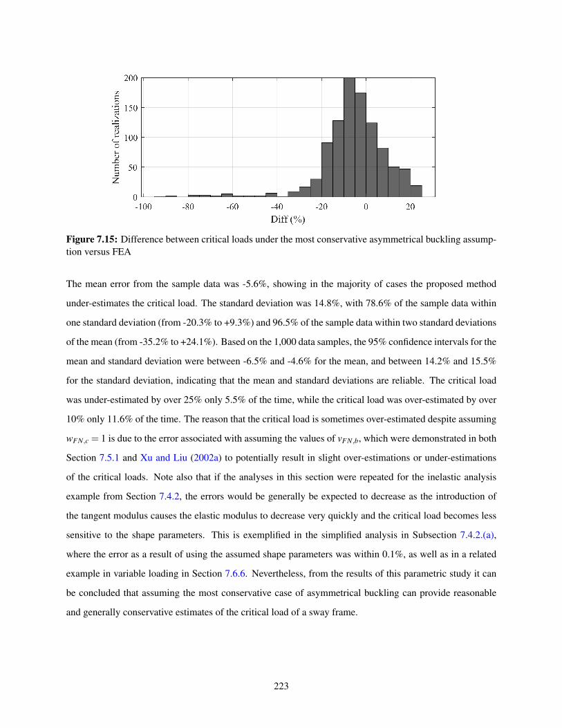
Figure 7.15: Difference between critical loads under the most conservative asymmetrical buckling assump-tion versus FEA

The mean error from the sample data was -5.6%, showing in the majority of cases the proposed method

under-estimates the critical load. The standard deviation was 14.8%, with 78.6% of the sample data within

one standard deviation (from -20.3% to +9.3%) and 96.5% of the sample data within two standard deviations

of the mean (from -35.2% to +24.1%). Based on the 1,000 data samples, the 95% confidence intervals for the

mean and standard deviation were between -6.5% and -4.6% for the mean, and between 14.2% and 15.5%

for the standard deviation, indicating that the mean and standard deviations are reliable. The critical load

was under-estimated by over 25% only 5.5% of the time, while the critical load was over-estimated by over

10% only 11.6% of the time. The reason that the critical load is sometimes over-estimated despite assuming

wFN,c = 1 is due to the error associated with assuming the values of vFN,b, which were demonstrated in both

Section 7.5.1 and Xu and Liu (2002a) to potentially result in slight over-estimations or under-estimations

of the critical loads. Note also that if the analyses in this section were repeated for the inelastic analysis

example from Section 7.4.2, the errors would be generally be expected to decrease as the introduction of

the tangent modulus causes the elastic modulus to decrease very quickly and the critical load becomes less

sensitive to the shape parameters. This is exemplified in the simplified analysis in Subsection 7.4.2.(a),

where the error as a result of using the assumed shape parameters was within 0.1%, as well as in a related

example in variable loading in Section 7.6.6. Nevertheless, from the results of this parametric study it can

be concluded that assuming the most conservative case of asymmetrical buckling can provide reasonable

and generally conservative estimates of the critical load of a sway frame.

223

7.6 Variable Loading of Multistorey Frames

The proposed decomposition method is herein extended to account for variable gravity loading. As origi-

nally proposed by Xu (2001), the worst and best case scenarios can be obtained by solving a minimization

problem to determine the minimum and maximum possible total applied gravity load that would be required

for instability to occur, respectively. Note that as the matrix formulation presented in Section 7.3 is rel-

atively computationally expensive it is not recommended for use in variable loading. As such, only the

decomposition method is applicable to this section.

7.6.1 Minimization Problem

In order to formulate the variable loading minimization problem, a pseudo-proportional loading scheme

is first defined. To account for the presence of permanent loads in structures, define a minimum value of

applied loading at each node (i, j) in a frame as Pl,i, j. Let the applied gravity load Pi, j at node (i, j) be

determined via the expression in Eq. (7.19), whereby Xi, j is a randomly generated pseudo-proportional load

factor, and λ is the load level in units of force.

Pi, j(λ ) = Pl,i, j +Xi, jλ (7.19)

In other words, the applied load at each node is proportionally increased via Eq. (7.19) over an initial load

of Pl . Let PPPm×n be a matrix of applied loads at each of the nodes of the frame, let NNNm×n be a matrix of axial

loads at each of the nodes of the frame obtained by summing the applied loads above each node via Eq.

(7.14), and let XXXm×n be a matrix of pseudo-proportional load factors assigned at each node. In the proposed

minimization problem the values of Xi, j are varied between zero and unity, with higher values corresponding

to higher loads applied at the node relative to the other nodes. For any randomly generated instance of XXX , let

λr,i be the value of λ that results in a zero lateral stiffness in storey i. In other words, λr,i is the root (hence

the subscript r) of (ΣS)i and is the critical load level corresponding to the instability of storey i. Also, let

λr,min be the lowest value of λr,i over all storeys. λr,min is therefore the critical load level of the frame. Then,

the minimization problem for variable loading in multistorey stability can be expressed in Eq. (7.20).

Minimize or Maximize: f (XXX) =n

∑j=1

m

∑i=1

Pi, j(λr,min(XXX)) (7.20a)

subject to:

XXX ∈ [000,111] (7.20b)

224

NNN ≤ NNNuuu (7.20c)

The objective function, f (XXX), in Eq. (7.20a) calculates the total load during instability of the frame given

some pseudo-proportional loading scheme XXX . The values in XXX are each randomly generated between zero

and unity. Now, it should be noted that the lateral stiffness equation in Eq. (7.13) becomes discontinuous

when any column (i, j) reaches its rotational buckling load, i.e. Ni, j = Nu,i, j (Xu, 2003). For loads exceeding

the rotational buckling load Nu,i, j, S∆ can potentially return a positive value via Eq. (7.12), but would

be invalid since rotational buckling has already occurred. As such, the region beyond NNN = NNNuuu should be

avoided via the constraint in Eq. (7.20c) when solving the minimization problem. NNNuuu is an m× n matrix

of upper bound axial loads Nu,i, j corresponding to the rotational buckling mode for each column and can be

calculated via the procedure outlined in Section 7.6.3.

7.6.2 Shape Parameters

Note that since the buckling shape of the frame varies depending on the pseudo-proportional loading scheme,

the shape parameters must be assumed. It is recommended to assume vFN = 1 for all members, wFN,c = 1

for all columns and wFN,b = 0 for all beams corresponding to the most conservative asymmetrical buckling

assumption described in Section 7.2.3. As such, the proposed variable loading problem will likely return

reasonable and conservative estimates of the worst and best case scenarios as demonstrated in Section 7.5.2.

7.6.3 Rotational Buckling

The recommendations for determining Nu are outlined in Sections 2.1.1 and 3.2.4, depending on whether or

not the effects of shear deformations on the result are considered. However, the solution is further compli-

cated in the case of multistorey frames since ru and rl now vary with the axial loads in the columns of the

frame. As such, the value of Nu for each column depends on the relative magnitudes of the loads applied

on other columns, and thus also on the pseudo-proportional loading scheme XXX . In order to determine the

values of Nu, the following iterative procedure may be used and repeated for each column (i, j) given some

proportional loading scheme XXX . Note that the recommended procedure varies slightly depending on whether

elastic analysis or inelastic analysis via the tangent modulus equation in Eq. (2.13) is assumed.

1. Set the load level to zero (λ = 0) and set PPP = 000.

2. Assume the shape parameters: vFN = 1 for all members, wFN,c = 1 for columns and wFN,b = 0 for

beams.

3. Calculate Ni, j for column (i, j) based on PPP by summing the applied loads above the column via Eq.

225

(7.14).

4. Update the tangent elastic modulus and shear modulus of the members if applicable.

5. Calculate the end fixity factors, ru and rl , for all columns via Eq. (2.2) with R calculated based on the

equations in Section 7.2.1.

6. Solve Eqs. (2.12) or (3.13) for φu using the current end fixity factors of the column (i, j).

7. For elastic analysis, calculate the resulting load level λ required to satisfy φ = φu in column (i, j). For

inelastic analysis, calculate N′u for column (i, j) via Eq. (7.21).

N′u = 0.85Ny(10−1/7.38) fy/ fE,0 (7.21a)

fE,0 = φ2u

E0IL2A

(7.21b)

where fE,0 is the stress in the column corresponding to the rotational buckling load with E = E0.

Check if N′u is within the range Ny/3 to Ny. If so, determine the load level λ resulting in N = N′u.

Otherwise, conduct the elastic analysis for this step instead. Note that Eq. (7.21) was obtained by

solving Eq. (2.12) with Eq. (2.13) within the range Ny/3 to Ny.

8. Calculate PPP(λ ) via Eq. (7.19) using the value of λ obtained from Step 7 and store the result as PPP′′′.

9. Update PPP using Eq. (7.22) with 0≤ kw ≤ 1 being the iterate weight.

PPP = kwPPP′′′+(1− kw)PPP (7.22)

10. Repeat Steps 3 through 9 until the value of until the value of Ni, j from Step 3 converges within an

allowable tolerance (a tolerance of 0.001 N or less is recommended). Set Nu,i, j = Ni, j as the solved

rotational buckling load of the column (i, j).

Note that the iterate weight, kw, affects the convergence of the solution. Lowering the value of k increases

the likelihood of convergence but also results in slower convergence. The procedure can be repeated for

each column in the frame (i from 1 to m and j from 1 to n) to obtain NNNuuu.

7.6.4 Solving the Objective Function

The evaluation of the objective function, f (XXX), in Eq. (7.20a) requires solving for λr,min, which is the critical

load level of the frame for the given pseudo-proportional loading scheme XXX . The solution is guaranteed via

the following procedure as long as NNNuuu is determined via the procedure in Section 7.6.3.

1. Verify that ΣS in each storey is positive for PPP === 000 (this should be guaranteed if asymmetrical buckling

is assumed). Otherwise, the shape parameters are invalid for the given scheme XXX .

226

2. Determine the lowest value of the load level λ that results in the rotational buckling of any column in

the frame (Ni, j = Nu,i, j for some i, j). Store this value as λmax.

3. For each storey i, search the region λ = λmax± ε , where ε is a relatively small value, for any value of

λ resulting in (ΣS)i < 0. If (ΣS)i < 0 occurs, store the corresponding value of λ as λneg,i. If no value

of λ is found in the vicinity of λmax which results in (ΣS)i < 0, then check if ru = rl for any column

in the storey. If so, then take λr,i = λmax and skip Step 4. Otherwise, the failure of the storey may not

govern the failure of the frame − skip Step 4 without assigning any value to λr,i.

4. For the storeys in which a value of λneg,i has been stored, the Intermediate Value Theorem guarantees

a solution of λr,i whereby (ΣS)i = 0 in the storey, since λ = 0 corresponds to (ΣS)i > 0, λneg,i cor-

responds to (ΣS)i < 0, and (ΣS)i is continuous between the two points. Use Brent’s method (Brent,

1973) or other bisection methods to solve for λr,i.

5. Repeat Steps 3 and 4 for each storey. Take λr,min as the minimum of the λr,i values, and calculate the

corresponding value of f (XXX), i.e. the total critical load, via Eq. (7.20a).

7.6.5 Elastic Analysis Example in Variable Loading

The application of variable loading towards the elastic analysis of the two-bay, two-storey frame in Section

7.4.1 is demonstrated in this section. Instead of the proportional loading scheme given in Fig. (7.4), the

applied loads are considered to be variable, with lower bound Pl,i, j = 300 kN for all columns. As consistent

with the recommendation of Section 7.6.2, the most conservative asymmetrical buckling shape assumption

is adopted. All other properties of the frame remain unchanged from Fig. (7.4). The minimization problem

in Eq. (7.20) was solved using Particle Swarm Optimization (Kennedy and Eberhart, 1995), which is a

meta-heuristic global search algorithm which employs both localized and global searching within the multi-

dimensional rectangular variable domain specified in Eq. (7.20b). Note that alternative meta-heuristic

global search algorithms such as the Cuckoo Search (Yang, 2009) and Firefly Algorithm (Yang and He,

2013) may also be used to solve this type of problem. With neglecting shear deformations, the results of

the minimum (worst case) and maximum (best case) solutions to Eq. (7.20) are shown in Table 7.3. Note

that a further analysis of this example with considering shear and axial beam deformations is provided in

Appendix A7.6.5, which produces similar conclusions.

Based on the results, the worst case solution involves only loading Column (2,3) until instability occurs.

Note that P2,3 = N2,3 = Nu,2,3− ε = 63,910 kN where ε is a very small value less than 0.1 kN for Column

(2,3) so rotational buckling is imminent. Hypothetically speaking, if rotational buckling were to occur in any

227

Table 7.3: Worst and best case gravity loading scenario causing instability for two-bay, two-storey frame

Column (i, j) (1,1) (1,2) (1,3) (2,1) (2,2) (2,3) Total

Pi, j (worst case, kN) 300.0 300.0 300.0 300.0 300.0 63,910 666555,,,444111000Pi, j (best case, kN) 57,364 6,888 378.5 23,109 9,309 18,717 111111555,,,777666666

of the columns in any scenario with a lower total load, such a load case would have governed the solution

to the minimization problem instead. Therefore, it is apparent that Column (2,3) is the weakest of all of the

columns (it also has the least moment of inertia). Moreover, loading only the top columns in a frame has the

most detrimental effect on the lateral stiffness since doing so increases the axial loads of the columns in all

storeys. The best case solution includes loads of various magnitudes throughout the frame and corresponds

to the lateral sway mode, since all of the axial loads in the columns are well below Nu. The highest value

of N/Nu out of all the columns during the instability is only 0.41, indicating that rotational buckling is not

imminent. The pseudo-proportional loading scheme corresponding to the best case solution presented in

Table 7.3 will thus provide the maximum efficiency related to the capacity of the frame and is therefore

useful to designers.To check the error of the worst case and best case solutions to the actual critical load

levels of the frame from FEA, the pseudo-proportional loading schemes XXX in Eq. (7.19) corresponding to

each solution was inputted into ABAQUS (Simulia, 2012) model described in Section 7.4.1 and the critical

load levels were determined via eigenvalue buckling analysis. The resulting total loads corresponding to the

instability of the worst and best cases in FEA were 61,214 kN and 112,908 kN, respectively. The errors of

the proposed method to the FEA results with respect to the total loads in each scenario were 6.4% and 2.5%,

respectively, which are not significant, and result from the assumption of asymmetrical buckling. Note that

further analysis of this example with considering shear and axial deformations in Appendix A7.6.5 produces

similar conclusions, and axial deformations are found to have a negligible effect on the results.

7.6.6 Inelastic Analysis Example in Variable Loading

The application of variable loading towards the inelastic analysis of the one-bay, three-storey frame in

Section 7.4.2 is demonstrated in this section. Instead of the proportional loading scheme given in Fig. (7.8),

the applied gravity loads are considered to be variable with Pl = 300 kN for all columns. Once again,

the most conservative case of asymmetrical buckling is assumed. Shear and beam axial deformations are

neglected in this section, but are considered via a re-analysis in Appendix A7.6.6 which produces similar

conclusions. The results of the minimum (worst case) and maximum (best case) solutions to Eq. (7.20) are

shown in Table 7.4.

228

Table 7.4: Worst and best case gravity loading scenario causing instability for one-bay, three-storey frame

Column (i, j) (1,1) (1,2) (2,1) (2,2) (3,1) (3,2) Total

Pi, j (worst case, kN) 300.0 300.0 300.0 300.0 300.0 1,971.6 333,,,444777222Pi, j (best case, kN) 1,318.0 1,008.0 521.0 353.3 656.0 1023.2 444,,,888888000

Similar to the previous example, the worst case solution involves the loading of only one column in the

uppermost storey until instability occurs with N3,2 = Nu,3,2− ε = 1971.6 kN. This reflects the imminence

of rotational buckling in Column (3,2). The best case solution again features loads of various magnitudes

throughout the frame and corresponds to sway buckling as no columns have axial loads near their corre-

sponding rotational buckling loads. The results of the minimum and maximum cases were also compared

with the results from FEA eigenvalue buckling analyses under the corresponding pseudo-proportional load-

ing schemes via in Eq. (7.19). Note that the inelastic results were achieved by manually adjusting the

tangent elastic modulus. Based on the analysis, the critical total loads of the frame for the worst and best

case scenarios are 3,470 kN and 4,880 kN, which correspond to errors of 0.1% and 0.0%, respectively. The

buckling modes obtained from FEA for the minimum and maximum solutions are illustrated in Fig. (7.16),

and are as predicted by the proposed decomposition analysis.

Figure 7.16: Buckling modes of minimum (left) and maximum (right) variable loading cases

As seen through the examples in this chapter thus far, the results of the variable loading analysis may not be

exact but the recommended procedure does provide a reasonable approximation of the worst and best case

loading scenarios causing instability. It also provides useful information regarding the weakest column in

the frame (minimum solution) and the estimates the optimal loading pattern corresponding to the maximum

loading scenario.

7.7 Other Considerations for Multistorey Frames

Some other considerations not yet addressed in this chapter but related to the topics covered in other chapters

are discussed herein, including the effects of initial imperfections and fire conditions on multistorey frame

229

analysis.

7.7.1 Initial Imperfections in Multistorey Frames

Conceptually, it is well known that column imperfections do not affect the stability analysis in single storey

frames (Ziemian, 2010). For multistorey frames, since the columns are assumed to be continually spliced in

this study, the columns are effectively single columns spanning multiple storeys. Therefore, the conclusion

that imperfections do not affect the stability can be extrapolated towards multistorey frames. It can also be

shown that the global stiffness matrix of a regular, rectangular structural system is not affected by initial off-

sets to the coordinates of the members (Leet et al., 2009). Thus, for the purposes of stability analysis, both

the proposed decomposition and matrix analysis procedures for multistorey frames can be applied regard-

less of the magnitude of imperfections as long as the deformations resulting from the initial imperfections

are small. In terms of the deformations, requirements for deflections are more commonly stipulated based

on either the inter-storey displacement (∆∗) or the maximum deflection of individual columns (δ ∗), as dis-

cussed in Section 4.3, rather than the deformation of the entire structure. As such, it is more convenient

to decompose the frames into individual storeys and perform individual storey analysis in accordance with

the methods presented in Chapter 4, and Chapter 6 for post-earthquake conditions. The contributions of the

column splices to the rotational stiffness of the column ends in each storey can be considered via Section

7.2.1. That said, however, caution should be taken to ensure that the cumulative initial drift caused by initial

imperfections summed over multiple storeys does not result in excessive deflections.

7.7.2 Elevated Temperatures in Multistorey Frames

So far, in this study the effects of fires on steel structures have mainly been modelled by reducing the elastic

modulus and shear modulus of the corresponding members or segments experiencing elevated tempera-

tures. The effects of restraints to thermal expansion have also been partially considered by increasing the

axial loads in the columns. However, when beam axial deformations are considered, the thermal expansion

and corresponding restraint forces have been neglected because they are assumed to be small and have little

influence on the results. Moreover, the thermal expansion of unrestrained beams can likely be treated as

column initial imperfections, which could be investigated in future studies. In any case, these same assump-

tions can be applied in multistorey frames subjected to fire conditions. Moreover, the same variable loading

methods presented in Sections 5.2.1 and 5.4.1 can be extended towards multistorey frames by making minor

adjustments to the respective objective functions and especially the stability constraints in Eqs. (5.7b) and

(5.16b). Instead of the single-storey constraints, the constraints of the minimization and maximization prob-

230

lems will be similar to those proposed in Xu and Wang (2008) in Eqs. (2.24c) and (2.23b), respectively. As

such, the minimization problem corresponding to the the minimum amount of heating resulting in instability

can be expressed via Eqs. (7.23).

Minimize: Tavg =1

mn

[ m

∑i=1

n

∑j=1

Tb,i, j

](7.23a)

subject to:

S∗i =n

∑j=1

12Ec,i, j(Tc,i, j)Ic,i

L3c,i, j

(β ′i, j(TTT c,TTT b)

1+ζ ′i, j(TTT c,TTT b)

)= 0 (7.23b)

Si =n

∑j=1

12Ec,i, j(TTT c)Ic,i

L3c,i, j

(β ′i, j(TTT c,TTT b)

1+ζ ′i, j(TTT c,TTT b)

)≥ 0; ∀i ∈ 1,2, ...,m ; i 6= i∗ (7.23c)

NNN < NNNu(TTT c,TTT b) (7.23d)

T0 ≤ TTT b ≤ Tu (7.23e)(max

r,s∈Ad j(i, j)Tr,s−Ti, j

)× IO,T,i, j ≥ 0; ∀i ∈ [1,m], j ∈ [1,n] (7.23f)

IF,T (TTT b) = 1 (7.23g)

where TTT ccc is an m× n matrix of column temperatures, and TTT bbb is an m× (n− 1) matrix of beam tempera-

tures. The temperature of each column can be calculated based on the proportional assumption of Eq. (5.8).

Note that, as always, ΣS may be replaced with Seq calculated via the equivalent spring stiffness method if

the effects of beam axial deformations are considered. Also, although the values of Nu,i are temperature

dependent, since the gravity loads are assumed to be constant in the variable fire loading analysis, a simple

check for NNN ≤ NNNu can be accomplished using either Eqs. (2.12) or (3.13) rather than the rigorous procedure

outlined in Section 7.6.3. Finally, Eqs. (7.23f) and (7.23g) correspond to the multistorey version of the

single fire constraint, which replaces the single storey version of the single fire constraint in Eq. (5.7e). In

multistorey frames, fires can spread both horizontally and vertically. In order to ensure that the scenarios be-

ing considered in the minimization problem correspond only to scenarios whereby there is a single location

of origin, the new constraints in Eqs. (7.23f) and (7.23g) are formulated based on the following logic. With

exception to the originating bay, the beams in all other bays in the frame must be located adjacent, either

vertically or horizontally, to a bay containing a beam that is at least as warm or hotter than itself. This first

requirement is satisfied mathematically via Eq. (7.23f), which must be satisfied in every bay not located at

the origin of the fire, and conveniently expresses the slack of the constraint in the form of a numerical value.

231

As such, Ad j(i, j) is defined as the set of bays directly adjacent (vertically and horizontally) to bay (i, j).

However, evaluating the term inside the brackets in Eq. (7.23f) for the originating bay will return a negative

value unless the term is multiplied by the indicator function IO,T,i, j, which returns a value of zero if bay (i, j)

contains the beam with temperature equal to the highest beam temperature in the frame, expressed in Eq.

(7.24).

IO,T,i, j =

0, if Ti, j = maxr∈[1,m],s∈[1,n] Tr,s

1, otherwise.(7.24)

In other words, if bay (i, j) is the originating bay, then the term in brackets will be overridden with a zero

value in order to satisfy the constraint. Still further, Eq. (7.23f) is insufficient by itself to eliminate the cases

where multiple bays contain beams with exactly the maximum beam temperature in the frame. Contrary

to its purpose, Eq. (7.23f) can also be satisfied if multiple unconnected bays in the frame have the same,

maximum temperature. To eliminate these exceptional cases, the additional constraint in Eq. (7.23g) is

required where IF,T is an indicator function that returns the value 1 if the set of all bays satisfying IO,T,i, j = 0

is geometrically connected (i.e. they are all physically touching), and 0 otherwise. As such, by satisfying

Eqs. (7.23f) and (7.23g) together, the realistic modelling of fire spread corresponding to a single fire ignition

event is guaranteed. Note that fires have been observed to spread between storeys in both the upward and

downward directions (Neilson, 1989; Kodur, 2003b), although upward spread is typically more common due

to the rising of warm air, while downward spread only occurs if burning items fall through floors. In any case,

the minimization problem includes the constraint whereby either the instability of any single storey occurs,

or multiple storeys become unstable instantaneously, and searches for the minimum average combination

of beam temperatures which satisfies this constraint. Similarly, the best case scenario corresponding to the

maximum amount of heating resulting in instability can be obtained by simply replacing Eq. (7.23b) and

(7.23c) with Eq. (7.25) and maximizing the objective function instead of minimizing.

Si =n

∑j=1

12Ec,i, j(TTT c)Ic,i

L3c,i, j

(β ′i, j(TTT c,TTT b)

1+ζ ′i, j(TTT c,TTT b)

)≥ 0; ∀i ∈ 1,2, ...,m (7.25)

Finally, the minimization problem corresponding to the minimum duration of fire resulting in instability can

be expressed via Eqs. (7.26), where ttt is an m×n matrix of fire durations ti, j in each bay of the frame.

Minimize: F = maxi∈[1,m], j∈[1,n]

(ti, j) (7.26a)

232

subject to:

S∗i =n

∑j=1

12Ec,i, j(ttt)Ic,i

L3c,i, j

(β ′i, j(ttt)

1+ζ ′i, j(ttt)

)= 0 (7.26b)

Si =n

∑j=1

12Ec,i, j(ttt)Ic,i

L3c,i, j

(β ′i, j(ttt)

1+ζ ′i, j(ttt)

)≥ 0; ∀i ∈ 1,2, ...,m ; i 6= i∗ (7.26c)

NNN < NNNu(ttt) (7.26d)

ti, j = tk; ∀ j,k ∈Cx; ∀1≤ x≤ nx (7.26e)

ti, j ≥ 0; ∀ j ∈ 1,2, ...,n (7.26f)(max

r,s∈Ad j(i, j)tr,s− ti, j

)× IO,t,i, j ≥ 0; ∀i ∈ [1,m], j ∈ [1,n] (7.26g)

IF,t(ttt) = 1 (7.26h)

In this problem, the single fire constraint in Eqs. (7.26g) and (7.26h) is similar to the one presented for

variable beam temperatures, but replaces the temperatures of the beams directly with the duration of fire in

each bay, and IO,t,i, j is given in Eq. (7.27).

IO,t,i, j =

0, if ti, j = F

1, otherwise.(7.27)

The function of IF,t is the same as IF,T in that it is an indicator function returning the value of 1 if the set of

all bays satisfying IO,t,i, j = 0 is geometrically connected, and zero otherwise. The indicator function IF,t can

be programmed into a subroutine. Note that if three-segment members are to be considered for the analysis,

then the corresponding equations for the column lateral stiffness, end fixity factors, rotational buckling loads

and equivalent rotational stiffness can be replaced with the ones presented in Chapter 6. The only remaining

equation to be presented is for the equivalent rotational stiffness contribution of an axially loaded member

containing three segments, which is derived in Section A7.7.2.

7.8 Numerical Example - Putting it All Together

A final example is presented, which combines all of the main concepts presented in this study to analyze a

three-bay, two-storey frame shown in Fig. (7.17) under elevated temperature conditions. First, a variable

fire loading analysis is conducted to determine the worst case fire duration leading to the instability of

the frame under normal fire conditions (i.e., the insulation is not damaged due to earthquakes for other

events). Secondly, the frame is analyzed under post-earthquake fire conditions whereby delamination of the

233

insulation is assumed to have occurred at the joints of the frame and an inter-storey drift is assumed. In the

post-earthquake fire analysis, the fire resistance of the frame is calculated based on defined fire scenarios.

Figure 7.17: Multistorey frame subjected to variable fire and post-earthquake fire conditions

The three-bay, two-storey frame contains six bays labelled in Fig. (7.17) and is subjected to the constant, ap-

plied service gravity loads shown. Note that while the frame is structurally adequate in ambient temperature

conditions according to CSA S16 (CSA, 2014) under the various factored load combinations stipulated the

Canadian Building Code (NRC, 2015), it will be shown that various fire scenarios can cause the instability

of the frame if the members are not adequately insulated. In the variable fire loading analysis, the Pettersson

et al. (1976) parametric fire curves are adopted based on the occupancies in the bays of the frame. For the

post-earthquake fire analysis, the more simplified, ASTM E119 fire curve is assumed to occur in some or all

of the bays depending on the respective fires scenarios. Although more conservative, the ASTM E119 fire

curve is commonly used in experimental and analytical practice to evaluate the fire resistance of structures

(Dwaikat and Kodur, 2013; ASTM, 2016). Tension-only lateral bracing is provided in the central bay with

Kbr = 1,000 kN/m for each storey in either direction at ambient temperatures. The lateral bracing is only

assumed to be present under the normal fire scenarios corresponding to the variable fire loading analysis,

as they are conservatively assumed to be rendered ineffective during the earthquake preceding the post-

earthquake fire analysis cases. For the purpose of simplicity, the stress in the braces is assumed to be within

the elastic range, i.e. E = Ea(T ) from Fig. (2.7). During elevated temperature conditions, the stiffness of

the bracing decreases proportionally with the elastic modulus of steel. As consistent with normal practice,

the bracing is assumed to be un-insulated because diagonal braces are primarily provided to resist lateral

234

loads, which seldom approach their maximum values during fires (Promat, 2017). The temperatures of the

braces are assumed to be equal to the temperature of fire in the standard curves. Semi-rigid connections are

also provided at every beam-to-column connection, with the rotational stiffness modelled in a similar way

to the previous examples in this study via Eq. (2.33b) with Z0 = 19,560 kNm/rad and mZ = 28.8 kNm/rad/C

and the temperatures of the connections assumed to be equal to that of the connecting beam segment. In ac-

cordance with the recommendations discussed in Sections 7.2.3 and 7.5, the shape parameters of the frame

are conservatively assumed to correspond to the most conservative case of asymmetrical buckling in all of

the analyses. The members of the frame are labelled in Fig. (7.17) and the section properties are tabulated

in Table 7.5.

Table 7.5: Cross-sectional properties for members in three-bay, two-storey example

Member(s) Section I A W D l60 κ

(×106 mm4) (mm2) (kg/m) (m) (mm) -

B11, B13 W410×67 245 8,580 67 1.52 17.4 0.44B12, B22 W410×39 126 4,950 39 1.35 21.2 0.44B21, B23 W410×54 186 6,840 54 1.50 19.3 0.44C11, C14, C21, C24 W200×52 52.7 6,650 52 1.21 17.7 0.44C12, C13, C22, C23 W200×59 61.1 7,550 59 1.22 16.6 0.44

where l60 is the thickness of insulation required to provide 60 minutes of fire resistance to the member

according to the prescriptive approach in Eq. (5.17) (Lie, 1992). The insulation thickness is linearly pro-

portional to the desired fire resistance, so doubling the thickness will supposedly provide 120 minutes of

fire resistance. The same material properties of insulation and steel from Table 5.13 are adopted for this

example. The values of κ are used to calculate the effective shear area, κA, and are based on the findings

of Cowper (1966). Note that all of the results in this example obtained using the proposed method con-

sider shear deformations via the derived equations based on the Timoshenko (1916) system of governing

differential equations and the Haringx (1948) assumption on the shear angle. Additionally, the effects of

axial deformations are approximately considered using the equivalent spring stiffness method evaluated at

each storey. The tangent shear modulus, Gt , is calculated using Eq. (5.12). The frame is assumed to be

thermally restrained, and the adjusted axial forces in the columns are calculated based on Eq. (6.28). In all

of the calculations of this example, the proposed decomposition method presented in Section 7.2 is used to

calculate the lateral stiffness and/or inter-storey displacements.

235

7.8.1 Variable Fire Analysis

For the variable fire analysis, the members are assumed to have uniform temperatures and the analysis

determines the fire event leading to the earliest possible instability of the frame. As the parametric fire

curves are used (Pettersson et al., 1976), general occupancies are assigned to each bay and the fire curve

parameters corresponding to each are shown in Table 7.6.

Table 7.6: Parameters for compartment fire curves in three-bay, two-storey example

Bay Occupancy At Ao ho fv ε f

(1,1) Residential 309 m2 8.0 m2 1.5 m 0.032 m0.5 500 MJ/m2

(1,2) Reception 250 m2 37.5 m2 1.5 m 0.184 m0.5 637 MJ/m2

(1,3) Kitchen 309 m2 4.0 m2 1.5 m 0.016 m0.5 314 MJ/m2

(2,1) Residential 268 m2 8.0 m2 1.5 m 0.037 m0.5 500 MJ/m2

(2,2) Residential 214 m2 8.0 m2 1.5 m 0.046 m0.5 500 MJ/m2

(2,3) Residential 268 m2 8.0 m2 1.5 m 0.037 m0.5 500 MJ/m2

The fuel load densities of the compartments were selected based on the mean surveyed values of fuel loads

reported in Ocran (2012). The resulting fire curves, plotted for the duration of fire in each bay, are shown in

Fig. (7.18).

Figure 7.18: Parametric fire curves in each bay for three-bay, two-storey example in variable fire loading

From Fig. (7.18) it can be seen that the reception occupancy in Bay (1,2) experiences the highest peak

236

temperature but also decays the most rapidly due to its high ventilation. The kitchen in Bay (1,3) has the

lowest peak temperature due to having the lowest fuel load density but remains burning for the longest

time due to its low ventilation. All of the bays corresponding to the residential occupancy have the same

fuel load of 500 MJ/m2 but their fire curves vary slightly based on the ventilation and surface area. Based

on the fire curves in Fig. (7.18), the temperatures of each member are calculated using the Pettersson

et al. (1976) incremental method with the same assumptions described in Section 5.4.1. However, for the

multistorey frame in this example, the temperatures of the beams are assumed to be only affected by the

fires in the containing compartment directly below since the floor systems directly above typically provide

more thermal resistance. Note that the fire curves are independent of each other, meaning that it is assumed

that the heat flux between adjacent compartments is assumed to be ignored. This assumption may either

be conservative or not conservative because fires that spread faster due to the increased heat flux between

adjacent compartments can also decay faster, resulting in faster cooling of members. In any case, it can

be anticipated prior to conducting the analysis that if a fire were to cause instability as quickly as possible,

it would originate in one of the slow burning compartments and eventually spread to the reception area

whereby the sharp and brief increase in temperatures to the members will be enough to cause failure as the

members in the other compartments have already been heating up for a significant duration of time. The

minimization problem in Eqs. (7.26) was solved, with including an additional floor separation resistance

constraint in Eq. (7.28).

| maxj∈[1,n]

ti, j− maxj∈[1,n]

ti+1, j| ≤ RF,i,i+1; ∀i ∈ 1,2, ...,m−1 (7.28)

The floor separation resistance constraint is newly proposed to account for the general vertical resistance

of fire spread between adjacent storeys, where RF,i,i+1 is a lower bound of the resistance to fire spread be-

tween storeys i and i+ 1. For this example, there are two floors and the resistance to fire spread between

storeys 1 and 2 is conservatively selected to be RF,1,2 = 30 minutes. By incorporating this constraint in the

minimization problem, the scenarios by which fire spreads too quickly between adjacent storeys (i.e. if the

minimum difference between fire durations in the adjacent storeys is less than 30 minutes) are eliminated

from the solution space as they are not likely to occur. Similar to the single fire constraint, the floor separa-

tion resistance constraint can be toggled on and off. In the first analysis, both the single fire constraints and

floor separation resistance constraints were toggled on. The thickness of insulation for each member was

l60, corresponding to 60 minutes of passive fire resistance shown in Table 7.5. The minimization problem in

Eqs. (7.26) was solved using the GRG Nonlinear (Lasdon et al., 1973) with Multi-Start (György and Kocsis,

237

2011) on a spreadsheet and the results are shown in Table 7.7.

Table 7.7: Fire durations in each bay for worst case fire causing instability based on duration; all constraintsactive

Bay 1 Bay 2 Bay 3

Storey 2 137.6 min 142.2 min 142.2 minStorey 1 112.2 min 11.7 min 69.1 min

As shown in Table 7.7, the duration of the worst case fire event leading to instability of the frame has

a duration of F∗ =142.2 minutes and begins in either Bay (2,2) or (2,3) in the residential areas, eventually

spreading through the rest of the building. The minimum floor separation resistance of 30 minutes is satisfied

since the fire takes 30 minutes to reach the first floor, after which the residential occupancy in Bay (1,1)

remains on fire for 112.2 minutes. As anticipated, the reception area in the central bay on the first storey

is the last to catch fire, but due to its high peak temperatures occurring within the first 12 minutes, enough

degradation occurs to the frame in combination with the already heated members of other compartments to

cause instability. The analysis was similarly repeated with the single fire constraints and floor separation

resistance constraints toggled off, and the results are shown in Table 7.8.

Table 7.8: Fire durations in each bay for worst case fire causing instability based on duration; single fireand floor separation constraints deactivated

Bay 1 Bay 2 Bay 3

Storey 2 125.5 min 99.3 min 125.3 minStorey 1 118.8 min 67.5 min 125.5 min

In the scenario shown in Table 7.8, the duration of fire in the frame is only F∗ = 125.5 minutes before the

instability occurs, which is 16.7 minutes earlier than the worst case scenario obtained with the single fire and

floor separation constraints toggled on. This scenario is not very realistic since the results imply that fires

need to start simultaneously in both Bays (1,1) and (2,3), which are located at opposite ends of the frame.

However, similar to the previous case, the reception area catches fire towards the end of the fire event,

as can be anticipated prior to the analysis. The effect of doubling the thickness of insulation to provide

120 minutes of passive fire protection on the results of the minimization problem was also investigated.

Curiously, when the insulation thickness is doubled, there are no possible fire scenarios in the frame, with

the given parameters, that can possibly cause instability. As such, the provision of adequate insulation can

prove vital to ensure that steel frames maintain their stability during fires, and the proposed method can be

used to assess whether any fire scenarios leading to instability are at all possible. Note that as the size of

238

the worst case fire scenario corresponding to the insulation resistance of 60 minutes in Table 7.7 is quite

large, it is also worth mentioning that as the buildings being analyzed under the proposed storey-based

stability analyses become larger with the advances made in this study, the presence of additional firefighting

measures such as fire sprinklers will become more important. In fact, building codes are progressing towards

the increased use of these active firefighting measures to mitigate property damage during fires. However,

sprinklers are not mandated in most building codes and many large buildings in the world still do not have

sprinklers, such as the Grenfell Tower which burned in 2017 (Watt, 2017). In fact, there are many cases

where fire sprinklers will not be available during the fires even if they are designed to be included, such as

during retrofitting in the case of the Windsor Tower fire in 2005 (SCOSS, 2008). In another case, the First

Interstate Bank fire in 1989 engulfed more than four storeys because the fire sprinklers had not yet been

fully installed (Neilson, 1989). Similarly, a fire broke out during the construction phase of Taipei 101 before

any fire protection measures could be installed (Chen, 2003). Still further, sprinklers do not necessarily

guarantee the prevention of fire spread, since fire can spread over the exterior cladding of a building (Watt,

2017). Finally, in post-earthquake fires, water may not be readily available. As such, the proposed method

of variable fire loading can be used as a tool for assessing the most extreme cases of fire. It is in these

extreme situations that, if it can be shown that the instability of a frame during a parametric fire is virtually

impossible regardless of the parameters within reasonable values, then perhaps the corresponding design of

a structure can be considered to be adequate.

Finally, to assess the accuracy of the proposed approach, a finite element model of the framing members was

constructed of wireframe B21 linear shear-deformable elements. The diagonal bracing was also included in

the form of appropriately sized T2D2 truss elements via Eq. (2.1). All of the member properties including

the cross-sectional areas, moments of inertia, elastic modulus E and transverse shear stiffness κAG were

inputted manually as constants based on the duration of fire. The connection rotational stiffness obtained

from Eq. (2.33b) was also inputted manually for each beam-to-column connection using "Join + Rotation"

connector sections. The adjusted values of the axial loads in the columns due to thermal restraints were

also manually inputted. The eigenvalue buckling analysis feature was used to calculate the factor of safety

based on the magnitudes of the applied gravity loads corresponding to the instability mode of the frame.

The duration of the fire event was then varied via trial and error with the durations of fire in each bay

increasing or decreasing uniformly while updating the manually inputted properties until the factor of safety

obtained in the eigenvalue analysis became unity, indicating that the frame would become unstable under

exactly the given loads, with the values of the manually inputted properties corresponding to the critical

239

duration of fire. Note that the concept of factor of safety was only used here to determine the duration

of failure corresponding to buckling, rather than as a design criterion. In the scenario shown in Table 7.7

corresponding to the use of the single fire and floor separation constraints, the safety factor obtained in FEA

during the reported duration of failure from the proposed method (F∗ = 142.2 min) was 1.12, and decreased

to unity when the duration of the fire event was increased to 154.4 min. The corresponding buckling mode

obtained from the FEA is shown in Fig. (7.19).

Figure 7.19: Buckled shape corresponding to the worst case fire scenario with all constraints activated

As seen in Fig. (7.19), the failure mode consists predominantly of the sway failure of Storey 2 since it has

been heated the longest and the temperatures of the members are still very high, as concluded by observing

Fig. (7.18) and noting that the fire temperatures in the second storey are still above 800C for ti, j = 150

minutes. In fact, upon further investigation it was found that the temperatures of the members in Storey 2

are close to 800C during the failure, all being between 776C and 797C after 154.4 minutes. At these

high temperatures the elastic modulus of the members in Storey 2 are severely degraded, causing them to

govern the buckling shape of the failure mode. Note also that the left-most column in Storey 1 also appears

to buckle outward due to having a high temperature of 715C. At this time, the other columns in Storey 1

only have temperatures ranging between 300C to 400C, and being more stiff than the other columns in the

frame, do not deform as much in the buckling shape. A similar analysis was conducted on the scenario in

Table 7.8, whereby it was found that the safety factor obtained in FEA corresponding to F∗ = 125.5 min was

1.10, and decreased to zero after the fire durations in the bays were increased uniformly until the duration

of the fire event reached 130.0 min. The buckling shape obtained in FEA appears similar to Fig. (7.20) and

is included in Fig. (7.20).

Figure 7.20: Buckled shape corresponding to the worst case fire scenario with single fire and floor separationconstraints deactivated

The reason that the FEA analysis produces a higher fire resistance in the frame is that the assumption of the

240

most conservative case of asymmetrical buckling discussed in Section 7.2.3 was adopted during the variable

loading analysis using the proposed method, which effectively neglects the contributions of column splices

to the connection rotational stiffness at the ends of the columns in each storey. Nevertheless, the conservative

errors in the critical fire durations obtained by the proposed method range are 8.6% and 3.6%, respectively,

which are fairly small when considering the unpredictable nature of fire-structural behaviour.

7.8.2 Post-Earthquake Fire Analysis

In the post-earthquake fire analysis, a delamination length of 100 mm is assumed to occur at both ends

of each member, to account for the ductile behaviour of the connections during a seismic loading event.

Additionally, an inter-storey drift of ∆0 = Hi/250 is assumed to occur at each storey, where Hi is the height

of each storey. The fire curves in the compartments are replaced with the standard ASTM E119 fire curve,

and the temperatures of the members are calculated using the Dwaikat and Kodur (2013) simplified method.

Five fire scenarios are analyzed and the fire resistance of the frame is reported for each scenario: (1) uniform

fire occurring throughout Storey 1; (2) uniform fire occurring throughout Storey 2; (3) uniform fire occurring

throughout the entire frame; (4) uniform fire occurring in Storey 1 and spreading to Storey 2 in which a

uniform fire occurs after a delay of 30 minutes; (5) uniform fire occurring in Storey 2 and spreading to

Storey 1 in which a uniform fire occurs after a delay of 30 minutes. In each scenario, the fire resistance

corresponding to two failure modes are reported: (a) stability failure via the loss of lateral stiffness in any

individual storey, and (b) deformation-related failure corresponding to excessive inter-storey displacement

equal to ∆+∆0 = Hi/100. Finally, a finite element model similar to the one described for the variable fire

analysis of the same example was constructed to calculate the actual time of instability in the frame in each

scenario. An attempt was made to also calculate the time corresponding to excessive deflection but the

displacements in the FEA model did not converge due to the complexity of the problem. Regardless of this,

the errors in fire resistance corresponding to the deformation-related failure between the proposed method

and FEA would have been similar to those reported for the stability failure mode. The analyses were first

conducted with the length of insulation for each member equal to l60 in Table 7.5, and the results are shown

in the second column of Table 7.9.

As seen in Table 7.9, when the entire building is subject to the uniform ASTM E119 fire (Case 3), excessive

inter-storey deflections occur at 72.6 minutes and instability occurs at 74.4 minutes according to the pro-

posed method. As expected, the deformation criteria are reached before the stability criteria. Note that the

proposed method yields conservative results in all reported cases due to the assumption of shape parame-

241

Table 7.9: Fire resistance of three-bay, two-storey frame with 60 minutes of passive fire resistance providedby insulation subject to post-earthquake fire scenarios

Failure criteria (a) Stability (a) Stability (b) Deformation

(Proposed Method) (FEA) (Proposed Method)

Case 1 85.9 min 100.8 min 78.6 min

Case 2 121.3 min 121.5 min 110.7 min

Case 3 74.4 min 77.1 min 72.6 min

Case 4 85.7 min 95.1 min 78.5 min

Case 5 101.5 min 105.0 min 95.7 min

ters corresponding to the most conservative case of asymmetrical buckling. The maximum error in the fire

resistance obtained using the proposed method is 15% and occurs for Case 1, whereby only the first storey

experiences a uniform fire. In contrast, the error in Case 2 between the proposed method and FEA is less

than 0.2%. The relative difference in errors between Case 1 and Case 2 can be explained by examining the

buckling shapes of the frame corresponding to each case, shown in Figs. (7.21) and (7.22), respectively. In

Figure 7.21: Buckled shape corresponding to Case 1 of the post-earthquake fire analysis

Figure 7.22: Buckled shape corresponding to Case 2 of the post-earthquake fire analysis

examining the buckling shapes, it is apparent that Case 1 involves the failure of the first storey. Although

the first storey is in reality well-restrained from rotation by the unheated columns in the second storey, the

proposed method effectively neglects this contribution via the conservative assumption of shape parameters

discussed in Section 7.2.3. For this reason, the resulting fire resistance of the frame under Case 1 is very

conservative under the proposed method compared to the FEA, which does capture the effect of rotational

stiffness provided by the splicing of columns between the storeys. In contrast, it is apparent in Fig. (7.22)

that Case 2 is governed by the failure of the second storey, which is significantly restrained rotationally at

the lower ends of its columns by the beams of the first storey, which are maintained at ambient temperature.

The rotational stiffness provided by these beams to the lower column ends of Storey 2 are considered in the

242

proposed method. As such, neglecting only the rotational stiffness contributed by the connecting column

splices below via the assumption of shape parameters has a much lesser effect on the results of the failure

analysis. In any case, the maximum error of 15% between the results of the proposed method and FEA is

once again relatively small when considering the variable nature of fire-structural behaviour. Anyway, the

analyses were repeated with the insulation of each member equal to 2l60, corresponding to 120 minutes of

passive fire protection. The results are shown in Table 7.10.

Table 7.10: Fire resistance of three-bay, two-storey frame with 120 minutes of passive fire resistance pro-vided by insulation subject to post-earthquake fire scenarios

Failure criteria (a) Stability (a) Stability (b) Deformation

(Proposed Method) (FEA) (Proposed Method)

Case 1 160.4 min 180.9 min 145.2 min

Case 2 219.0 min 219.4 min 203.5 min

Case 3 138.4 min 141.4 min 136.2 min

Case 4 160.2 min 162.9 min 145.0 min

Case 5 164.5 min 170.5 min 157.6 min

Unlike the parametric fires considered in the variable fire analysis, the ASTM E119 fire does not decay, but

only increases in temperature as time progresses. From comparing the results of Tables 7.9 and 7.10, it can

be concluded that the provision of insulation is critical to the structural integrity of steel members. The fire

resistance increased by at least 62% in every case when the thickness of insulation was doubled. Moreover,

as consistent with the conclusions of the Cardington tests (British Research Establishment, 1996), the results

of this example show that the actual fire resistance of a structural system (minimum 136.2 minutes for this

analysis) is generally greater than the fire resistance of the individual components (120 minutes for each

member based on the prescriptive approach).

7.9 Conclusion

This chapter has proposed the decomposition and matrix analysis methods for evaluating the stability of

multistorey, semi-braced, semi-rigidly connected steel frames. Unbraced frames and frames with idealized

connections correspond to special cases that can also be analyzed using the proposed methods. In the

decomposition method, frames are decomposed into individual storeys and the lateral stiffness of each storey

is evaluated with considering the effects of axial loads. As soon as the lateral stiffness of any individual

storey diminishes to zero, the frame is considered to be unstable. The equations of the decomposition

method is validated against a more complicated matrix analysis method also derived in this chapter, as

243

well as FEA. Practically, the proposed decomposition method can be used to identify the critical loads

and the weakest storey in a frame, defined as the first storey that reaches a lateral stiffness of zero. The

solutions of the proposed decomposition and matrix methods are sensitive to the shape of the buckling

mode, which is difficult to solve and may be assumed. Nevertheless, the assumption of the worst case

of asymmetrical buckling in the sway mode provides good estimates for the lower bound critical loads

of the frames, as demonstrated via parametric studies and numerical examples. Based on the results of

the parametric studies, the critical loads of the example frames can be reasonably estimated via the most

conservative asymmetrical buckling assumption, with errors between -20.3% to +9.3% occurring in 78.6%

of the test cases. A negative error corresponds to an under-estimation of the critical load, whereas a positive

error corresponds to an over-estimation of the critical load. A minimization problem is also presented and

demonstrated via numerical examples for determining the minimum and maximum total load cases resulting

in the instability of a frame subjected to variable gravity loading. The minimum and maximum total load

cases resulting in the instability of a frame are defined as the worst and best case variable loading scenarios,

respectively. It was found that with assuming the most conservative asymmetric buckling shape of the

example shapes, the proposed method identified the worst and best case loading scenarios with errors in

the total loads of up to only 6.4% from the actual solutions corresponding to the true buckling shapes of

the frame obtained via FEA. Practically, the variable loading algorithm can be used to identify the weakest

columns of a frame via the worst case scenario, as well as the loading patterns that are likely to yield the

maximum capacity of the frame via the best case scenario. Finally, the proposed method of multistorey

analysis is extended to consider all of the conditions addressed in previous chapters, including variable fire

loading with which the method is demonstrated via a numerical example.

244

Chapter 8

Conclusion

8.1 Summary

The issue of stability is a primary consideration in the design of steel structures. In extending the domain

of structural analysis towards fire conditions, there are a variety of effects and loading conditions that need

to be considered. In particular, the consideration of shear and axial deformations, the presence of column

initial imperfections, lateral loads, and changing material properties in elevated temperatures can all have

significant detrimental effects on the lateral stability and deformation of a steel frame. The conclusions

of this study relating to the investigations on all of these considerations towards the lateral stability and

deformation of steel frames are summarized in the following sections. Overall, a series of proposed method-

ologies was presented for evaluating the storey-based stability and deformation of steel frames susceptible

to side-sway and variable loading, expressed in closed-form solutions that can conveniently be applied for

engineering practice.

8.2 Effects of Shear and Axial Deformations on the Stability of Frames

The effects of shear and axial deformations in the members of a frame on its lateral stability are investigated

in Chapter 3. The effects of shear deformations are considered by replacing the governing Euler-Bernoulli

differential equation with the corresponding Timoshenko (1916) equations, which consider that the direction

of the shear force in a member may be different from its slope. As consistent with the literature (Wang

et al., 1991; Timoshenko and Gere, 1961; Ziemian, 2010), the effects of shear deformations increase as the

slenderness ratios of the members decrease, and can be neglected for sufficiently slender columns. Based

on the results of the numerical examples and parametric analyses, this study has concluded that the effects

of shear deformations on the storey-based stability analysis should not be neglected if the slenderness ratios

of the members are below 40. Similarly, the effects of beam axial deformations on the lateral stiffness of

a frame can be realized using the equivalent spring stiffness concept (Weggle et al., 2007). The effect of

beam axial deformations on the lateral stiffness of a frame was found to increase as the number of bays or

lengths of the beams in the frame increase. However, if the beams are sufficiently axially stiff in comparison

to the lateral stiffness of the columns, or if restraining concrete slabs are present, then the effects of axial

deformations are negligible. Also, if rotational buckling is imminent during the failure of a frame then

245

beam axial deformations become irrelevant. The ς ratio was introduced to as indicator for whether or not

the effects of axial deformations can be neglected. In the current study it is proposed that if the minimum

value of ς calculated for a frame is sufficiently high (above the order of 102) then axial deformations can

be neglected when computing its lateral stiffness. Both the stability equations relating to the effects of

shear deformations and the proposed equivalent spring stiffness method for considering axial deformations

are demonstrated and validated via numerical examples and finite element analyses. These effects are also

briefly considered in combination with the other loading conditions and considerations within each of the

other chapters contained in the current study.

8.3 Frame Capacity with Column Imperfections and Lateral Loading

The effect of column imperfections and lateral loads applied at the upper ends of storeys are investigated

in Chapter 4. Column imperfections and lateral loads are closely related in that the effects of column

imperfections can be simulated by applying a notional load laterally at the top of a storey (Schmidt, 1999).

In fact, a new pseudo-notional load relating to the effects of out-of-straightness imperfections on the upper

end lateral deflection of a column is proposed in the current study. It is demonstrated that the presence

of initial imperfections and lateral loads applied at the upper ends of storeys do not affect the buckling

loads of frames, but rather increase the deflections. Consequently, the capacity of a storey frame needed

to be re-defined based on various failure criteria relating to either the instability of the frame or excessive

deformations. Numerical examples are provided to illustrate the effects of column imperfections and lateral

loads on the deformations. A formulation of the minimization problems in variable loading analyses with

considering the proposed capacity criteria is presented, in which the gravity loads are considered as variables

in a minimization problem and the total gravity load is maximized or minimized to determine the best and

worst case loading scenarios causing the capacity criteria of the frame to be reached. Overall, column

imperfections and lateral loads, if present in significant magnitudes, were both found to reduce the capacity

of a frame and should not be neglected in structural analyses. However, the theoretical bifurcation loads

remain unaffected by column imperfections and lateral loads.

8.4 Frame Stability in Variable Fire Loading

The effect of heating of members in a frame towards its lateral stability was investigated in Chapter 5. Equa-

tions and corresponding computational procedures are presented for calculating the lateral stiffness of a

semi-braced or unbraced frame containing members with elevated temperatures. Due to the variable nature

246

of building fires, the concept of variable loading was applied by presenting two minimization problems for

determining the best and worst case fire scenarios causing instability of a given frame. The first minimiza-

tion problem employs the member temperatures as the optimization variables. The member temperatures

are minimized or maximized to determine the worst and best case scenarios causing instability of the frame.

In the field of fire-structural engineering design, however, the ability for a structure to resist fire loading is

most often expressed in terms of the fire resistance expressed in units of time. For this reason, a second

minimization problem is proposed, which employs the duration of a fire event as the optimization variable,

rather than the member temperatures. The duration of fire causing instability of the storey frame is mini-

mized in the new minimization problem, and presents much more meaningful results. In this way, the fastest

possible time of collapse can be predicted using the proposed method, and the corresponding fire scenario

is identified. Furthermore, a stochastic variable fire loading analysis approach is proposed, which outputs

the probability distribution of the fire resistance of a frame relating to the instability failure mode. Note that

many assumptions regarding the time-temperature relationships of fire and the heat transfer analyses are

required, and are discussed in detail throughout the chapter. Numerical examples are presented to demon-

strate the use of both minimization problems. Generally, it was concluded that the heating of the most stiff

members results in the greatest threat to the stability of a frame. Moreover, it is demonstrated based on the

results of the stochastic variable fire analysis that certain limitations can be made towards the fuel loads and

other variables in the analysis to eliminate certain fire scenarios and increase the worst case fire resistance

of the frame.

8.5 Frame Stability with Segmented Members

Finally, the presence of longitudinal thermal gradients or piece-wise varying temperatures in a member

requires the use of multi-segment members in the structural-thermal analysis of a frame. Multi-segment

members contain piece-wise varying elastic moduli throughout their lengths. These can arise due to many

reasons, including localized heating or damage to insulation, as discussed in Chapter 6. A comprehensive

derivation is presented for determining the lateral stiffness of a frame containing three-segment members,

which can be used to model the delamination of insulation occurring at plastic hinges during earthquakes

or due to blast explosions, along with other situations causing longitudinal temperature gradients such as

the phenomenon of warm air rising in a compartment fire. In order to calculate the lateral stiffness of

a multi-segment column, the end fixity factors, forces due to thermal restraints, and individual column

buckling load also needs to be calculated, and the corresponding derivations are also presented in Chapter 6.

247

Furthermore, numerical examples are used to demonstrate the applicability of the proposed method towards

localized heating scenarios, post-explosion fires, and post-earthquake fires. Modelling approaches for each

of these scenarios are proposed with justification from literature. The results of the proposed method in the

numerical examples are also validated via finite element analyses. It was found that damage to insulation

can have severe effects on the fire resistance of a frame, which cannot be accurately modelled using uniform

members. Seismically induced structural damage to a frame was also found to have considerable effects on

the post-earthquake fire resistance of a frame with respect to both stability and other deformation-related

capacity criteria. Finally, the three-segment model is conceptually extended towards members containing n

segments.

8.6 Stability of Multistorey Frames

Finally, with adopting the assumptions and equations presented in Chapter 7, all of the above concepts can

be extended towards multistorey frames. Multistorey frame analysis is useful since a significant portion

of modern steel structures are constructed with multiple storeys, and the interactions between members in

adjacent storeys need to be considered in order to produce accurate results of the storey-based stability

method. Two alternative methods of analysis are proposed for multistoreys. The first decomposes the frame

into individual storeys. While computationally inexpensive, the assumptions required for the decomposition

method may lead to less accurate results when compared to the second, matrix analysis method. The matrix

analysis method computes the global lateral stiffness matrix of the frame, which is an indicator of instability

when its determinant diminishes to zero. Although more robust, the proposed matrix analysis method is

computationally expensive and cannot be used to identify the weak storeys in a frame. The decomposition

method can also be adopted in the proposed variable gravity and fire loading analysis for frames containing

multiple storeys. The corresponding minimization problems are proposed and demonstrated via numerical

examples. The proposed decomposition and matrix methods are both validated via finite element analysis.

Both require the assumption of certain buckling shape parameters corresponding to the stiffness against

deformation at the member ends. As such, the results of the proposed methods are approximate, but are

shown via parametric analyses to be generally conservative and accurate when the most conservative case

of asymmetrical buckling is assumed during the instability of the frames. Finally, to combine all of the

concepts adressed in this thesis, minimization problems corresponding to the stability of multistorey steel

frames subjected to variable fire loading are proposed and demonstrated via a numerical example.

248

Chapter 9

Recommendations for Future Research

9.1 Overview of Recommendations

Some further research areas related to the content of this study are proposed in this chapter. The recommen-

dations are presented mainly for the purpose of refining and addressing various assumptions of the proposed

methods, and are divided into three categories. The first category relates to the process of fire-structural

modelling, and includes some considerations not yet addressed in the field of storey-based stability and

deformation analysis. The second category includes general considerations related to storey-based stabil-

ity and deformations. Finally, some recommendations are made regarding the use of experimentation to

validate the proposed methods with respect to the real world.

9.2 Fire-Structural Modelling

9.2.1 Variable Fuel Loading

The concept of variable fuel loading was briefly introduced in the presentation of the stochastic variable fire

analysis method in Section 5.6. It is possible that the methodology of determining the worst and best case

scenarios of loading via the use of minimization problems can be extended to determine the worst case of

fuel load distributions in a frame containing multiple compartments. Such a minimization problem might

resemble that of Eq. (9.1).

Minimize or Maximize:nk

∑k

qkAk (9.1a)

subject to:

ΣS = 0 (9.1b)

Pl,i ≤ Pi < Nu,i ∀i ∈ 1,2, ...,n+1 (9.1c)

where nk is the number of compartments in the frame, qk is the fuel load density in each compartment and

Ak is the surface area in each compartment. As such the objective function minimizes or maximizes the

total fuel load required to cause instability of the frame, as long as some model of temperature evolution in

the members is provided. This could be useful for designers in deciding which occupancies to place in a

frame, in that the best case scenario corresponding to maximizing the total fuel load will be highly desirable,

whereas the worst case scenario corresponding to minimizing the total fuel load will be best avoided.

249

9.2.2 Independent Fire Curve Assumption

The modelling of a room fire and the resulting temperatures of members requires many assumptions. In

considering the proposed minimization problem for determining the worst-case fire duration in a storey

frame causing collapse, some of the assumptions of the model can be improved upon. Particularly, fire

temperature in each compartment of the frame is assumed to be a function of only the duration of fire within

the compartment. However, if fire has spread between adjacent compartments, it is likely that barriers may

collapse and cause severe heat fluxes between hot and cool compartments due to radiation. Thus, in realistic

fire events the fire curves in each compartment may not be independent of each other. It may be possible

to formulate a more realistic model that considers the possibility of barrier failures between compartments

to calibrate the fire curves in the simulations accordingly. However, one should be mindful that as the

complexity of a fire-structural analysis increases, so does the required knowledge from the designer and

computational time. As such, an overly complex model may become impractical, and a balance is needed

between the level of refinement in the assumptions and the complexity of the correposponding fire model.

9.2.3 Thermal Gradients of Columns

In addition to the longitudinal temperature distributions addressed via the segmented member models in

Chapter 6, cross-sectional gradients commonly occur in steel members during fires. In this study, the tem-

peratures and material properties of the members have been assumed to be constant throughout any cross-

section. This was necessary in the application of the Euler-Bernoulli and Timoshenko governing differential

equations used in the derivations of the deformation mechanics in the semi-rigid members contained within

this study. Thermal gradients can occur when differing heat fluxes are delivered to the faces of a member,

such as when it is heated on only one side. In reality, the presence of thermal gradients in the cross sections

of members results in the commonly encountered issue of thermal bowing (Correia et al., 2014; Choe et al.,

2016), whereby the members (especially columns) bow either towards or away from the fire depending on

the axial load. In order to consider this common phenomenon in the storey-based stability and deformation-

capacity analysis, it may be possible to treat the effect of thermal bowing as an equivalent out-of-straightness

or other imperfection function such as the one proposed by Usmani et al. (2001), while assuming that the

cross-sectional properties are constant as necessary to apply the Euler-Bernoulli and Timoshenko differen-

tial equations for storey-based stability analysis. In doing so, some of the present storey-based stability and

deformation equations presented in this study can be directly applied to estimate the capacity of the frames.

However, a more detailed investigation would be required before making this conclusion.

250

9.2.4 Thermal Expansion of Beams

Although the consideration of beam axial deformations is facilitated for stability analysis via the equivalent

spring stiffness method in Section 3.3.2, the effect of thermal expansion and/or resulting restraint forces on

the storey-based deformation-related analyses remains to be investigated. The thermal elongation of beams

subjected to thermal effects may possibly have a similar effect as initial imperfections to columns, since

they alter the lateral displacement of the columns relative to each other. However, such investigations are

not within the scope of this study and will be conducted by a colleague.

9.2.5 Refinement of Seismic Structural Damage Assumptions

In the current study on post-earthquake fire modelling, the structural damage mechanism consists of an

inter-storey drift, with the deformed shapes of the columns assumed to be linearly varying along the height

of the storeys. While it is true that the deformed shapes of structures resulting from earthquakes are difficult

to predict, some refinements can be made to the structural damage model. It may be overly simplistic to

assume that the initially deformed shapes of the columns are linearly varying, and perhaps an envelope

of the results obtained from assuming a number of different shapes and adopting the worst case can be

produced. Moreover, the presence of plastic hinges resulting from the cyclic loading of a frame during

an earthquake is currently neglected in the derivations of structural behaviour in the proposed methods.

However, these may influence the deformed shape of the column during post-earthquake fire conditions.

The material properties of steel after it has plastically deformed may also change, especially in elevated

temperature conditions. Particularly, the stress-strain curve including the yield stress will differ after steel

has been plastically deformed in a process known as plastic hardening, although it is generally conservative

to ignore the effects of plastic hardening. Overall, it may be worthwhile to assess the sensitivity of the results

of the proposed storey-based analysis methods to refinements of these assumptions and determine whether

the current assumptions are sufficient to approximate the real structural behaviour of the frames.

9.3 Storey-Based Stability and Capacity Analysis

9.3.1 Progressive Collapse

The proposed storey-based stability methods are capable of detecting instability via rotational buckling, but

cannot predict what happens following rotational buckling. Typically in structures, redistribution of loads

can occur when members are overloaded. However, if load redistribution is not possible then progressive

collapse will occur. It is difficult to predict mathematically what will happen after an instability has occurred

251

in the frame. For example, consider the case where a very weak column (say, with Nu = ε where ε is a very

small load) is added to an otherwise adequately designed frame being considered, as illustrated in Fig. (9.1).

Figure 9.1: A weak column added to an otherwise structurally adequate frame

An instability can be created by simply loading the weak column until P = Nu = ε . The worst case scenario

of gravity loading causing instability obtained via the method of variable loading discussed in Section 4.3.1

will undoubtedly consist of just loading the weak column to its individual buckling load. That is, the

minimum applied load in the frame that causes an instability to occur will be obtained by just loading the

weak column. However, the failure of such a weak column may only be local, and the load ε may be readily

redistributed among the remaining members of the frame without causing failure to the original structure.

It is recommended that a method be proposed to predict whether or not load redistribution will occur in the

case of rotational buckling of an individual column. If load redistribution can occur, then the loads can be

transferred to the other columns of the frame and the analysis can continue without considering that a failure

has occurred. Otherwise, failure can be assumed to have occurred at the rotational buckling load.

9.3.2 Frame Capacity Defined by Residual Lateral Stiffness

On the topic of frame capacity analysis with consideration for initial imperfections, the current analysis

approach involves defining the capacity of a frame based on the loading corresponding to certain deformation

criteria, such as the maximum allowable deflection. The criteria adopted in the current study are discussed in

Section 4.3.2. These criteria are generally conservative and difficult to specify from a theoretical standpoint.

As the deflection of an imperfect column, or a frame containing imperfect columns, increases towards

infinity with respect to the diminishing of its lateral stiffness to zero, the small deformation assumption used

252

in the governing differential equation becomes violated. The column or frame collapses when the loads are

close to and slightly under the theoretical bifurcation load corresponding to zero lateral stiffness. It is very

difficult to mathematically model the instance at which this occurs due to the various assumptions of the

analysis methods available, unless perhaps computationally heavy methods such as finite element analysis

are procured. In any case, the specification of a deformation criterion such as the allowable deflection, inter-

storey displacement, or onset of yielding in Section 4.3.2 is arbitrary, and does not necessarily represent the

instance of collapse occurring in a frame. From a storey-based perspective, as the collapse of a structure is

related to its stability and occurs at loads slightly lower than the theoretical bifurcation loads, it may be of

some meaning to instead present the capacity criterion in relation to the residual lateral stiffness of a frame

before it diminishes completely to zero. In other words, this criterion can be presented as the expression

ΣS = ε , where ε is a residual lateral stiffness, which when reached, will indicate the imminent collapse of a

frame. Some further research is recommended to propose some empirical or theoretical values of ε for the

analysis.

9.3.3 Consideration of Transverse Loads

As consistent with traditional stability analysis methods (Higgins, 1965; Yura, 1971; Xu, 2001), the loads

in the current study are assumed to be applied at the end nodes of members. However, the results of both

the stability and deformation analyses covered within the scope of this study may be affected by the consid-

eration of the loads applied at transverse locations along members, rather than having the loads lumped at

the ends. For instance, the equivalent rotational stiffness contribution equations of a beam or column in Eq.

(2.5) for uniform members, Eq. (6.25) for three-segment members, and Eq. (A6.32) for n-segment members

are derived with assuming that no transverse loads act along the lengths of the members. Perhaps it will be

useful if these equations are re-derived for some simple cases of transverse loading, such as uniformly dis-

tributed loads. Similarly, the deformation of a single column in all of the conditions addressed within this

study is derived with assuming that no transverse loads act at intermediate heights. Although it is shown

in Chapter 4 frame lateral stiffness does not appear to be directly affected by the presence of lateral loads

applied at the upper end of a storey, the same might not apply if the lateral loads are applied at intermediate

heights until otherwise proven.

9.3.4 Robustness of Variable Loading Problem

It is a known issue that the minimization problems related to the storey-based stability variable loading anal-

yses investigated in this study are generally difficult to solve due the nonlinear nature of the lateral stiffness

253

equations. The complexity of the minimization problems is further increased by the presence of disconti-

nuities in the lateral stiffness equation corresponding to the rotational buckling modes, which may not be

easily detectable. Moreover, the complexity of the minimization problems increases as multistorey frames

are considered and more variables are added to the solution space for frames containing many bays and

compartments. It is generally known that minimization problems containing "smooth" objective functions

are more easily solved by the algorithms available in the literature, including the GRG Nonlinear (Lasdon

et al., 1973) and other meta-heuristic algorithms adopted in this study. A smooth objective function does

not change abruptly with the variables, whereas discontinuities add "roughness" to the objective function.

Perhaps some further research can be conducted to increase the smoothness of the current minimization

problems, or they can be transformed into equivalent problems that are more easily solvable, such as via the

transformation proposed in Section 7.6.1 or a penalty function similar to the one proposed by Xu (2003).

9.3.5 Stochastic Analysis of Non-Fire Scenarios

Although not within the original scope of this study, the concept of stochastic analysis to determine the

probability distribution of the fire resistance of a frame discussed in Section 5.6 can be extended towards

non-fire scenarios. For example, given a certain constant total live load (say, ΣP) present in a structure,

one can determine the probability of instability occurring in the frame via Monte Carlo simulation with

generating random instances of the locations of the loads being distributed in the frame. A design maximum

capacity of the structure can then be determined based on the stochastic analysis by limiting the probability

of failure for the given total load levels to a very low level.

9.3.6 Advanced Inelastic Deformation Analysis

Although the proposed methods in this study account for the P−∆ effect on deformations, they adopt the as-

sumption of a reduced modulus corresponding to the entire cross-section of a member. As such, the proposed

methods can be classified as secant analysis methods since the loads are applied at full magnitudes rather

than in increments. However, when excessive deflections and internal bending moments occur in columns,

partial yielding will occur. The theoretical analysis procedure for assessing the deflections and stresses in

the columns in such a state is highly non-linear and may become more accurate using incrementation and/or

iterative solutions based on the non-uniform properties in the cross-sections. Further investigations may be

useful to increase the accuracy of the analysis.

254

9.4 Experimental Validation

The proposed methods in this study have been shown to be theoretically accurate via validation in finite

element analyses. However, owing to many diverse factors there is always a difference between theory and

reality. Although not within the scope of this study, further validation of the proposed methods of storey-

based stability and deformation can be achieved via experimentation in a structural laboratory, as desired.

In fact, experimentation may be necessary in order to determine empirical relations and simplifications

which may assist in progressing the proposed methods from theory into common engineering practice.

For instance, as discussed in Section 5.2.4, if the effects of shear deformations on the fire resistance of

steel structures is to be further researched then the tangent shear modulus relations of steel at elevated

temperatures and Poisson’s ratio of austenite should be validated via experimentation.

255

Bibliography

AISC (2017). Steel construction manual. Chicago, IL, fifteenth edition.

Al-Jabri, K., Burgess, I., Lennon, T., and Plank, R. (2005). Moment-rotation-temperature curves for semi-

rigid joints. Journal of Constructional Steel Research, 61(2005):281–303.

Arablouei, A. and Kodur, V. (2016). Effect of insulation delamination on structural performance of steel

structures during fire following an earthquake or explosion. Fire Safety Journal, 84(2016):40–49.

Aristizabal-Ochoa, J. (1997). Storey stability of braced, partially braced, and unbraced frames: classical

approach. Journal of Structural Engineering, 123(6):799–807.

ASTM (2016). Standard Test Methods for fire tests of building construction and materials (ASTME119-16a).

West Conshohocken, PA.

Bahaz, A., Amara, S., Jaspart, J., and Demonceau, J. (2017). Analysis of the behaviour of semi rigid steel

end plate connections. MATEC Web of Conferences, 02058:1–6.

Batdorf, S. (1949). Theories of plastic buckling. Journal of Aeronautical Sciences, 16(7):404–408.

Bathurst, R., Allen, T., and Nowak, A. (2008). Calibration concepts for load and resistance factor design

(lrfd) of reinforced soil walls. Canadian Geotechnical Journal, 45(10):1377–1392.

Bayo, E., Cabrero, J., and Gil, B. (2006). An effective component-based method to model semi-rigid

connections for the global analysis of steel and composite structures. Engineering Structures, 28(1):97–

108.

Bazant, Z. and Cedolin, L. (1991). Stability of Structures. Oxford University Press, Oxford, UK.

Bažant, Z. and Xiang, Y. (1997). Postcritical imperfection-sensitive buckling and optimal bracing of large

regular frames. Journal of Structural Engineering, 123(4):513–522.

Becque, J. (2016). The application of plastic flow theory to inelastic column buckling. International Journal

of Mechanical Sciences, 111:116–124.

256

Benergee, J. and Williams, F. (1994). The effect of shear deformation on the critical buckling of columns.

Journal of Sound and Vibration, 174(5):607–616.

Braxtan, N. and Pessiki, S. (2011). Postearthquake fire performance of sprayed fire-resistive material on

steel moment frames. Journal of Structural Engineering, 137(9):946–953.

Brent, R. (1973). An Algorithm with Guaranteed Convergence for Finding a Zero of a Function, chapter 4.

Prentice Hall, Englewood Cliffs, NJ.

Bridge, R. and Fraser, D. (1987). Improved G-factor method for evaluating effective lengths of columns.

Journal of Structural Engineering, 113(6):1341–1358.

British Research Establishment (1996). Fire, static, dynamic tests at the large building test facility. In

Proceedings of the 2nd Cardington Conference.

BSI (1987). British Standard: Fire tests on building materials and structures. British Standards Institution,

London, UK.

BSI (2005). BS EN 1993-1.2: 2005 Eurocode 3, Design of steel structures, Part 1.2: General Rules -

Structural fire design. British Standards Institution, London, UK.

Buchanan, A. (2001). Structural Design for Fire Safety. John Wiley and Sons Ltd., Chichester, West Sussex,

England.

CEN (1992). ENV 1993-1-1 Eurocode 3, Design of steel structures, Part 1.1 - General rules and rules for

buildings. European Committee for Standardization, Brussels.

Chen, J. (2000). Storey-based buckling of semi-rigid steel frames. Master’s thesis, University of Waterloo.

Chen, K. (2003). Fire breaks out at taipei 101. Taipei Times.

Chen, K. (2010). Analysis of semi-rigidly connected frames. Master’s thesis, University of Waterloo.

Cheng, F. and Pentelides, C. (1988a). Dynamic timoshenko beam-columns on elastic media. Journal of

Structural Engineering, 114(5):1524–1550.

257

Cheng, F. and Pentelides, C. (1988b). Static timoshenko beam-columns on elastic media. Journal of Struc-

tural Engineering, 114(5):1152–1172.

Chin, D. (2013). Water-Resources Engineering: International Edition. Pearson Education Limited.

Choe, L., Agarwal, A., and Varma, A. (2016). Steel columns subjected to thermal gradients from fire

loading: Experimental evaluation. Journal of Structural Engineering, 142(7):04016037.

Clark, C. (1953). High-temperature Alloys. Pitman, New York.

Clarke, M. and Bridge, R. (1992). The inclusion of imperfections on the design of beam-columns. In

Proceedings of the 1992 Annual Tech Session, pages 327–346, Structural Stability Research Council,

Bethlehem, PA.

Clough, R. and Jenschke, V. (1963). The effect of diagonal bracing on the earthquake performance of a steel

frame building. Bulletin of the Seismological Society of America, 53(2):389–401.

Considère, A. (1891). Resistance des pièces comprimées. In Congrès international des procédés de con-

struction, volume 3, page 371, Paris, France.

Correia, A., Rodrigues, J., and Real, P. (2014). Thermal bowing on steel columns embedded on walls under

fire conditions. Fire Safety Journal, 67:53–69.

Couto, C., Real, P., Lopes, N., and Rodrigues, J. (2013). Buckling analysis of braced and unbraced steel

frames exposed to fire. Engineering Structures, 49(2013):541–559.

Cowper, G. (1966). The shear coefficient in timoshenko’s beam theory. Journal of Applied Mechanics,

33(2):335–340.

CSA (2014). Design of Steel Structures (CSA S16). CSA Group, Toronto, ON.

CSBTS (1999). GB/T 9978-1999 Fire-resistance tests-Elements of building construction. Standards Office-

Peoples Republic of China, Peoples Republic of China.

Culver, C., Aggarwal, V., and Ossenbruggen, P. (1973). Buckling of steel columns at elevated temperatures.

Journal of the structural division, 99:715–726.

258

Dawe, D. (1978). A finite element for the vibration analysis of timoshenko beams. Journal of Sound and

Vibration, 60(1):11–20.

Della Corte, G. and Landolfo, R. (2001). Post-earthquake fire resistance of steel structures. In Proceedings

of the European Conference on Safety and Reliability, volume 3, pages 1739–1746, Torino.

Della Corte, G., Landolfo, R., and Mazzolani, F. (2003). Post-earthquake fire resistance of moment resisting

steel frames. Fire Safety Journal, 38(2003):593–612.

Della Corte, G. and Mazzolani, F. (2002). Seismic stability of steel frames. In Proceedings of the Interna-

tional Colloquium on Stability and Ductility of Steel Structures.

Dever, D. (1972). Temperature dependence of the elastic constants in a-iron single crystals: Relationship to

spin order and diffusion anomalies. Journal of Applied Physics, 43(8):3293–3301.

Díaz-de Anda, A., Flores, J., Gutiérrez, L., Méndez-Sánchez, R., Monsivais, G., and Morales, A. (2012).

Experimental study of the timoshenko beam theory predictions. Journal of Sound and Vibration,

331(26):5732–5744.

Duan, L. and Chen, W. (1999). Effective Length Factors of Compression Members, chapter 17. CRC Press

LLC, Boca Raton.

Dwaikat, M. and Kodur, V. (2013). A simplified approach for predicting temperatures in fire exposed steel

members. Fire Safety Journal, 55(2013):87–96.

ECS (2002). Actions on Structures - Part 1-2: General Actions - Actions on Structures Exposed to Fire

(Eurocode 1). Brussels, Belgium.

Engesser, F. (1889). Zeitschrift fur architektur und ingenieurwesen. Zentralbl, Bauverwaltung, 35:455.

Engesser, F. (1891). Die knickfestigkeit gerader stabe. Zentralbl, Bauverwaltung, 11:483–486.

Faggiano, B., DeGregorio, D., and Mazzonai, F. (2010). Assessment of the robustness of structures sub-

jected to fire following earthquake through a performance-based approach. In Proceedings International

Conference Urban Habitat Construction under Catastrophic Events (CIST C26 Action), Naples, Italy.

259

Friedman, Z. and Kosmatka, J. (1993). An improved two-node timoshenko beam finite element. Computers

and Structures, 47(3):473–481.

Georgios, E. and Gantes, C. (2006). Buckling strength of multi-story sway, non-sway and partially-sway

frames with semi-rigid connections. Journal of Constructional Steel Research, 62:893–905.

Gil-Martín, L. and Hernández-Montes, E. (2012). Unified buckling length coefficient for sway and non-sway

structures. Engineering Structures, 40(2012):436–444.

Gunaydin, A. and Aydin, R. (2019). A simplified method for instability and second-order load effects of

framed structures: Story-based approach. Structural Design of Tall and Special Buildings, 28(4):1–23.

György, A. and Kocsis, L. (2011). Efficient multi-start strategies for local search algorithms. Journal of

Artificial Intelligence Research, 41(2011):407–444.

Hahn, G. (1972). Sample sizes for monte carlo simulation. IEEE Transactions on Systems, Man, and

Cybernetics, 2(5):678–680.

Hamarthy, T. and Stanzak, W. (1970). Elevated temperature tensile and creep properties of some structural

and prestressing steel, pages 186–208. American Society for Testing and Materials.

Hanson, R. (1958). Solutions of two plasticity problems by the deformation and incremental theories. PhD

thesis, Iowa State University.

Haringx, J. (1948). On highly compressible helical springs and rubber rods, and their application for

vibration-free mountings, i-iii (reports r 94, 101, 109). Philips research reports, pages 1–97.

Hellesland, J. (2009). Extended second order approximate analysis of frames with sway-braced column

interaction. Journal of Constructional Steel Research, 62:893–905.

Hellesland, J. and Bjorhovde, R. (1996). Improved frame stability analysis with effective lengths. Journal

of Structural Engineering, 122(11):1275–1283.

Higgins, T. (1965). Column stability under elastic support. Engineering Journal, 2(2):12.

Hoblit, F. (1951). Buckling load of a stepped column. Journal of the Aeronautical Sciences, 18(2):124–126.

260

Hutchinson, J. (1974). Plastic Buckling, pages 67–144. Academic, New York.

ISO (1990). Fire Resistance Tests - Part 1.1: General Requirements for Fire Resistance Testing. Geneva.

ISO (1999). Fire Resistance Tests - Elements of building construction (ISO 834). Switzerland.

Ivanyi, M. (2000). Full-scale tests of steel frames with semi-rigid connections. Engineering Structures,

22(2):168–179.

Keller, W. and Pessiki, S. (2012). Effect of earthquake-induced damage to spray-applied fire-resistive insu-

lation on the response of steel moment-frame beam-column connections during fire exposure. Journal of

Fire Protection Engineering, 22(4):271–299.

Kennedy, J. and Eberhart, R. (1995). Particle swarm optimization. In IEEE International Conference for

Neural Networks, pages 1942–1948, Australia.

Kim, N.-I. and Choi, D.-H. (2015). System buckling analysis for multi-story frames subjected to noncon-

servative forces. International Journal of Steel Structures, 15(2):285–297.

Kodur, V. (2003a). Role of fire resistance issues in the collapse of the twin towers. In Proceedings of the

CIB-CTBUH International Conference of Tall Buildings, pages 111–118, Kuala Lumpur, Malaysia.

Kodur, V. (2003b). Role of fire resistance issues in the collapse of the twin towers. In Proceedings of the

CIB 2nd Global Leaders Summit on Tall Buildings, pages 111–118, Kuala Lumpur, Malaysia.

Kodur, V. (2004). Role of fire resistance issues in the first ever collapse of a steel-framed building - wtc 7.

In Building for the Future: The 16th CIB World Building Congress 2004, Toronto, Canada.

Kodur, V. and Arablouei, A. (2014). Mechanics-based approach for modeling delamination of fire insulation

from steel structures. Journal of Engineering Mechanics, 140(6):0401037.

Kodur, V. and Hamarthy, T. (2002). Properties of building materials. In SFPE Handbook of Fire Protection

Engineering, pages 1.155–181.

Kondo, S., Ohguma, K., Miyauchi, T., Ikeda, K., and Suzuki, H. (2009). Structural stability of steel frames

damaged by earthquake at fire. Fire Science and Technology, 28(1):33–50.

261

Landau, L. and Lifshitz, E. (1970). Theory of Elasticity: Vol. 7 of Course of Theoretical Physics. Pergamon

Press, Ltd., Oxford, England.

Lasdon, L., Fox, R., and Ratner, M. (1973). Nonlinear optimization using the generalized reduced gradient

method. , Case Western Reserve University, Cleveland, OH.

Lau, S. and Hancock, G. (1989). Inelastic buckling analyses of beams, columns and plates using the spline

finite strip method. Thin-Walled Structures, 7(1989):213–238.

Leet, K., Uang, C., and Gilbert, A. (2009). Fundamentals of Structural Analysis. McGraw-Hill, 4 edition.

LeMesurrier, W. (1977). A practical method of second order analysis: Part 2 - rigid frames. Engineering

Journal, 14(2):49–67.

Li, Q., Zou, A., and Zhang, H. (2016). A simplified method for stability analysis of multi-story frames

considering vertical interactions between stories. Advances in Structural Engineering, 19(4):599–610.

Lie, T. (1992). Structural Fire Protection. American Society of Civil Engineers, New York, NY.

Lie, T. and Hamarthy, T. (1972). A numerical procedure to calculate the temperature of protected steel

columns exposed to fire. Fire Study, 28:40.

Lie, T. and Stanzak, W. (1974). Empirical method for calculating fire resistance of protected steel columns.

Engineering Journal, 57(5-6):73–80.

Lin, F., Glauser, E., and Johnston, B. (1970). Behavior of laced and battened structural members. Journal

of the Structural Division, 96(7):1377–1401.

Liu, Y. and Xu, L. (2005). Storey-based stability analysis of multi-storey unbraced frames. Structural

Engineering and Mechanics, 19(6):679–705.

Lubliner, J. (1990). Plasticity Theory. Macmillan, New York.

Lui, E. (1992). A novel approach for k factor determination. Engineering Journal, 29:150–159.

Ma, T. and Xu, L. (2018). A storey-based stability analysis approach for predicting of the worst-case fire

262

scenario of unbraced steel frames. In Conference Proceedings of the 10th International Conference on

Structures in Fire 2018, pages 309–316, Ulster University, Belfast, UK.

Ma, T. and Xu, L. (2019a). Critical loads of semi-rigid columns subjected to non-linear temperature dis-

tribution. In Proceedings of the SDSS 2019, International Colloquium on Ductility of Steel Structures,

pages 717–726, Prague, Czechia.

Ma, T. and Xu, L. (2019b). Effects of column imperfections on capacity of steel frames in variable loading.

Journal of Constructional Research, 165(2020):105819.

Ma, T. and Xu, L. (2019c). Shear deformation effects on stability of unbraced steel frames in variable

loading. Journal of Constructional Steel Research, 164(2020):105811.

Ma, T. and Xu, L. (2019d). Stability-based fire resistance duration of unbraced steel frames. Journal of

Structural Fire Engineering, 11(1).

Ma, T. and Xu, L. (2019f). The stability of semi-braced steel frames containing members with stepped

segments. In Proceedings of the SDSS 2019, International Colloquium on Ductility of Steel Structures,

pages 727–734, Prague, Czechia.

Ma, T. and Xu, L. (2019g). A stochastic fire resistance analysis approach of storey-based stability in semi-

braced steel frames. In Conference Proceedings of the 3rd International Conference on Structural Safety

Under Fire and Blast, pages 92–106, London, UK. ASRANet Ltd.

Ma, T. and Xu, L. (2019h). Storey-based stability of unbraced steel frames under piece-linear temperature

distributions. Engineering Structures, 194(2019):147–160.

Ma, T. and Xu, L. (submitted 2019e). Stability of semi-braced multi-storey steel frames with semi-rigid con-

nections under variable loading. ASCE Journal of Structural Engineering, Special Collection: Stability

of Members and Connections in Cold-Formed and Hot Rolled Steel Structures.

Ma, T., Xu, L., and Wang, W. (accepted 2020). Storey-based stability of steel frames subjected to post-

earthquake fire. Fire Technology.

Ma, T., Xu, L., and Zhang, L. (submitted 2019). The effects of beam axial deformations on the storey-based

stability of semi-braced steel frames. Engineering Structures.

263

Matsumoto, Y., Yamada, S., Iyama, J., Koyama, T., Kishiki, S., Shimada, Y., Asada, H., and Ikenaga,

M. (2012). Damage to steel educational facilities in the 2011 east japan earthquake: Part 1 outline of the

reconnaissance and damage to major structural components. In Proceedings of the 15th World Conference

on Earthquake Engineering, Lisbon.

McGuire, W., Gallagher, R., and Ziemian, R. (2000). Matrix Structural Analysis. Wiley and Sons Inc., 2

edition.

Meghezz-Larafi, I. and Tati, A. (2016). The effective length estimation of columns in semi-rigid jointed

braced frames. Journal of Applied Engineering Science Technology, 2(2):91–97.

Memari, M., Mahmoud, H., and Ellingwood, B. (2014). Post-earthquake fire performance of moment resist-

ing frames with reduced beam section connections. Journal of Constructional Steel Research, 103:215–

229.

Méndez-Sánchez, R., Morales, A., and Flores, J. (2005). Experimental check on the accuracy of timo-

shenko’s beam theory. Journal of Sound and Vibration, 279(1):508–512.

Monforton, G. and Wu, T. (1963). Matrix analysis of semi-rigidly connected frames. Journal of the Struc-

tural Division, 89(6):13–42.

Mousavi, S., Bagchi, A., and Kodur, V. (2008). Review of post-earthquake fire hazard to building structures.

Canadian Journal of Civil Engineering, 35(7):689–698.

Nanni, J. (1971). Das eulersche knickproblem unter berucksichtigung der querkrafte. Zeitschrift fur Ange-

wandte Mathematik und Phisysik, 22:156–185.

National Institute of Standards and Technology (2005). Federal Building and Fire Safety Investigation of

the World Trade Center Disaster: Mechanical Properties of Structural Steels. Washington.

Neilson, H. (1989). An engineering view of the fire of may 4, 1988 in the first interstate bank building los

angeles, california. , U.S. Department of Commerce, Gaithersburg, MD.

Newmark, N. (1949). A simple approximate formula for effective end-fixity of columns. Journal of Aero-

nautical Sciences, 16(2):116.

264

NRC (2015). National Building Code of Canada 2015. Ottawa, ON, Canada.

Ocran, N. (2012). Fire loads and design fires for mid-rise buildings. Master’s thesis, Carleton University,

Ottawa, ON, Canada.

Onat, E. and Drucker, D. (1953). Inelastic instability and incremental theories of plasticity. Journal of

Aeronautical Sciences, 20(3):181–186.

Outinen, J. and Mäkeläinen, P. (2002). Mechanical properties of structural steel at elevated temperatures

and after cooling down. In Structures in Fire, pages 273–290, Christchurch, New Zealand.

Paul, S., Murty, C., and Jain, S. (2000). State-of-the-art review of seismic design of steel moment resisting

frames part ii: Strength and drift criteria. Journal of Structural Engineering, 27(2):117–124.

Pettersson, O., Magnusson, S., and Thor, J. (1976). Fire engineering design of steel structures (bulletin of

division of structural mechanics and concrete construction, bulletin 52). , Lund Institute of Technology.

Plaxis (2019). PLAXIS Material Models Manual 2019.

Promat (2017). The Passive Fire Protection Handbook.

Rackauskaite, E., Kotsovinos, P., Jeffers, A., and Rein, G. (2017). Structural analysis of multi-storey steel

frames exposed to travelling fires and traditional design fires. Engineering Structures, 150(2017):271–

287.

Ramberg, W. and Osgood, W. (1943). Description of stress-strain curves by 3 parameters. Technical report.

SA (1990). AS4100-1990 steel structures. Standards Australia, Sydney, Australia.

Salem, A. (1969). Discussion of buckling analysis of one-storey frames. Journal of the Structural Division,

95.

Schmidt, J. (1999). Design of steel columns in unbraced frames using notional loads. Practice Periodical

on Structural Design and Construction, 4(1):24–28.

SCOSS (2008). The fire at the torre windsor office building, madrid 2005. Technical Report 5013, Structural-

Safety UK.

265

Simulia (2012). ABAQUS/CAE User’s Manual (version 6.12). Providence, RI.

Simulia (2014). ABAQUS Verification Guide (version 6.14). Providence, RI.

Sinaie, S., Heidarpour, A., and Zhao, X. (2014a). Mechanical properties of cyclically-damaged structural

mild steel at elevated temperatures. Construction Building Materials, 52:465–472.

Sinaie, S., Heidarpour, A., and Zhao, X. (2014b). Stress-strain-temperature relation for cyclically-damaged

structural mild steel. Engineering Structures, 77:84–94.

Slavin, A. (1962). The effective modulus of elasticity. The Academy, New York.

Teresa Guevara-Perez, L. (2012). “soft story” and “weak story” in earthquake resistant design: A multidis-

ciplinary approach. In 15th World Conference on Earthquake Engineering 2012, Lisbon, Portugal.

Thomas, D., Wilson, J., and Wilson, R. (1973). Timoshenko beam finite elements. Journal of Sound and

Vibration, 31(3):315–330.

Thomas, P., Hinkley, P., Theobald, C., and Simms, D. (1963). Investigation into the flow of hot gases in roof

venting. 7, Fire Research Station, London, UK.

Timoshenko, S. (1916). Course of Elasticity Theory. Part 2 – Columns and Plates. A.E. Collins Publishers,

St. Petersburg.

Timoshenko, S. and Gere, J. (1961). Theory of elastic stability. McGraw-Hill, New York, NY.

Toh, W., Fung, T., and Tan, K. (2001). Fire resistance of steel frames using classical and numerical methods.

Journal of Structural Engineering, 127(7):829–838.

Tomecek, D. and Milke, J. (1993). A study on the effect of partial loss of fire protection on the fire resistance

of steel columns. Fire Technology, 29(1):3–21.

TRB (2010). Highway Capacity Manual. Transportation Research Board.

Truesdell, C. and Euler, L. (1960). The rational mechanics of flexible or elastic bodies 1638-1788. Venditioni

Exponunt Orell Fussli Turici.

266

ULC Standards (2014). Standard Method of Fire Endurance Tests of Building Construction and Materials

(CAN/ULC-S101). Ottawa, ON.

Usmani, A., Rotter, J., Lamont, A., and Gillie, S. (2001). Fundamental principles of structural behviour

under thermal effects. Fire Safety Journal, 36(2001):721–744.

Valipour, H. and Bradford, M. (2012). An efficient compound-element for potential progressive collapse

analysis of steel frames with semi-rigid connections. Finite Elements in Analysis and Design 2012,

60:35–48.

Wang, C., Xiang, Y., and Kitipornchai, S. (1991). Buckling of restrained columns with shear deformation

and axial shortening. Journal of Engineering Mechanics, 117(9):1973–1989.

Wang, W.-Y., Li, G.-Q., and Kodur, V. (2013). Approach for modeling fire insulation damage in steel

columns. Journal of Structural Engineering, 139(4):491–503.

Wang, X. (2008). Storey-based stability analysis for multi-storey unbraced frames subjected to variable

loading. PhD thesis, University of Waterloo.

Wang, Y. and Kodur, V. (2000). Research toward the use of unprotected steel structures. Journal of Structural

Engineering, 126(12):1442–1450.

Watt, R. (2017). Grenfell tower fire – a tragic case study in health inequalities. British Dental Journal,

223(7).

Webber, A., Orr, J., Shepherd, P., and Crothers, K. (2015). The effective length of columns in multi-storey

frames. Engineering Structures, 102:132–143.

Weggle, D., Boyajian, D., and Chen, S. (2007). Modelling of structures as systems of springs. 6(1):169–172.

Williams, F. (1990). Discussion on “dynamic timoshenko beam-columns on elastic media”. Journal of

Structural Engineering, 116(2):558–561.

Xu, L. (1994). Optimal design of steel frameworks with semi-rigid connections. PhD thesis, University of

Waterloo.

267

Xu, L. (2001). The buckling loads of unbraced PR frames under non-proportional loading. Journal of

Constructional Steel Research, 58:443–465.

Xu, L. (2003). A NLP approach for evaluating storey-buckling strengths of steel frames under variable

loading. Structural and Multidisciplinary Optimization, 25(2):141–150.

Xu, L. and Liu, Y. (2002a). Storey-based effective length factors for unbraced PR frames. Engineering

Journal, 39(1):13–29.

Xu, L. and Liu, Y. (2002b). Story stability of semi-braced steel frames. Journal of Constructional Steel

Research, 58:467–491.

Xu, L., Ma, T., and Zhuang, Y. (2018). Storey-based stability of unbraced structural steel frames subjected

to variable fire loading. Journal of Constructional Steel Research", 147:145–153.

Xu, L. and Wang, X. (2007). Stability of multi-storey unbraced steel frames subjected to variable loading.

Journal of Constructional Steel Research, 63(2007):1506–1514.

Xu, L. and Wang, X. (2008). Storey-based column effective length factors with accounting for initial geo-

metric imperfections. Engineering Structures, 30(12):3434–3444.

Xu, L. and Zhuang, Y. (2012). Storey-based stability of unbraced steel frames at elevated temperature.

Journal of Constructional Steel Research, 78:79–87.

Xu, L. and Zhuang, Y. (2014). Storey stability of unbraced steel frames subjected to non-uniform elevated

temperature distribution. Engineering Structures, 62-63(2014):164–173.

Yang, X. (2009). Cuckoo search via Lévy flights. In Proceedings of World Congress on Nature & Biologi-

cally Inspired Computing, pages 9–11.

Yang, X. and He, X. (2013). Firefly algorithm: Recent advances and applications. International Journal of

Swarm Intelligence, 1(1):36–50.

Yazgan, U. and Dazio, A. (2012). Post-earthquake damage assessment using residual displacements. Earth-

quake Engineering and Structural Dynamics, 41:1257–1276.

Ypma, T. (1995). Historical development of the newton-raphson method. SIAM Review, 37(4):531–551.

268

Yura, J. (1971). The effective length of columns in unbraced frames. Engineering Journal, 8(2):37–42.

Yura, J. and Helwig, T. (1995). Bracing for stability. American Institute of Steel Construction.

Zhuang, Y. (2013). Storey-based Stability Analysis of Unbraced Steel Frames at Ambient and Elevated

Temperatures. PhD thesis, University of Waterloo.

Ziegler, H. (1982). Arguments for and against engesser’s buckling formulas. Ingenieur-Archiv,

52(1982):105–113.

Ziemian, R. (2010). Guide to Stability Design Criteria for Metal Structures. Wiley and Sons Ltd., sixth

edition.

Zweig, A. (1968). Buckling analysis of one-storey frames. Journal of the Structural Division,

94(ST9):2107–2134.

269

Appendix A2

Appendix for the Literature Review

A2.3 Deficiencies of the Liu and Xu (2005) Decomposition Method

This appendix section contrasts the difference between the Liu and Xu (2005) and the proposed method of

frame decomposition. In particular, the method proposed by Liu and Xu (2005) to partition the rotational

stiffness provided by beams between two connecting columns at a joint is shown to be theoretically unrealis-

tic. The proposed method of frame decomposition presented in Chapter 7 of this study therefore supersedes

the Liu and Xu (2005) method.

A2.3.1 Background of the Alignment Chart Method

The Liu and Xu (2005) method is theoretically grounded in the alignment chart method, which assumes that

all columns reach their buckling loads simultaneously (Yura, 1971; Duan and Chen, 1999). As explained

later, this assumption is critical in distinguishing the difference between the Liu and Xu (2005) and current

methods. The solution to the alignment chart method involves calculating the stiffness ratios of columns and

beams at two end joints and then solving a non-linear equation to determine the effective buckling length of

the column (Duan and Chen, 1999). Solutions for both braced and unbraced frames are available, but require

the assumption of either symmetrical or asymmetrical buckling, respectively (Duan and Chen, 1999). That

is, the magnitudes of rotation at every joint are assumed to be equal. Furthermore, all members are assumed

to be rigidly connected. For the purpose of this appendix, only a demonstration of the simplest case is

necessary. As such, the members in a braced frame shown in Fig. (A2.1) are first considered and assumed

to deform in the symmetrical configuration shown. The middle column, c2, is connected at the upper end

node (u) and lower end node (l). A rotation, θ , is imposed at all nodes in the directions shown.

It can be shown that for each beam, the effective rotational stiffness R′ provided by the beam at each end

via Eq. (2.5) is equal to 2EI/L (obtained by substituting vFN = 1, zF = 1, zN = 1). Thus, for column c2, the

moments at the upper and lower ends from the beams due to a rotation θ can be expressed in Eq. (A2.1).

Mu,b =

(2EI

L

)b,1

θ +

(2EI

L

)b,2

θ = ∑

(2EbuIbu

Lbu

)θ (A2.1a)

Ml,b =

(2EI

L

)b,3

θ +

(2EI

L

)b,4

θ = ∑

(2EblIbl

Lbl

)θ (A2.1b)

where the subscripts bu and bl refer to the beams connected at the upper and lower nodes, respectively. The

270

Figure A2.1: Members in a symmetrically buckling braced frame

moment Mu,b is distributed between the two columns at the upper node, u, while Ml,b is distributed between

the two columns at the lower node, l. The partitioning of the moments is in proportion to the stiffness of

each column (Duan and Chen, 1999; Liu and Xu, 2005). As such, for column c2, the upper end and lower

end moments Mu and Ml are given in Eqs. (A2.2).

Mu =

(Ec,2Ic,2/Lc,2

Ec,1Ic,1/Lc,1 +Ec,2Ic,2/Lc,2

)×Mu,b =

2Ec,2Ic,2

GuLc,2θ (A2.2a)

Ml =

(Ec,2Ic,2/Lc,2

Ec,3Ic,3/Lc,3 +Ec,2Ic,2/Lc,2

)×Ml,b =

2Ec,2Ic,2

GlLc,2θ (A2.2b)

where Gu and Gl are the stiffness ratios of columns and beams joined at nodes u and l, respectively, and

expressed in Eqs. (A2.3).

Gu =∑EcuIcu/Lcu

∑EbuIbu/Lbu(A2.3a)

Gl =∑EclIcl/Lcl

∑EblIbl/Lbl(A2.3b)

It is apparent from Eqs. (A2.2) that the rotational stiffness provided by the beams partitioned to the upper

and lower nodes of column c2 are therefore 2EI/GL. Define these as R′b,u and R′b,l . Re-substituting Eq.

(A2.3) into Eq. (A2.2) results in Eq. (A2.4).

R′b,u = ∑

(2EbuIbu

Lbu

)Ec,2Ic,2/Lc,2

∑EcuIcu/Lcu(A2.4a)

R′b,l = ∑

(2EblIbl

Lbl

)Ec,2Ic,2/Lc,2

∑EclIcl/Lcl(A2.4b)

It is evident from Eqs. (A2.4) that the rotational stiffness of the beams are partitioned to the columns n

271

the same way as the moments from the beams. The resulting model equivalent to the system shown in Fig.

(A2.1), is shown in Fig. (A2.2). In Fig. (A2.2), the beams connected at each node have been replaced by

Figure A2.2: Equivalent system in symmetrically buckling braced frame

two effective rotational springs located at the ends of each column joined at the node. To be clear, since

the total rotational stiffness of the beams has been partitioned between the columns, the following relations

apply.

R′b,u,2 +R′b,l,1 = ∑

(2EbuIbu

Lbu

)(A2.5a)

R′b,l,2 +R′b,u,3 = ∑

(2EblIbl

Lbl

)(A2.5b)

Note that Eqs. (A2.4) and (A2.5) apply to braced frames in the symmetric buckling mode, but the terms in the

summations can be replaced with the terms corresponding to other cases. Before adopting the assumption

of all columns reaching their buckling loads individually, it is important to note that the columns in Fig.

(A2.2) are still connected to each other, which means that normally they will provide rotational stiffness to

each other. For example, the column c1 provides rotational stiffness to the upper end of column c2, which

can be calculated by converting column c1 into an equivalent rotational spring at the upper end of c2. That

is, if the effect of axial loads to reduce the rotational stiffness is neglected, column c1 behaves the same way

as any of the beams, with rotational stiffness (2EI/L)c,1. Since the effective rotational spring R′b,l,1 is also

connected at node u, its rotational stiffness contributes to the upper end rotational stiffness of column c2 as

well. As such, the end conditions of column c2 can be represented via Fig. (A2.3).

Since all of the springs at either end of column c2 experience the same rotation, they act in parallel and the

272

Figure A2.3: Equivalent single column model

resulting equivalent stiffness at each end is additive. That is, the rotational stiffness experienced at the upper

end of column c2, Ru, supplied by all of the other members connected at that joint is given in Eq. (A2.6a).

Similarly, the rotational stiffness experienced at the lower end of column c2, Rl , supplied by all of the other

members connected at that joint, is given in Eq. (A2.6b).

Ru = R′b,u,2 +R′b,l,1 +R′c,1 (A2.6a)

Rl = R′b,l,2 +R′b,u,3 +R′c,3 (A2.6b)

This lumping process is illustrated in Fig. (A2.4). The values Ru and Rl are the ones that should be used as

the end boundary conditions when calculating the buckling loads of the column.

Figure A2.4: Equivalent single column model with lumped springs

It can be seen from recalling Eqs. (A2.5) that R′b,u,2+R′b,l,1 and R′b,l,2+R′b,u,3 in Eqs. (A2.6) sums to the total

rotational stiffness provided by the beams at either end, thus apparently obviating the need to partition the

rotational stiffness of the beams between the columns when calculating Ru and Rl . However, in the alignment

chart method, the columns are all assumed to reach their individual buckling loads simultaneously (Duan

and Chen, 1999). By now adopting this assumption, the columns are not assumed to provide any rotational

restraint to each other. With this assumption, R′c,1, R′c,3, R′b,l,1 and R′b,u,3 are assumed to be zero in the

analysis of column c2. Thus, only the end rotational stiffness from the beams partitioned to column c2 (Ru,2

273

and Rl,2) are considered via Eq. (A2.7).

Ru = R′b,u,2 (A2.7a)

Rl = R′b,l,2 (A2.7b)

In reality, it is highly unlikely that all columns in a frame will reach their individual buckling loads simul-

taneously, and the columns should be expected to interact. Anyway, partitioning of the beam rotational

stiffness between the columns is therefore only necessary if the assumption that all columns reach their in-

dividual buckling loads simultaneously is applied, because otherwise the effective stiffness of the springs in

Eq. (A2.5) are simply added together in Eqs. (A2.6).

A2.3.2 Inconsistency of the Liu and Xu (2005) Method

The Liu and Xu (2005) method adopts the partitioning of rotational stiffness from the beams to the columns

at each joint, common to the alignment chart method. In doing so, Liu and Xu (2005) implicitly assumes

that all columns reach their individual buckling loads simultaneously. However, Liu and Xu (2005) then

proceed to add the contribution R′c to the calculations of Ru and Rl in an attempt to consider the restraining

interaction between the columns. These assumptions are incompatible and the resulting formulation for R

proposed in Liu and Xu (2005) is therefore expressed for column c2 in Eq. (A2.8).

Ru = R′b,u,2 +R′c,1 (A2.8a)

Rl = R′b,l,2 +R′c,3 (A2.8b)

Eq. (A2.8) is not realistic as it neither fully adopts the assumption that all columns buckle simultaneously

via Eq. (A2.7) nor fully accounts for the summation of equivalent springs via Eq. (A2.6) and shown in

Fig. (A2.3). The proposed method of frame decomposition presented in Chapter 7 of this study does not

make the assumption of all columns reaching their individual buckling loads simultaneously. In doing so,

Eq. (A2.6) is adopted to calculate R, demonstrated in Eq. (7.10).

A2.3.3 Validation Example

A simple validation example is provided to demonstrate the accuracy of the proposed method compared to

the Liu and Xu (2005) method. Consider the joint consisting of four members labelled from 1 to 4 in Fig.

(A2.5). For the purpose of simplicity, all of the members are rigidly joined (zN = 1) and the far ends are

pinned (zF = 0).

274

Figure A2.5: Configuration of example joint

The resulting values of R′i at the joint contributed by each member i are therefore equal to 3EiIi/Li, obtained

by substituting the applicable values of z into Eq. (2.5) and shown in Table A2.1.

Table A2.1: Properties of members in example joint

Member Ei Ii Li (EI/L)i R′i(N/m2) (m4) (m) (Nm/rad) (Nm/rad)

1 2×1011 1×104 2.0 10.0×106 30.0×106

2 2×1011 2×104 3.0 13.3×106 40.0×106

3 2×1011 3×104 4.0 15.0×106 45.0×106

4 2×1011 4×104 5.0 16.0×106 48.0×106

A finite element model of this system was created in ABAQUS consisting of B23 Euler-Bernoulli wireframe

elements. A unit moment, M = 1 Nm was applied and the resulting joint rotation of θ = 6.135×10−9 was

obtained, exaggerated in Fig. (A2.6).

Figure A2.6: Rotation of example joint resulting from unit moment

This value of θ can also be obtained by dividing the moment by the sum of R′ from Table A2.1 (θ = M/ΣR

= 6.135×10−9). To investigate how the applied moment was distributed to the member ends, the bending

moment at the end of each member at the joint was also queried from the results, shown in Table A2.2. The

results show that the unit moment was distributed in proportion to the stiffness of the members.

275

Table A2.2: Moment distribution at member ends in example joint

Member R′i/ΣR′ Mi

- (Nm)

1 0.184 0.1842 0.245 0.2453 0.276 0.2764 0.294 0.294

Now, the system is decomposed in two subsequent cases: (a) to just the two columns (members 1 and 3),

each adjoined by equivalent rotational springs representing the restraints of members 2 and 4; and (b) to just

a singular column (member 1) adjoined by three equivalent rotational springs representing the restraints of

members 2 through 4. These two cases are shown in Fig. (A2.7) on the left and right, respectively.

(a) Analysis case (a) (b) Analysis case (b)

Figure A2.7: Analyses cases for decomposition of example joint

In case (a), the rotational stiffness of members 2 and 4 are distributed according to Eqs. (A2.9).

R′b,u,1 = (R′2 +R′4)[

(EI/L)1

(EI/L)1 +(EI/L)3

]= 88

[10

10+15

]= 35.2×106 Nm/rad (A2.9a)

R′b,l,3 = (R′2 +R′4)[

(EI/L)3

(EI/L)1 +(EI/L)3

]= 88

[15

10+15

]= 52.8×106 Nm/rad (A2.9b)

For case (a), the columns are still joined together. As such, member 3 and R′b,l,3 contribute to the rotational

stiffness experienced at the upper end of member 1, and vice versa. In such a case, the system becomes

equivalent to the one in case (b). To demonstrate the inaccuracy in Liu and Xu (2005), let the equivalent

rotational stiffness at the upper end of member 1, Ru,1, be taken via an expression similar to Eq. (A2.8) but

rewritten in terms of the numbering in this example via Eq. (A2.10).

Ru,1 = R′b,u,1 +R′c,3 = 35.2+45.0 = 80.2×106 Nm/rad (A2.10)

276

In contrast, in accordance with case (b) and the proposed method method, Ru,1 should include Rb,l,3 via Eq.

(A2.11).

Ru,1 = R′b,u,1 +R′b,l,3 +R′c,3 = 35.2+52.8+45.0 = 133×106 Nm/rad (A2.11)

Clearly, the two methods produce different results of the rotational stiffness. To prove that the proposed

method is accurate while the Liu and Xu (2005) method is inaccurate, a new finite element model was

constructed in ABAQUS with a single wireframe column representing member 1 (with B23 Euler-Bernoulli

elements), pinned at its lower end and connected at its upper end to a rotational spring with stiffness Ru,1.

The same unit moment, M = 1 Nm, is applied and the joint rotation at the upper end is recorded for both

cases in Eqs. (A2.10) and (A2.11). With using Ru,1 = 133× 106 Nm/rad corresponding to the proposed

method, the rotation is θ = 6.135×10−9, which matches the result of the full model. However, with Ru,1 =

80.2×106 Nm/rad corresponding to the Liu and Xu (2005) method, the rotation is θ = 9.074× 10−9 with

an error of 48%. As such, it is shown that the proposed method is accurate, superseding the Liu and Xu

(2005) method. The resulting deformed shape with Ru,1 = 133×106 Nm/rad corresponding to the proposed

method is shown in Fig. (A2.8).

Figure A2.8: Deformation of equivalent single column model due to unit moment

Finally, to demonstrate that the proposed method is consistent with the distribution of moments, a finite

element model was constructed to simulate case (a) with two wireframe members rigidly connected, and

then also attached to a rotational spring with stiffness 88×106 Nm/rad representing the combined rotational

stiffness provided by members 2 and 4. The unit moment was applied at the common joint and the internal

bending moments experienced at ends of each member are shown in Table A2.3. The results in Table A2.3

are identical to those in Table A2.2 except that the moment distributed to the ground connection at the

location of the joint in the FEA model is lumped.

The results in Table A2.3 further confirm that the proposed method is accurate and conforms to the theory

of distribution of moments. As shown in Fig. (A2.7), although the values of rotational stiffness of the

beams are technically partitioned between two connecting columns, the proposed decomposition method

277

Table A2.3: Moment distribution at member ends in case (a)

Member R′i/ΣR′ Mi

- (Nm)

1 0.184 0.1843 0.276 0.276

Ground 0.539 0.539

further replaces one of the connecting columns, along with its equivalent rotational spring contributed by

the beams, with an equivalent, lumped rotational spring that acts on the remaining column, causing the total

rotational stiffness of the beams to be considered.

278

Appendix A3

Appendix for Shear and Beam Axial Deformations

A3.2 Behaviour of Columns in Tension

A3.2.3 Solution to the Governing Differential Equations for Columns in Tension

Consider the column in Fig. (A3.1), which is the same as the column in Fig. (3.1) but is loaded with a tensile

axial load T .

Figure A3.1: Axially loaded semi-rigidly connected Timoshenko column in Tension

Note that once again the end moments are drawn in the positive-counter-clockwise convention but act in the

opposite direction. The resulting external equilibrium equation is now shown in Eq. (A3.1).

ϕlRl +ϕuRu = QL−T ∆ (A3.1)

The internal moment equation is similarly presented in Eq. (A3.2).

M(x) =−EIdϕ

dx=−Rlϕl +Qx−Ty (A3.2)

279

The internal shear function depends on the assumed direction of the shear force, and is presented in Eqs.

(3.5a) and (3.5b) corresponding to the Engesser (1891) and Haringx (1948) assumptions, respectively.

V (x) = κAG(−ϕ(x)+

dydx

)= Q−T ϕ (A3.3a)

V (x) = κAG(−ϕ(x)+

dydx

)= Q−T

dydx

(A3.3b)

Define the tensile axial load coefficient, φ , using the same expression for the axial load coefficient in Eq.

(2.8b) but with the compressive load N replaced by T as follows.

φ =

√TEI

L (A3.4)

Regardless of the shear angle assumption, the solution to the system of differential equations resulting from

Eq. (A3.2) and either of Eqs. (A3.3a) or (A3.3b) is in the form of Eq. (A3.5)

y(x) =C1 exp(

φ ω

Lx)+C2 exp

(− φ ω

Lx)− ϕlRl

T+

QT

x (A3.5a)

ϕ(x) =1

ω2

[C1

φ ω

Lexp(

φ ω

Lx)−C2

φ ω

Lexp(− φ ω

Lx)]

+QT

(A3.5b)

Where ω depends on the shear angle assumption and is given in Eq. (A3.6a) and Eq. (A3.6b) for the

Engesser (1891) and Haringx (1948) assumptions, respectively.

ω =

√1− T

κAG=

√1−ηφ 2 (A3.6a)

ω =1√

1+ TκAG

=1√

1+ηφ 2(A3.6b)

This time, if the Engesser (1891) assumption is used, it is apparent that Eq. (A3.6a) is valid in the range

T < κAG. Since κAG is typically very large, it is unlikely that this limit will be exceeded. A plot of the

obtained values of ω from either assumption is shown in Fig. (A3.2).

Based on Fig. (3.3), the obtained values of ω deviate as ηφ 2 increases, and the Haringx (1948) assumption

once again produces more conservative results. The same boundary conditions apply here as in Eqs. (3.9),

and solving the system of five equations comprising of Eqs. (3.9) and Eq. (A3.1) yields the lateral stiffness

equation in Eq. (A3.7).

S =Q∆=

[12EI

L3 β′](

1

1+ ζ ′

)(A3.7)

where β ′ is a modification factor related to the tensile axial loads (indicated via the ˆ symbol) and with

considering shear deformations (indicated via the ′ symbol), given in Eq. (A3.8a). Similarly, ζ ′ is given in

280

Figure A3.2: Comparison of the Engesser (1891) and Haringx (1948) assumptions on ω

Eq. (A3.8b).

β′ =

φ 3ω

12a′1φ ′(e2φ ′+1)+ a′2(e

2φ ′−1)

36rlrueφ ′− a′3(e2φ ′+1)+(a′2− a′1)φ ′(e2φ ′−1)(A3.8a)

ζ′ = (ω2−1)

[36rlrueφ ′−18rlru(e2φ ′+1)− a′1φ ′(e2φ ′−1)

36rlrueφ ′− a′3(e2φ ′+1)+(a′2− a′1)φ ′(e2φ ′−1)

](A3.8b)

φ′ = ωφ (A3.8c)

a′1 = 3[rl(1− ru)+ ru(1− rl)] (A3.8d)

a′2 = 9rlru +(1− rl)(1− ru)(φ′)2 (A3.8e)

a′3 = 18rlru− a′1(φ′)2 (A3.8f)

There are several differences between the lateral stiffness equation for tensile axial loads compared to the

lateral stiffness for compressive axial loads from Eq. (3.10). First, the sin and cos terms are replaced with

(e2φ−1) and (e2φ +1), respectively. Secondly, the denominators in β ′ and ζ ′ are different but still somewhat

resemble those in Eqs. (3.11a) and (3.11b), respectively. Finally, the signs of the right-most terms in a′2 and

a′3 are different. Note that in the absence of axial loading, β ′ converges to β0 in Eq. (3.12a) and ζ ′ converges

to ζ ′0 in Eq. (3.12b). Now, if shear deformations are neglected then η = 0 and the resulting lateral stiffness

equation is given in Eq. (A3.9).

S =12EI

L3 β (A3.9a)

β =φ 3ω

12a1φ(e2φ +1)+ a2(e2φ −1)

36rlrueφ − a3(e2φ +1)+(a2− a1)φ(e2φ −1)(A3.9b)

281

a1 = 3[rl(1− ru)+ ru(1− rl)] (A3.9c)

a2 = 9rlru +(1− rl)(1− ru)(φ)2 (A3.9d)

a3 = 18rlru− a1(φ)2 (A3.9e)

The behaviour of this solution is further studied in Section A3.2.5.

A3.2.5 Behaviour of the Lateral Stiffness Equation for Columns in Tension

In this section, the behaviour of the lateral stiffness equation of a column in tension is studied - first with

neglecting shear deformations, and secondly with shear deformations considered. First, the behaviour of the

lateral stiffness equation with neglecting the effects of shear deformations (η = 0) corresponding to tensile

axial loads is shown in Fig. (A3.3) for rl = 1 and varying ru. Note that theoretically there is no upper bound

to the value of φ until the yielding failure of the material is reached. In such a case, an upper bound limit on

the value of φ can be computed via Eq. (A3.10).

φ <

√fyAL2

EI=

Lr

√fy

E(A3.10)

where fy is the yield stress, A is the cross-sectional area and r is the radius of gyration. By substituting the

typical values of fy and E as 350 MPa and 200 GPa, respectively, φ is limited to at most within 8.4 and 16.7

for the high slenderness ratio L/r values of 200 and 400, respectively. In Fig. (3.3), the value of φ is plotted

up to φ = 17.

Figure A3.3: Plot of β with versus normalized tensile load φ 2 for rl = 1 and varying ru

From the figure, it can be seen that tensile loads increase the lateral stiffness of columns. Since φ is propor-

282

tional to√

T , the values of β are plotted with respect to φ 2 to demonstrate that β is approximately linear to

the tensile load, T . Similar to the case of compression loading, increasing the end fixity factors increases

the lateral stiffness and vice versa. Regardless of the end fixity factors that are selected, the behaviour of β

will be similar to that shown in Fig. (A3.3).

Finally, the effect of shear deformations on the lateral stiffness of a tension-loaded column is investigated.

In the case of shear deformations, φ is limited via the relation in Eq. (A3.11) when yielding failure of the

section is considered.

φ <

√fyAL2

EI×√

κAGκAG

=1√

η

√fy

κG≈ 0.1√

η(A3.11)

The value of 0.1 in the numerator of Eq. (A3.10) is valid for fy = 350 MPa, G = 77 GPa and κ ranging from

0.44 to 1.0, which is representative of most steel cross-sections (Cowper, 1966). Once again, the Engesser

(1891) assumption of the shear angle is used, and a plot of β ′/(1+ ζ ′) versus the normalized tensile load,

φ 2 is given in Fig. (A3.4). Since the range of the upper bound of φ varies greatly with η the plot only shows

up to φ 2 < 5. In any case, the curves have been confirmed to be approximately linear within the applicable

ranges, and are truncated past the limit given in Eq. (A3.10).

Figure A3.4: Plot of β ′/(1+ ζ ′) with versus normalized tensile load φ 2 for rl = 0.75 and ru = 0.5 via theEngesser (1891) assumption

Based on the figure, the effect of shear deformations reduces the lateral stiffness for tension-loaded columns.

As such, the consideration of shear deformations always reduces the lateral stiffness of a column, regardless

of whether it is in axial tension or compression. Repeating the analysis in Fig. (A3.4) but with the Haringx

(1948) assumption instead results in Fig. (A3.5), which is virtually identical.

283

Figure A3.5: Plot of β ′/(1+ ζ ′) with versus normalized tensile load φ 2 for rl = 0.75 and ru = 0.5 via theHaringx (1948) assumption

In comparing the values in Fig. (A3.4) and (A3.5), the Engesser (1891) assumption results in slightly more

conservative values of the lateral stiffness. This can be explained in that the Engesser (1891) assumption

results in a lower value of ω in Fig. (A3.2). Finally, it is noted that columns in tension are seldom considered

in stability analysis as they do not often occur in reality and the tension loads are even less commonly

sustained for long durations. As such, it is conservative to neglect any tensile loads present in the columns

and the investigation of columns loaded in tension within the scope of this study is herein concluded.

284

Appendix A4

Appendix for Column Imperfections and Lateral Loads

A4.2 Derivations with Considering Shear Deformations

A4.2.5 Timoshenko Column with Initial Imperfections and Lateral Loads

The derivation of the deformation behaviour of a single column in the frame in Section 4.2.1 is repeated in

this section but with considering shear deformations via the Timoshenko (1916) system of governing dif-

ferential equations. Consider the Timoshenko column depicted by Fig. (4.2) with transverse shear stiffness

κAG.

Figure A4.1: Timoshenko column subjected to column imperfections and and axial load

To be consistent with the theory presented in Chapter 3, the rotational stiffness values of the springs at the

ends are assumed to be linearly related to the rotations of the normal to the cross-section, ϕ , rather than

θ = dy/dx. In reality, this angle may be a value between ϕ and θ . The assumed relationship is represented

in Eq. (A4.1).

Mu = Ruϕu (A4.1a)

285

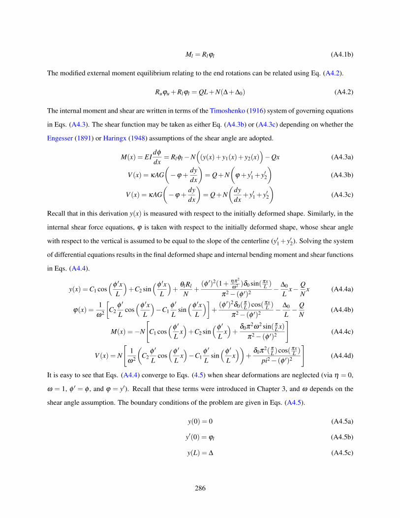
Ml = Rlϕl (A4.1b)

The modified external moment equilibrium relating to the end rotations can be related using Eq. (A4.2).

Ruϕu +Rlϕl = QL+N(∆+∆0) (A4.2)

The internal moment and shear are written in terms of the Timoshenko (1916) system of governing equations

in Eqs. (A4.3). The shear function may be taken as either Eq. (A4.3b) or (A4.3c) depending on whether the

Engesser (1891) or Haringx (1948) assumptions of the shear angle are adopted.

M(x) = EIdφ

dx= Rlφl−N

((y(x)+ y1(x)+ y2(x)

)−Qx (A4.3a)

V (x) = κAG(−ϕ +

dydx

)= Q+N

(ϕ + y′1 + y′2

)(A4.3b)

V (x) = κAG(−ϕ +

dydx

)= Q+N

(dydx

+ y′1 + y′2

)(A4.3c)

Recall that in this derivation y(x) is measured with respect to the initially deformed shape. Similarly, in the

internal shear force equations, ϕ is taken with respect to the initially deformed shape, whose shear angle

with respect to the vertical is assumed to be equal to the slope of the centerline (y′1+y′2). Solving the system

of differential equations results in the final deformed shape and internal bending moment and shear functions

in Eqs. (A4.4).

y(x) =C1 cos(

φ ′xL

)+C2 sin

(φ ′xL

)+

θlRl

N+

(φ ′)2(1+ ηπ2

ω2 )δ0 sin(πxL )

π2− (φ ′)2 − ∆0

Lx− Q

Nx (A4.4a)

ϕ(x) =1

ω2

[C2

φ ′

Lcos(

φ ′xL

)−C1

φ ′

Lsin(

φ ′xL

)]+

(φ ′)2δ0(π

L )cos(πxL )

π2− (φ ′)2 − ∆0

L− Q

N(A4.4b)

M(x) =−N

[C1 cos

(φ ′

Lx)+C2 sin

(φ ′

Lx)+

δ0π2ω2 sin(π

L x)π2− (φ ′)2

](A4.4c)

V (x) = N

[1

ω2

(C2

φ ′

Lcos(

φ ′

Lx)−C1

φ ′

Lsin(

φ ′

Lx))

+δ0π2(π

L )cos(πxL )

pi2− (φ ′)2

](A4.4d)

It is easy to see that Eqs. (A4.4) converge to Eqs. (4.5) when shear deformations are neglected (via η = 0,

ω = 1, φ ′ = φ , and ϕ = y′). Recall that these terms were introduced in Chapter 3, and ω depends on the

shear angle assumption. The boundary conditions of the problem are given in Eqs. (A4.5).

y(0) = 0 (A4.5a)

y′(0) = ϕl (A4.5b)

y(L) = ∆ (A4.5c)

286

y′(L) = ϕu (A4.5d)

As with before, the system of five equations obtained by substituting the four boundary conditions into Eqs.

(A4.4a) and (A4.4b) together with Eq. (A4.2) are then solved linearly for ∆, C1, C2, θl and θu. The upper

end displacement, ∆, is therefore given in Eq. (A4.6a).

∆ =Q+ N∆0

L + Nδ0L χ ′

12EIL3 β ′( 1

1+ζ ′ )(A4.6a)

χ′ =

3(φ ′)3ω2π sinφ ′(ru− rl)

(π2− (φ ′)2)(18rurl−a′3 cosφ ′+(a′1−a′2)φ ′ sinφ ′)

(1

1+ζ ′

)(A4.6b)

where β ′ and ζ ′ are defined previously in Eqs. (3.11a) and (3.11b) specifically to account for the effects of

shear deformations on the lateral stiffness, and χ ′ is the similarly generalized form of χ in Eq. (4.8). In all

cases, it is clear that the effect of shear deformations can be considered by modifying the original versions

of the appropriate terms with the coefficient ω . Shear deformations can be neglected by setting ω = 1,

upon which Eq. (A4.6a) will converge to Eq. (4.7). Finally, similar to the corresponding expression with

neglecting shear deformations, the denominator of Eq. (A4.6a) is the tangent lateral stiffness, ST = ∂∆/∂Q,

of the Timoshenko column derived in Section 3.2.2. Expressions of the integration coefficients, C1 and C2,

are similarly presented in Eqs. (A4.7).[C1

C2

]=

ωL3

φ 3EI

(1

a′1φ ′ sinφ ′+a′2 sinφ ′

)[γ ′

∆,1 γ ′δ ,1

γ ′∆,2 γ ′

δ ,2

][Q+ N∆0

LNδ0

L

](A4.7a)

γ′∆,1 = 9rurl(cosφ

′−1)−3rl(1− ru)φ sinφ (A4.7b)

γ′∆,2 = 9rurl sinφ

′−3ru(1− rl)φ′+3rl(1− ru)φ

′ cosφ′ (A4.7c)

γ′δ ,1 = 3rlφ sinφ

′−9rurl(1+ cosφ′) (A4.7d)

γ′δ ,2 = 3ru(1− rl)φ

′−3rl(1− ru)φ′ cosφ

′−9rurl sinφ′ (A4.7e)

Finally, expressions of the end rotations are given in Eqs (A4.8).[ϕu

ϕl

]=

ωL2

φEI

(1

a′1φ ′ sinφ ′+a′2 sinφ ′

)[γ ′

∆,u γ ′δ ,u

γ ′∆,l γ ′

δ ,l

][Q+ N∆0

LNδ0

L

](A4.8a)

γ′∆,u = 3rl(1− ru)(1− cosφ

′)+(1− ru)(1− rl)φ′ sinφ

′ (A4.8b)

γ′∆,l = 3ru(1− rl)(1− cosφ

′)+(1− ru)(1− rl)φ′ sinφ

′ (A4.8c)

γ′δ ,u =−3rl(1− ru)(1+ cosφ

′)+(1− ru)(1− rl)φ′ sinφ

′ (A4.8d)

γ′δ ,l = 3rl(1− ru)(1+ cosφ

′)− (1− ru)(1− rl)φ′ sinφ

′ (A4.8e)

287

Clearly, the integration coefficients and end rotations are also obtained by adjusting the equations slightly via

the ω coefficient. In conclusion, the effects of shear deformations on the stability analysis of a column, and

subsequently the frame that it is in are the same regardless of whether or not initial imperfections are present

in the columns. Moreover, by observation of Eq. (A4.6a), the relative influence of shear deformations on

lateral stiffness is simply inversely proportional to the upper end displacement of the columns, ∆.

A4.5 Numerical Example with Lateral Loads

This numerical example demonstrates the load-deformation behaviour and variable loading analysis of a

two-bay frame subjected to combined gravity and lateral loading. For this purpose, the presence of initial

imperfections is neglected in this example. In any case, they can easily be represented as lateral loads via

the notional method. The two-bay frame is adapted from Zhuang (2013) and shown in Fig. (A4.2) below.

Figure A4.2: Example two-bay frame subjected to a lateral load

The storey height is 7.315 m and the bays are each 7.315 m wide. The frame contains three columns, with

the exterior columns rigidly connected at the base (rl,1 = rl,3 = 1) and the interior column is semi-rigidly

connected at the base (rl,2 = 0.5). The exterior columns are oriented such that they sway on their weak

axes. As such, the weak axis moments of inertia for the columns are Ic,1 = Ic,3 = 39.9× 106 mm4 and

Ic,2 = 63.8×106 mm4. The moments of inertia for the beams are Ib,1 = Ib,2 = 245×106 mm4. The areas of

the columns are Ac,1 = Ac,3 = 10,100 mm2 and Ac,2 = 11,200 mm2. For the beam-to-column connections,

the exterior connections are rigid (z = 1) while the interior connections are pinned (z = 0). As consistent

288

with Xu (2001), the asymmetric buckling shape is assumed to occur for the beams (vFN = 1) when the frame

is subjected to lateral instability. However, upon further investigation is was found that the results of the

example are independent of the value of vFN . The resulting slenderness ratios of the columns are 116 for

the exterior columns and 97 for the interior column. As such, the columns are in the slenderness range of

inelastic buckling and the tangent modulus model in Eq. (2.13) is assumed, with E0 = 200 GPa. Moreover,

in this slenderness range shear deformations are unlikely to affect the results, and are thus neglected. A rigid

concrete slab is assumed to exist at the upper beam line of the storey, so the upper ends of the columns are

assumed to deform by the same distance.

A4.5.1 Proportional Loading Analysis

The gravity loads, Pi, are assumed to be distributed in proportion to the tributary width of each column such

that P1 = P3 = P and P2 = 2P. Let the lateral load, Q, be proportional to the total gravity load of the frame,

using the relation in Eq. (A4.9) below.

Q = λ

n+1

∑i=1

Pi (A4.9)

In this study, the parameter λ is varied from zero to 20%, which is representative of the typical lateral loading

assumptions used in equivalent static seismic loading analyses (NRC, 2015). To investigate the effects of

the induced axial loads caused by Q, the axial loads, N, were calculated with and without consideration of

the induced axial loads according to Eq. (4.17). The induced axial loads were determined from a first-order

frame analysis, and are given in Eqs. (A4.10). Positive values indicate compression while negative values

indicate tension.

HQ,1 = −0.1715Q (A4.10a)

HQ,2 = 0.0391Q (A4.10b)

HQ,3 = 0.1325Q (A4.10c)

In utilizing Eq. (4.7), the inter-storey displacement in the frame, ∆, is plotted against increasing values of

the base gravity load, P for different values of λ in Fig. (A4.3), with and without the adjustments to the axial

loads via Eqs. (A4.9). The dashed curves in the figure represent the results of the analysis with considering

the induced axial loads caused by Q (denoted ’WH’), whereas the solid lines represent the results of the

analysis with Ni = Pi (denoted ’NH’). Evidently, as λ is increased, representing an increase in the relative

magnitudes of Q for any given load scenario, the inter-storey displacement increases. However, all of the

curves asymptotically approach ∆ = ∞ at Psw = 765.8 kN, corresponding to instability via ΣS = 0. From a

289

Figure A4.3: Inter-storey displacement vs. gravity load in proportional loading case, with and withoutconsidering HQ

stability perspective, the buckling load is 765.8 kN for all the curves, regardless of the magnitude of Q. Thus,

similar to column imperfections, lateral loads, when present in combination with gravity loads, increase

deflections but do not affect the buckling loads. In terms of the excessive inter-storey displacement criterion,

however, the lateral load does significantly affect the capacity of the frame. For example, if ∆∗ = H/100

= 73.2 mm is taken as the failure criterion (corresponding to the NBCC (NRC, 2015) requirement under

seismic loads), then this displacement occurs as early as P = 77.9 kN with λ = 0.1, corresponding to a

89.8% reduction in the capacity when compared to the stability analysis. It can be seen that for this example

the difference between the curves with and without adjustments for the induced axial loads as a result of Q

is not significant. The relative error as a result of neglecting the induced axial loads is plotted in Fig. (A4.4)

for different values of λ . This error is calculated via Eq. (A4.11).

Error = 1− ∆WH −∆NH

∆WH(A4.11)

where ∆WH is calculated with considering the induced axial loads, and ∆NH is calculated with neglecting

the induced axial loads. A positive value indicates the under-estimation of ∆ as a result of neglecting the

induced axial loads. Clearly, the relative error increases as P/Psw approaches unity. As λ increases - that is,

as the relative values of Q increase with respect to the gravity loads, the effect of HQ on the results increases

and the errors become larger. Nevertheless, the error is within only 0.01% for P/Psw < 0.956. Thus, for

sufficiently small lateral loads, if the resulting axial loads from considering both the applied loads and

induced axial loads as a result of HQ can be shown to be sufficiently below the buckling limit, the errors due

290

Figure A4.4: Error due to neglecting the effects of induced axial loads resulting from Q

to neglecting the induced axial loads can be considered to be negligible. Note that this may not be the case

for tall frames, in which the magnitudes of the axial forces in the columns will be increased to counteract the

greater overturning moments caused by the lateral loads. Anyway, when buckling is imminent, the effect of

Q on the axial loads can no longer be neglected when calculating the deformations. However, as is the case

for this example, the deflections are usually extremely large when buckling is imminent and the analysis is

no longer considered to be accurate. Overall, the presence of lateral loads at the top of a frame affects the

deformation of the frame in two ways: (1) directly via Eq. (4.7), and (2) indirectly by inducing axial loads in

the columns which influences β . The first has a significant influence on the frame lateral stiffness, whereas

the second can be neglected for short frames unless buckling is imminent. As such, for the remainder of this

example, the effect of induced axial loads as a result of the lateral load will be neglected in the results.

A4.5.2 Effect of Lateral Bracing

For the purpose of the demonstration, the effects of semi-bracing on the frame are herein investigated. The

value of Kbr affects the value of Psw, which is independent of the imperfections and is plotted in Fig. (A4.5).

Kbr also affects the magnitude of deflection for P < Psw, according to Eq. (4.13).

From Fig. (A4.5), the sway load varies between a minimum value of Psw = 766 kN to a maximum value

of Pu = 1,143 kN, attained only with Kbr = ∞. Unlike that of the four-bay example in Section 4.4.3, which

has lean-on columns, the maximum value corresponding to the braced condition cannot be reached unless

291

Figure A4.5: Effect of Kbr on the buckling load for example two-bay frame, Psw

an infinitely stiff lateral brace is provided. However, if lateral bracing of at least 500 kN/m is provided then

the sway load will be within 99% of Pu and the frame can virtually be treated as fully braced. Pu = 1,143

kN corresponds to the rotational buckling of the interior column (since the load factor is 2, the rotational

buckling load of the interior column is 2,286 kN).

A4.5.3 Variable Loading Analysis - Instability Criterion

The two-bay frame was also analyzed under variable loading according to the minimization problem. No

lateral bracing is assumed to exist, and the same properties of the frame are used as in the proportional

loading example, except that the applied gravity loads are treated as variables. The values of the first-order

lateral stiffness and rotational buckling loads are tabulated in Table A4.1.

Table A4.1: Column properties in variable gravity loading for two-bay frame example

Scenario Col. 1 Col. 2 Col. 3 Storey

First-order lateral stiffness (kN/m) 211.9 48.9 211.9 444777222...777Rotational buckling load, Nu,i (kN) 2,467 2,286 2,467 -

First, the instability condition was used as the failure criterion, corresponding to the minimization problem

in Eqs. (4.18). As the applied lateral load has no theoretical effect on the results of the instability analysis,

the solution is identical to that which would be obtained from the minimization problem originally proposed

by Xu (2001). However, the elastic modulus is empirically modified here to account for inelastic buckling

at high axial loads. The results of the variable loading analysis corresponding to the worst and best case

instability scenarios are shown in Table A4.2.

Based on the results, the loading of the interior column until instability occurs governs the worst case

292

Table A4.2: Worst and best case gravity loading scenario causing instability in lateral loading example

P1 (kN) P2 (kN) P3 (kN) ΣP (kN)

Worst case load, Pi (kN) 0.0 2,228 0.0 222,,,222222888Best case load, Pi (kN) 844.5 1,378 844.5 333,,,000666888

scenario. In the best case scenario, the interior column is not as heavily loaded, and some loading occurs

in the exterior columns, with the same magnitude of load applied to both exterior columns. Note that in the

worst case solution, the interior column is loaded to within 93.7% of its rotational buckling load. In fact, its

tangent elastic modulus at the given load is reduced to 147 GPa, and would decrease further upon additional

loading. In contrast, for the best case scenario the tangent modulus of this column is relatively unaffected

at 199 GPa, making the reduction to the lateral stiffness much less severe at this level of loading. For this

reason, loading the interior column to only 1,378 kN results in a lower reduction to the lateral stiffness

compared to if the same load was applied on an exterior column. In any case, the best case scenario results

is a 37.7% increase in the total load compared to the worst case scenario. The frame can therefore be utilized

more efficiently if loads are proportioned in a similar way to that shown in the best case scenario.

A4.5.4 Variable Loading Analysis - Other Criteria

For each of the other failure criteria, the effect of varying the relative magnitude of the lateral load via λ

on the solutions to the minimization problems was investigated. Note that as column out-of-straightness

imperfections are not present in this model, the maximum deflection in the frame occurs at the top of the

storey, and is equal to ∆. As such, only the analyses related to the excessive inter-storey displacement

corresponding to criterion (b) and the onset of yielding corresponding to criterion (d) are conducted. For

the inter-storey displacement criterion, the total applied gravity loading corresponding to each of the worst

case scenarios with ∆∗ = H/100 are tabulated in Table A4.3. Note that in the absence of both lateral loads

and column imperfections (λ = 0) no deflections occur, and therefore no solution exists to the minimization

problems with λ = 0.

Similar to that of the instability analysis, Table A4.3 shows that the worst case scenario is governed by

loading of only one of the exterior columns. Loads are only shown on Column 1, but can be applied on

Column 3 instead to cause the same inter-storey displacement. As such, the the solution is not unique.

Moreover, the excessive inter-storey displacement criterion results in significant reductions to the minimum

capacity compared to the instability analysis, which has a total load of 2,228 kN. The loading pattern causing

293

Table A4.3: Worst case variable gravity loading analysis corresponding to excessive inter-storey displace-ment with lateral loads for two-bay frame

P1 (kN) P2 (kN) P3 (kN) ΣP (kN)

λ = 0.01 1,546 0.0 0.0 111,,,555444666λ = 0.02 1,091 0.0 0.0 111,,,000999111λ = 0.05 560.6 0.0 0.0 555666000...666λ = 0.10 309.5 0.0 0.0 333000999...555

failure is also different, as the inter-storey displacement failure is governed by the loading of an exterior

column, while the stability failure is governed by the interior column. The best case scenario analyses were

completed with ∆∗ = H/100 and tabulated in Table A4.4.

Table A4.4: Best case variable gravity loading analysis corresponding to excessive inter-storey displacementwith lateral loads for two-bay frame

P1 (kN) P2 (kN) P3 (kN) ΣP (kN)

λ = 0.01 126.0 1,400 126.0 111,,,666555222λ = 0.02 0.0 1,127 0.0 111,,,111222777λ = 0.05 0.0 571.4 0.0 555777111...444λ = 0.10 0.0 312.7 0.0 333111222...777

From the results of Table A4.4, the best case scenario is governed by the loading of the interior column,

sometimes accompanied by equal magnitude loading on both of the exterior columns. For the case of

λ = 0.01, equal loading of 126 kN exists in the exterior columns because increasing the load on the interior

column further would result in a significant decrease to its tangent elastic modulus, and subsequently its

lateral stiffness contribution. As such, if the loading of the interior column is increased then a lower total

load would be required among the columns in the frame to cause the same deflection. This does not occur for

λ = 0.02 and higher, as the elastic modulus of the interior column is not affected with the loads shown. Upon

comparison of Tables A4.3 and A4.4, it can be seen that the difference in total loads in the worst and best

case scenarios decreases as λ increases. The reason for this is that for increasing λ , the relative magnitude

of the lateral load increases, resulting in a larger contribution of Q to the inter-storey displacement. The

relative contribution of the applied gravity loads towards the deflection becomes smaller, resulting in a

smaller difference in the total gravity loads required to reach the failure criterion. In any case, the excessive

inter-storey displacement criterion results in a significant decrease to the maximum capacity of the frame

compared to the instability criterion, which has a maximum case total load of 3,068 kN. The application of

the onset of yielding criterion in the minimization problem via Eq. (4.19c) was also investigated. The total

294

loads in both the worst case and best case scenarios are summarized in Table A4.5 below.

Table A4.5: Variable gravity loading analysis corresponding to onset of yielding with lateral loads fortwo-bay frame

ΣP (Worst Case) ΣP (Best Case) Difference

λ = 0.01 1,631 kN 1,961 kN 16.8%λ = 0.02 1,223 kN 1,447 kN 15.5%λ = 0.05 712.0 kN 798.7 kN 10.9%λ = 0.10 424.2 kN 457.0 kN 7.2%

For all values of λ , the worst case scenario corresponding to onset of yielding is once again governed by

loading of only one of the exterior columns, and the solution is not unique. For the best case scenario

corresponding to the onset of yielding, the solution is governed by heavy loading of the interior column,

accompanied by some equal loading in the exterior columns. Note that no solution exists for λ = 0 because

the columns do not yield before instability occurs. Similar to the case of the analysis pertaining to excessive

inter-storey displacements, the difference in total loading between the best and worst case scenarios de-

creases as λ increases for the same reason. Moreover, it can be seen by observing the results of the analyses

corresponding to all of the failure criteria that the loading of the interior column is much less detrimental

to the deformation analysis than the loading of an exterior column. As such, to maximize the structural

efficiency of the frame, a designer may wish to designate the occupancies of the floor areas closer to the

interior column to have higher loads than the occupancies corresponding to floor areas closer the exterior of

the frame.

295

Appendix A5

Appendix for Frames in Elevated Temperatures

A5.2 Shear and Beam Axial Deformations in Elevated Temperatures

A5.2.1 Parametric Study of Lean-On Frame in Elevated Temperatures

A parametric study was conducted on the effects of shear and beam axial deformations on the lateral stability

of steel frames subjected to elevated temperatures. Particularly, the lean-on frame presented in Section 3.4

and illustrated in Fig. (3.27) was analyzed in elevated temperature conditions using the Eurocode 3 (BSI,

2005) model. The critical total loads, Pcr, of the frame were compared with and without consideration for

shear and/or beam axial deformations. The critical total load is assumed to be equally distributed among

the lean-on columns such that the applied gravity load on each lean-on column is equal to Pcr/n during

buckling. As consistent with Section 3.4.2, the frame has n bays and consists of n lean-on columns (ru = 0

and rl = 0) all supported by a single cantilever column (ru = 0 and rl = 1) in the end bay. The number

of bays n is varied between n = 1 and n = 5. All of the columns are assumed to have the same cross-

section properties (W760×582, I = 8,600× 106 mm4, A = 74,300 mm2), and all of the beams have the

same cross-sectional properties which will be varied using the sizes W100×19, W410×67, W610×174,

W840×392 and W920×784. These beam sizes correspond to cross-sectional areas of 1,630 mm2, 8,600

mm2, 22,200 mm2, 50,000 mm2 and 99,800 mm2, respectively. The slenderness ratios of the columns are

varied between 10 and 60 by changing the height of the storey, while the length of each beam is constant

at 7.315 m. As with all examples in the present study, E0 = 200 GPa and fy,0 = 350 MPa. Since all

of the member sections are I-shaped, κ = 0.44 is appropriately assumed (Cowper, 1966). The Engesser

(1891) assumption of the shear angle is adopted for this analysis. All of the beams are assumed to have

the same temperatures, while the temperatures of the columns are assumed to be kC/B = 0.8 times the

temperatures of the beams. The effects of thermal expansion in the beams is neglected, but otherwise can

be treated as causing initial out-of-plumbness imperfections in the columns, which do not affect the results

of stability analysis as demonstrated throughout Chapter 4. As such, only the beam axial stiffness, EA/L,

affects the results of the stability analysis. The first plot shown in Fig. (A5.1) illustrates the effect of

beam axial deformations on reducing the total critical load, Pcr, in the lean-on frame for different beam

sizes. The reduction is measured as a percentage of the total critical load calculated with neglecting beam

296

axial deformations. The effect of shear deformations is neglected in this figure. Additionally, for this

figure the number of bays is constrained to n = 1 and the slenderness of the columns is constrained to

L/r = 40. Based on the figure, the critical total loads are most severely reduced when the temperatures of

Figure A5.1: Reduction to the total critical load, Pcr, due to axial deformations in elevated temperatures forvarying beam sizes in lean-on frame example

the beams are around 700C. Due to the non-linearity of the material properties in the Eurocode 3 model

with respect to temperature and the selected value of the relative heating ratio kC/B, the effects of beam

axial deformations are more severe at some temperatures than at others. Note that although the percentage

reduction may decrease at higher temperatures between the calculations with and without considering the

beam axial deformations in Fig. (A5.1), the total critical loads still decrease with higher temperatures

overall. Finally, some of the values in the plot show zero percent difference between with and without

considering beam axial deformations. This can occur in two cases: (1) when the yielding of the lean-on

columns at Pcr/n = fyAc governs before sway buckling occurs, due to an instantaneous change in the elastic

moduli of the columns from E0 to zero at low temperatures (commonly known as elastic-perfectly-plastic

behaviour) as stipulated in the Eurocode 3 model (BSI, 2005); (2) when the elastic modulus is reduced so

low that rotational buckling becomes imminent during the instability - that is, the sway load is very close

to the rotational buckling load. Both of these failure modes can occur and are not functions of the beam

axial deformations, and as such, result in zero difference between the results of the total critical loads with

and without considering beam axial deformations. In any case, the effects of beam axial deformations were

297

found to significantly reduce the total critical load by up to 13% by changing the beam section. Also plotting

the value of ς corresponding to the end bay containing the supporting column in Fig. (A5.2) shows very

close relationship between ς and the percentage reductions from Fig. (A5.1). As the value of ς decreases,

Figure A5.2: Plot of ς in elevated temperatures for varying beam sizes in lean-on frame example

the percentage reduction to the total critical loads increases. For this example, the percentage reduction

exceeds 1% if ς is less than about 102. It was also shown in Section 3.4.2 that increasing the number of

bays also causes the effect of beam axial deformations to become more significant. Constraining the beam

size to W410×74 and slenderness of the columns to L/r = 40 while repeating the analysis with varying the

number of bays in the frame yields the plot in Fig. (A5.3). Based on the figure, increasing the number of

bays from n = 1 to n = 5 results in further reductions to the total critical loads when compared to neglecting

beam axial deformations. Note that for n = 1, at higher temperatures approaching 1,200C, yielding of the

lean-on columns governs the failure, resulting in no difference between the critical loads obtained with and

without considering beam axial deformations. For n > 1, however, as the stiffness of the beams approaches

zero towards 1,200C, the critical loads decrease rapidly towards zero using the equivalent spring stiffness

method. Meanwhile, if axial deformations are neglected, this behaviour is completely overlooked. As such,

the reduction to the critical loads due to considering beam axial deformations approaches -100%. However,

it should be noted that although the reductions become more significant if more bays are added to the

298

Figure A5.3: Reduction to the total critical load, Pcr versus number of bays in elevated temperatures forlean-on frame example

frame, the likelihood of a fire spanning the resulting larger area also decreases. Finally, the effect of shear

deformations is investigated by plotting the reductions to the total critical loads in Fig. (A5.4) with shear

deformations considered compared to when they are neglected. This time, axial deformations are neglected

and the number of bays is constrained to n = 5. As the beams are pinned to the columns and beam axial

deformations are neglected, their size does not affect the results of the stability analysis. Based on Fig.

(A5.4), if the columns in the frame have slenderness ratios below 20, then the yielding of the columns

governs the failure (Pcr/n = fyAc) and the results are are not affected by shear deformations. Once again,

this is particular to the Eurocode 3 model (BSI, 2005) which assumes elastic-perfectly-plastic behaviour at

some temperatures. However, when yielding does not govern the failure, the effects of shear deformations

decrease as the slenderness ratio increases. As such, the maximum effect of shear deformations occurs for

this frame at a slenderness ratio of 20, accounting for over 4% in reductions to the total critical loads. Note

that the plot is not sensitive to the member temperatures since the effect of shear deformations is dependent

on the shear flexibility coefficient, η , which as demonstrated in Eq. (A5.1), is relatively insensitive to

temperature via the Poisson’s ratio. As such, the slenderness ratio can still be used to predict the relative

effects of shear deformations on the lateral stiffness of a column.

η(T ) =E(T )I

L2κAG(T )=

2(1+ν(T ))κ

(1

(L/r)2

)(A5.1)

299

Figure A5.4: Reduction to the total critical load, Pcr due to shear deformations in elevated temperatures forvarying column slenderness ratios in lean-on frame example

As shown in Fig. (A5.4), the effects of shear deformations account for approximately 1% reduction to the

total critical load when the slenderness ratio is 40. Overall, the same guidelines suggested in Chapter 3

regarding the significance of shear deformations for columns with low slenderness ratios can therefore be

applied at elevated temperatures. Also, axial deformations may significantly affect the results of the stabil-

ity analysis at elevated temperatures even if they are insignificant during ambient temperature conditions.

Similar to the ambient case, the minimum value of ς in a frame can be used to predict whether axial defor-

mations will have an effect on the critical loads, with a threshold of about 102, and should be checked at

elevated temperatures. Finally, if rotational buckling governs the failure mode then only shear deformations

will affect the results, and if cross-sectional yielding governs the failure mode then neither shear nor axial

deformations will affect the results.

A5.3 Shear and Axial Beam Deformations in Variable Loading Examples

A5.3.1 Two Bay Example in Variable Temperature Loading

The results of the minimization and maximization problems based on the average temperatures of the mem-

bers in the two-bay example of Section 5.3.1, subjected to variable member temperatures, were repeated

for the two-bay examples with considering shear and beam axial deformations. The two considerations are

independent, with shear deformations accounted for via Eq. (5.7b) and beam axial deformations accounted

300

for via application of the equivalent spring stiffness algorithm in Fig. (3.14). As such, their individual ef-

fects on the results are also evaluated. As the slenderness ratios (L/r) of the columns in the frame range

from 37.5 to 64.6, shear deformations can potentially have a minor effect on the results. At ambient tem-

peratures, minimum absolute value of ς in the frame is 959, indicating that beam axial deformations will

not significantly affect the buckling loads at ambient temperatures. However, this value may change at el-

evated temperatures. Particularly, if the beams are heated severely then the stiffness of the beams will be

reduced and can possibly have a greater effect on the critical temperature scenarios. Note that in computing

the lateral stiffness of the frame with considering shear deformations, the Engesser (1891) assumption was

adopted in calculating ω and the shear modulus was calculated based on Eq. (5.12). Overall, the results

were not significantly affected in that the worst case scenario was still governed by heating in only the left

bay, and the best case scenario consisted of equal beam temperatures in both bays. As such, the temperature

of Beam 1 in the worst case scenario is tabulated along with the temperatures of both the beams in the best

case scenario in Table A5.1 with combinations of the shear and axial deformations considered on each row.

From the table it can be seen that the effects of shear and beam axial deformation combined result in only a

Table A5.1: Effects of shear and beam axial deformations on average beam temperatures in variable loadinganalysis results for two-bay frame

Tb,1 in worst case Tb,1 = Tb,2 in best case

Neglecting shear and axial deformations 601.0C 506.4CConsidering axial deformations only 601.0C 506.4CConsidering shear deformations only 598.0C 498.6CConsidering shear and axial deformations 597.9C 498.5C

0.5% decrease to the worst case solution, but also a 1.5% decrease to the best case solution. The reason that

the worst case solution is not as affected is that the interior column is nearer to its rotational buckling load

(P2/Nu,2 = 0.83) during the instability than in the best case solution, in which P2/Nu,2 = 0.71. To obtain

these ratios, Nu is calculated with the temperatures of the members during the given instability scenarios and

before considering shear deformations for simplicity. Column 2 also has a higher slenderness ratio (64.6),

which means that when the solution is governed by rotational buckling of Column 2, both the rotational

buckling load of Column 2 and also the buckling load of the frame will not significantly affected by shear

deformations. Comparatively, the beam axial deformations have a lesser effect on the results than the shear

deformations. The reason for this is that although the axial stiffness of the beams is decreased due to ele-

vated temperatures, the minimum absolute value of the ς indicator is still fairly high during the instability

301

(the minimum value from all the scenarios was 308). If it is reduced further then beam axial deformations

will have a more significant effect on the results. The effects on the solution also depend on whether a

small change of temperature can significantly affect the lateral stiffness of the frame. If the temperatures of

the members in the frame in the worst case scenario were to be held constant with Beam 1 at 601.0C and

the gravity loads are altered proportionally, then the critical gravity loads of the frame will be reduced by

0.4% (from 1,000 kN to 995.9 kN) when considering both shear and axial deformations. Likewise, if the

temperatures of the members in the frame in the best case scenario were held constant with the beams at

506.4C then the critical gravity loads of the frame will be reduced by 1.5% (from 1,000 kN to 985.5 kN)

when considering shear and beam axial deformations. The relative significance of these reductions are sim-

ilar to those obtained by keeping the gravity loads constant and finding the critical temperatures. Overall, as

predicted using the slenderness ratios of the columns, the effect of shear deformations has a small effect on

the results of variable loading analysis for this example. The beam axial deformations did not significantly

affect the results in this example, but if the beams are heated more severely then the effect can be increased.

A5.3.2 Four Bay Example in Variable Temperature Loading

The effects of shear and axial deformations on the results of the minimization problems in the four-bay

example of Section 5.3.2, subjected to variable member temperatures, were investigated. In this example,

the slenderness ratios of the exterior columns are 36.8 while the slenderness ratios of the interior columns

are 71.7. As such, shear deformations in the exterior columns have a small effect on the results. In terms of

the axial deformations, the minimum value of ς at ambient temperatures is 897, indicating that axial defor-

mations can be neglected at ambient temperatures. However, the effects of axial deformations temperatures

can be increased at elevated temperatures. With respect to the consideration of these effects, Table A5.2

shows the average temperatures reported in the solutions to the minimization problems corresponding to

the respective objective functions shown. The effects of shear and axial deformations are neglected for the

reason of simplicity.

Table A5.2: Effects of shear and beam axial deformations on average beam temperatures in variable loadinganalysis results for four-bay frame

Objective function minTb,avg maxTb,avg maxψ minψ

Neglecting shear and axial deformations 119.0C 401.1C 148.1C 400.4CConsidering axial deformations only 119.0C 401.1C 148.1C 400.4CConsidering shear deformations only 118.5C 400.5C 146.6C 400.0CConsidering shear and axial deformations 118.5C 400.4C 146.6C 400.0C

302

Note that the failure modes in each of the scenarios within the same column of the table are consistent.

That is, the rotational buckling of Column 1 governs the most localized fire solution (max ψ), uniform

beam temperatures governs the most distributed fire scenario (min ψ), the heating in Bay 3 only governs the

worst case temperature scenario (min Tb,avg), and the slightly higher temperature in Bay 1 compared to the

other bays which each are heated to the same temperatures governs the best case temperature scenario (max

Tb,avg). As seen in the results of the table, the effect of shear deformations accounts for a 1.0% decrease

to the critical average temperatures in the most localized fire scenario (maxψ). Clearly, axial deformations

have virtually no effect on the solutions. In terms of axial deformations, the minimum absolute value of ς

encountered in all of the scenarios in the tabulated solutions was 253, and even so this value corresponded to

the case governed by rotational buckling of Column 2 in Table 5.9. As discussed previously, when rotational

buckling governs the solution the buckling load is not affected by beam axial deformations. The next lowest

absolute value of ς experienced out of all the scenarios was 788, despite being lower than the value of 897

at ambient temperatures, is still close to the order of 103 and indicates that beam axial deformations would

not have a significant influence on the results.

303

Appendix A6

Appendix for Frames Containing Segmented Members

A6.2 Derivations for Three-Segment Members

A6.2.1 True End Fixity Factors for Three-Segment Timoshenko Members

This appendix provides the derivation of the true end fixity factor of a three-segment Timoshenko (1916)

member. The true end fixity factor, although shown in Section 3.2.8 to be inconvenient and unnecessary, is

also derived for informational purposes only. The shear deformation terms are hence added to Eq. (A6.1) as

follows.

1×θ =∫ L1

0

Mx2

L2E1Idx+

∫ L1+L2

L1

Mx2

L2E2Idx+

∫ L

L1+L2

Mx2

L2E3Idx

+∫ L1

0

ML2κAG1

dx+∫ L1+L2

L1

ML2κAG2

dx+∫ L

L1+L2

ML2κAG3

dx(A6.1)

Integrating and solving for RSS yields Eq. (A6.2).

RSS =Mθ

=3E0I

L

(1

τ(1+3η0τ ′/τ)

)(A6.2a)

τ′ =

L1/Lu1

+L2/L

u2+

L3/Lu3

(A6.2b)

us = Gs/G0; s = 1,2,3 (A6.2c)

where G0 and η0 are the shear modulus and shear flexibility coefficient defined in Eq. (2.19) corresponding

to reference conditions (i.e. ambient temperatures). Similar to the degradation factor for elastic modulus, µ ,

the degradation factor for the shear modulus is defined as us. The true end fixity factor is therefore obtained

via substitution of Eq. (A6.2) into Eq. (6.1) and presented in Eq. (A6.3).

r′ =1

1+ 3E0IRLτ(1+3η0τ ′/τ)

(A6.3)

The original end fixity factors can then be expressed as functions of the true end fixity factors via the

following substitution.

r = r′[

τ +3η0τ ′+ 3E0IRL

(τ +3η0τ ′)(1+ 3EIRL )

](A6.4)

304

A6.2.2 Rotational Stiffness Contribution at Connection of a Three-Segment Beam

The expression for Ri, j for a three-segment beam based on the Timoshenko (1916) system of governing

differential equations shown in Eqs. (A6.5) is presented in this appendix.

−EsIdϕs

dx= ΦNZN +YFx (A6.5a)

κAGs

(−ϕs +

dys

dx

)= YF (A6.5b)

where s corresponds to the near, middle or far segment subscripts. Solving the system of differential equa-

tions for all three segments results in the deformation and shear angle functions in Eqs. (A6.6) and (A6.7),

respectively.

yN(x) =C1 +C2x+YF

κAGNx− ZNΦN

2ENIx2− YF

6ENIx3 (A6.6a)

yM(x) =C3 +C4x+YF

κAGMx− ZNΦN

2EMIx2− YF

6EMIx3 (A6.6b)

yF(x) =C5 +C6x+YF

κAGFx− ZNΦN

2EF Ix2− YF

6EF Ix3 (A6.6c)

ϕN(x) =C2−ZNΦN

ENIx− YF

2ENIx2 (A6.7a)

ϕM(x) =C4−ZNΦN

EMIx− YF

2EMIx2 (A6.7b)

ϕF(x) =C6−ZNΦN

EF Ix− YF

2EF Ix2 (A6.7c)

The boundary and compatibility conditions are given as follows.

yN(0) = yN (A6.8a)

yF(L) = yF (A6.8b)

ϕN(0) = θN−ΦN (A6.8c)

ϕF(L) = θF −ΦF (A6.8d)

yN(LN) = yM(LN) (A6.8e)

yM(LN +LM) = yF(LN +LM) (A6.8f)

ϕN(LN) = ϕM(LN) (A6.8g)

ϕM(LN +LM) = ϕF(LN +LM) (A6.8h)

305

Finally Eq. (A6.9) is an additional compatibility condition necessary in the solution, and external equilib-

rium is provided in Eq. (A6.10).

L = LN +LM +LF (A6.9)

.ΦNZN +ΦFZF +YFL = 0 (A6.10)

Solving the system of ten linear equations formed by Eqs. (A6.8), (A6.9) and (A6.10) for the variables

θN ,θF ,YF ,C1,C2,C3,C4,C5,C6,L2 and applying Eq. (3.28) yields the result of R′i, j in Eq. (A6.11).

R′i, j =MN

θN=

6E0IL

[2γ ′NzN + vFNλ ′NF,vzNzF −wFNγ ′NF,w

4λ ′A + zNλ ′B + zFλ ′C− zNzFλ ′D

](A6.11)

where all of the coefficients marked with the symbol (′) are modified forms of the unmarked versions, as

shown in Eqs. (A6.12). In other words, Eq. (A6.11) is similar to Eq. (6.25) except that the coefficients are

replaced with the marked versions to account for shear deformations.

γ′N = τF(1− zF)µN µMµF +λ

′NN (A6.12a)

γ′NF,w = γNF,w (A6.12b)

λ′NN = λNN + γ

′1 (A6.12c)

λ′NF,v = λNF,v−2γ

′1 (A6.12d)

λ′A = λA (A6.12e)

λ′B = 4τF(κ

′N− τN µN µMµF) (A6.12f)

λ′C = 4τN(κ

′F − τN µN µMµF) (A6.12g)

λ′D = λD− γ

′2 (A6.12h)

κ′N = κN + γ

′1 (A6.12i)

κ′F = κF + γ

′1 (A6.12j)

γ′1 = 3η0µN µMµF

1L

(LN

µN+

LM

µM+

LF

µF

)(A6.12k)

γ′2 =36η0µN µMµF

1L2

(L2

N

µNuN+

L2M

µMuM+

L2F

µFuF+ ...

LNLF

µNuF+

LNLF

µFuN+

LNLM

µNuM+

LNLM

µMuN+

LMLF

µMuF+

LMLF

µFuM

) (A6.12l)

As such, in order to consider the effects of shear deformations in the expression of equivalent rotational

stiffness proivded by a beam connected to the end of a column, Ri, j, some of the coefficients in Eq. (6.25)

can simply be adjusted via the reference shear flexibility coefficient η0 and shear modulus degradation

306

factors, us.

A6.2.4 Frame Stability with Three-Segment Timoshenko Members

If the Euler-Bernoulli governing differential equations are replaced with the Timoshenko (1916) governing

differential equations the the internal bending moment and shear in each segment s can be expressed via

Eqs. (A6.13).

EsIdϕs

dx= Ml−N(y0(x)+ ys(x))−Qx; xs ≤ x≤ xs+1 (A6.13a)

κAGs

(−ϕ +

dydx

)= Q

(ϕ or

dydx

); xs ≤ x≤ xs+1 (A6.13b)

The shear angles ϕ and dy/dx correspond to the Engesser (1891) and Haringx (1948) assumptions, respec-

tively. As consistent with the other derivations in this study, it will be assumed that the rotational stiffness

of the end connections of the column is linear to the shear angle via Eq. (3.3). Continuity in the shear angle

at the interface between adjacent segments is also assumed. As such, the same boundary and compatibil-

ity equations as Eqs. (6.36) apply but with y′ replaced with ϕ . In following the same solving procedure,

expressions for the upper end displacement and tangent lateral stiffness ST are given in Eq. (A6.14). The

expression for ST in Eq. (6.41) can therefore be replaced with Eq. (A6.14b)

∆ =Q+ N∆0

Lc

S′T(A6.14a)

S′T =12E0Ic

L3c

( β ′3©1+ζ ′3©

)(A6.14b)

where the term β ′3©/(1+ζ ′3©) is analogous to the β ′/(1+ζ ′) term in Eq. (3.10) but now applies for three

segment columns and is given in Eq. (A6.15).

β ′3©1+ζ ′3©

=φ 2

012

[9rlruα ′2 +φ 4

0 τlτu(1− rl)(1− ru)α′1−3φ 2

0 α ′69rurl(α

′5−α ′2)+3φ 2

0 α ′7−φ 40 τlτu(1− rl)(1− ru)α ′1

](A6.15a)

α′1 = f ′(φ 2

m)− f ′(φlφm)− f ′(φmφu)− f ′(φlφu) (A6.15b)

α′2 = f ′(φ 2

l φmφu)+ f ′(φlφ2mφu)+ f ′(φlφmφ

2u )− f ′(φ 2

l φ2u ) (A6.15c)

α′3 = f ′(φ 2

l φm)+ f ′(φlφ2m)+ f ′(φ 2

l φu)− f ′(φlφmφu) (A6.15d)

α′4 = f ′(φmφ

2u )+ f ′(φ 2

mφu)+ f ′(φlφ2u )− f ′(φlφmφu) (A6.15e)

α′5 = α

′3 +α

′4 +2φlφmφuωlωmωu (A6.15f)

α′6 = rl(1− ru)τuα

′3 + ru(1− rl)τlα

′4 (A6.15g)

307

α′7 = rl(1− ru)τu(α

′3−α

′1)+ ru(1− rl)τl(α

′4−α

′1) (A6.15h)

where f ′ is the function given in Eq. (A6.16) for a,b,c ∈ 0,1,2.

f ′(φ a1 φ

b2 φ

c3 ) =φ

a1 φ

b2 φ

c3 ω

2−a1 ω

2−b2 ω

2−c3 × ...

C1′mod(a,2)C2

′mod(b,2)C′mod(c,2)3 × ...

S1′mod(a+1,2)S2

′mod(b+1,2)S3′mod(c+1,2)

(A6.16)

In this way, the lateral stiffness of a column with three segments can be calculated with considering shear

deformations, and equation is similar to the one without considering shear deformations except that the α ,

S and C coefficients are replaced with the marked versions which are functions of ω in each segment of the

column given in Eqs. (A6.17).

S′s = sin(

ωsφsLs

Lc

)(A6.17a)

C′s = cos(

ωsφsLs

Lc

)(A6.17b)

ωs =√

1+φ 2s ηs or

1√1−φ 2

s ηs(A6.17c)

ηs =EsI

L2cκAGs

(A6.17d)

where s is the segment subscript. All other terms are previously defined in the derivation for Euler-Bernoulli

members. The first and second terms in Eq. (A6.17c) correspond to the Engesser (1891) and Haringx (1948)

assumptions of the shear angle, respectively.

A6.2.5 Rotational Buckling Load of a Three-Segment Timoshenko Column

The derivation of the equations required to determine the rotational buckling load in Section 6.2.6 was

repeated using a Timoshenko (1916) column with following the same procedure as Hoblit (1951). In doing

so, the governing internal bending moment and shear functions are given as follows.

EsIcdϕ

dx=−N

(z(x)− z(xs)

)+M(xs)+V (x); xs ≤ x≤ xs +Ls (A6.18a)

−κAGs

(−ϕ +

dzdx

)=V −N

(ϕ or

dzdx

); xs ≤ x≤ xs +Ls (A6.18b)

where xs is the x-ordinate of the lower interface of segment s. Based on the solution to the governing system

of differential equations, the corresponding system of thirteen equations to be solved for N = Nu is listed as

308

follows.

z(Ll) = z(0)+M(0)

N(1−C′l)+

(ϕ(0)−V/N)ω2l

φ ′l /LcS′l +

V Ll

N(A6.19a)

z(Ll +Lm) = z(Ll)+M(Ll)

N(1−C′m)+

(ϕ(Ll)−V/N)ω2m

φ ′m/LcS′m +

V Lm

N(A6.19b)

z(Lc) = z(Ll +Lm)+M(Lm)

N(1−C′u)+

(ϕ(Lm)−V/N)ω2u

φ ′u/LcS′u +

V Lu

N(A6.19c)

ϕ(Ll) =M(0)

N

(φ ′l

ω2l Lc

)S′l +

(ϕ(0)− V

N

)C′l +

VN

(A6.19d)

ϕ(Ll +Lm) =M(Ll)

N

(φ ′m

ω2mLc

)S′m +

(ϕ(Ll)−

VN

)C′m +

VN

(A6.19e)

ϕ(Lc) =M(Ll +Lm)

N

(φ ′u

ω2u Lc

)S′u +

(ϕ(Ll +Lm)−

VN

)C′u +

VN

(A6.19f)

M(Ll) = M(0)C′l−(

ϕ(0)− VN

)Nω2

l Lc

φ ′lS′l (A6.19g)

M(Ll +Lm) = M(Ll)C′m−(

ϕ(Ll)−VN

)Nω2

mLc

φ ′mS′m (A6.19h)

M(Lc) = M(Ll +Lm)C′u−(

ϕ(Ll +Lm)−VN

)Nω2

u Lc

φ ′uS′u (A6.19i)

z(0) = 0 (A6.19j)

z(Lc) = 0 (A6.19k)

M(0) = +Rlϕ(0) (A6.19l)

M(Lc) =−Ruϕ(Lc) (A6.19m)

The system of equations in Eq. (A6.19) appears very similar to that of the Euler-Bernoulli solution, and is

also non-linear in N. The trigonometric S′ and C′ coefficients are given in Eq. (A6.17). In order to facilitate

the root-finding solution for N, the shear V was solved in a similar manner and is presented below.

V =1

ω2l

[ξ ′1Rl +ξ ′2LcN

ξ ′3Lc

]θl (A6.20a)

ξ′1 = φ

′l φ′mφ′u(1−C′lC

′mC′u)+φ

′l (φ′m)

2C′lS′mS′u +(φ ′l )

2φ′mS′lC

′mS′u +(φ ′l )

2φ′uS′lS

′mC′u (A6.20b)

ξ′2 = φ

′l φ′mC′lC

′mS′u +φ

′l φ′uC′lS

′mC′u +φ

′mφ′uS′lC

′mC′u− (φ ′m)

2S′lS′mS′u (A6.20c)

ξ′3 = φ

′l φ′mC′lC

′mS′u +φ

′l φ′uC′lS

′mC′u +φ

′mφ′uS′lC

′mC′u−φ

′l φ′mφ′u− (φ ′m)

2S′lS′mS′u (A6.20d)

The same computational procedure presented in the previous subsection can thus be used to solve for Nu

where shear deformations are considered.

309

A6.6 Derivations for n-segment Members

The proposed method for modelling frames with three-segments is conceptually extended towards frames

with n segments via the derivations in this appendix. The general derivational procedures from Section 6.2

for determining the end fixity factors, thermal restraint forces, deformation, lateral stiffness, and rotational

buckling loads of n-segment members are briefly presented in this section.

A6.6.1 End Fixity Factors for n-segment Members

Similar to the cases of the two- and three-segment members, the end fixity factors of a member containing

n segments can be derived using the principle of virtual work. To determine RSS, a simply-supported n-

segment member is shown in Fig. (A6.1).

Figure A6.1: Equivalent simply-supported n-segment member subjected to end moment

As with the derivation for three segments in Section 6.2.1, let the elastic modulus in each segment, s, be

some fraction µs of a reference modulus, E0. That is, Es = µsE0. Applying the principle of virtual work at

the location of the end moment, M, on the end A of the member results in Eq. (A6.21).

1×θ =n

∑s=1

[∫ xs+Ls

xs

Mx2

L2EsIdx

]+

n

∑s=1

[∫ xs+Ls

xs

ML2κAGs

dx

](A6.21)

where xs is the x-coordinate of the left end of the segment s measured from the left end of the beam, and

Ls is the length of the segment. The first term corresponds to flexural deformations, while the second term

corresponds to shear deformations. The first term corresponds to flexural deformations, while the second

term corresponds to shear deformations. The resulting value of RSS is generally expressed in Eq. (A6.22).

RSS =Mθ

=3E0I

L

(1

τn(1+3η0τ ′n/τn)

)(A6.22a)

τ′n =

n

∑s=1

Ls/Lus

(A6.22b)

where τn and τ ′n are adjustment factors that account for the non-uniformity of the elastic and shear modulus

of the n-segment member, respectively, and us is the shear modulus degradation factor defined in Eq. (A6.2).

Note that τ1 = 1, an expression of τ2 is provided in Zhuang (2013), and τ3 is given in Eq. (6.4a). Of course, τ2

310

can be obtained by simply substituting the properties of two adjacent segments to be equal in τ3. Expressions

for n > 3 are too complicated to express in closed form, but can be obtained from direct substitution of θ

from Eq. (A6.21) into Eq. (A6.22). Note also that the integration from Eq. (A6.21) is linear in M, which

means that M/θ can be simplified to Eq. (A6.23).

RSS =Mθ

=

n

∑s=1

[∫ xs+Ls

xs

x2

L2EsIdx

]+

n

∑s=1

[∫ xs+Ls

xs

1L2κAGs

dx

]−1

(A6.23)

Regardless of how many segments are present in the member, the end fixity factors can then be calculated

using Eq. (6.1).

A6.6.2 Calculation of Column End Fixity Factors with n Segments

As discussed in Section 6.2.2, the where no other members contribute to the rotational stiffness of the end

connection of a column, the end fixity factor at the corresponding end of an n-segment column is given in

Eq. (A6.24).

r =r0kZτn

1− r0(1− kZτn)(A6.24)

If the end of the column is connected to beams, then the effective rotational stiffness of the beam at the

joint must be calculated. This can be accomplished by following the conjugate beam method in the same

derivational procedure as in Section 6.2.2. Consider therefore the n-segment beam in Fig. (A6.2), which is

similar to Fig. (6.4) but contains n segments.

Figure A6.2: Equivalent simply-supported n-segment member subjected to end moment

The near and far ends are once again denoted by the subscripts N and F , while the properties of the segments

are numbered from 1 to n starting from the near end. The physical meanings of the variables were explained

in Section 6.2.2. The length of the member is the sum of the lengths of the segments according to Eq.

311

(A6.25).

L =n

∑k=1

Lk (A6.25)

As demonstrated previously and repeated below, the internal bending moment and shear functions can be

expressed via Eq. (A6.26).

−EsIdϕs

dx= ΦNZN +YFx ∀s ∈ 1,2, ...,n (A6.26a)

κAGs

(−ϕs +

dys

dx

)= YF ∀s ∈ 1,2, ...,n (A6.26b)

where x is measured from the end of the member at segment s = 1. Eq. (A6.26) refers to the Timoshenko

(1916) system of governing differential equations, which can be simplified to the Euler-Bernoulli equation

via ϕs = dys/dx and removing Eq.( A6.26b). Assuming that no transverse loads are applied on the beams

between the supports (q(x) = 0), the external equilibrium is given in Eq. (A6.10), and is identical to Eq.

(A6.10).

.ΦNZN +ΦFZF +YFL = 0 (A6.27)

The general solutions of the deformation and shear angle functions can be obtained from solving the system

of differential equations in Eqs. (A6.26) for each segment, shown below.

ys(x) =C2s−1 +C2sx+YF

κAGsx− ZNΦN

2EsIx2− YF

6EsIx3; ∀s ∈ 1,2, ...,n (A6.28a)

ϕs(x) =C2s−ZNΦN

EsIx− YF

2EsIx2; ∀s ∈ 1,2, ...,n (A6.28b)

where the C symbols are integration coefficients. Let the starting coordinate of each segment be defined as

follows.

xs =s−1

∑k=1

Lk (A6.29)

The applicable system of (2n+2) boundary conditions corresponding to the displacements and rotations at

the ends of the member as well as the continuity of deflection and slope between adjoining segments are

listed below.

y1(0) = yN (A6.30a)

yn(L) = yF (A6.30b)

ϕ1(0) = θN−ΦN (A6.30c)

ϕn(L) = θF −ΦF (A6.30d)

ys(xs+1) = ys+1(xs+1); ∀s ∈ 1,2, ...,n−1 (A6.30e)

312

ϕs(xs+1) = ϕs+1(xs+1); ∀s ∈ 1,2, ...,n−1 (A6.30f)

Note that if shear deformations are neglected, then ϕ = dy/dx. Solving the system of (2n + 4) linear

equations formed by Eqs. (A6.30), (A6.25) and (A6.27) for the (2n + 4) variables θN , θF , YF , Ln and

C1,C2, ...,C2n−1,C2n and then applying Eq. (3.28) yields the general result of R′i, j in Eq. (A6.31). To

be clear, R′i, j is the rotational stiffness supplied to the end of a column connected to the near end of the

n-segment beam.

R′i, j =MN

θN= f (vFN ,wFN ,zN ,zF ,E0, I,κ,A,G0,µµµ,uuu,τττ,LLL) (A6.31)

where µµµ , uuu, τττ and LLL contain all of the values µs, us, τs, and Ls of the segments, respectively. The ratio of end

rotations, vFN = θF/θN , needs to be assumed and is related to the buckling mode, as discussed in Xu and

Liu (2002a). The ratio of chord rotation to the near end rotation, wFN , can be assumed to be zero for beams,

and is discussed further in Chapter 7 for columns in multistorey frames. If shear deformations are neglected

then R′i, j will be a function of the following variables.

R′i, j =MN

θN= f (vFN ,wFN ,zN ,zF ,µµµ,τττ,LLL,E0, I) (A6.32)

A6.6.3 Thermal Restraints for n-segment Members

To determine the thermal restraint force on an n-segment column, the same derivational procedure of

(Zhuang, 2013) and Section 6.2.3 is followed. The axial load of an n-segment column can be expressed

as Eq. (A6.33), which is identical to Eq. (6.26).

Pi + ki(εiLc,i) =−σAc,i = Ni (A6.33)

where σ is the internal normal stress in the column, Ac,i is the area of the column, εi is the total shortening

strain of the column, and ki is vertical stiffness of the column. The effects of differential axial shortening

between the columns in the same storey are once again ignored for the reason of simplicity. The mechanical

elastic strain, εe, and thermal strain, εT , are expressed in Eq. A6.34.

εe =n

∑s=1

[σ

Es− σ

E0

](A6.34a)

εT =n

∑s=1

[∫ Ts

T0

α(T )dT

](A6.34b)

313

where Ts is the temperature of the segment s and α(T ) is given in Eq. (5.4). Substituting this into Eq.

(A6.33) and solving for the axial force Ni for some column i results in Eq. (A6.35) below.

Ni = Pi +HT,i =Pi +S⊥,iΨT,i

1+ S⊥,iLc,iAc,iEeq,i

(A6.35)

where ΨT,i is the total thermal shortening of the column given by Eq. (A6.36), and Eeq,i is the pseudo elastic

modulus of the column for the purposes of calculating elastic thermal restraints given in reciprocal form by

Eq. (A6.37).

ΨT,i =n

∑s=1

[Ls

∫ Ts

T0

α(T )dT

](A6.36)

1Eeq,i

=1

E0

[( n

∑s=1

Ls

Lcµs

)−1]

(A6.37)

As such, the resulting expression of the axial force for an n-segment is very similar to and generalizes the

one for three segments in Eq. (6.26). As with before, the vertical stiffness S⊥,i may be taken as the sum of

transverse stiffness of the restraining beams.

A6.6.4 Frame Stability with n-segment Members

A set of equations used to solve for the deformation and lateral stiffness of an n-segment column (and

equivalently, the transverse stiffness of a beam used to determine ki), is derived in this section. Consider the

n-segment column shown in Fig. (A6.3), which is similar to the one in Fig. (6.5).

As consistent with the derivation in Section 6.2.4, the column contains a linearly varying out-of-plumbness

function y0(x) given in Eq. (6.31). The end moments Mu and Ml are also assumed to be linear functions

of the end rotation via Eqs. (6.34). For Timoshenko (1916) columns the end rotation is ϕ , while for Euler-

Bernoulli columns ϕ = dy/dx = θ . As such, the general external moment equation for the column can be

written as follows.

Ruϕu +Rlϕl = QLc +N(∆0 +∆) (A6.38)

The generalized system of differential equations in Eqs. (A6.39) is provided for internal equilibrium within

any segment s in the column.

EsIcdϕs

dx= Rlϕl−N(y0(x)+ ys(x))−Qx; xs ≤ x≤ xs+1; ∀s ∈ 1,2, ...,n (A6.39a)

κAGs

(−ϕ +

dydx

)= Q

(ϕ or

dydx

); xs ≤ x≤ xs +Ls; ∀s ∈ 1,2, ...,n (A6.39b)

Note setting ϕs = dys/dx and removing the second equation results in the Euler-Bernoulli equation. The

314

Figure A6.3: Free-Body Diagram of an n-segment Column with Initial Out-of-Plumbness

system of differential equations in Eqs. (A6.39) can be solved individually for each segment, and then

combined using the boundary and compatibility equations in Eqs. (A6.40), in addition to satisfying external

equilibrium from Eq. (A6.38).

y1(0) = 0 (A6.40a)

yn(Lc) = ∆ (A6.40b)

ϕ1(0) = ϕl (A6.40c)

ϕn(Lc) = ϕu (A6.40d)

ys(xs+1) = ys+1(xs+1); ∀s ∈ 1,2, ...,n−1 (A6.40e)

ϕs(xs+1) = ϕs+1(xs+1); ∀s ∈ 1,2, ...,n−1 (A6.40f)

Note that in solving the internal moment equations for ys(x), each set of internal bending momenta and

shear equations will generate two integration coefficients, thus introducing 2n unknowns to the system of

equations. The final system of (2n+ 3) equations comprising of Eqs. (A6.40) and (A6.38) is linear with

respect to the 2n integration coefficients, ∆, θl and θu. As such, These (2n+ 3) unknowns can be solved

315

as expressions of all of the other variables. As such, the inter-storey displacement, ∆, and tangent lateral

stiffness, ST , of a column with n-segments can be expressed in its most general form via Eqs. (A6.41).

∆ = f (Q,N,∆0,Lc,E0, Ic,κ,Ac,G0,ru,rl,τu,τl,φ0,µµµ,uuu,LLL) (A6.41a)

ST =∂∆

∂Q=

12E0IL3

c

(β ′n©

1+ζ ′n©

)(A6.41b)

β ′n©1+ζ ′n©

= f (ru,rl,τu,τl,φφφ ,ωωω) (A6.41c)

where φφφ and ωωω refer to all the values of φs and ωs, respectively. For the cases of n ≤ 3, the tangent lateral

stiffness ST has been shown to be independent of Q and ∆0, meaning that the tangent lateral stiffness, and

therefore the stability analysis, is independent of the lateral loads and imperfections. It has also been shown

that for n≤ 3, the upper end lateral displacement, ∆, is equal to the sum of Q and the notional load, together

divided by the tangent lateral stiffness. From a conceptual standpoint, the same would be expected for

n > 3 but has not been confirmed. Finally, the lateral stiffness of a storey frame containing members with n

segments and neglecting beam axial deformations can be taken as the sum of ST plus the total lateral bracing

Kbr in the storey. If beam axial deformations are considered then the equivalent spring stiffness approach

described in Section 3.3.2 can be utilized. Finally, if shear deformations are neglected then the general

solution will take the form of Eq. (A6.42).

∆ = f (Q,N,∆0,Lc,E0, Ic,ru,rl,τu,τl,φ0,µµµ,LLL) (A6.42a)

ST =∂∆

∂Q=

12E0IL3

cβ n© (A6.42b)

β n© = f (ru,rl,τu,τl,φφφ) (A6.42c)

A6.6.5 Individual n-segment Column Rotational Buckling Load

To determine the individual rotational buckling load of an n-segment member, the method of Hoblit (1951)

described in Section 6.2.6 is once again utilized.

By once again assuming that no transverse loads are applied on the column between supports, the internal

shear force V is constant throughout the length of the column. The buckling load of the column is Nu and

the end moments from the semi-rigid connections are Ml and Mu. The expression relating to the external

equilibrium of moments is given in Eq. (A6.43).

Ml +Mu +V Lc = 0 (A6.43)

316

Figure A6.4: Buckled Shape of an n-segment Column

The internal bending moment and shear in each segment, s, can be expressed in Eq. (A6.44). These are

expressed for a Timoshenko (1916) but can be simplified to the Euler-Bernoulli equation via ϕ = dy/dx and

neglecting the second equation.

EsIcdϕ

dx=−N

(z(x)− z(xs)

)+M(xs)+V (x); xs ≤ x≤ xs +Ls (A6.44a)

−κAGs

(−ϕ +

dzdx

)=V −N

(ϕ or

dzdx

); xs ≤ x≤ xs +Ls (A6.44b)

With following the derivational procedure of Hoblit (1951), the expressions of the deflection z(x), rotation

z′(x), and bending moment M(x) can be evaluated at the endpoints of each segment (s ∈ 1,2, ...,n) in the

member according to Eqs. (A6.45).

z(xs +Ls) = z(xs)+M(xs)

N(1−C′s)+

(ϕ(xs)−V/N)ω2s

φ ′s/LcS′s +

V Ls

N(A6.45a)

ϕ(xs +Ls) =M(xs)

N

(φ ′s

ω2s Lc

)S′s +

(ϕ(xs)−

VN

)C′s +

VN

(A6.45b)

M(xs +Ls) = M(xs)C′s−(

ϕ(xs)−VN

)Nω2

s Lc

φ ′sS′s (A6.45c)

where the coefficients S and C are given in Eqs. (A6.46a) and (A6.46b), respectively, and φs is the modified

axial load coefficient given in Eq. (A6.46c).

S′s = sin(

φ ′sLs

Lc

)(A6.46a)

317

C′s = cos(

φ ′sLs

Lc

)(A6.46b)

φ′s =

ωsφ0√µs

(A6.46c)

In total, Eqs. (A6.45) contains 3n equations. The boundary conditions in Eqs. (A6.47) need to be satisfied

in order to achieve the buckling shape of the column. Note that these are identical to Eqs. (6.54).

z(0) = 0 (A6.47a)

z(Lc) = 0 (A6.47b)

M(0) = +Rlϕ(0) (A6.47c)

M(Lc) =−Ruϕ(Lc) (A6.47d)

Once again, an arbitrary value of ϕ(0) may be assumed in the analysis, since any value of the bottom end

rotation can satisfy equilibrium in the buckling configuration. The only exception to this is that if the bottom

end of the column is fixed, then z′(0) = 0 must be taken. To solve for Nu, the system of (3n+4) equations

comprising of Eqs. (A6.45) and the boundary conditions in Eqs. (A6.47) needs to be solved. As with the

case of n = 3 explained in Section 6.2.6, it is best to first express the shear, V , as a linear function of N, along

with the other known properties of the column. This can be done by solving for V with the system of (3n+3)

equations consisting of the aforementioned system but excluding Eq. (A6.47d). Once this is accomplished,

the value of N = Nu can be iterated via root-finding methods until Eq. (A6.47d) is satisfied. The minimum

positive value of N = Nu obtained from this procedure therefore corresponds to the fundamental rotational

buckling mode of the n-segment column.

318

Appendix A7

Appendix for Multistorey Frame Stability

A7.2 Derivations for Member in Multistorey Frames

A7.2.1 Rotational Stiffness Contribution with Second-Order Effects

The derivation of the rotational stiffness contribution of a member with considering the effects of axial

loads in Section 7.2.1 is continued for a Timoshenko (1916) member as follows. First, it is noted that if the

Timoshenko (1916) governing differential equations are used instead of the Euler-Bernoulli equation in Eq.

(7.3), then Eq. (7.3) can be replaced with Eq. (A7.1a) and either Eq. (A7.1b) or Eq. (A7.1c), depending on

whether the Engesser (1891) or Haringx (1948) assumptions on the shear angle are adopted.

M(x) =−EIdϕ

dx= N(y(x)− yA)+MA−YAx (A7.1a)

V (x) = κAG(−ϕ +

dydx

)=−YA +Nϕ (A7.1b)

V (x) = κAG(−ϕ +

dydx

)=−YA +N

dydx

(A7.1c)

The solution to the resulting system of governing differential equations is given in Eq. (A7.2).

y(x) = yA−ΦAZA

N− YB

Nx+C1 cos

(ωφ

Lx)+C2 sin

(ωφ

Lx)

(A7.2a)

ϕ(x) =−YB

N+

φ

ωL

[C2 cos

(ωφ

Lx)−C1 sin

(ωφ

Lx)]

(A7.2b)

Applying the same boundary conditions in Eqs. (7.5), solving for the same variables and expressing the end

moments MA and MB in matrix form via Eq. (7.6) results in the following expression of R′A.

R′A =3EIzAφ ′

L

[(1− zB)(φ

′)2 sinφ ′(1+Γ1−wBA)+3zBΘ′

18zAzB +(a′1−a′2)φ ′ sinφ ′−a′3 cosφ ′

][1

1+ζ ′

](A7.3a)

Θ′ = sinφ

′(1+Γ1− vBA(1+Γ2))−φ′ cosφ

′(1+Γ1−wBA)+φ′(vBA(1+Γ2)−wBA) (A7.3b)

Γ1 = (ω2−1)[

3rB sinφ ′

(1− zB)(φ ′)2 sinφ ′+3zB(sinφ ′−φ ′ cosφ ′)

](A7.3c)

Γ2 = (ω2−1)[

sinφ ′

sinφ ′−φ ′

](A7.3d)

The expression is similar to Eq. (7.7) except that φ is replaced with φ ′ = ωφ , and some new shear-related

terms, Γ1 and Γ2, are introduced, and the familiar 1/(1+ζ ′) factor appears again. The ω factor is given in

Eqs. (3.8) and depends on the shear angle assumption. Of course, when shear deformations are neglected

319

(η = 0), Eq. (A7.3) converges to Eq. (7.7). Also, in the absence of axial loading (φ → 0), Eq. (A7.3)

converges to Eq. (3.29).

A7.2.3 Derivation of Shape Coefficients

Exact expressions of the shape coefficients in Eq. (7.10) with considering the effects of axial forces are

herein derived. Consider first the deformed shape of the semi-rigidly connected column in Fig. (A7.1)

resulting from the axial load N and an arbitrary lateral load Q applied at the upper end of the column.

Figure A7.1: Semi-rigidly connected column subjected to axial and lateral load

By applying the external equilibrium of forces and moments, the following relation can be obtained.

Ml +Mu = N∆+QL (A7.4)

A7.2.3.(a) Without Shear Deformations

With assuming that the semi-rigid connections behave linearly, the end moments Ml and Mu are given in Eq.

(A7.5).

Ml = θlRl (A7.5a)

Mu = θuRu (A7.5b)

320

The internal bending moment is expressed via the Euler-Bernoulli equation in Eq. (A7.6). In doing so, shear

deformations are neglected until the end of this section.

−EId2ydx2 =−Ml +Qx+Ny (A7.6)

Substituting Eq. (A7.5a) into Eq. (A7.6) and solving the differential equation for y yields Eq. (A7.7).

y(x) =C1 cos(

φ

Lx)+C2 sin

(φ

Lx)+

θlRl

N− Q

Nx (A7.7)

There are four boundary conditions for Eq. (A7.7), which are listed in Eqs. (A7.8).

y(0) = 0 (A7.8a)

y(L) = ∆ (A7.8b)

y′(0) = θl (A7.8c)

y′(L) = θu (A7.8d)

Substituting Eqs. (A7.8) into Eq. (A7.7) and Eqs. (A7.5) into Eq. (A7.4) provides five equations which

can be used to solve for the variables ∆, θl , θu, C1 and C2 in terms of all other variables. The resulting

expressions for ∆, θl and θu are thus presented in Eqs. (A7.9).

∆ =QL3

φ 3EI

[18rlru−a3 cosφ +(a1−a2)φ sinφ

a1φ cosφ +a2 sinφ

](A7.9a)

θu =QL2(1− ru)

φEI

[(1− rl)φ sinφ +3rl(1− cosφ)

a1φ cosφ +a2 sinφ

](A7.9b)

θl =QL2(1− rl)

φEI

[(1− ru)φ sinφ +3ru(1− cosφ)

a1φ cosφ +a2 sinφ

](A7.9c)

The shape coefficients v and w can therefore be expressed via Eq. (A7.15) as follows.

vul =θu

θl=

[1− ru

1− rl

][(1− rl)φ sinφ +3rl(1− cosφ)

(1− ru)φ sinφ +3ru(1− cosφ)

](A7.10a)

vlu =θl

θu=

1vul

(A7.10b)

wul =∆

Lθl=

18rlru−a3 cosφ +(a1−a2)φ sinφ

φ 2(1− rl)[(1− ru)φ sinφ +3ru(1− cosφ)

] (A7.10c)

wlu =∆

Lθu=

wul

vul(A7.10d)

Note that Eq. (A7.15) is valid as long as the connection rotation is zero (i.e. Φ = 0 in Fig. (7.2)). This

requirement is satisfied when zu = zl = 1, which is globally satisfied if the columns are continuously spliced,

as per the discussion in Section 7.2.1. Note also that rearranging for Q/∆ in Eq. (A7.13a) yields S∆ in Eq.

(7.12), the lateral stiffness of the column derived in Xu (2001). Similarly, define Sθ ,u and Sθ ,l as the stiffness

321

against the rotation at the upper and lower column ends with respect to the lateral force Q, in Eq. (A7.11).

S∆ =Q∆=

φ 3EIL3

[a1φ cosφ +a2 sinφ

18rlru−a3 cosφ +(a1−a2)φ sinφ

]=

12EIL3 β (A7.11a)

Sθ ,u =Qθu

=φEI

L2(1− ru)

[a1φ cosφ +a2 sinφ

(1− rl)φ sinφ +3rl(1− cosφ)

](A7.11b)

Sθ ,l =Qθl

=φEI

L2(1− rl)

[a1φ cosφ +a2 sinφ

(1− ru)φ sinφ +3ru(1− cosφ)

](A7.11c)

Finally, for beams, vFN,b must be calculated with respect to the rotations of the connected columns and is

thus derived in Eq. (A7.12), which requires the assumption that all of the columns in the frame have the

same upper end displacement.

vFN,b =θu,F

θu,N=

QF/Sθ ,u, f

QN/Sθ ,u,N=

∆S∆,F/Sθ ,u,F

∆S∆,N/Sθ ,u,N=

S∆,F/Sθ ,u,F

S∆,N/Sθ ,u,N(A7.12)

where QF and QN are the portions of an arbitrarily appiled lateral load Q at the top of the storey partitioned

among the columns of the frame, and F and N refer to the far-end and near-end columns. The shape

parameters in Eq. (A7.15) and Eq. (A7.12) are exact but cannot easily be solved due to being transcendental

in ru and rl of the columns.

A7.2.3.(b) With Shear Deformations

If shear deformations are to be considered then the system of equations in Eqs. (3.6) and (3.9) can be solved

for the variables ∆,ϕu,ϕl,C1,C2 to obtain the following solution.

∆ =QL3(1+ζ ′)

φ 3ωEI

[18rlru−a′3 cosφ +(a′1−a′2)φ

′ sinφ ′

a′1φ ′ cosφ ′+a′2 sinφ ′

](A7.13a)

ϕu =QL2ω(1− ru)

φEI

[(1− rl)φ

′ sinφ ′+3rl(1− cosφ ′)

a′1φ ′ cosφ ′+a′2 sinφ ′

](A7.13b)

ϕl =QL2ω(1− rl)

φEI

[(1− ru)φ

′ sinφ ′+3ru(1− cosφ ′)

a′1φ ′ cosφ ′+a′2 sinφ ′

](A7.13c)

The corresponding stiffness terms are given as follows.

S∆ =Q∆=

φ 3ωEIL3(1+ζ ′)

[a′1φ ′ cosφ ′+a′2 sinφ ′

18rlru−a′3 cosφ ′+(a′1−a′2)φ ′ sinφ ′

]=

12EIL3 β

′(

11+ζ ′

)(A7.14a)

Sϕ,u =Qϕu

=φEI

L2ω(1− ru)

[a′1φ ′ cosφ ′+a′2 sinφ ′

(1− rl)φ ′ sinφ ′+3rl(1− cosφ ′)

](A7.14b)

Sϕ,l =Qϕl

=φEI

L2ω(1− rl)

[a′1φ ′ cosφ ′+a′2 sinφ ′

(1− ru)φ ′ sinφ ′+3ru(1− cosφ ′)

](A7.14c)

The resulting shape parameters can be therefore expressed as follows.

vul =ϕu

ϕl=

[1− ru

1− rl

][(1− rl)φ

′ sinφ ′+3rl(1− cosφ ′)

(1− ru)φ ′ sinφ ′+3ru(1− cosφ ′)

](A7.15a)

322

vlu =ϕl

ϕu=

1vul

(A7.15b)

vFN,b =ϕu,F

ϕu,N=

Sϕ,F/Sϕ,u,F

S∆,N/Sϕ,u,N(A7.15c)

wul =1+ζ ′

(φ ′)2(1− rl)

[∆

Lϕl=

18rlru−a′3 cosφ ′+(a1−a2)φ′ sinφ ′[

(1− ru)φ ′ sinφ ′+3ru(1− cosφ ′)] ] (A7.15d)

wlu =∆

Lϕu=

wul

vul(A7.15e)

Overall, the effect of shear deformations on the values of the shape coefficients can be accounted for via

replacement of some of the coefficients with their marked (symbol ′) counterparts and employing the ω and

(1+ζ ′) factors.

A7.3 Matrix Analysis Method of Multistorey Frames

The continuously spliced columns in a multistorey frame considered in the decomposition method of Section

7.2 can alternatively be considered as single entities spanning multiple storeys. An alternative method for

evaluating the stability of a multistorey, semi-braced and semi-rigidly connected steel frame is presented in

this section. In this method, the lateral stiffness matrix of the entire frame is determined, and as such, is

hereafter referred to as the matrix analysis method. Note that while shear deformations can be considered

using the proposed matrix method and the corresponding derivations are presented, the effects of axial

deformations overly complicate the problem will be neglected.

A7.3.1 Column Stiffness Matrix

Consider first the free-body diagram of the m-storey segmented column shown in Fig. (A7.2).

An applied load Pi also exists at each storey level. Let Hi be the height of each storey. The coordinates x and

y are measured from the bottom of the column and in the directions shown in the figure. Arbitrary lateral

forces Qi exist at each storey level i.

A7.3.1.(a) Without Shear Deformations

The moments Mi exist at each storey level as a result of the connected beams via Eq. (A7.16) and are

assumed to be linear to the end rotation.

Mi = θiRi; ∀i ∈ 0,1,2, ...,m (A7.16)

where Ri is the equivalent rotational stiffness provided by the connected beams at storey level i calculated

via Eq. (A7.17), which is similar to Eq. (7.10) but does not include the equivalent rotational stiffness of the

323

Figure A7.2: Free body diagram of an m-storey continuously spliced column

connected columns, since the columns are not being decomposed into equivalent springs for this analysis.

Note that M0 also exists and corresponds to the base connection with rotational stiffness R0 and rotation θ0.

R =nb

∑k=1

Rb,k (A7.17)

where Rb,k is in Eq. (7.10b). The external moment equilibrium is satisfied via Eq. (A7.18), with ∆i being

the relative drift of storey i.m

∑i=0

θiRi =m

∑i=1

[Pi

i

∑j=1

∆ j

]+

m

∑i=1

Qixi (A7.18)

The internal moment equation for the portion of the column in each storey i is given in Eq. (A7.19) for

xi−1 ≤ x≤ xi.

(EI)id2yi

dx2 =i−1

∑i′=0

θi′Ri′−i−1

∑i′=1

[Pi′

i′

∑i′′=1

∆i′′

]−Niyi−

i−1

∑i′=1

Qi′xi′−m

∑i′=i

Qi′x (A7.19)

where Ni is the axial load given in Eq. (7.14), H is the height of the frame given in Eq. (A7.20a), φi is the

axial load coefficient given in Eq. (A7.20b), and xi be the x-coordinate at the top of storey i given in Eq.

(A7.20c).

H =m

∑i=1

Hi (A7.20a)

324

φi =

√Ni

(EI)iH (A7.20b)

xi =i

∑i′=1

Hi′ (A7.20c)

Solving Eq. (A7.19) at each storey level results in the deflection functions in Eq. (A7.21) for the portion for

the column in each storey i.

yi(x) =i−1

∑i′=0

θi′Ri′

Ni−

i−1

∑i′=1

[Pi′

Ni

i′

∑i′′=1

∆i′′

]+C2i−1 cos

φixH

+C2i sinφixH−

i−1

∑i′=1

Qi′xi′

Ni−

m

∑i′=i

Qi′

Nix (A7.21)

where there are 2m integration coefficients, C. The set of compatibility equations relating to the continuity

of the column at each storey level are given in Eq. (A7.22).

yi(xi) = yi+1(xi); ∀i ∈ 1,2, ...,m−1 (A7.22a)

y′i(xi) = y′i+1(xi); ∀i ∈ 1,2, ...,m−1 (A7.22b)

The boundary conditions are given in Eq. (A7.23).

y′i(xi) = θi; ∀i ∈ 0,1,2, ...,m (A7.23a)

yi(xi) =i

∑i′=1

∆i′ ; ∀i ∈ 1,2, ...,m (A7.23b)

y1(0) = 0 (A7.23c)

The system of (4m+ 1) boundary conditions, compatibility equations, and external moment equilibrium

equation in Eqs. (A7.23), (A7.22) and (A7.18), respectively can be expressed as a linear system of equations

with the following (4m+1) variables: CCC2m×1,θθθ m×1,QQQm×1, where CCC is a vector of integration coefficients,

θθθ is a vector of rotations at each storey level, and QQQ is a vector of the storey lateral forces. This system of

equations can be solved in which the above (4m+ 1) variables as linear functions of the displacements,

∆∆∆m×1. From the result, the column lateral stiffness matrix KKK can be defined as follows.

QQQm×1 = KKKm×m∆∆∆m×1 (A7.24)

An expression for KKK cannot conveniently be written in closed form, even for a two-storey column. As the

problem is relatively complex, it is recommended to solve the above system of equations each time KKK needs

to be evaluated, and to substitute the values of known variables before solving the system. Nevertheless,

given that the system of equations to be solved is linear, a solution is guaranteed. It is also noted that for a

single storey column, KKK is a scalar and the system of equations presented above simplifies to the one in Xu

325

(2001) used to obtain Si in Eq. (2.7). In other words, KKK1×1 = Si from Eq. (2.7).

A7.3.1.(b) With Shear Deformations

With the consideration of shear deformations the column rotation at each storey level i is replaced with the

shear angle, ϕi. Let the shear angle function in each storey be denoted ϕi(x) in this section to distinguish the

shear angle function from the actual magnitudes of shear angles at each storey node, ϕi. The Timoshenko

(1916) system of governing equations at each storey level is presented in Eq. (A7.25).

(EI)idϕi

dx2 =i−1

∑i′=0

ϕi′Ri′−i−1

∑i′=1

[Pi′

i′

∑i′′=1

∆i′′

]−Niyi−

i−1

∑i′=1

Qi′xi′−m

∑i′=i

Qi′x (A7.25a)

(κAG)i

(−ϕi +

dyi

dx

)=

m

∑i′=i

Qi′+Ni

(ϕi or

dyi

x

)(A7.25b)

Regardless of whether the Engesser (1891) or Haringx (1948) assumptions are used, the general solution to

the system of differential equations is given in Eqs. (A7.26).

yi(x) =C2i−1 cosφ ′iH

x+C2i sinφ ′iH

x+i−1

∑i′=0

ϕi′Ri′

Ni−

i−1

∑i′=1

[Pi′

Ni

i′

∑i′′=1

∆i′′

]−

i−1

∑i′=1

Qi′xi′

Ni−

m

∑i′=i

Qi′

Nix (A7.26a)

ϕi(x) =φi

ωiH

[C2i cos

φ ′iH

x−C2i−1 sinφ ′iH

x]−

m

∑i′=i

Qi′

Ni(A7.26b)

By replacing all references of y′i with ϕi and θi with ϕi in the boundary and compatibility conditions in

Eqs. (A7.23) and (A7.22), respectively, the column lateral stiffness matrix, KKK, can be obtained via the same

procedure described above for non-shear-deformable columns.

A7.3.2 Frame-based Stability via the Matrix Method

Consider now the m-storey frame in Fig. (A7.3) with n columns each being considered as single entities and

behaving accordingly. For this section, the frame is assumed to be unbraced, and arbitrary external lateral

forces Qi are assumed to act at each storey level.

Assume that the floor and roof systems are sufficiently rigid such that the storey displacement vectors, ∆∆∆ j, for

each column j, are equal to ∆∆∆ = ∆1,∆2, ...,∆m. In other words, beam axial deformations are neglected for

this method. The upper end lateral force and applied gravity load experienced by each level of each column

are Qi, j and Pi, j. Eq. (A7.24) is therefore applied for any single column in the frame via Eq. (A7.27).

QQQ j = KKK j∆∆∆ (A7.27)

Where QQQ j is an m× 1 column vector of lateral forces experienced at each storey level in column j, KKK j is

the column stiffness matrix satisfying Eq. (A7.24), and ∆ is the m×1 column vector containing the storey

326

Figure A7.3: Free body diagram of an m-storey by n-column unbraced frame

displacements. To be clear, the elements of the matrices in Eq. (A7.27) are written out in Eq. (A7.28).Q1, j

Q2, j...

Qm, j

=

K j

11 K j12 · · · K j

1m

K j21 K j

22 · · · K j2m

· · · · · · . . . · · ·K j

m1 K jm2 · · · K j

mm

=

∆1

∆2...

∆m

(A7.28)

where K jik is the stiffness matrix element for column j. Note that the magnitudes of Qi, j are not prescribed,

nor are easily determinable if lateral loads are actually applied to the frame. The external lateral force applied

at the storey level i, Qi, is assumed to be distributed to the columns within the storey via Eq. (A7.29).

n

∑j=1

Qi, j = Qi; ∀i ∈ 1,2, ...,m (A7.29)

The QQQ j vectors for each column can be summed up in Eq. (A7.30).Q1,1

Q2,1...

Qm,1

+

Q1,2

Q2,2...

Qm,2

+ ...+

Q1,n

Q2,n...

Qm,n

= QQQ (A7.30)

where QQQ is the m× 1 vector of externally applied lateral loads. Substituting Eq. (A7.28) into Eq. (A7.30)

327

yields the familiar relation in Eq. (A7.31).

QQQ =

[ m

∑j=1

KKK j

]∆∆∆ (A7.31)

Therefore, the stiffness matrices for each column can be summed up to obtain the global stiffness matrix of

the frame, hereon referred to as ΣΣΣKKK. Instability will occur if ΣΣΣKKK becomes non-invertible − that is, when its

determinant diminishes to zero.

A7.3.3 Lateral Bracing via the Matrix Method

The global lateral stiffness matrix, ΣΣΣKKK, can be modified to consider the presence of lateral bracing. Par-

ticularly, the effect of tension-only diagonal bracing on the global lateral stiffness matrix is investigated in

this section. Depending on the direction of lateral loading, some of the braces will be oriented in a way

that causes tension, while others will be oriented in a way that causes compression and are conservatively

neglected due to the possibility of buckling. As such, a frame should be analyzed in both sway directions to

the left and right, and then the worst case scenario shall be assumed to govern. It is first assumed that the

external lateral loads QQQ act in the left direction, as consistent with the frame in Fig. (A7.4), where the forces

caused by the diagonal bracing are shown in gray.

Figure A7.4: Free body diagram of an m-storey by n-column unbraced frame

Let Ξi, j be the equivalent lateral stiffness provided by a brace with its upper end connected at node (i, j) and

328

its lower end connected to node (i−1, j+1). Then the deformation of the brace is governed by Eq. (A7.32).

Qb,i, j = Ξi, j∆i (A7.32)

The net lateral force, Qi, j,net , produced at storey level i of column j is obtained by modifying Qi, j defined in

Eq. (A7.29) with the net bracing forces at each node and can be equated to the stiffness matrix and deflection

of column j from Eq. (A7.28), shown in Eq. (A7.33).

QQQ j,net =

Q1, j,net

Q2, j,net...

Qm, j,net

=

Q1, j−Qb,1, j +Qb,2, j−1

Q2, j−Qb,2, j +Qb,3, j−1...

Qm, j−Qb,m, j +Qb,m+1, j−1

= KKK j∆∆∆; ∀ j ∈ 1,2, ...,n (A7.33)

For the sake of completeness, let Qb,i,0 = 0 for all i since no brace exists to the left of the first column.

Similarly, let Qb,m+1, j = 0 for all j since no brace exists at the level m+1. Furthermore, Qb,i,n = 0 for all i,

although if an external lateral bracing system exists on the right end of the frame then Qb,i,n can technically

take non-zero values. Define the bracing force vectors, QQQb, j and QQQ′′′b, j−1 in Eq. (A7.34) via substituting Eq.

(A7.32) into the applicable terms in Eq. (A7.33).

QQQb, j =

Qb,1, j

Qb,2, j...

Qb,m, j

=

Ξ1, j 0 · · · 0

0 Ξ2, j · · · 0...

.... . .

...

0 0 · · · Ξm, j

∆1

∆2...

∆m

= ΞΞΞ j∆∆∆ (A7.34a)

QQQ′′′b, j−1 =

Qb,2, j−1

Qb,3, j−1...

Qb,m, j−1

Qb,m+1, j−1

=

0 Ξ2, j−1 0 · · · 0 0

0 0 Ξ3, j−1 · · · 0 0...

......

. . ....

...

0 0 0 · · · 0 Ξm, j−1

0 0 0 · · · 0 0

∆1

∆2

∆3...

∆m

= ΞΞΞ

′′′j−1∆∆∆ (A7.34b)

where ΞΞΞ j and ΞΞΞ′′′j−1 are the m×m bracing stiffness matrices of column j. ΞΞΞ j corresponds to the deformations

of the braces connected to the adjacent column on the right of column j, while ΞΞΞ j−1 corresponds to the

deformations of the braces connected to the adjacent column to the left of column j. Let QQQ j be the vector

of all Qi, j for column j. Therefore, substituting Eqs. (A7.34) into Eq. (A7.33) and summing the resulting

equations via Eq. (A7.29) yields the solution in Eq. (A7.35).

QQQ =n

∑j=1

QQQ j =

[ n

∑j=1

KKK j +n

∑j=1

(ΞΞΞ j−ΞΞΞ j−1

)]∆∆∆ = KKKeq∆∆∆ (A7.35)

329

Therefore, the equivalent lateral stiffness matrix of the multistorey, semi-braced frame is KKKeq, which is

constructed from the unbraced global lateral stiffness matrix ΣΣΣKKK and bracing stiffness matrices, ΞΞΞ j and

ΞΞΞ j−1. Similar to the unbraced case, the frame is unstable when KKKeq becomes non-invertible (|KKKeq|= 0).

Eq. (A7.35) applies for analyzing the stability of the frame with regards to swaying in the left direction.

Similarly, an expression for the equivalent lateral stiffness matrix the right sway direction is derived as

follows. Let Ξi, j be the equivalent lateral stiffness provided by a brace with its upper end connected at node

(i, j) and its lower end connected to node (i−1, j−1). As such, the brace is in tension when the frame sways

to the right. Meanwhile, the braces considered in the left-direction sway case will now be in compression

and are neglected. In maintaining that the lateral forces and deformations are considered as positive in the

left direction, the brace force Qb,i, j at node (i, j) from the said brace is related to the deformation as follows.

Qb,i, j =−Ξi, j∆i (A7.36)

In following the same derivational procedure used to obtain Eq. (A7.35) for left direction sway, the equiva-

lent stiffness matrix can be expressed in Eq. (A7.37).

QQQ =n

∑j=1

QQQ j =

[ n

∑j=1

KKK j +n

∑j=1

(ΞΞΞ j−ΞΞΞ j+1

)]∆∆∆ = KKKeq∆∆∆ (A7.37)

Therefore, the right-sway lateral stiffness matrix of the multistorey, semi-braced frame is KKKeq, is constructed

from the unbraced stiffness matrix ΣΣΣKKK and bracing stiffness matrices, ΞΞΞ j and ΞΞΞ j+1. The ΞΞΞ j+1 matrix can be

obtained by replacing the j−1 elements in Eq. (A7.34b) with j+1. Finally, it is noted that where diagonal

braces span multiple storeys instead of one, a similar procedure can be followed to derive the equivalent

bracing stiffness matrix.

A7.3.4 Computational Procedure of the Matrix Method

The global stiffness matrix can be evaluated using the following computational procedure.

1. Establish known and constant properties of the frame, including the lengths and cross-sectional prop-

erties of members. Populate the lateral bracing matrices BBBm×m and BBB′′′m×m for each column.

2. Decompose the beams into equivalent springs at each level of each column, as shown in Fig. (A7.2).

Calculate the end rotational stiffness contribution of each beam to the columns on each end and sum

up the total rotational stiffness at each storey for each column. Also indicate the rotational stiffness of

the column base connections.

3. Calculate the axial forces at each level for each column, NNNm×m, via Eq. (7.14), and the related variables

330

in Eq. (A7.20).

4. Substitute all known values into Eq. (A7.21) and express y j(x) symbolically for each column j in

terms of the following variables: x j,

θθθ jjj(m+1)×1,

CCC jjj

2m×1 and

QQQ jjj

m×1. The vector

θθθ jjj(m+1)×1

contains the nodal rotations at each storey level, including the base level rotation of the column, θ0, j.

C j,1 through C j,2m are the integration coefficients in Eq. (A7.21) and

QQQ jjj

m×1 is a vector of column

lateral forces at each storey level. Note that all other variables can be expressed numerically at this

point.

5. Derive the resulting equation to get y′j(x) and substitute the results into the compatibility and boundary

equations in Eqs. (A7.22) and (A7.23). In addition, write out the external moment equilibrium equa-

tion in Eq. (A7.18) in terms of

θθθ jjj(m+1)×1,

QQQ jjj

m×1 and ∆∆∆m×1. There should now be a system

of (4m+ 1) linear equations in terms of the following (4m+ 1) variables:

θθθ jjj(m+1)×1,

CCC jjj

2m×1

and

QQQ jjj

m×1. Solve the system symbolically to express these variables in terms of only the storey

displacements, ∆∆∆m×1.

6. The resulting expressions of

QQQ jjj

m×1 should be linear combinations of the storey displacements (i.e.

Qi, j = α1∆+α2∆+ ...+αm∆m, where α are numerical constants). Express the result in the matrix

form represented in Eq. (A7.24) to obtain KKK j.

7. Construct the global stiffness matrix, KKKeq, corresponding to sway in either direction via Eqs. (A7.35)

and (A7.37), and evaluate the determinant as necessary. Note that matrix inversion is required to

evaluate determinants and may be computationally expensive. When |KKKeq| reaches zero in either

direction then instability has occurred.

A7.3.5 Advantages and Limitations of the Matrix Method

The matrix analysis procedure derived in this section requires assuming only the buckling shapes of the

beams (vFN,b) since the columns are not decomposed and the rotational stiffness of the columns do not need

to be computed. As there are fewer shape parameters to estimate, more accurate solutions can be obtained

via the matrix method when compared to the decomposition method. However, the matrix analysis proce-

dure is disadvantaged in that the solution of the lateral stiffness matrix in Eq. (A7.24) is computationally

expensive when compared to using the proposed method of decomposition, which does not require matrix

inversion. Also, the global stiffness matrix cannot be decomposed to provide information regarding the

relative stiffness of each storey nor to identify the weak storey. Finally, beam axial deformations must be

ignored in the matrix analysis procedure.

331

A7.4 Validation of Multistorey Examples

A7.4.1 Elastic Analysis Example with Considering Shear Deformations

The two-bay, two-storey frame example discussed in Section 7.4.1 was repeated with considering shear

deformations. The same finite element model used to validate the analysis in Section 7.4.1 was re-analyzed

using B22 quadratic shear-deformable elements instead of the B23 elements. From left-to-right, the columns

in the first storey were assigned cross-sectional areas of Ac = 1.40A, 1.29A and 1.23A, where A = 7,420

mm2. Similarly, from left-to-right, the columns in the second storey were assigned Ac = 1.48A, 1.48A and

1A. Finally, the beams were assigned Ab = 1.95A in the first storey and Ab = 1.72A in the second storey.

As such, the slenderness ratios of the columns range from 18 to 29, indicating that both shear deformations

and effects of inelasticity should be considered in the analysis, even though they were neglected by previous

researchers in the same example (Lui, 1992; Liu and Xu, 2005). Note that the transverse shear stiffness,

κAG was manually inputted for each member in order to maintain consistency with the assumption of

κ = 0.44 suggested by Cowper (1966). Also, the Haringx (1948) assumption of the shear angle was adopted

as the assumption is used in ABAQUS (Simulia, 2012). The resulting critical total load obtained via the

eigenvalue analysis is 98,985 kN, indicating that shear deformations apparently reduce the critical loads by

12.0% (down from 112,470 kN). The reason for such a large difference in this example is that the effects of

inelasticity and yielding of the cross section are not considered, in order to be consistent with the original

examples presented in Lui (1992) and Liu and Xu (2005), as well as to compare the results with those of

the non-shear deformable analysis. In other words, the effects of shear deformations increase as the loads

increase (as seen in the equations for ω), but the high load levels reported in this example are not realistic.

The buckling shape is shown in Fig. (A7.5) and appears similar to Fig. (7.5), which was obtained with

neglecting shear deformations.

Figure A7.5: Buckled shape obtained from FEA of example two-bay, two-storey frame under proportionalloading with considering shear deformations

As with the previous model, the failure mode consists of lateral sway, and Storey 1 appears to deflect more,

suggesting that it is the weak storey. The calibrated shape parameters based on the buckling shape in Fig.

332

(A7.5) are shown in Tables A7.1 and A7.2.

Table A7.1: Calibrated beam shape parameters for Example 1 with shear deformations considered

Beam (i, j) vRL wRL wLR

(1,1) 0.19 0.00 0.00

(1,2) 2.91 0.00 0.00

(2,1) 3.14 0.00 0.00

(2,2) 0.21 0.00 0.00

Table A7.2: Calibrated column shape parameters for Example 1 with shear deformations considered

Column (i, j) vul vlu wul wlu ru rl

(1,1) ∞∗ 0.00 ∞∗ 1.93 0.667 1.00

(1,2) ∞∗ 0.00 ∞∗ 9.94 0.927 1.00

(1,3) ∞∗ 0.00 ∞∗ 3.41 0.818 1.00

(2,1) 0.03 32.8∗ 0.46 15.0∗ 0.846 -0.571

(2,2) 0.49 2.03∗ 2.36 4.79∗ 0.850 0.719

(2,3) 0.04 28.2∗ 0.81 22.9∗ 0.953 0.225

* Denotes a value that was not needed in any of the computations but is included for additionalinformation

From Table A7.2, it can be observed that the end fixity factors have all decreased when compared to the non-

shear-deformable case in Table 7.2, due to the reduction in rotational stiffness contributed by the members

as a result of shear deformations when using Eq. (A7.3). As a result, the critical loads of the frame have

decreased as well. Storey 1 similarly becomes unstable via both the decomposition and matrix methods at

the critical load of 99,001 kN, indicating only a 0.016% difference between the FEA results and the proposed

methods. Note that in the decomposition method result a false root exists whereby Storey 2 apparently has

a negative lateral stiffness in the absence of loading which increases to zero at a slightly lower total load

of 98,642 kN with using the given calibrated shape parameters. However, this is not the case because the

shape parameters depend on the loads and would need to be adjusted accordingly. If they were calibrated

to the values obtained at 98,642 kN, instability will not occur in the decomposition method. As such, the

decomposition method is not recommended for conducting calibrated analyses.

A7.4.2 Inelastic Analysis Example with Considering Shear Deformations

Similar to the elastic analysis example in the previous section, the effect of shear deformations on the critical

loads was investigated for the inelastic analysis example in Section 7.4.2. The finite element model for the

inelastic analysis example in Section 7.4.2 was changed to use B22 quadratic shear-deformable elements.

333

From left-to-right, the columns in the bottom storey were assigned cross-sectional areas of Ac = 1.40A and

1.29A, where A = 7,420 mm2. On the middle storey, the columns were assigned Ac = 1.23A and 1.148A from

left-to-right. Finally, the columns in the top storey were assigned Ac = 1.48A and 1A from left-to-right. The

beams were assigned Ab = 1.95A in the first storey and Ab = 1.72A in the second and third storeys. Note that

the transverse shear stiffness, κAG was manually inputted for each member in order to maintain consistency

with the assumption of κ = 0.44 suggested by Cowper (1966). Once again, the Haringx (1948) assumption

of the shear angle was adopted as the assumption is used in ABAQUS (Simulia, 2012). The elastic moduli

of the columns during buckling were also inputted manually since the eigenvalue analysis requires a linear

problem. As expected, the effects of shear deformations were not significant and the finite element analysis

returned a critical total load of 4,870.96 kN (-0.3% from the non-shear deformable case). The buckling

shape also appears virtually identical to Fig. (7.9), which was obtained with neglecting shear deformations.

Using the calibrated shape parameters, the proposed decomposition and matrix methods returned critical

total loads of 4,871.09 kN and 4,871.12 kN, respectively, corresponding to a maximum of difference of

0.003% from the FEA result.

A7.4.3 Elastic Analysis Example with Considering Axial Beam Deformations

The equivalent spring stiffness method mentioned in Section 7.2.4 was used to approximate the effects

of beam axial deformations in the two-bay, two-storey frame example in Section 7.4.1. The results were

also compared with finite element models. To consider beam axial deformations, the linking constraints

which restricted the relative movement between beam ends were removed from the finite element models

in Section 7.4.1. As such, with shear deformations neglected or included respectively via B23 and B22

elements, the critical total loads obtained via FEA were 112,270 kN and 98,845 kN. These critical loads

correspond to differences of up to 0.19% when compared to the respective non-axially deformable cases

(112,470 kN and 98,985 kN, respectively). Using the approximate method of equivalent springs in the

decomposition method proposed in Section 7.2 with calibrated shape parameters from the FEA model, the

critical loads corresponding to the non-shear deformable and shear deformable cases were 112,300 kN and

98,881 kN, respectively. These correspond to errors of up to 0.36% between the finite element models and

the decomposition method. Although this error appears small, the actual effect of beam axial deformations

is also small, accounting for only a 0.19% reduction to the critical total load (the minimum absolute value of

ι during buckling is 99.6). In fact, the 0.36% error resulting from the approximation is nearly double that of

the actual reduction of 0.19% due to the consideration of axial deformations. As such, a deeper investigation

334

was conducted whereby the beam in the left bay of the first storey was weakened in order to increase the

influence of axial deformations on the results, illustrated in Fig. (A7.6).

Figure A7.6: Modified two-storey, two-bay frame example with weak beam

To do this, the area of Beam (1,1) shown in the figure was simply reduced by a factor of 0.01. Although

this is not very realistic, the purpose of such an investigation is to realize the potential for the effect of beam

axial deformations to influence the mathematical error resulting from the approximation of the equivalent

spring stiffness method. By reducing the axial stiffness of the beam in only the first storey, the accuracy

of the equivalent spring stiffness method on the lateral stiffness of the second storey will be compromised

because the lower ends of the first two columns from the left side will be displaced relative to each other.

First, shear deformations were neglected via use of B23 elements and the finite element model converged to

a critical total load of 105.888 MN. Of course, if axial deformations are also neglected then the beam area

does not affect the results and the critical load becomes 112.470 MN, as shown in the beginning of Section

7.4.1. The corresponding decrease to the critical load is therefore 5.9% due to beam axial deformations. The

buckling shape of the weakened frame is shown in Fig. (A7.7).

Figure A7.7: Buckled shape obtained from FEA of example two-bay, two-storey frame with weakened firststorey, left bay beam and considering axial deformations

Notice that the upper ends of the columns in each storey no longer laterally displace by the same distance.

With the calibrated values of the shape parameters from the buckling shape in the finite element model,

the corresponding critical total load obtained with the decomposition method used in conjunction with the

335

equivalent spring stiffness method applied to each storey was 104.524 MN, corresponding to a fairly small

-1.3% error compared to the FEA result (105.888 MN) despite the large reduction to the area of the beam.

The minimum absolute value of ι in the frame is 1.16 during buckling, indicating that the effect of beam

axial deformations is clearly significant. With shear deformations considered, the critical loads obtained in

FEA and the decomposition method were 82.731 MN and 82.940 MN, respectively (-0.25% error). As such,

the use of the equivalent spring stiffness method is approximate but still yields accurate results of the critical

loads. However, the decomposition method is still not recommended for calibrated analysis, especially when

the results cannot be verified using the matrix method, since it can produce highly inaccurate results of the

storey lateral stiffness, as discussed at the end of Section 7.4.2. For the time being, the matrix method does

not consider axial deformations. Nevertheless, reporting the lowest root of the storey lateral stiffness in

the decomposition method based on calibrated values corresponding to the critical load will always yield a

result that is equal or less than the actual critical load.

A7.6 Further Results of Multistorey Variable Loading Examples

A7.6.5 Elastic Analysis Example in Variable Loading

A7.6.5.(a) With Shear Deformations

The variable loading elastic analysis of the two-bay, two-storey frame in Section 7.6.5 was repeated with

shear deformations considered, and the results are shown in Table A7.3.

Table A7.3: Worst and best case gravity loading scenario causing instability for two-bay, two-storey frame,with shear deformations considered

Column (i, j) (1,1) (1,2) (1,3) (2,1) (2,2) (2,3) Total

Pi, j (worst case, kN) 300.0 300.0 300.0 300.0 300.0 50,159 555111,,,666555999Pi, j (best case, kN) 31,613 16,123 6,974 19,989 10,873 15,828 111000111,,,444000666

Not surprisingly, the loading pattern causing the minimum solution is the same as the one obtained with

neglecting shear deformations in Table 7.3. On the other hand, the maximum solution involves a completely

different loading pattern. Upon investigation it was found that there are many different loading configu-

rations that all result in instability with around the same total load, and the solution to the maximization

problem does not appear to be unique. Of course, the results of the critical loads with considering shear

deformations are significantly lower than those obtained with neglecting the shear deformations because the

high load levels in the solutions for this example are not realistic and are intended to match the assumptions

336

of Lui (1992) and Liu and Xu (2005). The finite element analysis results of the critical loads using the

same pseudo-proportional loading schemes corresponding to the minimum and maximum cases were also

obtained using shear-deformable B22 elements. The critical loads were 49,199 MN and 99,303 MN, corre-

sponding to only 4.8% and 2.1% errors, respectively. The failure modes observed in the finite element model

with shear deformable elements were also the same as those obtained based on the non-shear deformable

variable loading analysis. As such, the assumption of the worst case of asymmetrical buckling in the shape

parameters still produces relatively accurate solutions in the variable loading analysis.

A7.6.5.(b) With Beam Axial Deformations

The equivalent spring stiffness method was also used to approximate the effects of beam axial deformations

on the results of the variable loading analysis. The results of the minimization and maximization prob-

lems were re-run but with the equivalent spring stiffness method toggled instead of the simply summing the

column contributions to the lateral stiffness of each storey. It was found that since rotational buckling is

imminent in the minimum solution in both cases with including and neglecting the effects of shear deforma-

tions above, the minimum solution was unaffected by beam axial deformations. As such, only the maximum

solutions are presented in Table A7.4.

Table A7.4: Best case gravity loading scenario causing instability for two-bay, two-storey frame, with axialdeformations considered

Column (i, j) (1,1) (1,2) (1,3) (2,1) (2,2) (2,3) Total

Pi, j (best case, without sheardeformations, kN)

46,800 1,784 7,089 14,990 24,402 20,402 111111555,,,444666777

Pi, j (best case, with sheardeformations, kN)

27,740 18,524 18,348 20,565 10,035 6,147 111000111,,,333555999

When compared to the results of Tables 7.3 and A7.3, the effects of beam axial deformations on the critical

loads for this frame are negligible. In both cases, a corresponding finite element model was constructed

with the linking constraint disabled to produce the exact results of the critical loads under the given pseudo-

proportional loading configurations. The resulting critical loads were 111,518 MN and 99,744 MN, corre-

sponding to errors of 3.4% and 1.6%, respectively. Also, the mode of failure in both cases is sway buckling,

with agrees with the analyses without considering beam axial deformations.

337

A7.6.6 Inelastic Analysis Example in Variable Loading

A7.6.6.(a) With Shear Deformations

The variable loading analysis of the one-bay, three-storey frame in Section 7.6.6 was repeated with shear

deformations considered, and the results are shown in Table A7.5.

Table A7.5: Worst and best case gravity loading scenario causing instability for one-bay, three-storey framewith considering shear deformations

Column (i, j) (1,1) (1,2) (2,1) (2,2) (3,1) (3,2) Total

Pi, j (worst case, kN) 300.0 300.0 300.0 300.0 300.0 1,966.5 333,,,444666666Pi, j (best case, kN) 916.8 974.9 880.4 908.3 692.7 492.0 444,,,888666555

Similar to the elastic analysis example, the loading pattern causing the minimum solution is the same as

the one obtained with neglecting shear deformations in Table 7.4, while the maximum solution involves a

completely different loading pattern and does not appear to be unique. This time, the shear deformations

have a negligible influence on the values of the obtained solutions of the minimization and maximization

problems, since the slenderness ratios of the columns are well above 40 and the tangent modulus model is

considered. The finite element analysis results of the critical loads using the same pseudo-proportional load-

ing schemes corresponding to the minimum and maximum cases were also obtained using shear-deformable

B22 elements. The critical loads were 3,465 kN and 4,849 kN, corresponding to only 0.1% and 0.3% errors,

respectively. Once again, the buckling modes observed in the finite element model with shear deformable

elements were also the same as those obtained based on the non-shear deformable variable loading analysis.

As such, the assumption of the worst case of asymmetrical buckling in the shape parameters still produces

relatively accurate solutions in the variable loading analysis.

A7.6.6.(b) With Beam Axial Deformations

Beam axial deformations were found to have virtually no effect on the results of the variable loading analysis

for this example. The results of the minimum and maximum variable loading analyses with considering both

shear and beam axial deformations have total critical loads of 3,466 kN and 4,865 kN. When comparing these

results to the analysis with considering shear deformations only in Table A7.5, the difference accounted for

beam axial deformations is negligible.

338

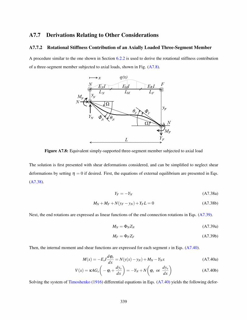
A7.7 Derivations Relating to Other Considerations

A7.7.2 Rotational Stiffness Contribution of an Axially Loaded Three-Segment Member

A procedure similar to the one shown in Section 6.2.2 is used to derive the rotational stiffness contribution

of a three-segment member subjected to axial loads, shown in Fig. (A7.8).

Figure A7.8: Equivalent simply-supported three-segment member subjected to axial load

The solution is first presented with shear deformations considered, and can be simplified to neglect shear

deformations by setting η = 0 if desired. First, the equations of external equilibrium are presented in Eqs.

(A7.38).

YF =−YN (A7.38a)

MN +MF +N(yF − yN)+YFL = 0 (A7.38b)

Next, the end rotations are expressed as linear functions of the end connection rotations in Eqs. (A7.39).

MN = ΦNZN (A7.39a)

MF = ΦFZF (A7.39b)

Then, the internal moment and shear functions are expressed for each segment s in Eqs. (A7.40).

M(x) =−EsIdϕs

dx= N(y(x)− yN)+MN−YNx (A7.40a)

V (x) = κAGs

(−ϕi +

dys

dx

)=−YN +N

(ϕs or

dys

dx

)(A7.40b)

Solving the system of Timoshenko (1916) differential equations in Eqs. (A7.40) yields the following defor-

339

mation equations for each segment.

ys(x) = yN +C2s−1 cos(

φ ′sL

x)+C2s sin

(φ ′sL

x)− ΦNZN

N− YF

Nx (A7.41a)

ϕs(x) =−YF

N+

φs

ωsL

[C2s cos

(φ ′sL

x)−C2s−1 sin

(φ ′sL

x)]

(A7.41b)

Then applying the same boundary and compatibility conditions in Eqs. (A6.8) to solve for all of the inte-

gration coefficients C1 through C6, ΦN , ΦF , YB and L2 in terms of the other variables and then rearranging

the solution into the form of Eq. (7.6) yields the following result for the equivalent rotational stiffness

contribution at the end of the three-segment member, R′i, j.

R′i, j =3E0IzN

L

[α ′0 +3zFφ 2

0 α ′vvul−α ′wwul

9zFzF(α ′5−α ′2)+3φ 20 α ′7−φ 4

0 τNτF(1− zN)(1− zF)α ′1

](A7.42)

where the α ′1 through α ′7 coefficients are given in Eqs. (A6.15), and the remaining coefficients are given as

follows.

α′0 = 3φ

20 zF(α

′4−α

′1)−φ

40 τF(1− zF)α

′1 (A7.43a)

α′v = φ

′Nφ′Mφ′F +α

′1 (A7.43b)

α′w = 3φ

20 zF(α

′4 +φ

′Nφ′Mφ′F)−φ

40 τF(1− zF)α

′1 (A7.43c)

340