arX

iv:1

802.

0490

1v2

[gr

-qc]

14

May

201

8

The shadow of a collapsing dark star

Stefanie Schneider and Volker Perlick

ZARM, University of Bremen, 28359 Bremen, Germany

Email: perlick@zarm.uni-bremen.de

Abstract

The shadow of a black hole is usually calculated, either analytically or numerically, on

the assumption that the black hole is eternal, i.e., that it has existed for all time. Here

we ask the question of how this shadow comes about in the course of time when a black

hole is formed by gravitational collapse. To that end we consider a star that is spherically

symmetric, dark and non-transparent and we assume that it begins, at some instant of

time, to collapse in free fall like a ball of dust. We analytically calculate the dependence

on time of the angular radius of the shadow, first for a static observer who is watching

the collapse from a certain distance and then for an observer who is falling towards the

centre following the collapsing star.

1 Introduction

When a black hole is viewed against a backdrop of light sources, the observer sees a blackdisc in the sky which is known as the shadow of the black hole. Points inside this black disccorrespond to past-oriented light rays that go from the observer towards the horizon of the blackhole, while points outside this black disc correspond to past-oriented light rays that are more orless deflected by the black hole and then meet one of the light sources. For a Schwarzschild blackhole, which is non-rotating the shadow is circular and its boundary corresponds to light raysthat asymptotically spiral towards circular photon orbits that fill the so-called photon sphereat 1.5 Schwarzschild radii around the black hole. For a Kerr black hole, which is rotating, theshadow is flattened on one side and its boundary corresponds to light rays that spiral towardsspherical photon orbits that fill a 3-dimensional photon region around the black hole. For thesupermassive black hole that is assumed to sit at the centre of our Galaxy, the predicted angulardiameter of the shadow is about 53 microarcseconds which is within reach of VLBI observations.There is an ongoing effort to actually observe this shadow, and also the one of the second-bestblack-hole candidate at the centre of M87, see http://www.eventhorizontelescope.org.

1

When calculating the shadow one usually considers an eternal black hole, i.e., a black holethat is static or stationary and exists for all time. For a Schwarzschild black hole, there is asimple analytical formula for the angular radius of the shadow which goes back to Synge [1].(Synge did not use the word “shadow” which was introduced much later. He calculated whathe called the escape cones of light. The opening angle of the escape cone is the complementof the angular radius of the shadow.) For a Kerr black hole, the shape of the shadow wascalculated for an observer at infinity by Bardeen [2]. More generally, an analytical formulafor the boundary curve of the shadow was given, for an observer anywhere in the domain ofouter communication of a Plebanski-Demianski black hole, by Grenzebach et al. [3, 4]. Forthe Kerr case, this formula was further evaluated by Tsupko [5]. These analytical results arecomplemented by ambitious numerical studies, performing ray tracing in black hole spacetimeswith various optical effects taken into account. We mention in particular a paper by Falckeet al. [6] where the perspectives of actually observing black-hole shadows were numericallyinvestigated taking the presence of emission regions and scattering into account, and a morerecent article by James et al. [7] which focusses on the numerical work that was done for themovie Interstellar but also reviews earlier work.

As we have already emphasised, in all these analytical and numerical works an eternal blackhole is considered. Actually, we believe that black holes are not eternal: They have comeinto existence some finite time ago by gravitational collapse (and are then possibly growing byaccretion or mergers with other black holes). This brings us to the question of how an observerwho is watching the collapse would see the shadow coming about in the course of time. This isthe question we want to investigate in this paper.

The visual appearance of a star undergoing gravitational collapse has been studied in severalpapers, beginning with the pioneering work of Ames and Thorne [8]. In this work, and in follow-up papers e.g. by Jaffe [9], Lake and Roeder [10] and Frolov et al. [11], the emphasis is on thefrequency shift of light coming from the surface of the collapsing star. More recent papers byKong et al. [12, 13] and by Ortiz et al. [14, 15] investigated the frequency shift of light passingthrough a collapsing transparent star, thereby contrasting the collapse to a black hole withthe collapse to a naked singularity. In contrast to all these earlier articles, here we consider adark and non-transparent collapsing star which is seen as a black disc when viewed against abackdrop of light sources and we ask how this black disc changes in the course of time.

For the collapsing star we use a particularly simple model: We assume that the star isspherically symmetric and that it begins to collapse, at some instant of time, in free fall likea ball of dust until it ends up in a point singularity at the centre. The metric inside such acollapsing ball of dust was found in a classical paper by Oppenheimer and Snyder [16]. However,for our purpose, as we assume the collapsing star to be non-transparent, we do not need thisinterior metric. All we need to know is that a point on the surface follows a timelike geodesicin the ambient Schwarzschild spacetime. We will demonstrate that in this situation the timedependence of the shadow can be given analytically. We do this first for a static observer

2

who is watching the collapse from a certain distance, and then also for an observer who isfalling towards the centre and ending up in the point singularity after it has formed. The lattersituation is (hopefully) not of relevance for practical astronomical observations but we believethat the calculation is quite instructive from a conceptual point of view.

The paper is organised as follows. In Section 2 we review some basic facts on the Schwarzschildsolution in Painleve-Gullstrand coordinates. These coordinates are particularly well suited forour purpose because they are regular at the horizon, so they allow to consider worldlines of ob-servers or light signals that cross the horizon without the need of patching different coordinatecharts together. In Section 3 we rederive in Painleve-Gullstrand coordinates the equations forthe shadow of an eternal Schwarzschild black hole. We do this both for a static and for aninfalling observer. The results of this section will then be used in the following two sections forcalculating the shadow of a collapsing star. We do this first for a static observer in Section 4and then for an infalling observer in Section 5. We summarise our results in Section 6.

2 Schwarzschild metric in Painleve-Gullstrand coordi-

nates

Throughout this paper, we work with the Schwarzschild metric in Painleve-Gullstrand coordi-nates [17, 18],

gµνdxµdxν = −

(

1− 2m

r

)

c2dT 2 + 2

√

2m

rc dT dr + dr2 + r2

(

dϑ2 + sin2ϑ dϕ2)

. (1)

Here

m =GM

c2(2)

is the mass parameter with the dimension of a length; M is the mass of the central object inSI units, G is Newton’s gravitational constant and c is the vacuum speed of light.

The Painleve-Gullstrand coordinates (T, r, ϑ, ϕ) are related to the standard text-book Schwarzschildcoordinates (t, r, ϑ, ϕ) by

c dT = c dt+

√

2m

r

dr(

1− 2m

r

)

. (3)

As a historical side remark, we mention that both Painleve [17] and Gullstrand [18] believedthat they had found a new solution to Einstein’s vacuum field equation before Lemaıtre [19]demonstrated that it is just the Schwarzschild solution in other coordinates. Whereas in the

3

standard Schwarzschild coordinates the metric has a coordinate singularity at the horizon atr = 2m, in the Painleve-Gullstrand coordinates the metric is regular on the entire domain0 < r < ∞.

On the domain 2m < r < ∞ we will use the tetrad

e0 =1

c

√

1− 2m

r

∂

∂T, e1 =

√

1− 2m

r

∂

∂r+

√

2m

r

c

√

1− 2m

r

∂

∂T,

e2 =1

r

∂

∂ϑ, e3 =

1

r sin ϑ

∂

∂ϕ. (4)

From (1) we read that this tetrad is orthonormal, gµνeµρe

νσ = ηρσ with (ηρσ) = diag(−1, 1, 1, 1),

for 2m < r < ∞. Up to a factor of c, the vector field e0 is the four-velocity field of observersthat stay at fixed spatial coordinates (r, ϑ, ϕ). We refer to them as to the static observers.

From (1) we find that, for a static observer at radius coordinate r(> 2m), proper time τ isrelated to the Painleve-Gullstrand time coordinate T by

dT

dτ=

1√

1− 2m

r

. (5)

In the Painleve-Gullstrand coordinates, the geodesics in the Schwarzschild spacetime arethe solutions to the Euler-Lagrange equations of the Lagrangian

L(

x, x)

=1

2

(

−(

1− 2m

r

)

c2T 2 + 2

√

2m

rc T r + r2 + r2

(

sin2ϑ ϕ2 + ϑ)

)

. (6)

Here the overdot means derivative with respect to an affine parameter.The T and ϕ components of the Euler-Lagrange equations give us the familiar constants of

motion E and L in Painleve-Gullstrand coordinates,

E = −∂L∂T

=

(

1− 2m

r

)

c2T −√

2m

rc r (7)

and

L =∂L∂ϕ

= r2sin2ϑ ϕ . (8)

For the purpose of this paper we will need the radial timelike geodesics and the lightlikegeodesics in the equatorial plane.

4

2.1 Radial timelike geodesics

We consider massive objects in radial free fall, i.e., radial geodesics (ϕ = 0 and ϑ = 0) whichare timelike. Then we may choose the affine parameter equal to proper time τ ,

− c2 = −(

1− 2m

r

)

c2(dT

dτ

)2

+ 2

√

2m

rcdT

dτ

dr

dτ+(dr

dτ

)2

. (9)

In this notation (7) can be rewritten as

ε :=E

c2=

(

1− 2m

r

)

dT

dτ−√

2m

r

1

c

dr

dτ(10)

whereas (8) requires L = 0.In the following we restrict to the case that the parametrisation by proper time is future

oriented with respect to the Painleve-Gullstrand time coordinate, dT/dτ > 0, and we consideronly ingoing motion, dr/dτ < 0, that starts in the domain r > 2m. Then ε > 0 and (10) and(9) imply

dr

dτ= − c

√

ε2 − 1 +2m

r,

dT

dτ=

ε−√

2m

r

√

ε2 − 1 +2m

r

1− 2m

r

(11)

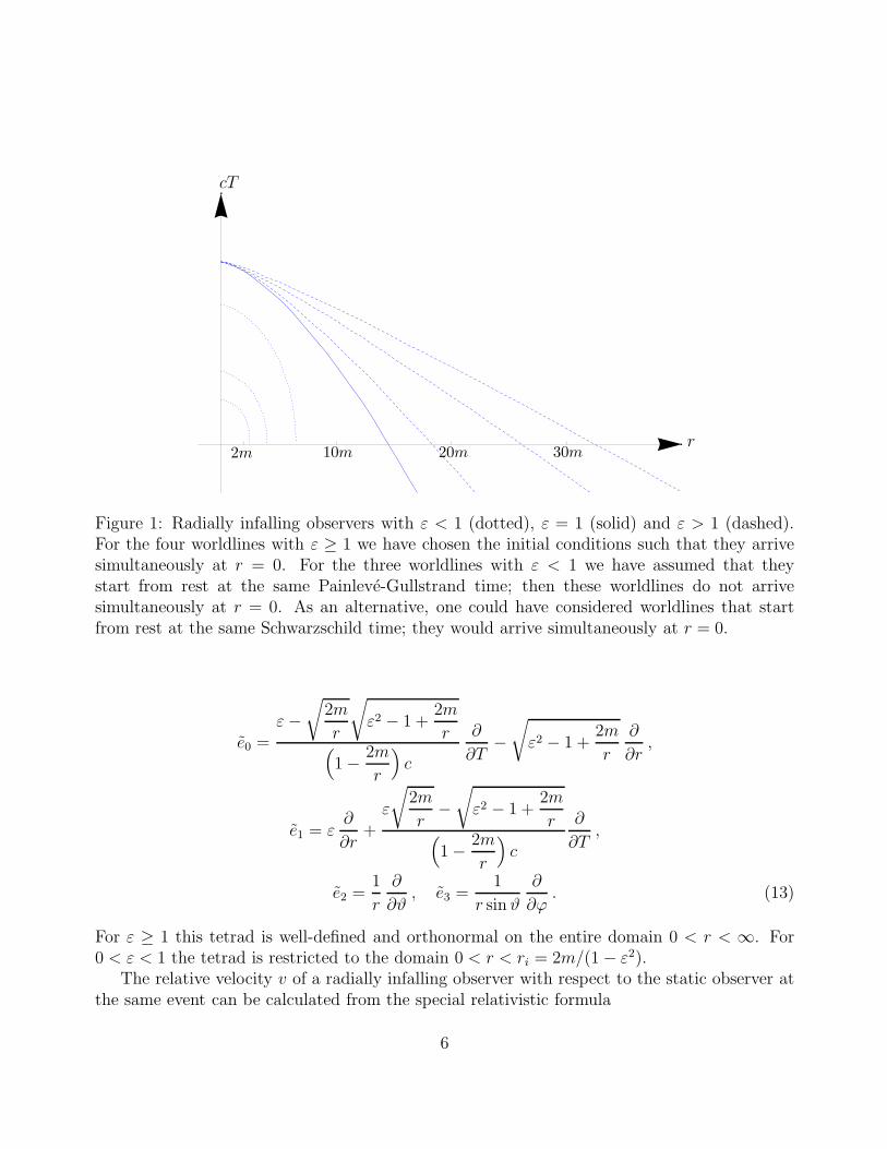
We distinguish three cases, see Fig. 1:(a) 0 < ε < 1: Then dr/dτ = 0 at a radius coordinate ri given by ε2 = 1− 2m/ri, i.e., this

case describes free fall from rest at ri. Clearly, the possible values of ri are 2m < ri < ∞.(b) ε = 1: This is the limit of case (a) for ri → ∞, i.e., free fall from rest at infinity. It is

usual to refer to such freely falling observers as to the Painleve-Gullstrand observers. In thiscase the two equations (11) reduce to

dr

dτ= − c

√

2m

r,

dT

dτ= 1 . (12)

The second equation shows that the coordinate T gives proper time along the worldlines of thePainleve-Gullstrand observers .

(c) 1 < ε < ∞: These are freely falling observers that come in from infinity with a non-zeroinwards-directed initial velocity and then fall towards the centre.

Choosing a value of ε > 0 defines a family of infalling observers. We associate with thisfamily the tetrad

5

PSfrag replacements

r

cT

2m 10m 20m 30m

Figure 1: Radially infalling observers with ε < 1 (dotted), ε = 1 (solid) and ε > 1 (dashed).For the four worldlines with ε ≥ 1 we have chosen the initial conditions such that they arrivesimultaneously at r = 0. For the three worldlines with ε < 1 we have assumed that theystart from rest at the same Painleve-Gullstrand time; then these worldlines do not arrivesimultaneously at r = 0. As an alternative, one could have considered worldlines that startfrom rest at the same Schwarzschild time; they would arrive simultaneously at r = 0.

e0 =ε−

√

2m

r

√

ε2 − 1 +2m

r(

1− 2m

r

)

c

∂

∂T−√

ε2 − 1 +2m

r

∂

∂r,

e1 = ε∂

∂r+

ε

√

2m

r−√

ε2 − 1 +2m

r(

1− 2m

r

)

c

∂

∂T,

e2 =1

r

∂

∂ϑ, e3 =

1

r sin ϑ

∂

∂ϕ. (13)

For ε ≥ 1 this tetrad is well-defined and orthonormal on the entire domain 0 < r < ∞. For0 < ε < 1 the tetrad is restricted to the domain 0 < r < ri = 2m/(1− ε2).

The relative velocity v of a radially infalling observer with respect to the static observer atthe same event can be calculated from the special relativistic formula

6

gµν eµ0 e

ν0 =

−1√

1− v2

c2

. (14)

This results in

v

c=

1

ε

√

ε2 − 1 +2m

r. (15)

Clearly, this formula makes sense only on the domain on which both families of observers aredefined. For ε ≥ 1 this is true on the domain 2m < r < ∞ whereas for 0 < ε < 1 it is true onthe domain 2m < r < ri = 2m/(1− ε2).

2.2 Lightlike geodesics in the equatorial plane

We will now rederive some results on lightlike geodesics in the Schwarzschild spacetime, us-ing Painleve-Gullstrand coordinates. Because of spherical symmetry, it suffices to considergeodesics in the equatorial plane, ϑ = π/2. For lightlike geodesics the Lagrangian is equal tozero,

0 = −(

1− 2m

r

)

c2T 2 + 2

√

2m

rc T r + r2 + r2 ϕ2 . (16)

Dividing by ϕ2 and using (7) and (8) yields

dr

dϕ=

r

ϕ= ±

√

E2r4

c2L2− r2 + 2mr (17)

Reinserting this result into (16) gives us the equation for the Painleve-Gullstrand travel timeof light,

cdT

dr= c

T

r=

√2mr

r − 2m± r

(r − 2m)

√

1− (r − 2m)c2L2

E2r3

. (18)

For all r > 2m, in the last expression the second term is bigger than the first. Therefore, inthis domain the upper sign has to be chosen if dT/dr > 0 and the lower sign has to be chosenif dT/dr < 0.

By differentiating (17) with respect to ϕ we find

d2r

dϕ2=

4E2r3

c2L2− 2r + 2m. (19)

7

If along a lightlike geodesic the radius coordinate goes through an extremum at value rm, (17)and (19) imply

0 =E2r3mc2L2

− rm + 2m, (20)

d2r

dϕ2

∣

∣

∣

r=rm

= rm − 3m. (21)

This demonstrates that only local minima may occur in the domain r > 3m and only localmaxima may occur in the domain r < 3m. The sphere at r = 3m is filled with circular photonorbits that are unstable with respect to radial perturbations. These well-known facts will becrucial for the following analysis.

For a lightlike geodesic with an extremum of the radius coordinate at rm, (20) may be usedfor expressing E2/L2 in (17) and (18) in terms of rm. This results in

dr

dϕ= ±

√

(rm − 2m)r4

r3m− r2 + 2mr (22)

and

cdT

dr=

√2mr

(r − 2m)±

√

(rm − 2m)r5

(r − 2m)√

(rm − 2m)r3 − (r − 2m)r3m(23)

3 The shadow of an eternal Schwarzschild black hole

In this section we rederive the formulas for the angular radius of the shadow of an eter-nal Schwarzschild black hole, both for a static and for an infalling observer, using Painleve-Gullstrand coordinates. The results of this section will then be used for calculating the shadowof a collapsing star in the following sections.

We consider a lightlike geodesic(

T (s), r(s), ϕ(s))

in the equatorial plane, where s is anaffine parameter. As before, we denote the derivative with respect to s by an overdot. Wemay then expand the tangent vector of the lightlike geodesic with respect to the static tetrad(4) and also, as an alternative, with respect to the infalling tetrad (13) for some chosen ε > 0.Of course, the resulting equations are restricted to the domain where the respective tetradis well-defined and orthonormal. As the tangent vector is lightlike, these expansions may be

8

written in terms of two angles α and α,

T∂

∂T+ r

∂

∂r+ ϕ

∂

∂ϕ= χ

(

e0 + cosα e1 − sinα e3

)

= χ(

e0 + cos α e1 − sin α e3

)

. (24)

If the parametrisation of the lightlike geodesic is future-oriented with respect to the T coor-dinate, the scalar factors χ and χ are positive; otherwise they are negative. α is the anglebetween the lightlike geodesic and the radial direction in the rest system of the static observer,whereas α is the analogously defined angle in the rest system of the infalling observer. α andα may take all values between 0 and π. Of course, α is well-defined on the domain where thestatic observer exists (i.e., for 2m < r < ∞) whereas α is well-defined on the domain where theinfalling observer exists (i.e., for 0 < r < ri = 2m/(1 − ε2) if 0 < ε < 1, and for 0 < r < ∞ if1 ≤ ε < ∞).

Comparing coefficients of ∂/∂r and ∂/∂ϕ in (24) yields

r = χ

√

1− 2m

rcosα = χ

(

ε cos α−√

ε2 − 1 +2m

r

)

, (25)

ϕ = −χsinα

r= −χ

sin α

r. (26)

From (25) and (26) we find

ϕ

r=

−sinα

r

√

1− 2m

rcosα

=−sin α

r

(

ε cos α−√

ε2 − 1 +2m

r

) . (27)

Now we apply these results to the case of a lightlike geodesic that goes through an extremumof the radius coordinate at some value rm. If we evaluate (27) at a radius value r > 3m thisextremum is necessarily a local minimum, whereas it is necessarily a local maximum if weevaluate (27) at a radius value r < 3m. In either case (22) implies that the angles α and α atr satisfy

1

r2(rm − 2m)

r3m− 1 +

2m

r

=sin2α

(

1− 2m

r

)

cos2α

=sin2α

(

ε cos α−√

ε2 − 1 +2m

r

)2 . (28)

From the second equality sign in (28) we find

9

sinα =

√

1− 2m

r

1

εsin α

1− 1

ε

√

ε2 − 1 +2m

rcos α

. (29)

By (15), this just demonstrates that α and α are related by the standard aberration formula.From the first equality sign in (28) we find

sinα =

√

r3m(r − 2m)

r3(rm − 2m)(30)

and equating the first to the third expression in (28) yields

sin α =

√

1− 2m

r

√

(r − 2m)r3m(rm − 2m)r3

ε±√

ε2 − 1 +2m

r

√

1− (r − 2m)r3m(rm − 2m)r3

. (31)

In (31) the upper sign is valid if dr/dϕ > 0 and the lower sign is valid if dr/dϕ < 0 at r.From (30) and (31) we can now easily determine the angular radius of the shadow. The

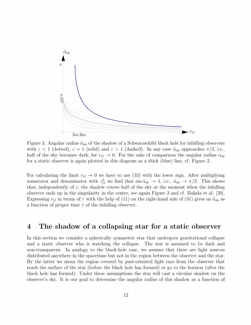
latter is defined in the following way: Consider an observer at radius coordinate r = rO > 3m.Then a lightlike geodesic issuing from the observer position into the past may either go toinfinity, possibly after passing through a minimum of the radius coordinate at some rm > 3m,or it may go to the horizon. Similarly, for an observer position 2m < rO < 3m there arelightlike geodesics that go to the horizon, possibly after passing through a maximum of theradius coordinate at some rm < 3m, and lightlike geodesics that go to infinity. In either casethe borderline between the two classes consists of lightlike geodesics that asymptotically spiraltowards a circular lighlike geodesic at r = 3m. If we assume that there are light sourcesdistributed in the spacetime anywhere but not between the observer and the black hole, thenwe have to associate darkness with the initial directions of lightlike geodesics that go to thehorizon and brightness with those that go to infinity. This results in a circular black disc inthe sky which is called the shadow of the black hole. The boundary of the shadow correspondsto lightlike geodesics that spiral towards r = 3m. Therefore, we get the angular radius of theshadow for an observer at r = rO if we send rm → 3m in (30) and (31). This results in

sinαsh =

√27m

rO

√

1− 2m

rO(32)

and

10

PSfrag replacements

rO

αsh

2m 3m

π

2

π

Figure 2: Angular radius αsh of the shadow of a Schwarzschild black hole for a static observer.What we have plotted here is Synge’s formula (32). For an observer at rO = 3m, we haveα = π/2, i.e., half of the sky is dark. For rO → 2m, we have α → π, i.e., in this limit the entiresky becomes dark.

sin αsh =

√27m

rO

(

ε∓√

ε2 − 1 +2m

rO

√

1− 27m2

r2O

(

1− 2m

rO

)

)

1 + 27m2

r2O

(

ε2 − 1 +2m

rO

) , (33)

respectively. (32) gives us the angular radius αsh as it is seen by a static observer at rO, seeFigure 2. This formula is known since Synge [1]. It is meaningful only for observer positions2m < rO < ∞ because the static observers exist on this domain only. By contrast, (33) givesus the angular radius αsh of the shadow as it is seen by an infalling observer at momentaryradius coordinate rO, see Figure 3. A similar formula was derived by Bakala et al. [20], evenfor the more general case of a Schwarzschild-deSitter (Kottler) black hole. (33) is meaningfulfor 0 < rO < ri = 2m/(1 − ε2) if 0 < ε < 1 and for 0 < rO < ∞ if 1 ≤ ε < ∞. We haveto choose the upper sign for 3m < rO < ∞ and the lower sign for 0 < rO < 3m. Nothingparticular happens if the infalling observer crosses rO = 3m or rO = 2m,

sin αsh

∣

∣

∣

rO=3m=

1√3ε

, sin αsh

∣

∣

∣

rO=2m=

√27 ε

1 +27

4ε2

. (34)

11

PSfrag replacements

rO

αsh

2m 3m

π

2

π

Figure 3: Angular radius αsh of the shadow of a Schwarzschild black hole for infalling observerswith ε < 1 (dotted), ε = 1 (solid) and ε > 1 (dashed). In any case αsh approaches π/2, i.e.,half of the sky becomes dark, for rO → 0. For the sake of comparison the angular radius αsh

for a static observer is again plotted in this diagram as a thick (blue) line, cf. Figure 2.

For calculating the limit rO → 0 we have to use (33) with the lower sign. After multiplyingnumerator and denominator with r3O we find that sin αsh → 1, i.e., αsh → π/2. This showsthat, independently of ε, the shadow covers half of the sky at the moment when the infallingobserver ends up in the singularity in the centre, see again Figure 3 and cf. Bakala et al. [20].Expressing rO in terms of τ with the help of (11) on the right-hand side of (31) gives us αsh asa function of proper time τ of the infalling observer.

4 The shadow of a collapsing star for a static observer

In this section we consider a spherically symmetric star that undergoes gravitational collapseand a static observer who is watching the collapse. The star is assumed to be dark andnon-transparent. In analogy to the black-hole case, we assume that there are light sourcesdistributed anywhere in the spacetime but not in the region between the observer and the star.By the latter we mean the region covered by past-oriented light rays from the observer thatreach the surface of the star (before the black hole has formed) or go to the horizon (after theblack hole has formed). Under these assumptions the star will cast a circular shadow on theobserver’s sky. It is our goal to determine the angular radius of this shadow as a function of

12

time.For the collapsing star we use the simplest model: We assume that the star has constant

radius rS = ri up to Painleve-Gullstrand time TS = 0 and then collapses in free fall like a ballof dust, i.e., such that each point on the surface of the star follows a radial timelike geodesic.Here and in the following we use the index S for the Painleve-Gullstrand coordinates of thesurface of the star, i.e., the star has radius rS at time TS. For times TS > 0 the worldline of anobserver on the surface of the star is then given by one of the dotted lines in Figure 1. From(11) with ε2 = 1− 2m/ri we find that for TS > 0

cTS =

∫

ri

rS

√ri − 2m

√r3 dr

(r − 2m)√

2m(ri − r)−

∫

ri

rS

√2mr dr

(r − 2m)(35)

Equating rS to zero gives the collapse time, T collS , i.e., the Painleve-Gullstrand time when the

star has collapsed to a point singularity at the centre, see Figure 4,

cT collS =

∫

ri

0

√ri − 2m

√r3 dr

(r − 2m)√

2m(ri − r)−

∫

ri

0

√2mr dr

(r − 2m). (36)

Note that necessarily 2m < ri. If 2m < ri ≤ 3m, the star casts the same shadow as an eternalblack hole, for any observer position outside the star. The reason is that then the past-orientedlight rays from the observer position separate into the same two classes as in the case of aneternal black hole: there is the class of light rays that go to infinity and the class of light raysthat do not, with the borderline corresponding to light rays that asymptotically spiral towardsthe light sphere at r = 3m. So the formulas of the preding section apply to this case as well.Of course, here it is crucial that the star is assumed to be dark and non-transparent.

We will, thus, assume from now on that the star collapses from an initial radius ri > 3m.For calculating the shadow we have to consider lighlike geodesics that graze the surface of thecollapsing star. If such a lightlike geodesic passes through a minimum radius value rm, we maydetermine rm by equating the first and the last expression in (28) with r = rS, α = π/2 andε2 = 1− 2m/ri. This results in

r3mrm − 2m

=rir

2S

ri − 2m. (37)

Recall that a minimum value is possible only for rm > 3m, i.e., in (37) rS must satisfy the

inequality rS > r(2)S where

r(2)S = 3m

√

3− 6m

ri. (38)

13

PSfrag replacements

r

T

rOrir(2)S

T(2)S

TcollS

Figure 4: Spacetime diagram of a collapsing star and a static observer. The star begins tocollapse at Painleve-Gullstrand time T = 0 with radius ri. The observer is static at radius rO.

As ri > 3m, (38) implies that

3m < r(2)S < ri . (39)

If ri varies over its allowed values from 3m to infinity, r(2)S monotonically increases from 3m to√

27m.By (35), the star passes through the critical radius value r

(2)S at

cT(2)S =

∫

ri

r(2)S

√ri − 2m

√r3 dr

(r − 2m)√

2m(ri − r)−

∫

ri

r(2)S

√2mr dr

(r − 2m). (40)

We divide the collapse of the star into three phases, see again Figure 4: In the first phasefrom TS = −∞ to TS = 0 the star has a constant radius ri. In the second phase from TS = 0 toTS = T

(2)S the star collapses to the critical radius value r

(2)S . In the third phase from TS = T

(2)S

to TS = T collS the star completes the collapse.

In Figure 4 we have indicated the worldline of an observer who is static at radius coordinaterO. We will now discuss the shadow of the collapsing star as seen by this observer. As necessarily2m < rO, we have to distinguish the following three cases, in accordance with (39): (a) ri < rO,

(b) r(2)S < rO < ri and (c) 2m < rO < r

(2)S .

In case (a), we distinguish three phases of the development of the shadow, corresponding tothe three phases of the collapse. In the first phase the observer sees a static star of radius ri. As

14

the star is assumed to be dark, the observer sees a shadow whose angular radius is determinedby light rays grazing the surface of the star, i.e., by light rays going through a minimum of theradius coordinate at rm = ri. From (30) we read that the angular radius αsh of this shadow isgiven by

sinαsh =

√

r3i (rO − 2m)

r3O(ri − 2m). (41)

This first phase ends when the observer sees the beginning of the collapse, i.e., at an observertime T

(1)O when a light signal that has gone through its minimum radius value rm = ri at time

TS = 0 reaches the observer at rO. From (23) with the plus sign we find that

c T(1)O =

∫

rO

ri

√2mr dr

(r − 2m)+

∫

rO

ri

√

(ri − 2m)r5 dr

(r − 2m)√

(ri − 2m)r3 − (r − 2m)r3i. (42)

During the second phase the observer sees a collapsing star. The boundary of the shadow isdetermined by light rays that graze the surface of the collapsing star. The minimum radiusvalue rm of such light rays is given by (37). Inserting this value into (30), with r = rO, givesus the angular radius of the shadow in the second phase as a function of the parameter rS,

sinαsh =

√

rir2S(rO − 2m)

r3O(ri − 2m). (43)

The time TO at which the shadow with this angular radius is seen is found by integrating(23),

c(TO − TS) =

∫

rO

rS

√2mr dr

(r − 2m)+

∫

rO

rS

√ri − 2m

√r5 dr

(r − 2m)√

(ri − 2m)r3 − (r − 2m)rir2S

(44)

where again we have chosen the plus sign in (23) because TO > TS. With (35) this results in

cTO =

∫

ri

rS

√ri − 2m

√r3 dr

(r − 2m)√

2m(ri − r)+

∫

rO

ri

√2mr dr

(r − 2m)(45)

+

∫

rO

rS

√ri − 2m

√r5 dr

(r − 2m)√

(ri − 2m)r3 − (r − 2m)rir2S

.

15

PSfrag replacements

cTO

αsh

15m 30mcT(1)O cT

(2)O

π

4

π

8

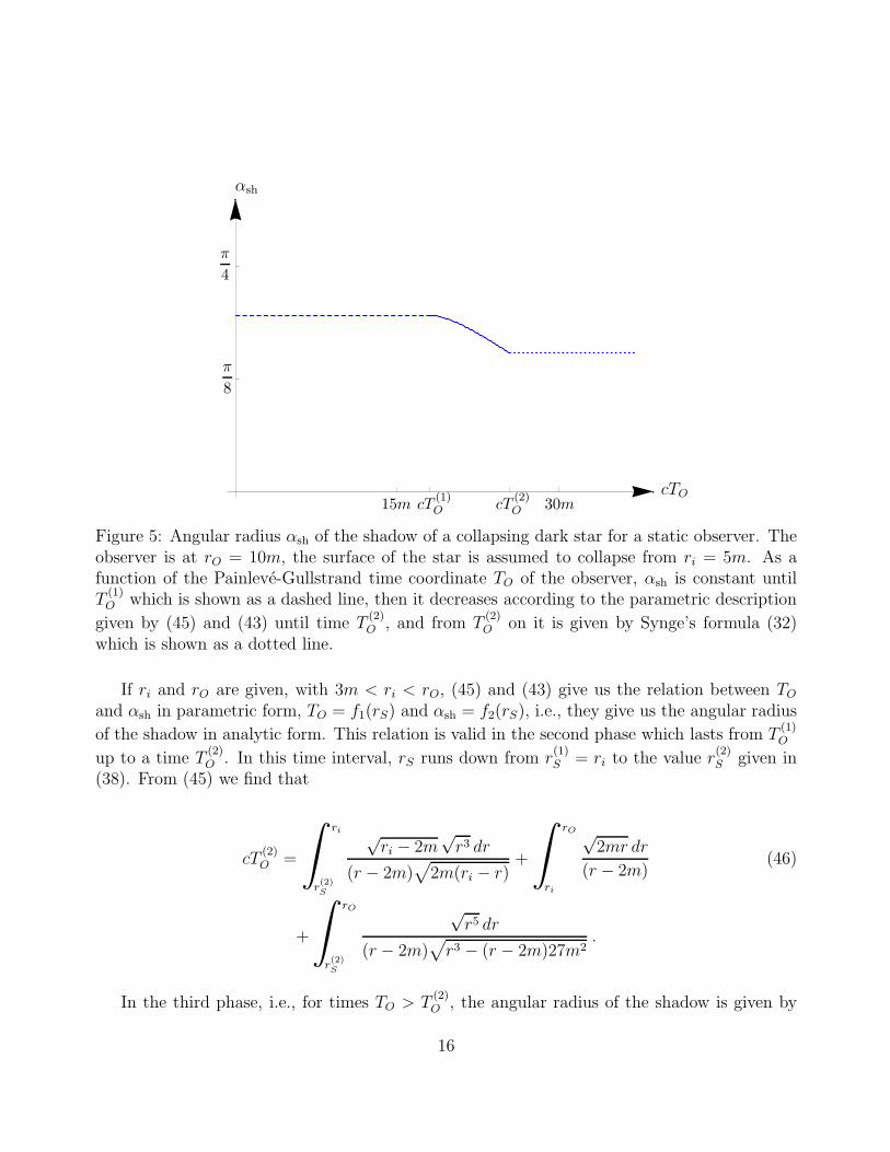
Figure 5: Angular radius αsh of the shadow of a collapsing dark star for a static observer. Theobserver is at rO = 10m, the surface of the star is assumed to collapse from ri = 5m. As afunction of the Painleve-Gullstrand time coordinate TO of the observer, αsh is constant untilT

(1)O which is shown as a dashed line, then it decreases according to the parametric description

given by (45) and (43) until time T(2)O , and from T

(2)O on it is given by Synge’s formula (32)

which is shown as a dotted line.

If ri and rO are given, with 3m < ri < rO, (45) and (43) give us the relation between TO

and αsh in parametric form, TO = f1(rS) and αsh = f2(rS), i.e., they give us the angular radius

of the shadow in analytic form. This relation is valid in the second phase which lasts from T(1)O

up to a time T(2)O . In this time interval, rS runs down from r

(1)S = ri to the value r

(2)S given in

(38). From (45) we find that

cT(2)O =

∫

ri

r(2)S

√ri − 2m

√r3 dr

(r − 2m)√

2m(ri − r)+

∫

rO

ri

√2mr dr

(r − 2m)(46)

+

∫

rO

r(2)S

√r5 dr

(r − 2m)√

r3 − (r − 2m)27m2.

In the third phase, i.e., for times TO > T(2)O , the angular radius of the shadow is given by

16

Synge’s formula (32). Past-oriented light rays grazing the surface of the star cannot escape toinfinity anymore, i.e., they do not give the boundary of the shadow; the latter is determinedby light rays that spiral asymptotically to r = 3m.

PSfrag replacements

rO

cT(2)O − cT

(1)O

25m 50m 75m 100m

25m

50m

75m

Figure 6: Time T(2)O −T

(1)O over which the static observer sees the star collapse, plotted against

the observer position rO. The star is collapsing from an initial radius ri = 5m (dotted),ri = 10m (solid) or ri = 15m (dashed), respectively.

We summarise our analysis in the following way. In the first phase, which lasts from TO =−∞ to TO = T

(1)O given by (42), the observer sees a shadow of constant angular radius given

by (41). In the second phase, which lasts from TO = T(1)O until TO = T

(2)O given by (46), the

observer sees a shrinking shadow whose angular radius as a function of observer time TO isgiven in parametric form by (45) and (43). The parameter rS runs down from r

(1)S = ri to

r(2)S = 3m

√

3− 6m/ri. The third phase lasts from TO = T(2)O to TO = ∞. In this period the

observer sees a shadow of constant angular radius given by Synge’s formula (32). The angularradius of the shadow is plotted against TO, over all three periods, for ri = 5m and rO = 10min Figure 5.

In Fig. 6 we plot the time T(2)O − T

(1)O over which the observer sees the star collapse against

the observer position rO. We see that this time is largely independent of rO, unless the observeris very close to the star. For a star collapsing from an initial radius of 5 Schwarzschild radii,ri = 10m, we see that T

(2)O −T

(1)O ≈ 34m/c for a sufficiently distant observer. For a stellar black

hole, a typical value would be m ≈ 15 km, resulting in T(2)O −T

(1)O ≈ 0.001 sec, so such a collapse

would happen quite quickly. Even for a supermassive black hole of m ≈ 106 km, the observerwould see the collapse happen in less than 2 minutes. For the case of a collapsing cluster ofgalaxies the formation of the shadow would take longer, but in this case it is more reasonable

17

to model the collapsing object as transparent. Note that on the worldline of a distant staticobserver Painleve-Gullstrand time TO is practically the same as proper time τO because, by (5),

τO =

√

1− 2m

rOTO + constant. (47)

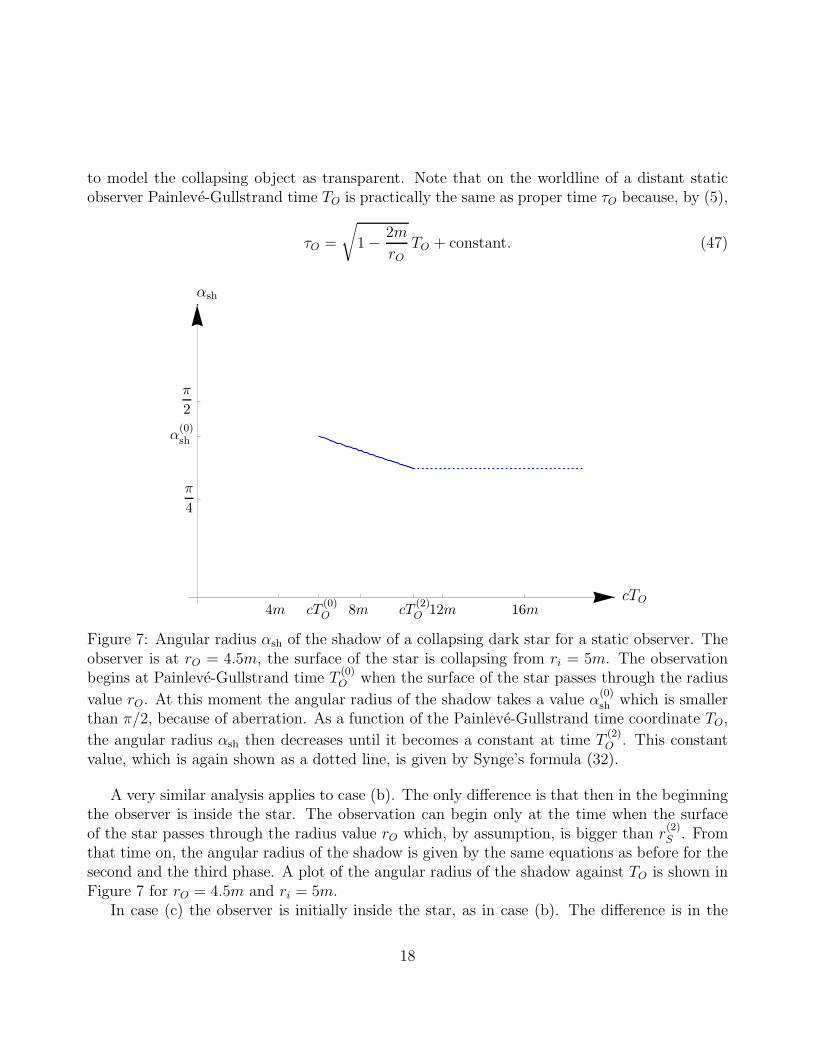
PSfrag replacements

cTO

αsh

4m 8m 12m 16mcT(0)O cT

(2)O

π

4

π

2

α(0)sh

Figure 7: Angular radius αsh of the shadow of a collapsing dark star for a static observer. Theobserver is at rO = 4.5m, the surface of the star is collapsing from ri = 5m. The observationbegins at Painleve-Gullstrand time T

(0)O when the surface of the star passes through the radius

value rO. At this moment the angular radius of the shadow takes a value α(0)sh which is smaller

than π/2, because of aberration. As a function of the Painleve-Gullstrand time coordinate TO,

the angular radius αsh then decreases until it becomes a constant at time T(2)O . This constant

value, which is again shown as a dotted line, is given by Synge’s formula (32).

A very similar analysis applies to case (b). The only difference is that then in the beginningthe observer is inside the star. The observation can begin only at the time when the surfaceof the star passes through the radius value rO which, by assumption, is bigger than r

(2)S . From

that time on, the angular radius of the shadow is given by the same equations as before for thesecond and the third phase. A plot of the angular radius of the shadow against TO is shown inFigure 7 for rO = 4.5m and ri = 5m.

In case (c) the observer is initially inside the star, as in case (b). The difference is in the

18

fact that now the radius of the star is smaller than r(2)S at the moment when the observation

begins. Therefore, the shadow is never determined by light rays that graze the surface of thestar; it is always determined by light rays that spiral towards r = 3m, i.e., the angular radiusof the shadow is constant from the beginning of the observation and given by Synge’s formula.

5 The shadow of a collapsing star for an infalling ob-

server

We consider the same collapsing dark star as in the preceding section, but now we want tocalculate the shadow as it is seen by an infalling observer. The relation between the coordinatesrO and TO of the infalling observer can be found by integrating (11),

cTO =

∫

r∗O

rO

(

ε√r3 −

√2mr

√ε2r − r + 2m

)

dr

(r − 2m)√ε2r − r + 2m

. (48)

Here r∗O is an integration constant that gives the position of the observer at T = 0 which is the

time when the star begins to collapse. We assume that ri > 3m, hence 3m < r(2)S < ri, and

that r∗O has been chosen big enough such that the observer is outside the star for all times, seeFigure 8. For the time being we leave the constant of motion ε unspecified.

We will determine the angular radius of the shadow as a function of the observer positionrO. As before, we distinguish three phases. In the first phase the observer sees a star of constantradius ri. The angular radius of the shadow can be read from (31) with the lower sign wherewe have to insert r = rO and rm = ri,

sin αsh =(rO − 2m)

√

r3i

ε r2O√ri − 2m−

√ε2rO − rO + 2m

√

(ri − 2m)r3O − (rO − 2m)r3i. (49)

If ri is given, this gives us explicitly αsh as a function of rO for the first phase.In the second phase we may again use (45). In combination with (48) this implies

∫

r∗O

rO

ε√r3 dr

(r − 2m)√ε2r − r + 2m

−

∫

r∗O

ri

√2mr dr

(r − 2m)(50)

=

∫

ri

rS

√ri − 2m

√r5 dr

(r − 2m)√

2m(ri − r)+

∫

rO

rS

√ri − 2m

√r5 dr

(r − 2m)√

(ri− 2m)r3 − (r − 2m)rir2S

.

19

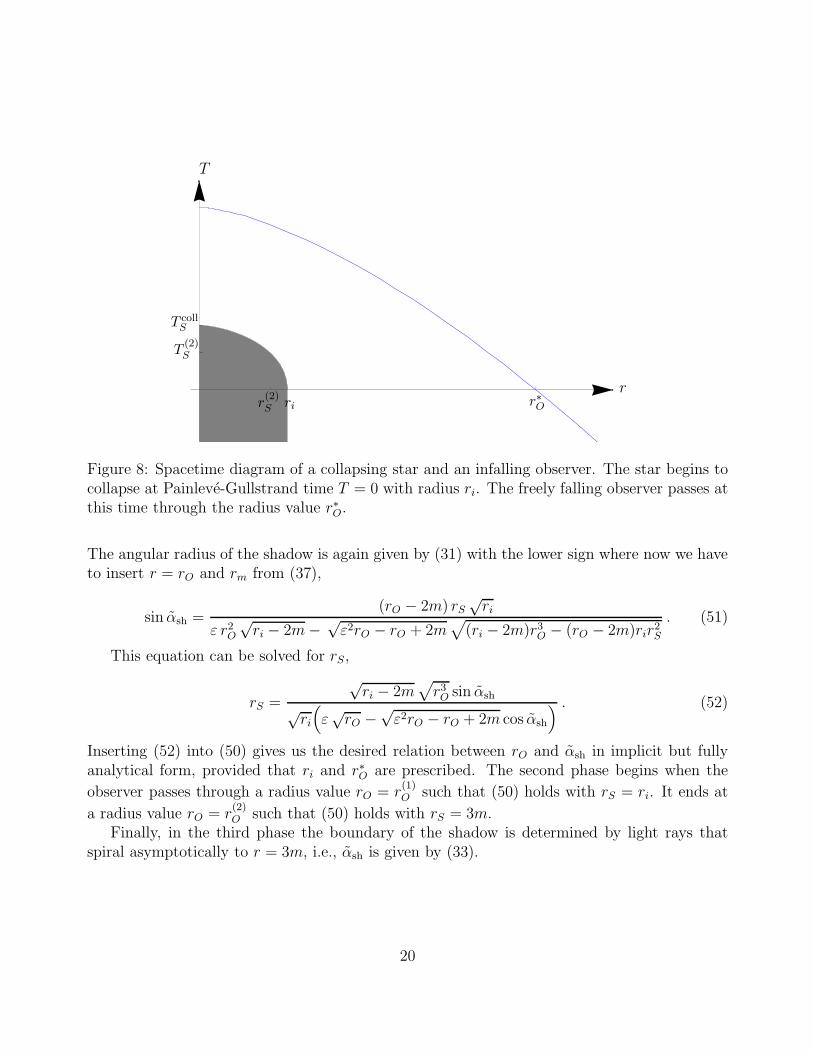
PSfrag replacements

r

T

r∗

Orir(2)S

T(2)S

TcollS

Figure 8: Spacetime diagram of a collapsing star and an infalling observer. The star begins tocollapse at Painleve-Gullstrand time T = 0 with radius ri. The freely falling observer passes atthis time through the radius value r∗O.

The angular radius of the shadow is again given by (31) with the lower sign where now we haveto insert r = rO and rm from (37),

sin αsh =(rO − 2m) rS

√ri

ε r2O√ri − 2m−

√ε2rO − rO + 2m

√

(ri − 2m)r3O − (rO − 2m)rir2S. (51)

This equation can be solved for rS,

rS =

√ri − 2m

√

r3O sin αsh

√ri

(

ε√rO −

√ε2rO − rO + 2m cos αsh

) . (52)

Inserting (52) into (50) gives us the desired relation between rO and αsh in implicit but fullyanalytical form, provided that ri and r∗O are prescribed. The second phase begins when the

observer passes through a radius value rO = r(1)O such that (50) holds with rS = ri. It ends at

a radius value rO = r(2)O such that (50) holds with rS = 3m.

Finally, in the third phase the boundary of the shadow is determined by light rays thatspiral asymptotically to r = 3m, i.e., αsh is given by (33).

20

PSfrag replacements

rO

αsh

3m r(2)O r

(1)O

10m

π

2

Figure 9: Angular radius αsh of the shadow of a collapsing dark star for an infalling observer.The observer is a Painleve-Gullstrand observer (ε = 1) passing at TO = 0 through the radiusvalue r∗O = 10m. At this time the surface of the star starts collapsing from ri = 5m. Theangular radius of the shadow is plotted against the radius coordinate of the observer. Wedistinguish three phases: In the first phase (dashed), the observer sees a star of constant radiusri and the angular radius of the shadow is given by (49). In the second phase (solid), theobserver sees a collapsing star and the angular radius of the shadow is implicitly given by (50)with rS inserted from (52). In the third phase (dotted), the boundary of the shadow is no longergiven by light rays grazing the surface of the star but rather by light rays spiralling towardsthe photon sphere at r = 3m, so αsh is given by (33), cf. Fig. 3.

6 Conclusions

In this paper we have demonstrated that, for a spherically symmetric dark and non-transparentstar that collapses in free fall like a ball of dust, the development of the shadow can be calculatedanalytically, both for a static and for an infalling observer. In particular we have shown thatfor a static observer the black-hole shadow according to Synge’s formula forms in a finite timewhich, for a stellar black hole, is in the order of fractions of a second. This result could not havebeen easily anticipated before doing the calculation: Intuitively, one might have expected thatthe black-hole shadow forms asymptotically. The situation is similar for an infalling observer(provided that the observer is sufficiently far behind not to catch up with the star): Also inthis case the surface of the star determines the shadow only over a finite time; during the laststage of the infall, the observer sees the same shadow as when infalling into an eternal blackhole.

Admittedly, getting analytical results was possible only because we used a somewhat over-

21

simplified model for a collapsing star. More realistically, instead of a spherically symmetricball of dust one should consider a rotating star with pressure which would probably make thecalculations so complicated that only a numerical treatment would be possible. However, webelieve that the simple model considered here gives a good idea of all the relevant qualitativefeatures of how the black-hole shadow comes about in the course of time.

In this paper we have concentrated on the formation of the shadow during gravitationalcollapse. However, we mention that some of our results may also be useful for investigating thetemporal change of the shadow of an already existing black hole. If a black hole is surroundedby matter its mass will grow by accretion, so its shadow will become bigger in the courseof time. We have not investigated this problem in detail, but we believe that the Painleve-Gullstrand approach pursued in this paper may be appropriate also for calculating the growthof the shadow of an accreting black hole.

Acknowledgements

We would like to thank Nico Giulini for helpful discussions. Moreover, we gratefully acknowl-edge support from the DFG within the Research Training Group 1620 “Models of Gravity”.

References

[1] J. L. Synge, The escape of photons from gravitationally intense stars, Mon. Not. Roy.Astron. Soc. 131, 463 (1966)

[2] J. Bardeen, in Black Holes, ed. by C. DeWitt, B. DeWitt (Gordon and Breach, New York,U.S.A., 1973), p. 215

[3] A. Grenzebach, V. Perlick, C. Lammerzahl, Photon regions and shadows of Kerr-Newman-NUT black holes with a cosmological constant, Phys. Rev. D 89, 124004 (2014)

[4] A. Grenzebach, V. Perlick, C. Lammerzahl, Photon regions and shadows of acceleratedblack holes, Int. J. Modern Phys. D 24, 1542024 (2015)

[5] O. Yu. Tsupko, Analytical calculation of black hole spin using deformation of the shadow,Phys. Rev. D 95, 104058 (2017)

[6] H. Falcke, F. Melia, E. Agol, Viewing the shadow of the black hole at the galactic center,Astrophys. J. 528, L13 (2000)

[7] O. James, E. Tunzelmann, P. Franklin, K. Thorne, Gravitational lensing by spinning blackholes in astrophysics, and in the movie Interstellar, Class. Quant. Grav. 32, 065001 (29015)

22

[8] W. Ames, K. Thorne, The optical appearance of a star that is collapsing through itsgravitational radius, Astrophys. J. 151, 659 (1968)

[9] J. Jaffe, Collapsing objects and the backward emission of light, Ann. Phys. (NY) 55, 374(1969)

[10] K. Lake, R. C. Roeder, Note on the optical appearance of a star collapsing through itsgravitational radius, Astrophys. J. 232, 277 (1979)

[11] V. P. Frolov, K. Kim, H. K. Lee, Spectral broadening of radiation from relativistic collaps-ing objects, Phys. Rev. D 75, 087501 (2007)

[12] L. Kong, D. Malafarina, C. Bambi, Can we observationally test the weak cosmic censorshipconjecture? Eur. Phys. J. C 74 2983 (2014)

[13] L. Kong, D. Malafarina, C. Bambi, Gravitational blueshift from a collapsing object, Phys.Lett. B 741 82 (2015)

[14] N. Ortiz, O. Sarbach, T. Zannias, Shadow of a naked singularity 92, 044035 (2015)

[15] N. Ortiz, O. Sarbach, T. Zannias, Observational distinction between black holes and nakedsingularities: the role of the redshift function, Class. Quant. Grav. 32, 247001 (2015)

[16] J. R. Oppenheimer, H. Snyder, On continued gravitational contraction, Phys. Rev. 56,455 (1939)

[17] P. Painleve, La mecanique classique et la theorie de la relativite, C. R. Acad. Sci. 173,677 (1921)

[18] A. Gullstrand, Allgemeine Losung des statischen Einkorperproblems in der EinsteinschenGravitationstheorie, Ark. Mat. Astr. Fys. 16, 1 (1922)

[19] G. Lemaıtre, L’Univers en expansion, Ann. Soc. Sci. Bruxelles A 53, 51 (1933)

[20] P. Bakala, P. Cermak, S. Hledık, Z. Stuchlık, K. Truparova, Extreme gravitational lensingin vicinity of Schwarzschild-deSitter black holes, Centr. Eur. J. Phys. 5, 599 (2007)

23