The Roles of Standing Genetic Variation andEvolutionary History in Determining the Evolvability ofAnti-Predator StrategiesDaniel R. O’Donnell1,2*., Abhijna Parigi1,2., Jordan A. Fish2,3., Ian Dworkin1,2,4, Aaron P. Wagner4

1 Program in Ecology, Evolutionary Biology, and Behavior, Michigan State University, East Lansing, Michigan, United States of America, 2 Department of Zoology, Michigan

State University, East Lansing, Michigan, United States of America, 3 Center for Microbial Ecology, Michigan State University, East Lansing, Michigan, United States of

America, 4 BEACON Center for the Study of Evolution in Action, Michigan State University, East Lansing, Michigan, United States of America

Abstract

Standing genetic variation and the historical environment in which that variation arises (evolutionary history) are bothpotentially significant determinants of a population’s capacity for evolutionary response to a changing environment. Usingthe open-ended digital evolution software Avida, we evaluated the relative importance of these two factors in influencingevolutionary trajectories in the face of sudden environmental change. We examined how historical exposure to predationpressures, different levels of genetic variation, and combinations of the two, affected the evolvability of anti-predatorstrategies and competitive abilities in the presence or absence of threats from new, invasive predator populations. We showthat while standing genetic variation plays some role in determining evolutionary responses, evolutionary history has thegreater influence on a population’s capacity to evolve anti-predator traits, i.e. traits effective against novel predators. Thisadaptability likely reflects the relative ease of repurposing existing, relevant genes and traits, and the broader potentialvalue of the generation and maintenance of adaptively flexible traits in evolving populations.

Citation: O’Donnell DR, Parigi A, Fish JA, Dworkin I, Wagner AP (2014) The Roles of Standing Genetic Variation and Evolutionary History in Determining theEvolvability of Anti-Predator Strategies. PLOS ONE 9(6): e100163. doi:10.1371/journal.pone.0100163

Editor: Nadia Singh, North Carolina State University, United States of America

Received February 7, 2014; Accepted May 22, 2014; Published June 23, 2014

Copyright: � 2014 O’Donnell et al. This is an open-access article distributed under the terms of the Creative Commons Attribution License, which permitsunrestricted use, distribution, and reproduction in any medium, provided the original author and source are credited.

Funding: Funding was provided by BEACON Center for the Study of Evolution in Action (NSF Cooperative Agreement DBI-0939454), beacon-center.org; andMichigan State University Institute for Cyber Enabled Research, icer.msu.edu. The funders had no role in study design, data collection and analysis, decision topublish, or preparation of the manuscript.

Competing Interests: The authors have declared that no competing interests exist.

* Email: odonn146@msu.edu

. These authors contributed equally to this work.

Introduction

The diversity and complexity of any biological system reflects

past evolutionary responses to environmental conditions. Under-

lying those responses are a number of extrinsic and intrinsic factors

influencing populations’ capacities to evolve responses through the

generation or utilization of genetic variation [1,2]. Because

evolutionary responses rely largely on available heritable variation,

mechanisms that influence the generation and maintenance of

variation [3] can strongly shape the evolutionary trajectories of

populations [4]. Among the potential factors involved, standing

genetic variation (SGV) and evolutionary history (EH) are likely to

be significant determinants of adaptability to novel environments

[5]. Accordingly, understanding how these critical factors either

promote or constrain population evolutionary potential provides

insight into the realized pathways that led to historical evolution-

ary outcomes, as well as those that will shape future populations.

Standing genetic variation is the presence of alternative forms of

a gene (alleles) at a given locus [5] in a population. While an allele

may be mildly deleterious or confer no fitness advantage over

other forms under one set of environmental conditions [6], that

allele may become beneficial if the environment changes. As

selection can act only on available variation, SGV provides a

potential means for more rapid adaptive evolution ([7–20];

reviewed in [21]) compared with the de novo mutations [5,22],

particularly if the environment changes (e.g. if a new predator or

competitor invades the system, or if abiotic conditions change).

In addition to SGV, a population’s historical selection

environment (i.e. evolutionary history) may play a strong role in

determining the speed and the extent to which populations can

adapt to directional environmental change [23–25]. In particular,

EH will have influenced the genetic variation and genetic

architecture of traits in contemporary populations. If changes in

the environment alter the strength of selection on a trait,

populations with an evolutionary history of adaptation to similar

pressures may be mutationally ‘‘closer’’ to the discovery of new

[26], or rediscovery of historical beneficial traits [27]. For

example, Gillings and Stokes [25] suggest that historical exposure

to antibiotics may confer greater adaptability of bacteria when

exposed to novel antibiotics.

With the contemporary rise of experimental evolution as a

means of testing evolutionary and ecological hypotheses [28,29], a

valuable and untapped opportunity now exists to elucidate the

roles SGV and EH have played in determining historical, realized

rates of adaptive evolution. Furthermore, while SGV is known to

be an important determinant of the speed of evolution [5,11], it is

less clear how levels of SGV and EH, alone or in combination,

impact the overall evolutionary potential of populations. Such an

understanding could allow population geneticists to evaluate how

PLOS ONE | www.plosone.org 1 June 2014 | Volume 9 | Issue 6 | e100163

SGV and EH may contribute to or constrain the future

evolvability of populations, particularly in human-modified

environments [1,30,31].

To evaluate the individual and interactive effects of SGV and

EH on evolutionary outcomes, we measured their independent as

well as their combined contributions toward evolutionary potential

in populations using the digital evolution software Avida [32].

Digital organisms in Avida inhabit a controlled, two-dimensional

environment, and experience evolutionary adaptation. The

complexity of evolutionary dynamics possible in Avida can be

compared to that of bacteria or viruses [33]. In Avida, as in

biological systems, three necessary and sufficient conditions for

producing evolution via natural selection are met: replication,

heritable variation, and differential fitness resulting from that

variation [34].

Digital evolution experiments carry several significant advan-

tages for addressing evolutionary questions requiring systematic

manipulation and highly controlled environments. Among these,

generation times are rapid, the experimenter has full control over

initial environmental conditions, and detailed genetic, demo-

graphic, and behavioral trait data can be recorded perfectly.

Organisms in Avida can also engage in ecological competition and

other complex interactions, and the system can allow for co-

evolution in predator-prey systems [35–37]. Furthermore, unlike

in evolutionary models and evolutionary simulations that impose

artificial selection via explicit selection functions, Avida uniquely

allows for unrestricted, unsupervised, and non-deterministic

evolution via natural selection [32]. With biological organisms, it

is difficult to know the exact number of unique genotypes present

at a given time, especially when population sizes are large. Hence,

manipulating levels of SGV in populations of biological organisms

is difficult (but see [19]). Because our question required precise

knowledge of the amount of genetic diversity present within each

treatment, experimental evolution with biological organisms

would have been impractical, given the scale of our study.

Predation is an ecologically important agent of selection [38,39]

as demonstrated by the diverse array of prey defenses that have

evolved in nature [40–43]. Accordingly, we used Avida to test

whether historical exposure to predation influenced how prey

populations responded to pressures from new, invasive predators.

We then further examined which factors (SGV, EH, and their

interaction) were important in determining the future defensive

and competitive abilities of those populations. While both factors

played significant roles, we show that evolutionary history has the

stronger influence on evolutionary potential, with the strength of

SGV’s role being contingent on a population’s evolutionary

history. Irrespective of the level of SGV, populations with predator

EH almost always outcompeted populations without predator EH.

In predator EH populations, SGV appeared to have no effect on

evolvability, whereas, in no predator EH populations, higher SGV

increased evolvability.

Materials and Methods

AvidaThe Avida digital evolution platform is a tool for conducting

evolutionary experiments on populations of self-replicating com-

puter programs, termed ‘‘digital organisms’’ [32]. Digital organ-

isms are composed of a set of instructions constituting their

‘‘genome’’. Organisms execute genome instructions in order to

perform actions such as processing information and interacting

with their environment, and for reproduction. Additionally,

predefined combinations of instructions allow organisms to

consume resources from the simulated environment. Sufficient

consumption of resources, to a level defined by the experimenter,

is a prerequisite for organisms to copy their genomes and divide

(i.e. reproduce). During the copy process, there is an experimenter-

defined probability that genomic instructions will be replaced with

a different instruction (substitution mutation) randomly selected

from the full set of all 60 possible instructions (instruction set files

are in the skel directory in the GitHub repository [https://github.

com/fishjord/avida_predation_scripts]). Separately, there are also

set probabilities for the copy of an instruction to fail (creating a

deletion mutation) or for a chance insertion of a new instruction

into the copy’s genome. In real-time, generation times in Avida are

typically only a few seconds, and experimental environments are

fully definable.

Environment. We ran all Avida trials in a 2516251 bounded

grid-cell environment. Each cell started with one unit of resource.

If a prey organism fed in a given cell (by executing an ‘output’

instruction), the resource in that cell was completely consumed and

that cell was replenished with resources after 100 updates (an

update is the measurement of time in Avida, reflecting the number

of genomic instructions executed across the population).

Timing. All Avida trials were run for a set number of updates,

as indicated in each of the Phase descriptions below. Here, each

organism executed 30 instructions per update. Organisms had a

maximum lifespan of 15,000 instructions executed (500 updates).

Realized average number of generations for the populations in

each treatment is given in their respective sections below.

Reproduction. Organisms, both predator and prey, were

required to have consumed 10 resource units (in one ‘‘bite’’,

individuals could consume a maximum of 1 resource unit) and be

at least 100 updates old to successfully reproduce. Genome

copying and reproduction occurred when the organism executed a

single reproduction (‘repro’) instruction. In most cases, biological

organisms must consume copious resources (and thus perform a

number of other feeding-related behaviors, e.g. moving, searching,

handling) in order to execute one reproductive event; thus,

execution of the reproduction instruction took one update,

compared to 1/30th of an update for other instructions (except

for predation handling time, as noted below). When an organism

reproduced, its offspring was placed in the cell the parent was

facing. This new organism’s genome was a copy of the parent’s

genome, with the exception any substitutions, insertions, and

deletions that occurred during the copy process. Substitutions were

independent and only one insertion or deletion was allowed per

reproduction (at rates specified in the ‘Phase 1’ and ‘Phase 2’

descriptions, below). In addition to the birth of the new organism

upon reproduction, the parent organism was effectively reborn,

with all internal states (e.g. stored values such as those describing

objects seen, genomic marker positions, and execution pointer

position) reset. Unlike in legacy Avida experiments, multiple

organisms could occupy the same cell (as in [35–37]). Thus,

newborn organisms did not replace existing occupants of the cells

into which they were born.

Predation. In Avida, predation occurs via the evolution of an

‘attack-prey’ instruction, the execution of which allows an

organism to attack and kill a non-predator in the cell it is facing.

Predation in Avida and the base predator Avida configuration

used are described in [32]. Here, as in handling time, the attack-

prey instruction costs the predator 10 cycles (one-third of an

update) if the attack is successful. Predators receive 10% of each

prey individual’s consumed resources after a successful kill, which

is then applied toward the consumption threshold required for

reproduction. An organism is classified as a predator in Avida if it

attacks a prey organism, not simply by evolving the ‘attack-prey’

Standing Genetic Variation, Evolutionary History, Antipredator Traits

PLOS ONE | www.plosone.org 2 June 2014 | Volume 9 | Issue 6 | e100163

instruction. Predators can only consume prey organisms, and

cannot consume resources.

In simple (i.e. lacking topographic features like refuges) and

confined environments like the one used here, Avida trials

containing predators typically require a minimum prey population

level below which predator attacks fail. In top-down limited

populations like those used here, minimum prey levels prevent

population extinctions and serve to standardize prey population

sizes and thus intra-specific competitive pressures. In practice,

because prey are constantly being born into populations, prey kills

are prevented for very short periods of time and failures simply

require predators to make multiple, rapid attacks. Here, attacks on

prey were always fatal if there were more than 1,000 prey in the

environment (i.e., 1,000 was a minimum prey level below which

fatal attacks were prevented). Similarly, in trials without predators,

prey population sizes were controlled via a preset maximum

population cap (1,000 organisms), as described for each Phase

below. When a birth caused that limit to be exceeded, a random

prey organism was removed from the population.

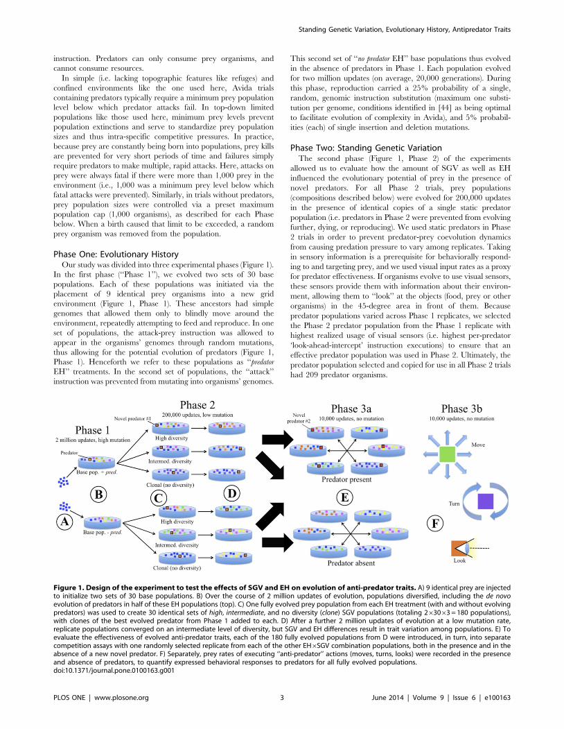
Phase One: Evolutionary HistoryOur study was divided into three experimental phases (Figure 1).

In the first phase (‘‘Phase 1’’), we evolved two sets of 30 base

populations. Each of these populations was initiated via the

placement of 9 identical prey organisms into a new grid

environment (Figure 1, Phase 1). These ancestors had simple

genomes that allowed them only to blindly move around the

environment, repeatedly attempting to feed and reproduce. In one

set of populations, the attack-prey instruction was allowed to

appear in the organisms’ genomes through random mutations,

thus allowing for the potential evolution of predators (Figure 1,

Phase 1). Henceforth we refer to these populations as ‘‘predator

EH’’ treatments. In the second set of populations, the ‘‘attack’’

instruction was prevented from mutating into organisms’ genomes.

This second set of ‘‘no predator EH’’ base populations thus evolved

in the absence of predators in Phase 1. Each population evolved

for two million updates (on average, 20,000 generations). During

this phase, reproduction carried a 25% probability of a single,

random, genomic instruction substitution (maximum one substi-

tution per genome, conditions identified in [44] as being optimal

to facilitate evolution of complexity in Avida), and 5% probabil-

ities (each) of single insertion and deletion mutations.

Phase Two: Standing Genetic VariationThe second phase (Figure 1, Phase 2) of the experiments

allowed us to evaluate how the amount of SGV as well as EH

influenced the evolutionary potential of prey in the presence of

novel predators. For all Phase 2 trials, prey populations

(compositions described below) were evolved for 200,000 updates

in the presence of identical copies of a single static predator

population (i.e. predators in Phase 2 were prevented from evolving

further, dying, or reproducing). We used static predators in Phase

2 trials in order to prevent predator-prey coevolution dynamics

from causing predation pressure to vary among replicates. Taking

in sensory information is a prerequisite for behaviorally respond-

ing to and targeting prey, and we used visual input rates as a proxy

for predator effectiveness. If organisms evolve to use visual sensors,

these sensors provide them with information about their environ-

ment, allowing them to ‘‘look’’ at the objects (food, prey or other

organisms) in the 45-degree area in front of them. Because

predator populations varied across Phase 1 replicates, we selected

the Phase 2 predator population from the Phase 1 replicate with

highest realized usage of visual sensors (i.e. highest per-predator

‘look-ahead-intercept’ instruction executions) to ensure that an

effective predator population was used in Phase 2. Ultimately, the

predator population selected and copied for use in all Phase 2 trials

had 209 predator organisms.

Figure 1. Design of the experiment to test the effects of SGV and EH on evolution of anti-predator traits. A) 9 identical prey are injectedto initialize two sets of 30 base populations. B) Over the course of 2 million updates of evolution, populations diversified, including the de novoevolution of predators in half of these EH populations (top). C) One fully evolved prey population from each EH treatment (with and without evolvingpredators) was used to create 30 identical sets of high, intermediate, and no diversity (clone) SGV populations (totaling 263063 = 180 populations),with clones of the best evolved predator from Phase 1 added to each. D) After a further 2 million updates of evolution at a low mutation rate,replicate populations converged on an intermediate level of diversity, but SGV and EH differences result in trait variation among populations. E) Toevaluate the effectiveness of evolved anti-predator traits, each of the 180 fully evolved populations from D were introduced, in turn, into separatecompetition assays with one randomly selected replicate from each of the other EH6SGV combination populations, both in the presence and in theabsence of a new novel predator. F) Separately, prey rates of executing ‘‘anti-predator’’ actions (moves, turns, looks) were recorded in the presenceand absence of predators, to quantify expressed behavioral responses to predators for all fully evolved populations.doi:10.1371/journal.pone.0100163.g001

Standing Genetic Variation, Evolutionary History, Antipredator Traits

PLOS ONE | www.plosone.org 3 June 2014 | Volume 9 | Issue 6 | e100163

To create Phase 2 Evolutionary History (EH) treatment source

populations, we first selected a single prey population from a

random Phase 1 replicate in each EH treatment (predator and no

predator EH), excluding the population from which the Phase 2

predator population was drawn. For each of the two selected

populations, we excluded any organisms that were classified as

predators or had parents that were predators (as determined by an

internal state, see [35,36]), to ensure that Phase 2 prey populations

consisted only of prey organisms. An organism must execute an

attack instruction to be designated a predator, and some prey

organisms may have attack instructions in their genomes, even if

they have not yet used them; we therefore replaced any attack

instructions in the remaining prey populations with a ‘do nothing’

(nop-X) instruction, and prevented any new copies of the attack

instruction from mutating into offspring genomes.

To create Phase 2 SGV treatment populations, we created

separate ‘‘clone’’, ‘‘intermediate’’, and ‘‘high’’ SGV populations by

sampling each of the two EH treatment source populations ("seed

populations"; one predator EH population and one no predator EH

population: Figure 1, Phase 2). First, for high SGV populations, we

simply used duplicates of the selected EH treatment source

populations. Because all possible genomes are present in this

treatment, evolutionary trajectories of replicates within this

treatment were not constrained by the lack of genetic variation.

Second, we created each clone SGV population by randomly

selecting a single genotype from a seed population and making as

many duplicates of that genotype as there were organisms in the

seed population. A genotype could be selected for multiple Phase 2

clone replicates. Given that most evolution experiments with

microorganisms begin with a single clone, we wanted to compare

the evolutionary trajectory of a clonal population to the high SGV

populations. Third, we created the intermediate SGV populations by

randomly sampling genotypes (with replacement) from a seed

population, creating up to 55 identical copies of each sampled

genotype. We repeated this process until the new intermediate SGV

population was the same size as the seed population; this sampling

scheme yielded intermediate SGV prey populations the same size as

their high SGV seed populations, but with ,50% lower diversity

(Shannon’s diversity index), on average. Evolution experiments

with diploid, sexually reproducing organism like Drosophila

melanogaster start with large, wild caught natural populations.

However, sampling from a natural population cannot capture all

possible genotypes. Intermediate SGV populations are analogous

to such ‘‘sampled’’ populations that have some, but not all the

available SGV. In all, there were six (2 EH63 SGV) Phase 2

treatments, each with 30 replicates (Figure 1).

For each of the six combinations of SGV (clone, intermediate, high)

and EH (predator, no predator EH), we evolved 30 replicate

populations for 200,000 updates (500 generations, on average),

each in the presence of a copy of the constructed Phase 2 predator

population. The mutation rates in Phase 2 were lowered to 0.1%

substitution probability, and 0.5% insertion and deletion proba-

bility per generation. We found empirically that these mutation

rates yielded, on average, 5% divergence (see below) between

ancestor and final organisms in Avida after 500 generations

(200,000 updates using the Phase 2 settings), matching the

expected divergence of a bacterial genome over 500 generations

[45]. Other configuration settings were identical to those used in

Phase 1.

At the end of Phase 2, we calculated how different the resulting

population was from the starting population by using a dynamic

programming algorithm [46]. We measured the genetic diver-

gence of each prey organism in each population by aligning the

current genome sequence with that of its ancestor from the

beginning of Phase 2 (alignment was necessary to account for

changes in genome length due to insertion/deletion). Each

organism from the seed population was tagged with a unique

Lineage ID, which is shared with all progeny of the organism. The

Lineage ID of the organisms present in the population at the end

of Phase 2 could then be used to identify their ancestor from the

beginning of Phase 2. We then calculated the divergence as the

percent identity between the two aligned genome sequences.

Phase 3: Competitive Evaluation of prey populations andassessment of trait evolution

For the third and final phase (Figure 1, Phase 3a), we used a set

of both ‘‘ecological’’ evaluation simulations to measure the fitness

of the final prey populations in the presence and absence of

predators (referred to as ‘‘PT’’ for ‘‘predator treatment’’ from now

on), and trait assays to evaluate the evolution of anti-predator traits

during Phase 2. For all Phase 3 evaluations, substitution, insertion

and deletion mutation rates were set to zero. For all types of Phase

3 trials (described below), in order to create an uneven resource

landscape (i.e. in the absence of consumption by prey, all cells

would contain resources that could be consumed), populations

were introduced into their test environments, run for an initial

1,000 updates, and then reintroduced a second time. Once prey

were reintroduced, we ran each trial for an additional 10,000

updates, and recorded population sizes for the two competing

populations.

As in Phase 2, Phase 3 trials used copies of a single Phase 1

predator population. The Phase 3 predator was intended to

exhibit novel strategies relative to the Phase 2 predator population.

We selected the Phase 3 predator population by first eliminating

the three Phase 1 replicates used for creating Phase 2 predator and

prey populations, and then selecting one predator population that

exhibited an average level of visual sensor usage (about half that of

the predator population selected for Phase 2). The final selected

predator population for Phase 3 contained 253 predators.

Phase 3 involved two sets of trials: the first set allowed for

evaluating competitiveness, while the second set allowed for

evaluating the effects of SGV and EH on expressed levels of

evolved anti-predator behavioral traits. In the first set of Phase 3

trials (Figure 1, Phase 3a), we conducted pairwise competitions in

which each population from each of the six Phase 2 treatments was

paired with a randomly selected population from each of the five

other treatments (for a total of 30 pairings 630 replicates = 900

competitions). For each pairing, the two populations were injected

once into an environment with the Phase 3 predator population

(‘‘predators present PT’’) and once into an environment without

predators (‘‘predators absent PT’’). For each of these trials, we

enforced a prey population level of 2,000 and recorded the relative

abundance of each of the two competing populations every 1,000

updates over the course of the 10,000-update trial.

The second set of Phase 3 trials was to evaluate the degree to

which traits likely involved in defense evolved in prey populations

during Phase 2 (Figure 1, Phase 3b), thus elucidating proximate

causes of the outcomes of ecological competition in Phase 3a. Each

of the starting (‘‘pre-Phase 2’’) and final (‘‘post-Phase 2’’) Phase 2

prey populations was exposed to a copy of the new Phase 3

predator population and reintroduced into a fresh environment.

We then recorded the number of moves and turns executed and

the usage of visual sensors (‘‘look’’ instructions), as proxies for anti-

predator responses. Each prey population was then introduced a

second time in a separate evaluation in a predators absent PT

environment. For each of these trials, we kept the number of prey

at a constant 1,000 individuals via enforcement of population caps

(i.e. a random prey was killed if a new birth would bring the prey

Standing Genetic Variation, Evolutionary History, Antipredator Traits

PLOS ONE | www.plosone.org 4 June 2014 | Volume 9 | Issue 6 | e100163

population above 1,000) and minimum thresholds (below which

predator attacks would fail).

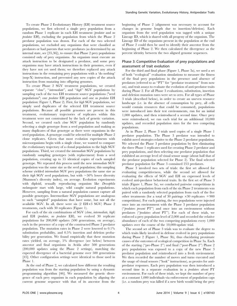
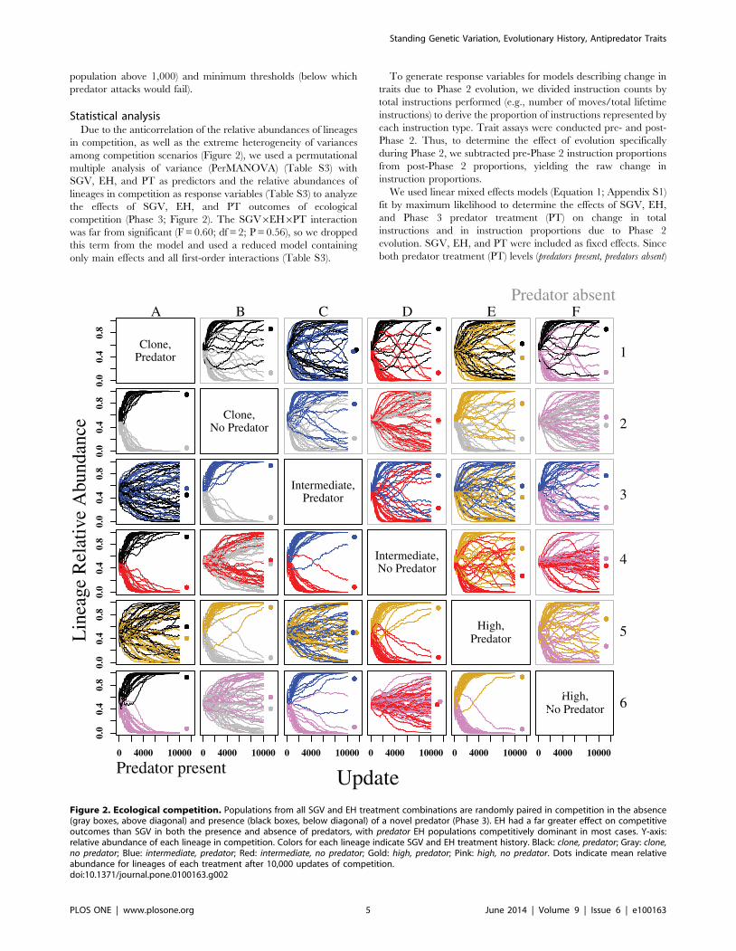
Statistical analysisDue to the anticorrelation of the relative abundances of lineages

in competition, as well as the extreme heterogeneity of variances

among competition scenarios (Figure 2), we used a permutational

multiple analysis of variance (PerMANOVA) (Table S3) with

SGV, EH, and PT as predictors and the relative abundances of

lineages in competition as response variables (Table S3) to analyze

the effects of SGV, EH, and PT outcomes of ecological

competition (Phase 3; Figure 2). The SGV6EH6PT interaction

was far from significant (F = 0.60; df = 2; P = 0.56), so we dropped

this term from the model and used a reduced model containing

only main effects and all first-order interactions (Table S3).

To generate response variables for models describing change in

traits due to Phase 2 evolution, we divided instruction counts by

total instructions performed (e.g., number of moves/total lifetime

instructions) to derive the proportion of instructions represented by

each instruction type. Trait assays were conducted pre- and post-

Phase 2. Thus, to determine the effect of evolution specifically

during Phase 2, we subtracted pre-Phase 2 instruction proportions

from post-Phase 2 proportions, yielding the raw change in

instruction proportions.

We used linear mixed effects models (Equation 1; Appendix S1)

fit by maximum likelihood to determine the effects of SGV, EH,

and Phase 3 predator treatment (PT) on change in total

instructions and in instruction proportions due to Phase 2

evolution. SGV, EH, and PT were included as fixed effects. Since

both predator treatment (PT) levels (predators present, predators absent)

Figure 2. Ecological competition. Populations from all SGV and EH treatment combinations are randomly paired in competition in the absence(gray boxes, above diagonal) and presence (black boxes, below diagonal) of a novel predator (Phase 3). EH had a far greater effect on competitiveoutcomes than SGV in both the presence and absence of predators, with predator EH populations competitively dominant in most cases. Y-axis:relative abundance of each lineage in competition. Colors for each lineage indicate SGV and EH treatment history. Black: clone, predator; Gray: clone,no predator; Blue: intermediate, predator; Red: intermediate, no predator; Gold: high, predator; Pink: high, no predator. Dots indicate mean relativeabundance for lineages of each treatment after 10,000 updates of competition.doi:10.1371/journal.pone.0100163.g002

Standing Genetic Variation, Evolutionary History, Antipredator Traits

PLOS ONE | www.plosone.org 5 June 2014 | Volume 9 | Issue 6 | e100163

were applied to each population, we fitted replicate as a random

intercept, and included a random slope across PT levels to account

for non-independence of PT levels. Where appropriate, we also

allowed for unequal variances among factor levels using the

‘‘varIdent()’’ function from the ‘‘nlme’’ [47] package (Table S4).

Equation 1 describes the change in total prey instructions due to

Phase 2 evolution. Models describing change in prey moves, turns,

and looks varied in complexity, but were of the same general form

(Appendix S1). For each trait, we used a likelihood ratio test for

model selection, starting with the full model (Equation 1) and

dropping interaction terms that did not improve the model fit

(Table S4).

EQUATION 1

y~

b0ijzb1ijzb1PTzb2EHzb3SGVzb4 PT|EHð Þz

b5 PT|SGVð Þzb6 EH|SGVð Þzb7 PT|EH|SGVð Þz

Eijk,b0ij~b0j ,s

2b0

� �,b1ij ~

b1j ,s2b1

� �,s2

b2 ~EH

where b0ij are the random intercepts, b1ij are the randomly varying

slopes across PT levels, and s2b2 ,EH is the variance function

allowing variances to differ between EH levels. We used a method

recently developed by [48] to calculate marginal R2 (proportion of

variation accounted for by fixed effects alone) and conditional R2

(proportion of variation accounted for by fixed and random effects

together). R2m and R2

c for each model are given in the Table S5.

To test the effects of SGV and EH on predator attack rates

during trait assays, we used a general linear model with SGV and

EH included as fixed effects, and the raw difference in attack rates

between pre- and post-Phase 2 evolution as the response variable.

A single replicate population was excluded from analyses of

change in total instructions, as this replicate had an unusually high

pre-Phase 2 instruction count, was highly unrepresentative of prey

populations in general, and greatly increased the variance of the

clone SGV + no predator EH treatment group (Figure S6).

Software and HardwareWe used Avida version 2.14 and the Heads-EX hardware [44]

for all experiments. Avida did not originally support immortal,

sterile predators as used in Phase 2 and Phase 3, so we added an

additional option to Avida that, when set, causes predators to

‘reset’ (akin to being reborn) instead of reproducing or dying of old

age. These modifications are available as a patch file against Avida

2.14, along with all analysis scripts, in the GitHub repository

(https://github.com/fishjord/avida_predation_scripts).

We conducted all experiments using the Michigan State

University’s High Performance Computing Cluster (HPCC). The

MSU HPCC contains three general purpose computing clusters

containing 2944 cores. Individual Avida runs were submitted as

compute jobs to the HPCC general processing queue in parallel

where possible. The Avida jobs took between 30 minutes and

seven days to run, depending on the number of updates (2,000 to

2,000,000 updates).

We performed all statistical analyses and constructed all figures

using the R statistical programming language version 3.0.2. The

PerMANOVA was conducted using the ‘‘adonis()’’ function in the

‘‘vegan’’ package (last updated by [49]). Linear mixed effects

models were constructed using the ‘‘lme’’ function from the

‘‘nlme’’ package (last updated by [47]), and we used the

‘‘allEffects’’ function from the ‘‘effects’’ package (last updated by

[50]) to extract marginalized fixed effects. To calculate marginal

and conditional R2, we used the ‘‘r.squaredGLMM’’ function

from the ‘‘MuMIn’’ package (last updated by [51]).

Results

Ecological competitionsEvolutionary history, i.e. historical exposure to predation in

Phase 1, was the most important selective agent shaping

competitive abilities of prey both in the presence and in the

absence of a novel predator. Prey that evolved with predator EH

were, in general, stronger competitors than those that evolved with

Figure 3. Change in total prey instructions executed (start of Phase 2 minus end of Phase 2), reflecting change in gestation time (orlifespan) resulting from Phase 2 evolution. ‘‘Predator present/absent’’ refers to the presence or absence of a novel predator during trait assaysbefore and after Phase 2 evolution. Total instructions either increased or decreased very little in predator EH populations, and universally decreased inno predator EH populations. Bars are 695% CI.doi:10.1371/journal.pone.0100163.g003

Standing Genetic Variation, Evolutionary History, Antipredator Traits

PLOS ONE | www.plosone.org 6 June 2014 | Volume 9 | Issue 6 | e100163

no predator EH. In competitions between predator EH and no predator

EH treatments, predator EH treatments always had the higher

mean final relative abundance (Figure 2; Table S3). Competitive

exclusion of a predator EH lineage by a no predator EH lineage after

10,000 updates in competition was extremely rare (but see e.g.

Figure 2, panel D3, in which 1 out of 30 predator lineages was

excluded). Competitive outcomes were not affected by the

presence of a novel predator, regardless of SGV or EH (Figure 2;

Table S3). While there was no main effect of SGV on mean final

relative abundances (SGV effect: Table S3), higher SGV seems to

have conferred some benefit to no predator EH populations

(Figure 2; SGV6EH effect: Table S3). Similarly, there appears

to be a subtle interaction between PT and EH, wherein in the

presence of a predator, the difference in relative abundances

between predator EH and no predator EH populations during

competition assays increases in favor of predator EH populations.

Evolution of prey traits during Phase 2Lifetime instruction counts for prey do not reflect higher rates of

instruction execution, but rather longer lifespans of prey organ-

isms. Changes in instruction counts varied greatly among

treatments (PT6EH6SGV interaction; Figure S2). During Phase

2 evolution, regardless of presence or absence of a novel predator

during trait assays, predator EH populations generally evolved to

increase total instructions executed per lifetime, except in the case

of clone populations in the absence of predators (Figure 3).

Conversely, no predator EH populations universally decreased in

lifetime instruction counts. In predator EH populations, SGV had a

markedly positive effect on the magnitude of the decrease in

instruction counts, while SGV had little or no effect on instruction

counts in predator EH populations. Prey generally changed more in

total instructions executed with predators present than with predators

absent (Figure 3).

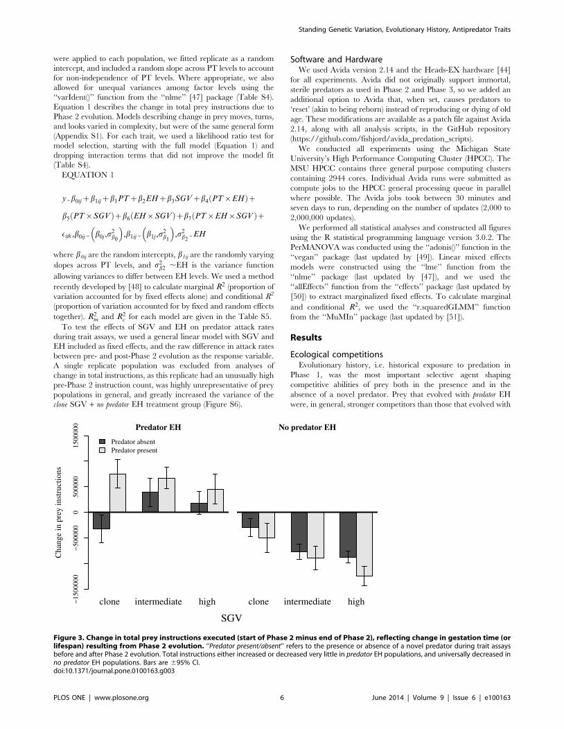
Prey moves as proportions of total prey instructions universally

decreased in predator EH populations as a result of Phase 2

Figure 4. Change in (top) prey moves, (middle) prey turns, and (bottom) prey looks as proportions of total prey instructions,resulting from Phase 2 evolution with a novel predator. ‘‘Predator present/absent’’ refers to the presence/absence of the Phase 3 novelpredator during the trait assays. Traits in predator EH populations generally evolved to a greater extent than did traits in no predator EH populations,and traits often evolved in different directions between the two EH treatments. Bars are 695% CI.doi:10.1371/journal.pone.0100163.g004

Standing Genetic Variation, Evolutionary History, Antipredator Traits

PLOS ONE | www.plosone.org 7 June 2014 | Volume 9 | Issue 6 | e100163

evolution, and largely increased in no predator EH populations (EH

effect, Figure 4; Figure S3). Effects of SGV on change in moves

were subtle, though slightly less so with predators absent. There was

no main effect of PT on change in moves (Figure 4; Figure S3).

Prey turns as proportions of total prey instructions increased

dramatically in predator EH populations, but changed very little in

no predator EH populations (Figure 4; Figure S4). Effects of SGV

were subtle, but were most pronounced in no predator EH

populations: clone and intermediate SGV populations decreased

slightly on average in proportion moves, while high SGV

populations increased (EH6SGV interaction, Figure S4). PT did

not affect change in turns (no PT main effect, Figure 4; Figure S4),

nor was there a main effect of SGV (Figure S4).

Proportions of instructions that were looks generally decreased

in predator EH populations, but changed little in no predator EH

populations; EH effects varied among levels of SGV, with the

smallest EH effects in clone SGV populations (EH6SGV interac-

tion, Figure 4; Figure S5). Main effects of SGV and PT were not

statistically significant (Figure S5).

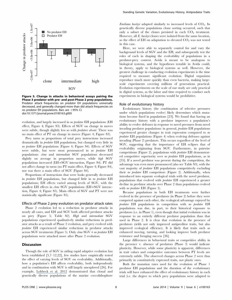
Effects of Phase 2 prey evolution on predator attack ratesPhase 2 evolution led to a reduction in predator attacks in

nearly all cases, and EH and SGV both affected predator attacks

on prey (Figure 5; Table S2). High and intermediate SGV

populations experienced qualitatively similar reductions in pred-

ator attacks as a result of Phase 2 evolution, and prey evolved with

predator EH experienced similar reductions in predator attacks

across SGV treatments (Figure 5). Only clone SGV + no predator EH

populations were attacked more after Phase 2 evolution.

Discussion

Though the role of SGV in aiding rapid adaptive evolution has

been established [5,7–12,22], few studies have empirically tested

the effect of varying levels of SGV on evolvability. Additionally,

how a population’s EH affects evolvability, both independently

and in combination with SGV is still largely unexplored [26]. For

example, Lohbeck et al. 2012 demonstrated that clonal and

genetically diverse populations of the marine coccolithophore

Emiliana huxleyi adapted similarly to increased levels of CO2. In

genetically diverse populations clone sorting occurred, such that

only a subset of the clones persisted in each CO2 treatment.

However, all E. huxleyi clones were isolated from the same location,

so the effect of EH on adaptation to elevated CO2 was not tested

in this case.

Here, we were able to separately control for and vary the

background levels of SGV and the EH, and subsequently test the

roles of each in shaping the evolvability of populations in a

predator-prey context. Avida is meant to be analogous to

biological systems, and the hypotheses testable in Avida could,

in theory, apply to biological systems as well. However, the

greatest challenge in conducting evolution experiments is the time

required to measure significant evolution. Digital organisms

reproduce much more quickly than even bacteria, making large-

scale experiments covering millions of generations practical.

Evolution experiments on the scale of our study are only practical

in digital systems, as the labor and time required to conduct such

experiments in biological systems would be prohibitive.

Role of evolutionary historyEvolutionary history (the combination of selective pressures

under which populations evolve) likely determines which muta-

tions become fixed in populations [23]. We found that having an

evolutionary history with a predator improves a population’s

ability to evolve defenses in response to novel pressures from novel

invading predator populations: in general, predator EH populations

experienced greater changes in trait expression compared to no

predator EH populations (Figure 4) when evolving defenses against

invading (Phase 2) predators. This occurs regardless of the level of

SGV, suggesting that the importance of EH eclipses that of

evolvability originating from SGV. Furthermore, in pairwise

competitions (Figure 2), populations with predator EH demonstrat-

ed competitive superiority over no predator EH populations, as in

[35]. If a novel predator was present during the competition, the

advantage was even more pronounced (also see Table S3), with the

vast majority of predator EH populations competitively excluding

their no predator EH competitors (Figure 2). Additionally, when

introduced into separate ecological trials with the novel predator,

populations that evolved with predator EH experienced a greater

decline in predator attacks over Phase 2 than populations evolved

with no predator EH (Figure 5).

Because populations in both EH treatments were further

evolved in the presence of predators (in Phase 2) before they were

competed against each other, the ecological advantage enjoyed by

predator EH populations in competition with no predator EH

populations was due, in part, to their historical exposure to

predators (i.e. in Phase 1), even though that initial evolution was in

response to an entirely different predator population than that

used in Phase 2. It is clear that evolution in the presence of

predators yields not only improved antipreditor traits, but also

improved ecological efficiency. It is likely that traits such as

enhanced moving, turning, and looking improve both predator

resistance and foraging success [36].

Large differences in behavioral traits or competitive ability in

the presence v. absence of predators (Phase 3) would indicate

plasticity. However, while some plasticity is apparent, differences

in trait values and competitive outcomes between PT levels are

extremely subtle. The observed changes across Phase 2 were thus

primarily in constitutively expressed traits, not plastic ones.

Both the mutation rates used for the evolution of Phase 1

predator EH populations and the duration of the evolutionary

trials will have enhanced the effect of evolutionary history in each

trial (i.e. the degree to which prey populations were adapted to

Figure 5. Change in attacks in behavioral assays pairing thePhase 3 predator with pre- and post-Phase 2 prey populations.Predator attack frequencies on predator EH populations universallydecreased, and generally changed more than did attack frequencies onno predator EH populations. Bars are 695% CI.doi:10.1371/journal.pone.0100163.g005

Standing Genetic Variation, Evolutionary History, Antipredator Traits

PLOS ONE | www.plosone.org 8 June 2014 | Volume 9 | Issue 6 | e100163

predators). Because we did not vary Phase 1 mutation rates or

duration, we cannot comment on how experimentally altering the

strength of historical selection could impact the observed trends in

trait evolution and competitive outcomes.

Role of standing genetic variationMany studies have pointed to SGV as a key component of a

population’s evolutionary potential [6]. When there is greater

genetic variation in a population, there is more raw material upon

which natural selection can act. Thus, we expected SGV alone to

play a significant role in the rapid evolution of anti-predator traits.

However, we found marginal effects of historical SGV in

determining the final outcomes of ecological competitions

(Figure 2). Furthermore, the effects of SGV on the evolution of

specific anti-predator traits (moves, turns, looks) were detectable

only within EH treatments (Figure 4).

Standing genetic variation (SGV) vs Evolutionary history(EH)

Across the predator EH populations, we found no detectable

effects of SGV on anti-predator trait values (Figure 4) or

competitive outcomes (Figure 2). We suggest that a lack of an

SGV effect on predator EH populations may be due, in part, to the

historical predator weeding out unfit prey genotypes. For example,

predators reduced prey diversity (Figure S1; Table S1) because

they operate as a very strong agent of selection against less fit

phenotypes. However, we would expect SGV to have an effect

within no predator EH populations (as seen in Figure 4). Given the

lack of an evolutionary history with predators, in no predator EH

populations, the odds of one sampled genotype (clone SGV) being

able to quickly acquire a beneficial mutation are low. On the other

hand, if the full suite of all discovered genotypes (high SGV)

remains in the population, there is a greater potential for providing

precursory material for rapidly generating anti-predator traits.

However, if EH leads to a large number of genotypes having the

prerequisites for rapid adaptive response, the odds of sampling a

beneficial genotype are high, and differences in SGV will not

significantly affect evolvability.

As we have shown, in order to adaptively address novel

predation pressures, it appears to be easier to modify historically

realized and relevant adaptations than to repurpose unrelated

genes, or evolve effective traits de novo. Thus, the greater

evolvability of the predator EH populations would have arisen out

of their ability to adapt anti-predator strategies across predation

contexts. More broadly, evolvability may commonly be deter-

mined by a population’s ability to use strategies across environ-

mental contexts, i.e. their adaptive complexity [52].

Supporting Information

Figure S1 Shannon’s diversity across 200,000 updates ofPhase 2 evolution in (A) high, (B) intermediate, and (C)clone SGV treatments. Filled circles represent no predator EH

treatments, open circles represent predator EH treatments. Bars are

695% CI.

(EPS)

Figure S2 Change in instructions. Shown are the margin-

alized fixed effects of a generalized linear mixed effects model of

scaled change in total prey instructions across Phase 2 evolution as

a function of SGV (A. clone; B. intermediate; C. high), EH, and

PT. Bars are 695% CI. EH had the greatest effect on change in

prey instructions, though PT also affected change in instructions,

especially in clone SGV populations. Formal model, random effects

output, and marginal and conditional R2 can be found in Table

S5.

(EPS)

Figure S3 Change in prey moves. Shown are the margin-

alized fixed effects of a generalized linear mixed effects model of

scaled change across Phase 2 evolution in the proportion of prey

instructions that were moves as a function of A. SGV and PT and

B. EH. Bars are 695% CI. Both EH and SGV affected change in

proportion moves, with SGV increasing more dramatically across

SGV treatments with predator present. Formal model, random effects

output, and marginal and conditional R2 can be found in Table

S5.

(EPS)

Figure S4 Change in prey turns. Shown are the marginal-

ized fixed effects of a generalized linear mixed effects model of

scaled change across Phase 2 evolution in the proportion of prey

instructions that were turns as a function of A. PT and B.

SGV6EH. Bars are 695% CI. Predator EH populations increased

turns as a results of Phase 2 evolution; change in turns was

marginal for no predator EH populations, and SGV affected predator

and no predator populations differently. PT had no detectable effect.

Formal model, random effects output, and marginal and

conditional R2 can be found in Table S5.

(EPS)

Figure S5 Change in prey looks. Shown are the marginal-

ized fixed effects of a generalized linear mixed effects model of

scaled change across Phase 2 evolution in the proportion of prey

instructions that were looks as a function of A. PT and B.

SGV6EH. Bars are 695% CI. Clone and high SGV populations

with predator EH increased looks as a result of Phase 2 evolution

and change in turns was marginal to negative for no predator EH

populations. PT had no detectable effect. Formal model, random

effects output, and marginal and conditional R2 can be found in

Table S5.

(EPS)

Figure S6 Total instructions executed by each replicateprey population before and after Phase 2 evolution. The

slope of each line represents the evolutionary change in

instructions executed per lifetime (i.e. gestation time). The same

replicate populations were assayed in the absence (top) and in the

presence (bottom) of the Phase 3 predator. Arrows indicate the

replicate population that was excluded from all statistical analyses,

as it is not representative of its treatment group (clone SGV, no

predator EH).

(EPS)

Table S1 Analysis of Variance (calculated using theanova() function in the R 3.0.2 base package) on a linearmodel*{ testing the effects of SGV and EH and theirinteraction on Shannon’s diversity among populations atthe 200,000th update of Phase 2 evolution.

(DOCX)

Table S2 Analysis of Variance (calculated using theanova() function in the R 3.0.2 base package) on a linearmodel*{ testing the effects of SGV and EH and theirinteraction on change in predator attacks as a result ofPhase 2 evolution.

(DOCX)

Table S3 Permutational multiple analysis of variance(PerMANOVA) output describing effects on SGV, EH,and PT (and all first-order interactions) on outcomes of

Standing Genetic Variation, Evolutionary History, Antipredator Traits

PLOS ONE | www.plosone.org 9 June 2014 | Volume 9 | Issue 6 | e100163

ecological competitions (see Figure 2). 999 permutations

were used.

(DOCX)

Table S4 AIC, LRT output, and model selection pro-cesses for linear mixed-effects models describingchange in A. total prey instructions; proportion moves;C. proportion turns and D. proportion looks. Variance

functions are shown with traits modeled (in italics).

(DOCX)

Table S5 Random intercepts and slopes (linear con-trasts) between levels of PT with parametric bootstrap95% confidence intervals for models describing changein A. total prey instructions; B. proportion moves; C.proportion turns; and D. proportion looks. Also included

are marginal and conditional R2 and residual standard deviations

with parametric bootstrap 95% CI.

(DOCX)

Appendix S1 S1.1: Genetic diversification during Phase 2

evolution. S1.2: Linear mixed effects models describing evolution-

ary change in traits.

(DOCX)

Acknowledgments

We thank Chris Adami for comments and feedback on an earlier draft of

this manuscript, and Max McKinnon for contributions to early stages of

this research. Finally, we thank two anonymous reviewers for comments on

the earlier versions of this work.

Author Contributions

Conceived and designed the experiments: AP DRO JAF APW. Performed

the experiments: JAF APW. Analyzed the data: DRO. Wrote the paper:

DRO AP JAF APW ID. Designed all figures and tables, aided in

experimental design, contributed significantly to interpretation of results,

and conducted significant revision of the manuscript: DRO. Significant

revision/editing of manuscript: ID.

References

1. Frankham R, Lees K, Montgomery ME, England PR, Lowe EH, et al. (1999)

Do population size bottlenecks reduce evolutionary potential? Anim Conserv 2:

255–260.

2. Colegrave N, Collins S (2008) Experimental evolution: experimental evolution

and evolvability. Heredity 100: 464–470.

3. Mitchell-Olds T, Willis JH, Goldstein DB (2007) Which evolutionary processes

influence natural genetic variation for phenotypic traits? Nat Rev Genet 8: 845–

856.

4. Futuyma DJ (1979). Evolutionary Biology. 1st ed. Sinauer Associates, Sunder-

land, Massachusetts. ISBN 0-87893-199-6.

5. Barrett R, Schluter D (2008) Adaptation from standing genetic variation. Trends

Ecol Evol 23: 38–44.

6. Orr HA, Betancourt AJ (2001) Haldane’s sieve and adaptation from the standing

genetic variation. Genetics 157: 875–884.

7. Innan H, Kim Y (2004) Pattern of polymorphism after strong artificial selection

in a domestication event. Proc Natl Acad Sci USA 101: 10667–10672.

8. Colosimo PF, Hosemann KE, Balabhadra S, Villarreal Jr G, Dickson M, et al.

(2005) Widespread parallel evolution in sticklebacks by repeated fixation of

ectodysplasin alleles. Science 307: 1928–1933.

9. Prezeworski M, Coop G, Wall JD (2005) The signature of positive selection on

standing genetic variation. Evolution 59: 2312–2323.

10. Pennings PS (2012) Standing genetic variation and the evolution of drug

resistance in HIV. PLoS Comput Biol 8: e1002527.

11. Elmer KR, Meyer A (2011) Adaptation in the age of ecological genomics:

insights from parallelism and convergence. Trends Ecol Evol 6: 298–306.

12. Yoshida T, Jones LE, Ellner SP, Fussmann GF, Hairston NG (2003) Rapid

evolution drives ecological dynamics in a predator-prey system. Nature 424:

303–306.

13. Litchman E, Edwards KF, Klausmeier CA, Thomas MK (2012) Phytoplankton

niches, traits and eco-evolutionary responses to global environmental change.

Mar Ecol Prog Ser 470: 235–248.

14. Jerome JP, Bell JA, Plovanich-Jones AE, Barrick JE, Brown CT, et al. (2011)

Standing Genetic Variation in Contingency Loci Drives the Rapid Adaptation

of Campylobacter jejuni to a Novel Host. PLoS ONE 6: e16399

15. Dionne M, Miller KM, Dodson JJ, Bernatchez L (2009) MHC standing genetic

variation and pathogen resistance in wild Atlantic salmon. Philos T Roy Soc B

364: 1555–1565.

16. Dettman JR, Anderson JB, Kohn LM (2008) Divergent adaptation promotes

reproductive isolation among experimental populations of the filamentous

fungus Neurospora. BMC Evol Biol 8: 35.

17. Bell G, Collins S (2008) Adaptation, extinction and global change. Evol Appl 1:

3–16.

18. McGuigan K, Sgro CM (2009) Evolutionary consequences of cryptic genetic

variation. Trends Ecol Evol 24: 305–311.

19. Lohbeck KT, Riebesell U, Reusch TBH (2012) Adaptive evolution of a key

phytoplankton species to ocean acidification. Nat Geosci 5: 346–351.

20. Hayden EJ, Ferrada E, Wagner A (2011) Cryptic genetic variation promotes

rapid evolutionary adaptation in an RNA enzyme. Nature 474: 92–95.

21. Messer PW, Petrov DA (2013) Population genomics of rapidadaptation by soft

selective sweeps. Trends Ecol Evol 28: 659–669.

22. Anderson CJ (2013) The role of standing genetic variation in adaptation of

digital organisms to a new environment. Artif Life 13: 3–10.

23. Hermisson J (2005) Soft sweeps: molecular population genetics of adaptation

from standing genetic variation. Genetics 169.4: 2335–2352.

24. Levins R (1963) Theory of fitness in a heterogeneous environment. II.

Developmental flexibility and niche selection. Am Nat 97: 75–90.

25. Gillings MR, Stokes HW (2012) Are humans increasing bacterial evolvability?

Trends Ecol Evol 27: 346–352.

26. Blount ZD, Borland CZ, Lenski RE (2008) Historical contingency and the

evolution of a key innovation in an experimental population of Escherichia coli.

Proc Natl Acad Sci USA 105: 7899–7906.

27. Hedrick PW (1976) Genetic variation in a heterogeneous environment. II.

Temporal heterogeneity and directional selection. Genetics 84: 145–157.

28. Kawecki TJ, Lenski RE, Ebert D, Hollis B, Olivieri I, et al. (2012) Experimental

evolution. Trends Ecol Evol 27: 547–560.

29. Fry JD (2001) Direct and correlated responses to selection for larval ethanol

tolerance in Drosophila melanogaster. J Evolution Biol 14: 296–309.

30. Bonnell ML, Selander RK (1974) Elephant seals: genetic variation and near

extinction. Science 184.4139: 908–909.

31. Lande R (1988) Genetics and demography in biological conservation. Science

241: 1455–1460.

32. Ofria C, Bryson DM, Wilke CO (2009) Avida: A Software Platform for Research

in Computational Evolutionary Biology. In: Adamatzky A, Komosinski M,

editors. Artificial Life Models in Software. London, UK: Springer Verlag,

London, UK. Second edition.

33. Wilke CO, Adami C (2002) The biology of digital organisms. Trends Ecol Evol

17: 528–532.

34. Lenski RE, Ofria C, Pennock RT, Adami C (2003) The evolutionary origin of

complex features. Nature 423: 139–144.

35. Fortuna MA, Zaman L, Wagner AP, Ofria C (2013) Evolving Digital Ecological

Networks. PLoS Comput Biol 9: e1002928.

36. Wagner AP, Zaman L, Dworkin I, Ofria C (2013) Coevolution, behavioral

chases, and the evolution of prey intelligence. arXiv:1310.1369v2.

37. Lehmann K, Goldman BW, Dworkin I (2013) From cues to signals: evolution of

interspecific communication via aposematism and mimicry in a predator-prey

system. PLoS One 9: e91783.

38. Lima SL, Dill LM (1990) Behavioral decisions made under the risk of predation:

a review and prospectus. Can J Zool 68: 619–640.

39. Sih A (1987) Predator and prey lifestyles: an evolutionary and ecological

overview. Predation: direct and indirect impacts on aquatic communities

(Kerfoot WC, Sih A, eds). Hanover, New Hampshire: University Press of New

England; 203–224.

40. McCollum SA, Van Buskirk J (1996) Costs and benefits of a predator-induced

polyphenism in the gray treefrog Hyla chrysoscelis. Evolution 50: 583–593.

41. Dodson S (1989) Predator-induced reaction norms. BioScience 39: 447–452.

42. Rundle HD, Nosil P (2005) Ecological speciation. Ecol Lett 8: 336–352.

43. Schmitz OJ (2008) Effects of predator hunting mode on grassland ecosystem

function. Science 319: 952–954

44. Bryson DM, Ofria C (2013) Understanding evolution potential in virtual CPU

architectures. PLoS ONE 8: e83242.

45. Drake JW, Charlesworth B, Charlesworth D, Crow JF (1998) Rates of

spontaneous mutation. Genetics 148: 1667–1686.

46. Needleman SB, Wunsch CD (1970) A general method applicable to the search

for similarities in the amino acid sequence of two proteins. J Mol Biol 48: 443–

453.

47. Pinheiro J, Bates D, DeRoy S, Sarkar D (R Core Development Team) (2014)

Linear and nonlinear mixed effects models. Version 3.1–117. Updated 31

March 2014.

48. Nakagawa S, Schielzeth H (2013) A general and simple method for obtaining R2

from generalized linear mixed-effects models. Methods Ecol Evol 4: 133–142.

49. Oksanen J, Blanchet FG, Kindt R, Legendre P, Minchin P, et al. (2013) vegan:

Community ecology package. Version 2.0–10. Updated 12 December 2013.

Standing Genetic Variation, Evolutionary History, Antipredator Traits

PLOS ONE | www.plosone.org 10 June 2014 | Volume 9 | Issue 6 | e100163

50. Fox J, Weisberg S, Friendly M, Hong J, Andersen R, et al. (2013) R package

effects: Effects displays for linear, generalized linear, multinomial-logit,proportional-odds logit models and mixed-effects models. Version 2.3–0.

Updated 7 November 2013.

51. Barton K (2013) R package MuMIn: Multi-modal inference. Version 1.9.13.

Updated 29 October 2013.

52. Potts R (1996) Evolution and climate variability. Science 273: 922–923.

Standing Genetic Variation, Evolutionary History, Antipredator Traits

PLOS ONE | www.plosone.org 11 June 2014 | Volume 9 | Issue 6 | e100163