the Removal of Pollutants using Aluminium Alloys, Stainless ...

Electrocoagulation for Water Treatment:

the Removal of Pollutants using Aluminium

Alloys, Stainless Steels and Iron Anodes

Adelaide Dura, M.Sc.

Thesis Submitted to the National University of Ireland in Fulfillment of the

requirements for the Degree of Doctor of Philosophy

Department of Chemistry

National University of Ireland Maynooth

August 2013

Head of Department: Dr. John C. Stephens

Supervisor: Prof. Carmel B. Breslin

i

Table of Contents

Declaration ..................................................................................................................... vi

Acknowledgments .......................................................................................................... ix

Abstract ........................................................................................................................... x

List of Figures xi

List of Tables xix

List of Symbols xxi

1. Introduction and Literature Review1 ..................................................................... 1

1.1 Research topic ....................................................................................................... 1

1.2 Water treatment technologies ................................................................................ 2

1.2.1 The removal of phosphates ............................................................................. 5

1.2.2 The removal of dyes ....................................................................................... 7

1.2.3 The removal of zinc ions ................................................................................ 8

1.3 Electrocoagulation ................................................................................................. 9

1.3.1 Advantages and disadvantages of the electrocoagulation technique ............ 10

1.3.2 Principles of electrocoagulation.................................................................... 11

1.3.2.1 Reactions at the electrodes ..................................................................... 13

1.3.2.2 Coagulation ............................................................................................ 15

1.3.2.3 Flocculation ............................................................................................ 21

1.3.3 Factors affecting electrocoagulation ............................................................. 21

1.3.3.1 Electrode materials ................................................................................. 21

1.3.3.2 Electrode arrangements .......................................................................... 23

1.3.3.3 Current density ....................................................................................... 24

1.3.3.4 Supporting electrolyte ............................................................................ 25

1.3.3.5 Solution pH ............................................................................................ 26

1.3.4 Removal of pollutants by electrocoagulation ............................................... 26

1.4 Electrochemistry and corrosion properties of materials ...................................... 29

1.4.1 Corrosion and passivity ................................................................................ 29

ii

1.4.1.1 Basic concepts of corrosion ................................................................... 31

1.4.1.2 Mixed potential theory ........................................................................... 35

1.4.1.3 Types of corrosion.................................................................................. 37

1.4.2 Corrosion properties of materials ................................................................. 42

1.4.2.1 Iron ......................................................................................................... 42

1.4.2.2 Stainless steel ......................................................................................... 43

1.4.2.3 Aluminium ............................................................................................. 46

1.4.2.4 Aluminium alloys ................................................................................... 47

1.5 Research presented in this thesis ......................................................................... 49

1.6 References ........................................................................................................... 51

2. Experimental ........................................................................................................... 57

2.1 Introduction ......................................................................................................... 57

2.2 Chemicals and electrode materials ...................................................................... 58

2.2.1 Chemicals and test electrolytes ..................................................................... 58

2.2.2 Electrode materials and sample preparation ................................................. 59

2.3 Experimental techniques ..................................................................................... 61

2.3.1 Electrochemical experiments ........................................................................ 61

2.3.1.1 The electrochemical cell for corrosion and RDV experiments .............. 62

2.3.1.2 The electrochemical cell for electrocoagulation experiments ................ 62

2.3.1.3 Corrosion techniques .............................................................................. 63

2.3.1.4 Electrocoagulation techniques ............................................................... 67

2.3.1.5 Rotating disk voltammetry, RDV .......................................................... 68

2.3.2 Microscopy ................................................................................................... 71

2.3.3 Spectroscopy ................................................................................................. 72

2.3.3.1 UV-Visible ............................................................................................. 72

2.3.3.2 Atomic absorption spectroscopy ............................................................ 76

2.3.4 Kinetic analysis of phosphate removal by electrocoagulation ...................... 77

2.3.5 Fitting of phosphate removal by electrocoagulation to adsorption isotherms78

2.3.6 Calculation of energy consumption during electrocoagulation .................... 80

2.3.7 Statistical methods for chemometric study on phosphate removal ............... 81

2.4 References ........................................................................................................... 89

iii

3. Performance of Al-2Mg and AISI 420 Electrodes for the Removal of Phosphates by Electrocoagulation ............................................................................................. 91

3.1 Introduction ......................................................................................................... 91

3.2 Al-2Mg electrode ................................................................................................ 94

3.2.1 The effect of the initial concentration of PO4-P ........................................... 96

3.2.1.1 The efficiency of removal ...................................................................... 96

3.2.1.2 The rate constant for the removal of phosphates ................................... 99

3.2.2 The effect of the current density ................................................................. 103

3.2.3 The effect of pH .......................................................................................... 106

3.2.3.1 The effect of initial pH ......................................................................... 106

3.2.3.2 The effect of final pH ........................................................................... 108

3.2.4 The effect of chloride concentration ........................................................... 111

3.2.5 Adsorption isotherms .................................................................................. 114

3.2.6 The removal of phosphates from real samples ........................................... 121

3.3 AISI 420 electrode ............................................................................................. 123

3.3.1 Iron speciation in electrocoagulation .......................................................... 126

3.3.2 The effect of the initial concentration of PO4-P ......................................... 132

3.3.2.1 The efficiency of removal .................................................................... 132

3.3.2.2 The rate constant for the removal of phosphates ................................. 134

3.3.3 The effect of the current density ................................................................. 136

3.3.4 The effect of pH .......................................................................................... 138

3.3.4.1 The effect of initial pH ......................................................................... 139

3.3.4.2 The effect of final pH ........................................................................... 140

3.3.5 The effect of chloride concentration ........................................................... 142

3.3.6 Adsorption isotherms .................................................................................. 145

3.3.7 The removal of phosphates from real samples ........................................... 147

3.4 Summary ........................................................................................................... 150

3.5 References ......................................................................................................... 152

4. Electrochemical Behaviour of Various Electrode Materials in Synthetic Wastewater ............................................................................................................ 158

4.1 Introduction ....................................................................................................... 158

4.2 Pure iron ............................................................................................................ 162

4.2.1 The effect of Cl- ions .................................................................................. 163

iv

4.2.2 The effect of SO42- ions .............................................................................. 167

4.2.3 The effect of PO43- ions .............................................................................. 170

4.2.4 The effect of co-existing anions in sww 1 and sww 2 ................................ 172

4.3 Stainless steel AISI 310 ..................................................................................... 175





4.4 Stainless steel AISI 420 ..................................................................................... 184





4.5 Pure aluminium ................................................................................................. 193



4.6 Al-2Mg alloy ..................................................................................................... 199





4.7 Al-Zn-In alloy .................................................................................................... 209





4.8 Summary ........................................................................................................... 219

4.9 References ......................................................................................................... 222

5. Performance of the Electrodes in Synthetic Wastewaters and a Screening Chemometric Study on the Removal of Phosphates by AISI 420 Electrode .. 226

5.1 Introduction ....................................................................................................... 226

5.2 Iron system ........................................................................................................ 229

v

5.2.1 The electrode performance in removing three representative pollutants from synthetic wastewaters .......................................................................................... 230

5.2.1.1 The removal of phosphates .................................................................. 230

5.2.1.2 The removal of Orange II dye .............................................................. 233

5.2.1.3 The removal of zinc ions ...................................................................... 236

5.2.2 The electrochemistry and the removal performance of the iron system ..... 239

5.2.3 Energy efficiency ........................................................................................ 244

5.3 Aluminium system ............................................................................................ 247

5.3.1 The electrode performance in removing three representative pollutants from synthetic wastewaters .......................................................................................... 247

5.3.1.1 The removal of phosphates .................................................................. 247

5.3.1.2 The removal of Orange II dye .............................................................. 250

5.3.1.3 The removal of zinc ions ...................................................................... 253

5.3.2 The electrochemistry and the removal performance of the aluminium system ............................................................................................................................. 257

5.3.3 Energy efficiency ........................................................................................ 259

5.4 Screening chemometric study............................................................................ 260

5.4.1 Estimating factor effects and forming the initial model ............................. 262

5.4.2 Performing statistical tests .......................................................................... 265

5.5 Summary ........................................................................................................... 267

5.6 References ......................................................................................................... 269

6. Conclusions ............................................................................................................ 272

6.1 General conclusions .......................................................................................... 272

6.2 Future works ...................................................................................................... 277

6.3 Conference presentations .................................................................................. 278

6.4 References ......................................................................................................... 278

Appendix .................................................................................................................... 280

vi

Declaration

I hereby certify that this thesis, which I now submit for assessment on the programme of

study leading to the award of PhD has not been submitted, in whole or part, to this or

any other University for any degree and is, except where otherwise stated the original

work of the author.

Date: Signed:

vii

To Francesco and my parents, with love.

viii

I am a clown...and I collect moments.

― Heinrich Böll, The Clown

Some things will always be stronger than time and distance.

Deeper than languages and ways. Like following your dreams, and learning to be yourself.

Sharing with others the magic you have found…

― Sergio Bambarén, The Dolphin: Story of a Dreamer

ix

Acknowledgments

I would like to express my sincere gratitude to my supervisor Prof. Carmel B. Breslin

for her guidance over the course of this research. She was always helpful, understanding

and provided a positive support. Particular thanks to Dr. John Colleran for his help over

the past years.

I wish to acknowledge the Irish Research Council's EMBARK Initiative for funding this

study.

I am extremely indebted to all the technical staff, in particular Ria Collery-Walsh, Orla

Fenelon, Anne Clearly, Dr. Ken Maddock, and the Executive Assistant Niamh Kelly,

who have always been available and willing to help whenever I needed it. A special

mention is for Noel Williams for his help, support and inspiring discussions.

A number of people have made my stay in Ireland an enjoyable experience. My friends

from the ESL course, Esteban and Sohrab, thanks for all the laughter, Wenbai, Maryam

and Buket, you are the sweetest people I have ever met, and the ‘Italians’ Giorgio,

Martina, Daniela and Francesco. I thank all my current and former colleagues in the

Department of Chemistry who provided such an enjoyable and great research

environment. A special word of thanks to Paul, Foxy, Conor, Richard, Niall (Joey),

Orla, Wayne, Emer, Gama, Sam, Dave, Declan, Niamh, Carol, Trish, Ken, my ‘fellow’

Owen and Rob.

I am forever indebted to Valeria and Sinéad. Thanks for your friendship, your support

and your being there whenever I needed it. I was unbelievably lucky for having you as

friends and lab mates. I am also particularly grateful to Enrico for his remarkable

knowledge and expertise, and Susan for her sincere friendship and all the good times we

had together.

To my parents, my sister Gabriella and the little Iris, thank you for your support,

encouragements and love. Finally, I am deeply grateful to Francesco, for his love and

understanding. He has always stood by me and given support even during the hardest

periods.

x

Abstract

The development of effective and sustainable wastewater treatments is becoming

increasingly important. Electrocoagulation is one of the more promising approaches as

it is simple and efficient and, compared with traditional processes, has the advantages of

short treatment times and low sludge production.

The objective of this research was to determine the feasibility of the electrocoagulation

technique as a method to remove pollutants from wastewater. Electrocoagulation tests

were first carried out in phosphate-containing solutions with an aluminium-magnesium

and a stainless steel electrode. Several operating conditions, such as the initial

concentration of phosphates, current density, initial pH and sodium chloride

concentration, were varied and the corresponding effects were investigated. Removal

efficiencies of 95.9% and 79.7% were observed after 60 min with the aluminium-

magnesium and the stainless steel electrodes, respectively, using an initial phosphate

concentration of 150 mg L-1, an initial pH of 5.0, a current density of 11.0 mA cm-2 and

a ratio of the surface area of the electrode to the volume of the solution of 11.7 m-1 and

10.5 m-1 for the aluminium-magnesium and the stainless steel electrodes, respectively.

The electrochemical behaviour of several electrode materials was then correlated with

the removal and energy performance of these electrodes in the treatment of phosphates,

an azo dye and zinc ions dissolved in synthetic wastewaters. The synthetic wastewaters

were designed to contain a mixture of ions with different conductivity values. Pure iron

and an aluminium-indium-zinc electrode were identified as the most promising

materials, giving low corrosion potentials and active dissolution. Excellent removal

efficiencies for the three pollutants were observed using the pure iron electrode (96%,

99% and 100% for phosphates, azo dye and zinc ions, respectively) with an energy

consumption of 0.52 Wh. The aluminium-indium-zinc alloy required the lowest energy

supply of 0.26 Wh, gave excellent removal for both the phosphates and zinc ions (95%

and 100%, respectively). However, only a moderate efficiency, 78%, was observed for

the removal of the azo dye.

A screening design of experiment, DoE, was carried out to determine the most

significant factors affecting the electrocoagulation removal process. These factors were

identified as the current density and the ratio of the surface area of the electrode to the

volume of the solution, SA/V.

xi

List of Figures

Figure 1.1: Typical water treatment process flow diagram. ............................................ 3 Figure 1.2: Distribution of major species of orthophosphates in water. .......................... 6 Figure 1.3: Simplified scheme of an electrocoagulation cell. ........................................ 12 Figure 1.4: (a) Schematic of the different regions of the electrical double layer based on the BDM model and (b) variation of the potential versus distance from the surface. .... 16 Figure 1.5: Representation of DLVO theory. ................................................................ 18 Figure 1.6: Speciation diagrams of the mononuclear hydrolysis products for (a) Al3+ and (b) Fe3+ ions at a concentration of 1.0 µM ............................................................... 21 Figure 1.7: Schematic diagrams of (a) monopolar and (b) bipolar electrode connections. ..................................................................................................................... 25 Figure 1.8: Pourbaix diagram for iron in water (dissolved iron concentration is 1.0 × 10-5 mol L-1 and the temperature is 25 °C). Only Fe, Fe3O4, Fe2O3 as solid products are considered.. ..................................................................................................................... 34 Figure 1.9: Evans diagram for zinc in HCl acid solution............................................... 37 Figure 1.10: Schematic diagrams representing pit initiation by (a) adsorption and thinning, (b) penetration and (c) film breaking ............................................................... 40 Figure 1.11: Schematic of an active corrosion pit on a metal in a chloride solution ..... 43 Figure 1.12: Simplified Pourbaix diagram for chromium in water (for a chromium concentration of 1.0 × 10-6 mol L-1 and a temperature of 25°C). .................................... 46 Figure 1.13: Simplified Pourbaix diagram for aluminium in water (for aluminium concentration of 1.0 × 10-5 mol L-1 and a temperature of 25°C). .................................... 48 Figure 1.14: Influence of alloying elements on the dissolution potential of aluminium alloys ............................................................................................................................... 50 Figure 2.1: Basic diagram of a potentiostat ................................................................... 56 Figure 2.2: A schematic representation of the electrochemical cell used for corrosion and RDV experiments ..................................................................................................... 57 Figure 2.3: A schematic representation of the electrochemical cell used for electrocoagulation experiments ....................................................................................... 58 Figure 2.4: Representative potentiodynamic polarisation curve .................................... 60 Figure 2.5: Classical Tafel analysis. .............................................................................. 61 Figure 2.6: Schematic showing the flow patterns to the rotating disk electrode, RDE. (a) The solution flow perpendicular to the electrode. (b) The electrode surface viewed from below. ..................................................................................................................... 64 Figure 2.7: Typical diffusion controlled voltammetric response under mass-transfer-limiting condition. ........................................................................................................... 65

xii

Figure 2.8: (a) Calibration curves for Fe(II) (R2 = 0.990) and Fe(III) (R2 = 0.994) and (b) representative standard addition plot for Fe(II) (R2 = 0.997). ........................ 66 Figure 2.9: Calibration curve for PO4-P determination (λ = 470 nm). The limit of detection, LD, was estimated as 0.25 mg L-1. (R2 = 0.999). ........................................... 69 Figure 2.10: Orange II dye (a) azo-hydrazone tautomerism and (b) representative UV-Vis spectrum. .................................................................................................................. 70 Figure 2.11: Calibration curve for Orange II dye determination (λ = 485 nm). The limit of detection, LD, was estimated as 0.18 mg L-1. (R2 = 0.999). ....................................... 70 Figure 2.12: Calibration curve for Zn determination. The limit of detection, LD, was estimated as 0.09 mg L-1. (R2 = 0.998). .......................................................................... 72 Figure 2.13: Relationship between response, design matrix and coefficients ............... 80 Figure 3.1: Aluminium hydrolysis products. The dashed lines denote an unknown sequence of reactions ...................................................................................................... 89 Figure 3.2: Simplified model for the removal of phosphates in electrocoagulation using aluminium electrodes. ..................................................................................................... 90 Figure 3.3: Normalised variation of the concentration, Pt/Po, of phosphates plotted as a function of the electrocoagulation time in solutions containing initial concentrations, Po, of 20.0 mg L-1, 60.0 mg L-1 and 150.0 mg L-1 PO4-P ........................................ 93 Figure 3.4: (a) Pseudo first-order and (b) pseudo second-order kinetics of phosphate removal at different initial concentrations of phosphates, P0: 20.0 mg L-1, 60.0 mg L-1 and 150.0 mg L-1 PO4-P. .................................................................... 97 Figure 3.5: Variation of the concentration of phosphates, Pt, plotted as a function of the electrocoagulation time in solutions containing initial concentration, P0, of 60.0 mg L-1 PO4-P at different current densities: 5.3 mA cm-2 and 11.0 mA cm-2 .................. 100 Figure 3.6: Kinetics of phosphate removal at different initial concentrations of phosphates, P0: 20.0 mg L-1, 60.0 mg L-1 and 150.0 mg L-1 PO4-P. ................ 101 Figure 3.7: Variation of the residual phosphate concentration, Pt, plotted as a function of the electrocoagulation time in solutions containing 85.0 mg L-1 of PO4-P at initial pH values of 3.2, 5.3, 6.7 and 7.5 .................................................................... 103 Figure 3.8: Evolution of final pH and removal efficiency, η, plotted as a function of the initial pH. ............................................................................................................ 105 Figure 3.9: Residual phosphate concentration, Pt, as a function of NaCl concentration. The concentrations of NaCl used were: 4.2, 7.0, 10.0, 25.0 and 44.0 × 10-3 M. .......... 109 Figure 3.10: Variation of the anode potential as a function of the electrolysis time in solutions containing −−− 4.2, ⋅ ⋅ ⋅ 7.0, − − − 10.0, − ⋅⋅ − 25.0 and −− −− −− 44.0 × 10-3 M NaCl .......................................................................................................................... 110 Figure 3.11: Experimental data, −−− Freundlich isotherm, − − − Langmuir isotherm and −·−·− Temkin isotherm fitting at 25 ± 1 ºC. .......................................................... 116 Figure 3.12: Removal efficiency, η, plotted as a function of the electrocoagulation time in sample no. 1 and sample no. 2 ........................................................................ 117 Figure 3.13: Variation of the anode potential as a function of the electrocoagulation

period in −−− sample no. 1 and ⋅ ⋅ ⋅ sample no. 2 ......................................................... 119

xiii

Figure 3.14: Monomeric iron (III) hydrolysis products ............................................... 120 Figure 3.15: Simplified model for the removal of phosphates in electrocoagulation using stainless steel electrodes. ..................................................................................... 121 Figure 3.16: Voltammograms recorded in 1.0 M H2SO4 containing: (a) −−− 20.0 × 10-3 M Fe(II), − − − 80.0 × 10-3 M Fe(III) and (b) · · · a mixture of 20.0 × 10-3 M Fe(II) and 80.0 × 10-3 M Fe(III). Calibration curves for Fe(II) and Fe(III) plotted from (c) the single solutions of Fe(II) and Fe(III) and (d) the mixtures of Fe(II) and Fe(III). .......................................................................................................... 125 Figure 3.17: (a) Voltammograms recorded in a 4.2 × 10-3 M NaCl solution collected at the end of an electrocoagulation test at 500, 1000, 1500, 2000, 2500, 3000, 3500 and 4000 rpm. Levich plots for (b) the upper and (c) lower limiting currents, IUL and ILL, read at 1.1 and -0.1 V vs. SCE, respectively, from the voltammograms. ..................... 126 Figure 3.18: (a) Voltammograms of a solution recorded at the end of the electrocoagulation test in 4.2 × 10-3 M NaCl. Standard addition plots for (b) Fe(II) and (c) Fe(III). ......... 127 Figure 3.19: Plot of normalised variation of the concentration of phosphates, Pt/P0, as a function of time in solutions containing initial concentrations, P0, of 20.0 mg L-1, 60.0 mg L-1 and 150.0 mg L-1 PO4-P. ................................................................... 129 Figure 3.20: Plot of kinetics of phosphate removal at different initial concentrations of phosphates, P0: 20.0 mg L-1, 60.0 mg L-1 and 150.0 mg L-1 PO4-P.................. 132 Figure 3.21: Graph illustrating the variation of the concentration of phosphates, Pt, as a function of the electrocoagulation time in solutions containing initial concentration, P0, of 60.0 mg L-1 PO4-P at different current densities: 2.6 mA cm-2 and 11.0 mA cm-2 ............................................................................................................. 133 Figure 3.22: Plot showing kinetics of phosphate removal at different initial concentration of phosphates, P0: 20.0 mg L-1, 60.0 mg L-1 and 150.0 mg L-1 PO4-P. ............................................................................................................................ 134 Figure 3.23: Variation of the residual phosphate concentration, Pt, plotted as a function of the electrocoagulation time in solutions containing 85.0 mg L-1 of PO4-P at initial pH values of 3.0, 7.2 and 9.7. ............................................................................... 135 Figure 3.24: Evolution of final pH and removal efficiency plotted as a function of the initial pH. ................................................................................................................. 138 Figure 3.25: Residual phosphate concentration, Pt, as a function of NaCl concentration. The concentrations of NaCl used were: 4.2, 7.0, 10.0, 25.0 and 44.0 × 10-3 M. .......... 140 Figure 3.26: Variation of the anode potential as a function of the electrolysis time in solutions containing −−− 2.8, ⋅ ⋅ ⋅ 4.2, − − − 10.0, − ⋅⋅ − 25.0 and −− −− −− 44.0 × 10-3 M NaCl .......................................................................................................................... 141 Figure 3.27: Experimental data, −−− Freundlich isotherm, − − − Langmuir isotherm and −·−·− Temkin isotherm fitting at 25 ± 1 ºC ............................................................ 143 Figure 3.28: Removal efficiency, η, plotted as a function of the electrocoagulation time in sample no. 1 and sample no. 2 ........................................................................ 144 Figure 3.29: Variation of the anode potential as a function of the electrocoagulation period in −−− sample no. 1 and ⋅ ⋅ ⋅ sample no. 2 ........................................................... 146

xiv

Figure 4.1: Potentiodynamic polarisation curves recorded at a scan rate of 1 mV s-1 for pure iron in ––– 0.017 M and – – – 0.170 M NaCl solutions at a pH of 5.0............... 157 Figure 4.2: Breakdown potential, Ebr, of the pure iron plotted as a function of the logarithm of the chloride concentration ........................................................................ 158 Figure 4.3: (a) Cyclic potentiodynamic polarisation curves recorded for the pure iron in ––– 0.017 M and – – – 0.170 M NaCl solutions at a pH of 5.0 at a scan rate of 1 mV s-1; micrographs of pure iron electrode at the end of the cyclic potentiodynamic polarisation scan in (b) 0.017 M NaCl, with the scale bar corresponding to 100 µm and (c) 0.170 M NaCl, with the scale bar corresponding to 200 µm. ...................................................... 160 Figure 4.4: Potentiodynamic polarisation curves recorded for the pure iron in ––– 0.017 M NaCl and 8.1 × 10-4 M Na2SO4 solution at a pH of 5.0 and – – – 0.017 M NaCl at a pH of 5.0, at a scan rate of 1 mV s-1. ............................................................................. 161 Figure 4.5: (a) Cyclic potentiodynamic polarisation curve for the pure iron recorded in

––– 0.017 M NaCl and 8.1 × 10-4 M Na2SO4 solution at a pH of 5.0, at a rate of 1 mV s-1; (b) micrograph, with the scale bar corresponding to 50 µm, of pure iron at the end of the cyclic potentiodynamic polarisation scan. .................................................................... 162 Figure 4.6: Potentiodynamic polarisation curve recorded at a scan rate of 10 mV s-1 for the pure iron electrode in ––– 0.016 M KH2PO4 solution at a pH of 5.0. ..................... 164 Figure 4.7: (a) Cyclic potentiodynamic polarisation curve recorded for the pure iron electrode at a scan rate of 1 mV s-1 in ––– 0.016 M KH2PO4 solution, at a pH of 5.0; (b) micrograph of the pure iron electrode at the end of the cyclic potentiodynamic polarisation scan, scale bar corresponds to 100 µm. ..................................................... 165 Figure 4.8: Potentiodynamic polarisation curves recorded at a scan rate of 1 mV s-1 for the pure iron electrode in ––– sww 1 and – – – sww 2 solutions, at a pH of 5.0. ......... 167 Figure 4.9: (a) Cyclic potentiodynamic polarisation curves for the pure iron electrode in ––– sww 1 and – – – sww 2 solution, at a pH of 5.0 at a scan rate of 1 mV s-1; micrographs of the pure iron electrode at the end of the cyclic potentiodynamic polarisation scan in sww 2 solutions (b) scale bar corresponding to 200 µm and (c) scale

bar corresponding to 100 µm. ....................................................................................... 167 Figure 4.10: (a) Potentiodynamic polarisation curves for the AISI 310 electrode in ––– 0.017 M and – – – 0.170 M NaCl solutions, at a pH of 5.0, recorded at a scan rate of 1 mV s-1. (b) Breakdown potential, Ebr, of AISI 310 as a function of the logarithm of the chloride concentration ............................................................................................. 171 Figure 4.11: (a) Cyclic potentiodynamic polarisation curves for the AISI 310 electrode in ––– 0.017 M and – – – 0.170 M NaCl solutions, at a pH of 5.0, recorded at a scan rate of 1 mV s-1; (b) and (c) micrographs of the AISI 310 electrode at the end of the cyclic potentiodynamic polarisation scan in 0.170 M NaCl solution, with the scale bar corresponding to 50 µm. ............................................................................................... 172 Figure 4.12: Potentiodynamic polarisation curves recorded for the AISI 310 at a scan rate of 1 mV s-1 in ––– 0.017 M NaCl and 8.1 × 10-4 M Na2SO4, at a pH of 5.0 and – – – 0.017 M NaCl, at a pH of 5.0. .............................................................................. 173

xv

Figure 4.13: (a) Potentiodynamic polarisation curve and (b) cyclic potentiodynamic polarisation curve recorded for the AISI 310 electrode at a scan rate of 1 mV s-1 in ––– 0.016 M KH2PO4 solution, at a pH of 5.0. ............................................................. 174 Figure 4.14: Potentiodynamic polarisation curves for the AISI 310 electrode in ––– sww 1 and – – – sww 2 solutions, at a pH of 5.0, recorded at a scan rate of 1 mV s-1. ........................................................................................................................ 176 Figure 4.15: (a) Cyclic potentiodynamic polarisation curves for the AISI 310 electrode in ––– sww 1 and – – – sww 2 solutions, at a pH of 5.0, at a scan rate of 1 mV s-1; micrographs of the AISI 310 electrode at the end of the cyclic potentiodynamic polarisation scan in sww 2 solution at (b) scale bar corresponding to 200 µm and

(c) scale bar corresponding to 100 µm. ......................................................................... 177 Figure 4.16: (a) Potentiodynamic polarisation curves for the AISI 420 electrode in ––– 0.017 M and – – – 0.170 M NaCl solutions, at a pH of 5.0, recorded at a scan rate of 1 mV s-1. (b) Breakdown potential, Ebr, of AISI 310 as a function of the logarithm of the chloride concentration. ............................................................................................ 179 Figure 4.17: Breakdown potential, Ebr, of AISI 310, AISI 420, and iron electrodes as a function of the logarithm of the chloride concentration. ...................... 181 Figure 4.18: Micrographs for the AISI 420 electrode polarised in (a) 0.017 M NaCl at a

pH of 5.0, scale bar corresponds to 100 µm and (b) and (c) 0.170 M NaCl solution at a

pH of 5.0, scale bar corresponds to 200 µm (d) 0.170 M NaCl solution at a pH of 5.0,

scale bar corresponds to 100 µm. .................................................................................. 182 Figure 4.19: (a) Potentiodynamic polarisation curves for the AISI 420 electrode in ––– 0.017 M NaCl and 8.1 × 10-4 M Na2SO4 at a pH of 4.8 and – – – 0.017 M NaCl at a pH of 5.0 recorded at a scan rate of 1 mV s-1. (b) Micrographs of AISI 420 recorded at the end of the cyclic potentiodynamic polarisation scan in 0.017 M NaCl and 8.1 × 10-4 M Na2SO4 with the scale bar corresponding to 200 µm and (c) scale bar corresponding to

100 µm. ......................................................................................................................... 184 Figure 4.20: (a) Potentiodynamic polarisation curves for the AISI 420 electrode in ––– 0.016 M KH2PO4 at a pH of 5.0, recorded at a scan rate of 1 mV s-1. (b) Micrograph of AISI 420 at the end of the cyclic potentiodynamic polarisation scan, scale bar

corresponds to 100 µm. ................................................................................................. 185 Figure 4.21: (a) Potentiodynamic polarisation curves for the AISI 420 electrode in ––– sww 1 and – – – sww 2 solutions, at a pH of 5.0, recorded at a scan rate of 1 mV s-1. Micrographs of AISI 420 electrode at the end of the cyclic potentiodynamic polarisation scan in (b) sww 1, with scale bar at 100 µm and (c) sww 2, with scale bar

at 100 µm. ..................................................................................................................... 186 Figure 4.22: (a) Potentiodynamic polarisation curves recorded for the pure aluminium in 0.100 M NaCl at a pH of 5.0, at a scan rate of 0.5 mV s-1 and (b) the corresponding open-circuit potential plotted as a function of time without any pre-treatment of the electrode surface............................................................................................................ 188

xvi

Figure 4.23: (a) Potentiodynamic polarisation curves recorded at a scan rate of 0.5 mV s-1 for the pure aluminium in 0.100 M NaCl at a pH of 5.0 and (b) the corresponding open-circuit potential plots for pure aluminium electrode in 0.100 M

NaCl solution after immersing the electrode in 0.1 M NaOH solution for 60 s at 70 °C

and then in 1.0 M HNO3 solution for 90 s at 70 °C. ..................................................... 189 Figure 4.24: Potentiodynamic polarisation curves for the pure aluminium

electrode in ––– 0.005 M, ⋅ ⋅ ⋅ 0.010 M, – – – 0.100 M, – ⋅⋅ – 0.250 M and 0.500 M NaCl solutions at a pH of 5.0, at a scan rate of 0.5 mV s-1............................. 190 Figure 4.25: Breakdown potential, Ebr, of the pure aluminium as a function of the logarithm of the chloride concentration ........................................................................ 191 Figure 4.26: Potentiodynamic polarisation curves recorded for the pure aluminium electrode at a scan rate of 10 mV s-1 in 6.5 × 10-3 M KH2PO4 solutions with – – – 5.0 × 10-4 M NaCl and ––– without NaCl, at a pH of 5.0. ................................... 193 Figure 4.27: (a) Potentiodynamic polarisation curves for the Al-2Mg electrode in ––– 0.017 M and – – – 0.170 M NaCl solutions at a pH of 5.0, recorded at a scan rate of 1 mV s-1. (b) Breakdown potential, Ebr, of the Al-2Mg electrode as a function of the logarithm of the chloride concentration ........................................................................ 195 Figure 4.28: (a) Cyclic potentiodynamic polarisation curves for the Al-2Mg electrode in ––– 0.017 M and – – – 0.170 M NaCl solutions at a pH of 5.0, at a scan rate of 1 mV s-1; micrographs of the Al-2Mg electrode at the end of the cyclic potentiodynamic

polarisation scan in 0.170 M NaCl solution (b) scale bar corresponding to 100 µm and

(c) scale bar corresponding to 50 µm. ........................................................................... 196 Figure 4.29: Potentiodynamic polarisation curves for the Al-2Mg electrode in ––– 0.017 M NaCl and 8.1 × 10-4 M Na2SO4 solution at a pH of 5.0 and – – – 0.017 M NaCl solution at a pH of 5.0, recorded at a scan rate of 1 mV s-1. ......................................... 198 Figure 4.30: (a) Cyclic potentiodynamic polarisation curve for the Al-2Mg electrode in ––– 0.017 M NaCl and 8.1 × 10-4 M Na2SO4 solution at a pH of 5.0, at a scan rate of 1 mV s-1; micrograph of the Al-2Mg electrode at the end of the cyclic potentiodynamic polarisation scan (b) scale bar corresponding to 200 µm and (c) scale bar corresponding

to 100 µm. ..................................................................................................................... 199 Figure 4.31: (a) Potentiodynamic polarisation curve and (b) cyclic potentiodynamic polarisation curve for the Al-2Mg electrode in ––– 0.016 M KH2PO4 solution at a pH of 5.0 recorded at a scan rate of 1 mV s-1. The inset shows a micrograph of the Al-2Mg electrode at the end of the cyclic potentiodynamic polarisation scan, scale bar

corresponds to 200 µm. ................................................................................................. 200 Figure 4.32: Potentiodynamic polarisation curves for the Al-2Mg electrode in ––– sww 1 and – – – sww 2 solutions at a pH of 5.0 recorded at a scan rate of 1 mV s-1. .......... 201 Figure 4.33: (a) Cyclic potentiodynamic polarisation curves for the Al-2Mg electrode in ––– sww 1 and – – – sww 2 solutions at a pH of 5.0 recorded at a scan rate of 1 mV s-1; micrographs of the Al-2Mg electrode at the end of the cyclic potentiodynamic polarisation scan in sww 2 solution with (b) scale bar corresponding to 200 µm and (c) scale bar corresponding to 100 µm. ..................................................... 202

xvii

Figure 4.34: (a) Potentiodynamic polarisation curves for Al-3Zn-0.02In electrode in ––– 0.017 M and – – – 0.170 M NaCl solutions at a pH of 5.0 recorded at a scan rate of 1 mV s-1. (b) Breakdown potential, Ebr, of the Al-3Zn-0.02In electrode as a function of the logarithm of the chloride concentration. ............................................................. 205 Figure 4.35: Breakdown potentials, Ebr, of Al-2Mg, pure aluminium, and Al-3Zn-0.02In electrodes plotted as a function of the logarithm of the chloride concentration. ................................................................................................................ 206 Figure 4.36: (a) Cyclic potentiodynamic polarisation curves for the Al-3Zn-0.02In electrode in ––– 0.017 M and – – – 0.170 M NaCl solutions at a pH of 5.0 recorded at a scan rate of 1 mV s-1; micrographs of the Al-3Zn-0.02In electrode at the end of the cyclic potentiodynamic polarisation scan in 0.017 M NaCl solution (b) scale bar

corresponding to 200 µm and (c) scale bar corresponding to 100 µm. ......................... 207 Figure 4.37: Potentiodynamic polarisation curves for the Al-3Zn-0.02In electrode in ––– 0.017 M NaCl and 8.1 × 10-4 M Na2SO4 solution at a pH of 5.0 and – – – 0.017 M NaCl solution at a pH of 5.0 recorded at a scan rate of 1 mV s-1. ................................. 208 Figure 4.38: (a) Cyclic potentiodynamic polarisation curve for the Al-3Zn-0.02In electrode in ––– 0.017 M NaCl and 8.1 × 10-4 M Na2SO4 solution at a pH of 5.0 recorded at a scan rate of 1 mV s-1; micrograph of the Al-3Zn-0.02In electrode at the end of the cyclic potentiodynamic polarisation scan with (b) scale bar corresponding to 200 µm and (c)

scale bar corresponding to 100 µm. .............................................................................. 209 Figure 4.39: (a) Potentiodynamic polarisation curve and (b) cyclic potentiodynamic polarisation curve for Al-3Zn-0.02In electrode in ––– 0.016 M KH2PO4 solution at a pH of 5.0 recorded at a scan rate of 1 mV s-1. The inset shows a micrograph of the Al-3Zn-0.02In electrode at the end of the cyclic potentiodynamic polarisation scan,

with the scale bar corresponding to 100 µm. ................................................................ 210 Figure 4.40: Potentiodynamic polarisation curves for the Al-3Zn-0.02In electrode in ––– sww 1 and – – – sww 2 solutions at a pH of 5.0 recorded at a scan rate of 1 mV s-1. ........................................................................................................................ 212 Figure 4.41: (a) Cyclic potentiodynamic polarisation curves for the Al-3Zn-0.02In electrode in ––– sww 1 and – – – sww 2 solutions at a pH of 5.0 recorded at a scan rate of 1 mV s-1; micrographs of the Al-3Zn-0.02In electrode at the end of the cyclic potentiodynamic polarisation scan in (b) sww 1, with the scale bar corresponding to 200 µm and (c) sww 2, with the scale bar corresponding to 200 µm. ................................. 213 Figure 5.1: Residual concentrations of PO4-P for pure iron, AISI 310 and AISI 420 electrodes plotted as a function of the electrocoagulation time in sww 1 solution .......................................................................................................................... 227 Figure 5.2: Residual concentrations of PO4-P for iron, AISI 310 and AISI 420 electrodes plotted as a function of the electrocoagulation time in sww 2 solution .......................................................................................................................... 228 Figure 5.3: Residual concentrations of Orange II for iron, AISI 310 and AISI 420 electrodes plotted as a function of the electrocoagulation time in sww 1 solution .......................................................................................................................... 230

xviii

Figure 5.4: Residual concentrations of Orange II for iron, AISI 310 and AISI 420 electrodes plotted as a function of the electrocoagulation time in sww 2 solution .......................................................................................................................... 231 Figure 5.5: Residual concentrations of Zn2+ ions for iron, AISI 310 and AISI 420 electrodes plotted as a function of the electrocoagulation time in sww 1 solution .......................................................................................................................... 233 Figure 5.6: Residual concentrations of Zn2+ ions for iron, AISI 310 and AISI 420 electrodes plotted as a function of the electrocoagulation time in sww 2 solution .......................................................................................................................... 235 Figure 5.7: UV-Vis spectrum of a representative sample at the end of the electrocoagulation experiment in sww 2 solution with the AISI 310 anode ................. 238 Figure 5.8: UV-Vis spectrum of a representative sample at the end of the electrocoagulation experiment in sww 2 solution with the AISI 420 anode ................. 239 Figure 5.9: Effect of anode material on the electrical energy consumption, EEC, for pure iron, stainless steel AISI 310 and stainless steel AISI 420 in sww 1 and sww 2 solutions ............................................................................................................. 242 Figure 5.10: Residual concentrations of PO4-P for Al-2Mg and Al-3Zn-0.02In electrodes plotted as a function of the electrocoagulation time in sww 1 solution ....... 244 Figure 5.11: Residual concentrations of PO4-P for Al-2Mg and Al-3Zn-0.02In electrodes plotted as a function of the electrocoagulation time in sww 2 solution ....... 245 Figure 5.12: Residual concentrations of Orange II for Al-2Mg and Al-3Zn-0.02In electrodes plotted as a function of the electrocoagulation time in sww 1 solution ....... 247 Figure 5.13: Residual concentrations of Orange II for Al-2Mg and Al-3Zn-0.02In electrodes plotted as a function of the electrocoagulation time in sww 2 solution ....... 248 Figure 5.14: Residual concentrations of Zn2+ ions for Al-2Mg and Al-3Zn-0.02In electrodes plotted as a function of the electrocoagulation time in sww 1 solution ....... 250 Figure 5.15: Residual concentrations of Zn2+ ions for Al-2Mg and Al-3Zn-0.02In electrodes plotted as a function of the electrocoagulation time in sww 2 solution. ...... 251 Figure 5.16: Speciation diagram of zinc in aqueous solutions .................................... 253 Figure 5.17: Effect of anode material on the electrical energy consumption, EEC, for Al-2Mg and Al-3Zn-0.02In in sww 1 and sww 2 solutions .................................. 255 Figure 5.18: Normal probability plot of the effects for the 25-1 fractional factorial design. ........................................................................................................................... 259 Figure 5.19: Main effects plot for the 25-1 fractional factorial design. ......................... 260 Figure 5.20: Interaction plot for the 25-1 fractional factorial design. C = 9.1 m-1, C = 13.7 m-1. ............................................................................................................. 260 Figure 5.21: (a) Normal probability plot of residuals and (b) plot of residuals versus predicted values. ............................................................................................................ 263

xix

List of Tables

Table 1.1: Levels and methods of water and wastewater treatments. .............................. 3 Table 1.2: Classification of aluminium wrought alloys. ................................................ 48 Table 2.1: Composition of the electrolyte solutions used in corrosion (Chapter 4) and electrocoagulation tests (Chapter 5). ............................................................................... 53 Table 2.2: Conductivity levels for the real samples used for the electrocoagulation tests in Chapter 3. .................................................................................................................... 54 Table 2.3: Chemical composition and surface area of electrodes. ................................. 54 Table 2.4: Design matrix for the 25-1 fractional factorial design. Each experiment was duplicated for a total of 32 experiments. ......................................................................... 82 Table 2.5: Confounding for the main effects, interactions and blocks in the 25-1 fractional factorial design. ............................................................................................... 83 Table 2.6: Analysis procedure for a factorial design [32] .............................................. 83 Table 3.1: Residual concentration of phosphates, Pt, and removal efficiency, η, for different initial concentrations of PO4-P. ........................................................................ 93 Table 3.2: Rate constant, kobs, and R2 values for pseudo first-order and second-order kinetics. ........................................................................................................................... 96 Table 3.3: Pseudo first-order constant, kobs, and R2 values for the removal of phosphates at different initial pH values. ...................................................................... 103 Table 3.4: Langmuir, Freundlich and Temkin isotherm model constants and adjusted R2 values. ........................................................................................................ 116 Table 3.5: Conductivity levels for the real samples. .................................................... 117 Table 3.6: Pseudo first-order constant, kobs, and R2 values for the removal of phosphates from the real samples. ................................................................................ 118 Table 3.7: Concentrations of the experimental Fe2+and Fe3+ ions, measured using the standard addition method, the experimental total Fe, computed as the sum of Fe(II) and Fe(III) and the theoretical total Fe, computed according to Faraday’s law in Eq. 3.17 ......................................................................................................................... 128 Table 3.8: Residual concentration of phosphates, Pt, and removal efficiency, η, for different initial concentrations of PO4-P ....................................................................... 130 Table 3.9: Rate constant, kobs, and R2 values for pseudo first- and second-order kinetics. ......................................................................................................................... 132 Table 3.10: Pseudo first-order constant, kobs, and R2 values for the removal of phosphate at different initial pH values. ....................................................................... 136 Table 3.11: Langmuir, Freundlich and Temkin isotherm model constants and adjusted R2 values. ........................................................................................................ 143

xx

Table 3.12: Pseudo first-order constant, kobs and R2 values for the removal of phosphate from the real samples ................................................................................... 145 Table 4.1: Composition of the electrolyte solutions used in the potentiodynamic polarisation and cyclic potentiodynamic polarisation tests. The two synthetic wastewaters, sww 1 and sww 2, also contained an azo dye called Orange II (1.4 × 10-4 M) and zinc ions (1.5 × 10-3 M). The pH was maintained at 5.0 ........................................ 155 Table 5.1: Composition of the electrolyte solutions, sww 1 and sww 2, used in the electrocoagulation tests. The pH was maintained at 5.0 ............................................... 224 Table 5.2: Residual concentrations of PO4-P for pure iron, AISI 310 and AISI 420 electrodes in sww 1 solution.. ....................................................................................... 227 Table 5.3: Residual concentrations of PO4-P for pure iron, AISI 310 and AISI 420 electrodes in sww 2 solution.. ....................................................................................... 228 Table 5.4: Residual concentrations of Orange II for pure iron, AISI 310 and AISI 420 electrodes in sww 1 solution. ........................................................................................ 230 Table 5.5: Residual concentrations of Orange II for pure iron, AISI 310 and AISI 420 electrodes in sww 2 solution.. ....................................................................................... 232 Table 5.6: Residual concentrations of Zn2+ ions for pure iron, AISI 310 and AISI 420 electrodes in sww 1 solution ......................................................................................... 234 Table 5.7: Residual concentrations of Zn2+ ions for pure iron, AISI 310 and AISI 420 electrodes in sww 2 solution.. ....................................................................................... 235 Table 5.8: Corrosion potentials, Ecorr, for pure iron, AISI 310 and AISI 420 electrodes measured in sww 1 and sww 2 solutions (Section 4.10). .............................................. 243 Table 5.9: Residual concentrations of PO4-P for Al-2Mg and Al-3Zn-0.02In electrodes in sww 1 solution .......................................................................................................... 245 Table 5.10: Residual concentrations of PO4-P for Al-2Mg and Al-3Zn-0.02In electrodes in sww 2 solution.. ....................................................................................... 246 Table 5.11: Residual concentrations of Orange II for Al-2Mg and Al-3Zn-0.02In electrodes in sww 1 solution. ........................................................................................ 247 Table 5.12: Residual concentrations of Orange II for Al-2Mg and Al-3Zn-0.02In electrodes in sww 2 solution ......................................................................................... 249 Table 5.13: Residual concentrations of Zn2+ ions for Al-2Mg and Al-3Zn-0.02In electrodes in sww 1 solution.. ....................................................................................... 250 Table 5.14: Residual concentrations of Zn2+ ions for Al-2Mg and Al-3Zn-0.02In electrodes in sww 2 solution. ........................................................................................ 252 Table 5.15: Corrosion potentials, Ecorr, for Al-2Mg and Al-3Zn-0.02In electrodes measured in sww 1 and sww 2 solutions ...................................................................... 256 Table 5.16: Factors investigated in the 25-1 fractional factorial design and their corresponding levels...................................................................................................... 258 Table 5.17: Analysis of variance for the model presented in Eq. 5.5. ......................... 262

xxi

List of Symbols

ROMAN SYMBOLS

Symbol Meaning

A absorbance

b path length

C concentration of a species

D diffusion coefficient of a species

E (a) potential of an electrode versus a reference

(b) flocculation rate correction factor or collision efficiency factor

E0 standard potential of an electrode

Ebr breakdown potential

Ecell potential of the cell

Ecorr corrosion potential

Eeq equilibrium potential of an electrode

Epass passivation potential

F the Faraday constant; charge on one mole of electrons

∆G Gibbs free energy change in a chemical process

I current

IL limiting current

j current density

j0 exchange current density

jcorr corrosion current density

j lim limiting current density

k rate constant for a reaction

K equilibrium constant

m mass of substance deposited or dissolved

n stoichiometric number of electrons involved in a reaction

R (a) gas constant

(b) resistance

t time

T absolute temperature

xxii

Symbol Meaning

V volume

W gram atomic weight

z stoichiometric number of electrons involved in a reaction

GREEK SYMBOLS

Symbol Meaning

α transfer coefficient

β Tafel slope

δ diffusion layer thickness for a species at an electrode fed by convective

transfer

ελ molar absorbtivity at a specific wavelength, λ

ζ zeta potential

η (a) overpotential, E-Eeq

(b) removal efficiency

θ fractional surface coverage

κ conductivity of a solution

ν kinematic viscosity

Ψ potential at the electrical interface

ω angular frequency of rotation

1

1

Introduction and Literature Review

1.1 Research topic

One of the more pressing challenges in the 21st century is the provision of an adequate

clean water supply that is free from pollutants. At the beginning of 2000, one-sixth of

the global population was without access to a clean water supply, leaving over 1 billion

people in Asia and Africa alone with a polluted water system [1]. In addition, legislative

regulations concerning the discharge of wastewater are drastically increasing and

becoming more stringent. Therefore, it is not surprising that there is a growing interest

in developing new technologies that are simple, cheap and highly efficient in the

removal of pollutants from water.

Existing treatments involve biological and chemical approaches. The biological

treatments are effective, but require long treatment times, large treatment facilities and

are expensive. The chemical approaches, which involve adding chemicals to extract or

precipitate the pollutant, are very effective in removing the target pollutant, but the

anion of the salt added can cause secondary pollution and large amounts of sludge.

Electrochemical techniques are, in this case, promising because of their versatility,

safety, selectivity, amenability to automation and environmental compatibility [2].

Electrocoagulation appears to be one of the most effective approaches.

1

CHAPTER 1

2

Electrocoagulation has been suggested as an alternative to chemical coagulation in the

treatment of waters and wastewaters. In this technology, metal cations are released into

the water by dissolving metal electrodes. Electrochemistry, coagulation, and flotation

are identified as the key elements in the electrocoagulation process [3]. Indeed, the

performance and energy efficiency of the electrocoagulation processes are directly

related to the choice of the electrode material (electrochemistry), the reactions occurring

in the bulk solution involving the coagulant species and the pollutants (coagulation),

and the separation of the pollutants either by flotation or settling.

The electrocoagulation treatment of wastewater has been extensively reported in the

literature, however the mechanisms are not yet clearly understood mainly because

electrocoagulation is a very complex chemical and physical system [4]. Although

recently more attention has been paid to identify the key underlying mechanisms of

pollutant removal, few researchers have addressed the problem of the electrode

materials employed in electrocoagulation [5]. Indeed, the electrocoagulation process

takes place in an electrochemical cell. Consequently, its efficiency performance is

directly related to the operational state of the electrodes. In addition, the choice of the

material has an important impact on the energy utilised in the process.

1.2 Water treatment technologies

Water and wastewater treatments can be defined as the processes used to achieve a

water quality that meets specific goals or standards [6]. In Ireland wastewater discharge

quality is governed by the S.I. no. 254/2001 and S.I. no. 684/2007 regulations. Water

treatment technologies can be broadly divided into three general methods:

mechanical/physical, chemical and biological [7]. More rigorous treatments can include

the removal of specific contaminants using advanced technologies. In order to achieve

different levels of contaminant removal, these methods are usually combined into a

variety of systems, classified as primary, secondary and tertiary wastewater treatments.

Figure 1.1 shows a schematic diagram used for typical treatment of surface water.

CHAPTER 1

3

Figure 1.1: Typical water treatment process flow diagram.

The removal of sand and large solid particles is brought about during the preliminary

treatment, which consists of screens, scrubbers or filters. A large fraction of the total

suspended solids and of the organic matter is removed by gravity in a primary

sedimentation tank. The screened water is held in the tank for several hours to allow

solid particles to settle to the bottom of the tank, while oil, grease and lighter solid

particles float to the surface. Both the settled and the floating materials are then

removed from the water. Moreover, settling can be enhanced using chemical

precipitation or coagulation. The secondary treatment process can remove up to 90% of

the organic matter in wastewater by using biological treatment processes [8]. For

example in an activated sludge process, which is the most commonly used biological

method, bacteria and other microorganisms use the organic matter for their growth in

the aeration tanks. A tertiary treatment is sometimes required for removal of residual

suspended solids and disinfection for pathogen reduction [9]. Eventually, advanced

treatment can be employed to further increase the quality of the effluent, for example

for potential water reuse applications or for removal of toxic compounds [9]. A list of

the processes used in water treatment is presented in Table 1.1.

CHAPTER 1

4

Table 1.1: Levels and methods of water and wastewater treatments.

Treatment Level Treatment Method

1. Preliminary Mechanical/physical Screening

Sedimentation

2. Primary Mechanical/physical Sedimentation

Flotation

Chemical Coagulation

Chemical precipitation

3. Secondary Biological Activated sludge

Aerated lagoon

Trickling filters

Rotating biological contactors

Pond stabilisation

Anaerobic digestion

Biological nutrient removal

4. Tertiary or advanced Physical Activated carbon adsorption

Ion exchange

Reverse osmosis

Membrane filtration

Gas stripping

Chemical Advanced oxidation

Chlorination

Ozonation

UV irradiation

Recently, with the increasing standards and the stringent environmental regulation

regarding wastewater discharge, electrochemical technologies have received particular

attention in water treatment [10]. Indeed, it has been suggested that they can potentially

replace some of the treatments discussed above, such as the preliminary, primary and

secondary treatments in a typical wastewater treatment plant presented in Figure 1.1

[11]. Electrochemical techniques include electrocoagulation [2], electroflotation [2],

electrodecantation [4] and others [12]. They offer distinctive major benefits in

comparison to the conventional technique. For example, Rajeshwar [13] listed several

advantages such as environmental compatibility, versatility, energy efficiency,

amenability to automation and cost effectiveness. Among the electrochemical

techniques, electrocoagulation has received particular interest as a very promising water

treatment technology [4].

CHAPTER 1

5

1.2.1 The removal of phosphates

Phosphorus is a commonly occurring element which is essential to the growth of algae

and most other biological organisms [8]. However, an excess of phosphorus can have

adverse effects on a water system, such as the phenomenon of eutrophication, which is

responsible for the proliferation of algal growth [14]. Nitrogen and phosphorus are the

main contributing nutrients to this process and the rate of enrichment of natural waters

has tended to be accelerated by particular anthropogenic activities. Eutrophication can

cause many problems including the extinction of some species of fish due to reduction

in the dissolved oxygen levels, unpleasant odours and discolouration of the water.

The phosphorus that enters a wastewater treatment facility comes from three main

sources: industrial, municipal and agricultural activities. The municipal contribution is

divided between cleaning products and species of human origin;, industrial contribution

is mainly from chemicals, and the agricultural component is from fertiliser drainage and

from animals [15]. Municipal wastewaters may contain from 4 to 16 mg L-1 of

elemental phosphorus as P [8].

Phosphorus typically exists in domestic wastewater in three forms: organic, condensed

inorganic (polyphosphates) and simple inorganic (orthophosphates) species [16]. The

first form typically accounts for 10% or less of the total phosphorus present. The

remaining is approximately divided equally between the other two forms. However,

most authors agree that the orthophosphates are the main compounds in natural water

and domestic wastewater [17, 18]. In solution, the orthophosphate speciation is pH

dependent, as displayed in Figure 1.2. The H2PO4- and HPO4

2- are the main species at

pH values between 6.0 and 8.0.

CHAPTER 1

6

Figure 1.2: Distribution of major species of orthophosphates in water. The diagram was realised with the

MEDUSA software developed by Puigdomenech [19] at the KTH Royal Institute of Technology,

Sweden, and based on the SOLGASWATER algorithm [20].

Two processes are mainly employed for removing phosphorus from wastewater,

chemical precipitation and enhanced biological removal [21]. Chemical precipitation,

the most commonly applied process, can remove up to 90% of all phosphate species

[22]. Maurer and Boller [23] suggested that the principle of chemical phosphorus

removal from wastewater is to transfer dissolved orthophosphates into a particulate

form by producing chemical precipitates of low solubility from the addition of metal

salts. Standard treatment processes such as sedimentation, flotation and filtration can

then remove the solids. Phosphate precipitation is achieved by the addition of metal

salts that form sparingly soluble phosphates such as calcium, ferric iron, ferrous iron,

and aluminium [24]. However, the addition of metal salts gives rise to an increase in the

volume of sludge. Sludges that are produced are then treated by a sludge treatment

processes. The increasing costs involved in the disposal of the large volumes of sludge

and in the chemicals required for the precipitation and for the control of the solution pH

represent the main disadvantages for this process [21].

Phosphorus can also be removed biologically from wastewater by incorporation into

cells, which are then removed as sludge. Conventional biological treatments typically

remove only 20% of the phosphates species present [25]. However, the establishment of

2 4 6 8 10 12 14

-8

-6

-4

-2

0

Lo

g C

onc.

pH

H+

PO43−H2PO4−H3PO4 HPO4

2−

OH−

CHAPTER 1

7

bacteria that can take up and store more phosphates than they need for their normal

metabolic requirements can increase this to 90%. This process is termed enhanced

biological phosphorus removal, EBPR, and relies on establishing a community of

phosphorus-accumulating organisms, PAO, that take up 20 to 30% of their dry weight

as phosphorous compared to 2% for conventional organisms [26]. Critical factors for a

successful treatment are the presence of sufficient quantities of readily biodegradable

matter, specifically volatile fatty acids, VFAs, and the integrity of an anaerobic zone

free from nitrate to avoid the competition of PAOs with other bacterial populations [25].

1.2.2 The removal of dyes

Dyes are substances that possess a high degree of colouration and are used in several

industries, such as textile, pharmaceutical, plastics, photography, paper and food [27].

The classification of dyes is based on the Colour Index, where each dye or pigment is

given two numbers referring to the basis of the colouristic and the chemical

classification. One number refers to the dye classification and its hue or shade, and it is

called C.I. Generic Name. The other number is called C.I. Constitution Number and

consists of five figures. Dyes are classified into two types based on their mode of

application on the fibres and on their chemical structure [27]. The azo compounds are

among the largest group of dyes and account for more than 50% of the dyes produced

annually [28]. Their chromophoric system consists of an azo group (-N=N-) associated

with aromatic systems and auxochromes (-OH, -SO3, etc.,) [27].

It has been estimated that over 700,000 tons of approximately 10,000 types of dyes and

pigments are produced annually worldwide and about 20% of these are discharged as

industrial effluent [29]. Several dyes, especially the ones containing the azo group, can

cause harmful effects to an organism [30]. Consequently, these wastewaters need to be

treated before they are discharged into the environment. However, wastewater

containing dyes is very difficult to treat, since the dyes are organic molecules, which are

resistant to aerobic digestion and are stable to light, heat and oxidising agents. The most

common method used for the treatment of dye-containing wastewaters is the

combination of biological oxidation and physical-chemical treatment. However, these

techniques are not completely effective since most dyes are toxic to the organism used

in the biological process, while the physical-chemical treatments provide only a phase

CHAPTER 1

8

transfer of the dyes, generating high volumes of hazardous sludge [29]. Recently, other

emerging techniques, known as advanced oxidation processes, have been applied with

success for pollutant degradation [31]. Although these methods are efficient for the

treatment of waters contaminated with pollutants, they are very costly and commercially

unattractive.

1.2.3 The removal of zinc ions

Heavy metals is a general term applied to the group of metals and metalloids with an

atomic density greater than 5 g cm-3 or with a molecular weight above 40 g mol-1 [32].

Although the term heavy metal has been considered meaningless by IUPAC [33], it is

still widely used and is commonly associated with pollution and toxic properties. Unlike

organic contaminants, heavy metals are not biodegradable and tend to accumulate in

living organisms. Many heavy metal ions are known to be toxic or carcinogenic [34].

The toxic heavy metals of particular concern in the treatment of industrial wastewaters

include zinc, copper, nickel, mercury, cadmium, lead and chromium.

Zinc is a trace element that is essential for human health. Indeed, it is important for the

physiological functions of living tissue and regulates many biochemical processes.

However, too much zinc can cause health problems [32]. Its uses are quite variable

ranging from galvanisation of steel, to the manufacture of the plates in electrical

batteries, and the preparation of some alloys, such as brass. As a pigment, zinc is used

in plastics, cosmetics, photocopier paper, wallpaper, printing inks etc., whereas in

rubber production its role is to act as a catalyst during manufacture and as a heat

disperser in the final product [35]. Since zinc is widely used in many industries, it

should be removed from the wastewater to protect people and the environment.

Many methods are used to remove heavy metal ions including chemical precipitation,

ion-exchange, adsorption, membrane filtration and electrochemical treatment

technologies. Chemical precipitation is effective and by far the most widely used

process in industry [34] because it is relatively simple and inexpensive to operate. In

precipitation processes, chemicals react with heavy metal ions to form insoluble

precipitates. The precipitates can then be separated from the water by sedimentation or

filtration. Although widely used, chemical precipitation has some limitations [34]. It

CHAPTER 1

9

generates large volumes of relatively low density sludge, which can present dewatering

and disposal problems. In addition, some metal hydroxides are amphoteric and thus the

pH plays an important role. Furthermore, if complexing agents are present in the

wastewater, they inhibit the precipitation of the metal ions. Physico-chemical

treatments, such as membrane filtration, adsorption, ion exchange, reverse osmosis or

solvent extraction commonly achieve incomplete metal removal and require high

reagent costs and energy requirements. Better efficiencies and more advantages are

offered from using biological methods, such as the actions of microorganisms and

microalgae. Indeed, they require reduced use of chemicals, low operating costs, are

more environmentally acceptable (as no toxic sludge results) and exhibit high efficiency

at low levels of contamination. They also offer possibilities for metal recovery and the

regeneration of the biosorbent [36]. However, these studies are still in the experimental

phase [34] and have not yet been employed in any real applications.

1.3 Electrocoagulation

Electrocoagulation consists of delivering metallic hydroxide flocs to the water by

electrodissolution of the electrodes. Using electricity to treat water was first proposed in

the UK in 1889 [37] and later electrocoagulation with aluminium and iron electrodes

was patented in the US in 1909 [10]. During this period, several water treatment plants

were operating in the UK [38, 39] using electrochemical techniques, for example in

Salford, England, a plant was commissioned to use iron electrodes with seawater as the

source for chlorine disinfection [39]. However, because of the relatively large capital

investment and the expensive electricity supply, coupled with the ready availability of

mass-produced alternatives for chemical coagulant dosing, electrochemical treatment of

water did not find widespread applications worldwide [40]. Later, during the 1970s and

1980s significant and growing interest was generated by Russian scientists on the use of

electrocoagulation for a variety of water treatment processes [41-50].

Today electrochemical technologies have reached such a state of consideration that they

are considered a reliable and effective technology. In specific situations, they may be

the indispensable step in treating wastewaters containing recalcitrant pollutants [12].

Electrocoagulation has been shown to remove a wide range of pollutants. For example,

it has been efficiently applied for the treatment of various wastewaters containing heavy

CHAPTER 1

10

metals [51-53], foodstuffs [54, 55], oil wastes [56, 57], textile dyes [58-63], fluoride

[64], polymeric waste [65], organic matter from landfill leachate [66], suspended

particles [67-70], chemical and mechanical polishing wastes [71], aqueous suspensions

of ultrafine particles [38], nutrients [72], phenolic waste [73], arsenic [74] and

refractory organic pollutants including lignin and EDTA [75]. Some authors have used

electrocoagulation for drinking water treatment [10, 39, 76]. This ability to remove a

wide range of contaminants accounts for the increasing interest from the industrial

sector in investigating the feasibility of the electrocoagulation process.

1.3.1 Advantages and disadvantages of the electrocoagulation technique

Mollah et al. [4] reported various advantages of the electrocoagulation process

compared to the traditional coagulation process. For example, the equipment required

for the electrocoagulation process is simple and easy to operate. As a consequence, it

can be carried out in small and compact treatment facilities, resulting in a relatively low

cost and gives the possibility of complete automation. In addition, the process has no

moving parts and most of the process is controlled electrically and, therefore, requires

less maintenance. It has also been claimed that the electrocoagulation technique can be

used in rural areas where electricity is not available. The energy required for the process

can be provided by solar panels [77]. Furthermore, the electrocoagulation process

represents a suitable choice where small, localised treatment technologies are preferable

over centralised treatments [3].

In the electrocoagulation process there is no need to use chemical coagulants.

Consequently, the occurrence of secondary pollution is minimised. Moreover, it

produces lower amounts of sludge, which tends to be readily settable and easy to

dewater. In addition, the flocs tend to be much larger, contain less bound water, are acid

resistant and more stable and, therefore, can be easily separated by filtration. The

electrocoagulation process has the advantage of removing small colloidal particles

because the applied electric field sets them in faster motion, thereby facilitating their

agglomeration. As a consequence, the produced effluent contains less total dissolved

solids compared to other chemical treatments, resulting in lower water recovery costs.

The generation of gas bubbles, produced during electrolysis, is considered another

CHAPTER 1

11

advantage. Indeed, the bubbles can carry the flocs to the top of the reactor where they

can be more easily collected and removed.

However, disadvantages are well known for the electrocoagulation process. For

example, the use of electricity is considered one of the main limitations, because of the

increase in the energy costs. The occurrence of an oxide or passive film on the surface

of the electrodes can lead to a loss in the efficiency of the process. Moreover, high

conductivity of the solutions is required and in some cases the gelatinous hydroxide

may tend to solubilise.

1.3.2 Principles of electrocoagulation

The electrocoagulation technique uses an electrochemical cell to treat the water. In the

simplest form, an electrochemical cell consists of two electrodes, the anode and the

cathode, immersed in a conducting solution or the electrolyte and connected together

via an electrical circuit which includes a current source and control device, as shown in

Figure 1.3. The chemical processes occurring in the cell are oxidation and reduction

reactions, which take place at the electrode/electrolyte interface. The electrode at which

reduction occurs is referred as the cathode, whereas the anode is the electrode at which

oxidation processes occur. The anode, also called the sacrificial electrode, corrodes to

release active coagulant cations, usually aluminium or iron, to the solution [38, 39, 64,

78]. Consequently, electrocoagulation introduces metal cations in situ, rather than by

external dosing. Simultaneously, electrolytic gases are generated, typically hydrogen at

the cathode.

The current flow in the electrocoagulation cell is maintained by the flow of electrons

resulting from the driving force of the electrical source. The solution electrolyte allows

the current to flow by the motion of its ionic charged species. High conductivity is an

advantage for the process, since it reduces the electrical resistance of the solution and

the electrical consumption.

CHAPTER 1

12

Figure 1.3: Simplified scheme of an electrocoagulation cell.

The metallic cations generated from the anode hydrolyse to form hydroxides,

polyhydroxides and polyhydroxymetallic compounds with a strong affinity for

dispersed particles and counter ions, thus causing coagulation [79]. Indeed, they can

reduce the net surface charge of colloidal particles that are in suspension due to the

reduction of the repulsive potential of the electrical double layer. As a result, the

repulsive forces between the colloidal particles decrease and this brings the particles

sufficiently close so that the van der Waals forces predominate and agglomeration of the

particles occurs. In summary, the electrocoagulation process involves three successive

stages [4, 11]. The first stage consists in the formation of coagulants by electrolytic

oxidation of the sacrificial anode electrodes (Section 1.3.2.1). Then the destabilisation

of the contaminants and particulate suspension takes place and finally the aggregation of

the destabilised phases to form flocs occurs. The destabilisation of the suspension

involves the occurrence of the coagulation process and can be brought about by several

mechanisms, as discussed in Section 1.3.2.2. On the other hand, the formation of flocs

is determined by flocculation models, as shown in Section 1.3.2.3. It is worth noting

that in electrocoagulation the processes of coagulation and flocculation occur

simultaneously and it is not possible to distinguish between the two stages as in

chemical coagulation. Indeed, when metal salts are used in water treatment facilities, the

two stages, coagulation and flocculation, are physically separated or differentiated on

the basis of the time required for each of the processes.

CHAPTER 1

13

1.3.2.1 Reactions at the electrodes

The electrodes that are commonly used for the electrocoagulation process are

aluminium and iron, in the form of plates [39, 64]. The electrode materials used

determine the type of coagulant. The nature of the coagulant, in turn, influences the

coagulation and the efficiency processes. When a potential or a current is applied across

the electrodes in the electrochemical cell displayed in Figure 1.3, the anode undergoes

oxidation while the cathode is subject to reduction. At the cathode the evolution of

hydrogen usually occurs and this gives rise to an increase in the pH of the solution at the

cathode (Eq. 1.1 and Eq. 1.2).

2He2H2 →+ −+ acid Eq. 1.1

−− +→+ OH2He2OH2 22 neutral/alkaline Eq. 1.2

When iron or iron alloys are used as the anode, they produce iron hydroxide, Fe(OH)n,

with n = 2 or 3. Two mechanisms have been proposed for the production of Fe(OH)n

and these are summarised as follows [4]:

Mechanism 1

−+ +→ e2FeFe 2 Eq. 1.3

2

2 )OH(FeOH2Fe →+ −+ Eq. 1.4

Mechanism 2

−+ +→ e8Fe4Fe4 2 Eq. 1.5

++ +→++ H8)OH(FeOOH10Fe4 3222 Eq. 1.6

In both cases, Fe2+ is generated from the oxidation of iron. The Fe(OH)2 is produced by

the reaction between Fe2+ and OH-, while in the presence of dissolved oxygen Fe(OH)3

is formed, containing the Fe3+ species.

CHAPTER 1

14

For aluminium and aluminium alloy anodes, the chemical reactions taking place at the

electrode and in the bulk for the production of Al(OH)3 are given as follows:

−+ +→ e3AlAl 3 Eq. 1.7

3

3 )OH(AlOH3Al →+ −+ Eq. 1.8

Oxygen evolution, Eq. 1.9, is also possible at the anode [64], although it is not always

detected or observed [80, 81].

−+ ++→ e4H4OOH2 22 Eq. 1.9

On the other hand, at the anode hydrogen evolution can also occur by the mechanism

concerned with the negative-difference effect, NDE [82]. The negative-difference effect

is a phenomenon well-known for magnesium and its alloys. However, it may occur at

other metals such as aluminium [83-85], aluminium alloys [86] and ferrous materials

[87]. It results in strong hydrogen evolution and the rate of this reaction has been found

to increase with the increase in the anodic polarization [82]. In the case of materials like

aluminium or ferrous alloys, it has been reported that hydrogen evolution is related to

occurrence of pitting corrosion, with conditions inside the pits that differ from those

outside with respect to potential and electrolyte composition [85].

Faraday’s laws of electrolysis provide a theoretical estimate of the amount of Fe2+ and

Al 3+ ions dissolved from the anodes. They relates the current passed, I, to the mass, m,

of the electrolytically generated material in the electrochemical cell, as shown in Eq.

1.10. Here, m is the mass in g, I is the current in A, t is the time in seconds, W is the

gram atomic weight in g mol-1, n is the valence of dissolution and F is Faraday’s

constant (96,485 C mol-1). However, dissolution efficiencies higher than 100% for both

Fe and Al electrodes have been reported [11]. Donini et al. [68] and Cañizares et al.

[88] identified the chemical dissolution as the likely source of the observed efficiency

beyond that computed by Faraday’s laws.

nF

ItWm = Eq. 1.10

CHAPTER 1

15

The electrogenerated Fe2+ and Al3+ ions (Eq. 1.3, Eq. 1.5 and Eq. 1.7) immediately

undergo further spontaneous reactions to produce the corresponding hydroxides, as

shown in Eq. 1.4, Eq. 1.6 and Eq. 1.8. In addition to these hydroxide species, Fe2+ and

Al 3+ ions also form monomeric, hydroxo complexes with hydroxide ions and polymeric

species, depending on the pH range [11, 40, 89].

1.3.2.2 Coagulation

The coagulation step consists of destabilising the particle surface charge that keeps the

particles in suspension. As a result, the suspended particles can stick to each other

forming microflocs that are not visible to the naked eye [90]. Electrocoagulation adds

the coagulant directly into the solution as a metal cation, therefore it could be

considered similar to a salt induced aggregation process in terms of the mechanisms

occurring in the solution. Consequently, the theory and the mechanisms reported for the

electrocoagulation process concern the studies carried out on the chemical coagulation.

However, it is worth noting that the time-dependent evolution of the chemical

environment may differ in the two systems [91].

The interaction between the hydrolysed species and the contaminants present in the

solution is described by coagulation theory. As already outlined in Section 1.3.2, the

coagulant destabilises the colloidal suspension by reducing the energy barrier, thus

allowing particles to aggregate. The stability of a colloidal particle is determined by the

double layer repulsion forces and van der Waals forces of attraction [92]. Most particles

in water are characterised by a surface charge, which can arise by different means, i.e.,

isomorphous substitution, ion dissolution, chemical reactions at the surface or

adsorption of ions onto the particle surface [93]. Because of the overall electrical

neutrality, the surface charge of a particle is counterbalances by ions of opposite charge

(counter ions) in water. The charged surface of the particle and the oppositely charged

layer of counter ions constitute the electrical double layer, which was first described by

Helmholtz in 1879 [94]. This theory was then extended by Gouy and Chapman and later

by Stern in 1924. The currently accepted model, based on the Bockris, Devanathan and

Muller, BDM, model is shown in the schematic presented in Figure 1.4(a) and Figure

1.4(b) illustrates the corresponding variation of the potential versus distance from the

surface.

CHAPTER 1

16

a)

(b)

Figure 1.4: (a) Schematic of the different regions of the electrical double layer based on the BDM

model and (b) variation of the potential versus distance from the surface.

The first part is a layer of ions specifically adsorbed to the interface and it is called

Stern layer. According to a model proposed by Grahame in 1947, the Stern layer can be

subdivided into the inner and outer Helmholtz regions [95]. The inner region, IHP, is

immediately adjacent to the interface and contains specifically adsorbed ions, which no

longer contain their hydration shells. In the outer Helmholtz region, OHP, hydrated

counter ions can be found. Across this layer, the potential falls from the surface value,

Ψ0, to a value Ψδ. Beyond the Stern layer, is the so-called diffuse or Gouy-Chapman

CHAPTER 1

17

layer where the potential decreases exponentially with increasing distance from the

interface. The boundary of this layer is called shear plane. In this region the ions subject

to normal thermal motion [93]. In 1963 Bockris, Devanathan and Muller proposed a

model that included the influence of the solvent near the interface [96]. The model

suggests that a layer of water is present within the inner Helmholtz plane. The dipoles

of these molecules have a fixed alignment because of the charge in the electrode. On the

other hand, some of the water molecules are displaced by specifically adsorbed ions as

shown in Figure 1.4(a). Other layers of water follow the first, however the dipoles in

these layers are not as fixed as those in the first layer.

The stability of the colloidal suspension is influenced by the potential of the Stern layer,

Ψδ. This potential cannot be measured directly, however it is approximated by the zeta

potential, ζ, representing the electrical potential between the shear plane and the bulk

solution [97]. The particles coalesce if the kinetic energy of the particle is sufficiently

large to overcome the potential created by the formation of the double layer, otherwise

they remain as a stable suspension [97, 98]. This theory was developed by Derjaguin

and Landau, and Verwey and Overbeek independently and is popularly known as the

DLVO theory [99]. The combined effect of electrostatic repulsion and van der Waals

attraction between two particles is described by the DLVO theory (Deryaguin and

Landau, 1941; Verwey and Overbeek, 1948). It assumes that the effect of the attraction

forces (London-van der Waals) and the repulsion forces (overlapping of electrical

double layer) is additive and the results can be displayed in the form of a potential

energy diagram shown in Figure 1.5. This figure suggests that, although it is

energetically favourable for particles to come into close contact, a large energy barrier

must first be overcome. The role of the coagulant is to destabilise the colloidal

suspension by reducing the repulsive forces and consequently lowering the energy

barrier and enabling particles to aggregate [100].

CHAPTER 1

18

Figure 1.5: Representation of the DLVO theory.

It has been postulated that a number of coagulation mechanisms, which depend on the

physical and chemical properties of the solution, pollutants and coagulant, are involved

in the destabilisation of a solution [101]. They include double layer compression, charge

neutralisation and bridging and sweep processes [102]. The compression of the diffuse

double layer is due to the reduction of the net surface charge [98]. Ions with opposite

charge to the net charge on the surface of the particles can reduce the repulsive potential

of the electric double layer. On the other hand, destabilisation can also be brought about

by charge neutralisation, which involves reducing the net surface charge of the particles.

Coagulants, such as hydrolysis products formed from the dissolution of iron and

aluminium electrodes, carrying a charge opposite in sign to the net surface charge of the

particle are adsorbed onto the particle surface [98]. The formation of flocs, instead,

forms a sludge blanket that entraps and removes the suspended particles when settling

down, as a result of an enmeshment process.

For a given electrocoagulation cell, the dominant coagulation mechanism will vary

according to the operating conditions of the reactor, the type and concentration of the

pollutant, and the type and concentration of the coagulant. Consequently, the speciation

of the cation generated by electrodissolution of the electrode in electrocoagulation is

extremely important. Indeed, depending on the predominant hydrolysis species in

solution, the coagulation mechanism can vary. The hydrolysed metal species can be

CHAPTER 1

19

adsorbed on the colloid surface to create bridges between the particles or, alternatively,

the amorphous solid hydroxide flocs that form may settle down causing the so-called

sweep flocculation.

As outlined in Section 1.3.2.1, electrogenerated Fe3+ and Al3+ ions undergo hydrolysis.

Indeed, all metal cations are hydrated in water. In the case of Fe3+ and Al3+, it is known

that the primary hydration shell consists of six molecules of water arranged in

octahedral co-ordination [103]. Depending on the solution pH, water molecules in the

primary hydration shell are polarised owing to a loss of one or more protons, according

to Eq. 1.11. The metal hydroxides considered in the coagulation process are the

amorphous precipitates, since the crystalline forms are usually formed very slowly. In

this context polynuclear hydrolysis species are not considered.

−+++++−+ → → →→+−−−

4OH

3OH

2OH23 )OH(M)OH(M)OH(M)OH(MOHM Eq. 1.11

The amorphous hydroxides have a minimum solubility at a certain pH value. For

example, it has been estimated that for aluminium this is approximately pH 6.0 at which

the solubility is of the order of 1.0 µM [104], while for iron the solubility is much lower,

approximately 0.01 µM and the region is broader than for aluminium, ranging from pH

values of 7.0 up to 10.0 [105]. However, the predominant species at these pH values

might not be an amorphous solid but a soluble hydrolysis species. If these soluble

species have a charge of the same sign as the contaminant, then the efficiency of the

coagulation process is reduced considerably.

The speciation of metal cations, such as Al3+ and Fe3+, present in solution at a given pH

can be calculated using thermodynamic data and displayed as speciation or distribution

diagrams. These diagrams provide a deeper understanding of the aqueous solution

chemistry of the Al3+ and Fe3+ ions and of their hydrolysis products, which depend on

the total metal concentration and solution pH. Figure 1.6 shows the speciation diagrams

for Al3+ and Fe3+. It is apparent from such diagrams that there is a significant difference

in the hydrolysis behaviour of Al3+ and Fe3+ cations. Indeed, all the ferric hydrolysis

species attain significant concentrations at different pH values, while in the aluminium

diagram two species are predominant, Al3+ and Al(OH)4-, at low and high pH,

CHAPTER 1

20

respectively. The other species, i.e., Al(OH)2+, Al(OH)2+ and Al(OH)3, are stable over a

narrow pH region from approximately 5.0 to 6.0 [102]. According to Figure 1.6, a small

amount of Al(OH)3 forms between pH 5.5 and 8.0, which covers the pH range where

the hydroxide has the minimum solubility. However, in this range Al(OH)2+ and

Al(OH)4- are the main hydrolysis products, representing almost 80% of the total Al3+ in

the system. On increasing the total concentration of Al 3+, the hydroxide precipitate

becomes more predominant in the system.

(a)

(b)

Figure 1.6: Speciation diagrams of the mononuclear hydrolysis products for (a) Al3+ and (b) Fe3+ ions at a

concentration of 1.0 µM. The diagrams were realised with the MEDUSA software developed by

Puigdomenech [19] at the KTH Royal Institute of Technology, Sweden and based on the

SOLGASWATER algorithm [20].

2 4 6 8 10 12

0.0

0.2

0.4

0.6

0.8

1.0

Fra

ction

pH

Al 3+

Al(OH)2+

Al(OH)3

Al(OH)4−

AlOH2+

0 2 4 6 8 10 12

0.0

0.2

0.4

0.6

0.8

1.0

Fra

cti

on

pH

Fe3+Fe(OH)2+

Fe(OH)3

Fe(OH)4−

FeOH2+

CHAPTER 1

21

1.3.2.3 Flocculation

Flocculation refers to the physical process of bringing particles together, once they have

been destabilised by the coagulation process. In the flocculation process, the collisions

of the microflocs formed during the coagulation step cause them to bond to produce

larger, visible flocs. The size of the flocs continues to increase because of the collisions

and interactions with the coagulant. The collisions between particles in a destabilised

suspension are influenced by several processes [98]. Three mechanisms are usually

adopted to explain the motion and collision of the particles and these include Brownian

diffusion, fluid shear and differential sedimentation models. Brownian diffusion, or

perikinetic flocculation, is due to the continuous bombardment by surrounding water

molecules, while fluid shear or orthokinetic flocculation is caused by differences in the

velocity gradients in either the laminar or turbulent fields. Differential sedimentation is

related to the gravity of the particles, where particles that settle faster overtake and

collide with slower settling particles [106].

Flocculation rate equations have been derived for each of these aforementioned

mechanisms by assuming that the aggregation is a process where the rate of collision

(fij) between i-and j-size particles is proportional to the product of the concentrations of

the two colliding units (Ci and Cj) [98]. The general form of this relationship is:

jiijijij CCkEf = Eq. 1.12

where kij is a second-order rate constant that depends on the transport mechanism and a

number of other factors, including particle size, and Eij is a flocculation rate correction

factor, or a collision efficiency factor.

1.3.3 Factors affecting electrocoagulation

1.3.3.1 Electrode materials

The electrode material determines the electrochemical reactions that take place in the

electrocoagulation process. Aluminium and iron electrodes are mostly used as the

electrode material in electrocoagulation systems [4]. Aluminium dissolves as Al3+.

However there is no general agreement on the nature of the iron species, with both Fe2+

CHAPTER 1

22

and Fe3+ proposed as the dissolved species [80, 107]. Indeed in some studies [5, 107,

108], the presence of Fe3+ is explained by the initial dissolution of iron to give Fe2+

species which are subsequently oxidised in the presence of dissolved oxygen at alkaline

pH. It has been pointed out that Fe2+ is a poor coagulant compared to Fe3+ due to the

higher solubility of the hydroxides and the lower positive charge of the ion [22].

The selection of the electrode materials depends on the pollutants to be removed and the

chemical properties of the electrolyte. In general, aluminium seems to be superior

compared to iron in most cases when only the efficiency of the treatment is considered.

However, aluminium is more expensive than iron. Inert electrodes, such as stainless

steel, are recommended as the cathode when significant amounts of calcium or

magnesium ions are present in the solution [10]. Linares-Hernández et al. [5] obtained

high removal of colour with aluminium electrodes, while iron was more effective than

aluminium in reducing COD from industrial wastewater. A combination of iron and

aluminium gave good efficiencies for the removal of the colour, 71%, and COD, 69%.

Similar results were obtained for the treatment of paper mill wastewaters using various

aluminium and iron electrode combinations [109]. Combined electrode systems have

been used for arsenic removal from groundwater [110]. Iron electrodes and a

combination of iron and aluminium electrodes gave the highest arsenic removal

efficiencies [110]. Similar results were obtained for copper, chromium and nickel

removal from metal plating wastewater [111] and for the removal of indium [112].

In some studies aluminium alloys have been employed as the anode material and they

resulted in better removal performances than those observed with the pure metal.

Vasudevan et al. used an aluminium-zinc alloy to treat successfully water containing

phosphates [113], iron [114], arsenate [115], chromium [116] and copper [117]. In all

cases, high removal efficiencies were obtained. For example, for the removal of

phosphates the aluminium alloy gave an efficiency of 99% after 30 min compared to the

efficiencies of 87% and 85% obtained with mild steel and pure aluminium electrodes

under the same conditions. An aluminium-copper alloy was used by Khemis et al. [118]

for the treatment of concentrated oil suspensions and again good removal efficiencies

for both COD and TOC were achieved.

CHAPTER 1

23

Studies were also carried out on electrocoagulation using iron-based alloys as the anode

materials. For example, stainless steel has been found as an effective colour removal

electrode. Arslan-Alaton et al. [119] reported complete decolorisation of reactive dye

bath effluents using stainless steel within the first 5 min of electrocoagulation at all the

studied pH values and applied current densities. Similar results were observed for the

treatment of dyes [120, 121]. Stainless steel was also used for the treatment of total

suspended solids and turbidity [67, 122], phthalic acid esters [123], nitrite [124] and

strontium [125] with excellent removal efficiencies. However, the stainless steel

electrodes were less efficient for the removal of COD and BOD. For example,

Arslan-Alaton et al. [119] observed that the performance of the stainless steel electrodes

was dependent on the initial pH of the dye bath solution. With pH values higher than

3.0, the COD removal was 80% and 90% after 25 and 60 min, respectively, with the

removal efficiency decreasing with an increase of the initial pH. However, Kabdasli et

al. [126] did not observe an improvement in the removal efficiency of TOC from metal

plating wastewaters containing complexed metals with low initial pH values. They

reported the highest TOC abatement as 66%, with a current density of 9 mA cm-2 and an

initial pH of 6.0 after 3 h.

1.3.3.2 Electrode arrangements

A typical electrocoagulation cell consists of plate electrodes and the water flows

through the space between the plates [10]. The electrodes can be arranged in several

ways. For example they can be connected in monopolar or bipolar modes, as shown in

Figure 1.7, and in series or parallel. In monopolar systems, displayed in Figure 1.7(a),

all the anodes are electrically connected and similarly all cathodes are also connected. In

bipolar systems, shown in Figure 1.7(b), only the outer electrodes are connected to a

power source and the current passes through the other electrodes. In the bipolar systems,

the side of the electrode facing the anode is negatively polarised and vice versa on the

other side facing the cathode. The different electrode connections, which affect the

pollutant removal efficiencies and operating costs, have been compared in several

studies [127-132]. For example, on studying the removal of Cr3+ using mild steel

electrodes, Golder et al. [127] found better removal efficiency when the electrodes were

in the bipolar arrangement. However, the treatment costs were lower with a monopolar

arrangement. Similar results were observed for the removal of fluoride from drinking

CHAPTER 1

24

water [57]. In general, the monopolar configuration shows lower operating costs,

however higher removal of the pollutants is usually achieved with the bipolar

configuration.

Figure 1.7: Schematic diagrams of (a) monopolar and (b) bipolar electrode connections.

1.3.3.3 Current density

In electrocoagulation, the applied current density affects the rate of the electrochemical

reactions that generate the coagulant and the size and the number of hydrogen bubbles.

In addition, it has an influence on the electrode potential, which determines the

reactions taking place on the electrode surface. Indeed, it has been reported that the

dissolution rate of the anode can be lower than the theoretical value computed by

Faraday’s law, indicating the occurrence of other reactions at the anode [107] and/or the

occurrence of the negative-difference effect, presented in Section 1.3.2.1.

The concentration of Al3+ and Fe2+ ions produced from the anodes is usually calculated

according to Faraday’s law (Eq. 1.10), provided that the current and electrocoagulation

times are known. However, current efficiencies higher than 100% have been observed

in both the Al and Fe systems. Cañizares et al. [88] explained this difference in terms of

the chemical dissolution of the electrode surface at alkaline pH for the Al system and at

acidic pH for the Fe system. This certainly has an effect when the same material is used

as the anode and the cathode. Indeed, the evolution of hydrogen at the cathode increases

the local pH, as shown in Eq. 1.2, causing the chemical dissolution of an aluminium

(a) (b)

CHAPTER 1

25

cathode. This was confirmed by a study carried out by Mouedhen et al. [133] on the

dissolution of aluminium from the cathodes using a platinised titanium anode. The

concentration of Al(III) generated from the chemical dissolution of the aluminium

cathodes increased with the electrocoagulation period. Indeed higher concentrations

were observed with lower current densities and longer electrocoagulation times.

1.3.3.4 Supporting electrolyte

In the electrocoagulation process, the electrolyte plays an important role and the

concentration and nature of the ions have a significant effect on the efficiency of the

process. For example, Chen [55] reported that the presence of NaCl in the supporting

electrolyte significantly reduced the adverse effects of anions, such as HCO3- and SO4

2-.

Indeed, in the presence of carbonate or sulfate ions the precipitation of Ca2+ or Mg2+

containing species forms an insulating layer on the surface of the electrodes, thus

increasing the potential between the electrodes.

The presence of anions can also influence the electrode behaviour. Indeed, sulfate ions

are well-known passivating agents, while chloride ions induce the breakdown of the

passive layer [134]. Trompette and Vergnes [135] studied the effect of the supporting

electrolyte on the electrocoagulation efficiency of unskimmed milk samples. They used

aluminium electrodes and NaCl, Na2SO4, NH4Cl and (NH4)2SO4 as supporting

electrolytes. An increase in electrical power consumption and lower efficiencies were

observed with sulfate anions. In addition, a ratio of [Cl-]/[SO4

2-] higher than 0.1 was

necessary to ensure the breakdown of the passive film.

It has been reported that the supporting electrolyte can compete with the contaminants

[136]. For example, on studying the removal of fluoride in the presence of chloride,

nitrate and sulfate anions, Hu et al. [137] obtained the best results in the absence of

these anions. In particular, they found that the sulfate ions have a significant effect on

the removal efficiency of the fluoride, probably because they compete with fluoride ions

to form precipitates with Al3+ species. Similar results were obtained by Vasudevan et al.

[113] on studying the removal of phosphate ions where fluoride and arsenate acted as

competitors.

CHAPTER 1

26

1.3.3.5 Solution pH

The efficiency of electrocoagulation depends on the pH of the solution, which increases

during the electrocoagulation process [10]. Indeed, it affects the current efficiency, the

dissolution of the electrodes and the speciation of the hydrolysis products. Chemical

dissolution occurs at acidic and alkaline pH for iron and aluminium electrodes,

respectively, as discussed in Section 1.3.3.3. As outlined in Section 1.3.2.2, the

predominant hydrolysed species that forms upon electrodissolution of the anode

depends on the solution pH. It has been shown that in alkaline pH, Al(OH)4- forms and

this species has poor coagulation performance. On the other hand, Fe3+ is effective in a

wider pH range as apparent from Figure 1.6.

It has been shown by Chen [10] that the solution pH increases for acidic solutions and

decreases for alkaline solutions during the electrocoagulation process. The increase of

pH under acidic conditions was attributed to the hydrogen evolution reaction which

occurs at the cathode and to the release of CO2 from hydrogen bubbling [39]. On the

other hand, the pH decrease from alkaline conditions was attributed to the amphoteric

character of aluminium hydroxide [138], according to Eq. 1.13.

−− →+ 43 )OH(AlOH)OH(Al Eq. 1.13

As with aluminium and iron, other metal cations can also form hydroxides in water that

have low solubility and, consequently, can be removed by precipitation and

co-precipitation with the electrocoagulation process. For example, Adhoum et al. [139]

studied the removal of Cu(II), Zn(II) and Cr(VI) by aluminium electrodes and found an

increase in the removal efficiency when the solution pH of the electroplating wastewater

was increased. Similar results have been obtained for the removal of Co(II) [140],

As(V) [74, 141], Cu(II), Cr(VI) and Ni(II) [111], Cu(II), Pb(II) and Cd(II) [142], Cu(II),

Ni(II), Zn(II) and Mn(II) [143], In(III) [112] and Cr(III) [144, 145].

1.3.4 Removal of pollutants by electrocoagulation

A wide range of pollutants can be removed by electrocoagulation. Indeed an extensive

literature exists on the use of the electrocoagulation technique for the treatment of water

and wastewater. Most of the applications have been discussed in a review article by

CHAPTER 1

27

Emamjomeh and Sivakumar [146]. Numerous researchers have investigated the

decolourisation of dye solutions, since dyeing represents an important process applied

in almost all the textile-manufacturing industries and produces large volumes of

wastewater. These wastewaters are usually treated with traditional biological methods.

However, due to the toxicity of most commercial dyes towards the organism used, the

growth of the organisms is inhibited [147]. Electrocoagulation offers a potential and

effective method for the treatment of textile wastewaters. A study carried out by Can et

al. [148] showed that electrocoagulation is an efficient process for removing dyes from

the solution. Indeed, an efficiency of 85% was observed for a reactive textile dye,

Remazol Red RB 133, after 10 min at an initial pH of 6.0 and current density of

10 mA cm-2 using aluminium electrodes. The removal was attributed to the precipitation

of aluminium hydroxopolymeric species formed during the earlier stage of the process

and of Al(OH)3 flocs in a subsequent stage. The authors also showed that the efficiency

of the process depends on several factors, such as the initial pH, conductivity and dye

concentration. A similar investigation was carried out by Daneshvar et al. [149] on the

operational parameters affecting the removal of two dyes used in the wool and blanket

industries. Using iron electrodes, the optimal removal efficiency was achieved with a

current density between 7 and 8 mA cm-2, a pH from 5.5 to 8.5 and a conductivity value

of 8 mS cm-1. Kobya et al. [40] compared the performance of iron and aluminium

electrodes for the treatment of textile wastewaters. They observed that iron was superior

to aluminium in terms of decolourisation, COD and energy consumption.

Several studies have been reported in the literature on the treatment of oily wastewaters.

These studies indicate that electrocoagulation is a feasible technique to destabilise

oil-in-water emulsions. Although several anode materials were proven effective,

aluminium electrodes showed the best removal performance. For example, Ogutveren

and Koparal [150] used iron or aluminium electrodes to treat solutions containing oil

concentrations of 50, 200 and 500 mg L-1. The removal efficiency was as high as 100%

for all experiments when aluminium electrodes were used, probably because of high

adsorption capacity of hydrous aluminium oxides. Chen et al. [138] presented an

extensive study on the treatment of wastewater from restaurants in Hong Kong,

containing high levels of oil and grease. Aluminium electrodes were used and the effect

of several parameters was investigated. The loading charge and the electrocoagulation

time were identified as the most important factors for an efficient treatment. On the

CHAPTER 1

28

other hand, the conductivity of the solution had no significant effect on the removal

efficiency when the solution pH was between 6.0 and 7.0. Removal efficiencies higher

than 94% were achieved, indicating that the electrocoagulation process can be

successfully used to remove oil and grease.

Electrocoagulation has also been used for the removal of heavy metals. Kumar et al.

[151] treated arsenite and arsenate containing water by electrocoagulation. Laboratory

scale experiments were conducted with three electrode materials, iron, aluminium and

titanium to assess their efficiency for arsenic removal. The highest removal, 99%, was

obtained using iron electrodes within a pH range of 6.0 to 8.0. The suggested

mechanism involved the oxidation of As(III) to As(V) and its subsequent

adsorption/complexation on ferric hydroxides. Other studies concerned the removal of

combinations of metals. For example, Merzouk et al. [152] investigated the removal of

some heavy metal ions, such as iron, nickel, copper, zinc, lead and cadmium, with

different initial concentrations in the range of 50 to 600 mg L-1 and an initial pH of 7.8

from a synthetic wastewater. Using aluminium electrodes, the results showed a fast

removal with efficiencies ranging between 70% and 99%. These values were observed

for all the metal ions except for iron and copper, which required 15 min to attain the

same removal efficiency. High removal efficiencies with aluminium electrodes were

also reported by Heidmann and Calmano [153] for the removal of zinc, copper, nickel,

silver and chromium ions. The removal rate of chromium appeared to depend on the

initial concentration, with high concentrations facilitating the removal. According to the

authors, zinc, copper, nickel and silver ions were removed following the same

mechanism, which involved hydrolysis and then co-precipitation as hydroxides. On the

other hand, Cr(VI) was reduced to Cr(III) at the cathode before precipitating as

hydroxides.

Electrocoagulation has been shown to be an efficient method to reduce fluoride

concentrations from potable water. Mameri et al. [64] studied the defluoridation of

Sahara water using bipolar aluminium electrodes. The effects of several parameters and

the kinetics of the process were investigated. The results showed that the removal of

fluoride was more efficient for pH values between 5.0 and 7.6, where the formation of

fluoro-aluminium complexes, such as AlF3, AlOHF3- and Al(OH)2F2

-, were favoured.

CHAPTER 1

29

Koparal and Ogutveren [154] compared electrocoagulation and electroreduction for

removing nitrate from water. A good efficiency was obtained in the electrocoagulation

process within a pH range of 9.0 to 11.0 using iron rings as electrodes. Similar

efficiencies with iron and aluminium electrodes were reported by Lacasa et al. [155].

The electrocoagulation process was identified as an effective technology for nitrate

removal because nitrate anions preferentially adsorb onto the surfaces of growing

metal-hydroxide precipitates. The removal of phosphate ions by iron and aluminium

electrodes was investigated by Irdemez et al. [156-158] and parameters such as the

initial pH, current density and initial phosphate concentration were studied. The pH was

identified as a key parameter, with a pH of 3.0 being the optimal value for obtaining

high removal efficiencies. Complete removal was achieved using aluminium electrodes,

while the iron electrodes were less effective in the treatment and removal of phosphates.

1.4 Electrochemistry and corrosion properties of materials

As outlined in Section 1.1, the performance of the electrocoagulation process is strictly

dependent on the electrode materials which are employed. For example, the electrode

material determines the type and the concentration of the coagulant delivered to the

solution. In addition, each material exhibits a different rate of dissolution, thus affecting

the energy consumption of the system. In this section, the electrochemistry and

corrosion properties of iron and aluminium and some of their alloys are briefly

presented and discussed.

1.4.1 Corrosion and passivity

Corrosion is the change of metallic materials as a result of exposure to environment.

Corrosion is normally referred as having a negative effect on materials of construction

in various systems [134], however it can be beneficial or desirable in some cases, such

as etching of metal surfaces, electropolishing, cathodic protection (galvanising), passive

film formation and battery operation).

Corrosion can take different forms in aqueous environments, ranging from uniform

corrosion to localised corrosion, such as pitting, or stress corrosion cracking. However,

all metals and alloys, except for gold, develop an oxide-containing film due to the

CHAPTER 1

30

reactions with the environment [159]. Some of these films are passive and protective

and these provide more corrosion resistant metal or alloy surfaces. These protective

surface films are responsible for the phenomenon of passivity, which reduces or limits

the corrosion of a metal or alloy [134]. The phenomenon of passivity was first noted by

Keir in 1790 and subsequently discussed by Schonbein and Faraday in 1836. In his

famous iron-in-nitric acid experiments Faraday showed that the sample changed from

the passive to the active state [160].

The nature and the composition of the passive films depend on the surface

characteristics of the metal surface. Sato and Okamoto proposed three main mechanisms

to account for the formation of passive films [161]. These models were based on direct

film formation, a dissolution precipitation process and anodic oxidation. The direct film

formation model involves the reaction of a metal surface with an aqueous solution to

form either a chemisorbed oxygen film or a compact three-dimensional film, usually an

oxide or oxyhydroxide film. It can be represented by Eq. 1.14 and Eq. 1.15:

−+ ++→+ e2H2MOOHM ads2 Eq. 1.14

−+ ++→+ e2H2)oxide(MOOHM 2 Eq. 1.15

The dissolution precipitation process produces a passive layer by the formation of an

oxide, oxyhydroxide, or hydroxide film by the precipitation of dissolved metal ions as

described by the two-step process:

−+ +→ eMM nn Eq. 1.16

++ +→+ H)OH(MOHM 2 nn nn Eq. 1.17

Lastly, the anodic oxidation of the metal in solution forms an oxide film containing the

metal ion in a higher oxidation state as shown by:

−+ +→ eMM nn Eq. 1.18

−++

+ +++→++ e2H)(2OMOH)(M2 )(22 zznzn znn Eq. 1.19

The phenomenon of passivity has a central position in corrosion processes and

corrosion control. Indeed, it is the breakdown of the passive film that results in several

CHAPTER 1

31

forms of localised corrosion. This, in turn, may lead to failure in some engineering

applications. In the electrocoagulation process, the existence of a passive layer on the

metal surface causes an increase in the potential required to dissolve the metal cations

from the electrodes. This leads to a corresponding increase in the energy demand of the

system. Consequently, materials exhibiting poor passivity and active dissolution are

preferred. Alloying elements play an important role in determining the properties of the

passive film. As a result, if the alloying elements can be used to limit the formation of

passive films, then the use of iron or aluminium alloys may be beneficial in

electrocoagulation applications.

1.4.1.1 Basic concepts of corrosion

Corrosion is a process created by the reaction between a material, often a metal or alloy,

and its environment that results in destruction or deterioration of that material [134].

Corrosion can be classified as wet or dry corrosion. The wet corrosion process involves

liquid solutions, such as the corrosion of steel by water containing dissolved salts,

whereas dry corrosion is associated with high temperatures and occurs in the absence of

a liquid phase, by mechanisms such as carburisation or metal dusting and sulphidation

[160]. Corrosion in aqueous environments occurs as a consequence of electrochemical

reactions. This involves two partial reactions, anodic and cathodic. At the anodic sites

an oxidation reaction occurs and simultaneously a reduction process takes place at the

cathodic sites [162]. The anodic reaction of the metal is of the form:

−+ +→ eMM nn Eq. 1.20

The corresponding reduction reaction of the metal ions, generated from the oxidation

reaction, can be represented as:

MeM →+ −+ nn Eq. 1.21

However, the reduction of dissolved oxygen and/or the release of hydrogen gas by the

reduction of hydrogen ions are the most common reduction reactions during aqueous

corrosion of metals or alloys [163]. The two reactions, anodic and cathodic, are

complementary events and must proceed at the same rate. Anodic and cathodic sites can

CHAPTER 1

32

form on the surface of the metal for many reasons: composition or grain size

differences, discontinuities on the surface, presence of impurities or inclusions in the

metal, local differences in the environment (e.g., temperature, oxygen, or salt

concentration) and localised stresses. For electrochemical corrosion to take place, there

are four fundamental requirements [162]: an anode, a cathode, a conducting

environment for ionic movement (electrolyte) and an electrical connection between the

anode and cathode for the flow of electrons. If any of these elements are missing or

disabled, electrochemical corrosion cannot occur.

Thermodynamics and electrochemical kinetics are the foundations of corrosion studies.

Thermodynamics gives an understanding of the energy changes involved in an

electrochemical reaction and determines the spontaneous direction for the reaction.

On the other hand, kinetics provides the basis of predicting the corrosion rate. In

particular, thermodynamics predicts whether a metal will corrode in a specific

environment and provides an understanding of the energy changes involved in the

electrochemical reactions. These energy changes provide the driving force and control

the direction for a chemical reaction. Each metal exhibits a potential with respect to its

environment. This potential depends on several factors, such as the ionic strength and

the composition of the electrolyte, the temperature, the metal or the alloy and other

factors. The potential of the electrochemical cell is the sum of the potentials of the

anodic and cathodic half cells, ea and ec, respectively. The potential of an

electrochemical reaction can be related to the change in Gibbs energy, ∆G, as shown in

Eq. 1.22, where n is the number of electrons participating in the reaction, F is Faraday’s

constant (96,485 C mol-1) and E is the electrode potential [160]:

nFEG −=∆ Eq. 1.22

The potential of the electrochemical cell, E, depends on the concentrations of the

reactants and products of the respective partial reactions and on the pH of the aqueous

solutions in contact with the metal. It is expressed by the Nernst equation:

z

n

nF

RTEE

dRe

Oxln0 += Eq. 1.23

CHAPTER 1

33

Here, E° is the standard electrode potential in V, R is the gas constant in J mol-1 K-1, Ox

is the activity of an oxidised species, Red is the activity of a reduced species and x and r

are the stoichiometric coefficients involved in the respective half-cell reactions.

Corrosion will occur if ∆G < 0, indicating that the spontaneous direction of the reaction

is the dissolution of the metal.

The application of thermodynamics to corrosion phenomena has been represented by

potential-pH plots, or Pourbaix diagrams. These diagrams are constructed from

calculations based on the Nernst equation and solubility data for various compounds.

From these diagrams, it is possible to differentiate regions of potential as a function of

pH in which the metal is either immune (no corrosion), passivated by a thin film or

actively dissolved [164]. The Pourbaix diagram of iron in an aqueous solution is shown

in Figure 1.8. In the region labelled as A, the iron is inert and stable, while in region B,

the iron dissolves and an oxide or hydroxide layer is formed in the region labelled as C.

Figure 1.8: Pourbaix diagram for iron in water (dissolved iron concentration is 1.0 × 10-5 mol L-1 and the

temperature is 25 °C). Only Fe, Fe3O4, Fe2O3 as solid products are considered. The diagram was realised

with the MEDUSA software developed by Puigdomenech [19] at the KTH Royal Institute of Technology,

Sweden and based on the SOLGASWATER algorithm [20].

Region C: Oxide Formation Region B:

Dissolution

Region A: Immunity

CHAPTER 1

34

The rate of the oxidation and reduction reactions increase as the potential is displaced

from its equilibrium value [165]. A system is removed from equilibrium when the

potential is displaced from the equilibrium potential by the application of an external

voltage. This deviation in potential is defined as polarisation, η [160]:

eqEE −=η Eq. 1.24

where, Eeq is the equilibrium potential. The magnitude of η depends mainly on the

activation polarisation, concentration polarisation and resistance polarisation [134, 166].

When the rate of the electrochemical process is controlled by the charge transfer across

the metal solution interface, then the system is under activation control. For such

systems the relationship between the current density, j, and the potential, E, is given by

the Butler–Volmer equation (Eq. 1.25) [166]:

−−−−

−=

RT

EEnF

RT

EEnFjj eqeq )()1(

exp)(

exp0

αα Eq. 1.25

Here, j is the current density in A cm-2, j0 is the exchange current density in A cm-2,

defined as the rate of oxidation or reduction of the electrode at equilibrium, α is the

charge transfer coefficient, n is the number of electrons involved, F is the Faraday

constant (96,485 C mol-1), R is the gas constant (8.314 J mol-1 K-1) and T is the

temperature in K.

For a sufficiently large value of anodic polarization from the equilibrium potential

(ηa > 50 mV), the first term on the right side of Eq. 1.25 dominates the second term.

Therefore, at large overpotentials, the Butler–Volmer equation simplifies to:

=

RT

nFjj aa,0 exp

ηα Eq. 1.26

and rearranging the Tafel equation is obtained (Eq. 1.27):

=

0aa,a log

j

jβη Eq. 1.27

CHAPTER 1

35

Here, ηa,a is the anodic activation overpotential and βa = (2.303RT)/(αnF) is the Tafel

slope for the anodic reaction. A similar equation can be written for the cathodic half

reaction.

When the transport of ions or molecules to or away from the metal surface determines

the rate of the electrochemical process, then the system is said to be under concentration

polarisation or transport control, ηc. For example, when the cathodic process in a

corroding system depends on the reduction of dissolved oxygen, the diffusion of oxygen

to the metal surface will often limit the rate of corrosion. The concentration polarisation

can be expressed as:

−=

limc 1ln

j

j

nF

RTη Eq. 1.28

where, j lim is the limiting current density which depends on the diffusivity of the

reacting species.

Resistance polarisation, ηIR, arises as a consequence of the ohmic resistance in the

system. It is the sum of all resistance elements present in the system. High-resistivity

solutions and insulating films deposited at either the cathode or anode restrict the

contact between the metal and the solution and will promote a high polarisation

resistance. Consequently, the total polarisation, ηtot, across an electrochemical cell is the

sum of these individual polarisations elements:

IRcatot ηηηη ++= Eq. 1.29

1.4.1.2 Mixed potential theory

Information on the kinetics of a corrosion reaction is usually presented as an Evans or

polarisation diagram where the relationship between the electrode potential and current

density is given for the reactions [134]. These diagrams are based on the principles of

mixed-potential theory that was first developed by Wagner and Traud in 1938 [167]. In

this analysis, any electrochemical reaction can be algebraically divided into separate

oxidation and reduction half reactions with no net accumulation of electrical charge. As

CHAPTER 1

36

a consequence, the rate of the oxidation reaction will equal the rate of the reduction

reaction. Figure 1.9 shows the two half-cell reactions which occur when pure zinc is

placed in an acid solution. In the corrosion of zinc, the oxidation half reaction

corresponds to the dissolution of zinc, while the reduction of H+ to liberate gaseous

hydrogen gives the reduction half reaction. The potential of these two half-cell reactions

are plotted as a function of the logarithm of the current density. When the corrosion

reactions are controlled by activation polarisation, linear plots are observed. The

corrosion potential, Ecorr, and the corrosion current density values, jcorr, correspond to

the intersection of the anodic and cathodic linear plots, as shown on the diagram. The

value of the current at this intersection gives the rate of corrosion, jcorr. It is clear from

this diagram that the slopes of the linear plots and the values of the exchange current

densities, j0, for the cathodic and anodic half reactions have a significant effect on the

rate of corrosion.

Figure 1.9: Evans diagram for zinc in HCl acid solution.

CHAPTER 1

37

1.4.1.3 Types of corrosion

Metals and alloys are susceptible to different types of corrosion. The process may be

quite complex, incorporating many factors, depending on the metal and the operating

conditions. In this section, some forms of corrosion, with a specific focus on pitting

corrosion, are introduced and discussed.

Uniform corrosion

Uniform corrosion, or general corrosion, proceeds evenly over the entire surface area, or

a large fraction of the total area. General thinning takes place until failure. This is the

most important and common form of corrosion in terms of amount of damage [134].

Measurements and predictions of uniform corrosion are relatively easy, making

disastrous failures rare.

Galvanic corrosion

Galvanic corrosion takes place when two different or dissimilar metals are joined

together in the presence of an electrolyte and a conductive path. Galvanic corrosion is

easily identified by the presence of a build-up of corrosion at the joint between the

dissimilar metals. When a galvanic couple forms, one of the metals in the couple, the

less noble metal, acts as the anode and corrodes faster than it would by itself, while the

other, the more noble metal, acts as the cathode and corrodes slower.

Intergranular corrosion

Intergranular corrosion is a form of localised attack which depends on the alloy

composition. Indeed, it occurs along the grain boundaries, which are regions separating

grains of different crystallographic orientation, or immediately adjacent to grain

boundaries, while the bulk of the grains remain largely unaffected. This form of

corrosion is usually associated with impurity segregation effects or specific phases

precipitated on the grain boundaries.

Crevice corrosion

Crevice corrosion is a localised form of corrosion associated with a stagnant solution in

small sheltered volumes. It occurs in localised areas such as crevices, joints, or bolted

and threaded parts. Crevice corrosion is associated with variations in the concentration

of salts, acids and moisture, which results in the development of an occluded corrosion

CHAPTER 1

38

cell. The potential drop, the change in composition of the crevice electrolyte, caused by

deoxygenation of the crevice, and a separation of electroactive areas drives the

corrosion reaction. Small anodes are created within the crevice with the remainder of

the body acting as a large cathode so corrosion in the crevice is highly accelerated.

Pitting corrosion

Pitting corrosion is a localised form of corrosion producing cavities or small pits in the

material. Pitting corrosion may be difficult to detect. In addition, corrosion products

often cover the pits. Pitting is initiated by localised chemical or mechanical damage to

the protective oxide film. Factors that can cause breakdown of a passive film are acidity,

low dissolved oxygen concentrations and the presence of halide anions, such as

chlorides. Other favourable factors include the presence of inclusions. The processes

involved in the formation of pits are complex and many still are not fully understood.

However, three fundamental stages can be identified in the process, initiation,

propagation and termination. The theories for passive film breakdown and pit initiation

can be summarised and divided into three main mechanisms, adsorption, film breaking

and film penetration [168]. These mechanisms are more relevant to pure metals, since

pits are usually associated with inclusions or secondary-phase (intermetallic) particles in

alloy systems.

The adsorption theory (Figure 1.10(a)) is based on the competitive adsorption of

chloride ions and oxygen for sites on the metal surface. In this theory, the passive film

is considered an adsorbed monolayer film of oxygen on the surface of the metal. Pits

develop at sites where passivating oxygen is displaced by the presence of aggressive

anions in order to overcome the repulsive forces between anions. The adsorbed halides

induce pitting by weakening the bonding of the metal ions to the metal lattice or by

thinning the passivating oxide film. According to Hoar and Jacobs [169] the adsorption

of the aggressive anions leads to the formation of a surface complex, which separates

from the surface and dissolves. As a consequence, the thinning of the oxide layer at a

localised spot occurs and a high electrical field strength is produced, facilitating the

migration of metal ions to the film/electrolyte interface. However, the breakdown can be

inhibited or delayed when the adsorption of inhibiting ions, such as sulfate, takes place.

On the other hand, Leckie and Uhlig [170] proposed a model where the passive film

CHAPTER 1

39

consists of adsorbed oxygen rather than metal oxide. When O2- is adsorbed, the metal

passivates, while the adsorption of chlorides does not produce a passive surface. When

anions other than chlorides are present, they also tend to adsorb on the passive

metal/alloy surface displacing the chloride ions.

In the penetration mechanism (Figure 1.10(b)), the aggressive anions migrate and are

incorporated throughout the film under the high electric field strength. The breakdown

of passivity occurs when the anion reaches the metal/film interface [168, 171]. This

migration requires an induction time, probably dependent on a critical concentration of

(a)

(b)

(c)

Figure 1.10: Schematic diagrams representing pit initiation by (a) adsorption and thinning, (b)

penetration and (c) film breaking [168].

Metal Oxide passive layer Electrolyte

CHAPTER 1

40

the anions in the inner oxide film [168, 172]. The anions can penetrate through the

lattice via defects or through interactions with the oxide lattice. The presence of

imperfections, such as grain boundaries, in the passive film can facilitate the entrance of

aggressive anions into the film. The efficiency of the aggressive anions in the

penetration of the film depends on their respective dimensions. The smaller anions, such

as chlorides, penetrate more readily and therefore are considered more aggressive than

bromide or iodide ions [73]. On the other hand, the incorporation of the aggressive

anions at the outer surface of the oxide layer results in the formation of vacancies [172].

These vacancies diffuse to the metal/oxide surface where they are annihilated by the

oxidative migration of cations from the metal. If the flux of these vacancies is larger

than can be accommodated by oxidation, the vacancies will condense at the metal/oxide

interface to form a void, which is believed to be the first step in the pitting process. The

growth of these voids up to a critical size requires an incubation period. As a

consequence, a semi-logarithmic dependence of the breakdown potential on chloride ion

concentration is observed experimentally.

Pit initiation by film breakdown (Figure 1.10(c)) considers that the thin passive film is

in a continuous state of breakdown and repair [168]. Mechanical stresses at the weak

sites or flaws on the oxide film can lead to the local breakdown of the passive film [55].

However, in a non-aggressive environment the passive film can reform very rapidly,

while the film reform will decrease rapidly in the presence of aggressive anions. As a

result, the metal surface at these defective sites becomes activated. In this model, the

role of chloride ions is restricted to prevent repassivation rather than promoting

breakdown. It is worth noting that not all the breakdown events result in pitting

corrosion. According to this model, breakdown will only lead to pitting corrosion where

pit growth is possible. It is assumed that breakdown will always occur, but the passive

film properties will influence the rate of its occurrence. Consequently, several

researchers suggested a critical factor for pit stability mainly consisting of the product

of pit depth and pit current density [173]. If this product exceeds a critical value, the pits

are stable and do not passivate.

Subsequent to pit initiation, propagation occurs. The rate of pit growth depends on

several factors, such as the composition of the metal, the electrolyte concentration

around the pit and the mass-transport characteristics. Pit propagation occurs through the

CHAPTER 1

41

establishment of local electrochemical cells, as shown in Figure 1.11. The anode is the

area in which the metal dissolves, while the cathode forms the area in which the surface

remains passive. The anodic metal dissolution reaction and the reduction reaction of

dissolved oxygen are represented by Eq. 1.30 and Eq. 1.31:

Anodic −+ +→ eMM nn Eq. 1.30

Cathodic −− →++ OH4e4OHO 22 Eq. 1.31

Initially, the whole surface is in contact with the electrolyte containing dissolved

oxygen, consequently oxygen reduction takes place across the surface. Due to the

continuing metal dissolution, an excess of positive ions, M+, is accumulated in the

anodic area. In order to maintain charge neutrality, anions, such as chlorides, migrate

from the electrolyte to the anodic area. The hydrolysis reaction of the cation, due to the

metal dissolution, causes a decrease of the local pit pH:

+++ +→+ H)OH(MOHM 2 nn nn Eq. 1.32

The acidity developed in the pit is not neutralised by the cathodic reaction because of

the spatial separation of the anodic and cathodic reactions. The presence of H+ ions and

chloride content prevents repassivation. As a result, pitting is considered to be

autocatalytic in nature; once a pit starts to grow, the local conditions are altered such

that further pit growth is promoted. The third stage of pitting is repassivation, which is

usually associated with dilution of the local pit environment or a potential drop.

CHAPTER 1

42

Figure 1.11: Schematic of an active corrosion pit on a metal in a chloride solution [174].

1.4.2 Corrosion properties of materials

In this section the electrochemistry of iron and aluminium and their alloys, which are

used in the present thesis, is discussed. The analysis of the pure metals is performed

using the Pourbaix diagrams, showing the stable domains of the metals as a function of

pH and potential. In addition, a brief description of the classification of the iron and

aluminium alloys and the effect of the alloying elements is given.

1.4.2.1 Iron

According to Evans [175], the corrosion of iron occurs when the metal surface is

covered by an aqueous film in air. In such conditions, two reactions occur, the anodic

dissolution or oxidation of iron and the reduction of dissolved oxygen. These reactions

result in the dissolution of iron and the subsequent formation of iron hydroxides and

oxides. In Figure 1.8 a simplified Pourbaix diagram for iron at 25 °C, giving the regions

of stability of iron and its oxides in water is shown. Intermediate products such as

Fe(OH)2 are not shown as these oxidise further to Fe3O4 and Fe2O3. From the diagram it

is seen that iron corrodes freely over a wide range of pH values and only a small region

of passivity exists, where the surface is protected by a passive film. In this passive

CHAPTER 1

43

region iron readily forms oxides, while under acidic conditions the dissolution of iron to

Fe2+ and Fe3+ occurs. Indeed, the electrochemical behaviour of iron is very dependent

on the solution pH. This pH effect was first reported by Kabanov et al. [176], who

observed a significant increase in the dissolution of iron in alkaline environments. This

was attributed to different dissolution mechanisms in acidic and alkaline media.

However, Hurlen [177] suggested that the mechanism was the same but it involved a

first-order catalytic interaction of the hydroxyl ions, according to the following:

−+OHFe2 −−+ ++ e4Fe2 2 OH Eq. 1.33

or

−+OHFe2 −++ ++ e4Fe)OH(Fe 2 Eq. 1.34

In Figure 1.8 region C delineates the conditions where the passive layer is formed on

the metal surface. For the chemical composition of this passive film, several models

have been reported involving either single or double layers that contain different

combinations and arrangements of the oxides, hydroxides, or oxyhydroxides, including

Fe3O4 (magnetite), γ-Fe2O3 (maghemite), γ-FeOOH (lepicrocite), Fe(OH)2 and a cation-

deficient Fe2O3 (Fe2-2xGxO3) [159, 178]. It appears that the passive film consists of a

composite of iron oxides and hydroxides and is dependent on the potential applied in

the growth of the film. The most common corrosion product formed on iron is due to

the oxidation of the metal in the presence of air and water, forming an oxide layer,

which is commonly known as rust. The process involves the oxidation of iron to give

Fe2+ and subsequently the Fe3+ species. Then, these ions combine with oxygen to form

ferric oxide, which is then hydrated according to the following equations:

OH2Fe2H4OFe2 22

2 +→++ ++ Eq. 1.35

++⋅→+++ HOHOFeOH)2(O21Fe2 23222 nn Eq. 1.36

1.4.2.2 Stainless steel

Stainless steel is a general term used to indicate a large group of enhanced corrosion

resistant alloy steels. These stainless steels are iron-based alloys containing at least 11

wt% chromium [179]. This amount of chromium gives the stainless steel the ability to

CHAPTER 1

44

form a protective or passive film that resists corrosion. This film is self-forming and

self-healing and is responsible for the resistance to corrosion of stainless steel. The

corrosion resistance can be increased with increasing levels of chromium, nickel and

molybdenum However, stainless steels cannot be considered to be 100% corrosion

resistant. Indeed, the passive state can be broken down under certain conditions and

then corrosion occurs locally.

According to Pardo et al. [180], the high corrosion resistance of stainless steels is

primarily due to the oxide layer formed on its surface. Many studies have revealed that

the passive film consists of a mixture of iron and chromium oxides with hydroxides and

water-containing compounds in the outermost region of the film and chromium oxide at

the metal–film interface [181-183]. Schweitzer [184] proposed that the passive film was

duplex in nature, consisting of an inner barrier oxide film and an outer deposit of

hydroxide or salt film. Indeed, a Cr-O-OH phase may be formed, which has better

protective properties than the chromium oxide, Cr2O3 [181].

Stainless steels are divided into four main groups: austenitic, ferritic, martensitic and

duplex. These groups are classified by their composition [179]. More specifically, a

series identification (200, 300 and 400) was introduced by the American Institute of

Steel and Iron, AISI, for a universal understanding of the components and the

percentage of the components within stainless steel [181]. The austenitic steels,

including the 200 and 300 series, are the most common stainless steels. This series

contains a minimum of 18% chromium and low carbon contents. The austenitic

stainless steels are known for high corrosion resistance and strength. The 300 series

contains nickel as an austenite stabiliser, while the 200 series contains manganese and

nitrogen stabilisers. The ferritic steels include the 400 series metals, with the chromium

content ranging from 12% to 30% and low nickel contents, offering moderate corrosion

resistance. The stability of the ferrite structure increases with an increase in the

chromium content. The martensitic stainless steels contain the AISI 400 stainless steel,

more specifically SS416 and SS420, commonly used for the manufacturing of cutlery

and medical instruments [134]. The duplex family consists of an equal proportion of

ferrite and austenite structures offering a high strength with approximately 23%

chromium and 4% nickel. Duplex stainless steels display enhanced resistance to stress

corrosion cracking and pitting corrosion in chloride solutions.

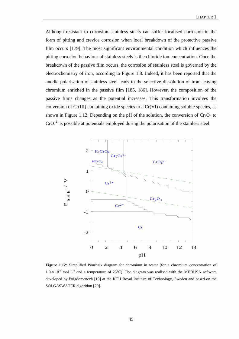
CHAPTER 1

45

Although resistant to corrosion, stainless steels can suffer localised corrosion in the

form of pitting and crevice corrosion when local breakdown of the protective passive

film occurs [179]. The most significant environmental condition which influences the

pitting corrosion behaviour of stainless steels is the chloride ion concentration. Once the

breakdown of the passive film occurs, the corrosion of stainless steel is governed by the

electrochemistry of iron, according to Figure 1.8. Indeed, it has been reported that the

anodic polarisation of stainless steel leads to the selective dissolution of iron, leaving

chromium enriched in the passive film [185, 186]. However, the composition of the

passive films changes as the potential increases. This transformation involves the

conversion of Cr(III) containing oxide species to a Cr(VI) containing soluble species, as

shown in Figure 1.12. Depending on the pH of the solution, the conversion of Cr2O3 to

CrO42- is possible at potentials employed during the polarisation of the stainless steel.

Figure 1.12: Simplified Pourbaix diagram for chromium in water (for a chromium concentration of

1.0 × 10-6 mol L-1 and a temperature of 25°C). The diagram was realised with the MEDUSA software

developed by Puigdomenech [19] at the KTH Royal Institute of Technology, Sweden and based on the


0 2 4 6 8 10 12 14

-2

-1

0

1

2

ES

HE

/ V

pH

Cr2+

Cr3+

CrO42−

Cr2O72−H2CrO4

Cr(c)

Cr2O3(cr)

CHAPTER 1

46

1.4.2.3 Aluminium

Freshly-formed aluminium easily reacts with air. Indeed, when it is exposed to the

atmosphere, a layer of aluminium oxide is immediately formed on the surface. The

thickness of the layer varies depending on the temperature and the presence of alloying

elements. For example, oxide films formed at room temperature are 2 to 3 nm thick on

pure aluminium [187]. At 425 °C the film thickness may reach 20 nm [187]. The natural

oxide film corresponds to A12O3, which is formed spontaneously according to Eq. 1.37.

The Gibbs energy of this oxidation reaction is -1675 kJ mol-1 and this explains the very

high affinity of aluminium towards oxygen.

322 OAlO23Al2 →+ Eq. 1.37

The Pourbaix diagram for the aluminium-water system at 25 °C is shown in Figure

1.13. In near neutral solution, between pH 4.0 and 8.6, the metal surface readily

develops an insoluble oxide, which grows to sufficient thickness to limit the reactivity

of the aluminium. Moreover, the diagram shows the amphoteric nature of the

aluminium oxide. Indeed, under strongly acid or alkaline conditions, the protective layer

is unstable and undergoes dissolution to form Al3+ or AlO2- species, respectively.

Aluminium is susceptible to localised corrosion, especially pitting and crevice attack

[188]. These forms of corrosion occur when species, such as chloride ions, compromise

the integrity of the oxide film at local sites.

CHAPTER 1

47

Figure 1.13: Simplified Pourbaix diagram for aluminium in water (for aluminium concentration of

1.0 × 10-5 mol L-1 and a temperature of 25°C). The diagram was realised with the MEDUSA software

developed by Puigdomenech [19] at the KTH Royal Institute of Technology, Sweden and based on the


1.4.2.4 Aluminium alloys

The properties of aluminium are altered by the addition of alloying elements [134]. The

common alloying constituents are copper, magnesium, silicon, zinc, manganese and

nickel. The cast alloys are cast directly into their desired forms, while the wrought

alloys are cast in ingots or billets and are then worked mechanically into extrusions,

forgings, sheets, foils, tubes and wires. The composition of the aluminium alloys is

regulated by an internationally agreed classification system or nomenclature. According

to the Aluminium Association, AA, system classification, which was adopted in the

European Standard EN 573, each wrought alloy is assigned by a four digit number, with

a further letter and number indicating the temper, or condition of the alloy, preceded by

EN-AW (European Norm Wrought Product). For example, EN-AW 6082-T6 is a

medium strength grade based on the aluminium-magnesium-silicon family, in the fully

heat treated condition. Only the first digit has practical importance. It designates the

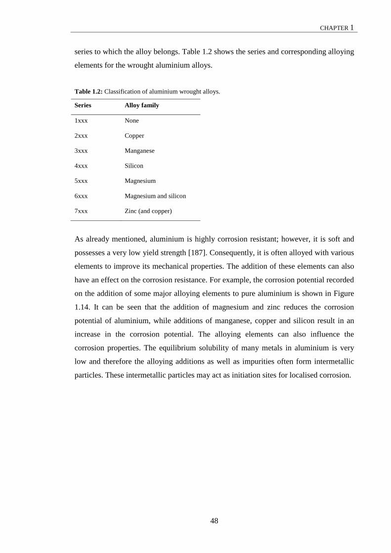
CHAPTER 1

48

series to which the alloy belongs. Table 1.2 shows the series and corresponding alloying

elements for the wrought aluminium alloys.

Table 1.2: Classification of aluminium wrought alloys.

Series Alloy family

1xxx None

2xxx Copper

3xxx Manganese

4xxx Silicon

5xxx Magnesium

6xxx Magnesium and silicon

7xxx Zinc (and copper)

As already mentioned, aluminium is highly corrosion resistant; however, it is soft and

possesses a very low yield strength [187]. Consequently, it is often alloyed with various

elements to improve its mechanical properties. The addition of these elements can also

have an effect on the corrosion resistance. For example, the corrosion potential recorded

on the addition of some major alloying elements to pure aluminium is shown in Figure

1.14. It can be seen that the addition of magnesium and zinc reduces the corrosion

potential of aluminium, while additions of manganese, copper and silicon result in an

increase in the corrosion potential. The alloying elements can also influence the

corrosion properties. The equilibrium solubility of many metals in aluminium is very

low and therefore the alloying additions as well as impurities often form intermetallic

particles. These intermetallic particles may act as initiation sites for localised corrosion.

CHAPTER 1

49

Figure 1.14: Influence of alloying elements on the dissolution potential of aluminium alloys [187].

1.5 Research presented in this thesis

The primary aim of this research is to investigate the feasibility of the

electrocoagulation technique for the treatment of water using novel electrode materials,

such as iron and aluminium alloys rather than the pure metals. Specifically, the

objectives of the research are as follow: (i) to determine the removal efficiency of

phosphates in terms of several parameters, such as the initial concentration of

phosphates, current density, initial pH and the chloride concentration; (ii) to develop a

kinetic and an adsorption model for the removal of phosphates; (iii) to relate the

electrochemical and corrosion behaviour of some electrode materials in synthetic

wastewaters containing several pollutants to their performance in terms of both removal

and energy efficiencies.

In this chapter, an introduction to conventional wastewater treatments and the removal

of the three pollutants subsequently used in the present study are given. This is followed

by an overview of the basic principles of the electrocoagulation process that involve

coagulation and flocculation. Finally, the electrochemistry of the electrode materials

used in the present study is presented. The second chapter concerns the relevant

CHAPTER 1

50

experimental techniques and apparatus employed, along with an overview of the

theories and related equations and models used in this thesis.

The results and main findings are presented and discussed in Chapters 3-6. In Chapter 3,

the efficiency of the electrocoagulation process for the removal of phosphate ions using

an aluminium-magnesium alloy and a stainless steel is investigated. The efficiency is

tested by varying parameters, such as the initial concentration of phosphates, current

density, initial pH and sodium chloride concentration. The kinetics of the removal and

the removal adsorption model are also presented. The electrocoagulation performance is

then studied for the removal of phosphates from real wastewater samples.

In Chapter 4, results are presented on the electrochemical and corrosion behaviour of

several electrode materials in synthetic wastewaters containing phosphates, an organic

dye and zinc ions. The corrosion behaviour of pure aluminium and iron and some of

their alloys has been extensively studied by several researchers [170, 173, 189-207].

However, few reports are available in the literature on the corrosion behaviour of these

electrodes in solutions which contain a mixture of anions, as occurs in real wastewaters.

In the present study, the effects of some common ions on the electrochemical behaviour

of the electrode materials and on their corrosion morphology are discussed.

In Chapter 5, a study of the performance of the electrode materials is carried out. The

test solutions are the synthetic wastewaters used in Chapter 4. The removal efficiencies

of the three pollutants are compared and correlated to the electrochemical behaviour of

the electrodes presented in Chapter 4. In addition, the energy consumption of the

process is computed and shown for each electrode material. This study is the first

attempt at relating the corrosion processes of the electrodes, in the presence of a mixture

of ions, with the efficiency and energy performance for the simultaneous removal of

various pollutants. Finally, conclusions are presented in Chapter 6.

CHAPTER 1

51

1.6 References

[1] WHO/Unicef, Global Water Supply and Sanitation Assessment 2000 Report, World Health Organization and United Nations Children's Fund, 2000. [2] Rajeshwar, K., Ibanez, J.G., Swain, G.M., J. Appl. Electrochem., 24 (1994) 1077-1091. [3] Holt, P.K., Barton, G.W., Mitchell, C.A., Chemosphere, 59 (2005) 355-367. [4] Mollah, M.Y.A., Schennach, R., Parga, J.R., Cocke, D.L., J. Hazard. Mater., 84 (2001) 29-41. [5] Linares-Hernandez, I., Barrera-Diaz, C., Roa-Morales, G., Bilyeu, B., Urena-Nunez, F., Chem. Eng. J., 148 (2009) 97-105. [6] Crittenden, J.C., Trussel, R.R., Hand, D.W., Howe, K.J., Tchobanoglous, G., MWH's Water Treatment: Principle and Design, John Wiley, 2012. [7] Cheremisinoff, N.P., Handbook of Water and Wastewater Treatment Technologies, Butterworth-Heinemann, 2002. [8] Metcalf and Eddy, I., Wastewater Engineering: Treatment and Reuse, McGraw-Hill, 2003. [9] Riffat, R., Fundamentals of Wastewater Treatment and Engineering, CRC Press, 2003. [10] Chen, G.H., Sep. Purif. Technol., 38 (2004) 11-41. [11] Mollah, M.Y.A., Morkovsky, P., Gomes, J.A.G., Kesmez, M., Parga, J., Cocke, D.L., J. Hazard. Mater., 114 (2004) 199-210. [12] Gray, N.F., Water Technology - An Introduction for Scientists and Engineers, 2nd ed., Butterworth-Heinemann, 1999. [13] Krishnan Rajeshwar, J.G.I., Environmental Electrochemistry: Fundamentals and Applications in Pollution Sensors and Abatement, Academic Press, 1997. [14] WEF, Biological and chemical systems for nutrient removal, Water Environment Federation, 1998. [15] Gray, A.V., J. Inst. Wat. Eng. Scient., 39 (1985) 137-154. [16] Ayoub, G.M., Koopman, B., Pandya, N., Water Environ. Res, 73 (2001) 478-485. [17] Stevenson, F.J., Cycles of soil, John Wiley, 1986. [18] Jenkins, D., Ferguson, J.F., Menar, A.B., Water Res., 5 (1971) 369-&. [19] Puigdomenech, I., Windows software for the graphical presentation of chemical speciation, March 26-30, in: 219th ACS National Meeting, San Francisco, CA, 2000, Am. Chem. Soc. [20] Eriksson, G., Anal. Chim. Acta, 112 (1979) 375-383. [21] Morse, G.K., Brett, S.W., Guy, J.A., Lester, J.N., Sci. Total Environ., 212 (1998) 69-81. [22] Thistleton, J., Berry, T.A., Pearce, P., Parsons, S.A., Process Saf. Environ. Protect., 80 (2002) 265-269. [23] Maurer, M., Boller, M., Water Sci. Technol., 39 (1999) 147-163. [24] Diagger, G.T., Sigmund, T.W., Design and operation of chemical phosphorus removal facilities., in: R. Sedlak (Ed.) Phosphorus and nitrogen removal from municipal wastewater – principles and practice, Lewis Publishers, 1991. [25] Nesbitt, J.B., J. Water Pollut. Control Fed., 41 (1969) 701-713. [26] Brett, S., Guy, J., Morse, G.K., Phosphorus Removal and Recovery Technologies, Seper Publications, 1997. [27] Zollinger, H., Color Chemistry - Synthesis, Properties and Application of Organic Dyes and Pigments, VHCA and Wiley-VCH, 1991. [28] Tauro, S., Coutinho, E., J. Mol. Struc.-Theochem., 532 (2000) 23-29. [29] Carneiro, P.A., Pupo Nogueira, R.F., Zanoni, M.V.B., Dyes Pigments, 74 (2007) 127-132. [30] Freeman, H.S., Esancy, J.F., Claxton, L.D., Dyes Pigments, 13 (1990) 55-70. [31] Crini, G., Bioresour. Technol., 97 (2006) 1061-1085. [32] Chen, J.P., Decontamination of Heavy Metals: Processes, Mechanisms, and Applications, Taylor & Francis Group, 2012. [33] Duffus, J.H., Pure Appl. Chem., 74 (2002) 793-807.

CHAPTER 1

52

[34] Fu, F., Wang, Q., J. Environ. Manage., 92 (2011) 407-418. [35] Gakwisiri, C., Raut, N., Al-Saadi, A., Al-Aisri, S., Al-Ajmi, A., in: World Congress on Engineering, London, U.K., 2012, July 4 - 6. [36] Srivastava, N.K., Majumder, C.B., J. Hazard. Mater., 151 (2008) 1-8. [37] Strokach, P.P., Electrochem. Ind. Process. Bio., 55 (1975). [38] Matteson, M.J., Dobson, R.L., Glenn, R.W., Kukunoor, N.S., Waits, W.H., Clayfield, E.J., Colloids Surf., A, 104 (1995) 101-109. [39] Vik, E.A., Carlson, D.A., Eikum, A.S., Gjessing, E.T., Water Res., 18 (1984) 1355-1360. [40] Kobya, M., Can, O.T., Bayramoglu, M., J. Hazard. Mater., 100 (2003) 163-178. [41] Amosov, V.V., Zil'brtman, A.G., Kucheryavykh, E.I., Sorkin, E.I., Tsarik, L.Y., Eppel, S.A., Timoshek, V.E., Titov, I.P., Chem. Technol. Fuels Oils, 12 (1976) 850-852. [42] Kaliniichuk, E.M., Vasilenko, I.I., Schepanyuk, V.Y., Sukhoverkhova, N.A., Makarov, I.A., Int. Chem. Eng., 16 (1976) 434-435. [43] Bochkarev, G.R., Lebedev, V.F., Nogin, N.M., Sov. Min. Sci., 13 (1977) 35-38. [44] Osipenko, V.D., Pogorelyi, P.I., Metallurgist, 21 (1977) 44-45. [45] Gavrilyuk, A.I., Sov. J. Water Chem. Technol., 3 (1981) 195-199. [46] Gavrya, N.A., Novosel'tseva, L.V., Shevchenko, L.Y., Yutina, A.S., Kompaniets, V.I., Shatokhina, E.A., Sov. J. Water Chem. Technol., 3 (1981) 527-528. [47] Kharlamova, T.A., Gorokhova, L.T., Sov. J. Water Chem. Technol., 4 (1982) 157-158. [48] Novikova, S.P., Shkorbatova, T.L., Sokol, E.Y., Sov. J. Water Chem. Technol., 4 (1982) 353-357. [49] Nikolaev, N.V., Kozlovskii, A.S., Utkin, I.I., Sov. J. Water Chem. Technol., 4 (1982) 244-247. [50] Avetisyan, D.P., Tarkhanyan, A.S., Safaryan, L.N., Sov. J. Water Chem. Technol., 6 (1984) 345-346. [51] Gnusin, N.P., Vitul'skaya, N.V., Zabolotskaya, L.I., Belobrov, I.A., J. Appl. Chem. (USSR), 50 (1997) 1663. [52] Gnusin, N.P., Zabolotskaya, L.I., Vitul'skaya, N.V., Sov. J. Water Chem. Technol., 7 (1985) 32. [53] Pogrebnaya, V.L., Klimenko, A.A., Bokovikova, E.P., Tsymbal, E.P., Pronina, N.P., Chem. Petrol. Eng., 31 (1995) 280. [54] Beck, E.C., Giannini, A.P., Ramirez, E.R., Food Technol., 22 (1974) 18. [55] Chen, G.H., Chen, X.M., Yue, P.L., J. Environ. Eng., 126 (2000) 858-863. [56] Biswas, N., Lazarescu, G., Int. J. Environ. Stud., 38 (1991) 65. [57] Lawrence, J., Knieper, L., Ind. Wastewater, 1-2 (2000) 20. [58] Do, J.S., Chen, M.L., J. Appl. Electrochem., 24 (1994) 785-790. [59] Gurses, A., Yalcin, M., Dogar, C., Waste Manage. (Oxford), 22 (2002) 491-499. [60] Ibanez, J.G., Singh, M.M., Szafran, Z., J. Chem. Educ., 75 (1998) 1040-1041. [61] Vlyssides, A.G., Loizidou, M., Karlis, P.K., Zorpas, A.A., Papaioannou, D., J. Hazard. Mater., 70 (1999) 41-52. [62] Vlyssides, A.G., Papaioannou, D., Loizidoy, M., Karlis, P.K., Zorpas, A.A., Waste Manage. (Oxford), 20 (2000) 569-574. [63] Xiong, Y., Strunk, P.J., Xia, H.Y., Zhu, X.H., Karlsson, H.T., Water Res., 35 (2001) 4226-4230. [64] Mameri, N., Yeddou, A.R., Lounici, H., Belhocine, D., Grib, H., Bariou, B., Water Res., 32 (1998) 1604-1612. [65] Panizza, M., Bocca, C., Cerisola, G., Water Res., 34 (2000) 2601-2605. [66] Tsai, C.T., Lin, S.T., Shue, Y.C., Su, P.L., Water Res., 31 (1997) 3073-3081. [67] Abuzaid, N.S., Bukhari, A.A., Al-Hamouz, Z.M., Adv. Environ. Res., 6 (2002) 325-333. [68] Donnini, J.C., Kan, J., Hassan, T.A., Kar, K.L., Can. J. Chem. Eng., 72 (1994) 667. [69] Renk, R.R., Energy Prog., 8 (1988) 205.

CHAPTER 1

53

[70] Szynkarczuk, J., Kan, J., Hassan, T.A.T., Donini, J.C., Clays Clay Miner., 42 (1994) 667-673. [71] Belongia, B.M., Haworth, P.D., Baygents, J.C., Raghavan, S., J. Electrochem. Soc., 146 (1999) 4124-4130. [72] Pretorius, W.A., Johannes, W.G., Lempert, G.G., Water SA, 17 (1991) 133-138. [73] Phutdhawong, W., Chowwanapoonpohn, S., Buddhasukh, D., Anal. Sci., 16 (2000) 1083-1084. [74] Balasubramanian, N., Madhavan, K., Chem. Eng. Technol., 24 (2001) 519– 521. [75] Chiang, L.C., Chang, J.E., Tseng, S.C., Water Sci. Technol., 36 (1997) 123-130. [76] Pouet, M.F., Grasmick, A., Water Sci. Technol., 31 (1995) 275-283. [77] Sharma, G., Choi, J., Shon, H.K., Phuntsho, S., Desalin. Water Treat., 32 (2011) 381-388. [78] Holt, P., Barton, G., Mitchell, C., Electrocoagulation as a Wastewater Treatment, in: The Third Annual Australian Environmental Engineering Research Event, Castlemaine, Victoria, 1999. [79] Johnson, P.N., Amirtharajah, A., J. Am. Water Works Ass., 75 (1983) 232-329. [80] Moreno C, H.A., Cocke, D.L., Gomes, J.A.G., Morkovsky, P., Parga, J.R., Peterson, E., Garcia, C., Ind. Eng. Chem. Res., 48 (2009) 2275-2282. [81] Moreno-Casillas, H.A., Cocke, D.L., Gomes, J.A.G., Morkovsky, P., Parga, J.R., Peterson, E., Sep. Purif. Technol., 56 (2007) 204-211. [82] Bagotsky, V.S., Fundamentals of Electrochemistry, 2nd ed., John Wiley, 2006. [83] Edeleanu, C., Evans, U.R., Transactions of the Faraday Society, 47 (1951) 1121-1135. [84] Richards, J.A., Wood, G.C., Corros. Sci., 10 (1970) 313-316. [85] Drazic, D.M., Popic, J.P., J. Appl. Electrochem., 29 (1999) 43-50. [86] Knörnschild, G., Kaesche, H., Formation, Properties and Significance for Advanced Luminescent Materials, in: 192th Meeting of The Electrochem. Society, Montreal, May,1997. [87] Pickering, H.W., Frankenthal, R.P., J. Electrochem. Soc., 119 (1972) 1297-1303. [88] Canizares, P., Jimenez, C., Martinez, F., Saez, C., Rodrigo, M.A., Ind. Eng. Chem. Res., 46 (2007) 6189-6195. [89] Barrera-Diaz, C., Bilyeu, B., Roa, G., Bernal-Martinez, L., Sep. Purif. Rev., 40 (2011) 1-24. [90] Pizzi, N.G., Water Treatment, American Water Works Association, 2010. [91] Harif, T., Khai, M., Adin, A., Water Res., 46 (2012) 3177-3188. [92] Benefield, L.D., Judkins, J.F., Weand, B.L., Process Chemistry for Water and Wastewater Treatment, Prentice-Hall, Inc., 1982. [93] Wiesner, M.R., Klute, R., Properties and Measurements of Particulate Contaminants in Water in: J.B. McEwen (Ed.) Treatment Process Selection for Particle Removal, American Water Works Association, 1998. [94] Eilbeck, W.J., Mattock, G., Chemical processes in Waste Water Treatment, Ellis Horwood, Ltd, 1987. [95] Israelachvili, J.N., Intermolecular and Surface Forces, Acadamic Press, 2011. [96] Bockris, J., Devanathan, M., Muller, K., Proc. R. Soc. London A, 274 (1963) 55-79. [97] Tripathy, T., De, B.R., J. Phys. Sci., 10 (2006) 93-127. [98] Letterman, R.D., Amirtharajah, A., O'Melia, C.R., Coagulation and Flocculation, in: R.D. Letterman, A.W.W. Association (Eds.) Water Quality and Treatment, A Handbook of community water supplies, McGraw-Hill, 1999. [99] Bratby, J., Coagulation and Flocculation in Water and Wastewater Treatment, IWA Publishing, 2006. [100] Thomas, D.N., Judd, S.J., Fawcett, N., Water Res., 33 (1999) 1579-1592. [101] Holt, P.K., Barton, G.W., Wark, M., Mitchell, C.A., Colloids Surf., A, 211 (2002) 233-248. [102] Duan, J.M., Gregory, J., Adv. Colloid Interface Sci., 100 (2003) 475-502. [103] Baes, C.F., Mesmer, R.E., The hydrolysis of cations, Wiley, 1976.

CHAPTER 1

54

[104] Wesolowski, D.J., Palmer, D.A., Geochim. Cosmochim. Acta, 58 (1994) 2947-2969. [105] Flynn, C.M., Chem. Rev., 84 (1984) 31-41. [106] Weber, W.J., Physicochemical Processes for Water Quality Control, John Wiley, 1972. [107] Ben Sasson, M., Calmano, W., Adin, A., J. Hazard. Mater., 171 (2009) 704-709. [108] Bagga, A., Chellam, S., Clifford, D.A., J. Membr. Sci., 309 (2008) 82-93. [109] Katal, R., Pahlavanzadeh, H., Desalination, 265 (2011) 199-205. [110] Gomes, J.A.G., Daida, P., Kesmez, M., Weir, M., Moreno, H., Parga, J.R., Irwin, G., McWhinney, H., Grady, T., Peterson, E., Cocke, D.L., J. Hazard. Mater., 139 (2007) 220-231. [111] Akbal, F., Camci, S., Desalination, 269 (2011) 214-222. [112] Chou, W.-L., Wang, C.-T., Huang, K.-Y., J. Hazard. Mater., 167 (2009) 467-474. [113] Vasudevan, S., Lakshmi, J., Jayaraj, J., Sozhan, G., J. Hazard. Mater., 164 (2009) 1480-1486. [114] Vasudevan, S., Jayaraj, J., Lakshmi, J., Sozhan, G., Korean J. Chem. Eng., 26 (2009) 1058-1064. [115] Vasudevan, S., Lakshmi, J., Sozhan, G., Clean-Soil Air Water, 38 (2010) 506-515. [116] Vasudevan, S., Lakshmi, J., Sozhan, G., Desalination, 275 (2011) 260-268. [117] Vasudevan, S., Lakshmi, J., Environ. Eng. Sci., 29 (2012) 563-572. [118] Khemis, M., Tanguy, G., Leclerc, J.P., Valentin, G., Lapicque, F., Process Saf. Environ. Protect., 83 (2005) 50-57. [119] Arslan-Alaton, I., Kabdasli, I., Vardar, B., Tuenay, O., J. Hazard. Mater., 164 (2009) 1586-1594. [120] Kabdasli, I., Vardar, B., Arslan-Alaton, I., Tuenay, O., Chem. Eng. J., 148 (2009) 89-96. [121] SenthilKumar, P., Umaiyambika, N., Gayathri, R., Environ. Eng. Manage. J., 9 (2010) 1031-1037. [122] Bukhari, A.A., Bioresour. Technol., 99 (2008) 914-921. [123] Kabdasli, I., Keles, A., Oelmez-Hanci, T., Tuenay, O., Arslan-Alaton, I., J. Hazard. Mater., 171 (2009) 932-940. [124] Abuzaid, N.S., Al-Hamouz, Z., Bukhari, A.A., Essa, M.H., Water Air Soil Pollut., 109 (1999) 429-442. [125] Murthy, Z.V.P., Parmar, S., Desalination, 282 (2011) 63-67. [126] Kabdasli, I., Arslan, T., Oelmez-Hanci, T., Arslan-Alaton, I., Tuenay, O., J. Hazard. Mater., 165 (2009) 838-845. [127] Golder, A.K., Samanta, A.N., Ray, S., J. Hazard. Mater., 141 (2007) 653-661. [128] Ghosh, D., Medhi, C.R., Purkait, M.K., Chemosphere, 73 (2008) 1393-1400. [129] Wang, C.-T., Chou, W.-L., Kuo, Y.-M., J. Hazard. Mater., 164 (2009) 81-86. [130] Asselin, M., Drogui, P., Benmoussa, H., Blais, J.-F., Chemosphere, 72 (2008) 1727-1733. [131] Bayramoglu, M., Eyvaz, M., Kobya, M., Chem. Eng. J., 128 (2007) 155-161. [132] Can, O.T., Kobya, M., Demirbas, E., Bayramoglu, M., Chemosphere, 62 (2006) 181-187. [133] Mouedhen, G., Feki, M., Wery, M.D.P., Ayedi, H.F., J. Hazard. Mater., 150 (2008) 124-135. [134] Uhlig, H.H., Revie, R.W., Uhlig's Corrosion Handbook, 2nd ed., John Wiley & Sons, 2000. [135] Trompette, J.L., Vergnes, H., J. Hazard. Mater., 163 (2009) 1282-1288. [136] Comninellis, C., Chen, G.E., Electrochemistry for the Environment, Springer, 2010. [137] Hu, C.Y., Lo, S.L., Kuan, W.H., Water Res., 37 (2003) 4513-4523. [138] Chen, X.M., Chen, G.H., Yue, P.L., Sep. Purif. Technol., 19 (2000) 65-76. [139] Adhoum, N., Monser, L., Bellakhal, N., Belgaied, J.E., J. Hazard. Mater., 112 (2004) 207-213. [140] Shafaei, A., Pajootan, E., Nikazar, M., Arami, M., Desalination, 279 (2011) 121-126. [141] Balasubramanian, N., Kojima, T., Basha, C.A., Srinivasakannan, C., J. Hazard. Mater., 167 (2009) 966-969.

CHAPTER 1

55

[142] Escobar, C., Soto-Salazar, C., Toral, M.I., J. Environ. Manage., 81 (2006) 384-391. [143] Al Aji, B., Yavuz, Y., Koparal, A.S., Sep. Purif. Technol., 86 (2012) 248-254. [144] Golder, A.K., Samanta, A.N., Ray, S., Sep. Purif. Technol., 53 (2007) 33-41. [145] Zongo, I., Leclerc, J.-P., Maiga, H.A., Wethe, J., Lapicque, F., Sep. Purif. Technol., 66 (2009) 159-166. [146] Emamjomeh, M.M., Sivakumar, M., J. Environ. Manage., 90 (2009) 1663-1679. [147] Martinez-Huitle, C.A., Brillas, E., Appl. Catal., B, 87 (2009) 105-145. [148] Can, O.T., Bayramoglu, M., Kobya, M., Ind. Eng. Chem. Res., 42 (2003) 3391-3396. [149] Daneshvar, N., Oladegaragoze, A., Djafarzadeh, N., J. Hazard. Mater., 129 (2006) 116-122. [150] Ogutveren, U.B., Koparal, S., J. Environ. Sci. Health., Part A, 32 (1997) 2507-2520. [151] Kumar, P.R., Chaudhari, S., Khilar, K.C., Mahajan, S.P., Chemosphere, 55 (2004) 1245-1252. [152] Merzouk, B., Gourich, B., Sekki, A., Madani, K., Chibane, M., J. Hazard. Mater., 164 (2009) 215-222. [153] Heidmann, I., Calmano, W., J. Hazard. Mater., 152 (2008) 934-941. [154] Koparal, A.S., Ogutveren, U.B., J. Hazard. Mater., 89 (2002) 83-94. [155] Lacasa, E., Canizares, P., Saez, C., Fernandez, F.J., Rodrigo, M.A., Chem. Eng. J., 171 (2011) 1012-1017. [156] Irdemez, S., Demircioglu, N., Yildiz, Y.S., J. Hazard. Mater., 137 (2006) 1231-1235. [157] Irdemez, S., Demircioglu, N., Yildiz, Y.S., Bingul, Z., Sep. Purif. Technol., 52 (2006) 218-223. [158] Irdemez, S., Yildiz, Y.S., Tosunoglu, V., Sep. Purif. Technol., 52 (2006) 394-401. [159] Kruger, J., Passivity, in: ASM Handbook Volume 13A: Corrosion: Fundamentals, Testing, and Protection, ASM International, 2003. [160] Fontana, M.G., Corrosion Engineering, McGraw-Hill, 1987. [161] Sato, N., Okamoto, G., Comprehensive Treatise of Electrochemistry,, Plenum Press, 1981. [162] Buchanan, E.E., Stansbury, R., Fundamentals of Electrochemical Corrosion, ASM International, 2000. [163] Scully, J.C., The Fundamentals of Corrosion, Pergamon Press, 1975. [164] Pourbaix, M., J. Electrochem. Soc., 123 (1976) C25-C36. [165] Roberge, P.R., Corrosion Engineering, Principles and Practice, McGraw-Hill, 2008. [166] Bard, A.J., Faulkner, L.R., Electrochemical Methods: Fundamentals and Applications, Wiley, 2001. [167] Wagner, C., Traud, W., Z. Elektrochem. Ang. Physik. Chemie, 44 (1938) 391. [168] Frankel, G.S., J. Electrochem. Soc., 145 (1998) 2186-2198. [169] Hoar, T.P., Jacob, W.R., Nature, 216 (1967) 1299-1301. [170] Leckie, H.P., Uhlig, H.H., J. Electrochem. Soc., 113 (1966) 1262-1267. [171] Heine, M.A., Pryor, M.J., J. Electrochem. Soc., 114 (1967) 1001-&. [172] Lin, L.F., Chao, C.Y., Macdonald, D.D., J. Electrochem. Soc., 128 (1981) 1194-1198. [173] Galvele, J.R., J. Electrochem. Soc., 123 (1976) 464-474. [174] Frankel, G.S., Pitting Corrosion, in: ASM Handbook Volume 13A: Corrosion: Fundamentals, Testing, and Protection, ASM International, 2003. [175] Evans, U.R., Nature, 206 (1965) 980-982. [176] Kabanov, B., Burstein, R., Frumkin, A., Discuss. Farady Soc., 1 (1947) 259-269. [177] Hurlen, T., Electrochim. Acta, 8 (1963) 609-619. [178] Cornell, R.M., Schwertmann, U., The Iron Oxides: Structure, Properties, Reactions, Occurrences and Uses, John Wiley, 2006. [179] Sedriks, A.J., Corrosion of Stainless Steel, John Wiley and Sons, New York, USA, 1979.

CHAPTER 1

56

[180] Pardo, A., Merino, M.C., Coy, A.E., Viejo, F., Arrabal, R., Matykina, E., Corros. Sci., 50 (2008) 780-794. [181] Olsson, C.O.A., Landolt, D., Electrochim. Acta, 48 (2003) 1093-1104. [182] Haupt, S., Strehblow, H.H., Corros. Sci., 37 (1995) 43-54. [183] Abreu, C.M., Cristobal, M.J., Losada, R., Novoa, X.R., Pena, G., Perez, M.C., Electrochim. Acta, 49 (2004) 3049-3056. [184] Schweitzer, P.A., Fundamentals of metallic corrosion: Atmospheric and media corrosion of metals, in: Corrosion Engineering Handbook, CRC Press, 2006. [185] Heine, B., Kirchheim, R., Corros. Sci., 31 (1990) 533-538. [186] Heusler, K.E., Corros. Sci., 31 (1990) 597-606. [187] Vargel, C., Corrosion of Aluminium, Elsevier, 2001. [188] Snodgrass, J., Corrosion Resistance of Aluminum Alloys, in: ASM Handbook, Vol. 13A,Corrosion:Fundamentals, Testing, and Protection, ASM International, 2003. [189] Alvarez, M.G., Galvele, J.R., Corros. Sci., 24 (1984) 27-48. [190] Bird, H.E.H., Pearson, B.R., Brook, P.A., Corros. Sci., 28 (1988) 81-86. [191] Galvele, J.R., in: R.P. Frankenthal, J. Kruger (Eds.) Passivity of Metals, The Electrochemical Society, Princeton, NJ, 1978, pp. 285-327. [192] Horvath, J., Uhlig, H.H., J. Electrochem. Soc., 115 (1968) 791-795. [193] Lakatos-Varsányi, M., Falkenberg, F., Olefjord, I., Electrochim. Acta, 43 (1998) 187-197. [194] Laycock, N.J., Newman, R.C., Corros. Sci., 39 (1997) 1771-1790. [195] Laycock, N.J., Newman, R.C., Corros. Sci., 40 (1998) 887-902. [196] MacDougall, B., Bardwell, J.A., J. Electrochem. Soc., 135 (1988) 2437-2441. [197] Nobe, K., Tobias, R.F., Corrosion, 20 (1964) 263. [198] Szklarska-Smialowska, Z., Staehle, R.W., J. Electrochem. Soc., 121 (1974) 1393-1401. [199] Bohni, H., Uhlig, H.H., J. Electrochem. Soc., 116 (1969) 906-910. [200] Breslin, C.B., Friery, L.P., Carroll, W.M., Corros. Sci., 36 (1994) 85-97. [201] Brillas, E., Cabot, P.L., Centellas, F., Garrido, J.A., Perez, E., Rodriguez, R.M., Electrochim. Acta, 43 (1998) 799-812. [202] Lee, W.J., Pyun, S.I., Electrochim. Acta, 45 (2000) 1901-1910. [203] Munoz, A.G., Saidman, S.B., Bessone, J.B., Corros. Sci., 44 (2002) 2171-2182. [204] Pyun, S.I., Moon, S.M., J. Solid State Electrochem., 3 (1999) 331-336. [205] Pyun, S.I., Moon, S.M., Ahn, S.H., Kim, S.S., Corros. Sci., 41 (1999) 653-667. [206] Pyun, S.I., Na, K.H., Lee, W.J., Park, J.J., Corrosion, 56 (2000) 1015-1021. [207] Shalaby, L.A., El Sobki, K.M., Abdul Azim, A.A., Corros. Sci., 16 (1976) 637-643.

57

2

Experimental

2.1 Introduction

The present research is concerned with the corrosion behaviour and electrocoagulation

performance of iron and aluminium and their alloys. The corrosion behaviour of these

metals was investigated using potentiodynamic and cyclic potentiodynamic polarisation

tests and open-circuit potential measurements. The morphology of the surfaces affected

by localised corrosion was monitored using light microscopy. The efficiency of the

electrocoagulation process was determined by measuring the removal of the pollutants

using either UV-Visible or atomic absorption spectroscopy. In particular, the removal of

phosphates by stainless steel and aluminium alloys was studied in detail. In addition, the

kinetics of the removal was modelled using simple models and the adsorption process

was fitted to standard isotherm equations. Furthermore, the speciation of the iron

electrodissolution from the steel alloy was studied using rotating disk voltammetry,

RDV. A screening chemometric study was carried out on the electrocoagulation process

with the steel electrodes to determine the most relevant factors affecting the process

efficiency.

In this chapter, the materials, methods and models used throughout the present work are

described in detail. A brief description of the theoretical background of the experimental

techniques is also presented.

2

CHAPTER 2

58

2.2 Chemicals and electrode materials

2.2.1 Chemicals and test electrolytes

The chemicals used in the present work were potassium dihydrogen phosphate (ACS

reagent, ≥ 99.0%), ammonium molybdate tetrahydrate (ACS reagent, ≥ 99.0%),

ammonium metavanadate (99%), sodium chloride (AR grade, ≥ 99%), Orange II

sodium salt (dye content, > 85%), calcium chloride dehydrate (ACS reagent, ≥ 99%),

magnesium sulfate heptahydrate (ACS reagent, ≥ 98%), nitric acid (ACS reagent, 70%),

sulfuric acid (reagent grade, 95-98%), sodium hydroxide (reagent grade, ≥ 98%),

sodium sulfate (ACS reagent, ≥ 99.0%), zinc sulfate heptahydrate (99.999%), potassium

chloride (super purum, 99.999+ %), ethanol (ACS reagent, ≥ 99.5%), ammonium

iron(II) sulfate hexahydrate (ACS reagent, 99%) and iron(III) chloride hexahydrate

(ACS reagent, 97%). All chemicals were supplied by Sigma-Aldrich® and used as

received. All the electrolyte solutions were prepared using distilled water, except for the

RDV experiments, which were carried out in Milli-Q purified water (14 MΩ, pH = 5.0).

The composition of the electrolyte solutions used in the corrosion tests is shown in

Table 2.1. The ion concentrations were determined according to the OECD synthetic

sewage [1].

Table 2.1: Composition of the electrolyte solutions used in corrosion (Chapter 4) and electrocoagulation

tests (Chapter 5).

KH 2PO4

/ M

NaCl

/ M

CaCl2.2H2O

/ M

MgSO4.7H2O

/ M

Na2SO4

/ M

Orange II

/ M

ZnSO4.7H2O

/ M

- 1.7 × 10-2 - - - - -

- 1.7 × 10-1 - - - - -

- 1.7 × 10-2 - - 8.1 × 10-4 - -

1.6 × 10-2 - - - - - -

sww 1 1.6 × 10-2 1.2 × 10-2 2.7 × 10-3 8.1 × 10-4 - 1.4 × 10-4 1.5 × 10-3

sww 2 1.6 × 10-2 1.7 × 10-1 2.7 × 10-3 8.1 × 10-4 - 1.4 × 10-4 1.5 × 10-3

6.5 × 10-3 - - - - - -

6.5 × 10-3 5.0 × 10-4 - - - - -

CHAPTER 2

59

The electrolyte solutions employed for electrocoagulation tests are divided into three

main categories. In Chapter 3, the electrolytes used were phosphate-containing solutions

in sodium chloride prepared in distilled water and, where necessary, the pH was

adjusted using HCl or NaOH to give the required value. In addition, two real samples

from treatment facilities were employed. The conductivity levels of these samples are

displayed in Table 2.2. In Chapter 5, the electrocoagulation tests were performed on two

electrolyte solutions, sww 1 and sww 2, and the composition of these solutions is shown

in Table 2.1.

Table 2.2: Conductivity levels for the real samples used for the electrocoagulation tests in Chapter 3.

Sample no. κ

/ mS cm-1

1 0.32

2 1.00

2.2.2 Electrode materials and sample preparation

The chemical composition and the exposed surface area of the various metals and alloys

employed in the present study are shown in Table 2.3. All the electrode materials were

supplied by Goodfellow© in rod, wire or sheet forms, which were then cut to provide the

exposed surface area displayed in Table 2.3. The rotating disk electrode was platinum

and this was purchased from Princeton Applied Research (Ametek).

Table 2.3: Chemical composition and surface area of electrodes.

Electrode Composition / wt. %

Geometric surface area / cm2

corrosion tests

electrocoagulation tests

Al 99.999 0.031 -

Al-2Mg

(EN AW-5251)

Mg 1.7-2.4, Fe 0.5, Mn 0.5-0.1, Si 0.4,

balance Al

0.50 40.8 – 38.7

Al-3Zn-0.02In Zn 3, In 0.02, Fe 0.12, Si 0.08, Cu 0.006,

balance Al

0.38 38.7

Pure Fe 99.99 0.071 38.7

AISI 310 Cr 24-26, Ni 19-22, Mn 2, Si 1.5, C 0.25,

balance Fe

0.58 38.7

AISI 420 Cr 13-14, Mn 1, Si 1, C 0.3, balance Fe 0.63 36.9 – 38.7

corrosion tests RDV

Pt 100 > 1 0.1257

CHAPTER 2

60

The samples used as working electrodes in the corrosion tests were set in a Teflon®

holder with epoxy resin. An electrical contact was made attaching a copper wire to the

sample with highly conductive silver-loaded resin. The quality of the electrical contact

was checked with a multimeter to ensure that the resistance between the surface of the

electrode and the connection was lower than 1.0 Ω. Prior to each experiment the

exposed electrode surface was abraded on a Buehler® Metaserve grinder polisher with

water lubricated Buehler® SiC grinding papers to a 2500 grit finish. The electrodes were

then polished to a mirror finish with successively finer grades of Buehler® MetaDi

monocrystalline diamond suspensions ranging from 30 to 1 µm on Buehler® polishing

microcloths. Finally, they were rinsed with distilled water and ethanol, sonicated in a

Branson 1510 ultrasonic bath and dried in a stream of air.

The samples used in the electrocoagulation tests were cut to form plates and the

electrical connections were made using crocodile clips. The exposed area of each

sample was defined by a mask of beeswax. Prior to each experiment they were abraded

with water lubricated Buehler® silicon carbide paper (Grit P 320). They were then

washed with distilled water and dried in a stream of air. If the electrodes were covered

by a layer of oxides, they were dipped in HCl solution (5% v/v) for 10 min and rinsed

thoroughly with water, before abrasion with SiC paper.

A platinum wire, with a high surface area, was used as the counter electrode in

corrosion tests and in the RDV experiments. It was periodically abraded with Buehler®

silicon carbide paper (Grit P 2500) and sonicated in distilled water to maintain a clean

surface. The reference electrode was a saturated calomel electrode, SCE (0.242 V

vs. NHE). The potential of the SCE reference electrode was regularly checked against a

virgin SCE. Moreover, the aqueous KCl solution in the reference electrode was replaced

periodically with a saturated solution of super purum KCl.

CHAPTER 2

61

2.3 Experimental techniques

The experimental procedures and the equations employed in the present work are

described in this section, along with a brief explanation of the parameters involved in

the experiments. Additional information and representative calibration curves are given

where necessary.

2.3.1 Electrochemical experiments

All the electrochemical experiments were carried out with a Solartron SI 1285A

potentiostat, which was controlled by a computer unit. The software package used was

CorrWare® for Windows version 3.2c by Scribner Associates, Inc. For the RDV

experiments, the Pt electrode, described in Section 2.2.2, was rotated using a Princeton

Applied Research Model 636 Ring-Disk Electrode System apparatus.

A basic diagram of a potentiostat controlling a three-electrode cell is presented inFigure

2.1. In this figure, the working, WE, reference, RE, and counter, CE electrodes are

identified and connected to the potentiostat, which, in turn, is interfaced to a function

generator. The potentiostat controls either the potential difference, VWE, between the

WE and the RE (potentiostatic mode) or the current flow, IRE, between the WE and the

CE (galvanostatic mode). The potential of the WE, VWE, is varied by controlling the

potential difference between WE and RE, VWR (VWR = VWE – VRE), since VRE is constant.

The current flow in the cell is ICE = IRE + IWE. However, IRE is taken as zero since the RE

is connected to a high input impedance element. Consequently, the current flow in the

cell is between WE and CE, IWE = ICE.

Figure 2.1: Basic diagram of a potentiostat (WE = working electrode, RE = reference electrode, CE =

counter electrode).

FunctionGenerator

Potentiostat

WE

RE

CE

VWC = VWE - VCE

VWR = VWE - VREVWR = VWE - VRE

IWE

ICE

IRE

CHAPTER 2

62

2.3.1.1 The electrochemical cell for corrosion and RDV experiments

A typical three-electrode cell employed in the corrosion and RDV measurements is

shown in Figure 2.2. This set-up consists of a working electrode, WE, a reference

electrode, RE, and a counter electrode, CE. The electrode materials and their

preparation are discussed in Section 2.2.2. The electrochemical cell was a glass cylinder

of 10 mL in volume capped with a Teflon® lid holding the electrodes. A 100 mL glass

cell was used for the RDE experiments. The three electrodes were immersed in the

electrolyte solution and connected to the potentiostat. All the experiments were

performed at room temperature. In some experiments, a micropipette was used to add

known aliquots of chemicals to the electrolyte solution.

Figure 2.2: A schematic representation of the electrochemical cell used for corrosion and RDV

experiments (WE = working electrode, RE = reference electrode, CE = counter electrode, lpt = laptop).

2.3.1.2 The electrochemical cell for electrocoagulation experiments

The electrocoagulation experiments were carried out using a standard three-electrode

cell, presented in Figure 2.2 and a two-electrode set-up, which is shown in Figure 2.3,

with an anode as the working electrode, WE, and a cathode as the counter electrode,

CE. This two-electrode configuration is usually employed when precise control of the

interfacial potential across the WE is not critical and the behaviour of the whole cell is

under investigation. For example, in the present study it was used to estimate the energy

consumption of the process, since its calculation required the cell voltage. The electrode

materials and their preparation are presented in Section 2.2.2. In both electrochemical

set-ups, a glass cell with a volume of 400 mL was equipped with a magnetic stirrer to

CHAPTER 2

63

ensure good mixing during each experiment. The distance between the anode and the

cathode was maintained at 1 cm for all the experiments.

Figure 2.3: A schematic representation of the electrochemical cell used for electrocoagulation

experiments (A = anode, C = cathode, ms = magnetic stirrer, lpt = laptop).

2.3.1.3 Corrosion techniques

Corrosion measurements are designed to predict the behaviour of a material before it is

used in an environment. They can be broadly classified as destructive or non-destructive

techniques [2]. A measurement is said to be destructive if it alters the corrosion process

during the measuring process (e.g., potentiodynamic polarisation tests) or if the material

is physically removed from the environment (e.g., weight loss measurements).

Non-destructive techniques, which include open-circuit potential, linear polarisation

resistance, electrochemical impedance spectroscopy and electrochemical noise, could be

used to make repeated measurements at different time intervals. In the present study,

two techniques were used for corrosion tests; open-circuit potential, OCP,

measurements and potentiodynamic and cyclic potentiodynamic polarisation tests.

Open-circuit potential measurements

The open-circuit potential, OCP, or rest potential, is the potential exhibited by an

electrode when no net current flows through the external circuit of the electrochemical

cell. It is a relatively simple technique where the voltage between the WE and the RE is

monitored as function of time [3]. By measuring the OCP it is possible, for example, to

determine whether the corrosion is in the active or the passive state, gain information on

the stability of the sample surface and obtain data for corrosion monitoring. The number

CHAPTER 2

64

of data points collected determines the resolution and in these experiments data points

were collected per second.

Potentiodynamic polarisation

The potentiodynamic polarisation technique for corrosion studies was introduced in the

1960s and became popular especially during the 1970s as a simple technique for routine

use [2, 4]. It is useful for the prediction of the corrosion property of passivating metals

or alloys prone to localised corrosion. This technique is based on the fact that when the

potential of a freely corroding metal surface is changed by connecting it with an

external power source, the metal will be polarised. ASTM [5] defines the term

polarisation as “the change for the open-circuit potential as a result of the passage of

current”. The most common approach in polarisation methods involves changing the

potential of the WE and monitoring the current which is produced. The potential is

scanned at a fixed rate between two set values and the current is measured at periodic

intervals [6]. In potentiodynamic polarisation tests, the measurement starts far away

from the corrosion potential (> 100 mV) and gives a curve of the type shown in Figure

2.4. Potentiodynamic polarisation over a wide range of potentials, such as seen in

Figure 2.4, provides important information about the system, for example the

determination of the electrode behaviour over that range of potential. An active, passive

and transpassive region can be identified and critical potentials, such as the corrosion

potential, Ecorr, breakdown potential, Ebr, passivation potential, Epass, or the slope of the

polarisation curve at the corrosion potential, Ecorr, can be estimated. However,

according to Silverman [2, 4], the polarisation scan should not be used to estimate

general or uniform corrosion rates. Making such an estimate from the potentiodynamic

polarisation scan requires the assumption that the corrosion mechanism does not change

over the wide potential range used for the scan. Other methods, such as electrochemical

impedance spectroscopy or polarisation resistance, can be used for this purpose.

CHAPTER 2

65

Figure 2.4: Representative potentiodynamic polarisation curve [6].

In the present study, potentiodynamic polarisation tests were performed on several

electrode materials, listed in Section 2.2.2, and are shown in Chapter 4. The scans were

started at a potential about 300 mV below the OCP and progressed in the anodic

direction until visible breakdown of the electrode occurred, or a current density of

1 mA cm-2 was reached. Further details on the potentials and scan rates employed are

given in the relevant sections of Chapter 4.

Under steady state conditions, electrochemical reactions under kinetic control obey the

Tafel equations, Eq. 2.1 and Eq. 2.2, for large overpotentials.

anodic reaction )log(a a jβη += Eq. 2.1

cathodic reaction )log(a c' jβη += Eq. 2.2

Here, a and a’ are the anodic and the cathodic constants, )log()/303.2( 0jαnFRTa −= and

)log())1/(303.2('0jnFRTa α−= , respectively, and βa and βc are the anodic and the

cathodic Tafel slopes, respectively (Section 1.4.1.1). Accordingly, a plot of the

logarithm of the current, log(j), as a function of the overvoltage gives the Tafel plot.

Many corrosion systems are kinetically controlled and consequently they follow Eq. 2.1

and Eq. 2.2. In a Tafel plot, a linear portion on both sides of the corrosion potential,

Ecorr, is indicative of kinetic control. Classical Tafel analysis is performed by

CHAPTER 2

66

extrapolating the linear portion of a log current versus potential plot back to their

intersection, as shown in Figure 2.5, giving the estimation of parameters such as

corrosion current density, jcorr, and Tafel slopes, βa and βc.

In the present study, the Tafel analysis was performed using the CorrView2™ Version

3.0 analysis package under the following assumptions: (i) the Tafel region (linear

portion of the semilogarithmic plot) extends for at least one order of magnitude of

current [7]; (ii) the rate of polarization in the potentiodynamic scans is between 0.1 and

1 mV s−1 in order to determine steady state behaviour [7]. However, the first condition

was not achievable in all the potentiodynamic scans due to interference from

concentration polarization or other processes, such as surface roughening or film

formation, which may alter the electrode surface [7]. The Appendix at the end of this

thesis summarises the parameters evaluated using the Tafel analysis, such as the

corrosion current density, jcorr, in A cm-1 and the anodic and the cathodic tafel slopes, βa

and βc, respectively, in mV decade-1.

Figure 2.5: Classical Tafel analysis.

Cyclic potentiodynamic polarisation

In cyclic potentiodynamic polarisation measurements the voltage is first increased in the

anodic direction (forward scan), then it is reversed at some chosen current or potential

and then scanned in the cathodic direction (backward or reverse scan). The scan is

Current density

Po

ten

tial

Intersect at Ecorr, jcorr

Extrapolated βc

Extrapolated βa

jcorr

CHAPTER 2

67

terminated usually at the corrosion potential, Ecorr. The cyclic potentiodynamic

polarisation provides information on the propensity for localised corrosion. In

particular, the occurrence of a hysteresis loop between the forward and the reverse

portions of the scan is considered a measure of the susceptibility of the sample to suffer

localised corrosion [4]. However, hysteresis in cyclic potentiodynamic polarisation

curves is not always associated with pitting or crevice corrosion and, consequently, it is

necessary to examine the electrode surface following testing to establish the nature of

the attack [8].

In Chapter 4, the cyclic potentiodynamic polarisation tests are presented for several

electrode materials. The electrodes were polarised from a potential about 300 mV lower

than the corrosion potential, Ecorr, and the scan was reversed at 1 mA cm-2, unless

otherwise stated. Then the potential was cycled in the reverse direction until the

corrosion potential, Ecorr, was reached. Further details on the potentials and scan rates

employed are given in the relevant sections of Chapter 4.

2.3.1.4 Electrocoagulation techniques

Electrocoagulation consists in either applying a constant current (galvanostatic mode) or

a constant potential (potentiostatic mode) to the electrochemical cell described in Figure

2.2 and Figure 2.3. As a consequence, dissolution of the anode or WE occurs with

simultaneous formation of hydroxyl ions, while hydrogen gas is usually produced at the

cathode as a result of water reduction.

In the present study, the electrocoagulation tests were carried out under the

galvanostatic mode in order to have consistent and reproducible anodic dissolution

rates. The test electrolytes, listed in Table 2.1 and Table 2.2, were placed in the

electrochemical cell, the solution pH was adjusted using either NaOH or NaCl when

necessary and a constant stirring rate was employed throughout each experiment. All

the electrocoagulation experiments were performed at room temperature, except for the

adsorption isotherm studies. A constant current density was then applied using the

potentiostat. Accordingly, the potential varied slightly depending on the resistance of

the system. Samples were periodically taken from the reactor and allowed to settle for

15 min. Then the supernatant was filtered with Whatman™ filter paper (Grade 1, pore

CHAPTER 2

68

size 11 µm) and analysed for the required quantitative determinations. The efficiency of

removal, η, was computed according to Eq. 2.3, where C0 is the initial concentration of

the species and Ct is the concentration of the species at time t.

100(%)η0

0 ×−

=C

CC t Eq. 2.3

Different operating settings were used for the electrocoagulation experiments,

consequently further details, such as the current density, solution pH or the surface area

to the solution volume ratio, SA/V, in cm-1, are given in the relevant chapters.

The adsorption isotherm studies were carried out with 74.0 mg L-1 of Al3+ or

361.3 mg L-1 of Fe2+ and phosphate solutions having concentrations ranging from 2.0 to

150.0 mg L-1 PO4-P with a pH of 5.0 and the temperature of the electrochemical cell

was controlled and maintained at 25 ± 1 ºC. The mass of the adsorbent (Al3+ or Fe2+)

used was calculated according to Faraday’s laws of electrolysis and taking into account

the composition of the electrode material used, as discussed in the relevant sections of

Chapter 3.

2.3.1.5 Rotating disk voltammetry, RDV

Rotating disk voltammetry, RDV, is an electrochemical technique where the potential of

the working electrode is swept between two chosen potential limits and the change in

current is monitored. Unlike other electrochemical techniques, the working electrode,

rotating disk electrode, RDE, is rotated at a controlled angular speed, ω (rad s-1). The

rotation motion determines a well-defined flow pattern of solution towards the surface

of the RDE, as is shown in Figure 2.6. The electrode acts as a pump, pulling the solution

upwards and perpendicular to the electrode surface [9]. However, the perpendicular flux

of solution falls to zero at the electrode surface. Consequently, the layer of solution

adjacent to the electrode surface manages to cling to the electrode and appears to be

motionless from the perspective of the RDE. In this layer, where the solution is

stagnant, the transport of the species is only by diffusion. The thickness of the layer, δ,

in cm, is governed by the rate of the rotation and is inversely proportional to ω1/2,

according to Eq. 2.4 [10].

CHAPTER 2

69

2/1

6/13/1

61.1ω

νδ D= Eq. 2.4

Here, D is the diffusion coefficient, in cm2 s-1, of the electroactive species, ν is the

kinematic viscosity, in cm2 s-1, of the solvent and ω is the angular velocity in rad s-1.

(a)

(b)

Figure 2.6: Schematic showing the flow patterns to the rotating disk electrode, RDE [10]. (a) The

solution flow perpendicular to the electrode. (b) The electrode surface viewed from below.

A classical RDV experiment consists of a linear sweep voltammogram performed at a

given scan rate, 1 to 50 mV s-1, while the current is recorded as a function of the applied

potential. The resulting voltammogram exhibits a typical sigmoidal wave, as is shown

in Figure 2.7. At potentials where the rate of the electron transfer is high, a plateau is

observed because the current is limited by the rate of mass transport. The limiting

current, IL, is given by the Levich equation, shown in Eq. 2.5

∞−= CnFADI L61213262.0 νω Eq. 2.5

In this equation, n is the number of electrons transferred, F is the Faraday’s constant

(96,485.34 C mol-1) and C∞ is the bulk concentration of the species in mol cm-3. It is

apparent from this equation that the limiting current, IL, is linearly dependent on the

square root of the rotational speed, ω1/2. Indeed, this is a useful test to determine if the

current is mass-transport controlled [9].

CHAPTER 2

70

Figure 2.7: Typical diffusion controlled voltammetric response under mass-transfer-limiting condition.

In the present work, the RDV was used for the simultaneous detection of ferrous and

ferric species, which were electrogenerated during electrocoagulation with a stainless

steel electrode. RDV was first used to obtain the calibration curves for Fe(II) and Fe(III)

in order to test the feasibility of the method. Then, the method was applied to the

solutions after the electrocoagulation process. At the end of the electrocoagulation tests,

1.0 M H2SO4 was added to the solutions in order to have complete dissolution of the

iron flocs formed during the process. After 24 h, samples of 25 mL were taken from

each solution and used in RDV measurements using a potential range of -0.2 to 1.2 V

vs. SCE, a scan rate of 10 mV s-1 and a rotation speed of the electrode of 3000 rpm. Due

to the complexity of the sample matrix, a standard addition method was used [11]. In

the standard addition method, small known concentrations of the analyte to be

determined were added to aliquots of the unknown samples [12]. In these experiments,

serial increments of the standard, Vs, were added to a constant volume, Vx, of the

solution. With this method, additions of both Fe(II) and Fe(III) were made to the same

samples keeping the IR drop and the ionic strength of the solution relatively constant.

The linear response, Y, which was obtained for each solution is expressed by Eq. 2.6:

( ) NkkNV ssxxsx CVCVIV L +=+ Eq. 2.6

Y b m x

In this equation, Vx (25 mL) and Vs (0.25 mL) are the volumes of the unknown and the

standard, respectively, Cx and Cs (0.5 M) are the concentrations of the unknown and the

standard, respectively, N is the multiple units of addition (0, 1, 2, etc.) and IL is the

CHAPTER 2

71

limiting current from the RDV measurements. By plotting Y, the entire left hand side of

Eq. 2.6, versus N a straight line results with an intercept, b, and a slope, m:

xxkb CV= sskm CV= Eq. 2.7

Then, the unknown concentration, Cx, can be obtained from m and b:

x

ssx m

b

V

CVC = Eq. 2.8

Figure 2.8 shows typical calibration curves for the Fe(II) and Fe(III) and a

representative standard addition plot obtained for the determination of Fe(II).

Figure 2.8: (a) Calibration curves for Fe(II) (R2 = 0.990) and Fe(III) (R2 = 0.994) and (b)

representative standard addition plot for Fe(II) (R2 = 0.997).

2.3.2 Microscopy

The standard optical microscope, which is still the most widely used type of

microscope, consists essentially of a combination of two lenses, an objective and an

eyepiece. The product of these magnifications produces the magnification of the final

image. The eyepiece can be replaced by a camera and the final image can be analysed

on a computer unit. The main disadvantage of the optical microscope is the resolution

limit, which restricts the minimum size of detail that can be seen at about 0.2 µm [13].

This limit cannot be overcome, since it is imposed by the wavelength of visible light,

which is of the same order. The optical microscope is very widely used in

Fe / mM

0 20 40 60 80 100

i / A

-0.006

-0.004

-0.002

0.000

0.002

0.004

0.006

N

0 1 2 3 4 5

Y

0.04

0.05

0.06

0.07

0.08

0.09

0.10

(a) (b)

CHAPTER 2

72

metallography, since it enables examination of materials and provides a magnified

image of the micro- and macrostructures. Indeed, optical microscopy is used to

characterise structures by revealing grain boundaries, phase boundaries, inclusion

distribution and evidence of surface deformation [14].

In the present work, optical microscopy was used to examine the electrode surface after

the corrosion tests were performed and to establish the nature of the localised corrosion.

This technique was also used to ensure an adequate grinding and polishing of the

samples prior to each experiment. The samples were washed thoroughly with distilled

water, dried with a stream of air and observed carefully using an Olympus® BX51M at

different magnifications in a dark-field mode. The micrographs were taken with a

computer interfaced to a CCD camera (Leica DFC 2280 digital camera) and Olympus®

DP version 3.2 software.

2.3.3 Spectroscopy

2.3.3.1 UV-Visible

UV‐Visible (UV-Vis) spectroscopy consists in the measurement of the attenuation of a

light beam after it passes through a sample. The intensity of the light absorbed is related

to the concentration of the absorbing species, according to the Beer-Lambert law [15],

Eq. 2.9:

CA bλε= Eq. 2.9

In this equation, A is the absorbance, ελ is the molar absorbtivity at a specific

wavelength, λ, b is the path length and C is the concentration of the absorbing species.

In the present work, UV-Vis spectroscopy was used to determine the concentration of

phosphate and Orange II, an organic dye, at the end of the electrocoagulation process in

order to compute the efficiency of removal, as shown in Eq. 2.3. A Unicam Thermo

Spectronic® UV 540 double-beam spectrometer was used. It comprises tungsten and

deuterium lamps, a holographic grating monochromator and a photomultiplier tube

detector. In all cases, a quartz cuvette with a path length of 1 cm was used. These data

CHAPTER 2

73

were recorded using Vision 32 PC software and analysis was done using SigmaPlot™

Version 12.2.0.45 by Systat Software, Inc.

Colorimetric tests

The phosphate concentration was measured according to the vanadomolybdophosphoric

acid colorimetric method [16]. This method consists of the reaction between phosphates

and ammonium molybdate in acidic conditions to form a heteropoly acid,

molybdophosphoric acid. When vanadium is added to the solution,

vanadomolybdophosphoric acid, which has a yellow colour, is formed. To avoid

interferences with ferric iron, the absorbance was measured at 470 nm. The calibration

curve, obtained with phosphate concentrations ranging from 0.5 to 15.0 mg L-1, is

shown in Figure 2.9. It was used to calculate the concentration of phosphates in

solution. The concentration of phosphates was expressed in units of mg L-1 PO4-P,

indicating the concentration of phosphorus in the form of phosphates. The limit of

detection, DL, of the technique, defined as in Eq. 2.10, was estimated using the

regression line of the calibration curve, according to Miller and Miller [17]. The value

of the intercept of the calibration curve was used as an estimate of the blank signal, yB,

while the random error in the y-direction was used in place of the standard deviation of

the blank, sB [18].

BB s3yDL += Eq. 2.10

Figure 2.9: Calibration curve for PO4-P determination (λ = 470 nm). The limit of detection, LD, was

estimated as 0.25 mg L-1. (R2 = 0.999).

C / mg L-1

0 2 4 6 8 10 12 14 16

A

0.00

0.05

0.10

0.15

0.20

0.25

0.30

CHAPTER 2

74

The structure of Orange II azo dye and its UV-Vis spectrum at a pH of approximately

10.0 are shown in Figure 2.10 (a) and (b), respectively. The chemical structure shows

that this azo dye exhibits tautomerism between the azo and hydrazone forms by a proton

exchange effect. In aqueous medium, the hydrazone form is the predominant species

[19]. The azo dye colour is the result of the conjugation between the azo bond and the

aromatic rings present in the dye molecule [20]. The UV-Vis spectrum has an

absorption band at 485 nm and a shoulder at 405 nm in the visible region due to the

chromophore-containing azo linkage and two bands at 310 and 230 nm in the UV

region due to the aromatic rings. The 485 and 405 nm bands are attributed to the π-π*

transition of the hydrazine form and to the n-π* transition of N=N azo group,

respectively [19]. The other two peaks located in the UV region are assigned to the π-π*

transitions of the aromatic naphthalene and benzene rings [19].

(a) (b)

Figure 2.10: Orange II dye (a) azo-hydrazone tautomerism and (b) representative UV-Vis spectrum.

In this work, the concentration of Orange II in solution was measured using the

hydrazone band intensity at 485 nm. The calibration curve, obtained with concentrations

ranging from 0.5 to 10.0 mg L-1 of Orange II, is shown in Figure 2.11. The limit of

detection of the technique was estimated according to Eq. 2.10.

λ / nm

200 300 400 500 600

A

0.0

0.2

0.4

0.6

0.8

1.0

CHAPTER 2

75

Figure 2.11: Calibration curve for Orange II dye determination (λ = 485 nm). The limit of detection, LD,

was estimated as 0.18 mg L-1. (R2 = 0.999).

The concentrations of phosphates presented in Chapter 5 were measured in samples

which also contained the Orange II dye. The spectra of these two species have some

regions where both species absorb. In order to avoid any interference in the reading of

the absorbance, the spectrophotometric determination of phosphates and Orange II was

carried out by solving the simultaneous linear equations given in Eq. 2.11. In this

equation, A470 and A485 are the absorbance values from the spectrum of the mixture at

470 and 485 nm, P470ε and P

485ε are the molar absorbtivities of phosphates at 470 and

485 nm computed from the spectrum of pure phosphates. Likewise, O470ε and O

470ε are

the molar absorbtivities of Orange II dye at 470 and 485 nm, computed from the

spectrum of the Orange II dye only, and CP and CO are the concentrations of phosphates

and Orange II dye, respectively. This method is usually used in the analysis of a mixture

of components. Provided that the spectra of the pure components are available, this

method allows the determination of the concentrations of the individual components by

analysing the spectrum of the mixture [21]. For the spectrophotometric determination of

the two components in a binary system, such as the one in the present work, absorbance

measurements at two different wavelengths are necessary. The resulting calculation to

solve the set of equations is simple and yields a determinant ratio which can be

evaluated readily by using Cramer’s rule [22].

C / mg L-1

0 2 4 6 8 10 12

A

0.0

0.1

0.2

0.3

0.4

0.5

0.6

0.7

CHAPTER 2

76

O

O470P

P470470 CCA εε +=

OO485P

P485485 CCA εε +=

Eq. 2.11

2.3.3.2 Atomic absorption spectroscopy

Atomic absorption, AA, spectroscopy relies on the fact that metal ions adsorb a specific

wavelength within the light spectrum. Applying the Beer-Lambert law, the

concentration of the metal is determined from the amount of absorption [23].

In the present work, AA spectroscopy was used to measure the concentration of Zn2+

ions in solution. A Perkin Elmer Analyst 200 atomic absorption spectrometer, with a

premix burner, hollow-cathode lamp, air-acetylene flame atomiser, echelle grating

monochromator and solid state detector, was employed. The wavelength was set at

213.9 nm. The standard solutions, used to obtain the calibration curve shown in Figure

2.12, were prepared by dissolving metallic zinc in HNO3. The limit of detection of the

technique was estimated according to Eq. 2.10.

Figure 2.12: Calibration curve for Zn determination. The limit of detection, LD, was estimated as

0.09 mg L-1. (R2 = 0.998).

C / mg L-1

0.0 0.5 1.0 1.5 2.0

A

0.00

0.05

0.10

0.15

0.20

0.25

0.30

0.35

0.40

CHAPTER 2

77

2.3.4 Kinetic analysis of phosphate removal by electrocoagulation

Chemical kinetics deals with the rate at which chemical reactions take place. The study

of chemical kinetics is based on the law of mass action, published by Guldberg and

Waage during 1864-1867 [24]. One of the key terms in reaction kinetics is the rate of

reaction, r, defined as the number of molecules of a chemical species being converted or

produced per unit volume with respect to time. Considering A reacting with B to

produce C: aA + bB → cC, the rate of reaction is given by Eq. 2.12, where rA, rB and rC

are the rates of reaction with respect to species A, B and C, respectively, a, b and c are

the stoichiometric coefficients for A, B and C, respectively, NA, NB and NC represent the

number of moles of A, B and C, respectively, and V is the volume containing the

species.

CBA rrrr ===

Eq. 2.12

t

N

Var

d

d1 AA ⋅

−= t

N

Vbr

d

d1 BB ⋅

−= t

N

Vcr

d

d1 CC ⋅

=

From experimental observations and based on the above mentioned law of mass action

and the collision theory, it was found that the rate of reaction can be expressed as the

rate law [25]:

yxkr ]B[]A[= Eq. 2.13

Here k is a proportionality factor called the rate coefficient or rate constant, which is

dependent on the temperature through the Arrhenius equation and x and y are the partial

orders with respect to A and B, respectively. The overall order of the reaction is equal to

the sum of the partial orders.

In the present study, the kinetics of phosphate removal by electrocoagulation using steel

and aluminium alloys is presented in Chapter 3. For this purpose, first- and second-

order kinetic reactions were used in order to fit the experimental data. After integration

of the rate laws, the first-order kinetics was expressed as a logarithmic relationship [15].

CHAPTER 2

78

kt−=]A[

]A[ln

0

Eq. 2.14

The second-order kinetics was given by a linear equation between the reciprocal of the

concentration and the time [15]:

kt=−]A[

1

]A[

1

0

Eq. 2.15

The experimental data were analysed and fitted to these proposed equations using

SigmaPlot™ Version 12.2.0.45 by Systat Software, Inc. The linear regression analysis

was based on the method of least squares with the Levenberg–Marquardt algorithm.

2.3.5 Fitting of phosphate removal by electrocoagulation to adsorption

isotherms

The phenomenon of adsorption on a solid is related to the unsaturated and unbalanced

forces that are present on solid surfaces. When a solid surface is brought into contact

with a liquid or gas, the solid surface tends to balance these forces by attracting and

retaining on its surface the molecules, atoms, or ions, of the liquid or gas. As a

consequence, a greater concentration of the gas or liquid occurs in the vicinity of the

solid than in the bulk. In this study, only the liquid-solid interface is relevant and is

discussed.

The adsorption falls into two broad categories; physisorption and chemisorption [15].

Physisorption is a non-specific loose binding of the adsorbate to the surface due to weak

interactions, such as van der Waals forces. On the other hand, chemisorption involves a

more specific binding, such as the exchange or sharing of electrons between the

adsorbate molecules and the solid surface, resulting in a chemical reaction. As a

consequence, only monolayer adsorption is possible.

The adsorption isotherm indicates how the adsorption molecules distribute between the

liquid phase and the solid phase, once the adsorption process reaches the equilibrium

state. The adsorption process can be modelled using different approaches and the most

used models are Langmuir’s isotherm, Freundlich’s isotherm and Temkin’s isotherm. In

CHAPTER 2

79

1932 Irving Langmuir was awarded the Nobel Prize for his studies concerning surface

chemistry [26]. Langmuir’s isotherm, describing the adsorption of adsorbate (A) onto

the surface of the adsorbant (S), is based on three important assumptions: the surface of

the solid has a specific number of sites, with the same energy, where the solute

molecules can be adsorbed, the adsorption involves the attachment of only one layer of

molecules to the surface, i.e., monolayer adsorption, and there are no interactions

among the adsorbates [15]. The monolayer adsorption and the corresponding

equilibrium constant, Kads, can be represented as follows:

A + S AS ]S][A[

]AS[=adsK Eq. 2.16

Introducing the fraction of the adsorption sites to which a solute molecule has attached,

θ, the final form of the Langmuir isotherm is obtained in Eq. 2.17.

]A[K1

]A[K

ads

ads

+=θ Eq. 2.17

However, in liquid-solid adsorption, it is common to express θ as the ratio of the

amount of adsorbate molecules per mass of adsorbant, qe in mg g-1, to the maximum

adsorption capacity, qm in mg g-1, to give Eq. 2.18. The Langmuir isotherm is limited to

a monolayer. It applies well to chemical adsorption and physical adsorption when

saturation is approached.

]A[1

]A[qq m

eads

ads

K

K

+= Eq. 2.18

In 1906, Herbert F. Freundlich presented the earliest known adsorption isotherm

equation [27]. This empirical model is applied to adsorption on heterogeneous surfaces

and multilayer processes. The model was derived by assuming an exponential decay of

the adsorption site energy distribution and it is expressed by the following equation:

n1

e ]A[q FK= Eq. 2.19

CHAPTER 2

80

where KF, in mg g-1 L, and n (dimensionless) represent the Freundlich’s temperature-

dependent constants.

The Temkin adsorption isotherm removes the restriction in the Langmuir model that the

heat of adsorption is independent of surface coverage θ. Indeed, it allows for a linear

decrease in the heat of adsorption with coverage [28]. The Temkin’s isotherm is

expressed by Eq. 2.20:

])A[ln(b

qT

e TKRT= Eq. 2.20

where bT is the Temkin constant related to heat of sorption in J mol-1, KT is the Temkin

isotherm constant in L g-1, R is the gas constant (8.314 J mol-1 K-1), and T is the absolute

temperature in K.

In the present study, the Langmuir, Freundlich and Temkin equations were used to

model the electrocoagulation removal of phosphates by steel and aluminium alloys.

These data were analysed using SigmaPlot™ Version 12.2.0.45 by Systat Software, Inc.

A nonlinear regression method based on the Levenberg-Marquardt algorithm was used

to fit the experimental data with these equations and the goodness of fit was obtained

using the adjusted R2 values.

2.3.6 Calculation of energy consumption during electrocoagulation

For water treatment it is essential to estimate the electrical energy consumption, EEC, in

order to determine if the process is a financially viable method. In the present study, the

energy consumption to carry out the electrocoagulation process was calculated as the

electrical power in Wh, using the values of the potential of the cell, Ecell, and of the

applied current, I, according to Eq. 2.21. The Ecell was obtained from the

electrocoagulation tests performed using the electrochemical set-up illustrated in Figure

2.3. However, it remained almost constant during the tests and, consequently, its

average value, ,cellE was used. Since the electrocoagulation tests were performed under

galvanostatic mode, the current, I, remained constant throughout the duration of the test.

CHAPTER 2

81

( ) tEIttEI cell

t

cell =×= ∫ dWhEEC0

Eq. 2.21

2.3.7 Statistical methods for chemometric study on phosphate removal

Statistical techniques are useful tools in process optimisation. One of the simplest

approaches is the OFAT method (one factor at a time). A single factor is varied during

the experiment and measurements are taken at each of the factor levels. Next, another

factor is varied and measurements are taken. Generally, the goal is to maximise the

response and, accordingly, a maximum is identified from the first set of experiments.

Then, the second factor is varied in an attempt to obtain an increase in the response,

which corresponds to the maximum for the selected response. However, the calculated

optimum conditions may be far from the true values as the factors influencing the

response are not independent. In chemometrics, this is called ‘interaction’. The major

limitation of this approach is that it does not allow the identification of important

interactions among the experimental variables. The Design of Experimental (DoE)

methods is a radical departure from the OFAT approach. The main objective of DoE is

to develop methods which simultaneously account for, or model, the effect of a set of

variables affecting the process under investigation. In particular, the use of the DoE

method is an efficient procedure for planning experiments so that the data obtained can

be analysed to yield valid and objective conclusions [29].

Chemometrics can be seen as a concept, or a tool box, containing tools that can be used

to effectively plan and evaluate experiments within almost any area of research. For

example, both computational and wet experiments usually generate a lot of information

but this information is encoded in the experimental data. Information in the data that is

relevant is often hidden with non-relevant information. For example, in the case of

spectroscopic data, this may be due to fluctuations in the measuring equipment (noise).

The DoE approach offers a statistical method when planning the experiments to

maximise the amount of relevant information in the data gathered. In addition, DoE is a

useful tool to extract maximum information with minimum experimentation and to draw

meaningful conclusions from the data using statistical techniques. A DoE approach

usually aims at one of the following:

CHAPTER 2

82

• determining which variables are most influential on the response;

• determining the variable settings by which the process is optimised.

The optimisation may take several forms, such as maximising the yield of a reaction or

minimising the variability of a process.

In the DoE approach, the mathematical models, the design matrices and the screening

models are all important aspects of the analysis. Usually experimental data are

described by mathematical relationships between the factors or variables, such as

temperature, and a response, such as synthetic yield, reaction time or percentage

impurity. Since the outcome of an experiment is dependent on the experimental

conditions [30], the result can be described as a function based on the experimental

variables:

y = f(x) Eq. 2.22

The function in Eq. 2.22 is approximated by a polynomial function and represents a

good description of the relationship between the experimental variables and the

responses. Considering two variables, x1 and x2, the simplest empirical model is a

polynomial one, which contains only linear terms and describes the linear relationship

between the experimental variables and the responses. In a linear model, the two

variables x1 and x2 are expressed as:

y =b0 + b1x1 + b2x2 Eq. 2.23

The next level of polynomial models contains additional terms that describe the

interaction between different experimental variables. Thus, a second-order interaction

model contains the following terms:

y =b0 + b1x1 + b2x2 + b12x1x2 Eq. 2.24

The two models shown in Eq. 2.23 and Eq. 2.24 are mainly used to investigate the

experimental system, i.e., with screening studies or robustness tests. To be able to

CHAPTER 2

83

determine an optimum response, quadratic terms are introduced into the model. By

introducing these terms in the model, it is possible to determine nonlinear relationships

between the experimental variables and responses. The following polynomial function

describes a quadratic model with two variables:

y =b0 + b1x1 + b2x2 + b11x21+ b22x

22 + b12x1x2 Eq. 2.25

The polynomial functions described in these equations, Eq. 2.23 to Eq. 2.25, contain a

number of unknown parameters (b0, b1, b2, etc.) that are to be determined. The use of a

DoE allows the determination of these parameters by means of an appropriate

experimental design. The design that is chosen depends on the proposed mathematical

model, the shape of the domain and the objectives of the study (screening, factor

influence, optimisation, etc.). For example, factorial or Plackett-Burman designs are

used for screening, while central composite designs, CCDs, are employed in

optimisation processes. In the present work, only factorial designs are presented and

discussed.

For different mathematical models, different types of experimental design are needed

and each experimental design gives a different series of experiments to be performed. In

order to determine the parameters of the model, it is convenient to work using matrices

and a +/- code. The list of experiments to be performed is usually displayed in a matrix

called a design matrix, D. In the design matrix the rows refer to the experiments and the

columns refer to factors. On the other hand, the results or responses of each experiment

form a vector, called y. In addition, to determine the coefficient b0 of the model another

vector, called b, is introduced. Consequently, the relationship between the response, the

coefficients and the experimental conditions can be expressed in a matrix form by Eq.

2.26:

y =D .b Eq. 2.26

This relationship is illustrated in Figure 2.13 for an example of the influence of

temperature and the reaction time on the yield of a chemical reaction. Using multiple

linear regression techniques and knowing D and y, it is surprisingly easy to calculate the

CHAPTER 2

84

coefficients of the mathematical model, representing the studied system. Once the

parameters of the model are known, it is possible to use the model to gain the following

information [31]:

- Ascertain the significance of the coefficients and, consequently, the relevant

factors affecting the process or system. This type of information is usually used

in screening experiments.

- Determine the coefficients to construct a model of the response, thus

establishing the optimum conditions for obtaining the best response.

- Produce a quantitative model in order to predict the response in the whole

experimental domain.

Figure 2.13: Relationship between response, design matrix and coefficients [31].

When an experiment is very large with multiple factors, it is often appropriate for a

screening experiment to be conducted [32]. Screening experiments allow an

identification of the factors that are of most importance. The factors that represent the

greatest amount of information about the response variable can then be further analysed.

Two-level screening designs, such as fractional factorial and Plackett–Burman designs,

are usually applied for this purpose [33]. In factorial designs, all possible combinations

of the two levels of the factors are tested. For example, a 2n factorial design is

comprised of all possible 2n combinations of the n factors, where each factor has only

two levels or settings. Consequently, it consists of 2n runs. A factorial design provides

information on all possible factorial effects, where a factorial effect is either the main

CHAPTER 2

85

information or an interaction between two or more factors. Eq. 2.27 presents a 22

design, i.e., a two-level factorial design testing two factors. The two design factors are

denoted by A and B and the two levels are represented by a +/- coding. Using this

notation, the 22 = 4 runs can be listed as the rows of the design matrix.

BA

+++−−+−−

Eq. 2.27

The main drawback of full factorial designs is the large number of experiments to be

performed. Indeed, as n, the number of factors increases, it is clearly apparent that the

required number of experiments may become prohibitive. However, higher order

interactions are usually negligible, such as three-factor interactions and higher [34].

Consequently, information about all the remaining main effects and interactions can be

obtained by running only a subset or fraction of the 2n factorial design [32]. In general,

a 2n-k design is defined as a fractional design with n factors, each at two levels, and

consists of 2n-k treatment combinations or runs. As it is evident, a 2n-k design is a 2-k-th

fraction that is 1/2, 1/4, 1/8 etc., of the 2n full factorial design. The drawback with

fractional factorials is that effects cannot be measured without the distortion risk from

aliased effects. Indeed, as the number of experiments is reduced, the amount of

information is correspondingly reduced. This implies that factors and interactions can

be confounded with each other. However, not all interactions are significant and the

purpose of a preliminary experiment is simply to sort out which factors should be

studied in detail later.

In general, the following steps are used to construct the experimental design and

interpret the results.

1. The first step is to choose a high and low level for each factor. The value of each

factor is usually coded as – (low) and + (high), as already mentioned.

2. Then, the experiments are performed and the response is observed.

3. The next step is to analyse the data by setting up a design matrix based on the

mathematical model, which has already been chosen.

CHAPTER 2

86

4. Using statistical techniques, the coefficients of the model are calculated and

interpreted.

In Chapter 5, a screening study on the electrocoagulation removal of phosphates by

steel electrodes is presented. This study was performed using a fractional factorial

design in order to determine the most influential factors affecting the electrocoagulation

process. The DoE and the corresponding statistical tests were carried out using

Design-Expert® Version 8.0.7.1 by Stat-Ease, Inc. The details of the chosen

experimental design are given in Chapter 5, Section 5.4. In this section, the design

matrix used to carry out the experiments and the statistical testing routines, which were

then used to analyse the data, are presented and discussed.

A 25-1 fractional factorial design with two replicates and blocking was used. The factors

studied were, current density (A), electrocoagulation time or EC time (B), surface area

of the electrode to the volume of the solution ratio or SA/V (C), flocculation time or

floc time (D) and settlement time or settl time (E). The five factors and the design

matrix of the experiments are given in Table 2.4.

Table 2.4: Design matrix for the 25-1 fractional factorial design. Each experiment was duplicated for a

total of 32 experiments.

Experimental

run

Current density, A

/ mA cm-2

EC time, B

/ min

SA/V, C

/ m-1

Floc time, D

/ min

Settl time, E

/ min

1 2 5 9.1 2 10

2 5.5 5 9.1 2 10

3 2 60 9.1 2 10

4 5.5 60 9.1 2 10

5 2 5 12.6 2 10

6 5.5 5 12.6 2 10

7 2 60 12.6 2 10

8 5.5 60 12.6 2 10

9 2 5 9.1 30 60

10 5.5 5 9.1 30 60

11 2 60 9.1 30 60

12 5.5 60 9.1 30 60

13 2 5 12.6 30 60

14 5.5 5 12.6 30 60

15 2 60 12.6 30 60

16 5.5 60 12.6 30 60

CHAPTER 2

87

The use of a fractional design involves the occurrence of confounding, which indicates

that the values of a main effect (e.g., A, B, C, etc.) come from both the main effect itself

and also contamination or bias from higher order interactions (e.g., AB, AC, ABC, etc.)

[29]. In DoE when the estimate of an effect also includes the influence of one or more

effects, usually higher order interactions, the effects are said to be aliased. In the 25-1

fractional factorial design used for the present work, the main effects were aliased or

confounded with 3-factor interactions. However, some of the 2-factor interactions were

aliased with other 2-factor interactions. Table 2.5 shows the effects which were aliased.

The use of blocking also entails confounding the effects, since the blocks were

considered as an additional factor that was added to the design. Four blocks were used

in this study, each one corresponding to a day in which the experiments were

performed. The effects of the blocks were aliased with 3-factor effects as is possible to

see from Table 2.5. Higher order interactions, such as 3-factor, are usually negligible

and were not considered in this analysis.

Table 2.5: Confounding for the main effects, interactions and blocks in the 25-1 fractional factorial design.

Estimated Terms Aliased Terms

Main effects

[A] A + BCE

[B] B + ACE

[C] C + ABE

[D] D

[E] E + ABC

Interactions

[AB] AB + CE

[AC] AC + BE

[AD] [AD]

[AE] AE + BC

[BD] BD

[CD] CD

[DE] DE

Blocks

[Block 1] Bock 1 – ABD + CDE

[Block 2] Bock 2 + ABD + CDE

[Block 3] Bock 3 – ABD - CDE

[Block 4] Bock 4 + ABD + CDE

CHAPTER 2

88

The general approach to the statistical analysis of a factorial design was proposed by

Montgomery [32] and is summarised in Table 2.6. It consists of four steps.

Table 2.6: Analysis procedure for a factorial design [32].

1 Estimate factor effects

2 Form initial model

3 Perform statistical testing

4 Analyse residuals

The first step consists of estimating the factor effects and examining their signs and

magnitudes. In the present study, normal probability plots were used to assess the

importance of the factor effects. The principle of normal probability plots is that if a

series of numbers is randomly selected, they will form a normal distribution in the

absence of systematic effects [31]. Consequently, According to Daniel [35], in DoE the

effects that are negligible are normally distributed, with mean zero and variance σ2 and

fall along a straight line on the plot, while important effects have nonzero means and do

not lie along the straight line. By selecting only the significant effects involving

important factors and interactions, the initial model can be formulated (Step 2).

The formulated model is then tested using statistical techniques in the third step. F-test

and p-value were used in the present work. F-test can be used to test the utility of a

model in predicting the experimental data and with this purpose it was used in Chapter

5. In this case the null hypothesis, H0, was that all the parameters of the model were

zero, while the alternative hypothesis, H1, was that at least one parameter was nonzero.

To test H0 versus H1, the F-test was used, Eq. 2.28. In this equation, SS are the sum of

squares, dof the degrees of freedom and MS the mean square.

error

elmod

error

elmod0 MS

MS

dof/SS

dof/SSF == Eq. 2.28

The F statistics can be seen as the ratio of the explained variability (the model) and the

unexplained variability (the error), each divided by the corresponding degrees of

freedom. Once a significance level, α, of the test has been specified, F0 is compared to

the critical value at the given significance level, Fα. If F0 ≥ Fα, H0 can be rejected in

CHAPTER 2

89

favour of H1. Setting a specific α-value or level of significance is often inadequate

because it gives no idea about whether the computed value of the test statistic was just

barely in the rejection region or far into this region [32]. Therefore, the p-value

approach has been adopted. The p-value provides information about the weight of

evidence against H0 and can be defined as the smallest level of significance that would

lead to rejection of the null hypothesis.

The last step, Step 4, consists in checking for model adequacy and assumptions. The

analysis of variance, carried out in Step 3, is an exact test of the hypothesis of no

difference. If the assumptions are valid, the errors are normally and independently

distributed with mean zero and constant σ2 [32]. Consequently, violations of the basic

assumptions are investigated by examining residual graphs. The residuals from a fitted

model are the differences between the observed responses and the corresponding

predictions of the response computed using the regression function. If the model fit to

the data is correct, the residuals appear to behave randomly. As a consequence, in a

normal probability plot, the effects would lie on a straight line. A plot of the residuals

versus the predicted values would be structureless [32], with no obvious pattern, since

the residuals should not be related to any other variable including the predicted

response.

2.4 References

[1] OECD, Test No. 303: Simulation Test - Aerobic Sewage Treatment - A: Activated Sludge Units; B: Biofilms, in: OECD Guidelines for the Testing of Chemicals, Adopted 22 January 2011. [2] Uhlig, H.H., Revie, R.W., Uhlig's Corrosion Handbook, 2nd ed., John Wiley & Sons, Inc., New York, 2000. [3] Ahmad, Z., Principles of Corrosion Engineering and Corrosion Control, Butterworth-Heinemann, Oxford, 2006. [4] Silverman, D.C., Tutorial on Cyclic Potentiodynamic Polarization Technique, in: Corrosion 98, March 22 - 27, San Diego CA, 1998, NACE International. [5] ASTM, in: Standard Terminology Relating to Corrosion and Corrosion Testing, G 15, 2008. [6] Frankel, G.S., Rohwerder, M., Electrochemical Techniques for Corrosion, in: A.J. Bard, M. Stratmann, G.S. Frankel (Eds.) Corrosion and Oxide Films, Wiley, 2007. [7] Bard, A.J., Stratmann, M., Corrosion and Oxide Films, Encyclopedia of Electrochemistry, Volume 4, John Wiley, 2003. [8] Beavers, J.A., Durr, C.L., Thompson, N.G., Unique Interpretation of Potentiodynamic Polarization Technique, in: Corrosion 98, March 22 - 27, San Diego CA, 1998, NACE International.

CHAPTER 2

90

[9] Pletcher, D., Greef, R., Peat, R., Peter, L.M., Robinson, J., Instrumental Methods in Electrochemistry, Horwood Publising, 2002. [10] Bard, A.J., Faulkner, L.R., Electrochemical Methods: Fundamentals and Applications, Wiley, 2000. [11] Bader, M., J. Chem. Educ., 57 (1980) 703-706. [12] Reichenbacher, M., Einax, J.W., Challenges in Analytical Quality Assurance, Springer, 2011. [13] Mertz, J., Introduction to Optical Microscopy, Roberts and Company Publisher, 2009. [14] Louthan, M.R., Optical Metallography, in: R.E. Whan (Ed.) ASM Handbook, Volume 10: Material Characterizations, ASM International, 1986. [15] Atkins, P., Paula, J.D., Physical Chemistry, 9th ed., Oxford University Press, 2010. [16] APHA-AWWA-WPCF, Standard Methods for the examination of Water and Wastewater, 18th ed., New York, 1992. [17] Miller, J.N., Miller, J.C., Statistics and Chemometrics for Analytical Chemistry, 5th ed., Pearson Prentice Hall, Harlow, 2005. [18] Hubaux, A., Vos, G., Anal. Chem., 42 (1970) 849-855. [19] Gonzales, G., Touraud, E., Spinelli, S., Thomas, O., Organic Constituents, in: O. Thomas, C. Burgess (Eds.) UV-Visible Spectrophotometry of Water and Wastewater, Elsevier, 2007. [20] Mollah, M.Y.A., Gomes, J.A.G., Das, K.K., Cocke, D.L., J. Hazard. Mater., 174 (2010) 851-858. [21] de Levie, R., Advanced Excel for Scientific Data Analysis, Oxford University Press, 2008. [22] de Levie, R., J. Chem. Sci., 121 (2009) 617-627. [23] Harris, D.C., Quantitative Chemical Analysis, W. H. Freeman, 2006. [24] Marin, G.B., Yablonsky, G.S., Kinetics of Chemical Reactions, Wiley, 2011. [25] Castellan, G.W., Physical Chemistry, Addison-Wesley Publishing Company, 1983. [26] Langmuir, I., J. Am. Chem. Soc., 40 (1918) 1361-1403. [27] Freundlich, H., J. Phys. Chem., 57A (1906) 385-470. [28] Temkin, M., Pyzhev, V., Acta Physiochim. USSR, 12 (1940) 217-222. [29] NIST/SEMATECH, e-Handbook of Statistical Methods, http://www.itl.nist.gov/div898/handbook, 10/10/2012. [30] Lundstedt, T., Seifert, E., Abramo, L., Thelin, B., Nystrom, A., Pettersen, J., Bergman, R., Chemom. Intell. Lab. Syst., 42 (1998) 3-40. [31] Brereton, R.G., Chemometrics: Data Analysis for the Laboratory and Chemical Plant, Wiley, 2003. [32] Montgomery, D.C., Design and Analysis of Experiments, 7th ed., John Wiley & Sons, Inc., 2009. [33] Box, G.E.P., Hunter, J.S., Hunter, W.G., Statistics for experimenters: design, discovery, and innovation, 2nd ed., Wiley, 2005. [34] Myers, R.H., Montgomery, D.C., Response surface methodology: process and product optimization using designed experiment, 2nd ed., Wiley, 2002. [35] Daniel, C., Technometrics, 1 (1959) 311-342.

91

3

Performance of Al-2Mg and AISI 420

Electrodes for the Removal of Phosphates by

Electrocoagulation

3.1 Introduction

The electrode materials employed in electrocoagulation are usually aluminium and iron

[1]. They are used for several applications, such as for treating wastewater containing

heavy metals [2-4], foodstuff [5, 6], oil wastes [7, 8], textile dyes [9-14], fluoride [15],

polymeric waste [16], organic matter from landfill leachate [17], suspended particles

[18-21], chemical and mechanical polishing wastes [22], aqueous suspensions of

ultrafine particles [23], nutrients [24], phenolic waste [25], arsenic [26] and refractory

organic pollutants including lignin and EDTA [27]. This list is not exhaustive. Several

authors have also attempted to use aluminium or iron electrodes for drinking water

treatment [1, 28, 29].

Phosphorus occurs in natural water and wastewater mainly as inorganic phosphates,

such as orthophosphates and polyphosphates [30]. The presence of excess phosphorus

in the effluent discharged to natural water bodies has long been known to be the cause

of algal bloom and eutrophication. Because of these problems, phosphate removal using

chemical precipitation and coagulation has been carried out for a number of years [31,

32]. Recently, other physicochemical processes have been used to remove phosphates

from wastewater as alternatives to the traditional methods. These techniques include

adsorption, ion-exchange, electrodialysis, hybrid systems containing fly-ash adsorption

and membrane filtration and electrocoagulation [33].

3

CHAPTER 3

92

A number of studies have been reported on electrocoagulation and the removal of

phosphates using pure iron or aluminium anodes [33-37]. However, alloys may have

beneficial effects in terms of removal efficiency and energy consumption. Indeed, a few

studies have been reported on the electrocoagulation process using aluminium and iron

alloys [38]. In particular, the removal of phosphates using an aluminium-zinc alloy was

investigated by Vasudevan et al. [39].

Although the removal of phosphates has been extensively investigated, the exact

mechanism of its removal is not yet completely understood [32]. It may involve the

precipitation and coagulation processes and is possibly influenced by the characteristics

of the wastewater, such as the pH. In wastewater treatment, precipitation and

coagulation are two distinct processes, although coagulation also involves precipitation

[40]. Coagulation is based on the destabilisation-adsorption mechanism of stable

particles in water, whereas precipitation involves the formation of insoluble compounds.

The removal of phosphate can neither be explained in terms of the equilibrium model of

a single chemical compound, such as AlPO4, nor as a co-precipitation of AlPO4 and

Al(OH)3 [32]. The degree of phosphate removal depends on the degree of hydrolysis of

the coagulant and its concentration, the presence and the concentration of other ions and

the pH. According to the model suggested by Hsu [41], phosphate removal is the result

of the competitive action of phosphates, hydroxyls and other ions which react with

aluminium and iron ions.

The coagulation process represents the preliminary stage for the removal of particles

from solutions, which is commonly a two-phase process. In this preliminary phase,

coagulants are added to the solution for the purpose of destabilising the pollutants either

by charge-neutralisation or enmeshments in precipitates or, in the case of phosphate

removal, formation of insoluble salts. However, as outlined previously, it is not always

possible to identify a prevailing mechanism since it depends on different parameters

that may change throughout the process, such as the initial coagulant concentration, pH,

temperature, ionic strength and the presence of other species in solution. Flocculation is

the second stage where the aggregation of destabilised particles and precipitation into

larger particles, known as flocculant particles or flocs, take place. Coagulation typically

occurs in less than 10 s [42] upon the addition of coagulants under rapid mixing

CHAPTER 3

93

conditions and afterwards the aggregation of the destabilised particles takes place for

several minutes under slow stirring. In chemical coagulation these two steps can be

physically separated or differentiated on the basis of the time required for each of the

processes. However, in electrocoagulation, the coagulation and flocculation phases

occur simultaneously.

The two terms coagulation and flocculation are often used loosely to describe the

overall process of aggregation. However, floc formation and growth can only take place

if certain conditions are satisfied [43]. Firstly, there must be a supply of material, for

example by direct nucleation on the particle surface, adsorption of material held in

suspension or from inter-particle aggregation. Secondly, the solution must be

destabilised to allow aggregation to proceed. The degree of destabilisation and transport

factors determine the rate of floc formation. The conditions necessary for the formation

of flocs can be satisfied regardless of the presence of pollutants in solution. Indeed, the

supply of material might be the result of the introduction of aluminium or iron salts to

the solution and the destabilisation of these particles might derive from processes of

charge-neutralisation or precipitation to give the formation and growth of flocs. It is

clear that the process of coagulation-flocculation is neither specific nor selective

towards certain species of pollutants. The removal of pollutants or particles from

solution is rather the result of competition between the hydrolysis of aluminium or iron

ions and the adsorption, precipitation or formation of complexes of ions and particles,

which are present in solution.

In this chapter results are presented and discussed on the removal efficiency of

phosphates using aluminium-magnesium (Al-2Mg) and stainless steel (AISI 420)

electrodes. The efficiency was investigated in terms of several parameters, such as the

initial concentration of phosphates, current density, initial and final pH and the chloride

concentration. The determination of a kinetic model for the removal is also attempted.

To date no reports have been published on the removal of phosphates using Al-2Mg

alloys or stainless steel anodes.

CHAPTER 3

94

3.2 Al-2Mg electrode

In chemical coagulation, aluminium salts, such as Al2(SO4)3⋅nH2O, are frequently used

to remove phosphates. When alum or other aluminium salts are added to water, they

dissociate to give trivalent, Al3+, ions, which hydrate to form the hexaaquoaluminium

ion, Al(H2O)63+. The aquoaluminium ion undergoes a series of rapid hydrolysis

reactions to form soluble monomeric and polymeric species as well as solid Al(OH)3

[44], as shown in Figure 3.1.

Figure 3.1: Aluminium hydrolysis products. The dashed lines denote an unknown sequence of reactions [22].

Aluminium and iron salts have been used extensively for the removal of phosphates,

however the present understanding that the use of these salts leads to the direct

formation of insoluble products, such as AlPO4, is now considered to be too simple to

explain the phosphate removal [40]. According to Aguilar et al. [45], the mechanism of

the interaction between alum and phosphates may be due to one or any of the following

processes:

• Direct adsorption of phosphate ions on the hydrolysis products shown in Figure

3.1, formed by the addition of alum to wastewater;

• Incorporation of the soluble phosphates to colloids in suspension;

• Formation of insoluble salts with aluminium, Al3+ + HnPO4n-3 AlPO4 + nH+.

However, the aluminium-orthophosphate system is complex, as discussed by Stumm

and Morgan [46]. Recht and Ghassemi [47] have suggested that the removal of

phosphates depends on the hydrolysis products of aluminium in addition to the Al3+ ion.

CHAPTER 3

95

A significant contribution to the understanding of the removal of phosphates using

coagulation was given by Hsu [41, 48]. He suggested that the Al-OH-Al and the

Al-PO4-Al linkages tend to integrate. Thus, the precipitation is governed by the

integrated particles giving the formation of aluminium-hydroxy-phosphate complexes,

Al(OH)3-x(PO4)x, rather than the individual AlPO4 and Al(OH)3 species. These

complexes either adsorb onto positively charged aluminium hydrolysis species or act as

further centres of precipitation or nucleation points for aluminium hydrolysis products [40].

Although chemical and electrochemical coagulation are substantially different in terms

of the dosing method of the coagulants, the mechanisms of coagulation-flocculation and

the series of reactions and processes which occur in solution are similar [49]. However,

the evolution of the chemical environment may differ in the two systems [50].

Considering the mechanisms reported previously for the removal of phosphates using

chemical coagulation, Figure 3.2 attempts to summarise and draw a simplified scheme

of the reactions which may occur during the electrocoagulation removal of phosphates.

The first step involves the generation of the Al3+, followed by the hydrolysis reactions,

then particle destabilisation and finally the formation of large flocs, step IV. [51]

Figure 3.2: Simplified model for the removal of phosphates in electrocoagulation using aluminium

electrodes.

CHAPTER 3

96

In this section an aluminium alloy containing 2% magnesium (EN-AW 5251), Al-2Mg,

was used as the anode material to remove phosphates. Several operational parameters,

such as the initial concentration of phosphates, current density, initial and final pH and

NaCl concentration, were investigated. Full experimental details are given in Section

2.3.1.4.

3.2.1 The effect of the initial concentration of PO4-P

3.2.1.1 The efficiency of removal

In order to study the effect of the initial concentration of phosphates on the removal

efficiency of solutions treated with the Al-2Mg electrode, electrocoagulation

experiments were carried out by varying the initial concentration of phosphate, Po.

Figure 3.3 shows the normalised concentration of phosphate, Pt/Po, plotted as a function

of the electrocoagulation period in solutions containing 20.0, 60.0 and 150.0 mg L-1 of

PO4-P. The initial pH was fixed at 5.0, the NaCl concentration was maintained at

4.2 × 10-3 M, the current density was 11.0 mA cm-2 and the ratio of the surface area of

the anode to the volume of solution, SA/V, was 11.7 m-1. The corresponding data are

shown in Table 3.1. It is clear from the data presented in Figure 3.3 and displayed in

Figure 3.1, that, although after 60 min the concentration of phosphates was considerably

reduced to very low levels for all three initial concentrations, the experiments performed

at lower initial concentrations show higher removal efficiency. Indeed, as the initial

concentration increased from 20.0 to 60.0 mg L-1, the removal efficiency, after 20 min,

decreased from 95% to 82%. These results are consistent with the findings of İrdemez et

al. [34] and Bektaş et al. [36]. Both authors studied the removal of phosphates by

electrocoagulation using pure aluminium electrodes and investigated the removal

efficiency with several initial concentrations of phosphates, ranging from 10 to

200 mg L-1. They found a decrease in the removal efficiency on increasing the initial

concentration of phosphates. İrdemez et al. [34] reported a removal efficiency of 100%

for 25, 50 and 100 mg L-1 phosphates and 88% for 150 mg L-1 phosphates at an initial

pH of 3.0, a current density of 1.0 mA cm-2 and a SA/V ratio of 88.2 m-1. Bektaş et al.

[36] used an initial pH of 6.2 and a current density of 10.0 mA cm-2 and reported the

complete removal of phosphate for initial phosphate concentrations of 25 and 50 mg L-1

and an efficiency of 90% for an initial concentration of 200 mg L-1 of PO4-P. The

CHAPTER 3

97

decrease in removal efficiency with increasing initial concentrations has been widely

reported in electrocoagulation for several pollutants [34, 52-60] and it is generally

ascribed to the amount of coagulant generated in solution relative to the concentration

of the pollutant.

In a study on chemical coagulation, Stumm and O’Melia [61] observed that the dosage

of coagulant necessary to bring about destabilisation of a solution depended upon the

amount of particles. Thus, they concluded that the optimum coagulant dose was clearly

proportional to the concentration of pollutants or colloids present in solution [42, 62].

O’Melia [63] described the residual turbidity observed in jar test experiments as a

function of coagulant dosage by means of four curves, each one representing a different

concentration of colloidal material. In each curve the author identified an area

corresponding to low dosage where the coagulant added was insufficient to induce

destabilisation of the particles present in solution. On increasing the coagulant dosage,

destabilisation and aggregation were achieved [63]. Although this mechanism was

suggested for chemical coagulation and for the removal of turbidity, it is reasonable to

assume that it is generally valid for the removal of pollutants by electrogenerated

coagulants. In electrocoagulation the coagulant dosage is clearly related to the

electrolysis time through Faraday’s laws of electrolysis. Consequently, the data

displayed in Figure 3.3 may be seen as the residual concentration of phosphates as a

function of the coagulant dosage. As the applied current was constant in each

experiment, the coagulant dose also remained constant in the three sets of experiments

shown in Figure 3.3. It is clearly evident from this figure that low initial concentrations

of phosphates are removed faster and require less coagulant. In contrast, longer times

are needed to treat the solution containing 150.0 mg L-1 of phosphates. At this higher

initial concentration of phosphates, the amount of coagulant produced is not sufficient

to destabilise the phosphate ions present in solution. These results are in good

agreement with the work reported by O’Melia [63] for the removal of turbidity in

chemical coagulation.

Interestingly, the amount of phosphates removed from the three initial concentrations

shown in Figure 3.3 is not the same at each time interval. After 10 min of the

electrocoagulation period, 16, 35 and 64 mg L-1 of PO4-P are removed from initial

CHAPTER 3

98

concentrations of phosphates of 20.0, 60.0 and 150.0 mg L-1, respectively, as can be

seen from the data presented in Table 3.1. It is clear that a greater amount of phosphates

is removed from the solution when a high initial concentration is used, although the

concentration of coagulants delivered to the solution is the same for all three

experiments.

Figure 3.3: Normalised variation of the concentration, Pt/Po, of phosphates plotted as a function of the

electrocoagulation time in solutions containing initial concentrations, Po, of 20.0 mg L-1, 60.0 mg L-1

and 150.0 mg L-1 PO4-P. (Anode/cathode = Al-2Mg/AISI 310, [NaCl] = 4.2 × 10-3 M, pH = 5.0,

j = 11.0 mA cm-2, SA/V = 11.7 m-1).

Table 3.1: Residual concentration of phosphates, Pt, and removal efficiency, η, for different initial

concentrations of PO4-P. Each experiment was performed in triplicate (n = 3).

Time

/ min

Pt

/ mg L-1

η

/ %

Pt

/ mg L-1

η

/ %

Pt

/ mg L-1

η

/ %

0 20.0 0 60.0 0 150.0 0

5 10.0 ± 1 52 ± 6 42 ± 2 30 ± 4 120 ± 4 20 ± 3

10 4.2 ± 0.8 79 ± 4 25 ± 1 58 ± 2 86 ± 2 43 ± 1

15 1.9 ± 0.7 90 ± 3 17 ± 1 72 ± 2 65 ± 3 57 ± 2

20 1.0 ± 0.5 95 ± 3 11 ± 1 82 ± 2 57 ± 4 62 ± 3

30 BDL* 99.8 ± 0.3 5.4 ± 0.9 91 ± 1 34 ± 3 78 ± 2

60 BDL* 100 ± 0 0.4 ± 0.3 99.3 ± 0.5 6 ± 1 95.9 ± 0.8

*BDL = Below Detection Limit (Section 2.3.3).

Time / min

0 10 20 30 40 50 60 70

Pt /

P0

0.0

0.2

0.4

0.6

0.8

1.0

1.2

CHAPTER 3

99

3.2.1.2 The rate constant for the removal of phosphates

As discussed previously in Section 3.1, the removal of pollutants upon addition of

aluminium or iron ions is the result of a two-phase process, which involves coagulation

and flocculation. Since in electrocoagulation these two phases occur simultaneously, it

is clear that a series of complex reactions and processes is involved. While the

coagulation phase depends primarily on the speciation of the coagulant, which, in turn,

is governed by the solution pH and coagulant dosage [42], it has been reported that the

flocculation phase is a function of the degree of destabilisation attained in the

coagulation phase and the collision rate between the particles [43, 64]. Taking into

account the complexity of these reactions, in the present study the removal of

phosphates using the Al-2Mg electrode can be described by Eq. 3.1.

[ ] [ ] ( )( )[ ]ynn

xkt

−−= 3OHAlPd

Pd Eq. 3.1

Here, P is the concentration of phosphates, Al(OH)n(3-n) is the concentration of the

hydrolysis products of Al3+ ions, k is the rate constant and x and y are the partial orders

of the reaction. As discussed in Section 3.2, it is believed that the removal of phosphates

is attained by a combination of processes involving the Al(OH)n(3-n) and aluminium

hydroxide species (Step III in Figure 3.2). The final removal of phosphates is attained

by particle collision and aggregation, as shown in Step IV in Figure 3.2. The chemistry

of aluminium is quite complex and polynuclear species can form, although these

products can often be ignored, especially in dilute and fresh solutions [65]. It is then

clear that determining the rate constant, k, and the reaction orders, x and y, is extremely

complicated, as the speciation of the hydrolysis products is governed by the pH and the

coagulant dose. In electrocoagulation the coagulant is dosed in a continuous manner and

the pH changes throughout the process. These conditions produce a dynamic system.

In an attempt to develop a kinetic model for the temporal variations of residual

phosphates, it was assumed that the production and consumption rates of the hydrolysis

products were equal. In this way the concentration of the Al(OH)n(3-n) species can be

considered constant (Step II in Figure 3.2) and Eq. 3.1 can be simplified to give Eq. 3.2.

[ ] [ ]xobsk

tP

d

Pd −= Eq. 3.2

CHAPTER 3

100

In this analysis, kobs represents the observed rate constant. In this approximation the rate

constant reflects the contribution of several reactions, involving both the coagulation

and the flocculation phases (Figure 3.2). A similar approach was used to study the

kinetics of electrochemical oxidation, ozonation and UV irradiation [66-70], where the

elimination of pollutants in water was accomplished by the mediation of compounds

generated in solution, such as ‘active chlorine’, ozone, hydrogen peroxide and other

strong oxidising agents.

Several authors have reported that in electrocoagulation the removal of a wide variety of

pollutants is described by pseudo first-order or pseudo second-order kinetics [15, 71-

79]. Consequently, the data presented in Figure 3.3 were fitted to pseudo first (x = 1)

and pseudo second-order (x = 2) models and the R2 values were used to attest the

goodness of the fit. These data are summarised in Table 3.2 and plotted in Figure 3.4(a)

and (b). They clearly show that the removal of phosphates using the Al-2Mg electrode

is better described by a pseudo first-order reaction. The R2 values show excellent

linearity. The pseudo first-order relationship is expressed in Eq. 3.3.

tkobs−=0

t

P

Pln Eq. 3.3

Here, P0 is the initial phosphate concentration in mg L-1, Pt is the phosphate

concentration at time t in mg L-1, kobs is the rate constant in min-1 and t is the time in

min. Typical plots where the logarithm of (Pt/P0) is shown as a function of time are

presented in Figure 3.4(a) and the values of kobs, obtained as the slope of the linear

regression analysis, are presented in Table 3.2. It is clearly evident that the rate constant,

kobs, decreases with increasing initial concentration of phosphates. In particular, the kobs

values vary from 0.1531 min-1 for 20.0 mg L-1 to 0.0525 min-1 for 150.0 mg L-1 of PO4-P.

The dependence of kobs on the initial concentration of phosphates suggests that the rate-

determining step involves the phosphate ions. El-Ashtoukhy and Amin [78] reported a

similar dependence of the rate constant for the removal of acid green dye 50 from

wastewater using anodic oxidation as well as electrocoagulation. They suggested that

the decrease of the pseudo first-order rate constant with increasing initial concentrations

of the dye was due to an association of the dye molecules in the solution at high

concentrations. However, dimerisation does not occur for phosphate ions.

CHAPTER 3

101

Table 3.2: Rate constant, kobs, and R2 values for pseudo first-order and second-order kinetics.

Initial concentration, P0

/ mg L-1

Pseudo first-order kinetics

tkobs−=0

t

P

Pln

Pseudo second-order kinetics

0t P

1

P

1 += tkobs

kobs

/ min-1

R2 kobs

/ min-1

R2

20.0 0.1531 0.999 0.0477 0.870

60.0 0.0832 0.999 0.0410 0.810

150.0 0.0525 0.997 0.0026 0.864

(a)

(b)

Figure 3.4: (a) Pseudo first-order and (b) pseudo second-order kinetics of phosphate removal at different

initial concentrations of phosphates, P0: 20.0 mg L-1, 60.0 mg L-1 and 150.0 mg L-1 PO4-P.

(Anode/cathode = Al-2Mg/AISI 310, [NaCl] = 4.2 × 10-3 M, pH = 5.0, j = 11.0 mA cm-2, SA/V = 11.7 m-1).

Time / min

0 20 40 60

ln (

Pt/P

0)

-6

-5

-4

-3

-2

-1

0

Time / min

0 20 40 60

ln (

Pt/P

0)

-1.0

-0.5

0.0

0.5

1.0

1.5

2.0

2.5

3.0

CHAPTER 3

102

It has been reported that the formation of hydroxycomplex species (Step II in Figure

3.2) shown in Figure 3.1 occurs rather rapidly, within microseconds for monomeric

species and within 1 second if polymeric species are involved [80-83]. For example,

according to Baes and Mesmer [81], half of the Al3+ ions hydrolyse to Al(OH)2+ within

1 × 10-5 s at a pH of 4.0. Hanh and Stumm [83], in studying the coagulation of silica

dispersions with Al3+, compared the rate of destabilisation in the coagulation phase, i.e.,

the rate of aluminum hydroxycomplexes adsorption on the particle surface and the rate

of particle collision in the flocculation stage. They concluded that the latter was the

rate-determining step, which can be identified as Step IV in Figure 3.2. Also, the

formation of aluminium hydroxide for entrapment of colloidal particles (sweep

coagulation) is completed within 1 to 7 s [84]. Therefore, the flocculation phase is the

rate-determining step and, in particular, the collision frequency and collision efficiency

are the parameters which affect the overall coagulation-flocculation rate [83].

According to Smoluchowski [85, 86], the frequency fij of binary collisions between

particles of type i and j is given by Eq. 3.4.

jiijijij CCkEf = Eq. 3.4

Here, Eij is the efficiency factor for collisions between i- and j-type particles, kij is a

collision frequency factor that depends on the specific mechanism responsible for the

collision, Ci and Cj are the respective concentrations of the two types of particles. In the

present work, Ci and Cj correspond to phosphate ions and aluminium hydroxycomplex

species. According to Eq. 3.4, provided that the collision mechanism does not change

upon the progression of the electrocoagulation process, the rate of particle collision is a

function of the particle concentrations. However, increasing the concentration of

phosphates does not result in an increase of the overall removal rate (as shown in Figure

3.4(a) and Table 3.2), which is determined by the collision frequency. The collision

frequency in Eq. 3.4 also comprises the efficiency factor, Eij, which is introduced

because not every collision will result in an successful attachment [87]. Whether or not

the particles remain attached after a collision depends on the net interparticle forces

[88], that is the magnitude of the repulsive force between the particles. In other words, a

successful particle aggregation depends on the destabilisation degree attained in the

coagulation phase [42, 50]; if particles have been destabilised completely, then Eij is

CHAPTER 3

103

equal to 1 [42, 88] and each collision will lead to adhesion. In coagulation, and

consequently in electrocoagulation, the degree of destabilisation is strictly dependent on

the ratio of coagulant dosage to the concentration of pollutants [89], the so called

‘stoichiometry of coagulation’.

Provided that the concentration of Al3+ ions dissolved from the electrode is constant and

the hydrolysis of Al3+ (Step II in Figure 3.2) is rapid, then in solutions containing high

initial concentrations of phosphates, the number of destabilised particles is small. In this

case, the ratio of coagulant, aluminium hydroxycomplex species, to phosphate ions is

low. As a consequence, the number of successful collisions between a coagulant particle

and a destabilised particle is also low [50], since the efficiency factor Eij in Eq. 3.4 is

lower than 1. Therefore, the observed rate constant, kobs, for the removal of phosphates

will decrease as the concentration of phosphates is increased, as reported in Table 3.2.

3.2.2 The effect of the current density

In electrocoagulation, the current density is an important parameter for controlling the

reaction rate. It is well known that the current density determines the amount of Al3+

ions released from the anode and, consequently, the coagulant dosage. At the same time,

the rate and size of the H2 bubbles produced at the cathode also depend on the applied

current density [90]. When large current densities are used, the potential might assume

high values resulting in a significant decrease in current efficiency and an increase of

the energy consumption of the system [1].

To investigate the effect of the current density on the efficiency of phosphate removal,

electrocoagulation experiments were carried out using various current densities. Figure

3.5 shows the residual concentration of phosphates, Pt, as a function of the

electrocoagulation time for current densities of 5.3 and 11.0 mA cm-2. It can be seen

from the figure that, at the end of the process, the phosphates were removed almost

completely for both values of current density, however the removal rate was rapid with

the high current density. Indeed, as the current density increases from 5.3 to 11.0 mA cm-2,

the removal efficiency, after 30 min, increases from 77% to 91%.

CHAPTER 3

104

Time

/ min

Pt

/ mg L-1

5.3 mA cm-2 11.0 mA cm-2

0 60.0 60.0

10 39 ± 2 25 ± 1

20 19 ± 3 11 ± 1

30 13.7 ± 2.9 5.4 ± 0.9

60 3.4 ± 1.9 0.4 ± 0.3

Figure 3.5: Variation of the concentration of phosphates, Pt, plotted as a function of the

electrocoagulation time in solutions containing initial concentration, P0, of 60.0 mg L-1 PO4-P at different

current densities: 5.3 mA cm-2 and 11.0 mA cm-2. Each experiment was performed in triplicate

(n = 3). (Anode/cathode = Al-2Mg/AISI 310, [NaCl] = 4.2 × 10-3 M, pH = 5.0, SA/V = 11.7 m-1).

The influence of the current density was studied by comparing the rate constants for the

removal of phosphate at 5.3 and 11.0 mA cm-2. In Figure 3.6 typical plots are shown of

the logarithm of the concentration ratio, Pt/P0, plotted as a function of the

electrocoagulation time for initial concentrations of phosphates of 20.0, 60.0 and

150.0 mg L-1 at a current density of 5.3 mA cm-2 and an initial pH of 5.0. The

experimental data were fitted by linear regression analysis and the resulting values of

the observed pseudo first-order rate constants and R2 are provided in Figure 3.6. The

high values of R2 indicate excellent agreement with pseudo first-order kinetics. The

same model was valid with a current density of 11.0 mA cm-2 as shown in Section 3.2.1,

Figure 3.4. As it can be seen from the table shown in Figure 3.6, the observed rate

constant, kobs, was 0.0877 min-1 for an initial phosphate concentration of 20.0 mg L-1,

while it was reduced to 0.0274 min-1 when the initial phosphate concentration is 150.0 mg L-1.

From Figure 3.6 it is clear that kobs decreased with increasing initial concentrations of

phosphates. This result is in good agreement with the analysis provided in Section

3.2.1.2. Furthermore, by comparing the values of the kobs obtained at 11.0 and

5.3 mA cm-2 in Figure 3.4(a) and Figure 3.6, respectively, it is evident that low current

densities reduced the rate of phosphate removal. Indeed, for an initial concentration of

phosphates of 60.0 mg L-1, the kobs ranges from 0.0832 to 0.0487 min-1 for current

Time / min

0 10 20 30 40 50 60 70

Pt /

mg

L-1

0

10

20

30

40

50

60

70

CHAPTER 3

105

densities of 11.0 and 5.3 mA cm-2, respectively. These results are in good agreement

with the data reported by Mameri et al. [15] on the defluoridation of Sahara waters by

electrocoagulation. It was shown that the removal of fluoride depends on the current

density and the temperature of the solution, with more efficient removal at a higher

current density. As shown in Section 3.2.1, a smaller degree of destabilisation of

phosphate ions is obtained in solutions containing a lower ratio of the coagulant to

phosphate concentrations. According to Faraday’s law, the concentration of Al3+ ions

dissolved from the anode and delivered to the solution is proportional to the applied

current. Accordingly, the amount of coagulant delivered is reduced at the lower current

density. A smaller amount of coagulant in solution leads to a lower degree of

destabilisation of phosphate, consequently, the collision efficiency seen in Eq. 3.4

diminishes and in turn the kobs decreases. In addition, the chemical composition of

solutions treated with different current densities is substantially different. For example,

Lacasa et al. [33] demonstrated that lower current densities result in lower final pH

values. In Section 3.2.3 it will be shown that the initial pH has an influence on the

removal efficiency and it also determines the final pH of the solution.

P0

/ mg L-1

kobs

/ min-1

R2

20.0 0.0877 0.995

60.0 0.0487 0.992

150.0 0.0274 0.995

Figure 3.6: Kinetics of phosphate removal at different initial concentrations of phosphates, P0: 20.0 mg L-1,

60.0 mg L-1 and 150.0 mg L-1 PO4-P. (Anode/cathode = Al-2Mg/AISI 310, [NaCl] = 4.2 ×10-3 M,

pH = 5.0, j = 5.3 mA cm-2, SA/V = 11.7 m-1).

Time / min

0 20 40 60

ln (

Pt/P

0)

-3.5

-3.0

-2.5

-2.0

-1.5

-1.0

-0.5

0.0

CHAPTER 3

106

3.2.3 The effect of pH

The initial pH is an important parameter affecting the performance of electrochemical

processes [1, 91, 92], since it affects the degree of hydrolysis of Al3+ ions. In

electrocoagulation, the solution pH increases during the process as the result of

hydrogen evolution at the cathode. Consequently, the final pH of the solution and, more

importantly, the range of pH values that the solution exhibits throughout the

electrocoagulation process play an important role in electrocoagulation.

3.2.3.1 The effect of initial pH

To investigate the effect of the pH on the electrocoagulation of phosphates using the

Al-2Mg electrode, the initial pH of a solution containing 85.0 mg L-1 of PO4-P was

adjusted in the range of 3.2 to 7.5 and the removal of phosphates was monitored with

time. The concentrations of phosphates remaining in solution as a function of the

electrocoagulation period at pH values of 3.2, 5.3, 6.7 and 7.5 are displayed in Figure

3.7. As evident from this figure, the effect of the initial pH is highly significant. The

maximum removal of phosphates at the end of the electrocoagulation experiments is

achieved at pH 3.2 with a residual phosphate concentration of 1.1 mg L-1 after a 30 min

period. On increasing the initial pH, a gradual decrease of the amount of phosphates

removed from the solution is observed. Indeed, with an initial pH of 7.5 the final

concentration of phosphates is 26.2 mg L-1.

CHAPTER 3

107

Time

/ min

Pt

/ mg L-1

pH

3.2

pH

5.3

pH

6.7

pH

7.5

0 85.0 85.0 85.0 85.0

5 44.4 63.4 64.8 68.9

10 21.2 46.2 54.3 57.7

15 7.8 36.7 45.1 45.2

20 4.2 26.3 35.3 38.8

30 1.1 15.5 21.8 26.2

Figure 3.7: Variation of the residual phosphate concentration, Pt, plotted as a function of the

electrocoagulation time in solutions containing 85.0 mg L-1 of PO4-P at initial pH values of 3.2, 5.3,

6.7 and 7.5. (Anode/cathode = Al-2Mg/AISI 310, [PO4-P] = 85.0 mg L-1, [NaCl] = 4.2 × 10-3 M,

j = 11.0 mA cm-2, SA/V = 11.7 m-1).

The rate constants, kobs, introduced in Section 3.2.1.2 were calculated for each initial pH

used in the experiments shown in Figure 3.7 and these are summarised in Table 3.3.

Again, high values of R2 were obtained, indicating that the kinetics of phosphate

removal follows the pseudo first-order model. The kobs values depend on the initial pH

values, varying from 0.1470 min-1 at pH 3.2 to 0.0396 min-1 at pH 7.5.

Table 3.3: Pseudo first-order constant, kobs, and R2 values for the removal of phosphates at different

initial pH values.

Initial pH kobs

/ min-1

R2

3.2 0.1470 0.995

5.3 0.0574 0.999

6.7 0.0447 0.996

7.5 0.0396 0.998

Although it has been reported that the highest removal occurs near a pH of 7.0 with

aluminium [1], it is well known that the performance also depends on the nature of

pollutants present in the solution. In the literature there is no general agreement on the

optimal initial pH required to remove phosphates. According to Bektaş et al. [36] the

optimal initial pH for phosphate removal using pure aluminium is 5.0 to 6.0. A similar

Time / min

0 5 10 15 20 25 30 35

Pt /

mg

L-1

0

20

40

60

80

100

CHAPTER 3

108

finding was reported by Vasudevan et al. [39] in their study on the removal of

phosphates using an aluminium-zinc electrode. In contrast, İrdemez and co-workers [34,

35] demonstrated that the highest efficiency removal of phosphates was achieved at an

initial pH of 3.0, using aluminium and iron electrodes. This finding is in good

agreement with the results obtained in the present study with the Al-2Mg electrode and

shown in Figure 3.7 and suggests that a similar mechanism is involved with pure

aluminium and the Al-2Mg electrode.

3.2.3.2 The effect of final pH

Figure 3.8 depicts the final pH of the solution after an electrocoagulation period of 30

min as a function of the initial pH. The removal efficiency of phosphates is also shown.

It is clear that the final pH depends on the initial pH of the solution. When the initial pH

is acidic, the final pH value shows a marked increase, from 3.2 to 7.1. On the other

hand, solutions with initial pH values close to neutrality exhibit a more moderate rise,

for example, from initial pH values of 6.7 and 7.5 to final values of 9.9 and 10.6,

respectively. This is in good agreement with previous studies [92-94], which describe a

levelling for the evolution of the pH in highly acidic or highly alkaline solutions.

Regarding the pH variation observed during electrocoagulation, some authors [29, 94,

95] have attributed these pH changes to the hydrogen evolution reaction at the cathode.

However, according to Chen et al. [93] the pH change may be due to other reasons. For

example, the pH increase may occur because of the release of CO2, which is over

saturated in acidic solutions and enhanced by H2 bubble evolution. The same authors

also indicated that some anions, such as Cl- and SO42-, may exchange partly with OH- in

Al(OH)3 to free OH-, giving an increase of the solution pH.

CHAPTER 3

109

Initial

pH

Final

pH

η

/ %

3.2 7.1 98.7

5.3 9.5 81.8

6.7 9.9 74.3

7.5 10.6 69.1

Figure 3.8: Evolution of final pH and removal efficiency, η, plotted as a function of the initial pH.

(Anode/cathode = Al-2Mg/AISI 310, [PO4-P] = 85.0 mg L-1, [NaCl] = 4.2 × 10-3 M, j = 11.0 mA cm-2,

SA/V = 11.7 m-1).

The effect of the initial pH on the removal efficiency of phosphate can be explained in

terms of the aluminium speciation. Cañizares and Rodrigo have published several works

[96-101] on the electrocoagulation process using aluminium electrodes and on the

speciation of aluminium. They characterised the hydrolysed aluminium species,

generated during electrodissolution of the electrode (Figure 3.1), using a time-resolved

spectrophotometric technique. This method involves the reaction between aluminium

and ferron (8-hydroxy-7-iodo-5-quinolinesulfonic acid) to form a complex Al(ferron)3

and allows the discrimination of monomeric, polymeric and precipitate species, since

each of these species has a different time of reaction. Monomeric aluminium species

react with ferron almost instantaneously (0 to 1 min), the fraction of aluminium reacting

slower (1 to 20 min) is thought to include polynuclear aluminium species, whereas the

fraction of aluminium that does not react with ferron is assumed to represent colloidal

or solid-phase aluminium [102-105].

Cañizares et al. [97] claimed that the speciation of aluminium in aqueous solutions is

dependent on the total concentration of aluminium and pH. They showed that at acidic

pH, monomeric hydroxyaluminium cations are the primary species. Increasing the pH

leads to a decline of the monomeric species with a gradual rise of aluminium hydroxide

precipitates, which represent the main aluminium species at pH values close to

neutrality. At alkaline pH, the precipitate dissolves to form monomeric anionic

Initial pH

2 3 4 5 6 7 8

Fin

al p

H

6

7

8

9

10

11

η / %

50

60

70

80

90

100

110

CHAPTER 3

110

hydroxyaluminium species in solution. In the light of these findings and taking into

account that, as shown in Figure 3.8, the pH value increases with time in the range of

pH investigated, it seems plausible that the removal of phosphates is accomplished

through several mechanisms/reactions depending on the instantaneous pH of the

solution.

The data shown in Figure 3.7 and supported by the study reported by İrdemez [34, 35]

indicate that the highest removal of phosphates is achieved at an initial pH of 3.2. As

evident from Figure 3.8, this corresponds to a final pH of 7.1. According to the findings

of Cañizares et al. [97], at pH 3.2 the predominant coagulant species is represented by

monomeric cations. At this pH the phosphate ions, which are negatively charged, are

mainly removed by charge neutralisation by the hydroxyaluminium cations. As the

solution pH increases with time, from 3.2 to 7.0, the primary removal mechanism

changes to involve the hydroxide and the hydroxy-phosphate precipitates in a process of

adsorption-precipitation and/or of sweep coagulation. It is important to note that in the

same pH range (5.5 to 6.5) AlPO4 has its minimum solubility.

When the initial pH is higher at 5.3, 6.7 or 7.5 a smaller pH change is observed during

the electrocoagulation experiment and the final solution is alkaline. As suggested by

Cañizares et al. [97], at a pH of 5.0 or higher the removal is attained prevalently as

adsorption-precipitation and/or sweep coagulation. Furthermore, at pH values above

8.0, the predominant species is the anionic monomeric hydroxyaluminium, which is

soluble and negatively charged [106]. Consequently, both species, the aluminate and

phosphate ions, have negative charge, repelling each other and therefore cannot interact,

decreasing the efficiency of the removal process [44]. Clearly, the initial pH affects the

final pH value and the pH evolution throughout the electrocoagulation experiment

determines the removal mechanism and the removal efficiency.

As outlined previously, some authors [36, 39] reported that the maximum removal

efficiency of phosphates is achieved at initial pH values in the range of 5.0 to 7.0. Their

findings are not consistent with the results shown in the present work and by İrdemez et

al. [34, 35], where the optimum initial pH was found at a pH of 3.0. However, on

examining the final pH of the solutions, it is evident that the authors who observed the

CHAPTER 3

111

highest removal efficiencies at initial pH values in the range of 5.0 to 7.0 recorded final

pH values of 6.5 to 6.7 [36] and 7.3 [39]. A comparable value of the final pH was

observed in the present work, 7.1, for an initial pH of 3.2, which corresponds to the

highest removal efficiency, as shown in Figure 3.8. This finding emphasises the role of

the final pH and the pH evolution in the electrocoagulation removal of phosphates.

3.2.4 The effect of chloride concentration

The effect of chloride concentration on electrocoagulation has been investigated in a

number of studies [1, 60, 71, 92, 97, 107]. The addition of NaCl leads to an increase of

the conductivity of the solution. Consequently, working in a galvanostatic mode, the

consumed electrical energy will decrease since the necessary voltage for attaining a

certain current density diminishes. Conversely, in a potentiostatic mode, an increase of

the conductivity leads to an increase of the current density and, in turn, higher amounts

of Al3+ ions are dissolved. Furthermore, it is well known that chloride ions can destroy

the passive film formed on the surface of aluminium [108]. Indeed, some authors have

recommended that the solution contains 20% of Cl- ions to ensure a normal operation of

the electrocoagulation process [1]. However, the addition of NaCl to wastewaters with a

low conductivity will affect the operating cost of the process, due to the increasing cost

of chemicals.

Kabdaşlı et al. [71] claimed that increasing NaCl concentrations might suppress the

efficiency of the process. The author did not provide any further explanation but, since

the chloride anions were connected to a lower efficiency, then it appears that the counter

ions influence the aluminium speciation and, in turn, the removal efficiency. Counter

ions have an active role in the stepwise hydrolysis process shown in Figure 3.1, since

they can compete with hydroxy ligands in the hydration shell of the aluminium

complexes [109]. It has been reported that the tendency of an anion to alter the

coagulation behaviour of hydrolysing metals is related to its electronegativity and its

tendency to react with the metal ion or positively charged sites on the metal hydroxide

precipitate [62, 110]. Chloride ions have a weak coordination capacity with metal ions

[62], consequently the presence of chloride does not strongly affect the speciation of the

aluminium hydrolysis products. X-ray and neutron diffraction studies carried out on

CHAPTER 3

112

aluminium trichloride hexahydrate (AlCl3·6H2O) demonstrated that the crystal structure

contains six tightly bound aqua ligands in the primary coordination sphere and three

chloro ligands in the secondary sphere. This indicates that the chloro ligands are less

tightly bound compared to the aqua ligands [111]. Moreover, according to the hard and

soft acid-base, HSAB, theory, introduced by Pearson [112], Al3+ ions have a greater

tendency to bind the hard base H2O rather than forming halo complexes. Stumm and

Morgan [113] have shown that for ions like Al3+, also called A-type metal cations,

chloro complexes are weak and occur mostly in acidic solutions, where unfavourable

competition of OH- occurs. However, if the [Cl-]/[OH-] ratio is sufficiently high,

hydroxyl ions are displaced from the coordination sphere of the metal ion complexes by

chloride ions [62] and consequently the removal efficiency might be suppressed.

In order to determine the effect of NaCl concentration on the removal of phosphates

using the Al-2Mg electrode, electrocoagulation experiments were carried out by varying

the concentration of NaCl. Figure 3.9 shows the residual concentration of phosphates

after 30 min in solutions containing 4.2, 7.0, 10.0, 25.0 and 44.0 × 10-3 M NaCl. The

initial concentration of phosphates was 85.0 mg L-1 and the initial pH was 5.0. A 10-

fold increase in the NaCl concentration, from 4.2 to 44.0 × 10-3 M, results in a slight

increase of the removal efficiency from 85.2% to 88.8%. This moderate increase of the

removal efficiency recorded with increasing NaCl concentrations may be due to a

higher degree of destabilisation attained in solution. Duan and Gregory [65] outlined

that the solution destabilisation can also be brought about by an increase in the ionic

strength, since it produces a compression of the electrical double layer of the particles.

Consequently, the presence of NaCl in solution promotes the coagulation of phosphates.

On the other hand, as already outlined, an excess concentration of Cl- ions tends to

displace the hydroxyl ions from the coordination sphere of Al3+ ions [62].

CHAPTER 3

113

NaCl

/ mM

Pt

/ mg L-1

4.2 13 ± 1

7.0 12.1 ± 0.8

10.0 12.0 ± 0.2

25.0 10 ± 2

44.0 9 ± 1

Figure 3.9: Residual phosphate concentration, Pt, as a function of NaCl concentration. The concentrations

of NaCl used were: 4.2, 7.0, 10.0, 25.0 and 44.0 × 10-3 M. Each experiment was performed in duplicate

(n = 2). (Anode/cathode = Al-2Mg/AISI 310, [PO4-P] = 85.0 mg L-1, pH = 5.0, j = 11.0 mA cm-2, t = 30 min,

SA/V = 11.7 m-1).

The NaCl concentration has a marked, important effect on the energy consumption of

the system. Indeed, the increase of the solution conductivity due to the presence of NaCl

has a direct effect on the potential between the electrodes. As shown in Figure 3.10, the

potential of the anode decreases as the concentration of NaCl increases and,

consequently, the conductivity of the solution increases. In solutions containing

4.2 × 10-3 M NaCl the average potential,E , is 2.2 V vs. SCE. Towards the end of the

electrocoagulation experiment, the potential exhibited a gradual increase and reached

values close to 3.0 V vs. SCE. At these potentials, concurrent reactions not resulting in

the dissolution of Al3+ ions may occur at the anode, such as the oxidation of water (1.23

V vs. SHE) or the formation of chlorine-oxygen compounds, as reported by several

authors [60, 90, 98, 114]. Although these parasitic reactions may help flotation or

pollutant oxidation, they give rise to a lower current efficiency of the process.

Consequently, the amount of the generated Al3+ ions is lower and, in turn, a small

amount of phosphate is removed, as was observed in Figure 3.9 for the solution

containing 4.2 × 10-3 M NaCl. In solutions containing 7.0 and 10.0 × 10-3 M NaCl, the

lower potentials of the anode, as shown in Figure 3.10, prevents these concurrent

reactions.

NaCl / mM

0 10 20 30 40 50

Pt /

mg

L-1

0

5

10

15

20

CHAPTER 3

114

NaCl

/ mM

E

/ V vs. SCE

4.2 2.22

7.0 0.71

10.0 0.62

25.0 0.11

44.0 -0.14

Figure 3.10: Variation of the anode potential as a function of the electrolysis time in solutions containing

−−− 4.2, ⋅ ⋅ ⋅ 7.0, − − − 10.0, − ⋅⋅ − 25.0 and −− −− −− 44.0 × 10-3 M NaCl. (Anode/cathode =

Al-2Mg/AISI 310, [PO4-P] = 85.0 mg L-1, pH = 5.0, j = 11.0 mA cm-2, t = 30 min, SA/V = 11.7 m-1).

3.2.5 Adsorption isotherms

In Section 3.2.1.2 it was shown that the electrocoagulation removal of phosphates

follows pseudo first-order kinetics and the rate-determining step would appear to be

associated with the flocculation stage, represented by Step IV in Figure 3.2, rather than

the coagulation phase that involves the destabilisation of the solution, Step III in Figure

3.2. Then, in Section 3.2.3 it was reported that the destabilisation of phosphate ions is

highly dependent on the solution pH, which determines the primary mechanism

involved in the removal of the phosphates. Step III in Figure 3.2 lists the possible

mechanisms. However, the solution pH changes throughout the electrocoagulation

process, consequently the removal of phosphates cannot be adequately described on the

basis of a single steady-state mechanism.

As indicated by Step III in Figure 3.2, one of the mechanisms responsible for the

removal of phosphates involves either the adsorption of the Al-hydroxy-phosphate

complexes on positively charged aluminium hydrolysis products, or the adsorption of

phosphate ions on the aluminium hydrolysis products, mainly the amorphous Al(OH)3

[40]. The phenomenon of adsorption was first observed in 1773 by C. W. Scheele for

Time / s

0 500 1000 1500 2000

Ano

de p

oten

tial /

V v

s. S

CE

-1

0

1

2

3

4

CHAPTER 3

115

gases and subsequently in 1930 for solutions by Lowitz [115] and has become a widely

used operation for purification of water and wastewater [116]. It involves the

accumulation of substances at a surface and can occur at an interface between any two

phases, such as liquid-liquid, gas-liquid, gas-solid or liquid-solid interfaces. With the

intention of determining whether adsorption was the primary mechanism for the

electrocoagulation removal of phosphates at pH values close to neutrality, adsorption

isotherm studies were carried out on phosphate-containing solutions at an initial pH of

5.0 and analysed using three important two-parameter adsorption models, the Langmuir,

Freundlich and Temkin models [117-119].

A number of studies have been reported in the literature on the adsorption isotherm

models in order to describe the phosphate removal using several adsorbents [44, 120-

122]. These studies were performed by varying the initial phosphate concentration in jar

test experiments using a constant amount of adsorbent and measuring the amount of

phosphates adsorbed at equilibrium. In the electrocoagulation process performed at

constant current density, the adsorbent or coagulant is dosed to the solution in a

continuous manner, generating an extremely dynamic system, thus the equilibrium is

attained progressively upon increasing the adsorbent concentration. Consequently, it is

not possible to carry out batch experiments to determine the equilibration time, as it is

usually done in adsorption isotherm studies. However, it is reasonable to assume that in

electrocoagulation, the process of adsorption is relatively rapid and does not represent

the rate-determining step, which instead corresponds to the flocculation phase (Step IV

in Figure 3.2), as reported in Section 3.2.1.2. This implies that at the end of the

electrocoagulation process the equilibrium for the adsorbed phosphates has been

achieved and, consequently, the concentration of phosphates at equilibrium, Pe, is equal

to the final concentration of phosphates in solution, Pt. To support this assumption, the

residual concentration of phosphate in solution was measured as a function of time

immediately after stopping the coagulant dosing. It was observed that equilibrium was

achieved in the first 2 min as there was no further change in the residual concentration

of phosphates after that interval of time. In the present work the concentration of

phosphates at equilibrium was measured after 15 min to ensure that the adsorption

process achieved the state of equilibrium. The test solutions contained initial

concentrations of phosphates ranging from 2.0 to 150.0 mg L-1 and 4.2 × 10-3 M NaCl at

CHAPTER 3

116

pH 5.0. The experimental procedure and fitting models are provided in more detail in

Sections 2.3.1.4 and 2.3.5.

Once equilibrium was reached, the adsorption capacity was obtained using a mass

equilibrium equation which is expressed by Eq. 3.5.

( )M

PPq e0

e

V−= Eq. 3.5

Here, qe is the amount of PO4-P adsorbed at equilibrium per unit mass of adsorbent in

mg g-1, P0 and Pe are the initial and the equilibrium concentrations of PO4-P,

respectively, in mg L-1, V is the volume of the solution in L and M is the amount of

adsorbent in g. The adsorption isotherm was constructed expressing the amount of

PO4-P adsorbed per unit weight of adsorbent, qe, as a function of Pe, the concentration

of PO4-P remaining in solution. The composition of the electrogenerated adsorbent

involved in the removal of phosphates is not known, since it may comprise Al(OH)3 as

well as other hydrolysis products of aluminium. Consequently, the amount of adsorbent

generated, M, was considered as the amount of Al3+ ions generated by electrodissolution

of the Al-2Mg electrode, mAl, and was calculated using Faraday’s law. According to

Faraday’s law, the amount of substance deposited or dissolved, m, by the same quantity

of charge is proportional to the chemical equivalent weight (EW) of the material, Eq. 3.6.

nF

ItW

F

It(EW)m == Eq. 3.6

Here, m is the mass in g, I is the current in A, t is the time in s, EW is the gram

equivalent weight of the material (or W/n where W is the gram atomic weight and n is

the valency of dissolution) and F is Faraday’s constant (96,485 C mol-1). The evaluation

of m is very simple for pure metals. However, it becomes difficult when the electrode is

made up of an alloy. In the present work an aluminium-magnesium alloy was used.

Since the experiments were carried out in galvanostatic mode, the potential varies and

therefore it can be assumed that the anode oxidation does not occur selectively towards

any of the components of the alloy [123]. In this case, the alloy composition needs to be

taken into account and this was achieved using Eq. 3.7 [123, 124]:

CHAPTER 3

117

+=+= Mg

Mg

MgAl

Al

AlMgAl f

n

Wf

n

W

F

Itmmm Eq. 3.7

In this analysis, W is the atomic weight, f is the mass fraction and n is the valence of the

elements present in the alloy. It is common to include in the calculation only elements

of the alloy above 1% by mass [123].

The literature on the electrocoagulation removal of pollutants using aluminium

electrodes presents several works [39, 107, 125-132] attempting to fit the experimental

data with adsorption isotherm models. In the present study three models were used, the

Langmuir equation, the Freundlich equation and the Temkin equation since they find

common use for describing isotherms for water and wastewater treatment applications

[133]. The Langmuir equation was derived in the 1900s to describe the adsorption of

gas molecules on a planar surface [134]. Later this model was extended to liquid

systems involving species in solution. The model suggests that adsorption occurs by

monolayer adsorption without interaction between the adsorbed molecules. Eq. 3.8

describes the Langmuir model,

e

eme P1

Pqq

L

L

K

K

+= Eq. 3.8

where qm is the maximum sorption capacity in mg g-1 and KL is a constant related to the

affinity of the binding sites in L mg-1.

On the other hand, the Freundlich model proposes multilayer adsorption with a

heterogeneous energetic distribution of active sites accompanied by interactions

between adsorbed species [135]. The Freundlich model is expressed by Eq. 3.9,

n1

ee Pq FK= Eq. 3.9

where KF (mg g-1 L) and n (dimensionless) represent the Freundlich’s temperature-

dependent constants, characteristic for the system. It has been suggested that these

constants are associated with the adsorption capacity (KF) and intensity (n) [136].

CHAPTER 3

118

Values of n > 1 represent favourable adsorption conditions and the smaller the values of

1/n the stronger is the adsorption bond. The greater values of KF correspond to a greater

capacity of the adsorbent.

Temkin and Pyzhev considered the effects of some indirect adsorbate/adsorbate

interaction on adsorption isotherms and suggested that because of these interactions the

heat of adsorption of all the molecules in the layer would decrease linearly with

coverage [137]. The Temkin isotherm has been generally applied in the following form

(Eq. 3.10):

)Pln(b

RTq e

Te TK= Eq. 3.10

where bT is the Temkin constant related to heat of sorption in J mol-1, KT is the Temkin

isotherm constant in L g-1, R is the gas constant (8.314 J mol-1 K-1), and T is the

absolute temperature in K.

Figure 3.11 shows the amount of PO4-P adsorbed at equilibrium per unit mass of Al3+

ions, qe, as a function of the final concentration of phosphates, Pe. The experiments were

carried out by varying the initial concentration of phosphates from 2.0 to 150.0 mg L-1

in solutions containing 4.2 × 10-3 M NaCl at an initial pH of 5.0 and at a temperature of

25 ± 1 ºC. Each experiment was performed in triplicate. The experimental data were

fitted by a nonlinear regression, since the transformation of the data into a linear form

may distort the experimental error or alter the relationship between the variables [138].

The nonlinear regression plot for the Langmuir, the Freundlich and the Temkin models

(Eq. 3.8, Eq. 3.9 and Eq. 3.10, respectively) are displayed in Figure 3.11. R2 was not

used to test the applicability of the two isotherm models, since it is traditionally defined

for linear and not for curved relationship [139] and is long known within the

mathematical literature that it is an inadequate measure for the goodness of fit in

nonlinear models [140]. The goodness of fit of the two models was instead tested using

the adjusted R2 value, which accounts for the degrees of freedom. The adjusted R2

values and the parameters of the Langmuir, Freundlich and Temkin isotherms are listed

in Table 3.4. Clearly, the Freundlich model gives a better fit than the Langmuir and

Temkin isotherm for the adsorption of phosphates using the Al-2Mg electrode. As

CHAPTER 3

119

reported in Table 3.4, the value of KF is 146 (mg g-1) (L mg-1) and the parameter n is

higher than 1, indicating favourable adsorption. This result suggests that adsorption is

indeed the primary mechanism for the removal of phosphates at the conditions used in

this study.

Georgantas and Grigoropoulou [44] reported that the adsorption of orthophosphates and

metaphosphates using alum or aluminium hydroxide is best described by the Freundlich

isotherm. Nitrate, another negatively charged pollutant, has been shown to be removed

in electrocoagulation according to the Freundlich model [128]. In studying the

adsorption properties of sand for phosphorus, Del Bubba et al. [141] reported that the

Langmuir model is useful to describe adsorption phenomena, whereas the Freundlich

model fitted well the phosphate removal even if precipitation, other than adsorption,

occurs. Consequently, it is not surprising that the electrocoagulation removal of

phosphates also follows the same adsorption model. This may be because the

Freundlich equation, although empirical, implies that the affinity for the adsorption sites

decreases exponentially with increasing saturation [142]. This assumption seems more

realistic than a constant binding energy inherent in the Langmuir equation. As already

outlined, the electrocoagulation process is extremely complex and it is reasonable to

suppose a heterogeneous surface of the adsorbent and a probable interaction among the

adsorbate, the phosphate ions or other particles present in the solution.

CHAPTER 3

120

Figure 3.11: Experimental data, −−− Freundlich isotherm, − − − Langmuir isotherm and −·−·− Temkin

isotherm fitting at 25 ± 1 ºC. (Anode/cathode = Al-2Mg/AISI 310, [PO4-P] = 2.0 to 150.0 mg L-1, [NaCl]

= 4.2 × 10-3 M, pH = 5.0, j = 11.0 mA cm-2, t = 30 min, SA/V = 11.7 m-1).

Table 3.4: Langmuir, Freundlich and Temkin isotherm model constants and adjusted R2 values.

Langmuir model

KL

/ L mg-1

qm

/ mg g-1

Adjusted R2

0.18 ± 0.08 552 ± 69 0.883

Freundlich model

KF

/ (mg g-1)(L mg-1)

n Adjusted R2

146 ± 22 2.9 ± 0.1 0.943

Temkin model

KT

/ L g-1

B

/ J mol-1

Adjusted R2

5 ± 3 91 ± 14 0.911

Pe / mg L-1

0 10 20 30 40 50

q e / m

g g-1

0

100

200

300

400

500

600

CHAPTER 3

121

3.2.6 The removal of phosphates from real samples

Given the positive results obtained for the removal of phosphates, the Al-2Mg electrode

was used as an anode material to treat real samples obtained from two wastewater

facilities. The samples were collected at the primary settlement areas and their

conductivity levels are presented in Table 3.5. As shown in Table 3.5, the conductivity

of the sample no. 1 was 0.32 ×10-3 S cm-1, while for the sample no. 2 it was 1.00 × 10-3 S cm-1.

Table 3.5: Conductivity levels for the real samples.

Sample

no.

κ

/ mS cm-1

1 0.32

2 1.00

The samples were used in electrocoagulation tests without any pre-treatment. Figure

3.12 shows the concentration of phosphates, Pt, plotted as a function of the

electrocoagulation period for both samples. The current density was 4.2 mA cm-2 and

the ratio of the surface area of the anode to the volume of solution, SA/V, was 13.0 m-1.

It is clear from Figure 3.12 that at the end of 15 min the phosphate ions are completely

removed from both samples. The removal is relatively fast, indeed, after just 5 min, the

concentration of phosphates is reduced by 73.3% and 91.3% for the sample no.1 and the

sample no. 2, respectively.

*BDL = Below Detection Limit

(Section 2.3.3).

Time

/ min

η

/ %

sample

no. 1

sample

no. 2

0 0 0

5 73.3 91.3

10 92.6 BDL*

15 97.4 BDL*

Figure 3.12: Removal efficiency, η, plotted as a function of the electrocoagulation time in sample no. 1

and sample no. 2 (Table 3.5). (Anode/cathode = Al-2Mg/AISI 310, j = 4.2 mA cm-2, SA/V = 13.0 m-1).

Time / min

0 2 4 6 8 10 12 14 16

η / %

0

20

40

60

80

100

120

CHAPTER 3

122

Table 3.6 gives the observed rate constant, kobs, for the data recorded with both samples

shown in Figure 3.12. The high values of R2 suggest that the removal of phosphates in

real wastewater samples follows the pseudo first-order model, in good agreement with

the data presented earlier. The values of kobs were computed as 0.2440 and 0.5438 min-1

for the sample no. 1 and the sample no. 2, respectively.

Table 3.6: Pseudo first-order constant, kobs, and R2 values for the removal of phosphates from the real

samples.

Sample

no.

kobs

/ min-1

R2

1 0.2444 0.997

2 0.5438 0.997

Although the removal of phosphates is rapid and complete for both samples, important

differences were observed in terms of the anode potential. In Figure 3.13 the potentials

recorded during the electrocoagulation experiments, shown in Figure 3.12, are presented

as a function of the electrocoagulation period. An average value, E , of about 1.31 V

vs. SCE was recorded for the sample no. 1, while the average potential adopted in the

sample no. 2 was considerably lower at 0.03 V vs. SCE. This difference is mainly due

to the conductivity of the two samples. As reported in Table 3.5, the conductivity of the

sample no. 2 is considerably higher. This is in good agreement with the results

presented in Section 3.2.4 on the effect of the concentration of NaCl and, consequently,

of the conductivity solution on the anode potential. It is clear that the treatment of a

solution with conductivity levels similar to the sample no. 1 would have a strong impact

on the energy consumption of the process.

CHAPTER 3

123

Sample

no.

E

/ V vs. SCE

1 1.31

2 0.03

Figure 3.13: Variation of the anode potential as a function of the electrocoagulation period in −−−

sample no. 1 and ⋅ ⋅ ⋅ sample no. 2 (Table 3.5). (Anode/cathode = Al-2Mg/AISI 310, j = 4.2 mA cm-2, SA/V =

13.0 m-1).

3.3 AISI 420 electrode

The chemical removal of phosphates is usually achieved by the addition of salts of di-

and tri-valent metal ions. Iron(II), iron(III) and aluminium(III) are most frequently used

in wastewater treatment because they form easily settleable flocs within short times

[143]. When iron salts are added to the solution, the metal ions react with the water

molecules to form hydrolysis products, as already outlined for aluminium ions in

Section 3.2 [63, 144, 145]. As postulated by Brønsted more than 60 years ago, the

hexaaquoiron(II) complex ion participates in a series of consecutive proton transfer

reactions, which are illustrated in Figure 3.14.

The hydrolysis products listed in Figure 3.14 are all known and identified, however the

intermediate steps are frequently complicated. Furthermore, the formation of polymeric

species has also been reported especially in solutions of high metal concentrations,

similarly to the case of Al3+ hydrolysis products [113].

Time / s

0 250 500 750 1000

Ano

de p

oten

tial /

V v

s. S

CE

-0.5

0.0

0.5

1.0

1.5

CHAPTER 3

124

Figure 3.14: Monomeric iron (III) hydrolysis products [113].

It has been suggested that for iron(II) salts the removal of phosphates depends on its

conversion to iron(III), since iron(III) complexes show better flocculation characteristics

[143], whereas iron(II) appears as finely dispersed colloids that can be washed out to the

effluent [146, 147]. The oxidation of Fe2+ ions to the Fe3+ form is dependent mainly on

pH and oxygen concentration [148]. Indeed, Stumm and Lee [149] demonstrated that at

pH values higher than 5.0 the oxidation rate is first order with respect to both the

concentrations of Fe2+ and dissolved oxygen and second order in the solution pH ([OH-]),

as shown in Eq. 3.11:

2Opk

t2]OH)][II(Fe[

d

)II(dFe −=− Eq. 3.11

Here, k is the rate constant in min-1 atm-1 L2 M-2, Fe(II) is the concentration of Fe2+ ions

in M, OH- is the concentration of hydroxyl ions in M and pO2 is the partial pressure of

oxygen in atm. Leprince et al. [145] pointed out that appreciable differences exist

between the chemistry of iron and aluminium ions in solution. In particular, the

hydrolysis of iron is more rapid and, consequently, more difficult to control [150].

Despite these differences, it has been suggested that a similar mechanism is involved in

the removal of phosphates using both iron and aluminium salts [41, 48, 151]. As

outlined in Section 3.1, the chemical reactions which take place between phosphates

and, in this case, ferric ions in wastewater are very complex and result in the formation

of Fe-hydroxo-phosphate complexes, Fe(OH)3-x(PO4)x [151]. According to SEM

analysis and a mathematical chemical precipitation model developed by Fytianos et al.

[152], the main precipitating species depends on the molar ratio of phosphates to the

iron salts. In particular, at a molar ratio, Fe:P > 1:1, a solid phase of Fe2.5PO4(OH)4.5

was identified. Similarly to the removal of phosphate by Al3+ salts presented in Section

3.2, the main mechanisms involved in the removal of phosphates in the presence of Fe3+

salts are [40]:

CHAPTER 3

125

• Adsorption of phosphate ions on the Fe3+ hydrolysis products, mainly

amorphous Fe(OH)3;

• Adsorption of the Fe-hydroxo-phosphate complexes onto positively charged

Fe3+ hydrolysis species;

• Incorporation of phosphate ions in the precipitation of Fe-hydroxo-complexes

and Fe3+ hydrolysis products.

It can be reasonably assumed that in the electrocoagulation removal of phosphates a

similar mechanism exists [49]. However, the process may be somewhat different since

different conditions develop in the chemical and the electrochemical systems. Figure

3.15 shows a simplified model for the removal of phosphates when iron based

electrodes are used. Unlike the scheme presented in Figure 3.2 for aluminium

electrodes, a further step, Step II, is added. This step is connected with the oxidation of

Fe2+ ions to Fe3+ due to the dissolved oxygen. As reported previously in Eq. 3.11, this

reaction is strongly dependent on the solution pH. Several studies have indeed reported

that iron dissolves from the anode as Fe2+ [147, 153, 154].

Figure 3.15: Simplified model for the removal of phosphates in electrocoagulation using stainless steel

electrodes.

CHAPTER 3

126

In this section the removal efficiency of phosphates using stainless steel AISI 420

(Fe86.7/Cr13.0/C0.3) as the anode material is presented. The removal performances

were tested by varying the operational parameters, such as the initial concentration of

phosphates, current density, initial pH and supporting electrolyte concentration.

Furthermore, the speciation of iron dissolved from the anode was determined using, for

the first time, an electrochemical method and the kinetics of phosphate removal was

investigated.

3.3.1 Iron speciation in electrocoagulation

The electrochemical oxidation of iron based anodes, such as the stainless steel AISI 420

used in the present research, can result in the generation of ferrous (Fe2+) or ferric (Fe3+)

ions, according to Eq. 3.12 and Eq. 3.13.

−+ +→ e2FeFe 2)s( E0 = 0.44 V vs. SHE Eq. 3.12

−+ +→ e3FeFe 3)s( E0 = 0.037 V vs. SHE Eq. 3.13

In the literature there is no general agreement on the species of iron that are produced at

the anode in electrocoagulation applications. Some studies [155-157] report that Fe(II)

is produced and then it hydrolyses to form insoluble hydroxide species, Fe(OH)2. Other

works [93, 147, 157, 158] claim that the dissolution of Fe(II) at the anode is followed by

its oxidation to Fe(III) by dissolved oxygen. Conversely, Fe(III) has been reported as

the iron species produced at the anode [26, 90, 159, 160]. In the electrocoagulation

process it is crucial to clearly establish what iron species is dissolved. This information

affects the number of electrons that are involved in the anode dissolution and,

consequently, the total amount of coagulant generated and the consumption of the

electrode. These parameters are important to determine the efficiency and the economic

feasibility of the electrocoagulation process. Furthermore, as previously reported in

Section 3.3, it has been suggested that Fe(III), rather than Fe(II), and its hydrolysis

products are responsible for the removal of particles and pollutants from wastewater

[143, 146, 147, 150].

CHAPTER 3

127

Some attempts have been made to differentiate between Fe(II) and Fe(III). For example,

Lakshmanan et al. [153] demonstrated that Fe2+ ions were produced at the anode. They

compared the total iron measured by atomic absorption spectroscopy, AAS, to the

theoretical total iron generated according to Faraday’s law (Eq. 3.6) for ferrous (n = 2)

and ferric (n = 3) iron. Their experimental data agreed with a two-electron transfer at all

pH values investigated. A similar approach was used by Bagga et al. [147] to determine

whether Fe(II) or Fe(III) was generated in the pre-treatment of surface water prior to

microfiltration. However, this approach suffers from limitations, particularly as

chemical dissolution of iron occurs [96, 154] or other reactions, such as oxygen

evolution, take place at the anode [33, 154]. On the other hand, Sasson et al. [154]

showed that Fe(II) was released from the iron anode at pH values between 5.0 and 9.0.

In this study, 1,10-phenanthroline was used in order to complex the Fe2+ ions and

prevent their oxidation. Subsequently, the concentration of Fe(II) was determined by

UV-Vis spectroscopy. Although this approach is simple to operate, it may give

inaccurate results since the addition of 1,10-phenanthroline only delays the oxidation of

Fe(II) to Fe(III) [154]. As shown in Section 3.3, the oxidation reaction is extremely

rapid especially at high pH values. Moreover, it has been reported that the determination

of Fe(II) with 1,10-phenanthroline in the presence of Fe(III) gives rise to less reliable

results owing to the redox processes induced by the chelating reagent on the

Fe(II)-Fe(III) system [161, 162]. Indeed, the presence of 1,10-phenanthroline seems to

promote the reduction of Fe(III) and the formation of the corresponding coloured

iron(II) chelate compound, according to Eq. 3.14:

( ) +−+ →++ 23

3 ]phenFe[e)phen(3Fe Eq. 3.14

Furthermore, it has been reported that the presence of strong complexing agents, such as

phosphates, might interfere with the spectrophotometric determination of iron with

1,10-phenanthroline [163, 164].

With the aim of determining whether the Fe(II) or Fe(III) ions were dissolved from the

anode at the conditions used in the present study, an electrochemical technique was

employed to simultaneously detect the concentration of ferrous and ferric species using

a rotating disk electrode, RDE. This technique was proposed by Jin and Botte [165] and

CHAPTER 3

128

has the advantage of being simple, rapid and does not require any pre-treatment

procedures, expensive reagents or instruments. It is based on the reduction-oxidation

reaction of Fe(III) and Fe(II):

+−+ →+ 23 FeeFe E0 = 0.77 V vs. SHE Eq. 3.15

This generates a sigmoidal wave when rotating disk voltammetry, RDV, is used. The

height of the sigmoidal wave which corresponds to the limiting current, IL, is described

by the Levich equation, Eq. 3.16.

∞−= CnFADI L61213262.0 νω Eq. 3.16

Here, n is the number of electrons transferred in the half reaction, F is Faraday’s

constant (96,485.34 C mol-1), A is the surface area of the electrode (cm2), D is the

diffusion coefficient (cm2 s-1), ω is the angular velocity of the rotating electrode

(rad s-1), ν is the kinematic viscosity of the solution (cm2 s-1) and C∞ is the bulk

concentration of the species (mol cm-3). Under steady state conditions, the limiting

currents, IL, are measured and related to the concentrations of the cations present in

solution. In particular, for the determination of the iron species, it has been found that

the upper limiting current, IUL, is related to the analytical signal of Fe(II) ions, while the

lower limiting current, ILL, is proportional to the analytical signal of Fe(III) ions.

Figure 3.16(a) shows representative voltammograms recorded in 1.0 M H2SO4

solutions containing 20.0 × 10-3 M Fe(II) or 80.0 × 10-3 M Fe(III), while in Figure 3.16

(b) the voltammogram recorded in a solution containing a mixture of 20.0 × 10-3 M

Fe(II) and 80.0 × 10-3 M Fe(III) is compared with the data recorded in 20.0 × 10-3 M

Fe(II) and in 80.0 × 10-3 M Fe(III). These data were recorded by scanning the potential

from -0.2 to 1.2 V vs. SCE at 1000 rpm at a scan rate of 50 mV s-1. The upper limiting

current, IUL, was monitored at 1.0 V vs. SCE and the lower limiting current, ILL, was

obtained at -0.1 V vs. SCE. Figure 3.16(c) and (d) provide the calibration curves for

Fe(II) and Fe(III) generated from the single solutions of the ions and from the mixtures,

respectively. The slopes of the curves were computed as 4.84 × 10-5 and 4.87 × 10-5

A mM-1 for Fe(II) in the single and in the mixture solutions, respectively, and -4.53 × 10-5

CHAPTER 3

129

and -4.39 × 10-5 A mM-1 for Fe(III) in the single and in the mixture solutions,

respectively. It is apparent that the values of the slope computed in single solutions are

consistent with those observed in the mixture. Consequently, it is clear from these data

that the concentration of each of the iron species can be determined simultaneously.

Figure 3.16: Voltammograms recorded in 1.0 M H2SO4 containing: (a) −−− 20.0 × 10-3 M

Fe(II), − − − 80.0 × 10-3 M Fe(III) and (b) · · · a mixture of 20.0 × 10-3 M Fe(II) and 80.0 × 10-3 M

Fe(III). The potential was scanned from -0.2 to 1.2 V vs. SCE at a scan rate of 50 mV s-1 and the rotation

of the disk electrode was set at 1000 rpm. Calibration curves for Fe(II) and Fe(III) plotted from (c)

the single solutions of Fe(II) and Fe(III) and (d) the mixtures of Fe(II) and Fe(III).

The Levich equation presented in Eq. 3.16 is valid under steady-state and mass transfer

limited conditions [166]. In the present study, a steady-state condition was achieved

after the third cycle. Furthermore, linear plots were obtained when the limiting current,

IL, was plotted as a function of the square root of the rotation speed, ω½, indicating that

the system was under mass transport control.

In Figure 3.17(a) typical voltammograms recorded in a 4.2 × 10-3 M NaCl solution

collected at the end of an electrocoagulation test are shown. The voltammograms were

recorded at a scan rate of 10 mV s-1 and at 500, 1000, 1500, 2000, 2500, 3000 and 4000

rpm. The upper and lower limiting currents, IUL and ILL, were plotted as a function of the

E / V vs. SCE

-0.4 -0.2 0.0 0.2 0.4 0.6 0.8 1.0 1.2 1.4

I / A

-0.04

-0.03

-0.02

-0.01

0.00

0.01

0.02

0.03

E / V vs. SCE

-0.4 -0.2 0.0 0.2 0.4 0.6 0.8 1.0 1.2 1.4

I / A

-0.04

-0.03

-0.02

-0.01

0.00

0.01

0.02

0.03

Fe / mM

0 20 40 60 80 100

i / A

-0.006

-0.004

-0.002

0.000

0.002

0.004

0.006

Fe / mM

0 20 40 60 80 100

i / A

-0.006

-0.004

-0.002

0.000

0.002

0.004

0.006

(a) (b)

(c) (d)

CHAPTER 3

130

square root of the rotation speed, ω½, and these plots are shown in Figure 3.17(b) and

(c). Linear plots, with correlation coefficients between 0.999 and 0.989, were obtained

in both cases in good agreement with the Levich equation (Eq. 3.16).

Figure 3.17: (a) Voltammograms recorded in a 4.2 × 10-3 M NaCl solution collected at the end of an

electrocoagulation test at 500, 1000, 1500, 2000, 2500, 3000, 3500 and 4000 rpm. The potential was

scanned from -0.2 to 1.2 V vs. SCE at a scan rate of 10 mV s-1. Levich plots for (b) the upper and (c)

lower limiting currents, IUL and ILL, read at 1.1 and -0.1 V vs. SCE, respectively, from the

voltammograms.

To determine the oxidation state of the iron species generated at the AISI 420 anode

during electrocoagulation, the total iron concentration, computed as the sum of the

concentrations of Fe2+ and Fe3+ ions measured using this electrochemical technique, was

compared with the theoretical iron concentration according to Faraday’s law. Firstly, the

concentration of Fe2+ and Fe3+ ions were measured by a standard addition method at the

end of the electrocoagulation tests carried out in 4.2 × 10-3 M NaCl without phosphates

for 45 min. The initial pH of the solutions was 5.0 and the current density was fixed at

11.0 mA cm-2. Full experimental details are given in Section 2.3.1.5. Figure 3.18(a)

shows the voltammograms of a representative solution and the relative stepwise

standard addition of the aliquots. Typical standard addition plots for Fe(II) and Fe(III)

are presented in Figure 3.18(b) and (c), indicating very good linearity.

E / V vs. SCE

-0.4 -0.2 0.0 0.2 0.4 0.6 0.8 1.0 1.2 1.4

I / A

-0.0004

-0.0002

0.0000

0.0002

0.0004

0.0006

0.0008

0.0010

ω1/2 / rad1/2 s-1/2

6 8 10 12 14 16 18 20 22

I UL /

mA

0.2

0.3

0.4

0.5

0.6

0.7

0.8

ω1/2 / rad1/2 s-1/2

6 8 10 12 14 16 18 20 22

I LL

/ mA

-0.30

-0.25

-0.20

-0.15

-0.10

(b) (a)

(c)

ω

CHAPTER 3

131

Figure 3.18: (a) Voltammograms of a solution recorded at the end of the electrocoagulation test in 4.2 × 10-3

M NaCl. The potential was scanned from -0.2 to 1.2 V vs. SCE at a scan rate of 10 mV s-1 and the

rotation of the disk electrode was set at 3000 rpm. Standard addition plots for (b) Fe(II) and (c) Fe(III).

Fe(II): y = 0.0477 + 0.0104 x, R2 = 0.997.

Fe(III): y = 0.00584 + 0.00970 x, R2 = 0.999.

In Table 3.7 the concentrations of Fe(II) and Fe(III) obtained by this standard addition

method are shown and compared to the theoretical total ion concentration. The

theoretical iron concentrations were obtained using Faraday’s law by considering a two-

or three-electron transfer reaction. Taking into account the composition of the stainless

steel AISI 420 electrode, the amount of iron is expressed by Eq. 3.17.

= FeFe

FeFe f

n

W

F

Itm Eq. 3.17

In this analysis, mFe is the mass of iron in g, I is the current in A, t is the time in

seconds, F is Faraday’s constant (96,485 C mol-1), WFe is the atomic weight of iron in g

mol-1, nFe is the valence of iron (n = 2 or n = 3) and fFe is the mass fraction of iron in the

alloy. By comparing the concentrations obtained using the experimental and theoretical

analyses from Table 3.7, it is clear that better agreement is achieved using the Fe(II)

species. This suggests that Fe(II) ions are generated at a pH of 5.0 and at a current

density of 11.0 mA cm-2 on oxidation of the AISI 420 electrode.

E / V vs. SCE

-0.4 -0.2 0.0 0.2 0.4 0.6 0.8 1.0 1.2 1.4

I / A

-0.0015

-0.0010

-0.0005

0.0000

0.0005

0.0010

0.0015

0.0020

N

0 1 2 3 4 5

Y

0.04

0.05

0.06

0.07

0.08

0.09

0.10

N

0 1 2 3 4 5

Y

-0.05

-0.04

-0.03

-0.02

-0.01

0.00

(b) (a)

(c)

Fe(II)

Fe(III)

CHAPTER 3

132

Table 3.7: Concentrations of the experimental Fe2+and Fe3+ ions, measured using the standard addition

method, the experimental total Fe, computed as the sum of Fe(II) and Fe(III) and the theoretical total Fe,

computed according to Faraday’s law in Eq. 3.17. Each measurement was performed in triplicate (n = 3).

3.3.2 The effect of the initial concentration of PO4-P

3.3.2.1 The efficiency of removal

The effect of the initial concentration of phosphate on the removal efficiency of

solutions treated with the stainless steel AISI 420 electrode was evaluated by

monitoring the residual concentration of PO4-P as a function of time in solutions

containing different initial concentrations. Figure 3.19 shows the normalised

concentrations, Pt/Po, obtained as a function of the electrocoagulation period for

solutions containing 20.0, 60.0 and 150.0 mg L-1 of PO4-P. The electrocoagulation tests

were carried out for 60 min using 4.2 × 10-3 M NaCl as a supporting electrolyte, the

initial pH of the solutions was 5.0 and the applied current density was 11.0 mA cm-2.

The results are further summarised in Table 3.8 where the residual concentration of

phosphates and the removal efficiency are presented as a function of the initial

phosphate concentrations. As evident from Figure 3.19 and Table 3.8, the removal

efficiency of phosphates decreases on increasing the initial concentration. After 20 min

the removal efficiency was calculated as 75%, 57% and 40.5% for initial concentrations

of phosphates of 20.0, 60.0 and 150.0 mg L-1, respectively.

These results are consistent with the studies reported in the literature. For example,

İrdemez et al. [34] studied the effect of the initial concentration of phosphates on the

removal efficiency from wastewater using iron plate electrodes. After 20 min the

complete removal of phosphate was achieved with initial concentrations of 25 and

50 mg L-1 PO4-P, while a removal efficiency of 95% and 75% was reached with 100

and 150 mg L-1 PO4-P, respectively. Also, Behbahani et al. [167] observed a decrease in

the removal efficiency on increasing the initial concentration of phosphates. For

Experimental Theoretical (from Faraday’s law)

Fe(II)

/ mM

Fe(III)

/ mM

FeTOT

/ mM

FeTOT

/ mM

n = 2 (Eq. 3.17) n = 3 (Eq. 3.17)

11.8 ± 0.8 1.60 ± 0.03 13.4 ± 0.8 13.86 9.24

CHAPTER 3

133

example, after 20 min of electrocoagulation with iron electrodes at an initial pH of 7.0,

8.33 mA cm-2 and a SA/V ratio of 12 m-1, a removal efficiency of 100% was observed

for initial concentrations of 25 and 100 mg L-1 PO4-P, while the efficiency was lowered

to 63.3% for an initial concentration of 400 mg L-1 PO4-P. A similar trend has been

reported for the electrochemical removal of several pollutants [34, 52-60] and this was

also observed in Section 3.2.1.1 for the removal efficiency of phosphates with the

Al-2Mg electrode. There is a general consensus that this is the result of a low coagulant

to pollutant ratio at high initial concentrations of pollutants, which is inadequate to

bring about an overall destabilisation of the solution.

Although the efficiency of phosphate removal declines with increasing initial

concentrations of phosphates, a greater amount of phosphate is removed at the higher

concentration, as shown in Table 3.8. This was also observed with the Al-2Mg electrode

in Section 3.2.1.1. A similar effect was reported by Zheng et al. [168] on studying the

removal of phosphates from human urine with iron electrodes. The removal efficiency

decreased with increasing urine dosage, however the amount of phosphates removed

increased.

Figure 3.19: Plot of normalised variation of the concentration of phosphates, Pt/P0, as a function of time

in solutions containing initial concentrations, P0, of 20.0 mg L-1, 60.0 mg L-1 and 150.0 mg L-1 PO4-P.

(Anode/cathode = AISI 420/AISI 310, [NaCl] = 4.2 × 10-3 M, pH = 5.0, j = 11.0 mA cm-2, SA/V = 10.5 m-1).

Time / min

0 10 20 30 40 50 60 70

Pt /

P0

0.0

0.2

0.4

0.6

0.8

1.0

1.2

CHAPTER 3

134

Table 3.8: Residual concentration of phosphates, Pt, and removal efficiency, η, for different initial

concentrations of PO4-P. Each experiment was performed in triplicate (n = 3).

Time

/ min

Pt

/ mg L-1

η

/ %

Pt

/ mg L-1

η

/ %

Pt

/ mg L-1

η

/ %

0 20.0 0 60.0 0 150.0 0

5 15 ± 1 27 ± 5 50 ± 1 16 ± 2 131 ± 1 13 ± 1

10 11 ± 2 46 ± 8 39.9 ± 0.2 33.5 ± 0.3 116 ± 1 23 ± 1

15 7.0 ± 0.5 65 ± 3 34 ± 2 43 ± 3 103 ± 2 31 ± 1

20 5 ± 1 75 ± 6 26 ± 1 57 ± 1 89 ± 1 40.5 ± 0.4

30 2.8 ± 0.7 86 ± 3 18.4 ± 0.7 69 ± 1 69 ± 0.7 54.2 ± 0.4

60 0.7 ± 0.6 97 ± 3 5.6 ± 0.5 90.6 ± 0.8 30 ± 0.7 79.7 ± 0.4

3.3.2.2 The rate constant for the removal of phosphates

In Section 3.2.1.2 it has been shown that, in a simplified model, the removal of

phosphates using the Al-2Mg electrode comprises four steps (Figure 3.2) and the last

step, Step IV, is the rate-determining step for the removal process. This step involves

the phosphate ions. As shown in Section 3.2.1.2, the removal of phosphates is best

described by a pseudo first-order reaction. However with the AISI 420 electrode, an

additional step is needed to be considered. Indeed, as shown in Figure 3.15 by Step II

and as has been reported in Section 3.3.1, the dissolution of iron from the anode

generates the Fe2+ ions. This species is subsequently oxidised to Fe3+ which has been

identified as the iron species responsible for the removal of particles or pollutants in

solution [143, 147, 150, 169]. Considering this further step, the kinetics for the removal

of phosphate using the AISI 420 electrode can be described by Eq. 3.18.

[ ] [ ] ( )( )[ ]ynn

xkt

−=− 3OHFeP)]III(Fe[d

Pd Eq. 3.18

Here, P is the concentration of phosphate, Fe(III) is the concentration of Fe3+ ions

resulting from the oxidation of Fe2+ ions, Fe(OH)n(3-n) is the concentration of the

hydrolysis products of Fe3+ ions, k is the rate constant and x and y are the partial orders

of the reaction. As shown in Eq. 3.11, the rate of Fe2+ oxidation increases sharply with

increasing pH. Morgan and Lahv [170] demonstrated that in oxygen saturated solutions

and at a pH between 5.0 and 8.0, Fe2+ is readily oxidised to Fe3+. Furthermore, Sasson et

al. [154] and Lakshmanan et al. [153] observed complete oxidation of Fe(II) during

CHAPTER 3

135

electrocoagulation operated at pH > 7.0. In the present research the experiments were

carried out at an initial pH of 5.0 and, as will be shown in Section 3.3.4, the pH

increases sharply as the electrocoagulation reactions proceed. As in the case of the

Al-2Mg electrode in Section 3.2.1.2, it can be assumed that the production and the

consumption rates of the hydrolysis products of iron are equal. Consequently, the

concentrations of Fe3+ and the hydrolysis products of iron, Fe(OH)n(3-n), can be

considered constant and Eq. 3.18 can be simplified as:

[ ] [ ]xobsk

tP

d

Pd =− Eq. 3.19

Here, kobs is the observed rate constant and x can be measured experimentally. In this

approximation the rate constant reflects the contribution of several reactions, involving

both the coagulation and the flocculation phases (Figure 3.15).

To determine the order of the coefficient x in Eq. 3.19, the data shown in Figure 3.19

were fitted to pseudo first (x = 1) and pseudo second (x = 2) order models and the R2

value was used to attest the goodness of the fit. Similarly to the Al-2Mg electrode, a

better fit was obtained for the pseudo first-order kinetics, as shown in Table 3.9. To fit

the experimental data to Eq. 3.19, the logarithm of (Pt/P0) was plotted as a function of

time and these plots are shown in Figure 3.20. The values of the observed rate constant,

kobs, obtained as the slope of the linear regression analysis, are presented in Table 3.9.

As already observed in Section 3.2.1.2 for the Al-2Mg electrode, the values of the

observed rate constant, kobs, for the removal of phosphates decrease with increasing

initial concentrations. For example, kobs varies from 0.0600 min-1 for 20.0 mg L-1 of

PO4-P to 0.0263 min-1 for 150.0 mg L-1 of PO4-P. These values are clearly lower than

those found for the Al-2Mg electrode in Table 3.2.

CHAPTER 3

136

Figure 3.20: Plot of kinetics of phosphate removal at different initial concentrations of phosphates, P0:

20.0 mg L-1, 60.0 mg L-1 and 150.0 mg L-1 PO4-P. (Anode/cathode = AISI 420/AISI 310, [NaCl] =

4.2 × 10-3 M, pH = 5.0, j = 11.0 mA cm-2, SA/V = 10.5 m-1).

Table 3.9: Rate constant, kobs, and R2 values for pseudo first- and second-order kinetics.

Initial concentration, P0

/ mg L-1

Pseudo first-order kinetics

tkobs−=0

t

P

Pln

Pseudo second-order kinetics

0t P

1

P

1 += tkobs

kobs

/ min-1

R2 kobs

/ min-1

R2

20.0 0.0600 0.983 0.0244 0.905

60.0 0.0396 0.999 0.0027 0.918

150.0 0.0263 0.999 0.0004 0.949

3.3.3 The effect of the current density

The effect of the applied current density was studied using a current density of 2.6 and

11 mA cm-2 for the electrocoagulation of solutions containing 60.0 mg L-1 of

phosphates. The initial pH of the solutions was 5.0 and the electrolysis time was 30 min.

Figure 3.21 shows the concentration of phosphates, Pt, plotted as a function of the

electrolysis time at current densities of 2.6 and 11.0 mA cm-2 in solutions containing

60.0 mg L-1 of phosphates. As the current density increases from 2.6 to 11.0 mA cm-2,

the removal efficiency, after 30 min, increases significantly from 46% to 69%. This

Time / min

0 20 40 60

ln (

Pt/P

0)

-4

-3

-2

-1

0

CHAPTER 3

137

result is clearly related to the low amount of iron dissolved from the anode at the lower

current density.

The effect of the applied current density was also investigated by comparing the rate

constant, kobs, for the electrocoagulation of solutions containing 20.0, 60.0 and 150.0 mg

L-1 of phosphate using a current density of 2.6 mA cm-2. The initial pH of the solutions

was 5.0 and the electrolysis time was 30 min. The plots obtained by plotting the

logarithm of (Pt/P0) as a function of time for the three phosphate-containing solutions

are shown in Figure 3.22. A linear regression analysis was used to fit the experimental

data and to provide the values of the observed rate constants, kobs. As can be seen from

Figure 3.22, high values of R2 were obtained for the three different initial concentrations

of phosphates, indicating that the data fit well the proposed pseudo first-order model

kinetics. In Section 3.3.2.2 it has been shown that the same kinetics model was valid for

the Al-Mg alloys using a current density of 11.0 mA cm-2.

It is evident from Figure 3.22 that the values of kobs decrease with increasing initial

concentrations of phosphate. The computed kobs is 0.0257 min-1 for initial phosphate

concentration of 20.0 mg L-1 while it is reduced to 0.0122 min-1 when the initial

concentration is 150.0 mg L-1. The same trend was observed in Section 3.3.2.2 for an

Time

/ min

Pt

/ mg L-1

2.6 mA cm-2 11.0 mA cm-2

0 60.0 60.0

10 50 ± 2 39.9 ± 0.2

15 46 ± 1 34 ± 2

20 41 ± 1 26 ± 1

30 32.6 ± 1.7 18.4 ± 0.7

Figure 3.21: Graph illustrating the variation of the concentration of phosphates, Pt, as a function of the

electrocoagulation time in solutions containing initial concentration, P0, of 60.0 mg L-1 PO4-P at different

current densities: 2.6 mA cm-2 and 11.0 mA cm-2. Each experiment was performed in triplicate

(n = 3). (Anode/cathode = AISI 420/AISI 310, [NaCl] = 4.2 × 10-3 M, pH = 5.0, SA/V = 10.5 m-1).

Time / min

0 5 10 15 20 25 30 35

Pt /

mg

L-1

0

10

20

30

40

50

60

70

CHAPTER 3

138

applied current density of 11.0 mA cm-2. These results can be explained by the low

coagulant to phosphate ratio when higher concentrations of phosphate are used.

Similarly to the Al-2Mg electrode in Section 3.2.2, by comparing the values of the kobs

obtained at 11.0 and 2.6 mA cm-2 in Figure 3.20 and Figure 3.22, it is evident that low

current densities reduce the rate of phosphate removal. Accordingly, kobs decreases from

0.0369 min-1 to 0.0196 min-1 for current densities of 11.0 and 2.6 mA cm-2, respectively.

P0

/ mg L-1

kobs

/ min-1

R2

20.0 0.0257 0.999

60.0 0.0196 0.994

150.0 0.0122 0.994

Figure 3.22: Plot showing kinetics of phosphate removal at different initial concentration of phosphates,

P0: 20.0 mg L-1, 60.0 mg L-1 and 150.0 mg L-1 PO4-P. (Anode/cathode = AISI 420/AISI 310,

[NaCl] = 4.2 × 10-3 M, pH = 5.0, j = 2.6 mA cm-2, SA/V = 10.5 m-1).

3.3.4 The effect of pH

The electrochemically produced iron ions from the AISI 420 electrode are involved in

hydrolysis reactions and these reactions will depend on the pH of the solution, thus

affecting the electrocoagulation performance. As for the Al-2Mg electrode, the initial

pH, the final pH and the changes in the pH during the electrocoagulation process are

important.

Time / min

0 10 20 30 40

ln (

Pt/P

0)

-1.0

-0.8

-0.6

-0.4

-0.2

0.0

CHAPTER 3

139

3.3.4.1 The effect of initial pH

The influence of the initial pH on the removal of phosphate using the AISI 420

electrode was studied by varying the initial pH in solutions containing 85.0 mg L-1 of

PO4-P. The pH was adjusted to 3.0, 7.2 and 9.7. The current density was 11.0 mA cm-2

and the electrocoagulation time was 30 min. The concentrations of phosphates at the

different initial pH values are shown as a function of the electrocoagulation time in

Figure 3.23. It is clear from this figure that the removal of phosphates is highly

dependent on the initial pH of the solution. At the lowest initial pH, pH of 3.0, the

highest removal efficiency of 97.1% was obtained. However, the removal efficiency

decreases on increasing the initial pH. Indeed, the removal efficiency was reduced to

67.8% and 56.7% for initial pH values of 7.2 and 9.7, respectively. These results are

consistent with the literature on the removal of phosphates using iron electrodes.

İrdemez et al. [171] reported removal efficiencies of 86% for an initial pH of 3.0, 71%

for an initial pH of 6.0 and a lower efficiency of 64% at an initial pH of 9.0 on using

iron electrodes. These results were obtained using an initial concentration of phosphates

of 100 mg L-1, a current density of 1 mA cm-2 and a surface area to volume ratio, SA/V,

of 88.2 m-1. Similarly, Behbahani et al. [167] found removal efficiencies of 85%, 69%

and 58% for initial pH values of 3.0, 7.0 and 10.0, respectively, at the end of 40 min

with an initial phosphate concentration of 400 mg L-1 and at 2.5 mA cm-2 using iron

electrodes.

Time

/ min

Pt

/ mg L-1

pH

3.0

pH

7.2

pH

9.7

0 85.0 85.0 85.0

5 49.2 68.4 75.9

10 24.6 58.3 62.3

15 17.3 50.3 54.9

20 6.7 38.0 49.6

30 2.5 27.4 36.8

Figure 3.23: Variation of the residual phosphate concentration, Pt, plotted as a function of the

electrocoagulation time in solutions containing 85.0 mg L-1 of PO4-P at initial pH values of 3.0,

7.2 and 9.7. (Anode/cathode = AISI 420/AISI 310, [PO4-P] = 85.0 mg L-1, [NaCl] = 4.2 × 10-4 M,

j = 11.0 mA cm-2, SA/V = 10.5 m-1).

Time / min

0 5 10 15 20 25 30 35

Pt /

mg

L-1

0

20

40

60

80

100

CHAPTER 3

140

In Table 3.10 the rate constants, kobs, calculated for each initial pH value used in the

data presented in Figure 3.23, are shown. The corresponding R2 values for the linear

regression analysis carried out on the experimental data are provided. It is clear from the

R2 values that the removal of phosphates follows the pseudo first-order model for all the

initial pH values investigated. As clearly evident from this table, the kobs values decrease

with increasing initial pH values. The kobs is high for an initial pH of 3.0, at 0.1186 min-

1, while for initial pH values of 7.2 and 9.7 the kobs values are much lower at 0.0381 min-

1 and 0.0280 min-1, respectively.

Table 3.10: Pseudo first-order constant, kobs, and R2 values for the removal of phosphate at different

initial pH values.

Initial pH kobs

/ min-1

R2

3.0 0.1186 0.992

7.2 0.0381 0.994

9.7 0.0280 0.995

3.3.4.2 The effect of final pH

As already shown in Section 3.2.3.2, the solution pH changes abruptly during the

electrocoagulation process using the Al-2Mg electrode. Similarly, in the

electrocoagulation removal of phosphate with AISI 420 electrode, the pH increases with

the electrolysis time. This is shown in Figure 3.24, where the final pH and the removal

efficiency of phosphates are presented as a function of the initial pH after an

electrocoagulation period of 30 min. The initial concentration of phosphates was 85.0

mg L-1 and the current density was 11.0 mA cm-2. Clearly, the initial pH strongly affects

the value of the final pH. Indeed, an initial acidic pH leads to a neutral value of the final

pH, varying from 3.0 to 7.2. The final pH values recorded for a neutral, pH value of 7.2

and an alkaline solution, pH value of 9.7, are similar reaching pH values of 10.9 and

11.3, respectively. Similar final pH values were found in Section 3.2.3.2 for the Al-2Mg

electrode at a current density of 11.0 mA cm-2. This result is in good agreement with the

findings of Lacasa et al. [33], who reported that, regardless of the type of electrode

employed, the final pH is related to the current density used during the

electrocoagulation process. They found that higher current densities resulted in higher

CHAPTER 3

141

final pH values. The final pH values observed in the present work are also in good

agreement with the data reported by İrdemez et al. [171] and Behbahani et al. [167].

It is evident from Figure 3.24 that the removal efficiency decreases with increasing the

final pH values. The highest removal efficiency was observed with an initial pH of 3.0,

which results in a final pH of 7.4. According to Jiménez et al. [172], who characterised

the hydrolysed iron species by the ferron method, at this neutral pH the main hydrolysis

products are iron hydroxide precipitates and the charge of the flocs is positive. They

explained this result in terms of adsorption of soluble monomeric species, generated at

acidic pH values, on the metal hydroxide precipitate formed. On the other hand, Lacasa

et al. [33] measured negative values of the zeta-potential when phosphates were present

in solution. After an initial decrease, then the zeta-potential increased up to a value close

to zero in the case of electrocoagulation with iron electrodes. The negatively charged

particles might be related in this case to the adsorption of phosphate ions on the surface

of the precipitates, leading to a gradual neutralisation of the zeta-potential. As in the

case of the Al-2Mg electrodes presented in Section 3.2.3.2, at an initial pH of 3.0 the

removal is attained through different mechanisms as the pH varies during the

electrocoagulation process. This may include charge neutralisation at acidic pH values

by means of monomeric hydrolysis species and adsorption on hydroxide precipitates, as

the pH increases, as shown in Figure 3.15.

Jiménez et al. [172] reported that the main hydrolysis species in alkaline solutions are

iron hydroxide precipitates and that charged flocs are only observed at pH values below

9.0. This finding was explained by the absence of soluble species in the solution that

can be adsorbed on the precipitate. However, when phosphate ions are present in

solution, as in the present research, it would be expected that these adsorb onto the

formed flocs facilitating their subsequent removal. As shown in Figure 3.24, at neutral

or alkaline initial pH values the removal efficiencies are low and correspond to final pH

values close to 11.0. Also, Behbahani et al. [167] found lower removal efficiencies

associated with high final pH values. A plausible explanation is provided by the

presence of a large quantity of hydroxyl ions, which compete with the phosphate ions

for adsorption on the iron precipitates. An extensive study on the variation of pH in

electrocoagulation using iron electrodes has been carried out by Moreno-Casillas et al.

CHAPTER 3

142

[173], where it was concluded that the formation of the final electrocoagulation

products involves green rust, which consists of alternating positively charged

Fe(II)-Fe(III) hydroxide layers and hydrated anion layers [117]. However, this does not

form if pH conditions in the bulk solution are too acidic or alkaline [173].

Initial

pH

Final

pH

η

/ %

3.0 7.4 97.1

7.2 10.9 67.8

9.7 11.3 56.7

Figure 3.24: Evolution of final pH and removal efficiency, η, plotted as a function of the initial pH.

(Anode/cathode = AISI 420/AISI 310, [PO4-P] = 85.0 mg L-1, [NaCl] = 4.2 × 10-3 M, j = 11.0 mA cm-2,

SA/V = 10.5 m-1).

3.3.5 The effect of chloride concentration

In electrocoagulation, the conductivity of the solution is a significant parameter. As

already outlined in Section 3.2.4 for the Al-2Mg electrode, it affects the current density,

the anode potential, the current efficiency and the usage of the electrical energy. To

overcome these problems, small amounts of a supporting electrolyte, usually sodium

chloride, are added to the solutions, resulting in an increase of the solution conductivity

and a reduction of the energy consumption. Furthermore, aggressive anions, such as

chlorides, are responsible for the breakdown of the protective chromium oxide layer

present on the surface of stainless steels [174]. Consequently, when stainless steel is

used as the anode material, the presence of chloride ions may reduce the voltage

required to overcome the electrode passivation. On the other hand, it is well known that

chlorides give rise to pitting attack at the passivated surface of stainless steels. As a

result, a high concentration of chloride ions may lead to an uneven consumption of the

electrode due to pitting corrosion.

Initial pH

2 4 6 8 10

Fin

al p

H

6

7

8

9

10

11

12

η / %

50

60

70

80

90

100

110

CHAPTER 3

143

As discussed previously in Section 3.2.4, high concentrations of the supporting

electrolyte may adversely affect the removal efficiency in the electrocoagulation

process. Indeed, the presence of counter ions can promote competition with the hydroxy

ligands in the hydrolysis process of iron, shown in Figure 3.14. However, it has been

reported that chloride ions, used in the present study as the supporting electrolyte, have

a weak coordination capacity with metal ions [62]. Moreover, according to the hard and

soft acid-base, HSAB, concept introduced by Pearson [112], Fe3+ ions have a greater

tendency to bind the hard base H2O rather than forming halo complexes.

In this study, sodium chloride, NaCl, was used as the supporting electrolyte for the

electrocoagulation removal of phosphate using the AISI 420 electrode. The effect of

chloride ions on the removal efficiency of phosphates was investigated in solutions

containing different concentrations of chloride. Figure 3.25 shows the residual

concentration of phosphates, Pt, after 60 min in solutions containing 2.8, 4.2, 10.0, 25.0

and 44.0 × 10-3 M NaCl. The initial concentration of phosphate was 85.0 mg L-1 and the

initial pH was maintained at 5.0. When the concentration of NaCl increases from 2.8 × 10-3

to 4.2 × 10-3 M, the removal efficiency improves slightly from 75% to 85%. However,

no significant improvement was observed when the concentration of NaCl was above

4.2 × 10-3 M. Indeed, as the NaCl concentration varies from 4.2 × 10-3 to 44.0 × 10-3 M,

the residual concentration of phosphates, after 60 min, ranges from 11 to 9.1 mg L-1,

giving very little difference in the extent of phosphate removal. These findings are in

good agreement with several reports on the electrocoagulation of phosphates with iron

electrodes [175-177], where an increase in the removal efficiency is observed, however

this effect is lost on further increasing the concentration of the supporting electrolyte.

CHAPTER 3

144

NaCl

/ mM

Pt

/ mg L-1

2.8 20 ± 2

4.2 12.5 ± 0.6

10.0 11 ± 1

25.0 10.0 ± 0.9

44.0 9.1 ± 0.8

Figure 3.25: Residual phosphate concentration, Pt, as a function of NaCl concentration. The

concentrations of NaCl used were: 4.2, 7.0, 10.0, 25.0 and 44.0 × 10-3 M. Each experiment was performed

in duplicate (n = 2). (Anode/cathode = AISI 420/AISI 310, [PO4-P] = 80.0 mg L-1, pH = 5.0, j = 11.0 mA cm-2,

t = 60 min, SA/V = 10.5 m-1).

The variation of the anode potential as a function of the electrocoagulation time is

reported in Figure 3.26 for 80.0 mg L-1 phosphate solutions containing 2.8, 4.2, 10.0,

25.0 and 44.0 × 10-3 M NaCl. As can be seen from this figure the average anode

potential,E , increases as the concentration of NaCl decreases. Similar results were

reported by İrdemez et al. [34] in solutions of low conductivity using iron plates

electrodes. By comparing the average values of the anode potential of the AISI 420

electrode with those of the Al-2Mg electrode at different NaCl concentrations, shown in

Figure 3.26 and Figure 3.9, respectively, it is evident that the Al-2Mg electrode exhibits

lower potentials. This result is in agreement with the findings of Izquierdo et al. [178],

who reported that the cell potential required with the iron electrodes to allow the same

current density was significantly higher than with aluminium plates. It is clear that in

the solution containing 2.8 × 10-3 M NaCl the average anode potential,E , is 3.2 V vs.

SCE, Figure 3.26. However, values up to 4.7 V vs. SCE were observed in the first few

minutes of the electrocoagulation experiment. As discussed previously in Section 3.2.4,

concurrent reactions may also occur at the anode, competing with the dissolution of

iron, at these high potentials. Consequently, the coagulant dosage and, in turn, the

removal efficiency would be lower. This may explain the lower removal efficiency of

phosphates observed in the 2.8 × 10-3 M NaCl solution, shown in Figure 3.25.

NaCl / mM

0 10 20 30 40 50

Pt /

mg

L-1

0

5

10

15

20

CHAPTER 3

145

NaCl

/ mM

E

/ V vs. SCE

2.8 3.21

4.2 2.90

10.0 2.41

25.0 2.24

44.0 2.19

Figure 3.26: Variation of the anode potential as a function of the electrolysis time in solutions containing

−−− 2.8, ⋅ ⋅ ⋅ 4.2, − − − 10.0, − ⋅⋅ − 25.0 and −− −− −− 44.0 × 10-3 M NaCl. (Anode/cathode =

AISI 420/AISI 310, [PO4-P] = 80.0 mg L-1, pH 5.0, j = 11.0 mA cm-2, t = 60 min, SA/V = 10.5 m-1).

3.3.6 Adsorption isotherms

In the simplified model drawn in Figure 3.15 to describe the process of phosphate

removal using the AISI 420 electrode, the mechanism involves either the adsorption of

phosphate ions on the Fe3+ hydrolysis products or the adsorption of the Fe-hydroxo-

phosphate complexes onto positively charged Fe3+ hydrolysis species (Step IV in Figure

3.15). In order to determine whether adsorption was the primary mechanism for the

removal of phosphate-containing solutions at an initial pH of 5.0, adsorption isotherm

studies were performed and the resulting data were compared to the Langmuir,

Freundlich and Temkin models, introduced in Section 3.2.5.

In Figure 3.27 the amount of P-PO4 adsorbed at equilibrium per unit mass of Fe2+ ions,

qe, as a function of the final concentration of phosphates, Pe is shown. The qe values

were calculated according to Eq. 3.5, where in this case M represents the amount of Fe2+

ions generated by electrodissolution of the stainless steel AISI 420 electrode and was

calculated using Faraday’s law, taking into account the composition of the material,

given in Section 2.2.2. The test solutions contained initial concentrations of phosphates

ranging from 2.0 to 150.0 mg L-1 and 4.2 × 10-3 M NaCl at pH 5.0. The solutions were

Time / s

0 1000 2000 3000 4000

Ano

de p

oten

tial /

V v

s. S

CE

1.5

2.0

2.5

3.0

3.5

4.0

4.5

5.0

CHAPTER 3

146

stirred throughout the experiment and the temperature was kept constant at 25 ± 1 ºC.

The final concentration of phosphates, Pe, was measured after 15 min from the end of

the electrocoagulation test in order to ensure that the adsorption equilibrium had been

achieved. The details of the experiments are given in Sections 2.3.1.4 and 2.3.5. The

experimental data were fitted by nonlinear regression analysis, according to the

Langmui, Freundlich and Temkin models (Eq. 3.8, Eq. 3.9 and Eq. 3.10, respectively),

and are shown in Figure 3.27. As evident from Table 3.11, a higher value of the

adjusted R2 was obtained for the Freundlich adsorption model. The high value of the

adjusted R2 indicates that adsorption is the primary mechanism for the removal of

phosphates using the AISI 420 electrode at the conditions used in the present study. The

values of KF and n were computed as 17 (mg g-1) (L mg-1) and 2.2, respectively. Also

the adsorption of phosphates using the Al-2Mg electrode was better described by the

Freundlich equation, as reported in Section 3.2.5. However, on comparing the values of

the parameters KF and n presented in Table 3.4 and Table 3.10 for the Al-2Mg electrode

and the AISI 420 electrode, respectively, it is evident that the aluminium system has a

greater affinity for the adsorption of phosphate ions. Indeed, the Freundlich constants

KF and n are 146 (mg g-1) (L mg-1) and 3.1 for the Al-2Mg system, while for the AISI

420 system they are considerably lower.

Different adsorbents that have been used for removing phosphates include iron based

materials, such as iron-rich and iron oxide [179-185]. However, there are no studies

carried out on the adsorption of phosphates using iron based electrodes. Lacasa et al.

[128] reported that nitrate ions, negatively charged pollutants similar to phosphate ions,

are removed according to the Freundlich model using iron electrodes. This is in good

agreement with the results presented in this section.

CHAPTER 3

147

Figure 3.27: Experimental data, −−− Freundlich isotherm, − − − Langmuir isotherm and −·−·− Temkin

isotherm fitting at 25 ± 1 ºC. (Anode/cathode = AISI 420/AISI 310, [PO4-P] = 2.0 to 150.0 mg L-1, [NaCl]

= 4.2 × 10-3 M, pH = 5.0, j = 11.0 mA cm-2, t = 60 min, SA/V = 10.5 m-1).

Table 3.11: Langmuir, Freundlich and Temkin isotherm model constants and adjusted R2 values.

Langmuir model

KL

/ L mg-1

qm

/ mg g-1

Adjusted R2

0.13 ± 0.06 124 ± 21 0.883

Freundlich model

KF

/ (mg g-1)(L mg-1)

n Adjusted R2

23 ± 3 2.2 ± 0.1 0.949

Temkin model

KT

/ L g-1

B

/ J mol-1

Adjusted R2

5 ± 2 18 ± 3 0.858

3.3.7 The removal of phosphates from real samples

The two real samples, treated with the Al-2Mg electrode in Section 3.2.6, were used to

investigate the feasibility of the AISI 420 electrode to remove phosphates from real

wastewater samples. The conductivity levels of the samples are given in Table 3.5.

Pe / mg L-1

0 10 20 30

q e / m

g g-1

0

20

40

60

80

100

120

140

CHAPTER 3

148

The current density was 4.1 mA cm-2 and the ratio of the surface area of the anode to the

volume of solution, SA/V, was 13.4 m-1. The removal efficiencies of phosphates for the

two samples as a function of the electrocoagulation time are given in Figure 3.28. The

removal of phosphates in the sample no. 1 was somewhat slow and after 15 min only

12% of the initial content of phosphates was removed from the sample. On the other

hand, complete removal was achieved for the sample no. 2.

*BDL = Below Detection Limit

(Section 2.3.3).

Time

/ min

η

/ %

sample

no. 1

sample

no. 2

0 0 0

5 4.5 71.7

10 9.0 91.3

15 11.7 BDL*

Figure 3.28: Removal efficiency, η, plotted as a function of the electrocoagulation time in sample no. 1

and sample no. 2 (Table 3.5). (Anode/cathode = AISI 420/AISI 310, j = 4.1 mA cm-2, SA/V = 13.4 m-1).

The values of the observed rate constant, kobs, are presented in Table 3.12 and the

corresponding R2 values are also included. It is clear from the high R2 values that the

removal of phosphates from the real wastewater samples followed pseudo first-order

kinetics. The kobs value is remarkably low for the sample no. 1, at 0.0084 min-1, while

for the sample no. 2 a much higher value of 0.2949 min-1 is obtained. By comparing this

value with the kobs value of 0.5438 min-1, obtained from the electrocoagulation removal

of phosphates using the Al-2Mg electrode and shown in Table 3.6, it is clear that

phosphate ions are removed faster and more efficiently when the Al-2Mg electrodes are

used. Nevertheless, at the end of a 15 min period, the concentration of phosphates is

lower than the threshold limit for discharge in receiving water bodies in both cases.

Time / min

0 2 4 6 8 10 12 14 16

η / %

0

20

40

60

80

100

120

CHAPTER 3

149

Table 3.12: Pseudo first-order constant, kobs and R2 values for the removal of phosphate from the real

samples.

Sample

no.

kobs

/ min-1

R2

1 0.0084 0.991

2 0.2949 0.981

The variation of the anode potential during the electrocoagulation removal of

phosphates from the real samples is shown in Figure 3.29. These data were recorded

under the same conditions as that described in Figure 3.28. Clearly, the potential for the

sample no. 1 is relatively high, with an average value,E , of 3.29 V vs. SCE, however it

is not unexpected since the sample has a low conductivity, Table 3.5. As already

discussed in Section 3.3.5, high values of the anode potential imply not just high energy

consumption for the process, they also mean that side reactions can take place at the

anode, reducing the current efficiency. The low removal obtained for the sample no. 1,

as evident from Figure 3.28, might indeed be explained in terms of low coagulant

dosage due to the occurrence of these side reactions at the anode not resulting in the

dissolution of Fe2+ ions. On the other hand, the average potential value,E , for the

sample no. 2 is 1.57 V vs. SCE. However, at the beginning of the experiment, the

potential increases sharply up to values close to 2.0 V vs. SCE and then gradually

declines. As listed in Table 3.6 and Table 3.12, the values of kobs for the sample no. 2

were computed as 0.5438 and 0.2949 min-1 using the Al-2Mg and the AISI 420

electrode, respectively. Although the removal of phosphates was complete using both

electrodes, it is clear that the performance of the Al-2Mg electrode is better. Again, the

small value of kobs, obtained using the AISI 420 electrode, is consistent with the

parasitic reactions, occurring at the anode surface especially during the first few minutes

of the experiments, which lower the amount of iron ions generated from the anode.

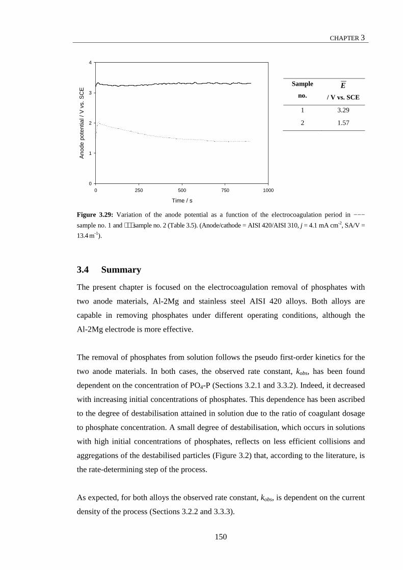
CHAPTER 3

150

Sample

no.

E

/ V vs. SCE

1 3.29

2 1.57

Figure 3.29: Variation of the anode potential as a function of the electrocoagulation period in −−−

sample no. 1 and ⋅ ⋅ ⋅ sample no. 2 (Table 3.5). (Anode/cathode = AISI 420/AISI 310, j = 4.1 mA cm-2, SA/V =

13.4 m-1).

3.4 Summary

The present chapter is focused on the electrocoagulation removal of phosphates with

two anode materials, Al-2Mg and stainless steel AISI 420 alloys. Both alloys are

capable in removing phosphates under different operating conditions, although the

Al-2Mg electrode is more effective.

The removal of phosphates from solution follows the pseudo first-order kinetics for the

two anode materials. In both cases, the observed rate constant, kobs, has been found

dependent on the concentration of PO4-P (Sections 3.2.1 and 3.3.2). Indeed, it decreased

with increasing initial concentrations of phosphates. This dependence has been ascribed

to the degree of destabilisation attained in solution due to the ratio of coagulant dosage

to phosphate concentration. A small degree of destabilisation, which occurs in solutions

with high initial concentrations of phosphates, reflects on less efficient collisions and

aggregations of the destabilised particles (Figure 3.2) that, according to the literature, is

the rate-determining step of the process.

As expected, for both alloys the observed rate constant, kobs, is dependent on the current

density of the process (Sections 3.2.2 and 3.3.3).

Time / s

0 250 500 750 1000

Ano

de p

oten

tial /

V v

s. S

CE

0

1

2

3

4

CHAPTER 3

151

The removal efficiency of phosphates is significantly affected by the initial pH of the

solution for both alloys (Sections 3.2.3.1 and 3.3.4.1). It has been observed that it

decreases with increasing initial pH values. However, the final pH and the pH evolution

also play a major role in the removal process (Sections 3.2.3.2 and 3.3.4.2). The highest

removal efficiency was observed at acidic initial pH and at final pH values around 7.0 in

both Al and Fe systems.

The concentration of chloride ions and the solution conductivity have a marginal effect

on the removal efficiency using Al-2Mg as the anode material (Section 3.2.4). On the

other hand, the performances of AISI 420 grade are strongly reduced in low conductive

solutions (Section 3.3.5).

Both Al-2Mg and AISI 420 alloys remove phosphates according to the Freundlich

adsorption isotherm model in the range of concentrations studied (Sections 3.2.5 and

3.3.6). This finding is consistent with removal mechanisms involving other processes

other than just adsorption, as shown in the literature.

By means of rotating disk voltammetry, RDV, it has been shown that Fe(II) ions are

generated at a pH of 5.0 and at a current density of 11.0 mA cm-2 on oxidation of the

AISI 420 electrode.

The phosphate content has been removed efficiently from two real samples using the

Al-2Mg alloy (Section 3.2.6), while it has been observed that the AISI 420 electrode is

not effective in removing phosphates from the real sample with low conductivity

(Section 3.3.7). This has been rationalised as the effect of the passive nature of this

material. The combination of small chloride concentration and low conductivity results

in the occurrence of concurrent reactions at the anode because of high potential values

exhibiting by the anode during the electrocoagulation process. These reactions do not

result in the dissolution of Fe2+ ions.

Although both alloys have shown to be effective in the removal of phosphates, some

limitations have arisen from treating real samples with specific physico-chemical

characteristics. In particular, the different performance observed for Al-2Mg and AISI

CHAPTER 3

152

420 electrodes to treat the real samples are related to the different electrochemical

behaviour and corrosion properties that these two alloys exhibit in a given medium. The

electrochemical behaviour will, indeed, be the subject of Chapter 4. Several anode

materials will be investigated in terms of their electrochemistry in two specific test

solutions.

3.5 References

[1] Chen, G.H., Sep. Purif. Technol., 38 (2004) 11-41. [2] Gnusin, N.P., Vitul'skaya, N.V., Zabolotskaya, L.I., Belobrov, I.A., J. Appl. Chem. (USSR), 50 (1997) 1663-1741. [3] Pogrebnaya, V.L., Klimenko, A.A., Bokovikova, E.P., Tsymbal, E.P., Pronina, N.P., Chem. Petrol. Eng., 31 (1995) 280-281. [4] Gnusin, N.P., Zabolotskaya, L.I., Vitul'skaya, N.V., Sov. J. Water Chem. Technol., 7 (1985) 32-35. [5] Chen, G.H., Chen, X.M., Yue, P.L., J. Environ. Eng., 126 (2000) 858-863. [6] Beck, E.C., Giannini, A.P., Ramirez, E.R., Food Technol., 22 (1974) 18. [7] Lawrence, J., Knieper, L., Ind. Wastewater, 1-2 (2000) 20-25. [8] Biswas, N., Lazarescu, G., Int. J. Environ. Stud., 38 (1991) 65. [9] Vlyssides, A.G., Papaioannou, D., Loizidoy, M., Karlis, P.K., Zorpas, A.A., Waste Manage. (Oxford), 20 (2000) 569-574. [10] Do, J.S., Chen, M.L., J. Appl. Electrochem., 24 (1994) 785-790. [11] Ibanez, J.G., Singh, M.M., Szafran, Z., J. Chem. Educ., 75 (1998) 1040-1041. [12] Vlyssides, A.G., Loizidou, M., Karlis, P.K., Zorpas, A.A., Papaioannou, D., J. Hazard. Mater., 70 (1999) 41-52. [13] Gurses, A., Yalcin, M., Dogar, C., Waste Manage. (Oxford), 22 (2002) 491-499. [14] Xiong, Y., Strunk, P.J., Xia, H.Y., Zhu, X.H., Karlsson, H.T., Water Res., 35 (2001) 4226-4230. [15] Mameri, N., Yeddou, A.R., Lounici, H., Belhocine, D., Grib, H., Bariou, B., Water Res., 32 (1998) 1604-1612. [16] Panizza, M., Bocca, C., Cerisola, G., Water Res., 34 (2000) 2601-2605. [17] Tsai, C.T., Lin, S.T., Shue, Y.C., Su, P.L., Water Res., 31 (1997) 3073-3081. [18] Donnini, J.C., Kan, J., Hassan, T.A., Kar, K.L., Can. J. Chem. Eng., 72 (1994) 667. [19] Abuzaid, N.S., Bukhari, A.A., Al-Hamouz, Z.M., Adv. Environ. Res., 6 (2002) 325-333. [20] Renk, R.R., Energy Prog., 8 (1988) 205. [21] Szynkarczuk, J., Kan, J., Hassan, T.A.T., Donini, J.C., Clays Clay Miner., 42 (1994) 667-673. [22] Belongia, B.M., Haworth, P.D., Baygents, J.C., Raghavan, S., J. Electrochem. Soc., 146 (1999) 4124-4130. [23] Matteson, M.J., Dobson, R.L., Glenn, R.W., Kukunoor, N.S., Waits, W.H., Clayfield, E.J., Colloids Surf., A, 104 (1995) 101-109. [24] Pretorius, W.A., Johannes, W.G., Lempert, G.G., Water SA, 17 (1991) 133-138. [25] Phutdhawong, W., Chowwanapoonpohn, S., Buddhasukh, D., Anal. Sci., 16 (2000) 1083-1084. [26] Balasubramanian, N., Madhavan, K., Chem. Eng. Technol., 24 (2001) 519– 521. [27] Chiang, L.C., Chang, J.E., Tseng, S.C., Water Sci. Technol., 36 (1997) 123-130. [28] Pouet, M.F., Grasmick, A., Water Sci. Technol., 31 (1995) 275-283.

CHAPTER 3

153

[29] Vik, E.A., Carlson, D.A., Eikum, A.S., Gjessing, E.T., Water Res., 18 (1984) 1355-1360. [30] Valsami-Jones, E., Phosphorus in Environmental Technologies: Principles and Applications, IWA Publishing, 2004. [31] Kirk, P.W.W., Perry, R., Hunter, M., Lester, J.N., Matthews, P.J., Environ. Technol. Lett., 9 (1988) 171-180. [32] Diamadopoulos, E., Benedek, A., J. Water Pollut. Control Fed., 56 (1984) 1165-1172. [33] Lacasa, E., Canizares, P., Saez, C., Fernandez, F.J., Rodrigo, M.A., Chem. Eng. J., 172 (2011) 137-143. [34] Irdemez, S., Demircioglu, N., Yildiz, Y.S., Bingul, Z., Sep. Purif. Technol., 52 (2006) 218-223. [35] Irdemez, S., Yildiz, Y.S., Tosunoglu, V., Sep. Purif. Technol., 52 (2006) 394-401. [36] Bektas, N., Akbulut, H., Inan, H., Dimoglo, A., J. Hazard. Mater., 106 (2004) 101-105. [37] Vasudevan, S., Sozhan, G., Ravichandran, S., Jayaraj, J., Lakshmi, J., Sheela, S.M., Ind. Eng. Chem. Res., 47 (2008) 2018-2023. [38] Emamjomeh, M.M., Sivakumar, M., J. Environ. Manage., 90 (2009) 1663-1679. [39] Vasudevan, S., Lakshmi, J., Jayaraj, J., Sozhan, G., J. Hazard. Mater., 164 (2009) 1480-1486. [40] Jiang, J.Q., Graham, N.J.D., Water SA, 24 (1998) 237-244. [41] Hsu, P.H., Water Res., 10 (1976) 903-907. [42] Crittenden, J.C., Trussell, R.R., Hand, D.W., Howe, K.J., Tchobanoglous, G., MWH's Water Treatment: Principles and Design, John Wiley & Sons, 2012. [43] Bache, D.H., Gregory, R., Flocs in Water Treatment, IWA Publishing, 2007. [44] Georgantas, D.A., Grigoropoulou, H.P., J. Colloid Interface Sci., 315 (2007) 70-79. [45] Aguilar, M.I., Saez, J., Llorens, M., Soler, A., Ortuno, J.F., Water Res., 36 (2002) 2910-2919. [46] Stumm, W., Morgan, J.J., J. Am. Water Works Assoc., 54 (1962) 971-994. [47] Recht, H.L., Ghassemi, M., Kinetics and mechanism of precipitation and nature of the precipitate obtained in phosphate removal from wastewater using aluminium (III) and iron (III) salts, in: Report No. 17010 EKI, 1970. [48] Hsu, P.H., Water Res., 9 (1975) 1155-1161. [49] Donini, J.C., Frenette, R.G., Kasperski, K.L., Kelebek, S., Electrocoagulation - Final Report, Division Report CRL 89-82(CF), CANMET, Energy, Mines and Resources Canada, in: September 1989. [50] Harif, T., Khai, M., Adin, A., Water Res., 46 (2012) 3177-3188. [51] Bayar, S., Yildiz, Y.S., Yilmaz, A.E., Irdemez, S., Desalination, 280 (2011) 103-107. [52] Koparal, A.S., Ogutveren, U.B., J. Hazard. Mater., 89 (2002) 83-94. [53] Akbal, F., Camci, S., Environ. Prog. Sustain. Energy, 31 (2012) 340-350. [54] Murthy, Z.V.P., Parmar, S., Desalination, 282 (2011) 63-67. [55] Secula, M.S., Cretescu, I., Petrescu, S., Desalination, 277 (2011) 227-235. [56] Behbahani, M., Moghaddam, M.R.A., Arami, M., Desalination, 271 (2011) 209-218. [57] Mollah, M.Y.A., Gomes, J.A.G., Das, K.K., Cocke, D.L., J. Hazard. Mater., 174 (2010) 851-858. [58] Abdelwahab, O., Amin, N.K., El-Ashtoukhy, E.S.Z., J. Hazard. Mater., 163 (2009) 711-716. [59] Kobya, M., Demirbas, E., Can, O.T., Bayramoglu, M., J. Hazard. Mater., 132 (2006) 183-188. [60] Daneshvar, N., Oladegaragoze, A., Djafarzadeh, N., J. Hazard. Mater., 129 (2006) 116-122. [61] Stumm, W., O'Melia, C.R., J. Am. Water Works Assoc., 60 (1968) 514-525. [62] Bratby, J., Coagulation and Flocculation in Water and Wastewater Treatment, IWA Publishing, 2006.

CHAPTER 3

154

[63] O'Melia, C.R., Coagulation and Flocculation, in: W.J. Weber (Ed.) Physicochemical Process for Water Quality Control, Wiley-Interscience, 1972. [64] Schick, M.J., Hubbard, A.T., Coagulation and Flocculation, Taylor & Francis, 2005. [65] Duan, J.M., Gregory, J., Adv. Colloid Interface Sci., 100 (2003) 475-502. [66] Szpyrkowicz, L., Kaul, S.N., Neti, R.N., Satyanarayan, S., Water Res., 39 (2005) 1601-1613. [67] Szpyrkowicz, L., Juzzolino, C., Kaul, S.N., Daniele, S., De Faveri, M.D., Ind. Eng. Chem. Res., 39 (2000) 3241-3248. [68] Szpyrkowicz, L., Kaul, S.N., Neti, R.N., J. Appl. Electrochem., 35 (2005) 381-390. [69] Murphy, U.N., Rekha, H.B., Bhavya, J.G., Int. J. Environ. Sci. Develop., 2 (2011) 484-487. [70] Khan, H., Ahmad, N., Yasar, A., Shahid, R., Pol. J. Environ. Stud., 19 (2010) 83-92. [71] Kabdasli, I., Keles, A., Oelmez-Hanci, T., Tuenay, O., Arslan-Alaton, I., J. Hazard. Mater., 171 (2009) 932-940. [72] Abuzaid, N.S., Al-Hamouz, Z., Bukhari, A.A., Essa, M.H., Water Air and Soil Poll., 109 (1999) 429-442. [73] Linares-Hernandez, I., Barrera-Diaz, C., Roa-Morales, G., Bilyeu, B., Urena-Nunez, F., Chem. Eng. J., 148 (2009) 97-105. [74] Ugurlu, M., Gurses, A., Dogar, C., Yalcin, M., J. Environ. Manage., 87 (2008) 420-428. [75] Fouad, Y.O.A., Konsowa, A.H., Farag, H.A., Sedahmed, G.H., Chem. Eng. J., 145 (2009) 436-440. [76] Kabdasli, I., Arslan, T., Oelmez-Hanci, T., Arslan-Alaton, I., Tuenay, O., J. Hazard. Mater., 165 (2009) 838-845. [77] Chou, W.-L., Wang, C.-T., Huang, K.-Y., Desalination, 251 (2010) 12-19. [78] El-Ashtoukhy, E.S.Z., Amin, N.K., J. Hazard. Mater., 179 (2010) 113-119. [79] Linares-Hernandez, I., Barrera-Diaz, C., Bilyeu, B., Juarez-GarciaRojas, P., Campos-Medina, E., J. Hazard. Mater., 175 (2010) 688-694. [80] Rubin, A.J., Kovac, T.W., Effect of Aluminum III Hydrolysis on Alum Coagulation, in: A.J. Rubin (Ed.) Chemistry of Water Supply, Treatment and Distribution, Ann Arbor Science, 1974. [81] Baes, C.F., Mesmer, R.E., The Hydrolysis of Cations, Wiley-Interscience, 1976. [82] Hudson, H.E., Wolfner, J.P., J. Am. Water Works Assoc., 70 (1967) 613-620. [83] Hahn, H.H., Stumm, W., J. Colloid Interface Sci., 28 (1968) 134-&. [84] Letterman Rd, Quon, J.E., Gemmell, R.S., J. Am. Water Works Assoc., 65 (1973) 716-722. [85] Smoluchowski, M., Physik. Z., 17 (1916) 557-585. [86] Smoluchowski, M., Z. Physik. Chem., 92 (1917) 129-168. [87] Hogg, R., Flocculation and Dewatering of Fine-Particle Suspensions, in: H. Stechemesser, B. Dobias (Eds.) Coagulation and Flocculation, Taylor & Francis, 2005. [88] Kusters, K.A., Wijers, J.G., Thoenes, D., Chem. Eng. Sci., 52 (1997) 107-121. [89] Stumm, W., O'Melia, C.R., J. AWWA, 60 (1968) 514-539. [90] Mollah, M.Y.A., Morkovsky, P., Gomes, J.A.G., Kesmez, M., Parga, J., Cocke, D.L., J. Hazard. Mater., 114 (2004) 199-210. [91] Canizares, P., Jimenez, C., Martinez, F., Rodrigo, M.A., Saez, C., J. Hazard. Mater., 163 (2009) 158-164. [92] Mouedhen, G., Feki, M., Wery, M.D.P., Ayedi, H.F., J. Hazard. Mater., 150 (2008) 124-135. [93] Chen, X.M., Chen, G.H., Yue, P.L., Sep. Purif. Technol., 19 (2000) 65-76. [94] Adhoum, N., Monser, L., Bellakhal, N., Belgaied, J.E., J. Hazard. Mater., 112 (2004) 207-213. [95] Kobya, M., Hiz, H., Senturk, E., Aydiner, C., Demirbas, E., Desalination, 190 (2006) 201-211.

CHAPTER 3

155

[96] Canizares, P., Jimenez, C., Martinez, F., Saez, C., Rodrigo, M.A., Ind. Eng. Chem. Res., 46 (2007) 6189-6195. [97] Canizares, P., Martinez, F., Jimenez, C., Lobato, J., Rodrigo, M.A., Ind. Eng. Chem. Res., 45 (2006) 8749-8756. [98] Canizares, P., Martinez, F., Jimenez, C., Lobato, J., Rodrigo, M.A., Environ. Sci. Technol., 40 (2006) 6418-6424. [99] Canizares, P., Martinez, F., Jimenez, C., Lobato, J., Rodrigo, M.A., Sep. Sci. Technol., 42 (2007) 2157-2175. [100] Canizares, P., Martinez, F., Jimenez, C., Saez, C., Rodrigo, M.A., J. Hazard. Mater., 151 (2008) 44-51. [101] Canizares, P., Martinez, F., Lobato, J., Rodrigo, M.A., J. Hazard. Mater., 145 (2007) 233-240. [102] Zhou, W.Z., Gao, B.Y., Yue, Q.Y., Liu, L.L., Wang, Y., Colloids Surf., A, 278 (2006) 235-240. [103] Jardine, P.M., Zelazny, L.W., Soil Sci. Soc. Am. J., 51 (1987) 889-892. [104] Parker, D.R., Zelazny, L.W., Kinraide, T.B., Soil Sci. Soc. Am. J., 52 (1988) 67-75. [105] Feng, C., Shi, B., Wang, D., Li, G., Tang, H., Colloids Surf., A, 287 (2006) 203-211. [106] Letterman, R.D., Amirtharajah, A., O'Melia, C.R., Coagulation and Flocculation, in: R.D. Letterman (Ed.) Water Quality and Treatment - A Handbook of Community Water Supplies, McGraw-Hill, 1999. [107] Sengil, I.A., Ozacar, M., J. Hazard. Mater., 137 (2006) 1197-1205. [108] Frankel, G.S., J. Electrochem. Soc., 145 (1998) 2970-2970. [109] F.G.R., G., Inorganic polymeric chemistry, Butterworths and Co., 1963. [110] Liang, Z., Wang, Y., Zhou, Y., Liu, H., Wu, Z., Sep. Purif. Technol., 68 (2009) 382-389. [111] Buchanan, D.R., Harris, P.M., Acta Crystallogr. Sect. B: Struct. Sci., B 24 (1968) 954-&. [112] Pearson, R.G., J. Am. Chem. Soc., 85 (1963) 3533-&. [113] Stumm, W., Morgan, J.J., Aquatic Chemistry: Chemical Equilibria and Rates in Natural Waters 3rd ed., John Wiley & Sons, 1996. [114] Martinez-Huitle, C.A., Brillas, E., Appl. Catal., B, 87 (2009) 105-145. [115] Kraemer, E.O., Colloids, in: H.S. Taylor (Ed.) A Treatise on Physical Chemistry, D. Van Nostrand Company, New York, 1930. [116] Weber, W.J., Adsorption, in: W.J. Weber (Ed.) Physicochemical Process for Water Quality Control, Wiley-Interscience, 1972. [117] Cornell, R.M., Schwertmann, U., The Iron Oxides: Structure, Properties, Reactions, Occurrences and Uses, Viley-VCH, 2003. [118] Xue, G., Gao, M., Gu, Z., Luo, Z., Hu, Z., Chem. Eng. J., 218 (2013) 223-231. [119] Crini, G., Badot, P.-M., Sorption processes and pollution: conventional and non-conventional sorbents for pollutant removal from wastemasters, Presses Universitaires de Franche-Comté, 2010. [120] Boisvert, J.P., To, T.C., Berrak, A., Jolicoeur, C., Water Res., 31 (1997) 1939-1946. [121] Xie, W.M., Wang, Q.H., Ma, H.Z., Ogawa, H.I., Int. J. Environ. Pollut., 23 (2005) 486-491. [122] Tanada, S., Kabayama, M., Kawasaki, N., Sakiyama, T., Nakamura, T., Araki, M., Tamura, T., J. Colloid Interface Sci., 257 (2003) 135-140. [123] ASTM, in: G 102 - 89: Standard Practice for Calculation of Corrosion Rates and Related Information from Electrochemical Measurements, 1999. [124] Cuevas-Arteaga, C., Porcayo-Calderon, J., Mater. Sci. Eng., A, 435 (2006) 439-446. [125] Vasudevan, S., Lakshmi, J., Water Sci. Technol., 65 (2012) 353-360. [126] Vasudevan, S., Kannan, B.S., Lakshmi, J., Mohanraj, S., Sozhan, G., J. Chem. Technol. Biotechnol., 86 (2011) 428-436. [127] Vasudevan, S., Lakshmi, J., Sozhan, G., Clean-Soil Air Water, 38 (2010) 506-515.

CHAPTER 3

156

[128] Lacasa, E., Canizares, P., Saez, C., Fernandez, F.J., Rodrigo, M.A., Chem. Eng. J., 171 (2011) 1012-1017. [129] Wang, C.-T., Chou, W.-L., Huang, K.-Y., Sep. Sci. Technol., 45 (2010) 212-220. [130] Xu, Y., Jiang, J.-Q., Quill, K., Simon, J., Shettle, K., Desalin. Water. Treat., 2 (2009) 131-138. [131] Chou, W.-L., J. Hazard. Mater., 177 (2010) 842-850. [132] Kalyani, K.S.P., Balasubramanian, N., Srinivasakannan, C., Chem. Eng. J., 151 (2009) 97-104. [133] Weber, W.J., Pure Appl. Chem., 37 (1974) 375-392. [134] Langmuir, I., J. Am. Chem. Soc., 40 (1918) 1361-1403. [135] Freundlich, H., J. Phys. Chem., 57A (1906) 385-470. [136] Mead, J., Aust. J. Soil. Res., 19 (1981) 3-342. [137] Temkin, M., Pyzhev, V., Acta Physiochim. USSR, 12 (1940) 217-222. [138] Brown, A.M., Comput. Meth. Prog. Bio., 65 (2001) 191-200. [139] Motulsky, H.J., Ransnas, L.A., FASEB J., 1 (1987) 365-374. [140] Spiess, A.-N., Neumeyer, N., BMC pharmacology, 10 (2010) 6-6. [141] Del Bubba, M., Arias, C.A., Brix, H., Water Res., 37 (2003) 3390-3400. [142] Kuo, S., McNeal, B.L., Soil Sci. Soc. Am. J., 48 (1984) 1040-1044. [143] Thistleton, J., Clark, T., Pearce, P., Parsons, S.A., Process Saf. Environ. Prot., 79 (2001) 339-344. [144] Johnson, P.N., Amirtharajah, A., J. Am. Water Works Assoc., 75 (1983) 232-239. [145] Leprince, A., Fiessinger, F., Bottero, J.Y., J. Am. Water Works Assoc., 76 (1984) 93-97. [146] Recht, H.L., Ghassemi, M., Phosphate precipitation with ferrous iron, 17010 EKI 09/71, in: Water Pollution Control Research Series, 1971. [147] Bagga, A., Chellam, S., Clifford, D.A., J. Membr. Sci., 309 (2008) 82-93. [148] Yeoman, S., Stephenson, T., Lester, J.N., Perry, R., Environ. Pollut., 49 (1988) 183-233. [149] Stumm, W., Lee, G.F., Ind. Eng. Chem., 53 (1961) 143-146. [150] Thistleton, J., Berry, T.A., Pearce, P., Parsons, S.A., Process Saf. Environ. Prot., 80 (2002) 265-269. [151] Hsu, P.H., Environmental Letters, 5 (1973) 115-136. [152] Fytianos, K., Voudrias, E., Raikos, N., Environ. Pollut., 101 (1998) 123-130. [153] Lakshmanan, D., Clifford, D.A., Samanta, G., Environ. Sci. Technol., 43 (2009) 3853-3859. [154] Sasson, M.B., Calmano, W., Adin, A., J. Hazard. Mater., 171 (2009) 704-709. [155] Parga, J.R., Cocke, D.L., Valverde, V., Gomes, J.A.G., Kesmez, M., Moreno, H., Weir, M., Mencer, D., Chem. Eng. Technol., 28 (2005) 605-612. [156] Osipenko, V.D., Pogorelyi, P.I., Metallurgist, 21 (1977) 628-630. [157] Mollah, M.Y.A., Schennach, R., Parga, J.R., Cocke, D.L., J. Hazard. Mater., 84 (2001) 29-41. [158] Hansen, H.K., Nunez, P., Grandon, R., Miner. Eng., 19 (2006) 521-524. [159] Kobya, M., Senturk, E., Bayramoglu, M., J. Hazard. Mater., 133 (2006) 172-176. [160] Moreno-Casillas, H.A., Cocke, D.L., Gomes, J.A.G., Morkovsky, P., Parga, J.R., Peterson, E., Sep. Purif. Technol., 56 (2007) 204-211. [161] Fadrus, H., Maly, J., Analyst, 100 (1975) 549-554. [162] Lee, T.S., Kolthoff, I.M., Leussing, D.L., J. Am. Chem. Soc., 70 (1948) 2348-2352. [163] Pehkonen, S., Analyst, 120 (1995) 2655-2663. [164] APHA-AWWA-WPCF, Standard Methods for the examination of Water and Wastewater, 18th ed., New York, 1992. [165] Jin, X., Botte, G.G., J. Appl. Electrochem., 39 (2009) 1709-1717. [166] Pletcher, D., Instrumental Methods in Electrochemistry, Woodhead Publishing Paperback, 2011.

CHAPTER 3

157

[167] Behbahani, M., Moghaddam, A.M.R., Arami, M., Int. J. Environ. Res., 5 (2011) 403-412. [168] Zheng, X.-y., Kong, H.-N., Wu, D.-y., Wang, C., Li, Y., Ye, H.-r., Water Sci. Technol., 60 (2009) 2929-2938. [169] Gendel, Y., Lahav, O., J. Hazard. Mater., 183 (2010) 596-601. [170] Morgan, B., Lahav, O., Chemosphere, 68 (2007) 2080-2084. [171] Irdemez, S., Demircioglu, N., Yildiz, Y.S., J. Hazard. Mater., 137 (2006) 1231-1235. [172] Jimenez, C., Saez, C., Martinez, F., Canizares, P., Rodrigo, M.A., Sep. Purif. Technol., 98 (2012). [173] Moreno-Casillas, H.A., Cocke, D.L., Gomes, J.A.G., Morkovsky, P., Parga, J.R., Peterson, E., Garcia, C., Ind. Eng. Chem. Res., 48 (2009) 2275-2282. [174] Uhlig, H.H., Revie, R.W., Uhlig's Corrosion Handbook, 2nd ed., John Wiley & Sons, New York, 2000. [175] Mollah, M.Y.A., Pathak, S.R., Patil, P.K., Vayuvegula, M., Agrawal, T.S., Gomes, J.A.G., Kesmez, M., Cocke, D.L., J. Hazard. Mater., 109 (2004) 165-171. [176] Modirshahla, N., Behnajady, M.A., Kooshaiian, S., Dyes Pigm., 74 (2007) 249-257. [177] Chou, W.-L., Wang, C.-T., Huang, K.-Y., J. Hazard. Mater., 167 (2009) 467-474. [178] Jimenez Izquierdo, C., Canizares, P., Rodrigo, M.A., Leclerc, J.P., Valentin, G., Lapicque, F., Desalination, 255 (2010) 15-20. [179] Persson, P., Nilsson, N., Sjoberg, S., J. Colloid Interface Sci., 177 (1996) 263-275. [180] Mayer, T.D., Jarrell, W.M., Water Res., 34 (2000) 3949-3956. [181] Kreller, D.I., Gibson, G., vanLoon, G.W., Horton, J.H., J. Colloid Interface Sci., 254 (2002) 205-213. [182] Tzou, Y.M., Wang, M.K., Loeppert, R.H., Arch. Environ. Contam. Toxicol., 44 (2003) 445-453. [183] Rentz, J.A., Turner, I.P., Ullman, J.L., Water Res., 43 (2009) 2029-2035. [184] Seida, Y., Nakano, Y., Water Res., 36 (2002) 1306-1312. [185] Heal, K.V., Dobbie, K.E., Bozika, E., McHaffie, H., Simpson, A.E., Smith, K.A., Water Sci. Technol., 51 (2005) 275-282.

158

4

Electrochemical Behaviour of Various

Electrode Materials in Synthetic Wastewater

4.1 Introduction

The main objective of the work presented in this chapter is to compare the

electrochemical properties and behaviour of iron and aluminium based anodes and to

assess the feasibility of using these anode materials in the electrocoagulation process.

Since electrocoagulation involves the oxidation of the electrode and the subsequent

generation of high concentrations of cations, the selection of the anode material is one

of the most important steps in developing a successful electrocoagulation unit. The

composition of the electrode material has a marked impact on the rate of dissolution and

several authors have identified it as a key factor in electrocoagulation applications [1-5].

The most widely used electrode materials are iron and aluminium as described by Vik et

al. [6] and Novikova et al. [7] because they are cheap, readily available, and have

proven effective [1, 2, 8]. For example, Do and Chen [9], on comparing the efficiency

of iron and aluminium electrodes in removing dyes, concluded that the optimum

conditions varied with the choice of iron or aluminium. Later, Baklan and Kolesnikova

[4] carried out a study to correlate the size of the flocculants produced with the removal

efficiency of organic substances. They conducted a single experiment and concluded

that iron electrodes were more efficient because of the size of the flocculant particles,

which ranged from 10 to 30 µm for Fe3+ compared to the smaller range from 0.05 to 1 µm

4

CHAPTER 4

159

for Al3+. On the other hand, Hülser et al. [10] investigated the cathodic corrosion of

aluminium during the electrodeposition of paint and found that electrocoagulation was

strongly enhanced with aluminium in comparison to steel. This was attributed to a

higher efficiency of in situ formed aluminium hydroxide complexes by hydrolysis of the

aluminate ion in acting as nuclei for the electrocoagulation process.

The choice of the electrode material can also affect the consumption of electrical energy

supplied to the system in order to induce oxidation of the electrodes. The metal cations,

which are necessary in forming the coagulation and flocculation of the pollutants, are

generated by applying a constant current or a constant potential. The power

consumption of this process depends mainly on the electrochemical properties of the

anode material and its resistance to dissolution or corrosion. Accordingly, passive

systems are likely to give rise to higher energy consumption. In the light of these

considerations, the addition of alloying elements to iron or aluminium is interesting, as

these alloying components have a significant effect on the electrochemical behaviour of

the metals [11]. The alloying elements can be used to enhance the rate of dissolution or

to alter the nature of the dissolution sites, varying from more localised to general

dissolution. Indeed, some iron- and aluminium-based alloys, other than pure iron and

aluminium, have already been used in electrocoagulation experiments [12].

The electrochemical behaviour of the electrode material is also determined by the nature

and the concentration of ions present in the test solution. Some ions are known to have

an inhibiting effect on the corrosion reactions, whereas other ions serve as activators,

enhancing the rate of dissolution. For example, the presence of chloride anions may

give rise to localised corrosion, such as pitting or crevice corrosion. This, in turn, gives

high rates of metal dissolution at localised sites, while the remaining surface corrodes at

a much lower rate. In contrast, the presence of inhibitors in the solution to be treated

gives rise to a decrease in the efficiency of the electrocoagulation due to the release of

lower concentrations of metal cations from the electrode [13]. Inhibitors and activators

occur together in wastewater treatment facilities and, although the role of the most

common ions on the electrode behaviour is well known from the literature, the effect of

co-existing ions has not been the subject of a systematic study.

CHAPTER 4

160

Localised corrosion gives rise to high rates of dissolution at specific sites and the

production of high concentrations of metal cations. It is no surprise that several authors

have pointed out that localised corrosion is desirable in electrocoagulation as high

concentrations of the metal cations are delivered [5, 14, 15]. However, localised

corrosion may adversely affect the lifetime of the electrode giving irregular dissolution

across the surface [16]. Furthermore, if active pits repassivate, it becomes increasingly

more difficult to induce metal dissolution at these passive sites. In contrast, uniform

dissolution gives a near uniform rate of dissolution across the electrode surface and this

rate of dissolution can be controlled to deliver the required concentration of metal

cations.

In this study several iron and aluminium based electrodes were used as anode materials

in electrocoagulation tests. The chemical composition of the electrode materials used is

given in Section 2.2.1. Pure iron and two stainless steel electrodes, AISI 310 (austenitic

grade) and AISI 420 (martensitic grade), were used as the iron-based system. The two

stainless steel grades were selected on the basis of their chromium content in order to

study the effect of the chromium addition on the removal efficiency in

electrocoagulation. AISI 310 has a high chromium content, namely 25%, while AISI

420 has a lower level of chromium, i.e., 13%. Although iron is widely used in

electrocoagulation applications, Chen and co-workers [1, 5] and indeed several other

authors [17-23] have reported some limitations in its use. In particular, at the end of the

treatment the effluent water developed a yellowish colour, thus affecting the overall

quality of the water and preventing its discharge to the receiving water bodies. The

yellowish colour has been attributed to the presence of fine particles of rust, which form

as a result of the oxidation of the ferrous species by dissolved oxygen in water [1], as

shown in Section 1.4.2.1. These particles are easily formed when the iron electrodes are

used in non-continuous operation [2]. Indeed, the iron electrode corrodes at the open-

circuit potential. With the intention of avoiding this negative effect of the rust on the

effluent colour, the stainless steels were selected as the presence of chromium facilitates

the formation of a protective or passive film preventing, or minimising, the formation of

rust [24].

CHAPTER 4

161

The aluminium-based electrodes included pure aluminium, and two alloys, Al-2Mg and

Al-3Zn-0.02In. Along with iron, aluminium has been extensively used in

electrocoagulation [8]. However, the existence of a passive film on its surface is one of

the main drawbacks of using pure aluminium in electrocoagulation, as the presence of

the passive film leads to an increase in the applied potential required to induce

dissolution [5, 6, 8, 25]. Furthermore, aluminium corrodes mainly in the form of pitting,

which has been recently considered a detrimental form of corrosion in

electrocoagulation from an operational perspective [16]. For the purpose of minimising

both the effects of the passive film and pitting corrosion, aluminium-magnesium and

aluminium-zinc-indium alloys were chosen. Although the addition of magnesium as an

alloying element does not have any significant effect in avoiding the pitting corrosion of

the electrode, it is known that the corrosion resistance of pure aluminium is affected by

the degree of purity of the metal and by the type of alloying elements [26, 27], as also

shown in Section 1.4.2.4. Therefore, it is expected that Al-Mg alloys, although still

showing good corrosion resistance [24], are less protective leading to more favourable

dissolution and generation of Al3+ ions in the solution at lower applied potentials. On

the other hand, it is known that zinc and indium have the ability to activate aluminium

and alter the nature of the dissolution reaction to give more uniform dissolution [28-30].

In this chapter results are presented and discussed on the corrosion behaviour of various

electrode materials, which are subsequently used in Chapter 5 to remove pollutants

using the electrocoagulation technique. Corrosion parameters, such as the corrosion

potential, breakdown potential, and corrosion current, were determined by

potentiodynamic polarisation tests, whereas the propensity of the various electrodes to

suffer localised corrosion was predicted by cyclic potentiodynamic polarisation

measurements and confirmed by light microscopy. As discussed in Section 1.4, the form

of corrosion depends on the electrode material and the solution composition and these

tests are useful in gaining information about the form and rate of the corrosion reaction

[11, 31].

The influence of the solution composition, particularly with regard to the nature and the

concentration of some anions commonly present in wastewaters, was studied. The

corrosion performance of the electrode materials was investigated in the solutions listed

CHAPTER 4

162

in Table 4.1. Two synthetic wastewaters, sww 1 and sww 2, which ion concentrations

were given from the OECD synthetic sewage [32], were selected in order to study the

effect of co-existing ions. They contained three model pollutants, namely phosphates,

an azo dye called Orange II (1.4 × 10-4 M), and zinc ions (1.5 × 10-3 M). The

composition of the two solutions differs in the chloride ion concentration, 0.017 M in

sww 1 and 0.170 M in sww 2. In addition, in order to study the single effect of the

anions present in the two synthetic wastewaters, Cl-, SO42-, and PO4

3-, the polarisation

tests were also carried out in solutions containing these anions at the same concentration

as in sww 1 and sww 2. Slightly higher and lower concentrations were also employed,

as highlighted in Table 4.1. For the sake of comparison, results are first presented for

the potentiodynamic polarisation and the cyclic potentiodynamic polarisation tests

carried out in the single component solutions. Then, results are presented for the mixed

solutions, sww 1 and sww 2. By presenting the results in this order, it is possible to

discern the effect of the individual anions on the overall electrochemical behaviour of

the electrodes in the synthetic wastewater test solutions.

Table 4.1: Composition of the electrolyte solutions used in the potentiodynamic polarisation and cyclic

potentiodynamic polarisation tests. The two synthetic wastewaters, sww 1 and sww 2, also contained an

azo dye called Orange II (1.4 × 10-4 M) and zinc ions (1.5 × 10-3 M). The pH was maintained at 5.0.

Solution

no.

KH 2PO4

/ M

NaCl

/ M

CaCl2.2H2O

/ M

MgSO4.7H2O

/ M

Na2SO4

/ M

Tot Cl -

/ M

1 - 1.7 × 10-2 - - - 1.7 × 10-2

2 - 1.7 × 10-1 - - - 1.7 × 10-1

3 - 1.7 × 10-2 - - 8.1 × 10-4 1.7 × 10-2

4 1.6 × 10-2 - - - - -

5 sww 1 1.6 × 10-2 1.2 × 10-2 2.7 × 10-3 8.1 × 10-4 - 1.7 × 10-2

6 sww 2 1.6 × 10-2 1.7 × 10-1 2.7 × 10-3 8.1 × 10-4 - 1.7 × 10-1

7 6.5 × 10-3 - - - - -

8 6.5 × 10-3 5.0 × 10-4 - - - 5.0 × 10-4

4.2 Pure iron

The potentiodynamic polarisation tests were carried out by polarising pure iron

(99.99%) electrodes with a geometric surface area of 0.071 cm2 in the anodic direction,

from -0.900 V vs. SCE up to the breakdown potential, Ebr, at a rate of 1 mV s-1, unless

CHAPTER 4

163

otherwise stated. To generate the cyclic potentiodynamic polarisation curves the iron

electrodes were cycled at a rate of 1 mV s-1 from -0.900 V vs. SCE, but the scan was

reversed at 1 mA cm-2 or 5 mA cm-2. Then the potential was cycled in the reverse

direction until the corrosion potential, Ecorr, was reached.

4.2.1 The effect of Cl- ions

Potentiodynamic polarisation curves of pure iron recorded in 0.017 M and 0.170 M

NaCl solutions are shown in Figure 4.1. It is evident from the figure that increasing the

chloride concentration causes a substantial shift of the corrosion potential, Ecorr, towards

less noble values. The shift reflects a greater susceptibility of iron to corrosion because

a higher concentration of chloride ions creates a more aggressive environment. For the

10-fold increase in NaCl concentration, the extent of the shift is about 100 mV, varying

from -0.360 V vs. SCE in 0.017 M NaCl to -0.460 V vs. SCE in 0.170 M NaCl. A

higher corrosion current, jcorr, is also recorded in the more concentrated NaCl solution.

At potentials higher than Ecorr, passivation of the iron electrode occurs and this is

characterised by a nearly constant current with increasing applied potential. However, at

higher applied potentials, there is a sharp and rapid increase in the current. This marks

the onset and initiation of pitting corrosion. The breakdown potential, Ebr, which

represents the potential at which pitting is initiated, is computed as -0.090 V vs. SCE in

0.017 M NaCl and -0.290 V vs. SCE in 0.170 M NaCl. Thus, it is evident that

increasing chloride concentration shifts the breakdown potential to more active values.

In addition, the extent of the passive range, ∆Epass, calculated as the difference between

the breakdown potential, Ebr, and the corrosion potential, Ecorr, increases with the

decreasing chloride concentrations. In 0.017 M NaCl, ∆Epass is approximately 0.270 V,

while it is reduced to 0.180 V in the more concentrated 0.170 M NaCl solution.

CHAPTER 4

164

Figure 4.1: Potentiodynamic polarisation curves recorded at a scan rate of 1 mV s-1 for pure iron

in ––– 0.017 M and – – – 0.170 M NaCl solutions at a pH of 5.0.

The effect of chloride ion concentration on the breakdown potential can also be shown

by plotting the breakdown potential, Ebr, as a function of the logarithm of the chloride

concentration. In order to determine this relationship for the pure iron electrode,

polarisation tests were carried out in 0.017, 0.100, 0.170, and 0.300 M NaCl solutions

adjusted to a pH of 5.0, and the resulting plot is displayed in Figure 4.2. As evident

from this figure, a linear relationship exists and, using linear regression analysis, the Eq.

4.1 is obtained.

]Cl[180.0409.0 −−−= Ebr Eq. 4.1

According to Eq. 4.1, as the chloride concentration decreases, the breakdown potential,

Ebr, is displaced to higher potentials. The value of the slope, which is represented by B,

is somewhat higher than the values presented by Galvele and co-workers [33, 34]. In

1976 Galvele developed an extensive model on the mechanism of pitting corrosion [33]

and he reported a logarithmic relationship between the breakdown potential, Ebr, and the

concentration of aggressive anions. Galvele accounted for this relationship, which is

valid with several anions and other metals [35], by considering the effect of chloride

concentration on the potential drop within the pit and this explanation was also used by

j / A cm-2

10-9 10-8 10-7 10-6 10-5 10-4 10-3

E /

V v

s. S

CE

-1.0

-0.8

-0.6

-0.4

-0.2

0.0

CHAPTER 4

165

Laycock and Newman [36, 37] in their studies on stainless steel electrodes. According

to Galvele, a value of 59 to 64 mV is obtained for pure iron in de-aerated NaCl

solutions, at a pH of 10, if the migration of the chloride ions inside the pits is the only

variable considered [33, 38]. However, several works reported different values of B for

iron, most of them are listed in a review by Galvele [34], containing a comprehensive

list of values for several electrode materials and environments. For pure iron in chloride

solutions the B values range from 30 to 150 mV. The value shown in Eq. 4.1 is beyond

that range, however it has to be considered that the value adopted by B can be affected

by several variables, such as the pH of the solution, the presence of a buffer, the oxygen

content, temperature, nature of the electrolyte, and roughness of the electrode surface

[36]. The measurement technique and the can rate can also influence the magnitude of

B. Indeed, several of the reported studies have been carried out using the potentiostatic

technique rather than the potentiodynamic approach. The experimental value of B,

shown in Eq. 4.1, can be used to compare the sensitivity of the various electrode

materials to chloride concentration. Accordingly, this analysis was performed on the

various electrodes and the B values were compared.

NaCl

/ M

Ebr

/ V vs. SCE

0.017 -0.10 ± 0.03

0.100 -0.21 ± 0.01

0.170 -0.28 ± 0.03

0.300 -0.324 ± 0.008

Figure 4.2: Breakdown potential, Ebr, of the pure iron plotted as a function of the logarithm of the

chloride concentration. Each experiment was performed in triplicate (n = 3). The breakdown potential,

Ebr, was obtained from potentiodynamic polarisation tests at a scan rate of 1 mV s-1. The experimental

points were fitted by a linear regression analysis to Ebr = A + B log [Cl-], A = −0.409 ± 0.022 V, B = −0.180

± 0.019 V, and R2 = 0.976.

[Cl-] / M

0.01 0.1 1

Ebr

/ V

vs.

SC

E

-0.35

-0.30

-0.25

-0.20

-0.15

-0.10

-0.05

CHAPTER 4

166

The susceptibility of the iron electrode to localised corrosion was investigated further

using cyclic potentiodynamic polarisation tests. Representative data are shown in Figure

4.3(a) where the cyclic polarisation curves for pure iron in 0.017 M and 0.170 M NaCl

are compared. The data recorded during the forward and reverse cycles are clearly

different giving hysteresis. This phenomenon is usually associated with the onset of

pitting attack and in some theories it is suggested that the larger the hysteresis, the more

likely a localised corrosion site will propagate once initiated [24]. However, a post-scan

microscopic examination of the sample is recommended in order to confirm the nature

of the attack [39].

The surface of the electrode was examined using light microscopy after the cyclic

polarisation tests were completed, and representative micrographs are shown in Figure

4.3(b) and (c). Pitting attack is clearly evident, with the size and distribution of the pits

depending on the concentration of the chloride solution. From Figure 4.3(b) it is evident

that in 0.017 M NaCl, the size of the pits ranges from 2 to 8 µm and these are evenly

dispersed over the electrode surface. In contrast, the micrograph recorded in the

presence of 0.170 M NaCl (Figure 4.3(c)) shows fewer pits, with the larger pits having

a diameter from 20 to 25 µm and these are scattered among several smaller pits with a

diameter of about 1 µm. These findings are consistent with the higher rates of

dissolution in the 0.170 M NaCl solution. Once a pit is nucleated, the propagation step

is more rapid at the higher chloride concentrations and this gives rise to larger pits. This

attack continues at several isolated sites, while new sites are activated to give the

smaller sized pits that are also observed on the surface. These sites are smaller as they

are not nucleated at the breakdown potential, Ebr, but sometime later during the forward

or reverse cycle.

CHAPTER 4

167

Figure 4.3: (a) Cyclic potentiodynamic polarisation curves recorded for the pure iron in ––– 0.017 M

and – – – 0.170 M NaCl solutions at a pH of 5.0 at a scan rate of 1 mV s-1; micrographs of pure iron

electrode at the end of the cyclic potentiodynamic polarisation scan in (b) 0.017 M NaCl, with the scale

bar corresponding to 100 µm and (c) 0.170 M NaCl, with the scale bar corresponding to 200 µm.

4.2.2 The effect of SO42- ions

Since the two synthetic wastewaters, sww 1 and sww 2, used as test solutions in the

electrocoagulation experiments contain sulfate ions, potentiodynamic polarisation tests

were carried out to investigate the effect of the presence of sulfate ions on the

electrochemical behaviour of pure iron. However, the conductivity of the 8.1 × 10-4 M SO42-

solution was too low for the corrosion tests and 0.017 M NaCl was added to the Na2SO4

solution as shown in Table 4.1, while the pH was maintained at a value of 5.0. The

resulting polarisation curve was compared to the data recorded in the absence of sulfate

ions (Section 4.2.1) and these data are presented in Figure 4.4. As can be seen from the

figure, the two curves are noticeably different. A clear passive region is evident in the

0.017 M NaCl solution, but with the addition of the sulfate ions there is a slight increase

in the corrosion potential, Ecorr, from -0.359 V vs. SCE in the absence of sulfate ions to

-0.319 V vs. SCE in the presence of sulfate. There is a corresponding increase in the

corrosion current from 9.29 × 10-7 A cm-2 to 1.90 × 10-6 A cm-2, and the breakdown

potential, Ebr is lowered from -0.091 to -0.162 V vs. SCE. Moreover, the passive current

density is higher and the passive region is less defined in the presence of the sulfate

ions. However, the rapid increase in the current at -0.162 V vs. SCE is consistent with

the onset of pitting attack.

j / A cm-2

10-9 10-8 10-7 10-6 10-5 10-4 10-3 10-2

E /

V v

s. S

CE

-1.0

-0.8

-0.6

-0.4

-0.2

0.0

(a)

(b)

(c)

CHAPTER 4

168

The effect of sulfate ions on the breakdown and dissolution of iron has been described

in several reports. For example, Vatankhah et al. [40] found that rotating iron disk

electrodes exhibit uniform corrosion in 1.0 M solutions containing sulfate ions. Also,

MacDougall and Bardwell [41] concluded that the passivation of iron is an efficient

process in 0.15 M sulfate solutions at pH 3.0 or 8.4. However, when iron is polarised in

a solution comprising chlorides and sulfates, localised dissolution and pitting attack is

observed. Bird et al. [42] showed that the presence of sulfate ions reduces the pitting

potential of iron as a result of competitive adsorption between the anions present in

solution. Nobe and Tobias [43] reported similar findings for iron in 1.0 M Na2SO4

solutions with various amounts of chloride ions (from 0.00 to 0.05 M) at pH 3.0. Nobe

and Tobias [43] observed an increase in the current density in the passive region with an

increase in the concentration of chloride ions. However, the current density varied with

the ratio of the sulfate to chloride concentration. The results presented in Figure 4.4 are

consistent with these studies reported in sulfate solutions with added chlorides.

Figure 4.4: Potentiodynamic polarisation curves recorded for the pure iron in ––– 0.017 M NaCl and

8.1 × 10-4 M Na2SO4 solution at a pH of 5.0 and – – – 0.017 M NaCl at a pH of 5.0, at a scan rate of

1 mV s-1.

To confirm the onset of pitting corrosion of the pure iron electrode in the sulfate-

containing solution, cyclic potentiodynamic polarisation tests were carried out in a

j / A cm-2

10-9 10-8 10-7 10-6 10-5 10-4 10-3

E /

V v

s. S

CE

-1.0

-0.8

-0.6

-0.4

-0.2

0.0

CHAPTER 4

169

0.017 M NaCl and 8.1 × 10-4 M Na2SO4 solution (Table 4.1). The cyclic curve is

displayed in Figure 4.5, and clearly shows hysteresis between the forward and reverse

cycle, indicating pitting corrosion. Indeed, pits were found on examination of the

electrode surface using light microscopy, as shown in Figure 4.5(b). This micrograph

shows the presence of large pits with a diameter of about 2 µm, and several smaller pits

distributed across the surface. These pits are smaller than the pits observed in the

chloride solution in the absence of sulfate anions (Section 4.2.1, Figure 4.3). These

results are consistent with the findings of Galvele [33], who observed inhibition of

pitting corrosion in the presence of sulfate anions. As the pits start to grow, sulfate ions

are accumulated inside the pits, since the anions with the higher charge are

preferentially accumulated at the metal-solution interface. This build up in the

concentration of the sulfate ions gives rise to repassivation of the pits. However,

chloride ions eventually diffuse to the site, reducing the concentration of sulfates inside

the pits. As a consequence, a continuous process of activation and deactivation of the

pits is observed. It is clear from the micrograph and the polarisation tests that iron is

susceptible to pitting attack in a solution containing 0.017 M NaCl and 8.1 × 10-4 M

Na2SO4 at a pH of 5.0.

Figure 4.5: (a) Cyclic potentiodynamic polarisation curve for the pure iron recorded in ––– 0.017 M

NaCl and 8.1 × 10-4 M Na2SO4 solution at a pH of 5.0, at a rate of 1 mV s-1; (b) micrograph, with the

scale bar corresponding to 50 µm, of pure iron at the end of the cyclic potentiodynamic polarisation scan.

j / A cm-2

10-9 10-8 10-7 10-6 10-5 10-4 10-3 10-2

E /

V v

s. S

CE

-1.0

-0.8

-0.6

-0.4

-0.2

0.0

(a)

(b)

CHAPTER 4

170

4.2.3 The effect of PO43- ions

Phosphates are one of the most popular corrosion inhibitors employed in the corrosion

protection of ferrous alloys [11, 44, 45]. In addition, phosphates were added to give the

two synthetic wastewaters, sww 1 and sww 2, as detailed in Table 4.1. Therefore,

corrosion studies were carried out in a phosphate-containing solution in order to

investigate the effects of the phosphate ions on the iron electrode and then to allow a

more direct comparison with the results obtained in the two synthetic wastewaters, sww

1 and sww 2. The polarisation plots were recorded in 0.016 M KH2PO4 (Table 4.1). A

typical plot is presented in Figure 4.6 and it is clearly evident that the polarisation

behaviour is very different to that observed in the chloride or sulfate solutions in

Sections 4.2.1 and 4.2.2, respectively. The corrosion potential, Ecorr, is -0.720 V

vs. SCE, considerably lower than the value observed in the chloride or sulfate solutions,

and the corrosion current, jcorr, is one order of magnitude higher, at 3.1 × 10-5 A cm-2.

These data clearly show that the corrosion rate is higher in the 0.016 M KH2PO4

solution. In addition, the anodic portion of the scan does not show any passive region.

The current increases in a near linear manner from the corrosion potential, Ecorr, to reach

a value of about 1 mA cm-2 at -0.550 V vs. SCE. This indicates significant dissolution.

Phosphates are well known as film-forming corrosion inhibitors [44, 45] and phosphate-

containing solutions have been proposed and used as environmentally acceptable

alternatives to chromates in corrosion inhibition applications [46-48]. The corrosion

protection is provided by the formation of precipitates on the surface of the metal,

thereby forming a protective film [44, 45]. However, as shown by the work of

Szklarska-Smialowska and Staehle [49], corrosion inhibition in phosphate-containing

solutions is highly dependent on the solution pH. The authors conducted an

ellipsometric study to elucidate the optical properties of the film growth on iron

electrodes in 0.1 M sodium orthophosphate solutions at different pH values, from 4.5 to

12.3. The growth of the film was found regardless of the solution pH, but the type and

nature of the film were considerably different. In particular, at pH 4.5 and 7.0 in the

presence of H2PO4- ions in solution, a porous and non-protective film was formed,

giving little or no corrosion protection. Similar results were reported by Pryor and

Cohen [50]. The results obtained in Figure 4.6 are consistent with active dissolution of

the pure iron electrode in the phosphate solution at a pH of 5.0 and are in good

CHAPTER 4

171

agreement with these literature reports. Furthermore, this active dissolution at a pH of

5.0 is consistent with the optimum pH range, from a value of 5.0 to 7.0, reported by

İrdemez et al. [51] in removing phosphates using electrocoagulation with iron

electrodes.

Polarisation tests were also recorded with a lower concentration of phosphate anions,

6.5 × 10-3 M KH2PO4, however in this case chloride anions, 5.0 × 10-4 M NaCl, were

added to the solution to increase the conductivity. Again, data similar to that presented

in Figure 4.6 were obtained, indicating active dissolution of the iron electrode.

Figure 4.6: Potentiodynamic polarisation curve recorded at a scan rate of 10 mV s-1 for the pure iron

electrode in ––– 0.016 M KH2PO4 solution at a pH of 5.0.

In an attempt to obtain more information on the nature of the dissolution, cyclic

potentiodynamic polarisation tests were recorded in 0.016 M KH2PO4 (Table 4.1). In

Figure 4.7(a), a representative cyclic polarisation plot is presented and in this case there

is little difference between the forward and reverse portions of the scan and there is no

evidence of any significant hysteresis. This phenomenon has been explained by

Silverman [52] in terms of relatively large amounts of charge and active or rapid

corrosion that gives a sharp increase in current under slight polarisation. The small

difference in current recorded at the same potential between the two portions of the scan

j / A cm-2

10-8 10-7 10-6 10-5 10-4 10-3 10-2

E /

V v

s. S

CE

-1.0

-0.9

-0.8

-0.7

-0.6

-0.5

CHAPTER 4

172

depends on the scan direction; in the reverse scan the current does not represent the

steady state current at the applied potential because of the large charge that has passed

in the forward scan. This finding is supported by the micrograph presented in Figure

4.7(b). This was recorded following the cyclic polarisation measurement. Several small

active sites are present on the surface. However, it was also possible to identify some

pits with a larger diameter of approximately 4 µm.

Figure 4.7: (a) Cyclic potentiodynamic polarisation curve recorded for the pure iron electrode at a scan

rate of 1 mV s-1 in ––– 0.016 M KH2PO4 solution, at a pH of 5.0; (b) micrograph of the pure iron

electrode at the end of the cyclic potentiodynamic polarisation scan, scale bar corresponds to 100 µm.

These results are important in terms of electrocoagulation. It is clear that the iron

electrode is not prone to significant passivation in the slightly acidic phosphate solution.

Furthermore, the absence or the presence of chloride ions has little influence on the

polarisation behaviour of the iron electrode. Accordingly, variations in the chloride

concentration should not pose any significant issue in water treatment facilities since the

electrochemical behaviour of iron remains almost constant.

4.2.4 The effect of co-existing anions in sww 1 and sww 2

The effect of the co-existing anions on the electrochemical properties of the pure iron

was studied by polarising the electrode in sww 1 and sww 2 (Table 4.1). The

potentiodynamic polarisation plots are shown in Figure 4.8 and, although the

polarisation curves are similar, the corrosion potentials, Ecorr, are slightly different at

j / A cm-2

10-8 10-7 10-6 10-5 10-4 10-3 10-2

E /

V v

s. S

CE

-1.0

-0.9

-0.8

-0.7

-0.6

-0.5

(a)

(b)

CHAPTER 4

173

approximately -0.710 V and -0.724 V vs. SCE in sww 1 and sww 2, respectively. This

small difference is probably due to the 10-fold increase in the chloride concentration for

the sww 2 solution (Table 4.1). However, the corrosion currents, jcorr, are nearly

identical at 3.1 × 10-5 A cm-2 in sww 1 and 2.9 × 10-5 A cm-2 in sww 2. Interestingly,

these values are significantly higher compared to the jcorr values obtained in the NaCl

solutions (Section 4.2.1, Figure 4.1). Furthermore, the polarisation curves, shown in

Figure 4.8, are very similar to that obtained in the KH2PO4 solution (Figure 4.6). Indeed

both the corrosion potential, Ecorr, and the corrosion current, jcorr, are similar and the

shapes of the polarisation curves are nearly identical (Figure 4.6), indicating active

dissolution of the electrode with little evidence of passivity. However, it has to be

considered that in the two synthetic wastewaters the phosphates are present in relatively

high concentrations with respect to the other electrolytes, thus potentially masking the

effect of the other anions. However, a potentiodynamic polarisation scan (data not

shown) performed in a solution with the same composition and concentration as in sww

1, but with 1.60 × 10-3 M KH2PO4, was similar. Although in this scan the corrosion

potential, Ecorr, was higher at -0.482 V vs. SCE and the corrosion current, jcorr, was

considerably lower at 8.38 × 10-6 A cm-2, there was no evidence of any passive region.

It is clear from these results that the phosphate ions have a significant influence on the

corrosion behaviour of pure iron in slightly acidic solutions, with a pH of 5.0.

Figure 4.8: Potentiodynamic polarisation curves recorded at a scan rate of 1 mV s-1 for the pure iron

electrode in ––– sww 1 and – – – sww 2 solutions, at a pH of 5.0 (Table 4.1).

j / A cm-2

10-8 10-7 10-6 10-5 10-4 10-3 10-2

E /

V v

s. S

CE

-0.95

-0.90

-0.85

-0.80

-0.75

-0.70

-0.65

-0.60

-0.55

CHAPTER 4

174

Again, cyclic potentiodynamic polarisation tests were carried out in sww 1 and sww 2

solutions and representative plots are presented in Figure 4.9(a). Clearly there is no

significant hysteresis, with the forward and reverse cycles in relatively good agreement.

These data are similar to that recorded in the phosphate solution (Section 4.2.3, Figure

4.7), highlighting the significant influence of the phosphate anions. Moreover, the

10-fold increase in the chloride concentration, sww 2, has little influence on the level of

agreement between the forward and reverse cycles. There is no obvious hysteresis in

either the sww 1 or sww 2 solutions. The surface of the electrodes was studied by post-

scan examinations of the electrode surface by light microscopy. The micrographs of the

iron electrode cycled in sww 2 are presented in Figure 4.9(b) and (c) and reveal that the

electrode surface is covered by small dissolution sites, with no significant pits. A similar

surface morphology was observed for the iron electrode after the cyclic scan in sww 1.

These results indicate that pitting attack induced by the chloride ions, even at reasonably

high concentrations, is mitigated or minimised in the presence of phosphate ions at a pH

of 5.0. This can be explained by the lack of a passive region. Since in sww 1 and sww 2

the pure iron electrode shows no passive behaviour and more general-like dissolution or

corrosion, it is a promising material in treating the two synthetic wastewaters using the

electrocoagulation technique.

Figure 4.9: (a) Cyclic potentiodynamic polarisation curves for the pure iron electrode in ––– sww 1

and – – – sww 2 solution, at a pH of 5.0 (Table 4.1) at a scan rate of 1 mV s-1; micrographs of the pure

iron electrode at the end of the cyclic potentiodynamic polarisation scan in sww 2 solutions (b) scale bar

corresponding to 200 µm and (c) scale bar corresponding to 100 µm.

j / A cm-2

10-8 10-7 10-6 10-5 10-4 10-3 10-2

E /

V v

s. S

CE

-1.0

-0.9

-0.8

-0.7

-0.6

-0.5

(a)

(b)

(c)

CHAPTER 4

175

4.3 Stainless steel AISI 310

Similar experiments were carried out with the AISI 310 (Fe/Cr25/Ni20) stainless steel

grade electrodes. The potentiodynamic polarisation tests were carried out by polarising

the electrodes, with a geometric area of 0.58 cm2, in the anodic direction, from an initial

potential of -0.900 V vs. SCE up to a final potential of 1.100 V vs. SCE at a scan rate of

1 mV s-1. In the cyclic potentiodynamic polarisation curves the scan was reversed when

the current reached a value of 1 mA cm-2. Again, the polarisation behaviour was studied

in simple chloride, sulfate and phosphate solutions, and then studies in the synthetic

wastewaters, sww 1 and sww 2, were performed. The pH of the solutions was

maintained at 5.0.


AISI 310 belongs to the austenitic stainless steel family, containing chromium and

nickel, as outlined in Section 1.4.2.2. In particular, the 310 grade is characterised by an

excellent corrosion resistance because of a high chromium and nickel content (24-26% Cr,

19-22% Ni). The corrosion resistance of stainless steel is attributed to the formation of a

thin, adherent and self-healing passive film consisting of mixed oxides of chromium and

iron. The increasing chromium content in stainless steel enhances the stability of the

passive film, while the presence of nickel delays the decrease in pH during pit growth

by neutralising the solution in the pit [53]. Austenitic steels, however, are not immune

to pitting corrosion, particularly in the presence of chloride ions [54]. The beneficial

effects of chromium, nickel, and other alloying elements are determined by the pitting

and crevice corrosion resistance index, known as the pitting resistance equivalent

number, PREN [55]. The PREN is given by the relative contribution of the alloying

elements, as shown in Eq. 4.2.

]W[65.1]N[16]Mo[3.3]Cr[PREN +++= Eq. 4.2

In this equation, [Cr] indicates the % weight of Cr in the alloy, while [Mo], [Ni], and

[W] give the contributions of the other alloying elements. In general, higher pitting and

crevice corrosion resistance is achieved when the numerical value of PREN is high. The

PREN value for AISI 310 has been computed as 25.0 [55].

CHAPTER 4

176

The evidence of this high corrosion resistance is provided in Figure 4.10(a), which

shows the potentiodynamic polarisation tests of the AISI 310 electrode in 0.017 M and

0.170 M NaCl (Table 4.1). There is no marked difference in the shape of the

polarisation curves and the electrode exhibits a wide, extended passive range of

approximately 500 mV in both solutions. The breakdown potentials, Ebr, are 0.102 V vs.

SCE and 0.054 V vs. SCE in 0.017 M and 0.170 M NaCl, respectively. Relatively low

corrosion currents are measured, with jcorr values of 2.23 × 10-6 A cm-2 in 0.017 M and

2.03 × 10-6 A cm-2 in 0.170 M NaCl, showing that the chloride concentration has little

influence. The extent of the passive region, ∆Epass, does not increase with decreasing

chloride concentrations, which is somewhat different to that observed with the iron

electrode (Section 4.2.1).

The shift in the breakdown potential with increasing concentration of chloride is in good

agreement with several reports on AISI 304, a stainless steel with 18% Cr and 8% Ni

(Fe-Cr18-Ni8). For example, Leckie and Uhlig [56] carried out a study on the

environmental factors affecting the breakdown potential of Fe-Cr18-Ni8. In a 0.1 M NaCl

solution, the breakdown potential was observed at 0.116 V vs. SCE and lower

breakdown potentials were recorded with increasing chloride concentrations. Several

studies have also been carried out to investigate the effect of increasing the

concentration of chromium in austenitic stainless steels. For example, Horvath and

Uhlig [57] studied the effect of the concentration of the alloying elements of the

Cr-Fe-Ni-Mo system in NaCl solutions. A significant increase in the breakdown

potential, Ebr, was observed for Cr concentrations between 25 and 40% in the Cr-Fe

binary alloys in 0.1 M NaCl, indicating a greater resistance to pitting attack. Pitting

attack was observed for the 48.8% Cr-Fe alloy, however pitting was not evident with

the 57.8% Cr-Fe. With regard to the ternary systems, 15% Cr-Fe-Ni-Mo, an increase in

the breakdown potential, Ebr, was observed with an increase in the Ni concentration.

The high breakdown potentials recorded for the AISI 310 stainless steel, which contains

25% Cr and 20% Ni, is consistent with these reports.

The AISI 310 electrode was polarised in a slightly acidic solution, with a pH of 5.0, and

the concentration of the chloride anion was varied. The breakdown potential was

measured as a function of the chloride concentration and a logarithmic relationship was

CHAPTER 4

177

obtained with the breakdown potential, Ebr, decreasing linearly with the logarithm of

chloride concentration, as depicted in Figure 4.10(b). A similar linear dependence was

found with the iron electrode polarised in NaCl solutions (Section 4.2.1) in agreement

with the results reported by Galvele [34]. The linear relationship obtained for AISI 310,

was found using linear regression analysis, and is shown in Eq. 4.3.

]Cl[046.0018.0 −−= Ebr Eq. 4.3

The value of B was computed as 46 mV (Eq. 4.3). This is somewhat smaller than the

value of approximately 88 mV reported for Fe-Cr18-Ni8 [56]. However, a smaller B

value is expected for the AISI 310 because it is less susceptible to pitting corrosion. It is

worth noting in Figure 4.10(a) that in 0.017 M NaCl a transition occurs at

about -0.040 V vs. SCE, where the current increases to reach a maximum value before

decaying again. This active-passive transition, which is also called the “anodic nose”,

has been reported for some austenitic stainless steel alloys in dilute acidic environments

[52]. This behaviour has been explained in terms of a passivation process or a valency

change. It is clear that this anodic nose is not present in the more concentrated 0.170 M

NaCl solution.

Figure 4.10: (a) Potentiodynamic polarisation curves for the AISI 310 electrode in ––– 0.017 M

and – – – 0.170 M NaCl solutions, at a pH of 5.0, recorded at a scan rate of 1 mV s-1. (b) Breakdown

potential, Ebr, of AISI 310 as a function of the logarithm of the chloride concentration. The breakdown

potential, Ebr, was obtained from potentiodynamic polarisation tests. Each experiment was performed in

triplicate (n = 3). The experimental points were fitted by a linear regression analysis to Ebr = A + B log [Cl-],

A = 0.018 ± 0.004 V, B = −0.046 ± 0.004 V, R2 = 0.986.

j / A cm-2

10-9 10-8 10-7 10-6 10-5 10-4 10-3

E /

V v

s. S

CE

-1.0

-0.5

0.0

0.5

1.0

1.5

[Cl-] / M

0.01 0.1 1

Ebr

/ V

vs.

SC

E

0.04

0.06

0.08

0.10

0.12

NaCl

M

Ebr

V vs. SCE

0.017 0.101 ± 0.007

0.100 0.055 ± 0.005

0.170 0.060 ± 0.006

0.300 0.044 ± 0.006

(a) (b)

CHAPTER 4

178

The cyclic potentiodynamic polarisation tests, recorded with the AISI electrode in 0.170

and 0.017 M NaCl at a pH of 5.0, are presented in Figure 4.11(a). In both cases,

significant hysteresis is observed and this can be attributed to the growth of large pits as

illustrated in the micrographs shown in Figure 4.11(b) and (c). Isolated pits with

irregular shape and with a size of about 50 to 70 µm are evident on the electrode

surface. This clearly shows that once the passive film is destroyed, the pits propagate at

relatively high rates, but this is also connected to the potentials applied to the electrode,

which extend to values in the vicinity of 1.40 V vs. SCE.

Figure 4.11: (a) Cyclic potentiodynamic polarisation curves for the AISI 310 electrode in ––– 0.017 M

and – – – 0.170 M NaCl solutions, at a pH of 5.0, recorded at a scan rate of 1 mV s-1; (b) and (c)

micrographs of the AISI 310 electrode at the end of the cyclic potentiodynamic polarisation scan in

0.170 M NaCl solution, with the scale bar corresponding to 50 µm.


The influence of sulfate anions on the polarisation behaviour of AISI 310 is shown in

Figure 4.12, where the potentiodynamic polarisation curve recorded in 0.017 M NaCl

solution is compared with the data obtained in 0.017 M NaCl with 8.1 × 10-4 M Na2SO4

(Table 4.1). Again, a clear passive region is evident in the sulfate-containing solution.

Indeed, the passive current density is somewhat lower in the presence of the sulfate

anions. The breakdown potential was computed as 0.131 V vs. SCE, which is slightly

higher than the value observed in the NaCl solution (Ebr = 0.102 V vs. SCE in 0.017 M NaCl).

j / A cm-2

10-10 10-9 10-8 10-7 10-6 10-5 10-4 10-3 10-2

E /

V v

s. S

CE

-1.5

-1.0

-0.5

0.0

0.5

1.0

1.5

(a)

(b)

(c)

CHAPTER 4

179

It is well known that the breakdown potential in chloride-containing solutions depends

on the concentration and nature of other anions in the solution [58]. In particular,

Brauns and Schwenk [59] observed this behaviour for OH- and SO42- additions. Leckie

and Uhlig [56] also found that the breakdown potential of Fe-Cr18-Ni8 stainless steel in

0.10 M NaCl increased with increasing Na2SO4 concentrations, and in 0.15 M Na2SO4

pitting did not occur. The data presented in Figure 4.12 are consistent with these

findings and show that sulfate additions inhibit the pitting corrosion of AISI 310.

According to Leckie and Uhlig [56, 58], the magnitude of the breakdown potential shift

depends on the ratio of sulfate to chloride ions. On addition of 0.0125 M Na2SO4 to

0.100 M NaCl, they observed a 50 mV increase in the breakdown potential. A smaller

increase of the breakdown potential, about 29 mV, is instead evident in Figure 4.12 for

AISI 310, however, this can be explained in terms of the low SO42-/Cl- ratio. It is also

evident from Figure 4.12 that although an anodic nose is observed at about 0.010 V vs.

SCE, the current is lower and this feature is less pronounced in the presence of the

sulfate anions. Moreover, when cyclic polarisation plots were recorded in the presence

of sulfate, in 0.017 M NaCl and 8.1 × 10-4 M Na2SO4, although hysteresis was observed

and pits were found on the surface, the pits were smaller in diameter (data not shown).

Again, this highlights the role of sulfate anions as inhibitors in the pitting corrosion of

AISI 310.

Figure 4.12: Potentiodynamic polarisation curves recorded for the AISI 310 at a scan rate of 1 mV s-1

in ––– 0.017 M NaCl and 8.1 × 10-4 M Na2SO4, at a pH of 5.0 and – – – 0.017 M NaCl, at a pH of 5.0.

j / A cm-2

10-9 10-8 10-7 10-6 10-5 10-4 10-3

E /

V v

s. S

CE

-1.0

-0.5

0.0

0.5

1.0

1.5

CHAPTER 4

180


As mentioned in Section 4.2.3, phosphate ions are well known to have an inhibiting

effect on the corrosion of ferrous alloys [11, 44, 45]. This property can adversely affect

the energy demand in removing phosphates from water using the electrocoagulation

technique. To investigate the extent of this effect, potentiodynamic polarisation tests

were carried out on the AISI 310 electrode in 0.016 M KH2PO4 (Table 4.1) and a

representative curve is shown in Figure 4.13(a). As illustrated in the figure, the

electrode remains passive and low currents of the order of 1 µA cm-2 are evident from

the corrosion potential, Ecorr, to values in the vicinity of 1.00 V vs. SCE.

Lakatos-Varsányi et al. [60] studied the influence of phosphate on the electrochemical

behaviour of AISI 304 exposed to neutral chloride-containing solutions and found that

phosphate ions enhance the repassivation properties of stainless steel. Indeed, this

finding is consistent with the results obtained from the cyclic potentiodynamic

polarisation curve, shown in Figure 4.13(b). In fact, the repassivation potential, which

corresponds to the potential at which the forward and reverse scans cross each other,

occurs at a very high potential of 1.10 V vs SCE. Below the repassivation potential a

stable growing pit or crevice site will cease to grow.

Figure 4.13: (a) Potentiodynamic polarisation curve and (b) cyclic potentiodynamic polarisation curve

recorded for the AISI 310 electrode at a scan rate of 1 mV s-1 in ––– 0.016 M KH2PO4 solution, at a pH of 5.0.

From the analysis of the polarisation and cyclic polarisation plots, it is evident that in

phosphate containing solutions, phosphate ions passivate the AISI 310 electrode and, as

reported by Lakatos-Varsányi et al. [60], improve the repassivation properties of the alloy.

j / A cm-2

10-9 10-8 10-7 10-6 10-5 10-4 10-3

E /

V v

s. S

CE

-1.0

-0.5

0.0

0.5

1.0

1.5

j / A cm-2

10-10 10-9 10-8 10-7 10-6 10-5 10-4 10-3 10-2

E /

V v

s. S

CE

-1.5

-1.0

-0.5

0.0

0.5

1.0

1.5

2.0

(a) (b)

CHAPTER 4

181


The effect of the co-existing ions on the electrochemical behaviour of AISI 310 was

studied by carrying out potentiodynamic polarisation tests in the multicomponent media

of sww 1 and sww 2 (Table 4.1). Again, the pH was maintained at a value of 5.0.

Representative polarisation plots are shown in Figure 4.14, and it is clear that the

composition of the two solutions, which differ in the concentration of chloride anions,

has a significant effect on the initiation, propagation and repassivation of pits. In sww 1

the anodic part of the curve exhibits an anodic nose at around -0.140 V vs. SCE, but

then the current decays to reach values of approximately 2.0 × 10-6 A cm-2, giving an

extended passivation region. A small increase in the current is visible at about 0.600 V

vs. SCE. The corrosion current was computed as 1.09× 10-6 A cm-2 which is comparable

to the values recorded in the sulfate-containing (2.62 × 10-6 A cm-2, Section 4.3.2) and

phosphate-containing solutions (2.28 × 10-6 A cm-2, Section 4.3.3). However, the most

significant variation between the data recorded in sww 1 and in 0.017 M NaCl is the

extent of the passive region.

These results are consistent with competitive adsorption between the aggressive

chloride anions and the sulfate and phosphate anions. As the chloride concentration,

which is 0.017 M, is low compared to the relatively high levels of phosphates,

adsorption of the chloride anions is inhibited. This is consistent with one of the most

recognised theories on pitting corrosion of stainless steels [58], which was briefly

presented in Section 1.4.1.3. According to the adsorption theory, pitting occurs as a

result of a competitive adsorption of chloride anions at the passive film. The alloy has a

greater affinity for oxygen, but as the potential is increased, the concentration of

chloride at the electrode surface increases and eventually pitting is initiated. Other ions,

such as sulfate or phosphate, compete with the chloride anions for the sites on the

passive film, shifting the breakdown potential, Ebr, to more positive values in order to

reach a chloride concentration sufficient for a successful exchange with the adsorbed

oxygen. However, there is a minimum anion concentration necessary to inhibit pitting

in a chloride solution, and this depends on both the chloride concentration and the

inhibitor anions (log [Cl-] = k × log (∑ [anions]) + constant). This relationship was

derived assuming that the ions adsorb according to the Freundlich isotherm [61].

CHAPTER 4

182

This theory also supports the dramatic change in the polarisation behaviour recorded

when the electrode is polarised in sww 2, which contains a higher concentration of

chloride ions, 0.170 M. As evident in Figure 4.14, a sharp increase of the current density

takes place at around 0.150 V vs. SCE, which corresponds to the breakdown potential.

This difference is evidently related to the ratio of inhibiting ions (sulfate and phosphate)

to chloride anions.

Figure 4.14: Potentiodynamic polarisation curves for the AISI 310 electrode in ––– sww 1 and – – – sww 2

solutions, at a pH of 5.0, recorded at a scan rate of 1 mV s-1.

The cyclic potentiodynamic polarisation tests were carried out on the AISI 310

electrode in sww 1 and sww 2 to establish the level of pitting attack compared to that

observed in the simple chloride solutions. Representative plots are shown in Figure

4.15(a) and, although the data are very different, both curves exhibit significant

hysteresis that is generally associated with the presence of pits on the electrode surface.

There was no evidence of any pits on the AISI 310 electrode polarised in sww 1,

however, pits were indeed found on examination of the surface of the electrode

polarised in sww 2. The corresponding micrographs are presented in Figure 4.15(b) and

(c). It is clear that these pits are very different to those observed in the simple chloride

solutions, (Section 4.3.1, Figure 4.11). These pits have a round shape and are much

closer together. However, the size of the pits is similar with an average diameter of

about 50 µm. Furthermore, the pits are surrounded by rings of the corrosion products.

j / A cm-2

10-9 10-8 10-7 10-6 10-5 10-4 10-3

E /

V v

s. S

CE

-1.0

-0.5

0.0

0.5

1.0

1.5

CHAPTER 4

183

The use of AISI 310 to treat wastewaters poses a potential health risk. In fact, in all the

potentiodynamic polarisation curves, Figure 4.10-Figure 4.15, at potentials between

0.800 and 0.900 V vs. SCE the current increases, then a partial repassivation of the

electrode surface takes place, and eventually, above about 1.20 V vs. SCE, the current

density rises sharply again. This behaviour may be connected with rapid pitting attack

or the transformation of Cr(III) to Cr(VI). Indeed, the conversion to Cr(VI) is consistent

with the potential-pH diagram for chromium shown in Section 1.4.2.2, Fig. 1.11, where

the transformation occurs at around 1.00 V vs. SHE. This transformation leads to the

formation of the most thermodynamically favoured species, HCrO4-, which is soluble,

thus a less protective surface is formed. This seems to indicate that Cr(VI) is released

during the electrolytic dissolution of the AISI 310 electrode at high potentials. This was

further investigated and the results are presented in Section 5.2.2.

Figure 4.15: (a) Cyclic potentiodynamic polarisation curves for the AISI 310 electrode in ––– sww 1

and – – – sww 2 solutions, at a pH of 5.0, at a scan rate of 1 mV s-1; micrographs of the AISI 310

electrode at the end of the cyclic potentiodynamic polarisation scan in sww 2 solution at (b) scale bar


It is evident that AISI 310 remains passive in both sww 1 and sww 2, but at some

applied potential, which depends on the concentration of the chloride anions,

breakdown of the passive film occurs. With a sufficient chloride concentration, the alloy

suffers severe localised corrosion in the form of large pits. This behaviour can

j / A cm-2

10-9 10-8 10-7 10-6 10-5 10-4 10-3 10-2

E /

V v

s. S

CE

-1.5

-1.0

-0.5

0.0

0.5

1.0

1.5

2.0

(a)

(b)

(c)

CHAPTER 4

184

negatively affect its use in electrocoagulation in terms of energy and electrode

consumption and is discussed in Sections 5.2.2 and 5.2.3.

4.4 Stainless steel AISI 420

It is clear from Section 4.3 that the high chromium content of the AISI 310 stainless

steel gives rise to passive conditions, which may adversely affect the energy

consumption when used in electrocoagulation experiments. Moreover, the surface

suffers from severe pitting attack, depending on the chloride concentration and the high

applied potential. In view of these findings, a less corrosion resistant stainless steel,

AISI 420, which is a martensitic stainless steel (Section 1.4.2.2), containing

13% chromium and 0.3% of carbon, was selected. The pitting resistance equivalent

number, PREN [55], which was introduced in Section 4.3.1, is 13 for AISI 420. The

martensitic stainless steels are generally used for their mechanical properties and the

corrosion resistance is considerably lower in comparison with other stainless steels [11].

Consequently, there are fewer reports on the corrosion resistant properties of these

alloys compared to other types of stainless steels.

The electrochemical behaviour of AISI 420 was studied using potentiodynamic

polarisation tests, which were performed by polarising the AISI 420 electrode, with a

geometric area of 0.63 cm2, in the anodic direction, from -0.900 V vs. SCE up to the

breakdown potential, Ebr, or up to 1.00 V vs. SCE at a scan rate of 1 mV s-1. Cyclic

potentiodynamic polarisation tests were not carried out since from preliminary

experiments it was evident that currents as low as 1.0 × 10-5 A cm-2 promoted the

growth of deep and large pits. Although AISI 420 is more resistant than pure iron to

corrosion, once corrosion or pitting is initiated, the damage caused by pitting is

extensive and severe.


The potentiodynamic polarisation curves recorded for the AISI 420 electrode in 0.017 M

and 0.170 M NaCl are displayed in Figure 4.16(a). In 0.017 M NaCl the electrode

shows a typical active-passive transition before the breakdown potential, Ebr, which

occurs at about 0.010 V vs. SCE, is reached. The passive region, ∆Epass, is

CHAPTER 4

185

approximately 150 mV smaller than that observed for AISI 310 (0.333 V and 0.484 V

for AISI 420 and AISI 310, respectively) and this confirms the lower corrosion

resistance of this alloy due to its low chromium content. Indeed, it has been reported

that the resistance of martensitic stainless steels in chloride solutions is only sufficient

for short-term contact and they are not suitable for continuous immersion [11]. Type

410 stainless steel specimens (containing 11.5-13.5% Cr and 0.15% C) with a thickness

of 6 mm, have been found completely perforated after 1 year of exposure to seawater in

the Pacific Ocean [11]. On increasing the concentration of chloride, 0.170 M NaCl,

there is considerable decrease in the breakdown potential from about 0.010 V vs. SCE

in 0.017 M NaCl to -0.180 V vs. SCE in 0.170 M NaCl. There is a corresponding

decrease in the passive region from 0.330 V to 0.16 V. As shown in Figure 4.16(a), the

active-passive transition is not observed in 0.170 M NaCl. This is in good agreement

with the results reported by de Cristofaro for a 13% Cr martensitic stainless steel in

0.7 M NaCl at pH 1.7 [62]. The concentration of chloride appears to have little effect on

the corrosion potential, Ecorr, which is approximately -0.340 V vs. SCE in both

solutions, and the corrosion currents, jcorr, which were computed as 6.25 × 10-7 A cm-2 in

0.017 M NaCl and 6.63 × 10-7 A cm-2 in 0.170 M NaCl.


and – – – 0.170 M NaCl solutions, at a pH of 5.0, recorded at a scan rate of 1 mV s-1. (b) Breakdown

potential, Ebr, of AISI 310 as a function of the logarithm of the chloride concentration. The breakdown

potential, Ebr, was obtained from potentiodynamic polarisation tests recorded at 1 mV s-1. Each

experiment was performed in triplicate (n = 3). The experimental points were fitted by a linear regression

analysis to Ebr = A + B log [Cl-], A = −0.319 ± 0.010 V, B = −0.179 ± 0.009 V, R2 = 0.994.

j / A cm-2

10-9 10-8 10-7 10-6 10-5 10-4

E /

V v

s. S

CE

-1.0

-0.8

-0.6

-0.4

-0.2

0.0

0.2

[Cl-] / M

0.01 0.1 1

Ebr

/ V

vs.

SC

E

-0.30

-0.25

-0.20

-0.15

-0.10

-0.05

0.00

0.05

(b) NaCl

M

Ebr

V vs. SCE

0.017 0.002 ± 0.007

0.100 -0.18 ± 0.01

0.170 -0.16 ± 0.01

0.300 -0.22 ± 0.02

(a)

CHAPTER 4

186

The influence of the chloride concentration on the breakdown potential of AISI 420 is

shown more clearly in Figure 4.16(b), where the breakdown potential is plotted as a

function of the logarithm of the chloride concentration. By fitting the experimental

points to a linear equation using linear regression analysis, the Eq. 4.4 was obtained.

]Cl[179.0319.0 −−−= Ebr Eq. 4.4

The value of the slope, which corresponds to B, is -0.179 V from Eq. 4.4, whereas for

AISI 310 a slope of -0.046 V was found in Section 4.3.1, Eq. 4.3. Clearly, the

susceptibility of AISI 420 to pitting corrosion by chloride ions is much higher than that

found with AISI 310. However, the value of B is similar to that calculated for the iron

electrode (Eq. 4.1) which was computed in Section 4.2.1. A clear comparison of the

linear dependence of the breakdown potential, Ebr, on the logarithm of chloride

concentration is presented in Figure 4.17 for the three iron-containing electrodes. It is

clear that the AISI 310 electrode is less sensitive to the concentration of chloride, as the

slope of the linear plot, which is equivalent to B, is small, at -0.046 V. As the

concentration of chloride ions may change from one electrocoagulation site to another

or even at the same site over an extended time period, the ideal electrode should exhibit

a low dependence on the chloride concentration. Although AISI 310 exhibits a

relatively low dependence on the chloride concentration (Figure 4.17), this electrode is

highly passive with high breakdown potentials and, as a consequence, high energy

consumption is expected when AISI 310 is used in electrocoagulation applications.

Lower breakdown potentials are found with AISI 420, however it shows a greater

sensitivity to the presence of chloride in solution since the value of B is -0.179 V, as it

is evident from Figure 4.17. A similar susceptibility to chloride ions is exhibited by the

pure iron electrode, with a B value of -0.181 V. However, the pure iron electrode

presents a positive characteristic, since it has low breakdown potentials, as shown from

the data presented in Figure 4.17.

CHAPTER 4

187

Figure 4.17: Breakdown potential, Ebr, of AISI 310, AISI 420, and iron electrodes as a function

of the logarithm of the chloride concentration.

As detailed earlier, large and deep pits were observed on the surface of the AISI 420

electrode and, in an attempt to minimise the growth of these pits, the polarisation tests in

0.017 M and 0.170 M NaCl solutions were stopped at a current density of 1.8 × 10-5 A cm-2.

The surface morphology of the electrodes was then studied using light microscopy.

Typical micrographs are shown in Figure 4.18(b)-(d). Even at this relatively low current

density, large pits are evident. In 0.017 M NaCl solutions (Figure 4.18(a)) the pits grow

as isolated active sites to reach a diameter of 60 to 70 µm. On the other hand, the

density of the pits observed at the higher concentration, in 0.170 M NaCl, was much

higher. The largest pits have a diameter of 120 to 130 µm (Figure 4.18(b)), however

other smaller sized pits were evident on the electrode surface. The pits appear to adopt a

reasonably circular geometry in both solutions, however the distance between the pits is

considerably smaller at the higher chloride concentration, as evident in Figure 4.18(c).

[Cl-] / M

0.01 0.1 1

Ebr

/ V

vs.

SC

E

-0.4

-0.3

-0.2

-0.1

0.0

0.1

0.2

CHAPTER 4

188

Figure 4.18: Micrographs for the AISI 420 electrode polarised in (a) 0.017 M NaCl at a pH of 5.0, scale

bar corresponds to 100 µm and (b) and (c) 0.170 M NaCl solution at a pH of 5.0, scale bar corresponds to

200 µm (d) 0.170 M NaCl solution at a pH of 5.0, scale bar corresponds to 100 µm.


As detailed earlier for pure iron and AISI 310, the influence of sulfate anions on the

polarisation behaviour of AISI 420 was studied by adding 8.1 × 10-4 M sulfate to 0.017 M

NaCl and the pH of the solution was maintained at 5.0. Representative polarisation

curves are shown in Figure 4.19(a). The potentiodynamic polarisation curve recorded

for the AISI 420 electrode in 0.017 M NaCl and 8.1 × 10-4 M Na2SO4 is shown, while

for comparison the polarisation curve recorded in 0.017 M NaCl is also presented. In

the presence of sulfate ions, the corrosion potential, Ecorr, is -0.277 V vs. SCE, about

60 mV more positive than that observed in 0.017 M NaCl. The anodic portion of the

scan exhibits a passive region of about 300 mV, which extends up to the breakdown

potential, Ebr, at 0.170 V vs. SCE. There is a clear increase in the passive region on

addition of the sulfate anions to the chloride-containing solution. Below the breakdown

potential, some current oscillations are visible. These are usually the result of pits

(a) (b)

(d) (c)

CHAPTER 4

189

nucleating and repassivating, and these nucleation and repassivation events continue

until breakdown of the film and the growth of larger pits is achieved in the presence of

the chloride ions at higher applied potentials [11]. It is clear that the addition of

8.1 × 10-4 M Na2SO4 to the chloride-containing solution shifts the breakdown potential

by about 150 mV towards more noble values. As discussed by Leckie and Uhlig [56,

58] with Fe-Cr18-Ni8 stainless steel in 0.1 M NaCl, the magnitude of the shift depends

on the ratio of sulfate to chloride ions. However, it is also evident from a comparison of

the results presented in Section 4.3.2 with the results obtained with the AISI 310

electrode that the composition of the steel has an influence on the breakdown potential

recorded in the presence of sulfates. A potential shift of 29 mV was evident with AISI

310 and this indicates that the Cr content has a role to play. Indeed, this is consistent

with the enhanced resistance to pitting attack, which is observed on increasing the Cr

content as an alloying element [57].

The micrographs recorded for the AISI 420 electrode polarised in 0.017 M NaCl and

8.1 × 10-4 M Na2SO4 are presented in Figure 4.19(b) and (c). Again, the electrodes were

polarised to a maximum current density of 8.1 × 10-5 A cm-2 to minimise the formation

of large and deep pits. The reasonably circular geometry of the pits present on the

electrode surface is similar to that observed in the NaCl solutions (Section 4.4.1, Figure

4.18). However, in the presence of the sulfate anions the size of the pits is significantly

smaller, with an average diameter of about 50 µm compared to the larger diameter of 60

to 70 µm found in the absence of the sulfate ions (Section 4.4.1). Similar results were

found with the AISI 310 in the presence of sulfates (Section 4.3.2) and these results can

be explained in terms of the inhibiting effects of the sulfate ions.

CHAPTER 4

190

Figure 4.19: (a) Potentiodynamic polarisation curves for the AISI 420 electrode in ––– 0.017 M NaCl and

8.1 × 10-4 M Na2SO4 at a pH of 4.8 and – – – 0.017 M NaCl at a pH of 5.0 recorded at a scan rate of

1 mV s-1. (b) Micrographs of AISI 420 recorded at the end of the cyclic potentiodynamic polarisation scan

in 0.017 M NaCl and 8.1 × 10-4 M Na2SO4 with the scale bar corresponding to 200 µm and (c) scale bar

corresponding to 100 µm.


As discussed previously, phosphate ions act as corrosion inhibitors for ferrous alloys,

thus AISI 420 may passivate in solutions containing phosphates. However, the

passivation of the electrode may have negative consequences from the perspective of

treating phosphate-containing solutions using electrocoagulation. In order to determine

the extent of this passivation effect, polarisation plots were recorded in a slightly acidic,

pH of 5.0, 0.016 M KH2PO4 solution. In Figure 4.20(a) the potentiodynamic

polarisation plot, recorded for AISI 420 in the phosphate solution, is shown. The

electrode exhibits an active-passive transition followed by a wide passive region which

extends up to about 0.850 V vs. SCE. Then the potential enters the transpassive region,

which corresponds to the end of the passive region and an increase in current density is

observed. In the transpassive region, oxygen evolution and possibly increased corrosion

is observed. For example, Uhlig [11] has attributed the loss of the protective nature of

the passive film of stainless steel in the transpassive region to the oxidation of Cr(III),

present in the protective layer, to the soluble species of Cr(IV). This explanation

indicates that at high potentials the electrochemistry of chromium is predominant and it

j / A cm-2

10-9 10-8 10-7 10-6 10-5 10-4

E /

V v

s. S

CE

-1.0

-0.8

-0.6

-0.4

-0.2

0.0

0.2

0.4

(a)

(b)

(c)

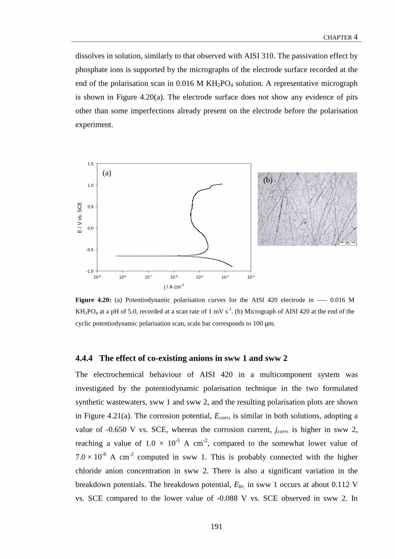
CHAPTER 4

191

dissolves in solution, similarly to that observed with AISI 310. The passivation effect by

phosphate ions is supported by the micrographs of the electrode surface recorded at the

end of the polarisation scan in 0.016 M KH2PO4 solution. A representative micrograph

is shown in Figure 4.20(a). The electrode surface does not show any evidence of pits

other than some imperfections already present on the electrode before the polarisation

experiment.


KH2PO4 at a pH of 5.0, recorded at a scan rate of 1 mV s-1. (b) Micrograph of AISI 420 at the end of the

cyclic potentiodynamic polarisation scan, scale bar corresponds to 100 µm.


The electrochemical behaviour of AISI 420 in a multicomponent system was

investigated by the potentiodynamic polarisation technique in the two formulated

synthetic wastewaters, sww 1 and sww 2, and the resulting polarisation plots are shown

in Figure 4.21(a). The corrosion potential, Ecorr, is similar in both solutions, adopting a

value of -0.650 V vs. SCE, whereas the corrosion current, jcorr, is higher in sww 2,

reaching a value of 1.0 × 10-5 A cm-2, compared to the somewhat lower value of

7.0 × 10-6 A cm-2 computed in sww 1. This is probably connected with the higher

chloride anion concentration in sww 2. There is also a significant variation in the

breakdown potentials. The breakdown potential, Ebr, in sww 1 occurs at about 0.112 V

vs. SCE compared to the lower value of -0.088 V vs. SCE observed in sww 2. In

j / A cm-2

10-9 10-8 10-7 10-6 10-5 10-4 10-3

E /

V v

s. S

CE

-1.0

-0.5

0.0

0.5

1.0

1.5

(a) (b)

CHAPTER 4

192

comparison with the 0.017 M and 0.0170 M NaCl solutions (Section 4.4.1), the

breakdown potential is shifted to more positive values in the sww 1 and sww 2

solutions. The magnitude of the shift is about 100 mV in both cases. This suggests a

competitive adsorption process between the anions present in the solution. A similar

effect was observed with the AISI 310 (Section 4.3.4), where the presence of phosphate

ions, which act as inhibitors and compete with chloride ions for adsorption on the

passive film, gives rise to a shift of the breakdown potential to more noble values. The

electrode surface was examined by light microscopy to reveal the presence of irregular-

shaped pits, as can be seen in Figure 4.21(b) and (c). The pits grown in sww 1 solution

have an average size of 30 to 50 µm (Figure 4.21(b)), whereas in sww 2, as the

concentration of chloride is higher, the pits are wider with an average diameter of 50 to

80 µm (Figure 4.21(c)). Again, the pits developed in the two synthetic wastewaters are

smaller in size compared to that observed in the corresponding NaCl solutions (Section

4.4.1, Figure 4.19) and this result supports the competitive action of the phosphate

inhibiting ions.

Figure 4.21: (a) Potentiodynamic polarisation curves for the AISI 420 electrode in ––– sww 1

and – – – sww 2 solutions, at a pH of 5.0, recorded at a scan rate of 1 mV s-1. Micrographs of AISI 420

electrode at the end of the cyclic potentiodynamic polarisation scan in (b) sww 1, with scale bar at 100 µm

and (c) sww 2, with scale bar at 100 µm.

j / A cm-2

10-9 10-8 10-7 10-6 10-5 10-4 10-3

E /

V v

s. S

CE

-1.0

-0.8

-0.6

-0.4

-0.2

0.0

0.2

(a)

(b)

(c)

CHAPTER 4

193

4.5 Pure aluminium

As outlined in Section 1.4.2.3, aluminium is well known to be resistant against

corrosion in aqueous media because of a uniform, natural oxide film, which is rapidly

formed on the metal surface [26]. However, when aluminium is exposed to aggressive

ions, such as chlorides, pitting attack occurs. The open-circuit potential measured on

aluminium does not correspond to that of the metal, but represents a mixed potential

between the oxide layer, which forms immediately (within 1 ms or even less), and the

metal [26]. Consequently, in an aggressive environment the rest potential of aluminium

is affected by the attack of the ions, causing fluctuations in the measured potential. For

this reason, the potentiodynamic polarisation tests carried out on the as-received

aluminium electrodes did not provide reproducible values of the corrosion potential,

Ecorr, although good reproducibility was obtained with the breakdown potential, Ebr. In

an attempt to increase the reproducibility of the corrosion potential, Ecorr, several

chemical and electrochemical pre-treatments of the electrode were considered. Good

reproducibility was achieved using a slight modification of the method proposed by Van

Gheem et al. [63]. After this pre-treatment the aluminium electrode was polarised in the

anodic direction from -1.400 V vs. SCE, or some other initial potential below the

corrosion potential, up to the breakdown potential, Ebr, at a rate of 10.0, 1.0 or

0.5 mV s-1. The exposed area of the working electrode was 0.031 cm2.


In Figure 4.22(a) potentiodynamic polarisation curves are shown for pure aluminium

recorded in a 0.100 M NaCl solution starting from an initial potential of -1.240 V

vs. SCE. These data were obtained for the pure aluminium electrode without any

chemical or electrochemical pre-treatment of the electrode surface. It is clearly evident

from the presented figure that the corrosion potential, Ecorr, varies considerably, ranging

from -1.153 V to -0.828 V vs. SCE. On the other hand, the breakdown potential, Ebr, is

reproducible and occurs at about -0.730 V vs. SCE. The open-circuit potential was

recorded in 0.100 M NaCl solution for 30 min immediately before the electrode was

polarised and these data are shown in Figure 4.22(b). Potential fluctuations, exceeding

400 mV, are evident. These potential oscillations are related to pitting attack and

indicate the occurrence of a process of activation and repassivation of the natural

CHAPTER 4

194

passive layer [64]. Given that the breakdown potential, Ebr, of pure aluminium in

0.100 M NaCl solution is -0.730 V vs. SCE, Figure 4.22(a), then the fluctuations of the

open-circuit potential occur below the breakdown potential, Ebr. This phenomenon is

attributed to the occurrence of metastable pits on the electrode surface [64]. These

metastable pits initiate and grow for a limited period before repassivation occurs and

this accounts for the increase and rapid decrease in the open-circuit potential [65]. The

reproducibility of the potentiodynamic polarisation curves is affected by this instability

of the natural passive film due to the growth and the repassivation of the metastable pits.

Figure 4.22: (a) Potentiodynamic polarisation curves recorded for the pure aluminium in 0.100 M NaCl

at a pH of 5.0, at a scan rate of 0.5 mV s-1 and (b) the corresponding open-circuit potential plotted as a

function of time without any pre-treatment of the electrode surface.

In order to promote a more stable passive film and, consequently, obtain reproducible

experiments, several chemical and electrochemical pre-treatments were considered.

Good reproducibility was achieved by modifying a method used by Van Gheem et al.

[63] to obtain a reproducible surface composition. Before the polarisation tests, the

specimen was immersed in 0.1 M NaOH solution at 70 °C for 60 s and subsequently in

1.0 M HNO3 solution at 70 °C for 90 s. The data recorded following this pre-treatment

are shown in Figure 4.23(a) and (b), where four potentiodynamic polarisation curves

and the corresponding open-circuit potentials are shown. In the polarisation curves

shown in Figure 4.23(a) the average corrosion potential of the four experiments is -

1.344 ± 0.029 V vs. SCE and the average breakdown potential occurs at -0.803 ±

0.016 V vs. SCE. These results show an extremely high reproducibility in comparison

with the data displayed in Figure 4.22. The average value of -0.800 V vs. SCE for the

j / A cm-2

10-10 10-9 10-8 10-7 10-6 10-5 10-4 10-3 10-2

E /

V v

s. S

CE

-1.4

-1.2

-1.0

-0.8

-0.6

-0.4

-0.2

Time / s

0 200 400 600 800 1000 1200 1400 1600 1800 2000

E /

V v

s. S

CE

-1.1

-1.0

-0.9

-0.8

-0.7

-0.6

-0.5

(a) (b)

CHAPTER 4

195

breakdown potential is slightly lower than the values of -0.640 V vs. SCE reported by

Böhni and Uhlig [66] for aluminium in 0.10 M NaCl. Also Broli and Holtan [67],

McCaffrey [68], and Pyun and co-workers [69, 70] reported higher breakdown values.

However, these studies used either a harsh surface pre-treatment or etching in alkaline

solutions or a multi-step of immersion treatments. Using such conditions a relatively

thicker surface oxide film may be developed and it might account for the higher

breakdown potential recorded in these studies. Furthermore, the polarisation scans

reported in Figure 4.23(a) were obtained in aerated NaCl solutions, whereas some of the

cited studies are performed in deaerated solutions. It has been reported that in the

absence of oxygen the breakdown potential of aluminium is shifted towards more

positive values [27, 63]. For example, Pyun et al. [70] reported a breakdown potential

of -0.720 V vs. SCE in aerated conditions, while Böhni and Uhlig [66] found that the

pitting starts at -0.640 V vs. SCE in the absence of oxygen.

The open-circuit potential of the aluminium electrode after the chemical pre-treatment

for the four experiments is presented in Figure 4.23(b). Although in the initial stage the

open-circuit potential is significantly different for the four experiments, it shows a sharp

increase followed by a gradual decline in all the experiments and then converges

towards the same potential value of -1.30 V vs. SCE. Since this chemical pre-treatment

of the electrode produced very reproducible results, it was then used to study the effect

of the chloride concentration on the electrochemical behaviour of the pure aluminium

electrode.

Figure 4.23: (a) Potentiodynamic polarisation curves recorded at a scan rate of 0.5 mV s-1 for the pure

aluminium in 0.100 M NaCl at a pH of 5.0 and (b) the corresponding open-circuit potential plots for pure

aluminium electrode in 0.100 M NaCl solution after immersing the electrode in 0.1 M NaOH solution for

60 s at 70 °C and then in 1.0 M HNO3 solution for 90 s at 70 °C.

j / A cm-2

10-10 10-9 10-8 10-7 10-6 10-5 10-4 10-3 10-2

E /

V v

s. S

CE

-1.8

-1.6

-1.4

-1.2

-1.0

-0.8

-0.6

-0.4

-0.2

Time / s

0 500 1000 1500 2000 2500

E /

V v

s. S

CE

-1.34

-1.32

-1.30

-1.28

-1.26

-1.24

-1.22

-1.20

-1.18

-1.16

-1.14

(a) (b)

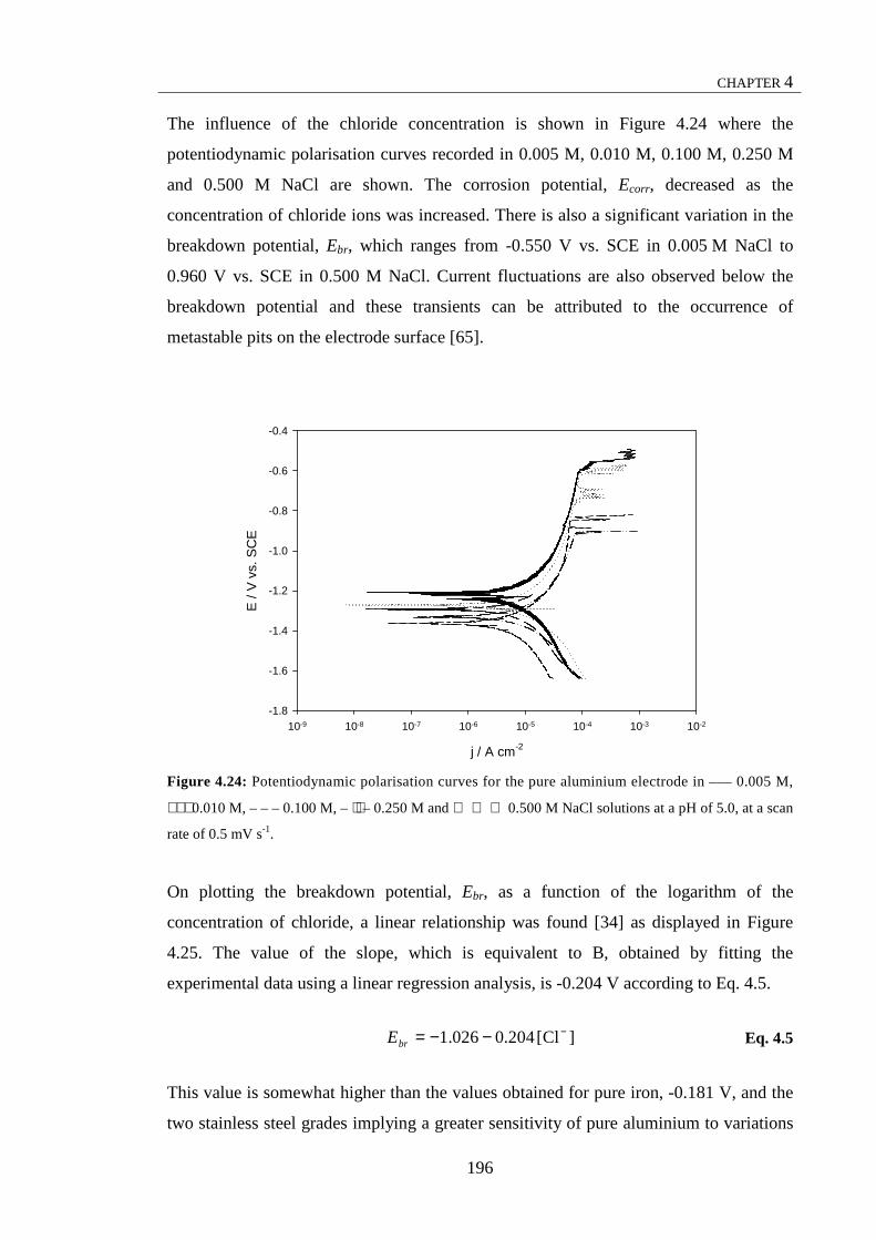
CHAPTER 4

196

The influence of the chloride concentration is shown in Figure 4.24 where the

potentiodynamic polarisation curves recorded in 0.005 M, 0.010 M, 0.100 M, 0.250 M

and 0.500 M NaCl are shown. The corrosion potential, Ecorr, decreased as the

concentration of chloride ions was increased. There is also a significant variation in the

breakdown potential, Ebr, which ranges from -0.550 V vs. SCE in 0.005 M NaCl to

0.960 V vs. SCE in 0.500 M NaCl. Current fluctuations are also observed below the

breakdown potential and these transients can be attributed to the occurrence of

metastable pits on the electrode surface [65].

Figure 4.24: Potentiodynamic polarisation curves for the pure aluminium electrode in ––– 0.005 M,

⋅ ⋅ ⋅ 0.010 M, – – – 0.100 M, – ⋅⋅ – 0.250 M and 0.500 M NaCl solutions at a pH of 5.0, at a scan

rate of 0.5 mV s-1.

On plotting the breakdown potential, Ebr, as a function of the logarithm of the

concentration of chloride, a linear relationship was found [34] as displayed in Figure

4.25. The value of the slope, which is equivalent to B, obtained by fitting the

experimental data using a linear regression analysis, is -0.204 V according to Eq. 4.5.

]Cl[204.0026.1 −−−= Ebr Eq. 4.5

This value is somewhat higher than the values obtained for pure iron, -0.181 V, and the

two stainless steel grades implying a greater sensitivity of pure aluminium to variations

j / A cm-2

10-9 10-8 10-7 10-6 10-5 10-4 10-3 10-2

E /

V v

s. S

CE

-1.8

-1.6

-1.4

-1.2

-1.0

-0.8

-0.6

-0.4

CHAPTER 4

197

in the chloride concentration. In the review of the breakdown of passivity by Galvele

[34], values of B are reported for pure aluminium and these range from -0.073 V

to -0.139 V vs. SCE. However, as outlined previously, the pre-treatment of the electrode

surface may have a significant impact on the thickness and protective properties of the

passive film and this will influence the magnitude of B. The relatively mild pre-

treatment, used in this study, was chosen in order to avoid any significant modifications

of the passive film of aluminium. In the electrocoagulation tests the aluminium

electrode was not subjected to any of these pre-treatments.

NaCl

/ M

Ebr

/ V vs. SCE

0.005 -0.557

0.010 -0.620

0.100 -0.829

0.250 -0.906

0.500 -0.961

Figure 4.25: Breakdown potential, Ebr, of the pure aluminium as a function of the logarithm of the

chloride concentration. The breakdown potential, Ebr, was obtained from potentiodynamic polarisation

tests recorded at a rate of 0.5 mV s-1. The experimental points were fitted by a linear regression analysis

to Ebr = A + B log [Cl-], A = −1.026 ± 0.004 V, B = −0.204 ± 0.003 V, R2 = 0.999.


It has been reported that phosphate ions act as inhibitors on the pit initiation of

aluminium in neutral chloride solutions by forming insoluble precipitates [71, 72].

Shalaby et al. [73] investigated the corrosion behaviour of aluminium in 0.01 M NaCl

containing different anions, including phosphates. They found that the phosphate ions

play a dual role. At low concentrations they modify the rate of nucleation and growth of

the passive oxide layer and at higher concentrations they become incorporated into this

[Cl-] / M

0.001 0.01 0.1 1

Ebr

/ V

vs.

SC

E

-1.0

-0.9

-0.8

-0.7

-0.6

-0.5

CHAPTER 4

198

layer and hence increase the protective nature of the film. As discussed earlier with the

iron and stainless steels (Sections 4.2.3, 4.3.3, and 4.4.3), phosphate ions act as

inhibitors towards the corrosion of aluminium. The potentiodynamic polarisation tests

carried out on the pure aluminium electrode in 6.5 × 10-3 M KH2PO4 solutions with and

without 5.0 × 10-4 M NaCl are shown in Figure 4.26 and confirm the inhibiting action of

the phosphates. In these experiments, the aluminium electrode was polarised in the

anodic direction from an initial potential of -1.000 V vs. SCE up to a final potential of

3.500 V vs. SCE. In the 6.5 × 10-3 M KH2PO4 solution the corrosion potential, Ecorr, of

pure aluminium is -0.869 V vs. SCE and the corresponding corrosion current, jcorr, is

1.4 × 10-7 A cm-2. The electrode exhibits a wide passive region that extends from

about -0.150 V vs. SCE up to 3.500 V vs. SCE. On addition of 5.0 × 10-4 M NaCl to the

phosphate-containing solution, there is little variation in the corrosion potential, Ecorr, or

the corrosion current, jcorr, however the breakdown potential, Ebr, occurs at 0.276 V

vs. SCE. At higher applied potentials the current reaches a limiting value which

corresponds to actively propagating pits that fail to repassivate at these high applied

potentials.

Figure 4.26: Potentiodynamic polarisation curves recorded for the pure aluminium electrode at a scan

rate of 10 mV s-1 in 6.5 × 10-3 M KH2PO4 solutions with – – – 5.0 × 10-4 M NaCl and ––– without NaCl,

at a pH of 5.0.

j / A cm-2

10-10 10-9 10-8 10-7 10-6 10-5 10-4 10-3 10-2 10-1

E /

V v

s. S

CE

-2

-1

0

1

2

3

4

CHAPTER 4

199

The presence of chloride anions, even in small concentrations, certainly represents an

advantage in terms of the energy needed to cause the breakdown of the passive film on

pure aluminium. However, as outlined earlier, the concentration of chloride ions in real

wastewater samples can drop to very low levels. Moreover, it is crucial to ascertain the

grade of damage caused by pitting corrosion to avoid an uneven consumption of the

electrodes and operational issues of the treatment plant.

4.6 Al-2Mg alloy

Pure aluminium exhibits good corrosion resistance due to the presence of a natural

passive oxide layer. Generally, the addition of alloying elements decreases the corrosion

resistance and, at the same time, modifies the solution-potential or corrosion potential of

the metal [27]. As shown in Section 1.4.2.4, Fig. 1.13, in magnesium-containing alloys

(5xxx series), the corrosion potential decreases slightly with the increasing content of

magnesium [26, 27] and this feature can be beneficial in electrocoagulation from the

perspective of the energy consumption. The 5xxx series also possesses an excellent

resistance to pitting corrosion [31]. For this reason, an alloy belonging to this series, the

EN-AW 5251 (Section 1.4.2.4), with 2% of magnesium, was selected for study.

The potentiodynamic polarisation tests were carried out by polarising the Al-2Mg

electrodes with a geometric surface area of 0.58 cm2 in the anodic direction,

from -1.000 V vs. SCE up to the breakdown potential, Ebr, at a scan rate of 1 mV s-1. In

the cases where the current density increased sharply above the corrosion potential,

Ecorr, the scan was stopped at 0.01 mA cm-2 and the potential corresponding to this

value of current density was recorded as the breakdown potential, Ebr. Cyclic

potentiodynamic polarisation curves were recorded at 1 mV s-1 and again the Al-2Mg

electrode was polarised in the anodic direction, but the scan was reversed when the

current density reached a value of 1 mA cm-2.


The potentiodynamic polarisations curves recorded for Al-2Mg electrode in 0.017 M

and 0.170 M NaCl solutions are compared in Figure 4.27(a). It is clear that these data

are very different to those obtained with pure aluminium and highlight the role of

CHAPTER 4

200

magnesium in modifying the properties of the passive film. The corrosion potential,

Ecorr, in 0.170 M NaCl is -0.664 V vs. SCE, compared to a value of -0.554 V vs. SCE in

0.017 M NaCl. However, there is little variation in the corrosion currents, jcorr, which

were computed at 1.20 × 10-6 A cm-2. Above the corrosion potential the current density

increases sharply. Consequently, the electrode does not exhibit any passive region

regardless of the concentration of chloride ions and in electrocoagulation applications

this feature would be advantageous for the energy supply to the system. The breakdown

potential, Ebr, was taken at a reasonably high current density of 0.01 mA cm-2, and in

0.017 M NaCl it was found at -0.530 V vs. SCE while in 0.170 M NaCl it is observed at

-0.636 V vs. SCE. Similar behaviour was recorded by other authors with Al-2.5Mg in

3.5 wt. % NaCl [74] and Al-3Mg in 3 wt. % NaCl [75]. In both studies the corrosion

potential coincided with the breakdown potential and there was no evidence of any

passive region.

In Figure 4.27(b) the breakdown potential, Ebr, of the Al-2Mg electrode is plotted as a

function of the logarithm of the chloride concentration to give a linear relationship. In

0.10 M NaCl an average breakdown potential of -0.590 V vs. SCE was found, which is

in good agreement with the value of -0.640 V vs. SCE reported by Böhni and Uhlig [66]

for an aluminium alloy containing 2.4% of magnesium polarised in 0.1 M NaCl

solution. As displayed in Figure 4.27(b), a linear regression analysis of the

experimental points provided a value of B as -0.108 V.

]Cl[108.0712.0 −−−= Ebr Eq. 4.6

By comparing this to the value obtained with pure aluminium, -0.204 V, in Section

4.5.1, Eq. 4.5, it is evident that the breakdown potential of the Al-2Mg electrode is less

affected by the presence of chloride ions in solution.

CHAPTER 4

201

Figure 4.27: (a) Potentiodynamic polarisation curves for the Al-2Mg electrode in ––– 0.017 M

and – – – 0.170 M NaCl solutions at a pH of 5.0, recorded at a scan rate of 1 mV s-1. (b) Breakdown

potential, Ebr, of the Al-2Mg electrode as a function of the logarithm of the chloride concentration. The

breakdown potential, Ebr, was obtained from potentiodynamic polarisation tests at a scan rate of 1 mV s-1.

Each experiment was performed in triplicate (n = 3). The experimental points were fitted by a linear

regression analysis to Ebr = A + B log [Cl-], A = −0.712 ± 0.013 V, B = −0.108 ± 0.012 V, R2 = 0.976.

The cyclic potentiodynamic polarisation curves recorded for the Al-2Mg alloy in 0.017 M

and 0.170 M NaCl solutions are shown in Figure 4.28(a). As can be seen from the

figure, both cyclic polarisation curves exhibit hysteresis. The size of the hysteresis loop

is comparable in both 0.017 M and 0.170 M NaCl solutions, implying that the extent of

the damage caused by pitting is not significantly different. Post-scan examinations of

the specimens using light microscopy confirmed that the dimensions of the pits are

similar regardless of the concentration of the chloride ions. In Figure 4.28(b) and (c) the

micrographs recorded for the Al-2Mg electrode surface after the cyclic polarisation scan

in 0.170 M NaCl are presented and these depict the nucleation of several, small pits.

The diameter of the cluster, which comprises several pits, was calculated as 110 µm.

Other small sites of attack are also visible in Figure 4.28(c), and these are probably at

an earlier stage of nucleation or development. The small number of active sites appears

to depend on the Mg content. Indeed, in studying the susceptibility to the

electrochemical corrosion of Al-Mg alloys with low Mg content, Brillas et al. [76]

concluded that the pitting attack was greater when the Mg content was increased. The

active sites were attributed to the solubility of magnesium. Although magnesium is

highly soluble in aluminium at high temperatures, it does not exceed 1% at room

temperature. Therefore, it precipitates as soon as the temperature is decreased. It has

been reported that magnesium precipitation starts at the grain boundaries as Al3Mg2 or

j / A cm-2

10-9 10-8 10-7 10-6 10-5 10-4

E /

V v

s. S

CE

-1.0

-0.9

-0.8

-0.7

-0.6

-0.5

[Cl-] / M

0.01 0.1 1

Ebr

/ V

vs.

SC

E

-0.70

-0.65

-0.60

-0.55

-0.50

-0.45

NaCl

M

Ebr

V vs. SCE

0.017 -0.52 ± 0.01

0.100 -0.59 ± 0.04

0.170 -0.63 ± 0.01

0.300 -0.66 ± 0.02

(a) (b)

CHAPTER 4

202

Al 8Mg5, which is commonly called the β-phase [27]. As reported in Section 1.4.2.4,

these intermetallics are anodic and therefore they represent a suitable site for localised

attack in the form of intergranular or stress corrosion, if the precipitation is continuous

at the grain boundaries. However, it has been reported that Al-Mg alloys containing less

than 3% in magnesium are resistant to these types of localised corrosion [11]. The

Al-Mg alloy used in this study contains 2% of Mg and as shown in Figure 4.28(b) and

(c), there is no presence of intergranular or stress corrosion. However, it is likely that

the peculiar form of pitting, a few sites made up of several pits, which was observed for

the Al-2Mg alloy in NaCl solutions, is due to the preferential attack at the intermetallic

compounds present on the electrode surface.

It is clear that the presence of a small concentration of chloride activates the surface of

the Al-2Mg electrode, giving rise to dissolution. The electrode does not exhibit any

passive region. However, the corrosion of the Al-2Mg alloy is predominantly in the

form of clusters of small pits, distributed across the surface.

Figure 4.28: (a) Cyclic potentiodynamic polarisation curves for the Al-2Mg electrode in ––– 0.017 M

and – – – 0.170 M NaCl solutions at a pH of 5.0, at a scan rate of 1 mV s-1; micrographs of the Al-2Mg

electrode at the end of the cyclic potentiodynamic polarisation scan in 0.170 M NaCl solution (b) scale bar


j / A cm-2

10-9 10-8 10-7 10-6 10-5 10-4 10-3 10-2

E /

V v

s. S

CE

-1.1

-1.0

-0.9

-0.8

-0.7

-0.6

-0.5

-0.4

-0.3

(a)

(b)

(c)

CHAPTER 4

203


The potentiodynamic polarisation curves of Al-2Mg recorded in a 0.017 M NaCl and

8.1 × 10-4 M Na2SO4 solution and in 0.017 M NaCl are compared in Figure 4.29.

Although sulfate is known to have an inhibiting activity towards aluminium [27, 66],

there are no significant differences in the shape of the polarisation curves recorded in

the absence and in the presence of sulfate ions. The addition of 8.1 × 10-4 M Na2SO4 to

the 0.017 M NaCl solution gave rise to a 50 mV increase in the corrosion potential,

Ecorr, and a slight decrease in the corrosion current, from 1.09 × 10-6 A cm-2 to

7.13 × 10-7 A cm-2 in 0.017 M NaCl, and in 0.017 M NaCl and 8.1 × 10-4 M Na2SO4,

respectively. Above the corrosion potential, Ecorr, which occurs at -0.508 V vs. SCE,

there is a large increase in current density without any passivity region. Similar behaviour

was recorded in 0.017 M NaCl (Section 4.6.1, Figure 4.27). The breakdown potential,

Ebr, was determined at a current density of 0.01 mA cm-2, and was found at -0.464 V vs.

SCE. This corresponds to a 70 mV increase compared with the data recorded in

0.017 M NaCl, where the breakdown potential was -0.530 V vs. SCE. This is in good

agreement with the extensive literature existing on the effect of sulfate ions on the

pitting corrosion of pure aluminium [69-72, 77-82]. The earlier studies showed that in

concentrated NaCl solutions the breakdown potential was shifted towards noble values

by adding sulfate ions at concentrations above 0.3 M, and that sulfate retarded pit

initiation due to its competitive adsorption with chloride [77, 78]. Later, Pyun and co-

workers [69, 70, 81, 82] deduced that sulfate ion addition retards the incorporation of

chloride ions into the oxide film on pure aluminium, impeding pit initiation. However,

they also reported that sulfate ions enhance the growth of pre-existing pits. These

findings are consistent with the results obtained in Figure 4.29. Here, with the addition

of sulfate to NaCl solution the breakdown potential, Ebr, is shifted in the anodic

direction by about 70 mV, thus retarding the initiation of pitting attack. This small shift

is compatible with the low concentration of sulfate used, 8.1 × 10-4 M Na2SO4. Böhni

and Uhlig [66] have reported a similarity in the behaviour of inhibiting anions for

aluminium and 18-8 stainless steel. It is reasonable to assume that in the case of the

Al-2Mg alloy the ratio of the SO42-/Cl- concentrations has an important role in defining

the extent of the sulfate effect (Sections 4.3.2 and 4.4.2).

CHAPTER 4

204

Figure 4.29: Potentiodynamic polarisation curves for the Al-2Mg electrode in ––– 0.017 M NaCl and

8.1 × 10-4 M Na2SO4 solution at a pH of 5.0 and – – – 0.017 M NaCl solution at a pH of 5.0, recorded at a

scan rate of 1 mV s-1.

Pitting corrosion was confirmed by cyclic potentiodynamic polarisation tests carried out

on the Al-2Mg electrode in 0.017 M NaCl and 8.1 × 10-4 M Na2SO4. A typical plot is

shown in Figure 4.30(a) and it is clear that a hysteresis loop exists. Furthermore, as

displayed in Figure 4.30(b) and (c), at the end of the scan the electrode surface shows

the nucleation of several pits, similar to that found on the surface of the Al-2Mg

electrode cycled in NaCl solutions (Section 4.6.1, Figure 4.28). The density of pits is

also similar. However, in the presence of sulfates the size of the pit clusters are slightly

smaller, about 80 µm, and the shape of some of the clusters are different. Indeed, as

shown in Figure 4.30(b) and (c), circular-like clusters and irregular shaped clusters are

present.

Clearly the sulfate ions have an important role in the pitting corrosion of the Al-2Mg

electrode. At low concentrations, they impede the initiation of pits and introduce

important changes in the morphology of the pit clusters. However, in the presence of

chloride anions, the sulfate ions cannot prevent pitting corrosion of the Al-2Mg alloy.

j / A cm-2

10-10 10-9 10-8 10-7 10-6 10-5 10-4

E /

V v

s. S

CE

-1.0

-0.9

-0.8

-0.7

-0.6

-0.5

-0.4

CHAPTER 4

205

Figure 4.30: (a) Cyclic potentiodynamic polarisation curve for the Al-2Mg electrode in ––– 0.017 M

NaCl and 8.1 × 10-4 M Na2SO4 solution at a pH of 5.0, at a scan rate of 1 mV s-1; micrograph of the Al-

2Mg electrode at the end of the cyclic potentiodynamic polarisation scan (b) scale bar corresponding to

200 µm and (c) scale bar corresponding to 100 µm.


Phosphates are well known as inhibitors in the corrosion protection of aluminium in

water [27]. For this reason, they are used in chemical conversion treatments to protect

aluminium against corrosion. As there are no reports on the influence of phosphate

anions on the electrochemical properties of Al-Mg alloys, polarisation curves were

recorded in a 0.016 M KH2PO4 solution. A representative potentiodynamic polarisation

curve for Al-2Mg electrode is shown in Figure 4.31(a) and it is clear that the

polarisation behaviour is very different to that observed in the chloride-containing

solutions. Above the corrosion potential, Ecorr, which occurs at -0.484 V vs. SCE, the

electrode is passivated and the passive region spans about 600 mV. As can be seen from

the figure, the breakdown potential, Ebr, is 0.103 V vs. SCE, significantly higher than

that observed in the chloride-containing solutions. However, the onset of metastable pits

is present well below this value, as evident from the fluctuations of the current density.

After the breakdown potential, Ebr, the current density increases rapidly suggesting a

fast growth of pits on the electrode surface. The cyclic polarisation scan, shown in

Figure 4.31(b), reveals the presence of a large hysteresis which is consistent with pitting

corrosion. Indeed, this was confirmed upon examining the specimen using light

j / A cm-2

10-10 10-9 10-8 10-7 10-6 10-5 10-4 10-3 10-2

E /

V v

s. S

CE

-0.9

-0.8

-0.7

-0.6

-0.5

-0.4

-0.3

(a)

(b)

(c)

CHAPTER 4

206

microscopy. The inset in Figure 4.31(b) provides a representative micrograph obtained

at the end of the scan. The pits developed on the electrode surface are very different

from those grown in chloride solutions (Section 4.6.1, Figure 4.30). The pits are not

gathered in clusters, have an average diameter of 60 µm, and have a irregular shape.

Although the phosphate ions act as inhibitors towards the Al-2Mg alloy giving a wide

passive region, the alloy corrodes at higher potentials and exhibits pitting corrosion. As

discussed in Section 4.1, the presence of a region of passivity represents a potential

disadvantage for the energy consumption in the electrocoagulation process to remove

phosphates.


for the Al-2Mg electrode in ––– 0.016 M KH2PO4 solution at a pH of 5.0 recorded at a scan rate of

1 mV s-1. The inset shows a micrograph of the Al-2Mg electrode at the end of the cyclic potentiodynamic

polarisation scan, scale bar corresponds to 200 µm.


The two synthetic wastewaters, sww 1 and sww 2, were formulated to investigate the

dissolution behaviour of the electrode in a multicomponent environment in the presence

of several co-existing ions. Again, potentiodynamic polarisation curves and cyclic

polarisation curves were recorded in sww 1 and sww 2. In Figure 4.32 the

potentiodynamic polarisation curves recorded for the Al-2Mg electrode in sww 1 and

sww 2 are compared. The cathodic branches are similar and above the corrosion

potential, Ecorr, the current density shows a sharp increase. This behaviour is similar to

j / A cm-2

10-9 10-8 10-7 10-6 10-5 10-4

E /

V v

s. S

CE

-1.0

-0.8

-0.6

-0.4

-0.2

0.0

0.2

0.4

j / A cm-2

10-10 10-9 10-8 10-7 10-6 10-5 10-4 10-3 10-2

E /

V v

s. S

CE

-1.0

-0.8

-0.6

-0.4

-0.2

0.0

0.2

0.4

0.6

0.8

(a) (b)

CHAPTER 4

207

that observed for the Al-2Mg alloy in NaCl solutions (Section 4.6.1) and indicates that,

above the corrosion potential, the electrode exhibits pitting corrosion. It is also evident

from the figure that the concentration of chloride ions, which varies from 0.170 M in

sww 2 to 0.017 M in sww 1, has a significant effect on the corrosion potential, Ecorr, and

the breakdown potential, Ebr. The corrosion potential, Ecorr, is shifted some 80 mV in

the cathodic direction in the sww 2, (from -0.598 V vs. SCE in sww 1 to -0.670 V vs.

SCE in sww 2). As can be observed in Section 4.6.1, Figure 4.27, a comparable shift of

100 mV was observed between the corrosion potentials recorded in 0.017 M and 0.170 M

NaCl solutions. The breakdown potentials, Ebr, were taken at 0.01 mA cm-2 and were

calculated as -0.587 V and -0.661 V vs. SCE in sww 1 and sww 2 solutions,

respectively. As shown in Section 4.6.1, Figure 4.27 a shift of about 100 mV in the

breakdown potential was observed with the 0.017 M and 0.170 M NaCl solutions. In the

two synthetic wastewaters the magnitude of the shift is somewhat smaller; in the sww 2

solution the breakdown potential, Ebr, is about 70 mV lower than in the sww 1 solution.

This smaller shift is likely due to the presence of the sulfate and phosphate anions,

which possess an inhibiting effect on the corrosion of the Al-2Mg electrode, as shown

in Sections 4.6.2 and 4.6.3.

Figure 4.32: Potentiodynamic polarisation curves for the Al-2Mg electrode in ––– sww 1 and – – – sww 2

solutions at a pH of 5.0 recorded at a scan rate of 1 mV s-1.

j / A cm-2

10-9 10-8 10-7 10-6 10-5 10-4

E /

V v

s. S

CE

-0.95

-0.90

-0.85

-0.80

-0.75

-0.70

-0.65

-0.60

-0.55

CHAPTER 4

208

The cyclic potentiodynamic polarisation curves recorded for Al-2Mg in sww 1 and sww 2

solutions are shown in Figure 4.33(a). In both scans the forward and the reverse traces

are different, generating hysteresis. The hysteresis loop is somewhat smaller in the

sww 2 solution. However, there was no significant difference in the distribution and

morphology of pits between the sww 1 and sww 2 solutions. The micrographs recorded

in the sww 2 solution are presented in Figure 4.33(b) and (c) and these depict the

electrode surface at the end of the cyclic scan. Pits with different diameters are visible

on the electrode surface and their dimensions range from 20 to 80 µm. This morphology

is very different to that observed in the chloride-containing solutions where circular-

shaped clusters of pits were observed (Section 4.6.1, Figure 4.28(b)). It is obvious that a

different process leads to pitting attack in the presence of co-existing ions. The effects

of the aggressive chloride actions may be mitigated in the presence of phosphate ions,

which exert an inhibiting role, as discussed in Section 4.6.3. In addition, both synthetic

wastewaters contain sulfate, 8.1 × 10-4 M. Since it was shown in Section 4.6.2 that

sulfate ions retard the growth of pits on Al-2Mg electrode, it seems plausible that their

presence in the sww 1 and sww 2 solutions may also have a role in the pitting attack,

giving rise to pits with different sizes and distribution.

Figure 4.33: (a) Cyclic potentiodynamic polarisation curves for the Al-2Mg electrode in ––– sww 1

and – – – sww 2 solutions at a pH of 5.0 recorded at a scan rate of 1 mV s-1; micrographs of the Al-2Mg

electrode at the end of the cyclic potentiodynamic polarisation scan in sww 2 solution with (b) scale bar


j / A cm-2

10-9 10-8 10-7 10-6 10-5 10-4 10-3 10-2

E /

V v

s. S

CE

-1.0

-0.9

-0.8

-0.7

-0.6

-0.5

-0.4

(a)

(b)

(c)

CHAPTER 4

209

In a multicomponent system, such as sww 1 and sww 2, which contains both activators

and inhibitors, the corrosion behaviour of Al-2Mg is affected by the presence of both

categories of anions. However, the presence of chloride ions, even in small

concentration, determines the electrochemical behaviour of the alloy, since the

polarisation curves obtained in the two synthetic wastewaters are similar to that

obtained in chloride solutions. Chloride has a positive influence on the dissolution of

the alloy which does not exhibit any passive region. The inhibiting phosphate and

sulfate anions exert some influence with a shift of the breakdown potentials, Ebr,

towards more noble values. However, more significant differences in the size, shape and

distribution of the pits are evident in the presence of the sulfate and phosphate anions.

4.7 Al-Zn-In alloy

Binary and ternary aluminium alloys have been recently investigated as materials for Al

batteries or cathodic protection systems [83-88]. Although pure aluminium is a very

attractive metal for its mechanical properties, the spontaneously formed oxide film on

its surface leads to a significant loss of available energy and does not allow the active

dissolution of the electrode as it is required in industrial applications. Numerous

investigations have been reported on the addition of alloying components, such as Zn,

In, Hg, Sn, Ga, Mg and Ti, to aluminium and these alloys give an active surface that

corrodes in a nearly uniform manner [28, 29, 83, 89-96]. Also in electrocoagulation the

passivation of the electrode surface has been identified as a primary disadvantage on

employing aluminium as the anode material [5, 6, 8, 25]. However, only a few studies

have been carried out on the electrocoagulation performances of Al-alloys [12, 97-100]

whereas the majority are focused on the use of the pure aluminium. For this reason, an

Al-Zn-In alloy was used as the anode material for electrocoagulation applications. This

alloy contained 3% zinc and 0.02% indium. The potentiodynamic polarisation tests

were carried out by polarising the Al-Zn-In electrode with an area of 0.38 cm2 in the

anodic direction, from -1.400 V vs. SCE up to the breakdown potential, Ebr, or up to a

current density value of 0.01 mA cm-2. A scan rate of 1 mV s-1 was employed. The

cyclic potentiodynamic polarisation curves were performed in a similar manner, but the

scan was reversed when the current density reached a value of 1 mA cm-2.

CHAPTER 4

210


The potentiodynamic polarisation curves of Al-3Zn-0.02In in 0.017 M and 0.170 M

NaCl solutions are shown in Figure 4.34(a). The corrosion potentials, Ecorr, are -0.912

V vs. SCE in 0.017 M NaCl and -1.07 V vs. SCE in 0.170 M NaCl. The shape of the

anodic curve is very similar in both solutions and presents an active dissolution without

any passivity with the breakdown potential, Ebr, occurring at -0.879 V vs. SCE

and -1.05 V vs. SCE in 0.017 M and 0.170 M NaCl solutions, respectively. It is clear

that the breakdown potentials, Ebr, have values very similar to the corrosion potentials,

Ecorr. Moreover, in 0.170 M NaCl the corrosion potential, Ecorr, and the breakdown

potential, Ebr, are shifted about 170 mV towards more negative values. The same

behaviour was found with the Al-2Mg electrode in NaCl solutions (Section 4.6.1),

although more positive values of both the corrosion potential and breakdown potential

were observed. These data are in good agreement with the results presented by Muňoz

et al. [29], where active behaviour above the corrosion potential was observed with

Al-5Zn-0.02In and Al-4Zn-0.015In-0.1Si in deaerated 0.5 M NaCl solutions. Breslin et

al. [28] have also studied the electrochemical behaviour of an Al-3.5Zn-0.02In alloy. In

this case a passive region, although with higher passive currents, was evident before the

breakdown of the film. However, the electrode was pre-polarised at -1.800 V vs. SCE

for 1 min generating an oxide-free surface.

The influence of the chloride concentration on the breakdown potential, Ebr, is

illustrated in Figure 4.34(b), where a linear relationship is obtained between the

breakdown potential, Ebr, and the logarithm of the concentration of chloride ions. The

value of the slope of the regression equation, which corresponds to B, is -0.123 V, as

shown in Eq. 4.7. This value is smaller than that obtained with pure aluminium, -0.204 V

(Section 4.5.1, Eq. 4.5), but higher than that calculated with the Al-2Mg alloy, -0.108 V

(Section 4.6.1, Eq. 4.6).

]Cl[123.0115.1 −−−= Ebr Eq. 4.7

CHAPTER 4

211

Figure 4.34: (a) Potentiodynamic polarisation curves for Al-3Zn-0.02In electrode in ––– 0.017 M

and – – – 0.170 M NaCl solutions at a pH of 5.0 recorded at a scan rate of 1 mV s-1. (b) Breakdown

potential, Ebr, of the Al-3Zn-0.02In electrode as a function of the logarithm of the chloride concentration.

The breakdown potential, Ebr, was obtained from potentiodynamic polarisation tests. Each experiment

was performed in triplicate (n = 3). The experimental points were fitted by a linear regression analysis to

E = A + B log [Cl-], A = −1.115 ± 0.018 V, B = −0.123 ± 0.016 V, R2 = 0.966.

Figure 4.35 provides a comparison of the data fitted by linear regression analysis for

pure aluminium (B = -0.204 V, Section 4.5.1, Eq. 4.5), Al-2Mg alloy (B = -0.108 V,

Section 4.6.1, Eq. 4.6), and Al-3Zn-0.02In alloy (B = -0.123 V, Section 4.7.1, Eq. 4.7).

As already outlined in the introduction (Section 4.1), an anode material with a low

sensitivity to the chloride concentration is preferred in the electrocoagulation of

wastewaters, since in treatment facilities the levels of chloride ions may vary

considerably and occasionally drop to very low concentrations. According to Figure

4.35, the Al-2Mg electrode is the less susceptible material to the chloride concentration,

since the B value is small, at -0.108 V. However, the Al-2Mg electrode also shows

resistance to corrosion, as highlighted from the relatively high values of the breakdown

potential, Ebr, in Figure 4.35. Although the values of the breakdown potentials for pure

aluminium are lower than the Al-2Mg electrode, pure aluminium is very sensitive to the

concentration of chloride ions, as shown in Figure 4.35. The value of B is high at -0.204 V.

The Al-3Zn-0.02In electrode shows a good compromise between the sensitivity to

chloride ions, with a B value of -0.123 V, and the values of the breakdown potential.

j / A cm-2

10-10 10-9 10-8 10-7 10-6 10-5 10-4

E /

V v

s. S

CE

-1.5

-1.4

-1.3

-1.2

-1.1

-1.0

-0.9

-0.8

[Cl-] / M

0.01 0.1 1

Ebr

/ V

vs.

SC

E

-1.15

-1.10

-1.05

-1.00

-0.95

-0.90

-0.85

NaCl

M

Ebr

V vs. SCE

0.017 -0.90 ± 0.03

0.100 -0.97 ± 0.03

0.170 -1.02 ± 0.03

0.300 -1.06 ± 0.04

(a) (b)

CHAPTER 4

212

Figure 4.35: Breakdown potentials, Ebr, of Al-2Mg, pure aluminium, and Al-3Zn-0.02In

electrodes plotted as a function of the logarithm of the chloride concentration.

The cyclic potentiodynamic polarisation curves recorded for the Al-3Zn-0.02In in 0.017 M

and 0.170 M NaCl solutions are shown in Figure 4.36(a). Hysteresis is evident in both

plots. However, the area of the hysteresis loop is smaller in 0.017 M NaCl. The

morphology of the electrodes recorded following the cyclic polarisation measurements

are presented in Figure 4.36(b) and (c), and it is clear that localised sites of dissolution

are uniformly dispersed over the entire surface of the electrode. It was not possible to

establish an average diameter of the pits as they tend to grow and propagate along the

grain boundaries of the alloy with a dendritic shape. The density of the pits is

considerably higher in comparison with the number of pits developed on the surface of

Al-2Mg in NaCl solutions (Figure 4.28). Similar findings were found by Muňoz et al.

[29], who observed that the attack of Al-5Zn-0.02In alloy in 0.5 M NaCl solution

initiates at the grain boundaries and propagates into the bulk of the grain through

interdendritic zones. The sites of initiation and growth of pits are preferentially located

at areas enriched in In and Zn during the solidification process of the alloy due to the

low solubility of Zn and In at ambient temperatures [101].

[Cl-] / M

0.001 0.01 0.1 1

Ebr

/ V

vs.

SC

E

-1.2

-1.1

-1.0

-0.9

-0.8

-0.7

-0.6

-0.5

-0.4

CHAPTER 4

213

Figure 4.36: (a) Cyclic potentiodynamic polarisation curves for the Al-3Zn-0.02In electrode in ––– 0.017 M

and – – – 0.170 M NaCl solutions at a pH of 5.0 recorded at a scan rate of 1 mV s-1; micrographs of the

Al-3Zn-0.02In electrode at the end of the cyclic potentiodynamic polarisation scan in 0.017 M NaCl

solution (b) scale bar corresponding to 200 µm and (c) scale bar corresponding to 100 µm.

The electrochemical behaviour of the Al-3Zn-0.02In electrode in NaCl solutions is

characterised by low corrosion potentials, even in low chloride concentrations. The

electrode corrodes mainly in the form of pitting. However, the extent of the damage is

low since the growth of the pits on the specimen surface is limited. In addition, an even

dispersion of the pits can be observed. A very low corrosion potential, the absence of

any passive region, and general/uniform corrosion are positive characteristics for a

material in electrocoagulation process.


The effect of small additions of sulfate to the chloride solution on the electrochemical

behaviour of the Al-3Zn-0.02In alloy was investigated by polarising the electrode in a

solution of 0.017 M NaCl and 8.1 × 10-4 M Na2SO4. The resulting potentiodynamic

polarisation curve recorded in this solution is presented in Figure 4.37. The polarisation

curve recorded in 0.017 M NaCl is also shown for comparison. In the presence of

sulfate ions the corrosion potential, Ecorr, of the Al-3Zn-0.02In electrode is shifted by

about 100 mV towards more cathodic values, adopting a value of -1.015 V vs. SCE.

This is somewhat different to that obtained for Al-2Mg alloy (Section 4.6.2). However,

j / A cm-2

10-10 10-9 10-8 10-7 10-6 10-5 10-4 10-3 10-2

E /

V v

s. S

CE

-1.6

-1.4

-1.2

-1.0

-0.8

-0.6

(a)

(b)

(c)

CHAPTER 4

214

at potentials slightly higher than the corrosion potential there was no sharp increase in

the current. All three replications of the polarisation scan, which were performed in the

0.017 M NaCl and 8.1 × 10-4 M Na2SO4 solution, exhibited a decrease in the current

density above the corrosion potential. This is probably due to repassivation of the

electrode surface in the presence of sulfate ions. The breakdown potential, Ebr, was read

at a current density of 0.01 mA cm-2 and was found at -0.858 V vs. SCE, which is

similar to that recorded in the 0.017 M NaCl solution, -0.912 V vs. SCE. As shown for

the Al-2Mg system, in Section 4.6.2, the addition of sulfate ions to the chloride solution

resulted in a 66 mV shift in the breakdown potential, which again is different to that

observed with the Al-3Zn-0.02In electrode.

Figure 4.37: Potentiodynamic polarisation curves for the Al-3Zn-0.02In electrode in ––– 0.017 M NaCl

and 8.1 × 10-4 M Na2SO4 solution at a pH of 5.0 and – – – 0.017 M NaCl solution at a pH of 5.0 recorded

at a scan rate of 1 mV s-1.

The cyclic potentiodynamic polarisation curve recorded for Al-3Zn-0.02In in the 0.017 M

NaCl and 8.1 × 10-4 M Na2SO4 solution is shown in Figure 4.38(a). The data exhibits a

small hysteresis effect, which may indicate localised dissolution. The surface

morphology of the electrode at the end of the cyclic scan is shown in Figure 4.38(b) and

(c). Pits very similar to that observed on the surface of the electrode in NaCl solutions

(Section 4.7.1, Figure 4.36) are present on the surface. As seen previously with the NaCl

solutions, the pits do not have a circular or semi-circular shape. Instead they begin to

j / A cm-2

10-10 10-9 10-8 10-7 10-6 10-5 10-4

E /

V v

s. S

CE

-1.5

-1.4

-1.3

-1.2

-1.1

-1.0

-0.9

-0.8

CHAPTER 4

215

grow and develop along the grain boundaries of the alloy. By comparing Figure 4.36(c)

and Figure 4.38(c) it appears that the pits formed in the 0.017 M NaCl and 8.1 × 10-4 M

Na2SO4 solution are larger, but a lower number of active sites are generated. These

results indicate that the sulfate ions inhibit the pit initiation, since the breakdown

potential, Ebr, is shifted towards slightly more noble values and fewer sites of attack are

found on the electrode surface. However, once the pits occur, the sulfate anions enhance

and increase the rate of propagation, as larger sized pits are now evident on the surface.

Indeed, this is consistent with several reports on the influence of sulfate anions on pure

aluminium [69, 70, 81, 82].

Figure 4.38: (a) Cyclic potentiodynamic polarisation curve for the Al-3Zn-0.02In electrode in ––– 0.017 M

NaCl and 8.1 × 10-4 M Na2SO4 solution at a pH of 5.0 recorded at a scan rate of 1 mV s-1; micrograph of

the Al-3Zn-0.02In electrode at the end of the cyclic potentiodynamic polarisation scan with (b) scale bar


It is clear that the presence of small concentrations of sulfate ions in the NaCl solution

is responsible for two contrasting effects. The corrosion potential, Ecorr, is shifted to less

noble values. On the other hand, the breakdown potential, Ebr, occurs at more positive

values, although the potential shift is small. Moreover, the growth of the pits on the

electrode surface is limited to a few sites, however it was observed that pits grow larger

in size in the presence of sulfates. This result may indicate the role of sulfate in

hindering the pit attack but facilitating the growth and propagation of existing pits.

j / A cm-2

10-9 10-8 10-7 10-6 10-5 10-4 10-3 10-2

E /

V v

s. S

CE

-1.6

-1.4

-1.2

-1.0

-0.8

-0.6

(a)

(b)

(c)

CHAPTER 4

216


The influence of phosphate anions on the properties of Al-3Zn-0.02In alloy was studied

by recording the potentiodynamic polarisation curves in a slightly acidic, pH 5.0, 0.016 M

KH2PO4 solution. A typical polarisation curve is shown in Figure 4.39(a). The corrosion

potential, Ecorr, is -0.680 V vs. SCE, while the corrosion current, jcorr, is relatively low at

1.41 × 10-6 A cm-2. The shape of the curve is characterised by a broad passive region,

about 400 mV, which extends from -0.680 V vs. SCE to -0.232 V vs. SCE. As evident

from the figure, current fluctuations are present before the onset of pit growth. Similar

behaviour was found for the Al-2Mg alloy in phosphate solution, as shown in Figure

4.31(a). Phosphate ions are well-known inhibiting agents in industrial applications, and

alter the behaviour of the Al-3Zn-0.02In electrode from active dissolution to more

passive behaviour. The cyclic potentiodynamic polarisation curve, which is presented in

Figure 4.39(b), shows significant hysteresis. This indicates considerable dissolution and

modification of the surface. The inset in the figure depicts the morphology of the

electrode surface at the end of the cyclic scan and it is clear that the surface is covered

by several pits with different forms. The majority of the pits are non-circular in shape

with a length of about 80 µm. This suggests that once the breakdown of the passive film

occurs, the damage of the specimen by pits and localised dissolution sites is extensive.


for Al-3Zn-0.02In electrode in ––– 0.016 M KH2PO4 solution at a pH of 5.0 recorded at a scan rate of 1 mV s-1.

The inset shows a micrograph of the Al-3Zn-0.02In electrode at the end of the cyclic potentiodynamic

polarisation scan, with the scale bar corresponding to 100 µm.

j / A cm-2

10-9 10-8 10-7 10-6 10-5 10-4

E /

V v

s. S

CE

-1.6

-1.4

-1.2

-1.0

-0.8

-0.6

-0.4

-0.2

0.0

j / A cm-2

10-9 10-8 10-7 10-6 10-5 10-4 10-3 10-2

E /

V v

s. S

CE

-2.0

-1.5

-1.0

-0.5

0.0

0.5

1.0

1.5

(a) (b)

CHAPTER 4

217

The potentiodynamic polarisation tests for the Al-3Zn-0.02In electrode were also

performed in 6.5 × 10-3 M KH2PO4 solution with and without the presence of 5.0 × 10-4 M

NaCl. They were carried out by polarising the electrode from -0.500 V vs. SCE at a

scan rate of 10 mV s-1. Although not shown, the addition of chloride had a significant

effect on increasing the dissolution rate of the Al-Zn-In alloy. This is significant given

the low concentration of the chloride anions, 5.0 × 10-4 M.


In Figure 4.40 the potentiodynamic polarisation curves recorded for Al-3Zn-0.02In in

sww 1 and sww 2 solutions are displayed. The corrosion potential, Ecorr, is -0.798 V vs.

SCE and -0.857 V vs. SCE in sww 1 and sww 2, respectively. On comparing these

values with the data obtained in 0.017 M and 0.170 M NaCl solutions in Section 4.7.1

and Figure 4.34, it is evident that the corrosion potential is shifted to more noble values

by 100 mV in sww 1 and 200 mV in sww 2. This shift is probably connected with the

presence of the phosphate anions. As shown in Section 4.7.2, the addition of sulfate ions

to the NaCl solution gave rise to a decrease in the corrosion potential, whereas

phosphate ions greatly shifted the corrosion potential to the anodic direction (Section

4.7.3). Consequently, the shift in the corrosion potential towards more positive values in

sww 1 and sww 2 solutions is due to the presence of phosphate ions. Above the

corrosion potential, active dissolution is observed and there is no evidence of any

passive region. This behaviour is similar to that observed in NaCl solutions (Section

4.7.1, Figure 4.34). The influence of the chloride concentration can be seen by the

difference in the gradients of the anodic current for the two synthetic wastewaters. In

sww 2 solution, which contains a higher concentration of chloride, the increase in

current above the corrosion potential is more rapid, giving a higher gradient. On the

other hand, in sww 1 solution the gradient of the current increase is lower.

CHAPTER 4

218

Figure 4.40: Potentiodynamic polarisation curves for the Al-3Zn-0.02In electrode in ––– sww 1

and – – – sww 2 solutions at a pH of 5.0 recorded at a scan rate of 1 mV s-1.

The cyclic potentiodynamic polarisation curves recorded for the Al-3Zn-0.02In

electrode in sww 1 and sww 2 solutions are shown in Figure 4.41(a). Both cyclic curves

show evidence of hysteresis, which is more significant in the case of sww 1. The

corresponding micrographs of the electrode surfaces, recorded after the cyclic scans in

sww 1 and sww 2 solutions, are shown in Figure 4.41(b) and (c), and reveal the

existence of pitting corrosion. However the morphology of the electrode surface in the

two solutions is quite different. In sww 1 the density of the attack is high and the pits

are relatively small. In the sww 2 solution the attack occurs preferentially at a limited

number of sites, but the extent of the pitting attack is more severe, as the pits are

considerably larger in size.

j / A cm-2

10-9 10-8 10-7 10-6 10-5 10-4 10-3

E /

V v

s. S

CE

-1.6

-1.4

-1.2

-1.0

-0.8

-0.6

CHAPTER 4

219

Figure 4.41: (a) Cyclic potentiodynamic polarisation curves for the Al-3Zn-0.02In electrode in ––– sww 1

and – – – sww 2 solutions at a pH of 5.0 recorded at a scan rate of 1 mV s-1; micrographs of the

Al-3Zn-0.02In electrode at the end of the cyclic potentiodynamic polarisation scan in (b) sww 1, with the

scale bar corresponding to 200 µm and (c) sww 2, with the scale bar corresponding to 200 µm.

The corrosion behaviour of the Al-3Zn-0.02In electrode in a multicomponent system is

clearly affected by the different ions present in the solutions. The activation of the

electrode, manifest by low corrosion potentials and the absence of a passive region, is

weakened by the inhibiting effects of the phosphate ions, which raise the value of the

corrosion potential. Higher concentrations of chloride anions seem to minimise this

passivation effect. However, more severe pitting attack, probably due to the role of

sulfate ions in enhancing the growth of existing pits is observed. It is clear that the

Al-3Zn-0.02In alloy has the lowest corrosion potential, which in turn denotes ease in the

dissolution process and makes this alloy interesting in electrocoagulation applications.

4.8 Summary

In this chapter the electrochemistry of several iron and aluminium alloys in synthetic

wastewaters was investigated. Corrosion parameters, such as the corrosion potential,

Ecorr, and the breakdown potential, Ebr, are computed and used to outline the dissolution

of the electrode and the occurrence of localised forms of corrosion. Low Ecorr values the

absence of passivity, and a uniform dissolution of the metal are considered

advantageous in the electrocoagulation process in terms of energy consumption and

j / A cm-2

10-9 10-8 10-7 10-6 10-5 10-4 10-3 10-2

E /

V v

s. S

CE

-1.5

-1.4

-1.3

-1.2

-1.1

-1.0

-0.9

-0.8

-0.7

-0.6

(a)

(b)

(c)

CHAPTER 4

220

operational perspective. Furthermore, the susceptibility of the various alloys to the

concentration of chloride was determined. In wastewater treatment plants, the level of

chlorides may vary considerably. Consequently, a great sensitivity of the metal

dissolution to the chloride concentration is considered an important drawback in

electrocoagulation.

The electrochemical behaviour of the pure iron electrode is highly dependent on the

chloride content of the test solution. In NaCl solutions, the corrosion potential, Ecorr, and

the breakdown potential, Ebr, decrease with increasing concentrations of chloride. On

the other hand, the corrosion current, jcorr, increases suggesting an enhanced dissolution.

In addition, the morphology of the attack is consistent with pitting corrosion. The

presence of sulfate ions, even in small concentration, mitigates the effect of chlorides.

This was most probably ascribed to the competitive adsorption of anions on the

electrode surface. Consequently, the mitigation effect depends on the ratio of the sulfate

to chloride concentration. The dissolution of the pure iron electrode is strongly

facilitated in the presence of phosphate ions. Indeed, the electrode exhibits active

dissolution and high corrosion currents. This behaviour is consistent with a solution pH in

the range of 4.5-7.0. In the two synthetic wastewaters, sww 1 and sww 2, a general

dissolution with no sign of passivity is observed. The pitting attack by chloride ions is

minimised by the presence of inhibiting anions, such as sulfates and phosphates.

Moreover, the variation in the chloride concentration has little influence on the

dissolution of the iron electrode.

The AISI 310 electrode is characterised by a passive nature because of the high content

of chromium. This feature has some implications in its electrochemical behaviour.

Indeed, the electrode remains passive for an extended region even in high

concentrations of chloride ions. When the breakdown occurs, isolated, large pits are

observed on the electrode surface. Sulfate ions inhibit the onset of pitting, shifting the

breakdown potential, Ebr, towards more noble values and lowering the corrosion

current, jcorr. A similar effect is observed in the presence of phosphate ions, which

passivate the electrode. The concentration of chloride gains relevance in the synthetic

wastewaters, which contain several anions. The electrode remains passive for a large

potential region and then eventually it suffers severe pitting corrosion at potentials

CHAPTER 4

221

dependent on the concentration of chlorides. The breakdown of the passive film and the

subsequent dissolution occur at high potentials, where the electrochemistry of

chromium might be involved with its dissolution in the test solution.

The low content in chromium greatly influences the electrochemical behaviour of the

AISI 420 electrode. Indeed, in NaCl solutions, the breakdown of the passive film occurs

at potential values lower than those observed with the AISI 310. In addition, the AISI

420 is susceptible to a severe form of localised corrosion which gives rise to large, deep

pits on the electrode surface. Again, the presence of inhibiting anions, such as sulfates

and phosphates, passivates the electrode. For example, in the sulfate-containing solution

a larger passive region and smaller pits are observed in comparison to the chloride-

containing solution. On the other hand, the electrode surface does not show any

evidence of pits in the presence of phosphate ions. The effect of these inhibiting ions is

evident in the synthetic wastewaters, which also contain chlorides. The breakdown

potential, Ebr, occurs at lower values due to the competitive action of the anions.

Consequently, smaller pits develop on the electrode surface.

The pure aluminium electrode is highly susceptible to pitting corrosion and the

occurrence of the breakdown of the passive film shows a significant dependence on the

concentration of chloride ions. For example, in phosphate-containing solutions, the

electrode remains in a passive state. However, when chloride ions are also present in the

solution, pitting occurs.

The dependence on the chloride concentration is minimised for the Al-2Mg electrode.

Indeed, in chloride solutions it shows active dissolution. Also in the presence of sulfate

ions, the electrode exhibits corrosion, although the onset of the pit initiation is retarded.

However, the inhibiting action of phosphate ions is clearly evident in the form of a large

passive region. The corrosion of the Al-2Mg electrode in the synthetic wastewaters is

very similar to that observed in chloride-containing solutions. The electrode does not

exhibit any passive region, although the presence of the inhibiting anions causes a shift

of the breakdown potential towards more noble values and changes the morphology of

the pitting attack on the electrode surface.

CHAPTER 4

222

The electrochemical behaviour of the Al-3Zn-0.02In in chloride solutions is

characterised by active dissolution with a uniform dispersion of the dissolution sites.

The dissolution of this alloy shows a low dependence on the chloride concentration and

a significant low corrosion potential, Ecorr, even in low concentrated solutions. While in

the presence of sulfate ions the electrode exhibits some signs of repassivation of its

surface, the inhibiting effect of phosphate ions is remarkably more evident. Indeed, a

broad passive region is observed. However, when the breakdown of the passive film

occurs, the damage on the electrode surface by localised dissolution is extensive. The

presence of a small concentration of chloride ions seems to have a positive effect on the

passivity in phosphate-containing solutions. An active dissolution is also exhibited in

the synthetic wastewaters, although the corrosion potentials, Ecorr, are shift towards

more noble values in the presence of the inhibiting sulfate and phosphate anions.

However, this alloy has the lowest corrosion potential, which denotes ease in the

dissolution process. The morphology of the attack is in the form of small, evenly

dispersed pits in low content chloride solutions. The electrode suffers a more severe

attack in highly concentrated chloride solutions.

4.9 References

[1] Chen, X.M., Chen, G.H., Yue, P.L., Sep. Purif. Technol., 19 (2000) 65-76. [2] Canizares, P., Jimenez, C., Martinez, F., Saez, C., Rodrigo, M.A., Ind. Eng. Chem. Res., 46 (2007) 6189-6195. [3] Holt, P., Barton, G., Mitchell, C., Electrocoagulation as a Wastewater Treatment, in: The Third Annual Australian Environmental Engineering Research Event, Castlemaine, Victoria, 1999. [4] Baklan, V.Y., Kolesnikova, I.P., J. Aerosol Sci., 27 (1996) S209-S210. [5] Chen, G.H., Sep. Purif. Technol., 38 (2004) 11-41. [6] Vik, E.A., Carlson, D.A., Eikum, A.S., Gjessing, E.T., Water Res., 18 (1984) 1355-1360. [7] Novikova, S.P., Shkorbatova, T.L., Sokol, E.Y., Sov. J. Water Chem. Tech., 4 (1982) 353-357. [8] Mollah, M.Y.A., Schennach, R., Parga, J.R., Cocke, D.L., J. Hazard. Mater., 84 (2001) 29-41. [9] Do, J.S., Chen, M.L., J. Appl. Electrochem., 24 (1994) 785-790. [10] Hülser, P., Krüger, U.A., Beck, F., Corros. Sci., 38 (1996) 47-57. [11] Uhlig, H.H., Revie, R.W., Uhlig's Corrosion Handbook, 2nd ed., John Wiley & Sons, New York, 2000. [12] Emamjomeh, M.M., Sivakumar, M., J. Environ. Manage., 90 (2009) 1663-1679. [13] Amani-Ghadim, A.R., Aber, S., Olad, A., Ashassi-Sorkhabi, H., Electrochim. Acta, 56 (2011) 1373-1380. [14] Mameri, N., Yeddou, A.R., Lounici, H., Belhocine, D., Grib, H., Bariou, B., Water Res., 32 (1998) 1604-1612.

CHAPTER 4

223

[15] Kuan, W.H., Hu, C.Y., Chiang, M.C., Water Sci. Technol., 60 (2009) 1341-1346. [16] Gadd, A., Ryan, D., Kavanagh, J., Beaurain, A.-L., Luxem, S., Barton, G., J. Appl. Electrochem., 40 (2010) 1511-1517. [17] Hutnan, M., Drtil, M., Kalina, A., J. Hazard. Mater., 131 (2006) 163-169. [18] Kobya, M., Hiz, H., Senturk, E., Aydiner, C., Demirbas, E., Desalination, 190 (2006) 201-211. [19] Buzzini, A.P., Patrizzi, L.J., Motheo, A.J., Pires, E.C., J. Environ. Manage., 85 (2007) 847-857. [20] Kobya, M., Delipinar, S., J. Hazard. Mater., 154 (2008) 1133-1140. [21] Yetilmezsoy, K., Ilhan, F., Sapci-Zengin, Z., Sakar, S., Gonullu, M.T., J. Hazard. Mater., 162 (2009) 120-132. [22] Bouhezila, F., Hariti, M., Lounici, H., Mameri, N., Desalination, 280 (2011) 347-353. [23] Secula, M.S., Cretescu, I., Petrescu, S., Desalination, 277 (2011) 227-235. [24] Baboian, R., Corrosion Tests and Standards: Application and Interpretation, 2nd Edition ed., ASTM, Baltimore, 2005. [25] Mouedhen, G., Feki, M., Wery, M.D.P., Ayedi, H.F., J. Hazard. Mater., 150 (2008) 124-135. [26] Vargel, C., Corrosion of Aluminium, Elsevier, 2001. [27] Davis, J.R., Corrosion of Aluminum and Aluminum Alloys, ASM International, 1999. [28] Breslin, C.B., Friery, L.P., Carroll, W.M., Corros. Sci., 36 (1994) 85-97. [29] Munoz, A.G., Saidman, S.B., Bessone, J.B., Corros. Sci., 44 (2002) 2171-2182. [30] Venugopal, A., Angal, R.D., Raja, V.S., Corrosion, 52 (1996) 138-142. [31] Ahmad, Z., Principles of Corrosion Engineering and Corrosion Control, Butterworth-Heinemann, Oxford, 2006. [32] OECD, Test No. 303: Simulation Test - Aerobic Sewage Treatment - A: Activated Sludge Units; B: Biofilms, in: OECD Guidelines for the Testing of Chemicals, Adopted 22 January 2011. [33] Galvele, J.R., J. Electrochem. Soc., 123 (1976) 464-474. [34] Galvele, J.R., in: R.P. Frankenthal, J. Kruger (Eds.) Passivity of Metals, The Electrochemical Society, Princeton, NJ, 1978, pp. 285-327. [35] Pletcher, D., Electrochemistry, The Royal Society of Chemistry, London, 1983. [36] Laycock, N.J., Newman, R.C., Corros. Sci., 39 (1997) 1771-1790. [37] Laycock, N.J., Newman, R.C., Corros. Sci., 40 (1998) 887-902. [38] Alvarez, M.G., Galvele, J.R., Corros. Sci., 24 (1984) 27-48. [39] Beavers, J.A., Durr, C.L., Thompson, N.G., Unique Interpretation of Potentiodynamic Polarization Technique, in: Corrosion 98, March 22 - 27, San Diego CA, 1998, NACE International. [40] Vatankhah, G., Drogowska, M., Menard, H., Brossard, L., J. Appl. Electrochem., 28 (1998) 173-183. [41] MacDougall, B., Bardwell, J.A., J. Electrochem. Soc., 135 (1988) 2437-2441. [42] Bird, H.E.H., Pearson, B.R., Brook, P.A., Corros. Sci., 28 (1988) 81-86. [43] Nobe, K., Tobias, R.F., Corrosion, 20 (1964) 263. [44] Roberge, P.R., Handbook of Corrosion Engineering, McGraw-Hill, New York, 1999. [45] McCaffrey, E., Introduction to Corrosion Science, Springer, 2010. [46] Cohen, S.M., Corrosion, 51 (1995) 71-78. [47] Vetere, V.F., Romagnoli, R., Br. Corros. J., 29 (1994) 115-119. [48] Sastri, V.S., Green Corrosion Inhibitors: Theory and Practice, John Wiley & Sons, 2011. [49] Szklarska-Smialowska, Z., Staehle, R.W., J. Electrochem. Soc., 121 (1974) 1393-1401. [50] Pryor, M.J., Cohen, M., J. Electrochem. Soc., 98 (1951) 263-272. [51] İrdemez, Ş., Demircioğlu, N., Yildiz, Y.Ş., J. Hazard. Mater., 137 (2006) 1231-1235.

CHAPTER 4

224

[52] Silverman, D.C., Tutorial on Cyclic Potentiodynamic Polarization Technique, in: Corrosion 98, March 22 - 27, San Diego CA, 1998, NACE International. [53] Sedriks, A.J., Corrosion of Stainless Steel, John Wiley and Sons, New York, USA, 1979. [54] Kamachi Mudali, U., Pujar, M.G., Pitting Corrosion of Austenitic Stainless Steel and Their Weldments, in: H.S. Khatak, B. Ray (Eds.) Corrosion of Austenitic Stainless Steel - Mechanism, Mitigation and Monitoring, Woodhead Publishing Limited, 2002. [55] Cramer, S.D., Covino, B.S., ASM Handbook Volume 13A: Corrosion: Fundamentals, testing, and Protection, ASM International, 2003. [56] Leckie, H.P., Uhlig, H.H., J. Electrochem. Soc., 113 (1966) 1262-1267. [57] Horvath, J., Uhlig, H.H., J. Electrochem. Soc., 115 (1968) 791-795. [58] Revie, R.W., Uhlig, H.H., Corrosion and Corrosion Control - An introduction to Corrosion Science and Engineering, 4th ed., John Wiley and Sons, 2008. [59] Brauns, E., Schwenk, W., Archiv. Eisenhuttenw., 32 (1961). [60] Lakatos-Varsányi, M., Falkenberg, F., Olefjord, I., Electrochim. Acta, 43 (1998) 187-197. [61] Uhlig, H., Gilman, G., Corrosion, 20 (1964). [62] de Cristofaro, N., Passivity and Passivity Breakdown of 13%Cr, 15%Cr and 13Cr5Ni2MoN Stainless Steel in Chloride-Containing Solutions, in: EUCORR '97 and EUCORR '98, 1999, IOM Communications Ltd. [63] Van Gheem, E., Vereecken, J., Le Pen, C., J. Appl. Electrochem., 32 (2002) 1193-1200. [64] Pyun, S.I., Lee, W.J., Corros. Sci., 43 (2001) 353-363. [65] Frankel, G.S., J. Electrochem. Soc., 145 (1998) 2970-2970. [66] Bohni, H., Uhlig, H.H., J. Electrochem. Soc., 116 (1969) 906-910. [67] Broli, A., Holtan, H., Corros. Sci., 13 (1973) 237-246. [68] McCafferty, E., Corros. Sci., 37 (1995) 481-492. [69] Pyun, S.I., Moon, S.M., J. Solid State Electrochem., 3 (1999) 331-336. [70] Pyun, S.I., Na, K.H., Lee, W.J., Park, J.J., Corrosion, 56 (2000) 1015-1021. [71] Na, K.-H., Pyun, S.-I., Corros. Sci., 49 (2007) 2663-2675. [72] Rudd, W.J., Scully, J.C., Corros. Sci., 20 (1980) 611-631. [73] Shalaby, L.A., El Sobki, K.M., Abdul Azim, A.A., Corros. Sci., 16 (1976) 637-643. [74] Ahmad, Z., Ul-Hamid, A., Bj, A.A., Corros. Sci., 43 (2001) 1227-1243. [75] Halambek, J., Berkovic, K., Vorkapic-Furac, J., Corros. Sci., 52 (2010) 3978-3983. [76] Brillas, E., Cabot, P.L., Centellas, F., Garrido, J.A., Perez, E., Rodriguez, R.M., Electrochim. Acta, 43 (1998) 799-812. [77] Flis, J., Kowalczyk, L., J. Appl. Electrochem., 25 (1995) 501-507. [78] Hampson, N.A., Jackson, N., Stirrup, B.N., Surf. Technol., 5 (1977) 277-289. [79] Hunkeler, F., Bohni, H., Werkst. Korros.-Mater. Corros., 34 (1983) 68-77. [80] Kolics, A., Polkinghorne, J.C., Wieckowski, A., Electrochim. Acta, 43 (1998) 2605-2618. [81] Lee, W.J., Pyun, S.I., Electrochim. Acta, 45 (2000) 1901-1910. [82] Pyun, S.I., Moon, S.M., Ahn, S.H., Kim, S.S., Corros. Sci., 41 (1999) 653-667. [83] El Shayeb, H.A., Abd El Wahab, F.M., El Abedin, S.Z., J. Appl. Electrochem., 29 (1999) 473-480. [84] Gudic, S., Smoljko, I., Kliskic, M., J. Alloys Compd., 505 (2010) 54-63. [85] Gudic, S., Smoljko, I., Kliskic, M., Mater. Chem. Phys., 121 (2010) 561-566. [86] Zecevic, S., Gajic, L., Despic, A.R., Drazic, D.M., Electrochim. Acta, 26 (1981) 1625-1631. [87] Zhuk, A.Z., Sheindlin, A.E., Kleymenov, B.V., Shkolnikov, E.I., Lopatin, M.Y., J. Power Sources, 157 (2006) 921-926. [88] Nestoridi, M., Pletcher, D., Wood, R.J.K., Wang, S., Jones, R.L., Stokes, K.R., Wilcock, I., J. Power Sources, 178 (2008) 445-455. [89] Bruzzone, G., Barbucci, A., Cerisola, G., J. Alloys Compd., 247 (1997) 210-216. [90] Burri, G., Luedi, W., Haas, O., J. Electrochem. Soc., 136 (1989) 2167-2171.

CHAPTER 4

225

[91] Keir, D.S., Pryor, M.J., Sperry, P.R., J. Electrochem. Soc., 116 (1969) 319-322. [92] Reding, J.T., Newport, J.J., Materials Protection, 5 (1966) 15-&. [93] Saidman, S.B., Garcia, S.G., Bessone, J.B., J. Appl. Electrochem., 25 (1995) 252-258. [94] Sakano, T., Toda, K., Hanada, M., Materials Protection, 5 (1966) 45-50. [95] Tuck, C.D.S., Hunter, J.A., Scamans, G.M., J. Electrochem. Soc., 134 (1987) 2970-2981. [96] Reboul, M.C., Gimenez, P., Rameau, J.J., Corrosion, 40 (1984) 366-371. [97] Vasudevan, S., Lakshmi, J., Sozhan, G., Clean-Soil Air Water, 38 (2010) 506-515. [98] Vasudevan, S., Lakshmi, J., Sozhan, G., Desalination, 275 (2011) 260-268. [99] Vasudevan, S., Lakshmi, J., Jayaraj, J., Sozhan, G., J. Hazard. Mater., 164 (2009) 1480-1486. [100] Khemis, M., Tanguy, G., Leclerc, J.P., Valentin, G., Lapicque, F., Process Saf. Environ. Protect., 83 (2005) 50-57. [101] Yan, H., Downes, J., Boden, P.J., Harris, S.J., J. Electrochem. Soc., 143 (1996) 1577-1583.

226

5

Performance of the Electrodes in Synthetic

Wastewaters and a Screening Chemometric Study

on the Removal of Phosphates by AISI 420 Electrode

5.1 Introduction

In Chapter 3 results on the removal of phosphates using Al-2Mg and AISI 420

electrodes were presented. The removal efficiency of these two electrodes was

investigated by varying several operating parameters, such as the initial concentration of

phosphates, current density, initial pH and the concentration of sodium chloride. A

simplified model for the removal mechanism and the kinetics of the phosphate removal

were discussed. In addition, the two alloys were tested to treat real samples from two

wastewater facilities in Co. Longford. The use of these real samples revealed that the

removal efficiency depends on the electrochemistry of each electrode and the

physico-chemical properties of the solution. As a consequence, the electrochemical

behaviour and the corrosion properties of several electrode materials were studied and

these results were presented in Chapter 4. The study was carried out in synthetic

wastewaters in order to obtain more realistic results in terms of the electrode behaviour

for potential applications in wastewater treatment plants.

An extensive literature exists on the use of iron and aluminium as electrode materials in

electrocoagulation processes [1]. Conversely, few studies have been reported on iron

and aluminium alloys. As shown in Chapter 4, alloying elements can enhance the rate of

dissolution of the electrodes or alter the nature of ferrous and non-ferrous alloys. These

5

CHAPTER 5

227

features may result in better performances from the perspectives of the removal

efficiency and the energy consumption.

In this chapter, results are presented and discussed on the performance of ferrous and

non-ferrous electrode materials in removing three different types of pollutants. The

efficiency of the electrodes, which is studied in the synthetic wastewaters, is compared

and correlated to the electrochemistry of the electrodes studied in the same test

solutions, Chapter 4. As shown in Chapter 4, the solution conductivity and the

concentration of chloride ions play a key role in the electrocoagulation performance of

the electrodes. Moreover, the composition of the wastewater in treatment plants is

typically complex and involves various ions. As shown in Chapter 4, these ions can act

as inhibitors or activators in electrocoagulation, thus affecting the removal performance

and the energy demand. In the present study, in order to investigate the effect of

co-existing ions, electrocoagulation tests were carried out in two synthetic wastewaters,

sww 1 and sww 2, which were formulated from the OECD synthetic sewage [2] and

contained some of the ions most commonly present in wastewater. The composition of

the two solutions is shown in Table 5.1 and differs in the chloride ion concentration,

0.017 M in sww 1 and 0.170 M in sww 2.

Three different pollutants were then added to the test solutions. Phosphate anions were

selected as a model of inorganic pollutants. These inorganic pollutants are not

particularly toxic, however they are still a danger to the environment because they are

used extensively as fertilisers [3] and are responsible for the phenomenon of

eutrophication. A dye was used as a model of soluble organic pollutants. Although there

are a lot of soluble organic compounds, special attention is paid to dyes because of the

great amount discharged from industries [4]. These compounds usually have functional

groups and a high molecular weight. Furthermore, they are highly soluble in water and

persistent once discharged into the natural environment [5]. An azo dye, C.I. Acid

Orange 7 or Orange II, was used. Its structure is shown in Section 2.3.3.1. This dye is

widely used in textile industries for dyeing [5] and several studies on its removal by

electrocoagulation have already been reported in the literature [6-10]. Finally, Zn2+ ions

were selected as a model of metallic pollutants. Zinc is used mainly for galvanising iron

but it is also important in the preparation of certain alloys, i.e. brass, and as a pigment,

i.e. ZnO [11].

CHAPTER 5

228

Table 5.1: Composition of the electrolyte solutions, sww 1 and sww 2, used in the electrocoagulation

tests. The pH was maintained at 5.0.

CaCl2.2H2O

/ g L-1

MgSO4.7H2O

/ g L-1

NaCl

/ g L-1

PO4-P

/ mg L-1

Orange II

/ mg L-1

Zn2+

/ mg L-1

κ

/ mS m-1

sww 1 0.4 0.2 0.7 500.0 50.0 100.0 3.7

sww 2 0.4 0.2 7.0 500.0 50.0 100.0 14.4

The energy consumption of the electrocoagulation process is also presented and

discussed in this chapter. Although quite attractive, few companies use

electrocoagulation for treating wastewater, which is mainly due to the energy costs.

Some examples of companies involved in electrocoagulation include Watertectonics

Inc., Kaselco Inc., Powell Water Systems Inc., Ecolotron Inc. and OilTrap

Environmental Products Inc. The major impediment to the more widespread use of

electrocoagulation over conventional methods is the uncertainty about the energy costs.

Therefore, a study on the energy consumption is one of the most important steps in

developing a successful electrocoagulation unit.

In electrocoagulation many factors, such as the pH, current density, composition and

concentration of the solution and conductivity, affect the efficiency of the process. The

efficiency of a specific process may be increased upon optimisation of these factors. As

mentioned in Section 2.3.7, the classical approach to optimise a process involves

varying a single factor while keeping the other factors fixed at a specific set of

conditions, ‘one-factor-a-time’ or OFAT [12]. However, this method is time consuming

and may give rise to optimisation conditions that are far from reality [12-14].

Recently, the use and the importance of the Design of Experiments, DoE, in agricultural

[15-17], industrial [12, 13, 18] and other scientific applications [19, 20] have been well

documented. These techniques are an efficient method of developing, improving and

optimising a process and can be used to determine the relative significance of a number

of factors and their interactions [21]. In the present study, the DoE was used as a

preliminary screening step in order to identify the non-relevant factors affecting the

efficiency of electrocoagulation in removing phosphates. Indeed, several studies have

reported that the current density and time are the most important factors in the

electrocoagulation efficiency. However, other factors that might be relevant have not

CHAPTER 5

229

been considered or investigated. In this chapter, the results of a DoE screening

experiment are presented and discussed. The factors, which were likely to affect the

efficiency of the electrocoagulation removal of phosphates using stainless steel AISI

420 electrode, were selected in order to determine which were relevant for the process.

5.2 Iron system

Three iron-based alloys, namely pure iron, stainless steel AISI 310 and stainless steel

AISI 420, were investigated as anodes in the electrocoagulation tests. As outlined in

Section 4.1, the two stainless steel grades were selected as alternatives to the pure iron

electrode. Indeed, several authors [4, 22-32] reported some limitations to the use of iron

electrodes in electrocoagulation, for example a yellowish colour of the effluent owing to

rust formation (Fe2O3). The presence of chromium in the stainless steels prevents the

formation of rust on the electrode surface.

Results are presented and discussed on the electrocoagulation performance of the three

anode materials for removing phosphates, Orange II dye and zinc from the two synthetic

wastewaters. The compositions of the two test solutions used are given in Table 5.1. A

comparison of the electrodes is shown and the results are correlated to the

electrochemical behaviour that has been presented in Chapter 4. Moreover, the energy

requirement for the process was calculated for the three electrode materials. For all the

electrocoagulation experiments, the current density was 11.7 mA cm-2, the ratio of the

surface area of the anode to the volume of solution, SA/V, was 19.4 m-1 and the

electrocoagulation time was 30 min. A plate of stainless steel AISI 310 was used as the

cathode. The composition of the electrode materials and the full experimental details are

given in Sections 2.2.2 and 2.3.1.2.

CHAPTER 5

230

5.2.1 The electrode performance in removing three representative

pollutants from synthetic wastewaters

5.2.1.1 The removal of phosphates

Iron is widely used as an electrode material in electrocoagulation applications [33]. In

particular, several studies have been reported on the electrocoagulation removal of

phosphates using iron as the anode material [34-37]. As outlined in Section 3.3, it is

believed that the removal of phosphates is mainly accomplished through the adsorption

of phosphates on Fe3+ hydrolysis products. As a result, iron is a promising electrode

material for the removal of phosphates. Indeed, İrdemez et al. [35] obtained the

complete removal of phosphates using iron plate electrodes with initial concentrations

of 25 and 50 mg L-1 PO4-P after 20 min and a removal efficiency of 95% and 75% was

reached with 100 and 150 mg L-1 PO4-P, respectively. On the other hand, there are no

studies carried out on the electrocoagulation removal of phosphates using stainless steel

electrodes. As detailed in Section 3.3, AISI 420 exhibits very good removal efficiencies

for the removal of phosphates. As a consequence, the removal efficiencies of

phosphates are compared in this section for three iron-based electrodes, pure iron, AISI

310 and AISI 420.

The residual concentrations of PO4-P in the sww 1 solution, plotted as a function of the

electrocoagulation period, are compared for pure iron, AISI 310 and AISI 420

electrodes in Figure 5.1. The corresponding data are presented in Table 5.2. It is clearly

apparent from these data that, at the end of the electrocoagulation period, the removal

efficiency of the pure iron electrode is considerably higher than that observed with the

other two materials. Indeed, the final concentration of phosphates is 40.7 mg L-1 for

pure iron, which corresponds to a removal efficiency of 92%. A lower removal

efficiency of 86% was obtained with AISI 420, while the removal efficiency of 38% for

AISI 310 was very poor. The results obtained for pure iron and AISI 420 compare well

with the findings reported in Section 3.3. However, it is evident from the data presented

that the performance of AISI 310 is poor in terms of the removal of phosphates.

CHAPTER 5

231

Figure 5.1: Residual concentrations of PO4-P for pure iron, AISI 310 and AISI 420 electrodes

plotted as a function of the electrocoagulation time in sww 1 solution (Table 5.1). (Cathode = AISI 310,

pH = 5.0, κ = 3.7 mS m-1, j = 11.7 mA cm-2, SA/V = 19.4 m-1).

Table 5.2: Residual concentrations of PO4-P and removal efficiency for pure iron, AISI 310 and AISI

420 electrodes in sww 1 solution. Each experiment was performed in triplicate (n = 3).

Time

/ min

[PO4-P]

/ mg L-1

η

/ %

Iron AISI 420 AISI 310 Iron AISI 310 AISI 420

0 500.0 500.0 500.0 0 0 0

5 343 ± 15 477 ± 18 354 ± 12 31 ± 3 4 ± 4 29 ± 4

10 200 ± 12 433 ± 13 267 ± 15 60 ± 2 13 ± 3 47 ± 3

20 98 ± 7 361 ± 11 129 ± 13 80 ± 1 28 ± 2 74 ± 3

30 40.7 ± 4.4 313 ± 11 70 ± 8 91.9 ± 0.9 37 ± 2 86 ± 2

Figure 5.2 shows the residual concentrations of PO4-P in the sww 2 solution, plotted as

a function of the electrocoagulation time, for pure iron, AISI 310 and AISI 420. The

corresponding data are given in Table 5.3. As can be seen, at the end of the 30 min

period, the concentrations recorded are 37, 292 and 68 mg L-1, giving removal

efficiencies of 93%, 42% and 87%, for pure iron, AISI 310 and AISI 420, respectively.

Again, the highest removal efficiency is observed with pure iron and the AISI 420

electrodes. Clearly, the removal efficiencies for the electrodes are very similar to that

Time / min

0 5 10 15 20 25 30 35

[PO

4-P

] / m

g L-1

0

100

200

300

400

500

600

CHAPTER 5

232

observed in the sww 1 solution (Table 5.2). This similarity observed in both solutions,

sww 1 and sww 2, which differ in the conductivity level, suggests that, in removing

phosphates, the performance of the iron system is not affected by the conductivity or the

chloride content of the solution. However, it is worth noting that the removal

efficiencies of AISI 310, recorded in sww 1 and sww 2, do not entirely fall within the

limits of the experimental errors. This may indicate a slight increase of the electrode

performance when the process is carried out in the more conducting solution, sww 2.

Figure 5.2: Residual concentrations of PO4-P for iron, AISI 310 and AISI 420 electrodes plotted

as a function of the electrocoagulation time in sww 2 solution (Table 5.1). (Cathode = AISI 310,


Table 5.3: Residual concentrations of PO4-P and removal efficiency for pure iron, AISI 310 and AISI


Time

/ min

[PO4-P]

/ mg L-1

η

/ %


0 500.0 500.0 500.0 0 0 0

5 327 ± 20 436 ± 20 353 ± 16 35 ± 4 13 ± 4 29 ± 3

10 209 ± 7 403 ± 16 264 ± 10 58 ± 1 19 ± 3 47 ± 2

20 90 ± 6 328 ± 16 128 ± 10 82 ± 1 34 ± 3 74 ± 2

30 37 ± 4 292 ± 6 68 ± 6 92.6 ± 0.8 42 ± 1 86 ± 1

Time / min

0 5 10 15 20 25 30 35

[PO

4-P

] / m

g L-1

0

100

200

300

400

500

600

CHAPTER 5

233

5.2.1.2 The removal of Orange II dye

The treatment of textile dyes using the electrocoagulation technique has been reported

by a number of authors [1]. Two mechanisms, involving iron flocs, have been proposed.

These two mechanisms focus on either surface complexation or electrostatic attraction,

although secondary reactions may occur if the anode potential is sufficiently high [38].

These reactions include direct oxidation of organic compounds present in the

wastewater. Rajeshwar and Ibanez [39] have concluded that iron anodes remove azo

dyes by the additional mechanism of degradation, possibly due to the action of reducing

Fe2+ ions [40], other than adsorption. However, there is no general agreement on how

azo dyes are removed from wastewaters and only limited information about the by-

products formed in the decolourisation process. For example, Daneshvar et al. [7]

claimed that, in the electrocoagulation process with iron electrodes, Orange II dye

molecules can also be removed by a degradation reaction. This theory was supported by

the UV, FT-IR and NMR spectra of the desorbed samples, which show the presence of

sulfanilic acid and 1-amino-2-naphtol. The degradation and the cleavage of the azo

bond is probably facilitated by the oxidation of electrogenerated Fe2+ and/or

hypochlorite ions [41]. In contrast, Chafi et al. [6] have shown that adsorption or

entrapment of the Orange II dye molecules is the prevailing mechanism when iron

electrodes are used in electrocoagulation. However, interactions between the iron flocs

and the dye molecules [9], could not be observed by comparing X-ray diffractograms of

blank samples and dye-containing residues. Regardless of the main mechanism involved

in the removal of the dye, the studies reported in the literature [6, 7, 9] show the

effectiveness of iron electrodes in the treatment of Orange II dye. On the other hand,

only a few studies have been focused on the electrocoagulation removal of azo dyes

with stainless steel electrodes [42, 43]. These studies showed excellent performances of

stainless steel electrodes. For example, Arsalan-Alaton et al. [42] reported complete and

fast colour removal in just 5 min during electrocoagulation of simulated reactive dye

bath effluent. It appears that the iron-based electrodes are promising in the removal of

Orange II.

In Figure 5.3 the residual concentrations of Orange II dye recorded in the sww 1

solution as a function of the electrocoagulation period for pure iron, AISI 310 and AISI

420 are presented. The corresponding data are shown in Table 5.4. As evident from

Figure 5.3, after the electrocoagulation period of 30 min, the removal efficiencies for

CHAPTER 5

234

pure iron and AISI 420 are similar, 98% and 99% and the dye was completely removed

at the end of the process. These results confirm high efficiencies of iron and stainless

steel electrodes in the treatment of Orange II. However, in contrast with the expected

results, the removal of the azo dye by the AISI 310 electrode is negligible, with an

efficiency of just 28%.

Figure 5.3: Residual concentrations of Orange II for iron, AISI 310 and AISI 420 electrodes



Table 5.4: Residual concentrations of Orange II and removal efficiency for pure iron, AISI 310 and AISI


Time

/ min

[Orange II]

/ mg L-1

η

/ %


0 50.0 50.0 50.0 0 0 0

5 27 ± 4 47 ± 3 26 ± 3 45 ± 7 7 ± 5 48 ± 5

10 16 ± 2 44 ± 2 12 ± 2 68 ± 4 12 ± 4 76 ± 5

20 3.3 ± 0.8 41 ± 3 3.6 ± 0.9 93 ± 2 18 ± 7 93 ± 2

30 1.1 ± 0.5 36 ± 2 0.6 ± 0.2 98 ± 1 28 ± 5 98.8 ± 0.4

Time / min

0 5 10 15 20 25 30 35

[Ora

nge

II] /

mg

L-1

0

10

20

30

40

50

60

CHAPTER 5

235

The residual concentrations of Orange II dye in the sww 2 solution, plotted as a function

of the electrocoagulation time, are shown in Figure 5.4 for pure iron, AISI 310 and AISI

420 electrodes. The corresponding data are displayed in Table 5.5. After 30 min, the

observed concentrations are 0.5, 34 and 0.7 mg L-1 of Orange II for pure iron, AISI 310

and AISI 420, respectively. It is clearly evident from these data that excellent

performances are achieved with pure iron and AISI 420 as the anode materials for

removing the dye. Conversely, the effectiveness of AISI 310 is quite low. Similar

results were observed for the electrocoagulation tests carried out in the sww 1 solution,

which contains a lower concentration of chloride ions. Indeed, on comparing the data

displayed in Table 5.4 for sww 1 and Table 5.5 for sww 2, it is apparent that the values

of the residual concentrations of Orange II using the three iron-based alloys are similar

in both sww 1 and sww 2.

Figure 5.4: Residual concentrations of Orange II for iron, AISI 310 and AISI 420 electrodes



Time / min

0 5 10 15 20 25 30 35

[Ora

nge

II] /

mg

L-1

0

10

20

30

40

50

60

CHAPTER 5

236

Table 5.5: Residual concentrations of Orange II and removal efficiency for pure iron, AISI 310 and AISI


Time

/ min

[Orange II]

/ mg L-1

η

/ %


0 50.0 50.0 50.0 0 0 0

5 23 ± 3 48 ± 3 24 ± 3 54 ± 6 4 ± 6 52 ± 5

10 13 ± 3 43.5 ± 0.8 13 ± 1 75 ± 5 13 ± 2 75 ± 2

20 2.9 ± 0.4 38 ± 2 3.1 ± 0.7 93.6 ± 0.8 24 ± 3 94 ± 1

30 0.5 ± 0.2 34 ± 2 0.7 ± 0.3 98.9 ± 0.3 32 ± 3 98.6 ± 0.5

5.2.1.3 The removal of zinc ions

In electrocoagulation applications for the removal of metal ions, according to Adhoum

et al. [44], the formed flocs act as adsorbents or traps for the metal ions, which are

subsequently removed from the solution. These mechanisms have been already

described in Chapter 3. However, the authors pointed out that the increase in the

solution pH, which occurs during the electrocoagulation period and reported by several

other authors and in Chapter 3, may induce the coprecipitation of Zn2+ in the form of its

corresponding hydroxide species [45-47]. This precipitation acts synergistically to

remove the metal ions from the solution. Although few studies have been reported in the

literature on the electrocoagulation removal of Zn2+ ions using iron electrodes [48-50],

they all support the synergistic effect of the hydroxide precipitation. In particular, Al Aji

et al. [48] studied the effect of the initial pH on the removal of some metal ions,

including zinc, with iron plate electrodes. For Zn2+ ions, they found the maximum

removal at an initial pH of 9.0. The precipitation of Zn(OH)2 begins at pH values

between 7.0 and 8.0 [51]. On the other hand, there are very few reports in the literature

on the removal of zinc ions by stainless steel electrodes. Kabdaşlı et al. [52]

investigated the treatability of metal plating wastewater containing complexed nickel

and zinc using stainless steel electrodes. According to their results, the organic

complexing reagent used in the metal plating bath did not form complex species with

zinc. Consequently, their results can be extrapolated to zinc solutions which do not

contain any complexing agents. The Zn2+ ions were completely and rapidly removed at

different current densities [52]. This was ascribed to the hydroxide precipitation in the

pH range of 7.0 to 12.0 [52].

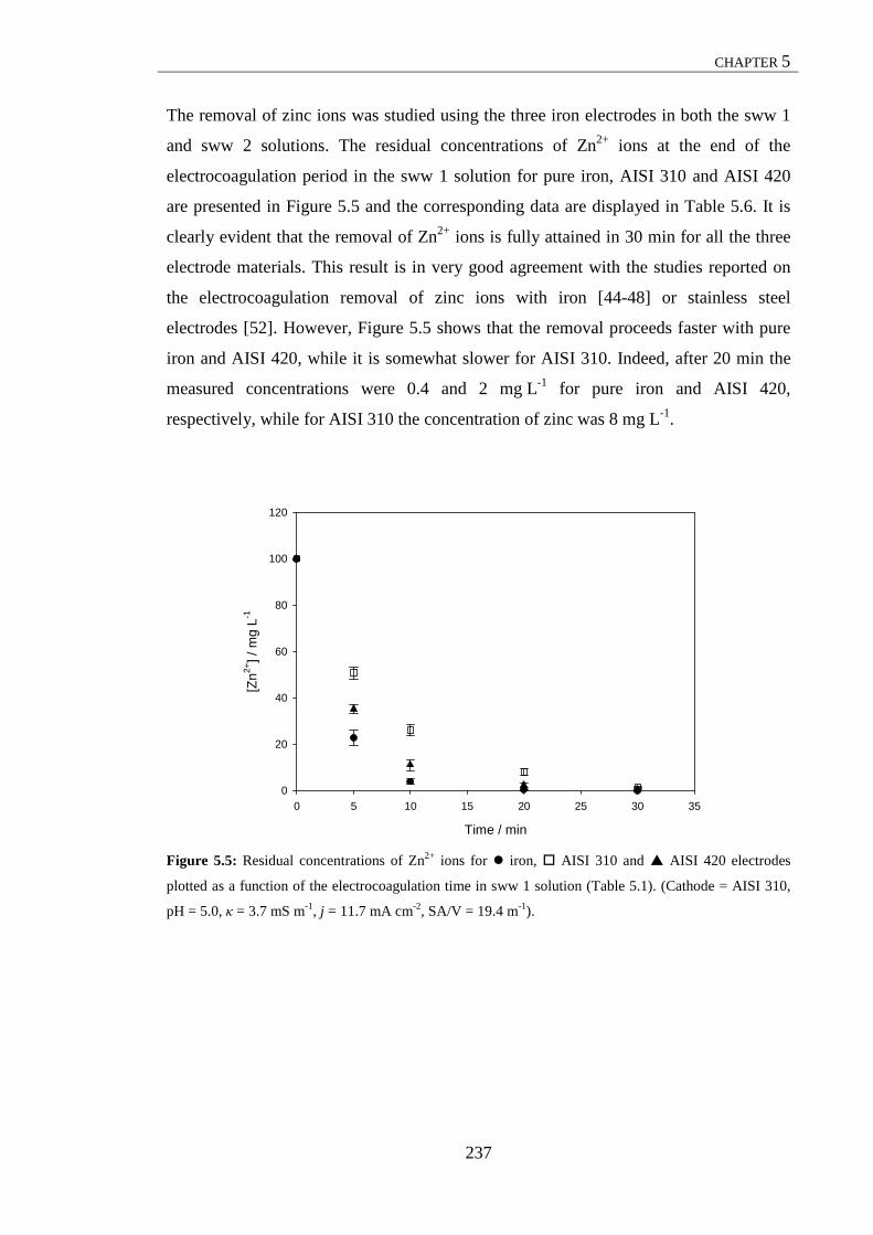
CHAPTER 5

237

The removal of zinc ions was studied using the three iron electrodes in both the sww 1

and sww 2 solutions. The residual concentrations of Zn2+ ions at the end of the

electrocoagulation period in the sww 1 solution for pure iron, AISI 310 and AISI 420

are presented in Figure 5.5 and the corresponding data are displayed in Table 5.6. It is

clearly evident that the removal of Zn2+ ions is fully attained in 30 min for all the three

electrode materials. This result is in very good agreement with the studies reported on

the electrocoagulation removal of zinc ions with iron [44-48] or stainless steel

electrodes [52]. However, Figure 5.5 shows that the removal proceeds faster with pure

iron and AISI 420, while it is somewhat slower for AISI 310. Indeed, after 20 min the

measured concentrations were 0.4 and 2 mg L-1 for pure iron and AISI 420,

respectively, while for AISI 310 the concentration of zinc was 8 mg L-1.

Figure 5.5: Residual concentrations of Zn2+ ions for iron, AISI 310 and AISI 420 electrodes



Time / min

0 5 10 15 20 25 30 35

[Zn2+

] / m

g L-1

0

20

40

60

80

100

120

CHAPTER 5

238

Table 5.6: Residual concentrations of Zn2+ ions and removal efficiency for pure iron, AISI 310 and AISI


Time

/ min

[Zn 2+]

/ mg L-1

η

/ %


0 100.0 100.0 100.0 0 0 0

5 23 ± 3 51 ± 3 35 ± 1 77 ± 3 49 ± 3 65 ± 2

10 4.0 ± 1 26 ± 2 11 ± 2 96 ± 1 74 ± 2 89 ± 2

20 0.4 ± 0.2 8 ± 1 2 ± 1 99.6 ± 0.2 92 ± 1 98 ± 1

30 BDL* 1.5 ± 0.4 0.5 ± 0.4 BDL* 98.5 ± 0.4 99.5 ± 0.4

*BDL = Below Detection Limit (Section 2.3.3). Figure 5.6 provides the residual concentrations of Zn2+ ions recorded in the sww 2

solution as a function of the electrocoagulation period for pure iron, AISI 310 and AISI

420 electrodes. The corresponding data are shown in Error! Reference source not

found.. According to these data, Zn2+ ions are readily removed from the solution using

pure iron and the AISI 420 electrodes, with an efficiency of 100% after 30 min.

Although somewhat lower, the AISI 310 electrode also shows a good removal

performance, with a final concentration of 1.8 mg L-1 Zn2+. By comparing the data

presented in Table 5.6 and Error! Reference source not found., it is clear that the

removal performances of the three iron-based electrodes are very similar in the sww 1 and

sww 2 test solutions. It appears that the concentration of chloride anions and the

conductivity of the solution have little effect on the removal of the Zn2+ ions.

CHAPTER 5

239

Figure 5.6: Residual concentrations of Zn2+ ions for iron, AISI 310 and AISI 420 electrodes



Table 5.7: Residual concentrations of Zn2+ ions and removal efficiency for pure iron, AISI 310 and AISI


Time

/ min

[Zn 2+]

/ mg L-1

η

/ %


0 100.0 100.0 100.0 0 0 0

5 16 ± 2 52 ± 3 30 ± 4 84 ± 2 48 ± 3 71 ± 4

10 3 ± 1 30 ± 2 7 ± 2 97 ± 1 70 ± 2 93 ± 2

20 0.1 ± 0.1 7.7 ± 0.8 0.7 ± 0.6 99.9 ± 0.1 92.3 ± 0.8 99.3 ± 0.6

30 BDL* 1.8 ± 0.8 BDL* BDL* 98.2 ± 0.8 BDL*


5.2.2 The electrochemistry and the removal performance of the iron system

As shown in Section 5.2.1, the pure iron electrode is the most efficient iron-based

material for removing the three pollutants from the synthetic test solutions. The AISI

420 grade exhibits removal efficiencies similar to those observed with the pure iron,

although they are slightly lower in the case of phosphates removal. On the other hand,

Time / min

0 5 10 15 20 25 30 35

[Zn2+

] / m

g L-1

0

20

40

60

80

100

120

CHAPTER 5

240

the high Cr content steel grade, AISI 310, results in poor removal efficiencies for

phosphates and Orange II dye. Good performance is instead achieved for the removal of

Zn2+ ions. However, it is worth noting that the removal of the three pollutants is brought

about through different mechanisms, as outlined in Section 5.2.1. The phosphate anions

are mainly removed by charge neutralisation and adsorption/sweep coagulation (Section

3.3), while the removal of Orange II dye and zinc ions has been ascribed to chemical

reactions involving the degradation of the molecule [39, 53] and to hydroxide

precipitation [44], respectively.

According to the results obtained in Section 4.2.4, the pure iron electrode shows no

passive behaviour and general dissolution or corrosion occurs. Consequently, secondary

reactions at the anode are minimised as only low potentials are required to facilitate

dissolution. These findings are in very good agreement with the high removal

efficiencies obtained in the treatment of the two synthetic wastewaters. In addition,

similar removal efficiencies for the three pollutants were measured in both sww 1 and

sww 2 solutions. This suggests that the pure iron anode behaves equally well in low and

high conductivity solutions. Indeed, the 10-fold increase in the chloride concentration,

from sww 1 to sww 2, shows little influence on the potentiodynamic polarisation

curves, as shown in Section 4.2.4.

On the other hand, the AISI 310 stainless steel electrode exhibits poor removal

efficiencies in the treatment of phosphates and Orange II dye in both the sww 1 and

sww 2 solutions. This is not consistent with the existing literature reported in Section

5.2. It is likely that the electrochemistry of this stainless steel is somehow involved.

Corrosion studies, performed in the sww 1 and sww 2 solutions and presented in

Section 4.3.4, have shown that the AISI 310 electrode remains passive in both

electrolytes over a wide range of potentials. The passive nature of this steel could

account for the results obtained in Section 5.2.1. When a constant current is applied in

the electrocoagulation tests, the anode potential may assume high values to overcome

this passivity. This may give rise to secondary reactions at the anode and to the

dissolution of chromium from steel. Secondary reactions that do not result in the

dissolution of Fe2+ ions may decrease the current efficiency of the process and be

responsible for less electrogenerated Fe2+ ions and, consequently, lower amounts of the

iron flocs in the solution. The poor removal of phosphates may be due to the low

CHAPTER 5

241

production of flocs. Indeed, at the end of the electrocoagulation tests performed with the

AISI 310, a relatively small number of flocs were observed in the solution compared

with the pure iron electrode. The low amount of electrogenerated Fe2+ ions is also likely

to be involved in the poor efficiency recorded for the removal of Orange II dye. Indeed,

as reported by Wilcock et al. [40] the removal of azo dyes is also carried out by

chemical reactions resulting in the cleavage of the azo bond. The Fe2+ ions released

from the electrode may act as a reducing agent to degrade the dye. The occurrence of

concurrent reactions that compete with the electrodissolution of the anode results in less

Fe2+ ions and, consequently, a lower rate of cleavage of the azo bonds. These concurrent

reactions may also involve the release of Cr(VI), as already postulated in Section 4.3.4.

Indeed, the presence of Cr(VI) was detected in the sample treated with the AISI 310

grade steel. Figure 5.7 shows the UV-Vis spectrum of a representative sample. The two

characteristic absorption peaks for Cr(VI) at an acidic pH at around 260 nm and 370 nm

and a peak minimum at around 313 nm are clearly evident from the spectrum [54-57].

The presence of chromium at the end of the electrocoagulation tests is quite surprising,

since several studies have been reported on the treatment of wastewater containing

hexavalent chromium by electrocoagulation [58-66]. The reduction of Cr(VI) to Cr(III)

is facilitated by the electrolytically generated ferrous ions, Eq. 5.1:

OH4Fe3CrFe3H8CrO 23322

4 ++→++ ++++− Eq. 5.1

Due to the low concentration of Fe2+ ions dissolved from the AISI 310 anode, the

hexavalent chromium, Cr(VI), was not removed from the solution and was detected in

both synthetic wastewaters.

CHAPTER 5

242

Figure 5.7: UV-Vis spectrum of a representative sample at the end of the electrocoagulation experiment

in sww 2 solution with the AISI 310 anode, where the solution pH was acidified. (Anode/cathode = AISI

310/AISI 310, pH = 5.0, κ = 14.4 mS m-1, j = 11.7 mA cm-2, SA/V = 19.4 m-1).

The slight increase in the efficiency for the removal of phosphates and Orange II in the

sww 2 solution may indicate that the side reactions at the anode are diminished and,

consequently, more Fe2+ ions are generated in the solution. This is supported by the

findings from Section 4.3.4, where the breakdown potential was observed at lower

potentials in the sww 2 solutions. On the other hand, the electrocoagulation removal of

Zn2+ ions with the AISI 310 electrode as the anode material is fully attained in 30 min in

both test solutions. As mentioned previously, these results are associated with the

alkaline pH values that the solutions exhibit during the electrocoagulation process and

that can result in the precipitation of zinc hydroxide.

The performance of the AISI 420 electrode in the removal of the Orange II dye and Zn2+

ions is similar to that observed with the pure iron electrode. However, slightly lower

removal efficiencies were obtained in the removal of phosphates. As mentioned earlier,

the removal of Orange II and zinc is mainly attained through other mechanisms other

than coagulation-flocculation. Consequently, the result observed for phosphates is likely

to be connected with the coagulant to pollutant ratio, which is a key factor in the

coagulation processes, as outlined in Chapter 3. Indeed, as reported in Section 3.3.5, the

occurrence at the anode of secondary reactions, which compete with the dissolution of

λ / nm

250 300 350 400 450 500

Abs

orba

nce

0.2

0.4

0.6

0.8

1.0

1.2

1.4

CHAPTER 5

243

iron, may result in lower coagulant dosage and, in turn, lower removal efficiency. These

reactions occur at high anode potentials, where chromium dissolution may take place in

a similar manner to that observed with the AISI 310 electrode. However, UV-Vis

spectra at a neutral pH, recorded on the samples at the end of the electrocoagulation

tests, did not detect any absorption peaks characteristic for Cr(VI). Figure 5.8 shows the

spectrum of a representative sample in the sww 2 solution. Moreover, similarly to the

pure iron electrode, the removal efficiencies of the three pollutants were similar in both

test solutions using the AISI 420 grade as the anode material. Clearly, the solution

conductivity does not affect the removal mechanism using the AISI 420 stainless steel

electrode. This is in good agreement with the potentiodynamic polarisation tests and the

corrosion parameters reported in Section 4.4.4, which are similar in both the sww 1 and

sww 2 solutions.

Figure 5.8: UV-Vis spectrum of a representative sample at the end of the electrocoagulation experiment

in sww 2 solution with the AISI 420 anode, where the solution was acidified. (Anode/cathode = AISI

420/AISI 310, pH = 5.0, κ = 14.4 mS m-1, j = 11.7 mA cm-2, SA/V = 19.4 m-1).

λ / nm

250 300 350 400 450 500

Abs

orba

nce

0.0

0.1

0.2

0.3

0.4

0.5

0.6

0.7

CHAPTER 5

244

5.2.3 Energy efficiency

It is widely recognised that the energy cost is the main drawback when electrochemical

processes are applied to wastewater treatment processes. Therefore, the costs of the

electrocoagulation systems are critical before this technique can be used and applied to

environmental problems [67]. The costs of an electrocoagulation system include the

operating costs due to the electrode materials, the electrical energy, as well as labour,

maintenance and other fixed costs [68]. In the present study, the energy consumption of

the iron-based anodes used in Section 5.2.1 to treat the two synthetic wastewaters is

taken into account.

When a current is applied between the anode and the cathode of the cell, the cell

potential depends on four main terms, the equilibrium potential difference, Eeq, the

anode overpotential, Ea, the cathode overpotential, Ec, and the ohmic potential drop of

the solution, EIR [69]. The anode overpotential includes the activation overpotential, ηa,a

and the concentration overpotential, ηa,c, as well as the possible passive overpotential,

ηa,p, due to the presence of a passive film at the anode surface, while the cathode

overpotential is mainly composed of the activation overpotential, ηc,a and concentration

overpotentials, ηc,c.

IReqcell EE Ec,ca,cp,ac,aa,a ++++++= ηηηηη Eq. 5.2

The equilibrium potential difference, Eeq, depends on the anode and cathode used in the

process and is related to the corrosion potential, Ecorr. Consequently, anodes with low

Ecorr in a given solution require less electrical energy for electrocoagulation. The

activation and concentration overpotentials increase with the current density. However,

the concentration overpotential is mainly related to the mixing conditions, consequently,

it can be considered negligible if good mixing is maintained during the process [70].

The ohmic potential drop of the solution, EIR, is directly proportional to the electrode

spacing, d, and inversely proportional to the solution conductivity, κ [38].

The energy supplied to the system is usually expressed in terms of specific electrical

energy consumption, SEEC, in Wh m-3, according to Eq. 5.3.

CHAPTER 5

245

( )V

ItE cell=−3mWhSEEC Eq. 5.3

Here, Ecell is the cell voltage in V vs. SCE, I is the current in A, t is the

electrocoagulation time in h and V is the volume of the solution treated in m3. In the

present study a constant current density was applied, while the average potential of the

cell, ,cellE recorded during each experiment was used in Eq. 5.3. Furthermore, the

energy consumption can be expressed simply as the electrical energy consumption,

EEC, in Wh, since the volume of the treated solutions was constant in each experiment,

200 mL.

( ) ItE cell=WhEEC Eq. 5.4

Figure 5.9 shows the energy consumption, in Wh, of the three iron-based anode

materials required to treat the sww 1 and sww 2 solutions. It is clear from the figure that

the energy requirements of pure iron and the AISI 420 electrodes in sww 1 are similar,

at 1.35 and 1.41 Wh, respectively. The same trend is observed in the sww 2 solution,

where 0.52 and 0.62 Wh are required for pure iron and the AISI 420 system,

respectively. On the other hand, considerably higher consumption is exhibited by the

AISI 310 grade in both test solutions, with 2.17 and 0.97 Wh in the sww 1 and sww 2

solutions, respectively. The lower energy observed in the electrocoagulation tests

carried out in the sww 2 solution is due to the higher conductivity of this solution, as

displayed in Table 5.1. Indeed, Eq. 5.2 shows that the IR drop can be easily minimised

by increasing the conductivity of the solution. A decrease of the IR drop term results in

a lower cell potential, Ecell and, consequently, a lower energy consumption, EEC (Eq.

5.4).

CHAPTER 5

246

Electrode EEC

/ Wh

sww 1 sww 2

Fe 1.35 0.52

AISI 310 2.17 0.97

AISI 420 1.41 0.62

Figure 5.9: Effect of anode material on the electrical energy consumption, EEC, for pure iron,

stainless steel AISI 310 and stainless steel AISI 420 in sww 1 and sww 2 solutions (Table 5.1).

(Cathode = AISI 310, pH = 5.0, j = 11.7 mA cm-2, SA/V = 19.4 m-1).

As mentioned earlier, the cell potential, Ecell, which determines the energy efficiency of

the electrocoagulation process, is connected to the corrosion potential, Ecorr, of the

anode/cathode used. Provided that the same type of cathode is used, anodes with low

Ecorr in a given solution are more efficient in terms of energy consumption. Table 5.8

shows the Ecorr values recorded in the potentiodynamic polarisation tests reported in

Section 4.10 for pure iron, stainless steel AISI 310 and stainless steel AISI 420

electrodes in the sww 1 and sww 2 solutions. It is clearly evident that the negative

values of Ecorr exhibited by the pure iron electrode result in high energy efficiency for

the electrocoagulation process. In addition, the values of Ecorr for AISI 420 are only

about 60 mV higher giving similar energy consumption of these two systems, as shown

in Figure 5.9. However, the Ecorr values recorded for the AISI 310 electrode are

significantly higher. As a consequence, the energy demand of this alloy for the

electrocoagulation tests is much higher.

Table 5.8: Corrosion potentials, Ecorr, for pure iron, AISI 310 and AISI 420 electrodes measured in sww 1

and sww 2 solutions (Section 4.10).

Electrode Ecorr

/ V vs. SCE

sww 1 sww 2

Pure iron -0.704 -0.724

AISI 310 -0.448 -0.525

AISI 420 -0.641 -0.659

sww 1 sww 2

EE

C /

Wh

0.0

0.5

1.0

1.5

2.0

2.5

CHAPTER 5

247

5.3 Aluminium system

In this section results are presented on the electrocoagulation removal and energy

efficiency performances of two aluminium-based alloys. Aluminium-magnesium,

Al-2Mg, and aluminium-zinc-indium, Al-3Zn-0.02In, alloys were chosen in order to

minimise both the effects of passivation and pitting corrosion of pure aluminium, which

are well-known drawbacks of the aluminium electrode in electrocoagulation [25, 33, 47,

71, 72], as already outlined in Section 4.1.

The same synthetic test solutions, which were presented in Table 5.1 and used for the

iron system, were employed to investigate the performance of the two aluminium alloys

for the treatment of phosphates, Orange II dye and zinc ions. The removal and the

energy efficiencies of the two alloys were compared. The electrocoagulation tests were

carried out with a current density of 11.7 mA cm-2, a ratio of the surface area of the

anode to the volume of solution, SA/V, of 19.4 m-1 and the electrocoagulation time was

maintained at 30 min. A plate of stainless steel AISI 310 was used as the cathode. The

composition of the electrode materials and the full experimental details are given in

Sections 2.2.2 and 2.3.1.2.

5.3.1 The electrode performance in removing three representative

pollutants from synthetic wastewaters

5.3.1.1 The removal of phosphates

Aluminium and aluminium alloys have been used as anode materials in the

electrocoagulation removal of phosphates from solutions [35, 73-77]. In Section 3.2,

results were presented on the removal of phosphates using the Al-2Mg electrode and

good removal efficiencies, which are consistent with the existing literature, were

observed. For example, after 20 min the removal efficiency was 75%, 57% and 40.5%

for initial concentrations of phosphates of 20.0, 60.0 and 150.0 mg L-1, respectively.

Similarly to the electrocoagulation with iron electrodes, the removal of phosphates with

aluminium electrodes is attained mainly through the mechanism of adsorption on

aluminium flocs.

CHAPTER 5

248

In this section the performance of the Al-2Mg and Al-3Zn-0.02In electrodes in

removing phosphates from the sww 1 and sww 2 solutions are compared. Figure 5.10

shows the residual concentrations of PO4-P in the sww 1 solution plotted as a function

of the electrocoagulation time for the Al-2Mg and Al-3Zn-0.02In electrodes. In Table

5.9 the corresponding data are reported. At the end of 30 min, the concentration of PO4-

P is 53 mg L-1 using the Al-2Mg electrode and 36 mg L-1 for the Al-3Zn-0.02In system.

It is apparent that the Al-3Zn-0.02In exhibits a better removal performance than the

Al-2Mg anode.

Figure 5.10: Residual concentrations of PO4-P for Al-2Mg and Al-3Zn-0.02In electrodes plotted as

a function of the electrocoagulation time in sww 1 solution (Table 5.1). (Cathode = AISI 310, pH = 5.0,

κ = 3.7 mS m-1, j = 11.7 mA cm-2, SA/V = 19.4 m-1).

Time / min

0 5 10 15 20 25 30 35

[PO

4-P

] / m

g L-1

0

100

200

300

400

500

600

CHAPTER 5

249

Table 5.9: Residual concentrations of PO4-P and removal efficiency for Al-2Mg and Al-3Zn-0.02In

electrodes in sww 1 solution. Each experiment was performed in triplicate (n = 3).

Time

/ min

[PO4-P]

/ mg L-1

η

/ %

Al-2Mg Al-3Zn-0.02In Al-2Mg Al-3Zn-0.02In

0 500.0 500.0 0 0

5 340 ± 21 328 ± 12 32 ± 4 34 ± 2

10 242 ± 14 205 ± 14 52 ± 3 59 ± 3

20 115 ± 9 90 ± 6 77 ± 2 82 ± 1

30 53 ± 6 36 ± 3 89 ± 1 92.8 ± 0.7

A 10-fold increase in the conductivity of the test solution results in improved removal

efficiencies for both aluminium alloys. This is shown in Figure 5.11, where the residual

concentrations of PO4-P recorded in the sww 2 solution are plotted as a function of the

electrocoagulation period. The corresponding data, which are displayed in Table 5.10,

show final concentrations of 35 mg L-1 for Al-2Mg and 24 mg L-1 for the Al-3Zn-0.02In

electrode. Clearly, better performances were achieved in the sww 2 solution. This

improvement is probably due to the higher concentration of chloride ions in the sww 2

solution. Indeed, as reported in Section 3.2.4, the presence of NaCl in solution promotes

the coagulation of phosphates.

Figure 5.11: Residual concentrations of PO4-P for Al-2Mg and Al-3Zn-0.02In electrodes plotted as

a function of the electrocoagulation time in sww 2 solution (Table 5.1). (Cathode = AISI 310, pH = 5.0,

κ = 3.7 mS m-1, j = 11.7 mA cm-2, SA/V = 19.4 m-1).

Time / min

0 5 10 15 20 25 30 35

[PO

4-P

] / m

g L-1

0

100

200

300

400

500

600

CHAPTER 5

250

Table 5.10: Residual concentrations of PO4-P and removal efficiency for Al-2Mg and Al-3Zn-0.02In


Time

/ min

[PO4-P]

/ mg L-1

η

/ %


0 500.0 500.0 0 0

5 325 ± 7 298 ± 17 35 ± 1 40 ± 4

10 205 ± 7 175 ± 6 59 ± 1 65 ± 1

20 83 ± 3 67 ± 5 83.4 ± 0.7 86 ± 1

30 35 ± 4 24 ± 3 93.0 ± 0.9 95.2 ± 0.5

5.3.1.2 The removal of Orange II dye

It has been shown that the iron system is more efficient for the removal of azo dyes

compared to the aluminium system, ascribing this difference to the removal mechanisms

involved in the two systems [4, 24, 39, 40, 46, 50]. For example, Chafi et al. [6]

reported that higher currents are required by the Al system to achieve the same

efficiency as the Fe system. Adsorption was identified as the main removal mechanism

for the Fe system, while the degradation of the dye into 2-naphtol was observed with the

Al system, suggesting a mechanism of electroreduction of the azo bond. Mollah et al.

[9] found an absorption band at 250 nm, which increased with the electrocoagulation

period using aluminium electrodes. They attributed the band to possible by-products of

Orange II dye degradation. In addition, FT-IR spectra did not reveal any trace of the

dye, suggesting a partial destruction of the dye molecule. However, the authors pointed

out that more research is needed in this direction since the detection of the dye in the

flocs is quite difficult due to dilution factors and to the sensitivity constraint of the

FT-IR instrument. In contrast with these findings, other studies [39, 40, 53] indicate that

the removal mechanism of azo dyes with aluminium electrodes is physical adsorption

rather than dye degradation.

In Figure 5.12 the residual concentrations of Orange II dye plotted as a function of the

electrocoagulation period for Al-2Mg and Al-3Zn-0.02In electrodes are shown. It is

clearly evident from this figure and from the corresponding data displayed in Table 5.11

that the removal is not complete in 30 min. The measured concentrations are 30 and 11 mg L-1

for Al-2Mg and Al-3Zn-0.02In, respectively, corresponding to removal efficiencies of

CHAPTER 5

251

40% and 78%. Clearly, the removal performance of the aluminium-zinc alloy is

somewhat better at 78%, but these efficiencies are considerably lower than the values

calculated with the AISI 420 and pure iron electrodes. These results are in good

agreement with a better performance of the iron system in removing azo dyes.

Figure 5.12: Residual concentrations of Orange II for Al-2Mg and Al-3Zn-0.02In electrodes



Table 5.11: Residual concentrations of Orange II and removal efficiency for Al-2Mg and Al-3Zn-0.02In


Time

/ min

[Orange II]

/ mg L-1

η

/ %


0 50.0 50.0 0 0

5 46 ± 1 43 ± 3 8 ± 3 14 ± 7

10 41 ± 4 28 ± 3 18 ± 8 43 ± 7

20 35 ± 3 19 ± 3 30 ± 5 63 ± 5

30 30 ± 2 11 ± 2 41 ± 4 78 ± 4

Time / min

0 5 10 15 20 25 30 35

[Ora

nge

II] /

mg

L-1

0

10

20

30

40

50

60

CHAPTER 5

252

The results obtained in the sww 2 solution are shown in Figure 5.13 and Table 5.12. In

particular, Figure 5.13 illustrates the residual concentrations of Orange II dye plotted as

a function of the electrocoagulation period for Al-2Mg and Al-3Zn-0.02In. Again it is

evident that the Al-3Zn-0.02In electrode is more efficient in removing the dye,

particularly at longer electrocoagulation times. The removal of the dye appears to reach

a limiting value after about 15-20 min min for the Al-2Mg electrode. The corresponding

data are displayed in Table 5.12. As can be observed from these data, the final

concentration of Orange II is 29 and 9 mg L-1 using the Al-2Mg and Al-3Zn-0.02In

electrodes, respectively. On comparing these values to those obtained in the sww 1

solution (Table 5.11), it is evident that the removal efficiencies are similar in both

solutions. Clearly, there is no evidence of any increase in the removal efficiency on

increasing the chloride concentration or the conductivity of the solution.

Figure 5.13: Residual concentrations of Orange II for Al-2Mg and Al-3Zn-0.02In electrodes



Time / min

0 5 10 15 20 25 30 35

[Ora

nge

II] /

mg

L-1

0

10

20

30

40

50

60

CHAPTER 5

253

Table 5.12: Residual concentrations of Orange II and removal efficiency for Al-2Mg and Al-3Zn-0.02In


Time

/ min

[Orange II]

/ mg L-1

η

/ %


0 50.0 50.0 0 0

5 45 ± 3 36 ± 2 10 ± 5 27 ± 4

10 40 ± 3 30 ± 3 19 ± 5 40 ± 5

20 33 ± 1 15 ± 3 34 ± 2 70 ± 6

30 29 ± 1 9 ± 1 42 ± 2 83 ± 3

5.3.1.3 The removal of zinc ions

Several studies have been reported in the literature on the removal of zinc ions from

solution using aluminium electrodes [38, 44, 78, 79]. Again in these studies, similar to

that found with the iron system (Section 5.2.1.3), the coprecipitation of Zn(OH)2 species

plays a dominant role in the removal mechanism. In particular, an extensive study on

the electrocoagulation removal of Zn(II), Cu(II), Ni(II), Ag(I) and Cr(VI) was presented

by Heidmann and Calmano [79]. The authors concluded that metallic cations are

removed through several mechanisms. However, the main mechanism for the removal

of Zn2+ ions is the precipitation as hydroxide species. The removal rate for zinc was

independent of its initial concentrations and was lowered by the presence of other metal

ions, which were removed similarly, because of the competition for OH- ions produced

at the cathode. According to these studies, it is then expected that the use of an

aluminium alloy, such as the Al-2Mg or Al-3Zn-0.02In electrodes, may result in an

efficient removal of zinc ions from the solution.

Figure 5.14 shows the residual concentrations of Zn2+ ions plotted as a function of the

electrocoagulation time for Al-2Mg and Al-3Zn-0.02In electrodes in the sww 1

solution. The corresponding data are given in Table 5.13. These data show very good

efficiencies in removing zinc ions, although the performance of Al-2Mg is somewhat

lower. In 30 min the residual concentration of Zn2+ ions is reduced to 1.4 mg L-1 for the

Al-2Mg electrode, while complete removal is achieved with Al-3Zn-0.02In.

CHAPTER 5

254

Figure 5.14: Residual concentrations of Zn2+ ions for Al-2Mg and Al-3Zn-0.02In electrodes



Table 5.13: Residual concentrations of Zn2+ ions and removal efficiency for Al-2Mg and Al-3Zn-0.02In


Time

/ min

[Zn 2+]

/ mg L-1

η

/ %


0 100.0 100.0 0 0

5 48 ± 2 27 ± 3 52 ± 2 73 ± 3

10 24 ± 2 7 ± 2 76 ± 2 93 ± 2

20 4 ± 2 0.8 ± 0.5 96 ± 1 99.2 ± 0.5

30 1.4 ± 0.5 BDL* 98.6 ± 0.5 BDL*


The removal performances of Al-2Mg and Al-3Zn-0.02In electrodes in the sww 2

solutions are similar to those observed in the sww 1 solution. In Figure 5.15 the residual

concentrations of Zn2+ ions in the sww 2 solution are presented as a function of the

electrocoagulation period for the two aluminium alloys. Table 5.14 provides the

corresponding data. The efficiency measured in the sww 2 solution (Table 5.14) is

similar to that observed in the sww 1 solution (Table 5.13). This is particularly

Time / min

0 5 10 15 20 25 30 35

[Zn2+

] / m

g L-1

0

20

40

60

80

100

120

CHAPTER 5

255

noticeable in the case of Al-2Mg. The concentration of Zn2+ ions at the end of the

electrocoagulation period is 0.9 mg L-1, which is within the experimental error if

compared with the value of 1.4 mg L-1 observed in the sww 1 solution. However, it is

clear from the data presented in Table 5.14 that a moderate increase of the removal

performance occurs in the sww 2 solution for the Al-3Zn-0.02In electrode. Although at

the end of the process Zn2+ ions are completely removed from both solutions, after 10

min of the electrocoagulation time the residual concentrations of zinc ions are 7.0 and

3.2 mg L-1 in the sww 1 and sww 2 solutions, respectively.

Figure 5.15: Residual concentrations of Zn2+ ions for Al-2Mg and Al-3Zn-0.02In electrodes



Time / min

0 5 10 15 20 25 30 35

[Zn2+

] / m

g L-1

0

20

40

60

80

100

120

CHAPTER 5

256

Table 5.14: Residual concentrations of Zn2+ ions and removal efficiency for Al-2Mg and Al-3Zn-0.02In


Time

/ min

[Zn 2+]

/ mg L-1

η

/ %


0 100.0 100.0 0 0

5 41 ± 2 19 ± 3 59 ± 2 81 ± 3

10 19 ± 2 3.2 ± 0.6 81 ± 2 96.8 ± 0.6

20 4 ± 2 0.2 ± 0.3 96 ± 2 99.8 ± 0.3

30 0.9 ± 0.3 BDL* 99.8 ± 0.3 BDL*


As reported in the literature on the electrocoagulation removal of Zn2+ ions with Al

electrodes [38, 44, 78, 79], these results are in agreement with a removal attained

mainly through precipitation of zinc hydroxide species owing to the alkaline pH of the

solution treated by electrocoagulation. In Section 3.2.3, it was shown that the final pH

of the solutions treated with Al-2Mg electrode was in the range of 9.0 to 10.0, when the

initial pH was 5.0. At these pH values, i.e. 9.0 to 10.0, the aluminium hydroxide

precipitate dissolves to form the monomeric anionic hydroxyaluminium species,

Al(OH)4-, as reported in Section 3.2.3, and in the speciation diagrams of aluminium in

Section 1.3.2.2, Fig. 1.5(a). The anionic hydroxyaluminium species is soluble in

solution. Consequently, the high removal efficiencies of Zn2+ ions observed for Al-2Mg

and Al-3Zn-0.02In is due to a mechanism different from adsorption. The speciation

diagram for aqueous zinc solutions, displayed in Figure 5.16, shows that the

predominant species in the pH range of 8.5 to 10.5 is Zn(OH)2 [38, 44, 78, 79],

therefore its removal is accomplished primarily through hydroxide precipitation due to

the alkaline pH of the solution during the electrocoagulation process.

CHAPTER 5

257

Figure 5.16: Speciation diagram of zinc in aqueous solutions. The diagram was calculated with the

MEDUSA software developed by Puigdomenech [80] at the KTH Royal Institute of Technology, Sweden

and based on the SOLGASWATER algorithm [81].

5.3.2 The electrochemistry and the removal performance of the aluminium

system

According to the results presented in Section 5.3.1, the Al-3Zn-0.02In electrode shows

better removal performance than the Al-2Mg electrode for the three pollutants contained

in the synthetic wastewaters. However, both alloys exhibit moderately good efficiency

for the removal of the Orange II dye. As in the case of the iron system, it is worth noting

that the three pollutants are removed through different mechanisms, with the removal of

phosphates depending mainly on the floc production and Zn2+ ions on the alkaline pH of

the solution and the formation and precipitation of the hydroxide species. On the other

hand, the removal of the Orange II dye in the aluminium system is attained by

adsorption or degradation, as outlined in Section 5.3.1.2.

As reported in Section 4.6.4, the electrochemical behaviour of the Al-2Mg electrode in

the sww 1 and sww 2 solutions is determined by the presence of chloride, which, even

in small concentration, has a positive influence on the dissolution of the alloy. The

potentiodynamic polarisation curves, do not exhibit any passive region. This behaviour

is connected to the good removal performance observed for phosphates, which are

removed through a mechanism involving the generation of Al3+, as shown in Section 3.2.

2 4 6 8 10 12 14

0.0

0.2

0.4

0.6

0.8

1.0

Fra

ction

pH

Zn2+

Zn(OH)2

Zn(OH)3−

Zn(OH)42−

ZnOH+

CHAPTER 5

258

On the other hand, the Orange II dye is not removed as efficiently as the phosphate

anions. In some studies carried out with aluminium electrodes, the removal of dyes is

attributed to the electroreduction of the azo bond [6, 9] as higher currents are required to

obtain the same decolourisation efficiency observed in the iron system [6]. In contrast,

other studies have shown that the lower efficiency observed with the aluminium

electrodes for removing azo dyes is due to the occurrence of a single removal

mechanism, based on adsorption on the flocs, rather than a combination of adsorption

and molecule degradation which occurs with the iron system [39, 40, 53]. The results

presented in Section 5.3.1.2 show similar removal efficiencies in the sww 1 and sww 2

solutions, which have different conductivities. As reported in Section 3.3.5, the

coagulant dosage, Al3+ ions, is higher in more conducting solutions because the low

potentials exhibited by the anode do not promote the occurrence of secondary reactions,

which compete with the dissolution of aluminium. Consequently, a removal mechanism

of Orange II, which involves only the Al3+ ions and, in turn, adsorption on the flocs, is

unlikely as the removal efficiency is similar in the sww 1 and sww 2 solutions. It seems

that the removal of the Orange II dye using the Al-2Mg electrode as the anode material

is more complex and depends on a combination of adsorption and molecule

degradation.

As shown in Section 4.7.4, the electrochemical behaviour of Al-3Zn-0.02In is consistent

with active dissolution with an absence of a passive region and low corrosion potentials,

even in solutions containing low concentrations of chloride anions. As a result, the

removal performance of this alloy is considerably higher than the Al-2Mg, as shown in

Section 5.3.1. The excellent results obtained for the removal of phosphates are probably

due to the ease of the dissolution process of the Al-3Zn-0.02In electrode. Higher

efficiencies are obtained in the more conducting solution, sww 2, suggesting a higher

rate of Al3+ dissolution, in good agreement with the polarisation curves shown in

Section 4.7.4. On the other hand, the similar removal efficiency recorded in the sww 1

and sww 2 solutions for the Orange II dye suggests that mechanisms other than

adsorption, probably concerning the degradation of the dye, are involved in the removal

of the Orange II dye.

CHAPTER 5

259

5.3.3 Energy efficiency

As detailed earlier, the energy consumption is important in the development and

applications of the electrocoagulation systems. In this section, results are presented on

the energy consumption of the Al-2Mg and Al-3Zn-0.02In electrodes in the

electrocoagulation tests described in Section 5.3.1 for treating the two synthetic

wastewaters. The energy requirements for each electrode were expressed as the

electrical energy consumption, EEC, in Wh, and computed according to Eq. 5.4.

Figure 5.17 shows the energy consumption, in Wh, of the two aluminium alloys

required in the treatment of the sww 1 and sww 2 solutions. It is apparent from this

figure that the Al-3Zn-0.02In electrode is consistently more efficient in terms of energy

in both test solutions. Indeed, the energy consumption is 0.51 and 0.26 Wh in the sww 1

and sww 2 solutions, respectively. On the other hand, higher energy consumption is

exhibited by the Al-2Mg electrode, with 1.53 Wh in sww 1 and 0.61 Wh in the sww 2

solution. As already observed for the iron system (Section 5.2.3), the energy demand

diminishes considerably in the sww 2 solution, which has a higher conductivity. This

effect is expected since the solution conductivity, κ, is one of the terms affecting the cell

voltage, Ecell, as indicated in Eq. 5.2.

Electrode EEC

/ Wh

sww 1 sww 2

Al-2Mg 1.53 0.51

Al-3Zn-0.02In 0.61 0.26

Figure 5.17: Effect of anode material on the electrical energy consumption, EEC, for Al-2Mg and

Al-3Zn-0.02In in sww 1 and sww 2 solutions (Table 5.1).

(Cathode = AISI 310, pH = 5.0, j = 11.7 mA cm-2, SA/V = 19.4 m-1).

sww 1 sww 2

EE

C /

Wh

0.0

0.2

0.4

0.6

0.8

1.0

1.2

1.4

1.6

1.8

CHAPTER 5

260

The cell potential, Ecell, depends on the type of electrodes employed in the

electrocoagulation tests. In addition, it is connected to the corrosion potential, Ecorr, of

the anode, as mentioned in Section 5.2.3. Consequently, materials which adopt low

values of Ecorr result in greater energy efficiency for the electrocoagulation process. The

Ecorr values for the Al-2Mg and Al-3Zn-0.02In electrodes are shown in Table 5.15.

They were measured from the potentiodynamic polarisation tests carried out in the sww

1 and sww 2 solutions and are presented in Section 4.10. As expected, the

Al-3Zn-0.02In electrode exhibits more negative values of Ecorr and, as a result, requires

lower energy, as shown in Figure 5.17.

Table 5.15: Corrosion potentials, Ecorr, for Al-2Mg and Al-3Zn-0.02In electrodes measured in sww 1 and

sww 2 solutions (Section 4.10).

Electrode Ecorr

/ V vs. SCE

sww 1 sww 2

Al-2Mg -0.598 -0.670

Al-3Zn-0.02In -0.798 -0.857

5.4 Screening chemometric study

The two main applications of the Design of Experiments, DoE, are screening and

optimisation [13]. In screening, the factors that most affect the process are identified,

while optimisation consists in determining the optimal settings or conditions for the

process. Firstly, a screening design is used and includes all the controllable factors that

may possibly influence the experiment. Once the most important factors have been

identified, an experimental optimisation design is carried out.

As described in Section 2.3.7, full factorial designs are usually used as screening

designs. They are indicated as 2n designs, where the base 2 stands for the number of

factor levels and n the number of factors, each with a high and low values. The lower

level is indicated with a ‘-’ sign, while the higher level with a ‘+’ sign. Fractional

factorial designs are good alternatives to a full factorial design. Indeed, if the number of

factors is considerably high, the number of experiments to be performed in a full

factorial design becomes prohibitive. A fractional design is a representative subset of a

CHAPTER 5

261

full factorial design, where the number of experiments is reduced by a number p,

according to a 2k-p design, where k is the number of factors investigated.

In the present study, a 25-1 fractional factorial design with two replicates and blocking

was employed as a screening design for the electrocoagulation removal of phosphates

using stainless steel AISI 420 as the anode material. Each block was performed on a

different day. In total, 32 experiments were carried out in four days. Five factors were

studied: current density (A), electrocoagulation time or EC time (B), surface area of the

electrode to the volume of the solution ratio or SA/V (C), flocculation time or floc time

(D) and settlement time or settl time (E). As detailed in Chapter 3, the current density

and the electrocoagulation time are important variables in the electrocoagulation

process. The electrode surface area to the volume solution ratio has been reported by

Holt et al. [82] as a key factor in electrocoagulation experiments. In addition, the

flocculation time and settlement time were included in the study. The flocculation time

was taken as the time period between the end of the experiment and the cessation of the

solution stirring, and the settlement time was determined as the time between the stop of

the solution stirring and the analysis of the sample. Table 5.16 shows the investigated

factors and the corresponding levels that were studied. Full experimental details,

including the design matrix, are given in Sections 2.3.1.4 and 2.3.7.

The choice of blocking the fractional factorial design came from the observation that it

was not possible to perform all the 32 experiments under homogeneous conditions. For

example, fresh solutions of phosphates and sodium chloride were prepared every day.

Moreover, although carefully cleaned before each experiment and every day, the state of

the electrode surface was not exactly reproducible. Blocking is a design technique used

to reduce or eliminate the variability that arises from nuisance factors, that is factors that

may influence the process but that are not the objectives of the investigation [12]. In the

present study, blocking was used to test the robustness of the electrocoagulation process

and assess whether blocking or not is necessary for future designs. The implications of

blocking on the fractional factorial design and the corresponding design matrix are

given in Section 2.3.7.

CHAPTER 5

262

Table 5.16: Factors investigated in the 25-1 fractional factorial design and their corresponding levels

(Anode/Cathode = AISI 420/AISI 310, [PO4-P] = 15.0 mg L-1, pH = 5.0).

Factors Levels

(-) low (+) high

current density / mA cm-2 A 2 5.5

EC time / min B 5 60

SA/V / m-1 C 9.1 13.7

floc time / min D 2 30

settl time / min E 10 60

5.4.1 Estimating factor effects and forming the initial model

As reported in Section 2.3.7, the first step in a DoE analysis is to determine the

significance of the coefficients. The simplest approach is to consider the magnitude of

the coefficients. However, a statistical indicator is usually employed. For example,

Student’s t-test and F-test can be performed. It is also convenient to present the

coefficients graphically and a classical approach is to plot the effects on a normal

probability plot [12]. In this case, the effects that are negligible are normally distributed

and fall along a straight line on the plot, while significant effects do not lie along the

straight line.

The normal probability plot of the effects obtained for the 25-1 fractional design is

displayed in Figure 5.18. All the effects that lie along the line are negligible, whereas

the large effects are far from the line. The important effects that emerge from this

analysis are the current density (A), electrocoagulation time (B), SA/V (C), settlement

time (E) and the interaction current density-SA/V (AC).

CHAPTER 5

263

Figure 5.18: Normal probability plot of the effects for the 25-1 fractional factorial design.

The main effects of A (current density), B (electrocoagulation time), C (SA/V) and E

(settlement time) are plotted in Figure 5.19. The effects of A, B and C are negative.

Consequently, considering only these main effects, the electrocoagulation tests would

be run at the high level to minimise the residual concentration of phosphates. On the

other hand, the main effect E is positive indicating that the residual concentration of

phosphates increases on increasing the settlement time. This may be due to a desorption

process of phosphates from the flocs. The main effects A and C are involved in

interactions. This interaction is plotted in Figure 5.20. From the figure it is apparent that

the current density effect is negligible when the SA/V ratio is at the high level, whereas

it is larger when the ratio is at the low level, with the best results obtained with low

SA/V and high current density. Consequently, when small SA/V ratios are used in

electrocoagulation tests, a higher current density would give better results in terms of

removal efficiencies.

Normal Plot

Nor

mal

% P

roba

bilit

y

Standardized Effect

-10.60 -7.58 -4.56 -1.54 1.48

1

5

10

20

30

50

70

80

90

95

99

A

B

C

E

AC

CHAPTER 5

264

Figure 5.19: Main effects plot for the 25-1 fractional factorial design.

Figure 5.20: Interaction plot for the 25-1 fractional factorial design. C = 9.1 m-1, C = 13.7 m-1.

2.00 2.70 3.40 4.10 4.80 5.50

A: Current density

Res

idua

l co

ncen

trat

ion

0

2

4

6

8

10

12

14Warning! Factor involved in AC interaction.

One Factor

5.00 16.00 27.00 38.00 49.00 60.00

B: Time

Res

idua

l co

nce

ntra

tion

0

2

4

6

8

10

12

14

One Factor

9.10 10.25 11.40 12.55 13.70

C: SA/V

Re

sid

ual c

onc

entra

tion

0

2

4

6

8

10

12

14 Warning! Factor involved in AC interaction.

One Factor

10.00 15.00 20.00 25.00 30.00 35.00 40.00 45.00 50.00 55.00 60.00

E: Settlement time

Re

sid

ual c

onc

entra

tion

0

2

4

6

8

10

12

14

One Factor

C: SA/V

2.00 2.70 3.40 4.10 4.80 5.50

A: Current density

Res

idu

al c

once

ntra

tion

0

2

4

6

8

10

12

14

Interaction

CHAPTER 5

265

The parameters in the effect model were estimated by the least square method using

Design-Expert® Version 8.0.7.1 by Stat-Ease, Inc. and are shown in Eq. 5.5:

[PO4-P] = 25.36 – 2.11 current density – 0.19 EC time – 0.89 SA/V + 0.03 floc time

+ 0.12 current density-SA/V Eq. 5.5

Again, this equation shows that the coefficient of the current density is the largest at

2.11, while the SA/V ratio is also significant.

5.4.2 Performing statistical tests

The significance and the adequacy of the model were evaluated by analysis of variance,

ANOVA, and the corresponding data are presented in Table 5.17. The Fisher’s variance

test (F-test) and the coefficient of determination between the experimental and predicted

values were used to test the significance. According to the data in Table 5.17, F0, which

is defined as the mean of squares of the model to the mean of squares of the error ratio,

MSModel/MSerror, is higher than the tabulated F-value (2.640 at 95% significance). In

addition, the p-value, which is lower than 0.0001 confirms that the regression model is

statistically significant. Furthermore, a value of 0.9813 was obtained as the adjusted R2

value. This indicates that the model explains about 98% of the variability observed in

the data.

It is also interesting to determine if blocking is necessary in future experiments. For this

purpose, the ratio of MSBlock to MSerror is considered. From Table 5.17, this ratio can be

computed as 2.33. This value is relatively low and indicates that the blocking factor

does not have a significant effect. This also highlights the robustness of the

electrocoagulation process carried out on different days. As a consequence, blocking is

not necessary in future DoE analyses.

CHAPTER 5

266

Table 5.17: Analysis of variance for the model presented in Eq. 5.5.

Source Analysis of variance

SSa dof b MSc F0 p-value

Model 1018.54 5 203.71 470.56 < 0.0001

Block 3.00 3 1.00

Error 9.96 23 0.43 a Sum of squares. b Degrees of freedom. c Mean square.

Before conclusions from the analysis of variance are adopted, the adequacy of the

model should be checked. An important diagnostic tool is the residual analysis [83].

Residuals, the difference between experimental and predicted responses, are considered

as unexplained variations in the model and occur based on a normal distribution, if the

model is a good predictor. The normal probability plot of the residuals for the present

25-1 fractional factorial design is shown in Figure 5.21(a). A moderate departure from

normality is evident from both sides of the plot, indicating the tendency of the normal

probability plot to bend down slightly on both right and left sides. However, it can be

concluded that the points lie reasonably close to a straight line. Figure 5.21(b) presents

the residuals plotted as a function of the predicted values. The residuals are distributed

well and randomly on both sides of the plot. However, this plot indicates a tendency for

the variance of the residuals to increase as the concentration of phosphates is halfway.

The residual analysis supports the conclusion that A (current density), B

(electrocoagulation time), C (SA/V ratio), E (settlement time) and AC (the current

density-SA/V ratio) are the only significant effects and that the underlying assumptions

of the analysis are satisfied.

CHAPTER 5

267

(a) (b)

Figure 5.21: (a) Normal probability plot of residuals and (b) plot of residuals versus predicted values.

5.5 Summary

The subject of the present chapter is the performance of iron and aluminium electrode

materials in removing three different types of pollutants from synthetic wastewaters.

Pure iron and Al-3Zn-0.02In electrodes appear as promising, effective materials in

terms of both removal efficiency and energy consumption.

It has been reported in the literature that the three pollutants, which were added to the

test solutions, are removed through different mechanisms. The removal of phosphates

depends mainly on adsorption, while the removal of Zn2+ ions depends on the alkaline

pH of the solution and the consequent precipitation of the hydroxide species. On the

other hand, the removal of the Orange II dye is attained by chemical degradation of the

molecule in the iron system and by a more complex process, probably involving

adsorption or degradation, in the aluminium system.

For the iron system, the pure iron is the most efficient material for removing

phosphates, Orange II and zinc ions. Moreover, its performance is not affected by the

conductivity of the solutions. The absence of passivity and the general-like corrosion of

the pure iron electrode, observed in the polarisation tests in Section 4.2 account for

these results. Stainless steel AISI 420 shows similar performance to that observed with

the pure iron electrodes. However, slightly lower removal efficiencies are obtained in

the removal of phosphates and are attributed to a lower coagulant dosage due to higher

Residuals

Nor

mal

% P

roba

bilit

y

Normal Plot of Residuals

-1 -0.5 0 0.5 1 1.5 2

1

5

10

20

30

50

70

80

90

95

99

Predicted

Res

idua

ls

Residuals vs. Predicted

-1

-0.5

0

0.5

1

1.5

2

-5.00 0.00 5.00 10.00 15.00

CHAPTER 5

268

potentials exhibited by the anode, as shown in Section 3.3.5. The very good removal

efficiencies exhibited by AISI 420, however, contrast with the extensive and severe

damage of the electrode surface caused by pitting, as shown in Section 4.4.4. It has been

reported in Section 4.1 that an uneven consumption of the electrode might adversely

affect the electrocoagulation process. The poor removal efficiency and, above all, the

leaching of hexavalent chromium, Cr(VI), from the stainless steel AISI 310 make this

material not suitable for electrocoagulation applications.

As regards the aluminium system, the Al-3Zn-0.02In shows better removal performance

than the Al-2Mg electrode. It would appear that the good results obtained with the

Al-3Zn-0.02In are related to the ease of the electrode dissolution, as highlighted in

Section 4.7.4. However, both alloys exhibit moderately good efficiency for the removal

of the Orange II dye. This is associated with the removal mechanism of the azo dye,

which, in the case of the aluminium system, appears as a complex process depending on

a combination of adsorption and molecule degradation.

The energy consumption in electrocoagulation is dependent on the potential of the cell,

Ecell, which, in turn, is related to the corrosion potential, Ecorr, of the anode. By

comparing the Ecorr values measured in the potentiodynamic polarisation tests, reported

in Chapter 4 for the iron and aluminium alloys, it has been observed that materials

which adopt low values of Ecorr result in greater energy efficiency for the

electrocoagulation process. As a result, pure iron and Al-3Zn-0.02In are more efficient

in terms of energy in the electrocoagulation process.

A chemometric technique, Design of Experiments or DoE, was used to identify the most

relevant factors affecting the electrocoagulation removal of phosphates using stainless

steel AISI 420 as the anode. According to this screening experimental design, the

current density and the ratio of the surface area of the electrode to the volume of the

solution, SA/V, are the most relevant variables influencing the removal efficiency of the

process. On the other hand, the effect of performing the electrocoagulation tests under

non homogeneous conditions, e.g., test solutions made up daily or non reproducible

electrode surfaces, was negligible.

CHAPTER 5

269

5.6 References

[1] Emamjomeh, M.M., Sivakumar, M., J. Environ. Manage., 90 (2009) 1663-1679. [2] OECD, Test No. 303: Simulation Test - Aerobic Sewage Treatment - A: Activated Sludge Units; B: Biofilms, in: OECD Guidelines for the Testing of Chemicals, Adopted 22 January 2011. [3] Valsami-Jones, E., Phosphorus in Environmental Technologies: Principles and Applications, IWA Publishing, Cornwall, UK, 2004. [4] Canizares, P., Jimenez, C., Martinez, F., Saez, C., Rodrigo, M.A., Ind. Eng. Chem. Res., 46 (2007) 6189-6195. [5] Hunger, K., Industrial Dyes - Chemistry, Properties, Applications, Wiley-VCH, Weinheim, 2003. [6] Chafi, M., Gourich, B., Essadki, A.H., Vial, C., Fabregat, A., Desalination, 281 (2011) 285-292. [7] Daneshvar, N., Ashassi-Sorkhabi, H., Tizpar, A., Sep. Purif. Technol., 31 (2003) 153-162. [8] Mollah, M.Y.A., Gomes, J.A.G., Das, K.K., Cocke, D.L., J. Hazard. Mater., 174 (2010) 851-858. [9] Mollah, M.Y.A., Pathak, S.R., Patil, P.K., Vayuvegula, M., Agrawal, T.S., Gomes, J.A.G., Kesmez, M., Cocke, D.L., J. Hazard. Mater., 109 (2004) 165-171. [10] Gomes, J.A., Cocke, D.L., Mahmud, M.A., Moreno, H., Peterson, E., Mollah, M.Y., Parga, J.R., ECS Transaction, 6 (2008) 29-41. [11] Ayres, D.C., Hellier, D., Dictionary of Environmentally Important Chemicals, 1st ed., Blackie Academic & Professional, London and New York, 1998. [12] Montgomery, D.C., Design and Analysis of Experiments, 7th ed., John Wiley & Sons, 2009. [13] Box, G.E.P., Hunter, J.S., Hunter, W.G., Statistics for experimenters: design, discovery, and innovation, 2nd ed., Wiley, Hoboken, NJ, 2005. [14] Fisher, R.A., The Design of Experiments, Halfner press, New York, 1935. [15] Yates, F., J. R. Stat. Soc., 2 (1935) 181-247. [16] Kempthorne, O., The Design and Analysis of Experiments, Wiley, New York, 1952. [17] Fisher, R.A., The Design of Experiments, Hafner Press, New York, 1960. [18] Wu, C.F.J., Hamada, M., Experiments: planning, analysis, and parameter design optimization, Wiley, New York, 2000. [19] Lindquist, E.F., Design and Analysis of Experiments in Psychology and Education, Houghton Mifflin Company, 1953. [20] Kirk, R.E., Experimental Design: Procedures for the Behavioral Sciences, Brooks/Cole Publishing Company, Monterey, CA, 1968. [21] Morgenthaler, S., Schumacher, M.M., Chemom. Intell. Lab. Syst., 47 (1999) 127-141. [22] Baklan, V.Y., Kolesnikova, I.P., J. Aerosol Sci, 27, (1996) S209-S210. [23] Bouhezila, F., Hariti, M., Lounici, H., Mameri, N., Desalination, 280 (2011) 347-353. [24] Buzzini, A.P., Patrizzi, L.J., Motheo, A.J., Pires, E.C., J. Environ. Manage., 85 (2007) 847-857. [25] Chen, G.H., Sep. Purif. Technol., 38 (2004) 11-41. [26] Chen, X.M., Chen, G.H., Yue, P.L., Sep. Purif. Technol., 19 (2000) 65-76. [27] Holt, P., Barton, G., Mitchell, C., Electrocoagulation as a Wastewater Treatment, in: The Third Annual Australian Environmental Engineering Research Event, Castlemaine, Victoria, 1999. [28] Hutnan, M., Drtil, M., Kalina, A., J. Hazard. Mater., 131 (2006) 163-169. [29] Kobya, M., Delipinar, S., J. Hazard. Mater., 154 (2008) 1133-1140. [30] Kobya, M., Hiz, H., Senturk, E., Aydiner, C., Demirbas, E., Desalination, 190 (2006) 201-211. [31] Secula, M.S., Cretescu, I., Petrescu, S., Desalination, 277 (2011) 227-235.

CHAPTER 5

270

[32] Yetilmezsoy, K., Ilhan, F., Sapci-Zengin, Z., Sakar, S., Gonullu, M.T., J. Hazard. Mater., 162 (2009) 120-132. [33] Mollah, M.Y.A., Schennach, R., Parga, J.R., Cocke, D.L., J. Hazard. Mater., 84 (2001) 29-41. [34] Irdemez, S., Demircioglu, N., Yildiz, Y.S., J Hazard Mater, 137 (2006) 1231-1235. [35] Irdemez, S., Demircioglu, N., Yildiz, Y.S., Bingul, Z., Sep. Purif. Technol., 52 (2006) 218-223. [36] Zheng, X.Y., Kong, H.N., Wu, D.Y., Wang, C., Li, Y., Ye, H.R., Water Sci. Technol., 60 (2009) 2929-2938. [37] Behbahani, M., Moghaddam, A.M.R., Arami, M., Int. J. Environ. Res., 5 (2011) 403-412. [38] Comninellis, C., Chen, G.E., Electrochemistry for the Environment, Springer, New York, 2010. [39] Rajeshwar, K., Ibanez, J., Environmental Electrochemistry: Fundamentals and Applications in Pollution Abatement, Academic Press, 1997. [40] Wilcock, A., Tebbens, J., Fuss, F., Wagner, J., Brewster, M., Text. Chem. Color., 24 (1992) 29-37. [41] Martinez-Huitle, C.A., Brillas, E., Appl. Catal., B, 87 (2009) 105-145. [42] Arslan-Alaton, I., Kabdasli, I., Vardar, B., Tuenay, O., J. Hazard. Mater., 164 (2009) 1586-1594. [43] Kabdasli, I., Vardar, B., Arslan-Alaton, I., Tuenay, O., Chem. Eng. J., 148 (2009) 89-96. [44] Adhoum, N., Monser, L., Bellakhal, N., Belgaied, J.E., J. Hazard. Mater., 112 (2004) 207-213. [45] Cenkin, V.E., Belevstev, A.N., Eff. Water Treat. J., 25 (1985) 243-249. [46] Biswas, N., Lazarescu, G., Int. J. Environ. Studies, 38 (1991) 65-72. [47] Vik, E.A., Carlson, D.A., Eikum, A.S., Gjessing, E.T., Water Res., 18 (1984) 1355-1360. [48] Al Aji, B., Yavuz, Y., Koparal, A.S., Sep. Purif. Technol., 86 (2012) 248-254. [49] Anbari, R.H.A., Alfatlawi, S.M., Albaidhani, J.H., Adv. Mater. Res., 468-471 (2012) 2882-2890. [50] Yadav, A.K., Singh, L., Mohanty, A., Satya, S., Sreekrishnan, T.R., Desalin. Water Treat., 46 (2012) 352-358. [51] Cotton, F.A., Wilkinson, G., Advanced Inorganic Chemistry - A Comprehensive Text, 4th ed., Wiley-Interscience, New York, 1980. [52] Kabdasli, I., Arslan, T., Oelmez-Hanci, T., Arslan-Alaton, I., Tuenay, O., J. Hazard. Mater., 165 (2009) 838-845. [53] Yang, C.L., McGarrahan, J., J. Hazard. Mater., 127 (2005) 40-47. [54] Cruywagen, J.J., Heyns, J.B.B., Rohwer, E.A., Polyhedron, 17 (1998) 1741-1746. [55] Poulopoulou, V.G., Vrachnou, E., Koinis, S., Katakis, D., Polyhedron, 16 (1997) 521-524. [56] Shenyang, T., Kean, L., Talanta, 33 (1986) 775-777. [57] Tandon, R.K., Crisp, P.T., Ellis, J., Baker, R.S., Talanta, 31 (1984) 227-228. [58] Akbal, F., Camci, S., Desalination, 269 (2011) 214-222. [59] Arroyo, M.G., Perez-Herranz, V., Montanes, M.T., Garcia-Anton, J., Guinon, J.L., J. Hazard. Mater., 169 (2009) 1127-1133. [60] Bazrafshan, E., Mahvi, A.H., Naseri, S., Mesdaghinia, A.R., Turk. J. Eng. Envir. Sci., 32 (2008) 59-66. [61] Gao, P., Chen, X.M., Shen, F., Chen, G.H., Sep. Purif. Technol., 43 (2005) 117-123. [62] Golder, A.K., Samanta, A.N., Ray, S., Sep. Purif. Technol., 53 (2007) 33-41. [63] Parga, J.R., Cocke, D.L., Valverde, V., Gomes, J.A.G., Kesmez, M., Moreno, H., Weir, M., Mencer, D., Chem. Eng. Technol., 28 (2005) 605-612. [64] Thella, K., Verma, B., Srivastava, V.C., Srivastava, K.K., J. Environ. Sci. Health., Part A, 43 (2008) 554-562. [65] Zaroual, Z., Chaair, H., Essadki, A.H., El Ass, K., Azzi, M., Chem. Eng. J., 148 (2009) 488-495.

CHAPTER 5

271

[66] Zongo, I., Leclerc, J., Maiga, H.A., Wethe, J., Lapicque, F., Sep. Purif. Technol., 66 (2009) 159-166. [67] Donini, J.C., Kan, J., Szynkarczuk, J., Hassan, T.A., Kar, K.L., Can. J. Chem. Eng., 72 (1994) 1007-1012. [68] Bayramoglu, M., Kobya, M., Can, O.T., Sozbir, M., Sep. Purif. Technol., 37 (2004) 117-125. [69] Chen, X.M., Chen, G.H., Yue, P.L., Chem. Eng. Sci., 57 (2002) 2449-2455. [70] Essadki, A.H., Bennajah, M., Gourich, B., Vial, C., Azzi, M., Delmas, H., Chem. Eng. Process., 47 (2008) 1211-1223. [71] Gadd, A., Ryan, D., Kavanagh, J., Beaurain, A.-L., Luxem, S., Barton, G., J. Appl. Electrochem., 40 (2010) 1511-1517. [72] Mouedhen, G., Feki, M., Wery, M.D.P., Ayedi, H.F., J. Hazard. Mater., 150 (2008) 124-135. [73] Bektas, N., Akbulut, H., Inan, H., Dimoglo, A., J. Hazard. Mater., 106 (2004) 101-105. [74] Irdemez, S., Yildiz, Y.S., Tosunoglu, V., Sep. Purif. Technol., 52 (2006) 394-401. [75] Lacasa, E., Canizares, P., Saez, C., Fernandez, F.J., Rodrigo, M.A., Chem. Eng. J., 172 (2011) 137-143. [76] Vasudevan, S., Lakshmi, J., Jayaraj, J., Sozhan, G., J. Hazard. Mater., 164 (2009) 1480-1486. [77] Vasudevan, S., Sozhan, G., Ravichandran, S., Jayaraj, J., Lakshmi, J., Sheela, S.M., Ind. Eng. Chem. Res., 47 (2008) 2018-2023. [78] Merzouk, B., Gourich, B., Sekki, A., Madani, K., Chibane, M., J. Hazard. Mater., 164 (2009) 215-222. [79] Heidmann, I., Calmano, W., Sep. Purif. Technol., 71 (2010) 308-314. [80] Puigdomenech, I., Windows software for the graphical presentation of chemical speciation, March 26-30, in: 219th ACS National Meeting, San Francisco, CA, 2000, Am. Chem. Soc. [81] Eriksson, G., Anal. Chim. Acta, 112 (1979) 375-383. [82] Holt, P., Barton, G., Mitchell, C., Electrocoagulation as a Wastewater Treatment, in: The Third Annual Australian Environmental Engineering Research Event, 23-26 November, Castlemaine, Victoria, 1999. [83] Brereton, R.G., Chemometrics: Data Analysis for the Laboratory and Chemical Plant, Wiley, Chichester, UK, 2003.

272

6

Conclusions

6.1 General conclusions

In this work, electrocoagulation was shown to be a robust, effective and reliable

technology as a wastewater treatment. As a first step, it was used for the removal of

phosphates using an iron and an aluminium alloy as the anode material. Since

electrocoagulation involves the electrolytic oxidation of the anode, it was important to

understand how the electrode corroded. Consequently, several materials were

investigated in terms of their electrochemical behaviour and corrosion properties, which

were then correlated to the efficiency and energy performance for the electrocoagulation

removal of three pollutants from synthetic wastewaters.

The feasibility of the electrocoagulation technique in removing phosphates was studied

using an aluminium-magnesium and a stainless steel electrode, namely Al-2Mg and

AISI 420, under different operating conditions. Both alloys showed excellent removal

efficiencies. However, the Al-2Mg electrode was more efficient than the AISI 420

electrode. Indeed, using the same settings, efficiencies of 95.9% and 79.7% were

observed for the Al-2Mg and the AISI 420, respectively, with an initial concentration of

phosphates of 150 mg L-1 and an initial pH of 5.0. Other initial concentrations were

used and, for both the Al and Fe systems, a decrease in the removal efficiency was

found on increasing the initial concentration of phosphates.

6

CHAPTER 6

273

As expected, the efficiency of the process was enhanced on increasing the current

density applied to the electrodes. For the Al-2Mg electrode, as the current density

increased from 5.3 to 11.0 mA cm-2, the removal efficiency increased accordingly from

77% to 91%. On the other hand, an increase from 46% to 69% was observed with

current densities of 2.6 and 11.0 mA cm-2 using the AISI 420 electrode.

The electrocoagulation process was highly dependent on the initial pH values of the

solution, in good agreement with several studies reported in the literature [1-3]. In the

present study, the highest efficiency for phosphate removal was achieved at an acidic

initial pH of 3.0, for both Al and Fe systems. These results are consistent with the

findings of İrdemez et al. [4, 5] on the removal of phosphates using aluminium and iron

electrodes. However, there is no general agreement in the literature on the optimal

initial pH for the electrocoagulation removal of phosphates. This is probably due to the

fact that the electrocoagulation performance also depends on the final pH of the

solution. Indeed, in the present study and in the available literature [4-7], the maximum

removal was observed when the final pH was around 7.0, regardless of the initial pH.

This was attributed to the nature of the hydrolysed species of the Al3+ and Fe3+ ions

which are present in solution. According to Cañizares et al. [8] and Jiménez et al. [9], at

this neutral pH the main Al3+ and Fe3+ species are the hydroxide precipitates. On

increasing the pH, the aluminium precipitate dissolves to form monomeric anionic

hydroxyaluminium species, which are soluble and negatively charged. Although the

iron precipitate is still the main hydrolysis species at alkaline pH values [9], the large

quantity of hydroxyl ions competes with the phosphate ions for adsorption on the iron

precipitates.

The performance of the Al-2Mg electrode was not greatly affected by the variation of

the concentration of chloride ions or the solution conductivity. A 10-fold increase in the

chloride concentration, from 4.2 × 10-3 to 44.0 × 10-3 M, resulted in a slight increase of

the removal efficiency from 85.2% to 88.8%. On the other hand, the performance of the

AISI 420 electrode was reduced in low chloride-containing solutions. Indeed, as the

concentration of chloride varied from 2.8 × 10-3 to 44.0 × 10-3 M, the removal efficiency

increased from 76.5% to 89.3%. This was ascribed to the high potentials exhibited by

the AISI 420 anode during the process. Potential values as high as 4.7 V vs. SCE, were

recorded during the electrocoagulation test with a concentration of chloride of 2.8 × 10-3 M.

CHAPTER 6

274

At these potentials concurrent reactions occur at the anode, which compete with the

dissolution of iron, reducing the current efficiency and, consequently, the amount of

Fe2+ generated. Low potential values were observed with the Al-2Mg electrode,

consistent with the literature [10].

Using rotating disk voltammetry, RDV, it was shown that Fe(II) ions were generated at

a pH of 5.0 and at a current density of 11.0 mA cm-2 on oxidation of the AISI 420

electrode.

The kinetics of the phosphate removal were studied and it was found that the rate law

followed a pseudo first-order model, with the observed rate constant, kobs, values of

0.0525 and 0.0263 min-1 for the Al-2Mg and the AISI 420 electrodes, respectively. The

kobs was dependent on the concentration of phosphates, ranging from 0.1531 to

0.0525 min-1 for the Al-2Mg electrode and 0.0600 and 0.0263 min-1 for the AISI 420

electrode with initial concentrations of phosphates of 20 and 150 mg L-1, respectively.

The kobs values were computed at different current densities and it was concluded that

they increased on increasing the current density, in good agreement with the data

reported by Mameri et al. [11]. The dependence of kobs on the concentration of

phosphates was attributed to the degree of destabilisation attained in solution. A small

degree of destabilisation, which occurs in solutions with high initial concentrations of

phosphates, results in less efficient collisions and aggregations of the destabilised

particles. This step was identified from the literature as the rate-determining step and is

in good agreement with the kinetic analyses.

Adsorption isotherm studies were carried out to determine whether adsorption was the

primary mechanism for the removal of phosphates under the conditions used in the

present study. It was found that the Freundlich model gave a better fit for both

aluminium and iron alloys, in agreement with a removal mechanism involving

processes other than simple adsorption [12]. However, the Al-2Mg electrode showed a

greater affinity for the adsorption of phosphates compared to the AISI 420 electrode.

Indeed, the values of KF and n were computed as 146 and 17 (mg g-1) (L mg-1), and 2.2

and 3.1 for the Al-2Mg and the AISI 420 electrodes, respectively.

CHAPTER 6

275

The electrocoagulation tests were performed on real samples containing phosphates.

Although the Al-2Mg electrode exhibited good removal efficiencies, the performance of

the AISI 420 electrode was low in removing phosphates from a sample with a low

conductivity. This was related to the passive nature of the material. It was concluded

that the removal efficiency was dependent on the electrochemistry of the electrode and

the physico-chemical properties of the solution. In the light of these findings, an

extensive study on the electrochemical properties of various electrode materials was

carried out, using classical corrosion techniques, such as polarisation and cyclic

polarisation tests.

Pure iron, two stainless steel grades, AISI 310 and AISI 420, and two aluminium alloys,

Al-2Mg and Al-3Zn-0.02In, were used as the anode materials in the corrosion studies.

In order to obtain more realistic results, these studies were performed in simple

chloride, sulfate and phosphate solutions and in synthetic wastewaters containing a

mixture of the most common ions and with different conductivity levels. Pitting attack

was observed for the pure iron electrode in simple chloride solutions. The pits ranged in

size from 2 to 25 µm depending on the concentration of the chloride anions. However,

this passive behaviour was reduced in the presence of phosphate anions and no passive

behaviour, and more general-like dissolution or corrosion, was observed in the synthetic

wastewaters. The AISI 310 and AISI 420 electrodes remained passive in the synthetic

wastewaters, however at a sufficiently high applied potential, breakdown of the passive

film occurred and the alloys suffered severe localised corrosion in the form of pits. Very

different results were obtained with the aluminium alloys. In the presence of chloride

anions, activation of the surface of the Al-2Mg electrode was observed, giving rise to

dissolution. In the multicomponent wastewater solution, the corrosion behaviour of

Al-2Mg was affected mainly by the presence of chloride ions, facilitating the

dissolution of the alloy with no evidence of any passive region. Similar results were

obtained with the Al-3Zn-0.02In alloy. Activation of the electrode, manifest by low

corrosion potentials and the absence of a passive region, was observed in the chloride-

containing solutions. In general, it was concluded that an efficient electrode material

corrodes uniformly, has a low corrosion potential and exhibits a small or no passive

region, making the pure iron, Al-2Mg and Al-3Zn-0.02In electrodes attractive in the

electrocoagulation experiments.

CHAPTER 6

276

The corrosion properties of the materials were then correlated to their efficiencies for

the removal of three pollutants, phosphates, an azo dye and zinc ions. For the iron

system, the pure iron electrode was the most efficient in terms of the removal of the

three pollutants and energy consumption. An efficiency of 92.6%, 99.0% and 100% was

observed for the removal of phosphates, azo dye and zinc ions, respectively, while 0.52

Wh was required for the process. These results are consistent with the general-like

dissolution of iron in low and high conductivity solutions.

The AISI 420 electrode exhibited similar removal efficiencies and energy demand to

those observed for the pure iron, with 86.4%, 98.6% and 100% for the removal of

phosphates, azo dye and zinc ions, respectively and an energy consumption of 0.62 Wh.

However, a lower efficiency was achieved for the removal of phosphates compared to

the pure iron electrode, which was 92.6%. This was attributed to the fact that phosphate

ions are removed mainly through a mechanism of adsorption on hydrolysed iron

species. The high potential values exhibited by the anode during the electrocoagulation

process, which facilitated the occurrence of concurrent reactions, reduced the

dissolution of the iron and, consequently, decreased the concentration of the hydrolysed

species in solution. However, the AISI 420 electrode was characterised by a severe form

of localised corrosion in terms of large, deep pits growing on its surface. This form of

corrosion is considered detrimental in electrocoagulation applications [13].

Poor energy and removal performance was observed using the AISI 310 stainless steel

as the anode material. This is in good agreement with the passive characteristics of this

anode. Good efficiencies, 98.2%, were achieved only for the removal of zinc ions, since

their removal is related to the pH of the solution and the formation and precipitation of

the corresponding hydroxide species. At the end of the electrocoagulation tests Cr(VI)

was detected in the solutions. Accordingly the AISI 310 stainless steel is not suitable in

the treatment of water by electrocoagulation.

As regards the aluminium system, both alloys showed excellent removal efficiencies for

the removal of phosphates and zinc ions, with the Al-2Mg showing efficiencies of

93.0% and 99.1%, and the Al-3Zn-0.02In giving equally high efficiencies of 95.2% and

100% for the removal of phosphates and zinc ions, respectively. In addition, the

Al-3Zn-0.02In electrode showed a consistent low corrosion potential, Ecorr. As a

CHAPTER 6

277

consequence, it also exhibited low energy consumption, 0.26 Wh compared to 0.51 Wh

for the Al-2Mg electrode, making this alloy interesting in electrocoagulation

applications. However, due to a complex mechanism of removing dyes, involving a

combination of adsorption and degradation, the azo dye was not removed in an efficient

way.

Some operating conditions of the electrocoagulation experiments were investigated to

identify the most relevant factors affecting the performance of the process. A screening

design of experiment, DoE, was used for this purpose and the current density and the

ratio of the surface area of the electrode to the volume of the solution, SA/V, were

determined as the most influencing factors for the electrocoagulation process.

6.2 Future works

The findings and the conclusions of this work provide basis for future research in

several areas.

- A study on the parameters affecting the electrocoagulation performance of the

aluminium-zinc-indium electrode would be valuable, since this electrode

material showed excellent properties in terms of both removal and energy

efficiencies. The effect of some other parameters in addition to those presented

in this research, such as the temperature and the type of supporting electrolyte

should also be evaluated.

- An investigation of the parasitic reactions occurring at the anode during

electrocoagulation. In particular, the study would examine the negative

difference effect, NDE, at the surface of the aluminium electrode and its effect at

different current densities.

- An understanding of the buffer capacity observed during the electrocoagulation

reactions and an estimation of the final pH value using Faraday’s law of

electrolysis. This would help on evaluating the final pH of the treated solution,

which is generally regulated by law.

- An economic comparison of electrocoagulation and chemical coagulation costs.

The comparison would also evaluate power demands, bulk chemical costs and

the costs related to the electrode manufacturing and its lifecycle.

CHAPTER 6

278

- Following the screening chemometric study, a complete design of experiment

would be applied in order to optimise the electrocoagulation process in terms of

removal efficiency and energy consumption.

- An application of the technique to the treatment of real samples and a possible

scale-up of the system .

6.3 Conference presentations

• Adelaide Dura and Carmel B. Breslin, “A low carbon footprint wastewater

treatment technology: electrocoagulation”, ENVIRON 2011, 21st Irish

Environmental Researchers Colloquium, UCC, Cork, Ireland, 6 - 8 April 2011

[Poster presentation].

• Adelaide Dura and Carmel B. Breslin, “Electrocoagulation for the Treatment of

Wastewaters: Minimisation of Electrode Passivation”, ENVIRON 2011, 8th

IWA Leading-Edge Conference on Water and Wastewater Technologies,

Amsterdam, The Netherlands, 6 - 10 June 2011 [Poster presentation].

• Adelaide Dura and Carmel B. Breslin, “Electrocoagulation for the effective

Removal of Pollutants”, 221st ECS Meeting, Seattle, WA, 6 - 10 May 2012

[Poster presentation].

• Adelaide Dura and Carmel B. Breslin, “Electrochemical Behaviour of Iron and

Aluminium Alloys in a Synthetic Wastewater for Electrocoagulation

Application”, 221st ECS Meeting, Seattle, WA, 6 - 10 May 2012 [Oral

presentation].

6.4 References

[1] Canizares, P., Jimenez, C., Martinez, F., Rodrigo, M.A., Saez, C., J. Hazard. Mater., 163 (2009) 158-164. [2] Chen, G.H., Sep. Purif. Technol., 38 (2004) 11-41. [3] Mouedhen, G., Feki, M., Wery, M.D.P., Ayedi, H.F., J. Hazard. Mater., 150 (2008) 124-135. [4] Irdemez, S., Demircioglu, N., Yildiz, Y.S., J. Hazard. Mater., 137 (2006) 1231-1235. [5] Irdemez, S., Yildiz, Y.S., Tosunoglu, V., Sep. Purif. Technol., 52 (2006) 394-401.

CHAPTER 6

279

[6] Bektas, N., Akbulut, H., Inan, H., Dimoglo, A., J. Hazard. Mater., 106 (2004) 101-105. [7] Vasudevan, S., Lakshmi, J., Jayaraj, J., Sozhan, G., J. Hazard. Mater., 164 (2009) 1480-1486. [8] Canizares, P., Martinez, F., Jimenez, C., Lobato, J., Rodrigo, M.A., Ind. Eng. Chem. Res., 45 (2006) 8749-8756. [9] Jimenez, C., Saez, C., Martinez, F., Canizares, P., Rodrigo, M.A., Sep. Purif. Technol., 98 (2012). [10] Jimenez Izquierdo, C., Canizares, P., Rodrigo, M.A., Leclerc, J.P., Valentin, G., Lapicque, F., Desalination, 255 (2010) 15-20. [11] Mameri, N., Yeddou, A.R., Lounici, H., Belhocine, D., Grib, H., Bariou, B., Water Res., 32 (1998) 1604-1612. [12] Del Bubba, M., Arias, C.A., Brix, H., Water Res., 37 (2003) 3390-3400. [13] Gadd, A., Ryan, D., Kavanagh, J., Beaurain, A.-L., Luxem, S., Barton, G., J. Appl. Electrochem., 40 (2010) 1511-1517.

280

4

Appendix

In this appendix some corrosion parameters are presented for pure iron, stainless steel

310, stainless steel 420, pure aluminium, aluminium-magnesium and aluminium-zinc-

indium electrodes in several electrolytes. The parameters were evaluated from the

potentiodynamic polarisation scans shown in Chapter 4 under the assumptions listed in

Section 2.3.1.3 and were: (i) the corrosion potential, Ecorr; (ii) the corrosion current

density, jcorr; (iii) the breakdown potential, Ebr; (iv) the extent of the passive range,

∆Epass; (v) the anodic Tafel slope, βa; (vi) and the cathodic Tafel slope, βc.

Table 1: Corrosion parameters for the pure iron electrode.

Pure iron (Fe 99.99%)

Solution

Parameter

Ecorr

V vs. SCE

jcorr

A cm-2

Ebr

V vs. SCE

∆∆∆∆Epass

V

ββββa

mV dec-1

ββββc

mV dec-1

0.017 M NaCl -0.359 9.29 × 10-7 -0.091 0.267 270.4 -123.5

0.170 M NaCl -0.463 3.04 × 10-6 -0.288 0.179 210.3 -120.8

0.017 M NaCl +

8.1 × 10-4 M Na2SO4 -0.319 1.90 × 10-6 -0.162 0.157 139.7 -121.2

0.016 M KH2PO4 -0.722 3.07 × 10-5 - - 94.2 -118.2

sww 1 -0.704 3.18 × 10-5 - - 67.2 -117.5

sww 2 -0.724 2.91 × 10-5 - - 64.1 -122.1

CHAPTER 4

281

Table 2: Corrosion parameters for the stainless steel 310 electrode.

AISI 310 (Fe/Cr25/Ni20)

Solution

Parameter

Ecorr

V vs. SCE

jcorr

A cm-2

Ebr

V vs. SCE

∆∆∆∆Epass

V

ββββa

mV dec-1

ββββc

mV dec-1

0.017 M NaCl -0.382 2.23 × 10-6 0.102 0.484 921.8 -134.9

0.170 M NaCl -0.421 2.03 × 10-6 0.054 0.475 964.7 -127.8

0.017 M NaCl +

8.1 × 10-4 M Na2SO4 -0.370 2.62 × 10-6 0.131 0.501 1358.4 -135.6

0.016 M KH2PO4 -0.384 2.28 × 10-6 - - 834.5 -173.7

sww 1 -0.448 1.09 × 10-6 - - 648.7 -143.2

sww 2 -0.525 1.41 × 10-6 0.145 0.671 634.0 -139.9

Table 3: Corrosion parameters for the stainless steel 420 electrode.

AISI 420 (Fe86.7/Cr13.0/C0.3)

Solution

Parameter

Ecorr

V vs. SCE

jcorr

A cm-2

Ebr

V vs. SCE

∆∆∆∆Epass

V

ββββa

mV dec-1

ββββc

mV dec-1

0.017 M NaCl -0.339 6.25 × 10-7 -0.005 0.333 153.3 -120.0

0.170 M NaCl -0.343 6.63 × 10-7 -0.180 0.163 478.1 -115.1

0.017 M NaCl +

8.1 × 10-4 M Na2SO4 -0.277 8.39 × 10-7 0.172 0.449 453.49 -183.8

0.016 M KH2PO4 -0.648 6.82 × 10-6 - - 221.49 -116.6

sww 1 -0.641 7.17 × 10-6 0.112 0.753 227.38 -132.3

sww 2 -0.659 1.01 × 10-5 -0.088 0.571 228.88 -126.1

CHAPTER 4

282

Table 4: Corrosion parameters for the pure aluminium electrode.

Pure aluminium (Al 99.999%)

Solution

Parameter

Ecorr

V vs. SCE

jcorr

A cm-2

Ebr

V vs. SCE

∆∆∆∆Epass

V

ββββa

mV dec-1

ββββc

mV dec-1

0.10 M NaCl -0.828 2.21 × 10-7 -0.744 0.084 111.3 -111.9

0.10 M NaCl -0.950 3.79 × 10-7 -0.775 0.176 96.0 -209.3

0.10 M NaCl -1.153 2.43 × 10-7 -0.657 0.895 116.4 -73.1

0.10 M NaCl -0.935 2.61 × 10-7 -0.734 0.200 167.3 -211.4

0.10 M NaCl

(chemical pre-treatment) -1.378 2.95 × 10-6 -0.794 0.584 122.3 -125.2

0.10 M NaCl


0.10 M NaCl


0.10 M NaCl


0.005 M NaCl


0.01 M NaCl


0.10 M NaCl


0.25 M NaCl


0.50 M NaCl


6.5 × 10-3 M KH2PO4 +

5.0 × 10-4 M NaCl -0.864 1.04 × 10-7 0.276 1.140 262.7 -

6.5 × 10-3 M KH2PO4 -0.869 1.40 × 10-7 - - 314.6 -

CHAPTER 4

283

Table 5: Corrosion parameters for the aluminium-magnesium electrode.

Al-2Mg

Solution

Parameter

Ecorr

V vs. SCE

jcorr

A cm-2

Ebr

V vs. SCE

∆∆∆∆Epass

V

ββββa

mV dec-1

ββββc

mV dec-1

0.017 M NaCl -0.554 1.09 × 10-6 -0.530 0.024 20.0 -398.9

0.170 M NaCl -0.664 1.27 × 10-6 -0.636 0.028 26.1 -382.0

0.017 M NaCl +

8.1 × 10-4 M Na2SO4 -0.508 7.13 × 10-7 -0.464 0.044 24.3 -389.1

0.016 M KH2PO4 -0.484 8.54 × 10-7 0.103 0.587 241.9 -168.7

sww 1 -0.598 5.61 × 10-6 -0.587 0.011 40.4 -406.2

sww 2 -0.670 7.21 × 10-6 -0.661 0.009 21.3 -349.5

Table 6: Corrosion parameters for the aluminium-zinc-indium electrode.

Al-3Zn-0.02In

Solution

Parameter

Ecorr

V vs. SCE

jcorr

A cm-2

Ebr

V vs. SCE

∆∆∆∆Epass

V

ββββa

mV dec-1

ββββc

mV dec-1

0.017 M NaCl -0.912 8.96 × 10-7 -0.879 0.034 30.5 -292.3

0.170 M NaCl -1.075 2.40 × 10-6 -1.055 0.020 27.2 -318.9

0.017 M NaCl +

8.1 × 10-4 M Na2SO4 -1.015 1.40 × 10-6 -0.858 0.156 80.1 -399.2

0.016 M KH2PO4 -0.680 1.41 × 10-6 -0.233 0.447 477.8 -165.7

sww 1 -0.798 1.48 × 10-5 -0.784 0.014 59.1 -453.2

sww 2 -0.857 1.11 × 10-5 -0.848 0.009 13.6 -484.5

the Removal of Pollutants using Aluminium Alloys, Stainless ...

Documents

Transcript of the Removal of Pollutants using Aluminium Alloys, Stainless ...