The Predatory or Virtuous Choices Governors Make:

Political Institutions and Economic Performance

Lee Alston

University of Colorado and NBER Marcus Melo

Federal University of Pernambuco - UFPE Bernardo Mueller

University of Brasilia – UNB Carlos Pereira

Michigan State University – MSU School of Economics of Sao Paulo – FGV

Abstract

States usually differ markedly in terms of public goods provision and corruption. Why are some state

governments able to provide adequate health and education services, but others tend to specialize in the

provision of private goods such as public sector jobs and targeted transfers to specific clienteles? Why are

some states better capable of promoting economic development while others allow stagnation? Why is

corruption more prevalent in some states than in others? Why are some states more efficient in the

provision of goods and service than others? Exploring the idea that political institutions are important

determinants of the policies implemented in states, we propose a model of the policymaking process and

then test its implications with state-level data for the period 1999 to 2006 in Brazil. The focus of the

empirical tests is on the impact of political competition and checks & balances on the characteristics of

the policies that emerge in the states. Political competition has important virtuous effects on the choices

made by governors and other political actors by determining how long they expect to be in power, what

they can do while in power, and at what costs. We develop an index of checks & balances for Brazilian

states and test the interaction of checks & balances with political competition. We found that the impact

of political competition varies with the degree of checks & balances.

2

Introduction

The main objective of this paper is to understand the conditions leading to predatory or virtuous

public policies. Brazil is our laboratory and is ideal because of the variation in socio-economic conditions

across the states yet still under the umbrella of the Brazilian federation, which controls for many macro

level institutional determinants. The focus of the research is on the determinants of the perceived wide

variation in policy outcomes across the Brazilian states. We are particularly interested in corruption and

the provision of public goods.

Broadly speaking, Brazilian states exhibit great similarity with respect to their macro level

institutional features which are established in state constitutions. Politicians in both the legislative and

executive branches are elected every four years under proportional representation, with open lists for the

former and plurality with a runoff for the latter. Legislators have no term-limit. Governors are allowed to

run for re-election just once and are very powerful at the state level, equipped with several institutional

tools to govern. The decision-making process within state legislatures is very centralized with an

extremely weak and unprofessional committee system. In fact, legislative bodies are mostly reactive to

executive dominance. The state courts are formally independent and in some cases work as an important

constraint to the executive’s preferences. Every state possesses audit courts that oversee the execution of

budgets. Even with these great similarities in terms of their institutional endowments, the twenty-seven

Brazilian states are very distinct with regard to their economic and policy outcomes.

If the macro state institutional endowments do not present enough variation to explain these

different outcomes, what are the other institutional and political aspects that can account for these

differences? We recognize that other economic aspects such as the stock of investment, level of economic

integration with other states and with the international market, and foreign investment play important

roles in economic and political outcomes. However, we would like to stress that micro institutional

aspects related to the state politics and policymaking play key roles in explaining different economic and

political performance at the state-level in Brazil. These include political competition, margin of victory of

incumbents over rivals, electoral volatility, durability of the elite group in power, coalition size, pork

3

barrel allocations, among others. We claim that these factors have a decisive impact on the propensity of

politicians to engage in the production of public goods. We also investigate the intertemporal dimension

of politicians’ choices. Governors with short political horizons – as opposed to dominant governors that

control a state for several terms - will have fewer incentives to provide public goods and promote

economic development. Dominant governors, in turn, will have incentives to promote economic

development because they feel they will benefit privately from an expanding pool of resources in his

state. This is key to explaining the puzzle posed by the existence of governors, in weakly institutionalized

states, that engage in predation while others promote welfare enhancing measures and public goods.

The paper is organized as follows. In the first section we introduce the research question. In the

second section we provide a literature review linking our discussion to current contributions on the theme.

The third section present an intuitive introduction as motivation for the formal model presented in the

next section. The regression tests are presented in the fifth section and the discussion of the interactions of

checks & balances and political competition are presented in a separate section. Finally, in the conclusion

we sum up the findings and discuss their implications for future research.

The determinants of public goods provision

In the last decade or so, our theoretical understanding of the institutional determinants of good

governance and the attending problem of corruption has expanded greatly (Persson and Tabellini 2000;

Bueno de Mesquita et al. 2003; Besley 2006; Treisman 2007). The bottom line of this literature is that

good governance involves to a large extent the ability to provide public goods. In recent contributions the

traditional socio-economic focus on the factors shaping the demand for private goods’ provisions gave

away to the study of the incentives politicians have to engage in the provision of private goods. Bueno de

Mesquita et al. (2003) have developed an ambitious research program aimed at explaining the choice of

public goods, private goods and personal wealth, potentially applicable to a great number of political

settings, both democratic and non-democratic. This research program investigates the “circumstances

under which leaders realize personal gain, promote public benefits and create special benefits for their

political allies ...(t)he degree to which they choose to emphasize one form of benefit over another is

4

shown to depend on the selection institutions under which they operate.” The authors find that the size of

the governing coalition is critical to the choice of public goods over private goods and self-benefits.

Research on the institutional determinants of the provision of public and private goods is

burgeoning, both that on developed and developing economies, but much of the existing empirical studies

is focused at the national level. A small but growing number of contributions, however, have explored

the issue at the sub-national level. We draw on these contributions and explore a different set of

explanatory in the explanation. In this strand of the literature scholars have examined the determinants of

the provision of public and private goods comparing different states (Besley, Persson, and Sturm. 2005;

Calvo and Murillo 2004; Remmer 2007; Stokes 2005; Magaloni 2002; Chibber and Noorudin 2004). This

research strategy has great advantages because it allows researchers to control for a number of invariants

in a country, and helps us deal with the web of complex causal relations involved. In this study we follow

the same overall strategy but depart from existing research in key ways.

These contributions have provided accounts of the determinants of private goods provision by

focusing on a single factor or on a small number of social and institutional explanatory factors. These

include ideology, ethnic fractionalization, type of party systems, and credibility issues in political

transactions between voters and politicians. Thus, Alesina and Roubini (1999) have explored the role of

ideological factors in public goods provision. In turn, Alesina et al. (2003) has showed how ethnic

fractionalization and social heterogeneity encourage the targeting of particularistic goods to ethnic groups

while discouraging the provision of public goods. A contrasting argument is provided in Chibber and

Noorudin (2004) who found evidence for Persson and Tabellini (2000) claim that proportional

representation leads to less public goods provision. Chibber and Noorudin (2004) argue that states with

two-party competition provide more public goods than states with multiparty competition, reflecting

contrasting mobilization strategies. In two-party systems, political parties require support from many

social groups and therefore provide public goods to win elections. In multiparty systems, needing only a

plurality of votes to win, parties use club, rather than public, goods to mobilize smaller segments of the

population.

5

The role of parties is also emphasized in other contributions (Keefer and Vlaicu 2007; Robinson

and Torvik 2005), but their focus is on the role of credibility issues and political markets imperfections.

Keefer and Vlaicu (2007) propose a model of electoral competition where candidates have two costly

means to make them credible: spending resources to communicate directly with voters and exploiting

preexisting patron-client networks. In their model the costs of building credibility are endogenous and

lead to higher targeted transfers and corruption and lower public good provision. A related argument is

found in Robinson and Torvik (2005) who argue that oversized infrastructural projects (white elephants)

are a particular type of inefficient redistribution, which are politically attractive when politicians find it

difficult to make credible promises to supporters. They show that it is the very inefficiency of such

projects that makes them politically appealing. This is so because it allows only some politicians to

credibly promise to build them and thus enter into credible redistribution.

Attributing problems regarding the under provision of public goods to patronage politics is

largely tautological - by definition patronage politics privilege selective incentives over the delivery of

public goods by discouraging direct appeals to voters that are essential for credible mass-based political

parties (Keefer 2005; Remmer 2007). Remmer (2007) and Calvo and Murillo (2004) focus upon the

political incentives influencing the ability and willingness of politicians to target public sector allocations

to political supporters (see also Alesina, Bakir and Easterly 1999). Political parties diversify their

resources, investing in private, club, and public goods for redistribution depending on the different

constituencies they target (Magaloni, Diaz-Cayeros and Estevez 2002). Calvo and Murillo (2004) explore

a model that considers both the demand side (the varying dependence on public sector resources across

constituencies) and the supply side of patronage (where they uncover a partisan bias), and explain why

some incumbents are more likely to benefit from pork politics than others. The use of particularistic

transfers to buy support is widespread in many countries but may look puzzling because if the secret

ballot hides voters’ actions from patrons, voters are able to renege, accepting benefits and then voting as

they choose. However, as argued by Stokes (2005) political machines use their deep insertion into voters’

social networks to try to circumvent the secret ballot and infer individuals’ votes.

6

Our approach to the study of public goods provision draws on the lessons from these

contributions and incorporates a much large set of institutional and political factors (including their

interaction). More importantly, we also build on the insights from the literature on checks & balances. We

use an extended notion of checks & balances by incorporating the role played by a variety of institutions

that check on governments such as the media, public prosecutors, independent regulatory agencies and

audit courts. Several contributors have showed how governments’ influence over the media affects

corruption (Adserá, A; Boix, C. and Page, M. 2003; Brunetti, A and Weder, B. 2003; Djankov 2003;

Besley and Prat 2006). In this study we include the governor’s control of the media as factor in the

explanation of the governors’ choice regarding private goods and personal gain. Similarly there is a large

theoretical and empirical literature on the effects of separation of powers on quality of government both at

the national and state level (Persson, Roland and Tabellini 2002; Alt and Lassen 2003; Alt and Lassen

2008). We also incorporate into our analysis the role of judicial and quasi-judicial institutions as

constraints to governors’ choice.

Rather than looking at each actor or political institution in isolation we look at the relevant

interaction of the institutions aiming at characterizing their role in the policymaking process across

Brazilian states. By doing so, we incorporate a broader range of players and embed them in models of

strategic interactions. This “new separation of power approach” (De Figueiredo, Jacobi, and Weingast

2006) allows us to study interlinked phenomena occurring in multiple institutions.

Institutions, players and powers

To motivate our model, we provide an intuitive discussion of our hypotheses. The key variables

are the level or “robustness” of checks & balances and the level of contestability in a state. By

institutionalization we mean essentially the robustness of checks & balances. High institutionalized

political environments are typically states that have effective regulatory institutions, autonomous and

independent courts of accounts, state assemblies with professional staff and active commissions, a

functional bureaucracy, a proactive public prosecutors office as well as other oversight and deliberative

institutions such as councils. By contestability we mean political competition. Low or non-contestable

7

environments are characterized by control wielded by elites in states. Typically, in Brazil, exercise some

or a great deal of control over the media, and over candidate selection at the state level.

Table 1 shows the possible combination of these variables and the likely outcomes. In the upper

right cell, low contestability co-exists with weak checks & balances. Because contestability is low, and

political elites dominate the political space, the political elites may have long policy horizons. However,

in these circumstances there are incentives for entrepreneurialism in the state and for the creation of a

professionalized bureaucracy and fiscal austerity. Governors are encouraged to engage in the production

of public goods that produce results in the long run. However because of the weak checks and balance

institutions there would also be incentives for elites to engage in private goods provision and to

appropriate public resources for private use.

In the upper left cell, there is a combination of high contestability and weak checks & balances.

In this case there are strong incentives for the provision of private goods and corruption, because elites

have a short time horizon. Low levels of checks & balances provide the ideal setting for predatory

practices, particularly if the level of contestability is high. We expect low incentives for the supply of

public goods and consequently poor developmental outcomes.

The bottom row represents cases of high levels of checks & balances. High levels of checks &

balances create incentives for the supply of public goods, but its interaction with levels of contestability

may produce divergent outcomes. Low contestability may create incentives for clientelism, which is

mitigated by strong checks on the executive. In turn, high levels of contestability may create policy

volatility in case there is strong adversarial political tradition in the state. This is the case when good

projects are discontinued because of preference polarization or predatory practices adopted by the elites to

differentiate themselves from their adversaries.

[Table 1 about here]

Theoretical Model

In this section we present a formal model of the governors’ choice about public policy. The

governor of a state maximizes votes and money. Votes include both votes for the governor’s own

8

reelection as well as votes for a successor, given the existence of term limits in Brazil. Money is desired

both for its own sake and in order to purchase votes through electoral campaigns. The governor’s choice

variables are Eu and ER which are the amount of effort the governor and his staff allocate towards

producing, respectively, public goods, Pu, such as public safety, health, and education, and private goods,

Pr, that is goods that benefit specific small closed groups.1 There is a limited amount of effort available to

the governor, E , so that Eu + Er = E . In addition the governor chooses how much of the resources

received from private groups are allocated to pursue reelection (or making a successor) and how much is

pocketed for personal gain. Let α be a variable that measures the share of total resource received by the

governor from private groups and through corruption (e.g. overinvoicing) that are used for electoral

purposes, where 0≤α≤1.

The governor thus chooses Eu, Er, and α so as to solve the following problem:

)],(()),(()1()),((),(),(([,,

θαααα

CEPREPREPEPVUMax rrrrrruuEE ru

−

subject to (1)

Eu + Er = E and 0≤α≤1.

The objective function shows that the governor’s utility is affected by both votes V(⋅) and by the

share of resources that are pocketed ))(()1( rr EPRα− . Votes are influenced by the public goods

provided by the governor Pu and through the private goods provided to the interest groups Pr. In addition

votes can obtained through electoral propaganda which is purchased using the resources R provided by

the private groups. A fraction α of the resources is used for electoral purposes and remaining (1- α) is

appropriated by the governor. Increased resources for personal uses raises the Governor’s utility but also

has a cost, C(α,θ). This term is the expected cost of being caught and prosecuted appropriating public

funds, capturing both the legal penalties involved as well as any potential electoral cost, such as loss of

reputation. The cost is inversely proportional to the share of funds used legitimately. The parameter θ

1 In order to simplify the presentation only one private group is included. This can easily be generalized to allow for

n groups (see, for example, Denzau and Munder 1986).

9

measures the probability of being caught, so that Cθ>0. The first order conditions that solve this problem

are:2

0=−=∂∂ λuu E

uPV

u

PVUE

U (2)

0)1(][ =−−++=∂∂ λαα rrrr EPREr

rPREr

rPV

r

PRUPRVPVUE

U (3)

αα

αCUVUCEPRUEPRVU

U RRVrr

Rrr

RV −=⇒+−=∂∂

))(())(( (4)

Where λ is the Lagrange multiplier on the restriction Eu + Er = E .

Equations (2) and (3) together yield the following condition:

λαα =−++= rrrrrruu EPREr

PRVEr

PVEu

PV PRUPRVUPVUPVU )1( (5)

This condition states that the marginal unit of effort will always be placed in that activity (public

or private good) which yields the greatest electoral return to the governor, given α. The term on the left

measures the gain from the marginal unit of effort on the public good, which comes through votes. The

middle term measures the gain from the marginal unit of effort on the private good. This comes in three

ways: (i) through the marginal votes generated by those policies (first part of this term); (ii) through the

marginal votes purchased with resources obtained in exchange for effort for private goods; and (iii)

through the marginal resources that the governor pockets due to the additional effort for private goods. In

equilibrium the gain in utility to the politician from the marginal unit of effort must be same for private

and public goods and is equal to λ.

Similarly, condition (4) states that the decision whether to use resources for electoral or for

personal purposes is taken so that the marginal real (R$) goes to that purpose which generates most

2 Let superscripts denote derivatives.

10

utility. Thus in equilibrium, the utility from the marginal real is the same whether it goes to finance the

governor’s campaign or his bank account.

Our interest in this paper is to analyze how the equilibrium values of the dependent variables Eu,

Er, and α are affected by checks & balances and by political institutions. Both of these factors enter as

parameters in several of the functions in equations (2-5). In appendix A we provide a brief discussion of

each of these functions as they are the channels through which the impact of checks & balances and

political competition affect governors’ choices over public policies. This will set the stage for the next

section where we test for these impacts econometrically. In addition a set of controls is added to take into

account the effect of each state’s economic and social level of development.

Let the level of checks & balances be denoted by θ, that of political competition by π, and the

social/economic effects as ψ. In what follows we present the comparative statistics exercise with the

function denoting the productivity of effort in producing public goods - Eu

uP (Eu ,θ, π, ψ) - and discuss

the results for the remaining other functions in the appendix. This function measures the amount of

additional public good that materializes when a governor allocates a marginal unit of effort towards Eu.

We explicitly note that it is affected by both θ and π. There is no theoretical reason for expecting the signs

of these impacts to be either positive or negative. To see this consider, as an example, the impact of a

change that increases the level of political competition faced by a governor. Depending on the

circumstances, this change may lead to either more or less public good being produced from the marginal

level of effort. Note that what is under consideration here is not how much effort the governor decides to

dedicate to public goods but rather more narrowly the amount of public good that results from the

marginal level of effort, whatever the optimal level of effort for public goods may be. Suppose for

example that the increased level of political competition leads to a situation where the governor needs to

bring additional parties into his coalition. Conceivably this may make the process of proposing, approving

and implementing the legislation that generates the public good slower and more cumbersome as it

requires more negotiation within the coalition. On the other hand it may be that the presence of these new

parties in the coalition may provide more pressure for the public goods to be provided in a timelier and

11

more effective manner. The point is that there is no reason to suppose that π∂∂ uE

uP

will necessarily have an

unambiguous sign (the same being true for π∂∂ rE

rP

.) In the same manner, improved checks & balances

may either improve or depreciate the productivity of effort in producing public goods. This being the

case, the net impact of π or θ on Eu, Er, and α will be an empirical issue, which we will test in Section 3.

Similar reasoning holds for the impact of θ on the dependent variables (see the example below).

Although the results in Appendix A do not yield nice tight hypotheses that can be tested, it

reflects the complexity of the relations that are being studied. Given the unwieldy nature of those

expressions, attempts to force an unambiguous prediction by assuming away certain relations and ad hoc

postulating of the signs of others, would abstract too much from reality and not provide useful results for

understanding the nature of the relationship between political institutions and economic performance in

Brazilian states. Instead our empirical strategy is to estimate reduced form regressions that will tell us the

net impacts of those parameters. The hypotheses being tested are whether checks & balances, political

competition and social/economic effects affect governors’ public policy choices. If they do, then we also

want to ascertain the direction of the net impact.

Measuring the Impact of Checks & Balances and Political Competition on Public Policy

The model presented above shows how the decisions of governors between providing public

goods, private goods and personal benefits is determined by parameters related to checks & balances,

political institutions, as well as economic and social characteristics of the states. The discussion of the

model showed the channels through which the parameters exert their effects and gave concrete examples

of the things these parameters represent. In this section we will test for the relationship between those

parameters and governors` choices. That is, we map from institutions to the characteristics of public

policies. The strategy is to estimate reduced form equations using panel data for all 27 Brazilian states for

the two legislatures of 1999-2002 and 2003-2006.3

3 Earlier periods were not included due to the lack of data for several variables for those periods.

12

Dependent Variables

The first challenge in pursing this strategy is to obtain measures of the dependent variables. We

use six different measures of public goods, private goods or corruption. The most obvious way to capture

the provision of public good is to directly measure expenditures in these areas. We use the expenditures in

health and sanitation divided by total expenditures. However, public goods do not only come in the form

of expenditures directly aimed at the final recipient. Public goods can also take the form actions that

improve the functioning of government, such as improving the tax system or realizing important reforms.

Many of these actions require upfront costs and yield benefits in the future, so that a politician’s choice on

whether to pursue these actions will depend on her political horizon. We pursue a measure of public

goods of this nature by using as a dependent variable an index of expenditure efficiency in the states

developed by Ferreira Júnior (2006), which covers the period of 1995 to 2004. The index is a ratio of the

part of total expenditure that is effectively spent in the final public good that is being provided (including

debt) divided by the administrative and other intermediary costs involved in producing those services.

States with a higher value of this index provide more public goods at a lower cost. This index also partly

captures the notion of private goods, as a low value of the index might reflect larger chunks of the state

budget going to groups such as civil servants and construction companies rather than to the final service

itself. The rationale behind using this variable to capture the notion of the governors’ choice to provide

public versus private goods is that improving the index, that is the ‘efficiency’ of public expenditure is a

difficult task for a governor, who will or will not be willing to incur such costs depending on the level and

type of political competition that she faces as well as on the level of institutionalization in the state.

Governors that foresee longer expected periods in office will be more inclined to seek improvements in

expenditure ‘efficiency.’ Similarly, governors in states that are more highly institutionalized and have

more checks & balances – e.g., independent judiciary, public prosecutors, audit office, free press, and

vigilant society - may have less ability to opportunistically refrain from investments in improving

expenditure “efficiency.”

13

A measure of private goods which we use as dependent variable is the percentage of total

expenditures that are used for civil service salaries and benefits. Doling out jobs has been a traditional

form of patronage in Brazilian local politics, which only recently started to be reigned in by the fiscal

responsibility law. The idea is to determine whether political competition and checks & balances affect

governor’s decision to indulge in this practice. In addition, we measured the variation in civil servant

expenditures from the first two years in a term to the second two years, so as to see if the effect of the

proximity of the next election in increasing this form of patronage is also affected by political

contestability and checks & balances.

The final dependent variable that emerges from the model presents an even larger challenge to

quantify, as data on corruption and illicit activity by politicians are generally not available. In order to

provide a measure that proxy for the amount of personal benefit the governors and other politicians

achieve from office, we use data from the Superior Electoral Tribunal that requires all candidates to

political office to publicly declare their wealth. The data is not without problems as a politician can

always lie or underreport his holdings and also because there is not data for all politicians as some fail to

report and others do not run for office at the end of their term so that they do not need to report their

wealth again. Clearly this provides the potential for there to be a selection bias. Note, however, that our

observations are at state level and not at individual level. We take the average wealth variation for all

state deputies. Thus the final variable used does not contain a selection bias. It may not be a good proxy if

the number of deputies sampled to create each state’s observation is not representative, however there will

be no selection bias as related to econometric estimation. In any case, we mitigate this problem by using

the number of deputies that was used to create each state observation as a regressor in the panel

regressions.4 Table 2 summarizes the dependent variables we use and provides the sources.

[Table 2 about here]

4 In his study of campaign finance, Samuels (2002, p. 851) points out that the data conform to commonsensical

expectations regarding cross-candidate, cross office, and cross-partisan differences and that such patterns could

never emerge if the declared contributions were false.

14

Explanatory Variables

As explanatory variables we need measures of the various different parameters that emerged from

the model and were discussed in the previous section. The checks & balances index will be discussed

below. Most of the other variables capture different aspects of the level of political competition and

fragmentation in each state. We use both the number of effective parties as well as indices of electoral

competition in the state assemblies. Another measure is the number of parties in the governor’s coalition,

which affects the executive’s ability to pass his agenda through the legislature. Ideally we would like to

have measures of whether each governor faced divided or unified government; however such data is not

available for most states, especially as it can change across the same legislative term, according to the

evolution of the political cycle. In compensation we do have the margin of victory of the current governor

in the previous election (in the first round) which provides a measure of power and expectation of

remaining in power. In the same vein we created a variable by multiplying a dummy for those governors

that would go on to win a new term in the next election and the margin by which they would win. This

variable selects for those governors that had good expectations of remaining in power thus allowing us to

test predictions concerning how a longer horizon affects policy choices. Another important variable that is

tested is the amount of patronage received by the state’s representatives in the House. The literature on

Executive-Legislative relations at the federal level has shown that individual and collective amendments

to the budget by the congressmen are approved or blocked by the President in reaction to the level of

support provided by the legislators (Alston and Mueller, 2006; Pereira and Mueller, 2006). Being able to

bring home these amendments is key for the electoral survival of the representatives and, since many of

the amendments involve public works contracts, they potentially create opportunities for corruption that

involve state and municipal level politicians such as governors, mayors and deputies (Samuels, 2002). In

a similar manner we have data on electoral campaign expenditures, which the candidates have to declare

to the Superior Electoral Courts after the election.5 The total spent in campaigns is summed for the state

5 This is also a problematic variable as many do not declare, especially the losers, and there is always the potential

for underreporting.

15

and divided by the GDP. The idea is that this variable measures certain aspects of political competition as

the more that is invested should reflect a tighter race. The final explanatory variables are education, GDP

per capita and income concentration (Gini). Education is used a proxy in the model as a parameter in the

functions that measure the electoral response to public and private goods. GDP per capita and income

concentration control for a series of other variable that are related to the stage of development of the state

and its level of income. The description of the explanatory variables and their sources are summarized in

Table 3.6

[Table 3 about here]

3.4 - Measuring Checks & balances

Whereas there are several obvious and readily available variables for measuring political

competition, it is not so easy to get a measure of checks & balances, a concept which is not even

straightforward to define. In order to create an index of checks & balances, we collected state-level data

on seven variables. The focus is on the existence, effectiveness and independence of several types of

agencies and organizations that have important roles in the checks & balances at different levels of

government, such as the judiciary, public prosecutors and the media. These variables are described in

Table 4, along with their sources. They were transformed into a single index by taking the first

component of an analysis of principal components and subsequently normalizing to range from zero to

one.7

6 Descriptive statistics of all dependent and explanatory variables are shown in the Appendix.

7 The three variables for the judiciary and the three variables for public prosecutors were reduced to single indices

by principal component analysis prior to principal component analysis using all seven variables in table 4. Note that

the two periods were estimated together so as to create an index that is comparable across time. The normalization

was done using the following formula: }),{},{/(}),{( 111 NNN xxMinxxMaxxxMinx −− , which does not

distort the variable distribution. In addition to this procedure, we also created a checks & balances index using the

average of the ranks of each variable, so as to allow for comparability among variables with different units. The

principal component index and the rank index were highly correlated (0.88), which provides evidence of the

16

[Table 4 about here]

The checks & balances index is shown in Table 5 ranked from highest to lowest. Overall the

results are intuitive and fit reasonably well with common preconceived notions of which states have better

institution. The bottom states are all state which our prior belief expected to find at the end of the list and

Rio Grande do Sul at the top also seems to fit. As with any index, any supposed abnormality might be a

result of poor data, poor design or incorrect expectations. In any case, overall the index seems reasonable

and will be used in the econometric tests both to estimate its direct effect on the dependent variables as

well as its effect on the way political competition affects the dependent variables.

Estimation Results

The purpose of the estimations is to analyze how political and institutional environments affect

the characteristics of the policies that emerge the Brazilian states. The six dependent variables (see Table

1 above) capture choices by governors to provide private goods, public goods or personal gain. The two

variables that represent private goods are civil servant expenditures and the variation in civil servant

expenditure over the political term. The three variables that measure public good provision are primary

deficit, health expenditures and expenditure efficiency. The final variable is the variation in politicians’

wealth over the political term, which proxies for corruption. Each of these variables will be regressed

against a series of explanatory variables that can be classified into three subsets of variables. The first is

the checks & balance index described in the previous section, which provides a quantitative measure of

the level of institutional constraints against opportunistic behavior by the governor. The second is a set of

variables that measure the level of political competition or contestability faced by the governor. Finally

there are variables that control for general economic and social features of the state, namely, GDP per

capita, wealth concentration and education, in addition to the controls for fixed effects. The estimations

are thus reduced forms that capture the net effect of the parameters of the model on the dependent

variables, without the pretence of estimating a structural model that would include the relationship among

robustness of the result. In the end the principal component index was chosen because this has become the standard

procedure for creating indices in recent literature.

17

the dependent variables. We used a panel of all twenty-seven Brazilian states across two periods that

cover two sets of four-year political terms (1999-2002, 2003-2006). Estimation was done controlling for

fixed effects except in two cases where a Lagrange multiplier test recommended random effects.8

When analyzing the results it is important to keep in mind the discussion in the previous section

about the expect impacts of checks & balances and political competition on the dependent variables. The

model showed that these factors work through a large number of channels (see Appendix ) and that there

is nothing that can be said a priori about the expected signs of the impacts they have through each of

these channels. As a consequence the signs of the final impacts of checks & balances and political

competition on governors’ choices are ambiguous. It is thus an empirical question which the estimations

aim to resolve.

Table 6 presents the estimation results for the first five dependent variables. In column 1 ‘civil

servant expenditures as a percentage of total revenues’ was regressed against the three subsets of variable

described above. As noted, jobs in the civil service have been a major form of patronage in Brazilian

politics and thus serve as a measure of private good provision. The checks & balances index is found to

have a negative and statistically significant effect (5%), indicating that constraints from other

governmental branches and agencies, such as the judiciary, public prosecutors, state audit offices, the

media, etc, do in fact, ceteris paribus, constrain governors’ historic propensity to over-hiring. A one

standard deviation increase in the checks & balances index, with all other explanatory variables at their

means (dummies set at zero), decreases the expenditures with civil servants from 43.6% to 38.3% of state

8 Note that simultaneity is not an issue in these regressions as there is no reason to suspect that the variables that

measure governors’ choices would have reverse causation on checks & balances or the variables that measure

political competition. Given the small sample size relative to the large number of potential explanatory variables,

specifications were chosen dropping statistically insignificant variables, except for the checks and balance index and

GDP per capita which were maintained throughout.

18

revenues. This is a fairly large impact and indicates that the characteristic of a state’s institutional

environment which we called checks & balances is an important determinant of a state’s public policy.9

Of our measures of political competition, three variables were found to have statistically

significant effects on civil servant expenditures. The first is the level of electoral competition for the state

assembly (candidates per seat), which has a non-linear impact, increasing expenditures at low levels of

competition and decreasing them at levels greater than 5 candidates per chair (the average is 4.6). This

result indicates that states with high levels of electoral competition will, ceteris paribus, have lower

public employment. Because this is a traditional form of patronage in Brazil, this result can be interpreted

as indicating that after a threshold level, electoral competition has a virtuous effect.

The two other political competition variables with significant effects in column (1) both measure

aspects related to the time horizon of the governors. The first is the margin of victory in the future

election for governors who went on to run for another term. This variable captures the expected

probability of remaining in office, as victories with high margins are generally not surprises but rather

well anticipated in advance. The second is a dummy for lame duck governors, who are already in their

second term and thus ineligible to run for reelection. Whereas the first of these variables is expected to be

positively related to a governor’s time horizon in office the second is negatively related. Both variables

were found to reduce civil servant expenditures. The fact that governors who expect to remain in office

for an additional four years seem to refrain from over-hiring indicates that a longer horizon, on net,

provides incentives against this form of private good. Why is it then that lame duck governors, who have

shorter horizons in office, also seem to indulge less job distribution. A possible explanation is that this

form of private good reverts into benefits for the governor overtime, in the form of sustained support from

9 Although considering the impact of a one standard deviation change is standard practice and makes sense to

compare the variation across states, it is important to keep in mind that a state’s checks & balances typically vary

very slowly so that one would not expect such a leap across a four year political term. For our data the checks &

balances index had a standard deviation of 0.229, whereas the average increase from the 1999-2002 term to the

2003-2006 term was 0.000037, with a minimum of -0.06 and maximum of 0.187.

19

the individuals and parties contemplated, rather than in a one-shot lump sum. As such it is of less use to

an outgoing governor who will prefer, perhaps, to pursue in-pocket resources.

GDP per capita and income concentration (gini coefficients) also entered the regression so as to

control for the states’ level of development and socio-economic characteristics (education was not found

to be statistically significant). The results show that, ceteris paribus, richer states tend to have lower civil

servant expenditures as a percent of revenues. Also, more income concentration in states has higher

expenditures, though the effect is non-linear and reduces as concentration increases. Other time-invariant

state characteristics are controlled for by fixed effects. The reported R2 is the within-R2 as we are

performing fixed effect estimation.10 The value of 0.75 indicates that our three subsets of explanatory

variables explain a good portion of the variation in the dependent variable.

[Table 6 about here]

The second column in Table 6 also uses civil servant expenditures (%) as a measure of private

goods, however, rather than using the average value over the four years in the political term it uses the

increase in the averages of the first two to the last two years. The idea is to explore the notion of a

political cycle that gives differing incentives over time to politicians depending on the distance to the next

election. This regression seeks to analyze whether checks & balances and political competition affects

those incentives. The average variation in civil servant expenditure within the electoral cycle is

approximately only 2%, but this masks much greater variation in individual states (maximum 44.9% and

minimum -46.9%).

Column (2) in Table 6 shows that increases in checks & balances reduce the propensity to hire

more servants as an election gets nearer. A one standard deviation increase in checks & balances, with all

10 The within R2 is a measure of how much the model helps when trying to predict a new observation on one of the

states already in our sample.

20

variables at their means (dummies set at 0), would cause the variation in civil servant over the electoral

term to change from 0.6% to -20.3%, once again quite a significant impact.11

Four of the political competition variables were found to have a statistically significant impact on

the change in civil servant hiring. Both higher levels of electoral competition in the state assembly and

greater number of parties in the governor’s coalition were found to restrain hiring as election approached.

These results provide empirical evidence that the net impact of political competition on private goods is

negative, that is, 0<∂∂

πrE . The regression also showed that states whose governors were from the same

party of the President, tended to increase their hiring over the electoral term less than those from other

parties. In addition it was found that lame duck governors tended to increase their hiring over their terms.

Column (1) showed that lame ducks governors tended to hire fewer civil servants than the other

governors. Column (2) shows that those civil servants that they did hire where predominately hired

towards the end of their term. That is, although they prefer to put less effort towards providing private

goods in the form of government jobs, possibly to concentrate on personal benefits, they do nevertheless

have the incentive to establish a fait accompli to tie the hands of the next administration by hiring more

workers. Although GDP per capita was not found to be significant it was kept in the regression to control

for economic and social characteristics of the states.

Column (3) of Table 6 has as the dependent variable the average primary deficit of the state in

each four-year period.12 The idea is that keeping public finances in order provides benefits to the state s’

citizens as a whole and as such has the qualities of a public good. Furthermore, balanced public finances

require effort from the government and have high opportunity costs, in the sense that a governor with a

short horizon would have much to gain from incurring deficits. The first result in column (3) is a negative,

11 Because the dependent variable is a variation, we control for the initial level of civil servant hiring in each term.

As expected this variable is found to have a negative impact on the subsequent variation, indicating that those states

that already have hire levels of hiring have less room for increased hiring.

12 The higher the value the greater the deficit, so that negative values indicate surpluses.

21

though convex, effect of checks & balances on primary deficit.13 As seems reasonable, states where

several different actors, such as audit offices, public prosecutors and the media, can constrain the

executive will tend to have lower deficits or higher surpluses, ceteris paribus. With all explanatory

variables at their means (dummies set at 0 and period set at 1999-2002) a one standard deviation increase

in the checks & balances index leads to an increase of the surplus from 6.12% to 14.9%. Once again the

evidence points to a large impact of checks & balances on public policies.

Of the political competition variables three are found to be statistically significant. The first is the

electoral competition in the state elections for federal deputies. Representatives in the National Congress

play an important role in defending the states interest at the federal level and in particular in assuring

higher transfers to the state. Clearly the level of competition among the group of federal deputies will

affect their ability and propensity to cooperate or compete in that task. Similarly the relationship of the

state executive with the deputies should have important consequences for which polices are adopted.

These factors are only imperfectly captured by the variable that measures the level of electoral

competition for federal deputies and it is not clear a priori what the impact of that competition will be on

the characteristics of public policies. What the data in this regression show is that higher levels of

competition lead to low deficits. On the other hand, a larger number of parties in the governor’s coalition

in the state assembly leads to greater deficits, possibly due to the need to appease more interests. The data

also indicate that governors that are from the same party of the President (FHC in the first period and Lula

in the second, tend to have less fiscal discipline. In principle, greater proximity to the federal government

could lead to either better or worse public finances, for example through larger transfers or through less

strict application of fiscal responsibility rules. The data indicate that the perverse effect dominates. Lastly,

the social-economic controls indicate that richer states (total GDP rather than per capita GDP) and more

educated states have lower primary deficits ceteris paribus.

13 The curve for predicted primary deficit is negatively slopes from 0 to 0.77 and then rises. All observations in our

sample of 54 state/period are on the negative portion except for three.

22

In the last column of Table 6 the dependent variable is health expenditures as a % of total

expenditures, an attempt to measure the provision of public goods in a very direct way. Checks &

balances were found to be positively related to health expenditures at a 10% level of statistical

significance. With all variables set at their mean values (dummies set at zero) the level of health

expenditures rises from 13.5% to 15.8% of total expenditures. This is a sizeable impact, though we cannot

tell from this analysis whether the additional expenditures come at the cost of other public goods or more

narrowly targeted policies.

Political competition is also found to have a virtuous effect on health expenditures. States with

greater electoral competition, both at the state and federal level, as well as states with more effective

parties in their state assemblies, have a higher proportion of their expenditures going towards health.

Lame duck governors, on the other hand, tend to have lower spending in this area, as do governors who

are of the same party of the President. In both of these instances the effect of lower competition is to

reduce the level of public good. It is also found that states that receive more pork in the form of individual

budget amendments (divided by GDP) have greater health expenditures, possibly because these

amendments often revert directly into health related expenditures or, alternatively, they free up resources

from other areas to be used for health. Finally, richer states spend a higher proportion of their total

expenditures on health, though the effect is not statistically significant at conventional levels.

In column (1) of Table 7 we present the results for a variable that captures the decision of the

governor to seek his/her own benefit as opposed to that of the public as a whole or of private groups.14 We

refrain from calling this a corruption equation as corruption may also be a means to provide private and

even public benefit. Because seeking personal benefit is typically illicit there is no data available that

14 In this table the estimations were done using random effects models as a Hausman specification test under the null

hypothesis that the individual effects are uncorrelated with the other regressors in the model did not reject the null

hypothesis: column (1) - 28χ = 9.17, p-value = 0.3282; column (2) - 26χ =4.10, p-value = 0.6636. Note that this test

is performed without an intercept or dummies.

23

measures this behavior directly. As a proxy we use the increase in personal wealth as declared by

politicians to the Supreme Electoral Court before and after each four years in power. Ideally we would

have liked to use data for the increase in the wealth of governors as the dependent variable, but there were

many missing observation as several governors could not or did not chose to run for office after their

gubernatorial term and thus did not have to declare their wealth. Our assumption in using state deputies is

that there is a high positive correlation between the increase in wealth of the governor and other

politicians in any given state.

Column (1) shows that the checks & balances index has a non-linear negative and increasing

impact on wealth variation, indicating that those states with stronger rule of law (as measured by the

quality of the judiciary, public prosecutors, audit offices, media, regulatory agencies, civic community

and the judicial watchdog) have lower levels of wealth increases for their state deputies. A one standard

deviation increase in checks & balances, with all variables set at their mean levels, reduces the average

wealth increase of politicians from 232% to 168% over the four year political term. This result indicates

that in states with higher rankings in the checks & balances index there are forces that mitigate the use of

power by politicians to pursue their own wealth. Ideally we would like to make this claim for the specific

case of the state Governors, but due to the lack of data on their wealth variation, we can only presume that

the same effect holds for them.

Several political competition variables were found to affect the variation of politicians’ wealth.

The effect of electoral competition within the state assembly has negative and statistically significant

(10%) effect on the wealth variation of the deputies. This index measures the relative number of

candidates per seat, indicating a virtuous effect of political competition in checking opportunistic

behavior. Similarly, the greater the number of parties in the governor’s coalition, the lower the increase in

state deputy wealth will be (significant at 5%). In principle it is not clear what we would expect of this

variable. Having to attract and manage a more fragmented coalition might require that the governor

concede more benefits to the deputies of the coalition. On the other hand, if the governor has a

supermajority, then having more parties in the coalition might allow the governor to play off one party

24

against the other and thus have to concede fewer benefits. That the effect is negative provides evidence

once again of a virtuous impact of political competition.

The higher the number of effective parties for which the state has representatives in the National

Congress, the greater will be the increase in wealth of the state deputies over the legislature, (5%). This is

a case where more political competition or fragmentation leads to more personal benefit to politicians

within the state. Our model does not inform what the relationship between federal and state deputies is; it

only suggests that there appears to be a robust connection reflected in the data. In order to understand this

result it would be necessary to analyze the relationship between the local politicians (state deputies and

mayors) and the states’ federal representatives. The key to understand this relationship is probably in the

pork brought by the federal legislators to local specific areas in the state, which is crucial for

strengthening popularity and reelection chances. This process is also an important source of corruption as

the implementation of the projects involved allow for over-invoicing and kick-backs. One way to interpret

our result is that in states where there are more parties bringing in the pork, state deputies are getting a

larger share.

For those governors that would go on to win the next election, the higher their margin of future

victory, the greater the wealth variation of the deputies. This variable was constructed to capture the effect

on governors of feeling safer in office. The positive and significant (1%) estimated coefficient shows that

those governors with longer-term horizons allowed greater increase in personal wealth. This result is

contrary to the notion of an end game giving incentives for opportunistic behavior. It may be that the

explanation for this result is that governors that will be in power for a longer period are more powerful

and better able to resist investigation and prosecution as they have privileges and immunities while in

office, which leads them to more, rather than less, opportunistic behavior. Finally, GDP per capita was

not found to be statistically significant but was nevertheless maintained to assure that the checks &

balances variable is not simply capturing the effect of greater economic development.

[Table 7 about here]

25

The second column in Table 7 shows the results of the regression for the variable that measures

expenditure efficiency. The basic idea is that improving expenditures has the characteristics of a public

good in the sense that it benefits the population at large, as well as having investment-like qualities in that

such efforts typically have upfront costs and deferred benefits. A governor will only expend resources in

pursuing such objectives if there are incentives for doing so. The rationale for the regressions, stemming

from our theoretical model, is that the incentives and restrictions for pursing effort in this direction have

as key determinants political competition and checks & balances.

Because some states may have already started off at a higher level of expenditure efficiency, thus

having less room for improvement, we use the initial level of expenditure efficiency as a control, that is,

its value in 1998 for the first term and for 2002 for the second term. The estimated coefficient for this

variable is negative but not quite statistically significant.15

The index of checks & balances was found to have a positive and significant effect (5%), which

indicates that states that have better rule of law and constraining institutions tended to improve to a

greater extent the quality of their expenditure over time. Although the regression does not provide

information on the mechanisms behind this relationship, it suggests that in states where the judiciary,

public prosecutors, audit office, and the press function better and are more independent from the

executive, policy outcomes tend to have better characteristics. A one standard deviation increase in the

checks & balances index takes a state with all variables set at their mean values from a 15.6% increase in

expenditure efficiency over the political term to a 42.7% increase, which is a very dramatic improvement,

though we note once again the caveat that typically checks & balances evolve slowly over time.

As before, we found that electoral competition in the state assembly has a virtuous effect, leading

to higher levels of expenditure efficiency improvement. However, the opposite effect was found for

electoral competition in the House of Representatives. None of the other political competition variables

15 For the second period we only had expenditure data for 2003 and 2004. The addition of 2005 and 2006 should

only strengthen the results as many effects may come into play towards the end of the term.

26

were significant in this equation, though GDP per capita did have a negative impact, showing that

expenditure efficiency increases as a state becomes richer.

What lessons regarding the determinants of the choices by governors on the provision of public

goods, private goods and personal benefits can be summarized from the six regressions in Tables 6 and 7?

The first important conclusion is that the checks & balances index was statistically significant in all

regressions, always having a virtuous effect, that is, increasing the level of public goods and reducing that

of private goods and personal benefits. Furthermore, the impact was found to be fairly large in every case.

It is important to point out that this result is not simply a spurious correlation of the checks & balances

index with higher levels of development, as we controlled for GDP per capita in all the regressions. The

second conclusion is that political competition variables also appear to be highly influential in the policy

choices of governors, as several political variables were found to have statistically and large impacts on

the dependent variables. In Section 2 we showed that theoretically these variables’ impact on governors’

choices were ambiguous as they worked through several channels and the signs of several functions in the

model could in principle be either positive or negative. However, the regressions showed that in general,

though with some exceptions, the political competition variables tended to have a virtuous effect, also

increasing the incentives for the provision of public goods and reducing those of private goods and

personal benefit. Finally, it was found that the social and economic variables, GDP per capita, education

and wealth concentration, had surprisingly little explanatory power.16 This provides empirical support to

the approach in this paper that focuses on political and institutional determinants of policies.

The Interaction of Political Competition and Institutionalization of checks & balances

The model in Section 2 predicted that political competition and checks & balances are key

determinants of the characteristics of the policymaking process and the regressions in Section 3 provided

evidence of the sign and magnitude of those relationships. It was found that political competition has

16 In previous versions we included variables for poverty, the Human Development Index, natural resources, exports

and violence, but they were not found to have any relevant impact.

27

virtuous effects in some cases but perverse effects in others.17 In addition, the coefficient on the checks &

balance variable was large and statistically significant in all of the regressions and found to always have

virtuous effects. In what follows we investigate the possible interaction between political competition and

checks & balances. The model allows for the possibility that the effect of checks & balances works

indirectly by affecting the way political competition impacts policy choices. It may be, for example, that

the impact of a political competition variable may be stronger or weaker if the checks & balances are

more highly developed. In principle both of these dimensions can reinforce each other or work in opposite

directions. Here we sort out whether such an interaction exists and if so what form it takes.

The strategy that we will pursue in order to address these issues is to run the regressions again

adding a multiplicative interaction term between each political competition variable and the checks &

balances index. The interaction term allows the impact of one the variables on the dependent variable to

vary as the other interacted variable changes. That is, we can quantify and draw inferences from the

varying effect of political competition on policy characteristics as the level of checks & balances changes.

This will allow us to determine, for example, whether the effect of political competition on politicians’

wealth variation gets more or less restrictive as we move form states with lower to higher levels of checks

& balances. If we find that the effect of political competition gets stronger (that is, larger in absolute

terms) in more institutionalized states, then we can conclude that political competition and checks &

balances are complements. If the effect of political competition gets smaller or even becomes statistically

equal to zero, then we can conclude that both of these dimensions are substitutes.18

We re-estimated each of the six regressions in Tables 6 and 7 including a multiplicative

interaction term between the checks & balances index and each of the following six political competition

17 We consider the effect of a variable virtuous when it leads to an increase in public good or a decrease in private

good or personal benefit. A variable that leads to the opposite results is considered to have a perverse effect.

18 We adopt the graphical method for analyzing multiplicative interaction terms proposed by Brambor, Clark and

Golder (2006). It displays all the information from the interaction of the variables, including the information needed

for inference purposes.

28

variables: (i) electoral competition in the State Assembly, (ii) electoral competition in the House of

Representatives, (iii) number of parties in the governor’s coalition, (iv) margin of victory in the last

election, (v) lame duck governor and (vi) governor in the President’s party.19 Before presenting the

aggregate results of this exercise it is useful to examine some of the individual results so as to understand

in detail what is being analyzed. We will focus on whether the political competition variables have

virtuous or perverse effects, and whether the interaction with checks & balances is substitute or

complementary. Of the 36 interactions we show the graphs of three due to space limitation and the rest

will be summarized in Table 8.20

Graph 3 shows the results from the interaction of checks & balances with the number of parties in

the governor’s coalition when the dependent variable is politicians’ wealth variation. We consider

whether and how the effect of a more fragmented coalition on politicians’ wealth changes as checks &

balances vary. The graph shows this effect as the upward sloping full line. The slope of the line is the

estimated coefficient for each level of checks & balances. In addition the graph shows other important

information for the interpretation of the results. The dashed lines are the upper and lower bounds of the

95% confidence interval throughout the range of checks & balances. Whenever this interval contains the

value zero, the estimated coefficient for that level of checks & balances can be considered to be

statistically equal to zero. Note that for low levels of checks & balances the estimated coefficient is

negative and significant, so that higher numbers of parties in the coalition have the effect of reducing

politicians’ wealth increases over the political term. This is simply the result obtained in the previous

section and it ascribes a virtuous effect to this type of political competition. What is new here is that we

can see how this effect changes as checks & balances varies. As C&B increases the estimated coefficient

19 Given the size of the sample a separate regression was run for each multiplicative term, so that 36 regressions

were run in total.

20 Note also that presenting the regression outputs does not provide the correct estimated coefficients or standard

errors given that the output does not calculate the correct formulas given the inclusion of an interaction term. The

correct estimates and confidence intervals for inference purposes are shown in the graphs.

29

becomes smaller (closer to zero). For values of C&B above 0.39, the coefficient becomes statistically

equal to zero indicating that for those points the political competition variable no longer affects

politicians’ wealth. It can be shown (see Table 5) that 16 states in the 1999-2002 period and 15 in the

2003-2006 period are in the range below 0.39 where the coefficient is statistically significant. Because the

number of parties in the coalition only affects the dependent variable in states with low checks &

balances, the presumption is then that these dimensions are substitutes. When states have well functioning

checks & balances against opportunistic behavior by politicians, political competition is unnecessary for

that end. This is thus a case of a virtuous and substitute form of political competition.

[Graph 3 about here]

The complete results of the 36 regressions with interactive terms are summarized in Table 8. The

six dependent variables form the column headings and the six political competition variables form the

rows. Each cell provides six pieces of information. The first line shows if the political variable increases

or decreases, ceteris paribus, the dependent variable. It also classifies this impact as virtuous (V) or

perverse (P). Note that this classification depends not only on the sign of the estimated coefficients and

whether the dependent variable is a public good, private good or personal benefit, but also on whether the

political variable is positively or negatively related with competition. Whereas the first three political

variables increase political competition, the opposite is true of the last three. Being a lame duck governor

or having won the last election by a larger margin are both instances of lower competition from the

governor’s point of view. The second line in the cell establishes whether the interaction between C&B

and political competition is substitute or complementary, depending on whether C&B mitigates or

reinforces the effect of the political variable. The third line in the cell provides information on the range

of C&B for which the interaction is statistically significant. The fourth line says what level of confidence

was used in the analysis. Finally the fifth cell shows how many states in each period (1999-2002 and

2003-2006) were in the significant range, so that the interaction was valid for them.

[Table 8 about here]

30

The first thing to notice is that the same political variable can have both perverse and virtuous effects

across different dependent variables. The number of parties in the governor’s coalition, for example, has a

virtuous effect in columns V and VI, reducing private goods and personal benefit, but a perverse effect in

column III where it increases the primary deficit. Table 9 shows the incidence of results along the two

dimensions perverse/virtuous and substitute/complement. It shows that in 14 of the 20 cases where an

impact was found, political competition had a virtuous effect. Nevertheless there were five cases in which

more competition implied less public good or more private good/personal gain. The nature of the

interactions was also not homogenous, with 10 cases where C&B reinforced the political variable’s

impact (complement) and 9 where it mitigated that impact (substitute).

The varying impact of the political variables as well as the differing nature of their interaction

with checks & balances, might seem disturbing to some readers, who would prefer a single overarching

result ascribing the same impact and interaction across dependent variables, such as was found in the case

of the impact of the checks & balances index. However, this result simply reflects the fact that the

different political variables actually measure different aspects of political competition. Political

competition encompasses several different attributes which are present in varying degrees in each of the

variables we used. Some attributes capture issues related to the governor’s time horizon, such as those

predominant in the lame duck variable and the margin of victory in the last election. Other attributes

capture issues related to contestability and the existence of more or less veto points, such as the electoral

competition variables. Yet another attribute that may permeate the political variables involves the issue of

transaction costs in realizing political exchanges, as in the variable that measures the number of parties in

the governor’s coalition. Each of these attributes may permeate, to a greater or lesser degree, each of the

political competition variables, so that greater levels of political competition may have different effects on

the dependent variable depending on which variable is involved. To see this, compare the expected

impact of the lame duck variable and the variable measuring the margin of victory in the last election.

Both a lame duck governor and one that has won the last election by an overwhelming majority are in a

position of reduced competition, as the first cannot run for reelection and the second supposedly has a

31

head start to win the next election. Nevertheless, the impact of this reduced competition can reasonably be

supposed to work in the opposite direction in each of these cases. Whereas the lame duck governor has a

short horizon and fewer electoral incentive to pursue good policies, the other has a longer horizon and

may find it in her interest to pursue good policy. Our results are consistent with these expectations (see

Table 8). The margin of victory variable was found to have a virtuous effect in two instances and the lame

duck variable to have a perverse effect in two cases and a virtuous effect in one.21 The fact that different

political competition variables can have different effects and interactions simply reflects the variety of

incentives contained in different variables. If, however, one had to classify each of the political

competition variables as virtuous or perverse, then the conclusion would be that political competition is

overwhelmingly virtuous, as five of the six variables had predominantly virtuous impacts on the public

policy variables.22 Only the margin of victory in the last election implies that more competition leads to

worse characteristics of public policy. In all other cases political competition is more often than not

virtuous.

Conclusions

This purpose of this paper was to model and test the determinants of the characteristics of public

polices at the state level in Brazil, in particular the decision by governors, who are the central

policymakers, to pursue public goods, private goods or their own personal wealth. The main argument is

that the key determinants of these decisions are not ideologies, taste or personality, but rather the political

institutions that determine the incentives and constraints faced by the governors in the pursuit of their own

self-interest. The model in the first section showed the relationship of the parameters that measure those

constraints and incentives with the governors’ choice of policy characteristics. This provided the

21 Note that in Table 8 the classification of virtuous or perverse considers the effect of an increase in political

competition. Here we are referring to the effect of an increase in the margin of victory and to being a lame duck

versus a first term governor, that is, an absence of competition, so that the classifications are reversed.

22 This classification simply considers which effect of a political competition variable is more frequent across all six

dependent variables. As there were no ties there is no need for a tie-breaking criterion.

32

implications that were subsequently tested by regressing variables capturing the nature of the choices

made by governors in each state against those parameters while also controlling for economic effects and

state characteristics. This exercise required finding suitable proxies for self-interested behavior by the

governor and for the provision of private and/or public goods. We tried a variety of different such

variables to check for the robustness of our results and extensions of this study should pursue further

proxies.

The main overall result of these exercises is that checks & balances and political competition are

major determinants of the decisions of governors, a result which should not come as a surprise but for

which there is not a wealth of empirical evidence in the literature. The regressions showed that better

developed checks & balances have a strong impact on the choices of governors- advancing public goods

and restricting the provision of private goods and the pursuit of personal benefits. The results for political

competition are not as clear cut, as different variables used to measure competition capture different

attributes of the incentives faced by governors. Nevertheless, the evidence points to an overwhelming

predominance of a virtuous impact of political competition on policy choice.

In addition to the direct effects of checks & balances and political competition, we analyzed

whether there existed an interaction of these factors impacting the choices of governors. We analyzed

whether the impact of political competition on the characteristics of the policies in a state is affected by

level of checks & balances. Here the evidence was divided with approximately equal number of instances

in which checks & balances augmented and in which it mitigated the effect of political competition.

Given that political competition was found to have an overwhelmingly virtuous effect, this means that

greater levels of checks & balances are generally more desirable, as it will either amplify those effects,

when the interaction is complementary, or act as a replacement when the interaction is a substitute.

33

References

Adserá, Alicia; Boix, Carles. & Page, Mark. (2003), “Are you being served? Political accountability and

quality of government”. Journal of Law, Economics and Organization, 19 (2): 445-490.

Alston, Lee. and Bernardo Mueller. 2006. “Pork for Policy: Executive and Legislative Exchange in

Brazil,” The Journal of Law Economics and Organization. Vol.22, No.1 Spring.

Alesina, Alberto, Reza Baqir, and William Easterly (1998). “Redistributive Public Employment.” NBER

Working Paper Series No. 6746.

Alesina, Alberto, and Roubini, Nouriel (1999). Political cycles and the macroeconomy. Cambridge, MA:

MIT Press.

Alesina, Alberto, Baqir, Reza, & Easterly, William. (1999) “Public goods and ethnic divisions”.

The Quarterly Journal of Economics, 114, 1243-1284.

Alston, Lee, Marcus. Melo, Bernardo Mueller and Carlos Pereira. (2005). “Political Institutions,

Policymaking Processes and Policy Outcomes in Brazil” Inter-American Development Bank.

Alt, James and Lassen, David D. (2003) “The Political Economy of Institutions and Corruption in

American States”, Journal of Theoretical Politics.2003; 15: 341-365

Alt, James E. and Lassen, David D.(2008) "Political and Judicial Checks on Corruption: Evidence from

American State Governments" . Economics & Politics, Vol. 20, Issue 1, pp. 33-61, March.

Besley, Timothy, T.Persson, and D. Sturm. (2005). "Political Competition and Economic Performance:

Theory and Evidence from the United States." London School of Economics, working paper.

Besley, Timothy, and Andrea Prat. (2006). “Handcuffs for the Grabbing Hand? The Role of the Media in

Political Accountability” American Economic Review 96(3):720-36.

Brunetti, Aymo, and Beatrice Weber. (2003) . “A Free Press is Bad News for Corruption.” Journal of

Public Economics 87:1801-24

Brambor, T., W.R. Clark and M. Golder. 2006. “Understanding Interaction Models: Improving Empirical

Analyses,” Political Analysis, Vol. 14:63-82.

34

Bueno de Mesquita, Bruce, Alasdair Smith, R. M. Silverson and James.D.Morrow. 2003. The Logic of

Political Survival, Cambridge, MASS: MIT Press.

Calvo, E. and M.V. Murillo. 2004. “Who Delivers? Partisan Clients in the Argentine Electoral Market,”

American Journal of Political Science, Vol. 48, No. 4, October 2004, Pp. 742–757.

Correa, P., M.A. Melo, B. Mueller and C. Pereira. 2006. Regulatory Governance in Infrastructure

Industries: Assessment and Measurement of Brazilian Regulators. 1St ed. Washington: The World

Bank Publications, 2006. v. 1000, 77 p.

Corregedoria Nacional de Justiça. 2006. Relatório Anual das Atividades da Corregedoria Nacional de

Justiça – Ano Base 2006. Brasília.

Djankov, Simeon, McLiesh, Caralee, Nenova, Tatiana and Shleifer, Andrei, "Who Owns the Media?"

(April 19, 2001). Harvard Institute of Economic Research Paper No. 1919.

Djankov, , Simeon, McLeishC., Nenova, T., and Shleifer, A (2003) Who owns the media?, Journal of

Law and Economics, 46 (2): 341-82.

De Figueiredo, Rui J. P., Weingast, B., and Jacobi, T. (2006) “ The new separation of powers approach to

American politics”, in Weingast, B. and D Wittman eds. The Oxford Handbook of Political

Science, Oxford and New York, 199-221.

Denzau, A. T. and M. C. Munger. 1986. “Legislators and Interest Groups: how Unorganized Interests get

Represented.” American Political Science Review 80(1): 89-106.

Ferreira Júnior, S. 2006. As Finanças Públicas nos Estados Brasileiros: Uma Avaliação da Execução

Orçamentária no Período de 1995-2004, Tese de doutoramento, Universidade de Viçosa.

IBGE. 2004. Perfil dos Municípios Brasileiros: Gestão Pública. Rio de Janeiro, Pesquisa de Informações

Básicas Municipais.

Keefer, Phillip and Vlaicu, Razvlan (2007) “Democracy, credibility and clientelism”, Journal of Law,

Economics, and Organization.

Keefer, Philip (2005) Democratization and clientelism: why are young democracies badly governed ?

World Bank, Policy Research working paper series no. WPS 3594.

35

Magaloni, Beatriz, Alberto Diaz-Cayeros, and Federico Estévez. (2002). “The Erosion of Party

Hegemony, Clientelism, and Portfolio Diversification: The Programa Nacional de Solidaridad

(Pronosol) in Mexico.” Presented at the Annual Meeting of the American Political Science

Association, Boston.

Ministério da Justiça. 2004. Diagnóstico do Poder Judiciário. Brasília: Ministério da Justiça.

Ministério da Justiça. 2006. II Diagnóstico Defensoria Pública no Brasil. Brasília: Ministério da Justiça.

Pereira, Carlos and Bernardo. Mueller. 2004. “The Cost of Governing: Strategic Behavior of the President

and Legislators in Brazil’s Budgetary Process.” Comparative Political Studies, Vol.37, No.7,

September:781-815.

Persson, Torsten, Roland, Gerard. & Tabellini, Guido. (1997), “The separation of powers and political

accountability”. The Quarterly Journal of Economics, 112 (4): 1163-1202.

Persson, Torsten and Guido Tabellini. (2000). Political Economics: Explaining Economic Policy.

Cambridge, MA: M.I.T. Press.

Remmer, Karen (2007) “The Political Economy of Patronage: Expenditure Patterns in the Argentine

Provinces, 1983-2003” , The Journal of Politics, Volume 69, Issue 2 (May).

Robinson, James and Ragnar Torvik (2005)”White elephants”, Journal of Public Economics, Volume 89,

Issues 2-3, February 2005, Pages 197-210

Rodrigues, F. 2006. Políticos do Brasil: Uma Investigação sobre o Patrimônio Declarado e a Ascensão

Daqueles que Exercem o Poder, Rio de Janeiro, Editora Publifolha, 424 páginas.

Sadek, Maria. T. e F.D. Lima. 2006. Diagnóstico Ministério Público dos Estados. Brasília: MJ.

Samuels, David. (2002). “Pork-Barreling is Not Credit-Claiming or Advertising: Campaign Finance and

the Sources of the Personal Vote in Brazil”, The Journal of Politics, 64(3) 845-863.

Santos, S. S. e Capparelli. 2005. “Coronelismo, Radiodifusao e Voto: a Nova Face de um Velho

Conceito” In: Valerio Britto; Cesar Bolano. (Org.). Rede Globo: 40 Anos de Poder e Hegemonia.

1 ed. São Paulo: Paulus, v. 1, p. 71-101.

36

Santos, Wanderley.G. (coordenador) Almanaque de Dados Eleitorais (Laboratório de Estudos

Experimentais) http://www.ucam.edu.br/leex/ (Accessed in Jan. 2007).

Stokes, Susan. 2005. “Perverse Accountability: A Formal Model of Machine Politics with Evidence from

Argentina.” American Political Science Review (99): 315-325.

Treisman, Daniel (2007) “What have we learned about corruption from ten years of cross-national

political research”, Annual Review of Political Science, Vol 10.

37

Table 1: Contestability versus Checks & Balances

Contestability

High Low

Che

ches

& B

alan

ces Low

Predatory Political Environment

(politicians with short Political

horizons)

Ex. Rondônia

Patrimonialist entrepreneurial

Politics

Ex. Bahia

High

Governance-enhancing Incentives

(may produce policy

volatility if preferences are

polarized)

Ex. Rio Grande do Sul

Governance-enhancing

Incentives

Ex. Minas Gerais

38

Table 2 – Dependent Variables Num. Name Description Source

1 Expenditure efficiency variation

The increase during the 4 year term of an index of expenditure efficiency that measures the ratio of final expenditures to ‘input’ or ‘means’ expenditures (e.g. administrative costs). Data for 1999-2002 and 2003-2004.

Ferreira Júnior, S. (2006).

2

Wealth variation state assembly deputies.

Percent variation of state assembly deputies’ declared wealth. Average for all deputies in the state for which there is information. Data for 1999-2002 and 2003-2006.

Rodrigues (2006) Políticos do Brasil.

3 Civil servant expenditures

Total expenditure with civil servants (salaries + benefits) as percent of total revenues in the state. (Average for 1999-2002 and 2003-2005)

IPEADATA.

4

Variation of expenditure on civil servants

Measures the increase in these expenditures (%) from the average of the first two years in the electoral term to the second two years.

IPEADATA.

5 Primary Deficit

Calculated as the difference between non-financial expenditures and non-financial revenues, divided by total revenues.

Ferreira Júnior, S. (2006)

7 Health and sanitation expenditures

Total health and sanitation expenditures divided by total expenditures. (average for 1999-2002 and 2003-2005)

IPEADATA.

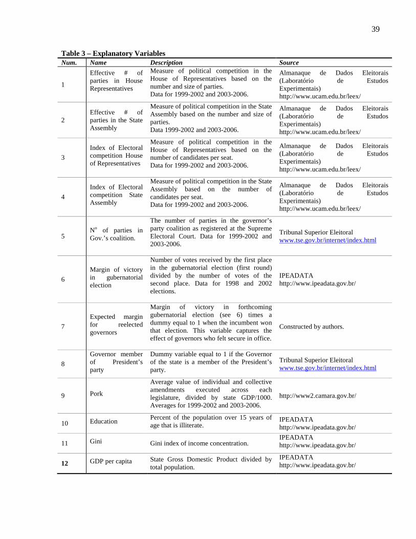
39

Table 3 – Explanatory Variables Num. Name Description Source

1

Effective # of parties in House Representatives

Measure of political competition in the House of Representatives based on the number and size of parties. Data for 1999-2002 and 2003-2006.

Almanaque de Dados Eleitorais (Laboratório de Estudos Experimentais) http://www.ucam.edu.br/leex/

2 Effective # of parties in the State Assembly

Measure of political competition in the State Assembly based on the number and size of parties. Data 1999-2002 and 2003-2006.

Almanaque de Dados Eleitorais (Laboratório de Estudos Experimentais) http://www.ucam.edu.br/leex/

3

Index of Electoral competition House of Representatives

Measure of political competition in the House of Representatives based on the number of candidates per seat. Data for 1999-2002 and 2003-2006.

Almanaque de Dados Eleitorais (Laboratório de Estudos Experimentais) http://www.ucam.edu.br/leex/

4

Index of Electoral competition State Assembly

Measure of political competition in the State Assembly based on the number of candidates per seat. Data for 1999-2002 and 2003-2006.

Almanaque de Dados Eleitorais (Laboratório de Estudos Experimentais) http://www.ucam.edu.br/leex/

5 No of parties in Gov.’s coalition.

The number of parties in the governor’s party coalition as registered at the Supreme Electoral Court. Data for 1999-2002 and 2003-2006.

Tribunal Superior Eleitoral www.tse.gov.br/internet/index.html

6

Margin of victory in gubernatorial election

Number of votes received by the first place in the gubernatorial election (first round) divided by the number of votes of the second place. Data for 1998 and 2002 elections.

IPEADATA http://www.ipeadata.gov.br/

7

Expected margin for reelected governors

Margin of victory in forthcoming gubernatorial election (see 6) times a dummy equal to 1 when the incumbent won that election. This variable captures the effect of governors who felt secure in office.

Constructed by authors.

8

Governor member of President’s party

Dummy variable equal to 1 if the Governor of the state is a member of the President’s party.

Tribunal Superior Eleitoral www.tse.gov.br/internet/index.html

9 Pork

Average value of individual and collective amendments executed across each legislature, divided by state GDP/1000. Averages for 1999-2002 and 2003-2006.

http://www2.camara.gov.br/

10 Education Percent of the population over 15 years of age that is illiterate.

IPEADATA http://www.ipeadata.gov.br/

11 Gini Gini index of income concentration. IPEADATA http://www.ipeadata.gov.br/

12 GDP per capita State Gross Domestic Product divided by total population.

IPEADATA http://www.ipeadata.gov.br/

40

Table 4 – Variables used to Create the Checks & Balances Index Num. Name Description Source

1 Regulatory Agencies

Regulatory Governance Index. Measures governance of state and federal reg. agencies in Brazil based on survey data. States with no agency at the time of the studied were set at 0.53 (avg. of other states). Data for 2004/2005.

Correa, Melo, Mueller and Pereira (2006).

2 Judiciary*

Index composed of three variables using principal component analysis: i) an efficiency index calculated through nonparametric efficiency frontiers; ii) ratio of number of cases tried over cases opened. iii) number of new cases opened per 100,000 inhabitants.

i) Swengberger, 2006, pg 79. ii) Ministério da Justiça. 2004. Diagnóstico do Poder Judiciário. iii) CNJ Indicadores Estat. da Justiça Estadual 2005, pg.278, 2004.

3 Public Prosecutors*

Index composed of three variables using principal component analysis: i) Expenditures with public prosecutors per resident; ii) Number of prosecutors per 100,000 residents. iii) Number of staff per 100,000 residents.

Sadek and Lima (2006).

4 Audit Office An index of the level of activity in each state’s Audit Office (TCE).

Melo and Pereira (2006).

5

National Justice Council (CNJ)

Number of procedures initiated in each state by the CNJ (agency that serves as a watchdog over the Judiciary) divided by state GDP (divided by 100,000). Data for 2006.

Corregedoria Nacional de Justiça. 2006

6 Media Percent of all media concession in each state are not in the hands of politicians.

Santos, S. S. e Capparelli. 2005

7 Civic Community index

An index of Civic Community in the states constructed by principal component analysis using (i) voter turnout (1990-2006), (ii) voto de legenda (1990-2006), and (iii) nonprofit sectors workers per capita (ABONG-IBGE 2002 study).

Timothy Powers.

* Variables for which there is separate data for both periods 1999-2002 and 2003-2006.

41

Table 5 – Checks & balances Index.

Num State C&B Index

1999-2002 Num State

C&B Index

2003-2006

1 Rio Grande do Sul 0.813 1 Rio Grande do Sul 1.000

2 Distrito Federal 0.775 2 Rio de Janeiro 0.728

3 Rio de Janeiro 0.684 3 São Paulo 0.684

4 Mato Grosso do Sul 0.619 4 Distrito Federal 0.671

5 São Paulo 0.569 5 Mato Grosso do Sul 0.585

6 Santa Catarina 0.555 6 Santa Catarina 0.545

7 Espírito Santo 0.530 7 Minas Gerais 0.519

8 Pernambuco 0.509 8 Espírito Santo 0.506

9 Rondônia 0.501 9 Pernambuco 0.483

10 Minas Gerais 0.426 10 Bahia 0.454

11 Bahia 0.414 11 Paraná 0.402

12 Mato Grosso 0.390 12 Goiás 0.400

13 Sergipe 0.389 13 Mato Grosso 0.377

14 Goiás 0.387 14 Sergipe 0.345

15 Paraná 0.378 15 Rondônia 0.318

16 Amazonas 0.299 16 Amazonas 0.315

17 Amapá 0.271 17 Ceará 0.258

18 Ceará 0.248 18 Amapá 0.247

19 Pará 0.227 19 Pará 0.242

20 Paraíba 0.207 20 Alagoas 0.183

21 Acre 0.198 21 Paraíba 0.161

22 Tocantins 0.189 22 Tocantins 0.159

23 Alagoas 0.186 23 Acre 0.146

24 Piauí 0.088 24 Piauí 0.059

25 Rio Grande do Norte 0.032 25 Roraima 0.049

26 Roraima 0.023 26 Maranhão 0.043

27 Maranhão 0.000 27 Rio Grande do Norte 0.029

Mean 0.367 Mean 0.367

Std. Dev. 0.222 Std. Dev. 0.240

42

Table 6 – Determinants of Governors’ Choices (1)

Civil Servant Expenditures

(%)

(2) Variation of Civil Servant Expen.

over electoral cycle

(3) Primary Deficit

(4) Health

Expenditures (% of GDP)

Checks & Balances Index

-0.231** (-2.39)

-1.250* (-1.95)

-89.222** (-2.26)

0.010*

(1.91)

Checks & Balances Index squared

58.065* (1.91)

Initial level of Civil Servant Expend. (%)

-7.352*** (-3.24)

Electoral competition in the State Assembly

0.069**

(2.63) -0.097** (-2.61)

0.008*

(1.85)

Electoral competition in the State Assembly sqrd.

-0.007**

(-2.84)

Electoral competition House of Represent.

-0.013

(-1.57) -3.584*

(-1.92) 0.012*** (3.20)

Effective number of parties in State Assembly

0.003* (2.09)

Number of parties in Governor’s coalition

0.001 (0.78)

-0.015* (1.68)

0.445** (2.11)

Margin of victory in last election (Gov.)

-0.004 (-0.73)

0.004 (1.44)

Expected Margin of victory in next election

-0.016***

(-2.93)

Governor in President’s Party -0.169** (-2.33)

3.935** (2.37)

-0.018*** (-3.35)

Lame duck Governor -0.015*

(1.73) 0.142** (2.11)

-0.008* (-1.77)

Pork (%gdp/1000) 0.0002*** (3.74)

Gini coefficient of wealth concentration

8.693* (1.75)

Gini squared -7.984* (-1.79)

GDP per capita -0.0548** (-2.36)

0.058 (0.49)

0.0.13 (1.45)

GDP -0.0001*** (-3.39)

Education -1.249* (1.87)

Period 4.063 (1.54)

43

Constant -1.650 (-1.17)

1.407** (2.24)

87.458*** (4.03)

-0.077

(-1.67)

Method Fixed Effects. 2 periods, 27

states

Fixed Effects. 2 periods, 27 states

Fixed Effects. 2 periods, 27

states

Fixed Effects. 2 periods, 27

states Periods 1999-2002

2003-2006 1999-2002 2003-2006

1999-2002 2003-2006

1999-2002 2003-2006

Observations 54 54 54 54

R-squared (within) 0.75 0.51 0.63 0.85

Notes: In parentheses, t-stats. *** indicates significant at 1%, ** at 5%, and * at 10%.

44

Table 7 – Determinants of Politicians Wealth Variation and Expenditure Efficiency

(1) Politicians’ Wealth Variation

(2) Expenditure Efficiency

Checks & Balances Index

-8.385**

(-2.12) 1.183** (2.04)

Checks & Balances Index squared

6.359* (0.102)

Initial level of Expenditure Efficiency -0.084 (-1.27)

Initial level of Wealth 0.0000 (0.66)

Electoral competition State Assembly -0.284*

(-2.44) 0.105**

(2.06)

Electoral competition House of Represent.

-0.225**

(-2.38)

Effective number of parties in the House 0.436** (2.50)

Expected Margin of victory in next election 0.698*** (2.95)

Number of Parties in Governor’s coalition -0.141** (-2.18)

Governor in President’s Party -0.160 (-0.95)

Gini 3.505

(1.35) GDP per capita 0.113

(0.53) -0.103* (-1.62)

Number of respondents/seat in Wealth variable -2.599 (-1.31)

Constant 4.34***

(2.89) -1.343 (-0.92)

Method Random Effects - 2 periods, 27 states

Random Effects 2 periods, 27 states

Periods 1999-2002 2003-2006

1999-2002 2003-2006

Observations 54 54

Hausman test for random vs. fixed effects χ2(8)= 9.17 p-value = 0.3282

χ2(6)= 4.10 p-value = 0.6636

R-squared R-sq: within = 0.4610 between = 0.2718 overall = 0.3546

R-sq: within = 0.2310 between = 0.3421 overall = 0.2803

Notes: In parentheses, t-stats. *** indicates significant at 1%, ** at 5% and * at 10%.

45

Graph 3 – Effect of Number of Parties in Gov’s Coalition on Politicians’ Wealth Variation -.

50

.51

Est

imat

ed C

oeff

icie

nt

0 .2 .4 .6 .8 1Checks & Balances

95% confidence interval

________ Effect of # of Parties in Coalition on Wealth Variation

46

Table 8 – Interaction between Political Competition Variables and Checks & Balances

I II III IV V VI

Political Competition Variable

Dependent Variable

Health Expend.

(Public Good)

Expend. Efficiency

(Public Good)

Primary Deficit

(Public Good)

Civil Servant Expend. (Private Good)

Civil Servant Expen. Var.

(Private Good)

Wealth Variation

(Personal Benefit)

Electoral competition in State Assembly

Variable’s impact: Interaction with C&B: Significant range: Level of confidence: # states sig. each period:

+ (V) Complement 0.31 – 0.55 95% 10 / 11

+ (V) Substitute 0.00 - 0.38 95% 13 / 15

No impact

+ / - (P/V)23 Comp. / Sub. 0.00 – 1.00 95% 27 / 27

- (V) Complement 0.04 – 0.38 95% 12 / 15

- (V) Substitute 0.00 – 0.38 95% 13 / 15

Electoral competition in House of Rep.

Variable’s impact: Interaction with C&B: Significant range: Level of confidence: # states sig. each period:

+ (V) Complement 0.24 – 1.00 95% 17 / 17

- (P) Complement 0.24 – 0.64 95% 15 / 15

- (V) Complement 0.28 – 0.92 95% 25 / 26

- (V) Complement 0.47 – 0.76 95% 7 / 8

No impact

No impact

Number of Parties in Gov’s coalition

Variable’s impact: Interaction with C&B: Significant range: Level of confidence: # states sig. each period:

No impact

No impact

+ (P) Complement 0.27 – 0.52 90% 10 / 10

No impact

- (V) Substitute 0.08 – 0.41 90% 14 / 13

- (V) Substitute 0.00 – 0.39 95% 16 / 15

Margin of victory in last election

Variable’s impact Interaction with C&B:

+ (P) Substitute

No impact No impact

- (P) Substitute

No impact

No impact

23 In this case the explanatory variable enters the regression including a squared term so that its impact changes as

the variable increases. At low values of electoral competition, the impact on civil service expenditures is positive, so

that it has a perverse and complementary effect. At values close to the mean it has no impact. At higher values its

impact is negative (virtuous) and it has a substitute interaction with C&B. The formulas for calculating the estimated

coefficient and standard errors were modified to account for the quadratic effect. For the correct formulas in such

cases see http://homepages.nyu.edu/~mrg217/interaction.html.

47

(Gov.) Significant range: Level of confidence: # states sig. each period:

0.16 – 0.34 90% 8 / 8

0.04 – 0.22 90% 8 / 8

Lame duck Governor

Variable’s impact: Interaction with C&B: Significant range: Level of confidence: # states sig. each period:

- (V) Substitute 0.20 – 0.33 90% 5 / 5

No impact No impact

- (P) Complement 0.27 – 0.43 90% 8 / 6

+ (V) Complement 0.31 – 1.00 95% 15 - 16

No impact

Governor in President’s Party

Variable’s impact: Interaction with C&B: Significant range: Level of confidence: # states sig. each period:

- (V) Substitute 0.00 – 0.47 95% 18 / 18

- (V) Substitute 0.00 – 0.25 90% 10 / 10

+ (V) Complement 0.17 - 0.55 90% 18 / 15

No impact

No impact

No impact

Code: + or – indicates whether the political competition variable has a positive or negative effect on the dependent variable. (V) or (P) indicates whether this is a virtuous or perverse effect. The second line in the result cells shows whether the interaction between political competition and C&B is substitute or complementary. The third line provides the range of C&B for which the estimated coefficient is statistically significant and the fifth line shows how many states are in that range for in each period 1999-2002 / 2003 – 2006. The fourth line shows the level of confidence used for inference. Note that the first three political competition variables are positively related to competition and the last three are negatively related and this information is already incorporated when labeling (V) or (P).

Appendix

Table A1 – Descriptive Statistics

Variable Period Obs. Mean Std. Dev. Min. Max.

GDP per capita 1999-2002 27 5.006 2.843 1.605 13.504

GDP per capita 2003-2006 27 5.171 2.696 1.728 12.406

Effective # of parties in the State Assembly

1999-2002 27 6.581 1.771 3.3 10.0

Effective # of parties in the State Assembly

2003-2006 27 8.026 2.034 5.2 12.5

Effective # of parties in the House of Represent.

1999-2002 27 4.656 1.393 2.5 7.4

Effective # of parties in the House of Represent.

2003-2006 27 5.359 1.652 3.2 9.5

Index of Electoral compet. House of Rep.

1999-2002 27 2.189 0.841 0.51 4.44

Index of Electoral compet. House of Rep.

2003-2006 27 3.284 1.085 0.72 5.69

Index of Electoral compet. State Assembly

1999-2002 27 3.909 2.158 1.58 11.92

Index of Electoral compet. State Assembly

2003-2006 27 4.684 2.283 1.82 12.1

Governor in President’s party. (dummy)

1999-2002 27 0.296 0.465 0 1

Governor in President’s party. (dummy)

2003-2006 27 0.111 0.320 0 1

# of parties in Gov.’s coalition.

1999-2002 27 8.111 3.994 1 16

# of parties in Gov.’s coalition.

2003-2006 27 7.259 3.789 1 14

Margin of victory in gubernatorial election

1998 27 1.849 1.161 1.01 5.01

Margin of victory in gubernatorial election

2002 27 1.459 0.363 1.012 2.512

2

Expenditure efficiency variation

1999-2002 27 0.298 0.702 -0.48 2.83

Expenditure efficiency variation

2003-2004 27 -0.051 0.176 -0.601 0.22

Expenditure efficiency in levels.

1999-2002 27 2.682 1.226 1.37 7.453

Expenditure efficiency in levels.

2003-2004 27 1.997 0.473 1.065 3.15

Education 1999-2006 27 14.786 8.267 5.178 31.238

Education 2003-2006 27 13.977 7.690 4.431 29.391

N0 state deputies in wealth var. variable

1999-2002 27 16.444 8.803 5 40

N0 state deputies in wealth var. variable

2003-2006 27 18.363 9.987 7 49

Pork per capita 1999-2002 27 56.931 131.583 0.36 675.15

Pork per capita 2003-2004 27 13.555 36.356 0 178.77

Wealth variation state assembly deputies

1999-2002 27 2.052 1.890 0.29 7.14

Wealth variation state assembly deputies

2003-2006 27 2.602 1.791 0.28 7.78

Wealth variation of a sample of all politicians

1999-2002 27 0.555 0.519 -0.247 1.474

Civil Servant Expenditures (% of revenues)

1999-2002 27 0.437 0.065 0.331 0.628

Civil Servant Expenditures (% of revenues)

2003-2006 27 0.425 0.062 0.274 0.530

Variation in Civil Servant Expenditures (% of rev.)

1999-2002 27 0.017 0.168 -0.260 0.449

Variation in Civil Servant Expenditures (% of rev.)

2003-2006 27 0.021 0.178 -0.470 0.440

Health Expenditures (% of Total Expen.)

1999-2002 27 0.116 0.041 0.051 0.219

Health Expenditures (% of Total Expen.)

2003-2006 27 0.141 0.037 0.082 0.245

Checks & Balances index

1999-2002 27 0.367 0.222 0 0.813

3

Checks & Balances index

2003-2006 27 0.367 0.240 0.029 1.00

4

Model Comparative Statistics

Let the level of checks & balances be denoted by θ, that of political competition by π, and the

social/economic effects as ψ.

i) Productivity of effort in producing public goods: EuuP (Eu ,θ, π, ψ) – This function measures the amount

of additional public good that materializes when a governor allocates a marginal unit of effort towards Eu.

We explicitly note that it is affected by both θ and π. There is no theoretical reason for expecting the signs

of these impacts to be either positive or negative. To see this consider, as an example, the impact of a

change that increases the level of political competition faced by a governor. Depending on the

circumstances, this change may lead to either more or less public good being produced from the marginal

level of effort. Note that what is under consideration here is not how much effort the governor decides to

dedicate to public goods but rather more narrowly the amount of public good that results from the

marginal level of effort, whatever the optimal level of effort for public goods may be. Suppose for

example that the increased level of political competition leads to a situation where the governor needs to

bring additional parties into his coalition. Conceivably this may make the process of proposing, approving

and implementing the legislation that generates the public good slower and more cumbersome as it

requires more negotiation within the coalition. On the other hand it may be that the presence of these new

parties in the coalition may provide more pressure for the public goods to be provided in a more timely

and more effective manner. The point is that there is no reason to suppose that π∂

∂ uEuP

will necessarily

have an unambiguous sign (the same being true for π∂

∂ rErP

.) In the same manner, improved checks &

balances may either improve or depreciate the productivity of effort in producing public goods. This

being the case, the net impact of π or θ on Eu, Er, and α will be an empirical issue, which we will test in

Section 3. Similar reasoning holds for the impact of θ on the dependent variables (see the example

below).

5

ii) Productivity of effort in producing private good: rErP (Er , θ, π, ψ) – This function is similar to that in

(i), except that it involves the governor’s productivity in producing private goods, that is, transfers to

restricted groups. Here again, although intuition may point to a negative effect of θ and π, a positive

effect is conceivable. Suppose, for example, an increase in the level of checks & balances. If the provision

of private goods requires illegal or illegitimate means, such as rigging procurement contracts to assure

certain firms are chosen, then an increase in θ will make those activities more difficult and will reduce the

governor’s productivity in providing those goods. However, in many instances providing private goods is

perfectly legal, as when governors decide to build infrastructure that benefits specific firms

disproportionately. In such cases, better checks & balances may actually make the governor more

productive by assuring that contracts and cooperation among the various agencies and organizations

involved work more smoothly. The point, analogous to that made above, is that θ∂

∂ rErP

can be either

positive or negative (the same being true for θ∂

∂ uEuP

.)

iii) The electoral response to public goods: uPV (·,θ, π, ψ) – This function measures the reaction of voters

to the provision by the governor of public goods. Here the most important factor may be ψ, as the

education level of the electorate will typically affect how public goods translate into votes. Nevertheless,

θ and π may also have an impact. More polarized electorates, for example may be less sensitive to public

goods, as there are less central voters prone to switch their votes when confronted with increased public

goods. Similarly checks & balances can affect the governors’ ability to claim credit for the provision of

public goods. One important component of checks & balances (which we explicitly include in our index

below) is the control of media by politicians. A governor that owns the main newspaper and other

communication outlets in a state can probably squeeze more votes from a given public good by better

advertising the government’s role in its provision. Here once again it is conceivable that the impacts of

political competition and checks & balances may be either negative or positive.

6

iv) The electoral response to private goods: PrV (·,θ, π, ψ) – This function is similar to (iii) except that it

involves the impact of private rather than public goods on voters. The governor has an incentive to

provide private goods to interest groups. However, the policies that transmit those private goods are

perceived by the voters and affect the way they vote. Generally we would expect that policies providing

private goods would reduce the votes received by the governor, though that need not necessarily be so. A

culture of ‘rouba mas faz’ (approving politicians that steal but get things done), for example, would

mitigate the negative impact of private good provision on votes received by the governor. Whatever the

case, the governor will take into account the voters’ preferences regarding the policies aimed at private

groups. The same comments as in (iii) apply concerning the signs of the impacts of θ and π on electoral

response.

v) The marginal utility of votes to the governor: UV(·,θ, π, ψ) – This function measures the value given by

the governor to additional votes. Clearly the level of political competition, π, is an important determinant

of this value. Governors in states with lower levels of contestability, dominated by their own political

group, will attach a smaller value to marginal votes, that is, lower UV. Similarly, if a governor is in the

first or second term (lame duck) will affect how badly he needs more votes. Checks & balances may also

affect the governor’s utility from additional votes, and this impact, as before, may be either positive or

negative. A lower θ, for example, may imply a greater ability to rig ballots in certain areas, so that the

governor will have less need for the authentic votes, which have to be obtained through public goods and

costly campaign propaganda (thus a positive relation between θ and UV). Alternatively, a higher θ makes

it harder for a governor to appropriate public funds, and by making the spoils of office less attractive

reduces the utility of additional votes. As before, the final word on the net impact of θ and π will be an

empirical test.

vi) The productivity of private policies in generating resources: rPR (·,θ, π, ψ) - An important element of

the model is that governors are rewarded with resources for providing private goods. How much marginal

resources a governor receives in exchange for additional private goods is clearly affected by all three

7

parameters. Lower political competition may give the current governor greater monopoly power in the

provision of public goods and thus induce a higher price to be paid. Checks & balances affect how easy or

hard it will be to realize those transfers, which may be both legal and illegal. The level of education may

have on impact on voter’s perception of the legitimacy of campaign contributions. As before, though

there are typically intuitive notions of the directions of all these impacts, they can conceivably go either

way, and which will prevail, on average, will be an empirical issue.

vii) The voters sensitivity to electoral campaigns: VR(·,θ, π, ψ) – This function measures the electorate’s

sensitivity to campaign propaganda. This can be thought of as Denzau and Munger’s (1986) continuum

between rationally ignorant to ‘civics class’ voters. In states with more highly educated voters the same

amount of resources used in the electoral campaign yield less votes (lower VR). Both θ and π affect the

amount and quality of information received by voters and can thus affect their response. Again the sign of

the impact is indeterminate. For example, whereas some forms of political competition may lead to better

information being provided to voters, other forms may degenerate into negative campaigning which

confuse and repulse voters.

viii) The marginal utility of money in pocket (rather than in the campaign) for the governor UM(·,θ, π, ψ)

– A marginal unit of money appropriated by the governor provides him with additional utility, however

the size of this increase depends on all three parameters. Better checks & balances, for example, may

reduce the marginal utility of money if detection and prosecution become more probable with a higher θ.

On the other hand better checks & balances may make money more valuable as resources may be

necessary to defend oneself against prosecution once out of office, when immunity expires. Similarly,

more political competition may make money more or less valuable, depending whether the strategy

against competitors relies primarily on higher campaign resources (e.g. more propaganda) or on tactics

that rely instead on other instruments (e.g. bribes).

It is possible to perform comparative static analysis on the equilibrium conditions in equations (2), (3) and

(4), in order to get an expression that shows how each of the dependent variables, Eu, Er and α are

affected by changes in the parameters θ, π, and ψ, which is the objective of the paper. However, because

8

this involves a system of four dependent variables (including λ) in which the parameters appear in many

different places and without predetermined signs for the impact of these parameters on the various

functions involved, the signs of the expressions for κ∂

∂ uE,

κ∂∂ rE

and κα

∂∂

, ∀ κ = θ, π, and ψ, are all

ambiguous and no clear prediction can be made.