1

The Long-Term Effects of Price Promotions

on Category Incidence, Brand Choice and Purchase Quantity

Koen Pauwels

Dominique M. Hanssens

S. Siddarth1

January 11, 2002

1Koen Pauwels is Assistant Professor at the Tuck School of Business at Dartmouth (e-mail:koen.pauwels@dartmouth.edu). Dominique M. Hanssens is the Bud Knapp Professor ofManagement at the Anderson Graduate School of Management, University of California LosAngeles (e-mail: dominique.hanssens@anderson.ucla.edu). S. Siddarth is Associate Professorat the Marshall School of Business, University of Southern California (e-mail:siddarth@usc.edu). The authors thank A.C. Nielsen for the data used in this study, ScottNeslin for the storability and impulse scales and Bart Bronnenberg for valuable suggestions.The constructive comments of the editor and three anonymous Journal of Marketing Researchreviewers were helpful in strengthening this paper.

2

The Long-Term Effects of Price Promotions onCategory Incidence, Brand Choice and Purchase Quantity

To what extent do price promotions have a long-term effect on the components of brand sales,

i.e. category incidence, brand choice and purchase quantity? This paper answers this question by

using persistence modeling on weekly sales data of a perishable and a storable product derived

from a scanner panel. We test each sales component for permanent changes in its time series, and

for whether these changes are due to price promotions. The tests reveal that the components of

brand sales are predominantly stationary or mean-reverting, so that permanent effects of price

promotions are virtually absent.

Absence of permanent effects does not mean, however, that the dynamic effects of price

promotions are negligible. For those component series that are stationary, we develop and apply

an impulse response approach to estimate the promotional adjustment period, i.e. the length of

time for the dependent variable to revert to its mean after being shocked by a price promotion.

We combine this measure with the total effect of a price shock on each sales component to

obtain a complete account of the temporal effects of promotions on category incidence, brand

choice and purchase quantity. Specifically, we calculate the long-term equivalent of Gupta’s

(1988) 14/84/2 breakdown of promotional effects. Because of positive adjustment effects for

incidence but negative adjustment effects for choice, we find a reversal of the importance of

category incidence and brand choice: 66/11/23 for the storable product and 58/39/3 for the

perishable product. We discuss the implications of our findings and suggest some areas for future

research.

3

1. Introduction

Since the early seventies, price promotions have emerged to account for the main share of the

marketing budget in most consumer packaged goods categories (Currim and Schneider 1991),

and a substantial body of academic research has established the nature of short-term sales

response to temporary price reductions. While some recent work has examined the long-term

effects of price promotions, this area is still “probably the most debated issue in the promotional

literature and one for which the jury is still out” (Blattberg, Briesch and Fox 1995, p. G127).

Any study of long-term effects needs to carefully define and operationalize the long run. In

this respect, academic research has proceeded along three research streams, each with different

methodologies and findings. First, Mela, Gupta and Lehmann (1997), Mela, Jedidi and Bowman

(1998) and Jedidi, Mela and Gupta (1999) examine how promotions change consumers’ price

and promotional sensitivity over time. The first paper considers brand choice, the second paper

category incidence and purchase quantity and the third paper brand choice and purchase quantity.

This stream of research defines “long term” as “the cumulative effect on consumer brand choice,

lasting over several years” (Mela et al.1997, p.249) and examines this effect with a distributed-

lag (Koyck) response model. The key findings are that, as a result of repeated promotional

activity in a category, category incidence decreases but purchase quantity increases. Moreover,

promotions increase consumer price sensitivity and decrease “brand equity” over time. Overall,

these studies confirm the existence of a negative ‘promotion usage effect’ on consumer behavior

(Blattberg and Neslin 1990).

A second research stream confirms the positive ‘mere purchase effect’ of promotions.

Ailawadi and Neslin (1998) find that promotions induce consumers to buy more and consume

faster. They examine both a spline function and a continuous function to model flexible category

consumption rates as a function of household inventory. The key finding is that promotion-

induced inventory buildup temporarily increases usage rates. Ailawadi, Lehmann and Neslin

(2001) examine market share response to a long-term change in the marketing mix (Procter &

Gamble’s Value Pricing Strategy). They define deal activity as the percent of yearly brand sales

sold on deal. This variable has strong positive effects on market share in a multiplicative

response model, and the authors conclude that P&G’s loss of market share was “attributable to

its severe cuts in coupons and deals, and the consequent increase in net price” (p.55).

4

While both research streams model dynamic effects of price promotions, they can only

capture transient, not enduring effects because they assume mean reversion of the dependent

variable. First, the Koyck model in Mela et al. (1997) assumes that a fixed fraction 0 < λ < 1 of

the effects in one period is retained in the next period. Since limn→∞ λ n = 0 , this model implies

that the dependent variable eventually returns to its historical mean. Second, both flexible

functions in Ailawadi and Neslin (1998) imply that consumption rates return to their average

levels as the excess inventory depletes. Finally, the multiplicative response model in Ailawadi et

al. (2001) also assumes mean reversion of the sales components. Therefore, these models do not

give a complete account of the long-term effects of price promotions on sales.

A third stream of research uses persistence modeling to capture the potential for permanent

effects of promotions (Dekimpe, Hanssens and Silva-Risso 1999). First, sales are classified as

stationary or evolving. When sales are stationary, they eventually return to their pre-promotion

mean. In this scenario, promotions can impact sales immediately and over the next several weeks

(the adjustment period), but not in a permanent way. In contrast, when sales are evolving, they

do not have a fixed mean, and therefore could (but need not) be permanently affected by

promotions.

Dekimpe et al. (1999) apply persistence modeling to 4 product categories and use impulse-

response functions to estimate permanent versus transitory effects of promotions on sales. A key

finding of their research is that permanent effects of promotions are largely absent. This implies

that promotions do not structurally change sales over time, and that their long-run profitability

depends only on the magnitudes of response and cost parameters. However, it is possible that the

absence of permanent promotion effects on sales is due to cancellation of permanent effects in

the three components of brand sales, i.e. category incidence, brand choice and purchase quantity.

For example, the use of promotions can train consumers to buy higher quantities on fewer

occasions (Mela et al. 1998). Such a long-run scenario could be attractive to brand managers,

because the higher inventory keeps the consumer out of the market for competitive products, but

unattractive to retailers because consumers now need fewer store visits (Bell, Chiang and

Padmanabhan 1999). At present, no study has examined the total over-time impact of price

promotions on all three sales components.

5

In terms of quantification of promotion effects, several studies break down the immediate

impact on incidence, choice and quantity. Gupta (1988) found a 14/84/2 breakdown in the

coffee market, while Bell et al. (1999) analyzed 13 categories and reported an average

breakdown of 11/75/14. Does a similar decomposition of promotional effects hold in the long

run ?

This study uses persistence modeling to examine whether, and to what extent, price

promotions have a long-run impact on the three components of brand sales. Based on a scanner

panel, we compute for each store, category incidence (the total number of panelists buying in the

product category), brand choice (the share of these consumers buying the brand) and purchase

quantity (the average quantity purchased by the brand’s consumers). For each component, we

test for permanent changes in the time series and examine whether such changes are due to the

price shocks of the major brands in this store. Furthermore, for component series that are found

to be stationary, we apply an impulse-response approach to estimate the time it takes for the

dependent variable to revert to its mean, after being shocked by a price promotion. Finally, we

quantify the total over-time impact of a price promotion on each sales component, and calculate

the breakdown for the immediate and the total effects. Therefore, this study is the first to

quantify total promotional effects as the sum of immediate, adjustment and permanent effects on

each sales component. This enables us to compare and contrast the relative importance of the

three components of promotional effectiveness in the short run and the long run.

The remainder of the paper is organized as follows. Section 2 defines the time windows of

promotional effects on the three sales components and reviews previous studies in this

framework. Section 3 develops hypotheses on the impact of promotions on category incidence,

brand choice and purchase quantity. Section 4 describes our methodology and data. The findings

for a storable product (canned soup) and a perishable product (yogurt) are presented in Section 5.

Section 6 concludes with the managerial implications and limitations of this work, and offers

directions for future research.

6

2. The time frame of promotional effects on three sales components

We classify previous research on promotional effects on two dimensions: a) the time frame in

which the promotional impact on sales is measured, i.e. immediate effects, adjustment effects

and permanent effects1 and b) the type of purchase behavior studied, i.e. category incidence,

brand choice, and purchase quantity.

The immediate effects of price promotions are reflected in short-term (contemporaneous)

changes in sales. Most previous research falls in this category and reports consistently high

promotional effects (Blattberg et al. 1995; Blattberg and Neslin 1990).

The adjustment effects of promotions refer to the transition period between the short-term

response and the resulting equilibrium, which can be either mean reversion or a new sales level.

These adjustment effects can be positive or negative, and their sign and magnitude greatly

impact the overall profitability of the promotion (Blattberg and Neslin 1990; Greenleaf, 1995).

Dynamic effects are modeled through, among others, purchase loyalty (Guadagni and Little

1983), reference price (e.g. Lattin and Bucklin 1989), inventory (e.g. Gupta 1988), time-varying

parameters (e.g. Papatla and Krishnamurthi 1996; Mela et al. 1997) and flexible usage rates

(Ailawadi and Neslin, 1998). Several studies equate these adjustment effects with long-term

effects. Indeed, the implicit assumption underlying distributed lag models (e.g., Mela et al. 1998)

is that the impact of marketing effort dies out over time. While this operationalization allows

promotions to have more than a contemporaneous influence on sales, it ignores the more

complex “permanent” changes found in many sales series (Dekimpe and Hanssens, 1995b).

Finally, permanent effects of a marketing action require that a proportion of the event’s impact

is carried forward and sets a new trend. If the sales series is evolving, with no fixed mean, then

the permanent effects of marketing efforts can be captured by relating these efforts to the

evolution of sales. These permanent effects are the focus of our first research question, as their

analysis provides a necessary first step for a complete account of the long-term impact of price

promotions on sales.

1 Our terminology is based on the time-series literature and will be used throughout this paper. Previous authorsintroduced alternative terms that fit our framework: effects are either contemporaneous (immediate) or dynamic(long term), which could be transient (adjustment) or enduring (permanent).

7

Recent disaggregate models in the marketing literature (Chiang 1991; Chintagunta 1993;

Bucklin et al. 1998) also distinguish the brand-sales components of category incidence, brand

choice and purchase quantity. For retailers, price discounts mainly serve to create store traffic

and to increase category sales (Putsis and Dhar 1999). Therefore, promotions lose their attraction

if the immediate gains in category incidence and quantity are offset by negative effects during

the off-promotion weeks. For manufacturers, the over-time impact on brand choice is the most

important metric. In the current study, we analyze the dynamic effects of price promotions on

time series of all three sales components. Specifically, we compute the total number of panelists

buying in the product category (category incidence), the share of these consumers buying a

particular brand (brand choice) and the average quantity purchased by the brand’s consumers.

This breakdown, which is calculated separately for each store in the sample, allows us to

compare results from the time-series analysis of the three sales components with the findings

from disaggregate analyses that apply this distinction. Table 1 summarizes previous research on

promotions along the two dimensions of time frame and type of data.

Three inferences from Table 1 provide the motivation for the current study. First, empirical

evidence on permanent effects of price promotions is virtually non-existent (Dekimpe et al.

1999; Nijs, Dekimpe, Steenkamp and Hanssens 2001). Second, none of these studies considers

the breakdown of sales in category incidence, brand choice and purchase quantity. Third, all

previous persistence modeling has focused on market level data, whereas managers often need

analysis at the account or store level (Bucklin and Gupta 1999). We seek to fill this void by

studying the permanent, adjustment and immediate effects of price promotions on each of the

different sales components for each store in our scanner panel data set.

3. Hypothesis development

Consistent with our framework, we first develop hypotheses on the temporal dimension of

promotional effectiveness. In particular, we focus on the sign and magnitude of the total

promotional impact on the sales components. Table 2 summarizes our hypotheses on the

immediate, adjustment, permanent and total effects of price promotions for storable and

perishable products. Our hypotheses on the length of the adjustment period are more tentative,

as this topic has not received much attention in the context of price promotions.

8

3.1. Immediate effects of price promotions

Promotions cause a substantial immediate increase in all three sales components (Blattberg et

al. 1995; Bell et al. 1999). The economic rationale is clear: temporary price reductions increase

the value of the product to the consumer and require immediate action. The marketing literature

distinguishes different consumer behaviors that contribute to the immediate sales boost

(Blattberg and Neslin 1990). Category incidence increases due to timing acceleration (purchasing

earlier), impulse purchases and category switching (substituting purchases between categories).

Brand choice benefits from consumers switching to the promoted item. Finally, purchase

quantity benefits from quantity acceleration (forward buying) and stockpiling behavior. As for

the relative magnitude of the promotional effect, Bell et al. (1999) report an average elasticity

breakdown (incidence/choice/quantity) of 3/75/22 for storable products and 17/75/8 for

perishable products. Our first hypothesis is therefore:

H1: The immediate promotional effects are higher for brand choice than for the other two sales

components.

3.2 Adjustment effects of price promotions

We distinguish three reasons for adjustment effects: 1) dynamic consumer response,

including the post-deal trough, the mere purchase effect and the promotion usage effect, 2)

competitive reaction and 3) performance feedback.

The post-deal trough logically follows from timing and quantity acceleration. Given their

larger stock, consumers will reduce their purchases in subsequent weeks. Interestingly however,

the empirical evidence on post-deal troughs in brand sales is mixed (Blattberg et al. 1995). On

the one hand, Blattberg et al. (1981), Neslin et al. (1985), Leone (1987), Jain and Vilcassim

(1991) and Van Heerde et al. (2000) report post-deal troughs. On the other hand, Grover and

Srinivasan (1992) and Vilcassim and Chintagunta (1992) find no post-promotion dips. Litvack,

Calantone and Warshaw (1985) consider several categories and do not observe a post-promotion

dip for the categories that could experience purchase acceleration. Moriarty (1985) finds

significant post-promotion dips for only 3 out of 15 cases, by including one-week lagged

promotion variables in the sales-response function. As a general rule, the post-deal trough

appears small in comparison with the immediate sales increase (Abraham and Lodish 1987).

9

The mere purchase effect holds that promotion-induced purchases increase future sales

(Blattberg and Neslin 1990). Three behavioral theories could account for this effect. First,

learning theory holds that promotions offers a risk premium for trial by new consumers, some of

whom will like the product and repurchase it in the future (Mela et al. 1997). Second, promotions

remind existing consumers to buy the brand and reinforce their tastes for it (Erdem 1996). Both

theories imply benefits for both category incidence and brand choice. Finally, promotions induce

consumers to buy in larger quantities (stockpiling), which can increase their consumption rates

(Chandon and Wansink 1997; Ailawadi and Neslin 1998).

The promotion usage effect concentrates on the impact of promotions on consumer

perceptions. First, self-perception theory (Bem 1967) implies that consumers are likely to

attribute their purchase to an external cause (taking advantage of a promotion) instead of an

internal cause (e.g. brand liking). Second, price perception theory holds that consumers form a

reference price for the brand based on past prices (Kalyanaram and Winer 1995). This reference

serves as an internal standard against which current prices are compared (Helson 1964).

Promotions lower the reference price, making consumers reluctant to buy the brand at all in non-

promotion periods (Lattin and Bucklin 1989). Finally, object perception theory (Blattberg et al.

1995) postulates that promotions will damage the brand’s quality image.

Given the opposite directions of the mere purchase effect versus the post-deal trough and the

promotion usage effect, the net impact of promotions on dynamic consumer response remains an

empirical puzzle in marketing literature. Early research reported positive total effects on brand

choice and sales (Guadagni and Little 1983; Blattberg and Neslin 1990; Davis et al. 1992),

whereas later studies reported predominantly negative dynamic effects (Mela et al. 1998; Jedidi

et al. 1999).

In addition to dynamic consumer response, competitors may react to the focal brand's

promotion (Leeflang and Wittink 1992; 1996). The impact of competitive reaction should differ

for brand choice versus incidence. For brand choice, we expect competitive reaction to hurt the

focal brand (Bass et al., 1984). In contrast, category incidence should benefit from promotional

reaction by competitors in the same category (Putsis and Dhar 1999). If the focal brand's

promotion attracts consumers to the category, so should the competitive promotions.

Finally, performance feedback and company decision rules may lead to repetition of

marketing actions that were considered successful (Dekimpe and Hanssens 1995a; 1999).

10

Therefore, a successful promotion can increase future promotional activity. Promotional

effectiveness may either benefit from this reinforcement, or suffer as consumers adjust to a

higher level of promotional activity (Assunςao and Meyer 1993; Krishna 1992; 1994).

In summary, the net adjustment effects of price promotions could be positive or negative

and will differ for the three sales components. For category incidence, both the mere purchase

aspect of dynamic consumer response as well as competitive reaction and performance feedback,

yield positive effects, whereas the timing acceleration and promotion usage aspect of consumer

response yields negative effects. As a net result, we predict positive adjustment effects for

category incidence. In contrast, brand choice has been found to suffer from post-deal trough,

promotion usage effects and competitive reactions. Therefore, we predict negative adjustment

effects. Finally, average purchase quantity is negatively affected by quantity acceleration but

positively affected by timing acceleration. Neither direction has strong empirical support.

H2: The adjustment effects are a) positive for category incidence, b) negative for brand choice.

3.3 Permanent effects of price promotions

With the exception of the post-deal trough, all the above dynamic effects could be permanent

in nature. First, the mere purchase effect may persist if promotion-induced trial results in repeat

purchase (Blattberg and Neslin 1990). However, this phenomenon is most likely to occur for

new-product categories and for new consumers in the geographic area or in the store (Gijsbrechts

1993). Any impact would be small for mature products (Mela et al. 1997). Second, the

promotion-usage effect may persist if consumers continue to associate the brand with the

negative perception of the promotion. Again, such a permanent phenomenon is unlikely.

Moreover, existing models of dynamic choice, including inventory management, predict that

sales will eventually return to their pre-promotion level (Assunςao and Meyer 1993; Krishna

1992; 1994). Finally, competitive reactions to the promotion typically die out over time, with the

rare exception of a discount that escalates into an all-out price war. In summary, permanent sales

effects by promotions seem unlikely in mature product categories.

Empirical studies investigating permanent promotional effects are scarce, because most

models assume mean-reverting behavior. Dekimpe, Hanssens and Silva-Risso (1999) report

positive permanent effects for one brand’s promotions in one out of four category sales series.

11

Nijs et al. (2001) find evolution in category demand in only 36 out of 560 product categories

(6.5%) of their Dutch data set. Three percent of product categories experience a positive

permanent impact, one percent a negative permanent impact. In other words, permanent effects

of promotions on category sales are the exception rather than the rule. In both studies however,

the absence of permanent effects could be caused by the cancellation of positive effects on one

sales component by negative effects on the other. For instance, inventory management changes

could persist, resulting in lower incidence but higher purchase quantity levels. Within a mean-

reverting model, Mela et al. (1998) find that increased expectations of future promotions reduce

the likelihood of category incidence and increase purchase quantity, given incidence. The present

study is the first to empirically investigate whether the assumed absence of permanent

promotional effects holds for a storable and a perishable product. We expect to find that

H3: Permanent effects of promotions are absent for all sales components.

3.4. Total effects of price promotions

Whereas the time frame of promotional effects may be of some interest to practitioners, their

major question is: what is the total over-time impact of the price promotion I am planning to run?

As discussed above, both the immediate effects and the adjustment effects are expected to differ

for each sales component. Therefore, our hypotheses on the total promotional impact logically

follow from hypotheses 1-3. First, we expect a positive promotional impact on all three sales

components. In other words, negative adjustment effects will not completely cancel out the

positive immediate impact (Ailawadi and Neslin 1998; Jedidi et al. 1999). However, the different

signs of the proposed adjustment effects for incidence and choice will greatly affect their relative

magnitude in the total effect decomposition. Whereas the immediate benefits for brand choice

are largely reduced in the adjustment period (Jedidi et al. 1999), we expect positive adjustment

effects to enhance the category incidence hike. Therefore, the empirical generalization that price

promotions have the largest immediate impact on brand choice (Bell et al. 1999), will not hold

when the total effect horizon is considered. Instead, we expect category incidence effects to

dominate the total promotional impact. The relative importance of quantity effects should depend

on product storability. For their storable product, Jedidi et al. (1999) report larger total effects for

purchase quantity than for brand choice. We expect the opposite ordering for perishables, which

12

are difficult to stockpile and therefore less likely to yield increased consumption. Thus our

hypotheses are:

H4: The total promotional impact is positive for all sales components.

H5a: The total promotional effects are higher for category incidence than for the other two

sales components.

H5b: For storable products, the total promotional impact is higher for purchase quantity than

for brand choice.

H5c: For perishable products, the total promotional impact is higher for brand choice than for

purchase quantity.

Product storability may also influence the magnitude of total effects compared to other

categories. Bell et al. (1999) find that immediate effects on all sales components are larger for

storable products than for perishables. In the long run, we see no theoretical rationale for this

phenomenon for category incidence and brand choice. In contrast, purchase quantity effects

should depend on product storability, as consumers are more flexible in their quantity decisions

when it is easy to stockpile the product. Therefore,

H6: The total promotional impact is larger for storable products than for perishables on

purchase quantity only.

3.5 The time window of promotional adjustment

Advertising research has long developed an interest in estimating the time window of

advertising carry-over effects on sales. Leone (1995) concludes that 90% of the effects of

advertising on sales die out within 6 to 9 months. In contrast, the promotional literature has been

surprisingly vague about the duration interval of promotional effects. The two exceptions are the

studies by Mela et al. (1997; 1998), who report intervals of, respectively, 33 weeks and 21 weeks

and conclude that promotions have a ‘slightly less enduring effect’ compared to advertising.

However, these findings may be specific to the non-food product under study, and to the

assumption of exponential decay of promotion effects.

13

In contrast to advertising, price promotions are tools for generating immediate sales (Blattberg

and Neslin 1990). We therefore expect that promotional effects die out soon, i.e. within the

standard short-term management planning horizon of one quarter. Moreover, the exponential

decay assumption in the Koyck model is less appropriate for promotional adjustment effects,

which may include both positive and negative coefficients. In our framework, the adjustment

period refers to the number of weeks between the short-term response and the long-run

equilibrium. In the absence of permanent effects, this period corresponds to the number of weeks

with adjustment effects that are significantly different from zero.

The length of the adjustment period may depend on the sales component and on product

storability. As for the former, there is no previous literature that can generate a priori predictions.

As for the latter, product storability enables rational consumers to sharply adjust their quantity

decisions to the promotional pattern in the category (Assunςao and Meyer 1993). For a

substantive period after the promotion, these consumers will not return to their previous quantity

levels. For perishables, quantity effects are necessarily short-lived because of consumer

stockpiling limitations. Therefore, we expect the storable products to show longer quantity

adjustment periods than perishable products. In conclusion,

H7a: For each sales component, promotional effects die out within a quarter (13 weeks).

H7b: The quantity adjustment period is longer for storable products than for perishables.

4. Methodology and data description

4.1 Overview

Three steps are necessary for the assessment of the long-term impact of price promotions on

the dependent variables (Dekimpe and Hanssens 1995; Bronnenberg et al. 2000). First, unit-root

tests identify whether or not there is evolution in the data-generating process of the variables. If

evolution is detected, then cointegration analysis determines whether a long-run equilibrium

exists between the series of the dependent variable and the independent variables of interest. In

that case, a vector-error correction (VEC) model is estimated, otherwise a vector-autoregressive

(VAR) model in differences is specified. Finally, impulse-response and multivariate persistence

estimates visualize and quantify the long-term impact of price shocks.

14

If the unit-root tests fail to identify evolution, we conclude that the time series are stationary,

they return to their mean (or a deterministic trend) after the effects of a shock have died out. In

that case, vector-autoregressive models are estimated on the levels of the data, and the

coefficients of the impulse response functions can be used to compute the finite total effect of

promotions, as well as the length of the promotion-response (adjustment) period.

4.2 Data description

Our dataset is constructed from the A.C. Nielsen household scanner data in the Sioux Falls

market (South Dakota) for the period 7/14/1986 until 9/5/1988. These data have been made

available through the Marketing Science Institute and have been widely used in the marketing

literature. Based on the above discussion on product storability, we consider canned soup, a

storable product that is not generally bought on impulse, and yogurt, a perishable product that is

often bought on impulse (Narasimhan et al. 1996). The number of consumers in the panel is 2399

for yogurt and 1826 for soup. Total consumption is 690780 oz for yogurt and 539116 oz for

soup. The consumption average is 288 oz for yogurt and 295 oz for soup.

To prepare the scanner data for time series analysis, we first compute the number of

consumers and the total number of ounces sold per brand and per store. We then select the

brands that occupy the major positions in the market (more than 80% for both categories), and

the 5 best selling stores, provided they belong to different chains. This procedure resulted in 4

stores, each with 3 soup brands (two national brands and one private label) and 3 stores, each

with 5-6 yogurt brands (4 national brands and 1-2 private labels). Table 3 describes the average

market shares, prices2 and promotional activities. As the VAR approach requires equally-spaced

time series, we transform the purchase-occasion based scanner data into weekly ratio-scaled data

on the store level. In particular, we compute the weekly number of panelists who made a

purchase in the category (category incidence), the fraction of these consumers who bought the

brand (brand choice3) and the average quantity per purchasing consumer. Although some

aggregation bias might result from this procedure (Pesaran and Smith 1995), the fact that all

consumers are exposed to the same marketing-mix variables, that the brands are close

2 We obtained SKU market shares from separate store sales information over the full period. These full periodmarket shares then served as weights to aggregate SKU-level prices to brand-level prices.3 Because choice share is a limited dependent variable, the normality assumption on its error term may not hold. Wetherefore perform our analysis using choice = share/(1-share) as a dependent variable.

15

substitutes, and that the price distribution is not concentrated at an extreme value, greatly reduces

this bias (Allenby and Rossi 1991). Separate analyses for each store provide variability in the

pricing and promotional pattern of the same brand in different retailer settings.

4.3 Unit-root testing of the sales components and prices

The Augmented Dickey-Fuller test is performed for each series in several versions (see

Dekimpe, Hanssens and Silva-Risso 1999 for details). First, we decide on the number of lags to

include in the test by the Schwarz Bayesian Information Criterion and by the maximum lag for

which the regression coefficient is significant. Schwarz’s Bayesian Information Criterion (BIC)

is designed to consistently estimate the lag structure as a uniform criterion that minimizes the

sum of squared errors while taking model complexity into account. In order to assess the

robustness of this procedure, we also performed the tests using the number of statistically

significant lagged terms as the criterion for lag selection. Except for a few series, test

conclusions were identical. In comparison with the maximum significant lag criterion,

minimization of the BIC has the additional advantage of model parsimony, since fewer lags will

be included. Second, we account for structural breaks in the data, such as the two new-product

entries in the yogurt category. We incorporate these potential breaks in the unit-root test and in

the vector-autoregressive model estimation.

Before we proceed with estimating VAR models, we also need to investigate whether a unit

root is present in prices. For the yogurt category, prices are mean-stationary with a few

exceptions due to two new-brand entries. When accounting for these interventions by dummy

variables, these cases test as stationary as well. Prices in the soup market are trend-stationary, i.e.

they become stationary after removing a positive trend, possibly due to inflation.

4.4 Specification of vector-autoregressive models

The order of the VAR models is based on Schwarz’s Bayesian Information Criterion. For all

our series, either a first-order or a second-order VAR was selected. In order to facilitate

comparison across brands and stores, we proceed by estimating a second-order VAR for all

series. Such a second-order VAR model for a store with 3 brands is presented in Figure 1.

Stationary variables are included in levels, difference-stationary variables in differences and

16

trend-stationary variables in detrended levels. When two or more variables are evolving, we also

test for cointegration using the Johansen Likelihood Ratio (trace) test.

An important decision is which variables to include in the VAR estimation, and whether to

treat them as endogenous or exogenous. The simple base model, as depicted in Figure 1, features

the three response variables for the focal brand and the prices of all brands in the market as

endogenous variables, and feature and display of all brands as exogenous variables. The

treatment of prices as endogenous implies that lagged effects of the performance variables

(performance feedback) and competitor prices (competitive reaction) are accounted for. Feature

and display are treated as control variables with contemporaneous effects on the response

measures. The contemporaneous effects among the endogenous variables are modeled through

the residual covariance matrix (Lü tkepohl 1993).

Modeling assumptions for tractability include independent errors for each brand and for each

sales component. Specifically, the estimation of a VAR-model for each brand implies that choice

share errors are assumed independent and that category incidence effects are estimated separately

for each brand. Even for this relatively simple model, the second-order VAR-model estimates 2 *

(3+n)2 φ-coefficients, with n being the number of brands.

A first extension of the base model is the inclusion of feature and display as endogenous

variables, because they too can display dynamic effects (Papatla and Krishnamurthi 1996).

Although feature and display are not the focus of our research, we validate our results by

estimating the extended model and reporting the correlation of estimated promotional effects.

Second, the functional form of the depicted model is linear in incidence, choice and quantity,

similar to previous models in this research stream (Dekimpe et al. 1999). An alternative

specification is the multiplicative model, yielding linear equations after taking logarithms.

Compared to the constant elasticity of the log-log model, the linear model yields an elasticity that

is increasing in price. The implied decreasing returns to price promotions are intuitive, given our

promotional definition. An unexpected, one-standard deviation error shock to price will yield

increased consumption (i.e. will in all likelihood cross the threshold of being noticed and acted

upon by some consumers). However, doubling this promotional depth will not result in twice the

effect of the lower discount, because of limits to increases in all three sales components.

Incidence gains are limited by the number of consumers considering buying into the category.

Choice-share gains are limited by hard-core loyals for the other brands. Quantity gains are

17

limited by storability and inventory carrying costs. By means of flexible parametrization

methods, Van Heerde et al. (2000b) recently found that most promotions indeed show decreasing

returns to the magnitude of the discount. The authors conclude that "test results indicate that the

assumption of constant elasticities is untenable" (p.28) and that "one possible interpretation is

that consumers tend to switch at relatively low price discount levels, and that higher price

discounts do not result in much further switching" (p. 27). For these reasons we use a linear

specification, and we validate our results by applying the log-log model and examining the

correlations between the parameters of the two models.

4.5 Impulse- response functions

The selected VAR models are used to simulate the over-time effects of one-standard-

error price shocks on the system, using impulse-response functions. This method yields estimates

of the incremental effect of the price promotion on the response variable relative to its baseline4.

The impulse-response function is calculated from an initial shock, which requires the

specification of a causal ordering of the contemporaneous shocks (see Dekimpe and Hanssens

1999 for a detailed discussion). We shock brand price first, allowing for contemporaneous

effects on competitive prices and the response variable (category incidence, brand choice, or

purchase quantity)5. Given that the marketing data are weekly, this ordering is meaningful

because firms need time to react to competitive price promotions or demand fluctuations

(Leeflang and Wittink 1992). Our simulation only excludes instant price reactions of the focal

brand to competitive-price or performance shocks.

4.6 Operationalization of the promotional effects

In the framework of the impulse-response functions derived from our VAR model, the

immediate promotion impact is the effect of a one-standard-deviation price shock on the

response variable (for previous applications of this operationalization, see Dekimpe et al. 1999

and Srinivisan et al. 2001). Note that this immediate effect is captured by the residual correlation

matrix, as contemporaneous price does not directly appear in the regression equation for the

4 For stationary series this baseline is the mean value of the full time series and for evolving series it is the lastobservation of the time series.5 Note that this simulation is numerically equivalent to the simultaneous-shocking approach used in Dekimpe &Hanssens (1999), provided the focal variable is shocked first.

18

response variable. The sign (negative for own price, positive for cross-price effects) and

magnitude of the immediate effect provides a validity check on our findings.

We operationalize the total effects of a price promotion as the sum of all impulse-response

weights with a t-statistic greater than one in absolute value (Dekimpe et al. 1999). Since this

generous cutoff-point translates into wide confidence intervals, we focus on the sign and relative

magnitude of total effects. The length of the adjustment period is operationalized as the number

of weeks it takes to observe 90% of the significant impulse-response weights. We test the

corresponding hypothesis for both product categories by computing the average adjustment

period for each sales component, weighted by category sales share for each store.

Finally, the decomposition of promotional effects requires several choices. First, we need a

common scale to compare the promotional impact on the three sales components. In order to

facilitate a comparison with previous literature, we choose to compute elasticities. To that end,

we write brand sales as:

Brand Sales i (S) = # Category Consumers (I) * Share of consumers for i (C) * Average purchase quantity i (Q)

Therefore, assuming independence among the three components, we write incremental sales as:

In this equation the change in demand on the total number of consumers (incidence) is

weighted by choice and quantity, choice changes are weighted by incidence and quantity and

quantity changes by incidence and choice. This procedure parallels the elasticity calculations in

household-level models (e.g. Bucklin et al. 1998). The elasticity decomposition becomes:

19

We apply equation (2) to calculate the immediate, adjustment, permanent and total effects. For

the adjustment and total effects, the signs of elasticity estimates may differ, which complicates

the computation of average elasticities over all brands and stores. Our calculation procedure is

the following: for each store, we compute the elasticities per decision variable and per brand.

Next, we compute the weighted average across all brands for each decision variable. The weight

used is the average choice share of the brand, divided by the sum of the average choice shares of

all analyzed brands in the store (in order to ensure that the weights add up to 100%). This

procedure is repeated for each decision variable and each store, after which we compute the

weighted average across the three stores for each decision variable 6. Category sales are used as

store weights. Finally, we compute the elasticity decomposition by dividing each elasticity by the

sum of the absolute values of three elasticities for ease of comparison.

Because of different model assumptions and the possibility of negative effects, our

decomposition analysis does not completely correspond to the decomposition procedures of

Gupta (1988), Bucklin et al. (1998) or Bell et al. (1999). Therefore, we will verify that our

immediate effect breakdown is similar to the immediate elasticity breakdown obtained in

previous research. Moreover, we estimate the household-level model in Bucklin et al. (1998) and

compare the immediate effects obtained by the two different methodologies on the same data.

Finally, we check the robustness of our results by repeating the analysis using logarithms of sales

components and prices.

4.7 Comparison with previous models in the promotion literature

Table 4 compares and contrasts our methodology with previous approaches to capture the

dynamic effects of price promotions on incidence, choice and quantity. First, nested logit models

have allowed for flexible inventory (e.g. Gupta 1988) and consumption (Ailawadi and Neslin

1998). Second, time-varying parameter models have analyzed the dynamic effect of promotional

activity on consumer price and promotional sensitivity (e.g. Mela et al. 1997; Jedidi et al. 1999).

Finally, Vector-Autoregressive models have been applied to marketing problems by Dekimpe et

al. (1999) and Bronnenberg et al. (2000). For ease of exposure, we summarize the typical

elements of each approach and focus on their differences.

6 We investigated the influence of forecasts errors for the adjustment and total effects by also weighting the brandelasticities by the t-statistic of the accumulated impulse response function. Results are similar: the substantivefindings on the decomposition of adjustment and total effects continue to hold.

20

The models differ in mathematical formulation, promotional definition, incorporation of

dynamic factors and time-varying components. As for model formulation, the main differences

are that 1) the VAR model treats prices as endogenous, i.e. it allows lagged effects of sales

components (performance feedback) and competitor prices (competitor reaction) on the brand’s

current price and 2) the VAR model requires equally spaced time series in contrast to the

unequally spaced purchase occasion data at the household level. We discuss these points in turn.

First, VAR models capture not only direct (immediate and/or lagged) consumer response

to promotions, but also the performance implications of the induced competitive reaction and

company performance feedback. As for the former, a promotional shock may trigger competitive

price reactions. As for the latter, the promotion may generate a strong boost in the managerially

relevant performance variable(s), which induces further promotions for the same brand. For this

reason, own and competitive prices are endogenous variables: they explain performance and are

explained by past prices and performance variables. Our main interest lies in the net result of all

these actions and reactions, which can be derived from a VAR model through its associated

impulse-response functions.

Second, the VAR approach requires the endogenous performance and marketing

variables to be equally-spaced time series. Therefore, we transform the purchase-occasion based

scanner data into weekly data at the store level. Previous literature has compared advantages and

disadvantages of household-level purchase occasion data and weekly store-level data (Allenby

and Rossi 1991; Bucklin and Gupta 1999). An important difference is the unit of analysis:

purchase occasions and individual probabilities of incidence, choice and quantity in household-

level models versus store-level variables in the VAR-model (number of category consumers, the

fraction of these consumers who bought the brand and the average purchase quantity per

consumer). For our decomposition approach, it is important to note that in the VAR model, the

total number of consumers reflects only those occasions when a purchase was made, whereas a

household-level approach also models no-purchase ('non-incidence'). As a result, the incidence

and choice measures are related: choice is only observable when a category purchase is made 7.

The definition of a price promotion also differs among the three modeling approaches in

Table 4. Nested logit models typically consider the price elasticity, whereas the time-varying

parameter models look at the elasticity for a temporary price reduction and at long-term

7 We thank an anonymous reviewer for this insight.

21

promotional activity. Our analysis considers the incremental impact of an unexpected price

shock. If consumers indeed incorporate price expectations in their buying behavior, they will

only respond to the unanticipated part of a given price reduction (Helson 1964; Kalyanaram and

Winer 1995). By definition, all the price shocks in our models are "unexpected", which is not

true of the price reductions in a typical household-level model. Therefore, we expect our

approach to yield larger elasticity estimates than typical household-level models.

Finally, dynamic effects of promotions are captured by inventory, loyalty and reference

price measures in the nested logit models, by Koyck-type regressions on promotional activity

measures in time-varying parameter models, and by impulse-response functions in the VAR

approach. Impulse-response functions are the most inclusive in dealing with dynamic effects,

because they do not impose a lag structure and allow for competitive reactions and performance

feedback. VAR models also allow past promotional activities to influence the current price and

promotional elasticities through their impact on the “shock value” of a current price promotion.

Frequent, predictable promotions are incorporated in consumers’ expected price levels, so that

larger deals would be needed to obtain a one-standard deviation price shock.

5. Empirical results

Following our research design, we start with a discussion of the temporal behavior of the three

sales components. Our findings on evolution and time-to-mean reversion describe the temporal

boundaries of the promotional effect. Next we focus on the sign and magnitude of the

promotional impact, broken down as immediate effects, adjustment effects and permanent

effects. We compare these effects across sales components and product categories.

5.1 Permanent effects of promotions on the sales components

The unit-root test results in Table 5 show that the time series for all three sales components

are stationary for 82% of the brand-store combinations. In other words, the most common

competitive scenario in our data is business-as-usual (Dekimpe and Hanssens 1999). In these

cases, no permanent promotional effects are present and all series revert to their means after the

immediate and the adjustment effect.

22

The few cases with at least one evolving sales component are not of a uniform nature. For the

yogurt category, evolution is present only at the brand-choice level for two brands in the first

store. Both are small national brands, with average market shares of, respectively, 7% and 6%. In

the first case (brand 2), this evolution is not caused by price changes. Only in the second case

(brand 4) is there evidence of permanent effects of price promotions, with a small persistence of

6.5% of the immediate effect. For clarity purposes, we will abstract from this isolated and small

permanent effect in the remainder of our analysis.

For the soup category, evolution is present only at the category incidence level for the fourth

store. This store experienced a steady decline in the total number of soup consumers, which

cannot be explained by price evolution. We expect that external factors may have caused the

decline in category incidence, because both panelists’ visits to and spending in this store showed

negative evolution as well. Subsequent cointegration tests demonstrate that soup category

incidence is in a long-run equilibrium with these store-wide variables. Possible reasons for the

store-wide decline include new competition from a nearby store or mall, or interruptions due to

store remodeling. Because it is difficult to measure and interpret promotional effectiveness

against this anomalous background, we do not include this store in the subsequent analysis.

In summary, the empirical evidence supports hypothesis 3 for all sales components in both

product categories. Permanent effects of promotions on category incidence or purchase quantity

exist for none of the products in none of the stores in our data. Moreover, only 2 out of 29 cases

(7%) show evolution in brand choice, and only in 1 case (3%) do we find permanent effects of

price promotions. These results are consistent with the findings of Nijs et al. (2001): examining

560 product categories in the Netherlands, they find sales evolution in 6.5% of all cases, and

permanent effects of price promotions in only 4% (3% positive, 1% negative).

5.2 VAR model results

For each brand in each store, the VAR model in Figure 1 is estimated on stationary variables,

after differencing or detrending as needed8. For model comparison purposes, we focus on fit

indices and on the covariance estimates between each brand’s price and its response variables.

The expected negative price elasticity implies negative covariance estimates of the brand’s price

with category incidence and with brand choice. Average purchase quantity may actually decrease

8 Detailed model estimates, fit indices and residual variance-covariance matrices are available from the first author.

23

if a promotion attracts mainly light users. Therefore, we only investigate the incidence and

choice covariance estimates for sign consistency with expectations (18 estimates for the soup

category and 34 for the yogurt category).

For model validation purposes, we compare the fit and the sign of the covariance estimates of

the base model with those of the multiplicative model (log-log specification) and the extended

endogenous model (with feature and display as endogenous variables). Compared to the

multiplicative model, the base linear model always yields lower values for the Akaike

Information Criterion and the Bayesian Information Criterion. Moreover, the number of

incorrectly signed error covariance estimates for the log-log specification is 3 out of 18 (16.7%)

versus none for the linear specification in the soup category. For the incidence and choice

components in the yogurt category, the number of incorrect signs is 11 out of 34 for the log

specification (32.4%) versus 4 out of 34 (11.8%) for the linear specification. Compared to the

extended endogenous model, the base model yields lower values for the Akaike Information

Criterion and the Bayesian Information Criterion (on average respectively 30% and 24% lower).

The number of incorrectly signed error covariance estimates is similar. In summary, the

estimated VAR model outperforms both alternatives in model fit and yields theoretically

meaningful relations between price and market response, which allows an analysis of

promotional effects by means of the derived impulse-response functions.

5.3 Immediate effects of price promotions

Table 6 presents the incidence, choice and quantity elasticities calculated from the immediate

response to an own-price shock. Because promotions are defined as unexpected price decreases,

we reverse the sign of the impulse-response estimates to obtain promotional elasticities. This

procedure enhances ease of interpretation throughout the paper, as positive elasticities indicate

beneficial promotional effects on the sales components. All immediate promotional elasticities

either have the expected positive sign, or do not significantly differ from zero. The average

immediate elasticities for category incidence, brand choice and purchase quantity are 1.78, 2.84

and 1.26 for soup and 0.88, 4.45 and 0.81 for yogurt. These estimates are similar to deal discount

elasticities in the range [0.49, 14.34] reported in previous literature (Blattberg and Neslin 1990,

p.356). The immediate elasticity decomposition is 30%/48%/21% for soup and 14%/73%/13%

24

for yogurt. Hypothesis 1 is supported: brand choice is the dominant factor in the immediate

elasticity breakdown. This empirical finding holds on average for each store and each category.

5.4 Adjustment effects of price promotions on the sales components

Tables 7 and 8 report, respectively, the length of the adjustment period and the cumulative

promotional impact on each sales component during this period. First, the 90% duration interval

ranges from 0 to 8 weeks. On average, the adjustment period is about 2 weeks for both product

categories. For the soup brands, the average adjustment period is 1.92 weeks for incidence, 2.75

weeks for brand choice, and 2.38 weeks for purchase quantity. For yogurt, category incidence

takes 2.53 weeks to adjust, while brand choice and purchase quantity effects die out in

respectively 1.70 and 1.47 weeks. In summary, our findings support hypothesis 7: the adjustment

period is less than a quarter in each case and the quantity adjustment period is longer for the

storable soup category than for the perishable yogurt category.

For the first brand in the first store, Figures 2-3 show the dynamic elasticity estimates in the

soup and the yogurt category. The irregular shape of the impulse response functions for

promotional effects contrasts sharply with the exponential decay pattern of advertising effects

reported in previous research. The post-promotion dip (defined as the occurrence of a

significantly negative adjustment effect) is significant for over half the brands in brand choice

(14 out of 26) and for a minority of the brands in category incidence (7 out of 26) and purchase

quantity (8 out of 17). The impulse-response functions are able to pick up drastic fluctuations in

the dynamic promotional effects.

The cumulative promotional impact during the adjustment period is reflected in the

adjustment elasticities in Table 8. As expected, adjustment elasticities reflect both beneficial and

harmful promotional effects. Overall, brand choice elasticities are typically negative, whereas

category incidence effects are typically positive 9. The average elasticities for category incidence,

brand choice and purchase quantity are 2.56, −0.98 and 0.41 for soup and 3.23, −1.30 and −.064

for yogurt. The relative magnitudes are 65%/−25%/10% for soup and 58%/−31%/−11% for

yogurt. Thus, hypothesis 2 is supported for category incidence and for brand choice. The

9 An alternative explanation for positive incidence effects could be loss leader promotions in other categories, whichmay attract store switchers that also buy in the target categories. However, the impulse response functions track theincremental incidence due to a price promotion of a brand in the target category; the effects of price promotions inother categories are reflected in baseline incidence.

25

directional results for purchase quantity are mixed, as the adjustment effects are typically

positive for soup brands and negative for yogurt brands.

5.5 Total effects of price promotions on the three sales components

Table 9 presents the total promotional elasticity as the sum of immediate and adjustment

elasticities. In support of hypothesis 4, the total promotional elasticity is positive on average for

each sales component. With one exception (yogurt quantity in store 3), this finding holds for

each store and each product category. Six out of 9 soup brands and 11 out of 17 yogurt brands

experience positive total elasticities on all sales components. Category incidence effects are

almost exclusively positive (8 out of 9 soup brands and 15 out of 17 yogurt brands). Overall, our

results are in line with the category expansion findings in previous literature (Ailawadi and

Neslin 1998; Dekimpe et al. 1999).

The average elasticities for category incidence, brand choice and purchase quantity are 3.18,

1.56 and 2.62 for soup and 3.83 , 2.57 and 0.24 for yogurt. The relative magnitudes are

66%/11%/23% for soup and 58%/39%/3% for yogurt. Hypothesis 5 is supported: category

incidence dominates the total elasticity breakdown. Furthermore, purchase quantity is more

important than brand choice for the storable product, and the opposite holds for the perishable

product.

Table 10 breaks down the store-level results into the findings for national brands versus

private labels. The main finding is that the reported long-run dominance of category incidence is

driven by the national-brand results. Indeed, private labels in both product categories typically

obtain higher long-run brand choice elasticities than incidence elasticities. The reason is twofold:

private labels typically obtain lower immediate incidence elasticities than national brand and

private labels typically have positive instead of negative adjustment elasticities for brand choice.

We further investigated the generalizability of our main finding by regressing total elasticities

on store, brand type and product category dummy variables. Only brand type and storability have

a significant impact. First, incidence elasticies are significantly lower for private labels than for

national brands. This is the result of both the lower immediate and the lower adjustment effects

of private labels on category incidence. Second, in support of hypothesis 6, the storable product

soup obtains higher total quantity elasticities than the perishable product yogurt. The difference

between the product categories may be explained by rational consumer behavior, as extra yogurt

26

quantities have to be consumed in a short period of time. Studying the same yogurt category,

Bucklin et al. (1998) find that the majority of consumers are prone to early buying, but not to

stockpiling.

5.6 Comparison of the elasticity breakdown in the VAR model and a household-level model

Even though equivalent measures for adjustment and total effects do not exist in previous

literature, we compare our findings with the immediate elasticities obtained by household-level

models. Moreover, we estimate the one-segment version of the household-level model by

Bucklin et al. (1998) on the same dataset.

For the yogurt category, Bucklin et al. (1998) and Bell et al. (1999) report elasticity

breakdowns of, respectively, 20/58/22 and 12/78/9. No such findings exist for the soup category,

but we can compare this product with coffee, which has similar scores on the Narasimhan et al.

(1996) scales of storability (.62 for soup, .71 for coffee) and impulse buying (−.13 for soup, −.14

for coffee). For coffee, Gupta’s (1988) elasticity breakdown is 14/84/2 and Bell et al.’s (1999)

elasticity breakdown is 3/53/45.

We estimated the household-level model in Bucklin et al. (1998) on the scanner data that

served as the source for our time-series analysis. For both categories, the last 51 weeks of the

data were used for model calibration and the preceding 61 weeks were used for initializing

model variables. Households qualified for inclusion in the sample if they made at least one

grocery purchase in the first and last six months of the total time period, and made at least one

product purchase both in initialization and calibration periods. A random sample of 300 panelists

in each product category was then drawn from this set of qualified households. The panelists in

the yogurt category made 30,180 shopping trips and 2,091 choices while those in the soup

category made 32,499 shopping trips and made 4,567 choices. Parameter estimates from the

integrated model appear in the Table 11. These parameter estimates were used to calculate price

elasticities for each consumer decision. The elasticities and their breakdowns for the two

categories are:

Soup: Incidence: 0.56 (18%), Choice: 1.68 (54%), and Quantity: 0.86 (28%)

Yogurt: Incidence: 0.46 (18%), Choice: 1.82 (64%), and Quantity: 0.56 (20%)

27

These compare to the immediate elasticity breakdowns for the VAR model reported earlier:

Soup: Incidence: 1.78 (30%), Choice: 2.84 (48%), and Quantity: 1.26 (22%)Yogurt: Incidence: 0.88 (14%), Choice: 4.45 (73%), and Quantity: 0.81 (13%)

In both categories, we find that the household-level model and the VAR-model yield the same

dominance for brand choice effects in the short run. Moreover, incidence and quantity obtain

about the same % breakdown in the yogurt category while quantity effects are larger in the soup

category. On the other hand, the aggregate elasticities are higher in absolute value. This may be

due to the difference in promotional shock definition in the VAR approach and the 1% price

change used in the household-level model. In time-series analysis, a shock of a certain magnitude

(i.e. 1 %) represents the unanticipated change in price. If, in fact, consumers react to the

unanticipated part of a 1% price change, the real shock value will be less than 1 %. Thus it is

intuitive that we obtain higher elasticities than those in the household-level model. 10

In summary, our aggregate measures of the immediate breakdown yield results that are

comparable to the elasticity breakdowns in previous literature. Price promotions have a larger

immediate impact on selective demand (brand choice) than on primary demand (category

incidence and purchase quantity). Table 12 summarizes our findings on the elasticity breakdown

for the immediate, adjustment, permanent and total effects11.

6. Conclusions and directions for future research

This paper has established, first, that permanent effects of promotions on aggregate sales

components are the exception rather the rule for both product categories under study. Therefore,

the reported absence of sales evolution is not due to offsetting permanent effects of promotions

10 Other reasons may exist for differences between estimates. First, the VAR model calculates elasticity at the mean.Second, the consumer sample and time periods are not exactly the same. In the disaggregate approach we samplepanelists and use the first 60 weeks of data to initialize household variables such as loyalty and inventory.11 Our validation procedures test the robustness of our main finding with respect to model specification andweighting choices. First, the inclusion of feature and display as endogenous variables yields impulse responsefunctions that are highly correlated with the original findings (94% for soup and 90%) for yogurt. The sameobservation holds for the multiplicative versus the linear model specification (correlation of 79% for soup and 65%for yogurt). The multiplicative specification yields a total elasticity breakdown of 62/28/10 for soup and 67/25/8 foryogurt. Finally, we weigh the brand-level estimates by the t-statistic of the accumulated impulse response functionto arrive at the forecast error-weighted total elasticity decomposition of 52/20/28 for soup and 51/42/7 for yogurt.We conclude that our main empirical finding is not sensitive to these specification and weighting choices.

28

on category incidence and purchase quantity. Instead, we find that each sales component

generally lacks a permanent promotion effect.

Mature markets are less likely than emerging markets to exhibit permanent effects of

marketing actions (Bronnenberg et al. 2000). We expect that for established products, only

dramatically shocking the market (breaking with a previous pricing policy, disrupting consumer

expectations) can achieve permanent benefits. Future research should analyze the long-term

effects of promotions in growth categories to assess whether our hypotheses hold in these

markets.

In terms of adjustment effects, we find that promotional effects are short-lived (on average 2

weeks, at most 8 weeks) in both categories. We compare this finding to the advertising decay in

Clarke (1976), which is approximately 39 weeks (although based on monthly data, see Mela et

al. 1998). The availability of weekly advertising and price data would allow us to make a direct

comparison between the effect duration of promotions versus advertising, which is a promising

topic for future research.

Finally, our analysis of the total effects shows that the immediate gains on all three sales

components are typically not outweighted by negative adjustment effects. In fact, adjustment

elasticities are typically positive for category incidence (both categories) and purchase quantity

(soup). Negative adjustment effects do occur as a general rule for brand choice, but are

insufficient to completely offset the immediate promotional impact. The findings for the soup

category correspond to Jedidi et al.'s (1999) results of negative long-term effects for choice, but

positive for purchase quantity (incidence is not considered). Note that their analysis is based on a

storable, non-food product. For the yogurt category, Ailawadi and Neslin (1998) find significant

consumption increases that explain why total quantity effects are positive. The precise reasons

for positive incidence effects in our analysis are a promising area for future research, both in

household-level as in store-level models. In this paper, positive incidence adjustment effects

typically occur after a few weeks and could be caused by (1) consumer purchase reinforcement

and (2) additional promotions in subsequent weeks because of competitive reaction and company

performance feedback First, some of the consumers who made an additional category purchase

during the promotion (i.e. impulse buyers, category switchers, store switchers) may experience

taste reinforcement and buy into the category again in subsequent weeks. Second, competitive

29

promotion reaction and own performance feedback in subsequent weeks can also increase

incidence. The separation of these effects would add considerable insight to our results.

In contrast to the immediate effects, the breakdown for adjustment effects and total effects

make category incidence the dominant factor. The relative magnitude of the total effects of a

price shock are 66/11/23 for soup and 58/39/3 for yogurt. A comparison with the immediate

breakdown of 30/48/21 for soup and 14/73/13 for yogurt, reveals different implications for the

three sales components. For purchase quantity, the relative importance of the total impact closely

corresponds to that of the immediate impact. In contrast, the importance of category incidence

and brand choice components is reversed: although price promotions have a large immediate

impact on brand choice, their total impact on brand choice is relatively low.

Our main finding holds for different stores and categories, but not for private labels. This

unanticipated finding provides a promising area for future research. Several plausible

explanations deserve future research attention. First, promotions on national brands have

superior drawing power towards the category, both in the short-term as (Blattberg et al. 1995) as

in the long-term. Second, in line with Mela et al. (1997; 1998) and Jedidi et al. (1999), price

promotions may increase consumer price sensitivity. This phenomenon could benefit private

labels, with typically lower base prices than national brands. The combination of both factors

represents the different benefits of promotions to retailers: discounts on national brands increase

category incidence, and discounts on private labels gain share. Similar to the findings of Putsis

and Dhar (1999) and Dekimpe et al. (1999), we observe that, in the long run and assuming

profitability, price promotions may benefit the retailer (primary demand) more than the

manufacturer (selective demand). Our brand- and store-specific results show considerable

variance in effect decomposition. Brand- and store-specific policies may be responsible for these

differences, and could be addressed in future research.

In summary, our findings support the notion that brand choices are in equilibrium in mature

markets, and that price promotions produce only temporary benefits for established brands.

Because most consumers have already bought and experienced the brand, the learning effect

from mere purchase is limited and easily offset by competitive activity. The opposite results

holds for category incidence: although the immediate effects are smaller than those for brand

choice, the short-term gains are reinforced rather than cancelled in the adjustment period. Price

promotions can induce non-category shoppers to make a purchase, and this expansion effect

30

cannot be entirely explained by purchase acceleration. In other words, the incremental brand-

specific sales (selective demand) are partly borrowed from sales in off-promotion periods,

whereas the immediate boost in category incidence is largely retained for several periods.

The current study has several limitations, which provide promising avenues for future

research. First, our data are limited to twenty-six brand-store combinations in two product

categories. A larger set of product categories and brands could quantitatively assess how

category and brand characteristics and promotional policies impact the timing, sign and

magnitude of promotional effects. Second, our analysis covers a two-year period in a mature

market. Data over longer intervals and/or for emerging markets could reveal more permanent

effects than those reported in this study. Third, while competitive price behavior is modeled, we

do not distinguish between the different objectives of manufacturer-induced versus retailer-

induced promotions (Putsis and Dhar 1999). Finally, the specifics of the store-level aggregation

of our data and the VAR methodology invite a replication of our findings with household-level

models that allow for complex dynamic effects and model the non-purchase option.

Combined with other recent work on long-term promotional effects, our paper yields two

major managerial implications. First, the general absence of permanent effects reassures

practitioners that promotional activity does not structurally damage any of the three sales

components. It suffices to monitor sales and profits during and up to two months after the

promotion. As long as the immediate and adjustment effects are profitable, playing the

promotional game appears better than staying out of it. This implication is confirmed by

Ailawadi et al.’s (2001) study of the effects of Procter & Gamble’s ‘Value Pricing’.

Second, our analysis provides additional support for primary demand – or market expansion –

effects of price promotions. The immediate benefits on category incidence and quantity are

typically not cancelled by negative adjustment effects. These results emphasize the value of price

promotions to the retailer, who is primarily interested in increasing category demand, and could

explain why retailers induce manufacturers to promote, even at the expense of their own store

brands (Putsis and Dhar 1999). The complex promotions game between retailers and

manufacturers offers a promising area for future research.

31

References

Abraham, M. and L. Lodish (1987),”PROMOTER: An Automated Promotion Evaluation System”, MarketingScience, 6(2), 101-123.

Ailawadi, Kusum, Don Lehmann and Scott Neslin (2001),”Market Response to a Major Policy Change in theMarketing Mix: Learning from Procter & Gamble’s Value Pricing Strategy”, Journal of Marketing, vol. 65, no. 1(January), 44-61.

Ailawadi, Kusum, and Scott Neslin (1998),”The Effect of Promotion on Consumption: Buying More andConsuming it Faster”, Journal of Marketing Research, 35 (August), 390-398.

Allenby, G.M. and P. Rossi (1991), “There is No Aggregations Bias: Why Macro Logit Models Work”, Journal ofBusiness and Economic Statistics, 9, 1-14.

Assunςao, Joao L. and Robert J. Meyer (1993), “The rational effect of price promotions on sales and consumption”,Management Science, 39 (5), 517-535.

Bass F. M., M.M. Givon, M.V. Kalwani, D. Reibstein and G.P. Wright (1984), “An Investigation into the Order ofthe Brand Choice process”, Marketing Science, 3, 267-287.

Bell, David, Jeongwen Chiang and V. Padmanabhan (1999), “The Decomposition of Promotional Response: AnEmpirical Generalization”, Marketing Science, 18(4), 504-526.

Bem, D.J. (1967), “Self-Perception: An Alternative Explanation of Cognitive Dissonance Phenomena”,Psychological Review , 74, 183-200.

Blattberg, R, R. Briesch and E. Fox (1995),”How Promotions Work”, Marketing Science, 14 (3), G122-132.

----, G. Eppen and J. Lieberman (1981),”A Theoretical and Empirical Evaluation of Price Deals for ConsumerNondurables”, Journal of Marketing, 45 (1), 166-129.

---- and S. Neslin (1990), Sales Promotion Concepts, Methods, and Strategies, Englewood Cliffs, NJ: Prentice-Hall.

Bronnenberg, Bart J., Vijay Mahajan and Wilfried Vanhonacker (2000), “ The Emergence of Market Structure inNew Repeat-Purchase Categories: The Interplay of Market Share and Retailer Distribution”, Journal of MarketingResearch, vol. 37 (February), 16-31.

Bucklin, Randolph E., and Sunil Gupta (1999), “Commercial Use of UPC Scanner Data: Industry and AcademicPerspectives”, Marketing Science, vol. 18 (3), p 247-273.

----, ---- and S. Siddarth (1998), “Determining Segmentation in Sales Response Across Consumer PurchaseBehaviors”, Journal of Marketing Research, 35 (May), 189-197.

Chandon, P. and B. Wansink (1997), “ When and Why Does Promotional Stockpiling Accelerate Consumption?”,Working Paper No. 97-116, School of Commerce, University of Illinois, Champaign-Urbana.

Chiang, Jeonweng (1991), “A Simultaneous Approach to the Whether, What and How Much to Buy Questions”,Marketing Science, 12 (Spring), 184-209.

Chintagunta, Pradeep K. (1993),”Investigating Purchase Incidence, Brand Choice and Purchase Quantity Decisionsof Households”, Marketing Science, 12, 184-208.

Clarke, D. (1976), “Econometric Measurement of the Duration of Advertising Effects on Sales”, Journal ofMarketing Research, 13 (November), 345-357.

32

Currim, I. and L. Schneider (1991),”A Taxonomy of Consumer Purchase Strategies in a Promotion IntensiveEnvironment”, Marketing Science, 10 (Spring), 91-110.

Davis, S., J. Inman and L. McAllister (1992),”Promotion Has a Negative Effect on Brand Evaluations - Or Does It?Additional Disconfirming Evidence”, Journal of Marketing Research, 29 (February), 143-148.

Dekimpe, Marnik and Dominique Hanssens (1995a), “The Persistence of Marketing Effects on Sales”, MarketingScience, 14(1), 1-21.

---- and ---- (1995b), “Empirical Generalizations about Market Evolution and Stationarity”, Marketing Science ,14(3), G109-121.

---- and ---- (1999), “Sustained Spending and Persistent Response: A New Look at Long-Term MarketingProfitability”, Journal of Marketing Research, November, .

----, ----and J. Silva-Risso (1999), “Long-Run Effects of Price Promotions in Scanner Markets”,Journal of Econometrics, 89, 269-291.

Erdem, Tulin (1996), “A dynamic analysis of market structure based on panel data”, Marketing Science, 15 (4), 359-378.

Gijsbrechts, E. (1993),”Prices and Pricing Research in Consumer Marketing: Some Recent Developments”,International Journal of Research in Marketing, 10, 115-151.

Greenleaf, Eric (1995), “The Impact of Reference Price Effects on the Profitability of Price Promotions”, MarketingScience, 14, 82-93.

Grover, R. and V. Srinivasan (1992),”Evaluating the Multiple Effects of Retail Promotions on Brand Loyal andBrand Switching Segments”, Journal of Marketing Research, 29 (February), 72-81.

Guadagni Peter and John Little (1983), “ A Logit Model of Brand Choice Calibrated on Scanner Data”, MarketingScience, 2 (Summer), 203-238.

Gupta, S. (1988), “Impact of Sales Promotions on When, What and How Much to Buy”, Journal of MarketingResearch, vol.15 (November), 342-355.

Helson, H. (1964), Adaptation-Level Theory, New York: Harper & Row.

Jain, D. and N. Vilcassim (1991),”Investigating Household Purchase Timing Decisions: A Conditional HazardFunction Approach”, Marketing Science, 10 (1), 1-23.

Jedidi, Kamel, Carl F. Mela, and Sunil Gupta (1999), “Managing Advertising and Promotion for Long-RunProfitability”, Marketing Science, 18(1), 1-22.

Kalyanaram, Gurumurthy and Russell S. Winer (1995), “Empirical generalizations from reference price research”,Marketing Science, 14 (3), G161-169.

Krishna, Aradhna (1992),”The Normative Impact of Consumer Price Expectations for Multiple Brands on ConsumerPurchase Behavior”, Marketing Science, 11 (3), 266-86.

---- (1994),”The Impact of Dealing Patterns on Purchase Behavior”, Marketing Science, 13 (4), 351-73.

Krishnamurthi, Lakshman, T. Mazumbar and S.P. Raj (1992), “Asymmetric Response to Price in Consumer Choiceand Purchase Quantity Decisions”, Journal of Consumer Research, 19, 387-400.

33

Lal, Rajiv and V. Padmanabhan (1995),” Competitive Response and Equilibria”, Marketing Science, 14(3), G101-108.

Lattin, James and Randolph Bucklin (1989), “Reference Effects of Price and Promotion on Brand Choice Behavior”,Journal of Marketing Research, 26 (August), 299-310.

Leeflang, P.S.H. and D.R. Wittink (1992), “ Diagnosing Competitive Reactions Using (Aggregated) Scanner Data”,International Journal of Research in Marketing, 9, 39-57.

---- and ---- (1996), “Competitive Reaction versus Response: Do Managers overreact?”, International Journal ofResearch in Marketing , 13 (2), 103-119.

Leone, Robert P. (1987),”Forecasting the Effect of an Environmental Change on Market Performance: AnIntervention Time Series Approach”, International Journal of Forecasting, 3, 463-478.

---- (1995),”Generalizing What is Known about Temporal Aggregation and Advertising Carryover”, MarketingScience, 14 (2), G141-151.

Litvack, David S., Roger J. Calantone and Paul R. Warshaw (1985),”An examination of Short-Term Retail GroceryPrice Effects”, Journal of Retailing, 61 (Fall), 9-26.

Lütkepohl, Helmut (1993), Introduction to Multiple Time Series Analysis, Second Edition, Springer-Verlag.

Moriarty, Mark M. (1985),"Retail Pomotional Effects on Intra-and Interbrand Store Performance", Journal ofRetailing, 61 (3), 27-47.

Mela, Carl F., Sunil Gupta and Donald R. Lehmann (1997), “The Long-Term Impact of Promotion and Advertisingon Consumer Brand Choice”, Journal of Marketing Research, 34 (2), 248-261.

----, Kamel Jedidi and Douglas Bowman (1998), “The Long-Term Impact of Promotions on Consumer StockpilingBehavior”, Journal of Marketing Research, 35 (May), 250-262.

Narasimhan, Chakravarthi, Scott Neslin, and Subrata Sen (1996),”Promotional Elasticities and CategoryCharacteristics”, Journal of Marketing, 60 (April), 17-30.

Neslin, Scott A., Caroline Henderson and John Quelch (1985), “Consumer Promotions and the Acceleration ofProduct Purchases”, Marketing Science, 4 (2), 147-165.

Nijs, Vincent R., Marnik G. Dekimpe, Jan-Benedict E.M. Steenkamp and Dominique M. Hanssens (2001), “TheCategory Demand Effects of Price Promotions”, Marketing Science, 20 (1), 1-22.

Papatla, Purushottam and Lakshman Krishnamurthi (1996), “Measuring the dynamic effects of promotions onbrand choice”, Journal of Marketing Research, 33 (1), 20-35.

Pesaran M.H.and R. Smith (1995), “Estimating long-run relationships from dynamic heterogeneous panels”, Journalof Econometrics, 23, 479-484.

Putsis, William and Ravi Dhar (1999),”Category Expenditure, Promotion, and Competitive Market Interactions: CanPromotions Really Expand the Pie?”, Working Paper, London Business School.

Srinivasan, Shuba, Peter T.L. Popkowski Leszczyc, Frank M. Bass (2001), “Market share and competitive response:The impact of temporary, evolving, and structural changes in prices’, International Journal of Research inMarketing, 17 (4), 281-305.

Van Heerde, Harald J., Peter S.H. Leeflang and Dick R. Wittink (2000a), The Estimation of Pre- and PostpromotionDips with Store-level Scanner Data, Journal of Marketing Research, 37 (August), 383-395.

34

----, ---- and ----(2000b), "Flexible Decomposition of Sales Promotion Effects Using Store-LevelScanner Data", Working Paper, December 15; available from first author at heerde@kub.nl

Vilcassim, N.J. and P.K. Chintagunta (1992), “Investigating Retailer Pricing Strategies from Household ScannerPanel Data”, Working Paper, February.

35

Table 1: Empirical research on the temporal effects of price promotions

Brand Choice Purchase Quantity Category Incidence

Immediate

Effects

e.g. Gupta, 1988

Chiang, 1991

Krishnamurthi et al (1992)

Chintagunta, 1993

Bucklin et al, 1998

Bell et al., 1999

This study (choice share)

e.g. Gupta, 1988

Chiang, 1991

Krishnamurthi et al (1992)

Chintagunta, 1993

Bucklin et al, 1998

Bell et al, 1999

This study (average quantity)

e.g. Gupta, 1988 (timing)

Chiang, 1991

Chintagunta, 1993

Bucklin et al, 1998

Bell et al, 1999

This study (category consumers)

Adjustment

Effects

e.g. Lattin and Bucklin, 1989

Greenleaf, 1995

Erdem, 1996

Papatla & Krishnamurthi, 1996

Mela et al, 1997

Ailawadi and Neslin, 1998

Foekens et al, 1999 (brand sales)

Jedidi et al, 1999

Van Heerde et al, 2000 (brand sales)

Ailawadi et al, 2001 (market share)

This study (choice share)

Mela et al, 1998

Ailawadi and Neslin, 1998

Ailawadi et al, 2001 (market share)

This study (average quantity)

Mela et al, 1998

Jedidi et al, 1999

This study (category consumers)

Permanent

Effects

Dekimpe et al, 1999 (brand sales)

Bronnenberg et al, 2000 (market share)

This study (choice share)

Dekimpe et al, 1999 (category sales)

Nijs et al, 2001 (category sales)

This study (average quantity) This study (category consumers)

Table 2: Hypotheses for the promotional effects on the three sales components

Sales Component Category Incidence Brand Choice Purchase Quantity

Product Category Storable Perishable Storable Perishable Storable Perishable

Immediate Effects + + +++ +++ ++ +

Adjustment Effects + + −− −− − −

Permanent Effects 0 0 0 0 0 0

Total Effects ++ ++ + + + 0

36

Table 3: Data description for the soup category and the yogurt category

Soup Brand name 12 Market share13 Price per oz14 Promotion frequency15 Promotion depth16

Store 1Brand 1 Campbell 0.69 5.03 6% 21%Brand 2 Store brand 0.19 3.88 14% 29%Brand 3 Swanson 0.01 3.47 9% 12%Store 2Brand 1 Campbell 0.81 4.96 12% 15%Brand 2 Store brand 0.07 3.78 2% 21%Brand 3 Swanson 0.01 3.45 4% 23%Store 3Brand 1 Campbell 0.77 4.53 7% 21%Brand 2 Store brand 0.07 3.45 5% 28%Brand 3 Swanson 0.01 3.06 5% 10%Store417

Brand 1 Campbell 0.81 4.40 10% 3%Brand 2 Store brand 0.04 2.95 5% 4%Brand 3 Swanson 0.01 3.18 1% 1%

Yogurt Brand name Market share Price per oz Promotion frequency Promotion depthStore 1Brand 1 Yoplait 0.17 11.19 6% 6%Brand 2 Weight

Watchers0.07 7.96 7% 6%

Brand 3 Danon 0.14 8.09 11% 15%Brand 4 Nordica 0.06 7.33 7% 12%Brand 5 WBB 0.09 5.4 15% 24%Brand 6 Store brand 0.31 4.49 6% 7%Store 2Brand 1 Yoplait 0.13 9.93 5% 20%Brand 2 Weight

Watchers0.18 7.31 1% 14%

Brand 3 Danon 0.16 8.42 2% 19%Brand 4 Nordica 0.14 6.57 19% 21%Brand 5 Store Brand 0.17 5.32 13% 13%Brand 6 QCH 0.12 5.56 5% 16%Store 3Brand 1 Yoplait 0.13 9.62 9% 15%Brand 2 Weight

Watchers0.12 7.19 12% 7%

Brand 3 Danon 0.11 8.15 5% 25%

12 National brands are identified in the store file with their full name; smaller (not nationally distributed) brands areidentified with acronyms such as WBB and QCH or as store brands. For conciseness reasons, we term both smallerbrands and store brands as 'private labels' in the remainder of this papera Average market share within the storeb Average price per oz over all UPC’s and time periodsc Number of weeks the price is at least 1 standard deviation lower than the expected price from an AR(2) modeld Average discount depth: % price difference between promoted and non-promoted weeks.17 Store 4, which hardly offers any promotions, experiences steadily declining sales throughout the store. Based onour discussion in section 5.1, this store is excluded from the VAR analysis.

37

Brand 4 Nordica 0.12 6.53 21% 14%Brand 5 Store brand 0.12 5.44 17% 33%

Table 4: Model comparison on the dynamic effects of price promotions

Model MathematicalFormulation

Definitionpromotion

Dynamic effectsof promotions

Time-VaryingComponents

Integrated choicemodel:Exact specificationsvary, but the mosttypical model combines:Nested Logit model forincidence and choicePoisson model forpurchase quantity

Examples:Chintagunta (1993)Bucklin et al. (1998)

P th (inc) = exp (Vth)/ [1+exp(Vt

h ) ]Vt

h = c + CVth + INVt

h + CRth

CVth = ln (Σ exp(Ujt

h ))

P th (choice j |inc) =exp (Ujt

h / Σ Ujth)

Ujth = uj+ BLj

h + LBP jth + PRICE jt +

Feature/Display jt

P th (q | inc & choice j ) =

(λhjt) q / [(exp (λh

jt ) – 1) q! ]λh

jt = cj + PRh + INVth + BLj

h +PRICE jt + Feature/Display jt

Simulate 1%price decrease;Recalculate to getprice elasticity

PRICE jt affectsutility Ujt

h

and thus choiceand incidence

PRICE jt affectsPoisson rate λh

jt

and thus quantity

Inventory (Neslin et al.,1985; Gupta, 1988):INVt

h = INVt−1h

+ Qt−1h− CRh

Last brand purchased(Guadagni and Little,1983)

Reference price(Lattin and Bucklin, 1989)

Consumption (Ailawadiand Neslin , 1998):CRt

h = INVth *

[CRh / (CRh + (INV ht)f ) ]

Information set (Erdem;Erdem and Keane, 1996)

Time-varyingParameter modelsPrice and promotionalelasticities vary withtime, marketing andcontrol variables

Papatla andKrishnamurthi (1996)Mela et al. (1997)Mela et al. (1998)Jedidi et al. (1999)

Similar to the above formulation

P th (choice j) =exp (Ujt

h / Σ Ujth)

Ujth = β j0t uj + β j1t PRICE jt +

βj2t PROM jt+ ....

PROM =Temporary pricereduction

Promshare =Share ofpromotionalpurchases

LTPROM =Long-termexposure topromotions

Past promotional activity:

1) LTPROMjq = proportionof PROM weeks inquarter(Mela et al., 1997)

2) Promshareht = a

Promsharehjt−1 + (1−a)

PROMhjt−1

(Papatla & Krishnamurthi,1996; Mela et al. 1998):

3) LTPROMjt = PROMjt +λ PROMjt−1 + λ2 PROMjt−2

+ ..(Jedidi et al., 1999)

Price & Prom. Elasticities

1) βjq = cj + λj β jq−1+ γj LTPROMqt + δ Cjq

(Mela et al., 1997)

2) βjkt = γjk0+γjk2LTPROMjt

+ ...

(Papatla & Krishnamurthi,1996; Mela et al., 1998;Jedidi et al. ,1999)

Vector-AutoregressiveModel (VAR)Dynamic system Y ofsales components andthe endogenous prices

Dekimpe et al. (1999)Bronnenberg et al.(2000)

Y = [Sales components,Pricej,Pricec]’X = [Fj , Fc, Dj, Dc ]’ ExogenousStructural form:A0 Yt = C + S k=1

p Ak Yt−k + B Xt + et

Reduced form (premultiply by A0−1)

Yt = C’ + Sk=1p Fk Yt−k + T k Xt + ? t

Final form (divide by lag operator)Yt = Sk=0

8 ? k ? t−k + S k=08 ? k Xt−k

Price shock ?p=Price– E(Price)of 1 standarddeviation

E(Price) =Expected pricefrom VAR

?Y / ? ?price = ? k

Orthogonalized impulseresponse by CholeskyDecomposition

Immediate effect = ? 0

Adjustment effect = S ? k

Permanent effect = ? 8

Promotional definition:

One standard deviationeprice requires larger $-offwhen promotions arepredictable and prices arehigh

Legend: P = Probability of category incidence (inc) ; brand j choice (choice j) and quantity (q)CV = Category ValueU = UtilityINV = InventoryCR = Consumption rateBL = Brand LoyaltyLBP = Last brand purchasedF = FeatureD = Displayc = Competition

38

Table 5: Unit root test results (absolute value of Augmented Dickey-Fuller test)

Soup Category Incidence Brand 1 Choice Brand 2 Choice Brand 3 ChoiceStore 1 6.98 7.50 7.22 6.47Store 2 3.52 8.31 8.20 8.22Store 3 7.45 8.88 9.07 6.99Store 4 2.30* 9.44 9.05 11.32

Soup Category Sales Brand 1 Quantity Brand 2 Quantity Brand 3 QuantityStore 1 7.76 8.92 9.58 5.39Store 2 5.65 7.18 10.88 10.71Store 3 11.15 8.03 11.71 8.27Store 4 2.78* 11.54 9.94 11.25

Yogurt CategoryIncidence

Brand 1Choice

Brand 2Choice

Brand 3Choice

Brand 4Choice

Brand 5Choice

Brand 6Choice

Store 1 8.69 9.15 .66* 8.81 .08* 7.25 6.94Store 2 5.63 7.87 8.67 5.63 8.78 8.99 7.86Store 3 3.37 6.19 5.34 8.41 8.09 N/A 10.86

Yogurt CategorySales

Brand 1Quantity

Brand 2Quantity

Brand 3Quantity

Brand 4Quantity

Brand 5Quantity

Brand 6Quantity

Store 1 7.04 8.88 10.09 7.99 5.19 10.48 7.83Store 2 8.77 10.11 11.46 8.99 9.04 3.62 7.24Store 3 4.62 9.53 11.49 10.32 10.07 N/A 10.86

*failure to reject unit root at 5% significance level

39

Table 6: Promotional elasticity and decomposition for the immediate effects

Category Incidence Brand Choice Purchase QuantitySoup Store 1 1.78

(31%)3.15

(55%)0.78

(14%) Store 2 1.56

(28%)2.31

(42%)1.60

(29%) Store 3 2.02

(30%)2.83

(42%)1.85

(28%)

Average 1.78(30%)

2.84(48%)

1.26(21%)

Yogurt Store 1 0.96

(12%)5.57

(70%)1.41

(18%) Store 2 1.21

(21%)4.20

(72%)0.39(7%)

Store 3 0.22(9%)

2.27(90%)

0.03(1%)

Average 0.88(14%)

4.45(73%)

0.81(13%)

40

Table 7: Duration interval for 90% of the total promotional effects (in weeks)

Category Incidence Brand Choice Purchase QuantitySoup

Store 1 Brand 1 0 8 3Brand 2 1 0 2Brand 3 2 2 0

Store 2 Brand 1 5 6 4Brand 2 5 2 0Brand 3 3 0 0

Store 3 Brand 1 1 2 1Brand 2 2 1 0Brand 3 0 2 1

Average 1.92 2.75 2.38

YogurtStore 1 Brand 1 7 1 2

Brand 2 0 2 3Brand 3 0 3 1Brand 4 0 1 4Brand 5 0 0 0Brand 6 4 0 0

Store 2 Brand 1 1 7 0Brand 2 1 7 5Brand 3 8 2 0Brand 4 4 1 0Brand 5 0 2 0Brand 6 0 0 0

Store 3 Brand 1 5 0 6Brand 2 4 0 1Brand 3 6 1 3Brand 4 4 0 0Brand 5 3 3 0

Average 2.53 1.70 1.47

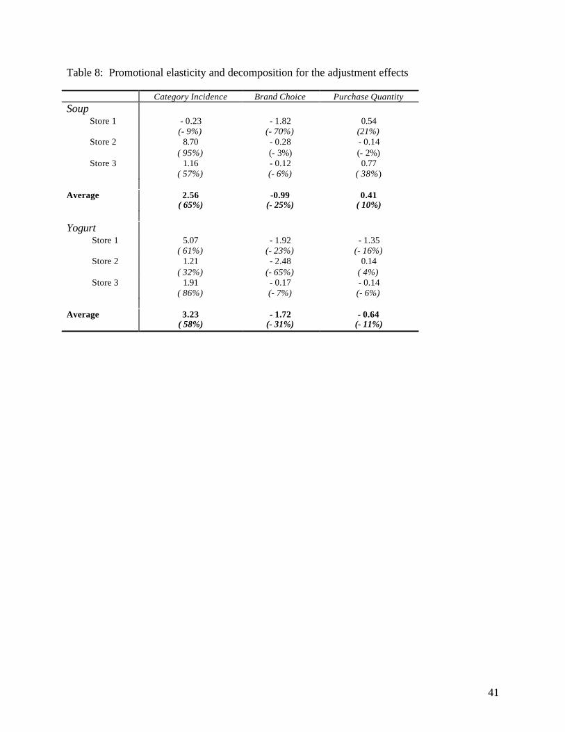
41

Table 8: Promotional elasticity and decomposition for the adjustment effects

Category Incidence Brand Choice Purchase QuantitySoup Store 1 - 0.23

(- 9%)- 1.82

(- 70%)0.54

(21%) Store 2 8.70

( 95%)- 0.28(- 3%)

- 0.14(- 2%)

Store 3 1.16( 57%)

- 0.12(- 6%)

0.77( 38%)

Average 2.56( 65%)

-0.99(- 25%)

0.41( 10%)

Yogurt Store 1 5.07

( 61%)- 1.92

(- 23%)- 1.35

(- 16%) Store 2 1.21

( 32%)- 2.48

(- 65%)0.14

( 4%) Store 3 1.91

( 86%)- 0.17(- 7%)

- 0.14(- 6%)

Average 3.23( 58%)

- 1.72(- 31%)

- 0.64(- 11%)

42

Table 9: Promotional elasticity and decomposition for the total effects

Category Incidence Brand Choice Purchase QuantitySoup Store 1 2.76

(55%)0.92

( 18%)1.32

( 26%) Store 2 10.25

( 87%)0.02

( 1 %)1.46

( 12%) Store 3 3.18

( 43%)1.56

( 21%)2.62

( 36%)

Average 4.92( 66%)

0.83( 11%)

1.67( 22%)

Yogurt Store 1 5.47

( 59%)3.56

( 39%)0.20

( 2%) Store 2 2.41

( 57%)1.32

( 31%)0.53

( 12%) Store 3 2.13

( 49%)2.09

( 48%)- 0.11(- 3%)

Average 3.83( 58%)

2.57(39%)

0.24( 3%)

Table 10: Promotional elasticity for national brands and private labels

Brand type Category Incidence Brand Choice Purchase QuantitySoupImmediate National 1.91 2.74 1.2

Private label 1 3.42 1.63Adjustment National 3.33 -1.3 0.64

Private label -2.01 0.84 -0.97Total National 5.93 0.34 1.84

Private label -1.01 3.71 0.66

YogurtImmediate National 1.1 4.71 1.22

Private label 0.45 3.96 0Adjustment National 4.35 -2.53 -0.86

Private label 0.26 0.14 0Total National 5.45 1.9 0.36

Private label 0.71 3.84 0

43

Table 11: Household-level model parameter estimates*

Soup category Yogurt categoryIncidence Estimate t-value Estimate t-value

Consumption Rate 0.05 (19.07) 4.12 (16.11)Inventory –0.32 (–12.6) –0.094 (–1.76)Category Value 0.12 (2.19) 0.41 (9.09)

ChoiceBrand Loyalty 2.11 (20.93) 1.75 (18.80)Last Brand Purchased 0.14 (2.77) 1.28 (23.94)Price –1.59 (–6.51) –0.42 (–10.62)Promotion 0.73 (4.28) 1.35 (15.06)

Quantity

Brand Loyalty 0.17 (3.10) 0.12 (2.70)Inventory –0.17 (–11.65) –0.09 (–1.76)Price –0.24 (–5.33) –0.09 (–10.6)Promotion 0.25 (2.86) 0.12 (3.55)*asymptotic t-statistics in parentheses

Table 12: Summary of elasticity decomposition

Category Incidence Brand Choice Purchase Quantity

Soup 1.78(30%)

2.84(48%)

1.26(21%)

ImmediateElasticityBreakdown

Yogurt .88(14%)

4.45(73%)

.81(13%)

Soup 2.56(65%)

−0.98(−25%)

.41(10%)

AdjustmentElasticityBreakdown

Yogurt 3.23(62%)

−1.30(−25%)

−0.63(−12%)

Permanent Elasticity 0 0* 0

Soup 4.92(66%)

0.83(11%)

1.67(23%)

TotalElasticityBreakdown

Yogurt 3.83(58%)

2.57(39%)

0.24(3%)

* Except for yogurt brand 4 in store 1.

44

Figure 1: Second-order VAR for a store with 3 brands

CI = Category incidence

BC = Brand choice for the focal brand (in this case, brand 1)

PQ = Average purchase quantity for the focal brand (in this case, brand 1)

P = Price for each brand per oz (weighted average over package sizes)

DISP = Display dummy variable for each brand

FEAT = Feature dummy variable for each brand

+

+

+

+

=

−

−

−

−

−

−

=∑

tp

tp

tp

tPQ

tBQ

tCI

it

it

it

PQ

BC

t

t

t

FEATFEATFEAT

DISPDISPDISP

PPPPQBCCI

PPPPQBCCI

it

it

it

i

iiiiii

iiiiii

iiiiii

iiiiii

iiiiii

iiiiii

P

p

p

CI

t

t

t

,3

,2

,1

,1

,1

,

3

2

1

636261

535251

434241

333231

232221

131211

3

2

1

636261

535251

434241

333231

232221

131211

3

2

1

666564636261

565554535251

464544434241

363534333231

262524232221

161514131211

1

1

3

2

1

***1

1

2

1

3

2

1

1

1

εεεεεε

γγγγγγγγγγγγγγγγγγ

γγγγγγγγγγγγγγγγγγ

φφφφφφφφφφφφφφφφφφφφφφφφφφφφφφφφφφφφ

αααααα

45

Figure 2: Impulse elasticity functions for soup brand 1 in store 1

Figure 3: Impulse elasticity functions for yogurt brand 1 in store 1