The Long-Term Effects of Housing and Criminal JusticePolicy: Evidence and Methods

by

Matthew B. Gross

A dissertation submitted in partial fulfillmentof the requirements for the degree of

Doctor of Philosophy(Economics)

in The University of Michigan2021

Doctoral Committee:Assistant Professor Michael Mueller-Smith, ChairProfessor Charlie BrownAssistant Professor Sara HellerProfessor Brian A. Jacob

Matthew B. Grossmbgross@umich.edu

ORCID ID 0000-0003-4721-421X© Matthew B. Gross 2021

To my grandparents - Pearl, Mel, Florence, and Elliot - who instilled in their families thevalue of education and the joy of exploring the world.

ii

ACKNOWLEDGEMENTS

To rephrase the saying, it takes a village to complete a dissertation. I am indebted to somany people for their support over the past 7 years. I have been fortunate to work with someexceptionally smart and committed professors who helped me drag my dissertation over thefinish line. I am constantly amazed by the dedication and intellectual firepower exhibited bymy dissertation committee. Mike Mueller-Smith, my dissertation chair, boss, and coauthor,was a constant advocate and incredible adviser throughout the process. Mike taught me theskills required to be an empirical economist, and I would not have been able to completethis journey without his mentorship and help. Charlie Brown was unrelentingly enthusiasticwhile also displaying an uncanny ability to simultaneously ask the right questions and suggestconstructive solutions. Sara Heller’s brilliance as both a researcher and communicator helpedme to improve my dissertation and the way I presented it in countless ways. Brian Jacobhas been a research adviser going back to my third-year paper. In particular, his suggestionsand comments were instrumental in pushing me to improve the matching methodology in myfirst chapter.

Other faculty who engaged with my research and contributed helpful suggestions includeMel Stephens, John Bound, Joel Slemrod, Ash Craig, and Gabriel Ehrlich. I would also liketo thank the participants of the Labor Lunch and Labor Seminar for their attention, humor,and intelligent comments and questions at various stages of my dissertation.

The second and third chapters of my dissertation were coauthored with very talentedresearchers. Mike Mueller-Smith is a coauthor on the second chapter while Mike, Keith Finlay,and Elizabeth Luh are coauthors on the third chapter. I would like to thank Elizabeth formoving this paper forward when I was focused on different projects. On top of being a valuedcoauthor, Keith has been very gracious with his time to help shepherd this project throughthe sometimes maze-like Census Bureau disclosure process.

For the second and third chapters of my dissertation, I am indebted to the incrediblydedicated past and present employees working at the Criminal Justice Administrative RecordsSystem (CJARS). Matt Van Eseltine helped the project grow in its early stages and assistedwith preliminary versions of the entity resolution model. Jay Choi had a hand in nearly everyaspect of the project.

iii

For my second dissertation chapter, Jay Choi, Madeleine Danes, Francis Fiore, JordanPapp, Benjamin Pyle, Lyllian Simerly, David Smith, Brittany Street, and Peixin Yang helpedout with an important handcoding exercise. Peixin also worked on the database of researchpapers that discuss administrative data. For the second chapter, Martha Bailey, John Bound,Charlie Brown, Aaron Chalfin, Connor Cole, James Feigenbaum, Keith Finlay, Sara Heller,Kirabo Jackson, Emily Nix, Joseph Price, Mel Stephens, Jesse Rothstein, Sarah Tahamont,and Chelsea Temple all provided substantive comments to improve the paper.

For the third chapter, many of the same CJARS employees worked together to transformmillions of rows of raw criminal justice records into data that could be used for research.Diana Sutton provided important institutional knowledge when trying to understand thecharges associated with driver responsibility fees. In addition, Katie Genadek was extremelyhelpful and generous with her time in getting a large disclosure review package released.

There are a number of teachers and mentors who have guided me throughout my academicand professional career, and without whose assistance I would not have been able to reachthis milestone. Jeanne Hogarth, Ellen Merry, and Max Schmeiser took a chance on me andoffered me the opportunity to conduct research professionally while at the Federal ReserveBoard. Paula Malone, David Albouy, Martha Bailey, David Lam, and Mel Stephens wereinfluential undergraduate teachers who ignited my passion for economics and research.

I am very grateful to my colleagues and friends, both within the economics department andin various other departments, for their support, help and friendship. It would be impossibleto name everyone but there are a few in particular that I would like to acknowledge. TingLan and Huayu Xu were patient study group partners in my first year. Ellen Stuart was agracious host on holidays and Friday evenings. Steph Owen was a committed Blank Slatebuddy. Ari Binder was a gracious BBQ host and a game bike rider. Anirudh Jayanti was agreat neighbor, movie buff and friend. Dhiren Patki is an all-around wonderful friend. Theresidents of 809 Lawrence, including Sam Haltenhof and Chad Milando, added much-neededlevity and fun. George Fenton and Max Gross, the other two initials in GMM, are incrediblefriends who provided constant support and were with me every step of the way over the past7 years.

I would like to thank my family for making all of this possible. My in-laws Bob, Jackieand Elizabeth welcomed me into their family with open arms despite my less than flawlesstable manners. My brother Adam and sister-in-law Reanna helped me generate research ideasand always supported me, even when they did not know my research topic. Most importantly,they had Mason and Brody, who made it hard to leave NYC every time I had to go back toAnn Arbor, but who also provided excellent motivation to finish my dissertation.

My parents are more responsible for my achievements and success than anyone in the world.

iv

For treating education as an expectation and making sure that I had the best opportunitiesto learn. For allowing me to see the the world and stoking my intellectual curiosity. Forsupporting me in so many different ways throughout my time in college, Washington DC andgraduate school. For nursing me through multiple shoulder surgeries while in graduate school.For knowing when not to ask me “how is your dissertation research going?” For these andcountless other reasons, I have the best parents in the world, and I am so thankful for theirpresence in my life.

Last and most importantly, I would like to thank the brains behind the operation: mywife Rachel. Rachel encouraged me through every twist and turn of this research project fromits initial conception to its current state. One silver lining of the Covid-19 pandemic wasthat I was able to type every word of my dissertation sitting within a few feet of Rachel. Mycompleted dissertation is a testament to her love and support, and I could not have done thiswithout her.

v

TABLE OF CONTENTS

DEDICATION . . . . . . . . . . . . . . . . . . . . . . . . . . . . . . . . . . . . . . ii

ACKNOWLEDGEMENTS . . . . . . . . . . . . . . . . . . . . . . . . . . . . . . iii

LIST OF FIGURES . . . . . . . . . . . . . . . . . . . . . . . . . . . . . . . . . . . viii

LIST OF TABLES . . . . . . . . . . . . . . . . . . . . . . . . . . . . . . . . . . . . x

LIST OF APPENDICES . . . . . . . . . . . . . . . . . . . . . . . . . . . . . . . . xii

ABSTRACT . . . . . . . . . . . . . . . . . . . . . . . . . . . . . . . . . . . . . . . xiii

CHAPTER

I. The Long-Term Impacts of Rent Control . . . . . . . . . . . . . . . . 1

1.1 Introduction . . . . . . . . . . . . . . . . . . . . . . . . . . . . . . . 11.2 Relevant Literature . . . . . . . . . . . . . . . . . . . . . . . . . . . 61.3 Rent Control Sites and Institutional Background . . . . . . . . . . . 91.4 Data . . . . . . . . . . . . . . . . . . . . . . . . . . . . . . . . . . . . 121.5 Methodology . . . . . . . . . . . . . . . . . . . . . . . . . . . . . . . 15

1.5.1 Additional Methodological Assumptions . . . . . . . . . . . 211.6 Results . . . . . . . . . . . . . . . . . . . . . . . . . . . . . . . . . . 22

1.6.1 Rent Control at Different Points of the Income Distribution 251.6.2 Rent Control Effects on Housing and Demographics . . . . 27

1.7 Discussion and Limitations . . . . . . . . . . . . . . . . . . . . . . . 281.8 Conclusion . . . . . . . . . . . . . . . . . . . . . . . . . . . . . . . . 30

II. Modernizing Person-Level Entity Resolution with BiometricallyLinked Records . . . . . . . . . . . . . . . . . . . . . . . . . . . . . . . . . 47

2.1 Introduction . . . . . . . . . . . . . . . . . . . . . . . . . . . . . . . 472.2 Statement of Linkage Problem and Related Literature . . . . . . . . 502.3 Data and Background . . . . . . . . . . . . . . . . . . . . . . . . . . 562.4 Matching Algorithm . . . . . . . . . . . . . . . . . . . . . . . . . . . 57

vi

2.5 Evaluating Classification Performance . . . . . . . . . . . . . . . . . 612.5.1 Baseline Results . . . . . . . . . . . . . . . . . . . . . . . . 612.5.2 Decomposing Model Performance and Assessing Demographic

Heterogeneity . . . . . . . . . . . . . . . . . . . . . . . . . 642.5.3 Assessing Performance Degradation in External Applications 66

2.6 Data Simulation . . . . . . . . . . . . . . . . . . . . . . . . . . . . . 672.7 Conclusion . . . . . . . . . . . . . . . . . . . . . . . . . . . . . . . . 70

III. Effect of Financial Sanctions: Evidence From Michigan’s DriverResponsibility Fees . . . . . . . . . . . . . . . . . . . . . . . . . . . . . . 88

3.1 Introduction . . . . . . . . . . . . . . . . . . . . . . . . . . . . . . . 883.2 Michigan’s Driver Responsibility Fees Law . . . . . . . . . . . . . . . 913.3 Data . . . . . . . . . . . . . . . . . . . . . . . . . . . . . . . . . . . . 923.4 Research Design and Methodology . . . . . . . . . . . . . . . . . . . 94

3.4.1 Traffic Offense Recidivism and Integrity of the ExperimentalVariation . . . . . . . . . . . . . . . . . . . . . . . . . . . . 97

3.5 Results . . . . . . . . . . . . . . . . . . . . . . . . . . . . . . . . . . 983.5.1 Direct Impacts on Labor Market Outcomes and Recidivism 983.5.2 Evolution of the Effects on Labor Market Outcomes and

Recidivism . . . . . . . . . . . . . . . . . . . . . . . . . . . 1003.5.3 Heterogeneous Effects by Ability to Pay . . . . . . . . . . . 1013.5.4 Heterogeneous Effects Across DRF Fee Levels . . . . . . . 1023.5.5 Effects of DRFs on Romantic Partners . . . . . . . . . . . . 104

3.6 Relationship to Prior Work . . . . . . . . . . . . . . . . . . . . . . . 1053.7 Conclusion . . . . . . . . . . . . . . . . . . . . . . . . . . . . . . . . 106

APPENDICES . . . . . . . . . . . . . . . . . . . . . . . . . . . . . . . . . . . . . . 122A.1 Opportunity Insight Data Description . . . . . . . . . . . . . . . . . 123A.2 Appendix Tables and Figures . . . . . . . . . . . . . . . . . . . . . . 124B.1 Generating a Hand-Coded Sample . . . . . . . . . . . . . . . . . . . 131B.2 Defining Prediction Algorithms . . . . . . . . . . . . . . . . . . . . . 131B.3 Applying a Corruption Algorithm to the Social Security

Administration’s Master Death File . . . . . . . . . . . . . . . . . . 135

BIBLIOGRAPHY . . . . . . . . . . . . . . . . . . . . . . . . . . . . . . . . . . . . 137

vii

LIST OF FIGURES

Figure

1.1 Timeline of Relevant Rent Control Laws and Data Construction Dates . . . 321.2 Estimated ATT of Rent Control on Immigration Outcomes by Year . . . . 331.3 Estimated ATT of Rent Control on Housing Outcomes by Year . . . . . . . 341.4 Estimated ATT of Rent Control on Demographic Outcomes . . . . . . . . 352.1 Total Publications Mentioning “administrative data” in the Top 5 Economic

Journals, 1995-2019. . . . . . . . . . . . . . . . . . . . . . . . . . . . . . . . 722.2 Model Training and Testing Overview . . . . . . . . . . . . . . . . . . . . . 732.3 Diagnostic Performance for Varying Statistical Match Thresholds . . . . . 742.4 First Order Impact on Predicted Match Probability . . . . . . . . . . . . . 752.5 Convergence of Model Performance as Training Sample Increases . . . . . . 762.6 Model Performance Under Varying Training Sample Composition, Conditional

on Training Sample Size . . . . . . . . . . . . . . . . . . . . . . . . . . . . 772.7 Average Estimated ∆ Over 1,000 Simulation Runs with Varying Model

Parameterizations (Scenario 1) . . . . . . . . . . . . . . . . . . . . . . . . . 782.8 Average Estimated P-Value Over 1,000 Simulation Runs with Varying Model

Parameterizations (Scenario 1) . . . . . . . . . . . . . . . . . . . . . . . . . 792.9 Average Estimated ∆ Over 1,000 Simulation Runs with Varying Model

Parameterizations (Scenario 2) . . . . . . . . . . . . . . . . . . . . . . . . . 802.10 Average Estimated P-Value Over 1,000 Simulation Runs with Varying Model

Parameterizations(Scenario 2) . . . . . . . . . . . . . . . . . . . . . . . . . 813.1 Balance Tests Showing Smoothness Around the DRF Effective Date . . . . 1083.2 First Stage: Likelihood of Receiving Driver Responsibility Fee Before and

After DRF Effective Date . . . . . . . . . . . . . . . . . . . . . . . . . . . . 1093.3 Evolution of Cumulative Likelihood of DRF Conviction Regression-Discontinuity

Estimates Over Time and by Contamination Group . . . . . . . . . . . . . 1103.4 Means of Selected Characteristics Across the Distribution of Predicted DRF

Recidivism . . . . . . . . . . . . . . . . . . . . . . . . . . . . . . . . . . . . 1113.5 Balance Test for Likelihood of Above-Median DRF Recidivism Two Years

After Initial DRF Conviction . . . . . . . . . . . . . . . . . . . . . . . . . . 1123.6 Effects of DRF Conviction on Long-Term Labor Market Outcomes and

Criminal Behavior, by Contamination Group . . . . . . . . . . . . . . . . . 1133.7 Evolution of DRF Effects on Labor and Recidivism Outcomes Over Time,

by Contamination Group . . . . . . . . . . . . . . . . . . . . . . . . . . . . 114

viii

3.8 Heterogeneity Analysis of Effects of DRF Conviction on Labor MarketOutcomes and Criminal Behavior, by Predicted Income and by ContaminationGroup . . . . . . . . . . . . . . . . . . . . . . . . . . . . . . . . . . . . . . 115

A.1 Estimated ATT of Rent Control on Immigration Outcomes by Year: HighRental Tract Sample . . . . . . . . . . . . . . . . . . . . . . . . . . . . . . 125

A.2 Estimated ATT of Rent Control on Housing Outcomes by Year: High RentalTract Sample . . . . . . . . . . . . . . . . . . . . . . . . . . . . . . . . . . 126

A.3 Estimated ATT of Rent Control on Demographic Outcomes . . . . . . . . 127

ix

LIST OF TABLES

Table

1.1 T-Test of Means to Compare Characteristics of Treated and ControlledCensus Tracts . . . . . . . . . . . . . . . . . . . . . . . . . . . . . . . . . . 36

1.2 T-Test of Means to Compare Characteristics of Treated and Controlled Cities 371.3 T-Test of Means to Compare Outcomes of Treated and Controlled Census

Tracts . . . . . . . . . . . . . . . . . . . . . . . . . . . . . . . . . . . . . . 381.4 Comparing Means and Variances of the Raw and Weighted Samples Using

the Two-Step Nearest Neighbor Matching Algorithm . . . . . . . . . . . . . 391.5 Mahalanobis Distance Nearest NeighborMatch Estimates of Average Treatment

Effect on the Treated of Rent Control on Location as Child and Adult . . . 401.6 Mahalanobis Distance Nearest NeighborMatch Estimates of Average Treatment

Effect on the Treated of Rent Control on Long-Term Outcomes . . . . . . . 411.7 Mahalanobis Distance Nearest NeighborMatch Estimates of Average Treatment

Effect on the Treated of Rent Control on Long-Term Outcomes, Weightedby Children Linked to a Tract . . . . . . . . . . . . . . . . . . . . . . . . . 42

1.8 Mahalanobis Distance Nearest NeighborMatch Estimates of Average TreatmentEffect on the Treated of Rent Control on Location as Child and Adult: HighRental Tract Sample . . . . . . . . . . . . . . . . . . . . . . . . . . . . . . 43

1.9 Mahalanobis Distance Nearest NeighborMatch Estimates of Average TreatmentEffect on the Treated of Rent Control on Long-Term Outcomes: High RentalTract Sample . . . . . . . . . . . . . . . . . . . . . . . . . . . . . . . . . . 44

1.10 Mahalanobis Distance Nearest NeighborMatch Estimates of Average TreatmentEffect on the Treated of Rent Control on Long-Term Predicted Outcomes . 45

1.11 Mahalanobis Distance Nearest NeighborMatch Estimates of Average TreatmentEffect on the Treated of Rent Control on Long-Term Predicted Outcomes:High Rental Tract Sample . . . . . . . . . . . . . . . . . . . . . . . . . . . 46

2.1 Matching Strategies Used in 2019 Administrative Data Papers From the“Top 5” Journals . . . . . . . . . . . . . . . . . . . . . . . . . . . . . . . . 82

2.2 Summary Statistics of Training Data, External Testing Data, and the GeneralU.S. Population . . . . . . . . . . . . . . . . . . . . . . . . . . . . . . . . . 83

2.3 Description of Individual Blocks . . . . . . . . . . . . . . . . . . . . . . . . 842.4 Comparison of Out-of-Sample Model Performance . . . . . . . . . . . . . . 852.5 Demographic-Specific Performance Statistics . . . . . . . . . . . . . . . . . 862.6 Testing Model Performance in External Applications . . . . . . . . . . . . 87

x

3.1 Michigan Driver Responsibility Fee Amounts and Eligible Offenses . . . . . 1163.2 Balance Tests of Selected Characteristics at Date of Conviction Across DRF

Effective Date . . . . . . . . . . . . . . . . . . . . . . . . . . . . . . . . . . 1173.3 Balance Tests of Predicted Variables Across DRF Effective Date . . . . . . 1183.4 Effects of DRF Conviction on Labor Market Outcomes and Criminal Behavior1193.5 Effects of DRF Conviction on Labor Market Outcomes and Criminal Behavior

by Fee Level . . . . . . . . . . . . . . . . . . . . . . . . . . . . . . . . . . . 1203.6 Effects of DRF Conviction on Partnership Outcomes and Partner’s Labor

Market Outcomes and Criminal Behavior . . . . . . . . . . . . . . . . . . . 121A.1 Comparing Means and Variances of the Raw and Weighted Samples Using

the Two-Step Nearest Neighbor Matching Algorithm: High Rental Tract Sample128B.1 Description of Matching Variables . . . . . . . . . . . . . . . . . . . . . . . 130

xi

LIST OF APPENDICES

Appendix

A. Appendix to The Long-Term Impacts of Rent Control . . . . . . . . . . . . . 123

B. Appendix to Modernizing Person-Level Entity Resolution with BiometricallyLinked Records . . . . . . . . . . . . . . . . . . . . . . . . . . . . . . . . . . 129

xii

ABSTRACT

This dissertation combines research from multiple areas of applied economics and is mostlyfocused on estimating the long-term impacts of housing and criminal justice policy. In addition,this dissertation covers an important methodological tool that is increasingly necessary forempirical researchers when linking multiple data sets to estimate causal treatment effects.

In the first chapter, I study the effects of rent control on the long-term outcomes ofchildren. Rent control is a common policy enacted to limit the growth of rents and allowtenants to remain in their homes for longer. Prior empirical research has mainly focused onrent control’s impact on neighborhoods and housing markets while ignoring the potentiallong-term impacts of rent control for the people directly affected by the policy, particularlychildren. Using nearest neighbor matching at the census tract level, I estimate the effects ofrent control on average long-term outcomes for children, measured at the childhood censustract level. I find weakly suggestive evidence that rent control can improve the long-termlabor market outcomes for children while also creating negative spillovers for children who donot directly benefit from the policy.

In the second chapter, coauthored with Michael Mueller-Smith, we develop a record linkagealgorithm that is trained using a large, novel data set that includes fingerprint identifiers.Record linkage is a crucial empirical tool for contemporary applied researchers who areinterested in linking data sets that do not contain unique identifiers. We show that this largetraining data substantially improves model performance compared to the smaller trainingsamples frequently reported in the literature. We also show evidence that training data basedon human coding can be overly conservative when identifying matches on a target samplewith different characteristics than the human coder. This research has major implicationsfor empirical researchers who wish to link data sets and estimate heterogeneous treatmenteffects on subpopulations.

In the last chapter, coauthored with Keith Finlay, Elizabeth Luh, andMichael Mueller-Smith,we study the long-term impacts of criminal financial sanctions on labor market outcomes andcriminal recidivism. The rising use of financial sanctions in the criminal justice system in theUnited States necessitates a rigorous test of their impacts on criminal defendants and theirfamilies. We use data that has been processed and linked together using the record linkage

xiii

algorithm detailed in my second chapter and utilize the implementation of a 2003 Michigan lawthat sharply increased fines associated with certain driving crimes. After carefully accountingfor how the long-run behavioral effects of the policy could undermine the integrity of theresearch design, we find null to slightly positive effects of the policy on labor outcomes,minimal deterrent effects, and suggestive evidence of a financial burden on romantic partners.

xiv

CHAPTER I

The Long-Term Impacts of Rent Control

1.1 Introduction

There is an ongoing national conversation about inequality of opportunity and the fact thateconomic mobility has become increasingly difficult for those born at the bottom of the incomeand wealth distribution. Research by Chetty et al. (2017) confirms that economic mobility inthe United States decreased for birth cohorts between 1940 and 1980, and suggests that thesocioeconomic status of parents is a growing predictor of a child’s life outcomes. Researchershave identified early childhood as an especially important development period when well-timedinterventions can mitigate some of the gaps in achievement between children of differentincome or wealth levels. Because of the cumulative nature of childhood development, relativelysmall childhood investments can have large long-run impacts, particularly when targetingchildren from marginalized populations (Cunha et al., 2006). As a result, there is a largebody of literature studying and measuring the effects of these interventions.1

Although not directly targeting families with children, rent control is an example of apolicy intervention that could improve childhood development for impacted children. Definedas government regulation of allowable rent, rent control is a policy tool that is intended totransfer resources from landlords to renters. The goal of the policy is to make it easier forlow-income tenants and families to remain in their current housing. In most cities with rentcontrol, the policies were enacted in response to low rental vacancy rates, rising rental pricesand the fear that without regulations, many tenants would face a heightened threat of evictionand homelessness. In the ideal scenario, rent control operates as a transfer from landlords torenters, both in the form of below-market rents and insurance against rent increases in thefuture.

While the short-term effect of rent control on impacted renters is likely positive, the

1See Almond et al. (2018) for a recent review of the literature.

1

long-term effects on children have never been studied. The literature on childhood interventionssuggests a number of channels through which the child beneficiaries of rent control couldhave improved long-run outcomes as a result of growing up in rent controlled housing. Rentcontrol can be thought of as a form of government mandated housing assistance, which hasbeen shown in other contexts to increase earnings and decrease future incarceration ratesof impacted children (Andersson et al., 2016). The benefits of rent control also include anincome effect component, allowing families to shift expenditures from housing to other goodssuch as improved healthcare or education. Hoynes et al. (2016) shows that cash assistance tofamilies with young children can improve child health while Carneiro et al. (2021) show howthe timing of income shocks during childhood plays an important role in education outcomes.Lastly, the added housing security associated with rent control has the potential to reduceparental stress and the number of housing moves a child makes during childhood. Researchshows that a mother’s exposure to distressing news, such as a threat of eviction, can impacta newborn’s birth weight (which is itself correlated with long-term health and achievementoutcomes), while frequent childhood moves are known to be harmful to a child’s academicperformance and long-term development (Carlson, 2015; Wood et al., 1993; South et al.,2007).

Research also shows that one’s childhood neighborhood has a causal exposure effect onlong-run labor market and social outcomes, suggesting that the direction of the effect ofrent control on outcomes may depend on the neighborhood (Chetty and Hendren, 2018a,c;Chyn, 2018, for example). If rent control leads children to have longer tenant durations inneighborhoods that provide negative exposure effects, then rent control could even lead todeclines in long-term outcomes when compared with similar children who grew up in non-rentcontrolled cities. The implication from this strand of the literature is that the impacts of rentcontrol on long-term outcomes is an empirical question in that the sign of the likely effect isambiguous.

This paper is organized around a central research question: how does rent control affect thelong-term outcomes of children? In addition to the main question, I also seek to understandhow this long-term impact varies by family income. Does rent control provide benefits tochildren growing up at the bottom of the income distribution?

Despite the potential effects of rent control on tenants, the economics literature has mainlyfocused on quantifying rent control’s effect on the housing market and negative spillovers onneighborhoods. Rent control is often associated with a decrease in the quality of controlledhousing (Gyourko and Linneman, 1990; Sims, 2007, for example) and a misallocation oftenants and apartments (Glaeser and Luttmer, 2003; Krol and Svorny, 2005). More recently,Autor et al. (2014, 2017) show that rent control has potential negative spillover effects, not only

2

on the value of rent controlled units, but also on the value of neighboring properties that arenot rent controlled. One of the large drivers of this negative capitalization is increased crimein areas close to rent controlled units suggesting that rent control suppresses gentrification.Diamond et al. (2019) shows that rent control in San Francisco leads landlords to remove theirunits from the rental market, thereby decreasing the supply of rental housing and ultimatelyleading to a more segregated and unequal housing landscape. Asquith (2018) confirms thatlandlords are more likely to convert rentals to owner occupied housing as the local price ofhousing increases.

While the costs of rent control are well-established, the benefits are much harder toquantify. A major reason for this is that it is very difficult to define a suitable counterfactualfor individuals that live in rent controlled units. Traditionally, economists used hedonic priceregressions to quantify the benefit of rent control to renters by estimating the rent that wouldprevail in the absence of controls (Gyourko and Linneman, 1989). The difference betweenthe controlled rent and the estimated market-rate rent is a measure of the compensatingvariation of the policy; however, a static measure of rent control benefits ignores the potentiallong-term benefits that the policy confers. From a policy perspective, these long-term benefitsare fundamental to determining whether rent control passes a cost-benefit analysis.

To answer the main research questions, I use a matching method to compare tract-levelaverage outcomes of areas that received rent control to counterfactual tracts that did not. Thiscorresponds to the average treatment effect on the treated (ATT) of rent control on long-termtract outcomes. I measure these long-term outcomes using the publicly available OpportunityInsights data described in Chetty et al. (2018). This data set is constructed by linking childrenborn between 1978 and 1983 to their childhood census tracts using restricted federal tax data,allowing the authors to measure the average exposure effects of neighborhoods on long-termoutcomes such as economic mobility, employment, marriage, teen pregnancy and incarceration.The benefit of this data is that it is able to follow children over time regardless of where theylive as adults when measuring tract-level outcomes.

For each tract and outcome variable, the data reports the unconditional mean over allchildren from the analysis cohort that lived in the tract between ages 6 and 23. As an example,the data on economic mobility reports the tract-level probability that a child will reachthe top 20% of the income distribution in 2015. The realization of this variable gives theproportion of all children linked to a tract who have income in the top 20% of their birthcohort. Throughout this paper, I use the term “tract-level outcomes” to refer to the averageoutcomes of children growing up in a particular census tract.

From 1970 to 1985, a number of municipalities enacted rent control legislation in responseto rising inflation and low rental vacancy rates. I identify 116 cities in California, Massachusetts

3

and New Jersey that codify new rent control laws during this time period. For each rentcontrolled city, I determine the census tracts that comprise the city, enabling me to map rentcontrol laws to the outcome data set which is measured at the tract level. Rent control lawsare passed by cities according to an unknown function of economic, housing, demographic,political and other local characteristics. Many of the predictors of rent control are also likelyto be correlated with the long-term outcomes of children, implying that the difference inaverage outcomes between places with and without rent control is a biased estimate for theeffect of rent control on long-term outcomes. Unfortunately, the direction of the bias is notimmediately clear based on observable traits. While tracts that receive rent control havehigher unemployment rates, minority population and single parent rates, for example, theyalso have higher average income, college attendance and property values.

To recover a causal estimate of rent control on the average long-term outcomes measuredat the tract-level, I utilize a Mahalanobis distance nearest neighbor matching procedureto pair each treated census tract with a similar comparison tract that did not receive rentcontrol. The Mahalanobis distance is a common metric used to measure distance between twopoints based on underlying covariate values. I estimate the Mahalanobis distance betweentracts using data from multiple sources including the 1970 decennial census, the 1972 Censusof Governments and county-level voting preferences in the 1968 presidential election. Thisdata allows me to account for observable differences between census tracts and cities thatenact rent control. The census data is reported at the tract-level and includes controls fordemographic, housing, income and other characteristics that are predictive of receipt of rentcontrol and correlated with the potential outcomes of children in a given tract. The Census ofGovernments data includes detailed municipal-level information on government expendituresand revenue. Under the strong ignorability assumption that conditioning on the observedcovariates removes all confounding variation in the assignment of rent control, I am able tointerpret the estimated average treatment effect as a causal parameter. To minimize imbalanceon observed covariates in the matched sample, I implement a caliper match to prune treatedobservations that do not have comparison tracts with similar underlying covariate values.After pruning slightly more than half of all rent controlled tracts, I show evidence that thematching strategy does an adequate job of balancing the covariates for the remaining rentcontrolled tracts.2 When estimating the average effects of rent control on treated tracts, Ialso include bias adjustments for all covariates as proposed by Abadie and Imbens (2011).

My baseline estimates show that rent control leads to a 3.6% increase in the average time

2By pruning 50% of census tracts, my analysis sample is no longer representative of the baseline sampleof tracts treated with rent control. Despite this, matching models with more permissive calipers yieldquantitatively similar results, suggesting that the tradeoff between balance and external validity is fairlysmall.

4

that children spend in a given census tract, which implies that rent control laws achieve theirprimary policy goal of allowing families to stay in their housing for longer. I also show thatrent control leads to slight decreases in average tract-level economic mobility. Rent control isassociated with a 1.3 and 0.9 percentage point decrease in the average probability of reachingthe top 20% of the family and individual income distributions, respectively. These estimatesare both statistically insignificant (95% confidence interval of [ −0.052, 0.026] on a baselinemean of 23.7%). The estimates also show that rent control has a negligible effect on teenpregnancy, incarceration and employment.

The sample of tracts used to estimate the baseline results includes tracts with a lowproportion of rental housing that are unlikely to have large direct effects resulting from rentcontrol. I also generate matching estimators while limiting the sample to tracts where rentalunits represent at least 30% of all housing units. This removes approximately one half of thenon-rent controlled tracts and 25% of the treated tracts from the sample. I find that whenlimiting the sample to high rental tracts, rent control increases the average time that a childspends in a given tract by 12%. This provides even stronger evidence that rent control leadsfamilies to remain in rental housing, since the tract-level effect is magnified in areas wherewe expect there to be more rent control.

Using the high rental sample, I also show that rent control increases the average probabilityof reaching the top 20% of the family (individual) income distribution by 5.9% (3.9%). Rentcontrol also increases the tract-level average employment rate by 2.7%. Alternatively, rentcontrol has a minimal effect on the average teen pregnancy rate while increasing the tract-levelprobability of being incarcerated during the 2010 census by 16.8%.

Assessing the results from the baseline and high rent samples, there is suggestive evidencethat rent control does improve the average tract-level economic mobility in areas with ahigh percentage of renters, while also negatively impacting the economic mobility of non-rentcontrolled children living in cities with rent control. This result is consistent with the literatureon the impact of government transfers on child outcomes as well as the literature showing thatrent control is associated with negative spillovers on non-controlled housing. Furthermore,I use data from the 1980 to 2000 censuses to show that rent control leads to a decrease inthe tract-level percentage of college attendance and an increase in the tract-level povertyrate and unemployment rate. According to Chetty et al. (2018), each of these demographicvariables is associated with declines in the long-term outcomes of children.

An important shortcoming of the Opportunity Insights data is the fact that it is reportedat the census tract level. Tract-level averages will include many children who did not growup with rent control when aggregating over all children in a tract, making it more difficultto credibly measure small treatment effects. Assuming 20% of all children in a tract receive

5

rent control, and rent control improves the average probability of reaching the top incomequintile by 10% from a baseline of 0.1, the average tract level economic mobility rate wouldbe (0.8 × 0.1) + (0.2 × 0.11) = 0.102 ≈ 0.1. In this hypothetical example, the tract-leveloutcome is approximately unaffected by the existence of rent control despite the large benefitit provides to children who live in rent controlled units.

Lastly, I utilize the Opportunity Insights data on predicted outcomes for children at the25th and 75th percentiles of parental income to determine how rent control affects childrenat the bottom and top of the parent income distribution. I generate estimates using both thebaseline sample and the high-rent sample. In the baseline sample, rent control has a negativeeffect on the predicted economic mobility of children with parents at the 25th percentile ofincome distribution. By contrast, rent control has a minimal effect on the economic mobilityof children with parents at the 75th percentile of the income distribution. In the high-rentsample, rent control leads to small and statistically significant improvements in the predictedeconomic mobility for children at the 25th percentile of the parent income distribution. Forchildren at the 75th percentile of the family income distribution, rent control has a significantpositive effect on predicted rates of reaching the top income quintile as adults. The resultsfrom the high rent sample suggest that rent control helps individuals at the bottom of theincome distribution, though the effects are substantially stronger for children growing up atthe top of the parent income distribution. These results are consistent with previous findingsshowing that the benefits of rent control may be larger for higher income families; however, Iview the results from this exercise as merely suggestive and warranting future study withindividual-level data to better grasp the heterogeneity of the effect of rent control on futureoutcomes by income levels.

This research adds to the economics literature on rent control by tracking the outcomesof people that are affected by the policy and quantifying the long-term benefits. This articleis the first to estimate these benefits in a causal framework and will be of immediate interestto policymakers deciding whether rent control policies pass a cost benefit analysis. Whilethe results from the high-rent sample suggest that there are positive long-term benefits forchildren growing up with rent control, future research can build on this work by generatingmore precise estimates of these effects and potentially utilizing alternative data sources toleverage individual-level variation in the assignment of rent control.

1.2 Relevant Literature

Rent control is a commonly studied topic in the economics literature going back to Grampp(1950) who argued strongly in favor of removing rent regulations to help avoid housing shortages

6

and improve economic efficiency. This view is consistent with the implications of a simplesupply and demand model which predicts that rent control leads to over-consumption anddeadweight loss. For many years, a lack of natural experiments and suitable data preventedeconomists from estimating well-identified causal effects of rent control. As a result, there is asignificant body of theoretical work exploring the implications of various rent control regimes(Fallis and Smith, 1984; McFarlane, 2003; Suen, 1989, for example). In addition, the standardeconomic model’s clear predictions of efficiency costs due to price controls may have led someeconomists to think that empirical research on this topic would be superfluous (Gyourko andLinneman, 1990).

There are a number of papers that attempt to quantify the costs of rent control on housingquality (Moon and Stotsky, 1993; Gyourko and Linneman, 1990; Sims, 2007, for example),generally showing that rent controlled units are maintained at a lower quality than they wouldbe in the absence of price controls. Other research shows how rent control negatively affectshousing prices for the controlled (Autor et al., 2014) and uncontrolled stock (Fallis and Smith,1984; Early, 2000). Lastly, there is a body of literature that attempts to characterize andquantify the costs of rent control that result from inefficiently long tenant durations (Kroland Svorny, 2005; Ault and Saba, 1990; Ault et al., 1994) and the misallocation of tenantsand apartments (Glaeser and Luttmer, 2003).

Measuring the benefits of rent control to renters can be challenging without longitudinaldata. There is ample evidence that rent control is associated with increased tenant durationswhich implies that renters with rent control receive some benefit from the policy (Olsen,1972; Ault et al., 1994; Nagy, 1995; Munch and Svarer, 2002, for example). One commonmethod used to estimate the size of the benefit in the absence of exogenous variation is tomeasure the difference between controlled rent and the predicted rent that would occur inthe absence of controls. This can be done using the two-step method proposed by Gyourkoand Linneman (1989) to estimate hedonic rent regressions of the uncontrolled rental stockon housing characteristics. These regressions are then used to predict what the rent wouldbe at controlled units, conditional on observable characteristics. The difference between thepredicted and actual rent can be thought of as the compensating variation or monetary valueof rent control to the renter. In the second step, one can regress the compensating variationon tenant characteristics to determine how the benefits of rent control are distributed todifferent groups. Other papers that use this methodology include Gyourko and Linneman(1990), Ault and Saba (1990), Munch and Svarer (2002), and Early (2000). In general, thesepapers find that the benefits are not particularly well-targeted to the lower-income groupsthat price controls are intended to help.

In 1995, Massachusetts voters banned rent control in a closely contested statewide

7

referendum, providing economists with a natural experiment to measure the effect of theend of rent control. Sims (2007) was the first to utilize this policy variation and found thatrent control in Boston was associated with both decreases in the price of housing as well ashousing quality. While his results indicate that rent control had no impact on the constructionof new housing, he presents evidence that rent control decreased the value of neighboring,unaffected housing stock, though by a relatively small amount. Autor et al. (2014) focus onCambridge, Massachusetts and study both the direct effect on home values of rent decontrol,and the effects on housing values of homes that were never regulated. They find that rentcontrol suppresses the value of controlled homes, and also find substantial neighborhoodeffects implying that rent controlled units also suppress the value of nearby unregulated units.The end of rent control in Cambridge caused nearly $2 billion in housing value appreciation.Using a similar methodology in a follow-up paper, Autor et al. (2017) utilize detailed crimedata from 1992 to 2005 to measure the effect that the end of rent control had on local crimerates. They conclude that areas with more rent controlled housing prior to decontrol sawlarger decreases in crime rates than otherwise similar areas. This implies that the end of rentcontrol had a significant effect on decreasing crime rates in Cambridge and accounts for 15%of the home value appreciation as a result of rent control found by Autor et al. (2014).

Building on the research using the 1995 Massachusetts rent decontrol natural experiment,Diamond et al. (2019) estimate a well-identified causal effect of rent control on tenants,landlords and inequality using a 1994 change in the San Francisco rent control regime. Priorto 1994, all buildings built before 1980 were subject to rent control except those that containedfour or fewer units. In 1994, the small building exemption was removed such that all rentalbuildings with four or fewer units were now subject to rent control. Buildings with four orfewer units built after 1980 continued to be exempt from the rent control ordinance, providinga natural control group. Using a novel linkage, they collect address histories for San Franciscoresidents in addition to building and landlord information. The authors find that receipt ofrent control led to a 15% increase in the duration of rental stays; however, they also findthat rent control incentivizes landlords to remove units from the market, thereby decreasingthe number of rental units. Unlike previous studies, they conclude that the benefits of rentcontrol were well targeted to minorities, but that rent controlled units were more likely to bein neighborhoods with lower amenities (where the benefits of rent control are lower). Lastly,because landlords were more likely to remove rent controlled units in neighborhoods withmore amenities, the authors argue that rent control has accelerated gentrification, inequalityand rental prices in San Francisco. Asquith (2018) shows a similar result that San Franciscolandlords react to increasing land values by removing tenants through no-fault evictions,allowing them to convert to non-rental uses such as condominiums.

8

The paper by Diamond et al. (2019) is the only research that attempts to track rentersover time to measure the effect of rent control on the mobility and location decisions oftenants; however, we still do not know how rent control affects important long-term economic,labor market and social outcomes for tenants. Measuring these outcomes is key to a morecomplete understanding of the costs and benefits of rent control. I fill a critical gap in theliterature to date with evidence from a new intergenerational perspective on the consequencesof rent control.

1.3 Rent Control Sites and Institutional Background

The rent control policies that I utilize in this paper were passed in the 1970s and early1980s, and are considered part of the second generation of rent control in the United States;however, rent control policies in the U.S. date back to the end of World War I when housingshortages in a number of cities caused states to restrict evictions of soldiers and workersinvolved with the war effort.3 During World War II, the Federal Emergency Price ControlsAct (EPCA) subjected many aspects of the economy to price regulation including rentalhousing. These federal controls continued in modified form until 1952, though some areasand units that had been initially controlled by the EPCA were decontrolled before the end offederal rent regulation. The 1947 Housing and Rent Act gave states additional authority toeither extend rent regulations or decontrol rents on their own. By 1948, 10 states had someform of rent control legislation, though by the mid 1950s, New York was the only remainingstate with rent controlled housing (Lett, 1976).

In the 1970s, high levels of inflation and low rental vacancy rates in cities around thecountry led renter advocates to push for new laws to regulate the level and growth of rents. Asa result, a number of states and municipalities began to implement new rent control regimes.States that added rent control during this wave include California, New Jersey, Maryland,Massachusetts, the District of Columbia and Alaska. I focus on the laws passed in citiesin California, Massachusetts and New Jersey.4 5 In most of these places, the justificationfor passing rent control was that low rental vacancy rates coupled with large rent increases

3See Fogelson (2013) for a detailed historical account of New York City’s experience with rent control inthe post World War I period.

4In Maryland, Takoma Park enacted rent control in 1981. Lett (1976) claims that a number of othercounties implemented rent control in the early 1970s, though I have been unable to independently verify theselaws. As a result, I drop Maryland from the analysis sample to ensure that I do not have measurement errorin the treatment group.

5Washington D.C. implemented rent control in 1975 in the middle of a major, unrelated demographicshift. The population in Washington D.C. dropped 15% between 1970 and 1980 and declined from 800thousand residents in 1950 to 570 thousand in 2000. These unrelated changes might add additional noise tothe measured effects of rent control leading me to drop Washington D.C. from the analysis.

9

constituted an emergency that incentivized “rent gouging” and placed many residents at risk ofeviction (Lett, 1976). Furthermore, evicted residents were more likely to end up homeless giveninadequate supplies of rental housing. Many other cities and states considered implementingrent control during this time but had proposals fail to garner sufficient support.6 In Maine,the state passed legislation enabling localities to implement rent control though none endedup being passed (Lett, 1976).

Rent control laws regulate the legal terms of rental agreements as well as the rent that alandlord can charge a tenant. In practice, there are many different ways that governmentsimplement rent regulation. In the most restrictive cases, governments determine an exactprice for rental housing or place a freeze on rents to prevent them from increasing for anyreason.7 In other cases, governments may place limits on the maximum possible rent increase,either through arbitrarily defined price ceilings or by tying rent increases to inflation. Inthese cases, rent control is only binding if the landlord would be able to raise rents above thegovernment imposed limit in a competitive market. Another common aspect of rent controllegislation is vacancy decontrol, which determines the rent that landlords are allowed tocharge the next tenant after the previous tenant voluntarily vacates the rental. Depending onthe law, landlords may be allowed to raise rents to market rates under full vacancy decontrolwhile in other cases, landlords may only be allowed to raise rents by a fixed percentage. Lastly,rent control legislation often places additional limits on evictions though the implementationof eviction restrictions varies widely by location.

In New Jersey, most rent control laws are based on the legislation enacted in 1972 by themunicipal government of Fort Lee, which was the first city in New Jersey to implement rentcontrol. Landlords quickly challenged the legality of the legislation, but in 1973, the StateSupreme Court of New Jersey ruled that local governments were allowed to regulate localrent. After the court decision affirming the legality of local rent control, many New Jerseymunicipal governments followed Fort Lee’s example and instituted their own regulations. By1976, nearly 100 cities and townships had rent control laws. Although the laws in New Jerseyare not identical, many are based on the original law from Fort Lee (Lett, 1976). In general,the laws set base rents at current (as of the date of enactment) levels and then tied allowablerent increases to inflation. The laws generally exempted small-scale landlords (usually ownersof buildings with fewer than three rentals) from the law. Also, rental units constructed afterrent control enactment were often exempt from the legislation to incentivize new housing,and landlords were given permission to raise rents by more than inflation in the event that

6For example, municipal rent control proposals in Colorado, Pennsylvania andWisconsin were all consideredand ultimately not approved during the early 1970s.

7For example, see Washington D.C.’s temporary rent freeze, Regulation 74 - 13 passed in 1974.

10

they invested in capital improvements or if operating costs increased.In Massachusetts, the state passed rent control enabling legislation in 1969 which allowed

certain cities to pass rent control laws. Following this legislation, Boston, Somerville, Cambridge,Brookline and Lynn passed rent control laws which went into effect in 1970. Lynn andSomerville repealed rent control in 1974 and 1979 respectively. Under the laws, base rentswere set at current levels and rents were allowed to increase to return a reasonable netoperating income. Rent increases were also allowed for capital improvements and changesin operating expenses. New buildings and units in owner occupied houses were exempt,while all other extant rentals were subject to the law (Lett, 1976). In 1995, the voters ofMassachusetts narrowly approved a referendum which made it illegal for cities to enact rentcontrol legislation. Although Boston and Brookline loosened rent control restrictions prior to1995, both still had a substantial percentage of units subject to control (Autor et al., 2014).Cambridge still had a heavily controlled housing market at the time of the ballot initiative in1995.

In California, Berkeley was among the first cities to pass rent control legislation in 1972;however, this law was ruled unconstitutional by the California Supreme Court. Starting in1979, a number of large cities began passing rent control laws including San Francisco, LosAngeles and Oakland. By 1985, 12 cities in California had implemented rent control legislation.Rent control laws varied by the city; however, all cities were forced to adhere to both the EllisAct passed in 1985 and the Costa-Hawkins act passed in 1995. The former allowed landlordsto evict tenants if they wished to remove their rental housing from the market. This waspassed by the state legislature in response to a State Supreme Court ruling which stated thatcities could prevent landlords from evicting tenants even when the landlord wanted to occupythe house. This forced cities with strong restrictions to allow landlords the ability to exitthe rental market, though the administration of this law varied by city. The Costa-Hawkinsact forced cities to allow for vacancy decontrol after a renter leaves a rent controlled unit.This allowed base rents to rise to reflect market conditions after a tenant leaves, regardless ofthe rent that the previous tenant paid. In terms of exemptions, most new construction andsmall-scale rental buildings (1-3 units) were not subject to rent regulation.

In summary, rent control laws rolled out across California, Massachusetts and New Jersey inthe 1970s and early 1980s. While these policies were not identical, each placed new restrictionson landlords that could have long-run consequences for tenants, especially children. Next Idiscuss the data I use to estimate these effects before presenting the key results.

11

1.4 Data

In the states that passed rent control legislation beginning in the 1970s, the power toimplement rent control devolved to local political units, meaning that rent control existed insome cities but not others. This was particularly true in California, Massachusetts and NewJersey, which are the three states I focus on to estimate the effect that rent control has onlong-term outcomes of children. I follow Krol and Svorny (2005) in using Lett (1976) to collectinformation on local rent control laws passed in the 1970s, particularly in New Jersey andMassachusetts. This book includes a comprehensive list of cities that passed rent control by1976, covering nearly all of the New Jersey and Massachusetts cities that added rent control. Isupplement this resource with internet searches of legislative histories for large municipalities,particularly in California, to determine which cities added rent control legislation in the yearsfollowing 1976.

Throughout the paper, I measure rent control as a binary variable and do not distinguishbetween rent control policies in Massachusetts, California and New Jersey. Though there aredifferences in the regulations across municipalities and states, the number of different citieswith unique regulations makes it difficult to account for policy variation. Future researchshould attempt to study specific dimensions of rent control and the heterogeneity of treatmenteffects by rent control policy type. Despite this, there are reasons to believe that policieswithin states are fairly similar to each other. Most laws at this time were in reaction to lowvacancy rates which allowed landlords to raise rents quickly. In New Jersey, rent controllaws are enacted around the same time and are based on a law passed by the municipalgovernment of Fort Lee. In Massachusetts, despite some differences between Boston, Brooklineand Cambridge, all three cities had a substantial number of controlled units until 1995 whenall rent control laws were invalidated by the statewide ballot initiative. Lastly, in California,the laws across cities had similar exemptions and rent increase mechanisms and were subjectto statewide legislation that standardized vacancy decontrol and landlord exit.

I utilize geographic and shapefile data provided by the Census Bureau to identify censustracts that were subject to rent control. First, I merge a Census shapefile of incorporatedcities from the 1990 census with a shapefile of the 2010 census tracts to create an overlaplayer. Using this intersection, I determine the 2010 census tracts that comprise every city inthe country. I then merge in the list of cities passing rent control between 1970 and 1985 togenerate a binary variable for rent control status for each census tract in the United States. InNew Jersey, there are a number of municipalities that passed rent control that do not appearin the list of census places. For these remaining locations, I use the more detailed countymaps provided at www2.census.gov to manually identify the tracts associated with each rent

12

controlled city. This leaves me with a database of census tracts for California, Massachusettsand New Jersey along with a binary variable indicating whether the tract had rent controlestablished between 1970 and 1985.

Since rent control is implemented by local elected representatives, the decision to enactthese policies is likely dependent on underlying observable and unobservable city characteristics.In other words, rent control is not assigned randomly throughout the country, so comparingoutcomes of rent controlled and uncontrolled cities is likely to be a biased measure of the effectof rent control. Instead, I utilize data from the 1970 Decennial Census as balancing covariatesin a matching framework to estimate the effect of rent control on long-term outcomes. TheCensus data is pulled from the SocialExplorer website, which aggregates individual responsesfrom the 1970 Census up to the census tract level. Census tract borders change over time,so I use the 1970 Census data that is reported at the 2010 census tract level to maintain aconsistent measure of geography.8

The matching procedure also includes city-level data on municipal spending and revenues.The municipal tax and revenue data comes from the Government Finance Database describedby Pierson et al. (2015).9 The database compiles information from the Census of Governmentsbeginning in 1967. In years ending in either a 2 or 7, the U.S. Census Bureau collectsinformation on the finances of every incorporated government in the United States. Unfortunately,this full census did not begin until 1972, so I use the data collected from the 1972 census toensure that I have maximum coverage of all cities in my sample.

The enactment of rent control is a local political decision. As a result, it is necessary tocontrol for local political views when comparing places that did or did not have rent control.To account for local political differences, I use data on the county-level partisan vote shares forthe presidential election of 1968. This data is collected by Clubb et al. (2006) and distributedby the ICPSR.

The data for long-term outcomes is described in Chetty et al. (2018) and is available forpublic download on the Opportunity Insights website.10 This data combines multiple sourcesof restricted government data to measure a series of financial, social, educational and otheroutcomes for children born between 1978 and 1983. Using federal income tax returns from

8SocialExplorer uses the area interpolation method described in Logan et al. (2014) to convert 1970-1990tracts to the 2010 tracts. Area interpolation assigns populations from one area to another based on areaoverlap and does not account for the distribution of population density within tracts. This is a potentialsource of error, particularly in tracts with changing borders and unequal distribution of population. To thebest of my knowledge, no research has theorized the direction of the expected bias.

9The data is publicly available at https://willamette.edu/mba/research-impact/public-datasets/;however, I downloaded the data through the Inter-university Consortium for Political and Social Research(ICPSR) website (study number 37641): https://www.icpsr.umich.edu/web/pages/ICPSR/index.html.

10https://opportunityinsights.org

13

1989 to 2000, the authors identify all children who are listed as tax dependents and wereborn between 1978 and 1983. Next, they utilize the Census Bureau’s Protected IdentificationKey (PIK) to link these children to the 2000 and 2010 Decennial Census waves, 2000-2015American Community Surveys and IRS income tax returns from 1989-2015.11 The sampleselected is representative of all children in the 1978 to 1983 birth cohort that were born inthe United States or authorized immigrants and whose parents were either born in the U.S.or authorized immigrants.12

Once the sample is selected, the authors map children to the census tracts they grow upin through their age 23 year. A child born in 1983 can be linked to a particular tract through12 distinct years of tax returns (1989, 1994-1995 and 1998-2006) between ages 6 and 23.Children born in 1978 are only linked to 7 years of tract data (1989, 1994-1995 and 1998-2001)between ages 11 and 23. For each 2010 census tract, the authors report the unconditionalmean outcome value for all children linked to the tract. Children that appear in multipletracts due to childhood moves are weighted to represent the relative time spent in each tract.As an example, a child born in 1983 who is linked to tract A in 6 years of tax returns andtract B for the other 6, would receive 0.5 weight in both tracts A and B when calculatingtract level outcomes.

I focus on six census tract outcomes reported in the Opportunity Insights data: (1) theprobability of reaching the top income quintile,13 (2) the average income percentile,14 (3) theprobability of having a teen birth, (4) the probability of being in a correctional facility atthe time of the 2010 Decennial Census, (5) the probability of having positive W2 earningsin 2015, and (6) the probability of living in a low poverty neighborhood as an adult. Thesevariables allow me to measure how rent control impacts long-term economic mobility andother important social outcomes.

In addition to the unconditional mean outcomes, Chetty et al. also report average predictedoutcomes at the tract level for children at 5 different levels of the parent income distribution.These fitted values are generated from a regression of individual outcomes on parental incomelevel at the tract level. The regressions are estimated using all children linked to a particulartract (weighted for the number of linked years). I utilize the estimates at the 25th and

11The PIK is created using a probabilistic matching algorithm that is based on an individual’s SocialSecurity Number, as well as name, date of birth and address. The PIK can be used to follow an individualacross a number of Census Bureau, IRS and other governmental data sets.

12External validity is a common concern when using data limited to those who file tax returns. Accordingto Chetty et al., the sample used to create the public Opportunity Insights data is representative of theoverall population covered by the American Community Survey and the Current Population Survey.

13The income quintile is measured relative to all other people born in the same year to account for risingexpected earnings with age.

14Income percentiles are reported based on either the distribution of family income or individual income.

14

75th percentile of the parent income distribution to investigate whether rent control has adifferential effect on children at the bottom or top of the distribution; however, it is importantto emphasize that these estimates represent fitted values of a regression and may not reflecttrue outcomes of children. For example, a very wealthy tract may have relatively few parentsat the bottom of the national income distribution. Running a regression of child outcomes onparental income percentile might predict that children with parents at the 25th percentilehave positive outcomes in this hypothetical tract; however, this prediction is based entirely ona projection of children at the top of the parent income distribution. I only focus on predictedvalues from the 25th and 75th percentiles, ignoring estimates from the 1st, 50th and 100thpercentiles. See appendix A.1 for a slightly more technical description of the OpportunityInsight data.

1.5 Methodology

Rent control legislation is not randomly assigned to cities, but is instead implementedaccording to an unknown function of local housing, demographic and political characteristics.Tables 1.1 and 1.2 show summary statistics broken down by rent control status at the tractand municipal level respectively. In both tables, the treated group are the tracts and citieslocated in California, Massachusetts and New Jersey that receive rent control between 1970and 1985, while the control groups represent tracts and cities from the remainder of thecountry that are located in incorporated cities with a population greater than 5,000 peopleand that are represented in the 1972 Census of Governments. I also remove observations fromNew York, Maryland and Washington D.C. due to a mix of timing issues (New York), rentcontrol measurement ambiguity (Maryland), and likely confounding variation (WashingtonD.C.).

Out of 31,261 total census tracts, 2,444 are treated with rent control. These 2,444 treatedtracts comprise the 99 cities that received rent control between 1970 and 1985, have populationsover 5,000 and responded to the 1972 Census of Governments.15 In California, 26% of thepopulation lived in cities with rent control. In Massachusetts, 15% of the population lived ina rent controlled city while in New Jersey, over 48% of the state population lived in citieswith rent control.

From Table 1.1, it is clear that tracts that receive rent control are fundamentally differentthan those that do not. The difference in average value between treatment and controlgroups is statistically significant for most of the covariates suggesting that rent control is

15There are 16 small cities that enacted rent control between 1970 and 1985 but are not included in theCensus of Governments. These are mostly located in New Jersey.

15

not distributed quasi-randomly. Instead, places with rent control have a higher single parentrate, minority population and higher unemployment rate, which are all variables that arenegatively correlated with long-term outcomes for children. On the other hand, tracts withrent control have higher college attendance rates, average incomes and home values whichare correlated with improved child outcomes.

In Table 1.2, I report summary statistics at the city level comparing cities that enactedrent control to those that never implemented a rent control law. Not surprisingly, cities withrent control had lower vacancy rates and a higher percentage of rentals as a share of totalunits. These cities with rent control were more likely to be in counties that had higher shareof votes for Hubert Humphrey, the Democratic candidate, in the 1968 presidential election.In addition, the cities with rent control have higher municipal revenue per capita, and spenda higher fraction of total expenditures on education, police and welfare compared to non-rentcontrolled cities. The results from Tables 1.1 and 1.2 show that assignment of rent control iscorrelated with observable characteristics that are also likely correlated with the long-termoutcomes of children.

Each row of Table 1.3 represents an outcome variable of interest. We can see that theaverage fraction of years spent in a rent controlled tract is only slightly (0.4 percentage points)higher than the non-controlled tracts; however, on average, tracts with rent control are muchmore likely to report a higher probability of children living with their parents as adults andstaying in the same tract or commuting zone as an adult. Rows 5 through 12 show thattracts with rent control report greater average economic mobility, lower teen pregnancy andincarceration rates and higher rates of employment and living in tracts with low povertyrates as an adult. In general, the naive treatment effects suggest that rent control improveslong-term outcomes; however, the differences in pre-rent control characteristics, particularlyat the tract-level, imply that a simple difference in outcomes between treated and controltracts is likely to be a biased measure of the effect of rent control. Unfortunately, it is notimmediately clear which direction this bias shifts the naive estimates given the countervailingeffects of the individual variable imbalances.

In many observational studies, treatment is not assigned randomly but is instead assignedaccording to some (unknown) function of observable and unobservable characteristics. Ilean on Rubin’s model of causal inference to formalize the analysis and provide theoreticaljustification for the estimand of interest (Holland, 1986). In my setting, there is a rentcontrol treatment T ∈ 0, 1 that is assigned to the population of census tracts of size N . Ihypothesize that rent control treatment T has a causal effect on long-term average outcomesat the tract level, denoted Y (T ). The causal effect of T on Yi for tract i can be measuredas Yi(T = 1) − Yi(T = 0). Aggregating up to the full sample of census tracts, the average

16

treatment effect (ATE) can be written as 1N

∑Ni=1[Yi(1)− Yi(0)]. Alternatively, the average

treatment effect on the treated (ATT) which measures the effect of a treatment only onthe treated tracts, is written as 1

N1

∑N1i=1([Yi(1)− Yi(0)]|T = 1). Since we cannot observe the

treated and untreated potential outcome at the same time, measurement of the causal effect ofinterest is reduced to a missing data problem. Unless otherwise noted, I estimate the averagetreatment effect on the treated throughout my analysis.

To bypass the missing data issue, I utilize techniques that balance the treatment andcontrol groups on observable characteristics to find a suitable counterfactual and allow forimproved estimates of the effect of rent control on outcomes. Rosenbaum and Rubin (1983)were among the first to formalize the framework for achieving causal estimates in observationalstudies by conditioning on a vector of control variables to facilitate matching. The assumptionsrequired to identify the average treatment effect on the treated of rent control can be writtenas:16

(Y0) ⊥ T |X, pr(T = 1|X = x) < 1

where X is a vector of covariates and pr(T = 1|X = x) is the probability that a tract isrent controlled conditional on any realization of the covariate vector. The second part of theassumption states that the covariates cannot perfectly predict treatment. Under this strongignorability assumption, Rosenbaum and Rubin show that treatment effects can be recoveredby matching observations of different treatment levels with the same value of the conditioningfunction based on X. In the original case, Rosenbaum and Rubin use an estimated propensityscore; however, any function of X can be used. The intuition behind this result is thatcontrolling for the covariates X is sufficient to make the treatment assignment random. Forthis to be true, there must not be any unobserved variables that predict treatment and arecorrelated with the outcome after controlling for X. The assumption that controlling for Xremoves all confounding variation is quite strong and hard to prove.

I use the Mahalanobis distance metric (MDM) to determine the “closest” counterfactualmatch for each rent controlled tract. The Mahalanobis distance for any two tracts i, j iscalculated as:

MDMi,j =√

(Xi −Xj)TS−1(Xi −Xj)

where X is a vector of covariates and S is the covariance matrix of X. The intuition behindthe Mahalanobis metric is that it calculates the distance between two points in a way that is

16Note that the identification assumption is slightly less restrictive than the one needed to identify theATE (Abadie and Imbens, 2006).

17

independent of the scale of each component of X. Recent work by King and Nielsen (2019)suggests that matching on the MDM is preferable to matching on estimated propensityscores, since the matched pairs come closer to mimicking a fully blocked experiment comparedto propensity score matches which mimic a fully randomized experiment.17 Fully blockedexperiments are more efficient and should have substantially less noise in the estimatedtreatment effects. I match tracts with replacement, which allows a control tract to serve asthe counterfactual for multiple observations.

Throughout the paper, I use 38 main covariates to calculate the MDM as well as test forbalance in the subsequent matched or weighted samples. In Chetty et al. (2018), the authorsreport tract level variables that correlate with long-term outcomes. In particular, they showthat education, poverty rates, single parenthood, income, unemployment, minority populationand proxies for social capital are all correlated with economic mobility at the tract level.Therefore, it is crucially important to include these variables when calculating the distancebetween tracts and to ensure that they are balanced in the post-match sample. In additionto the variables highlighted by Chetty et al., I also include various housing and populationvariables that are likely to predict the imposition of rent control at the municipal level. Thesevariables include per capita municipal revenue, expenditures and county level data on votingbehavior from the 1968 presidential election. The municipal and county level data allows meto control for city-level differences that are not accounted for at the tract level and that couldbe correlated with the outcomes of interest. The full set of covariates are the same tract andcity-level variables that are listed in Tables 1.1 and 1.2.

As Ho et al. (2007) suggests, the main goal of a matching strategy is to reduce covariateimbalance across treatment status (with the hope that the covariates remove all confoundingvariation). Despite the large body of research on propensity score and distance metric matching,there is limited consensus on the best way to estimate matching metrics (Hainmueller, 2012).This is particularly true in the context of estimating propensity scores, though still relevantfor the MDM when deciding which variables to include and whether to use higher order termswhen assessing the distance between two observations. Given the large number of tract andcity-level covariates I control for, I do not include any higher order terms when calculatingthe Mahalanobis distance.18

Another common strategy in the matching literature is to limit matches to observations

17In a fully randomized experiment, treatment is assigned at random across a given population. In a fullyblocked experiment, the sample is stratified based on pre-treatment characteristics, and treatment is assignedrandomly within strata.

18There is some older research showing that the Mahalanobis distance metric performs poorly with manycovariates (Gu and Rosenbaum, 1993, for example); however, in my context, the Mahalanobis distanceprovides the best matches resulting in the lowest residual imbalance on observables despite the large numberof covariates.

18

that are within a given distance caliper or radius. Conducting a nearest neighbor matchwithout a caliper will find the closest match for each treated observation. As one decreasesthe size of the matching caliper, the matches that are farthest in measured Mahalanobisdistance are pruned, leaving the better matches with closer covariate realizations. This processof determining the match caliper is another way of describing the bias - variance trade offcommon to many empirical approaches. In addition, as treated observations are pruned,the estimated treatment effect from the reduced sample may not be relevant for the targetsample. As a result, it is up to the researcher to determine the caliper that minimizes covariateimbalance while also maintaining a sufficient sample of observations to estimate treatmenteffects.

I use an iterative process to determine the optimal caliper by instituting different calipervalues and checking the number of treated observations that are pruned and the resultingcovariate imbalance. In all iterations of the model, I check covariate balance by comparingthe standardized mean difference between the treated and control group before and afterimplementing the matching procedure. The standardized mean difference is given by Y1−Y0√

V1+V02

,

and is thus measured in units of the pooled standard deviation of the treatment and controlmeans (Austin, 2009). Its use allows us to standardize the measure of divergence regardlessof the units of each covariate. In addition, it satisfies the conditions of a good balance checkstatistic suggested by Imai et al. (2008) in that it is a characteristic of the sample (and not ahypothetical population) and that the value is unaffected by sample size. It is also importantto note that the iterative caliper selection process is estimated without estimating treatmenteffects to avoid data mining particular results while searching for the optimal match radius.

Once I have finalized the caliper selection, I estimate the average treatment effect on thetreated for all outcome variables by averaging the difference between the treated and matchedcounterfactual across all treated tracts. I also account for the bias that results when matchingon continuous covariates (Abadie and Imbens, 2006) by including post matching regressionadjustment on all covariates. This is equivalent to the bias-adjusted matching estimatorsproposed in Abadie and Imbens (2011). I report clustered standard errors at the city levelusing the influence function proposed by Jann (2019). Note that this standard error is likelyconservative, compared to the consistent standard errors proposed by Abadie and Imbens(2006) which are harder to calculate while including clusters. In addition Abadie and Imbens(2008) show that bootstrapped standard errors are not consistent for matching estimatorsdespite their use in the literature.

The ideal post-matching sample will have a standardized mean difference of 0 thoughresearchers sometimes use simple thresholds such as 0.1 or 0.25 to signify when a covariatehas a large enough difference to warrant returning to the matching procedure (Stuart et al.,

19

2013; Rubin, 2001; Cohen, 1977; Normand et al., 2001; Austin, 2009). Ultimately it is up tothe practitioner to identify whether the imbalanced covariate could plausibly lead to biasedestimation of treatment effects. Slight imbalances of covariates that are highly correlatedwith the outcome will be more problematic than larger differences in a variable which has aweak correlation with the outcome of interest.

I also measure the ratio of the mean variance for the treated and control groups for eachcovariate. Austin (2009) shows that propensity scores that are balanced on means still maybe incorrectly specified. Covariates that are fully balanced should have a variance ratio of1, though the literature gives little direction when it comes to determining what varianceratio threshold implies an imbalanced covariate. I view variance imbalances as subordinate toimbalances of the mean when determining the match caliper.

Table 1.4 show the standardized mean differences (SMD) and variance ratios for the rawand matched data after selecting the optimal caliper. Given the large number of covariates,the resulting imbalances are expected though larger than ideal. The caliper drops slightlymore than half of the original treated tracts, leaving a sample of 1,174 tracts which will beused to estimate the relevant ATTs. Out of 38 covariates, 18 have SMD of less than the desired0.1, while 13 have SMD values of between 0.1 and 0.25. This leaves 7 covariates that havepost matching SMD values of greater than 0.25. The post-matching variance ratios show thatthe majority of covariates have variance ratios within the [0.7, 1.3] interval; however, thereare still 13 covariates with variance ratios outside of this interval, further suggesting someresidual imbalance. Given the resulting imbalance, the post matching regression adjustmentis especially important when estimating treatment effects.

Across the distribution of included treated tracts, there are a total of 549 unique controltracts that are selected as matches. This means that each counterfactual observation is selectedas the closest neighbor match for an average of 2.1 treated observations. The maximumnumber of times a control observation is matched is 24 while the median is 1. The caliperselection process dropped 1,290 treated tracts including most of the tracts from rent controlledcities in Massachusetts. Of the remaining treated tracts, approximately 35.4% are located inNew Jersey (416 tracts), 63.1% are located in California (741 tracts) and 1.4% are located inMassachusetts (17 tracts). These tracts represent 88 out of the potential 99 cities that areincluded in the final analysis sample.

The observation pruning suggests that the estimated average treatment effect on thetreated is not equivalent to the overall sample average treatment effect on the treated. I viewthe change in underlying sample to be a worthy tradeoff to achieve better covariate balance.It is also worth noting that matching models with more permissive calipers yield very similarresults to this more restrictive matching procedure.

20

Lastly, I also estimate a matching model that limits treated and control tracts to thosethat have a high proportion of rental units. This removes over one half of the total tracts inthe original sample, including 25% of the treated tracts. I use the same baseline covariatesand matching caliper to construct these matches, which are used to determine the effect ofrent control on a sample of tracts that are especially likely to be affected by the policy. Thebalance results from this matching procedure are reported in Table A.1. Of the 840 tractsincluded in the high rent sample, 72% are located in California and 28% are located in NewJersey.

1.5.1 Additional Methodological Assumptions

The publicly available outcome data has shortcomings in the context of my paper thatrequire me to make a strong assumption before interpreting my results. The sample of childrenincluded in each tract’s outcome is determined by links made starting in 1989, when theanalysis cohort is between 6 and 11 years old. Figure 1.1 shows a timeline of the relevant dateswhen states began implementing rent control, as well as the dates when children were eligibleto be linked to a given census tract. Given the timing, I must assume that rent control did notcause any selective immigration to or from census tracts in the years after it is implementedand before 1989. Under this assumption, the people living in rent controlled tracts in 1989should be roughly equivalent to those living in the matched counterfactual tracts in 1989.This assumption is stronger for the rent controlled cities in New Jersey and Massachusettsthan it is in California due to the longer duration between rent control implementation andaddress linkage.

Prior work suggests that violations of this assumption could bias the estimated treatmenteffects in either direction. Research by Autor et al. (2014, 2017) shows that the removalof rent control in Cambridge, Massachusetts led to significant property appreciation anddecreased crime, suggesting that rent control is associated with reverse gentrification. Ifthis is true, rent controlled areas may be less likely to receive an influx of new residentsthan similar areas without rent control. Under this scenario, the estimated ATT of rentcontrol on long-term outcomes would likely be biased downward. Alternatively, research byDiamond et al. (2019) suggests differences in the short and long run effects of rent controlon neighborhood immigration. While rent control allows some lower income individuals theability to stay in their homes for longer, it also incentivizes landlords to exit the rental market.In the long run, they suggest that rent control increases gentrification by substituting rentalhousing for more expensive private uses. Under this latter scenario, we might expect thechildren living in rent controlled neighborhoods in 1989 and later to be relatively wealthierthan the children comprising the counterfactual tracts. This would likely create an upward

21

bias on the estimated effect of rent control on long-term outcomes, since the outcome samplewould include wealthier people that select into areas with rent control.

In Figure 1.2, I test this immigration assumption by looking at the effect that rent controlhas on the tract level proportions of immigrants from other counties, states and countries.These variables are based on the census question asking respondents over 5 years old wherethey lived 5 years ago and are aggregated up to the census tract level. For each year of thedecennial census, I estimate the average treatment effect on the treated on these immigrationoutcomes using the baseline Mahalanobis distance matching estimator. The top left panelshows the effect of rent control on the tract level percentage of people who migrated from adifferent census tract. The estimated ATT is negative in 1980 and positive in 1990, suggestingthat rent control does not have a consistent effect on cross county migration. The top rightpanel shows that rent controlled tracts have fewer residents migrate from other states thanthe counterfactual tracts. The bottom panel shows that rent controlled tracts have a slightlyhigher proportion of international immigrants than non-controlled tracts in 1980 and 1990,though this effect reverses signs in 2000. These findings are very similar when using thehigh-rent sample and are shown in Figure A.1. In general, the balance of the evidence fromthis figure suggests that the Autor et al. prediction is better supported by the evidence, thatrent control should lead to fewer new immigrants. Given this fact, I expect any violationof the selective immigration assumption to bias downwards the estimated benefits of rentcontrol.

1.6 Results

I first show evidence that rent control affects the location decisions of the householdsincluded in the Opportunity Insights sample. The central finding is that rent control allowsfamilies to stay in their housing for longer. Specifically, the first column of Table 1.5 showsthat rent control leads to a 2.1 percentage point (3.6%) increase in the tract-level averageduration of tenancy compared to counterfactual tracts. Each child included in the OpportunityInsights data can be linked to a particular tract in up to 12 distinct tax years, but theseyears are not continuous. As a result, a 3.6% increase in the tract-level average of the fractionof years that a child is linked understates the increased tenant durations resulting from rentcontrol. As an illustration of this fact, a child that lives in a given tract from 1989 to 1995would only be linked to that tract in 3 separate years (1989, 1994, 1995) despite living therefor a total of 6 years. I interpret the result as evidence that rent control increases rentaldurations without focusing on the exact magnitude of the increase.

The second column reports that rent control leads to a 3.1 percentage point (14.6%)

22

increase in the tract-level probability that a child will live with their parents as an adult.The third column shows that rent control leads to a 1.6 percentage point (7.1%) increase inthe average probability that a child will live in their childhood tract as an adult. The finalcolumn shows that rent control has minimal effect on the tract-level probability that a childwill live in the same commuting zone as an adult. The main takeaway is that rent controlallows families to stay in their housing for longer which is exactly what we would expect ifrent control laws were binding and provided benefits to families in the form of lower thanmarket rents.

The long-term outcome results are reported in Table 1.6. The columns represent differentoutcome variables while the top row represents the estimated ATT of rent control on therelevant tract-level average outcome. This row is measured in percentage point differences.Standard errors are reported in parenthesis beneath the ATT estimates.19 The first twocolumns report the tract-level probability that a child will reach the top family or individualincome quintile in 2015. The third and fourth columns report the tract-level average incomepercentile in the family or individual income distribution in 2015. The fifth column reportsthe tract-level probability that someone linked to a given track will have a teenage birth(females only). The sixth and seventh columns report the tract-level probability that someonelinked to a given tract will be in jail or prison in April, 2010 or will have positive earningsin 2015. Lastly, the eighth column reports the tract-level probability that someone linkedto a given tract will live in a low poverty neighborhood as an adult, defined as a tract witha poverty rate of less than 10% according to 2000 Census data. The baseline row reportsthe average counterfactual value for the relevant outcome while the %∆ row calculates thepercent change the ATT row represents from the baseline value.

Columns 1 and 2 show that rent control has a -1.3 and -0.9 percentage point (-5.4 and-3.5%) effect on the tract-level probability that a child will reach the top family and individualincome quintile respectively, though neither result is statistically significant. For the probabilityof reaching the top 20% of the family income distribution, I can rule out percentage pointeffects outside the interval [−0.052, 0.026]. Column 3 shows that rent control has a small andinsignificant (-1.3%) effect on the tract-level average family income percentile and a negligibleeffect on the average individual income percentile. For the family income percentile, I can ruleout percentage point effects outside the interval [−0.017, 0.031]. Columns 5 through 7 showthat rent control has a minimal effect on the tract-level probability that a child will have ateenage pregnancy, be incarcerated during the 2010 census or report positive employment

19As a reminder, the standard errors in Table 1.6 are calculated using the influence function methodproposed by Jann (2019) and account for clustering at the city level. These standard errors are likely to beoverly conservative compared to the consistent matching standard errors proposed by Abadie and Imbens(2006) which are more difficult to calculate including clusters.

23

earnings in 2015. Lastly, column 8 shows that rent control is associated with an insignificant2.6 percentage point (5.2%) reduction in the tract-level probability that children will live inlow poverty neighborhoods as an adult.

The unit of observation for the results in Table 1.6 is the tract level. Although tractsare constructed to have roughly the same population, it is possible that tracts with morechildren may have different estimated treatment effects. Table 1.7 reports the same matchingATT results but weights each tract by the number of children that are used to calculate theoutcome variable.20 While this does not allow for an individual-level interpretation of theresults, it does scale the estimated ATT to better reflect differences in the size of tracts and,more importantly, the number of children used to measure the outcome variable. On balance,the point estimates all fail to reject the null hypothesis of no effect and are very similar tothe unweighted baseline results.

In the last part of my baseline analysis, I limit the sample of tracts to include only thosetracts that have a high proportion of renters, defined as any tract with greater than a 30%share of rentals of the total housing units. This sample modification drops slightly more thanhalf of the non-rent controlled tracts and one quarter of all rent controlled tracts. The theoryunderpinning this adjustment is that tracts with a high percentage of rentals are more likelyto exhibit effects directly related to rent control. Indeed, Table 1.8 shows that rent controlleads to an estimated 6.1 percentage point (12%) increase in the fraction of years spent in agiven tract and a 2.8 percentage point (13.7%) increase in the probability of living in thesame tract as an adult. These results provide further proof that the rent control laws I studyallow families to stay in their homes for longer.

In Table 1.9, I show the effect of rent control on long-term outcomes for children growingup in tracts with a high proportion of rentals. Column 1 shows that rent control leads to a1.1 and 0.9 percentage point (5.9 and 3.9%) increase in the average tract-level probabilityof reaching the top 20% of the family and individual income distribution. Rent control isalso associated with a 1.2 and 1.6 percentage point (2.7 and 3.3%) increase in the tract-levelaverage family and individual income percentile. The coefficient on the individual incomepercentile is significant at the 10% reporting level. Based on the crosswalk converting incomepercentiles to income in 2015 dollars, the increase in average individual income attributedto rent control is between $850 and $1,709. In the high rent sample, the average tract isapproximately 66% rental housing. If we assume that half of the rental units are rent controlled,and there are no spillover effects on the non-rent-controlled children, then the direct impact ofrent control on the roughly 30% of children who receive the benefit would be $2,800 - $5,700

20The Opportunity Insights data reports the underlying sample size for each outcome variable.

24

in 2015 income.21

The results in columns 5 and 6 show that rent control has minimal impact on the averageteen-pregnancy rate, and leads to a 0.2 percentage point (16.8%) increase in the tract-levelprobability of being in jail on April 1, 2010. Column 7 shows that rent control leads to a 2percentage point (2.7%) increase in the tract-level employment average. This estimate is alsosignificant at the 10% reporting level. Lastly, rent control leads to a 1.8 percentage point(4.2%) decrease in the probability of living in a low poverty neighborhood as an adult. Onething to note is that the sample of tracts used for the high-rental estimates is fairly small.By definition, these tracts are not representative of the full sample of rent controlled tracts.Despite this, the change in estimated effects between the full sample results and the highrental results shows that rent control leads to greater economic and employment outcomes inareas where there is a higher probability of residents living in rent controlled housing.

These results are suggestive though not conclusive that rent control leads to long-termbenefits for children that grow up in rent controlled housing. The difference in estimatedeffects between the baseline and high rent sample is also consistent with prior work showingthat rent control has negative spillover effects, and these negative effects may harm thelong-term outcomes of children that live in close proximity to rent controlled housing. In thenext subsection, I try to determine how these long-term impacts are distributed across theincome distribution.

1.6.1 Rent Control at Different Points of the Income Distribution

In Table 1.10, I show the estimated average treatment effect on the treated tracts ofrent control on the predicted outcomes at the 25th and 75th percentile of the parent incomedistribution. For these results, the outcome variable is a predicted value of a regressionperformed for each census tract in the data, regressing the relevant outcome on parent incomerank. The 25th (75th) percentile outcome is thus the fitted value from this regression at therelevant parent income level. This means that the predicted outcomes are a projection basedon the outcomes of all children that are linked to a given tract.

Panel A of the table shows the effect of rent control on predicted tract-level economicmobility for children at the 25th percentile of parent income. In general, the estimatedtract-level effects of rent control on economic mobility for children at the 25th incomepercentile are similar to those reported in Table 1.6. Column 1 shows that rent control isassociated with a 0.8 percentage point (4.9%) decrease in the predicted tract-level probability

21The estimate of 50% rent control exposure is a hypothetical based on summary statistics reported byAutor et al. (2014), which shows that roughly 50% of Cambridge condominiums were rent controlled in 1994.Many of the non-controlled condominiums were likely owner occupied, so the true rate of rent control amongrental units was likely higher than 50%.

25

of reaching the top family income quintile, but this estimate has a standard error over 2times larger than the point estimate. Columns 3 and 4 show that rent control has littleeffect on the tract-level predicted family and individual income percentile. Column 5 showsthat rent control is associated with a 0.9 percentage point (4.5%) decrease in the tract-levelprobability of having a teen pregnancy. Column 7 shows that rent control is associated with a1.3 percentage point (1.9%) increase in the predicted tract-level probability of being employedas an adult. This estimate is significant at the 10% reporting level. Lastly, column 8 showsthat rent control decreases the average probability of living in a low poverty neighborhood by1.5 percentage points (3.2%).

Panel B of the table shows the effect of rent control on predicted economic mobility forchildren at the 75th percentile of parent income. The reported effects of rent control oneconomic mobility and average income are quite small. Rent control is associated with aslight increase in the average probability of having a teen pregnancy, and a large (thoughstatistically insignificant) decrease in the average probability of being incarcerated.

In Table 1.11, I show the results of this same exercise but limiting the sample to the highrental tracts. In panel A, I show that rent control has a small and slightly positive effect onthe average predicted economic mobility of children at the 25th percentile of parent income,though none of the estimates are statistically significant. This contrasts with the effect shownin panel B for children at the 75th percentile of the parent income distribution, where rentcontrol is associated with a 2.9 and 2.2 percentage point (13.2 and 8.2%) increase in thepredicted probability of reaching the top family and individual income quintile. The estimatesin columns 1-4 are all significant at the 5% significance level, further suggesting that rentcontrol leads to better economic outcomes for children at higher income levels.

Comparing the effect of rent control on average predicted teen pregnancy between panelsA and B, the estimates indicate that rent control leads to a 1.2 percentage point (5%) decreasein average teen pregnancy for lower income children, and a 1.6 percentage point (15.5%)increase in teen pregnancy for children towards the top of the parent income distribution;however, neither result is statistically significant.

The results reported in Table 1.11 suggest that there is variation in the benefits of rentcontrol based on family income and that higher income families seem to derive a higherbenefit; however, since the outcomes are projections, it is entirely possible that the results aredriven by people towards the top of the parent income distribution. As such, these resultsshould be interpreted with care and certainly do not provide conclusive proof of the effectthat rent control has on children at the bottom or top of the income distribution.

26

1.6.2 Rent Control Effects on Housing and Demographics

In this section, I use census data from the 1980-2000 surveys to see how rent controlaffects the demographic composition of tracts, as well as the housing market. For each censusyear between 1980 and 2000, I estimate the average treatment effect on the treated tractsof rent control on a host of demographic and housing variables. Note that the census dataI use in this section is comprised of people who live in the tracts in the year of the surveyas opposed to the Opportunity Insights data which is comprised of people who grew up ina given census tract. Part of the goal of this section is to examine possible mechanisms toexplain the baseline ATT results. Prior research has shown that rent control can suppressgentrification in a neighborhood or city by making it easier for tenants to remain in theircurrent housing. This might explain why rent control has a slight negative effect on economicmobility when estimating the baseline ATT model. People who do not receive rent controlbut live in a city with rent control may receive a negative spillover from the policy. I usethe same nearest neighbor matching methodology with bias adjustments to generate theseestimates. As a result, the analysis sample is the same, meaning that the results are basedon 1,174 rent controlled tracts spread over California, Massachusetts and New Jersey. I alsoestimate these effects using the high rental sample, though the results are largely the same.These supplemental figures are reported in appendix A.2.

Figure 1.3 displays estimated average treatment effects on the treated for housing marketconditions. The first panel on the left column shows the average tract-level effect of rentcontrol on the probability that a resident has been living in their current house for at least 5years. The estimated effect of rent control on the probability of living in one’s house for morethan 5 years is statistically significant in all three census years reported. This indicates thatrent control increases tenancy duration in tracts with rent control and provides corroboratingevidence that rent control allows renters to stay in housing for longer. The top panel on theright shows that rent control leads to a small but negative effect on the average tract-levelvacancy rate, though these estimates are not statistically significant.

The middle panels show the effect that rent control has on the tract-level proportionof people that have long commutes, and the tract-level percentage of rentals as a share oftotal housing units. The panel on the left provides weak evidence that rent control leads todecreased commutes of over 1 hour. This contrasts with Krol and Svorny (2005) who findthat rent control in New Jersey lead to spatial mismatch between where people live andwork further resulting in longer average commutes; however, none of the point estimates inmy analysis are statistically significant.22 The panel on the right shows that compared to

22The result from Krol and Svorny is not causally identified, so the comparison of results is difficult. Theresults from Table A.2 show estimates for the high-rental samples which are more in line with the results

27

counterfactual tracts, rent control has a negative effect on the proportion of rentals in 1980,and zero effect on the proportion of total units that are rentals in 1990 and 2000. The panelon the bottom shows that rent control has a statistically significant (though small) effecton the average total number of units in a tract. Taken together, this partially corroboratesevidence reported in Diamond et al. (2019) and Sims (2007) that rent control leads landlordsto remove rental units from the rental market.

Figure 1.4 displays estimated average treatment effects on the treated tracts for demographicvariables that could play a role in changing the long-term outcomes of residents. Chetty et al.(2018) show that long-term outcomes are correlated with tract level characteristics such asthe poverty rate, education, unemployment and rate of single parent families. In the top leftpanel, I show that rent control is associated with a small increase in the proportion of singleparent families. In the top right panel, I show that rent control is associated with a consistentdecrease in the tract-level share of college graduates. In the bottom panels, I show that rentcontrol is associated with a slight increase in the tract-level poverty rate and increases in theunemployment rate in the 1990 and 2000 decennial census. Although the measured effectsare small, the results suggest that rent control leads to a reversal or hold on neighborhoodgentrification. This is mostly consistent with results reported by Autor et al. (2014, 2017). Inaddition, this suggests that the benefits of rent control might be offset by negative spillovereffects on long-term outcomes for those that do not live in rent controlled housing.

1.7 Discussion and Limitations

The results from the high rental sample provide suggestive though not convincing evidencethat rent control improves economic mobility and employment outcomes in areas where weshould see rent controlled tenants exert a greater effect on the tract-level average outcome.I interpret these latter results to indicate that rent control provides a long-term benefit tochildren that grow up in rent-controlled housing, though the exact magnitude of this benefitis difficult to quantify with the data in this study. While few of the estimated ATT effects inthe high rent sample are statistically significant, the data limitations may make it difficult toidentify small effects of rent control on renters. In addition, conservative standard errors arelikely to overstate the variance of my estimates, making it more difficult to reject the nullhypothesis of 0 effect.

The methodology I use is only capable of estimating the net effect of rent control in acensus tract and cannot disentangle the effects on rent-controlled tenants and everyone else.As the figures in section 1.6.2 show, rent control is associated with a slight demographic shift

from Krol and Svorny, particularly in 1990 and 2000.

28

that leads to lower college attendance, higher unemployment rates and higher poverty rates.Chetty et al. (2018) reports that the long-term outcomes of children are negatively correlatedwith these demographic shifts, implying that rent control could harm children growing upin neighborhoods with rent control but who do not live in rent controlled housing. If thisis the case, the estimated benefit of rent control on tract-averages would include both theeffect on those who receive rent control and the spillover effects on those children who do notbut are affected by the changing neighborhood demographics. This would indicate that theeffects I measure understate the true benefit of rent control to children who grow up in rentcontrolled housing.

Even if we suppose that these spillover effects are negligible, it would still require a largemagnitude effect to detect tract-level changes in outcomes as a result of rent control. Supposethere are 100 children in a tract, and the true effect of rent control is that it improves theprobability of reaching the top income quintile by 10% (improving the baseline probabilityfrom 20 to 22%). If we also assume that half of the children live in rental housing (whichis roughly equal to the share of rental housing in rent controlled tracts), and half of theserenter children live in rent controlled housing, then 25 children will have improved chancesof reaching the top income quintile; however, the tract-level economic mobility probabilitywill be ((0.75) × (0.2)) + ((0.25) × (0.22)) = 0.205, which is roughly equal to the baselineprobability of 0.2, even though rent control has a large effect on those that receive the benefit.

From the high rental sample, the estimated effect of rent control on the average tract-levelindividual income is 1.6 percentiles. The difference in annual income between percentile 49.2and percentile 50.8 is roughly equivalent to $1,111, measured in 2015 dollars. This representsa 4% increase (from a baseline of $28,500) that is attributable to rent control. This effect issimilar though slightly smaller than the one reported byAndersson et al. (2016), who findthat an additional year of public housing is associated with a 5% increase in annual earnings.

Another related issue that can attenuate the estimated benefits of rent control is the factthat I do not have tract-level measures of rent control prevalence. By treating rent control asa binary variable, I do not account for the fact that different tracts are likely to have differentlevels of rent control intensity. Rent control intensity can be thought of as a combinationof the number of households that receive rent control as well as the degree that the rentregulations are binding. Given the complicated rules that govern exemptions to rent controllaws, it would be very challenging to construct a measure of the true rate of rent controlintensity in each tract over all cities in California, Massachusetts and New Jersey that enactedrent control between 1970 and 1985. Despite this, the methodological decision to measurerent control as binary will likely lead to an attenuation bias of the target average treatmenteffect on the treated. This bias is likely mitigated in the high rental sample analysis, though

29

there is still the probability that there is differential rent control treatment within these tractsleading to measurement error and attenuation bias.

Lastly, the causal interpretation of the matching results rests on the assumption thatconditioning the receipt of rent control on the matching covariates removes all confoundingvariation. I attempt to use a wide variety of tract and city-level covariates when matching toaccount for as many observable characteristics as possible. The large number of covariatesmakes it more difficult to balance the full covariate vector after matching, which further leadsto possible bias of the estimated ATT on the outcomes of interests. I mitigate this concern byusing the bias corrected estimators proposed by Abadie and Imbens (2011); however, this is asuboptimal method for dealing with residual imbalance and likely cannot remove all potentialsources of confounding variation.

Future research can avoid these problems using a number of different strategies. Mostimportantly, access to better data that is reported at the individual child level would allowfor one to disentangle the direct and spillover long-term effects of rent control. Additionally,studies that include more detail on the level of rent control intensity would have a betterchance of avoiding the attenuation bias that is likely to plague my results. Lastly, researcherscan utilize random or quasi-random variation in the assignment of rent control to moreconfidently avoid potential confounding of the effect of interest.

1.8 Conclusion

This paper is the first to provide estimates of the long-term benefits to children of growingup with rent controlled housing. Rent control is a commonly implemented policy that currentlyexists in 5 states including some of the largest cities in the country. Despite its ubiquity,previous research on rent control has mainly focused on its impact to housing markets andneighborhoods while ignoring the potential benefits to renters. There has been some attemptto quantify the benefits of rent control by calculating the difference between controlled rentand the rent that would be charged in a competitive market, but these static measures ignorethe potential long-term benefits that the policy confers.

I show that rent control leads to statistically insignificant decreases in economic mobilityand minimal changes in tract-level teen pregnancy rates, incarceration and employment;however, when limiting the sample of tracts to those that have at least a 30% rental share, Ishow that the estimated effect of rent control on economic mobility, income and employment ismarginally positive. These findings are weakly consistent with prior research showing that rentcontrol leads to negative spillovers on surrounding properties, while also providing benefitsto those who live in controlled housing. To further contextualize these results, I use census

30

data from the 1980 to 2000 census to show that rent control leads to tract-level changesin demographics and housing variables that are consistent with rent control suppressinggentrification.

In addition, I show some evidence that rent control can lead to minor improvements ineconomic mobility for people at the bottom of the income distribution; however, the economicmobility effects of rent control appear significantly stronger for children growing up at thetop of the parent income distribution.

These results represent an important first step in measuring the long-term benefits ofrent control for children that live in rent controlled housing, as well as the potential negativespillovers that worsen long-run outcomes for those that live in non-rent controlled housing. Thisresearch suggests that the long-term direct benefits may be positive, though future researchshould explore this topic using alternative data to determine whether the estimated effectscan be reproduced using individual-level variation instead of aggregated data. Additionalinquiry can also help to determine how the direct benefits of rent control compare to thepotential negative long-term spillovers which can help policymakers measure the net effect ofrent control on residents.

31

1975 1980 1985 1990 1995 2000 2005 2010 2015

Massachu

setts

NewJersey

California

Outcome

cohort

Addresslink 1

Addresslink 2

Addresslink 3

Figure 1.1: Timeline of Relevant Rent Control Laws and Data Construction DatesFigure shows the years that each state began to implement rent control, as well as the years that are relevantto the construction of the Opportunity Insights data. There is a sizeable gap between the implementation ofrent control and the first address link, particularly for New Jersey and Massachusetts. To recover a causalestimate of the impact of rent control, I must assume that there is no selective inmigration to areas with rentcontrol between the date of implementation and the address link.

32

Migrate county Migrate state

Country migrant

Figure 1.2: Estimated ATT of Rent Control on Immigration Outcomes by YearSource: 1980 - 2000 decennial census data reported at the tract level by SocialExplorer.Notes: Figures show the average treatment effect on the treated tracts of rent control on immigration outcomes.Each outcome is the percentage of tract inhabitants that have moved from a given location in the last 5 years.The error bars represent 95% confidence intervals from standard errors that are clustered at the city level.

33

P(Living in same house) Rental Vacancy Rt.

Long Commute % Rentals

Total Units

Figure 1.3: Estimated ATT of Rent Control on Housing Outcomes by YearSource: 1980 - 2000 decennial census data reported at the tract level by SocialExplorer.Notes: Figures show the average treatment effect on the treated tracts of rent control on housing outcomes.The average outcomes are generated using the baseline nearest neighbor match model. The error bars represent95% confidence intervals from standard errors that are clustered at the city level.

34

Single Parent Rt. College

Poverty Rt. Unemployment Rt.

Figure 1.4: Estimated ATT of Rent Control on Demographic OutcomesSource: 1980 - 2000 decennial census data reported at the tract level by SocialExplorer.Notes: Figures show the average treatment effect on the treated tracts of rent control on employment anddemograhic outcomes. The average outcomes are generated using the baseline nearest neighbor match model.The error bars represent 95% confidence intervals from standard errors that are clustered at the city level.

35

Table 1.1: T-Test of Means to Compare Characteristics of Treated and Controlled Census Tracts

AverageControl Treat Difference CA Diff. MA Diff. NJ Diff.

Population 3,065.197 3,422.419 357.222*** 348.446*** -327.377** 243.072**Male (%) 0.485 0.478 -0.007*** -0.010*** -0.011*** -0.002*Pop./sq. mile 4,607.690 13,303.566 8,695.876*** 6,557.932*** 14,391.206*** 11,001.167***Age median 28.322 30.856 2.534*** 2.323*** -0.748 1.762***White (%) 0.898 0.818 -0.081*** -0.141*** -0.132*** -0.051***Black (%) 0.092 0.144 0.052*** 0.113*** 0.121*** 0.049***Married (%) 0.634 0.561 -0.074*** -0.082*** -0.125*** -0.032***Single parent fam. (%) 0.071 0.100 0.029*** 0.026*** 0.047*** 0.016***Educ. Less than HS (%) 0.437 0.434 -0.002 0.012** -0.039*** 0.073***Educ. HS (%) 0.320 0.308 -0.012*** -0.025*** -0.012 -0.026***LFP rate 0.598 0.603 0.005*** 0.013*** -0.012** 0.013***Unemployment rate 0.043 0.060 0.017*** 0.007*** 0.003* 0.004***Avg. inc. 4,557.440 4,914.329 356.889*** 272.167*** -9.041 -346.089***Family poverty rt. (%) 0.089 0.093 0.003** 0.016*** 0.041*** 0.015***Current addr. 5 years (%) 0.478 0.474 -0.004 0.015*** -0.096*** -0.026***Housing units 1,026.231 1,237.823 211.592*** 232.245*** 17.667 154.410***Rental (% of total units) 0.334 0.532 0.197*** 0.142*** 0.249*** 0.233***Rental vacancy rate (%) 0.052 0.035 -0.017*** -0.000 0.025*** 0.000Rent vacancy x Rental % 0.020 0.021 0.001* 0.006*** 0.018*** 0.004***Avg. rent 127.908 143.727 15.819*** 6.621*** 18.171*** -3.224Avg. home value 20,213.463 26,258.793 6,045.330*** 3,713.865*** 2,200.790** -343.242N 28,813 2,444N by State:California 4,052 1,563Massachusetts 538 184New Jersey 506 697Other States 23,717Source: Author calculations of 1970 decennial census data reported at the tract level by SocialExplorer.Sample includes tracts in all states except Washington DC, Maryland and New York. These excluded states had cities with rent control and cannotbe used as possible control tracts. * = p < 0.1, ** = p < 0.05, *** = p < 0.01.

36

Table 1.2: T-Test of Means to Compare Characteristics of Treated and Controlled Cities

AverageControl Treat Difference CA Diff. MA Diff. NJ Diff.

City rental (% of total units) 0.298 0.450 0.152*** 0.130** 0.311*** 0.166***City rental vacancy rate (%) 0.066 0.023 -0.043*** 0.003 -0.004 -0.001City white (%) 0.914 0.904 -0.010 -0.085* -0.087 -0.020City black (%) 0.054 0.069 0.015 0.077* 0.063 0.020City unemployment rate 0.041 0.038 -0.003 0.001 -0.003 0.002City avg. rent 118.028 140.819 22.790*** 23.756** 50.587 11.518***County Dem. vote share 1968 41.408 45.876 4.468*** 5.802** 3.040 3.296***County Wallace vote share 1968 14.154 8.005 -6.149*** -0.927** 0.264 -0.766**City population 33,718.552 88,277.263 54,558.711* 435,493.354 204,199.588 26,450.147***City family poverty rt. (%) 0.076 0.054 -0.022*** -0.003 0.018 0.006City revenue per capita 0.173 0.228 0.055*** 0.189** 0.214* 0.031*City tax revenue per capita 0.075 0.146 0.072*** 0.086** 0.151** 0.029**Property tax share of rev. 0.293 0.511 0.218*** 0.033 0.022 0.029Other gov. sources share of rev. 0.142 0.155 0.013 -0.069*** -0.080** 0.008Educ. share of expenditure 0.032 0.133 0.101*** 0.000 -0.115* 0.040Police share of expenditure 0.155 0.178 0.023*** -0.045*** 0.015 0.003Welfare share of expenditure 0.002 0.010 0.008*** 0.027 -0.002 0.003***N 2,373 99N by State:California 274 10Massachusetts 34 3New Jersey 149 86Other States 1,916Source: Author calculations of 1972 Census of Governments data and publicly available county level vote shares.Sample includes cities from all states except Washington DC, Maryland and New York. These excluded states had cities with rent control and cannot beused as possible control cities. * = p < 0.1, ** = p < 0.05, *** = p < 0.01.

37

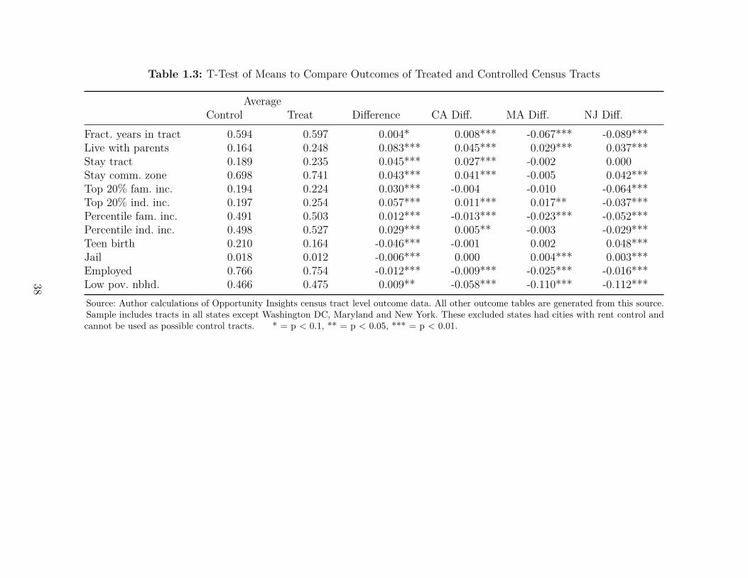
Table 1.3: T-Test of Means to Compare Outcomes of Treated and Controlled Census Tracts

AverageControl Treat Difference CA Diff. MA Diff. NJ Diff.

Fract. years in tract 0.594 0.597 0.004* 0.008*** -0.067*** -0.089***Live with parents 0.164 0.248 0.083*** 0.045*** 0.029*** 0.037***Stay tract 0.189 0.235 0.045*** 0.027*** -0.002 0.000Stay comm. zone 0.698 0.741 0.043*** 0.041*** -0.005 0.042***Top 20% fam. inc. 0.194 0.224 0.030*** -0.004 -0.010 -0.064***Top 20% ind. inc. 0.197 0.254 0.057*** 0.011*** 0.017** -0.037***Percentile fam. inc. 0.491 0.503 0.012*** -0.013*** -0.023*** -0.052***Percentile ind. inc. 0.498 0.527 0.029*** 0.005** -0.003 -0.029***Teen birth 0.210 0.164 -0.046*** -0.001 0.002 0.048***Jail 0.018 0.012 -0.006*** 0.000 0.004*** 0.003***Employed 0.766 0.754 -0.012*** -0.009*** -0.025*** -0.016***Low pov. nbhd. 0.466 0.475 0.009** -0.058*** -0.110*** -0.112***Source: Author calculations of Opportunity Insights census tract level outcome data. All other outcome tables are generated from this source.Sample includes tracts in all states except Washington DC, Maryland and New York. These excluded states had cities with rent control andcannot be used as possible control tracts. * = p < 0.1, ** = p < 0.05, *** = p < 0.01.

38

Table 1.4: Comparing Means and Variances of the Raw and Weighted Samples Using the Two-StepNearest Neighbor Matching Algorithm

Std. Mean Diff. Var. RatioRaw Matched Raw Matched

Population 0.185 -0.203 0.655 1.080Male (%) -0.226 0.026 1.101 1.259Pop./sq. mile 0.910 -0.046 3.533 0.928Age median 0.357 -0.068 1.139 1.220White (%) -0.322 -0.080 1.616 0.951Black (%) 0.211 0.041 1.548 0.931Married (%) -0.694 -0.053 1.210 1.433Single parent fam. (%) 0.447 0.191 2.121 1.301Educ. Less than HS (%) -0.012 -0.214 0.962 1.075Educ. HS (%) -0.157 -0.009 0.695 1.096LFP rate 0.076 -0.052 0.683 1.175Unemployment rate 0.583 0.422 1.494 1.311Avg. inc. 0.216 0.043 1.630 1.238Family poverty rt. (%) 0.044 0.104 0.894 1.165Current addr. 5 years (%) -0.026 -0.362 0.938 1.175Housing units 0.315 -0.164 0.739 1.107Rental (% of total units) 0.843 0.116 1.616 1.183Rental vacancy rate (%) -0.258 0.066 0.470 1.407Rent vacancy x Rental % 0.037 0.082 0.762 1.265Avg. rent 0.367 0.153 1.334 1.124Avg. home value 0.683 0.266 1.348 1.044City rental (% of total units) 1.448 0.167 1.399 0.828City rental vacancy rate (%) -0.586 -0.167 0.240 0.739City white (%) -0.528 0.134 0.960 0.537City black (%) 0.341 -0.254 0.822 0.416City unemployment rate 0.912 0.638 0.976 1.659City avg. rent 0.190 0.041 0.012 0.580County Dem. vote share 1968 0.875 -0.010 0.536 0.521County Wallace vote share 1968 -0.904 -0.120 0.021 0.870City population 1.015 -0.021 4.548 0.681City family poverty rt. (%) -0.057 -0.017 0.395 0.880City revenue per capita 0.882 0.257 2.282 1.454City tax revenue per capita 0.935 0.048 2.677 1.052Property tax share of rev. 0.394 -0.221 1.464 1.444Other gov. sources share of rev. 0.135 -0.131 0.677 1.011Educ. share of expenditure 0.375 -0.043 2.296 1.128Police share of expenditure -0.022 -0.382 0.419 0.687Welfare share of expenditure 0.293 -0.058 5.377 0.879N 31,443N Treat 1,174N unique control 549Source: Author calculations of 1970 census, 1972 Census of Governments, and 1968 county-level vote data.Table shows the standardized differences in means and variances between the raw and weighted sample. The unit ofobservation is a census tract. The treated tracts are matched to a control tract using a nearest neighbor Mahalanobisdistance matching procedure. The Mahalanobis distance metric includes linear terms for tract-level, city-level andcounty-level characteristics.

39

Table 1.5: Mahalanobis Distance Nearest Neighbor Match Estimates ofAverage Treatment Effect on the Treated of Rent Control on Location as Child

and Adult

Frac. years Stay Stay Stayin tract home Tract Comm. Zone

ATT 0.021** 0.031*** 0.016 0.004(0.010) (0.011) (0.010) (0.025)

Baseline 0.576 0.216 0.219 0.738%∆ 0.036 0.146 0.071 0.005N Treat 1,156 1,155 1,156 1,156N Control 541 539 540 540The ATT row reports the average treatment effect on the treated of rent control on theaverage tract outcome. The ATT estimates are generated using a nearest neighbor Mahalanobisdistance metric matching estimator. The baseline row represents the average outcome of thematched counterfactual tracts. * = p < 0.1, ** = p < 0.05, *** = p < 0.01.

40

Table 1.6: Mahalanobis Distance Nearest Neighbor Match Estimates of Average Treatment Effect on the Treated of Rent Control onLong-Term Outcomes

Top 20% Top 20% Percentile Percentile Teen Low Pov.Fam. Ind. Fam. Inc. Ind. Inc. birth Jail Employed nbhd.

ATT -0.013 -0.009 -0.007 0.000 -0.000 -0.000 0.005 -0.026(0.020) (0.018) (0.012) (0.009) (0.013) (0.002) (0.004) (0.022)

Baseline 0.237 0.263 0.510 0.526 0.164 0.012 0.749 0.501%∆ -0.054 -0.035 -0.013 0.001 -0.000 -0.001 0.007 -0.052N Treat 1,172 1,172 1,172 1,172 1,171 1,172 1,172 1,172N Control 549 549 549 549 549 549 549 549The ATT row reports the average treatment effect on the treated of rent control on the average tract outcome. The ATT estimates are generated using a nearestneighbor Mahalanobis distance matching estimator that accounts for tract, city and county-level traits. The baseline row represents the average outcome of the matchedcounterfactual tracts. * = p < 0.1, ** = p < 0.05, *** = p < 0.01.

41

Table 1.7: Mahalanobis Distance Nearest Neighbor Match Estimates of Average Treatment Effect on the Treated of Rent Control onLong-Term Outcomes, Weighted by Children Linked to a Tract

Top 20% Top 20% Percentile Percentile Teen Low Pov.Fam. Ind. Fam. Inc. Ind. Inc. birth Jail Employed nbhd.

ATT -0.009 -0.007 -0.004 0.002 -0.003 -0.001 0.005 -0.012(0.013) (0.013) (0.009) (0.007) (0.016) (0.002) (0.005) (0.020)

Baseline 0.219 0.248 0.499 0.518 0.183 0.014 0.752 0.477%∆ -0.042 -0.026 -0.008 0.005 -0.017 -0.091 0.006 -0.024N Treat 1,172 1,172 1,172 1,172 1,171 1,172 1,172 1,172N Control 549 549 549 549 549 549 549 549The ATT row reports the average treatment effect on the treated of rent control on the average tract outcome, weighted by the number of children linked to each tract.The ATT estimates are generated using a nearest neighbor Mahalanobis distance matching estimator that accounts for tract, city and county-level traits. The baselinerow represents the average outcome of the matched counterfactual tracts. * = p < 0.1, ** = p < 0.05, *** = p < 0.01.

42

Table 1.8: Mahalanobis Distance Nearest Neighbor Match Estimates ofAverage Treatment Effect on the Treated of Rent Control on Location as Child

and Adult: High Rental Tract Sample

Frac. years Stay Stay Stayin tract home Tract Comm. Zone

ATT 0.061** 0.047** 0.028* 0.019(0.027) (0.020) (0.017) (0.021)

Baseline 0.507 0.204 0.207 0.737%∆ 0.121 0.230 0.137 0.026N Treat 827 826 826 826N Control 372 373 372 372The ATT row reports the average treatment effect on the treated of rent control on the averagetract outcome. The unit of observation is a census tract with at least 30% rental share. TheATT estimates are generated using a nearest neighbor Mahalanobis distance metric matchingestimator. The baseline row represents the average outcome of the matched counterfactualtracts. * = p < 0.1, ** = p < 0.05, *** = p < 0.01.

43

Table 1.9: Mahalanobis Distance Nearest Neighbor Match Estimates of Average Treatment Effect on the Treated of Rent Control onLong-Term Outcomes: High Rental Tract Sample

Top 20% Top 20% Percentile Percentile Teen Low Pov.Fam. Ind. Fam. Inc. Ind. Inc. birth Jail Employed nbhd.

ATT 0.011 0.009 0.012 0.016* -0.001 0.002 0.020* -0.018(0.012) (0.012) (0.010) (0.008) (0.015) (0.002) (0.010) (0.021)

Baseline 0.181 0.218 0.466 0.492 0.188 0.012 0.726 0.440%∆ 0.059 0.039 0.027 0.033 -0.005 0.168 0.027 -0.042N Treat 840 840 840 840 839 840 840 840N Control 373 373 373 373 373 373 373 373The ATT row reports the average treatment effect on the treated of rent control on the average tract outcome. Only tracts with more than 30% rental share are includedin the sample. The ATT estimates are generated using a nearest neighbor Mahalanobis distance matching estimator that accounts for tract, city and county-level traits.The baseline row represents the average outcome of the matched counterfactual tracts. * = p < 0.1, ** = p < 0.05, *** = p < 0.01.

44

Table 1.10: Mahalanobis Distance Nearest Neighbor Match Estimates of Average Treatment Effect on the Treated of Rent Control onLong-Term Predicted Outcomes

Top 20% Top 20% Percentile Percentile Teen Low Pov.Fam. Ind. Fam. Inc. Ind. Inc. birth Jail Employed nbhd.

Panel A: ATT estimates for children at P25 of parent income distributionEstimate -0.008 -0.006 -0.002 0.003 -0.009 0.001 0.013** -0.015

(0.018) (0.017) (0.010) (0.008) (0.017) (0.002) (0.007) (0.019)Baseline 0.172 0.206 0.452 0.480 0.210 0.014 0.714 0.459%∆ -0.049 -0.027 -0.003 0.007 -0.045 0.039 0.019 -0.032

Panel B: ATT estimates for children at P75 of parent income distributionEstimate -0.002 0.000 -0.003 0.006 0.003 -0.001 0.006 -0.014

(0.012) (0.011) (0.008) (0.005) (0.010) (0.001) (0.007) (0.018)Baseline 0.271 0.303 0.554 0.566 0.108 0.008 0.792 0.537%∆ -0.008 0.001 -0.005 0.010 0.024 -0.081 0.007 -0.026

N Treat 1,172 1,172 1,172 1,172 1,171 1,172 1,172 1,172N Control 549 549 549 549 549 549 549 549Estimates are reported for the predicted outcomes of children growing up in tracts at the 25th and 75th percentile of parent income. The predicted outcomes aregenerated by regressing individual outcomes on a transformation of parent income rank and recovering the fitted values at these two points of the parent income rank.The ATT is estimated using the baseline Mahalanobis distance matching estimator. * = p < 0.1, ** = p < 0.05, *** = p < 0.01.

45

Table 1.11: Mahalanobis Distance Nearest Neighbor Match Estimates of Average Treatment Effect on the Treated of Rent Control onLong-Term Predicted Outcomes: High Rental Tract Sample

Top 20% Top 20% Percentile Percentile Teen Low Pov.Fam. Ind. Fam. Inc. Ind. Inc. birth Jail Employed nbhd.

Panel A: ATT estimates for children at P25 of parent income distributionEstimate 0.003 0.004 0.004 0.007 -0.012 0.001 0.012 -0.014

(0.011) (0.011) (0.009) (0.007) (0.016) (0.003) (0.010) (0.022)Baseline 0.140 0.180 0.432 0.467 0.231 0.014 0.715 0.408%∆ 0.019 0.021 0.009 0.015 -0.050 0.094 0.016 -0.034

Panel B: ATT estimates for children at P75 of parent income distributionEstimate 0.029** 0.022** 0.022** 0.021** 0.016 0.000 0.016* 0.006

(0.012) (0.011) (0.010) (0.009) (0.017) (0.002) (0.009) (0.021)Baseline 0.222 0.269 0.515 0.543 0.106 0.008 0.778 0.474%∆ 0.132 0.082 0.043 0.039 0.155 0.004 0.020 0.012

N Treat 840 840 840 840 839 840 840 840N Control 373 373 373 373 373 373 373 373Estimates are reported for the predicted outcomes of children growing up in tracts at the 25th and 75th percentile of parent income. Only tracts with more than30% rental share are included in the sample. The predicted outcomes are generated by regressing individual outcomes on a transformation of parent income rankand recovering the fitted values at these two points of the parent income rank. The ATT is estimated using the baseline Mahalanobis distance matching estimator.* = p < 0.1, ** = p < 0.05, *** = p < 0.01.

46

CHAPTER II

Modernizing Person-Level Entity Resolution withBiometrically Linked Records

2.1 Introduction

With the revolution in information technology, social science and policy, researchersnow have access to more data and computing power than ever. Increasing data availability,especially when linked, gives us the ability to answer new important questions. Recent workon economic mobility (Chetty et al., 2016; Chetty and Hendren, 2018b,d), crime prevention(Heller et al., 2016), health (Finkelstein et al., 2012), environmental policy (Keiser and Shapiro,2018) and the long term impacts of the great recession (Yagan, 2019) represent a small sampleof topics being advanced through the utilization of linked data.

The number of papers citing “administrative data” among “top five” economics journalshas rapidly increased in recent decades, especially since 2010 (see Figure 2.1).1 These outletstogether published 7 articles mentioning administrative data per year between 1995 and 2010;by 2017-2019, the corresponding figure grew to 54. Yet, the fastest growing type of cuttingedge data – administrative records – are created without the primary intention of researchapplications and are instead a byproduct of the regular activities of public agencies, privatebusinesses, or non-profits. So while administrative data clearly is now a major component ofmodern economic research, social scientists are regularly confronted with needing to developand deploy an array of empirical methods to prepare non-research data for analysis purposes.

One of the most common tasks is record linkage, which merges rows of observations fromtwo or more data sources using common identifiers available in the different data sources.2 In

1These are The American Economic Review, Econometrica, The Journal of Political Economy, TheQuarterly Journal of Economics, and the Review of Economic Studies.

2Another form of record linkage, as in the focus of this paper, is identifying who is the same individualacross rows in the same dataset without a reliable unique identifier (e.g. deduplication). This distinction issomewhat arbitrary as any deduplication problem can be restated as a matching problem.

47

the absence of accurate, unique identifiers, researchers must rely on similarity comparisons ofplausibly identifying variables common to all data.3 For person-level linkage, issues like dataentry and optical character recognition errors, name confusion, nicknames and abbreviations,or naturally occurring name changes raise questions of how best to quantify similarity, whichvariables to weigh more or less, and what index threshold should be established to merit astatistical match. Traditionally, most researchers rely on either deterministic rules (e.g. perfectmatch on first name, last name, and date of birth) for the sake of simplicity or probabilisticlinear models trained on a subset of hand-coded records that undergo a clerical review toestablish plausible true match status (see Table 2.1).4

This paper introduces a different approach leveraging a unique source of previouslyunexploited data. We use biometrically linked (fingerprint-matched) records from the U.S.criminal justice system to construct unbiased measures of true match status. While theadministrative data is drawn from a highly selected portion of the general population (i.e.those accused of criminal activity or in prison for criminal conduct), it provides trillions ofpotential training pairs to fine tune a high-dimensional, non-linear, machine learning basedlinkage model that would otherwise be cost-prohibitive or impractical to estimate. The datais comprised of decades of personally identifiable information (PII) from two separate sources:(1) misdemeanor and felony defendants in criminal cases from a large district court and (2)incarcerated individuals from a state Department of Corrections. Both data sets includebiometric ID numbers as well as the inconsistent, flawed PII information as originally enteredinto the data system.5

We compare the performance of a range of matching strategies from simple deterministicrules to more sophisticated prediction algorithms like random forests and neural networks.Our preferred specification is a demographic enhanced random forest specification that allowsthe determinants of PII match quality to flexibly vary by race/ethnicity and sex, tailoring theprediction according to the differential naturally occurring and error-induced variation in PIIby demographic group. We also evaluate the relative gains of integrating a large, biometricallyverified training sample compared to a feasible set of hand-coded training data, conditional onmatching algorithm. We find that human coders tend to be overly conservative in assigningtrue match status through the process of clerical review, especially for Hispanic individuals

3Also referred to as probabilistic matching, entity resolution, or fuzzy matching.4Depending on the setting and application, hand-coded training samples can range from as little as 50 to

as many as 80,000 observations. For example, recent work by Abowd et al. (2019), Wisselgren et al. (2014),and Feigenbaum (2016) hand-code 1,000, 8,000, and 80,000 observations respectively. In general however, thehand-coded samples used to estimate supervised learning models are somewhere between 500 and 10,000observations.

5While there are a number of criminal justice data repositories that leverage fingerprint based IDs, oftenthe incorrect PII is overwritten to standardize entries therefore eliminating its use as training data.

48

and women.6 Allowing our machine learning algorithm to train on a 1 million observationsample strengthens performance on both recall (% of true matches correctly identified) andprecision (% of statistical matches that are correct), demonstrating significant gains overtypical sample sizes for model estimation.

Because our training data is highly selected, non-representative of the general population,and drawn only from the state of Texas, it is appropriate to question its general relevancebeyond criminal justice applications and in the U.S. overall. We conduct three exercises toevaluate the degree of performance degradation as we extrapolate to other contexts withincreasingly dissimilar populations: (1) a deduplication of multi-state prison data from asingle date in time to assess national scaleability,7 (2) a one-to-one record linkage of registeredWashington voters in 2008 and 2012 to assess performance in a more representative population,and (3) entity resolution applied to corrupted synthetic data created from all deaths in the U.S.between 2000 and 2009 from the Social Security Administration’s Death Master File (DMF)to assess model degradation among large populations with higher likelihood of naturallyoccurring PII similarity.8 Across all three exercises, we surprisingly observe strong performanceclose to matching or exceeding the effectiveness of the model in our main application.

Another useful finding from these exercises is the broad applicability of our approach toboth record linkage (matching rows across datasets) and deduplication (matching rows withina dataset) problems. These two matching problems are closely related; for example, anydeduplication exercise can be restated as a record linkage exercise.9 But, specific applicationsgenerate important distinctions; a one-to-one record linkage problem does not allow forindependent error terms, which is not necessarily the case for deduplication. The performancestability of the algorithm across these diverse applications broadens the relevance of ourfindings to a range of contexts.10

While details on matching often get shortchanged in academic publications,11 the common

6This is largely the result of an over-reliance on name similarity over date of birth similarity whendetermining hand-coded match status.

7The goal in this exercise is to evaluate whether the algorithm incorrectly identifies a single person asbeing in two places at the same time.

8We generate several synthetic data sets by corrupting names and dates of birth in the spirit of Tranet al. (2013) to determine performance in the event of different transcription and data entry errors. SeeAppendix B.3 for more details.

9In lieu of matching set A to set B, simply consider matching set A to set A (itself) excluding pairwiseexact matches.

10In fact, the model developed in this paper simultaneously serves both record linkage and deduplicationpurposes in practice in constructing the Criminal Justice Administrative Record System’s (CJARS) (seeFinlay and Mueller-Smith (2021) data through identifying unique individuals both within and across criminaljustice administrative datasets from jurisdictions around the United States.

11Recent literature has explored the concept of data matching strategies and its implications for empiricalresearch in specific contexts. See, for example, Bailey et al. (2017) and Abramitzky et al. (2019) for a discussionof historical data linkage and Tahamont et al. (2019) for a discussion on linking an experimental intervention

49

matching performance metrics of recall and precision directly relate to concepts of internaland external validity in causal inference, which empirical researchers care about. To illustratethese points, we conduct a series of simulation exercises that increasingly corrupt the recordlinkage process and track the resulting impact on parameter bias and inference. We considertwo common scenarios: (1) designs where a matched record is an indication that an outcomehas occurred (e.g., recidivism, employment, or public program take-up) for an individual, and(2) situations where analysis is conditioned on being in the matched sample (e.g. wage effectsamong those who file taxes, or health care utilization among those with Medicaid coverage).In the first scenario, we show that errors in recall and precision systematically attenuate theestimated coefficient of interest and impair statistical precision, making it less likely that thenull hypothesis of a null effect will be rejected. In the second scenario, errors in precision leadto a similar attenuation effect and lack of statistical precision; however, errors in recall leadto inflated estimates of the effect of interest. This last fact is directly related to the conceptof external validity, where the observations that are successfully matched and included in theanalysis sample are not representative of the general population.

This research has led to the creation of the Biometrically Validated Entity ResolutionSystem (“B-VERS”) tool. This trained algorithm captures much of the work describedin this paper, allowing social science researchers to leverage the benefits of our unique,biometrically-linked data and improve their person-level record linkage.12 It has been builtto perform both deduplication and record linkage applications while providing options for anumber of common data quality issues including missing demographic information, missingor abbreviated middle name, or omitted exact date of birth (i.e., year or age only).

The remainder of the paper is organized as follows. The next section of the paper reviewsrelevant literature. The third section discusses the algorithm methodology, while section fourreports results from our out of sample tests. The fifth section reports results from performingthe algorithm on synthetic data, and the sixth section concludes.

2.2 Statement of Linkage Problem and Related Literature

There is a large and diverse literature devoted to record linkage and probabilistic matching.Whether aiming to identify common entities within a given dataset (i.e. deduplication) orcombining two or more datasets without a unique linking variable (i.e. record linkage),a range of statistical techniques and methodologies have been developed. Although thegoals of deduplication and record linkage are different in practice, the underlying theory

to administrative data.12B-VERS will be published publicly online through GitHub for general use in the coming months.

50

and methodology are closely related as either problem can be restated as the other withonly modest restrictions imposed. For example, a historical linkage of two census wavescan be thought of as a one-to-one match between two separate datasets; or alternatively, adeduplication using the two waves appended together and limiting to singular matches amongobservations from different sources. Both linkage strategies would generate the same matchesin practice if using the same underlying prediction model.

Record Linkage and Economic Research

In most economic applications, researchers leverage matching techniques as tools tosupport the analysis of two or more linked datasets. As researchers have noted, however, thelinkage process itself becomes an added source of error that can have serious implicationson estimated coefficients and standard errors (Scheuren and Winkler, 1993). For example,Scheuren and Winkler (1997) report a simulation where a naive estimator based on a faultymatch is attenuated by as much as 60%. The authors propose an iterative methodology thatcorrects for errors in the match stage. Although based on an “ad hoc” modeling intervention,their method allows them to account for matching errors when estimating the regressionof interest. They show that their proposed method allows them to recover nearly all of theattenuated coefficient. Lahiri and Larsen (2005) propose an unbiased estimator using matchprobabilities estimated by the linkage procedure as regression weights.In addition, they alsopropose a bootstrapping method to achieve closer coverage of the unbiased confidence interval.In the simulation exercises, the estimator proposed by Lahiri and Larsen outperforms theone proposed in Scheuren and Winkler (1997); however, the assumption of independencebetween match probabilities and outcome variables is somewhat restrictive and likely to beviolated in many cases.13 Lastly, Abowd et al. (2019) use a multiple imputation method tobuild 10 imputed datasets to account for errors in the linkage process. As an applicationof their methodology they show that the wage-firm size gradient as measured by surveys isoverstated.

Bailey et al. (2017) review some common algorithms used to link historical datasetsand show how different linking strategies can attenuate estimates of the intergenerationalincome elasticity. In the context of historical record linkage, matching algorithms are oftenused to perform a one-to-one match between successive Census waves. The authors link theLIFE-M data and the 1940 Census to measure the intergenerational income elasticity of menwith regard to their fathers.14 Then, they attempt the link using methodologies previously

13We explore a simulation where this assumption does not hold in section 2.6.14Information about the LIFE-M data linking project can be found at https://sites.lsa.umich.edu/

life-m/

51

published in the historical record linkage literature to see how each method yields differentintergeneration elasticity of income estimates. They show that the choice of linkage methodcan lead to attenuation bias, with some estimates off by as much as 20% of the underlyingtrue value.

Tahamont et al. (2019) show how in modern settings – e.g. linking administrative data witha randomized control trial to track binary outcomes – the linkage choices can impact statisticalprecision and attenuate the estimated treatment effect. The relevant research design occurswhen a researcher attempts to link a treatment to an external (often administrative) datasetwhere the match status determines the outcome variable of interest. There are numerousexamples of this type of design, such as measuring the effects of crime policy on recidivismand labor market outcomes (Mueller-Smith and Schnepel, 2021), the effects of job retrainingprograms on employment (Biewen et al., 2014) or the effects of payday loans on financialoutcomes Skiba and Tobacman (2019) among many others. Tahamont et al. show that overlyconservative matching strategies, such as mandating a match only on perfect agreement ofcomparison variables, can attenuate estimated causal treatment effects and reduce statisticalpower. The authors also show that probabilistic algorithms, despite increasing the number offalse positive matches, perform better than strict algorithms by increasing the number oftrue positive matches.

Economics research utilizing linked records has become more prevalent given the increase inreliance on administrative data. Recent examples of the kind of data that can be linked includeFederal Government data sources such as IRS tax records and U.S. Census Bureau Records(Chetty et al., 2016; Chetty and Hendren, 2018b,d), randomized control trial participationrecords, public school records and arrest records (Heller et al., 2016), health insurance records,hospital discharge records and credit bureau records (Finkelstein et al., 2012) and pollutionrecords and grants for pollution abatement (Keiser and Shapiro, 2018). These data aregenerated by a mix of public and private sources and represent a small sample of the types ofdata that can be linked.

Defining Record Linkage

Fellegi and Sunter (1969) provide one of the earliest formalizations of the record linkageproblem. Specifically, given two sets, A and B, which contain elements a and b, one seeks toidentify which elements of A and B are common to both sets. The full set of ordered pairs

A×B = (a, b); a ∈ A, b ∈ B

52

is the union of two disjoint sets

M = (a, b); a = b, a ∈ A, b ∈ B

andN = (a, b); a 6= b, a ∈ A, b ∈ B

which together account for all matches and non-matches among the ordered pairs.The elements of A and B are assumed to contain a vector of common variables that

provide identifying information (e.g. names, addresses, demographic traits, etc), but lack thecertainty of a known unique identifier. A comparison function γ is defined to quantify thesimilarity of the identifying information for a given pair

γ(a, b) =γ1 [α(a), β(b)] , · · · , γK [α(a), β(b)]

over K dimensions from the full set of ordered pairs in A×B.

To complete the algorithm, one must define a decision rule mapping the comparison space,Γ, to one of three possible designations: a statistical match (MS), a statistical non-match(NS) , or statistical uncertainty (US).

MS =

(a, b);P (M|γ) > P (N|γ), P (M|γ) > ρU , a ∈ A, b ∈ B)

NS =

(a, b);P (N|γ) > P (M|γ), P (N|γ) > ρU , a ∈ A, b ∈ B)

US =

(a, b); ρU > P (M|γ) + P (N|γ), a ∈ A, b ∈ B)

where ρU represents a baseline probability threshold for asserting statistical match ornon-match status. Fellegi and Sunter (1969) define these together as the linkage rule.

Putting aside the issue of pairs with uncertain designations, the linkage result will be astatistical designation of match status, which may contain type I and type II errors.

(a, b) ∈MS (a, b) ∈ NS

(a, b) ∈M True Positive False Negative(a, b) ∈ N False Positive True Negative

Algorithmic Approaches to Record Linkage

Operationalizing record linkage requires defining comparison functions and thresholdvalues for determining predicted match status. Two related approaches are most frequentlyused in modern record linkage: (1) deterministic and (2) probabilistic.

53

In simple applications of deterministic algorithms, two records are classified as a match ornon-match based on the exact match of one or more variables common to both records. Insome deterministic models, paired observations must match on all common variables to beclassified as a match. In other settings with a rich set of matching variables, multiple linkagerules are defined to allow for more flexibility in the match process (Setoguchi et al., 2014, forexample). Lastly, some deterministic models utilize an “iterative method” of rules to identifymatches (Ferrie, 1996; Abramitzky et al., 2012, 2014; Dahis et al., 2019, for example). Ingeneral, the researcher determines the rules used to classify matches based on the setting andthe variables available. For example, data that includes Social Security numbers will leveragethis variable at the expense of agreement on address or middle name; however, researchersattempting to link data that includes only name and date of birth may specify that the lastname must be the same to consider two records a match.

Probabilistic algorithms, on the other hand, attempt to predict the match probabilityof any two observations based on the relative agreement of their matching variables. Thisrequires the additional step of defining comparator functions that measure the degree ofnon-exact similarity between two potential comparison values (e.g. “Mike” as opposed to“Michael”). But, this approach has benefits over the purely deterministic models in that it moreflexibly sets a decision rule that optimizes the tradeoff between making more matches andlimiting false matches (Mèray et al., 2007; Tromp et al., 2011; Moore et al., 2016), especiallyin settings where there is no direct identifier such as Social Security Number (Dusetzina et al.,2014).

Fellegi and Sunter propose a weighting system that places different value on each variableused to determine a statistical match or link. These weights are based on the underlyingprobability that a variable will match given that (a, b) are a true match and the probabilitythat a variable will match given that (a, b) are a true non-match. Once the weights areestimated, it is possible to calculate a composite score for any pair of observations from Aand B, and use a threshold system where observations above a certain cumulative score areclassified as a statistical match.

Building on Fellegi and Sunter (1969), Jaro (1989) and Larsen and Rubin (2001) use anExpectation-Maximization (EM) routine to estimate the underlying match weights in theclassic Fellegi-Sunter (F-S) framework. Sadinle and Fienberg (2013) extends the model byproposing a F-S model that matches observations between three different sets instead of two.The EM routine is especially useful when the researcher does not have access to trainingdata, as the match weights are determined through a process of picking weights to maximizean objective function, followed by clerical review. The process is repeated until the researcheris satisfied with the identified matches.

54

More recently, researchers have estimated match weights using insights from machine orsupervised learning. These algorithms typically require training data to estimate a modelfor out of sample prediction (Feigenbaum, 2016; Abowd et al., 2019) with the resultingmatch predictions depending both on the quality of the model as well as the accuracy of thetraining data. Recent work on commonly used training data sets underscores the importanceof training data accuracy by showing that errors in the training data are particularly costlywhen estimating non-linear or higher feature machine learning models (Northcutt et al., 2021).Elaborate models can overlearn from the improperly labeled training set, leading to situationswhere simpler models may actually outperform high feature models.

Usually training data is created by manually determining match status for a sample ofpaired observations through a process referred to as clerical review.15 This process can betime consuming and expensive, which limits the available sample size for training models.With training data in hand, however, one can extrapolate predicted match status for theremainder of paired observations using one of many possible statistical models. Feigenbaum(2016) attempts to match individuals from the 1915 Iowa State Census to the 1940 FederalCensus. He runs a probit regression of true match status on a host of match variables usingavailable training data. The probit model estimates the predicted probability of a matchgiven a vector of match variables. Once this model is recorded, he uses it to estimate matchesfrom the full sample of the data. Other non-regression based classifier algorithms that can beused to make predictions include neural networks, Naive Bayes Classifiers (NBC), SupportVector Machines (SVM) and Random Forests.16 We discuss these alternative algorithms inthe latter part of the paper.

Lastly, a newer class of probabilistic models have recently been proposed utilizing Bayesiantechniques (Steorts et al., 2016; Fortini et al., 2001, for example). From a practical perspective,the complexity of these algorithms require more computational power and lack scaleability foradministrative data applications which often contain hundreds of thousands if not millions ofobservations; however, one of the benefits of Bayesian models is that they more naturallyallow the researcher to directly characterize and account for matching error in the analysisstage (Steorts, 2015).

15A notable exception is the paper by Price et al. (2019), which leverages a public family-tree website togenerate a large training sample of “true links.” This method is an improvement over typical clerical-reviewgenerated training sets since the people identifying matches have more information and a higher incentive tocreate correct links than a standard hand-coder.

16Feigenbaum (2016) also estimates versions of Random Forest and SVM models.

55

2.3 Data and Background

We utilize a novel method for identifying true matches and generating training databy leveraging finger-print based identifiers found in two criminal justice data sources. Thetraining data is then used to estimate the model described in Section 2.4. The first trainingdata source comes from the Harris County Justice Information Management System (JIMS)in Texas and includes personally identifying information (PII) for all criminal defendantsfor cases charged between 1980 and 2017. Harris County creates a system person number(SPN) to track individuals across interactions within JIMS. This SPN is a biometric IDthat is tied to one’s fingerprints, meaning that it should uniquely identify individuals 17 andremain relatively constant over time.18 An individual with multiple charges and appearancesin court will show up many times in the Harris County data. The SPN number links thesame individual across charges; however, the PII recorded for each individual charge hasnot been synchronized. This creates a data system where the same SPN can have differentcombinations of PII. These differences could be caused by typographic errors, legal namechanges, or the use of an alias. Our data contains 1,317,063 unique SPN, and 1,722,575 uniquecombinations of name and date of birth, indicating approximately 1.31 combinations of PIIwithin each SPN.19

The second data source we use to generate our matching algorithm is from the TexasDepartment of Criminal Justice (TDCJ). This data includes PII for inmates in the Texasstate prison system between 1978 and 2014. In addition to PII, the TDCJ data also containsa biometric identifier, the Texas State Identification Number (SID), which is also built off offingerprints. Similar to the Harris County data, the recorded PII varies within a given ID. Intotal, there are 905,528 unique IDs and 1,042,450 unique PII combinations, implying slightlyless PII variation within a given ID relative to Harris County data.20

While there are overlapping populations between the TDCJ and JIMS data systems and

17Fingerprint uniqueness is generally accepted; however, there is some concern that the automated methodsused to match fingerprints use substantially less information than a full print and therefore increases thechances of false positives (Pankanti et al., 2002). Comparisons of fingerprint matching technology suggestthat the state of the art systems have false positive and negative rates of approximately 0.1% (Maltoni et al.,2017; Watson et al., 2014).

18Recent work by Yoon and Jain (2015) and Galbally et al. (2019) raise some concerns about the permanenceof fingerprints as the subject ages and the duration of time between imprints grows. The lack of criminalactivity by the elderly should reduce the set of individuals that offend over long periods of time, making thisconcern relatively minor in our setting. Large numbers of individuals with multiple assigned IDs would likelyindicate that our precision estimates are a lower bound, but we see limited evidence that this is the case.

19When conditioning on individuals who have more than one appearance in the court system, this ratioincreases to 1.47 combinations of PII within each SPN.

20When conditioning on individuals who have more than one appearance in the prison data, this ratioincreases from 1.15 to 1.17 combinations of PII within each SID.

56

their biometric IDs are built off of the same underlying variation (fingerprints), the systemshave not been unified and so there does not exist a unique SPN to SID crosswalk. As such,throughout our analysis, we treat these data as appended but disjoint sets, generating trainingpair matches and statistical matches only within a given dataset rather than across the TDCJand JIMS records.

Individuals involved in the criminal justice system are a highly selected group in the generalpopulation, which raises important questions about the general relevance of our empiricalmodels to other settings. Table 2.2 describes the demographic traits of these data sources ascompared to the general population in the United States. Not surprisingly, the Harris Countycourt and Texas prison data have a disproportionate number of men and people of colorcompared to the population at large. As a result, the types of within-biometric ID variation inPII may differ systematically with a broader population. For instance, women more regularlychange their last names due to marriage. Because women are not well represented in thecriminal justice system, our prediction algorithm may not be optimized to recognize theseerrors as much as we might hope for a general population application.

Given this discrepancy, in Section 2.5.3 we evaluate whether performance degrades whenapplying our prediction algorithm to several settings beyond the scope of our training data.This analysis sheds light on the general suitability of our model for non-criminal justiceapplications.

2.4 Matching Algorithm

We define our match problem in terms of data deduplication: identifying which recordsin a given dataset belong to the same individual. We start with set D containing N totalobservations, each with unique combinations of full name and date of birth.21 The potentialmatch space ∆ of all records di ∈ D contains N×(N−1)

2 unique ordered pairings:

∆ = (di, dj); i < j, di ∈ D, dj ∈ D

We seek to identify the subset Ω containing pairings of observations that belong to the samelatent identity

Ω =

(di, dj); Ωdi= Ωdj

, (di, dj) ∈∆

21There are many observations with perfectly matching PII in the raw data, reflecting the high recidivismrates in the criminal justice system. As is common in the matching literature, we eliminate duplicativeobservations with the exact same combination of PII. This ensures that measures of the algorithm’s performanceare not driven by observations with identical PII that are likely to be matched regardless of the matchingstrategy that is employed.

57

where there are µ ≤ N total entities in dataset D.Assessing the match potential for every pair of observations is impractical due to the size

of most administrative data applications (including our own). In order to save computationalresources and focus our search on pairs with likely matches, we utilize a blocking methodto reduce the number of comparisons. Specifically, we propose a simple blocking strategy B,comprised of B1 ∪ ... ∪ BL individual blocks. Each block Bl≤L creates a partition of ∆. Anexample of a block partition could be the subset of records that exactly match on date of birth.Another might be those that share the exact same first and last names. The more specifica blocking criteria is the fewer comparisons that are made and the greater chance that anunderlying set of matched records is missed by the algorithm. The goal in building in multiple(potentially overlapping) blocks is to restrict the comparison space for computational feasibilitywhile also providing flexibility to identify matches that may not satisfy the criteria for anygiven block. Any pair of records that are not in the subset created by B are automaticallyclassified as a non-match.

In practice, we utilize the union of 10 blocks described in Table 2.3. For a given pair ofobservations to be compared, it must appear in the same block group for at least 1 of the 10block definitions. The first four blocks are created by limiting comparisons to those with thesame date of birth and either the phonex or soundex code (described in more detail below) forthe first or last name. The next six blocks rely on pairings that share the first and last namesoundex or phonex code with a single component of the date of birth also being common(i.e. day of birth, month of birth, or year of birth). Given the reliance on the soundex andphonex codes to generate candidate pairs, our algorithm will perform poorly in the eventof simultaneous typos in the first syllable of both the first and last names. Together, thesesteps reduce the comparison space of ∆ from 2 trillion observation pairs to just 17,577,515observation pairs, with 95.2% of actual matches included in the blocked subset of pairedobservations.22

We also must introduce a comparison function γ(di, dj) to quantify record similarity andcreate predictions regarding match status. For each pair of observations, we generate 46variables that apply different comparators to various components of the PII. We include

22A review of the non-blocked true-match pairs indicate stark differences in PII that would likely beimpossible to resolve with any probabilistic matching technique. We believe two potential phenomenon mightcontribute to this pattern. First, errors can be made with fingerprint entry creating a false biometric linkbetween two distinct individuals. Second, justice involved individuals may intentionally falsify their PIIthrough the use of an alias. Both of these issues in the data are likely non-trivial given that the source dataextends back to the 1980’s, before advances in information technology infrastructure reduced the risk ofthese problems. As a consequence, the external (non-criminal justice) relevance of our model may be bestcharacterized when focusing on just the hold-out blocked sample, excluding the non-blocked observations,which presents an even more optimistic view of the model’s performance.

58

dummy variables for whether there is an exact match for first name, last name, middlename or the soundex or phonex code matches for any of the three name components. Weinclude a dummy variable for whether the standardized first or middle name is an exactmatch. The standardized name is created using a U.S. Census Bureau crosswalk of nicknames.For example, the standardized name for someone named Matt or Mike would be Matthewand Michael respectively. This allows us to account for common nicknames when creatingmatching weights. Vick and Huynh (2011) provide evidence that using standardized namescan improve the performance of matching algorithms.

In addition to binary match variables, we calculate a number of distance metrics tomeasure the similarity of names and dates of birth. For each name component we includethe Jaro-Winkler, Levenshtein Edit Distance normalized by the string length and raw editdistance.23 At this stage, we also account for the possibility that names can be flipped bycalculating the distance between first-middle, first-last and middle-last names. When theflipped name comparison reveals a closer string edit distance than the original comparison, weupdate the string edit distance to reflect the flipped value. Lastly, we calculate a measure ofuniqueness for each first, middle and last name in our data.24 We then take an average of theuniqueness measure within the comparison pair and interact it with the relevant Jaro-Winklercomparison score and the number of raw edits to create two different measures. The ideabehind these variables is to give extra weight to rare names that match. For example, twoobservations with the last name “Smith” (the most common last name in the 2010 Census)are less likely to be the same person than two observations with the last name “Cooke”(the 1,000th most common last name in the 2010 Census). This should give extra weightto individuals with rare names that are similar. To measure date similarity, we include rawstring edit distances and absolute numerical distance between the month, day and year ofthe dates of birth as well as the date of birth overall. See Table B.1 for a list of each variableincluded in the model.

A variety of linear and non-linear prediction algorithms as well as rules of thumb couldbe applied to the data at this point to determine which comparators receive more or lessweight in generating a prediction of true match probability. We are agnostic with regard toempirical methods and explore a range of candidate algorithms in Section 2.5, ultimatelysettling on a random forest classifier as our preferred specification.

23These edit distances attempt to quantify the similarity of two text strings. The raw edit distancecalculates the number of edits one would have to make to make string A equivalent to string B. The JaroWinkler and Levenshtein Edit Distance are variations of the raw edit distance.

24The uniqueness variable is measured by calculating the reciprocal of the total number observations withthe same name. Person A who has a first name shared by 500 other people has a first name uniqueness scoreof 1/500, while person B who has a unique first name has a uniqueness score of 1.

59

The random forest algorithm, as proposed by Breiman (2001), allows for classification bybuilding many decision trees using random draws of the training data such that each decisiontree is constructed using a different bootstrapped sample.25 In addition, the variables usedto split the tree are randomly selected in each tree. The bootstrapped samples combinedwith the randomly selected splitting variables allow for the construction of a large numberof prediction models with minimal correlation between them. Classification is based on themode prediction over the full sample of trees.26

A single decision tree effectively captures non-linearities and interactions among terms;however, predictions based on individual trees often have high variance. Building many treesbased on bootstrapped samples allows us to build a non-linear model while also alleviatingconcerns of overfitting (Hastie et al., 2016). Based on these properties, a random forestclassifier is particularly well-suited to our application of building a non-linear model for entityresolution.

While random forest models are commonly used by computer scientists, they are utilizedrelatively infrequently in applied economics research. In most cases, they are used as toolsto predict macroeconomic trends (Alessi and Detken, 2018, for example), though otherapplications include predicting future criminal recidivism (Grogger et al., 2020) or thedeterminants of preferences for income distribution (Keely and Tan, 2008). There is also arecent theoretical literature showing the benefits of using random forests over more traditionallinear regression or matching models in the estimation of heterogeneous treatment effects(Taddy et al., 2016; Wager and Athey, 2018).

To assess model performance, we take a 1,000,000 pair random sample from the blockedpair set, which is slightly more than 5% of blocked pairs. The same million observations areused to train each of the candidate prediction models, while the remaining 16,577,515 blockedpairs are held back for out-of-sampling testing purpose. This is especially important in thecontext of highly non-linear machine learning models, which can have a tendency to overfittraining data.

The sequence of steps in the data construction, model training, and out-of-sample testingis presented in Figure 2.2.

25The technique of utilizing multiple draws of a random sample is also known as bagging.26See appendix B.2 for more details about the random forest classification methodology.

60

2.5 Evaluating Classification Performance

2.5.1 Baseline Results

Table 2.4 presents six performance metrics for evaluating the relative strength of tendifferent prediction algorithms. These range from a basic deterministic model, which requiresexact matching on 5 out of 6 variables (first name, middle name, last name, day of birth,month of birth, and year of birth), to more sophisticated machine learning algorithms likeneural networks and random forests. A description of each prediction algorithm is describedin detail in Appendix B.2.

We evaluate performance along six criteria, five of which focus on the quality of statisticalmatches while the sixth measures computational intensity. Statistical match quality criteriaare measured using various combinations of true positives (TP), false positives (FP), truenegatives (TN), and false negatives (FN) in the out-of-sample blocked pairs as well asthe universe of non-blocked pairs.27 Defining these outcomes for the trillions of candidatematched pairs is accomplished through comparing predicted statistical match status againstthe fingerprint-based measure of true match status. Through excluding the 1 million trainingobservations, we avoid conflating model performance with concerns about data overfitting.We also impose linkage transitivity in our algorithm to ensure that if record A matches torecord B, and record B matches to record C, then we count records A and C as matchesregardless of whether the model determines them to be a match. This will affect measures ofthe model’s performance by increasing the number of true and false positives.

Accuracy ( TP+TNTP+FP+TN+FN ) and the False Positive Rate ( FP

FP+TN ), although widely reportedin the record linkage literature, are relatively meaningless in this context due to the largenumber of true negatives. We utilize slightly modified definitions that replace TN with10× (TP +FN) implying that we cap the number of true negatives at a ratio of 10:1 relativeto the number of true matches in the data. Because of the need for this modification, wefocus instead primarily on Precision ( TP

TP+FP ), which captures the true match rate amongstatistical matches, and Recall ( TP

TP+FN ), which captures the statistical match rate amongtrue matches.

No single algorithm dominates all performance criteria. Most algorithms deliver precisionrates in the 0.92 to 0.94 range, suggesting most classifiers generate reliable statistical matches.A much wider performance range is observed for recall (0.72 to 0.88) meaning that “better”and “worse” algorithms distinguish themselves by being able to better identify marginalmatches where the similarity of PII between two records may not be clearly obvious.

27All non-blocked pairs are defaulted to be a statistical non-match meaning they can only be classified asTN or FN. This saves substantial computing resources.

61

Non-linear machine learning algorithms (random forests, neural networks) outperformother classifiers with regard to recall. The flexibility provided in these models in accountingfor non-linearities drives this result. Our preferred specification enhances the standard randomforest model with 8 additional comparison variables accounting for the shared demographictraits (sex, race/ethnicity) between the pairs, which adds another dimension of comparisonbut also adds flexibility in the treatment of existing comparison variables (e.g. pairs of femalerecords may rely less on last name matching in establishing a statistical match given thehigher natural rate of last name changes in the female population). We call this model,which is our preferred specification, the demographic-enhanced random forest (DE-RF) model.Alternatively, the random forest (Year of Birth) model is the same as the baseline randomforest except we drop all comparators that are based on the day or month of birth. In manyhistorical linkage contexts, matching is based on name and age, so we view this model as arough comparison to the methods used in the historical linkage literature. Not surprisingly,the algorithm performs worse when date and month of birth are not included.

Figure 2.3 shows a variety of diagnostic graphs from the training data for the DE-RF model.Figure 2.3a plots a histogram of the predicted match probabilities as well as the underlying truematch rate across the distribution. High performing binary classification models differentiatelikely matches from non-matches (visible from the clear bimodal distribution in this probabilitydensity in this figure) as well as efficiently sort ambiguous pairings into those more and lesslikely to be true matches (visible from the monotonic increase in true match rate throughoutthe distribution as well as the fairly sharp increase in true match rate starting around roughly0.4).

The receiver operating characteristic (ROC) curve plots the true positive rate (also knownas recall) against the false positive rate for varying thresholds in the predicted index forestablishing a statistical match (see Figure 2.3b). Improving the true positive rate comes at theexpense of the false positive rate and vice versa, which is also reflected in the tradeoff betweenrecall and precision shown in Figure 2.3c. At very high thresholds, the few statistical matchesmade are almost always true matches, which raises precision; however, such high thresholdsmeans many true matches are missed lowering recall. The only method of simultaneouslyimproving both recall and precision is through model improvements that better predictmatches and non-matches in the first place.

The F-Score balances these tradeoffs through combining the concepts of recall and precisioninto a single measure that takes the harmonic mean of both components:

F-Score = 2× Precision×RecallPrecision+Recall

62

We utilize the F-Score for two purposes. First, in the training data, we establish our statisticalmatch threshold using the predicted probability that maximizes the in-sample F-Score (0.42in the case of our demographic-enhanced random forest model as seen in Figure 2.3d). Second,we identify the preferred algorithm in Table 2.4 based on the routine that delivers the bestout-of-sample F-Score.

It happens that our preferred specification also performs relatively well on our secondperformance criteria: the duration of combined estimation and prediction routines.28 In ourapplication, the demographic-enhanced random forest model processing time took 0.28 hoursto complete. While this is longer than the deterministic model, which entailed no modelestimation or prediction, it is significantly lower than many of the other candidate algorithms,sometimes by a matter of days.

Figure 2.4 examines the relative contribution of the individual PII components on statisticalmatch probability in the DE-RF model. We consider first name, middle name, last name,and the complete date of birth. To assess the impact of each variable, we residualize thepredicted match probability by the non-focal string edit distances and plot resulting residualagainst the string edit distance for the focal variable using a local polynomial plot. Thisapproach abstracts from the variety of comparators used in the model to assess similarity forthe same pair of variables as well as the inherent non-linear nature of the model given therandom forest specification, but should generally capture the first order contribution of eachcomponent of PII.

Perfect or close to perfect alignment on date of birth has the strongest overall contributionto statistical match probability. Once two or more edits are necessary to align a given pair ofdates of birth, there is no relative contribution to match probability. There are a variety ofreasons that contribute to this pattern. First, exact dates of birth are highly unique withinthe population. Second, there is no naturally occurring reason why a date of birth shouldchange over time (as opposed to a name change or nickname), making it a more reliablepredictor of match status. Finally, although speculative, numeric information may be lessprone to data entry error again making this a better predictor.

On the name components, similarity on last name followed by first name followed bymiddle name have strongest predictive power for match status. Last names are more uniquein the United States compared to first names, which have a tendency to cluster aroundcommonly occurring names. Both last and first names though exhibit a degree linearity withmore edits further decreasing the likelihood of a statistical match. Middle name, however,has minimal to no contribution to match status after 3 or more edits are necessary to align

28All models are estimated on the Criminal Justice Administrative Record System’s (CJARS) server whichhas 256 GB of RAM and 12 virtual processors.

63

the pair of variables, likely reflecting the fact that middles names are irregularly collected,often receiving less oversight than other components of PII.

2.5.2 Decomposing Model Performance and Assessing DemographicHeterogeneity

We compare the DE-RF model’s performance to three alternatives in Table 2.5, whichinclude standard practices in the economics literature: (1) a deterministic model, (2) a randomforest model trained on 5,000 hand-coded paired observations, and (3) a random forest modeltrained on the same 5,000 paired observation sample but using the biometric identifier.29 Thepoint in making these comparisons is to respectively highlight factors that together contributeto the overall success of the DE-RF model: (1) model flexibility, (2) elimination of potentialhuman bias in the training sample, and (3) depth of training data. We also examine howperformance changes overall as well as across various demographic groups (race/ethnicity,sex, and birth decade).

The deterministic and hand-coded models share similar features. Both strategies yieldresults with high precision rates and low recall rates, meaning the quality of statistical matchesis quite high but many potential matches are missed. In practice, this suggests that bothexact matching as well as probabilistic strategies built off of human-driven clerical reviewmay be overly conservative.30

The random forest model trained on just 5,000 candidate pairs (the “slim biometric model”)represents a sizable shift towards recall at a slight cost to precision. The fingerprint-basedmeasure of true match status pushes the model to identify more marginal candidate pairs asstatistical matches, increasing recall. Overall, the deterministic, hand-coded, and the slimbiometric model deliver F-Scores that are roughly similar, falling into the 0.8 to 0.9 rangeacross the various demographic subgroups.

The DE-RF model performs quite well relative to these three comparison models. There isa 12 to 13 percentage point improvement on recall relative to the deterministic and hand-codedstrategies. When compared to the “slim biometric model,” the DE-RF model achieves aneven greater improvement in recall at a similarly small cost of 1 to 2 percentage points ofprecision. The improvement on recall without substantial penalty to precision indicates theDE-RF is better able to predict match status and sort candidate pairs accordingly.

Figure 2.5 further investigates performance gains as training sample size is increased.

29See Appendix B.1 for details on our hand-coding procedure.30A review of the discrepancy between the hand-coded and biometric match statuses indicate that the

reviewers systematically favored name similarity over date of birth similarity, which consequently lead to bothfalse positive and false negatives. This lines up with the results from Figure 2.4 that date of birth informationis more uniquely identifying that other components of PII.

64

This figure shows the convergence of out-of-sample model performance as the size of thetraining sample is increased incrementally from 5,000 training observations up to 1 milliontraining observations.31 Models trained on fewer than 250,000 observations show a surprisingdegree of inconsistency, especially regarding precision when using 50,000 training observationsor fewer. One challenge these models face is insufficient coverage of marginal match andnon-match training pairs in order to identify the optimal statistical match threshold. Even so,performance gains accrue at each larger sample size, pushing the production frontier higher interms of both recall and precision, demonstrating the benefit of combining highly non-linearmachine learning models with large sample sizes.

A natural follow-up question is whether out-of-sample performance can be improvedby adjusting the composition rather than the size of the training sample. For example,including more marginal matches in the training data may strengthen the model’s ability tocorrectly differentiate hard-to-classify, ambiguous matches as well as identify an appropriatematch threshold. Figure 2.6 explores this concept in a bootstrapping exercise that variesthe composition of the training records. First, we use OLS to predict the likelihood of beinga true match using the full sample, and split the training data into three predicted matchlikelihood groups: low (1% TM), marginal (51% TM), and high (89% TM).32 Then, wesample records according to various targeted sample compositions to generate 5,000 trainingpairs per iteration. This repeated 100 times per composition scenario, with the resultingout-of-sample precision and recall estimates plotted in panels a and b. Changing compositioncan substantially improve precision with only slight penalties to recall (see Panel a).33 Takingthis logic to an extreme, though, can degrade model performance: populating the trainingdata exclusively with “marginal” pairs worsens recall and precision relative to our baselinescenario (see Panel b).

Returning to Table 2.5, the DE-RF model is the clear choice in the sample overall andfor all demographic subgroups. Interestingly, the largest improvements are observed fordemographic groups with the lowest baseline statistics (e.g. female, Hispanic, 1960’s births)from the deterministic model. As a result, match rate statistics across various demographicsubgroups exhibit lower variance than traditional strategies yield. We will return to this

31For this specific exercise, 16.6 million observations of the total 17.6 million blocked matched pairs wereselected at random to be eligible for use in the training sample; the remaining 1 million observations were heldback as out-of-sample testing data. 100 independent models were estimated for each given level of trainingdata, with training observations selected at random (with replacement) from the 16.6 million pool of eligiblepairs in order to gauge the speed of model convergence.

32Note that this exercise is academic in nature as it presupposes the existence of true match variable togenerate the “low”, “marginal”, and “high” predicted match likelihood variables.

33To help better quantify the gain from a tailored sample, average recall and precision rates in panel awhich are built on 5,000 training observations approach the sample size results for 25,000 training observationssee in Figure 2.5 although with greater variability.

65

theme in Section 2.6 where we discuss the implications of match quality for causal inference.

2.5.3 Assessing Performance Degradation in External Applications

One contribution of this paper is practical in nature. We have designed and estimated amodel that could be applied to other settings where quality training data may not be available.For example, the model could be used to match education records (Zimmerman, 2019), creditbureau records (Miller et al., 2020), home financing records (Cloyne et al., 2019) or healthrecords (Duggan et al., 2018). To the extent that a given target application resembles theTexas criminal justice system, the algorithm should perform well. Whether the model worksin dissimilar populations remains an open question.

We develop three exercises that tests the limits of the model. In the first, we take theuniverse of prisoners incarcerated on July 1, 2017 from 9 states34 (excluding Texas where thetraining data comes from), run the deduplication, and measure the number of false positivescreated by the model. Because we know each record is from a distinct individual on that day,matching the data to itself can only produce false positives. The goal of the exercise is toassess the performance in non-Texas criminal justice settings.

The second exercise attempts a one-to-one match among voter registration records inthe state of Washington from 2008 to 2012. This is a special case of deduplication, and isparticularly relevant for social scientists linking individuals across multiple survey waves.Voter registration IDs create a measure of true match status while the PII retains its originalnon-synchronized values, meaning there is variation of PII within voter IDs. A voter’s PIImay change if they move or change their name and must register again.35 The goal of thisapplication is to assess model performance in a non-criminal justice record linkage setting.

The final exercise selects all deaths in the United States from 2000 to 2009 as captured inthe Social Security Administration’s Master Death File. We apply a corruption algorithmthat introduces phonetic, typographic, and nickname errors into the data and try to reconcilethe corrupted files with their original source observations using the matching algorithm.36

Our focus in this exercise is testing model degradation under increasingly large sample sizes.With a fixed set of names and dates of birth, large populations present a particular challengeas there is increasing risk that any given entity has an exact or close match in PII withanother entity. As the PII space becomes more crowded, it becomes increasingly difficult todifferentiate true matches from true non-matches.

34The nine states are Arkansas, Connecticut, Florida, Illinois, Michigan, Mississippi, North Carolina,Nebraska and Ohio.

35The Washington Secretary of State elections webpage indicates that approximately 10-15% of thepopulation moves each year while another 40,000 people change their name each year.

36See Appendix B.3 for a more detailed description of the corruption algorithm.

66

Table 2.6 shows the results of these three exercises. Out of 330,756 inmates incarceratedon July 1, 2017 in non-Texan prisons that we can track, we create 463,969 blocked pairswhich generate to 2001 predicted statistical matches, or a 0.00% false positive rate (0.4% ifconditioning on being in the blocked pair sample).37 Fewer than 1 percent of the statisticallygenerated identifiers are in two places at the same time.

The Washington voter registration experiment pushes our algorithm further along anumber of dimensions. The population is more demographically representative of the generalpopulation and larger overall than the criminal justice records in our main results (7,551,570registration records from 2008 and 2012 combined). This latter issue can be quite challengingas with a larger population, there can be higher density in the space of PII, making it moredifficult to differentiate marginal true positives from marginal false positives. In spite ofthese challenges, we observe precision at 0.92, recall at 0.88, and a combined F-Score at 0.90.A degree of performance loss is to be expected as there are more women in this generalpopulation dataset, who are harder to link based on higher rates of naturally occurring legalname changes compared to men.

The final exercise scales up the issue of PII density to the national scale using records fromthe national Master Death File. Based on 20,298,659 unique deaths between 2000 and 2009,we generate roughly 4 million corrupted records, bringing the total sample for the exercise upto 24,300,530 records. If the algorithm is working properly, the statistical matches will beable to link the corrupted records back to their unique source information without also beinglinked to other, unrelated individuals. The table reports promising performance statistics:0.97 precision, 0.93 recall, and a combined 0.95 F-Score. This suggests that scaling up thepotential applications well beyond the original training data is feasible, in spite of the lack ofuniqueness in names and dates of birth in the general population.

2.6 Data Simulation

In this final section, we conduct two groups of simulation exercises to examine how recalland precision errors can impact estimated treatment effects, and how these biases relatedirectly to the concepts of external and internal validity in causal inference. The first scenarioconsiders a research setting where a matched record is an indication that an outcome hasoccurred (e.g., recidivism, employment, or public program take-up) for an individual.38 In thesecond setting, the analysis sample itself is conditioned on being matched because a givenoutcome is only observed in the linked data. Examples include studying the impact of an

37The effective false positive rate in the data overall is 0.00%, but this is a relatively meaningless statistic.38Tahamont et al. (2019) provides an example of how conservative deterministic matching techniques can

bias estimated treatment effects in a randomized control trial.

67

intervention on wage effects among those who file taxes, health care utilization among thosewith Medicaid coverage, or consumer behavior among those holding a specific brand of creditcard.

For the first scenario, we use the following data generating process:

yi = 1

(βdi + εi > F−1(µ)

)where, outcome yi is a function of individual i’s treatment status (di) and a random shockterm (εi ∼ N(0, 1)). The outcome is normalized by taking the inverse standard normal CDFof the parameter µ, which sets the average rate of the outcome (i.e. the match rate) in thenon-treated control group.

The econometrician is interested in estimating the following linear probability model:

yi = ∆di + νi

but, only observes yi which is contaminated by both problems of recall and precision. Tooperationalize these ideas, we introduce two match quality shock terms: ρi, πi ∈ U(0, 1).

yi =

0 if yi = 1 & ρi ≥ ρ

1 if yi = 0 & πi ≥ π

yi otherwise

where matched outcome yi = 1 is replaced with 0 creating a false negative if the recall shock(ρi) exceeds the recall threshold of ρ. Similarly, the match outcome yi = 0 is replaced with 1creating a false positive if the precision shock (πi) exceeds the precision threshold of π. Thissetup allows us to examine the potential interactions of better and worse match quality onthese two important dimensions simultaneously.

We conduct 1,000 empirical simulations of this model, where di is assigned at random (i.e.di⊥εi, νi) to 50 percent of 5,000 observations. For each individual simulation, we estimate anumber of distinct parameterizations, cycling over a control outcome mean (µ) of 0.25, 0.50,and 0.75, a β of 0.05, 0.10, and 0.25, a recall threshold (ρ) ranging from 0.50 to 1.00, and aprecision threshold (π) ranging from 0.50 to 1.00.

Figures 2.7 and 2.8 report the average estimated ∆ and corresponding p-value testingthe null hypothesis that ∆ = 0 over the 1,000 independent simulations. Worse precision andrecall rates bias estimates of ∆ towards zero systematically,39 and impair statistical precision

39An unbiased measure of ∆ is included in the top right hand corner of each plot where precision andrecall rates are both 100% and there is effectively no data corruption in place.

68

increasing the likelihood that there is a failure to reject the null hypothesis. With largercontrol means and low precision rates, there is increased likelihood of actually flipping thesign of ∆ and rejecting the null hypothesis. Note the saddle-like shape in the bottom row ofFigure 2.8, where depending on precision and recall parameters, the same model will lead torejecting the null in favor of both positively and negatively signed ∆’s.

For the second scenario, we use the following data generating process, which introduces acovariate (xi ∼ N(0, 1)) into the model resulting in heterogeneous treatment effects of theintervention:

yi = µ+ β(di − di × xi) + γxi + εi

Again, the econometrician is interested in estimating the linear model (yi = ∆di + νi),but only observes yi which is contaminated by both problems of recall and precision. In thissetting, we operationalize the match quality problems in the following way:

yi =

missing if ρi ≥ ρ

yi if πi ≥ π

yi otherwise

Because the outcome now is dependent on the match in the first place, low recall rates willresult in a larger share of the outcome data being missing and reducing the sample sizeconsequently. The term yi represents a completely different draw of the yi outcome fromthe population distribution (both in terms of di, xi, and εi) in order to align with thoughtexperiment that a record has matched to the outcome database, but simply randomly matchedto the wrong row.

We also allow the correlation of xi with ρi and πi to be positive, creating a scenario wherethose least likely to benefit from a given intervention are most likely to face issues in matchquality. As we saw in Section 2.5.2, match quality does vary by key demographic traits thatin many settings drive heterogeneous response to interventions, making this setup consistentwith common applications.

Like the first scenario, we conduct 1,000 empirical simulations of this model, where di isassigned at random (i.e. di⊥εi, νi) to 50 percent of 5,000 observations. For each individualsimulation, we estimate a number of distinct parameterizations, cycling over a control outcomemean (µ) of 0.25, 0.50, and 0.75,40 a β of 0.05, 0.10, and 0.25, a recall threshold (ρ) rangingfrom 0.50 to 1.00, and a precision threshold (π) ranging from 0.50 to 1.00.

Figures 2.9 and 2.10 report the average estimated ∆ and corresponding p-value testing the

40Because the change in µ is essentially just a level shift in the regression intercept, we should not expectthis to create meaningfully different patterns across the simulations.

69

null hypothesis that ∆ = 0 over the 1,000 independent simulations. Due to the heterogeneoustreatment effects and the correlation of demographic traits with match quality, lower recallrates exclude those least likely to benefit from the intervention resulting in estimates thatexaggerate the average treatment effect of di. As the estimate of ∆ is pushed higher, it ismore likely to reject the null hypothesis, which could facilitate a more opaque form of datamining in social science. The exclusion of these records though from the empirical analysisexactly invokes the challenge of external validity, creating an internally valid estimate thatjust does not apply to the population overall.

Worse precision operates similarly to the first experiment, where lower precision ratesbias the estimated ∆ closer to zero and reduce statistical precision.

Across both sets of thought experiments, a wide range of match quality parameterizationsare considered. In practice, it may be unrealistic to think that moving from a 50% recall rateand precision rate to the full elimination of match quality errors is a feasible improvement.In our setting (Table 2.5), we observe several groups that experience recall improvements onthe order of 20 percentage points going from deterministic matching (which is still commonin the literature) to our proposed DE-RF model without meaningful sacrifice to precision. Asseen in the figures, this can have meaningful implications for both bias in the estimation oftreat effects as well as precision in evaluating null hypotheses.

2.7 Conclusion

This paper addresses the increasingly common challenge of integrating individual-levelrecords from disparate administrative datasets for the purposes of cutting edge social scienceresearch. We leverage a novel source of variation, millions of fingerprint-based biometricidentifiers, to train a flexible machine learning-based entity resolution model that outperformsa variety of standard practices in the literature. Evidence suggests continuing returns toutilizing a large training sample well beyond current recommendations in the literature.

We show how the model’s performance extrapolates to non-criminal justice contexts,including settings with significantly more records which could in principle reduce performancedue to crowding in the PII space, and to both record linkage and deduplication applications.While there are many theoretical reasons why we should observe performance degradation,the model manages to yield match rates at or exceeding our baseline results, suggestingbroader potential returns to the model through a range of fields of economic research thatrely on linked administrative records.

Model simulations connect the statistical matching performance criteria of precision andrecall to the concepts of external and internal validity in causal inference. This is especially

70

important given the documented inconsistent performance of standard matching techniquesacross demographic groups, where individuals with limited naturally occurring name variationor name confusion (e.g. white men) are easiest to match. Without affording a more flexiblematching strategy, results may be biased towards these demographic groups depending onthe exact model specification.

Future work is needed to further test the limits of the model’s effectiveness, including itsability to successfully differentiate non-deceased individuals in the full national populationin the United States, for which there is no public roster currently available. That said, thisresearch represents an important first step in bringing discipline to an increasingly commonaspect of empirical social science research in the U.S.

71

1995 1998 2001 2004 2007 2010 2013 2016 20190

10

20

30

40

50

60American Economic ReviewEconometricaJournal of Political EconomyQuarterly Journal of EconomicsReview of Economics StudiesTotal

Figure 2.1: Total Publications Mentioning “administrative data” in the Top 5 EconomicJournals, 1995-2019.

Note: The figure was compiled by searching the top 5 economic journals for papers that contain the exactphrase “administrative data.” We used search functions provided by Oxford Journals, JSTOR, Wiley OnlineLibrary and University of Chicago Press to cover the relevant journals and years.

72

All Matched Pairs

Block 1 …

Blocked Matched Pairs

…

668,620 TM1.9 trillion NM

2.0 trillion matched pairs

ꓴ ꓴBlock n Block 10

636,409 TM16,989,722 NM

17,626,131 matched pairs

36,195 statistical matches: Identify 97% of true matches

1,250 incorrect matches specified: 98% of matches identified are correct

Full Data Sample

603,050 statistical matches: Identify 95% of true matches

41,717 incorrect matches specified: 93 % of matches identified are correct

Random Blocked Training Sample

1,000,000 matched pairs

Full Testing Sample (Statistically Matched

Holdout + Non-Blocked)

Match Space

Unique PII Space

2,772,636 observations 2,138,266 unique individuals

Non-Blocked Matched Pairs

2.0 trillion matched pairs

32,211 TM1.9 trillion NM

Random Blocked Holdout Sample

16,577,515 matched pairs

590,788 TM15,986,727 NM

2.0 trillion matched pairs

35,760 TM964,240 NM

600,649 TM2.0 trillion NM

Matching Algorithm

Out-of-Sample Testing DataTraining Data

608,055 statistical matches: Identify 93% of true matches

43,508 incorrect matches specified: 89% of matches identified are correct

Statistically Matched Blocked Holdout

Sample

Statistically Matched Blocked Training

Sample

16,577,515 matched pairs

590,788 TM15,986,727 NM

1,000,000 matched pairs

35,760 TM964,240 NM

Figure 2.2: Model Training and Testing OverviewNotes: TM - True Match; NM - True Non-Match. Performance statistics based on the demographic enhancedrandom forest model described in Section 2.4. Starting with the original court and inmate data, this flow chartshows how the model is trained and tested to generate out of sample predictions. The blocking strategy cutsdown the potential match space from 2 trillion to 17.6 million matches at the cost of removing approximately5% of the total true matches. Once the blocking has identified candidate matches, the pairs are split into atraining sample and a testing sample. The demographic enhanced random forest algorithm is used to train apredictive model. The recall and precision of the training set is shown on the bottom left box. The resultsfrom the testing blocked pairs is shown in the middle gray box, while the full out-of-sample results (includingpairs that are not matched together) are shown in the box on the bottom right.

73

0.2

.4.6

.81

Frac

tion

of T

rain

ing

Sam

ple

Pairs

; % T

rue

Mat

ch

0 .2 .4 .6 .8 1Predicted True Match Probability

(a) Histogram of match probability index andunderlying true match rate

.6.7

.8.9

1R

ecal

l

0 .01 .02 .03 .04False Positive Rate

(b) Receiver operating characteristic (ROC) curve

.6.7

.8.9

1R

ecal

l

.5 .6 .7 .8 .9 1Precision

(c) Recall/precision tradeoff curve

.7.8

.91

F-St

atis

tic

0 .2 .4 .6 .8 1Statistical Match Threshold

(d) Implied F-Statistic at varying threshold values

Figure 2.3: Diagnostic Performance for Varying Statistical Match ThresholdsPanel a shows that the probability of correctly classifying a match increases with the underlying true matchrate, though the increase levels off around a true match rate of 0.6. Panels b and c show the ROC curveand precision vs. recall curves, respectively. These plots illustrate the tradeoffs between conservative andaggressive matching thresholds. Panel d illustrates the maximization process used to select the optimal matchthreshold. The red line indicates the statistical match threshold that maximizes the F-statistic in the trainingsample.

74

0.1

.2.3

.4Fr

actio

n of

Blo

cked

Pai

rs

-.06

-.04

-.02

0.0

2.0

4Fi

rst O

rder

Effe

ct

0 2 4 6 8# String Edits - First Name

(a) First Name

0.0

5.1

.15

.2Fr

actio

n of

Blo

cked

Pai

rs

-.01

0.0

1.0

2.0

3Fi

rst O

rder

Effe

ct

0 5 10# String Edits - Middle Name

(b) Middle Name

0.1

.2.3

.4Fr

actio

n of

Blo

cked

Pai

rs

-.1-.0

50

.05

Firs

t Ord

er E

ffect

0 2 4 6 8 10# String Edits - Last Name

(c) Last Name

0.1

.2.3

.4Fr

actio

n of

Blo

cked

Pai

rs

-.05

0.0

5.1

.15

Firs

t Ord

er E

ffect

0 1 2 3 4# String Edits - Date of Birth

(d) Date of Birth

Figure 2.4: First Order Impact on Predicted Match ProbabilityPanel a shows the first derivative first name raw edits on the predicted match probability, indicating thatthere is a non-linear and decreasing relationship between the first name edit distance and predicted matchprobability. Blocked pairs with the same first name are a predicted match between 3 and 4% of the time. Panelb shows the same first derivative but for the number of middle name edits, indicating that the relationship iscubic. Panel c shows that the predicted match status decreases with the number of last name edits, and paneld shows that predicted match status decreases with date of birth (string) edits.

75

.6.6

5.7

.75

.8.8

5.9

.95

1

0 200,000 400,000 600,000 800,000 1,000,000Size of training sample

(a) Precision

.6.6

5.7

.75

.8.8

5.9

.95

1

0 200,000 400,000 600,000 800,000 1,000,000Size of training sample

(b) Recall

.6.6

5.7

.75

.8.8

5.9

.95

1

0 200,000 400,000 600,000 800,000 1,000,000Size of training sample

(c) F-Statistic

.5.6

.7.8

.91

Prec

isio

n

.85 .9 .95 1Recall

5,000 obs10,000 obs25,000 obs50,000 obs100,000 obs250,000 obs500,000 obs1,000,000 obs

(d) Performance Distribution

Figure 2.5: Convergence of Model Performance as Training Sample IncreasesThis figure shows the convergence of out-of-sample model performance as the size of the training sample isincreased from 5,000 training observations up to 1 million training observations. 16.6 million observations ofthe total 17.6 million blocked matched pairs were selected at random to be eligible for use in the trainingsample; the remaining 1 million observations were held back as out-of-sample testing data for this exercise. 100independent models were estimated for each given level of training data, with training observations selectedat random (with replacement) from the 16.6 million pool of eligible pairs. Panels a, b, and c show the changein average as well as 5th/95th percentile model performance as the sample size grows. Panel d shows the fullset of precision and recall results per bootstrapped sample for a subset of training sample levels evaluated.

76

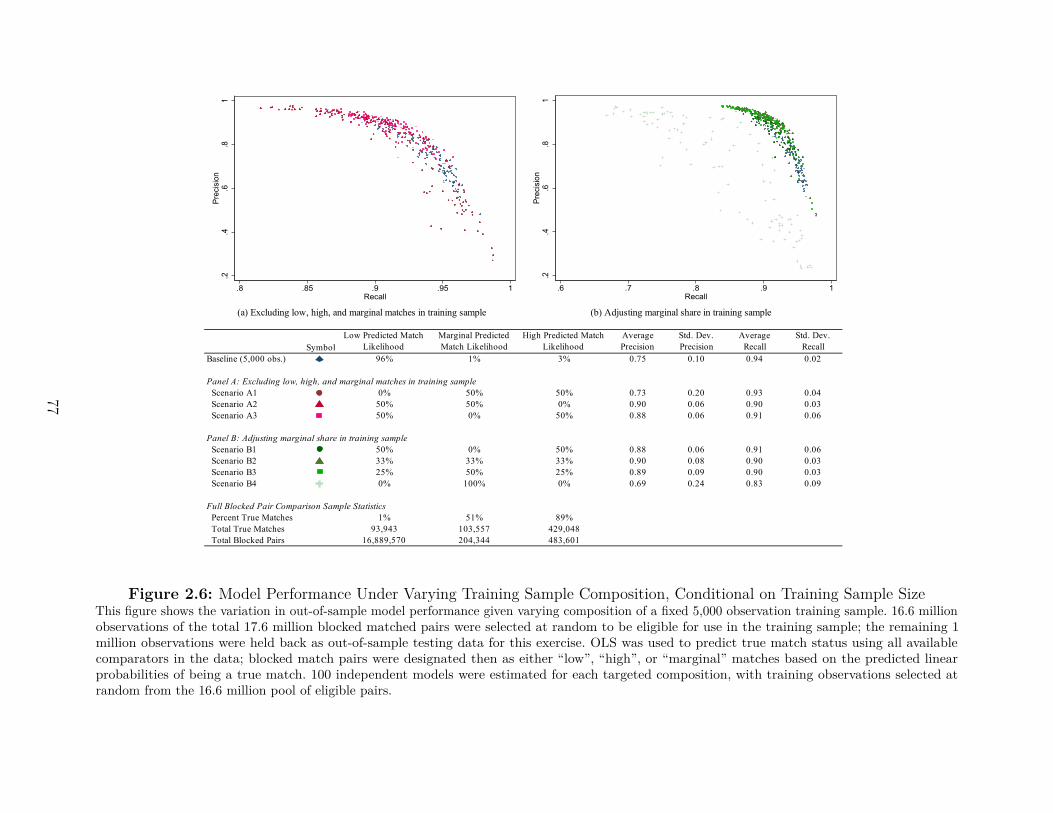
SymbolLow Predicted Match

LikelihoodMarginal Predicted Match Likelihood

High Predicted Match Likelihood

Average Precision

Std. Dev. Precision

Average Recall

Std. Dev. Recall

Baseline (5,000 obs.) 96% 1% 3% 0.75 0.10 0.94 0.02

Panel A: Excluding low, high, and marginal matches in training sample Scenario A1 0% 50% 50% 0.73 0.20 0.93 0.04 Scenario A2 50% 50% 0% 0.90 0.06 0.90 0.03 Scenario A3 50% 0% 50% 0.88 0.06 0.91 0.06

Panel B: Adjusting marginal share in training sample Scenario B1 50% 0% 50% 0.88 0.06 0.91 0.06 Scenario B2 33% 33% 33% 0.90 0.08 0.90 0.03 Scenario B3 25% 50% 25% 0.89 0.09 0.90 0.03 Scenario B4 0% 100% 0% 0.69 0.24 0.83 0.09

Full Blocked Pair Comparison Sample Statistics Percent True Matches 1% 51% 89% Total True Matches 93,943 103,557 429,048 Total Blocked Pairs 16,889,570 204,344 483,601

(a) Excluding low, high, and marginal matches in training sample (b) Adjusting marginal share in training sample

3UHFLVLRQ

5HFDOO

3UHFLVLRQ

5HFDOO

3UHFLVLRQ

5HFDOO

3UHFLVLRQ 3UHFLVLRQ3UHFLVLRQ 3UHFLVLRQ

3UHFLVLRQ

5HFDOO

3UHFLVLRQ 3UHFLVLRQ3UHFLVLRQ 3UHFLVLRQ

3UHFLVLRQ

5HFDOO

3UHFLVLRQ 3UHFLVLRQ3UHFLVLRQ 3UHFLVLRQ

3UHFLVLRQ

5HFDOO

3UHFLVLRQ 3UHFLVLRQ3UHFLVLRQ 3UHFLVLRQ

3UHFLVLRQ

5HFDOO

3UHFLVLRQ 3UHFLVLRQ3UHFLVLRQ 3UHFLVLRQ3UHFLVLRQ

3UHFLVLRQ

5HFDOO

3UHFLVLRQ 3UHFLVLRQ3UHFLVLRQ 3UHFLVLRQ3UHFLVLRQ

3UHFLVLRQ

5HFDOO

3UHFLVLRQ 3UHFLVLRQ3UHFLVLRQ 3UHFLVLRQ3UHFLVLRQ

3UHFLVLRQ

5HFDOO

3UHFLVLRQ 3UHFLVLRQ3UHFLVLRQ 3UHFLVLRQ3UHFLVLRQ

Figure 2.6: Model Performance Under Varying Training Sample Composition, Conditional on Training Sample SizeThis figure shows the variation in out-of-sample model performance given varying composition of a fixed 5,000 observation training sample. 16.6 millionobservations of the total 17.6 million blocked matched pairs were selected at random to be eligible for use in the training sample; the remaining 1million observations were held back as out-of-sample testing data for this exercise. OLS was used to predict true match status using all availablecomparators in the data; blocked match pairs were designated then as either “low”, “high”, or “marginal” matches based on the predicted linearprobabilities of being a true match. 100 independent models were estimated for each targeted composition, with training observations selected atrandom from the 16.6 million pool of eligible pairs.

77

.5.6

.7.8

.91

Prec

isio

n

.5 .6 .7 .8 .9 1Recall

.005

.01

.015

Estim

ated

∆

(a) Control Mean = 0.25; β = 0.05

.5.6

.7.8

.91

Prec

isio

n

.5 .6 .7 .8 .9 1Recall

.01

.015

.02

.025

.03

.035

Estim

ated

∆

(b) Control Mean = 0.25; β = 0.10

.5.6

.7.8

.91

Prec

isio

n

.5 .6 .7 .8 .9 1Recall

.02

.04

.06

.08

.1

Estim

ated

∆

(c) Control Mean = 0.25; β = 0.25

.5.6

.7.8

.91

Prec

isio

n

.5 .6 .7 .8 .9 1Recall

0

.005

.01

.015

.02

Estim

ated

∆

(d) Control Mean = 0.50; β = 0.05.5

.6.7

.8.9

1Pr

ecis

ion

.5 .6 .7 .8 .9 1Recall

0

.01

.02

.03

.04

Estim

ated

∆

(e) Control Mean = 0.50; β = 0.10

.5.6

.7.8

.91

Prec

isio

n

.5 .6 .7 .8 .9 1Recall

-.05

0

.05

.1

Estim

ated

∆

(f) Control Mean = 0.50; β = 0.25

.5.6

.7.8

.91

Prec

isio

n

.5 .6 .7 .8 .9 1Recall

-.01

-.005

0

.005

.01

.015

Estim

ated

∆

(g) Control Mean = 0.75; β = 0.05

.5.6

.7.8

.91

Prec

isio

n

.5 .6 .7 .8 .9 1Recall

-.02

-.01

0

.01

.02

.03

Estim

ated

∆

(h) Control Mean = 0.75; β = 0.10

.5.6

.7.8

.91

Prec

isio

n

.5 .6 .7 .8 .9 1Recall

-.05

0

.05

.1

Estim

ated

∆

(i) Control Mean = 0.75; β = 0.25

Figure 2.7: Average Estimated ∆ Over 1,000 Simulation Runs with Varying Model Parameterizations (Scenario 1)This figure reports the average estimated ∆ over 1,000 independent simulations described in 2.6. The figure shows that worse precision and recall ratesbias estimates of ∆ towards zero systematically.

78

.5.6

.7.8

.91

Precision

.5 .6 .7 .8 .9 1Recall

.3

.35

.4

.45

.5

P-Value

(a) Control Mean = 0.25; β = 0.05

.5.6

.7.8

.91

Precision

.5 .6 .7 .8 .9 1Recall

0

.1

.2

.3

.4

P-Value

(b) Control Mean = 0.25; β = 0.10

.5.6

.7.8

.91

Precision

.5 .6 .7 .8 .9 1Recall

0

.05

.1

.15

P-Value

(c) Control Mean = 0.25; β = 0.25

.5.6

.7.8

.91

Precision

.5 .6 .7 .8 .9 1Recall

.25

.3

.35

.4

.45

.5

P-Value

(d) Control Mean = 0.50; β = 0.05.5

.6.7

.8.9

1Precision

.5 .6 .7 .8 .9 1Recall

0

.1

.2

.3

.4

.5

P-Value

(e) Control Mean = 0.50; β = 0.10

.5.6

.7.8

.91

Precision

.5 .6 .7 .8 .9 1Recall

0

.1

.2

.3

.4

.5

P-Value

(f) Control Mean = 0.50; β = 0.25

.5.6

.7.8

.91

Precision

.5 .6 .7 .8 .9 1Recall

.3

.35

.4

.45

.5

P-Value

(g) Control Mean = 0.75; β = 0.05

.5.6

.7.8

.91

Precision

.5 .6 .7 .8 .9 1Recall

.1

.2

.3

.4

.5

P-Value

(h) Control Mean = 0.75; β = 0.10

.5.6

.7.8

.91

Precision

.5 .6 .7 .8 .9 1Recall

0

.1

.2

.3

.4

.5

P-Value

(i) Control Mean = 0.75; β = 0.25

Figure 2.8: Average Estimated P-Value Over 1,000 Simulation Runs with Varying Model Parameterizations (Scenario 1)This figure reports the p-value testing the null hypothesis that ∆ = 0 over the 1,000 independent simulations described in 2.6. Worse precision andrecall rates impair statistical precision, increasing the likelihood that there is a failure to reject the null hypothesis.

79

.5.6

.7.8

.91

Prec

isio

n

.5 .6 .7 .8 .9 1Recall

.04

.05

.06

.07

.08

Estim

ated

∆

(a) Control Mean = 0.25; β = 0.05

.5.6

.7.8

.91

Prec

isio

n

.5 .6 .7 .8 .9 1Recall

.08

.1

.12

.14

.16

Estim

ated

∆

(b) Control Mean = 0.25; β = 0.10

.5.6

.7.8

.91

Prec

isio

n

.5 .6 .7 .8 .9 1Recall

.2

.25

.3

.35

.4

Estim

ated

∆

(c) Control Mean = 0.25; β = 0.25

.5.6

.7.8

.91

Prec

isio

n

.5 .6 .7 .8 .9 1Recall

.04

.05

.06

.07

.08

Estim

ated

∆

(d) Control Mean = 0.50; β = 0.05.5

.6.7

.8.9

1Pr

ecis

ion

.5 .6 .7 .8 .9 1Recall

.08

.1

.12

.14

.16

Estim

ated

∆

(e) Control Mean = 0.50; β = 0.10

.5.6

.7.8

.91

Prec

isio

n

.5 .6 .7 .8 .9 1Recall

.2

.25

.3

.35

.4

Estim

ated

∆

(f) Control Mean = 0.50; β = 0.25

.5.6

.7.8

.91

Prec

isio

n

.5 .6 .7 .8 .9 1Recall

.04

.05

.06

.07

.08

Estim

ated

∆

(g) Control Mean = 0.75; β = 0.05

.5.6

.7.8

.91

Prec

isio

n

.5 .6 .7 .8 .9 1Recall

.08

.1

.12

.14

.16

Estim

ated

∆

(h) Control Mean = 0.75; β = 0.10

.5.6

.7.8

.91

Prec

isio

n

.5 .6 .7 .8 .9 1Recall

.2

.25

.3

.35

.4

Estim

ated

∆

(i) Control Mean = 0.75; β = 0.25

Figure 2.9: Average Estimated ∆ Over 1,000 Simulation Runs with Varying Model Parameterizations (Scenario 2)This figure reports the average estimated ∆ over 1,000 independent simulations described in 2.6 for the scenario with heterogeneous treatment effects. Due to the heterogeneity ofthe treatment effect, decreases in recall lead to systematic overestimates of ∆. Similar to scenario 1, decreases in precision bias ∆ towards zero systematically.

80

.5.6

.7.8

.91

Precision

.5 .6 .7 .8 .9 1Recall

.25

.3

.35

.4

P-Value

(a) Control Mean = 0.25; β = 0.05

.5.6

.7.8

.91

Precision

.5 .6 .7 .8 .9 1Recall

0

.05

.1

.15

.2

P-Value

(b) Control Mean = 0.25; β = 0.10

.5.6

.7.8

.91

Precision

.5 .6 .7 .8 .9 1Recall

0

.001

.002

.003

P-Value

(c) Control Mean = 0.25; β = 0.25

.5.6

.7.8

.91

Precision

.5 .6 .7 .8 .9 1Recall

.2

.25

.3

.35

.4

P-Value

(d) Control Mean = 0.50; β = 0.05.5

.6.7

.8.9

1Precision

.5 .6 .7 .8 .9 1Recall

0

.05

.1

.15

.2

P-Value

(e) Control Mean = 0.50; β = 0.10

.5.6

.7.8

.91

Precision

.5 .6 .7 .8 .9 1Recall

0

.0005

.001

.0015

.002

.0025

P-Value

(f) Control Mean = 0.50; β = 0.25

.5.6

.7.8

.91

Precision

.5 .6 .7 .8 .9 1Recall

.2

.25

.3

.35

.4

P-Value

(g) Control Mean = 0.75; β = 0.05

.5.6

.7.8

.91

Precision

.5 .6 .7 .8 .9 1Recall

0

.05

.1

.15

.2

P-Value

(h) Control Mean = 0.75; β = 0.10

.5.6

.7.8

.91

Precision

.5 .6 .7 .8 .9 1Recall

0

.0005

.001

.0015

.002

P-Value

(i) Control Mean = 0.75; β = 0.25

Figure 2.10: Average Estimated P-Value Over 1,000 Simulation Runs with Varying Model Parameterizations(Scenario 2)This figure reports the p-value testing the null hypothesis that ∆ = 0 over the 1,000 independent simulations described in 2.6 for the scenario withheterogeneous treatment effects. Worse precision and recall rates impact statistical precision though the effects are not systematic.

81

Table 2.1: Matching Strategies Used in 2019 Administrative DataPapers From the “Top 5” Journals

No MatchingRequired

Matching RequiredNot Discussed

DeterministicMatching

FuzzyMatching

TotalPapers

Papers 23 19 10 2 54

The table was compiled by searching the top 5 economic journals for papers thatcontain the exact phrase “administrative data.” We used search functions providedby Oxford Journals, JSTOR, Wiley Online Library and University of Chicago Pressto cover the relevant journals and years. Papers published in 2019 in the “top 5”economics journals are classified according to the matching procedure used to linkthe data. Approximately 40% of the papers do not require matches, while 35% ofpapers do not explicitly discuss the matching method used to create data. Mostdeterministic strategies use unique identifiers to execute merges.

82

Table 2.2: Summary Statistics of Training Data, External Testing Data, and the General U.S.Population

TDCJInmates1978-2014

Harris CountyJIMS

1980-2017

WAVoters

2008 and 2012

Multi-StatePrison Snapshot,

July 1, 2017

DMFDeath Year,

2000

United StatesPopulation,

2010

Share Male 0.880 0.800 0.500 0.930 0.480 0.490Share White 0.360 0.270 0.720 0.440 0.820 0.640Share Black 0.370 0.330 0.350 0.510 0.080 0.120Share Hispanic 0.260 0.320 0.110 0.040 0.060 0.160Average Age 42.500 40.900 37.800 44.200 78.300 37.200Share in Texas 100.000 100.000 0 0 0.050 0.080

Observations 3,152,630 4,119,621 11,808,233 330,756 8,922,820 308,745,538Unique IDs 905,530 1,317,315 5,379,888 N/A 2,230,705Unique PII Combinations 1,095,054 1,723,008 6,164,621 329,088 4,202,455 N/A

Summary statistics of demographics for all relevant samples. USA data is measured using the 2010 Decennial Census.Washington data is measured using the 2008 and 2012 ACS 1 year sample. The average age is as of April 1, 2010, exceptin the WA ACS sample where it is the average across the 2008 and 2012 waves. The samples used to train the matchingmodel have a higher proportion of men and people of color than the comparison populations.

83

Table 2.3: Description of Individual Blocks

BlockFraction of

True MatchesTrue MatchesNot Included

Date of birth + last soundex 77.900 147,654Date of birth + first soundex 81.500 123,808Month of birth + first soundex + last soundex 72.700 182,324Day of birth + First soundex + last soundex 72.100 186,694Year of birth + first soundex + last soundex 72.100 186,798Date of birth + last phonex 77.900 147,761Date of birth + first phonex 82.100 119,861Month of birth + first phonex + last phonex 73.200 179,241Day of birth + First phonex + last phonex 72.500 183,624Year of birth + first phonex + last phonex 72.500 183,720

Union of Blocks 95.200 32,211

Each row represents a separate block that is used to partition the data. Thefull match space is generated by taking the union of pairs created across all 10blocks.

84

Table 2.4: Comparison of Out-of-Sample Model Performance

Model Accuracy Precision Recall F-Statistic

FalsePositiveRate

Estimation +PredictionDuration(Hours)

Deterministic 0.970 0.930 0.760 0.840 0.006 0.00Naive Bayes Classifier (Discrete) 0.97 0.900 0.72 0.80 0.008 0.060Naive Bayes Classifier (Kernel) 0.970 0.880 0.810 0.840 0.011 1.420Support Vector Machine 0.980 0.94 0.830 0.880 0.006 199.55Lasso Shrinkage Model 0.980 0.900 0.820 0.860 0.009 21.010Random Forest 0.980 0.930 0.880 0.900 0.006 0.260Random Forest (Demog. Enhanced) 0.98 0.930 0.89 0.91 0.007 0.280Random Forest (Year of Birth) 0.970 0.82 0.820 0.820 0.018 0.180Neural Net Perceptron 0.980 0.930 0.850 0.890 0.006 2.110Neural Net 0.980 0.920 0.880 0.900 0.008 10.130

This table compares performance across a number of classifiers. Because there are roughly 2 trillion true negatives, whichswamp comparison of accuracy and false positive rates across models, we limit the ratio of false negatives to true matches at aratio of 10:1. Otherwise, the accuracy rate for all models would be 1.00 and the false positive rate would be 0.00. In eithercase, we focus on the precision, recall and F-statistic to differentiate model performance. Numbers in bold indicate the bestperformance across all models for a given statistic. Numbers in italics represent the worst performance across all models for agiven statistic. The demographic enhanced random forest achieves the highest F-statistic and recall rate, and has a precisionrate that is slightly lower than the SVM classifier.

85

Table 2.5: Demographic-Specific Performance Statistics

Demographic Enhanced Random Forest

Deterministic5,000 Hand-Coded

Training Obs.5,000 BiometricTraining Obs.

1,000,000 BiometricTraining Obs.

Panel A: Precision RatesOverall 0.930 0.95 0.91 0.930Race/EthnicityWhite 0.960 0.97 0.94 0.940Black 0.970 0.97 0.960 0.95Hispanic 0.88 0.98 0.950 0.930

SexMale 0.92 0.96 0.950 0.940Female 0.97 0.950 0.83 0.900

Decade of Birth1960s 0.930 0.94 0.89 0.9201970s 0.940 0.96 0.93 0.9301980s 0.970 0.97 0.93 0.9401990s 0.98 0.980 0.95 0.960

Panel B: Recall RatesOverall 0.76 0.770 0.840 0.89Race/EthnicityWhite 0.810 0.81 0.890 0.93Black 0.80 0.810 0.860 0.91Hispanic 0.73 0.740 0.880 0.93

SexMale 0.790 0.77 0.830 0.90Female 0.68 0.760 0.860 0.88

Decade of Birth1960s 0.72 0.720 0.800 0.861970s 0.80 0.820 0.880 0.921980s 0.86 0.880 0.930 0.961990s 0.88 0.900 0.950 0.98

Panel C: F-StatisticsOverall 0.84 0.850 0.870 0.91Race/EthnicityWhite 0.880 0.88 0.910 0.94Black 0.88 0.890 0.900 0.93Hispanic 0.84 0.840 0.920 0.93

SexMale 0.85 0.870 0.890 0.92Female 0.80 0.840 0.840 0.89

Decade of Birth1960s 0.81 0.810 0.840 0.891970s 0.86 0.880 0.900 0.931980s 0.91 0.920 0.930 0.951990s 0.93 0.940 0.950 0.97

This table compares performance across a number of classifiers and training data. Entries in boldrepresent the best performance compared to other models, while entries in italics represent the worstperformance across models. The demographic enhanced model performs the best in terms of recalland the overall F-statistic for every demographic group. The model trained with hand-coded trainingdata is more conservative in identifying matches since high precision comes at the expense of lowrecall. Similarly, the deterministic model is successful at limiting false matches (precision), though isunable to identify true matches as well as the random forest algorithms.

86

Table 2.6: Testing Model Performance in External Applications

False Pos.Application Accuracy Precision Recall F-Stat. Rate

Multi-State Inmate Snapshot (July 1, 2017) 1.000 – – – 0.000Washington State Voter Records (2008 & 2012) 0.980 0.920 0.880 0.900 0.008Corrupted Death Master File (2000-2009) 0.980 0.970 0.930 0.950 0.003

Comparison of model performance across a range of external applications. Row 1 refers to the deduplication of all prisonersin incarceration in different states on July 1, 2017. The 2nd row refers to the one-to-one match of Washington state voterrecords using the 2008 and 2012 voter files. Row 3 refers to the deduplication of the corrupted DMF. For each exercise,we use the baseline random forest model generated from the 1,000,000 observation training sample. For the prisonerdeduplication exercise, there are no “true matches” so precision and recall cannot be calculated. The low false positiverate in row 1 suggests that the model is not overly permissive when identifying matches. Rows 2 and 3 suggest that themodel performance is dependent on the target data population, though the model performs well in both the Washingtonvoter match and the corrupted DMF match. Because there are an excessive number of true negatives, which swamp theaccuracy and false positive rates in each external application, we limit the ratio of false negatives to true matches at a ratioof 10:1 where possible. Since by construction there are no true matches in the July 1 prisoner application, this adjustmentis not feasible. Otherwise, the accuracy rate for all models would be 1.00 and the false positive rate would be 0.00.87

CHAPTER III

Effect of Financial Sanctions: Evidence From Michigan’sDriver Responsibility Fees

3.1 Introduction

Understanding the impacts of legal financial obligations (LFO) on criminal justice involvedindividuals has become more urgent over the past twenty years as state and municipal courtshave steadily increased the number and magnitude of fines and fees owed by defendants(Bannon et al., 2010; Harris et al., 2010). Many state and local governments rely on therevenue generated from these fines and fees to fund courts and other government services.According to the Survey of Inmates in State and Federal Correctional Facilities, the percentageof inmates that had LFOs imposed by courts has increased from 25% in 1991 to 66% in 2007Harris et al. (2010).

Descriptive research has found strong correlational evidence linking fines and fees withfinancial instability, criminal recidivism, and poor labor market outcomes (Harris et al.,2010; Pleggenkuhle, 2018).1 Given the high incidence of criminal convictions in the UnitedStates, such evidence would suggest that these fees may have wide-ranging impacts on notonly the most disadvantaged criminal defendants but also on the economy at large. Causalevidence remains quite limited given the lack of data availability and exogenous variation. Oneexception is Mello (2021) who finds that driver fees in Florida are associated with short-termfinancial distress, using difference-in-differences and event-study research designs applied totraffic stop data linked with high-frequency credit report data.

In this paper, we exploit a policy change in the state of Michigan as a source of exogenousvariation on the magnitude of financial sanctions faced by defendants to get a more completeunderstanding of the ways that criminal financial sanctions impact long-term recidivism and

1See Martin et al. (2018) or Fernandes et al. (2019) for recent reviews of the literature on financialsanctions.

88

labor market outcomes. In 2003, Michigan passed Public Act 165, or the driver responsibilityfee (DRF), which mandated new fines to criminal defendants who were convicted of certaindriving crimes. The goal of the act was to raise revenue for the government while improvingdriving safety.2 The amount of the fines varied based on the severity of the offense, rangingfrom $300 to $2,000. Failure to pay these fines would lead to driver’s license suspension, whichcould lead to even more fines since driving with a suspended license was also a DRF-qualifyingoffense. In the first two years after the law was enacted, the state levied over $250 million indriver responsibility fines (Wild, 2008).

To estimate the long-term causal effect of the financial sanctions, we exploit the fact thatthe DRF program in Michigan applied only to individuals convicted of a DRF-eligible offenseon or after October 1, 2003, a context well-suited for regression discontinuity analysis. Twokey mechanisms potentially link DRF sanctions to behavioral responses: (1) an income effectgenerated from the fine itself, and (2) a license revocation in the event of non-payment. Achallenge in studying this program is that a subset of the caseload commits DRF-relatedoffenses at a regular interval, meaning that those to the left of the cutoff who originally avoidedthe DRF sanction pick up DRF sanctions when they reoffend in a year or two. Ignoring thisissue might underestimate the true impact of the policy since the license revocation channelis partially neutralized through such behavior.

To address this challenge, we develop a prediction model based on observable demographicinformation, criminal history, and longitudinal earnings profiles to distinguish between thoselikely and unlikely to commit a new DRF-related offense in the short-run.3 Among thosewith with low likelihood of DRF recidivism, defined as having a predicted likelihood of DRFrecidivism below the median, which we refer to as the low contamination sample, the integrityof both mechanisms is maintained over roughly the entire 10-year follow-up period. For thehigh contamination sample, the extensive margin of the first stage (i.e., getting one or moreDRF sanctions) declines by over 50 percent within five years, severely curtailing our abilityto capture the long-term impact of the license revocation mechanism for this subpopulation.

Our results show modest behavioral responses to DRF sanctions. For the low contaminationsample, we observe no economically meaningful or statistically significant long-term labormarket responses overall. Subgroup analysis, however, suggests improved earnings outcomesat the median of the predicted income distribution. We find short-term negative impacts onearnings that are likely mitigated through the channel of incapacitation following driver’slicense revocation from non-payment; these effects attenuate in the long run. This subsample

2This program is not unique to Michigan as New Jersey, New York, Texas, and Virginia have all hadsimilar programs.

3There is no imbalance across the discontinuity in being categorized as either being part of the high orlow risk samples.

89

does not show a crime response either in the short or long-run. For the high contaminationsample, we observe a short-run increase in earnings from the income effect that is not sustainedin the long-run. We also find evidence of small long-run deterrent effects. Finally, we findspillover labor market effects onto the romantic partners of the high contamination group inthe long-run. Specifically, we find a 9% increase in the cumulative earnings of partners from2005 to 2015 relative to a mean of $202,900, suggesting other household members may bestepping in to cover the cost of the LFO.

Overall, we find DRFs to be a regressive form of funding for the government with limitedbenefits in terms of labor market outcomes or criminal behavior. We observe no change in therate of DRF-related offending in the general population, suggesting no evidence of a generaldeterrence response, and no fall in recidivism, suggesting no evidence of a specific deterrenceresponse in the study sample. Given the low average income of individuals in our sample, theimpacts of the policy were concentrated on those less likely to pay the fees, placing them athigher risk for driver’s license suspension. While unmeasured, it is possible that consumptiondeclined in response to the fines without a concurrent change in income to compensate forthe negative financial shocks. Even more concerning, the spillover impacts onto partners’earnings indicate that some people who did not commit the DRF offense bore the monetaryburden of the fines.

The findings of our paper are surprising given the small but growing economics literatureon the impacts of financial sanctions, which find negative effects on labor outcomes. In thepaper that is most similar to ours, Mello (2021) finds that speeding ticket citations lead tofinancial instability and decreased labor force participation in the two years following theinitial fine using data from credit reporting agencies.4 The result is particularly strong forlower income individuals, suggesting that even small negative income shocks in the form ofunexpected fines can lead to negative labor market outcomes. In contrast, our paper relies onadministrative tax records, covering a wider range of individuals.

Previous empirical work on financial sanctions has mostly focused on the direct impactson the defendants but has ignored the potential effects on other household members; however,qualitative and anecdotal work on this topic suggests that spillover effects are importantto quantify, especially in the context of the criminal justice system (Kearney et al., 2014;Shapiro, 2014; Mathews and Curiel, 2019).5 Our paper is the first to attempt to document

4In general, research on driving infractions finds that higher cost citations and stronger enforcement deterpeople from future offenses and lead them to drive more safely (Makowsky and Stratmann, 2009; Mello, 2021;Hansen, 2015; Luca, 2015). Compared to past work, our paper examines costs from administrative fees, ratherthan citations and also significantly increases the timeline in which we study the effect of these financialsanctions.

5A range of literatures in economics provide evidence on the household spillovers of negative incomeshocks (Page et al., 2009; Mörk et al., 2014; Liu and Zhao, 2014; Coile, 2004; Bloemen and Stancanelli, 2008;

90

and measure these spillover effects on romantic partners.This paper makes several important contributions to the literature. First, we provide

robust, causal estimates on the effects of financial sanctions on labor market and recidivismoutcomes. Second, our unique data allows us to estimate these effects on a longer timeframe and test how they might generate spillovers to other household members, which helpsbetter characterize the full impact of the policy. Third, we develop a methodological strategyto address high DRF recidivism rates, which would otherwise undermine the use of thepolicy changes over time in regression discontinuity research designs. Our findings are muchmore modest compared with the previous literature. Future research is needed to expandthe evidence base on financial sanctions and increase our understanding on the potentialmechanisms that might contribute to behavioral changes.

The remainder of the paper is as follows: Section 3.2 describes the policy change and judicialsystem of the state of Michigan; Section 3.3 describes the data used in this analysis; Section 3.4describes the empirical methodology and provides evidence to support the identificationstrategy; Section 3.5 presents the results; lastly, we conclude in Section 3.7.

3.2 Michigan’s Driver Responsibility Fees Law

In an effort to promote safer driving and increase state revenue, the governor of Michigansigned Public Act 165 into law on August 11, 2003. The legislation, which became effectiveon October 1, 2003, mandated new fines to defendants who were convicted of certain drivingcrimes.6 The DRF would be enforced by the Michigan State Treasurer as its revenue wouldbe directed toward the state’s General Fund. As a result, the DRFs were classified asadministrative fines, rather than criminal penalties (Wild, 2008).

The act created two categories of fees. Category 1 was for drivers who accrued sevenor more driving or traffic violations in two years. Category 2, which is the focus of thisresearch, fined drivers for specific violations ranging from driving without a driver’s licenseto driving under the influence. This fee was determined using three distinct tiers of drivingviolations, where the lowest level defendants were forced to pay a $150 or $200 dollar fee fortwo consecutive years, the middle level defendants were forced to pay a $500 dollar fee fortwo consecutive years, and the highest level defendants were forced to pay a $1000 fee fortwo consecutive years (Wild, 2008). Table 3.1 shows a detailed list of the Category 2 type ofoffenses associated with each fee level.

One particular criticism of the DRF policy relates to its onerous impact on poor defendants

Hankins and Hoekstra, 2011).6The law was modeled on similar legislation in New Jersey. Since the passage of Michigan’s law, Texas,

New York, and Virginia have each instituted their own version of DRFs.

91

(Hausman, 2013). Failure to pay the fees after 60 days led to the suspension of one’s driver’slicense and driving with a suspended license was itself a DRF-qualifying offense, so that lowerincome recipients may have been more at risk of receiving multiple DRFs. By the time thatthe law was repealed in 2018, an estimated 317,000 drivers had had their driver’s licensessuspended for failure to pay DRFs (Carrasco, 2018). In order to reinstate a license, one wasrequired to pay all outstanding DRFs along with an additional $125 fee, otherwise drivingwithout a license put individuals at risk for new criminal charges and additional fines andfees. In fact, from 2005 to 2007, the number of citations for driving with a suspended licenseincreased by 44% (Wild, 2008).

The fees failed to generate planned revenue or improve driver safety. The initial collectionrate, from 2003 to 2008, of 52% was lower than the state’s initial projected collection rate of60%. Alcohol-related driving crimes increased by 21% after the bill went into effect, whichsuggested that the deterrent aims of the policy failed to materialize (Wild, 2008).

In 2018, the state of Michigan repealed the driver responsibility fee legislation andcanceled all remaining debt owed under the law.78 At the time of nullification, the stateforgave approximately $630 million in outstanding driver responsibility payments (Carrasco,2018). From 2004 to 2008, Michigan assessed approximately $780 million in fees but collectedonly 49% of them (Wild, 2008). This collection rate is lower than the one reported by thestate of New Jersey for their DRF program (Wild, 2008).

Driver responsibility fees were assessed upon conviction for a qualifying offense and wereadministered by the Michigan Secretary of State. It is worth noting that these fees weredistinct from fines, restitution payments, and other fees that could be imposed by the courtsupon conviction for any crime. As such, driver responsibility fees in this paper represent alower bound on the total financial burden imposed after a conviction for a driving offense.

3.3 Data

This project leverages several sources of rich population-level data, including criminalrecords from the Criminal Justice Administrative Record System (CJARS), longitudinalearnings data from IRS W-2 information returns, and romantic partner linkages compiledfrom a combination of survey and administrative data. All of these data were analyzed withinthe Census Bureau’s Data Linkage Infrastructure, where data can be linked at the personlevel using the anonymous Protected Identification Key (PIK).

7Since Michigan’s repeal, Texas and New Jersey have also repealed their own versions of the DRF law.Virginia repealed its law in 2009.

8This repeal only covered the Category 2 fees, which is the focus of this study. Category 1 fees wererepealed in 2011.

92

Michigan DRF-eligible offenses that form the basis of our sample are identified from theadjudication records in CJARS. We use the charge offense to identify all charges that wouldtrigger a DRF as defined in Michigan Public Act 165. Our sample consists of an individual’sfirst conviction for a DRF-eligible offense in Michigan from April 1, 2001 to March 31, 2006,which covers the 2.5 years before and after the DRF effective date of October 1, 2003.9

To measure criminal outcomes, we identify all misdemeanor or felony convictions inMichigan for the set of individual in our analytic sample who received a DRF-eligible offenseduring the 2.5 years surrounding the effective date of the DRF law, starting in April 1, 2001and ending in March 31, 2006.

To measure employment and earnings, we use IRS W-2 information returns from 2005, thefirst year we have W-2 information, to 2015. We define earnings as the sum of inflation-adjustedwages across all W-2 filings in a given period.10 One major benefit of using W-2s is thatthey cover all formal employment regardless of the duration of the employment; they are notaffected by the selective tax filing behavior inherent in IRS 1040 individual tax returns.11

Furthermore, if an individual works for multiple employers in one year, each of the employersmust issue a W-2 tax return. We can use the number of W-2 returns filed in a year on behalfof an individual as a measure of the number of jobs that individual worked.

In order to document spillover effects within romantic partnerships, we link individualsto their partner or spouse using a wide array of government data including the 2000and 2010 Decennial Censuses, IRS 1040 individual tax returns, housing assistance datafrom the Department of Housing and Urban Development, American Community Surveyresponses, and other survey and administrative records that identify romantic partnershipsbetween individuals over time.12 Romantic relationships of interest in our sample are spousal,romantic non-cohabiting, or romantic cohabiting. Once we have linked an individual witha DRF-qualifying offense to a romantic partner whose relationship inception predates theDRF-eligible offense, we are able to draw on the same IRS and CJARS data to identify thelabor market outcomes and criminal behavior of the partner. This enables us to test howpre-existing relationships and partners’ outcomes are affected by the fees.13

Finally, we leverage Census Bureau survey and administrative records to identify demographiccharacteristics so that we do not have to rely on possibly mismeasured analogues in court

9We focus on conviction date because the DRF law affected only cases disposed after October 1, 2003.10All earnings are inflated to 2017 dollars using the Consumer Price Index for All Urban Consumers

(CPI-All Urban). Fines and fees generated from DRF-eligible offenses are not adjusted.11Employers are required to file W-2 returns if an employee earns at least $600 in a tax year.12See Finlay et al. (2021) for more details on how these links were identified.13A limitation of this approach is that we are less likely to observe informal relationships, such as unmarried

romantic relationships that do not involve cohabitation, since they are unlikely to jointly file taxes, co-reside,or respond to household surveys together.

93

records.14 We use date of birth and gender records from the 2020 Census Bureau Numidentfile, which is based on the Social Security Administrations Numident register. For race andethnicity information, we use the Census Bureau 2016 Title 13 race and ethnicity file, whichcombines self-reported and administrative records of an individual’s race and ethnicity fromvarious sources, such as the Census Numident and the 2000 and 2010 Decennial Censuses.

3.4 Research Design and Methodology

To determine the causal effects of DRF sanctions, we exploit the discontinuous implementationof the policy on October 1, 2003. Specifically, the statute only applied to individuals convictedof a DRF eligible offense on or after October 1, 2003. Therefore, individuals convicted of thesame offense prior to October 1, 2003 would not be subject to the additional fine. Given thepolicy design, we utilize a sharp regression discontinuity designed to compare outcomes forindividuals convicted of the same crimes right before and after the policy implementation.Under standard assumptions, the difference in outcomes can be attributed to the policychange at the discontinuity. In order to have a causal interpretation, the change in policy mustbe the only variable correlated with the outcomes to shift. In other words, the convictionsaround the discontinuity must be randomly sorted, so there should be no difference in thepeople charged with DRF crimes in the neighborhood of the policy change.

For the formal regression discontinuity estimates, we follow the method proposed byCalonico et al. (2014) and implemented in the Stata command rdrobust (Calonico et al.,2017). The point estimates τ are estimated using the following framework:

τ = µ+ − µ−,

where µ is the estimating equation of the outcome variable and

µ+ = limx→d+

µ(x), µ− = limx→d−

µ(x), µ(x) = E[Yi|Xi = x].

In this model, the average outcome function, E[Yi] is estimated on either side of thethreshold where the DRF conviction date (Xi) is equal to the date of the policy change,X = d. The causal effect of the driver responsibility fees, τ , is thought of as the jump in theestimating equation moving from the left (d−) to the right side (d+) of the conviction datethreshold. Instead of taking a simple average of the outcome variable, Calonico et al. (2014)propose a parameterization of the estimating equation using first-order local polynomials on

14Hispanic ethnicity is especially underreported in criminal justice administrative records (Eppler-Epsteinet al., 2016; Ford, 2015).

94

each side of the discontinuity.15

Throughout the analysis, we use the sharp RD design defined above with initial DRFconviction date as the running variable. We also include sample averages of the outcomes tocontextualize estimate effect sizes.

The identifying assumption of this research design is that justice-involved individualswhose cases were disposed right before October 1, 2003 are observationally equivalent toindividuals whose cases were disposed right after October 1, 2003. Behavioral responses tothe policy, such as deterrence or delayed sentencing, would violate this assumption. This isof particular concern since Public Act 165 was signed into law six months before the driverresponsibility fee policy went into effect. Thus, both government agents and drivers couldchange their behavior in anticipation of the adoption of the new fees. We test both of thesethreats to identification by providing graphical and regression evidence that the caseload anddemographic composition of DRF defendants is smooth around the policy threshold.

Table 3.2 reports regression discontinuity estimates for select demographic and pre-offenseincome variables. Nearly all balance test estimates are statistically insignificant and closeto zero supporting the causal interpretation of the proposed research design. We estimatea significant, but small increase in the likelihood of being black and small decreases in thelikelihood of being white or convicted of a DRF level 1 offense, but these estimates are relativelysmall when compared to the overall sample averages. All other estimates are statisticallyindistinguishable from zero. We also show that the estimated probability of linking to aromantic partner in the year of DRF conviction is unchanged at the discontinuity. This lastfact is used to justify our empirical analysis of the effects of the fees on partner labor supplyin Section 3.5.5.

One of the benefits of the regression discontinuity methodology is that results are easilyvisualized. By plotting local polynomial estimates for outcome variables on either side ofthe threshold, we can visually represent the estimated jump or discontinuity.16 Panel C ofFigure 3.1 shows the smoothed case counts of all DRF convictions around the discontinuity.The difference in case load count is smooth across the threshold suggesting that there was nochange in enforcement or charging behavior after the implementation of the new fees. Forthis local polynomial figure as well as throughout the remainder of the paper, we use theEpanechnikov kernel and a 120-day bandwidth to estimate the outcome function and display

15We use a uniform kernel which equally weights all observations within the bandwidth and a data-drivenbandwidth selector that chooses two mean squared error optimal bandwidths, one for each side of thediscontinuity. This corresponds to the msetwo bandwidth selector within the rdrobust command. We estimatefirst-order linear polynomials with second-order bias correction and implement heteroskedasticity-robustplug-in residuals variance estimators with HC2 weights.

16For our local polynomial graphs, we residualize the variables using the same set of controls with themean added back to aid in interpretability.

95

95% confidence intervals.17 The scatter plots are binned at the monthly level with markersize scaled according to the number of convictions in each bin.

For further evidence of the robustness of the identification strategy, we calculate predictedincome using cumulative income reported on annual IRS W-2 information returns from2005 to 2015 and predicted recidivism using total future convictions 10 years after DRFconviction shown in Table 3.3. Since W-2 information is only available starting in 2005, weuse different measures of time across the labor and recidivism measures. To generate bothpredicted variables, we use a fully interacted regression model with the following variables: ageat conviction for DRF offense, gender, race/ethnicity, average annual 1040 income, average1040 form filing rates 1–3 years prior to conviction, fixed effects for the number of previousconvictions, and the full interaction of fixed effects for the DRF offense level with fixed effectsfor the county of adjudication. Since we do not use the cutoff in constructing these predictions,the smoothness in the predicted variables across the cutoff would imply that the identifyingassumptions of the sharp RD design are met. This is indeed what we show in the bottom tworows of Table 3.3 where coefficients on the predicted outcomes are insignificant.18

A visualization of the balance tests of the predicted income and predicted recidivismvariables are shown in Panels A and B of Figure 3.1. Both figures are smooth around thediscontinuity, further underscoring the overall balance of covariates.

Given the balance in demographic characteristics and predicted variables, we quantify thefirst-stage relationship in Figure 3.2, which shows the changing likelihood of being subjectto a driver responsibility fee conditional on being convicted of a DRF-qualifying offense forindividuals in our sample over time. Unsurprisingly, we find a sharp jump of approximately100% in the likelihood of being charged with a driver responsibility fee after the law goesinto effect.

Throughout the analysis below of labor market and recidivism outcomes, all outcomes areresidualized by including controls for the driver’s demographic characteristics (age, gender,race/ethnicity, total convictions 1–3 years before DRF conviction, income 1–3 years beforeDRF conviction as reported on 1040 tax filings, and the likelihood of filing a 1040 tax return1–3 years before DRF conviction) and fixed effects for the DRF level of offense.

17Census Bureau disclosure rules prevented release of the binned quantities from the uniform kernel modelusing for tabular output. The kernel differences result in slightly varied regression discontinuity point estimatesacross tables and figures.

18Due to limits on the number of results that can be disclosed by the Census Bureau, we do not includesmoothed local polynomial figures for all covariates. As a compromise, we report the caseload density, predictedW-2, and predicted recidivism (which aggregate the individual covariates into two indices).

96

3.4.1 Traffic Offense Recidivism and Integrity of the Experimental Variation

One possible threat to identification of the impact of DRFs is that individuals convictedof DRF-eligible offenses before the DRF goes into effect will eventually be convicted ofDRF-eligible offenses after the effective date, thereby exposing the group to DRFs andcontaminating the RDD. This type of DRF-eligible recidivism is particularly likely given therole of license revocation and the fees associated with driving without a license discussedearlier.

To circumvent this issue, we identify drivers at risk of reoffending two years after their firstconviction within the sample time period based on a prediction model using the full interactionof age at conviction for DRF offense, gender, race/ethnicity, average 1040 income and filingrates 1–3 years prior to conviction, and fixed effects for number of previous convictions andthe full interaction of controls for the DRF offense level with fixed effects for the countyof adjudication and case characteristics (fixed effects for the DRF level of offense, countyof adjudication). Using the median of the predicted risk of DRF recidivism, we separateour sample into “high contamination” and “low contamination” groups where the highcontamination group has greater than median predicted risk of DRF recidivism and istherefore more likely to contaminate our treated group. For the rest of the paper, we refer tothe high (low) contamination group as the group with more (less) contamination.

To illustrate this contamination over time and to demonstrate the stability of the lowcontamination group, the top panels of Figure 3.3 show the year-by-year evolution of thecumulative likelihood of being convicted of a DRF offense after the effective date separately forindividuals in the high contamination group compared to individuals in the low contaminationgroup. The DRF conviction estimates for Year 0 are equivalent to the first-stage estimates inFigure 3.2, with each additional year increasing the follow-up period by a year.

For the high contamination group, we find that the validity of the experiment erodessignificantly on the extensive margin and that the first-stage estimate falls from nearly 100percentage point to almost 60 percentage points two years after the first DRF conviction.This implies that a significant portion of observations in the untreated sample were convictedof an additional DRF-qualifying offense after the effective date, thus contaminating thesample. In contrast, the low contamination group is significantly more stable. In fact, the lowcontamination group is relatively stable, with the first-stage estimate falling from nearly 100percentage points to 95 percentage points four years after the first conviction.

Since some individuals with initial DRF-eligible convictions before the law’s effectivedate will go on to lose their licenses (i.e., the high contamination group), we cannot as easilymeasure the impact of DRF conviction on labor market and recidivism outcomes that mayresult from license suspension. We can, however, still measure the impacts of the accumulation

97

of fines from DRF conviction that operate through the income effect.Since the analysis will be stratified by contamination group, we should consider how these

groups differ along other dimensions. Figure 3.4 plots the average demographic characteristicsacross 5 percentage point intervals of the distribution of the predicted DRF recidivism. Weinclude individuals within 15 percentiles on either side of the central point. For example, atthe 20th percentile, we include individuals from the 5th to 35th percentile. Statistics near theends of the distribution will have fewer observations as they are bounded by 0 and 100. Wealso mark where the sample splits between the low contamination group (0–50) and the highcontamination group (50–100).

Taken together, these figures show that the low contamination group is older and iscomposed of more females and fewer Blacks relative to the high contamination group. We alsofind that predicted income is lower in the high contamination group. We also find a sharpcontrast in criminal histories between the low and high contamination groups. Specifically,individuals with any prior criminal convictions one to three years prior to DRF conviction aremore likely to have a predicted likelihood of DRF recidivism above the median and therebybe in the high contamination group.

To ensure that splitting the sample by predicted risk of DRF recidivism does not violatethe identifying assumptions for a sharp RD, we graph the local polynomial estimates on eitherside of the discontinuity in Figure 3.5 of the likelihood of being in the high contaminationgroup. We also show the regression discontinuity estimate in Table 3.3. Both the figure andthe estimates show smoothness across the discontinuity.

3.5 Results

We split our discussion of the effects of financial sanctions into two categories: directeffects on individuals charged with a DRF-qualifying offense in the sample period and partnerspillovers. For our direct effects analysis, we also include heterogeneity analysis across predictedincome, recognizing that personal financial stability may influence the impact of the DRFs.We also separate our results across the different DRF levels to assess how the monetary sizeof the fees affects criminal justice and labor market outcomes. As mentioned in the priorsection, we show results separately for the predicted high and low contamination groups.

3.5.1 Direct Impacts on Labor Market Outcomes and Recidivism

Our main analysis examines the direct effect of the fees on the charged individual’scumulative employment outcomes from 2005 to 2007, from 2005 to 2015, and on recidivismoutcomes two years and ten years after initial DRF conviction. We use different periods of

98

measurement for recidivism and labor market outcomes because the IRS W-2 return data areonly available beginning in 2005.

Table 3.4 shows the regression discontinuity estimates and standard errors as well as theunderlying mean of the outcome from the sample of defendants with initial DRF convictiondates within 2.5 years of the policy threshold. Panel A reports the estimates for labor marketoutcomes and Panel B reports the estimates for criminal activity. All estimates in the tableare estimated using a sharp RD design and should be interpreted as causal.We split our resultsby contamination group to separate the two potential mechanisms: the income effect fromthe additional fines and the incapacitation effect from license suspension due to non-paymentof DRFs. For comparison purposes, we also include long-run results for the full sample.

Using W-2 tax return information from 2005–2007, we find differing effects of DRF feeson earnings in the short run across the high and low contamination groups. For the highcontamination group, DRF fees are associated with increased earnings of $2,185 from 2005 to2007. Since individuals in the high contamination group are at a higher risk of re-committinga DRF-qualifying offense, increased earnings are consistent with a labor supply income effectcaused by the DRF conviction. We observe no change in the average number of W-2 returnsfiled during the same period, which indicates that individuals increased labor supply withinexisting jobs rather than taking on more jobs to pay off the fees.

For the low contamination group, DRF fees are associated in the short run with a smalldecrease in the average number of W-2 returns received per year (0.03 percentage pointdecrease from a mean of 1.18 annual returns). Since there is no statistically significant decreasein the likelihood of any W-2 return being filed or on cumulative earnings within the sameperiod, the reduction of jobs was focused on secondary employment. Given that the incomeeffect would generate the opposite labor supply response, the reduction in the number of jobscould be caused by driver’s license revocation from non-payment of DRF fees.

For both low and high contamination groups, effects of DRF fees attenuate when weincrease the period of study to 2005–2015. We find no effects of DRF conviction on laboroutcomes on the long-run intensive or extensive margin for either contamination group.Specifically, our estimates show small and mostly insignificant effects on the likelihood ofreceiving a W-2 tax return, the average number of W-2 returns received, and on cumulativeearnings measured using total earnings reported on W-2 tax return.

These results taken together indicate that the imposition of DRFs did not create barriersto employment for individuals in either group as we do not see a corresponding fall in thelikelihood of receiving a W-2 return from 2005 to 2007. As mentioned previously, this wasa major concern given that the punishment for DRF non-payment led to driver’s licensesuspension, potentially eliminating a means of transportation to work. Furthermore, all

99

significant impacts generated by DRF conviction in 2005–2007 are no longer significant from2005–2015.

In Panel B of Table 3.4, we shift our focus to recidivism outcomes. The first row showsthe impacts of the fees on the likelihood of receiving any conviction (felony or misdemeanor,all offense types), measured by average recidivism. We find insignificant effects of DRFs onrecidivism two and ten years after DRF conviction for the high contamination group. Theestimates and standard errors are small relative to the mean, which indicated precise nulleffects. On the intensive margin (total convictions), estimates show similar null effects ofDRFs on recidivism for each contamination group.

For the low contamination group, we find a statistically significant but small decrease inthe likelihood of felony conviction two years after the initial DRF conviction. This decreasedrecidivism is not sustained when measured ten years after DRF conviction. We also find nulleffects when we measure effects by type of crime. Overall, DRF conviction had no meaningfulimpact on criminal behavior.

Our results using the full sample show null results for nearly all outcomes except forincreased cumulative earnings measured using income reported on 1040 tax filings anddecreased total convictions. Without correcting for the contamination in our sample, wewould incorrectly conclude that the policy improved market labor outcomes and increaseddeterrence. We observe none of these effects in either the high or low contamination results.The contrast in results for long-run outcomes between the full sample and the results bycontamination group only highlights the need for careful consideration of the interaction ofthe research design and behavioral responses to the policy.

Figure 3.6 shows graphical evidence of selected results from Table 3.4 by reportingnon-parametric smoothed estimates of long-term cumulative W-2 earnings and total convictionsbefore and after effective date of the DRF law in October 2003. These figures confirm thefindings in Table 3.4.

3.5.2 Evolution of the Effects on Labor Market Outcomes and Recidivism

Next we shift our focus to investigating the evolution of the effects over time. Figure3.7 shows the year-by-year estimates of the discontinuity and 95% confidence intervals forthe main income and recidivism outcomes and for the low and high contamination groupsseparately. To help quantify the estimated effect size, we also include the mean of the entiresample in the figures. The first estimate represents the effect of a DRF offense charge oncumulative income (cumulative recidivism) one year after DRF conviction (from 2005–2006)with each additional estimate increasing the follow-up an additional year up to ten years.

For the low contamination group, we observe no statistically significant effects on cumulative

100

income or cumulative recidivism over time. Notably, the estimates for cumulative earningsare close to zero until the 2005–2011 measurement period. Similarly, estimates for cumulativerecidivism are close to zero until seven years after conviction. Given the size of the sample,we are confident that these are precisely estimated null effects for both outcomes.

For the high contamination group, we observe a different pattern on the estimated impactson cumulative earnings. From 2005–2007 and 2005–2011, we find statistically significantincreases in cumulative earnings reported on W-2 information returns. These estimatedimpacts begin decreasing and become statistically insignificant from zero from the 2005–2012period onward. One possible reason for the effect fade out could be the loss of labor marketopportunities during Great Recession, but further research is needed to confirm this.

For total convictions, we observe a different pattern over time with no statisticallysignificant impacts on criminal behavior across all years in the follow-up period after the firstDRF conviction.

3.5.3 Heterogeneous Effects by Ability to Pay

Our findings so far show null effects of DRFs on criminal recidivism and labor marketoutcomes over the long run. Despite this, the fees may have real but countervailing effects indifferent subsets of the population. In particular, we are interested in determining whetheran individual’s initial ability to pay off driver responsibility fees may play a role in drivingthe headline null effects.

We proxy for the ability to pay driver responsibility fees using predicted W-2 income.Because we do not have access to IRS W-2 returns before 2005, we cannot condition analysison pre-conviction income. We do have access to IRS 1040 individual tax returns before theDRF policy goes into effect, but, as discussed earlier, the 1040 tax filing rate is only around60%, so its use would greatly reduce the power of the heterogeneity analysis. Instead werank individuals based on their predicted cumulative 2005–2015 W-2 income. The predictedincome model is estimated using the same covariates used in predicting DRF recidivism.These covariates are: age at conviction for DRF offense, gender, race/ethnicity, average 1040income and filing rates 1–3 years prior to conviction, and fixed effects for number of previousconvictions and the full interaction of controls for the DRF offense level with fixed effects forthe county of adjudication. Therefore, this measure of predicted W-2 income does not includeany information that is affected by DRF-eligible charges. As a result, we use it as a wayto rank people in the sample by their ability to pay the fees. People with higher predictedincome will have greater capacity to earn money to pay for the fines. We use the predictedW-2 income as a proxy for “affordability” and estimate how the effects of the fees differ bypredicted income.

101

After generating predicted income, we estimate regression discontinuity models at differentpoints of the predicted income distribution—every 5 percentiles between the 5th and 95th.To reduce noise, we include individuals within 15 percentiles of the central point in eitherdirection. As an example, our estimate at the 20th percentile will include everyone withpredicted income between the 5th and 35th percentile. Note that the estimates for the 5thand 10th (90th and 95th) percentiles include fewer observations as they are bounded below(above) by 0 (100).

Panels A–D of Figure 3.8 show the effects of DRFs on earnings and recidivism across thedistribution of predicted income and separately for individuals with predicted low and highrisk of DRF recidivism (with 95% confidence intervals for each point estimate).

For the heterogeneous effects of the driver responsibility fees on cumulative income, wefind statistically significant increases of about $20,000 in income for drivers in the 60th to65th percentile of the income distribution.

For the low contamination group, Panel B shows that there is little variation in the effect ofDRF fees on ten-year average recidivism rates. Most of the beneficial effects are concentratedon individuals in the 65th to 70th percentiles of the income distribution with a statisticallysignificant reduction in total recidivism of around 0.1 crimes ten years after conviction. Theestimated decreases in recidivism overlap with the effects on income at the 65th percentile ofpredicted income.

Only the income effect from a DRF conviction could generate these results. Driver’slicense revocation from non-payment would place the individual at higher risk for recidivismif caught driving with a suspended license, thereby increasing recidivism. Furthermore, therevocation could potentially reduce an individual’s earnings through their ability to work byremoving their means of transportation and thereby reducing employment or earnings.

We observe a different pattern across predicted income for individuals in the highcontamination sample. Notably, there are no effects on total convictions throughout the entiredistribution except for a statistically significant decrease of approximately 0.2 crimes at the45th and 50th percentile of the distribution. We do not observe a corresponding effect on totalearnings. For individuals in the 20th to 40th percentile, we observe similarly sized increasesin earnings of nearly $10,000, but the estimates are not quite statistically significant.

3.5.4 Heterogeneous Effects Across DRF Fee Levels

The previous section analyzes how the effects of the fees vary by the individual’s abilityto pay. However, the size of the fees relative to income can also be an important determinantfor the DRF impacts. Furthermore, heterogeneity in the characteristics of the subpopulationsof individuals across the fee levels could influence measurement of the impact of DRFs.

102

Given that being charged with a DRF-eligible offense may have monetary consequences andincapacitation effects from driver’s license revocation, analyzing the outcomes across the feelevels may provide insight on the main mechanisms driving the outcomes.

To test this hypothesis, we stratify the analysis of the impacts on cumulative earningsand total convictions by the three DRF levels and the two predicted risk groups. Using thesame sharp regression discontinuity design, Table 3.5 reports the effect of being convictedwith a DRF by the fee amount for both the high contamination and low contamination groupon short-run and long-run cumulative earnings and total convictions.

In the high contamination sample, we observe effects similar to what we observe in theanalysis of heterogeneity in ability to pay DRFs. Specifically, for cumulative earnings from2005–2015, we find no significant effects for any of the fee amounts; for total recidivism tenyears after conviction, we estimate a decrease of 0.3 convictions for individuals assignedthe $300 fee, which is similar to the estimate from the heterogeneity analysis at the 50thpercentile. The estimated decrease is small relative to the average of 4.3 total convictions.Interestingly, for the estimated impacts on the short run, the positive increase in earnings isnot concentrated at a particular fine level.

For individuals in the low contamination sample, we estimate heterogeneous impacts ofDRFs on cumulative earnings from 2005–2007 across the different fees. For individuals assignedthe $300 fee, we find an increase of earnings of $5,608, but for individuals assigned the $2,000fee, we estimate a decrease of $7,830. One possible explanation for the short-term negativeimpacts for individuals assigned the $2,000 is license suspension from fee non-payment. Giventhat average annual income is approximately $28,000 (calculated from average total incomefrom 2005–2007 of $83,930 in Table 3.5), a $2,000 fine paid over the course of two yearsrepresents a significant portion of income, which places these individuals at higher risk ofdriver’s license suspension from fee non-payment.

These effects on earnings are sustained for those assigned the $300 fee. We estimate thatDRFs caused a statistically significant $27,080 increase in long-run cumulative W-2 earnings,which is equivalent to an 11% increase relative to mean earnings of $254,900. Individuals inthis sample are unlikely to receive a second DRF conviction so this income growth stemsfrom the first DRF conviction. Thus, the fee of $300 had a sustained increase in earningseven after the fee had been paid.

Assignment of fees stemming from a DRF conviction did not impact criminal behaviorfor any level of fees in the low contamination sample. Across all levels and time periods, weobserve no statistically significant effect on total convictions. The estimates and standarderrors are also small relative to the means—indicating null effects.

103

3.5.5 Effects of DRFs on Romantic Partners

While we generally find that the driver responsibility fees have small or null effects on labormarket and recidivism outcomes of DRF recipients, we are also interested in how potentialimpacts may be internalized by households or romantic partners. For example, a large finemay trigger a change in a partner’s labor supply if he or she is the primary earner or ina better position to adjust labor supply on the intensive margin by increasing work hours.To measure partner spillovers, we use the household crosswalk discussed in Section 3.3 thatsynthesizes information from a variety of Census Bureau, IRS and other federal programdata. This crosswalk allows us to link individuals convicted of DRF-eligible offenses to theirpartners in the year of their initial DRF conviction.

In order to identify the causal impact of DRFs on partner outcomes, we need to havebalance in the likelihood of being linked to a partner across the DRF effective date. Panel Aof Table 3.6 shows no effect of the fines on the likelihood an individual charged with a DRFoffense is linked to a romantic partner in the year of conviction—for individuals in either lowor high contamination groups.

The rest of Table 3.6 shows outcomes of interest for partners: the likelihood of remainingin a relationship and the length of the relations in Panel B; cumulative W-2 earnings inPanel C and the total number of convictions in Panel D. As before, we split our results bycontamination group. We also consider both short- and long-term versions of the outcomes(relationship status in 2007 and 2015, labor market outcomes from 2005–2007 and 2005–2015,and recidivism outcomes two and ten years after the initial DRF conviction). All outcomesare estimated using the same covariates in previous analyses describing the individual chargedwith the offense (not the partner).

For the low contamination group, we find no evidence of spillover effects of the DRFs onpartnership rates or partner outcomes. Not only are estimates statistically indistinguishablefrom zero, but, relative to the mean, the effect sizes and standard errors are small, whichindicates null effects. These results indicate that earlier findings of null impacts of DRFson labor market and recidivism outcomes were not confounded by secondary impacts onpartnership length, partner labor supply, or partner criminal activity.

For the high contamination group, we find a statistically significant effect of DRFs onpartner long-term cumulative earnings (2005–2015), but no statistically significant effects oncriminal behavior or partnership outcomes. That is, for individuals at a higher risk of DRFrecidivism, partners increased labor supply as a result of DRF conviction, and some of thefinancial burden affected someone other than the individual convicted of a DRF offense.

104

3.6 Relationship to Prior Work

Our paper represents the first attempt to measure the long-term impact of financialsanctions using detailed complete criminal case histories, administrative tax records onearnings, and population-level links to romantic partners. In contrast to previous empiricalstudies on the impacts of financial sanctions from driving offenses, our results generally shownull impacts on labor market and recidivism outcomes with some small increases in laborsupply of fee recipients and their partners.

These results are divergent from past research, especially that of Mello (2021), whichstudies the effect of Florida drivers receiving a traffic citation on future employment andeconomic stability. Using highly detailed credit report data, he finds that driving fines areassociated with an increase in financial instability as well as a small but significant decreasein labor supply over the following two years. Below we lay out potential hypotheses as to whyour results diverge from past research on the effect of financial sanctions on driving outcomes.

First, the institutional context of our study is markedly different than that of paststudies, which affects the efficacy of the financial sanction. In our study, those convictedof a DRF-qualifying offense were subjected to a higher financial burden because they wererequired to pay the DRF on top of the traffic fine. In contrast, the focus of Mello (2021) isonly on traffic citations.

Second, from the definition of Public Act 165, we are only able to study a subset oftraffic violations. In contrast, Mello’s sample includes all individuals with a traffic violationin Florida. Furthermore, we identify individuals in our sample using court adjudication data.Therefore, even if an individual was convicted of a DRF-qualifying offense but did not go tocourt, they are not in our data set. In Mello’s sample, he is able to identify all individualswho received a citation in Florida.

Third, our earnings data cover a greater scope of employment relationships. Mello’sprimary employment data comes from monthly credit reports, which may select toward largeemployers who choose to report to credit agencies. We rely on W-2 information returns thatcover all formally employed individuals regardless of employer firm size, as long as thoseemployees earned at least $600 in a tax year.

Finally, there may be differences in data and sample composition between the two settings.Our sample is conditioned on individuals with a DRF-eligible offense receiving a PIK at theCensus Bureau, which excludes undocumented immigrants. The sample in Mello’s paper isconditioned on individuals with a driving citation data being linked to credit bureau reportingdata, which may also exclude some undocumented immigrants.

105

3.7 Conclusion

This paper examines the effects of financial sanctions on labor market and recidivismoutcomes in the state of Michigan. Despite widespread criticism of the law, especially relatedto driver’s license suspensions, we find relatively muted impacts of DRFs. After carefullyaddressing research design contamination caused by DRF recidivism, we find that the fees hada small positive effect on short-term W-2 income for individuals in the high contaminationsample. This effect attenuates in the long term, which may relate to the erosion of thelicense revocation channel in this subgroup over time. We find suggestive evidence that theseindividuals may be shifting part of the financial burden onto their romantic partners who haveincreased earnings of approximately $1,700 on average from 2005 to 2015. We also observeslight deterrent effects for individuals assigned the $300 fee ten years after DRF conviction.

At the same time, we find predominantly null effects on both short and long-term outcomesfor individuals in the overall, low contamination sample with no spillover effects onto partners.Our heterogeneity analysis reveals long-term positive impacts of the fees on individuals’cumulative earnings and mild deterrent effects for individuals at the 60th–70th percentiles.Separating individuals by the assigned fee reveals potential incapacitation effects for thosewith the most severe offense, who have reduced total earnings of almost $8,000 from 2005to 2007. Since these individuals have low likelihood of re-committing a DRF offense, thenegative impact on earnings is not sustained in the long-run. To the best of our knowledge,our results are the first to find such consistent and precisely estimated null to mildly positiveeffects of these types of financial sanctions.

Our findings contrast with prior work, in particular the causal estimates from Mello (2021).We believe four factors may contribute to these divergent findings: (1) different approaches toresearch design (RD versus event study); (2) measurement of labor market outcomes (W2 taxfilings versus credit bureau employment data, which principally comes from large employers);(3) different study populations; and, (4) the size of the financial sanctions. Further research iswarranted to better understand the contribution of each of these differences.

While we find no significant harm on individuals’ labor market outcomes or criminalbehavior, we also find limited evidence of benefits to justify this policy. As a source of revenuegeneration, the DRF was an inefficient and regressive form of taxation; if LFOs increasedwithout a concurrent change in labor supply, consumption may have in fact been negativelyimpacted. Funds were being raised from individuals with lower income compared to the generalpopulation.19 It is therefore unsurprising that DRF payment rates were quite low, reducing

19Average per capita, annual personal income in 2005 in Michigan was just over $30,000, unadjusted(of Economic Analysis and of St. Louis, 2021). From Table 3.4, average annual income per capita in oursample is just over $19,000 from 2005-2007 using W-2 information.

106

revenue and placing these individuals at higher risk of recidivism due to driver’s licenserevocation from non-payment. Our results show that DRF conviction increased the laborsupply of romantic partners, suggesting that other household members may be shouldering themonetary burden of the DRF fines. Without clear evidence of general or specific deterrencearising from the DRF policy, it still remains unlikely that the DRF regime was welfareimproving even if our causal estimates are less pessimistic than prior research has found.

107

Panel A: Predicted cumulative 2005–2015W-2 income

Panel B: Predicted total convictions 10 yearsafter DRF conviction

Panel C: Caseload density

Figure 3.1: Balance Tests Showing Smoothness Around the DRF Effective DateSource: Authors’ calculations from 1998–2015 IRS 1040 individual tax returns, 2005–2015 IRS W-2 informationreturns, the 2020 Census Numident (to measure year of birth, state of birth, and gender), the 2020 CensusBureau Title 13 race/ethnicity file, and Michigan criminal justice histories from the CJARS 2020Q1 vintage.Notes: These figures represent a series of balance tests done to ensure that there is smoothness around thediscontinuity. Equivalent RD estimates shown in Table 3.2 support the figures findings that the discontinuityis not significant. Predicted total recidivism ten years after conviction and predicted cumulative 2005–2015W-2 income are predicted using the full interaction of age at conviction for DRF offense, gender, race/ethnicity,average 1040 income and filing rates 1–3 years prior to conviction, and fixed effects for number of previousconvictions and the full interaction of: controls for the DRF offense level and fixed effects for the county ofadjudication. Caseload density is measured using the total number of DRF convictions per day. The estimatesare based off of a sample of all individuals convicted of a driver responsibility fee qualifying offense fromApril 1st, 2001 to March 31st, 2006 in Michigan. The sample contains only the first DRF-qualifying offense ofthe individuals within the relevant time period. Estimates and sample sizes have been rounded accordingto Census Bureau DRB rules. All results were approved for release by the Census Bureau, authorizationnumber CBDRB-FY21-ERD002-023. RD figure notes: Figures show smoothed, nonparametric estimates and95% confidence intervals of the relevant outcome variable, estimated on either side of the discontinuity. Inaddition, the monthly average of the outcome variable is plotted as a scatter, where the size of each point isweighted by the monthly case count. The estimates are generated using a non-parametric local polynomialwith a 120-day bandwidth and weighted with an Epanechnikov kernel estimated separately across both sidesof the discontinuity.

108

0

.2

.4

.6

.8

1

% A

ssig

ned D

RF

01apr2001 01oct200301apr2001 31mar2006Date of First Conviction

Figure 3.2: First Stage: Likelihood of Receiving Driver Responsibility Fee Before and AfterDRF Effective Date

Source: Author’s calculations from Michigan criminal justice histories from the CJARS 2020Q1 vintage.Notes: This figure shows the smoothed non-parametric estimates and 95% confidence intervals of the first stageestimated on either side of the discontinuity. The outcome is likelihood of DRF conviction after the policyenactment. Equivalent RD estimates support the figures findings that the discontinuity is not significant. Theestimates are based off of a sample of all individuals convicted of a driver responsibility fee qualifying offensefrom April 1st, 2001 to March 31st, 2006 in Michigan. The sample contains only the first DRF-qualifying offenseof the individuals within the relevant time period. Estimates and sample sizes have been rounded accordingto Census Bureau DRB rules. All results were approved for release by the Census Bureau, authorizationnumber CBDRB-FY21-ERD002-023. RD figure notes: Figures show smoothed, nonparametric estimates and95% confidence intervals of the relevant outcome variable, estimated on either side of the discontinuity. Inaddition, the monthly average of the outcome variable is plotted as a scatter, where the size of each point isweighted by the monthly case count. The estimates are generated using a non-parametric local polynomialwith a 120-day bandwidth and weighted with an Epanechnikov kernel estimated separately across both sidesof the discontinuity.

109

Panel A: Cumulative likelihood of DRFconviction, high contamination sample

Panel B: Cumulative likelihood of DRFconviction, low contamination sample

.4.6

.81

Estim

ate

s,

% A

ssig

ne

d D

RF

.4.5

.6.7

.8M

ea

n,

% A

ssig

ne

d D

RF

Year 0 Year 2 Year 4 Year 6 Year 8 Year 10Year after first conviction

Estimate Mean

.8.8

5.9

.95

1E

stim

ate

s,

% A

ssig

ne

d D

RF

.46

.48

.5.5

2.5

4M

ea

n,

% A

ssig

ne

d D

RF

Year 0 Year 2 Year 4 Year 6 Year 8 Year 10Year after first conviction

Estimate Mean

Figure 3.3: Evolution of Cumulative Likelihood of DRF ConvictionRegression-Discontinuity Estimates Over Time and by Contamination Group

Source: Authors’ calculations from 1998–2015 IRS 1040 individual tax returns, 2005–2015 IRS W-2 informationreturns, the 2020 Census Numident (to measure year of birth, state of birth, and gender), the 2020 CensusBureau Title 13 race/ethnicity file, and Michigan criminal justice histories from the CJARS 2020Q1 vintage.Note: These figures plot regression discontinuity estimates measuring likelihood of being assigned a DRF overa cumulative time period starting from the first conviction and the ten years after. The left graphs are for thesubsample of individuals in the high contamination group and the right is for the low contamination group.Low (high) contamination is defined as having below (above) median risk for predicted DRF recidivism 2 yearsafter conviction. Two-year DRF recidivism is predicted using the full interaction of age at conviction for DRFoffense, gender, race/ethnicity, average 1040 income and filing rates 1–3 years prior to conviction, and fixedeffects for number of previous convictions and the full interaction of controls for the DRF offense level withfixed effects for the county of adjudication. The sample means are included for each outcome variable (darkgrey circles). All estimates are shown with 95% confidence intervals. The estimates are based off of a sampleof all individuals convicted of a driver responsibility fee qualifying offense from April 1st, 2001 to March 31st,2006 in Michigan. The sample contains only the first DRF-qualifying offense of the individuals within therelevant time period. Estimates and sample sizes have been rounded according to Census Bureau DRB rules.All results were approved for release by the Census Bureau, authorization number CBDRB-FY21-ERD002-023.RD estimate notes: We present estimates using a local-polynomial regression discontinuity. Unless otherwisenoted, all regressions include covariates for individual characteristics (age at conviction, gender, race andethnicity, average income reported on 1040 tax filings 1–3 years pre-conviction, average 1040 filing rate 1–3years pre-conviction) and the full interaction of fixed effects for county of adjudication with fixed effects forthe level of DRF offense.

110

Panel A: Age at conviction Panel B: % male

28

30

32

34

36

38

Ag

e a

t C

on

vic

tio

n

0 20 40 60 80 100Rank Percentile of Predicted 2 Year DRF Recidivism Risk

.65

.7

.75

.8

.85

% M

ale

0 20 40 60 80 100

Rank Percentile of Predicted 2 Year DRF Recidivism Risk

Panel C: % Black Panel D: Predicted cumulative 2005–2015 W-2income

.1

.15

.2

.25

.3

.35

% B

lack

0 20 40 60 80 100

Rank Percentile of Predicted 2 Year DRF Recidivism Risk

100000

150000

200000

250000

300000

Pre

dic

ted

20

05

−2

01

5 C

um

. W

−2

In

co

me

0 20 40 60 80 100

Rank Percentile of Predicted 2 Year DRF Recidivism Risk

Panel E: Total convictions 1–3 years prior tofirst DRF conviction

0

1

2

3

4

To

tal P

rio

r C

on

vic

tio

ns

0 20 40 60 80 100

Rank Percentile of Predicted 2 Year DRF Recidivism Risk

Figure 3.4: Means of Selected Characteristics Across the Distribution of Predicted DRFRecidivism

Source: Authors’ calculations from 1998–2015 IRS 1040 individual tax returns, 2005–2015 IRS W-2 information returns, the 2020 Census Numident(to measure year of birth, state of birth, and gender), the 2020 Census Bureau Title 13 race/ethnicity file, and Michigan criminal justice historiesfrom the CJARS 2020Q1 vintage.Note: This figure shows the average of select individual characteristics at different points on the distribution of predicted DRF recidivism two yearsafter original conviction date. Two-year DRF recidivism and 2005–2015 cumulative W-2 income is predicted using the full interaction of age atconviction for DRF offense, gender, race/ethnicity, average 1040 income and filing rates 1–3 years prior to conviction, and fixed effects for number ofprevious convictions and the full interaction of controls for the DRF offense level with fixed effects for the county of adjudication. Pre-convictioncriminal history is total convictions 1–3 years prior to DRF conviction. Wages and income are adjusted to 2017 dollars using the CPI-All Urban.The means are calculated at every 5th percentile from the 5th to 95th percentile. To reduce noise, we include individuals in the 15 percentiles aboveand below the central point. The estimates are based off of a sample of all individuals convicted of a driver responsibility fee qualifying offense fromApril 1st, 2001 to March 31st, 2006 in Michigan. The sample contains only the first DRF-qualifying offense of the individuals within the relevanttime period. Estimates and sample sizes have been rounded according to Census Bureau DRB rules. All results were approved for release by theCensus Bureau, authorization number CBDRB-FY21-ERD002-023.

111

.45

.5

.55

.6

% A

bove M

edia

n P

redic

ted R

isk o

f D

RF

Recid

.

01apr2001 01oct200301apr2001 31mar2006Date of First Conviction

Figure 3.5: Balance Test for Likelihood of Above-Median DRF Recidivism Two Years AfterInitial DRF Conviction

Source: Authors’ calculations from 1998–2015 IRS 1040 individual tax returns, 2005–2015 IRS W-2 informationreturns, the 2020 Census Numident (to measure year of birth, state of birth, and gender), the 2020 CensusBureau Title 13 race/ethnicity file, and Michigan criminal justice histories from the CJARS 2020Q1 vintage.Note: This figure shows the smoothed non-parametric estimates and 95% confidence intervals of the likelihoodof having above median predicted risk of DRF recidivism 2 years after original conviction date on either sideof the discontinuity. Two-year DRF recidivism is predicted using the full interaction of: age at conviction forDRF offense, gender, race/ethnicity, average 1040 income and filing rates 1–3 years prior to conviction, andfixed effects for number of previous convictions and the full interaction of controls for the DRF offense levelwith fixed effects for the county of adjudication. Equivalent RD estimates in Table 3.2 support the figure’sfindings that the discontinuity is not significant. The estimates are based off of a sample of all individualsconvicted of a driver responsibility fee qualifying offense from April 1st, 2001 to March 31st, 2006 in Michigan.The sample contains only the first DRF-qualifying offense of the individuals within the relevant time period.Estimates and sample sizes have been rounded according to Census Bureau DRB rules. All results wereapproved for release by the Census Bureau, authorization number CBDRB-FY21-ERD002-023. RD figurenotes: Figures show smoothed, nonparametric estimates and 95% confidence intervals of the relevant outcomevariable, estimated on either side of the discontinuity. In addition, the monthly average of the outcome variableis plotted as a scatter, where the size of each point is weighted by the monthly case count. The estimatesare generated using a non-parametric local polynomial with a 120-day bandwidth and weighted with anEpanechnikov kernel estimated separately across both sides of the discontinuity.

112

Panel A: Cumulative 2005–2015 W-2 income,high contamination

Panel B: Cumulative 2005–2015 W-2 income,low contamination

145000

150000

155000

160000

165000

20

05

−2

01

5 C

um

. W

−2

In

co

me

01apr2001 01oct200301apr2001 31mar2006Date of First Conviction

240000

250000

260000

270000

280000

20

05

−2

01

5 C

um

. W

−2

In

co

me

01apr2001 01oct200301apr2001 31mar2006Date of First Conviction

Panel C: 10-year total convictions, highcontamination

Panel D: 10-year total convictions, lowcontamination

3.6

3.8

4

4.2

4.4

10

Ye

ar

To

tal C

on

vic

tio

ns

01apr2001 01oct200301apr2001 31mar2006Date of First Conviction

.55

.6

.65

.7

.75

.8

10

Ye

ar

To

tal C

on

vic

tio

ns

01apr2001 01oct200301apr2001 31mar2006Date of First Conviction

Figure 3.6: Effects of DRF Conviction on Long-Term Labor Market Outcomes andCriminal Behavior, by Contamination Group

Source: Authors’ calculations from 1998–2015 IRS 1040 individual tax returns, 2005–2015 IRS W-2 information returns, the 2020Census Numident (to measure year of birth, state of birth, and gender), the 2020 Census Bureau Title 13 race/ethnicity file, andMichigan criminal justice histories from the CJARS 2020Q1 vintage.Note: This figure shows smoothed nonparametric estimates and 95% confidence intervals of the effect of DRF conviction on totalrecidivism 10 years after and 2005–2015 cumulative W-2 income (adjusted to 2017 dollars using the CPI-All Urban), estimatedon either side of the discontinuity for the low and high contamination groups separately. Low (high) contamination is defined ashaving below (above) median risk for predicted DRF recidivism 2 years after conviction. 2 year DRF recidivism is predictedusing the full interaction of: age at conviction for DRF offense, gender, race/ethnicity, average 1040 income and filing rates 1–3years prior to conviction, and fixed effects for number of previous convictions and the full interaction of controls for the DRFoffense level with fixed effects for the county of adjudication. For all subfigures, the outcome variable is residualized using thefull interaction of: age at conviction for DRF offense, gender, race/ethnicity, average 1040 income and filing rates 1–3 yearsprior to conviction, and fixed effects for number of previous convictions and the full interaction of controls for the DRF offenselevel and fixed effects for the county of adjudication. The mean of the outcome variable is added back to the residuals. Theestimates are based off of a sample of all individuals convicted of a driver responsibility fee qualifying offense from April 1st,2001 to March 31st, 2006 in Michigan. The sample contains only the first DRF-qualifying offense of the individuals within therelevant time period. Estimates and sample sizes have been rounded according to Census Bureau DRB rules. All results wereapproved for release by the Census Bureau, authorization number CBDRB-FY21-ERD002-023. RD figure notes: Figures showsmoothed, nonparametric estimates and 95% confidence intervals of the relevant outcome variable, estimated on either side ofthe discontinuity. In addition, the monthly average of the outcome variable is plotted as a scatter, where the size of each pointis weighted by the monthly case count. The estimates are generated using a non-parametric local polynomial with a 120-daybandwidth and weighted with an Epanechnikov kernel estimated separately across both sides of the discontinuity.

113

Panel A: Cumulative W-2 income, lowcontamination

Panel B: Total convictions, lowcontamination

−1

00

00

01

00

00

20

00

0E

stim

ate

s,

20

05

−2

01

5 C

um

. W

−2

In

co

me

50

00

01

00

00

01

50

00

02

00

00

02

50

00

0M

ea

n,

20

05

−2

01

5 C

um

. W

−2

In

co

me

2005−2007 2005−2009 2005−2011 2005−2013 2005−2015

Year Range

Estimate Mean

−.1

−.0

50

.05

Estim

ate

s,

10

Ye

ar

To

tal C

on

vic

tio

ns

0.2

.4.6

.8M

ea

n,

10

Ye

ar

To

tal C

on

vic

tio

ns

Year 2 Year 4 Year 6 Year 8 Year 10Year after first conviction

Estimates Mean

Panel C: Cumulative W-2 income, highcontamination

Panel D: Total convictions, highcontamination

−5

00

00

50

00

10

00

0E

stim

ate

s,

20

05

−2

01

5 C

um

. W

−2

In

co

me

05

00

00

10

00

00

15

00

00

Me

an

, 2

00

5−

20

15

Cu

m.

W−

2 I

nco

me

2005−2007 2005−2009 2005−2011 2005−2013 2005−2015

Year Range

Estimate Mean

−.2

−.1

0.1

Estim

ate

s,

10

Ye

ar

To

tal C

on

vic

tio

ns

01

23

4M

ea

n,

10

Ye

ar

To

tal C

on

vic

tio

ns

Year 2 Year 4 Year 6 Year 8 Year 10Year after first conviction

Estimate Mean

Figure 3.7: Evolution of DRF Effects on Labor and Recidivism Outcomes Over Time, byContamination Group

Source: Authors’ calculations from 1998–2015 IRS 1040 individual tax returns, 2005–2015 IRS W-2 information returns, the 2020Census Numident (to measure year of birth, state of birth, and gender), the 2020 Census Bureau Title 13 race/ethnicity file, andMichigan criminal justice histories from the CJARS 2020Q1 vintage.Note: This figure plots regression discontinuity estimates measuring the effects of DRFs on labor and recidivism outcomes over acumulative time period that varies by graph. For the labor market outcomes (Adjusted to 2017 dollars using the CPI-All Urban)(subgraphs (a) and (c), the time frame covered is from 2005–2006 to 2005–2015. For the recidivism outcomes (subgraphs (b) and(d)) the time frame is between 1 and 10 years following conviction of first DRF offense. The full sample means are also includedfor each outcome variable (dark grey circles). All estimates are generated for individuals in the low and high contaminationgroup separately. Low (high) contamination is defined as having below (above) median risk for predicted DRF recidivism twoyears after conviction. Two-year DRF recidivism is predicted using the full interaction of: age at conviction for DRF offense,gender, race/ethnicity, average 1040 income and filing rates 1–3 years prior to conviction, and fixed effects for number of previousconvictions and the full interaction of controls for the DRF offense level with fixed effects for the county of adjudication. Allestimates are shown with 95% confidence intervals. The estimates are based off of a sample of all individuals convicted of adriver responsibility fee qualifying offense from April 1st, 2001 to March 31st, 2006 in Michigan. The sample contains only thefirst DRF-qualifying offense of the individuals within the relevant time period. Estimates and sample sizes have been roundedaccording to Census Bureau DRB rules. All results were approved for release by the Census Bureau, authorization numberCBDRB-FY21-ERD002-023. RD estimate notes: We present estimates using a local-polynomial regression discontinuity. Unlessotherwise noted, all regressions include covariates for individual characteristics (age at conviction, gender, race and ethnicity,average income reported on 1040 tax filings 1–3 years pre-conviction, average 1040 filing rate 1–3 years pre-conviction) and thefull interaction of fixed effects for county of adjudication with fixed effects for the level of DRF offense.

114

Panel A: 10-year total convictions, lowcontamination

Panel B: Cumulative 2005–2015 W-2 income,low contamination

−.2

−.1

0

.1

.2

10

Ye

ar

To

tal C

on

vic

tio

ns

5 10 15 20 25 30 35 40 45 50 55 60 65 70 75 80 85 90 95

Rank Percentile for Predicted 2005−2015 Cumulative W2 Income

−50000

0

50000

100000

20

05

−2

01

5 C

um

. W

−2

In

co

me

5 10 15 20 25 30 35 40 45 50 55 60 65 70 75 80 85 90 95

Rank Percentile for Predicted 2005−2015 Cumulative W2 Income

Panel C: 10-year total convictions, highcontamination

Panel D: Cumulative 2005–2015 W-2 income,high contamination

−.5

0

.5

10

Ye

ar

To

tal C

on

vic

tio

ns

5 10 15 20 25 30 35 40 45 50 55 60 65 70 75 80 85 90 95

Rank Percentile for Predicted 2005−2015 Cumulative W2 Income

−40000

−20000

0

20000

40000

20

05

−2

01

5 C

um

. W

−2

In

co

me

5 10 15 20 25 30 35 40 45 50 55 60 65 70 75 80 85 90 95

Rank Percentile for Predicted 2005−2015 Cumulative W2 Income

Figure 3.8: Heterogeneity Analysis of Effects of DRF Conviction on Labor MarketOutcomes and Criminal Behavior, by Predicted Income and by Contamination Group

Source: Authors’ calculations from 1998–2015 IRS 1040 individual tax returns, 2005–2015 IRS W-2 information returns, the 2020Census Numident (to measure year of birth, state of birth, and gender), the 2020 Census Bureau Title 13 race/ethnicity file, andMichigan criminal justice histories from the CJARS 2020Q1 vintage.Notes: This figure presents the sharp RD estimates for the effect of the DRFs on labor and criminal outcomes at different points inthe percentile rank of predicted 2005-2015 cumulative W-2 income distribution for individuals in the low and high contaminationgroup separately. Low (high) contamination is defined as having below (above) median risk for predicted DRF recidivism 2years after conviction. Predicted 2005–2015 cumulative W-2 income (Adjusted to 2017 dollars using the CPI-All Urban) andtwo-year DRF recidivism are predicted using the full interaction of: age at conviction for DRF offense, gender, race/ethnicity,average 1040 income and filing rates 1–3 years prior to conviction, and fixed effects for number of previous convictions and thefull interaction of controls for the DRF offense level with fixed effects for the county of adjudication. Estimates are generatedseparately at every 5 percentiles from the 5th through 95th percentiles. To improve stability, we include individuals in the 15percentiles above and below the central point. We also include robust 95% confidence intervals of the estimate. The left panelsmeasure the 10 year total recidivism, the top right panels measure the 2005-2015 cumulative W-2 income. The low and highcontamination groups are presented separately in the top and bottom panel respectively. The estimates are based off of a sampleof all individuals convicted of a driver responsibility fee qualifying offense from April 1st, 2001 to March 31st, 2006 in Michigan.The sample contains only the first DRF-qualifying offense of the individuals within the relevant time period. Estimates andsample sizes have been rounded according to Census Bureau DRB rules. All results were approved for release by the CensusBureau, authorization number CBDRB-FY21-ERD002-023. RD estimate notes: We present estimates using a local-polynomialregression discontinuity. Unless otherwise noted, all regressions include covariates for individual characteristics (age at conviction,gender, race and ethnicity, average income reported on 1040 tax filings 1–3 years pre-conviction, average 1040 filing rate 1–3 yearspre-conviction) and the full interaction of fixed effects for county of adjudication with fixed effects for the level of DRF offense.

115

Table 3.1: Michigan Driver Responsibility Fee Amounts and Eligible Offenses

Feeamounts

Eligible offenses

$300–400 • No proof of insurance at the time of the stop• Driving with an expired/invalid license

$1,000

• Driving on a suspended/revoked/denied license• No insurance• Operating with presence of drugs• Operating while impaired by liquor/controlled substance• Reckless driving

$2,000

• Vehicular manslaughter• Felony with an auto• Unlawful/felonious driving• Failing to stop after accident causing injury• Operating while intoxicated• Fleeing or eluding an officer

Source: Michigan Department of StateNotes: This table presents the list of offenses associated with the driver responsibility fee(DRF) assigned upon conviction. This list includes offenses enumerated under MichiganPublic Act 165, Category 2, which was in effect from October 1, 2003 to October 1, 2018.

116

Table 3.2: Balance Tests of Selected Characteristics at Date of Conviction Across DRFEffective Date

RD estimate RD estimate(standard error) (standard error)

Variable [sample mean] Variable [sample mean]Average daily DRF -16 DRF level 1 -0.012∗∗caseload (32) (0.006)

[265] [0.195]Age at conviction 0.250 DRF level 2 -0.006

(0.170) (0.008)[32.370] [0.369]

Male 0.009 DRF level 3 0.004(0.008) (0.009)[0.741] [0.343]

Hispanic 0.002 Pre-conviction average -0.001(0.003) 1040 filing rate (0.007)[0.028] [0.617]

Black 0.022∗∗ Pre-conviction average -8(0.008) 1040 income (723)[0.247] [23,890]

White -0.026∗∗ Pre-conviction average -0.004(0.009) total convictions (0.033)[0.686] [1.117]

Matched to romantic partner -0.006in conviction year (0.005)

[0.200]Observations 423,000 Observations 423,000Source: Authors’ calculations from 1998–2015 IRS 1040 individual tax returns, 2005–2015 IRS W-2information returns, the 2020 Census Numident (to measure year of birth, state of birth, and gender), the2020 Census Bureau Title 13 race/ethnicity file, and Michigan criminal justice histories from the CJARS2020Q1 vintage. Individuals are linked to their romantic partners using the universe of 1040 filings andsurvey responses to the Decennial (2000) and American Community Survey (ACS) (2005–2018).Note: This table presents the sharp RD estimates for select characteristics describing the individual atthe time of conviction. The estimates are based off of a sample of all individuals convicted of a driverresponsibility fee qualifying offense from April 1, 2001 to March 31, 2006 in Michigan. The sample containsonly the first DRF-qualifying offense of the individuals within the relevant time period. Estimates andsample sizes have been rounded according to Census Bureau DRB rules. All results were approved forrelease by the Census Bureau, authorization number CBDRB-FY21-ERD002-023. Standard errors areenclosed in parentheses and sample means are enclosed in brackets. ∗ p<0.1, ∗∗ p<0.05, ∗ ∗ ∗ p<0.01.

117

Table 3.3: Balance Tests of Predicted Variables Across DRF Effective Date

RD estimate(standard error)

Variable [sample mean]Predicted cumulative 2005-2015 W-2 income 914

(2,589)[209,300]

Predicted total convictions 10 years after DRF disposition -0.011(0.038)[2.310]

Predicted above-median risk for two-year DRF recidivism -0.007(0.007)[0.500]

Observations 423,000Source: Authors’ calculations from 1998–2015 IRS 1040 individual tax returns, 2005–2015IRS W-2 information returns, the 2020 Census Numident (to measure year of birth, stateof birth, and gender), the 2020 Census Bureau Title 13 race/ethnicity file, and Michigancriminal justice histories from the CJARS 2020Q1 vintage. Individuals are linked to theirromantic partners using the universe of 1040 filings and survey responses to the Decennial(2000) and American Community Survey (ACS) (2005–2018).Note: This table presents the sharp RD estimates for select predicted variables. All predictedvariables are predicted using the full interaction of: age at conviction for DRF offense, gender,race/ethnicity, average 1040 income and filing rates 1–3 years prior to conviction, and fixedeffects for number of previous convictions and the full interaction of controls for the DRFoffense level with fixed effects for the county of adjudication. Wages and income are adjustedto 2017 dollars using the CPI-All Urban. The estimates are based off of a sample of allindividuals convicted of a driver responsibility fee qualifying offense from April 1, 2001 toMarch 31, 2006 in Michigan. The sample contains only the first DRF-qualifying offense of theindividuals within the relevant time period. Estimates and sample sizes have been roundedaccording to Census Bureau DRB rules. All results were approved for release by the CensusBureau, authorization number CBDRB-FY21-ERD002-023. Standard errors are enclosed inparentheses and sample means are enclosed in brackets. ∗ p<0.1, ∗∗ p<0.05, ∗ ∗ ∗ p<0.01.

118

Table 3.4: Effects of DRF Conviction on Labor Market Outcomes and Criminal Behavior

Panel A: Labor market outcomesSample→ High contamination Low contamination Full sample

Outcome Period→ 2005–2007 2005–2015 2005–2007 2005–2015 2005–2015

Average W-2 return rate 0.005 0.010 -0.011 -0.000 0.004(0.007) (0.006) (0.009) (0.007) (0.005)[0.675] [0.597] [0.725] [0.650] [0.624]

Average number of annual -0.001 0.013 -0.033∗ -0.015 -0.001W-2 returns (0.021) (0.014) (0.020) (0.014) (0.010)

[1.211] [0.976] [1.181] [0.980] [0.978]Cumulative W-2 earnings 2,185∗∗ 2,818 134 9,660 5,171

(1,055) (3,732) (1,922) (6,561) (3,959)[42,510] [157,100] [73,810] [261,500] [209,300]

Cumulative 1040 earnings 1,291 4,699 1,217 12,980 11,430∗(1,422) (5,494) (3,511) (11,900) (6,522)[48,590] [196,700] [106,200] [401,100] [298,900]

Panel B: Criminal activitySample→ High contamination Low contamination Full sample

Outcome Period→ 2 years 10 years 2 years 10 years 10 years

Any conviction 0.014 0.008 -0.003 -0.011 -0.003(0.010) (0.007) (0.005) (0.009) (0.006)[0.582] [0.866] [0.070] [0.292] [0.579]

Any felony conviction -0.008 -0.004 -0.004∗ -0.002 -0.002(0.006) (0.008) (0.002) (0.004) (0.005)[0.131] [0.319] [0.011] [0.062] [0.191]

Total convictions 0.040 -0.070 -0.007 -0.031 -0.071∗(0.029) (0.069) (0.008) (0.031) (0.038)[1.284] [3.958] [0.100] [0.661] [2.310]

Total drug convictions -0.006 -0.039 -0.002 0.002 -0.020(0.011) (0.024) (0.003) (0.007) (0.013)[0.131] [0.449] [0.009] [0.065] [0.257]

Total property convictions 0.006 -0.012 -0.000 -0.002 -0.009(0.011) (0.026) (0.002) (0.009) (0.014)[0.163] [0.529] [0.011] [0.075] [0.302]

Total violent convictions 0.002 -0.016 -0.002 -0.007 -0.010(0.008) (0.014) (0.002) (0.006) (0.008)[0.098] [0.322] [0.008] [0.051] [0.187]

Observations 211,500 211,500 423,000Source: Authors’ calculations from 1998–2015 IRS 1040 individual tax returns, 2005–2015 IRS W-2 information returns, the 2020 Census Numident(to measure year of birth, state of birth, and gender), the 2020 Census Bureau Title 13 race/ethnicity file, and Michigan criminal justice histories fromthe CJARS 2020Q1 vintage. Note: This table presents the sharp RD estimates for the effects of DRF conviction on labor and criminal outcomesacross varying time periods noted in the column names. Wages and income are CPI adjusted to 2017 dollars using the CPI-All Urban. Estimates aregenerated for individuals in the low and high contamination group and the full sample separately. Low (high) contamination is defined as having below(above) median risk for predicted DRF recidivism two years after conviction. Two-year DRF recidivism is predicted using the full interaction of age atconviction for DRF offense, gender, race/ethnicity, average 1040 income and filing rates 1–3 years prior to conviction, and fixed effects for number ofprevious convictions and the full interaction of controls for the DRF offense level with fixed effects for the county of adjudication. All results wereapproved for release by the Census Bureau, authorization number CBDRB-FY21-ERD002-023. Standard errors are enclosed in parentheses and samplemeans are enclosed in brackets. The estimates are based off of a sample of all individuals convicted of a driver responsibility fee qualifying offense fromApril 1, 2001 to March 31, 2006 in Michigan. The sample contains only the first DRF-qualifying offense of the individuals within the relevant timeperiod. Estimates and sample sizes have been rounded according to Census Bureau DRB rules. All results were approved for release by the CensusBureau, authorization number CBDRB-FY21-ERD002-023. Standard errors are enclosed in parentheses and sample means are enclosed in brackets.RD estimate notes: We present estimates using a local-polynomial regression discontinuity. Unless otherwise noted, all regressions include covariatesfor individual characteristics (age at conviction, gender, race and ethnicity, average income reported on 1040 tax filings 1–3 years pre-conviction,average 1040 filing rate 1–3 years pre-conviction) and the full interaction of fixed effects for county of adjudication with fixed effects for the level ofDRF offense. ∗ p<0.1, ∗∗ p<0.05, ∗ ∗ ∗ p<0.01.

119

Table 3.5: Effects of DRF Conviction on Labor Market Outcomes andCriminal Behavior by Fee Level

Panel A: Cumulative W-2 earningsSample→ High contamination Low contamination

Fine Period→ 2005–2007 2005–2015 2005–2007 2005–2015$300 2,574 3,376 5,608∗ 27,080∗∗

(2,843) (8,060) (3,330) (12,320)[37,990] [147,000] [68,310] [254,900]

$1000 1,400 3,941 4,199 15,160(1,365) (5,086) (4,083) (15,020)[41,550] [154,200] [61,250] [208,700]

$2000 2,113 4,907 -7,830∗∗ -16,090(2,522) (8,266) (3,668) (12,160)[49,140] [173,600] [83,930] [291,400]

Panel B: Total convictionsSample→ High contamination Low contamination

Fine Period→ 2 years 10 years 2 years 10 years$300 0.086 -0.263∗∗ 0.002 -0.021

(0.065) (0.134) (0.014) (0.044)[1.433] [4.341] [0.091] [0.639]

$1000 0.016 -0.043 -0.019 -0.083(0.038) (0.094) (0.019) (0.068)[1.176] [3.780] [0.128] [0.858]

$2000 0.028 0.050 -0.006 -0.031(0.062) (0.137) (0.012) (0.045)[1.373] [3.972] [0.094] [0.585]

Source: Authors’ calculations from 1998–2015 IRS 1040 individual tax returns, 2005–2015 IRS W-2information returns, the 2020 Census Numident (to measure year of birth, state of birth, and gender), the2020 Census Bureau Title 13 race/ethnicity file, and Michigan criminal justice histories from the CJARS2020Q1 vintage. Note: This table presents the sharp RD estimates for the effects of DRF conviction oncumulative income (Adjusted to 2017 dollars using the CPI-All Urban) measured using W-2 tax returnsand total convictions by the fee amount across varying time periods noted in the columns. Estimatesare generated for individuals in the low and high contamination group. Low (high) contamination isdefined as having below (above) median risk for predicted DRF recidivism two years after conviction.Two-year DRF recidivism is predicted using the full interaction of: age at conviction for DRF offense,gender, race/ethnicity, average 1040 income and filing rates 1–3 years prior to conviction, and fixed effectsfor number of previous convictions and the full interaction of controls for the DRF offense level with fixedeffects for the county of adjudication. The estimates are based off of a sample of all individuals convicted ofa driver responsibility fee qualifying offense from April 1, 2001 to March 31, 2006 in Michigan. The samplecontains only the first DRF-qualifying offense of the individuals within the relevant time period. Estimatesand sample sizes have been rounded according to Census Bureau DRB rules. All results were approvedfor release by the Census Bureau, authorization number CBDRB-FY21-ERD002-023. Standard errorsare enclosed in parentheses and sample means are enclosed in brackets. RD estimate notes: We presentestimates using a local-polynomial regression discontinuity. Unless otherwise noted, all regressions includecovariates for individual characteristics (age at conviction, gender, race and ethnicity, average incomereported on 1040 tax filings 1–3 years pre-conviction, average 1040 filing rate 1–3 years pre-conviction)and the full interaction of fixed effects for county of adjudication with fixed effects for the level of DRFoffense. ∗ p<0.1, ∗∗ p<0.05, ∗ ∗ ∗ p<0.01.

120

Table 3.6: Effects of DRF Conviction on Partnership Outcomes and Partner’sLabor Market Outcomes and Criminal Behavior

Panel A: Balance testsOutcome Sample→ High contamination Low contamination

Matched to romantic partner -0.005 -0.008in year of conviction (0.007) (0.008)

[0.1756] [0.2151]Observations 211,500 211,500

Panel B: Relationship outcomesSample→ High contamination Low contamination

Outcome Period→ 2007 2015 2007 2015

Survival rate -0.020 -0.002 0.005 -0.013(0.026) (0.024) (0.022) (0.023)[0.627] [0.314] [0.739] [0.474]

Years together -0.103 -0.153 0.009 -0.072(0.068) (0.204) (0.061) (0.205)[2.047] [5.139] [2.341] [6.450]

Observations 36,000 44,500

Panel C: Partner labor market outcomesSample→ High contamination Low contamination

Outcome Period→ 2005–2007 2005–2015 2005–2007 2005–2015

Cum. W-2 earnings 4,040 18,670∗ -1,400 -3,214(3,601) (11,310) (4,489) (17,680)[58,690] [202,900] [100,900] [361,900]

Observations 36,000 44,500

Panel D: Partner criminal behaviorSample→ High contamination Low contamination

Outcome Period→ 2 years 10 years 2 years 10 years

Total convictions 0.007 0.037 -0.004 0.022(0.036) (0.112) (0.025) (0.068)[0.284] [1.051] [0.139] [0.529]

Observations 36,000 44,500Source: Authors’ calculations from 1998–2015 IRS 1040 individual tax returns, 2005–2015 IRS W-2 information returns, the 2020Census Numident (to measure year of birth, state of birth, and gender), the 2020 Census Bureau Title 13 race/ethnicity file, andMichigan criminal justice histories from the CJARS 2020Q1 vintage. Individuals are linked to their romantic partners using theuniverse of IRS 1040 returns and survey responses to the Decennial (2000) and American Community Survey (ACS) (2005–2018).Note: This table presents the sharp RD estimates for the effects of DRF conviction on partnership and partner outcomes. Panel A isa balance test for the likelihood an individual is in a relationship in the year of conviction. Panel B presents results on partnershipoutcomes, cumulative W-2 earnings (Adjusted to 2017 dollars using the CPI-All Urban), and total convictions for the partners ofindividuals conditional on observing a relationship during the year of conviction. Estimates are generated separately for individualsin the low and high contamination group. Low (high) contamination is defined as having below (above) median risk for predictedDRF recidivism two years after conviction. Two-year DRF recidivism is predicted using the full interaction of age at conviction forDRF offense, gender, race/ethnicity, average 1040 income and filing rates 1–3 years prior to conviction, and fixed effects for number ofprevious convictions and the full interaction of controls for the DRF offense level with fixed effects for the county of adjudication.Theestimates are based off of a sample of all individuals convicted of a driver responsibility fee qualifying offense from April 1, 2001to March 31, 2006 in Michigan. The sample contains only the first DRF-qualifying offense of the individuals within the relevanttime period. Estimates and sample sizes have been rounded according to Census Bureau DRB rules. All results were approved forrelease by the Census Bureau, authorization number CBDRB-FY21-ERD002-023. Standard errors are enclosed in parentheses andsample means are enclosed in brackets. RD estimate notes: We present estimates using a local-polynomial regression discontinuity.Unless otherwise noted, all regressions include covariates for individual characteristics (age at conviction, gender, race and ethnicity,average income reported on 1040 tax filings 1–3 years pre-conviction, average 1040 filing rate 1–3 years pre-conviction) and the fullinteraction of fixed effects for county of adjudication with fixed effects for the level of DRF offense. ∗ p<0.1, ∗∗ p<0.05, ∗ ∗ ∗ p<0.01.

121

APPENDICES

122

APPENDIX A

Appendix to The Long-Term Impacts of Rent Control

A.1 Opportunity Insight Data Description

As discussed in the body of the paper, the Opportunity Insights includes unconditionalmean outcome estimates for all children linked to a given census tract. In addition, theyprovide predicted outcomes for children growing up at 5 specific points of the parent incomedistribution. Using data on the income level of parents, as well as the race, gender and censustract that children grew up in, they run the following regression:

yi = αcrg + βcrg × frg(pi) + εi

where yi is an outcome for child i, αcrg is a fixed effect for the combination of census tract(c), race (r) and gender (g). frg(pi) refers to a transformation of parental income rank that isestimated at the national level using local polynomial regression. This is done because thetrue relationship between parental income and the outcome of children is often non-linear,so the transformed variable allows for the capture of these non-linearities within a simpleregression framework. Once the individual regression is estimated, the authors use predictedvalues at a given level of parental income for each census tract-race-gender combination tocreate outcome predictions at the census tract level. The outcome data released to the publicis the average fitted value over the entire census tract for the given population. Lastly, theauthors add a small amount of noise to the estimates to avoid involuntary disclosure beforereleasing the data to the public.

The noise infusion procedure is detailed in Chetty and Friedman (2019), though the mainintuition behind the algorithm is that the amount of noise added is proportional to the

123

sensitivity of the statistic to one observation. For each tract, they determine the observationthat has the largest impact on the result by estimating the result in the absence of eachobservation in the tract. Once they determine the maximum observed sensitivity, they addnoise to the final result with a mean zero, normally distributed term that has a standarddeviation proportional to the maximum observed sensitivity. Chetty et al. (2018) report thatthe added noise is generally smaller than the sampling variance. This will be especially true intracts located in cities that have higher populations since the influence of any one observationhas a smaller effect on the final output.

A.2 Appendix Tables and Figures

124

Migrate county Migrate state

Country migrant

Figure A.1: Estimated ATT of Rent Control on Immigration Outcomes by Year: HighRental Tract Sample

Source: 1980 - 2000 decennial census data reported at the tract level by SocialExplorer.Notes: Figures show the average treatment effect on the treated tracts of rent control on immigration outcomes.The unit of observation is a census tract with at least 30% rental share. Each outcome is the percentage oftract inhabitants that have moved from a given location in the last 5 years. The error bars represent 95%confidence intervals from standard errors that are clustered at the city level.

125

P(Living in same house) Rental Vacancy Rt.

Long Commute % Rentals

Total Units

Figure A.2: Estimated ATT of Rent Control on Housing Outcomes by Year: High RentalTract Sample

Source: 1980 - 2000 decennial census data reported at the tract level by SocialExplorer.Notes: Figures show the average treatment effect on the treated tracts of rent control on housing outcomes.The unit of observation is a census tract with at least 30% rental share. The average outcomes are generatedusing the baseline nearest neighbor match model. The error bars represent 95% confidence intervals fromstandard errors that are clustered at the city level.

126

Single Parent Rt. College

Poverty Rt. Unemployment Rt.

Figure A.3: Estimated ATT of Rent Control on Demographic OutcomesSource: 1980 - 2000 decennial census data reported at the tract level by SocialExplorer.Notes: Figures show the average treatment effect on the treated tracts of rent control on employment anddemograhic outcomes. The unit of observation is a census tract with at least 30% rental share. The averageoutcomes are generated using the baseline nearest neighbor match model. The error bars represent 95%confidence intervals from standard errors that are clustered at the city level.

127

Table A.1: Comparing Means and Variances of the Raw and Weighted Samples Using theTwo-Step Nearest Neighbor Matching Algorithm: High Rental Tract Sample

Std. Mean Diff. Var. RatioRaw Matched Raw Matched

Population -0.033 -0.199 0.567 1.128Male (%) -0.101 0.008 1.028 1.225Pop./sq. mile 0.868 -0.006 2.552 0.882Age median 0.347 -0.079 1.060 1.150white (%) -0.189 -0.104 1.167 1.083black (%) 0.086 0.064 1.126 1.099Married (%) -0.492 -0.135 0.910 1.652Single parent fam. (%) 0.282 0.220 1.537 1.127Educ. Less than HS (%) -0.149 -0.198 0.861 1.340Educ. HS (%) 0.113 0.050 0.679 1.330LFP rate 0.145 -0.046 0.696 1.189Unemployment rate 0.443 0.481 1.245 1.002Avg. inc. 0.309 0.004 1.269 1.352Family poverty rt. (%) -0.142 0.114 0.683 0.941Current addr. 5 years (%) -0.019 -0.346 0.844 1.098Housing units 0.072 -0.160 0.645 1.254Rental (% of total units) 0.807 0.216 1.128 1.111Rental vacancy rate (%) -0.478 0.051 0.358 1.130Rent vacancy x Rental % -0.223 0.088 0.572 1.191Avg. rent 0.478 0.100 0.962 1.305Avg. home value 0.782 0.315 1.404 1.221City rental (% of total units) 1.560 0.248 1.249 0.933City rental vacancy rate (%) -0.720 -0.298 0.311 0.768City white (%) -0.444 0.060 0.816 0.536City black (%) 0.256 -0.188 0.717 0.390City unemployment rate 0.842 0.682 0.825 1.412City avg. rent 0.994 0.165 0.417 0.752County Dem. vote share 1968 0.792 0.024 0.641 0.232County Wallace vote share 1968 -0.884 -0.136 0.019 0.735City population 0.935 0.218 3.001 0.753City family poverty rt. (%) -0.136 -0.029 0.387 0.888City revenue per capita 0.952 0.328 2.169 1.264City tax revenue per capita 0.959 0.061 2.667 0.760Property tax share of rev. 0.406 -0.272 1.536 1.308Other gov. sources share of rev. 0.180 -0.111 0.863 1.354Educ. share of expenditure 0.426 -0.026 2.233 1.206Police share of expenditure -0.121 -0.406 0.377 0.465Welfare share of expenditure 0.270 -0.077 4.426 0.571N 15,199N Treat 840N unique control 373Table shows the standardized differences in means and variances between the raw and weighted sample. Theunit of observation is a census tract with at least 30% rental share. The treated tracts are matched to a controltract using a nearest neighbor Mahalanobis distance matching procedure. The Mahalanobis distance metricincludes linear terms for tract-level, city-level and county-level characteristics.

128

APPENDIX B

Appendix to Modernizing Person-Level EntityResolution with Biometrically Linked Records

Appendix Tables

129

Table B.1: Description of Matching Variables

Metric Variables Number offeatures

Jaro-Winkler distance (JW)

first, middle,last, first

standardized,middle

standardized

5

Levenshtein distance (LD)

first, middle,last, first

standardized,middle

standardized,birth month,birth day,birth year

8

Levenshtein distance normalized by string length (LDN)

first, middle,last, first

standardized,middle

standardized

5

Missing indicator middle 1

Exact match indicator (EM)

first, middle,last, first

standardized,middle

standardized

5

Soundex match indicator first, middle,last 3

Phonex match indicator first, middle,last 3

Date distance date,month,day, year 4

Uniqueness interactions

first (EM,JW, LD,LDN),

middle (EM,JW, LD,LDN), last(EM, JW,LD, LDN)

12

Total variables 46Each row represents a metric used in the matching algorithm. First, middle and last refer to individual name components,while first and middle standardized refer to the root name as determined by the census bureau crosswalk. Birth month, dayand year refer to the individual components of birth date. For example, the matching algorithm includes the Jaro-Winklerdistance for each name component listed under the variable column. In total, there are 46 variables used in the baselinemodel.

130

B.1 Generating a Hand-Coded Sample

Many supervised learning algorithms are estimated using training data created through aprocess of hand-coding and clerical review. To quantify the benefit of our methodology, weconstruct a version of the training dataset that we would need to generate in the absence ofa biometric ID linking observations.

We take a 5,000 observation random sample of the candidate pairs created from ourblocking strategy, and have multiple research assistants code each observation to determinewhether the two individuals represent the same person.1 Approximately 31% of the pairsare from the Harris County Court data and 69% are from the Texas Prison data. For eachpair in the random sample, we include the name, date of birth and race of each individualto be used as match variables by the research assistant. For the court data, we also includeinformation about the charge associated with each observation as well as the final disposition.For the prison movement data, we include whether the observation is a prison entry or exitand the date of the movement.

We instruct the RAs to code a match only when they are confident that a given pairrepresents the same person. Each observation in the 5,000 pair sample is coded independentlyby 3 analysts. For the final training sample, we take the mode designation for each pair, so if2 analysts code it as a match, it is considered a match. If only one analyst codes it a match,we consider it a non-match.

Of the 5,000 candidate pairs, the RAs coded 161, or 3.2% as a match. The RAs correctlyidentified 92% of the “true-matches” while 4% of the hand-coded matches are incorrect, bothaccording to the underlying biometric ID.

B.2 Defining Prediction Algorithms

Deterministic

The deterministic model represents a conservative, ad-hoc strategy of record linkage basedon exact matches. Using first name, last name, middle name and the three components ofdate of birth (month, day, year), we define a statistical match as any pair that has an exactmatch on 5 out of 6 non-missing components. As an example, two observations with the samebirth date, first name and last name but a different middle name would be considered the

1Another possible strategy could take a demographically stratified sample to ensure that specificdemographic groups are sufficiently represented in the training sample. While this may improve modelperformance within smaller demographic groups, it could come at the expense of worse performance in largerdemographic groups and consequentially worse overall performance given a fixed budget constraint on thetotal number of feasible hand-coded training observations.

131

same person by the deterministic algorithm.

Naive Bayes Classifier (Discrete and Kernel)

We use Sayers et al. (2015) as a template to implement a Naive Bayes Classification (NBC)model using string comparators. This model is functionally equivalent to the one proposedby Winkler (1990) and accounts for typographical errors in matching variables by utilizing astring distance function instead of a binary comparator. String distance comparators allowtwo strings to get a positive match weight, even if they are not identical. To run the NBCmodel, we must estimate a set of match weights that determine the odds that a pair is amatch given a vector of matching variables. For each continuous comparison variable, weestimate the probability that the comparison variable is a match, conditional on the truematch status. We consider partial agreement when a continuous distance metric measured onthe [0,1] interval has a value of 0.85 or greater. We use the estimated weights to generate ascore for each pair, and set a threshold by maximizing the F-Score over the score space.

Next, we test a minor variant to the Naive Bayes Classifier, by estimating the conditionaldistribution of continuous comparison variables through kernel density estimation (Hastieet al., 2016; Pérez et al., 2009). This flexible NBC does not require us to discretize continuousmatch variables and instead allows to flexibly estimate their conditional probabilities. Thematch weights for discrete variables are unchanged in this algorithm.

To operationalize the continuous NBC, we estimate kernel density functions for the thedistribution of each continuous variable, conditional on match status. This implies that for eachvariable, we estimate two kernel density distributions: one for the distribution conditional on amatch, and the other for the distribution conditional on non-match. We use the Epanechnikovkernel function to estimate the each distribution.

Once we estimate the probability distribution functions for the continuous variables, weare able to construct weights at each point of the distribution by taking the natural log of theP(match)/P(non-match)for each value in the support of the continuous variable. Once wehave match weights for each variable, we aggregate the weights for all variables and determinethe optimal threshold by maximizing the F-Score over the score space.

Support Vector Machine

Support Vector Machine models (SVM) are another type of supervised classificationalgorithm. SVM models perform classification by using training data to construct a hyperplanethat separates the training data into target classes. In ideal applications, the training datacan be perfectly separated by a hyperplane; however, in many cases, a perfectly separating

132

boundary is not possible. For example, one could imagine two pairs of observations withthe same name and birthday. If one pair represents the same person, while the other pairrepresents two different people, it would be impossible to construct a hyperplane that wouldseparate these two pairs.

We implement an SVM model using the Stata application written by Guenther andSchonlau (2016). We use the radial basis function kernel and conduct a grid search asdescribed by Guenther and Schonlau to identify the optimal weight and scaling parameterson a 1% sample of the training data set. For each parameter, we run the model at 8 evenlyspaced points within the interval [0.001,10,000]. Since there are 2 parameters and 8 possiblevalues for each, we run the model 8× 8 = 64 times and pick the parameter values for the runwith the highest resulting F-Score. Once the optimal tuning parameters are established, werun the SVM on the full sample of 1,000,000 training pairs. This application of SVM takes asubstantial amount of time to both train and estimate.

Lasso Shrinkage Model

Least absolute shrinkage and selection operator (Lasso) models are a popular method forvariable selection and prediction. Lasso models are shrinkage estimators, meaning that someindependent variables are essentially removed from the final model used for prediction. Thishelps to avoid overfitting in the presence of many explanatory variables (Hastie et al., 2016).More formally, we estimate a linear probability model of the form:

TMi,j = βX + εi,j stK∑β=1|βk| <= t

where TMi,j is the match status of observations i,j as measured by the biometric ID andX is a matrix of match variables. We use the Lasso command written by Ahrens et al. (2018)for Stata. The constraint, t, is selected using the extended Bayesian information criteriaproposed by Chen and Chen (2008).

After estimating the Lasso model, we use the coefficients on the selected variables topredict the match probability of each pair in our training set. Note that since this is a linearprobability model, the resulting score is not constrained to be in the [0,1] interval. We pickthe match threshold that maximizes the F-Score over the match space.

Random Forest (Standard, Demographic Enhanced, and hand-coded)

We implement a random forest machine learning algorithm proposed by Breiman (2001),and developed as a Python application in the Scikit-learn package by Pedregosa et al. (2011).

133

The model is run using 4 parallel processors.Our standard random forest model has 250 trees, where each tree is estimated on a

bootstrapped sample of 1,000,000 observations with replacement. The maximum number ofsplitting variables is determined by the number of inputs/3 which is equal to 15. The splittingvariables on each tree are chosen at random, so every tree will have a different group of inputvariables. Once the model is finished estimating on the training pairs, we are able to predictin sample and out of sample classification by taking the mode prediction over the 250 trees.

The demographic enhanced random forest model is the same as the standard model, exceptwe add indicator variables to determine whether 1 or both observations is female, as well aswhether 1 or both observations are white, black or hispanic. These extra demographic variablesraise the number of inputs so the maximum number of splitting variables to be selected is 18.We run this model on 250 trees where each tree is estimated using a bootstrapped sample of1,000,000 pairs.

Lastly, we run a version of the random forest model with a 5,000 observation trainingsample that is hand-coded by research assistants. 2 In this model, we estimate 250 trees whereeach tree is split using a bootstrapped sample of 5,000 observations from the hand-codedpairs. Because we include demographic variables, the maximum number of variables that areeligible to be selected is 18.

Neural Net (Perceptron and Hidden Layers)

Neural networks are a class of prediction models designed to mimic the function of ahuman brain. Neural networks are capable of creating highly non-linear models through theuse of hidden layers that receive signals from input (match) variables and then transmit asignal through a linking function. One can increase the complexity of a neural network byincreasing the number of hidden layers and nodes within each hidden layer.

First, we implement a neural network with one hidden layer comprised of 24 nodes, anduse Stata’s BRAIN command (Doherr, 2018) to estimate the output layer. The initial signalvalue for each node in the hidden layer is randomly chosen in the interval [-0.25, 0.25]. Foreach iteration through the training sample, the observations are sorted randomly and thenthe signal weights for each node are updated subject to the training factor which is set at0.25. After a full cycle through the training sample, the data are quasi-randomly resorted andthen the same process of signal updating occurs. In total, we include 500 iterations throughthe training sample. After estimating the model, we are left with the predicted probabilitythat each training pair is a match. To assign statistical matches based on the predicted score,we select the threshold that maximizes the F-Score across the score space.

2See Appendix B.2 for details on sample construction.

134

Next we implement a neural network with no hidden layers, sometimes referred to as asimple perceptron. The specifications for estimating the simple perceptron are the same as thehidden layer model, and we use the predicted probabilities after iterating 500 times throughthe training sample. The match threshold is assigned using the same F-stat maximizationroutine.

B.3 Applying a Corruption Algorithm to the Social SecurityAdministration’s Master Death File

In many record linkage applications, it is prohibitively difficult to acquire data that canbe used to test the out of sample performance of a matching algorithm. We follow a commonstrategy (Christen and Churches, 2002; Christen, 2012; Ferrante and Boyd, 2012; Bailey et al.,2017, for example) by testing our algorithm on a synthetic, corrupted data set. As an input,we use the Social Security Administration’s Death Master File (DMF). The DMF recordsthe social security number, birth date, name and date of death for all deaths reported to theSSA. We downloaded a publicly available copy of the file that goes through November 30,2011, which contains approximately 85 million records. Using these variable inputs, we areable to construct a new data set that has been randomly edited to include a number of dataerrors common to large tables. Below is a description of the methodology used to create thissynthetic data.

We limit our sample to individuals that died between the years 2000-2009, leaving us witha base file of approximately 20.3 million unique death records. The original data include veryfew middle names or middle initials. Because our main algorithm is estimated on data thatincludes middle names, we impute middle initials for those who are missing names based onthe year and location of birth. 3

Next, we identify three separate, common transcription errors -name standardizationedits, phonetic edits and general edits- that we use to corrupt the DMF data file. The namestandardization edits replaces a name with a common nickname or vice-versa. For example, arecord with a first name of “Matt” could be adjusted to instead have the first name “Matthew”.The phonetic edits identify character groups that are commonly used interchangeably due totheir similar phonetic sound. For example the letters “ck” and “k’ are often used to makesimilar sounds and therefore are a common source of misspelled names. The general edits areintended to mimic errors as a result of faulty data entry and optical character recognition

3Based on the first three digits of the SSN, we are able to determine the individual’s state of birth usingthe crosswalk published by the SSA at https://www.ssa.gov/employer/stateweb.htm. Note that the SSAstopped allocating SSN by geography in 2011.

135

(OCR). These include mostly typographic errors and account for mistakes common to users ofa QWERTY keyboard. Common examples of OCR errors include interchanging “m” and “n”or “l” and “i”. Note that the phonetic and general edits use data files from corruptor softwarewritten by Tran et al. (2013) to identify common errors in these two categories. These fileshave been supplemented by other common phonetic misspellings.

Beginning with our base file, we corrupt our data in the following order: (1) namestandardization edits, (2) phonetic edits and (3) general edits. After removing observationsthat do not receive an edit, we are left with approximately 4 million observations (20%) thathave at least one type of edit. Of the edited observations, 42% have a name standardizationerror, 34% have a phonetic error and 32% have a general error. Next, we append the base fileto the corrupted observations, resulting in a dataset of 24.3 million records, where 20 millionare original records, and 4 million represent corrupted records from at least one of the threepossible edits.

136

BIBLIOGRAPHY

137

BIBLIOGRAPHY

Abadie, A. and Imbens, G. W. (2006). Large sample properties of matching estimators foraverage treatment effects. Econometrica, 74(1):235–267.

Abadie, A. and Imbens, G. W. (2008). On the failure of the bootstrap for matching estimators.Econometrica, 76(6):1537–1557.

Abadie, A. and Imbens, G. W. (2011). Bias-corrected matching estimators for averagetreatment effects. Journal of Business & Economic Statistics, 29(1):1–11.

Abowd, J. M., Abramowitz, J., Levenstein, M. C., McCue, K., Patki, D., Raghunathan, T.,Rodgers, A. M., Shapiro, M. D., and Wasi, N. (2019). Optimal Probabilistic Record Linkage:Best Practice for Linking Employers in Survey and Administrative Data. Working Papers19-08, Center for Economic Studies, U.S. Census Bureau.

Abramitzky, R., Boustan, L. P., and Eriksson, K. (2012). Europe’s tired, poor, huddledmasses: Self-selection and economic outcomes in the age of mass migration. The AmericanEconomic Review, 102(5):1832–1856.

Abramitzky, R., Boustan, L. P., and Eriksson, K. (2014). A nation of immigrants: Assimilationand economic outcomes in the age of mass migration. Journal of Political Economy,122(3):467–506.

Abramitzky, R., Boustan, L. P., Eriksson, K., Feigenbaum, J. J., and Pérez, S. (2019).Automated linking of historical data. Working Paper 25825, National Bureau of EconomicResearch.

Ahrens, A., Hansen, C. B., and Schaffer, M. E. (2018). LASSOPACK: Stata module forlasso, square-root lasso, elastic net, ridge, adaptive lasso estimation and cross-validation.Statistical Software Components, Boston College Department of Economics.

Alessi, L. and Detken, C. (2018). Identifying excessive credit growth and leverage. Journalof Financial Stability, 35:215 – 225. Network models, stress testing and other tools forfinancial stability monitoring and macroprudential policy design and implementation.

Almond, D., Currie, J., and Duque, V. (2018). Childhood circumstances and adult outcomes:Act ii. Journal of Economic Literature, 56(4):1360–1446.

Andersson, F., Haltiwanger, J. C., Kutzbach, M. J., Palloni, G. E., Pollakowski, H. O., andWeinberg, D. H. (2016). Childhood housing and adult earnings: A between-siblings analysis

138

of housing vouchers and public housing. Working Paper 22721, National Bureau of EconomicResearch.

Asquith, B. J. (2018). Do rent increases reduce the housing supply under rent control?evidence from evictions in san francisco. Working Paper.

Ault, R. and Saba, R. (1990). The economic effects of long-term rent control: The case ofnew york city. The Journal of Real Estate Finance and Economics, 3(1):25–41.

Ault, R. W., Jackson, J. D., and Saba, R. P. (1994). The effect of long-term rent control ontenant mobility. Journal of Urban Economics, 35(2):140 – 158.

Austin, P. C. (2009). Balance diagnostics for comparing the distribution of baseline covariatesbetween treatment groups in propensity-score matched samples. Statistics in Medicine,28(25):3083–3107.

Autor, D. H., Palmer, C. J., and Pathak, P. A. (2014). Housing market spillovers: Evidencefrom the end of rent control in cambridge, massachusetts. Journal of Political Economy,122(3):661–717.

Autor, D. H., Palmer, C. J., and Pathak, P. A. (2017). Gentrification and the amenity valueof crime reductions: Evidence from rent deregulation. Working Paper 23914, NationalBureau of Economic Research.

Bailey, M., Cole, C., Henderson, M., and Massey, C. (2017). How well do automated linkingmethods perform? lessons from u.s. historical data. Working Paper 24019, National Bureauof Economic Research.

Bannon, A., Mitali, N., and Rebekah, D. (2010). Criminal justice debt: A barrier to reentry.Brennan Center for Justice.

Biewen, M., Fitzenberger, B., Osikominu, A., and Paul, M. (2014). The effectiveness ofpublic-sponsored training revisited: The importance of data and methodological choices.Journal of Labor Economics, 32(4):837–897.

Bloemen, H. and Stancanelli, E. (2008). How do parents allocate time? Tinbergen InstituteDiscussion Paper 08-079/3.

Breiman, L. (2001). Random forests. Machine Learning, 45(1):5–32.

Calonico, S., Cattaneo, M. D., Farrell, M. H., and Titiunik, R. (2017). rdrobust: Software forregression-discontinuity designs. Stata Journal, 17(2):372–404.

Calonico, S., Cattaneo, M. D., and Titiunik, R. (2014). Robust nonparametric confidenceintervals for regression discontinuity designs. Econometrica, 82(6):2295–2326.

Carlson, K. (2015). Fear itself: The effects of distressing economic news on birth outcomes.Journal of Health Economics, 41:117 – 132.

139

Carneiro, P., García, I. L., Salvanes, K. G., and Tominey, E. (2021). Intergenerational mobilityand the timing of parental income. The Journal of political economy.

Carrasco, Jr., J. (2018). Slamming the brakes on driver responsibility fees. State Notes:Topics of Legislative Interest, Fall 2018.

Chen, J. and Chen, Z. (2008). Extended bayesian information criteria for model selectionwith large model spaces. Biometrika, 95(3):759 – 771.

Chetty, R., Friedman, J., Hendren, N., Jones, M., and Porter, S. (2018). The opportunityatlas: Mapping the childhood roots of social mobility. Working Paper 25147, NationalBureau of Economic Research.

Chetty, R. and Friedman, J. N. (2019). A practical method to reduce privacy loss whendisclosing statistics based on small samples. Journal of Privacy and Confidentiality, 9(2).

Chetty, R., Grusky, D., Hell, M., Hendren, N., Manduca, R., and Narang, J. (2017). The fadingamerican dream: Trends in absolute income mobility since 1940. Science, 356(6336):398–406.

Chetty, R. and Hendren, N. (2018a). The Impacts of Neighborhoods on IntergenerationalMobility I: Childhood Exposure Effects*. The Quarterly Journal of Economics,133(3):1107–1162.

Chetty, R. and Hendren, N. (2018b). The Impacts of Neighborhoods on IntergenerationalMobility I: Childhood Exposure Effects*. The Quarterly Journal of Economics,133(3):1107–1162.

Chetty, R. and Hendren, N. (2018c). The Impacts of Neighborhoods on IntergenerationalMobility II: County-Level Estimates*. The Quarterly Journal of Economics,133(3):1163–1228.

Chetty, R. and Hendren, N. (2018d). The Impacts of Neighborhoods on IntergenerationalMobility II: County-Level Estimates*. The Quarterly Journal of Economics,133(3):1163–1228.

Chetty, R., Hendren, N., and Katz, L. F. (2016). The effects of exposure to better neighborhoodson children: New evidence from the moving to opportunity experiment. The AmericanEconomic Review, 106(4):855–902.

Christen, P. (2012). Data matching.

Christen, P. and Churches, T. (2002). Febrl - freely extensible biomedical record linkage.Technical report.

Chyn, E. (2018). Moved to opportunity: The long-run effects of public housing demolition onchildren. American Economic Review, 108(10):3028–56.

Cloyne, J., Huber, K., Ilzetzki, E., and Kleven, H. (2019). The effect of house prices onhousehold borrowing: A new approach. American Economic Review, 109(6):2104–36.

140

Clubb, J. M., Flanigan, W. H., and Zingale, N. H. (2006). Electoral data for counties in theunited states: Presidential and congressional races, 1840-1972.

Cohen, J. (1977). Statistical power analysis for the behavioral sciences.

Coile, C. (2004). Retirement incentives and couples’ retirement decisions. Topics in EconomicAnalysis and Policy, 4(1):1–30.

Cunha, F., Heckman, J. J., Lochner, L., and Masterov, D. V. (2006). Interpreting the evidenceon life cycle skill formation. volume 1 of Handbook of the Economics of Education, pages697 – 812. Elsevier.

Dahis, R., Nix, E., and Qian, N. (2019). Choosing racial identity in the united states, 1880-1940.Working Paper 26465, National Bureau of Economic Research.

Diamond, R., McQuade, T., and Qian, F. (2019). The effects of rent control expansionon tenants, landlords, and inequality: Evidence from san francisco. American EconomicReview, 109(9):3365–94.

Doherr, T. (2018). Brain: Stata module to provide neural network.

Duggan, M., Gruber, J., and Vabson, B. (2018). The consequences of health careprivatization: Evidence from medicare advantage exits. American EconomicJournal: Economic Policy, 10(1):153–186. Date revised - 2017-12-01; Availability- URL:http://www.aeaweb.org.proxy.lib.umich.edu/aej-policy/] Publisher’s URL; Lastupdated - 2018-03-01.

Dusetzina, S. B., Tyree, S., Meyer, A.-M., Meyer, A., Green, L., and Carpenter, W. R. (2014).Linking data for health services research: A framework and instructional guide. TechnicalReport 14-EHC033-EF.

Early, D. W. (2000). Rent control, rental housing supply, and the distribution of tenantbenefits. Journal of Urban Economics, 48(2):185 – 204.

Eppler-Epstein, S., Gurvis, A., and King, R. (2016). The alarming lack of data on latinos inthe criminal justice system. Washington, DC: Urban Institute.

Fallis, G. and Smith, L. B. (1984). Uncontrolled prices in a controlled market: The case ofrent controls. The American Economic Review, 74(1):193–200.

Feigenbaum, J. J. (2016). A machine learning approach to census record linking. Technicalreport.

Fellegi, I. P. and Sunter, A. B. (1969). A theory for record linkage. Journal of the AmericanStatistical Association, 64(328):1183–1210.

Fernandes, A. D., Cadigan, M., Edwards, F., and Harris, A. (2019). Monetary sanctions:A review of revenue generation, legal challenges, and reform. Annual Review of Law andSocial Science, 15(1):397–413.

141

Ferrante, A. and Boyd, J. (2012). A transparent and transportable methodology for evaluatingdata linkage software. Journal of Biomedical Informatics, 45(1):165 – 172.

Ferrie, J. P. (1996). A new sample of males linked from the public use microdata sampleof the 1850 u.s. federal census of population to the 1860 u.s. federal census manuscriptschedules. Historical Methods, 29(4):141. Last updated - 2013-02-23.

Finkelstein, A., Taubman, S., Wright, B., Bernstein, M., Gruber, J., Newhouse, J. P., Allen,H., Baicker, K., and Group, O. H. S. (2012). The oregon health insurance experiment:Evidence from the first year. The Quarterly Journal of Economics, 127(3):1057–1106.

Finlay, K. and Mueller-Smith, M. (2021). Criminal Justice Administrative Records System(CJARS) [dataset]. https://cjars.isr.umich.edu.

Finlay, K., Mueller-Smith, M., and Street, B. (2021). Inequalities in child exposure to the uscriminal justice system and implications of changing household structure. Working Paper.

Fogelson, R. M. (2013). The Great Rent Wars : New York, 1917-1929. Yale University Press.

Ford, M. (2015). The missing statistics of criminal justice. The Atlantic.

Fortini, M., Liseo, B., Nuccitelli, A., and Scanu, M. (2001). On bayesian record linkage.Research in official statistics, 4:185–198.

Galbally, J., Haraksim, R., and Beslay, L. (2019). A study of age and ageing in fingerprintbiometrics. IEEE Transactions on Information Forensics and Security, 14(5):1351–1365.

Glaeser, E. L. and Luttmer, E. F. P. (2003). The misallocation of housing under rent control.The American Economic Review, 93(4):1027–1046.

Grampp, W. D. (1950). Some effects of rent control. Southern Economic Journal,16(4):425–447.

Grogger, J., Ivandic, R., and Kirchmaier, T. (2020). Comparing conventional andmachine-learning approaches to risk assessment in domestic abuse cases. Technical ReportDiscussion Paper No 1676, Centre for Economic Performance.

Gu, X. S. and Rosenbaum, P. R. (1993). Comparison of multivariate matching methods:Structures, distances, and algorithms. Journal of Computational and Graphical Statistics,2(4):405–420.

Guenther, N. and Schonlau, M. (2016). Support vector machines. The Stata Journal,16(4):917–937.

Gyourko, J. and Linneman, P. (1989). Equity and efficiency aspects of rent control: Anempirical study of new york city. Journal of Urban Economics, 26(1):54 – 74.

Gyourko, J. and Linneman, P. (1990). Rent controls and rental housing quality: A note onthe effects of new york city’s old controls. Journal of Urban Economics, 27(3):398 – 409.

142

Hainmueller, J. (2012). Entropy balancing for causal effects: A multivariate reweighting methodto produce balanced samples in observational studies. Political Analysis, 20(1):25–46.

Hankins, S. and Hoekstra, M. (2011). Lucky in life, unlucky in love? the effect of randomincome shocks on marriage and divorce. Journal of Human Resources, 46(2):403–26.

Hansen, B. (2015). Punishment and deterrence: Evidence from drunk driving. AmericanEconomic Review, 105(4):1581–1617.

Harris, A., Evans, H., and Beckett, K. (2010). Drawing blood from stones: Legal debtand social inequality in the contemporary united states. American Journal of Sociology,115(6):1753–99.

Hastie, T., Tibshirani, R., and Friedman, J. (2016). The elements of statistical learning.

Hausman, J. S. (2013). Driving up fees: Muskegon court officials bemoan michigan’s driverresponsibility fees’ effects on poor. Michigan Live.

Heller, S. B., Shah, A. K., Guryan, J., Ludwig, J., Mullainathan, S., and Pollack, H. A. (2016).Thinking, Fast and Slow? Some Field Experiments to Reduce Crime and Dropout inChicago*. The Quarterly Journal of Economics, 132(1):1–54.

Ho, D. E., Imai, K., King, G., and Stuart, E. A. (2007). Matching as nonparametricpreprocessing for reducing model dependence in parametric causal inference. PoliticalAnalysis, 15(3):199–236.

Holland, P. W. (1986). Statistics and causal inference. Journal of the American StatisticalAssociation, 81(396):945–960.

Hoynes, H., Schanzenbach, D. W., and Almond, D. (2016). Long-run impacts of childhoodaccess to the safety net. The American Economic Review, 106(4):903–934.

Imai, K., King, G., and Stuart, E. A. (2008). Misunderstandings between experimentalistsand observationalists about causal inference. Journal of the Royal Statistical Society. SeriesA (Statistics in Society), 171(2):481–502.

Jann, B. (2019). Influence functions for linear regression (with an application to regressionadjustment). Working Paper 32, University of Bern.

Jaro, M. A. (1989). Advances in record-linkage methodology as applied to matching the 1985census of tampa, florida. Journal of the American Statistical Association, 84(406):414–420.

Kearney, M. S., Harris, B. H., Jácome, E., and Parker, L. (2014). Ten economic facts aboutcrime and incarceration in the united states. Washington, DC: Brookings InstitutionHamilton Project Policy Memo.

Keely, L. C. and Tan, C. M. (2008). Understanding preferences for income redistribution.Journal of Public Economics, 92(5):944 – 961.

143

Keiser, D. A. and Shapiro, J. S. (2018). Consequences of the Clean Water Act and theDemand for Water Quality*. The Quarterly Journal of Economics, 134(1):349–396.

King, G. and Nielsen, R. (2019). Why propensity scores should not be used for matching.Political Analysis, 27(4):435–454.

Krol, R. and Svorny, S. (2005). The effect of rent control on commute times. Journal ofUrban Economics, 58(3):421 – 436.

Lahiri, P. and Larsen, M. D. (2005). Regression analysis with linked data. Journal of theAmerican Statistical Association, 100(469):222–230.

Larsen, M. D. and Rubin, D. B. (2001). Iterative automated record linkage using mixturemodels. Journal of the American Statistical Association, 96(453):32–41.

Lett, M. R. (1976). Rent Control: Concepts, Realities, and Mechanisms. Center for UrbanPolicy Research.

Liu, H. and Zhao, Z. (2014). Parental job loss and children’s health: Ten years after themassive layoff of the soes’ workers in china. China Economic Review, 31:303–19.

Logan, J., Xu, Z., and Stults, B. (2014). Interpolating u.s. decennial census tract data fromas early as 1970 to 2010: A longitudinal tract database. The Professional Geographer, 66.

Luca, D. L. (2015). Do traffic tickets reduce motor vehicle accidents? evidence from a naturalexperiment. Journal of Policy Analysis and Management, 34(1):85–106.

Makowsky, M. D. and Stratmann, T. (2009). Political economy at any speed: What determinestraffic citations? American Economic Review, 99(1):509–27.

Maltoni, D., Cappelli, R., and Meuwly, D. (2017). Automated fingerprint identificationsystems: From fingerprintsto fingermarks. In Tistarelli, M. and Champod, C., editors,Handbook of Biometrics for Forensic Science, pages 37 – 61.

Martin, K. D., Sykes, B. L., Shannon, S., Edwards, F., and Harris, A. (2018). Monetarysanctions: Legal financial obligations in us systems of justice. Annual Review of Criminology,1(1):471–95.

Mathews, John, I. and Curiel, F. (2019). Criminal justice debt problems. Human RightsMagazine, 44(3).

McFarlane, A. (2003). Rent stabilization and the long-run supply of housing. Regional Scienceand Urban Economics, 33(3):305 – 333.

Mello, S. (2021). Fines and financial wellbeing. Working Paper.

Mèray, N., Reitsma, J. B., Ravelli, A. C., and Bonsel, G. J. (2007). Probabilistic recordlinkage is a valid and transparent tool to combine databases without a patient identificationnumber. Journal of Clinical Epidemiology, 60(9):883.e1 – 883.e11.

144

Miller, S., Wherry, L. R., and Foster, D. G. (2020). The economic consequences of beingdenied an abortion. Working Paper 26662, National Bureau of Economic Research.

Moon, C.-G. and Stotsky, J. G. (1993). The effect of rent control on housing quality change:A longitudinal analysis. Journal of Political Economy, 101(6):1114–1148.

Moore, C. L., Gidding, H. F., Law, M. G., and Amin, J. (2016). Poor record linkage sensitivitybiased outcomes in a linked cohort analysis. Journal of Clinical Epidemiology, 75:70 – 77.

Mörk, E., Sjögren, A., and Svaleryd, H. (2014). Parental unemployment and child health.CESifo Economic Studies, 60(2):366–401.

Mueller-Smith, M. and Schnepel, K. (2021). Diversion in the Criminal Justice System. TheReview of Economic Studies, 88(2).

Munch, J. R. and Svarer, M. (2002). Rent control and tenancy duration. Journal of UrbanEconomics, 52(3):542 – 560.

Nagy, J. (1995). Increased duration and sample attrition in new york city’s rent controlledsector. Journal of Urban Economics, 38(2):127 – 137.

Normand, S.-L. T., Landrum, M. B., Guadagnoli, E., Ayanian, J. Z., Ryan, T. J., Cleary,P. D., and McNeil, B. J. (2001). Validating recommendations for coronary angiographyfollowing acute myocardial infarction in the elderly: A matched analysis using propensityscores. Journal of Clinical Epidemiology, 54(4):387 – 398.

Northcutt, C. G., Athalye, A., and Mueller, J. (2021). Pervasive label errors in test setsdestabilize machine learning benchmarks.

of Economic Analysis, U. B. and of St. Louis, F. R. B. (2021). Per Capita Personal Incomein Michigan [MIPCPI].

Olsen, E. O. (1972). An econometric analysis of rent control. Journal of Political Economy,80(6):1081–1100.

Page, M., Stevens, A. H., and Lindo, J. (2009). Parental Income Shocks and Outcomes ofDisadvantaged Youth in the United States, pages 213–36. University of Chicago Press.

Pankanti, S., Prabhakar, S., and Jain, A. K. (2002). On the individuality of fingerprints.IEEE Transactions on Pattern Analysis and Machine Intelligence, 24(8):1010–1025.

Pedregosa, F., Varoquaux, G., Gramfort, A., Michel, V., Thirion, B., Grisel, O., Blondel,M., Prettenhofer, P., Weiss, R., Dubourg, V., Vanderplas, J., Passos, A., Cournapeau, D.,Brucher, M., Perrot, M., and Duchesnay, E. (2011). Scikit-learn: Machine learning inPython. Journal of Machine Learning Research, 12:2825–2830.

Pérez, A., Larrañaga, P., and Inza, I. (2009). Bayesian classifiers based on kernel densityestimation: Flexible classifiers. International Journal of Approximate Reasoning, 50(2):341– 362. Special Section on The Imprecise Dirichlet Model and Special Section on BayesianRobustness (Issues in Imprecise Probability).

145

Pierson, K., Hand, M. L., and Thompson, F. (2015). The government finance database: Acommon resource for quantitative research in public financial analysis.

Pleggenkuhle, B. (2018). The financial cost of a criminal conviction: Context and consequences.Criminal Justice and Behavior, 45(1):121–45.

Price, J., Buckles, K., Van Leeuwen, J., and Riley, I. (2019). Combining family history andmachine learning to link historical records. Working Paper 26227, National Bureau ofEconomic Research.

Rosenbaum, P. R. and Rubin, D. B. (1983). The central role of the propensity score inobservational studies for causal effects. Biometrika, 70(1):41–55.

Rubin, D. B. (2001). Using propensity scores to help design observational studies: Applicationto the tobacco litigation. Health Services and Outcomes Research Methodology, 2(3):169–188.

Sadinle, M. and Fienberg, S. E. (2013). A generalized fellegi-sunter framework for multiplerecord linkage with application to homicide record systems. Journal of the AmericanStatistical Association, 108(502):385–397.

Sayers, A., Ben-Shlomo, Y., Blom, A. W., and Steele, F. (2015). Probabilistic record linkage.International Journal of Epidemiology, 45(3):954–964.

Scheuren, F. and Winkler, W. (1997). Regression analysis of data files that are computermatched - part ii. Survey Methodology, 23.

Scheuren, F. and Winkler, W. E. (1993). Regression analysis of data files that are computermatched - part i. Survey Methodology, 19(1):39–58.

Setoguchi, S., Zhu, Y., Jalbert, J., Williams, L. A., and Chen, C.-Y. (2014). Validity ofdeterministic record linkage using multiple indirect personal identifiers: Linking a largeregistry to claims data. Circulation: Cardiovascular Quality & outcomes, 7(3):475–480.

Shapiro, J. (2014). As court fees rise, the poor are paying the price. NPR.

Sims, D. P. (2007). Out of control: What can we learn from the end of massachusetts rentcontrol? Journal of Urban Economics, 61(1):129 – 151.

Skiba, P. M. and Tobacman, J. (2019). Do payday loans cause bankruptcy? The Journal ofLaw and Economics, 62(3):485–519.

South, S. J., Haynie, D. L., and Bose, S. (2007). Student mobility and school dropout. SocialScience Research, 36(1):68 – 94.

Steorts, R. C. (2015). Entity resolution with empirically motivated priors. Bayesian Anal.,10(4):849–875.

Steorts, R. C., Hall, R., and Fienberg, S. E. (2016). A bayesian approach to graphicalrecord linkage and deduplication. Journal of the American Statistical Association,111(516):1660–1672.

146

Stuart, E. A., Lee, B. K., and Leacy, F. P. (2013). Prognostic score based balance measures canbe a useful diagnostic for propensity score methods in comparative effectiveness research.Journal of Clinical Epidemiology, 66(8, Supplement):S84 – S90.

Suen, W. (1989). Rationing and rent dissipation in the presence of heterogeneous individuals.Journal of Political Economy, 97(6):1384–1394.

Taddy,M., Gardner, M., Chen, L., and Draper, D. (2016). A nonparametric bayesian analysis ofheterogenous treatment effects in digital experimentation. Journal of Business & EconomicStatistics, 34(4):661–672.

Tahamont, S., Jelveh, Z., Chalfin, A., Yan, S., and Hansen, B. (2019). Administrative datalinking and statistical power problems in randomized experiments. Working Paper 25657,National Bureau of Economic Research.

Tran, K.-N., Vatsalan, D., and Christen, P. (2013). Geco: An online personal data generatorand corruptor. In Proceedings of the 22Nd ACM International Conference on Information& Knowledge Management, CIKM ’13, pages 2473–2476, New York, NY, USA. ACM.

Tromp, M., Ravelli, A. C., Bonsel, G. J., Hasman, A., and Reitsma, J. B. (2011). Resultsfrom simulated data sets: probabilistic record linkage outperforms deterministic recordlinkage. Journal of Clinical Epidemiology, 64(5):565 – 572.

Vick, R. and Huynh, L. (2011). The effects of standardizing names for record linkage: Evidencefrom the united states and norway. Historical Methods: A Journal of Quantitative andInterdisciplinary History, 44(1):15–24.

Wager, S. and Athey, S. (2018). Estimation and inference of heterogeneous treatment effectsusing random forests. Journal of the American Statistical Association, 113(523):1228–1242.

Watson, C., Fiumara, G., Tabassi, E., Cheng, S. L., Flanagan, P., and Salamon, W. (2014).Fingerprint vendor technology evaluation. Technical Report NISTIT 8034, National Instituteof Standards and Technology.

Wild, E. (2008). Driver responsibility fees: A five-year checkup. State Notes: Topics ofLegislative Interest, July/August 2008.

Winkler, W. E. (1990). String comparator metrics and enhanced decision rules in thefellegi-sunter model of record linkage.

Wisselgren, M. J., Edvinsson, S., Berggren, M., and Larsson, M. (2014). Testing methods ofrecord linkage on swedish censuses. Historical Methods: A Journal of Quantitative andInterdisciplinary History, 47(3):138–151.

Wood, D., Halfon, N., Scarlata, D., Newacheck, P., and Nessim, S. (1993). Impact of FamilyRelocation on Children’s Growth, Development, School Function, and Behavior. JAMA,270(11):1334–1338.

147

Yagan, D. (2019). Employment hysteresis from the great recession. Journal of PoliticalEconomy, 127(5):2505–2558.

Yoon, S. and Jain, A. K. (2015). Longitudinal study of fingerprint recognition. Proceedingsof the National Academy of Sciences of the United States of America, 112(28):8555–8560.

Zimmerman, S. D. (2019). Elite colleges and upward mobility to top jobs and top incomes.American Economic Review, 109(1):1–47.

148