The joint dynamics of capital and

employment at the plant level�

William Hawkins

Yeshiva University

Ryan Michaels

University of Rochester

Jiyoon Oh

KDI

Preliminary and incomplete

April 1, 2013

Abstract

This paper uses plant-level data to document the joint adjustment of capital and

employment. The data are analyzed through the lens of a model that integrates fea-

tures from in�uential theories of costly capital and labor adjustment. Although the

model is rich enough to account for several dimensions of individual factor dynamics,

complementarity of the factors implies a strong restriction on their joint adjustment:

investment ought to perfectly predict employment growth (Dixit, 1997). In contrast,

42 percent of gross capital accumulation in our data occurs at times when employ-

ment falls. The paper considers several extensions to the baseline model, but the key

prediction is robust to, among other considerations, the introduction of delivery lags,

alternative adjustment costs, and standard theories of factor-biased technical change.

To engage the data, the paper �nds that a more fundamental change in production

technology might be needed, namely, a production function in which machinery directly

replaces labor in certain tasks. The paper concludes by illustrating the macroeconomic

implications of its �ndings.

�We are grateful to seminar participants at the University of Rochester and the Université de Mon-tréal and to conference participants at the 2012 Comparative Analysis of Enterprise Data and the 2012New York/Philadelphia Workshop on Quantitative Macroeconomics. E-mail address for correspondence:ryan.michaels@rochester.edu.

1

Recent research in macroeconomics has emphasized models whose microeconomic envi-

ronments are designed to be consistent with certain establishment-level observations. For

instance, studies of an array of topics have incorporated adjustment costs which often make

it optimal to �do nothing�in response to shocks. These Ss-type models are grounded in the

empirical observation that inaction is fairly common at the micro level: in any given month

or quarter, a share of establishments do not invest, change employment, replenish inventory

and/or adjust product prices.1

Most quantitative theoretical analysis within this literature has focused on a single deci-

sion problem in order to isolate the consequences of one friction, such as the cost to invest

or to change employment. All other variables under the control of a �rm are assumed to be

costless to adjust. There is growing interest, though, in Ss-type models which study how

plants adjust along multiple margins when each choice is subject to a cost of adjustment.2

In reaction to this, the present paper investigates the joint adjustment of capital and

employment at the establishment level. The paper exploits the fact that the integration of

multiple frictions within a single model yields testable implications on the joint dynamics of

the control variables at the plant level. The performance of the model along these dimensions

provides valuable information as to the structure of the environment in which �rms operate.

These insights may then guide the re-evaluation of single-decision problems as well as the

further development of models which study adjustment along multiple margins.

To organize our analysis of the establishment-level data, we consider in section 1 the

implications of a prototypical model of capital and employment adjustment that integrates

features from in�uential theories of dynamic capital and labor demand. The model assumes

piece-wise linear costs of adjustment on each factor, that is, the cost of adjusting is pro-

portional to the size of the change (and the factor of proportionality may depend on the

sign of the change).3 Dixit (1997) and Eberly and van Mieghem (1997) showed that this

1A number of papers have documented this fact on U.S. data. On investment, see Cooper and Haltiwanger(2006); on employment, Cooper, Haltiwanger, and Willis (2007); on inventory, Mosser (1990) and McCarthyand Zakrajsek (2000); and on prices, Bils and Klenow (2004), Nakamura and Steinsson (2008), and Klenowand Malin (2011). The literature on investment (see also Doms and Dunne, 1998) has stressed the skewnessand kurtosis of the investment distribution more than inaction. But as we discuss below, inaction ratesmight be relatively low in the U.S. sample because it consists of relatively large establishments.

2Theoretical analyses of models with multiple frictions include Bloom (2009); Reiter, Sveen, and Weinke(2009); and Bloom, Floetotto, Jaimovich, Saporta-Eksten and Terry (2011). Empirical analyses includeEslava, Haltiwanger, Kugler, and Kugler (2010) and Sakellaris (2000, 2004). I discuss the latter papers inmore detail below.

3Piece-wise linear costs generate inaction because they imply a discrete change in the marginal cost ofadjusting at zero adjustment. Hence, the payo¤ from adjusting in response to small variations in produc-tivity does not outweigh the cost. Linear costs of control have been studied theoretically, in the contextof investment, by Abel and Eberly (1996), Veracierto (2002), and Khan and Thomas (2011). Ramey and

2

model places testable restrictions on factor adjustment: the relatively less costly-to-adjust

factor may be updated without changing the other, but if the relatively more costly-to-

adjust factor is changed, complementarity across the factors in production implies that the

less costly-to-adjust factor is always updated.

The data analysis of section 2 reveals that the model�s prediction is at odds with plant-

level behavior. We use annual establishment-level data on machinery investment and em-

ployment from the censuses of manufacturing in Chile and South Korea.4 The empirical

frequencies of adjustment indicate that capital is the more costly-to-adjust factor.5 Hence,

the model implies that investment perfectly predicts positive employment growth. Yet in

the data, we �nd that between 29.5 percent (Chile) and 39.5 percent (Korea) of plants that

undertake investment also reduce employment.

This coincidence of investment with declines in employment is not due to episodes in

which one of the factors changes only slightly. For example, among plants which invest,

the declines in employment at those which reduce their workforce are almost as large as the

expansions in employment at those which increase their workforce. Moreover, if we cumulate

all of the investment undertaken at times when employment falls, the total amounts to 42

percent of aggregate gross capital accumulation in our sample.

Our result does not contradict research which �nds that, on average, plant-level employ-

ment growth is higher conditional on investment (Letterie, et al, 2004; Eslava, et al, 2010).

We stress, however, that the class of theoretical models which often provides the conceptual

underpinnings of earlier empirical analysis implies much stronger restrictions on the joint

dynamics of capital and labor demand.6 In this sense, we have sought to provide a more

rigorous test of this class of models.

To assess the sensitivity of this result, we �rst vary the threshold for what constitutes

positive net investment. To limit instances where zero investment is mis-reported as small

positive investment, our baseline analysis conditions on an investment rate (annual invest-

ment divided by end-of-last-year capital) in excess of 10 percent. We also consider a threshold

Shapiro (2001) give direct evidence on the cost of reversibility, and Cooper and Haltiwanger (2006) estimatethe degree of irreversibility in a structural model. Linear costs of adjusting employment have been consideredin Bentolila and Bertola (1990), Anderson (1993), and Veracierto (2008).

4Throughout, we use �establishment�and �plant�interchangeably. The notion of a ��rm�is very distinct.We discuss later the advantages of plant-level, as opposed to �rm-level, data.

5Within the model of section 1, the relatively costly-to-adjust factor is, in essence, the factor whose Ssbands are wider. When we calibrate the model to replicate the adjustment frequencies of the individualfactors observed in the data, the result is that the bands of the investment policy rule are further apart.

6Eslava, Haltiwanger, Kugler, and Kugler appear to have in mind a model where there are (at least) �xedcosts of adjusting each factor. The addition of �xed costs complicates the analytics, but, as we show later,the quantitative implications are una¤ected.

3

of 20 percent, which is used in the related literature to de�ne an investment �spike�(Cooper

and Haltiwanger, 2006). The results are largely una¤ected.

We then investigate forms of aggregation bias. For instance, plants are arguably aggre-

gates over at least somewhat heterogeneous production units. If one unit reduces employ-

ment substantially while another invests, the establishment as a whole is seen to reduce its

labor demand even as it invests. It is di¢ cult to address this issue conclusively. We do note,

though, that if this aggregation bias were pronounced, the coincidence of positive investment

and net separations would become negligible at smaller plants, where there is less scope for

heterogeneous operations. However, the result holds for both small and large establishments.

A second source of aggregation bias is time aggregation. Speci�cally, the establishment

may invest in one quarter, but contract employment signi�cantly later in the year. We can

only address this concern by simulation analysis. We calibrate the model at a quarterly

frequency and select structural parameters to replicate the annual adjustment frequencies

of individual factors. We ask whether the model replicates the relatively weak correlation

between annual investment and employment adjustment and �nd that it does not.

Section 3 discusses a number of possible theories for the comovement between capital and

labor. We conclude that many of them do not provide fully satisfactory accounts of the data.

We mention a few here. First, the measured co-movement between machinery investment

and employment growth weakens if there are lags in the delivery of capital goods and if plants

record investment only when the equipment arrives. In this case, a plant may place an order

now but by the time the new machinery is delivered, TFP (or product demand) has fallen

to the point where desired employment is lower. However, the available evidence suggests a

fairly modest average delivery lag of around 6 months. As a result, when we generalize the

baseline model to allow for delivery lags, the coincidence between positive investment and

negative employment growth in the model-generated data remains signi�cantly below what

we �nd in the (actual) data.7

Second, the coincidence of positive investment and negative employment growth suggests

factor-biased technical change. To address this, we �rst modify the baseline model to in-

clude a constant-elasticity-of-substitution (CES) production function with labor-augmenting

technology. Technical progress in this model stimulates investment8 and, since it reduces the

required labor input for a given level of output, depresses labor demand. However, unless the

plant faces a very low price elasticity of demand for its product, the increase in output that

7Delivery lags in machinery are smaller than the time-to-build in the case of nonresidential structures.This is one reason we focus on machinery investment. For a discussion of time-to-build, see Edge (2000).

8This is so if machinery and e¤ective labor input are gross complements. Raval (2012) presents evidencefor this.

4

accompanies the improvement in technology typically leads, on net, to higher labor demand.

For instance, even if product demand is so inelastic as to imply a mark-up of 70 percent,

an increase in labor-augmenting TFP still triggers an increase in labor demand. The same

argument applies, as we show, in the case of capital-augmenting technical change.9

The paper next considers the form of technical progress studied in Krusell, et al (2000).

These authors analyze a model of investment-speci�c technical change in which the technol-

ogy embodied in new capital is a gross complement to skilled labor and a gross substitute

to unskilled labor. This suggests the decline in plant-wide employment may re�ect a shift

against unskilled labor. To investigate this, we can distinguish between production and non-

production workers; the literature has typically treated non-production status as a proxy for

high skill (see Berman, Bound, and Machins, 1998). In contrast to the model�s prediction,

we �nd that there are nearly as many episodes of positive investment and declines in non-

production workers as there are episodes of positive investment and declines in production

workers.

Lastly, we study a form of technical change that represents a more marked deviation

from the older literature. We adapt a recent model of Acemoglu (2010) in which labor can

be directly replaced by machinery in tasks. In this model, an increase in capital-augmenting

technology raises the e¤ective supply of capital available to the �rm, which, in turn, lowers

its (internal) shadow price. This motivates the �rm to deploy machinery to take over more

tasks within the plant. This directly reduces, in absolute terms, the contribution of labor

to production. In other words, capital-augmenting technical change in a model of tasks

represents an adverse shift in labor productivity. To the best of our knowledge, this is the

�rst time this model has been applied to account for plant-level factor adjustment dynamics.

The task-based model has much more success engaging the plant-level data. In particular,

it very nearly replicates both the incidence of positive investment and negative employment

growth and the size of the contractions in employment in these episodes. The challenge faced

by the model is that, in order to target these moments, it typically �and, given its structure,

quite naturally �implies a very high elasticity of substitution. This may prove di¢ cult to

reconcile with the evidence from U.S. plants in Ober�eld and Raval (2012). These authors

do not �nd that labor income shares react strongly enough to shifts in the relative price

9The assumption that the plant has some monopoly power, and so faces a downward-sloped demandschedule, is one way to introduce decreasing returns into the plant�s revenue function. More generally, then,one must assume a signi�cant degree of decreasing returns in order to generate the empirical coincidencebetween positive investment and negative employment growth. For instance, an elasticity of demand of 2:5(used in simulations in section 3) implies a degree of decreasing returns of 0:6 (that is, a doubling of capitaland labor leads to a 20:6 �= 1:52�fold increase in revenue).

5

of labor (the wage rate relative to the capital rental price) for capital and labor to be so

substitutable. But at the same time, their estimates are very hard to square with our results

on factor adjustment. Clearly, further work in this area is needed.

Before we leave this topic of tasks, it is important to stress that, although the baseline

model might be ��xed�by changing the production technology along these lines, the cost-of-

adjustment framework has been critical to the analysis. Without it, we would have no way to

engage the data given the prevalence of inaction in capital and labor. The cost-of-adjustment

framework provides a means to develop clear testable implications when inaction is optimal

and thus more fully unlocks the potential for plant-level data on factor adjustment to inform

us as to the environment in which �rms operate.

The paper�s analysis concludes in section 4 with a brief discussion of the macroeconomic

implications of our results. In recent years, there has been interest, among academics and

policy advocates, in legislation that attempts to accelerate capital demand, such as invest-

ment subsidies. The popular interest in investment subsidies in particular tends to stem,

though, from the belief that they will raise labor demand. Our plant-level data, however, has

pushed us in the direction of a model of tasks in which labor demand can react negatively to

reductions in the cost of capital. To investigate this further, we consider a simple extension

of this model to allow for aggregate investment tax incentive. We provide an illustrative

simulation that con�rms that, in the model of tasks, an investment subsidy has depressive

e¤ects on aggregate labor demand.

Although we have data from just two countries, we believe the results of our empirical

and theoretical analysis are relevant to industrialized economies more broadly. We say this,

in part, because our empirical results echo �ndings from a few other studies. In Sakellaris�

(2000) analysis of the U.S. Annual Survey of Manufacturers, for instance, he �nds that in

years of investment spikes (when the net investment rate exceeds 20 percent), large declines

in employment (declines in excess of 10 percent) occur with the same frequency as large in-

creases in employment.10 Polder and Verick (2004) studied German and Dutch data and also

observed that employment often declines when investment is positive.11 Our contribution,

relative to these papers, is to relate the results to the speci�c predictions of the baseline

factor demand model of section 1 and to explore extensions of that model that may reconcile

10Sakellaris mentions the result only in the working paper version (2000) of his paper. The �nal publishedpaper (Sakellaris (2004)) omits any discussion of the �nding.11We should note that in Polder and Verick (2004), the inaction rate on investment is lower than the

inaction rate on employment �labor is the harder-to-adjust factor. In this case, the canonical model suggeststhat, conditional on positive investment, plants ought to always hire. This prediction is clearly violated intheir data.

6

theory and evidence.

The rest of the paper proceeds as follows. Section 1 introduces the baseline model and

discusses its key testable implication on the joint dynamics of capital and employment ad-

justment. Section 2 compares the model�s prediction to the data. This section discusses a

number of robustness tests and, in particular, analyzes the implications of time aggregation.

Section 3 then takes up a number of possible extensions to the baseline model that may ra-

tionalize the empirical result. Section 4 analyzes the aggregate implications of an investment

subsidy in a model in which increases in investment can coincide with contractions in labor

demand. Section 5 concludes.

1 The �rm�s problem

We �rst consider a model of capital and labor demand in which the cost of adjusting either

factor is proportional to the size of the change. Formally, the costs of adjusting capital and

employment, respectively, are assumed to be12

Ck (k; k�1) =(c+k (k � k�1) if k > k�1c�k (k�1 � k) if k < k�1

Cn (n; n�1) =(c+n (n� n�1) if n > n�1c�n (n�1 � n) if n < n�1

:

(1)

The cost (c+n ) of expanding employment is often interpreted as the price of recruiting and/or

training. The cost (c�n ) of contracting employment may represent a statutory layo¤ cost.13

Capital decisions can be costly to reverse because of trading frictions (e.g., lemons problems,

illiquidity) in the secondary market for capital goods (Abel and Eberly, 1996). In that

case, c+k is interpreted as the purchase price and �c�k is the resale value such that c+k >�c�k > 0. For concreteness, we interpret the problem along these lines, but the analysis doesaccommodate any linear adjustment cost that implies costly reversibility, i.e., c+k > �c�k .12Throughout, a prime (0) indicates a next-period value, and the subscript, �1; indicates the prior period�s

value.13In South Korea�s two-tier labor market, the termination of a permanent worker does not entail a layo¤

cost per se �dismissals are regulated more directly. Labor law directs managers to �make every e¤ort toavoid dismissal�of permanent workers and, if the plant is unionized, to engage in �sincere consultation�withthe workers�representatives (Grubb, Lee and Tergeist, 2007). Temporary workers include those on �xed-termemployment contracts. A �xed-term contract lasts for up to two years, but there are few restrictions on theirrenewal. The dismissal of �xed-term employees is largely unregulated. To retain tractability, we (and muchof the literature) do not attempt to model labor market institutions in detail. Permanent and temporaryworkers are melded into a representative worker, and the adjustment frictions are assumed to act, in e¤ect,as a simple tax on adjustments.

7

For now, we omit �xed costs of adjusting from (1), but we consider the e¤ect of these later.

The problem of a competitive �rm subject to (1) is characterized by its Bellman equation,

�(k�1; n�1; x) = maxk;n

(x1����k�n� � wn� Ck (k; k�1)� Cn (n; n�1)

+%R�(k; n; x0) dG (x0jx)

); (2)

where x is plant-speci�c productivity, w is the wage rate and % is the discount factor. We

assume revenue is given by x1����k�n�. The Cobb-Douglas form is particularly tractable,

but the analysis carries through as long as (k; n; x) are (q-) complements; technology is

Hicks-neutral; and the production function displays constant returns jointly in the triple,

(k; n; x) : Throughout, we assume plant-level TFP, x, follows a geometric random walk,

x0 = xe"0; "0 � N

��12�2; �2

�: (3)

We omit depreciation and attrition only to economize on notation and simplify (slightly) the

presentation of the dynamics below. They do not a¤ect the predictions of the model, and

will be included in the quantitative assessment in the next section.14

Figure 1 summarizes the optimal policy and is taken from Dixit (1997).15 The assumption

of a random walk ensures that the problem is linearly homogeneous in (k; k�1; n; n�1,x). As

such, it admits a normalization.16 We normalize with respect to x. So let us set

~n � n�1=x; ~k � k�1=x:

The �gure then places log ~n along the vertical axis and log ~k along the horizontal. We

summarize the policy rule with respect to employment; the capital demand rule follows by

symmetry.17 Holding k�1 and x constant, a higher start-of-period level of employment, n�1,

is tolerated within a range because of the cost of adjusting. But if the �rm inherits a n�1from last period that is su¢ ciently high, the marginal value of the worker, evaluated at n�1,

14The only source of variation in (2) is idiosyncratic TFP shifts. Unless otherwise noted, we abstract fromaggregate uncertainty. This is consistent with our current focus on the cross section rather than aggregate�uctuations.15See also Eberly and van Mieghem (1997).16We have numerically investigated the behavior of the model when productivity is stationary. Persistent

but stationary shocks do not overturn the main implication of the analysis.17The form of the optimal policy follows from the concavity, supermodularity, and linear homogeneity of

the value function. See Dixit (1997) and Eberly and van Mieghem (1997) for details. Our discussion in thissection is based on their analysis.

8

is so low as to make �ring optimal. That is, if we let

~� (k�1; n�1; x) � x1����k��1n��1 � wn�1 + %

Z�(k�1; n�1; x

0) dG (x0jx) ;

then ~�2 (k�1; n�1; x) < �c�n . At this point, the �rm reduces employment to the point wheren satis�es the �rst-order condition, ~�2 (k�1; n; x) = �c�n . Thus, the upper barrier (the

northernmost horizontal line in the parallelogram) traces the values of log ~n which satisfy this

FOC, making the �rm just indi¤erent between �ring one more worker and �doing nothing�.

Conversely, if the �rm inherits an especially low value of employment, then it is optimal

to hire (i.e., ~�2 (k; n�1; x) > c+n ). Employment is then reset along the lower barrier (the

southernmost horizontal line). This lower threshold thus traces the values of log ~n which

satisfy the FOC for hires, making the �rm indi¤erent between inaction and hiring one more

worker.

It is important to note that, if log ~k increases, then the �rm tolerates higher employment

than otherwise � that is, the upper (�ring) barrier is increasing in log ~k. This is because

of the complementarity between capital and labor. Complementarity also implies that the

lower threshold is increasing in log ~k; the �rm is willing to hire given higher values of log ~n

if its capital stock is larger.18

Figure 2, also from Dixit (1997), distills the implications of the optimal policy for the joint

dynamics of capital and employment. Assume a �rm has initial levels of capital and labor

such that log ~k and log ~n lie in the middle of the inaction region. Now suppose productivity,

x, rises, in which case log ~k and log ~n each begin to fall toward their lower barriers.19 The

�gure is drawn to convey that the cost of adjusting capital is relatively high � the space

between the capital adjustment barriers exceeds that between the labor adjustment barriers

�so as productivity increases, the hiring barrier is the �rst to be reached. At this point,

employment, n, is set such that ~�2 (k�1; n; x) = c+n .

If x continues to rise, the �rm repeatedly hires in observance of its �rst-order condition.

18The thresholds are �at in regions where the �rm adjusts both factors. For instance, if ~n and ~k aresu¢ ciently low, then the �rm increases both such that ~�k (k; n; x) = c

+k and ~�n (k; n; x) = c

+n . For any x,

this system of �rst-order conditions yields a unique solution for n=x and k=x. On the �gure, this uniquepair is given by the southwestern corner of the parallelogram. Regardless of the exact levels of capital

and employment, the �rm resets to this point as long as�~n; ~k

�initially lies to the southwest. Hence, in

this region, the hiring threshold is independent of the initial level of capital and the investing barrier isindependent of the initial level of employment.19If x rises by one log point, for instance, then ~n and ~k each fall by one log point. Hence, the pair�log ~n; log ~k

�travels along the 450 degree line. This simple characterization is made possible when both

factors are expressed in logs, which explains why we do so in Figures 1 and 2.

9

This implies that log ~n moves southwest along the lower barrier. As a result, when log ~k

eventually reaches the investment barrier, the �rm is already just indi¤erent between hiring

and inaction. Therefore, complementarity implies that the increase in capital must tip the

marginal value of labor, ~�n, above the marginal cost, c+n : an increase in capital is always

accompanied by hiring.

Now suppose that x begins to decline. As a result, log ~n and log ~k reverse course and

travel northeast through the parallelogram. The �ring barrier is reached �rst. This is

because the capital adjustment barriers are relatively far apart in the sense that the 450

degree line extending from the southwest corner crosses the �ring barrier before reaching

the disinvestment barrier. Along the �ring barrier, the �rm sets n to satisfy the �rst-order

condition, ~�2 (k�1; n; x) = �c�n :When the pair�log ~k; log ~n

�later reaches the disinvestment

barrier, complementarity implies that both factors are reduced. If productivity begins to

improve, the pair�log ~k; log ~n

�will again travel southwest toward the hiring barrier, and

the process repeats.20

This argument has essentially traced the ergodic set of�log ~k; log ~n

�induced by the

model. This is shown in the shaded region of the �gure. This set stretches from the 450

ray from the southwest corner to the 450 ray that extends from the northeast corner of the

parallelogram. The shape of the policy rules (and the structure of the stochastic process,

x) implies that, any particle�log ~k; log ~n

�will eventually enter this space. Moreover, as our

discussion has shown, the particle, once inside, will never leave.

2 Evaluation of the baseline model

2.1 The basic properties of the data

To assess the implications of the model, we use two sources of plant-level data. The �rst

is the Korean Annual Manufacturing Survey, for which we have data from 1990-2006. The

second is the Chilean Manufacturing Census, for which we have annual data from 1979-96.

Both surveys cover all manufacturing establishments with at least 10 workers and include

20There is another, somewhat more subtle point to note, namely, the investment barrier has slope greater

than one. Therefore, as�log ~k; log ~n

�travels northeast along the 450 line, it does not intersect the investment

barrier before reaching the �ring barrier. As Dixit (1997) and Eberly and van Meighiem (1997) observe, thisproperty is implied by the homogeneity of the value function. Since capital satis�es the �rst-order condition~�1 (k; n; x) = c

+k along the investment barrier, it follows that a perturbation to labor of d logn yields a log

change in capital demand, d logkd logn =~�12n�~�11k

> 0: That ~�1 is homogeneous of degree zero restricts the size of

the cross-partial, ~�12. Speci�cally, by Euler�s Theorem, ~�12n = �k ~�11 � x~�13 < �k ~�11, where the secondinequality follows by supermodularity (e.g., ~�13 > 0).

10

observations on the size of the plant�s workforce and investment.21 In what follows, we focus

on machinery investment speci�cally, since that category is most consistent with the type of

capital envisioned in the baseline model.

Though we have analyzed both datasets, we regard the South Korean survey as our

principal source. The reason is that the measurement of employment in the Korean data is

better suited to our purposes. Since investment is measured in both datasets as the cumula-

tion of all machinery purchases over a calendar year, the analogous measure of employment

growth is the change in employment between the end of the prior year and the end of the

current year. However, employment in the Chilean Census is typically reported as an annual

average. There are several consecutive years in the 1990s in which employment is reported

as of the end of the (calendar) year, and our use of Chilean data must be restricted to this

subsample. This is, in part, why the South Korean panel is so much larger. There are about

508,000 plant-year observations in the Korean survey between 1990-2006, which is an order

of magnitude larger than than the (usable) Chilean panel.

Accordingly, our discussion in the main text focuses on the Korean data. Moreover, the

results from Korean data will also serve as the targets of our calibration when we study the

baseline model quantitatively. Appendix A catalogues the results from Chilean data. As

noted in the introduction, the �ndings from Chilean data are largely similar to what we

report o¤ the Korean sample.

To take the model to data, we recall that the model�s prediction pertains to employment

growth conditional on any positive investment. However, measurement error in investment

may mean that some of the smaller reported investments are in fact zeros. This is problematic

insofar as negative employment growth conditional on zero investment is quite consistent

with the baseline model. Hence, this form of measurement error could lead us to wrongly

reject the model. Therefore, we wish to condition on investment rates in excess of 10 percent

to guard against this. The investment rate is de�ned as i=k�1, where i is real investment

and k�1 is the end of the prior year real machinery stock.

The construction of a series for i=k�1 is done in the usual way via the perpetual inventory

method. The capital stock in the �rst year of a plant�s life in the sample is computed by

de�ating the book value of machinery by an equipment price index. Capital in the succeeding

years is calculated using the law of motion, k = (1� �) k�1+ i, assuming a depreciation rateof � = 0:1. Real investment, i, is obtained by de�ating investment expenditure by the

equipment price index. Note that each dataset includes information on gross purchases and

21After 2006, plants with 5 � 10 workers were included in the Korean Census. For comparability acrosstime, we use data only through 2006.

11

sales; investment expenditure is the di¤erence of the two.22

Our exploration of the data begins with a characterization of the distributions of net

investment and employment growth. This is shown in Table 1. Two features of the data are

signi�cant. First, judging by the adjustment frequencies of the individual factors, capital

appears to be the more costly one to adjust. Investment is reported to be zero in South Korea

manufacturing in 47 percent of all plant-year observations, whereas employment growth is

zero in 13.5 percent of plant-year observations. (As shown in Appendix A, the telative

frequency of investment is similar in Chile.) We will see that, when we calibrate the baseline

model, these adjustment frequencies do in fact map to a relatively wide Ss band with respect

to capital, which in turn makes capital the hard-to-adjust factor in the baseline model.23

The pervasiveness of inaction with respect to investment contrasts with estimates from

other datasets. Cooper and Haltiwanger (2006) report that less than 10 percent of plant-year

observations in their U.S. data show zero net investment. Letterie, Pfann, and Polder (2004)

also report a small inaction rate in Dutch data. There are two points to bear in mind here.

It is important to bear in mind that the results based on U.S. and Dutch data are derived

from a balanced sample of relatively large plants. For instance, Cooper and Haltiwanger�s

panel is related to that used in Caballero, Engel, and Haltiwanger (1997), and mean em-

ployment in the latter�s sample was nearly 600.24 Since large plants tend to be aggregations

over at least somewhat heterogeneous production units, we anticipate that inaction rates are

lower in these establishments. At plants with more than 100 workers, the share of plant-

year observations in Korean data that involve no investment is 10.6 percent, and the share

with zero employment change is 4 percent. These estimates are in the neighborhood of the

numbers reported in the related papers. Note that, for large plants, investment is still the

relatively less frequently adjusted factor.25

For most of the paper, we use our full sample. But, in an attempt to strike a compromise

between our approach and that of others, we have re-run the main analysis �the distribution

22We use the price index for equipment purchases in the manufacturing sector. The price index is availablefrom the OECD STAN database.23To the degree that employment adjustment is less costly than capital adjustment in Korea, it is likely

due to the �xed-term contract (see footnote 13 for more on this contract). However, our data do not identify�xed-term workers, so we are unable to investigate this more deeply.24Letterie, Pfann, and Polder (2004) also use a balanced sample, so their sample is likely to consist of

relatively large units. In related work by Polder and Verick (2004) on Dutch and German data, mean plantsize is three (Dutch) and 9.5 (German) times that in Korean data.25Of course, the adjustments at these larger plants contribute greatly to the change in aggregate employ-

ment. However, the approach in the literature has been to study the problem of a production unit, and thedynamics among small and mid-sized plants can inform our assessment of this model. To the extent thereare heterogeneous units within a single plant, this aggregation problem ought to be addressed explicitly, butthere is no consensus in the literature in this regard.

12

of employment growth conditional on positive investment �with a sample that excludes the

�rst and last years of any plant�s lifespan if that establishment enters or exits in our sample.

The results hardly change. This should help address concerns that entry and exit drive the

di¤erence between the empirical moments and the model�s predictions.

The second feature of the data that is worth notice has to do with the re-sale of machinery.

Our data allows us to measure the gross sales of machinery by manufacturers. The frequency

of re-sale in Korea (6.3 percent of sample observations) is roughly in line with that in U.S.

(Cooper and Haltiwanger, 2006). More intriguingly, if a plant sells machinery, it is very

likely to purchase equipment in the same year. The probability of an investment purchase

conditional on positive sales in the same year is 74.6 percent. To the best of our knowledge,

this fact has not been documented in the recent literature on factor adjustment. It is a

fact that is at odds with the baseline model; the plant would never simultaneously sell and

purchase the same machinery.26 We suspect that this result suggests a kind of vintage-

capital model in which a plant scraps or sells one machine and upgrades to a new vitnage

(see Cooper, Haltiwanger, and Power (1999)). This fact is not the focus of this paper, but

we return to the issue below since it might bear on the principal moment of interest, namely,

the change in employment conditional on positive investment.

2.2 The principal result and its robustness

Given the relative frequency of investment, the baseline model predicts that investment

(or disinvestment) is always accompanied by employment adjustment. The left panel of

Figure 1 shows that it is not (we will discuss the right panel shortly). The �gure shows the

unconditional distribution of the net change in log employment across calendar years and

the distribution conditional on a plant-level investment rate (i=k�1) greater than 10 percent.

The distribution of net employment growth, conditional on positive investment, is slightly

shifted to the right �plants do typically raise employment more if they also invest �but

the similarity across these distributions is inconsistent with the model. The model predicts

that investment should perfectly predict an expansion in labor demand; employment growth

should lie everywhere to the right of zero.27

26Although it is possible in the baseline model that a plant may purchase machinery in one month after apositive TFP realization but sell later in the year when a new productivity level is revealed, our work belowsuggests that this is unlikely given the size of the Ss bands on investment.27Results in this section are based on episodes of (su¢ ciently) positive net investment. But since a plant

may sell and purchase machinery in the same year, there will be more instances of positive gross investmentthan net investment. However, because re-sale is relatively infrequent, there are not that many instancesin which gross investment exceeds 10 percent when net investment does not. Therefore, when we conditioninstead on gross investment rates greater than 10 percent, our results are largely una¤ected.

13

To summarize the features of Figure 1, there are two moments that are particularly

helpful and are reported in Table 1. First, among those plant-year observations that involve

an investment rate greater than 10 percent, we compute the share in which employment

declines. Second, we calculate the average contraction among the set of plants that both

invest and ��re�. In Korea, the former is 39.5 percent, and the latter is 19 percent (the

median is 12:9 percent). To put the latter number in context, consider the average expansion

in employment among plants that both invest and hire. This is 21:4 percent (the median

is 15:4 percent). Thus, it is not the case that the baseline model is violated because small

declines in employment coincide with positive investment �the declines are nearly as large

as the increases in employment at expanding plants.

We now consider the robustness of these results. We are particularly concerned about ag-

gregation bias. One concern that is relatively straightforward to address has to do industrial

composition. In other words, perhaps there are (�xed) features of certain industries that

a¤ect the co-movement of capital and labor. We do not �nd any evidence of this. In Korea,

for instance, we re-run the analysis by industry and �nd that the probability of negative

employment growth conditional on positive investment is contained in a narrow range from

37 to 46 percent (see Table 2).

Second, the result may be partly due to aggregation over heterogeneous production units

within large plants. Perhaps one division of the establishment undertakes investment and

hires. Another division contracts employment substantially, though does not disinvest. The

net establishment-wide employment change may well be negative, even though establishment-

wide investment is positive.

This issue is di¢ cult to address conclusively. We do note, however, that the scope

for heterogeneous operations is presumably limited at smaller plants. Thus, within-plant

aggregation were largely responsible for the result, the probability that employment declines

conditional on positive investment should vanish at smaller plants. We do not �nd this.

The bottom panel of Table 2 presents results by size class. The probability of employment

contraction, conditional on positive investment, is lower at smaller plants: in Korea, for

instance, it is 35:8 percent at plants with 10 � 24 workers and 47:6 percent at plants withmore than 100 workers. But the frequency with which employment falls in years of positive

investment still appears economically signi�cant.28

Third, the equipment stocks of plants are aggregates over heterogeneous machines. This

28That we are able to repeat the analysis on relatively smaller plants is an important advantage of thesedata. This sort of robustness test would not be possible if we performed this analysis on Compustat data,which includes only (relatively large) U.S. publicly traded corporations.

14

means it is possible that episodes of negative employment grwth and positive investment

involve, predominantly, �small� investments, such as the replacement of hand tools. We

have tried to minimize this possibility insofar as we condition on investment rates in excess

of 10 percent. We have veri�ed that the results are largely una¤ected if we condition on

investment rates greater than 20 percent, which is the threshold used to de�ne investment

spikes in Cooper and Haltiwanger (2006). The probability of negative employment growth,

conditional on this 20 percent threshold, is 37.6 percent (it is 39:5 percent when the 10

percent threshold is used). The fact is that the investment undertaken in years of negative

employment growth accounts for a signi�cant fraction of total capital accumulation in our

sample. When we cumulate investment in these episodes, it amounts to 42 share of all

investment done.

Fourth, it is possible that the result re�ects time aggregation. Establishments may invest

and hire in one quarter but later reduce employment more signi�cantly. As a result, the

data show positive investment over the year but a net employment decline. This concern is

more di¢ cult to address, since we do not have higher-frequency data. In leiu of that, we can

address this concern only via simulation analysis. We now detail our approach.

The objective is to simulate quarterly plant-level decisions from the model of section 1

and determine whether time-aggregating these observations to an annual frequency yields the

joint adjustment dynamics observed in the annual data. There are �ve parameters introduced

in section 1 whose values must be pinned down: the adjustment costs,�c+k ; c

�k ; c

+n ; c

�n

�, and

the standard deviation, �, of the innovation to productivity. In addition, since we want to

allow for depreciation in the simulation, we must select the rate of decay, �k:

These structural parameters are chosen as follows. The price of the investment good,

c+k , is normalized to one. The resale price, �c�k , is calibrated to target the frequency ofinvestment. The idea behind this strategy is straightforward: a large wedge between the

purchase and resale prices raises the cost of reversing investment decisions, and so induces

a greater degree of inaction. Next, we impose symmetry on the costs of adjusting labor,

c+n = c�n and choose this cost to target the frequency of net employment adjustment.

29 The

variance of the innovation to productivity is used to target the average expansion in (log)

employment among plants which increase employment and undertake investment. Given

this, we ask whether the model can also generate the average contraction in employment

29The assumption c+n = c�n � cn may seem at odds with the sense that layo¤ restrictions are nontrivial in

Korea (see footnote 13). However, without data on the gross �ows of workers into and out of the plant, wecan only target the distribution of net employment growth, and this is roughly symmetric about zero. Thesymmetry between c+n and c

�n allows us to replicate this.

15

among those plants which decrease employment and invest. Lastly, we �x �k = 0:02.30

The other parameters are selected partly based on external information and partly to be

consistent with choices in the related literature. The full list of parameters is given in Table

3. The discount factor, % = 0:9875, is set to be consistent with the average real interest rate

in South Korea over the sample for which we have data. The elasticity of output with respect

to labor is assumed to be � = 0:50, which is consistent with the labor share of value-added in

South Korean manufacturing.31 To ensure a well-de�ned notion of plant size, the coe¢ cient,

�, attached to capital must then be set below 1 � �. We �x � = 0:40, so �=� is broadly

consistent with the ratio of capital income to labor income in the sectoral accounts.32 Note

that for the moment, worker attrition is set to zero; we return to this matter below.33

Once the model is calibrated, it is solved via value function iteration. The homogeneity

of the value function with respect to x is helpful at this point, as it allows us to re-cast the

model in terms of the normalized variables, ~n and ~k. This eliminates a state variable. Once

the policy functions are obtained, we simulate 20,000 plants for 250 quarters. Results are

reported based on the �nal 20 years of data. (Appendix B reports the exact normalized

model used in the simulations.)

Table 4 summarizes the simulation results. The table reports a few sets of statistics,

each computed o¤ the simulated panel. The top panel allows one to gauge how well the

model matches the marginal distributions of each factor change. We report, for instance, the

inaction rates with respect to employment and investment. (More precisely, these are the

shares of establishment-year observations in the simulated panel for which there is no net

change in employment and no investment, respectively.) These were moments targeted in

30All else equal, depreciation reduces the frequency of resale. If �k is high, the cost of reversing disinvest-ment (i.e., of having to pay a price for new machinery that exceeds what one can now earn by selling it)induces �rms to shed capital exclusively via depreciation. Our choice of �k = 0:02 implies too few sales inthe baseline model, but we leave �k where it is since typical estimates of depreciation are not less than 2percent.31The real interest rate is calculated from OECD data on the short-term nominal interest and (realized)

CPI in�ation. Labor share can be computed directly o¤ our census data; it is also publicly available throughthe EU KLEMS dataset. Note that in what follows, if we refer to sectoral accounts data, we mean EUKLEMS.32To be precise, in the sectoral accounts, labor share�s of value-added is measured to be 0:56 and capital�s

share is therefore 0:44. The di¤erence between �; �; and these estimates implicitly represents the returns to�xed factors that, we assume, are imputed to capital owners and labor in the sectoral accounts. These mayinclude the entrepreneurial capital of plant owners and/or managers and the value of land. The presence ofof �xed factors implies a degree of decreasing returns that allows for a well-de�ned plant size.33The use of value-added to compute labor share implicitly assumes a �true�production function of gross

output of the form x1������� k��n

��m , where m is materials. If materials are costless to adjust and if the

materials price is �xed, then one may concentrate out m and obtain y = x1�������

1� k��

1� n��

1� . The exponentattached to labor, � � ��

1� , is now interpretable as labor�s share in value-added.

16

the calibration, so the model (nearly) reproduces the empirical estimates. In the top panel,

we also report the unconditional standard deviation of the year-over-year change in log

employment. This moment was not targeted, and the model does understate this measure of

dispersion. An increase in � would ameliorate this, but the presence of larger shocks would

also imply larger average employment changes conditional on positive investment, which

was targeted in the calibration. Note that the model does very nearly replicate this latter

moment.

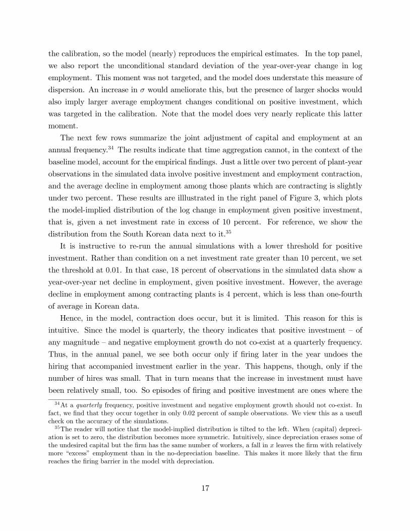
The next few rows summarize the joint adjustment of capital and employment at an

annual frequency.34 The results indicate that time aggregation cannot, in the context of the

baseline model, account for the empirical �ndings. Just a little over two percent of plant-year

observations in the simulated data involve positive investment and employment contraction,

and the average decline in employment among those plants which are contracting is slightly

under two percent. These results are illlustrated in the right panel of Figure 3, which plots

the model-implied distribution of the log change in employment given positive investment,

that is, given a net investment rate in excess of 10 percent. For reference, we show the

distribution from the South Korean data next to it.35

It is instructive to re-run the annual simulations with a lower threshold for positive

investment. Rather than condition on a net investment rate greater than 10 percent, we set

the threshold at 0:01. In that case, 18 percent of observations in the simulated data show a

year-over-year net decline in employment, given positive investment. However, the average

decline in employment among contracting plants is 4 percent, which is less than one-fourth

of average in Korean data.

Hence, in the model, contraction does occur, but it is limited. This reason for this is

intuitive. Since the model is quarterly, the theory indicates that positive investment �of

any magnitude �and negative employment growth do not co-exist at a quarterly frequency.

Thus, in the annual panel, we see both occur only if �ring later in the year undoes the

hiring that accompanied investment earlier in the year. This happens, though, only if the

number of hires was small. That in turn means that the increase in investment must have

been relatively small, too. So episodes of �ring and positive investment are ones where the

34At a quarterly frequency, positive investment and negative employment growth should not co-exist. Infact, we �nd that they occur together in only 0.02 percent of sample observations. We view this as a useu�check on the accuracy of the simulations.35The reader will notice that the model-implied distribution is tilted to the left. When (capital) depreci-

ation is set to zero, the distribution becomes more symmetric. Intuitively, since depreciation erases some ofthe undesired capital but the �rm has the same number of workers, a fall in x leaves the �rm with relativelymore �excess� employment than in the no-depreciation baseline. This makes it more likely that the �rmreaches the �ring barrier in the model with depreciation.

17

investment was quite limited, e.g., less than 10 percent. This is a revealing property of the

model because it contrasts so clearly with the plant-level data. As we discussed, the share

of observations which involve investment and employment contraction in the actual data is

much more robust to the choice of the investment threshold.

We now introduce worker attrition. This does not disrupt the theoretical predictions

discussed in section 1 �in any given quarter, positive investment and negative employment

growth do not occur. But one may suspect that attrition interacts with time aggregation.

Speci�cally, the plant may hire and invest in one quarter, but attrition over the subsequent

quarters results in a net decline in employment over the year. To consider this more carefully,

we set the attrition rate, �n, to be 4 percent per quarter. For the purpose of this exercise,

this is likely a fairly generous estimate of attrition. Chang, Nam, and Rhee (2003) actually

estimate the separation rate in 1994 in Korea to be no more than 2 percent per quarter.

Results are shown in Table 4. There are two remarks we wish to make in this regard.

First, the reader will notice that, since attrition is assumed to be costless, it is now virtually

impossible (at least within the baseline model) to generate any inaction in employment. It is

possible to remedy this if we assume that there are some jobs which are relatively costless to

re�ll after a separation. But since that merely makes labor even more �exible, it is unclear

that such an amendment would a¤ect the bottom line of this analysis.36

Second, with regard to the co-movement of capital and labor, the e¤ects of attrition are

minimal. The intuition behind this result is straightforward. Attrition does deplete the

workforce. But �rms also hire more often than otherwise, since attrition makes hiring less

costly to reverse. This means that, after a period in which the plant hires and invests, it

typically does not undergo quarter after quarter in which attrition simply wears away its

workforce � it will tend to hire at some point in the year. This blunts the ability of the

model to produce years in which the plant both invests and sees its workforce shrink.37

36Since we can no longer calibrate the cost of adjusting to the inaction rate, we leave c�n = c+n at thevalue used in the prior simulation. Other parameters are updated as needed to reproduce the targetedmoments. We have also considered an alternative in which we re-calibrate the cost of adjusting labor sothat the probability of not �actively�adjusting equals the unconditional probability of inaction in the modelwithout attrition. A plant is said to not actively adjust its workforce if employment at the end of the year,n; exactly equals the prior year�s workforce that survived attrition, (1� �n)4 n�4. This approach requiresa much larger cost of adjusting labor in order to to deter hiring even in the face of 4 percent per quarterattrition. But as labor becomes more costly to adjust, we also have to reduce the resale price of capital,or else plants will instead adjust too often along this margin. Thus, in the end, the relative frequency ofadjusting labor is retained, and the co-movement of the two factors is very similar to what we show in Table4.37This is not to say that attrition is unimportant �it accounts for the vast majority of quarterly declines

in employment in the simulated data. This role of attrition in the model appears to mirror its role in theKorean labor market in particular. The restrictions on the layo¤ of permanent workers makes attrition a

18

3 Extensions to the baseline model

In this section, we discuss a few modi�cations of the baseline model that may plausibly

induce more realistic co-movement of investment and employment growth at the plant level.

The theories discussed in this section fall into two broad classes. The �rst preserves factor-

neutral technical change and seeks to account for the data along other lines. The second

class introduces factor-biased technology.38

3.1 Non-technological explanations

Sticky product prices. In the macroeconomics literature, it has been noted that ifthe �rm�s product price is sticky, factor-neutral technical change can be contractionary. If

the �rm does not wish to lower its price in order to sell additional output, it does not need

its current factors given the higher level of TFP. So its factor demand declines. However, in

these models, technology is contractionary with respect to both capital and labor (see Basu,

Fernald, and Kimball, 2006).39

Shifts in factor prices. We have taken the real wage as given and abstracted from factorsupply. We have done so because factor price movements in general equilibrium are unlikely

to generate qualitatively di¤erent joint dynamics at the plant level. If the two physical

factors are q-complements in production and if revenue exhibits decreasing returns to k and

n jointly, then an increase in the price of either factor (perhaps because of a withdrawal of

supply) reduces demand for both factors �factor demands react in the same direction. This

is straightforward to show in the frictionless model, and it remains true in the model with

frictions.40 Of course, if there is, for instance, an increase in the wage that faces the plant,

the optimal capital-labor ratio will rise, but capital will not increase absolutely.

Structural change. Recent models of long-run growth have shown that neutral technol-ogy improvements in manufacturing can lead to a secular decline in that sector�s employment

critical means by which plants shrink their permanent workforces (Grubb, Lee, and Tergeist, 2007).38As we noted in the introduction, our results echo �ndings of a few earlier studies that analyzed data

from the U.S., the Netherlands, and Germany. For this reason, we do not tailor the discussion in this sectionto the speci�c institutional features of the economies for which we have data. Our result regarding theco-movement of capital and labor appears to be robust across economies.39This literature has also explored the e¤ects of investment-speci�c shocks. But in this case, the shocks

are typically expansionary despite price stickiness (see Smets and Wouters, 2007).40Appendix C provides a summary of the robustness analysis we have performed that is not reported in

detail here. In one exercise, we include exogenous shifts in the (aggregate) price of capital in the model ofsection 1. As we would anticipate from the frictionless model, these shocks failed to induce positive investmentcoincidence with employment declines.

19

share if the price elasticity of demand for the composite manufactured good is su¢ ciently

small. Moreover, the fact that this elasticity of demand at the industry level is so low does

not imply a counterfactually high (or any) markup over marginal cost at the individual

plants. However, in our data, the vast majority of variation in factor inputs is not due to

industry-wide shocks; all of our empirical results hold within narrowly de�ned sectors. Thus,

we interpret the incidence of negative comovement between machinery and employment as

largely driven by idiosyncratic shocks to plants. In other words, it does not seem that this

pattern is due to a common shock that drives all plants up a steeply sloped industry demand

schedule. As a result, the relevant demand elasticity is that which operates at the plant-level.

We return to explanations that rely on low plant-level elasticities in section 3.2.

Machinery replacement. When machinery is subject to stochastic breakdown, it

is possible to partially de-couple investment from employment adjustment. For instance,

suppose that a share of a plant�s machinery is �critical�to production in that output falls

virtually to zero if this subset of equipment fails (irreparably). Assume these failures are

orthogonal to productivity and/or demand (and their histories). This means that there will

be quarters in which a �rm may invest merely to keep the plant open, even if productivity

is so low as to warrant a reduction in employment.

This account of plant-level dynamics has some evidence in its favor. For instance, when

we look at transportation equipment (such as trucks used for delivery), we also see that

plants sometimes contract employment even as they increase invest in these vehicles. This

seems consistent with the notion that the failure of a truck would create such a disruption

that replacement is necessary even if productivity is relatively low.

The challenge with respect to this explanation is that it is very hard to assess its quanti-

tative importance. We are not aware of a point estimate (or even a distribution of estimates)

as to the share of a plant�s machinery that is critical in the sense described above. But this

matter deserves further attention.41

The lag between order and delivery. The baseline model assumes that new machin-ery is installed and operated in the period in which it is ordered. But in reality there may be

41It should be noted that there is not necessarily a uniform de�nition of criticality, which makes it hardto apply results from the related maintenance literature. For instance, some research in plant maintenanceand reliability treats electricity supply as critical, but we do not, of course, interpret that as a subset ofmachinery. Furthermore, even if a machine is critical, the plant might have redundancies. This is importantif plants are credit-constrained and redundant parts have high prices. In that case, the plant will tend toinvest in redundancies when its internal funds are high, which is precisely when it would want to hire. Hence,this model of criticality would not deliver negative comovement between machinery and employment. Wewish to thank (without implicating, of course) Andrew Starr (Manufacturing and Materials Department,Cran�eld University) for sharing his thoughts on the issue of criticality.

20

a delay between the order and delivery of new capital goods. If the plant reports investment

in the year in which the order is placed, then this delay does not disrupt the implications

of the baseline model: orders, and thus recorded investment, should still perfectly predict

positive employment growth.

The implications of a delay are more signi�cant if plants record investment in the year in

which the machinery is delivered. Suppose machinery is ordered in August 2001 and received

in February 2002. If plant productivity deteriorates over the course of 2002, employment

may be reduced that year even though positive investment is observed. The delivery lag, in

other words, ampli�es time aggregation. If there were no delay, the delivery would coincide

with the order. Thus, productivity would have to decline su¢ ciently between August 2001

and December 2001 in order to generate a year in which the plant undertakes investment

and reduces its labor demand (on net). But if there is a delay, productivity can fall at any

point in 2002 and trigger a decline in employment that year even though investment would

be recorded.

To investigate this, we generalize the baseline model in a simple way in order to allow

for delivery lags. We adopt a Calvo-like mechanism: an order for machinery, regardless of

when it was made, is �lled with probability � in any one period. As a result, if an order

goes un�lled this period, it takes its place in the prior backlog of un�lled orders, and whole

stock is �lled with probability � next period. This assumption greatly simpli�es the problem,

albeit at the expense of a certain degree of realism.

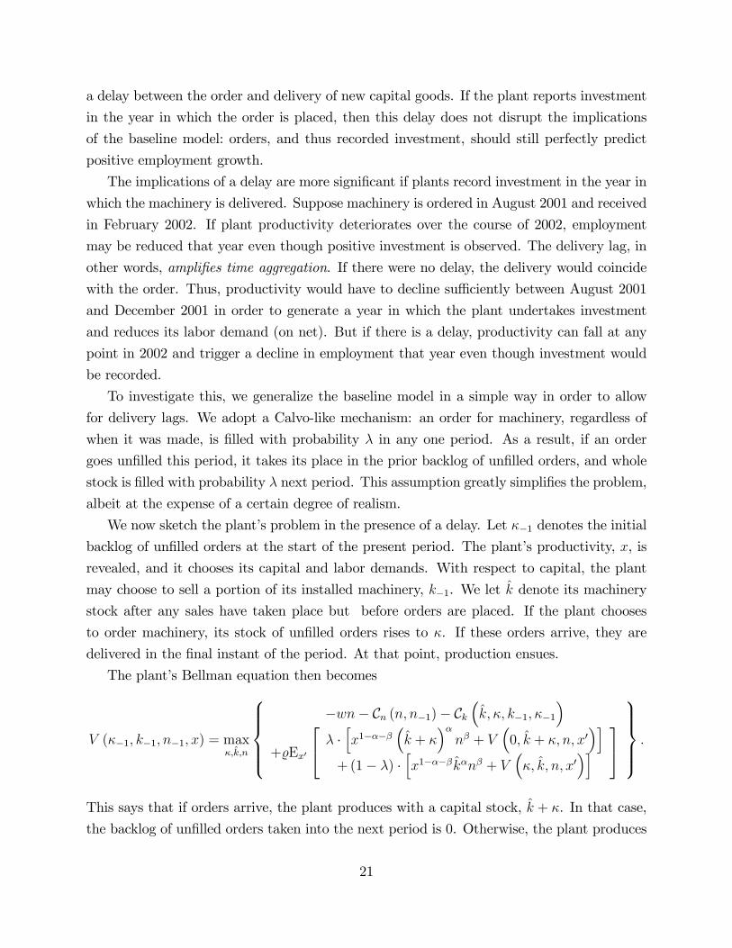
We now sketch the plant�s problem in the presence of a delay. Let ��1 denotes the initial

backlog of un�lled orders at the start of the present period. The plant�s productivity, x, is

revealed, and it chooses its capital and labor demands. With respect to capital, the plant

may choose to sell a portion of its installed machinery, k�1. We let k̂ denote its machinery

stock after any sales have taken place but before orders are placed. If the plant chooses

to order machinery, its stock of un�lled orders rises to �. If these orders arrive, they are

delivered in the �nal instant of the period. At that point, production ensues.

The plant�s Bellman equation then becomes

V (��1; k�1; n�1; x) = max�;k̂;n

8>>><>>>:�wn� Cn (n; n�1)� Ck

�k̂; �; k�1; ��1

�+%Ex0

24 � � hx1���� �k̂ + ��� n� + V �0; k̂ + �; n; x0�i+(1� �) �

hx1����k̂�n� + V

��; k̂; n; x0

�i 359>>>=>>>; :

This says that if orders arrive, the plant produces with a capital stock, k̂ + �. In that case,

the backlog of un�lled orders taken into the next period is 0. Otherwise, the plant produces

21

with k̂, and takes an un�lled order stock � into the next period.42 The cost of adjusting

capital, Ck�k̂; �; k�1; ��1

�; is notationally more cumbersome but substantively the same as

before. It is given by

Ck�k̂; �; k�1; ��1

�= c+k (�� ��1)1[�>��1] + c

�k

�k�1 � k̂

�1[k�1>k̂]

:

The di¤erence, � � ��1, represents the new orders placed this period, and k�1 � k̂ is thenumber of units sold.

We solve the model numerically. The calibration of the size of the adjustment costs, the

returns to scale, and the stochastic process of productivity (x) does not di¤er materially

from that presented in Table 3. The only free parameter to be pinned down, then, is � �

the probability per quarter that a delivery is made. There is a not great deal of evidence on

this, and what we have found pertains to the U.S. rather than Korea. Abel and Blanchard

(1988) estimate a delivery lag of 2 to 3 quarters, whereas 2 quarters is on the high end of

the range of estimates reported in Carlton (1983). In Table 5, we therefore present results

for � = 1=3. Note that if � = 1=3, then (2=3)3 �= 30 percent of �rms wait longer than 3

quarters for delivery.43

The results in Table 5 indicate that delivery lags do not appear to be so large as to

account for the majority of the coincidence of positive investment and negative employment

growth. As shown in the bottom panel, the share of plant-year observations that involve

opposite movements in investment and employment is now 12:5 percent. This is far higher

than in the baseline model but still less than one-third of the empirical estimate. The mean

decline in log employment, conditional on positive investment, is 3:5 points, which is less than

one-�fth what we see in the data. This re�ects the di¢ culty in generating sizable reductions

in employment purely from time aggregation. As shown in the middle panel, orders of

machinery (at the quarterly frequency) are virtually never accompanied by contractions in

labor demand �desired employment perfectly co-moves with desired capital. Arguably, a

model might have more potential if increases in investment triggered a reduction in desired

labor demand. We will take up such a theory in the next subsection.

The disruption of factor adjustment. Cooper and Haltiwanger (1993) provided amodel in which machine replacement disrupts production and reduces current labor demand.

42Note that we assume the plant pays for the orders when they are placed. This is innocuous in a modelwith perfect credit markets.43To be clear, when the model is simulated, investment is recorded at the time of delivery. This captures

the mis-match between the dates at which employment is adjusted and investment is recorded in the data.

22

Formally, disruption means that, in the period in which machinery is installed, the marginal

product of labor is lower (for any given k). This is intended to represent the idea that

production must be stopped or slowed as new machinery is put into place. Further, Cooper

and Haltiwanger assume labor is a �exible factor and that machinery is not available for use

in production during its installation. It follows that employment will be reduced at the time

of installation.

The model of Cooper and Haltiwanger (1993) is deterministic, but it is possible to sustain

the argument in a stochastic environment. Suppose the installation of capital disrupts pro-

duction in the sense that revenue is given by�1� � � 1[�k>0]

��x1����k�n�, where � 2 (0; 1).

This says that if investment is undertaken, the marginal product of each factor is degraded

by � for any given (k; n; x) :44 If we retain the assumptions that new capital is not available

for use in production and that labor is a frictionless factor, then the choice of labor condi-

tional on �k > 0 is governed by the static �rst-order condition, (1� �) �x1����k�n��1 = w,where k is interpreted as the given, start-of-period machinery stock. If the �rm was near its

Ss band with respect to investment prior to this period, it does not require a large increase

in productivity, x, to be induced to invest. If x increases only marginally from last period,

the �tax�on the marginal product, � , may dominate and lead to a fall in labor demand.45

In addition to the disruption cost, this set-up di¤ers from the model of section 1 in

two ways. The �rst relates to timing �in section 1, we assume new machinery is available

for use in production in the period in which investment is undertaken. This is important

because investment is �lumpy�in the presence of a disruption cost.46 As a result, the large

adjustment to k will likely o¤set the e¤ect of � on the marginal product of labor, triggering

an increase in labor demand. The second di¤erence is that, in the model of section 1, labor

is subject to costs of adjusting. In this case, it is much less clear it would be optimal

for a �rm to reduce employment during the installation period. Even if new machinery is

not available this period, the scheduled, discrete increase in capital next period raises the

expected marginal value of labor. If layo¤s are costly to reverse, the �rm has an incentive

44A speci�cation like this has been used often in the more recent dynamic factor demand literature. See,among others, Caballero and Engel (1999), Cooper, Haltiwanger, and Willis (2005), and Bloom (2009).45Cooper, Haltiwanger, and Power (1999) incorporate stochastic plant-speci�c TFP into a machine re-

placement model. However, their model omits labor adjustment.46The disruption cost, given by � � x1����k�n�, is a kind of �xed cost. This is easy to see if new capital

does not become operative until next period. In that case, current revenue �and thus, the disruption cost �isindependent of the size of the change in the capital stock. But even if capital becomes operative immediately,the disruption cost has a discontuity at the origin, as in lim�k!0 � � x1����k�n� 6= 0: This means that itrises at an in�nitely fast rate when any investment is undertaken. This discontinuity is the unifying featureof �xed costs and gives rise to the economies of scale in adjusting which make lumpy changes optimal.

23

to retain its workforce.47

We now explore this issue numerically. Speci�cally, we modify the baseline model in two

regards. First, a disruption cost associated with capital adjustment is introduced. Second,

we assume a one-period delay between the date of installation and the date at which the

new capital becomes operative. The question we ask is whether the costly reversibility of

labor deters layo¤s in the periods in which new capital is installed.

In this modi�ed model, the costs of adjusting must be re-calibrated. We now have to

select two parameters with respect to the cost of adjusting capital �the resale price, c�n , and

the disruption cost, � . Therefore, we need another moment, in addition to the frequency of

investment. We set the resale price of capital to target the frequency of negative investment.

This leaves � to target the degree of inaction in investment.48 We found that it takes only

an exceptionally small value of � to induce a substantial amount of inaction. Yet if � is set

too low, then the model has little chance of engaging the data �the marginal product of

labor would not fall by enough to induce declines in employment at the time of installation.

To strike a compromise, we �x � = 0:025, which implies that investment is zero around 70

percent of the time. This inaction rate about 1:5 times that in the data.49

Table 5 displays the results. The middle panel of the table shows that the disruption

cost does not trigger declines in employment in the quarter in which the installation is

undertaken. However, since capital is not operative until the next period, the growth in

employment in the installation period is subdued relative to the baseline (see Table 4).

This may account for why, at an annual frequency, we do see some instances of employment

declines and investment, although the coincidence of the two is still far below that in the data.

Suppose the plant �res in quarter one but x then reverses course and by the fourth quarter,

it is optimal to hire and invest. Since the new machinery is not operative, the increase

in employment is muted in quarter four. This shows through as a larger net reduction in

employment for the year.50

47In a richer model, one might di¤erentiate between a temporary furlough and a permanent severance ofthe �rm-worker match. If the former is allowed, then temporary layo¤s would likely coincide with machineinstallation. It is unlikely that this is the source of the co-movement we see in the data, though. First,since we measure year-over-year changes in our data, this kind of short-term (intra-year) variation in theworkforce is unlikely to account for our results. Moreover, as discussed in section 2, there is no evidence thatemployment declines, conditional on investment, are reversed at a faster rate than otherwise.48We continue to calibrate the cost of labor adjustment to target the frequency of plant-year observations

that display zero net employment growth.49Such a low value of � is in con�ict with Cooper and Haltiwanger (Table 5, 2006). But they did not

target the adjustment frequency.50On the other hand, if the plant installs machinery in quarter 2, there will be a large increase in em-

ployment in the next quarter. This re�ects the lumpy change in the marginal product due to (discrete)machinery investment. As a result, Table 5 shows that the average annual change in employment, condi-

24

3.2 Factor-biased technical change

The coincidence of investment and (net) separations suggests the presence of factor-biased

technical change. However, we argue that relatively standard implementations of factor-

biased technical change do not induce the incidence of investment and separations that we

observe in the data. These production functions do induce, conditional on output, a shift

away from labor after a technology improvement. However, the scale e¤ect of an increase

in technology dominates unless demand is highly inelastic.

Thus, one may view the co-movement of capital and labor in one of two ways. It may be

treated as a moment which informs the calibration of the demand schedule and the mark-up,

in which case typical estimates of the mark-up used in macroeconomic analysis appear very

low. Or, if the implied mark-up clashes with reliable external evidence, it may be interpreted

as a challenge to canonical models of technical change.

In this paper, we (at least tentatively) adopt the latter view and so consider an alter-

native model of factor-biased technology. In this framework, the �nal good is produced by

aggregating over the outputs of many tasks. The �rm allocates machinery to a subset of

tasks and labor to the remainder. If there an increase in the productivity of machinery in

this model, labor is directly replaced in the marginal task by capital. This form of factor

bias will enable the model to replicate the coincidence of investment and (net) separations.

Factor-augmenting technology in CES production. We �rst consider a model

of CES production in which there is labor-augmenting technical change. The latter can, in

theory, be labor-saving and thus capable of inducing a simultaneous increase in capital and

reduction in employment. However, for a wide range of parameter values, labor-augmenting

innovations are not contractionary with respect to labor.51

To introduce labor-augmenting technology in a meaningful way, we must depart from the

Cobb-Douglas production function used above. Instead, we specify that production is given

by the CES function,

y =�#k

'�1' + (1� #) (�n)

'�1'

� ''�1

; (4)

where ' is the elasticity of substitution across the factors, � is labor-augmenting technical

change, and # is related to capital�s share of output. This function displays constant returns,

under which plant size is indeterminate. To have a notion of plant size, we assume the �rm

tional on positive investment, is around 30 log points. We could ratchet down the size of TFP shocks tobring this more closely in line with the data. However, this comes at a price: we would further understatethe unconditional dispersion in employment growth.51Capital-augmenting technical change is arguably even less promising as a means of inducing investment

and employment contraction, as we discuss below.

25

faces an isoelastic product demand schedule given by

y = �P��: (5)

where � is the demand shifter and P is the price of the plant�s product. It follows that the

value of the �rm becomes

�(k�1; n�1; �; �)

= maxk;n

(�1=�y

��1� � wn� Ck (k; k�1)� Cn (n; n�1)

+%R R

�(k; n; �0; � 0) f� (�0j�) f� (� 0j�) d�d�;

);

(6)

where, for any �; f� is the conditional p.d.f. of �. It is useful to assume, as we did above

with regard to the Hicks-neutral technology, that the demand shifter follows a geometric

random walk. Then the problem is homogeneous of degree one in (k; n; �; �). This allows

us to normalize the factors with respect to �; giving ~n � n=� and ~k � k=�, and recast theproblem in terms of

�~k; ~n; �

�. Thus, the policy rules given in section 1 (and plotted in Figure

1) hold here, conditional on �.

To gauge how well this model matches the plant-level co-movement of capital and labor, it

is instructive to consider a simple exercise. Suppose a plant is now investing and �ring, so its

�rst-order conditions corresponding to these choices are in e¤ect. Then if � is labor-saving,

these FOCs must remain in e¤ect after an increase in �, implying an increase in k and a

decrease in n. To pursue this point, consider the version of (6) with static expectations, i.e.,

the �rm does not anticipate that � or � will evolve from current levels. In that case, one can

di¤erentiate the FOCs for investing and �ring to obtain the comparative static, d lnn=d ln �:

This yieldsd lnn

d ln �= (�� 1)� (�� ') s

s+ 1;

where s is the ratio of capital income to labor-related payments (the wage bill plus the

amortized cost of �ring). This is negative only if

�� 1 < (1� ') s: (7)

This says, in part, that the elasticities of demand and substitution must be su¢ ciently

small. When ' is near zero, the factors are highly complementary, so an increase in the

e¤ective supply of labor induces the plant to increase capital relative to labor. This can

involve an absolute reduction in labor. However, at the same time, an increase in � reduces

the marginal cost of production and the product price. This yields an increase in sales. If

26

demand is su¢ ciently inelastic (� is small), though, this scale e¤ect is muted. As a result,

(7) is more likely to hold, and labor declines.

Equation (7) provides a hint as to the di¢ culty that (4) has in generating contractionary

technology improvements. The range of 's that satisfy (7) is increasing in s and declining

in �. But even for polar values of s and �, it is di¢ cult to make d lnnd ln �

turn negative. Table 6

illustrates this. To interpret the table, note that (7) implies that the elasticity of substitution,

', must satisfy ' < '̂ � 1 � ��1s. The table shows the values of the threshold, '̂, that

correspond to values of � listed along rows and s listed along columns. Since ' is bounded

below by zero, only the shaded values of '̂ are feasible. Hence, if s = 0:8, which is the mean

among Korean manufacturers, the product elasticity, �, would have to be less 2 to even be

consistent with (7). This is well below estimates in the literature.52

Of course, the ratio s is likely to vary across plants. Perhaps the coincidence of positive

investment and (net) separations in the data re�ects the presents of plants that are relatively

capital intensive. Unfortunately, it is hard to investigate this in our data since we do not

have detailed information on capital income.53

What we can say is that, if s were higher, one must still invoke what seem like low values

of (�; ') to make (7) hold. For example, suppose s = 1:6, or twice its empirical average. We

are not aware of plant-level estimates of ', but a value of 0:1 brings us close to Leontief and

arguably serves as a reasonable lower bound. In that case, one needs values of � below 2:44

in order to make (7) hold. This is less than the estimates in Broda and Weinstein (2006,

Table IV, �Median� row, �TSUSA/HTS� column). Moreover, in this model, an � of 2:44

implies a markup of almost 70 percent. This con�icts with recent evidence from Feenstra

and Weinstein (2010), who estimate a richer translog demand system and �nd an implied

median mark-up of around 30 percent.54

We now demonstrate that our intuition gleaned from (7) is highly indicative of the be-

havior of the dynamic factor demand model. To do this, we set � = 2:44, ' = 0:1, and

s = 1:6 and simulate plant-level data on investment and employment growth.55 Table 7 re-

52According to the model, we would like to measure the denominator in s by summing the wage bill andthe amortized cost of �ring. However, the data do not include the latter. Thus, the empirical estimate ofs = 0:8 likely overstates the value of s that is relevant for evaluating (7).53For the U.S., the Bureau of Labor Statistics does provide industry-level data on rental prices. These data

reveal that the average value of s is less than one in 14 of 16 three-digit NAICS manufacturing industries.This limits the degree to which plausible variation in s could account for the degree of negative co-movementbetween capital and labor documented by Sakelleris (2000) on U.S. data.54Both of these papers use detailed data on U.S. imports. In particular, the Broda andWeinstein estimate is

based on 10-digit Harmonized Tari¤System data. We highlight these estimates, since the more disaggregateddata are arguably more indicative of the elasticities faced by individual plants.55For this exercise, we omit capital disruption costs. Thus, we re-calibrate the resale price of capital and

27

ports the results. Positive investment and negative employment growth hardly ever coexist

in the simulated data.

Before we leave this subsection, we note that a model of capital-augmenting technical

change is even less e¤ective at engaging the data. To see this, suppose production is now

given by

y =�# (�k)

'�1' + (1� #)n

'�1'

� ''�1

: (8)

Rearranging this, we may write y = n�#�

'�1' + (1� #)

� ''�1, where � � �k

nis the e¤ective

capital-labor ratio. This indicates that the e¤ect of an increase in � on labor demand will

hinge on the reaction of the marginal revenue product of labor, MRPL, to a change in �.

Speci�cally, the �rm�s �rst-order conditions imply56

d lnn

d ln �= (�� ') s

s+ 1/ d lnMRPL

d ln �: (9)

If � > ', d lnnd ln �

is unambiguously positive.

The condition on � � ' is intuitive, since � > ' implies the factors are q-complements.This accounts for why, under � > ', an increase in the e¤ective supply of capital raises labor

demand. Unfortunately, it is hard to assess the restriction � > ', since estimates of the

elasticity of substitution ', conditional on the form of (8), are not available at the plant

level. But Raval (2012) does provide estimates o¤ U.S. county-level data for each two-digit

manufacturing sector. Virtually all of his estimates are less than 1. Therefore, acknowledging

the obvious caveats, we view the restriction �� ' > 0 as a reasonably safe one to make.

Investment-speci�c technical change & skill bias. Thus far, we have assumed

only two factors. Within the skill-biased technical change, literature, though, it is common

to allow for skilled and unskilled labor, such that the capital and skilled labor are gross

complements whereas capital and unskilled labor are gross substitutes. Krusell, Ohanian,

Rios-Rull, and Violante (2000) consider this kind of production function. Technical change

in their model takes the form of advances in the rate at which investment is transformed

into installed capital.

There are two reasons we do not believe this model is consistent with our data. First, the

model would lead us to expect that employment declines are concentrated among low-skilled

workers. But the evidence for this is far from clear. In the Korean census, plants record

the number of production and non-production workers. In the literature on skill-biased

the cost of labor adjustment to target the individual frequences of adjusting.56We again derive the comparative static under the assumption of static expectations.

28

technical change, non-production status is often treated as a proxy for skill.57 Therefore, we

re-compute the share of plant-year observations that involve both positive investment and

declines in non-production workers. This is 35.5 percent, which is only slightly less than

the baseline estimate reported in Table 1. Moreover, conditional on positive investment and

negative non-production employment growth, the average contraction in non-production

workers is not any smaller than the decline among the general workforce reported in Table

1.58

These results are not that surprising in light of what we have learned about the impact

of technology on the workplace. The tasks performed by clerical and administrative workers,

who would be classi�ed as non-production employees in our data, have become increasingly

codi�ed and performed by machines (Acemoglu and Autor, 2010). This suggests that it is

not only workers on the factory �oor for whom machines may substitute.59

The second reason we doubt this model is consistent with the plant-level is that, even

if it induces declines in unskilled labor, it is very unlikely to generate plant-wide declines

in labor demand given plausible parameter values. This is straightforward to show in the

model of Krusell, et al, where factors are assumed to be perfectly �exible.

Suppose there are skilled, s, and unskilled, u, workers. Production is given by

y = (#uu� + (1� #u) � (k; s)�)1=� ; (10)

where � (k; s) � (#kk� + (1� #k) s�)1=� is the CES bundle of capital and skilled labor and

#u; #k 2 (0; 1). Based on the estimates in Krusell, et al, we assume that � < 1; which impliesan elasticity of substitution, '� � 1

1�� , between unskilled labor and the capital-skill bundle

that is greater than one. We also assume � < 0, which implies an elasticity of substitution,

'� � 11�� , between capital and skill that is less than one. If demand is given by equation

(5), then revenue is y��1� . Hence, the �rm maximizes

1Xs=0

�s

8<:h#uu

�t+s + (1� #u) (#kk�t+s + (1� #k) s�t+s)

��

i 1���1�

�wuut+s � wsst+s � it+s

9=; ;57See, e.g., Berman, Bound, and Machin (1998) and Berman and Machin (2000).58Nonetheless, there has been an upward trend in the non-production worker share in our data. Fuentes

and Gilchrist (2005) also �nd such an upward trend in Chile even though the non-production worker sharein their dataset does not tend to increase in periods of investment spikes. They argue that the source of thesecular trend was a shift in favor of R&D-related personnel after trade liberalization.59The evidence for the prevalence of computing equipment is typically taken from the U.S. and European

countries. But South Korea is a relatively advanced economy by this measure. If we take the volume ofexports and imports of computer equipment (per capita) as indicative of pervasiveness of this technology,then Korea ranks on par with several Western European and North Atlantic economies (see OECD, 2008).

29

subject to kt+s = (1� �) kt+s�1 + qt+sit+s. Here, q is the investment-speci�c technologyshock.

To get some insight into the model, �x qt = qt+j for j � 1 and consider a once-and-for-allincrease in q in time t. We �rst compute the change in the demand for unskilled labor in

response to this shift in q. Appendix B shows that d lnutd ln qt

< 0 if and only if the elasticity of

substitution between capital (and skill) and unskilled labor exceeds the elasticity of product

demand, '� > �. In other words, the scale e¤ect � the increase in the demand for labor

derived from the increase in output �must be dominated by the incentive to substitute

capital for unskilled labor. In what follows we assume this holds.

We then compute the response of plant-wide employment, n � s + u, to this shift in

q. Investment-speci�c technology is labor-saving if d lnntd ln qt

< 0. Appendix B shows that this

holds only if

� <12

�'� + '�

�� �

'� � �;

where � � @ ln y@ lnu

2 (0; 1) is the elasticity of output with respect to unskilled labor. By

assumption, '� > �. However, just to make sure the numerator on the right side is positive

(so that there are at least some values of � consistent with d lnntd ln qt

< 0), a stronger condition

is needed. Since � 2 (0; 1) and � < 0, then '� > '�, in which case we require '� >12

�'� + '�

�> �: To assess this, suppose � = 2=3 and � = �0:5, as Krusell, et al found.

Then 12

�'� + '�

�= 11

6< 2 : this is the upper bound on �. As noted above, elasticities of

demand below 2 fall well outside the range in the literature.

Machinery replaces labor in tasks. There has been growing interest in models in

which machinery directly replaces labor in tasks. As we will show, this model has a greater

capability of generating the incidence of investment and separations observed in the data.

Our analysis here is based on the framework of Acemoglu (2010) (who in turn adapts the

model of Zeira (1998)).

The plant produces a single good that is subject to the demand schedule (5). The good

is produced by aggregating the outputs of a continuum of tasks. A task is indexed by v on

the unit interval. We assume plant output is then given by the CES aggregate,

y =

�Z 1

0

y (v)'�1' dv

� ''�1

; (11)

where y (v) is the output of task v. A task may be performed by labor or machinery.60

60That is, we imagine a single type of worker and a single machine. This same machine is used in each

30

Speci�cally, one unit of output in task v can be produced with � (v) units of labor or { (v)units of machinery:

y (v) =

(n(v)�(v); or

k(v){(v) :

(12)

We assume tasks may be ordered from 0 to 1 such that tasks at which machines are relatively

productive are ordered �rst. Therefore, the relative productivity of labor, � (v) � 1=�(v)1={(v) =

{(v)�(v); is increasing in v.

The plant�s optimization problem can be solved in two steps. First, given total workers n

and machinery k, the �rm chooses which tasks to perform with capital and which to perform

with labor. It also decides the quantities of each factor to allocate to its respective tasks.

These are static problems. Second, the �rm solves a dynamic problem to select n and k;

subject to the adjustment costs described in equation (1). We now brie�y summarize the

�rst step.

Formally, the allocation of factors across tasks solves the following problem. (The details

of the solution are provided in Appendix B.) The monotonicity of � (v) suggests the existence

of a single crossing, v�, such that all tasks v � v� are automated and all other tasks are

performed by labor. Taking this as given for the time being, the �rm�s problem is to decide

the quantities of each factor to allocate per task in order to maximize revenue. Hence, given

(5) and (11), the �rm solves

maxfy(v)gv=1v=0

�1=��Z 1

0

y (v)'�1' dv

� ��1�

''�1

subject to the resource constraints,

k =

Z 1

0

k (v) dv =

Z v�

0

{ (v) y (v) dv

n =

Z 1

0

n (v) dv =

Z 1

v�� (v) y (v) dv:

Here, n (v) denotes the quantity of labor allocated to task v, and k (v) represents the number

of machines allocated to task v.

The solution to this problem gives the optimal quantity y (v) of each intermediate in

terms of k ; n, and v�. We are then able to rewrite the plant-wide production function (11)

exclusively in terms of the total stocks, k and n, and the threshold, v�. Speci�cally, one can

task, but, as we will see, it is relatively more productive in some tasks.

31

show that

y =hA (v�)

1' k

'�1' +B (v�)

1' n

'�1'

i ''�1

; (13)

where the terms, A (v�), and B (v�), are de�ned by

A (v�) �R v�0

�1

{(v)

�'�1dv

B (v�) �R 1v�

�1�(v)

�'�1dv

:

To understand these terms, recall that 1{(v) is output per machine in task v. Hence, A (v

�)

is an aggregate over the average products of machinery on the tasks to which machinery is

applied. In this sense, it may be interpreted as an index of capital productivity. The same

idea applies, of course, to B (v�).

The indexes, A and B, di¤erentiate (13) from the standard models of factor-augmenting

technical change. For instance, if output is produced according to (8), then an increase

in capital-augmenting technology does not imply a degradation, in absolute terms, in the

contribution of labor to output. In other words, there is no decline in the analogue of B in

that model. However, when production is given by (13), an increase in the threshold, v�,

leads to a replacement of labor in tasks, which implies a greater contribution per unit of

(plant-wide) capital, k, and a smaller contribution per worker. This deterioration in labor

productivity ampli�es the e¤ective bias of technical change.

Thus far, we have taken v� as given, but it is straightforward to determine the threshold.

Cost minimization implies that the �rm uses machinery for task v if the marginal cost of

machinery is less. The marginal cost is evaluated using the shadow price of capital to the �rm,

conditional on the total stock k. Since this shadow price is declining in k, it is not surprising

that the threshold task is increasing in the capital-labor ratio. Formally, as demonstrated in

Appendix B, v� satis�esk

n= � (v�)'

A (v�)

B (v�)� �(v�) (14)

The right side of (14) is increasing in v�, implying a single-crossing. Equation (14) is intuitive,

as it says that the optimal allocation of factors across tasks requires that the �rm executes

a greater share of tasks with the more abundant factor.

It should be noted at this point that the solution (14) assumes a frictionless reallocation

of factors within plant across tasks. This abstracts from a number of issues, but we do not

believe this omission invalidates the application of (13) to problems of plant-level dynamics.

For instance, machinery is likely speci�c, to some degree, to the task. This raises the

question of whether we ought to require the plant to purchase new machinery when capital

32

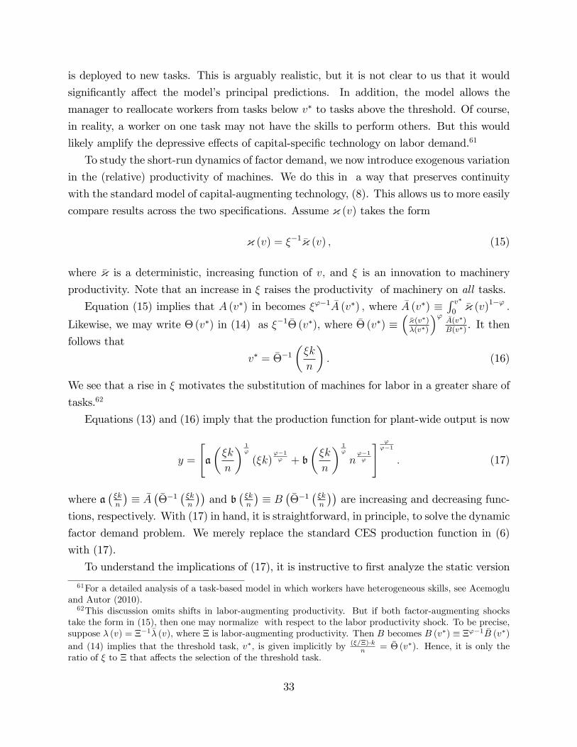
is deployed to new tasks. This is arguably realistic, but it is not clear to us that it would

signi�cantly a¤ect the model�s principal predictions. In addition, the model allows the

manager to reallocate workers from tasks below v� to tasks above the threshold. Of course,

in reality, a worker on one task may not have the skills to perform others. But this would

likely amplify the depressive e¤ects of capital-speci�c technology on labor demand.61

To study the short-run dynamics of factor demand, we now introduce exogenous variation

in the (relative) productivity of machines. We do this in a way that preserves continuity

with the standard model of capital-augmenting technology, (8). This allows us to more easily

compare results across the two speci�cations. Assume { (v) takes the form

{ (v) = ��1 �{ (v) ; (15)

where �{ is a deterministic, increasing function of v; and � is an innovation to machineryproductivity. Note that an increase in � raises the productivity of machinery on all tasks.

Equation (15) implies that A (v�) in becomes �'�1 �A (v�) ; where �A (v�) �R v�0�{ (v)1�' :

Likewise, we may write �(v�) in (14) as ��1 �� (v�), where �� (v�) ���{(v�)�(v�)

�' �A(v�)B(v�) . It then

follows that

v� = ���1��k

n

�: (16)

We see that a rise in � motivates the substitution of machines for labor in a greater share of

tasks.62

Equations (13) and (16) imply that the production function for plant-wide output is now

y =

"a

��k

n

� 1'

(�k)'�1' + b

��k

n

� 1'

n'�1'

# ''�1

: (17)

where a��kn

�� �A

����1

��kn

��and b

��kn

�� B

����1

��kn

��are increasing and decreasing func-

tions, respectively. With (17) in hand, it is straightforward, in principle, to solve the dynamic

factor demand problem. We merely replace the standard CES production function in (6)

with (17).

To understand the implications of (17), it is instructive to �rst analyze the static version

61For a detailed analysis of a task-based model in which workers have heterogeneous skills, see Acemogluand Autor (2010).62This discussion omits shifts in labor-augmenting productivity. But if both factor-augmenting shocks

take the form in (15), then one may normalize with respect to the labor productivity shock. To be precise,suppose � (v) = ��1�� (v), where � is labor-augmenting productivity. Then B becomes B (v�) � �'�1 �B (v�)and (14) implies that the threshold task, v�, is given implicitly by (�=�)�k

n = �� (v�). Hence, it is only theratio of � to � that a¤ects the selection of the threshold task.

33

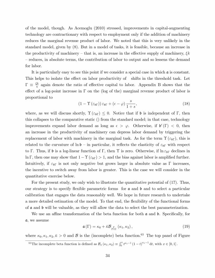
of the model, though. As Acemoglu (2010) stressed, improvements in capital-augmenting

technology are contractionary with respect to employment only if the addition of machinery

reduces the marginal revenue product of labor. We noted that this is very unlikely in the

standard model, given by (8). But in a model of tasks, it is feasible, because an increase in

the productivity of machinery �that is, an increase in the e¤ective supply of machinery, �k

�reduces, in absolute terms, the contribution of labor to output and so lessens the demand

for labor.

It is particularly easy to see this point if we consider a special case in which a is constant.

This helps to isolate the e¤ect on labor productivity of shifts in the threshold task. Let

� � �knagain denote the ratio of e¤ective capital to labor. Appendix B shows that the

e¤ect of a log-point increase in � on the (log of the) marginal revenue product of labor is

proportional to

(1��("b�)) "b� + (�� ')s

1 + s; (18)

where, as we will discuss shortly, �("b�) � 0. Notice that if b is independent of �, then

this collapses to the comparative static () from the standard model; in that case, technology

improvements expand labor demand as long as � > '. Otherwise, if b0 (�) < 0, then

an increase in the productivity of machinery can depress labor demand by triggering the

replacement of labor with machinery in the marginal task. As for the term �("b�), this is

related to the curvature of ln b �in particular, it re�ects the elasticity of "b� with respect

to �. Thus, if b is a log-linear function of �, then � is zero. Otherwise, if ln "b� declines in

ln �, then one may show that 1��("b�) > 1, and the bias against labor is ampli�ed further.Intuitively, if "b� is not only negative but grows larger in absolute value as � increases,

the incentive to switch away from labor is greater. This is the case we will consider in the

quantitative exercise below.

For the present study, we only wish to illustrate the quantitative potential of (17). Thus,

our strategy is to specify �exible parametric forms for a and b and to select a particular

calibration that engages the data reasonably well. We hope in future research to undertake

a more detailed estimation of the model. To that end, the �exibility of the functional forms

of a and b will be valuable, as they will allow the data to select the best parameterization.

We use an a¢ ne transformation of the beta function for both a and b. Speci�cally, for

a; we assume

a (�) = �0 + ��B ��+1(�1; �2) ; (19)

where �0; �1; �2; �� > 0 and B is the (incomplete) beta function.63 The top panel of Figure63The incomplete beta function is de�ned as Bx (�1; �2) �

R x0t�1�1 (1� t)�1�1 dt; with x 2 [0; 1] :

34

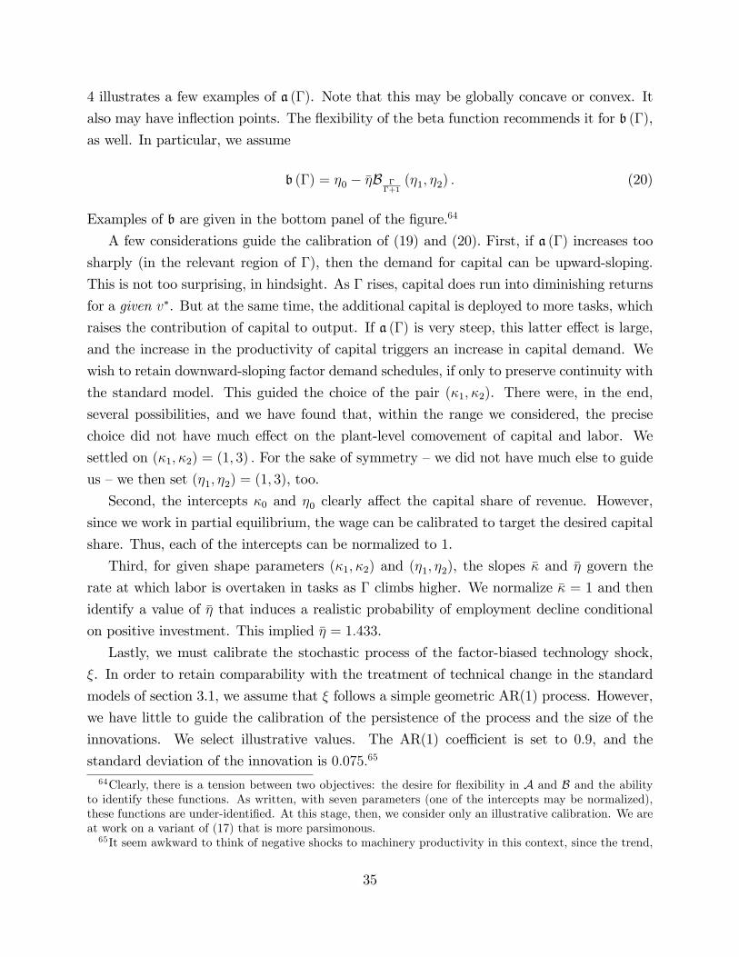
4 illustrates a few examples of a (�). Note that this may be globally concave or convex. It

also may have in�ection points. The �exibility of the beta function recommends it for b (�),

as well. In particular, we assume

b (�) = �0 � ��B ��+1(�1; �2) : (20)

Examples of b are given in the bottom panel of the �gure.64

A few considerations guide the calibration of (19) and (20). First, if a (�) increases too

sharply (in the relevant region of �), then the demand for capital can be upward-sloping.

This is not too surprising, in hindsight. As � rises, capital does run into diminishing returns

for a given v�. But at the same time, the additional capital is deployed to more tasks, which

raises the contribution of capital to output. If a (�) is very steep, this latter e¤ect is large,

and the increase in the productivity of capital triggers an increase in capital demand. We

wish to retain downward-sloping factor demand schedules, if only to preserve continuity with

the standard model. This guided the choice of the pair (�1; �2). There were, in the end,

several possibilities, and we have found that, within the range we considered, the precise

choice did not have much e¤ect on the plant-level comovement of capital and labor. We

settled on (�1; �2) = (1; 3) : For the sake of symmetry �we did not have much else to guide

us �we then set (�1; �2) = (1; 3), too.

Second, the intercepts �0 and �0 clearly a¤ect the capital share of revenue. However,

since we work in partial equilibrium, the wage can be calibrated to target the desired capital

share. Thus, each of the intercepts can be normalized to 1.

Third, for given shape parameters (�1; �2) and (�1; �2), the slopes �� and �� govern the

rate at which labor is overtaken in tasks as � climbs higher. We normalize �� = 1 and then

identify a value of �� that induces a realistic probability of employment decline conditional

on positive investment. This implied �� = 1:433.

Lastly, we must calibrate the stochastic process of the factor-biased technology shock,

�. In order to retain comparability with the treatment of technical change in the standard

models of section 3.1, we assume that � follows a simple geometric AR(1) process. However,

we have little to guide the calibration of the persistence of the process and the size of the

innovations. We select illustrative values. The AR(1) coe¢ cient is set to 0:9, and the

standard deviation of the innovation is 0:075:65

64Clearly, there is a tension between two objectives: the desire for �exibility in A and B and the abilityto identify these functions. As written, with seven parameters (one of the intercepts may be normalized),these functions are under-identi�ed. At this stage, then, we consider only an illustrative calibration. We areat work on a variant of (17) that is more parsimonous.65It seem awkward to think of negative shocks to machinery productivity in this context, since the trend,

35

Table 7 reports the results. They appear to largely coincide with the intuition gleaned

from (18). The share of observations that involve a decline in employment, conditional

on positive investment, now nearly replicates that observed in the data. The model also

reproduces the size of the decline in these episodes. At the same time, the presence of a

factor-neutral (demand) shock, �, allows the model to induce, at other instances, realistically

large expansions in employment conditional on positive investment. Figure 5 illustrates the

results graphically. It plots the distribution of employment growth conditional on positive

investment in both the data and model. This represents a stark improvement relative to the

baseline model (see Figure 3).

4 Macroeconomic implications

The plant-level data have pushed us in the direction of a model in which machinery directly

replaces labor in production tasks. In this section, we brie�y demonstrate a macroeconomic

implication of this result. Speci�cally, we amend the model based around (17) to allow for a

stochastic investment subsidy. A reduction in the after-tax price of machinery will stimulate

investment. Hence, the reaction of labor demand to the subsidy rests on how the marginal

revenue product of labor responds to a shift in the desired capital-labor ratio. But this is

governed by (18). Since b0 < 0, the increase in machinery will displace some labor from tasks

and potentially depress aggregate labor demand.

A stochastic investment tax policy is incorporated in a simple way. Based on evidence

from Cummins, Hasset, and Hubbard (1994), we calibrate a process for the subsidy such

that it �uctuates between 0 and 10 percent and changes, on average, once every 2.5 years.

Once we have solved for the capital and labor demand functions, we then calculate the

impulse response of aggregate employment to a �ve percentage-point increase in the subsidy.

Speci�cally, we assume the subsidy rises from 2.5 to 7.5 percent and remains high for 10

quarters, before it returns to its original level.

The impulse response of employment is plotted in Figure 6. As we anticipated, aggregate

employment declines after the increase in the subsidy. The presence of capital adjustment

costs appears to elongate the response, so the decline continues well after the initial impulse.

After 10 quarters, the subsidy is reduced, and employment begins to climb.

This is of course only illustrative, in no small part because it is carried out in partial

in reality, has been toward the steady replacement of labor by machinery. But remember (footnote 61) that� is more accurately interpreted as the productivity of machinery relative to labor. We assume that theremay be innovations to how labor is used in production that imply at least short run declines in �.

36

equilibrium. Nonetheless, it demonstrates the potential of the plant-level data, and the

model suggested by those data, to inform our analysis of macroeconomic policy shocks.

5 References

Abel, Andrew and Olivier Blanchard (1988). �Investment and Sales: Some Empirical Evi-

dence,�in William A. Barnett, Ernst R. Berndt, and Halbert White (eds.), Dynamic Econo-

metric Modelling, Cambridge University Press, pp. 269-296.

Abel, Andrew and Janice Eberly (1996). �Optimal Investment with Costly Reversibility,�

Review of Economic Studies, Vol. 63, No. 4 (October), pp. 581-594.

Acemoglu, Daron and David Autor (2011). �Skills, Tasks and Technologies: Implications

for Employment and Earnings,�Handbook of Labor Economics, 4(B), pp. 1043-1171.

Acemoglu, Daron (2010). �When Does Labor Scarcity Encourage Innovation?,�Journal

of Political Economy, Vol. 118, No. 6, pp. 1037-1078.

Anderson, Patricia (1993). �Linear Adjustment Costs and Seasonal Labor Demand:

Evidence from Retail Trade Firms,�Quarterly Journal of Economics, Vol. 108, (November),

pp. 1015-1042.

Bentolila Samuel and Guiseppe Bertola (1990). �Firing costs and labour demand: How

bad is Eurosclerosis?�, Review of Economic Studies, 57(3), July, pp. 381-402.

Berman, Eli, John Bound and Steve Machin (1998). �Implications of Skill-Biased Tech-

nological Change: International Evidence,�Quarterly Journal of Economics, Vol. 113, pp.

1245-79.

Berman, Eli and Steve Machin (2000). �Skill-Biased Technology Transfer Around the

World,�Oxford Review of Economic Policy, Vol. 16, No. 3, pp. 12-22.

Bils, Mark and Peter Klenow (2004). �Some Evidence on the Importance of Sticky

Prices,�Journal of Political Economy, Vol. 112 (October), pp. 947-985.

Bloom, Nicholas (2009). �The impact of uncertainty shocks,�Econometrica.

Bloom, Nicholas, Max Floetotto, Nir Jaimovich, Itay Saporta-Eksten and Stephen Terry

(2011). �Really Uncertain Business Cycles,�mimeo.

Broda, Christian and David Weinstein (2006). �Globalization and the Gains from Vari-

ety,�Quarterly Journal of Economics, Vol. 121, Issue 2 (May), pp. 541-585.

Carlton, Dennis (1983). �Equilibrium Fluctuations When Price and Delivery Lags Clear

the Market,�Bell Journal of Economics, (Autumn).

Chang, Yongsung, Jaeryang Nam, and Changyong Rhee (2004). �Trends in Unemploy-

ment Rates in Korea: A Search-Matching Model Interpretation,�Journal of the Japanese

37

and International Economies, Vol. 18, No. 2, pp. 241-263.

Corbo, Vittorio and Andres Solimano (1991). �Chile�s Experience with Stabilization,

Revisited,�World Bank WPS 579.

Cooper, Russell and John Haltiwanger (1993). �The Macroeconomic Implications of

Machine Replacement: Theory and Evidence,�American

Economic Review, Vol. 83, pp. 360-382.

Cooper, Russell, John Haltiwanger, and Laura Power (1999). �Machine Replacement and

the Business Cycle: Lumps and Bumps,�American Economic Review, Vol. 89, pp. 921-46.

Cooper, Russell and John Haltiwanger (2006). �On the Nature of Capital Adjustment

Costs�, Review of Economic Studies, vol. 73, pp. 611-633.

Cooper, Russell, John Haltiwanger, and Jonathan Willis (2007). �Search frictions:

Matching aggregate and establishment observations,�Journal of Monetary Economics.

Davis, Steven and John Haltiwanger (1992). �Gross job creation, gross job destruction,

and employment reallocation,�Quarterly Journal of Economics, pp. 819-864.

Dixit, Avinash (1997). �Investment and Employment Dynamics in the Short Run and

the Long Run,�Oxford Economic Papers, Vol. 49, No. 1 (January), pp. 1-20.

Doms, Mark and Timothy Dunne (1998). �Capital adjustment patterns in manufacturing

plants,�Review of Economic Dynamics, Vol. 1, pp. 409-429.

Eberly, Janice and Jan van Mieghem (1997). �Multi-factor Dynamic Investment Under

Uncertainty,�Journal of Economic Theory, Vol. 75, No. 2 (August), pp. 345-387.

Edge, Rochelle (2000). �The E¤ect of Monetary Policy on Residential and Structures In-

vestment Under Di¤erential Project Planning and Completion Times,�International Finance

Discussion Papers 671.

Eslava, Marcela, John Haltiwanger, Adriana Kugler, and Maurice Kugler (2010). �Fac-

tor Adjustment After Deregulation: Panel Evidence from Colombia Plants,�Review of Eco-

nomics and Statistics (May).

Feenstra, Robert and David Weinstein (2010). �Globalization, Markups, and the US

Price Level,�NBER WP #15749.

Fuentes, Olga and Simon Gilchrist (2005). �Skill-biased technology adoption: Evidence

for the Chilean manufacturing sector,�mimeo.

Grubb, David, Jae-Kap Lee, and Peter Tergeist (2007). �Addressing Labour Market

Duality in Korea,�OECD Social, Employment, and Migration Working Papers No. 61.

Khan, Aubhik and Julia Thomas (2011). �Credit Shocks and Aggregate Fluctuations in

an Economy with Production Heterogeneity,�mimeo.

Klenow, Peter and Benjamin Malin (2011). �Microeconomic Evidence on Price-Setting,�

38

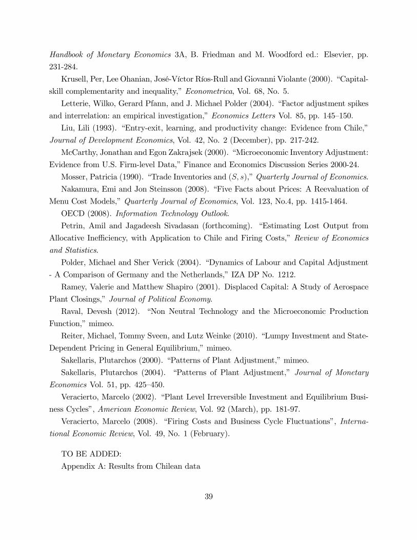
Handbook of Monetary Economics 3A, B. Friedman and M. Woodford ed.: Elsevier, pp.

231-284.

Krusell, Per, Lee Ohanian, José-Víctor Ríos-Rull and Giovanni Violante (2000). �Capital-

skill complementarity and inequality,�Econometrica, Vol. 68, No. 5.

Letterie, Wilko, Gerard Pfann, and J. Michael Polder (2004). �Factor adjustment spikes

and interrelation: an empirical investigation,�Economics Letters Vol. 85, pp. 145�150.

Liu, Lili (1993). �Entry-exit, learning, and productivity change: Evidence from Chile,�

Journal of Development Economics, Vol. 42, No. 2 (December), pp. 217-242.

McCarthy, Jonathan and Egon Zakrajsek (2000). �Microeconomic Inventory Adjustment:

Evidence from U.S. Firm-level Data,�Finance and Economics Discussion Series 2000-24.

Mosser, Patricia (1990). �Trade Inventories and (S; s),�Quarterly Journal of Economics.

Nakamura, Emi and Jon Steinsson (2008). �Five Facts about Prices: A Reevaluation of

Menu Cost Models,�Quarterly Journal of Economics, Vol. 123, No.4, pp. 1415-1464.

OECD (2008). Information Technology Outlook.

Petrin, Amil and Jagadeesh Sivadasan (forthcoming). �Estimating Lost Output from

Allocative Ine¢ ciency, with Application to Chile and Firing Costs,�Review of Economics

and Statistics.

Polder, Michael and Sher Verick (2004). �Dynamics of Labour and Capital Adjustment

- A Comparison of Germany and the Netherlands,�IZA DP No. 1212.

Ramey, Valerie and Matthew Shapiro (2001). Displaced Capital: A Study of Aerospace

Plant Closings,�Journal of Political Economy.

Raval, Devesh (2012). �Non Neutral Technology and the Microeconomic Production

Function,�mimeo.

Reiter, Michael, Tommy Sveen, and Lutz Weinke (2010). �Lumpy Investment and State-

Dependent Pricing in General Equilibrium,�mimeo.

Sakellaris, Plutarchos (2000). �Patterns of Plant Adjustment,�mimeo.

Sakellaris, Plutarchos (2004). �Patterns of Plant Adjustment,� Journal of Monetary

Economics Vol. 51, pp. 425�450.

Veracierto, Marcelo (2002). �Plant Level Irreversible Investment and Equilibrium Busi-

ness Cycles�, American Economic Review, Vol. 92 (March), pp. 181-97.

Veracierto, Marcelo (2008). �Firing Costs and Business Cycle Fluctuations�, Interna-

tional Economic Review, Vol. 49, No. 1 (February).

TO BE ADDED:

Appendix A: Results from Chilean data

39

Appendix B.1: Baseline simulation model

Appendix B.2: Details of derivations

Appendix C: Robustness analysis

40

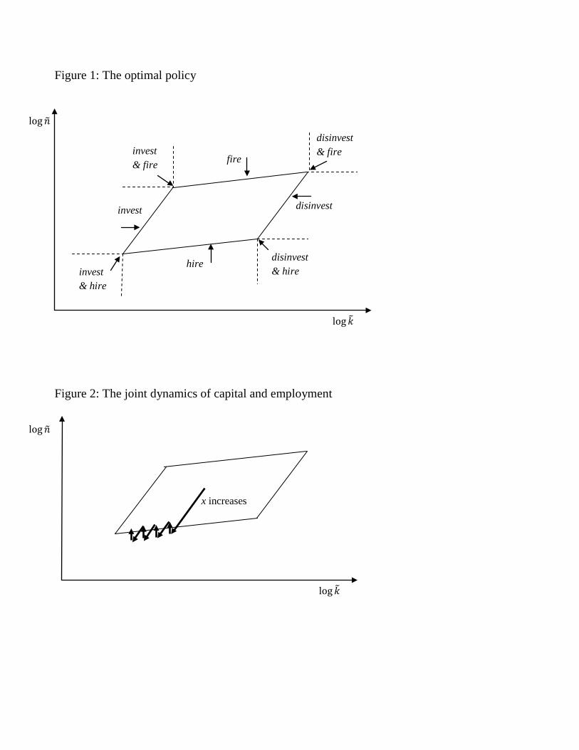
Figure 1: The optimal policy

Figure 2: The joint dynamics of capital and employment

x increases

fire

hire

disinvest invest

log𝑘�

log𝑛�

invest & hire

invest & fire

disinvest & hire

disinvest & fire

log𝑛�

log𝑘�

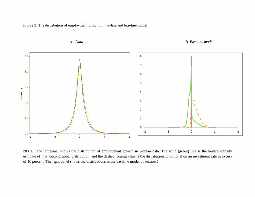
Figure 3: The distribution of employment growth in the data and baseline model

A. Data B. Baseline model

NOTE: The left panel shows the distribution of employment growth in Korean data. The solid (green) line is the kernsel-density

estimate of the unconditional distribution, and the dashed (orange) line is the distribution conditional on an investment rate in excess of 10 percent. The right panel shows the distributions in the baseline model of section 1.

0

1

2

3

4

5

6

7

8

-2 -1 0 1 2

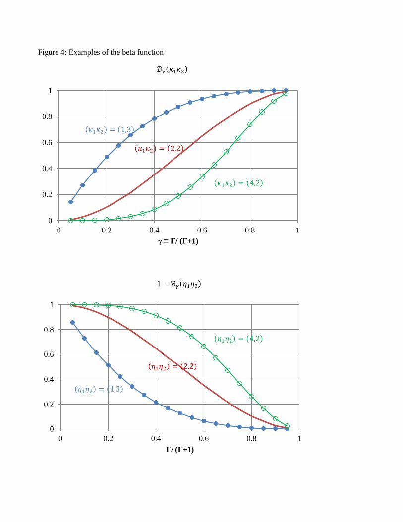
Figure 4: Examples of the beta function

ℬ𝛾(𝜅1𝜅2)

1 − ℬ𝛾(𝜂1𝜂2)

0

0.2

0.4

0.6

0.8

1

0 0.2 0.4 0.6 0.8 1 γ ≡ Γ/ (Γ+1)

0

0.2

0.4

0.6

0.8

1

0 0.2 0.4 0.6 0.8 1 Γ/ (Γ+1)

(𝜅1𝜅2) = (1,3)

(𝜅1𝜅2) = (2,2)

(𝜅1𝜅2) = (4,2)

(𝜂1𝜂2) = (1,3)

(𝜂1𝜂2) = (2,2)

(𝜂1𝜂2) = (4,2)

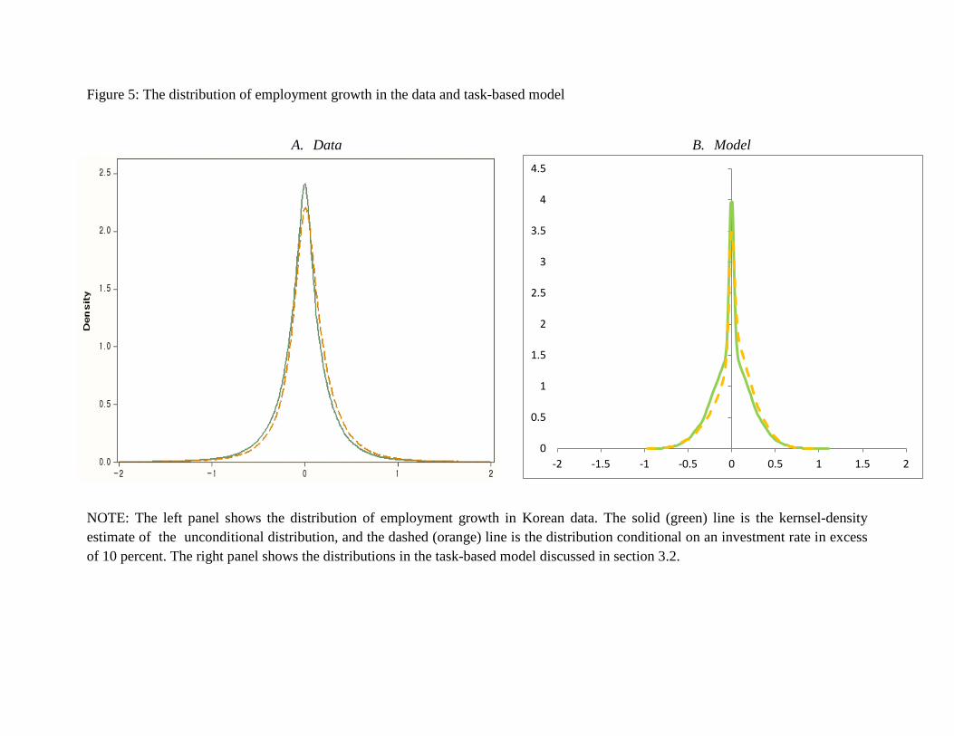
Figure 5: The distribution of employment growth in the data and task-based model

A. Data

B. Model

NOTE: The left panel shows the distribution of employment growth in Korean data. The solid (green) line is the kernsel-density estimate of the unconditional distribution, and the dashed (orange) line is the distribution conditional on an investment rate in excess of 10 percent. The right panel shows the distributions in the task-based model discussed in section 3.2.

0

0.5

1

1.5

2

2.5

3

3.5

4

4.5

-2 -1.5 -1 -0.5 0 0.5 1 1.5 2

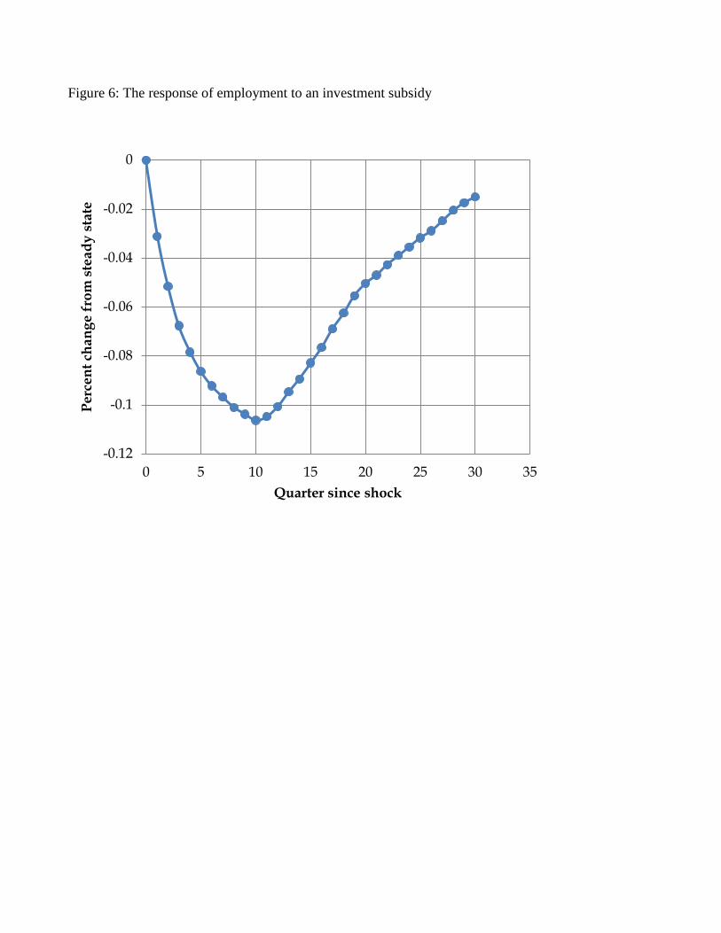
Figure 6: The response of employment to an investment subsidy

-0.12

-0.1

-0.08

-0.06

-0.04

-0.02

0

0 5 10 15 20 25 30 35

Perc

ent c

hang

e fr

om s

tead

y st

ate

Quarter since shock

Table 1: Factor adjustment in Korea

Panel A: Frequency and magnitude of individual factor adjustments

Share of plant-year obs. for which 𝐼𝐾−1

= 0 0.47

Share of plant-year obs. for which Δ ln𝑛 = 0 0.135

Standard deviation of 𝐼𝐾−1

(pooled across plants and time) 0.326

Standard deviation of Δ ln𝑛 (pooled across plants and time) 0.266

Share of plant-year obs. with positive gross sales of machinery 0.143

Share of plant-year obs. with positive gross purchases given gross sales 0.746

Panel B: Joint factor adjustment

Share of plant-year obs. in which Δ ln𝑛 < 0, given 𝐼𝐾−1

> 0 0.395

Average decrease in ln𝑛, given Δ ln𝑛 < 0 and 𝐼𝐾−1

> 0 0.19

Average increase in ln𝑛, given Δ ln𝑛 > 0 and 𝐼𝐾−1

> 0 0.214

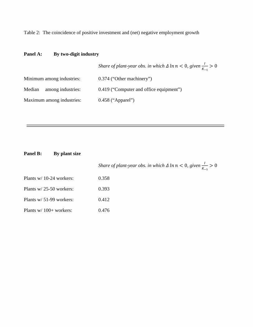
Table 2: The coincidence of positive investment and (net) negative employment growth

Panel A: By two-digit industry

Share of plant-year obs. in which 𝛥 𝑙𝑛 𝑛 < 0, given 𝐼𝐾−1

> 0

Minimum among industries: 0.374 (“Other machinery”)

Median among industries: 0.419 (“Computer and office equipment”)

Maximum among industries: 0.458 (“Apparel”)

Panel B: By plant size

Share of plant-year obs. in which 𝛥 𝑙𝑛 𝑛 < 0, given 𝐼𝐾−1

> 0

Plants w/ 10-24 workers: 0.358

Plants w/ 25-50 workers: 0.393

Plants w/ 51-99 workers: 0.412

Plants w/ 100+ workers: 0.476

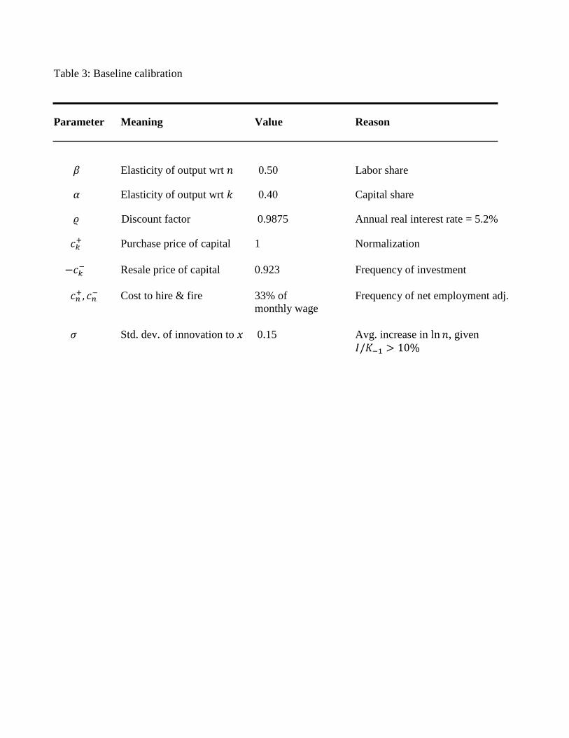
Table 3: Baseline calibration

Parameter Meaning Value Reason

𝛽 Elasticity of output wrt 𝑛 0.50 Labor share

𝛼 Elasticity of output wrt 𝑘 0.40 Capital share

𝜚 Discount factor 0.9875 Annual real interest rate = 5.2%

𝑐𝑘+ Purchase price of capital 1 Normalization −𝑐𝑘− Resale price of capital 0.923 Frequency of investment 𝑐𝑛+, 𝑐𝑛− Cost to hire & fire 33% of Frequency of net employment adj.

monthly wage 𝜎 Std. dev. of innovation to 𝑥 0.15 Avg. increase in ln𝑛, given 𝐼/𝐾−1 > 10%

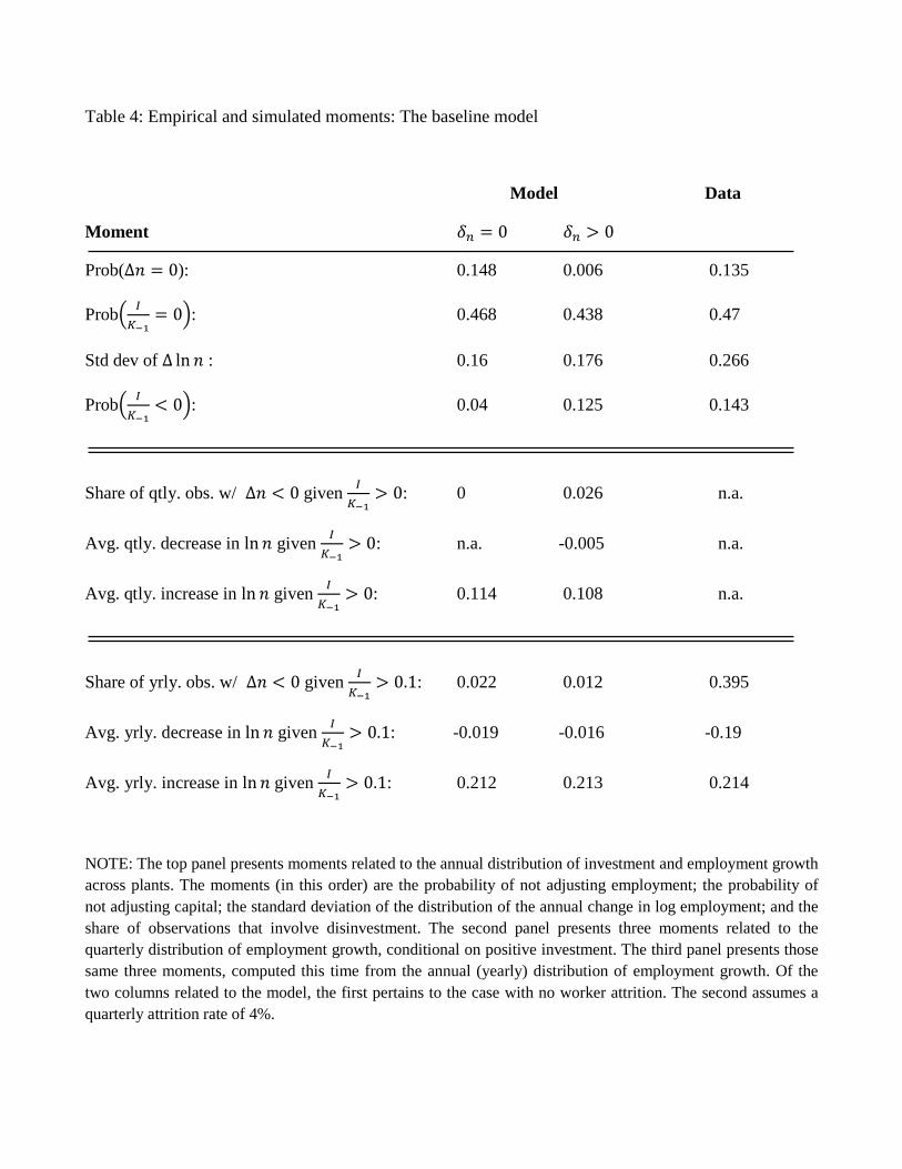
Table 4: Empirical and simulated moments: The baseline model

Model Data

Moment 𝛿𝑛 = 0 𝛿𝑛 > 0

Prob(Δ𝑛 = 0): 0.148 0.006 0.135

Prob� 𝐼𝐾−1

= 0�: 0.468 0.438 0.47

Std dev of Δ ln𝑛 : 0.16 0.176 0.266

Prob� 𝐼𝐾−1

< 0�: 0.04 0.125 0.143

Share of qtly. obs. w/ Δ𝑛 < 0 given 𝐼𝐾−1

> 0: 0 0.026 n.a.

Avg. qtly. decrease in ln𝑛 given 𝐼𝐾−1

> 0: n.a. -0.005 n.a.

Avg. qtly. increase in ln𝑛 given 𝐼𝐾−1

> 0: 0.114 0.108 n.a.

Share of yrly. obs. w/ Δ𝑛 < 0 given 𝐼𝐾−1

> 0.1: 0.022 0.012 0.395

Avg. yrly. decrease in ln𝑛 given 𝐼𝐾−1

> 0.1: -0.019 -0.016 -0.19

Avg. yrly. increase in ln𝑛 given 𝐼𝐾−1

> 0.1: 0.212 0.213 0.214

NOTE: The top panel presents moments related to the annual distribution of investment and employment growth across plants. The moments (in this order) are the probability of not adjusting employment; the probability of not adjusting capital; the standard deviation of the distribution of the annual change in log employment; and the share of observations that involve disinvestment. The second panel presents three moments related to the quarterly distribution of employment growth, conditional on positive investment. The third panel presents those same three moments, computed this time from the annual (yearly) distribution of employment growth. Of the two columns related to the model, the first pertains to the case with no worker attrition. The second assumes a quarterly attrition rate of 4%.

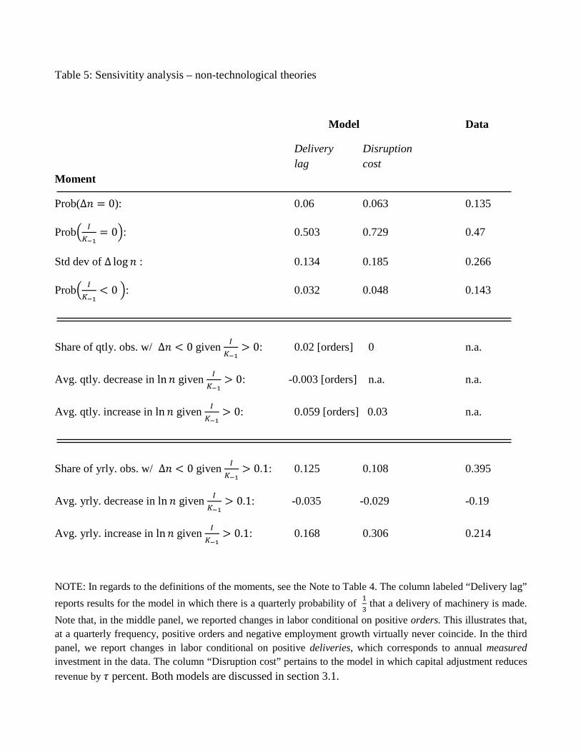
Table 5: Sensivitity analysis – non-technological theories

Model Data

Delivery Disruption lag cost Moment

Prob(Δ𝑛 = 0): 0.06 0.063 0.135

Prob� 𝐼𝐾−1

= 0�: 0.503 0.729 0.47

Std dev of Δ log 𝑛 : 0.134 0.185 0.266

Prob� 𝐼𝐾−1

< 0 �: 0.032 0.048 0.143

Share of qtly. obs. w/ Δ𝑛 < 0 given 𝐼𝐾−1

> 0: 0.02 [orders] 0 n.a.

Avg. qtly. decrease in ln𝑛 given 𝐼𝐾−1

> 0: -0.003 [orders] n.a. n.a.

Avg. qtly. increase in ln𝑛 given 𝐼𝐾−1

> 0: 0.059 [orders] 0.03 n.a.

Share of yrly. obs. w/ Δ𝑛 < 0 given 𝐼𝐾−1

> 0.1: 0.125 0.108 0.395

Avg. yrly. decrease in ln𝑛 given 𝐼𝐾−1

> 0.1: -0.035 -0.029 -0.19

Avg. yrly. increase in ln𝑛 given 𝐼𝐾−1

> 0.1: 0.168 0.306 0.214

NOTE: In regards to the definitions of the moments, see the Note to Table 4. The column labeled “Delivery lag” reports results for the model in which there is a quarterly probability of 1

3 that a delivery of machinery is made.

Note that, in the middle panel, we reported changes in labor conditional on positive orders. This illustrates that, at a quarterly frequency, positive orders and negative employment growth virtually never coincide. In the third panel, we report changes in labor conditional on positive deliveries, which corresponds to annual measured investment in the data. The column “Disruption cost” pertains to the model in which capital adjustment reduces revenue by 𝜏 percent. Both models are discussed in section 3.1.

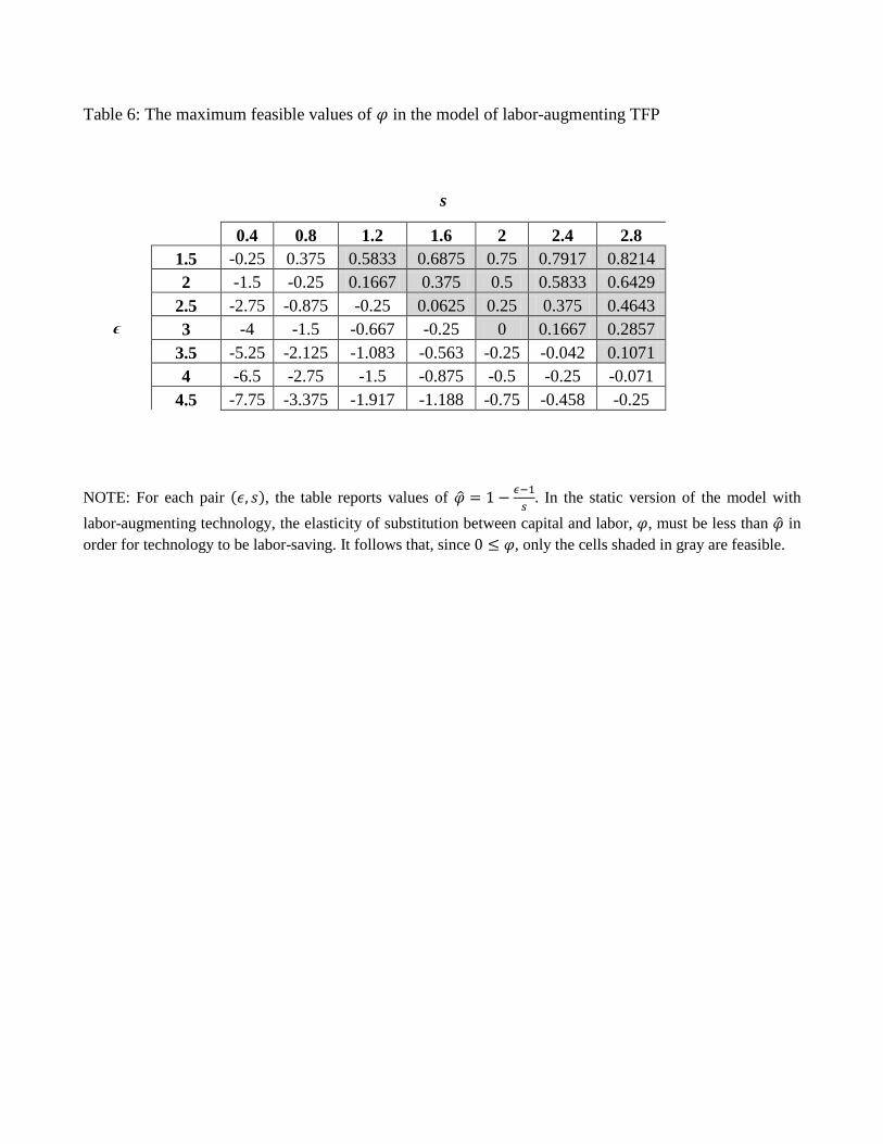
Table 6: The maximum feasible values of 𝜑 in the model of labor-augmenting TFP

s

0.4 0.8 1.2 1.6 2 2.4 2.8

ϵ

1.5 -0.25 0.375 0.5833 0.6875 0.75 0.7917 0.8214 2 -1.5 -0.25 0.1667 0.375 0.5 0.5833 0.6429

2.5 -2.75 -0.875 -0.25 0.0625 0.25 0.375 0.4643 3 -4 -1.5 -0.667 -0.25 0 0.1667 0.2857

3.5 -5.25 -2.125 -1.083 -0.563 -0.25 -0.042 0.1071 4 -6.5 -2.75 -1.5 -0.875 -0.5 -0.25 -0.071

4.5 -7.75 -3.375 -1.917 -1.188 -0.75 -0.458 -0.25

NOTE: For each pair (𝜖, 𝑠), the table reports values of 𝜑� = 1 − 𝜖−1𝑠

. In the static version of the model with labor-augmenting technology, the elasticity of substitution between capital and labor, 𝜑, must be less than 𝜑� in order for technology to be labor-saving. It follows that, since 0 ≤ 𝜑, only the cells shaded in gray are feasible.

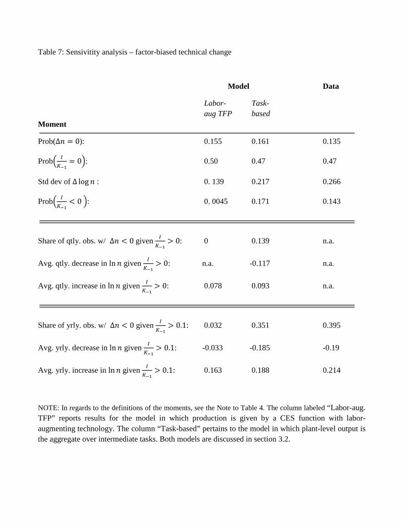
Table 7: Sensivitity analysis – factor-biased technical change

Model Data

Labor- Task- aug TFP based Moment

Prob(Δ𝑛 = 0): 0.155 0.161 0.135

Prob� 𝐼𝐾−1

= 0�: 0.50 0.47 0.47

Std dev of Δ log 𝑛 : 0. 139 0.217 0.266

Prob� 𝐼𝐾−1

< 0 �: 0. 0045 0.171 0.143

Share of qtly. obs. w/ Δ𝑛 < 0 given 𝐼𝐾−1

> 0: 0 0.139 n.a.

Avg. qtly. decrease in ln𝑛 given 𝐼𝐾−1

> 0: n.a. -0.117 n.a.

Avg. qtly. increase in ln𝑛 given 𝐼𝐾−1

> 0: 0.078 0.093 n.a.

Share of yrly. obs. w/ Δ𝑛 < 0 given 𝐼𝐾−1

> 0.1: 0.032 0.351 0.395

Avg. yrly. decrease in ln𝑛 given 𝐼𝐾−1

> 0.1: -0.033 -0.185 -0.19

Avg. yrly. increase in ln𝑛 given 𝐼𝐾−1

> 0.1: 0.163 0.188 0.214

NOTE: In regards to the definitions of the moments, see the Note to Table 4. The column labeled “Labor-aug. TFP” reports results for the model in which production is given by a CES function with labor-augmenting technology. The column “Task-based” pertains to the model in which plant-level output is the aggregate over intermediate tasks. Both models are discussed in section 3.2.