sustainability

Article

The Impact of Air Pollution on Domestic Tourism inChina: A Spatial Econometric Analysis

Daxin Dong * , Xiaowei Xu, Hong Yu and Yanfang Zhao

School of Business Administration, Southwestern University of Finance and Economics, Chengdu 611130, China* Correspondence: dongdaxinedu@126.com

Received: 23 June 2019; Accepted: 30 July 2019; Published: 1 August 2019�����������������

Abstract: This study utilizes a spatial econometric model to analyze the impact of air pollution ondomestic tourism in China. Based on a panel dataset covering 337 cities from 2004–2013, this studyderives the following findings. (1) Air pollution significantly reduces domestic tourist arrivals inthe local city. On average, if the concentration of PM2.5 (particulate matter equal to or less than2.5 micrometers in width) in one city increases by 1 µg/m3, the number of domestic tourists to thecity declines by 0.7%. (2) Air pollution demonstrates significant spatial spillover effects. If the PM2.5

in other cities simultaneously increases by 1 µg/m3, the number of domestic tourists traveling tothe local city rises by 4.1%. (3) The magnitude of the spillover effects of air pollution is larger thanthe negative direct effects on local cities. This study suggests that enhancing air quality in the localarea will effectively promote the domestic tourism industry in the local city. In addition, it is impliedthat a simultaneous improvement in the air quality in all cities might not lead to an increase in thenumber of domestic tourist arrivals. Thus, in order to deal with the spillover effects of air pollutionon the domestic tourism industry, local governments should make efforts to develop cross-city orcross-region tourism.

Keywords: air pollution; PM2.5; domestic tourism; China; spatial econometric analysis;spillover effect

1. Introduction

Given that air pollution poses a great threat to human health, the climate, and ecosystem, in 2014,the United Nations Environment Assembly (UNEA) made air quality improvement a top priority forworld sustainable development [1]. Air pollution also puts enormous stress on sustainable growthin tourist arrivals and receipts. Previous studies have reported the impact of air pollution on thetourism industry worldwide, from both micro [2–5] and macro perspectives [6,7]. In recent years,China’s tourism industry has seen unprecedented development and become one of the world’s topinbound and outbound tourist markets [8]. However, the severe air pollution problem in some Chinesedistricts has harmed tourism development. For instance, in 2016, it was reported that hundreds offlights were canceled in Beijing because thick smog cut visibility to less than 200 m [9]. Given thatair pollution in China has bought disruption to outdoor travel activities due to low visibility andincreased health risk, the extensive air pollution problem in China has received a lot of attention fromscholars in the tourism industry. However, studies focus mainly on the impact of air pollution oninbound tourism [2–5], and few research efforts have been dedicated to the impact of air pollutionon China’s domestic tourism market, with the exceptions of Liu et al. [10], Peng and Xiao [11], andZhang et al. [12].

It is widely acknowledged that China has become one of the world’s most important tourismdestinations, with 141 million inbound visits in 2018 [13]. However, the rise of China’s domestictourism market is also worthy of attention, as the number of domestic tourist trips reached 5.54 billion

Sustainability 2019, 11, 4148; doi:10.3390/su11154148 www.mdpi.com/journal/sustainability

Sustainability 2019, 11, 4148 2 of 16

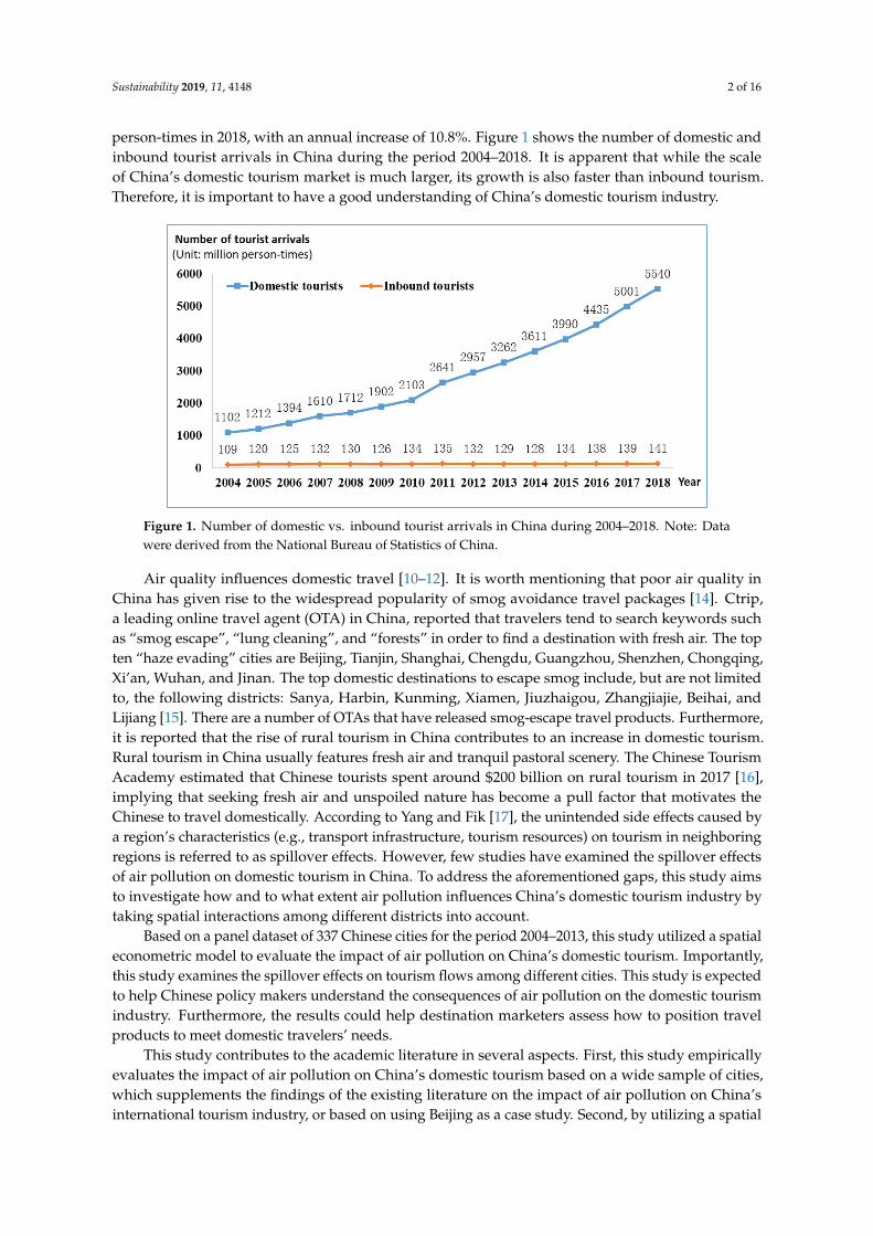
person-times in 2018, with an annual increase of 10.8%. Figure 1 shows the number of domestic andinbound tourist arrivals in China during the period 2004–2018. It is apparent that while the scaleof China’s domestic tourism market is much larger, its growth is also faster than inbound tourism.Therefore, it is important to have a good understanding of China’s domestic tourism industry.

Figure 1. Number of domestic vs. inbound tourist arrivals in China during 2004–2018. Note: Datawere derived from the National Bureau of Statistics of China.

Air quality influences domestic travel [10–12]. It is worth mentioning that poor air quality inChina has given rise to the widespread popularity of smog avoidance travel packages [14]. Ctrip,a leading online travel agent (OTA) in China, reported that travelers tend to search keywords suchas “smog escape”, “lung cleaning”, and “forests” in order to find a destination with fresh air. The topten “haze evading” cities are Beijing, Tianjin, Shanghai, Chengdu, Guangzhou, Shenzhen, Chongqing,Xi’an, Wuhan, and Jinan. The top domestic destinations to escape smog include, but are not limitedto, the following districts: Sanya, Harbin, Kunming, Xiamen, Jiuzhaigou, Zhangjiajie, Beihai, andLijiang [15]. There are a number of OTAs that have released smog-escape travel products. Furthermore,it is reported that the rise of rural tourism in China contributes to an increase in domestic tourism.Rural tourism in China usually features fresh air and tranquil pastoral scenery. The Chinese TourismAcademy estimated that Chinese tourists spent around $200 billion on rural tourism in 2017 [16],implying that seeking fresh air and unspoiled nature has become a pull factor that motivates theChinese to travel domestically. According to Yang and Fik [17], the unintended side effects caused bya region’s characteristics (e.g., transport infrastructure, tourism resources) on tourism in neighboringregions is referred to as spillover effects. However, few studies have examined the spillover effectsof air pollution on domestic tourism in China. To address the aforementioned gaps, this study aimsto investigate how and to what extent air pollution influences China’s domestic tourism industry bytaking spatial interactions among different districts into account.

Based on a panel dataset of 337 Chinese cities for the period 2004–2013, this study utilized a spatialeconometric model to evaluate the impact of air pollution on China’s domestic tourism. Importantly,this study examines the spillover effects on tourism flows among different cities. This study is expectedto help Chinese policy makers understand the consequences of air pollution on the domestic tourismindustry. Furthermore, the results could help destination marketers assess how to position travelproducts to meet domestic travelers’ needs.

This study contributes to the academic literature in several aspects. First, this study empiricallyevaluates the impact of air pollution on China’s domestic tourism based on a wide sample of cities,which supplements the findings of the existing literature on the impact of air pollution on China’sinternational tourism industry, or based on using Beijing as a case study. Second, by utilizing a spatial

Sustainability 2019, 11, 4148 3 of 16

econometric framework, this study is among the first to assess the unintended side effects of airpollution from other cities on local cities’ domestic tourism industry. The results of this study areexpected to help local governments and tourism organizations develop strategies to reach a sustainablebalance between the domestic tourism industry and environmental quality management.

2. Literature Review

This study is closely relevant to three streams of literature. The first stream studies the impactsof air pollution on tourism. The second stream evaluates tourism spatial spillover effects. The thirdconcerns the spatial spillover impacts of air pollution in China.

2.1. Impacts of Air Pollution on Tourism

A number of studies have found a negative impact of air pollution on tourism, which supports theassertion by Buckley [18] that the tourism industry remains far from sustainable. For instance, Anamanand Looi [6] estimated the effect of haze-related air pollution on the inbound tourism industry in BruneiDarussalam. According to their estimate, the haze-related air pollution reduced monthly arrivals byabout 28.7%, resulting in total direct loss of about eight million Brunei dollars (BND). Sajjad et al. [7]regarded deforestation and natural source depletion as two negative indicators of tourism developmentand revealed that, on average, air pollution in Asia and Africa negatively influenced the tourismindustry. Some scholars have broadened the scope of research by focusing on the impact of adverseclimate changes, which may exacerbate air pollution problems. Hamilton et al. [19] indicated thatthe growth of international tourism is projected to decrease in the long term due to climate change.Gössling et al. [20] indicated that the climate change of destinations is important in forming traveldecisions. Based on an overview of the relationship between tourism and global climate change,Pang et al. [21] suggested that climate change could negatively influence the tourism industry bymaking trip planning difficult and decreasing visitor satisfaction.

In recent years, some areas of China have suffered from serious air pollution. This phenomenonhas gained attention from scholars who seek to investigate the impact of particle pollution on China’stourism industry. Given that Beijing is China’s capital city and one of the top tourism destinations, itsair pollution is especially remarkable. A number of studies took Beijing as a case study and examinedthe impact of air pollution on the tourism industry from a micro-level perspective. Li et al. [22]found that smog concern among international travelers in Beijing would negatively influence theirsatisfaction. Zhang et al. [12] indicated that tourists who intend to visit Beijing in the next two yearssaw haze pollution as a crucial influencing factor when making decisions. Peng and Xiao [11] laterexamined domestic travelers’ attitudes towards smog in Beijing, indicating that travelers’ perceivedhealth risk and experience risk associated with smog had a negative impact on destination image andsubsequently led to a behavioral tendency of avoidance.

Besides Beijing, Cheung and Law [3] examined the inbound tourists’ perceptions of choosingHong Kong as a tourist destination. It was found that Asian visitors were more concerned with airquality when selecting a destination than Western travelers. Law and Cheung [4] further indicatedthat international travelers generally did not regard air pollution as a concern while making traveldecisions, but they became aware of Hong Kong’s air quality issues after their visits. At a nationallevel, Becken et al. [2] reported that the U.S. and Australian residents regarded air pollution issuesin China as one of the major travel risks, which negatively influenced destination image and visitintention to China. Based on a cross-sectional sample survey, Qiao et al. [5] reported that for Australianresidents, the pollution and air quality issues in China were considered as the substantially negativefactors when considering travel to China.

From a macro perspective, the negative impact of air pollution on China’s inbound tourismindustry has been verified by previous studies. In the case of Beijing, Tang et al. [23] applied monthlytimes series data from January 2004–December 2015 and found air pollution had a negative impact oninbound tourism in the long term rather than the short term. Deng et al. [24] utilized panel data on

Sustainability 2019, 11, 4148 4 of 16

31 Chinese provinces and found that industrial waste gas emissions had a significant negative effect.Dong et al. [25] analyzed the data from 274 Chinese cities during the period 2009–2012, confirming thenegative impact of air pollution on inbound tourism in China. Liu et al. [10] used panel data from the17 undeveloped provinces of China during the period 2005–2015 and found that domestic travelersin China were more sensitive to PM2.5 concentration than international travelers. Wang et al. [26]provided further evidence of the impact of air pollution on outbound tourism in China. Using datafrom a dominant online travel agent (OTA) in China, they discovered that air pollution is a push factorthat motivates Chinese people to travel abroad.

The literature on the impact of air quality in the place of destination on the tourism industrysubstantially outnumbered the studies on the impact of air quality in the place of origin. In addition,prior studies tended to place much greater emphasis on inbound tourism, neglecting the domestictourism market in China. This current study intends to shrink the gap in the literature by focusingon domestic tourism in China and using a spatial analysis method to investigate the impacts of airpollution in both tourist origin and destination cities.

2.2. Spatial Spillover Effects in the Tourism Industry

Previous studies have confirmed the existence of spillover effects in the tourism industry. From thesupply side, Li et al. [27] examined the role of tourism development in reducing regional incomeinequality in China using a spatiotemporal autoregressive model, indicating that the development ofdomestic tourism significantly narrows regional inequality. Ma et al. [28] showed the spatial spillovereffect of tourism development on urban economic growth. Previous studies also have identified aspatial correlation between tourism building investments and tourist revenues, the flow of touristcapital and labor and tourism-related economic growth, as well as local tourism development patterns(e.g., hotel infrastructure, tourism resource endowments) and regional tourism growth [17,29]. It hasalso been found that the growth of cruise tourism has a spillover effect on other tourism sectors, suchas hotels and restaurants [30].

From the demand side, previous studies examined the spatial spillover effects in tourism flows.Yang and Wong [31] found spatial spillover effects in both inbound and domestic tourism flows to341 cities in mainland China. It is suggested that physical infrastructure factors, tourist attractions, andthe severe acute respiratory syndrome (SARS) outbreak exhibited spatial spillover effects. Investigating55 countries participating in the “One Belt, One Road” initiative, Deng and Hu [32] confirmedthe existence of positive spillover effect in Chinese outbound tourist flows among countries withgeographic and cultural proximity. Using data from 98 cities in Eastern China during the period2004–2012, Zhou et al. [33] also found that tourist attractions in the regions surrounding a specificdestination had a positive spatial spillover effect on tourist flows to that destination.

2.3. Spatial Spillover Effects of Air Pollution in China

The existing literature includes spatial analyses of urban air pollution and air pollution control.Based on a panel covering 285 cities, Feng et al. [34] utilized the spatial Durbin model to examinethe spatial spillover effect of air pollution control on urban development quality in China, providingevidence of heterogeneity within different spatial regions in China. Fang et al. [35] later discovered theunintended spillover effects of regional air pollution policies on mitigating air pollution in urban areas.Previous research has also explored the spatial spillover effect of air pollution on public health andhealthcare expenditure in China [36,37].

Based on the above review of the literature on the impact of air pollution and spatial spillovereffects, it can be concluded that the spatial correlation between air pollution and tourist flows isunderexplored. A notable exception is the research of Deng et al. [24], who reported that air pollutionhad a negative spatial spillover effect on China’s inbound tourism industry, implying that internationaltourists are unlikely to visit a province that is surrounded by seriously polluted regions. Similarly, thisfinding was later supported by Xu et al. [38], who conducted a spatial analysis on inbound tourism in

Sustainability 2019, 11, 4148 5 of 16

174 cities of mid-eastern China. It seems that no empirical studies have examined the spatial spillovereffects of air pollution on the domestic tourism industry. This current study attempts to shrink this gapin the literature.

On the basis of the literature, two hypotheses are proposed to address precisely whether and towhat extent air pollution influences the sustainable development of the domestic tourism industry.

Hypothesis 1. Air pollution in the local city negatively affects the number of domestic tourist arrivals inthat city.

Hypothesis 2. Air pollution in other cities positively affects the number of domestic tourist arrivals in thelocal city.

3. Empirical Model and Data

3.1. Regression Model

The spatial Durbin model (SDM) is widely used in spatial analysis of tourism economics, becauseit considers both the spatial lagged dependent and independent variables [24,39]. We use the SDMas follows:

y = ρWy + Xβ + WXγ + u + ε, (1)

where the dependent variable y refers to ln(Arrivals), the logarithmic value of the number of domestictourist arrivals (in 10,000 person-times) in a city during one year. The vector X is a set of explanatoryvariables. The core explanatory variable of interest is PM2.5, the concentration density (µg/m3) ofparticulate matter in the air that is 2.5 micrometers or less in width. Besides, we also consideredsix important control variables: Scenic, Hotel, Transport, GovSize, ln(GDPpc), and ln(Population).(i) Scenic is an index for the abundance of tourism resource endowment, calculated by the numberof 5A- and 4A-rated scenic spots. One 5A spot is regarded as equal to two 4A spots, as a 5A spot isusually considered to be much more attractive than a 4A spot. (ii) Hotel is an indicator of tourisminfrastructure availability. As hotels are one of the most important tourism facilities, we used thenumber of star-rated hotels divided by the local population to index this variable. (iii) Transport isan indicator of the density of transportation infrastructure, proxied by the road length (km) per area(km2). (iv) GovSize refers to government size, measured by the ratio of fiscal spending to local GDP.This variable intends to capture the role of local government in tourism development. (v) ln(GDPpc)is the logarithmic value of the gross domestic product (GDP) per capita. This variable measures thedegree of economic development. (vi) ln(Population) is the logarithmic population within the city.The population is included as a control variable to control for the possible economies of scale in thetourism industry.

W is a spatial weight matrix. In our model, W is a distance matrix constructed based on thelongitude and latitude data of the cities. Based on the classical assumption that spillover effects declineas the geographic distance increases, the off-diagonal elements of W were set equal to the inverse ofthe linear distance (km) between two cities, and the diagonal elements were zero. Another spatialweight matrix will be used for the robustness check, which will be discussed in detail in Section 4.3.

u refers to the fixed effect (FE) or random effect (RE) incorporated into the panel data model,depending on whether we apply an FE or RE model. ε is the error term. ρ, β, and γ are coefficients tobe estimated. Based on these coefficients, we were able to measure the direct and indirect effects ofeach explanatory variable. We focus in particular on the effects of air pollution.

Sustainability 2019, 11, 4148 6 of 16

3.2. Data

The data were collected from several different sources. The data of PM2.5 were taken fromNASA’s Global Annual PM2.5 Grids data [40,41]. Data of Arrivals, Hotel, Transport, GovSize, GDPpc,and Population came from the China Statistical Yearbook for Regional Economy [42]. The dataregarding Scenic were collected from the public information released by the local governmentaldepartments of tourism in different provinces. The spatial weight matrix W is a distance matrixconstructed based on the longitude and latitude data from the National Geomatics Center ofChina (NGCC).

The dataset comprised both temporal and spatial dimensions. In terms of its time dimension,it covered the period from 2004–2013. In fact, the China Statistical Yearbook for Regional Economyprovides data for the period 2002–2013. The data for 2002 and 2003 were intentionally dropped becausethe tourism industry in China was greatly affected by the SARS issue in 2003 [43]. Thus, the databefore and after 2003 are not comparable. The sampling period ended in 2013, because the city-leveltourism data were substantially incomplete since 2014. In terms of its spatial dimension, it had a widegeographic range covering almost all areas within Mainland China. To be precise, the sample consistedof 337 districts in Mainland China, covering all four province-level municipalities (Beijing, Shanghai,Tianjin, and Chongqing) and all prefecture-level administrative regions except Sansha City of HainanProvince. For convenience, these administrative districts are denoted as “cities” in the rest of the paper.Sansha City, which was established in 2012, was excluded due to its extremely small population size ofapproximately 3000 residents and a lack of relevant statistical data. Chaohu City in Anhui Provincelacked data during 2011–2013, because it was no longer a prefecture-level city due to the adjustment ofadministrative division in 2011. Thus, for simplicity, the missing values during the period 2011–2013were imputed using the data for 2010. After a data cleansing process, a balanced panel dataset of 337cities for 10 years was kept for further analyses, which generated 3370 observations. The summarystatistics of the variables used in our regressions are shown in Table 1. (The data are available online assupplementary materials.)

Table 1. Summary statistics of the variables used in the spatial Durbin model (SDM).

Variable Observations Mean Standard Deviation Minimum Maximum

ln(Arrivals) 3370 6.378 1.320 0 10.185PM2.5 3370 33.191 17.881 2.002 90.856Scenic 3370 3.499 5.490 0 69Hotel 3370 0.143 0.226 0.003 4.338Transport 3370 0.769 0.498 0.003 2.249GovSize 3370 0.189 0.179 0.040 3.581ln(GDPpc) 3370 9.719 0.730 7.613 11.874ln(Population) 3370 5.666 0.877 2.077 7.996

4. Results

The empirical results are presented in this section. We first show the results of the statisticaltests of spatial autocorrelation. Then, we demonstrate the main estimation results for the regressionmodel expressed by Equation (1). After that, several robustness checks are discussed. Some importantextended analyses based on the estimates are presented at the end of this section.

4.1. Statistical Tests of Spatial Autocorrelation

Table 2 shows the estimated value of Moran’s I, a well-known measure of spatial autocorrelation,and the associated z-score for the variables of ln(Arrivals) and PM2.5 in each sample year. As presentedin the table, tourism and air pollution both displayed statistically-significant spatial autocorrelation.

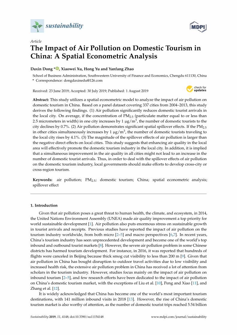
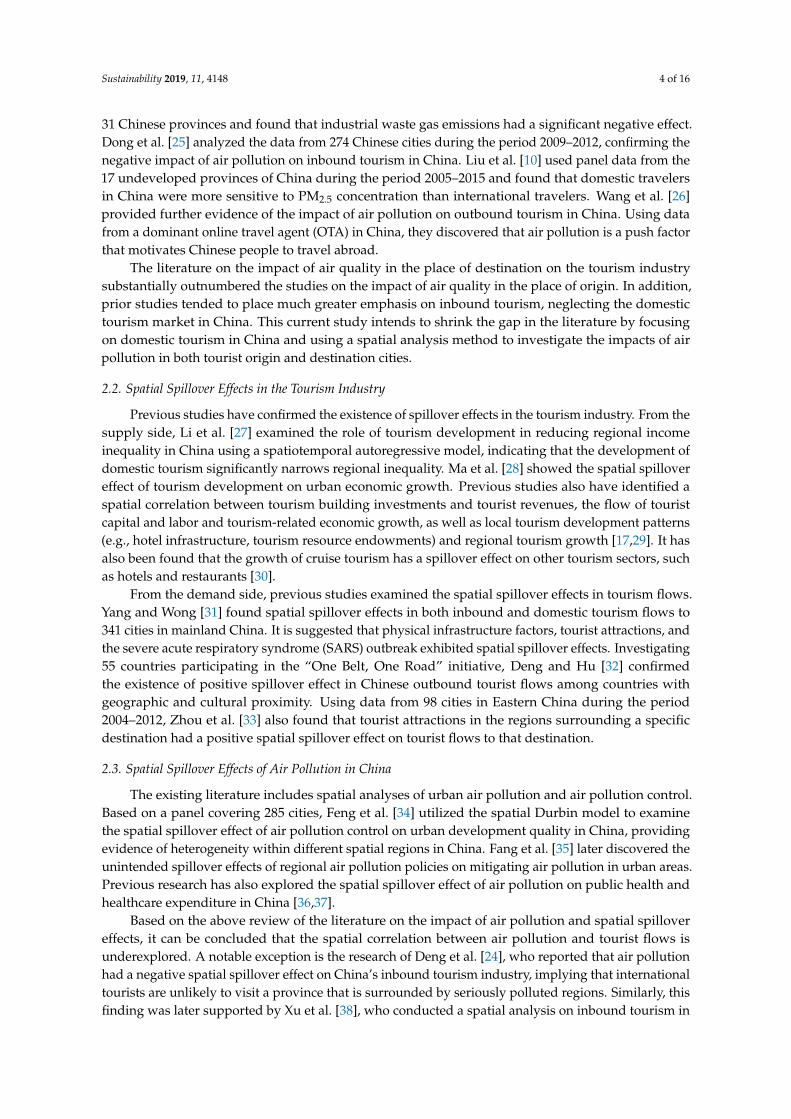
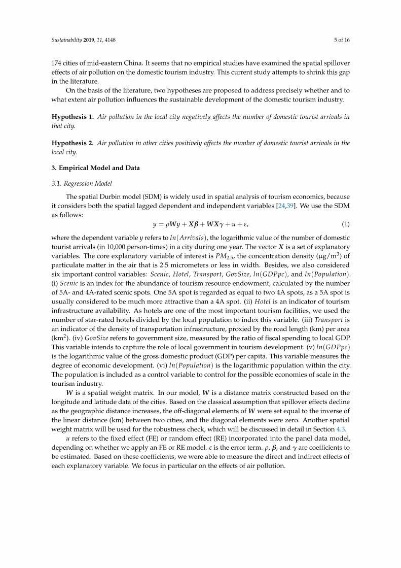
Next, scatter plots were used to visualize the existence of spatial autocorrelation of ln(Arrivals)and PM2.5, shown in Figure 2 and 3, respectively. We only present the scenario for 2013 for the sake of

Sustainability 2019, 11, 4148 7 of 16

simplicity. Scenarios in other years yielded similar results. Figures 2 and 3 respectively exhibit strongsigns of spatial autocorrelation of the domestic tourism industry and air pollution data. In other words,the distributions of tourist arrivals and PM2.5 were not geographically random, but demonstratedsubstantial spatial agglomeration in space. Therefore, this study adopted a spatial econometric modelto take into account the spatial spillover effects among independent and dependent variables.

Table 2. Tests of spatial autocorrelation of tourism and air pollution in each year.

Year ln(Arrivals) PM2.5

Moran’s I z-Score Moran’s I z-Score

2004 0.121 *** 22.876 0.243 *** 45.1102005 0.120 *** 22.612 0.245 *** 45.4742006 0.122 *** 23.030 0.240 *** 44.6492007 0.122 *** 23.048 0.265 *** 49.2282008 0.135 *** 25.336 0.256 *** 47.5032009 0.131 *** 24.646 0.252 *** 46.7992010 0.130 *** 24.429 0.251 *** 46.4802011 0.129 *** 24.313 0.254 *** 47.1882012 0.129 *** 24.367 0.246 *** 45.6612013 0.123 *** 23.208 0.253 *** 47.014

Note: *** indicates statistical significance at the 1% level.

-10

0.5

-0.5

Spat

ially

lagg

ed ln

(Arri

vals

)

-5 -4 -3 -2 -1 0 1 2 3ln(Arrivals)

(Moran's I=0.1229 and P-value=0.0010)

Figure 2. Moran’s scatter plot for domestic tourist arrivals in 2013.

Sustainability 2019, 11, 4148 8 of 16

01

0.5

-0.5

Spat

ially

lagg

ed P

M2.

5

-2 -1 0 1 2 3PM2.5

(Moran's I=0.2532 and P-value=0.0010)

Figure 3. Moran’s scatter plot for PM2.5 concentration in 2013.

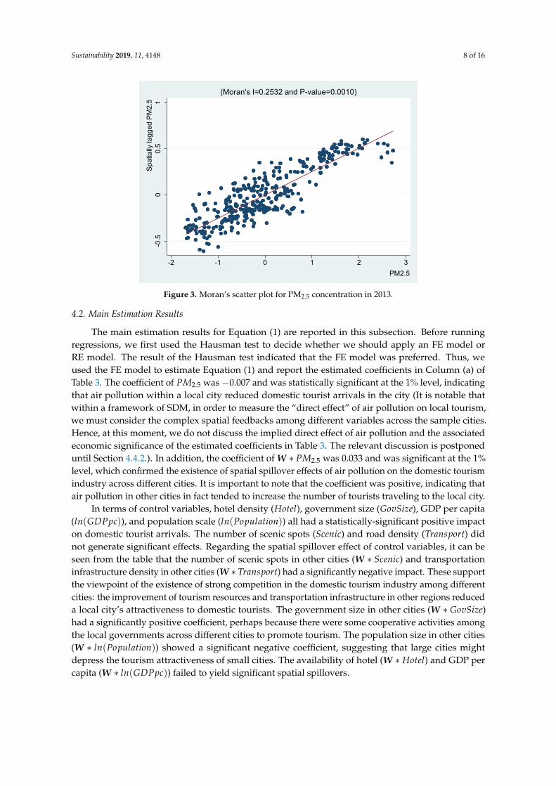
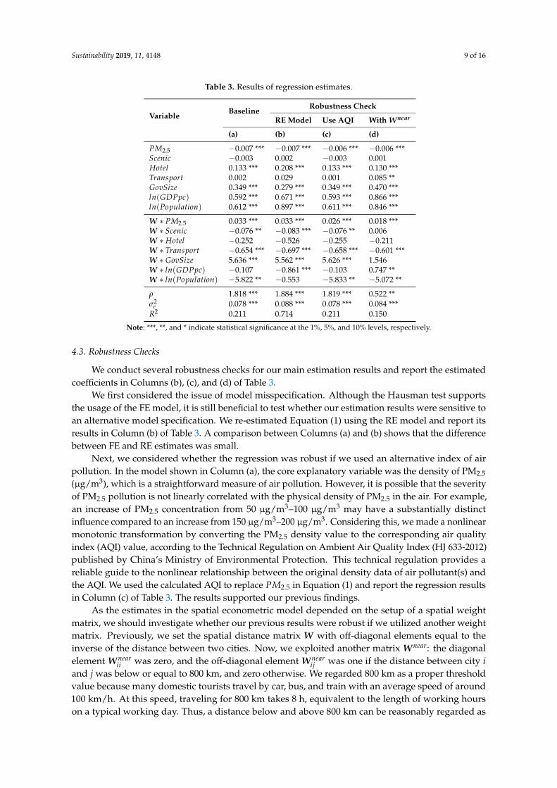
4.2. Main Estimation Results

The main estimation results for Equation (1) are reported in this subsection. Before runningregressions, we first used the Hausman test to decide whether we should apply an FE model orRE model. The result of the Hausman test indicated that the FE model was preferred. Thus, weused the FE model to estimate Equation (1) and report the estimated coefficients in Column (a) ofTable 3. The coefficient of PM2.5 was −0.007 and was statistically significant at the 1% level, indicatingthat air pollution within a local city reduced domestic tourist arrivals in the city (It is notable thatwithin a framework of SDM, in order to measure the “direct effect” of air pollution on local tourism,we must consider the complex spatial feedbacks among different variables across the sample cities.Hence, at this moment, we do not discuss the implied direct effect of air pollution and the associatedeconomic significance of the estimated coefficients in Table 3. The relevant discussion is postponeduntil Section 4.4.2.). In addition, the coefficient of W ∗ PM2.5 was 0.033 and was significant at the 1%level, which confirmed the existence of spatial spillover effects of air pollution on the domestic tourismindustry across different cities. It is important to note that the coefficient was positive, indicating thatair pollution in other cities in fact tended to increase the number of tourists traveling to the local city.

In terms of control variables, hotel density (Hotel), government size (GovSize), GDP per capita(ln(GDPpc)), and population scale (ln(Population)) all had a statistically-significant positive impacton domestic tourist arrivals. The number of scenic spots (Scenic) and road density (Transport) didnot generate significant effects. Regarding the spatial spillover effect of control variables, it can beseen from the table that the number of scenic spots in other cities (W ∗ Scenic) and transportationinfrastructure density in other cities (W ∗ Transport) had a significantly negative impact. These supportthe viewpoint of the existence of strong competition in the domestic tourism industry among differentcities: the improvement of tourism resources and transportation infrastructure in other regions reduceda local city’s attractiveness to domestic tourists. The government size in other cities (W ∗ GovSize)had a significantly positive coefficient, perhaps because there were some cooperative activities amongthe local governments across different cities to promote tourism. The population size in other cities(W ∗ ln(Population)) showed a significant negative coefficient, suggesting that large cities mightdepress the tourism attractiveness of small cities. The availability of hotel (W ∗ Hotel) and GDP percapita (W ∗ ln(GDPpc)) failed to yield significant spatial spillovers.

Sustainability 2019, 11, 4148 9 of 16

Table 3. Results of regression estimates.

Variable Baseline Robustness Check

RE Model Use AQI With Wnear

(a) (b) (c) (d)

PM2.5 −0.007 *** −0.007 *** −0.006 *** −0.006 ***Scenic −0.003 0.002 −0.003 0.001Hotel 0.133 *** 0.208 *** 0.133 *** 0.130 ***Transport 0.002 0.029 0.001 0.085 **GovSize 0.349 *** 0.279 *** 0.349 *** 0.470 ***ln(GDPpc) 0.592 *** 0.671 *** 0.593 *** 0.866 ***ln(Population) 0.612 *** 0.897 *** 0.611 *** 0.846 ***

W ∗ PM2.5 0.033 *** 0.033 *** 0.026 *** 0.018 ***W ∗ Scenic −0.076 ** −0.083 *** −0.076 ** 0.006W ∗ Hotel −0.252 −0.526 −0.255 −0.211W ∗ Transport −0.654 *** −0.697 *** −0.658 *** −0.601 ***W ∗ GovSize 5.636 *** 5.562 *** 5.626 *** 1.546W ∗ ln(GDPpc) −0.107 −0.861 *** −0.103 0.747 **W ∗ ln(Population) −5.822 ** −0.553 −5.833 ** −5.072 **

ρ 1.818 *** 1.884 *** 1.819 *** 0.522 **σ2

e 0.078 *** 0.088 *** 0.078 *** 0.084 ***R2 0.211 0.714 0.211 0.150

Note: ***, **, and * indicate statistical significance at the 1%, 5%, and 10% levels, respectively.

4.3. Robustness Checks

We conduct several robustness checks for our main estimation results and report the estimatedcoefficients in Columns (b), (c), and (d) of Table 3.

We first considered the issue of model misspecification. Although the Hausman test supportsthe usage of the FE model, it is still beneficial to test whether our estimation results were sensitive toan alternative model specification. We re-estimated Equation (1) using the RE model and report itsresults in Column (b) of Table 3. A comparison between Columns (a) and (b) shows that the differencebetween FE and RE estimates was small.

Next, we considered whether the regression was robust if we used an alternative index of airpollution. In the model shown in Column (a), the core explanatory variable was the density of PM2.5

(µg/m3), which is a straightforward measure of air pollution. However, it is possible that the severityof PM2.5 pollution is not linearly correlated with the physical density of PM2.5 in the air. For example,an increase of PM2.5 concentration from 50 µg/m3–100 µg/m3 may have a substantially distinctinfluence compared to an increase from 150 µg/m3–200 µg/m3. Considering this, we made a nonlinearmonotonic transformation by converting the PM2.5 density value to the corresponding air qualityindex (AQI) value, according to the Technical Regulation on Ambient Air Quality Index (HJ 633-2012)published by China’s Ministry of Environmental Protection. This technical regulation provides areliable guide to the nonlinear relationship between the original density data of air pollutant(s) andthe AQI. We used the calculated AQI to replace PM2.5 in Equation (1) and report the regression resultsin Column (c) of Table 3. The results supported our previous findings.

As the estimates in the spatial econometric model depended on the setup of a spatial weightmatrix, we should investigate whether our previous results were robust if we utilized another weightmatrix. Previously, we set the spatial distance matrix W with off-diagonal elements equal to theinverse of the distance between two cities. Now, we exploited another matrix Wnear: the diagonalelement Wnear

ii was zero, and the off-diagonal element Wnearij was one if the distance between city i

and j was below or equal to 800 km, and zero otherwise. We regarded 800 km as a proper thresholdvalue because many domestic tourists travel by car, bus, and train with an average speed of around100 km/h. At this speed, traveling for 800 km takes 8 h, equivalent to the length of working hourson a typical working day. Thus, a distance below and above 800 km can be reasonably regarded as

Sustainability 2019, 11, 4148 10 of 16

“near” and “far”, respectively. (We also tried other values, such as 500 km or 1000 km, as a threshold toconstruct the binary matrix Wnear, and found similar regression results. To save space, we only reportthe estimates based on the weighting matrix using 800 km as the threshold.) Column (d) of Table 3shows our estimates. It was found that the coefficient of PM2.5 was close to the previous estimates inthe baseline model. The coefficient of W ∗ PM2.5 became smaller, but was still positive and statisticallysignificant at the 1% level.

In brief, the robustness checks validated the estimates based on the baseline model and confirmedour previous findings that air pollution damages domestic tourism in the local city, but tends toincrease the domestic tourist arrivals in other cities.

4.4. Extended Analyses

We further analyzed our main estimation results presented in Section 4.2. We first examinedthe heterogeneity across different regions in China. Then, we decomposed the marginal effect of airpollution into two parts: direct effect and indirect effect.

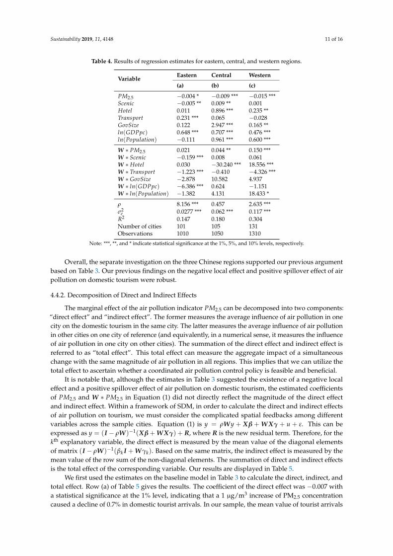
4.4.1. Circumstances in Different Districts

As the eastern, central, and western areas of China are highly heterogeneous in the degreeof economic and social development, it is possible that the impact of air pollution on domestictourism is not homogenous over these three regions. To deal with this concern, we re-estimatedEquation (1) for the subsamples of these three regions separately and then compared the results.The sample was divided according to the official classification by the National Bureau of Statisticsof China. In our sample, 101, 105, and 131 cities belonged to the eastern, central, and western areas,respectively. Columns (a), (b), and (c) in Table 4 display the estimates for the eastern, central, andwestern subsamples, respectively. Focusing on the effect of air pollution, there were two main findings.(1) In all regions, air pollution generated a significant negative impact on domestic tourism in localcities. The significant negative coefficients of variable PM2.5 in Columns (a), (b), and (c) made thispoint clear. (2) In all regions, air pollution had a positive spatial spillover effect on domestic tourism inother cities. As displayed in the table, the coefficients of W ∗ PM2.5 were positive in Columns (a), (b),and (c). In particular, the coefficients for the central and western regions were statistically significant atthe 1% level.

Sustainability 2019, 11, 4148 11 of 16

Table 4. Results of regression estimates for eastern, central, and western regions.

Variable Eastern Central Western

(a) (b) (c)

PM2.5 −0.004 * −0.009 *** −0.015 ***Scenic −0.005 ** 0.009 ** 0.001Hotel 0.011 0.896 *** 0.235 **Transport 0.231 *** 0.065 −0.028GovSize 0.122 2.947 *** 0.165 **ln(GDPpc) 0.648 *** 0.707 *** 0.476 ***ln(Population) −0.111 0.961 *** 0.600 ***

W ∗ PM2.5 0.021 0.044 ** 0.150 ***W ∗ Scenic −0.159 *** 0.008 0.061W ∗ Hotel 0.030 −30.240 *** 18.556 ***W ∗ Transport −1.223 *** −0.410 −4.326 ***W ∗ GovSize −2.878 10.582 4.937W ∗ ln(GDPpc) −6.386 *** 0.624 −1.151W ∗ ln(Population) −1.382 4.131 18.433 *

ρ 8.156 *** 0.457 2.635 ***σ2

e 0.0277 *** 0.062 *** 0.117 ***R2 0.147 0.180 0.304Number of cities 101 105 131Observations 1010 1050 1310

Note: ***, **, and * indicate statistical significance at the 1%, 5%, and 10% levels, respectively.

Overall, the separate investigation on the three Chinese regions supported our previous argumentbased on Table 3. Our previous findings on the negative local effect and positive spillover effect of airpollution on domestic tourism were robust.

4.4.2. Decomposition of Direct and Indirect Effects

The marginal effect of the air pollution indicator PM2.5 can be decomposed into two components:“direct effect” and “indirect effect”. The former measures the average influence of air pollution in onecity on the domestic tourism in the same city. The latter measures the average influence of air pollutionin other cities on one city of reference (and equivalently, in a numerical sense, it measures the influenceof air pollution in one city on other cities). The summation of the direct effect and indirect effect isreferred to as “total effect”. This total effect can measure the aggregate impact of a simultaneouschange with the same magnitude of air pollution in all regions. This implies that we can utilize thetotal effect to ascertain whether a coordinated air pollution control policy is feasible and beneficial.

It is notable that, although the estimates in Table 3 suggested the existence of a negative localeffect and a positive spillover effect of air pollution on domestic tourism, the estimated coefficientsof PM2.5 and W ∗ PM2.5 in Equation (1) did not directly reflect the magnitude of the direct effectand indirect effect. Within a framework of SDM, in order to calculate the direct and indirect effectsof air pollution on tourism, we must consider the complicated spatial feedbacks among differentvariables across the sample cities. Equation (1) is y = ρWy + Xβ + WXγ + u + ε. This can beexpressed as y = (I − ρW)−1(Xβ + WXγ) + R, where R is the new residual term. Therefore, for thekth explanatory variable, the direct effect is measured by the mean value of the diagonal elementsof matrix (I − ρW)−1(βk I + Wγk). Based on the same matrix, the indirect effect is measured by themean value of the row sum of the non-diagonal elements. The summation of direct and indirect effectsis the total effect of the corresponding variable. Our results are displayed in Table 5.

We first used the estimates on the baseline model in Table 3 to calculate the direct, indirect, andtotal effect. Row (a) of Table 5 gives the results. The coefficient of the direct effect was −0.007 witha statistical significance at the 1% level, indicating that a 1 µg/m3 increase of PM2.5 concentrationcaused a decline of 0.7% in domestic tourist arrivals. In our sample, the mean value of tourist arrivals

Sustainability 2019, 11, 4148 12 of 16

across all cities was 12.17 million person-times. Thus, a decline of 0.7% corresponds to a reductionof 85,190 person-times in domestic tourist arrivals. This was indeed a large loss. The coefficient ofthe indirect effect was 0.041 with statistical significance at the 5% level, indicating that the domestictourists visiting the local city would rise by 4.1% if PM2.5 concentration in other cities simultaneouslyincreased by 1 µg/m3. This was a substantial influence. According to our estimates, the size of the(positive) indirect effect exceeded the size of the (negative) direct effect. As a consequence, the totaleffect, equal to the direct effect plus the indirect effect, had a positive coefficient of 0.034. This positivevalue had an interesting implication: a simultaneous depravation in air quality in all cities actuallyincreased the number of domestic tourists. This phenomenon might be explained by the possibilitythat air pollution stimulates the demand for tourism.

Table 5. Estimated direct, indirect, and total effects of PM2.5 on domestic tourist arrivals inChinese cities.

Model Direct Effect Indirect Effect Total Effect

(a) Baseline −0.007 *** 0.041 ** 0.034 *(−3.23) (2.25) (1.93)

(b) RE model −0.007 *** 0.042 0.035(−3.56) (0.30) (0.24)

(c) Use AQI −0.005 *** 0.032 ** 0.27 *(−3.55) (2.28) (1.94)

(d) With Wnear −0.006 *** 0.009 ** 0.003(−2.80) (2.70) (1.14)

Note: ***, **, and * indicate statistical significance at the 1%, 5%, and 10% levels, respectively.The corresponding t-statistics are reported in parentheses.

Next, we inspected the robustness of our estimates. In Row (b) of Table 5, we calculate the direct,indirect, and total effect of pollution based on the RE model in Table 3. The results were similar:a negative direct effect, positive indirect effect, and positive total effect. In Row (c) of Table 5, we reportthe calculation results using AQI as the independent variable. The results were close to those shownin Row (a). In Row (d) of Table 5, we estimated with the spatial weight matrix Wnear. The estimateddirect effect was close to that in Row (a). The estimated indirect effect was still significantly positive,but had a magnitude considerably smaller than that in Row (a). The shrinkage in the size of indirecteffect was because Wnear artificially imposed that the cities farther than 800 km had no effect. Nomatter the shrinkage of indirect effect, the magnitude of the estimated indirect effect was still largerthan the direct effect, and the total effect was still positive.

In general, the baseline model and different robustness checks provided consistent results. Ourcore findings can be summarized as follows. (1) Air pollution had a significantly negative directeffect on the domestic tourist arrivals in the local city. This had an important policy implication:an improvement of air quality will effectively promote the development of domestic tourism in thelocal city. (2) According to our estimates, the magnitude of the positive indirect effect of air pollutionin other cities was larger than the magnitude of the negative direct effect of air pollution in thelocal city. Thus, the total effect of air pollution was actually positive, which might be explained asa tourism-demand-inducement effect (i.e., the deterioration of environmental quality increases thedemand of traveling to the regions with a relatively better environment).

5. Discussion and Implications

This study implies that air quality is an important consideration factor when domestic touristsselect a travel destination. Hypothesis 1 was supported. The result is consistent with Cheung andLaw [3], whose study indicated that Asian visitors are conscious of air quality when selecting a traveldestination. This result is also in line with Peng and Xiao [11] who examined the impact of smog

Sustainability 2019, 11, 4148 13 of 16

on the domestic travel demand for Beijing and found a significant impact of travel risk perceptionon avoidance tendency and Liu et al. [10] who used panel data from the 17 undeveloped provincesin China and reported that the number of domestic travelers is negatively correlated with PM2.5

concentration. This study supplements the literature based on a wide city-level sample. It is impliedthat air pollution is not only viewed as an international travel risk [2], but also poses a threat todomestic travel. Therefore, it is suggested that China should implement effective policies to reduce airpollution so as to ensure sustainable growth for its domestic tourism industry.

Additionally, this study suggests that air pollution in other cities in fact tends to increase thenumber of tourists traveling to the local city. Hypothesis 2 was supported. This kind of spatial spillovereffect may be attributed to two reasons. To facilitate interpretation of this result, let us consider anarea that consists of three cities: City A with good air quality and Cities B and C with air pollutionproblems. (1) The first reason is relevant to the increased tourism demand in air polluted areas. Peopledislike air pollution and are unwilling to stay in polluted places for a long time. The air pollution inCities B and C may motivate the residents in those cities to travel, and of course, City A with relativelycleaner air will be an attractive destination. In this way, an increase in PM2.5 density in other citiescauses a rise of tourist arrivals at the local city. This result supplements the finding by Wang et al. [26],who indicated that a deterioration of air quality in the place of origin increases outbound tourismdemand. This study shows the possibility of the tourism-demand-inducement effect of air pollutionon domestic tourism, which is consistent with previous findings indicating that seeking fresh airis a push motivational factor for travel, especially for wellness or rural tourism [44,45]. Thus, it issuggested that Chinese cities with fresh air or cities with better air quality than their neighboringcities could develop haze-avoidance tourism packages to attract customers who are eager to escapeair pollution. (2) The second reason is relevant to the competition between local and other cities fordomestic tourism. For instance, suppose that a resident in City B is planning to travel and there are twocandidate destinations: Cities A and C. Naturally this potential tourist will compare the characteristicsof these two cities. Holding all variables else constant, this tourist will prefer City A over C because ofthe difference in air quality. Following the same logic, the air pollution in City B will raise the relativeattractiveness of City A to the tourists originating from City C, because poor air quality was foundto influence travelers’ aesthetic judgments on destinations [46] and perceived health risk [11]. In thisway, an increase in PM2.5 concentration in other cities diverts some potential tourists from those citiesto the local city. An implication for tourism marketing is that online travel agents could add a filterfunction by PM2.5 to each destination so that customers could make better decisions when choosinga destination.

Finally, this study implies that a simultaneous improvement of air quality in all cities does notcause an increase in the number of domestic tourist arrivals in each city. In other words, in theshort term, for the purpose of expanding domestic tourism, there is a non-cooperative game amongdifferent cities: while it is beneficial to control unilaterally for the air pollution in the local area,a joint activity to reduce pollution in all cities simultaneously is not preferred because the local citycan actually benefit from the air pollution in other cities. However, from a long-term perspective,since a tourism destination might reach a “decline” phase (during which the visitor flows to thedestination decrease) according to the tourism-life-cycle model [47], awareness about different regions’joint tourism resources and cooperation opportunities could help rejuvenate a tourism destination.Moreover, given the damage of air pollution to human health, the Chinese government should stillmake efforts to remedy air quality problems for the foreseeable future. As such, in the long term, it issuggested that cross-region or cross-city tourism destinations should be developed to deal with thespillover effect of air pollution on domestic tourism.

Sustainability 2019, 11, 4148 14 of 16

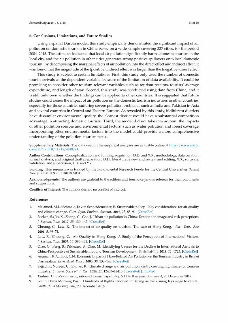
6. Conclusions, Limitations, and Future Studies

Using a spatial Durbin model, this study empirically demonstrated the significant impact of airpollution on domestic tourism in China based on a wide sample covering 337 cities, for the period2004–2013. The estimates indicated that local air pollution significantly harms domestic tourism in thelocal city, and the air pollution in other cities generates strong positive spillovers onto local domestictourism. By decomposing the marginal effects of air pollution into the direct effect and indirect effect, itwas found that the magnitude of the (positive) indirect effect was larger than the (negative) direct effect.

This study is subject to certain limitations. First, this study only used the number of domestictourist arrivals as the dependent variable, because of the limitation of data availability. It could bepromising to consider other tourism-relevant variables such as tourism receipts, tourists’ averageexpenditure, and length of stay. Second, this study was conducted using data from China, and itis still unknown whether the findings can be applied to other countries. It is suggested that futurestudies could assess the impact of air pollution on the domestic tourism industries in other countries,especially for those countries suffering severe pollution problems, such as India and Pakistan in Asiaand several countries in Central and Eastern Europe. As revealed by this study, if different districtshave dissimilar environmental quality, the cleanest district would have a substantial competitionadvantage in attracting domestic tourists. Third, the model did not take into account the impactsof other pollution sources and environmental factors, such as water pollution and forest coverage.Incorporating other environmental factors into the model could provide a more comprehensiveunderstanding of the pollution–tourism nexus.

Supplementary Materials: The data used in the empirical analyses are available online at http://www.mdpi.com/2071-1050/11/15/4148/s1.

Author Contributions: Conceptualization and funding acquisition, D.D. and X.X.; methodology, data curation,formal analysis, and original draft preparation, D.D.; literature review and review and editing, X.X.; software,validation, and supervision, H.Y. and Y.Z.

Funding: This research was funded by the Fundamental Research Funds for the Central Universities (GrantNos. JBK1801039 and JBK1809054).

Acknowledgments: The authors are grateful to the editors and four anonymous referees for their commentsand suggestions.

Conflicts of Interest: The authors declare no conflict of interest.

References

1. Melamed, M.L.; Schmale, J.; von Schneidemesser, E. Sustainable policy—Key considerations for air qualityand climate change. Curr. Opin. Environ. Sustain. 2016, 23, 85–91. [CrossRef]

2. Becken, S.; Jin, X.; Zhang, C.; Gao, J. Urban air pollution in China: Destination image and risk perceptions.J. Sustain. Tour. 2017, 25, 130–147. [CrossRef]

3. Cheung, C.; Law, R. The impact of air quality on tourism: The case of Hong Kong. Pac. Tour. Rev.2001, 5, 69–74.

4. Law, R.; Cheung, C. Air Quality in Hong Kong: A Study of the Perception of International Visitors.J. Sustain. Tour. 2007, 15, 390–401. [CrossRef]

5. Qiao, G.; Peng, S.; Prideaux, B.; Qiao, M. Identifying Causes for the Decline in International Arrivals toChina-Perspective of Sustainable Inbound Tourism Development. Sustainability 2019, 11, 1723. [CrossRef]

6. Anaman, K.A.; Looi, C.N. Economic Impact of Haze-Related Air Pollution on the Tourism Industry in BruneiDarussalam. Econ. Anal. Policy 2000, 30, 133–143. [CrossRef]

7. Sajjad, F.; Noreen, U.; Zaman, K. Climate change and air pollution jointly creating nightmare for tourismindustry. Environ. Sci. Pollut. Res. 2014, 21, 12403–12418. [CrossRef] [PubMed]

8. Xinhua. China’s domestic, inbound tourist trips to top 5.1 bln this year. Xinhuanet, 20 December 2017.9. South China Morning Post. Hundreds of flights canceled in Beijing as thick smog lays siege to capital.

South China Morning Post, 20 December 2016.

Sustainability 2019, 11, 4148 15 of 16

10. Liu, J.; Pan, H.; Zheng, S. Tourism Development, Environment and Policies: Differences between Domesticand International Tourists. Sustainability 2019, 11, 1390. [CrossRef]

11. Peng, J.; Xiao, H. How does smog influence domestic tourism in China? A case study of Beijing. Asia Pac. J.Tour. Res. 2018, 23, 1115–1128. [CrossRef]

12. Zhang, A.; Zhong, L.; Xu, Y.; Wang, H.; Dang, L. Tourists’ Perception of Haze Pollution and the PotentialImpacts on Travel: Reshaping the Features of Tourism Seasonality in Beijing, China. Sustainability2015, 7, 2397–2414. [CrossRef]

13. Xinhua. China’s inbound tourism remains steady in 2018. Xinhuanet, 5 February 2019.14. Arlt, W.G. As Smog Hits China, Chinese Tourists Seek Fresh Air on Pollution Free Holidays. Forbes,

5 January 2017.15. China Daily. Top 8 domestic destinations to escape smog. China Daily, 7 January 2016.16. Skift. China’s Domestic Tourism Boom Has Lessons for the Rest of the World. Skift, 18 August 2018.17. Yang, Y.; Fik, T. Spatial effects in regional tourism growth. Ann. Tour. Res. 2014, 46, 144–162. [CrossRef]18. Buckley, R. Sustainable tourism: Research and reality. Ann. Tour. Res. 2012, 39, 528–546. [CrossRef]19. Hamilton, J.M.; Maddison, D.J.; Tol, R.S.J. Effects of climate change on international tourism. Clim. Res.

2005, 29, 245–254. [CrossRef]20. Gössling, S.; Bredberg, M.; Randow, A.; Sandström, E.; Svensson, P. Tourist Perceptions of Climate Change:

A Study of International Tourists in Zanzibar. Curr. Issues Tour. 2006, 9, 419–435. [CrossRef]21. Pang, S.F.H.; McKercher, B.; Prideaux, B. Climate Change and Tourism: An Overview. Asia Pac. J. Tour. Res.

2013, 18, 4–20. [CrossRef]22. Li, J.; Pearce, P.L.; Morrison, A.M.; Wu, B. Up in Smoke? The Impact of Smog on Risk Perception and

Satisfaction of International Tourists in Beijing. Int. J. Tour. Res. 2016, 18, 373–386. [CrossRef]23. Tang, J.; Yuan, X.; Ramos, V.; Sriboonchitta, S. Does air pollution decrease inbound tourist arrivals? The case

of Beijing. Asia Pac. J. Tour. Res. 2019, 24, 597–605. [CrossRef]24. Deng, T.; Li, X.; Ma, M. Evaluating impact of air pollution on China’s inbound tourism industry: A spatial

econometric approach. Asia Pac. J. Tour. Res. 2017, 22, 771–780. [CrossRef]25. Dong, D.; Xu, X.; Wong, Y.F. Estimating the Impact of Air Pollution on Inbound Tourism in China:

An Analysis Based on Regression Discontinuity Design. Sustainability 2019, 11, 1682. [CrossRef]26. Wang, L.; Fang, B.; Law, R. Effect of air quality in the place of origin on outbound tourism demand:

Disposable income as a moderator. Tour. Manag. 2018, 68, 152–161. [CrossRef]27. Li, H.; Chen, J.L.; Li, G.; Goh, C. Tourism and regional income inequality: Evidence from China.

Ann. Tour. Res. 2016, 58, 81–99. [CrossRef]28. Ma, T.; Hong, T.; Zhang, H. Tourism spatial spillover effects and urban economic growth. J. Bus. Res.

2015, 68, 74–80. [CrossRef]29. Zhou, M.; Liu, X.; Pan, B.; Yang, X.; Wen, F.; Xia, X. Effect of Tourism Building Investments on Tourist

Revenues in China: A Spatial Panel Econometric Analysis. Emerg. Mark. Financ. Trade 2017, 53, 1973–1987.[CrossRef]

30. Skrede, O.; Tveteraas, S.L. Cruise spillovers to hotels and restaurants. Tour. Econ. 2019. [CrossRef]31. Yang, Y.; Wong, K.K.F. A Spatial Econometric Approach to Model Spillover Effects in Tourism Flows.

J. Travel Res. 2012, 51, 768–778. [CrossRef]32. Deng, T.; Hu, Y. Modelling China’s outbound tourist flow to the ‘Silk Road’: A spatial econometric approach.

Tour. Econ. 2018. [CrossRef]33. Zhou, B.; Yang, B.; Li, H.; Qu, H. The spillover effect of attractions: Evidence from Eastern China. Tour. Econ.

2016, 23, 731–743. [CrossRef]34. Feng, Y.; Wang, X.; Du, W.; Liu, J. Effects of Air Pollution Control on Urban Development Quality in Chinese

Cities Based on Spatial Durbin Model. Int. J. Environ. Res. Public Health 2018, 15, 2822. [CrossRef]35. Fang, D.; Chen, B.; Hubacek, K.; Ni, R.; Chen, L.; Feng, K.; Lin, J. Clean air for some: Unintended spillover

effects of regional air pollution policies. Sci. Adv. 2019, 5, eaav4707. [CrossRef]36. Chen, X.; Shao, S.; Tian, Z.; Xie, Z.; Yin, P. Impacts of air pollution and its spatial spillover effect on public

health based on China’s big data sample. J. Clean. Prod. 2017, 142, 915–925. [CrossRef]37. Zeng, J.; He, Q. Does industrial air pollution drive health care expenditures? Spatial evidence from China.

J. Clean. Prod. 2019, 218, 400–408. [CrossRef]

Sustainability 2019, 11, 4148 16 of 16

38. Xu, D.; Huang, Z.; Hou, G.; Zhang, C. The spatial spillover effects of haze pollution on inbound tourism:Evidence from mid-eastern China. Tour. Geogr. 2019. [CrossRef]

39. Yu, N.; de Jong, M.; Storm, S.; Mi, J. Spatial spillover effects of transport infrastructure: Evidence fromChinese regions. J. Transp. Geogr. 2013, 28, 56–66. [CrossRef]

40. van Donkelaar, A.; Martin, R.V.; Brauer, M.; Hsu, N.C.; Kahn, R.A.; Levy, R.C.; Lyapustin, A.; Sayer, A.M.;Winker, D.M. Global Estimates of Fine Particulate Matter Using a Combined Geophysical-Statistical Methodwith Information from Satellites. Environ. Sci. Technol. 2016, 50, 3762–3772. [CrossRef]

41. Van Donkelaar, A.; Martin, R.V.; Brauer, M.; Hsu, N.C.; Kahn, R.A.; Levy, R.C.; Lyapustin, A.; Sayer, A.M.;Winker, D.M. Global Annual PM2.5 Grids from MODIS, MISR and SeaWiFS Aerosol Optical Depth (AOD) withGWR, 1998–2016; Columbia University: New York, NY, USA, 2018.

42. National Bureau of Statistics of China. China Statistical Yearbook for Regional Economy 2005–2014; ChinaStatistics Press: Beijing, China, 2015. (In Chinese)

43. Dombey, O. The effects of SARS on the Chinese tourism industry. J. Vacat. Mark. 2004, 10, 4–10. [CrossRef]44. Heung, V.C.S.; Kucukusta, D. Wellness Tourism in China: Resources, Development and Marketing. Int. J.

Tour. Res. 2013, 15, 346–359. doi:10.1002/jtr.1880. [CrossRef]45. Park, D.B.; Yoon, Y.S. Segmentation by motivation in rural tourism: A Korean case study. Tour. Manag.

2009, 30, 99–108. [CrossRef]46. Kirillova, K.; Fu, X.; Lehto, X.; Cai, L. What makes a destination beautiful? Dimensions of tourist aesthetic

judgment. Tour. Manag. 2014, 42, 282–293. [CrossRef]47. Butler, R.W. The Concept of a Tourist Area Cycle of Evolution: Implications for Magagement of Resources.

Can. Geogr. 1980, 24, 5–12. [CrossRef]

c© 2019 by the authors. Licensee MDPI, Basel, Switzerland. This article is an open accessarticle distributed under the terms and conditions of the Creative Commons Attribution(CC BY) license (http://creativecommons.org/licenses/by/4.0/).