The homotopy of the K(2)-local Moore spectrum at the prime 3 ...

HAL Id: hal-00331831https://hal.archives-ouvertes.fr/hal-00331831

Submitted on 1 Nov 2008

HAL is a multi-disciplinary open accessarchive for the deposit and dissemination of sci-entific research documents, whether they are pub-lished or not. The documents may come fromteaching and research institutions in France orabroad, or from public or private research centers.

L’archive ouverte pluridisciplinaire HAL, estdestinée au dépôt et à la diffusion de documentsscientifiques de niveau recherche, publiés ou non,émanant des établissements d’enseignement et derecherche français ou étrangers, des laboratoirespublics ou privés.

The homotopy of the K(2)-local Moore spectrum at theprime 3 revisited

Hans-Werner Henn, Nasko Karamanov, Mark Mahowald

To cite this version:Hans-Werner Henn, Nasko Karamanov, Mark Mahowald. The homotopy of the K(2)-local Moorespectrum at the prime 3 revisited. Mathematische Zeitschrift, Springer, 2013, �10.1007/s00209-013-1167-4�. �hal-00331831�

https://hal.archives-ouvertes.fr/hal-00331831

https://hal.archives-ouvertes.fr

THE HOMOTOPY OF THE K(2)-LOCAL MOORE SPECTRUM AT THE

PRIME 3 REVISITED

HANS-WERNER HENN, NASKO KARAMANOV AND MARK MAHOWALD

Abstract. In this paper we use the approach introduced in [5] in order to analyze thehomotopy groups of LK(2)V (0), the mod-3 Moore spectrum V (0) localized with respect to

Morava K-theory K(2). These homotopy groups have already been calculated by Shimomura[12]. The results are very complicated so that an independent verification via an alternativeapproach is of interest. In fact, we end up with a result which is more precise and also differs insome of its details from that of [12]. An additional bonus of our approach is that it breaks upthe result into smaller and more digestible chunks which are related to the K(2)-localizationof the spectrum TMF of topological modular forms and related spectra. Even more, theAdams-Novikov differentials for LK(2)V (0) can be read off from those for TMF .

1. Introduction

Let K(2) be the second Morava K-theory for the prime 3. For suitable spectra F , e.g. if F isa finite spectrum, the homotopy groups of the Bousfield localization LK(2)F can be calculatedvia the Adams-Novikov spectral sequence. By [3] this spectral sequence can be identified withthe descent spectral sequence

Es,t2 = Hs(G2, (E2)tF ) =⇒ πt−s(LK(2)F )

for the action of the (extended) Morava stabilizer group G2 on E2 ∧ F where the action is viathe Goerss-Hopkins-Miller action on the Lubin-Tate spectrum E2 (see [5] for a summary ofthe necessary background material). Here we just recall that the homotopy groups of E2 arenon-canonically isomorphic to WF9 [[u1]][u

±1] where WF9 denotes the ring of Witt vectors of F9,where u1 is of degree 0 and u is of degree −2. We also recall that G2 is a profinite group andits action on the profinite module (E2)∗F is continuous; group cohomology is, throughout thispaper, taken in the continuous sense.

The cohomological dimension of G2 is well-known to be infinite and therefore a finite pro-jective resolution of the trivial profinite G2-module Z3 cannot exist. However, in [5] a finiteresolution of the trivial module Z3 was constructed in terms of permutation modules. Moreprecisely, the group G2 is isomorphic to the product G1

2 ×Z3 of a central subgroup (isomorphicto) Z3 and a group G1

2 which is the kernel of a homomorphism G12 → Z3, also called the reduced

norm. One of the main technical achievements of [5] was the construction of a permutationresolution of the trivial module Z3 for the group G1

2. This resolution is self-dual in a suitablesense (cf. section 3.4) and has the form

0 → C3 → C2 → C1 → C0 → Z3 → 0(1)

with C0 = C3 = Z3[[G12/G24]] and C1 = C2 = Z3[[G

12]] ⊗Z3[SD16] χ. Here G24 is a certain

subgroup of G12 of order 24, isomorphic to the semidirect product Z/3 ⋊Q8 of the cyclic group

of order 3 with a non-trivial action of the quaternion group Q8, and SD16 is another subgroup,isomorphic to the semidihedral group of order 16 (see section 2.2). Furthermore, χ is a suitableone-dimensional representation of SD16, defined over Z3, and if S is a profinite G1

2-set we denotethe corresponding profinite permutation module by Z3[[S]].

Date: November 1, 2008.The authors would like to thank the Mittag-Leffler Institute, Northwestern University, Universite Louis Pas-

teur at Strasbourg and the Ruhr-Universitat Bochum for providing them with the opportunity to work together.

1

2 Hans-Werner Henn, Nasko Karamanov and Mark Mahowald

For any Z3[[G12]]-module M the resolution (1) gives rise to a first quadrant cohomological

spectral sequence

Es,t1 = Extt

Z3[[G12]]

(Cs,M) =⇒ Hs+t(G12,M)(2)

refered to in the sequel as the algebraic spectral sequence. By Shapiro’s Lemma we have

(3) E0,t1 = E3,t

1∼= Ht(G24,M), E1,t

1 = E2,t1

∼=

{HomZ3[SD16](χ,M) t = 0

0 t > 0 .

The bulk of our work is the calculation of this spectral sequence if M = (E2)∗(V (0)). In this casethe E1-term is well understood and can be interpreted in terms of modular forms in characteristic3. In fact, it is determined by the following result which we include for the convenience of thereader and in which v1 denotes the well-known G2-invariant class u1u

−2 ∈M4. For the definitionof the other classes figuring in this result the reader is referred to section 5.1.

Theorem 1.1. Let M = (E2)∗(V (0)).

a) There are elements β ∈ H2(G24,M12), α ∈ H1(G24,M4) and α ∈ H1(G24,M12), aninvertible G24-invariant element ∆ ∈M24, and an isomorphism of graded algebras

H∗(G24,M) ∼= F3[[v61∆

−1]][∆±1, v1, β, α, α]/(α2, α2, v1α, v1α, αα+ v1β) .

b) The ring of SD16-invariants of M is given by the subalgebra MSD16 = F3[[u41]][v1, u

±8]and HomZ3[SD16](χ,M) is a free MSD16-module of rank 1 with generator ω2u4, i.e.

HomZ3[SD16](χ,M) ∼= ω2u4F3[[u41]][v1, u

±8] . �

Remark We note that v61∆−1 is a G24-invariant class in the maximal ideal of M0 and hence

a formal power series in v61∆−1 converges in M and is also invariant. Similarly with u4

1. Ofcourse, the name for ∆ is chosen to emphasize the close relation with the theory of modularforms. For example we note that MG24 is isomorphic to the completion of M3 := F3[∆

±1, v1]with respect to the ideal generated by v6

1∆−1, and M3 is isomorphic to the ring of modular

forms in characteristic 3 (cf. [2] and [1]). Similarly, MSD16 is isomorphic to the completion ofF3[v1, u

±8] with respect to the ideal generated by u41 = v4

1u8. The larger algebra F3[v1, u

±4] isisomorphic to the ring M3(2) of modular forms of level 2 (in characteristic 3) (cf. [1]). Therelation with modular forms could be made tight if in [5] we had worked with a version of E2

which uses a deformation of the formal group of a supersingular curve rather than that of theHonda formal group.

As (E2)∗(V (0)) is a graded module, the spectral sequence is trigraded. The differentials inthis spectral sequence are v1-linear and continuous. Therefore d1 is completely described bycontinuity and the following formulae in which we identify the E1-term via Theorem 1.1.

Theorem 1.2. There are elements

∆k ∈ E0,0,24k1 , b2k+1 ∈ E1,0,16k+8

1 , b2k+1 ∈ E2,0,16k+81 , ∆k ∈ E3,0,24k

1

for each k ∈ Z satisfying

∆k ≡ ∆k, b2k+1 ≡ ω2u−4(2k+1), b2k+1 ≡ ω2u−4(2k+1), ∆k ≡ ∆k

(where the congruences are modulo the ideal (v61∆

−1) resp. (v41u

8) and in the case of ∆0 weeven have equality ∆0 = ∆0 = 1) such that

d1(∆k) =

(−1)m+1b2.(3m+1)+1 k = 2m+ 1

(−1)m+1mv4.3n−21 b2.3n(3m−1)+1 k = 2m.3n,m 6≡ 0 (3)

0 k = 0

d1(b2k+1) =

(−1)nv6.3n+21 b3n+1(6m+1) k = 3n+1(3m+ 1)

(−1)nv10.3n+21 b3n(18m+11) k = 3n(9m+ 8)

0 else

The homotopy of the K(2)-local Moore spectrum at the prime 3 revisited 3

d1(b2k+1) =

(−1)m+1v21∆2m 2k + 1 = 6m+ 1

(−1)m+nv4.3n

1 ∆3n(6m+5) 2k + 1 = 3n(18m+ 17)

(−1)m+n+1v4.3n

1 ∆3n(6m+1) 2k + 1 = 3n(18m+ 5)

0 else .

It turns out that the d2-differential of this spectral sequence is determined by the followingprinciples: it is non-trivial if and only if v1-linearity and sparseness of the resulting E2-termpermit it, and in this case it is determined up to sign by these two properties. The remainingd3-differential turns out to be trivial. More precisely we have the following result.

Proposition 1.3.

a) The differential d2 : E0,1,∗2 → E2,0,∗

2 is determined by

d2(∆kα) =

(−1)m+n+1v6.3n+11 b3n+1(6m+1) k = 2.3n(3m+ 1)

(−1)m+nv10.3n+1+11 b3n+1(18m+11) k = 2.3n(9m+ 8)

0 else

d2(∆kα) =

{(−1)mv11

1 b18m+11 k = 6m+ 5

0 else .

b) The d3-differential is trivial.

Remark 1 on notation Of course, the elements ∆kα and ∆kα are only names for elements in theE2-term which are represented in the E1-term as products, but which are no longer products inthe E2-term. Similar abuse of notation will be used in Theorem 1.4, Proposition 1.5, Theorem1.6 and in section 6 and 8.

Next we use that the element β of Theorem 1.1 lifts to an element with the same name inH2(G1

2,M12) resp. in H2(G2,M12). In fact this latter element detects the image of β1 ∈ π10(S0)

in π10(LK(2)V (0)). The previous results yield the following E∞-term as a module over F3[β, v1].

Theorem 1.4. As an F3[β, v1]-module the E∞-term of the algebraic spectral sequence (2) forM = (E2)∗/(3) is isomorphic to a direct sum of cyclic modules generated by the followingelements and with the following annihilator ideals:

a) For E0,∗,∗∞ we have the following generators with respective annihilator ideals

1 = ∆0 (βv21)

∆mβ m 6= 0 (v21)

α (v1)∆2m+1α (v1)∆2.3n(3m−1)α m 6≡ 0 mod (3) (v1)∆2mα (v1)∆2m+1α m 6≡ 2 mod (3) (v1)∆2.3n(3m+1)αβ (v1)∆2.3n(3m−1)αβ m ≡ 0 mod (3) (v1)∆2m+1αβ m ≡ 2 mod (3) (v1) .

b) For E1,∗,∗∞ we have the following generators with respective annihilator ideals

b1 (β)

b2.3n(3m−1)+1 m 6≡ 0 mod (3) (v4.3n−21 , β) .

c) For E2,∗,∗∞ we have the following generators with respective annihilator ideals

b3n+1(6m+1) (v6.3n+11 , β)

b3n(6m+5) m ≡ 1 mod (3) (v10.3n+11 , β) .


d) For E3,∗,∗∞ we have the following generators with respective annihilator ideals

∆2m (v21)

∆3n(6m±1) (v4.3n

1 , βv21)

∆mα (v1)∆mα (v1) . �

To get at H∗(G12, (E2)∗/(3)) we still need to know the extensions between the filtration

quotients. They are given by the following result.

Proposition 1.5. The F3[β, v1]-module generators of the E∞-term of Theorem 1.4 can be liftedto elements (with the same name) in H∗(G1

2; (E2)∗/(3)) such that the relations defining theannihilator ideals of Theorem 1.4 continue to hold with the following exceptions

v1α = b1v1∆2.3n(9m+2)α = (−1)m+1b2.3n+1(9m+2)+1

v1∆2.3n(9m+5)α = (−1)m+1b2.3n+1(9m+5)+1

v1∆6m+1α = (−1)mb2(9m+2)+1

v1∆6m+3α = (−1)m+1b2(9m+5)+1

βb3n+1(6m+1) = ±∆3n(6m+1)α

βb3n+1(18m+11) = ±∆3n(18m+11)α

βb18m+11 = ±∆6m+4α .

Apart from the last group of β-extensions (which are simple consequences of the calculationof H∗(G2, (E2)∗/(3, u1)), cf. [4]) one can summarize the result by saying that nontrivial v1-extensions exist only between E0,1,∗

∞ and E1,0,∗+4∞ and there is such an extension whenever

sparseness permits it, and then the corresponding relation is unique up to sign. Unfortunatelythis is not clear a priori, but needs proof and the proof gives the exact value of the sign. Incontrast determining the sign for the β-relations would require an extra effort.

The main results can now be stated as follows.

Theorem 1.6. As an F3[β, v1]-module H∗(G12, (E2)∗/(3)) is isomorphic to the direct sum of

the cyclic modules generated by the following elements and with the following annihilator ideals

1 = ∆0 (βv21)

∆mβ m 6= 0 (v21)

α (βv1)∆2m+1α (v1)

∆2.3n(3m−1)α m 6≡ 0 mod (3) (v4.3n+1−11 , βv1)

∆2mα (v1)∆2m+1α m 6≡ 2 mod (3) (v3

1 , βv1)∆2.3n(3m+1)αβ (v1)∆2.3n(3m−1)αβ m ≡ 0 mod (3) (v1)∆2m+1αβ m ≡ 2 mod (3) (v1)

b3n+1(6m+1) (v6.3n+11 , βv1)

b3n(6m+5) m ≡ 1 mod (3) (v10.3n+11 , βv1)

∆2m (v21)

∆3n(6m±1) (v4.3n

1 , βv21)

∆2m+1α (v1)∆2mα m 6≡ 2 mod (3) (v1)∆2mα (v1)∆3n(6m+5)α m 6≡ 1 mod (3) (v1) . �


We emphasize that even though this result is involved the mechanism which produces isquite transparent. The passage to the cohomology of G2 results now from the decompositionG2

∼= Z3 × G12 and the fact that the central factor Z3 acts trivially on (E2)∗/(3).

Theorem 1.7. There is a class ζ ∈ H1(G2, (E2)0/(3)) and an isomorphism of graded algebras

H∗(G12; (E2)∗/(3)) ⊗Z3 ΛZ3(ζ)

∼= H∗(G2, (E2)∗/(3)) . �

Remark We warn the reader that there is something subtle about this Kunneth type isomor-phism. In fact, the class α of Theorem 1.1 is defined via the Greek letter formalism inH1(G24,−)as the Bockstein of the class v1 with respect to the obvious short exact sequence

0 → (E2)∗/(3)3

−→ (E2)∗/(9) −→ (E2)∗/(3) → 0 .

The same formalism allows to define classes α(F ) ∈ H1(F, (E2)4/(3)) for any closed subgroupF of G2 and these classes are well compatible with respect to restrictions among different sub-groups. However, with respect to the isomorphism of Theorem 1.7 the class α(G2) correspondsto α(G1

2) − v1ζ (cf. Corollary 7.2). We will insist on the notation α(G2) and α(G12) in order to

avoid possible confusion when we deal with H∗(G2,−). Fortunately similar notation is unneces-sary for the classes α and β (cf. Corollary 7.2). The difference between α(G2) and α(G1

2) turnsout to be important for studying the differentials in the Adams-Novikov spectral sequence forπ∗(LK(2)V (0)).

In fact, these differentials can be derived from those of the Adams-Novikov spectral sequencefor π∗(LK(2)V (1)) which have been determined in [4].

Remark 2 on notation In the following theorem we give the E∞-term of the Adams-Novikovspectral sequence for π∗(LK(2)V (0)) as a subquotient of its E2-term which itself has been de-scribed in Theorem 1.6 and Theorem 1.7 as a module over F3[β, v1] ⊗ Λ(ζ) with generatorsrepresented in the E1-term of the algebraic spectral sequence (2) for M = (E2)∗V (0). As be-fore, generators of E∞ which are represented by products in this E1-term are not necessarilyproducts in E∞. In order to distinguish between module multiplication and the name of agenerator we write β and v1 as right hand factors in such a product if they are only part of thename of a generator, e.g. in the case of ∆6m+1βv1. We have also renamed (for reasons whichwill be explained below) generators involving ∆k by Σ48∆k−2.

Theorem 1.8. As a module over F3[β, v1] ⊗ Λ(ζ) the E∞-term of the Adams-Novikov spectralsequence for π∗(LK(2)V (0)) is the quotient of the direct sum of cyclic F3[β, v1] ⊗ Λ(ζ)-moduleswith the following generators and annihilator ideals

1 = ∆0 (βv21 , β

3v1, β6)

∆3mβ, m 6= 0 (v21 , β

2v1, β5)

∆6m+1βv1 (v1, β2)

∆6m+4βv1 (v1, β3)

α(G12) (βv1, β

3)∆2m+1α(G1

2) m 6≡ 2 mod (3) (v1, β3)

∆2.3n(3m−1)α(G12) m 6≡ 0 mod (3), n ≥ 1 (v4.3n+1−1

1 , βv1, β3)

∆2(3m−1)α(G12) m 6≡ 0 mod (3) (v11

1 , βv1, β4)

∆6mα (v1, β5)

b2(9m+2)+1 (v21 , β)

∆6m+3α (v31 , βv1, β

5)

∆2.3n(3m+1)α(G12)β n ≥ 1 (v1, β

2)∆2.3n(3m−1)α(G1

2)β m ≡ 0 mod (3), n ≥ 1 (v1, β2)

∆2(3m−1)α(G12)β m ≡ 0 mod (3) (v1, β

3)


b3n+1(6m+1)v1 n ≥ 0 (v6.3n

1 , β)

b3n(6m+5)v1 m ≡ 1 mod (3), n 6= 1 (v10.3n

1 , β)

b3(6m+5) m ≡ 1 mod (3) (v311 , βv1, β

5)

Σ48∆3n(6m+1)−3 n ≥ 1 (v21 , β

2v1, β5)

Σ48∆3n(6m+5)−3 m 6≡ 1 mod (3), n ≥ 1 (v21 , β

3v1, β5)

Σ48∆3n(6m+5)−3 m ≡ 1 mod (3), n ≥ 1 (v21 , β

2v1, β5)

Σ48∆(6m+1)−3v1 (v1, β2)

Σ48∆3n(6m±1)−2v1 n ≥ 1 (v4.3n−11 , βv1, β

3)Σ48∆(6m+1)−2v

21 (v2

1 , β)Σ48∆(6m+5)−2 (v4

1 , βv21 , β

3v1, β5)

Σ48∆2m−1α(G12) m 6≡ 0 mod (3) (v1, β

3)Σ48∆3n(6m+1)−3α(G1

2) n ≥ 0 (v1, β2)

Σ48∆3n(6m+5)−3α(G12) m 6≡ 1 mod (3), n ≥ 1 (v1, β

3)

Σ48∆3n(6m+5)−3α(G12) m ≡ 1 mod (3), n ≥ 1 (v1, β

2)Σ48∆6mα (v1, β

4)Σ48∆6m+3α m 6≡ 1 mod (3) (v1, β

4)

modulo the following relations (in which module generators are put into brackets in order todistinguish between module multiplications and generators.)

β3[∆kα(G12)] = β2ζ[∆kβv1] k = 2(3m− 1) m 6≡ 0 mod (3)

β2[∆kα(G12)β] = β2ζ[∆kβv1] k = 2(3m− 1) m ≡ 0 mod (3)

β4[∆kβ] = β4ζ[∆kα] k = 6m+ 3β2[Σ48∆kα(G1

2)] = β2ζ[Σ48∆kv1] k = 6m+ 1β2[Σ48∆kα(G1

2)] = β2v1ζ[Σ48∆k] k = 6m+ 3

β2[Σ48∆kα(G12)] = β2v1ζ[Σ

48∆k] k = 3n(6m+ 5) − 3 m 6≡ 1 mod (3), n ≥ 1β4[Σ48∆k] = β3ζ[Σ48∆kα] k = 6m .

We remark that some but not all of the relations figuring in this result could have beenavoided by choosing different generators, e.g. if we had chosen, for k = 2(3m− 1) and m ≡ 0mod (3), ∆kα(G2)β as a generator instead of ∆kα(G1

2)β.

Furthermore we remark that this description of the E∞-term as an F3[β, v1] ⊗ Λ(ζ)-moduledoes not lift to π∗(LK(2)V (0)). In fact, it is not hard to see that there are exotic relations like

v1∆α = β2α which hold in π∗(EhG242 ∧ V (0)), in particular v1[∆α(G1

2)] 6= 0 in π∗(LK(2)V (0)).

As stated above this result is obtained without much trouble from the calculation of theAdams-Novikov E2-term given in Theorem 1.6 and Theorem 1.7 by using knowledge of theAdams-Novikov differentials for LK(2)V (1). However, even if the rigorous proof proceeds thisway, we feel that the final result can be better appreciated from the following point of view.In [5] the algebraic resolution (1) for G1

2 resp. the companion resolution for G2 (obtained bytensoring with a minimal resolution for Z3) was “realized” by resolutions of the homotopy fixed

point spectrum EhG

12

2 resp. of LK(2)S0 via homotopy fixed point spectra with respect to the

corresponding finite subgroups of G2. In particular there is a resolution

∗ → LK(2)S0 → X0 → X1 → X2 → X3 → X4 → ∗(4)

with X0 = EhG242 , X1 = EhG24

2 ∨ Σ8EhSD162 , X2 = Σ8EhSD16

2 ∨ Σ40EhSD162 , X3 = Σ48EhG24

2 ∨

Σ40EhSD162 and X4 = Σ48EhG24

2 . We note that the 48-fold suspension appearing in the definitionof X3 and X4 is the reason for the (abusive) change of notation from ∆k in Theorem 1.6 to

Σ48∆k−2 in Theorem 1.8. Furthermore, the spectrum EhG242 can be identified with the K(2)-

localization of the spectrum TMF of topological modular forms and EhSD162 with “half” of

the K(2)-localization of the spectrum TMF0(2) of topological modular forms of level 2 (cf.[1]). These spectra are of considerable independent interest and their Adams-Novikov spectral


sequences and their homotopy is well understood (cf. the appendix or [1], [5]). The Adams-

Novikov differentials for LK(2)V (0) can be completely understood by those for EhG242 ∧V (0) (cf.

the remarks following Lemma 8.1 and Lemma 8.4 for more precise statements). The complicatedfinal result described in Theorem 1.8 can thus be deduced, just as in the case of Theorem 1.6,from more basic structures by an essentially simple though elaborate mechanism.

We believe that our results have the following advantages over those by Shimomura [12]. Inour approach the final result relates well to modular forms and the homotopy of the spectrumTMF of topological modular forms; in particular the approach helps to understand how thecomplicated structure of π∗(LK(2)V (0)) is built from that of the comparatively simple homotopyof TMF . This is also reflected in our notation which is very different from that in [11] whereclassical chromatic notation is used. Furthermore we determine E∞ as a module over F3[β, v1].In contrast Theorem 2.8. in [12] gives a direct sum decomposition as an F3[v1]-module (ofE∞ and not as claimed in [12] of π∗(LK(2)V (1))) and this decomposition only partially reflectsthe F3[β, v1]-module structure. In fact, many non-trivial β-multiplications are not recorded in[12], for example those on the classes ∆2.3n(9m+2)α(G1

2), ∆2.3n(9m+8)α(G12), b3(18m+11), ... , nor

are the additional β-relations of Theorem 1.8. There are related discrepancies on the heightof β-torsion; for example, in [12] all elements in the same bidegree as the elements Σ48∆6m

appear to be already killed by β4. Finally the classes v9m+22 ξ/v3

1 of [12] which correspond tov1Σ

48∆(6m+1)−2 in our notation and which support a non-trivial Adams-Novikov d9-differential(cf. Lemma 8.4) seem to be permanent cycles in [12].

The paper is organized as follows. In section 2 we recall background material on the stabilizergroups, we introduce important elements of G2 and we recall the definition of its subgroups SD16

and G24 as well as that of an important torsionfree subgroup K of finite index in G12. In section

3 we study the maps in the permutation resolution (1). In fact, in [5] the maps C3 → C2 andC2 → C1 of the permutation resolution (1) were not described explicitly so that the resolutionwas not ready yet to be used for detailed calculations. The subgroup K plays a crucial role infinding an approximation to the map C2 → C1. We also show that the map C3 → C2 is in asuitable sense dual to the map C1 → C0. In section 4 we study the action of the stabilizer groupon (E2)∗/(3) and we derive formulae for the action of the elements of G2 introduced in section2. In section 5 we comment on Theorem 1.1 and we verify Theorem 1.2 (cf. Proposition 5.7,Proposition 5.10 and Proposition 5.12). Most of the new results of these sections, in particularthe formulae for the action of the stabilizer group, the approximation of the map C2 → C1 andthe evaluation of the induced map

E1,0,∗1 = Ext0

Z3[[G12]](C1, (E2)∗/(3)) → Ext0

Z3[[G12]]

(C2, (E2)∗/(3)) = E2,0,∗1

are taken from the second author’s thesis [8]. The evaluation of this map is by far the hardestcalculation in our approach. In section 6 we prove Proposition 1.3 and Proposition 1.5. In ashort section 7 we discuss the subtleties of the Kunneth isomorphism of Theorem 1.7 and section8 contains the discussion of the differentials in the Adams-Novikov spectral sequence and provesTheorem 1.8. For the convenience of the reader we have collected the description of the relatedAdams-Novikov spectral sequences for EhG24

2 ∧ V (0), for EhG242 ∧ V (1) and for LK(2)V (1) in an

appendix.

2. Background on the Morava Stabilizer Group

In the sequel we will recall some of the basic properties of the Morava stabilizer groups Sn

resp. Gn. The reader is refered to [10] for more details (see also [7] and [5] for a summary ofwhat will be important in this paper).

2.1. Generalities. We recall that the Morava stabilizer group Sn is the group of automorphismsof the p-typical formal group law Γn over the field Fq (with q = pn) whose [p]-series is given

by [p]Γn(x) = xpn

. Because Γn is already defined over Fp the Galois group Gal(Fq/Fp) of the


finite field extension Fp ⊂ Fq acts naturally on Aut(Γn) = Sn and Gn can be identified with thesemidirect product Sn ⋊ Gal(Fq/Fp).

The group Sn is also equal to the group of units in the endomorphism ring of Γn, and thisendomorphism ring can be identified with the maximal order On of the division algebra Dn

over Qp of dimension n2 and Hasse invariant 1n. In more concrete terms, On can be described

as follows: let W := WFqdenote the Witt vectors over Fq. Then On is the non-commutative

ring extension of W generated by an element S which satisfies Sn = p and Sw = wσS, wherew ∈ W and wσ is the image of w with respect to the lift of the Frobenius automorphism of Fq.The element S generates a two sided maximal ideal m in On with quotient On/m canonicallyisomorphic to Fq. Inverting p in On yields the division algebra Dn, and On is its maximal order.

Reduction modulo m induces an epimorphism O×n −→ F×

q . Its kernel will be denoted by Sn

and is also called the strict Morava stabilizer group. The group Sn is equipped with a canonicalfiltration by subgroups FiSn, i = k

n, k = 1, 2, . . ., defined by

FiSn := {g ∈ Sn|g ≡ 1 mod (Sin)} .

The intersection of all these subgroups contains only the element 1 and Sn is complete withrespect to this filtration, i.e. we have Sn = limiSn/FiSn. Furthermore, we have canonicalisomorphisms

FiSn/Fi+ 1nSn

∼= Fq

induced byx = 1 + aSin 7→ a .

Here a is an element in On, i.e. x ∈ FiSn and a is the residue class of a in On/m ∼= Fq.

The associated graded object grSn with griSn := FiSn/Fi+ 1nSn, i = 1

n, 2

n, . . . becomes a

graded Lie algebra with Lie bracket [a, b] induced by the commutator [x, y] := xyx−1y−1 inSn. Furthermore, if we define a function ϕ from the positive real numbers to itself by ϕ(i) :=min{i+1, pi} then the p-th power map on Sn induces maps P : griSn −→ grϕ(i)Sn which defineon grSn the structure of a mixed Lie algebra in the sense of Lazard (cf. Chap. II.1. of [9]). Ifwe identify the filtration quotients with Fq as above then the Lie bracket and the map P areexplicitly given as follows (cf. Lemma 3.1.4 in [7]).

Lemma 2.1. Let a ∈ griSn, b ∈ grjSn. Then

a)

[a, b] = abpni

− bapnj

∈ gri+jSn

b)

P a =

a1+pni+...+p(p−1)ni

i < (p− 1)−1

a+ a1+pni+...+p(p−1)ni

i = (p− 1)−1

a i > (p− 1)−1. �

The right action of Sn on On determines a group homomorphism Sn → GLn(W). Theresulting determinant homomorphism Sn → W× extends to a homomorphism

Gn → W× ⋊ Gal(Fpn/Fp)

which factors through Z×p ×Gal(Fpn/Fp). By choosing a fixed isomorphism between the quotient

of Z×p by its maximal finite subgroup with Zp we get the “reduced determinant” homomorphism

Gn → Zp .

We denote its kernel by G1n and the intersection of G1

n with Sn resp. S1n by Sn resp. S1

n. Thecenter of Gn is equal to the center of Sn and can be identified with Z×

p (if we identify Sn with

O×n ) and the composite

Z×p → Gn → Z×

p

sends z to zn. Thus if p does not divide n we get an isomorphism

Gn∼= Zp × G1

n .


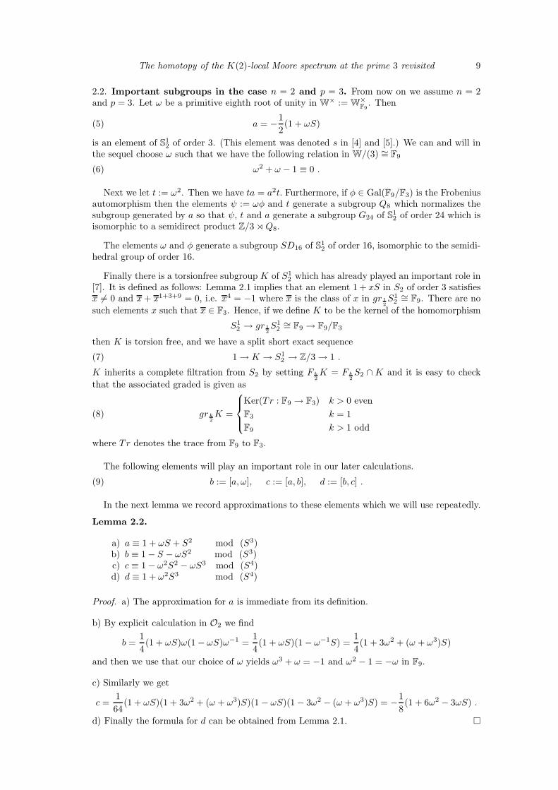
2.2. Important subgroups in the case n = 2 and p = 3. From now on we assume n = 2and p = 3. Let ω be a primitive eighth root of unity in W× := W×

F9. Then

(5) a = −1

2(1 + ωS)

is an element of S12 of order 3. (This element was denoted s in [4] and [5].) We can and will in

the sequel choose ω such that we have the following relation in W/(3) ∼= F9

(6) ω2 + ω − 1 ≡ 0 .

Next we let t := ω2. Then we have ta = a2t. Furthermore, if φ ∈ Gal(F9/F3) is the Frobeniusautomorphism then the elements ψ := ωφ and t generate a subgroup Q8 which normalizes thesubgroup generated by a so that ψ, t and a generate a subgroup G24 of S1

2 of order 24 which isisomorphic to a semidirect product Z/3 ⋊Q8.

The elements ω and φ generate a subgroup SD16 of S12 of order 16, isomorphic to the semidi-

hedral group of order 16.

Finally there is a torsionfree subgroup K of S12 which has already played an important role in

[7]. It is defined as follows: Lemma 2.1 implies that an element 1 + xS in S2 of order 3 satisfiesx 6= 0 and x+ x1+3+9 = 0, i.e. x4 = −1 where x is the class of x in gr 1

2S1

2∼= F9. There are no

such elements x such that x ∈ F3. Hence, if we define K to be the kernel of the homomorphism

S12 → gr 1

2S1

2∼= F9 → F9/F3

then K is torsion free, and we have a split short exact sequence

(7) 1 → K → S12 → Z/3 → 1 .

K inherits a complete filtration from S2 by setting F k2K = F k

2S2 ∩ K and it is easy to check

that the associated graded is given as

(8) gr k2K =

Ker(Tr : F9 → F3) k > 0 even

F3 k = 1

F9 k > 1 odd

where Tr denotes the trace from F9 to F3.

The following elements will play an important role in our later calculations.

(9) b := [a, ω], c := [a, b], d := [b, c] .

In the next lemma we record approximations to these elements which we will use repeatedly.

Lemma 2.2.

a) a ≡ 1 + ωS + S2 mod (S3)b) b ≡ 1 − S − ωS2 mod (S3)c) c ≡ 1 − ω2S2 − ωS3 mod (S4)d) d ≡ 1 + ω2S3 mod (S4)

Proof. a) The approximation for a is immediate from its definition.

b) By explicit calculation in O2 we find

b =1

4(1 + ωS)ω(1 − ωS)ω−1 =

1

4(1 + ωS)(1 − ω−1S) =

1

4(1 + 3ω2 + (ω + ω3)S)

and then we use that our choice of ω yields ω3 + ω = −1 and ω2 − 1 = −ω in F9.

c) Similarly we get

c =1

64(1 + ωS)(1 + 3ω2 + (ω + ω3)S)(1 − ωS)(1 − 3ω2 − (ω + ω3)S) = −

1

8(1 + 6ω2 − 3ωS) .

d) Finally the formula for d can be obtained from Lemma 2.1. �


The information in the following proposition will be important for a closer inspection of thepermutation resolution (1).

Proposition 2.3.

a) H∗(K; F3) is a Poincare duality algebra of dimension 3.b) H2(K; F3) ∼= H1(K; F3) ∼= (F3)

2.c) H1(K; Z3) ∼= Z/9 ⊕ Z/3 where Z/9 resp. Z/3 is generated by b resp. by c.d) H2(K; Z3) = 0.e) H0(K; Z3) ∼= H3(K,Z3) ∼= Z3.

Proof. Parts (a) and (b) have already been shown in Proposition 4.4. of [7].

For part (c) we note that H1(K; Z3) ∼= K/[K,K] where [K,K] is the closure of the commu-tator subgroup [K,K] of K. By Lemma 2.1 the commutator map

griK × grjK → gri+jK, (x, y) 7→ [x, y]

is surjective when i = 32 and j = k

2 with k even, and also when i = 12 and j = l

2 with l > 1 odd.

Thus F2K ⊂ [K,K]. If i = 12 and j = 1 then the image of the commutator map is the kernel

of the trace map. Together with part (b) of Lemma 2.1 this shows that K/[K,K] ∼= Z/9 ⊕ Z/3and it is easy to check that b and c generate Z/9 resp. Z/3.

The remaining parts (d) and (e) now follow from a simple Bockstein calculation. �

3. The maps in the permutation resolution

3.1. Generalities. LetG be a profinite p-group. We say thatG is finitely generated ifH1(G,Zp)is finitely generated over Zp. The kernel of the augmentation Zp[[G]] → Zp is denoted by IG,or simply by I. We say that a Zp[[G]]-module M is I-complete if the filtration by the submod-ules InM , n ≥ 0, is complete. As in [5] we use a Nakayama type lemma to show that certainhomomorphisms are surjective. Its proof is the same as that of Lemma 4.3 of [5].

Lemma 3.1. Let G be a finitely generated profinite p-group and f : M → N a homomorphismof IG-complete Zp[[G]]-modules. Suppose that H0(f) : H0(G,M) → H0(G,N) is surjective.Then f is surjective. �

In [5] we used the analogous Lemma 4.3 for G = S12 in order to show that certain Z3[[S

12 ]]-

linear maps are surjective. Here we use Lemma 3.1 for G = K together with the action of theelement a on H0(K,−) resulting from the exact sequence (7) in order to show that the samemaps are surjective. The advantage of working with K will become clear when we will discussthe kernel of the map C1 → C0 (see the remark after Proposition 3.4 below). We begin theconstruction of the permutation resolution exactly as in [5].

3.2. The homomorphism ∂1. Let C0 = Z3[[G12]] ⊗Z3[G24] Z3 and e0 = e ⊗ 1 ∈ C0 if e is the

unit in G12. Let ∂0 : C0 → Z3 be the standard augmentation and let N0 be the kernel of ∂0 so

that we have a short exact sequence

(10) 0 → N0 → C0 → Z3 → 0 .

Proposition 3.2.

a) As Z3[[K]]-module N0 is generated by the elements f1 := (e − ω)e0, f2 := (e − b)e0and f3 := (e − c)e0. If we denote the class of fi in H0(K,N0) by fi then we have anisomorphism

H0(K;N0) ∼= Z3{f1} ⊕ Z/9{f2} ⊕ Z/3{f3} .

b) The action of a on H0(K,N0) is given by :

a∗f1 = f1 + f2, a∗f2 = f2 + f3, a∗f3 = f3 − 3f2 .


c) H1(K;N0) = 0.

Proof. a) We consider the long exact sequence inH∗(K,−) associated to the short exact sequence(10). As C0 is free K-module we have H1(K;C0) = 0. Furthermore, H0(K;C0) ∼= Z2

3, generatedby the classes of e0 and ωe0 so that the end of this long exact sequence has the following form

0 → H1(K; Z3) ∼= Z/9 ⊕ Z/3 → H0(K;N0) → H0(K;C0) ∼= Z23 → H0(K; Z3) ∼= Z3 → 0 .

Now (a) follows from Proposition 2.3 and the identification of H1(K,Z3) with IK/(IK)2 whichsends x ∈ K to the class of x− e in IK/(IK)2.

b) By definition we have ae0 = e0 and thus

aωe0 = aωa−1ω−1ωae0 = [a, ω]ωe0 = bωe0 .

Consequently

(11) a(e− ω)e0 = (e− aω)e0 = (e− bω)e0 = b(e− ω)e0 + (e− b)e0

and we obtain the first formula by passing to K-coinvariants.

Similarly, ab = cba and ae0 = e0 imply

(12) a(e− b)e0 = (e− ab)e0 = (e− cba)e0 = (e− cb)e0 = c(e− b)e0 + (e− c)e0

and by passing to K-coinvariants we get the second formula.

The third formula can now be deduced from the fact that a3∗f1 = f1.

c) This follows from the long exact sequence in H0(K,−) associated to the exact sequence(10) by using that Hi(K,C0) = 0 for i = 1, 2 and H2(K,Z3) = 0. �

Let C1 = Z3[[G12]]⊗Z3[SD16] χ where χ is the non trivial character of SD16 defined over Z3 on

which ω and φ both act by multiplication by −1. Let e1 be the generator of C1 given by e⊗ 1where e is as before the unit in G1

2.

Corollary 3.3. There is a Z3[[G12]]-linear epimorphism ∂1 : C1 → N0 given by e1 7→ (e− ω)e0.

Proof. The elements ω2, φω and ω−1φ all belong to G24 and hence they act trivially on e0.Therefore we have

ω(e− ω)e0 = (ω − ω2)e0 = −(e− ω)e0

and

φ(e− ω)e0 = (φ− φω)e0 = (ω(ω−1φ) − e)e0 = −(e− ω)e0 .

This implies that there is a well defined homomorphism C1 → N0 which sends e1 to (e− ω)e0.To see that this homomorphism is surjective we note that C1 is free as Z3[[K]]-module of rank3 with generators e1, ae1 and a2e1. Then we use Lemma 3.1 and Proposition 3.2. �

3.3. The homomorphism ∂2. Now we turn towards the construction of the second homomor-phism in our permutation resolution. This is substantially more intricate; in [5] its existencewas established but no explicit formula was given.

Let N1 be the kernel of ∂1 so that we have a short exact sequence

(13) 0 → N1 → C1 → N0 → 0 .

Proposition 3.4.

a) H0(K;N1) ∼= Z23. The inclusion of N1 into C1 induces an injection H0(K,N1) →

H0(K,C1) and identifies H0(K,N1) with the submodule generated by the classes gi,i = 1, 2, of g1 = 3(a− e)2e1 and g2 = 9(a− e)e1.

b) The action of a on H0(K,N1) is determined by

a∗g1 = −2g1 − g2, a∗g2 = 3g1 + g2 .


c) H0(S12 , N1) ∼= Z/3 and if n1 is any element of N1 which agrees in H0(K,C1) with g1

then its class in H0(S12 , N1) is non-trivial.

d) The elements ω and φ both act on H0(S12 , N1) by multiplication by −1.

Proof. a) We observe that C1 is a free K-module of rank 3 generated by e1, ae1 and ae2. Then(a) follows from Proposition 3.2 by using the long exact sequence in H0(K,−) associated to theshort exact sequence (13) .

b) The formulae for the action of a already hold in H0(K,C1).

c) This follows from part (b) by passing to coinvariants with respect to the action of a.

d) This has already been observed in Lemma 4.6. of [5]. �

Remark We remark that working with S12 -coinvariants only (as in [5]) does not give us a good

hold on a generator of N1. The reason is that the map H0(S12 , N1) ∼= Z/3 → H0(S

12 , C1) ∼= Z3 is

necessarily trivial and therefore such a generator cannot be easily associated with an element inC1. Working with K-coinvariants gives us a starting point, namely the element g1 ∈ C1, fromwhich we can try to construct an element n1 of N1 whose class in H0(K,C1) agrees with that ofg1 and thus projects to a generator of H0(S

12 , N1). A first step in the direction of finding such

a generator n1 is taken in Lemma 3.6 below.

Corollary 3.5. Let C2 = Z3[[G12]] ⊗Z3[SD16] χ, let n1 ∈ N1 be any element which projects

non-trivially to the coinvariants H0(S12 ;N1) and let

n′1 :=

1

16

∑

g∈SD16

χ(g−1)g(n1) .

Then there is a Z3[[G12]]-linear epimorphism ∂2 : C2 → N2 given by e2 7→ n′

1.

Proof. By construction the group SD16 acts on n′1 via the mod-3 reduction of the character χ

and thus there is a homomorphism ∂2 as claimed. Surjectivity of ∂2 follows from Lemma 3.1. �

Lemma 3.6.

a) Let l1 = (a− b)e1, l2 = (a− c)l1 and l3 = 3cl2 + (e− c)2l2. Then

∂1(l1) = (e− b)e0, ∂1(l2) = (e− c)e0 , ∂1(l3) = (e− c3)e0 .

b) There exist elements x, y ∈ IK such that e− c3 = x(e− b) + y(e− c).c) If x, y ∈ IK satisfy e− c3 = x(e− b) + y(e− c) then

n1 := l3 − xl1 − yl2

belongs to N1 and projects non-trivially to H0(S12 , N1).

Proof. We start with the following two observations:

• Proposition 3.2 implies that ∂1((a− e)2e1) ≡ (e− c)e0 mod (IK)N0.• In Z3[[K]] we have the relation 3c(e− c) + (e− c)3 = e− c3.

a) By equations (11) and (12) of the proof of Proposition 3.2 we see that

∂1(l1) = (e− b)e0 and ∂1(l2) = (e− c)e0 .

The result for ∂1(l3) is now obvious.

b) By Proposition 2.3.c we know that IK is generated by e − b and e − c. Furthermore c3

belongs to F2K, hence it is trivial in H1(K,Z3) by Proposition 2.3.c . Therefore e− c3 belongsto IK2 and we get the existence of x, y ∈ IK as required in (b).

c) By (a) and (b) n1 belongs to N1. Furthermore it is clear that n1 and 3(a− e)2e1 agree inH0(K,C1), hence n1 projects non-trivially to H0(S

12 , N1). �


The question becomes now how we can determine x and y. In fact, we do not have explicitformulae for x and y. However, in section 5.3 we will give approximations for them which aresufficient for our homological calculations.

3.4. The homomorphism ∂3. In [5] it was shown (by using that K is a Poincare dualitygroup) that the kernel of ∂2 can be identified with Z3[[G

12/G24]]. However, the identification

and thus the construction of ∂3 was not explicit. The following result shows that ∂3 can bereplaced by the dual of ∂1, at least up to isomorphism.

If G is a profinite group and M a continuous left Zp[[G]]-module then we define its dualM∗ by HomZp[[G]](M,Zp[[G]]). This becomes a left Zp[[G]]-module via (g.ϕ)(m) = ϕ(m)g−1 ifg ∈ G, ϕ ∈ HomZp[[G]](M,Zp[[G]]) and m ∈ M . We observe that for a finite subgroup H thereis a canonical Zp[[G]]-linear isomorphism

(14) Zp[[G/H ]] → Zp[[G/H ]]∗ ∼= Zp[[G]]H , g 7→(g∗ : g 7→ g(

∑

h∈H

h)g−1)↔ (

∑

h∈H

h)g−1 .

Proposition 3.7.

a) There is an exact complex of Z3[[G12]]-modules

0 −→ C∗0

∂∗

1−→ C∗1

∂∗

2−→ C∗2

∂∗

3−→ C∗3

ǫ−→ Z3 −→ 0

in which ∂∗i is the dual of ∂i for i = 1, 2, 3.b) There is an isomorphism of complexes of Z3[[G

12]]-modules

0 −→ C∗0

∂∗

1−→ C∗1

∂∗

2−→ C∗2

∂∗

3−→ C∗3

ǫ−→ Z3 −→ 0

↓ f3 ↓ f2 ↓ f1 ↓ f0 ↓=

0 −→ C3∂3−→ C2

∂2−→ C1∂1−→ C0

ǫ−→ Z3 −→ 0 .

such that fi induces the identity on TorZ3[[S

12 ]]

0 (F3, Ci) for i = 2, 3 if we identify C∗i with

C3−i via the isomorphism of (14).c) The homomorphism ∂∗1 : C∗

0 → C∗1 is given by e∗0 7→ (e+ a+ a2)e∗1.

Proof. a) Each Ci is free as a Z3[[K]]-module and therefore the complex

0 −→ C3∂3−→ C2

∂2−→ C1∂1−→ C0

ǫ−→ Z3 −→ 0

is a free Z3[[K]]-resolution of Z3. Because K is of finite index in G12 the coinduced module of

Z3[[K]] is isomorphic to Z3[[G12]]. Therefore there are natural isomorphisms

C∗i = HomZ3[[G1

2]](Ci,Z3[[G

12]])

∼= HomZ3[[K]](Ci,Z3[[K]])

and the n-th cohomology of the complex HomZ3[[K]](Ci; Z3[[K]]) isHn(K; Z3[[K]]). BecauseK isa Poincare duality group this is zero except when n = 3 and then it is isomorphic to Z3. Finally,one sees as in Proposition 5 of [13] that the Z3[[G

12]]-module structure on Hn(G1

2; Z3[[G12]])

∼=Hn(K; Z3[[K]]) is trivial.

b) The augmentation Z3[[G12]] → Z3 induces an isomorphism

HomZ3[[G12]](Z3,Z3) ∼= HomZ3[[G1

2]](Z3[[G

12]],Z3) .

Thus the right hand square is commutative up to a unit in Z3 if we choose for f0 the isomorphismgiven in (14), and we can modify f0 by a unit so that it commutes on the nose. Then f0 inducesan isomorphism Kerǫ ∼= Kerǫ and

C2∂2−→ C1

∂1−→ Kerǫ resp. C∗1

∂∗

2−→ C∗2

∂∗

3−→ Kerǫ

is the beginning of a resolution of Kerǫ resp. Kerǫ by projective Z3[[G12]]-modules and the

isomorphism induced by f0 lifts to a chain map f• between the projective resolutions. By

Lemma 4.5 of [5] we have TorZ3[[S1

2 ]]i (F3,Kerǫ) ∼= F3 if i = 0, 1 and this implies that the maps

f1 : C1 → C∗2 and f2 : C2 → C∗

1 induce isomorphisms on TorZ3[[S

12 ]]

0 (F3,−) and hence they are


themselves isomorphisms by Lemma 4.3 of [5]. Finally, f3 is trivially an isomorphism becausef2 and f1 are isomorphisms.

The isomorphism of chain complexes (considered as automomorphism via (14)) induces anautomorphism of spectral sequences

TorZ3[[S

12 ]]

j (F3, Ci) ⇒ TorZ3[[S

12 ]]

i+j (F3,Z3)

which converges towards the identity, and this easily implies the remaining part of (b).

c) By (14) we have for each g ∈ G12

(e+ a+ a2)∗(e∗1)(g) = g( ∑

h∈SD16

χ(h−1)h)(e+ a−1 + a−2) = g

( ∑

h∈SD16

χ(h−1)h)(e+ a+ a2)

and

∂∗1 (e∗0)(g) = e∗0(g(e− ω)) = g(e− ω)( ∑

h∈G24

h)

= g(e− ω)( ∑

h∈Q8

h)(e+ a+ a2) .

Then we conclude via the identity (e− ω)( ∑

h∈Q8h)

=∑

h∈SD16χ(h−1)h. �

4. On the action of the stabilizer group

In this section we will produce formulae for the action of the elements a, b, c and d ofthe stabilizer group G2 on F9[[u1]][u

±1], at least modulo suitable powers of the invariant idealgenerated by u1. It turns out that it is sufficient to have a formula for the action of a and b onu modulo (u6

1), and for the action of c and d on u modulo (u101 ).

4.1. Generalities. We recall (cf. [10]) that BP∗∼= Z(p)[v1, v2, . . .] where the Araki generators

vi satisfy the following equation (in BP∗ ⊗ Q)

(15) pλk =∑

0≤i≤k

λivpi

k−i .

Here the λi ∈ BP∗ ⊗ Q are the coefficients of the logarithm of the universal p-typical formalgroup law F on BP∗,

logF (x) =∑

i≥0

λixpi

(with λ0 = 1), and thus the [p]-series of F is given by

[p]F (x) =∑

i≥0

Fvix

pi

.

The homomorphism

BP∗ → (En)∗ = WFpn [[u1, . . . , un−1]][u±1], vi 7→

uiu1−pi

i < nu1−pn

i = n0 i > n

defines a p-typical formal group law Fn over (En)∗. Then the formal group law Gn over (En)0defined by Gn(x, y) = u−1Fn(ux, uy) is a universal deformation of Γn and is p-typical withp-series

(16) [p]Gn(x) = px+Gn

u1xp +Gn

· · · +Gnun−1x

pn−1

+Gnxpn

.

Next we recall how one can get at the action of an element g ∈ Sn on (En)0. For a given g

we choose a lift g ∈ (En)0[[x]] of g and let G be the formal group law defined by

G(x, y) = g−1(Gn(g(x), g(y))

).


Then there is a unique ring homomorphism g∗ : (En)0 → (En)0 and a unique ∗-isomorphism

from g∗Gn to G such that the composition

hg : g∗Gn → Gg→ Gn

is an isomorphism of p-typical formal group laws and can therefore be written (cf. Appendix 2of [10]) as

hg(x) =∑

i≥0

Gnti(g)xpi

for unique continuous functions

(17) ti : Sn → (En)0 .

We note that

(18) ti(g) ≡ gi mod (3, u1)

if g =∑

i giSi ∈ Sn with gp2

i = gi. Then we have

(19) g∗(u) = t0(g)u

and the equation

(20) hg([p]g∗Gn(x)) = [p]Gn

(hg(x))

can be used to recursively find better and better approximations for t0(g) as well as for theaction of g on the deformation parameters u1, . . . , un−1.

4.2. A formula modulo (3) for the formal group law G2. From now on we restrict attentionto the case n = 2 and p = 3.

Lemma 4.1. The logarithm and exponential of the formal group law G2 satisfy

logG2(x) = x− u1

24x3 + 1

1−38

(13 −

u41

72

)x9 mod (x27)

expG2(x) = x+ u1

24x3 +

3u21

242 x5 +

12u31

243 x7 −

(1

1−38

(13 −

u41

72

)+

55u41

244

)x9 mod (x11) .

Proof. From (15) we get λ1 = − v1

24 and λ2 = 11−38

(v2

3 −v41

72

). To obtain the result for logG2

we

use the classifying homomorphism for F2 and that logG2(x) = u−1 logF2

(ux). �

Corollary 4.2. The formal group law G2 satisfies

x+G2 y ≡ x+ y − u1(xy2 + x2y) + u2

1(xy4 + x4y)

−u31(xy

6 + x6y) − u31(x

3y4 + x4y3)−(x3y6 + x6y3) + u4

1(x4y5 + x5y4) mod (3, (x, y)11) .

Proof. This follows directly from x+G2 y = expG2(logG2

(x) + logG2(y)). �

4.3. Formulae for the action modulo (3). To simplify notation we will denote in the re-mainder of this section the mod-3 reduction of the value of the function ti of (17) on an elementg again by ti(g), or even by ti if g is clear from the context.

Proposition 4.3. Let g ∈ Sn and let u1 be Araki’s u1. Then the following equations hold

a) g∗(u1) = t20u1

b) t0 + t60t1u31 = t90 + t31u1

c) t1 − t80t1u41 ≡ t91 + t32u1 − t180 t

31u

21 − t90t

61u

31 mod (u7

1)d) If g ≡ 1 mod (S2) then t2 ≡ t92 + t33u1 mod (u2

1).


Remark If we want to know g∗(u1) modulo (u71) then (a) shows that it is enough to know t0

modulo (u61) and this can be calculated from (b) if we know t0 modulo (u1) and t1 modulo (u3

1).Furthermore, t1 can be calculated modulo (u3

1) from (c) if we know t0, t1 and t2 modulo (u1).In the same manner we can even calculate g∗(u1) modulo (u8

1).

Similarly, if we want to know g∗(u1) modulo (u111 ) then (a) shows that it is enough to know

t0 modulo (u101 ) and this can be calculated from (b) if we know t0 modulo (u1) and t1 modulo

(u71). Furthermore, t1 can be calculated modulo (u7

1) from (c) if we know t0 modulo (u31), t1

modulo (u1) and t2 modulo (u21). Finally (d) can be used to calculate t2 modulo (u2

1) if we knowt2 and t3 modulo (u1).

Proof. In this proof we abbreviate G2 simply by G. We consider equation (20)

hg([3]g∗G)(x) = [3]G(hg(x))

over (E2)0/(3)[[x]] and compare coefficients of x3k

for k = 1, 2, 3, 4. By (16) we have

hg([3]g∗G)(x) ≡ t0(g∗(u1)x

3 +g∗G x9)

+G t1(g∗(u1)x

3 +g∗G x9)3

+Gt2(g∗(u1)x

3 +g∗G x9)9

+G t3(g∗(u1)x

3 +g∗G x9)27

mod (x82)

[3]G(hg(x)) ≡ u1(t0x+G t1x3 +G t2x

9 + t3x27)3

+G(t0x+G t1x3 +G t2x

9)9 mod (x82) .

a) For the coefficient of x3 we obviously get g∗(u1)t0 = u1t30 which proves (a).

b) The coefficient of x9 in hg([3]g∗G)(x) is equal to t0 + g∗(u1)3t1 which by (a) is equal to

t0 + u31t

60t1. The coefficient of x9 in [3]G(hg(x)) is equal to the same coefficient in

u1(t0x+G t1x3)3 +G (t0x)

9

which is clearly equal to u1t31 + t90 and hence we get (b).

c) The coefficient of x27 in hg([3]g∗G)(x) is equal to the coefficient of x27 in

t0(g∗(u1)x

3 +g∗G x9)

+G t1(g∗(u1)x

3 +g∗G x9)3

+G t2(g∗(u1)x

3)9

and the latter coefficient is equal to

t1 + t2g∗(u1)9 + c

where c is the coefficient of x27 in

t0(g∗(u1)x

3 +g∗G x9)

+G t1g∗(u1)3x9 .

Next we observe that Corollary 4.2 yields

g∗(u1)x3 +g∗G x9 ≡ g∗(u1)x

3 + x9 − g∗(u1)3x15

−g∗(u1)2x21 + g∗(u1)

6x21 − g∗(u1)9x27 mod (x28) .

Applying Corollary 4.2 once more and using (a) and calculating modulo (u71) we obtain

c ≡ −u1t20t1g∗(u1)

3 = −u41t

80t1 mod (u7

1)

and hence modulo (u71) the coefficient of x27 in hg([3]g∗G)(x) is equal to

t1 − u41t

80t1 .

On the other hand the coefficient of x27 in [3]G(hg(x)) is equal to the same coefficient in

u1(t0x+G t1x3 +G t2x

9)3 +G (t0x+G t1x3)9

and this coefficient is equal to

u1t32 + t91 + d

where d is the coefficient of x27 in

u1(t0x+G t1x3)3 +G t90x

9 .


Next we observe that Corollary 4.2 yields

(t0x+G t1x3)3 ≡ t30x

3 + t31x9 − u3

1t60t

31x

15

−u31t

30t

61x

21 + u61t

120 t

31x

21 − u91t

180 t

31x

27 mod (x28) .

Applying Corollary 4.2 once more and using (a) and calculating modulo (u71) we obtain

u1(t0x+G t1x3)3 +G t90x

9 ≡ u1

(t30x

3 + t31x9 − u3

1t60t

31x

15 − u31t

30t

61x

21) + t90x9

−u31

(t30x

3 + t31x9 − u3

1t60t

31x

15 − u31t

30t

61x

21)2t90x9

−u21

(t30x

3 + t31x9 − u3

1t60t

31x

15 − u31t

30t

61x

21)t180 x18

+u61

(t30x

3 + t31x9 − u3

1t60t

31x

15 − u31t

30t

61x

21)4t90x9 mod (x28)

and henced ≡ −u3

1(t61 − 2u3

1t90t

31)t

90 − u2

1t180 t

31 + 4u6

1t180 t

31 mod (u7

1) .

Therefore the coefficient of x27 in [3]G(hg(x)) is equal to

t91 + u1t32 − u2

1t180 t

31 − u3

1t90t

61 + 2u6

1t180 t

31 + 4u6

1t180 t

31 mod (u7

1)

and (c) follows.

d) The coefficient of x81 in hg([3]g∗G)(x) is equal to the same coefficient in

t0(g∗(u1)x

3 +g∗G x9)

+G t1(g∗(u1)x

3 +g∗G x9)3

+G t2(g∗(u1)x

3 +g∗G x9)9

+G t3(g∗(u1)x3)27

which modulo (u31) is equal to the same coefficient in

t0(g∗(u1)x

3 +g∗G x9)

+G t1x27 +G t2x

81

and by Corollary 4.2 this is easily seen to be equal to t2 modulo (u21).

On the other hand the coefficient of x81 in [3]G(hg(x)) is equal to the same coefficient in


9 + t3x27)3 +G (t0x+G t1x

3 + t2x9)9

and this coefficient is equal tou1t

33 + t92 + e

where e is the coefficient of x81 in the series


9)3 +G (t0x+G t1x3)9 .

Now g ≡ 1 mod (S2) implies t1 ≡ 0 mod (u1) and thus modulo (u21) we find that e is also the

coefficient of x81 inu1(t0x+G t2x

9)3 +G t90x9

and by Corollary 4.2 even of the coefficient of x81 in

u1(t0x+G t2x9)3 .

Now Lemma 4.4 below shows that the coefficient of x27 in t0x+G t2x9 is trivial modulo (u1) (if

not, either the coefficient of x18y or of x9y2 in x+G y would have to be nontrivial modulo (u1)),hence e is trivial modulo (u2

1) and the proof of (d) is complete. �

Lemma 4.4.

x+G2 y ≡ x+ y +∑

i≥1

P8i+1(x, y) mod (3, u1)

where P8i+1 is a homogeneous polynomial of degree 8i+ 1 without terms x8i+1 and y8i+1.

Proof. It is enough to show this for the graded formal group law F2 over (E2)∗. This group lawis a homogeneous series of degree −2 if x and y are given degree −2 and thus, if we write

x+G2 y ≡ x+ y +∑

j≥1

Pj(x, y) mod (3, u1)

with homogeneous polynomials in x and y of degree −2j then the coefficients in Pj have to bein (E2)2j−2. Furthermore, this group law has its coefficients in the subring generated by u1u

−2

and u−8. However, (E2)∗/(3, u1) ∼= F9[[u±1]] and thus 2j − 2 has to be a multiple of 16. �


Corollary 4.5. The following equations hold in (E2)0/(3).

a) Let g = 1 + g1S + g2S2 mod (S3). Then we have

t1 ≡ g1 + g32u1 − g3

1u21 − g6

1u31 mod (u4

1)t0 ≡ 1 + g3

1u1 − g1u31 + (g2 − g3

2)u41 + g3

1u51 + (g2

1 + g61)u

61 mod (u7

1) .

b) Let g = 1 + g2S2 + g3S

3 mod (S4). Then we have

t2 ≡ g2 + g33u1 mod (u2

1)t1 ≡ g3

2u1 + g3u41 + (g3

2 − g2)u51 mod (u7

1)t0 ≡ 1 + (g2 − g3

2)u41 − g3u

71 + (g2 − g3

2)u81 mod (u10

1 ) .

Proof. a) From Proposition 4.3.c we obtain

t1 ≡ t91 + t32u1 − t180 t31u

21 − t90t

61u

31 mod (u4

1)

and by using (18) we immediately get the formula for t1 modulo (u41). Then Proposition 4.3.b

and (18) yield

t0 + t60(g1 + g32u1 − g3

1u21 − g6

1u31)u

31 ≡ 1 + (g3

1 + g2u31)u1 mod (u7

1)

from which we easily get the formula for t0 modulo (u71). The formula for g∗(u1) follows now

from Proposition 4.3.a .

b) From Proposition 4.3.d and (18) we immediately obtain the formula for t2. Substitutingthe value for t2 into the formula of Proposition 4.3.c and using (18) yields

t1 − t80t1u41 ≡ (g3

2 + g3u31)u1 − t180 t

31u

21 mod (u7

1) .

Substituting the values of t0 modulo (u71) and t1 modulo (u4

1) from (a) into this yields

t1 − g32u

51 ≡ (g3

2 + g3u31)u1 − g2u

51 mod (u7

1)

from which we get the value of t1 modulo (u71). Next we substitute this value of t1 together with

the value of t0 modulo (u71) of (a) into the formula of Proposition 4.3.b and obtain

t0 +(1 + (g2 − g4

2)u41

)6(g32u1 + g3u

41 + (g3

2 − g2)u51

)u3

1 ≡ 1 + g2u41 mod (u10

1 )

from which we easily get the formula for t0 modulo (u101 ). �

The following calculation will be used repeatedly in later sections. The result is only givento the precision needed later.

Lemma 4.6. Let g = 1 + g1S + g2S2 mod (S3) and let k be an integer. Then we have

t0(g)k ≡

1 + g31u1 + (k′ − 1)g1u

31 + (k′g4

1 + g2 − g32)u

41 + g3

1u51 mod (3, u6

1) k = 3k′ + 11 − g3

1u1 + g61u

21 + (k′ + 1)g1u

31+

(g41 − k′g4

1 + g32 − g2)u

41 + (k′g7

1 − g31 − g3

1g2 + g31g

32)u

51 mod (3, u6

1) k = 3k′ + 2 .

Proof. The result follows easily from Corollary 4.5 and from

t0(g)k =

((1 + (t0(g) − 1)

))k ≡

5∑

j=1

(k

3

)(t0(g) − 1)j mod (3, u6

1)

by using that(kj

)≡

∏i

(ki

ji

)mod (p) if k =

∑i kip

i and j =∑

i jipi are the p-adic expansions

of k and j respectively. �

Using Lemma 2.2 we finally get the following information on the action of a, b, c and d on(E2)∗/(3). We use 1 and ω2 as a basis of F9 considered as an F3-vector space (rather then 1and ω).


Corollary 4.7. The action of the elements a, b, c and d on (E2)∗/(3) satisfy the formulae

a∗u1 ≡ u1 − (1 + ω2)u21 − ω2u3

1 + (1 − ω2)u41 − u5

1 − (1 + ω2)u61 mod (u7

1)b∗u1 ≡ u1 + u2

1 + u31 − u4

1 + (1 + ω2)u51 + (1 − ω2)u6

1 mod (u71)

c∗u1 ≡ u1 − ω2u51 + (−1 + ω2)u8

1 − (1 + ω2)u91 mod (u11

1 )d∗u1 ≡ u1 + ω2u8

1 mod (u111 )

a∗u ≡(1 + (1 + ω2)u1 + (−1 + ω2)u3

1 + (1 + ω2)u51

)u mod (u6

1)b∗u ≡

(1 − u1 + u3

1 − ω2u41 − u5

1

)u mod (u6

1)c∗u ≡

(1 + ω2u4

1 + (1 − ω2)u71 + ω2u8

1

)u mod (u10

1 )d∗u ≡

(1 − ω2u7

1

)u mod (u10

1 ) . �

5. The E2-term of the algebraic spectral sequence

5.1. The E1-term. We begin by giving some background on Theorem 1.1, or equivalently, onthe E1-term of the spectral sequence (2)

Es,t,∗1 = Extt

Z3[[G12]]

(Cs, (E2)∗/(3)) =⇒ Hs+t(G12, (E2)∗/(3)) .

We note that for s = 1, 2 the module Cs is projective as Z3[[G12]]-module and thus we have a

Shapiro isomorphism

(21) Es,t1 = Extt

Z3[[G12]]

(χ ↑G

12

SD16, (E2)∗/(3)) ∼=

{HomZ3[SD16](χ, (E2)∗/(3)) t = 0

0 t > 0 .

The action of SD16 on (E2)∗ is known (cf. the proof of Lemma 22 of [6] for an explicit reference)to be given by

(22) ω∗u1 = ω2u1 and ω∗u = ωu

and the Frobenius φ acts Z3-linearly by extending the action of Frobenius on W via

(23) φ∗u1 = u1 and φ∗u = u .

This implies immediately that (E2)∗/(3)SD16 is isomorphic to F3[[u41]][v1, u

±8] as a graded alge-bra and that there is an isomorphism of (E2)∗/(3)SD16 -modules

(24) Ext0Z3[SD16](χ, (E2)∗/(3)) ∼= ω2u4F3[[u41]][v1, u

±8].

For s = 0, 3 we have a Shapiro isomorphism

Es,t1 = Extt

Z3[[G12]](Z3[[G

12/G24]], (E2)∗/(3)) ∼= Ht(G24, (E2)∗/(3)) .

Let G12 be the subgroup of G24 generated by the elements a and t. The calculation of thecohomology algebra H∗(G12, (E2)∗/(3)) was deduced from that of H∗(G12, (E2)∗) in section 1.3of [4]. In precisely the same way one deduces the calculation of H∗(G24, (E2)∗/(3)) from thatof H∗(G12, (E2)∗) which was given in section 3 of [5]. In particular there are classes

∆ ∈ H0(G24, (E2)24/(3)), α ∈ H1(G24, (E2)4/(3))α ∈ H1(G24, (E2)12/(3)), β ∈ H2(G24, (E2)12/(3))

and an isomorphism of algebras

(25) H∗(G24, (E2)∗/(3)) ∼= F3[[v61∆−1]][v1,∆

±1, β, α, α]/(α2, α2, v1α, v1α, αα+ v1β) .

In the sequel we need some control over the elements occuring in this isomorphism (cf. section1.3 of [4]). First we recall that α is defined as δ0(v1) where δ0 is the Bockstein with respect tothe short exact sequence of continuous Z3[[G2]]-modules

(26) 0 → (E2)∗/(3)3→ (E2)∗/(9) → (E2)∗/(3) → 0 .

Similarly, v2 := u−8 determines an invariant in H0(G2, (E2)16/(3, u1)) and α is defined as δ1(v2)where δ1 is the Bockstein with respect to the short exact sequence of continuous Z3[[G2]]-modules

(27) 0 → Σ4(E2)∗/(3)v1→ (E2)∗/(3) → (E2)∗/(3, u1) → 0 .


Next β is defined to be the mod 3-reduction of δ0δ1(v2). These elements are thus defined aselements in H∗(G2, (E2)∗/(3)). We denote their restriction to H∗(G24, (E2)∗/(3)) by the samename.

The relation between ∆ (which lifts to an invariant of the same name in H0(G24, (E2)24))and the classes u and u1 is more subtle. Here we record the following result.

Proposition 5.1. ∆ ≡ (1 − ω2u21 + u4

1)ω2u−12 mod (3, u6

1).

Proof. By (3.11) of [5] the integral lift of ∆ is defined as

∆ =ω2

4(x(a∗x)(a∗(a∗x))

)4

and by the proof of Lemma 3.1 of [5] we know x ≡ u mod (3, u1), hence ∆ ≡ ω2u−12 mod (3, u1).Because ∆ is invariant with respect to G24, in particular with respect to Q8, we get from (22)and (23) that ∆ is of the form

∆ ≡ (1 + λ2ω2u2

1 + λ4u41)ω

2u−12 mod (3, u61) with λi ∈ F3 ⊂ F9 .

Because ∆ is also invariant with respect to the action of a we get from (19)

∆ = a∗(∆) ≡ t0(a)−12(1 + λ2ω

2a∗(u1)2 + λ4a∗(u1)

4)ω2u−12 mod (3, u61) .

The right hand side of this equation can be evaluated modulo (u61) by using Corollary 4.5.a

and Corollary 4.7. By looking at the coefficients of u31 and u5

1 in the right hand side we obtainλ2 = −1 and λ4 = 1. �

5.2. The d1-differential. First of all we note that all differentials are v1-linear.

Lemma 5.2. Let k 6≡ 0 mod (3). Then the differential d1 : E0,01 → E1,0

1 satisfies

d1(∆k) ≡

{(−1)m+1ω2(1 + u4

1)u−12k mod (u8

1) k = 2m+ 1(−1)m+1mω2u2

1u−12k mod (u6

1) k = 2m.

Proof. By Corollary 3.3 the differential is induced by the homomorphism C1 → C0 which sendse1 to (e− ω)e0. Furthermore Proposition 5.1 and (22) give

∆k ≡(1 − kω2u2

1 + ku41 −

(k2

)u4

1

)ω2ku−12k mod (u6

1)

ω∗(∆k) ≡

(1 + kω2u2

1 + ku41 −

(k2

)u4

1

)ω2k−12ku−12k mod (u6

1)

and the result follows easily. (Note that by (24) the congruence for d1(∆2m+1) improves to a

congruence modulo (u81) rather than only modulo (u6

1).) �

Proposition 5.3. For each integer k 6= 0 there exists an element ∆k ∈ E0,0,24k1 such that

a) ∆k ≡ ∆k mod (u61)

b) the differential d1 : E0,01 → E1,0

1 satisfies

d1(∆k) ≡

(−1)m+1ω2u−12k mod (u41) k = 2m+ 1

(−1)m+1mω2u4.3n−21 u−12k mod (u4.3n+2

1 ) k = 2.3nm, m 6≡ 0 mod (3)0 k = 0 .

Proof. For k = 0, k odd or k = 2m with m 6≡ 0 mod (3) we define ∆k to be equal to ∆k. Theformula for d1 is then satisfied by the previous result.

If k = 2.3nm with n ≥ 0 and m 6≡ 0 mod (3) we recursively define

(28) ∆3k : = ∆3k −mv

3(4·3n−2)1 ∆3k−2.3n+1.

The previous proposition gives

d1(∆3k−2.3n+1) ≡ (−1)mω2(1 + u4

1)u−12(3k−2.3n+1) mod (u6

1) .


and by induction on n we have

d1(∆k)3 ≡((−1)m+1mω2u4.3n−2

1 u−12k)3

≡ (−1)mmω2u4.3n+1−61 u−12·3k mod (u4.3n+1+6

1 ) .

Therefore v1-linearity of d1 yields

d1(∆3k) = d1(∆3k) −mv

3(4.3n−2)1 d1(∆3k−2.3n+1)

≡ (−1)m+1ω2mu4.3n+1−21 u12·3k mod (u4.3n+1+2

1 )

and the induction step is established. �

Corollary 5.4. There is an isomorphism of F3[v1]-modules E0,02

∼= F3[v1]. �

Remark By (25) the elements ∆k form a topological basis of the continuous graded F3[v1]-

module E0,01 (in fact, this has been implicitly used in the last corollary) and by (24) a topological

basis of the continuous graded F3[v1]-module E1,01 can be given by any family of elements b2k+1,

k ∈ Z, such that b2k+1 ≡ ω2u−8k−4 mod (u41). By Proposition 5.3 we know that there are such

elements b2.(3m+1)+1 for m ∈ Z and b2.3n(3m−1)+1 for n ≥ 0, m 6≡ 0 mod (3), such that the firstformula of Theorem 1.2 holds. Because the E1-term is torsion free as a F3[v1]-module and thed1-differential is F3[v1]-linear it is clear that those b2k+1’s are in the kernel of the differential

d1 : E1,01 → E2,0

1 . To complete this family to a topological basis we need to choose elementsb2k+1 for k = 3n+1(3m+ 1) with n ≥ 0, m ∈ Z, for k = 3n(9m+ 8) with n ≥ 0, m ∈ Z, and fork = 0. Thus we are lead to concentrate on the differential on ω2u−4(2k+1) for such k. The crucialstep is given by Proposition 5.6 below whose proof is quite elaborate and will be postponed tosection 5.3. The proof of Proposition 5.5 will be given in section 6.

Proposition 5.5. There exists an element b1 ∈ E1,01 such that b1 ≡ ω2u−4 mod (u4

1) andv1α = b1 in H∗(G1

2; (E2)∗/(3)). In particular, d1(b1) = 0.

Proposition 5.6. Let k be an integer such that 8k+4 is not divisible by 3. Then the differentiald1 : E1,0

1 → E2,01 satisfies

d1(ω2u8k+4) ≡ −(k′ + k′2)ω2u12

1 u8k+4 mod (u16

1 ) 8k + 4 = 3k′ + 1d1(ω

2u8k+4) ≡ (k′ − k′2)ω2u81u

8k+4 mod (u121 ) 8k + 4 = 3k′ + 2 .

Proof. This will be proved in section 5.3. �

Proposition 5.7. For each integer k there exists an element b2k+1 ∈ E1,0,8(2k+1)1 such that

a) b2k+1 ≡ ω2u−4(2k+1) mod (u41)

b) d1(∆k) =

(−1)m+1b2(3m+1)+1 k = 2m+ 1,m ∈ Z

(−1)m+1mv4.3n−21 b2.3n(3m−1)+1 k = 2m.3n, m 6≡ 0 mod (3)

0 k = 0

c) the differential d1 : E1,01 → E2,0

1 satisfies

d1(b2k+1) ≡

(−1)nω2u6.3n+21 u−4(2k+1) mod (u2.3n+1+6

1 ) k = 3n+1(3m+ 1), m ∈ Z

(−1)nω2u10.3n+21 u−4(2k+1) mod (u10.3n+6

1 ) k = 3n(9m+ 8), m ∈ Z

0 otherwise .

Proof. For k = 3m+1 with m ∈ Z we define b2k+1 to be (−1)m+1d1(∆2m+1). For k = 3n(3m−1)with n ≥ 0 and m 6≡ 0 mod (3) we note that Proposition 5.3 shows that d1(∆2m.3n) is divisible

by v4.3n−21 and we define b2k+1 to be (−1)m+1mv

−(4.3n−2)1 d1(∆2m.3n). For k = 0 we take the

element given in Proposition 5.5. With these definitions (b) holds as well as the last case of (c).

For k = 3n+1(3m+1) resp. k = 3n(9m+8), with n ≥ 0 and m ∈ Z, we define elements b2k+1

by induction on n such that (a) and (c) are satisfied. In fact, for n = 0 we define

b2k+1 : = ω2u−4(2k+1)

and then Proposition 5.6 gives

d1(b18m+7) ≡ ω2u81u

−4(18m+7) mod (u121 ), d1(b18m+17) ≡ ω2u12

1 u−4(18m+17) mod (u12

1 ) .


Now suppose that b2k+1 has already been defined for k = 3n+1(3m+1) resp. k = 3n(9m+8) withwith n ≤ N and m ∈ Z so that (a) and (c) are satisfied. Then we observe that by Proposition5.2 the elements

b32k+1 + b2(3k+1)+1 = b32k+1 + (−1)k+1d1(∆2k+1) ≡(ω6 + ω2(1 + u4

1))u−4(6k+3) mod (u8

1)

are divisible by v41 and thus we can define

(29) b6k+1 : = v−41

(b32k+1 + b2(3k+1)+1

).

Then it is clear that b6k+1 ≡ ω2u−4(6k+1) mod (u41). Furthermore, d1d1(∆2k+1) = 0 and

because d1 commutes with taking third powers and is F3[v1]-linear we see that both (a) and (c)are satisfied for k = 3n+1(3m+ 1) resp. k = 3n(9m+ 8) with n ≤ N + 1 and m ∈ Z and thusthe induction step is complete. �

Corollary 5.8. There is an isomorphism of F3[v1]-modules

E1,02

∼=∏

n≥0,m∈Z\3Z

F3[v1]/(v4.3n−21 ){b2.3n(3m−1)+1} × F3[v1]{b1} . �

Proof. Because the elements ∆k and bk form a topological basis of the graded continuous F3[v1]-

modules E0,01 and E1,0

1 this follows immediately from Proposition 5.7. �

Remark By inspection one sees that the infinite product is finite in each bidegree and thereforeit can also be identified with the direct sum.

To evaluate the homomorphism d1 : E2,01 → E3,0

1 we need the following result.

Lemma 5.9. Let k be any integer. Then

(e∗ + a∗ + (a2)∗)(uk) ≡

((k − k2)ω2u2

1 + (k(k3

)+ k − k2)u4

1

)uk mod (3, u5

1) .

Proof. By (19) we have a∗(uk) = ukt0(a)

k and (a2)∗(uk) = ukt0(a)

ka∗(t0(a)k). Corollary 4.5

gives

t0(a)k ≡

(1 + (1 + ω2)u1 + (−1 + ω2)u3

1

)k

≡ 1 + k(1 + ω2)u1 + k(−1 + ω2)u31

−(k2

)ω2u2

1 −(k2

)(1 + ω2)(−1 + ω2)u4

1 +(k3

)(1 + ω2)3u3

1 −(k4

)u4

1

≡ 1 + k(1 + ω2)u1 −(k2

)ω2u2

1

+((k3

)− k)(1 − ω2)u3

1 − ((k2

)+

(k4

))u4

1 mod (3, u51)

and by Corollary 4.7 we get

a∗(t0(a)k) ≡ 1 + k(1 + ω2)

(u1 − (1 + ω2)u2

1 − ω2u31 + (1 − ω2)u4

1

)

−(k2

)ω2

(u2

1 + (1 + ω2)u31

)

+((k3

)− k)(1 − ω2)u3

1 − ((k2

)+

(k4

))u4

1

≡ 1 + k(1 + ω2)u1 + (k −(k2

))ω2u2

1

+((k3

)+

(k2

))(1 − ω2)u3

1 − (k +(k2

)+

(k4

))u4

1 mod (3, u51) .

Finally an easy calculation (which only uses that(k2

)≡ −k(k− 1) mod (3) and k3 ≡ k mod (3))

givest0(a)

ka∗(t0(a)k) ≡ 1 − k(1 + ω2)u1 + (k2 − k)ω2u2

1

+(−(k3

)+ k)(1 − ω2)u3

1

+((k4

)+

(k2

)+ k

(k3

)+ k − k2)u4

1 mod (3, u51)

and the result clearly follows. �

Proposition 5.10. For each integer k there exists an element b2k+1 ∈ E2,0,4(2k+1)1 such that

a) b2k+1 ≡ ω2u−4(2k+1) mod (u41)

b) d1(b2k+1) =

{(−1)nv6.3n+2

1 b3n+1(6m+1) k = 3n+1(3m+ 1)

(−1)nv10.3n+21 b3n(18m+11) k = 3n(9m+ 8)


c) the differential d1 : E2,01 → E3,0

1 satisfies

d1(b2k+1) ≡

−u21u

−4(2k+1) mod (u41) 2k + 1 = 6m+ 1

ω2u4.3n

1 u−4(2k+1) mod (u4.3n+21 ) 2k + 1 = 3n(18m+ 17)

−ω2u4.3n

1 u−4(2k+1) mod (u4.3n+21 ) 2k + 1 = 3n(18m+ 5)

0 otherwise .

Proof. For 2k+1 = 3n+1(3m+1) resp. 2k+1 = 3n(9m+8) Proposition 5.7 shows that d1(b2k+1)

is divisible by v6.3n+21 resp. v10.3n+2

1 and can thus be written as (−1)nv6.3n+21 b3n+1(6m+1) resp.

(−1)nv10.3n+21 b3n(18m+11) for unique elements b3n+1(6m+1) resp. b3n(18m+11) which satisfy (a)

and (b).

So we still need to define b2k+1 if 2k + 1 can be written as 2k + 1 = 6m+ 1 with m ∈ Z or2k+1 = 3n(18m+11±6) with n ≥ 0 and m ∈ Z. In those cases we define b2k+1 : = ω2u−4(2k+1)

and note that −4(2k + 1) ≡ 2 mod (3) if 2k + 1 = 6m + 1 and that −4(2k + 1) ≡ 7 mod (9)if 2k + 1 = 18m + 5 resp. −4(2k + 1) ≡ 4 mod (9) if 2k + 1 = 18m + 17. Then (c) holds byLemma 5.9 and Proposition 3.7.c, at least if we pretend that the differential is induced by themap ∂∗1 : C∗

0 → C∗1 after identification of C3 with C∗

0 and of C2 with C∗1 via the isomorphisms

given by (14). In reality the differential is induced by ∂∗1 only up to the automorphisms of

Ei,01 , i = 2, 3, induced by the isomorphisms fi of Proposition 3.7 and the isomorphisms of (14).

However, by Proposition 3.7 these automorphisms induce the identity on TorZ3[[S

12 ]]

0 (F3, Ci) for

i = 2, 3. Then Corollary 4.5 shows that they induce automorphisms of Ei,01 as continuous

graded F3[v1]-modules which map ω2u−4(2k+1) to itself modulo (u41) respectively ω2ku−12k to

itself modulo (u21) and part (c) follows. �


E2,02

∼=∏

n≥0

m∈Z

F3[v1]/(v2.3n+1+21 ){b3n+1(6m+1)} ×

∏

n≥0

m∈Z

F3[v1]/(v10.3n+21 ){b3n(18m+11)} . �

Remark By inspection one sees again that the infinite product is finite in each bidegree andtherefore it can also be identified with the direct sum.

Proposition 5.12. For each integer k there exists an element ∆k ∈ E3,01 such that

a) ∆k ≡ ∆k mod (u21)

b) The differential d1 : E2,01 → E3,0

1 is given by

d1(b2k+1) ≡

(−1)m+1v21∆2m 2k + 1 = 6m+ 1

(−1)m+nv4·3n

1 ∆3n(6m+5) 2k + 1 = 3n(18m+ 17)

(−1)m+n+1v4·3n

1 ∆3n(6m+1) 2k + 1 = 3n(18m+ 5)0 otherwise .

Proof. Proposition 5.10 shows that d1(b2k+1) is divisible by the appropriate power of v1. Thesign is then determined by comparing the coefficients of the “leading term” u2

1u−4(2k+1) resp.

ω2u4.3n

1 u−42k+1 in d1(b2k+1) on one hand and in v21∆2m resp. v4.3n

1 ∆3n(6m+3±2) on the otherhand. �


E3,02

∼=∏

m∈Z

F3[v1]/(v21){∆2m} ×

∏

n≥0,m∈Z

F3[v1]/(v4·3n

1 ){∆3n(6m+1),∆3n(6m+5)} . �

Remark By inspection one sees once again that the infinite product is finite in each bidegreeand it can therefore also be identified with the direct sum.


5.3. The proof of Proposition 5.6. By Corollary 3.5 the differential E1,01 → E2,0

1 is inducedby the homomorphism C2 → C1, e2 7→ n′

1 where

n′1 :=

1

16

∑

g∈SD16

χ(g−1)g(n1) ,

and by Lemma 3.6 we can take for n1 any element of the form n1 = θe1 with

(30) θ := 3c(a− c)(a− b) + (e− c)2(a− c)(a− b) − x(a− b) − y(a− c)(a− b)

and x, y ∈ IK satisfying e− c3 = x(e− b) + y(e− c). The next result gives approximations forx and y which are sufficient for our homological calculations.

Lemma 5.14. Let

x = b−1d−1(e− d) − b−1d−1(e− b)b−1c−1(e− c)y = b−1d−1(e− b)b−1c−1(e− b) .

Then there exists z ∈ IF 52S1

2 + IK.IF2S12 such that the following identity holds in IK

e− c3 = x(e− b) + y(e− c) + z .

Proof. From Lemma 2.1 and Lemma 2.2 we deduce

c3 ≡ [b−1, d−1] mod F 52S1

2 .

Thus by using the elementary formulae

(31) 1 − [X,Y ] = XY((1 − Y −1)(1 −X−1) − (1 −X−1)(1 − Y −1)

)

(32) 1 −XY = X(1 − Y ) + (1 −X)

which hold in any associative algebra we obtain

(33) e− c3 ≡ b−1d−1((e− d)(e− b) − (e− b)(e− d)

)mod IF 5

2S1

2 .

Using Lemma 2.1 and Lemma 2.2 again we get

d = [b, c] ≡ [b−1, c−1] mod F2S12

and hence we obtain from (31)

e− d ≡ b−1c−1((e− c)(e− b) − (e− b)(e− c)

)mod IF2S

12 .

Substituting this into (33) gives the result. �

We will thus be interested in analyzing the action of

(34) 3c(a− c)(a− b) + (e− c)2(a− c)(a− b) − x(a− b) − y(a− c)(a− b)

as well as in the influence of the “error term” z on the elements ω2u−4k+2. This analysis willbe simplified by the following result in which I denotes the ideal IS1

2 .

Lemma 5.15. Let r ≥ 1 be an integer. Then we have the following inclusions of left ideals

a) IFrS12 ⊂ I3r−1(e− b) + I2.(3r−1−1)(e− c) + 3I ⊂ I2.3r−1

+ 3Ib) IF r

2S1

2 ⊂ I3r−1(e− b) + I3r−2(e− c) + 3I ⊂ I3r

+ 3I.

Proof. We note that for every integer r ≥ 0 we have an isomorphism

IF r2S1

2∼= limq>r I(F r

2S1

2/F q

2S1

2)

and it will therefore be enough to show the corresponding statements for the correspondingideals in the finite quotient groups FrS

12/FqS

12 . Next we remark that for every finite p-group G

the ideal IG is a free Zp-module with basis e− g, g ∈ G− {e}. Therefore it is enough to showthat

e− g ∈ I3r−1(e− b) + I2.(3r−1−1)(e− c) + 3I for every g ∈ FrS12/FqS

12

resp.

e− g ∈ I3r−1(e− b) + I3r−2(e− c) + 3I for every g ∈ Fr+ 12S1

2/FqS12 .


(By abuse of notation we do not distinguish between g ∈ S12 and its image in the quotients

S12/FqS

12 .) Furthermore by (32) it is enough to show this for a system of multiplicative generators

of FrS12/FqS

12 resp. Fr+ 1

2S1

2/FqS12 . By Lemma 2.1 the element c3

q−1

forms a basis of the one

dimensional F3-vector space FqS12/Fq+ 1

2S1

2 , and d3q−1

and b3q

form a basis of the two dimensional

F3-vector space Fq+ 12S1

2/Fq+1S12 and therefore it is enough to consider those elements.

We have c = [a, b] and d = [b, c], and thus (31) shows first

e− c ∈ I2

and thene− d ∈ I2(e− b) + I(e− c) ⊂ I3 .

Furthermore e− g3 ≡ (e− g)3 mod (3) and hence, modulo (3), we obtain for any integer r ≥ 1

e− c3r−1

≡ (1 − c)3r−1−1(e− c) ⊂ I2.(3r−1−1)(e− c)

e− b3r

≡ (e− b)3r−1(e− b) ⊂ I3r−1(e− b)

e− d3r−1

≡ (e− d)3r−1−1(e− d) ⊂ I3r−3(e− d) ⊂ I3r−1(e− b) + I3r−2(e− c)

and (a) and (b) follow. �

Remark The previous lemma can in principle also be used to get better explicit approximationsof the elements x and y of Lemma 5.14, at least modulo (3). For this one has to express the

element c3[b−1, d−1]−1 in F 52S1

2/FqS12 as explicit product of the elements b3

r−1

, d3r−2

and c3r−1

for q ≥ r ≥ 3 and then use (32) and the formulae in the proof of the previous lemma.

We will now give a qualitative description of the action of powers of I on (E2)∗/(3). Thefollowing lemma is an immediate consequence of Lemma 4.6 and of the formula g∗(u

l1u

k) =t0(g)

k+2lul1u

k (cf. (19) and Lemma 4.3.a).

Lemma 5.16.

a) IS12 sends the F9[[u1]]-submodule of F9[[u1]]u

k generated by ul1u

k to the submodule gen-

erated by ul+11 uk.

b) If k+2l ≡ 1 mod (3) then IS12 sends ul

1uk to the additive subgroup of ukF9[[u1]] generated

by ul+11 uk and the ideal generated by ul+3

1 uk.c) If k + 2l ≡ 0 mod (3) then IS1

2 sends the F9[[u31]]-submodule generated by ul

1uk to the

F9[[u31]]-submodule generated by ul+3

1 uk. �

Lemma 5.17.

a) Let k + 2l = 3m+ 1 and r ≥ 1 be an integer. Then (IS2)r sends ul

1uk to an element of

the form (αul+3(r−1)+11 + βul+3r

1 )uk modulo (ul+3r+11 ) for suitable α, β ∈ F9.

b) Let k + 2l = 3m+ 2 and r ≥ 2 be an integer. Then (IS2)r sends ul

1uk to an element of

the form (γul+3(r−2)+21 + δu

l+3(r−2)+41 )uk modulo (u

l+3(r−2)+51 ) for suitable γ, δ ∈ F9.

Proof. a) This follows by an easy induction on r by using the previous lemma.

b) If k+2l = 3m+2, the previous lemmma shows that (IS2)2 sends ul

1uk to (λul+2

1 +µu41)u

k

modulo (ul+51 ) for suitable λ, µ ∈ F9. Now the result follows again by an easy induction on r ≥ 2

by using once more the previous lemma. �

The following immediate corollary tells us that for the evaluation of the differential we shouldconcentrate on the coefficients of u8

1 and u101 in the case of u3k′+2 resp. of u10

1 and u121 in the

case of u3k′+1. It also gives us more flexibility for approximating θ.

Corollary 5.18. Let k′ be an integer and ϑ ∈ (3, I4). Then there exist α, β, γ, δ ∈ F9 whichonly depend on ϑ modulo (3, I5) such that we have the following congruences.

a) ϑ∗(u3k′+1) ≡ (αu10

1 + βu121 )u3k′+1 mod (3, u13

1 ) for suitable α, β ∈ F9.


b) ϑ∗(u3k′+2) ≡ (γu8

1 + δu101 )u3k′+2 mod (3, u11

1 ) for a suitable γ, δ ∈ F9. �

The next lemma gives a simplified approximation to θ and hence to d1.

Proposition 5.19. Let

x′ = (e− d) − (e− b)(e− c) and y′ = (e− b)(e− b)

and define

θ′ :=1

16

∑

g∈SD16

χ(g−1)g(3c(a− c)(a− b) + (e− c)2(a− c)(a− b)− x′(a− b)− y′(a− c)(a− b)

).

Then the differential d1 : E1,01 → E2,0

1 satisfies

d1(ω2u−4(2k+1)) ≡ (θ′)∗(ω

2u−4(2k+1)) mod (u161 ) −4(2k + 1) = 3k′ + 1

d1(ω2u−4(2k+1)) ≡ (θ′)∗(ω

2u−4(2k+1)) mod (u121 ) −4(2k + 1) = 3k′ + 2 .

Proof. First we note that Lemma 5.15 shows that the element z of Lemma 5.14 belongs to(I8(e − b) + I7(e − c)) + I.(I8(e − b) + I4.(e − c)) and therefore does not contribute to the

calculation of d1 modulo the specified precision. Furthermore θ′ belongs to (3, I4). Now thelast corollary shows that we have equality modulo (u13

1 ) resp. (u111 ) if we replace x and y from

Lemma 5.14 by x′ and y′, and then the following lemma implies equality even modulo (u161 )

resp. (u121 ). �

Lemma 5.20. Let k and l ≥ 0 be integers and λ ∈ F9. Then

1

16

∑

g∈SD16

χ(g−1)g(λul1u

k) =

{12 (λ− λ3)ul

1uk k + 2l ≡ 4 mod (8)

0 else .

Proof. By (22) and (23) we have∑

g∈SD16χ(g−1)g(λul

1uk) =

∑7j=0(−1)j(ωj)∗(λu

l1u

k) +∑7

j=0(−1)j+1(ωjφ)∗(λul1u

k)

=( ∑7

j=0(−1)jωj(k+2l))λul

1uk −

( ∑7j=0(−1)jωj(k+2l)

)λ3ul

1uk .

Furthermore∑7

j=0(−1)jωj(k+2l) = 0 unless k + 2l ≡ 4 mod (8) in which case it is equal to 8.The result follows. �

The previous result tells us how to get the “leading term” in the differential once we know

the coefficients α, β, γ and δ of Corollary 5.18 in the case of ϑ = θ :=∑4

i=1 θi with

θ1 := 3c(a− c)(a− b) + (e− c)2(a− c)(a− b)

θ2 := −(e− d)(a− b)

θ3 := (e− b)(e− c)(a− b)

θ4 := −(e− b)(e− b)(a− c)(a− b) ,

and in fact α and δ will not even matter. The coefficients β and γ of Corollary 5.18 for the

action of each θi are given in the following result.

Lemma 5.21. Let k be an integer not divisible by 3. For k = 3k′ + 1 there are elementsαi,k, βi,k ∈ F9, i = 1, 2, 3, 4, and for k = 3k′ + 2 there are elements γi,k, δi,k ∈ F9, i = 1, 2, 3, 4,such that we have the following congruences

(θi)∗uk ≡

{(αi,ku

101 + βi,ku

121 )uk mod (3, u13

1 ) k = 3k′ + 1(γi,ku

81 + δi,ku

101 )uk mod (3, u11

1 ) k = 3k′ + 2 .

Furthermore we have

β1,k = 0 γ1,k = 0β2,k = −(1 + ω2) γ2,k = −(1 + ω2)β3,k = (k′ − 1)ω2 γ3,k = (k′ + 1)ω2

β4,k = −(k′2 + k′ − 1 + (k′ + 1)ω2

)γ4,k = 1 + k′ − k′2 − k′ω2 .


Proof. The first part of the lemma is clear by Corollary 5.18. Furthermore, the case of βi,k

and γi,k follows immediately from Lemma 5.17 because by Lemma 5.15 we have θ1 ∈ I6 +3I. The actual evaluation of the other βi,k and γi,k uses Lemma 4.6 and is a lengthy butstraightforward calculation whose verification we leave to the reader. Here we just note thatLemma 5.16 guarantees that for this calculation it is enough to know the action of I on ul

1uk

modulo (ul+61 ). �

Proof of Proposition 5.6. This is an immediate consequence of the previous lemma, of Proposi-tion 5.19 and Lemma 5.20. �

6. Higher differentials and extensions in the algebraic spectral sequence

In this section we will give a proof of Proposition 5.5 and we will determine the extensionsand higher differentials in the algebraic spectral sequence (2) in the case of M∗ = (E2)∗/(3).This spectral sequence allows for non-trivial d2- and d3-differentials. Their evaluation will bereduced to studying the long exact sequence in ExtZ3[[G1

2]](−,M∗) associated to the short exact

sequence (10). In fact, we have the following more general lemma.

Lemma 6.1. Let R be a ring and n > 0 be an integer and let M be a left R-module. Supposethat

0 −→ Cn+1∂n+1−→ Cn

∂n−→ . . .∂1−→ C0

∂0−→ L −→ 0

is an exact complex of left R-modules such that Ci is projective for each 0 < i < n+ 1.

a) Then there is a first quadrant cohomological spectral sequence E∗,∗r , r ≥ 1, converging

to Ext∗R(L,M) with

Es,t1 = Extt

R(Cs,M) ⇒ Exts+tR (L,M)

in which Es,t1 = 0 for 0 < s < n+ 1 and t > 0, and Es,t

1 = 0 for t ≥ 0 and s > n+ 1.b) The higher differentials in this spectral sequence can be described as follows. Let N0 be

the kernel of ∂0 and let j : N0 → C0 denote the resulting inclusion. Then there areisomorphisms which are natural in M

ExttR(N0,M) ∼=

Ker : E1,01

d1,01−→ E2,0

1 t = 0

Et+1,02 = Et+1,0

t+1 1 ≤ t ≤ n

En+1,t−nn+1 t > n

such that the homomorphism ExttR(C0,M) → Extt

R(N0,M) induced by j identifies with

d0,tt+1 : E0,t

t → Et+1,0t if 1 ≤ t ≤ n and with d0,t

n+1 : E0,tn+1 → En+1,t−n

n+1 if t > n. (Note thatby (a) these are the only potentially non-trivial differentials in this spectral sequence.)

Proof. a) The spectral sequence can be obtained as the spectral sequence of an exact couple.In fact, if Ni is the kernel of ∂i then we have short exact sequences 0 → Ni → Ci → Ni−1 → 0for 0 ≤ i ≤ n (with N−1 : = L) and the long exact sequences in Ext∗R(−,M) combine to givean exact couple from which the spectral sequence is derived. Projectivity of the modules Ci for1 ≤ i ≤ n gives the vanishing results.

b) For the first statement we note that N0 admits a projective resolution Q• which is obtainedfrom splicing the exact complex

0 −→ Cn+1∂n+1−→ Cn

∂n−→ . . .∂2−→ C1

∂1−→ N0 −→ 0

with a projective resolution of Cn+1. The second statement is easily seen by inspection of thehigher differentials in an exact couple. We leave the details to the reader. �


Remark The higher differentials can therefore be evaluated if we know projective resolutionsQ• of N0 and P• of C0 as well as a chain map φ : Q• → P• covering j. These data can alsobe assembled in a double complex T•• with T•0 = P•, T•1 = Q•, vertical differentials δP andδQ and “horizontal differentials” (−1)nφn : Qn → Pn. The lemma implies that the filtration ofthe spectral sequence of this double complex agrees (up to reindexing) with that of the spectralsequence of the lemma. Hence extension problems in the spectral sequence of the lemma canalso be studied by using the double complex.

We apply this lemma and the remark to the algebraic spectral sequence associated to thecase of the exact complex (1). We will make use of explicit projective resolutions Q• of N0 andP• of C0 and a suitable chain map φ : Q• → P• covering j. The essential step is given in thefollowing elementary result whose proof is left to the reader.

Lemma 6.2. Let χ be the Z3[Q8]-module whose underlying Z3-module is Z3 and on which tacts by multiplication by −1 and ψ by the identity. Then the trivial Z3[G24]-module Z3 admitsa projective resolution P ′

• of period 4 of the following form

a2−a−→ 1 ↑G24

Q8

e+a+a2

−→ 1 ↑G24

Q8

a2−a−→ χ ↑G24

Q8

e+a+a2

−→ χ ↑G24

Q8

a2−a−→ 1 ↑G24

Q8−→Z3 . �

In the sequel we work with the induced projective resolution P• := Z3[[G12]] ⊗Z3[G24] P

′• of

C0 = Z3[[G12]]⊗Z3[G24] Z3 and the resolution Q• of N0 which is obtained from splicing the exact

complex obtained from (1)0 → C3 → C2 → C1 → N0 → 0

with a projective resolution of C3 = C0, i.e. by splicing it with P•. The next result records allwe need to know about the chain map φ.

Lemma 6.3. There is a chain map φ : Q• → P• covering the homomorphism j such that

φ0 : Q0 = C1 → 1 ↑G

12

Q8= P0

sends e1 to (e − ω)e0. (Here the generator e0 ∈ P0 is given by e ⊗ 1 ∈ P0 and we continue todenote the generator of C1 introduced in section 3.2, and also given by e⊗ 1, by e1.)

Proof. In fact, as in the proof of Corollary 3.3 we see that SD16 acts on (e − ω)e0 via thecharacter χ. Hence φ0 is well defined and it is clear that φ0 covers j. �

Proof of Proposition 5.5. From its definition it is clear that α ∈ H1(G24,M4) is a perma-nent cycle in the algebraic spectral sequence for M∗ = (E2)∗/(3) (the restriction of the classwith the same name in H1(G1

2,M4)), i.e. there are cochains c ∈ HomZ3[[G12]]

(P1,M4) and

d ∈ HomZ3[[G12]]

(Q0,M4) such that c+ d is a cocycle in the total complex of the double complex

HomZ3[[G12]](T••,M4) and such that c represents α ∈ Ext1

Z3[[G12]]

(C0,M4) = H1(G24,M4). Fur-

thermore, the cocycle c can be obtained as the mod-3 reduction of a cocycle representing δ0(v1)(cf. the discussion in section 5.1), i.e. we can take c = 1

3 (a∗2 − a∗)v1 and this is known to be

of the form ωu−2 mod (u1) (cf. the proof of Lemma 1 in [4]). Then v1c is a cocycle represent-ing v1α. However, v1α is trivial in Ext1

Z3[[G12]]

(C0,M4) by Theorem 1.1, and hence there exists

h ∈ HomZ3[[G12]]

(P0,M4) such that

v1c = δP (h) = a2∗h− a∗h .

Because v1c is equal to ωu1u−4 mod (u2

1), h must have the form ǫu−4 mod (u1) for some unitǫ ∈ F9. Corollary 4.7 shows that

(a∗2 − a∗)(u

−4) = −(1 + ω2)u1u−4 mod (u1)

and hence ǫ = ω2 by (6). In the double complex HomZ3[[G12]]

(T••,M4) the cochain v1c is thereforecohomologous to

−φ∗0(h) ≡ −(e− ω)∗(ω2u−4) ≡ −ω2u−4 + ω−2u−4 ≡ ω2u−4 mod (u1)

and hence v1(c+d) is cohomologous to ω2u−4+v1dmod (u1) and this implies the proposition. �

Now we turn towards the calculation of higher differentials and extensions.


Proposition 6.4.

a) The differential d2 : E0,12 → E2,0

2 in the algebraic spectral sequence (2) for M =(E2)∗/(3) is given by

d2(∆kα) =

(−1)m+n+1v6.3n+11 b3n+1(6m+1) k = 2.3n(3m+ 1)

(−1)m+nv10.3n+1+11 b3n+1(18m+11) k = 2.3n(9m+ 8)

0 otherwise

d2(∆kα) =

{(−1)mv11

1 b18m+11 k = 6m+ 50 otherwise .

b) In H∗(G12; (E2)∗/(3)) we have the following relations

v1∆2.3n(9m+2)α = (−1)m+1b2.3n+1(9m+2)+1

v1∆2.3n(9m+5)α = (−1)m+1b2.3n+1(9m+5)+1

v1∆2k+1α = 0v1∆6m+1α = (−1)mb2.(9m+2)+1

v1∆6m+3α = (−1)m+1b2.(9m+5)+1

v1∆2kα = 0 .

Remark We repeat that after the fact one can check that the d2-differential is, up to sign,determined by v1-linearity and the principle that it is non-trivial whenever it has a chance tobe so.

In the proof of the proposition we make repeated use of the following lemma.

Lemma 6.5. Let s > 0, x ∈ Hs(G24,M∗) and c ∈ HomZ3[[G12]]

(Ps,M∗) be a representing

cocycle. Suppose that vk1x = 0 ∈ Hs(G24,M∗) and suppose that h ∈ HomZ3[[G1

2]](Ps−1,M∗)

satisfies δP (h) = vk1 c.

a) Then there are elements d, d′ ∈ HomZ3[[G12]]

(Qs−1,M∗) and d′′ ∈ HomZ3[[G12]]

(Qs,M∗)

such that φ∗s−1(h) = d′ + vk1d and δQ(d′) = vk

1d′′.

b) If d, d′ and d′′ are as in (a) then

j∗(x) = (−1)s[d′′] ∈ Exts(N0,M∗) .

c) If d, d′ and d′′ are as in (a) and d′′ = 0 then

vk1x

′ = (−1)s[d′] ∈ H∗(G12,M∗)

for any x′ in H∗(G12,M∗) which restricts to x. In particular, if d′ = 0, then vk

1x′ = 0.

Proof. We can write φ∗s−1(h) ∈ HomZ3[[G12]](Qs−1,M∗) ⊂ M∗ as utf for some t ∈ Z and f a

power series in u1. Then we write f = f0 +uk1f1 with f0 a polynomial in u1 of degree less than k

and f1 a power series in u1. If we put d′ = utf0 and d = u2k+tf1 then the first part of (a) holds.Next we use that the double complex HomZ3[[G1

2]](T••,M∗) is a double complex of torsionfree

F3[[v1]]-modules and F3[[v1]]-linear differentials. Then we get

δQ(d′) + vk1δQ(d) = δQ(d′ + vk

1d) = δQ(φ∗s−1(h)) = φ∗s(δP (h)) = φ∗s(vk1 c) ≡ 0 mod (vk

1 )

and

vk1 j

∗(c) = vk1 (−1)sφ∗s(c) = (−1)sφ∗s(v

k1 c) = (−1)sφ∗s(δP (h))

= (−1)sδQφ∗s−1(h) = (−1)sδQ(d′ + vk

1d) = (−1)svk1d

′′ + (−1)svk1δQ(d) .

and thus the second part of (a) and (b) follow.

If d′′ = 0 then the equations

vk1 c = δP (h), (−1)s−1vk

1d+ (−1)s−1d′ = (−1)s−1φ∗s−1(h)

show that vk1 (c+(−1)s−1d) and (−1)sd′ are cohomologous in the double complex. Furthermore,

d′ is a cycle by assumption and hence vk1 (c+ (−1)s−1d) is a cycle. Because the double complex

is v1-torsion free, c+ (−1)s−1d is a cycle as well and (c) follows. �


Proof of Proposition 6.4. We begin with the case of ∆kα. As in the proof of Proposition 5.5let c ∈ HomZ3[[G1

2]](P0,M4) be a cocycle representing α ∈ Ext1

Z3[[G12]]

(C0,M4). Then ∆kα is

represented by the cocycle ∆kc. As ∆k is G24-invariant we have

∆kv1c = δP (∆kh)

where h is as in the proof of Proposition 5.5 above. In particular h ≡ ω2u−4 and hence

φ∗0(∆kh) ≡ (e− ω)∗(ω2k+2u−12k−4) ≡ (1 − (−1)−3k−1)ω2k+2u−12k−4 mod (u4

1) .

(We note that the congruence is modulo (u41) by (24)!) In particular, if k is odd we see that

φ∗0(∆kh) = v41z

for some z ∈ HomZ3[[G12]](Q0,M∗) and if k is even, k = 2.3n(3m± 1), we get

φ∗0(∆kh) = (−1)mb3k+1 + v41z

for some z ∈ HomZ3[[G12]]

(Q0,M∗). Then Lemma 6.5 and Theorem 1.2 give easily the differentialsand extensions on all elements ∆kα for k 6= 0.

In the case of ∆kα the definition of α (cf. section 5.1) shows that α can be represented by acocycle c ∈ HomZ3[[G1

2]](P1,M12) such that v1c = δP (v2). Because ∆k is G24-invariant we have

δP (∆kv2) = ∆kδP (v2). Furthermore,

∆kv2 ≡ ω2ku−12k−8 mod (u21)

and thus

φ∗0(∆kv2) ≡ (e− ω)∗(ω2ku−12k−8) ≡ (1 − (−1)−3k−2)ω2ku−12k−8 mod (u4

1) .

(Again we note that the congruence is modulo (u41) by (24)!) In particular, if k is even we deduce

thatφ∗0(∆kv2) = v4

1z

for some z ∈ HomZ3[[G12]](Q0,M∗) and for k = 6m+ j with j ∈ {1, 3, 5} we have

φ∗0(∆kv2) = (−1)m+1ω2j−2b18m+3j+2 + v41z

for some z ∈ HomZ3[[G12]]

(Q0,M∗) and as before Lemma 6.5 and Theorem 1.2 give easily the

differentials and extensions on all elements ∆kα. �

The following result together with Proposition 5.5 and Proposition 6.4 finishes off the proofof Proposition 1.3 and Proposition 1.5.

Proposition 6.6.

a) For i ≥ 3 the differentials di in the algebraic spectral sequence (2) for the mod-3 Moorespectrum are all trivial.

b) For each integer k ∈ Z and l > 0 we have v21∆kβ

l = v1∆kβlα = v1∆kβ

lα = 0 inH∗(G1

2; (E2)∗/(3)).

Proof. The differential is linear with respect to the natural ExtZ3[[G12]](Z3,F3) = H∗(G1

2,F3)-module structure on its target and source. Hence it is enough show that the classes ∆kβα,∆kβα and ∆kβ are d3-cycles and to prove (b) in the case l = 1. In both cases we use Lemma6.5 once again.

We begin with the case of ∆kβ. Let c1 be a cocycle in HomZ3[[G12]]

(P2,M12) representing β.

As v21β = 0 in H2(G24,M20) there exists h1 ∈ HomZ3[[G1

2]](P1,M20) such that

v21c1 = δP (h1) = (e+ a+ a2)∗h1 .

Next we use that Q1 = C2 = Z3[[G12]] ⊗Z3[SD16] χ. Hence we have (cf. (24))

HomG12(Q1,M∗) ∼= ω2u4F3[[u

41]][v1, u

±8]

and by degree reasons we need to have φ∗1(h1) = v31z for some z ∈ HomZ3[[G1

2]](Q1,M8), and

then Lemma 6.5 shows that β is not only the restriction of a permanent cycle (which we knewanyway), but also that v2

1β = 0 in H2(G12,M20). Furthermore, as ∆k is G24-invariant we have


δP (∆kh1) = ∆kv21c1 and in order to apply Lemma 6.5 in the case of ∆kβ we need to understand

φ∗1(∆kh1). For this we recall that Q1 = C2 is a free Z3[[S12 ]]-module generated by e2. Hence we

can write φ1(e1) = xe2 for (a unique) x ∈ Z3[[S12 ]] and thus φ∗1(∆kh1) = x∗(∆kh1). Furthermore,

because ∆ ≡ ω2u−12 mod (u21) we have for any g ∈ S1

2

g∗(∆kh1) = g∗(∆k)g∗(h1) ≡ t0(g)12k∆kg∗(h1) ≡ ∆kg∗(h1) mod (u2

1) ,

thusφ∗1(∆kh1) = x∗(∆kh1) ≡ ∆kx∗(h1) = ∆kφ

∗1(h1) ≡ 0 mod (u2

1)

and then Lemma 6.5 shows that ∆kβ is a permanent cycle and inH2(G12;M) we have v2

1∆kβ = 0.

In the case of ∆kβα we choose a representing cocycle c2 ∈ HomZ3[[G12]](P3,M16) for βα.

Because v1βα = 0 in H1(G24,M20) there exists h2 ∈ HomZ3[[G12]]

(P2,M20) such that v1c2 =

δP (h2). Then

φ∗2(h2) ∈ HomZ3[[G12]](Q2,M20) = HomZ3[[G1

2]](P0,M20) ∼= (M20)

Q8

is divisible by v1 by degree reasons (cf. (22) or Remark 3.12.3 of [5]) and then Lemma 6.5 showsthat ∆kβα is a permanent cycle and in H2(G1

2,M∗) we have v1∆kβα = 0. The case of v1βα iscompletely analogous. �

Proposition 6.7. If x ∈ H1(G12,M∗) is represented in E1,0,∗

∞ then βx = 0 in H3(G12,M∗).

Proof. It is enough to show βb1 = 0 and βb2.3n(3m−1)+1 = 0 whenever m 6≡ 0 mod (3). ByProposition 5.5 we have b1 = v1α and thus βb1 = v1βα = 0 by the previous proposition.Similarly, by Proposition 6.4 we have b2.3n+1(3m−1)+1 = ±v1∆2.3n(3m−1)α and b2(3m−1)+1 =±v1∆2m−1α and using the previous proposition once more shows βb2.3n(3m−1)+1 = 0. �

The following result finishes off the proof of Proposition 1.5.

Proposition 6.8. The following relations hold in H∗(G12;M∗)

βb3n+1(6m+1) = ±∆3n(6m+1)α

βb3n+1(18m+11) = ±∆3n(18m+11)α

βb18m+11 = ±∆6m+4α .

Proof. First we observe that α ∈ H∗(G24, (E2)∗/(3)) is non-divisible by v1 and this implies thatthe mod-u1 reduction homomorphism H∗(G24, (E2)∗/(3)) → H∗(G24, (E2)∗/(3, u1)) must send

α to ±ω2u−4α (cf. Theorem A.3). Likewise, this map must send ∆2k+1 to ±ω2v3k+12 u−4, and

it clearly sends α to α. Thus the proposition follows from Theorem A.3.c and naturality. �

7. Passing from G12 to G2

Theorem 1.7 is a simple instance of a Kunneth isomorphism: in fact, if we have an isomor-phism of profinite 3-groups G = F ×Z3, and if Z3 acts trivially on a 3-profinite module M , thenthe exterior product in cohomology induces an isomorphism

(35) H∗(F,M) ⊗Z3 ΛZ3(ζ)∼= H∗(F,M) ⊗Z3 H

∗(Z3; Z3) → H∗(G2,M) .

In particular this holds if G = G2, F = G12 and M = (E2)∗/(3) or M = (E2)∗/(3, u1). We will

need to know how the Bockstein homomorphisms δ1 and δ0 associated to the exact sequences(26) and (27) behave with respect to these isomorphisms.

The proof of the following lemma is a straightforward exercise with the double complex ob-tained from tensoring a projective resolution of the trivial Z3[[F ]]-module Z3 with the projectiveresolution of the trivial Z3[[Z3]]-module Z3 given by

0 → Z3[[T ]]T

−→ Z3[[T ]] → Z3 → 0

and is left to the reader. (Here we have identified Z3[[T ]] with Z3[[Z3]] via the continuousisomorphism which sends T to t− e if t is a topological generator of Z3.)


Lemma 7.1. Let G = F ×Z3 and H be a closed subgroup of G, 0 →M1 →M2 →M3 → 0 be ashort exact sequence of continuous G-modules and δH be the associated Bockstein in H∗(H,−).If Z3 acts trivially on M1 and M3, and if we identify H∗(G,Mi) with H∗(F,Mi)⊕H

∗−1(F,Mi)ζfor i = 1, 3 via (35), M3 with H0(Z3,M3) and M1 with H1(Z3,M1), then

δG(x) = δF (x) + (−1)nHn(F, δZ3)(x)ζ x ∈ Hn(F,M3)δG(yζ) = δF (y)ζ y ∈ Hn−1(F,M3) . �

Corollary 7.2. Let M = (E2)4k/(3) resp. M = (E2)4k/(3, u1) and identify H∗(G2,M) withH∗(G1

2,M) ⊕H∗−1(G12,M)ζ via (35).

a) For x ∈ Hn(G12, (E2)4k/(3, u1)) we have δ1

G2(x) = δ1

G12(x).

b) For x ∈ Hn(G12, (E2)4k/(3)) we have δ0

G2(x) = δ0

G12(x) + (−1)nkxζ.

In particular, if we define

α(G2) := δ0G2

(v1) α(G2) := δ0G2

(v2) β(G2) := δ0G2δ1

G2(v2)

α(G12) := δ0

G12(v1) α(G1

2) := δ0G1

2(v2) β(G1

2) := δ0G1

2δ1

G12(v2)

then

α(G2) = α(G12) − v1ζ, α(G2) = α(G1

2), β(G2) = β(G12) .

Proof. The central factor Z3 of G2 is generated by the element t := 1 + 3 ∈ Z×3 . In this case

t acts trivially on (E2)0 and on u via t∗(u) = 4u. Therefore t acts trivially on M and viamultiplication by (1 + 3)−2k = 1 − 6k on (E2)4k/(9). Hence δZ3 is given by multiplication by−2k ≡ k mod (3) and the result follows. �

8. The Adams-Novikov spectral sequence for LK(2)V (0)

As before we use the E1-term of the algebraic spectral sequence (2) for M = (E2)∗V (0) torepresent elements in the E2-term of the Adams-Novikov spectral sequence for π∗(LK(2)V (0)).However, unlike in the introduction, we do not always insist on writing elements in terms ofthe F3[β, v1]⊗Λ(ζ)-module generators of Theorem 1.4. This allows for simplified statements ofLemma 8.1, Corollary 8.2, Lemma 8.4 and Corollary 8.5 below.

The E2-term satisfies Es,t2 = 0 unless t ≡ 0 mod (4), hence its differentials dr are trivial if

r 6≡ 1 mod (4). Furthermore, the differentials are linear with respect to F3[β, v1]⊗Λ(ζ), and theexistence of the resolution (4) of [5] gives further restrictions on the behaviour of the Adams-Novikov differentials. In fact, they have to preserve the filtration on its E2-term given by thealgebraic resolution for G2, and modulo this filtration the differentials are easily determined bythe differentials in the Adams-Novikov spectral sequence for EhG24

2 ∧ V (0) (cf. Theorem A.1).However, to settle the ambiguities coming from potential contributions of smaller filtration termswe need to fall back on knowledge of the differentials in π∗(LK(2)V (1)) (cf. Theorem A.4).

The following Lemma records some immediate consequences of the knowledge of the d5-differential in the Adams-Novikov spectral sequence for π∗(LK(2)V (1)).

Lemma 8.1. The following identities hold in H∗(G2, (E2)∗/(3)) ∼= E∗,∗2

∼= E∗,∗5 of the Adams-

Novikov spectral sequence for π∗(LK(2)V (0)).

a) Let k 6≡ 0 mod (3). Then there are constants ǫk ∈ {±1} such that

d5(∆kαβ) = ǫk∆k−1β4v1

d5(∆kβ2) = ǫk∆k−1α(G2)β

4

d5(Σ48∆kα) = ǫkΣ48∆k−1β

3v1d5(Σ

48∆kβ) = ǫkΣ48∆k−1α(G2)β3 .


b) Let k ≡ 0 mod (3). Then

d5(∆kαβ) = 0d5(∆kβ

2) = 0d5(Σ

48∆kα) = 0d5(Σ

48∆kβ2) = 0 .

Remark By identifying vector space generators in the appropriate bidegrees it is easy to seethat there are unique elements λi, µi, νi ∈ F3 such that

d5(∆kαβ) = λ1∆k−1β4v1 + µ1Σ

48∆k−2α(G12)β

2 + ν1Σ48∆k−2β

2v1ζ

d5(∆kβ2) = λ2∆k−1α(G1

2)β4 + µ2∆k−1β

4v1ζ + ν2Σ48∆k−2α(G1

2)β2ζ

d5(Σ48∆kα) = λ3Σ

48∆k−1β3v1

d5(Σ48∆kβ) = λ4Σ

48∆k−1α(G12)β

3 + µ4Σ48∆k−1β

3v1ζ .

Naturality and the geometric boundary theorem (cf. Theorem 2.3.4 of [10]) applied to the reso-lution (4) allow to determine the values of the λi, i.e. to show the lemma modulo elements oflower filtration. The Lemma confirms these values and also determines µi and νi; formally µi

and νi can be deduced by simply replacing in the differentials for EhG242 ∧ V (0) the elements α

by α(G2).

Proof. We start with ∆kαβ. This is in the kernel of v1-multiplication and must therefore (after4-fold suspension) be in the image of the Bockstein homomorphism δ1

G2in H∗(G2,−) and δ1

G12

in H∗(G12,−) associated to the short exact sequence (27). Similarly with ∆kβv1. By Theorem

A.3 and by degree reasons we must therefore have

δ1G1

2((ω2u−4)3k+2β) = ±Σ4∆kαβ, δ1

G12((ω2u−4)3k+2α(G1

2)) = ±Σ4∆kβv1

and, by Corollary 7.2, we even get

(36) δ1G2((ω2u−4)3k+2β) = ±Σ4∆kαβ, δ1G2

((ω2u−4)3k+2α(G12)) = ±Σ4∆kβv1 .

and by β-linearity δ1((ω2u−4)3k+2αβ3) = ±Σ4∆kβ4v1. Then the geometric boundary theorem

and Theorem A.4.b show that ∆6kαβ and ∆6k+3αβ are permanent cycles and the value of thedifferential in the other cases is as stated (with a suitable constant ǫk).

The case of Σ48∆kαβ can be treated similarly but in this case it would also suffice to use thestrategy described in the remark above. The sign is clearly the same as in the previous case.

The remaining two cases are deduced from what has already been established by using theBockstein δ0

G2in H∗(G2,−) associated to the short exact sequence (26) and the geometric

boundary theorem. By Corollary 7.2 we have

δ0G2

(∆kαβ) = ∆kβ2, δ0

G2(Σ48∆kα) = Σ48∆kβ

δ0G2

(∆kβ4v1) = ∆kα(G2)β

4, δ0G2

(Σ48∆kβ3v1) = Σ48∆kα(G2)β

3 .

In fact, by the Corollary we only need to determine δ0G1

2and this is straightforward in the case of

Σ48∆kβ3v1 and Σ48∆kαβ

3. In the other two cases it is straightforward modulo terms of lowerfiltration and by degree reasons there are no error terms of lower filtration. �

Corollary 8.2. The d5-differential in the Adams-Novikov spectral sequence for LK(2)V (0) islinear with respect to F3[β, v1]⊗Λ(ζ) and is trivial on all F3[β, v1]⊗ Λ(ζ)-module generators ofH∗(G1

2, (E2)∗/(3)) of Theorem 1.6 except the following:


d5(∆mβ) = ±∆m−1α(G2)β3 m 6≡ 0 mod (3)

d5(∆2mα) = ±∆2m−1β3v1 m 6≡ 0 mod (3)

d5(∆6m+1α) = ±∆6mβ3v1

d5(∆6m+5αβ) = ±∆6m+4β4v1

d5(b3n+1(6m+1)) = ±Σ48∆3n(6m+1)−3β2v1 n ≥ 0

d5(b3n(6m+5)) = ±Σ48∆3n−1(6m+5)−3β2v1 m ≡ 1 mod (3), n ≥ 2

d5(Σ48∆2m) = ±Σ48∆2m−1α(G2)β

2 m 6≡ 0 mod (3)d5(Σ

48∆3n(6m+1)−2) = ±Σ48∆3n(6m+1)−3α(G2)β2 n ≥ 0

d5(Σ48∆3n(6m+5)−2) = ±Σ48∆3n(6m+5)−3α(G2)β

2 n ≥ 1d5(Σ

48∆2mα) = ±Σ48∆2m−1β3v1 m 6≡ 0 mod (3)

d5(Σ48∆3n(6m+5)−2α) = ±Σ48∆3n(6m+5)−3β

3v1, m 6≡ 1 mod (3), n ≥ 1 .

Proof. Linearity with respect to F3[β, v1]⊗Λ(ζ) is clear. The rest is an immediate consequenceof the previous lemma together with sparseness, Proposition 1.5, Theorem 1.6, and the fact thatβ-multiplication is injective above cohomological degree 3. �

Corollary 8.3. E6 is the quotient of the direct sum of cyclic F3[β, v1]⊗Λ(ζ)-modules with thefollowing generators and annihilating ideals

1 = ∆0 (βv21 , β

3v1)

∆mβ 0 6= m ≡ 0 mod (3) (v21 , β

2v1)∆6m+1βv1 (v1, β

2)∆6m+4βv1 (v1, β

3)∆mβv1 m ≡ 2 mod (3) (v1)

α(G12) (βv1, β

3)∆2m+1α(G1

2) m 6≡ 2 mod (3) (v1, β3)

∆2m+1α(G12) m ≡ 2 mod (3) (v1)

∆2.3n(3m−1)α(G12) m 6≡ 0 mod (3), n ≥ 1 (v4.3n+1−1

1 , βv1, β3)

∆2(3m−1)α(G12) m 6≡ 0 mod (3) (v11

1 , βv1, β4)

∆6mα (v1)b2(9m+2)+1 (v2

1 , β)∆6m+3α (v3

1 , βv1)

∆2.3n(3m+1)α(G12)β n ≥ 1 (v1, β

2)∆2(3m+1)α(G1

2)β m ≡ 0 mod (3) (v1)∆2.3n(3m−1)α(G1

2)β n ≥ 1 (v1, β2)

∆2(3m−1)α(G12)β m ≡ 0 mod (3) (v1, β

3)

b3n+1(6m+1)v1 n ≥ 0 (v6.3n

1 , β)

b3n(6m+5)v1 m ≡ 1 mod (3), n ≥ 2 (v10.3n

1 , β)

b3n(6m+5) m ≡ 1 mod (3), n = 0, 1 (v10.3n+11 , βv1)

Σ48∆3n(6m+1)−3 n ≥ 1 (v21 , β

2v1)Σ48∆3n(6m+5)−3 m 6≡ 1 mod (3), n ≥ 1 (v2

1 , β3v1)

Σ48∆3n(6m+5)−3 m ≡ 1 mod (3), n ≥ 1 (v21 , β

2v1)Σ48∆(6m+1)−3v1 (v1, β

2)Σ48∆(6m+5)−3v1 (v1)

Σ48∆3n(6m±1)−2v1 n ≥ 1 (v4.3n−11 , βv1, β

3)Σ48∆(6m+1)−2v1 (v3

1 , βv1)

Σ48∆(6m+5)−2 (v41 , βv

21 , β

3v1)


Σ48∆2m−1α(G12) m 6≡ 0 mod (3) (v1, β

3)Σ48∆6m+5α(G1

2) (v1)Σ48∆3n(6m+1)−3α(G1

2) n ≥ 0 (v1, β2)

Σ48∆3n(6m+5)−3α(G12) m 6≡ 1 mod (3), n ≥ 1 (v1, β

3)Σ48∆3n(6m+5)−3α(G1

2) m ≡ 1 mod (3), n ≥ 1 (v1, β2)

Σ48∆6mα (v1)Σ48∆(6m+5)−2α m 6≡ 1 mod (3) (v1)

modulo the following relations in which module generators are put into paranthesis (in order todistinguish between module multiplications and generators)

β3(∆kα(G12)) = β2ζ(∆kβv1), k = 2(3m− 1) m 6≡ 0 mod (3)

β2(∆kα(G12)β) = β2ζ(∆kβv1), k = 2(3m− 1) m ≡ 0 mod (3)

β2(Σ48∆kα(G12)) = β2v1ζ(Σ

48∆k), k = 2m− 1 m 6≡ 0 mod (3)β2(Σ48∆kα(G1

2) = β2v1ζ(Σ48∆k) k = 3n(6m+ 5) − 3 m 6≡ 1 mod (3), n ≥ 1 .

Proof. In principle this is a straightforward consequence of the previous corollary and Theorem1.6. Complications arise because some of the time integers are distinguished by their residueclass modulo (2), some of the time by their residue class modulo (3) and some of the time thedistinction is more involved.

The most complicated case is perhaps that of the classes Σ48∆m for m even. There one usesthat an even integer can be uniquely written in the form k − 3 with k odd and an odd integerk can be uniquely written either as 3n(6m ± 1) with n ≥ 1. This together with the previouscorollary and Theorem 1.6 leads to the result for the first block of generators involving Σ48∆m.The other blocks can be treated similarly. �

The following Lemma records immediate consequences of the knowledge of the d9-differentialin the Adams-Novikov spectral sequence for π∗(LK(2)V (1)).

Lemma 8.4. The following identities hold in the E9-term of the Adams-Novikov spectralsequence for π∗(LK(2)V (0)).

a) Let k ≡ 2 mod (3). Then there are constants ǫ′k ∈ {±1} such that

d9(∆kα(G2)β2) = ǫ′k∆k−2β

7

d9(∆kβ2v1) = ǫ′k∆k−2αβ

6

d9(Σ48∆kα(G2)β) = ǫ′kΣ48∆k−2β

6

d9(Σ48∆kβv1) = ǫ′kΣ48∆k−2αβ

5 .

b) Let k ≡ 0, 1 mod (3). Then

d9(∆kα(G2)β2) = 0

d9(∆kβ2v1) = 0

d9(Σ48∆kα(G2)β) = 0

d9(Σ48∆kβv1) = 0 .

Remark By identifying vector space generators in the appropriate bidegrees it is easy to seethat there are unique elements λi, µi, νi ∈ F3 such that

d9(∆kα(G12)β

2) = λ5∆k−2β7 + µ5∆k−2αβ

6ζ + ν5Σ48∆k−3β

5ζ

d9(∆kβ2v1) = λ6∆k−2αβ

6 + µ6Σ48∆k−3β

5 + ν6Σ48∆k−3αβ

4ζd9(Σ

48∆kα(G12)β) = λ7Σ

48∆k−2β6 + µ7Σ

48∆k−2αβ5ζ

d9(Σ48∆kβv1) = λ8Σ

48∆k−2αβ5 .

As before naturality and the geometric boundary theorem applied to the resolution (4) allowto show the lemma modulo elements of lower filtration, i.e. to determine the values of the λi.Again the Lemma confirms these values and also determines µi and νi, and formally µi andνi can be deduced by simply replacing in the differentials for EhG24

2 ∧ V (0) the elements α byα(G2).


Proof. The proof resembles that of Lemma 8.1. We start with the class ∆kβ2v1. From (36) and

β-linearity of δ1G2

we get

δ1G2((ω2u−4)3k+2α(G2)β) = ±Σ4∆kβ

2v1, δ1G2((ω2u−4)3k−4β6) = ±Σ4∆k−2αβ

6

and as before the geometric boundary theorem and Theorem A.4.c yield the value of the differ-ential (with a suitable constant ǫ′k).

The case of Σ48∆kβv1 can be treated similarly but we can also use the strategy described inthe remark above. Again the sign is clearly the same as in the previous case.

The remaining two cases can once again be deduced by using the Bockstein δ0G2

in H∗(G2,−)associated to the short exact sequence (26). As in the proof of Lemma 8.1 we obtain

δ0G2

(∆mβ2v1) = ∆mα(G2)β

2, δ0G2

(Σ48∆mβv1) = Σ48∆mα(G2)β

δ0G2

(∆mαβ6) = ∆mβ

7, δ0G2

(Σ48∆mαβ5) = Σ48∆mβ

6

and the geometric boundary theorem gives the result. �

Corollary 8.5. The d9-differential in the Adams-Novikov spectral sequence for LK(2)V (0) islinear with respect to F3[β, v1]⊗Λ(ζ) and is trivial on all F3[β, v1]⊗ Λ(ζ)-module generators ofE∗,∗

6 given in Corollary 8.3 except the following:

d9(∆mβv1) = ±∆m−2αβ5 m ≡ 2 mod (3)

d9(∆6m+5α(G12)) = ±(∆6m+3β

5 + ∆6m+3αβ4ζ)

d9(∆2(3m+1)α(G12)β) = ±(∆6mβ

6 + ∆6mαβ5ζ)

d9(b18m+11) = ±(Σ48∆6mβ4 + Σ48∆6mαβ

3ζ)

d9(Σ48∆6m+2v1) = ±Σ48∆6mαβ

4

d9(Σ48∆6m+5v1) = ±Σ48∆6m+3αβ

4 m 6≡ 1 mod (3)

d9(Σ48∆6m+5v1) = ±b3(6m+5)β

5 m ≡ 1 mod (3)d9(Σ

48∆6m+5α(G12)) = ±(Σ48∆6m+3β

5 + Σ48∆6m+3αβ4ζ) .

Proof. Linearity with respect to F3[β, v1]⊗Λ(ζ) is clear. Then we note that the β-torsion classesin the E6-term are in too low a cohomological degree to interact via d9 and hence d9 is trivial onthem. The rest is an immediate consequence of Proposition 1.5, Corollary 8.3 and the previousLemma, and the fact that β-multipication is injective in the relevant bidegrees. �

This finally allows us to calculate the homotopy of π∗(LK(2)V (0)).

Proof of Theorem 1.8. By using the last corollary it is straightforward to verify that the E10-term has the structure described in Theorem 1.8. Then we see that Es,∗

10 = 0 for s > 11 andhence there is no room for higher differentials and we get E10 = E∞.

Appendix A. The Adams-Novikov spectral sequences converging towards

π∗(EhG242 ∧ V (0)), π∗(E

hG242 ∧ V (1)) and π∗(LK(2)V (1))

The behaviour of the spectral sequence for π∗(EhG242 ∧ V (0)) can be deduced from that for

π∗(EhG242 ). We record this in the following result.

Theorem A.1.

a) The differentials in the Adams-Novikov spectral sequence

Es,t2

∼= F3[[v61∆

−1]][v1,∆±1, β, α, α]/(α2, α2, v1α, v1α, αα+ v1β) =⇒ πt−s(E

hG242 ∧ V (0))

are linear with respect to F3[∆±3, v1, β, α, α]. The only nontrivial differentials are d5

and d9. They are (redundantly) determined by

d5(∆) = ±αβ2, d5(∆α) = ±ααβ2 = ∓v1β3

andd9(∆

2α) = ±β5, d9(∆2v1) = ∓αβ4 .


b) We have an inclusion of subalgebras

E0,∗∞

∼= F3[[v61∆

−1]][v1, v1∆,∆±3] .

In positive filtration Es,t∞ has an F3-vector space basis given by the 16 elements which

are represented on E2 by α, βα, ∆α, β∆α, αα = βv1, βαα = β2v1, ∆αα = β∆v1,β∆αα = β2∆v1, β

j , j = 1, 2, 3, 4, βkα, k = 0, 1, 2, 3 and their multiples by powers of∆±3.

Proof. This is a consequence of the behaviour of the spectral sequence converging to π∗(EhG242 )

(cf. [4], [5]). First one observes that every element in the transfer from π∗(E2) is a permanentcycle. Together with the fact that v1 is a permant cycle as well, this shows that the only classeson the 0-line which can carry non-trivial differentials are the classes ∆kvǫ

1 with k ∈ Z and ǫ = 0or k 6= 0 and ǫ = 1. Furthermore we recall that the elements α and β are permanent cycles inthe Adams-Novikov spectral sequence converging to π∗(E

hG242 ) and α in that for V (0) detecting

homotopy classes fow which we use the same names.

Now the spectral sequence for π∗(EhG242 ) shows d5(∆) = ±αβ2 and from the fact that the

spectral sequence for π∗(EhG242 ∧ V (0)) is a module over that for π∗(E

hG242 ) we deduce

d5(∆α) = ±ααβ2 = ∓v1β3, d5(∆

kv1) = 0, k ≡ 1, 2 mod (3) ,

and d5 happens to be a derivation. In particular we obtain an isomorphism of algebras

E0,∗6

∼= F3[[v61∆−1]][∆±3, v1,∆v1,∆

2v1] ,

and in positive filtration Es,t6 has an F3-vector space basis given by the elements βk, k > 0,

βkv1, k = 1, 2, βkα, k = 0, 1, βkα, k ≥ 0, βk∆v1, k = 1, 2, βk∆α, k = 0, 1, βk∆2v1, k > 0 andβk∆2α, k ≥ 0 and their multiples by ∆±3.

Next the Adams-Novikov spectral sequence for π∗(EhG242 ) implies d9(β

l∆3k+2α) = ±βl+5∆3k,

hence the module structure of the spectral sequence for π∗(EhG242 ∧V (0)) with respect to that of

π∗(EhG242 ) gives d9(β

l+1∆3k+2v1) = d9(βl∆3k+2αα) = ±βl+5∆3kα and thus d9(β

l∆3k+2v1) =±βl+4∆3kα. Furthermore sparseness shows that d9 is trivial on all other classes of positivecohomological degree. In the resulting E10-term we have Es,∗

2 = 0 for s > 8 and thus there isno more room for higher differentials. Hence we get E10 = E∞ and the structure of E∞ agreeswith the stated result. �

The following result has already been proved in [4] for the subgroup G12 instead of G24. Infact, part (a) is an immediate consequence of the formulae (22) and (23) and the fact that theaction of G24 on (E2)∗/(3, u1) factors through an action of the quotient G24/Z/3 = Q8 ⊂ SD16.The proof of part (b) and (c) is analogous to the case of G12. We leave the details to the reader.

Theorem A.2. (cf. Theorem 9 of [4])

a) The E2-term of the Adams-Novikov spectral sequence converging to π∗(EhG242 ∧V (1)) is

given by

E∗,∗2

∼= H∗(G24, (E2)∗/(3, u1)) ∼= F3[ω2u±4, β, α]/(α2) .

b) The only non-trivial differentials in this Adams-Novikov spectral sequence are d5 and d9.They are determined by linearity with respect to F3[ω

2u±4, β, α] and the formulae

d5((ω2u±4)k) =

{0 k ≡ 0, 1, 2 mod (9)±(ω2u±4)k−3αβ2 k ≡ 3, 4, 5, 6, 7, 8 mod (9)

and

d9((ω2u±4)kα) =

{0 k ≡ 0, 1, 2, 3, 4, 5 mod (9)±(ω2u±4)k−3β5 k ≡ 6, 7, 8 mod (9) .


c) There are elements in π8k(EhG242 ∧ V (1)) represented by (ω2u−4)k, k = 0, 1, 2, and in

π8k+3(EhG242 ∧ V (1)) represented by (ω2u−4)kα, k = 0, 1, 2, 3, 4, 5, such that there is an

isomorphism of modules over F9[∆±3, β]

π∗(EhG242 ∧ V (1)) ∼= F9[∆

±3] ⊗(F9[β]/(β5){1, ω2u−4, (ω2u−4)2}⊕

⊕F9[β]/(β2){α, · · · , (ω2u−4)5α}).

Next we turn towards the algebraic spectral sequence (2) in the case of M = (E2)∗/(3, u1)and the Adams-Novikov spectral sequence converging towards π∗(LK(2)V (1)). This has alreadybeen discussed in [4] and [11]. Here we merely translate those results into a form suitable forour discussion. As before v2 is defined to be u−8.

Theorem A.3. (cf. section 4 of [4])

a) As a module over F3[v±12 , β, α]/(α)2 the E1-term of the algebraic spectral sequence (2)

for (E2)∗/(3, u1) is given as follows (with β and α acting trivially on Es,∗,∗1 if s = 1, 2,

and the elements es, s = 0, 1, 2, 3, serving as module generators in tridegree (s, 0, 0). )

Es,∗,∗1

∼=

F3[ω2u±4][β, α]/(α2)es s = 0, 3

ω2u4F3[v±12 ]es s = 1, 2

0 s > 3 .

b) The differentials in this spectral sequence are F3[v±12 , β, α]-linear. The only non-trivial

differential in this spectral sequence is d1 and is determined by

d0,01 (ω2u−12e0) = ω2u−12e1, d1,0

1 = 0, d2,01 = 0 .

c) The following β-extensions hold in H∗(G12, (E2)∗/(3, u1))

βω2u4vk2e2 = ±vk

2αe3 .

d) H∗(G12; (E2)∗/(3, u1)) is a free module over F3[v

±12 , β] on generators

e0, αe0, ω2u−4αe0, ω2u−4βe0, ω2u−4e2, e3, ω2u−4e3, ω2u−4αe3 .

e) There is an isomorphism of F3[v±12 , β] ⊗ Λ(ζ)-modules (even of algebras)

H∗(G2, (E2)∗/(3, u1)) ∼= H∗(G12, (E2)∗/(3, u1)) ⊗ Λ(ζ) .

Proof. a) The action of G12 on (E2)∗/(3, u1) is trivial on its Sylow-subgroup S1

2 , and on thequotient group G1

2/S2∼= SD16 the action is given by the formulae in (22) and (23). With this

information the calculation of the E1-term is straightforward and is left to the reader.

b) As module over F3[v±12 , β, α] the E1-term is generated by es and ω2u−12es for s = 0, 3

and ω2u−4es for s = 1, 2. The map of algebraic spectral sequences (2) induced by the canonicalhomomorphism (E2)∗/(3) → (E2)∗/(3, u1) of Z3[[G

12]]-modules sends ∆2k to v3k

2 e0, b2k+1 to

ω2u−4vk2e1, b2k+1 to ω2u−4vk

2e2 and ∆2k to v3k2 e3. This and Theorem 1.2 determine the d1-

differential and the E2-page. The abutment of the spectral sequence is known by Corollary 19of [4] and comparing the E2-term with the abutment shows that the spectral sequence collapsesat its E2-term.

c) From the same corollary we know that H∗(S2, (E2)∗/(3, u1)) is free as module over F9[β],hence H∗(G2, (E2)∗/(3, u1)) and then also H∗(G1

2, (E2)∗/(3, u1)) are free as modules over F3[β].

This requires nontrivial β-multiplications on E2,02 and by degree reasons these multiplications

must be as claimed.

d) This is an immediate consequence of (a), (b) and (c).

e) This is an easy consequence of the isomorphism G2∼= G1

2×Z3 and the fact that the centralfactor Z3 acts trivially on (E2)∗/(3, u1). �


Next we note that as before the existence of the resolution (4) of [5] puts additional restrictionson the Adams-Novikov differentials for LK(2)V (1). In fact, again by naturality and the geometric

boundary theorem, these differentials can be easily read off from those for EhG242 ∧V (1), at least

modulo the filtration on H∗(G2, (E2)∗/(3, u1)) determined by the algebraic resolution (2). Itturns out that the potential terms of lower filtration are always trivial although showing thisrequires a non-trivial effort which has essentially been carried out in [4].

Theorem A.4. (cf. section 3 of [4])

a) The only non-trivial differentials in the Adams-Novikov spectral sequence converging toπ∗(LK(2)V (1)) are d5 and d9. They are both determined by the fact that they are linear

with respect to F3[v±92 , β] ⊗ Λ(ζ) and by the following formulae in which we identify

vk+32 e3 with Σ48vk

2 e3 etc. .b) The differential d5 is given by

d5(vk2αe0) = 0

d5(vk2ω

2u−4αe0) = 0d5(v

k2ω

2u−4e2) = 0d5(Σ

48vk2ω

2u−4αe3) = 0

for all k, and

d5(vk2 e0) =

{0 k ≡ 0, 1, 5 mod (9)

±vk−22 ω2u−4αβ2e0 k ≡ 2, 3, 4, 6, 7, 8 mod (9)

d5(vk2ω

2u−4βe0) =

{0 k ≡ 0, 4, 5 mod (9)

±vk−12 αβ3e0 k ≡ 1, 2, 3, 6, 7, 8 mod (9)

d5(Σ48vk

2e3) =

{0 k ≡ 0, 1, 5 mod (9)

±Σ48vk−22 ω2u−4αβ2e3 k ≡ 2, 3, 4, 6, 7, 8 mod (9)

d5(Σ48vk

2ω2u−4e3) =

{0 k ≡ 0, 4, 5 mod (9)

±Σ48vk−12 αβ2e3 k ≡ 1, 2, 3, 6, 7, 8 mod (9) .

c) The differential d9 is given by

d9(vk2e0) = 0 k ≡ 0, 1, 5 mod (9)

d9(vk2ω

2u−4βe0) = 0 k ≡ 0, 4, 5 mod (9)d9(Σ

48vk2e3) = 0 k ≡ 0, 1, 5 mod (9)

d9(Σ48vk

2ω2u−4βe3) = 0 k ≡ 0, 4, 5 mod (9)

d9(vk2αe0) =

{0 k ≡ 0, 1, 2, 5, 6, 7 mod (9)

±vk−32 β5e0 k ≡ 3, 4, 8 mod (9)

d9(vk2ω

2u−4αe0) =

{0 k ≡ 0, 1, 2, 4, 5, 6 mod (9)

±vk−32 ω2u−4β5e0 k ≡ 3, 7, 8 mod (9)

d9(vk+22 ω2u−4e2) =

{0 k ≡ 0, 1, 2, 5, 6, 7 mod (9)

±Σ48vk−52 β4e3 k ≡ 3, 4, 8 mod (9)

d9(Σ48vk

2ω2u−4αe3) =

{0 k ≡ 0, 1, 2, 4, 5, 6 mod (9)

±Σ48vk−32 β5ω2u−4e3 k ≡ 3, 7, 8 mod (9) .


d) As a module over P = F3[v±92 , β] ⊗ Λ(ζ) there is an isomorphism

π∗(LK(2)V (1)) ∼= P/(β5){vk2e0}k=0,1,5 ⊕ P/(β3){vk

2αe0}k=0,1,2,5,6,7

⊕ P/(β4){vk2ω

2u−4βe0}k=0,4,5 ⊕ P/(β2){vk2ω

2u−4αe0}k=0,1,2,4,5,6

⊕ P/(β4){Σ48vk2e3}k=0,1,5 ⊕ P/(β3){vk+2

2 ω2u−4e2}k=0,1,2,5,6,7

⊕ P/(β5){Σ48vk2ω

2u−4e3}k=0,4,5 ⊕ P/(β2){Σ48vk2ω

2u−4αe3}k=0,1,2,4,5,6 .

Proof. This is an immediate reformulation of the main theorem of [4]. We just have to use thefollowing dictionary which translates between the F9[v

±12 , β]-module generators used in Corollary

19 of [4] and those of H∗(S12, (E2)∗/(3, u1)) of Theorem A.31.

By degree reasons the generators 1, α, v122 α, v

122 β, αa35 and v

122 βαa35 of [5] must correspond,

up to a unit in F9, to e0, αe0, ω2u−4αe0, ω

2u−4βe0, ω2u−4v2

2e2 and Σ48ω2u−4αe3 of Theorem

A.3. The generators βa35 and v122 βa35 are not determined (not even up to a unit) by their

bidegree, but if one takes into account that they are in the kernel of the restriction map toH∗(G12; (E2)∗/(3, u1)) then they are also determined up to a unit and they must thereforeagree, up to a unit, with the elements Σ48e3 and Σ48ω2u−4e3. �

References

1. Mark Behrens, A modular description of the K(2)-local sphere at the prime 3, Topology 45 (2006), no. 2,343–402.

2. P. Deligne, Courbes elliptiques: Formulaire (d’apres J. Tate), Modular Fonctions of One Variable IV, LectureNotes in Math. (Springer), vol. 476, pp. 53–73.

3. Ethan S. Devinatz and Michael J. Hopkins, Homotopy fixed point spectra for closed subgroups of the Moravastabilizer groups, Topology 43 (2004), no. 1, 1–47.

4. Paul Goerss, Hans-Werner Henn, and Mark Mahowald, The homotopy of L2V (1) for the prime 3, Categoricaldecomposition techniques in algebraic topology (Isle of Skye, 2001), Progr. Math., vol. 215, pp. 125–151.

5. Paul Goerss, Hans-Werner Henn, Mark Mahowald, and Charles Rezk, A resolution of the K(2)-local sphere,Annals of Mathematics 162 (2005), no. 2, 777–822.

6. Hans-Werner Henn, On finite resolutions of K(n)-local spheres, Elliptic Cohomology (Cambridge 2002),

London Math. Soc. LMS, vol. 342, pp. 122–169.7. , Centralizers of elementary abelian p-subgroups and mod-p cohomology of profinite groups, Duke

Math. J. 91 (1998), no. 3, 561–585.8. Nasko Karamanov, A propos de la cohomologie du deuxieme groupe stabilisateur de Morava; application au

calcul de π∗(LK(2)V (0)) et du groupe Pic2 de Hopkins, Ph.D. thesis, Strasbourg, 2006.

9. Michel Lazard, Groupes analytiques p-adiques, Inst. Hautes Etudes Sci. Publ. Math. (1965), no. 26, 389–603.10. Douglas C. Ravenel, Complex cobordism and stable homotopy groups of spheres, Pure and Applied Mathe-

matics, vol. 121, Academic Press Inc., Orlando, FL, 1986.11. Katsumi Shimomura, The homotopy groups of the L2-localized Toda-Smith spectrum V (1) at the prime 3,

Trans. Amer. Math. Soc. 349 (1997), no. 5, 1821–1850.12. , The homotopy groups of the L2-localized mod 3 Moore spectrum, J. Math. Soc. Japan 52 (2000),

no. 1, 65–90.13. Neil P. Strickland, Gross-Hopkins duality, Topology 39 (2000), 1021–1033.

Institut de Recherche Mathematique Avancee, C.N.R.S. - Universite Louis Pasteur, F-67084 Stras-

bourg, France

Ruhr-Universitat Bochum, Fakultat fur Mathematik, D-44780, Germany

Department of Mathematics, Northwestern University, Evanston, IL 60208, U.S.A.

1For the translation we pass from H∗(G12; (E2)∗/(3, u1)) to H∗(S1

2; (E2)∗/(3, u1)) in Theorem A.3 and from

H∗(S2; (E2)∗/(3, u1)) to H∗(S12; (E2)∗/(3, u1)) in [4]. This passage is straightforward and left to the reader.

The homotopy of the K(2)-local Moore spectrum at the prime 3 ...

Documents

Transcript of The homotopy of the K(2)-local Moore spectrum at the prime 3 ...