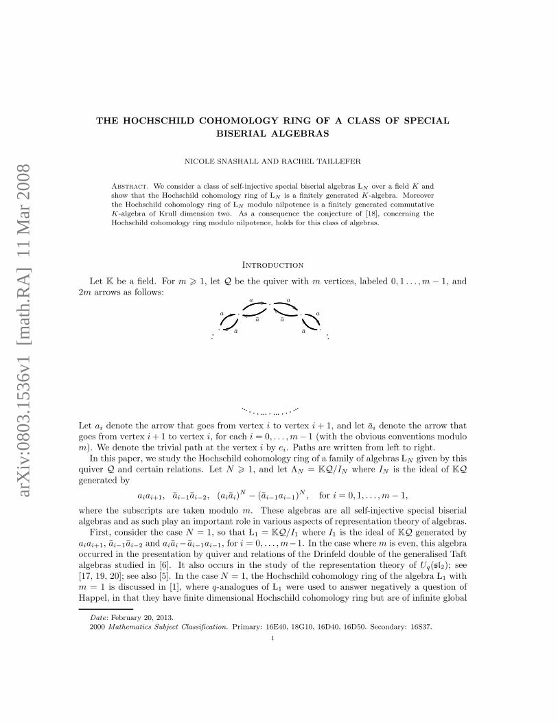
arX

iv:0

803.

1536

v1 [

mat

h.R

A]

11

Mar

200

8

THE HOCHSCHILD COHOMOLOGY RING OF A CLASS OF SPECIAL

BISERIAL ALGEBRAS

NICOLE SNASHALL AND RACHEL TAILLEFER

Abstract. We consider a class of self-injective special biserial algebras LN over a field K andshow that the Hochschild cohomology ring of LN is a finitely generated K-algebra. Moreoverthe Hochschild cohomology ring of LN modulo nilpotence is a finitely generated commutativeK-algebra of Krull dimension two. As a consequence the conjecture of [18], concerning theHochschild cohomology ring modulo nilpotence, holds for this class of algebras.

Introduction

Let K be a field. For m > 1, let Q be the quiver with m vertices, labeled 0, 1 . . . ,m − 1, and2m arrows as follows:

·a

a

ll·

a ,,

aqq

· a

��a

``

·

a 11

·a

VV

·

Let ai denote the arrow that goes from vertex i to vertex i + 1, and let ai denote the arrow thatgoes from vertex i+ 1 to vertex i, for each i = 0, . . . ,m− 1 (with the obvious conventions modulom). We denote the trivial path at the vertex i by ei. Paths are written from left to right.

In this paper, we study the Hochschild cohomology ring of a family of algebras LN given by thisquiver Q and certain relations. Let N > 1, and let ΛN = KQ/IN where IN is the ideal of KQgenerated by

aiai+1, ai−1ai−2, (aiai)N − (ai−1ai−1)N , for i = 0, 1, . . . ,m− 1,

where the subscripts are taken modulo m. These algebras are all self-injective special biserialalgebras and as such play an important role in various aspects of representation theory of algebras.

First, consider the case N = 1, so that L1 = KQ/I1 where I1 is the ideal of KQ generated byaiai+1, ai−1ai−2 and aiai− ai−1ai−1, for i = 0, . . . ,m−1. In the case where m is even, this algebraoccurred in the presentation by quiver and relations of the Drinfeld double of the generalised Taftalgebras studied in [6]. It also occurs in the study of the representation theory of Uq(sl2); see[17, 19, 20]; see also [5]. In the case N = 1, the Hochschild cohomology ring of the algebra L1 withm = 1 is discussed in [1], where q-analogues of L1 were used to answer negatively a question ofHappel, in that they have finite dimensional Hochschild cohomology ring but are of infinite global

Date: February 20, 2013.2000 Mathematics Subject Classification. Primary: 16E40, 18G10, 16D40, 16D50. Secondary: 16S37.

1

dimension when q ∈ K∗ is not a root of unity. The more general algebras LN occur in [8, 9], inwhich the authors determine the Hopf algebras associated to infinitesimal groups whose principalblocks are tame when K is an algebraically closed field of characteristic p > 3; among the principalblocks that are obtained in this classification are the algebras Lpn with m = pr vertices, for someintegers n and r.

This paper describes explicitly the structure of the Hochschild cohomology ring of the algebras LN , for all N > 1 and m > 1, and in all characteristics. In particular, we determine the Hochschildcohomology ring of the algebras L1 of [6] and the algebras of [8].

The main results show that the Hochschild cohomology ring, HH∗( LN ), is a finitely generatedK-algebra. We give an explicit basis for each cohomology group HHn( LN ) together with gen-erators of the algebra HH∗( LN ). We then determine explicitly the Hochschild cohomology ringmodulo nilpotence, HH∗( LN )/N , where N is the ideal of HH∗( LN ) generated by all homogeneousnilpotent elements. Furthermore, we show that the conjecture of [18] holds for all LN , that is,that HH∗( LN )/N is a finitely generated K-algebra. Moreover, we show that HH∗( LN )/N is acommutative ring of Krull dimension 2.

It is to be expected that the results in this paper will give some insight into the more generalproblem of verifying the conjecture of [18] for all special biserial algebras, and, indeed, for allKoszul algebras since the algebra L1 is a Koszul algebra. A general description of the multiplicativestructure of the Hochschild cohomology ring of a Koszul algebra was given in [2], but it remainsopen as to whether the conjecture of [18] holds for all Koszul algebras. For comparison, we recallthat the conjecture has been verified for finite-dimensional monomial algebras A in [12], where itwas shown that HH∗(A)/N is a finitely generated commutative algebra of Krull dimension at most1.

We now outline the structure of the paper. Section 1 describes the minimal projective resolution(P ∗, ∂∗) of the algebra LN as a bimodule, together with an explanation of the construction of thisresolution. This construction is of more general interest and applicability. Section 2 describes themethods used to find the dimensions of the kernel and image of the induced maps in the complexHom(P ∗, LN ) and hence gives the dimension of each Hochschild cohomology group HHn( LN ) inthe case m > 3. In calculating HH∗( LN ), we first consider the general case m > 3, and start witha description in section 3 of the centre of LN , that is, of HH0( LN ), before giving the structure ofthe Hochschild cohomology ring for m > 3 in sections 4 and 5. Section 6 deals with the case m = 2and section 7 with the case m = 1. The final section summarises the paper, and remarks that thefiniteness conditions (Fg1) and (Fg2) of [7] hold when N = 1, thus enabling one to describe thesupport varieties for finitely generated modules over the algebras L1.

1. A minimal projective bimodule resolution

Let N > 1, and let ΛN = KQ/IN where IN is the ideal of KQ generated by aiai+1, ai−1ai−2 and(aiai)

N − (ai−1ai−1)N , for i = 0, 1, . . . ,m − 1. Where there is no confusion, we label the arrowsof Q generically by a and a. We write o(α) for the trivial path corresponding to the origin of thearrow α, so that o(ai) = ei and o(ai) = ei+1. We write t(α) for the trivial path corresponding tothe terminus of the arrow α, so that t(ai) = ei+1 and t(ai) = ei. Recall that a non-zero elementr ∈ KQ is said to be uniform if there are vertices v, w such that r = vr = rw. Let Si denote thesimple module at the vertex i, so that {S0, . . . , Sm−1} is a complete set of non-isomorphic simplemodules for ΛN .

The Hochschild cohomology ring of a K-algebra Λ is given by HH∗( L) = Ext∗ Le( L, L) =

⊕n>0 Extn Le( L, L) with the Yoneda product, where Le = Lop ⊗K L is the enveloping algebra of

L. Since all tensors are over the field K we write ⊗ for ⊗K throughout.2

We now describe a minimal projective bimodule resolution (P ∗, ∂∗) of ΛN . By [14], we know thatthe multiplicity of Λei ⊗ ejΛ as a direct summand of Pn is equal to the dimension of Extn

Λ(Si, Sj).Thus we have, for n > 0, that

Pn = ⊕m−1i=0 [⊕n

r=0ΛNei ⊗ ei+n−2rΛN ].

We wish to label the summands of Pn by certain elements in the path algebra KQ. Thedescription given here is motivated by [11] where the first terms of a minimal bimodule resolutionof a finite-dimensional quotient of a path algebra were determined explicitly from the early termsof the minimal right Λ-resolution of Λ/r, where r is the Jacobson radical of L, using [13].

We start by recalling briefly the theory of projective resolutions developed in [13] and [11]. In[13], the authors give an explicit inductive construction of a minimal projective resolution of Λ/ras a right Λ-module, for a finite-dimensional algebra Λ over a field K. For Λ = KQ/I and finite-dimensional, they define g0 to be the set of vertices of Q, g1 to be the set of arrows of Q, and g2 tobe a minimal set of uniform relations in the generating set of I, and then show that there are subsetsgn, n ≥ 3, of KQ, where x ∈ gn are uniform elements satisfying x =

∑

y∈gn−1 yry =∑

z∈gn−2 zsz

for unique ry, sz ∈ KQ, which can be chosen in such a way that there is a minimal projectiveΛ-resolution of the form

· · · → Q4 → Q3 → Q2 → Q1 → Q0 → Λ/r → 0

having the following properties.

(1) For each n ≥ 0, Qn =∐

x∈gn t(x)Λ.

(2) For each x ∈ gn, there are unique elements rj ∈ KQ with x =∑

j gn−1j rj .

(3) For each n ≥ 1, using the decomposition of (2), for x ∈ gn, the map Qn → Qn−1 is givenby

t(x)λ 7→∑

j

rj t(x)λ.

where the elements of the set gn are labeled by gn = {gnj }. Thus the maps in this minimal

projective resolution of Λ/r as a right Λ-module are described by the elements rj which are uniquelydetermined by (2).

In [11], these same sets gn are used to give an explicit description of the first three maps ina minimal projective resolution of Λ as a Λ,Λ-bimodule, thus connecting the minimal projectiveresolution of Λ/r as a right Λ-module with a minimal projective resolution of Λ as a Λ,Λ-bimodule.We use the same ideas here to give a minimal projective bimodule resolution for the algebra ΛN ,for all N > 1. In the case where N = 1, the algebra L1 is Koszul, and we refer to [10] which usesthis approach and gives a minimal projective bimodule resolution for any Koszul algebra.

We start with the case N = 1 and define sets gn in the path algebra KQ which we will use tolabel the generators of Pn.

1.1. The bimodule resolution for Λ1. Consider the algebra L1. For each vertex i = 0, . . . ,m−1and for each r = 0, . . . , n, we define elements gn

r,i in KQ as follows. Let

gnr,i =

∑

p

(−1)sp

where the sum is over all paths p of length n, written p = α1α2 · · ·αn where the αi are arrows inQ, such that

(i) p ∈ eiKQ,(ii) p contains r arrows of the form a and n− r arrows of the form a, and

(iii) s =∑

αj=a j.

3

It follows that gnr,i ∈ ei(KQ)ei+n−2r, for i = 0, . . . ,m− 1 and r = 0, . . . , n. Since the elements gn

r,i

are uniform elements, we may define o(gnr,i) = ei and t(gn

r,i) = ei+n−2r. Then

Pn = ⊕m−1i=0 [⊕n

r=0Λ1o(gnr,i) ⊗ t(gn

r,i)Λ1].

We set

gn =

m−1⋃

i=0

{gnr,i | r = 0, . . . , n}.

It is easy to see, for the cases n = 0, 1, 2, that we have g00,i = ei, g

10,i = ai and g1

1,i = −ai−1, whilst

g20,i = aiai+1, g2

1,i = aiai − ai−1ai−1 and g22,i = −ai−1ai−2. Thus

g0 = {ei | i = 0, . . . ,m− 1},g1 = {ai,−ai | i = 0, . . . ,m− 1},g2 = {aiai+1, aiai − ai−1ai−1, −ai−1ai−2 for all i},

so that g2 is a minimal set of uniform relations in the generating set of I1.

To describe the map ∂n : Pn → Pn−1, we need to write the elements of the set gn in terms ofthe elements of the set gn−1. The proof of the next lemma is straightforward, and is left to thereader.

Lemma 1.1. For the algebra L1, for i = 0, 1, . . . ,m− 1 and r = 0, 1, . . . , n, we have:

gnr,i = gn−1

r,i ai+n−2r−1 + (−1)ngn−1r−1,iai+n−2r = (−1)raig

n−1r,i+1 + (−1)rai−1g

n−1r−1,i−1

with the conventions that gn−1,i = 0 and gn−1

n,i = 0 for all n, i. Thus

gn0,i = gn−1

0,i ai+n−1 = aign−10,i+1 and gn

n,i = (−1)ngn−1n−1,iai−n+1 = (−1)nai−1g

n−1n−1,i−1.

Since L1 is Koszul, we now use [10] to give a minimal projective bimodule resolution (Pn, ∂n)of L1. We define the map ∂0 : P 0 → L1 to be the multiplication map. However, to define ∂n

for n > 1, we first need to introduce some notation. In describing the image of o(gnr,i) ⊗ t(gn

r,i)

under ∂n in the projective module Pn−1, we use subscripts under ⊗ to indicate the appropriatesummands of the projective module Pn−1. Specifically, let ⊗r denote a term in the summand ofPn−1 corresponding to gn−1

r,− , and ⊗r−1 denote a term in the summand of Pn−1 corresponding

to gn−1r−1,−, where the appropriate index − of the vertex may always be uniquely determined from

the context. Indeed, since the relations are uniform along the quiver, we can also take labelingelements defined by a formula independent of i, and hence we omit the index i when it is clearfrom the context. Recall that nonetheless all tensors are over K.

Now, for n > 1, keeping the above notation and using [10], we define the map ∂n : Pn → Pn−1

for the algebra Λ1 as follows:

∂n : o(gnr,i) ⊗ t(gn

r,i) 7→ (ei ⊗r ai+n−2r−1 + (−1)nei ⊗r−1 ai+n−2r)+(−1)n((−1)rai ⊗r ei+n−2r + (−1)rai−1 ⊗r−1 ei+n−2r).

Using our conventions that gn−1,i = 0 and gn−1

n,i = 0 for all n, i, the degenerate cases (r = 0, r = n)simplify to

∂n : o(gn0,i) ⊗ t(gn

0,i) 7→ ei ⊗0 ai+n−1 + (−1)nai ⊗0 ei+n

where the first term is in the summand corresponding to gn−10,i and the second term is in the

summand corresponding to gn−10,i+1, whilst

∂n : o(gnn,i) ⊗ t(gn

n,i) 7→ (−1)nei ⊗n−1 ai−n + ai−1 ⊗n−1 ei−n,4

with the first term in the summand corresponding to gn−1n−1,i and the second term in the summand

corresponding to gn−1n−1,i−1.

The following result is now immediate from [10, Theorem 2.1].

Theorem 1.2. With the above notation, (Pn, ∂n) is a minimal projective resolution of Λ1 as aΛ1,Λ1-bimodule.

1.2. The bimodule resolution for ΛN with N > 1. We now consider the general case N > 1.In this case we use the approach of [10, 11] to construct a minimal projective resolution for LN .We keep the conventions that gn

−1,i = 0 and gn−1n,i = 0, for all n, i, throughout the paper.

Definition 1.3. For the algebra LN (N > 1), for i = 0, . . . ,m − 1 and r = 0, . . . , n, we defineg00,i = ei, and, inductively for n > 1,

gnr,i =

gn−1r,i a+ (−1)ngn−1

r−1,ia(aa)N−1 if n− 2r > 0;

gn−1r,i a(aa)N−1 + (−1)ngn−1

r−1,ia if n− 2r < 0;

gn−1r,i a(aa)N−1 + gn−1

r−1,ia(aa)N−1 if n = 2r.

Remark. (1) If N = 1, the above definition reduces to that given for L1.(2) We have g1

0,i = ai and g11,i = −ai−1, for all i. Also g2

0,i = aiai+1, g21,i = (aiai)

N −

(ai−1ai−1)N and g22,i = −ai−1ai−2, for all i. Hence g2 is a minimal set of uniform relations

in the generating set of IN .(3) The projectives in a minimal projective bimodule resolution of ΛN are given by

Pn = ⊕m−1i=0 [⊕n

r=0 LNo(gnr,i) ⊗ t(gn

r,i) LN ].

The next result is an analogue of Lemma 1.1 for the cases n−2r > 0 and n−2r < 0. The proofof the Lemma is easy to verify and is omitted.

Lemma 1.4. For the algebra LN (N > 1), for i = 0, . . . ,m− 1, n > 1, and r = 0, . . . , n, we have:

gnr,i =

gn−1r a+ (−1)ngn−1

r−1 a(aa)N−1 = (−1)ragn−1r + (−1)ra(aa)N−1gn−1

r−1 if n− 2r > 0;

gn−1r a(aa)N−1 + (−1)ngn−1

r−1 a = (−1)ra(aa)N−1gn−1r + (−1)ragn−1

r−1 if n− 2r < 0.

We now define the maps ∂n.

Definition 1.5. For the algebra LN (N > 1), and for n > 0, we define maps ∂n as follows. Forn = 0, the map ∂0 : P 0 → LN is the multiplication map. For n > 1, and i = 0, 1, . . . ,m − 1, themap ∂n : Pn → Pn−1 is given by ∂n : ei ⊗r ei+n−2r 7→

ei ⊗r ei+(n−1)−2ra+ (−1)n+raei+1 ⊗r ei+1+(n−1)−2r

+(−1)n+ra(aa)N−1ei−1 ⊗r−1 ei−1+(n−1)−2(r−1)

+(−1)nei ⊗r−1 ei+(n−1)−2(r−1)a(aa)N−1 if n− 2r > 0,

ei ⊗r ei+(n−1)−2ra(aa)N−1 + (−1)n+ra(aa)N−1ei+1 ⊗r ei+1+(n−1)−2r

+(−1)n+raei−1 ⊗r−1 ei−1+(n−1)−2(r−1)

+(−1)nei ⊗r−1 ei+(n−1)−2(r−1)a if n− 2r < 0,

∑N−1k=0 (aa)k[ei ⊗n

2ei−1a+ (−1)

n2 aei−1 ⊗n−2

2

ei](aa)N−k−1

+(aa)k[(−1)n2 aei+1 ⊗n

2ei + ei ⊗n−2

2

ei+1a](aa)N−k−1 if n− 2r = 0.

5

In order to prove that (Pn, ∂n) is a minimal projective resolution of ΛN as a LN , LN -bimodule,we use an argument which was given in [11]. To do this, we note that

LN/r ⊗ LNPn ∼= ⊕m−1

i=0 ⊕nr=0 t(gn

r,i) LN

as right LN -modules and that the map id⊗ ∂n : LN/r⊗ LNPn → LN/r⊗ LN

Pn−1 is equivalent to

the map ⊕m−1i=0 ⊕n

r=0 t(gnr,i) LN → ⊕m−1

i=0 ⊕n−1r=0 t(gn−1

r,i ) LN given by

t(gnr,i) 7→

t(gn−1r,i )a+ (−1)n

t(gn−1r−1,i)a(aa)N−1 if n− 2r > 0,

t(gn−1r,i )a(aa)N−1 + (−1)n

t(gn−1r−1,i)a if n− 2r < 0,

t(gn−1n2

,i )a(aa)N−1 + t(gn−1n−2

2,i

)a(aa)N−1 if n− 2r = 0.

It is then straightforward (with Lemma 1.4) to see that ( LN/r⊗ LNPn, id⊗ ∂n) is a minimal pro-

jective resolution of ΛN/r as a right ΛN -module, which satisfies the conditions of [13] as explainedabove, for all N > 1. For completeness in the proof of Theorem 1.6, we explain in full the strategyused in [11, Proposition 2.8].

Theorem 1.6. With the above notation, (Pn, ∂n) is a minimal projective resolution of ΛN as aΛN ,ΛN -bimodule, for all N > 1.

Proof The first step is to verify that we have a complex by showing that ∂2 = 0; this isstraightforward and the details are left to the reader.

Now suppose for contradiction that Ker ∂n−1 6⊆ Im ∂n for some n > 1. Then there is some non-zero map Ker ∂n−1 → Ker ∂n−1/ Im∂n. Hence there is a simple LN , LN -bimodule U ⊗ V and epi-morphism Ker ∂n−1/ Im∂n ։ U⊗V such that the composition f : Ker∂n−1 → Ker ∂n−1/ Im∂n ։

U ⊗ V is a non-zero epimorphism.Now, U is a simple left LN -module, V is a simple right LN -module and the functor LN/r⊗ LN

−

preserves monos and epis. Since ( LN/r ⊗ LNPn, id ⊗ ∂n) is a minimal projective resolution of

ΛN/r as a right ΛN -module, we have that LN/r ⊗ LNIm ∂n ∼= Im(id ⊗ ∂n) = Ker(id ⊗ ∂n−1) ∼=

LN/r ⊗ LNKer∂n−1. Thus, applying the functor LN/r ⊗ LN

− to the map ∂n : Pn → Pn−1 gives:

LN/r ⊗ LNPn

id⊗∂n

��

id⊗∂n

// LN/r ⊗ LNPn−1

LN/r ⊗ LNIm ∂n ∼= // LN/r ⊗ LN

Ker ∂n−1 id⊗f // LN/r ⊗ LNU ⊗ V.

The map id ⊗ f is non-zero so the composition LN/r ⊗ LNPn → LN/r ⊗ LN

U ⊗ V is non-zero.

However, this is simply the functor LN/r⊗ LN− applied to the composition Pn ∂n

→ Ker ∂n f→ U⊗V .

Now the composition Pn ∂n

→ Ker ∂n f→ U⊗V is zero since Im ∂n−1 ⊆ Ker ∂n. This gives the required

contradiction, so the complex is exact.Finally, minimality follows since we know that the projectives are those of a minimal projective

resolution of LN as a LN , LN -bimodule from [14]. �

We note that the degenerate cases (r = 0, r = n) in the maps ∂n may be written as:

∂n : ei ⊗0 ei+n 7→ ei ⊗0 ei+n−1a+ (−1)naei+1 ⊗0 ei+n

and

∂n : ei ⊗n ei−n 7→ aei−1 ⊗n−1 ei−n + (−1)nei ⊗n−1 ei−n+1a.

6

1.3. Conventions on notation. So far, we have tried to simplify notation by denoting the idem-potent o(gn

r,i)⊗ t(gnr,i) of the summand LNo(gn

r,i)⊗ t(gnr,i) LN of Pn uniquely by ei⊗r ei+n−2r where

0 6 i 6 m− 1. However, even this notation with subscripts under the tensor product symbol be-comes cumbersome in computations and in describing the elements of the Hochschild cohomologyring. Thus we make some conventions (by abuse of notation) which we keep throughout the paper.

First, we note that, in the language of [3], the n-th projective module Pn in a projective bimoduleresolution of ΛN is denoted S ⊗S Vn ⊗S S where S is the semisimple K-algebra generated by theidempotents {e0, e1, . . . , em−1} and Vn is the S, S-bimodule generated by the set

{gnr,i | i = 0, 1, . . . ,m− 1, r = 0, 1, . . . , n}.

(Note that here ⊗S denotes a tensor over S, that is, over a finite sum of copies of K; we continue toreserve the notation ⊗ exclusively for tensors over K.) There is a bijective correspondence betweenthe idempotent o(gn

r,i)⊗ t(gnr,i) and the term ei ⊗S g

nr,i ⊗S ei+n−2r in Vn, for i = 0, 1, . . . ,m− 1 and

r = 0, 1, . . . , n.Since ei+n−2r ∈ {e0, e1, . . . , em−1}, it would be usual to reduce the subscript i+ n− 2r modulo

m. However, to make it explicitly clear to which summand of the projective module Pn we arereferring and thus to avoid confusion, whenever we write ei ⊗ ei+k for an element of Pn, we willalways have i ∈ {0, 1, . . . ,m − 1} and consider i + k as an element of Z, in that r = (n − k)/2and ei ⊗ ei+k = ei ⊗n−k

2

ei+k and thus lies in the n−k2 -th summand of Pn. We do not reduce

i + k modulo m in any of our computations. In this way, when considering elements in Pn, ourelement ei ⊗ ei+k corresponds uniquely to the idempotent o(gn

r,i) ⊗ t(gnr,i) of Pn (or, equivalently,

to ei ⊗S gnr,i ⊗S ei+n−2r) with r = (n− k)/2, for each i = 0, 1, . . . ,m− 1.

Since we take 0 ≤ i ≤ m− 1 we clarify our conventions in Definition 1.5 in the cases i = 0 andi = m − 1, to ensure that we always have 0 ≤ j ≤ m − 1 in the first idempotent entry of eachtensor (ej ⊗−). Specifically, we have:∂n : e0 ⊗ en−2r 7→

e0 ⊗ e(n−1)−2ra+ (−1)n+rae1 ⊗ e1+(n−1)−2r

+(−1)n+ra(aa)N−1em−1 ⊗ em−1+(n−1)−2(r−1)

+(−1)ne0 ⊗ e(n−1)−2(r−1)a(aa)N−1 if n− 2r > 0,

e0 ⊗ e(n−1)−2ra(aa)N−1 + (−1)n+ra(aa)N−1e1 ⊗ e1+(n−1)−2r

+(−1)n+raem−1 ⊗ em−1+(n−1)−2(r−1)

+(−1)ne0 ⊗ e(n−1)−2(r−1)a if n− 2r < 0,

∑N−1k=0 (aa)k[e0 ⊗ e−1a+ (−1)

n2 aem−1 ⊗ em](aa)N−k−1

+(aa)k[(−1)n2 ae1 ⊗ e0 + e0 ⊗ e1a](aa)N−k−1 if n− 2r = 0,

and ∂n : em−1 ⊗ em−1+n−2r 7→

em−1 ⊗ em−1+(n−1)−2ra+ (−1)n+rae0 ⊗ e(n−1)−2r

+(−1)n+ra(aa)N−1em−2 ⊗ em−2+(n−1)−2(r−1)

+(−1)nem−1 ⊗ em−1+(n−1)−2(r−1)a(aa)N−1 if n− 2r > 0,

em−1 ⊗ em−1+(n−1)−2ra(aa)N−1 + (−1)n+ra(aa)N−1e0 ⊗ e(n−1)−2r

+(−1)n+raem−2 ⊗ em−2+(n−1)−2(r−1)

+(−1)nem−1 ⊗ em−1+(n−1)−2(r−1)a if n− 2r < 0,

∑N−1k=0 (aa)k[em−1 ⊗ em−2a+ (−1)

n2 aem−2 ⊗ em−1](aa)N−k−1

+(aa)k[(−1)n2 ae0 ⊗ e−1 + em−1 ⊗ ema](aa)N−k−1 if n− 2r = 0.

7

Our notation ei ⊗ ei+k is used without further comment throughout the rest of the paper.

We end this section by determining the dimension of each space HomΛeN

(Pn,ΛN ) for each n > 0.

1.4. The complex HomΛeN

(Pn,ΛN ). All our homomorphisms are ΛeN -homomorphisms and so we

write Hom(−,−) for HomΛeN

(−,−).

Lemma 1.7. If m > 3, write n = pm+ t where p > 0 and 0 6 t 6 m− 1. Then

dimK Hom(Pn,ΛN) =

{

(4p+ 2)mN if t 6= m− 1(4p+ 4)mN if t = m− 1.

If m = 1 or m = 2 thendimK Hom(Pn, LN ) = 4N(n+ 1).

Proof An element f in Hom(Pn,ΛN ) is determined by the elements f(ei ⊗ ei+n−2r), which canbe arbitrary elements of eiΛNei+n−2r.

Suppose first that m > 3. Then, for vertices i, j, we have

dim eiΛNej =

2N if i = j,N if i− j ≡ ±1 (mod m),0 otherwise.

For a finite subset X ⊂ Z and 0 6 s 6 m − 1, we define νs(X) = |{x ∈ X : x ≡ s (mod m)}|.With this we have

dim Hom(Pn,ΛN) = mN(2ν0(In) + ν1(In) + ν−1(In))

where In = {n− 2r : 0 6 r 6 n}. We observe that the disjoint union In ∪ In−1 is equal to [−n, n],the set of all integers x with −n 6 x 6 n. Clearly ν0([−n, n]) = 2p+ 1 and

ν1([−n, n]) =

2p if t = 02p+ 1 if 1 6 t 6 m− 22p+ 2 if t = m− 1.

Moreover ν−1([−n, n]) = ν1([−n, n]), by symmetry.The lemma now follows by induction on n, with the case n = 0 being clear. For the inductive

step, note that

dim Hom(Pn,ΛN) = mN(2ν0(In) + ν1(In) + ν−1(In))= mN(2ν0([−n, n]) + 2ν1([−n, n])) − dim Hom(Pn−1,ΛN ).

The statement for dim Hom(Pn,ΛN) now follows for m > 3.In the case m = 1, we have Pn = ⊕n

r=0 LN ⊗ LN and dim LN = 4N . Thus dim Hom(Pn,ΛN) =4N(n+ 1).

Finally, for m = 2, suppose first that n is even. Then Pn has n + 1 summands equal to LNe0 ⊗ e0 LN and n + 1 summands equal to LNe1 ⊗ e1 LN . By symmetry, dim Hom(Pn,ΛN ) =2(n+ 1) dim e1 LNe1 = 4N(n+ 1). For n odd, Pn has n+ 1 summands equal to LNe0 ⊗ e1 LN andn+1 summands equal to LNe1⊗e0 LN . Hence, again using symmetry, we have dim Hom(Pn,ΛN) =2(n+ 1) dim e0 LNe1 = 4N(n+ 1). This completes the proof. �

2. The dimensions of the Hochschild cohomology spaces for m > 3.

We give here the main arguments we used to compute the kernel and the image of the differen-tials, and leave the details to the reader. We denote both the map Pn → Pn−1 and its inducedmap Hom(Pn−1, LN ) → Hom(Pn, LN ) by ∂n. Then we have that HHn(ΛN ) = Ker(∂n+1)/ Im(∂n).We assume without further comment that m > 3 throughout this section.

8

2.1. Explicit description of maps. In order to compute the Hochschild cohomology groups,we need an explicit description of the image of each ei ⊗r ei+n−2r = ei ⊗ ei+n−2r under f ∈Hom(Pn,ΛN ) for i = 0, 1, . . . ,m− 1. We write n = pm+ t with 0 6 t 6 m− 1, p > 0.

The image f(ei ⊗ ei+n−2r) lies in ei LNej where j ∈ Zm with j ≡ i + n − 2r (mod m). Sinceei LNej = (0) if the vertices i and j are sufficiently far apart in the quiver of LN (at least form > 3), for a non-zero image f(ei ⊗ ei+n−2r) we are only interested in examining the caseswhere i + n − 2r ≡ i, i − 1, i + 1 (mod m). This leads to the consideration of terms of the formf(ei ⊗ ei+sm), f(ei ⊗ ei+sm−1) and f(ei ⊗ ei+sm+1) where s ∈ Z, s > 0.

For any s > 0 and 0 6 i 6 m − 1, we have that f(ei ⊗ ei+sm) is a linear combination of theelements (aa)k, 0 6 k 6 N−1, and (aa)k, 1 6 k 6 N ; f(ei⊗ei+sm−1) is a linear combination of thea(aa)k, 0 6 k 6 N − 1; and f(ei ⊗ ei+sm+1) is a linear combination of the a(aa)k, 0 6 k 6 N − 1.For m > 3, we give here a list of the terms which must be considered in giving a possible non-zero image of f ; these are used without further comment throughout the paper. (We assumem > 3; the cases m = 1 and m = 2 are different and are considered separately later.) For eachi = 0, 1, . . . ,m− 1:

m even, m 6= 2 t even f(ei ⊗ ei+αm), −p 6 α 6 p,t odd, t 6= m− 1 f(ei ⊗ ei+βm−1), −p 6 β 6 p,

f(ei ⊗ ei+γm+1), −p 6 γ 6 p,t = m− 1 f(ei ⊗ ei+βm−1), −p 6 β 6 p+ 1,

f(ei ⊗ ei+γm+1), −p− 1 6 γ 6 p,m odd, m 6= 1 t even, t 6= m− 1 f(ei ⊗ ei+(p−2α)m), 0 6 α 6 p,

f(ei ⊗ ei+(p−2β−1)m−1), 0 6 β 6 p− 1,f(ei ⊗ ei+(p−2γ−1)m+1), 0 6 γ 6 p− 1,

t odd f(ei ⊗ ei+(p−2α−1)m), 0 6 α 6 p− 1,f(ei ⊗ ei+(p−2β)m−1), 0 6 β 6 p,f(ei ⊗ ei+(p−2γ)m+1), 0 6 γ 6 p,

t = m− 1 f(ei ⊗ ei+(p−2α)m), 0 6 α 6 p,f(ei ⊗ ei+(p−2β−1)m−1), −1 6 β 6 p− 1,f(ei ⊗ ei+(p−2γ−1)m+1), 0 6 γ 6 p.

2.2. Kernel of ∂pm+t+1 : Hom(P pm+t,ΛN) → Hom(P pm+t+1,ΛN ). An element f inHom(P pm+t,ΛN) is determined by f(ei ⊗ ei+n−2r) for appropriate i ∈ {0, 1, . . . ,m − 1}. Eachterm f(ei ⊗ ei+n−2r) can be written as a linear combination of the basis elements in eiΛNei+n−2r,and we need to find the conditions on the coefficients in this linear combination when f is inKer ∂pm+t+1. To do this, we separate the study into several cases: when m is even, we considerthe three cases (i) t = m− 1, (ii) t even, and (iii) t odd with t 6= m− 1, and, when m is odd, welook at the four cases (i) t = m − 1, (ii) t = m − 2, (iii) t even with t 6= m − 1, and (iv) t oddwith t 6= m − 2. Note that in some cases a factor N appears so that the results depend on thecharacteristic of K. Note also that, when m is odd, the case char K = 2 needs to be consideredseparately.

For f ∈ Hom(P pm+t,ΛN), we write

f(ei ⊗ ei+αm) =∑N−1

k=0 σαi,k(aiai)

k +∑N

k=1 ταi,k(ai−1ai−1)k,

f(ei ⊗ ei+βm−1) =∑N−1

k=0 λβi,k(aa)kai−1,

f(ei ⊗ ei+γm+1) =∑N−1

k=0 µγi,k(aa)kai,

with coefficients σαi,k, τ

αi,k, λ

βi,k and µγ

i,k in K, for i = 0, 1, . . . ,m− 1.We shall now do two of the cases above, in order to illustrate the general method. In both

these cases, for consistency with our convention on the writing of elements ei ⊗ ei+k with i ∈{0, 1, . . . ,m− 1} and k ∈ Z, and to simplify, we shall use the following notation: if n ∈ Z, 〈n〉denotes the representative of n modulo m in {0, 1, . . . ,m− 1} . In particular, 〈m〉 = 〈0〉, and this

9

must be borne in mind when computing kernels and images. We write ∂f (rather than ∂pm+t+1f)for the image of f under the map ∂pm+t+1 : Hom(P pm+t, LN ) → Hom(P pm+t+1, LN).

Case m even and t even. In this case, f is entirely determined by the f(ei ⊗ ei+α′m) for−p 6 α′ 6 p and i ∈ {0, 1, . . . ,m− 1} and ∂f is determined by{

∂f(ei ⊗ ei+βm−1) for − p 6 β 6 p (or −p 6 β 6 p+ 1 if t = m− 2)

∂f(ei ⊗ ei+γm+1) for − p 6 γ 6 p (or −p− 1 6 γ 6 p if t = m− 2)with 0 6 i 6 m− 1. So f

is in the kernel of ∂ if and only if ∂f(ei ⊗ ei+βm−1) = 0 = ∂f(ei ⊗ ei+γm+1) for all i, β and γ. Now∂f(ei ⊗ ei+βm−1) =

[

(−1)(p−β) m2 σβ

〈i−1〉,0 − σβi,0

]

a(aa)N−1 if β > 0[

(−1)(p−β) m2 σβ

〈i−1〉,0 − σβi,0

]

a+∑N−1

k=1

[

(−1)(p−β) m2 σβ

〈i−1〉,k − τβi,k

]

(aa)ka if β 6 0

∂f(ei ⊗ ei+γm+1) =

[

σγi,0 − (−1)(p−γ) m

2 σγ〈i+1〉,0

]

a+∑N−1

k=1

[

σγi,k − (−1)(p−γ) m

2 τγ〈i+1〉,k

]

a(aa)k if γ > 0[

σγi,0 − (−1)(p−γ) m

2 σγ〈i+1〉,0

]

a(aa)N−1 if γ > 0.

For any α′ with −p 6 α′ 6 p, we can see that σα′

0,0 determines the other σα′

i,0 (setting β or γ to be

α′). Combining the cases β 6 0 and γ > 0 tells us that the τα′

i,k for k = 1, . . . , N−1 are determined

by the σα′

i,k. Finally the τα′

i,N are arbitrary, and the σα′

i,k for k = 1, . . . , N−1 are arbitrary. Therefore

the dimension of Ker ∂pm+t+1 in this case is (2p+ 1) + (2p+ 1)m+ (2p+ 1)m(N − 1).

Case m even and t odd, t 6= m − 1. In this case, f is entirely determined by{

f(ei ⊗ ei+β′m−1) for − p 6 β′ 6 p,

f(ei ⊗ ei+γ′m+1) for − p 6 γ′ 6 p,with i ∈ {0, 1, . . . ,m− 1}

and ∂f ∈ Hom(P (p+1)m,ΛN) is determined by ∂f(ei ⊗ ei+αm) for −p 6 α 6 p. Now

∂f(ei ⊗ ei+αm) =

N[

λ0i,0 + (−1)(p+1) m

2 λ0〈i+1〉,0 + (−1)(p+1) m

2 µ0〈i−1〉,0 + µ0

i,0

]

(aa)N if α = 0[

λαi,N−1 + (−1)(p+1+α) m

2 λα〈i+1〉,N−1 + (−1)(p+1+α) m

2 µα〈i−1〉,0 + µα

i,0

]

(aa)N

+∑N−2

k=0 λαi,k(aa)k+1 + (−1)(p+1+α) m

2

∑N−2k=0 λα

〈i+1〉,k(aa)k+1 if α > 0[

λαi,0 + (−1)(p+1+α) m

2 λα〈i+1〉,0 + (−1)(p+1+α) m

2 µα〈i−1〉,N−1 + µα

i,N−1

]

(aa)N

+(−1)(p+1+α) m2

∑N−2k=0 µα

〈i−1〉,k(aa)k+1 +∑N−2

k=0 µαi,k(aa)k+1 if α < 0.

So for α = 0, λ0i,0, for i ∈ {0, . . . ,m− 1} and µ0

0,0 determine the other µ0i,0, unless the charac-

teristic of K divides N. For α > 0, µαi,0 and λα

0,N−1 determine the other λαi,N−1, and for α < 0,

λαi,0 and µα

0,N−1 determine the other µαi,N−1. Moreover, for α > 0 the λα

i,k for k = 0, . . . , N − 2 areall 0, and for α < 0 the µα

i,k for k = 0, . . . , N − 2 are 0. The remaining λαi,k, µ

αi,k are arbitrary,

and there are 2m(N − 1) + pm(N − 1) + pm(N − 1) = 2(p + 1)m(N − 1) of these coefficients.This gives dimension: (m + 1) + p(m + 1) + p(m + 1) + 2(p + 1)m(N − 1) if char K ∤ N and(m+ 1) + p(m+ 1) + p(m+ 1) + 2(p+ 1)m(N − 1) +m− 1 if char K | N.

Note that when computing the dimensions in the case m odd and char K 6= 2, we often need tointroduce additional cases depending on the value of p modulo 4 and the value of m modulo 4. Wesummarise the results in the following two propositions, which separate the cases char K ∤ N andchar K | N .

10

Proposition 2.1. If char K ∤ N, the dimension of Ker ∂pm+t+1 is as follows.

If m even (2p+ 1)(mN + 1) if t even,(2p+ 1)(mN + 1) +m(N − 1) if t odd, t 6= m− 1(2p+ 1)(mN + 1) +m(N − 1) + 2 if t = m− 1.

If m odd (2p+ 1)(mN + 1) if t 6= m− 1, p+ t even,and char K = 2 (2p+ 1)(mN + 1) +m(N − 1) if t 6= m− 1, p+ t odd,

(2p+ 1)(mN + 1) + 2 if t = m− 1, p even,(2p+ 1)(mN + 1) +m(N − 1) + 2 if t = m− 1, p odd.

If m odd (2p+ 1)mN + p2 + 1 if t ≡ 0 (mod 4), t 6= m− 1, p even,

and char K 6= 2 (2p+ 1)mN + p2 if t ≡ 2 (mod 4), t 6= m− 1, p even,

(2p+ 1)mN +m(N − 1) + p+12 if m+ t ≡ 1 (mod 4), t 6= m− 1, p odd,

(2p+ 1)mN +m(N − 1) + p−12 if m+ t ≡ 3 (mod 4), t 6= m− 1, p odd,

(2p+ 1)mN +m(N − 1) + p2 + 1 if t ≡ 1 (mod 4), p even,

(2p+ 1)mN +m(N − 1) + p2 if t ≡ 3 (mod 4), p even,

(2p+ 1)mN + p−12 if t ≡ m (mod 4), p odd,

(2p+ 1)mN + p+12 if t ≡ m+ 2 (mod 4), p odd,

(2p+ 1)mN + p2 + 3 if t = m− 1 ≡ 0 (mod 4), p even,

(2p+ 1)mN + p2 + 2 if t = m− 1 ≡ 2 (mod 4), p even,

(2p+ 1)mN +m(N − 1) + p+12 if t = m− 1, p odd.

Proposition 2.2. If char K | N, the dimension of Ker ∂pm+t+1 is given by the following.

If m even (2p+ 1)(mN + 1) if t even,(2p+ 2)mN + 2p if t odd, t 6= m− 1(2p+ 2)(mN + 1) if t = m− 1.

If m odd (2p+ 1)(mN + 1) if t 6= m− 1, p+ t even,and char K = 2 (2p+ 2)mN + 2p if t 6= m− 1, p+ t odd,

(2p+ 1)(mN + 1) + 2 if t = m− 1, p even,(2p+ 2)(mN + 1) if t = m− 1, p odd.

If m odd (2p+ 1)mN + p2 + 1 if t ≡ 0 (mod 4), p even,

and char K 6= 2 (2p+ 1)mN + p2 if t ≡ 2 (mod 4), p even,

(2p+ 2)mN + p−12 if t even, p ≡ 1 (mod 4)

(2p+ 2)mN + p+12 if m+ t ≡ 1 (mod 4), p ≡ 3 (mod 4)

(2p+ 2)mN + p−32 if m+ t ≡ 3 (mod 4), p ≡ 3 (mod 4)

(2p+ 2)mN + p2 if t odd, p ≡ 0 (mod 4)

(2p+ 2)mN + p2 + 1 if t ≡ 1 (mod 4), p ≡ 2 (mod 4)

(2p+ 2)mN + p2 − 1 if t ≡ 3 (mod 4), p ≡ 2 (mod 4)

(2p+ 1)mN + p−12 if t ≡ m (mod 4), p odd

(2p+ 1)mN + p+12 if t ≡ m+ 2 (mod 4), p odd

(2p+ 2)mN + p+12 if t = m− 1, p ≡ 3 (mod 4)

(2p+ 2)mN + p−12 if t = m− 1, p ≡ 1 (mod 4)

(2p+ 1)mN + p2 + 3 if t = m− 1 ≡ 0 (mod 4), p even

(2p+ 1)mN + p2 + 2 if t = m− 1 ≡ 2 (mod 4), p even.

2.3. Image of ∂pm+t : Hom(P pm+t−1,ΛN) → Hom(P pm+t,ΛN ). We explain here how to computeIm ∂pm+t explicitly (rather than simply compute its dimension with the rank and nullity theorem)

11

on the same cases as for the kernels, in order to be able to give a basis of cocycle representatives foreach Hochschild cohomology group HHn(ΛN ). For an element g ∈ Hom(P pm+t−1,ΛN), we consider∂pm+tg, and find the dimension of the subspace of Ker(∂pm+t+1) spanned by all the ∂pm+tg. Weshall again use the notation 〈n〉 for the representative modulo m of the integer n, and write ∂g for∂pm+tg.

Case m even and t even, t 6= 0.The map ∂g is determined by ∂g(ei ⊗ ei+αm) for −p 6 α 6 p and g is determined by

{

g(ei ⊗ ei+β′m−1) for −p 6 β′ 6 p

g(ei ⊗ ei+γ′m+1) for −p 6 γ′ 6 pwith i ∈ {0, 1, . . . ,m− 1} . Now

∂g(ei ⊗ ei+αm) =

N[

(−1)p m2 µ0

〈i−1〉,0 + µ0i,0 + λ0

i,0 + (−1)p m2 λ0

〈i+1〉,0

]

(aa)N if α = 0[

(−1)(p+α) m2 µα

〈i−1〉,0 + µαi,0 + λα

i,N−1 + (−1)(p+α) m2 λα

〈i+1〉,N−1

]

(aa)N

+∑N−2

k=0 λαi,k(aa)k+1 +

∑N−2k=0 λα

〈i+1〉,k(aa)k+1 if α > 0[

(−1)(p+α) m2 µα

〈i−1〉,N−1 + µαi,N−1 + λα

i,0 + (−1)(p+α) m2 λα

〈i+1〉,0

]

(aa)N

+∑N−2

k=0 µαi,k(aa)k+1 + (−1)(p+α) m

2

∑N−2k=0 µα

〈i−1〉,k(aa)k+1 if α < 0.

We can check that in each case, the sum or the alternate sum over i ∈ {0, . . . ,m− 1} of thecoefficients of the (aa)N is zero (recall that 〈m〉 = 〈0〉 and that m is even), so for each α we addm− 1 to the dimension, except when char K | N and α = 0, in which case, ∂g(ei ⊗ ei) = 0 and thismakes no contribution to dim Im ∂pm+t. Moreover, for α 6= 0, we can take arbitrary coefficientsfor the (aa)k+1 with 0 6 k 6 N − 2, and the coefficients of the (aa)k+1 are completely determinedby those of the (aa)k+1.

So dimK Im ∂pm+t =

{

(2p+ 1)(m− 1) + 2pm(N − 1) if char K ∤ N

2p(mN − 1) if char K | N.

Case m even and t odd, t 6= m− 1.

The element ∂g is determined by

{

∂g(ei ⊗ ei+βm−1) for −p 6 β 6 p

∂g(ei ⊗ ei+γm+1) for −p 6 γ 6 pand g is determined by

g(ei ⊗ ei+α′m) for −p 6 α′ 6 p. Now

∂g(ei ⊗ ei+βm−1) =

−[

(−1)(p+β+1) m2 σβ

〈i−1〉,0 + σβi,0

]

(aa)N−1a if β > 0

−[

(−1)(p+β+1) m2 σβ

〈i−1〉,0 + σβi,0

]

a−∑N−1

k=1

[

(−1)(p+β+1) m2 σβ

〈i−1〉,k + τβi,k

]

(aa)ka if β 6 0

∂g(ei ⊗ ei+γm+1) =

[

σγi,0 + (−1)(p+γ+1) m

2 σγ〈i+1〉,0

]

a+∑N−1

k=1

[

σγi,k + (−1)(p+γ+1) m

2 τγ〈i+1〉,k

]

a(aa)k if γ > 0[

σγi,0 + (−1)(p+γ+1) m

2 σγ〈i+1〉,0

]

a(aa)N−1 if γ < 0.

For 0 < α′ 6 p (resp. −p 6 α′ < 0), the coefficient of (aa)N−1a (resp. a) in ∂g(ei ⊗ ei+α′m−1)is equal, up to sign, to the coefficient of a (resp. a(aa)N−1) in ∂g(ei ⊗ ei+α′m+1). The coefficientof a in ∂g(ei ⊗ ei−1) (that is, when α′ = 0) is equal, up to sign, to that of a in ∂g(ei ⊗ ei+1).Moreover, either the sum or the alternate sum over i ∈ {0, . . . ,m− 1} of these coefficients is zero(depending on the parity of (p+ α′ + 1)m

2 ). They contribute m− 1 to the dimension of Im ∂pm+t

for each α′. The remaining coefficients of the (aa)ka and a(aa)k, for k = 1, . . . , N−1, are arbitraryexcept for the case γ = 0, where the coefficient of a(aa)k is equal, up to sign, to that of (aa)ka in∂g(ei ⊗ ei−1) (for β = 0).

So dimK Im ∂pm+t = (2p+ 1)(m− 1) + (2p+ 1)m(N − 1).12

2.4. Dimension of HHn(ΛN ). We will now give the dimension of each of the Hochschild coho-mology groups of LN . Note that the dimensions can be verified using Propositions 2.1 and 2.2,together with the rank and nullity theorem in the form dim Im(∂pm+t) = dim Hom(P pm+t−1,ΛN)−dim Ker(∂pm+t).

Proposition 2.3. If m is even, or if m is odd and char K = 2, then dimK HH0(ΛN ) = Nm + 1and, for pm+ t 6= 0,

dimK HHpm+t(ΛN ) =

4p+ 2 +m(N − 1) if t 6= m− 1, char K ∤ N ,

4p+ 4 +m(N − 1) if t = m− 1, char K ∤ N ,

4p+ 1 +mN if t 6= m− 1, char K | N ,

4p+ 3 +mN if t = m− 1, char K | N .

Proposition 2.4. If m is odd, char K 6= 2 and char K ∤ N , then dimK HH0(ΛN ) = Nm + 1 and,for pm+ t 6= 0,

dimK HHpm+t(ΛN ) = m(N − 1) + p+

1 if t = 0, p even,

3 if t = 0, p odd, m−12 even,

1 if t = 0, p odd, m−12 odd,

1 if t even, t 6= 0,m− 1, p even,

−1 if m+ t ≡ 3 (mod 4) even, t 6= 0,m− 1, p odd,

1 if m+ t ≡ 1 (mod 4) even, t 6= 0,m− 1, p odd,

2 if t ≡ 1 (mod 4), p even,

0 if t ≡ 3 (mod 4), p even,

0 if t odd, p odd,

3 if t = m− 1, p even,

1 if t = m− 1, p odd.

13

Proposition 2.5. If m is odd, char K 6= 2 and char K | N , then dimK HH0(ΛN ) = Nm + 1 and,for pm+ t 6= 0,

dimK HHpm+t(ΛN ) = mN + p+

1 if t = 0, p ≡ 0, 1 (mod 4)

0 if t = 0, p ≡ 2 (mod 4)

3 if t = 0, p ≡ 3 (mod 4), m ≡ 1 (mod 4)

0 if t = 0, p ≡ 3 (mod 4), m ≡ 3 (mod 4)

1 if t even, t 6= 0,m− 1, p+ t ≡ 0 (mod 4)

0 if t even, t 6= 0,m− 1, p+ t ≡ 2 (mod 4)

0 if m+ t ≡ 1 (mod 4), t 6= 0,m− 1, p ≡ 1 (mod 4),

−1 if m+ t ≡ 3 (mod 4), t 6= 0,m− 1, p ≡ 1 (mod 4)

1 if m+ t ≡ 1 (mod 4), t 6= 0,m− 1, p ≡ 3 (mod 4)

−2 if m+ t ≡ 3 (mod 4), t 6= 0,m− 1, p ≡ 3 (mod 4)

1 if t ≡ 1 (mod 4), p ≡ 0 (mod 4)

0 if t ≡ 3 (mod 4), p ≡ 0 (mod 4)

2 if t ≡ 1 (mod 4), p ≡ 2 (mod 4)

−1 if t ≡ 3 (mod 4), p ≡ 2 (mod 4)

−1 if t odd, p+m− t ≡ 1 (mod 4)

0 if t odd, p+m− t ≡ 3 (mod 4)

3 if t = m− 1, p+m ≡ 1 (mod 4)

2 if t = m− 1, p+m ≡ 3 (mod 4)

0 if t = m− 1, p ≡ 1 (mod 4)

1 if t = m− 1, p ≡ 3 (mod 4).

3. The centre of the algebra LN

We start by describing Z( LN ), the centre of LN , since it is well known that HH0( LN ) = Z( LN ).Note that the next result requires m > 2; the case m = 1 is dealt with separately in Theorem 7.1.

Theorem 3.1. Suppose that N > 1,m > 2. Then dim HH0( LN ) = Nm+ 1 and the set{

1, (aiai)N , [(aiai)

s + (aiai)s] for i = 0, 1, . . . ,m− 1 and s = 1, . . . , N − 1

}

is a K-basis of HH0(ΛN ).Moreover, HH0(ΛN ) is generated as an algebra by the set

{1, aiai for i = 0, 1 . . . ,m− 1} if N = 1;{

1, (aiai)N , [aiai + aiai] for i = 0, 1 . . . ,m− 1

}

if N > 1.

The proof is straightforward since, for N > 1, we have [(aiai)s + (aiai)

s] = ([aiai + aiai])s.

4. The Hochschild cohomology ring HH∗( LN ) for m > 3 and m even.

In this section, we assume that N > 1, m > 3 and m even (so that, necessarily, m > 4) and giveall the details of HH∗( LN ). In the subsequent sections we will consider the case N > 1, m > 3 andm odd, and leave many of the details to the reader since the computations are similar.

14

4.1. Basis of HHn( LN ). For each n > 1, we describe the elements of a basis of the Hochschildcohomology group HHn( LN ) in terms of cocycles in Hom(Pn,ΛN ), that is, we give a set of elementsin Ker∂n+1, each of which is written as a map in Hom(Pn,ΛN), such that the corresponding set ofcosets in Ker∂n+1/ Im ∂n with these representatives forms a basis of Ker∂n+1/ Im ∂n = HHn( LN ).Following standard usage, our notation does not distinguish between an element of HHn( LN ) and acocycle in Hom(Pn,ΛN ) which represents that element of HHn( LN ). However the precise meaningis always clear from the context. For each cocycle in Hom(Pn,ΛN), we simply write the images ofthe generators ei ⊗ ei+n−2r in Pn which are non-zero. We keep to these conventions throughoutthe whole paper.

Proposition 4.1. Suppose that N > 1, m > 3 and m is even. For each n > 1, the followingelements define a basis of HHn( LN ).

(1) For n even, n > 2:

(a) For −p 6 α 6 p: χn,α : ei ⊗ ei+αm 7→ (−1)(n2−α m

2 )iei for i = 0, 1, . . . ,m− 1;(b) For −p 6 α 6 p: πn,α : e0 ⊗ eαm 7→ (a0a0)N ;(c) For each j = 0, 1, . . . ,m− 2 and each s = 1, . . . , N − 1:

Fn,j,s :

{

ej ⊗ ej 7→ (aj aj)s

ej+1 ⊗ ej+1 7→ (−1)n2 (ajaj)s;

(d) For each s = 1, . . . , N − 1:

Fn,m−1,s :

{

em−1 ⊗ em−1 7→ (am−1am−1)s

e0 ⊗ e0 7→ (−1)n2 (a0a0)s;

(e) Additionally in the case char K | N , for each j = 1, . . . ,m−1: θn,j : ej⊗ej 7→ (aj aj)N .(2) For n odd, n > 1:

(a) For −p 6 γ < 0 and, if t = m− 1, γ = −p− 1 also:

ϕn,γ : ei ⊗ ei+γm+1 7→ (−1)(n−1−γm

2 )iai(aiai)N−1 for all i = 0, 1, . . . ,m− 1;

(b) For 0 6 γ 6 p: ϕn,γ : ei ⊗ ei+γm+1 7→ (−1)(n−1−γm

2 )iai for all i = 0, 1, . . . ,m− 1;(c) For 0 < β 6 p and, if t = m− 1, β = p+ 1 also:

ψn,β : ei ⊗ ei+βm−1 7→ (−1)n−1−βm

2iai−1(ai−1ai−1)N−1 for all i = 0, 1, . . . ,m− 1;

(d) For −p 6 β 6 0: ψn,β : ei ⊗ ei+βm−1 7→ (−1)n−1−βm

2iai−1 for all i = 0, 1, . . . ,m− 1;

(e) For each j = 0, 1, . . . ,m−1 and each s = 1, . . . , N−1: En,j,s : ej ⊗ej+1 7→ (aj aj)saj;(f) Additionally in the case char K | N , for each j = 1, . . . ,m− 1: ωn,j : ej ⊗ ej+1 7→ aj.

4.2. Computing products in cohomology. In order to compute the products in the Hochschildcohomology ring, we require a lifting of each element in the basis of HHn( LN ), that is, for eachcocycle f ∈ Hom(Pn,ΛN ), we give a map L∗f : P ∗+n → P ∗ such that

(1) the composition Pn L0f−→ P 0 ∂0

−→ ΛN is equal to f , and

(2) the square P q+nLqf //

∂q+n

��

P q

∂q

��P q−1+n

Lq−1f

// P q−1

commutes for every q > 1.

It should be noted that such liftings always exist but are not unique. It is easy to check that themaps given in this paper are indeed liftings of the appropriate cocycle.

For homogeneous elements η ∈ HHn( LN ) and θ ∈ HHk( LN ) represented by cocycles η : Pn → LN and θ : P k → LN respectively, the cup product (or Yoneda product) ηθ ∈ HHn+k( LN ) is

15

the coset represented by the composition Pn+k Lnθ−→ Pn η

−→ LN . The fact that the cup productis well-defined means that the composition ηθ does not depend on the choice of representativecocycles for η and θ or on the choice of the liftings of these cocycles.

4.3. Liftings for N = 1. We continue to assume that m is even in the details that follow.

Proposition 4.2. For n > 1 and the algebra L1, m > 3 and m even, the following maps areliftings of the cocycle basis of HHn( L1) given in Proposition 4.1.

(1) For n even, n > 2, and for −p 6 α 6 p:

• Lqχn,α : ei ⊗ ei+αm+q−2ℓ 7→ (−1)(n2−α m

2 )iei ⊗ ei+q−2ℓ for all i = 0, 1, . . . ,m− 1 and all0 6 ℓ 6 q,

• Lqπn,α : e0 ⊗ eαm+q−2ℓ 7→ a0a0e0 ⊗ eq−2ℓ for all 0 6 ℓ 6 q,(2) For n odd:

• For

{

−p 6 γ 6 p if t 6= m− 1

−p− 1 6 γ 6 p if t = m− 1:

Lqϕn,γ : ei ⊗ ei+γm+1+q−2ℓ 7→ (−1)(n−1

2−γ m

2 )i+qei ⊗ ei+q−2ℓ ai+q−2ℓ

for all i = 0, 1, . . . ,m− 1 and all 0 6 ℓ 6 q,

• For

{

−p 6 β 6 p if t 6= m− 1

−p 6 β 6 p+ 1 if t = m− 1:

Lqψn,β : ei ⊗ ei+βm−1+q−2ℓ 7→ (−1)(n−1

2−β m

2 )iei ⊗ ei+q−2ℓ ai+q−2ℓ−1

for all i = 0, 1, . . . ,m− 1 and all 0 6 ℓ 6 q.

4.4. Liftings for N > 1.

Proposition 4.3. For n > 1 and the algebra LN with N > 1,m > 3 and m even, the followingmaps give a lifting of the cocycles in Proposition 4.1 above. Once again, to simplify cases and forconsistency with our conventions, we use the notation 〈n〉 ∈ {0, 1, . . . ,m− 1} for the representativeof the integer n modulo m.

(1) For n even, n > 2:• For −p 6 α 6 p:Lqχn,α(ei ⊗ ei+q−2ℓ+αm) =

(−1)n−αm

2iei ⊗ ei+q−2ℓ if (q − 2ℓ)α > 0

0 if (q − 2ℓ)α < 0 and |q − 2ℓ| > 2

(−1)n−αm

2i(aa)N−1ei ⊗ ei+2(aa)N−1 if α < 0 and q − 2ℓ = 2

(−1)n−αm

2i(aa)N−1ei ⊗ ei−2(aa)N−1 if α > 0 and q − 2ℓ = −2

(−1)n−αm

2i[

∑N−1k=0 (aa)kei ⊗ ei+1(aa)N−k−1

+(−1)q+1

2

∑N−2k=0 (aa)kae〈i+1〉 ⊗ e〈i+1〉−1a(aa)N−k−2

]

if α < 0 and q − 2ℓ = 1

(−1)n−αm

2i[

∑N−1k=0 (aa)kei ⊗ ei−1(aa)N−k−1

+(−1)q+1

2

∑N−2k=0 (aa)kae〈i−1〉 ⊗ e〈i−1〉+1a(aa)N−k−2

]

if α > 0 and q − 2ℓ = −1

for all i = 0, 1, . . . ,m− 1 and all 0 6 ℓ 6 q.16

• For −p 6 α 6 p:

Lqπn,α(e0 ⊗ eq−2ℓ+αm) =

(aa)Ne0 ⊗ eq−2ℓ if α(q − 2ℓ) > 0

(aa)Ne0 ⊗ e1(aa)N−1 if q − 2ℓ = 1 and α < 0

(aa)Ne0 ⊗ e−1(aa)N−1 if q − 2ℓ = −1 and α > 0

0 otherwisefor all 0 6 ℓ 6 q.

• For each j = 0, 1, . . . ,m− 2 and each s = 1, . . . , N − 1:

LqFn,j,s :

{

ej ⊗ ej+q−2ℓ 7→ (aj aj)sej ⊗ ej+q−2ℓ

ej+1 ⊗ ej+1+q−2ℓ 7→ (−1)n2 (ajaj)sej+1 ⊗ ej+1+q−2ℓ

for all 0 6 ℓ 6 q.• For each s = 1, . . . , N − 1:

LqFn,m−1,s :

{

em−1 ⊗ em−1+q−2ℓ 7→ (am−1am−1)sem−1 ⊗ em−1+q−2ℓ

e0 ⊗ eq−2ℓ 7→ (−1)n2 (am−1am−1)se0 ⊗ eq−2ℓ

for all 0 6 ℓ 6 q.• In the case char K | N , for each j = 1, . . . ,m− 1:Lqθn,j : ej ⊗ ej+q−2ℓ 7→ (aj aj)Nej ⊗ ej+q−2ℓ for all 0 6 ℓ 6 q.

(2) For n odd:• For −p 6 γ < 0 and, if t = m− 1, γ = −p− 1 also:

Lqϕn,γ(ei⊗ei+γm+1+q−2ℓ) =

0 if q − 2ℓ > 1

−(−1)n−1−γm

2i(aa)N−1ei ⊗ ei+1a(aa)N−1 if q − 2ℓ = 1

(−1)q+ n−1−γm2

iei ⊗ ei+q−2ℓa(aa)N−1 if q − 2ℓ 6 0for all i = 0, 1, . . . ,m− 1 and all 0 6 ℓ 6 q.

• For 0 6 γ 6 p :⋄ If γ > 0 then Lqϕn,γ(ei ⊗ ei+γm+1+q−2ℓ) =

(−1)q+ n−1−γm2

iei ⊗ ei+q−2ℓa if q − 2ℓ > 0

−(−1)n−1−γm

2i

[

N−1∑

k=0

(aa)kei ⊗ ei−1(aa)N−k−1a+

(−1)q+1

2

N−2∑

k=0

(aa)kae〈i−1〉 ⊗ e〈i−1〉+1(aa)N−k−1

]

if q − 2ℓ = −1

(−1)n−1−γm

2i(aa)N−1ei ⊗ ei−2(aa)N−1a if q − 2ℓ = −2

0 if q − 2ℓ < −2for all i = 0, 1, . . . ,m− 1 and all 0 6 ℓ 6 q.

17

⋄ If γ = 0 then Lqϕn,0(ei ⊗ ei+1+q−2ℓ) =

(−1)q+ n−1

2iei ⊗ ei+q−2ℓa if q − 2ℓ = q

(−1)q+ n−1

2i[

ei ⊗ ei+q−2ℓa− (−1)q(N − 1)ei ⊗ ei+q−2ℓ+2a(aa)N−1]

if 0 6 q − 2ℓ < q

(−1)q+ n−1

2iNei ⊗ ei+q−2ℓa(aa)N−1 if q − 2ℓ < −1

−(−1)n−1

2i

{

N−1∑

k=1

k−1∑

v=0

[

(aa)vei ⊗ ei+1a(aa)N−v−1+

(−1)q+1

2 (aa)vae〈i+1〉 ⊗ e〈i+1〉−1(aa)N−v−1+

(−1)q+1

2 (aa)v ae〈i−1〉 ⊗ e〈i−1〉+1(aa)N−v−1+

(aa)vei ⊗ ei−1a(aa)N−v−1]

+

N−1∑

k=0

(aa)kei ⊗ ei−1a(aa)N−k−1

}

if q − 2ℓ = −1

for all i = 0, 1, . . . ,m− 1 and all 0 6 ℓ 6 q.• For 0 < β 6 p and, if t = m− 1, β = p+ 1 also:

Lqψn,β(ei⊗ei+βm−1+q−2ℓ) =

0 if q − 2ℓ < −1

(−1)n−1−βm

2i(aa)N−1ei ⊗ ei−1a(aa)N−1 if q − 2ℓ = −1

(−1)n−1−βm

2iei ⊗ ei+q−2ℓa(aa)N−1 if q − 2ℓ > −1

for all i = 0, 1, . . . ,m− 1 and all 0 6 ℓ 6 q.• For −p 6 β 6 0:⋄ If β < 0, then Lqψn,β(ei ⊗ ei+βm−1+q−2ℓ) =

(−1)n−1−βm

2iei ⊗ ei+q−2ℓa if q − 2ℓ < 1

(−1)n−1−βm

2i

[

N−1∑

k=0

(aa)kei ⊗ ei+1a(aa)N−k−1+

(−1)q+1

2

∑N−2k=0 (aa)kae〈i+1〉 ⊗ e〈i+1〉−1(aa)N−k−1

]

if q − 2ℓ = 1

(−1)n−1−βm

2i(aa)N−1ei ⊗ ei+2(aa)N−1a if q − 2ℓ = 2

0 if q − 2ℓ > 2for all i = 0, 1, . . . ,m− 1 and all 0 6 ℓ 6 q.

⋄ If β = 0 then Lqψn,0(ei ⊗ ei−1+q−2ℓ) =

(−1)n−1

2iei ⊗ ei+q−2ℓa if q − 2ℓ = −q

(−1)n−1

2i[

ei ⊗ ei+q−2ℓa− (−1)q(N − 1)ei ⊗ ei+q−2ℓ−2a(aa)N−1]

if −q < q − 2ℓ 6 0

(−1)n−1

2iNei ⊗ ei+q−2ℓa(aa)N−1 if q − 2ℓ > 1

(−1)n−1

2i

{

N−1∑

k=1

k−1∑

v=0

[

(aa)vei ⊗ ei−1a(aa)N−v−1+

(−1)q+1

2 (aa)vae〈i−1〉 ⊗ e〈i−1〉+1(aa)N−v−1

+(−1)q+1

2 (aa)vae〈i+1〉 ⊗ e〈i+1〉−1aa)N−v−1+

(aa)vei ⊗ ei+1a(aa)N−v−1]

+

N−1∑

k=0

(aa)kei ⊗ ei+1a(aa)N−k−1

}

if q − 2ℓ = 1

for all i = 0, 1, . . . ,m− 1 and all 0 6 ℓ 6 q.

18

• For each j = 0, 1, . . . ,m− 1 and each s = 1, . . . , N − 1:LqEn,j,s =

ej ⊗ ej+1 7→ (aa)sej ⊗ eja if q is even

ej ⊗ ej 7→N−s∑

k=0

N−s∑

v=k

[

(aa)v+sej ⊗ ej+1a(aa)N−v−1+

(−1)q+1

2 (aa)v+sae〈j+1〉 ⊗ e〈j+1〉−1(aa)N−v−1]

if q is odd

e〈j+1〉 ⊗ e〈j+1〉 7→ (−1)n−1

2

N−s−1∑

k=0

N−s∑

v=k

[

(−1)q+1

2 (aa)v+saej ⊗ ej+1(aa)N−v−1

+(aa)v+s+1e〈j+1〉 ⊗ e〈j+1〉−1a(aa)N−v−2]

if q is odd

• In the case char K | N , for each j = 1, . . . ,m− 1:Lqωn,j =

ej ⊗ ej 7→N−1∑

k=1

k−1∑

v=0

[

(−1)q−1

2 (aa)vaej+1 ⊗ ej(aa)N−v−1−

(aa)vej ⊗ ej+1a(aa)N−v−1]

if q is odd

e〈j+1〉 ⊗ e〈j+1〉 7→ (−1)n+1

2

N−1∑

k=1

k−1∑

v=0

[

(aa)v+1e〈j+1〉 ⊗ e〈j+1〉−1a(aa)N−v−2+

(−1)q+1

2 (aa)vaej ⊗ ej+1(aa)N−v−1]

if q is odd

e〈j−v〉 ⊗ e〈j−v〉+2v 7→ (−1)n−1

2v[

(−1)v+ q+1

2 ae〈j−v+1〉 ⊗ e〈j−v+1〉+2v−1+

e〈j−v〉 ⊗ e〈j−v〉+2v+1a(aa)N−1]

for 1 6 v 6q+12 and q odd

e〈j−v〉 ⊗ e〈j−v〉+2v+1 7→ (−1)n−1

2v[

e〈j−v〉 ⊗ e〈j−v〉+2va−

(−1)v+ q2 a(aa)N−1e〈j−v−1〉 ⊗ e〈j−v−1〉+2v+2

]

for 0 6 v 6q2 and q even.

4.5. The Hochschild cohomology ring HH∗( L1) for N = 1, m > 3, m even.

Theorem 4.4. For N = 1, m > 3 and m even, HH∗( L1) is a finitely generated algebra withgenerators:

1, aiai for i = 0, 1, . . . ,m− 1 in degree 0,ϕ1,0, ψ1,0 in degree 1,χ2,0 in degree 2,ϕm−1,−1, ψm−1,1 in degree m− 1,χm,1, χm,−1 in degree m.

It is known from [18, Proposition 4.4] that those generators in HH∗( L1) whose image is in r arenilpotent, and it may be seen that the remaining generators of HH∗( L1), namely 1, χ2,0, χm,1 andχm,−1, are not nilpotent. Moreover χm

2,0 = χm,1χm,−1. Thus we have the following corollary.

Corollary 4.5. For N = 1, m > 3 and m even,

HH∗(Λ1)/N ∼= K[χ2,0, χm,1, χm,−1]/(χm2,0 − χm,1χm,−1)

and hence HH∗( L1)/N is a commutative finitely generated algebra of Krull dimension 2.

19

4.6. The Hochschild cohomology ring HH∗( LN ) for N > 1, m > 3, m even. In this sectionwe describe the main arguments behind the presentation of HH∗( LN) by generators and relations.The first lemma indicates the method required to show that HH∗( LN ) is a finitely generated algebrawhilst the second lemma considers the relations between the generators.

Lemma 4.6. Suppose N > 1, m > 3 and m even. Then

(1) χ2,0χ2,0 = χ4,0;(2) π2,0 = (a0a0)Nχ2,0.

Proof (1) By definition, χ2,0χ2,0 = χ2,0 · L2χ2,0. Now, from Proposition 4.3, L2χ2,0(ei ⊗ei+2−2ℓ) = (−1)iei ⊗ ei+2−2ℓ for i = 0, . . . ,m − 1 and 0 6 ℓ 6 2, and χ2,0(ei ⊗ ei) = (−1)iei fori = 0, . . . ,m− 1. Thus

χ2,0 · L2χ2,0(ei ⊗ ei+2−2ℓ) =

{

(−1)i(−1)iei = ei if ℓ = 1,0 otherwise,

for all i = 0, . . . ,m− 1. Hence χ2,0χ2,0 = χ4,0.(2) We know that χ2,0(ei ⊗ ei) = (−1)iei for i = 0, . . . ,m − 1, π2,0 : e0 ⊗ e0 7→ (a0a0)N , and

(a0a0)N ∈ HH0( LN ). Then

((a0a0)Nχ2,0)(ei ⊗ ei) = χ2,0((a0a0)Nei ⊗ ei) =

{

(−1)0e0(a0a0)N if i = 0,0 if i = 1, . . . ,m− 1.

Thus π2,0 = (a0a0)Nχ2,0. �

We remark that, for n even, 2 6 n < m and writing n = pm + t as usual, we necessarily havep = 0, and thus, from Proposition 4.1, we have {χn,α | −p 6 α 6 p} = {χn,0}. Inductively, Lemma4.6 (1) gives, for n = 2k even, 2 6 n 6 m− 2, that χn,0 = (χ2,0)k.

Lemma 4.7. Suppose N > 1, m > 3 and m even. Then

(1) χm,1χm,−1 = 0;(2) ϕ2

1,0 = 0;

(3) ϕ1,0ψ1,0 = Nm(a0a0)Nχ2,0;

(4) for char K | N , S =∑N

k=1 k and εi = (aiai)N for i = 0, 1, . . . ,m− 1, we have

ϕ1,0ω1,i =

Sχ2,0(εi + εi+1) if char K = 2 and i 6= m− 1

Sχ2,0(εm−1 + ε0) if char K = 2 and i = m− 1

0 if char K 6= 2.

Proof (1) We have χm,1χm,−1 = χm,1 · Lmχm,−1. Since m is even, Proposition 4.3 gives

Lmχm,−1(ei ⊗ ei+m−2ℓ−m) =

ei ⊗ ei+m−2ℓ if m− 2ℓ 6 0

0 if m− 2ℓ > 0 and |m− 2ℓ| > 2

(aa)N−1ei ⊗ ei+2(aa)N−1 if m− 2ℓ = 2

for all i = 0, 1, . . . ,m − 1 and all 0 6 ℓ 6 m. Also χm,1(ei ⊗ ei+m) = ei for i = 0, 1, . . . ,m − 1.Hence χm,1 · Lmχm,−1(ei ⊗ ei+m−2ℓ−m) = 0 and χm,1χm,−1 = 0.

(2) If char K 6= 2, then ϕ21,0 = 0 by graded commutativity of HH∗( LN ) so we may assume

char K = 2. Thus we have ϕ1,0(ei ⊗ ei+1) = ai for i = 0, 1, . . . ,m − 1, and, from Proposition 4.3,20

L1ϕ1,0(ei ⊗ ei+1+1−2ℓ) =

ei ⊗ ei+1ai+1 if ℓ = 0,

−

{

N−1∑

k=1

k−1∑

v=0

[

(aa)vei ⊗ ei+1a(aa)N−v−1 − (aa)vae〈i+1〉 ⊗ e〈i+1〉−1(aa)N−v−1

−(aa)vae〈i−1〉 ⊗ e〈i−1〉+1(aa)N−v−1 + (aa)vei ⊗ ei−1a(aa)N−v−1]

+

N−1∑

k=0

(aa)kei ⊗ ei−1a(aa)N−k−1

}

if ℓ = 1,

for all i = 0, 1, . . . ,m− 1. Hence

ϕ1,0·L1ϕ1,0(ei⊗ei+1+1−2ℓ) =

aiai+1 if ℓ = 0,

−N−1∑

k=1

k−1∑

v=0

[

(aa)vaia(aa)N−v−1 + (aa)v aai−1(aa)N−v−1]

if ℓ = 1.

But aiai+1 = 0 and (aiai)N +(ai−1ai−1)N = 0 since char K = 2. Thus ϕ1,0 ·L1ϕ1,0(ei⊗ei+1+1−2ℓ) =

0 and so ϕ21,0 = 0.

(3) We have ϕ1,0(ei ⊗ ei+1) = ai for i = 0, 1, . . . ,m− 1, and, from Proposition 4.3, L1ψ1,0(ei ⊗ei−1+1−2ℓ) =

ei ⊗ ei−1ai−2 if ℓ = 1,{

N−1∑

k=1

k−1∑

v=0

[

(aa)vei ⊗ ei−1a(aa)N−v−1 − (aa)v ae〈i−1〉 ⊗ e〈i−1〉+1(aa)N−v−1

−(aa)vae〈i+1〉 ⊗ e〈i+1〉−1aa)N−v−1 + (aa)vei ⊗ ei+1a(aa)N−v−1]

+

N−1∑

k=0

(aa)kei ⊗ ei+1a(aa)N−k−1

}

if ℓ = 0,

for i = 0, 1, . . . ,m − 1. Thus ϕ1,0 · L1ψ1,0(ei ⊗ ei−1+1−2ℓ) = 0 if ℓ = 1. On the other hand,

if ℓ = 0, then ϕ1,0 · L1ψ1,0(ei ⊗ ei) =

N−1∑

k=1

k−1∑

v=0

[

−(aa)v aai−1(aa)N−v−1 + (aa)vaia(aa)N−v−1]

+

N−1∑

k=0

(aa)kaia(aa)N−k−1 =N−1∑

k=0

(aiai)N = N(aiai)

N .

Now define g ∈ Hom(P 1, LN ) by ei ⊗ ei+1 7→ (m − 1 − i)ai for i = 0, 1, . . . ,m − 2 (with ourusual convention that all other summands are mapped to zero). Then ∂2g ∈ Hom(P 2, LN ) and,for i = 1, . . . ,m− 2, we have

∂2g(ei ⊗ ei) =∑N−1

k=0 [−(aa)kag(ei−1 ⊗ ei)(aa)N−k−1 + (aa)kg(ei ⊗ ei+1)a(aa)N−k−1]

=∑N−1

k=0 [−(aa)ka(m− i)ai−1(aa)N−k−1 + (aa)k(m− 1 − i)aia(aa)N−k−1]

=∑N−1

k=0 [−(m− i)(ai−1ai−1)N + (m− 1 − i)(aiai)N ]

= −N(aiai)N .

In a similar way, we also have ∂2g(em−1 ⊗ em−1) = −N(am−1am−1)N . For i = 0 we have,

∂2g(e0 ⊗ e0) =∑N−1

k=0 [−(aa)kag(em−1 ⊗ em)(aa)N−k−1 + (aa)kg(e0 ⊗ e1)a(aa)N−k−1]

=∑N−1

k=0 (aa)k(m− 1)a0a(aa)N−k−1

= N(m− 1)(a0a0)N .21

Moreover, ∂2g is zero on all other summands. Hence

∂2g(ei ⊗ ei) =

{

N(m− 1)(a0a0)N if i = 0,−N(aiai)

N if i = 1, . . . ,m− 1.

So ϕ1,0 · L1ψ1,0 + ∂2g is the map given by e0 ⊗ e0 7→ Nm(a0a0)N and thus ϕ1,0 · L1ψ1,0 + ∂2g =Nmπ2,0. Using Lemma 4.6(2), we have that the cocycles ϕ1,0ψ1,0 and Nm(a0a0)Nχ2,0 representthe same elements in Hochschild cohomology so that ϕ1,0ψ1,0 = Nm(a0a0)Nχ2,0 as required.

(4) Finally, suppose char K | N , S =∑N

k=1 k and let εi = (aiai)N for i = 0, 1, . . . ,m−1. For ease

of notation we consider the product ϕ1,0ω1,i where 1 6 i 6 m−2; the cases i = 0 and i = m−1 aresimilar. We know ϕ1,0(ej ⊗ ej+1) = aj for j = 0, 1, . . . ,m− 1 and, from Proposition 4.3, we have

L1ω1,i :

ei ⊗ ei 7→N−1∑

k=1

k−1∑

v=0

[

(aa)vaei+1 ⊗ ei(aa)N−v−1 − (aa)vei ⊗ ei+1a(aa)N−v−1]

ei+1 ⊗ ei+1 7→ −N−1∑

k=1

k−1∑

v=0

[

(aa)v+1ei+1 ⊗ eia(aa)N−v−2 − (aa)vaei ⊗ ei+1(aa)N−v−1]

ei−1 ⊗ ei+1 7→ aei ⊗ ei+1.

Hence ϕ1,0 · L1ω1,i(ei ⊗ ei) =

N−1∑

k=1

k−1∑

v=0

−(aa)vaia(aa)N−v−1 =

N−1∑

k=1

−k(aiai)N = −S(aiai)

N . And

ϕ1,0 · L1ω1,i(ei+1 ⊗ ei+1) = (−1)

N−1∑

k=1

k−1∑

v=0

(−1)(aa)v aai(aa)N−v−1 =

N−1∑

k=1

k(aiai)N = S(aiai)

N .

Finally, ϕ1,0 · L1ω1,i(ei−1 ⊗ ei+1) = 0. Hence ϕ1,0 · L1ω1,i :

{

ei ⊗ ei 7→ −S(aiai)N

ei+1 ⊗ ei+1 7→ S(ai+1ai+1)N .

Now, χ2,0(εi + εi+1) :

{

ei ⊗ ei 7→ (−1)i(aiai)N

ei+1 ⊗ ei+1 7→ (−1)i+1(ai+1ai+1)N .If char K = 2, then ϕ1,0ω1,i =

ϕ1,0 · L1ω1,i = Sχ2,0(εi + εi+1). However, if char K 6= 2 then, since char K | N , we have 2S =(N − 1)N = 0 so that S = 0 and hence ϕ1,0ω1,i = 0. �

By considering all possible products of the basis elements of HH∗( LN ) from Proposition 4.1, weare now able to give the main result of this section. We do not explicitly list the relations which area direct consequence of the graded commutativity of HH∗( LN ). Note that we can check that we doindeed have all the relations by comparing dim HHn( LN ) from Proposition 2.3 with the dimensionin degree n of the algebra given in Theorem 4.8 below.

Theorem 4.8. Suppose N > 1, m > 3 and m even.

(1) HH∗( LN ) is a finitely generated algebra with generators:

1, (aiai)N , [aiai + aiai] for i = 0, 1, . . . ,m− 1 in degree 0

ϕ1,0, ψ1,0 in degree 1ω1,j for j = 1, . . . ,m− 1 if char K | N in degree 1χ2,0 in degree 2ϕm−1,−1, ψm−1,1 in degree m− 1χm,1, χm,−1 in degree m.

(2) Let εi = (aiai)N for i = 0, 1, . . . ,m − 1 and S =

∑Nk=1 k. Then HH∗( LN ) is a finitely

generated algebra over HH0( LN ) with generators:22

1 in degree 0ϕ1,0, ψ1,0 in degree 1ω1,j for j = 1, . . . ,m− 1 if char K | N in degree 1χ2,0 in degree 2ϕm−1,−1, ψm−1,1 in degree m− 1χm,1, χm,−1 in degree m,

and relations

ϕ21,0 = 0 ϕ1,0ψ1,0 = Nmε0χ2,0 ϕ1,0ϕm−1,−1 = 0ψ2

1,0 = 0 ψ1,0ψm−1,1 = 0 ϕ2m−1,−1 = 0

ϕm−1,−1ψm−1,1 = 0 ϕm−1,−1χm,1 = 0 ψ2m−1,1 = 0

ψm−1,1χm,−1 = 0 χm,1χm,−1 = 0 ψ1,0χm,1 = Nχ2,0ψm−1,1

ϕ1,0χm,−1 = Nχ2,0ϕm−1,−1 ω1,jψm−1,1 = (−1)m2

jχm,1ε0 ω1,jχm,±1 = 0ω1,iω1,j = 0 if i 6= j ϕ1,0ψm−1,1 = mχm,1ε0 = ψ1,0ϕm−1,−1

ϕ1,0ω1,i = ψ1,0ω1,i = ω21,i =

Sχ2,0(εi + εi+1) if char K = 2 and i 6= m− 1

Sχ2,0(εm−1 + ε0) if char K = 2 and i = m− 1

0 if char K 6= 2.

(3) Let εi = (aiai)N and fi = [aiai + aiai] for i = 0, 1, . . . ,m−1. Then the action of HH0( LN )

on the generators of HHn( LN ) is described as follows, for all i, j = 0, 1, . . . ,m− 1.

εig = 0 ∀g 6= χn,α εiχ2,0 = 0 if i 6= 0 and char K ∤ N εiχm,±1 = (−1)iε0χm,±1

fifj = 0 if i 6= j fiϕ1,0 = fiψ1,0 fNi = εi + εi+1

fiϕm−1,−1 = 0 fiψm−1,1 = 0 fiχm,±1 = 0fiω1,j = 0 for i 6= j fiω1,i = fiϕ1,0.

Corollary 4.9. For N > 1, m > 3 and m even,

HH∗( LN )/N ∼= K[χ2,0, χm,1, χm,−1]/(χm,1χm,−1)

and hence HH∗( L1)/N is a commutative finitely generated algebra of Krull dimension 2.

5. The Hochschild cohomology ring HH∗( LN ) for m > 3, m odd.

In this section, N > 1, m > 3 and m is odd. Most of the details are similar to those in theprevious section and are left to the reader. We consider separately the cases char K 6= 2 andchar K = 2.

5.1. Basis of HHn( LN ) for N > 1, m > 3, m odd and char K 6= 2.

Proposition 5.1. Suppose that N > 1, m > 3, m odd and char K 6= 2. For n > 1, the followingelements define a basis of HHn( LN ):

(1) For n even, n > 2:(a) χn,δ : ei ⊗ ei+δm 7→ ei for all i = 0, 1, . . . ,m− 1, with

δ =

{

p− 2α− 1, 0 6 α 6 p− 1 when t is odd and α+ m−t2 is odd,

p− 2α, 0 6 α 6 p when t is even and α+ t2 is even;

(b) πn,δ : e0 ⊗ eδm 7→ (a0a0)N , with

δ =

{

p− 2α− 1, 0 6 α 6 p− 1 when t is odd and α+ m−t2 is even,

p− 2α, 0 6 α 6 p when t is even and α+ t2 is odd;

23

(c) For each j = 0, 1, . . . ,m− 2 and each s = 1, . . . , N − 1:

Fn,j,s :

{

ej ⊗ ej 7→ (aj aj)s,

ej+1 ⊗ ej+1 7→ (−1)n2 (ajaj)s;

(d) For each s = 1, . . . , N − 1:

Fn,m−1,s :

{

em−1 ⊗ em−1 7→ (am−1am−1)s,

e0 ⊗ e0 7→ (−1)n2 (am−1am−1)s;

(e) For t = m − 1 and σ = −(p + 1): ϕn,σ : ei ⊗ ei+σm+1 7→ (aa)N−1ai for all i =0, 1, . . . ,m− 1;

(f) For t = m − 1 and τ = p + 1: ψn,τ : ei ⊗ ei+τm−1 7→ (aa)N−1ai−1 for all i =0, 1, . . . ,m− 1;

(g) Additionally, if char K | N , and for each

{

j = 0, 1, . . . ,m− 1 if n2 is even

j = 1, . . . ,m− 1 if n2 is odd:

θn,j : ej ⊗ ej 7→ (aj aj)N .(2) For n odd:

(a) For t = 0 and δ = ±p: πn,δ : e0 ⊗ eδm 7→ (a0a0)N ;(b) ϕn,σ : ei ⊗ ei+σm+1 7→ (aa)N−1ai for all i = 0, 1, . . . ,m− 1, with

σ = p− 2γ if t is odd, 2γ > p, γ 6 p, γ + t−12 is even,

σ = p− 2γ − 1 if t is even, t 6= m− 1, γ 6 p− 1, 2γ > p− 1 and γ + m−12 + t

2 even,

σ = p− 2γ − 1 if t = m− 1, γ 6 p, 2γ > p− 1, γ even;

(c) ϕn,σ : ei ⊗ ei+σm+1 7→ ai for all i = 0, 1, . . . ,m− 1, with{

σ = p− 2γ if t is odd, 2γ 6 p, γ > 0 and γ + t−12 even,

σ = p− 2γ − 1 if t is even, γ > 0, 2γ 6 p− 1 and γ + m−12 + t

2 even;

(d) ψn,τ : ei ⊗ ei+τm−1 7→ (aa)N−1ai−1 for all i = 0, 1, . . . ,m− 1, with

τ = p− 2β if t is odd, 2β < p, β > 0, and β + t−12 even,

τ = p− 2β − 1 if t is even, t 6= m− 1, β > 0, 2β < p− 1 and β + m−12 + t

2 even,

τ = p− 2β − 1 if t = m− 1, β > −1, 2β < p− 1, and β even;

(e) ψn,τ : ei ⊗ ei+τm−1 7→ ai−1 for all i = 0, 1, . . . ,m− 1, with{

τ = p− 2β if t is odd, 2β > p, β 6 p, 2β > p, and β + t−12 even,

τ = p− 2β − 1 if t is even, β 6 p− 1, 2β > p− 1, and β + m−12 + t

2 even;

(f) For each j = 0, 1, . . . ,m− 1 and each s = 1, . . . , N − 1: En,j,s : ej ⊗ ej+1 7→ (aa)saj;

(g) Additionally, if char K | N , and for each

{

j = 0, 1, . . . ,m− 1 if n−12 is odd

j = 1, . . . ,m− 1 if n−12 is even:

ωn,j : ej ⊗ ej+1 7→ aj.

5.2. The Hochschild cohomology ring HH∗( LN ) for N > 1, m > 3, m odd and char K 6= 2.

Theorem 5.2. For N = 1, m > 3, m odd and char K 6= 2, HH∗( L1) is a finitely generated algebrawith generators:

1, aiai for i = 0, 1, . . . ,m− 1 in degree 0,ϕ1,0, ψ1,0 in degree 1,π2,0 in degree 2,χ4,0 in degree 4,ϕm−1,−1, ψm−1,1 in degree m− 1,πm,1, πm,−1 in degree m,χ2m,2, χ2m,−2 in degree 2m.

24

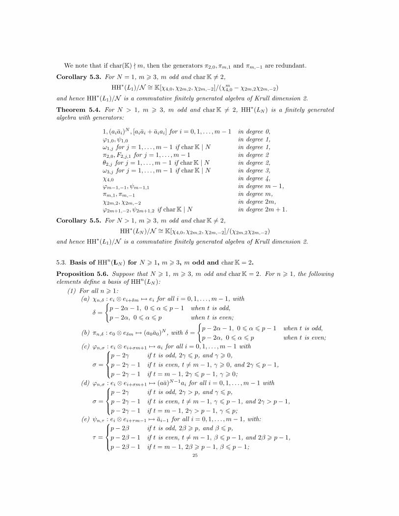
We note that if char(K) ∤ m, then the generators π2,0, πm,1 and πm,−1 are redundant.

Corollary 5.3. For N = 1, m > 3, m odd and char K 6= 2,

HH∗( L1)/N ∼= K[χ4,0, χ2m,2, χ2m,−2]/(χm4,0 − χ2m,2χ2m,−2)

and hence HH∗( L1)/N is a commutative finitely generated algebra of Krull dimension 2.

Theorem 5.4. For N > 1, m > 3, m odd and char K 6= 2, HH∗( LN ) is a finitely generatedalgebra with generators:

1, (aiai)N , [aiai + aiai] for i = 0, 1, . . . ,m− 1 in degree 0,

ϕ1,0, ψ1,0 in degree 1,ω1,j for j = 1, . . . ,m− 1 if char K | N in degree 1,π2,0, F2,j,1 for j = 1, . . . ,m− 1 in degree 2θ2,j for j = 1, . . . ,m− 1 if char K | N in degree 2,ω3,j for j = 1, . . . ,m− 1 if char K | N in degree 3,χ4,0 in degree 4,ϕm−1,−1, ψm−1,1 in degree m− 1,πm,1, πm,−1 in degree m,χ2m,2, χ2m,−2 in degree 2m,ϕ2m+1,−2, ψ2m+1,2 if char K | N in degree 2m+ 1.

Corollary 5.5. For N > 1, m > 3, m odd and char K 6= 2,

HH∗( LN )/N ∼= K[χ4,0, χ2m,2, χ2m,−2]/(χ2m,2χ2m,−2)

and hence HH∗( L1)/N is a commutative finitely generated algebra of Krull dimension 2.

5.3. Basis of HHn( LN ) for N > 1, m > 3, m odd and char K = 2.

Proposition 5.6. Suppose that N > 1, m > 3, m odd and char K = 2. For n > 1, the followingelements define a basis of HHn( LN ):

(1) For all n > 1:(a) χn,δ : ei ⊗ ei+δm 7→ ei for all i = 0, 1, . . . ,m− 1, with

δ =

{

p− 2α− 1, 0 6 α 6 p− 1 when t is odd,

p− 2α, 0 6 α 6 p when t is even;

(b) πn,δ : e0 ⊗ eδm 7→ (a0a0)N , with δ =

{

p− 2α− 1, 0 6 α 6 p− 1 when t is odd,

p− 2α, 0 6 α 6 p when t is even;

(c) ϕn,σ : ei ⊗ ei+σm+1 7→ ai for all i = 0, 1, . . . ,m− 1 with

σ =

p− 2γ if t is odd, 2γ 6 p, and γ > 0,

p− 2γ − 1 if t is even, t 6= m− 1, γ > 0, and 2γ 6 p− 1,

p− 2γ − 1 if t = m− 1, 2γ 6 p− 1, γ > 0;

(d) ϕn,σ : ei ⊗ ei+σm+1 7→ (aa)N−1ai for all i = 0, 1, . . . ,m− 1 with

σ =

p− 2γ if t is odd, 2γ > p, and γ 6 p,

p− 2γ − 1 if t is even, t 6= m− 1, γ 6 p− 1, and 2γ > p− 1,

p− 2γ − 1 if t = m− 1, 2γ > p− 1, γ 6 p;

(e) ψn,τ : ei ⊗ ei+τm−1 7→ ai−1 for all i = 0, 1, . . . ,m− 1, with:

τ =

p− 2β if t is odd, 2β > p, and β 6 p,

p− 2β − 1 if t is even, t 6= m− 1, β 6 p− 1, and 2β > p− 1,

p− 2β − 1 if t = m− 1, 2β > p− 1, β 6 p− 1;25

(f) ψn,τ : ei ⊗ ei+τm−1 7→ (aa)N−1ai−1 for all i = 0, 1, . . . ,m− 1, with:

τ =

p− 2β if t is odd, 2β < p, and β > 0,

p− 2β − 1 if t is even, t 6= m− 1, β > 0, and 2β < p− 1,

p− 2β − 1 if t = m− 1, 2β < p− 1, β > −1.

(2) For n even, n > 2:(a) For each j = 0, 1, . . . ,m− 2 and each s = 1, . . . , N − 1:

Fn,j,s :

{

ej ⊗ ej 7→ (aj aj)s,

ej+1 ⊗ ej+1 7→ (ajaj)s;

(b) For each s = 1, . . . , N − 1:

Fn,m−1,s :

{

em−1 ⊗ em−1 7→ (am−1am−1)s,

e0 ⊗ e0 7→ (am−1am−1)s;

(c) Additionally, if char K | N and for each j = 0, 1, . . . ,m− 1: θn,j : ej ⊗ ej 7→ (aj aj)N .(3) For n odd:

(a) For each j = 0, 1, . . . ,m− 1 and each s = 1, . . . , N − 1: En,j,s : ej ⊗ ej+1 7→ (aa)saj;(b) For each j = 0, 1, . . . ,m− 1: ωn,j : ej ⊗ ej+1 7→ aj.

5.4. The Hochschild cohomology ring HH∗( L1) for N > 1, m > 3, m odd and char K = 2.

Theorem 5.7. For N = 1, m > 3, m odd and char K = 2, HH∗( L1) is a finitely generated algebrawith generators:

1, aiai for i = 0, 1, . . . ,m− 1 in degree 0,ϕ1,0, ψ1,0 in degree 1,χ2,0 in degree 2,ϕm−1,−1, ψm−1,1 in degree m− 1,χm,1, χm,−1 in degree m.

Corollary 5.8. For N = 1, m > 3, m odd and char K = 2,

HH∗( L1)/N ∼= K[χ2,0, χm,1, χm,−1]/(χm2,0 − χm,1χm,−1)

and hence HH∗( L1)/N is a commutative finitely generated algebra of Krull dimension 2.

Theorem 5.9. For N > 1, m > 3, m odd and char K = 2, HH∗( LN ) is a finitely generatedalgebra with generators:

1, (aiai)N , [aiai + aiai] for i = 0, 1, . . . ,m− 1 in degree 0,

ϕ1,0, ψ1,0 in degree 1,ω1,j for j = 0, 1, . . . ,m− 1 if char K | N in degree 1,χ2,0 in degree 2,ϕm−1,−1, ψm−1,1 in degree m− 1,χm,1, χm,−1 in degree m.

Corollary 5.10. For N > 1, m > 3, m odd and char K = 2,

HH∗(ΛN )/N ∼= K[χ2,0, χm,1, χm,−1]/(χm,1χm,−1)

and hence HH∗( LN )/N is a commutative finitely generated algebra of Krull dimension 2.

6. The Hochschild cohomology ring HH∗( LN ) for m = 2

Recall, from Theorem 3.1, that dim HH0(ΛN ) = 2N + 1. We start with the case N = 1.26

6.1. The case N = 1.

Proposition 6.1. For m = 2 and N = 1,

dim HHn(Λ1) =

{

3 if n = 0,

2(n+ 1) if n 6= 0.

Proposition 6.2. For m = 2 and N = 1, the following elements define a basis of HHn(Λ1) forn > 1.

(1) For n = 2p even, n > 2:(a) For −p 6 α 6 p: χn,α : ei ⊗ ei+2α 7→ (−1)(p+α)iei for i = 0, 1;(b) For −p 6 α 6 p: πn,α : e0 ⊗ e2α 7→ a0a0.

(2) For n = 2p+ 1 odd:(a) For −p− 1 6 γ 6 p: ϕn,γ : ei ⊗ ei+2γ+1 7→ (−1)(p+γ)iai for i = 0, 1;

(b) For −p− 1 6 β 6 p: ψn,β : ei ⊗ ei+2β+1 7→ (−1)(p+β+1)iai+1 for i = 0, 1.

It is straightforward to give liftings of these elements and we omit the details. Further compu-tations enable us to give generators for HH∗(Λ1).

Theorem 6.3. For m = 2 and N = 1, HH∗( L1) is a finitely generated algebra with generators:

1, a0a0, a1a1 in degree 0,ϕ1,0, ϕ1,−1, ψ1,0, ψ1,−1 in degree 1,χ2,0, χ2,1, χ2,−1 in degree 2.

In order to give the structure of the Hochschild cohomology ring modulo nilpotence, it can nowbe verified that 1, χ2,0, χ2,1, χ2,−1 are the non-nilpotent generators of HH∗( L1) and that χ2

2,0 =χ2,1χ2,−1. This gives the following result.

Corollary 6.4. For m = 2 and N = 1,

HH∗( L1)/N ∼= K[χ2,0, χ2,1, χ2,−1]/(χ22,0 − χ2,1χ2,−1)

with χ2,0, χ2,1, χ2,−1 all in degree 2. Thus HH∗( L1)/N is a commutative finitely generated algebraof Krull dimension 2.

6.2. The case N > 1. We start by giving a basis of cocycles for each cohomology group, togetherwith a lifting for each basis element. We shall use once more the notation 〈n〉 ∈ {0, 1, . . . ,m− 1}for the representative of n modulo m.

Proposition 6.5. For m = 2 and N > 1,

dim HHn(ΛN ) =

2N + 1 if n = 0,

2N + 2n if n > 1 and char K ∤ N ,

2N + 2n+ 1 if n > 1 and char K | N .

Proposition 6.6. For m = 2, N > 1 and for each n > 1, we give a basis for the cohomologygroup HHn(ΛN ) together with a lifting for each basis element.

(1) For n even, n > 2:• For −p 6 α 6 p:

⋄ χn,α : ei ⊗ ei+2α 7→ (−1)(n2−α)iei for i = 0, 1,

27

⋄ Lqχn,α(ei ⊗ ei+q−2ℓ+2α) =

(−1)(n2−α)iei ⊗ ei+q−2ℓ if (q − 2ℓ)α > 0

0 if (q − 2ℓ)α < 0 and |q − 2ℓ| > 2

(−1)(n2−α)i(aa)N−1ei ⊗ ei+2(aa)N−1 if α < 0 and q − 2ℓ = 2

(−1)(n2−α)i(aa)N−1ei ⊗ ei−2(aa)N−1 if α > 0 and q − 2ℓ = −2

(−1)(n2−α)i

[

∑N−1k=0 (aa)kei ⊗ ei+1(aa)N−k−1+

(−1)q+1

2

∑N−2k=0 (aa)kae〈i+1〉 ⊗ e〈i+1〉−1a(aa)N−k−2

]

if α < 0 and q − 2ℓ = 1

(−1)(n2−α)i

[

∑N−1k=0 (aa)kei ⊗ ei−1(aa)N−k−1+

(−1)q+1

2

∑N−2k=0 (aa)kae〈i−1〉 ⊗ e〈i−1〉+1a(aa)N−k−2

]

if α > 0 and q − 2ℓ = −1

for i = 0, 1 and 0 6 ℓ 6 q.• For −p 6 α 6 p:⋄ πn,α : e0 ⊗ e2α 7→ (a0a0)N ,

⋄ Lqπn,α(e0 ⊗ eq−2ℓ+2α) =

(aa)Ne0 ⊗ eq−2ℓ if α(q − 2ℓ) > 0

(aa)Ne0 ⊗ e1(aa)N−1 if q − 2ℓ = 1 and α < 0

(aa)Ne0 ⊗ e−1(aa)N−1 if q − 2ℓ = −1 and α > 0

0 otherwisefor all 0 6 ℓ 6 q.

• For each 1 6 s 6 N − 1:

⋄ Fn,0,s :

{

e0 ⊗ e0 7→ (a0a0)s

e1 ⊗ e1 7→ (−1)n2 (a0a0)s,

⋄ LqFn,0,s :

{

e0 ⊗ eq−2ℓ 7→ (a0a0)se0 ⊗ eq−2ℓ

e1 ⊗ e1+q−2ℓ 7→ (−1)n2 (a0a0)se1 ⊗ e1+q−2ℓ,

for all 0 6 ℓ 6 q.• For each 1 6 s 6 N − 1:

⋄ Fn,1,s :

{

e1 ⊗ e1 7→ (a1a1)s

e0 ⊗ e0 7→ (−1)n2 (a1a1)s,

⋄ LqFn,1,s :

{

e1 ⊗ e1+q−2ℓ 7→ (a1a1)se1 ⊗ e1+q−2ℓ

e0 ⊗ eq−2ℓ 7→ (−1)n2 (a1a1)se0 ⊗ eq−2ℓ,

for all 0 6 ℓ 6 q.• Additionally for char K | N :⋄ θn : e1 ⊗ e1 7→ (a1a1)N ,⋄ Lqθn : e1 ⊗ e1+q−2ℓ 7→ (a1a1)Ne1 ⊗ e1+q−2ℓ for all 0 6 ℓ 6 q.

(2) For n odd:• For −p− 1 6 γ < 0:

⋄ ϕn,γ : ei ⊗ ei+2γ+1 7→ (−1)(n−1

2−γ)iai(aa)N−1 for i = 0, 1,

⋄ Lqϕn,γ(ei⊗ei+2γ+1+q−2ℓ) =

0 if q − 2ℓ > 1

−(−1)(n−1

2−γ)i(aa)N−1ei ⊗ ei+1a(aa)N−1 if q − 2ℓ = 1

(−1)(n−1

2−γ)iei ⊗ ei+q−2ℓa(aa)N−1 if q − 2ℓ 6 0

for i = 0, 1 and for all 0 6 ℓ 6 q.• For 0 6 γ 6 p :

⋄ ϕn,γ : ei ⊗ ei+2γ+1 7→ (−1)(n−1

2−γ)iai for i = 0, 1,

28

⋄ If γ > 0, then Lqϕn,γ(ei ⊗ ei+2γ+1+q−2ℓ) =

(−1)q+( n−1

2−γ)iei ⊗ ei+q−2ℓa if q − 2ℓ > 0

−(−1)q+( n−1

2−γ)i

[

N−1∑

k=0

(aa)kei ⊗ ei−1(aa)N−k−1a+

(−1)q+1

2

N−2∑

k=0

(aa)kae〈i−1〉 ⊗ e〈i−1〉+1(aa)N−k−1

]

if q − 2ℓ = −1

(−1)q+( n−1

2−γ)i(aa)N−1ei ⊗ ei−2(aa)N−1a if q − 2ℓ = −2

0 if q − 2ℓ < −2for i = 0, 1 and for all 0 6 ℓ 6 q.

⋄ If γ = 0, then Lqϕn,0(ei ⊗ ei+1+q−2ℓ) =

(−1)q+ n−1

2iei ⊗ ei+q−2ℓa if q − 2ℓ = q

(−1)q+ n−1

2i[

ei ⊗ ei+q−2ℓa− (−1)q(N − 1)ei ⊗ ei+q−2ℓ+2a(aa)N−1]

if 0 6 q − 2ℓ < q

(−1)q+ n−1

2iNei ⊗ ei+q−2ℓa(aa)N−1 if q − 2ℓ < −1

(−1)1+n−1

2i

{

N−1∑

k=1

k−1∑

v=0

[

(aa)vei ⊗ ei+1a(aa)N−v−1+

(−1)q+1

2 (aa)vae〈i+1〉 ⊗ e〈i+1〉−1(aa)N−v−1+

(−1)q+1

2 (aa)v ae〈i−1〉 ⊗ e〈i−1〉+1(aa)N−v−1+

(aa)vei ⊗ ei−1a(aa)N−v−1]

+N−1∑

k=0

(aa)kei ⊗ ei−1a(aa)N−k−1

}

if q − 2ℓ = −1

for i = 0, 1 and for all 0 6 ℓ 6 q.• For 0 6 β 6 p:

⋄ ψn,β : ei ⊗ ei+2β+1 7→ (−1)(n+1

2−β)ia(aa)N−1,

⋄ Lqψn,β(ei⊗ei+2β+1+q−2ℓ) =

0 if q − 2ℓ < −1

(−1)(n+1

2−β)i(aa)N−1ei ⊗ ei−1a(aa)N−1 if q − 2ℓ = −1

(−1)(n+1

2−β)iei ⊗ ei+q−2ℓa(aa)N−1 if q − 2ℓ > −1

for i = 0, 1 and for all 0 6 ℓ 6 q.• For −p− 1 6 β < 0:

⋄ ψn,β : ei ⊗ ei+2β+1 7→ (−1)(n+1

2−β)ia,

⋄ If β < −1, then Lqψn,β(ei ⊗ ei+2β+1+q−2ℓ) =

(−1)(n+1

2−β)iei ⊗ ei+q−2ℓa if q − 2ℓ < 1

(−1)(n+1

2−β)i

[

N−1∑

k=0

(aa)kei ⊗ ei+1a(aa)N−k−1+

(−1)q+1

2

N−2∑

k=0

(aa)kae〈i+1〉 ⊗ e〈i+1〉−1(aa)N−k−1

]

if q − 2ℓ = 1

(−1)(n+1

2−β)i(aa)N−1ei ⊗ ei+2(aa)N−1a if q − 2ℓ = 2

0 if q − 2ℓ > 2for i = 0, 1 and for all 0 6 ℓ 6 q.

29

⋄ If β = −1, then Lqψn,−1(ei ⊗ ei−1+q−2ℓ) =

(−1)n−1

2iei ⊗ ei+q−2ℓa if q − 2ℓ = −q

(−1)n−1

2i[

ei ⊗ ei+q−2ℓa− (−1)q(N − 1)ei ⊗ ei+q−2ℓ−2a(aa)N−1]

if −q < q − 2ℓ 6 0

(−1)n−1

2iNei ⊗ ei+q−2ℓa(aa)N−1 if q − 2ℓ > 1

(−1)n−1

2i

{

N−1∑

k=1

k−1∑

v=0

[

(aa)vei ⊗ ei−1a(aa)N−v−1+

(−1)q+1

2 (aa)v ae〈i−1〉 ⊗ e〈i−1〉+1(aa)N−v−1+

(−1)q+1

2 (aa)vae〈i+1〉 ⊗ e〈i+1〉−1(aa)N−v−1+

(aa)vei ⊗ ei+1a(aa)N−v−1]

+

N−1∑

k=0

(aa)kei ⊗ ei+1a(aa)N−k−1

}

if q − 2ℓ = 1

for i = 0, 1 and for all 0 6 ℓ 6 q.• For each j = 0, 1 and each 1 6 s 6 N − 1:⋄ En,j,s : ej ⊗ ej−1 7→ (aa)saj,⋄ LqEn,j,s :

ej ⊗ ej−1 7→ (aa)sej ⊗ ej a if q is even

ej ⊗ ej 7→N−s∑

k=0

N−s∑

v=k

[

(aa)v+sej ⊗ ej−1a(aa)N−v−1+

(−1)q+1

2 (aa)v+saej−1 ⊗ ej(aa)N−v−1]

if q is odd

e〈j−1〉 ⊗ e〈j−1〉 7→ (−1)n−1

2

N−s−1∑

k=0

N−s∑

v=k

[

(−1)q+1

2 (aa)v+saej ⊗ ej+1(aa)N−v−1

+(aa)v+s+1e〈j+1〉 ⊗ e〈j+1〉−1a(aa)N−v−2]

if q is odd

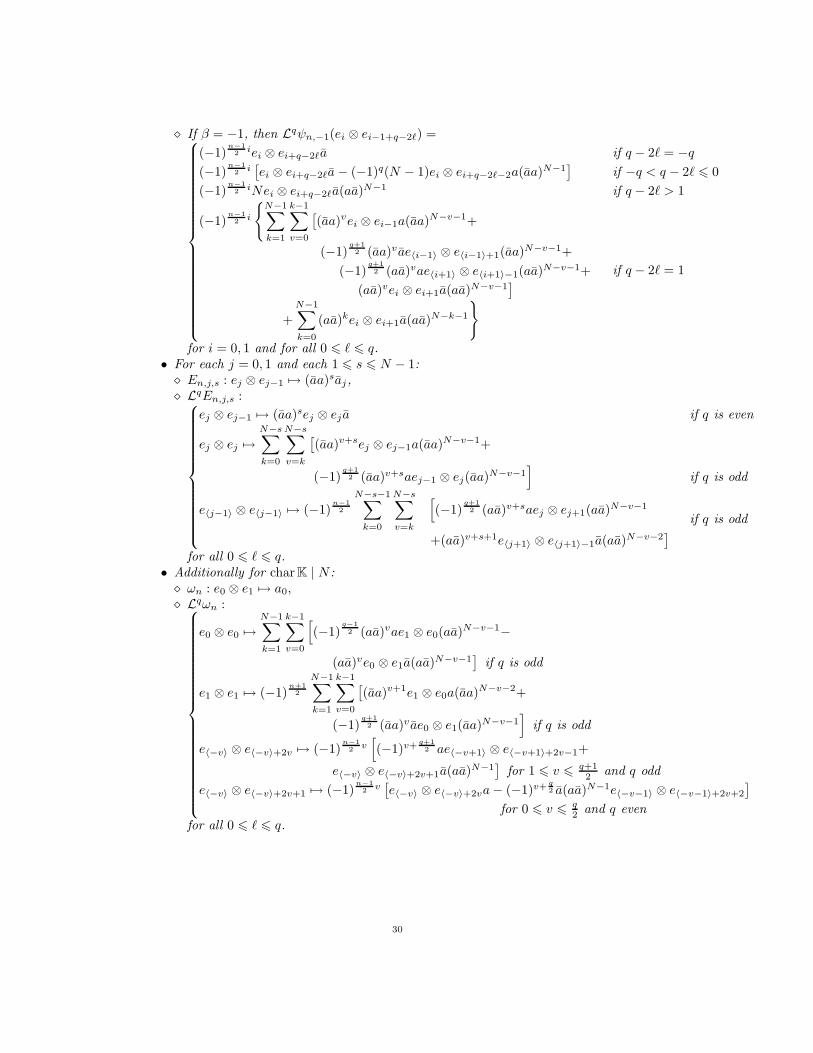
for all 0 6 ℓ 6 q.• Additionally for char K | N :⋄ ωn : e0 ⊗ e1 7→ a0,⋄ Lqωn :

e0 ⊗ e0 7→N−1∑

k=1

k−1∑

v=0

[

(−1)q−1

2 (aa)vae1 ⊗ e0(aa)N−v−1−

(aa)ve0 ⊗ e1a(aa)N−v−1]

if q is odd

e1 ⊗ e1 7→ (−1)n+1

2

N−1∑

k=1

k−1∑

v=0

[

(aa)v+1e1 ⊗ e0a(aa)N−v−2+

(−1)q+1

2 (aa)v ae0 ⊗ e1(aa)N−v−1]

if q is odd

e〈−v〉 ⊗ e〈−v〉+2v 7→ (−1)n−1

2v[

(−1)v+ q+1

2 ae〈−v+1〉 ⊗ e〈−v+1〉+2v−1+

e〈−v〉 ⊗ e〈−v〉+2v+1a(aa)N−1]

for 1 6 v 6q+12 and q odd

e〈−v〉 ⊗ e〈−v〉+2v+1 7→ (−1)n−1

2v[

e〈−v〉 ⊗ e〈−v〉+2va− (−1)v+ q2 a(aa)N−1e〈−v−1〉 ⊗ e〈−v−1〉+2v+2

]

for 0 6 v 6q2 and q even

for all 0 6 ℓ 6 q.

30

Theorem 6.7. For m = 2 and N > 1, HH∗( LN ) is a finitely generated algebra, with generators:

1, (a0a0)N , (a1a1)N , (a0a0 + a0a0), (a1a1 + a1a1) in degree 0,ϕ1,0, ϕ1,−1, ψ1,0, ψ1,−1, E1,0,1 in degree 1,ω1 if char K | N in degree 1,χ2,0, χ2,1, χ2,−1, F2,0,1 in degree 2.

It is easy to verify that the non-nilpotent generators of HH∗( LN ) are 1, χ2,0, χ2,1 and χ2,−1, andthat χ2,1χ2,−1 = 0. Thus we have the following theorem.

Corollary 6.8. For m = 2 and N > 1,

HH∗( LN )/N ∼= K[χ2,0, χ2,1, χ2,−1]/(χ2,1χ2,−1).

Hence HH∗( LN )/N is a commutative finitely generated algebra of Krull dimension 2.

7. The Hochschild cohomology ring HH∗( LN ) for m = 1

We start by giving the centre of the algebra, since HH0( LN ) = Z( LN ).

Theorem 7.1. Suppose that m = 1. Then the dimension of HH0(ΛN ) is N + 3, and a K-basis ofHH0(ΛN ) is given by

{

1, (aa)N , [(aa)s + (aa)s] for 1 6 s 6 N − 1, a(aa)N−1, a(aa)N−1}

.

Thus HH0(ΛN ) is generated as an algebra by

{1, a, a} if N = 1;{

1, (aa)N , [aa+ aa], a(aa)N−1, a(aa)N−1}

if N > 1.

7.1. The case N = 1. The algebra L1 is a commutative Koszul algebra. The quiver has a singlevertex 1 and two loops a and a such that a2 = 0, a2 = 0, and aa = aa. The structure of theHochschild cohomology ring for L1 with m = 1 was determined in [1]; we state the result here forcompleteness. Note that we have HH0( L1) = L1 in this case.

Theorem 7.2. [1] For m = 1 and N = 1, we have

HH∗( L1) ∼=

{

L1〈u0, u1, x0, x1〉/〈u20, u

21, au0, au1, ax0, ax1〉 if char K 6= 2,

L1[y0, y1] if char K = 2,

where x0, x1 are in degree 2 and u0, u1, y0, y1 are in degree 1.

We remark that we could also have used the Kunneth formula [16, Theorem 7.4 p297] togetherwith HH∗(A), where A = K[x]/(x2). The cohomology of A has been studied in several places inthe literature including in [4, 15].

We can now give the structure of the Hochschild cohomology ring of L1 modulo nilpotence andits Krull dimension.

Corollary 7.3. For m = 1 and N = 1,

HH∗(Λ1)/N ∼=

{

K[x0, x1] if char K 6= 2

K[y0, y1] if char K = 2,

where x0, x1 are in degree 2 and y0, y1 are in degree 1. Hence HH∗(Λ1)/N is a commutative finitelygenerated algebra of Krull dimension 2.

31

7.2. The case N > 1 and char K 6= 2. For the case N > 1 and m = 1 there are two subcases toconsider, depending on whether the characteristic of the field is or is not equal to 2. Firstly wesuppose that char K 6= 2.

Proposition 7.4. For m = 1, N > 1 and char K 6= 2, the dimensions of the Hochschild cohomologygroups are given by dim HH0(ΛN ) = N + 3 and, for n > 1,

dim HHn(ΛN ) =

N + 4n+ 3 if char K = 2,N + n+ 2 if char K 6= 2, char K ∤ N ,N + n+ 2 if char K 6= 2, char K | N , n ≡ 1, 2 (mod 4),N + n+ 3 if char K 6= 2, char K | N , n ≡ 0, 3 (mod 4).

We now describe explicitly the elements of the Hochschild cohomology groups HHn(ΛN ) forn > 1, in order to give a set of generators for HH∗(ΛN ) as a finitely generated algebra. Recallthat HH0(ΛN ) = Z(ΛN) and was described in Theorem 7.1. For each cocycle f ∈ Hom(Pn,ΛN),we continue our practice of writing only the image of each generator ei ⊗ ei+n−2r in Pn wherethat image is non-zero. However, since we have a single vertex, we write 1 for e0, and we use thenotation 1 ⊗r 1 instead of e0 ⊗ en−2r for the generator of the r-th summand ΛNe0 ⊗ en−2rΛN ofPn. (Recall that r = 0, . . . , n.) This notation ensures that, in this single idempotent case m = 1,we continue to avoid any confusion as to which summand of Pn we are referring.

Proposition 7.5. Suppose that m = 1, N > 1 and char K 6= 2. The following elements define abasis of HHn(ΛN ) for n > 1.

(1) For all n > 1 and 0 6 r 6 n with r even: χn,r : 1 ⊗r 1 7→ 1.(2) For n even, n > 2:

(a) ψn,0 : 1 ⊗0 1 7→ a(aa)N−1;(b) ϕn,n : 1 ⊗n 1 7→ a(aa)N−1;(c) For 1 6 r 6 n and r odd: πn,r : 1 ⊗r 1 7→ (aa)N ;(d) For each s such that 1 6 s 6 N − 1: Fn,s : 1 ⊗n/2 1 7→ (aa)s + (−1)

n2 (aa)s;

(e) Additionally, for char K | N , if n ≡ 0 (mod 4): θn : 1 ⊗n/2 1 7→ (aa)N .(3) For n odd:

(a) For 0 6 r 6 n−12 and r even: ϕn,r : 1 ⊗r 1 7→ a;

(b) For n+12 6 r 6 n− 1 and r even: ϕn,r : 1 ⊗r 1 7→ (aa)N−1a;

(c) For 1 6 r 6 n−12 and r odd: ψn,r : 1 ⊗r 1 7→ (aa)N−1a;

(d) For n+12 6 r 6 n and r odd: ψn,r : 1 ⊗r 1 7→ a;

(e) πn,+ : 1 ⊗0 1 7→ (aa)N ;(f) πn,− : 1 ⊗n 1 7→ (aa)N ;(g) For each s such that 1 6 s 6 N − 1: En,s : 1 ⊗(n−1)/2 1 7→ (aa)sa.

(h) Additionally, for char K | N , if n ≡ 3 (mod 4) and r = n+12 : ψn,r : 1 ⊗r 1 7→ a.

We omit the liftings for this case, since the calculations are straightforward, and give generatorsof the Hochschild cohomology ring.

Theorem 7.6. For m = 1, N > 1, char K 6= 2, HH∗( LN ) is a finitely generated algebra withgenerators:

1, aa+ aa, a(aa)N−1, a(aa)N−1, (aa)N in degree 0,ϕ1,0, ψ1,1 in degree 1,χ2,0, χ2,2, π2,1, F2,1, ϕ2,2, ψ2,2 in degree 2,ϕ3,2, ψ3,1 in degree 3,ψ3,2 if char K | N in degree 3,χ4,2, F4,1 in degree 4.

32

The non-nilpotent generators of HH∗(ΛN ) are precisely those elements given in the above theo-rem whose image does not lie in r, that is, the elements 1, χ2,0, χ2,2 and χ4,2. This gives the nextresult.

Corollary 7.7. For m = 1, N > 1 and char K 6= 2,

HH∗(ΛN )/N ∼= K[χ2,0, χ2,2, χ4,2]/(χ2,0χ2,2).

Hence HH∗(ΛN )/N is a commutative finitely generated algebra of Krull dimension 2.

7.3. The case N > 1 and char K = 2. In this final case, we continue to keep the notation that1 ⊗r 1 = e0 ⊗ en−2r for r = 0, 1, . . . , n.

Proposition 7.8. For m = 1, N > 1 and char K = 2, then dim HHn( LN ) = 4n + N + 3 for alln > 0.

Proposition 7.9. Suppose that m = 1, N > 1 and char K = 2. For n > 0, the following elementsdefine a basis of HHn( LN ).

(1) For all n > 0:(a) For r = 0, . . . , n: χn,r : 1 ⊗r 1 7→ 1;(b) For r = 0, . . . , n: πn,r : 1 ⊗r 1 7→ (aa)N .

(2) For n even, n > 2:(a) For r = 0, 1, . . . n−2

2 : ϕn,r : 1 ⊗r 1 7→ a;

(b) For r = n2 , . . . , n− 1, n: ϕn,r : 1 ⊗r 1 7→ (aa)N−1a;

(c) For r = 0, 1, . . . , n2 : ψn,r : 1 ⊗r 1 7→ (aa)N−1a;

(d) For r = n+22 , . . . , n− 1, n: ψn,r : 1 ⊗r 1 7→ a;

(e) For j = 1, . . . , N − 1: Fn,j : 1 ⊗n/2 1 7→ (aa)j + (aa)j.(3) For n odd:

(a) For r = 0, 1, . . . n−12 : ϕn,r : 1 ⊗r 1 7→ a;

(b) For r = n+12 , . . . , n− 1, n: ϕn,r : 1 ⊗r 1 7→ (aa)N−1a;

(c) For r = 0, 1, . . . , n−12 : ψn,r : 1 ⊗r 1 7→ (aa)N−1a;

(d) For r = n+12 , . . . , n− 1, n: ψn,r : 1 ⊗r 1 7→ a;

(e) For j = 1, . . . , N − 1: En,j : 1 ⊗n+1

2

1 7→ a(aa)j.

Again we omit the details of the liftings, and state directly the generators of HH∗( LN ).

Theorem 7.10. For m = 1, N > 1 and char K = 2, the Hochschild cohomology ring HH∗( LN ) isfinitely generated as a K-algebra with generators

1, aa+ aa, (aa)N−1a, (aa)N−1a, (aa)N in degree 0,χ1,0, χ1,1, ϕ1,0, ψ1,1 in degree 1,χ2,1, ψ2,2 in degree 2.

Corollary 7.11. For m = 1, N > 1 and char K = 2,

HH∗( LN )/N ∼= K[χ1,0, χ1,1, χ2,1]/(χ1,0χ1,1)2.

Thus HH∗( LN )/N is a commutative ring of Krull dimension 2.

33

8. Summary

In conclusion we have the following theorem.

Theorem 8.1. For all N > 1 and m > 1, HH∗( LN ) is a finitely generated K-algebra. MoreoverHH∗( LN )/N is a finitely generated K-algebra of Krull dimension 2.

In particular the theorem holds for the algebras L1 which occur in the representation theory ofthe Drinfeld doubles of the generalised Taft algebras ([6]), and for the algebras of Farnsteiner andSkowronski ([8]). Moreover the conjecture of [18] has been proved for this class of algebras.

We conclude the paper by recalling the following simultaneous conditions which were consideredin [7]:(Fg1) There is a commutative Noetherian graded subalgebra H of HH∗( L1) such that H0 =HH0( L1).(Fg2) Ext∗ L1

( L1/r, L1/r) is a finitely generated H-module.

In the case N = 1, it is immediate from the above results that the algebras L1 satisfy thecondition (Fg1) with H = HHev( L1). We know that L1 is a Koszul algebra with Ext∗ L1

( L1/r, L1/r)

being the Koszul dual of L1. Hence Ext∗ L1( L1/r, L1/r) = KQ/T where Q is the quiver of L1 and T

is the ideal of KQ generated by aiai + ai−1ai−1 for all i = 0, 1, . . . ,m− 1. It may be verified thatthe condition (Fg2) also holds with H = HHev( L1), the full details being left to the reader.

The conjecture of [18] concerning the finite generation of the Hochschild cohomology ring modulonilpotence was motivated by the work on support varieties. The fact that L1, which is self-injective,and H = HHev( L1) together satisfy (Fg1) and (Fg2) means that the support varieties for finitelygenerated L1-modules satisfy all the properties of [18] and the subsequent work of [7] on self-injective algebras.

Acknowledgements

The authors thank Karin Erdmann for all her helpful comments and valuable suggestions onthis paper.

References

[1] Buchweitz, R.-O., Green, E.L., Madsen, D. and Solberg, Ø., Finite Hochschild cohomology without finite global

dimension, Math. Res. Lett. 12 (2005), 805-816.[2] Buchweitz, R.-O., Green, E.L., Snashall, N. and Solberg, Ø., Multiplicative structures for Koszul algebras,

Quart. J. Math. (to appear).[3] Butler, M.C.R and King, A.D., Minimal resolutions of algebras, J. Algebra 212 (1999), 323-362.[4] Cibils, C., Hochschild cohomology algebra of radical square zero algebras, Algebras and modules, II (Geiranger,

1996), 93-101, CMS Conf. Proc., 24, Amer. Math. Soc., Providence, RI, 1998.[5] Chin, W. and Krop, L., Representation theory of liftings of quantum planes, arXiv:0712.1078.[6] Erdmann, K., Green, E.L., Snashall, N. and Taillefer, R., Representation theory of the Drinfeld doubles of a

family of Hopf algebras, J. Pure Appl. Algebra 204 (2006), 413-454.[7] Erdmann, K., Holloway, M., Snashall, N., Solberg, Ø. and Taillefer, R., Support varieties for selfinjective

algbras, K-Theory 33 (2004), 67-87.[8] Farnsteiner, R. and Skowronski, A., Classification of restricted Lie algebras with tame principal block, J. Reine

Angew. Math. 546 (2002), 1-45.[9] Farnsteiner, R. and Skowronski, A., The tame infinitesimal groups of odd characteristic, Adv. Math. 205

(2006), 229-274.[10] Green, E.L., Hartman, G., Marcos E.N. and Solberg, Ø., Resolutions over Koszul algebras, Archiv der Math.

85 (2005), 118-127.[11] Green, E.L. and Snashall, N., Projective bimodule resolutions of an algebra and vanishing of the second

Hochschild cohomology group, Forum Math. 16 (2004), 17-36.[12] Green, E.L., Snashall, N. and Solberg, Ø., The Hochschild cohomology ring modulo nilpotence of a monomial

algebra, J. Algebra Appl. 5 (2006), 153-192.

34

[13] Green, E.L., Solberg, Ø. and Zacharia, D., Minimal projective resolutions, Trans. Amer. Math. Soc. 353 (2001),2915-2939.

[14] Happel, D., Hochschild cohomology of finite-dimensional algebras, Springer Lecture Notes in Mathematics 1404

(1989), 108-126.[15] Locateli, A.C. Hochschild cohomology of truncated quiver algebras, Comm. Algebra 27 (1999), 645-664.[16] MacLane, S., Homology, Classics in Mathematics, Springer-Verlag, 1995.[17] Patra, M.K., On the structure of nonsemisimple Hopf algebras, J. Phys. A Math. Gen. 32 (1999), 159-166.[18] Snashall, N. and Solberg, Ø., Support varieties and Hochschild cohomology rings, Proc. London Math. Soc. 88

(2004), 705-732.[19] Suter, R., Modules for Uq(sl2), Comm. Math. Phys. 163 (1994), 359-393.[20] Xiao, J., Finite-dimensional representations of Ut(sl(2)) at roots of unity, Can. J. Math. 49 (1997), 772-787.

Nicole Snashall, Department of Mathematics, University of Leicester, University Road, Leicester,

LE1 7RH, England

E-mail address: N.Snashall@mcs.le.ac.uk

Rachel Taillefer, Laboratoire de Mathematiques, Faculte des Sciences et Techniques, 23 Rue Doc-

teur Paul Michelon, 42023 Saint-Etienne Cedex 2, France

E-mail address: rachel.taillefer@univ-st-etienne.fr

35