arX

iv:0

807.

2047

v3 [

cs.C

V]

16

Jul 2

008

The Five Points Pose Problem : A New and

Accurate Solution Adapted to any Geometric

Configuration

Mahzad Kalantari a,b,c, Franck Jungd, Jean-Pierre Guedonb,c andNicolas Paparoditisa

aMATIS Laboratory, Institut Geographique National2, Avenue Pasteur. 94165 Saint-Mande Cedex - FRANCE - firstname.lastname@ign.fr

b Institut Recherche Communications Cybernetique de Nantes (IRCCyN) UMRCNRS 6597

1, rue de la Noe BP 92101F-44321 Nantes Cedex 03 - FRANCEc Institut de Recherche sur les Sciences et Techniques de la Ville CNRS FR 2488

d DDE - Seine Maritime - firstname.lastname@equipement.gouv.fr

Abstract. The goal of this paper is to estimate directly the rotationand translation between two stereoscopic images with the help of fivehomologous points. The methodology presented does not mix the ro-tation and translation parameters, which is comparably an importantadvantage over the methods using the well-known essential matrix. Thisresults in correct behavior and accuracy for situations otherwise knownas quite unfavorable, such as planar scenes, or panoramic sets of im-ages (with a null base length), while providing quite comparable resultsfor more ”standard” cases. The resolution of the algebraic polynomialsresulting from the modeling of the coplanarity constraint is made withthe help of powerful algebraic solver tools (the Grobner bases and theRational Univariate Representation).

1 Introduction

The determination of the relative orientation between two cameras with the helpof homologous points is the basis of many applications in the domains of pho-togrammetry and computer vision. The configuration often called ”minimal caseproblem” takes the intrinsic parameters (i. e. the elements of calibration) of thecamera as a priori known. Then only five points homologous are necessary toestimate the remaining three unknowns of rotation and two ones of translation(up to a scale factor). This problem has been dealt by many authors, and mostof recent methods published provide a resolution based on the properties of theessential matrix. Even if its use simplifies remarkably the problem of the relativeorientation, in some cases, due to the fact that all parameters of rotation andtranslation are mixed, this is the origin of geometric ambiguousnesses. So as toimprove this point, we propose in this article a model that separates completelythe rotation and the translation unknowns. We show that the major advan-tage of this model is that it allows to solve degenerate problems such as pure

2 Authors Suppressed Due to Excessive Length

rotations (null translation). We use an algebraic modeling for the coplanarityconstraint, through a system of polynomial equations. We solve them with thehelp of powerful algebraic solver tools, the Grobner bases and the Rational Uni-variate Representation. So as to assess this new approach, three cases have beenprocessed: a classical case, a planar scene, and a case where the base length isclose to zero. We will see that the new method is still accurate even for the lasttwo cases - quite unfavorable - configurations. We will also compare with theStewenius’s algorithm and see that in planar scenes the new algorithm is moreaccurate. An evaluation on real scenes will finally be presented.

2 Historical background of the five points relative pose

problem.

It was for the first time demonstrated by Kruppa [1] in 1913 that the directresolution of the relative orientation from 5 points in general contained at most 11solutions. The described method consisted to find all intersections of two curvesof degree 6. Unfortunately, one century ago, this method could not lead to anumerical implementation. Lately in [2], [3], [4], [5] it has been demonstrated thatthe number of solutions is in general equal to 10, including the complex solutions.Triggs [6] has provided a detailed version for a numeric implementation. Philip[7] presented in 1996 a solution using a polynomial of degree 13, and has proposeda numeric method to solve his system. The roots of his polynomial give directlythe relative orientation. Philip has exploited the constraints on essential matrix.Philip’s ideas have been followed in 2004 by Nister [8] who has refined thisalgorithm, has obtained a 10th order polynomial and has given a numericalresolution using a Gauss-Jordan elimination. Since then, number of papers triedto give some improvements to the method of Nister, notably Stewenius [9] thathas provided a polynomial resolution using the Grobner bases. Many papershave proposed some modifications to the method of Nister in view of a numericimprovement [12], [13], or for a simplification of implementation [10], [11].

3 Geometry review of Relative Orientation

In this section we recall the various ways to present the geometry of relativeorientation, that consist in the determination of the translation and the relativerotation between two images of a scene having a common informational part.In general, the position of the first camera is taken as the origin of the systemS1 (Fig. 1) and therefore the position of the second camera (S2) is calculated inrelationship to the first one. O named as the principal point of the camera, f isthe focal length. A is the world point, and the image projection of A on the leftimage is a with coordinates (xa, ya, f)T , and a′ (xa′ , ya′ , f)T in the right image.

The vector of translation−→T (Tx, Ty, Tz) is the basis that relies the optic centers

of the cameras (S1 and S2). R is the relative rotation between the two cameras.A way for modelling the relative orientation is known as condition of coplanarity.

Title Suppressed Due to Excessive Length 3

f f

R

S1 S2

−→

V1−→

V2

a a’

A

Epipolar

Plane

−→

T

xc

yc

O O

Fig. 1. Geometry of relative orientation

This constraint has been often used by the community of computer vision sincethree decades. As pictured in the Fig. 1, the condition of coplanarity between

two images expresses the fact that the vector−→V1, the vector

−→V2(expressed in the

reference of−→V1), and the vector of the translation

−→T are in the same plane, called

the epipolar plane. One can translate this condition by a null value for the tripleproduct between these 3 vectors. In other words:

−→V2 · (R

−→V1 ∧

−→T ) = 0 (1)

4 Algebraic modelling of the five-points problem

In this section, different ways for algebraic modelling of the relative orientationare recalled. The goal is to obtain a polynomial system, so as to use the powerfulmathematical tools developed for solving such systems.The coplanarity constraint (equation 1) under its algebraic shape is expressedby the equation:

[

xa′ ya′ f]

0 Tz −Ty

−Tz 0 Tx

Ty −Tx 0

r11 r12 r13

r21 r22 r23

r31 r32 r33

xa

ya

f

= 0. (2)

In this equation the unknowns are the matrix of rotation R and the translationT . Different ways exist to parameter the system so as to obtain polynomialswith the rotation and the translation as unknowns. In the present part the mainmodelling solutions for the rotation and the translation to be used in this researchare described.

4.1 Modelling of the translation

The translation of unity length between the two centres of the cameras may beunderstood as imaging on the unity sphere its center. The translation has only2 degree of freedom, and for that reason, with the relative orientation, the scalecannot be determined. The equation of the unity sphere is the following :

T 2x + T 2

y + T 2z = 1. (3)

4 Authors Suppressed Due to Excessive Length

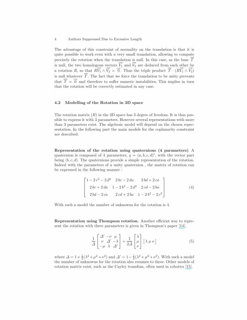
The advantage of this constraint of normality on the translation is that it isquite possible to work even with a very small translation, allowing to compute

precisely the rotation when the translation is null. In this case, as the base−→T

is null, the two homologous vectors−→V1 and

−→V2 are deduced from each other by

a rotation R, so that R−→V1 ∧

−→V2 =

−→0 . Thus the triple product

−→T · (R

−→V1 ∧

−→V2)

is null whatever−→T . The fact that we force the translation to be unity prevents

that−→T =

−→0 and therefore to suffer numeric instabilities. This implies in turn

that the rotation will be correctly estimated in any case.

4.2 Modelling of the Rotation in 3D space

The rotation matrix (R) in the 3D space has 3 degree of freedom. It is thus pos-sible to express it with 3 parameters. However several representations with morethan 3 parameters exist. The algebraic model will depend on the chosen repre-sentation. In the following part the main models for the coplanarity constraintare described.

Representation of the rotation using quaternions (4 parameters) Aquaternion is composed of 4 parameters, q = (a, b, c, d)t, with the vector partbeing (b, c, d). The quaternions provide a simple representation of the rotation.Indeed with the parameters of a unity quaternion , the matrix of rotation canbe expressed in the following manner :

1 − 2 c2 − 2 d2 2 bc − 2 da 2 bd + 2 ca

2 bc + 2 da 1 − 2 b2 − 2 d2 2 cd − 2 ba

2 bd − 2 ca 2 cd + 2 ba 1 − 2 b2 − 2 c2

(4)

With such a model the number of unknowns for the rotation is 4.

Representation using Thompson rotation. Another efficient way to repre-sent the rotation with three parameters is given in Thompson’s paper [14].

1

∆

∆′ −ν µ

ν ∆′ −λ

−µ λ ∆′

+1

2∆

λ

µ

ν

[

λ µ ν]

(5)

where ∆ = 1+ 14 (λ2 +µ2 +ν2) and ∆′ = 1− 1

4 (λ2 +µ2 +ν2). With such a modelthe number of unknowns for the rotation also resumes to three. Other models ofrotation matrix exist, such as the Cayley transfom, often used in robotics [15].

Title Suppressed Due to Excessive Length 5

4.3 Algebraic modelling of the coplanarity constraint

Model with 7 equations With the model of rotation matrix given by equation4, every couple of homologous points (a and a′) gives an equation of the type :

(xa′

i(−Tz(2bc+2da)+Ty(2bd−2ca))+ya′

i(Tz(1−2c2−2d2)−Tx(2bd−2ca))+

za′

i(−Ty(1−2c2−2d2)+Tx(2bc+2da)))xa2+(xa′

i(−Tz(1−2b2−2d2)+Ty(2cd+2ba))+

ya′

i(Tz(2bc−2da)−Tx(2cd+2ba))+za′

i(−Ty(2bc−2da)+Tx(1−2b2−2d2)))ya2+

(xa′

i(−Tz(2cd−2ba)+Ty(1−2b2−2c2))+ya′

i(Tz(2bd+2ca)−Tx(1−2b2−2c2))+

za′

i(−Ty(2bd + 2ca) + Tx(2cd − 2ba)))za2 = 0 (6)

5 couples of points gives 5 equations. It is otherwise necessary to add along withthis equations the constraint of normality on the quaternion, as well as on thetranslation.

T 2x + T 2

y + T 2z = 1, (7)

a2 + b2 + c2 + d2 = 1. (8)

Finally, the unknowns of the system are [a, b, c, d, Tx, Ty, Tz]

Model with 6 equations While using the Thompson rotation matrix, therotation is expressed with 3 parameters. The system will have 6 unknowns,considering the three parameters of translation. The polynomial expressing thecoplanarity constraint for a couple of homologous points, taking for model theThompson rotation, is the following :

(xai(−4Tzν − 2Tzλµ − 4Tyµ + 2Tyλν) + yai(4Tz + Tzλ2 − Tzµ

2 − Tzν2+

4Txµ − 2Txλν) + zai(−4Ty − Tyλ2 + Tyµ2 + Tyν

2 + 4Txν + 2Txλµ))xa′

i+

(xai(−4Tz +Tzλ2−Tzµ

2 +Tzν2 +4Tyλ+2Tyµν)+yai(−4Tzν +2Tzλµ−4Txλ−

2Txµν)+zai(4Tyν−2Tyλµ+4Tx−Txλ2+Txµ2−Txν2))ya′

i+(xai(4Tzλ−2Tzµν

+4Ty −Tyλ2 −Tyµ

2 +Tyν2)+ yai(4Tzµ+2Tzλν −4Tx +Txλ2 +Txµ2−Txν2)+

zai(−4Tyµ − 2Tyλν − 4Txλ + 2Txµν))za′

i = 0 (9)

The constraint of normality on the translation (equation 3) is added to these 5equations. So the system has 6 equations and 6 unknowns [λ, µ, ν, Tx, Ty, Tz].

In conclusion of this section, we have built two polynomial systems, wherethe translation and rotation parameters are distinct and correspond to separatedunknowns. Next, we show how to solve this type of polynomial systems.

5 Resolution of the polynomial systems

The ways to solve the polynomial systems are widely published [16], [17], andare briefly recalled for the reader not familiar with this topic. The resolution

6 Authors Suppressed Due to Excessive Length

of a polynomial system consists in finding the zeros of an algebraic equationsystem such as : P (x) = 0 with P = (p1, p2, .., pn) where pi is a l − variable

polynomial x = (x1, x2, ..., xl) over the field C of complex numbers. Differentstypes of solvers for polynomial equations exist, such as analytic solvers, subdi-vision solvers, geometric solvers, homotopic solvers and algebraic solvers [18]. Inthis paper the focus is on algebraic solvers, that exploit the known relationshipsbetween the unknowns. They subdivide the problem of the resolution into twosteps : the first consists in transforming the system into one or several equivalentsystems, but better adapted, and this constitutes what one will call an algebraicsolution. The second step consists, in the case where one works in one subfieldof the complex field, to calculate the numeric values of the solutions from thealgebraic solution. We will see now briefly the principal tools used in this paperfor solving polynomial systems. But first, some remainders of geometric algebraare necessary.

5.1 Notations

Q [X1, X2, ..., Xn] is the polynomial rings with rational coefficients and unknownsX1, X2, ..., Xn. S = P1, P2, ...Ps is any subset of Q [X1, X2, ..., Xn]. A pointx ∈ Cn is a zero of S if Pi(x) = 0 ∀i = 1, 2, ..., s. The variety of P is the set ofall common complex zeros :

V(P ) = {(a1, ..., an) ∈ Cn : pi(a1, ..., an) = 0 for all 1 ≤ i ≤ s}. (10)

The ideal I generated by a finite set of multivariate polynomials < P1, P2, ..., Ps >

is defined as:

I = {

n∑

i=1

hiPi|hi ∈ Q [X1, X2, ..., Xn]}. (11)

The ideal contains all polynomials which can be generated as an algebraiccombination of its generators. An ideal can be generated by many different setsof generators, which all have the same solutions.

5.2 Construction of the algebraic solver : an introduction to theGrobner bases.

A Grobner basis is a set of multivariate polynomials that has ”nice” algorithmicproperties. Every set of polynomials can be transformed into a Grobner basis.This process generalizes three familiar techniques : the Gauss elimination forsolving linear systems of equations, the Euclidean algorithm for computing thegreatest common divisor of two univariate polynomials, and the Simplex Algo-rithm for linear programming [3]. The Grobner bases were developed initially byB. Buchberger in the years 1960 [19]. The first step, when we want to compute aGrobner basis, is to define an monomial order. For polynomial rings with sever-able variables, there are many possible choices of monomial orders. Some of themost important orders are given in the following definitions.

Title Suppressed Due to Excessive Length 7

Definition 1 Lexicographic Order (Lex)

Xα1

1 ... Xαnn <Lex X

β1

1 ... Xβnn ⇔ ∃ i0 ≤ n ,

{

αi = βi, for i = 1, 2, ..., i0−1

αi0 < βi0

Definition 2 Degree Reverse Lexicographic Order (DRL)

Xα1

1 ... Xαnn <DRL X

β1

1 ... Xβnn ⇔ X

Pαkk

0 X−αn

1 ...X−α1

n <Lex XPβk

k

0 X−βn

1 ...X−β1

n

The DRL ordering, although somewhat nonintuitive, has some interesting com-putational properties.The following terms and notation are present in the literature of Grobner basesand will be useful later on. The degree of a polynomial P , denoted DEG(f), isthe highest degree of the terms in P . The leading term of P , denoted LT (P ), isthe term with the highest degree. The leading coefficient of P denoted LC(P ) isthe coefficient of the leading term in P . Finally Grobner bases can be defined:

Definition 3 Fix a monomial order > on Q [X1, X2, ..., Xn], andlet I ⊂ Q [X1, X2, ..., Xn] be an ideal. A Grobner base for I (with respect to >)is a finite collection of polynomials G = {g1, ..., gt} ⊂ I with the property thatfor every nonzero f ∈ I, LT (f) can be divided by LT (gi) for some i.

Two principal questions immediately arise from this definition :

1. the existence of Grobner bases for any ideal I.Hilbert’s Basis Theorem says that : Every ideal I has a Grobner basis G.Furthermore, I =< g1, ..., gt >.

2. the issue of uniqueness of the Grobner bases.The Buchberger theorem proves that if we fix a term order, then every non-zero ideal I has an unique reduced Grobner basis with respect to this termorder.

There are several possible algorithms to effectively compute Grobner bases. Thetraditional one is Buchbergers algorithm, it has several variants and it is im-plemented in most general computer algebra systems like Maple, Mathematica,Singular [20], Macaulay2 [21], CoCoA [22] and the Salsa Software [23]. In thispaper we use the Salsa Software with the F4 algorithm [24]. The Faugere F4algorithm is based on the intensive use of linear algebra methods.

5.3 Application of Grobner bases for systems solving

Grobner bases (G) give important informations about the initial system of poly-nomial equations. Here some of these informations with their application on the2 systems of polynomials defined in Section 4.2 and Section 4.3 are summarized:

1. Solvability of the polynomial system. It is easy to check if it is possible tosolve the system of polynomials or not with the help of the Grobner bases G.If G = {1}, the system has no solution. We check this on our two systems,and we find that: G 6= {1}. In other terms V is not empty.

8 Authors Suppressed Due to Excessive Length

2. Finite solvability of polynomial equations. It is easy to see whether the systemhas a finite number of complex solutions or not : we just check that for eachi, 1 ≤ i ≤ n, there is an mi ≥ 0 such that xmi

i = LT (g) for some g ∈ G.This type of system is called zero-dimensional system. In this case, the setof solutions does not depend on the chosen algebraically closed field. If weapply this on two systems, we find that the dimension of the two systems iszero. So the set of solutions is finite.

3. Counting number of finite solutions of the polynomial system. One importantinformation is that the Grobner basis also gives the number of solutions ofthe system. If we suppose that the system of polynomial equations P has afinite number of solutions, then the number of solutions is equal to the car-dinality of the set of monomials that are not multiple of the leading termsof the polynomials in the Grobner basis (any term ordering may be chosen).This monomials are called basis monomials or standard monomials (B).For the system of 7 polynomial equations (Section 4.2), the number of thestandard bases is equal to 80. It means that the system has a total of80 complex solutions. This high figure is due to the symmetries of the 2equations of constraints, for example the quaternion Q(a, b, c, d) is equal toQ′(−a,−b,−c,−d). It has been reminded previously in the literature thatthe maximum number of solutions for the essential matrix is 10. Every es-sential matrix gives 4 families of solutions, rotation and translation, whichprovides 40 families of solutions. In the present system, with the symmetryon the quaternion, there are twice more solutions, therefore the total is 80.Using the system of polynomial equations defined in Section 4.3, the stan-dards bases of this system are the following (in the DRL order):

B = [1, Tz, Ty, Tx, ν, µ, λ, T 2z , TyTz, T

2y , TxTz, TxTy, νTz, νTy, νTx, ν2, µTz,

µTy, µTx, uν, µ2, λTz, λTy, λTx, λν, λµ, λ2, T 3z , TyT 2

z , T 2y Tz, TxT 2

z ,

TxTyTz, νT 2z , νTyTz, ν

2Tz, µT 2z , µTyTz, µνTz, λT 2

z , λνTz]

(12)

Which makes a total of 40 bases and therefore 40 solutions. In the present pa-per the Salsa library has been used. It is quite possible to use the resolutionsaccording to Stewenius [9] and [25], but it requires a heavier implementationwork.

5.4 Finding the real roots of the polynomial systems

Once the Grobner basis is calculated, different ways exist to find the roots of thesystem of polynomial equations, e.g. the method that solves the polynomial sys-tems with the help of elimination and lex Grobner basis. Another most popularway to solve polynomial systems is via eigenvalues and eigenvectors, with thehelp of standard monomials [16]. Here the emphasis is put on the other method,called the Rational Univariate Representation (abbreviated by RUR) [26]. Rep-resenting the roots of a system of polynomial equations in the RUR was first

Title Suppressed Due to Excessive Length 9

introduced by Leopold Kronecker [27], but started to be used in computer alge-bra only recently [28], [29], [26]. The RUR is the simplest way for representingsymbolically the roots of a zero-dimensional system without loosing information(multiplicities or real roots) since one can get all the information on the roots ofthe system by solving univariate polynomials. Let P (X) = 0 (< P1, P2, ...Ps >)where Pi ∈ Q [X1, X2, ..., Xn] be a zero-dimensional system with its solutionset V = P−1(0), Rational Univariate Representation of V consists in expressingall the coordinates as functions of the roots of a univariate polynomial such as :

f0(T ) = 0, X1 =f1(T )

q(T ), X2 =

f2(T )

q(T ), ...., Xn =

fn(T )

q(T )(13)

where f0, f1, f2, ..., fn, q ∈ Q [T ] (T is a new variable). Computing a RUR reducesthe resolution of a zero-dimensional system to solving one polynomial with one

variable (ft) and to evaluate n rational fractions (fi(T )q(T ) , i = 1, ..., n) as its roots.

The goal is to compute all the real roots of the system (and only the real roots),providing a numerical approximation with an arbitrary precision (set by theuser) of the coordinates. Many efficients algorithms have been implemented tocalcultate RUR. More details are easily found in the literature, but a completeexplication can be found in [30], [26], [31]. An implementation of the Rouillieralgorithm for RUR computation can be found in the SALSA software [23].

6 Algorithm Outlines

Now, the different steps of our algorithm for the calculation of the relative ori-entation are described.Step 1 : 5 couples of homologous points are randomly selected with the RANSACmethod [32] [33] [34].Step 2 : Build the system of polynomial equations.Step 3 : Solve polynomials system. In the present paper the Salsa library hasbeen used (it is quite possible to use the resolutions according to Stewenius [9]and [25], it requires a heavier implementation work, but has the advantage thata great part of the calculation is made off-line).Step 4 : Identify the solution with a physical sense. The ambiguity resolutionmay be done through the use of a third image [8], but we prefer to be able towork with only two images. It is important to find the ”true” solution in thisvery large set, and it is necessary to inject information bound to the geometryof the scene. We proceed in this way :

– when intersecting the rays relative to all homologous couples of points, onekeeps the solution where the rays cut themselves in front of the image,

– for the 5 randomly selected couples, we calculate the distance to the worldpoints. We keep only the solutions that give a depth superior to the value ofthe normalised baseline, i. e. 1, the other ones being considered as unrealistic,

– the last step consists in selecting the solution which fits with the highestnumber of points. This hypothesis requires of course to have more than

10 Authors Suppressed Due to Excessive Length

five points. Other methods exist to find the good solution among all thoseproduced by the direct resolutions, but in general they consist in using athird image [8].

As an example, Fig. 2 illustrates the different steps. The reference image is inblue frame, all real solutions are presented in green frame, and the final solutionhas a red frame.

Fig. 2. Representation of all real solutions

7 Results and Evaluation

Here we present the results of an experimentation on both synthetic and realdata.

7.1 Experimentation on Synthetic Data

To quantify the performances of the presented method, synthetic data have beensimulated. The parameters used for the simulations, are the same as Nister’sones. The images size is 352 x 288 pixels (CIF). The field of view is 45 degreeswide. The distance to the scene is equal to 1. Several cases have been treated :

1. Simple configuration : the baseline between the 2 images has a length of 0.3,the depth varies from 0 to 2.

Title Suppressed Due to Excessive Length 11

2. Planar Structure and short baseline (0.1) : a degenerate case where all sim-ulated points are on the plane Z = 2.

3. Zero translation : the configuration of the points is the same as in the simpleconfiguration, the main difference is that the baseline length is null.

In each configuration a Gaussian noise with a standard deviation varying between0 and 1 pixel is added. The results are average of 100 times independant experi-ments. For each situation the minimal case only has been treated, correspondingto the minimum number of points required (5). No least square adjustment hasbeen done. The geometry of the different configurations is illustrated in the Fig.3.

Baseline

=0.3

0 < Depth < 21

Z

Baseline

=0.1

2

ZZ

Z

1

1<

Dep

th<

2

20◦

(a) (b) (c)

Fig. 3. (a) Easy condition (b) Planar Condition (c) Zero translational condition

Results in the so-called easy configuration . As a comparison our methodhas been confronted with Stewenius’s one, thanks to the codes that he kindlymade downloadable on his website [35]. This allowed us to use it as a reference forthe algorithm of 5 points. Two sorts of translations have been treated, one in X(sideway motion) and one in Z (forward motion). Our results are mostly similar,even slightly better. Remark: In these simulations, it is important to specify thatthe rotation between the two optical axes is always very well determined. Thedifference between the different methods is the precision of evaluation on theorientation of the base, so this is the assessment that we have used.

Planar Structure and short base . Several surfaces are known as ”dan-gerous” [36] the reason of this appellation is due to the fact that if the pointschosen for the evaluation of the relative orientation are on this kind of surface,the configuration becomes degenerate. In the following, one of the most unfavor-able configurations has been chosen. We note that the method of the 5 pointsof Stewenius is not robust in the sideways motion case. Besides, Sarkis [13] has

12 Authors Suppressed Due to Excessive Length

(a) (b)

Fig. 4. Error on the base orientation (in degree). Easy Case, a) sideway motion. b)forward motion.

shown this weakness of the algorithm, and concluded that it is better in suchcases to use an homography. On the other hand, with the method presented herethis kind of configuration does not lead to any problem.

(a) (b) (c)

Fig. 5. a) Error on the base orientation (in degree) and standard deviation, planar case,sideway motion b) idem, for a forward motion. c) Error on the relative orientation, nonplanar case, null base length.

Results for a null base length Even with a null translation, the rotationis very well defined. This is probably due to the fact that the parameters toestimate in our initial equations are completely separated. The rotation is notmixed with the translation. This may explain why a translation of zero lengthdoes not affect the results. Fig. 5(c).

7.2 Tests on Real Images

So as to test the algorithm presented in section 6, we have used the recentlyavailable image base set up by ISPRS [37] for relative orientation tests. Wehave checked especially our ambiguity resolution so as to find the good physical

Title Suppressed Due to Excessive Length 13

solution. The mean error on the baseline orientation is equal to 5.25◦ and meanerror on the rotation is 1.26◦. At the present time, an average of 20 seconds on a1.65 GHz machine is necessary to get the solution. This time of calculation maybe to improved by using offline resolutions as done by Stewenius.

8 Conclusion

In this paper a new method for the problem of the ”five points pose problem”has been described. The main difference with the previous methods is that therotation and the translation are directly the unknowns of the system. Then wehave shown that with the available tools of geometric algebra, this kind of systemcan be solved. The major advantage, when compared to other methods, is thatit works accurately on all cases of plane scenes, or on couples of images with anull base.

References

1. Kruppa, E.: Zur ermittlung eines objektes aus zwei perspektiven mit innerer ori-entierung. Other (1913) 1939–1948

2. M., D.: Sur deux problemes de reconstruction. Technical Report 882, INRIA (1988)3. Faugeras, O.: Three-Dimensional Computer Vision: A Geometric Viewpoint. MIT

Press (1993)4. Faugeras, O.D., Maybank, S.: Motion from point matches: multiplicity of solutions.

International Journal of Computer Vision 4 (1990) 225–2465. Heyden, A., Sparr, G.: Reconstruction from calibrated cameras-a new proof of

the kruppa-demazure theorem. Journal of Mathematical Imaging and Vision 10

(March 1999) 123–142(20)6. Triggs, B.: Routines for relative pose of two calibrated cameras from 5 points.

Technical report, INRIA (2000)7. Philip, J.: A non-iterative algorithm for determining all essential matrices corre-

sponding to five point pairs. Photogrammetric Record 15 (1996) 589–5998. Nister, D.: An efficient solution to the five-point relative pose problem. IEEE

Transactions on Pattern Analysis and Machine Intelligence 26 (2004) 756–7779. Stewenius, H., Engels, C., Nister, D.: Recent developments on direct relative orien-

tation. ISPRS Journal of Photogrammetry and Remote Sensing 60 (2006) 284–29410. Li, H., Hartley, R.: Five-point motion estimation made easy. (2006) I: 630–63311. Sarkis, M., Diepold, K., Huper, K.: A fast and robust solution to the five-point

relative pose problem using gauss-newton optimization on a manifold. In: IEEEInternational Conference on Accoustics, Speech and Signal Processing (ICASSP).(2007)

12. Batra, D., Nabbe, B., Hebert, M.: An alternative formulation for five point relativepose problem. (2007) 21–21

13. Segvic, M., Schweighofer, G., Pinz, A.: Performance evaluation of the five-pointrelative pose with emphasis on planar scenes. In: Performance Evaluation for Com-puter Vision, Austria, Workshop of the Austrian Association for Pattern Recogni-tion (2007) 33–40

14. Thompson, E.H.: A rational algebraic formulation of the problem of relative ori-entation, photogrammetric record. Photogrammetric Record 3 (1959) 152–159

14 Authors Suppressed Due to Excessive Length

15. Faugere, J., Merlet, J., Rouillier, F.: On solving the direct kinematics problem forparallel robots. Technical Report 5923, INRIA (2006)

16. Cox, D., Little, J., O’Shea, D.: Using Algebraic Geometry. 2 edn. Graduate textsin mathematics. Springer-Verlag New York-Berlin-Paris (2004)

17. Cox, D., Little, J., O’Shea, D.: Ideals, varieties, and algorithms an introduction tocomputational algebraic geometry and commutative algebra. 3 edn. Undergraduatetexts in mathematics. Springer-Verlag New York-Berlin-Paris (2007)

18. Elkadi, M., Mourrain, B.: Introduction la resolution des systemes polynomiaux.Volume 57 of Mathmatiques et Applications. Springer-Verlag (2007)

19. Buchberger, B.: Groebner-Bases: An Algorithmic Method in Polynomial IdealTheory. In Bose, N., ed.: Multidimensional Systems Theory - Progress, Directionsand Open Problems in Multidimensional Systems. Copyright: Reidel PublishingCompany, Dordrecht - Boston - Lancaster, The Netherlands (1985) 184–232

20. Greuel, G.M., Pfister, G., Schonemann, H.: Singular 3.0. A Computer AlgebraSystem for Polynomial Computations, Centre for Computer Algebra, University ofKaiserslautern (2005) http://www.singular.uni-kl.de.

21. Grayson, D.R., Stillman, M.E.: Macaulay 2, a software system for research inalgebraic geometry. (http://www.math.uiuc.edu/Macaulay2/)

22. CoCoATeam: CoCoA: a system for doing Computations in Commutative Algebra.(Available at http://cocoa.dima.unige.it)

23. SALSA: Solvers for algebraic systems and applications.(http://www.inria.fr/recherche/equipes/salsa.en.html)

24. Faugere, J.C.: A new efficient algorithm for computing grobner bases (f4). Journalof Pure and Applied Algebra 139 (1999) 61–88

25. Kukelova, Z., Pajdla, T.: A minimal solution to the autocalibration of radialdistortion. In: CVPR 2007, Minneapolis, USA (2007)

26. Rouillier, F.: On the rational univariate representation. In: International Confer-ence on Polynomial System Solving. (2004) 75–79

27. Kronecker, L.: Werke. Teubner, Leipzig (1895-1931)

28. Rojas, J.M.: Solving degenerate sparse polynomial systems faster. Journal ofSymbolic Computation 28 (1999) 155–186

29. Gonzalez-Vega, L.: Implicitization of parametric curves and surfaces by usingmultidimensional newton formulae. Journal of Symbolic Computation 23 (1997)137–152

30. Ouchi, K., Keyser, J., Rojas, J.M.: The exact rational univariate representationand its application. Technical Report 2003-11-1, Department of Computer Science,3112 Texas A&M University, College Station, TX,77843-3112 (2003)

31. Rouillier, F.: Solving zero-dimensional systems through the rational univariaterepresentation. Journal of Applicable Algebra in Engineering, Communicationand Computing 9 (1999) 433–461

32. Fischler, M., Bolles, R.: Random sample consensus: A paradigm for model fittingwith applications to image analysis and automated cartography. Comm. of theACM 24 (1981) 381–395

33. Hartley, R.I., Zisserman, A.: Multiple View Geometry in Computer Vision. Secondedn. Cambridge University Press, ISBN: 0521540518 (2004)

34. Ma, Y., Soatto, S., Kosecka, J., Sastry, S.: An invitation to 3D vision, from imagesto models. Springer Verlag (2003)

35. Stewenius, H.: Matlab code for the for solving the fivepoint problem.(http://vis.uky.edu/~stewe/FIVEPOINT/)

Title Suppressed Due to Excessive Length 15

36. Philip, J.: Critical point configurations of the 5-, 6-, 7-, and

8-point algorithms for relative orientations. Technical report,

TRITA-MAT, KTH,Sweden (1998)

37. Camillo, H.: Test data sets for automatic image orientation.

http://www.ipf.tuwien.ac.at/car/isprs/test-data/ (2007)