The evolution of large-scale cooperation in human populations
267
THE EVOLUTION OF LARGE-SCALE COOPERATION IN HUMAN POPULATIONS Shakti Lamba Department of Anthropology UCL A thesis submitted for the degree of Doctor of Philosophy 2010
-
Upload
khangminh22 -
Category
Documents
-
view
0 -
download
0
Transcript of The evolution of large-scale cooperation in human populations
THE EVOLUTION OF
LARGE-SCALE COOPERATION
IN HUMAN POPULATIONS
Shakti Lamba
Department of Anthropology
UCL
A thesis submitted for the degree of
Doctor of Philosophy
2010

2
DECLARATION
I, Shakti Lamba, confirm that the work presented in this thesis is my own. Where
information has been derived from other sources, I confirm that this has been indicated in
the thesis.
3
ABSTRACT
Large-scale cooperation between unrelated humans is a major evolutionary puzzle. Natural
selection should favour traits benefiting the self, whereas cooperation entails a cost to self
to benefit another. The work presented in this thesis makes an empirical contribution
towards understanding the evolution of large-scale cooperation in humans.
Theory posits that large-scale cooperation evolves via selection acting on populations
amongst which variation is maintained by cultural transmission. While cross-cultural
variation in cooperation is taken as evidence in support of this theory, most studies
confound cultural and environmental differences between populations. I test and find
support for the hypothesis that variation in levels of cooperation between populations is
driven by differences in demography and ecology rather than culture.
I use economic games and a new ‘real-world’ measure of cooperation to demonstrate
significant variation in levels of cooperation across 21 villages of the same small-scale,
forager society, the Pahari Korwa of central India. Demographic factors explain part of this
variation. Variation between populations of the same cultural group in this study is
comparable in magnitude to that found between different cultural groups in previous studies.
Experiments conducted in 14 of the villages demonstrate that the majority of individuals do
not employ social learning in the context of a cooperative dilemma. Frequency of social
learning varies considerably across populations; I identify demographic factors associated
with the learning strategy individuals employ.
My findings empirically challenge cultural group selection models of large-scale
cooperation; behavioural variation driven by demographic and ecological factors is unlikely
to maintain stable differences essential for selection at the population-level. This calls for
re-interpretation of cross-cultural data sampled from few populations per society;
behavioural variation attributed to ‘cultural norms’ may reflect environmental variation.
The work presented in this thesis emphasises the central role of demography and ecology in
shaping human social behaviour.

4
ACKNOWLEDGEMENTS
I thank the Pahari Korwa for welcoming me into their villages and homes and for their
hospitality. I am indebted to Gangaram Paikra; this study would not have been possible
without his extraordinary help and unfailing support in Chhattisgarh.
The work presented in this thesis has benefited from the input of Ruth Mace, Laura
Fortunato, David Lawson, Heidi Colleran, Tom Currie, Kesson Magid and Fiona Jordan, in
the form of discussion, comments and encouragement. I am grateful to Ruth Mace for
acting as my primary supervisor and to Michael Stewart for acting as my secondary
supervisor.
This research was funded via a Cogito Foundation PhD Studentship, a Cogito Foundation
Research Grant, a Parkes Foundation Small Grant and a UCL Graduate School Research
Grant.
I thank Kundal Singh, Anil Kumar, Laxman Shastri, Narendra Das, Shivcharan Das and
Petrus Lakra for their assistance and company in the field. Many thanks to Tirki Ji and
Chandrabhan Singh for their input on logistics, as well as to Lata Paikra and members of
the organisation Chaupal for looking after me through my stay in Chhattisgarh. I also thank
Karam Vir Lamba and Katharine Balolia for help with entering the data and checking it for
errors, as well as Christian Hennig and Mai Stafford for advice on multilevel analyses, and
Andrew Bevan for advice on GIS analyses.
I am very grateful to Laura Fortunato and David Lawson who provided detailed and
thoughtful comments on a draft of the entire thesis. Many thanks to Gayatri Lamba for
proof-reading the thesis and to Waleed Mohammed for help with formatting.
Above all, I am grateful to my family for their continuing and unfailing love and support
and to Waleed Mohammed for looking after me through it all.
5
CONTENTS
Figures ................................................................................................................................. 11
Tables .................................................................................................................................. 13
Acronyms ............................................................................................................................ 18
Definitions ........................................................................................................................... 19
Chapter 1. Introduction..................................................................................................... 20
1.1 Preamble..................................................................................................................... 20
1. 2 The evolutionary dilemma of cooperation ................................................................ 20
1.3 Solving the dilemma of cooperation .......................................................................... 22
1.3.1 Natural selection in a structured population........................................................ 22
1.3.2 The function of population structure - variance between groups or relatedness
within them ........................................................................................................ 23
1.3.3 Defining relatedness............................................................................................ 25
1.3.4 Generating phenotypic relatedness ..................................................................... 26
1.4 Evolutionary models of cooperation .......................................................................... 27
1.4.1 Kin selection (relatedness by common ancestry)................................................ 27
1.4.2 Green beard and tag-based models (relatedness by assortment)......................... 28
1.4.3 Reciprocity (relatedness by prior interaction)..................................................... 30
1.5. The evolutionary dilemma of large-scale cooperation.............................................. 31
1.6 Solving the dilemma of large-scale cooperation........................................................ 32
1.6.1 Cultural group selection (relatedness by social learning) ................................... 32
1.6.2 The empirical evidence ....................................................................................... 33
1.7 Aims of the thesis....................................................................................................... 37
1.8 Structure of the thesis................................................................................................. 39
CONTENTS
6
Chapter 2. Study populations and methods..................................................................... 40
2.1 Features of a good model system for this study......................................................... 40
2.2 The Pahari Korwa ...................................................................................................... 41
2.2.1 Ethnographic description .................................................................................... 41
2.2.2 Distribution ......................................................................................................... 44
2.2.3 Climate, flora and fauna...................................................................................... 45
2.3 Study site..................................................................................................................... 46
2.3.1 Establishing the field-site.................................................................................... 46
2.3.2 Study set-up......................................................................................................... 47
2.3.2.1 Sampling and logistics ................................................................................. 47
2.3.2.2 Village details............................................................................................... 49
2.4 Methods...................................................................................................................... 55
2.4.1 Behavioural data.................................................................................................. 55
2.4.1.1 Anonymity ................................................................................................... 55
2.4.1.2 Game instructions and testing ...................................................................... 56
2.4.1.3 Administration ............................................................................................. 56
2.4.1.4 Payments ...................................................................................................... 57
2.4.2 Demographic and individual data ....................................................................... 58
2.4.3 Qualitative data ................................................................................................... 64
2.5 Analyses ..................................................................................................................... 64
2.5.1 Data processing ................................................................................................... 64
2.5.2 Multilevel models ............................................................................................... 64
2.5.3 GIS analyses........................................................................................................ 67
Section I. Variation in cooperation across populations .................................................. 68
Chapter 3. Variation in cooperation across populations: evidence from the ultimatum
game................................................................................................................... 69
3.1 Introduction ................................................................................................................ 69
3.1.1 Background and related research ........................................................................ 69
3.1.2 Behavioural measures ......................................................................................... 71
3.2 Results ........................................................................................................................ 72
CONTENTS
7
3.2.1 Proposers ............................................................................................................. 73
3.2.1.1 Do proposer offers vary across populations? ............................................... 73
3.2.1.2 Do properties of populations and/or individuals explain variation in proposer
offers between and within populations?....................................................... 75
3.2.2 Responders .......................................................................................................... 77
3.2.2.1 Does responder behaviour vary across populations? ................................... 77
3.2.2.2 Do self-reported MAOs vary across populations? ....................................... 79
3.2.2.3 Do properties of populations and/or individuals explain variation in self-
reported MAOs between and within populations?....................................... 82
3.2.3 Is proposer behaviour contingent on responder behaviour? ............................... 86
3.3 Discussion .................................................................................................................. 87
3.3.1 Variation in proposer behaviour ......................................................................... 87
3.3.2 Correlates of proposer behaviour ........................................................................ 87
3.3.3 Variation in responder behaviour........................................................................ 89
3.3.4 Self-reported behavioural strategies.................................................................... 91
3.3.5 Discrepancies in proposer and responder behaviour........................................... 92
3.3.6 Concluding remarks ............................................................................................ 93
3.4 Methods...................................................................................................................... 94
3.4.1 Experimental set-up ............................................................................................ 94
3.4.2 Statistical analyses .............................................................................................. 95
Chapter 4. Variation in cooperation across populations: evidence from public goods
games and a ‘real-world’ measure of behaviour ........................................ 97
4.1 Introduction ................................................................................................................ 97
4.1.1 Background and related research ........................................................................ 97
4.1.2 Behavioural measures ......................................................................................... 99
4.2 Results ...................................................................................................................... 101
4.2.1 Do PGG contributions and salt deviations vary across populations? ............... 102
4.2.2 Do properties of populations and/or individuals explain variation in PGG
contribution and salt deviation between and within populations? ................... 105
4.2.3 Is there a correlation between individuals’ PGG contributions and salt
deviations?........................................................................................................ 107
CONTENTS
8
4.3 Discussion ................................................................................................................ 107
4.3.1 Variation in cooperative behaviour................................................................... 107
4.3.2 Correlates of cooperative behaviour ................................................................. 107
4.3.3 A new measure of cooperation.......................................................................... 110
4.3.4 Concluding remarks .......................................................................................... 111
4.4 Methods.................................................................................................................... 112
4.4.1 Public goods game set-up.................................................................................. 112
4.4.2 Salt decisions set-up.......................................................................................... 113
4.4.3 Statistical analyses ............................................................................................ 114
Section II. Social learning in the cooperative domain .................................................. 115
Chapter 5. Social learning in the cooperative domain: evidence from public goods
game experiments........................................................................................... 116
5.1 Introduction .............................................................................................................. 116
5.1.1 Background and related research ...................................................................... 116
5.1.2 Behavioural measures ....................................................................................... 120
5.2 Results ...................................................................................................................... 125
5.2.1 Is there evidence that individuals use information on the MC and HEC in making
their PGG2 contributions?................................................................................ 126
5.2.2. Do the overall frequencies of learning strategies vary? ................................... 130
5.2.3. Does the distribution of learning strategies vary across populations? ............. 132
5.2.4. Are properties of populations and/or individuals associated with the learning
strategies employed by individuals? ................................................................ 139
5.2.5. Do different learning strategies result in the acquisition of different behavioural
traits? ................................................................................................................ 142
5.3 Discussion ................................................................................................................ 146
5.3.1 Evidence for social learning in a cooperative dilemma .................................... 146
5.3.2 Correlates of learning strategies........................................................................ 147
5.3.3 The impact of learning on the distribution of trait variants .............................. 150
5.3.4 Unidentifiable strategies.................................................................................... 151
5.3.5 Concluding remarks .......................................................................................... 152
CONTENTS
9
5.4 Methods.................................................................................................................... 153
5.4.1 Experimental set-up .......................................................................................... 153
5.4.2 Statistical analyses ............................................................................................ 154
Section III. Conclusion .................................................................................................... 156
Chapter 6. Conclusion ..................................................................................................... 157
6.1 Implications for an understanding of the evolution of large-scale cooperation in
humans ...................................................................................................................... 157
6.2 Implications for an understanding of the structure of cultural inheritance systems 163
References ......................................................................................................................... 166
Appendix A. Game Scripts .............................................................................................. 195
A.1 Ultimatum game (UG) ............................................................................................ 195
A.2 Public goods game round 1 (PGG1) ....................................................................... 203
A.3 Salt decision ............................................................................................................ 212
A.4 Public goods game round 2 (PGG2) ....................................................................... 213
Appendix B. Data Sheets ................................................................................................. 218
B.1 Individual data sheet................................................................................................ 218
B.2 Village data sheet .................................................................................................... 222
B.3 Housing data sheet................................................................................................... 225
B.4 Qualitative data sheet .............................................................................................. 226
Appendix C. Statistical Analyses .................................................................................... 229
C.1 UG Proposer offer (Chapter 3, Section 3.2.1) ......................................................... 230
C.1.1 Univariate Models ............................................................................................ 230
C.1.2 Domain-wise models ........................................................................................ 232
C.1.3 Full model fitting summary.............................................................................. 234
C.2 UG Responder MAO (Chapter 3, Section 3.2.2)..................................................... 235
C.2.1 Univariate Models ............................................................................................ 235
CONTENTS
10
C.2.1.1 Normal linear models ................................................................................ 235
C.2.1.2 Ordinal multinomial models...................................................................... 237
C.2.2 Domain-wise models ........................................................................................ 239
C.2.2.1 Normal linear models ................................................................................ 239
C.2.2.2 Ordinal multinomial models...................................................................... 241
C.2.3 Full model fitting summary.............................................................................. 243
C.2.3.1 Normal linear models ................................................................................ 243
C.2.3.2 Ordinal multinomial models...................................................................... 244
C.3 Salt decision and PGG1 contribution (Chapter 4, Section 4.2)............................... 245
C.3.1 Univariate Models ............................................................................................ 245
C.3.2 Domain-wise models ........................................................................................ 247
C.3.3 Full model fitting summary.............................................................................. 249
C.4 PGG2 contribution (Chapter 5, Section 5.2.1) ........................................................ 250
C.4.1 Univariate Models ............................................................................................ 250
C.4.2 Domain-wise models ........................................................................................ 252
C.4.3 Full model fitting summary.............................................................................. 254
C.5 PGG2 learning strategies (Chapter 5, Sections 5.2.3 and 5.2.4) ............................. 255
C.5.1 Univariate Models ............................................................................................ 255
C.5.1.1 Four category classification of learning strategies (payoff copier, conformist,
individualist and unidentifiable) ................................................................ 255
C.5.1.2 Three category classification of learning strategies (social learner,
individualist and unidentifiable) ................................................................ 258
C.5.2 Domain-wise models ........................................................................................ 260
C.5.2.1 Four category classification of learning strategies (payoff copier, conformist,
individualist and unidentifiable) ................................................................ 260
C.5.2.2 Three category classification of learning strategies (social learner,
individualist and unidentifiable) ................................................................ 262
C.5.3 Full model fitting summary.............................................................................. 264
C.5.3.1 Four category classification of learning strategies (payoff copier, conformist,
individualist and unidentifiable) ................................................................ 264
C.5.3.2 Three category classification of learning strategies (social learner,
individualist and unidentifiable) ................................................................ 267
11
FIGURES
2.1 Map of Chhattisgarh...................................................................................................... 44
2.2 Maps of (A) the distribution of the 21 study villages and the town Ambikapur, and (B)
the elevation of the 21 study villages and Ambikapur................................................... 51
3.1 Distributions of UG proposer offers across 21 villages ................................................ 74
3.2 Distributions of UG responder responses across 21 villages ........................................ 78
3.3 Distributions of UG responder MAOs across 16 villages............................................. 81
4.1 Distributions of PGG contributions across 16 villages ............................................... 103
4.2 Distributions of salt deviations across 16 villages ...................................................... 104
5.1 Classification of a player’s learning strategy .............................................................. 124
5.2 Distributions of (A) PGG2 contributions, and (B) PGG1 contributions, across 14
villages.. ....................................................................................................................... 128
5.3 Frequencies of player learning strategies for individuals from 14 villages pooled
together......................................................................................................................... 131
5.4 Distributions of player learning strategies across 14 villages. Figures compare
frequencies of, (A) payoff copiers, conformists, individualists and unidentifiable
individuals, and (B) social learners, individualists and unidentifiable individuals. ... 134
FIGURES
12
5.5 Frequencies of player learning strategies within each village. Figures compare
frequencies of (A) payoff copiers, conformists, individualists and unidentifiable
individuals, and (B) social learners, individualists and unidentifiable individuals...... 141
5.6 Mean contributions to the group pot in the PGG1 and PGG2 pooled across 14 villages
for players with different learning strategies for (A) payoff copiers, conformists,
individualists and unidentifiable individuals respectively, and (B) social learners,
individualists and unidentifiable individuals respectively ........................................... 144

13
TABLES
2.1 Summary statistics of demographic variables for the study populations and the
behavioural measures of cooperation implemented in each village............................... 50
2.2 Village means for basic individual descriptors and residence and migration variables for
participants from each study population.. ...................................................................... 52
2.3 Village means for measures of wealth, market contact and social networks for
participants from each study population.. ...................................................................... 53
2.4 Summary of amenities in each village. .......................................................................... 54
2.5 List of village and individual descriptors included in all analyses. ............................... 60
3.1 Numbers (n) of proposers and responders from each of 21 study villages.................... 72
3.2 (A) Associations of each predictor term (fixed effect) with proposer offers in the null
(intercept only) and full models. (B) Village and individual level variance components
for proposer offer in the null and full models ................................................................ 76
3.3 Numbers (n) of UG responder responses for each of 21 study villages......................... 77
3.4 (A) Associations of each predictor term (fixed effect) with responder MAO in the null
(intercept only) and full models. (B) Village and individual level variance components
for responder MAO in the null and full models ............................................................. 84
3.5 (A) Associations of each predictor term (fixed effect) with the probability of responder
MAO ≤ 10 Indian rupees in the null (intercept only) and full models. (B) Village level
variance and the VPC for the logit (probability of responder MAO ≤ 10 Indian rupees)
in the null and full models.............................................................................................. 85

TABLES
14
3.6 Income-maximising offers (IMO) and mean proposer offers for villages where at least
one offer was rejected. ................................................................................................... 86
4.1 Numbers (n) of PGG players and salt takers from each of 16 study villages .............. 101
4.2 (A) Associations of each predictor term (fixed effect) with salt deviation and PGG
contribution respectively in the null (intercept only) and full models. (B) Village and
individual level variance components for salt deviation and PGG contributions
respectively in the null and full models ....................................................................... 106
5.1 Number of players (n) who played both PGG1 and PGG2 from each of 14 study
villages ......................................................................................................................... 125
5.2 Null model (intercept only) variance components for PGG1 and PGG2 contributions
...................................................................................................................................... 127
5.3 (A) Associations of each predictor term (fixed effect) with PGG2 contribution in the
null (intercept only) and full models. (B) Village and individual level variance
components for PGG2 contribution in the null and full models .................................. 129
5.4 Results of chi-squared tests comparing frequencies of player learning strategies for
individuals from 14 villages pooled together............................................................... 132
5.5A Associations of each predictor term (fixed effect) with the odds of being a payoff
copier, conformist or unidentifiable relative to an individualist respectively, in the null
(intercept only) and full models ................................................................................... 135
5.5B Variance components for the log odds of being a payoff copier, conformist or
unidentifiable relative to an individualist respectively in the null and full models…. 135
TABLES
15
5.6A Associations of each predictor term (fixed effect) with the odds of being a social
learner or unidentifiable relative to an individualist respectively, in the null (intercept
only) and full models ................................................................................................... 137
5.6B Variance components for the log odds of being a social learner or unidentifiable
relative to an individualist respectively in the null and full models………………… 137
5.7 Results of Kruskal-Wallis and Mann-Whitney tests comparing the PGG1 and PGG2
contributions of players with different learning strategies from 14 villages pooled
together......................................................................................................................... 145
C.1 Univariate associations between each predictor term (fixed effect) and UG
offer………………………………………………………………………………… 230
C.2 Multivariate associations between domains of predictor terms (fixed effects) and UG
offer ................................................................................................................... ……232
C.3 Summary of model-fitting process in the fourth stage of analyses for UG offers….234
C.4 Univariate associations between each predictor term and UG MAO.................. …235
C.5 Univariate associations between each predictor term (fixed effect) and logit (probability
of UG MAO Indian Rupees 10+ or below)....................................................... ……237
C.6 Multivariate associations between domains of predictor terms (fixed effects) and UG
MAO ......................................................................................................................... 239
C.7 Multivariate associations between domains of predictor terms (fixed effects) and logit
(probability of UG MAO Indian Rupees 10+ or below)........................................... 241
C.8 Summary of model-fitting process in the fourth stage of analyses for UG MAO
modelled as a continous variable .............................................................................. 243
TABLES
16
C.9 Summary of model-fitting process in the fourth stage of analyses for UG MAO
modelled as an ordinal variable................................................................................. 244
C.10 Univariate associations between each predictor term (fixed effect) and Salt deviation
and PGG1 contribution respectively ......................................................................... 245
C.11 Multivariate associations between domains of predictor terms (fixed effects) and Salt
deviation and PGG1 contribution respectively ......................................................... 247
C.12 Summary of model-fitting process in the fourth stage of analyses for Salt deviation
and PGG1 contributions............................................................................................ 249
C.13 Univariate associations between each predictor term (fixed effect) and PGG2
contribution.. ............................................................................................................. 250
C.14 Multivariate associations between domains of predictor terms (fixed effects) and
PGG2 contribution .................................................................................................... 252
C.15 Summary of model-fitting process in the fourth stage of analyses for PGG2
contribution. .............................................................................................................. 254
C.16 Univariate associations between each predictor term (fixed effect) and the log-odds of
being a payoff copier, conformist or unidentifiable relative to an individualist
respectively ............................................................................................................... 255
C.17 Univariate associations between each predictor term (fixed effect) and the log-odds of
being a social learner or unidentifiable relative to an individualist respectively...... 258
C.18 Multivariate associations between domains of predictor terms (fixed effects) and the
log-odds of being a payoff copier, conformist or unidentifiable relative to an
individualist respectively. ......................................................................................... 260
TABLES
17
C.19 Multivariate associations between domains of predictor terms (fixed effects) and the
log-odds of being a social learner or unidentifiable relative to an individualist
respectively ............................................................................................................... 262
C.20 Summary of model-fitting process in the fourth stage of analyses for payoff copiers,
conformists and unidentifiable individuals, relative to individualists respectively .. 264
C.21 Alternative Block 1 analyses for model-fit summary presented in Table C3.20. .. 266
C.22 Summary of model-fitting process in the fourth stage of analyses for social learners,
and unidentifiable individuals, relative to individualists respectively ...................... 267
18
ACRONYMS
UG Ultimatum game
PGG Public goods game
SD Salt decision
PGG1 Public goods game round 1
PGG2 Public goods game round 2
MAO Minimum acceptable offer
IMO Income maximising offer
HEC Highest earner’s contribution
MC Modal contribution
DIC Deviance information criterion
BCI Bayesian confidence interval
VPC Variance partition coefficient
19
DEFINITIONS
The definitions in this list apply throughout this thesis.
Culture
Information capable of affecting individuals’ phenotypes which they acquire from other
conspecifics by teaching or imitation (Boyd & Richerson 1985).
Social learning / Cultural transmission
The non-genetic transfer of information from one individual to another via mechanisms
such as teaching, imitation and language (Boyd & Richerson 1985; Mesoudi 2009). The
above two terms are used interchangeably.
Cultural group/ ethnic group/society
A group of individuals whose members identify with each other and are recognised as a
group by others on the basis of shared ancestry, language, religion, institutions or other
ethnic traits. The above three terms are used interchangeably. This definition emphasises
that other than when groups are defined on the basis of shared ancestry, the defining traits
of a group are culturally transmitted.
Environment
The ecological and demographic features of an organism’s habitat.
20
CHAPTER 1
INTRODUCTION
1.1 Preamble
At the height of Nazi persecution of the Jews during the Second World War, all 117
inhabitants of a small Dutch village called Nieuwlande resolved that each household would
hide and shelter at least one Jewish person during the German occupation of The
Netherlands. The 117 residents of Nieuwlande are among the 23,226 individuals (as of
January 1st, 2010) on whom the State of Israel has conferred the title of ‘The Righteous
among the Nations’, an honour bestowed on non-Jews who risked their lives to save Jews
from extermination during the Holocaust (Yad Vashem 2010). The honourees include
people from 44 countries.
1.2 The evolutionary dilemma of cooperation
Humans are not always selfish. Helping behaviour is commonplace in most human
societies and, one may argue, it is the very premise of social organisation. The degree and
scale of helping may vary across human populations, but its ubiquity is unequivocal. What
makes widespread and frequent helping behaviour so remarkable? More often than not,
extending help to another individual imposes an immediate cost on the helper, be this in
terms of material resources, time or energy. The term cooperation refers to such instances
of costly helping. The preamble in Section 1.1 demonstrates the magnitude of the costs that
individuals are willing to bear for the sake of others, as well as the scale and universality of
cooperation in humans. Inhabitants of an entire village extended help to individuals who
were not even members of their families; this large-scale cooperation entailed a high risk of
1.2 THE EVOLUTIONARY DILEMMA OF COOPERATION
21
death, arguably the greatest cost an individual can incur. Moreover, the behaviour of the
residents of Nieuwlande was not unique; thousands of individuals from across 44 nations
took the same risk.
Natural selection should favour traits that increase the fitness of an organism (Li 1967;
Price 1970; Robertson 1966), where fitness represents the lifetime number of offspring an
organism produces. Assuming that costs and benefits from behaviour translate into fitness
losses and gains respectively, cooperation by definition entails an apparent reduction in the
immediate fitness of an organism. The evolution of cooperation thus presents an inherent
dilemma – how does natural selection favour the cooperative trait that decreases the
immediate fitness of an organism?
This thesis contributes towards an understanding of the evolution of large-scale cooperation
in human populations. I begin, in Section 1.3, by outlining a unifying theoretical framework
that can be used to study the evolution of cooperation across species. Within this
framework, in Section 1.4 I review the principal theoretical models of the evolution of
cooperation (excluding large-scale cooperation) and the empirical evidence in support of
these models in humans. In Section 1.5 I provide a definition of large-scale cooperation as
regarded in this thesis, and explain why the theoretical models described in Section 1.4 do
not provide a satisfactory explanation for its evolution in humans. In Section 1.6 I review
the theoretical models proposed to explain the evolution of large-scale cooperation in
humans, and identify the empirical questions that must be addressed for these models to
find support in nature. In Section 1.7 I define the aims of this thesis in light of the empirical
questions identified in Section 1.6. Finally, Section 1.8 provides an outline of the structure
of the thesis.
1.3 SOLVING THE DILEMMA OF COOPERATION
22
1.3 Solving the dilemma of cooperation
In this section I outline a unifying theoretical framework that can be used to study the
evolution of cooperation across species.
1.3.1 Natural selection in a structured population
Evolution by natural selection is characterised by a change in trait frequency from one
generation to the next (Darwin 1859) when the trait under selection affects the survival or
reproduction of its bearers. A solution to the evolutionary dilemma of cooperation must
therefore explain how an individually costly cooperative trait increases in frequency in a
population when competing with an individually advantageous selfish trait. An appropriate
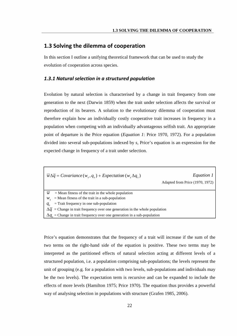
point of departure is the Price equation (Equation 1: Price 1970, 1972). For a population
divided into several sub-populations indexed by s, Price’s equation is an expression for the
expected change in frequency of a trait under selection.
Equation 1
Adapted from Price (1970, 1972)
w = Mean fitness of the trait in the whole population
ws = Mean fitness of the trait in a sub-population
qs = Trait frequency in one sub-population
q = Change in trait frequency over one generation in the whole population
qs = Change in trait frequency over one generation in a sub-population
Price’s equation demonstrates that the frequency of a trait will increase if the sum of the
two terms on the right-hand side of the equation is positive. These two terms may be
interpreted as the partitioned effects of natural selection acting at different levels of a
structured population, i.e. a population comprising sub-populations; the levels represent the
unit of grouping (e.g. for a population with two levels, sub-populations and individuals may
be the two levels). The expectation term is recursive and can be expanded to include the
effects of more levels (Hamilton 1975; Price 1970). The equation thus provides a powerful
way of analysing selection in populations with structure (Grafen 1985, 2006).
)(),( ssss qwnExpectatioqwCovarianceqw
1.3 SOLVING THE DILEMMA OF COOPERATION
23
The Price equation contains within it a schema for the evolution of cooperation: an
individually costly cooperative trait may increase in frequency if its positive payoff at a
higher level of selection in a structured population exceeds its cost at a lower level. Natural
selection acting at multiple levels of a structured population may therefore be key to the
evolution of cooperation.
1.3.2 The function of population structure - variance between groups or
relatedness within them
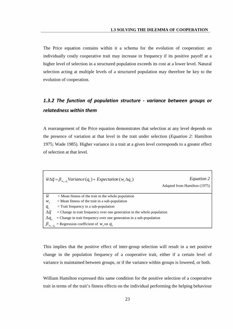
A rearrangement of the Price equation demonstrates that selection at any level depends on
the presence of variation at that level in the trait under selection (Equation 2: Hamilton
1975; Wade 1985). Higher variance in a trait at a given level corresponds to a greater effect
of selection at that level.
Equation 2
Adapted from Hamilton (1975)
w = Mean fitness of the trait in the whole population
ws = Mean fitness of the trait in a sub-population
qs = Trait frequency in a sub-population
q = Change in trait frequency over one generation in the whole population
qs = Change in trait frequency over one generation in a sub-population
ss qw , = Regression coefficient of ws on qs
This implies that the positive effect of inter-group selection will result in a net positive
change in the population frequency of a cooperative trait, either if a certain level of
variance is maintained between groups, or if the variance within groups is lowered, or both.
William Hamilton expressed this same condition for the positive selection of a cooperative
trait in terms of the trait’s fitness effects on the individual performing the helping behaviour
)()(, sssqw qwnExpectatioqVarianceqwss
1.3 SOLVING THE DILEMMA OF COOPERATION
24
(Hamilton 1964a, 1975), henceforth referred to as the focal individual. Hamilton’s rule tells
us that a cooperative behaviour that costs the focal individual c units of fitness and benefits
the recipient of cooperation by b units will evolve if rb c0 , where r represents the
genetic relatedness of the focal individual to the recipient. Individuals act to maximise
‘inclusive fitness’, comprising a ‘direct fitness’ component attributed to an individual’s
own offspring and an ‘indirect fitness’ component attributed to the offspring of other
genetically related individuals (Grafen 1984, 2009; Hamilton 1964a, 1964b). Helping
behaviour that reduces direct fitness by an amount c can still evolve if it increases inclusive
fitness via a positive effect on indirect fitness represented by .br Hence, natural selection
will favour cooperative behaviour preferentially directed towards related individuals.
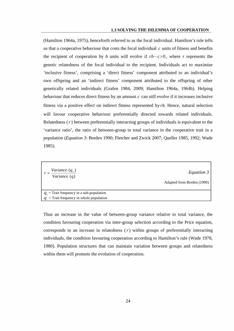
Relatedness ( r ) between preferentially interacting groups of individuals is equivalent to the
‘variance ratio’, the ratio of between-group to total variance in the cooperative trait in a
population (Equation 3: Breden 1990; Fletcher and Zwick 2007; Queller 1985, 1992; Wade
1985).
Equation 3
Adapted from Breden (1990)
qs = Trait frequency in a sub-population
q = Trait frequency in whole population
Thus an increase in the value of between-group variance relative to total variance, the
condition favouring cooperation via inter-group selection according to the Price equation,
corresponds to an increase in relatedness ( r ) within groups of preferentially interacting
individuals, the condition favouring cooperation according to Hamilton’s rule (Wade 1978,
1980). Population structures that can maintain variation between groups and relatedness
within them will promote the evolution of cooperation.
)(
)(
qVariance
qVariancer s
1.3 SOLVING THE DILEMMA OF COOPERATION
25
1.3.3 Defining relatedness
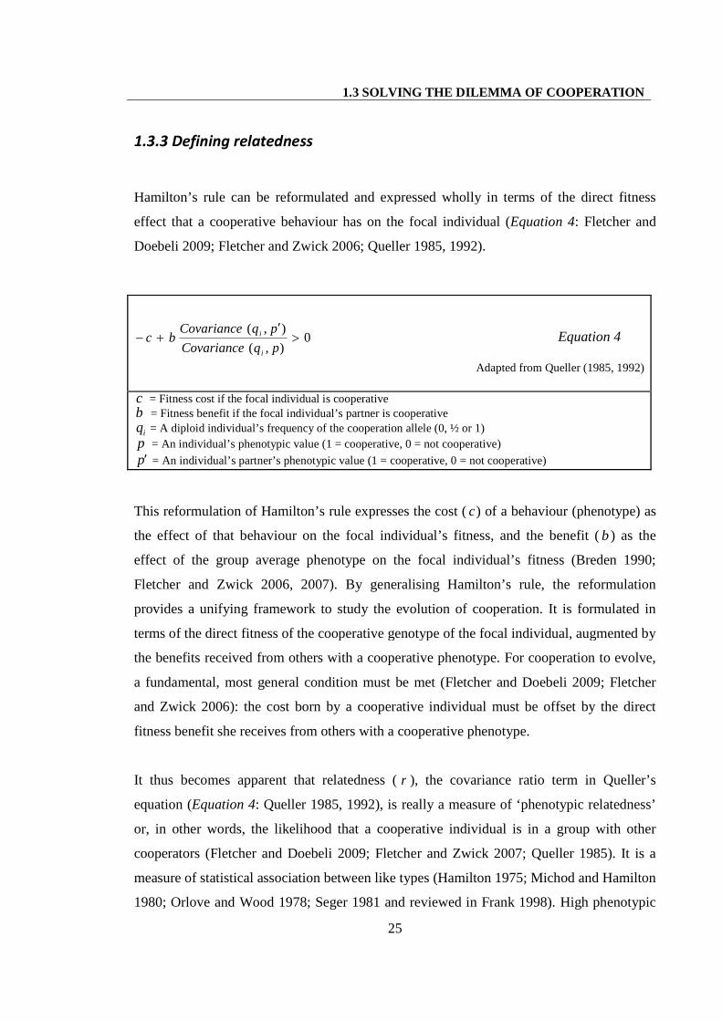
Hamilton’s rule can be reformulated and expressed wholly in terms of the direct fitness
effect that a cooperative behaviour has on the focal individual (Equation 4: Fletcher and
Doebeli 2009; Fletcher and Zwick 2006; Queller 1985, 1992).
Equation 4
Adapted from Queller (1985, 1992)
c = Fitness cost if the focal individual is cooperativeb = Fitness benefit if the focal individual’s partner is cooperative
qi = A diploid individual’s frequency of the cooperation allele (0, ½ or 1)
p = An individual’s phenotypic value (1 = cooperative, 0 = not cooperative)
p = An individual’s partner’s phenotypic value (1 = cooperative, 0 = not cooperative)
This reformulation of Hamilton’s rule expresses the cost ( c) of a behaviour (phenotype) as
the effect of that behaviour on the focal individual’s fitness, and the benefit ( b ) as the
effect of the group average phenotype on the focal individual’s fitness (Breden 1990;
Fletcher and Zwick 2006, 2007). By generalising Hamilton’s rule, the reformulation
provides a unifying framework to study the evolution of cooperation. It is formulated in
terms of the direct fitness of the cooperative genotype of the focal individual, augmented by
the benefits received from others with a cooperative phenotype. For cooperation to evolve,
a fundamental, most general condition must be met (Fletcher and Doebeli 2009; Fletcher
and Zwick 2006): the cost born by a cooperative individual must be offset by the direct
fitness benefit she receives from others with a cooperative phenotype.
It thus becomes apparent that relatedness ( r ), the covariance ratio term in Queller’s
equation (Equation 4: Queller 1985, 1992), is really a measure of ‘phenotypic relatedness’
or, in other words, the likelihood that a cooperative individual is in a group with other
cooperators (Fletcher and Doebeli 2009; Fletcher and Zwick 2007; Queller 1985). It is a
measure of statistical association between like types (Hamilton 1975; Michod and Hamilton
1980; Orlove and Wood 1978; Seger 1981 and reviewed in Frank 1998). High phenotypic
0),(
),(
pqCovariance
pqCovariancebc
i
i
1.3 SOLVING THE DILEMMA OF COOPERATION
26
relatedness between preferentially interacting group members ensures that the cost born by
a cooperative individual can be offset by the benefit she receives from the cooperation of
other group members. The conventional formulation of Hamilton’s rule specifies
relatedness ( r ) as the degree of genetic similarity between the focal individual and the
recipient of cooperation. This is valid for phenotypic traits that are completely specified by
their genotype (Fletcher and Zwick 2007), since the degree of genetic similarity
corresponds to the phenotypic similarity between individuals. However, when genotype
does not completely specify phenotype, genetic relatedness no longer coincides with
phenotypic similarity and must be replaced with a measure of phenotypic relatedness. So
long as there is covariance between phenotype and fitness, Price’s equation can be used to
estimate the change in the trait’s frequency under selection.
1.3.4 Generating phenotypic relatedness
A cooperative trait will increase in frequency as the likelihood that a cooperator will
interact with another cooperator increases. Mechanisms that increase this likelihood should
promote the evolution of cooperation by allowing cooperators to preferentially associate.
Associations between individuals may arise in space, time or via other mechanisms such as
genetic or cultural similarity (see Sections 1.4.1 to 1.4.3 and Section 1.6.1). Solving the
evolutionary dilemma presented by cooperation thus entails identifying mechanisms that
create population structures allowing individuals with similar trait values to be associated
within groups, and the maintenance of variance in trait values between groups. Since most
population processes are likely to affect inter- and intra-group variation simultaneously
(Fletcher and Zwick 2007), the distinction between the independent effects of the inter- and
intra-group components of selection may be superfluous, except for serving as an analytical
tool.
1.4 EVOLUTIONARY MODELS OF COOPERATION
27
1.4 Evolutionary models of cooperation
I now review the existing principal theoretical models of the evolution of cooperation.
While the theoretical framework outlined above (Section 1.3) applies to the evolution of
cooperation in any species, I focus on the extent to which this framework explains
cooperation in humans. I therefore do not review the vast literature on cooperation in other
species (for reviews of this literature see Dugatkin 2002; Dugatkin 1999). For each model
presented, I identify the mechanism that facilitates within-group relatedness between
individuals for the cooperative phenotype. Since most of these models can be (and usually
are) constructed such that the cooperative phenotype corresponds perfectly with the
cooperative genotype, the benefits of cooperation to the focal individual can either be
formulated wholly in terms of direct fitness (Fletcher and Doebeli 2009; Queller 1985,
1992) or in terms of indirect fitness (Hamilton 1964a; Queller 1985). Some authors make a
distinction between the terms ‘cooperation’ and ‘altruism’ (Hamilton 1964a, 1964b;
Lehmann and Keller 2006; West et al. 2007) or ‘weak altruism’ and ‘strong altruism’
(Wilson 1979, 1990) based on whether a helping behaviour provides any direct fitness
benefits to the focal individual or only indirect fitness benefits respectively (Kerr et al.
2004). This distinction is no longer useful if we work within David Queller and Jeffrey
Fletcher and colleagues’ framework for the evolution of cooperation as the inclusive fitness
approach is simply an alternative accounting system that is applicable to a subset of the
mechanisms facilitating the phenotypic association of cooperators (Fletcher and Doebeli
2009).
1.4.1 Kin selection (relatedness by common ancestry)
Cooperation can evolve when help is preferentially directed towards genetic relatives of the
focal individual (Hamilton 1964a, 1964b, 1975). Kin selection (Maynard Smith 1964)
describes the specific circumstance where cooperation evolves due to within-group
relatedness arising via common ancestry. Common ancestry is a reliable indicator that the
recipient of cooperation shares genes, including the cooperation allele, with the focal
1.4 EVOLUTIONARY MODELS OF COOPERATION
28
individual (Grafen 2007, 2009) and is therefore also likely to exhibit the cooperative
phenotype. Limited dispersal in multi-generational populations or the collective dispersal of
relatives in groups promotes the association of relatives and the action of kin selection
(Gardner and West 2006; Hamilton 1964a; Irwin and Taylor 2001; Kümmerli et al. 2009;
Mitteldorf and Wilson 2000; Nowak et al. 1994; Nowak and May 1992; Taylor and Irwin
2000; West et al. 2002).
At a proximate level, kin selection is contingent on the availability of information about
common ancestry. This information may most commonly be obtained from spatial cues
such as a shared nest, colony or household or phenotype-matching when interacting
individuals can estimate genotypic similarity based on phenotypic resemblance (Hamilton
1964b; Holmes and Sherman 1982; Lacy and Sherman 1983; Lehmann and Perrin 2002;
Reeve 1989; Sherman et al. 1997).
There is substantial empirical evidence that humans favour kin across domains such as food
sharing (Gurven et al. 2002; Gurven et al. 2000b; Marlowe 2010), cooperative hunting
(Alvard 2003; Morgan 1979), providing financial aid (Bowles and Posel 2005), child care
(Anderson et al. 1999; Flinn 1988; Marlowe 1999), mitigation of conflict (Chagnon and
Bugos 1979; Daly and Wilson 1988a; Daly and Wilson 1988b) and even in their
willingness to suffer physical pain to benefit someone in an experimental context (Madsen
et al. 2007).
1.4.2 Green beard and tag-based models (relatedness by assortment)
Cooperation can evolve when help is preferentially directed towards individuals
specifically sharing the cooperative allele with the focal individual (Grafen 2009; Hamilton
1964a; Lehmann and Keller 2006; Wilson and Dugatkin 1997). Theoretical models vary
based on the mechanism by which such assortment is achieved. For instance, linkage
disequilibrium between the allele responsible for cooperation and another allele encoding
some phenotypic trait (a green beard for example) allows individuals to identify others
possessing the cooperation allele (Haig 1997; Jansen and van Baalen 2006). An alternative
1.4 EVOLUTIONARY MODELS OF COOPERATION
29
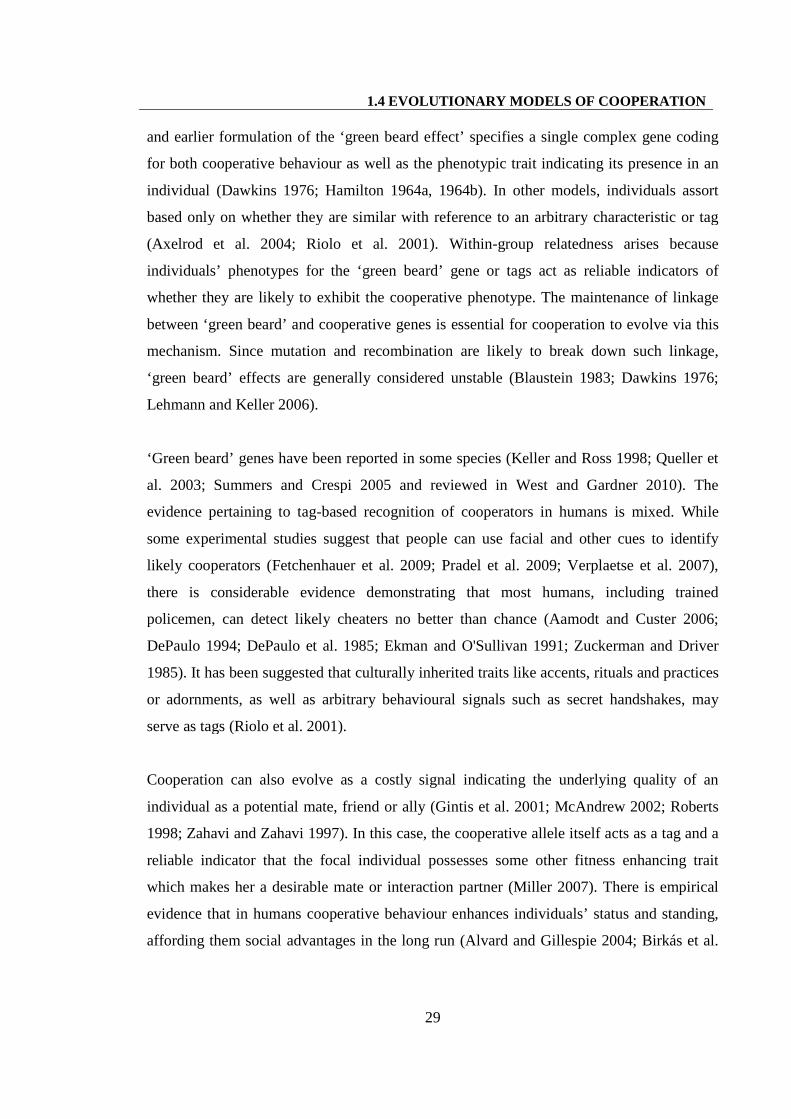
and earlier formulation of the ‘green beard effect’ specifies a single complex gene coding
for both cooperative behaviour as well as the phenotypic trait indicating its presence in an
individual (Dawkins 1976; Hamilton 1964a, 1964b). In other models, individuals assort
based only on whether they are similar with reference to an arbitrary characteristic or tag
(Axelrod et al. 2004; Riolo et al. 2001). Within-group relatedness arises because
individuals’ phenotypes for the ‘green beard’ gene or tags act as reliable indicators of
whether they are likely to exhibit the cooperative phenotype. The maintenance of linkage
between ‘green beard’ and cooperative genes is essential for cooperation to evolve via this
mechanism. Since mutation and recombination are likely to break down such linkage,
‘green beard’ effects are generally considered unstable (Blaustein 1983; Dawkins 1976;
Lehmann and Keller 2006).
‘Green beard’ genes have been reported in some species (Keller and Ross 1998; Queller et
al. 2003; Summers and Crespi 2005 and reviewed in West and Gardner 2010). The
evidence pertaining to tag-based recognition of cooperators in humans is mixed. While
some experimental studies suggest that people can use facial and other cues to identify
likely cooperators (Fetchenhauer et al. 2009; Pradel et al. 2009; Verplaetse et al. 2007),
there is considerable evidence demonstrating that most humans, including trained
policemen, can detect likely cheaters no better than chance (Aamodt and Custer 2006;
DePaulo 1994; DePaulo et al. 1985; Ekman and O'Sullivan 1991; Zuckerman and Driver
1985). It has been suggested that culturally inherited traits like accents, rituals and practices
or adornments, as well as arbitrary behavioural signals such as secret handshakes, may
serve as tags (Riolo et al. 2001).
Cooperation can also evolve as a costly signal indicating the underlying quality of an
individual as a potential mate, friend or ally (Gintis et al. 2001; McAndrew 2002; Roberts
1998; Zahavi and Zahavi 1997). In this case, the cooperative allele itself acts as a tag and a
reliable indicator that the focal individual possesses some other fitness enhancing trait
which makes her a desirable mate or interaction partner (Miller 2007). There is empirical
evidence that in humans cooperative behaviour enhances individuals’ status and standing,
affording them social advantages in the long run (Alvard and Gillespie 2004; Birkás et al.
1.4 EVOLUTIONARY MODELS OF COOPERATION
30
2006; Gurven et al. 2000a; Hawkes and Bird 2002; Sosis 2000 and reviewed in Miller
2007).
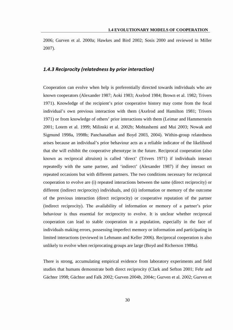
1.4.3 Reciprocity (relatedness by prior interaction)
Cooperation can evolve when help is preferentially directed towards individuals who are
known cooperators (Alexander 1987; Aoki 1983; Axelrod 1984; Brown et al. 1982; Trivers
1971). Knowledge of the recipient’s prior cooperative history may come from the focal
individual’s own previous interaction with them (Axelrod and Hamilton 1981; Trivers
1971) or from knowledge of others’ prior interactions with them (Leimar and Hammerstein
2001; Lotem et al. 1999; Milinski et al. 2002b; Mohtashemi and Mui 2003; Nowak and
Sigmund 1998a, 1998b; Panchanathan and Boyd 2003, 2004). Within-group relatedness
arises because an individual’s prior behaviour acts as a reliable indicator of the likelihood
that she will exhibit the cooperative phenotype in the future. Reciprocal cooperation (also
known as reciprocal altruism) is called ‘direct’ (Trivers 1971) if individuals interact
repeatedly with the same partner, and ‘indirect’ (Alexander 1987) if they interact on
repeated occasions but with different partners. The two conditions necessary for reciprocal
cooperation to evolve are (i) repeated interactions between the same (direct reciprocity) or
different (indirect reciprocity) individuals, and (ii) information or memory of the outcome
of the previous interaction (direct reciprocity) or cooperative reputation of the partner
(indirect reciprocity). The availability of information or memory of a partner’s prior
behaviour is thus essential for reciprocity to evolve. It is unclear whether reciprocal
cooperation can lead to stable cooperation in a population, especially in the face of
individuals making errors, possessing imperfect memory or information and participating in
limited interactions (reviewed in Lehmann and Keller 2006). Reciprocal cooperation is also
unlikely to evolve when reciprocating groups are large (Boyd and Richerson 1988a).
There is strong, accumulating empirical evidence from laboratory experiments and field
studies that humans demonstrate both direct reciprocity (Clark and Sefton 2001; Fehr and
Gächter 1998; Gächter and Falk 2002; Gurven 2004b, 2004c; Gurven et al. 2002; Gurven et
1.5 THE EVOLUTIONARY DILEMMA OF LARGE-SCALE COOPERATION
31
al. 2000b; Kaplan and Hill 1985 and reviewed in Fehr and Fischbacher 2003 and Gächter
and Herrmann 2009) as well as indirect reciprocity (Alpizar et al. 2008; Milinski et al.
2001; Milinski et al. 2002a, 2002b; Seinen and Schram 2006; Wedekind and Braithwaite
2002; Wedekind and Milinski 2000 and reviewed in Fehr and Fischbacher 2003 and
Gächter and Herrmann 2009). However, studies of food sharing in small-scale societies
have reported the high frequency of reciprocity amongst kin (Allen-Arave et al. 2008;
Gurven et al. 2000b). Kin selection and reciprocity may therefore augment and stabilise
each other in establishing cooperation in these populations.
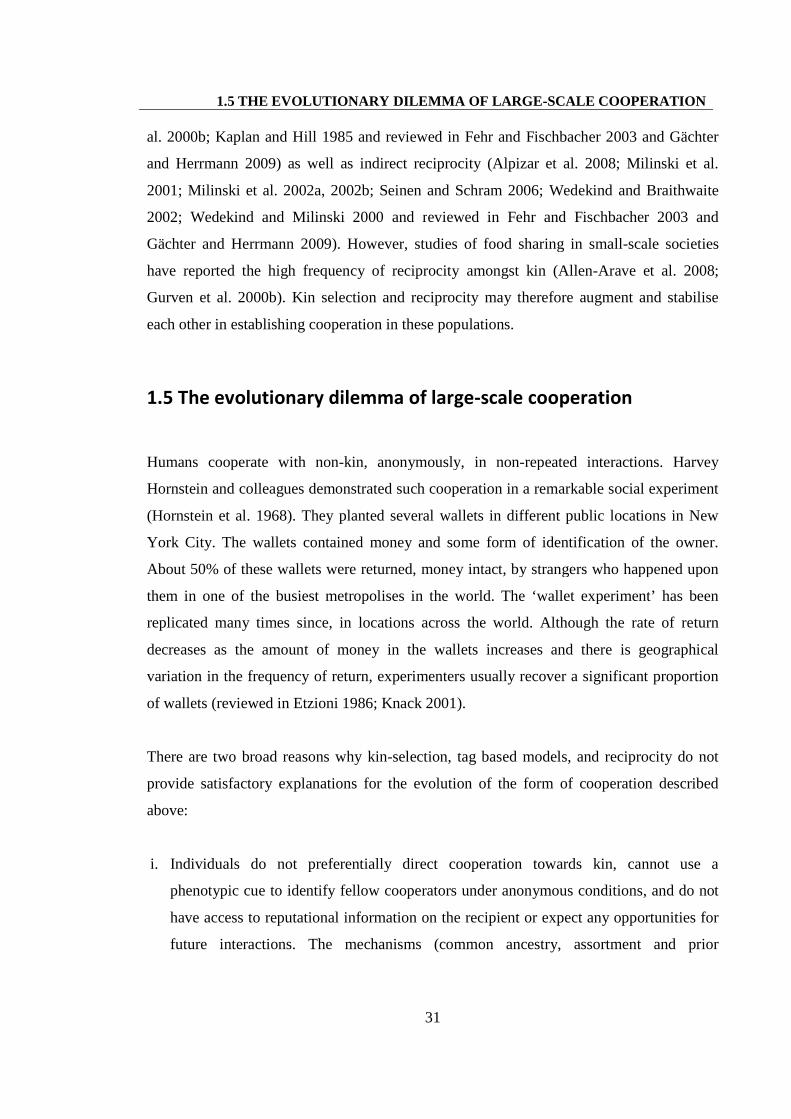
1.5 The evolutionary dilemma of large-scale cooperation
Humans cooperate with non-kin, anonymously, in non-repeated interactions. Harvey
Hornstein and colleagues demonstrated such cooperation in a remarkable social experiment
(Hornstein et al. 1968). They planted several wallets in different public locations in New
York City. The wallets contained money and some form of identification of the owner.
About 50% of these wallets were returned, money intact, by strangers who happened upon
them in one of the busiest metropolises in the world. The ‘wallet experiment’ has been
replicated many times since, in locations across the world. Although the rate of return
decreases as the amount of money in the wallets increases and there is geographical
variation in the frequency of return, experimenters usually recover a significant proportion
of wallets (reviewed in Etzioni 1986; Knack 2001).
There are two broad reasons why kin-selection, tag based models, and reciprocity do not
provide satisfactory explanations for the evolution of the form of cooperation described
above:
i. Individuals do not preferentially direct cooperation towards kin, cannot use a
phenotypic cue to identify fellow cooperators under anonymous conditions, and do not
have access to reputational information on the recipient or expect any opportunities for
future interactions. The mechanisms (common ancestry, assortment and prior
1.6 SOLVING THE DILEMMA OF LARGE-SCALE COOPERATION
32
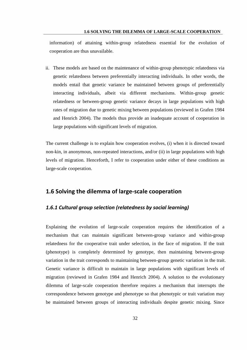
information) of attaining within-group relatedness essential for the evolution of
cooperation are thus unavailable.
ii. These models are based on the maintenance of within-group phenotypic relatedness via
genetic relatedness between preferentially interacting individuals. In other words, the
models entail that genetic variance be maintained between groups of preferentially
interacting individuals, albeit via different mechanisms. Within-group genetic
relatedness or between-group genetic variance decays in large populations with high
rates of migration due to genetic mixing between populations (reviewed in Grafen 1984
and Henrich 2004). The models thus provide an inadequate account of cooperation in
large populations with significant levels of migration.
The current challenge is to explain how cooperation evolves, (i) when it is directed toward
non-kin, in anonymous, non-repeated interactions, and/or (ii) in large populations with high
levels of migration. Henceforth, I refer to cooperation under either of these conditions as
large-scale cooperation.
1.6 Solving the dilemma of large-scale cooperation
1.6.1 Cultural group selection (relatedness by social learning)
Explaining the evolution of large-scale cooperation requires the identification of a
mechanism that can maintain significant between-group variance and within-group
relatedness for the cooperative trait under selection, in the face of migration. If the trait
(phenotype) is completely determined by genotype, then maintaining between-group
variation in the trait corresponds to maintaining between-group genetic variation in the trait.
Genetic variance is difficult to maintain in large populations with significant levels of
migration (reviewed in Grafen 1984 and Henrich 2004). A solution to the evolutionary
dilemma of large-scale cooperation therefore requires a mechanism that interrupts the
correspondence between genotype and phenotype so that phenotypic or trait variation may
be maintained between groups of interacting individuals despite genetic mixing. Since
1.6 SOLVING THE DILEMMA OF LARGE-SCALE COOPERATION
33
natural selection acts on the phenotype (Fletcher and Zwick 2007; Mayr 1997), so long as
there is covariance between the phenotype and fitness, the phenotypic trait with a positive
fitness benefit should be selected for.
One mechanism that allows phenotype to diverge from genotype is social learning. If
individuals can acquire behaviour by learning from or copying the behaviour of other
individuals in their environment, then phenotypic variance may be maintained between
groups despite genetic mixing (Boyd and Richerson 1985; Henrich 2004; Henrich and
Boyd 1998). Random behavioural variance introduced between groups by stochastic
processes like drift may be stabilised by social learning strategies such as conformity (a
tendency to copy high frequency behaviour) and payoff biased learning (a tendency to
acquire behaviour that has produced the highest payoff or greatest success for another
individual), thus maintaining multiple stable equilibria and phenotypic variance across
groups; selection acting on these alternative stable equilibria among competing groups can
lead to the evolution of cooperation if group-level cooperation positively affects group
survival or proliferation (Boyd et al. 2003; Boyd and Richerson 1982; Boyd and Richerson
1985; Gintis 2003; Guzmán et al. 2007; Henrich 2004; Henrich and Boyd 1998; Henrich
and Boyd 2001; Richerson and Boyd 2005). In the absence of social learning, phenotypic
variation corresponding to genetic variation between groups would be depleted by
migration between them. Hence, within-group relatedness arises in cultural group selection
models because individuals in a preferentially interacting group are likely to have the same
behavioural strategy due to social learning (cultural transmission). The cost of cooperation
is offset by the direct fitness benefit that a focal individual receives from being part of a
group of cooperators. It may therefore be possible to use Queller’s formulation of
Hamilton’s Rule to analyse the evolution of cooperation via cultural group selection
(Fletcher and Zwick 2006, 2007).
1.6.2 The empirical evidence
Although we have a theoretical framework that potentially explains the evolution of large-
scale cooperation in humans, much of this theory remains empirically untested in real-

1.6 SOLVING THE DILEMMA OF LARGE-SCALE COOPERATION
34
world populations. In order to establish whether cultural group selection models of the
evolution of cooperation find support in nature, there are two major empirical questions that
need to be answered:
A. Is there stable, heritable variation in levels of cooperation across human
populations?
If cultural transmission maintains behavioural variance between groups, then we should
expect to find stable, heritable differences in levels of cooperation across groups. Note that
it is not adequate to simply establish that there is variation across groups. Selection at the
group level requires that the variation between groups be heritable. Hence, in order to
ascertain whether stable between-group variation in cooperation exists in the real world, it
is important to establish whether (a) there is between-group variation in cooperation, and
(b) the drivers of any existing variation are likely to maintain stable, heritable differences
between groups across generations.
Experimental cross-cultural studies in small-scale (Henrich et al. 2004; Henrich et al. 2001;
Henrich et al. 2005; Henrich et al. 2010; Henrich et al. 2006) and large-scale (Cardenas and
Carpenter 2005; Herrmann et al. 2008; Roth et al. 1991) societies demonstrate variation in
patterns of cooperation across cultural groups. The findings of these studies are taken as
support for the existence of stable variation in levels of cooperation across human
populations (Henrich et al. 2005; Henrich et al. 2006). However, these studies have mostly
sampled from one population (city/village/settlement) per culture and confound cultural and
environmental differences between populations. We cannot differentiate whether the
behavioural variation across populations is driven by cultural transmission or
environmental (demographic or ecological) differences between populations. While
variation driven by cultural transmission is heritable, variation driven by demographic or
ecological factors is not necessarily stable or heritable; environmental drivers of
behavioural variation are less likely to maintain stable differences essential for selection at
the population level.
1.6 SOLVING THE DILEMMA OF LARGE-SCALE COOPERATION
35
If cultural transmission occurs such that individuals are equally likely to sample behaviour
from different populations of the same cultural group, and the benefit of cooperation is at
the level of the cultural group (increased survival or proliferation), then selection between
cultural groups can lead to the evolution of cooperation. In this case, support for cultural
group selection models entails (a) behavioural variation across cultural groups, and (b)
significantly lower variation across populations of the same cultural group than between
different cultural groups. If the latter condition is not met, i.e. we find that variation across
populations of the same cultural group is equal to or greater than variation between cultural
groups, then the strength of selection between cultural groups would have to be very much
higher than the strength of selection within groups for individually costly cooperation to be
favoured by selection at the level of the cultural group; however, this constraint is generally
considered too stringent to be satisfied often in nature (Henrich 2004), although it remains a
theoretical possibility. The first focus of this thesis is to test the predictions outlined above
(Section 1.7).
Alternatively, if cultural transmission occurs such that individuals selectively sample
behaviour only from their population, rather than from other populations of the same
cultural group, and the benefit of cooperation is at the level of the population, then selection
between populations of the same cultural group can lead to the evolution of cooperation. In
this case, support for cultural group selection models entails (a) behavioural variation
across populations of the same cultural group, and (b) significantly lower variation across
individuals of the same population than between different populations (assuming that the
strength of selection between populations is not very much higher than the strength of
selection within populations). It is less likely that populations of the same endogamous
cultural group are the units of selection at the group level. Migration rates between these
inter-marrying populations are likely to be very high. Forces maintaining within-population
similarity (such as conformity and punishment of norm violation) need to be strong enough
to counteract the variation introduced by migration. It is also unlikely that individuals
sample and acquire behaviour only from members of the same population when migration
between populations is high; sampling behaviour across populations will decrease between-
population variance.
1.6 SOLVING THE DILEMMA OF LARGE-SCALE COOPERATION
36
To demonstrate support for cultural group selection models when the unit of selection is the
cultural group, we need to establish that there is behavioural variation across cultural
groups and that the variation between different endogamous cultural groups is greater than
that between populations of the same endogamous cultural group; this assumes that the
strength of selection between cultural groups is not much higher than the strength of
selection within groups. Current empirical data do not answer the first empirical question.
B. Do people use social learning to acquire cooperative strategies?
Cultural group selection models of cooperation assume that individuals acquire cooperative
strategies via social learning. We therefore need to establish whether humans have any
proclivity to acquire cooperative behavioural strategies via social learning. Note that it is
not adequate to simply establish that individuals have a tendency to acquire behaviour in
general via social learning. Social learning is expected to be employed selectively in
different task domains (Eriksson and Coultas 2009; Eriksson et al. 2007; Rowthorn et al.
2009). Hence, we need to determine whether humans tend to specifically acquire
behavioural strategies in the cooperative domain via social learning; the second focus of
this thesis is to test this assumption made by cultural group selection models of large-scale
cooperation (Section 1.7).
The empirical literature demonstrating that humans use social learning to acquire behaviour
and make judgements and decisions is vast (Bandura 1977; Festinger 1954 and reviewed in
Laland 2004 and Mesoudi 2009). While a small number of studies have investigated the
role of conformist learning in determining behaviour in a public goods dilemma (Bardsley
and Sausgruber 2005; Carpenter 2004; Samuelson and Messick 1986; Schroeder et al.
1983; Smith and Bell 1994; Velez et al. 2009), these studies do not unequivocally measure
conformist learning as defined and implemented in cultural group selection models, i.e. the
disproportionate tendency to copy the majority (Boyd and Richerson 1985; Efferson et al.
2008; Mesoudi 2009); it is only such a disproportionate individual proclivity to acquire
majority behaviour that has demonstrable homogenising effects within populations and
1.6 SOLVING THE DILEMMA OF LARGE-SCALE COOPERATION
37
creates heterogeneity between them (Boyd and Richerson 1985; Efferson et al. 2008). Thus,
the present literature (reviewed in Section 5.1.1) does not adequately address the question
of whether humans acquire behavioural strategies via social learning specifically in the
cooperative domain. Current empirical data do not answer the second empirical question.
1.7 Aims of the thesis
In this thesis I contribute toward answering the two aforementioned empirical questions. I
investigate (i) whether there is variation in levels of cooperation across populations of the
same endogamous, small-scale, forager-horticulturist society, the Pahari Korwa of central
India, and (ii) whether people demonstrate any proclivity to acquire cooperative
behavioural strategies via social learning. The thesis is divided into three sections:
I. Variation in cooperation across populations
In this section I examine whether there is variation in levels of cooperation within and
between multiple populations of the same endogamous small-scale society, the Pahari
Korwa, and whether demographic or ecological factors explain any part of this variation.
This helps clarify whether behavioural variation between populations of the same
endogamous cultural group is less than the behavioural variation found between different
endogamous cultural groups in previous studies (Henrich et al. 2001; Henrich et al. 2005;
Henrich et al. 2006; Herrmann et al. 2008); support for cultural group selection models,
when the unit of selection is the cultural group, requires establishing that there is
behavioural variation across cultural groups and that it is greater than the variation between
populations of the same endogamous cultural group, assuming that the strength of selection
between cultural groups is not much higher than the strength of selection within groups
(Section 1.6.2). I control for cultural differences between populations to tease apart the
effects on behavioural variation of environment (ecology and demography) versus culture.
There are several reasons that advocate controlling for culture rather than environment in
the first instance. First, finding variation between cultural groups living in the same
1.7 AIMS OF THE THESIS
38
environment would not allow us to exclude the hypothesis that this variation is driven by
demographic processes, unless we also ascertain the level of variation across populations of
the same cultural group. Second, cultural identity is more clearly defined than consistency
in environment, especially for endogamous small-scale societies, where there are clear rules
regarding individuals’ inclusion in and exclusion from the cultural group. Third, the null
hypothesis derived from assuming systematic or mechanistic continuity with species that
are acultural (although see Hoppitt et al. 2008, Laland 2008 and Laland and Janik 2006 for
reviews of evidence for social learning in non-human animals) is that any within-species,
between-population behavioural variation is driven by ecological and demographic
processes.
I use three measures of cooperation: two different economic games (Camerer 2003; Kagel
and Roth 1995) and one ‘real-world’ measure of cooperative behaviour in up to 21 distinct
Pahari Korwa populations. I examine whether any existing variation in game behaviour
within and between populations is explained by properties of populations and/or individuals.
Economic games derived from behavioural game theory are the best available tools that we
can currently employ to quantitatively measure one-shot, anonymous, cooperative
behaviour in humans. They allow us the flexibility to control experimental parameters of
interest or sources of error. Over past decades, they have provided great insights into
human economic and social behaviour, both in the laboratory and in the field (Roth 1995b).
II. Social learning in the cooperative domain
In this section I use an economic game experiment to investigate whether individuals facing
a public goods dilemma use information about others’ behavioural strategies to make their
decisions; the experiments were conducted in 14 Pahari Korwa populations. I further
examine whether there is variation in the distribution of different learning strategies across
populations and whether properties of populations and/or individuals are associated with
the type of learning strategy employed by individuals. Finally, I consider whether the
learning strategies employed by individuals influence the distribution of trait variants
within populations.
1.8 STRUCTURE OF THE THESIS
39
III. Conclusion
In this section I summarise the findings from the previous two sections and discuss their
collective implications for an understanding of the evolution of large-scale cooperation in
humans, as well as the structure of cultural inheritance systems.
1.8 Structure of the thesis
In Chapter 2 I describe the study populations and provide an overview of the methods and
analyses employed.
The remainder of the thesis is in three sections. Section I comprises Chapters 3 and 4. In
Chapter 3 I present findings from the ultimatum game (UG), my first measure of
cooperative behaviour, implemented in 21 Pahari Korwa villages. In Chapter 4 I present
findings from two further measures of cooperative behaviour, a public goods game (PGG)
and a new ‘real-world’ measure of behaviour, both implemented in 16 Pahari Korwa
villages. Section II of the thesis consists of Chapter 5, where I present findings from public
goods game experiments implemented in 14 Pahari Korwa populations, examining whether
people employ social learning in the context of a cooperative dilemma. Each chapter opens
with the relevant background to the sub-study and a review of related research, as well as a
description of the behavioural measures employed and of the study design; this is followed
by the findings of the sub-study and a discussion of these findings. Methodological details
specific to each sub-study are provided at the end of each chapter; I have adopted this
format rather than conventionally including the methods at the start of the chapter as these
details are not crucial to the interpretation of results and may otherwise interrupt the
narrative.
In Section III, consisting of Chapter 6, I conclude by discussing the implications of my
findings for theory on the evolution of large-scale cooperation in humans and the structure
of cultural inheritance systems.
40
CHAPTER 2
STUDY POPULATIONS AND METHODS
In this chapter I describe my study populations and provide an overview of the methods and
analyses employed in the work presented in this thesis. Section 2.1 outlines the features of a
good model system for this study and Section 2.2 provides an ethnographic account of the
Pahari Korwa, as well as a description of the geographical region in which they live.
Section 2.3 describes the study site and the study set-up, as well as provides details of the
21 villages included in this study. Sections 2.4 and 2.5 provide an overview of the methods
and analyses employed respectively.
2.1 Features of a good model system for this study
The aim of this thesis is to identify whether there is significant variation in levels of
cooperation across human populations, and whether social learning or environmental
variability is the likely driver of any existing variation. The foremost requirement of a good
model system for this study is therefore a set of real-world populations. Since I wish to
control for cultural differences between the study populations, I require multiple
populations of the same endogamous cultural group living as predominantly uni-ethnic
communities. Furthermore, populations with distinct boundaries are essential in order to
compare naturally defined populations and measure the population level correlates of
cooperation. This will ensure that the analyses are not affected by the arbitrary assignation
of population boundaries. To facilitate detection of any effects of demography and ecology
on levels of cooperation across populations, the sample populations should capture
sufficient variation in these variables. A final feature of a good model system is therefore
populations that vary in size, migration rates, distances to towns and markets and so on. In
summary, a good model system for this study comprises multiple, uni-ethnic meta-
2.2 THE PAHARI KORWA
41
populations of the same endogamous cultural group, with distinct population boundaries
and demographic and ecological variation across populations; Pahari Korwa populations
have all these features of a good model system.
2.2 The Pahari Korwa
2.2.1 Ethnographic description
The Pahari Korwa (‘Hill Korwa’) are a small-scale forager-horticulturist society, classified
as a ‘primitive tribal group’ by the Government of India (UN FAO report 1998), and living
largely in the central Indian state of Chhattisgarh. They belong to the Kolarian group of
tribes, an ethno-linguistic grouping, with a close affinity to the Austro-Asiatic Munda
language family (Rizvi 1989; Sharma 2007; Srivastava 2007). The introduction of forest
protection laws by the Government of India in 1952 precipitated a shift from their
traditional nomadic lifestyle completely reliant on hunting, gathering and swidden
agriculture to settled communities based around individually owned land (Rizvi 1989).
They remain heavily reliant on gathered forest products which are a primary source of food
and income, but they also practice agriculture on small tracts of land, usually adjoining
forested areas. These economic resources are supplemented by opportunistic hunting and
fishing and wage labour. Men hunt in groups with bows and arrows and with the exception
of the shooter who usually gets a larger share, the meat is shared equally. Typically hunted
animals are wild boar, small deer species, and species of birds such as the kotri also known
as the Rufous Treepie (Dendrocitta vagabunda). Fishing may be conducted solitarily, in
pairs (often a conjugal pair), or in small groups, and the catch is shared equally. Fields are
always tended by family units, but families with larger fields may enlist the help of other
village residents in exchange for a meal and liquor. The staple is rice, but maize, millet,
pulses, potatoes and small quantities of vegetables are also grown. Small numbers of goats,
chickens and pigs are reared by families, mostly for personal consumption.
Individuals in all populations visited during this study speak Sargujia, a regional dialect of
Hindi; the Korwa language is infrequently used on an everyday basis. Villages differ in
2.2 THE PAHARI KORWA
42
their access to markets. Most individuals attend a local weekly market with varying
frequency where they buy, sell and barter goods. The weekly market usually assembles in
one of the larger multi-ethnic villages in the plains, and is visited by people of various
ethnicities from surrounding villages. Korwas often have to walk several kilometres
downhill to their nearest market site. Settlements have well-defined boundaries;
neighbouring villages are generally separated by large tracts of forest and hills. Both uni-
ethnic as well as multi-ethnic villages of varying sizes exist, although uni-ethnic
settlements predominate.
The Pahari Korwa typically live in nuclear households. Lineally extended households
where a married couple live with their married children are also seen. An endogamous,
patrilineal and patrilocal society, exogamous marriages usually incur severe penalties,
typically entailing ostracism and excommunication from the tribe and village. The
excommunication can sometimes be reversed by what amounts to a substantial fine
imposed on the offenders; they sponsor a large ritual feast. The majority of Korwas marry
monogamously, but polygyny is practiced by some, usually more affluent, men (Rizvi
1989; Srivastava 2007; personal observation). The Korwas practice bride-price. Although,
following the marriage the woman usually moves to the home of the man, couples often
cohabit at either’s parents’ home, and may even bear a first child before the formalities of
the marriage are completed. There is no caste system.
Korwas live in either temporary huts made of Sal (Shorea robusta) tree branches with
thatched roofs, or more permanent mud houses with a roof constructed from baked mud
tiles (Rizvi 1989; Srivastava 2007; personal observation). Mud houses usually comprise
one central room surrounded by a corridor on three sides. A verandah may be constructed
on one side of the house and families who rear goats also build an enclosure for them in a
section of the corridor within the main house. Korwa settlements are dispersed, with large
distances between houses, often spanning a kilometre or more. Clustered settlements are
rare. This may be largely because people build their homes adjoining their cultivated plots
of land. In my qualitative interviews, subjects often cited proximity to their land as a
criterion used to choose the location of their homes. Other criteria cited were proximity to
2.2 THE PAHARI KORWA
43
the forest and a generally good ambience and surroundings, including the availability of
open space, as well as the presence of holy or ancestral spirits.
Across villages, sources of water include small streams and rivers, natural springs and wells
and hand pumps constructed by the Indian government. People sometimes walk up to a
kilometre to their primary source of water. Electricity has not reached most villages. Of the
21 villages that I worked in, only one village was partially electrified; here too power lines
had been laid within the last five years and only a handful of houses were receiving a
limited quota of electricity. Sal tree wood is the primary source of fuel, used essentially for
cooking and to provide warmth in the winter.
The Korwas practice ancestor worship (Srivastava 2007; personal observation). They also
worship indigenous gods and goddesses, often associated with the forest, hunting, or a
prominent local geographical site such as a big hill or cave in the region. They have
recently started adopting Hindu practices and deities in some villages, although these still
tend to coexist with their indigenous divinities. Korwa festivals are usually centred around
the sowing or harvest of certain crops, the harvest of seasonal forest products, or protection
and prosperity during particular seasons like the monsoon (Rizvi 1989; personal
observation). One of the biggest festivals in the calendar year is the harvest festival called
‘Cherta’, usually celebrated in the month of January. The festival is celebrated with gusto
and involves the slaughter and consumption of chickens and goats, as well as the
consumption of special foods and vast quantities of ‘hadiya’ (rice beer) and ‘mahua’
(potent alcohol manufactured from a flowering tree of the same name). People visit others’
homes and invite their friends and relatives, both from the village and from other villages,
to wine and dine at their homes. There is much merriment, music and dance and the
celebration engulfs the village for two or three days.
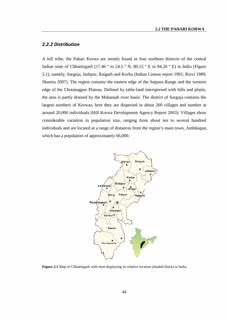
2.2 THE PAHARI KORWA
44
2.2.2 Distribution
A hill tribe, the Pahari Korwa are mostly found in four northern districts of the central
Indian state of Chhattisgarh (17.46 º to 24.5 º N, 80.15 º E to 84.20 º E) in India (Figure
2.1), namely, Sarguja, Jashpur, Raigarh and Korba (Indian Census report 1991; Rizvi 1989;
Sharma 2007). The region contains the eastern edge of the Satpura Range and the western
edge of the Chotanagpur Plateau. Defined by table-land interspersed with hills and plains,
the area is partly drained by the Mahanadi river basin. The district of Sarguja contains the
largest numbers of Korwas; here they are dispersed in about 260 villages and number at
around 20,000 individuals (Hill Korwa Development Agency Report 2003). Villages show
considerable variation in population size, ranging from about ten to several hundred
individuals and are located at a range of distances from the region’s main town, Ambikapur,
which has a population of approximately 66,000.
Figure 2.1 Map of Chhattisgarh with inset displaying its relative location (shaded black) in India.
2.2 THE PAHARI KORWA
45
2.2.3 Climate, flora and fauna
Chhattisgarh has a hot and humid tropical climate. The Tropic of Cancer passes through the
state. The northern hilly region where the Korwas reside is cooler than the rest of the state;
summer temperatures range between 25 and 39 ºC (Rizvi 1989). Average annual rainfall in
the region is about 140 cm. The state falls in the Sal (Shorea robusta) forest belt and has
44% of its geographical area under forest cover. Other common species of trees are Teak
(Tectona grandis), Mahua (Madhuca indica), Tendu (Diospyros melanoxylon), Amla
(Embilica officinalis), Karra (Cleistanthus collinus) and Bamboo (Dendrocalamus strictus).
The region has been home to the tiger, leopard and elephant, populations of which are
either endangered or locally extinct. Sloth Bears, wild boar, sambhar deer, nilgai, chinkara,
striped hyenas, porcupines and chital are more common. Chhattisgarh is also home to
several species of birds including the wood pecker, peacock, jungle fowl, quail, gray-
partridge and parrot.
2.3 STUDY SITE
46
2.3 Study site
2.3.1 Establishing the field-site
I first visited Chhattisgarh in May 2007 in order to set-up a field-site and conduct a pilot
study. Prior to my visit, I had made contact with a local non-government organisation
called Chaupal, based in the town of Ambikapur (District Sarguja), Chhattisgarh. Chaupal
was established about eight years ago under the leadership of Mr. Gangaram Paikra, and
comprises individuals from several tribal groups from within Chhattisgarh. The primary
aim of this grass-roots organisation is to disseminate information on and facilitate access to
national rural livelihood and employment schemes run by the Indian government. The
organisation works in several hundred villages mainly across three districts of northern
Chhattisgarh. Gangaram Paikra generously agreed to assist me in establishing my study. In
May 2007, I made my way from Delhi to Ambikapur, rucksack on my back. An overnight
train journey and a day-long bus ride later, I met Gangaram Paikra for the first time in
Ambikapur. I had originally planned to conduct my research on a different tribal group, the
Gond. However, upon spending several weeks in Chhattisgarh, I realised that the Gond are
sub-divided into several endogamous communities and very rarely live in uni-ethnic
villages. Further enquiries and research led me to the Pahari Korwa, who met my
established criteria for a model population system.
With extraordinary and indispensible assistance from Gangaram Paikra and the other
members of Chaupal, I spent the month of May recruiting and training research assistants,
translating game scripts into Sargujia, standardising questionnaires used to collect
demographic and individual data, working out the practical details of running the games in
a village, identifying villages to work in and making logistical arrangements such as
transportation to villages. My research assistants were members of Chaupal who are from
villages in the region and combine their work at Chaupal with small-scale agriculture to
maintain a livelihood. They are literate and have at least completed middle school. I ran the
first set of games in the village of Gotidoomar in the last week of May 2007.
2.3 STUDY SITE
47
2.3.2 Study set-up
2.3.2.1 Sampling and logistics
I obtained a list of Pahari Korwa villages with their population sizes as estimated in the
most recent Indian population census conducted in the year 2001 from the Hill Korwa
Development Agency, a department of the Chhattisgarh state government. I also obtained
more recent census data for a subset of these villages, collected by Chaupal in 2004 and
2005. Information from the lists was combined with that obtained from members of
Chaupal to identify a set of villages incorporating reasonable variation in population size
and distances from Ambikapur and each other. My sample of villages is therefore not
random. Demographic variation in the village sample is a crucial feature of my study
design (Section 2.1). To be certain of obtaining a dataset with reasonable demographic
variation using a fully randomised sampling strategy, a large number of villages need to be
sampled. Constraints on resources and time necessitated adoption of the sampling strategy
for villages described above; this allowed me to obtain the minimum recommended sample
size (about fifteen villages according to a rule of thumb) suitable for the application of
multilevel models (Section 2.5.2).
The research team consisted of two research assistants and myself. Upon our arrival in a
village, we would make contact with the village head or other senior person in the village
and describe the purpose of our visit. We informed him that we were a group of researchers
from a university (a big school) and were conducting a study with the Pahari Korwa. We
stated that we would stay in the village for about a week, the first three days of which we
would conduct a programme in which we sought the participation of village residents, both
adult men and women. We further informed him that all participants in our study would
receive 30 Indian rupees (henceforth rupees) and a meal for each day they attended, and
would have the opportunity to earn more money based on their performance in certain
games we would play with them. We assured him that participation was completely
voluntary and that the games were thought-based and did not involve physical exertion.
Once the village head was convinced of our credentials, we enlisted his help and that of any
other assembled individuals to advertise the study in the village via door to door visits.
2.3 STUDY SITE
48
Individuals who willingly gathered on the day of the games participated in this study. Note
that any non-Korwa residents in the village did not participate in the study.
23 villages were visited during the study period. The games were successfully conducted in
21 of these villages. We failed to conduct the games in two villages; although we advertised
the study and stayed in these villages for two days, the residents did not gather to
participate in the games. In these two villages, while most residents did not refuse to
participate, they simply did not assemble on the day we were scheduled to conduct the
games. These villages were located in a different district (District Jashpur) to the 21
villages successfully included in this study (District Sarguja) and were situated between 10
and 20 km apart. Possible reasons for their failure to participate may include mistrust of
outsiders; residents of one village were mildly hostile to us. Pre-occupation with preparing
their fields for the new crop and mending the roofs of their homes in readiness for the
incoming monsoon may have been another reason.
As noted above in Section 2.2.1, Korwas usually live atop hills amidst forest with no road
infrastructure, electricity or running water; access to most villages is therefore by foot. We
provided a meal to every participant on the day of the games, and so transported rations
catering two meals for about 50 people to each village along with our own supplies for a
week. We thus carried about 45 kg of rice, 10 kg of lentils, 10 kg of potatoes, 10 kg of other
vegetables and various other supplies and equipment to each village. We also took 50 kg of
salt to each village in order to implement a ‘real-world’ measure of cooperation (see
Sections 2.4.1, 4.1.2 and 4.4.2 for details). All supplies and equipment were transported in
a four-wheel-drive vehicle up to the closest motorable point from where we trekked by foot,
sometimes for several hours, up to the Korwa village. We often enlisted the help of
residents of a nearby village accessible by car to help us carry the heavy rations from the
vehicle to our destination village. Alternatively, two of us would trek to the Korwa village
under investigation and bring back residents from there to help us carry the rations to their
village. During our stay in each village, we resided in the home of one of the village
residents who generously provided us space inside their house or in the verandah that is
attached to most houses. We cooked our meals separately on a wood fire (our hosts
provided us the firewood), and our hosts typically invited us to at least one meal at their

2.3 STUDY SITE
49
hearth. We presented our hosts a gift in the form of food rations and some money when we
departed.
2.3.2.2 Village details
The study was conducted in a total of 21 Pahari Korwa villages. Table 2.1 summarises
important demographic features of these villages and the behavioural measures of
cooperation implemented in each village. Five villages were visited between May 23rd and
June 21st, 2007 and the remaining 16 villages were visited between February 2nd and May
16th, 2008. Figure 2.2 displays the geographical distribution of study villages and the town
of Ambikapur. Village means for participants from each study population are presented for
basic individual descriptors, residence, and migration variables in Table 2.2 and for
measures of wealth, market contact and social networks in Table 2.3 (see Table 2.5 for
descriptions of these variables). Table 2.4 summarises the availability of amenities, such as
a primary school and health care centre, in each village.
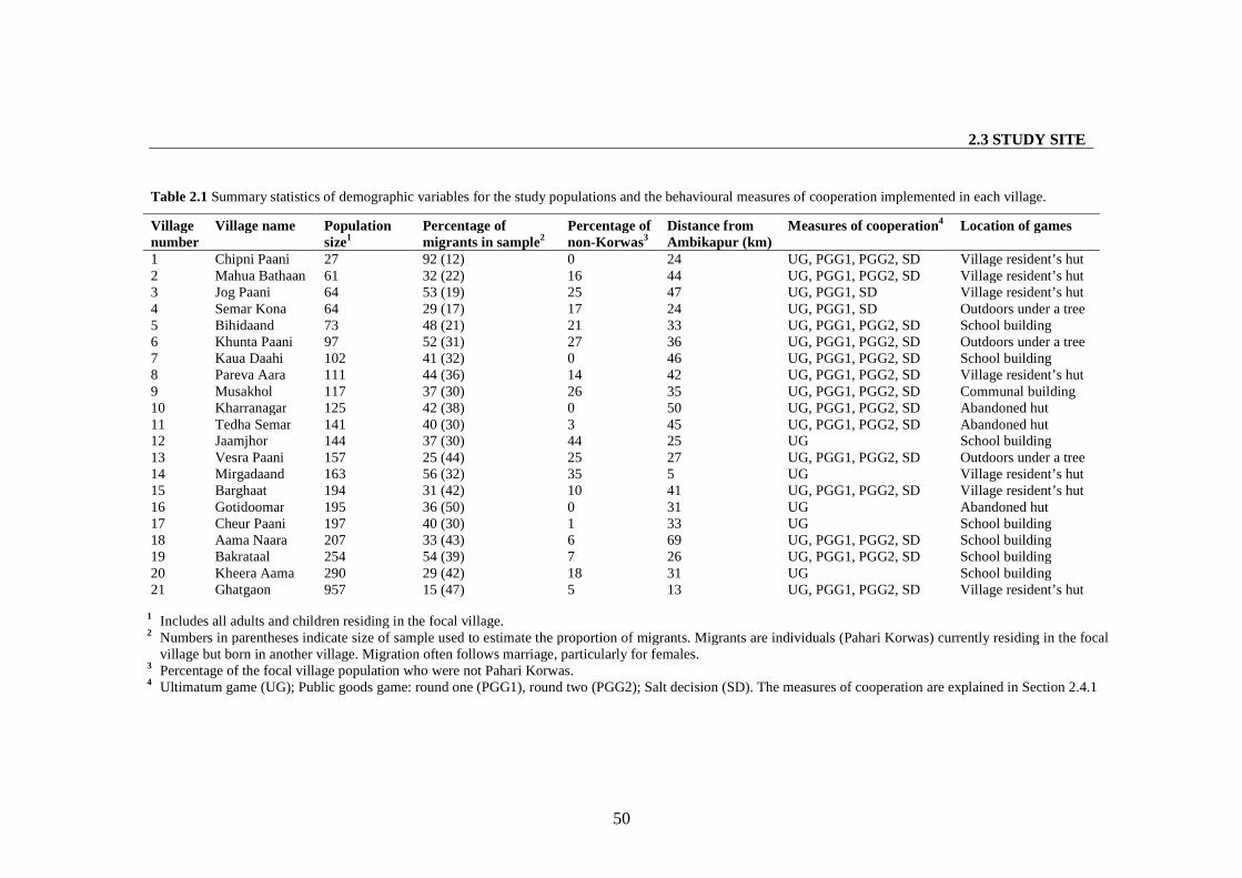
2.3 STUDY SITE
50
Table 2.1 Summary statistics of demographic variables for the study populations and the behavioural measures of cooperation implemented in each village.
Villagenumber
Village name Populationsize1
Percentage ofmigrants in sample2
Percentage ofnon-Korwas3
Distance fromAmbikapur (km)
Measures of cooperation4 Location of games
1 Chipni Paani 27 92 (12) 0 24 UG, PGG1, PGG2, SD Village resident’s hut2 Mahua Bathaan 61 32 (22) 16 44 UG, PGG1, PGG2, SD Village resident’s hut3 Jog Paani 64 53 (19) 25 47 UG, PGG1, SD Village resident’s hut4 Semar Kona 64 29 (17) 17 24 UG, PGG1, SD Outdoors under a tree5 Bihidaand 73 48 (21) 21 33 UG, PGG1, PGG2, SD School building6 Khunta Paani 97 52 (31) 27 36 UG, PGG1, PGG2, SD Outdoors under a tree7 Kaua Daahi 102 41 (32) 0 46 UG, PGG1, PGG2, SD School building8 Pareva Aara 111 44 (36) 14 42 UG, PGG1, PGG2, SD Village resident’s hut9 Musakhol 117 37 (30) 26 35 UG, PGG1, PGG2, SD Communal building10 Kharranagar 125 42 (38) 0 50 UG, PGG1, PGG2, SD Abandoned hut11 Tedha Semar 141 40 (30) 3 45 UG, PGG1, PGG2, SD Abandoned hut12 Jaamjhor 144 37 (30) 44 25 UG School building13 Vesra Paani 157 25 (44) 25 27 UG, PGG1, PGG2, SD Outdoors under a tree14 Mirgadaand 163 56 (32) 35 5 UG Village resident’s hut15 Barghaat 194 31 (42) 10 41 UG, PGG1, PGG2, SD Village resident’s hut16 Gotidoomar 195 36 (50) 0 31 UG Abandoned hut17 Cheur Paani 197 40 (30) 1 33 UG School building18 Aama Naara 207 33 (43) 6 69 UG, PGG1, PGG2, SD School building19 Bakrataal 254 54 (39) 7 26 UG, PGG1, PGG2, SD School building20 Kheera Aama 290 29 (42) 18 31 UG School building21 Ghatgaon 957 15 (47) 5 13 UG, PGG1, PGG2, SD Village resident’s hut
1 Includes all adults and children residing in the focal village.2 Numbers in parentheses indicate size of sample used to estimate the proportion of migrants. Migrants are individuals (Pahari Korwas) currently residing in the focal
village but born in another village. Migration often follows marriage, particularly for females.3 Percentage of the focal village population who were not Pahari Korwas.4 Ultimatum game (UG); Public goods game: round one (PGG1), round two (PGG2); Salt decision (SD). The measures of cooperation are explained in Section 2.4.1
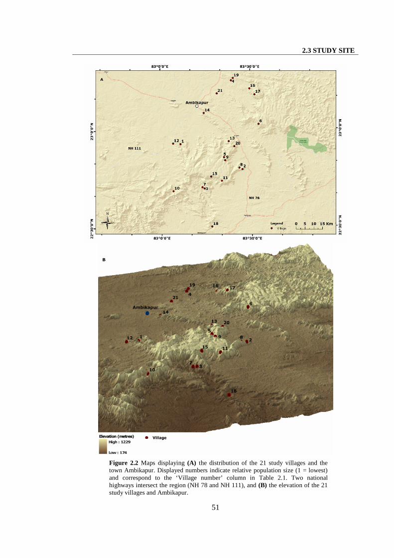
2.3 STUDY SITE
51
Figure 2.2 Maps displaying (A) the distribution of the 21 study villages and thetown Ambikapur. Displayed numbers indicate relative population size (1 = lowest)and correspond to the ‘Village number’ column in Table 2.1. Two nationalhighways intersect the region (NH 78 and NH 111), and (B) the elevation of the 21study villages and Ambikapur.
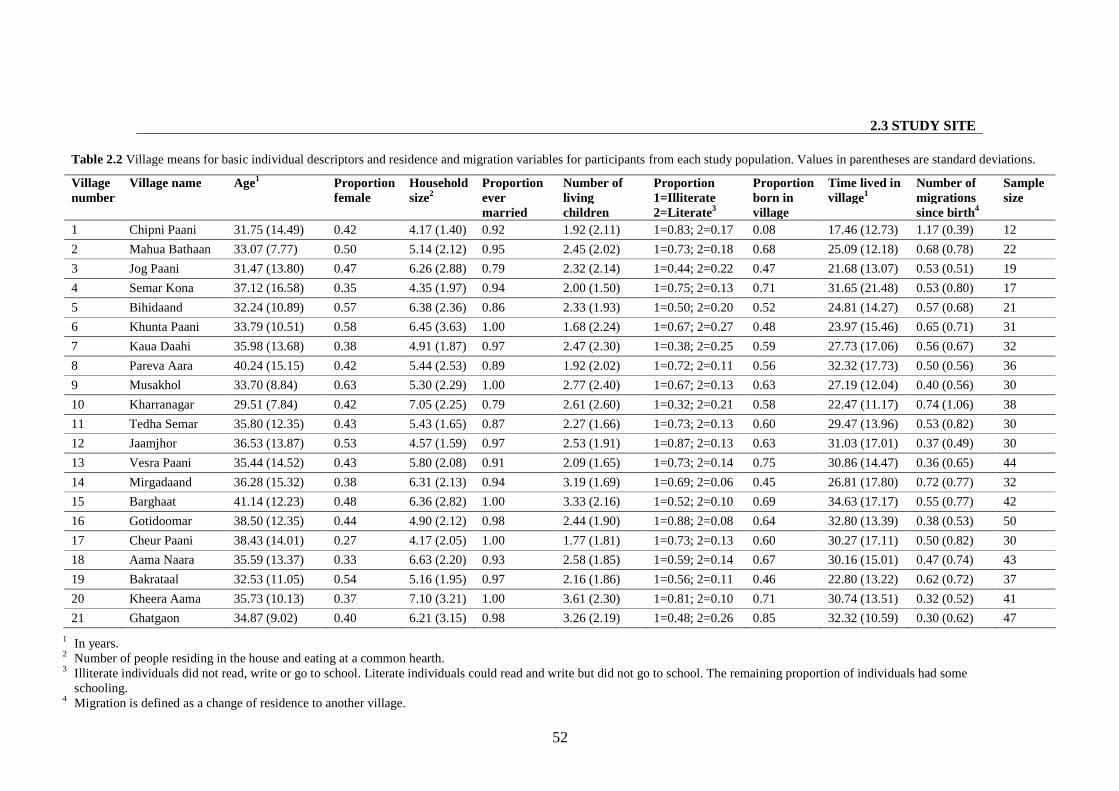
2.3 STUDY SITE
52
Table 2.2 Village means for basic individual descriptors and residence and migration variables for participants from each study population. Values in parentheses are standard deviations.
Villagenumber
Village name Age1 Proportionfemale
Householdsize2
Proportionevermarried
Number oflivingchildren
Proportion1=Illiterate2=Literate3
Proportionborn invillage
Time lived invillage1
Number ofmigrationssince birth4
Samplesize
1 Chipni Paani 31.75 (14.49) 0.42 4.17 (1.40) 0.92 1.92 (2.11) 1=0.83; 2=0.17 0.08 17.46 (12.73) 1.17 (0.39) 12
2 Mahua Bathaan 33.07 (7.77) 0.50 5.14 (2.12) 0.95 2.45 (2.02) 1=0.73; 2=0.18 0.68 25.09 (12.18) 0.68 (0.78) 22
3 Jog Paani 31.47 (13.80) 0.47 6.26 (2.88) 0.79 2.32 (2.14) 1=0.44; 2=0.22 0.47 21.68 (13.07) 0.53 (0.51) 19
4 Semar Kona 37.12 (16.58) 0.35 4.35 (1.97) 0.94 2.00 (1.50) 1=0.75; 2=0.13 0.71 31.65 (21.48) 0.53 (0.80) 17
5 Bihidaand 32.24 (10.89) 0.57 6.38 (2.36) 0.86 2.33 (1.93) 1=0.50; 2=0.20 0.52 24.81 (14.27) 0.57 (0.68) 21
6 Khunta Paani 33.79 (10.51) 0.58 6.45 (3.63) 1.00 1.68 (2.24) 1=0.67; 2=0.27 0.48 23.97 (15.46) 0.65 (0.71) 31
7 Kaua Daahi 35.98 (13.68) 0.38 4.91 (1.87) 0.97 2.47 (2.30) 1=0.38; 2=0.25 0.59 27.73 (17.06) 0.56 (0.67) 32
8 Pareva Aara 40.24 (15.15) 0.42 5.44 (2.53) 0.89 1.92 (2.02) 1=0.72; 2=0.11 0.56 32.32 (17.73) 0.50 (0.56) 36
9 Musakhol 33.70 (8.84) 0.63 5.30 (2.29) 1.00 2.77 (2.40) 1=0.67; 2=0.13 0.63 27.19 (12.04) 0.40 (0.56) 30
10 Kharranagar 29.51 (7.84) 0.42 7.05 (2.25) 0.79 2.61 (2.60) 1=0.32; 2=0.21 0.58 22.47 (11.17) 0.74 (1.06) 38
11 Tedha Semar 35.80 (12.35) 0.43 5.43 (1.65) 0.87 2.27 (1.66) 1=0.73; 2=0.13 0.60 29.47 (13.96) 0.53 (0.82) 30
12 Jaamjhor 36.53 (13.87) 0.53 4.57 (1.59) 0.97 2.53 (1.91) 1=0.87; 2=0.13 0.63 31.03 (17.01) 0.37 (0.49) 30
13 Vesra Paani 35.44 (14.52) 0.43 5.80 (2.08) 0.91 2.09 (1.65) 1=0.73; 2=0.14 0.75 30.86 (14.47) 0.36 (0.65) 44
14 Mirgadaand 36.28 (15.32) 0.38 6.31 (2.13) 0.94 3.19 (1.69) 1=0.69; 2=0.06 0.45 26.81 (17.80) 0.72 (0.77) 32
15 Barghaat 41.14 (12.23) 0.48 6.36 (2.82) 1.00 3.33 (2.16) 1=0.52; 2=0.10 0.69 34.63 (17.17) 0.55 (0.77) 42
16 Gotidoomar 38.50 (12.35) 0.44 4.90 (2.12) 0.98 2.44 (1.90) 1=0.88; 2=0.08 0.64 32.80 (13.39) 0.38 (0.53) 50
17 Cheur Paani 38.43 (14.01) 0.27 4.17 (2.05) 1.00 1.77 (1.81) 1=0.73; 2=0.13 0.60 30.27 (17.11) 0.50 (0.82) 30
18 Aama Naara 35.59 (13.37) 0.33 6.63 (2.20) 0.93 2.58 (1.85) 1=0.59; 2=0.14 0.67 30.16 (15.01) 0.47 (0.74) 43
19 Bakrataal 32.53 (11.05) 0.54 5.16 (1.95) 0.97 2.16 (1.86) 1=0.56; 2=0.11 0.46 22.80 (13.22) 0.62 (0.72) 37
20 Kheera Aama 35.73 (10.13) 0.37 7.10 (3.21) 1.00 3.61 (2.30) 1=0.81; 2=0.10 0.71 30.74 (13.51) 0.32 (0.52) 41
21 Ghatgaon 34.87 (9.02) 0.40 6.21 (3.15) 0.98 3.26 (2.19) 1=0.48; 2=0.26 0.85 32.32 (10.59) 0.30 (0.62) 47
1 In years.2 Number of people residing in the house and eating at a common hearth.3 Illiterate individuals did not read, write or go to school. Literate individuals could read and write but did not go to school. The remaining proportion of individuals had some
schooling.4 Migration is defined as a change of residence to another village.
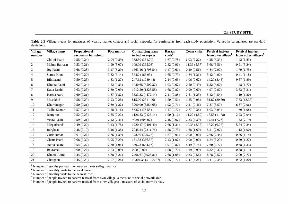
2.3 STUDY SITE
53
1 Number of months per year the household eats self-grown rice.2 Number of monthly visits to the local bazaar.3 Number of monthly visits to the nearest town.4 Number of people invited to harvest festival from own village; a measure of social network size.5 Number of people invited to harvest festival from other villages; a measure of social network size.
Table 2.3 Village means for measures of wealth, market contact and social networks for participants from each study population. Values in parentheses are standarddeviations.
Villagenumber
Village name Proportion ofearners in household
Rice months1 Outstanding loansin Indian rupees
Bazaarvisits2
Town visits3 Festival inviteesfrom own village4
Festival inviteesfrom other villages5
1 Chipni Paani 0.55 (0.24) 2.04 (0.89) 362.50 (351.70) 1.67 (0.78) 6.03 (7.22) 4.25 (3.33) 1.42 (1.83)
2 Mahua Bathaan 0.53 (0.21) 1.99 (3.07) 109.09 (365.03) 2.82 (0.96) 11.36 (5.37) 5.68 (3.51) 0.91 (3.24)
3 Jog Paani 0.68 (0.28) 3.17 (3.29) 1563.16 (1708.54) 1.47 (0.61) 0.49 (0.56) 4.84 (2.97) 1.79 (1.75)
4 Semar Kona 0.64 (0.20) 3.32 (3.14) 58.82 (166.05) 1.65 (0.79) 1.84 (1.31) 5.12 (4.00) 0.41 (1.18)
5 Bihidaand 0.50 (0.25) 1.83 (1.27) 247.62 (1089.44) 2.14 (0.65) 1.06 (0.62) 14.29 (8.48) 9.67 (6.89)
6 Khunta Paani 0.62 (0.24) 1.52 (0.83) 1080.65 (3507.37) 1.03 (0.67) 0.50 (0.49) 6.32 (3.60) 1.48 (1.77)
7 Kaua Daahi 0.63 (0.25) 2.30 (2.09) 1912.50 (1828.58) 1.68 (0.82) 0.99 (0.60) 4.97 (2.87) 3.63 (3.31)
8 Pareva Aara 0.60 (0.21) 1.87 (1.82) 3333.33 (4472.14) 2.11 (0.88) 2.51 (1.23) 5.42 (4.54) 1.19 (1.80)
9 Musakhol 0.56 (0.23) 2.93 (2.28) 815.00 (2511.46) 1.50 (0.51) 1.25 (0.98) 51.87 (20.50) 7.33 (13.38)
10 Kharranagar 0.50 (0.21) 2.89 (1.22) 3900.00 (3354.68) 1.92 (0.71) 0.21 (0.46) 7.87 (5.59) 6.87 (7.96)
11 Tedha Semar 0.57 (0.24) 1.58 (1.16) 56.67 (175.55) 1.47 (0.72) 0.77 (0.38) 6.03 (3.03) 1.60 (1.98)
12 Jaamjhor 0.52 (0.23) 2.85 (2.22) 1126.83 (2125.14) 1.90 (1.16) 11.20 (4.80) 16.53 (11.78) 2.93 (2.94)
13 Vesra Paani 0.59 (0.21) 2.22 (2.41) 90.91 (603.02) 2.15 (0.97) 7.33 (4.39) 12.41 (7.26) 1.32 (2.19)
14 Mirgadaand 0.49 (0.20) 3.13 (1.78) 1220.47 (2401.40) 2.66 (1.31) 10.38 (8.35) 16.22 (6.26) 5.84 (2.34)
15 Barghaat 0.45 (0.19) 3.46 (1.35) 2045.24 (2211.74) 1.58 (0.73) 1.68 (1.69) 5.21 (2.97) 1.12 (1.90)
16 Gotidoomar 0.61 (0.26) 2.76 (1.39) 328.50 (779.26) 1.87 (0.91) 0.00 (0.00) 2.66 (2.44) 0.36 (1.14)
17 Cheur Paani 0.68 (0.30) 3.95 (3.29) 131.33 (336.57) 2.43 (1.07) 0.00 (0.00) 6.24 (8.29) 0.59 (1.27)
18 Aama Naara 0.54 (0.22) 2.80 (1.94) 330.23 (634.16) 1.97 (0.82) 4.49 (3.74) 7.60 (4.72) 0.58 (1.33)
19 Bakrataal 0.60 (0.26) 2.53 (2.09) 0.00 (0.00) 1.58 (0.70) 1.19 (0.99) 6.32 (4.32) 0.38 (1.11)
20 Kheera Aama 0.44 (0.20) 4.88 (3.21) 2466.67 (6926.81) 2.68 (1.08) 0.33 (0.56) 8.78 (9.52) 2.00 (2.77)
21 Ghatgaon 0.45 (0.23) 2.07 (3.28) 10304.35 (51955.57) 1.55 (0.72) 2.47 (4.24) 3.11 (2.38) 0.72 (1.80)
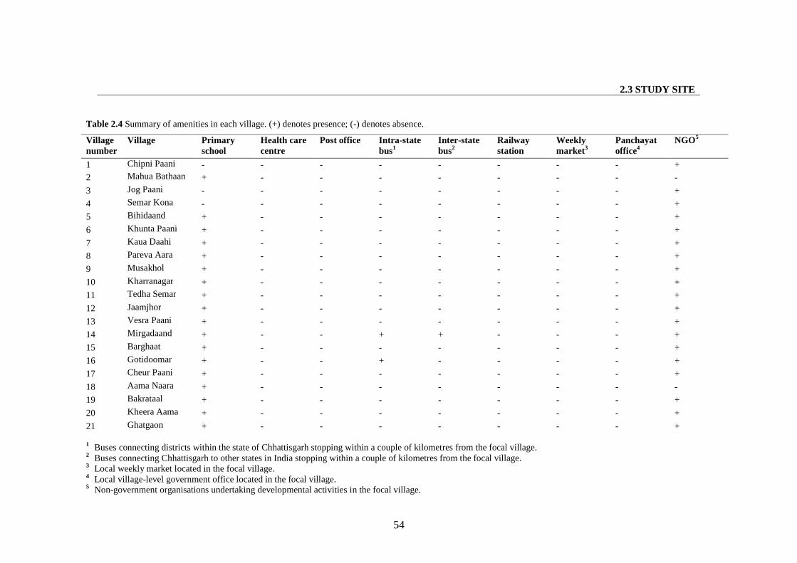
2.3 STUDY SITE
54
Table 2.4 Summary of amenities in each village. (+) denotes presence; (-) denotes absence.
Villagenumber
Village Primaryschool
Health carecentre
Post office Intra-statebus1
Inter-statebus2
Railwaystation
Weeklymarket3
Panchayatoffice4
NGO5
1 Chipni Paani - - - - - - - - +
2 Mahua Bathaan + - - - - - - - -
3 Jog Paani - - - - - - - - +
4 Semar Kona - - - - - - - - +
5 Bihidaand + - - - - - - - +
6 Khunta Paani + - - - - - - - +
7 Kaua Daahi + - - - - - - - +
8 Pareva Aara + - - - - - - - +
9 Musakhol + - - - - - - - +
10 Kharranagar + - - - - - - - +
11 Tedha Semar + - - - - - - - +
12 Jaamjhor + - - - - - - - +
13 Vesra Paani + - - - - - - - +
14 Mirgadaand + - - + + - - - +
15 Barghaat + - - - - - - - +
16 Gotidoomar + - - + - - - - +
17 Cheur Paani + - - - - - - - +
18 Aama Naara + - - - - - - - -
19 Bakrataal + - - - - - - - +
20 Kheera Aama + - - - - - - - +
21 Ghatgaon + - - - - - - - +
1 Buses connecting districts within the state of Chhattisgarh stopping within a couple of kilometres from the focal village.2 Buses connecting Chhattisgarh to other states in India stopping within a couple of kilometres from the focal village.3 Local weekly market located in the focal village.4 Local village-level government office located in the focal village.5 Non-government organisations undertaking developmental activities in the focal village.
2.4 METHODS
55
2.4 Methods
2.4.1 Behavioural data
Three measures of cooperation were used in this study. Of these, two are economic games,
namely, the ultimatum game (UG) and the public goods game (PGG) (Camerer 2003;
Kagel and Roth 1995), while one is a ‘real-world’ measure of cooperation which I term the
‘salt decision’. The UG and the PGG are experimental tools developed by economists; they
have previously been implemented extensively both in the laboratory as well as in field
studies (see Section 3.1.1 and Section 4.1.1 for reviews of literature on the UG and PGG
respectively). The ‘salt decision’ is a new measure of cooperation developed and
implemented for the first time in this study (see Sections 4.1.2 and 4.4.2). Table 2.1
summaries the measures implemented in each village. The details of each game including
specific game protocols are described in subsequent chapters. Here I illustrate the broad
features common to all game protocols used.
The study design excludes the following confounding causes of variation across
populations: (i) context and framing effects, (ii) experimenter variation, (iii) experimenter
familiarity, (iv) differences in recruitment methods and time periods over which games
were conducted in different populations, and (v) differences in protocols.
2.4.1.1 Anonymity
Participants made all game decisions once and anonymously, and were made explicitly
aware of the one-shot, anonymous set-up of each game. A player made her decisions
individually at a private location, and apart from the player and myself, no other individual
was present while she made her decisions. Player names were not recorded; a player’s only
identification in the study was a numbered token. Each player retained the same token
throughout the study in order to facilitate the comparison of individuals’ decisions across
all three measures of cooperative behaviour. Players were unaware of the identity of the
individuals they played with and remained so even after the study was completed. No
2.4 METHODS
56
village resident could therefore know the decision of a player or what s/he earned in the
game, either during or after the study.
2.4.1.2 Game instructions and testing
Instructions were delivered from standardised scripts in Sargujia. I first translated game
scripts from English to Hindi. The scripts were then translated from Hindi to Sargujia by
research assistants. The back translation method was used to ensure accuracy of translation.
Real money was used to demonstrate game rules and examples, and the instructions
explicitly demonstrated the complete anonymity of decisions. Only players who
individually answered a set of test questions correctly played any game. The questions were
designed to assess their understanding of the game and features of the experimental set-up
such as anonymity.
2.4.1.3 Administration
All games in all villages were administered by me within the first four days following our
arrival in a village. Prior to this study, I had no contact with any individual from any of the
21 villages included in this study. This protocol minimised experimenter familiarity with
the players. On each day of the games, all participants collected at a common location in
the village that was usually outdoors. We then designated three sites; the first for players
who were waiting to play the game, the second for those who had played, and the third as a
private location where the players made their game decisions. The locations were at least
10-20 m apart from each other, typically further, and always out of earshot. The private
location was often in the village school building or a village resident’s hut, and on occasion
an isolated outdoor site (Table 2.1).
The UG was played first, and was usually run for the first two days subsequent to our
arrival in a village. This was followed by the PGG, generally played on the third day after
our arrival in a village. All PGGs were completed in one day. Note that only those
individuals who had successfully understood and played the UG were recruited to play the
PGG on the third day. All games were played for real money with substantial stakes
2.4 METHODS
57
ranging from one to two days’ local wages. Stake size was determined as an approximate
multiple of mean local wages estimated by sampling several villages in the study region.
Individuals across all villages participate in similar economic activities and visit the same
markets. Moreover, previous studies suggest that stake size does not significantly affect
behaviour in the PGG and UG (Cameron 1999; Kocher et al. 2008). For all of the above
reasons, the stakes were kept constant across villages.
Participants made all their game decisions by physically manipulating real money. Play
order was randomised for all games. Individuals who had played a game were prevented
from interacting with those who had not yet played that game; participants who had played
the game were seated at a separate location to those who had yet to play and research
assistants monitored the two groups to ensure there was no discussion about the game.
Participants were forbidden from discussing the game during the study period and warned
that the games would be discontinued if they did. We provided rations, which were cooked
and consumed on the day of the games, for a full meal for each player. The meal was
cooked by the waiting participants themselves; this kept them occupied for a few hours.
They prepared a full meal for 25 to 30 people and manufactured plates and bowls from Sal
tree leaves for everyone to eat off.
2.4.1.4 Payments
All participants received a show-up fee of 30 rupees, which is just under one day’s local
wages. From demographic data collected on 784 adults I estimated mean local wages in the
region at 38.68 ± 12.05 rupees per day. The show-up fee was handed to players on the day
that they participated in a game. Each player’s earnings from the different games were
summed and paid together on the final day of game play in each village, once all games had
been completed. This was done because (a) it eliminated outcome-based feedback to UG
players who played on the first day, and who could otherwise have communicated these
outcomes to village residents scheduled to play on day two, thus influencing their decisions,
(b) it allowed me to collect data on individuals’ salt decisions (see Sections 4.1.2 and 4.4.2
for details) that could be compared to their PGG behaviour, and (c) it made it easier for me
to pay individuals their exact earnings without doubling the amount of small currency that I
2.4 METHODS
58
needed to carry to each village. Players collected their payments individually at a private
location in exchange for their identification tokens, and the order in which they did so was
randomised. All payments were made in real money in exact change. Players made their
salt decisions (see Sections 4.1.2 and 4.4.2 for details) upon arriving to collect their
payments at the private location. The salt decision was made before a player’s earnings
from the games were made known and given to her.
2.4.2 Demographic and individual data
Demographic and other data on individuals were collected via a standardised questionnaire
(see Appendix B, Section B.1 for the individual data sheet). The questionnaire used to
collect individual data was administered by a research assistant once a participant had
played the UG. Once all games in a village had been completed, a population census was
conducted and the geographic coordinates for every house in the village were recorded (see
Appendix B, Section B.3 for the housing data sheet) using a Global Positioning System
(GPS; Garmin GPS 12XL). I also recorded whether a village had access to basic facilities
such as a primary school, a hospital or health care centre, a post office, bus services, local
government office or any non-government organisations working in the area, and the
location of these facilities (see Appendix B, Section B.2 for the village data sheet).
Table 2.5 lists all village and individual descriptors that were included in all analyses and
provides a description of each variable. Five village descriptors were included in this study.
The village descriptors ‘population size’ and ‘proportion of migrants’ (a measure of
migration rates between populations) are of interest because they are directly linked to the
evolutionary stability of cooperation in a population; the theoretical literature demonstrates
that large populations and high rates of migration work against the evolution of cooperation
(reviewed in Grafen 1984 and Henrich 2004). The village descriptor ‘proportion of non-
Korwas’ is used to examine whether any variation between villages is explained by the co-
residence of other ethnic groups; theoretical and empirical studies demonstrate that inter-
group competition can promote within-group cooperation (e.g. Bernhard et al. 2006;
Burton-Chellew et al. 2010; Choi and Bowles 2007; de Cremer and van Vugt 1999;
Puurtinen and Mappes 2009). The variables ‘household dispersion’ and ‘distance from
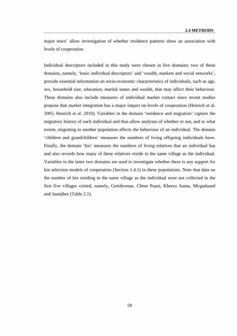
2.4 METHODS
59
major town’ allow investigation of whether residence patterns show an association with
levels of cooperation.
Individual descriptors included in this study were chosen in five domains; two of these
domains, namely, ‘basic individual descriptors’ and ‘wealth, markets and social networks’,
provide essential information on socio-economic characteristics of individuals, such as age,
sex, household size, education, marital status and wealth, that may affect their behaviour.
These domains also include measures of individual market contact since recent studies
propose that market integration has a major impact on levels of cooperation (Henrich et al.
2005; Henrich et al. 2010). Variables in the domain ‘residence and migration’ capture the
migratory history of each individual and thus allow analyses of whether or not, and to what
extent, migrating to another population affects the behaviour of an individual. The domain
‘children and grandchildren’ measures the numbers of living offspring individuals have.
Finally, the domain ‘kin’ measures the numbers of living relatives that an individual has
and also records how many of these relatives reside in the same village as the individual.
Variables in the latter two domains are used to investigate whether there is any support for
kin selection models of cooperation (Section 1.4.1) in these populations. Note that data on
the number of kin residing in the same village as the individual were not collected in the
first five villages visited, namely, Gotidoomar, Cheur Paani, Kheera Aama, Mirgadaand
and Jaamjhor (Table 2.1).
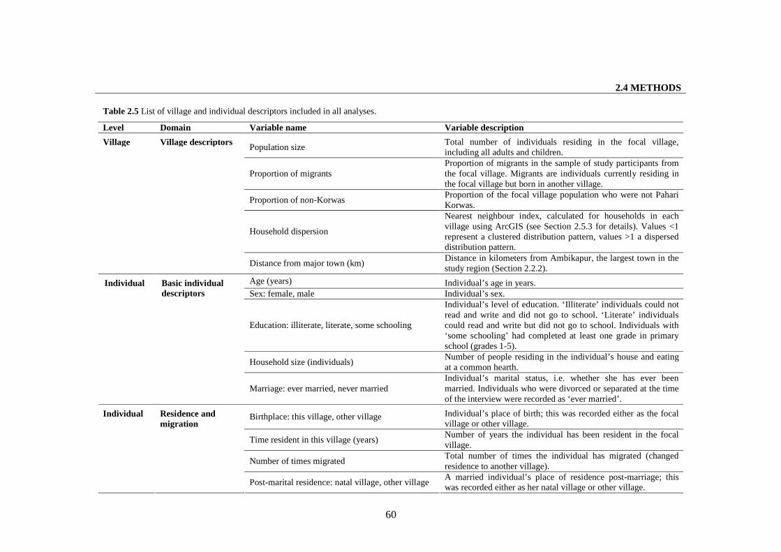
2.4 METHODS
60
Table 2.5 List of village and individual descriptors included in all analyses.
Level Domain Variable name Variable description
Population sizeTotal number of individuals residing in the focal village,including all adults and children.
Proportion of migrantsProportion of migrants in the sample of study participants fromthe focal village. Migrants are individuals currently residing inthe focal village but born in another village.
Proportion of non-KorwasProportion of the focal village population who were not PahariKorwas.
Household dispersion
Nearest neighbour index, calculated for households in eachvillage using ArcGIS (see Section 2.5.3 for details). Values <1represent a clustered distribution pattern, values >1 a disperseddistribution pattern.
Village Village descriptors
Distance from major town (km)Distance in kilometers from Ambikapur, the largest town in thestudy region (Section 2.2.2).
Age (years) Individual’s age in years.Sex: female, male Individual’s sex.
Education: illiterate, literate, some schooling
Individual’s level of education. ‘Illiterate’ individuals could notread and write and did not go to school. ‘Literate’ individualscould read and write but did not go to school. Individuals with‘some schooling’ had completed at least one grade in primaryschool (grades 1-5).
Household size (individuals)Number of people residing in the individual’s house and eatingat a common hearth.
Individual Basic individualdescriptors
Marriage: ever married, never marriedIndividual’s marital status, i.e. whether she has ever beenmarried. Individuals who were divorced or separated at the timeof the interview were recorded as ‘ever married’.
Birthplace: this village, other village Individual’s place of birth; this was recorded either as the focalvillage or other village.
Time resident in this village (years)Number of years the individual has been resident in the focalvillage.
Number of times migratedTotal number of times the individual has migrated (changedresidence to another village).
Individual Residence andmigration
Post-marital residence: natal village, other villageA married individual’s place of residence post-marriage; thiswas recorded either as her natal village or other village.
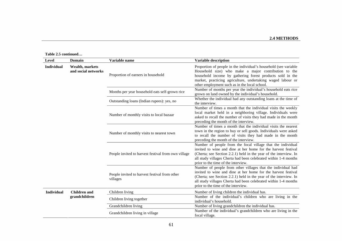
2.4 METHODS
61
Table 2.5 continued…
Level Domain Variable name Variable description
Proportion of earners in household
Proportion of people in the individual’s household (see variableHousehold size) who make a major contribution to thehousehold income by gathering forest products sold in themarket, practicing agriculture, undertaking waged labour orother employment such as in the local school.
Months per year household eats self-grown riceNumber of months per year the individual’s household eats ricegrown on land owned by the individual’s household.
Outstanding loans (Indian rupees): yes, noWhether the individual had any outstanding loans at the time ofthe interview.
Number of monthly visits to local bazaar
Number of times a month that the individual visits the weeklylocal market held in a neighboring village. Individuals wereasked to recall the number of visits they had made in the monthpreceding the month of the interview.
Number of monthly visits to nearest town
Number of times a month that the individual visits the nearesttown in the region to buy or sell goods. Individuals were askedto recall the number of visits they had made in the monthpreceding the month of the interview.
People invited to harvest festival from own village
Number of people from the focal village that the individualinvited to wine and dine at her home for the harvest festival(Cherta; see Section 2.2.1) held in the year of the interview. Inall study villages Cherta had been celebrated within 1-4 monthsprior to the time of the interview.
Individual Wealth, marketsand social networks
People invited to harvest festival from othervillages
Number of people from other villages that the individual hadinvited to wine and dine at her home for the harvest festival(Cherta; see Section 2.2.1) held in the year of the interview. Inall study villages Cherta had been celebrated within 1-4 monthsprior to the time of the interview.
Children living Number of living children the individual has.
Children living togetherNumber of the individual’s children who are living in theindividual’s household.
Grandchildren living Number of living grandchildren the individual has.
Individual Children andgrandchildren
Grandchildren living in villageNumber of the individual’s grandchildren who are living in thefocal village.
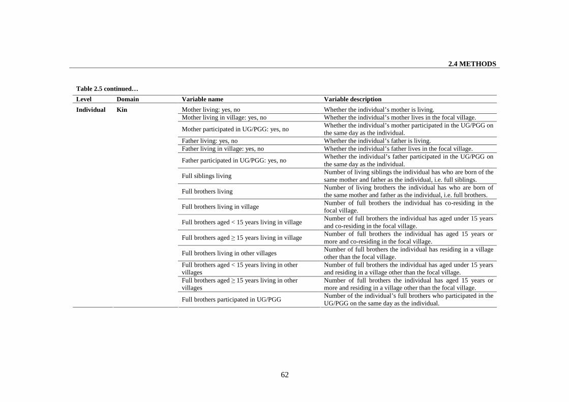
2.4 METHODS
62
Table 2.5 continued…
Level Domain Variable name Variable description
Mother living: yes, no Whether the individual’s mother is living.Mother living in village: yes, no Whether the individual’s mother lives in the focal village.
Mother participated in UG/PGG: yes, noWhether the individual’s mother participated in the UG/PGG onthe same day as the individual.
Father living: yes, no Whether the individual’s father is living.Father living in village: yes, no Whether the individual’s father lives in the focal village.
Father participated in UG/PGG: yes, noWhether the individual’s father participated in the UG/PGG onthe same day as the individual.
Full siblings livingNumber of living siblings the individual has who are born of thesame mother and father as the individual, i.e. full siblings.
Full brothers livingNumber of living brothers the individual has who are born ofthe same mother and father as the individual, i.e. full brothers.
Full brothers living in villageNumber of full brothers the individual has co-residing in thefocal village.
Full brothers aged < 15 years living in villageNumber of full brothers the individual has aged under 15 yearsand co-residing in the focal village.
Full brothers aged ≥ 15 years living in villageNumber of full brothers the individual has aged 15 years ormore and co-residing in the focal village.
Full brothers living in other villagesNumber of full brothers the individual has residing in a villageother than the focal village.
Full brothers aged < 15 years living in othervillages
Number of full brothers the individual has aged under 15 yearsand residing in a village other than the focal village.
Full brothers aged ≥ 15 years living in othervillages
Number of full brothers the individual has aged 15 years ormore and residing in a village other than the focal village.
Individual Kin
Full brothers participated in UG/PGGNumber of the individual’s full brothers who participated in theUG/PGG on the same day as the individual.
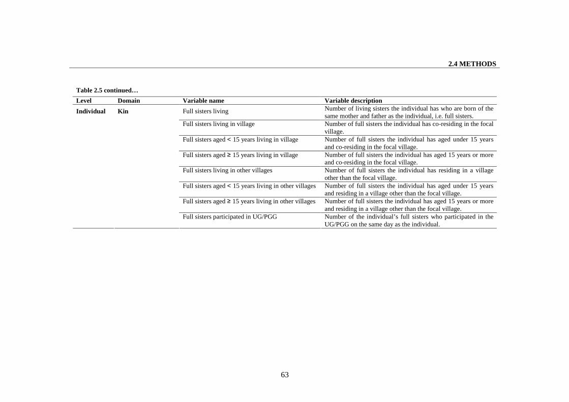
2.4 METHODS
63
Table 2.5 continued…
Level Domain Variable name Variable description
Full sisters living Number of living sisters the individual has who are born of thesame mother and father as the individual, i.e. full sisters.
Full sisters living in village Number of full sisters the individual has co-residing in the focalvillage.
Full sisters aged < 15 years living in village Number of full sisters the individual has aged under 15 yearsand co-residing in the focal village.
Full sisters aged ≥ 15 years living in village Number of full sisters the individual has aged 15 years or moreand co-residing in the focal village.
Full sisters living in other villages Number of full sisters the individual has residing in a villageother than the focal village.
Full sisters aged < 15 years living in other villages Number of full sisters the individual has aged under 15 yearsand residing in a village other than the focal village.
Full sisters aged ≥ 15 years living in other villages Number of full sisters the individual has aged 15 years or moreand residing in a village other than the focal village.
Individual Kin
Full sisters participated in UG/PGG Number of the individual’s full sisters who participated in theUG/PGG on the same day as the individual.
2.5 ANALYSES
64
2.4.3 Qualitative data
In every village visited, I made observational notes and, in addition conducted informal
interviews with a few individuals to obtain historical information on the village as well as
qualitative information on kin relations, sharing norms, religious and communal activities
and day to day living patterns (see Appendix B, Section B.4 for the qualitative data sheet).
2.5 Analyses
2.5.1 Data processing
All data were manually entered into spreadsheets in Microsoft Office Excel 2003 version
11 (Microsoft Corporation 2003). A separate spreadsheet was created for each village.
Error checks were performed by two people (including myself) by checking every entry for
errors. The data were then collated to construct the full dataset and imported into the
relevant statistical packages for analyses.
2.5.2 Multilevel models
I have used multilevel statistical models (Gelman and Hill 2007; Snijders and Roel 1999) to
explicitly analyse variation at the village and individual levels in my structured data
(individuals within villages), and the relationship of population and individual descriptors
with the measure of cooperation (outcome variable). Multilevel models are used to analyse
hierarchically clustered units of analysis, for instance individuals within villages within
cultural groups. These models account for the possibility that units within a cluster, such as
individuals from a village, may be more alike than units across clusters, such as individuals
across villages. Ignoring the potential correlation of units within a cluster, i.e. the multilevel
structure of data, can result in an underestimation of standard errors. Multilevel models
correct for such non-independence of clustered data, reducing the likelihood of type I errors.
They also allow us to accurately estimate the effects of groups along with group-level
predictors. Traditional regression models used in previous cross- and intra-cultural studies
(e.g. Gurven et al. 2008; Henrich et al. 2005) treat the units of analysis as independent, an
assumption that is severely violated if group membership, whether at the culture or
2.5 ANALYSES
65
population level, affects individual behaviour. Rather than traditional significance testing,
in this thesis I mainly use an information theoretic model fitting approach to analyse data
and interpret results (see Burnham and Anderson 1998, Burnham and Anderson 2002 and
Efferson and Richerson 2007 for comparative discussions of these approaches). All
multilevel analyses were conducted in MLwiN version 2.14 (Browne 2009; Rasbash et al.
2009), while other statistical analyses were conducted in SPSS version 16.0.2 (SPSS Inc.
2008).
All multilevel models were run with two levels: individuals (level 1) nested within villages
(level 2). Analyses proceeded in four stages. In the first stage, null models (with intercept
terms only) were constructed with and without a multilevel structure and these were
compared to establish whether the multilevel model provided a significantly better fit to the
data. The Deviance Information Criterion (DIC) was used to compare models
(Spiegelhalter et al. 2002). The DIC is a Bayesian measure of model fit and complexity; it
accounts for the change in degrees of freedom between nested models. Models with a lower
DIC value provide a better fit to the data and a difference in DIC values of 5-10 units or
more is considered substantial (Burnham and Anderson 1998; Spiegelhalter et al. 2002). In
the second stage, a series of multilevel univariate models were constructed to explore the
relationship between each explanatory variable in the dataset and the outcome variable. A
Wald test (Rasbash et al. 2009) was used to establish the statistical significance level of an
explanatory variable. In the third stage, a series of domain-wise (sets of related variables
such as those measuring wealth, kin etc. described in Table 2.5) models were produced to
identify the important explanatory variables within each domain. Once again, the Wald test
was used to establish the statistical significance of variables.
The full model was constructed in the fourth stage, implementing a step-wise procedure
with three serially entered blocks of variables. The first block entered contained all those
variables from the domains of village descriptors, basic individual descriptors, residence
and migration, wealth, markets and social networks that reached significance at p<0.10
within their domains (in the third stage domain-wise analyses); the block additionally
contained age and sex even if they did not reach significance. The model obtained was then
reduced by a backwards procedure eliminating predictor terms that did not reach
2.5 ANALYSES
66
significance in a Wald test at the p<0.05 level. However, reduced and non-reduced models
were compared for fit using their DIC values and the model with the lower DIC value was
always retained, whether or not the variables in it reached significance at p<0.05. All
variables that were not discarded at this stage were carried forward and the next block of
variables was added into this model. The second block added contained all those variables
from the domain of children and grandchildren that reached significance at p<0.10 within
this domain. The backward stepwise procedure was repeated with the new block of
variables. The third block added contained all those variables from the domain of kin that
reached significance at p<0.10 within this domain. The variables age and sex were carried
forward to the last block even if they did not reach significance at p<0.05. They were only
eliminated at the very end if they did not reach significance at the p<0.05 level. Hence, the
three blocks of variables were always added in the same order in a forward step-wise
procedure, but within each block variables were eliminated in a backward step-wise
procedure to obtain the full model. Appendix C presents the univariate and domain-wise
models, and a step-wise summary of the full model fitting process implemented in the
fourth stage, for all analyses presented in this thesis.
Iterative Generalised Least Squares (IGLS) estimation or Restricted Iterative Generalised
Least Squares (RIGLS) estimation with a 2nd order predictive (or penalised) quasi-
likelihood (PQL) approximation was used to fit all univariate (second stage) and domain-
wise models (third stage). The null (first stage) and full models (fourth stage) were fitted
using Markov Chain Monte Carlo (MCMC) estimation (Browne 2009) run for 10,000
iterations and a burn-in period of 500 iterations.
The small sample sizes in some villages are a reflection of the small populations in these
villages (e.g. Chipni Paani had only 12 adults, all of whom participated in this study).
Multilevel models account for sample size differences between populations when
computing the variance components and parameter estimates. 70-100% of households had
at least one household member participate in the games in all villages except Ghatgaon,
Bakrataal and Tedha Semar, where this proportion was 17%, 55% and 55% respectively.
The latter three villages are among those with the largest populations in my dataset (Table
2.1). Although I estimated how many households were represented by at least one
2.5 ANALYSES
67
individual once all games had been completed, I did not collect data on which household
each individual belonged to in order to avoid compromising players’ anonymity. Hence, I
cannot include households as an additional level in my models.
2.5.3 GIS analyses
Geographic Information Systems (GIS) data were processed and analysed in ArcGIS
version 9.2 (ArcGIS 2006). All maps (Figure 2.2) were created and analysed using the
WGS 1984 Geographic Coordinate System with a Transverse Mercator Projection. A 30m
Digital Elevation Model (ASTER Global Digital Elevation Model V001) was used for the
relevant map area; this was obtained from the NASA Land Processes Distributed Active
Archive Center (https://wist.echo.nasa.gov). The base map [ESRI Street Map World 2D
(old) © 2009 ESRI, and, TANA, ESRI Japan, UNEP-WCMC] used in Figure 2.2A was
obtained from the ARCGIS Online Resource Centre
(http://resources.esri.com/gateway/index.cfm). The nearest neighbour index (Clark and
Evans 1954), calculated for households in each village, is used as the measure of household
dispersion for each village (see village descriptors in Table 2.5).
68
SECTION I
VARIATION IN COOPERATION ACROSS POPULATIONS
69
CHAPTER 3
VARIATION IN COOPERATION ACROSS POPULATIONS:
EVIDENCE FROM THE ULTIMATUM GAME
3.1 Introduction
3.1.1 Background and related research
The first question addressed in this thesis is: is there stable, heritable variation in levels of
cooperation across human populations? In this chapter I present findings from the
ultimatum game (UG), my first measure of cooperative behaviour, implemented in 21
Pahari Korwa villages.
Several studies have demonstrated variation in cooperative behaviour across human
populations (Cardenas and Carpenter 2005; Henrich et al. 2004; Henrich et al. 2005;
Henrich et al. 2010; Henrich et al. 2006; Herrmann et al. 2008; Marlowe et al. 2008;
Oosterbeek et al. 2004; Roth et al. 1991); this variation has been attributed to cultural
differences between populations. However, since these studies sampled from one (or very
few) populations per culture, they confound cultural and ecological differences between
populations (Section 1.6.2). We cannot differentiate whether cultural transmission or
environmental (demographic and ecological) differences drive the observed behavioural
variation across populations. Controlling for cultural differences between populations, I
examine whether there is variation in levels of cooperation within and between multiple
populations of the same endogamous small-scale society, the Pahari Korwa. I compare
variance across populations of the same small-scale society to that found previously across
3.1 INTRODUCTION
70
15 different small-scale societies (Henrich et al. 2005); if cultural transmission at the
cultural group level drives variation across populations, then we should expect greater
variation between cultural groups than across populations of the same cultural group. I
further investigate whether environmental (demographic and ecological) factors explain
any part of the variation across populations in my study. While variation driven by cultural
transmission is heritable, variation driven by demographic or ecological factors is not
necessarily stable or heritable; environmental drivers of behavioural variation are less likely
to maintain stable differences essential for selection at the population-level.
The few studies that have examined intra-cultural variation in cooperative behaviour
(Gurven 2004a; Gurven et al. 2008; Marlowe 2004) obtained inadequate sample sizes to
enable reliable, explicit analyses of relative variation at the population and individual levels.
Moreover, traditional regression models employed in these studies treat the units of
analysis as independent, an assumption that is severely violated if group membership,
whether at the culture or population level, affects individual behaviour (Section 2.5.2).
While the above-cited studies do report behavioural variation across populations/camps of
the same cultural group, small sample sizes (five to nine villages), unsuitable model
populations with ill-defined population boundaries (e.g. Marlowe 2004), and the use of
inappropriate statistical tools, make their estimates of population level variance unreliable.
The UG (Güth et al. 1982) is a two-player game where one of a pair of individuals, the
‘proposer’, must divide a sum of money (the stake, S) between herself and an unknown
‘responder’. If the responder accepts the proposer’s offer (x), the responder earns x, and the
proposer earns S-x. If the responder rejects the offer, neither player earns anything. In this
game the income-maximising strategy entails that a responder accept any offer made by the
proposer. Assuming that the responder will play the income-maximising strategy, the
income-maximising strategy for a proposer is to make the smallest possible offer. The UG
is one of the most extensively employed experimental economic games. It has been played
both in populations of small-scale societies (Henrich et al. 2005; Henrich et al. 2010;
Henrich et al. 2006; Marlowe et al. 2008) and large-scale, industrialized societies, although
mostly amongst university students in the latter (reviewed in Camerer 2003, Oosterbeek et
al. 2004 and Roth 1995a). Behaviour in the UG varies considerably across populations of
3.1 INTRODUCTION
71
small-scale societies (e.g. Henrich et al. 2005). There is less variation across populations of
large-scale societies; individuals typically make offers between 40% and 50% of the stake
and reject offers below about 30% of the stake (reviewed in Camerer 2003).
3.1.2 Behavioural measures
In this study, the UG was played with the rules described above (see Section 2.4 for details
of study set-up and Section 3.4.1 for details of the games). The size of the stake (S) for each
game was 100 rupees, equivalent to a little over two days’ wages in the region. Offer values
were restricted to multiples of five. Each individual played the game once and in one role,
as a proposer or a responder, under anonymous conditions. Pairs of players were
constituted by randomly matching token numbers. In 16 of the 21 populations where the
UG was played, once a responder had made her decision regarding whether she wished to
accept or reject the offered amount, I additionally asked her what minimum offer from a
proposer she was willing to accept; this was recorded as the minimum acceptable offer
(MAO) for that individual. The game outcome and payoffs were determined on the basis of
the accept/reject response and players were fully aware of this. Hence, the MAO is a self-
reported figure and players knew that its value did not affect their actual payoffs in the
game. I use MAO values to examine whether players’ self-reported behavioural strategies
agree with their game behaviour. I also examine whether properties of the village and/or
individual are associated with such self-reported MAOs.
I employ multilevel normal linear models (Browne 2009; Rasbash et al. 2009; Snijders and
Bosker 1999) to explicitly analyse variation in UG behaviour at the village and individual
levels.

3.2 RESULTS
72
3.2 Results
344 individuals participated as proposers and 340 as responders in UGs played across 21
villages. Table 3.1 presents sample sizes of UG proposers and responders for the 21
villages. The total number of proposers differs from the total number of responders since in
eight villages an odd number of individuals participated in the games. In these villages, one
individual was paired randomly with two other players from the village in order to
determine the payoff to all participating players.
Table 3.1 Number (n) of proposers (total n = 344) and responders (total n = 340) from each of 21 studyvillages.
Village number Village Proposers (n) Responders (n)
1 Chipni Paani 6 62 Mahua Bathaan 11 113 Jog Paani 10 94 Semar Kona 9 85 Bihidaand 11 106 Khunta Paani 16 157 Kaua Daahi 16 168 Pareva Aara 18 189 Musakhol 15 1510 Kharranagar 19 1911 Tedha Semar 15 1512 Jamjhor 15 1513 Vesra Paani 22 2214 Mirgadaand 16 1615 Barghaat 21 2116 Gotidoomar 25 2517 Cheur Paani 15 1518 Aama Naara 21 2219 Bakrataal 19 1820 Kheera Aama 20 2121 Ghatgaon 24 23
In Section 3.2.1 I present findings on proposer offers; Section 3.2.1.1 examines whether
proposer offers vary across populations and Section 3.2.1.2 investigates whether properties
of villages and/or individuals explain any variation in proposer offers. In Section 3.2.2 I
present findings on responder behaviour; Sections 3.2.2.1 and 3.2.2.2 examine whether
responders’ game responses and self-reported MAOs vary across populations respectively,
and Section 3.2.2.3 investigates whether properties of villages and/or individuals explain
3.2 RESULTS
73
any variation in responders’ self-reported MAOs. Finally, in Section 3.2.3 I investigate
whether proposer and responder behaviour co-vary in the study populations.
3.2.1 Proposers
3.2.1.1 Do proposer offers vary across populations?
Distributions of proposer offers (Figure 3.1) vary considerably across villages. The modal
offer across all villages is 50 rupees (50% of the stake). While the primary mode (the most
frequently made offer) varies little across villages, the secondary mode (the second most
frequently made offer) varies between 30 and 70 rupees across villages. Mean offers vary
between about 31 and 52 rupees. 14.4% of the variance in offers occurs between villages
[Table 3.2B; null model (multilevel)]. The DIC value for the null model with village level
intercepts (multilevel) is about 44 units lower than for the null model without village level
intercepts (single level), indicating that the multilevel model accounting for village effects
provides a substantially better fit to the data (Table 3.2A; null models). Once village and
individual descriptors are included in the full model, the unexplained between-village
variance reduces to 11.2% [Table 3.2B; full model (multilevel)]. Variance in UG proposer
offers between 15 small-scale societies was estimated at about 12% (Henrich et al. 2004;
Henrich et al. 2005). Behavioural variance between 21 populations of the same small-scale
society is therefore comparable to that between 15 populations of 15 different societies.
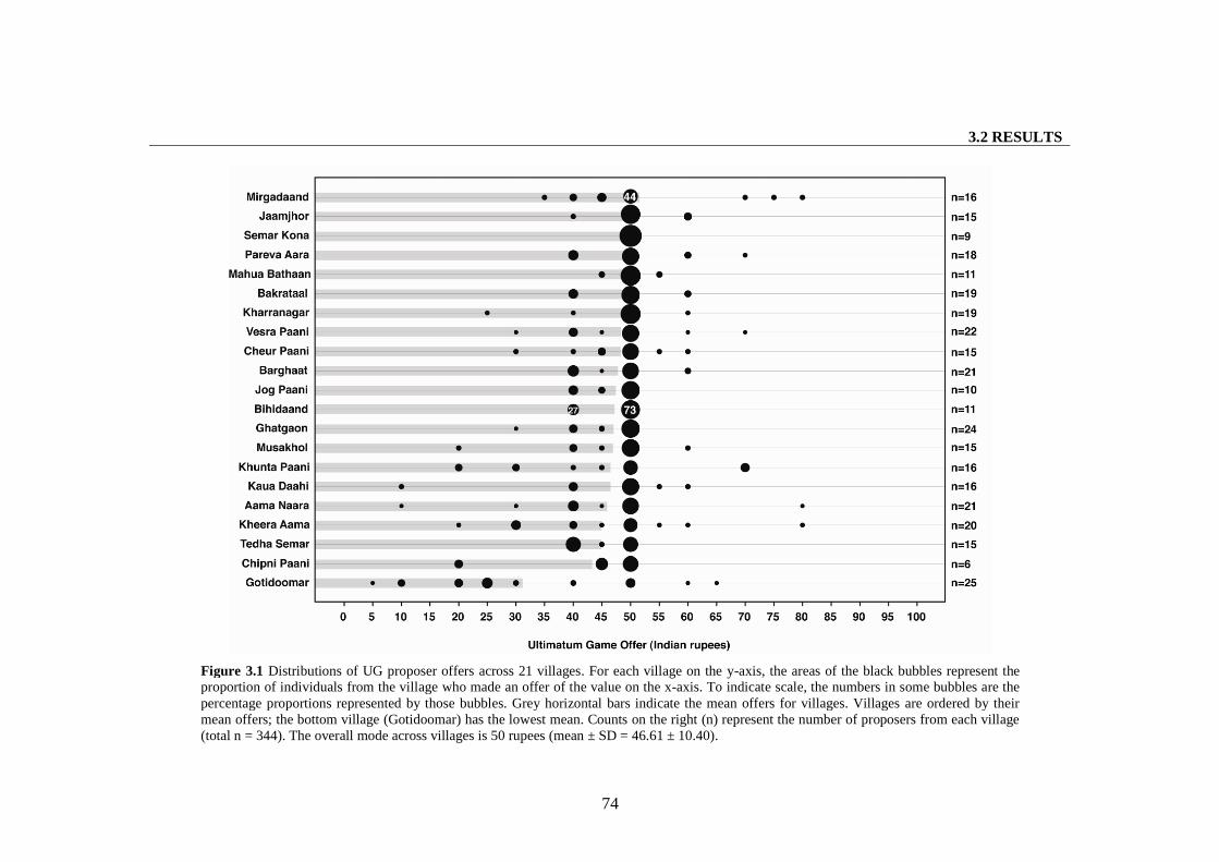
3.2 RESULTS
74
Figure 3.1 Distributions of UG proposer offers across 21 villages. For each village on the y-axis, the areas of the black bubbles represent theproportion of individuals from the village who made an offer of the value on the x-axis. To indicate scale, the numbers in some bubbles are thepercentage proportions represented by those bubbles. Grey horizontal bars indicate the mean offers for villages. Villages are ordered by theirmean offers; the bottom village (Gotidoomar) has the lowest mean. Counts on the right (n) represent the number of proposers from each village(total n = 344). The overall mode across villages is 50 rupees (mean ± SD = 46.61 ± 10.40).
3.2 RESULTS
75
3.2.1.2 Do properties of populations and/or individuals explain variation in proposer
offers between and within populations?
One population descriptor and two individual descriptors are retained in the full model and
explain a significant amount of variation in proposer offers between and within populations
[Table 3.2A; full model (multilevel)]. Pseudo R2 values 1 indicate that about 22% of
variance between populations and 9% of variance within populations is explained by the
three descriptor variables retained in the full model. The proportion of non-Korwas (village
residents who are not Pahari Korwas) has a strong positive effect on proposer offers. Each
additional non-Korwa living in the village is associated with offer values that are about 14
rupees (14% of the stake) higher on average. Note that non-Korwas did not participate in
the games in any village. A player’s household size has a small negative effect on her offer.
People with an additional person in their household make offers that are about half a rupee
lower on average. Finally, people who played on the second or third day of the games in
any village made offers that were about five rupees higher on average. While I report p
values for all variables, and although the effect of the proportion of non-Korwas (p = 0.057)
and household size (p = 0.060) is marginally significant by conventional standards, I rely
mainly on model fit criteria in interpreting these results (Section 2.5.2).
1Pseudo R2 values were computed according to Snijders and Bosker (1999).

3.2 RESULTS
76
Table 3.2 (A) Associations of each predictor term (fixed effect) with proposer offers in the null (intercept only) and fullmodels. (B) Village and individual level variance components for proposer offer in the null and full models.1 The variancepartition coefficient [VPC = village level variance/ (village level variance + individual level variance)] is 0.144 0.054(95% BCI2 = 0.063, 0.273) in the null model, and 0.112 0.049 (95% BCI2 = 0.040, 0.228) in the full model. ***p<0.01,**p<0.05, *p<0.10
AProposer offer (Indian rupees)
Fixed effect SE 95% BCI2 DIC3
Null modelsIntercept (single level) 46.624 0.562*** 45.506, 47.717 2590.199Intercept (multilevel) 46.928 1.031*** 44.903, 49.037 2546.072
Full model (multilevel) 2528.601Intercept 45.888 1.853*** 42.304, 49.607Proportion of non-Korwas 13.821 7.256* -1.045, 27.509Household size (individuals) -0.400 0.213* -0.819, 0.024Day on which game was played: day 2+ (ref: day 1) 4.940 1.162*** 2.658, 7.189
B
Village level Individual level
Variance SE 95% BCI2 Variance SE 95% BCI2
Null model (multilevel) 15.720 7.090 6.314, 33.725 91.781 7.310 78.660, 107.180
Full model (multilevel) 11.234 5.674 3.705, 25.155 87.018 6.873 74.694, 101.473
1 For the two multilevel models (null and full), fixed effect parameters in each model are specified in Table 3.2A, while Table 3.2Bpresents the village and individual level variances in proposer offers for each model respectively. For instance, in Table 3.2A, the fullmodel (multilevel) has four fixed effects including the intercept; for each fixed effect (column 1), the associated β value (column 2)and its 95% BCI2 (column 3) can be read in the corresponding row. The DIC3 value (see Section 2.5.2 for details) for the model ispresented in column 4 of Table 3.2A. The variance components for the full model (multilevel) can be read in the last row of Table3.2B; column 2 represents the village level variance in proposer offers with its 95% BCI2 (column 3), and column 4 represents theindividual level variance in proposer offers with its 95% BCI2 (column 5). The fixed effect parameters for the single level null modelare presented in Table 3.2A; this model does not have variance components.
2 Bayesian Credible Interval. Calculated from the posterior distribution, a k% interval contains k% of possible values of a parameter(Ellison 1996).
3 Deviance Information Criterion.
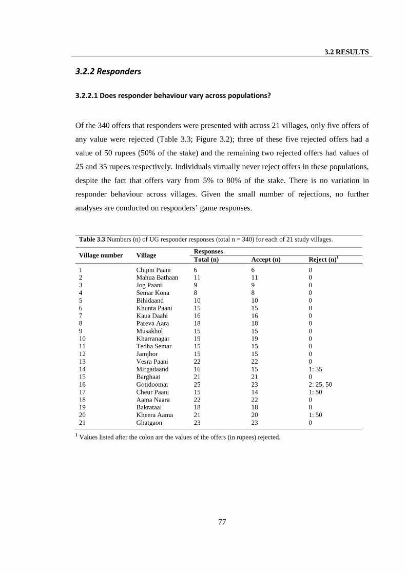
3.2 RESULTS
77
3.2.2 Responders
3.2.2.1 Does responder behaviour vary across populations?
Of the 340 offers that responders were presented with across 21 villages, only five offers of
any value were rejected (Table 3.3; Figure 3.2); three of these five rejected offers had a
value of 50 rupees (50% of the stake) and the remaining two rejected offers had values of
25 and 35 rupees respectively. Individuals virtually never reject offers in these populations,
despite the fact that offers vary from 5% to 80% of the stake. There is no variation in
responder behaviour across villages. Given the small number of rejections, no further
analyses are conducted on responders’ game responses.
Table 3.3 Numbers (n) of UG responder responses (total n = 340) for each of 21 study villages.
ResponsesVillage number Village
Total (n) Accept (n) Reject (n)1
1 Chipni Paani 6 6 02 Mahua Bathaan 11 11 03 Jog Paani 9 9 04 Semar Kona 8 8 05 Bihidaand 10 10 06 Khunta Paani 15 15 07 Kaua Daahi 16 16 08 Pareva Aara 18 18 09 Musakhol 15 15 010 Kharranagar 19 19 011 Tedha Semar 15 15 012 Jamjhor 15 15 013 Vesra Paani 22 22 014 Mirgadaand 16 15 1: 3515 Barghaat 21 21 016 Gotidoomar 25 23 2: 25, 5017 Cheur Paani 15 14 1: 5018 Aama Naara 22 22 019 Bakrataal 18 18 020 Kheera Aama 21 20 1: 5021 Ghatgaon 23 23 0
1 Values listed after the colon are the values of the offers (in rupees) rejected.
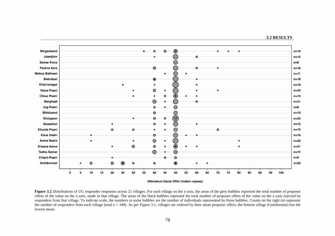
3.2 RESULTS
78
Figure 3.2 Distributions of UG responder responses across 21 villages. For each village on the y-axis, the areas of the grey bubbles represent the total number of proposeroffers of the value on the x-axis, made in that village. The areas of the black bubbles represent the total number of proposer offers of the value on the x-axis rejected byresponders from that village. To indicate scale, the numbers in some bubbles are the number of individuals represented by those bubbles. Counts on the right (n) representthe number of responders from each village (total n = 340). As per Figure 3.1, villages are ordered by their mean proposer offers; the bottom village (Gotidoomar) has thelowest mean.
3.2 RESULTS
79
3.2.2.2 Do self-reported MAOs vary across populations?
Distributions of responder MAOs (Figure 3.3) vary across villages. The modal MAO across
all villages is zero. 80% of individuals across the 16 populations stated that they were
willing to accept either nothing or the minimum non-zero division of the stake, i.e. five
rupees. 4.9% of the variance in MAOs occurs between villages [Table 3.4B; null model
(multilevel)]. The DIC value for the null model with village level intercepts (multilevel) is
about 3.5 units lower than for the null model without village level intercepts (single level),
indicating that the multilevel model accounting for village effects provides a slightly better
fit to the data (Table 3.4A; null models). Once individual descriptors are included in the full
model, the unexplained between-village variance reduces to 2.7% [Table 3.4B; full model
(multilevel)].
Since the distribution of MAOs is skewed (80% of individuals have an MAO of zero or
five and very few individuals have an MAO greater than 10), analyses were also conducted
with the MAO modelled as an ordinal response variable with three categories (MAO = 0,
MAO = 5, MAO => 10) (Table 3.5). In the ordinal multinomial model 3.3% of the variance
in MAOs occurs between villages [Table 3.5B; null model (multilevel)]. The DIC value for
the ordinal multinomial null model with village level intercepts (multilevel) is only about
one unit lower than for the ordinal multinomial null model without village level intercepts
(single level), indicating that the multilevel model accounting for village effects does not
provide a considerably better fit to the ordinal data (Table 3.5A; null models); village level
variance in MAOs is less important in these models. Once individual descriptors are
included in the full ordinal multinomial model, the unexplained between-village variance
reduces to 2% [Table 3.5B; full model (multilevel)].
Hence, although the percentage of between-village variance in MAOs is the same whether
the MAO is modelled as a normal or ordinal response variable, differences between villages
are more important in the normal linear models than in the ordinal multinomial response
models. The ordinal response variable was constructed such that MAO values greater than
or equal to 10 were pooled together with the result that between-village differences became
unimportant in these models; this may indicate that between-village variance in MAOs

3.2 RESULTS
80
(captured by the linear models) may mostly be in the range and frequency of values greater
than 10. In other words, villages may be similar in their distributions of MAO values of
zero and five (see Figure 3.3).
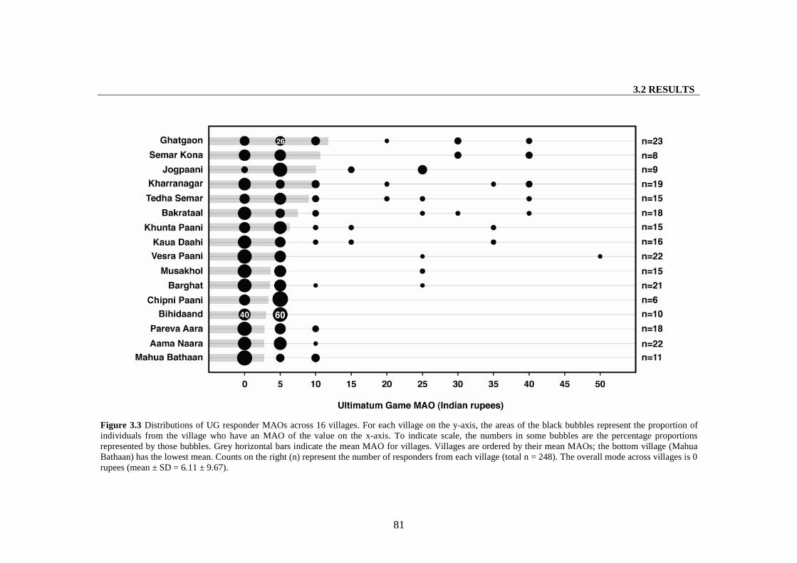
3.2 RESULTS
81
Figure 3.3 Distributions of UG responder MAOs across 16 villages. For each village on the y-axis, the areas of the black bubbles represent the proportion ofindividuals from the village who have an MAO of the value on the x-axis. To indicate scale, the numbers in some bubbles are the percentage proportionsrepresented by those bubbles. Grey horizontal bars indicate the mean MAO for villages. Villages are ordered by their mean MAOs; the bottom village (MahuaBathaan) has the lowest mean. Counts on the right (n) represent the number of responders from each village (total n = 248). The overall mode across villages is 0rupees (mean ± SD = 6.11 ± 9.67).
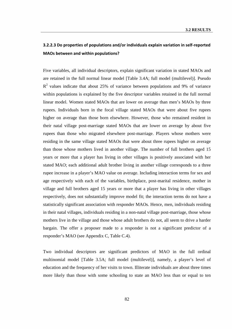
3.2 RESULTS
82
3.2.2.3 Do properties of populations and/or individuals explain variation in self-reported
MAOs between and within populations?
Five variables, all individual descriptors, explain significant variation in stated MAOs and
are retained in the full normal linear model [Table 3.4A; full model (multilevel)]. Pseudo
R2 values indicate that about 25% of variance between populations and 9% of variance
within populations is explained by the five descriptor variables retained in the full normal
linear model. Women stated MAOs that are lower on average than men’s MAOs by three
rupees. Individuals born in the focal village stated MAOs that were about five rupees
higher on average than those born elsewhere. However, those who remained resident in
their natal village post-marriage stated MAOs that are lower on average by about five
rupees than those who migrated elsewhere post-marriage. Players whose mothers were
residing in the same village stated MAOs that were about three rupees higher on average
than those whose mothers lived in another village. The number of full brothers aged 15
years or more that a player has living in other villages is positively associated with her
stated MAO; each additional adult brother living in another village corresponds to a three
rupee increase in a player’s MAO value on average. Including interaction terms for sex and
age respectively with each of the variables, birthplace, post-marital residence, mother in
village and full brothers aged 15 years or more that a player has living in other villages
respectively, does not substantially improve model fit; the interaction terms do not have a
statistically significant association with responder MAOs. Hence, men, individuals residing
in their natal villages, individuals residing in a non-natal village post-marriage, those whose
mothers live in the village and those whose adult brothers do not, all seem to drive a harder
bargain. The offer a proposer made to a responder is not a significant predictor of a
responder’s MAO (see Appendix C, Table C.4).
Two individual descriptors are significant predictors of MAO in the full ordinal
multinomial model [Table 3.5A; full model (multilevel)], namely, a player’s level of
education and the frequency of her visits to town. Illiterate individuals are about three times
more likely than those with some schooling to state an MAO less than or equal to ten

3.2 RESULTS
83
rupees. Individuals who make an additional trip to town each month are about 10% more
likely to state an MAO less than ten rupees.
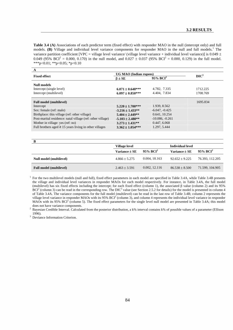
3.2 RESULTS
84
Table 3.4 (A) Associations of each predictor term (fixed effect) with responder MAO in the null (intercept only) and fullmodels. (B) Village and individual level variance components for responder MAO in the null and full models.1 Thevariance partition coefficient [VPC = village level variance/ (village level variance + individual level variance)] is 0.049 0.049 (95% BCI2 = 0.000, 0.170) in the null model, and 0.027 0.037 (95% BCI2 = 0.000, 0.129) in the full model.***p<0.01; **p<0.05; *p<0.10
AUG MAO (Indian rupees)
Fixed effect SE 95% BCI2 DIC3
Null modelsIntercept (single level) 6.071 0.648*** 4.782, 7.335 1712.225Intercept (multilevel) 6.097 0.850*** 4.404, 7.834 1708.769
Full model (multilevel) 1695.834Intercept 5.220 1.700*** 1.939, 8.562Sex: female (ref: male) -3.216 1.433** -6.047, -0.425Birthplace: this village (ref: other village) 5.404 2.449** 0.641, 10.254Post-marital residence: natal village (ref: other village) -5.103 2.480** -10.086, -0.261Mother in village: yes (ref: no) 3.273 1.431** 0.447, 6.068Full brothers aged ≥ 15 years living in other villages 3.362 1.054*** 1.297, 5.444
B
Village level Individual level
Variance SE 95% BCI2 Variance SE 95% BCI2
Null model (multilevel) 4.866 5.275 0.004, 18.163 92.652 9.225 76.393, 112.205
Full model (multilevel) 2.463 3.591 0.002, 12.116 86.538 8.500 71.599, 104.905
1 For the two multilevel models (null and full), fixed effect parameters in each model are specified in Table 3.4A, while Table 3.4B presentsthe village and individual level variances in responder MAOs for each model respectively. For instance, in Table 3.4A, the full model(multilevel) has six fixed effects including the intercept; for each fixed effect (column 1), the associated β value (column 2) and its 95%BCI2 (column 3) can be read in the corresponding row. The DIC3 value (see Section 2.5.2 for details) for the model is presented in column 4of Table 3.4A. The variance components for the full model (multilevel) can be read in the last row of Table 3.4B; column 2 represents thevillage level variance in responder MAOs with its 95% BCI2 (column 3), and column 4 represents the individual level variance in responderMAOs with its 95% BCI2 (column 5). The fixed effect parameters for the single level null model are presented in Table 3.4A; this modeldoes not have variance components.
2 Bayesian Credible Interval. Calculated from the posterior distribution, a k% interval contains k% of possible values of a parameter (Ellison1996).
3 Deviance Information Criterion.
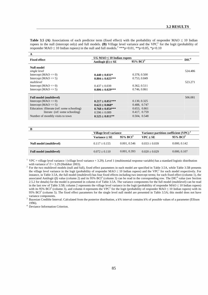
3.2 RESULTS
85
Table 3.5 (A) Associations of each predictor term (fixed effect) with the probability of responder MAO ≤ 10 Indianrupees in the null (intercept only) and full models. (B) Village level variance and the VPC1 for the logit (probability ofresponder MAO ≤ 10 Indian rupees) in the null and full models.2 ***p<0.01, **p<0.05, *p<0.10
AUG MAO ≤ 10 Indian rupees
Fixed effectAntilogit () SE 95% BCI3 DIC4
Null modelsingle level 524.486Intercept (MAO <= 0) 0.440 0.031* 0.378, 0.500Intercept (MAO <= 5) 0.804 0.025*** 0.753, 0.849multilevel 523.271Intercept (MAO <= 0) 0.437 0.039 0.362, 0.511Intercept (MAO <= 5) 0.806 0.029*** 0.746, 0.861
Full model (multilevel) 506.081Intercept (MAO <= 0) 0.217 0.051*** 0.130, 0.325Intercept (MAO <= 5) 0.623 0.068* 0.488, 0.747Education: illiterate (ref: some schooling)
literate (ref: some schooling)0.768 0.054***0.596 0.089
0.653, 0.8610.417, 0.759
Number of monthly visits to town 0.525 0.011** 0.504, 0.548
BVillage level variance Variance partition coefficient (VPC) 1
Variance SE 95% BCI3 VPC SE 95% BCI3
Null model (multilevel) 0.117 0.155 0.001, 0.546 0.033 0.039 0.000, 0.142
Full model (multilevel) 0.072 0.110 0.001, 0.393 0.020 0.029 0.000, 0.107
1 VPC = village level variance / (village level variance + 3.29). Level 1 (multinomial response variable) has a standard logistic distributionwith variance π2/3 = 3.29 (Hedeker 2003).
2 For the two multilevel models (null and full), fixed effect parameters in each model are specified in Table 3.5A, while Table 3.5B presentsthe village level variance in the logit (probability of responder MAO ≤ 10 Indian rupees) and the VPC1 for each model respectively. Forinstance, in Table 3.5A, the full model (multilevel) has four fixed effects including two intercept terms; for each fixed effect (column 1), theassociated Antilogit (β) value (column 2) and its 95% BCI3 (column 3) can be read in the corresponding row. The DIC4 value (see Section2.5.2 for details) for the model is presented in column 4 of Table 3.5A. The variance components for the full model (multilevel) can be readin the last row of Table 3.5B; column 2 represents the village level variance in the logit (probability of responder MAO ≤ 10 Indian rupees)with its 95% BCI3 (column 3), and column 4 represents the VPC1 for the logit (probability of responder MAO ≤ 10 Indian rupees) with its95% BCI3 (column 5). The fixed effect parameters for the single level null model are presented in Table 3.5A; this model does not havevariance components.
3 Bayesian Credible Interval. Calculated from the posterior distribution, a k% interval contains k% of possible values of a parameter (Ellison1996).
4 Deviance Information Criterion.
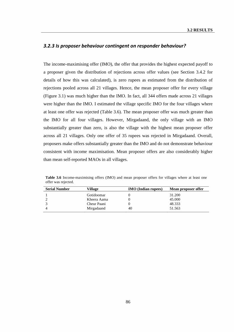
3.2 RESULTS
86
3.2.3 Is proposer behaviour contingent on responder behaviour?
The income-maximising offer (IMO), the offer that provides the highest expected payoff to
a proposer given the distribution of rejections across offer values (see Section 3.4.2 for
details of how this was calculated), is zero rupees as estimated from the distribution of
rejections pooled across all 21 villages. Hence, the mean proposer offer for every village
(Figure 3.1) was much higher than the IMO. In fact, all 344 offers made across 21 villages
were higher than the IMO. I estimated the village specific IMO for the four villages where
at least one offer was rejected (Table 3.6). The mean proposer offer was much greater than
the IMO for all four villages. However, Mirgadaand, the only village with an IMO
substantially greater than zero, is also the village with the highest mean proposer offer
across all 21 villages. Only one offer of 35 rupees was rejected in Mirgadaand. Overall,
proposers make offers substantially greater than the IMO and do not demonstrate behaviour
consistent with income maximisation. Mean proposer offers are also considerably higher
than mean self-reported MAOs in all villages.
Table 3.6 Income-maximising offers (IMO) and mean proposer offers for villages where at least oneoffer was rejected.
Serial Number Village IMO (Indian rupees) Mean proposer offer
1 Gotidoomar 0 31.2002 Kheera Aama 0 45.0003 Cheur Paani 0 48.3334 Mirgadaand 40 51.563
3.3 DISCUSSION
87
3.3 Discussion
3.3.1 Variation in proposer behaviour
Variation in UG proposer behaviour across 21 populations of the same small-scale society
is comparable to that found previously across 15 different small-scale societies (Henrich et
al. 2004; Henrich et al. 2005). There is significant behavioural heterogeneity across
populations of the same endogamous cultural group. These findings challenge the
conclusions of studies attributing behavioural variation across populations to cultural
differences between them based on samples from one (or very few) populations per culture
(e.g. Henrich et al. 2001; Henrich et al. 2005; Henrich et al. 2010; Henrich et al. 2006;
Herrmann et al. 2008; Roth et al. 1991). Population level replicates within each society are
crucial to determine whether there is behavioural variation between cultural groups in
addition to the variation between populations. Behavioural variation currently ascribed to
the cultural transmission of cooperative norms may, in fact, be driven by environmental
(demographic and ecological) differences between populations.
It has been suggested that cultural transmission may occur at the level of the village unit,
rather than at the level of the endogamous cultural unit (Gurven 2004a; Henrich et al. 2005).
If between-village variation is maintained by cultural transmission within villages, cultural
group selection could occur, the village being the unit of selection instead of the cultural
group. I discuss this potential explanation for my results at some length in the final chapter
of this thesis (Section 6.1).
3.3.2 Correlates of proposer behaviour
Proposer offers have a strong positive association with the proportion of non-Korwas
residing in the village. Participants in this study always played with other Pahari Korwas
and the non-Korwa residents of the village did not participate in the games. These results
3.3 DISCUSSION
88
may therefore be interpreted in two ways. First, the positive association of offers with the
frequency of non-Korwas may indicate that Korwas tend to increase levels of cooperation
towards Korwas when people of other ethnicities co-reside with them. Second, higher
levels of cooperation may prevail in villages where individuals from multiple ethnicities co-
reside, irrespective of whether the beneficiary of cooperation shares the ethnic identity of
the cooperator. Data from this study cannot distinguish between these two interpretations.
However, if the first interpretation is correct, then my results support the findings of
previous work (e.g. Bernhard et al. 2006; de Cremer and van Vugt 1999; Tajfel et al. 1971
and reviewed in Brewer and Schneider 1990) that people tend to be more cooperative
towards those they identify as the in-group (even if the criteria for grouping are arbitrary).
Inter-group competition promotes within-group cooperation (Burton-Chellew et al. 2010;
Choi and Bowles 2007; Puurtinen and Mappes 2009).
Alternatively, if the second interpretation is correct, then my results raise the possibility
that in-group favouritism is not universal and that ethnic diversity may even promote
cooperation under certain conditions, although it is unclear at this stage what the underlying
mechanism for this may be. However, Yamagishi and colleagues have suggested that in-
group favouritism observed in laboratory studies may reflect the operation of a ‘group
heuristic’ (e.g. Karp et al. 1993; Yamagishi and Kiyonari 2000; Yamagishi and Mifune
2008; Yamagishi et al. 2008); people contribute more to their groups in expectation of
indirect future payoffs from group members, i.e. via indirect reciprocity. Hence, one
possibility is that people only increase cooperation toward the in-group when a grouping
context is explicitly created; future work should investigate whether group biases continue
to emerge when explicit references to the grouping context are eliminated.
Proposer offers are negatively associated with household size, i.e. the number of
individuals residing in the same house and eating at a common hearth. Individuals with
larger households may be provisioning more people, leaving them with lower resource
surpluses; in my dataset, household size is positively correlated with the number of living
children an individual has. Hence, cooperation may be more costly for individuals with
large households. The analyses investigated associations between proposer offers and other
demographic variables potentially correlated with household size, such as age and measures
3.3 DISCUSSION
89
of wealth; these variables were not retained in the full model and therefore do not explain
the association between household size and proposer offers.
Finally, people who played on the second or third day of the games in any village made
offers that were slightly but significantly higher than those who played on the first day.
Individuals who played on the second or third day were not present at the venue of the
games on preceding days. Since all players were informed of the outcome of their game
decisions and received their game payments only once all games in a village had been
concluded, later players could not have known the outcomes of games played on previous
days. Individuals who played on day two or three may have learnt the game rules from
those who played before them. They may also have asked people who had already played
about the offers they made, accepted or rejected. Hence, although the association between
day of play and proposer offer may be interpreted as an effect of learning, it is puzzling that
those who played later increased rather than decreased their offers, given that Pahari
Korwas never seem to reject offers of any value. It is unlikely that familiarity with the
research team is responsible for an increase in offers as we had little interaction with village
residents until the day they played the games. Since we ran the study for about 8-9 hours
each day, there was little time for interaction outside the context of the study while we were
still running the games in a village. The finding that day of play is associated with
individuals’ behaviour emphasises that researchers working in small populations need to
take account of the length of time over which their data are collected.
3.3.3 Variation in responder behaviour
Only 1.5% of responders across 21 Pahari Korwa villages rejected offers of any value.
Hence, individuals virtually never rejected offers of any size even though offers varied
from 5% to 80% of the stake. Taken together, UG responders in these populations played
the income-maximising strategy. The rejected offers were not the lowest made and in fact
three of the total five offers rejected were for 50% of the stake. The rejection of offers of
50% of the stake is not unique to Pahari Korwa populations; it has been reported in
3.3 DISCUSSION
90
Sursurunga populations in Papua New Guinea and in Hadza populations in Tanzania (Barr
et al. 2009; Henrich et al. 2006).
There is almost no variation in response distributions across villages. Variation in
responder behaviour across 21 populations of the same small-scale society is lower than
that found across 15 different small-scale societies (Henrich et al. 2004; Henrich et al.
2005; Henrich et al. 2006). Hence, since I find little variation in responder behaviour across
populations of the same cultural group, I cannot reject the hypothesis that variation in
responder behaviour observed across 15 different cultural groups in previous studies
(Henrich et al. 2004; Henrich et al. 2005; Henrich et al. 2006) may in fact be driven by
cultural differences between the study populations.
The low frequency of rejections observed in Pahari Korwa populations is comparable to
that found in several other populations including populations of the Ache (0%), Tsimane
(0%), Kazakh (0%), Quichua (0%), Isanga (3%), Orma (3.5%), Sanquianga (4%),
Machiguenga (4.7%), Sangu herders (5%) and Samburu (5%) (Barr et al. 2009; Henrich et
al. 2005). In about half of the 15 populations sampled by Henrich et al. (2005), responder
behaviour was comparable to that observed in my study populations.
A meta-analysis of 75 UG studies (Oosterbeek et al. 2004) conducted across 26 countries,
largely sampling university students, reveals that the average rejection rate across studies is
16%. However, rejection rates vary significantly by region (group of neighbouring
countries), and reported rejection rates are less than 5% in populations from several
countries including Bolivia (0%), Paraguay (0%), Kenya (4%), Peru (4.8%) and Mongolia
(5%). The meta-analysis also demonstrates that, across studies, rejection rates are far more
sensitive to changes in the relative proportion of the stake offered than the absolute value of
the offered share. This suggests that “responders care (a lot) about the relative amount they
receive” (Oosterbeek et al. 2004).
In summary, while responders in some parts of the world are willing to accept any offer
made to them, those in other places care considerably about relative payoffs. Barr et al.
(2009) find some support for their hypothesis that variation in inequality aversion explains
3.3 DISCUSSION
91
variation in UG behaviour across 15 small-scale societies. These patterns may reflect
underlying differences in individuals’ concern with absolute versus relative payoffs in
different environments. For instance, selection may favour strategies that ensure near-equal
splits of resources in stochastically more stable environments, where relative payoffs may
matter more in terms of improving long-term fitness than maximizing absolute payoffs in
the short-term. Individuals living in unpredictable environments, such as when there is a
high prevalence of disease or reliance on seasonal resource bases to meet livelihood needs,
may be less concerned with relative payoffs and more focussed on maximising immediate
absolute payoffs. Hence, differences in levels of environmental uncertainty across
populations may explain the observed patterns of variation in responder behaviour;
‘fairness norms’ may simply be behavioural heuristics reflecting the importance of relative
versus absolute payoffs in particular environments.
3.3.4 Self-reported behavioural strategies
80% of responders reported that they were willing to accept either nothing or the smallest
possible division of the stake, i.e. five rupees. Considering the low rate of actual rejections
in these populations (even of small offers), these results suggest that the Pahari Korwa do
as they say. The modal self-reported MAO across populations (zero) is equal to the IMO
(calculated from the distribution of actual rejections). Moreover, even though the village
level variation in MAO values is higher than the variation in actual responses, this does not
necessarily imply divergence between real and self-reported behaviour. The modal MAO in
all villages is either zero or five rupees and very few individuals stated MAOs greater than
ten. Since only one proposer made an offer less than ten rupees, variation in real responses
may have been comparable to variation in MAOs if more offers of zero and five rupees had
been made. If people were simply justifying their accept/reject decisions, then we should
expect a closer resemblance between the distributions of proposer offers and responder
MAOs; I find no relationship between the two.
Variation in self-reported MAOs measured across 16 populations of the same small-scale
society in this study is 4.9%; this is much lower than the variation in MAOs found

3.3 DISCUSSION
92
previously across 15 different societies (34.4%, Henrich et al. 2006). However, the two
results are not really comparable because the MAO in this study is a self-reported value
with no real payoff implications; in Henrich et al.’s (2006) study individuals’ MAOs
affected their payoffs. While the MAOs are unreliable measures of real bargaining
preferences, they are a measure of what individuals would like others, or at least a visiting
researcher, to believe. It is notable that most people in these populations project themselves
as an easy bargain, at least in the game as it is presently framed. However, men, individuals
residing in their natal villages, individuals residing in a non-natal village post-marriage,
those whose mothers live in the village and those whose adult brothers do not, all emerge as
harder bargainers in the full linear model. Taken together these results suggest that whether
individuals reside in their natal village or not may be an important determinant of their
projected or real (if self-reported MAOs reflect real bargaining preferences) behavioural
strategies. Those who are illiterate and visit town more often are more likely to state a
lower MAO in the full ordinal multinomial model. That different variables emerge as
significant predictors of MAO in the linear (continuous data) and ordinal logistic (ranked
data) models may indicate that individuals’ MAOs are influenced by different variables
above and below a certain threshold value.
3.3.5 Discrepancies in proposer and responder behaviour
In this study, proposers often offered substantial proportions of the stake, even though
responders appear willing to accept any offer. The income-maximising offer - the offer that
maximises proposers’ expected payoffs given the observed probabilities of rejection across
offer values - is much lower than the average offer made in all villages; this suggests that
proposers were not acting strategically to maximise their income by making such high
offers. My findings agree with those of previous studies demonstrating that mean offers in
most populations of small-scale societies are much higher than income-maximising offers
(Henrich et al. 2004; Henrich et al. 2005) and mean minimum acceptable offers (Henrich et
al. 2010; Henrich et al. 2006). Moreover, while responders in my study collectively played
the income-maximising strategy, proposers did not.
3.3 DISCUSSION
93
These data add to growing evidence that proposer and responder behaviour in the UG does
not always co-vary. In populations of large-scale societies, there is much greater variation
in rejection rates than in offers (Oosterbeek et al. 2004); I find the reverse pattern in my
study populations. A recent study demonstrates that while proposers respond to reputation
concerns by increasing their offers in a public context, responders do not do so (Lamba and
Mace 2010). All these findings contradict models predicting that proposer behaviour should
be a best response to responder behaviour in the UG (e.g. Bolton and Ockenfels 2000; Fehr
and Schmidt 1999). Patterns of empirical data from the UG provide support for the
hypothesis that proposer and responder strategies in a bargaining situation are influenced by
different considerations and selection pressures.
3.3.6 Concluding remarks
I find significant variation in cooperative behaviour, measured via proposer’s offers in the
UG, across 21 populations of the same small-scale society. This variation is comparable to
that found previously between 15 different small-scale societies. My results suggest that
behavioural variation in proposer’s offers that has previously been attributed to cultural
differences between populations may in fact be driven by environmental differences
between them. Environmental drivers of behavioural variation are unlikely to maintain
stable, heritable differences essential for selection at the population-level. On the other
hand, responders’ behaviour varies little across 21 populations of the same small-scale
society; variation in responder behaviour observed previously across populations from 15
different small-scale societies may be driven by cultural differences between them. Drivers
of behavioural variation may differ for proposers and responders in a bargaining situation.

3.4 METHODS
94
3.4 Methods
3.4.1 Experimental set-up
The games were played in two phases; five villages were visited between May 23rd and
June 21st, 2007, and the remaining 16 villages were visited between February 2nd and May
16th, 2008. The games were played over two consecutive days in each village except one
village (Vesra Paani) where they were played over four consecutive days. Games were
played within two (18 villages), three (two villages), or four (one village) days following
our arrival in a village. Mean age ± SD of participants was 35.57 ± 12.49 years and 44%
were female.
All participants collected at a common location in the village on the day of the games; only
individuals who were playing on a particular day were present at the study venue on that
day. They were collectively given general instructions about the day’s programme. These
instructions excluded a description of the rules of the game but explained that a set of one-
shot, anonymous economic games would be played in pairs for real money (see Appendix
A, Section A.1.1 for script). Players were tested collectively for their understanding of
these general instructions. Upon arriving at the private location, players were individually
instructed about the game rules and examples (see Appendix A, Sections A.1.2 and A.1.3
for game scripts). They were then tested for their understanding of the game rules and of
the anonymity of their decisions. Only a player who individually answered all test
questions correctly played the game. Players were randomly designated as proposers or
responders. A proposer made her offer by manipulating real five rupee coins into two piles
and placing them on two sides of a string, one pile for herself and one for the responder. A
responder was presented with two piles of five rupee coins in accordance with the division
made by the proposer, and asked whether she wished to accept or reject the pile offered to
her. She was then asked what minimum offer from the proposer she would be willing to
accept. In order to facilitate comprehension of this question, I started with a pile of five
rupee coins summing to the amount the responder had accepted, deducted five rupees from
the pile and asked if the amount was still acceptable to the player. This process was
repeated until the player said she would not accept an offer value and the next greater
3.4 METHODS
95
acceptable offer value was recorded as the MAO. The MAO was recorded as zero for
players who were willing to accept an offer of value zero. The only five players who
rejected the offers made to them came from the five populations where MAOs were not
recorded.
Pairs of players were constituted by randomly matching token numbers. In eight villages,
an odd number of individuals participated in the games. In these villages, one individual
was paired randomly with two other players from the village, in order to determine the
payoff to all participating players. This does not confound the analyses, which are
conducted on the offers and responses of individuals, not their payoffs. Players were
unaware of the total number of people who had successfully played the game and the
number of individuals who did not play due to a failure to answer all test questions
correctly.
3.4.2 Statistical analyses
Multilevel normal linear models (Browne 2009; Rasbash et al. 2009; Snijders and Bosker
1999) were used to analyse variation in proposer offers and responder self-reported MAOs
across villages, and the association of population and individual descriptors with
individuals’ offers or self-reported minimum acceptable offers respectively. Responder
MAOs were also modelled as an ordinal response variable with three categories (MAO = 0,
MAO = 5, MAO >= 10) using multilevel ordinal multinomial models with a logit link
function (Browne 2009; Rasbash et al. 2009). The analyses for each outcome variable
(proposer offer, responder MAO as continuous variable, responder MAO as ordinal
variable) proceeded in four stages as described in Section 2.5.2.
The IMO was calculated as follows (Henrich et al. 2004). A binary logistic regression was
run with responder response (accept/reject) as the dependent variable and proposer offer as
the only explanatory variable. This regression estimates the relationship between the
probability of acceptance and proposer offer, from the distribution of offers accepted and
rejected. The parameter values derived from the regression equation (β and c) were used to

3.4 METHODS
96
estimate the probability of acceptance (pi) for each offer value (i) from 0 to 100 [pi = exp(βi
+ c)/{1+ exp(βi + c)}], with i increasing in increments of five. The estimated probability of
acceptance (pi) for each offer value (i) was multiplied with the payoff received if that offer
value was accepted; this is the expected payoff (payoffi) from an offer [payoffi = pi (S - i) =
pi (100 – i)] given its probability of acceptance. The IMO is then the offer value with the
highest expected payoff.
97
CHAPTER 4
VARIATION IN COOPERATION ACROSS POPULATIONS:
EVIDENCE FROM PUBLIC GOODS GAMES AND A ‘REAL-
WORLD’ MEASURE OF BEHAVIOUR
4.1 Introduction
4.1.1 Background and related research
Different measures of behaviour may not always yield consistent results. Therefore, in this
chapter I continue to address the question of whether there is stable, heritable variation in
levels of cooperation across human populations, using two further measures of cooperative
behaviour. I present findings from a public goods game (PGG) and a new ‘real-world’
measure of behaviour, both employed in 16 Pahari Korwa villages.
A broad range of experimental games have the structure of a public goods dilemma
(Ledyard 1995). Garrett Hardin’s ‘tragedy of the commons’ (Hardin 1968) typifies a public
goods dilemma; this is a scenario in which although every individual increases her payoff
by maximally harvesting a finite resource replenished at a constant rate that she shares with
other consumers (e.g. grazing cattle on the village commons), if all consumers do the same,
the consequent over-harvesting and depletion of the resource would result in a reduced
payoff for all consumers. A PGG framed thus employs what is termed the “common-pool
resource mechanism”. In an alternative formulation, the “voluntary contributions
mechanism”, individuals must decide how much of a personal endowment they each wish
4.1 INTRODUCTION
98
to contribute to a public good; the return from the public good is shared equally by all
participating individuals, irrespective of how much they each contribute to it. The return
from the public good is a positive function of the collective investment in it; the total
amount contributed to the public good is multiplied by some factor and the product is
divided equally among all participating individuals. The income-maximising strategy in a
PGG implementing the voluntary contributions mechanism is to contribute nothing, but
players profit more if everyone contributes something as opposed to if no one makes any
contribution.
PGGs have been implemented extensively in the laboratory amongst samples of university
students (reviewed in Davis and Holt 1993, Gächter and Herrmann 2009, Kollock 2003,
Ledyard 1995, Sally 1995 and Zelmer 2003). Laboratory studies have provided substantial
insights about individuals’ behaviour in cooperative dilemmas. Studies have investigated
how group size (e.g. Carpenter 2007; Isaac and Walker 1988; Isaac et al. 1994; Marwell
and Ames 1979), payoff structures (e.g. Brandts and Schram 2001; Goeree et al. 2002;
Isaac and Walker 1988), repeated interactions between players (e.g. Andreoni 1988;
Andreoni and Croson 2008; Croson 1996; Ostrom et al. 1992), and opportunities for
punishing defection (e.g. Fehr and Gächter 2000, 2002; Gächter et al. 2008; Gurerk et al.
2006; Ostrom et al. 1992; Rockenbach and Milinski 2006) affect levels of cooperation in a
PGG. As expected, individuals cooperate more when the costs of cooperation are lower,
there are opportunities for repeated interactions, and defection may be punished. However,
substantial contributions are observed in PGGs even when players interact under one-shot,
anonymous conditions (e.g. Gächter and Herrmann 2006; Gächter et al. 2004; Walker and
Halloran 2004).
Few studies have examined variation in PGG behaviour across populations (Barr 2001;
Henrich et al. 2005; Herrmann et al. 2008). Herrmann et al. (2008) implemented an
anonymous, repeated PGG, with and without punishment, across 16 populations from 15
countries (large-scale societies); all participants in the study were university students.
Henrich et al. (2005) employed an anonymous, one-shot PGG in six populations from six
small-scale societies. Barr (2001) played anonymous and non-anonymous, repeated PGGs
in 18 ethnically mixed villages in Zimbabwe. All three studies find significant variation in

4.1 INTRODUCTION
99
players’ contributions to the public good across populations. Herrmann et al. (2008) also
find significant variation in the frequency and degree of punishment across countries.
Henrich et al. (2005) and Herrmann et al. (2008) infer that cultural differences drive this
behavioural variation between their sample populations. However, all three studies
confound cultural and environmental differences between populations and thus cannot
differentiate whether cultural transmission, or environmental variation, is the likely driver
of the observed variation.
4.1.2 Behavioural measures
In this study, a PGG implementing the voluntary contributions mechanism was played
under one-shot, anonymous conditions (see Section 2.4 for details of study set-up and
Section 4.4.1 for details of the games). Participants were divided into groups of six players.
Each player received an endowment of 20 rupees and decided how much of it she wished to
contribute to a group pot in divisions of five rupees. Once all six players had made their
decisions, the total amount in the pot was doubled and then split equally between all six
players. Each player’s earnings consisted of the money she retained from her endowment
plus an equal share of the earnings from the group pot. In this game the income-maximising
strategy entails that a player contribute nothing to the group pot.
A new ‘real-world’ measure of behaviour was implemented that involves taking a useful
commodity from a common pool (see Section 4.4.2 for details). I used salt, which is valued
among the Pahari Korwa and a commodity that they are most likely to buy at market
(Srivastava 2007). On concluding the PGG in a village, when a participant collected her
earnings at a private location, she was informed that I had brought along x kg of salt to
distribute amongst the y individuals who participated in the games and therefore z = x/y kg
of salt was available per person. The participant could then take as much of the total
amount of available salt (x kg) as she desired without her decision becoming public
knowledge. The stated amount was given to her along with her earnings from the game. In
each village I started with a total quantity of salt (in kg) equal to the total number of
participants so that the initial amount available per person was 1 kg. I then recalculated and
4.1 INTRODUCTION
100
updated the total amount available (x), the number of people remaining (y), and the amount
available per person (z = x/y) to the nearest 100 g for each person based on how much salt
remained after the preceding person had taken their desired salt quantity. I stopped
distributing salt when either the penultimate player had taken salt or when the amount
available per person fell below 100 g per person. Participants encountered the salt for the
first time when they individually collected their payments, and possessed no prior
information about it. Moreover, they did not know how much salt was available to anyone
else. The income-maximising strategy entails that a player take the maximum amount of
available salt. For each player, I use the deviation of the salt taken from the amount
available per person as a measure of cooperative propensity. The more negative a player’s
salt deviation is, the more selfish the player’s behaviour. I use these salt decisions to
measure behavioural variance across villages and to assess whether behaviour captured by a
formal economic game, such as the PGG, correlates with a ‘real-world’ measure of
cooperation.
I employ multilevel, multivariate response models (Rasbash et al. 2009; Snijders and
Bosker 1999) to explicitly analyse variation at the village and individual levels.
Multivariate response models let us simultaneously examine the effect of explanatory
variables on multiple response variables, in this case PGG contribution and salt deviation.
They also allow us to partition the correlation between the two response variables into
village and individual level components.
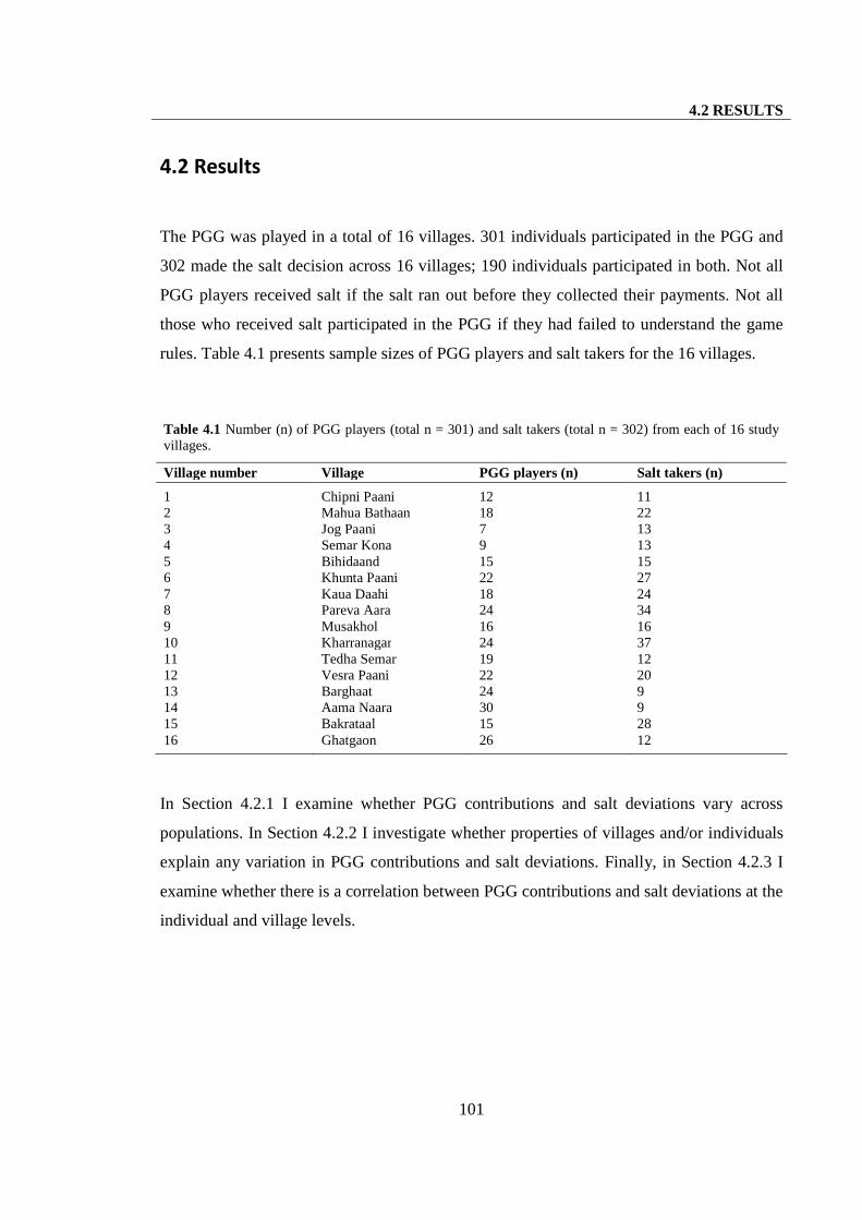
4.2 RESULTS
101
4.2 Results
The PGG was played in a total of 16 villages. 301 individuals participated in the PGG and
302 made the salt decision across 16 villages; 190 individuals participated in both. Not all
PGG players received salt if the salt ran out before they collected their payments. Not all
those who received salt participated in the PGG if they had failed to understand the game
rules. Table 4.1 presents sample sizes of PGG players and salt takers for the 16 villages.
Table 4.1 Number (n) of PGG players (total n = 301) and salt takers (total n = 302) from each of 16 studyvillages.
Village number Village PGG players (n) Salt takers (n)
1 Chipni Paani 12 112 Mahua Bathaan 18 223 Jog Paani 7 134 Semar Kona 9 135 Bihidaand 15 156 Khunta Paani 22 277 Kaua Daahi 18 248 Pareva Aara 24 349 Musakhol 16 1610 Kharranagar 24 3711 Tedha Semar 19 1212 Vesra Paani 22 2013 Barghaat 24 914 Aama Naara 30 915 Bakrataal 15 2816 Ghatgaon 26 12
In Section 4.2.1 I examine whether PGG contributions and salt deviations vary across
populations. In Section 4.2.2 I investigate whether properties of villages and/or individuals
explain any variation in PGG contributions and salt deviations. Finally, in Section 4.2.3 I
examine whether there is a correlation between PGG contributions and salt deviations at the
individual and village levels.
4.2 RESULTS
102
4.2.1 Do PGG contributions and salt deviations vary across populations?
Distributions of both PGG contributions (Figure 4.1) and salt deviations (Figure 4.2) vary
considerably across villages, including the modes and means. 4.1% of the variance in PGG
contributions and 18.2% of the variance in salt deviations occurs between villages [Table
4.2B; null model (multilevel)]. The between-village variation in salt deviation is
remarkable; in some villages the salt ran out before less than half the players had taken any
salt, while in others almost everyone received some salt. The DIC value for the null model
with village level intercepts (multilevel) is about 58 units lower than for the null model
without village level intercepts (single level), indicating that the multilevel model
accounting for village effects provides a substantially better fit to the data (Table 4.2A; null
models). Once village and individual descriptors are included in the full model, the
unexplained between-village variance reduces to 1.4% in PGG contributions and 11.8% in
salt deviations [Table 4.2B; full model (multilevel)]. Variance in UG behaviour between 15
small-scale societies was estimated at about 12% (Henrich et al. 2005). Once again,
behavioural variance between 16 populations of the same small-scale society is comparable
to that between 15 populations of 15 different small-scale societies.
Dummy variables encoding 16 populations from 15 different large-scale societies account
for 7% of the variance in group average contributions in repeated PGG experiments
(without punishment) run by Herrmann et al. (2008). In their study, mean contributions in
the first round of the PGG vary between about 8 and 14 units of the initial endowment (also
20 units), and mean contributions averaged across all 10 rounds of the PGG vary between
4.9 and 11.5 units. Mean PGG contributions across 16 populations of the same society in
this study vary between 7.2 and 14.7 units (Figure 4.1). Hence, the variance in
contributions and range of mean contributions across 16 populations of the same society is
comparable to that across 16 populations of 15 different societies.
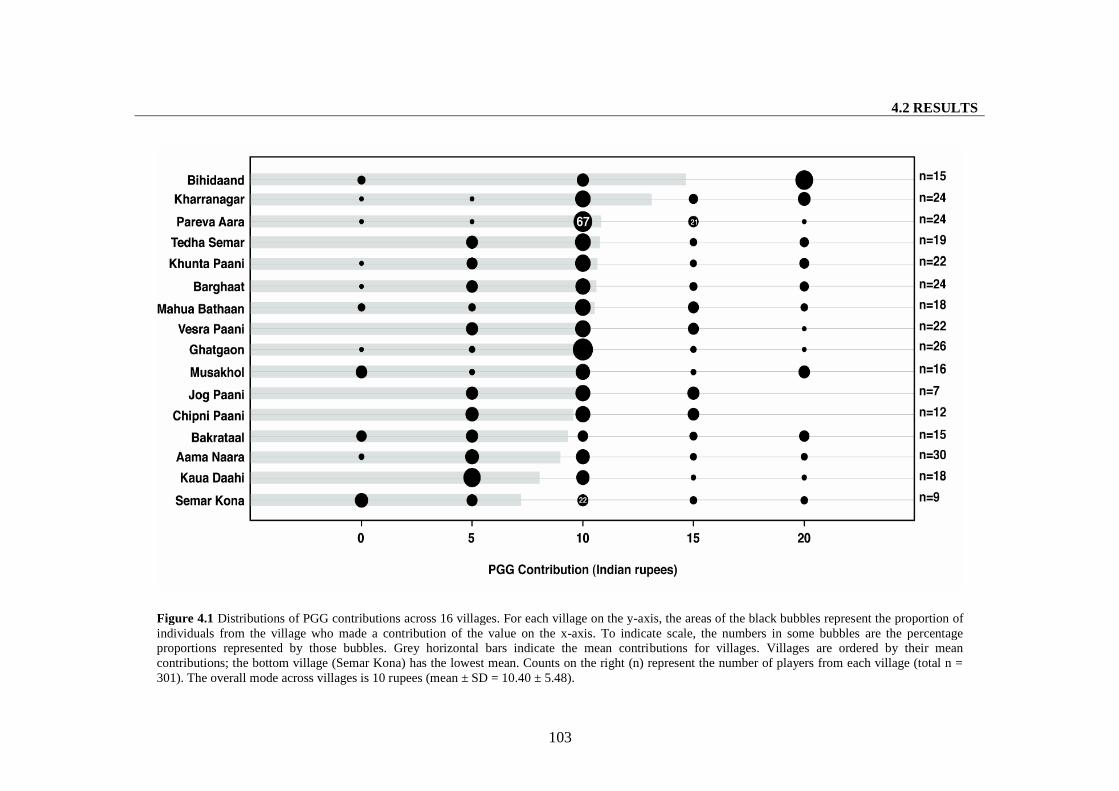
4.2 RESULTS
103
Figure 4.1 Distributions of PGG contributions across 16 villages. For each village on the y-axis, the areas of the black bubbles represent the proportion ofindividuals from the village who made a contribution of the value on the x-axis. To indicate scale, the numbers in some bubbles are the percentageproportions represented by those bubbles. Grey horizontal bars indicate the mean contributions for villages. Villages are ordered by their meancontributions; the bottom village (Semar Kona) has the lowest mean. Counts on the right (n) represent the number of players from each village (total n =301). The overall mode across villages is 10 rupees (mean ± SD = 10.40 ± 5.48).
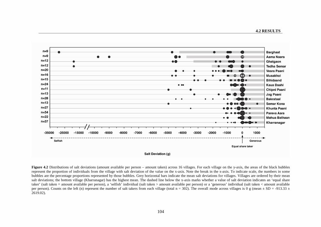
4.2 RESULTS
104
Figure 4.2 Distributions of salt deviations (amount available per person – amount taken) across 16 villages. For each village on the y-axis, the areas of the black bubblesrepresent the proportion of individuals from the village with salt deviation of the value on the x-axis. Note the break in the x-axis. To indicate scale, the numbers in somebubbles are the percentage proportions represented by those bubbles. Grey horizontal bars indicate the mean salt deviations for villages. Villages are ordered by their meansalt deviations; the bottom village (Kharranagar) has the highest mean. The dashed line below the x-axis marks whether a value of salt deviation indicates an ‘equal sharetaker’ (salt taken = amount available per person), a ‘selfish’ individual (salt taken > amount available per person) or a ‘generous’ individual (salt taken < amount availableper person). Counts on the left (n) represent the number of salt takers from each village (total n = 302). The overall mode across villages is 0 g (mean ± SD = -913.33 ±2619.02).
4.2 RESULTS
105
4.2.2 Do properties of populations and/or individuals explain variation in
PGG contribution and salt deviation between and within populations?
The only explanatory variables that have a significant association with PGG contribution
are age and number of individuals from other villages invited to the annual harvest festival
by a player’s household (representing a measure of social network size); both have small
positive effects on PGG contribution [Table 4.2A; full model (multilevel)]. An increment of
ten years in an individual’s age corresponds to an increase in her PGG contribution by 3.7%
of the initial endowment of 20 rupees. Ten additional people in a player’s social network
correspond to contributions that are higher by 5.8% of the initial endowment.
Only two variables are significantly associated with player salt deviation, namely, village
population size and the number of full sisters over the age of 15 years (adult sisters)
residing in the village, both of which have negative effects [Table 4.2A; full model
(multilevel)]. 10 additional individuals in the village population are associated with salt
deviations that are 29 g lower on average; players were more selfish in larger villages. The
number of adult sisters residing in the village has a large effect on salt deviation; each
additional adult sister living in the village corresponds to salt deviations that are lower by
624 g on average.
Pseudo R2 values indicate that for PGG contribution about 28% of variance between
populations and 4% of variance within populations is explained by the descriptor variables
retained in the full model. For salt deviation about 32% of variance between populations
and 9% of variance within populations is explained by the descriptor variables retained in
the full model.
Players’ migration histories, frequency of market contact and multiple measures of wealth
have little effect on their PGG contributions or salt decisions. The total amount of salt
available (pie size) has a small negative effect on salt deviation; people took more salt
when more was available (see Appendix C, Table C.10). However, the association of
behaviour with population and individual descriptors is independent of this pie-size effect.
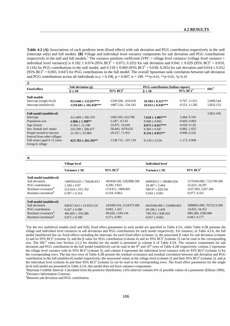
4.2 RESULTS
106
Table 4.2 (A) Associations of each predictor term (fixed effect) with salt deviation and PGG contribution respectively in the null(intercept only) and full models. (B) Village and individual level variance components for salt deviation and PGG contributionsrespectively in the null and full models.1 The variance partition coefficient [VPC = village level variance/ (village level variance +individual level variance)] is 0.182 0.074 (95% BCI2 = 0.073, 0.355) for salt deviation and 0.041 0.029 (95% BCI2 = 0.010,0.116) for PGG contributions in the null model, and 0.118 0.060 (95% BCI2 = 0.038, 0.265) for salt deviation and 0.014 0.012(95% BCI2 = 0.003, 0.047) for PGG contributions in the full model. The overall Spearman rank correlation between salt deviationand PGG contributions across all individuals is = 0.196, p = 0.007, n = 190. ***p<0.01, **p<0.05, *p<0.10
ASalt deviation (g) PGG contribution (Indian rupees)
Fixed effect SE 95% BCI2
SE 95% BC12 DIC3
Null modelsIntercept (single level) -913.646 152.037*** -1209.508, -618.018 10.394 0.321*** 9.767, 11.021 12890.544Intercept (multilevel) -1210.605 345.050*** -1887.124, -534.183 10.413 0.436*** 9.553, 11.285 12832.153
Full model (multilevel) 12821.456Intercept -513.409 585.370 -1683.305, 616.786 7.618 1.085*** 5.484, 9.764Population size -2.866 1.390** -5.587, -0.133 0.000 0.002 -0.003, 0.003Age (years) -9.363 12.108 -32.871, 14.418 0.073 0.027*** 0.020, 0.126Sex: female (ref: male) 516.599 288.477 -56.843, 1078.635 0.383 0.647 -0.882, 1.655People invited to harvestfestival from other villages
21.103 25.984 -29.257, 71.955 0.116 0.055** 0.008, 0.226
Full sisters aged ≥ 15 yearsliving in village
-623.783 261.295** -1138.715, -107.139 -0.139 0.534 -1.172, 0.908
B
Village level Individual level
Variance SE 95% BCI2 Variance SE 95% BCI2
Null model (multilevel)Salt deviation 1409354.625 764246.813 491858.500, 3282888.500 6099303.5 506483.656 5179439.000, 7151700.500PGG contribution 1.284 0.97 0.290, 3.815 29.487 2.464 25.023, 34.597Residual covariance4
512.024 551.762 -374.911, 1808.605 580.97 829.541 -1027.803, 2207.266Residual correlation4
0.397 0.314 -0.310, 0.863 0.043 0.061 -0.077, 0.161
Full model (multilevel)Salt deviation 830317.813 513355.531 241699.516, 2154373.500 6010546.000 510689.003 5088691.000, 7072213.500PGG contribution 0.427 0.380 0.092, 1.425 29.196 2.439 24.825, 34.352Residual covariance4
495.605 334.386 90.628, 1349.136 749.763 838.424 -889.288, 2399.088Residual correlation4
0.871 0.188 0.271, 0.991 0.057 0.063 -0.067, 0.177
1For the two multilevel models (null and full), fixed effect parameters in each model are specified in Table 4.2A, while Table 4.2B presents thevillage and individual level variances in salt deviations and PGG contributions for each model respectively. For instance, in Table 4.2A, the fullmodel (multilevel) has six fixed effects including the intercept; for each fixed effect (column 1), the associated β value for salt deviation (column2) and its 95% BCI2 (column 3), and the β value for PGG contribution (column 4) and its 95% BCI2 (column 5) can be read in the correspondingrow. The DIC3 value (see Section 2.5.2 for details) for the model is presented in column 6 of Table 4.2A. The variance components for saltdeviation and PGG contribution in the full model (multilevel) can be read in the 9th and 10th rows of Table 4.2B respectively; column 2 representsthe village level variance with its 95% BCI2 (column 3), and column 4 represents the individual level variance with its 95% BCI2 (column 5) forthe corresponding rows. The last two rows of Table 4.2B present the residual covariance and residual correlation between salt deviation and PGGcontribution in the full (multilevel) model respectively; the associated values at the village level (column 2) and their 95% BCI2 (column 3), and atthe individual level (column 4) and their 95% BCI2 (column 5) can be read in the corresponding rows. The fixed effect parameters for the singlelevel null model are presented in Table 4.2A; this model does not have variance components.2Bayesian Credible Interval. Calculated from the posterior distribution, a k% interval contains k% of possible values of a parameter (Ellison 1996).3Deviance Information Criterion.4Between salt deviation and PGG contribution.
4.3 DISCUSSSION
107
4.2.3 Is there a correlation between individuals’ PGG contributions and salt
deviations?
PGG contributions and salt deviations show a significant positive correlation across all
individuals (Table 4.2); players who made higher contributions took away less salt.
However, partitioning the correlation shows that most of the association is at the village
level ( = 0.397), with only a weak correlation at the individual level ( = 0.043). Once
explanatory variables are included in the full model, residual correlation increases
substantially at the village level ( = 0.871), and marginally at the individual level ( =
0.057). This suggests that properties of the common village environment trigger similar
cooperative propensities in the PGG and salt decisions, but individual variation in some
aspect of personality does not determine behaviour in these measures of cooperation.
4.3 Discussion
4.3.1 Variation in cooperative behaviour
Variation in PGG contributions and salt decisions between 16 villages of the same small-
scale society is comparable to the variation previously found between 16 different large-
scale societies (Herrmann et al. 2008) and 15 different small-scale societies (Henrich et al.
2005). This variation is partly explained by demographic differences between populations,
such as population size and age structures. These results suggest that individuals’
cooperative propensities are affected by local evolutionary dynamics that produce
behavioural variation across populations which may not be stable.
4.3.2 Correlates of cooperative behaviour
Age and a measure of social network size have a positive effect on PGG contributions
(Table 4.2). With the exceptions of Gächter and Herrmann (in press) and List (2004), age
effects have seldom been observed in the PGG, perhaps since most experimental work is
4.3 DISCUSSSION
108
conducted with undergraduate students of similar age. Egas and Riedl (2008) conducted a
study implementing a PGG amongst a wider cross-section of individuals from The
Netherlands and found that age was not a robust predictor of PGG contribution but was
positively associated with the allocation of punishment in a PGG. Age had a small positive
association with UG offers amongst the Sangu, a population of agro-pastoralists in
southwest Tanzania (McElreath 2004a); UG offers in this study have a negative association
with age, although this association is not statistically significant (Appendix C, Table C.1)
and age was not retained in the full model.
It is notable that, specifically, the number of individuals invited to the harvest festival from
other villages, as opposed to the player’s village, is associated with PGG contributions.
This finding raises the possibility that particular features of an individual’s social network,
such as its width or composition, influence levels of cooperation. Indeed, many authors
suggest that the structure of the social network should impact levels of cooperation between
members of the network, largely by increasing communication and/or allowing cooperators
to selectively interact (Granovetter 2005; Jaramillo 2004; Lieberman et al. 2005; Ohtsuki et
al. 2006; Santos and Pacheco 2005; Santos et al. 2006; Taylor et al. 2007). Among the
Pahari Korwa, festival invitees from other villages often comprise affinal kin between
whom the maintenance of reciprocal relationships may be important. A recent study
demonstrates that more connected individuals in a network of interacting players make
higher contributions to an anonymous PGG (Cardenas and Jaramillo 2007). Specific
structural parameters of an individual’s social network may indicate characteristics of other
individuals in the network and whether they are likely cooperators.
The negative relationship between levels of cooperation and village population size
identified in this study (Table 4.2) is in the direction predicted by evolutionary models
(Boyd et al. 2003; Traulsen and Nowak 2006). Previous studies based on considerably
smaller samples have either found no effect (Gurven et al. 2008), or a positive effect of
population size (Henrich et al. 2005; Marlowe 2004). Population size is negatively
correlated with the proportion of migrants in my populations and larger populations were
often associated with degraded forest (personal observation). Hence, one possibility is that
4.3 DISCUSSSION
109
ecological and resource constraints drive both these relationships, making cooperation more
costly in larger populations and also making larger populations less attractive to migrants.
Two recent studies found that individuals from large populations are more willing to punish
defectors (Henrich et al. 2010; Marlowe et al. 2008); they infer that the enforcement of
norms promoting cooperation is stronger in large, more complex societies. Both these
studies sampled from one or a few populations per society, therefore, their inference
assumes that population size effects reflect the influence of societal complexity. My results
challenge this conclusion since I demonstrate an association between population size and
cooperation that is independent of variation in structural features of populations, such as
socio-political complexity or religion.
The negative effect on salt deviation of sisters over the age of 15 residing in the village
(Table 4.2), as opposed to other siblings, may also be related to the cost of cooperation. The
average age of marriage for women is about 15 (Sharma 2007), so most of these adult
sisters are probably women who married within their natal villages in a predominantly
patrilocal society. 66.5% of all women (n = 388) in my survey sample moved to a village
other than their natal village after marriage, as opposed to 15.6% of all men (n = 392). The
additional pressure of competing for material or other resources (e.g. grandmaternal care)
with kin who usually move out of the local group may make cooperation more costly,
tipping the balance from kin-biased cooperation to competition (West et al. 2002).
Frequencies of particular kin may cue individuals’ likely average genetic relatedness to
others in the local group, and indicate the intensity of competition experienced within the
group at large, not just from direct kin. A similar and symmetrical effect was found in a
matrifocal community, where men are the predominantly migrating sex; women made
lower offers in a UG when they had more brothers in the village (Macfarlan and Quinlan
2008).
Players’ migration histories, frequency of market contact and multiple measures of wealth
have little effect on their PGG contributions or salt decisions. These variables are also not
associated with players’ UG offers. Henrich et al. (2005) constructed the variable “market
integration” by ranking the 15 small-scale societies in their study based on ethnographic

4.3 DISCUSSSION
110
observations of how frequently individuals from each society engage in market exchange;
this variable accounted for a substantial amount of variation in UG offers across societies.
In this study, individuals’ frequency of market contact does not show an association with
game behaviour.
There may be several reasons why salt decisions and PGG contributions are affected by
different explanatory variables, including differences in the decision-structure, the use of a
commodity as opposed to money, or the less game-like, more ‘real-world’ context of the
salt decision. Different explanatory variables are associated with the three measures of
cooperation implemented in this study; this is not surprising as the three measures have
different decision and payoff structures which may be sensitive to different factors.
However, further work is required to ascertain whether or not and why cooperation in
different contexts may be sensitive to different explanatory variables. A large number of
predictor variables were included in this study. Although there are theoretical grounds for
why we might expect associations between these variables and cooperative behaviour
(Section 2.4.2), replications of this study will establish whether the associations I find are
stable and consistent across varied ecologies.
4.3.3 A new measure of cooperation
Semi-experimental methods, as implemented with the salt decision, offer promise for
modifying economic game methodology to obtain measures of human behaviour outside
the laboratory. Such measures are more likely to capture behaviour in the real world, i.e.,
they have greater external validity (Loewenstein 1999). To my knowledge, this is the first
study that examines whether cooperative behaviour as captured by one-shot, anonymous
economic games reflects real-world behaviour under comparable conditions. Polly
Wiessner compared one-shot, anonymous game behaviour to non-anonymous, probably
repeated, real-life interactions and, unsurprisingly, found little association (Wiessner 2009).
4.3 DISCUSSSION
111
4.3.4 Concluding remarks
Findings from the PGG and salt decision agree with those from the UG (Chapter 3). There
is significant variation in levels of cooperation across 16 populations of the same small-
scale society, comparable to the variation previously found between 15 different small-
scale societies. This variation is partly explained by demographic differences between
populations, such as population size and age structures, which may affect the balance of
cooperation and competition within each village (Doebeli et al. 1997; West et al. 2002).
Congruent results from three measures of cooperative behaviour administered in up to 21
populations provide strong evidence that levels of cooperation vary substantially across
populations of the same cultural group.
As discussed in Section 1.7, the first question I address in this thesis is: is there stable,
heritable variation in levels of cooperation across human populations? My findings do not
provide evidence that behavioural variation across populations is stable or heritable.
Although there is behavioural variation across human populations, it is unlikely to be stable
or heritable if environmental (demographic or ecological) factors, as opposed to cultural
transmission, drive this variation.
4.4 METHODS
112
4.4 Methods
4.4.1 Public goods game set-up
All games were played between February 2nd and May 16th, 2008. All games in most
villages were administered on the third day after arrival in the village (the second day in
four villages and the fourth day in one village) and completed in one day. Mean age ± SD
of participants was 34.59 ± 12.13 years and 46% were female.
All participants collected at a common location in the village on the day of the games. They
were instructed about the game rules and examples both collectively and then individually
at the private location where they played the game (see Appendix A, Section A.2. for
scripts). The PGG is a more complicated game than the UG. From prior experience piloting
the UG in similar populations, I estimated that if I explained the PGG rules and examples to
each player one at a time only, the total time required to obtain adequate sample sizes in
each village would have been in the order of several days. This would have created ample
opportunity for individuals who had played the game to discuss it with other village
residents who were yet to play. To avoid such inevitable contamination, I first instructed all
participants collectively (this usually took about 45 minutes) and then individually, in order
to complete the games in one day. Participants were informed that the game would be
discontinued if any discussion about the game ensued and two research assistants
constantly monitored them to ensure that no such discussion occurred.
Players were tested both collectively and individually for their understanding of the game
rules and of the anonymity of their decisions. Only a player who individually answered all
test questions correctly played the game. Participants made their decisions by manipulating
real five rupee coins and depositing their contributions into a money box.
Groups of six were constituted by randomly matching token numbers. Of the 52 games
played across 16 villages, the total number of players was indivisible by six in nine games;
six games had a group size less than six (three or four) and three games had a group size
greater than six (seven or eight). These differences in group size do not change the relative
4.4 METHODS
113
payoff structure of the game. Players always thought they were in a group of six players,
including individuals who were actually in smaller or larger groups, as they were unaware
of the number of people who did not play the game due to a failure to answer all test
questions correctly.
Note that due to an oversight, data on the number of kin who participated in the PGG
(Appendix B, Section B.1, questionnaire item 7g) were not collected in the first three
villages visited namely, Kharranagar, Chipni Paani and Pareva Aara.
4.4.2 Salt decisions set-up
The private location for the payments was chosen so that players could subsequently go
home by a route unseen by the other waiting players. This ensured that each player could
take away her desired salt quantity unseen by others and that waiting participants did not
prematurely find out about the salt. Hence, participants encountered the salt for the first
time when they individually collected their payments and possessed no prior information
about it. Moreover, they did not know how much salt was available to anyone else.
Participants would have been unaware that the research team had brought large quantities
of salt to the village as the salt was brought in opaque sacks with the other food rations
distributed during the games.
All information about the salt was delivered by me from a standardised script (see
Appendix A, Section A.3 for script) and a research assistant weighed the desired quantity.
Participants were informed about their PGG earnings once they had stated their desired salt
quantity. I used salt as the currency of the decision-frame as it is a commodity that is valued
by the Pahari Korwa, can be measured on a continuous scale, is transported and stored
without spoiling, and is unlikely to cause social repercussions after the games. The other
obvious choice, rice, is often traded for or converted into alcohol if acquired in excess by
Pahari Korwas. A recent ethnography (Srivastava 2007) confirms that salt is one of the top
commodities that the Pahari Korwa are most likely to buy at market. It is very unlikely that
limitations on physical strength affected the amount of salt that individuals took because
4.4 METHODS
114
both Korwa women and men regularly carry large amounts of weight (tens of kilograms),
in the form of wood, forest products, rice and other commodities, for long distances in hilly
terrain, to and from the forest, markets and town.
4.4.3 Statistical analyses
Multilevel multivariate response models (Browne 2009; Rasbash et al. 2009; Snijders and
Bosker 1999) were used to analyse the data. Models contained two response variables,
PGG contribution and salt deviation, for individuals (level 1) nested within villages (level
2). They therefore allow simultaneous estimation of effects of explanatory variables on
each response variable. I also obtained the residual correlation between the two response
variables, both at the individual (level 1) and village (level 2) levels, through an analysis of
the co-variance structure. Multivariate response models accommodate missing data for the
response variables; individuals who had a response value for only PGG contribution or salt
deviation were included in the analyses. The analyses proceeded in four stages as described
in Section 2.5.2.
115
SECTION II
SOCIAL LEARNING IN THE COOPERATIVE DOMAIN
116
CHAPTER 5
SOCIAL LEARNING IN THE COOPERATIVE DOMAIN:
EVIDENCE FROM PUBLIC GOODS GAME EXPERIMENTS
5.1 Introduction
5.1.1 Background and related research
Cultural group selection models posit that social learning at the individual level - the non-
genetic transfer of information from one individual to another via mechanisms such as
teaching, imitation and language (Boyd and Richerson 1985; Mesoudi 2009) - can have
population level consequences and maintain stable behavioural variation between
populations (Boyd and Richerson 1985; Efferson and Richerson 2007; Henrich and Boyd
1998; Henrich and McElreath 2003; Richerson and Boyd 2005). The behavioural variation
between populations may then be subject to natural selection. This process can lead to the
evolution of large-scale cooperation if cooperative strategies are acquired via social
learning (Boyd et al. 2003; Boyd and Richerson 1982; Boyd and Richerson 1985; Boyd and
Richerson 2005; Gintis 2003; Guzmán et al. 2007; Henrich 2004; Henrich and Boyd 2001).
In this chapter I present findings from public goods games experiments addressing whether
people demonstrate any proclivity to acquire cooperative behavioural strategies via social
learning. The experiments were conducted in 14 Pahari Korwa villages.
5.1 INTRODUCTION
117
Social learning encompasses a variety of structurally different learning rules or strategies
(Laland 2004). Individuals can employ various criteria in selecting the behaviour they
should adopt, including the success or status of individuals exhibiting a behaviour
(exemplars), the frequency of exemplars and the similarity between self and an exemplar
(Boyd and Richerson 1985; Laland 2004; Mesoudi 2009). I focus on two social learning
strategies, regarded as important for the evolution of large-scale cooperation due to their
predicted population-level effects (Boyd and Richerson 1985; Henrich 2004). The first
strategy I consider is payoff biased learning, the tendency to acquire behaviour that has
produced the highest payoff or greatest success for an observed individual exhibiting the
behaviour relative to other observed behaviours (Boyd and Richerson 1985; Henrich and
Gil-White 2001; Richerson and Boyd 2005). The second strategy is conformity, the
disproportionate tendency to acquire the behaviour exhibited with the highest frequency in
a group of sampled individuals (Boyd and Richerson 1985).
Payoff biased learning has been extensively investigated in the theoretical literature and
studies have examined the conditions under which it evolves, as well as its impact on the
evolution of cooperation and other traits (e.g. Boyd et al. 2003; Boyd and Richerson 1985;
Ellison and Fudenberg 1993, 1995; Gintis 2003; Guzmán et al. 2007; Henrich and Boyd
2001; Henrich and Gil-White 2001; Henrich and McElreath 2003; Kendal et al. 2009;
Lehmann et al. 2008; McElreath et al. 2008; Schlag 1998, 1999; Vega-Redondo 1997);
payoff biased learning can facilitate the evolution of cooperation in combination with some
levels of conformity and/or punishment of defection (Boyd et al. 2003; Boyd and Richerson
1985; Gintis 2003; Guzmán et al. 2007; Henrich and Boyd 2001). Many social psychology
studies find evidence that people tend to copy successful, high status or prestigious
individuals (reviewed in Mesoudi 2009). Recent studies of cultural learning, guided directly
by the theoretical literature on cultural evolution, provide evidence that people do employ
payoff biased learning to some extent in complex laboratory task environments (Efferson et
al. 2007; McElreath et al. 2008; Mesoudi 2008; Mesoudi and O'Brien 2008). There is also
evidence from the experimental economics literature that payoff biased learning may play a
role in determining the behaviour of firms in a market (e.g. Apesteguia et al. 2007;
Offerman et al. 2002; Offerman and Sonnemans 1998; Selten and Apesteguia 2005); the
extent to which it is employed may vary with informational and environmental parameters
5.1 INTRODUCTION
118
(Bosch-Domènech and Vriend 2003). To my knowledge, no previous studies have
investigated whether people use payoff biased learning in the context of a cooperative
dilemma.
Conformity has been the subject of extensive theoretical research examining the conditions
under which it evolves, as well as its impact on the evolution of cooperation and other traits
(e.g. Boyd and Richerson 1985; Eriksson and Coultas 2009; Eriksson et al. 2007; Guzmán
et al. 2007; Henrich and Boyd 1998; Henrich and Boyd 2001; Kendal et al. 2009;
Nakahashi 2007; Wakano and Aoki 2007; Whitehead and Richerson 2009); conformity
facilitates the evolution of cooperation (Boyd et al. 2003; Boyd and Richerson 1982; Boyd
and Richerson 1985; Guzmán et al. 2007; Henrich 2004; Henrich and Boyd 2001). A
multitude of empirical studies from social psychology demonstrate that individuals do tend
to copy the majority (e.g. Asch 1951, 1955, 1956; Bond and Smith 1996; Sherif 1936).
However, these studies do not unequivocally measure conformity as it is defined and
implemented in cultural group selection models, i.e. the disproportionate tendency to copy
the highest frequency behaviour (Boyd and Richerson 1985; Efferson et al. 2008; Mesoudi
2009). It is only such a disproportionate individual proclivity to acquire the most frequent
behaviour that has demonstrable homogenising effects within populations, thus creating
variation between them (Boyd and Richerson 1985; Efferson et al. 2008); a tendency to
simply copy a behaviour with the likelihood of its occurrence in the population does not
produce a homogenising effect within a population (Efferson et al. 2008; Henrich 2004).
Furthermore, in the social psychology studies cited above, the experimental task was set up
such that an individual experienced no clear benefit from attaining the correct solution to
the task, as opposed to adopting the incorrect solution advocated by the majority. An
exception is a study by Baron et al. (1996) which found that in a perceptual task of low
difficulty, individuals’ tendency to copy the majority decreased when incentives to make
accurate judgements were introduced.
Jacobs and Campbell (1961) were the first to design experiments that can be used to
investigate whether individuals demonstrate conformity as defined in cultural group
selection models; these authors formed laboratory “micro-societies” consisting of varying
numbers of individuals and demonstrated that the evaluations individuals made in an
5.1 INTRODUCTION
119
estimation task were nonlinearly affected by the number of other individuals who had
stated a particular estimate. More recent empirical work has been guided directly by
theoretical models of cultural transmission in investigating whether individuals demonstrate
conformity as defined in cultural group selection models (Coultas 2004; Efferson et al.
2008; Efferson et al. 2007; Eriksson and Coultas 2009; Eriksson et al. 2007; McElreath et
al. 2008; McElreath et al. 2005). Some of these studies were implemented so that an
individual’s performance in the experimental task translated into proportionate monetary
gains (Efferson et al. 2008; Efferson et al. 2007; McElreath et al. 2008; McElreath et al.
2005). These empirical studies find mixed support (Coultas 2004; Efferson et al. 2008;
Eriksson et al. 2007; McElreath et al. 2008; McElreath et al. 2005), or no support (Efferson
et al. 2007; Eriksson and Coultas 2009) for conformist learning.
Many studies have demonstrated that individuals’ contributions to a public good correlate
positively with the contributions of other individuals (e.g. Bardsley 2000; Croson 2007;
Falk et al. 2003; Fischbacher and Gächter 2010; Fischbacher et al. 2001; Frey and Meier
2004; Gächter 2007; Weimann 1994); these studies cannot distinguish whether conformity
or other strategic considerations explain such “conditional cooperation”. Only a small
number of studies have investigated whether individuals employ conformist learning in the
context of a cooperative dilemma (Bardsley and Sausgruber 2005; Carpenter 2004;
Samuelson and Messick 1986; Schroeder et al. 1983; Smith and Bell 1994; Velez et al.
2009). Although these studies find some evidence of social learning, they do not
unequivocally demonstrate conformist learning as defined and implemented in cultural
group selection models. While they show that individuals respond to information about
other players’ contributions to a PGG, they do not demonstrate that individuals
preferentially make contributions that correspond to the most frequent contribution made
by other players. Moreover, features of these studies, such as repeated interactions
(Samuelson and Messick 1986; Schroeder et al. 1983; Smith and Bell 1994; Velez et al.
2009) and the measurement of conformity as individuals’ responses to anticipated rather
than real behaviour (Velez et al. 2009), cannot rule out other mechanisms (e.g. reciprocity)
as explanations for the observed behaviour. Carpenter (2004) and Bardsley and Sausgruber
(2005) provide the best evidence for social learning in a PGG. While the authors claim to
observe conformity, what they demonstrate instead is that players’ contributions in a PGG
5.1 INTRODUCTION
120
positively co-vary with those of other players, even when the contributions of other players
do not affect their own payoffs; they do not demonstrate that players contribute an amount
that equals the contribution value made most frequently by other players. Thus, the current
literature does not provide clear evidence that individuals employ conformist learning in the
context of a cooperative dilemma.
A few studies have examined the effects on cooperative behaviour of other types of social
information. Revealing the behaviour of only one other individual, who participated in a
different session of the experiment to the focal individual, has little effect on the focal
individual’s allocation in the dictator game (Cason and Mui 1998), another economic game
used to measure cooperation. Informing individuals playing a two-person PGG of the
average contribution made by players in a previous session also does not affect game
behaviour (Brandts and Fatás 2001).
Thus, one of the core assumptions of cultural group selection models of large-scale
cooperation - that people use social learning to acquire behavioural strategies in a
cooperative dilemma - is largely untested. I investigate whether individuals employ pay-off
biased, conformist and individual learning when making decisions in a PGG. I compare the
prevalence of different learning strategies across 14 Pahari Korwa villages and assess the
association of properties of populations and individuals with the learning strategy employed
by an individual.
5.1.2 Behavioural measures
Two rounds of an anonymous, one-shot PGG were played (see Section 2.4 for details of
study set-up and Section 5.4.1 for details of the experimental set-up). Data from the first
round of the PGG are presented in Chapter 4. Participants were only informed that there
would be a second round after they had played the first round. For each round participants
were divided into groups of six players. Groups were reconstituted in round two so that a
player’s group composition in round two was different to her group composition in round
one. Players were explicitly informed about the reconstitution of groups in round two and
5.1 INTRODUCTION
121
told that their group in round two would be different to their group from round one; all
information and instructions about round two were provided only once round one had been
completed. This process ensured that each round of the game was one-shot, i.e. there were
no repeated interactions between players. Each player received an endowment of 20 rupees
and decided how much of it she wished to contribute to a group pot in divisions of five
rupees. Once all six players had made their decisions, the total amount in the pot was
doubled and then split equally between all six players. Each player’s earnings consisted of
the money she retained from her endowment plus an equal share of the earnings from the
group pot. In this game the income-maximising strategy entails that a player contribute
nothing to the group pot.
The difference between the first (PGG1) and second (PGG2) round is that in the second
round each player was presented two pieces of information prior to deciding how much she
wished to contribute to her new group pot. Each player was told i) the highest earner’s
contribution (HEC), i.e. the contribution made by the player who had earned the highest
amount in her group from round one, and ii) the modal contribution (MC), i.e. the
contribution made most frequently by the players in her group from round one. Once a
player was told the HEC and MC for her group from round one, she decided how much of
her new endowment she wished to contribute to her new group pot. Players were only
informed of their earnings from each round at the end of both rounds. Hence, they did not
know how much they or anyone else had earned in round one prior to making their
decisions in round two.
To test whether individuals copied MCs and HECs in round two, i.e. whether they
employed conformist and/or payoff biased learning respectively in making their PGG2
decisions, I compare variation in PGG1 and PGG2 contributions within and between
villages. There is significant variation in PGG1 contributions between villages (Section
4.2.1). Each player received information about the MC and HEC derived from the PGG1
contributions of other players only from her village; hence, if individuals did copy the MC
and/or HEC, we should expect the variance in PGG2 contributions to decrease within
villages and increase between villages, compared to the within- and between-village
variance in PGG1 contributions respectively. Although I did not provide players feedback
5.1 INTRODUCTION
122
about their earnings from the PGG1 before they made their decisions in the PGG2, they did
have opportunities for individual learning from prior experience with the game structure,
since they were playing the game for the second time in the PGG2 (albeit with different
players). However, such individual learning is not expected to increase between-village
variance in contributions, even though it may decrease overall variance in contributions.
Thus, if players employed conformist and/or payoff biased learning in the PGG2, we
should expect a higher ratio of between-village to total (between-village and within-village)
variance for PGG2 contributions, compared to PGG1 contributions.
I also examine frequencies of different learning strategies in my study populations. Each
player is classified into one of four mutually exclusive categories: (i) ‘payoff copier’ if her
PGG2 contribution equalled the HEC, (ii) ‘conformist’ if her PGG2 contribution equalled
the MC, (iii) ‘individualist’ if her PGG2 contribution equalled neither the HEC nor the MC,
and (iv) ‘unidentifiable’ if either (a) her PGG2 contribution equalled her PGG1 contribution
as well as the HEC, MC or both, or (b) her PGG2 contribution equalled both the HEC and
MC, i.e. when the HEC was equal to the MC. The ‘unidentifiable’ category thus includes
players who cannot unambiguously be classified as ‘payoff copiers’ or ‘conformists’.
Figure 5.1 provides a schematic representation of the criteria used to classify a player’s
learning strategy. Although my experimental design cannot elucidate the strength of the
conformist bias, i.e. the magnitude of the tendency to acquire the highest frequency
behaviour (equivalent to the frequency dependent bias parameter D in (Boyd and Richerson
1985), p. 208), individuals who copy the MC demonstrate an explicit preference for
adopting the highest frequency behaviour and are therefore classified as conformists.
Two sets of analyses are presented using two different classifications of player learning
strategies. The first classification has four categories; individuals are either ‘payoff copiers’,
‘conformists’, ‘individualists’ or ‘unidentifiable’. The second classification has three
categories; individuals are either ‘social learners’ (which includes ‘payoff copiers’,
‘conformists’ and those ‘unidentifiable’ players whose round two contribution equalled
both the HEC and MC but not their round one contribution), ‘individualists’ (as defined
previously), or ‘unidentifiable’ (which includes players whose round two contribution
equalled their round one contribution as well as the HEC, MC or both). While the
5.1 INTRODUCTION
123
‘unidentifiable’ category is included in all analyses, I do not test any hypotheses regarding
these individuals. The distribution of different social learning strategies may vary across
populations even though the overall frequencies of social learning do not or vice versa; the
two sets of analyses were conducted to investigate this possibility.
Multilevel normal linear models (Browne 2009; Rasbash et al. 2009; Snijders and Bosker
1999) are used to explicitly analyse variation in PGG2 contributions at the village and
individual levels. I employ non-parametric statistics to analyse the distribution of different
learning strategies pooled across villages and to compare player contributions between the
first and second round of the PGG. Multilevel multinomial logistic models (Browne 2009;
Rasbash et al. 2009; Snijders and Roel 1999) are used to explicitly analyse variation in
learning strategies at the village and individual levels.
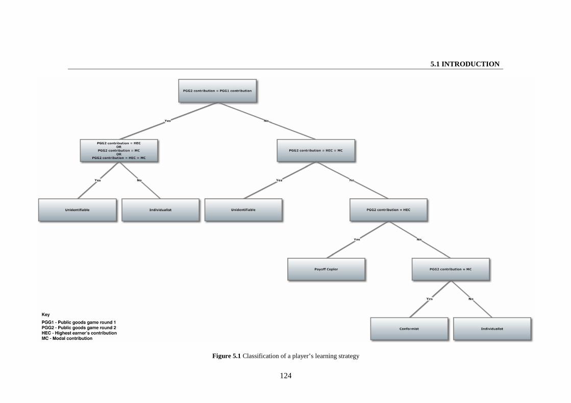
5.1 INTRODUCTION
124
Figure 5.1 Classification of a player’s learning strategy
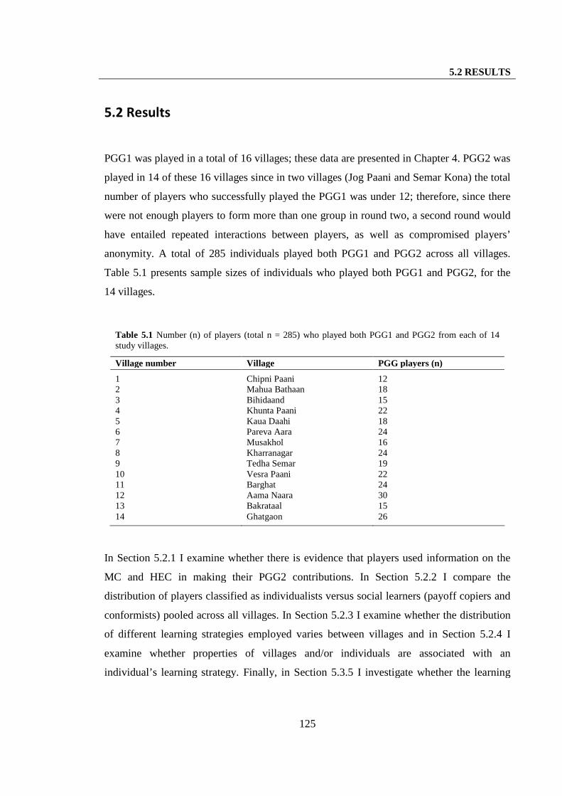
5.2 RESULTS
125
5.2 Results
PGG1 was played in a total of 16 villages; these data are presented in Chapter 4. PGG2 was
played in 14 of these 16 villages since in two villages (Jog Paani and Semar Kona) the total
number of players who successfully played the PGG1 was under 12; therefore, since there
were not enough players to form more than one group in round two, a second round would
have entailed repeated interactions between players, as well as compromised players’
anonymity. A total of 285 individuals played both PGG1 and PGG2 across all villages.
Table 5.1 presents sample sizes of individuals who played both PGG1 and PGG2, for the
14 villages.
Table 5.1 Number (n) of players (total n = 285) who played both PGG1 and PGG2 from each of 14study villages.
Village number Village PGG players (n)
1 Chipni Paani 122 Mahua Bathaan 183 Bihidaand 154 Khunta Paani 225 Kaua Daahi 186 Pareva Aara 247 Musakhol 168 Kharranagar 249 Tedha Semar 1910 Vesra Paani 2211 Barghat 2412 Aama Naara 3013 Bakrataal 1514 Ghatgaon 26
In Section 5.2.1 I examine whether there is evidence that players used information on the
MC and HEC in making their PGG2 contributions. In Section 5.2.2 I compare the
distribution of players classified as individualists versus social learners (payoff copiers and
conformists) pooled across all villages. In Section 5.2.3 I examine whether the distribution
of different learning strategies employed varies between villages and in Section 5.2.4 I
examine whether properties of villages and/or individuals are associated with an
individual’s learning strategy. Finally, in Section 5.3.5 I investigate whether the learning
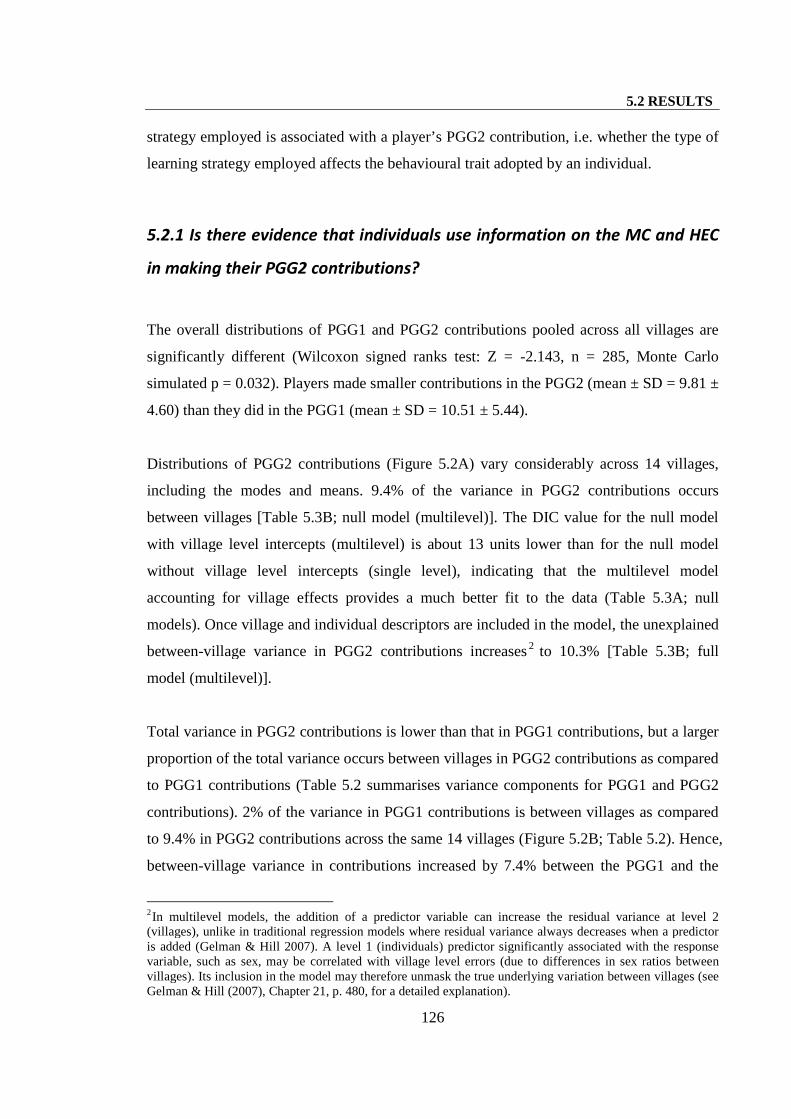
5.2 RESULTS
126
strategy employed is associated with a player’s PGG2 contribution, i.e. whether the type of
learning strategy employed affects the behavioural trait adopted by an individual.
5.2.1 Is there evidence that individuals use information on the MC and HEC
in making their PGG2 contributions?
The overall distributions of PGG1 and PGG2 contributions pooled across all villages are
significantly different (Wilcoxon signed ranks test: Z = -2.143, n = 285, Monte Carlo
simulated p = 0.032). Players made smaller contributions in the PGG2 (mean ± SD = 9.81 ±
4.60) than they did in the PGG1 (mean ± SD = 10.51 ± 5.44).
Distributions of PGG2 contributions (Figure 5.2A) vary considerably across 14 villages,
including the modes and means. 9.4% of the variance in PGG2 contributions occurs
between villages [Table 5.3B; null model (multilevel)]. The DIC value for the null model
with village level intercepts (multilevel) is about 13 units lower than for the null model
without village level intercepts (single level), indicating that the multilevel model
accounting for village effects provides a much better fit to the data (Table 5.3A; null
models). Once village and individual descriptors are included in the model, the unexplained
between-village variance in PGG2 contributions increases 2 to 10.3% [Table 5.3B; full
model (multilevel)].
Total variance in PGG2 contributions is lower than that in PGG1 contributions, but a larger
proportion of the total variance occurs between villages in PGG2 contributions as compared
to PGG1 contributions (Table 5.2 summarises variance components for PGG1 and PGG2
contributions). 2% of the variance in PGG1 contributions is between villages as compared
to 9.4% in PGG2 contributions across the same 14 villages (Figure 5.2B; Table 5.2). Hence,
between-village variance in contributions increased by 7.4% between the PGG1 and the
2In multilevel models, the addition of a predictor variable can increase the residual variance at level 2(villages), unlike in traditional regression models where residual variance always decreases when a predictoris added (Gelman & Hill 2007). A level 1 (individuals) predictor significantly associated with the responsevariable, such as sex, may be correlated with village level errors (due to differences in sex ratios betweenvillages). Its inclusion in the model may therefore unmask the true underlying variation between villages (seeGelman & Hill (2007), Chapter 21, p. 480, for a detailed explanation).
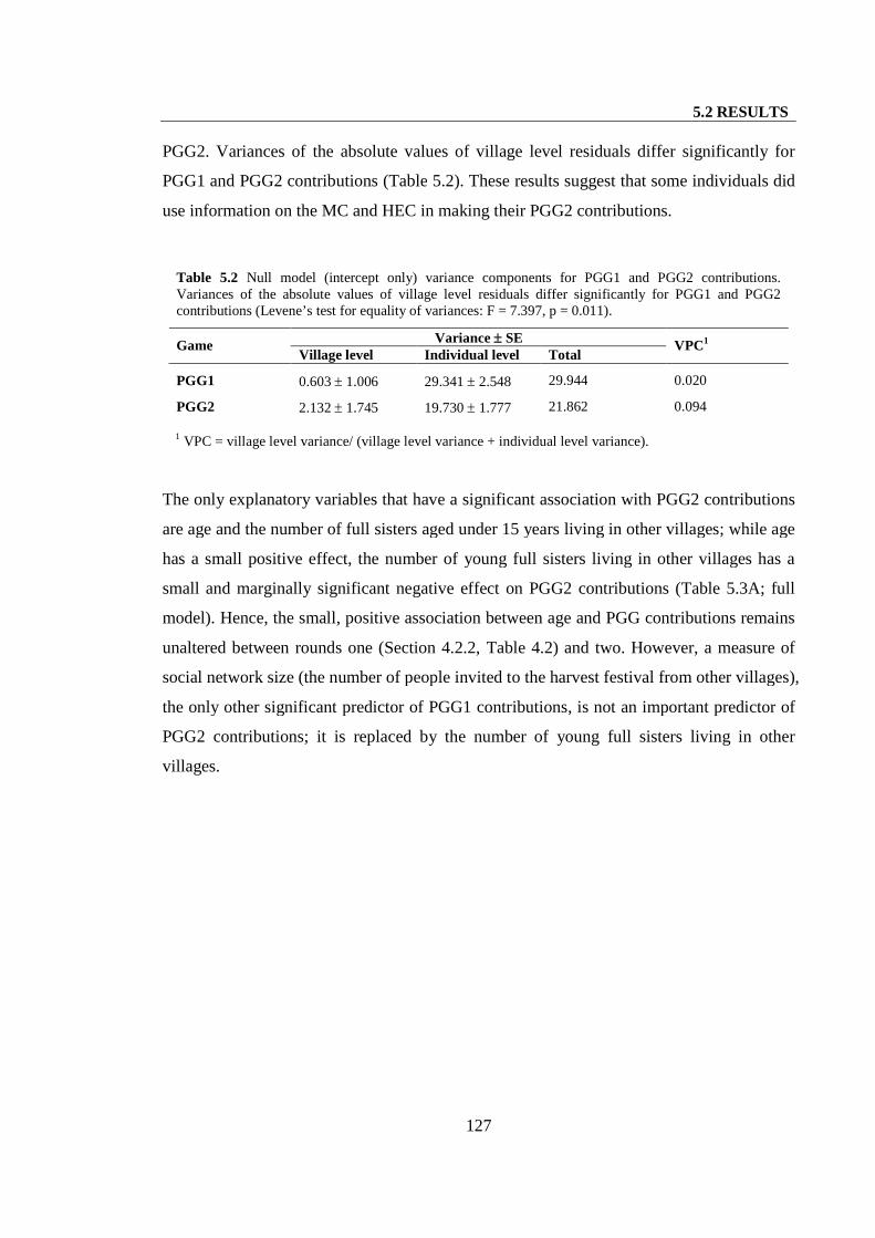
5.2 RESULTS
127
PGG2. Variances of the absolute values of village level residuals differ significantly for
PGG1 and PGG2 contributions (Table 5.2). These results suggest that some individuals did
use information on the MC and HEC in making their PGG2 contributions.
Table 5.2 Null model (intercept only) variance components for PGG1 and PGG2 contributions.Variances of the absolute values of village level residuals differ significantly for PGG1 and PGG2contributions (Levene’s test for equality of variances: F = 7.397, p = 0.011).
Variance SEGame
Village level Individual level TotalVPC1
PGG1 0.603 1.006 29.341 2.548 29.944 0.020
PGG2 2.132 1.745 19.730 1.777 21.862 0.094
1 VPC = village level variance/ (village level variance + individual level variance).
The only explanatory variables that have a significant association with PGG2 contributions
are age and the number of full sisters aged under 15 years living in other villages; while age
has a small positive effect, the number of young full sisters living in other villages has a
small and marginally significant negative effect on PGG2 contributions (Table 5.3A; full
model). Hence, the small, positive association between age and PGG contributions remains
unaltered between rounds one (Section 4.2.2, Table 4.2) and two. However, a measure of
social network size (the number of people invited to the harvest festival from other villages),
the only other significant predictor of PGG1 contributions, is not an important predictor of
PGG2 contributions; it is replaced by the number of young full sisters living in other
villages.
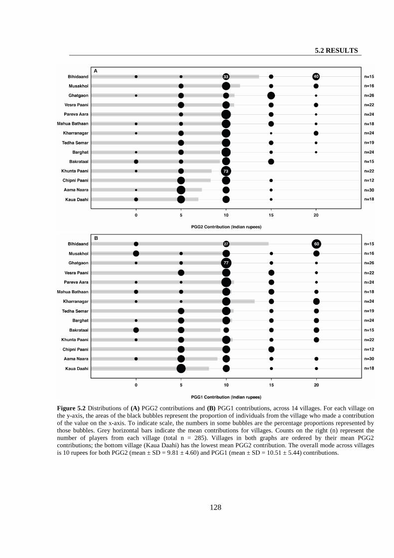
5.2 RESULTS
128
Figure 5.2 Distributions of (A) PGG2 contributions and (B) PGG1 contributions, across 14 villages. For each village onthe y-axis, the areas of the black bubbles represent the proportion of individuals from the village who made a contributionof the value on the x-axis. To indicate scale, the numbers in some bubbles are the percentage proportions represented bythose bubbles. Grey horizontal bars indicate the mean contributions for villages. Counts on the right (n) represent thenumber of players from each village (total n = 285). Villages in both graphs are ordered by their mean PGG2contributions; the bottom village (Kaua Daahi) has the lowest mean PGG2 contribution. The overall mode across villagesis 10 rupees for both PGG2 (mean ± SD = 9.81 ± 4.60) and PGG1 (mean ± SD = 10.51 ± 5.44) contributions.
A
B
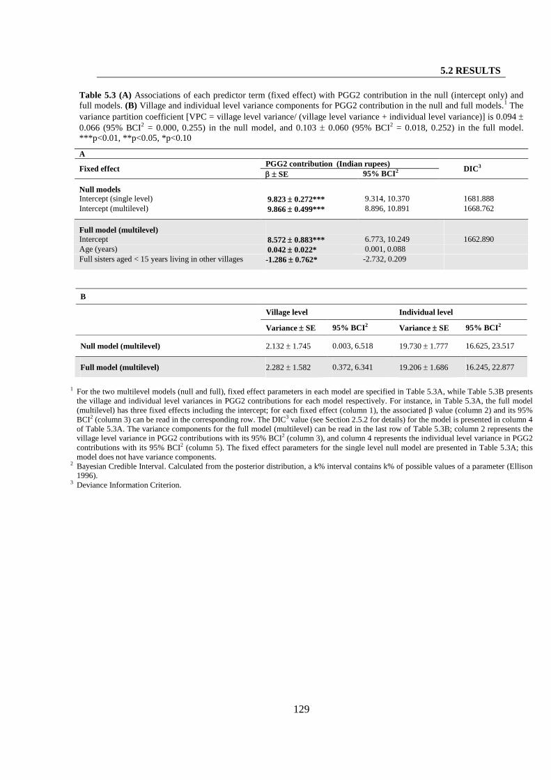
5.2 RESULTS
129
Table 5.3 (A) Associations of each predictor term (fixed effect) with PGG2 contribution in the null (intercept only) andfull models. (B) Village and individual level variance components for PGG2 contribution in the null and full models.1 The
variance partition coefficient [VPC = village level variance/ (village level variance + individual level variance)] is 0.094 0.066 (95% BCI2 = 0.000, 0.255) in the null model, and 0.103 0.060 (95% BCI2 = 0.018, 0.252) in the full model.***p<0.01, **p<0.05, *p<0.10
APGG2 contribution (Indian rupees)
Fixed effect SE 95% BCI2 DIC3
Null modelsIntercept (single level) 9.823 0.272*** 9.314, 10.370 1681.888Intercept (multilevel) 9.866 0.499*** 8.896, 10.891 1668.762
Full model (multilevel)Intercept 8.572 0.883*** 6.773, 10.249 1662.890Age (years) 0.042 0.022* 0.001, 0.088Full sisters aged < 15 years living in other villages -1.286 0.762* -2.732, 0.209
B
Village level Individual level
Variance SE 95% BCI2 Variance SE 95% BCI2
Null model (multilevel) 2.132 1.745 0.003, 6.518 19.730 1.777 16.625, 23.517
Full model (multilevel) 2.282 1.582 0.372, 6.341 19.206 1.686 16.245, 22.877
1 For the two multilevel models (null and full), fixed effect parameters in each model are specified in Table 5.3A, while Table 5.3B presentsthe village and individual level variances in PGG2 contributions for each model respectively. For instance, in Table 5.3A, the full model(multilevel) has three fixed effects including the intercept; for each fixed effect (column 1), the associated β value (column 2) and its 95%BCI2 (column 3) can be read in the corresponding row. The DIC3 value (see Section 2.5.2 for details) for the model is presented in column 4of Table 5.3A. The variance components for the full model (multilevel) can be read in the last row of Table 5.3B; column 2 represents thevillage level variance in PGG2 contributions with its 95% BCI2 (column 3), and column 4 represents the individual level variance in PGG2contributions with its 95% BCI2 (column 5). The fixed effect parameters for the single level null model are presented in Table 5.3A; thismodel does not have variance components.
2 Bayesian Credible Interval. Calculated from the posterior distribution, a k% interval contains k% of possible values of a parameter (Ellison1996).
3 Deviance Information Criterion.
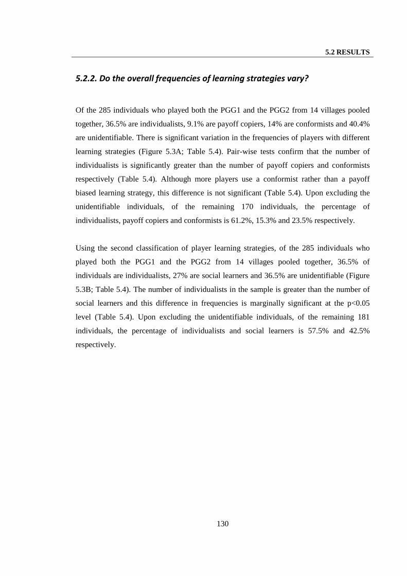
5.2 RESULTS
130
5.2.2. Do the overall frequencies of learning strategies vary?
Of the 285 individuals who played both the PGG1 and the PGG2 from 14 villages pooled
together, 36.5% are individualists, 9.1% are payoff copiers, 14% are conformists and 40.4%
are unidentifiable. There is significant variation in the frequencies of players with different
learning strategies (Figure 5.3A; Table 5.4). Pair-wise tests confirm that the number of
individualists is significantly greater than the number of payoff copiers and conformists
respectively (Table 5.4). Although more players use a conformist rather than a payoff
biased learning strategy, this difference is not significant (Table 5.4). Upon excluding the
unidentifiable individuals, of the remaining 170 individuals, the percentage of
individualists, payoff copiers and conformists is 61.2%, 15.3% and 23.5% respectively.
Using the second classification of player learning strategies, of the 285 individuals who
played both the PGG1 and the PGG2 from 14 villages pooled together, 36.5% of
individuals are individualists, 27% are social learners and 36.5% are unidentifiable (Figure
5.3B; Table 5.4). The number of individualists in the sample is greater than the number of
social learners and this difference in frequencies is marginally significant at the p<0.05
level (Table 5.4). Upon excluding the unidentifiable individuals, of the remaining 181
individuals, the percentage of individualists and social learners is 57.5% and 42.5%
respectively.
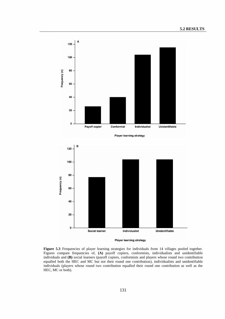
5.2 RESULTS
131
Figure 5.3 Frequencies of player learning strategies for individuals from 14 villages pooled together.Figures compare frequencies of, (A) payoff copiers, conformists, individualists and unidentifiableindividuals and (B) social learners (payoff copiers, conformists and players whose round two contributionequalled both the HEC and MC but not their round one contribution), individualists and unidentifiableindividuals (players whose round two contribution equalled their round one contribution as well as theHEC, MC or both).
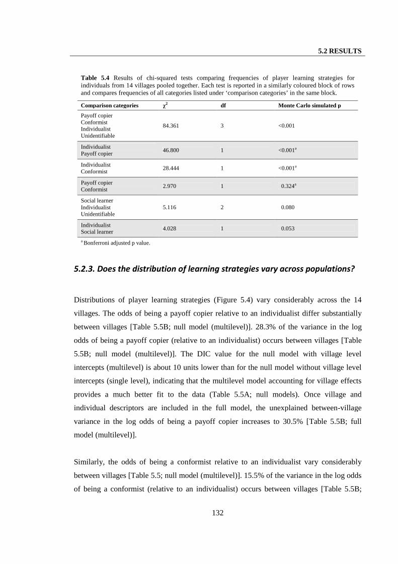
5.2 RESULTS
132
5.2.3. Does the distribution of learning strategies vary across populations?
Distributions of player learning strategies (Figure 5.4) vary considerably across the 14
villages. The odds of being a payoff copier relative to an individualist differ substantially
between villages [Table 5.5B; null model (multilevel)]. 28.3% of the variance in the log
odds of being a payoff copier (relative to an individualist) occurs between villages [Table
5.5B; null model (multilevel)]. The DIC value for the null model with village level
intercepts (multilevel) is about 10 units lower than for the null model without village level
intercepts (single level), indicating that the multilevel model accounting for village effects
provides a much better fit to the data (Table 5.5A; null models). Once village and
individual descriptors are included in the full model, the unexplained between-village
variance in the log odds of being a payoff copier increases to 30.5% [Table 5.5B; full
model (multilevel)].
Similarly, the odds of being a conformist relative to an individualist vary considerably
between villages [Table 5.5; null model (multilevel)]. 15.5% of the variance in the log odds
of being a conformist (relative to an individualist) occurs between villages [Table 5.5B;
Table 5.4 Results of chi-squared tests comparing frequencies of player learning strategies forindividuals from 14 villages pooled together. Each test is reported in a similarly coloured block of rowsand compares frequencies of all categories listed under ‘comparison categories’ in the same block.
Comparison categories χ2 df Monte Carlo simulated p
Payoff copierConformistIndividualistUnidentifiable
84.361 3 <0.001
IndividualistPayoff copier
46.800 1 <0.001a
IndividualistConformist
28.444 1 <0.001a
Payoff copierConformist
2.970 1 0.324a
Social learnerIndividualistUnidentifiable
5.116 2 0.080
IndividualistSocial learner
4.028 1 0.053
a Bonferroni adjusted p value.
5.2 RESULTS
133
null model (multilevel)]. Once village and individual descriptors are included in the full
model, the unexplained between-village variance in the log odds of being a conformist
decreases to 6.3% [Table 5.5B; full model (multilevel)].
11.9% of the variance in the log odds of being a social learner (relative to an individualist)
occurs between villages [Table 5.6B; null model (multilevel)]. The unexplained between-
village variance increases to 21% once individual descriptors are included in the full model
[Table 5.6B; full model (multilevel)]. The DIC value for the null model with village level
intercepts (multilevel) is about five units lower than for the null model without village level
intercepts (single level), indicating that the multilevel model accounting for village effects
provides a much better fit to the data (Table 5.6A; null models). Hence, populations vary in
their relative distribution of individuals employing different learning strategies, as well as
individuals employing social versus individual learning.
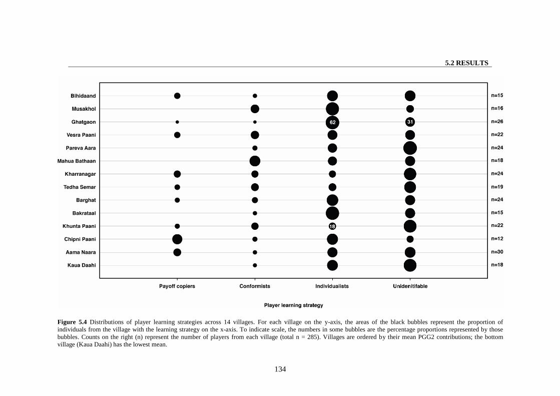
5.2 RESULTS
134
Figure 5.4 Distributions of player learning strategies across 14 villages. For each village on the y-axis, the areas of the black bubbles represent the proportion ofindividuals from the village with the learning strategy on the x-axis. To indicate scale, the numbers in some bubbles are the percentage proportions represented by thosebubbles. Counts on the right (n) represent the number of players from each village (total n = 285). Villages are ordered by their mean PGG2 contributions; the bottomvillage (Kaua Daahi) has the lowest mean.

5.2 RESULTS
135
Table 5.5A Associations of each predictor term (fixed effect) with the odds of being a payoff copier, conformist or unidentifiable relative to an individualistrespectively, in the null (intercept only) and full multinomial logistic models (see Table 5.5B for variance components of these models). Odds ratios less than,equal to, or greater than one represent lower, equal, or higher probabilities of occurrence (compared to the reference category) respectively.1 ***p<0.001,**p<0.05, *p<0.10
Payoff copier Conformist UnidentifiableFixed effect
exp () SE 95% BCI2exp () SE 95% BCI2
exp () SE 95% BCI2 DIC3
Null modelsIntercept (single level) 0.251 0.056 *** 0.156, 0.371 0.386 0.069*** 0.265, 0.540 1.114 0.147 0.843, 1.426 705.890Intercept (multilevel) 0.201 0.084 *** 0.074, 0.406 0.385 0.111*** 0.208, 0.643 1.148 0.245 0.752, 1.697 695.860
Full model (multilevel) 679.990
Intercept 0.127 0.154** 0.008, 0.559 4.908 4.223* 0.803, 15.730 2.923 1.658* 0.933, 7.415Sex: female (ref: male) 1.530 0.858 0.462, 3.690 1.193 0.538 0.460, 2.514 2.304 0.749** 1.202, 4.100Population size 0.998 0.002 0.993, 1.002 0.997 0.002** 0.993, 0.999 0.999 0.001* 0.997, 1.000Outstanding loans: yes (ref: no) 0.268 0.175** 0.062, 0.721 0.546 0.252 0.207, 1.164 0.613 0.198* 0.306, 1.086HEC 1.232 0.111** 1.032, 1.477 0.903 0.063 0.783, 1.031 1.068 0.052 0.975, 1.178MC 1.065 0.062 0.944, 1.192 0.906 0.044** 0.822, 0.993 0.923 0.030** 0.863, 0.982
1 For the two multilevel models (null and full), fixed effect parameters in each model are specified in Table 5.5A, while Table 5.5B presents the village level variances in log odds ofbeing a payoff copier, conformist or unidentifiable (relative to an individualist respectively) for each model respectively. For instance, in Table 5.5A, the full model (multilevel)has six fixed effects including the intercept; for each fixed effect (column 1), the associated exp (β) value for a payoff copier (column 2), conformist (column 4) and unidentifiable(column 6) and their respective 95% BCI2 (columns 3, 5 and 7) can be read in the corresponding row. The DIC3 value (see Section 2.5.2 for details) for the model is presented incolumn 8 of Table 5.5A. The variance components for the full model (multilevel) can be read in the 12th, 13th and 14th, rows of Table 5.5B; column 2 represents the village levelvariance with its 95% BCI2 (column 3), and column 4 represents the VPC with its 95% BCI2 (column 5) for the corresponding rows. The last three rows of Table 5.5B present theresidual covariances in the full (multilevel) model respectively; the associated values at the village level (column 2) and their 95% BCI2 (column 3) can be read in thecorresponding rows. The fixed effect parameters for the single level null model are presented in Table 5.5A; this model does not have variance components.
2 Bayesian Credible Interval. Calculated from the posterior distribution, a k% interval contains k% of possible values of a parameter (Ellison 1996). For exp () values, 95% BCI notcontaining the value 1 indicates significance at p<0.05.
3 Deviance Information Criterion.
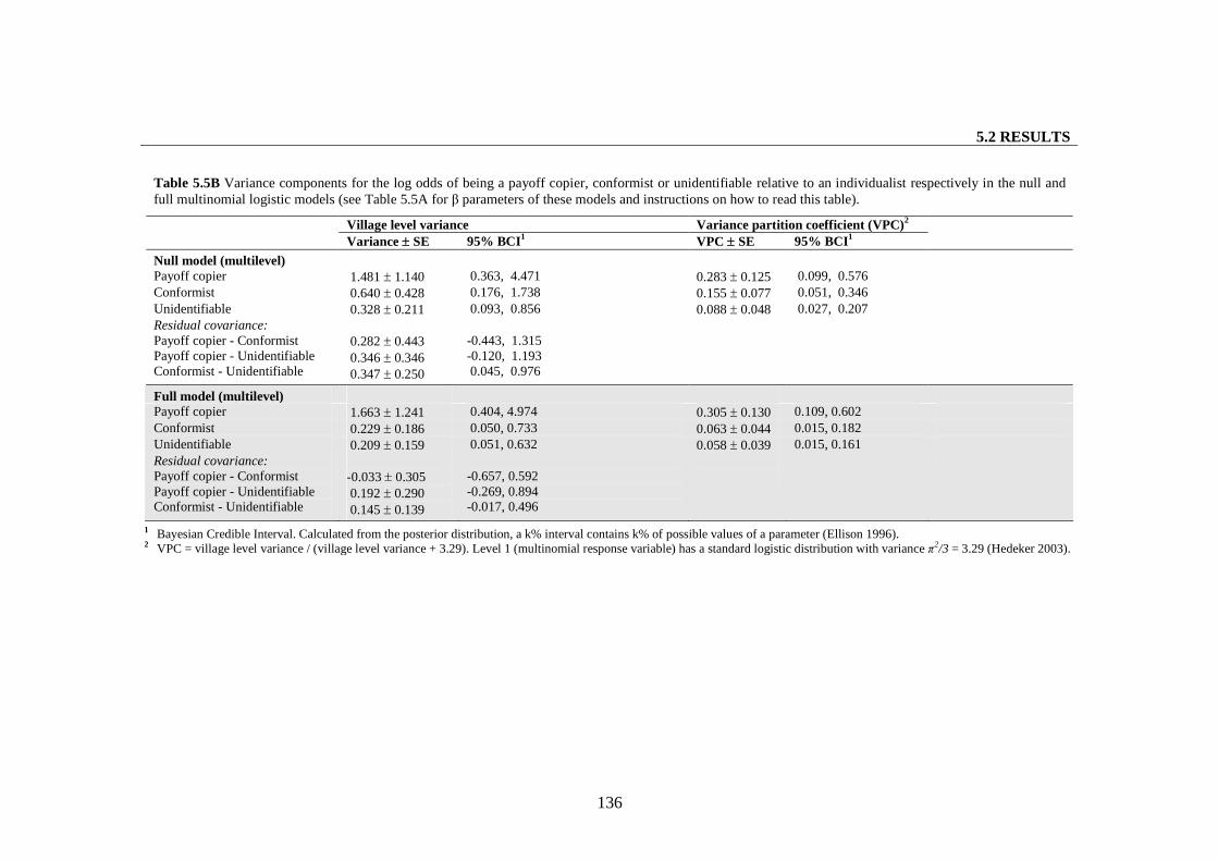
5.2 RESULTS
136
Table 5.5B Variance components for the log odds of being a payoff copier, conformist or unidentifiable relative to an individualist respectively in the null andfull multinomial logistic models (see Table 5.5A for β parameters of these models and instructions on how to read this table).
Village level variance Variance partition coefficient (VPC)2
Variance SE 95% BCI1 VPC SE 95% BCI1
Null model (multilevel)Payoff copier 1.481 1.140 0.363, 4.471 0.283 0.125 0.099, 0.576Conformist 0.640 0.428 0.176, 1.738 0.155 0.077 0.051, 0.346Unidentifiable 0.328 0.211 0.093, 0.856 0.088 0.048 0.027, 0.207Residual covariance:Payoff copier - ConformistPayoff copier - UnidentifiableConformist - Unidentifiable
0.282 0.4430.346 0.3460.347 0.250
-0.443, 1.315-0.120, 1.1930.045, 0.976
Full model (multilevel)Payoff copier 1.663 1.241 0.404, 4.974 0.305 0.130 0.109, 0.602Conformist 0.229 0.186 0.050, 0.733 0.063 0.044 0.015, 0.182Unidentifiable 0.209 0.159 0.051, 0.632 0.058 0.039 0.015, 0.161Residual covariance:Payoff copier - ConformistPayoff copier - UnidentifiableConformist - Unidentifiable
-0.033 0.3050.192 0.2900.145 0.139
-0.657, 0.592-0.269, 0.894-0.017, 0.496
1 Bayesian Credible Interval. Calculated from the posterior distribution, a k% interval contains k% of possible values of a parameter (Ellison 1996).2 VPC = village level variance / (village level variance + 3.29). Level 1 (multinomial response variable) has a standard logistic distribution with variance π2/3 = 3.29 (Hedeker 2003).
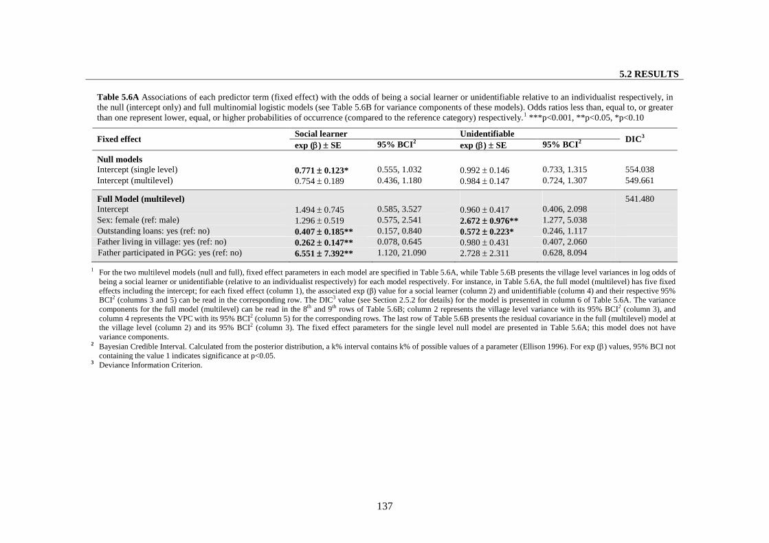
5.2 RESULTS
137
Table 5.6A Associations of each predictor term (fixed effect) with the odds of being a social learner or unidentifiable relative to an individualist respectively, inthe null (intercept only) and full multinomial logistic models (see Table 5.6B for variance components of these models). Odds ratios less than, equal to, or greaterthan one represent lower, equal, or higher probabilities of occurrence (compared to the reference category) respectively.1 ***p<0.001, **p<0.05, *p<0.10
Social learner UnidentifiableFixed effect
exp () SE 95% BCI2exp () SE 95% BCI2 DIC3
Null modelsIntercept (single level) 0.771 0.123* 0.555, 1.032 0.992 0.146 0.733, 1.315 554.038Intercept (multilevel) 0.754 0.189 0.436, 1.180 0.984 0.147 0.724, 1.307 549.661
Full Model (multilevel) 541.480Intercept 1.494 0.745 0.585, 3.527 0.960 0.417 0.406, 2.098Sex: female (ref: male) 1.296 0.519 0.575, 2.541 2.672 0.976** 1.277, 5.038Outstanding loans: yes (ref: no) 0.407 0.185** 0.157, 0.840 0.572 0.223* 0.246, 1.117Father living in village: yes (ref: no) 0.262 0.147** 0.078, 0.645 0.980 0.431 0.407, 2.060Father participated in PGG: yes (ref: no) 6.551 7.392** 1.120, 21.090 2.728 2.311 0.628, 8.094
1 For the two multilevel models (null and full), fixed effect parameters in each model are specified in Table 5.6A, while Table 5.6B presents the village level variances in log odds ofbeing a social learner or unidentifiable (relative to an individualist respectively) for each model respectively. For instance, in Table 5.6A, the full model (multilevel) has five fixedeffects including the intercept; for each fixed effect (column 1), the associated exp (β) value for a social learner (column 2) and unidentifiable (column 4) and their respective 95%BCI2 (columns 3 and 5) can be read in the corresponding row. The DIC3 value (see Section 2.5.2 for details) for the model is presented in column 6 of Table 5.6A. The variancecomponents for the full model (multilevel) can be read in the 8th and 9th rows of Table 5.6B; column 2 represents the village level variance with its 95% BCI2 (column 3), andcolumn 4 represents the VPC with its 95% BCI2 (column 5) for the corresponding rows. The last row of Table 5.6B presents the residual covariance in the full (multilevel) model atthe village level (column 2) and its 95% BCI2 (column 3). The fixed effect parameters for the single level null model are presented in Table 5.6A; this model does not havevariance components.
2 Bayesian Credible Interval. Calculated from the posterior distribution, a k% interval contains k% of possible values of a parameter (Ellison 1996). For exp () values, 95% BCI notcontaining the value 1 indicates significance at p<0.05.
3 Deviance Information Criterion.
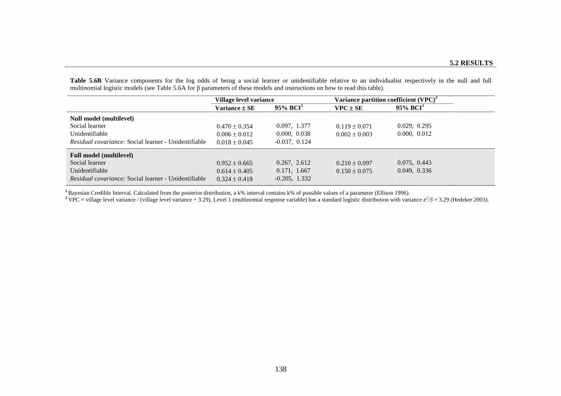
5.2 RESULTS
138
Table 5.6B Variance components for the log odds of being a social learner or unidentifiable relative to an individualist respectively in the null and fullmultinomial logistic models (see Table 5.6A for β parameters of these models and instructions on how to read this table).
Village level variance Variance partition coefficient (VPC)2
Variance SE 95% BCI1VPC SE 95% BCI1
Null model (multilevel)Social learner 0.470 0.354 0.097, 1.377 0.119 0.071 0.029, 0.295Unidentifiable 0.006 0.012 0.000, 0.038 0.002 0.003 0.000, 0.012
Residual covariance: Social learner - Unidentifiable 0.018 0.045 -0.037, 0.124
Full model (multilevel)Social learner 0.952 0.665 0.267, 2.612 0.210 0.097 0.075, 0.443Unidentifiable 0.614 0.405 0.171, 1.667 0.150 0.075 0.049, 0.336Residual covariance: Social learner - Unidentifiable 0.324 0.418 -0.205, 1.332
1 Bayesian Credible Interval. Calculated from the posterior distribution, a k% interval contains k% of possible values of a parameter (Ellison 1996).2 VPC = village level variance / (village level variance + 3.29). Level 1 (multinomial response variable) has a standard logistic distribution with variance π2/3 = 3.29 (Hedeker 2003).
5.2 RESULTS
139
5.2.4. Are properties of populations and/or individuals associated with the
learning strategies employed by individuals?
Five variables are significantly associated with the odds of being a payoff copier or a
conformist (relative to an individualist), namely sex, village population size, outstanding
loans, the value of the HEC, and the value of the MC. Sex was retained in the full model
and women are more likely to be payoff copiers and conformists relative to individualists,
but these relationships are not significant at conventional levels. The odds of being a
conformist relative to an individualist significantly decrease as population size increases, as
do the odds of being a payoff copier, although this latter relationship is not significant at
conventional levels [Table 5.5A; full model (multilevel)].
Figure 5.5Figure 5.5A presents the observed frequencies of the three strategies within each
village; villages are ordered by increasing population size. The odds of being a conformist
relative to an individualist decrease by about 3% for a ten person increase in population
size.
The odds of being a payoff copier relative to an individualist are significantly lower for
individuals with outstanding loans as compared to those with no loans [Table 5.5A; full
model (multilevel)]. People with outstanding loans are about four times more likely to be
individualists than payoff copiers. Outstanding loans also decrease the likelihood of a
player being a conformist, but this relationship is not significant at conventional levels. The
odds of being a payoff copier increase by about 23% for every one rupee increase in the
value of the HEC. A one rupee increase in the HEC reduces the odds of being a conformist
by about 10%. At the same time, the odds of being a conformist are about 9% lower for
every one rupee increase in the value of the MC. Hence, players are more likely to be
payoff copiers as the HEC increases and less likely to be conformists as the MC increases.
The odds of being a social learner relative to an individualist are significantly associated
with four variables. Women are about 30% more likely to be social learners than men are,
but this relationship is not significant at conventional levels. Outstanding loans and the co-
5.2 RESULTS
140
residence of the father in the village both make individuals less likely to be social learners
[Table 5.6A; full model (multilevel)]. On the other hand, the participation of the father in
the PGG on the day of the games makes individuals 6.5 times more likely to be social
learners [Table 5.6A; full model (multilevel)].
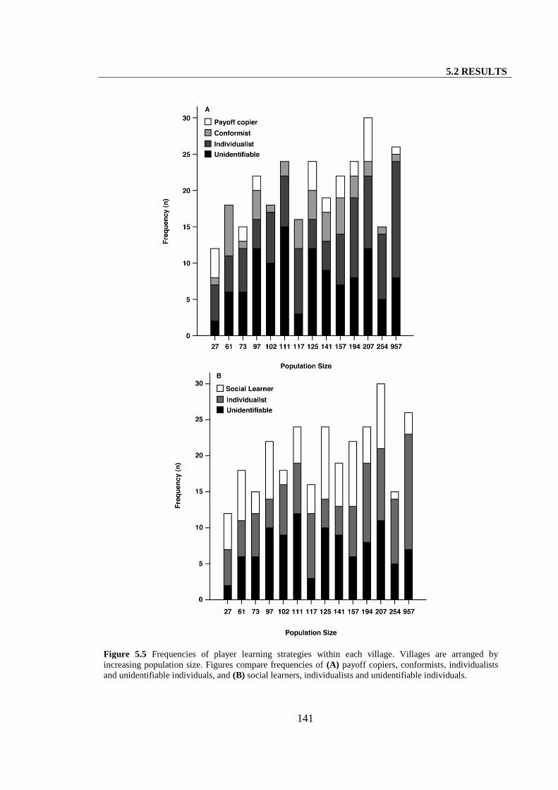
5.2 RESULTS
141
Figure 5.5 Frequencies of player learning strategies within each village. Villages are arranged byincreasing population size. Figures compare frequencies of (A) payoff copiers, conformists, individualistsand unidentifiable individuals, and (B) social learners, individualists and unidentifiable individuals.

5.2 RESULTS
142
5.2.5. Do different learning strategies result in the acquisition of different
behavioural traits?
Players employing different learning strategies made significantly different contributions to
their respective group pots in both the PGG2 (Figure 5.6, unfilled bars; Table 5.1) and the
PGG1 (Figure 5.6, filled bars; Table 5.7). However, pair-wise comparisons reveal that
individuals whose behaviour is most affected by their learning strategy are payoff copiers
(Figure 5.6A; Table 5.7). Individualists made much higher PGG2 contributions than payoff
copiers; the mean PGG2 contribution for individualists is about six rupees higher than that
for payoff copiers. However, individualists’ PGG2 contributions did not differ from those
of conformists. Conformists made much higher PGG2 contributions than payoff copiers;
the mean PGG2 contribution for conformists is about six rupees higher than that for payoff
copiers.
On the other hand, individualists’ PGG1 contributions are on average about 1.5 rupees
lower than those of payoff copiers, although this difference is not statistically significant.
Individualists’ PGG1 contributions are about 2.5 rupees higher on average than those of
conformists; this difference is marginally significant. Conformists made significantly lower
PGG1 contributions than payoff copiers; the mean PGG1 contribution for conformists is
about four rupees lower than that for payoff copiers.
Hence, individualists did not change their contributions significantly between rounds one
and two (Wilcoxon signed ranks test: Z = -0.26, n = 104, Monte Carlo simulated p = 0.803).
Payoff copiers dramatically changed their behaviour between round one and two of the
PGG, lowering their contributions in round two by about seven rupees on average
(Wilcoxon signed ranks test: Z = -4.65, n = 26, Monte Carlo simulated p<0.001). While
conformists did increase their contributions in round two compared to their contributions in
round one, this difference in their behaviour between rounds is not significant (Wilcoxon
signed ranks test: Z = -1.49, n = 40, Monte Carlo simulated p = 0.128).
Social learners made PGG2 contributions that were lower than those of individualists by
about two rupees on average (Figure 5.6B; Table 5.7), although their PGG1 contributions

5.2 RESULTS
143
did not differ from those of individualists (Figure 5.6B; Table 5.7). Social learners made
significantly lower PGG2 contributions as compared to their PGG1 contributions
(Wilcoxon signed ranks test: Z = -2.673, n = 77, Monte Carlo simulated p = 0.007).
Individualists did not change their contributions between rounds one and two (Wilcoxon
signed ranks test: Z = -0.256, n = 104, Monte Carlo simulated p = 0.800).
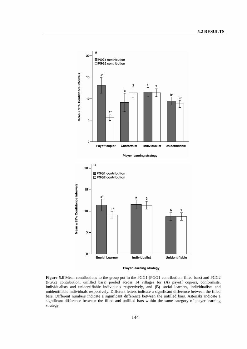
5.2 RESULTS
144
Figure 5.6 Mean contributions to the group pot in the PGG1 (PGG1 contribution; filled bars) and PGG2(PGG2 contribution; unfilled bars) pooled across 14 villages for (A) payoff copiers, conformists,individualists and unidentifiable individuals respectively, and (B) social learners, individualists andunidentifiable individuals respectively. Different letters indicate a significant difference between the filledbars. Different numbers indicate a significant difference between the unfilled bars. Asterisks indicate asignificant difference between the filled and unfilled bars within the same category of player learningstrategy.
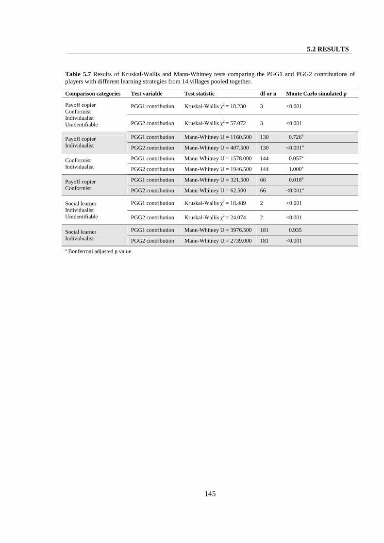
5.2 RESULTS
145
Table 5.7 Results of Kruskal-Wallis and Mann-Whitney tests comparing the PGG1 and PGG2 contributions ofplayers with different learning strategies from 14 villages pooled together.
Comparison categories Test variable Test statistic df or n Monte Carlo simulated p
PGG1 contribution Kruskal-Wallis χ2 = 18.230 3 <0.001Payoff copierConformistIndividualistUnidentifiable PGG2 contribution Kruskal-Wallis χ2 = 57.072 3 <0.001
PGG1 contribution Mann-Whitney U = 1160.500 130 0.726aPayoff copierIndividualist PGG2 contribution Mann-Whitney U = 407.500 130 <0.001a
PGG1 contribution Mann-Whitney U = 1578.000 144 0.057aConformistIndividualist PGG2 contribution Mann-Whitney U = 1946.500 144 1.000a
PGG1 contribution Mann-Whitney U = 321.500 66 0.018aPayoff copierConformist PGG2 contribution Mann-Whitney U = 62.500 66 <0.001a
PGG1 contribution Kruskal-Wallis χ2 = 18.489 2 <0.001Social learnerIndividualistUnidentifiable PGG2 contribution Kruskal-Wallis χ2 = 24.074 2 <0.001
PGG1 contribution Mann-Whitney U = 3976.500 181 0.935Social learnerIndividualist PGG2 contribution Mann-Whitney U = 2739.000 181 <0.001
a Bonferroni adjusted p value.
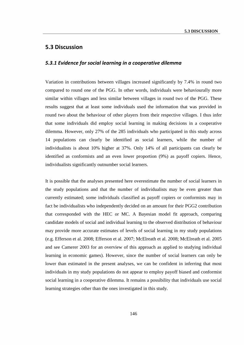
5.3 DISCUSSION
146
5.3 Discussion
5.3.1 Evidence for social learning in a cooperative dilemma
Variation in contributions between villages increased significantly by 7.4% in round two
compared to round one of the PGG. In other words, individuals were behaviourally more
similar within villages and less similar between villages in round two of the PGG. These
results suggest that at least some individuals used the information that was provided in
round two about the behaviour of other players from their respective villages. I thus infer
that some individuals did employ social learning in making decisions in a cooperative
dilemma. However, only 27% of the 285 individuals who participated in this study across
14 populations can clearly be identified as social learners, while the number of
individualists is about 10% higher at 37%. Only 14% of all participants can clearly be
identified as conformists and an even lower proportion (9%) as payoff copiers. Hence,
individualists significantly outnumber social learners.
It is possible that the analyses presented here overestimate the number of social learners in
the study populations and that the number of individualists may be even greater than
currently estimated; some individuals classified as payoff copiers or conformists may in
fact be individualists who independently decided on an amount for their PGG2 contribution
that corresponded with the HEC or MC. A Bayesian model fit approach, comparing
candidate models of social and individual learning to the observed distribution of behaviour
may provide more accurate estimates of levels of social learning in my study populations
(e.g. Efferson et al. 2008; Efferson et al. 2007; McElreath et al. 2008; McElreath et al. 2005
and see Camerer 2003 for an overview of this approach as applied to studying individual
learning in economic games). However, since the number of social learners can only be
lower than estimated in the present analyses, we can be confident in inferring that most
individuals in my study populations do not appear to employ payoff biased and conformist
social learning in a cooperative dilemma. It remains a possibility that individuals use social
learning strategies other than the ones investigated in this study.
5.3 DISCUSSION
147
5.3.2 Correlates of learning strategies
The relative distribution of different learning strategies varies considerably across
populations. Properties of villages and individuals that systematically explain some of the
variation in patterns of learning across 14 populations are population size, which has a
negative association with the likelihood of being a conformist, and outstanding loans,
which have a negative association with the likelihood of being a payoff copier.
At least three hypotheses may explain the negative association between population size and
conformity. First, the lower prevalence of conformity in larger populations may be a
response to an increased likelihood of adopting the wrong or maladaptive behaviour in
larger populations, if individuals sample the behaviour of only a fraction of the population.
A theoretical model has demonstrated that conformist transmission is disfavoured when the
costs of adopting a maladaptive behaviour are high (Nakahashi 2007). In another
theoretical study Kendal et al. (2009) find that the probability of conforming is negatively
affected by population size when the frequency of individuals possessing the adaptive
behaviour for an environment is less than half. Behavioural tracking of the environment
may be less accurate in larger populations if most people are conformists sampling from a
subset of the population and the proportion of individual learners in the population is small.
My results are consistent with the theoretical finding that social learning is less likely to
fixate in larger populations (Whitehead and Richerson 2009); however, this study examined
the likelihood of fixation only in populations of 500 individuals or more, whereas my study
populations are smaller.
A second hypothesis is that large or growing populations may contribute to environmental
instability, which in turn disfavours conformist learning. Large populations may experience
accelerated consumption of local resources (like wood and water) and greater competition
for them. This may be especially true for populations, like those of the Pahari Korwa, that
rely heavily on locally available resources for their subsistence and survival. If conformist
transmission is disfavoured in rapidly changing, unstable environments, the prevalence of
conformity would decline in large or growing populations. The current theoretical literature
exploring the effects of environmental instability on the frequency of conformity provides
5.3 DISCUSSION
148
mixed predictions. While most authors are in agreement that environmental instability has a
negative effect on the frequency of unbiased social learning (copying a randomly selected
phenotype from the parental generation; Aoki et al. 2005; Borenstein et al. 2009; Boyd and
Richerson 1985; Feldman et al. 1996; Rogers 1988; Wakano and Aoki 2006; Wakano et al.
2004), some authors suggest that it negatively affects the strength of conformity (Henrich
and Boyd 1998), while others argue the opposite (Kendal et al. 2009; Nakahashi 2007;
Wakano and Aoki 2007).
The third hypothesis reverses the direction of causality; populations with fewer conformists
(or more individualists) may be more productive and therefore grow to be larger. Support
for this hypothesis requires identifying mechanisms that counter “Rogers’ paradox”, the
theoretical expectation that the mean fitness of a population (or individual) with social
learning should be no different to one without it (Rogers 1988). A recent theoretical study
finds that when learning is structured, i.e. individuals learn only from a set of neighbours
and do not disperse far, social learning can become common and negatively affect fitness
and thus population size (Rendell et al. 2009).
I propose two hypotheses that potentially explain the relationship between outstanding
loans and a reduced dependence on social learning. Outstanding loans may reflect long-
term financial stress and instability, making individuals more risk-averse and therefore less
willing to chance adopting a non-optimum costly behaviour via social learning.
Alternatively, that outstanding loans are associated with a lower likelihood of being a
payoff copier may indicate that individuals who are more likely to receive help via loans
are also more willing to reciprocate by contributing to a public good.
It is notable that a player’s likelihood of being a conformist decreases as the actual value of
the MC increases, indicating that the conformist strategy may be flexible; individuals may
avoid conforming if it is too expensive to do so. It is, however, puzzling that individuals are
more likely to be payoff copiers as the HEC increases; if payoff copiers are motivated by a
desire to increase payoffs, then they should favour lower HEC values which, given the
structure of the PGG, will provide higher payoffs. Nonetheless, these results raise the
5.3 DISCUSSION
149
possibility that conformist or payoff biased learning is conditional on the cost incurred by
adopting a trait.
Players whose fathers live in the same village as them are less likely to be social learners,
whereas those whose fathers participate with them in the games are more likely to be social
learners. These seemingly contradictory results may indicate that fathers are important
models of socially learned behaviour. A co-resident father may make individuals less
sensitive to the behaviour of others. However, when the father is part of an aggregate
behavioural pool being sampled (such as when a player’s father participates in the games),
individuals may pay more attention to information derived from this pool than they would
otherwise. These are speculations to guide future research.
Together, my results support the idea that individuals’ learning strategies are sensitive to
the relative costs of individual versus social learning and the relative likelihood that each of
these strategies will result in the adoption of the optimal behaviour in different
environments. Certainly they suggest that people do not use a single learning strategy
across all environments and irrespective of their circumstances. Thus, my findings
challenge the suggestion by some authors (Boyd and Richerson 1985; Gintis 2003) that
conformity evolved as an all-purpose learning strategy that individuals employ across task-
domains, even though it leads to the acquisition of sub-optimal behaviour in some domains.
These authors argue that conformity is advantageous to individuals averaged across several
domains; its averaged benefit across domains mitigates the costs incurred on account of it
in some domains. Indeed, there has been a tendency to take as given the as yet unconfirmed
theoretical assumption that people acquire behavioural traits via conformist learning (Gintis
2007; Henrich 2004; Henrich and Boyd 2001). It is, however, more likely that whether
social learning is employed at all or not depends on the task domain (Eriksson and Coultas
2009; Eriksson et al. 2007; Rowthorn et al. 2009), its cost-benefit outcomes with respect to
the current environment, as well as the circumstances of the individual. The specific
learning strategy used should depend on many factors, including, among others, the
availability of information about the choice of cultural/behavioural variants and the number
of different variants available (Eriksson et al. 2007).
5.3 DISCUSSION
150
It is noteworthy that demographic factors such as migration (Aoki and Nakahashi 2008;
Boyd and Richerson 1985; Boyd and Richerson 1988b) and population size (Whitehead
and Richerson 2009) are expected to inversely affect the prevalence of social learning in
populations; the same factors, i.e. large populations and high rates of migration, impede the
evolution of cooperation (reviewed in Grafen 1984 and Henrich 2004). Hence, while
cultural group selection models invoke social learning to explain the evolution of
cooperation in large populations with high rates of migration, social learning itself is less
likely to be employed in such populations.
5.3.3 The impact of learning on the distribution of trait variants
Models of cultural evolution predict that social learning should influence the distribution of
trait variants within and across populations by affecting which variants are acquired by
individuals (Boyd and Richerson 1985). I find evidence that employing a payoff biased
learning strategy unsurprisingly led to the acquisition of more selfish behaviour in a one-
shot, anonymous PGG, and instrumented a change in players’ behaviour between round one
and two of the game. Alternatively, although a conformist learning strategy is associated
with a statistically non-significant increase in a player’s PGG2 contribution as compared to
her PGG1 contribution, this small increase in contribution eliminated the difference
between conformists’ and individualists’ behaviour in round one. Most individualists in the
population maintain stable behaviour between rounds one and two. Overall, these data
suggest that the learning strategies employed by individuals do influence the distribution of
trait variants within the population. However, how social learning affects trait variation
between populations in the real world depends greatly on whether social learners
selectively sample the behaviour of only those residing in their population, thus increasing
trait variation between populations, or not, thus decreasing trait variation between
populations. Moreover, while players in this study were told the values of the MC and HEC,
individuals in the real world must estimate these values by sampling the behaviour of
others over time; individual errors in estimation are likely to increase behavioural variance,
whether it is within or between populations.
5.3 DISCUSSION
151
The mean contribution is lower in round two as compared to round one of the PGG.
Previous studies have found that contributions in a PGG decline when the game is played
repeatedly, even when individuals play with a different set of players each time (e.g. Fehr
and Gächter 2002). While the decrease in individuals’ contributions between round one and
two in this study may be explained by repeated play (albeit with a different set of players)
in part, it is likely that at least some of this effect is the consequence of payoff biased
learning.
5.3.4 Unidentifiable strategies
A potential drawback of the current study design is the large number of unidentifiable
individuals; individuals who could not unequivocally be classified as payoff copiers,
conformists or individualists. This category of individuals most likely contains not only an
assortment of payoff copiers, conformists and individualists, but also players using
complex or alternative learning strategies. While the analyses presented here take account
of these unidentifiable individuals, their large number warrants a closer investigation of
how best we may identify their strategies. One way that the number of unidentifiable
individuals could have been eliminated is by presenting players with false values for the
MC or HEC in games where the two were equal, or where either or both of these values
was equal to a player’s PGG1 contribution. This was avoided as I did not wish to deceive
participants, a policy adopted throughout this work. However, it is not obvious that
eliminating this category by design would improve the inferences of this study. Several
individuals in the unidentifiable category may genuinely possess complex strategies, such
as using social information to confirm the benefit of a behavioural strategy they already
possess (the “confirmation” strategy modelled by McElreath et al. 2005). Indeed, 90% of
the unidentifiable individuals in my sample are those who contributed the same amount in
round two as they did in round one and this amount was also the same as the HEC, MC or
both. The current study design thus allows the separation, if not explicit identification, of
such complex strategy learners, instead of forcing them to use one of three pure learning
strategies; it also likely captures a more real-world decision making environment.

5.3 DISCUSSION
152
Hence, the distribution of learning strategies captured in this study may be a more accurate
representation of the true distribution of strategies in the study populations, than if
individuals had been provided incomplete information. Although studies have modelled
complex learning strategies (e.g. Borenstein et al. 2009; Boyd and Richerson 1995; Boyd
and Richerson 1996; Enquist et al. 2007; Kameda and Nakanishi 2003; McElreath et al.
2008; McElreath et al. 2005; Rendell et al. 2009), my results highlight the need for both
more theoretical and empirical work, focussing not only on the effects of complex learning
strategies on individual behaviour, but also their population level consequences; this work
is particularly important if complex strategy learners are relatively numerous in populations.
5.3.5 Concluding remarks
The second question I address in this thesis is: do people use social learning to acquire
cooperative strategies? My findings suggest that some minority of individuals do employ
social learning in the context of a cooperative dilemma, although most individuals do not.
The frequencies of different learning strategies are highly variable across populations; this
variation is partly explained by demographic differences between populations, most notably
population size. Theoretical work is required to clarify whether these low and variable
levels of social learning can maintain stable behavioural differences between populations,
given the high rates of migration between my study villages (see Section 2.3.2.2, Table 2.1).
Furthermore, whether social learning increases or decreases behavioural variation between
populations depends crucially on whether social learners selectively sample the behaviour
of only those residing in their population or not respectively; empirical work in real-world
populations will shed light on this matter.
5.4 METHODS
153
5.4 Methods
5.4.1 Experimental set-up
All games were played between February 2nd and May 16th, 2008. All games in most
villages were administered on the third day after arrival in the village (the second day in
two villages and the fourth day in one village) and completed in one day. Mean age ± SD of
participants was 34.59 ± 12.13 years and 46% were female.
All participants collected at a common location in the village on the day of the games. They
were instructed about the game rules and examples both collectively and then individually
at the private location where they played the game (see Appendix A, Sections A.2 and A.4
for scripts). Players were tested both collectively and individually for their understanding of
the game rules and of the anonymity of their decisions in each round of the game. Only a
player who individually answered all test questions correctly played the game in round one.
Only a player who had played in round one and answered all test questions for round two
correctly played in round two. In all 14 villages where both rounds of the PGG were played,
all individuals (n = 285) who understood the game rules in round one did so in round two;
they therefore played in both rounds. Participants made their decisions in each round by
manipulating real five rupee coins and depositing their contribution into a money box. In
round two, prior to making their contribution decisions, players were informed about the
HEC and the MC for their group from round one; this was done by placing five rupee coins
summing to the relevant amount on the right and left side of the money box respectively. 11
of 49 round one groups across 14 villages generated two MCs. Players from three such
groups were presented both MCs; these groups were in the first two villages the PGG2 was
implemented in. In the remaining 12 villages, for players from nine such groups, I
presented the MC that was most different to the HEC. For the three groups where both MCs
were presented, a player is classified as a conformist if her PGG2 contribution equalled
either of these MCs.
5.4 METHODS
154
Groups of six players 3 were constituted in each round by randomly matching token
numbers. Of the 49 games played in each round across 14 villages, the total number of
players was indivisible by six in seven games; five games had a group size less than six
(three or four) and two games had a group size greater than six (seven or eight). These
differences in group size do not change the relative payoff structure of the game. Players
always thought they were in a group of six players as they were unaware of the number of
people who did not play the game due to a failure to answer all test questions correctly.
Note that due to an oversight, data on the number of kin who participated in the PGG
(Appendix B, Section B.1, questionnaire item 7g) were not collected in the first three
villages visited namely, Kharranagar, Chipni Paani and Pareva Aara.
5.4.2 Statistical analyses
Multilevel normal linear models (Browne 2009; Rasbash et al. 2009; Snijders and Bosker
1999) were used to explicitly analyse variation in PGG2 contributions at the village and
individual levels. Non-parametric statistics were used to analyse the distribution of different
learning strategies pooled across villages and to compare player PGG1 and PGG2
contributions. Multilevel multinomial logistic models (Browne 2009; Rasbash et al. 2009;
Snijders and Bosker 1999) were used to analyse variation in learning strategies between
villages, and the relationship of population and individual descriptors with an individual’s
likelihood of possessing a particular learning strategy. Individuals (level 1) were nested
within villages (level 2). Two sets of models were run, each based on a different
classification of player learning strategies. For the first set of models, the response variable
was categorical with four categories for individuals classified as either ‘payoff copier’,
‘conformist’, ‘individualist’ or ‘unidentifiable’. For the second set of models, the response
variable was categorical with three categories for individuals classified as either ‘social
learner’, ‘individualist’ or ‘unidentifiable’. The inclusion of the ‘unidentifiable’ category
3 Group size was chosen as six because player contributions could assume five possible values (0, 5, 10, 15,20), so a minimum group size of six was required to ensure that there was a clear mode in every group. Largergroup sizes were avoided in order to minimise the likelihood that an individual played again with any of themembers of her group from round one, once groups were reconstituted in round two.
5.4 METHODS
155
reduces biases that may be introduced in the analyses by the exclusion of players who have
complex strategies and thus affords more conservative analyses. For each set of models, the
analyses proceeded in four stages as described in Section 2.5.2. However, for the first set of
models (response variable with four categories), an additional fourth block of variables was
included in the fourth stage of analyses (full model fitting); this block contained two
predictor variables, the values of a player’s group one MC and HEC.
156
SECTION III
CONCLUSION
157
CHAPTER 6
CONCLUSION
The work presented in this thesis makes an empirical contribution towards understanding
the evolution of large-scale cooperation in humans. There has been intense debate over the
extent to which such cooperation results from natural selection acting not only on
individuals, but also on groups of individuals (West et al. submitted; West et al. 2007,
2008; Wilson 2008; Wilson and Sober 1994; Wilson and Wilson 2007). The substantive
contributions of this thesis are (i) to systematically outline theoretical assumptions and
predictions that require validation for cultural group selection models of large-scale
cooperation to find support in nature, and (ii) to establish an empirical research programme
that tests these assumptions and predictions in real-world populations. The findings of this
thesis have implications not only for an understanding of the evolution of large-scale
cooperation in humans, but also for an understanding of the structure of a cultural
inheritance system; I conclude by discussing these implications.
6.1 Implications for an understanding of the evolution of large-
scale cooperation in humans
Cultural group selection models posit that social learning at the individual level can
maintain stable, heritable behavioural variation between populations; this variation may
then be subject to natural selection, enabling the evolution of large-scale cooperation if
cooperative strategies are acquired via social learning (reviewed in Henrich 2004). Hence,
6.1 IMPLICATIONS FOR AN UNDERSTANDING OF THE EVOLUTION OF LARGE-SCALE COOPERATION IN HUMANS
158
to demonstrate support for cultural group selection models of large-scale cooperation we
need to establish that there is stable, heritable behavioural variation between populations,
maintained as a consequence of individuals acquiring cooperative behavioural strategies via
social learning (Section 1.6.2).
The first major question addressed in this thesis is: is there stable, heritable variation in
levels of cooperation across human populations? Current empirical data on cooperation in
real-world populations, from previous studies and this study, together do not provide
evidence that variation across populations is stable or heritable. In Chapters 3 and 4 I
demonstrate that variation in levels of cooperation across populations of the same cultural
group is equivalent to that found previously across populations of different cultural groups
(Henrich et al. 2004; Henrich et al. 2005; Herrmann et al. 2008). If the cultural group is a
unit of selection, then assuming that the strength of selection between cultural groups is not
very much higher than the strength of selection within groups, we must establish that there
is greater behavioural variation between different endogamous cultural groups than
between populations of the same endogamous cultural group (Section 1.6.2). I do not find
support for this prediction. Moreover, I identify demographic factors, such as population
size and age, explaining part of the variation between my study populations (Chapters 3 and
4). Together, these results suggest that behavioural variation across my study populations,
which belong to the same cultural group, is driven by environmental (ecological and
demographic) differences between them. While variation driven by cultural transmission is
heritable, variation driven by demographic or ecological factors is not necessarily stable or
heritable; environmental drivers of behavioural variation are less likely to maintain stable
differences essential for selection at the population level. I address whether populations of
the same cultural group are likely to be units of selection later in this chapter.
I find significant variation across populations living in broadly similar environments; the
populations compared in most cross-cultural studies, on the other hand, often exist in wildly
different ecologies. For example, Henrich et al.’s (2005) study compared populations
spanning a considerable range of ecologies including tropical rainforest (e.g. Machiguenga,
Quichua, Tsimane), temperate plains (e.g. Mapuche), high latitude desert (e.g. Torguuds,
Kazakhs) and tropical islands (e.g. Lamalera). The costs of cooperation are likely to vary

6.1 IMPLICATIONS FOR AN UNDERSTANDING OF THE EVOLUTION OF LARGE-SCALE COOPERATION IN HUMANS
159
substantially across different ecologies. For instance, cooperation may not be as expensive
where subsistence is based wholly on hunting large game (which cannot be done alone)
versus gathering small fruit. In fact, Henrich et al. (2005) constructed a variable called
“payoffs to cooperation” which explained a significant amount of variation in ultimatum
game behaviour (47% together with the variable “market integration”) between the 15
cultural groups in their study; this variable purportedly captures the degree to which
“economic life depend[s] on cooperation with non-immediate kin”, such as in different
subsistence activities. That “payoffs to cooperation” explain substantial variation across
their study populations supports the proposition made here: ecological factors affecting the
cost of cooperation drive much of the behavioural variation across populations.
The second major question addressed in this thesis is: do people use social learning to
acquire cooperative strategies? In Chapter 5 I present evidence that while some individuals
do employ social learning in the context of a cooperative dilemma, the majority do not use
conformist or payoff biased learning. There is considerable variation across populations in
the frequencies of different learning strategies used; population size and an individual’s
economic status are associated with the learning strategy (payoff copying, conformity,
individual learning) employed (Chapter 5).
The frequency of social or conformist learning required to maintain behavioural variation
between populations depends on several factors, including rates of migration between
populations and the degree of environmental stability, as well as the strength of
homogenising forces within populations, such as conformity and punishment of norm
violation (e.g. Boyd et al. 2003; Boyd and Richerson 1985; Guzmán et al. 2007; Henrich
and Boyd 2001). It is not apparent whether the levels of social learning observed in my
study can maintain stable between-population variation; to clarify this requires constructing
theoretical models that incorporate these real-world estimates of levels of social learning, as
well as estimates of levels of migration between populations. However, rates of migration
between villages in my study are high; about 38% of individuals across my study
populations are living in a village they were not born in (Section 2.3.2.2, Table 2.1). Hence,
forces generating behavioural homogeneity within these populations, such as conformity or
punishment of norm violation, must be strong enough to counter the variation introduced
6.1 IMPLICATIONS FOR AN UNDERSTANDING OF THE EVOLUTION OF LARGE-SCALE COOPERATION IN HUMANS
160
by migration in each generation; only then can stable variation be maintained between
villages. Only about 14% of individuals across my study populations can be identified as
conformists in the cooperative domain (Section 5.2.2). Furthermore, the frequency of
conformity varies considerably across populations. It is therefore unlikely that stable
variation can be maintained between villages under these conditions of high migration and
low and variable levels of conformity.
It has been suggested that cultural transmission may occur at the level of the village unit,
rather than at the level of the endogamous cultural unit (Gurven 2004a; Henrich et al. 2005).
If between-village variation is maintained by cultural transmission within villages, cultural
group selection could occur, the village being the unit of selection instead of the cultural
group. We should then expect substantial behavioural variation between villages of the
same cultural group and significantly lower variation between individuals of the same
village. Although there is substantial behavioural variation between villages in my study,
there is much greater variation at the individual level than at the village level (Chapters 3
and 4). Moreover, as mentioned previously, it is unlikely that the levels of social learning
observed in these populations can maintain stable behavioural variation given the high rates
of migration between populations. However, even if the observed levels of conformity are
theoretically sufficient to maintain variation between villages, whether they do so depends
greatly on whether individuals sample and acquire behaviour only from members of the
same village; sampling the behaviour of those belonging to other villages will decrease
between-village variance. Since there is considerable migration between villages (see
Section 2.3.2.2, Table 2.1), and individuals often visit other villages (personal observation),
they frequently encounter people from other villages; it is, therefore, unlikely that
individuals sample only the behaviour of members of their respective villages. Empirical
work will clarify whether individuals selectively socially learn only from members of their
populations, an assumption made by all existing cultural group selection models. While it
seems less likely that inter-marrying villages of the same endogamous, cultural group are
units of selection, for reasons outlined above, this hypothesis needs to be empirically tested.
However, that behavioral variation between populations is at least partly contingent on
environmental differences between them, questions the existence of stable norms of
cooperation.
6.1 IMPLICATIONS FOR AN UNDERSTANDING OF THE EVOLUTION OF LARGE-SCALE COOPERATION IN HUMANS
161
My findings call for re-interpretation of existing cross-cultural studies on cooperation that
endorse the existence of culturally learned ‘cooperative norms’ based on samples from one
(or few) populations per culture (Henrich et al. 2005; Henrich et al. 2010; Henrich et al.
2006; Herrmann et al. 2008; Roth et al. 1991). A failure to account for the fact that the
environment in which any organism lives provides the landscape for adaptation, and is thus
a major source of variation between organisms and populations, can lead to grossly
incorrect inferences about the origin and function of traits. For instance, as discussed in
Section 4.3.2, two recent studies (Henrich et al. 2010; Marlowe et al. 2008) infer that
societal complexity, including religious institutions, played an important role in the
evolution of large-scale cooperation by promoting the enforcement of cooperative norms;
this inference is based on the finding that individuals from large populations are more
willing to punish defectors. Since in both these studies the authors sampled behaviour from
one or a few populations per society, they confound population size and societal complexity.
My results challenge the conclusions of these studies since I demonstrate an association
between population size and cooperation that is independent of variation in structural
features of populations, such as socio-political complexity or religion.
Population level replicates from each cultural group are crucial to determine whether there
is behavioural variation between cultural groups in addition to variation between
populations within a cultural group. However, if the cultural groups being compared are
found in extremely dissimilar environments, such as different ecosystems, simply
demonstrating that variation at the cultural group level is greater than that at the population
level is also not sufficient to infer that this variation is driven by cultural transmission
rather than environmental differences between populations; in this case culture is
confounded with ecosystem, and populations existing in the same ecosystem may be more
similar than populations living in different ecosystems due to an effect of environment
rather than culture. To demonstrate that behaviour is acquired via cultural transmission
independent of environmental conditions, we need to establish that there is greater
behavioural variation between cultural groups than between populations of the same
cultural group, when all compared populations live in the same ecosystem.
6.1 IMPLICATIONS FOR AN UNDERSTANDING OF THE EVOLUTION OF LARGE-SCALE COOPERATION IN HUMANS
162
As discussed previously (Section 1.6.2), individually costly cooperation may be favoured
by selection at the level of the cultural group even when variation across populations of the
same cultural group is equal to or greater than variation between cultural groups; for this to
occur the strength of selection between cultural groups would have to be very much higher
than the strength of selection within groups. While this constraint is generally considered
too stringent to be satisfied often in nature (Henrich 2004), it nonetheless remains a
theoretical possibility.
In sum, my findings empirically challenge cultural group selection models of the evolution
of large-scale cooperation. While we cannot yet discard evolutionary accounts of large-
scale cooperation based on cultural group selection, we must continue to look for other
possible explanations. One hypothesis that I propose for the evolution of large-scale
cooperation is as follows. Mechanisms that maintain environmental stability can allow the
inheritance of selection pressures across generations, the idea of an “ecological inheritance”
(Odling-Smee et al. 2003). For instance, beavers colonising new habitat produce long-term
changes in the habitat by constructing damns that create swampland; this process of “niche
construction” (Odling-Smee et al. 2003) ensures that generations of beavers are born into a
similar environment and therefore face selection pressures that are similar to those faced by
their ancestors. It is therefore possible that mechanisms that maintain environmental
(ecological and demographic) stability across generations ensure that the selection
pressures acting for or against cooperation within a population remain constant across
generations. In this case, behavioural variation may be maintained between populations if
populations live in varying environments but the environmental differences are stable
across generations. Selection on between-population variation may then lead to the
evolution of large-scale cooperation. However, the plausibility of this ‘ecological group
selection’ hypothesis depends on whether we can identify mechanisms that can maintain
environmental stability across generations such that the selection pressures acting for or
against cooperation remain constant within populations.
While the theoretical literature on the evolution of cooperation is vast, more often than not
theoreticians have paid little attention to empirical observation and the validity of their
assumptions. Much of the theoretical debate on the evolution of cooperation (see references
6.1 IMPLICATIONS FOR AN UNDERSTANDING OF THE EVOLUTION OF LARGE-SCALE COOPERATION IN HUMANS
163
cited in the first paragraph of this chapter) may be futile, once we reject particular models
on the basis of assumptions that they make and which do not reflect reality. A tighter
integration of theory and empiricism is essential if our ultimate aim is to provide a rigorous
scientific framework explaining phenomena in the real world.
6.2 Implications for an understanding of the structure of cultural
inheritance systems
This study demonstrates that frequencies of different learning strategies are highly variable
across populations and the prevalence of social learning is influenced by demographic
features of populations (Chapter 5). These findings suggest that whether individuals use
social learning in the cooperative domain or not, and the extent to which they do so,
depends considerably on the environment they live in; individuals do not use a uniform
learning strategy across all environments and irrespective of their circumstances.
It is not surprising that the use of social learning in the cooperative domain may be
particularly sensitive to environmental parameters. Social learning should be favoured if it
saves learners the cost of individual trial and error learning in acquiring the optimum
behaviour for an environment (Boyd and Richerson 1988b). Cooperation by definition is
costly. Hence, factors that make individual learning more costly and/or cooperation less
costly should favour the social learning of cooperative behaviour; however, these factors
may vary greatly in different environments.
In their 1985 book, Boyd and Richerson (p. 16) state that, “The evolution of the structure of
cultural transmission in humans is analogous to the evolution of the genetic system.
Changes in the structure of cultural transmission simultaneously affect all the characters
that are culturally transmitted. If we want to understand the evolution of the structure of
cultural inheritance itself, we have to average over all these effects. On the other hand, if
we want to understand the evolution of social behaviour in humans, we take the structure of
the cultural inheritance system as fixed.” The authors speak of the issue that lies at the
6.2 IMPLICATIONS FOR AN UNDERSTANDING OF THE STRUCTURE OF CULTURALINHERITANCE SYSTEMS
164
centre of a comprehensive understanding of the processes of cultural evolution, its impact
on the evolution of human behaviour and the differences between cultural and acultural
animals (see Hoppitt et al. 2008, Laland 2008 and Laland and Janik 2006 for reviews of
evidence for culture in non-human animals); what factors shape and determine the structure
of a cultural inheritance system? Do systems of inheritance, cultural or genetic, evolve as
all-purpose mechanisms according to their averaged effects on multiple traits or domains?
Or can they evolve to incorporate some degree of mechanistic variation with different
inheritance rules applying to different traits or task domains?
There are no a priori grounds to believe that all the components of a cultural inheritance
system evolved as all-purpose mechanisms averaged over many domains. Even genetic
inheritance systems demonstrate variation in inheritance mechanisms, certainly across
species and even across traits within a species. For instance, most antibiotic resistance
genes are more frequently transmitted via horizontal gene transfers between bacteria of the
same and different species than via vertical transmission (Davies 1994; Neu 1992; Salyers
and Amabile-Cuevas 1997). Moreover, the horizontal gene transfer can occur via an
assortment of mechanisms: for example, transformation involves the uptake of DNA from
the physical environment, transduction involves the transfer of DNA between bacteria by a
virus, and conjugation involves the direct physical exchange of DNA between two bacteria.
As Ochman et al. (2000, p. 301) point out, “it is not surprising that antibiotic resistance
genes are associated with highly mobile genetic elements, because the benefit to a
microorganism derived from antibiotic resistance is transient, owing to the temporal and
spatial heterogeneity of antibiotic bearing environments.”
A ‘clever’ learning strategy that selectively learns from others only in domains where the
cost of adopting the suboptimal behaviour is low should outcompete a strategy that does
not discriminate between more and less costly domains (Nakahashi 2007; Rowthorn et al.
2009). Richard McElreath found evidence that the Sangu of Tanzania employ social
learning in acquiring their beliefs about witchcraft but not their beliefs about the
importance of kin versus friends or the role of elders in society (McElreath 2004b);
adopting incorrect beliefs about the importance of kin, friends and elders who directly
6.2 IMPLICATIONS FOR AN UNDERSTANDING OF THE STRUCTURE OF CULTURALINHERITANCE SYSTEMS
165
impact individuals’ lives may be much more costly for individuals than adopting incorrect
beliefs about witchcraft which likely have no real repercussions.
The structure of cultural inheritance systems and the learning mechanisms associated with
them need to be considered on a trait by trait, domain by domain basis. Investigations of the
repercussions of cultural transmission must not “take the structure of the cultural
inheritance system as fixed”; this was a reasonable first assumption in a project (Boyd and
Richerson 1985; Cavalli-Sforza and Feldman 1981; Rogers 1988) that significantly
advanced the theoretical study of cultural evolution. In light of both the empirical and
theoretical work that has followed, studies of the evolutionary repercussions of cultural
transmission must be accompanied by investigations of the underlying inheritance
structures themselves. A comprehensive science of the evolution of behaviour must (1)
describe and explain the origin of the inheritance systems, be they genetic or cultural,
governing the transmission of traits between organisms, and (2) take account of the central
role of the environment in determining the traits favoured by natural selection; this will
provide a unifying framework that explains both systematic or mechanistic continuity
between species, as well as the diversity of behaviour within and across species.
166
REFERENCES
Aamodt, M. G. and Custer, H. (2006). Who can best catch a liar?: A meta-analysis of
individual differences in detecting deception. The Forensic Examiner, 15(1), 6-11.
Alexander, R. (1987). The biology of moral systems. New York, NY: Aldine de Gruyter.
Allen-Arave, W., Gurven, M., and Hill, K. (2008). Reciprocal altruism, rather than kin
selection, maintains nepotistic food transfers on an Ache reservation. Evolution and
Human Behavior, 29(5), 305-318.
Alpizar, F., Carlsson, F., and Johansson-Stenman, O. (2008). Anonymity, reciprocity, and
conformity: Evidence from voluntary contributions to a national park in Costa Rica.
Journal of Public Economics, 92(5-6), 1047-1060.
Alvard, M. (2003). Kinship, lineage, and an evolutionary perspective on cooperative
hunting groups in Indonesia. Human Nature, 14(2), 129-163.
Alvard, M. and Gillespie, A. (2004). Good Lamalera whale hunters accrue reproductive
benefits: Re-evaluating the hunting hypothesis. Research in Economic Anthropology,
23, 225-247.
Anderson, K. G., Kaplan, H., Lam, D., and Lancaster, J. (1999). Paternal care by genetic
fathers and stepfathers II: Reports by Xhosa high school students. Evolution and
Human Behavior, 20(6), 433-451.
Andreoni, J. (1988). Why free ride?: Strategies and learning in public goods experiments.
Journal of Public Economics, 37(3), 291-304.
REFERENCES
167
Andreoni, J. and Croson, R. (2008). Partners versus strangers: The effect of random
rematching in public goods experiments. In C. Plott and V. Smith (Eds.), The handbook
of experimental economic results (pp. 776–783). Amsterdam, The Netherlands: Elsevier.
Aoki, K. (1983). A quantitative genetic model of reciprocal altruism: A condition for kin or
group selection to prevail. Proceedings of the National Academy of Sciences of the
United States of America, 80(13), 4065-4068.
Aoki, K. and Nakahashi, W. (2008). Evolution of learning in subdivided populations that
occupy environmentally heterogeneous sites. Theoretical Population Biology, 74(4),
356-368.
Aoki, K., Wakano, Joe Y., and Feldman, Marcus W. (2005). The emergence of social
learning in a temporally changing environment: A theoretical model. Current
Anthropology, 46(2), 334-340.
Apesteguia, J., Huck, S., and Oechssler, J. (2007). Imitation-theory and experimental
evidence. Journal of Economic Theory, 136(1), 217-235.
ArcGIS. (2006). ArcgGIS version 9.2. Environmental Systems Research Institute, Inc.,
Redlands, CA.
Asch, S. E. (1951). Effects of group pressure on the modification and distortion of
judgments. In H. Guetzkow (Ed.), Groups, leadership and men (pp. 177–190).
Pittsburgh, PA: Carnegie.
Asch, S. E. (1955). Opinions and social pressure. Scientific American, 193(5), 31-35.
Asch, S. E. (1956). Studies of independence and conformity: A minority of one against a
unanimous majority. Psychological Monographs, 70(9), 1-70.
Axelrod, R. (1984). The evolution of cooperation. New York, NY: Basic Books.
Axelrod, R. and Hamilton, W. D. (1981). The evolution of cooperation. Science, 211(4489),
1390-1396.
REFERENCES
168
Axelrod, R., Hammond, R. A., and Grafen, A. (2004). Altruism via kin-selection strategies
that rely on arbitrary tags with which they coevolve. Evolution, 58(8), 1833-1838.
Bandura, A. (1977). Social learning theory. Oxford, England: Prentice-Hall.
Bardsley, N. (2000). Control without deception. Tinbergen Institute Discussion Papers 00-
107/1, Tinbergen Institute.
Bardsley, N. and Sausgruber, R. (2005). Conformity and reciprocity in public good
provision. Journal of Economic Psychology, 26(5), 664-681.
Baron, R. S., Vandello, J. A., and Brunsman, B. (1996). The forgotten variable in
conformity research: Impact of task importance on social influence. Journal of
Personality & Social Psychology, 71(5), 915-927.
Barr, A. (2001). Social dilemmas and shame-based sanctions: Experimental results from
rural Zimbabwe. Center for the Study of African Economies Working Paper.
WPS2001.11.
Barr, A., Wallace, C., Ensminger, J., Henrich, J., Barrett, C., Bolyanatz, A. et al. (2009).
Homo æqualis: A cross-society experimental analysis of three bargaining games.
Documento CEDE No. 2009-09. Available at SSRN: http://ssrn.com/abstract=1485862.
Bernhard, H., Fischbacher, U., and Fehr, E. (2006). Parochial altruism in humans. Nature,
442(7105), 912-915.
Birkás, B., Bereczkei, T., and Kerekes, Z. (2006). Generosity, reputation, and costly
signaling: A preliminary study of altruism toward unfamiliar people. Journal of
Cultural and Evolutionary Psychology, 4(2), 173-181.
Blaustein, A. R. (1983). Kin recognition mechanisms: Phenotypic matching or recognition
alleles? The American Naturalist, 121(5), 749-754.
Bolton, G. E. and Ockenfels, A. (2000). ERC: A theory of equity, reciprocity, and
competition. The American Economic Review, 90(1), 166-193.
REFERENCES
169
Bond, R. and Smith, P. B. (1996). Culture and conformity: A meta-analysis of studies using
Asch's (1952b, 1956) line judgement task. Psychological Bulletin, 119, 111-137.
Borenstein, E., Feldman, M. W., Aoki, K., and Wolf, J. (2009). Evolution of learning in
fluctuating environments: When selection favors both social and exploratory individual
learning. Evolution, 62(3), 586-602.
Bosch-Domènech, A. and Vriend, N. J. (2003). Imitation of successful behaviour in cournot
markets. The Economic Journal, 113(487), 495-524.
Bowles, S. and Posel, D. (2005). Genetic relatedness predicts South African migrant
workers' remittances to their families. Nature, 434(7031), 380-383.
Boyd, R., Gintis, H., Bowles, S., and Richerson, P. J. (2003). The evolution of altruistic
punishment. Proceedings of the National Academy of Sciences, 100(6), 3531-3535. doi:
10.1073/pnas.0630443100
Boyd, R. and Richerson, P. J. (1982). Cultural transmission and the evolution of
cooperative behavior. Human Ecology, 10(3), 325-351.
Boyd, R. and Richerson, P. J. (1985). Culture and the evolutionary process. Chicago:
University of Chicago Press.
Boyd, R. and Richerson, P. J. (1988a). The evolution of reciprocity in sizable groups.
Journal of Theoretical Biology, 132(3), 337-356.
Boyd, R. and Richerson, P. J. (1988b). An evolutionary model of social learning: The
effects of spatial and temporal variation. In T. R. Zentall and B. G. Galef (Eds.), Social
learning: Psychological and biological perspectives (pp. 29–48). Hillsdale, NJ:
Lawrence Erlbaum Associates.
Boyd, R. and Richerson, P. J. (1995). Why does culture increase human adaptability?
Ethology and Sociobiology, 16(2), 125-143.
Boyd, R. and Richerson, P. J. (1996). Why culture is common, but cultural evolution is rare.
Proceedings of the British Academy, 88, 77-93.
REFERENCES
170
Boyd, R. and Richerson, P. J. (2005). Solving the puzzle of human cooperation. In S.
Levinson (Ed.), Evolution and culture (pp. 105–132). Cambridge, MA: MIT Press.
Brandts, J. and Fatás, E. (2001). Social information and social influence in an experimental
dilemma game. LINEES Working Paper 29/00. University of València.
Brandts, J. and Schram, A. (2001). Cooperation and noise in public goods experiments:
Applying the contribution function approach. Journal of Public Economics, 79(2), 399-
427.
Breden, F. (1990). Partitioning of covariance as a method for studying kin selection. Trends
in Ecology & Evolution, 5(7), 224-228.
Brewer, M. B. and Schneider, S. K. (1990). Social identity and social dilemmas: A double-
edged sword. In D. Abrams and M. A. Hogg (Eds.), Social identity theory: Constructive
and critical advances (pp. 169-184). London: Harvester Wheatsheaf.
Brown, J. S., Sanderson, M. J., and Michod, R. E. (1982). Evolution of social behavior by
reciprocation. Journal of Theoretical Biology, 99(2), 319-339.
Browne, W. J. (2009). MCMC estimation in MLwiN, v2.13: Centre for Multilevel
Modelling, University of Bristol.
Burnham, K. P. and Anderson, D. R. (1998). Model selection and inference. New York,
NY: Springer.
Burnham, K. P. and Anderson, D. R. (2002). Model selection and multi-model inference: A
practical information-theoretic approach. 2nd ed. New York, NY: Springer-Verlag.
Burton-Chellew, M. N., Ross-Gillespie, A., and West, S. A. (2010). Cooperation in
humans: Competition between groups and proximate emotions. Evolution and Human
Behavior, 31(2), 104-108.
Camerer, C. F. (2003). Behavioral game theory: Experiments in strategic interaction.
Princeton, NJ: Princeton University Press.
REFERENCES
171
Cameron, L. A. (1999). Raising the stakes in the ultimatum game: Experimental evidence
from Indonesia. Economic Inquiry, 37, 47-59.
Cardenas, J. C. and Carpenter, J. P. (2005). Experiments and economic development:
Lessons from field labs in the developing world. Middlebury College working paper
series. Middlebury College, Department of Economics.
Cardenas, J. C. and Jaramillo, C. R. (2007). Cooperation in large networks. An
experimental approach. Documento CEDE 2007-06 (Edición Electrónica). Bogotá,
Colombia: Universidad de los Andes.
Carpenter, J. P. (2004). When in Rome: Conformity and the provision of public goods.
Journal of Socio-Economics, 33(4), 395-408.
Carpenter, J. P. (2007). Punishing free-riders: How group size affects mutual monitoring
and the provision of public goods. Games and Economic Behavior, 60(1), 31-51.
Cason, T. N. and Mui, V. L. (1998). Social influence in the sequential dictator game.
Journal of Mathematical Psychology, 42, 248-265.
Cavalli-Sforza, L. L. and Feldman, M. W. (1981). Cultural transmission and evolution:
a quantitative approach. Princeton, NJ: Princeton University Press.
Chagnon, N. A. and Bugos, P. (1979). Kin selection and conflict: An analysis of a
Yanomamö ax fight. In N. A. Chagnon and W. Irons (Eds.), Evolutionary biology and
human social behavior: An anthropological perspective. North Scituate, MA: Duxbury
Press.
Choi, J.K. and Bowles, S. (2007). The coevolution of parochial altruism and war. Science,
318(5850), 636-640. doi: 10.1126/science.1144237
Clark, K. and Sefton, M. (2001). The sequential prisoner's dilemma: Evidence on
reciprocation. The Economic Journal, 111(468), 51-68.
Clark, P. J. and Evans, F. C. (1954). Distance to nearest neighbor as a measure of spatial
relationships in populations. Ecology, 35(4), 445-453.

REFERENCES
172
Coultas, J. C. (2004). When in Rome... An evolutionary perspective on conformity. Group
Processes Intergroup Relations, 7(4), 317-331. doi: 10.1177/1368430204046141
Croson, R. T. A. (1996). Partners and strangers revisited. Economics Letters, 53(1), 25-32.
Croson, R. T. A. (2007). Theories of commitment, altruism and reciprocity: Evidence from
linear public goods games. Economic Inquiry, 45(2), 199-216.
Daly, M. and Wilson, M. (1988a). Evolutionary social psychology and family homicide.
Science, 242(4878), 519-524.
Daly, M. and Wilson, M. (1988b). Homicide. New York, NY: Aldine de Gruyter.
Darwin, C. (1859). The origin of species by means of natural selection, or the preservation
of favoured races in the struggle for life. 6th ed., with additions and corrections.
London: J. Murray.
Davies, J. (1994). Inactivation of antibiotics and the dissemination of resistance genes
Science, 264 375-382.
Davis, D. D. and Holt, C. (1993). Experimental economics. Princeton, N.J: Princeton
University Press.
Dawkins, R. (1976). The selfish gene. Oxford: Oxford University Press.
de Cremer, D. and van Vugt, M. (1999). Social identification effects in social dilemmas: A
transformation of motives. European Journal of Social Psychology, 29, 871-893.
DePaulo, B. M. (1994). Spotting lies: Can humans learn to do better? Current Directions in
Psychological Science, 3(3), 83-86.
DePaulo, B. M., Stone, J., and Lassiter, D. (1985). Deceiving and detecting deceit. In B. R.
Schlenker (Ed.), The self and social life (pp. 323-370). New York, NY: McGraw-Hill.
Doebeli, M., Blarer, A., and Ackermann, M. (1997). Population dynamics, demographic
stochasticity, and the evolution of cooperation. Proceedings of the National Academy of
Sciences, 94, 5167-5171
REFERENCES
173
Dugatkin, L. A. (2002). Animal cooperation among unrelated individuals.
Naturwissenschaften, 89(12), 533-541.
Dugatkin, L. A. (1999). Cheating monkeys and citizen bees: The nature of cooperation in
animals and humans. New York, NY: The Free Press.
Efferson, C., Lalive, R., Richerson, P. J., McElreath, R., and Lubell, M. (2008).
Conformists and mavericks: The empirics of frequency-dependent cultural transmission.
Evolution and Human Behavior, 29(1), 56-64.
Efferson, C. and Richerson, P. J. (2007). A prolegomenon to nonlinear empiricism in the
human behavioral sciences. Biology and Philosophy, 22(1), 1-33.
Efferson, C., Richerson, P. J., McElreath, R., Lubell, M., Edsten, E., Waring, T. M.,
Paciotti, B., Baum, W. (2007). Learning, productivity, and noise: An experimental
study of cultural transmission on the Bolivian Altiplano. Evolution and Human
Behavior, 28(1), 11-17.
Egas, M. and Riedl, A. (2008). The economics of altruistic punishment and the
maintenance of cooperation. Proceedings of the Royal Society B: Biological Sciences,
275, 871-878. doi: 10.1098/rspb.2007.1558
Ekman, P. and O'Sullivan, M. (1991). Who can catch a liar? American Psychologist, 46(9),
913-920.
Ellison, A. M. (1996). An introduction to bayesian inference for ecological research and
environmental decision-making. Ecological Applications, 6, 1036-1046.
Ellison, G. and Fudenberg, D. (1993). Rules of thumb for social learning. Journal of
Political Economy, 101(4), 612-643. doi: 10.1086/261890
Ellison, G. and Fudenberg, D. (1995). Word-of-mouth communication and social learning.
The Quarterly Journal of Economics, 110(1), 93-125.
Enquist, M., Eriksson, K., and Ghirlanda, S. (2007). Critical social learning: A solution to
Rogers's paradox of nonadaptive culture. American Anthropologist, 109(4), 727-734.
REFERENCES
174
Eriksson, K. and Coultas, J. (2009). Are people really conformist-biased? An empirical test
and a new mathematical model. Journal of Evolutionary Psychology, 7(1), 5-21.
Eriksson, K., Enquist, M., and Ghirlanda, S. (2007). Critical points in current theory of
conformist social learning. Journal of Evolutionary Psychology, 5(1), 67-87.
Etzioni, A. (1986). The case for a multiple utility conception. Economics and Philosophy, 2,
159–183.
Falk, A., Fischbacher, U., and Gächter, S. (2003). Living in two neighborhoods: Social
interactions in the lab. IEW working paper no. 150. Institute of Empirical Research in
Economics. University of Zurich.
Fehr, E. and Fischbacher, U. (2003). The nature of human altruism. Nature, 425, 785-791.
Fehr, E. and Gächter, S. (2000). Cooperation and punishment in public goods experiments.
The American Economic Review, 90(4), 980-994.
Fehr, E. and Gächter, S. (2002). Altruistic punishment in humans. Nature, 415(6868), 137-
140.
Fehr, E. and Gächter, S. (1998). Reciprocity and economics: The economic implications of
Homo reciprocans. European Economic Review, 42(3-5), 845-859.
Fehr, E. and Schmidt, K. M. (1999). A theory of fairness, competition, and cooperation.
Quarterly Journal of Economics, 114(3), 817-868. doi: 10.1162/003355399556151
Feldman, M. W., Aoki, K., and Kumm, J. (1996). Individual versus social learning:
Evolutionary analysis in a fluctuating environment. Anthropological Science, 104, 209-
232.
Festinger, L. (1954). A theory of social comparison processes. Human Relations, 7(2), 117-
140.
Fetchenhauer, D., Groothuis, T., and Pradel, J. (2010). Not only states but traits - humans
can identify permanent altruistic dispositions in 20 s. Evolution and Human Behavior,
31(2), 80-86
REFERENCES
175
Fischbacher, U. and Gächter, S. (2010). Social preferences, beliefs, and the dynamics of
free riding in public goods experiments. The American Economic Review, 100, 541-556.
Fischbacher, U., Gächter, S., and Fehr, E. (2001). Are people conditionally cooperative?
Evidence from a public goods experiment. Economics Letters, 71(3), 397-404.
Fletcher, J. A. and Doebeli, M. (2009). A simple and general explanation for the evolution
of altruism. Proceedings of the Royal Society B: Biological Sciences, 276(1654), 13-19.
Fletcher, J. A. and Zwick, M. (2006). Unifying the theories of inclusive fitness and
reciprocal altruism. The American Naturalist, 168(2), 252-262.
Fletcher, J. A. and Zwick, M. (2007). The evolution of altruism: Game theory in multilevel
selection and inclusive fitness. Journal of Theoretical Biology, 245(1), 26-36.
Flinn, M. V. (1988). Step- and genetic parent/offspring relationships in a Caribbean village.
Ethology and Sociobiology, 9(6), 335-369.
Frank, S. A. (1998). Foundations of social evolution. Princeton, NJ: Princeton University
Press.
Frey, B. S. and Meier, S. (2004). Social comparisons and pro-social behavior: Testing
"Conditional cooperation" in a field experiment. The American Economic Review, 94(5),
1717-1722.
Gächter, S. (2007). Conditional cooperation: Behavioral regularities from the lab and the
field and their policy implications. In B. S. Frey and A. Stutzer (Eds.), Psychology and
economics: A promising new cross-disciplinary field (pp. 19-50). Cambridge, MA: MIT
Press.
Gächter, S. and Falk, A. (2002). Reputation and reciprocity: Consequences for the labour
relation. Scandinavian Journal of Economics, 104(1), 1-26.
Gächter, S. and Herrmann, B. (in press). The limits of self-governance when cooperators
get punished: Experimental evidence from urban and rural Russia. European Economic
Review. doi: 10.1016/j.euroecorev.2010.04.003
REFERENCES
176
Gächter, S. and Herrmann, B. (2009). Reciprocity, culture and human cooperation:
Previous insights and a new cross-cultural experiment. Philosophical Transactions of
the Royal Society B: Biological Sciences, 364(1518), 791-806. doi:
10.1098/rstb.2008.0275
Gächter, S., Herrmann, B., and Thöni, C. (2004). Trust, voluntary cooperation, and socio-
economic background: Survey and experimental evidence. Journal of Economic
Behavior & Organization, 55(4), 505-531.
Gächter, S., Renner, E., and Sefton, M. (2008). The long-run benefits of punishment.
Science, 322(5907), 1510. doi: 10.1126/science.1164744
Gardner, A. and West, S. A. (2006). Demography, altruism, and the benefits of budding.
Journal of Evolutionary Biology, 19(5), 1707-1716. doi: 10.1111/j.1420-
9101.2006.01104.x
Gelman, A. and Hill, J. (2007). Data analysis using regression and multilevel/hierarchical
models. Cambridge: Cambridge University Press.
Gintis, H. (2003). The hitchhiker's guide to altruism: Gene-culture coevolution, and the
internalization of norms. Journal of Theoretical Biology, 220(4), 407-418.
Gintis, H. (2007). A framework for the unification of the behavioral sciences. Behavioral
and Brain Sciences, 30(01), 1-16. doi: 10.1017/S0140525X07000581
Gintis, H., Smith, E.A., Bowles, S. (2001). Costly signalling and cooperation. Journal of
Theoretical Biology, 213(1), 103-119.
Goeree, J. K., Holt, C. A., and Laury, S. K. (2002). Private costs and public benefits:
Unraveling the effects of altruism and noisy behavior. Journal of Public Economics,
83(2), 255-276.
Grafen, A. (1984). Natural selection, kin selection and group selection. In J. R. Krebs and N.
B. Davies (Eds.), Behavioural ecology. An evolutionary approach (pp. 62–84). Oxford:
Blackwell Scientific Publications.
REFERENCES
177
Grafen, A. (1985). A geometric view of relatedness. Oxford Surveys in Evolutionary
Biology, 2, 28-89.
Grafen, A. (2006). Optimization of inclusive fitness. Journal of Theoretical Biology, 238(3),
541-563.
Grafen, A. (2007). Detecting kin selection at work using inclusive fitness. Proceedings of
the Royal Society B: Biological Sciences, 274(1610), 713-719.
Grafen, A. (2009). Formalizing Darwinism and inclusive fitness theory. Philosophical
Transactions of the Royal Society B: Biological Sciences, 364(1533), 3135-3141.
Granovetter, M. (2005). The impact of social structure on economic outcomes. The Journal
of Economic Perspectives, 19(1), 33-50.
Gurerk, O., Irlenbusch, B., and Rockenbach, B. (2006). The competitive advantage of
sanctioning institutions. Science, 312(5770), 108-111. doi: 10.1126/science.1123633
Gurven, M. (2004a). Economic games among the Amazonian Tsimane: Exploring the roles
of market access, costs of giving, and cooperation on pro-social game behavior.
Experimental Economics, 7(1), 5-24.
Gurven, M. (2004b). Reciprocal altruism and food sharing decisions among Hiwi and Ache
hunter–gatherers. Behavioral Ecology and Sociobiology, 56(4), 366-380.
Gurven, M. (2004c). To give and to give not: The behavioral ecology of human food
transfers. Behavioral and Brain Sciences, 27(04), 543-559
Gurven, M., Allen-Arave, W., Hill, K., and Hurtado, M. (2000a). "It's a wonderful life":
Signaling generosity among the Ache of Paraguay. Evolution and Human Behavior,
21(4), 263-282.
Gurven, M., Hill, K., and Kaplan, H. (2002). From forest to reservation: Transitions in
food-sharing behavior among the Ache of Paraguay. Journal of Anthropological
Research, 58(1), 93-120.
REFERENCES
178
Gurven, M., Hill, K., Kaplan, H., Hurtado, A., and Lyles, R. (2000b). Food transfers among
Hiwi foragers of Venezuela: Tests of reciprocity. Human Ecology, 28(2), 171-218.
Gurven, M., Zanolini, A., and Schniter, E. (2008). Culture sometimes matters: Intra-cultural
variation in pro-social behavior among Tsimane Amerindians. Journal of Economic
Behavior & Organization, 67(3-4), 587-607.
Güth, W., Schmittberger, R., and Schwarze, B. (1982). An experimental analysis of
ultimatum bargaining. Journal of Economic Behavior & Organization, 3(4), 367-388.
Guzmán, R. A., Rodríguez-Sickert, C., and Rowthorn, R. (2007). When in Rome, do as the
Romans do: The coevolution of altruistic punishment, conformist learning, and
cooperation. Evolution and Human Behaviour, 28, 112-117.
Haig, D. (1997). The social gene. In J. R. Krebs and N. B. Davies (Eds.), Behavioural
ecology, fourth edition (pp. 284-304). Oxford: Blackwell Scientific.
Hamilton, W. D. (1964a). The genetical evolution of social behaviour. I. Journal of
Theoretical Biology, 7(1), 1-16.
Hamilton, W. D. (1964b). The genetical evolution of social behaviour. II. Journal of
Theoretical Biology, 7(1), 17-52.
Hamilton, W. D. (1975). Innate social aptitudes in man: An approach from evolutionary
genetics. In R. Fox (Ed.), Biosocial anthropology. New York, NY: John Wiley & Sons.
Hardin, G. (1968). The tragedy of the commons. Science, 162(3859), 1243-1248. doi:
10.1126/science.162.3859.1243
Hawkes, K. and Bird, R. B. (2002). Showing off, handicap signaling, and the evolution of
men's work. Evolutionary Anthropology: Issues, News, and Reviews, 11(2), 58-67.
Hedeker, D. (2003). A mixed-effects multinomial logistic regression model. Statistics in
Medicine, 22, 1433-1446.
Henrich, J. (2004). Cultural group selection, coevolutionary processes and large-scale
cooperation. Journal of Economic Behavior & Organization, 53(1), 3-35.
REFERENCES
179
Henrich, J. and Boyd, R. (1998). The evolution of conformist transmission and the
emergence of between-group differences. Evolution and Human Behavior, 19(4), 215-
241.
Henrich, J. and Boyd, R. (2001). Why people punish defectors: Weak conformist
transmission can stabilize costly enforcement of norms in cooperative dilemmas.
Journal of Theoretical Biology, 208(1), 79-89.
Henrich, J., Boyd, R., Bowles, S., Camerer, C., Fehr, E., and Gintis, H. (2004).
Foundations of human sociality: Economic experiments and ethnographic evidence
from fifteen small-scale societies. Oxford: Oxford University Press.
Henrich, J., Boyd, R., Bowles, S., Camerer, C., Fehr, E., Gintis, H., McElreath, R. (2001).
In search of Homo economicus: Behavioral experiments in 15 small-scale societies. The
American Economic Review, 91(2), 73-78.
Henrich, J., Boyd, R., Bowles, S., Camerer, C., Fehr, E., Gintis, H., McElreath, R, Alvard,
M., Barr, A., Ensminger, J., Henrich, N. S., Hill, K., Gil-White, F., Gurven, M.,
Marlowe, F. W., Patton, J. Q., Tracer, D. (2005). In cross-cultural perspective:
Behavioral experiments in 15 small-scale societies. Behavioral and Brain Sciences,
28(06), 795-815. doi: 10.1017/S0140525X05000142
Henrich, J., Ensminger, J., McElreath, R., Barr, A., Barrett, C., Bolyanatz, A., Cardenas, J.
C., Gurven, M., Gwako, E., Henrich, N. S., Lesorogol, C., Marlowe, F. W., Tracer, D.,
Ziker, J. (2010). Markets, religion, community size, and the evolution of fairness and
punishment. Science, 327(5972), 1480-1484.
Henrich, J. and Gil-White, F. J. (2001). The evolution of prestige: Freely conferred
deference as a mechanism for enhancing the benefits of cultural transmission. Evolution
and Human Behavior, 22(3), 165-196.
Henrich, J. and McElreath, R. (2003). The evolution of cultural evolution. Evolutionary
Anthropology: Issues, News, and Reviews, 12(3), 123-135.
REFERENCES
180
Henrich, J., McElreath, R., Barr, A., Ensminger, J., Barrett, C., Bolyanatz, A., Cardenas, J.
C., Gurven, M., Gwako, E., Henrich, N. S., Lesorogol, C., Marlowe, F. W., Tracer, D.,
Ziker, J. (2006). Costly punishment across human societies. Science, 312(5781), 1767-
1770. doi: 10.1126/science.1127333
Herrmann, B., Thoni, C., and Gächter, S. (2008). Antisocial punishment across societies.
Science, 319(5868), 1362-1367. doi: 10.1126/science.1153808
Hill Korwa Development Agency Report. (2003). Ambikapur, Chhattisgarh.
Holmes, W. G. and Sherman, P. W. (1982). The ontogeny of kin recognition in two species
of ground squirrels. Integrative and Comparative Biology, 22(3), 491-517.
Hoppitt, W. J. E., Brown, G. R., Kendal, R., Rendell, L., Thornton, A., Webster, M. M.,
Laland, K. N. (2008). Lessons from animal teaching. Trends in Ecology & Evolution,
23(9), 486-493.
Hornstein, H. A., Fisch, E., and Holmes, M. (1968). Influence of a model’s feeling about
his behavior and his relevance as a comparison other on observers’ helping behaviour.
Journal of Personality and Social Psychology, 10, 222-226.
Indian Census report. (1991).
Irwin, A. J. and Taylor, P. D. (2001). Evolution of altruism in stepping-stone populations
with overlapping generations. Theoretical Population Biology, 60(4), 315-325.
Isaac, R. M. and Walker, J. M. (1988). Group size effects in public goods provision: The
voluntary contributions mechanism. The Quarterly Journal of Economics, 103(1), 179-
199.
Isaac, R. M., Walker, J. M., and Williams, A. W. (1994). Group size and the voluntary
provision of public goods: Experimental evidence utilizing large groups. Journal of
Public Economics, 54(1), 1-36.
Jacobs, R. C. and Campbell, D. T. (1961). The perpetuation of an arbitrary tradition
through several generations of a laboratory microculture. Journal of Abnormal and
Social Psychology, 62, 649-658.
REFERENCES
181
Jansen, V. A. A. and van Baalen, M. (2006). Altruism through beard chromodynamics.
Nature, 440(7084), 663-666.
Jaramillo, C. R. (2004). The role of networks in collective action with costly communication.
Documentos CEDE 2005-34.
Kagel, J. H. and Roth, A. E. (Eds.). (1995). The handbook of experimental economics.
Princeton: Princeton University Press.
Kameda, T. and Nakanishi, D. (2003). Does social/cultural learning increase human
adaptability?: Rogers's question revisited. Evolution and Human Behavior, 24(4), 242-
260.
Kaplan, H. and Hill, K. (1985). Food sharing among Ache foragers: Tests of explanatory
hypotheses. Current Anthropology, 26(2), 223.
Karp, D., Jin, N., Yamagishi, T., and Shinotsuka, H. (1993). Raising the minimum in the
minimal group paradigm. Japanese Journal of Experimental Social Psychology, 32(3),
231-240.
Keller, L. and Ross, K. G. (1998). Selfish genes: A green beard in the red fire ant. Nature,
394(6693), 573-575.
Kendal, J., Giraldeau, L.-A., and Laland, K. (2009). The evolution of social learning rules:
Payoff-biased and frequency-dependent biased transmission. Journal of Theoretical
Biology, 260(2), 210-219.
Kerr, B., Godfrey-Smith, P., and Feldman, M. W. (2004). What is altruism? Trends in
Ecology & Evolution, 19(3), 135-140.
Knack, S. (2001). Trust, associational life and economic performance. Paper presented at
the OECD/HRDC conference Quebec, March 19–21, 2000, HDRC, Ottawa.
Kocher, M. G., Martinsson, P. and Visser, M. (2008). Does stake size matter for
cooperation and punishment? Economics Letters, 99, 508-511.
REFERENCES
182
Kollock, P. (2003). Social dilemmas: The anatomy of cooperation. Annual Review of
Sociology, 24(1), 183-214.
Kümmerli, R., Gardner, A., West, S. A., and Griffin, A. S. (2009). Limited dispersal,
budding dispersal, and cooperation: An experimental study. Evolution, 63(4), 939-949.
Lacy, R. C. and Sherman, P. W. (1983). Kin recognition by phenotype matching. The
American Naturalist, 121(4), 489-512.
Laland, K. (2004). Social learning strategies. Learning & Behavior, 32, 4-14.
Laland, K. N. (2008). Animal cultures. Current Biology, 18(9), R366-R370.
Laland, K. N. and Janik, V. M. (2006). The animal cultures debate. Trends in Ecology &
Evolution, 21(10), 542-547.
Lamba, S. and Mace, R. (2010). People recognise when they are really anonymous in an
economic game. Evolution and Human Behavior, 31(4), 271-278.
Ledyard, J. O. (1995). Public goods: A survey of experimental research. In J. H. Kagel and
A. E. Roth (Eds.), The handbook of experimental economics (pp. 111-181). Princeton,
NJ: Princeton University Press.
Lehmann, L., Feldman, M. W., and Foster, K. R. (2008). Cultural transmission can inhibit
the evolution of altruistic helping. The American Naturalist, 172(1), 12-24. doi:
10.1086/587851
Lehmann, L. and Keller, L. (2006). The evolution of cooperation and altruism - a general
framework and a classification of models. Journal of Evolutionary Biology, 19(5),
1365-1376.
Lehmann, L. and Perrin, N. (2002). Altruism, dispersal, and phenotype-matching kin
recognition. The American Naturalist, 159(5), 451-468.
Leimar, O. and Hammerstein, P. (2001). Evolution of cooperation through indirect
reciprocity. Proceedings of the Royal Society B: Biological Sciences, 268(1468), 745-
753.
REFERENCES
183
Li, C. C. (1967). Fundamental theorem of natural selection. Nature, 214(5087), 505-506.
Lieberman, E., Hauert, C., and Nowak, M. A. (2005). Evolutionary dynamics on graphs.
Nature, 433(7023), 312-316.
List, J. A. (2004). Young, selfish and male: Field evidence of social preferences. The
Economic Journal, 114(492), 121-149.
Loewenstein, G. (1999). Experimental economics from the vantage-point of behavioural
economics. The Economic Journal, 109(453), F25-F34.
Lotem, A., Fishman, M. A., and Stone, L. (1999). Evolution of cooperation between
individuals. Nature, 400, 226-227.
Macfarlan, S. and Quinlan, R. (2008). Kinship, family, and gender effects in the ultimatum
game. Human Nature, 19, 294-309.
Madsen, E. A., Tunney, R. J., Fieldman, G., Plotkin, H. C., Dunbar, R. I. M., Richardson,
J.-M., McFarland, D. (2007). Kinship and altruism: A cross-cultural experimental study.
British Journal of Psychology, 98, 339-359.
Marlowe, F. W. (1999). Male care and mating effort among Hadza foragers. Behavioral
Ecology and Sociobiology, 46(1), 57-64.
Marlowe, F. W. (2004). Dictators and ultimatums in an egalitarian society of hunter-
gatherers - the Hadza of Tanzania. In J. Henrich, R. Boyd, S. Bowles, C. Camerer, E.
Fehr and H. Gintis (Eds.), Foundations of human sociality: Economic experiments and
ethnographic evidence from fifteen small-scale societies. Oxford: Oxford University
Press.
Marlowe, F. (2010). The Hadza: Hunter-gatherers of Tanzania (Origins of human behavior
and culture) Berkeley, CA: University of California Press.
Marlowe, F. W., Berbesque, J. C., Barr, A., Barrett, C., Bolyanatz, A., Cardenas, J. C.,
Ensminger, J., Gurven, M., Gwako, E., Henrich, J., Henrich, N. S., Lesorogol, C.,
McElreath, R., Tracer, D. (2008). More 'altruistic' punishment in larger societies.

REFERENCES
184
Proceedings of the Royal Society B: Biological Sciences, 275(1634), 587-592. doi:
10.1098/rspb.2007.1517
Marwell, G. and Ames, R. E. (1979). Experiments on the provision of public goods. I.
Resources, interest, group size, and the free-rider problem. American Journal of
Sociology, 84(6), 1335. doi: 10.1086/226937
Maynard Smith, J. (1964). Group selection and kin selection. Nature, 201(4924), 1145-
1147.
Mayr, E. (1997). The objects of selection. Proceedings of the National Academy of
Sciences of the United States of America, 94(6), 2091-2094.
McAndrew, F. T. (2002). New evolutionary perspectives on altruism: Multilevel-selection
and costly-signaling theories. Current Directions in Psychological Science, 11(2), 79-
82.
McElreath, R. (2004a). Community structure, mobility, and the strength of norms in an
African society: The Sangu of Tanzania. In J. Henrich, R. Boyd, S. Bowles, C. Camerer,
E. Fehr and H. Gintis (Eds.), Foundations of human sociality: Economic experiments
and ethnographic evidence from fifteen small-scale societies (pp. 335-355). Oxford:
Oxford University Press.
McElreath, R. (2004b). Social learning and the maintenance of cultural variation: An
evolutionary model and data from East Africa. American Anthropologist, 106(2), 308-
321.
McElreath, R., Bell, A. V., Efferson, C., Lubell, M., Richerson, P. J., and Waring, T.
(2008). Beyond existence and aiming outside the laboratory: Estimating frequency-
dependent and pay-off-biased social learning strategies. Philosophical Transactions of
the Royal Society B: Biological Sciences, 363(1509), 3515-3528. doi:
10.1098/rstb.2008.0131
McElreath, R., Lubell, M., Richerson, P. J., Waring, T. M., Baum, W., Edsten, E., Efferson,
C., Paciotti, B. (2005). Applying evolutionary models to the laboratory study of social
learning. Evolution and Human Behavior, 26(6), 483-508.
REFERENCES
185
Mesoudi, A. (2008). An experimental simulation of the "copy-successful-individuals"
cultural learning strategy: Adaptive landscapes, producer-scrounger dynamics, and
informational access costs. Evolution and Human Behavior, 29(5), 350-363.
Mesoudi, A. (2009). How cultural evolutionary theory can inform social psychology and
vice versa. Psychological Review, 116(4), 929-952.
Mesoudi, A. and O'Brien, M. J. (2008). The cultural transmission of great basin projectile-
point technology I: An experimental simulation. American Antiquity, 73(1), 3-28.
Michod, R. E. and Hamilton, W. D. (1980). Coefficients of relatedness in sociobiology.
Nature, 288(5792), 694-697.
Microsoft Corporation. (2003). Microsoft Office Excel 2003 (version 11). Redmond, WA.
Milinski, M., Semmann, D., Bakker, T. C. M., and Krambeck, H.-J. (2001). Cooperation
through indirect reciprocity: Image scoring or standing strategy? Proceedings of the
Royal Society B: Biological Sciences, 268(1484), 2495-2501.
Milinski, M., Semmann, D., and Krambeck, H.-J. (2002a). Donors to charity gain in both
indirect reciprocity and political reputation. Proceedings of the Royal Society B:
Biological Sciences, 269(1494), 881-883.
Milinski, M., Semmann, D., and Krambeck, H.-J. (2002b). Reputation helps solve the
‘tragedy of the commons’. Nature, 415(6870), 424-426.
Miller, G. F. (2007). Sexual selection for moral virtues. The Quarterly Review of Biology,
82(2), 97-125.
Mitteldorf, J. and Wilson, D. S. (2000). Population viscosity and the evolution of altruism.
Journal of Theoretical Biology, 204(4), 481-496.
Mohtashemi, M. and Mui, L. (2003). Evolution of indirect reciprocity by social
information: The role of trust and reputation in evolution of altruism. Journal of
Theoretical Biology, 223, 523-531.
REFERENCES
186
Morgan, C. J. (1979). Eskimo hunting groups, social kinship, and the possibility of kin
selection in humans. Ethology and Sociobiology, 1(1), 83-86.
Nakahashi, W. (2007). The evolution of conformist transmission in social learning when
the environment changes periodically. Theoretical Population Biology, 72(1), 52-66.
Neu, H. C. (1992). The crisis in antibiotic resistance. Science, 257, 1064-1073.
Nowak, M. A., Bonhoeffer, S., and May, R. M. (1994). Spatial games and the maintenance
of cooperation. Proceedings of the National Academy of Sciences of the United States of
America, 91(11), 4877-4881.
Nowak, M. A. and May, R. M. (1992). Evolutionary games and spatial chaos. Nature,
359(6398), 826-829.
Nowak, M. A. and Sigmund, K. (1998a). The dynamics of indirect reciprocity. Journal of
Theoretical Biology, 194, 561-574.
Nowak, M. A. and Sigmund, K. (1998b). Evolution of indirect reciprocity by image scoring.
Nature, 393(6685), 573-577.
Ochman, H., Lawrence, J. G., and Groisman, E. A. (2000). Lateral gene transfer and the
nature of bacterial innovation. Nature, 405, 299-304.
Odling-Smee, F. J., Laland, K. N., and Feldman, M. F. (2003). Niche construction: The
neglected process in evolution. Monographs in Population Biology, 37. New Jersey:
Princeton University Press.
Offerman, T., Potters, J., and Sonnemans, J. (2002). Imitation and belief learning in an
oligopoly experiment. The Review of Economic Studies, 69(4), 973-997.
Offerman, T. and Sonnemans, J. (1998). Learning by experience and learning by imitating
successful others. Journal of Economic Behavior & Organization, 34(4), 559-575.
Ohtsuki, H., Hauert, C., Lieberman, E., and Nowak, M. A. (2006). A simple rule for the
evolution of cooperation on graphs and social networks. Nature, 441(7092), 502-505.
REFERENCES
187
Oosterbeek, H., Sloof, R., and van de Kuilen, G. (2004). Cultural differences in ultimatum
game experiments: Evidence from a meta-analysis. Experimental Economics, 7(2), 171-
188.
Orlove, M. J. and Wood, C. L. (1978). Coefficients of relationship and coefficients of
relatedness in kin selection: A covariance form for the rho formula. Journal of
Theoretical Biology, 73(4), 679-686.
Ostrom, E., Walker, J., and Gardner, R. (1992). Covenants with and without a sword: Self-
governance is possible. The American Political Science Review, 86(2), 404-417.
Panchanathan, K. and Boyd, R. (2003). A tale of two defectors: The importance of standing
for evolution of indirect reciprocity. Journal of Theoretical Biology, 224(1), 115-126.
Panchanathan, K. and Boyd, R. (2004). Indirect reciprocity can stabilize cooperation
without the second-order free rider problem. Nature, 432(7016), 499-502.
Pradel, J., Euler, H. A., and Fetchenhauer, D. (2009). Spotting altruistic dictator game
players and mingling with them: The elective assortation of classmates. Evolution and
Human Behavior, 30(2), 103-113.
Price, G. R. (1970). Selection and covariance. Nature, 227(5257), 520-521.
Price, G. R. (1972). Extension of covariance selection mathematics. Annals of Human
Genetics, 35(4), 485-490.
Puurtinen, M. and Mappes, T. (2009). Between-group competition and human cooperation.
Proceedings of the Royal Society B: Biological Sciences, 276(1655), 355-360. doi:
10.1098/rspb.2008.1060
Queller, D. C. (1985). Kinship, reciprocity and synergism in the evolution of social
behaviour. Nature, 318(6044), 366-367.
Queller, D. C. (1992). A general model for kin selection. Evolution, 46(2), 376-380.
REFERENCES
188
Queller, D. C., Ponte, E., Bozzaro, S., and Strassmann, J. E. (2003). Single-gene
greenbeard effects in the social amoeba Dictyostelium discoideum. Science, 299(5603),
105-106.
Rasbash, J., Steele, F., Browne, W. J., and Goldstein, H. (2009a). A user’s guide to MLwiN,
v2.10. Centre for Multilevel Modelling, University of Bristol.
Reeve, H. K. (1989). The evolution of conspecific acceptance thresholds. The American
Naturalist, 133(3), 407.
Rendell, L., Fogarty, L., and Laland, K. N. (2009). Rogers' paradox recast and resolved:
Population structure and the evolution of social learning strategies Evolution, 64(2),
534-548.
Richerson, P. J. and Boyd, R. (2005). Not by genes alone: How culture transformed human
evolution. Chicago: University of Chicago Press.
Riolo, R. L., Cohen, M. D., and Axelrod, R. (2001). Evolution of cooperation without
reciprocity. Nature, 414(6862), 441-443.
Rizvi, B. R. (1989). Hill Korwas of Chhattisgarh. New Delhi: Gian Publishing House
Roberts, G. (1998). Competitive altruism: From reciprocity to the handicap principle.
Proceedings of the Royal Society B: Biological Sciences, 265(1394), 427-431.
Robertson, A. (1966). A mathematical model of the culling process in dairy cattle. . Animal
Production, 8, 95-108.
Rockenbach, B. and Milinski, M. (2006). The efficient interaction of indirect reciprocity
and costly punishment. Nature, 444(7120), 718-723.
Rogers, A. R. (1988). Does biology constrain culture? American Anthropologist, 90(4),
819-831.
Roth, A. E. (1995a). Bargaining experiments. In J. Kagel and A. E. Roth (Eds.), The
handbook of experimental economics (pp. 253-348). Princeton, NJ: Princeton
University Press.
REFERENCES
189
Roth, A. E. (1995b). Introduction to experimental economics. In J. H. Kagel and A. E. Roth
(Eds.), The handbook of experimental economics (pp. 3-109). Princeton, NJ: Princeton
University Press.
Roth, A. E., Prasnikar, V., Okuno-Fujiwara, M., and Zamir, S. (1991). Bargaining and
market behavior in Jerusalem, Ljubljana, Pittsburgh, and Tokyo: An experimental study.
The American Economic Review, 81(5), 1068-1095.
Rowthorn, R. E., Guzmán, R. A., and Rodríguez-Sickert, C. (2009). Working paper:
Theories of the evolution of cooperative behaviour: A critical survey plus some new
results. Working paper (MPRA Paper No. 12574). Faculty of Economics, University of
Cambridge; Escuela de Administración, Pontificia Universidad Católica de Chile.
Sally, D. (1995). Conversation and cooperation in social dilemmas: A meta-analysis of
experiments from 1958 to 1992. Rationality and Society, 7(1), 58-92. doi:
10.1177/1043463195007001004
Salyers, A. A. and Amabile-Cuevas, C. F. (1997). Why are antibiotic resistance genes so
resistant to elimination? Antimicrobial Agents and Chemotherapy, 41, 2321-2325.
Samuelson, C. D. and Messick, D. M. (1986). Alternative structural solutions to resource
dilemmas. Organizational Behavior and Human Decision Processes, 37(1), 139-155.
Santos, F. C. and Pacheco, J. M. (2005). Scale-free networks provide a unifying framework
for the emergence of cooperation. Physical Review Letters, 95(9), 098104.
Santos, F. C., Rodrigues, J. F., and Pacheco, J. M. (2006). Graph topology plays a
determinant role in the evolution of cooperation. Proceedings of the Royal Society B:
Biological Sciences, 273(1582), 51-55. doi: 10.1098/rspb.2005.3272
Schlag, K. H. (1998). Why imitate, and if so, how?: A boundedly rational approach to
multi-armed bandits. Journal of Economic Theory, 78(1), 130-156.
Schlag, K. H. (1999). Which one should I imitate? Journal of Mathematical Economics,
31(4), 493-522.
REFERENCES
190
Schroeder, D. A., Jensen, T. D., Reed, A. J., Sullivan, D. K., and Schwab, M. (1983). The
actions of others as determinants of behavior in social trap situations. Journal of
Experimental Social Psychology, 19(6), 522-539.
Seger, J. (1981). Kinship and covariance. Journal of Theoretical Biology, 91(1), 191-213.
Seinen, I. and Schram, A. (2006). Social status and group norms: Indirect reciprocity in a
repeated helping experiment. European Economic Review, 50(3), 581-602.
Selten, R. and Apesteguia, J. (2005). Experimentally observed imitation and cooperation in
price competition on the circle. Games and Economic Behavior, 51(1), 171-192.
Sharma, S. (2007). Hill Korwas: Biology & behaviour. Delhi: Academic Excellence.
Sherif, M. (1936). The psychology of social norms. New York, NY: Harper and Brothers.
Sherman, P. W., Reeve, H. K., and Pfennig, D. W. (1997). Recognition systems. In J. R.
Krebs and N. B. Davies (Eds.), Behavioural ecology, 4th edn. (pp. 69–96). Oxford:
Blackwell.
Smith, J. M. and Bell, P. A. (1994). Conformity as a determinant of behavior in a resource
dilemma. Journal of Social Psychology, 134(2), 191-200.
Snijders, T. A. B. and Bosker, R. J. (1999). Multilevel analysis: An introduction to basic
and advanced multilevel modeling. London: Sage Publications.
Sosis, R. (2000). Costly signaling and torch fishing on Ifaluk atoll. Evolution and Human
Behavior, 21(4), 223-244.
Spiegelhalter, D. J., Best, N. G., Carlin, B. P., and van der Linde, A. (2002). Bayesian
measures of model complexity and fit. Journal of the Royal Statistical Society. Series B
(Statistical Methodology), 64(4), 583-639.
SPSS Inc. (2008). SPSS 16.0.2 for Windows. Chicago, IL.
Srivastava, V. K. (2007). The Pahari Korwas. Socio-economic condition and their
development. New Delhi: Sonali Publications.
REFERENCES
191
Summers, K. and Crespi, B. (2005). Cadherins in maternal-foetal interactions: Red queen
with a green beard? Proceedings of the Royal Society B: Biological Sciences, 272(1563),
643-649.
Tajfel, H., Billig, M. G., Bundy, R. P., and Flament, C. (1971). Social categorization and
intergroup behaviour. European Journal of Social Psychology, 1(2), 149-178.
Taylor, P. D., Day, T., and Wild, G. (2007). Evolution of cooperation in a finite
homogeneous graph. Nature, 447(7143), 469-472.
Taylor, P. D. and Irwin, A. J. (2000). Overlapping generations can promote altruistic
behavior. Evolution, 54(4), 1135-1141.
Traulsen, A. and Nowak, M. A. (2006). Evolution of cooperation by multilevel selection.
Proceedings of the National Academy of Sciences, 103(29), 10952-10955. doi:
10.1073/pnas.0602530103
Trivers, R. (1971). The evolution of reciprocal altruism. The Quarterly Review of Biology,
46, 35-57.
UN FAO report. (1998). http://www.fao.org/docrep/007/ae393e/ae393e00.htm.
Vega-Redondo, F. (1997). The evolution of Walrasian behavior. Econometrica, 65(2), 375-
384.
Velez, M. A., Stranlund, J. K., and Murphy, J. J. (2009). What motivates common pool
resource users? Experimental evidence from the field. Journal of Economic Behavior &
Organization, 70(3), 485-497.
Verplaetse, J., Vanneste, S., and Braeckman, J. (2007). You can judge a book by its cover:
The sequel.: A kernel of truth in predictive cheating detection. Evolution and Human
Behavior, 28(4), 260-271.
Wade, M. J. (1978). Kin selection: A classical approach and a general solution.
Proceedings of the National Academy of Sciences of the United States of America,
75(12), 6154-6158.
REFERENCES
192
Wade, M. J. (1980). Kin selection: Its components. Science, 210(4470), 665-667.
Wade, M. J. (1985). Soft selection, hard selection, kin selection, and group selection. The
American Naturalist, 125(1), 61-73.
Wakano, J. Y. and Aoki, K. (2006). A mixed strategy model for the emergence and
intensification of social learning in a periodically changing natural environment.
Theoretical Population Biology, 70(4), 486-497.
Wakano, J. Y. and Aoki, K. (2007). Do social learning and conformist bias coevolve?
Henrich and Boyd revisited. Theoretical Population Biology, 72(4), 504-512.
Wakano, J. Y., Aoki, K., and Feldman, M. W. (2004). Evolution of social learning: A
mathematical analysis. Theoretical Population Biology, 66(3), 249-258.
Walker, J. M. and Halloran, M. A. (2004). Rewards and sanctions and the provision of
public goods in one-shot settings. Experimental Economics, 7(3), 235-247.
Wedekind, C. and Braithwaite, V. A. (2002). The long-term benefits of human generosity
in indirect reciprocity. Current Biology, 12(12), 1012-1015.
Wedekind, C. and Milinski, M. (2000). Cooperation through image scoring in humans.
Science, 288(5467), 850-852.
Weimann, J. (1994). Individual behaviour in a free riding experiment. Journal of Public
Economics, 54(2), 185-200.
West, S. A., El Mouden, C., and Gardner, A. (submitted). Social evolution theory and its
application to the evolution of cooperation in humans.
West, S. A. and Gardner, A. (2010). Altruism, spite, and greenbeards. Science, 327(5971),
1341-1344. doi: 10.1126/science.1178332
West, S. A., Griffin, A. S., and Gardner, A. (2007). Social semantics: Altruism, cooperation,
mutualism, strong reciprocity and group selection. Journal of Evolutionary Biology,
20(2), 415-432.
REFERENCES
193
West, S. A., Griffin, A. S., and Gardner, A. (2008). Social semantics: How useful has group
selection been? Journal of Evolutionary Biology, 21(1), 374-385.
West, S. A., Pen, I., and Griffin, A. S. (2002). Cooperation and competition between
relatives. Science, 296(5565), 72-75.
Whitehead, H. and Richerson, P. J. (2009). The evolution of conformist social learning can
cause population collapse in realistically variable environments. Evolution and Human
Behavior, 30(4), 261-273.
Wiessner, P. (2009). Experimental games and games of life among the Ju/'hoan bushmen.
Current Anthropology, 50(1), 133-138.
Wilson, D. S. (1979). Structured demes and trait-group variation. The American Naturalist,
113(4), 606-610.
Wilson, D. S. (1990). Weak altruism, strong group selection. Oikos, 59(1), 135-140.
Wilson, D. S. (2008). Social semantics: Toward a genuine pluralism in the study of social
behaviour. Journal of Evolutionary Biology, 21(1), 368-373.
Wilson, D. S. and Dugatkin, L. A. (1997). Group selection and assortative interactions. The
American Naturalist, 149(2), 336.
Wilson, D. S. and Sober, E. (1994). Reintroducing group selection to the human behavioral
sciences. Behavioral and Brain Sciences, 17(04), 585-608. doi:
10.1017/S0140525X00036104
Wilson, D. S. and Wilson, E. O. (2007). Rethinking the theoretical foundation of
sociobiology. The Quarterly Review of Biology, 82(4), 327-348.
Yad Vashem - The Holocaust Martyrs' and Heroes' Remembrance Authority. (2010).
Righteous among the nations - per country & ethnic origin January 1, 2010:
http://www1.yadvashem.org/righteous_new/statistics.html.
Yamagishi, T. and Kiyonari, T. (2000). The group as the container of generalized
reciprocity. Social Psychology Quarterly, 63(2), 116-132.
REFERENCES
194
Yamagishi, T. and Mifune, N. (2008). Does shared group membership promote altruism?:
Fear, greed, and reputation. Rationality and Society, 20(1), 5-30. doi:
10.1177/1043463107085442
Yamagishi, T., Mifune, N., Liu, J. H., and Pauling, J. (2008). Exchanges of group-based
favours: Ingroup bias in the prisoner's dilemma game with minimal groups in Japan and
New Zealand. Asian Journal of Social Psychology, 11(3), 196-207.
Zahavi, A. and Zahavi, A. (1997). The handicap principle: A missing piece of Darwin’s
puzzle. New York, NY: Oxford University Press.
Zelmer, J. (2003). Linear public goods experiments: A meta-analysis. Experimental
Economics, 6(3), 299-310.
Zuckerman, M. and Driver, R. E. (1985). Telling lies: Verbal and nonverbal correlates of
deception. In W. A. Siegman and S. Feldstein (Eds.), Multichannel integration of non-
verbal behavior (pp. 129-147). Hillsdale, NJ: Erlbaum.
195
APPENDIX A
GAME SCRIPTS
A.1 Ultimatum game (UG)
A.1.1 Script read collectively to all assembled UG participants
Thank you for attending this study. For the time that you are taking out from work to spend
here, we will give each of you Rs30. This money is yours to keep, is being given to you in
place of your day’s wages and will be given to you at the end of the programme. We have
also made arrangements for a meal for you.
We would like to play a game with each individual assembled here. Please play this game
seriously because you can earn more money in this game. The money earned in this game
will be given to you, along with your Rs30, one at a time at the end of this programme.
Hence, at the end of the programme, you will anyway receive Rs30 but along with that you
will also receive the money that you have earned in the game.
For this programme you must remember three things (literally talk):
First thing (talk) – Each person present here will play this game with another person from
the village. But you will never know who the other person playing the game with you is.
And this other person will also never know who you are. You two will never meet and
neither will you be able to know each others name. Neither during the programme, nor after
it.

A.1 UG
196
I will give you a token of this kind. Each token has a different symbol on it. For this
programme, only this token will be your identity. Even I will not ask you for your name.
Your complete identity is in this token and with the exception of me and X (RA) you
should not show this token to anyone else here. Therefore even I cannot tell anyone here
about what decisions you made in the game since I only know your token and not your
name, and besides me no one else here knows your token.
Which two people from the village will play this game with each other will be determined
by pairing tokens. For instance, four of you please come here.
(4 individuals were called forth and handed a token each. It was explained that the tokens
would be randomly matched to determine who played with whom but that any two
individuals would never meet each other or know each others’ identity either during or
after the game.)
Now, through these tokens we will determine who will play this game with whom. But
these two people will never meet and will never be able to know each others’ names or
anything about each other. Of these two people, one will be called the ‘first player’ and one
will be called the ‘second player’. You will come into this room one by one where I will
tell you the rules of the game and will tell you whether you are the first or the second player
of the game.
You will never know who took what decision in the game from amongst the other people
here, either during the programme or after it. At the end of the programme, you will give
me your token one at a time in the room and in exchange will receive the money you have
earned in the game.
Second thing (talk) - All the decisions you will make in the game will be for REAL money.
At the end of the programme you will receive your earnings in the game in real money.

A.1 UG
197
Third thing (talk) - This money that you are receiving today does not belong to me. It has
been given to me by the school to conduct this programme. It does not matter to the school
whether this money gets spent or not.
All of you will come into the room one at a time where I will be seated. I will give you a
token. Then I will tell you the rules of the game and you will play the game. After that, you
will come out of the room and go to X (RA) who will ask you some questions. Upon
answering X’s questions you will sit on this side (point out where). After this you will not
be able to talk to or meet with all the remaining people assembled here who have not yet
played the game. When everyone has played the game, you will come into the room one at
a time, give me your token and take the money you earned in the game along with Rs30.
Then this programme will end.
Now we will give you this information one more time so you can fully understand the
programme.
Questions asked collectively:
Now I will ask you some questions to check whether you have understood the information about
the programme or not. Please raise your hand if you know the answer to the question.
1. Will this game be played for real money? Will you get real money in it?
2. Why are you being given Rs30?
3. Is this yours to keep and for your use?
4. Besides this Rs30, can you earn more money? How?
5. Who has given the money for this programme?
6. How will we determine who will play with whom?
7. Can you ever know who the other person playing the game with you is, either during
the programme or after it?
8. Why are you being given the token?
9. Will I ask for your name?
10. Can I tell any other person in the village what decision you made in the game?
A.1 UG
198
Does anybody want to leave this programme?
Now we will begin. You will come into the room one by one. X (research assistant) will
tell you when it is your turn to come into the room. The rest of you will have to sit here
until your turn. There are arrangements for food and water for you.
A.1.2 Script read individually to UG proposers
Thank you for coming here.
You will play this game with another person from your village. But you two will never
meet and you will never know each other’s name or identity. I will give you a token and for
me only this token will be your identity. Therefore, the decisions you will take here cannot
be known by anyone else in the village.
This game will be played for 5 ‘kori’4 meaning Rs100, in 20 Rs5 coins. I will give this 5
kori or Rs100 to the first player. Of this 5 kori or Rs100, the first player may keep as much
as s/he likes and can give away as much as s/he likes to the second player playing with him.
Afterwards, I will show the second player how much the first player wants to give away
from the 5 kori or Rs100 and what part he wants to keep himself. I will not tell the second
player the first player’s name, token or anything else about him. The second player can
either accept this share or not accept it. If the second player accepts the share, then both
players will be given money according to the decision of the first player. If the second
player does not accept the share, then both players will receive no money from this 5 kori
or Rs100. Neither the first player, nor the second player.
Note that the first players’ role is to make two shares of the Rs100 according to his own
wishes, one for himself and one for the second player. And the second player’s role is to
determine whether s/he accepts the two shares that the first player has made of the 5 kori or
Rs100. If the second player accepts it, then both players will be given their shares
41 ‘kori’ = 20 units.

A.1 UG
199
according to the division made by the first player. If the second player does not accept it,
then both players will receive nothing. All decisions will only be taken once.
Now I will ask you some questions to check if you have understood the rules or not.
1. What is the role of the first player in this game?
2. If the second player accepts the share then what will happen?
3. If the second player does not accept the share then what will happen?
4. Does the second player know that his share is being given out of Rs100?
5. Can the other player playing with you know your name or who you are?
Remember that:
1. These decisions are for real money. The person playing with you and you will receive
real money according to the outcome of both your decisions.
2. You will never find out who the other person playing with you is and this other player
will also never find out who you are; neither during the programme, nor after it.
You are the first player in the game.
Now show me how much money you want to give to the second player out of this 5 kori or
Rs100 and how much you want to keep for yourself. Place the amount you want to give
away to him on this side of the rope. Place the amount you want to keep for yourself on this
side of the rope.
(The coins were placed in the middle of two strings to start with. The player was therefore
instructed to place the share he wanted to keep on one side of one string and to place the
share he wanted to give away on one side of the second string.)
If the second player accepts this then you will receive …. and he will receive …. If he does
not accept it, then both of you will receive nothing.

A.1 UG
200
This is your token, keep it safe and do not show it to anyone. At the end of the programme
you will come here again, give me your token, and I will give you Rs30 and the money you
have earned in this programme.
Now you can leave the room, meet X and answer his questions.
Thank you.
Note: The words ‘he’ and ‘she’ used in this script do not translate as such into Hindi and
Sargujia since the word ‘player’ in Hindi and Sargujia is a neutral gender word.
A.1.3 Script read individually to UG responders
Thank you for coming here.
You will play this game with another person from your village. But you two will never
meet and you will never know each other’s name or identity. I will give you a token and for
me only this token will be your identity. Therefore, the decisions you will take here cannot
be known by anyone else in the village.
This game will be played for 5 ‘kori’ meaning Rs100, in 20 Rs5 coins. I will give this 5
kori or Rs100 to the first player. Of this 5 kori or Rs100, the first player may keep as much
as s/he likes and can give away as much as s/he likes to the second player playing with him.
Afterwards, I will show the second player how much the first player wants to give away
from the 5 kori or Rs100 and what part he wants to keep himself. I will not tell the second
player the first player’s name, token or anything else about him. The second player can
either accept this share or not accept it. If the second player accepts the share, then both
players will be given money according to the decision of the first player. If the second
player does not accept the share, then both players will receive no money from this 5 kori
or Rs100. Neither the first player, nor the second player.
Note that the first players’ role is to make two shares of the Rs100 according to his own
wishes, one for himself and one for the second player. And the second players’ role is to

A.1 UG
201
determine whether s/he accepts the two shares that the first player has made of the 5 kori or
Rs100. If the second player accepts it, then both players will be given their shares
according to the division made by the first player. If the second player does not accept it,
then both players will receive nothing. All decisions will only be taken once.
Now I will ask you some questions to check if you have understood the rules or not.
1. What is the role of the first player in this game?
2. If the second player accepts the share then what will happen?
3. If the second player does not accept the share then what will happen?
4. Does the second player know that his share is being given out of Rs100?
5. Can the other player playing with you know your name or who you are?
Remember that:
1. These decisions are for real money. The person playing with you and you will receive
real money according to the outcome of both your decisions.
2. You will never find out who the other person playing with you is and this other player
will also never find out who you are; neither during the programme, nor after it.
You are the second player in the game.
The first player wants to give ………..out of Rs100.
The first player wants to give you ……..coins and wants to keep ……..coins for himself.
(The two piles of coins made by the first player were recreated, counted out and shown to
the second player)
Now tell me if you accept this share or not?
You will receive …. And the first player will receive ….
This is your token, keep it safe and do not show it to anyone. At the end of the programme
you will come here again, give me your token, and I will give you Rs30 and the money you
have earned in this programme.

A.1 UG
202
Now you can leave the room, meet X and answer his questions.
Thank you.

A.2 PGG1
203
A.2 Public goods game round 1 (PGG1)
A.2.1 Script read collectively to all assembled PGG1 participants
Thank you for attending this study. For the time that you are taking out from work to spend
here, we will give each of you 30 rupees. This money is yours to keep, is being given to
you in place of your day’s wages and will be given to you at the end of the programme. We
have also made arrangements for a meal for you.
Please remember that if at any time you feel that you do not wish to participate in this study,
you are free to leave whether we have started the programme or not.
We would like to play a game with every person assembled here. Please play this game
seriously because you can earn more money in this game. The money earned in this game,
along with your 30 rupees, will be given to you one at a time at the end of this programme.
Hence, at the end of the programme, you will receive 30 rupees but on top of that you will
also receive the money that you have earned in the game.
For this programme you must remember four points:
First point – The game we will play today is different from the game played earlier. For
this game, you will be divided into groups of six players. These six players will play the
game with each other. However, you will never know who the other 5 players in your group
are, either during or after the game. These other 5 players will also never know who you are,
either during or after the game. You will never meet the other players in your group or be
able to know their names either during or after the game.
I will give you a token like this. Every token has a different symbol (number) on it. In this
programme, this token will be your only identity. Even I will not ask you your name. Your
complete identity will be in this token. Besides me and X (research assistant), do not show

A.2 PGG1
204
this token to anyone assembled here. And even I will not be able to tell anyone what
decisions you have taken since I only know your token numbers and not your names. And
besides me, no one else will know your token numbers. Which six people from the village
play the game with each other will be determined by randomly matching token numbers.5
Second point - All the decisions you will make in the game will be for real money. You
will receive real money at the end of the programme in accordance with the decisions you
have made and how much you have earned.
Third point - The money that you are receiving today does not belong to me. It has been
given to me by the school to conduct this programme. It does not matter to the school
whether this money is spent or not.
Fourth point – Once I have told you the rules of the game, please do not discuss the game
between yourselves and also do not discuss it with other people from the village who are
yet to play the game. This is very important. You cannot ask questions or talk about the
game until this programme is over. You will get a chance to ask questions when you are in
the private room. Please be sure that you obey this rule, because even one person
disobeying can spoil the game for everyone. If even one person starts talking about the
game while sitting here, then we will not be able to play the game in your village. Once you
have played the game, you will not be able to talk to or meet with all the remaining people
assembled here who have not yet played the game.
I will now tell you the rules of this game6. It is important that you listen carefully and
understand these rules, because only those people who understand the rules will be able to
play.
5Since the PGG was played in each village after the ultimatum game had already been played, participantswere familiar with the use of tokens to anonymise identities as well as to randomly match players in thegames. This procedure had been demonstrated in great detail with real tokens and models pulled up fromamong the participants. Participants were also familiar with procedural details such as the fact that the gameswere all played individually at a private location and that the tokens would be exchanged for earnings in thegame.6All game rules and examples were demonstrated with real money and a money box.

A.2 PGG1
205
For this game you will all be divided into groups of six players and each group will be
given a group pot. Each individual in the group will receive an endowment of 20 rupees
(meaning one kori7) in rupee 5 coins. These 20 rupees (one kori) are yours. Now, you can
deposit as much of these 20 rupees (one kori) as you wish to the group pot, in 5 rupee
increments. This means that if you wish you can deposit nothing in the group pot, or you
can deposit 5, 10, 15 or 20 rupees (one kori) in your group pot. The money that you do not
deposit in the pot will be yours to keep and to take home. Once each of the 6 people in your
group have decided how much of their 20 rupees they want to deposit in the group pot, then
I will count the money deposited in your group pot, double the total amount of money
deposited, and then divide this doubled amount equally between the six people in your
group. Hence at the end of the game, you will receive the amount of money that you did not
deposit in the group pot, plus an equal share of double the total amount of money
accumulated in the group pot. Therefore in this game you have to decide how much of your
20 rupees (one kori) you wish to keep for yourself, and how much you wish to deposit in
your group pot. Note that you will make your decision independently and in private so that
none of the other members of your group can ever know your decision. All decisions will
only be taken once.
Now I will give you some examples so that you can understand the game properly:
First example - If all the women and men in your group deposit their whole 20 rupees (one
kori) in the group pot, then the pot will accumulate a total of 20 multiplied by 6 meaning
120 rupees (six koris). 120 rupees (six koris) doubled is 240 rupees (twelve koris). If 240
rupees (twelve koris) are divided into 6 equal shares, then one share will contain 40 rupees
(two koris). Therefore each group player will receive 40 rupees (two koris). If no one in
your group deposits anything in the pot, then you will each receive only your endowment
of 20 rupees (two koris).
Second example - If everyone in your group deposits nothing in the group pot, then the pot
will contain nothing and each of your group players will receive only your endowment of
20 rupees (two koris).
71 kori = 20 units.
A.2 PGG1
206
Third example - If one group player does not deposit anything in the pot and the
remaining five group players deposit their whole 20 rupees (one kori) in the group pot, then
the pot will accumulate a total of 20 multiplied by 5 meaning 100 rupees (five koris). 100
rupees (five koris) doubled is 200 rupees (ten koris). And if 200 rupees (ten koris) are
divided into 6 equal shares, then one share will contain 33 rupees (one kori and thirteen).
Therefore each of the 5 group players who deposited their whole 20 rupees (one kori) into
the pot will receive 33 rupees (one kori and thirteen) and the one group player who
deposited nothing in the pot will receive 33 rupees (one kori and thirteen) plus his
endowment of 20 rupees which he kept for himself. Therefore he will receive a total of 53
rupees (two koris and thirteen). Hence, if one group player does not deposit anything in the
pot, and the remaining 5 group players deposit their whole endowment of 20 rupees (one
kori), then this first player will earn more money than the remaining five players and will
also earn more money than he would have earned if all six players had deposited their
whole endowment of 20 rupees into the group pot as illustrated in the first example.
Fourth example - If one group player deposits 20 rupees (one kori) in the group pot and all
the other players deposit nothing, then the pot will accumulate a total of 20 rupees (one
kori). 20 rupees (one kori) doubled is 40 rupees (two koris). And if the 40 rupees (two
koris) are divided into 6 equal shares, then each share will contain 6.5 rupees (six rupees
and eight annas). Hence the group player who deposited his whole endowment of 20 rupees
(one kori) in the group pot will receive 6.5 rupees (six rupees and eight annas) and the
remaining five group players will receive 6.5 rupees (six rupees and eight annas) plus their
endowments of 20 rupees which they kept for themselves. Therefore they will each receive
a total of 26.5 rupees (one kori, six rupees and eight annas). Hence if only one group player
deposited his whole endowment of 20 rupees (one kori) into the group pot but the
remaining five group players do not deposit anything, then this first player will earn less
money than the remaining five players and will also earn less money than he would have
earned in the other three examples given so far.

A.2 PGG1
207
Hence,
1. If all 6 group players deposit some money in the group pot, then they will earn more
money than if no one deposits anything in the pot.
2. If most group players deposit some money in the group pot, but a few group players do
not deposit any money, then the few players who did not deposit any money earn more
than the players who did deposit money.
3. If most group players do not deposit any money in the pot, and a few players do deposit
some money, then these few group players earn the least amount of money.
Now I will ask you some questions to check whether you have understood the rules of the
game or not.
1. How many players are there in each group?
2. Can you ever know who the other players in your group are?
3. Can the other players in your group ever know your identity?
4. What is the endowment that each player of the group receives at the beginning of the
game?
5. What decision must each player take about these 20 rupees (one kori)?
6. If you so wish, can you take the decision to deposit nothing in the group pot?
7. If you so wish, can you take the decision to deposit the whole 20 rupees (one kori) into
the group pot?
8. Once all 6 group players have decided how much money they want to deposit in the
group pot, then what will I do?
9. What will your total earnings consist of?
10. Will you be given your earnings in real money at the end of the game?
11. Why are each of you being given a token?
12. Will I ask for your name while you are playing this game?
13. Can I tell any other person in the village what decision you made in the game? Why
not?
Does anybody want to leave this programme? Is everyone happy to participate?

A.2 PGG1
208
Now we will begin. You will each pick a number out of this bowl to determine the order in
which you will play the game. You will come into the private room one by one. Y
(research assistant) will tell you when it is your turn to come into the room. Then I will ask
you some questions to check whether you have understood the rules of the game or not. If
you answer my questions correctly then you will play the game. Arrangements for a meal
have been made for you all.
A.2.2 Script read individually to PGG1 participants
Now I will explain the rules of this game to you one more time8. For this game you will all
be divided into groups of six players and each group will receive a group pot. Each player
in the group will receive an endowment of 20 rupees (meaning one kori) in rupee 5 coins.
Each person has to decide how much of their 20 rupees (one kori) they want to deposit in
their group pot and how much they want to keep for themselves. The money that you do
not deposit in the pot will be yours to keep.
Meaning,
If you deposit 5 rupees in the group pot then how much money remains?
If you deposit 10 rupees in the group pot then how much money remains?
If you deposit 15 rupees in the group pot then how much money remains?
If you deposit 20 rupees in the group pot then how much money remains?
If you deposit nothing in the group pot then how much money remains?
8All game rules and test question examples were demonstrated with real money and a money box. Participantsmade their decisions by physically manipulating real money.

A.2 PGG1
209
So the money that you do not deposit in your group pot, the money that remains, will be
yours to keep. And on top of that once each of the 6 people in your group have decided
how much money they want to deposit in the group pot and how much they want to keep
for themselves, then I will count the money deposited in your group pot, double the total
amount of money deposited and then divide this doubled amount equally between the six
people in your group. Hence at the end of the game, you will receive the amount of money
out of your endowment of 20 rupees (one kori) that you did not deposit in the group pot,
plus an equal share of double the total amount of money accumulated in the group pot. You
cannot know what decisions the remaining five people in your group have taken and they
cannot know what decision you have taken.
Now I will ask you some questions to check whether you have understood the rules of the
game or not.
First question – If all the six players in your group want to keep their 20 rupees (one kori)
for themselves and do not want to deposit any money in the group pot then no money will
accumulate in the group pot. If nothing accumulates in the pot then no one gets any share
out of the pot but all you six group players have kept your endowment of 20 rupees (one
kori) for yourselves.
So,
i. How much money will you earn?
ii. How much money will each of the other players in your group earn?
Second question - If each of the six players in your group deposit their endowments of 20
rupees (one kori) into the group pot, then the group pot will accumulate 120 rupees (six
koris). 120 rupees (six koris) doubled is 240 rupees (twelve koris). If I divide 240 rupees
(twelve koris) equally between six people, then each share will contain 40 rupees (two
koris).
So,
i. How much money will you earn?

A.2 PGG1
210
ii. How much money will each of the other players in your group earn?
Third question - If all the other five players of your group want to keep their 20 rupees
(one kori) for themselves and do not want to deposit anything in the group pot and you
want to deposit your 20 rupees (one kori) in the group pot, then the group pot will
accumulate only 20 rupees (one kori). 20 rupees (one kori) doubled is 40 rupees (two koris).
And if I divide 40 rupees (two koris) equally between six people, then each share will
contain 6.5 rupees (six rupees and eight annas).
So,
i. How much money will you earn?
ii. How much money will each of the other players in your group earn?
Therefore if all the six players in your group keep their 20 rupees (one kori) for themselves
and do not deposit anything in the group pot, the group pot will accumulate no money and
each player will only receive their endowment of 20 rupees (one kori). If all six players in
your group deposit their 20 rupees (one kori) in the group pot, then the group will
accumulate 120 rupees (six koris). 120 rupees (six koris) doubled is 240 rupees (twelve
koris) and if I divide 240 rupees (twelve koris) equally between six people, then each share
will contain 40 rupees (two koris). So all six players in your group will receive 40 rupees
(two koris) each. But you cannot know whether the remaining five players in your group
have deposited anything in the group pot or not. So if the remaining five players do not
deposit anything in your group pot and you deposit your whole endowment of 20 rupees
(one kori) then you will earn less money and they will earn more money.
Now tell me, can you know who the other five players in your group are or what decision
they have made?
Can any of the other players know your name or the decision you have made?
Now you will play the game. Remember that you must take your decision independently
and there is no right or wrong answer in this game. Here are your 20 rupees (one kori) in
A.2 PGG1
211
four Rs 5 coins. You must decide how much of these 20 rupees (one kori) you want to
deposit in your group pot and how much of it you want to keep for yourself. Remember
that if you so wish you can deposit nothing in the pot, or 5, 10, 15 or the whole 20 rupees.
Please put the amount you want to deposit in the pot into the pot and keep the rest on this
side. Thank you.
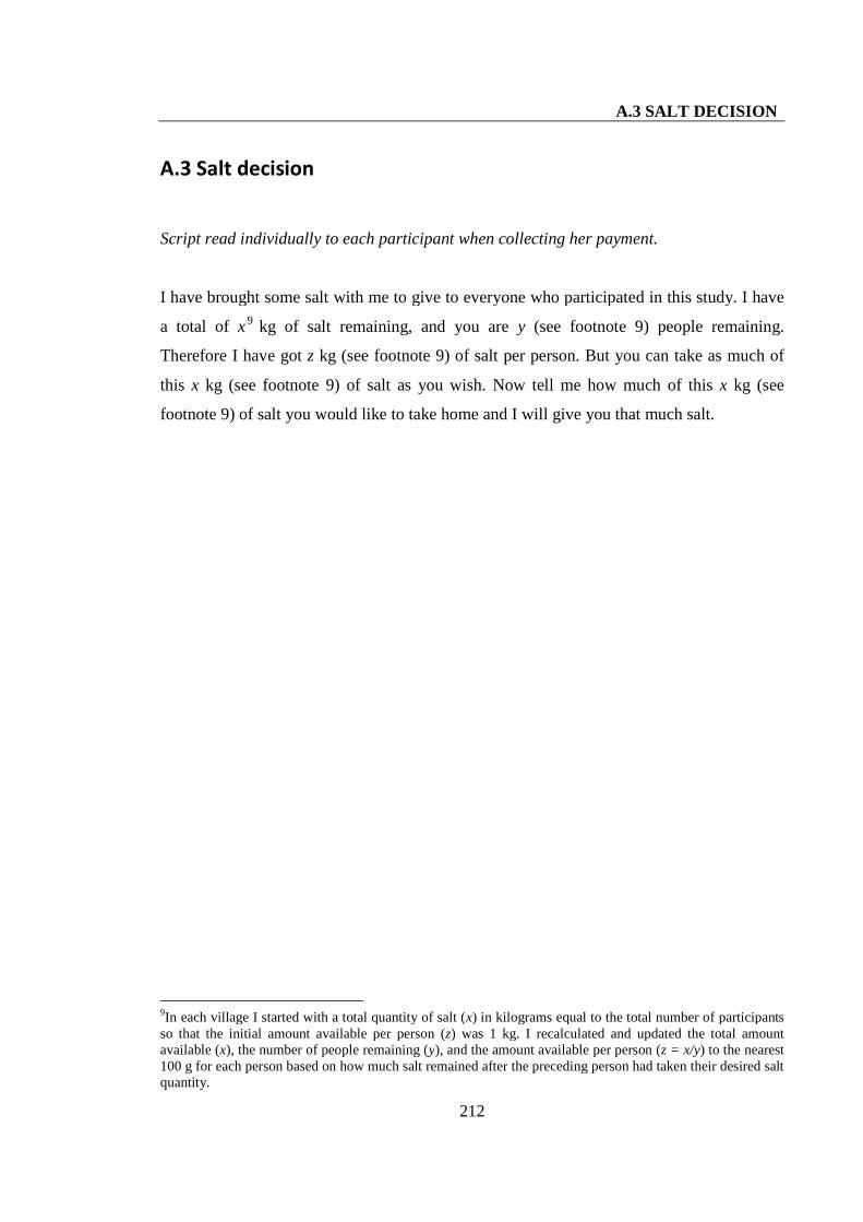
A.3 SALT DECISION
212
A.3 Salt decision
Script read individually to each participant when collecting her payment.
I have brought some salt with me to give to everyone who participated in this study. I have
a total of x 9 kg of salt remaining, and you are y (see footnote 9) people remaining.
Therefore I have got z kg (see footnote 9) of salt per person. But you can take as much of
this x kg (see footnote 9) of salt as you wish. Now tell me how much of this x kg (see
footnote 9) of salt you would like to take home and I will give you that much salt.
9In each village I started with a total quantity of salt (x) in kilograms equal to the total number of participantsso that the initial amount available per person (z) was 1 kg. I recalculated and updated the total amountavailable (x), the number of people remaining (y), and the amount available per person (z = x/y) to the nearest100 g for each person based on how much salt remained after the preceding person had taken their desired saltquantity.

A.4 PGG2
213
A.4 Public goods game round 2 (PGG2)
A.4.1 Script read collectively to all assembled PGG2 participants
Now we will play another game with you. This game is very similar to the first game you
have played today. The rules of this game are the same as the rules of the previous game10.
Again, you will be divided into groups of six players but this time, you will not be grouped
with the same people you played with the previous time. This time new groups will be
made in which you will be grouped with a new set of players. The six players in the each
new group will play the game with each other. This time too you will never know who the
other five players in your group are, either during or after the game. These other five
players will also never know who you are, either during or after the game. You will never
meet the other players in your group or be able to know their names either during or after
the game. Your token11 will be your only identification and even I will not be able to tell
anyone what decision you made in the game because I will not know your names.
This time too for this game you will all be divided into groups of six players and each
group will be given a group pot. Each individual in the group will receive an endowment of
20 rupees (meaning one kori12) in rupee 5 coins. These 20 rupees (one kori) are yours. Now,
you can deposit as much of these 20 rupees (one kori) as you wish to the group pot, in 5
rupee increments. This means that if you wish you can deposit nothing in the group pot, or
you can deposit 5, 10, 15 or 20 rupees (one kori) in your group pot. The money that you do
not deposit in the pot will be yours to keep and to take home. Once each of the 6 people in
your group have decided how much of their 20 rupees they want to deposit in the group pot,
then I will count the money deposited in your group pot, double the total amount of money
10All game rules and examples were demonstrated with real money and a money box. Participants made theirdecisions by physically manipulating real money.11Since both rounds of the PGG were played in each village after the ultimatum game had already beenplayed, participants were familiar with the use of tokens to anonymise identities as well as to randomly matchplayers in the games. This procedure had been demonstrated in great detail with real tokens and models pulledup from among the participants. Participants were also familiar with procedural details such as the fact thatthe games were all played individually at a private location and that the tokens would be exchanged forearnings in the game.121 kori = 20 units.
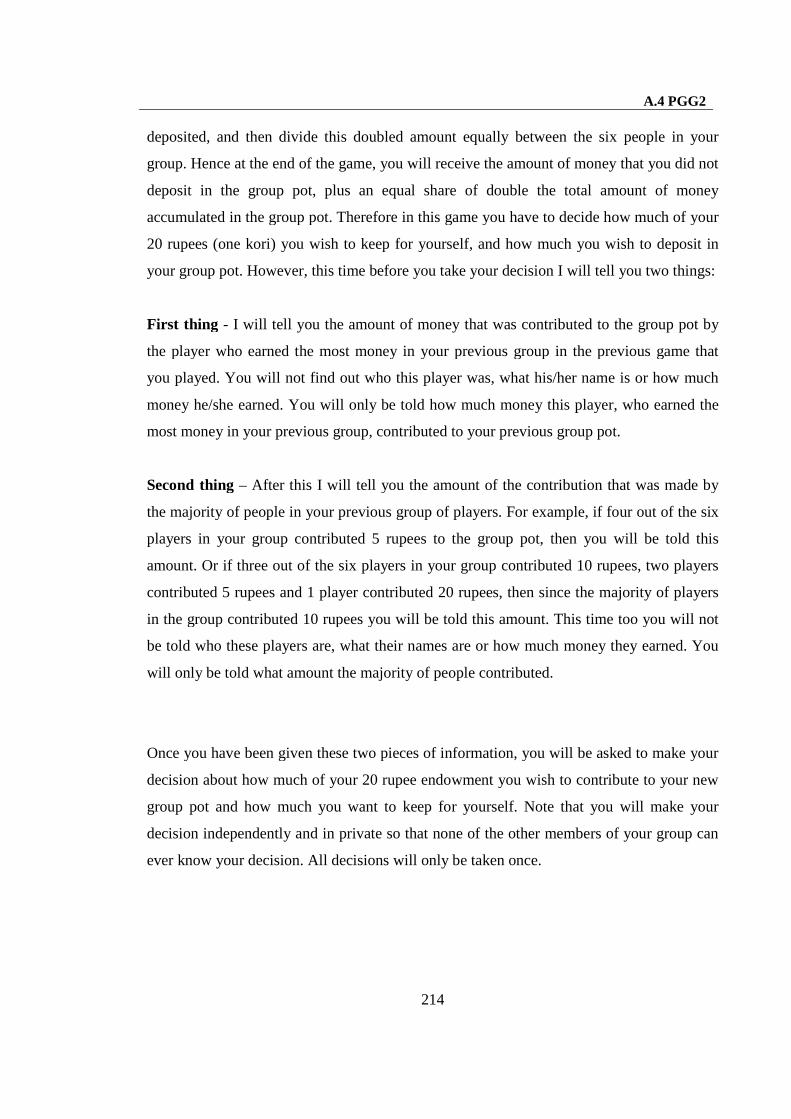
A.4 PGG2
214
deposited, and then divide this doubled amount equally between the six people in your
group. Hence at the end of the game, you will receive the amount of money that you did not
deposit in the group pot, plus an equal share of double the total amount of money
accumulated in the group pot. Therefore in this game you have to decide how much of your
20 rupees (one kori) you wish to keep for yourself, and how much you wish to deposit in
your group pot. However, this time before you take your decision I will tell you two things:
First thing - I will tell you the amount of money that was contributed to the group pot by
the player who earned the most money in your previous group in the previous game that
you played. You will not find out who this player was, what his/her name is or how much
money he/she earned. You will only be told how much money this player, who earned the
most money in your previous group, contributed to your previous group pot.
Second thing – After this I will tell you the amount of the contribution that was made by
the majority of people in your previous group of players. For example, if four out of the six
players in your group contributed 5 rupees to the group pot, then you will be told this
amount. Or if three out of the six players in your group contributed 10 rupees, two players
contributed 5 rupees and 1 player contributed 20 rupees, then since the majority of players
in the group contributed 10 rupees you will be told this amount. This time too you will not
be told who these players are, what their names are or how much money they earned. You
will only be told what amount the majority of people contributed.
Once you have been given these two pieces of information, you will be asked to make your
decision about how much of your 20 rupee endowment you wish to contribute to your new
group pot and how much you want to keep for yourself. Note that you will make your
decision independently and in private so that none of the other members of your group can
ever know your decision. All decisions will only be taken once.

A.4 PGG2
215
Remember,
1. All the decisions you will make in the game will be for real money. You will
receive real money at the end of the programme in accordance with the decisions
you have made and how much you have earned.
2. Please do not discuss the game between yourselves and also do not discuss it with
other people from the village who are yet to play the game. This is very important.
You cannot ask questions or talk about the game until this programme is over. You
will get a chance to ask questions when you are in the private room. Please be sure
that you obey this rule, because even one person disobeying can spoil the game for
everyone. If even one person starts talking about the game while sitting here, then
we will not be able to play the game in your village. Once you have played the
game, you will not be able to talk to or meet with all the remaining people
assembled here who have not yet played the game.
Note that you will only find out how much you have earned in the previous game and this
new game, after you have finished playing both games.
Now I will ask you some questions to check whether you have understood the rules of the
game or not.
14. What is the difference between this game and the game you played previously?
15. Are the rules of this game the same as the rules of the game you played previously?
16. What are the two things you will be told before you make your decision?
17. Will you play this game with the players from your old group or with the new
players in a new group?
18. Can you ever know who the other players in your group are?
19. Can the other players in your group ever know your identity?
20. Will I ask for your name while you are playing this game?

A.4 PGG2
216
21. Can I tell any other person in the village what decision you made in the game? Why
not?
Does anybody want to leave this programme?
Now we will begin. You will each pick a number out of this bowl to determine the order in
which you will play the game. You will come into the private room one by one. Y
(research assistant) will tell you when it is your turn to come into the room. Then I will ask
you some questions to check whether you have understood the rules of the game or not. If
you answer my questions correctly then you will play the game.
A.4.2 Script read individually to PGG2 participants
Have you understood the rules of the game?
Now I will ask you some questions to check whether you have understood the rules of the
game or not. If you answer the questions correctly then you will play the game.
1. Are the rules of this new game the same as the rules of the game you played
previously?
2. Will you play this game with the players from your old group or with the new players in
a new group?
3. Can you ever know who the other players in your new group are?
4. Can the other players in your new group ever know your identity?
Now I will tell you two things.
The first thing I will tell you is the amount of money that was contributed to the group pot
by the player who earned the most money in your previous group in the previous game that
you played.

A.4 PGG2
217
The second thing I will tell you is the amount of the contribution that was made by the
majority of people in your previous group of players.
So from your previous group in the previous game, the player who earned the most money
contributed …. rupees to the group pot13.
And, the majority of people from your previous group of players contributed … rupees to
the group pot14.
1. How much did the player who earned the most money contribute to the group pot?
2. How much did the majority of people contribute to the group pot?
Now you will play the game. Remember that you must take your decision independently
and there is no right or wrong answer in this game.
Here are your 20 rupees (one kori) in four Rs 5 coins. You must decide how much of these
20 rupees (one kori) you want to deposit in your group pot and how much of it you want to
keep for yourself. Please put the amount you want to deposit in the pot into the pot and
keep the rest on this side.
Thank you.
13The appropriate amount of money was placed in rupee 5 coins to the left of the money box.14The appropriate amount of money was placed in rupee 5 coins to the right of the money box.

218
APPENDIX B
DATA SHEETS
B.1 Individual data sheet
Tola:Village:Block:District:
Recorder:Date:
Game:
1. Token number:
2. Tribe: P. Korwa Other:
3. Age15:
4. Gender: Male Female
5. Education
Illiterate LiteratePrimary
1-5Middle
6-8High9-10
HigherSecondary
University
6. Occupation
Agriculture Gathering Daily wage Labour Other
15 Many individuals did not know their exact age. We estimated their age by using a combination of thefollowing criteria: (a) whether they were married (b) the number of children they had (c) whether they hadbeen born and experienced a major festival that occurred in the region in the 1950’s and if so whether theyhad been a child, adolescent or a married adult at the time (d) whether they had been born and experienced amajor drought that occurred in the region in the 1980’s and if so whether they had been a child, adolescent ora married adult at the time (e) physical appearance.
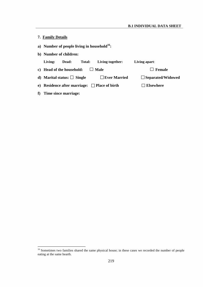
B.1 INDIVIDUAL DATA SHEET
219
7. Family Details
a) Number of people living in household16:
b) Number of children:
Living: Dead: Total: Living together: Living apart:
c) Head of the household: Male Female
d) Marital status: Single Ever Married Separated/Widowed
e) Residence after marriage: Place of birth Elsewhere
f) Time since marriage:
16 Sometimes two families shared the same physical house; in these cases we recorded the number of peopleeating at the same hearth.

B.1 INDIVIDUAL DATA SHEET
220
g) Relatives
RelativeTotalnumber
Numberparticipatedin the game
Number living in thisvillage
Number living inother villages
Sons
Daughters
Grandchildren
Mother
Father
Under 15 years Under 15 yearsFull brothers born of mother
Over 15 years Over 15 yearsChildren of full brothers bornof motherWives of full brothers born ofmother
Under 15 years Under 15 yearsFull sisters born of mother
Over 15 years Over 15 yearsChildren of full sisters born ofmotherHusbands of full sisters born ofmother
Under 15 years Under 15 yearsHalf brothers born of mother
Over 15 years Over 15 yearsChildren of half brothers bornof motherWives of half brothers born ofmother
Under 15 years Under 15 yearsHalf sisters born of mother
Over 15 years Over 15 yearsChildren of half sisters born ofmotherHusbands of half sisters born ofmother
Under 15 years Under 15 yearsHalf brothers born of father
Over 15 years Over 15 yearsChildren of half brothers bornof fatherWives of half brothers born offather
Under 15 years Under 15 yearsHalf sisters born of father
Over 15 years Over 15 years

B.1 INDIVIDUAL DATA SHEET
221
RelativeTotalnumber
Numberparticipatedin the game
Number living in thisvillage
Number living inother villages
Children of half sisters born offatherHusbands of half sisters born offather
Mothers’ siblings
Mothers’ siblings children
Fathers’ siblings
Fathers’ siblings’ children
8. Migration status
a) Place of birth
b) Time lived in this village
c) Number of times village changed since birth17
9. Income
a) How many major wage earners are there in your family?
b) How many months in the year do you eat self grown rice?
c) How much outstanding loan money have you taken in all from any source18?
d) How much do you earn for one day’s labour?10. Markets
a) How many times a month do you visit the weekly tribal market?
b) How many times a month do you visit your nearest city to buy or sell something?
11. Network data
How many people did you invite to your home last Cherta:
a) From this village:
b) From other villages:
17 If the individual was currently residing in the natal village this was recorded as 0.18 This is a record of the total amount of outstanding loans an individual had at the time of the survey.
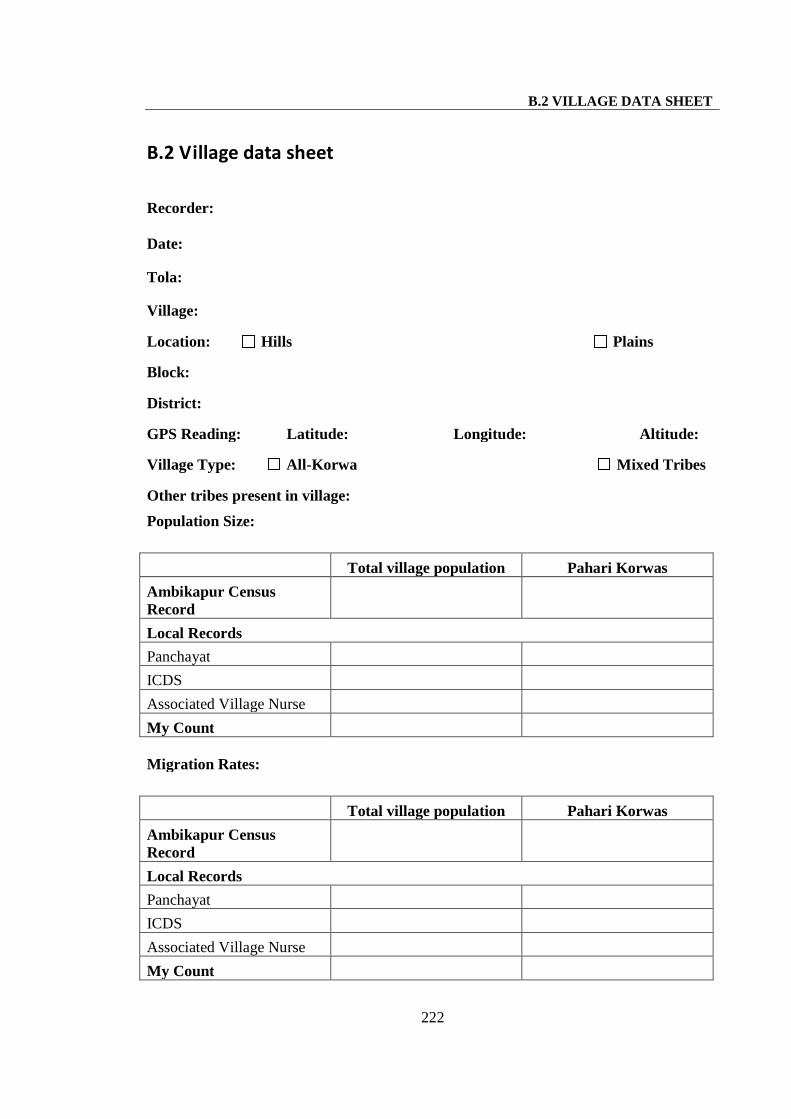
B.2 VILLAGE DATA SHEET
222
B.2 Village data sheet
Recorder:
Date:
Tola:
Village:
Location: Hills Plains
Block:
District:
GPS Reading: Latitude: Longitude: Altitude:
Village Type: All-Korwa Mixed Tribes
Other tribes present in village:
Population Size:
Total village population Pahari Korwas
Ambikapur CensusRecord
Local Records
Panchayat
ICDS
Associated Village Nurse
My Count
Migration Rates:
Total village population Pahari Korwas
Ambikapur CensusRecord
Local Records
Panchayat
ICDS
Associated Village Nurse
My Count

B.2 VILLAGE DATA SHEET
223
Amenities:
Type Present in village
Y/N
Closest place ofaccess
GPS Reading
School
Hospital/health carecentre
Post office
Railway Station
Inter-state busservice
Inter-village/districtbus service
Village PanchayatOffice
Presence of NGO’sworking with them
Resource Distribution: Water bodies, markets (tribal & city), grazing grounds
SNo. Resource Type
Identificationname GPS reading Additional notes

B.2 VILLAGE DATA SHEET
224
Information from local land ownership records:
a) Total registered land in the village (‘Patte valee’):
Additional Comments on village:

B.3 HOUSING DATA SHEET
225
B.3 Housing data sheet
Recorder:
Date:
Tola:
Village:
Block:
District:
House Latitude Longitude AltitudeMalehead
Femalehead
Saltused
Number ofresidents
B.4 QUALITATIVE DATA SHEET
226
B.4 Qualitative data sheet
Village
1. How old is this village? How long has it been here?
2. Have you always practiced agriculture here or has there been any other main source
of income and living in the last two generations?
3. In what generation according to your memory, did you primarily hunt and gather and
practice Jhoom?
4. How much movement is there between villages? What villages do people most visit
in the neighboring areas in their lifetimes?
5. How often do you normally change your place of residence? Why?
6. Do you use the grazing land? How much do people use the grazing land? How do you
decide when and how it should be used? How do you make sure that it isn’t over-
grazed?
7. What are the daily wages in the area?
8. How many people in the village engage in daily wage labour?
9. What do people identify themselves with? The ‘tola’ or the village?
General ethnographic survey
Kinship:
10. Who do people marry? Those within the village or those in other villages?
11. Do people marry other members of the family?
12. Do people look after their parents when they are old and provide them a roof and
food?
13. Up to what age do people look after their children?

B.4 QUALITATIVE DATA SHEET
227
14. Do sisters and brothers help each other to do things (e.g. tend fields, fish, hunt, gather,
build houses etc)?
15. What about aunts and uncles and their children?
16. Do the above relatives help each other when:
a. They don’t have food
b. Need care when they are ill
c. Need help in the field
d. Hunting or fishing
e. Collecting water
f. Building houses
g. Anything else?
17. Who lives in a household? What relatives? Your mother, father, children, siblings,
grand parents etc?
18. Do grandmothers look after their grandchildren? From the mothers’ side, from the
fathers’ side?
19. What is the in laws’ role:
a. From the girls side?
b. From the boys side?
Subsistence:
20. What is the main source of subsistence?
a. Self grown food
b. Bought food
c. Wages used to buy food
d. Gathered food (fruit, vegetables, roots, honey etc?)
e. Hunted food (fishing, other meat)?

B.4 QUALITATIVE DATA SHEET
228
21. Are there any subsistence related activities that are communal in nature?
a. Farming related
b. Fishing
c. Gathering
d. Hunting
e. Tending to animals
f. Honey gathering
g. Other?
Communal Activities:
22. What types of activities do people do together?
229
APPENDIX C
STATISTICAL ANALYSES
This appendix presents the univariate and domain-wise models, and a step-wise summary
of the full model fitting process implemented in the fourth stage, for all analyses presented
in this thesis. Section C.1 presents analyses for UG proposer offers (Chapter 3, Section
3.2.1) and Section C.2 presents analyses for UG responder MAOs (Chapter 3, Section
3.2.2). Section C.3 presents analyses for PGG1 contributions and salt deviations (Chapter 4,
Section 4.2). Section C.4 presents analyses for PGG2 contributions (Chapter 5, Section
5.2.1). Section C.5 presents analyses for learning strategies in the PGG2 (Chapter 5,
Sections 5.2.3 and 5.2.4). For a description of a variable in any of the following tables see
Chapter 2, Section 2.4.2, Table 2.5).
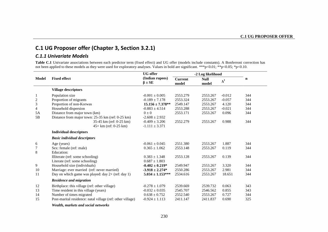
C.1 UG PROPOSER OFFER
230
C.1 UG Proposer offer (Chapter 3, Section 3.2.1)
C.1.1 Univariate ModelsTable C.1 Univariate associations between each predictor term (fixed effect) and UG offer (models include constants). A Bonferroni correction hasnot been applied to these models as they were used for exploratory analyses. Values in bold are significant. ***p<0.01; **p<0.05; *p<0.10.
-2 Log likelihoodModel Fixed effect
UG offer(Indian rupees)β ± SE
Currentmodel
Nullmodel
Δ1 n
Village descriptors
1 Population size -0.001 ± 0.005 2553.279 2553.267 -0.012 3442 Proportion of migrants -0.189 ± 7.178 2553.324 2553.267 -0.057 3443 Proportion of non-Korwas 15.156 ± 7.378** 2549.147 2553.267 4.120 3444 Household dispersion -0.883 ± 4.514 2553.288 2553.267 -0.021 3445A Distance from major town (km) 0 ± 0 2553.171 2553.267 0.096 3445B Distance from major town: 25-35 km (ref: 0-25 km)
35-45 km (ref: 0-25 km)45+ km (ref: 0-25 km)
-2.608 ± 2.932-0.409 ± 3.206-1.111 ± 3.371
2552.279 2553.267 0.988 344
Individual descriptors
Basic individual descriptors
6 Age (years) -0.061 ± 0.045 2551.380 2553.267 1.887 3447 Sex: female (ref: male) 0.365 ± 1.062 2553.148 2553.267 0.119 3448 Education:
Illiterate (ref: some schooling)Literate (ref: some schooling)
0.383 ± 1.3480.687 ± 1.803
2553.128 2553.267 0.139 344
9 Household size (individuals) -0.402 ± 0.219* 2549.947 2553.267 3.320 34410 Marriage: ever married (ref: never married) -3.918 ± 2.274* 2550.286 2553.267 2.981 34411 Day on which game was played: day 2+ (ref: day 1) 5.034 ± 1.153*** 2534.616 2553.267 18.651 344
Residence and migration
12 Birthplace: this village (ref: other village) -0.278 ± 1.079 2539.669 2539.732 0.063 34313 Time resident in this village (years) -0.032 ± 0.035 2545.707 2546.562 0.855 34314 Number of times migrated 0.638 ± 0.752 2552.540 2553.267 0.727 34415 Post-marital residence: natal village (ref: other village) -0.924 ± 1.113 2411.147 2411.837 0.690 325
Wealth, markets and social networks
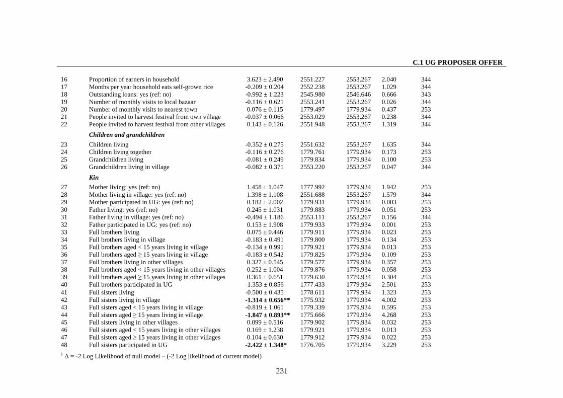
C.1 UG PROPOSER OFFER
231
16 Proportion of earners in household 3.623 ± 2.490 2551.227 2553.267 2.040 34417 Months per year household eats self-grown rice -0.209 ± 0.204 2552.238 2553.267 1.029 34418 Outstanding loans: yes (ref: no) -0.992 ± 1.223 2545.980 2546.646 0.666 34319 Number of monthly visits to local bazaar -0.116 ± 0.621 2553.241 2553.267 0.026 34420 Number of monthly visits to nearest town 0.076 ± 0.115 1779.497 1779.934 0.437 25321 People invited to harvest festival from own village -0.037 ± 0.066 2553.029 2553.267 0.238 34422 People invited to harvest festival from other villages 0.143 ± 0.126 2551.948 2553.267 1.319 344
Children and grandchildren
23 Children living -0.352 ± 0.275 2551.632 2553.267 1.635 34424 Children living together -0.116 ± 0.276 1779.761 1779.934 0.173 25325 Grandchildren living -0.081 ± 0.249 1779.834 1779.934 0.100 25326 Grandchildren living in village -0.082 ± 0.371 2553.220 2553.267 0.047 344
Kin
27 Mother living: yes (ref: no) 1.458 ± 1.047 1777.992 1779.934 1.942 25328 Mother living in village: yes (ref: no) 1.398 ± 1.108 2551.688 2553.267 1.579 34429 Mother participated in UG: yes (ref: no) 0.182 ± 2.002 1779.931 1779.934 0.003 25330 Father living: yes (ref: no) 0.245 ± 1.031 1779.883 1779.934 0.051 25331 Father living in village: yes (ref: no) -0.494 ± 1.186 2553.111 2553.267 0.156 34432 Father participated in UG: yes (ref: no) 0.153 ± 1.908 1779.933 1779.934 0.001 25333 Full brothers living 0.075 ± 0.446 1779.911 1779.934 0.023 25334 Full brothers living in village -0.183 ± 0.491 1779.800 1779.934 0.134 25335 Full brothers aged < 15 years living in village -0.134 ± 0.991 1779.921 1779.934 0.013 25336 Full brothers aged ≥ 15 years living in village -0.183 ± 0.542 1779.825 1779.934 0.109 25337 Full brothers living in other villages 0.327 ± 0.545 1779.577 1779.934 0.357 25338 Full brothers aged < 15 years living in other villages 0.252 ± 1.004 1779.876 1779.934 0.058 25339 Full brothers aged ≥ 15 years living in other villages 0.361 ± 0.651 1779.630 1779.934 0.304 25340 Full brothers participated in UG -1.353 ± 0.856 1777.433 1779.934 2.501 25341 Full sisters living -0.500 ± 0.435 1778.611 1779.934 1.323 25342 Full sisters living in village -1.314 ± 0.656** 1775.932 1779.934 4.002 25343 Full sisters aged < 15 years living in village -0.819 ± 1.061 1779.339 1779.934 0.595 25344 Full sisters aged ≥ 15 years living in village -1.847 ± 0.893** 1775.666 1779.934 4.268 25345 Full sisters living in other villages 0.099 ± 0.516 1779.902 1779.934 0.032 25346 Full sisters aged < 15 years living in other villages 0.169 ± 1.238 1779.921 1779.934 0.013 25347 Full sisters aged ≥ 15 years living in other villages 0.104 ± 0.630 1779.912 1779.934 0.022 25348 Full sisters participated in UG -2.422 ± 1.348* 1776.705 1779.934 3.229 253
1 Δ = -2 Log Likelihood of null model – (-2 Log likelihood of current model)
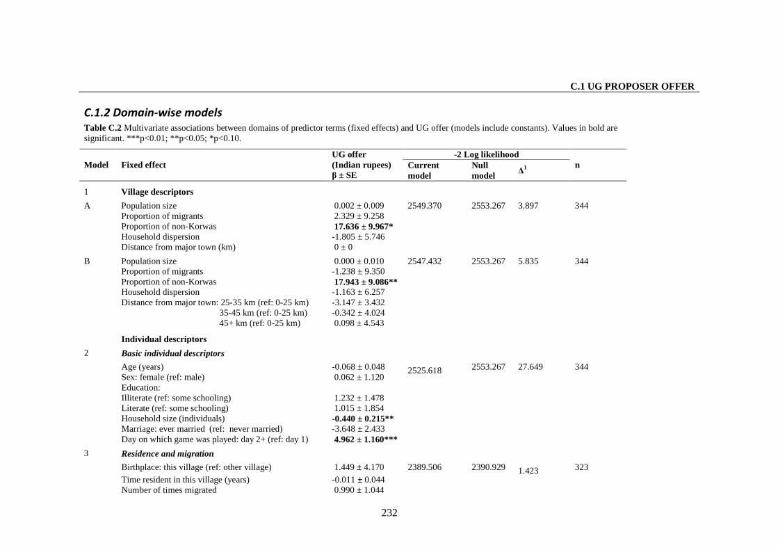
C.1 UG PROPOSER OFFER
232
C.1.2 Domain-wise modelsTable C.2 Multivariate associations between domains of predictor terms (fixed effects) and UG offer (models include constants). Values in bold aresignificant. ***p<0.01; **p<0.05; *p<0.10.
-2 Log likelihoodModel Fixed effect
UG offer(Indian rupees)β ± SE
Currentmodel
Nullmodel
Δ1 n
1 Village descriptors
Population size 0.002 ± 0.009Proportion of migrants 2.329 ± 9.258Proportion of non-Korwas 17.636 ± 9.967*Household dispersion -1.805 ± 5.746
A
Distance from major town (km) 0 ± 0
2549.370 2553.267 3.897 344
Population size 0.000 ± 0.010Proportion of migrants -1.238 ± 9.350Proportion of non-Korwas 17.943 ± 9.086**Household dispersion -1.163 ± 6.257
B
Distance from major town: 25-35 km (ref: 0-25 km)35-45 km (ref: 0-25 km)45+ km (ref: 0-25 km)
-3.147 ± 3.432-0.342 ± 4.0240.098 ± 4.543
2547.432 2553.267 5.835 344
Individual descriptors
Basic individual descriptors
Age (years) -0.068 ± 0.048Sex: female (ref: male) 0.062 ± 1.120Education:Illiterate (ref: some schooling)Literate (ref: some schooling)
1.232 ± 1.4781.015 ± 1.854
Household size (individuals) -0.440 ± 0.215**Marriage: ever married (ref: never married) -3.648 ± 2.433
2
Day on which game was played: day 2+ (ref: day 1) 4.962 ± 1.160***
2525.618 2553.267 27.649 344
Residence and migration
Birthplace: this village (ref: other village) 1.449 ± 4.170
Time resident in this village (years) -0.011 ± 0.044
3
Number of times migrated 0.990 ± 1.044
2389.506 2390.929 1.423 323
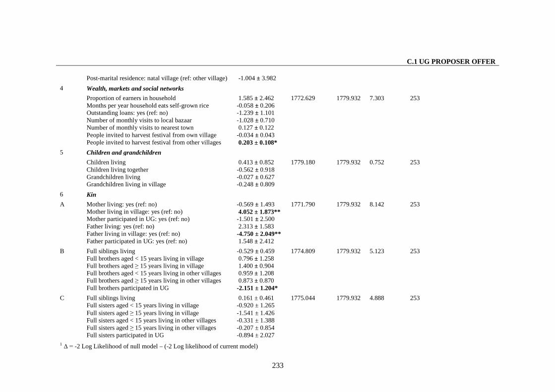
C.1 UG PROPOSER OFFER
233
Post-marital residence: natal village (ref: other village) -1.004 ± 3.982
4 Wealth, markets and social networks
Proportion of earners in household 1.585 ± 2.462Months per year household eats self-grown rice -0.058 ± 0.206Outstanding loans: yes (ref: no) -1.239 ± 1.101Number of monthly visits to local bazaar -1.028 ± 0.710Number of monthly visits to nearest town 0.127 ± 0.122People invited to harvest festival from own village -0.034 ± 0.043People invited to harvest festival from other villages 0.203 ± 0.108*
1772.629 1779.932 7.303 253
Children and grandchildren
Children living 0.413 ± 0.852Children living together -0.562 ± 0.918Grandchildren living -0.027 ± 0.627
5
Grandchildren living in village -0.248 ± 0.809
1779.180 1779.932 0.752 253
6 Kin
Mother living: yes (ref: no) -0.569 ± 1.493Mother living in village: yes (ref: no) 4.052 ± 1.873**Mother participated in UG: yes (ref: no) -1.501 ± 2.500Father living: yes (ref: no) 2.313 ± 1.583Father living in village: yes (ref: no) -4.750 ± 2.049**
A
Father participated in UG: yes (ref: no) 1.548 ± 2.412
1771.790 1779.932 8.142 253
Full siblings living -0.529 ± 0.459Full brothers aged < 15 years living in village 0.796 ± 1.258Full brothers aged ≥ 15 years living in village 1.400 ± 0.904Full brothers aged < 15 years living in other villages 0.959 ± 1.208Full brothers aged ≥ 15 years living in other villages 0.873 ± 0.870
B
Full brothers participated in UG -2.151 ± 1.204*
1774.809 1779.932 5.123 253
Full siblings living 0.161 ± 0.461Full sisters aged < 15 years living in village -0.920 ± 1.265Full sisters aged ≥ 15 years living in village -1.541 ± 1.426Full sisters aged < 15 years living in other villages -0.331 ± 1.388Full sisters aged ≥ 15 years living in other villages -0.207 ± 0.854
C
Full sisters participated in UG -0.894 ± 2.027
1775.044 1779.932 4.888 253
1 Δ = -2 Log Likelihood of null model – (-2 Log likelihood of current model)
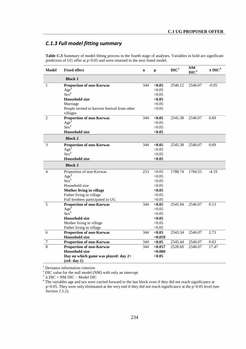
C.1 UG PROPOSER OFFER
234
C.1.3 Full model fitting summary
Table C.3 Summary of model-fitting process in the fourth stage of analyses. Variables in bold are significantpredictors of UG offer at p<0.05 and were retained in the next listed model.
Model Fixed effect n p DIC1 NMDIC2 Δ DIC3
Block 1
1 Proportion of non-KorwasAge4
Sex4
Household sizeMarriagePeople invited to harvest festival from othervillages
344 <0.05>0.05>0.05<0.05>0.05>0.05
2546.12 2546.07 -0.05
2 Proportion of non-KorwasAge4
Sex4
Household size
344 <0.05>0.05>0.05<0.05
2545.38 2546.07 0.69
Block 2
3 Proportion of non-KorwasAge4
Sex4
Household size
344 <0.05>0.05>0.05<0.05
2545.38 2546.07 0.69
Block 3
4 Proportion of non-KorwasAge4
Sex4
Household sizeMother living in villageFather living in villageFull brothers participated in UG
253 >0.05>0.05>0.05>0.05<0.05>0.05>0.05
1788.74 1784.55 -4.19
5 Proportion of non-KorwasAge4
Sex4
Household sizeMother living in villageFather living in village
344 <0.05>0.05>0.05<0.05>0.05>0.05
2545.94 2546.07 0.13
6 Proportion of non-KorwasHousehold size
344 <0.05=0.059
2543.34 2546.07 2.73
7 Proportion of non-Korwas 344 <0.05 2545.44 2546.07 0.638 Proportion of non-Korwas
Household sizeDay on which game was played: day 2+(ref: day 1)
344 =0.057=0.060<0.05
2528.60 2546.07 17.47
1 Deviance information criterion2 DIC value for the null model (NM) with only an intercept3 Δ DIC = NM DIC – Model DIC4 The variables age and sex were carried forward to the last block even if they did not reach significance at
p<0.05. They were only eliminated at the very end if they did not reach significance at the p<0.05 level (seeSection 2.5.2).
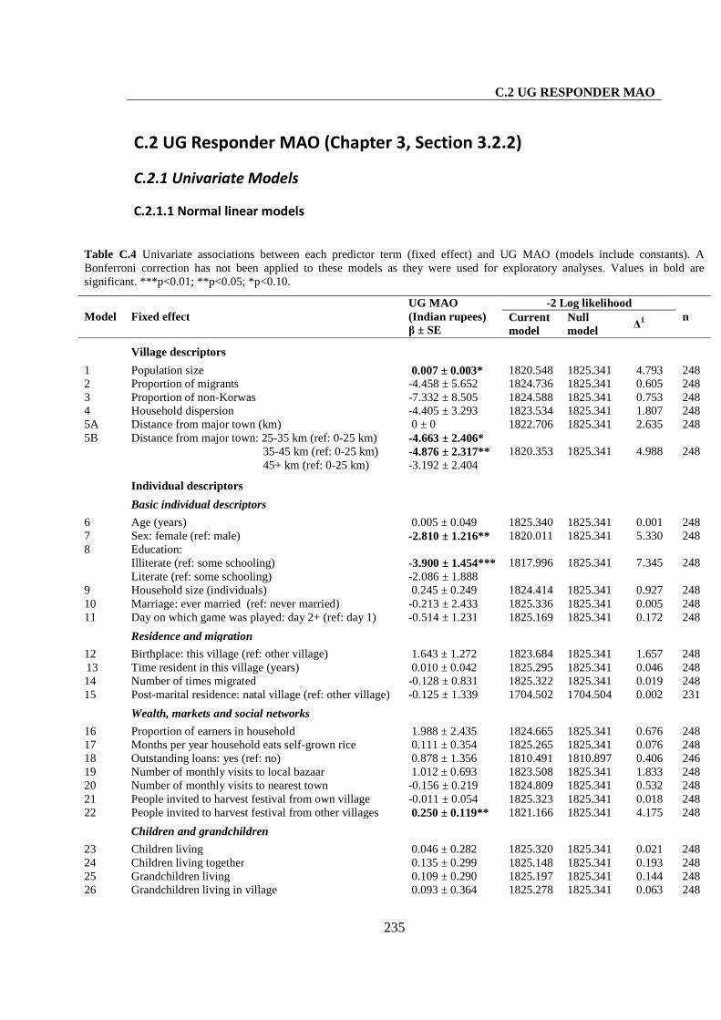
C.2 UG RESPONDER MAO
235
C.2 UG Responder MAO (Chapter 3, Section 3.2.2)
C.2.1 Univariate Models
C.2.1.1 Normal linear models
Table C.4 Univariate associations between each predictor term (fixed effect) and UG MAO (models include constants). ABonferroni correction has not been applied to these models as they were used for exploratory analyses. Values in bold aresignificant. ***p<0.01; **p<0.05; *p<0.10.
-2 Log likelihoodModel Fixed effect
UG MAO(Indian rupees)β ± SE
Currentmodel
Nullmodel
Δ1 n
Village descriptors
1 Population size 0.007 ± 0.003* 1820.548 1825.341 4.793 2482 Proportion of migrants -4.458 ± 5.652 1824.736 1825.341 0.605 2483 Proportion of non-Korwas -7.332 ± 8.505 1824.588 1825.341 0.753 2484 Household dispersion -4.405 ± 3.293 1823.534 1825.341 1.807 2485A Distance from major town (km) 0 ± 0 1822.706 1825.341 2.635 2485B Distance from major town: 25-35 km (ref: 0-25 km)
35-45 km (ref: 0-25 km)45+ km (ref: 0-25 km)
-4.663 ± 2.406*-4.876 ± 2.317**-3.192 ± 2.404
1820.353 1825.341 4.988 248
Individual descriptors
Basic individual descriptors
6 Age (years) 0.005 ± 0.049 1825.340 1825.341 0.001 2487 Sex: female (ref: male) -2.810 ± 1.216** 1820.011 1825.341 5.330 2488 Education:
Illiterate (ref: some schooling)Literate (ref: some schooling)
-3.900 ± 1.454***-2.086 ± 1.888
1817.996 1825.341 7.345 248
9 Household size (individuals) 0.245 ± 0.249 1824.414 1825.341 0.927 24810 Marriage: ever married (ref: never married) -0.213 ± 2.433 1825.336 1825.341 0.005 24811 Day on which game was played: day 2+ (ref: day 1) -0.514 ± 1.231 1825.169 1825.341 0.172 248
Residence and migration
12 Birthplace: this village (ref: other village) 1.643 ± 1.272 1823.684 1825.341 1.657 24813 Time resident in this village (years) 0.010 ± 0.042 1825.295 1825.341 0.046 24814 Number of times migrated -0.128 ± 0.831 1825.322 1825.341 0.019 24815 Post-marital residence: natal village (ref: other village) -0.125 ± 1.339 1704.502 1704.504 0.002 231
Wealth, markets and social networks
16 Proportion of earners in household 1.988 ± 2.435 1824.665 1825.341 0.676 24817 Months per year household eats self-grown rice 0.111 ± 0.354 1825.265 1825.341 0.076 24818 Outstanding loans: yes (ref: no) 0.878 ± 1.356 1810.491 1810.897 0.406 24619 Number of monthly visits to local bazaar 1.012 ± 0.693 1823.508 1825.341 1.833 24820 Number of monthly visits to nearest town -0.156 ± 0.219 1824.809 1825.341 0.532 24821 People invited to harvest festival from own village -0.011 ± 0.054 1825.323 1825.341 0.018 24822 People invited to harvest festival from other villages 0.250 ± 0.119** 1821.166 1825.341 4.175 248
Children and grandchildren
23 Children living 0.046 ± 0.282 1825.320 1825.341 0.021 24824 Children living together 0.135 ± 0.299 1825.148 1825.341 0.193 24825 Grandchildren living 0.109 ± 0.290 1825.197 1825.341 0.144 24826 Grandchildren living in village 0.093 ± 0.364 1825.278 1825.341 0.063 248
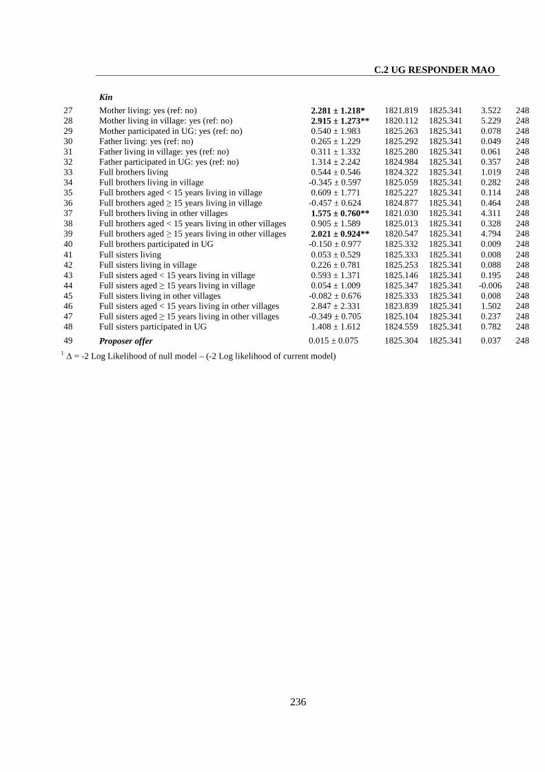
C.2 UG RESPONDER MAO
236
Kin
27 Mother living: yes (ref: no) 2.281 ± 1.218* 1821.819 1825.341 3.522 24828 Mother living in village: yes (ref: no) 2.915 ± 1.273** 1820.112 1825.341 5.229 24829 Mother participated in UG: yes (ref: no) 0.540 ± 1.983 1825.263 1825.341 0.078 24830 Father living: yes (ref: no) 0.265 ± 1.229 1825.292 1825.341 0.049 24831 Father living in village: yes (ref: no) 0.311 ± 1.332 1825.280 1825.341 0.061 24832 Father participated in UG: yes (ref: no) 1.314 ± 2.242 1824.984 1825.341 0.357 24833 Full brothers living 0.544 ± 0.546 1824.322 1825.341 1.019 24834 Full brothers living in village -0.345 ± 0.597 1825.059 1825.341 0.282 24835 Full brothers aged < 15 years living in village 0.609 ± 1.771 1825.227 1825.341 0.114 24836 Full brothers aged ≥ 15 years living in village -0.457 ± 0.624 1824.877 1825.341 0.464 24837 Full brothers living in other villages 1.575 ± 0.760** 1821.030 1825.341 4.311 24838 Full brothers aged < 15 years living in other villages 0.905 ± 1.589 1825.013 1825.341 0.328 24839 Full brothers aged ≥ 15 years living in other villages 2.021 ± 0.924** 1820.547 1825.341 4.794 24840 Full brothers participated in UG -0.150 ± 0.977 1825.332 1825.341 0.009 24841 Full sisters living 0.053 ± 0.529 1825.333 1825.341 0.008 24842 Full sisters living in village 0.226 ± 0.781 1825.253 1825.341 0.088 24843 Full sisters aged < 15 years living in village 0.593 ± 1.371 1825.146 1825.341 0.195 24844 Full sisters aged ≥ 15 years living in village 0.054 ± 1.009 1825.347 1825.341 -0.006 24845 Full sisters living in other villages -0.082 ± 0.676 1825.333 1825.341 0.008 24846 Full sisters aged < 15 years living in other villages 2.847 ± 2.331 1823.839 1825.341 1.502 24847 Full sisters aged ≥ 15 years living in other villages -0.349 ± 0.705 1825.104 1825.341 0.237 24848 Full sisters participated in UG 1.408 ± 1.612 1824.559 1825.341 0.782 248
49 Proposer offer 0.015 ± 0.075 1825.304 1825.341 0.037 248
1 Δ = -2 Log Likelihood of null model – (-2 Log likelihood of current model)

C.2 UG RESPONDER MAO
237
C.2.1.2 Ordinal multinomial models
Table C.5 Univariate associations between each predictor term (fixed effect) and logit (probability of UG MAO Indian Rupees 10+ or below) (models includeconstants). A Bonferroni correction has not been applied to these models as they were used for exploratory analyses. Values in bold are significant. ***p<0.01;**p<0.05; *p<0.10.
-2 Log likelihood
Model Fixed effect
Logit (probability of UGMAO Indian Rupees 10+or below)β ± SE
Current model Null model Δ1 n
Village descriptors
1 Population size -0.001 ± 0.001** 536.391 548.483 12.092 2482 Proportion of migrants 0.085 ± 1.066 548.320 548.483 0.163 2483 Proportion of non-Korwas 1.228 ± 1.579 544.717 548.483 3.766 2484 Household dispersion 0.843 ± 0.615 539.327 548.483 9.156 2485A Distance from major town (km) 0 ± 0 543.568 548.483 4.915 2485B Distance from major town: 25-35 km (ref: 0-25 km)
35-45 km (ref: 0-25 km)45+ km (ref: 0-25 km)
0.984 ± 0.450**0.753 ± 0.430*0.547 ± 0.444
534.864 548.483 13.619 248
Individual descriptors
Basic individual descriptors
6 Age (years) 0.013 ± 0.010 547.619 548.483 0.864 2487 Sex: female (ref: male) 0.688 ± 0.248*** 529.969 548.483 18.514 2488 Education:
Illiterate (ref: some schooling)Literate (ref: some schooling)
1.170 ± 0.297***0.341 ± 0.374
514.761 548.483 33.722 248
9 Household size (individuals) -0.103 ± 0.050** 543.523 548.483 4.960 24810 Marriage: ever married (ref: never married) 0.444 ± 0.473 547.800 548.483 0.683 24811 Day on which game was played: day 2+ (ref: day 1) 0.147 ± 0.243 548.390 548.483 0.093 248
Residence and migration
12 Birthplace: this village (ref: other village) -0.242 ± 0.252 546.228 548.483 2.255 24813 Time resident in this village (years) 0.009 ± 0.008 547.637 548.483 0.846 24814 Number of times migrated -0.072 ± 0.163 548.214 548.483 0.269 24815 Post-marital residence: natal village (ref: other village) -0.087 ± 0.261 509.702 509.643 -0.059 231
Wealth, markets and social networks

C.2 UG RESPONDER MAO
238
16 Proportion of earners in household -0.091 ± 0.479 548.168 548.483 0.315 24817 Months per year household eats self-grown rice -0.060 ± 0.069 547.978 548.483 0.505 24818 Outstanding loans: yes (ref: no) -0.452 ± 0.264* 535.036 540.463 5.427 24619 Number of monthly visits to local bazaar -0.203 ± 0.137 544.196 548.483 4.287 24820 Number of monthly visits to nearest town 0.098 ± 0.044** 541.811 548.483 6.672 24821 People invited to harvest festival from own village -0.004 ± 0.010 549.287 548.483 -0.804 24822 People invited to harvest festival from other villages -0.042 ± 0.024* 543.02 548.483 5.463 248
Children and grandchildren
23 Children living -0.011 ± 0.055 548.509 548.483 -0.026 24824 Children living together -0.025 ± 0.059 548.547 548.483 -0.064 24825 Grandchildren living -0.009 ± 0.057 548.289 548.483 0.194 24826 Grandchildren living in village 0.016 ± 0.072 548.73 548.483 -0.247 248
Kin
27 Mother living: yes (ref: no) -0.491 ± 0.245** 527.873 532.095 4.222 24828 Mother living in village: yes (ref: no) -0.684 ± 0.256*** 523.11 532.095 8.985 24829 Mother participated in UG: yes (ref: no) -0.435 ± 0.389 530.996 532.095 1.099 24830 Father living: yes (ref: no) -0.222 ± 0.243 530.438 532.095 1.657 24831 Father living in village: yes (ref: no) -0.399 ± 0.263 529.439 532.095 2.656 24832 Father participated in UG: yes (ref: no) -0.721 ± 0.440 528.507 532.095 3.588 24833 Full brothers living -0.266 ± 0.347 530.864 532.095 1.231 24834 Full brothers living in village 0.015 ± 0.118 531.901 532.095 0.194 24835 Full brothers aged < 15 years living in village -0.266 ± 0.347 530.864 532.095 1.231 24836 Full brothers aged ≥ 15 years living in village 0.054 ± 0.124 531.426 532.095 0.669 24837 Full brothers living in other villages -0.159 ± 0.150 529.944 532.095 2.151 24838 Full brothers aged < 15 years living in other villages -0.164 ± 0.311 531.164 532.095 0.931 24839 Full brothers aged ≥ 15 years living in other villages -0.178 ± 0.183 530.751 532.095 1.344 24840 Full brothers participated in UG -0.116 ± 0.192 531.253 532.095 0.842 24841 Full sisters living 0.011 ± 0.105 532.023 532.095 0.072 24842 Full sisters living in village 0.095 ± 0.156 531.397 532.095 0.698 24843 Full sisters aged < 15 years living in village -0.099 ± 0.269 531.902 532.095 0.193 24844 Full sisters aged ≥ 15 years living in village 0.206 ± 0.203 529.398 532.095 2.697 24845 Full sisters living in other villages -0.051 ± 0.133 531.624 532.095 0.471 24846 Full sisters aged < 15 years living in other villages -0.336 ± 0.457 530.584 532.095 1.511 24847 Full sisters aged ≥ 15 years living in other villages -0.032 ± 0.139 532.013 532.095 0.082 24848 Full sisters participated in UG -0.114 ± 0.317 531.954 532.095 0.141 248
1 Δ = -2 Log Likelihood of null model – (-2 Log likelihood of current model)

C.2 UG RESPONDER MAO
239
C.2.2 Domain-wise models
C.2.2.1 Normal linear models
Table C.6 Multivariate associations between domains of predictor terms (fixed effects) and UG MAO (models include constants). Values in bold are significant.***p<0.01; **p<0.05; *p<0.10.
-2 Log likelihoodModel Fixed effect
UG MAO (Indian rupees)β ± SE Current model Null model Δ1 n
1 Village descriptors
Population size 0.001 ± 0.007Proportion of migrants -0.493 ± 7.105Proportion of non-Korwas -5.713 ± 10.222Household dispersion -2.954 ± 5.594
A
Distance from major town (km) 0 ± 0
1819.636 1825.341 5.705 248
Population size -0.001 ± 0.010Proportion of migrants 0.898 ± 7.617Proportion of non-Korwas 7.522 ± 13.456Household dispersion -6.366 ± 8.358
B
Distance from major town: 25-35 km (ref: 0-25 km)35-45 km (ref: 0-25 km)45+ km (ref: 0-25 km)
-5.640 ± 4.736-5.683 ± 4.857-4.106 ± 5.241
1820.073 1825.341 5.268 248
Individual descriptors
Basic individual descriptors
Age (years) 0.051 ± 0.058Sex: female (ref: male) -1.967 ± 1.367Education:Illiterate (ref: some schooling)Literate (ref: some schooling)
-3.762 ± 1.682**-3.221 ± 2.017
Household size (individuals) 0.270 ± 0.250Marriage: ever married (ref: never married) 0.180 ± 2.603
2
Day on which game was played: day 2+ (ref: day 1) -0.489 ± 1.227
1813.546 1825.341 11.795 248
Residence and migration
Birthplace: this village (ref: other village) 5.646 ± 2.490**
3
Time resident in this village (years) 0.008 ± 0.0521699.290 1704.472 5.182 231
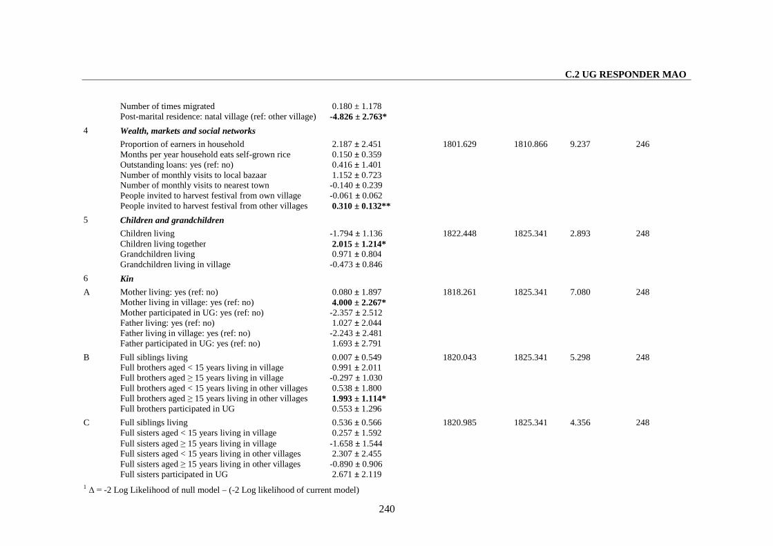
C.2 UG RESPONDER MAO
240
Number of times migrated 0.180 ± 1.178Post-marital residence: natal village (ref: other village) -4.826 ± 2.763*
Wealth, markets and social networks
Proportion of earners in household 2.187 ± 2.451Months per year household eats self-grown rice 0.150 ± 0.359Outstanding loans: yes (ref: no) 0.416 ± 1.401Number of monthly visits to local bazaar 1.152 ± 0.723Number of monthly visits to nearest town -0.140 ± 0.239People invited to harvest festival from own village -0.061 ± 0.062
4
People invited to harvest festival from other villages 0.310 ± 0.132**
1801.629 1810.866 9.237 246
Children and grandchildren
Children living -1.794 ± 1.136Children living together 2.015 ± 1.214*Grandchildren living 0.971 ± 0.804
5
Grandchildren living in village -0.473 ± 0.846
1822.448 1825.341 2.893 248
6 Kin
Mother living: yes (ref: no) 0.080 ± 1.897Mother living in village: yes (ref: no) 4.000 ± 2.267*Mother participated in UG: yes (ref: no) -2.357 ± 2.512Father living: yes (ref: no) 1.027 ± 2.044Father living in village: yes (ref: no) -2.243 ± 2.481
A
Father participated in UG: yes (ref: no) 1.693 ± 2.791
1818.261 1825.341 7.080 248
Full siblings living 0.007 ± 0.549Full brothers aged < 15 years living in village 0.991 ± 2.011Full brothers aged ≥ 15 years living in village -0.297 ± 1.030Full brothers aged < 15 years living in other villages 0.538 ± 1.800Full brothers aged ≥ 15 years living in other villages 1.993 ± 1.114*
B
Full brothers participated in UG 0.553 ± 1.296
1820.043 1825.341 5.298 248
Full siblings living 0.536 ± 0.566Full sisters aged < 15 years living in village 0.257 ± 1.592Full sisters aged ≥ 15 years living in village -1.658 ± 1.544Full sisters aged < 15 years living in other villages 2.307 ± 2.455Full sisters aged ≥ 15 years living in other villages -0.890 ± 0.906
C
Full sisters participated in UG 2.671 ± 2.119
1820.985 1825.341 4.356 248
1 Δ = -2 Log Likelihood of null model – (-2 Log likelihood of current model)
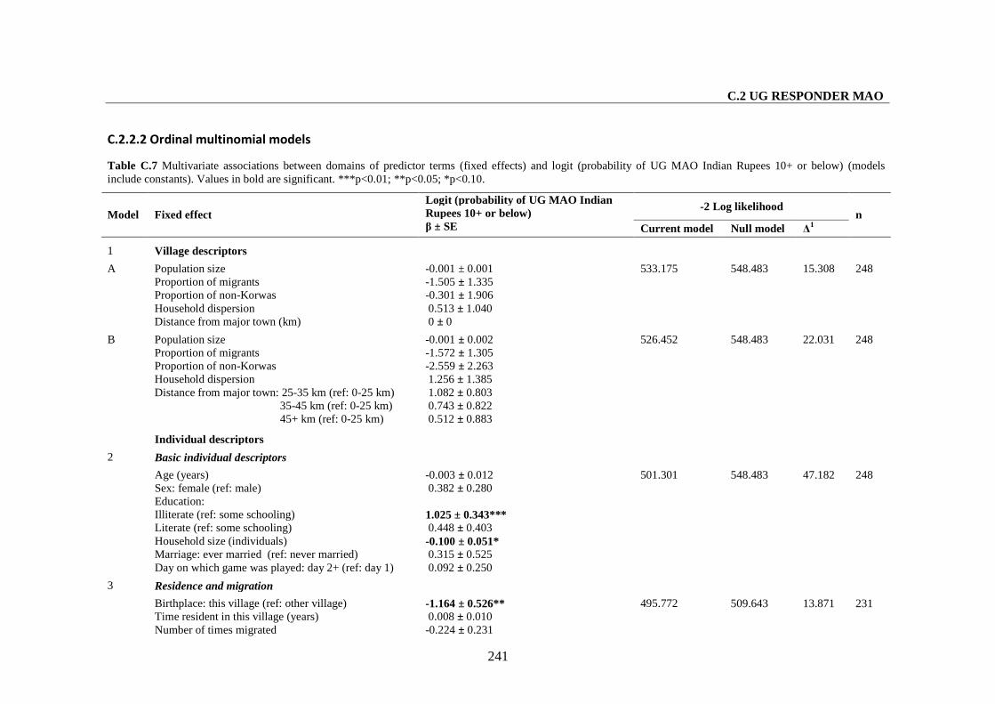
C.2 UG RESPONDER MAO
241
C.2.2.2 Ordinal multinomial models
Table C.7 Multivariate associations between domains of predictor terms (fixed effects) and logit (probability of UG MAO Indian Rupees 10+ or below) (modelsinclude constants). Values in bold are significant. ***p<0.01; **p<0.05; *p<0.10.
-2 Log likelihoodModel Fixed effect
Logit (probability of UG MAO IndianRupees 10+ or below)β ± SE Current model Null model Δ1
n
1 Village descriptors
Population size -0.001 ± 0.001Proportion of migrants -1.505 ± 1.335Proportion of non-Korwas -0.301 ± 1.906Household dispersion 0.513 ± 1.040
A
Distance from major town (km) 0 ± 0
533.175 548.483 15.308 248
Population size -0.001 ± 0.002Proportion of migrants -1.572 ± 1.305Proportion of non-Korwas -2.559 ± 2.263Household dispersion 1.256 ± 1.385
B
Distance from major town: 25-35 km (ref: 0-25 km)35-45 km (ref: 0-25 km)45+ km (ref: 0-25 km)
1.082 ± 0.8030.743 ± 0.8220.512 ± 0.883
526.452 548.483 22.031 248
Individual descriptors
Basic individual descriptors
Age (years) -0.003 ± 0.012Sex: female (ref: male) 0.382 ± 0.280Education:Illiterate (ref: some schooling)Literate (ref: some schooling)
1.025 ± 0.343***0.448 ± 0.403
Household size (individuals) -0.100 ± 0.051*Marriage: ever married (ref: never married) 0.315 ± 0.525
2
Day on which game was played: day 2+ (ref: day 1) 0.092 ± 0.250
501.301 548.483 47.182 248
Residence and migration
Birthplace: this village (ref: other village) -1.164 ± 0.526**Time resident in this village (years) 0.008 ± 0.010
3
Number of times migrated -0.224 ± 0.231
495.772 509.643 13.871 231
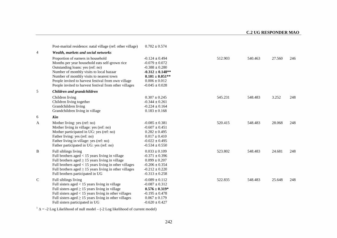
C.2 UG RESPONDER MAO
242
Post-marital residence: natal village (ref: other village) 0.702 ± 0.574
Wealth, markets and social networks
Proportion of earners in household -0.124 ± 0.494Months per year household eats self-grown rice -0.079 ± 0.072Outstanding loans: yes (ref: no) -0.388 ± 0.280Number of monthly visits to local bazaar -0.312 ± 0.148**Number of monthly visits to nearest town 0.101 ± 0.051**People invited to harvest festival from own village 0.006 ± 0.012
4
People invited to harvest festival from other villages -0.045 ± 0.028
512.903 540.463 27.560 246
Children and grandchildren
Children living 0.307 ± 0.245Children living together -0.344 ± 0.261Grandchildren living -0.224 ± 0.164
5
Grandchildren living in village 0.183 ± 0.168
545.231 548.483 3.252 248
6 Kin
Mother living: yes (ref: no) -0.085 ± 0.381Mother living in village: yes (ref: no) -0.607 ± 0.451Mother participated in UG: yes (ref: no) 0.282 ± 0.495Father living: yes (ref: no) 0.017 ± 0.410Father living in village: yes (ref: no) -0.022 ± 0.495
A
Father participated in UG: yes (ref: no) -0.534 ± 0.550
520.415 548.483 28.068 248
Full siblings living 0.033 ± 0.109Full brothers aged < 15 years living in village -0.371 ± 0.396Full brothers aged ≥ 15 years living in village 0.099 ± 0.207Full brothers aged < 15 years living in other villages -0.206 ± 0.354Full brothers aged ≥ 15 years living in other villages -0.212 ± 0.220
B
Full brothers participated in UG -0.313 ± 0.258
523.802 548.483 24.681 248
Full siblings living -0.089 ± 0.112Full sisters aged < 15 years living in village -0.087 ± 0.312Full sisters aged ≥ 15 years living in village 0.576 ± 0.319*Full sisters aged < 15 years living in other villages -0.195 ± 0.478Full sisters aged ≥ 15 years living in other villages 0.067 ± 0.179
C
Full sisters participated in UG -0.620 ± 0.427
522.835 548.483 25.648 248
1 Δ = -2 Log Likelihood of null model – (-2 Log likelihood of current model)
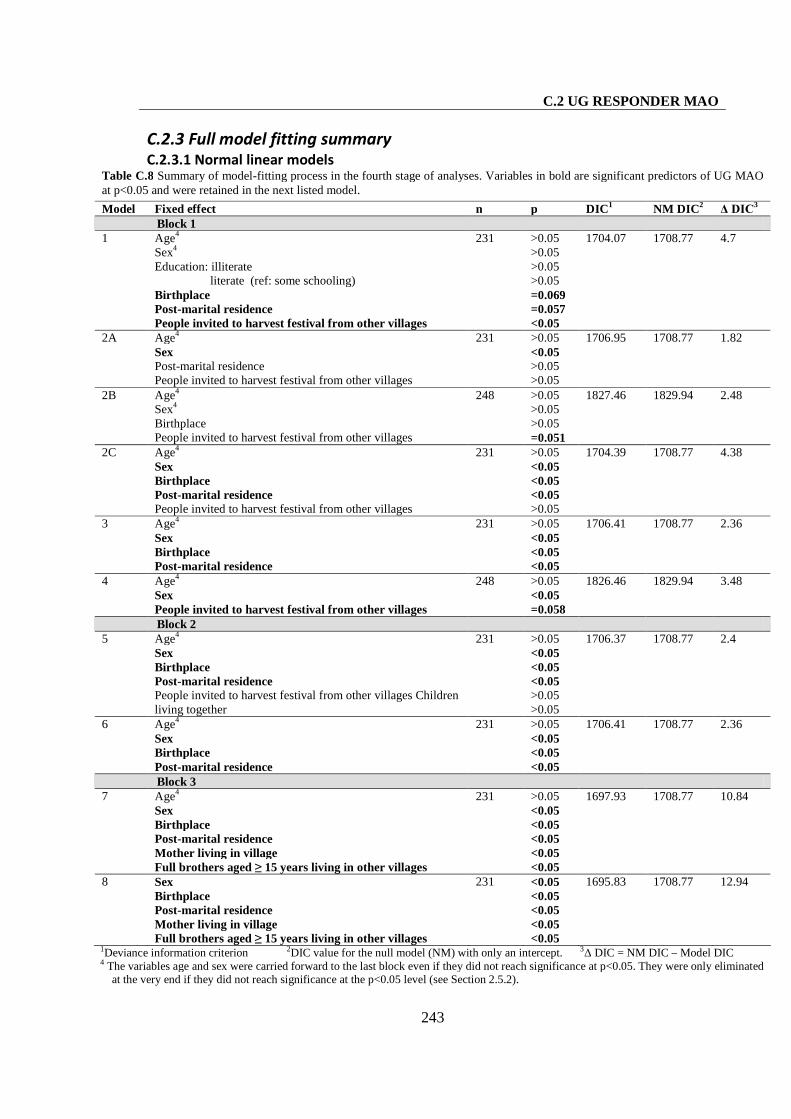
C.2 UG RESPONDER MAO
243
C.2.3 Full model fitting summaryC.2.3.1 Normal linear models
Table C.8 Summary of model-fitting process in the fourth stage of analyses. Variables in bold are significant predictors of UG MAOat p<0.05 and were retained in the next listed model.
Model Fixed effect n p DIC1 NM DIC2 Δ DIC3
Block 11 Age4
Sex4
Education: illiterateliterate (ref: some schooling)
BirthplacePost-marital residencePeople invited to harvest festival from other villages
231 >0.05>0.05>0.05>0.05=0.069=0.057<0.05
1704.07 1708.77 4.7
2A Age4
SexPost-marital residencePeople invited to harvest festival from other villages
231 >0.05<0.05>0.05>0.05
1706.95 1708.77 1.82
2B Age4
Sex4
BirthplacePeople invited to harvest festival from other villages
248 >0.05>0.05>0.05=0.051
1827.46 1829.94 2.48
2C Age4
SexBirthplacePost-marital residencePeople invited to harvest festival from other villages
231 >0.05<0.05<0.05<0.05>0.05
1704.39 1708.77 4.38
3 Age4
SexBirthplacePost-marital residence
231 >0.05<0.05<0.05<0.05
1706.41 1708.77 2.36
4 Age4
SexPeople invited to harvest festival from other villages
248 >0.05<0.05=0.058
1826.46 1829.94 3.48
Block 25 Age4
SexBirthplacePost-marital residencePeople invited to harvest festival from other villages Childrenliving together
231 >0.05<0.05<0.05<0.05>0.05>0.05
1706.37 1708.77 2.4
6 Age4
SexBirthplacePost-marital residence
231 >0.05<0.05<0.05<0.05
1706.41 1708.77 2.36
Block 37 Age4
SexBirthplacePost-marital residenceMother living in villageFull brothers aged ≥ 15 years living in other villages
231 >0.05<0.05<0.05<0.05<0.05<0.05
1697.93 1708.77 10.84
8 SexBirthplacePost-marital residenceMother living in villageFull brothers aged ≥ 15 years living in other villages
231 <0.05<0.05<0.05<0.05<0.05
1695.83 1708.77 12.94
1Deviance information criterion 2DIC value for the null model (NM) with only an intercept. 3Δ DIC = NM DIC – Model DIC4 The variables age and sex were carried forward to the last block even if they did not reach significance at p<0.05. They were only eliminated
at the very end if they did not reach significance at the p<0.05 level (see Section 2.5.2).
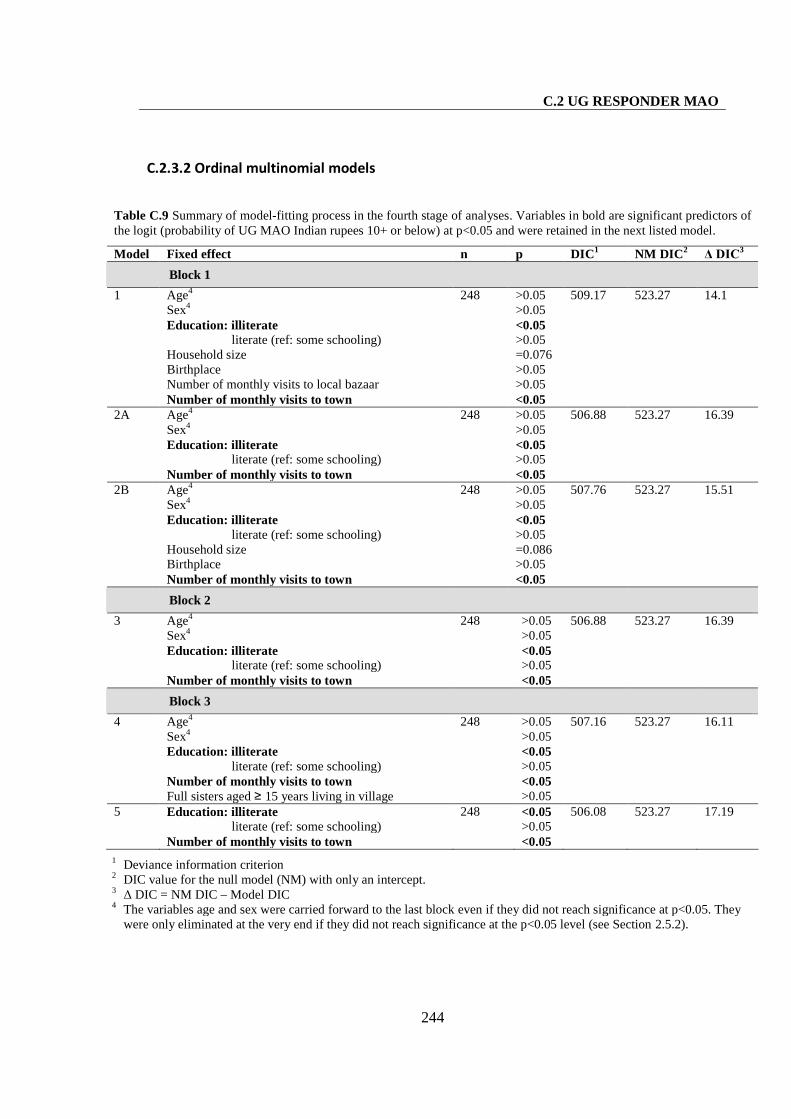
C.2 UG RESPONDER MAO
244
C.2.3.2 Ordinal multinomial models
Table C.9 Summary of model-fitting process in the fourth stage of analyses. Variables in bold are significant predictors ofthe logit (probability of UG MAO Indian rupees 10+ or below) at p<0.05 and were retained in the next listed model.
Model Fixed effect n p DIC1 NM DIC2 Δ DIC3
Block 1
1 Age4
Sex4
Education: illiterateliterate (ref: some schooling)
Household sizeBirthplaceNumber of monthly visits to local bazaarNumber of monthly visits to town
248 >0.05>0.05<0.05>0.05=0.076>0.05>0.05<0.05
509.17 523.27 14.1
2A Age4
Sex4
Education: illiterateliterate (ref: some schooling)
Number of monthly visits to town
248 >0.05>0.05<0.05>0.05<0.05
506.88 523.27 16.39
2B Age4
Sex4
Education: illiterateliterate (ref: some schooling)
Household sizeBirthplaceNumber of monthly visits to town
248 >0.05>0.05<0.05>0.05=0.086>0.05<0.05
507.76 523.27 15.51
Block 2
3 Age4
Sex4
Education: illiterateliterate (ref: some schooling)
Number of monthly visits to town
248 >0.05>0.05<0.05>0.05<0.05
506.88 523.27 16.39
Block 3
4 Age4
Sex4
Education: illiterateliterate (ref: some schooling)
Number of monthly visits to townFull sisters aged ≥ 15 years living in village
248 >0.05>0.05<0.05>0.05<0.05>0.05
507.16 523.27 16.11
5 Education: illiterateliterate (ref: some schooling)
Number of monthly visits to town
248 <0.05>0.05<0.05
506.08 523.27 17.19
1 Deviance information criterion2 DIC value for the null model (NM) with only an intercept.3 Δ DIC = NM DIC – Model DIC4 The variables age and sex were carried forward to the last block even if they did not reach significance at p<0.05. They
were only eliminated at the very end if they did not reach significance at the p<0.05 level (see Section 2.5.2).
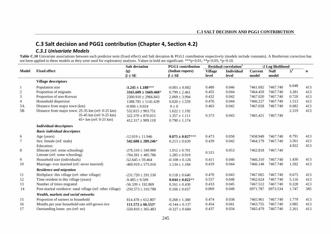
C.3 SALT DECISION AND PGG1 CONTRIBUTION
245
C.3 Salt decision and PGG1 contribution (Chapter 4, Section 4.2)C.3.1 Univariate Models
Table C.10 Univariate associations between each predictor term (fixed effect) and Salt deviation & PGG1 contribution respectively (models include constants). A Bonferroni correction hasnot been applied to these models as they were used for exploratory analyses. Values in bold are significant. ***p<0.01; **p<0.05; *p<0.10.
Residual correlation1 -2 Log likelihoodModel Fixed effect
Salt deviation(g) SE
PGG1 contribution(Indian rupees) SE
Villagelevel
Individuallevel
Currentmodel
Nullmodel
Δ2 n
Village descriptors
1 Population size -3.245 1.188*** -0.001 0.002 0.480 0.046 7461.692 7467.740 6.048 4132 Proportion of migrants 3165.609 1669.468* 0.799 2.461 0.455 0.044 7464.459 7467.740 3.281 4133 Proportion of non-Korwas 2300.910 2966.843 2.069 3.994 0.432 0.042 7467.020 7467.740 0.720 4134 Household dispersion 1388.781 1141.639 0.020 1.559 0.476 0.044 7466.227 7467.740 1.513 4135A Distance from major town (km) -0.006 0.024 0 0 0.463 0.042 7467.658 7467.740 0.082 4135B Distance from major town: 25-35 km (ref: 0-25 km)
35-45 km (ref: 0-25 km)45+ km (ref: 0-25 km)
532.815 903.751322.370 870.015412.317 909.118
1.622 1.1921.357 1.1110.790 1.174
0.373 0.043 7465.421 7467.740
2.319 413
Individual descriptors
Basic individual descriptors
6 Age (years) -12.019 11.946 0.075 0.027*** 0.473 0.058 7458.949 7467.740 8.791 413
7 Sex: female (ref: male) 542.688 289.246* 0.213 0.639 0.439 0.042 7464.179 7467.740 3.561 413
8Education:Illiterate (ref: some schooling)Literate (ref: some schooling)
-276.510 349.900-704.591 485.786
1.012 0.7011.285 0.919
0.3150.053 7462.818 7467.740
4.922 413
9 Household size (individuals) -52.645 59.464 -0.108 0.126 0.411 0.040 7466.310 7467.740 1.430 41310 Marriage: ever married (ref: never married) -469.919 575.016 1.134 1.184 0.419 0.044 7466.148 7467.740 1.592 413
Residence and migration
11 Birthplace: this village (ref: other village) -231.720 291.530 0.118 0.640 0.470 0.043 7467.065 7467.740 0.675 41312 Time resident in this village (years) -9.485 9.509 0.044 0.022** 0.557 0.048 7462.624 7467.740 5.116 41313 Number of times migrated -56.339 192.869 0.161 0.430 0.433 0.045 7467.512 7467.740 0.228 41314 Post-marital residence: natal village (ref: other village) -250.573 310.788 0.166 0.657 0.869 0.048 6971.787 6973.534 1.747 385
Wealth, markets and social networks
15 Proportion of earners in household 814.478 612.807 0.268 1.380 0.474 0.038 7465.961 7467.740 1.779 41316 Months per year household eats self-grown rice 111.572 66.553* -0.144 0.137 0.454 0.041 7463.755 7467.740 3.985 41317 Outstanding loans: yes (ref: no) -550.810 365.483 -0.327 0.684 0.437 0.034 7465.479 7467.740 2.261 413
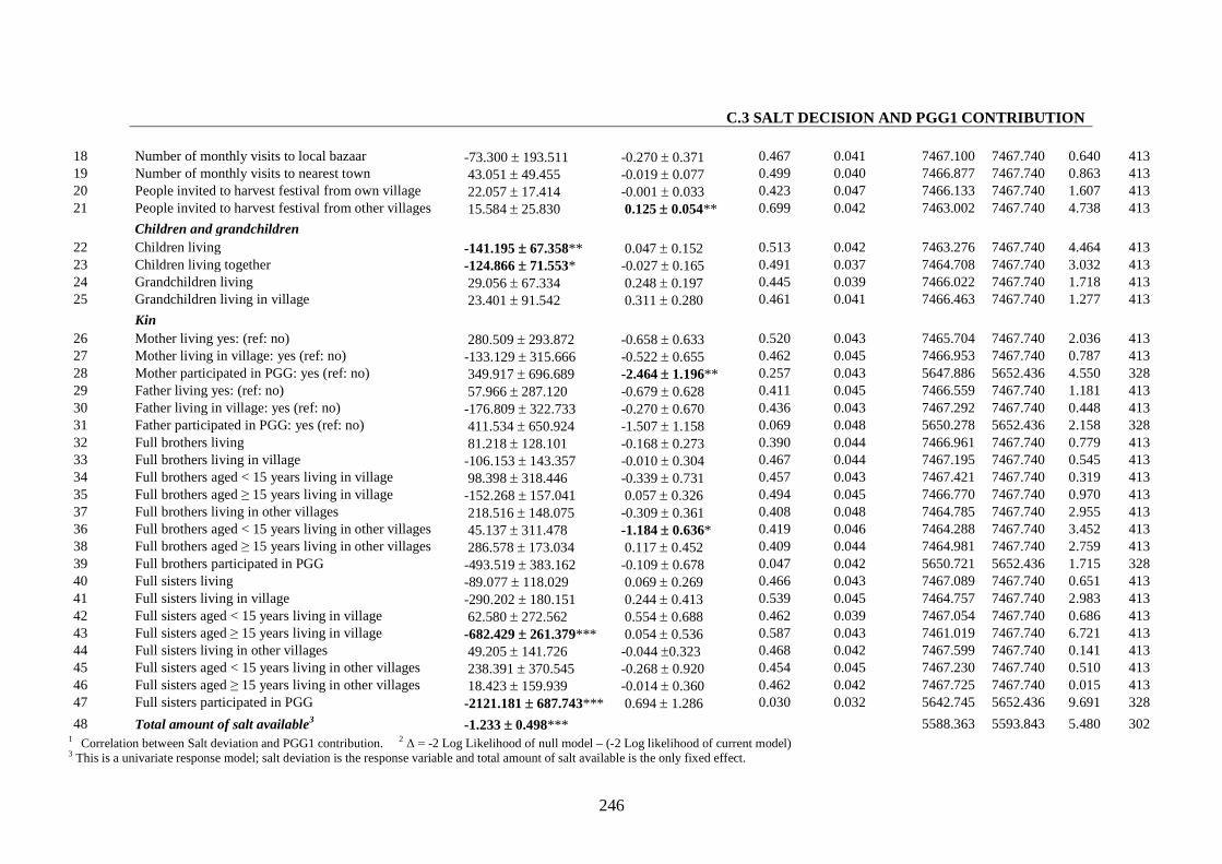
C.3 SALT DECISION AND PGG1 CONTRIBUTION
246
18 Number of monthly visits to local bazaar -73.300 193.511 -0.270 0.371 0.467 0.041 7467.100 7467.740 0.640 41319 Number of monthly visits to nearest town 43.051 49.455 -0.019 0.077 0.499 0.040 7466.877 7467.740 0.863 41320 People invited to harvest festival from own village 22.057 17.414 -0.001 0.033 0.423 0.047 7466.133 7467.740 1.607 41321 People invited to harvest festival from other villages 15.584 25.830 0.125 0.054** 0.699 0.042 7463.002 7467.740 4.738 413
Children and grandchildren
22 Children living -141.195 67.358** 0.047 0.152 0.513 0.042 7463.276 7467.740 4.464 41323 Children living together -124.866 71.553* -0.027 0.165 0.491 0.037 7464.708 7467.740 3.032 41324 Grandchildren living 29.056 67.334 0.248 0.197 0.445 0.039 7466.022 7467.740 1.718 41325 Grandchildren living in village 23.401 91.542 0.311 0.280 0.461 0.041 7466.463 7467.740 1.277 413
Kin
26 Mother living yes: (ref: no) 280.509 293.872 -0.658 0.633 0.520 0.043 7465.704 7467.740 2.036 41327 Mother living in village: yes (ref: no) -133.129 315.666 -0.522 0.655 0.462 0.045 7466.953 7467.740 0.787 41328 Mother participated in PGG: yes (ref: no) 349.917 696.689 -2.464 1.196** 0.257 0.043 5647.886 5652.436 4.550 32829 Father living yes: (ref: no) 57.966 287.120 -0.679 0.628 0.411 0.045 7466.559 7467.740 1.181 41330 Father living in village: yes (ref: no) -176.809 322.733 -0.270 0.670 0.436 0.043 7467.292 7467.740 0.448 41331 Father participated in PGG: yes (ref: no) 411.534 650.924 -1.507 1.158 0.069 0.048 5650.278 5652.436 2.158 32832 Full brothers living 81.218 128.101 -0.168 0.273 0.390 0.044 7466.961 7467.740 0.779 41333 Full brothers living in village -106.153 143.357 -0.010 0.304 0.467 0.044 7467.195 7467.740 0.545 41334 Full brothers aged < 15 years living in village 98.398 318.446 -0.339 0.731 0.457 0.043 7467.421 7467.740 0.319 41335 Full brothers aged ≥ 15 years living in village -152.268 157.041 0.057 0.326 0.494 0.045 7466.770 7467.740 0.970 41337 Full brothers living in other villages 218.516 148.075 -0.309 0.361 0.408 0.048 7464.785 7467.740 2.955 41336 Full brothers aged < 15 years living in other villages 45.137 311.478 -1.184 0.636* 0.419 0.046 7464.288 7467.740 3.452 41338 Full brothers aged ≥ 15 years living in other villages 286.578 173.034 0.117 0.452 0.409 0.044 7464.981 7467.740 2.759 41339 Full brothers participated in PGG -493.519 383.162 -0.109 0.678 0.047 0.042 5650.721 5652.436 1.715 32840 Full sisters living -89.077 118.029 0.069 0.269 0.466 0.043 7467.089 7467.740 0.651 41341 Full sisters living in village -290.202 180.151 0.244 0.413 0.539 0.045 7464.757 7467.740 2.983 41342 Full sisters aged < 15 years living in village 62.580 272.562 0.554 0.688 0.462 0.039 7467.054 7467.740 0.686 41343 Full sisters aged ≥ 15 years living in village -682.429 261.379*** 0.054 0.536 0.587 0.043 7461.019 7467.740 6.721 41344 Full sisters living in other villages 49.205 141.726 -0.044 0.323 0.468 0.042 7467.599 7467.740 0.141 41345 Full sisters aged < 15 years living in other villages 238.391 370.545 -0.268 0.920 0.454 0.045 7467.230 7467.740 0.510 41346 Full sisters aged ≥ 15 years living in other villages 18.423 159.939 -0.014 0.360 0.462 0.042 7467.725 7467.740 0.015 41347 Full sisters participated in PGG -2121.181 687.743*** 0.694 1.286 0.030 0.032 5642.745 5652.436 9.691 328
48 Total amount of salt available3 -1.233 0.498*** 5588.363 5593.843 5.480 3021 Correlation between Salt deviation and PGG1 contribution. 2 Δ = -2 Log Likelihood of null model – (-2 Log likelihood of current model)3 This is a univariate response model; salt deviation is the response variable and total amount of salt available is the only fixed effect.

C.3 SALT DECISION AND PGG1 CONTRIBUTION
247
C.3.2 Domain-wise modelsTable C.11 Multivariate associations between domains of predictor terms (fixed effects) and Salt deviation & PGG1 contribution respectively (models include constants). Values in bold aresignificant. ***p<0.01; **p<0.05; *p<0.10.
Residual correlation1 -2 Log likelihoodModel
Fixed effectSalt deviation(g) SE
PGG1 contribution(Indian rupees) SE
Villagelevel
Individuallevel
Currentmodel
Nullmodel
Δ2 n
1 Village descriptors
Population Size -6.626 2.035** -0.001 0.003Proportion of migrants 1486.957 1706.084 1.746 3.509Proportion of non-Korwas 865.413 2475.859 3.659 5.127Household dispersion -3239.822 1459.157* -1.813 2.724
A
Distance from major town (km) -0.062 0.027* 0 0
0.663 0.039 7454.254 7467.740 13.486 413
Population size -6.279 2.503** 0.004 0.004Proportion of migrants 2622.388 1773.903 2.062 3.23Proportion of non-Korwas 4854.912 3352.811 -2.764 5.918Household dispersion -4211.28 2223.623* 2.015 3.381
B
Distance from major town: 25-35 km (ref: 0-25 km)35-45 km (ref: 0-25 km)45+ km (ref: 0-25 km)
-1708.313 1185.381-2046.77 1253.946-2027.191 1322.038
3.322 2.0443.133 2.0572.488 2.183
1.072 0.045 7452.569 7467.740 15.171 413
Individual descriptors
Basic individual descriptors
Age (years) -0.592 14.083 0.070 0.032**Sex: female (ref: male) 680.289 329.782** 0.371 0.695Education:Illiterate (ref: some schooling)Literate (ref: some schooling)
-470.939 410.184-526.473 506.037
0.187 0.8020.515 0.981
Household size (individuals) -55.824 59.494 -0.081 0.126
2
Marriage: ever married (ref: never married) -504.254 626.889 -0.174 1.267
0.373 0.055 7451.441 7467.740 16.299 413
3 Residence and migration
Birthplace: this village (ref: other village) -87.644 763.658 -0.394 1.844Time resident in this village (years) -5.654 12.372 0.056 0.026**Number of times migrated -281.327 264.675 0.517 0.609Post-marital residence: natal village (ref: other village) -341.197 797.520 0.254 1.880
1.154 0.058 6965.558 6973.534 7.976 385
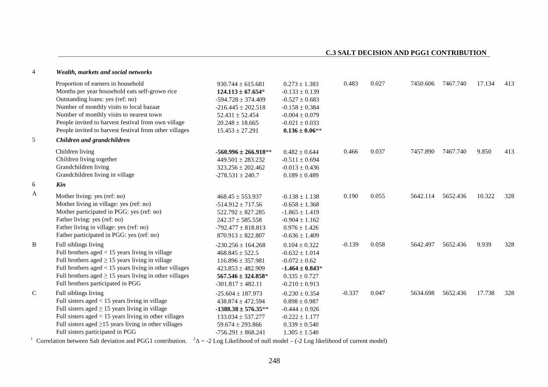
C.3 SALT DECISION AND PGG1 CONTRIBUTION
248
4 Wealth, markets and social networks
Proportion of earners in household 930.744 615.681 0.273 1.383Months per year household eats self-grown rice 124.113 67.654* -0.133 0.139Outstanding loans: yes (ref: no) -594.728 374.409 -0.527 0.683Number of monthly visits to local bazaar -216.445 202.518 -0.158 0.384Number of monthly visits to nearest town 52.431 52.454 -0.004 0.079People invited to harvest festival from own village 20.248 18.665 -0.021 0.033People invited to harvest festival from other villages 15.453 27.291 0.136 0.06**
0.483 0.027 7450.606 7467.740 17.134 413
Children and grandchildren
Children living -560.996 266.918** 0.482 0.644Children living together 449.501 283.232 -0.511 0.694Grandchildren living 323.256 202.462 -0.013 0.436
5
Grandchildren living in village -278.531 240.7 0.189 0.489
0.466 0.037 7457.890 7467.740 9.850 413
6 Kin
Mother living: yes (ref: no) 468.45 553.937 -0.138 1.138Mother living in village: yes (ref: no) -514.912 717.56 -0.658 1.368Mother participated in PGG: yes (ref: no) 522.792 827.285 -1.865 1.419Father living: yes (ref: no) 242.37 585.558 -0.904 1.162Father living in village: yes (ref: no) -792.477 818.813 0.976 1.426
A
Father participated in PGG: yes (ref: no) 870.913 822.807 -0.636 1.409
0.190 0.055 5642.114 5652.436 10.322 328
Full siblings living -230.256 164.268 0.104 0.322Full brothers aged < 15 years living in village 468.845 522.5 -0.632 1.014Full brothers aged ≥ 15 years living in village 116.896 357.981 -0.072 0.62Full brothers aged < 15 years living in other villages 423.853 482.909 -1.464 0.843*Full brothers aged ≥ 15 years living in other villages 567.546 324.858* 0.335 0.727
B
Full brothers participated in PGG -301.817 482.11 -0.210 0.913
-0.139 0.058 5642.497 5652.436 9.939 328
Full siblings living -25.604 187.973 -0.230 0.354Full sisters aged < 15 years living in village 438.874 472.594 0.898 0.987Full sisters aged ≥ 15 years living in village -1388.38 576.35** -0.444 0.926Full sisters aged < 15 years living in other villages 133.034 537.277 -0.222 1.177Full sisters aged ≥15 years living in other villages 59.674 293.866 0.339 0.540
C
Full sisters participated in PGG -756.291 868.241 1.305 1.540
-0.337 0.047 5634.698 5652.436 17.738 328
1 Correlation between Salt deviation and PGG1 contribution. 2Δ = -2 Log Likelihood of null model – (-2 Log likelihood of current model)
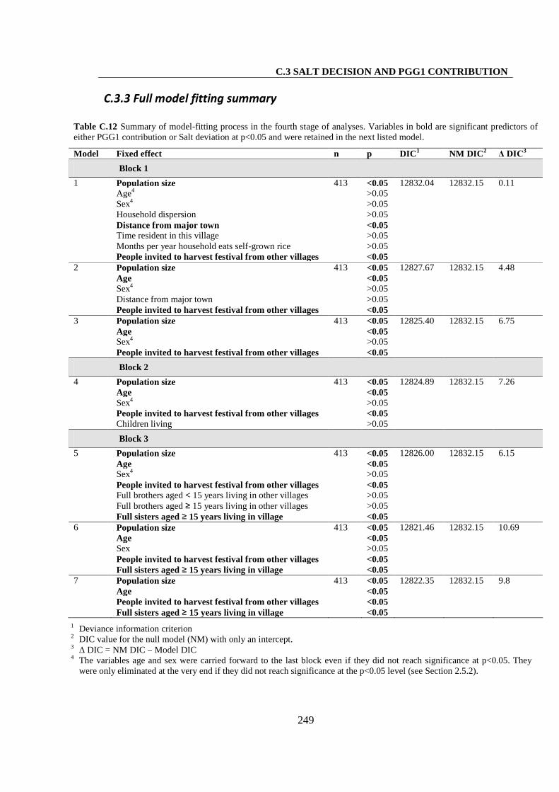
C.3 SALT DECISION AND PGG1 CONTRIBUTION
249
C.3.3 Full model fitting summary
Table C.12 Summary of model-fitting process in the fourth stage of analyses. Variables in bold are significant predictors ofeither PGG1 contribution or Salt deviation at p<0.05 and were retained in the next listed model.
Model Fixed effect n p DIC1 NM DIC2 Δ DIC3
Block 1
1 Population sizeAge4
Sex4
Household dispersionDistance from major townTime resident in this villageMonths per year household eats self-grown ricePeople invited to harvest festival from other villages
413 <0.05>0.05>0.05>0.05<0.05>0.05>0.05<0.05
12832.04 12832.15 0.11
2 Population sizeAgeSex4
Distance from major townPeople invited to harvest festival from other villages
413 <0.05<0.05>0.05>0.05<0.05
12827.67 12832.15 4.48
3 Population sizeAgeSex4
People invited to harvest festival from other villages
413 <0.05<0.05>0.05<0.05
12825.40 12832.15 6.75
Block 2
4 Population sizeAgeSex4
People invited to harvest festival from other villagesChildren living
413 <0.05<0.05>0.05<0.05>0.05
12824.89 12832.15 7.26
Block 3
5 Population sizeAgeSex4
People invited to harvest festival from other villagesFull brothers aged < 15 years living in other villagesFull brothers aged ≥ 15 years living in other villagesFull sisters aged ≥ 15 years living in village
413 <0.05<0.05>0.05<0.05>0.05>0.05<0.05
12826.00 12832.15 6.15
6 Population sizeAgeSexPeople invited to harvest festival from other villagesFull sisters aged ≥ 15 years living in village
413 <0.05<0.05>0.05<0.05<0.05
12821.46 12832.15 10.69
7 Population sizeAgePeople invited to harvest festival from other villagesFull sisters aged ≥ 15 years living in village
413 <0.05<0.05<0.05<0.05
12822.35 12832.15 9.8
1 Deviance information criterion2 DIC value for the null model (NM) with only an intercept.3 Δ DIC = NM DIC – Model DIC4 The variables age and sex were carried forward to the last block even if they did not reach significance at p<0.05. They
were only eliminated at the very end if they did not reach significance at the p<0.05 level (see Section 2.5.2).
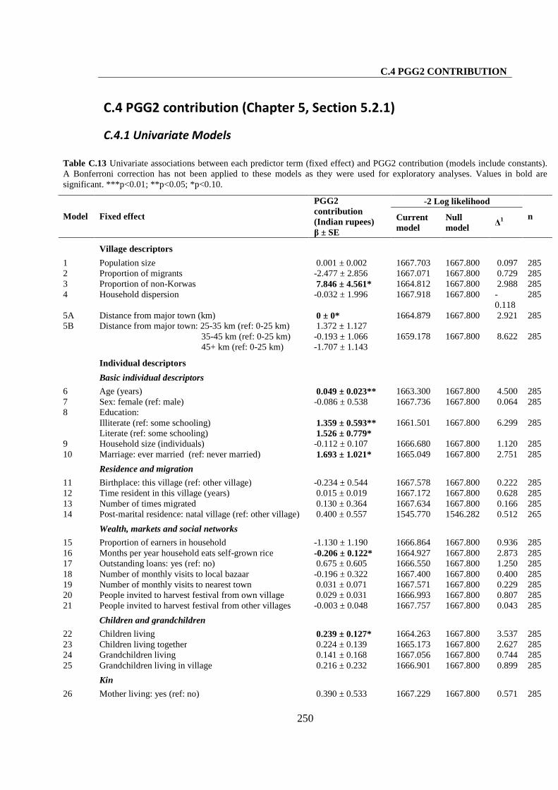
C.4 PGG2 CONTRIBUTION
250
C.4 PGG2 contribution (Chapter 5, Section 5.2.1)
C.4.1 Univariate Models
Table C.13 Univariate associations between each predictor term (fixed effect) and PGG2 contribution (models include constants).A Bonferroni correction has not been applied to these models as they were used for exploratory analyses. Values in bold aresignificant. ***p<0.01; **p<0.05; *p<0.10.
-2 Log likelihood
Model Fixed effect
PGG2contribution(Indian rupees)β ± SE
Currentmodel
Nullmodel
Δ1 n
Village descriptors
1 Population size 0.001 ± 0.002 1667.703 1667.800 0.097 2852 Proportion of migrants -2.477 ± 2.856 1667.071 1667.800 0.729 2853 Proportion of non-Korwas 7.846 ± 4.561* 1664.812 1667.800 2.988 2854 Household dispersion -0.032 ± 1.996 1667.918 1667.800 -
0.118285
5A Distance from major town (km) 0 ± 0* 1664.879 1667.800 2.921 2855B Distance from major town: 25-35 km (ref: 0-25 km)
35-45 km (ref: 0-25 km)45+ km (ref: 0-25 km)
1.372 ± 1.127-0.193 ± 1.066-1.707 ± 1.143
1659.178 1667.800 8.622 285
Individual descriptors
Basic individual descriptors
6 Age (years) 0.049 ± 0.023** 1663.300 1667.800 4.500 2857 Sex: female (ref: male) -0.086 ± 0.538 1667.736 1667.800 0.064 2858 Education:
Illiterate (ref: some schooling)Literate (ref: some schooling)
1.359 ± 0.593**1.526 ± 0.779*
1661.501 1667.800 6.299 285
9 Household size (individuals) -0.112 ± 0.107 1666.680 1667.800 1.120 28510 Marriage: ever married (ref: never married) 1.693 ± 1.021* 1665.049 1667.800 2.751 285
Residence and migration
11 Birthplace: this village (ref: other village) -0.234 ± 0.544 1667.578 1667.800 0.222 28512 Time resident in this village (years) 0.015 ± 0.019 1667.172 1667.800 0.628 28513 Number of times migrated 0.130 ± 0.364 1667.634 1667.800 0.166 28514 Post-marital residence: natal village (ref: other village) 0.400 ± 0.557 1545.770 1546.282 0.512 265
Wealth, markets and social networks
15 Proportion of earners in household -1.130 ± 1.190 1666.864 1667.800 0.936 28516 Months per year household eats self-grown rice -0.206 ± 0.122* 1664.927 1667.800 2.873 28517 Outstanding loans: yes (ref: no) 0.675 ± 0.605 1666.550 1667.800 1.250 28518 Number of monthly visits to local bazaar -0.196 ± 0.322 1667.400 1667.800 0.400 28519 Number of monthly visits to nearest town 0.031 ± 0.071 1667.571 1667.800 0.229 28520 People invited to harvest festival from own village 0.029 ± 0.031 1666.993 1667.800 0.807 28521 People invited to harvest festival from other villages -0.003 ± 0.048 1667.757 1667.800 0.043 285
Children and grandchildren
22 Children living 0.239 ± 0.127* 1664.263 1667.800 3.537 28523 Children living together 0.224 ± 0.139 1665.173 1667.800 2.627 28524 Grandchildren living 0.141 ± 0.168 1667.056 1667.800 0.744 28525 Grandchildren living in village 0.216 ± 0.232 1666.901 1667.800 0.899 285
Kin
26 Mother living: yes (ref: no) 0.390 ± 0.533 1667.229 1667.800 0.571 285
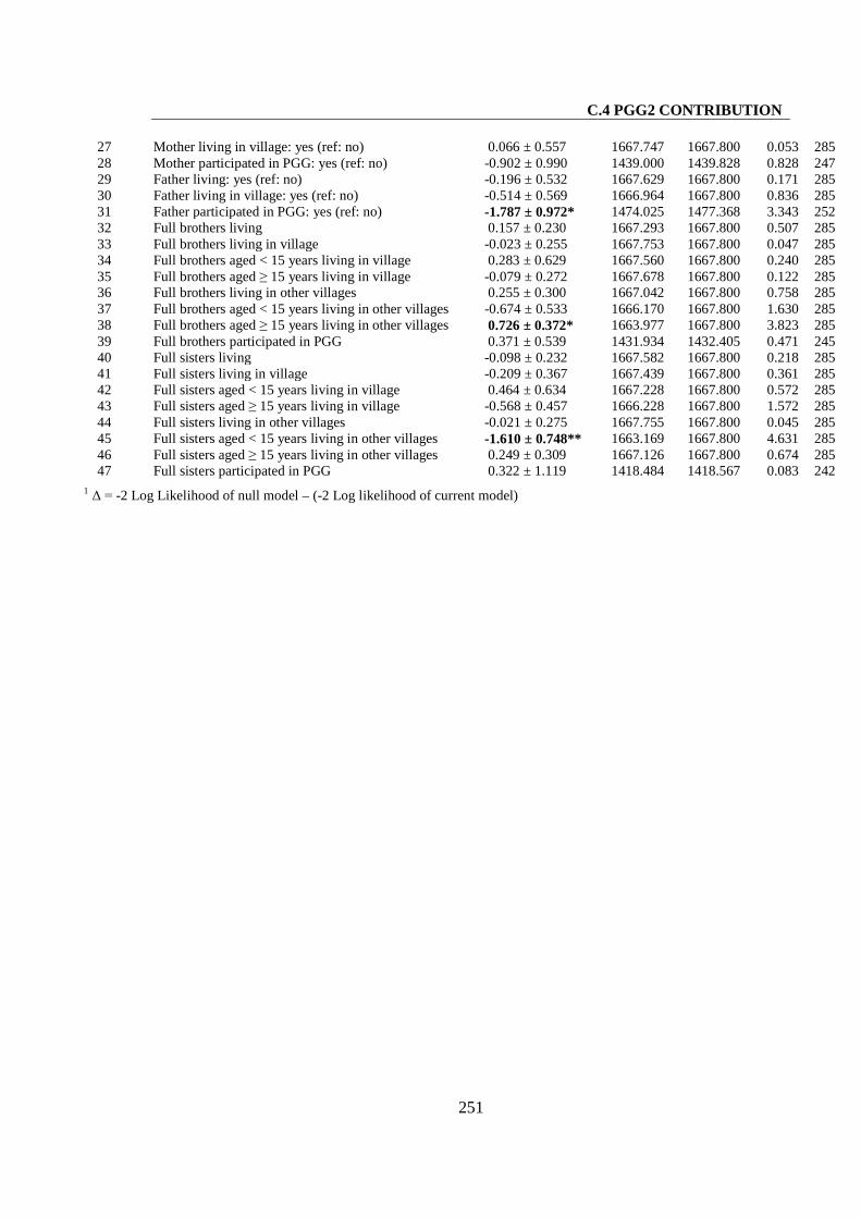
C.4 PGG2 CONTRIBUTION
251
27 Mother living in village: yes (ref: no) 0.066 ± 0.557 1667.747 1667.800 0.053 28528 Mother participated in PGG: yes (ref: no) -0.902 ± 0.990 1439.000 1439.828 0.828 24729 Father living: yes (ref: no) -0.196 ± 0.532 1667.629 1667.800 0.171 28530 Father living in village: yes (ref: no) -0.514 ± 0.569 1666.964 1667.800 0.836 28531 Father participated in PGG: yes (ref: no) -1.787 ± 0.972* 1474.025 1477.368 3.343 25232 Full brothers living 0.157 ± 0.230 1667.293 1667.800 0.507 28533 Full brothers living in village -0.023 ± 0.255 1667.753 1667.800 0.047 28534 Full brothers aged < 15 years living in village 0.283 ± 0.629 1667.560 1667.800 0.240 28535 Full brothers aged ≥ 15 years living in village -0.079 ± 0.272 1667.678 1667.800 0.122 28536 Full brothers living in other villages 0.255 ± 0.300 1667.042 1667.800 0.758 28537 Full brothers aged < 15 years living in other villages -0.674 ± 0.533 1666.170 1667.800 1.630 28538 Full brothers aged ≥ 15 years living in other villages 0.726 ± 0.372* 1663.977 1667.800 3.823 28539 Full brothers participated in PGG 0.371 ± 0.539 1431.934 1432.405 0.471 24540 Full sisters living -0.098 ± 0.232 1667.582 1667.800 0.218 28541 Full sisters living in village -0.209 ± 0.367 1667.439 1667.800 0.361 28542 Full sisters aged < 15 years living in village 0.464 ± 0.634 1667.228 1667.800 0.572 28543 Full sisters aged ≥ 15 years living in village -0.568 ± 0.457 1666.228 1667.800 1.572 28544 Full sisters living in other villages -0.021 ± 0.275 1667.755 1667.800 0.045 28545 Full sisters aged < 15 years living in other villages -1.610 ± 0.748** 1663.169 1667.800 4.631 28546 Full sisters aged ≥ 15 years living in other villages 0.249 ± 0.309 1667.126 1667.800 0.674 28547 Full sisters participated in PGG 0.322 ± 1.119 1418.484 1418.567 0.083 242
1 Δ = -2 Log Likelihood of null model – (-2 Log likelihood of current model)
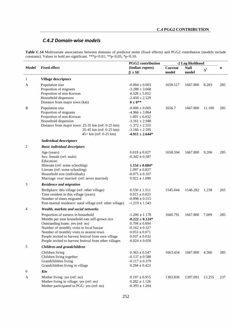
C.4 PGG2 CONTRIBUTION
252
C.4.2 Domain-wise models
Table C.14 Multivariate associations between domains of predictor terms (fixed effects) and PGG2 contribution (models includeconstants). Values in bold are significant. ***p<0.01; **p<0.05; *p<0.10.
-2 Log likelihoodModel Fixed effect
PGG2 contribution(Indian rupees)
± SECurrentmodel
Nullmodel
Δ1 n
1 Village descriptors
Population size -0.004 ± 0.003Proportion of migrants -3.288 ± 3.668Proportion of non-Korwas 4.328 ± 5.052Household dispersion -2.458 ± 2.529
A
Distance from major town (km) 0 ± 0**
1659.517 1667.800 8.283 285
Population size -0.006 ± 0.005Proportion of migrants -4.966 ± 3.864Proportion of non-Korwas 1.601 ± 6.032Household dispersion -3.161 ± 2.948
B
Distance from major town: 25-35 km (ref: 0-25 km)35-45 km (ref: 0-25 km)45+ km (ref: 0-25 km)
-1.372 ± 2.555-3.166 ± 2.595-4.911 ± 2.644*
1656.7 1667.800 11.100 285
Individual descriptors
Basic individual descriptors
Age (years) 0.019 ± 0.027Sex: female (ref: male) -0.342 ± 0.587Education:Illiterate (ref: some schooling)Literate (ref: some schooling)
1.154 ± 0.684*1.097 ± 0.837
Household size (individuals) -0.075 ± 0.107
2
Marriage: ever married (ref: never married) 0.922 ± 1.090
1658.594 1667.800 9.206 285
Residence and migration
Birthplace: this village (ref: other village) 0.550 ± 1.511Time resident in this village (years) 0.015 ± 0.023Number of times migrated -0.098 ± 0.515
3
Post-marital residence: natal village (ref: other village) -1.219 ± 1.543
1545.044 1546.282 1.238 265
Wealth, markets and social networks
Proportion of earners in household -1.206 ± 1.178Months per year household eats self-grown rice -0.222 ± 0.124*Outstanding loans: yes (ref: no) 0.704 ± 0.604Number of monthly visits to local bazaar -0.162 ± 0.327Number of monthly visits to nearest town 0.053 ± 0.071People invited to harvest festival from own village 0.037 ± 0.032
4
People invited to harvest festival from other villages -0.024 ± 0.050
1660.791 1667.800 7.009 285
Children and grandchildren
Children living 0.363 ± 0.547Children living together -0.137 ± 0.588Grandchildren living -0.117 ± 0.379
5
Grandchildren living in village 0.294 ± 0.423
1663.434 1667.800 4.366 285
6 Kin
Mother living: yes (ref: no) 0.197 ± 0.915Mother living in village: yes (ref: no) 0.282 ± 1.126
A
Mother participated in PGG: yes (ref: no) -0.393 ± 1.204
1383.836 1397.091 13.255 237

C.4 PGG2 CONTRIBUTION
253
Father living: yes (ref: no) -0.297 ± 0.937Father living in village: yes (ref: no) 0.085 ± 1.167Father participated in PGG: yes (ref: no) -1.699 ± 1.189
Full siblings living 0.002 ± 0.253Full brothers aged < 15 years living in village 0.094 ± 0.830Full brothers aged ≥ 15 years living in village -0.217 ± 0.499Full brothers aged < 15 years living in other villages -0.890 ± 0.662Full brothers aged ≥ 15 years living in other villages 0.585 ± 0.575
B
Full brothers participated in PGG 0.690 ± 0.733
1427.948 1445.476 17.528 245
Full siblings living 0.039 ± 0.271Full sisters aged < 15 years living in village 0.147 ± 0.886Full sisters aged ≥ 15 years living in village -0.241 ± 0.737Full sisters aged < 15 years living in other villages -2.101 ± 0.925**Full sisters aged ≥ 15 years living in other villages 0.417 ± 0.429
C
Full sisters participated in PGG 0.536 ± 1.314
1411.670 1418.567 6.897 242
1 Δ = -2 Log Likelihood of null model – (-2 Log likelihood of current model)
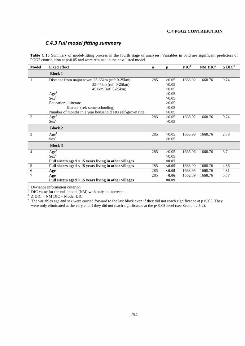
C.4 PGG2 CONTRIBUTION
254
C.4.3 Full model fitting summary
Table C.15 Summary of model-fitting process in the fourth stage of analyses. Variables in bold are significant predictors ofPGG2 contribution at p<0.05 and were retained in the next listed model.
Model Fixed effect n p DIC1 NM DIC2 Δ DIC3
Block 1
1 Distance from major town: 25-35km (ref: 0-25km)35-45km (ref: 0-25km)45+km (ref: 0-25km)
Age4
Sex4
Education: illiterateliterate (ref: some schooling)
Number of months in a year household eats self-grown rice
285 >0.05>0.05>0.05>0.05>0.05>0.05>0.05>0.05
1668.02 1668.76 0.74
2 Age4
Sex4285 >0.05
>0.051668.02 1668.76 0.74
Block 2
3 Age4
Sex4285 >0.05
>0.051665.98 1668.76 2.78
Block 3
4 Age4
Sex4
Full sisters aged < 15 years living in other villages
285 >0.05>0.05=0.07
1665.06 1668.76 3.7
5 Full sisters aged < 15 years living in other villages 285 <0.05 1663.90 1668.76 4.866 Age 285 <0.05 1663.95 1668.76 4.817 Age
Full sisters aged < 15 years living in other villages285 =0.06
=0.091662.89 1668.76 5.87
1 Deviance information criterion2 DIC value for the null model (NM) with only an intercept.3 Δ DIC = NM DIC – Model DIC4 The variables age and sex were carried forward to the last block even if they did not reach significance at p<0.05. They
were only eliminated at the very end if they did not reach significance at the p<0.05 level (see Section 2.5.2).
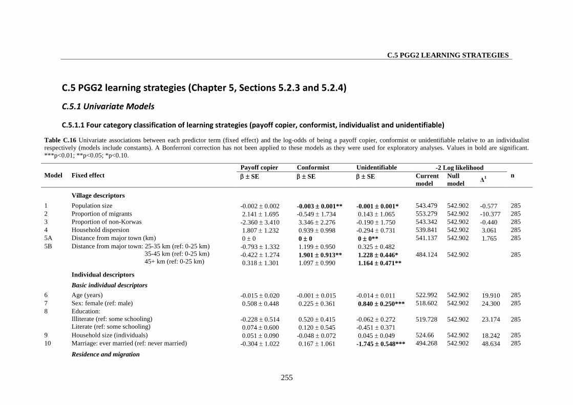
C.5 PGG2 LEARNING STRATEGIES
255
C.5 PGG2 learning strategies (Chapter 5, Sections 5.2.3 and 5.2.4)
C.5.1 Univariate Models
C.5.1.1 Four category classification of learning strategies (payoff copier, conformist, individualist and unidentifiable)
Table C.16 Univariate associations between each predictor term (fixed effect) and the log-odds of being a payoff copier, conformist or unidentifiable relative to an individualistrespectively (models include constants). A Bonferroni correction has not been applied to these models as they were used for exploratory analyses. Values in bold are significant.***p<0.01; **p<0.05; *p<0.10.
Payoff copier Conformist Unidentifiable -2 Log likelihoodModel Fixed effect SE SE SE Current
modelNullmodel
Δ1 n
Village descriptors
1 Population size -0.002 0.002 -0.003 0.001** -0.001 0.001* 543.479 542.902 -0.577 2852 Proportion of migrants 2.141 1.695 -0.549 1.734 0.143 1.065 553.279 542.902 -10.377 2853 Proportion of non-Korwas -2.360 3.410 3.346 2.276 -0.190 1.750 543.342 542.902 -0.440 2854 Household dispersion 1.807 1.232 0.939 0.998 -0.294 0.731 539.841 542.902 3.061 2855A Distance from major town (km) 0 0 0 0 0 0** 541.137 542.902 1.765 285
5B Distance from major town: 25-35 km (ref: 0-25 km)35-45 km (ref: 0-25 km)45+ km (ref: 0-25 km)
-0.793 1.332-0.422 1.2740.318 1.301
1.199 0.950
1.901 0.913**1.097 0.990
0.325 0.482
1.228 0.446*1.164 0.471**
484.124 542.902 285
Individual descriptors
Basic individual descriptors
6 Age (years) -0.015 0.020 -0.001 0.015 -0.014 0.011 522.992 542.902 19.910 2857 Sex: female (ref: male) 0.508 0.448 0.225 0.361 0.840 0.250*** 518.602 542.902 24.300 2858 Education:
Illiterate (ref: some schooling)Literate (ref: some schooling)
-0.228 0.5140.074 0.600
0.520 0.4150.120 0.545
-0.062 0.272-0.451 0.371
519.728 542.902 23.174 285
9 Household size (individuals) 0.051 0.090 -0.048 0.072 0.045 0.049 524.66 542.902 18.242 28510 Marriage: ever married (ref: never married) -0.304 1.022 0.167 1.061 -1.745 0.548*** 494.268 542.902 48.634 285
Residence and migration
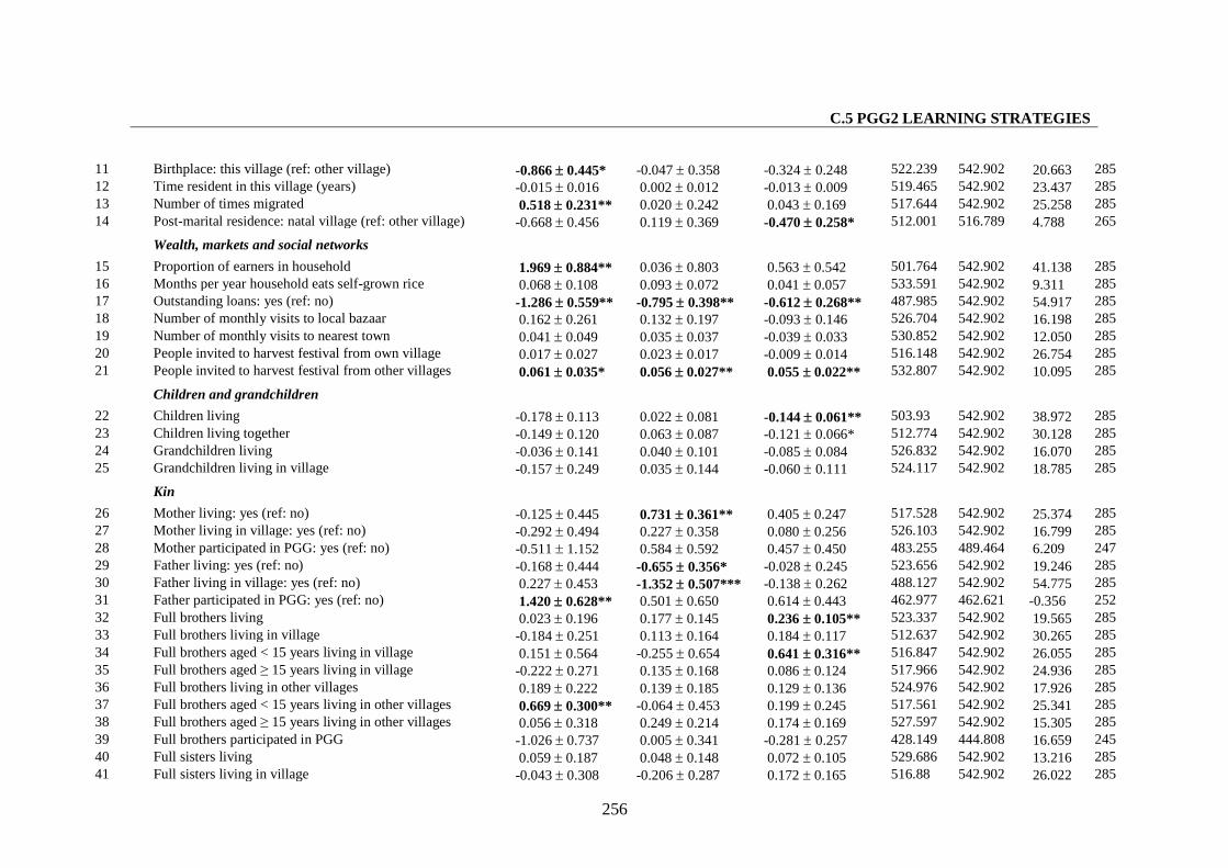
C.5 PGG2 LEARNING STRATEGIES
256
11 Birthplace: this village (ref: other village) -0.866 0.445* -0.047 0.358 -0.324 0.248 522.239 542.902 20.663 28512 Time resident in this village (years) -0.015 0.016 0.002 0.012 -0.013 0.009 519.465 542.902 23.437 28513 Number of times migrated 0.518 0.231** 0.020 0.242 0.043 0.169 517.644 542.902 25.258 28514 Post-marital residence: natal village (ref: other village) -0.668 0.456 0.119 0.369 -0.470 0.258* 512.001 516.789 4.788 265
Wealth, markets and social networks
15 Proportion of earners in household 1.969 0.884** 0.036 0.803 0.563 0.542 501.764 542.902 41.138 28516 Months per year household eats self-grown rice 0.068 0.108 0.093 0.072 0.041 0.057 533.591 542.902 9.311 28517 Outstanding loans: yes (ref: no) -1.286 0.559** -0.795 0.398** -0.612 0.268** 487.985 542.902 54.917 28518 Number of monthly visits to local bazaar 0.162 0.261 0.132 0.197 -0.093 0.146 526.704 542.902 16.198 28519 Number of monthly visits to nearest town 0.041 0.049 0.035 0.037 -0.039 0.033 530.852 542.902 12.050 28520 People invited to harvest festival from own village 0.017 0.027 0.023 0.017 -0.009 0.014 516.148 542.902 26.754 28521 People invited to harvest festival from other villages 0.061 0.035* 0.056 0.027** 0.055 0.022** 532.807 542.902 10.095 285
Children and grandchildren
22 Children living -0.178 0.113 0.022 0.081 -0.144 0.061** 503.93 542.902 38.972 28523 Children living together -0.149 0.120 0.063 0.087 -0.121 0.066* 512.774 542.902 30.128 28524 Grandchildren living -0.036 0.141 0.040 0.101 -0.085 0.084 526.832 542.902 16.070 28525 Grandchildren living in village -0.157 0.249 0.035 0.144 -0.060 0.111 524.117 542.902 18.785 285
Kin
26 Mother living: yes (ref: no) -0.125 0.445 0.731 0.361** 0.405 0.247 517.528 542.902 25.374 28527 Mother living in village: yes (ref: no) -0.292 0.494 0.227 0.358 0.080 0.256 526.103 542.902 16.799 28528 Mother participated in PGG: yes (ref: no) -0.511 1.152 0.584 0.592 0.457 0.450 483.255 489.464 6.209 24729 Father living: yes (ref: no) -0.168 0.444 -0.655 0.356* -0.028 0.245 523.656 542.902 19.246 28530 Father living in village: yes (ref: no) 0.227 0.453 -1.352 0.507*** -0.138 0.262 488.127 542.902 54.775 28531 Father participated in PGG: yes (ref: no) 1.420 0.628** 0.501 0.650 0.614 0.443 462.977 462.621 -0.356 25232 Full brothers living 0.023 0.196 0.177 0.145 0.236 0.105** 523.337 542.902 19.565 28533 Full brothers living in village -0.184 0.251 0.113 0.164 0.184 0.117 512.637 542.902 30.265 28534 Full brothers aged < 15 years living in village 0.151 0.564 -0.255 0.654 0.641 0.316** 516.847 542.902 26.055 28535 Full brothers aged ≥ 15 years living in village -0.222 0.271 0.135 0.168 0.086 0.124 517.966 542.902 24.936 28536 Full brothers living in other villages 0.189 0.222 0.139 0.185 0.129 0.136 524.976 542.902 17.926 28537 Full brothers aged < 15 years living in other villages 0.669 0.300** -0.064 0.453 0.199 0.245 517.561 542.902 25.341 28538 Full brothers aged ≥ 15 years living in other villages 0.056 0.318 0.249 0.214 0.174 0.169 527.597 542.902 15.305 28539 Full brothers participated in PGG -1.026 0.737 0.005 0.341 -0.281 0.257 428.149 444.808 16.659 24540 Full sisters living 0.059 0.187 0.048 0.148 0.072 0.105 529.686 542.902 13.216 28541 Full sisters living in village -0.043 0.308 -0.206 0.287 0.172 0.165 516.88 542.902 26.022 285
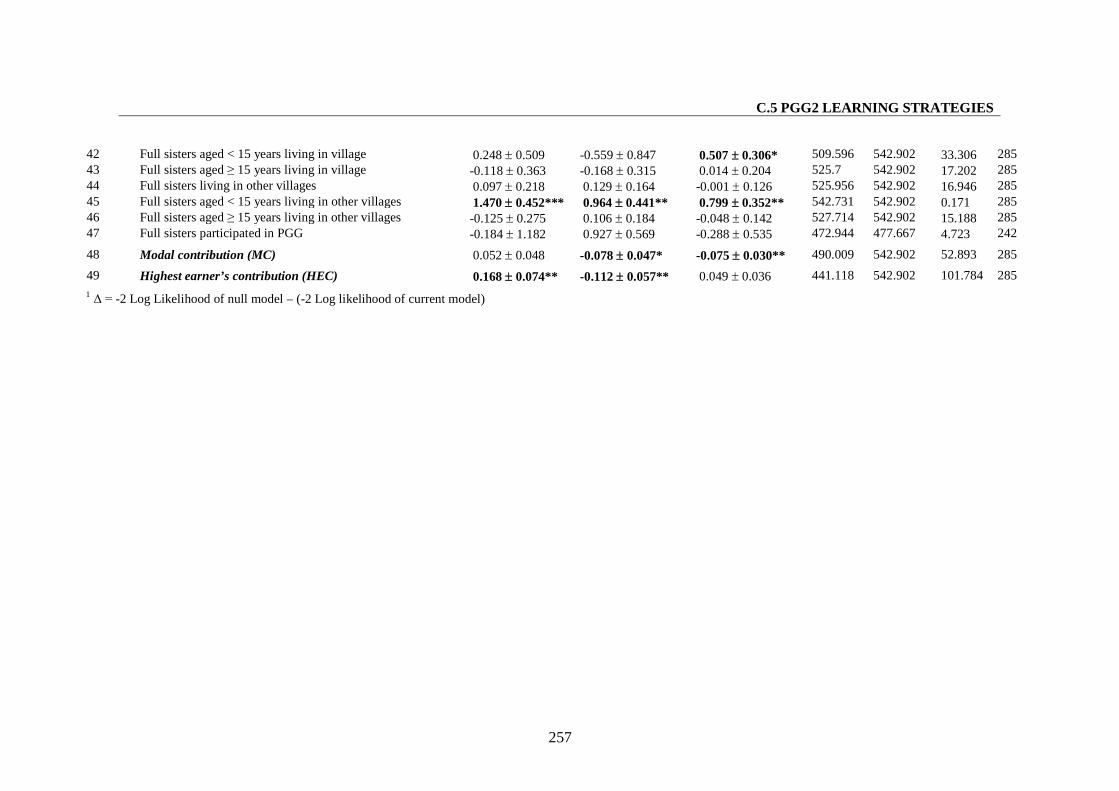
C.5 PGG2 LEARNING STRATEGIES
257
42 Full sisters aged < 15 years living in village 0.248 0.509 -0.559 0.847 0.507 0.306* 509.596 542.902 33.306 28543 Full sisters aged ≥ 15 years living in village -0.118 0.363 -0.168 0.315 0.014 0.204 525.7 542.902 17.202 28544 Full sisters living in other villages 0.097 0.218 0.129 0.164 -0.001 0.126 525.956 542.902 16.946 28545 Full sisters aged < 15 years living in other villages 1.470 0.452*** 0.964 0.441** 0.799 0.352** 542.731 542.902 0.171 28546 Full sisters aged ≥ 15 years living in other villages -0.125 0.275 0.106 0.184 -0.048 0.142 527.714 542.902 15.188 28547 Full sisters participated in PGG -0.184 1.182 0.927 0.569 -0.288 0.535 472.944 477.667 4.723 242
48 Modal contribution (MC) 0.052 0.048 -0.078 0.047* -0.075 0.030** 490.009 542.902 52.893 285
49 Highest earner’s contribution (HEC) 0.168 0.074** -0.112 0.057** 0.049 0.036 441.118 542.902 101.784 285
1 Δ = -2 Log Likelihood of null model – (-2 Log likelihood of current model)
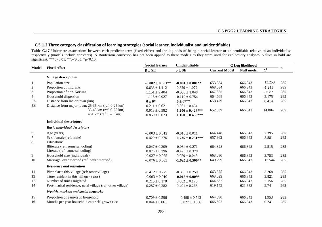
C.5 PGG2 LEARNING STRATEGIES
258
C.5.1.2 Three category classification of learning strategies (social learner, individualist and unidentifiable)
Table C.17 Univariate associations between each predictor term (fixed effect) and the log-odds of being a social learner or unidentifiable relative to an individualistrespectively (models include constants). A Bonferroni correction has not been applied to these models as they were used for exploratory analyses. Values in bold aresignificant. ***p<0.01; **p<0.05; *p<0.10.
Social learner Unidentifiable -2 Log likelihoodModel Fixed effect
SE SE Current Model Null model Δ1 n
Village descriptors
1 Population size -0.002 0.001** -0.001 0.001** 653.584 666.843 13.259 2852 Proportion of migrants 0.638 1.412 0.329 1.072 668.084 666.843 -1.241 2853 Proportion of non-Korwas 1.151 2.404 -0.353 1.848 667.825 666.843 -0.982 2854 Household dispersion 1.113 0.927 -0.119 0.754 664.668 666.843 2.175 2855A Distance from major town (km) 0 0* 0 0*** 658.429 666.843 8.414 2855B Distance from major town: 25-35 km (ref: 0-25 km)
35-45 km (ref: 0-25 km)45+ km (ref: 0-25 km)
0.211 0.6210.913 0.5820.850 0.623
0.361 0.464
1.206 0.428***1.160 0.450***
652.039 666.843 14.804 285
Individual descriptors
Basic individual descriptors
6 Age (years) -0.003 0.012 -0.016 0.011 664.448 666.843 2.395 2857 Sex: female (ref: male) 0.429 0.276 0.735 0.251*** 657.962 666.843 8.881 2858 Education:
Illiterate (ref: some schooling)Literate (ref: some schooling)
0.047 0.3090.075 0.396
-0.084 0.271-0.425 0.378
664.328 666.843 2.515 285
9 Household size (individuals) -0.027 0.055 0.059 0.048 663.090 666.843 3.753 28510 Marriage: ever married (ref: never married) -0.076 0.683 -1.625 0.500** 649.299 666.843 17.544 285
Residence and migration
11 Birthplace: this village (ref: other village) -0.412 0.275 -0.303 0.250 663.575 666.843 3.268 28512 Time resident in this village (years) -0.003 0.010 -0.015 0.009* 663.022 666.843 3.821 28513 Number of times migrated 0.215 0.178 0.062 0.170 664.687 666.843 2.156 28514 Post-marital residence: natal village (ref: other village) 0.287 0.282 0.401 0.263 619.143 621.883 2.74 265
Wealth, markets and social networks
15 Proportion of earners in household 0.709 0.596 0.498 0.542 664.890 666.843 1.953 28516 Months per year household eats self-grown rice 0.044 0.061 0.027 0.056 666.602 666.843 0.241 285
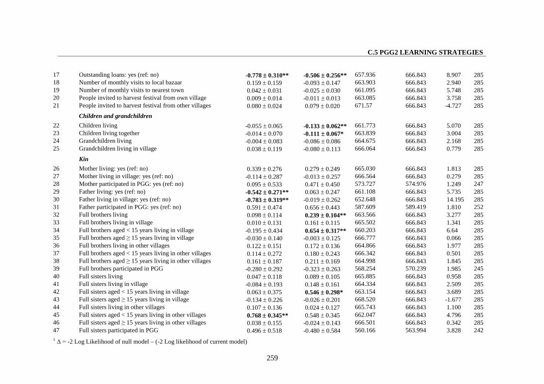
C.5 PGG2 LEARNING STRATEGIES
259
17 Outstanding loans: yes (ref: no) -0.778 0.310** -0.506 0.256** 657.936 666.843 8.907 28518 Number of monthly visits to local bazaar 0.159 0.159 -0.093 0.147 663.903 666.843 2.940 28519 Number of monthly visits to nearest town 0.042 0.031 -0.025 0.030 661.095 666.843 5.748 28520 People invited to harvest festival from own village 0.009 0.014 -0.011 0.013 663.085 666.843 3.758 28521 People invited to harvest festival from other villages 0.080 0.024 0.079 0.020 671.57 666.843 -4.727 285
Children and grandchildren
22 Children living -0.055 0.065 -0.133 0.062** 661.773 666.843 5.070 28523 Children living together -0.014 0.070 -0.111 0.067* 663.839 666.843 3.004 28524 Grandchildren living -0.004 0.083 -0.086 0.086 664.675 666.843 2.168 28525 Grandchildren living in village 0.038 0.119 -0.080 0.113 666.064 666.843 0.779 285
Kin
26 Mother living: yes (ref: no) 0.339 0.276 0.279 0.249 665.030 666.843 1.813 28527 Mother living in village: yes (ref: no) -0.114 0.287 -0.013 0.257 666.564 666.843 0.279 28528 Mother participated in PGG: yes (ref: no) 0.095 0.533 0.471 0.450 573.727 574.976 1.249 24729 Father living: yes (ref: no) -0.542 0.271** 0.063 0.247 661.108 666.843 5.735 28530 Father living in village: yes (ref: no) -0.783 0.319** -0.019 0.262 652.648 666.843 14.195 28531 Father participated in PGG: yes (ref: no) 0.591 0.474 0.656 0.443 587.609 589.419 1.810 25232 Full brothers living 0.098 0.114 0.239 0.104** 663.566 666.843 3.277 28533 Full brothers living in village 0.010 0.131 0.161 0.115 665.502 666.843 1.341 28534 Full brothers aged < 15 years living in village -0.195 0.434 0.654 0.317** 660.203 666.843 6.64 28535 Full brothers aged ≥ 15 years living in village -0.030 0.140 -0.003 0.125 666.777 666.843 0.066 28536 Full brothers living in other villages 0.122 0.151 0.172 0.136 664.866 666.843 1.977 28537 Full brothers aged < 15 years living in other villages 0.114 0.272 0.180 0.243 666.342 666.843 0.501 28538 Full brothers aged ≥ 15 years living in other villages 0.161 0.187 0.211 0.169 664.998 666.843 1.845 28539 Full brothers participated in PGG -0.280 0.292 -0.323 0.263 568.254 570.239 1.985 24540 Full sisters living 0.047 0.118 0.089 0.105 665.885 666.843 0.958 28541 Full sisters living in village -0.084 0.193 0.148 0.161 664.334 666.843 2.509 28542 Full sisters aged < 15 years living in village 0.063 0.375 0.546 0.298* 663.154 666.843 3.689 28543 Full sisters aged ≥ 15 years living in village -0.134 0.226 -0.026 0.201 668.520 666.843 -1.677 28544 Full sisters living in other villages 0.107 0.136 0.024 0.127 665.743 666.843 1.100 28545 Full sisters aged < 15 years living in other villages 0.768 0.345** 0.548 0.345 662.047 666.843 4.796 28546 Full sisters aged ≥ 15 years living in other villages 0.038 0.155 -0.024 0.143 666.501 666.843 0.342 28547 Full sisters participated in PGG 0.496 0.518 -0.480 0.584 560.166 563.994 3.828 242
1 Δ = -2 Log Likelihood of null model – (-2 Log likelihood of current model)
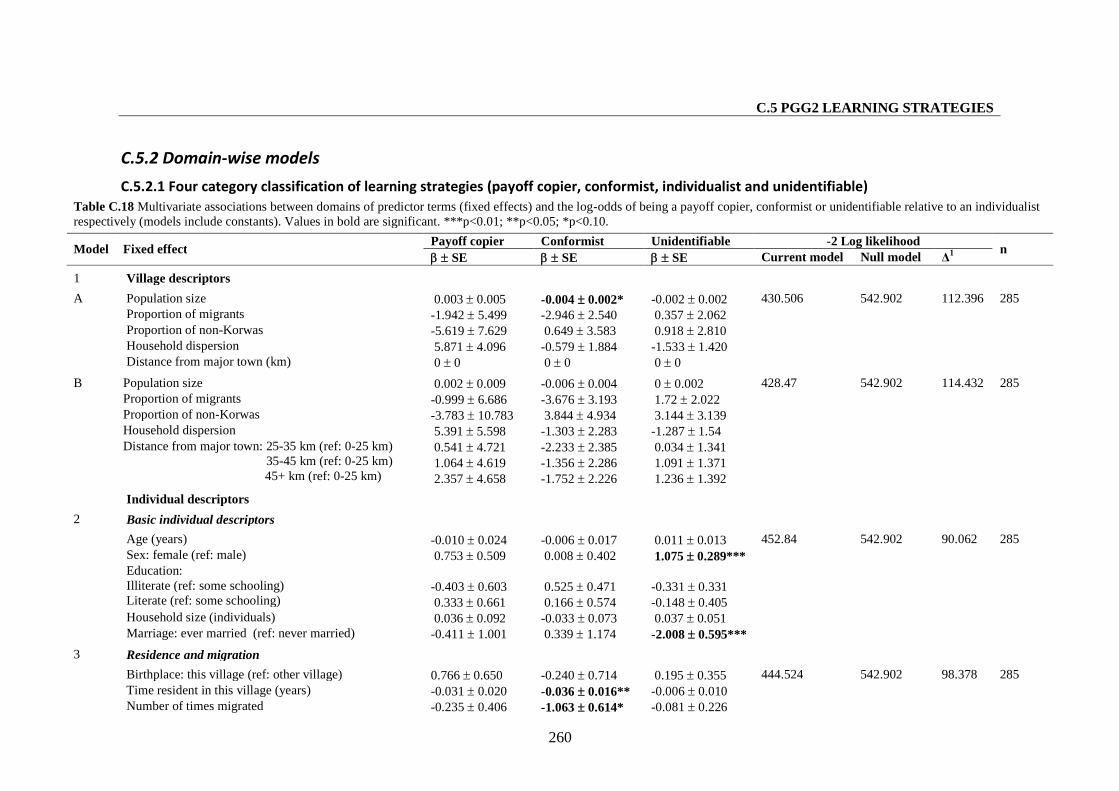
C.5 PGG2 LEARNING STRATEGIES
260
C.5.2 Domain-wise models
C.5.2.1 Four category classification of learning strategies (payoff copier, conformist, individualist and unidentifiable)
Table C.18 Multivariate associations between domains of predictor terms (fixed effects) and the log-odds of being a payoff copier, conformist or unidentifiable relative to an individualistrespectively (models include constants). Values in bold are significant. ***p<0.01; **p<0.05; *p<0.10.
Payoff copier Conformist Unidentifiable -2 Log likelihoodModel Fixed effect
SE SE SE Current model Null model Δ1 n
1 Village descriptors
Population size 0.003 0.005 -0.004 0.002* -0.002 0.002Proportion of migrants -1.942 5.499 -2.946 2.540 0.357 2.062Proportion of non-Korwas -5.619 7.629 0.649 3.583 0.918 2.810Household dispersion 5.871 4.096 -0.579 1.884 -1.533 1.420
A
Distance from major town (km) 0 0 0 0 0 0
430.506 542.902 112.396 285
Population size 0.002 0.009 -0.006 0.004 0 0.002Proportion of migrants -0.999 6.686 -3.676 3.193 1.72 2.022Proportion of non-Korwas -3.783 10.783 3.844 4.934 3.144 3.139Household dispersion 5.391 5.598 -1.303 2.283 -1.287 1.54
B
Distance from major town: 25-35 km (ref: 0-25 km)35-45 km (ref: 0-25 km)45+ km (ref: 0-25 km)
0.541 4.7211.064 4.6192.357 4.658
-2.233 2.385-1.356 2.286-1.752 2.226
0.034 1.3411.091 1.3711.236 1.392
428.47 542.902 114.432 285
Individual descriptors
Basic individual descriptors
Age (years) -0.010 0.024 -0.006 0.017 0.011 0.013Sex: female (ref: male) 0.753 0.509 0.008 0.402 1.075 0.289***Education:Illiterate (ref: some schooling)Literate (ref: some schooling)
-0.403 0.6030.333 0.661
0.525 0.4710.166 0.574
-0.331 0.331-0.148 0.405
Household size (individuals) 0.036 0.092 -0.033 0.073 0.037 0.051
2
Marriage: ever married (ref: never married) -0.411 1.001 0.339 1.174 -2.008 0.595***
452.84 542.902 90.062 285
Residence and migration
Birthplace: this village (ref: other village) 0.766 0.650 -0.240 0.714 0.195 0.355Time resident in this village (years) -0.031 0.020 -0.036 0.016** -0.006 0.010
3
Number of times migrated -0.235 0.406 -1.063 0.614* -0.081 0.226
444.524 542.902 98.378 285
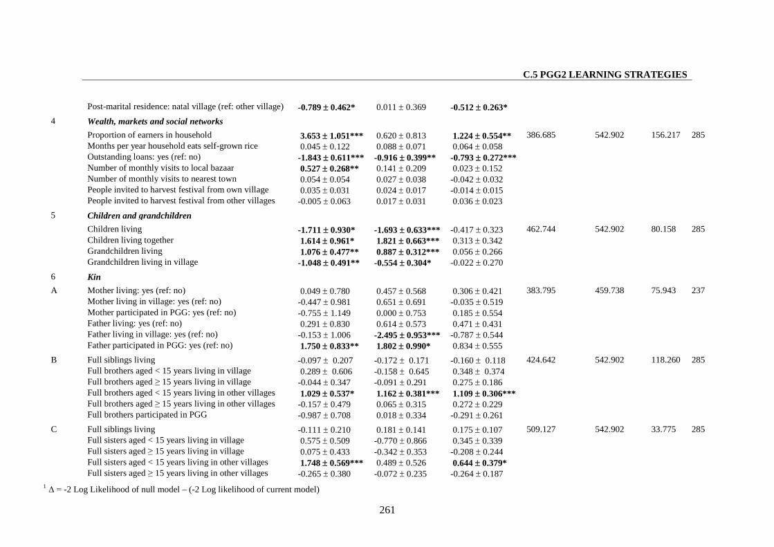
C.5 PGG2 LEARNING STRATEGIES
261
Post-marital residence: natal village (ref: other village) -0.789 0.462* 0.011 0.369 -0.512 0.263*
Wealth, markets and social networks
Proportion of earners in household 3.653 1.051*** 0.620 0.813 1.224 0.554**Months per year household eats self-grown rice 0.045 0.122 0.088 0.071 0.064 0.058Outstanding loans: yes (ref: no) -1.843 0.611*** -0.916 0.399** -0.793 0.272***Number of monthly visits to local bazaar 0.527 0.268** 0.141 0.209 0.023 0.152Number of monthly visits to nearest town 0.054 0.054 0.027 0.038 -0.042 0.032People invited to harvest festival from own village 0.035 0.031 0.024 0.017 -0.014 0.015
4
People invited to harvest festival from other villages -0.005 0.063 0.017 0.031 0.036 0.023
386.685 542.902 156.217 285
Children and grandchildren
Children living -1.711 0.930* -1.693 0.633*** -0.417 0.323Children living together 1.614 0.961* 1.821 0.663*** 0.313 0.342Grandchildren living 1.076 0.477** 0.887 0.312*** 0.056 0.266
5
Grandchildren living in village -1.048 0.491** -0.554 0.304* -0.022 0.270
462.744 542.902 80.158 285
6 Kin
Mother living: yes (ref: no) 0.049 0.780 0.457 0.568 0.306 0.421Mother living in village: yes (ref: no) -0.447 0.981 0.651 0.691 -0.035 0.519Mother participated in PGG: yes (ref: no) -0.755 1.149 0.000 0.753 0.185 0.554Father living: yes (ref: no) 0.291 0.830 0.614 0.573 0.471 0.431Father living in village: yes (ref: no) -0.153 1.006 -2.495 0.953*** -0.787 0.544
A
Father participated in PGG: yes (ref: no) 1.750 0.833** 1.802 0.990* 0.834 0.555
383.795 459.738 75.943 237
Full siblings living -0.097 0.207 -0.172 0.171 -0.160 0.118Full brothers aged < 15 years living in village 0.289 0.606 -0.158 0.645 0.348 0.374Full brothers aged ≥ 15 years living in village -0.044 0.347 -0.091 0.291 0.275 0.186Full brothers aged < 15 years living in other villages 1.029 0.537* 1.162 0.381*** 1.109 0.306***Full brothers aged ≥ 15 years living in other villages -0.157 0.479 0.065 0.315 0.272 0.229
B
Full brothers participated in PGG -0.987 0.708 0.018 0.334 -0.291 0.261
424.642 542.902 118.260 285
Full siblings living -0.111 0.210 0.181 0.141 0.175 0.107Full sisters aged < 15 years living in village 0.575 0.509 -0.770 0.866 0.345 0.339Full sisters aged ≥ 15 years living in village 0.075 0.433 -0.342 0.353 -0.208 0.244Full sisters aged < 15 years living in other villages 1.748 0.569*** 0.489 0.526 0.644 0.379*
C
Full sisters aged ≥ 15 years living in other villages -0.265 0.380 -0.072 0.235 -0.264 0.187
509.127 542.902 33.775 285
1 Δ = -2 Log Likelihood of null model – (-2 Log likelihood of current model)
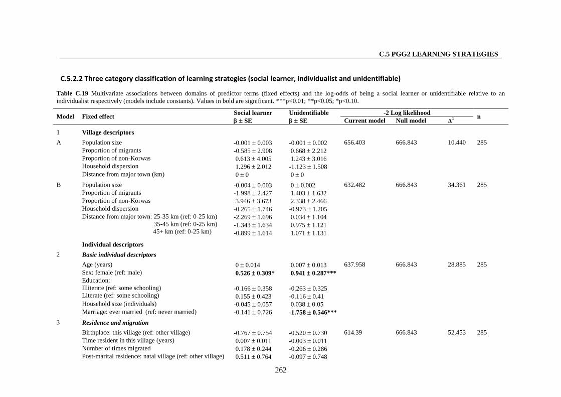
C.5 PGG2 LEARNING STRATEGIES
262
C.5.2.2 Three category classification of learning strategies (social learner, individualist and unidentifiable)
Table C.19 Multivariate associations between domains of predictor terms (fixed effects) and the log-odds of being a social learner or unidentifiable relative to anindividualist respectively (models include constants). Values in bold are significant. ***p<0.01; **p<0.05; *p<0.10.
-2 Log likelihoodModel Fixed effect
Social learner SE
Unidentifiable SE Current model Null model Δ1 n
1 Village descriptors
Population size -0.001 0.003 -0.001 0.002Proportion of migrants -0.585 2.908 0.668 2.212Proportion of non-Korwas 0.613 4.005 1.243 3.016Household dispersion 1.296 2.012 -1.123 1.508
A
Distance from major town (km) 0 0 0 0
656.403 666.843 10.440 285
Population size -0.004 0.003 0 0.002Proportion of migrants -1.998 2.427 1.403 1.632Proportion of non-Korwas 3.946 3.673 2.338 2.466Household dispersion -0.265 1.746 -0.973 1.205
B
Distance from major town: 25-35 km (ref: 0-25 km)35-45 km (ref: 0-25 km)45+ km (ref: 0-25 km)
-2.269 1.696-1.343 1.634
-0.899 1.614
0.034 1.1040.975 1.121
1.071 1.131
632.482 666.843 34.361 285
Individual descriptors
Basic individual descriptors
Age (years) 0 0.014 0.007 0.013Sex: female (ref: male) 0.526 0.309* 0.941 0.287***Education:Illiterate (ref: some schooling)Literate (ref: some schooling)
-0.166 0.3580.155 0.423
-0.263 0.325-0.116 0.41
Household size (individuals) -0.045 0.057 0.038 0.05
2
Marriage: ever married (ref: never married) -0.141 0.726 -1.758 0.546***
637.958 666.843 28.885 285
Residence and migration
Birthplace: this village (ref: other village) -0.767 0.754 -0.520 0.730Time resident in this village (years) 0.007 0.011 -0.003 0.011Number of times migrated 0.178 0.244 -0.206 0.286
3
Post-marital residence: natal village (ref: other village) 0.511 0.764 -0.097 0.748
614.39 666.843 52.453 285
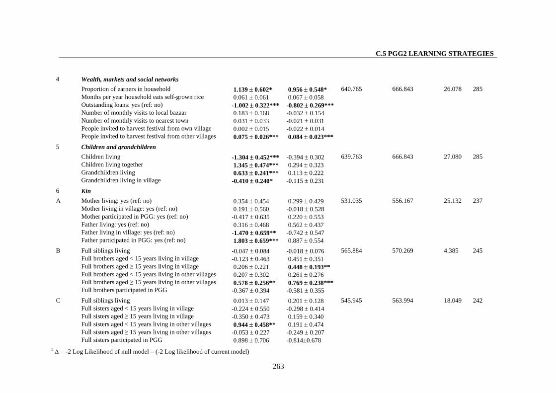
C.5 PGG2 LEARNING STRATEGIES
263
Wealth, markets and social networks
Proportion of earners in household 1.139 0.602* 0.956 0.548*Months per year household eats self-grown rice 0.061 0.061 0.067 0.058Outstanding loans: yes (ref: no) -1.002 0.322*** -0.802 0.269***Number of monthly visits to local bazaar 0.183 0.168 -0.032 0.154Number of monthly visits to nearest town 0.031 0.033 -0.021 0.031People invited to harvest festival from own village 0.002 0.015 -0.022 0.014
4
People invited to harvest festival from other villages 0.075 0.026*** 0.084 0.023***
640.765 666.843 26.078 285
Children and grandchildren
Children living -1.304 0.452*** -0.394 0.302Children living together 1.345 0.474*** 0.294 0.323Grandchildren living 0.633 0.241*** 0.113 0.222
5
Grandchildren living in village -0.410 0.240* -0.115 0.231
639.763 666.843 27.080 285
6 Kin
Mother living: yes (ref: no) 0.354 0.454 0.299 0.429Mother living in village: yes (ref: no) 0.191 0.560 -0.018 0.528Mother participated in PGG: yes (ref: no) -0.417 0.635 0.220 0.553Father living: yes (ref: no) 0.316 0.468 0.562 0.437Father living in village: yes (ref: no) -1.470 0.659** -0.742 0.547
A
Father participated in PGG: yes (ref: no) 1.803 0.659*** 0.887 0.554
531.035 556.167 25.132 237
Full siblings living -0.047 0.084 -0.018 0.076Full brothers aged < 15 years living in village -0.123 0.463 0.451 0.351Full brothers aged ≥ 15 years living in village 0.206 0.221 0.448 0.193**Full brothers aged < 15 years living in other villages 0.207 0.302 0.261 0.276Full brothers aged ≥ 15 years living in other villages 0.578 0.256** 0.769 0.238***
B
Full brothers participated in PGG -0.367 0.394 -0.581 0.355
565.884 570.269 4.385 245
Full siblings living 0.013 0.147 0.201 0.128Full sisters aged < 15 years living in village -0.224 0.550 -0.298 0.414Full sisters aged ≥ 15 years living in village -0.350 0.473 0.159 0.340Full sisters aged < 15 years living in other villages 0.944 0.458** 0.191 0.474Full sisters aged ≥ 15 years living in other villages -0.053 0.227 -0.249 0.207
C
Full sisters participated in PGG 0.898 0.706 -0.8140.678
545.945 563.994 18.049 242
1 Δ = -2 Log Likelihood of null model – (-2 Log likelihood of current model)
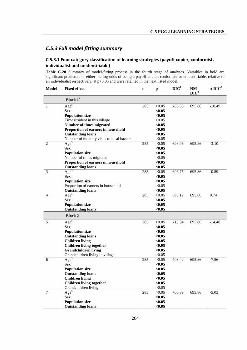
C.5 PGG2 LEARNING STRATEGIES
264
C.5.3 Full model fitting summary
C.5.3.1 Four category classification of learning strategies (payoff copier, conformist,individualist and unidentifiable)
Table C.20 Summary of model-fitting process in the fourth stage of analyses. Variables in bold aresignificant predictors of either the log-odds of being a payoff copier, conformist or unidentifiable, relative toan individualist respectively, at p<0.05 and were retained in the next listed model.
Model Fixed effect n p DIC1 NMDIC2
Δ DIC3
Block 14
1 Age5
SexPopulation sizeTime resident in this villageNumber of times migratedProportion of earners in householdOutstanding loansNumber of monthly visits to local bazaar
285 >0.05<0.05<0.05>0.05<0.05<0.05<0.05>0.05
706.35 695.86 -10.49
2 Age5
SexPopulation sizeNumber of times migratedProportion of earners in householdOutstanding loans
285 >0.05<0.05<0.05>0.05<0.05<0.05
698.96 695.86 -3.10
3 Age5
SexPopulation sizeProportion of earners in householdOutstanding loans
285 >0.05<0.05<0.05>0.05<0.05
696.75 695.86 -0.89
4 Age5
SexPopulation sizeOutstanding loans
285 >0.05<0.05<0.05<0.05
695.12 695.86 0.74
Block 2
5 Age5
SexPopulation sizeOutstanding loansChildren livingChildren living togetherGrandchildren livingGrandchildren living in village
285 >0.05<0.05<0.05<0.05<0.05<0.05<0.05>0.05
710.34 695.86 -14.48
6 Age5
SexPopulation sizeOutstanding loansChildren livingChildren living togetherGrandchildren living
285 >0.05<0.05<0.05<0.05<0.05<0.05>0.05
703.42 695.86 -7.56
7 Age5
SexPopulation sizeOutstanding loans
285 >0.05<0.05<0.05<0.05
700.89 695.86 -5.03
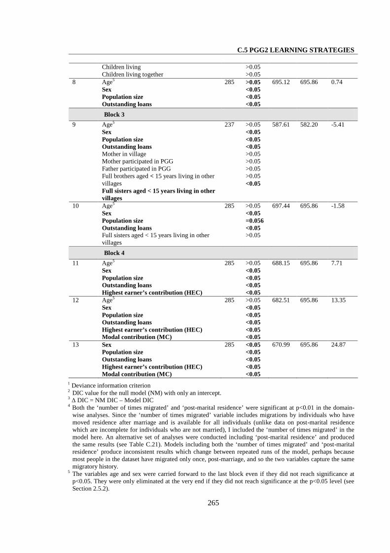
C.5 PGG2 LEARNING STRATEGIES
265
Children livingChildren living together
>0.05>0.05
8 Age5
SexPopulation sizeOutstanding loans
285 >0.05<0.05<0.05<0.05
695.12 695.86 0.74
Block 3
9 Age5
SexPopulation sizeOutstanding loansMother in villageMother participated in PGGFather participated in PGGFull brothers aged < 15 years living in othervillagesFull sisters aged < 15 years living in othervillages
237 >0.05<0.05<0.05<0.05>0.05>0.05>0.05>0.05<0.05
587.61 582.20 -5.41
10 Age5
SexPopulation sizeOutstanding loansFull sisters aged < 15 years living in othervillages
285 >0.05<0.05=0.056<0.05>0.05
697.44 695.86 -1.58
Block 4
11 Age5
SexPopulation sizeOutstanding loansHighest earner’s contribution (HEC)
285 >0.05<0.05<0.05<0.05<0.05
688.15 695.86 7.71
12 Age5
SexPopulation sizeOutstanding loansHighest earner’s contribution (HEC)Modal contribution (MC)
285 >0.05<0.05<0.05<0.05<0.05<0.05
682.51 695.86 13.35
13 SexPopulation sizeOutstanding loansHighest earner’s contribution (HEC)Modal contribution (MC)
285 <0.05<0.05<0.05<0.05<0.05
670.99 695.86 24.87
1 Deviance information criterion2 DIC value for the null model (NM) with only an intercept.3 Δ DIC = NM DIC – Model DIC4 Both the ‘number of times migrated’ and ‘post-marital residence’ were significant at p<0.01 in the domain-
wise analyses. Since the ‘number of times migrated’ variable includes migrations by individuals who havemoved residence after marriage and is available for all individuals (unlike data on post-marital residencewhich are incomplete for individuals who are not married), I included the ‘number of times migrated’ in themodel here. An alternative set of analyses were conducted including ‘post-marital residence’ and producedthe same results (see Table C.21). Models including both the ‘number of times migrated’ and ‘post-maritalresidence’ produce inconsistent results which change between repeated runs of the model, perhaps becausemost people in the dataset have migrated only once, post-marriage, and so the two variables capture the samemigratory history.
5 The variables age and sex were carried forward to the last block even if they did not reach significance atp<0.05. They were only eliminated at the very end if they did not reach significance at the p<0.05 level (seeSection 2.5.2).
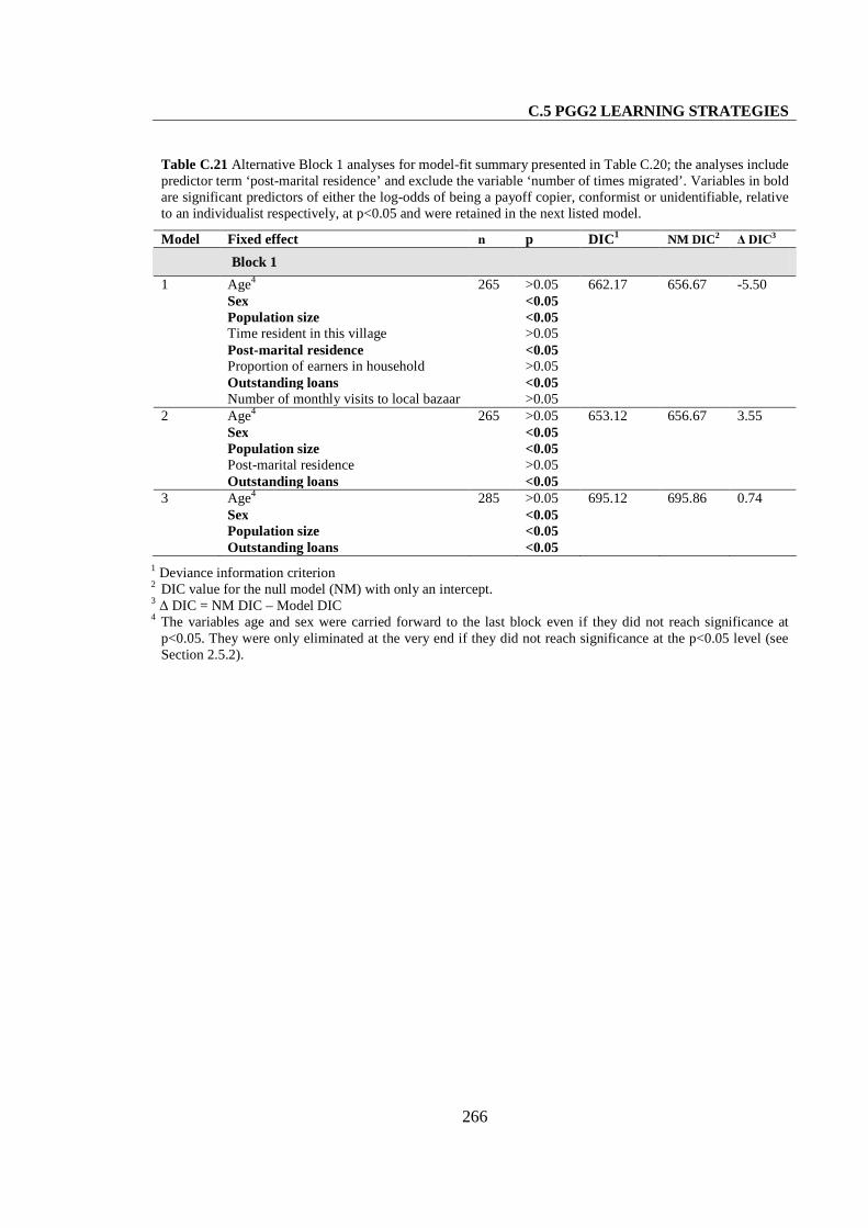
C.5 PGG2 LEARNING STRATEGIES
266
Table C.21 Alternative Block 1 analyses for model-fit summary presented in Table C.20; the analyses includepredictor term ‘post-marital residence’ and exclude the variable ‘number of times migrated’. Variables in boldare significant predictors of either the log-odds of being a payoff copier, conformist or unidentifiable, relativeto an individualist respectively, at p<0.05 and were retained in the next listed model.
Model Fixed effect n p DIC1 NM DIC2 Δ DIC3
Block 1
1 Age4
SexPopulation sizeTime resident in this villagePost-marital residenceProportion of earners in householdOutstanding loansNumber of monthly visits to local bazaar
265 >0.05<0.05<0.05>0.05<0.05>0.05<0.05>0.05
662.17 656.67 -5.50
2 Age4
SexPopulation sizePost-marital residenceOutstanding loans
265 >0.05<0.05<0.05>0.05<0.05
653.12 656.67 3.55
3 Age4
SexPopulation sizeOutstanding loans
285 >0.05<0.05<0.05<0.05
695.12 695.86 0.74
1 Deviance information criterion2 DIC value for the null model (NM) with only an intercept.3 Δ DIC = NM DIC – Model DIC4 The variables age and sex were carried forward to the last block even if they did not reach significance at
p<0.05. They were only eliminated at the very end if they did not reach significance at the p<0.05 level (seeSection 2.5.2).
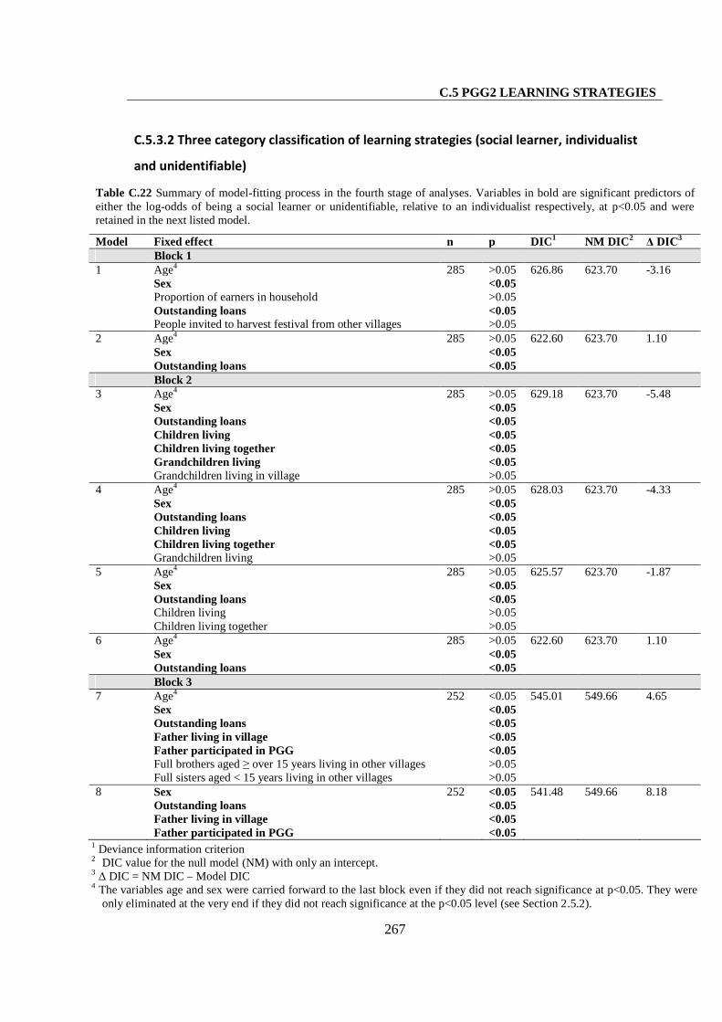
C.5 PGG2 LEARNING STRATEGIES
267
C.5.3.2 Three category classification of learning strategies (social learner, individualist
and unidentifiable)
Table C.22 Summary of model-fitting process in the fourth stage of analyses. Variables in bold are significant predictors ofeither the log-odds of being a social learner or unidentifiable, relative to an individualist respectively, at p<0.05 and wereretained in the next listed model.
Model Fixed effect n p DIC1 NM DIC2 Δ DIC3
Block 11 Age4
SexProportion of earners in householdOutstanding loansPeople invited to harvest festival from other villages
285 >0.05<0.05>0.05<0.05>0.05
626.86 623.70 -3.16
2 Age4
SexOutstanding loans
285 >0.05<0.05<0.05
622.60 623.70 1.10
Block 23 Age4
SexOutstanding loansChildren livingChildren living togetherGrandchildren livingGrandchildren living in village
285 >0.05<0.05<0.05<0.05<0.05<0.05>0.05
629.18 623.70 -5.48
4 Age4
SexOutstanding loansChildren livingChildren living togetherGrandchildren living
285 >0.05<0.05<0.05<0.05<0.05>0.05
628.03 623.70 -4.33
5 Age4
SexOutstanding loansChildren livingChildren living together
285 >0.05<0.05<0.05>0.05>0.05
625.57 623.70 -1.87
6 Age4
SexOutstanding loans
285 >0.05<0.05<0.05
622.60 623.70 1.10
Block 37 Age4
SexOutstanding loansFather living in villageFather participated in PGGFull brothers aged ≥ over 15 years living in other villagesFull sisters aged < 15 years living in other villages
252 <0.05<0.05<0.05<0.05<0.05>0.05>0.05
545.01 549.66 4.65
8 SexOutstanding loansFather living in villageFather participated in PGG
252 <0.05<0.05<0.05<0.05
541.48 549.66 8.18
1 Deviance information criterion2 DIC value for the null model (NM) with only an intercept.3 Δ DIC = NM DIC – Model DIC4 The variables age and sex were carried forward to the last block even if they did not reach significance at p<0.05. They were
only eliminated at the very end if they did not reach significance at the p<0.05 level (see Section 2.5.2).