The efficacy of TM satellite imagery for rapid assessment of Chihuahuan xeric habitat intactness for...

Journal of Arid Environments (2002) 52: 135–153doi:10.1006/jare.2001.0984, available online at http://www.idealibrary.com on

The efficacy of TM satellite imagery for rapidassessment of Chihuahuan xeric habitat intactness

for ecoregion-scale conservation planning

Thomas F. Allnutt%*, Wesley W. Wettengel%, Jesus Valdes Reynaw,Ricardo C. de Leon Garciaz, Eduardo E. Inigo Elias},

David M. Olson%

%Conservation Science Program, World Wildlife Fund, 1250 24th St., NW,Washington, DC 20037-1175, U.S.A.

wDepartamento de Botanica, Universidad Autonoma Agraria AntonioNarro, Buenavista, Saltillo, Coahuila, 25315, Mexico

zOaxaca 610, P.O. Box 38-C, Col. Republica Oriente, Saltillo,Coahuilla 25280, Mexico

}1743 Ellis Hollow Rd, Ithaca, NY 14850, U.S.A.

(Received 27 June 2001, accepted 12 December 2001)

A critical step in designing effective conservation landscapes is theidentification of relatively intact natural habitats. Satellite remote sensinghas been effectively used to distinguish relatively intact and degraded forestsat a number of scales. However, the utility of remote sensing data for rapidand cost-effective assessments of habitat intactness across large arid regionshas not been adequately tested. To this end, we tested the ability of TMimagery to rapidly discriminate different levels of habitat degradation acrosslarge regions of the Chihuahuan Desert. We were able to identify relativelyintact habitat in many cases. However, degraded habitat was oftenmisidentified as relatively intact. The use of both mid- and late-seasonimagery provides some improvement by highlighting phenological differencesamong the intactness classes. Overall, low vegetation cover and inter- andintra-seasonal variability diminish the utility of TM imagery for large-scaleconservation planning in the Chihuahuan Desert.

# 2002 Published by Elsevier Science Ltd.

Keywords: conservation planning; remote sensing; habitat intactness;Chihuahuan Desert

Introduction

The conservation community increasingly recognizes the distinctive and importantbiodiversity of deserts and other arid ecosystems (Olson & Dinerstein, 1998; Rickettset al., 1999; Dinerstein et al., 2000). Cost-effective planning tools are needed to help

*Corresponding author. E-mail: [email protected]

0140-1963/02/010135 + 19 $35.00/0 # 2002 Published by Elsevier Science Ltd.

136 T.F. ALLNUTT ET AL.

develop effective conservation strategies for deserts as these ecosystems facesignificant threats and we have limited time and resources for their conservation.Conservation planners require information on the distribution and extent of relativelyintact desert habitats across ecoregions to identify areas where populations of sensitivespecies and ecological phenomena are most likely to occur and where they have thebest chance for persistence. For example, large predators such as the jaguar (Pantheraonca) may be more likely to persist in areas where domestic livestock grazing has notreduced forage availability for native prey species, or where there is sufficient area ofnatural habitat to support a viable population over the long term (Sanderson et al., inpress). Some rare cacti or plant communities may only survive in areas that have notbeen exposed to extensive trampling by livestock (Anderson et al., 1994). In addition,these relatively intact habitats may ultimately form the core of protected area networksand determine types of land use and restoration efforts necessary in different zones.For these reasons, a method to rapidly assess the intactness of non-forest habitats overwhole ecoregions would be an invaluable tool for conservation planning.

Remote sensing data have been used to measure intact and converted forests acrosslarge regions (Skole & Tucker, 1993; NASA, 1998). Detailed classification andground-truthing of imagery has also produced accurate habitat maps and assessmentsof habitat quality at individual sites in forest and non-forest ecosystems such asgrasslands, deserts, and coastal marine habitats (Sader et al., 1991; Kremer &Running, 1993; Lauver, 1997). However, the efficacy of remote sensing tools forrapidly assessing the relative intactness of non-forest habitats across entire ecoregions(50 000–300 000 km2) has not been tested, particularly within the context ofbiodiversity features rather than range conditions. Here we test the efficacy of acommonly used and widely available remote-sensing data source, Landsat ThematicMapper (TM), for rapidly mapping the relative intactness of two broad habitat typesin the Chihuahuan Desert over larger landscapes.

Previous methods used for mapping xeric habitat intactness

Satellite-borne remote sensing has a long history of application to arid-landsecological research (Tueller, 1987). Previous workers have utilized numerous sensors,including the advanced very high resolution radiometer (AVHRR), for measuringdesert spatial extent (Tucker & Justice, 1986), monitoring desertification (Tucker etal., 1991), mapping vegetation (Kremer & Running, 1993; Peters et al., 1997),vegetation change over time (Warren & Hutchinson, 1984), and habitat degredation(Eve, 1995). AVHRR’s high temporal resolution and coarse spatial resolution enableone to frequently image large areas with relatively low data volume. However, itscoarse spatial resolution (1?1 km pixel as opposed to 30 m for Landsat TM) make itless suitable for measuring fine-scale land-cover changes resulting from overgrazingand loss of riparian habitats, significant factors leading to habitat degradation andbiodiversity loss in xeric environments.

Others have used high-resolution satellite data to map plant communities at the sitelevel (Franklin et al., 1993), to map grassland species diversity (Lauver, 1997), and toidentify ‘natural’ grassland areas (Lauver & Whistler, 1993) in a single county inKansas. These studies demonstrate the utility of high-resolution sensors for vegetationmapping at local scales. Few studies exist, however, which test these applications atthe ecoregional scale. Brazilian Cerrado savannas have recently been mapped at largescales using a combination of TM and radar imagery (CABS, 2000), but thevegetative cover in this habitat is typically more pronounced than in deserts. Inaddition, few have approached arid-lands remote sensing research from a standpointof the intactness of native biotas and habitats, concentrating instead on ‘range’features, or in some cases ‘ecosystem health’ (Milton & Dean, 1996). Finally, xeric

ASSESSMENT OF RELATIVELY INTACT HABITAT IN THE CHIHUAHUAN DESERT 137

habitat loss is typically viewed in the context of increasing shrub-cover, ignoring thepotential occurrence of relatively intact, natural, desert-scrub communities.

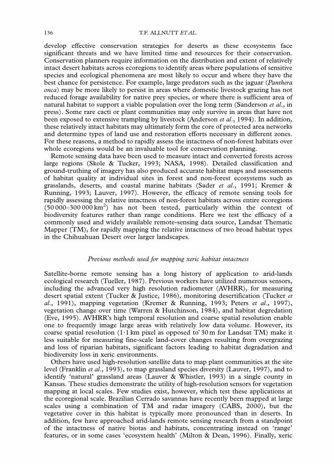
In the Chihuahuan Desert, few data exist to adequately categorize desert habitatintactness. Brown’s (1994) map broadly characterizes potential natural vegetationcommunities in the Southwestern United States and Northern Mexico. Otherresearch has coarsely characterized botanical features of the Chihuahuan desert( Johnston, 1977; Henrickson & Johnston, 1986). In another study, the InstitutoNacional de Estadıstica, Geografıa e Informatica (INEGI, 1998) used AVHRR,ground-truthing, and interpretation by regional experts to classify Mexico intoapproximately 180 land-cover classes. Within the Chihuahuan Desert, we categorizedthe descriptors for these 180 classes into three major intactness categories: heavilyaltered (e.g. urban or converted, agricultural), altered (i.e. degraded), and relativelyintact (i.e. natural to semi-natural habitats). Mapping these three intactness categoriesresults in extensive portions of the ecoregion being covered by the last category, whichmight be interpreted as relatively intact (Fig. 1). However, initial ground-truthing andconsultations with regional experts (Dinerstein et al., 2000) suggest that most of thearea covered under these categories is better classified as altered (degraded) to highlyaltered. Thus, this mapping effort has limited value for conservation planning, largelybecause habitat degradation and biodiversity features were not used or emphasized inthe classification process. Further, this classification also does not qualify as a rapidassessment analysis as it required several years and extensive resources to complete.

We asked regional experts at a Chihuahuan Desert conservation workshop(Dinerstein et al., 2000) to identify larger areas (50–500+ km2) within the ecoregionthat harbored particularly intact habitats and to evaluate the relative intactness ofdifferent priority areas (Fig. 1). The information provided by the experts was deemedaccurate and detailed for sites well known to individuals, and adequate for designingbroader conservation landscapes for certain priority areas. However, there was asufficient level of uncertainty regarding the existence or location of other relativelyintact natural habitats throughout the ecoregion to explore the possibility of rapidmapping of these habitats at the scale of whole basins and ranges using TM data.Some of the areas identified as intact by the experts are also likely to containheterogeneous landscapes of intact, altered (degraded), and highly altered habitats atfiner scales.

Defining intactness

We define relatively intact habitat as relatively undisturbed areas that still supportnatural ecological processes (e.g. disturbance regimes, seasonal movements of species)and harbor natural communities with most of the original assemblage of native speciespresent within their range of natural abundances. Altered habitats are more impactedby human disturbance but retain the potential to sustain native species and processes.Heavily altered habitat represents areas that have been degraded to the point ofretaining little or no potential value for biodiversity conservation without long-termand extensive restoration. As virtually all of the Chihuahuan desert has been altered insome way since the arrival of humans, there are no longer any truly intact areas.Therefore, this work can only consider the relative degradation of the habitats inquestion. Below we characterize each of these intactness levels in more detail for xericecosystems.

Relatively intact: The habitat has not been plowed, chained, or altered by majorchanges in hydrologic patterns. The full suite of native plant species is still present,each in abundance within its natural range of variation, and successional patternsfollow natural cycles (e.g. grazing by domestic livestock has not had a significantimpact on species compositions or seral stages). Natural fire regimes are still present.

Figure 1. Two sources of existing intactness data for Chihuahuan desert.


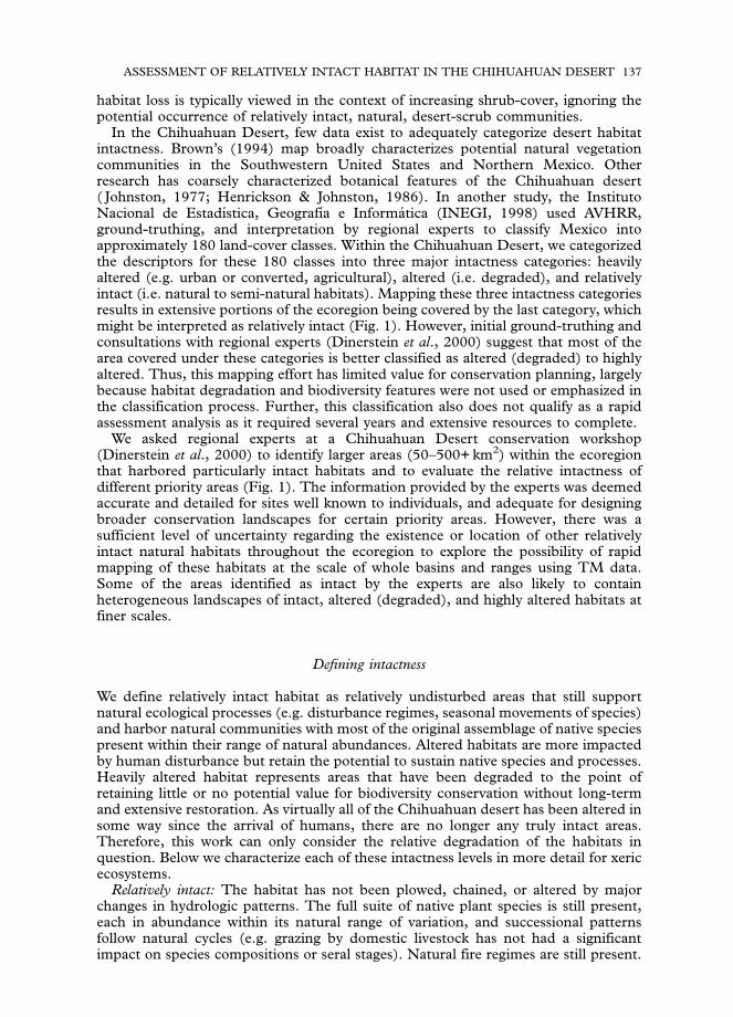
Although large mammal and bird populations may presently be absent from someblocks of habitat due to exploitation, insufficient area, or diminished resources, suchblocks may still sustain many native communities and populations of plant,invertebrate, and vertebrate species, as well as their associated ecological processes(Fig. 2(a,b)).

Altered (degraded ): Heavy grazing has altered dominance patterns of plant species.Some exotic species are present and surface water patterns may be altered, but thesubstrate has not been physically disturbed. Natural fire regimes have beensignificantly altered. Original habitat is likely to return with time, moderaterestoration, and adequate source pools of native species.

Heavily altered: Habitat is almost entirely altered by human development, plowing,chaining, and burning. Native species have been almost entirely replaced by exotics.

Figure 2. Examples of intact (a) and degraded (b) desert grassland (photos T. Allbutt).


Surface water patterns have been extensively altered. Natural fire regimes have beensignificantly altered. In some cases there can be total or near-total conversion of nativehabitat to human-dominated landscapes such as urban areas, settlements, andagricultural zones (Fig. 3(a,b)).

Specific ecological and physical features used to measure relative intactness at fieldsites are described under Methods and materials and in Table 3.

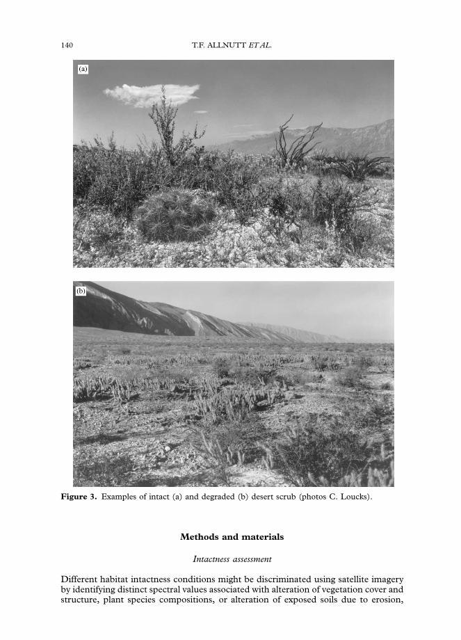
Figure 3. Examples of intact (a) and degraded (b) desert scrub (photos C. Loucks).


Methods and materials

Intactness assessment

Different habitat intactness conditions might be discriminated using satellite imageryby identifying distinct spectral values associated with alteration of vegetation cover andstructure, plant species compositions, or alteration of exposed soils due to erosion,


trampling, burning, or other forms of physical disturbance. Furthermore, varyinglevels of intactness may be evident seasonally, assuming that relatively intact anddegraded communities may exhibit different phenological responses over the course ofa growing season.

The key question for regional scale planning purposes is whether these data areeffective predictors from one area to another despite potential spectral variationcaused by differences in bedrock, soil types, soil moisture, soil features, erosionfeatures, topography, season, sun-angle, aspect, and view-angle. We know satelliteinformation can be useful for assessing variation in habitat intactness for differenthabitat types within sites (areas ranging from several kilometers to 100 km2) withextensive ground-truthing and manual image manipulation. But does the predictivevalue of these classifications hold when applied across whole basins, multiple basins,or entire desert ecoregions? The significance of confounding variables is likely toincrease at broader scales as the range of biophysical features and ecologicalconditions expands beyond that experienced by single sites and as the grain of theanalysis becomes coarser.

This study tests the predictive value of TM for assessing relative habitatintactness for multiple sites across several basins. We focused on two wide-spread and important habitat types of the Chihuahuan Desert, desert grasslandand desert scrub, in order to reduce the influence of habitat type on satelliteresponse.

Desert grasslands and scrub

Middle and lower elevation communities in the Chihuahuan Desert can bebroadly categorized into two types: desert grasslands and desert scrubs.Desert and semi-desert grasslands once dominated many Chihuahuan basins withdesert scrub on the margins and hillsides. These formerly extensive grasslandssupport a rich fauna of herbivores and predators, including pronghorn (Antilocapraamericana), black-tailed and Mexican prairie dog (Cynomys ludovicianus andC. mexicanus) colonies, various small predators, and now-extirpated wolves(Canis lupus), bison (Bison bison), and brown or Mexican grizzly (Ursus arctos) bears(Wilson & Ruff, 1999). Most basins are now dominated by ‘disclimax’ desertscrub (Brown, 1994) due to centuries of degradation. Native desert scrubcommunities often contain a significant grass component. Where they are relativelyundisturbed they often host diverse plant communities with many local endemicsrestricted to single basins or even hillsides, particularly for cacti (Hernandez &Barcenas, 1995, 1996).

Methods for assessing the value of TM data for mapping relative habitat intactness

We utilized two approaches for testing the relationship between the TM imagery andthe field-derived intactness data: image classification of single-date imagery, and ananalysis of early- and late-season image ratios.

Image classification of single-date imagery

The first method employed relatively standard image classification methods in orderto develop predictive maps of relatively intact habitat, by extrapolation from ourknown study areas. The results were then tested using accuracy assessments of theresulting maps, as well as field checking of predicted relatively intact sites. All of theprocessing was performed using PCI’s EASI/PACE and Imageworks software (Silicon


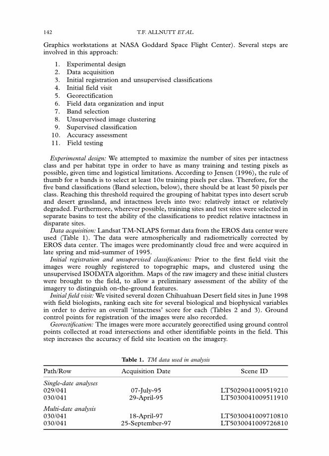
Graphics workstations at NASA Goddard Space Flight Center). Several steps areinvolved in this approach:

1. Experimental design

2. Data acquisition

3. Initial registration and unsupervised classifications

4. Initial field visit

5. Georectification

6. Field data organization and input

7. Band selection

8. Unsupervised image clustering

9. Supervised classification

10. Accuracy assessment

11. Field testing

Experimental design: We attempted to maximize the number of sites per intactnessclass and per habitat type in order to have as many training and testing pixels aspossible, given time and logistical limitations. According to Jensen (1996), the rule ofthumb for n bands is to select at least 10n training pixels per class. Therefore, for thefive band classifications (Band selection, below), there should be at least 50 pixels perclass. Reaching this threshold required the grouping of habitat types into desert scruband desert grassland, and intactness levels into two: relatively intact or relativelydegraded. Furthermore, wherever possible, training sites and test sites were selected inseparate basins to test the ability of the classifications to predict relative intactness indisparate sites.

Data acquisition: Landsat TM-NLAPS format data from the EROS data center wereused (Table 1). The data were atmospherically and radiometrically corrected byEROS data center. The images were predominantly cloud free and were acquired inlate spring and mid-summer of 1995.

Initial registration and unsupervised classifications: Prior to the first field visit theimages were roughly registered to topographic maps, and clustered using theunsupervised ISODATA algorithm. Maps of the raw imagery and these initial clusterswere brought to the field, to allow a preliminary assessment of the ability of theimagery to distinguish on-the-ground features.

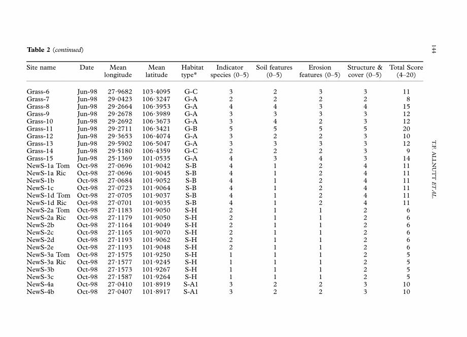
Initial field visit: We visited several dozen Chihuahuan Desert field sites in June 1998with field biologists, ranking each site for several biological and biophysical variablesin order to derive an overall ‘intactness’ score for each (Tables 2 and 3). Groundcontrol points for registration of the images were also recorded.

Georectification: The images were more accurately georectified using ground controlpoints collected at road intersections and other identifiable points in the field. Thisstep increases the accuracy of field site location on the imagery.

Table 1. TM data used in analysis

Path/Row Acquisition Date Scene ID

Single-date analyses029/041 07-July-95 LT5029041009519210030/041 29-April-95 LT5030041009511910

Multi-date analysis030/041 18-April-97 LT5030041009710810030/041 25-September-97 LT5030041009726810

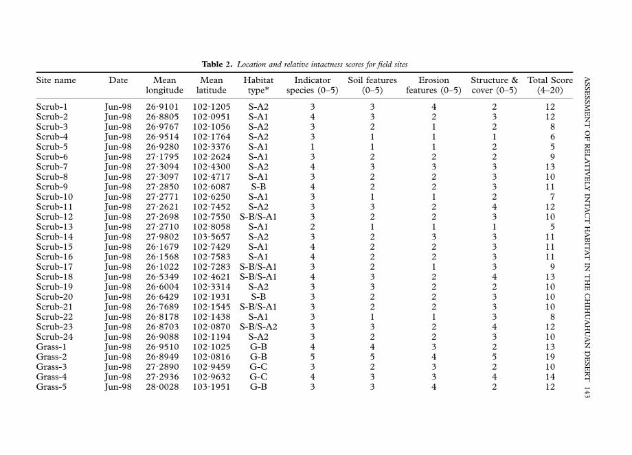
Table 2. Location and relative intactness scores for field sites

Site name Date Meanlongitude

Meanlatitude

Habitattype*

Indicatorspecies (0–5)

Soil features(0–5)

Erosionfeatures (0–5)

Structure &cover (0–5)

Total Score(4–20)

Scrub-1 Jun-98 26?9101 102?1205 S-A2 3 3 4 2 12Scrub-2 Jun-98 26?8805 102?0951 S-A1 4 3 2 3 12Scrub-3 Jun-98 26?9767 102?1056 S-A2 3 2 1 2 8Scrub-4 Jun-98 26?9514 102?1764 S-A2 3 1 1 1 6Scrub-5 Jun-98 26?9280 102?3376 S-A1 1 1 1 2 5Scrub-6 Jun-98 27?1795 102?2624 S-A1 3 2 2 2 9Scrub-7 Jun-98 27?3094 102?4300 S-A2 4 3 3 3 13Scrub-8 Jun-98 27?3097 102?4717 S-A1 3 2 2 3 10Scrub-9 Jun-98 27?2850 102?6087 S-B 4 2 2 3 11Scrub-10 Jun-98 27?2771 102?6250 S-A1 3 1 1 2 7Scrub-11 Jun-98 27?2621 102?7452 S-A2 3 3 2 4 12Scrub-12 Jun-98 27?2698 102?7550 S-B/S-A1 3 2 2 3 10Scrub-13 Jun-98 27?2710 102?8058 S-A1 2 1 1 1 5Scrub-14 Jun-98 27?9802 103?5657 S-A2 3 2 3 3 11Scrub-15 Jun-98 26?1679 102?7429 S-A1 4 2 2 3 11Scrub-16 Jun-98 26?1568 102?7583 S-A1 4 2 2 3 11Scrub-17 Jun-98 26?1022 102?7283 S-B/S-A1 3 2 1 3 9Scrub-18 Jun-98 26?5349 102?4621 S-B/S-A1 4 3 2 4 13Scrub-19 Jun-98 26?6004 102?3314 S-A2 3 3 2 2 10Scrub-20 Jun-98 26?6429 102?1931 S-B 3 2 2 3 10Scrub-21 Jun-98 26?7689 102?1545 S-B/S-A1 3 2 2 3 10Scrub-22 Jun-98 26?8178 102?1438 S-A1 3 1 1 3 8Scrub-23 Jun-98 26?8703 102?0870 S-B/S-A2 3 3 2 4 12Scrub-24 Jun-98 26?9088 102?1194 S-A2 3 2 2 3 10Grass-1 Jun-98 26?9510 102?1025 G-B 4 4 3 2 13Grass-2 Jun-98 26?8949 102?0816 G-B 5 5 4 5 19Grass-3 Jun-98 27?2890 102?9459 G-C 3 2 3 2 10Grass-4 Jun-98 27?2936 102?9632 G-C 4 3 3 4 14Grass-5 Jun-98 28?0028 103?1951 G-B 3 3 4 2 12

AS

SE

SS

ME

NT

OF

RE

LA

TIV

EL

YIN

TA

CT

HA

BIT

AT

INT

HE

CH

IHU

AH

UA

ND

ES

ER

T143

Grass-6 Jun-98 27?9682 103?4095 G-C 3 2 3 3 11Grass-7 Jun-98 29?0423 106?3247 G-A 2 2 2 2 8Grass-8 Jun-98 29?2664 106?3953 G-A 4 4 3 4 15Grass-9 Jun-98 29?2678 106?3989 G-A 3 3 3 3 12Grass-10 Jun-98 29?2692 106?3673 G-A 3 4 2 3 12Grass-11 Jun-98 29?2711 106?3421 G-B 5 5 5 5 20Grass-12 Jun-98 29?3653 106?4074 G-A 3 2 2 3 10Grass-13 Jun-98 29?5902 106?5047 G-A 3 3 3 3 12Grass-14 Jun-98 29?5180 106?4359 G-C 2 2 2 3 9Grass-15 Jun-98 25?1369 101?0535 G-A 4 3 4 3 14NewS-1a Tom Oct-98 27?0696 101?9042 S-B 4 1 2 4 11NewS-1a Ric Oct-98 27?0696 101?9045 S-B 4 1 2 4 11NewS-1b Oct-98 27?0684 101?9052 S-B 4 1 2 4 11NewS-1c Oct-98 27?0723 101?9064 S-B 4 1 2 4 11NewS-1d Tom Oct-98 27?0705 101?9037 S-B 4 1 2 4 11NewS-1d Ric Oct-98 27?0701 101?9035 S-B 4 1 2 4 11NewS-2a Tom Oct-98 27?1183 101?9050 S-H 2 1 1 2 6NewS-2a Ric Oct-98 27?1179 101?9050 S-H 2 1 1 2 6NewS-2b Oct-98 27?1164 101?9049 S-H 2 1 1 2 6NewS-2c Oct-98 27?1165 101?9070 S-H 2 1 1 2 6NewS-2d Oct-98 27?1193 101?9062 S-H 2 1 1 2 6NewS-2e Oct-98 27?1193 101?9048 S-H 2 1 1 2 6NewS-3a Tom Oct-98 27?1575 101?9250 S-H 1 1 1 2 5NewS-3a Ric Oct-98 27?1577 101?9245 S-H 1 1 1 2 5NewS-3b Oct-98 27?1573 101?9267 S-H 1 1 1 2 5NewS-3c Oct-98 27?1587 101?9264 S-H 1 1 1 2 5NewS-4a Oct-98 27?0410 101?8919 S-A1 3 2 2 3 10NewS-4b Oct-98 27?0407 101?8917 S-A1 3 2 2 3 10


Meanlatitude

Habitattype*





Total Score(4–20)

Table 2 (continued)

144

T.F

.A

LL

NU

TT

ET

AL

.

NewS-4c Oct-98 27?0425 101?8919 S-A1 3 2 2 3 10NewS-5a Tom Oct-98 26?8605 102?0755 S-A1 3 1 2 3 9NewS-5a Ric Oct-98 26?8602 102?0744 S-A1 3 1 2 3 9NewS-5b Oct-98 26?8583 102?0755 S-A1 3 1 2 3 9NewS-5c Oct-98 26?8603 102?0757 S-A1 3 1 2 3 9NewS-6a Tom Oct-98 26?8493 101?0703 S-A1 4 1 1 4 10NewS-6a Ric Oct-98 26?8493 101?0704 S-A1 4 1 1 4 10NewS-6b Oct-98 26?8477 101?0713 S-A1 4 1 1 4 10NewS-6c Oct-98 26?8464 101?0711 S-A1 4 1 1 4 10NewS-6d Oct-98 26?8482 101?0695 S-A1 4 1 1 4 10NewS-7a Tom Oct-98 26?8308 102?0599 S-A2 4 2 3 4 13NewS-7a Ric Oct-98 26?8303 102?0648 S-A2 4 2 3 4 13NewS-7b Oct-98 26?8302 102?0605 S-A2 4 2 3 4 13NewS-8a Tom Oct-98 26?9819 102?0990 S-A2 1 1 1 2 5NewS-8a Ric Oct-98 26?9813 102?0993 S-A2 1 1 1 2 5NewS-8b Oct-98 26?9835 102?1004 S-A2 1 1 1 2 5NewS-8c Oct-98 26?9800 102?1005 S-A2 1 1 1 2 5NewS-9 Oct-98 27?0521 102?2251 S-A1 2 2 1 2 7NewS-10a Oct-98 27?3077 102?4616 S-A1 3 2 2 2 9NewS-10b Oct-98 27?3080 102?4604 S-A1 3 2 2 2 9NewS-10c Oct-98 27?3087 102?4613 S-A1 3 2 2 2 9NewS-10d Oct-98 27?3085 102?4612 S-A1 3 2 2 2 9NewS-10e Oct-98 27?3077 102?4622 S-A1 3 2 2 2 9NewG-1a Oct-98 27?2610 102?6661 G-B 4?5 4?5 5 5 19NewG-1b Oct-98 27?2596 102?6658 G-B 4?5 4?5 5 5 19NewG-1c Oct-98 27?2609 102?6666 G-B 4?5 4?5 5 5 19NewG-1d Oct-98 27?2609 102?6666 G-B 4?5 4?5 5 5 19NewG-2a Oct-98 27?2864 102?9381 G-C 4 1 1 2 8NewG-2b Oct-98 27?2889 102?9386 G-C 4 1 1 2 8NewG-2c Oct-98 27?2885 102?9387 G-C 4 1 1 2 8NewG-3a Oct-98 27?4342 103?0486 G-B 5 1 4 3 13NewG-3b Oct-98 27?4359 103?0482 G-B 5 1 4 3 13NewG-3c Oct-98 27?4360 103?0474 G-B 5 1 4 3 13NewG-3d Oct-98 27?4353 103?0470 G-B 5 1 4 3 13

AS

SE

SS

ME

NT

OF

RE

LA

TIV

EL

YIN

TA

CT

HA

BIT

AT

INT

HE

CH

IHU

AH

UA

ND

ES

ER

T145

NewG-4a Oct-98 27?9662 103?4171 G-C 4 2 4 3 13NewG-4b Oct-98 27?9666 103?4178 G-C 4 2 4 3 13NewG-4c Oct-98 27?9664 103?4169 G-C 4 2 4 3 13NewG-5a Oct-98 28?0306 103?2167 G-B 5 1 3 2 11NewG-5b Oct-98 28?0243 103?2224 G-B 5 1 3 2 11NewG-5c Oct-98 28?0248 103?2232 G-B 5 1 3 2 11NewG-5d Oct-98 28?0258 103?2223 G-B 5 1 3 2 11NewG-6a Oct-98 28?0156 103?2191 G-B 4 1 4 3 12NewG-6b Oct-98 28?0145 103?2198 G-B 4 1 4 3 12NewG-6c Oct-98 28?0157 103?2202 G-B 4 1 4 3 12NewG-7 Oct-98 27?9907 103?1826 G-B 4 3 3 4 14Validation-1 Oct-98 27?2931 102?9597 G-C 3 1 2 2 8Validation-2 Oct-98 27?2944 102?9639 G-C 1 1 1 1 4Validation-3 Oct-98 27?3000 102?9611 G-C 3 2 3 2 10Validation-4 Oct-98 27?2944 102?9583 G-C 1 1 1 1 4Validation-5 Oct-98 27?2972 102?9639 G-C 3 1 2 2 8Validation-6 Oct-98 28?0000 103?2472 G-C 1 2 4 1 8Validation-7 Oct-98 28?0028 103?2472 G-C 1 2 4 1 8Validation-8 Oct-98 28?0000 103?2444 G-C 1 2 4 1 8Validation-9 Oct-98 27?9944 103?2417 G-C 1 1 4 1 7Validation-10 Oct-98 27?9917 103?2389 G-C 3 2 3 1 9

*Key to habitat types listed above: Desert scrub: S-A1FChihuahuan Desert scrub: Larrea scrub (gobernadora), S-A2FChihuahuan Desert scrub: mixed desert scrub(chaparillo), S-BFLechugilla scrub (lechugillal), S-HFsubmontane mattoral. Desert grassland: G-AFGramma grasslands (pastizal de grama o navajita), G-BFSacatongrassland (zacatonal), G-CFTobosa grassland (Pastizal de tobosa).


Meanlatitude

Habitattype*





Total Score(4–20)

Table 2 (continued)

146

T.F

.A

LL

NU

TT

ET

AL

.

Table 3. Field assessment of intactness features

The following feature categories (scores reported above) were evaluated at each site:K indicator plant species (indicator species)K presence of living soil crusts & plant litter (soil features)K absence of fire or grazing induced erosion features such as pedestals, rills, terraces,

mineral crusts, evident impact on plants (erosional features)K percentage ground cover of characteristic species (structure and cover)In each feature category, scores were developed from the following criteria:

Indicator native plant species and presence of introduced species3 or more native spp. 5 pointsPresence of 2 or more 3 pointsPresence of 1 1 point

Presence of living soil crusts & plant litterRelatively intact crust & litter 5 points50–75% intact 3 points25–49% intact 1 point

Grazing induced erosional features such as pedestals, rills, terraces, mineral crustsNo presence of features 5 pointsMedium level of features 3 pointsHigh level of features 1 point

Percentage ground cover of characteristic species75–100% 5 points50–75% 3 points25–50% 1 point

Points Intactness status

Total scores indicate the following intactness levels in a four-class scheme:0–4 Altered5–9 Degraded10–14 Partially degraded15–20 Relatively intact

These values were lumped into two classes for the purpose of classification:0–9 Relatively degraded10–20 Relatively intact

AS

SE

SS

ME

NT

OF

RE

LA

TIV

EL

YIN

TA

CT

HA

BIT

AT

INT

HE

CH

IHU

AH

UA

ND

ES

ER

T147


Field data organization and input: Field sites were georeferenced on the imagery andused as training sites for band selection and supervised classification. Because thereare few (generally o100) training pixels for each intactness class, all grass and scrubsites are therefore grouped together, and the mean intactness score used as thresholdsfor two intactness categories: relatively intact vs. relatively degraded.

Band selection: Discriminant analysis was used to identify the band combinationsbest able to separate the field-measured intactness scores. All raw bands (minus band6) plus several derived ratios, including principal components, brightness, greenness,normalized difference vegetation index (NDVI) and soil-adjusted vegetation index(SAVI), were tested in a set of standard combinations known to be useful fromprevious studies (Duncan et al., 1993; Lauver, 1997). For both the scrub and grasssites, the best separation was provided by bands 2 and 7, eigenvectors 1 and 2,brightness, and NDVI.

Unsupervised image clustering: Raw images were classified using the unsupervisedISODATA algorithm. These clusters were then assigned a value of grass, scrub, orneither, based on habitat information obtained during field testing. These clustersserved as masks during the supervised classification. This represents a primarydiscrimination of the data, essentially reducing the choices available for classificationin subsequent steps.

Supervised classification: Approximately two-thirds of the field data training sites(Table 2) were used to classify the image within the grass or scrub clusters created.The grass training data was used only under the grass mask, and the scrub data onlyunder the scrub mask. The result is a map of relatively intact/degraded scrub habitat,relatively intact/degraded grass habitat, or neither.

Accuracy assessment: Data from the remainder of the field sites was used to test theaccuracy of predicted intactness levels of the image classification (Table 1).

Field testing: In October 1998, we performed a field check of ten sites chosenrandomly within predicted intact areas (Fig. 4).

Analysis of early- and late-season imagery

Testing the hypothesis that we could use seasonality to better separate the variouslevels of intactness, we attempted to use seasonal changes evident in a spring vs. a fallimage in order to identify areas of relatively intact grass. To explore this relationship,regression analyses between the field-measured intactness and several image-derivedvariables were performed on several sets of spring and fall images of the same localities(Table 1). The regressions were of two types: between the field data and band radiancevalues, and between the field data and seasonal NDVI ratios. First, the digitalnumbers for bands 2–5 were converted to radiance values for both spring and fallimages. Radiance is a measurement of the electromagnetic energy received at thesensor, and thus is a more physical measurement of ground conditions than arethe digital numbers available in the image itself. Regressions were performed betweenthe radiance values and the field-measured intactness values.

Second, we performed regressions between the field-measured intactness and thefall-to-spring NDVI ratio. NDVI is a measurement of total photosynthetic activity(Tucker, 1979). NDVI has been used with the data from many different remote-sensing platforms, to assess everything from crop health and desertification, tomapping vegetation and deforestation (Justice et al., 1985; Tucker et al., 1985;Townshend et al., 1993). Generally, higher NDVI values indicate more activephotosynthesis in a given pixel. Grasses in xeric ecoregions are generally C4 plants,therefore they tend to green-up in the fall following the late-season monsoon rains. Indesert scrubs, however, C3 species are more common, and tend to be more green inthe spring. Therefore, a high fall-to-spring NDVI value might indicate a pixel that is

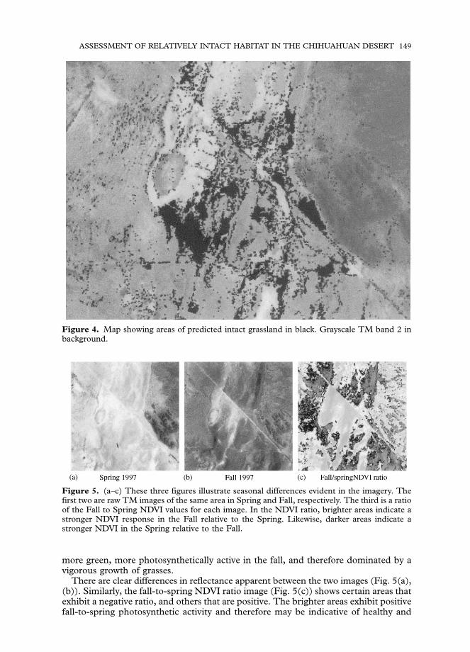
Figure 4. Map showing areas of predicted intact grassland in black. Grayscale TM band 2 inbackground.

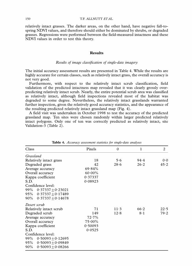
Figure 5. (a–c) These three figures illustrate seasonal differences evident in the imagery. Thefirst two are raw TM images of the same area in Spring and Fall, respectively. The third is a ratioof the Fall to Spring NDVI values for each image. In the NDVI ratio, brighter areas indicate astronger NDVI response in the Fall relative to the Spring. Likewise, darker areas indicate astronger NDVI in the Spring relative to the Fall.


more green, more photosynthetically active in the fall, and therefore dominated by avigorous growth of grasses.

There are clear differences in reflectance apparent between the two images (Fig. 5(a),(b)). Similarly, the fall-to-spring NDVI ratio image (Fig. 5(c)) shows certain areas thatexhibit a negative ratio, and others that are positive. The brighter areas exhibit positivefall-to-spring photosynthetic activity and therefore may be indicative of healthy and


relatively intact grasses. The darker areas, on the other hand, have negative fall-to-spring NDVI values, and therefore should either be dominated by shrubs, or degradedgrasses. Regressions were performed between the field-measured intactness and theseNDVI values in order to test this theory.

Results

Results of image classification of single-date imagery

The initial accuracy assessment results are presented in Table 4. While the results arehighly accurate for certain classes, such as relatively intact grass, the overall accuracy isnot very good.

Furthermore, with respect to the relatively intact scrub classification, fieldvalidation of the predicted intactness map revealed that it was clearly grossly over-predicting relatively intact scrub. Nearly, the entire potential scrub area was classifiedas relatively intact, although field inspections revealed most of the habitat wasdegraded to some degree. Nevertheless, the relatively intact grasslands warrantedfurther inspection, given the relatively good accuracy statistics, and the appearance ofthe resulting predicted relatively intact grassland map (Fig. 4).

A field visit was undertaken in October 1998 to test the accuracy of the predictedgrassland map. Ten sites were chosen randomly within larger predicted relativelyintact polygons. Only one of ten was correctly predicted as relatively intact, siteValidation-3 (Table 2).

Table 4. Accuracy assessment statistics for single-date analyses

Class Pixels 0 1 2

GrasslandRelatively intact grass 18 5?6 94?4 0?0Degraded grass 42 28?6 26?2 45?2Average accuracy 69?84%Overall accuracy 60?00%Kappa coefficient 0?37337S.D. 0?08923Confidence level:99% 0?3733770?2302195% 0?3733770?1748990% 0?3733770?14678

Desert scrubRelatively intact scrub 71 11?3 66?2 22?5Degraded scrub 149 12?8 8?1 79?2Average accuracy 72?7%Overall accuracy 75?00%Kappa coefficient 0?50093S.D. 0?0525Confidence level:99% 0?5009370?1269595% 0?5009370?0984990% 0?5009370?08266

Results of analysis of early- and late-season imagery


The regressions show that overall, the radiance values are not significantly correlatedwith the field-measured intactness (Figs 6 and 7). The only significant relationship isthat of the tobosa sites against the NDVI ratio (Fig. 7). This may be explained by theextensive growth and cover exhibited in this habitat type during the rainy season.

Discussion

TM data is known to be useful for characterizing desert habitat at the site level withextensive field verification. However, the results of this study suggest that TM data haslimited value as a rapid assessment tool for automated mapping of even grosscategories of intactness in desert habitats at scales ranging from sites, to basins, toentire ecoregions.

Several factors may explain why the variance in habitat intactness is not thedominant influence on the radiative response measured by the satellite. First,vegetation makes a low contribution to the overall reflectance of a given pixel due tolow crown cover, small size and number of leaves, and low moisture content of thevegetation itself (Franklin et al., 1993). Therefore, soil features, litter, and shadowbecome significant components of the radiative response. These factors lead to areduced relationship between green vegetation indices (NDVI, SAVI, greenness, etc.)and vegetation cover. Second, Chihuahuan soils are often bright, with reflectance incertain bands greater than that of the vegetation present. At the same time, there areextensive areas containing dark and volcanic soils which can have reflectances similarto that of healthy vegetation, particularly in the near-infrared band. Overall, variancein the pixel values is more often attributable to soil and geological features than tovegetation and habitat characteristics.

Third, seasonality is also an important issue, particularly for C4 dominatedcommunities that exhibit significant seasonal growth and inter-annual variability.Degraded sites may appear spectrally similar to those in senescence, or thoseexperiencing dry seasons or years. The reverse is also true. The dynamic nature ofthese communities, therefore, has significant implications for single-date mapping ofsites, and points to the need for using the most current imagery available.

For these reasons, predicting the relative intactness of large desert areas through arapid classification of Landsat TM data does not appear to be a cost-effective tool forconservation planning. Perhaps, new applications or advances of remote sensingtechnologies, or more detailed analyses of relationships among signatures, biodiversityfeatures, and relative intactness, will improve the utility of TM for rapid regional scaleconservation planning. Presently, conservation planning efforts may be better servedthrough a combination of visual interpretation of TM scenes for degradation featuressuch as roads and erosion halos around water sources and direct mapping incollaboration with regional experts. This conclusion does not diminish the value ofTM data for interpreting habitat types, relative intactness, and change at the level ofsites. However, its value is currently limited as a rapid and cost-effective assessmenttool for identifying larger blocks of relatively intact desert habitat at the scale of entirebasins and ecoregions.

This study is a collaborative effort between NASA’s Goddard Space Flight Center and EarthScience Enterprise Program, World Wildlife Fund, and The Nature Conservancy. We wouldlike to thank the following individuals and organizations for their support of this project: formerNASA Administrator Daniel Goldin, Woody Turner (NASA Earth Science Enterprise), TonyJanetos (World Resources Institute), Compton J. Tucker (Goddard Space Flight Center),Andrew Lynch (SSAI/GSFC), Jackie Kendall (SSAI/GSFC), Gary Bell (TNC New Mexico),


Esteban Muldavin (University of New Mexico/TNC New Mexico), Maria de la Luz (WWFMexico), INEGI, CONABIO and NASA/GSFC for providing data and technical support.Funding for this project was provided by the Earth Science Enterprise NASA/NGO/Museumsteering committee.

References

Anderson, E.F., Montes, S.A., Taylor, N.P. & Cattabriga, A. (1994). Threatened Cacti of Mexico.Kew: The Trustees of the Roayal Botanic Gardens.

Brown, D.E. (Ed.) (1994). Biotic Communities: Southwestern United States and NorthwesternMexico. Salt Lake City: University of Utah Press. 342 pp.

CABS. (2000). Designing Sustainable Landscapes: The Brazilian Atlantic Forest. Washington, DC:Center for Applied Biodiversity Science, Conservation International. 29 pp.

Dinerstein, E., Olson, D.M., Atchley, J., Loucks, C., Contreras-Balderas, S., Abell, R., Inigo, E.,Enkerlin, E., Williams, C.E. & Castilleja, G. (Eds) (2000). Ecoregion-based Conservation in theChihuahuan Desert: A Biological Assessment. Washington, DC: World Wildlife Fund, ComisıonNational para el Conocimiento y Uso de la Biodiversidad (CONABIO), The NatureConservancy, PRONATURA Noreste, and the Instituto Tecnologico y de Estudios Superioresde Monterrey (ITESM). 318 pp.

Duncan, J., Stow, D., Franklin, J. & Hope, A. (1993). Assessing the relationship between spectralvegetation indices and shrub cover in the Jornada Basin, New Mexico. International Journal ofRemote Sensing, 14: 3395–3416.

Eve, M.D. (1995). High temporal resolution analysis of land degradation in the northernChihuahuan Desert using satellite imagery. Ph.D. thesis, New Mexico State University, LasCruces, NM.

Franklin, J., Duncan, J. & Turner, D.L. (1993). Reflectance of vegetation and soil in ChihuahuanDesert plant communities from ground radiometry using SPOT wavebands. Remote Sensing ofEnvironment, 46: 291–304.

Henrickson, J. & Johnston, M.C. (1986). Vegetation and community types of the ChihuahuanDesert. In: Barlow, J.C., Powell, M.A. & Timmermann, B.N. (Eds), Invited Papers from theSecond Symposium on Resources of the Chihuahuan Desert U.S. and Mexico Region, pp. 20–39,Alpine, TX: Chihuahuan Desert Research Institute, 172 pp.

Hernandez, H.M. & Barcenas, R.T. (1995). Endangered cacti in the Chihuahuan Desert: I.Distribution patterns. Conservation Biology, 9: 1176–1188.

Hernandez, H.M. & Barcenas, R.T. (1996). Endangered cacti in the Chihuahuan Desert: II.Biogeography and conservation. Conservation Biology, 10: 1200–1209.

INEGI (1998). Landcover Map of Mexico: Draft Database. Mexico, DF, Mexico: InstitutoNacional de Estadıstica, Geografıa e Informatica.

Jensen, J.R. (1996). Introductory Digital Image Processing. Upper Saddle River, NJ: Prentice Hall.316 pp.

Johnston, M.C. (1977). Brief resume of botanical, including vegetation, features of theChihuahuan Desert region with special emphasis on their uniqueness. In: Wauer, R.H.& Riskind, D.H. (Eds), Transactions of the Symposium on the Biological Resources in theChihuahuan Desert Region, United States and Mexico, p. 6792. Washington: U.S. National ParkService. 658 pp.

Justice, C.O., Townshend, J.R.G., Holben, B.N. & Tucker, C.J. (1985). Analysis of thephenology of global vegetation using meteorological satellite data. International Journal ofRemote Sensing, 6: 1271–1318.

Kremer, R.G. & Running, S.W. (1993). Community type differentiation using NOAA/AVHRRdata within a sagebrush-steppe ecosystem. Remote Sensing of Environment, 46: 311–318.

Lauver, C.L. (1997). Mapping species diversity patterns in the Kansas shortgrass region byintegrating remote sensing and vegetation analysis. Journal of Vegetation Science, 8: 387–394.

Lauver, C.L. & Whistler, J.L. (1993). A hierarchical classification of Landsat TM imagery toidentify natural grassland areas and rare species habitat. Photogrammetric Engineering andRemote Sensing, 59: 627–634.

Milton, S.J. & Dean, W.R.J. (1996). Karoo Veld: Ecology and Management. Lynn East, SouthAfrica: Agricultural Research Council. 94 pp.


NASA (1998). NASA Landsat Pathfinder Humid Tropical Deforestation Project. College Park, MD:Geography Department, University of Maryland.

Olson, D.M. & Dinerstein, E. (1998). The Global 200: a representation approach to conservingEarth’s most biologically valuable ecoregions. Conservation Biology, 12: 502–515.

Peters, A. J., Eve, M. D., Holt, E. H. & Whitford, W. G. (1987). Analysis of desert plantcommunity growth patterns with high temporal resolution satellite spectra. Journal of AppliedEcology, 34: 418–432.

Ricketts, T.H., Dinerstein, E., Olson, D.M., Loucks, C.J., Eichbaum, W., DellaSala, D.,Kavanagh, K., Hedao, P., Hurley, P., Carney, K.M., Abell, R. & Walters, S. (1999). TerrestrialEcoregions of North America: A Conservation Assessment. Washington, DC: Island Press. 485 pp.

Sader, S.A., Powell, G.V.N. & Rappole, J.H. (1991). Migratory bird habitat monitoring throughremote sensing. International Journal of Remote Sensing, 12: 363–372.

Sanderson, E.W., Chetkiewicz, C.-L. B, Rabinowitz, A., Redford, K.H., Robinson, J.G. & Taber,A.B. (in press). A geographic analysis of the status and distribution of jaguars across the range.In: Medellin, R.A., Chetkiewicz, C., Rabinowitz, A., Redford, K.H., Robinson, J.G.,Sanderson, E.W. & Taber, A. (Eds), El Jaguar en el nuevo milenio. Una evaluacion de su estado,deteccion de prioridades y recomendaciones para la conservacion de los jaguares en America. Mexico,DF: Universidad Nacional Autonoma de Mexico/Wildlife Conservation Society (in press).

Skole, D. & Tucker, C.J. (1993). Tropical deforestation and habitat fragmentation in theAmazon: satellite data from 1978 to 1988. Science, 260: 1905–1909.

Townshend, J.R.G., Tucker, C.J. & Goward, S.N. (1993). Global vegetation mapping. In:Gurney, R.J., Foster, J.L. & Parkinson, C.L. (Eds), Atlas of Satellite Observations Related toGlobal Change. Cambridge, UK: Cambridge University Press. 231 pp.

Tucker, C.J. (1979). Red and photographic infrared linear combinations for monitoringvegetation. Remote Sensing of Environment, 8: 127–150.

Tucker, C.J. & Justice C.O. (1986). Satellite remote sensing of desert spatial extent.Desertification Control Bulletin, 13: 2–5.

Tucker, C.J., Townshend, J.R.G. & Goff, T.E. (1985). African land cover classification usingsatellite data. Science, 227: 369–375.

Tucker, C.J., Dregne, H.E. & Newcomb, W.W. (1991). Expansion and contraction of the SaharaDesert from 1980 to 1990. Science, 253: 369–375.

Tueller, P.T. (1987). Remote sensing science applications in arid environments. Remote Sensing ofEnvironment, 23: 143–154.

Warren, P.L. & Hutchinson, C.F. (1984). Indicators of rangeland change and their potential forremote sensing. Journal of Arid Environments, 7: 107–126.

Wilson, D.E. & Ruff, S.R. (1999). The Smithsonian Book of North American Mammals.Washington, DC: Smithsonian Institution. 750 pp.

The efficacy of TM satellite imagery for rapid assessment of Chihuahuan xeric habitat intactness for...

Documents

Transcript of The efficacy of TM satellite imagery for rapid assessment of Chihuahuan xeric habitat intactness for...