The effect of temporal undersampling on primary production estimates

JOURNAL OF GEOPHYSICAL RESEARCH, VOL. 99, NO. C2, PAGES 3361-3371, FEBRUARY 15, 1994

The effect of temporal undersampling on primary production estimates

Jerry Wiggert, Tom Dickey, and Tim Granata Ocean Physics Group, Depa•t of Earth S•ienees, University of Southem California, Lo• Angeles

Abstract. Annual primary production estimates for •ific oceanic regions have typically been made using a variety of measures of productivity spaced, at best, several weeks apart. Primary productivity in the oceans is known to be extremely episodic. It is hypothesized here that primary production data with a temporal resolution of several weeks have a high potential for error due to undersampling. In the present analysis, time series of gross primary productivity were calculated using time series of photosynthetically available radiation and chlorophyll a concentration as input to an optical production model. The input data are of minute scale resolution and were gathered during a number of moored experiments. These took place over the past 5 years at several oceanic sites. The minute scale productivity time series were integrated to form time series of daily estimates of gross production. These range in duration from 40 to 260 days. The time series exhibit several regimes characteristic of •ic primary productivity, such as phytoplankton blooms, productivity pulses associated with advected water masses, steady state growth, and development of a subsurface productivity maximum. The presence of these features makes our time series ideal for investigating (1) the sensitivity of annual production estimates to the timing of the sample set and (2) the error introduced by undersampling inherent in coarser sampling methods. It was found that distinct pulses of productivity generate the greatest error and that high variability leads to large errors, even for well-resolved sampling intervals. The maximum percent error due to undersampling was found to be 85%. Additionally, up to a fourfold range between the maximum and minimum estimates of average daily production was found over all sampling intervals. Finally, the maximum expected range (300 g C m -2 yr •) and the expected standard deviation (+42 g C m -2 yr •) for annual water column production were determined at a Sargasso Sea site for which long-term productivity time series were available at four depths within the euphotic zone.

Introduction

Temporal spacing between traditional measurements of oceanic primary productivity is generally large when compared to the duration of episodic phytoplankton blooms ubiquitous to the oceanic environment. Thus errors induced by undersampling can lead to grossly incorrect estimates of yearly primary production in these data sets. Therefore, determining the temporal and spatial sampling scales needed to adequately quantify the primary ecosystem of the upper ocean is of extreme importance. This is necessary for accurately assessing the magnitude of photosynthetic production and for determining whether biological processes in the ocean are occurring at steady state. The latter condition is important to modeling studies focusing on carbon flux through the ocean and uptake of anthropogenic COa, since elevated levels of atmospheric COa will not be affected by oceanic biological processes occurring at steady state [Sarmiento and Siegenthaler, 1992].

The range of oceanic primary production estimates, generated by a variety of analytical and sampling techniques, has been the subject of much discourse through the years [e.g.,

Cc. pyright 1994 by the American Gex?hysical Union.

Paper number 93JC03163. 0148-0227/94/93JC-03163505.00

Eppley, 1980; Jahnke, 1990]. The seminal papers of Menzel and Ryther [1960, 1961] report gross and net production estimates of 160 and 72 g C m '• yr '•, respectively, for station S (32'N, 65'W), 24 km (15 miles) SE of Bermuda. These estimates were determined using an early optical production model and the 14C method, respectively, with data obtained over a 2-year period having a nominal sampling interval of 2 weeks. The value for carbon flux out of the euphotic zone (7 g C m '• yr '•) based on this estimate of net production is an order of magnitude lower than the flux estimate (50 g C m '2 yr '•) determined using oxygen utilization rates (OUR) [Jenkins and Goldman, 1985]. Yearly carbon flux estimates, based on subeuphotic zone OUR, integrate over many high-frequency production events because of the time scales involved in vertically propagating carbon fluxes and the dispersion of local events through horizontal advection. Thus these estimates provide a value which has been averaged in time over an unspecified region. Comparisons between these apparently differing results must be made with reservation because they are based on processes occurring over vastly differing time and space scales [Platt and Harrison, 1985].

A deep ocean carbon flux estimate of 14.6 g C m '• yr '• has been reported for a site just east (32'N, 64'W) of station S using a series of sediment traps anchored at 3200 m [Deuser, 1986]. Six years of observations were used to obtain an annual cycle which was integrated to obtain this yearly production estimate. If it is assumed that 15-25% of the flux

3361

3362 WIGGERT ET AL.: UNDERSAMPLING PRIMARY PRODUCTION ESTIMATES

from the top of the aphotic zone reaches the deep ocean [Jahnke, 1990], there is reasonable agreement between the carbon flux estimates of the trap measurements and the OUR estimates reported by Jenkins and Goldman [1985]. It must be noted that sediment trap observations, in addition to being subject to hydrodynamical biases previously discussed for OUR estimates, are prone to errors due to trap geometry, biased preservation of materials due to the use of preservatives and poisons, and zooplankton invasion and carbon export not attributable to sinking particulate matter [Jahnke, 1990]. However, the latter two processes are insignificant in the deep ocean below the range of the diel vertical migration paRems of zooplankton.

There is increasing evidence tha• phytoplankton not only have variability at pro. vioasly unsampled temporal and spatial scales but also that the variability at these scales is significant for obtaining accurate production estimates for a region. Previously unseen temporal variability in the physiological state of phytoplankton is now measurable using the recently developed pump and probe fluorometer [Falkowski et al., 1992]. Measurements of maximum quantum yield •)m, absorption cross section a , and the rate of phytoplankton electron transport x have been obtained using this pump and probe technique. Results show that •)m, which is generally held constant in optical production models, may range from 0.5 to 1.6 mol C/mol photons and is modulated by nutrient supply. Previously undetected vertical variability has been discovered in preliminary results using a recently developed laser/fiber optic system which measures microscale variability in fluorescence profides [Desiderio et al., 1993]. This device, which is attached to a physical microsu'ucture instrument, has revealed thin (20-40 cm), persistent biomass layers, believed to be related to density structure within the water column. When the high-resolution fluorescence profile is smoothed to simulate a typical strobe fiuorometer profile, a twofold difference in chlorophyll concentration is obtained down to one optical depth. Finally, remote sensing platforms (e.g., sea-viewing wide field-of-view sensor (SeaWiFs)) have the advantage of providing synoptic coverage of oceanic biomass with the mechanics of the orbit serving to return samples for a given location every 2 days, cloud conditions permitting. However, the nature of phytoplankton distributions within a water column, as observed by the microscale instrument just described, implies significant errors when utilizing satellites to make quantitative biomass observations [Carder et al., 1991].

Over the past 6 years the multivariable moored system (MVMS) has been developed. A number of moored experiments incorporating these devices have been carried out in several oceanic regions [e.g., Dickey, 1991; Dickey et al., 1991, 1993a, b, also Bio-optical and physical variability in the Subarctic North Ariantic Ocean, submitted to Journal of Geophysical Research, 1993]. These experiments have utilized a surface meteorological buoy and up to eight MVMSs distributed through the upper 250 m of the ocean. The MVMSs were designed to sample colocated physical (currents and temperature) and bio-optical (photosynthetically available radiation (PAR), stimulated chlorophyll fluorescence, beam attenuation coefficient (660 nm), and dissolved oxygen) characteristics for continuous periods of up to 6 months. The temporal resolution of the collected data is of the order of minutes (Dickey et al., 1991, 1993a, b, also submitted manuscript, 1993]. In this paper the in situ PAR and

chlorophyll fluorescence time series at a given depth have been used as inputs to an optical production model [Kiefer, 1993] to generate time series of gross primary productivity (GPP). Through the use of consecutive deployments, extended productivity time series (up to 260 days) have been generated. These encompass the full range of oceanic seasons and exhibit bloom features for a variety of ocea•c regimes, such as spring conditions in the oligotrophic ocean and productivity pulses associated with instability waves traveling along the equatorial waveguide.

Shipboard sampling of primary production, done repeatedly at a given site, is limited by various constraints to sampling intervals of, at best, 2-3 weeks [Menzel and Ryther, 1960, 1961; Lohrenz et al., 1992; Winnet al., 1993]. At sites where such time series data are gathered, yearly production estimates have been calculated. It is felt that the episodic nature of oce•c primary productivity can lead to serious overestimates or underestimates of yearly production when phytoplankton blooms are included in or excluded from these d•_t_o sets. Thus it

is hypothesized that yearly production estimates, based on coarse resolution measurements, may have serious errors as a result of undersampling. The GPP time series generated from the mooring data sets are ideally suited for investigating undersampling errors because of their duration and temporal resolution. However, no inferences may be drawn regarding the various problems associated with different measurement techniques. Error in determining yearly production estimates, introduced by coarse resolution sampling schemes, may be quantified using these moored time series by addressing the following related questions: (1)' How sensitive are estimates of yearly production to the timing of the samples in a data set? (2) What is the potential severity of the error generated via undersampling?

Methods

The geographic locations included in this analysis are the Sargasso Sea (Biowatt [Dickey et al., 1991, 1993a; Matra et al., 1992]), the North Atlantic (Marine Light in the Mixed Layer program (MLML) [Strarnska and Dickey 1992; Dickey et al., submitted manuscript 1993]), the equatorial Pacific (EQPAC), and the Palos Vetdes shelf south of Los Angeles (Sea Grant [Dickey et al., 1993b]). Specific information about the data sets taken from each moored experiment is provided in Table 1.

GPP calculations were made using the following set of equations recently introduced by Kiefer [1993]:

GPP(z,t)=a•(z,O Io(z,0 •z,t) CHL(z,t) (1)

•m P O(z,t) (2)

a,m(z,t) •,• Io(z,t) + P O(z,t)

D (3)

O(z,t)-- O,?+ ao•(z,t) Io(z,t) •)m b P (4)

The stimulated fiuorometers on the MVMS packages, used to obtain the chlorophyll fluorescence time series during the experiments, were calibrated using either in situ chlorophyll measurements (e.g., Biowatt [Marra et al., 1992]) or

WIGGERT ET AL.: UNDERSAMPLING PRIMARY PRODUCTION ESTIMATES 3363

Table 1. Experiment Descriptions

Experiment Oceanic Region Location Time Series Label Year Time Period, Resolution, with Depth, m Julian Day min

Biowatt 1I Sargasso Sea 34'N,70'W SS20 1987 60-300 4.0 Biowatt II Sargasso Sea 34'N,70'W SS60 1987 60-308 4.0 Biowatt 1I Sargasso Sea 34'N,70'W SS80 1987 60-319 4.0 Biowatt II Sargasso Sea 34'N,70'W SS100 1987 60-328 4.0 MLML North Ariantic 59,N,20'W NATL10 1991 120-200 1.0 EQPAC Equatorial 0,140'W EQ10 1992 122-245 3.75

Pacific

Sea Grant Palos Vetdes 33'N, 118'W PV10 1992 9-48 1.0 Shelf

laboratory cultures with comparisons provided by chlorophyll extractions measured with a Turner Designs fluorometer (e.g., EQPAC, MLML, Sea Grant (B. Jones and D. Foley, personal communication, 1993)). Thus the chlorophyll fluorescence time series in the data sets are input as instantaneous chlorophyll concentration (CH L in equation (1)) to the optical production model along with the time series of instantaneous PAR (I o in equations (1), (2), and (4)). For the Sargasso Sea data set, chlorophyll-specific absorption coefficients a•a(z,t) were interpolated from in situ profiles obtained during the interdeploymental cruises [see Marra et al., 1992, Table 2], while for the North Atlantic, equatorial Pacific, and Palos Verdes shelf data sets, a constant value of 16 m2/g chlorophyll a was used. The full expression for (2) was generated by inserting the expressions for instantaneous light-saturated, carbon-specific photosynthetic rate P and the carbon-to- chlorophyll a ratio O, (equations (3) and (4)) and reveals the quantum yield • to be explicitly dependent upon both I o and the photoperiod D, calculated given latitude and Julian day. The constants (•n (maximum quantum yield) and O m (minimum carbon-to-chlorophyll a ratio) are taken from Kiefer [1993] (0.1 mol C/mo! photons and 3 mol C/g chlorophyll a, respectively). The term gsat(N,T) (the light-saturated, carbon- specific cell growth rate) was held constant (2/day), since nutrient N information was sparse, while the temperature T range over each experimental site (maximum range was 18.5- 27.5'C in the Sargasso Sea) was considered to be of minor consequence. Laboratory data were used to determine the empirical constant b found in (4) [Sakshaug et al., 1989; Kiefer, 19931.

Time series of GPP with resolutions equivalent to the input mooring data were generated using the optical production model summarized by (1) - (4). These minute resolution estimates were integrated for each day, resulting in time series of daily integrated gross production (Figure 1). The following procedure was used to examine the two questions posed at the end of the introduction. Subsets, with different starting times within each available daily time series, were extracted (e.g., Figure 2a), in order to generate multiple estimates of average daily production suitable for statistically investigating the importance of sample timing. Each extracted subset was then subsampled (e.g., Figures 2a and 2b) in order to determine the undersampling error before systematically shifting the start

.

time by 1 day in order to obtain a new subset for the

subsampling algorithm (e.g., Figures 2b and 2c). The maximum sampling interval (SIm•) for a given time series was set to either the totql length of that time series in days (Lt•) minus 12 divided by 2 (i.e., SI•--(Ltc12)/2), or 90 days, whichever was smaller. This ensured that at least 13

production estimates per SI would be acquired for each fane series. The length of the subsets was limited to twice SIm•, except for the three Sargasso Sea time series which were of sufficient length to arbitrarily set SIma x to 90 days. In this latter case the length of the extracted subset was limited by the number of 90-day intervals contained within the complete time series. The subsampling operation was performed using $I which ranged incrementally from 1 day to SIm• days in order to quantify the error potential over a range of $I.

Results

The four Sargasso Sea time series were used to analyze differences within the water column. The near-surface time

series (SS20) revealed a spring bloom followed by low- amplitude, low-variability, quasi steady state productivity characteristic of the oligotrophic ocean during the summer months (Figure l a). This is contrasted by the three deeper Sargasso Sea time series (SS60, SS80, and SS100) which showed elevated subsurface production corresponding to the formation of a deep chlorophyll maximum during the summer months (Figures lb - l d). The equatorial Pacific (EQ10) time series showed high levels of production with a series of productivity maxima apparenfiy caused by interaction with passing instability waves (Figure le). The North Atlantic (NATL10) time series is characterized by extremely high values of GPP and a strong spring bloom which is temporarily interrupted by a period of deep mixing due to surface forcing (Figure lf). Finally, the Palos Vetdes shelf (PV10) time series revealed productivity pulses caused by the combination of strong tidal forcing, wind-induced mixing, and terrigenous input, characteristic of coastal regions (Figure l g). The potential for incurring undersampling error in each time series is a function of signal shape; it will be seen that multiple, distinct pulses of productivity generate the greatest error and that high variability leads to large errors even for relatively well-resolved (i.e., order of several days) sampling schemes.

Error introduced by subsampling is calculated for each time- shifted subset using (5), where SI ranges between 1 and


13.8

9.2

4.6

16.2

100 150 200 250 300

3.2

ss8o -:

-¸ -_ I00 150 200 250 300

4.8

3.2

80 100 120 140 160 180 2.00

JULIAN DAY 1987

Figure 1. Daily integrated gross primary production time series used for undersampling analysis. The axes are individually scaled for each time series with the units consisting of milligrams of carbon per cubic meter per day for the vertical axis and Julian day for the horizontal axis. The four Sargasso Sea time series were taken from depths of (a) 20 m, Co) 60 m, (c) 80 m, and (d) 100 m. The (e) equatorial Pacific, (f) North Atlantic and (g) Palos Vetdes shelf time series are all taken from a depth of 10 m.

and k ranges from 1 to the number of time shifts N•(SI).

Error(Sl, k)= [ ABS[GPP(SI'k)'GPP(I'k)] I (5) GPP(1,k) J

The integrated production value GPP(1,k)for the 1-day resolution version of each time-shifted subset (e.g., Figure 2a) is used as the error basis for the production estimates GPP(SI, k) for each SI applied to a given subset. Thus each full resolution time-shifted subset has zero error by definition, and

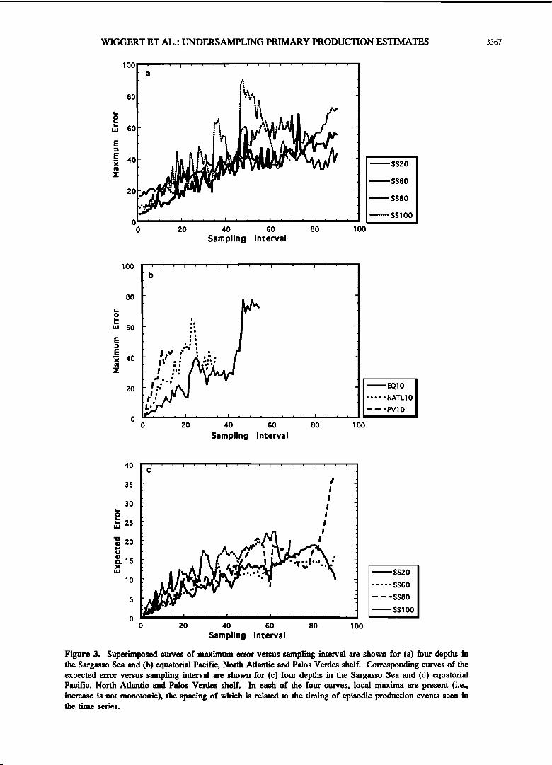
a number of error estimates, corresponding to the number of subsets achievable, were calculated for each SI. Superimposed curves of maximum error as a function of SI (Figures 3a and 3b) were created to illustrate what we observed as the worst case

scenario for the effect of decreasing resolution. The maximum error is defined to be the maximum error calculated over all

time shifts for a given SI, i.e., MAX(Error(Sl, k)). In addition, superimposed curves of the most probable '(expected) error have been formed (Figures 3c and 3d) to provide insight into


I ' I A ' I [ I '

I t ! ' .

Z40

130 140 150 160 17'0 180 190

I i -

0 I I , ! I ! I IO 15 2:0 25 :30 3,5 40 45

JULIAN DAY

Fig. 1. (continued)

what magnitude of error should be expected. The "expected" error EE(SI) is def'med as the average error value over all time shifts for a given SI and was calculated using (6).

•(st• •-• 5• •or(S/,t0 •.1 (6)

Undersampling error generally increases with SI. However, as exemplified by the temporary decreases in error shown in Figure 3, this increase is not monotonic. The spacing of these dips with respect to $I are related to the spacing of phytoplankton blooms in the productivity time series (Figure 1). The signal form characteristic of these blooms generates jumps in the undersampling error as the subsampling algorithm steps around and between the difference in amplitudes between short-lived blooms and steady state productivity regimes (e.g., Figures 2b and 2c). The overall increase in error with $I has • quantified using linear fits to the scattered points in order to estimate the "growth rate" of undersampling error. These slopes and SI•,.• for each time series included in this analysis are listed in Table 2. Additionally, over all time shifts (k) and SI considered for each time series, extrema for GPP GPP=,.•=max(GPP(SI, k)) and GPP=i•=min(GPP(SI, k)), extrema for 68% confidence limits

SENS•,.•--max(EE(SI)+o) and SENS.a.--min(EE(SI)-cO, and the maximum error are listed. Considering all time series, the estimates of maximum error range from 43% (SS20) to 85% (SSS0).

The maximum error curves (i.e., the maximum of Error(Sl, k) over /c:, Figures 3a and 3b) reveal the error's worst case magnitude as a function of $I; however, the range in productivity estimates is more than twofold. Envelopes of the maximum and minimum values of GPP at each SI are used to

represent the maximum error due to undersampling, while envelopes of the 68% confidence levels (i.e., EE($1)-I-o, equation (6)) are used to represent sensitivity to temporal shifting. as functions of $I (Figure 4). In order to force the minimum value to be 1.0, the scales for the left axes of Figure 4 have been normalized by the value of GPP=a = (Table 2) for each case. These envelopes are useful for determining the n fold range of the estimates, since all normalized values will be >_ 1.0. The four frames representing the $argasso Sea time series (Figures 4a-4d) use the same scaling for the left axis in order to compare error ranges within the water column. The frames representing the remaining three time series (Figures 4e-4g) are scaled individually in order to emphasize the salient features. The right axes give production estimate values in grams of carbon per cubic meter per year in order to emphasize


I

• ao

$:: IO

0 '•

I ] [ I I

Avg. Doily GPP = 18.098 mgC/m 3/doy I I I I I I I • I , I 140 160 180 2:00 220 240

3O

2O

I0

Avg. Doily GPP= 15.59:5 mgC/m 3/doy I , I I I • I • I [ I

140 160 180 200 220 240

I [ I • I

30

E I0

fi• Avg' DøiIy GPP = 19'195 mgC/m 3/døY 0 I • I , I • I I I • I 140 160 180 200 220 240

JULIAN DAY 1992

Figure 2. Variation of the gross primary productivity (GPP) signal due to shifting of the initial time and subsampling within a time series subset..Average daily values of gross primary production, obtained by integrating the thick curve shown in each frame, are listed. All three frames show the full equatorial Pacific GPP time series (thin line), (a) the position of the subset (the superimposed thick line) •fter it has been shifted 11 days, (b) a subsampled form (sampling interval ($/) =12 days) of the subset in Figure 2a, (c) another subsampled time series (again at $1=12 days) which has been taken from a different subset (not shown). Comparing Figure 2b with Figure 2c reveals the differences which may result when the samples of GPP are shifted 4 days. Note the difference in the average daily gross primary production values obtained for Figures 2b and 2c. The value for Figure 2a is used for making error estimates for all subsampled forms of that subset (e.g., Figure 2b).

the extent of the undersampling-induced error over a yearly time scale.

Comparing the four frames corresponding to the Sargasso Sea time series reveals that the maximum range in productivity

estimates, between twofold and fourfold, comes from the deeper time series (SS60, SS80, and SS100) which exhibit the summertime subsurface productivity maximum. The frame for SS20 (Figure 4a) shows little variation in the range of


lOO

a

80 I

4O

2O

0 0 20 40 60 80 100

Sampling Interval

SS20

SS60

------SS80

......... SSlO0

100 ' ' ' I ' , I , I ' , I , • , I I I , • I , , I , I

b

8O

.• :. "' 60 "

I I • I

=E .' ß I i

l!:"" ..... NATL10

-PVlO

0 ' 0 20 40 60 80 100

Sampling Interval

ii i

I 35

!

ß ' I

3O

m 2O

c1.15

10

0 zo 40 60 80 100

Sampling Interval

f , ,

SS20

..... SS60

-- -- -SS80

------ SS 1 O0

Figure 3. Superimposed curves of maximum error versus sampling interval are shown for (a) four depths in the Sargasso Sea and (b) equatorial Pacific, North Atlantic and Palos Verdes shelf. Corresponding curves of the expected error versus sampling interval are shown for (c) four depths in the Sargasso Sea and (d) equatorial Pacific, North Ariantic and Palos Vetdes shelf. In each of the four curves, local maxima are present (i.e., increase is not monotonic), the spacing of which is related to the timing of episodic production events seen in the time series.


40

35

30

• •o

• '" .":'• i •.•s

10 I.' -

0 0 20 40 60 80 100

Sarnpling Interval

, ,

"' EQ10

..... NATL 10

-- -- 'PV10

Fig. 3. (continued)

estimates or the 68% confidence levels. Thus changes in SI had little effect on the degree of undersampling error or the sensitivity of the estimates. This is due to the extremely low variability in SS20 during the summertime regime of quasi steady state growth, notwithstanding the spring bloom which appeared around Julian Day 100 (Figure la). The range and variability of the other time series can be seen to increase steadily with $I. The frames for SS80 and SS100 show the most striking examples of this, exhibiting a fourfold range (Figures 4c and 4d) caused by the difference between the spring and early summer levels of productivity. This illustrates the potential severity of undersampling error, although in this case the magnitude of the uncertainty in the f'mal result is only around 2 g C m '3 yr 4, because of the low levels of productivity. In the more productive oceanic regions (Figures 4e-4g) the range is around threefold. This is smaller than ranges seen for the Sargasso Sea cases but corresponds to an uncertainty of 5- 13 g C m '3 yr 4. The equatorial Pacific case (Figure 4e) shows a relatively low undersampling error for $! less than 10 days but exhibits a marked increase near the 50-day $I due to the spacing of the bloom periods appearing in the time series (Figure le). The North Atlantic and Palos Vetdes shelf cases both exhibit high sensitivities (e.g., Figures 4f and 4g, dashed

lines) at the lowest $l, corresponding to the elevated variance contained within these signals. Nevertheless, both cases exhibit significant increases in sensitivity and undersampling-induced error as $I is increased. This is especially prominent in the coastal ocean case (Palos Vetdes shelf), for which the maximum undersampling error is estimated to grow at 3.3%/d which is threefold higher than the worst of the other cases (Table 2).

Discussion and Conclusions

It is becoming increasingly evident that sampling at appropriate spatial and temporal scales is important for accurately assessing oceanic primary production. Many recent works reveal variability on previously unsampled, albeit significant, scales [e.g., Dickey et al., 1991, 1993a; Fallowski et al., 1992; Desiderio et al., 1993]. The analysis presented here has focused on quantifying errors in gross primary productivity (GPP) estimates due to temporal undersampling. Time series of daily GPP estimates have been obtained by performing daily integrations of minute resolution GPP estimates. These were calculated from minute

Table 2. Highlights of Subsampling Analysis

Time Series Maximum Gross Primary Production* Confidelice •imibs Maximum Error growth Label with Sampling Error, % rate•, %/d Depth, m Interval, days Maximum M'mimum Maximum Minimum

SS20 90 6.7 2.8 5.7 3.5 43 0.4 SS60 90 13.1 4.3 9.6 6.6 55 0.5 SS80 90 4.6 1.2 3.9 1.7 85 0.7 SS100 69 3.1 0.8 2.3 1.3 81 0.7 EQ10 54 31.7 12.6 28.1 15.4 77 1.2 NATL10 35 97.6 33.4 81.2 45.0 65 1.2 PV10 14 28.4 10.5 23.1 13.2 45 3.3

*Values are given in milligrams of carbon per cubic meter per day •Values are obtained from linear fits to the maximum percent error versus sampling interval curves.


• I I i I I i i $$ o

I0 20 :50 40 50 60 70 80 I

90

3 4.8 c•

3

I 1.6 I0 20 $0 40 50 60 70 80 90

0.4 I0 20 :50 40 50 60 70 80 90

SAMPLING INTERVAL

Figure 4. The outer envelope (solid lines) is formed by the maximum and minimum productivity estimates for each sampling interval. The inner envelope (dashed lines) shows the 68% confidence intervals. The horizontal axis is the sampling interval (in units of days). The vertical axis on the right side indicates values of productivity in absolute units transformed to grams of carbon per cubic meter per year. The vertical axis on the left side indicates values of productivity normalized by GPP•a• for that case (see Table 2). This normalization allows for easy comparison of the range of undersampling-induced error between cases. The four Sargasso Sea cases at depths of (a) 20 m, (b) 60 m, (c) 80 m, and (d) 100 m, have been plotted using the same limits on the left axis in order to simplify comparisons between depths. The (e) equatorial Pacific, (f) North Atlantic and (g) Palos Vetdes shelf cases have been scaled individually on the left vertical axis in order to emphasize individual characteristics.

scale CHL and Io time series obtained during several recent moored experiments. It should be emphasized that the optical production model (equations (1)- (4))employed to generate the high-resolution GPP estimates contains several parameters which have been held constant (e.g., a•hl, •m, gs,t(N,T), Ore) because of a lack of more precise information. These phytoplankton growth characteristics have been shown to be quite variable [e.g., Prdzelin et al., 1991; Falkowski et al., 1992]. In addition, no parameterization for a spectrally decomposed light field [e.g., Morel, 1991; Platt and Sathyendranath, 1991; Bidigare et al., 1992] has been included in these calculations. These exclusions underscore the

difficulty in accurately determining levels of oceanic primary

production. and it should be emphasized that the subsampling errors reported here do not include variability due to these processes.

The daily integrated GPP signals used in this .analysis include various phytoplankton bloom and steady state regimes. This variety of signal forms proved to be useful in providing insight into generators of undersampling error. Not surprisingly, signals containing short-lived, episodic phytoplankton blooms are most prone to undersampling error. This is best exemplified by considering the SS20 case (Figure la), characterized by a single, sustained bloom followed by a low-variability, quasi steady state regime and contrasting it with the equatorial Pacific or North Atlantic cases (Figures l e


1.5

2.4

1.6

2.8

2.1

1.4

I I I I ' I ' I '

EQIO

,

IO 2o •o 40 50

10.4

7.8

5.2:

:57.6

28.2:

18.8

2 4 6 8 I0 12

I ' I ' I '

-I0

7.5

5

SAMPLING INTERVAL

Fig. 4. (continued)

and l f), both of which are characterized by multiple productivity peaks. The results of the time- shifting/subsarnpling analysis for the SS20 case show that the growth rate of the maximum undersampling error is 0.4%/d, whereas for both the equatorial Pacific and North Atlantic cases it is 1.2%/d (Table 2). As already noted, the SS20 results (Figures 3a, 3c and 4a) do not show the characteristic increase in undersampling error with $I exhibited in both the EQ10 and NATL10 results (Figures 3b, 3d, 4e, and 40. The equatorial Pacific case shows the undersampling-induced error to be increasing essentially monotonically, whereas for the North Ariantic case a peak is reached, followed by a decrease. The North Ariantic case would seem to be more representative of the overall behavior, with the peak occurring at an $I which is equivalent to the temporal spacing of the blooms.

The growth rate in maximum undersampling error for the Sargasso Sea case ranges from 0.4%/d to 0.7%/d. These low values are a result of the nonepisodic nature of the primary production regimes in the oligotrophic time series. The values for the other three cases are all greater than 1.0%/d (Table 2). The Palos Verdes shelf case, for which the growth rate was estimated as 3.3%/d, warrants further examination. The

reduced range in $I for this case, caused by the relative brevity of the data set, casts some suspicion on this elevated value. However, the superimposed error versus Sl curves (Figure 3) and linear fits (not shown) to the first 14 Sis in the corresponding curves for the other locations did not indicate such elevated error growth rates. Thus the Palos Verdes shelf result is not considered to be an artifact of a limited data set.

Additionally, the Palos Verdes shelf case shows elevated values of undersampling error and sensitivity for relatively

short SI (Figure 4g). Indeed, the maximin error for this case (45%, Table 2), which occm for an SI of 9 days, is of the same order as the error value for several other cases, which occur at

$I that are at least 4 times greater (Figures 3b and 3d). This suggests that yearly production estimates from coastal oceans are extremely prone to undersampling error, even at relatively frequent sampling intervals, due to episodic productivity events driven by such processes as tidal activity, wind-driven mixing, and terrigenous input.

Differences between GPPm• and GPP•t• obtained using the Sargasso Sea data range between 0.8 and 3.2 g C m '3 yr • over the four depths. Vertical integration of these range differences resulted in an estimate of the maximum expected range to be found in estimates of annual water column production (300 g C m '2 yr-1). This is equivalent to subtracting the value obtained by vertically integrating the GPPmi • estimates from the value obtained by integrating the GPPm• x estimates. An expected standard deviation for an estimate of annual water column

production was determined to be +42 g C m '2 yr 'l. This estimate was obtained by integrating the profile of the differences between SENS,•,• and SENSIng, which ranged from 0.37 to 1.12 g C m '3 yr 1. Yearly production at this Sargasso Sea site was estimated to be 140 g C m'2yr 'l [Marta et al., 1992], using a different method for the production calculation but the same high-resolution data set presented in this work. This oligotrophic site was characterized above as a region of low undersampling error due to its quasi steady state behavior. Thus these estimates for the range in production values and sensitivity within the euphotic zone, caused 'by undersampling and sample timing, must be recognized as underestimates when considering episodic, highly productive oceanic regions.


Indeed, the differences between the GPP extreme for the yearly production estimates for the equatorial Pacific, North Ariantic, and Palos Verdes shelf cases are 7.0, 23.4, and 6.5 g C m '3 yr 'l, respectively (Table 2). Using these ranges and assuming an average mixed layer depth of 40 m result in values for the range in annual water column production which are of the same order or greater than the oligotrophic case just presented. Differences between the sensitivity extreme for these cases are 4.6, 13.2, and 3.6 g C m '3 yr '•, respectively (Table 2). Again applying the 40 m mixed layer depth assumption results in values for the expected standard deviation for annual production estimates which are at least twice as large as the sensitivity determined for the Sargasso Sea case. It must be remembered that these ranges are all estimated using time series from a depth of 10 m. These time series do not include subsurface chlorophyll maxima which are characterized by elevated chlorophyll concentrations and signal variability. Thus the error range and sensitivity estimates based on these time series from 10 m are not

representative of the elevated variability which occurs deeper in the water column.

In summary, highly productive regions characterized by short-lived episodic blooms are more susceptible to the hazards of undersampling. These regions are responsible for the bulk of the primary productivity occurring within the world's oceans. Thus obtaining amply resolved production estimates through the use of high-resolution sampling techniques is vital to achieving more accurate assessments of the present state of the ocean's primary ecosystem.

Acknowledgment. The authors would like •o thank Dale Kiefcr for useful discussions concerning the application of his revised productivity model, and John Marta and Chris Langdon for cellaberating in the collection of data during the Biowatt and MLML experiments. We would also like to express our thanks to Darek Bogucki, Dave Foley, Mike Hamilton, Anne Petrenko, Margaret Stramska, Isabellc Taupicr- Letage, and Libe Washburn for data processing and/or useful discussions. Finally, as always, we would especially like to thank Derek Manor for his expertise in developing and deploying the MVMS systems. The moored experiments were funded by ONR grants N0014- 87-K0084 and N00014-89-J-1498 (Biowatt and MLML), NOAA grant NA16RC0088-02 and NSF grant NSFOCE9013896 (EQPAC), and Sea Grant contract NA90AA-D-SG525.

References

Bidigare, R.R., B.B. Pr6zelin, and R.C. Smith, Bio-optical models and problems of scaling, in Primary Productivity and Biogeochemical Cycles in the Sea, edited by P.G. Falkowski and A.H. Woodh•, pp. 175-212' Plenum, New York, 1992.

Carder, K.L., S.K. Hawes, K.A. Baker, R.C. Smith, R.G. Steward, and B.G. Mitche• Reflectance model for quantifying chlorophyll a in the presence of productivity degradation products, J. Geephys. Res., 96, 20,599-20,611, 1991.

Desiderio, R.A., T.L Cowles, and J.N. Moum, Microstructure profiles of laser-induced chl'orophyll fluorescence spectra: Evaluation of backscatter and forward-scatter fiber-optic sensors, J. Atmos. Oceanic Technol., 10, 209-224, 1993.

Deuser, W.G., Seasonal and interannual variations in deep-water particle fluxes in the Sargasso Sea and their relation to surface hydrography, Deep Sea Res., Part A, 33, 225-246, 1986.

Dickey, T.D., The emergence of concurrent high-resolution physical and bio-optical measurements in the upper ocean and their applications, Rev. Geephys.,29, 383-413, 1991.

Dickey, T.D., I. Matra, T. Granata, C. Langdon, M. Hamilton, I,

Wiggert, D. Siegel, and A. Bratkovich, Concurrent high-resolution bio-optical and physical time series observations in the Sargasso Sea during the spring of 1987, J. Geophys. Res, 96, 8643-8664, 1991.

Dickey, T., et al., Seasonal variability of bio-optical and physical properties in the Sargasso Sea, $. Geoph•. Res, 98, 865-898, 1993a.

Dickey, T.D., R.H. Douglass, D• Manov, D. Bogucki, P.C. Walker, and P. Petrelis, An experiment in two-way communication with a multivariable moored system in coastal waters, J. Ate. and Oceanic Tec•l., 10, 637-644, 1993b.

Eppley, R.W., Estimating phytoplankton growth rates in the central oligotro•c ocean, in Primary Productivity in the Sea, edited by P.G. Falkowski, pp. 231-242, Plenum, New York, 1980.

Falkowski, P.G., R.M. Grmae, and R.I.C.,eider, Physiological limitations on phytoplankton productivity in the ocean, Oceanography, 5, 84-91, 1992.

Jahnke, R.A., Ocean flux studies: A status report, Rev. Geephys., 28, 381-398, 1990.

Ienkim, W.I., and I.C. Goldman, Seasonal oxygen cycling and primary production in the Satgeese Sea, J. Mar. Res., 45, 46•-491, 1985.

Kiefer, D. A., Growth and light absorption in the marine diatom $keletonema Costatum, in Toward• a Model of Ocean Biogeochemical Processes, edited by G. Evam and M. Fasbare, pp. 93-122, Springer-Verlag, New York, 1993.

Lohrenz, S.E., G.A. Knaner, V.L. Asper, M. Tuel, A.F. Michaels, and A.H. Knap, Sea,real variability in primary production and particle flux in the northwestern Sargasso Sea: U.S. JGOFS Bermuda Atlantic time-seri•s •tudy, Deep Sea Res., Part A, $9, 1373-1391, 1992.

Marta, J., et el., The estimation of seasonal primary production from moored optical senson in the Sargasso Sea, J. Geephys. Res, 97, 7399-7412, 1992.

Menzel, D. W., and J. H. Ryther, The annual cycle of primary production in the Sargauo Sea off Bermuda, Deep Sea Res., 6, 351- 367, 1960.

Menzel, D.W., and J.H. Ryther, Annual variations in primary production of the Sargasso Sea off Bermuda, Deep Sea Res., 7, 282-288, 1961.

Morel, A., Light and marine photosynthesia: A spectral model with geoche• and climatological implications, Prog. Oceanogr., 26, 263-306, 1991.

PlalI, T., and W.G. Harrison, Biogenic fluxes of ca,ben and oxygen in the ocean, Nature, $18, 55-58, 1985.

Platt, T., and S. Sathyendranath, Biological production models as elements of coupled, aunosphere-ocean model, for climate re•earch, J. Geephys. Res., 96, 2585-2592, 1991.

Pr•zelin, B.B., MaM. Tilzer, O. Sehonfield, and C. Haese, The control of the production process of phytoplankton by the physical mucmre of the aquatic environment with special reference to its optical propenies, Aquat. $ci.,55, 136-186, 1991.

Sakshaug, E., D.A. Kiefer, and K. Andersen, A steady atate deacription of growth and light absorption in the marine planktonic diatom $keletonema costatum, Limael. Oceanogr., $4, 198-205, 1989.

Sarmiento, J.L., and U. Siegenthaler, New production and the global carbon cycle, in Primary Productivity and Biogeochemical Cycles in the Sea, edited by P.O. Falkow•ki and A.H. Woodhead, pp. 317-332, Plenum, New York, 1992.

Stramska M., and T.D. Dickey, Variability of bio-optical properlies of the upper ocean associated with diel cycles in phytoplankton population, J. Geephi. Res., 97, 17,8/3-17,888, 1992.

Winn C., R. Lukas, D. Karl, and E. Firing, Hawaii Ocean time-series data report 3, $OEST Tech. Rep. 95-$, 228 pp., Univ. of Hawaii, Honolulu, Hawaii, 1993.

T. Dickey, T. Granata, and I. Wiggert, Ocean Physics Group, Depamnent of Earth Sciences, University of Southern California, Los Angeles, CA 90089-0740. (e-mail: Telemail: t. dickey; /ntemet: [email protected];/nternet: wiggem•oce.usc.edu)

(Received June 28, 1993; revised October 8, 1993; accepted October •, 1993.)

The effect of temporal undersampling on primary production estimates

Documents

Transcript of The effect of temporal undersampling on primary production estimates