The Economic Development of Latin America in the Twentieth ...
338
The Economic Development of Latin America in the Twentieth Century André A. Hofman Researcher, Economic Commission for Latin America and the Caribbean, Chile Edward Elgar Cheltenham, UK • Northampton, MA, USA
-
Upload
khangminh22 -
Category
Documents
-
view
0 -
download
0
Transcript of The Economic Development of Latin America in the Twentieth ...
The Economic Development of Latin America in the Twentieth Century
André A. Hofman
R esearch er, E con om ic C om m ission f o r L atin A m erica a n d the C aribbean , C hile
Edward ElgarCheltenham, UK • Northampton, MA, USA

© André A. Hofman 2000
All rights reserved. No part of this publication may be reproduced, stored in a retrieval system or transmitted in any form or by any means, electronic, mechanical or photocopying, recording, or otherwise without the prior permission of the publisher.
Published byEdward Elgar Publishing LimitedGlensanda HouseMontpellier ParadeCheltenhamGlos GL50 1UAUK
Edward Elgar Publishing, Inc.136 West Street Suite 202 Northampton Massachusetts 01060 USA
A catalogue record for this book is available from the British Library
L ib ra ry o f C ongress C ataloguing in P ub lica tion D ata
Hofman, André A., 1953—The economic development of Latin America in the twentieth century
/ André A. Hofman.1. Latin America—Economic conditions—20th century. I. Title.
HC125.H645 1999338.98—dc21 98-27904
CIP
ISBN 1 85898 852 7Printed and bound in Great Britain by Bookcraft (Bath) Ltd.

Contents
List o f Figures viiList o f Tables ixAcknowledgements xv
1 Introduction 12 Some Distinctive Characteristics of Latin America over the Long
Run 73 Economic Performance in Latin America - A Comparative
Quantitative Perspective 294 New Standardised Estimates of Labour Input and Human Capital 475 New Standardised Estimates of Capital Stock for Latin America
and the USA 696 Explaining Latin American Post-War Development - The Growth
Accounts 997 Performance and Policy in Latin America 1278 Conclusions 147
APPENDICES
Appendix A Population 155Appendix B GDP Indices (1950 = 100) and Levels of Total and
Per Capita GDP 159Appendix C Activity Rates, Employment, Education and Labour
Productivity 173Appendix D Total and Disaggregated Gross Investment,
1900-1994 183Appendix E Standardised Estimates of Capital Stock 205Appendix F Foreign Trade 249Appendix G Prices 261Appendix H Previous Non-Standardised Capital Stock Estimates
in Latin America 265
References 293Index 313

List of Figures
3.1 Latin America: Share of Individual Countries in the Six Country TotalGDP, 1900-1994 36
3.2 Latin America: Volume Movements of GDP, 1900-1994 425.1 Latin America: Total and Non-Residential Capital Productivity,
1950-94 835.2 Total Gross Fixed Capital Stock per Capita, 1950-94 875.3 Residential Gross Fixed Capital Stock per Capita, 1950-94 875.4 Non-Residential Gross Fixed Capital Stock per Capita, 1950-94 885.5 Gross Fixed Machinery and Equipment Capital Stock per Capita,
1950-94 896.1 Latin America: Total Factor Productivity without Augmentation,
1950-94 1156.2 Latin America: Labour-Augmented Total Factor Productivity,
1950-94 1156.3 Latin America: Capital-Augmented Total Factor Productivity,
1950-94 1166.4 Latin America: Doubly-Augmented Total Factor Productivity,
1950-94 1166.5 Doubly-Augmented Total Factor Productivity: An International
Comparison, 1950-94 118
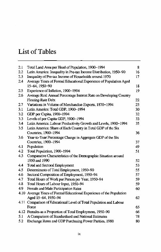
List of Tables
2.1 Total Land Area per Head of Population, 1900-1994 82.2 Latin America: Inequality in Pre-tax Income Distribution, 1950-90 162.3 Inequality of Pre-tax Income of Households around 1970 172.4 Average Years of Formal Educational Experience of Population Aged
15-64,1950-90 182.5 Experience of Inflation, 1900-1994 192.6 Average Real Annual Percentage Interest Rate on Developing Country
Floating-Rate Debt 222.7 Variations in Volume of Merchandise Exports, 1870-1994 233.1 Latin America: Total GDP, 1900-1994 303.2 GDP per Capita, 1900-1994 323.3 Levels of per Capita GDP, 1900-1994 333.4 Latin America: Labour Productivity Growth and Levels, 1900-1994 353.5 Latin America: Share of Each Country in Total GDP of the Six
Countries, 1900-1994 363.6 Year-to-Year Percentage Change in Aggregate GDP of the Six
Countries, 1900-1994 374.1 Population 494.2 Total Population, 1900-1994 514.3 Comparative Characteristics o f the Demographic Situation around
1950 and 1990 524.4 Total and Sectoral Employment 534.5 Determinants of Total Employment, 1950-90 554.6 Sectoral Composition of Employment, 1950-94 574.7 Total Hours of Work per Person per Year, 1950-94 594.8 Total Hours of Labour Input, 1950-94 594.9 Female and Male Participation Rates 604.10 Average Years of Formal Educational Experience of the Population
Aged 15-64,1950-94 624.11 Comparison of Educational Level of Total Population and Labour
Force 654.12 Females as a Proportion of Total Employment, 1950-90 665.1 A Comparison of Standardised and National Estimates 785.2 Exchange Rates and GDP Purchasing Power Parities, 1980 80

X The Economic Development of Latin America
5.3 Capital Formation PPP-Exchange Rate Deviation Indices, 1980 815.4 Latin America: Weighted Average Service Life of Total and Non-
Residential Fixed Capital Stock, 1950-94 825.5 Average Age of Total, Non-Residential and Residential Fixed Capital
Stocks, 1950-94 845.6 Levels o f Total and Residential Gross Fixed Capital Stock per Capita,
1950-94 855.7 Levels of Gross Fixed Capital Stock per Capita of Non-Residential
Structures and Machinery and Equipment, 1950-94 865.8 Latin America: Total Gross Fixed Capital Stock, 1950-94 895.9 Latin America: Gross Fixed Non-Residential Capital Stock, 1950-94 905.10 Comparative Growth of Gross and Net Total Fixed Capital Stock,
1950-94 905.11 Latin America: Composition of Gross Total Fixed Capital Stock,
1950-94 915.12 Latin America: Composition of Gross Total Fixed Capital Stock,
1950-94 925.13 Latin America: Difference between Growth of Fixed Capital Stocks in
National Currencies and International Dollars, 1950-94 925.14 Latin America: Ratio of Non-Residential Fixed Capital Stock to Total
Fixed Capital Stock, 1950-94 935.15 Total Fixed Gross Capital-Output Ratios, 1950-94 945.16 Non-Residential Fixed Gross Capital-Output Ratios, 1950-94 945.17 A Comparison of Gross and Net Total Capital-Output Ratios,
1950-94 956.1 Comparative Levels o f Economic Performance of 16 Countries
Between 1950 and 1994 1006.2 Latin America: Labour Force (LF) and Employment (EMP), 1950-94 1036.3 Latin America: Level of Education of the Population Aged 15-64 1046.4 Rate of Growth of Labour Inputs, 1950-94 1056.5 Capital Productivity Growth, 1950-94 1056.6 Rate of Growth of Capital Inputs, 1950-94 1066.7 Latin America: Movement of the Agricultural Frontier - Expansion of
Area of Land in Use for Agriculture 1066.8 Capital, Labour and Natural Resource Shares in GDP, 1950-94 1086.9 Standardised Capital, Labour and Natural Resource Shares in GDP,
1950-94 1086.10 Basic Indicators of Growth Performance, 1950-94 1096.11 Sources of GDP Growth with Country-Specific Factor Shares,
1950-94 1106.12 Sources of GDP Growth, Standardised Factor Shares, 1950-94 1116.13 Explanatory Power of Total Factor Productivity in Growth, 1950-94 112
Tables x i
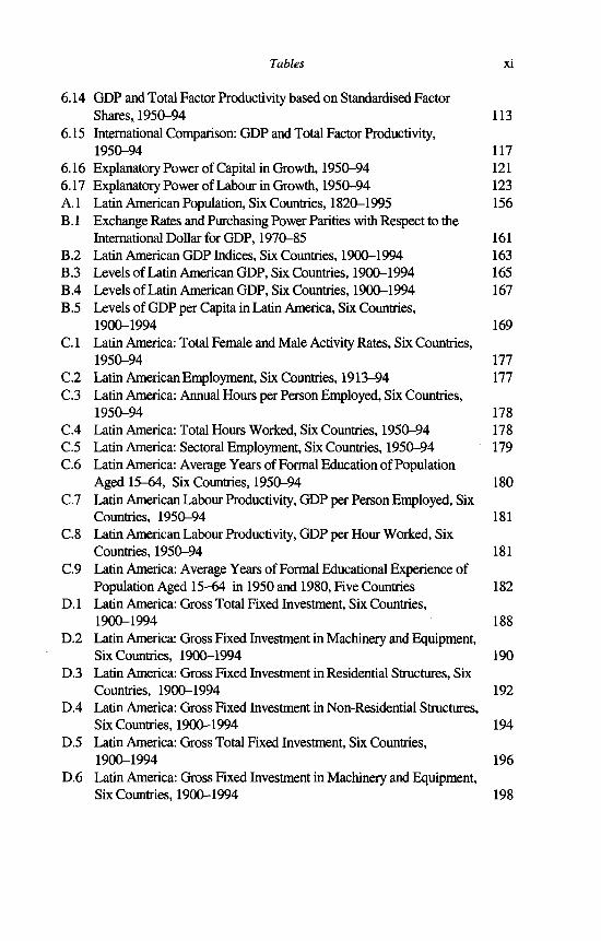
6.14 GDP and Total Factor Productivity based on Standardised FactorShares, 1950-94 113
6.15 International Comparison: GDP and Total Factor Productivity,1950-94 117
6.16 Explanatory Power of Capital in Growth, 1950-94 1216.17 Explanatory Power of Labour in Growth, 1950-94 123A.1 Latin American Population, Six Countries, 1820-1995 156B .l Exchange Rates and Purchasing Power Parities with Respect to the
International Dollar for GDP, 1970-85 161B.2 Latin American GDP Indices, Six Countries, 1900-1994 163B.3 Levels of Latin American GDP, Six Countries, 1900-1994 165B.4 Levels of Latin American GDP, Six Countries, 1900-1994 167B.5 Levels of GDP per Capita in Latin America, Six Countries,
1900-1994 169C .l Latin America: Total Female and Male Activity Rates, Six Countries,
1950-94 177C.2 Latin American Employment, Six Countries, 1913-94 177C.3 Latin America: Annual Hours per Person Employed, Six Countries,
1950-94 178C.4 Latin America: Total Hours Worked, Six Countries, 1950-94 178C.5 Latin America: Sectoral Employment, Six Countries, 1950-94 179C.6 Latin America: Average Years of Formal Education of Population
Aged 15-64, Six Countries, 1950-94 180C .l Latin American Labour Productivity, GDP per Person Employed, Six
Countries, 1950-94 181C.8 Latin American Labour Productivity, GDP per Hour Worked, Six
Countries, 1950-94 181C.9 Latin America: Average Years of Formal Educational Experience of
Population Aged 15-64 in 1950 and 1980, Five Countries 182D .l Latin America: Gross Total Fixed Investment, Six Countries,
1900-1994 188D.2 Latin America: Gross Fixed Investment in Machinery and Equipment,
Six Countries, 1900-1994 190D.3 Latin America: Gross Fixed Investment in Residential Structures, Six
Countries, 1900-1994 192D.4 Latin America: Gross Fixed Investment in Non-Residential Structures,
Six Countries, 1900-1994 194D.5 Latin America: Gross Total Fixed Investment, Six Countries,
1900-1994 196D.6 Latin America: Gross Fixed Investment in Machinery and Equipment,
Six Countries, 1900-1994 198

D.7 Latin America: Gross Fixed Investment in Residential Structures, Six Countries, 1900-1994
D.8 Latin America: Gross Fixed Investment in Non-Residential Structures, Six Countries, 1900-1994
E. 1 Capital Formation PPPs-Exchange Rate Deviation Index, 1970-80 E.2 Argentina: Procedure for Estimating Alternative Benchmark of the
Stocks of Non-Residential Structures at 31 December 1949 E.3 Argentina: Procedure for Estimating Alternative Variants of 1950-94
Estimates of the Stock of Non-Residential Structures E.4 Argentina 1. Gross and Net Fixed Tangible Reproducible Capital
Stocks by Type o f Asset, 1950-94 E.5 Argentina 2. Gross and Net Fixed Tangible Reproducible Capital
Stocks by Type of Asset, 1950-94 E.6 Argentina 3. Capital Stock: Average Ages, Average Service Lives and
Capital-Output Ratios, 1950-94 E.7 Argentina 4. Capital Stock: Average Ages, Average Service Lives and
Capital-Output Ratios, 1950-94 E.8 Brazil 1. Gross and Net Fixed Tangible Reproducible Capital Stocks
by Type of Asset, 1950-94 E.9 Brazil 2. Gross and Net Fixed Tangible Reproducible Capital Stocks
by Type of Asset, 1950-94 E. 10 Brazil 3. Capital Stock: Average Ages, Average Service Lives and
Capital-Output Ratios, 1950-94 E. 11 Brazil 4. Capital Stock: Average Ages, Average Service Lives and
Capital-Output Ratios, 1950-94 E.12 Chile 1. Gross and Net Fixed Tangible Reproducible Capital Stocks
by Type of Asset, 1950-94 E.13 Chile 2. Gross and Net Fixed Tangible Reproducible Capital Stocks
by Type o f Asset, 1950-94 E.14 Chile 3. Capital Stock: Average Ages, Average Service Lives and
Capital-Output Ratios, 1950-94 E.15 Chile 4. Capital Stock: Average Ages, Average Service Lives and
Capital-Output Ratios, 1950-94E.16 Colombia 1. Gross and Net Fixed Tangible Reproducible Capital
Stocks by Type of Asset, 1950-94E. 17 Colombia 2. Gross and Net Fixed Tangible Reproducible Capital
Stocks by Type of Asset, 1950-94E. 18 Colombia 3. Capital Stock: Average Ages, Averages Service Lives
and Capital-Output Ratios, 1950-94E.19 Colombia 4. Capital Stock: Average Ages, Average Service Lives
and Capital-Output Ratios, 1950-94
x ii The Economic Development of Latin America
202207
208
209
211
213
215
216
217
219
221
222
223
225
227
228
229
231
233
234
200

Tables x iii
E.20 Mexico 1. Gross and Net Fixed Tangible Reproducible Capital Stocks by Type of Asset, 1950-94
E.21 Mexico 2. Gross and Net Fixed Tangible Reproducible Capital Stocks by Type of Asset, 1950-94
E.22 Mexico 3. Capital Stock: Average Ages, Average Service Lives and Capital-Output Ratios, 1950-94
E.23 Mexico 4. Capital Stock: Average Ages, Average Service Lives and Capital-Output Ratios, 1950-94
E.24 Venezuela 1. Gross and Net Fixed Tangible Reproducible Capital Stocks by Type of Asset, 1950-94
E.25 Venezuela 2. Gross and Net Fixed Tangible Reproducible Capital Stocks by Type of Asset, 1950-94
E.26 Venezuela 3. Capital Stock: Average Ages, Average Service Lives and Capital-Output Ratios, 1950-94
E.27 Venezuela 4. Capital Stock: Average Ages, Average Service Lives and Capital-Output Ratios, 1950-94
F. 1 Latin American Exports, Six Countries, 1900-1994F.2 Latin American Imports, Six Countries, 1900-1994F.3 Latin American Export Volume Indices, Six Countries, 1900-1994F.4 Latin American Import Volume Indices, Six Countries, 1900-1994G. 1 Annual Change in Consumer Price Indices in Six Latin American
Countries, 1900-1994H. 1 Argentina: Net Capital Stock, GDP and Capital-Output Ratio,
ECLAC Estimate, 1945-52 H.2 Argentina: Net Capital, GDP and Capital-Output Ratio, ECLAC
Estimate, 1900-1955 H.3 Argentina: Net Capital Stock, GDP and Capital-Output Ratio,
IEERAL Estimate, 1950-84 H.4 Argentina: Capital Output Ratios, Goldberg and Ianchilovici
Estimates, 1970-86 H.5 Argentina: Capital-Output (C/O) Ratio, 1950-86, Comparison of
Standardised and Existing Estimates H.6 Brazil: Net Capital Stock, GDP and Capital-Output Ratio, ECLAC
Estimate, 1945-52 H.7 Brazil: Net Capital Stock, GDP and Capital-Output Ratio, United
Nations Estimate, 1939-53 H.8 Brazil: GDP and Capital-Output Estimates, Langoni Estimate,
1948-69H.9 Brazil: Capital Stock, Gross and Net Capital Formation and
Capital-Output Ratio, Goldsmith Estimate, 1913-80
235
237
239
240
241
243
245
246252254256258
262
267
268
269
270
271
272
273
273
274

x iv The Economic Development of Latin America
H.10 Brazil: Capital-Output (C/O) Ratio, 1950-80, Comparison of Standardised and Existing Estimates
H. 11 Chile: Net Capital Stock, GDP and Capital-Output Ratio, ECLAC Estimate, 1945-52
H.12 Chile: Net Capital Stock, GDP and Capital-Output Ratio, Gutiérrez Estimate, 1950-82
H. 13 Chile: Net Capital Stock, GDP and Capital-Output Ratio, Haindl and Fuentes Estimate, 1960-84
H.14 Chile: Capital-Output (C/O) Ratio, 1950-84, Comparison of Standardised and Existing Estimates
H.15 Colombia: Capital, GDP and Capital-Output Ratio, ECLAC Estimate, 1950-53
H.16 Colombia: Alternative Capital Stock Estimates, GDP and Capital- Output Ratio, Harberger Estimate, 1952-67
H.17 Colombia: Total Fixed Capital Stock, GNP and Capital-Output Ratio, Henao Estimate, 1950-81
H.18 Colombia: Capital-Output (C/O) Ratio, 1950-81, Comparison of Standardised and Existing Estimates
H. 19 Mexico: Net Capital Stock, GDP and Capital-Output Ratio, ECLAC Estimate, 1950-52
H.20 Mexico: Net Capital Stock, GDP and Capital-Output Ratio, ECLAC Estimate, 1950-55
H.21 Mexico: Total Fixed Net Capital Stock, Banco de Mexico Estimate, 1950-67
H.22 Mexico: Gross and Net Capital Stock, Banco de Mexico Estimate, 1960-85
H.23 Mexico: Capital-Output (C/O) Ratio, 1950-67, Comparison of Standardised and Existing Estimates
H.24 Venezuela: Capital Stock, GDP and Capital-Output Ratio, Banco Central Estimate, 1950-65
H.25 Venezuela: Total Capital Stock, GDP and Capital-Output Ratio, Baptista Estimate, 1950-89
H.26 Venezuela: Capital-Output (C/O) Ratio, 1950-89, Comparison of Standardised and Existing Estimates
275
276
277
278
279
280
281
282
283
284
285
285
286
287
288
289
290
Acknowledgements
I am greatly indebted to a large number of people in the preparation of this book; I will never be able to repay these debts. My interest in Latin America and its economic history started towards the end of my studies at the University of Groningen, while I was working on Mexico’s economic development, under supervision of Angus Maddison, and continued with a study on demographic decline in Latin America after the European conquest. Fernando Fajnzylber’s interest in comparing Latin America with countries outside the region and Angus Maddison’s unreserved support, were great sources of motivation in the preparation of this book.
I am very grateful to many of my colleagues at ECLAC in Santiago, Chile. Oscar Altimir has been a constant motivational force and Barbara Stallings gave me the opportunity to finish this study. I am grateful to the following for their comments or other assistance; Asdrubal Baptista, Renato Baumann, Gloria Bensan, Ricardo Bielschowsky, Jorge Bravo, Ruud Buitelaar, Rodrigo Carrasco, Juan Chackiel, Ricardo Crosa, Pascual Gerstenfeld, Gunther Held, John Hennelly, Sebastián Herreros, Felipe Jiménez, Graciela Moguillansky, Guillermo Mundt, Marcelo Ortúzar, Igor Paunovic, José Miguel Pujol, Carlos Rodriguez, Monica Roeschmann, Gert Rosenthal, Pedro Sáinz, Horacio Santamaría, Osvaldo Sunkel, Rosemary Thorp, Daniel Titelman, Raffael Urriola, Víctor Urquidi, Andras Uthoff, Miguel Villa, Richard Webb and Jürgen Weller.
I am also grateful to Derek Blades, Alberto Fffacchia, Alan Heston, Daniel Heymann, Mark Keese and Michael Ward for assistance on methodological issues. I owe thanks to Ricardo Fffench-Davis, Simon Kuipers, Juan Carlos Lerda, Nanno Mulder, Joseph Ramos and Bart van Ark who kindly read substantial parts of the book and commented extensively on many chapters. Mario Castillo was helpful at the initial stage of the research project and Sergio Zamora helped with the capital stock estimation. I am very grateful to Ana Maria Amengual and Christine Boniface who helped in the final editing of the book. I have received continuous support from colleagues all over Latin America, with whom I made contact when I visited their countries, or when they visited ECLAC in Santiago. Without their support this book could not have been completed.
Being a member of the Groningen ICOP (International Comparisons of Output and Productivity) team has been very stimulating and I have been working with several of its members. I am very grateful to Bart van Ark for efficient, graceful
xv

xv i The Economic Development of Latin America
and continuous support, and to Peter Groote for comments and advice. I would particularly like to thank Dirk Pilat on whose support I always could count. I have had a very fruitful relation with Nanno Mulder with respect to capital stock estimation.
Angus Maddison has been my main source of inspiration. In spite of the long geographical distance he always provided guidance, redirecting my efforts where appropriate. Probably more than he is aware, his support, new ideas and challenges have been a major source of professional satisfaction, and his untiring and timely comments during all stages of the preparation o f this book was admirable.
I dedicate this book to my wife and children who accepted, although not always without protest, the many hours of work on this book that should have been dedicated to them.

1. Introduction
This book provides an assessment of Latin America’s1 twentieth-century economic performance and policy from a comparative and historical perspective. The theory and empirics of economic growth have come to be the focus of attention once again. Surveying the literature, one sees many new interesting ideas and the rediscovery of older, somewhat forgotten ones. The empirical work - and this book is in that tradition - concentrates on determining trends and main sources of growth in a cross-section of countries. Economic growth in Latin America is explained on two levels: (a) proximate and measurable influences which are captured in the growth accounts; (b) causes of a more ultimate character, that is, qualitative and institutional influences which are more difficult to measure.
The analysis of economic performance concentrates on the quantification of economic growth, long-run estimates of GDP growth and the measurement of factor inputs and total factor productivity. Another important element of this study is an international comparison with countries outside the region, both developed and developing. Maddison (1991a) defines proximate causes o f growth as:
those areas of causality where measures and models have been developed by economists and statisticians. Here the relative importance of different influences can be more readily assessed. At this level one can derive significant insights from comparative macroeconomic growth accounts, (p. 11)
Through growth accounting it is possible to identify and quantify the proximate causes o f growth but no light is shed on the ultimate causes o f growth.
This study is for the most part eminently empirical in nature, and presents longterm series not available until now for several variables which can serve to analyse Latin American growth, levels o f performance, and phases when growth accelerated or decelerated. For the 1950-94 period, a growth accounting analytical framework is presented using a total factor productivity analysis in which step-by- step explanatory factors are listed, and given their weight in ‘explaining’ economic growth in the sample of countries. Growth accounting shows the contribution of factor inputs (capital, labour and land) and total factor productivity to output growth. For these quantitative growth accounts long-term GDP and capital formation series were required which permit analysis o f GDP (per capita) and labour productivity developments since 1900.
1

2 The Economic Development of Latin America
This kind of growth accounting exercise may serve different purposes such as explaining differences in growth rates between countries, illuminating the process of convergence and divergence, assessing the role of technical progress and calculating potential output losses. Growth accounting cannot provide a full causal explanation. It deals with ‘proximate’ rather than ‘ultimate’ causality and records the facts about growth components: it does not explain the underlying elements of policy or circumstance, national or international, but it does identify which facts need further explanation.
Ultimate causes are those factors related to economic growth which are difficult to quantify in economic or statistical models. They include the role of institutions, ideologies, pressures of socioeconomic interest groups, historical accidents, and economic policy at the national level (Maddison, 1991a). They also involve consideration of the international economic order, foreign ideologies or shocks originating in friendly or unfriendly neighbours. The ultimate sources of Latin American performance are less clearly established than its proximate causes and constitute an extremely interesting area for further research. The contribution of this book to the understanding of the role of these ultimate sources in economic growth is only modest. Chapter 2 analyses some of the topics to be included in the realm of ultimate sources, such as the institutional set-up, social capabilities and path dependency. In Chapter 7 policy and international context are analysed.
It should be stressed that the proximate causes are not independent o f the ultimate causes of growth. To a rather significant degree proximate causes are dimensions through which ultimate causes can be seen to operate. However, the importance of interaction and interdependency between the different sources of growth is emphasised. On the proximate level the interaction between capital accumulation and technological progress is an example of this interdependence. On the ultimate level there exists interaction between the institutional framework of a society and the implementation of economic policy. An example of interdependence between the ultimate and proximate levels is the relationship between technological progress and the institutional context.
In this book Latin American performance is compared with three other groups of countries: (a) two rapidly growing Asian countries (Korea and Taiwan) whose economic growth in the past couple of decades has been remarkably fast; (b) Portugal and Spain, whose institutional heritage had a good deal in common with Latin America; and (c) six advanced capitalist countries (France, Germany, Japan, the Netherlands, UK and USA), whose levels o f income and productivity are among the highest in the world.
Judging from the performance of several countries in the early 1990s, it would seem that Latin America is now climbing out of the depths of one of the most profound crises of the twentieth century. The ‘lost decade’ of the 1980s was characterised by low or negative real economic growth, huge external indebtedness, great macroeconomic instability represented by two to three digit
Introduction 3
inflation, fiscal crisis, and great distortions in resource allocation. Some lessons can be learned from studying Latin America in a comparative perspective.
- There are lessons from the lost decade, which was a period of stagnation rather than growth. The situation in Latin America in the 1980s was highly unusual, with slow or negative growth. Although other regions also experienced lower growth, this did not lead to negative total factor productivity. The implication is that policy at that time was less efficient in Latin America than in many other areas.
- In the period 1950-80 Latin America was not an outlier. Total factor productivity was then positive as it was in other regions. Total factor productivity growth was fastest in Europe, followed by the Asian developing countries and the Latin American countries. Growth accounting, o f course, accounts only for the so-called proximate causes. An evaluation of policy, institutions and shocks of an internal or external character is important, in order to be able to get a frilly rounded view of growth performance and of the efficacy of countries.
Previous work on economic growth accounting in Latin America has concentrated mainly on detailed studies of specific country experience. This book, by contrast, takes a comparative view of a substantial array of countries, within and outside Latin America. Unlike some recent econometric analysis it does not use a maximalist approach, where available data are used without regard to their quality. In this study great attention is given to the construction of comparable series, which data are reasonably reliable. A very important element of this study is the transparency of the methodology used. The complete description of the sources gives the reader the opportunity to judge the quality of the available information. This is the reason for the inclusion of appendices in which the basic series are given together with a description of methodology and sources.
In Chapter 2 some of Latin America’s most salient characteristics, such as unequal income distribution, persistent macroeconomic instability and the institutional context, are analysed in a historical perspective. This historical perspective is important because some of the roots of these characteristics might be found, for example, in pre-Columbian society, the colonial period or in the relatively early independence of Latin America compared to other developing regions. This study provides a short, not exhaustive, description of some of the most important characteristics of Latin America in comparison especially with the United States. In this context it is interesting to compare Latin America with the United States because both belong to the same hemisphere, were ‘discovered’ at the same time by European countries, and had very substantial natural resources endowment by world standards. Now, however, income levels in Latin America and the United States are quite different and the latter leads the world in
4 The Economic Development of Latin America
productivity. The first element to be analysed is the physical endowment of Latin America followed by the institutional framework, inequality, human capital, debt, foreign trade and inflation to finish with policy and ideology.
A long-run perspective of growth acceleration and slowdown in Latin America compared with the other groups of countries is presented in Chapter 3. Labour productivity for the 1913-94 period shows some additional evidence concerning the cycles of acceleration and deceleration of growth in the twentieth century. Per capita GDP showed recovery in the 1989-94 period after the negative growth in the lost decade of the 1980s. The analysis of the business cycle and comparison of similarities and differences in the periods commonly used are also studied in this chapter. The main causes of cyclical instability, either of an internal or external nature, are identified.
In Chapter 4, which deals with the human capital dimension, I analyse the results with respect to employment, unemployment and annual days worked. This section also takes into consideration the quality aspects of the population as reflected in educational levels. The results with respect to physical capital are the subject of Appendix G and Chapter 5. Appendix G gives a systematic comparison of previous capital stock estimates in Latin America. The lack of comparable estimates of fixed capital stocks for Latin American countries has long hindered analysis of economic development within the region as well as comparison with other developing and developed countries. Chapter 5 attempts to fill this gap by providing estimates of gross and net fixed capital stock for the six Latin American countries selected. The estimates have been generated by employing the ‘perpetual inventory method’ currently used by most OECD countries to estimate their capital stocks, and hence the most appropriate in an international comparison.
Chapter 6 presents a causal analysis of Latin American post-war development using the methodology of the growth accounts, providing for labour and capital a detailed breakdown of their components and indicating the weighting procedure of all inputs (including land) into a measure of augmented total factor input. Performance and policy of Latin America in the post-war period is analysed in Chapter 7. An overall description of policy and performance in the Latin American region is given. The chapter concludes with a description of the major policy issues on which consensus has been reached and the ones which are still subject to debate.
In eight appendices, the complete series, sources and measurement procedures are presented. Appendix A contains long-term population series from 1820-1995. Appendix B provides time series for GDP, levels of GDP and GDP per capita both in national currencies and international dollars. Some basic quantification with respect to the labour market is given in Appendix C, which presents activity rates, employment, educational level of the population and labour productivity series from 1950 onwards, as well as estimates of hours worked. Estimates for total and disaggregated capital formation for the 1900-1994 period, which are the essential

Introduction 5
building blocks for the construction of capital stock estimates using the ‘Perpetual Inventory Method’, are presented in Appendix D. Appendix E presents the standardised estimates with respect to the fixed capital stock, both in national currencies and international dollars. Appendix F presents import and export series in current dollars as well as indices representing volume movement. Appendix G gives the evolution of consumer prices on a year-to-year basis. Appendix H consists of previous non-standardised capital stock estimates and examines in some detail the history of capital stock and national wealth estimation in Latin America in the twentieth century.
NOTE
1. Latin America refers, if not indicated otherwise, to: Argentina, Brazil, Chile, Colombia, Mexico and Venezuela, which cover around 80 per cent of Latin America’s population, territory and GDP, see also Chapter 3 for a description of our sample. The origin of the term Latin America is not totally clear. Bushnell and Macauly (1988) attribute it to the Colombian José Maria Torres Caicedo in 1856 while Annino (1995) gives Fiance as the origin, citing one of Napoleon ffl’s advisors on imperial projects as having used the term.


2. Some Distinctive Characteristics of Latin America over the Long Run
There is a consensus among analysts that the origin of some of the most pressing problems of Latin America, for example unequal income distribution and macroeconomic instability, can be found in its history. It is for this reason that I do not keep as strictly to the twentieth century in this chapter as I do elsewhere. The colonial period and the achievement of independence, which came rather early in Latin America compared to other developing regions, are important in understanding the Latin American reality. A short description is presented o f some of the most important characteristics of Latin America especially in comparison with the United States, another ex-colony in the same hemisphere. The initial situation as regards natural resources endowment was not better in the United States than in Latin America, but the United States became the world productivity leader.
NATURAL RESOURCE ENDOWMENT
The relationship between the natural resource endowment of a country and its economic development is not straightforward. Long-run empirical evidence shows that the availability of natural resources is not a decisive factor in economic development. There are examples of resource-rich countries that have grown rapidly over the long term while others have had only a modest economic performance. On the other hand there are examples of countries, despite being very poor in natural resources, that have grown at a spectacular pace.
In economic theory, the classical economists assigned a very important role to the impact of natural resources on the growth potential of an economy. Adam Smith stressed the availability of land as a factor in economic growth.1 Ricardo and Malthus were quite pessimistic about the availability of natural resources for growth. More recent studies, like those prepared by the Club of Rome, stress the same point. However, it has become clear that technological advances have increased the productivity of agriculture enormously and that technology and geological prospecting have also increased proven reserves and the yield of mineral resources.
7
8 The Economic Development of Latin America
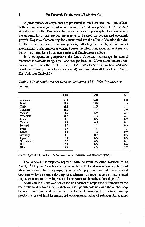
A great variety of arguments are presented in the literature about the effects, both positive and negative, o f natural resources on development. On the positive side the availability of minerals, fertile soil, climate or geographic location present the opportunity to capture economic rents to be used for accelerated economic growth. Negative elements regularly mentioned are the effect o f deterioration due to the structural transformation process, affecting a country’s pattern of international trade, hindering efficient resource allocation, inducing rent-seeking behaviour, formation of dual economies and Dutch disease effects.
In a comparative perspective the Latin American advantage in natural resources is overwhelming. Total land area per head in 1950 in Latin America was two or three times the level in the United States (which is the best endowed developed country among those considered), and more than 20 times that of South East Asia (see Table 2.1).
Table 2.1 Total Land Area per Head o f Population, 1900-1994 (hectares per capita)
1900 1950 1994Argentina 58.3 16.0 8.0Brazil 47.3 15.9 5.3Chile 25.2 12.3 5.4Colombia 26.0 8.7 3.0Mexico 14.0 6.9 2.1Venezuela 34.7 17.3 4.1Korea 1.1 0.5 0.2Taiwan 1.3 0.5 0.2Portugal 1.7 1.1 0.9Spain 2.7 1.8 1.3Ranee 1.4 1.3 0.9Germany 1.1 0.7 0.5Japan 0.9 0.5 0.3Netherlands 0.7 0.3 0.2UK 0.6 0.5 0.4USA 12.5 6.3 3.7
Source: Appendix A, FAO, Production Yearbook, various issues and Maddison (1995).The Western Hemisphere together with Australia is often referred to as
‘empty’.2 They are ‘countries of recent settlement’. Land was obviously the most abundantly available natural resource in these ‘empty’ countries and offered a great opportunity for economic development. Mineral resources have also had a great impact on economic development in Latin America since the colonial period.
Adam Smith (1776) was one of the first writers to emphasise differences in the use of the land between the English and the Spanish colonies, and the relationship between land use and economic development. Among the factors limiting productive use of land he mentioned engrossment, rights of primogeniture, taxes

Some Distinctive Characteristics 9
and levies and a restrictive trade system. The land system introduced by the Spanish, the ‘encomienda’, granted large properties to ‘conquistadores’ as well as the right to exploit indigenous labour more or less like serfs. The ‘encomienda’ was gradually replaced by the ‘hacienda’ which was the form of landownership that prevailed at the end of the colonial period.
However, it is important to note that during the colonial period Spain was not at all interested in agriculture and most part o f its energies went into obtaining gold and silver. The first source was, of course, the gold already found by native Americans from alluvial sources. The second step was to expand alluvial gold mining. The third step was the introduction of the mercury amalgamation technique which improved the efficiency of extraction and made the mining of lower grade silver ore possible. Mining developments generally created mineral rents that helped to maintain external equilibrium. But it produced a pattern of resource use that made the distribution of income worse, the economy less diversified, export earnings more concentrated on primary products. Mineral development may well have caused a lower growth rate in the non-mining sectors of the economy than otherwise would have occurred (Lewis, 1984).
In the colonial period, the Southern Cone countries, Argentina and Chile, established a system of great landed estates, haciendas or latifundios. Argentina (Río de la Plata in colonial times) was an impoverished colony. It was only during the second half o f the eighteenth century that exports o f hides provided an indication of the enormous potential of this rich and fertile country (Diaz- Alejandro, 1983 and Cortés Conde, 1985). Chile, which had some mining but nothing on the scale of the silver mines of Peru and Bolivia, experienced a great expansion of livestock herds in the seventeenth century to meet the strong demand for leather and for fats for making candles and soap. The eighteenth century saw the transformation of Chile’s pastoral economy when it captured the Peruvian market for wheat (Carióla and Sunkel, 1985).
Brazil was somewhat different as it was colonised by Portugal and mining was, initially, relatively unimportant. Portugal did not exercise as strong an authority as Spain did on its colonies. The plantation economy introduced in the sixteenth century, when Brazil became the world’s most important producer and exporter of sugar, also had distinct characteristics compared to the rest o f Latin America, particularly the use of slave labour on a great scale. Like the Southern Cone countries, Brazil was only sparsely populated at the time of conquest. Two centuries after Columbus’ discovery of the Americas, gold was found in Minas Gerais and the subsequent discovery of diamonds in 1729 generated an era of spectacular opulence that lasted into the second half o f the eighteenth century (Cardoso and Helwege, 1992).
Agriculture in Mexico towards the end of the colonial period was a hacienda system with great church estates. Production on these haciendas was mainly self- sufficient and only partly directed to the market. Most agricultural production was

10 The Economic Development of Latin America
for domestic consumption. There were also a few export crops such as dyes for the booming European textiles industry, cacao, vanilla and henequen. These haciendas were not ‘feudal’ as was originally claimed, especially by the Berkeley school (Borah, 1951), as they were connected to domestic markets, especially in supplying workers for the mining industry and urban settlements. Although some plantations were developed in Mexico, for example for sugar cane, these were never as important as in Brazil. Mexico’s agriculture was basically oriented to the domestic market.
Independence was seen by many as a great opportunity for Latin America to accelerate its economic development.3 The new opportunities for trade, now that the region was no longer hindered by Spanish regulations, and access to international capital are regularly mentioned as potentially the most important factors for inducing faster development. Most scholars point to the beginning of the nineteenth century as the starting point of accelerated capitalist development, with much faster growth than in the ‘protocapitalist’ period from 1500-1820 (Maddison, 1991a). However, Latin America did not enjoy the same acceleration as achieved in Europe and the United States, because the first half of the nineteenth century was devoted to political consolidation of independence and the formation of more stable political and economic regimes. Brazil and Chile were the first to form stable regimes and suffered less from political instability than other countries, especially Mexico, Colombia and Venezuela.
During the first half century after independence, Argentina’s considerable land- based natural resources remained undeveloped, as the country was immersed, most of the time, in political turmoil. Diaz-Alejandro (1983) claimed that a political and social framework compatible with export-oriented growth was established in Argentina only shortly after the middle of the nineteenth century. By 1880 the best land on the Pampas had been appropriated in a manner leading to concentrated ownership. All exports were based upon natural resource wealth, especially land, and the first exports were wool, hides and salted meat, to which wheat, com and linseed were added. Later on frozen beef exports became important. Brazil experienced an agricultural revival at the end of the eighteenth century based on its plantation economy. First sugar, later cotton and, at the end of the colonial period, coffee were to become extremely important in Brazil.
Mining, which had not been particularly important in Chile during the colonial period became prominent after independence. Chile then experienced an expansion based on exports of gold, silver and copper, followed in the 1850s and 1860s by substantial trade in grain. The grain exports originating from the area around the capital, Santiago, and the south, were very important during parts of the nineteenth century. This expansion was ended by the War of the Pacific in 1879. After the war, with the incorporation of the provinces of Tarapaca and Antofagasta, a second major cycle of expansion began. This cycle reached its height about 1920 and ended with the Great Depression of the 1930s. The boom in
Some Distinctive Characteristics 11
nitrate production in the provinces of the Norte Grande relegated grain and flour exports to a secondary role (Cariola and Sunkel, 1985).
The export-oriented development strategy of Latin America continued at least until 1913. It was after the Great Depression of 1929-33 that the debate: on industrialisation as a development strategy assumed importance in many countries. Industrial development was promoted after the Great Depression and during World War II as imports became scarce. This policy was at the expense of agricultural exports though mining exports remained important. Many authors have indicated that the process of industrialisation had already started long before the Great Depression4 but the import substitution strategy was intensified after the World War II and was maintained longer than many commentators, often in retrospect, thought necessary.
In the economic development of Latin America in the twentieth century, natural resources remained a very important element. Currently in all countries the single most important export product is a primary product.5 Several countries have added manufactures to their exports, but only in Mexico and Brazil do these represent more than 50 per cent of total exports. Recently, since the debt crisis of the 1980s, there has been some indication of change in Latin America’s development strategy. Chile is the prime example of a country which, after a process of macroeconomic stabilisation and economic restructuring, adopted a strategy based upon its abundant natural resources. The growth of the natural- resource based export sector has given new momentum, through forward and backward linkages, to the entire economy which has been growing at a rate of over 6 per cent for more than 10 years.
INSTITUTIONS
The institutional set-up and its relation to economic growth, a subject normally located in the sphere of the so-called ultimate causality, is extremely important and, in the case of Latin America, further study of the relationship between growth and institutions can be very useful. Institutions provide the incentive structure of a society and they comprise the formal rules, constitutions, laws and regulations; and informal constraints, conventions, norms of behaviour and self-imposed codes of conduct, and their enforcement characteristics (North, 1993). In a historical context the comparison between Latin America and the United States in terms of the institutional set-up might explain part of the difference in performance. North refers to the idea of path dependence, originated by David (1985) and Arthur (1988), and applied it to institutional evolution, indicating that once on a particular path economies find it very hard to fundamentally change direction because of the built-in characteristics of institutions. His striking comparison between the institutional evolution of Spain and England and the consequences for the
12 The Economic Development of Latin America
subsequent course of events in Latin and North America provides a striking illustration of the role of path dependency (see also North, 1990).
In this respect the ‘social capability’,6 that enhanced growth in the successful Asian countries, is deficient in Latin America. ‘Social capability’ refers to different elements such as the adequacy of the institutional framework, the role of government in designing and implementing economic policy and the skill level of the population.
During the conquest and the colonial period, Spain was to a large degree isolated from the forces important to modernisation in the rest o f Europe, especially in Northern Italy. The Renaissance and Enlightenment made possible recognition of man’s ability to transform the forces of nature through rational investigation and experiment. But Spain retained, to a great extent, medieval thinking and medieval ways. The wars of Reconquest against the Moors had allowed the Castilian Crown to obtain great wealth. Agriculture, crafts and commerce took second place to armed conquest as sources of wealth in the eyes of both hidalgos (noblemen) and peasants. It was this way of thinking which induced the followers of Hernán Cortés and Francisco Pizarra to seek fame and fortune in the new world. This behaviour and its modem, rent-seeking variant, is still, in many Latin American countries, an important component of the behaviour of economic agents.
In a comparison of institutional development in Latin America and the United States during their respective colonial periods, several features become clear.7 The level o f interference by the colonial power was much lower in the case of the English than in the case of the Spanish. As Smith (1776) noted:
Hie Spanish colonies, therefore, from the moment of their first establishment, attractedvery much the attention of their mother country; while those of the other Europeannations were for a long time in a great measure neglected, (p. 612)
Spain deliberately followed a policy of total conquest, modelling the colonies on the institutional structure of Spain and destroying the indigenous political and cultural institutions, together with indigenous religion and architecture. The other colonial powers had a much stronger tendency to a system o f coexistence with indigenous institutions.
The Spanish Crown established a centralised, hierarchical system with several viceroys,8 who also had responsibility for appointing bishops and therefore exercised control over the church. The authority of these viceroys was hardly challenged during the whole colonial period.9 Underneath this centralised structure there was a complicated method for dispensing favours, land mineral concessions and so on, which made it important to be close to power and which partially explains the absentee character of landownership.
The indigenous population was considered and treated as inferior. They were subjected to military oppression and faced unknown diseases like measles and

Some Distinctive Characteristics 13
smallpox that caused epidemics with extremely high death rates (Maddison, 1995). Later they were subject to cruelty, racism, injustice and indifference, elements characteristic o f colonial Latin America which continued to be a feature o f the independent Latin American countries.
The labour relations established under Spanish colonial rule were of an extremely dependent, debt peonage, and oppressive character. This impeded practically all forms of labour mobility and stands in marked contrast to the conditions experienced by settlers in the English colonies, who were basically independent, working their own land.
An important distinction between the English and Spanish colonies concerns the fiscal burden imposed upon them by the colonial power. There are very clear indications that taxes in the Spanish colonies were much higher than in the English ones. The Crown taxed the production of agricultural estates and mines by levying a ‘fifth’. Remittances of profits to Spain were quite high. In the case of the English colonies taxes were much lower and basically trade related. There was a big difference in the style of government between the English and the Spanish colonies in the Americas. The English colonies of North America were split up into 13 virtually autonomous colonies, while the Spanish featured a highly centralised power structure, and their top officials had a sumptuous lifestyle.
The mercantilist restrictions imposed on Latin America by the Spanish were much tougher than those on English colonies. They confined all their trade by their colonies to a particular port in the mother country; ships were obliged to sail from that port, in convoy at a particular season, or, if on their own, only once a special licence had been granted, which in most cases was very expensive. Trade was limited to a few ports in Latin America and Cadiz and Seville in Spain. The monopolistic character of this trade had very detrimental effects on prices, production and trade.10 The mercantile policy of Spain and Portugal practically prohibited the development of manufacturing industries in Latin America.
One of the institutional arrangements that changed as a result o f independence was the new ability to raise capital on the international financial market, which had been impossible during the colonial period. It is interesting to note, however, that all Latin American governments were in default by the end of the 1820s for a myriad of reasons. The colonial period did not prepare them for financial independence.
The origins of fiscal irresponsibility can be traced to Spain’s own practices. It is an irony of history that when Spain conquered Latin America, its relative power was already on the decline in Europe. One reason for this was the establishment of more efficient institutional arrangements in several European countries, such as the Netherlands and the UK, which were the world productivity leaders until the beginning of the twentieth century. The institutional systems of Portugal and Spain were very different from those in the more advanced northern European countries

14 The Economic Development of Latin America
in terms of religious practice, centralisation of power, the role of science and technology and the degree of fiscal responsibility.
Argentina was created as a nation, in the sense of definitively bringing the national territory under a single regime, in the third quarter o f the nineteenth century. Formal political unity was achieved between 1859-62, with the accession of Buenos Aires province to the Argentine Federation. But the issue of governance was only resolved in the following two decades, with the closing of the Indian frontier in Patagonia, the suppression o f the last regional revolt and the creation of a federal district separating the city of Buenos Aires from the province of the same name in 1880. Diaz-Alejandro (1970) states:
From 1860 to 1930 Argentina grew at a rate that has few parallels in economic history, perhaps comparable only to the performance during the same period of other countries of recent settlement, (p. 18)
Differences in the role of central government in the economies o f Latin America can be explained partly by political considerations, as well as by differing relations with the world economy. The state in Brazil was internally strong and internationally respected, while in Mexico the state was internally fragmented and internationally dependent. The republicans who took power in Brazil in 1889 inherited a state with fairly strong institutions that had the support of the elite, since Brazil’s path to independence had been smooth. A weak church and the social cement of slavery tended to convince the country’s ruling class of the necessity to maintain a united front. Arguably, a nation was built and a state formed earlier in Brazil than anywhere else in Latin America.
Brazil experienced a peaceful transition to independence. It was much more dependent on the world economy than Mexico, its ratio of exports to GDP was twice that of Mexico, and exports were concentrated in two commodities, coffee and rubber. The Brazilian state relied upon taxes on international trade to a much greater degree than Mexico. Foreign exchange was a more pressing concern, since Brazil’s foreign debt was twice the size of Mexico’s.
The transformation and the strengthening of the economies of Latin American countries occurred at different moments in their national histories, depending on the export commodities involved and their relative success in state-building. Chile’s economy was affected by overseas demand as early as the 1850s (copper exports to Europe and wheat to California), and Argentina and Brazil followed in the 1860s. These countries, along with Mexico, then felt the full impact of the combined effects o f the European economic expansion, which, as far as Argentina and Brazil were concerned, triggered an unprecedented level o f European immigration. Chile established a constitutional regime in 1833 and was widely admired in Spanish America for its stability. Mexico and Argentina were not to have stable regimes until the late 1860s.
Some Distinctive Characteristics 15
In Colombia the doctrine of economic liberalism went unchallenged from the late 1840s until the 1880s. The basic tenet of economic thinking in Colombia until the 1940s was economic liberalism. Independence brought a more general commitment to economic liberalism in the 1820s by the Colombian government. It adopted free trade and attempted both to reform some taxes and to privatise Indian communal holdings in accordance with liberal prescriptions. The state that Porfirio Díaz seized in 1876 was less secure; Mexico before Diaz had been plagued by civil wars, regional rivalries, and foreign invasions. The treasury was plundered, foreign credit scant, power splintered and sovereignty mocked. Internal peace and external pressures were constant concerns of Diaz.
INEQUALITY OF INCOME AND WEALTH
The distribution of income and wealth in Latin America is extremely unequal in comparison with most of the rest of the world, and these levels o f inequality have been persistent over time. The roots of this situation can be found in the distribution of land, mineral rights and education during the colonial period.
Labour relations inherited from the system of landownership, which tied the workers and their families to the land, also caused very uneven initial conditions and proved to be a major obstacle to a more equal distribution of income. Education of the masses was completely neglected during the colonial period; Spain even tried to prevent the population from becoming literate because this was deemed dangerous for religious and political reasons. Two particular facets o f the colonial period provide a partial explanation of the uneven income distribution in Latin America. Unequal income distribution was a legacy from the old colonial system of labour exploitation, with slavery in Brazil and peonage elsewhere. Restricted access to education was another cause of inequality, and was more important than in many Asian countries (Maddison, 1989).
Cardoso and Helwege (1992) describe the roots of inequality as follows:
The colonial division of property had implications not only for the usage of land but for the political structure of die region as well. The encomienda system established a landed aristocracy that dominated political life for centuries and then shared power as industry displaced agriculture as the central economic activity. It established a sharp division between the haves and the have-nots, creating a class structure that is extremely bifurcated by comparison to other cultures. Problems of unequal income distribution and widespread rural poverty that face the region today are rooted in events of the sixteenth and seventeenth centuries, (p. 37)
The problem of inequality in income and wealth was inherited from the colonial period, in which the distribution of assets (principally land) favoured a concentration of income, and for most of the post-independence period the

16 The Economic Development of Latin America
dynamics of the dominant model of economic development have either preserved the existing level o f inequality or have exacerbated it (Bulmer-Thomas, 1994).
A long-term view of Latin American income distribution is very difficult to obtain because o f huge methodological difficulties.11 In Table 2.2 Gini coefficients12 are presented for the 1950-90 period based upon a methodology of linking appropriate pairs of Gini coefficients.
Altimir (1987) describes these pairs which were selected on the ground that they are comparable with regard to the concept of income, the procedure used for measuring income and the geographical coverage of the surveys used to collect the data, as well as the units and criteria used by the respective authors in processing or adjusting the survey data (see also Altimir, 1992).
A first step in the preparation of Table 2.2 was the selection of a base period Gini for which there were reliable estimates of income distribution in the specific country. This base period Gini estimate was linked over time to the other available estimates. The results indicate that income distribution in Latin America in the post-war period either remained the same or worsened. The worsening of the income distribution was especially marked after 1980.13
Table 2.2 Latin America: Inequality in Pre-tax14 Income Distribution, 1950-90 (Gini coefficients around benchmark years)
1950 1960 1970 1980 1990Argentina 0.400 0.419 0.412 0.472 0.423Brazil - 0.570 0.630 0.619 0.631Chile - 0.459 0.473 0.522 0.520Colombia 0.513 0.542 0.516 0.566 0.494Mexico 0.516 0.606 0.586 0.478 0.523Venezuela 0.613 0.462 0.494 0.390 0.442Average Gini 0.510 0.509 0.518 0.507 0.506
Source: Oscar Altimir kindly provided access to his extensive database on income distribution (see also Altimir 1997 and 1998). The 1950 estimate for Venezuela is a direct interpolation based upon estimates fra-1944 and 1962 from Baptista (1991).15
In Table 2.3 the Latin American countries are compared with the other countries of our sample, and the results show markedly higher inequality in Latin America than in all the other country groups. There are also reasons to presume that these differences have persisted over time. Inequality may have risen somewhat in recent decades in the advanced countries.

Some Distinctive Characteristics 17
Table 2.3 Inequality o f Pre-tax Income o f Households around 1970
Year Gini coefficientTop decile per capita income as multiple o f that in bottom deciles
Argentina 0.412 11.2Brazil 0.630 20.0Chile 0.505 21.3Colombia 0.539 21.8Mexico 0.586 25.5Venezuela 0.494 25.0Arithmetic average 0.528 20.8
Korea 1970 0.351 7.6Taiwan 1959 0.396 7.0Arithmetic average 0.374 7.3
Spain 1965 0.393France 1970 0.416 14.4Germany 1973 0.396 10.5Japan 1969 0.335 7.5Netherlands 1967 0.385 10.5UK 1973 0.344 9.1USA 1972 0.404 13.5Arithmetic average 0.382 10.9
Source: If not otherwise mentioned, from sources given in Maddison (1989) and (1995). See Table 2.2 for Latin American Gini coefficients. Gini coefficients for Spain from Jain (1975).
HUMAN CAPITAL
The renewed interest expressed by the ‘new growth’ theorists in human capital highlights once again the importance of this factor in improving productivity and growth. A higher level of education permits faster incorporation of technical progress and most growth analysts, since Schultz (1961) and Denison (1962), attribute an important weight to this factor. Education had an extremely low priority during the colonial period in Latin America. Far fewer universities were established than in the United States even though the population was much larger. To a great degree, the indigenous population went uneducated during the entire colonial period. Argentina had moved toward mass primary education as early as 1860 (Bulmer-Thomas, 1994), and was the first country in Latin America in the twentieth century to provide compulsory primary education, paid for by the State, for all o f the population (Cortés Conde, 1985).
Brazil’s educational system lagged behind those of most Latin American countries. Women were almost totally left out until well into the twentieth century. At the end of the colonial period the whole rural and urban population was illiterate. The situation had improved somewhat by the end of the nineteenth

18 The Economic Development of Latin America
century, especially with respect to the urban population, whose literacy rates reached a figure of just below 50 per cent. Education in Chile became a priority during the government of José Manuel Balmaceda (1886-91) and major progress was made at the primary level (Blakemore, 1992). However, primary education became compulsory only in 1920 (Mamalakis, 1976).
The rural indigenous population of Colombia received almost no formal education during the colonial period. From the middle of the nineteenth century some increase in elementary education took place and the proportion of the population able to read reached about 30 per cent at the beginning of the twentieth century. The National University was founded in 1867 but most professionals received their education abroad (see Orlando Melo, 1987 and Safford, 1976).
In Mexico the indigenous population was almost completely denied education during the colonial period. The education of the middle and upper classes was entirely dominated by the Catholic Church. After independence there was little change in education policy. An educational reform was initiated in 1833 but could not be fully implemented. During the second half of the nineteenth century education was reformed and removed from clerical control, and there was some state intervention in favour of popular education. After the Mexican Revolution, free compulsory education was introduced but initially coverage was extremely low. Table 2.4 shows the evolution, during the second half o f the twentieth century, of the situation in Latin America as regards years of primary, secondary and higher education.
Table 2.4 Average Years of Formal Educational Experience of Population Aged 15-64,1950-90
I1950n m I
1970n in I
1980n m I
1990n ffl
Argentina 3.9 0.8 0.1 4.7 1.5 0.2 5.0 2.0 0.4 5.1 2.7 0.7Brazil 1.5 0.2 0.1 2.2 0.6 0.1 3.2 0.9 0.1 3.9 1.3 0.2
Chile 3.6 0.7 0.1 4.4 1.4 0.3 4.9 2.1 0.3 5.3 3.0 0.4
Colombia 2.0 0.3 0.1 3.0 0.9 0.1 3.4 1.4 0.2 4.4 2.4 0.4
Mexico 1.9 0.2 0.0 2.9 0.5 0.1 4.2 1.3 0.2 4.6 1.9 0.4
Venezuela 1.7 0.2 0.0 2.8 0.6 0.1 4.1 1.2 0.2 5.4 2.3 0.4
Note: I refers to primary, II to secondary and III to higher education.
Source: Appendix C.

Some Distinctive Characteristics 19
INFLATION
The issue of inflation has generated intense debate in Latin America, especially between the so-called monetarists and structuralists. The former see inflation as detrimental, and contend that a stable price level is a necessary condition for economic growth, whilst the structuralist school regards inflation as an inevitable byproduct of economic growth. Simonsen (1964) differentiates the monetarist and the structuralist school by the sign of the correlation between growth and inflation. For the structuralists this is positive while the monetarists expect it to be negative.
Table 2.5 Experience o f Inflation, 1900-1994 (annual average compound growth rates)
1900-13 1913-29 1929-38 1938-50 1950-73 1973-80 1980-94
Argentina n.a 2.2 -0.7 30.6 30.5 189.1 629.1Brazil -1.6 6.4 -0.2 12.3 31.6 47.0 748.6Chile 7.3 5.1 6.5 16.4 48.6 236.2 22.3Colombia 4.6 7.7 3.1 11.7 10.8 27.2 26.4Mexico 5.3 2.9 2.2 10.0 5.7 22.5 58.9Venezuela 3.0 1.7 -4.4 6.0 1.8 11.3 28.9Arithmeticaverage 3.7 4.3 1.1 14.5 21.5 88.9 252.4
Korea 30.1 20.0 8.7Taiwan 7.2 13.0 3.2Arithmeticaverage 18.6 16.5 6.0
Portugal 3.4 23.9 16.7Spain 6.7 19.6 9.7Arithmeticaverage 5.0 21.7 13.2
France 0.9 12.1 1.4 28.1 5.0 11.1 5.5Germany 1.3 2.5 -2.2 3.8 2.7 4.8 2.8Japan 2.8 4.8 1.2 82.4 5.2 9.7 2.1Netherlands 1.1 2.0 -2.1 7.4 4.1 7.1 2.6UK 0.9 3.3 -0.7 5.3 4.6 15.8 6.4USA 1.3 3.1 -2.1 4.5 2.7 8.9 4.5Arithmeticaverage 1.4 4.7 -0.7 21.9 4.1 9.6 4.0
Note: For the Asian and the Iberian countries, no information for the pre-war period was available.
Source: Maddison (1989), IMF (various issues) and Appendix G.
In comparative terms Latin American inflation has been higher than in OECD countries, particularly since World War H. One of the most interesting findings is the fact that the acceleration of inflation had started well before the 1950s, as a

20 The Economic Development of Latin America
matter of fact the starting point is similar to that documented in Table 3.4, which shows the growth acceleration in GDP per capita and labour productivity.
Table 2.5 presents the inflationary experience in the twentieth century of a sample of 17 countries, and shows that Latin America had the highest inflation of all regions in most periods. It also makes clear that the Latin American inflationary experience was, surprisingly, not very different from that of the advanced countries during the first half of the twentieth century. The advanced countries witnessed more or less the same levels of inflation before the Great Depression, and the acceleration of inflation during the 1938-50 period was greater than in the case of the Latin American countries. However, with the exception of Japan (the country that had by far the highest inflation in this period), inflation in the advanced countries was somewhat less than in Latin America.
Table 2.5 shows that the big difference occurred after World War II when all areas, except Latin America, experienced a reduction in inflationary momentum. In the period 1973-80 inflation accelerated in all countries, with Latin America again recording the highest rates. While inflation abated in the rest o f the world after 1980, Latin American inflation accelerated further. In the early 1990s, in the context of economic stabilisation and restructuring, most Latin American countries were able to drastically reduce their rates of inflation. In particular, Argentina and later Brazil which had recorded extremely high rates succeeded in stabilising their economies; Chile and Colombia reduced inflation even further, while in Mexico and Venezuela inflation increased somewhat.
DEBT PROBLEMS
The recent debt crises of the 1980s and the 1990s are not unprecedented events, but part of a chain of recurrent crises throughout the history of Latin America. During more than a century and a half the Latin American nations have repeatedly experienced international financial storms that greatly damaged their economies and strapped them into an apparendy irrevocable succession of boom and bust cycles that reinforce underdevelopment (Marichal, 1989).
Foreign capital can foster economic development in various ways, for example through increases in the rate of growth of the capital stock, mitigating payment problems and helping technology transfer. However, Latin America’s experience has been one of booms and crises. Productive use of foreign investment very often did not have priority; indeed the first inflow of capital into Latin America shortly after independence was used principally for military expenses. Defaults were usually followed by a 20- to 30-year drought in access to private credit.
One of the first significant financial waves came in 1822 as newly independent Latin American countries attracted European capital for the consolidation of independence and trade promotion.16 The financial boom was short-lived,
Some Distinctive Characteristics 21
however, as debtors and investors overestimated the region’s export earnings potential and were also adversely affected by the European financial crisis of 1825-26; servicing problems and financial panic occurred shortly thereafter in 1827. The severe losses experienced by creditors helped keep foreign investors away from the region for more than two decades. Nevertheless, foreign capital returned with some enthusiasm in the 1850s due to expansive forces in some European capital markets and the fading memories of the past losses. The second wave of credit was also followed by severe payment problems: 58 per cent of Latin American public debt to Great Britain was in default by the end of 1880 (ECLAC, 1965a).
Notwithstanding these earlier problems foreign capital flowed into Latin America during the rest o f the nineteenth century and the early part of the twentieth century, although there were other payments crises in the 1870s, triggered by the world crisis of 1873, and in 1890, as a result o f the Anglo-Argentine financial panic of that year (Marichal, 1989). During this period Latin America managed to attract a steadily increasing number of foreign investors, and by the eve of World War I the region had become the target of keen competition among the great international financial centres.
During World War I capital flows to Latin America slumped, but serious payments problems did not develop, in part because exports and payments capacities were boosted in wartime. In the 1920s another investment boom ensued, followed by the famous crash of the 1930s, which was brought on by the Great Depression and the dramatic fall in the region’s export prices. Private capital flows dried up almost completely in the fifteen years following the 1929 depression due to defaults. It was only after World War II that Latin America’s access to private international capital began to be gradually restored.
Immediately following World War II, the region’s foreign finance was heavily dependent on direct foreign investment flows and bilateral lending. This was complemented by World Bank funding at the end of the 1950s, as that institution turned its attention from the reconstruction of Europe to development finance. Additional multilateral finance became available in the early 1960s with the establishment of the Inter-American Development Bank. Private commercial banks had a very low profile in the region’s external finance situation, generally limiting themselves to export credits guaranteed by their own government and relatively risk-free short-term trade credit. Meanwhile, bond issues were for only limited amounts due to investors’ lingering memories of the 1929 crash, and the institutional restrictions that limited access to these markets.
The picture changed radically in the 1970s. Capital flows boomed, partly as a result o f increased liquidity due to the first oil crisis and partly because of increasing Latin American demand. These new inflows were largely provided by private commercial banks. A good deal of the flow was in the form of bank credits at floating rates of interest, most of them denominated in dollars. The situation
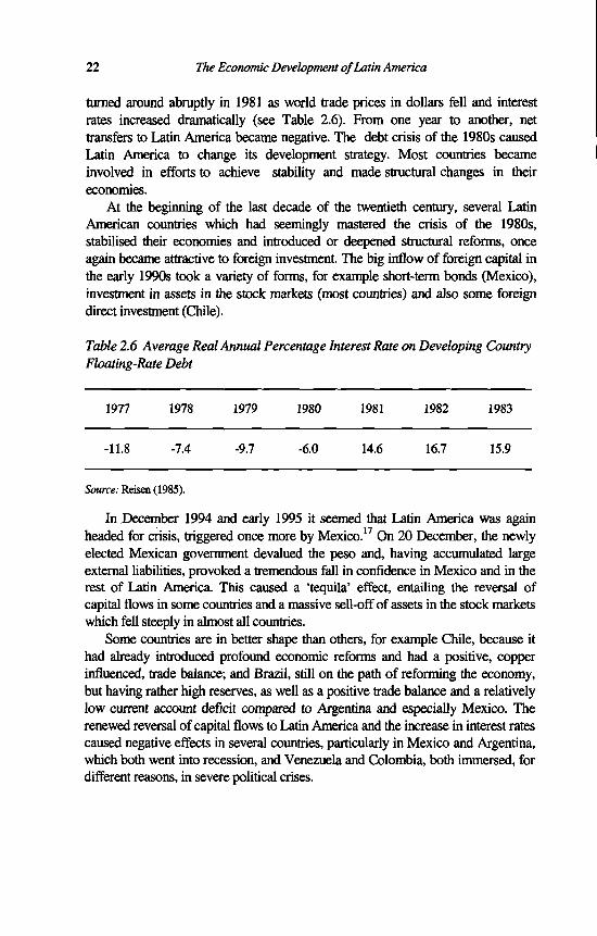
22 The Economic Development o f Latin America
turned around abruptly in 1981 as world trade prices in dollars fell and interest rates increased dramatically (see Table 2.6). From one year to another, net transfers to Latin America became negative. The debt crisis of the 1980s caused Latin America to change its development strategy. Most countries became involved in efforts to achieve stability and made structural changes in their economies.
At the beginning of the last decade of the twentieth century, several Latin American countries which had seemingly mastered the crisis o f the 1980s, stabilised their economies and introduced or deepened structural reforms, once again became attractive to foreign investment. The big inflow o f foreign capital in the early 1990s took a variety of forms, for example short-term bonds (Mexico), investment in assets in the stock markets (most countries) and also some foreign direct investment (Chile).
Table 2.6 Average Real Annual Percentage Interest Rate on Developing Country Floating-Rate Debt
1977 1978 1979 1980 1981 1982 1983
-11.8 -7.4 -9.7 -6.0 14.6 16.7 15.9
Source: Reisen (1985).
In December 1994 and early 1995 it seemed that Latin America was again headed for crisis, triggered once more by Mexico.17 On 20 December, the newly elected Mexican government devalued the peso and, having accumulated large external liabilities, provoked a tremendous fall in confidence in Mexico and in the rest of Latin America. This caused a ‘tequila’ effect, entailing the reversal of capital flows in some countries and a massive sell-off of assets in the stock markets which fell steeply in almost all countries.
Some countries are in better shape than others, for example Chile, because it had already introduced profound economic reforms and had a positive, copper influenced, trade balance; and Brazil, still on the path o f reforming the economy, but having rather high reserves, as well as a positive trade balance and a relatively low current account deficit compared to Argentina and especially Mexico. The renewed reversal of capital flows to Latin America and the increase in interest rates caused negative effects in several countries, particularly in Mexico and Argentina, which both went into recession, and Venezuela and Colombia, both immersed, for different reasons, in severe political crises.
Some Distinctive Characteristics 23
THE MOVE FROM OPEN TO CLOSED ECONOMIES - 1929-1980s
Latin America’s role in the world economy is a story of ups and downs. During the colonial period trade was officially limited only to Spain and Portugal, although smuggling became increasingly important. After independence there was freer trade and although initial political instability did not help the export sector, exports increased in some countries, for example Chile, and Latin America’s terms o f trade probably improved as prices of imports fell after the termination o f the colonial monopoly.
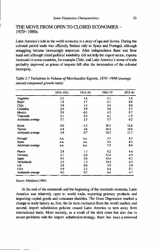
Table 2.7 Variations in Volume o f Merchandise Exports, 1870—1994 (average annual compound growth rates)
1870-1913 1913-50 1950-73 1973-94
Argentina 5.2 1.6 3.1 5.8Brazil 1.8 1.7 4.7 8.9Chile 3.4 1.4 2.4 8.8Colombia 2.0 3.9 3.8 5.7Mexico 5.9 -0.5 4.3 9.7Venezuela 4.1 5.4 4.1 -1.9Arithmetic average 3.7 2.3 3.7 6.2
Korea 0.0 -1.3 20.3 12.6Taiwan 4.8 2.6 16.3 10.8Arithmetic average 2.4 0.7 18.3 11.7
Portugal n.a. n.a. 5.7 8.5Spain n.a. n.a. 9.4 8.2Arithmetic average n.a. n.a. 7.5 8.4
France 2.8 1.1 8.2 4.4Germany 4.1 -2.8 12.4 4.0Japan 8.5 2.0 15.4 6.2Netherlands 2.3 1.5 10.3 4.3UK 2.8 0.0 3.9 3.9USA 4.9 2.2 6.4 5.1Arithmetic average 4.2 0.7 9.4 4.7
Source: Maddison (1995).
At the end of the nineteenth and the beginning of the twentieth centuries, Latin America was relatively open to world trade, exporting primary products and importing capital goods and consumer durables. The Great Depression marked a change in trade history as, first, the de facto exclusion from the world market, and second, import substitution policies caused Latin America to turn away from international trade. More recently, as a result o f the debt crisis but also due to severe problems with the import substitution strategy, there has been a renewed
24 The Economic Development of Latin America
trend to use trade as an engine o f growth.Latin America has always been an exporter of primary commodity exports: in
the colonial period, first minerals like silver and gold, and later on agricultural products like sugar and coffee. Surprisingly, for all the countries of our sample the first export product, by value, is actually still a primary commodity: coffee in the case of Brazil and Colombia, oil in Mexico and Venezuela, maize in Argentina and copper in Chile. In the section dealing with natural resources, it was pointed out that some Latin American countries had been quite successful in entering the world market on the basis o f agricultural and mining products.
In Table 2.7 the export performance o f Latin America, in terms o f volume growth rates, is compared with other regions. At the beginning of the century Latin America’s performance was similar to the rest of the world. The 1913-50 period was much better for Latin America, among other reasons because it was not that directly affected by the World Wars.
In 1950-73 the export performance of Latin America in comparison with the rest o f the world was extremely poor. Latin America did not profit from the rapid expansion of trade opportunities, indeed Latin American trade barriers and protection were increased. The data presented for the 1973-94 period were disaggregated in the case of Latin America to show somewhat higher overall growth rates in the 1980-94 period. Argentina, Colombia and Venezuela had higher growth rates in 1980-94 than in 1973-80. Brazil had similar growth rates in both periods and Chile and especially Mexico had lower growth rates in the 1980-94 period.
POLITICAL AND POLICY INSTABILITY
One of the points stressed by many authors is the importance of ideology in Latin America’s macroeconomic management as opposed to the more pragmatic approach followed, for example, by some Asian newly industrialising countries.
As has been indicated above, in the discussion on institutions, economic policy in Latin America during the colonial period was guided principally by the mercantilist doctrine imposed by Spain. After independence a shift can be observed towards a more laissez-faire orientation. At the end o f the nineteenth century free trade and liberal commercial policies had favourable effects on economic growth. However, Latin America already had quite high levels of protection compared to other regions in the world.
The 1930s are widely regarded as a major turning point in Latin America’s development. The decade marks the acceleration of import-substituting industrialisation and the start of public policy more concerned with growth and social objectives. An important element was the emergence o f strong protectionism and nationalism in most of the advanced countries. By the end of 1931 most Latin

Some Distinctive Characteristics 25
American countries were experimenting with balance of payments measures previously regarded as heterodox.
As a result of the unfavourable shocks of the Great Depression, the Latin American policy mix changed more by force of circumstance than deliberate strategy. The countries of the region abandoned the gold standard, imposed exchange controls and discriminatory trade restrictions (such as quotas, tariffs, and multiple exchange rate systems) on imports of consumer goods, and adopted countercyclical fiscal and monetary policies. This set of policies has been called the model of domestically-oriented growth. Import-competing manufacturing activities were given an advantage not only through protective trade policies, but also through tax and credit incentives. Specifically, the dynamic growth component, instead of being the export sector as it was before the Great Depression, was private and public investment in import-substituting industries and public investment in infrastructure geared to these industries’ needs (Corbo, 1988).
Latin America abandoned economic orthodoxy in the beginning of the 1930s with remarkable success. Most Latin American countries had by 1932 erected exchange control barriers, raised tariffs, devalued very substantially and begun to default on foreign debt. In thus breaking away from the liberal international economic order and gold standard rules they felt able to follow expansionary fiscal and monetary policies to promote recovery (Maddison, 1985). The drastic experience of recession in the independent countries of Latin America had induced a change in attitudes towards the liberal international economic order, and an inward-looking approach to development which had its first successes in the 1930s (Maddison, 1985).
After World War n , when the advanced countries embarked on a period of growth characterised by dismantling of barriers to international trade and capital and so on, Latin America’s policies did not change much and came to be characterised as ‘structuralism’ (Corbo, 1988). The main characteristic was promotion of industrialisation for the domestic market. Import substitution was implemented by a set of policies designed to shift the domestic terms of trade between agriculture and industry in favour of the latter. The major tool was the trade regime. Moreover, in these years of increasing intervention, the state itself often became directly involved in import-substitution industrialisation by setting up public enterprises in highly protected sectors, such as steel, petroleum, and chemicals. One of the major results of this policy was discrimination against exports (Corbo, 1988).
In the late 1940s and the 1950s the Santiago-based Economic Commission for Latin America and the Caribbean (ECLAC) worked on the theoretical foundations of what was to be called the structuralist position in economic development. Raul Prebisch, one of the most controversial and influential intellectual leaders in Latin America, formed a team in the late 1940s and onwards at ECLAC and produced a

26 The Economic Development o f Latin America
series of studies of which the one by Prebisch (1991) is the best known.18 Here the influential concept of the ‘centre-periphery system’ in economic relations was revealed for the first time.
Prebisch’s best known academic contribution is the so-called Singer-Prebisch thesis (see also Singer, 1950) on the secular deterioration of terms of trade which led him to advocate industrialisation in Latin America and for a long time made ECLAC and import substitution inseparable. Many of these ideas were initially developed as a result o f analysis o f problems of inflation. Structuralist analysis attempted to identify specific rigidities, lags, shortages and surpluses, low elasticities of supply and demand, and other characteristics of the structure of developing countries that affect economic adjustments and the choice of development policy (Chenery, 1965). Structuralist analysts emphasised, among many other factors, the role of the state in economic development, the structural shift from agriculture to industry, and the lack of economic surplus for accumulation; they became influential in many countries in Latin America, particularly in Brazil and Chile.
A more critical analysis, also with respect to import substitution industrialisation, was provided by the Marxist structuralist interpretations, o f which André Gunder Frank (1969) and Paul Baran probably offered the best known. The relationship between the ‘core’ and the ‘periphery’ is not one of mutual benefits but of exploitation. The surplus in the periphery will be caught by foreign capital or by the local elite. The basic theory is that import substitution increases dependency on imports and increases the power of the industrialists and multinational corporations at the expense of the poor and the rural peasants.
In the mid 1960s, both at ECLAC and elsewhere, another more sociological and political line of interpretation was developed to be known as ‘dependency theory’, which tried to explain why some of the presumed consequences of industrialisation for the periphery were not being produced. One of the basic economic arguments was that the industrialisation that took place in Latin America was largely limited to the production of consumer goods. The fruits o f the dynamic capital goods sector where technical progress was concentrated went once again to the centre nations (Cardoso and Faletto, 1969).
Another set o f ideas was developed at ECLAC to counter the foreign exchange constraint through economic planning and economic integration of the Latin American market, in order to be able to move to a second, more difficult stage of import substitution which could not be enacted at the national level alone. This analysis, together with the structuralists’ view on inflation, was very influential in the 1960s and has been labelled Structuralism II (Corbo, 1988).
From early on several critics, within and outside Latin America, criticised the import substitution strategy. As early as 1950, Viner (1950), had rejected most of the arguments for protecting import-competing industry and recommended elimination of discrimination against exports. Another influential critic was

Some Distinctive Characteristics 27
Roberto Campos (1967), who questioned the emphasis in favour o f industry at the expense o f agriculture, and the confidence in the theory that, by substituting public for private initiative, new resources would be created, and the assumption that inflation could be used to increase capital formation in a sustainable way.
Around the middle of the 1970s, a group of Southern Cone countries started to experiment with new policies which abandoned import-substitution policies and government intervention. These so-called neoconservative experiments were inspired as much by political and ideological as by economic factors and were implemented under the reign of military governments. Although many observers acknowledged serious problems in Latin America’s development strategy in the mid 1970s, including the inefficient role of the state, the application of a radical anti-interventionist model paid very little attention to the limits o f the market and the private sector (Ramos, 1986).
The debt crisis o f the 1980s caused many Latin American countries to rethink their development strategy due to the economic necessity of debt servicing and external constraints; many countries started to implement neo-liberal policies consisting of economic adjustment, stabilisation and outward orientation, and also including policies to reduce state intervention, promotion of private enterprise, fiscal discipline, getting the prices right and improving allocation in the product, factor, and financial markets. Most of these policy elements were included in the ‘Washington Consensus’ (Williamson, 1990); additional themes like income distribution and social issues have been added to the agenda in the 1990s.
NOTES
1. Smith (1776, p. 617): ‘Plenty of good land, and the liberty to manage their own affairs their own way, seem to be the two great causes of the prosperity of all new colonies’.
2. H ie term ‘empty’ countries, used for the American hemisphere and Australia, was of course not appropriate as both areas had significant indigenous populations. North America, the Southern Cone and Australia were sparsely populated. The more densely populated parts o f the Americas experienced very drastic reductions in their population in the first decades after the conquest
3. Most Latin American countries became independent during the first half o f the nineteenth century. All countries, except Brazil, declared their independence in 1810 and won it soon after 1816 in Argentina, 1818 in Chile and Colombia and 1821 in Mexico and Venezuela. Brazil became independent from Portugal in 1822.
4. See in the case of Argentina (Diaz-Alejandto, 1970 and 1983), in Brazil (Suzigan, 1976), in Chile (Palma, 1979 and 1984), and in Colombia (Ocampo, 1987).
5. In the case o f Argentina, maize (8.0 per cent) and beef (6.7 per cent) are the first and second export products and 68 per cent o f all expats are of primary origin. The respective figures f a other countries are: Brazil, coffee (8.5 per cent) and iron ore (5.2 per cent) and 40 per cent; Chile, copper (42.9) and grapes (4.6 per cent) and 81 per cent; Colombia, coffee (49 per cart), oil (12.6 p a cent) and 69 per cent; Mexico, oil (43.6 per cent), coffee (3.5 per cent) and 47 per cent; and Venezuela, oil (79.1 per cent), aluminium (4.2 per cent) and 86 per cent (Bulmer-Thomas, 1994 and W a ld Bank, 1995).
6. A term introduced by Okhawa and Rosovski (1973) but recently emphasised especially by Abramovitz (1986,1990).

28 The Economic Development of Latin America
7. The comparison by Adam Smith (1776) of colonies in the Western Hemisphere was not the fust but he concentrated on economics while other comparisons, for example Buffon (1761), de Pauw (1768) and Hegel (1820) were more of a theological-philosophical nature (Annino, 1995).
8. Around 1800 Latin America was divided in die Viceroyalties o f New Spain, New Granada, Peru and Rio de la Plata (Lynch, 1991).
9. Between 1535 and 1816 there was a steady succession of 60 viceroys in New Spain (Maddison, 1995).
10. However, these detrimental effects of mercantilism on Latin American production, trade and development should not be overestimated; see the careful summary in Cardoso and Helwege (1992), emphasizing that mercantilism may not have been as important in slowing industrial and agricultural growth as the distorting nature o f the mineral boom itself. They also stress that most European countries were extremely protectionist until the late nineteenth century. This makes it difficult to assess how much trade would have occurred in the absence o f mercantilism.
11. Among those most mentioned are: underestimation o f income that affects differently both income level and their concentration, the technique for measuring income and the geographical coverage of the surveys, see Altimir (1987) for a review and discussion of the income measurements from different types of surveys in Latin America and their comparability problems.
12. The Gini coefficient is a measure o f income concentration that ranges from 0 to 1, the larger the coefficient, the greater the inequality. Thus 0 represents perfect equality and 1 represents perfect inequality.
13. It cannot be stressed enough that these estimates give only an indication of a tendency as the linking procedure involved linking series o f different coverage, definition and quality.
14. In the strict sense it is difficult, especially in die case of the Latin American countries, to differentiate between pre- and post-tax income distribution, again; see Altimir (1987).
15. I did not use the 1957 estimate (0.802) o f Baptista (1991) because it seemed unreasonably high, especially compared with his 1962 estimate (0.462).
16. The following description of Latin America’s history of capital flow and debt is based largely upon Devlin (1989), ECLAC (1965a) and Marichal (1989).
17. By the middle o f 1995 things had settled again; the major countries affected by the crisis were Mexico and (to a lesser extent) Argentina, both entering into recession. The repercussions in the rest o f Latin America were relatively minor and most countries recovered part o f the losses, especially those on the stock markets. However, on a negative note, several observers have commented that the crisis o f the 1980s started the same way, through a number of mine»' crises in several countries. On the other band, more optimistic observers suggest that the situation in Latin America is now structurally different from the 1980s as many countries have restructured their economies. In fact, only a few countries have advanced far in structural reforms, notably Chile, but several others are in the process of restructuring and it is to be hoped that economic growth will resume (or continue) in Latin America as restructuring is always much easier in times of economic growth but is extremely painful in times of crisis. It should also be stressed that structural reforms do not prevent crisis per se, as Chile found out so painfiilly in the early 1980s.
18. Many studies could be mentioned; o f special importance were a series of country studies titled, “The Economic Development o f ...” , which used what for that period were quite advanced techniques; capital stock estimation, econometric analysis and extensive data collection, and which are up-to-date valuable statistical sources for historical research due to their excellent empirical base. Other important ECLAC studies dealt with external financing, inflation and industrialization.

3. Economic Performance in Latin America - A Comparative Quantitative Perspective
A primary purpose of this book is to provide a new quantitative assessment of Latin American economic growth performance in the twentieth century. For the period after 1950 a growth accounting framework is presented in Chapter 6. Chapters 4 and 5 provide the necessary basic series for capital stock and labour input.
In this chapter the growth performance of Latin America throughout the twentieth century is treated from a comparative perspective using indicators of demographic development, growth rates of GDP and GDP per capita and labour productivity. Our sample covers only six of the 44 countries of Latin America and the Caribbean - Argentina, Brazil, Chile, Colombia, Mexico and Venezuela - but these had in 1994 a combined population of 359 million, equivalent to 75 per cent of the total for Latin America. They cover about 80 per cent of Latin American territory, and about 85 per cent of Latin America’s GDP. Two major biases of the sample should be emphasised. First, it excludes the smaller countries of the Latin American continent which generally have a (much) lower per capita GDP. Second, it also excludes all 23 islands of the Caribbean which make up for around 5 per cent of GDP in the area, and of which 15 have higher than average per capita GDP.
Latin America’s performance is compared with three other groups of countries:(a) two Asian countries (Korea and Taiwan) whose economic growth in the past couple of decades has been remarkably fast; (b) Portugal and Spain, whose institutional heritage had a good deal in common with Latin America; and (c) six advanced capitalist countries (France, Germany, Japan, the Netherlands, the United Kingdom and the United States), whose levels o f income and productivity are amongst the highest in the world.
AGGREGATE GROW TH PERFORM ANCE
The GDP growth rates presented in Table 3.1 show a quite respectable performance by Latin America for the whole of the twentieth century. The slowest growth was in Chile and Argentina, with Brazil and Venezuela having the best
29

30 The Economic Development o f Latin America
overall performance. A comparison o f these results with the other countries o f the sample shows that the average growth of 4.2 per annum was faster than the advanced and Iberian countries, which both grew at an average o f 2.8 per cent a year. Growth in Latin America was slower than in the Asian group, which grew at4.8 per cent in the twentieth century.
Table 3.1 Latin America: Total GDP, 1900-1994 (average annual compound growth rates)
1900--13 1913-29 1929-50 1950-73 1973-80 1980-89 1989-94 1900-94
Argentina 6.4 3.5 2.5 4.0 3.0 -1.0 6.1 3.5Brazil 4.5 4.7 5.0 6.9 7.2 2.3 0.9 5.0Chile 3.7 2.9 2.2 3.6 2.8 2.9 6.4 3.2Colombia 4.2 4.7 3.6 5.1 5.0 3.3 4.3 4.4Mexico 2.6 0.8 4.0 6.5 6.4 1.4 3.0 3.7VenezuelaArithmetic
3.3 8.2 5.9 6.4 4.1 -0.1 3.6 5.2
average 4.1 4.1 3.9 5.4 4.8 1.5 4.0 4.2
Korea 2.0 3.0 0.7 7.5 7.1 8.7 7.6 4.5TaiwanArithmetic
1.8 3.8 1.8 9.3 8.3 7.4 6.3 5.2
average 1.9 3.4 1.3 8.4 7.7 8.0 6.9 4.8
Portugal 1.7 0.6 2.6 5.5 3.2 2.5 1.5 2.8SpainArithmetic
2.3 2.4 0.1 6.1 2.1 2.8 1.5 2.7
average 2.0 1.5 1.4 5.8 2.7 2.7 1.5 2.8
France 1.7 1.9 0.6 5.1 2.8 2.2 1.1 2.4Germany 3.0 1.2 1.4 5.9 2.2 1.9 2.7 2.8Japan 2.5 3.7 1.1 9.6 2.9 4.0 2.2 4.2Netherlands 2.3 3.6 1.5 4.7 2.4 1.8 2.1 2.9UKArithmetic
1.5 0.7 1.7 3.0 0.9 2.9 0.6 1.8
average 2.2 2.2 1.3 5.7 2.3 2.6 1.8 2.8
USA 4.0 3.1 2.6 3.7 2.1 3.0 1.7 3.1
Sources: Latin America from Appendix B and other countries from Maddison (1995). Korea updated to 1994 with growth rates from IMF (various issues) and Taiwan from Council far Economic Development (1994), 1994 updated using growth rate fra-1992-93.
In Chapter 7 policy regimes in Latin America in the post-war period will be analysed together with their role in the performance of the region. In this section I give only a condensed description of the performance of the different countries during the twentieth century. The périodisation and the appropriateness of my benchmarks are discussed in the section o f this chapter on fluctuations in growth.
In the twentieth century most of our countries performed best in the 1950-73 period. Of the 16 countries in our sample, 10 experienced the highest growth o f the

Economie Performance in Latin America 31
century in this period. These include all the advanced countries, with the exception of the United States and three Latin American countries. Three countries o f the sample group are currently experiencing their best growth period of the twentieth century, with two of them, Korea and Taiwan, coming, not very surprisingly, from Asia. The other one is, quite significantly, Chile, which managed this performance amid one of the worst crises for Latin America in the twentieth century. However, one must take into consideration that Chile’s performance in the past has been extremely weak; its overall performance in the twentieth century is the worst for the Latin American sample. For two countries, Argentina and the United States, the first part of the century, 1900-1913, was their best period in terms of total GDP growth. Finally, there is a clear distinction between developing and advanced countries in 1973-80. Growth performance deteriorated abrupdy in all advanced countries after the OPEC crisis, while the pace of growth remained high in Latin America and Asia.
The inter-war period was by far the worst in terms of total GDP growth for most countries in the twentieth century. Six countries (France, Japan, the Netherlands and Spain of the advanced countries, and Korea and Chile) experienced their lowest point in the 1929-50 period, while the United Kingdom, Germany, Portugal and Mexico had their low period from 1913-29. Latin America, with the exception of Chile and Mexico, experienced its major crisis during the lost decade of the 1980s.1 For the Asian countries 1900-1913 and 1929-50 were the worst periods.
PER CAPITA GROW TH
Table 3.2 shows the long-term per capita growth record since 1900. The final years of the liberal world order were years of prosperity for most countries in our sample. On a comparative basis it was the best period of the twentieth century for Latin America, but per capita growth was very slight in the Asian developing countries, which grew at a rate of 0.6 per cent before World War I. The Iberian countries grew at 1.3 per cent, about the same rate as the more advanced European countries. The United States did even better with a growth rate of 2.0 per cent.
The period 1913-50 can usefully be divided into three different sub-periods with benchmark years in 1929, the year the Great Depression began, and 1938, the dividing point between the Great Depression and World War II.
From 1913-29, when the liberal world trading order broke down, the expansion of per capita real income in different regions was quite similar, with Asia as the laggard. Latin America experienced fast growth during the first years of the twentieth century. In the period 1929-50 when growth was interrupted by the collapse of international trade and World War II, most areas suffered major setbacks and their growth performance was generally very poor, or, in the case of

32 The Economic Development o f Latin America
Asia,2 negative. Several primary exporters in Latin America had already experienced difficulties in the late 1920s; Brazil lost control over the coffee market and Chile lost ground as a result of the introduction of synthetic nitrates.
Table 3.2 GDP per Capita, 1900—1994 (average annual compound growth rates)
1900-13 1913-29 1929-50 1950-73 1973-80 1980-89 1989-94 1900-94
Argentina 2.5 0.9 0.6 2.3 1.4 -2.5 4.8 1.3Brazil 2.3 2.5 2.6 3.9 4.7 0.2 -0.8 2.6Chile 2.4 1.6 0.6 1.4 1.2 1.3 4.6 1.5Colombia 2.1 2.1 1.6 2.2 2.7 1.3 2.5 2.0Mexico 1.9 0.1 1.6 3.3 3.5 -0.8 1.1 1.7VenezuelaArithmetic
2.3 7.3 3.8 2.6 0.5 -2.5 1.2 2.9
average 2.2 2.4 1.8 2.6 2.3 -0.5 2.2 2.0
Korea 0.8 1.3 -1.3 5.2 5.3 7.4 6.6 2.7TaiwanArithmetic
0.4 2.1 -0.9 6.2 6.2 5.9 5.2 3.0
average 0.6 1.7 -1.1 5.7 5.7 6.6 5.9 2.8
Portugal 0.9 -0.1 1.5 5.4 1.3 2.6 1.4 2.2SpainArithmetic
1.6 1.5 -0.7 5.1 1.0 2.3 1.4 1.9
average 1.3 0.7 0.4 5.3 1.2 2.5 1.4 2.0
France 1.5 1.9 0.5 4.1 2.3 1.7 0.8 2.0Germany 1.6 0.8 0.4 4.9 2.3 1.8 1.8 2.1Japan 1.3 2.4 -0.2 8.3 1.8 3.4 2.0 3.1Netherland 0.9 2.1 0.3 3.4 1.7 1.3 1.6 1.7sUKArithmetic
0.7 0.3 1.3 2.5 0.9 2.7 0.4 1.4
average 1.2 1.5 0.4 4.6 1.8 2.2 1.3 2.1
USA 2.0 1.7 1.5 2.2 1.0 2.0 1.2 1.8
Source: See Table 3.1.
In contrast with most of the rest of the world, 1929-50 were remarkably good years in Latin America. Unlike other areas, GDP per capita accelerated. The general trend towards import substitution and expansionary fiscal and monetary policies produced impressive results by world standards. If there was an engine of growth in Latin America during the 1930s, that engine was import-substituting industrialisation.
There is truth in the assertion that the Latin American countries that performed reasonably well during the 1930s were those which had large domestic markets and some industrial base prior to 1929, as was the case in Argentina, Brazil, Colombia and Mexico. One may conclude that a substantial domestic market and a degree of autonomy with regard to exchange rates, fiscal and monetary policy were conditions required for industrialisation in Latin America in the 1930s.

Economie Performance in Latin America 33
Table 3.2 shows GDP per capita growth rates. Latin America averaged 1.8 per cent per capita growth a year, compared with a mere 0.4 per cent in Europe, and - 1.1 per cent in Asia. The USA grew by an average of 1.5 per cent for 1929-50 as a whole, but the average includes the depressed 1930s and the wartime boom. Analysis o f Table 3.3, on comparative levels of performance, clearly reveals that the whole period 1900-1950 was, comparatively, a very prosperous one for Latin America. Its per capita GDP increased somewhat compared to the United States whilst all other countries show a relative decline. The figure for the Asian group fell from an average of 17 per cent in 1900 to 8 per cent in 1950. The Iberian level had fallen to 21 per cent by 1950. Also, the advanced countries’ level had fallen drastically. The detrimental effects of World War n on most countries, and the relatively sheltered position of Latin America, explain this performance to a great extent.
Table 3.3 Levels o f per Capita GDP, 1900-1994 (international 1980 dollars, USA = 100)
1900 1913 1929 1950 1973 1980 1989 1994
Argentina 52 55 49 41 42 43 29 34Brazil 10 11 12 15 22 29 24 22Chile 38 40 39 33 27 28 26 31Colombia 18 18 19 19 19 22 21 22Mexico 35 35 27 27 35 42 33 33VenezuelaArithmetic
10 10 24 38 41 40 26 26
average 27 28 28 29 31 34 26 28
Korea 19 16 15 8 16 22 35 45TaiwanArithmetic
15 12 13 8 19 27 38 46
average 17 14 14 8 17 24 36 45
Portugal 25 22 16 16 33 34 36 36SpainArithmetic
43 41 40 25 48 48 50 50
average 34 31 28 21 41 41 43 43
France 55 52 54 44 68 74 73 71Germany 58 55 47 37 69 75 74 76Japan 23 21 24 17 64 67 77 80Netherlands 74 64 69 53 71 74 69 71UKArithmetic
96 81 65 62 68 67 72 69
average 61 55 52 43 68 71 73 73
USA 100 100 100 100 100 100 100 100
Source: Table 3.1.

34 The Economic Development o f Latin America
Since 1950, Latin America’s performance has been systematically much worse than that of almost all the other areas. The period 1950-73 witnessed great expansion in Latin America, with growth per capita averaging 2.6 per cent a year (faster than the 1.8 average for 1929-50). However, most other areas had a golden age with a much greater acceleration of growth. Asian growth averaged 5.7 per cent a year from 1950-73, Iberia 5.3 per cent, and the advanced European countries 4.7 per cent. US performance was much more modest at 2.2 per cent a year.
In the post-war period Latin America did not enjoy positive growth to the same extent as other countries which were enjoying reconstruction and catch-up, rapid expansion of international trade and the commercial exploitation of a backlog of technological advances made during the war. An additional important factor in explaining Latin America’s lacklustre performance was the fact that Latin America had grown faster than any other region during the first half o f the twentieth century and was thus much closer to its potential, while many other countries had much larger scope for recovery.
In 1973 the period of post-war expansion abruptly came to an end. The advanced and the Iberian countries settled into a much lower pace of growth. The Asian countries continued growing at extremely high average per capita rates of above 5 per cent. Latin America experienced a modest slow-down between 1973-80 but a complete collapse in the 1980s.
The crisis o f the 1980s was triggered off by the rapid increase of interest rates in the international market and affected Latin America profoundly as many of its countries had rapidly increased their foreign debt in the 1970s when international liquidity was very high. The debt crisis forced them to reevaluate their development strategy and in many cases a more outward looking, private sector oriented strategy was adopted. Table 3.4 presents labour productivity in Latin America for the 1913-94 period (1913 being the earliest year for which data were available).
One of the most important findings is that the process of acceleration of GDP growth and labour productivity had already started in Latin America around 1938, when per capita GDP and productivity growth accelerated with growth rates about three times as high as the previous 1929-38 period. It should be noted that growth was more homogeneous compared to the 1913-29 period when average per capita growth was also relatively high in Latin America. Growth accelerated from 1938 onwards, especially in Argentina, Chile, Mexico and Venezuela. It was during this period that the combined effect o f expansionary fiscal and monetary policy and import substitution resulted in high growth of productivity per man hour and per capita GDP, some countries also benefiting from the positive effect of World War II.
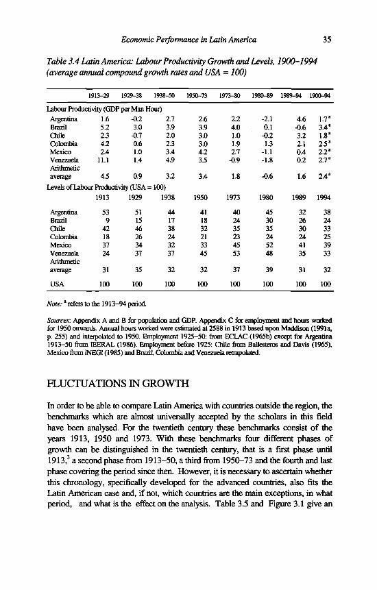
Economie Performance in Latin America 35
Table 3.4 Latin America: Labour Productivity Growth and Levels, 1900-1994 (average annual compound growth rates and USA = 100)
1913-29 1929-38 1938-50 1950-73 1973-80 1980-89 1989-94 1900-94
Labour Productivity (GDP per Man Hour) Argentina 1.6 -0.2 2.7 2.6 2.2 -2.1 4.6 1.7“Brazil 5.2 3.0 3.9 3.9 4.0 0.1 -0.6 3.4*Chile 2.3 -0.7 2.0 3.0 1.0 -0.2 3.2 1.8“Colombia 4.2 0.6 2.3 3.0 1.9 1.3 2.1 2.5*Mexico 2.4 1.0 3.4 4.2 2.7 -1.1 0.4 2.2“Venezuela 11.1 1.4 4.9 3.5 -0.9 -1.8 0.2 2.7“Arithmeticaverage 4.5 0.9 3.2 3.4 1.8 -0.6 1.6 2.4“
Levels of Labour Productivity (USA = 1913 1929
100)1938 1950 1973 1980 1989 1994
Argentina 53 51 44 41 40 45 32 38Brazil 9 15 17 18 24 30 26 24Chile 42 46 38 32 35 35 30 33Colombia 18 26 24 21 23 24 24 25Mexico 37 34 32 33 45 52 41 39Venezuela 24 37 37 45 53 48 35 33Arithmeticaverage 31 35 32 32 37 39 31 32
USA 100 100 100 100 100 100 100 100
Note: a refers to the 1913-94 period.
Sources: Appendix A and B for population and GDP. Appendix C for employment and hours worked for 1950 onwards. Annual hours worked were estimated at 2588 in 1913 based upon Maddison (1991a, p. 255) and interpolated to 1950. Employment 1925-50: from ECLAC (1965b) except for Argentina 1913-50 from IEERAL (1986). Employment before 1925: Chile from Ballesteros and Davis (1965), Mexico from INEGI (1985) and Brazil, Colombia and Venezuela retrapolated.
FLUCTUATIONS IN GROW TH
In order to be able to compare Latin America with countries outside the region, the benchmarks which are almost universally accepted by the scholars in this field have been analysed. For the twentieth century these benchmarks consist o f the years 1913, 1950 and 1973. With these benchmarks four different phases of growth can be distinguished in the twentieth century, that is a first phase until1913,3 a second phase from 1913-50, a third from 1950-73 and the fourth and last phase covering the period since then. However, it is necessary to ascertain whether this chronology, specifically developed for the advanced countries, also fits the Latin American case and, if not, which countries are the main exceptions, in what period, and what is the effect on the analysis. Table 3.5 and Figure 3.1 give an
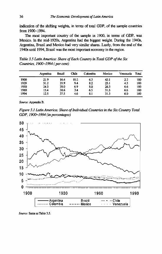
36 The Economic Development o f Latin America
indication of the shifting weights, in terms of total GDP, of the sample countries from 1900-1994.
The most important country of the sample in 1900, in terms of GDP, was Mexico. In the mid-1920s, Argentina had the biggest weight. During the 1940s, Argentina, Brazil and Mexico had very similar shares. Lastly, from the end o f the 1940s until 1994, Brazil was the most important economy in the region.
Table 3.5 Latin America: Share of Each Country in Total GDP o f the Six Countries, 1900-1994 ( percent)
Argentina Brazil Chile Colombia Mexico Venezuela Total
1900 21.9 16.4 10.2 6.3 43.1 2.2 1001929 31.2 21.9 9.4 8.2 25.1 4.3 1001950 24.3 28.0 6.9 8.0 26.3 6.6 1001980 13.4 38.6 3.4 6.5 31.5 6.6 1001994 12.5 37.5 4.6 8.1 31.3 6.0 100
Source: Appendix B.
Figure 3.1 Latin America: Share o f Individual Countries in the Six Country Total GDP, 1900-1994 (in percentages)
50 -,-------------------------------------------------------------------------------------
0 11 m i m i i n m i m i 111 m i m i i n 11 i l m i i n n u n i m i 11 i l n i i m i m I il 11 i l 1111 i n i l 11 i n 11
1900 1930 1960 1990
-----------Argentina - -------- Brazil -----------Chile............Colombia -------- Mexico --------- Venezuela
Source: Same as Table 3.5.

Economie Performance in Latin America 37
In Table 3.6 the annual fluctuations in GDP are presented on the basis of aggregating total GDP of the six countries. The 1950 benchmark is not very clear in terms of fluctuations of GDP growth, as Latin America continued the growth process initiated in the late 1930s. It can be concluded that growth in Latin America from 1950 onwards was more stable than in the period after the Great Depression.
The 1900-1994 period will be analysed graphically for each country on the basis of yearly GDP estimates for each country in order to see whether the individual country cycles coincide with the phases distinguished above. For each country we will also analyse the sensitivity of changes in the benchmarks to growth rates.
Table 3.6 Year-to-Year Percentage Change in Aggregate GDP o f the Six Countries, 1900-1994 (annual growth rates)
1900 1914 -3.2 1930 -4.4 1950 5.4 1973 8.9 1981 0.71901 8.1 1915 -0.2 1931 -5.3 1951 6.0 1974 6.6 1982 -0.71902 -1.6 1916 2.0 1932 -4.1 1952 3.2 1975 3.7 1983 -2.41903 8.6 1917 0.5 1933 9.5 1953 4.8 1976 6.2 1984 3.81904 3.8 1918 5.3 1934 8.2 1954 6.9 1977 5.0 1985 3.31905 8.5 1919 0.3 1935 4.9 1955 6.2 1978 4.9 1986 3.51906 2.0 1920 6.0 1936 6.4 1956 4.2 1979 7.1 1987 3.11907 5.7 1921 0.4 1937 5.2 1957 7.3 1980 7.1 1988 1.01908 1.4 1922 6.2 1938 2.5 1958 5.3 1989 1.61909 4.6 1923 8.6 1939 4.6 1959 2.6 1990 0.41910 4.6 1924 3.3 1940 1.5 1960 7.4 1991 3.31911 1.1 1925 3.1 1941 6.0 1961 7.1 1992 2.71912 5.7 1926 4.8 1942 0.2 1962 4.0 1993 3.11913 1.5 1927 3.4 1943 3.5 1963 3.5 1994 4.5
1928 7.8 1944 8.0 1964 8.01929 2.0 1945 2.7 1965 5.4
1946 9.5 1966 4.61947 5.8 1967 4.81948 6.7 1968 7.91949 4.1 1969 7.6
1970 5.11971 6.71972 7.6
Source: Appendix B.
CAUSES O F CYCLICAL INSTABILITY
There are many factors, external or internal, which may cause instability. Of course, they cannot be separated completely and a combination o f the two can generate all kinds of different results. A good example of the combined effects of internal and external factors was the first oil crisis in 1973 which caused distinct

38 The Economic Development o f Latin America
domestic reactions with different results in terms of economic stability. Most countries experienced a fall in growth rates as they adopted policies to adjust to the change in relative prices. Latin American countries, including the non-oil exporters, borrowed heavily, with only minor adjustment to changes in relative prices, and the growth process continued. In the 1980s the combined effect o f lack of price adjustment and heavy indebtedness caused the ‘lost decade’.
Here we will give a description of the most recurrent causes of cyclical fluctuations in Latin America.4 Several causes of instability of external origin can be identified:
- As already indicated in Chapter 2, the sudden drop in capital and trade flows due to external reasons represents a major cause of instability in Latin America. The crises o f the 1820s, the 1870s, the 1930s and the 1980s were caused predominandy by such developments.
- Another relevant factor producing instability is extreme dependence on one or a few primary commodities, with fluctuations in demand or supply factors generating instability. This factor is quite important in Latin America as the single most important export product is still a primary commodity in all countries of our sample.
- External factors of a non-economic character, like war or extreme political unrest, influence stability through falls in exports and deterioration of the terms of trade.
Many internal factors are also important:
- Climatic variations can create instability in countries specialising in agricultural primary products. Droughts, with their effects on harvests or energy generation; extreme temperature changes, either at sea or on land; storms; and earthquakes, still have significant influence.
- A traditionally important cyclical factor in Latin America is the political process, where electoral considerations often have powerful economic effects. This has been the case in countries with relatively high political stability, for example Mexico, or countries with higher instability and more populist political processes.
- Another cause of economic instability stemming from internal political events comes in the form of extreme situations such as military interventions. This has been the case in Chile, Argentina and many other countries. Arguably, other extreme cases fall into this same category, like the Unidad Popular experiment of President Allende in the early 1970s in Chile.
- Some crises in Latin America can be clearly attributed to mistakes in domestic economic policy. Populism and neo-conservative experiments in Argentina and Chile in the 1970s and the Mexican crisis in the 1990s are examples.
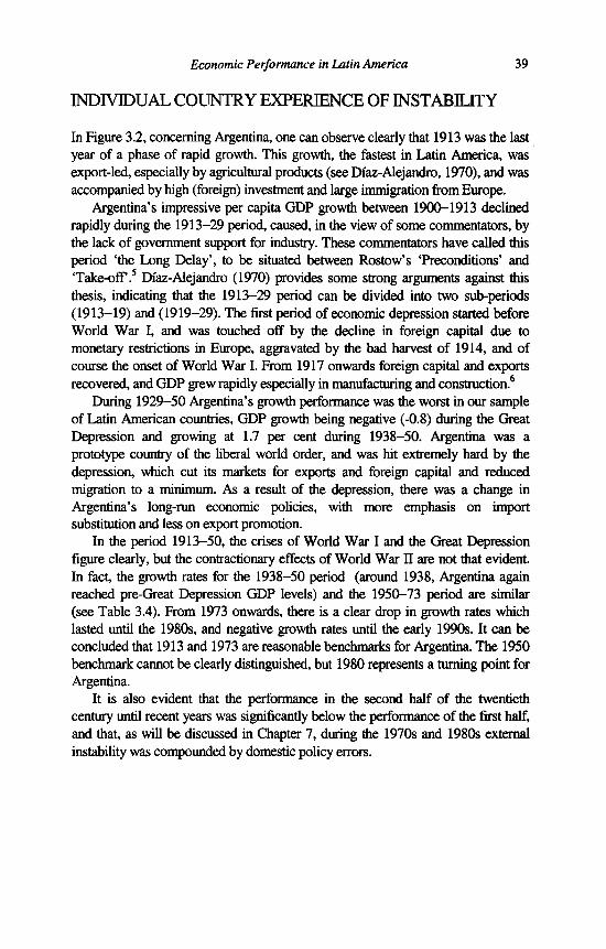
Economie Performance in Latin America 39
INDIVIDUAL COUNTRY EXPERIENCE OF INSTABILITY
In Figure 3.2, concerning Argentina, one can observe clearly that 1913 was the last year of a phase of rapid growth. This growth, the fastest in Latin America, was export-led, especially by agricultural products (see Diaz-Alejandro, 1970), and was accompanied by high (foreign) investment and large immigration from Europe.
Argentina’s impressive per capita GDP growth between 1900-1913 declined rapidly during the 1913-29 period, caused, in the view of some commentators, by the lack of government support for industry. These commentators have called this period ‘the Long Delay’, to be situated between Rostow’s ‘Preconditions’ and ‘Take-off.5 Diaz-Alejandro (1970) provides some strong arguments against this thesis, indicating that the 1913-29 period can be divided into two sub-periods (1913-19) and (1919-29). The first period of economic depression started before World War I, and was touched off by the decline in foreign capital due to monetary restrictions in Europe, aggravated by the bad harvest o f 1914, and of course the onset of World War I. From 1917 onwards foreign capital and exports recovered, and GDP grew rapidly especially in manufacturing and construction.6
During 1929-50 Argentina’s growth performance was the worst in our sample of Latin American countries, GDP growth being negative (-0.8) during the Great Depression and growing at 1.7 per cent during 1938-50. Argentina was a prototype country of the liberal world order, and was hit extremely hard by the depression, which cut its markets for exports and foreign capital and reduced migration to a minimum. As a result o f the depression, there was a change in Argentina’s long-run economic policies, with more emphasis on import substitution and less on export promotion.
In the period 1913-50, the crises of World War I and the Great Depression figure clearly, but the contractionary effects o f World War II are not that evident. In fact, the growth rates for the 1938-50 period (around 1938, Argentina again reached pre-Great Depression GDP levels) and the 1950-73 period are similar (see Table 3.4). From 1973 onwards, there is a clear drop in growth rates which lasted until the 1980s, and negative growth rates until the early 1990s. It can be concluded that 1913 and 1973 are reasonable benchmarks for Argentina. The 1950 benchmark cannot be clearly distinguished, but 1980 represents a turning point for Argentina.
It is also evident that the performance in the second half o f the twentieth century until recent years was significantly below the performance of the first half, and that, as will be discussed in Chapter 7, during the 1970s and 1980s external instability was compounded by domestic policy errors.

Brazil
40 The Economic Development o f Latin America
Brazil experienced a period of rapid growth at the beginning o f the twentieth century, following important political changes during the last quarter o f the nineteenth century such as the abolition of slavery and the establishment of the Republic. As in the case of Argentina this growth was export-led, based upon exports of agricultural products such as coffee and rubber, but the Brazilian government also initiated a programme of public works. Unlike in Argentina, this was the starting point of a period of rapid growth which was to continue until the 1980s (see Merrick and Graham, 1979 and Villela and Suzigan, 1977).
Brazil’s performance was among the best in Latin America during the 1913-50 period. Of particular note is the fact that the country recovered relatively rapidly from the adverse effects of the Great Depression. One element that has been stressed is the coffee support programme which had some countercyclical effects of a Keynesian nature.7 The promotion of industry through import substitution was not a deliberate policy choice; however, the industrial sector benefited indirectly from the coffee support programme and the various stabilisation programmes, for example from the protection offered by the numerous exchange-rate devaluations and the tariffs on imports.
Although 1913 and 1929 are years characterised by slower growth and even economic recession, it is hardly possible to conclude that the 1900-1913 period is distinctively different from 1913-50. During the whole period Brazil experienced a growth rate of around 2.5 per cent and the crises of 1913 and 1929 only interrupted this growth process briefly. In the second half of the twentieth century Brazil experienced an acceleration in growth to rates around 4 per cent while the 1973-80 period shows even higher rates of growth.
Figure 3.2 shows very clearly that Brazilian growth accelerated after the Great Depression and continued growing until the crisis of the 1980s. External factors had a major impact on economic growth in Brazil in the twentieth century; however, in the 1980s and also 1990s internal political and policy factors limited growth (see also Chapter 7).
Chile
As Figure 3.2 shows conclusively, Chile is by far the most vulnerable country in Latin America in terms of GDP fluctuations. At least six major economic crises can be identified during the twentieth century. The first was related to World War I, a second occurred at the beginning of the 1920s and the Great Depression also hit hard in Chile. From the middle of the 1930s, Chile experienced a rather stable low growth path until the early 1970s. In the 1970s and the 1980s, another pair of profound crises beset the Chilean economy.
Economic growth in Chile during the first years of the twentieth century was
Economie Performance in Latin America 41
influenced by the natural sodium nitrate boom which had started in the 1880s. The enormous expansion in production and exports of nitrate transformed Chile’s society and economy as documented in Carióla and Sunkel (1985) and Mamalakis (1976). Per capita GDP grew at a fast rate that would not be repeated until very recently in the twentieth century.
During 1913-50 Chile’s growth performance can be divided into the 1913-29 period of somewhat higher than average per capita GDP growth for Latin America, and the 1929-50 period of much Iowa- comparative performance. The nitrate boom was affected by the outbreak of World War I and the contraction of European markets; however, the rapid growth o f the North American market compensated for the loss of European markets and the boom apparently continued until the 1930s when the combined effect of the discovery o f artificial nitrate and the low technological level caused the industry to collapse. Copper production and exports entered a new period of expansion after the great decline from 1880 until the 1920s; however, the interactions between large-scale copper production and the rest of Chile’s economy were limited, and fewer linkages were established than in the case o f nitrate. Chile was hit hard by the Great Depression and average per capita GDP fell between 1929-38. This development prompted the government to adopt a policy designed to reduce external dependence, and industrialisation became an important instrument for attaining economic growth.
Again it becomes clear that 1913 and 1973 are good benchmarks. Since the beginning of the 1980s, following a severe crisis, Chile is experiencing high economic growth, compared with the rest of the century. Chile is the country where external dependency and domestic policy errors caused extremely high economic volatility, as will be documented in Chapter 7.
Colombia
In complete contrast to Chile in terms of volatility is Colombia, which has experienced by far the most stable economic growth of all Latin American countries during this century. Growth accelerated in Colombia at the beginning of the twentieth century, after the period of stagnation caused by the War of a Thousand Days. The pace set between 1900-1913 was to continue throughout the rest o f the twentieth century, and during certain periods growth was even faster (see McGreevy, 1985). World War I did not affect Colombia very much, and 1913 was not a crisis year in Colombia.
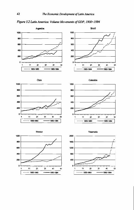
42 The Economic Development o f Latin America
Figure 3.2 Latin America: Volume Movements of GDP; 1900-1994
Argentina Brazil
1900-1950 1900-1950 - 1950-1994
Mexico Venezuela
1900-1950 1950-1994 1900-1950 1950-1994

Economie Performance in Latin America 43
Figure 3.2 (continued)
Latin America
1 9 0 0 - 1 9 5 0 1 9 5 0 - 1 9 9 4
Source: Appendix B.
However, the Great Depression negatively impacted the growth process and for the only time in the twentieth century, the country experienced negative growth. The recovery from the recession has been comparatively swift in Colombia owing partly to an anti-cyclical policy (at the national and especially the local level) and partly to exports of gold and coffee (see Maddison, 1985). During World War II per capita GDP remained stable, but from 1945 onwards growth resumed. Colombia is the only country in our group to record lower growth rates in the 1938-50 period compared to the 1929-38 period, as a result o f the fall in economic growth in the early 1940s. From then on, the country recorded uninterrupted growth until the early 1980s when the debt crisis caused the country to experience a fall in growth rates.
Mexico
During the final years of the ‘Porfiriato’ (1876-1910) growth was relatively fast in Mexico but this process was interrupted by the Mexican Revolution and later by the Great Depression. Mexico’s growth performance during 1913-50 was of course greatly affected by the revolution and the civil war. Our figures show constant per capita GDP for 1913-29 and an average performance between 1929-50. During the later period per capita GDP was stagnant from 1929-38 when the first reaction to the Great Depression was to enforce a restrictive monetary policy, but during the Cárdenas government (1934-40) a more Keynesian policy was followed. Growth sped up from 1938-50, especially as a result of World War II, which improved exports from, and tourism to, the United States and boosted remittances from temporary workers in that country.

44 The Economic Development o f Latin America
However, Fitzgerald (1984) emphasises that:
the orthodox view of the decade leading up to 1929 in Mexico as one of economic and institutional stagnation, awaiting the reforms of the 1930s and growth in the 1940s, is not correct. It is in fact a period of considerable change: the basis of the modem State was laid; commercial agriculture and manufacturing were emerging as new leading sectors; and pressure on both peasants’ and workers’ incomes was increasing. It is against this background that the impact of the Depression should be assessed, (p. 248)
Therefore, economic growth in Mexico was extremely low during the first three to four decades of this century. From the mid-1930s until the 1980s Mexico experienced a long period of rather stable growth which was interrupted by the debt crisis o f the 1980s.
At the end o f the 1980s and the beginning of the 1990s the country was growing at modest rates, though this was again interrupted at the end of 1994 when a new crisis broke out causing a serious recession in 1995 (see also Chapter 7).
Venezuela
During the first two decades of the twentieth century Venezuela experienced fairly low growth rates. This changed in the 1920s when the country, boosted by the oil sector, began to experience extremely high growth rates. The period 1913-50 was a very prosperous one for Venezuela, with growth rates of per capita GDP well above the Latin American average. The acceleration of the growth process initiated in the second and third decade was very closely associated with foreign firms’ (particularly Anglo-Dutch and US) exploitation of the oil reserves (Quero Morales, 1978). From 1913-29 and 1938-50, Venezuela grew at the unprecedented rates of7.3 and 5.0 per cent per capita, respectively. Growth rates were somewhat lower in the 1929-38 period as the country was severely hit by the Great Depression, followed by swift recovery until a new crisis at the end of the 1930s caused negative growth; but the rest of the 1940s were again years o f extremely high growth. From 1950 onwards growth rates tended to fall and between 1980-94 there was a tendency towards recession. However, the overall growth rate recorded in the twentieth century has been the highest of all countries in our sample.
The above analysis indicates that, for the first half of the twentieth century, the benchmarks normally accepted do fit the Latin American situation to a reasonable degree. In almost all cases 1913 is a crisis year (except in Colombia and Venezuela). Looking at the two major crises that affected the world in the 1913-50 period, Latin America was hit on a comparable scale during the Great Depression, although the region recovered fairly quickly, but World War II did not have as devastating an effect on Latin America as it had on the rest o f the world, and in several countries in Latin America it provided opportunities for growth.
Economic Performance in Latin America 45
It therefore seems reasonable also to include 1938 in the case of Latin America, since its growth performance was quite different from the rest o f the world between 1938-50. In the post-war period the 1973 benchmark seems quite acceptable, as argued for above; but it is also necessary to include 1980 as a benchmark in the case of Latin America because the beginning o f the 1980s marked one of the most profound crises in Latin America.
The main conclusions which can be drawn from the above discussion are reflected in the Latin American total in Figure 3.2. The years 1929,1980 and, to a lesser degree, 1913 show recessions. Slower growth occurred around the 1940s, and 1973 marked a slowdown in growth in most sample countries outside Latin America. In Latin America 1950 is not as clear a benchmark year as in the other countries in our sample. As a general conclusion, it seems acceptable to use the benchmarks identified for the international comparison, although it would be reasonable to include two additional benchmarks in the case of Latin America: 1938 and 1980.
In order to be able to combine the results obtained by other scholars, I have chosen to present a combination of the phases identified for the rest of the world and those for Latin America. A good case can be made, on the basis o f empirically measurable characteristics, for the following phases in the cases of Latin America. A first phase ended in 1929 with very similar overall growth rates in the periods 1900-1913 and 1913-29. Argentina and Mexico slowed down while Venezuela accelerated, starting its oil based growth boom. A second phase from 1929-50 was characterised by a sharp recession as a result o f the Great Depression but also a fairly quick recovery, compared to the rest of the world. During this period Latin America was forced into a strategy of import substitution. This was especially due to external conditions such as the protective measures adopted by many countries in the 1930s and the de facto trade contraction caused by World War 13.
A third phase can be identified from 1950 to 1980, with relatively stable growth rates, although with a slight trend towards slowdown at the end of the period, especially since 1973. In this phase most Latin American countries adopted a development strategy based upon import substitution. A final phase started in 1980, showing a drastic slowdown in economic growth and the start of a process of changing the development strategy towards a more outward-oriented one. From the late 1980s (in some countries even earlier) and the 1990s onwards several countries are growing again, and the benchmark adopted for this recovery period is 1989.

46 The Economic Development o f Latin America
NOTES
1. This result is, of course, dependent on the périodisation since the ‘Great Depression’ in Latin America was rather short-lived, and by 1938 most countries were approaching or above the previous total GDP peak level (see also Table 2.5). In the 1980s the crisis lasted much longer, and several countries only recovered to pre-crisis levels at the end of the decade.
2. The Asian countries selected are, of course, not at all representative of Asia, and therefore summarizing them as ‘the Asian case’ is misleading. This is even more the case in the period before 1950 when Korea and Taiwan were colonies of Japan.
3. This phase started much earlier than 1900, possibly around 1870. See Maddison (1995) for a description of phases of growth in the nineteenth century, in which he distinguishes a first growth acceleration in Europe and its ‘offshoots’, Australia, Canada, New Zealand and the USA, starting around 1820 when Europe had more or less recovered from the previous period of revolution, war and economic blockade affecting it since the 1790s. Another well-accepted benchmark, also especially relevant for Latin America, is around 1870 when a sharp growth acceleration occurred in a much greater area of the world compared to the 1820 acceleration. For Latin America, as for most other countries, growth acceleration happened around this benchmark, in the case of Chile, Brazil and Argentina probably somewhat earlier, and Mexico, Colombia and Venezuela somewhat later (see Reynolds, 1983). So also for Latin America a case can be made for 1870-1913 as a period of growth acceleration which ended with the outbreak of World War I.
4. There are many sources for cyclical analysis in Latin America, one of the best known is the Economic Survey, which ECLAC has published since the end of the 1940s; for many countries and for the first half of the century there exists an ever growing literature. See for a classification of business cycle causality, Maddison (1985).
5. See Di Telia and Zymelman (1973) who situated this period from 1914 to 1933.6. See Diaz-Alejandro (1970) pp. 6 1 ^ 5 .7. In the study of the economic development of Brazil, the anticyclical Keynesian policy followed
during the Great Depression is a topic of great debate: see Fishlow (1972), Furtado (1963) and Villela and Suzigan (1977).
4. New Standardised Estimates of Labour Input and Human Capital
INTRODUCTION
Traditional analysis o f growth performance always included measures of employment and labour productivity, and Denison (1962 and 1967) was one of the first to present a more sophisticated analysis of labour input, considering length of the work year, disaggregation of inputs by age and by levels of education. Since then most growth analysts have emphasized the importance o f taking a broader view of human capital, though large series cross country econometric work has often used rough proxies for education - enrolment rates - rather than educational stock. Here we have followed the Denison tradition to ensure that the components of our labour input analysis are robust.
Recently, the human capital dimension to economic growth has again returned to centre.1 As Denison (1993) observed in one of his last contributions:
If one were forced to choose a single growth source as most important in the long run,the choice would have to be advances in knowledge, (p. 58)
Appendices A and C present a comprehensive set of tables on population and employment, the number of days and hours worked per person and data on sectoral employment and educational level of the population. The main conclusions that can be inferred from this database for the six Latin American countries are commented on, and the existing empirical material reviewed to corroborate our results. The basic sources are national censuses, population censuses, agricultural censuses and so on, and the surveys (for example household surveys) which are conducted regularly in each country. However, these censuses contain big differences between countries and I attempt to make adjustments in order to make the series as comparable as possible for the Latin American countries.
This chapter also includes disaggregated estimates of employment for 1950-94 broken down into agriculture, industry and services. It presents estimates of the average number of years of formal education of the population. The quality of human capital is affected by many other factors such as health and nutrition. Widespread schooling and good health care and nutrition early in a country’s development have a positive effect on its economic performance. There is a
47

48 The Economic Development o f Latin America
growing consensus in Latin America and elsewhere that investments in schooling, training, health and nutrition are important elements of a successful development strategy.
The past four decades of development show that appropriate government policies for human capital development are just as critical as macroeconomic stability, global competitiveness and physical infrastructure. Human resource investments are required both to facilitate the adjustment process in the short term, so that production and employment can adapt to the changing national and international economic picture and to increase the prospects for sustained productivity growth over the long term. Moreover, better schooled and trained people are more likely to explore and share market and technological innovations. Furthermore, overall social reform can be pursued more effectively, through such investments, providing opportunities for all members of society to participate in the benefits o f development (IDB, 1993).
POPULATION
Table 4.1 presents population growth rates for the sample of countries. This table reflects the process of demographic transition that has been taking place since the beginning of the twentieth century.2 Average growth rates rose till the late 1960s and started falling afterwards. The last column of Table 4.1 shows the average population growth from 1900-1994. The country that grew fastest at the beginning of the century (Argentina), is currently growing at the slowest pace. On the contrary, Venezuela, the slowest growing country at the beginning of the century, has been the fastest growing country in the last decades.
As indicated above, population grew at very different rates in the various countries of Latin America during the 1900-1913 period, when the highest growth rates were experienced by Argentina with an average annual growth rate of 3.8 per cent. This was due in large part to immigration from Europe which accounted for more than 50 per cent of total population growth. About half o f all immigrants came from Italy while around 30 per cent came from Spain.3 In 1914, foreigners made up about 30 per cent of the total population (Sanchez-Albomoz, 1991).
Brazil also had rather high population growth rates, though much lower than Argentina. An important reason for this was the much lower, though still significant, influx of foreigners. This accounts for almost 15 per cent of population growth (Merrick and Graham, 1979). Between 1880 and 1930, Brazil received around four million immigrants from Italy (36 per cent), Portugal (29 per cent), Spain (14 per cent), Germany (5 per cent) and Japan (3 per cent), as documented in Sanchez-Albomoz (1991).
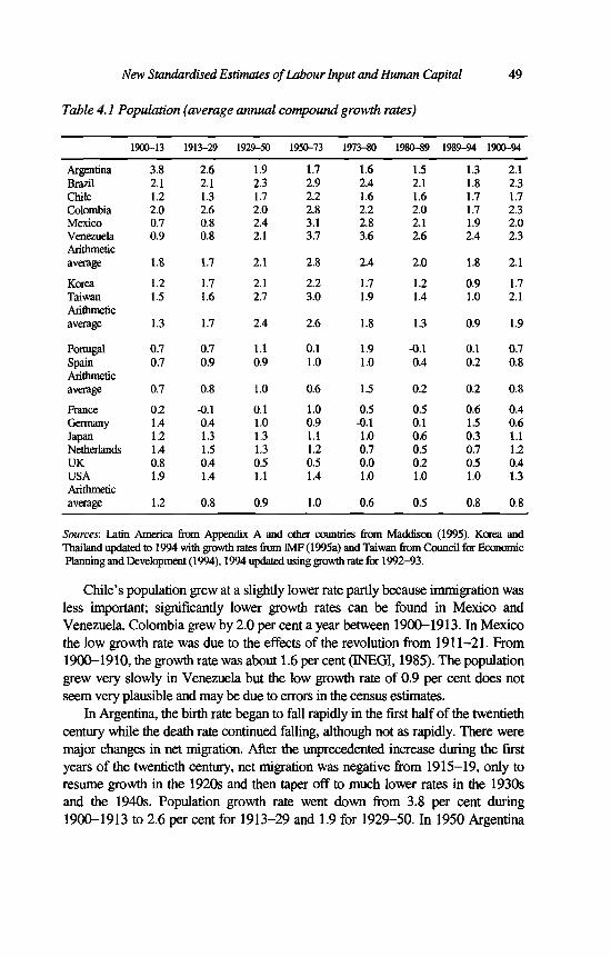
New Standardised Estimates o f Labour Input and Human Capital 49
Table 4.1 Population (average annual compound growth rates)
1900-13 1913-29 1929-50 1950-73 1973-80 1980-89 1989-94 1900-94
Argentina 3.8 2.6 1.9 1.7 1.6 1.5 1.3 2.1Brazil 2.1 2.1 2.3 2.9 2.4 2.1 1.8 2.3Chile 1.2 1.3 1.7 2.2 1.6 1.6 1.7 1.7Colombia 2.0 2.6 2.0 2.8 2.2 2.0 1.7 2.3Mexico 0.7 0.8 2.4 3.1 2.8 2.1 1.9 2.0VenezuelaArithmetic
0.9 0.8 2.1 3.7 3.6 2.6 2.4 2.3
average 1.8 1.7 2.1 2.8 2.4 2.0 1.8 2.1
Korea 1.2 1.7 2.1 2.2 1.7 1.2 0.9 1.7TaiwanArithmetic
1.5 1.6 2.7 3.0 1.9 1.4 1.0 2.1
average 1.3 1.7 2.4 2.6 1.8 1.3 0.9 1.9
Portugal 0.7 0.7 1.1 0.1 1.9 -0.1 0.1 0.7SpainArithmetic
0.7 0.9 0.9 1.0 1.0 0.4 0.2 0.8
average 0.7 0.8 1.0 0.6 1.5 0.2 0.2 0.8
Ranee 0.2 -0.1 0.1 1.0 0.5 0.5 0.6 0.4Germany 1.4 0.4 1.0 0.9 -0.1 0.1 1.5 0.6Japan 1.2 1.3 1.3 1.1 1.0 0.6 0.3 1.1Netherlands 1.4 1.5 1.3 1.2 0.7 0.5 0.7 1.2UK 0.8 0.4 0.5 0.5 0.0 0.2 0.5 0.4USAArithmetic
1.9 1.4 1.1 1.4 1.0 1.0 1.0 1.3
average 1.2 0.8 0.9 1.0 0.6 0.5 0.8 0.8
Sources: Latin America from Appendix A and other countries from Maddison (1995). Korea and Thailand updated to 1994 with growth rates from IMF (1995a) and Taiwan from Council for Economic Planning and Development (1994), 1994 updated using growth rate for 1992-93.
Chile’s population grew at a slightly lower rate partly because immigration was less important; significantly lower growth rates can be found in Mexico and Venezuela. Colombia grew by 2.0 per cent a year between 1900-1913. In Mexico the low growth rate was due to the effects of the revolution from 1911-21. From 1900-1910, the growth rate was about 1.6 per cent (INEGI, 1985). The population grew very slowly in Venezuela but the low growth rate of 0.9 per cent does not seem very plausible and may be due to errors in the census estimates.
In Argentina, the birth rate began to fall rapidly in the first half of the twentieth century while the death rate continued falling, although not as rapidly. There were major changes in net migration. After the unprecedented increase during the first years of the twentieth century, net migration was negative from 1915-19, only to resume growth in the 1920s and then taper off to much lower rates in the 1930s and the 1940s. Population growth rate went down from 3.8 per cent during 1900-1913 to 2.6 per cent for 1913-29 and 1.9 for 1929-50. In 1950 Argentina
50 The Economic Development o f Latin America
was the first country in Latin America to reach the final stage of the demographic transition, recording more or less stable, low crude birth and death rates.
Brazil continued the trend of 1900-1913 in terms of a constant birth rate and a slightly falling death rate. Net immigration came to a halt during World War I but resumed during the 1920s faltering, as in Argentina, in the 1930s and 1940s.4 The population growth rate was 2.1 per cent for 1913-29, the same as during 1900-1913, and a slightly higher 2.3 per cent for 1929-50. From 1920 onwards Chile experienced an accelerated decline of its rather high, by Latin American standards, crude death rate. Initially the birth rate also tended to fall, but later stabilised, rising somewhat at the end of the 1940s. In the case of Chile, immigration was not as important in size as in Argentina and Brazil, although entrepreneurs seeking fortune in Chile have had a great impact on its economic development. The population growth rate rose somewhat from 1.2 per cent between 1900-1913 to 1.3 per cent between 1913-29, and reached 1.7 per cent in the period 1929-50.
Demographic developments in Colombia closely resembled those in Brazil, except for the migratory movement. The crude birth rate was stable during the first half of the twentieth century, while the crude death rate experienced a slow but constant decline. The resulting growth rates were 2.6 per cent between 1913-29 and 2.0 per cent between 1929-50. Population growth in Mexico was of course strongly affected by the Mexican revolution. Starting in the 1920s, the birth rate remained at a high level for much of the twentieth century while the death rate showed a systematic decline. In the case of Venezuela the long-run population estimates do not seem to be very reliable. However, the figures indicate a constant crude birth rate during the first part of the century, even showing a tendency to rise from the mid-1930s onwards. The crude death rate started to decline from the 1920s onwards resulting in a growth rate of 0.8 per cent between 1913-29 and about 2.1 per cent between 1929-50.
At the beginning of the 1950s, most Latin American countries were still in the first phase o f demographic transition. However, in most countries the growth acceleration between 1950-73 was more accentuated than between 1929-50, and this was principally due to the fall in mortality. The Southern Cone countries were at a more advanced stage in the demographic transition, especially Argentina, which was growing at less than 2 per cent; and, to a lesser degree, Chile, which still had rather high birth and mortality rates.
The 1973-80 period shows a uniform tendency in all Latin American countries towards a fall in population growth. This indicates that all countries are now at a more advanced stage of demographic transition, in which the fertility rates also start to fall. During the 1980-94 period, the abovementioned trend continued and all countries (except Chile, whose population growth rate had fallen strongly from 1973-80), experienced lower population growth.
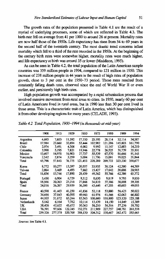
New Standardised Estimates o f Labour Input and Human Capital 5 1
The growth rates of the population presented in Table 4.1 are the result of a myriad of underlying processes, some of which are reflected in Table 4.3. The birth rate fell on average from 41 per 1000 to around 26 at present. Mortality rates are now half those of the 1950s. Life expectancy has risen from 54 to 69 years in the second half of the twentieth century. The most drastic trend concerns infant mortality which fell to a third of the rate recorded in the 1950s. At the beginning of the century birth rates were somewhat higher, mortality rates were much higher, and life expectancy at birth was around 35 or lower (Maddison, 1995).
As can be seen in Table 4.2, the total population of the Latin American sample countries was 359 million people in 1994, compared to 121 million in 1950. This increase of 238 million people in 44 years is the result of high rates of population growth, close to 3 per cent in the 1950-73 period. Those rates resulted from constantly falling death rates, observed since the end of World War II or even earlier, and persistently high birth rates.
High population growth was accompanied by a rapid urbanisation process that involved massive movement from rural areas to cities. In 1950, nearly 60 per cent of Latin Americans lived in rural areas, but in 1990 less than 30 per cent lived in those areas. This is a characteristic trait of Latin America, which has distinguished it from other developing regions for many years (CELADE, 1993).
Table 4.2 Total Population, 1900-1994 (in thousands at mid-year)
1900 1913 1929 1950 1973 1980 1989 1994
Argentina 4,693 7,653 11,592 17,150 25,193 28,114 32,114 34,587Brazil 17,984 23,660 32,894 53,444 102,982 121,286 145,803 161,790Chile 2,974 3,491 4,306 6,082 9,992 11,147 12,883 14,210Colombia 3,998 5,195 7,821 11,946 22,778 26,525 31,739 35,101Mexico 13,607 14,970 16,903 27,737 55,539 67,570 81,666 91,145Venezuela 2,542 2,874 3,259 5,094 11,796 15,091 19,025 21,844Total 45,798 57,843 76,775 121,453 228,280 269,733 323,230 358,677
Korea 8,772 10,277 13,397 20,557 33,935 38,124 42,380 44,389Taiwan 2,864 3,469 4,493 7,882 15,427 17,642 20,006 20,983Total 11,636 13,746 17,890 28,439 49,362 55,766 62,386 65,372
Portugal 5,450 6,004 6,729 8,512 8,630 9,819 9,795 9,850Spain 18,566 20,263 23,210 27,868 34,810 37,386 38,888 39,205Total 24,016 26,267 29,939 36,380 43,440 47,205 48,683 49,055
France 40,598 41,463 41,230 41,836 52,118 53,880 56,423 58,022Germany 34,666 37,843 40,595 49,983 61,976 61,566 62,063 66,802Japan 44,103 51,672 63,244 83,563 108,660 116,800 123,120 125,188Netherlands 5,142 6,164 7,782 10,114 13,439 14,150 14,849 15,389UK 38,426 42,622 45,672 50,363 56,210 56,314 57,236 58,702USA 76,391 97,606 122,245 152,271 211,909 227,757 248,781 261,558Total 239,326 277,370 320,768 388,130 504,312 530,467 562,472 585,661
Sources: See Table 4.1.
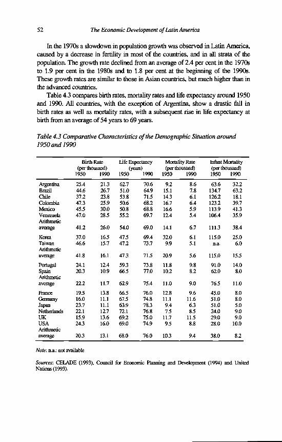
52 The Economic Development o f Latin America
In the 1970s a slowdown in population growth was observed in Latin America, caused by a decrease in fertility in most of the countries, and in all strata of the population. The growth rate declined from an average of 2.4 per cent in the 1970s to 1.9 per cent in the 1980s and to 1.8 per cent at the beginning of the 1990s. These growth rates are similar to those in Asian countries, but much higher than in the advanced countries.
Table 4.3 compares birth rates, mortality rates and life expectancy around 1950 and 1990. All countries, with the exception o f Argentina, show a drastic fall in birth rates as well as mortality rates, with a subsequent rise in life expectancy at birth from an average of 54 years to 69 years.
Table 4.3 Comparative Characteristics o f the Demographic Situation around 1950 and 1990
Birth Rate Life Expectancy Mortality Rate Infant Mortality (per thousand) (years) (per thousand) (per thousand)
1950 1990 1950 1990 1950 1990 1950 1990
Argentina 25.4 21.3 62.7 70.6 9.2 8.6 63.6 32.2Brazil 44.6 26.7 51.0 64.9 15.1 7.8 134.7 63.2Chile 37.2 23.8 53.8 71.5 14.3 6.1 126.2 18.1Colombia 47.3 25.9 50.6 68.2 16.7 6.4 123.2 39.7Mexico 45.5 30.0 50.8 68.8 16.6 5.9 113.9 41.3VenezuelaArithmetic
47.0 28.5 55.2 69.7 12.4 5.4 106.4 35.9
average 41.2 26.0 54.0 69.0 14.1 6.7 111.3 38.4
Korea 37.0 16.5 47.5 69.4 32.0 6.1 115.0 25.0TaiwanArithmetic
46.6 15.7 47.2 73.7 9.9 5.1 n.a. 6.0
average 41.8 16.1 47.3 71.5 20.9 5.6 115.0 15.5
Portugal 24.1 12.4 59.3 73.8 11.8 9.8 91.0 14.0SpainArithmetic
20.3 10.9 66.5 77.0 10.2 8.2 62.0 8.0
average 22.2 11.7 62.9 75.4 11.0 9.0 76.5 11.0
fiance 19.5 13.8 66.5 76.0 12.8 9.6 45.0 8.0Germany 16.0 11.1 67.5 74.8 11.1 11.6 51.0 8.0Japan 23.7 11.1 63.9 78.3 9.4 6.3 51.0 5.0Netherlands 22.1 12.7 72.1 76.8 7.5 8.5 24.0 9.0UK 15.9 13.6 69.2 75.0 11.7 11.5 29.0 9.0USAArithmetic
24.3 16.0 69.0 74.9 9.5 8.8 28.0 10.0
average 20.3 13.1 68.0 76.0 10.3 9.4 38.0 8.2
Note: n.a.: not available
Sources: CELADE (1993), Council for Economic Planning and Development (1994) and United Nations (1993).

New Standardised Estimates o f Labour Input and Human Capital 53
The increase in life expectancy of about 15 years was mainly due to the reduction in death rates in the early years of life and, especially, infant mortality, the decrease being much less among older people. The reduced incidence of infectious diseases (diarrhoea, acute respiratory infections and immune-preventible diseases) in infant and child mortality, as well as reduced death rates related to chronic diseases in adulthood such as cancer and cardiovascular disease, have been two of the most significant factors in the so-called epidemiological transition (CELADE, 1993).
Comparisons of the levels of, and trends in, Latin American death rates and those of the other countries in the sample show that the gap in life expectancy has fallen from 13 years to 5 years. Nevertheless, current levels o f life expectancy are similar to those experienced in the United States 40 years ago, when there was neither the current knowledge nor the means of preventing and treating a large number of diseases (CELADE, 1990).
Table 4.4 Total and Sectoral Employment (thousands o f persons)
Argentina Brazil Chile Colombia Mexico Venezuela
Agriculture1950 1,723 10,606 722 2,164 5,338 7101973 1,429 14,199 626 2,577 6,032 7821980 1,333 13,078 540 2,524 7,221 7311989 1,464 13,527 709 3,004 6,076 7801994 1,508 13,243 822 3,258 5,645 845
Industry1950 2,141 3,116 684 700 1,464 3151973 3,182 7,911 1,011 1,498 4,211 8511980 3,654 12,596 984 2,204 5,239 1,3411989 3,033 13,226 1,031 2,501 6,542 1,3641994 2,673 13,056 1,054 2,642 7,568 1,438
Services1950 2,957 3,935 850 980 1,963 5461973 4,791 11,055 1,257 2,541 4,937 1,7051980 5,078 17,417 1,794 3,685 7,162 2,5541989 7,233 27,893 2,563 4,982 11,701 3,5781994 8,302 33,610 3,078 5,770 14,804 4,441
Total1950 6,821 17,657 2,256 3,844 8,765 1,5711973 9,402 33,165 2,894 6,616 15,180 3,3381980 10,065 43,091 3,318 8,413 19,622 4,6261989 11,730 54,646 4,303 10,487 24,319 5,7221994 12,483 59,909 4,954 11,670 28,017 6,724
Sources: Appendix C.
This circumstance implies that the region could have made even greater progress than it has to date, especially since the gains achieved by the Asian countries of our sample were bigger than those of Latin America, with the former

54 The Economic Development o f Latin America
reaching a life expectancy of about 70 years, while the level at the beginning of the 1950s was about 7 years lower than the average for Latin America.
Another area where substantial progress has been made is in infant mortality which has declined, especially due to mass vaccination, oral rehydration and expanded health services, and again it becomes clear that in a comparative perspective the Latin American countries performed worse than the other countries in our sample, regardless of whether, at the initial point, those countries were below the level of Latin America, at the same level or above it.
LABOUR INPUT
For the Latin American countries total and sectoral employment was estimated separately for agriculture, industry and services (according to the International Industrial Uniform Classification IIUC Rev. 1, see Table 4.4). I have used the following statistical sources: (i) population estimates by the Latin American Demographic Centre (CELADE); (ii) specific participation rates of the male and female population derived from Population Censuses and Household Surveys; (iii) employment rates obtained from Population Censuses; and (iv) 1990 estimates of the economically active population generated by CELADE (1992) were used and the ECLAC Projections Centre provided us with estimates of total employment based upon national surveys. The benchmark years used in this study that did not coincide with census and survey years were intrapolated and 1994 was extrapolated.
Methodology and Results
The methodology for estimating the employment series consisted of the following steps: estimation o f the economically active population (EAP) for the 1950-80 period; estimation of total employment for the 1950-80 period; estimation of sectoral composition of employment; and estimation of the EAP and employment for 1990. For each country, the EAP was estimated on the basis o f population data and participation rates, for the age group ten years and older (see Table 4.5). The data on population aged 10 years and over was obtained from CELADE (1993). The participation rates were obtained from a study by ECLAC (1985). These were updated to 1990 using the CELADE (1992) study on the economically active population. Some cases showed rather big differences in trends (for example, Argentina and Mexico) and the specific adjustments made are commented on in Appendix C on human capital.
The ECLAC (1985) study, based upon population censuses and household surveys, presents a homogeneous series of specific participation rates of the economic active population aged 10 years and over for 1950, 1960, 1970 and
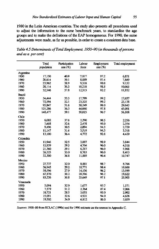
New Standardised Estimates o f Labour Input and Human Capital 55
1980 in the Latin American countries. The study also presents all procedures used to adjust the information to the same benchmark years, to standardise the age groups and to make the definitions of the EAP homogeneous. For 1990, the same adjustments were made, as far as possible, in order to create a consistent data base.
Table 4.5 Determinants o f Total Employment, 1950-90 (in thousands o f persons and as a percent)
Totalpopulation
Participationrate(%)
Labourforce
Employmentrate(%)
Total employment
Argentina1950 17,150 40.9 7,017 97.2 6,8211960 20,614 39.1 8,059 97.4 7,8491970 23,962 38.9 9,318 98.0 9,1321980 28,114 36.3 10,218 98.5 10,0651990 32,546 37.8 12,313 92.2 11,932
Brazil1950 54,444 33.3 17,799 99.2 17,6571960 72,594 32.1 23,325 99.2 23,1381970 95,847 31.6 30,249 98.0 29,6431980 121,286 36.3 44,060 97.8 43,0911990 148,477 39.1 58,023 96.7 56,108
Chile1950 6,082 37.6 2,290 98.5 2,2561960 7,608 32.6 2,478 95.0 2,3541970 9,496 30.5 2,894 94.3 2,7291980 11,147 31.6 3,519 94.3 3,3181990 13,100 36.4 4,772 92.8 4,429Colombia1950 11,946 32.5 3,887 98.9 3,8441960 15,939 29.5 4,704 96.0 4,5161970 21,360 29.1 6,217 96.0 5,9681980 26,525 33.0 8,763 96.0 8,4131990 32,300 36.8 11,889 90.4 10,747
Mexico1950 27,737 32.0 8,881 98.7 8,7661960 36,945 29.2 10,771 98.4 10,6001970 50,596 27.9 14,136 96.2 13,5991980 67,570 30.2 20,396 96.2 19,6221990 83,226 30.8 25,649 97.1 25,905Venezuela1950 5,094 32.9 1,677 93.7 1,5711960 7,579 31.2 2,364 87.4 2,0661970 10,721 28.5 3,055 95.0 2,9021980 15,091 32.6 4,921 94.0 4,6261990 19,502 34.9 6,812 86.0 5,859
Sources: 1950-80 from ECLAC (1990c) and for 1990 estimate see the sources in Appendix C.

56 The Economic Development o f Latin America
In Appendix C tables are given with all relevant data starting from population and ending with the total amount o f hours worked in the benchmark years. In this Appendix I also indicate for each country what specific adjustments have been made in each case.
The step from the economically active population to total employment was made by estimating employment rates. The employment rates were obtained from population censuses based upon a uniform definition of the working population for the entire 1950-80 period. In order to obtain this uniformity, a thorough analysis of all definitions used in the population censuses was made, especially concerning period of reference, the inclusion in the category unemployed of those who seek work for the first time, the minimum age to be included in the EAP and the minimum time worked in order to be included. The uniform census employment rates therefore have a standard definition for all countries except in some, explicitly mentioned, cases.
Table 4.6 presents the sectoral composition of agriculture, industry and services. The distribution was estimated using information on the sectoral economically active population obtained from the population censuses. The information for 1990 was obtained, where possible, from the same census source as the 1950-80 estimates. If the census for 1990 was not available, an estimate by ECLAC’s Projections Centre was used.
It was necessary to standardise the sectoral distributions in line with the International Industrial Uniform Classification, revision 1 (DUC 1). In those cases where the censuses used revision 2 (DUC 2) the necessary adjustments were made, and when the censuses were conducted in different years, the percentile distribution data were intrapolated to obtain homogeneous series.
The employment estimate for 1990 was based upon a study by CELADE (1992) which provided estimates of the economically active population. These estimates are projections made by CELADE based upon assumptions with respect to population growth and male and female participation rates, and do not completely reflect changes in demographic and participation rates tendencies. This is clearly shown in some cases where the population census for around 1990 is available. In the case o f Chile the estimates are rather precise but in the case of Mexico it was shown that the 1980 population census contained substantial errors and new estimates were provided by CELADE.
The ECLAC Projections Centre estimated total employment based upon National Household Surveys. Disaggregated unemployment was assumed to be 2 per cent in agriculture, and unemployment for the remaining sectors was then estimated assuming equal unemployment rates in the other sectors. I also assumed equal unemployment rates for female and male workers as it is extremely difficult to obtain data on disaggregated employment rates.
Unemployment is normally somewhat higher in the case of women and Arriagada (1994) presents the results for three capital cities in our sample

countries, reporting higher female unemployment rates in two cases, with 20 per cent higher unemployment rate on average. Unemployment estimates for 1990 come from the population censuses or from national sources as indicated in Appendix C.
New Standardised Estimates o f Labour Input and Human Capital 57
Table 4.6 Sectoral Composition of Employment, 1950-94 (per cent)
Argentina Brazil Chile Colombia Mexico Venezuela
Agriculture1950 25.3 60.1 32.0 56.3 60.9 45.21973 15.2 42.8 21.6 38.9 39.7 23.41980 13.2 30.3 16.3 30.0 36.8 15.81989 12.5 24.8 16.5 28.6 25.0 13.61994 12.1 22.1 16.6 27.9 20.1 12.6
Industiy1950 31.4 17.6 30.3 18.2 16.7 20.11973 33.8 23.9 34.9 22.6 27.7 25.51980 36.3 29.2 29.7 26.2 26.7 29.01989 25.9 24.2 24.0 23.8 26.9 23.81994 21.4 21.8 21.3 22.6 27.0 21.4
Services1950 43.4 22.3 37.7 25.5 22.4 34.81973 51.0 33.3 43.4 38.4 32.5 51.11980 50.5 40.4 54.1 43.8 36.5 55.21989 61.7 51.0 59.6 47.5 48.1 62.51994 66.5 56.1 62.1 49.4 52.8 66.0
Total1950 100 100 100 100 100 1001973 100 100 100 100 100 1001980 100 100 100 100 100 1001989 100 100 100 100 100 1001994 100 100 100 100 100 100
Source: Derived from Table 4.4.
In order to check the results a comparison with alternative estimates was made. The economically active population and employment were compared, using as additional sources CELADE, ELO and national studies. The results show some differences in the cases of Mexico and Colombia. With respect to the EAP, there exist two other estimates, one by CELADE (see CELADE 1985a and 1985b) and the other by the International Labour Organisation (ELO, 1986). The estimates of the EAP made by CELADE and ILO correspond to a comprehensive and consistent set of data, based on uniform concepts, methods and classification schemes for all countries. The data take into account information on the economically active population obtained from national population censuses, labour force sample surveys and other related surveys conducted during the period 1945-85.

58 The Economic Development o f Latin America
In general the levels are rather similar, though the estimates of this study are somewhat closer to those of ILO. The greatest differences with respect to CELADE’s EAP concerned Colombia with a difference of 9.5 per cent in 1980, and Chile, with 7.5 per cent, also in 1980. In the case of the ILO’s measure of the EAP, the biggest difference was in Mexico, with a 9.4 per cent difference in 1980, and Chile, with a 6.7 per cent difference in the same year. Another comparison consisted of the sectoral composition of the EAP compared with the ILO. The comparison showed both to be very similar, with the exception of Colombia in 1980 and Mexico in 1960, with differences o f 4.2 and 5.6 per cent in agriculture, respectively.
Finally, with respect to the comparison of the employment series, two sources were used; first, an estimation of employment series on the basis o f ILO data and second, estimates based upon national case studies. The procedure followed to estimate the employment series on the basis of ILO data was as follows: (i) the basis information was the EAP of the ILO disaggregated in agriculture, industry and services; (ii) an unemployment rate was chosen on the basis o f the available information of the censuses and PREALC; (iii) the non-agricultural unemployment rate was estimated on the basis that the agricultural unemployment rate was half of the non-agricultural rate; (iv) it was assumed that the ILO estimate o f EAP correspond to employment in the latter sector since population censuses tend to overestimate unemployment in agriculture, due to the type of questions used in rural areas.
Hours worked
The measurement of labour inputs for growth accounting purposes can be done either in terms of the number of persons employed or number of hours worked. In Latin America the first method has been used almost exclusively, because o f its simplicity and the easier availability of statistics. It is obvious, however, that the second method is preferable for our purposes, the measurement of productivity, comparing not only countries within the region, which may themselves feature substantial differences in hours worked, but also with countries outside the region where the variation is known to be large.3
Table 4.7 shows the summary results on working hours per person per year for the period 1950-94, indicating a clear downward trend for all countries6. The average decline was about 200 hours or around 10 per cent. The extent of the decline varied from 122 hours in Mexico to 348 hours in Colombia. The Latin American sample shows remarkable homogeneity, at the end of the reference period, in terms o f the number o f hours worked per person. The standard deviation was somewhat less than 20 per cent in the 1950s, and fell below 10 per cent in the 1980s.
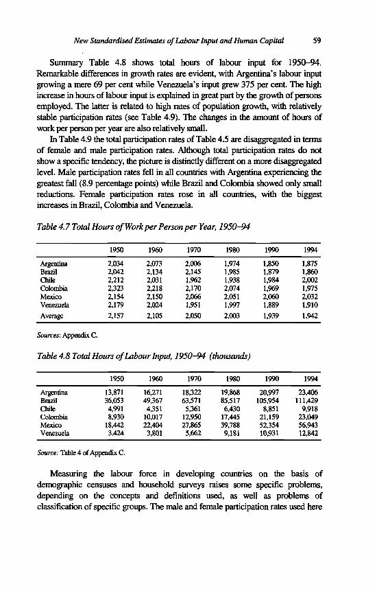
Summary Table 4.8 shows total hours of labour input for 1950-94. Remarkable differences in growth rates are evident, with Argentina’s labour input growing a mere 69 per cent while Venezuela’s input grew 375 per cent. The high increase in hours of labour input is explained in great part by the growth o f persons employed. The latter is related to high rates of population growth, with relatively stable participation rates (see Table 4.9). The changes in the amount of hours of work per person per year are also relatively small.
In Table 4.9 the total participation rates of Table 4.5 are disaggregated in terms of female and male participation rates. Although total participation rates do not show a specific tendency, the picture is distinctly different on a more disaggregated level. Male participation rates fell in all countries with Argentina experiencing the greatest fall (8.9 percentage points) while Brazil and Colombia showed only small reductions. Female participation rates rose in all countries, with the biggest increases in Brazil, Colombia and Venezuela.
New Standardised Estimates o f Labour Input and Human Capital 59
Table 4.7 Total Hours o f Work per Person per Year, 1950-94
1950 1960 1970 1980 1990 1994
Argentina 2,034 2,073 2,006 1,974 1,850 1,875Brazil 2,042 2,134 2,145 1,985 1,879 1,860Olile 2,212 2,031 1,962 1,938 1,984 2,002Colombia 2,323 2,218 2,170 2,074 1,969 1,975Mexico 2,154 2,150 2,066 2,051 2,060 2,032Venezuela 2,179 2,024 1,951 1,997 1,889 1,910Average 2,157 2,105 2,050 2,003 1,939 1,942
Sources: Appendix C.
Table 4.8 Total Hours o f Labour Input, 1950-94 (thousands)
1950 1960 1970 1980 1990 1994
Argentina 13,871 16,271 18,322 19,868 20,997 23,406Brazil 36,053 49,367 63,571 85,517 105,954 111,429Chile 4,991 4,351 5,361 6,430 8,851 9,918Colombia 8,930 10,017 12,950 17,445 21,159 23,049Mexico 18,442 22,404 27,865 39,788 52,354 56,943Venezuela 3,424 3,801 5,662 9,181 10,931 12,842
Source: Table 4 of Appendix C.
Measuring the labour force in developing countries on the basis of demographic censuses and household surveys raises some specific problems, depending on the concepts and definitions used, as well as problems of classification of specific groups. The male and female participation rates used here
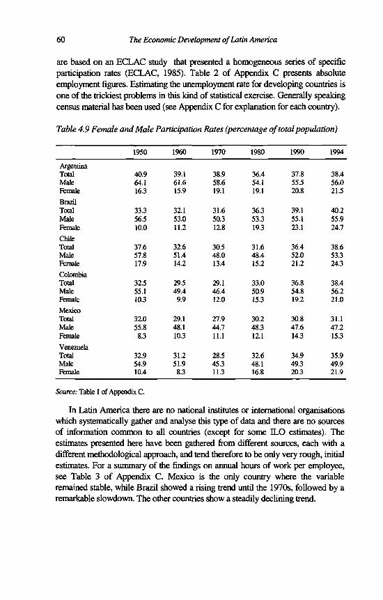
60 The Economic Development o f Latin America
are based on an ECLAC study that presented a homogeneous series of specific participation rates (ECLAC, 1985). Table 2 of Appendix C presents absolute employment figures. Estimating the unemployment rate for developing countries is one of the trickiest problems in this kind of statistical exercise. Generally speaking census material has been used (see Appendix C for explanation for each country).
Table 4.9 Female and Male Participation Rates (percentage o f total population)
1950 1960 1970 1980 1990 1994
ArgentinaTotal 40.9 39.1 38.9 36.4 37.8 38.4Male 64.1 61.6 58.6 54.1 55.5 56.0Female 16.3 15.9 19.1 19.1 20.8 21.5
BrazilTotal 33.3 32.1 31.6 36.3 39.1 40.2Male 56.5 53.0 50.3 53.3 55.1 55.9Female 10.0 11.2 12.8 19.3 23.1 24.7
ChileTotal 37.6 32.6 30.5 31.6 36.4 38.6Male 57.8 51.4 48.0 48.4 52.0 53.3Female 17.9 14.2 13.4 15.2 21.2 24.3
ColombiaTotal 32.5 29.5 29.1 33.0 36.8 38.4Male 55.1 49.4 46.4 50.9 54.8 56.2Female 10.3 9.9 12.0 15.3 19.2 21.0
MexicoTotal 32.0 29.1 27.9 30.2 30.8 31.1Male 55.8 48.1 44.7 48.3 47.6 47.2Female 8.3 10.3 11.1 12.1 14.3 15.3
VenezuelaTotal 32.9 31.2 28.5 32.6 34.9 35.9Male 54.9 51.9 45.3 48.1 49.3 49.9Female 10.4 8.3 11.3 16.8 20.3 21.9
Source: Table 1 of Appendix C.
In Latin America there are no national institutes or international organisations which systematically gather and analyse this type of data and there are no sources of information common to all countries (except for some ILO estimates). The estimates presented here have been gathered from different sources, each with a different methodological approach, and tend therefore to be only very rough, initial estimates. For a summary of the findings on annual hours of work per employee, see Table 3 o f Appendix C. Mexico is the only country where the variable remained stable, while Brazil showed a rising trend until the 1970s, followed by a remarkable slowdown. The other countries show a steadily declining trend.

New Standardised Estimates o f Labour Input and Human Capital 61
Human Capital
In growth accounting considerable effort has been devoted to capturing quality changes in labour input.7 The most important of these, considered to have a direct effect on productivity, is the level o f education and its rate of change. There are, as mentioned in the introduction, other aspects which have an important effect on increasing productivity and reducing poverty, such as health care and nutrition, but no estimates for these are provided in this chapter. Some factors which do have an effect on the productivity of the labour force are not included in the quantification. For example, one factor already considered by Denison (1967) is work effort. Denison cites industry observers which indicate that the pace of work in Canada and the United States is markedly faster than in Western Europe. It would not be too difficult to arrive at a similar opinion with respect to the Latin American countries, and making a case for a much wider gap than exists between Europe and the United States. However, these differences are very difficult to quantify, insofar as they are not due to differences in working hours or education, and belong largely to the realm of the ultimate causes of economic growth. Another factor is the general health of the population and the labour force; however, the impact of malnutrition and disease on labour input and productivity in developing countries has until now largely gone unmeasured.
Length of work yearOne factor which has been considered by Denison (1967) and some other growth analysts is the length of the work year, measured by hours worked. They assumed that, above a certain level, decreases in time worked were fully compensated by increases in work intensity and, up until a level of about 1700 hours a year, a partial compensation was used. Currently, most growth analysts do not include this kind of analysis, maybe because of the relative uniformity of working hours in the advanced countries. This issue might be again of interest in comparisons between advanced and developing countries, marked by huge differences in annual working time. However, in this study I have assumed, as did Maddison (1987), that a reduction in working hours leads to an equiproportionate cut in labour input.
EducationIn the advanced countries and successful ‘late industrialisers’, there is a clear recognition of the central role that education and the generation of knowledge play in the development process, and this attitude has been spreading gradually to the countries of Latin America. In most countries of the region the systems of education, training, and scientific and technological development have undergone noteworthy expansion in the last decades. However, they still display shortcomings in terms of the quality of their results, their degree of adaptation to the

requirements of the economic and social environment, and the extent to which they are accessible to the different strata of society (ECLAC, 1992).
The rise in the average educational level of the population in the post-war period has had a crucial effect on the quality of labour. An individual’s level of education affects the type of work he or she can do and the efficiency with which work is performed. In all countries in our sample the population’s average number of formal years of education has risen rapidly (see Table 4.10). However, the most rapid growth was experienced by the developing countries, with the Asian developing countries growing at by far the fastest rate. In a recent publication concerning the rapid growth of some East Asian countries, several explanatory factors were put forward to explain the fast growth in human capital. These were identified as rapid economic growth, the decline in population growth, the relatively equal income distribution, and policies with respect to human capital formation (World Bank, 1993a).
62 The Economic Development o f Latin America
Table 4.10 Average Years o f Formal Educational Experience o f the Population Aged 15-64,1950-94
Argentina Brazil Chile Colombia Mexico Venezuela
Total1950 4.72 1.83 4.46 2.45 2.06 1.931973 6.87 3.23 6.46 4.41 3.81 3.941980 7.41 4.22 7.34 5.07 5.72 5.511989 8.38 5.25 8.65 6.91 6.78 7.761994 8.96 5.93 9.48 8.20 7.45 9.38Primary1950 3.86 1.53 3.65 2.04 1.88 1.741973 4.92 2.41 4.55 3.19 3.14 3.111980 4.97 3.22 4.91 3.45 4.17 4.111989 5.09 3.87 5.30 4.29 4.60 5.231994 5.15 4.29 5.54 4.83 4.86 5.98Secondary1950 0.77 0.25 0.70 0.34 0.16 0.161973 1.68 0.69 1.55 1.06 0.56 0.741980 2.04 0.88 2.12 1.40 1.32 1.201989 2.65 1.23 2.93 2.27 1.83 2.161994 3.01 1.48 3.45 2.93 2.16 2.90Higher1950 0.09 0.05 0.11 0.07 0.03 0.031973 0.27 0.13 0.35 0.15 0.11 0.091980 0.40 0.12 0.31 0.22 0.23 0.201989 0.63 0.15 0.42 0.34 0.34 0.361994 0.81 0.16 0.49 0.44 0.43 0.51
Source: Appendix C.
New Standardised Estimates o f Labour Input and Human Capital 63
The number o f formal years of education enjoyed by the population aged between 15 and 64 years is probably not the most adequate measure o f quality change. First, some authors consider the labour force as the more relevant unit o f analysis and, second, important elements such as on-the-job training are not taken into consideration. On the one hand, unfortunately, in Latin America, the only data available for the whole period and all countries of coverage concerns years of formal education o f the population. However, it is also true that higher levels o f education o f the population as a whole have positive effects, especially in terms o f adaptability to changing markets and new technologies; these factors assume greater importance in the global integration process marked by rapid changes in markets and technologies and, in the case of Latin America, export-oriented development strategies.
Table 4.11 presents a comparison o f formal years o f education o f the total population and o f the labour force. The general conclusion is that differences are small at the primary level but can be significant at the tertiary level. This information, obtained from population censuses, is only available for a few benchmark years in a limited number of countries. Hence, I have opted for average years of formal education of the population as the best proxy available for human capital improvement.
As regards on-the-job training, Psacharopoulos (1993) indicates that there exists strong education-training complementarities. Psacharopoulos and Vêlez (1992), using data for Colombia, found a strong positive interaction between training and years of formal education in determining earnings. They concluded that training really has an effect on earnings only after a worker has eight years of formal education. A study by Mingat and Tan (1988) confirmed the above- mentioned findings since they concluded that training was particularly productive when a country’s educational system is highly developed. The rate of return on training was, according to their most conservative estimate, in the order of 20 per cent, assuming that 50 per cent of the population is literate.
Unfortunately, as education expanded in Latin America, its overall quality declined and the educational system became more inefficient. Several factors can be identified. One was the explosion of social demand for education, which led to the incorporation of more and more children, without redefining the educational content or increasing resources to meet expanded enrolments. Moreover, the traditional preference for physical investments over qualitative ones and the lack of interest in education also contributed to a poor implementation of the growth of the educational system, with the corresponding deterioration in results. In Latin America, it is o f fundamental importance to design and put into effect a strategy for promoting the transformation of education and training and increasing the scientific and technological potential o f the region which makes sustained growth possible on the basis of the incorporation and spread of technological progress (ECLAC, 1992). A very important consideration is whether the quantity indicator

64 The Economic Development o f Latin America
of years of education also reflects the quality changes, which have occurred in the sample countries. The crisis o f the 1980s has affected the quality o f education in countries of Latin America while, for example, the Asian countries may well have improved their educational systems, but this is not reflected in our data. Although it is very difficult to make an assessment of quality changes, I will analyse some aspects of deteriorating education in Latin America, together with policies for improving the quality of education.
One striking difference between Latin America and the other regions is its much higher level o f grade repetition, especially in the first grade; 50 per cent in 1980 and 42 per cent in 1988.8 There is some grade repetition in any school system because some students are not yet mature enough to be promoted or show some learning disability. Students then benefit enough from repetition to make it efficient from an economic viewpoint. However, the high repetition rates suggest a major problem. The greatest problem lies not in the lack of schools but in the quality of education. High repetition rates limit access to education, delay entrance, and have high resource costs. Some rather simple measures have been suggested for the schooling system, such as wider provision of textbooks and writing materials, which could reduce the enormous amount of resources now devoted to grade repetition (IDB, 1993).
Some micro-evidence on the effects of schooling indicates that the impact of educational attainment on wages and economic productivity is considerable. One important element, as indicated above, is the fact that schooling has both important private and social returns. In fact, the IDB (1993) study indicates that private returns are lower and social returns higher than in standard estimates.
Psacharopoulos gives a brief summary of the recent research on returns to investment in education; primary education continues to be the number one investment priority in developing countries; educating females is marginally more profitable than educating males; the general secondary school curriculum is a better investment than the technical/vocational track; and the returns to education obey the same rules as investment in conventional capital, that is, they decline as investment expands (Psacharopoulos, 1993). One of the conclusions with respect to differences in pay between different segments of employment, self-employment and dependent employment, is that empirical studies generally find no significant difference in income between the two as documented by Psacharopoulos (1993). This result, although important in itself, is also useful with respect to the determination of the respective factor shares.
The estimates of educational levels are presented for each country as a whole and in this sense the wide variations within countries in average years of education are not taken into account. For example, in Brazil, there are huge educational differences between the north-eastern region and other parts of the country. In Latin America, the quality of schooling and attendance rates tends to be systematically lower in rural areas and for the indigenous people.

New Standardised Estimates o f Labour Input and Human Capital 65
Hours worked by males and females, and within each sex by individuals of different age, change over time. Women do proportionally more temporary or part- time work, and their labour market participation and skill acquisition is interrupted by child bearing and raising, resulting in lower compensation rates. Lower compensation for women is partly due to discrimination, which therefore exacerbates the quality differential between men and women. Psacharopoulos and Tzannatos (1992) estimate that women’s pay is 70.5 per cent o f men’s for Latin America as a whole, with a somewhat higher figure for our sample countries.
Table 4.11 Comparison o f Educational Level o f Total Population and Labour Force (years o f formal education)
Year Country Type of education
Total population (15-64)
Labour force Difference (%)
1951 Colombia Primary 2.07 2.04 -1.3Secondary 0.35 0.35 0.0Higher 0.07 0.07 0.0Total 2.49 2.46 -1.2
1961 Venezuela Primary 2.14 2.19 2.3Secondary 0.24 0.27 14.1Higher 0.05 0.07 31.0Total 2.43 2.53 4.1
1970 Chile Primary 4.42 4.40 -0.5Secondary 1.43 1.46 2.1Higher 0.28 0.37 32.1Total 6.13 6.23 1.6
1980 Argentina Primary 4.97 5.07 2.1Secondary 2.04 1.98 -3.0Higher 0.40 0.49 22.8Total 7.41 7.54 1.8
1981 Venezuela Primary 4.27 4.32 1.2Secondary 1.28 1.43 11.8Higher 0.22 0.26 16.3Total 5.77 6.01 4.1
1990 Mexico Primary 4.63 4.73 1.7Secondary 1.90 2.36 24.2Higher 0.63 0.50 38.9Total 7.16 7.59 6.0
1992 Chile Primary 5.44 5.44 0.0Secondary 3.14 3.20 1.9Higher 0.44 0.58 31.8Total 9.02 9.22 2.2
Source: Elaborated by the author on the basis of population censuses.
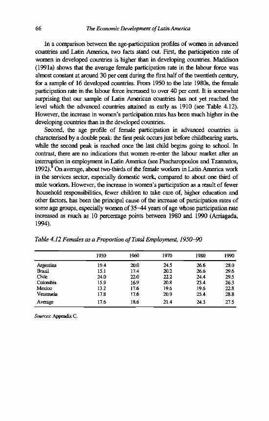
66 The Economic Development o f Latin America
In a comparison between the age-participation profiles o f women in advanced countries and Latin America, two facts stand out. First, the participation rate of women in developed countries is higher than in developing countries. Maddison (1991a) shows that the average female participation rate in the labour force was almost constant at around 30 per cent during the first half of the twentieth century, for a sample of 16 developed countries. From 1950 to the late 1980s, the female participation rate in the labour force increased to over 40 per cent. It is somewhat surprising that our sample of Latin American countries has not yet reached the level which the advanced countries attained as early as 1910 (see Table 4.12). However, the increase in women’s participation rates has been much higher in the developing countries than in the developed countries.
Second, the age profile of female participation in advanced countries is characterised by a double peak: the first peak occurs just before childbearing starts, while the second peak is reached once the last child begins going to school. In contrast, there are no indications that women re-enter the labour market after an interruption in employment in Latin America (see Psacharopoulos and Tzannatos, 1992).9 On average, about two-thirds of the female workers in Latin America work in the services sector, especially domestic work, compared to about one third of male workers. However, the increase in women’s participation as a result of fewer household responsibilities, fewer children to take care of, higher education and
other factors, has been the principal cause of the increase of participation rates of some age groups, especially women of 35-44 years of age whose participation rate increased as much as 10 percentage points between 1980 and 1990 (Arriagada, 1994).
Table 4.12 Females as a Proportion o f Total Employment, 1950-90
1950 1960 1970 1980 1990
Argentina 19.4 20.0 24.5 26.6 28.0Brazil 15.1 17.4 20.2 26.6 29.6Chile 24.0 22.0 22.2 24.4 29.5Colombia 15.9 16.9 20.8 23.4 26.3Mexico 13.2 17.6 19.6 19.6 22.8Venezuela 17.8 17.6 20.9 25.4 28.8Average 17.6 18.6 21.4 24.3 27.5
Sources: Appendix C.
New Standardised Estimates o f Labour Input and Human Capital 67
NOTES
1. The renewed focus on causes of economic growth in the ‘new growth theory’ and especially in the role of human capital, see for example Lucas (1988), was preceded in die 1960s when the human capital theory received much attention, promoted amongst others by Becker (1964), Harbison and Myers (1964), Schultz (1961) and Tinbergen and Bos (1965).
2. Most of the data on vital rates is obtained from the excellent book by Collver (1965).3. See Diaz-Alejandro (1970, tables 1 -14 and 1-15, pp. 37-38). Another indicator of the
importance of immigration is that in 1914 30.3 per cent of the population were foreigners. This indicates that the relative importance of immigrants was much higher in Argentina than in the USA, where the ratio of foreigners in the total population reached a maximum of 14.4 per cent (in 1890 and 1910). See Diaz Alejandro (1970, p. 36).
4. An interesting thesis suggested by Collver (1965), which falls outside the scope of this study, is that the immigrants themselves played a major part in the change in reproductive behaviour in Brazil and especially Argentina.
5. The 1950 level of hours worked per year was quite similar in the different country groupings. It was somewhat lower in the advanced countries, with high levels in Japan, Germany and the Netherlands, and somewhat higher in the Asian developing countries. By 1990, this situation changed and differences are substantial - with levels around 2300 hours in the Asian countries and somewhat above 1600 hours in the advanced countries.
6. It should be noted that in many cases the only available information concerned the formal sector and no statistics were available regarding the informal and rural sector where people tend to work very long hours.
7. See the works of Denison, and in Latin America for example, Selowski, Elias and Langoni.8. These averages relate to the whole of Latin America; our sample countries have a lower average
(35 per cent) because the Southern Cone countries have much lower levels (especially Chile).9. The female participation rates in this study coincide rather well with our estimates. However, it
is necessary to be cautious with their mean because it apparently contains a calculation error.


5. New Standardised Estimates of Capital Stock for Latin America and the USA
INTRODUCTION
The lack of comparable estimates of fixed capital stocks in Latin American countries has hindered the analysis of economic development within the region, as well as comparisons with other developing and developed countries. This chapter tries to fill the gap by providing standardised estimates of gross and net stocks for Argentina, Brazil, Chile, Colombia, Mexico and Venezuela.
The estimates were generated by employing the ‘Perpetual Inventory Method’ (PIM) currently used by most OECD countries and, hence, the most appropriate in an international comparison. The analysis concentrates on the methodology and results for Latin America but also includes a comparison with the USA,1 using the same methodology.
In spite of both the theoretical and practical difficulties associated with the use, estimation and meaning of capital stock estimates, they continue to be extensively employed and are useful for many kinds of economic analysis, such as growth accounting, productivity analysis, economic forecasting, studies of cyclical fluctuations and of the relationship between capital, output and labour and the role of technical progress.
In the past, significant efforts have been made to estimate capital stocks in many Latin American countries, and a review of these is presented in Appendix H. However, no official time series on capital stocks are prepared on a regular basis. Hence there have been estimates by a variety of independent researchers and institutes. This explains the great differences in methodology and coverage. These estimates may be useful for various types of analysis within each country, but are difficult to use in international comparisons because of differences in definitions and assumptions with respect to the different variables such as GDP, capital formation and its disaggregation, estimation of the initial stock, length of asset lives, retirement patterns (that is, distribution of service lives around the mean life), and differences in the relative prices of assets.
69
70 The Economic Development o f Latin America
M ETHODOLOGY
There are basically two methods, each with its variations, for measuring capital stocks:
(a) direct measurement of the stock for a benchmark year, through different types of survey of physical assets, insured values, company book values, or stock exchange values;
(b) by cumulating historical series on past investment and deducting assets which are scrapped, written off or destroyed by war.
The second is widely known as the 'Perpetual Inventory Method’ and was pioneered by Raymond Goldsmith (1951). In this chapter, annual fixed capital stock estimates are presented for the 1950-94 period using the Goldsmith method.2 The attraction of the perpetual inventory model is based on its use of a methodology which facilitates international comparison. It produces more meaningful figures because all the hypotheses and calculations are transparent and consistent It permits analysis o f the structure and age distribution of the capital stock. It is now generally used in official estimates, sometimes in combination with direct estimates o f the initial stock, for example Japanese statisticians use a postwar wealth survey benchmark.3
The capital assets considered in this study are the same as those included in gross fixed capital formation in the national accounts. Generally the countries examined in this study follow the United Nations classification (United Nations, 1968), where gross fixed capital formation is defined as outlays (purchases and own-account production) by industries, producers of government services, and producers of private non-profit services to households, for new durable goods (commodities) less net sales of similar second-hand and scrapped goods. Excluded are government outlays on durable goods for military use. In general, the goods included are durable (lasting more than one year), reproducible and tangible. Intangible assets like patents and other intellectual property are excluded, as are inventories, work in progress and non-reproducible assets like forests, land and mineral deposits.4
Capital formation is separated here into three asset types - residential structures, non-residential structures, and machinery and equipment. For each type fixed capital stocks have been estimated on the basis of past investment. Estimates are given for both gross and net fixed capital stocks. This makes it possible to differentiate between ‘ex-post’ and ‘ex-ante’ concepts of capital,5 that is, between actual and expected contributions of capital to production. Here the ‘ex-post’ concept is used. Capital stocks are valued at constant 1980 prices. GDP and capital stocks were converted to international dollars, using the International Comparison Project (ICP) purchasing power parities (PPP), rather than exchange rates.

New Standardised Estimates o f Capital Stock 71
Separate PPPs were used for GDP, investment in residential structures, non- residential structures and machinery and equipment.
The perpetual inventory method estimates capital stock as a weighted sum of past investment flows. This involves estimation of a base year capital stock consisting of the sum of past investment during the assumed life-times o f the different asset categories. The gross stock is calculated by adding investment during the year and subtracting assets that are scrapped. The net stock is obtained by adding investment during the year and deducting depreciation.
The objective of this chapter is to generate capital stocks for the 1950-94 period. To be able to use the perpetual inventory method, historical time series of gross fixed investment are needed over a long period of time, basically since 1900. This requirement was difficult to meet for Latin America since in many cases official series do not go further back than 1950.
The reliability of the stock estimates depends primarily on the accuracy of these basic data. Hence, Appendices B and D provide a detailed description o f the sources and series used for each country. A set o f three tables is provided for each country with long-term series (1900-1994) for GDP at constant 1980 national prices, GDP at constant 1980 international dollars, population, GDP per capita, gross total and disaggregated investment in national currencies and as a percentage of GDP. These appendices also contain an explanation o f the estimation procedures applied to fill holes in the data base.
For most countries it was relatively easy to obtain information dating back to 1925 although, for example, finding data on investment in residential construction gave problems for the whole period in some countries. For 1900-1925 the basic series are mostly very rough estimates.
A working life of 50 years was assumed for residential structures, 40 years for other structures and 15 years for machinery and equipment, for all countries, over the whole period. These assumptions seem rather realistic for non-residential structures and machinery and equipment.
Several countries use asset life estimates which are close to the ones used here (for example the asset lives which the US Bureau of Economic Analysis uses in its estimation for the United States are practically the same, although the official United States estimates are more finely disaggregated). In the case of residential structures, the asset life of 50 years is probably rather low but it is practically impossible to obtain data on residential investment before 1900 in Latin America.6 In order to be able to generate the initial total capital stock for 1950, data on capital formation in machinery and equipment was needed since 1935, in non-residential construction since 1910 and in residential construction since 1900.
A rectangular retirement pattern was assumed, that is, assets are completely scrapped after serving their respective lives (15, 40 and 50 years). These assumptions about the mortality function and the fixed nature of service life have been adopted for reasons of transparency and simplicity. Blades (1989) analyses

72 The Economic Development o f Latin America
these different assumptions in detail. In my model, the simultaneous exit mortality function was applied, which is also still in use in Canada, Japan and Norway. Simultaneous exit may be regarded as a limiting case of a bell-shaped function which Blades considers the only plausible candidate for a mortality function. In my approach all assets of a given vintage disappear simultaneously, but the results are not very different from the bell-shaped hypothesis.7
A major problem in this kind of research is the estimation of the length of life of capital assets. For developing countries, especially Latin American ones, these length-of-life assumptions may be critical as they are often not only related to technological and economic considerations but also to shortages of foreign exchange and the absence of regular repairs and maintenance because of budgetary constraints. Furthermore, the obsolescence of capital seems to be less significant than the collapse o f the product market in determining utilisation rates. Future research should clarify the relative importance of these issues for Latin American capital stock estimates. Not much empirical information is available about service lives, especially in Latin America.8 Changing service life assumptions affect the size of the capital stock and its rate of growth.9
One obvious question is whether average service lives remain constant over time as I assumed. The service life of a given type of asset almost certainly varies both between different users and from one period to another. When business conditions are favourable, assets will be used more intensively and discarded sooner. Relative price movements, maintenance levels, management efficiency and tax rates also have an effect. OECD concludes that there was ‘little evidence o f any secular tendency for given types of assets to be retained in production for longer or shorter periods’ (OECD, 1993, p. 39). This does not, of course, mean that the average life o f the aggregate capital stock remains constant because this is affected by changes in the structure of the stock.
For the calculation of net capital stock, one has to define a depreciation function for allocating the cost of the asset over its service life.10 There exists a close relationship between replacement, service life and depreciation; see Jorgenson (1974) for theoretical aspects of replacement and its twin, the theory of depreciation. There is currendy no agreement over this depreciation function, but in the literature two approaches stand out. The first is the straight-line pattern of depreciation, in which efficiency declines linearly over the lifetime of the capital good. A second method, also used quite often, is the so-called declining balance depreciation in which efficiency of the capital good declines geometrically.11
In order to obtain the net capital stock I chose the first method, assuming that the capital services are used up in equal instalments over time, that is, applying straight-line depreciation over the working life of the different types of assets. Not much attention is given in the literature on capital stock estimation to the moment depreciation starts. This assumption, however, is not without importance.12 Very fast depreciation is often allowed for tax purposes in the developed countries, but

New Standardised Estimates o f Capital Stock 73
is much less frequent in Latin America. After instalment machinery and equipment as well as structures need some time to start operating normally. Hulten (1990) presents a perpetual inventory model in which no first-year depreciation takes place, and Jorgenson and Sullivan (1981) also apply a depreciation lag. Thus, in this study, straight-line depreciation starts with a lag of one year. It has also been assumed that the scrap value of capital goods at the end of their economic life is zero, which is o f course often not the case, but this treatment of obsolescence simplifies the calculation a great deal. This procedure is used in several OECD countries for estimation of net capital stock.
A model layout for capital stock estimation was developed to make all procedures transparent and to facilitate the replication of these results by other researchers (see Appendix E). Here I give the algebra involved in the procedures. In Table E.2 in Appendix E an example is presented of the procedure for estimating alternative benchmark capital stocks in non-residential structures as at 31 December 1949 in Argentina, a procedure which is the same for each country. The procedure is also the same for each category of investment and the only difference is that, in the case of residential capital stock the series starts in 1900, and in the case o f machinery and equipment in 1935. The gross gross increment to capital stock in column 3 of Table E.2 is the result from the multiplying GDP at constant 1980 prices in column 1 and the ratio of total gross fixed investment in construction to GDP at constant prices in column 2. At the end of 1949 gross fixed capital stock in construction equals the sum of 1910-49 gross fixed investment or gross increments to capital stock as given at the bottom of column 3. The initial end-year gross capital stock was calculated as follows:
GGI\ = alt* GDP, (5.1)
bGKb= X GGVm (5.2)
m=b-9'+I
Gross increment to capital stock of asset i during period tGross domestic product in tGross initial capital stock of asset i at bRatio of total gross fixed investment of asset i to GDP at constant prices in t Initial yearLength of life of asset i Type of asset Time
where:
G G I\ GDP, GK'b
J ,
bi
eit

74 The Economic Development o f Latin America
Column 4 o f Table E.2 presents the annual depreciation provision based upon straight-line depreciation which means that, in each year in which depreciation takes place, l/40th o f gross investment is depreciated. Column 5 gives the yearly components of depreciated capital formation remaining by the end of 1949, corresponding to l/40th for 1910,2/40th for 1911, and so on. End 1949 net stock consists o f the sum of 1910-49 components of depreciated capital formation which equals the 1910-49 sum of column 5. Net mid-year capital stock was calculated as follows:
Nt?b Net initial capital stock o f asset i at b
This procedure of benchmark year capital stock estimation can of course also be used to estimate the 1950-94 end-year net and gross capital stocks. Alternatively, the procedures which are detailed in Table E.3 o f Appendix E can be applied. In this table capital stock estimates for the 1950-94 period are elaborated. In Table E .3 ,1950 end-year gross capital stock (column 6) equals the benchmark end-year 1949 capital stock plus the gross gross increment in capital stock in 1950 as given in column 3 minus retirement of gross gross increment to capital stock of 40 years ago (column 4). The 1950 end-year net stock equals the 1949 stock plus the gross gross increment to capital stock (column 3) minus annual depreciation (column 7). The respective net and gross end-year capital stock series were calculated as follows:
(5.3)m-t+1-0'
m=b-Q'+l
where:
Ü , Depreciation of asset i during t
b (m - b + e l L Qi GGIrn (5.4)
GK't - GK't-i + GGl‘i - GGl‘t-e (t > b ) (5.5)
NKÌ = NKÌ.i + GGIÌ-D" (5.6)
where:
GK‘t Gross capital stock of asset i at tNK‘t Net capital stock of asset i at t
Columns 10 and 11 o f Table E.3 present average ages of gross and net capital stocks, respectively, and in columns 12 and 13 the end-year gross and net capital stock estimates are brought to a mid-year basis. Column 14 gives the average of
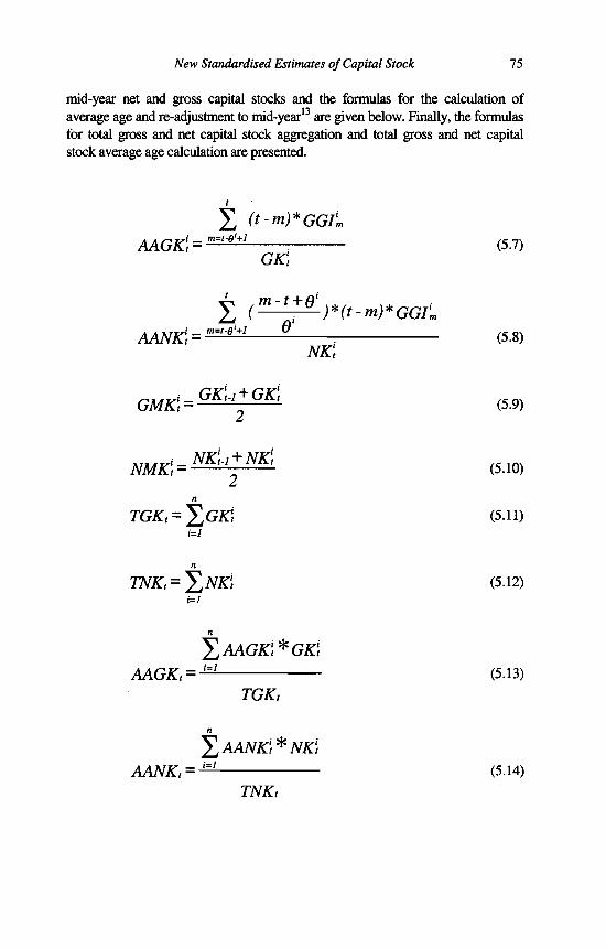
New Standardised Estimates o f Capital Stock 75
mid-year net and gross capital stocks and the formulas for the calculation of average age and re-adjustment to mid-year13 are given below. Finally, the formulas for total gross and net capital stock aggregation and total gross and net capital stock average age calculation are presented.
j (t-m)*GGIim
GK\AAGK\ = ~ ^ --------- ;------------- (5.7)
. ÌÌI - t + fl*
A A N K ^ ^ 1 ----------:----------------------- (5.8)NK,
GM K, = G K i^ G K i (59)
(,10)n
TGK, = ^ G K Ì (5.11)(=7
n
TNK, = ^ N K ' t (5.12)i= l
^ AAGKÌ * GK‘t
TGKtAAGKt = — ------------------------- (5.13)
^ A A N K Ì* N K Ì
TNK,AANKt = — ------------------------- (5.14)
76 The Economic Development of Latin America
where:
AAGKp Average age of gross capital stock of asset i in tAANKV Average age of net capital stock of asset i in tGMK¿ Gross capital stock, mid-year tNMKp Net capital stock, mid-year tTGK,• Total gross capital stock in tTNK,: Total net capital stock in tAAGKp Average age of total gross capital stock in tAANK,: Average age of net capital stock in tn: Number of assets i
RESULTS
Appendix E presents a complete set of net and gross capital stock estimates for each country, that is, gross and net fixed tangible capital stocks by type of asset, 1950-94 at constant 1980 national prices as well as at constant 1980 international dollars. It also gives average age, average service lives and capital-output ratios for 1950-94 on the basis of national currencies and calculated on the basis of international dollars.
Previous Estimates
Appendix H contains a detailed analysis of previous capital stock estimates in Latin America. Table 5.1 presents a comparison of the national estimates with the standardized capital stock estimates of this chapter. The existing estimates have been elaborated for different time periods and we present those closest to our benchmark years. It is especially interesting to compare the national capital stock estimates with the standardised ones for the initial year. The standardised estimates were generated with the perpetual inventory method while many of the national estimates calculated the initial stock on the basis of direct estimation or used another methodology, for example the one developed by Harberger (1972).
For Argentina the Goldberg and Ianchivolici (1986) article is an excellent study which is also the only existing estimate completely based upon the perpetual inventory method. The differences with our standardised estimates come mainly from the different assumptions regarding service lives of assets which are higher than our standardised estimate. As a result the Secretaría de Planificación (1991) study, which is an update of Goldberg and Ianchivolici (1986), has higher fixed capital stock levels and lower growth rates than our estimate. The initial values of the IEERAL and ECLAC studies are quite high, especially the United Nations study (1959).

New Standardised Estimates o f Capital Stock 11
In the case of Brazil the estimates of Goldsmith (1986) and Langoni (1974) are worth consideration. The Goldsmith estimate is mainly based upon the study by Langoni which is one of the few dealing with the problem of fixed capital stock estimation in Brazil. However, his initial fixed stock estimate seems rather high and the falling capital-output ratio shows a tendency contrary to ours. Most o f the other estimates also show relatively high initial capital stock estimates, much higher than the standardised estimates.
The movement of the capital-output ratio in the Haindl and Fuentes (1986) study for Chile coincides with ours. This is also largely the case in the Gutierrez study.
In Colombia the estimates of Harberger (1972) coincide largely with ours in terms of both trend and level. The more recent estimates of Henao (1983) show much higher levels and a clear downward tendency of the capital-output ratio. The ECLAC (1957) study finds much higher initial levels. The Mexican estimates by the Banco de Mexico (1969) are very difficult to interpret because they lack a methodological explanation. In the case of Venezuela the Baptista (1991) estimates growth rates are similar to ours but the levels show important differences. The Banco Central de Venezuela (1968) estimate is very similar to ours, but not much is known about the methodology used.
Exchange Rates and Purchasing Power Parities
A crucial consideration in international comparisons is how to convert estimates in local currencies into a common currency, either using exchange rates or purchasing power parities (PPP).14 The use of exchange rates as the conversion factor is the easiest and most direct way,15 but at best the official exchange rate reflects the purchasing power of tradable goods and services. It does not include non-tradables and thus may give rise to distortions. These distortions may be small, as is probably the case between two very open economies such as the Netherlands and Belgium, but can be quite large in the case of low-income developing countries.
The aim of the present study is to make internationally comparable estimates. Therefore, purchasing power parities are needed for non-residential and residential construction and machinery and equipment. Capital stocks normally consist partly of tradables, especially machinery and equipment, which in Latin America are purchased mainly from abroad, and partly of non-tradables. It is for this reason that purchasing power parities are the most appropriate conversion factor. However, purchasing power parities are only available for a limited number of countries for a limited number of years.

78 The Economic Development o f Latin America
Table 5.1 A Comparison of Standardised and National Estimates (on the basis o f national currency capital-output ratios)
Argentina Standardised Goldberg/' 1EERAL ECLAC Unitedestimates Ianchilovici (1986) (1954) Nations
(1986) (1959)Gross Net Gross Net Net Net Net
1950 3.6 2.1 2.5 2.8 3.61973 3.5 2.3 2.31980 4.1 2.7 4.2 2.7 2.81984 4.6 2.9 4.9 3.2
Brazil Standardised Langoni (1974) Goldsmith ECLAC Unitedestimates (1986) (1954) Nations
(1959)Gross Net Net Net Net Net
1950 1.4 0.9 2.6 2.6 1.81952 1.6 1.1 2.5 1.81968 2.0 1.4 2.2 2.01980 2.4 1.8 2.0
Chile Standardised Gutiérrez (1983) Haindl/Fuentes ECLACestimates (1986) (1954)
Gross Net Net Net Net1950 3.6 2.3 2.8 2.21973 3.9 2.4 2.8 3.01980 3.6 2.1 2.4 2.61984 4.2 2.4 3.0
Colombia Standardised Harberger (1972) Henao(1983) ECLACestimates (1957)
Gross Net Net Net Net1952 2.8 1.8 2.0 3.3 2.91967 2.7 1.6 1.9 2.71973 2.4 1.5 2.21980 2.4 1.5 2.2
Mexico Standardised Banco de México ECLAC Unitedestimates (1969) (1954) Nations
(1957b)Gross Net Net Net Net
1950 1.7 1.2 2.8 1.8 2.21967 2.2 1.6 2.3
Venezuela Standardised Banco Central de Baptista (1974)estimates Venezuela (1986)
Gross Net Net Gross Net1950 2.8 2.1 2.1 1.7 1.31965 3.0 2.0 1.9 1.9 1.21973 3.0 2.0 2.0 1.31980 3.8 2.7 3.1 2.21989 5.0 2.9 3.8 2.2
Source: See Appendix H.
In Latin America the first efforts to estimate purchasing power parities date from the late 1940s, under the influence of the path-breaking study by Colin Clark
New Standardised Estimates o f Capital Stock 79
(1940). One of the earliest was an interesting, yet largely unknown, study conducted at the Inter-American Statistical Institute. Under the technical guidance of Simon Kuznets, Dominguez (1947) used PPPs to convert 1940 national income estimates into dollars. The national income data available at that time were not very reliable and the basket of goods compared in order to estimate a PPP consisted only of 12 items, all o f them foodstuffs. Despite its shortcomings, the study provided a rough estimate of real income levels and gave an indication of the range of income disparities within Latin America and facilitated comparisons with the USA.
The first ECLAC estimates of real income in dollars were made for the 1945-52 period (ECLAC, 1954). However, the methodology was not very rigorous and was based partly on a 1950 United Nations study which calculated dollar estimates of real income on the basis of projections of exchange rates for a ‘normal’ period, and partly on arbitrary estimates by economists who were familiar with price levels and living standards in Latin America. The first systematic effort to calculate purchasing power figures in Latin America was the pioneering 1963 ECLAC study conducted by Stanley Braithwaite.
Towards the end of the 1960s, ECIEL,16 a research programme of comparative studies on economic integration, initiated an international comparison project on the same lines as the ECLAC study. Finally, during the 1970s and the 1980s, ECLAC and ECIEL cooperated in the various phases of the International Comparison Project (ICP), which at the onset was a joint effort o f the United Nations and the World Bank and, in later phases, involved the Statistical Office of the European Communities (EUROSTAT) and the Organisation for Economic Cooperation and Development (OECD).17
Table 5.2 presents the exchange rate and the purchasing power parities (PPPs) prepared during phase IV of the ICP project. I also give the adjusted exchange rates used in 1980 by ECLAC and the World Bank for conversion to dollars. For 1980, the benchmark year, I compare the PPPs used, which were supplied to us by Alan Heston, formerly with the ICP project, with the ones published by the United Nations/EUROSTAT (1987).
In this table the AH column includes also PPPs for Mexico which were not published in ICP IV. The AH results show that all countries, with the exception of Argentina, have much higher exchange rates than PPPs as can be seen in the lower panel which gives PPP-GDP exchange rate deviation indices. The range varies from 0.46 in Colombia to 1.41 in Argentina. The PPP-exchange rate deviation indices in the lower panel of Table 5.2 indicates that the AH results for 1980 are similar to those of ICP IV.
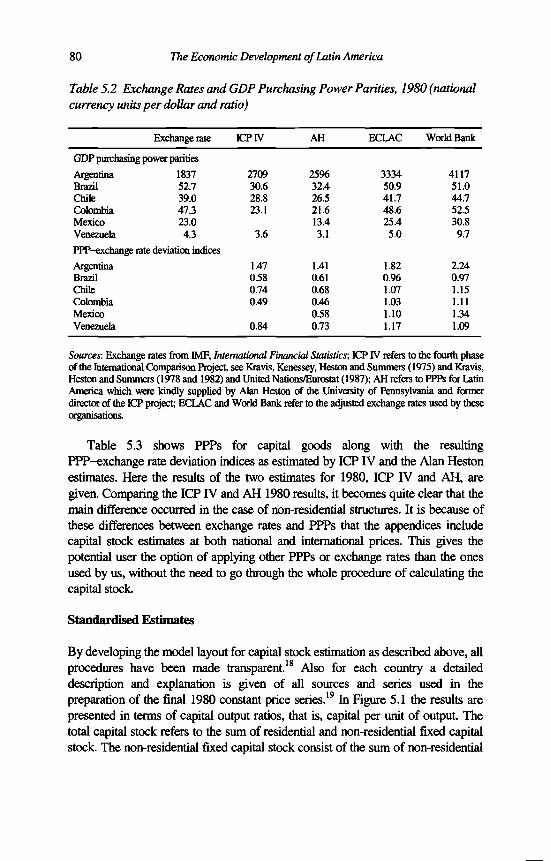
80 The Economic Development o f Latin America
Table 5.2 Exchange Rates and GDP Purchasing Power Parities, 1980 (national currency units per dollar and ratio)
Exchange rate ICP IV AH ECLAC World Bank
GDP purchasing power parities
Argentina 1837 2709 2596 3334 4117Brazil 52.7 30.6 32.4 50.9 51.0Chile 39.0 28.8 26.5 41.7 44.7Colombia 47.3 23.1 21.6 48.6 52.5Mexico 23.0 13.4 25.4 30.8Venezuela 4.3 3.6 3.1 5.0 9.7
PPP-exchange rate deviation indices
Argentina 1.47 1.41 1.82 2.24Brazil 0.58 0.61 0.96 0.97Chile 0.74 0.68 1.07 1.15Colombia 0.49 0.46 1.03 1.11Mexico 0.58 1.10 1.34Venezuela 0.84 0.73 1.17 1.09
Sources: Exchange rates from IMF, International Financial Statistics-, ICPIV refers to the fourth phase of the International Comparison Project, see Kravis, Kenessey, Heston and Summers (1975) and Kravis, Heston and Summers (1978 and 1982) and United Nations/Eurostat (1987); AH refers to PPPs for Latin America which were kindly supplied by Alan Heston of the University of Pennsylvania and former director of the ICP project; ECLAC and World Bank refer to the adjusted exchange rates used by these organisations.
Table 5.3 shows PPPs for capital goods along with the resulting PPP-exchange rate deviation indices as estimated by ICP IV and the Alan Heston estimates. Here the results of the two estimates for 1980, ICP IV and AH, are given. Comparing the ICP IV and AH 1980 results, it becomes quite clear that the main difference occurred in the case of non-residential structures. It is because of these differences between exchange rates and PPPs that the appendices include capital stock estimates at both national and international prices. This gives the potential user the option of applying other PPPs or exchange rates than the ones used by us, without the need to go through the whole procedure of calculating the capital stock.
Standardised Estimates
By developing the model layout for capital stock estimation as described above, all procedures have been made transparent.18 Also for each country a detailed description and explanation is given of all sources and series used in the preparation of the final 1980 constant price series.19 In Figure 5.1 the results are presented in terms of capital output ratios, that is, capital per unit o f output. The total capital stock refers to the sum of residential and non-residential fixed capital stock. The non-residential fixed capital stock consist of the sum of non-residential
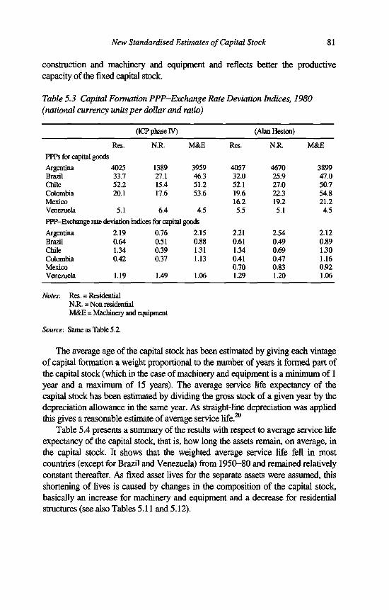
construction and machinery and equipment and reflects better the productive capacity of the fixed capital stock.
New Standardised Estimates o f Capital Stock 81
Table 5.3 Capital Formation PPP-Exchange Rate Deviation Indices, 1980 (national currency units per dollar and ratio)
(ICP phase IV) (Alan Heston)
Res. N.R. M&E Res. N.R. M&E
PPPs for capital goods
Argentina 4025 1389 3959 4057 4670 3899Brazil 33.7 27.1 46.3 32.0 25.9 47.0Chile 52.2 15.4 51.2 52.1 27.0 50.7Colombia 20.1 17.6 53.6 19.6 22.3 54.8Mexico 16.2 19.2 21.2Venezuela 5.1 6.4 4.5 5.5 5.1 4.5
PPP-Exchange rate deviation indices for capital goods
Argentina 2.19 0.76 2.15 2.21 2.54 2.12Brazil 0.64 0.51 0.88 0.61 0.49 0.89Chile 1.34 0.39 1.31 1.34 0.69 1.30Colombia 0.42 0.37 1.13 0.41 0.47 1.16Mexico 0.70 0.83 0.92Venezuela 1.19 1.49 1.06 1.29 1.20 1.06
Notes: Res. = ResidentialN.R. = Non residentialM&E = Machinery and equipment
Source: Same as Table 5.2.
The average age of the capital stock has been estimated by giving each vintage of capital formation a weight proportional to the number of years it formed part of the capital stock (which in the case of machinery and equipment is a minimum of 1 year and a maximum of 15 years). The average service life expectancy of the capital stock has been estimated by dividing the gross stock of a given year by the depreciation allowance in the same year. As straight-line depreciation was applied this gives a reasonable estimate of average service life.20
Table 5.4 presents a summary of the results with respect to average service life expectancy of the capital stock, that is, how long the assets remain, on average, in the capital stock. It shows that the weighted average service life fell in most countries (except for Brazil and Venezuela) from 1950-80 and remained relatively constant thereafter. As fixed asset lives for the separate assets were assumed, this shortening of lives is caused by changes in the composition of the capital stock, basically an increase for machinery and equipment and a decrease for residential structures (see also Tables 5.11 and 5.12).

82 The Economic Development o f Latin America
In Table 5.5 the average age of the total, non-residential and residential gross capital stock is presented. This figure reflects a combination of changes in the composition of the capital stock as well as its growth rate. A faster rate of growth of the capital stock, without changes in its composition, leads to a greater share of newer vintages in the stock and a reduction of its average age. However, changes in the composition o f the capital stock can also substantially affect the average age.
Table 5.4 Latin America: Weighted Average Service Life o f Total and Non- Residential Fixed Capital Stock, 1950-94 (on the basis of international dollars)
Total N.R. Res. Total N.R. Res.
1950 1973
Argentina 38.6 29.4 50 34.3 26.7 50Brazil 30.4 23.9 50 33.6 28.9 50Chile 36.5 32.3 50 33.8 29.9 50Colombia 39.3 35.3 50 37.5 32.9 50Mexico 38.0 35.1 50 31.9 27.5 50Venezuela 26.3 24.8 50 28.3 25.4 50
1980 1994
Argentina 33.3 25.7 50 32.4 23.5 50Brazil 32.4 28.4 50 34.8 30.6 50Chile 34.4 30.6 50 34.3 31.2 50Colombia 36.5 32.1 50 35.6 31.0 50Mexico 30.7 26.3 50 30.7 24.7 50Venezuela 27.6 24.7 50 27.2 24.5 50
Source: Appendix E.
Table 5.5 shows only a relatively small reduction in average age in the 1950-80 period. As the composition of the capital stock did not change very much, on average, this largely reflects the acceleration in growth of the capital stock. In 1980-94, the combined effect of changing composition and falling capital stock growth causes a sharp increase in the stock’s average age.
The changes in the level of total and non-residential gross fixed capital stock per capita relative to the United States were especially important during 1950-73 (Table 5.6). On average, there was an increase in per capita stocks relative to the United States from 1950-80 but thereafter the relative levels fell somewhat.

New Standardised Estimates o f Capital Stock 83
Figure 5.1 Latin America: Total and Non-Residential Capital Productivity, 1950-94 (ratio of GDP to gross fixed capital stock in constant prices)
Argentina Brazil
total stock non-resldenttal
Source: Appendices B and E.
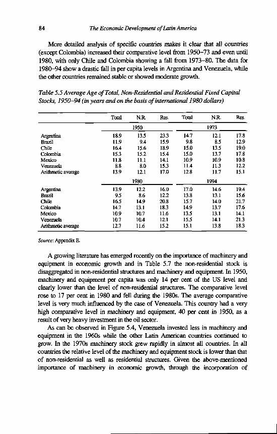
84 The Economic Development o f Latin America
More detailed analysis o f specific countries makes it clear that all countries (except Colombia) increased their comparative level from 1950-73 and even until 1980, with only Chile and Colombia showing a fall from 1973-80. The data for 1980-94 show a drastic fall in per capita levels in Argentina and Venezuela, while the other countries remained stable or showed moderate growth.
Table 5.5 Average Age o f Total, Non-Residential and Residential Fixed Capital Stocks, 1950-94 (in years and on the basis o f international 1980 dollars)
Total N.R. Res. Total N.R. Res.
1950 1973
Argentina 18.9 13.5 23.3 14.7 12.1 17.8Brazil 11.9 9.4 15.9 9.8 8.5 12.9Chile 16.4 15.6 18.9 15.0 13.5 19.0Colombia 15.3 15.2 15.4 15.0 13.7 17.8Mexico 11.8 11.1 14.1 10.9 10.9 10.8Venezuela 8.8 8.0 15.3 11.4 11.3 12.2Arithmetic average 13.9 12.1 17.0 12.8 11.7 15.1
1980 1994
Argentina 13.9 12.2 16.0 17.0 14.6 19.4Brazil 9.5 8.6 12.2 13.8 13.1 15.6Chile 16.5 14.9 20.8 15.7 14.0 21.7Colombia 14.7 13.1 18.3 14.9 13.7 17.6Mexico 10.9 10.7 11.6 13.5 13.1 14.1Venezuela 10.7 10.4 12.1 15.5 14.1 21.3Arithmetic average 12.7 11.6 15.2 15.1 13.8 18.3
Source: Appendix E.
A growing literature has emerged recently on the importance of machinery and equipment in economic growth and in Table 5.7 the non-residential stock is disaggregated in non-residential structures and machinery and equipment. In 1950, machinery and equipment per capita was only 14 per cent of the US level and clearly lower than the level o f non-residential structures. The comparative level rose to 17 per cent in 1980 and fell during the 1980s. The average comparative level is very much influenced by the case of Venezuela. This country had a very high comparative level in machinery and equipment, 40 per cent in 1950, as a result of very heavy investment in the oil sector.
As can be observed in Figure 5.4, Venezuela invested less in machinery and equipment in the 1960s while the other Latin American countries continued to grow. In the 1970s machinery stock grew rapidly in almost all countries. In all countries the relative level of the machinery and equipment stock is lower than that of non-residential as well as residential structures. Given the above-mentioned importance o f machinery in economic growth, through the incorporation of
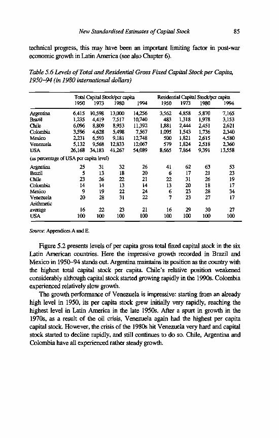
technical progress, this may have been an important limiting factor in post-war economic growth in Latin America (see also Chapter 6).
Table 5.6 Levels o f Total and Residential Gross Fixed Capital Stock per Capita, 1950-94 (in 1980 international dollars)
New Standardised Estimates o f Capital Stock 85
Total Capital Stock/per capita Residential Capital Stock/per capita1950 1973 1980 1994 1950 1973 1980 1994
Argentina 6,415 10,598 13,000 14,256 3,562 4,858 5,870 7,165Brazil 1,235 4,419 7,517 10,740 483 1,318 1,978 3,153Chile 6,096 8,809 8,953 11,392 1,881 2,444 2,451 2,621Colombia 3,596 4,628 5,498 7,567 1,095 1,543 1,736 2,340Mexico 2,231 6,593 9,181 12,748 500 1,821 2,615 4,580Venezuela 5,132 9,568 12,833 12,067 579 1,824 2,518 2,360USA 26,168 34,183 41,267 54,089 8,665 7,864 9,391 13,558
(as percentage of USA per capita level)
Argentina 25 31 32 26 41 62 63 53Brazil 5 13 18 20 6 17 21 23Chile 23 26 22 21 22 31 26 19Colombia 14 14 13 14 13 20 18 17Mexico 9 19 22 24 6 23 28 34Venezuela 20 28 31 22 7 23 27 17Arithmeticaverage 16 22 23 21 16 29 30 27USA 100 100 100 100 100 100 100 100
Source: Appendices A and E.
Figure 5.2 presents levels o f per capita gross total fixed capital stock in the six Latin American countries. Here the impressive growth recorded in Brazil and Mexico in 1950-94 stands out. Argentina maintains its position as the country with the highest total capital stock per capita. Chile’s relative position weakened considerably although capital stock started growing rapidly in the 1990s. Colombia experienced relatively slow growth.
The growth performance of Venezuela is impressive: starting from an already high level in 1950, its per capita stock grew initially very rapidly, reaching the highest level in Latin America in the late 1950s. After a spurt in growth in the 1970s, as a result of the oil crisis, Venezuela again had the highest per capita capital stock. However, the crisis of the 1980s hit Venezuela very hard and capital stock started to decline rapidly, and still continues to do so. Chile, Argentina and Colombia have all experienced rather steady growth.

86 The Economic Development o f Latin America
Table 5.7 Levels o f Gross Fixed Capital Stock per Capita o f Non-Residential Structures and Machinery and Equipment, 1950-94 (in 1980 international dollars)
Non-residential structure/per capita M&E /per capita1950 1973 1980 1994 1950 1973 1980 1994
Argentina 2,168 3,737 4,453 3,910 685 2,004 2,677 3,181Brazil 346 2,067 3,716 6,037 406 1,035 1,823 1,531Chile 3,494 4,908 5,098 6,807 721 1,385 1,405 1,901Colombia 2,238 2,559 3,038 4,132 262 526 724 1,095Mexico 1,483 3,086 3,965 4,946 248 1,685 2,602 3,223Venezuela 2,362 4,743 5,955 6,086 2,191 3,001 4,359 3,621USA 11,967 16,563 18,653 22,216 5,536 9,756 13,224 18,315
(as percentage of USA per capita level)
Argentina 18 23 24 18 12 21 20 17Brazil 3 12 20 27 7 11 14 8Chile 29 30 27 31 13 14 11 10Colombia 19 15 16 19 5 5 5 6Mexico 12 19 21 22 4 17 20 18Venezuela 20 29 32 27 40 31 33 20Arithmeticaverage 17 21 23 24 14 16 17 13USA 100 100 100 100 100 100 100 100
Source: Appendices A and E.
Another interesting point is the fact that all countries, with the exception of Venezuela, resumed growth in capital stock per capita in the 1990s. Venezuela has yet to recover from the crisis o f the 1980s, which had a severe impact on all countries. As mentioned above, Colombia experienced steady growth but at a low rate, especially in the 1950s and the 1960s, and its total capital stock per capita ended at the lowest level in the Latin American sample. Figure 5.3 reflects level and growth of the residential fixed capital stock. In comparison with the other stock components the stock of dwellings grow at a smoother rate. One of the main reasons for this is the fact that the service life of dwellings is the longest (50 years) o f all assets considered.
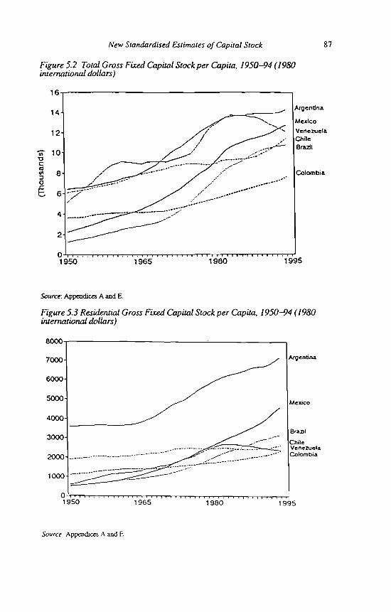
Figure 5 2 Total Gross Fixed Capital Stock per Capita, 1950-94 (1980 international dollars)
New Standardised Estimates o f Capital Stock 87
Source: Appendices A and E.
Figure 5.3 Residential Gross Fixed Capital Stock per Capita, 1950-94 (1980 international dollars)
Source Appendices A and E

88 The Economic Development o f Latin America
Figure 5.4 Non-Residential Gross Fixed Capital Stock per Capita, 1950-94 (1980 international dollars)
Source: Appendices A and E.
Figure 5.4 shows the level of gross fixed non-residential capital stock per capita in the sample of Latin American countries for the 1950-94 period. Figure 5.4. is, of course, very similar to Figure 5.2 but there are also interesting differences. The non-residential stock is the best indicator of a country’s productive capacity, and is therefore the most appropriate indicator in a growth accounting exercise. Brazil has been the fastest growing country. The growth of per capita non-residential capital in Venezuela is very similar to that in Figure 5.2. Colombia’s non-residential stock per capita grew steadily but not very fast. Chile and Argentina were other poor performers.
Figure 5.5 shows per capita stock of machinery and equipment. As one would expect, this type of capital asset was the most volatile, as becomes especially clear in the case of Venezuela where it is related to the big investment boost in the oil sector which occurred in the 1940s and 1950 and again after the first oil crisis in the 1970s. Brazil’s stock grew rapidly from the mid-1960s until the beginning of the 1980s. Since then machinery and equipment growth has been extremely low.
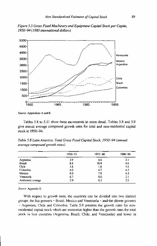
New Standardised Estimates o f Capital Stock 89
Figure 5.5 Gross Fixed Machinery and Equipment Capital Stock per Capita, 1950-94 (1980 international dollars)
Source'. Appendices A and E.
Tables 5.8 to 5.11 show these movements in more detail. Tables 5.8 and 5.9 give annual average compound growth rates for total and non-residential capital stock in 1950-94.
Table 5.8 Latin America: Total Gross Fixed Capital Stock, 1950-94 (annual average compound growth rates)
1950-73 1973-80 1980-94
Argentina 3.9 4.6 2.1Brazil 8.8 10.4 4.6Chile 3.8 1.8 3.4Colombia 4.0 4.7 4.3Mexico 8.0 7.8 4.4Venezuela 6.7 8.0 2.1Arithmetic average 5.9 6.2 3.5
Source: Appendix E.
With respect to growth rates, the countries can be divided into two distinct groups: the fast growers - Brazil, Mexico and Venezuela - and the slower growers - Argentina, Chile and Colombia. Table 5.9 presents the growth rates for non- residential capital stock which are somewhat higher than the growth rates for total stock in four countries (Argentina, Brazil, Chile, and Venezuela) and lower in

90 The Economic Development o f Latin America
Colombia and Mexico in the 1950-80 period. From 1980-94 the growth of non- residential capital stock was slower than that of total stock in most of the countries.
Table 5.9 Latin America: Gross Fixed Non-Residential Capital Stock, 1950-94 (annual average compound growth rates)
1950-73 1973-80 1980-94
Argentina 4.8 4.8 1.4Brazil 9.4 11.2 4.3Chile 4.2 1.9 3.8Colombia 3.8 5.1 4.3Mexico 7.7 7.6 3.6Venezuela 6.2 7.8 2.1Arithmetic average 6.0 6.4 3.3
Source: Appendix E.
The relationship between the growth of net and gross stocks depends on the history of capital formation. When growth slows down as in 1980-94, gross stock will grow more rapidly than net stock. This is what happened in all the countries. The converse is true in periods of growth acceleration. Table 5.10 gives annual average compound growth rates for total net and gross capital stock for the 1950-94 period.
Table 5.10 Comparative Growth of Gross and Net Total Fixed Capital Stock, 1950-94 (annual average compound growth rates)
1950-73 Gross Net
1973-Gross
-80Net
1980-94Gross Net
Argentina 3.9 4.4 4.6 4.9 2.1 1.1Brazil 8.8 9.2 10.4 10.5 4.6 3.6Chile 3.8 4.0 1.8 0.9 3.4 3.6Colombia 4.0 4.0 4.7 4.8 4.3 4.1Mexico 8.0 8.0 7.8 7.5 4.4 3.8Venezuela 6.7 6.2 8.0 8.7 2.1 0.6Arithmetic average 5.9 6.0 6.2 6.2 3.5 2.8
Source: See Appendix E.
During 1950-80 net stock grew faster in Argentina and Brazil. The growth rates of both stocks were about the same in Colombia and Mexico, indicating a process of steady growth. For Chile and Venezuela, the period 1950-94 was not homogeneous as both had sub-periods of faster and slower growth in net stock compared to gross. In the case of some countries, especially Chile, the 1980-94

New Standardised Estimates o f Capital Stock 91
period should be divided into a crisis period in the 1980s and recuperation in the 1990s.
The changing composition and age structure of the capital stock gives an indication of the rate at which technical change has been embodied in the capital stock (Maddison, 1993). Table 5.11 gives an indication of changes in the composition of gross total capital stock, measured in international dollars, during the 1950-94 period. In all countries the share of machinery and equipment in the total capital stock increased from 1950 to 1980 (except in Brazil and Venezuela, which had very high shares) and stabilised or dropped slightly during 1980-94. The share of residential structures fell in Argentina, Brazil and Chile, and rose in Mexico and Venezuela. The share of non-residential structures increased in Brazil, Chile and Venezuela and fell in Argentina, Colombia and Mexico. Here I am interested in the effect on the growth rates of the different stocks. Growth rates expressed in international dollars may be different from those in national currencies, because the PPPs change the composition of the capital stock. The sign of the change in the growth rate will depend on these compositional changes.
Table 5.11 Latin America: Composition of Gross Total Fixed Capital Stock, 1950-94 (in 1980 international dollars and as a % of total capital stock)
Dwellings Non-residential structures M&E
1950 1973 1980 1994 1950 1973 1980 1994 1950 1973 1980 1994
Argentina 55 46 45 50 34 35 34 27 11 19 21 22Brazil 39 30 26 30 28 47 49 56 33 23 24 14Chile 31 28 27 23 57 56 57 60 12 16 16 17Colombia 31 33 32 31 62 55 55 55 7 11 13 14Mexico 22 28 29 36 67 47 43 39 11 25 28 25VenezuelaArithmetic
11 19 20 20 46 50 46 50 43 31 34 30
average 32 31 30 32 49 48 47 48 19 21 23 20
Source: Appendix E.
A comparison of Tables 5.11 and 5.12 shows that whether the measurement is performed in international dollars or national currencies makes a big difference to the composition of the capital stock. The difference was very notable in the cases of machinery and equipment in Chile and Colombia.

92 The Economic Development o f Latin America
Table 5.12 Latin America: Composition of Gross Total Fixed Capital Stock, 1950-94 (on the basis of national currencies and asa% of total capital stock)
Dwellings Non-residential structures M&E
1950 1973 1980 1994 1950 1973 1980 1994 1950 1973 1980 1994
Argentina 53 44 43 49 37 39 38 30 10 17 19 21Brazil 35 29 26 30 21 37 39 48 44 34 35 22Chile 43 38 38 33 41 42 41 44 16 21 21 23Colombia 25 26 24 23 58 49 48 47 17 25 28 30Mexico 19 24 24 31 68 47 44 40 13 29 32 29Venezuela 13 21 22 22 48 51 47 51 39 28 31 27Arithmeticaverage 31 30 30 31 46 44 43 43 23 26 28 25
Source: Appendix E.
Table 5.13 Latin America: Difference between Growth of Fixed Capital Stocks in National Currencies and International Dollars, 1950-94 (difference in annual average compound growth rates at constant prices f
1950-73 Gross Net
1973-Gross
-80Net
1980-94 Gross Net
Total capital stockArgentina 0.0 0.0 0.0 0.0 0.1 0.0Brazil 0.4 0.4 0.0 0.0 0.4 0.5Chile 0.0 0.2 0.2 0.1 0.2 -0.2Colombia -0.2 -0.2 -0.4 -0.4 -0.1 0.0Mexico 0.0 0.0 0.0 0.0 0.1 0.1Venezuela 0.1 0.1 0.0 0.1 0.0 0.0
Non-residential capital stockArgentina 0.1 0.1 0.1 0.1 0.1 0.1Brazil 0.6 0.7 0.0 0.0 0.6 0.7Chile -0.1 0.0 0.1 0.0 0.0 -0.1Colombia -0.4 -0.3 -0.4 -0.3 -0.1 -0.1Mexico -0.1 -0.1 -0.1 0.0 0.0 0.0Venezuela 0.0 0.1 0.1 0.1 0.0 0.1
Note: * Difference calculated as growth rate in international dollars minus growth rate in national currency.
Source: Appendix E.
Table 5.13 compares the growth of capital stock as measured in national currencies with measures in international dollars (the latter being the method I prefer). Argentina, Mexico and Venezuela show very small differences between the two growth rates, while the other countries show larger differences.

New Standardised Estimates o f Capital Stock 93
There are sometimes differences of over 10 per cent in the growth rates, especially in the 1980-94 period when growth was slow. For 1950-80 only Colombia showed differences of over 10 per cent with respect to non-residential capital stock. Brazil showed the largest absolute differences in total capital stock and in non-residential capital stock in 1950-73 and 1980-94, while Colombia presented the largest differences in 1973-80.
Table 5.14 presents the ratio of non-residential capital stock to total capital stock. This ratio can be seen as an indicator of the share of the productive capital stock (measured as the non-residential stock) in the total stock. The initial 1950 ratio of productive to total fixed capital was very low in Argentina where residential capital stock is more substantial than non-residential. The other countries had much higher productive capital stock participation levels. In 1994, at the end of the period under consideration, Argentina remains the country with the highest level of residential capital stock. The role of productive capital is more dominant in the other countries, of which Venezuela has the lowest residential capital stock levels.
Table 5.14 Latin America: Ratio ofNon-Residential Fixed Capital Stock to Total Fixed Capital Stock, 1950-94 (on the basis of international dollars)
1950 1973 1980 1994Gross Net Gross Net Gross Net Gross Net
Argentina 0.44 0.47 0.54 0.53 0.55 0.52 0.50 0.45Brazil 0.61 0.60 0.70 0.70 0.74 0.73 0.71 0.68Chile 0.69 0.67 0.72 0.72 0.73 0.72 0.77 0.78Colombia 0.70 0.67 0.67 0.66 0.68 0.68 0.69 0.68Mexico 0.78 0.77 0.72 0.69 0.72 0.68 0.64 0.59Venezuela 0.89 0.89 0.81 0.78 0.80 0.78 0.80 0.79Arithmetic average 0.68 0.68 0.69 0.68 0.70 0.69 0.68 0.66
Source-. Appendix E.
The following tables present estimates of capital-output ratios. There are many forces that affect the development of the capital-output ratios, including technical progress, capital widening or deepening, demand and supply factors, the interest rate and so on. It is not the objective of this chapter to attempt to explain developments for six countries over a 44-year period. These estimates are included, however, because they are used quite intensively in economic forecasting, planning and econometric models.
In Tables 5.15 to 5.17, a comparison of capital-output ratios of total and non- residential capital stock is given for the 1950-94 period based on estimations in international dollars. It becomes clear from Table 5.15 that in 1950 the Latin American countries showed considerable variation in their gross capital-output ratios. Measured in national currencies, Argentina had the highest, and Brazil and

94 The Economic Development o f Latin America
Mexico the lowest. In 1980 international dollars, Colombia had the highest level in 1950. This situation had changed at the end of the period under consideration. In national currencies, Argentina and Venezuela again had the highest level, and Colombia the lowest. In international dollars Brazil and Venezuela had the highest level, and Chile and Colombia the lowest. During the 1950-94 period, the capital-output ratios of Chile and Colombia have remained more or less stable while the ratios of the other countries have risen substantially.
Table 5.15 Total Fixed Gross Capital-Output Ratios, 1950-94 (in 1980 international dollars)
1950 1973 1980 1994Argentina 2.3 2.3 2.6 2.8Brazil 1.2 1.8 2.2 3.3Chile 2.8 3.0 2.8 2.5Colombia 2.8 2.2 2.1 2.3Mexico 1.2 1.7 1.9 2.6Venezuela 2.1 2.1 2.8 3.1Arithmetic average 2.1 2.2 2.4 2.8
Source: Appendix E.
The gross non-residential capital-output ratios (Table 5.16) show quite different, and much lower, ratios than the total fixed gross capital-output ratios of Table 5.15. In 1994 the gross total capital-output ratio of Brazil (the highest) was about 50 per cent higher than the ratio in Colombia (the lowest). With respect to gross non-residential capital-output ratios, in 1994 this spread was much wider (80 per cent), with Venezuela being the highest and Argentina the lowest. This difference in spread between total capital and non-residential capital-output ratios can be observed for the whole 1950-94 period.
Table 5.16 Non-Residential Fixed Gross Capital-Output Ratios, 1950-94 (in 1980 international dollars)
1950 1973 1980 1994Argentina 1.0 1.2 1.5 1.4Brazil 0.7 1.3 1.6 2.3Chile 1.9 2.1 2.0 1.9Colombia 1.9 1.4 1.5 1.6Mexico 0.9 1.2 1.3 1.7Venezuela 1.8 1.7 2.2 2.5Arithmetic average 1.4 1.5 1.7 1.9
Source: Appendix E.

New Standardised Estimates o f Capital Stock 95
Table 5.17 shows a comparison of gross and net capital-output ratios for the 1950-94 period. Table 5.13 showed that the comparison of the growth rates of capital stock in national currencies and international dollars does not yield very large differences.
Table 5.17 A Comparison of Gross and Net Total Capital-Output Ratios, 1950-94 (in 1980 international dollars)
1950Gross Net
1973Gross Net
1980Gross Net
1994Gross Net
Argentina 2.3 1.4 2.3 1.5 2.6 1.7 2.8 1.6Brazil 1.2 0.8 1.8 1.3 2.2 1.7 3.3 2.2Chile 2.8 1.7 3.0 1.9 2.8 1.6 2.5 1.5Colombia 2.8 1.8 2.2 1.4 2.1 1.4 2.3 1.5Mexico 1.2 0.9 1.7 1.2 1.9 1.3 2.6 1.7Venezuela 2.1 1.5 2.1 1.4 2.8 1.9 3.1 1.8Arithmetic average 2.1 1.4 2.2 1.5 2.4 1.6 2.8 1.7
Source: Appendix E.
CONCLUSIONS
This chapter presented a comprehensive set of standardised and hitherto unavailable capital stock estimates for six Latin American countries, employing the perpetual inventory method. These estimates can be used in the analysis of comparative economic performance, productivity growth, convergence and catchup.
Total capital stock increased in all Latin American countries but at very different rates. In Brazil it grew by about 8 per cent between 1950-94, but only by some 3 per cent in Argentina and Chile. In 1950 Argentina had the highest level of total stock per capita, with Brazil by far the lowest. At the end of the period under consideration, Argentina remained the country with the highest level, while Colombia had the lowest. The non-residential stock level for the period as a whole was clearly highest in Venezuela, while Brazil made an impressive catch-up from the lowest level in 1950.
These trends are also true for the ‘productive’, that is, non-residential, capital stock. This stock grew slightly faster then total stock in the 1950-80 period, especially in the cases of Argentina and Brazil. When economic activity fell down sharply in the 1980s the growth rate of the ‘productive’ fixed capital stock became lower than the rate of the total stock.
It is also important to emphasise some points with respect to the composition of the stock. On the one hand, the relatively high level of the residential capital stock in Argentina and the corresponding somewhat lower level, in comparative

96 The Economic Development o f Latin America
perspective, of its productive capital stock. Venezuela is the extreme case on the other hand, presenting a relatively small stock of dwellings and the highest stock of machinery and equipment in our sample. This last fact is related to the very heavy investment in the oil sector over time. In the case of Brazil it is possible to observe rather high levels of machinery and equipment, especially initially in the 1950s, in the composition of the total capital stock.
Maddison (1993) found that the evidence for advanced capitalist countries did not confirm Kaldor’s (1961) hypothesis of constant capital-output ratios over the long run in capitalist countries. The Latin American evidence also contradicts Kaldor’s view and indicates increasing capital-output ratios in Argentina, Brazil, Mexico and Venezuela. Capital productivity remained almost constant in Chile and increased somewhat in Colombia. There are some small differences between the evidence for total as opposed to non-residential capital-output ratios (Argentina and Chile for example) but the general trend is clear. However, Maddison’s evidence refers to a much longer period, for some countries since 1820. For Latin America the evidence is restricted to the relatively short, for this type of analysis, 1950-94 period.
NOTES
1. The investment estimates for the USA are taken from Maddison (1995) but the stock estimation procedure was adjusted slightly due to changes in the benchmark year and for the use of somewhat different asset service life assumptions.
2. The description of this model is based upon Michael Ward (1976a).3. See Maddison (1991a), Appendix D.4. See Derek Blades (1989), p. 3.5. See Ward (1976a), pp. 19-20.6. The official estimate of the US Department of Commerce (1993), uses a service life of 80 years for
new, one- to four-unit structures and 65 years for new, five or more unit structures based upon estimates from Goldsmith and Lipsey (1963). Improvements to residential structures are assigned the following lives: additions and alterations are assumed to have lives one-half as long as those for new structures; and lives for residential major replacements are based cm industry estimates far items replaced during the 1970s. Mobile homes are assigned a life of 20 years on the basis of trade association data. The resulting average service life is probably above our 50 years estimate but well below 80 years.
7. See Blades (1989, figure 2, p. 25).8. Well-known studies for the USA were made by Terborgh (1954) and Winfiey (1935). The main
sources used by the OECD countries as described in OECD (1993) ate: asset lives prescribed by tax authorities, company accounts, surveys, expat advice and other countries, estimates. Tax authorities in many countries specify the number of years over which the depreciation of assets may be deducted from profits before charging taxes. The estimation procedure for these asset lives is not very clear, Hibbert, Griffin and Walker (1977), note that tax lives in the United Kingdom are based on ‘custom and practice rather than any scientific study on the longevity of assets’. However, about half of the OECD countries make use of tax life estimates in their capital stock estimation, five countries use company accounts and industry studies. Japan is the only country for which large scale surveys are available; in the USA and the United Kingdom some small scale surveys have been carried out In several countries, investigations are under way with respect to service lives; for

New Standardised Estimates o f Capital Stock 97
example, Canada, Italy, the Netherlands and Spain. Finally, most countries rely on expert advice and use other countries’ estimates (at least to check their own estimates). The empirical material for OECD countries is abundant compared to what is available for Latin America (see Bernstein and Shah, 1993).
9. If service life assumptions are changed with respect to die whole period of capital stock estimation, this will cause the stock size to change but the effect on the growth rate will be limited to change in the stocks composition. Changes within the period of estimation can have substantial effects on growth rates.
10. Hudson and Matthews (1963) analyse three theoretical variants of calculating depreciation charges over the working life of the asset: reducing, constant or increasing depreciation. Hie authors indicate that increasing depreciation over the asset’s life is a rather unreal example, because it obviously implies that net services will continue to increase throughout the asset’s life until the asset is ready for scrapping. They also discuss diminishing-balance and straight-line depreciation. With respect to the latter they observe: ‘A pattern of gradually diminishing periodic net services could arise in practice as a result, say, of the need for increasing maintenance expenses in the later years of the asset’s life’ (Hudson and Matthews, 1963, p. 234).
11. The specification of the depreciation function is especially relevant far tax deduction purposes. The imposed tax system asset lives have, therefore, a direct effect on depreciation. Hulten and Wykoff (1980) conclude in a study cm the USA that economic depreciation and tax depreciation are interrelated.
12. Depreciation represents a decline in efficiency and here we have assumed that efficiency decline is constant over time. For calculating convenience this assumption has to be expressed in discrete time for which we use the normal year period. We have assumed that the stock is at its maximum efficiency during the first period and starts declining by a fixed proportion in the subsequent periods (see Jorgenson 1974 and Jorgenson and Sullivan 1981). This assumption can have a sizable effect on the levels of the net capital stock. To give an example: assuming constant investment (100) and a working life of four years, means that the gross stock will be 400 at the end of the period. The net stock with immediate depreciation will amount to 150 (75 + 50 + 25) and with lagged depreciation will be 250 (100 + 75 + 50 + 25). The difference will vary according to investment flows and, again, will depend especially on working life assumptions, being lower with longer lives.
13. The calculation procedure comes from Ward (1976a, p. 58) who calls this the approximate method.14. I use the 1980 international dollar which represents the same purchasing power parity over total
GDP as the US dollar, but with a purchasing power over subaggregates and over detailed categories determined by average international prices rather than by US relative prices.
15. The exchange rates normally used are the annual average (rf) series of the IMF, published in International Financial Statistics.
16. Spanish acronym standing for: Programa de Estudios Conjuntos sobre la Integration Econ6mica Latinoamericana.
17. Unfortunately the Latin American countries did not participate in die last phases of the ICP, which makes it impossible to change die benchmark to a more recent year.
18. For an example of this layout see Appendix E and for a complete description see the pages above.19. See Appendices B and D.20. See Maddison (1982, p. 216).

6. Explaining Latin American Post-War Development - The Growth Accounts
There have been relatively few growth accounting studies for Latin America.1 One of the problems in comparing these is the great variety of methodologies used. The heterogeneity is especially evident in the case of capital stock estimation, but GDP and employment measures also differ widely. A major contribution of the present study is the use of a standardised approach applied both to Latin American and other countries with which Latin America is compared.
STARTING POINT AND COMPARATIVE PERFORMANCE
Table 6.1 presents comparative levels of economic performance between 1950 and 1994 in 16 countries and averages for regional groups. 1950 was for many countries a new dynamic starting point after two world wars and the Great Depression. In the post-war period many European and Asian countries started growing and converging much faster. This convergence process was much weaker in Latin America.
In 1950, per capita real income in Latin America was three times as high as that of developing Asia, a bit higher than the Iberian level and about a third of that of the United States. Within Latin America, real per capita income ranged in 1950 from around 40 per cent of the United States’ level in Argentina and Venezuela, 30 per cent in Chile and Mexico and 19 and 15 per cent in Colombia and Brazil, respectively.
This picture had changed totally by 1994 when per capita real income in Latin America was about 30 per cent lower than in developing Asia, about two thirds of the Iberian level, around a quarter to a third of that in the United States and the other advanced countries. However, within Latin America, some convergence can be observed with levels of per capita GDP ranging from 35 per cent of the United States level for Argentina to 22 per cent in Colombia.
Latin American labour productivity (GDP per hour worked) was 3.5 times as high as developing Asia in 1950. Venezuela and Argentina had the highest level at around 40 per cent of the United States, Chile and Mexico about 30 per cent and Colombia and Brazil around 20 per cent. In 1994, labour productivity in Latin
99

100 The Economic Development o f Latin America
Table 6.1 Comparative Levels of Economic Performance of 16 Countries Between 1950 and 1994 (USA = 100)
GDP GDP per hour per capita worked
1950 1994 1950 1994
Labour input per capita
1950 1994
Years of education per capita
1950 1994
Argentina 41 35 38 39 107 90 45 61Brazil 15 23 17 24 89 92 18 37Chile 33 31 30 34 109 94 43 63Colombia 19 22 20 25 99 88 24 54Mexico 27 33 30 40 90 84 19 49Venezuela 38 27 42 34 90 79 18 61Arithmetic average 29 29 29 33 97 88 28 54
Korea 8 46 9 33 90 141 30 86Taiwan 8 47 7 36 106 132 32 98Arithmetic average 8 46 8 34 98 136 31 92
Portugal 16 37 15 36 109 102 22 54Spain 25 51 21 75 122 69 42 62Arithmetic average 21 44 18 56 116 85 32 58
France 44 72 37 92 120 79 85 88Germany 37 76 29 86 130 88 92 67Japan 17 81 14 64 122 128 81 82Netherlands 53 71 45 92 119 77 72 74UK 62 69 54 82 115 85 96 78Arithmetic average 43 74 36 83 121 91 85 78
Total land area per Merchandise exports Gross NR. capital stockcapita po-capita per employee
1950 1994 1950 1994 1950 1994
Argentina 214 224 102 23 16 19Brazil 99 108 38 14 4 20Chile 72 61 68 42 25 23Colombia 88 59 49 12 15 14Mexico 92 52 28 20 10 22Venezuela 110 52 275 37 27 26Arithmetic average 113 93 93 25 16 21
Korea 7 6 2 110 5 48Taiwan 5 3 14 97 6 24Arithmetic average 6 5 8 103 5 36
Portugal 22 34 33 91 10 26Spain 51 56 21 95 34 40Arithmetic average 37 45 27 93 22 33
Ranee 33 38 109 207 45 97Germany 10 13 59 326 29 103Japan 5 5 15 162 21 128Netherlands 8 8 207 516 45 89UK 12 15 186 178 30 64Arithmetic average 13 16 115 278 34 96
Source: Latin America from Appendices A, B, C, E and F. Other countries from Maddtson (1995), updated to 1994 using his sources, and OECD and FAO sources. Capital stocks estimated by the author.
The Growth Accounts 101
America is the same as in the Asian developing countries, which is surprising given that average per capita income in the Latin American countries is 30 per cent lower than in Asia. However, only about 35 per cent of the population is employed in Latin America compared with almost 50 per cent in the Asian countries. Annual hours worked were less than 2000 hours per person employed, compared to over 2300 in Asia. Latin American labour productivity in 1994 was 33 per cent of the level in the United States, 40 per cent of that in the advanced capitalist countries and 59 per cent of the Iberian countries (see Maddison, 1995).
An element of growth that continues to receive much attention in the literature is the role of human capital, that is the increase of a country’s productive potential through education and training. Table 6.1 shows that in 1950 the levels for Latin America, the Iberian Peninsula and the Asian countries were very similar (around 30 per cent of the US level). Although all countries show impressive growth in years of education, by 1994 the Latin American level is less than two thirds of the Asian level.
With respect to natural resources, the Latin American advantage was, and still is, overwhelming. A comparison of levels of total land area per capita in 1950 shows Latin American endowments above the level of the United States (the best endowed developed country among those considered), and well over ten times the natural resource endowment of our two South-East Asian countries. Moreover, this measure does not include mineral resources, which most probably would amplify the differences. With respect to the physical reproducible capital stock, Latin America’s position relative to the United States improved slightly from an average of 16 per cent per capita in 1950 to around 21 per cent in 1994.
Latin American export performance has also been poor. From a relatively strong position in 1950, Latin America became the worst performer in 1994, indicating an important comparative loss of growth potential to realise efficiency gains through specialisation.
THE 1950-94 GROWTH ACCOUNTS
The objective of this book is to analyse economic development in Latin America in the twentieth century. In this chapter growth accounts are presented which constitute a useful framework for assembling quantitative ‘facts’ and qualified hypotheses about growth causality in a coherent way (Maddison, 1987). The growth accounts start in 1950 as data inadequacy prevents systematic analysis of previous periods for Latin America. Growth accounting exercises are important because they can serve many different purposes - explaining differences in growth rates and levels between countries, illuminating processes of convergence and divergence, assessing the role of technical progress and calculating potential output losses. The results with respect to the most traditional explanatory factors, that is changes in the quantity and quality of labour inputs and changes in the quantity and

102 The Economic Development o f Latin America
quality of capital inputs are presented. I also include natural resources as an explanatory factor.
In order to explain in more detail the complex developments which have occurred since 1950, measures of total factor productivity have been prepared which differ from the traditional labour productivity indicator presented in Chapter 3. Increases in different factor inputs are measured in terms of average annual compound growth rates. Labour input is derived by multiplying employment and annual hours per person. The quantity and quality effects are weighted by the relevant factor shares to show the contribution of augmented labour input.2
The average annual compound growth rates of the gross capital stock and of the quality of the capital stock (vintage effect) were also weighted by the respective factor shares to give the augmented capital input. The sum of augmented capital and labour input, and the growth rate of the natural resources input weighted by 0.1, gives the augmented joint factor input, which is an indicator of the impact of factor inputs on economic growth.
A very important element of the analytical framework is its transparency. The appendices present all the basic series, giving the reader the opportunity to follow each step in the reasoning and test alternative hypotheses, because in this kind of research, large judgmental elements are inevitable.
Labour Input
Labour input was estimated in terms of hours worked rather than employment because average annual hours worked per employee year vary substantially between countries and over time.3 Average annual hours in 1994 were around 2500 in Korea, compared to about 1400 in the Netherlands. Within Latin America the variation is much lower.
It is important to adjust for changes in the quality of labour input. In this study, this is represented by changes in the level of education of the population aged between 15 and 64 years. Our estimate consists of equivalent years of education per person. The quality effect of labour results from the growth of equivalent years of education, and is based on the assumption that a 1 per cent increase in education causes a 0.5 proportionate gain in labour quality.4
Table 6.2 shows the growth rates of the labour force and employment, respectively. The labour force is related, much more than employment, to demographic forces, and in the post-war period many countries in Latin America entered the initial phase of demographic transition, with its characteristics of still high birth rates, and falling mortality rates. During 1950-73, the labour force grew somewhat more rapidly than employment. In the period from 1973-80, employment growth accelerated and both employment and the labour force grew at approximately the same rate. This situation changed in the crisis period since 1980, when in all countries (except Mexico) employment grew more slowly than the
labour force, with unemployment growing especially fast in Colombia and Venezuela.
The Growth Accounts 103
Table 6.2 Latin America: Labour Force (LF) and Employment (EMP), 1950-94 (annual average compound growth rates)
1950-73 L.F. EMP.
1973LF.
-8 0EMP.
1980-94 L F. EMP.
Argentina 1.4 1.4 0.9 1.0 1.8 1.6Brazil 2.8 2.8 3.8 3.8 2.7 2.4Chile 1.3 1.1 1.9 2.0 3.1 2.9Colombia 2.5 2.4 3.5 3.5 3.0 2.4Mexico 2.6 2.4 3.6 3.7 2.2 2.6Venezuela 3.3 3.3 5.0 4.8 3.2 2.7Arithmetic average 2.3 2.2 3.1 3.1 2.7 2.4
Source: Appendix C.
Table 4.7 of Chapter 4 showed a downward trend in working hours per person per year for the 1950-94 period in all countries, with an average decline of about 10 per cent. The range of decline varied from 122 hours for Mexico to 348 hours in the case of Colombia.
Chapter 4 highlighted the importance of the increasing average educational level in the post-war period as a crucial element in raising the quality of labour and labour productivity. The type of work an individual can do and the efficiency with which he or she performs is determined to a large degree by the level of educational attainment.
Table 6.3 presents the increase in the level of formal education of the population, measured in years. For growth accounting purposes, primary education has been given a weight of 1, secondary education a weight of 1.4 and higher education a weight of 2. These weights were applied to the whole sample and are the same as used by Maddison (1995). Maddison based his weights on Psacharopoulos’ (1984) evidence on the relative earnings associated with different levels of education.
In all Latin American countries, the average level of education increased rapidly from 1950 to 1994, primary education was the first to increase, ultimately followed by secondary and higher education. The differences in levels of education are still very considerable, ranging in 1994 from 6.7 years in Brazil to 11.4 in Chile. Many authors consider the educational level of the labour force, instead of the total population, as the relevant measure for the quality of labour adjustment. Unfortunately, information regarding educational level for the whole 1950-94 period is not available in most countries in Latin America.5

104 The Economic Development o f Latin America
Table 6.3 Latin America: Level of Education of the Population Aged 15-64 (weighted years of formal education)
1950 1973 1980 1989 1994
Argentina 5.12 7.63 8.63 10.07 10.97Brazil 1.98 3.64 4.69 5.89 6.69Chile 4.85 7.41 8.50 10.25 11.38Colombia 2.66 4.92 5.85 8.16 9.82Mexico 2.16 4.46 6.48 7.86 8.75Venezuela 2.02 4.42 6.19 8.99 11.06Arithmetic average 3.13 5.41 6.72 8.54 9.78
Sources: Appendix C and applying the following weights; 1 for primary education, 1.4 for secondaty education and 2 for higher education.
Table 6.4 summarises the main trends in labour quantity and quality growth in Latin America. Employment in Latin America also grew fast but annual hours per person declined steadily during the whole period. Labour quality, which is reflected in educational level, shows a steady increase over the whole period.
In Table 6.4 the quantitative and qualitative changes in labour inputs are presented separately. No uniform trend can be distinguished from this table. Comparing the 1950-73 and 1973-80 periods, all countries, except Argentina and Brazil, showed slow to marked acceleration in the incorporation of labour. In 1980-89, four countries experienced a slowdown (Brazil, Colombia, Mexico and Venezuela), while in the case of Chile the trend was acceleration. In the 1989-94 period, most countries increased the rate of incorporation of labour, with the exception of Brazil and Chile. However, in the case of Chile labour quantity incorporation was maintained at a comparatively high level.
Reproducible Capital Input
An important element in growth accounting from a comparative perspective is the availability of reliable measures of capital stock. In Chapter 4 comparable capital stock estimates were generated using the perpetual inventory method. With respect to quality improvement in successive vintages of the capital stock, representing technical progress in physical investment, modest assumptions were made regarding the embodiment in non-residential structures and machinery and equipment (see also the section on capital and investment in this chapter).
It is interesting to see that capital productivity, presented in Table 6.5, behaves quite different from labour productivity. Table 3.4 in Chapter 3 shows that labour productivity growth is generally positive: long-run growth is about 2.4 per cent annually and only 1980-89 shows negative growth. Table 6.5 shows that capital productivity growth in the Latin American countries has been negative for large periods. On average, capital productivity fell over the 1950-89 period and only

1989-94 shows increasing capital productivity. However, on a country-by-country comparison large differences can be observed, as well as between periods in particular countries.
The Growth Accounts 105
Table 6.4 Rate of Growth of Labour Inputs, 1950-94 (annual average compound growth rates)
1950-73Labour quantity
1973-80 1980-89 1989-94 1950-73Labour quality
1973-80 1980-89 1989-94
Argentina 1.32 0.82 1.06 1.39 0.87 0.88 0.86 0.86Brazil 2.90 3.01 2.11 1.54 1.33 1.83 1.27 1.28Chile 0.55 1.85 3.17 3.10 0.93 0.99 1.05 1.05Colombia 2.03 3.02 1.95 2.12 1.35 1.24 1.87 1.87Mexico 2.22 3.66 2.46 2.60 1.59 2.70 1.08 1.08VenezuelaArithmetic
2.87 5.01 1.83 3.39 1.80 1.01 1.35 0.27
average 1.98 2.90 2.10 2.36 1.31 1.44 1.25 1.07
Source: Appendix C.
The quantity and quality increases of capital are presented in Table 6.6 below6. On the quality side the average growth rates were 0.7 per cent during the 1950-73 period, 0.9 per cent in 1973-80, 0.8 per cent in 1980-89, and 0.6 per cent in 1989-94. The combined effect of quantity and quality growth makes clear that especially in 1950-80, capital inputs grew at a very high pace. Since then, growth has been much slower.
Table 6.5 Capital Productivity Growth, 1950-94 (annual average compound growth rates)
1950-73 1973-80 1980-89 1989-94
Argentina 0.03 -0.44 -1.21 0.91Brazil -1.46 -0.88 -1.03 -0.29Chile -0.25 0.29 0.20 0.34Colombia 0.84 -0.06 -0.49 0.08Mexico -1.52 -0.40 -1.21 1.39Venezuela 0.03 -1.12 -1.13 0.92Arithmetic average -0.39 -0.44 -0.81 0.56
Source: Appendices B and E.
The results with respect to quantity increases were discussed in detail in Chapter 5. During 1950-73, Argentina, Chile and Colombia witnessed the slowest growth, and fastest growth occurred in Brazil, Mexico and Venezuela. During the 1973-80 period, capital stock growth showed no signs of slowing down (except in Chile). However, in the 1980-94 period, growth rates decelerated drastically in all countries, with the exception of Chile and Colombia.
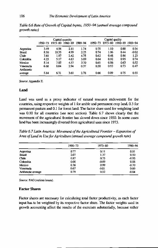
Table 6.6 Rate of Growth of Capital Inputs, 1950-94 (annual average compound growth rates)
106 The Economic Development o f Latin America
Capital quantity Capital quality1950-73 1973-80 1980-89 1989-94 1950-73 1973-80 1980-89 1989-94
Argentina 3.59 4.56 2.11 1.74 0.75 1.10 0.88 0.34Brazil 8.50 10.35 4.99 2.25 0.74 1.06 0.44 -0.02Chile 3.85 1.87 2.42 4.75 0.62 0.48 0.86 1.23Colombia 4.25 5.17 4.63 3.89 0.64 0.92 0.95 0.74Mexico 8.14 7.85 4.57 3.70 0.61 0.86 0.63 0.52VenezuelaArithmetic
6.68 8.04 2.94 0.37 0.58 0.93 0.73 0.47
average 5.84 6.31 3.61 2.78 0.66 0.89 0.75 0.55
Source: Appendix E.
Land
Land was used as a proxy indicator of natural resource endowment for the countries, using respective weights of 1 for arable and permanent crop land, 0.3 for permanent pasture and 0.1 for forest land. The factor share used for weighting land was 0.10 for all countries (see next section). Table 6.7 shows clearly that the movement of the agricultural frontier has slowed down since 1950. In some cases land has been increasingly diverted from agricultural uses since 1973.
Table 6.7 Latin America: Movement of the Agricultural Frontier - Expansion of Area of Land in Use for Agriculture (annual average compound growth rate)
1950-73 1973-80 1980-94
Argentina 0.77 0.11 0.01Brazil 2.07 1.37 0.50Chile 0.87 0.75 -0.93Colombia 0.00 -0.09 0.88Mexico 0.36 0.99 -0.70Venezuela 0.67 -0.01 0.00Arithmetic average 0.79 0.52 -0.04
Source: FAO (various issues).
Factor Shares
Factor shares are necessaiy for calculating total factor productivity, as each factor input has to be weighted by its respective factor share. The factor weights used in growth accounting affect the results of the exercises substantially, because rather

The Growth Accounts 107
big differences exist in growth rates of labour and capital stocks. The three main components of GDP are fixed capital consumption, compensation of employees and operating surplus. This last component must be divided between capital, labour and land income.
In Latin America an important part of the operating surplus, much more than in the advanced countries, consists of labour compensation for the self-employed and these earnings have to be attributed to labour’s share. The total capital share has been disaggregated into the capital shares of its three components, residential and non-residential capital and machinery and equipment. In some growth-accounting exercises, the individual items in the capital stock are weighted at their total stock value. However, the service flow per unit of capital in machinery and equipment is much higher than from a unit of residential capital. Therefore, the components of the capital stock have been weighted by their asset life, and the resulting disaggregated capital stock shares were multiplied by the national accounts total capital share. For the standardised capital shares the disaggregation of Maddison (1991a) has been used. For land income, used as a proxy for natural resource endowment, it was impossible to obtain estimates for all countries and a 10 per cent share was assumed for the whole period based on national accounts estimates available for some years in the case of Argentina and Mexico. Table 6.8 presents the resulting shares of capital, labour and natural resources in GDP for the six Latin American countries.
However, several authors have expressed their preference for constant factor shares (for example Maddison, 1987) and the sensitivity of the results was tested by using alternatively a set of standardised factor shares, with similar weights as used in Maddison (1991a), constant over time for all countries, as presented in Table 6.9. In general, the standardised factor shares will generate somewhat lower factor input growth as a result of a slightly lower standardised capital share combined with the fact that the capital stock generally grows faster than labour input.

108 The Economic Development o f Latin America
Table 6.8 Capital, Labour and Natural Resource Shares in GDP, 1950-94 (percentage of GDP)
1950-73 1973-80 1980-89 1989-94 1950-73 1973-80 1980-89 1989-94
Argentina Brazil
Labour 52.9 49.7 37.8 36.0 70.1 56.8 56.7 57.6Residential capital 11.8 11.4 14.9 16.3 3.1 4.6 4.9 5.6Non-res. structures 12.1 12.5 14.5 13.5 4.4 8.2 9.6 11.0M&E 13.2 16.5 22.7 24.2 12.5 20.4 18.8 15.7Total capital 37.1 40.3 52.2 54.0 19.9 33.2 33.3 32.4Natural resources 10.0 10.0 10.0 10.0 10.0 10.0 10.0 10.0Total 100 100 100 100 100 100 100 100
Chile Colombia
Labour 5.9 54.4 54.4 55.6 53.3 53.6 52.2 49.3Residential capital 14.7 13.2 12.5 11.4 9.4 5.1 4.8 5.0Non-res. structures 12.1 11.4 12.4 12.3 18.8 12.4 12.3 13.0M&E 11.2 11.0 10.7 10.8 8.5 18.9 20.7 22.7Total capital 38.1 35.6 35.6 34.4 36.7 36.4 37.8 40.7Natural resources 10.0 10.0 10.0 10.0 10.0 10.0 10.0 10.0Total 100 100 100 100 100 100 100 100
Mexico Venezuela
Labour 42.7 54.3 41.6 35.5 63.0 51.5 48.3 43.4Residential capital 6.1 4.6 6.9 9.0 2.9 4.5 4.8 5.5Non-res. structures 16.7 10.8 14.4 15.9 9.2 12.7 13.2 15.9M&E 24.5 20.4 27.1 29.6 15.0 21.3 23.7 25.2Total capital 47.3 35.7 48.4 54.5 27.0 38.5 41.7 46.6Natural resources 10.0 10.0 10.0 10.0 10.0 10.0 10.0 10.0Total 100 100 100 100 100 100 100 100
Source: Estimated by the author on the basis of national account and census information.
Table 6.9 Standardised Capital, Labour and Natural Resource Shares in GDP, 1950-94 (percentage of GDP)
1950-73 1973-80 1980-89 1989-94
Labour 60.0 60.0 60.0 60.0Residential capital 7.5 7.5 7.5 7.5Non-residential structures 10.0 10.0 10.0 10.0M&E 12.5 12.5 12.5 12.5Total capital 30.0 30.0 30.0 30.0Natural resources 10.0 10.0 10.0 10.0Total 100 100 100 100
Source: Estimated by the author.

The Growth Accounts 109
Table 6.10 Basic Indicators of Growth Performance, 1950-94 (annual average compound growth rates)
1950-73 1973-80 1980-89 1989-94 1950-73 1973-80 1980-89 1989-94
Argentina Brazil
Population 1.69 1.58 1.49 1.25 2.89 2.36 2.07 1.77GDP 3.99 3.04 -1.02 6.09 6.91 7.18 2.26 0.90Employment 1.41 0.98 1.72 1.25 2.78 3.81 2.67 1.86Hours per employee -0.08 -0.16 -0.65 0.14 0.11 -0.77 -0.55 -0.31Education 0.87 0.88 0.86 0.86 1.33 1.83 1.27 1.28M&E 6.71 5.84 3.11 1.52 7.44 10.76 2.05 -2.66Residential capital 3.07 4.36 2.92 2.75 7.48 8.48 6.17 4.06Non-res. struct 4.12 4.16 0.50 0.40 11.21 11.31 6.54 3.81Capital quality 0.75 1.10 0.88 0.34 0.74 1.06 0.44 -0.02Natural resources 0.77 0.11
Chile
0.03 -0.03 2.07 1.37
Colombia
0.49 0.52
Population 2.18 1.57 1.62 1.67 2.85 2.20 2.01 1.71GDP 3.58 2.84 2.95 6.38 5.12 4.97 3.31 4.27Employment Hours per
1.09 1.97 2.93 2.86 2.39 3.49 2.48 2.16
employee -0.54 -0.12 0.23 0.23 -0.35 -0.45 -0.52 -0.04Education 0.93 0.99 1.05 1.05 1.35 1.24 1.87 1.87M&E 5.13 2.25 1.91 7.60 6.16 7.08 5.16 4.37Residential capital 3.35 1.61 1.58 3.12 4.39 3.93 3.93 4.42Non-res. struct 3.77 1.91 3.40 4.60 3.45 4.74 4.64 3.33Capital quality 0.62 0.48 0.68 1.23 0.64 0.92 0.95 0.74Natural resources 0.87 0.75
Mexico
-1.53 0.14 0.00 -0.09
Venezuela
1.33 0.07
Population 3.06 2.84 2.13 1.86 3.79 3.58 2.61 2.36GDP 6.50 6.43 1.36 2.99 6.44 4.10 -0.01 3.61Employment Hours per
2.42 3.73 2.41 2.87 3.33 4.77 2.39 3.28
employee -0.19 -0.07 0.04 -0.26 -0.45 0.23 -0.55 0.11Education 1.59 2.70 1.08 1.08 1.80 1.01 1.35 0.27M&E 12.29 9.30 3.21 3.62 5.22 9.43 3.18 -3.20Residential capital 9.03 8.30 6.00 6.57 9.03 8.46 2.72 0.84Non-res. struct 6.40 6.59 4.70 1.81 6.91 7.01 2.87 2.34Capital quality 0.61 0.86 0.63 0.52 0.58 0.93 0.73 0.47Natural resources 0.36 0.99 -1.05 -0.06 0.67 -0.01 0.02 -0.04
Source: Appendices A, B, C and E.
Results
The core of the causal analysis is presented in Tables 6.10-6.12 stating the basic indicators of growth performance and the sources of growth. Tables 6.11 and 6.12 on sources of GDP growth have been generated weighting the basic indicators of Table 6.10 by their respective factor shares. Table 6.11 represents the specific

factor weights, either in time as per country, as presented in Table 6.8 and in Table 6.12 the standardised shares of Table 6.9 were employed.
110 The Economic Development o f Latin America
Table 6.11 Sources of GDP Growth with Country-Specific Factor Shares, 1950-94 (annual average percentage point contribution to growth rates)
1950-73 1973-80 1980-89 1989-94 1950-73 1973-80 1980-89 1989-94
Argentina Brazil
GDP 3.99 3.04 -1.02 6.09 6.91 7.18 2.26 0.90Employment 0.74 0.49 0.65 0.45 1.95 2.17 1.52 1.07Hours per employee -0.04 -0.08 -0.24 0.05 0.08 -0.44 -0.31 -0.18Education 0.46 0.44 0.33 0.31 0.93 1.04 0.72 0.74M&E 0.52 0.75 0.48 0.42 1.06 2.11 0.94 0.35Residential capital 0.47 0.52 0.31 0.28 0.26 0.47. 0.25 0.13Non-res. structures 0.48 0.57 0.31 0.24 0.38 0.85 0.48 0.25Capital quality 0.28 0.44 0.46 0.18 0.15 0.35 0.15 -0.01Natural resources 0.08 0.01 0.00 0.00 0.21 0.14 0.05 0.05Total factor input Doubly augmented total factor
2.98 3.14 2.29 1.93 5.01 6.68 3.78 2.40
productivity 1.00 -0.10 -3.31
Chile
4.16 1.90 0.50 -1.53
Colombia
-1.50
GDP 3.58 2.84 2.95 6.38 5.12 4.97 3.31 4.27Employment 0.56 1.07 1.59 1.59 1.27 1.87 1.29 1.07Hours per employee -0.28 -0.07 0.13 0.13 -0.19 -0.24 -0.27 -0.02Education 0.48 0.54 0.57 0.58 0.72 0.67 0.97 0.92M&E 0.61 0.30 0.38 0.75 0.36 0.98 0.96 0.88Residential capital 0.37 0.16 0.19 0.34 0.40 0.26 0.22 0.20Non-res. structures 0.48 0.21 0.29 0.55 0.80 0.64 0.57 0.50Capital quality 0.23 0.17 0.24 0.42 0.24 0.34 0.36 0.30Natural resources 0.09 0.07 -0.15 0.01 0.00 -0.01 0.13 0.01Total factor input Doubly augmented total factor
2.56 2.45 3.24 4.38 3.60 4.50 4.24 3.86
productivity 1.03 0.39 -0.29
Mexico
2.01 1.53 0.47 -0.92
Venezuela
0.41
GDP 6.50 6.43 1.36 2.99 6.44 4.10 -0.01 3.61Employment 1.03 2.03 1.00 1.02 2.10 2.46 1.16 1.42Hours per employee -0.08 -0.04 0.02 -0.09 -0.28 0.12 -0.27 0.05Education 0.68 1.47 0.45 0.38 1.13 0.52 0.65 0.12M&E 1.99 1.60 1.24 1.10 1.00 1.71 0.70 0.09Residential capital 0.50 0.36 0.31 0.33 0.19 0.36 0.14 0.02Non-res. structures 1.36 0.84 0.66 0.59 0.61 1.02 0.39 0.06Capital quality 0.29 0.31 0.30 0.28 0.16 0.36 0.30 0.22Natural resources 0.04 0.10 -0.10 -0.01 0.07 0.00 0.00 0.00Total factor input Doubly augmented total factor
5.81 6.66 3.88 3.60 4.98 6.55 3.07 1.97
productivity 0.70 -0.24 -2.52 -0.62 1.46 -2.45 -3.08 1.64
Source: Tables 6.8 and 6.10.

The Growth Accounts 111
Table 6.12 Sources of GDP Growth, Standardised Factor Shares, 1950-94 (annual average percentage point contribution to growth rates)
1950-73 1973-80 1980-89 1989-94 1950-73 1973-80 1980-89 1989-94Argentina Brazil
GDP 3.99 3.04 -1.02 6.09 6.91 7.18 2.26 0.90Employment 0.84 0.59 1.03 0.75 1.67 2.29 1.60 1.11Hours per employee -0.05 -0.09 -0.39 0.08 0.07 -0.46 -0.33 -0.19Education 0.52 0.53 0.52 0.52 0.80 1.10 0.76 0.77M&E 0.49 0.57 0.26 0.22 1.06 1.29 0.62 0.28Residential capital 0.30 0.34 0.16 0.13 0.64 0.78 0.37 0.17Non-res. structures 0.40 0.46 0.21 0.17 0.85 1.03 0.50 0.23Capital quality 0.17 0.25 0.20 0.08 0.17 0.24 0.10 0.00Natural resources 0.08 0.01 0.00 0.00 0.21 0.14 0.05 0.05Total factor input 2.75 2.65 1.99 1.95 5.46 6.40 3.69 2.42Doubly augmentedtotal factorproductivity 1.24 0.39 -3.01 4.15 1.46 0.78 -1.43 -1.52
Chile Colombia
GDP 3.58 2.84 2.95 6.38 5.12 4.97 3.31 4.27Employment 0.65 1.18 1.76 1.71 1.43 2.10 1.49 1.30Hours per employee -0.32 -0.07 0.14 0.14 -0.21 -0.27 -0.31 -0.02Education 0.56 0.59 0.63 0.63 0.81 0.75 1.12 1.12M&E 0.48 0.23 0.30 0.59 0.53 0.65 0.58 0.49Residential capital 0.29 0.14 0.18 0.36 0.32 0.39 0.35 0.29Non-res. structures 0.38 0.19 0.24 0.48 0.42 0.52 0.46 0.39Capital quality 0.14 0.11 0.15 0.28 0.14 0.21 0.21 0.17Natural resources 0.09 0.07 -0.15 0.01 0.00 -0.01 0.13 0.01Total factor input 2.27 2.44 3.25 4.20 3.45 4.32 4.03 3.73Doubly augmentedtotal factorproductivity 1.22 0.40 -0.30 2.18 1.68 0.65 -0.72 0.53
Mexico Venezuela
GDP 6.50 6.43 1.36 2.99 6.44 4.10 -0.01 3.61Employment 1.45 2.24 1.45 1.72 2.00 2.86 1.43 1.97Hours per employee -0.12 -0.04 0.03 -0.16 -0.27 0.14 -0.33 0.06Education 0.95 1.62 0.65 0.65 1.08 0.60 0.81 0.16M&E 1.02 0.98 0.57 0.46 0.83 1.00 0.37 0.05Residential capital 0.61 0.59 0.34 0.28 0.50 0.60 0.22 0.03Non-res. structures 0.81 0.78 0.46 0.37 0.67 0.80 0.29 0.04Capital quality 0.14 0.19 0.14 0.12 0.13 0.21 0.16 0.11Natural resources 0.04 0.10 -0.10 -0.01 0.07 0.00 0.00 0.00Total factor input 4.90 6.47 3.53 3.43 5.01 6.23 2.96 2.40Doubly augmentedtotal factorproductivity 1.60 0.04 -2.17 -0.45 1.43 -2.13 -2.96 1.20
Source: Tables 6.9 and 6.10.
The results indicate that the growth accounts are a useful framework in the quantitative interpretation of economic growth in Latin America in the post-war

112 The Economic Development o f Latin America
period. The degree of explanation of the exercise over a 44-year period shows positive results for the countries as a group, though for individual countries the degree to which growth is explained leads in some periods for some countries to overexplanation. It was also possible to compare Latin America’s relative stance in a comparative perspective. The main results of the growth accounting exercise are presented in Tables 6.10-6.15 and Figures 6.1-6.5.
The interpretation of total factor productivity is still a matter of debate; here, a step-by step approach has been followed, starting with measurement of total factor productivity, including quantities of factor inputs and doubly augmented total factor productivity, which includes also the quality improvement of the factor inputs. The doubly augmented total factor productivity which finally remains can be considered as an approximate measure of the effect of disembodied technical progress on long term growth, but it is also includes other measured influences, especially changes in capacity utilisation rates, statistical and other errors.
The finally remaining ‘residual’ includes advances of knowledge, it also picks up the net error (positive or negative) in the other estimates as well as the net contribution of other sources of growth for which no estimation was attempted (Denison, 1967). I will return to this subject in the next section on growth causality in Latin America.
Table 6.13 resumes the explanatory power of the growth components presented in the causal analysis of Tables 6.10, 6.11 and 6.12. Two variants of total factor productivity are expressed as a percentage of GDP, in order to give an idea of the order of magnitude of the role of factor inputs and TFP in the growth performance of Latin America. I have left out the period 1980-89, showing highly negative total factor productivity growth caused by the significant difference between actual and potential output in this period, see also below. The degree of explanation varies significantly across countries and, within each country, between periods.
Table 6.13 Explanatory Power of Total Factor Productivity in Growth, 1950-94 (by sub-period, in percentages of GDP growth)
Total factor productivity (TFP) Doubly augmented total factorproductivity (DATFP)
1950-73 1973-80 1989-94 1950-73 1973-80 1989-94Argentina 50 39 78 33 13 68Brazil 38 31 -77 24 13 -162Chile 59 41 49 39 17 34Colombia 51 32 43 33 13 13Mexico 42 29 10 25 1 -15Venezuela 42 -32 41 23 -52 33Arithmetic average Latin America 47 23 24 30 1 -5
Source: Tables 6.10 and 6.12.
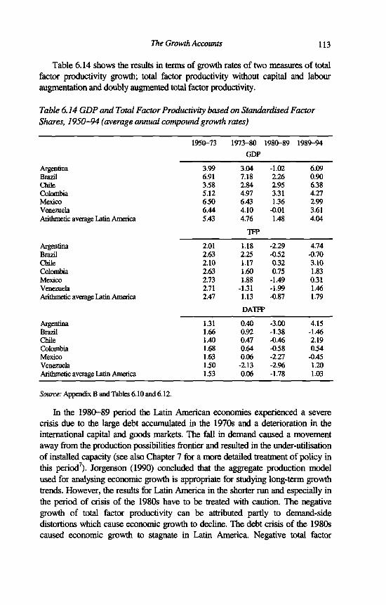
The Growth Accounts 113
Table 6.14 shows the results in terms of growth rates of two measures of total factor productivity growth; total factor productivity without capital and labour augmentation and doubly augmented total factor productivity.
Table 6.14 GDP and Total Factor Productivity based on Standardised Factor Shares, 1950-94 (average annual compound growth rates)
1950-73 1973-80GDP
1980-89 1989-94
Argentina 3.99 3.04 -1.02 6.09Brazil 6.91 7.18 2.26 0.90Chile 3.58 2.84 2.95 6.38Colombia 5.12 4.97 3.31 4.27Mexico 6.50 6.43 1.36 2.99Venezuela 6.44 4.10 -0.01 3.61Arithmetic average Latin America 5.43 4.76
TFP
1.48 4.04
Argentina 2.01 1.18 -2.29 4.74Brazil 2.63 2.25 -0.52 -0.70Chile 2.10 1.17 0.32 3.10Colombia 2.63 1.60 0.75 1.83Mexico 2.73 1.88 -1.49 0.31Venezuela 2.71 -1.31 -1.99 1.46Arithmetic average Latin America 2.47 1.13 -0.87
DATFP
1.79
Argentina 1.31 0.40 -3.00 4.15Brazil 1.66 0.92 -1.38 -1.46Chile 1.40 0.47 -0.46 2.19Colombia 1.68 0.64 -0.58 0.54Mexico 1.63 0.06 -2.27 -0.45Venezuela 1.50 -2.13 -2.96 1.20Arithmetic average Latin America 1.53 0.06 -1.78 1.03
Source: Appendix B and Tables 6.10 and 6.12.
In the 1980-89 period the Latin American economies experienced a severe crisis due to the large debt accumulated in the 1970s and a deterioration in the international capital and goods markets. The fall in demand caused a movement away from the production possibilities frontier and resulted in the under-utilisation of installed capacity (see also Chapter 7 for a more detailed treatment of policy in this period7). Jorgenson (1990) concluded that the aggregate production model used for analysing economic growth is appropriate for studying long-term growth trends. However, the results for Latin America in the shorter run and especially in the period of crisis of the 1980s have to be treated with caution. The negative growth of total factor productivity can be attributed partly to demand-side distortions which cause economic growth to decline. The debt crisis of the 1980s caused economic growth to stagnate in Latin America. Negative total factor

114 The Economic Development o f Latin America
productivity growth has to be attributed in part to this difference between potential and actual growth. In Table 6.14 this is reflected in the very low average GDP growth rate of 1.48 per cent for the 1980-89 period and in the negative total factor productivity.
When comparing the results of growth accounting exercises, one must be aware that the residual may differ, depending of the factors included in its calculation. Very often a total factor productivity without quality augmentation is what is presented in this kind of study. Figure 6.1 presents this estimate for the Latin American countries. Figures 6.2 and 6.3 include the quality effects of labour and capital respectively. Figure 6.4 presents doubly augmented total factor productivity growth including both capital and labour quality effects.
Figure 6.1, presenting total factor productivity growth without quality augmentation, shows that only two countries, Colombia and Chile, experienced continuous total factor productivity growth over the whole 1950-94 period. Argentina was consistendy the lowest ranking country over the whole period despite its rapid recuperation in 1989-94. Venezuela was the only country to experience a significant fall in the 1973-80 period. In 1980-89, Brazil, Mexico, Venezuela and Argentina all showed falling total factor productivity. All countries, with the exception of Brazil, witnessed positive total factor productivity growth in the 1989-94 period.
Figure 6.2, presenting labour-augmented total factor productivity growth, shows some interesting differences with respect to Table 6.1. Colombia scores higher than all other countries for the whole period. At the lower end, Argentina managed to leave Mexico and Venezuela behind in the 1989-94 period.
In Venezuela the fall in total factor productivity growth started in 1973. Also Mexico and Argentina had experienced negative labour-augmented total factor productivity growth, although to a lower degree than Venezuela, in 1973-80.
In Figure 6.3 quality improvement through embodiment of capital quality is taken into account. It is similar to the figures presented above. Mexico is the country with the lowest overall total factor productivity growth, if capital and labour augmentation are taken into account. In general, it is possible to conclude that only Colombia maintained a relatively stable total factor productivity growth over the whole period, while the other Latin American countries experienced major setbacks in one or more periods. Finally, Figure 6.4 presents doubly augmented total factor productivity growth in Latin America.
When analysing total factor productivity in a comparative perspective at least two striking results become clear.8 First, the similarity of total factor productivity growth rates between Asia and the advanced and Iberian countries, especially in the 1950-80 period. From 1980 onwards Asian total factor productivity growth rates are much higher than in Iberia and the advanced countries. Latin America’s total factor productivity growth rates are much lower than those of Asia or the other countries of our sample.
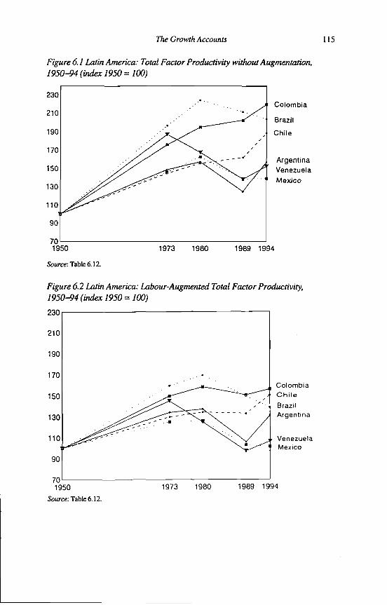
The Growth Accounts
Figure 6.1 Latin America: Total Factor Productivity without Augmentation, 1950-94 (index 1950 = 100)
Source: Table 6.12.
Figure 6.2 Latin America: Labour-Augmented Total Factor Productivity, 1950-94 (index 1950 = 100)
Source: Table 6.12.
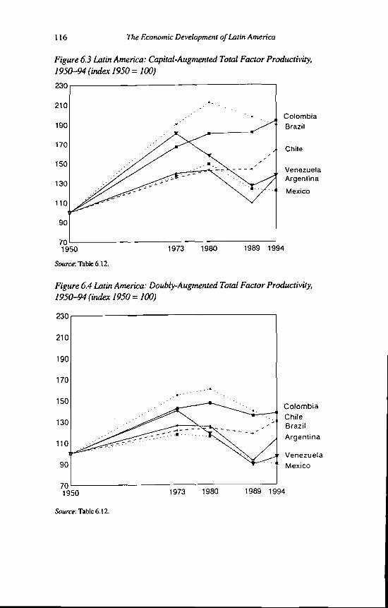
116 The Economic Development o f Latin America
Figure 6.3 Latin America: Capital-Augmented Total Factor Productivity, 1950-94 (index 1950 = 100)
Source: Table 6.12.
Figure 6.4 Latin America: Doubly-Augmented Total Factor Productivity, 1950-94 (index 1950 = 100)
Source: Table 6.12.

The Growth Accounts 117
The second striking result is, the relatively small differences in total factor productivity growth, measured as a percentage of GDP growth, between Latin America and the Asian group for the 1950-80 period, both as regards total factor productivity and doubly augmented total factor productivity. In very general terms, there is less than a 10 percentage point difference between the Latin American and Asian group (Asia being higher) along with a difference of equal magnitude, or somewhat higher, between Asia and the advanced countries.
Table 6.15 International Comparison: GDP and Total Factor Productivity, 1950-94 (average annual compound growth rates and % of GDP)
1950-73 1973-80 1980-89 1989-94
Arithmetic averages:
GDP
Latin America 5.4 4.8 1.5 4.0Asia 8.4 7.7 8.0 6.9Iberian countries 5.8 2.7 2.7 1.8Advanced countries 5.3 2.2
TFP
2.6 1.8
Latin America 2.5 1.1 -0.9 1.8Asia 4.4 1.6 3.9 3.4Iberian countries 4.1 1.1 1.3 0.8Advanced countries 3.5 1.0
DATFP1.3 1.1
Latin America 1.5 0.1 -1.8 1.0Asia 2.9 -0.1 2.5 2.0Iberian countries 2.9 0.0 -0.2 0.1Advanced countries 2.8 0.3 0.6 0.8
Explanatory Power of Total Factor Productivity (as % of GDP):
TFP
Latin America 46 23 -60 45Asia 52 21 48 50Iberian countries 71 41 48 44Advanced countries 66 45
DATFP
50 61
Latin America 28 2 -120 25Asia 35 -2 31 29Iberian countries 50 0 -7 6Advanced countries 53 14 23 41
Source: See note 7.

118 The Economic Development o f Latin America
Krugman (1994) generated a lively debate about the Asian growth performance by asserting that:
Asian growth seems to be driven by extraordinary growth in inputs like labour andcapital rather than by gains in efficiency, (p. 70)
He considered in particular Singapore, using the data of Young (1994), showing that total factor productivity was zero. However, my data show that although factor accumulation explains a great part of the growth performance in Asia (see Table 6.15), total factor productivity also played an important role.9
Latin America’s ‘lost decade’ of the 1980s caused the residual to become highly negative, indicating that total factor productivity growth was negative. This was not, however, the case in the Asian or the developed countries (although doubly augmented total factor productivity was also negative in some periods in those countries), since their total factor productivity remained positive, albeit with declining growth rates.
Figure 6.5 Doubly-Augmented Total Factor Productivity: An International Comparison, 1950-94 10 (index 1950 ~ 100)
Source: Table 6.13, Maddison (1995) and see note 7

The Growth Accounts 119
Figure 6.5 indicates clearly that Latin America’s performance has been worse than all the other regions of our sample. Total factor productivity grew at an annual 2.5 per cent between 1950-73, falling to 1 per cent from 1973-80, and then became sharply negative in the 1980s (some recovery occurred in the 1989-94 period). It shows a widening gap between Latin America and the other groups of countries for the whole period since 1950. Interestingly, Figure 6.5 shows that Latin America’s performance was nearest to that of the United States.
G RO W TH CAUSALITY IN LA TIN AM ERICA
In this and the following sections, some aspects of growth causality will be discussed. First I analyse some of the proximate causes of growth, and then look at ultimate causes of growth in the last section of this chapter. Through growth accounting it is possible to identify and quantify the proximate causes of growth but no light is shed on the ultimate causes of growth.
A major shortcoming of the growth accounts is that interactions among the sources are not taken into account. The proximate sources of growth are probably not as independent as is assumed in growth accounting. Abramovitz (1993) traced one line of dependence, namely the dependence of tangible and human capital accumulation on the pace and character of technological progress.
As Abramovitz (1993) stated:
Standard growth accounting is based on the notion that the several proximate sources of growth that it identifies operate independently of one another. The implication of this assumption is that the contributions attributable to each can be added up. And if the contributions of every substantial source other than technological progress has been estimated, whatever of growth is left over - that is, not accounted for by the sum of the measured sources - is the presumptive contribution of technological progress, (p. 220)
Maddison (1991a) stressed that:
The most difficult problem at the proximate level is analysing the role of technical progress, which interacts in myriad ways with other items in the growth accounts. Hence technical progress must be treated separately from other elements of proximate causality, because it is almost as difficult to quantify satisfactorily as are the elements of ultimate causality, (p. 11)
A new line of reasoning, with inverted causality from capital accumulation to technical progress, is emphasised in the new growth theories. In the last decade the general theme of interdependence has become imbedded in those new theories of economic growth.
In the past decades the literature on technology has increasingly moved away from the neo-classical framework, where knowledge is assumed to be completely exogenous and equally accessible to all firms as in the case of a public good.

120 The Economic Development o f Latin America
Recent models of technological change focus on the process in which the firm searches for new techniques in an environment characterised by incomplete information. Such models also point more clearly in the direction of ultimate causes, such as institutional and organisational factors, which determine the pace of technological change.
These factors bear much resemblance to what Abramovitz referred to as the social capability of a society to adopt, and adapt to, new technology. The search for such ultimate causes is one of the major challenges in the study of comparative productivity levels (Van Ark, 1993). In previous chapters I have analysed in detail two of the most important proximate sources of growth: human resources and physical capital. In this section I will return to them shortly to analyse some factors directly related to growth accounting.
Capital and Investment
One of the most important factors explaining Latin America’s economic performance is without doubt its investment and capital stock formation. In Chapter 5 standardised estimates of capital stock were generated and analysed, and in this section, I will concentrate on the importance of capital stocks in growth accounting and the role of investment in Latin America’s development process.
Growth accounting only becomes possible if reliable estimates of the flow of services from physical capital are available. Making an analogy with labour, one would like to know the amount of machine hours used in production during the period of reference. However, the lack of available data normally does not permit this procedure, so I used the general accepted proxy for this calculation, that is, the estimation of the capital stock based upon the ‘perpetual inventory model’ developed by Raymond Goldsmith (1951).11
The capital stock was disaggregated into machinery and equipment, structures and dwellings with service lives of 15, 40 and 50 years, respectively. The ‘perpetual inventory model’ provides an indication of productive capacity. It includes all capital assets, but some of these may be temporarily idle while others may have been withdrawn from production and held in reserve in case they may be needed to meet an unexpected rise in demand. Therefore, this model will not produce estimates of the ‘utilised’ stock.
The service lives used in this method refer to the total length of time from the initial installation of assets to the moment when they are finally scrapped. Clearly these lives may include periods when some assets are not being used to produce anything. In this study, capital stock estimates are basically used to explain Latin America’s performance in comparison with other regions in the 1950-94 period (see Table 6.16). Therefore capital has been used in the ‘ex-post’ sense, that is, in its observable role as a factor input in the production process. This notion should be distinguished from the one in which capital is used as an indicator of net worth

The Growth Accounts 121
which embodies potential economic services and has the capacity to generate future income. The present net worth of a capital asset, which is related to its future earning potential, progressively declines as it gets older, even though the annual real value of its services may remain unchanged over time.
To estimate capital-augmented total factor productivity one needs to augment the capital stock. The rates of vintage improvement chosen here are rather low, 1.5 per cent for machinery and equipment and a 0.5 per cent for structures. Following Maddison (1991a) no vintage improvement was used for dwellings. This capital embodiment effect is not a ‘catch-all’ effect of technical progress (as suggested initially by Solow), because a portion of technical progress is embodied in the labour force and consists of organisational and other improvements. This quality effect is the result of three forces; embodied technical progress, changes in the average age of the stock, and changes in its composition. If the average age of the capital stock goes down, this raises the embodiment effect as newer vintages will have more weight in the total capital stock.
Table 6.16 Explanatory Power of Capital in Growth, 1950-94 (by subperiods, in percentages)
Quantity of capital Quality of capital1950-73 1973-80 1980-94 1950-73 1973-80 1980-94
Argentina 30 45 40 4 8 11Brazil 37 43 68 2 3 4Chile 32 20 23 4 4 5Colombia 25 31 36 3 4 5Mexico 38 37 66 2 3 7Venezuela 31 59 48 2 5 11Arithmetic average Latin America 32 39 47 3 5 7
Source: Table 6.12.
The idea of embodying technical progress in the form of quality improvement in successive vintages of capital was first put forward by Robert Solow (1962). The basic argument is that physical investment is the prime vehicle by which technical progress is realised. The debate is about whether technical progress is due primarily to improvements in the design of new capital (‘embodiment’), or is mainly ‘disembodied’ and thus independent of the rate of capital formation (Hulten, 1992).
This point, also known as the Solow-Salter vintage argument (Maddison, 1972), leads to the inclusion in growth accounting exercises of an adjustment for differences in vintages of capital. Denison (1993) formulates it as follows:
It was argued that when advances in knowledge permit later vintages of capital goods to have higher marginal product than capital with the same production cost in earlier
122 The Economic Development o f Latin America
vintages, the quantity of capital should be counted as increasing proportionally, thus transferring part of the contribution of advances in knowledge to capital, (p. 48)
Denison (1993) suggests that ‘this procedure divorces cause from effect’. A strong argument is that it defies measurement, like a capital stock series that equates different vintages by their marginal product. Maddison (1991a) finds Solow’s basic point extraordinarily illuminating and inclusion of a modest element of technical progress in the analysis does help explain the nature of the growth process, and clarifies the impact of changes in the age of capital in a way that is not possible outside the vintage context.
It has been argued that existing differences in technology between advanced countries are increasingly related to differences in work practice and shop-floor organisation, these being typically features of disembodied rather than embodied technological change (Van Ark, 1993). However, in the case of the Latin American countries the difference between their capital stock and that of the technological leader is still very substantial and it seems reasonable to assume that technological advance in Latin America will take place, at least partially, through the embodiment of technology in the capital stock.
The age of capital is the basic argument for the inclusion of a vintage element and our analysis shows a secular trend of a falling average age of the capital stock for all countries (except Brazil). Direct measurement of the vintage effect is very difficult but the empirical information on age gives us a clue as to the importance of this effect. However, the age effect is only one factor in the embodiment effect. A recent article by Hulten (1992) shows that the failure to adjust capital explicitly for quality changes diverts the quality effects into the conventional total-factor- productivity residual. Hulten found that approximately 20 per cent of the residual growth of quality-adjusted output could be attributed to embodied technical change. This estimate is based on the American economy, using data obtained from the US Bureau of Labor Statistics (1983) and Gordon (1990).
Employment
Table 6.17 provides an indication of the importance of labour inputs in the economic performance of Latin America. On average for the 1950-94 period the quantity of labour ‘explains’ a quarter of economic growth, while quality of labour explains an additional 15 per cent. The quality effect of labour has been estimated with respect to the segment of the population aged 15-64, but in Chapter 4 an additional exercise was carried out comparing the results for the population with some available estimates concerning the work force.
Table 4.11 provided a comparison between the educational level of the population and the labour force for some countries over the 1951-92 period. On average the labour force had a somewhat higher level of education (2.5 per cent).

The Growth Accounts 123
The difference was small in primary education (0.8 per cent) but substantial in higher education (23.6 per cent). On the basis of the somewhat scanty evidence of Table 4.11, there is no discernible trend towards change in the differences of level in time. This fact, together with the lack of systematic information on the educational level of the labour force, obliged us to adopt the educational level of the population as the measure for quality improvement. In terms of my model for explaining economic growth, this approach probably does not introduce a large error. In level accounting exercises this factor obviously assumes greater importance (see Van Ark, 1993 and Pilat, 1994).
Table 6.17 Explanatory Power of Labour in Growth, 1950-94 (percentage of GDP growth)
Quantity of labour Quality of labour1950-73 1973-80 1980-94 1950-73 1973-80 1980-9
Argentina 20 16 48 13 17 35Brazil 25 25 65 12 15 43Chile 9 39 45 15 21 15Colombia 24 37 33 16 15 31Mexico 21 34 78 15 25 33Venezuela 27 73 113 17 15 45Arithmetic average Latin America 21 37 64 15 18 34
Source: Table 6.12.
Some Remarks on Ultimate Causes
The breakdown of economic growth gives an indication regarding the costs of increasing the growth rate of output. However, growth accounting can only explain part of the process of economic growth, it does not take into consideration other factors such as economic policy, the national and international environments and non-economic factors such as natural disasters and war. These belong to the realm of what is now generally termed the ultimate causes of growth, in contrast to the proximate causes of growth analysed earlier.
The study of ultimate causality involves giving consideration to institutions, ideologies, pressures of socioeconomic interest groups, historical accidents, and economic policy at the national level (Maddison, 1995). The ultimate sources of Latin American economic performance are less clearly identified than its proximate causes. In Chapter 2,1 have analysed some of the topics included in the realm of ultimate sources; institutional set-up, social capabilities and path dependency.
In the next chapter, economic policy, probably the single most important ultimate cause in Latin America’s economic performance, will be analysed in some detail for the post-war period, with some consideration also of the international

124 The Economic Development o f Latin America
economic context. The growth accounting results presented here fit in rather well with the nature of the policy problems experienced, for example, in the 1970s and 1980s. In Chapter 2 some possible historical causes of political and policy instability in Latin America were discussed.
Some of the ultimate sources of economic growth in Latin America have recently been discussed in the context of the concept of path dependency. Path dependency has been defined as the incapacity of a society to leave a certain development path due to some specific factor. Factors identified include the institutional set-up, historical events, social capability and technological congruence.
Finally, it is again important to stress the interdependency of growth factors, either in the proximate or the ultimate sphere, or in combination. As Abramovitz (1993) emphasised, the growth accounting framework, even in its extended version, is not able to specify the interrelationship that exists between the different factors.
NOTES
1. Among the first authors were Bruton (1967), Correa (1970) and Langoni (1974). More recently Cavallo and Mundlak (1982), De Gregorio (1991), Coeymans (1992) and Elias (1992) have worked on growth accounting in Latin America.
2. The country-specific factor shares were estimated by the author on the basis of national accounts and population censuses, especially adjusting for own account workers.
3. See Chapter 4 for a more elaborate treatment, with respect to data sources and estimation procedures, of human capital.
4. See Maddison (1972 and 1987), Denison (1967) and Psacharopoulos (1984) for the rationale of the education adjustment.
5. See Table 4.11 of Chapter 4 for a comparison of the educational level of the total population with that of the labour force.
6. See the section on capital and investment (pp. 120-122) for a discussion of the quality aspect in capital stock estimation and the actual vintages used in the calculation.
7. One of the authors who treated this theme is Ffrench-Davis, see for example Fffench-Davis (1994).
8. The growth accounting exercise presented here for the six Larin American countries was also done for the whole sample group of 16 countries. This thesis is about Latin American economic development so I do not present the whole data base for all countries but these are available upon request by the author. Most of the data with respect to GDP and employment come from Maddison (1995) and were updated by me using the same sources. If necessary I used national sources or data bases of international organisations such as OECD, IMF, World Bank or United Nations. The capital stock estimates necessary for this exercise come from Maddison (1993) for the advanced countries, and were updated to 1994 by me, using the same methodology as in the case of the Larin American countries. I prepared specific estimates, again using the same methodology, for the Asian and Iberian countries.
9. The results of Young (1995), which is an updated version of Young (1994), presenting slightly higher total factor productivity growth estimates, coincide to a great extent with the results of this study. His estimates of total factor productivity growth for Korea and Taiwan for the

The Growth Accounts 125
1960-90 period are 1.7 and 2.6 per cent respectively. My estimates for the 1950-94 period are 1.7 and 3.0 per cent, respectively.
10. Hie advanced countries group includes the USA, although this country is also presented separately.
11. See Chapter 5 for a more detailed treatment of capital stock estimation and its limitations.


7. Performance and Policy in Latin America
INTRODU CTIO N
Performance and policy are related and Latin America is a region where policy regimes have changed dramatically in the twentieth century. This chapter concentrates on the second half of the century and relates the results obtained in the productivity analysis of the previous chapters to the policy regimes adopted.
Chapter 3 analysed in some detail the events of the first half of the century, namely the breakdown of the liberal world order and Latin America’s policy reaction. Of particular relevance was the period of recovery after the Great Depression and the subsequent world war in which Latin America adopted a more inward-looking policy regime of industrialisation through import substitution, though this was to a certain extent forced on it by the circumstances. The strong recovery process, both in terms of GDP growth and, especially, in labour productivity, had repercussions on the policy regime adopted in the second half of the twentieth century. The policy of industrialisation through import substitution remained in place long after World War II, and in some countries even until the debt crisis of the early 1980s. Since then almost all Latin American countries have drastically altered their development strategy, placing greater emphasis on neoliberal policies and export-oriented policies.
During the twentieth century, Latin America faced two major economic crises: the Great Depression of the 1930s and the ‘lost decade’ of the 1980s. Through analysis of just a few economic indicators, total GDP, GDP per capita and labour productivity, it becomes clear that the crisis of the 1980s, which continued partly in the 1990s, was more profound for Latin America than the Great Depression. On the other hand, our international comparison shows that Latin America’s relative performance in the 1930s was much more favourable than that of the other countries in the sample. This was in marked contrast to the current situation which has obliged Latin America to adopt a more outward orientation.
A comparison of trends in levels of GDP per capita in Latin America, as compared to the United States, shows striking results. Its relative position vis-à-vis the United States improved during the 1929-38 period. The results were quite different in 1980-94, when Latin America’s performance was disastrous compared to the United States and the rest of the world. The results with respect to the development of labour productivity in Latin America also speak for themselves:
127
128 The Economic Development o f Latin America
whereas labour productivity rose by 0.9 per cent per annum from 1929-38, it fell by an average 0.6 per cent per annum between 1980-89.
The situation facing Latin America today is totally different from the one it faced in the 1930s, when inward orientation yielded results in terms of growth performance. The post-war experience and especially the crisis of the 1980s demonstrates that Latin America now stands at the crossroads, and that the process of modernising its productive system, its institutions and policies can no longer be delayed (see also ECLAC, 1990c).
TH E PO ST-W A R GOLDEN AG E (1950-73)
For the world economy, 1950-73 was a period of unparalleled prosperity with the OECD countries in our sample growing at 5.3 per cent, almost three times the rate of the period 1913-50. The Iberian countries grew by 5.8 per cent, compared with a mere 1.4 per cent between 1913-50, while the Asian countries grew by 7.7 per cent, 3.5 times faster than in the period 1913-50. The Latin American countries grew by 5.4 per cent, compared with about 3.8 per cent during 1913-50. In 1950, per capita real income in Latin America countries was three times higher than that of developing Asia, a bit higher than the Iberian countries and about half of that of the six advanced countries. Within Latin America, real income per capita ranged from around 35 per cent of the US level in Argentina, Chile and Venezuela, to 27 per cent in Mexico and 19 and 15 per cent respectively for Colombia and Brazil.
In 1950, the international economy embarked on an expansion that was to continue unabated until 1973, when the first oil crisis erupted. Moreover, the growth in world output was the highest ever recorded. Latin America also achieved an expansion during this quarter century that probably outstripped regional growth in any previous 25 year period. Furthermore, the rate of growth in regional output between 1950 and 1973 exceeded both the rate of growth in world gross domestic product and the rate of output growth of the United States. However, there was a fundamental contrast between the growth performance of Latin America and that of much of the rest of the world.
In effect, while the expansion of world commerce, and especially of advanced countries’ trade, was appreciably more intense than the growth in world output, the growth of Latin America’s exports was significantly less than the growth of its gross domestic product and, during the final third of this period, considerably less than one half the rate of increase of its imports. And whereas the unprecedented expansion of the advanced countries was achieved with an exceptional degree of price stability, in Latin America the acceleration of growth was accompanied, in a good number of countries, by sustained price instability.
While mildly expansionary monetary and fiscal policies, in combination with large devaluations, promoted the strong recovery of Latin American economies
Performance and Policy in Latin America 129
from the Great Depression, expansionary monetary and fiscal policies continued to be pursued or even intensified over the course of the 1950s and 1960s, that is, long after output had returned to, or approached, its potential. Moreover, in a number of countries money supply growth far exceeded the potential rate of growth of output.
The evolution of the Latin American economies thus continued to diverge considerably from that of other developing economies; but in this historical instance the departure entailed the progressive build-up of macroeconomic disequilibria (Bianchi and Nohara, 1988). Income growth resulting from the expansion of primary exports led to a rise in demand for manufactured consumer goods and their inputs in Latin America. This demand had increasingly been satisfied by domestic production that enjoyed the ‘natural protection’ provided by transportation costs, complemented in some cases by tariff protection prior to World War H. The foreign exchange scarcity created by the fall in primary exports during the Great Depression and limited access to foreign goods during World War II subsequently boosted import substitution. Only after the war, however, did import substitution become a doctrine, guiding policy making in much of Latin America.
Although there was some variation across the range of countries, the policies pursued by the respective governments to promote industrialisation in the early post-war era were broadly similar. Under these policies, the production of import substitutes was encouraged through the exclusion of foreign competition, the allocation of foreign exchange, bank credit, essential inputs at preferential rates, and exemption from, or remission of, certain taxes and duties. At the same time the production of traditional exports was discouraged by unfavourable exchange rates, export taxes and pricing policies (Lin, 1988).
Although average nominal protection gradually increased in the course of the 1950s, the average tariff was still rather low in a number of Latin American countries in 1950. However, between the mid-1950s and the mid-1960s tariffs soared to reach extremely high protective levels. It becomes clear that the rates of effective protection came rather close to those of nominal protection. As a rule, effective protection rates were lowest, or even negative, for commodities, including importables as well as traditional exports, and highest for manufactured consumer importables.
Argentina
The government of Juan Perbn (1943-55) established a populist tradition which was based on favouring import substitution industrialisation, high manufacturing wages, price controls, a squeeze on the agricultural sector, and antagonism towards the export orientation of the old landowning oligarchy, increases in public-sector employment, hostility to foreign capital and nationalisation of foreign assets. Diaz- Alejandro (1970) concluded that Argentina’s economic history, especially since

130 The Economic Development o f Latin America
1943, is a dramatic example of the clangers arising in the development process when a balance between the production of exportables, importables, and home goods is neglected. The paradox of post-war Argentine experience is that, if there had been less discrimination against exports, manufacturing expansion would have been greater.
Brazil
In the post-war period, Brazil continued the policy of industrialisation which had begun before World War Ü, and which was given an extra boost during the war, as was the case in many other Latin American countries. President Vargas who returned to power in 1951, on this occasion through elections, initiated a growth- oriented strategy. In response to greater international competition after the war, Brazil reintroduced exchange controls, imposed a system of multiple exchange rates and increased tariff protection, particularly favouring the domestic production of consumer goods. With the military threatening to take power, Vargas committed suicide in 1954.
Again, in 1956-61, this time under Juscelino Kubitschek, there was a new surge of industrialisation. Massive state investment occurred in electric power and transport, and in the capital and intermediate goods industries. The private sector was given high protection in the consumer goods industries, but low or negative effective protection in capital goods (which was partly compensated by direct government subsidies). Multiple exchange rates were also used. Liberal policies towards foreign capital were adopted, and in response direct foreign investment in manufacturing rose very rapidly. In 1969, the most recent surge of industrial expansion began. This period, which effectively ended in 1976, was marked by rapid growth and in fact is known as the ‘Brazilian miracle’ (Griffin, 1989).
Chile
In the 1950s, Chile continued the industrialisation through the import substitution strategy already started a decade before, in the wake of the Great Depression and the collapse of the nitrate market, after the replacement of natural nitrate by a synthetic substitute. However, this development model began to encounter problems, such as a stagnated agriculture, and the emphasis on import substitution hindered the development of new exports, severely restricting external trade options and the management of the balance of payments. The instability of traditional export prices was transmitted to the domestic economy through recurrent balance-of-payments shocks (Ffrench-Davis and Muñoz, 1992). The increasing price instability drove policy makers to the conclusion that new economic strategies were needed. A first attempt was based on the recommendations of the Klein-Saks mission which marked the return to more
Performance and Policy in Latin America 131
orthodox short-term economic policies, with maximum priority accorded to price stabilisation and proposals for a gradual liberalisation of the Chilean economy. However, as inflation was stopped it triggered the worst short-term recession since the Great Depression and provoked a public outcry (Mamalakis, 1976).
During the presidency of Alessandri (1958-64), the reform of the economic system was tackled in a more comprehensive fashion. The private sector was seen as the engine of growth and was supported by an active fiscal policy in the Keynesian tradition but the government also took an active role as entrepreneur through the creation of new public enterprises. This required a broader scope for the market, prices and competition, especially from external sources. However, great importance was given to stabilisation in the short run based on: a fixed nominal exchange rate, the elimination of ‘inflationary’ Central Bank financing of the fiscal deficit, wage and salaries increases in line with productivity increases and the promotion of domestic and foreign investment (Ffrench-Davis, 1973). This programme enjoyed considerable though temporary success, especially in the reduction of inflation1 but around the half-way mark of Alessandri’s presidency a balance of payments crisis occurred, caused by the rapid increase in imports, especially of consumer goods, while exports grew at a slower pace, which obliged the government to devalue, close the economy and reintroduce exchange controls while the inflation surfaced.
The strategy of the Frei administration was based upon a three point programme: First, a gradual stabilisation programme; second, an industrial modernisation programme, and third, a programme of structural and social change including agrarian reform and the first steps towards the nationalisation of the copper mines. The role of the state in production was reinforced, and protection increased to promote domestic production of electronic and other durable consumer goods. However, it became clear that the system’s low capacity to convert internal and external resources into physical, human, and institutional capital remained the main bottleneck to growth and economic independence. Another crucial element was that during Frei’s government the antagonism felt between the country’s principal social and political actors became more and more evident.
The Allende administration attempted to achieve within three years what Chile’s previous presidents had failed to achieve in almost a hundred years: maximum growth and economic independence through a revolutionary but bloodless redistribution of income. The policy of nationalising foreign mining interests, takeover of private banks, industry and transnational firms caused a great redistribution of income and power. Public sector salaries and wages were raised and the expansion of demand quickly affected sales and production, which rose sharply in 1971. But the expansionary fiscal and monetary policies, combined with sluggishness of production due to labour disputes, accelerated inflation. During 1973 output started to fall, inflation continued to rise, the external sector deficit

132 The Economic Development o f Latin America
reduced external reserves, black markets transactions increased, all of these developments together with domestic economic opposition and the foreign economic embargo caused the economy to enter into a state of near chaos (Dombusch and Edwards, 1990).
Colombia
Monetary policy was expansionary during the 1950-73 period, with a little less than 20 per cent average annual growth in money supply. Throughout this period also the size of the state did not expand appreciably. During the 1950s and through the mid 1960s, the peso was chronically overvalued from the viewpoint of competitiveness of non-coffee exports, effectively constraining export diversification. The country’s success in increasing exports during the 1967-75 period was based on an outward-looking policy that was in part the result of significant domestic inducements to export promotion. The most important element of the new policies was the introduction of a crawling peg-exchange rate system and a package of export incentives, including fiscal incentives, concessionary credits for export-related activities from the Export Promotion Fund and an expanded and more effective import-export regime (Plan Vallejo). The new policies represented an attempt to compensate for the distortions in relative prices generated by the import-substitution effort. Together with the favourable development of world trade, this shift in policy emphasis brought about impressive results (Thomas, 1985).
Mexico
The period from the beginnings of the 1950s until the 1970s is often referred to as the period of stabilising development because it was one of steady GDP growth, while at the same time the price level stayed relatively stable (Hofman, 1982). However, beneath the surface a number of problems were brewing: (a) levels of unemployment and underemployment2 were high and rising; (b) the balance of payments was steadily worsening; (c) there were major sectoral disequilibria; (d) inadequate and deteriorating fiscal revenues.
Venezuela
Venezuela experienced rather high total GDP growth coupled with price stability during the period under consideration. Until 1958 the economy grew fast as a result of an expansive public expenditures policy based upon the revenues of oil exports, Venezuela’s major export product. In 1958, when oil prices fell some 25 per cent, influenced by the reopening of the Suez canal, the development of new

Performance and Policy in Latin America 133
oil fields in the Middle East and a world recession, the administration opted for development on the basis of import substitution.
STRUCTURAL PROBLEM S STILL CONCEALED (1973-80)
For the world economy, 1973-80 saw the departure from the uniform tendency of very high growth experienced during the previous period. The OECD countries as a whole experienced a sharp slowdown, GDP per capita growth rates being less than a half as in the previous period. However Latin America and Asian developing countries continued growing. The period 1973-80 showed a uniform tendency in all Latin American countries to falling population growth. All our sample countries are now in a more advanced stage of demographic transition, in which the fertility rates also start falling. During this period Latin America’s GDP per capita continued to grow rather fast compared to the United States and its comparative level reached 34 per cent in 1980, the highest level of the entire twentieth century. However, when this is compared with other areas, Latin America’s performance is not as good as first appears. Asian developing countries more than doubled their income level, while the other OECD countries also markedly improved their position relative to the United States.
In Latin America the drastic changes which occurred in the world economic system at the beginning of the 1970s, such as the demise of the Bretton Woods fixed exchange rate mechanism (1971) and the action of the OPEC price cartel, did not have the same effect on policy making as in the developed countries, where a sharp change in economic policy occurred. The new disturbance was simply a new variation on a familiar theme, and was not regarded as a razor’s edge situation, calling for drastic policy change (Maddison, 1989).
Many Latin American countries delayed pursuing stabilisation policies while relying on expanded external borrowing to sustain a higher rate of domestic demand. These policies provided for stronger growth of the economy in 1974-75, but they also resulted in the persistence of inflationary trends and the continuation of large current account deficits. For Latin American countries whose exports were dominated by primary commodities, the upsurge of inflationary pressures in the world economy did not constitute a serious problem as long as their export prices rose. In fact, the market prices of non-oil primary commodities continued to surge in 1974, in line with the jump in oil prices, thus enabling many Latin American countries to realise large gains in export receipts.
Moreover, to business enterprises in many of these countries, having domestic finances that had been constricted by the persistence of inflation, the increased availability of external credit after the first oil shock appeared as a blessing. The real interest costs of these credits was negative or relatively low. This explains why, after the first oil shock, many governments in Latin America condoned or
134 The Economic Development o f Latin America
encouraged the expanded use of external credit in order to sustain a high rate of investment and imports. It also explains why, in countries such as Brazil and Mexico, the growth of real wages and real private consumption was not restrained, thus contributing to the persistence of inflationary pressures and balance of payments difficulties (Lin, 1988).
In the 1960s and especially in the early 1970s several countries implemented trade policies combining import protection with export promotion. However, the intensity of policy reform fluctuated over time because of the lack of social consensus. In many countries of Latin America, the rural landed class and organised urban labour had considerable, but opposing, political influence, with the import substituting industrialists occupying a middle ground. Policy conflicts often occurred between these groups, resulting in frequent shifts of political alliances and economic policies (Lin, 1988).
The combination of biased macroeconomic policies and compensatory sectoral subsidies with unlimited access to international capital markets led to economic growth in the 1973-80 period. Eventually it created pervasive imbalances, including stagnation of exports, overproduction of non-traded goods and services, uncommonly large resource gaps, unparalleled excess external debt and rampant domestic price instability (Bianchi and Nohara, 1988). During this period several countries experimented with neo-conservative economic policies, that is, the marriage of monetarist views concerning economic stabilisation and radical conservative approaches. Both ingredients were present in varying degrees in the economic plans of Chile after 1973 and Argentina after 1976, both put into practice by strong military governments (Foxley, 1983).
Argentina
Argentina’s GDP growth was among the slowest of the countries in our sample. During the first years of the period under consideration, Juan Perón tried to repeat the policies of his previous administration, with an expansionary monetary and fiscal policy, and wage increases combined with price control. His successor, Isabel Perón, first made a stabilisation effort to deal with the huge budget deficit, but under pressure from union interests, large wage increases were granted. In early 1976, in the midst of a severe economic social and political crisis, the armed forces once again took power in Argentina. The economic objectives of the new government were to correct the basic macroeconomic disequilibria and to change the course of the inward-oriented development strategy, which had been followed since the Great Depression (Ramos, 1986).
This neo-conservative experiment started with a substantial devaluation, reduction in real wages and the government deficit, deregulation of prices and abolition of subsidies, followed by a tight monetary policy, gradual tariff reduction and liberalisation of exchange controls. There was a notable improvement in the

Performance and Policy in Latin America 135
balance-of-payments situation, but inflation slowed down only partially. A second period was characterised by the ready availability of foreign capital and the extensive use of such capital to reduce inflation. The exchange rate was used principally to control inflation, and tariffs were lowered. What progress there was in this phase was at the expense of an increasingly artificial exchange rate. The neo-conservative policies took four years to bring down the average annual rate of inflation from 443 to 101 per cent, but also depressed economic activity, caused widespread bankruptcies, led to a large trade deficit in 1980 and permitted large- scale capital flight by Argentineans who correctly foresaw that they would unlikely be able to continue buying US dollars so cheaply (Maddison, 1985).
Brazil
Brazil relaxed its export promotion drive and shifted its trade policies in favour of a renewed inward orientation. This took the form of increased import control, widespread tariff increases, and the establishment of a prohibitive prior deposit system. The country also became dependent on external borrowing when its terms of trade worsened drastically. However, Brazil’s creditworthiness was very high because of the creditors’ continued belief in its development potential and also, of course, because of the great liquidity in the international capital markets due to the first oil shock.
The Brazilian approach to policy in 1973-80 was rather eclectic and growth oriented. It avoided the deflationary shocks imposed by extreme neo-conservatism in Chile and Argentina, its expansionism was never as wild as that of the Lopez Portillo administration in Mexico, and the policy course was very much steadier than in Argentina. The political regime was a stable military autocracy which was somewhat liberalised in the 1980s. The government intervened actively to control economic activity with very high levels of public investment, effective control of wage rates, exchange controls, and various devices to manipulate exports and imports. It also followed a rather consistent crawling peg policy for most of the period, without episodes of extreme overvaluation. Brazil is also notable in Latin America for its export diversification into manufactures and a wide variety of new primary products like soybeans and iron ore.
Chile
Two overriding concerns marked the economic policy of the Chilean junta upon its assumption of power at the end of 1973: (1) the unavoidable need to restore basic macroeconomic equilibria, and (2) the intention to instil dynamism in an economy whose performance in recent decades was considered quite unsatisfactory. The main objective of the first period (1973-76) was to restore market mechanisms in an economy with extended controls and severe imbalances. The initial policy mix

136 The Economic Development o f Latin America
sought to: (a) free virtually all prices; (b) devalue the exchange rate sharply with the purpose of narrowing the deficit in the balance of payments; (c) control wages by demobilising labour unions and by changing the wage adjustment system (from looking backward to looking forward); (d) follow a restrictive monetary policy to reduce the fiscal deficit. During the second period of the Chilean neo-conservative experiment, the price stabilisation strategy was modified as inflation was still advancing at 250 per cent per year. Emphasis was not placed on monetary and wage restrictions, but rather on controlling expectations and exerting downward pressure on domestic prices via foreign competition and real exchange appreciation.
Foxley (1983) summarises the economic results for Chile in the 1973-80 period as follows: the rate of inflation decreased; after a deep recession GDP reached pre-recession levels; the fiscal deficit was eliminated; there was an accumulation of reserves, and nontraditional exports expanded rapidly. At the same time, a low investment rate, a significant deficit in the trade balance, increasing external indebtedness, high unemployment, real wage reduction, and a deterioration in the distribution of income, consumption, and basic social services were among the negative factors.
Colombia
Activism in export promotion in Colombia diminished significantly after the mid- 1970s, partly on account of the increase in foreign-exchange earnings that accompanied the commodity price boom of 1976-79. Rapid increases in external demand for Colombian agriculture products were the most significant development of this period, with the demands for coffee and illegal drugs leading other exports (Thomas, 1985). These revenues were used to reduce the debt and to build up reserves (World Bank, 1991).
Mexico
Mexico had an excellent growth record during 1973-80, the best of the Latin American countries in our sample. This can be attributed partly to the stability of the political system and to a greater socioeconomic consensus than in the rest of Latin America about appropriate policies to follow. It also can be explained by the booming government revenues from oil exports after the first oil shock and heavy foreign borrowing to finance expanded public consumption and investment, and subsidies on basic private consumer items. In Mexico, import controls were tightened and tariffs increased while the exchange rate became increasingly overvalued.

Performance and Policy in Latin America 137
Venezuela
The oil crisis, together with the increase in public expenditures and private consumption, caused a rapid rise in GDP and imports. Inflation was on the rise but for Latin American standards was still very low. In the latter part of the 1970s the expansionary monetary and fiscal policies caused bottlenecks in domestic production and caused GDP growth to fall and inflation to rise. Severe balance-of- payments problems and a rapid increase in the foreign debt were also features of the economy.
TH E LO ST DECA D E (1980-89) AND TH E FIRST SIGNS O F RECO V ERY (1989-94)
The period since 1980 has witnessed a broad range of economic performance and policy shifts. It also showed a diverging economic performance between Latin America and the rest of the world. The years since 1980 can be divided into the crisis period (1980-89) for Latin America and the subsequent period of recovery. As can be seen in Table 3.2 most Latin American countries experienced this recovery as Argentina and Chile grew almost 5 per cent per capita, Colombia 2.5 per cent and Mexico and Venezuela over 1 per cent. The most notable exception, however, was Brazil which had negative growth per capita of about 1 per cent a year.
During 1980-89 the world economy recovered to some degree from the slow growth of the previous period, with the exception of Latin America. Total GDP of the OECD countries grew on average 2.5 per cent a year compared to around 2 per cent in 1973-80. The Asian developing countries continued to grow at the same or somewhat higher growth rates. Latin American growth performance was abysmal, as per capita income fell by 0.5 per cent a year.
In 1989 GDP per capita in Latin America had fallen, on average, to the lowest relative levels of the twentieth century, from a level of 32 per cent of the United States in 1980 to 24 per cent in 1989. Argentina experienced the biggest decline from being a rather prosperous country in 1900 (ranking sixth among our 16 countries) to being one of the poorest in Latin America in 1989 (ranking fifteenth).
Between 1980 and 1989 Latin America experienced its deepest and most prolonged economic crisis since the ill-fated years of the Great Depression. Indeed, so much ground was lost that from the standpoint of economic welfare, the 1980s turned out to be truly a lost decade. On average GDP per capita fell from 4392 to 3727 constant 1980 international dollars with heavy per capita income losses in Argentina, Venezuela and, to a lesser degree, Mexico, virtual stability in Brazil and (recently) some improvement in Chile and Colombia.
138 The Economic Development o f Latin America
Another disturbing characteristic of the crisis was the generalised and simultaneous deterioration of virtually all main economic indicators. Many countries have not only experienced a decline in the level or in the rate of growth of total output but also a deterioration in the employment situation and decreases in real wages. Inflationary processes intensified enormously and became more widespread.
The period 1989-94 can be looked at in different ways. From the growth perspective it was disastrous. But it was also a period in which Latin America prepared itself for a change in development strategy. The growth figures for the 1989-94 period of Tables 3.1 and 3.2 show that although a great effort is still needed, important progress was made in Latin America in the last decade.
Argentina
Argentina is one of a number of countries which went through a major crisis and several failures of orthodox and heterodox stabilisation programmes during the 1980s until finally at the beginning of the 1990s the programme introduced by Domingo Cavallo under the presidency of Carlos Menem led to the stabilisation of the Argentine economy. After negative growth of 2.5 per cent per capita in 1980-94 the Argentine economy has grown rapidly since then, recording about 4.8 per cent per capita growth for the 1989-94 period.
The Menem government introduced a fiscal reform in 1990 which included centralisation of expenditure-related decisions. It put public enterprises under the direct authority of the minister of economic affairs in order to exercise tighter control over their financial management. The reform also included improved tax administration and tax simplification.
One of the most important and controversial elements of the stabilisation plan was the anchoring of the exchange rate. Under the ‘Convertibility Law’, the Central Bank is obliged to meet any demand for US dollars at the rate of 10.000 australes to the dollar, that is, the exchange rate could not rise above this level unless Congress passed another bill allowing it to do so. The second provision required that the Central Bank’s monetary liabilities must at all times be less than the external assets making up its reserves; the purpose of this provision was to ensure that the currency would have backing and to limit money creation via domestic credit. These measures meant establishing a fixed exchange-rate system under which fluctuations in the primary money supply would be closely linked to the balance of payments.
Significant steps have been taken in the field of trade liberalisation as exports taxes were eliminated and overall tariffs were reduced to 0-20 per cent range. The government also initiated an ambitious process of privatisations and many public enterprises have been sold. Argentina entered the ‘Mercado Común del Sur’ (MERCOSUR) together with Brazil, Paraguay and Uruguay, in order to promote

Performance and Policy in Latin America 139
intra-regional trade and establish a common external tariff between the members and the rest of the world. Trade between these countries has risen considerably recently.
Argentina was strongly affected by the ‘tequila effect’ of the Mexican crisis. After four years of growth, unparalleled in recent history, the economy fell into a recession in 1995, with open unemployment reaching record levels of close to 20 per cent. The country experienced a deficit in the capital account after receiving annually 10 billion US dollars in previous years. Argentina’s banking sector, at great risk after the Mexico crisis and the resulting removal of around 8 billion US dollars, experienced great liquidity problems and embarked on a major restructuring process reducing significantly the number of banks and financial institutions operating in the country. However, there are some signs of improvement in the major economic indicators and the Menem government has also reached an agreement with the United Kingdom about oil exploitation of the disputed ‘Islas Malvinas’ or Falkland Islands. At the beginning of 1996 the bulk of the capital that left the country after 20 December 1994 has returned; however, the economy is growing at much lower rates than before the crisis. The country’s annual inflation rate has fallen to less than 2 per cent, the lowest it has been in the last 50 years.
Brazil
Brazil experienced a major growth crisis at the beginning of the 1980s, but during the middle of the decade growth rates went up again and the pressure for structural reform became less acute. However, Brazilian growth performance at the end of the 1980s and in the 1990s has been very bad. Inflation, which did not subside after the first oil shock, accelerated sharply in 1979 when wage adjustments were changed from once to twice a year, at a time when the economy was subjected to renewed import costs and balanee-of-payments pressures (Dombusch and Simonsen, 1987). In Brazil, no major fiscal reform has taken place although in the field of trade liberalisation some measures have been taken, such as tariff reduction. Nonetheless, the Brazilian economy has not been, until now, opened up to the world. The privatisation process was set into motion and some enterprises have been sold, but recently privatisations have slowed down.
The Brazilian government’s latest attempt at stabilisation (the eighth in nearly a decade) - the Real Plan - has also been the most successful, having reduced inflation from a monthly 50 per cent in June 1994 to about 22 per cent for the whole of 1995, the lowest rate in the last two decades. Nonetheless, some difficulties have arisen which could hamper efforts to consolidate this process, such as emerging inflationary pressures, a significant increase in demand, the risk of a return to indexation, a somewhat overvalued exchange rate and problems in controlling liquidity. Unlike previous stabilisation plans, the Real Plan was notable

140 The Economic Development o f Latin America
for its transparency with regard to the measures contemplated and the timetable for their implementation: price freezes, intervention in labour contracts and all other types of drastic or unexpected action were explicidy ruled out. The plan was carried out in three stages, which were announced and described ahead of time in December 1993. The first stage involved fiscal adjustment to balance the budget in 1994, for which purpose mandatory allocations of taxes and social security contributions were reduced in order to provide greater flexibility in the use of fiscal resources.
The second stage, launched in March 1994, sought to coordinate the economy’s prices. To that end, a basic indexing instrument was created, the unit of real value (URV), whose level was adjusted daily. In order to avoid the traumatic situations caused by previous plans the authorities eschewed the use of punitive measures opting instead, and only in the case of highly sensitive items in the family budget, for negotiation and persuasion.
The third stage of the plan was initiated in July 1994, with the introduction of a new currency, the real, the sixth since 1986. A new monetary regime was established; the old currency still in circulation was replaced at the rate of one real for one URV, or 2,750 cruzeiros reales, the value as of 30 June 1994. Furthermore, the plan specified mechanisms for the issuance of the new currency, under which the Central Bank would be required to maintain international reserves in an amount equivalent to the value of reales in circulation, at the selling rate of one real per dollar. The plan also placed quarterly limits on the monetary base.
Since the plan does not call for strict convertibility, the Central Bank will not make any commitment to purchase foreign exchange. In addition, the plan limits public-sector financing. With regard to monetary policy, the Central Bank has replaced the automatic buy-back of public securities with standard rediscount operations.
Under the Real stabilisation programme, the Brazilian economy started growing again after the economic and political instability of the late 1980s and early 1990s. The government of President Cardoso is embarked on an ambitious plan of restructuring the Brazilian economy, including major privatisations and reorganisation of the central and local state apparatus, the judiciary and the financial system. However, the maintenance of the stabilisation programme is the priority, and due to a worsening of the trade balance the government opted for an increase in tariffs on motor vehicles and electronic goods, and maintained a tight monetary policy with high interest rates and an increasing budget deficit. Capital flows have increased recently as Brazil received 28 billion US dollars in 1995, partly in foreign direct investment but also a substantial part of a short-term nature attracted by the high internal interest rates. At the same time 1995 showed an all- time record in exports, with a substantial share of industrial exports.

Performance and Policy in Latin America 141
Chile
At the beginning of the 1980s the Chilean economy was growing rapidly and the key instrument in the modified price-stabilisation strategy remained the exchange rate. Early in 1982 the Chilean economy went into a nosedive. The continued build-up of imbalances in the foregoing period, especially the increased disparity between domestic and international prices and persistently high real rates of interests, led to a very sharp fall in output. Increased imports and the resulting loss in international reserves caused an automatic adjustment and aggregate demand fell drastically. Because of the crisis the government was obliged to take drastic steps and sharply restrictive policies aimed at deflating the economy and avoiding devaluation were implemented. These policies proved ineffective and unnecessarily costly. A massive devaluation was eventually inevitable, generating great uncertainty and causing a massive exit of the dollar. Output fell 14 per cent in 1982 and unemployment reached unprecedented levels (Ramos, 1986).
The adjustment programme started in 1983 was less drastic than the previous programmes, and included a restrictive monetary and fiscal policy combined with devaluations. In late 1982, Chile put into effect a ‘crawling peg’ exchange-rate system based on mini-devaluations. The policy of uniform import tariffs was basically continued but the base rate was raised to 20 per cent in March 1983 and to 35 per cent in September 1984, and was only lowered to 15 per cent in 1988. The economy started growing again in the context of macroeconomic stability, although there was a very high level of foreign indebtedness, see UNCTAD (1992) and ECLAC (1989). The 1980s ended with the Chilean economy experiencing fast growth, close to full utilisation of its productive capacity, and with relatively moderate levels of inflation.
The privatisation programme in Chile started around 1974, earlier than in any other country in Latin America.3 In the 1982 crisis, the privatisations programme experienced a reversal and the government took over 50 banks and firms from the ‘grupos’. Many of these - plus some others - were sold off again in the second half of the 1980s. The democratic government that assumed office in 1990 respected the sales and embarked on a limited privatisation programme.
Chile has become the showcase of the Latin American economies, growing rapidly since 1984 and in the 1990s. The 1989-94 per capita growth rate was close to 5 per cent. Inflation fell to 8 per cent, the lowest rate in more than three decades. The export-led growth also boosted other sectors of the economy such as construction, telecommunications and other services. The economic restructuring initiated two decades ago has brought about very important changes in economic strategy and the institutional framework. After initially applying rather drastic neoliberal policies and institutional change, the economic policy makers opted for a more pragmatic approach, including an active macroeconomic policy stance, which has yielded very good results. However, there have been some

142 The Economic Development o f Latin America
disappointing results with respect to the distribution of these gains, as the latest equity report shows a decrease of several points of the GDP share of the lowest deciles, together with an increase in the share of the highest decile.
The country has become a major foreign direct investor in Latin America, investing around 10 billion US dollars abroad in the last 5 years, especially in Argentina and Peru, but also increasingly in Bolivia, Brazil and Colombia. Most of the investments were channelled towards the energy and industrial sector.
Colombia
In the late 1970s Colombia started a public investment boom in order to counteract any recession the fall in coffee prices might engender. This boom involved foreign borrowing. The move could be regarded as a sensible countercyclical policy, and for a while the country was able to afford it. However, in 1981 coffee prices collapsed, and gradually Colombia’s Keynesian strategy got out of hand, especially in 1983, when a serious recession resulted. Colombia continued its policy of stimulating the domestic economy by fiscal and monetary expansion into 1984, running up ever larger public-sector and current-account deficits, supporting the policy by a fall in reserves and heavy borrowing.
In 1984 Colombia undertook an orthodox adjustment programme, involving fiscal discipline and substantial depreciation; this programme was so successful that by 1986-88 the current account was roughly in balance (World Bank, 1991). Although fiscal reform started in Colombia much earlier than in many other countries the government found it necessary to introduce new fiscal reforms in 1991 and 1992. Also big steps have been taken in the field of trade liberalisation in the late 1980s and the early 1990s. The objective was to change Colombia from a regulated and closed economy to a more open and flexible one, more responsive to market forces. The average tariff, which was close to 100 per cent at the beginning of the 1980s, was reduced to less than 10 per cent in the 1990s. Currency exchange controls were loosened and the market was given a greater role in determining the exchange rate. There were few privatisations in Colombia also because government intervention in the productive process had been limited.
Colombia was beset by major economic and political turmoil in the 1990s although the country continued growing at a stable and rather high rate. The country also became increasingly interesting for foreign investors mainly because of its abundant natural resources and - at least in the Latin American context - a relatively stable economy. Colombia is stepping up its oil production after bringing on stream several new oil fields in the eastern part of the country.
Performance and Policy in Latin America 143
Mexico
In Mexico, a country which enjoyed the benefits of increased oil revenues in the late 1970s, the ongoing inflation accelerated sharply in 1982 and 1983, when declining oil revenues and expanded external deficits compelled the authorities to resort increasingly to deficit financing and sharp exchange rate depreciations. At the beginning of 1982, the exchange crisis pieannounced the debt moratorium that was to come. In August 1982, the debt crisis broke out as the Minister of Finance flew to Washington to announce that Mexico could not meet its obligations.
The Mexican government had already started in 1983 an ambitious programme of privatisations, and has since then sold over a thousand state-owned enterprises, leaving less than a hundred in government hands. Mexico initiated around 1986 a rather successful stabilisation and reform programme which consisted of a drastic fiscal reform, a cautious exchange rate policy, a plan to deregulate, modernise and open the economy, and a social programme which was the result of concerted social agreement.4
Until 1989, the objectives were basically stabilisation and structural adjustment, and as inflation went down growth again became a major objective. However, growth was moderate at an average of 1.1 per cent per capita for 1989-94. The current account and trade balance started showing deficits from the late 1980s onwards and capital flows into Mexico were increasing.
The North American Free Trade Agreement (NAFTA), whose members are Canada, Mexico and the United States, was implemented in 1994. Early in the same year, the country was shocked by the insurgency in the province of Chiapas of the Ejército Zapatista de Liberación Nacional (EZLN).5 Several hundreds of people died, and the year was characterised by political unrest due to the campaign for the upcoming elections, in which several political candidates were murdered. Mexico’s dominant political party for the major part of the twentieth century is facing great problems, and has lost elections in several states.
At the end of 1994, the newly elected government devalued the peso by 15.3 per cent and after losing 5 billion US dollars in international reserves in two days, the peso was allowed to float freely. The Mexican devaluation caused a major crisis of confidence in business circles, which spread rapidly to the whole of Latin America; indeed several observers foresaw the coming of a major crisis. However, this did not occur, although several countries, particularly Argentina, were severely affected by the crisis. The Mexican economy went into a recession; GDP per capita fell over 8 per cent in 1995 and inflation soared to around 50 per cent.
The Mexican crisis was caused by the financing, through large capital inflows, of high and unsustainable current account deficits. The high level of capital inflows was partly due to the very positive evaluation of Mexico by the international financial community, the reforms undertaken and sheers overconfidence. The Mexican crisis emphasised the importance of sound macroeconomic policy with
144 The Economic Development o f Latin America
respect to a sustainable deficit in the current account and the level and composition of capital inflows (short- and long-term or speculative and direct investment).
Venezuela
The debt crisis also hit Venezuela hard, its economy having experienced five consecutive years of negative GDP per capita growth at the beginning of the 1980s, with GDP per capita falling over 8 per cent in 1983. In the second part of the 1980s the country recovered somewhat, although in 1989 the country implemented a severe adjustment and stabilisation programme designed to reduce macroeconomic imbalances that caused GDP to fall by almost 8 per cent and led to severe social unrest. However, after the relaxation of the adjustment programme, the first part of the 1990s showed a strong recovery with annual per capita GDP growth over 5 per cent, also influenced by the higher oil prices prompted by the Gulf War.
Economic, social and political instability continued, however, causing wide fluctuations in economic performance. The recession which started in 1993, was aggravated in 1994, fuelled by a crisis in the financial system, and the Government opted to reverse the liberalisation policy adopted in 1989. Among the many problems facing Venezuela are the consistendy big budget deficits and the continued delay of necessary fiscal and tax reforms.
Some measures have been taken in the field of trade liberalisation, in particular those concerning elimination of quantitative restrictions; and also the privatisation process has begun. Venezuela has become the country with one of the highest rates of inflation of all Latin American countries, with price increases of over 50 per cent in the last years. The country’s stabilisation process was affected by serious political and social problems aggravated by inconsistencies in its economic policies, especially with respect to economic restructuring and modernisation, the role of the private and public sectors, and exchange rate and prices policies.
NOTES
1. Inflation was on average less than 5 per cent during 1960-62, compared with an average of around 40 per cent during the 1950s and about 30 per cent in the remainder of the 1960s (Ffrench-Davis, 1973, Table 29, p. 242).
2. Underemployment refers to persons working part-time but wanting to work more and persons earning salaries below a certain minimum, for example, the minimum salary.
3. Some of the privatisations in the 1970s consisted of returning enterprises seized by the Unidad Popular to their owners, and some involved selling banks and firms to the private sector.
4. Since 1987, government, business associations and labour unions have agreed to coordinate economic policies in so-called pacts whose names reflect their emphasis. The names changed from ‘Economic Solidarity Pact’ to ‘Pact for Stability and Economic Growth’, then ‘Stability, Competitiveness and Employment Pact’, and finally, to ‘Alliance for Economic Recovery’.

The Zapatist National Liberation Army can be compared to Emiliano Zapata’s movement which, during the Mexican Revolution, fought against the system of land tenure and bad living conditions of the people in Mexico’s south and obtained the incorporation of land reform in the 1917 Constitution (Hofman, 1982).
Performance and Policy in Latin America 145


8. Conclusions
This book analyses Latin America’s economic development in the twentieth century in a comparative historical perspective. On the one hand, emphasis is placed on measurable supply-side evidence through the comparative use of growth accounts. This involved examination of the systematic quantification of output, human and physical capital, the role of diffusion and adaptation of technical progress and its potential in economic growth and catch-up.
On the other hand, there is considerable emphasis on the historical and institutional context in which economic development took place, as well as the role of policy. After the lost decade of the 1980s, the region is reaching a consensus on new types of domestic policy weapons needed to achieve macroeconomic stability. There is also consensus on the need for a more outward-looking strategy. The need for structural and institutional reform is recognised, although there is a wide spectrum of opinion with respect to its implementation.
Several of Latin America’s most pressing problems are rooted in its history. Throughout this study, elements like macroeconomic instability, institutional deficiencies and unequal distribution of income and wealth have been identified as factors in Latin America’s relatively poor performance. These have offset the region’s enormous comparative advantage in natural resources.
Latin America has the world’s most unequal income distribution, and there is evidence that this situation has not improved during the last half century. The region’s leading economic performer in recent years, Chile, has an impressive record in reducing poverty, but income distribution has not improved and there are slightly increasing Gini coefficients. The recurrence of financial crises and their effects on economic activity show that history keeps repeating itself. Latin America is still characterised by high inflation rates.
Latin America’s GDP per capita level relative to the United States remained almost stable during the first 80 years of the twentieth century, but deteriorated steadily during the ‘lost decade’ of the 1980s. The relative position of the Asian countries in our sample worsened during the first half of the twentieth century, but improved dramatically from 1950 onwards. The relative position of the European countries and Japan deteriorated during 1900-1950 but improved gradually during the second half of the twentieth century, as these countries reduced the gap with the United States.
147

148 The Economic Development o f Latin America
The growth phases identified in this study are somewhat different from those in most other regions. If one looks both at performance and policy, four phases can be identified in the twentieth century. The first phase, which ended in 1929, was a rather prosperous period of stable growth. At that time world trade was the main engine. Average population and GDP growth were very similar in 1900-1913 and 1913-29. From 1929 to 1950, the world experienced crisis and war but Latin America was relatively sheltered and its growth rates faltered less than those of most countries. Its fast recovery in the 1930s initiated a growth process, which gave great emphasis to import substitution. This emphasis in policy was adventitious and induced by the world crisis, but from 1950 onwards import substitution became the main development strategy in most Latin American countries. This emphasis only ended with the debt crisis of the early 1980s.
The first oil crisis that finished the golden age of expansion of the advanced European countries also affected Latin America, and 1973 was therefore adopted as an additional benchmark. From 1980 onwards, through the crisis of the ‘lost decade’, Latin America began to adopt neo-liberal policies and, especially, a more outward looking economic orientation.
The results with respect to joint factor inputs and total factor productivity growth are among the most interesting of this study. Total factor productivity provides an approximate measure of technical progress, and suggests a rather weak process of incorporation of technical progress in Latin America. Latin America’s performance in terms of total factor productivity shows that total factor productivity growth is a less important source of growth than in other regions. It shows also a steady tendency to deteriorate, only in the 1990s does one observe an incipient improvement of total factor productivity growth. From 1950 to 1973, when GDP grew quickly, total factor productivity growth was correspondingly high, although much lower than in other regions. From 1973 to 1980, when GDP growth remained fast, total factor productivity growth slowed down drastically. In the 1980s, during the ‘lost decade’, total factor productivity became negative.
These developments with respect to total factor productivity in the post-war period are related to growing macro- and microeconomic misallocations in Latin America. Macroeconomic misallocations became manifest with the debt crisis at the beginning of the 1980s, when the combination of internal and external factors caused a deep recession, generating highly negative total factor productivity growth. However, microeconomic misallocations related to the strategy of industrialisation through import substitution and heavy state intervention had been building up for a very long period. High levels of allocative and technical inefficiency at the micro level can explain the fact that the 1980s crisis in Latin America has been so profound. The implementation of a vast programme of structural reforms implicates a rather long transition period with a relatively poor economic performance.

Conclusions 149
In the Asian countries, total factor productivity played a more important role than in Latin America, although the contribution was on average only 10 per cent higher. Technical progress during the 1950-73 period accounted for around 40 per cent of growth in Taiwan and about 30 per cent in Korea. During 1973-80 these countries increased their factor input (especially capital) and total factor productivity growth faltered. They did better after 1980.
Total factor productivity’s role was more important in the advanced countries than in the developing ones and negative estimates are rarely found. This can partly be explained by better resource allocation but is also due to structural differences with respect to factor inputs. Labour input growth in particular was much smaller in developed countries than in developing ones. First, there is a very clear difference in the role of labour input, which is increasing rapidly in the developing countries (although in many cases not fast enough to keep pace with demographic trends), while it has virtually come to a halt in the advanced European countries. Second, employment is growing quite fast over the whole range of developing countries but working hours showed markedly different trends. In Latin America there was a clear downward trend and in Asia they increased substantially. On the quality side, educational levels showed systematic improvement in all countries. Education grew fastest in Asia, at a moderate rate in Latin America and the Iberian countries, and at a much lower rate in the developed countries.
Recently, the human capital dimension to economic growth has returned to the centre of attention, and indeed the human capital factor is a very important source of growth. The quality of labour input is affected by many factors such as education, health and nutrition, as well as social norms and values. Widespread schooling, good health care and nutrition early in a country’s development have a positive effect on economic performance. It is recognised that the quality and flexibility of labour supply is important, but the deregulation of the labour market was not, until recently, a priority of the reform programme in most countries in Latin America.
One of the major contributions of the present study is the generation of comparable measures of capital stock disaggregated into machinery and equipment, productive structures, and dwellings, using a similar methodology, the perpetual inventory method. In our analysis, we have included the effect of natural resources, measured as the amount of land in use. Latin America saw an increase in cropped area (especially in Brazil), while in other parts of the world land in use either remained stable (as in Asia) or declined as in the advanced capitalist group.
For a comparison of the standardised capital stock estimates presented in Chapter 6 and the national estimates, see Appendix G, which gives details of the history of capital stock and national wealth estimation in Latin America in the twentieth century. Given the great differences between the national and the standardised estimates in assumptions and methodology, it was concluded that the

150 The Economic Development o f Latin America
latter estimates are the most appropriate for international comparisons of capital-output ratios, growth performance and the role of technical progress.
This study therefore presents a new comprehensive set of standardised capital stock estimates for the six Latin American countries, employing the perpetual inventory method. Total capital stock increased in all Latin American countries. While in Brazil it grew at about 8 per cent during 1950-94, the corresponding growth was just over 3 per cent in Argentina and Chile. These variations can also be seen when looking at the ‘productive’, non-residential capital stock.
Capital-output ratios increased in Argentina, Brazil, Mexico and Venezuela, indicating a fall in capital productivity. Capital productivity remained almost constant in Chile and increased somewhat in Colombia. There are some small differences between total or non-residential capital-output ratios (Argentina and Chile for example) but the general trend is clear. The estimates in this study are presented in national currencies and international dollars, and the analysis indicates that the difference between the two estimates is not that big as regards the growth rates, but is more substantial as regards the level of the capital stocks.
There exists a growing consensus among Latin American leaders and policy makers with respect to economic policy (see Williamson, 1990 and Edwards, 1995). First, it is almost universally recognised that macroeconomic adjustment and stabilisation is a precondition for sustainable economic growth, and in this respect inflation should be controlled and government spending brought into line with tax revenues. Second, it has become clear that Latin American leaders and policy makers are increasingly convinced that an outward-looking strategy is essential for the achievement of rapid growth. This means export-oriented policies, lower tariff barriers for imports, and also new approaches with respect to foreign capital and foreign direct investment. The strategy reflects the view that regional economic integration, within the process of opening up to the world, will play an important role in the region’s future. Third, each country has to adopt structural reforms in its economy, such as privatisation and deregulation, and so on. Structural measures are also needed with respect to equity and poverty. In order for the reforms to advance, there exists consensus that the political sustainability of the process should go hand in hand with measures directed at reducing poverty and inequality. Fourth, the role of the state has been reformulated, putting less emphasis on its role in production and more on creating institutions conducive to modernisation and growth.
There is still considerable disagreement on some issues (see Edwards, 1995 and Moguillansky, 1995). First, the need for regulation and control of the financial system. There is a growing conviction that the financial system in many Latin American countries is rather weak and unable to meet the growing and diversified need for new financial instruments. Empirical analysis reveals that liberalisation and deregulation did not automatically increase the savings rate to the level of investment required to secure economic growth, for example increases in external

Conclusions 151
savings correlate negatively with internal savings, and sometimes they promote capital outflow. The institutional framework of the financial system, the relationship between savings and investment, the improvement in width and depth of the financial market, all remain important and controversial issues in Latin America. A second problem is the sequencing and speed of trade reform, financial liberalisation and the opening of the capital account, on which a growing literature has emerged. Elimination of export bias and import liberalisation is one of the controversial sequencing issues. Most analysts agree that trade reform should precede the liberalisation of the capital account.
The liberalisation of the capital account is in itself controversial. Recent developments in Mexico have once more highlighted the importance of this issue. It seems increasingly clear that the unconditional liberalisation of capital flows of all sorts,, speculative and short-term, brings considerable risks. Keeping speculative capital under control, while encouraging long-term investment, seems recommendable but difficult to implement (Fffeneh-Davis and Griffith-Jones, 1995).
There is a need to improve export promotion schemes or other sectoral policies with incentives for industry, agriculture or technological development. This subject is perhaps one of the most controversial, and not only in Latin America. In Latin America the debate has a highly ideological content, while in many other regions the problem is dealt with more pragmatically.
The privatisation strategy and the regulation of the private sector, such as energy, telecommunications and infrastructure, is also a major issue. In some countries privatisation is well advanced, although there are major exceptions, such as Brazil, Colombia and Venezuela. However, it is important to distinguish between markets which are self-regulating, through competition or contestability, and markets which are not. An important task facing many countries is to regulate those privatised sectors, such as utilities and the financial sector, which are difficult to be made self-regulating.


APPENDICES

Appendix A. Population
In this appendix population estimates, on a mid-year basis, are presented for the 1820-1995 period. The pre-1950 data com e from the sources mentioned in Maddison (1995) linked with the data from CELADE (1995) latest estimates for the post-war period. In the case o f M exico INEGI (1985) was used for yearly estimates between 1900 and 1921 and the 1922-49 series was used to link 1921 with 1950. For 1950-80 CELADE gives 5-yearly estimates which were interpolated, and the 1980-95 figures come from the yearly estimates o f CELADE.
155

156 The Economic Development of Latin America
Table A. 1 Latin American Population, Six Countries, 1820-1995 (in thousands at midyear)
Argentina Brazil Chile Colombia Mexico Venezuela
1820 534 4,507 885 1,206 6,587 7181850 1,100 7,234 1,443 2,065 7,662 1,3241870 1,796 9,797 1,943 2,392 9,219 1,6531890 3,376 14,199 2,651 3,369 11,729 2,224
1900 4,693 17,984 2,974 3,998 13,607 2,5421901 4,873 18,367 3,011 4,079 13,755 25161902 5,060 18,759 3,048 4,162 13,904 2,6091903 5,254 19,159 3,086 4,247 14,055 2,6431904 5,455 19,568 3,124 4,334 14,208 2,6901905 5,664 19,985 3,163 4,422 14,363 2,7061906 5,881 20,411 3,202 4,512 14,591 2,7201907 6,107 20,846 3,242 4,604 14,676 2,7411908 6,341 21,291 3,282 4,697 14,836 2,7611909 6,584 21,745 3,323 4,793 14,997 2,7801910 6,836 22,209 3,364 4,890 15,000 2,8051911 7,098 22,682 3,406 4,990 14,990 2,8341912 7,370 23,166 3,448 5,091 14,980 2,8561913 7,653 23,660 3,491 5,195 14,970 2,8741914 7,885 24,152 3,537 5,330 14,960 2,8991915 8,072 24,655 3,584 5,468 14,950 2,9181916 8,226 25,168 3,631 5,609 14,940 2,9291917 8,374 25,692 3,679 5,754 14,930 2,9441918 8,518 26,226 3,728 5,903 14,920 2,9581919 8,672 26,772 3,777 6,056 14,910 2,9731920 8,861 27,329 3,827 6,213 14,900 2,9921921 9,092 27,898 3,877 6,374 14,895 3,0081922 9,368 28,478 3,928 6,539 15,114 3,0251923 9,707 29,071 3,980 6,709 15,358 3,0491924 10,054 29,675 4,033 6,882 15,605 3,0771925 10,358 30,293 4,086 7,061 15,857 3,1141926 10,652 30,923 4,140 7,243 16,112 3,1521927 10,965 31,567 4,195 7,431 16,372 3,1851928 11,282 32,224 4,250 7,624 16,635 3,2211929 11,592 32,894 4,306 7,821 16,903 3,2591930 11,896 33,568 4,370 7,914 17,176 3,3001931 12,167 34,255 4,434 8,009 17,473 3,3361932 12,402 34,957 4,500 8,104 17,776 3,3681933 12,623 35,673 4,567 8,201 18,085 3,4011934 12,834 36,404 4,634 8,299 18,398 3,4311935 13,044 37,150 4,703 8,398 18,717 3,4651936 13,260 37,911 4,773 8,498 19,040 3,5101937 13,490 38,687 4,843 8,599 19,370 3,5651938 13,724 39,480 4,915 8,702 19,705 3,6231939 13,984 40,489 5,003 8,935 20,047 3,6991940 14,169 41,524 5,093 9,174 20,393 3,7841941 14,402 42,585 5,184 9,419 20,955 3,8581942 14,638 43,673 5,277 9,671 21,532 3,9431943 14,877 44,790 5,371 9,930 22,125 4,0201944 15,130 45,934 5,467 10,196 22,734 4,114

Appendix A
Table A. 1 (continued)
157
Argentina Brazil Chile Colombia Mexico Venezuela
1945 15,390 47,108 5,565 10,469 23,361 4,2231946 15,654 48,312 5,665 10,749 24,004 4,3471947 15,942 49,547 5,767 11,036 24,665 4,4861948 16,307 50,813 5,870 11,332 25,345 4,6561949 16,737 52,112 5,975 11,635 26,043 4,8431950 17,150 53,444 6,082 11,946 27,737 5,0941951 17,492 55,155 6,213 12,288 28,495 5,2191952 17,840 56,922 6,346 12,641 29,273 5,4371953 18,196 58,744 6,482 13,003 30,073 5,6641954 18,558 60,626 6,622 13,376 30,894 5,9011955 18,928 62,567 6,764 13,759 31,738 6,2301956 19,254 64,455 6,925 14,170 32,717 6,3981957 19,586 66,400 7,090 14,593 33,726 6,6571958 19,923 68,404 7,258 15,028 34,767 6,9281959 20,267 70,468 7,431 15,477 35,839 7,2091960 20,616 72,594 7,608 15,939 36,945 7,5791961 20,939 74,796 7,792 16,422 38,110 7,7751962 21,267 77,065 7,980 16,920 39,311 8,0581963 21,601 79,402 8,173 17,433 40,551 8,3511964 21,939 81,811 8,370 17,961 41,829 8,6551965 22,283 84,292 8,572 18,506 43,148 9,0941966 22,609 86,486 8,749 19,045 44,544 9,2751967 22,940 88,737 8,930 19,599 45,986 9,5911968 23,276 91,046 9,115 20,169 47,474 9,9171969 23,616 93,416 9,304 20,756 49,010 10,2551970 23,962 95,847 9,496 21,360 50,596 10,7211971 24,366 98,169 9,659 21,823 52,193 10,9871972 24,776 100,547 9,824 22,295 53,840 11,3851973 25,193 102,982 9,992 22,778 55,539 11,7961974 25,618 105,477 10,163 23,272 57,291 12,2231975 26,049 108,032 10,337 23,776 59,099 12,7341976 26,449 110,562 10,494 24,302 60,704 13,1051977 26,856 113,150 10,654 24,840 62,352 13,5611978 27,269 115,800 10,816 25,389 64,045 14,0321979 27,688 118,511 10,980 25,951 65,784 14,5191980 28,114 121,286 11,147 26,525 67,570 15,0911981 28,546 124,010 11,319 27,105 69,188 15,5151982 28,987 126,768 11,493 27,699 70,776 15,9171983 29,432 129,538 11,672 28,298 72,344 16,3111984 29,879 132,303 11,856 28,895 73,904 16,7131985 30,325 135,042 12,047 29,481 75,465 17,1371986 30,771 137,751 12,247 30,054 77,023 17,5901987 31,221 140,445 12,454 30,619 78,571 18,0611988 31,670 143,127 12,667 31,180 80,117 18,5421989 32,114 145,803 12,883 31,739 81,666 19,0251990 32,546 148,477 13,100 32,300 83,226 19,5021991 32,965 151,152 13,320 32,863 84,803 19,9721992 33,374 153,824 13,545 33,426 86,391 20,4411993 33,778 156,491 13,771 33,987 87,983 20,9091994 34,180 159,147 13,994 34,546 89,570 21,3771995 34,587 161,790 14,210 35,101 91,145 21,844


Appendix B. GDP Indices (1950 = 100) and Levels of Total and Per Capita GDP
As the output measure gross domestic product (GDP) at market prices was used because it is the most easily available aggregate for comparative purposes and also widely used in growth accounting (see Maddison, 1987 for a comparison o f different output measures used in growth accounting studies). The output measure as well as the capital formation measure are actually under scrutiny because o f the so-called ‘productivity paradox’, that is, the seeming paradox contradiction between the perception that technological change has accelerated in the recent decade and the observed fact that productivity growth has not recovered its average post World War II level (see OECD, 1991a).
For all countries a detailed description is given o f the sources used for the construction o f the GDP series. For 1950 onwards, if not otherwise specified, the series used for Latin America are derived from currently collected official estimates by ECLAC corresponding to the most recent revision o f the United Nations System o f National Accounts (SNA).
For the years before 1950 the estimates have nearly all been made retrospectively and the underlying data are less complete. Nevertheless, most o f the historical estimates are based upon substantial statistical research by distinguished scholars, and in some cases emanate from the governmental statistical service responsible for making the more recent official estimates. But the estimates for the first half o f the twentieth century are obviously not as comparable as those for 1950 onwards, and in some cases may well be substantially revised when further research is done.
In order to compare levels o f output, capital and income per capita, or productivity in different countries, it is useful to have a unit which expresses the comparative value o f their currencies better than exchange rates. The latter reflect purchasing power over tradeable goods and services, and are subject to a good deal o f fluctuations as a result o f capital movements.
In this study the results o f the United Nations ICP IV were used which generated purchasing power parities (PPP) for GDP and the different types o f capital formation.1 The PPPs were expressed in ‘international dollars’ obtained by applying a common set o f prices, representative o f the world price structure, to the
159

160 The Economic Development of Latin America
quantities o f the commodities and services entering into each country’s final expenditure on GDP. The PPPs for Latin America were provided by Alan Heston j o f the University o f Pennsylvania and former director o f the ICP. These PPPs differ somewhat from the ones published in United Nations/EUROSTAT (1987) which contained some computational errors.
Table B .l presents a comparison o f the exchange rate and the purchasing power parities (PPPs) prepared during different phases o f the ICP project from 1970-85. I also give the adjusted exchange rates used in 1980 by ECLAC and World Bank for conversion to dollars. For 1980, our benchmark year, I compare the PPPs used, provided to us by Alan Heston, with the ones published by the United Nations/EUROSTAT (1987).
The results are presented in 1980 constant international dollars while the base year in Summers and Heston (1991) is 1985. A lso enclosed are the PPPs for M exico which were originally not published. The AH results show that all countries, with the exception o f Argentina which has a lower exchange rate, have much higher exchange rates than PPPs as can be seen in the column which gives the total GDP/PPP exchange rate deviation index. The range goes from 0.46 in Colombia to 1.41 in Argentina. This implies that for all countries, except Argentina, a conversion from national currencies to international dollars gives higher GDPs than in the case o f conversion with the exchange rate.
The PPP-exchange rate deviation index in the lower part o f Table B .l indicates, in spite o f the scanty evidence, that the AH results for 1980 are similar to those o f ICP IV. At the same time the comparison o f these results with previous phases o f the ICP shows that the PPPs are rather stable in time. Somewhat an exception are the 1985 Summers and Heston estimates which are on average somewhat lower than previous ones.
SOURCES
Argentina
The source for 1900-1950 is Banco Central de la República Argentina (1976). From 1970-94, ECLAC estimates based upon official statistics were used, taking into account the following considerations.
In 1987 the Central Bank o f Argentina, in cooperation with the Buenos Aires office o f ECLAC, initiated a project regarding the revision o f the national accounts, income distribution and input-output matrix. The final report2 presented an extensive description o f the methodology applied in the elaboration o f the new series. The results were the updating o f the current and constant series, by sector and expenditure, an estimation o f factor shares3 and a base year change from 1970

Appendix B 161
to 1986. The increase in GDP level o f 43.2 per cent occurred mainly in the manufacturing and construction sector. Much o f the increase was due to improved
Table B .l Exchange Rates and Purchasing Power Parities with Respect to theInternational Dollar fo r GDP, 1970-85 (national currency units p er international dollar)________________________________________ _________________________
1970 1973 1975
o00-
1985
Exchange rateArgentina 1837 8753Brazil 8.2 52.7 / 39230Chile 39.0 / 245Colombia 18.4 23.8 30.9 47.3 2992Mexico 12.5 23.0 2250Venezuela 4.3 14.5
ICPI icpn icpin icpiy AH World ECLAC S&HBank
GDP purchasing power parities^ ^
Argentina 2709 2596 4117 3334 5689Brazil 5.2 30.6 32.4 51.0 50.9 8045Chile Æ i > 76.5 44.7 41.7 90.7Colombia 7.3 9.5 10.8 23t 21.6 52.5 48.6 101.7Mexico 7.4 13.4 30.8 25.4 900Venezuela 3.6 3.1 9.7 5.0 7.0
PPP/exchange rate deviation indexArgentina 1.47 1.41 2.24 1.82 0.65Brazil 0.63 0.58 0.61 0.97 0.96 0.46Chile 0.74 0.68 1.15 1.07 0.37Colombia 0.40 0.40 0.35 0.49 0.46 1.11 1.03 0.34Mexico 0.59 0.58 1.34 1.10 0.40Venezuela 0.84 0.73 1.09 1.17 0.48
Source: Table 5.2
statistical sources, for example, industrial and household surveys, and better coverage o f the informal sector.
Afterwards, the Banco Central de la República Argentina (1993) published new series, based upon the 1991 revision, but once again revised. In this last revision, much less detailed, the increase o f GDP was reduced from 43.2 to 35.5 per cent and the greater part o f this reduction occurred in the construction sector, while the level o f output in the industrial sector increased even more.
Several problems had to be addressed in order to be able to include these new estimates in our series. Backwards, the revision influenced both the level and the growth o f the long-run series. As it was not reasonable to include all the differences in 19801 decided, after extensive consultations with Argentine national accounts experts who had participated in the latest revision and some in previous
162 The Economic Development of Latin America
ones, to distribute half o f the increase in GDP as a level adjustment for the 1900-1980 period and to treat the other half o f the increase as a linear augmentation o f the growth rate over the 1961-1980 period. The basic argument for this distribution was that the national accounts before 1961 were considered rather reliable and it did not seem reasonable to increase the level o f Argentina’s GDP for the whole period by the whole o f the 35 per cent. For 1 9 8 0 -9 4 1 used the revised GDP estimates.
Brazil
Total GDP for 1900-1920 from Haddad (1975); for 1920-50 from Zerkowsky and D e Gusmao Veloso (1982).
Chile
Total GDP for 1900-1908 from Maddison (1989); for 1908-25 from Ballesteros and Davis (1965); for 1925-40 ECLAC (1951); and for 1940-50 ECLAC (1972). An official revision o f the national accounts for the base year 1986 was published in 1994.4 The most important results were an increase in the level o f capital formation in machinery and equipment and non-residential construction. Total GDP level estimates were somewhat lower due basically to changes in the sectorial composition.
Colombia
Total GDP for 1900-1925 from Maddison (1989) using his benchmarks for 1900, 1913 and 1929, with interpolation for the years in between, 1925-50 from ECLAC (1972).
Mexico
Total GDP, 1900-1950 from Banco de M éxico (1986b). The period 1911-20 was interpolated on the basis o f the 1910 and 1921 data.
Venezuela
Total GDP for the period 1900-1950 was based upon Baptista (1991) which is the most complete statistical source available on Venezuela’s quantitative econom ic history.

Appendix B 163
Table B.2 Latin American GDP Indices, Six Countries, 1900-1994 (1950 = 100)
Argentina Brazil Qtile Colombia Mexico Venezuela
1900 15.1 9.8 24.9 13.2 27.6 5.61901 16.4 10.9 25.7 13.8 29.9 5.51902 16.1 11.7 26.6 14.3 27.8 6.01903 18.4 11.8 27.5 14.9 30.9 6.51904 20.3 11.8 28.4 15.6 31.5 6.31905 23.0 12.1 29.4 16.2 34.7 6.21906 24.2 12.6 30.4 16.9 34.4 5.81907 24.7 14.4 31.4 17.6 36.4 5.81908 27.1 13.0 32.5 18.3 36.3 6.21909 28.5 14.3 33.0 19.1 37.4 6.41910 30.5 15.4 35.7 19.9 37.7 6.61911 31.1 15.4 35.4 20.8 38.0 7.11912 33.6 17.1 39.3 21.6 38.2 7.31913 34.0 17.3 39.8 22.5 38.5 8.51914 30.5 17.5 37.1 23.4 38.7 7.41915 30.6 17.3 34.4 24.3 39.0 7.61916 29.7 18.1 40.9 25.2 39.3 7.21917 27.3 19.1 44.2 26.2 39.5 8.41918 32.3 19.5 44.2 27.2 39.8 8.41919 33.5 20.6 35.0 28.3 40.1 7.81920 36.0 22.7 39.9 29.4 40.3 9.41921 36.9 23.1 34.4 30.5 40.6 9.81922 39.8 25.6 36.8 31.7 41.5 10.01923 44.2 27.8 45.8 32.9 43.0 11.61924 47.7 27.9 49.9 34.2 42.3 13.41925 47.5 28.3 50.5 35.5 44.9 17.31926 49.8 28.9 49.2 38.9 47.6 21.01927 53.3 31.6 47.2 42.4 45.5 23.51928 56.6 36.0 57.3 45.5 45.8 26.31929 59.2 35.9 62.8 47.1 44.0 29.91930 56.8 34.4 59.0 46.7 41.3 30.41931 52.8 33.3 44.5 46.0 42.6 24.61932 51.1 34.2 44.0 49.0 36.3 23.51933 53.5 38.6 52.1 51.8 40.4 25.81934 57.7 42.0 59.3 55.1 43.1 27.51935 60.2 44.0 60.4 56.4 46.3 29.51936 60.7 49.3 62.7 59.4 50.0 32.41937 65.1 51.2 67.4 60.3 51.6 37.21938 65.3 53.8 66.3 63.5 52.5 40.21939 67.8 55.9 68.3 68.2 55.3 42.61940 68.9 56.6 71.3 69.7 56.1 41.01941 72.5 61.1 71.4 70.8 61.5 40.31942 73.3 57.7 75.3 71.0 65.0 35.21943 72.8 62.4 78.5 71.3 67.4 38.41944 81.0 65.3 79.6 76.1 72.9 47.41945 78.4 67.1 86.8 79.6 75.2 57.61946 85.4 75.4 92.2 86.9 80.1 69.21947 94.9 78.7 86.0 90.3 82.9 82.71948 100.1 85.9 96.0 93.1 86.3 92.1

164 The Economic Development of Latin America
Table B.2 (continued)
Argentina Brazil Chile Colombia Mexico Venezuela
1949 98.8 93.4 95.4 98.2 91.0 97.71950 100.0 100.0 100.0 100.0 100.0 100.0
1951 103.9 106.2 104.3 103.1 107.5 111.71952 98.6 114.5 110.3 109.6 110.7 119.81953 103.9 118.1 116.0 116.3 116.7 127.21954 108.2 131.2 116.5 124.3 123.1 139.51955 115.8 138.4 116.4 129.2 132.8 151.81956 119.0 142.9 117.0 134.4 139.9 167.91957 125.2 154.5 129.3 137.4 150.4 187.41958 132.8 166.3 132.8 140.8 157.4 189.91959 124.3 175.1 132.1 151.0 164.2 204.81960 134.0 192.0 140.8 157.4 176.4 207.71961 143.6 212.2 147.6 165.4 185.1 218.11962 142.3 221.9 154.5 174.4 193.8 238.11963 140.0 224.9 164.3 180.1 209.2 254.51964 155.5 233.8 168.0 191.2 233.7 279.21965 171.1 240.3 169.3 198.1 248.9 295.71966 173.4 249.5 188.2 208.5 266.1 302.51967 179.4 261.5 194.3 217.1 282.8 314.71968 188.5 290.8 201.3 230.0 305.8 331.41969 206.1 319.7 208.8 244.0 325.1 345.21970 218.8 327.5 213.1 259.2 347.6 371.61971 228.7 364.7 232.1 274.6 362.1 383.01972 235.1 408.2 229.3 295.7 392.9 395.51973 245.8 465.2 224.8 315.6 425.9 420.21974 261.0 503.1 227.0 333.1 451.9 445.71975 261.3 529.1 196.8 341.4 477.3 472.81976 263.3 583.4 203.2 357.6 497.5 514.21977 282.1 612.2 220.0 372.5 514.7 548.81978 275.1 642.6 237.0 404.0 557.1 560.51979 296.5 686.1 253.9 425.7 608.1 568.01980 303.1 755.9 ¿73.5 443.1 658.7 556.71981 286.7 723.8 291.8 453.2 716.5 555.11982 277.6 729.8 252.6 457.5 712.0 558.81983 289.0 708.4 243.8 464.7 682.2 527.51984 294.8 746.7 258.7 480.3 706.8 520.31985 274.3 805.3 267.7 495.2 725.1 521.31986 293.9 865.6 282.7 524.1 697.9 555.31987 301.3 896.1 301.3 552.2 710.8 575.11988 295.4 895.6 323.3 574.6 719.7 608.61989 274.7 923.9 355.2 594.3 749.9 556.51990 271.1 882.9 366.8 619.7 787.9 592.51991 299.5 885.9 393.4 632.1 821.2 650.11992 330.4 878.6 436.9 657.7 851.0 689.51993 351.0 915.4 464.3 691.7 867.6 686.71994 381.0 970.3 484.0 733.4 905.9 664.3

Appendix B 165
Table B.3 Levels o f Latin American GDP, Six Countries, 1900-1994 (national currencies in 1980 constant prices)
Argentina(million
australes)
Brazil(thousandcruzeiros)
Chile(millionpesos)
Colombia(millionpesos)
Mexico(millionpesos)
Venezuela(million
bolivares)
1900 1,917 161,934 95,016 47,060 187,004 2,5511901 2,079 180,932 98,229 49,035 203,230 2,5091902 2,037 193,597 101,551 51,093 188,739 2,7291903 2,329 194,501 104,985 53,237 209,877 2,9501904 2,577 195,406 108,535 55,471 213,567 2,8801905 2,919 199,929 112,205 57,799 235,756 2,8461906 3,066 208,976 115,999 60,225 233,093 2,6561907 3,131 237,925 119,922 62,752 246,770 2,6541908 3,437 214,404 123,977 65,386 246,395 2,8391909 3,607 237,020 125,990 68,130 253,636 2,9381910 3,869 254,209 136,346 70,989 255,893 3,0331911 3,939 255,114 135,195 73,968 257,615 3,2461912 4,261 282,253 150,153 77,073 259,350 3,3561913 4,305 286,777 151,879 80,307 261,095 3,8751914 3,859 290,395 141,523 83,407 262,853 3,3881915 3,879 286,777 131,456 86,626 264,622 3,4911916 3,768 299,442 155,906 89,970 266,404 3,2961917 3,463 315,726 168,562 93,443 268,197 3,8451918 4,097 322,058 168,850 97,049 270,002 3,8201919 4,248 341,056 133,469 100,795 271,820 3,5701920 4,557 375,433 152,454 104,686 273,650 4,2861921 4,674 381,613 131,168 108,726 275,492 4,4591922 5,048 423,328 140,373 112,923 281,911 4,5841923 5,604 460,408 174,603 117,282 291,596 5,2891924 6,041 461,953 190,424 121,809 286,831 6,1281925 6,015 468,133 192,725 126,510 304,670 7,9191926 6,305 477,403 187,808 138,589 322,949 9,5781927 6,753 522,207 180,192 151,073 308,743 10,7431928 7,171 596,367 218,592 162,169 310,657 12,0301929 7,501 594,822 239,810 168,006 298,642 13,6411930 7,191 568,557 225,300 166,561 279,923 13,8861931 6,692 551,562 169,690 163,903 289,201 11,2251932 6,470 565,467 167,819 174,768 246,061 10,7511933 6,774 638,082 198,657 184,593 273,863 11,7621934 7,309 695,246 226,182 196,209 292,345 12,5551935 7,627 727,691 230,431 201,006 314,013 13,4631936 7,690 815,756 239,196 211,640 339,135 14,7881937 8,248 846,656 257,394 214,935 350,360 16,9681938 8,273 889,915 253,038 226,320 356,038 18,3471939 8,590 925,450 260,708 242,965 375,180 19,4541940 8,729 936,265 272,118 248,224 380,353 18,6991941 9,185 1,010,425 272,423 252,385 417,400 18,3931942 9,287 954,805 287,473 252,905 440,819 16,0831943 9,223 1,032,055 299,472 253,945 457,144 17,5541944 10,262 1,079,949 303,743 271,110 494,460 21,6561945 9,933 1,110,849 331,301 283,825 509,994 26,3211946 10,820 1,248,354 351,740 309,516 543,506 31,583

166 The Economic Development of Latin America
Table B.3 (continued)
Argentina(million
auslrales)
Brazil(thousandcruzeiros)
Chile(millionpesos)
Colombia(millionpesos)
Mexico(millionpesos)
Venezuela(million
bolivares)
1947 12,023 1,302,428 328,250 321,697 562,225 37,7801948 12,682 1,421,393 366,282 331,664 585,391 42,0581949 12,517 1,544,992 364,045 349,991 617,478 44,6311950 12,669 1,654,687 381,637 356,359 678,580 45,6591951 13,161 1,757,506 398,110 367,446 729,585 50,9861952 12,498 1,894,044 420,888 390,639 751,441 54,7001953 13,161 1,954,403 442,853 414,389 792,059 58,0831954 13,704 2,171,698 444,683 443,041 835,207 63,6761955 14,672 2,289,503 444,073 460,363 901,244 69,3301956 15,080 2,364,016 446,616 479,043 949,418 76,6521957 15,861 2,556,751 493,494 489,717 1,020,705 85,5531958 16,829 2,751,567 506,917 501,751 1,067,789 86,6901959 15,742 2,896,846 504,200 538,020 1,113,943 93,5131960 16,982 3,176,998 537,404 560,970 1,197,080 94,8301961 18,188 3,510,849 563,105 589,524 1,256,095 99,5831962 18,032 3,671,115 589,789 621,426 1,314,783 108,7001963 17,735 3,720,651 627,100 641,854 1,419,816 116,1841964 19,707 3,868,428 641,053 681,446 1,585,837 127,4661965 21,673 3,976,659 646,235 705,973 1,688,675 135,0091966 21,974 4,128,651 718,298 742,943 1,805,725 138,1111967 22,723 4,327,622 741,618 773,663 1,918,943 143,6831968 23,876 4,811,233 768,166 819,565 2,075,061 151,3171969 26,106 5,289,316 796,751 869,579 2,206,284 157,6271970 27,715 5,419,200 813,135 923,561 2,358,990 169,6771971 28,970 6,033,900 885,953 978,612 2,457,397 174,8881972 29,791 6,754,300 875,205 1,053,663 2,665,977 180,5851973 31,136 7,697,800 857,832 1,124,501 2,890,162 191,8811974 33,062 8,325,500 866,191 1,186,949 3,066,771 203,5161975 33,110 8,755,700 751,212 1,216,738 3,238,851 215,8651976 33,353 9,653,700 77535S 1,274,270 3,376,136 234,7981977 35,745 10,130,100 839,453 1,327,260 3,492,367 250,5821978 34,848 10,633,500 904,525 1,439,678 3,780,483 255,9401979 37,571 11,352,300 969,008 1,517,120 4,126,581 259,3581980 38,400 12,508,000 1,043,92CI 1,579,130 4,470,077 254,2011981 36,318 11,976,000 Ì,1Ì3,6Ì9 1,615,166 4,862,219 253,4341982 35,171 12,076,000 964,151 1,630,403 4,831,689 255,1631983 36,617 11,722,000 930,511 1,656,064 4,628,937 240,8301984 37,350 12,355,000 987,196 1,711,554 4,796,050 237,5701985 34,754 13,325,000 1,021,550 1,764,734 4,920,430 238,0291986 37,237 14,323,000 1,078,718 1,867,513 4,735,721 253,5251987 38,179 14,828,000 1,149,852 1,967,779 4,823,604 262,6061988 37,432 14,819,000 1,233,921 2,047,753 4,883,679 277,8931989 34,809 15,288,000 1,355,756 2,117,665 5,088,710 254,0781990 34,343 14,610,000 1,399,930 2,208,343 5,346,622 270,5121991 37,949 14,659,367 1,501,538 2,252,546 5,572,369 296,8321992 41,857 14,538,692 1,667,315 2,343,659 5,774,572 314,8211993 44,473 15,147,556 1,771,909 2,465,036 5,887,206 313,5541994 48,264 16,055,367 1,847,183 2,613,490 6,147,145 303,301

Appendix B 167
Table B.4 Levels o f Latin American GDP, Six Countries, 1900-1994 (million 1980 international dollars)
Argentina Brazil Chile Colombia Mexico Venezuela
1900 7,076 5,292 3,299 2,037 13,955 7071901 7,675 5,913 3,411 2,123 15,166 6951902 7,520 6,327 3,526 2,212 14,085 7561903 8,596 6,356 3,645 2,305 15,662 8171904 9,513 6,386 3,769 2,401 15,938 7981905 10,775 6,534 3,896 2,502 17,594 7881906 11,317 6,829 4,028 2,607 17,395 7361907 11,556 7,775 4,164 2,717 18,416 7351908 12,688 7,007 4,305 2,831 18,388 7861909 13,315 7,746 4,375 2,949 18,928 8141910 14,283 8,307 4,734 3,073 19,096 8401911 14,540 8,337 4,694 3,202 19,225 8991912 15,728 9,224 5,214 3,336 19,354 9301913 15,891 9,372 5,274 3,476 19,485 1,0741914 14,246 9,490 4,914 3,611 19,616 9381915 14,321 9,372 4,564 3,750 19,748 9671916 13,908 9,786 5,413 3,895 19,881 9131917 12,782 10,318 5,853 4,045 20,015 1,0651918 15,125 10,525 5,863 4,201 20,149 1,0581919 15,681 11,146 4,634 4,363 20,285 9891920 16,822 12,269 5,294 4,532 20,422 1,1871921 17,252 12,471 4,554 4,707 20,559 1,2351922 18,632 13,834 4,874 4,888 21,038 1,2701923 20,685 15,046 6,063 5,077 21,761 1,4651924 22,299 15,096 6,612 5,273 21,405 1,6981925 22,205 15,298 6,692 5,477 22,737 2,1941926 23,276 15,601 6,521 6,000 24,101 2,6531927 24,927 17,066 6,257 6,540 23,041 2,9761928 26,471 19,489 7,590 7,020 23,183 3,3321929 27,691 19,439 8,327 7,273 22,287 3,7791930 26,545 18,580 7,823 7,210 20,890 3,8471931 24,703 18,025 5,892 7,095 21,582 3,1091932 23,884 18,479 5,827 7,566 18,363 2,9781933 25,007 20,852 6,898 7,991 20,438 3,2581934 26,981 22,720 7,854 8,494 21,817 3,4781935 28,154 23,781 8,001 8,702 23,434 3,7291936 28,388 26,659 8,305 9,162 25,309 4,0961937 30,445 27,668 8,937 9,305 26,146 4,7001938 30,539 29,082 8,786 9,797 26,570 5,0821939 31,708 30,243 9,052 10,518 27,999 5,3891940 32,223 30,597 9,449 10,746 28,385 5,1801941 33,907 33,020 9,459 10,926 31,149 5,0951942 34,280 31,203 9,982 10,948 32,897 4,4551943 34,047 33,727 10,398 10,993 34,115 4,8631944 37,882 35,292 10,547 11,736 36,900 5,9991945 36,666 36,302 11,504 12,287 38,059 7,2911946 39,940 40,796 12,213 13,399 40,560 8,7491947 44,382 42,563 11,398 13,926 41,957 10,4651948 46,814 46,451 12,718 14,358 43,686 11,651

Table B.4 (continued)
168 Die Economic Development of Latin America
Argentina Brazil Chile Colombia Mexico Venezuela
1949 46,207 50,490 12,640 15,151 46,080 12,3631950 <54,075 13,251 15,427 50,640 12,6481951 57,435 13,823 15,907 54,447 14,1241952 46,136 61,897 14,614 16,911 56,078 15,1521953 48,582 63,869 15,377 17,939 59,109 16,0891954 50,588 70,971 15,440 19,179 62,329 17,6391955 54,161 74,820 15,419 19,929 67,257 19,2051956 55,665 77,255 15,507 20,738 70,852 21,2331957 58,551 83,554 17,135 21,200 76,172 23,6991958 62,124 89,920 17,601 21,721 79,686 24,0141959 58,111 94,668 17,507 23,291 83,130 25,9041960 62,687 103,823 18,660 24,284 89,334 26,2691961 67,139 114,734 19,552 25,521 93,738 27,5851962 66,564 119,971 20,479 26,902 98,118 30,1111963 65,468 121,590 21,774 27,786 105,956 32,1841964 72,747 126,419 22,259 29,500 118,346 35,3091965 80,002 129,956 22,439 30,562 126,020 37,3991966 81,116 134,923 24,941 32,162 134,756 38,2581967 83,880 141,426 25,751 33,492 143,205 39,8011968 88,135 157,230 26,672 35,479 154,855 41,9161969 96,369 172,853 27,665 37,644 164,648 43,6641970 102,306 177,098 28,234 39,981 176,044 47,0021971 106,941 197,186 30,762 42,364 183,388 48,4451972 109,970 220,729 30,389 45,613 198,953 50,0241973 114,935 251,562 29,786 48,680 215,684 53,1531974 122,044 272,075 30,076 51,383 228,864 56,3761975 122,223 286,134 26,084 52,673 241,705 59,7%1976 123,118 315,480 26,922 55,163 251,950 65,0411977 131,951 331,049 29,148 57,457 260,624 69,4131978 128,638 347,500 31,407 62,324 282,126 70,8981979 138,688 370,990 33,646 65,676 307,954 71,8441980 141,750 408,758 36,247 68,361 333,588 70,4161981 134,065 391,373 38,667 69,921 362,852 70,2031982 129,831 394,641 33,477 70,580 360,574 70,6821983 135,170 383,072 32,309 71,691 345,443 66,7121984 137,873 403,758 34,278 74,093 357,914 65,8091985 128,289 435,458 35,470 76,395 367,196 65,9361986 137,457 468,072 37,455 80,845 353,412 70,2291987 140,932 484,575 39,925 85,185 359,970 72,7441988 138,175 484,281 42,844 88,647 364,454 76,9791989 128,493 499,608 47,075 91,674 379,754 70,3821990 126,774 477,451 48,609 95,599 399,002 74,9341991 140,083 479,064 52,137 97,513 415,848 82,2251992 154,511 475,121 57,893 101,457 430,938 87,2081993 164,169 495,018 61,525 106,712 439,344 86,8571994 178,163 524,685 64,138 113,138 458,742 84,017

Appendix B 169
Table B.5 Levels o f GDP p er Capita in Latin America, Six Countries, 1900-1994 (1980 international dollars)
Argentina Brazil Chile Colombia Mexico Venezuela
1900 1,508 294 1,109 510 1,026 2781901 1,575 322 1,133 520 1,103 2701902 1,486 337 1,157 531 1,013 2901903 1,636 332 1,181 543 1,114 3091904 1,744 326 1,206 554 1,122 2971905 1,902 327 1,232 566 1,225 2911906 1,924 335 1,258 578 1,192 2701907 1,892 373 1,284 590 1,255 2681908 2,001 329 1,312 603 1,239 2851909 2,022 356 1,316 615 1,262 2931910 2,089 374 1,407 628 1,273 3001911 2,048 368 1,378 642 1,283 3171912 2,134 398 1,512 655 1,292 3251913 2,076 396 1,511 669 1,302 3741914 1,807 393 1,389 677 1,311 3241915 1,774 380 1,274 686 1,321 3311916 1,691 389 1,491 694 1,331 3121917 1,526 402 1,591 703 1,341 3621918 1,776 401 1,573 712 1,350 3581919 1,808 416 1,227 720 1,361 3331920 1,898 449 1,383 729 1,371 3971921 1,898 447 1,175 738 1,380 4111922 1,989 486 1,241 748 1,392 4201923 2,131 518 1,523 757 1,417 4811924 2,218 509 1,640 766 1,372 5521925 2,144 505 1,638 776 1,434 7041926 2,185 505 1,575 828 1,496 8421927 2,273 - 541 1,492 880 1,407 9341928 2,346 605 1,786 921 1,394 1,0351929 2,389 591 1,934 930 1,319 1,1591930 2,231 554 1,790 911 1,216 1,1661931 2,030 526 1,329 886 1,235 9321932 1,926 529 1,295 934 1,033 8841933 1,981 585 1,510 974 1,130 9581934 2,102 624 1,695 1,024 1,186 1,0141935 2,158 640 1,701 1,036 1,252 1,0761936 2,141 703 1,740 1,078 1,329 1,1671937 2,257 715 1,845 1,082 1,350 1,3181938 2,225 737 1,788 1,126 1,348 1,4031939 2,267 747 1,809 1,177 1,397 1,4571940 2,274 737 1,855 1,171 1,392 1,3691941 2,354 775 1,825 1,160 1,487 1,3211942 2,342 714 1,892 1,132 1,528 1,1301943 2,289 753 1,936 1,107 1,542 1,2101944 2,504 768 1,929 1,151 1,623 1,4581945 2,382 771 2,067 1,174 1,629 1,7271946 2,551 844 2,156 1,247 1,690 2,0131947 2,784 859 1,977 1,262 1,701 2,3331948 2,871 914 2,167 1,267 1,724 2,502
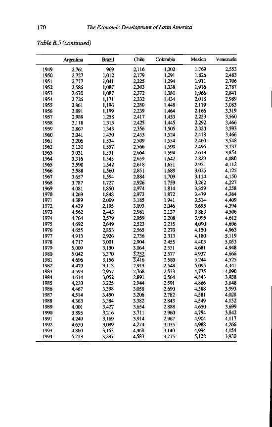
170 The Economic Development of Latin America
Table B.5 (continued)
Argentina Brazil Chile Colombia Mexico Venezuela
1949 2,761 969 2,116 1,302 1,769 2,5531950 2,727 1,012 2,179 1,291 1,826 2,4831951 2,777 1,041 2,225 1,294 1,911 2,7061952 2,586 1,087 2,303 1,338 1,916 2,7871953 2,670 1,087 2,372 1,380 1,966 2,8411954 2,726 1,171 2,332 1,434 2,018 2,9891955 2,861 1,196 2,280 1,448 2,119 3,0831956 2,891 1,199 2,239 1,464 2,166 3,3191957 2,989 1,258 2,417 1,453 2,259 3,5601958 3,118 1,315 2,425 1,445 2,292 3,4661959 2,867 1,343 2,356 1,505 2,320 3,5931960 3,041 1,430 2,453 1,524 2,418 3,4661961 3,206 1,534 2,509 1,554 2,460 3,5481962 3,130 1,557 2,566 1,590 2,496 3,7371963 3,031 1,531 2,664 1,594 2,613 3,8541964 3,316 1,545 2,659 1,642 2,829 4,0801965 3,590 1,542 2,618 1,651 2,921 4,1121966 3,588 1,560 2,851 1,689 3,025 4,1251967 3,657 1,594 2,884 1,709 3,114 4,1501968 3,787 1,727 2,926 1,759 3,262 4,2271969 4,081 1,850 2,974 1,814 3,359 4,2581970 4,269 1,848 2,973 1,872 3,479 4,3841971 4,389 2,009 3,185 1,941 3,514 4,4091972 4,439 2,195 3,093 2,046 3,695 4,3941973 4,562 2,443 2,981 2,137 3,883 4,5061974 4,764 2,579 2,959 2,208 3,995 4,6121975 4,692 2,649 2,523 2,215 4,090 4,6961976 4,655 2,853 2,565 2,270 4,150 4,9631977 4,913 2,926 2,736 2,313 4,180 5,1191978 4,717 3,001 2,904 2,455 4,405 5,0531979 5,009 3,130 3,064 2,531 4,681 4,9481980 5,042 3,370 2,577 4,937 4,6661981 4,696 3,156 3,416 2,580 5,244 4,5251982 4,479 3,113 2,913 2,548 5,095 4,4411983 4,593 2,957 2,768 2,533 4,775 4,0901984 4,614 3,052 2,891 2,564 4,843 3,9381985 4,230 3,225 2,944 2,591 4,866 3,8481986 4,467 3,398 3,058 2,690 4,588 3,9931987 4,514 3,450 3,206 2,782 4,581 4,0281988 4,363 3,384 3,382 2,843 4,549 4,1521989 4,001 3,427 3,654 2,888 4,650 3,6991990 3,895 3,216 3,711 2,960 4,794 3,8421991 4,249 3,169 3,914 2,967 4,904 4,1171992 4,630 3,089 4,274 3,035 4,988 4,2661993 4,860 3,163 4,468 3,140 4,994 4,1541994 5,213 3,297 4,583 3,275 5,122 3,930

Appendix B 171
NOTES
1. See Chapter 6 for a more extensive analysis of exchange rates and purchasing power parities. I used the results of ICP IV for 1980 because Latin America did not participate in the following rounds. Mexico now participates as an OECD member with the OECD secretariat and EUROSTAT. There exist good prospects that Latin America will participate in the next round of ICP as many countries expressed their interest, especially the MERCOSUR and Andean Pact countries. ECLAC will coordinate the ICP work with the substantive and financial assistance of World Bank and OECD.
2. Banco Central de la República Argentina (1991) is only available in mimeographed form and was never published officially.
3. Of which no official estimates were available since 1973.4. Banco Central de Chile (1994).

Appendix C. Activity Rates, Employment, Education and Labour Productivity
In order to analyse the labour market in Latin America some basic quantification is necessary. There are many institutes working on this theme, som e regional like the former PREALC. The basic value added o f this appendix is its presentation o f series since 1950, estimates on hours worked and the human capital estimates. The appendix presents a complete description o f the sources for each country. First, a general source note is given which presents the databases and other general information we used in common for all countries. Then, in specific source notes, the sources and procedures are detailed if they are different from the one described in the general source note. It should be noted that the basic tables have as benchmark years: 1950, 1960, 1970, 1980 and 1990. This is the case because the information with respect to activity rates, labour force and employment normally comes from population censuses which are only available on a decade basis. These benchmarks are used in this appendix although the text often presents a périodisation with benchmarks in 1950, 1973, 1980, 1989 and 1994. If not otherwise indicated, the data for 1973, 1989 and 1994 have been estimated by intra- and extrapolation.
SOURCE NOTE
Table C.1
M ale and female activity rates for 1950-80 from ECLAC (1985). These activity rates were calculated on the basis o f population censuses and household surveys. However, the population figures o f CELADE are adjusted for undercounting, especially for males, in the censuses. This adjustment causes small changes in total activity rates. W e used ECLAC’s sex-specific activity rates for the respective population and calculated the total activity rate. For 1990 I used population censuses when available. For Brazil and Colombia CELADE (1992) was used.
173
174 The Economic Development of Latin America
Table C.2
The employment rates for 1950-80 come from the Projections Center o f ECLAC and are based upon population censuses. The 1990 estimate was elaborated by the author using population censuses. For Brazil IBGE (1990) was used and in the case o f Colombia the 1985 census (DANE, 1986), updated to 1990 and ECLAC (1992). The updating to 1994 was done with the employment information o f the household surveys o f the countries available at the employment data base o f the Statistics and Projections Division o f ECLAC. Unemployment rates were assumed equal for both sexes.
Table C.3
Annual hours per person employed were calculated on the basis o f the number o f days worked per year and the average number o f hours worked per day. Number o f days worked during the year on the basis o f public and statutory holidays from ILO (1982) and estimated for missing years. H alf day Saturday working was assumed in 1950 and 1960 in the cases o f Argentina, Brazil, Colombia and M exico, and only in 1950 in the cases o f Chile and Venezuela and a free Saturday onwards. Time lost through industrial disputes from ILO, Yearbook o f Labour Statistics, various issues. Annual hours data from DLO, Yearbook o f Labour Statistics, various issues, and other sources. In the case o f Brazil the 1960 and 1970 estimate from Bonelli (1976), with 1959 and 1969 estimates for manufacturing. The estimates for 1980 and 1990 were based upon IBGE, Anuario Estadístico do Brasil, various issues, and IBGE, Recenseamento Geral do Brasil, 1970 and 1980. The Chile 1960 and 1970 estimates were on the basis o f information from Instituto de Economía, Ocupación y Desocupación, Universidad de Chile, Santiago (various issues) and INE, Muestra Nacional de Hogares, Santiago, 1966 and 1971. In the case o f Colombia, 1950 from DANE (1956), Anuario General de Estadística Colombia. 1956, p. 412, figures for 1956 and 1980 and 1990 were estimates. M exico for 1950-90, Instituto Nacional de Estadística, Encuesta Anual de Trabajo y Salarios Nacionales, various issues. The 1950 and 1960 figures for Venezuela are estimates. The 1994 estimates were from ILO (1995) in the case o f Chile and M exico; the remainder were estimated by the author.
Table C.5
The 1950-80 sectoral employment data were provided by ECLAC’s Projections Center. For 1990 national census and country sources were used as follows: Argentina’s 1990 sectoral employment from PREALC (1993); the 1990 sectoral employment in Brazil from IBGE (1990) which represents the 1988 estimate; the

Appendix C 175
Chilean 1990 sectoral employment from García (1992); Colombia’s 1990 sectoral employment was estimated on the basis o f Junguito (1990) and ECLAC (1992); the M exican 1990 sectoral employment data was from INEGI (1992); the 1990 sectoral employment in Venezuela was from OCEI (1990).
Table C.6
The estimates for average years o f formal education o f the population between 15 and 64 years were made on the basis o f the population censuses o f the countries. In many cases the information o f the census had to be adjusted which generally (for specifics see the country notes) has been done as follows: in the cases where the census presented only data o f the educational level o f 15 years and older, the information from previous censuses was used to estimate the cohort 65-75 and the census was adjusted with this information. If information within the 50 -6 4 group was insufficient we tried to apply the same procedures. W e adjusted for differences in the number o f years particulary in primary and secondary education. The first six years were considered primary education and the second six years secondary education. If, for example, Argentina has seven years o f primary education and five years o f secondary, then we considered the seventh year o f primary as the first year o f secondary and so on.
In case the census was not available from national sources, the World Bank database on capital stock, which was kindly provided to us by the World Bank, or the estimates o f Maddison (1989) were used as indicated in the country source notes. In Table C.9 o f this appendix, the Maddison (1989) and the World Bank data with respect to formal years o f education are presented. In the case o f the World Bank data the extremely low (in comparison with Maddison’s (1989) and my data) level o f secondary education draws the attention. This becom es extreme, for example, in the case o f Argentina, where formal educational experience in higher education exceeds the experience in secondary education, implying that Argentina’s brilliant youngsters jump directly from primary to higher education.
Argentina’s 1950 estimate was obtained from Maddison (1989) using as the linkage year 1980, for which we had estimates in common. Total years of education in 1990 was estimated by using the World Bank database 1980-87 growth rate. The disaggregation o f years o f education was obtained on the basis o f retropolation, in the case o f 1950, or extrapolation, in 1990 o f the available distribution. Brazil’s 1950-70 estimates are based upon Langoni (1974). The 1990 estimate was based upon the 1980 population census, containing the educational level o f the population aged 25 -64 and IBGE (1992) which contained information about educational level o f the population aged 15-24.
The estimates for Chile in 1950,1980 and 1990 were based on intrapolation of the census information o f 1952, 1982 and 1992. In 1952 the group with special education was distributed over secondary and higher education and not, as in the

176 The Economic Development of Latin America
case o f Maddison (1989), completely to higher education. The level o f education from 1962 onwards was given for total population over 15. In order to obtain population figures for the age group 15-64 previous population censuses were used to subtract the educational level o f the cohort over 64. The Colombian estimates for 1950-80 were based on intrapolation o f the census information o f 1951, 1964, 1973 and 1985. Special adjustments were made using cohorts o f previous population censuses to estimate the educational level o f the 6 0 -6 4 age group. For 1990 the 1980-87 growth rate o f the World Bank database was used. The 1950 estimate for M exico was obtained from Maddison (1989) using as the linkage year 1980 for which we had estimates in common. For 1960-80 an adjustment was made, using cohorts from other censuses to estimate the educational level over 65, to obtain the educational level 15-64. In the case o f Venezuela for 1960-80 the estimates for 1961,1971 and 1981 were retropolated. The distribution with respect to educational level for 1971 was obtained through cohort analysis o f the available censuses. For 1990 the 1980-87 growth rate o f the World Bank database was used.

Appendix C 111
Table C .l Latin America: Total Female and Male Activity Rates, Six Countries, 1950-94 (economic active population divided by total population)
Argentina Brazil Chile Colombia Mexico Venezuela
Total1950 40.91 33.30 37.64 32.54 32.02 32.921960 39.09 32.13 32.57 29.51 29.15 31.191970 38.89 31.56 30.47 29.11 27.94 28.491973 38.11 32.92 30.80 30.23 28.59 29.671980 36.34 36.33 31.57 33.04 30.19 32.611989 36.79 37.13 32.96 34.13 30.37 33.291990 37.83 39.08 36.43 36.81 30.82 34.931994 38.45 40.24 38.58 38.43 31.08 35.91Female1950 16.33 10.04 17.91 10.31 8.30 10.391960 15.87 11.18 14.18 9.90 10.28 8.251970 19.09 12.77 13.38 12.04 11.13 11.271973 19.08 14.46 13.90 12.95 11.42 12.701980 19.06 19.33 15.19 15.34 12.11 16.781989 19.57 20.39 16.80 16.41 12.73 17.761990 20.80 23.07 21.24 19.20 14.31 20.291994 21.54 24.76 24.29 21.00 15.30 21.89Male1950 64.10 56.54 57.77 55.07 55.77 54.881960 61.59 53.00 51.38 49.36 48.12 51.911970 58.56 50.30 48.02 46.36 44.73 45.281973 57.17 51.20 48.13 47.69 45.78 46.101980 54.07 53.34 48.39 50.95 48.32 48.051989 54.49 53.88 49.44 52.04 48.09 48.431990 55.47 55.14 51.98 54.68 47.55 49.331994 56.04 55.88 53.49 56.25 47.24 49.86
Source: Hie values for 1973 and 1989 are intrapolations. 1994 was extrapolated using the 1980-90 growth rate.
Table C.2 Latin American Employment, Six Countries, 1913-94 (thousand persons engaged at mid-year)
Argentina Brazil Chile Colombia Mexico Venezuela
1913 3,201 11,302 1,323 2,099 5,521 5291950 6,821 17,657 2,256 3,844 8,766 1,5711960 7,849 23,138 2,354 4,516 10,600 2,0661970 9,132 29,643 2,729 5,968 13,599 2,9021973 9,402 33,164 2,894 6,616 15,180 3,3381980 10,065 43,091 3,318 8,413 19,622 4,6261989 11,731 54,646 4,303 10,487 24,318 5,7221990 11,932 56,108 4,429 10,747 24,905 5,8591994 12,483 59,908 4,954 11,670 28,018 6,724
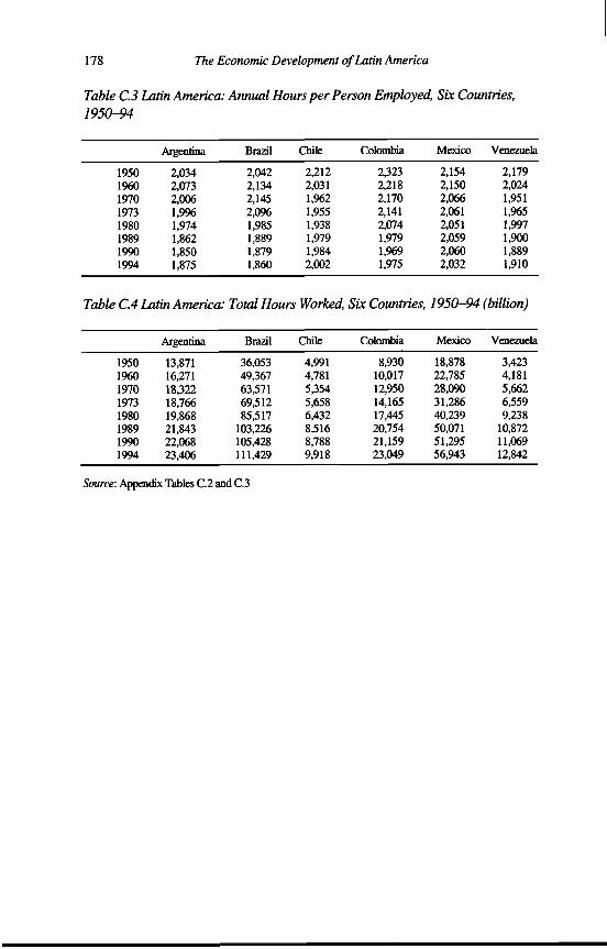
178 The Economic Development of Latin America
Table C.3 Latin America: Annual Hours per Person Employed, Six Countries, 1950-94
Argentina Brazil Chile Colombia Mexico Venezuela
1950 2,034 2,042 2,212 2,323 2,154 2,1791960 2,073 2,134 2,031 2,218 2,150 2,0241970 2,006 2,145 1,962 2,170 2,066 1,9511973 1,996 2,096 1,955 2,141 2,061 1,9651980 1,974 1,985 1,938 2,074 2,051 1,9971989 1,862 1,889 1,979 1,979 2,059 1,9001990 1,850 1,879 1,984 1,969 2,060 1,8891994 1,875 1,860 2,002 1,975 2,032 1,910
Table C.4 Latin America: Total Hours Worked, Six Countries, 1950-94 (billion)
Argentina Brazil Chile Colombia Mexico Venezuela
1950 13,871 36,053 4,991 8,930 18,878 3,4231960 16,271 49,367 4,781 10,017 22,785 4,1811970 18,322 63,571 5,354 12,950 28,090 5,6621973 18,766 69,512 5,658 14,165 31,286 6,5591980 19,868 85,517 6,432 17,445 40,239 9,2381989 21,843 103,226 8,516 20,754 50,071 10,8721990 22,068 105,428 8,788 21,159 51,295 11,0691994 23,406 111,429 9,918 23,049 56,943 12,842
Source: Appendix Tables C.2 and C.3

Appendix C 179
Table C.5 Latin America: Sectoral Employment, Six Countries, 1950-94 (thousand persons employed at mid-year)
Argentina Brazil Chile Colombia Mexico Venezuela
Agriculture1950 1,723 10,606 722 2,164 5,338 7101960 1,589 12,687 705 2,317 5,247 7281970 1,483 13,437 636 2,477 5,684 7471973 1,429 14,199 626 2,577 6,032 7821980 1,333 13,078 540 2,524 7,221 7311989 1,464 13,527 709 3,004 6,076 7801990 1,480 13,578 731 3,063 5,960 7861994 1,508 13,243 822 3,258 5,645 845Industry1950 2,141 3,116 684 700 1,464 3151960 2,807 4,146 704 867 2,258 4571970 3,130 6,619 920 1,301 3,549 7161973 3,182 7,911 1,011 1,498 4,211 8511980 3,654 12,596 984 2,204 5,239 1,3411989 3,033 13,226 1,031 2,501 6,542 1,3641990 2,971 13,298 1,036 2,536 6,705 1,3671994 2,673 13,056 1,054 2,642 7,568 1,438Services1950 2,957 3,935 850 980 1,963 5461960 3,453 6,304 945 1,332 3,095 8811970 4,519 9,587 1,173 2,190 4,365 1,4391973 4,791 11,055 1,257 2,541 4,937 1,7051980 5,078 17,417 1,794 3,685 7,162 2,5541989 7,233 27,893 2,563 4,982 11,701 3,5781990 7,481 29,232 2,662 5,148 12,240 3,7061994 8,302 33,610 3,078 5,770 14,804 4,441Total1950 6,821 17,657 2,256 3,844 8,765 1,5711960 7,849 23,137 2,354 4,516 10,600 2,0661970 9,132 29,643 2,729 5,968 13,598 2,9021973 9,402 33,165 2,894 6,616 15,180 3,3381980 10,065 43,091 3,318 8,413 19,622 4,6261989 11,730 54,646 4,303 10,487 24,319 5,7221990 11,932 56,108 4,429 10,747 24,905 5,8591994 12,483 59,909 4,954 11,670 28,017 6,724

180 The Economic Development of Latin America
Table C.6 Latin America: Average Years o f Formal Education o f Population Aged 15-64, Six Countries, 1950-94
Argentina Brazil Chile Colombia Mexico Venez
Total1950 4.72 1.83 4.46 2.45 2.07 1.931960 5.09 2.09 5.16 3.05 2.66 2.381970 6.41 2.92 6.13 4.05 3.51 3.511973 6.87 3.23 6.45 4.40 3.81 3.941980 7.41 4.22 7.34 5.07 5.72 5.511989 8.37 5.25 8.65 6.90 6.77 7.751990 8.49 5.38 8.82 7.15 6.91 8.061994 8.97 5.93 9.48 8.20 7.45 9.39Primary1950 3.86 1.53 3.65 2.04 1.88 1.741960 4.00 1.73 4.00 2.37 2.33 2.10
1970 4.69 2.23 4.42 2.98 2.93 2.841973 4.92 2.41 4.55 3.19 3.14 3.111980 4.97 3.22 4.91 3.45 4.17 4.111989 5.09 3.87 5.30 4.29 4.60 5.231990 5.10 3.95 5.35 4.39 4.65 5.371994 5.15 4.29 5.54 4.83 4.86 5.98Secondary1950 0.77 0.25 0.70 0.34 0.16 0.161960 0.96 0.30 1.03 0.54 0.29 0.231970 1.49 0.58 1.43 0.92 0.49 0.591973 1.68 0.69 1.55 1.06 0.56 0.741980 2.04 0.88 2.12 1.40 1.32 1.20
1989 2.65 1.23 2.93 2.27 1.83 2.161990 2.73 1.28 3.04 2.40 1.90 2.301994 3.01 1.48 3.45 2.93 2.16 2.90Higher1950 0.09 0.05 0.11 0.07 0.03 0.031960 0.13 0.06 0.13 0.14 0.04 0.051970 0.23 0.11 0.28 0.15 0.09 0.081973 0.27 0.13 0.35 0.15 0.11 0.091980 0.40 0.12 0.31 0.22 0.23 0.20
1989 0.63 0.15 0.42 0.34 0.34 0.361990 0.66 0.15 0.43 0.36 0.36 0.391994 0.81 0.16 0.49 0.44 0.43 0.51

Appendix C 181
Table C. 7 Latin American Labour Productivity, GDP per Person Employed, Six Countries, 1950-94 (in 1980 international dollars)
Argentina Brazil Chile Colombia Mexico Venezuela
1950 8,519 3,062 5,875 4,013 5,777 8,0501960 7,986 4,487 7,926 5,378 8,428 12,7161970 11,203 5,974 10,346 6,699 12,946 16,1961973 12,224 7,585 10,292 7,358 14,208 15,9241980 14,084 9,486 10,924 8,126 17,001 15,2221989 11,428 7,162 10,940 8,742 15,616 12,3001990 10,625 8,510 10,976 8,895 16,021 12,7901994 14,272 8,758 12,947 9,695 16,373 12,496
Source: Appendix Tables B.3 and C.2.
Table C.8 Latin American Labour Productivity, GDP per Hour Worked, Six Countries, 1950-94 (in 1980 international dollars)
Argentina Brazil Chile Colombia Mexico Venezuela
1950 3.37 1.50 2.66 1.73 2.68 3.691960 3.85 2.10 3.90 2.42 3.92 6.281970 5.58 2.79 5.27 3.09 6.27 8.301973 6.12 3.62 5.26 3.44 6.89 8.101980 7.13 4.78 5.64 3.92 8.29 7.621989 5.88 4.84 5.53 4.42 7.58 6.471990 5.74 4.53 5.53 4.52 7.78 6.771994 7.61 4.71 6.47 4.91 8.06 6.54
Source: Appendix Tables B.3 and C.3.

182 The Economic Development of Latin America
Table C.9 Latin America: Average Years o f Formal Educational Experience o f Population Aged 15-64 in 1950 and 1980, Five Countries
Total Primary Secondary Higher
Argentina1950 4.60 4.15 0.42 0.031980 7.21 5.00 1.74 0.47Brazil1950 1.83 1.36 0.42 0.051980 3.94 2.52 1.31 0.11
Chile1950 4.88 3.59 1.16 0.131980 7.57 4.38 2.77 0.42Colombia1950 3.61 2.95 0.56 0.10
1980 6.66 3.47 2.77 0.42Mexico1950 2.30 1.61 0.65 0.041980 4.94 2.87 1.95 0.12
Source: Maddison (1989).

Appendix D. Total and Disaggregated Gross Investment, 1900-1994
Estimates for total and disaggregated capital formation are the essential building blocks for the construction o f capital stock estimates using the ‘perpetual inventory method’. Tables D .l to D .8 present total and disaggregated gross fixed investment for the 1900-1994 period, in national currencies as w ell as a percentage o f GDP. For all countries a detailed description is given o f the sources used for the construction o f the series which consist o f total capital formation, capital formation in machinery and equipment and capital formation in residential and non- residential structures. For 1950 onwards, if not otherwise specified, the series used for Latin America are derived from currently collected official estimates by ECLAC corresponding to the most recent revision o f the United Nations System o f National Accounts (SNA).
These official estimates since 1950 apply especially to GDP and in many cases total capital formation estimates. In the case o f disaggregated capital formation the official series in Latin America often only start in the 1970s and for residential capital formation sometimes no official estimates were available. As already indicated in Appendix B , for years before 1950, the estimates have nearly all been made retrospectively and the underlying data are less complete. Nevertheless, most of the historical estimates are based upon substantial statistical research by distinguished scholars. But the estimates for the first half o f the twentieth century are obviously not as comparable as those for 1950 onwards, and in some cases may well be substantially revised when further research is done. This applies especially for the data before 1925 in the case o f disaggregated capital formation.
SOURCES
Argentina1
The source for 1900-1950 including GDP, total fixed capital formation and fixed capital formation in machinery and equipment is Banco Central de la Republica Argentina (1976). Fixed capital formation in residential structures for 1900-1955 is from ECLAC (1958). For 1955-70 fixed capital formation was estimated at 46
183
184 The Economic Development of Latin America
per cent o f fixed capital formation in non-residential structures, which is the average residential/non-residential structures ratio for 1955 and 1970. From 1970-94, ECLAC estimates based upon official statistics were used, taking into account the following considerations. In 1987 the Central Bank o f Argentina, in cooperation with the Buenos Aires office o f ECLAC, initiated a project regarding the revision o f the national accounts, income distribution and input-output matrix. The final report2 presented an extensive description o f the methodology applied in the elaboration o f the new series. The results were the updating o f the current and constant series, by sector and expenditure, an estimation o f factor shares3 and a base year change from 1970 to 1986. The increase in the GDP level o f 43.2 per cent occurred mainly in the manufacturing and construction sector, and expenditure-wise in fixed capital formation in private construction (114 per cent) and machinery and equipment (64 per cent). Much o f the increase was due to improved statistical sources, for example, industrial and household surveys, and better coverage o f the informal sector. Afterwards, the Banco Central de la República de Argentina (1993) published new series, based upon the 1991 revision, but once again revised. Expenditure-wise capital formation grew less than in the former revision.
Several problems had to be addressed in order to be able to include these new estimates in our series. Backwards, the revision influenced both the level and the growth o f the long-run series. From 1980 onwards only gross total capital formation was presented, so estimates had to be made for fixed capital formation. A s it was not reasonable to include all the difference in 1980 I decided, after extensive consultations with Argentine national accounts experts, who had participated in the latest revision and some in previous ones, to distribute half o f the increase in GDP and fixed capital formation as a level adjustment for the 1900-1980 period and to treat the other half o f the increase as a linear augmentation o f the growth rate over the 1961-80 period. The basic argument for this distribution was that the national accounts before 1961 were considered rather reliable and it did not seem reasonable to increase the level o f Argentina’s GDP for the whole period by the whole o f the 35 per cent. For 1980-94 we used the revised GDP estimates.
In order to be able to reach the needed level o f disaggregation in capital formation, available in the 1991 revision, but not in the April 1993 revision, the following procedure was applied. The new (1993) revision contained a major change in methodology with respect to the estimation o f capital formation in residential construction. I used therefore the unchanged 1991 estimates for machinery and equipment. A lso public capital formation was unchanged, assumed to be non-residential, so I had to disaggregate private capital formation in residential and non-residential capital formation. A level increase o f private non- residential capital formation o f 50 per cent was assumed. This resulted in level increase o f 64 per cent in machinery and equipment, 85 per cent in residential and
Appendix D 185
22 per cent in non-residential capital formation. H alf o f this level increase was applied to increase the level o f the 1900-1980 series and the remainder half consisted o f a linear augmentation o f the growth rate over the 1961-80 period. For the 1980-94 period capital formation was disaggregated using these growth rates. Comparing the results o f disaggregated fixed capital formation series with total capital formation o f the new 1993 series and the stock variations estimate available from the old series leads to an upward adjustment o f 10 per cent o f the components o f capital formation and the resulting increase in stocks distribution fitted rather well with the older series, as w ell as with fluctuations o f the economy.
Brazil
Total capital formation for 1900-1925 is calculated as the sum o f capital formation in machinery and equipment and capital formation in residential and non-residential construction. For 1925-50 ECLAC (1951) was used to calculate a capital coefficient as the ratio o f capital goods and the sum o f agricultural and industrial production with an adjustment for differences in base year. The figures for capital formation in machinery and equipment for 1900-1925 are from V illela and Suzigan (1977), table 133, p. 363 using a quantum index o f industrial capital goods imports, for 1925-49 from ECLAC (1951), using index o f imports o f other capital goods; and for 1949-69 from Langoni (1974), based upon an unpublished study o f the Getulio Vargas Foundation (1970). The figures for capital formation in non-residential structures for 1900-1925 are based upon V illela and Suzigan (1977, p. 359), using a combined quantum index o f domestic cement consumption and domestic rolled-steel consumption. The figures for capital formation in residential structures for 1900-1920 are from V illela and Suzigan (1977, p. 359), using a quantum index o f domestic cement consumption and 1920-85 was based upon IBGE, Brasil, Censo Demografico, 1920, 1940, 1950, 1970, 1980. For the 1985 data the national household survey o f IBGE was used. On the basis o f the census and household survey information a stock o f housing was estimated. Gross investment was calculated on the basis o f the yearly increase o f the housing stock plus the depreciation. With these data an index o f investment in residential structures was calculated with base year 1974. For 1974, Borges and Vasconcellos (1974), estimated capital formation in residential structures at 20 per cent o f total capital formation. For 1985-92 capital formation in residential structures was estimated as 39 per cent o f capital formation in non-residential structures.
186 The Economic Development of Latin America
Chile
Total capital formation for 1900-1904 and 1916-19 was estimated at three times capital formation in machinery and equipment, and for 1905-15 it was estimated at two times capital formation in machinery and equipment. Total capital formation for 1920-22 was estimated at 9 per cent o f GDP and for 1923-24 at 14 per cent o f GDP, for 1925-40 ECLAC (1951) (adjusted for 1925-31 to 2/3) and for 1940-50 ECLAC (1972). Capital formation in machinery and equipment for 1900-1940, using a quantum index o f imports o f capital goods from ECLAC (1951) (adjusting the 1900-1931 level by 2/3 to avoid extremely high estimates caused by linking problems) and for 1940-50, CORFO (1963). Capital formation in residential structures for 1920-25 was estimated applying the index o f total capital formation and for 1925-28 using the 1928 ratio o f capital formation in residential structures to total capital formation. For 1928-40 ECLAC (1951) was used; for 1940-54 CORFO (1957); for 1954-60, CORFO (1963); for 1960-75 ODEPLAN (1976). For 1974-82, ECLAC was used, based upon official estimates and for 1982-92 Banco Central de Chile, Boletín Mensual, various issues. In the case o f Chile a revision o f the national accounts for the base year 1986 took place in the early 1990s. The most important results are an increase o f capital formation in machinery and equipment and non-residential construction.
Colombia
Total GDP for 1900-1925 is from Maddison (1989) using his benchmarks for 1900, 1913 and 1929, and interpolating the years in between, and for 1925-50 from ECLAC (1972). Total capital formation for 1900-1909 was estimated constant at 10 per cent o f GDP, for 1910-24 at 18 per cent o f GDP based upon the périodisation and description o f M cGreevey (1985), and for 1925-50 from ECLAC (1972). Capital formation in machinery and equipment for 1900-1925 was estimated at 33 per cent o f total capital formation and for 1925-50 from ECLAC (1957). Capital formation in residential structures from 1900-1925 was estimated at 25 per cent o f capital formation in non-residential structures and for 1925-50 from ECLAC (1957). For 1950-70, it was estimated at 28 per cent o f capital formation in non-residential structures.
Mexico
Total capital formation for 1900-1910 and for 1920-25 was estimated at 10 per cent o f GDP. For the period 1911-20 we have assumed that no capital formation occurred, that is, capital formation in this period was offset by war destruction caused by the M exican Revolution. For total capital formation from 1925-39, ECLAC (1951) was used to calculate a capital coefficient as the ratio total o f

Appendix D 187
available capital goods (see table 6, p. 414) and national production (table 3A, p. 404) and for 1939-60 from Banco de M exico (1986a). Capital formation in machinery and equipment for 1920-25 was calculated applying the ratio o f 1925 and for 1925-39 using ECLAC (1951), based upon imports o f other capital goods (see table 6, p. 414). The figures for 1939-50 were from the W orld Bank (1953), and for 1950-60 from Banco de M exico (1969). Capital formation in non- residential structures for 1900-1929 were assumed to move as total capital formation, the figures for 1929-70 are from INEGI (1985) using an index o f the total housing stock adjusted for the changing weight o f brick houses in total housing stock.
Venezuela
Capital formation estimates were based upon Baptista (1991) which is the most complete statistical historical source available on Venezuela’s quantitative economic history. Total capital formation was estimated as follows: 1900-1909 at 10 per cent o f GDP, with 3.1 per cent in residential and non-residential structures each, and 3.7 per cent in machinery and equipment; 1910-19 at 15 per cent o f GDP, with 4.7 per cent in residential and non-residential construction and 5.6 per cent in machinery and equipment on the basis o f the growth figures o f Baptista (1991) and the description o f Venezuela’s economic development in Quero Morales (1978) and Brito Figueroa (1966) which both indicate that the period 1900-1909 was one o f stagnation and that during 1910—19 foreign investment increased especially in the oil sector (63 per cent o f total capital formation in industry came from foreign investment, see Brito Figueroa, 1966, p. 398). Total and disaggregated capital formation from 1920-50 is based upon Baptista (1991, Cuadro IV-1, p. 149). For 1950-76, the figures are from Banco Central de Venezuela (1978, p. 177).

188 The Economic Development of Latin America
Table D. 1 Latin America: Gross Total Fixed Investment, Six Countries, 1900-1994 (constant 1980 national prices)
Argentina(thousandaustrales)
Brazil(million
cruzeiros)
Chile(millionpesos)
Colombia(millionpesos)
Mexico(millionpesos)
Venezuela (mi Ilion
bolívares)
1900 318,869 26,187 12,880 4,706 18,907 2551901 331,235 26,185 15,224 4,903 20,548 2511902 327,113 18,491 19,371 5,109 19,082 2731903 358,362 21,147 19,886 5,324 21,220 2951904 518,461 23,728 25,760 5,547 21,593 2881905 801,693 33,675 22,583 5,780 23,836 2851906 958,601 37,901 36,544 6,022 23,567 2661907 1,183,723 52,330 41,576 6,275 24,950 2651908 1,009,662 52,898 43,929 6,539 24,912 2841909 1,137,848 54,392 29,332 6,813 25,644 2941910 1,360,311 65,337 27,769 12,778 25,872 4551911 1,339,833 80,830 44,753 13,314 0 4871912 1,092,371 107,437 44,186 13,873 0 5031913 1,107,796 91,538 42,950 14,455 0 5811914 686,538 39,161 31,976 15,013 0 5081915 412,216 19,847 14,769 15493 0 5241916 364,744 23,348 27,331 16,195 0 4941917 275,652 20,654 36,965 16,820 0 5771918 278,046 19,235 26,687 17,469 0 5731919 325,118 40,112 27,846 18,143 0 5361920 603,297 61,349 15,403 18,843 27,667 5531921 697,841 60,666 13,252 19,571 27,854 7061922 819,245 53,935 14,182 20,326 28,503 6451923 1,131,731 64,229 26,461 21,111 29,482 8881924 1,214,307 86,677 28,858 21,926 29,000 1,4511925 1,222,817 110,147 43,810 23,957 36,952 2,6201926 1,206,063 93,486 63,010 29,896 31,850 3,6821927 1,385,310 91,396 42,999 36,085 28,639 3,5701928 1,646,336 97,380 44,503 42,773 29,346 3,1581929 1,883,426 113,489 63,470 36,933 32488 4,0611930 1,585,833 61,082 64,990 24,057 26,336 3,4281931 970,568 26,399 31,335 19,814 18,058 1,8161932 680,687 27,067 16,017 23,408 11,060 1,2581933 760,471 44,302 19,449 22,909 16482 2,0761934 1,007,667 57,348 25,421 23,358 22,414 2,1981935 991,977 71,106 37,297 26,702 27,697 1,9271936 1,042,506 78,640 41,416 29,397 28,779 3,0671937 1,398,474 105,919 46,559 34,138 38,538 3,9931938 1,540,090 100,927 52,197 34,887 20,890 4,9221939 1,291,298 91,470 44,559 39,828 27,044 5,0891940 1,132,795 76,386 50,943 38,281 35,308 4,1251941 1,135,587 74,721 50,309 36,684 43,072 3,0411942 1,062,053 52,594 39,951 32,242 37,318 2,6771943 1,031,470 62,799 42,911 34,188 37,350 2,9261944 1,185,585 92,065 48,195 37,233 46,994 5,0101945 1,176,144 99,829 50,943 46,416 67,509 7,2111946 1,463,631 98,654 70,602 54,851 89,993 9,795

Appendix D 189
Table D .l (continued)
Argentina(thousandaustrales)
Brazil(million
cruzeiros)
Chile(millionpesos)
Colombia(millionpesos)
Mexico(millionpesos)
Venezuela(million
bolfvares)
1947 2,323,034 235,526 77,578 66,181 101,421 12,8451948 2,322,236 199,158 68,911 64,733 %,143 15,8361949 1,950,311 241,019 78,846 49,411 87,604 16,3731950 1,959,353 310,611 72,716 57,047 100,638 14,5021951 2,410,316 380,546 82,651 56,636 127,610 15,4221952 2,145,958 409,003 86,667 61,019 132,307 19,3631953 2,120,041 345,337 87,513 82,566 127,545 21,2601954 2,035,378 375,723 84,765 %,108 132,379 24,2851955 2,361,937 354,019 98,082 101,582 149,319 22,9261956 2,513,985 381,511 93,431 %,3% 173,320 24,8541957 2,755,881 432,636 106,960 72,276 187,775 26,4221958 3,002,960 458,199 105,269 68,716 176,758 26,1%1959 2,377,487 517,524 90,683 73,840 179,131 26,9511960 3,592,148 538,746 117,529 86,970 205,852 20,9931961 4,188,247 566,238 119,040 94,358 207,555 17,8561962 3,852,110 583,601 133,646 94,708 218,773 18,6431963 3,297,120 567,202 153,375 87,135 243,945 19,1361964 3,695,795 581,189 144,635 98,042 293,610 23,0061965 3,898,929 566,238 135,895 92,588 315,182 24,6941966 4,067,647 680,064 140,265 105,406 343,114 25,2231967 4,312,835 692,604 143,266 114,666 390,132 26,0671968 4,898,295 842,122 156,816 130,468 427,579 29,7991969 5,937,388 1,019,131 164,727 142,819 459,119 32,0781970 6,310,089 1,114,600 175,361 160,105 497,179 31,5081971 6,891,500 1,285,600 171,294 167,885 488,666 35,3471972 7,037,744 1,500,600 136,878 164,577 548,467 40,6401973 6,595,551 1,815,500 128,630 178,890 629,341 44,4551974 6,931,004 2,056,200 142,438 194,422 679,070 43,3561975 7,015,7% 2,256,400 111,818 186,974 741,988 54,4731976 7,825,806 2,414,900 95,517 204,759 745,319 69,9841977 9,557,860 2,386,600 114,088 206,201 695,276 90,2491978 8,419,729 2,500,000 133,672 225,476 800,774 93,8431979 9,081,094 2,597,100 153,504 234,059 %2,921 75,0341980 9,619,295 2,947,000 194,537 264,894 1,106,758 64,1451981 8,197,575 2,589,000 230,491 281,500 1,286,376 66,0701982 6,571,945 2,413,000 136,520 289,830 1,070,371 63,6041983 6,595,427 2,019,000 113,958 293,252 767,667 46,8501984 6,424,684 2,015,000 143,519 2%,899 817,006 38,0121985 5,505,986 2,191,000 161,269 281,398 881,160 40,5011986 6,135,219 2,687,000 165,168 302,900 777,198 44,0871987 7,021,012 2,650,000 201,031 305,371 776,246 44,3171988 6,706,316 2,519,000 229,482 338,568 821,117 48,2471989 5,234,993 2,549,000 284,174 320,840 873,599 35,9441990 4,714,846 2,269,000 289,322 310,111 988,265 33,7891991 5,899,822 2,1% , 000 283,0% 290,%8 1,070,379 45,7%1992 7,723,865 1,9%, 000 356,663 327,0% 1,186,485 58,2631993 8,799,094 2,192,000 419,860 435,544 1,171,780 54,7861994 10,400,469 2,466,000 434,451 493,906 1,267,019 40,870

190 The Economic Development of Latin America
Table D.2 Latin America: Gross Fixed Investment in Machinery and Equipment, Six Countries, 1900-1994 (constant 1980 national prices)
Argentina(thousandaustrales)
Brazil(million
cruzeiros)
Chile(millionpesos)
Colombia(millionpesos)
Mexico(millionpesos)
Venezuela(million
bolívares)
1900 30,536 22,791 4,293 1,569 0 951901 25,938 22,783 5,075 1,634 0 931902 36,094 12,715 6,457 1,703 0 102
1903 48,925 15,242 6,629 1,775 0 110
1904 81,039 16,566 8,587 1,849 0 1071905 86,803 24,989 11,291 1,927 0 1061906 120,289 26,513 18,272 2,007 0 991907 129,553 37,303 20,788 2,092 0 991908 102,105 38,667 21,964 2,180 0 1061909 119,123 41,274 14,666 2,271 0 1091910 136,346 47,612 13,884 4,259 0 1701911 138,611 61,610 22,376 4,438 0 1811912 162,765 82,348 22,093 4,624 0 1881913 176,489 61,209 21,475 4,818 0 2171914 116,996 25,430 15,988 5,004 0 1891915 87,627 10,108 7,384 5,198 0 1951916 89,548 12,916 9,110 5,398 0 1841917 71,021 12,836 12,322 5,606 0 2151918 62,924 14,801 8,896 5,823 0 2131919 83,647 25,912 9,282 6,048 0 2001920 136,072 43,360 7,943 6,281 6,465 2571921 151,099 50,460 9,376 6,524 6,509 3011922 135,180 36,702 10,141 6,775 6,660 3051923 196,114 47,892 13,275 7,037 6,889 3991924 246,206 60,568 16,108 7,308 6,776 6221925 288,887 83,912 15,834 8,520 8,635 9821926 313,796 63,475 22,935 10,350 7,775 1,4591927 315,854 58,394 15,310 14,375 7,138 1,3551928 381,454 67,164 15,748 17,511 7,624 1,3391929 421,116 84,058 22,574 13,904 7,999 1,5941930 302,954 46,170 22,995 5,907 6,569 1,4421931 201,397 16,603 10,871 3,189 4,327 7671932 130,033 16,021 2,769 2,980 2,134 5461933 144,855 24,695 2,718 4,025 2,855 8081934 176,420 31,484 5,152 5,645 3,892 9201935 226,855 46,974 9,943 5,698 5,043 9311936 242,020 45,771 11,888 7,318 5,430 1,3271937 348,242 64,646 12,880 9,775 6,557 1,9181938 384,062 66,708 14,219 10,350 3,772 2,2731939 279,692 49,694 11,515 10,820 4,774 2,5021940 248,539 34,047 13,292 8,207 5,857 2,1591941 229,874 36,742 12,837 7,684 7,198 1,6201942 185,752 23,569 10,427 2,875 4,051 1,2431943 158,991 29,846 10,722 2,718 4,314 1,0731944 160,432 45,676 9,333 4,652 6,429 2,0401945 164,274 50,219 11,042 11,604 13,799 3,2311946 276,467 83,577 16,280 17,668 16,625 4,349

Appendix D
Table D.2 (continued)
191
Argentina(thousandaustrales)
Brazil(million
cruzeiros)
Chile(millionpesos)
Colombia(millionpesos)
Mexico(millionpesos)
Venezuela(million
bolívares)
1947 706,091 135,416 23,510 26,084 19,442 6,6101948 575,509 115,934 21,727 20,857 19,376 8,5431949 343,096 137,460 25,772 17,041 16,686 7,9001950 324,912 151,929 23,731 22,582 18,097 6,6191951 500,381 216,559 28,404 24,914 23,958 5,3191952 436,574 212,701 29,510 26,769 23,153 8,5381953 413,066 123,955 26,436 40,712 24,964 9,6981954 392,077 164,469 23,362 44,670 24,293 11,4511955 528,087 137,460 29,264 47,002 28,104 9,9641956 591,894 147,106 34,183 42,388 31,765 9,5731957 646,465 180,868 45,495 23,698 35,128 11,4961958 662,417 182,797 45,618 22,779 32,136 11,7671959 533,124 220,418 31,847 22,631 33,545 12,8321960 1,012,516 211,254 40,085 34,488 36,919 8,3271961 1,268,583 219,936 48,663 36,853 82,823 7,5591962 1,176,214 228,135 46,142 34,981 87,299 8,8191963 945,815 224,759 40,552 32,534 97,344 8,4221964 1,086,203 227,170 44,323 39,152 117,162 9,5881965 1,154,111 215,595 38,676 34,603 125,771 9,7531966 1,186,988 286,013 47,868 41,186 136,917 9,7681967 1,231,262 279,260 49,971 36,872 155,679 9,2111968 1,364,647 345,337 57,137 44,487 170,622 10,3611969 1,646,348 419,614 56,165 49,613 183,207 11,7891970 1,735,159 463,500 59,310 63,371 198,395 11,4091971 1,923,174 553,100 53,699 70,195 194,684 13,1871972 2,062,034 637,000 41,246 69,333 219,624 15,0541973 2,047,341 771,400 46,019 68,846 256,874 16,7581974 2,052,797 917,100 43,211 76,039 284,541 17,3601975 1,945,225 1,025,000 43,908 75,803 317,039 23,3421976 2,068,574 1,058,300 38,572 87,087 305,320 30,3591977 2,941,236 959,000 53,283 83,915 268,912 41,2561978 2,276,889 983,800 64,994 98,764 317,253 41,2961979 2,737,406 1,024,600 74,369 108,925 412,392 29,0221980 3,096,194 1,120,700 90,001 121,830 485,720 25,9181981 3,367,910 874,000 104,663 127,728 579,675 28,7491982 2,403,583 739,100 56,844 130,322 409,180 29,0431983 2,701,008 587,000 38,991 127,494 255,205 19,0181984 2,898,643 600,000 44,901 124,717 284,491 18,1871985 2,390,729 692,000 51,859 102,791 329,424 22,3601986 2,713,125 920,000 50,095 113,742 280,329 24,9771987 3,111,747 870,000 68,508 133,176 269,902 24,6171988 2,902,700 794,000 82,679 144,646 321,096 27,4181989 2,385,729 772,000 108,575 142,875 357,709 20,2451990 2,220,375 665,000 108,706 146,864 434,832 15,0861991 2,313,505 646,000 101,549 129,709 499,674 21,5651992 3,028,884 549,000 141,891 153,420 574,165 26,8951993 3,450,630 674,000 172,223 204,286 540,104 23,3471994 4,078,701 876,200 180,663 231,660 584,002 17,417

192 The Economic Development of Latin America
Table D.3 Latin America: Gross Fixed Investment in Residential Structures, Six Countries, 1900-1994 (constant 1980 national prices)
Argentina(thousandaustrales)
Brazil(million
cruzeiros)
Chile(millionpesos)
Colombia(millionpesos)
Mexico(millionpesos)
Venezuela(million
bolivares)
1900 247,063 1,459 2,582 784 1,891 801901 245,226 1,460 4,364 817 2,055 791902 225,012 2,301 5,553 852 1,908 861903 218,478 2,497 5,701 887 2,122 931904 238,284 3,678 7,384 925 2,159 901905 384,480 5,071 4,855 963 2,384 891906 485,143 7,055 7,857 1,004 2,357 831907 694,024 7,016 8,939 1,046 2,495 831908 677,485 7,744 9,445 1,090 2,491 891909 672,380 7,897 6,306 1,136 2,564 921910 856,351 10,339 5,970 2,130 2,587 1431911 849,612 10,515 9,622 2,219 0 1531912 652,574 14,361 9,500 2,312 0 1581913 654,004 18,208 9,234 2,409 0 1821914 287,900 7,075 6,875 2,502 0 1591915 147,626 5,670 3,175 2,599 0 1641916 124,144 6,645 7,835 2,699 0 1551917 98,009 3,858 10,597 2,803 0 1811918 120,877 2,023 7,650 2,911 0 1801919 142,113 7,764 7,983 3,024 0 1681920 306,277 6,770 3,208 3,141 2,949 1441921 352,219 6,140 1,667 3,262 2,248 1521922 469,216 12,507 1,738 3,388 2,648 1531923 706,479 8,742 5,670 3,518 2,761 1731924 677,893 12,413 5,482 3,654 3,137 1871925 621,334 16,460 12,021 2,304 2,990 2191926 517,404 17,937 17,289 3,213 2,898 2451927 576,822 19,224 11,798 4,142 3,377 2731928 676,668 18,971 12,211 5,531 3,086 3291929 845,325 19,283 13,680 6,078 2,994 3631930 752,829 10,000 10,603 4,311 3,276 3891931 506,378 6,000 4,700 3,930 3,586 3251932 356,915 7,000 6,057 4,924 3,924 3241933 341,805 14,000 7,894 6,205 4,295 3351934 442,877 21,350 14,145 5,574 4,701 3611935 338,538 21,579 15,135 6,380 5,145 4031936 293,413 24,677 13,073 6,667 5,630 4021937 402,652 27,720 15,645 8,311 6,162 4581938 434,301 26,615 14,339 8,118 6,744 4821939 456,761 29,505 18,247 10,526 7,900 5161940 410,615 30,543 20,819 10,450 6,874 5161941 490,452 27,678 20,598 9,673 7,579 5201942 541,702 25,944 18,137 10,008 8,356 4531943 574,576 27,725 22,110 10,634 9,212 4861944 646,244 32,109 25,391 9,763 10,156 5781945 636,239 33,757 19,748 9,984 11,197 6841946 704,029 10,000 35,156 10,955 12,345 789

Appendix D
Table D.3 (continued)
193
Argentina(thousandaustrales)
Brazil(million
cruzeiros)
Chile(millionpesos)
Colombia(millionpesos)
Mexico(millionpesos)
Venezuela (million
boli vares)
1947 737,515 49,076 27,145 12,915 13,610 9371948 811,838 45,375 25,065 14,568 15,005 1,0211949 799,996 51,788 24,013 12,754 16,543 1,0721950 908,213 67,656 26,099 13,786 18,238 1,1641951 917,606 75,056 25,360 12,689 18,765 2,4991952 908,213 85,378 26,118 13,700 20,535 2,8441953 838,382 93,821 30,735 16,741 22,472 3,9521954 883,711 92,815 34,339 20,575 24,592 3,2251955 958,647 96,078 39,318 21,832 26,911 3,2461956 1,005,567 102,830 25,868 21,603 29,449 4,0451957 1,103,504 109,549 19,982 19,431 32,227 3,4731958 1,223,282 118,070 18,629 18,375 35,266 5,0031959 964,184 126,177 25,627 20,484 38,592 2,9271960 1,354,067 136,749 32,577 20,993 42,232 2,8181961 1,535,081 144,307 27,637 17,252 48,764 2,2311962 1,413,104 149,380 38,058 17,918 53,670 3,1221963 1,244,965 148,578 45,469 16,380 59,070 3,4621964 1,388,293 154,576 37,209 17,667 65,014 4,5391965 1,466,593 156,673 39,525 17,396 71,555 5,3841966 1,545,005 171,591 40,760 19,266 78,755 5,7551967 1,658,669 180,143 38,444 23,338 86,680 5,5851968 1,908,657 206,233 44,157 25,794 95,401 5,9611969 2,327,030 237,727 50,101 27,962 105,000 5,9461970 2,692,252 255,560 49,020 29,921 115,565 64191971 2,685,340 285,914 56,740 29,120 142,727 7,9401972 2,560,080 326,220 47,554 26,229 148,696 9,4951973 2,419,476 380,166 39,448 34,477 152,304 10,6331974 2,740,898 411,240 45,006 34,117 149,498 9,8391975 3,479,417 441,877 33,752 29,369 175,814 10,8141976 3,355,967 481,732 27,229 31,344 194,237 13,0321977 3,012,400 507,238 27,498 35,083 186,692 14,3321978 3,054,126 537,855 23,545 40,724 173,841 15,6001979 3,361,661 560,090 32,061 36,469 190,016 16,6551980 3,472,979 636,185 45,414 35,695 198,510 15,2431981 3,047,975 613,828 43,103 37,981 214,240 124821982 2,580,584 610,906 27,705 39,328 217,557 9,0901983 2,383,802 554,065 22,662 47,064 204,734 6,7481984 2,452,109 558,594 22,246 47,405 215,051 4,9831985 2,242,132 590,972 29,813 49,129 232,479 4,5911986 2,469,233 689,130 35,410 52,712 228,704 4,6641987 2,827,810 694,200 40,236 57,066 238,828 4,6651988 2,757,813 672,750 47,921 55,273 235,924 4,3901989 2,071,202 693,030 58,088 55,273 262,825 3,4651990 1,817,076 625,560 58,907 51,299 319,491 2,2341991 2,618,598 604,500 66,032 60,319 367,133 2,4221992 3,436,159 564,330 79,462 71,182 421,865 3,2251993 3,923,568 592,020 93,541 94,782 396,839 3,1591994 4,648,330 620,022 96,792 107,482 429,093 2,357

194 The Economic Development of Latin America
Table D.4 Latin America: Gross Fixed Investment in Non-Residential Structures, Six Countries, 1900-1994 (constant 1980 national prices)
Argentina(thousandaustrales)
Brazil(million
cruzeiros)
Chile(millionpesos)
Colombia(millionpesos)
Mexico(millionpesos)
Venezuela(million
bolivares)
1900 41,270 1,938 6,005 2,353 0 801901 60,071 1,942 5,785 2,452 0 791902 66,008 3,475 7,361 2,555 0 86
1903 90,958 3,408 7,557 2,662 0 931904 199,138 3,484 9,789 2,774 0 901905 330,410 3,615 6,436 2,890 0 891906 353,168 4,333 10,415 3,011 0 831907 360,147 8,010 11,849 3,138 0 831908 230,072 6,487 12,520 3,269 0 891909 346,345 5,221 8,359 3,407 0 921910 367,614 7,386 7,914 6,389 0 1431911 351,610 8,705 12,755 6,657 0 1531912 277,032 10,728 12,593 6,937 0 1581913 277,304 12,121 12,241 7,228 0 1821914 281,642 6,655 9,113 7,507 0 1591915 176,963 4,069 4,209 7,796 0 1641916 151,052 3,787 10,386 8,097 0 1551917 106,623 3,960 14,047 8,410 0 1811918 94,245 2,411 10,141 8,734 0 1801919 99,359 6,436 10,582 9,072 0 1681920 160,948 11,219 4,252 9,422 18,253 1511921 194,523 4,067 2,209 9,785 19,097 2541922 214,849 4,727 2,304 10,163 19,194 1871923 229,138 7,594 7,516 10,555 19,832 3161924 290,208 13,697 7,267 10,963 19,086 6421925 312,597 9,775 15,956 13,132 25,328 1,4201926 374,863 12,073 22,786 16,333 21,177 1,9791927 492,634 13,777 15,891 17,569 18,124 1,9421928 588,213 11,246 16,545 19,730 18,636 1,4911929 616,985 10,148 27,216 16,951 21,596 2,1041930 530,050 4,911 31,391 13,839 16,491 1,5971931 262,793 3,796 15,765 12,696 10,144 7231932 193,739 4,046 7,191 15,505 5,002 3881933 273,811 5,606 8,838 12,679 9,432 9331934 388,371 4,513 6,125 12,139 13,821 9171935 426,583 2,553 12,219 14,625 17,510 5921936 507,073 8,192 16,454 15,412 17,719 1,3381937 647,580 13,553 18,035 16,052 25,819 1,6161938 721,728 7,604 23,639 16,419 10,374 2,1671939 554,845 12,270 14,798 18,482 14,370 2,0711940 473,641 11,796 16,832 19,624 22,576 1,4511941 415,261 10,301 16,874 19,327 28,295 9021942 334,599 3,082 11,387 19,359 24,911 9821943 297,903 5,228 10,079 20,836 23,823 1,3671944 378,909 14,279 13,472 22,818 30,408 2,3921945 375,630 15,853 20,154 24,828 42,513 3,2961946 483,136 5,077 19,166 26,229 61,024 4,657
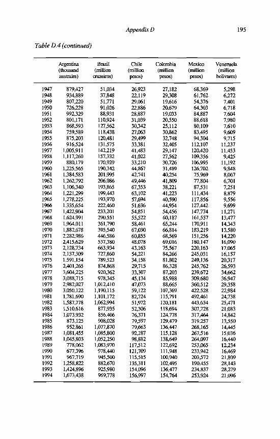
Appendix D
Table D.4 (continued)
195
Argentina(thousandaustrales)
Brazil(million
cruzeiros)
Chile(millionpesos)
Colombia(millionpesos)
Mexico(millionpesos)
Venezuela(million
bolivares)
1947 879,427 51,034 26,923 27,182 68,369 5,2981948 934,889 37,848 22,119 29,308 61,762 6,2721949 807,220 51,771 29,061 19,616 54,376 7,4011950 726,228 91,026 22,886 20,679 64,303 6,7181951 992,329 88,931 28,887 19,033 84,887 7,6041952 801,171 110,924 31,039 20,550 88,618 7,9801953 868,593 127,562 30,342 25,112 80,109 7,6101954 759,589 118,438 27,063 30,862 83,495 9,6091955 875,203 120,481 29,499 32,748 94,304 9,7151956 916,524 131,575 33,381 32,405 112,107 11,2371957 1,005,911 142,219 41,483 29,147 120,420 11,4531958 1,117,260 157,332 41,022 27,562 109,356 9,4251959 880,179 170,929 33,210 30,726 106,995 11,1921960 1,225,565 190,742 44,867 31,489 126,702 9,8481961 1,384,583 201,995 42,741 40,254 75,969 8,0671962 1,262,792 206,086 49,446 41,809 77,804 6,7011963 1,106,340 193,865 67,353 38,221 87,531 7,2511964 1,221,299 199,443 63,102 41,223 111,434 8,8791965 1,278,225 193,970 57,694 40,590 117,856 9,5561966 1,335,654 222,460 51,636 44,954 127,442 9,6991967 1,422,904 233,201 54,851 54,456 147,774 11,2711968 1,624,991 290,551 55,522 60,187 161,557 13,4771969 1,964,011 361,790 58,461 65,244 170,911 14,3431970 1,882,678 395,540 67,030 66,814 183,219 13,5801971 2,282,986 446,586 60,855 68,569 151,256 14,2201972 2,415,629 537,380 48,078 69,016 180,147 16,0901973 2,128,734 663,934 43,163 75,567 220,163 17,0651974 2,137,309 727,860 54,221 84,266 245,031 16,1571975 1,591,154 789,523 34,158 81,802 249,136 20,3171976 2,401,265 874,868 29,715 86,328 245,762 26,5931977 3,604,225 920,362 33,307 87,203 239,672 34,6621978 3,088,715 978,345 45,134 85,988 309,680 36,9471979 2,982,027 1,012,410 47,073 88,665 360,512 29,3581980 3,050,122 1,190,115 59,122 107,369 422,528 22,9841981 1,781,690 1,101,172 82,724 115,791 492,461 24,7381982 1,587,778 1,062,994 51,972 120,181 443,634 25,4711983 1,510,616 877,935 52,306 118,694 307,728 21,0831984 1,073,932 856,406 76,371 124,778 317,464 14,8421985 873,125 908,028 79,597 129,479 319,257 13,5501986 952,861 1,077,870 79,663 136,447 268,165 14,4451987 1,081,455 1,085,800 92,287 115,128 267,516 15,0361988 1,045,803 1,052,250 98,882 138,649 264,097 16,4401989 778,062 1,083,970 117,512 122,692 253,065 12,2341990 677,396 978,440 121,709 111,948 233,942 16,4691991 967,719 945,500 115,515 100,940 203,572 21,8091992 1,258,822 882,670 135,311 102,495 190,455 28,1431993 1,424,896 925,980 154,096 136,477 234,837 28,2791994 1,673,438 969,778 156,997 154,764 253,924 21,096

196 The Economic Development of Latin America
Table D.5 Latin America: Gross Total Fixed Investment, Six Countries, 1900-1994 (as percentage o f GDP a t constant 1980 national currencies)
Argentina Brazil Chile Colombia Mexico Venezuela
1900 16.6 16.2 13.6 10.0 10.1 10.01901 15.9 14.5 15.5 10.0 10.1 10.01902 16.1 9.6 19.1 10.0 10.1 10.01903 15.4 10.9 18.9 10.0 10.1 10.01904 20.1 12.1 23.7 10.0 10.1 10.01905 27.5 16.8 20.1 10.0 10.1 10.01906 31.3 18.1 31.5 10.0 10.1 10.01907 37.8 22.0 34.7 10.0 10.1 10.01908 29.4 24.7 35.4 10.0 10.1 10.01909 31.5 22.9 23.3 10.0 10.1 10.01910 35.2 25.7 20.4 18.0 10.1 15.01911 34.0 31.7 33.1 18.0 0.0 15.01912 25.6 38.1 29.4 18.0 0.0 15.01913 25.7 31.9 28.3 18.0 0.0 15.01914 17.8 13.5 22.6 18.0 0.0 15.01915 10.6 6.9 11.2 18.0 0.0 15.01916 9.7 7.8 17.5 18.0 0.0 15.01917 8.0 6.5 21.9 18.0 0.0 15.01918 6.8 6.0 15.8 18.0 0.0 15.01919 7.7 11.8 20.9 18.0 0.0 15.01920 13.2 16.3 10.1 18.0 10.1 12.91921 14.9 15.9 10.1 18.0 10.1 15.81922 16.2 12.7 10.1 18.0 10.1 14.11923 20.2 14.0 15.2 18.0 10.1 16.81924 20.1 18.8 15.2 18.0 10.1 23.71925 20.3 23.5 22.7 18.9 12.1 33.11926 19.1 19.6 33.6 21.6 9.9 38.41927 20.5 17.5 23.9 23.9 9.3 33.21928 23.0 16.3 20.4 26.4 9.4 26.21929 25.1 19.1 26.5 22.0 10.9 29.81930 22.1 10.7 28.8 14.4 9.4 24.71931 14.5 4.8 18.5 12.1 6.2 16.21932 10.5 4.8 9.5 13.4 4.5 11.71933 11.2 6.9 9.8 12.4 6.1 17.71934 13.8 8.2 11.2 11.9 7.7 17.51935 13.0 9.8 16.2 13.3 8.8 14.31936 13.6 9.6 17.3 13.9 8.5 20.71937 17.0 12.5 18.1 15.9 11.0 23.51938 18.6 11.3 20.6 15.4 5.9 26.81939 15.0 9.9 17.1 16.4 7.2 26.21940 13.0 8.2 18.7 15.4 9.3 22.11941 12.4 7.4 18.5 14.5 10.3 16.51942 11.4 5.5 13.9 12.7 8.5 16.61943 11.2 6.1 14.3 13.5 8.2 16.71944 11.6 8.5 15.9 13.7 9.5 23.11945 11.8 9.0 15.4 16.4 13.2 27.41946 13.5 7.9 20.1 17.7 16.6 31.01947 19.3 18.1 23.6 20.6 18.0 34.01948 18.3 14.0 18.8 19.5 16.4 37.7
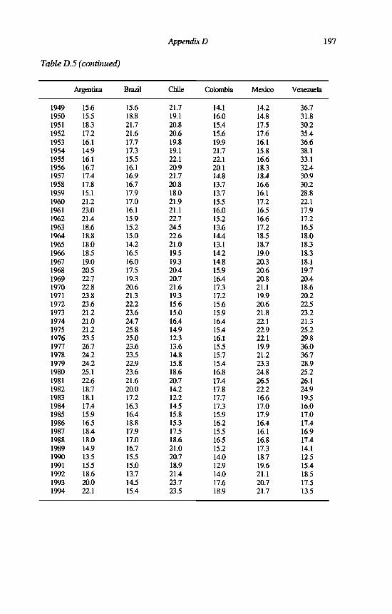
Appendix D
Table D.5 (continued)
197
Argentina Brazil Chile Colombia Mexico Venezuela
1949 15.6 15.6 21.7 14.1 14.2 36.71950 15.5 18.8 19.1 16.0 14.8 31.81951 18.3 21.7 20.8 15.4 17.5 30.21952 17.2 21.6 20.6 15.6 17.6 35.41953 16.1 17.7 19.8 19.9 16.1 36.61954 14.9 17.3 19.1 21.7 15.8 38.11955 16.1 15.5 22.1 22.1 16.6 33.11956 16.7 16.1 20.9 20.1 18.3 32.41957 17.4 16.9 21.7 14.8 18.4 30.91958 17.8 16.7 20.8 13.7 16.6 30.21959 15.1 17.9 18.0 13.7 16.1 28.81960 21.2 17.0 21.9 15.5 17.2 22.11961 23.0 16.1 21.1 16.0 16.5 17.91962 21.4 15.9 22.7 15.2 16.6 17.21963 18.6 15.2 24.5 13.6 17.2 16.51964 18.8 15.0 22.6 14.4 18.5 18.01965 18.0 14.2 21.0 13.1 18.7 18.31966 18.5 16.5 19.5 14.2 19.0 18.31967 19.0 16.0 19.3 14.8 20.3 18.11968 20.5 17.5 20.4 15.9 20.6 19.71969 22.7 19.3 20.7 16.4 20.8 20.41970 22.8 20.6 21.6 17.3 21.1 18.61971 23.8 21.3 19.3 17.2 19.9 20.21972 23.6 22.2 15.6 15.6 20.6 22.51973 21.2 23.6 15.0 15.9 21.8 23.21974 21.0 24.7 16.4 16.4 22.1 21.31975 21.2 25.8 14.9 15.4 22.9 25.21976 23.5 25.0 12.3 16.1 22.1 29.81977 26.7 23.6 13.6 15.5 19.9 36.01978 24.2 23.5 14.8 15.7 21.2 36.71979 24.2 22.9 15.8 15.4 23.3 28.91980 25.1 23.6 18.6 16.8 24.8 25.21981 22.6 21.6 20.7 17.4 26.5 26.11982 18.7 20.0 14.2 17.8 22.2 24.91983 18.1 17.2 12.2 17.7 16.6 19.51984 17.4 16.3 14.5 17.3 17.0 16.01985 15.9 16.4 15.8 15.9 17.9 17.01986 16.5 18.8 15.3 16.2 16.4 17.41987 18.4 17.9 17.5 15.5 16.1 16.91988 18.0 17.0 18.6 16.5 16.8 17.41989 14.9 16.7 21.0 15.2 17.3 14.11990 13.5 15.5 20.7 14.0 18.7 12.51991 15.5 15.0 18.9 12.9 19.6 15.41992 18.6 13.7 21.4 14.0 21.1 18.51993 20.0 14.5 23.7 17.6 20.7 17.51994 22.1 15.4 23.5 18.9 21.7 13.5

198 The Economic Development of Latin America
Table D.6 Latin America: Gross Fixed Investment in Machinery and Equipment, Six Countries, 1900—1994 (as percentage o f GDP a t constant 1980 national currencies)
Argentina Brazil Chile Colombia Mexico Venezuela
1900 1.6 14.1 4.5 3.3 0.0 3.71901 1.2 12.6 5.2 3.3 0.0 3.71902 1.8 6.6 6.4 3.3 0.0 3.71903 2.1 7.8 6.3 3.3 0.0 3.71904 3.1 8.5 7.9 3.3 0.0 3.71905 3.0 12.5 10.1 3.3 0.0 3.71906 3.9 12.7 15.8 3.3 0.0 3.71907 4.1 15.7 17.3 3.3 0.0 3.71908 3.0 18.0 17.7 3.3 0.0 3.71909 3.3 17.4 11.6 3.3 0.0 3.71910 3.5 18.7 10.2 6.0 0.0 5.61911 3.5 24.2 16.6 6.0 0.0 5.61912 3.8 29.2 14.7 6.0 0.0 5.61913 4.1 21.3 14.1 6.0 0.0 5.61914 3.0 8.8 11.3 6.0 0.0 5.61915 2.3 3.5 5.6 6.0 0.0 5.61916 2.4 4.3 5.8 6.0 0.0 5.61917 2.1 4.1 7.3 6.0 0.0 5.61918 1.5 4.6 5.3 6.0 0.0 5.61919 2.0 7.6 7.0 6.0 0.0 5.61920 3.0 11.5 5.2 6.0 2.4 6.01921 3.2 13.2 7.1 6.0 2.4 6.71922 2.7 8.7 7.2 6.0 2.4 6.6
1923 3.5 10.4 7.6 6.0 2.4 7.61924 4.1 13.1 8.5 6.0 2.4 10.11925 4.8 17.9 8.2 6.7 2.8 12.41926 5.0 13.3 12.2 7.5 2.4 15.21927 4.7 11.2 8.5 9.5 2.3 12.6
1928 5.3 11.3 7.2 10.8 2.5 11.11929 5.6 14.1 9.4 8.3 2.7 11.71930 4.2 8.1 10.2 3.5 2.3 10.41931 3.0 3.0 6.4 1.9 1.5 6.81932 2.0 2.8 1.7 1.7 0.9 5.11933 2.1 3.9 1.4 2.2 1.0 6.91934 2.4 4.5 2.3 2.9 1.3 7.31935 3.0 6.5 4.3 2.8 1.6 6.91936 3.1 5.6 5.0 3.5 1.6 9.01937 4.2 7.6 5.0 4.5 1.9 11.31938 4.6 7.5 5.6 4.6 1.1 12.41939 3.3 5.4 4.4 4.5 1.3 12.91940 2.8 3.6 4.9 3.3 1.5 11.51941 2.5 3.6 4.7 3.0 1.7 8.81942 2.0 2.5 3.6 1.1 0.9 7.71943 1.7 2.9 3.6 1.1 0.9 6.11944 1.6 4.2 3.1 1.7 1.3 9.41945 1.7 4.5 3.3 4.1 2.7 12.31946 2.6 6.7 4.6 5.7 3.1 13.8

Appendix D
Table D .6 (continued)
199
Argentina Brazil Chile Colombia Mexico Venezuela
1947 5.9 10.4 7.2 8.1 3.5 17.51948 4.5 8.2 5.9 6.3 3.3 20.31949 2.7 8.9 7.1 4.9 2.7 17.71950 2.6 9.2 6.2 6.3 2.7 14.51951 3.8 12.3 7.1 6.8 3.3 10.41952 3.5 11.2 7.0 6.9 3.1 15.61953 3.1 6.3 6.0 9.8 3.2 16.71954 2.9 7.6 5.3 10.1 2.9 18.01955 3.6 6.0 6.6 10.2 3.1 14.41956 3.9 6.2 7.7 8.8 3.3 12.51957 4.1 7.1 9.2 4.8 3.4 13.41958 3.9 6.6 9.0 4.5 3.0 13.61959 3.4 7.6 6.3 4.2 3.0 13.71960 6.0 6.6 7.5 6.1 3.1 8.81961 7.0 6.3 8.6 6.3 6.6 7.61962 6.5 6.2 7.8 5.6 6.6 8.11963 5.3 6.0 6.5 5.1 6.9 7.21964 5.5 5.9 6.9 5.7 7.4 7.51965 5.3 5.4 6.0 4.9 7.4 7.21966 5.4 6.9 6.7 5.5 7.6 7.11967 5.4 6.5 6.7 4.8 8.1 6.41968 5.7 7.2 7.4 5.4 8.2 6.81969 6.3 7.9 7.0 5.7 8.3 7.51970 6.3 8.6 7.3 6.9 8.4 6.71971 6.6 9.2 6.1 7.2 7.9 7.51972 6.9 9.4 4.7 6.6 8.2 8.31973 6.6 10.0 5.4 6.1 8.9 8.71974 6.2 11.0 5.0 6.4 9.3 8.51975 5.9 11.7 5.8 6.2 9.8 10.81976 6.2 11.0 5.0 6.8 9.0 12.91977 8.2 9.5 6.3 6.3 7.7 16.51978 6.5 9.3 7.2 6.9 8.4 16.11979 7.3 9.0 7.7 7.2 10.0 11.21980 8.1 9.0 8.6 7.7 10.9 10.21981 9.3 7.3 9.4 7.9 11.9 11.31982 6.9 6.1 5.9 8.0 8.5 11.41983 7.4 5.0 4.2 7.7 5.5 7.91984 7.8 4.9 4.5 7.3 5.9 7.71985 6.9 5.2 5.1 5.8 6.7 9.41986 7.3 6.4 4.6 6.1 5.9 9.91987 8.2 5.9 6.0 6.8 5.6 9.41988 7.8 5.4 6.7 7.1 6.6 9.91989 6.8 5.0 8.0 6.7 7.1 8.01990 6.3 4.6 7.8 6.7 8.2 5.61991 6.1 4.4 6.8 5.8 9.1 7.31992 7.3 3.8 8.5 6.5 10.2 8.51993 7.8 4.5 9.7 8.3 9.6 7.41994 8.7 5.5 9.8 8.9 10.0 5.7

200 The Economic Development of Latin America
Table D .7 Latin America: Gross Fixed Investment in Residential Structures, Six Countries, 1900-1994 (as percentage o f GDP a t constant 1980 national currencies)
Argentina Brazil Chile Colombia Mexico Venezuela
1900 12.9 0.9 2.7 1.7 1.0 3.11901 11.8 0.8 4.4 1.7 1.0 3.11902 11.0 1.2 5.5 1.7 1.0 3.11903 9.4 1.3 5.4 1.7 1.0 3.11904 9.2 1.9 6.8 1.7 1.0 3.11905 13.2 2.5 4.3 1.7 1.0 3.11906 15.8 3.4 6.8 1.7 1.0 3.11907 22.2 2.9 7.5 1.7 1.0 3.11908 19.7 3.6 7.6 1.7 1.0 3.11909 18.6 3.3 5.0 1.7 1.0 3.11910 22.1 4.1 4.4 3.0 1.0 4.71911 21.6 4.1 7.1 3.0 0.0 4.71912 15.3 5.1 6.3 3.0 0.0 4.71913 15.2 6.3 6.1 3.0 0.0 4.71914 7.5 2.4 4.9 3.0 0.0 4.71915 3.8 2.0 2.4 3.0 0.0 4.71916 3.3 2.2 5.0 3.0 0.0 4.71917 2.8 1.2 6.3 3.0 0.0 4.71918 3.0 0.6 4.5 3.0 0.0 4.71919 3.3 2.3 6.0 3.0 0.0 4.71920 6.7 1.8 2.1 3.0 1.1 3.41921 7.5 1.6 1.3 3.0 0.8 3.41922 9.3 3.0 1.2 3.0 0.9 3.31923 12.6 1.9 3.2 3.0 0.9 3.31924 11.2 2.7 2.9 3.0 1.1 3.11925 10.3 3.5 6.2 1.8 1.0 2.8
1926 8.2 3.8 9.2 2.3 0.9 2.61927 8.5 3.7 6.5 2.7 1.1 2.51928 9.4 3.2 5.6 3.4 1.0 2.71929 11.3 3.2 5.7 3.6 1.0 2.71930 10.5 1.8 4.7 2.6 1.2 2.81931 7.6 1.1 2.8 2.4 1.2 2.91932 5.5 1.2 3.6 2.8 1.6 3.01933 5.0 2.2 4.0 3.4 1.6 2.91934 6.1 3.1 6.3 2.8 1.6 2.91935 4.4 3.0 6.6 3.2 1.6 3.01936 3.8 3.0 5.5 3.2 1.7 2.71937 4.9 3.3 6.1 3.9 1.8 2.71938 5.2 3.0 5.7 3.6 1.9 2.61939 5.3 3.2 7.0 4.3 2.1 2.71940 4.7 3.3 7.7 4.2 1.8 2.81941 5.3 2.7 7.6 3.8 1.8 2.81942 5.8 2.7 6.3 4.0 1.9 2.81943 6.2 2.7 7.4 4.2 2.0 2.81944 6.3 3.0 8.4 3.6 2.1 2.71945 6.4 3.0 6.0 3.5 2.2 2.61946 6.5 0.8 10.0 3.5 2.3 2.5

Appendix D
Table D.7(continued)
201
Argentina Brazil Chile Colombia Mexico Venezuela
1947 6.1 3.8 8.3 4.0 2.4 2.51948 6.4 3.2 6.8 4.4 2.6 2.41949 6.4 3.4 6.6 3.6 2.7 2.41950 7.2 4.1 6.8 3.9 2.7 2.61951 7.0 4.3 6.4 3.5 2.6 4.91952 7.3 4.5 6.2 3.5 2.7 5.21953 6.4 4.8 6.9 4.0 2.8 6.81954 6.4 4.3 7.7 4.6 2.9 5.11955 6.5 4.2 8.9 4.7 3.0 4.71956 6.7 4.3 5.8 4.5 3.1 5.31957 7.0 4.3 4.0 4.0 3.2 4.11958 7.3 4.3 3.7 3.7 3.3 5.81959 6.1 4.4 5.1 3.8 3.5 3.11960 8.0 4.3 6.1 3.7 3.5 3.01961 8.4 4.1 4.9 2.9 3.9 2.21962 7.8 4.1 6.5 2.9 4.1 2.91963 7.0 4.0 7.3 2.6 4.2 3.01964 7.0 4.0 5.8 2.6 4.1 3.61965 6.8 3.9 6.1 2.5 4.2 4.01966 7.0 4.2 5.7 2.6 4.4 4.21967 7.3 4.2 5.2 3.0 4.5 3.91968 8.0 4.3 5.7 3.1 4.6 3.91969 8.9 4.5 6.3 3.2 4.8 3.81970 9.7 4.7 6.0 3.2 4.9 3.81971 9.3 4.7 6.4 3.0 5.8 4.51972 8.6 4.8 5.4 2.5 5.6 5.31973 7.8 4.9 4.6 3.1 5.3 5.51974 8.3 4.9 5.2 2.9 4.9 4.81975 10.5 5.0 4.5 2.4 5.4 5.01976 10.1 5.0 3.5 2.5 5.8 5.61977 8.4 5.0 3.3 2.6 5.3 5.71978 8.8 5.1 2.6 2.8 4.6 6.11979 8.9 4.9 3.3 2.4 4.6 6.41980 9.0 5.1 4.4 2.3 4.4 6.01981 8.4 5.1 3.9 2.4 4.4 5.01982 7.4 5.1 2.9 2.4 4.5 3.61983 6.6 4.7 2.4 2.8 4.4 2.81984 6.6 4.5 2.3 2.8 4.5 2.11985 6.5 4.4 2.9 2.8 4.7 1.91986 6.7 4.8 3.3 2.8 4.8 1.81987 7.4 4.7 3.5 2.9 5.0 1.81988 7.4 4.5 3.9 2.7 4.8 1.61989 5.9 4.5 4.3 2.6 5.2 1.41990 5.2 4.3 4.2 2.3 6.1 0.81991 6.9 4.1 4.4 2.7 6.7 0.81992 8.3 3.9 4.8 3.0 7.5 1.01993 8.9 3.9 5.3 3.8 7.0 1.01994 9.9 3.9 5.2 4.1 7.3 0.8
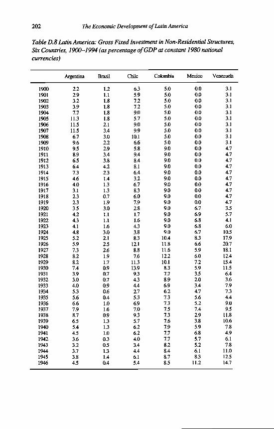
202 The Economic Development of Latin America
Table D .8 Latin America: Gross Fixed Investment in Non-Residential Structures, Six Countries, 1900—1994 (as percentage o f GDP at constant 1980 national currencies)
Argentina Brazil Chile Colombia Mexico Venezuela
1900 2.2 1.2 6.3 5.0 0.0 3.11901 2.9 1.1 5.9 5.0 0.0 3.11902 3.2 1.8 7.2 5.0 0.0 3.11903 3.9 1.8 7.2 5.0 0.0 3.11904 7.7 1.8 9.0 5.0 0.0 3.11905 11.3 1.8 5.7 5.0 0.0 3.11906 11.5 2.1 9.0 5.0 0.0 3.11907 11.5 3.4 9.9 5.0 0.0 3.11908 6.7 3.0 10.1 5.0 0.0 3.11909 9.6 2.2 6.6 5.0 0.0 3.11910 9.5 2.9 5.8 9.0 0.0 4.71911 8.9 3.4 9.4 9.0 0.0 4.71912 6.5 3.8 8.4 9.0 0.0 4.71913 6.4 4.2 8.1 9.0 0.0 4.71914 7.3 2.3 6.4 9.0 0.0 4.71915 4.6 1.4 3.2 9.0 0.0 4.71916 4.0 1.3 6.7 9.0 0.0 4.71917 3.1 1.3 8.3 9.0 0.0 4.71918 2.3 0.7 6.0 9.0 0.0 4.71919 2.3 1.9 7.9 9.0 0.0 4.71920 3.5 3.0 2.8 9.0 6.7 3.51921 4.2 1.1 1.7 9.0 6.9 5.71922 4.3 1.1 1.6 9.0 6.8 4.11923 4.1 1.6 4.3 9.0 6.8 6.01924 4.8 3.0 3.8 9.0 6.7 10.51925 5.2 2.1 8.3 10.4 8.3 17.91926 5.9 2.5 12.1 11.8 6.6 20.71927 7.3 2.6 8.8 11.6 5.9 18.11928 8.2 1.9 7.6 12.2 6.0 12.41929 8.2 1.7 11.3 10.1 7.2 15.41930 7.4 0.9 13.9 8.3 5.9 11.51931 3.9 0.7 9.3 7.7 3.5 6.41932 3.0 0.7 4.3 8.9 2.0 3.61933 4.0 0.9 4.4 6.9 3.4 7.91934 5.3 0.6 2.7 6.2 4.7 7.31935 5.6 0.4 5.3 7.3 5.6 4.41936 6.6 1.0 6.9 7.3 5.2 9.01937 7.9 1.6 7.0 7.5 7.4 9.51938 8.7 0.9 9.3 7.3 2.9 11.81939 6.5 1.3 5.7 7.6 3.8 10.61940 5.4 1.3 6.2 7.9 5.9 7.81941 4.5 1.0 6.2 7.7 6.8 4.91942 3.6 0.3 4.0 7.7 5.7 6.11943 3.2 0.5 3.4 8.2 5.2 7.81944 3.7 1.3 4.4 8.4 6.1 11.01945 3.8 1.4 6.1 8.7 8.3 12.51946 4.5 0.4 5.4 8.5 11.2 14.7
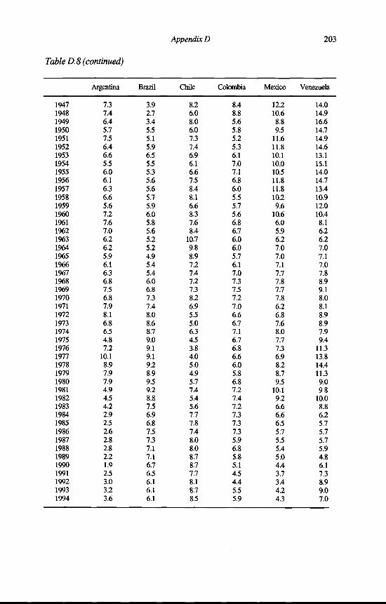
Appendix D
Table D .8 (continued)
203
Argentina Brazil Chile Colombia Mexico Venezuela
1947 7.3 3.9 8.2 8.4 12.2 14.01948 7.4 2.7 6.0 8.8 10.6 14.91949 6.4 3.4 8.0 5.6 8.8 16.61950 5.7 5.5 6.0 5.8 9.5 14.71951 7.5 5.1 7.3 5.2 11.6 14.91952 6.4 5.9 7.4 5.3 11.8 14.61953 6.6 6.5 6.9 6.1 10.1 13.11954 5.5 5.5 6.1 7.0 10.0 15.11955 6.0 5.3 6.6 7.1 10.5 14.01956 6.1 5.6 7.5 6.8 11.8 14.71957 6.3 5.6 8.4 6.0 11.8 13.41958 6.6 5.7 8.1 5.5 10.2 10.91959 5.6 5.9 6.6 5.7 9.6 12.01960 7.2 6.0 8.3 5.6 10.6 10.41961 7.6 5.8 7.6 6.8 6.0 8.11962 7.0 5.6 8.4 6.7 5.9 6.21963 6.2 5.2 10.7 6.0 6.2 6.21964 6.2 5.2 9.8 6.0 7.0 7.01965 5.9 4.9 8.9 5.7 7.0 7.11966 6.1 5.4 7.2 6.1 7.1 7.01967 6.3 5.4 7.4 7.0 7.7 7.81968 6.8 6.0 7.2 7.3 7.8 8.91969 7.5 6.8 7.3 7.5 7.7 9.11970 6.8 7.3 8.2 7.2 7.8 8.01971 7.9 7.4 6.9 7.0 6.2 8.11972 8.1 8.0 5.5 6.6 6.8 8.91973 6.8 8.6 5.0 6.7 7.6 8.91974 6.5 8.7 6.3 7.1 8.0 7.91975 4.8 9.0 4.5 6.7 7.7 9.41976 7.2 9.1 3.8 6.8 7.3 11.31977 10.1 9.1 4.0 6.6 6.9 13.81978 8.9 9.2 5.0 6.0 8.2 14.41979 7.9 8.9 4.9 5.8 8.7 11.31980 7.9 9.5 5.7 6.8 9.5 9.01981 4.9 9.2 7.4 7.2 10.1 9.81982 4.5 8.8 5.4 7.4 9.2 10.01983 4.2 7.5 5.6 7.2 6.6 8.81984 2.9 6.9 7.7 7.3 6.6 6.21985 2.5 6.8 7.8 7.3 6.5 5.71986 2.6 7.5 7.4 7.3 5.7 5.71987 2.8 7.3 8.0 5.9 5.5 5.71988 2.8 7.1 8.0 6.8 5.4 5.91989 2.2 7.1 8.7 5.8 5.0 4.81990 1.9 6.7 8.7 5.1 4.4 6.11991 2.5 6.5 7.7 4.5 3.7 7.31992 3.0 6.1 8.1 4.4 3.4 8.91993 3.2 6.1 8.7 5.5 4.2 9.01994 3.6 6.1 8.5 5.9 4.3 7.0

204 The Economic Development of Latin America
NOTES
1. The source note is the same as in Appendix B but includes also the disaggregation of capital formation.
2. Banco Central de la República de Argentina (1991) is only available in mimeographed form and was never published officially.
3. Of which no official estimates were available since 1973.

Appendix E. Standardised Estimates of Capital Stock
This appendix presents standardised gross and net fixed capital stock estim ates, starting with the estimation o f the initial capital stock and subsequently the yearly additions to the gross and net stocks. It gives the potential user the possibility to check on our assumptions and eventually replicate the capital stock estim ates using different assumptions about, for exam ple, service lives.
In the second part o f this appendix a set o f four tables for each o f the Latin American countries and the U SA is presented, giving gross and net fixed tangible reproducible capital stocks for 1950-94 in national currencies and 1980 international dollars. It also presents, again on the basis o f estim ates in national currencies and 1980 international dollars, average ages, average service lives and capital-output ratios for 1950-94. A s indicated in Chapter 6 the capital stocks have been generated applying the perpetual inventory method which estim ates capital stocks as a weighted sum o f past investment flow s. The detailed sources used for the calculation o f the investment series used in the capital stock estimation are given in Appendix D.
A very crucial elem ent in international comparisons is how to convert estim ates in local currencies into estim ates expressed in a common currency, either existing, for example the US dollar, or fictitious such as the concept o f the constant 1980 international dollar.1 The use o f exchange rates as the conversion factor is the easiest and most direct way,2 but the official exchange rate basically reflects the purchasing power o f tradable goods and services and does not include the non-tradables, and thus may give rise to distortions. See Chapter 6 for a detailed description o f real incom e estimation in Latin America.
In Table E .l the disaggregated PPPs with respect to capital formation are presented with the resulting PPP-exchange rate deviation index as estimated by various phases o f ICP which is still the only source for this kind o f disaggregated information. Here the results for the two estim ates for 1980, ICP IV and AH are given, and these PPPs are also analysed for the 1970-80 period since for 1985 we do not dispose o f the disaggregation. Comparing the ICP IV and AH 1980 results it becom es directly clear that the main difference occurred in the case o f non-residential structures. In this case the results for ICP IV are not very reliable as a major transcription error occurred.
205

206 The Economic Development o f Latin America
In analysing the PPPs o f the components o f gross investment in tim e the pattern is obviously not as uniform as in the case o f total GDP, but the deviation index o f machinery and equipment is higher in all cases. Non-residential structures PPPs are generally lower. In the case o f Colom bia, with five observations, the first three (1970,1973 and 1975) are alm ost identical, and also the 1980 estimates show a fairly stable tendency. In the case o f Brazil the estim ates for 1975 and 1980 are rather similar, as is the case in M exico although with somewhat higher differences.
It is in the light o f all the abovementioned that this appendix shows capital stock estimates both in national currencies and at international prices, therefore giving the potential user the option to apply other PPPs or exchange rates than the ones used by us, without having to go through the whole procedure o f calculating the capital stock. The application o f these disaggregated PPPs has, as shown in Chapter 6, a great impact on the capital stock levels. Tables E.2 and E.3 give a step-by-step explanation o f the procedures used to calculate the capital stock using as an exam ple non-residential stock estim ation in Argentina.

Appendix E 207
Table E .l Capital Formation PPPs-Exchange Rate Deviation Index, 1970-80 (national currency units per international dollar)
Argentina Brazil Chile Colombia Mexico Venezuela
PPPs of capital formation1970 (ICP phase I)
Res. 4.3N.R. 4.5M&E 21.6
1973 (ICP phase II)Res. 5.2N.R. 5.5M&E 32.5
1975 (ICP phase HI)Res. 4.6 8.3 6.6N.R. 5.4 7.4 5.9M&E 7.6 4.3 17.0
1980 (ICP phase IV)Res. 4025 33.7 52.2 20.1 5.1N.R. 1389 27.1 15.4 17.6 6.4M&E 3959 46.3 51.2 53.6 4.55
1980 (Alan Heston)Res. 4057 32.0 52.1 19.6 16.2 5.5N.R. 4670 25.9 27.0 22.3 19.2 5.1M&E 3899 47.0 50.7 54.8 21.2 4.5
PPP-Exchange rate deviation index1970 (ICP phase I)
Res. 0.23N.R. 0.25M&E 1.18
1973 (ICP phase II)Res. 0.22N.R. 0.23M&E 1.36
1975 (ICP phase HI)Res. 0.56 0.27 0.53N.R. 0.66 0.24 0.47M&E 0.93 1.38 1.34
1980 (ICP phase IV)Res. 2.19 0.64 1.34 0.42 1.19N.R. 0.76 0.51 0.39 0.37 1.49M&E 2.15 0.88 1.31 1.13 1.06
1980 (Alan Heston)Res. 2.21 0.61 1.34 0.41 0.70 1.29N.R. 2.54 0.49 0.69 0.47 0.83 1.20M&E 2.12 0.89 1.30 1.16 0.92 1.06
Notes: Res. = Residential; N.R. = Non-residential; M&E = Machinery and equipment
Source: Table 5.2.
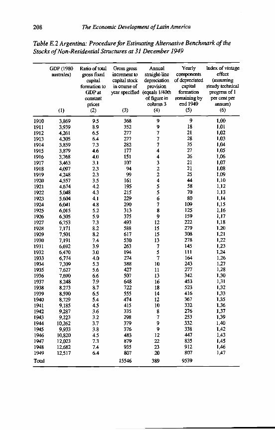
208 The Economic Development of Latin America
Table E.2 Argentina: Procedure fo r Estimating Alternative Benchmark o f the Stocks o f Non-Residential Structures a t 31 December 1949
GDP (1980 Ratio of total australes) gross fixed
capital formation to
GDP at constant prices
(1) (2)
Gross gross Annual increment to straight-line capital stock depreciation in course of provision
year specified (equals l/40th of figure in column 3
(3) (4)
Yearly components
of depreciated capital
formation remaining by
end 1949 (5)
Index of vintage effect
(assuming steady technical
progress of 1 per cent per
annum)(6)
1910 3,869 9.5 368 9 9 1,00
1911 3,939 8.9 352 9 18 1,011912 4,261 6.5 277 7 21 1,02
1913 4,305 6.4 277 7 28 1,031914 3,859 7.3 282 7 35 1,041915 3,879 4.6 177 4 27 1,051916 3,768 4.0 151 4 26 1,061917 3,463 3.1 107 3 21 1,071918 4,097 2.3 94 2 21 1,081919 4,248 2.3 99 2 25 1,091920 4,557 3.5 161 4 44 1,101921 4,674 4.2 195 5 58 1,121922 5,048 4.3 215 5 70 1,131923 5,604 4.1 229 6 80 1,141924 6,041 4.8 290 7 109 1,151925 6,015 5.2 313 8 125 1,161926 6,305 5.9 375 9 159 1,171927 6,753 7.3 493 12 222 1,181928 7,171 8.2 588 15 279 1,201929 7,501 8.2 617 15 308 1,21
1930 7,191 7.4 530 13 278 1,22
1931 6,692 3.9 263 7 145 1,231932 6,470 3.0 194 5 111 1,241933 6,774 4.0 274 7 164 1,261934 7,309 5.3 388 10 243 1,271935 7,627 5.6 427 11 277 1,281936 7,690 6.6 507 13 342 1,301937 8,248 7.9 648 16 453 1,311938 8,273 8.7 722 18 523 1,321939 8,590 6.5 555 14 416 1,331940 8,729 5.4 474 12 367 1,351941 9,185 4.5 415 10 332 1,361942 9,287 3.6 335 8 276 1,371943 9,223 3.2 298 7 253 1,391944 10,262 3.7 379 9 332 1,401945 9,933 3.8 376 9 338 1,421946 10,820 4.5 483 12 447 1,431947 12,023 7.3 879 22 835 1,451948 12,682 7.4 935 23 912 1,461949 12,517 6.4 807 20 807 1,47Total 15546 389 9539

209
Table E.3 Argentina: Procedure fo r Estimating Alternative Variants o f 1950—94 Estimates o f the Stock o f Non-Residential Structures
(1 ) (2 ) (3) (4) (5) (6) (7) (8) (9) (10 ) (1 1 ) (1 2 ) (13) (14) (15) (16)
1949 12517 6.4 807 15546 9539 16.46 10.521950 12669 5.7 726 368 359 15904 389 338 9877 16.16 10.55 15725 9708 12716 0.8 1.2
1951 13161 7.5 992 352 641 16545 398 595 10471 15.68 10.28 16225 10174 13199 0.8 1.2
1952 12498 6.4 801 277 524 17069 414 388 10859 15.55 10.21 16807 10665 13736 0.9 1.31953 13161 6.6 869 277 591 17660 427 442 11301 15.40 10.14 17365 11080 14222 0.8 1.31954 13704 5.5 760 282 478 18138 442 318 11619 15.38 10.14 17899 11460 14680 0.8 1.31955 14672 6.0 875 177 698 18837 453 422 12041 15.43 10 .11 18487 11830 15159 0.8 1.31956 15080 6.1 917 151 765 19602 471 446 12486 15.52 10 .12 19219 12263 15741 0.8 1.31957 15861 6.3 1006 107 899 20501 490 516 13002 15.63 10.20 20052 12744 16398 0.8 1.31958 16829 6.6 1117 94 1023 21524 513 605 13607 15.71 10.31 21013 13304 17159 0.8 1.2
1959 15742 5.6 880 99 781 22305 538 342 13949 15.99 10.48 21915 13778 17846 0.9 1.41960 16982 7.2 1226 161 1065 23370 558 668 14617 15.98 10.32 22837 14283 18560 0.8 1.31961 18188 7.6 1385 195 1190 24560 584 800 15417 15.89 10.12 23965 15017 19491 0.8 1.31962 18032 7.0 1263 215 1048 25608 614 649 16066 15.90 10.07 25084 15741 20413 0.9 1.41963 17735 6.2 1106 229 877 26485 640 466 16532 16.03 10.14 26046 16299 21173 0.9 1.51964 19707 6.2 1221 290 931 27416 662 559 17091 16.06 10.15 26951 16812 21881 0.9 1.41965 21673 5.9 1278 313 966 28382 685 593 17684 16.08 10.17 27899 17388 22643 0.8 1.31966 21974 6.1 1336 375 961 29342 710 626 18310 16.04 10.27 28862 17997 23430 0.8 1.31967 22723 6.3 1423 493 930 30273 734 689 18999 15.90 10.26 29808 18655 24231 0.8 1.31968 23876 6.8 1625 588 1037 31310 757 868 19868 15.62 10 .11 30791 19434 25112 0.8 1.31969 26106 7.5 1964 617 1347 32657 783 1181 21049 15.22 9.96 31983 20458 26221 0.8 1.2
1970 27715 6.8 1883 530 1353 34009 816 1066 22115 14.99 9.95 33333 21582 27457 0.8 1.2
1971 28970 7.9 2283 263 2020 36029 850 1433 23548 14.86 9.79 35019 22832 28925 0.8 1.2
1972 29791 8.1 2416 194 2222 38251 901 1515 25063 14.79 9.64 37140 24305 30723 0.8 1.2
1973 31136 6.8 2129 274 1855 40106 956 1172 26235 14.83 9.64 39179 25649 32414 0.8 1.31974 33062 6.5 2137 388 1749 41855 1003 1135 27370 14.84 9.59 40981 26803 33892 0.8 1.2
1975 33110 4.8 1591 427 1165 43020 1046 545 27915 15.04 9.83 42437 27642 35040 0.8 1.31976 33353 7.2 2401 507 1894 44914 1075 1326 29240 14.96 9.80 43967 28578 36272 0.9 1.31977 35745 10.1 3604 648 2957 47871 1123 2481 31722 14.49 9.49 46392 30481 38437 0.9 1.3
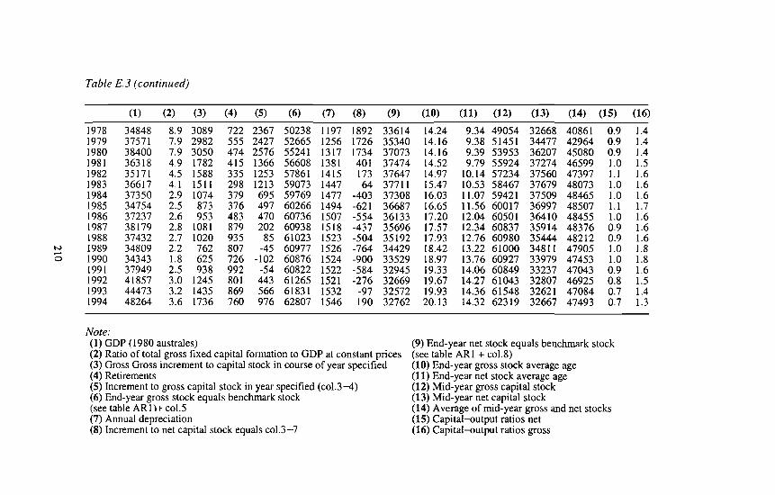
Table E.3 (continued)
(1) (2) (3) (4) (5) (6) (7) (8) (9) (10) (11) (12) (13) (14) (15) (16)
1978 34848 8.9 3089 722 2367 50238 1197 1892 33614 14.24 9.34 49054 32668 40861 0.9 1.41979 37571 7.9 2982 555 2427 52665 1256 1726 35340 14.16 9.38 51451 34477 42964 0.9 1.41980 38400 7.9 3050 474 2576 55241 1317 1734 37073 14.16 9.39 53953 36207 45080 0.9 1.41981 36318 4.9 1782 415 1366 56608 1381 401 37474 14.52 9.79 55924 37274 46599 1.0 1.51982 35171 4.5 1588 335 1253 57861 1415 173 37647 14.97 10.14 57234 37560 47397 1.1 1.61983 36617 4.1 1511 298 1213 59073 1447 64 37711 15.47 10.53 58467 37679 48073 1.0 1.61984 37350 2.9 1074 379 695 59769 1477 -403 37308 16.03 11.07 59421 37509 48465 1.0 1.61985 34754 2.5 873 376 497 60266 1494 -621 36687 16.65 11.56 60017 36997 48507 1.1 1.71986 37237 2.6 953 483 470 60736 1507 -554 36133 17.20 12.04 60501 36410 48455 1.0 1.61987 38179 2.8 1081 879 202 60938 1518 -437 35696 17.57 12.34 60837 35914 48376 0.9 1.61988 37432 2.7 1020 935 85 61023 1523 -504 35192 17.93 12.76 60980 35444 48212 0.9 1.61989 34809 2.2 762 807 -45 60977 1526 -764 34429 18.42 13.22 61000 34811 47905 1.0 1.81990 34343 1.8 625 726 -10 2 60876 1524 -900 33529 18.97 13.76 60927 33979 47453 1.0 1.81991 37949 2.5 938 992 -54 60822 1522 -584 32945 19.33 14.06 60849 33237 47043 0.9 1.61992 41857 3.0 1245 801 443 61265 1521 -276 32669 19.67 14.27 61043 32807 46925 0.8 1.51993 44473 3.2 1435 869 566 61831 1532 -97 32572 19.93 14.36 61548 32621 47084 0.7 1.41994 48264 3.6 1736 760 976 62807 1546 190 32762 20.13 14.32 62319 32667 47493 0.7 1.3
Note:(1) GDP (1980 australes)(2) Ratio o f total gross fixed capital form ation to GDP at constant prices(3) Gross Gross increm ent to capital stock in course of year specified(4) Retirements(5) Increm ent to gross capital stock in year specified (col.3 -4 )(6) End-year gross stock equals benchmark stock (see table A R1H co l.5(7) Annual depreciation(8) Increm ent to net capital stock equals col.3 -7
(9) End-year net stock equals benchmark stock (see table AR1 + col.8)(10) End-year gross stock average age(11) End-year net stock average age(12) M id-year gross capital stock(13) M id-year net capital stock(14) A verage o f m id-year gross and net stocks(15) C apital-ou tpu t ratios net(16) C apital-ou tpu t ratios gross

1 U O I
Stoc,
Mid-;
19501951195219531954195519561957195819591960196119621963196419651966196719681969197019711972197319741975197619771978197919801981198219831984198519861987198819891990199119921993
Appendix E 211
Gross and Net Fixed Tangible Reproducible Capital >e o f Asset, 1950-94 (constant 1980 australes)
Gross stocksNon-residential
Total Total M&E Structures Res.
45,084 20,304 4,579 15,725 24,78146,429 20,982 4,757 16,225 25,44747,863 21,737 4,930 16,807 26,12549,131 22,354 4,989 17,365 26,77750,369 22,959 5,060 17,899 27,40951,762 23,743 5,256 18,487 28,01953,362 24,7% 5,577 19,219 28,56755,071 26,040 5,988 20,052 29,03156,992 27,483 6,470 21,013 29,50958,751 28,823 6,908 21,915 29,92860,679 30,356 7,519 22,837 30,32363,318 32,404 8,439 23,%5 30,91465,891 34,254 9,170 25,084 31,63767,949 35,636 9,590 26,046 32,31370,256 37,097 10,147 26,951 33,15973,200 38,832 10,933 27,899 34,36876,291 40,553 11,691 28,862 35,73879,468 42,239 12,431 29,808 37,22982,999 44,0% 13,305 30,791 38,90387,280 46,391 14,408 31,983 40,89092,146 48,971 15,638 33,333 43,17597,461 51,927 16,907 35,019 45,535
103,168 55,421 18,281 37,140 47,747108,508 58,860 19,681 39,179 49,649113,651 62,114 21,133 40,981 51,537118,794 64,797 22,360 42,437 53,997124,038 67,193 23,226 43,%7 56,845130,383 70,901 24,508 46,392 59,482136,999 75,110 26,056 49,054 61,889143,335 78,999 27,548 51,451 64,336150,251 83,297 29,344 53,953 66,954156,915 87,330 31,406 55,924 69,585162,284 90,317 33,082 57,234 71,%8166,904 92,804 34,337 58,467 74,100171,178 95,052 35,631 59,421 76,126174,685 %,602 36,585 60,017 78,083177,931 97,809 37308 60,501 80,122181,487 99,064 38,228 60,837 82,423184,887 100,124 39,144 60,980 84,763187,353 100,677 39,677 61,000 86,676188,891 100,797 39,870 60,927 88,094190,608 100,857 40,009 60,849 89,751193,369 101,166 40,122 61,043 92,203197,614 102,2% 40,748 61,548 95,318203,506 104,412 42,093 62,319 99,094

212
Tabl
Mid-;
195019511952195319541955195619571958195919601961196219631964196519661967196819691970197119721973197419751976197719781979198019811982198319841985198619871988198919901991199219931994
ed) A & i j
Net stocks
The Economic Development of Latin America
Non-residential
Total Total M&E Structures Res.
26,089 12,374 2,666 9,708 13,71527,079 12,947 2,773 10,174 14,13228,126 13,590 2,925 10,665 14,53628,987 14,101 3,021 11,080 14,88729,763 14,551 3,091 11,460 15,21230,629 15,043 3,214 11,830 15,58531,694 15,687 3,423 12,263 16,00732,905 16,415 3,671 12,744 16,49034,303 17,230 3,926 13,304 17,07335,447 17,870 4,092 13,778 17,57736,824 18,687 4,405 14,283 18,13739,036 20,061 5,044 15,017 18,97541,276 21,445 5,704 15,741 19,83142,980 22,452 6,153 16,299 20,52744,539 23,342 6,530 16,812 21,19846,323 24,361 6,974 17,388 21,96248,193 25,413 7,415 17,997 22,78050,168 26,500 7,845 18,655 23,66752,455 27,748 8,314 19,434 24,70755,438 29,391 8,933 20,458 26,04658,983 31,245 9,663 21,582 27,73862,845 33,281 10,450 22,832 29,56366,896 35,621 11,315 24,305 31,27670,611 37,800 12,151 25,649 32,81074,089 39,692 12,889 26,803 34,39877,599 41,122 13,479 27,642 36,47781,388 42,573 13,996 28,578 38,81586,295 45,433 14,952 30,481 40,86291,301 48,595 15,927 32,668 42,70695,850 51,174 16,697 34,477 44,676
100,791 53,984 17,778 36,207 46,806105,055 56,327 19,053 37,274 48,728107,556 57,406 19,845 37,560 50,150109,064 57,871 20,192 37,679 51,193110,341 58,212 20,703 37,509 52,129110,923 57,970 20,972 36,997 52,954111,243 57,495 21,085 36,410 53,748112,219 57,425 21,510 35,914 54,794113,281 57,377 21,933 35,444 55,904113,285 56,717 21,907 34,811 56,567112,118 55,433 21,454 33,979 56,686111,209 54,178 20,941 33,237 57,031111,904 53,700 20,892 32,807 58,204114,107 54,073 21,452 32,621 60,034117,768 55,255 22,588 32,667 62,513

Mid-;
195019511952195319541955195619571958195919601961196219631964196519661967196819691970197119721973197419751976197719781979198019811982198319841985198619871988198919901991199219931994
Appendix E 213
tentina 2. Gross and Net Fixed Tangible Reproducible Capital >e o f Asset, 1950-94 (constant million 1980 international dollars)
Gross stocksNon-residential
Total Total M&E Structures Res.
106,498 45,416 11,744 33,672 61,081109,668 46,943 12,201 34,742 62,725113,031 48,635 12,645 35,990 64,395115,981 49,980 12,796 37,184 66,001118,867 51,306 12,977 38,329 67,561122,132 53,068 13,480 39,588 69,064125,871 55,458 14,303 41,155 70,413129,854 58,295 15,358 42,938 71,559134,326 61,590 16,594 44,996 72,736138,413 64,645 17,718 46,927 73,769142,928 68,186 19,283 48,903 74,742149,160 72,960 21,643 51,317 76,200155,214 77,232 23,518 53,713 77,982160,018 80,370 24,596 55,774 79,648165,466 83,734 26,024 57,710 81,732172,495 87,781 28,040 59,741 84,714179,878 91,788 29,984 61,804 88,090187,477 95,712 31,884 63,828 91,765195,949 100,058 34,123 65,934 95,892206,226 105,439 36,952 68,487 100,788217,907 111,485 40,108 71,377 106,421230,589 118,352 43,363 74,988 112,237244,106 126,416 46,886 79,530 117,689256,750 134,372 50,477 83,895 122,377268,987 141,956 54,202 87,754 127,031281,316 148,220 57,347 90,873 133,096293,834 153,717 59,569 94,148 140,117308,817 162,200 62,858 99,342 146,617324,419 171,870 66,829 105,042 152,549339,408 180,828 70,653 110,175 158,580355,826 190,793 75,261 115,532 165,034371,820 200,302 80,548 119,753 171,518384,798 207,407 84,848 122,558 177,391395,912 213,264 88,065 125,198 182,648406,267 218,626 91,385 127,241 187,641414,813 222,349 93,832 128,518 192,464422,730 225,239 95,685 129,553 197,491431,479 228,317 98,044 130,273 203,162439,904 230,974 100,395 130,580 208,929446,030 232,385 101,763 130,622 213,645449,864 232,723 102,258 130,465 217,141454,136 232,911 102,612 130,298 221,225460,888 233,620 102,904 130,715 227,268471,252 236,304 104,508 131,796 234,948485,659 241,405 107,958 133,447 244,254
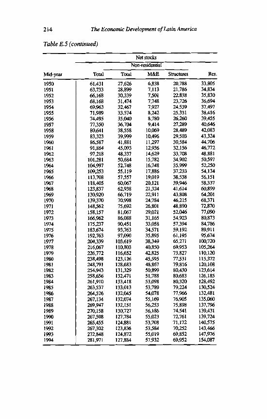
214
Tabi
Mid-;
195019511952195319541955195619571958195919601961196219631964196519661967196819691970197119721973197419751976197719781979198019811982198319841985198619871988198919901991199219931994
The Economic Development of Latin America
Net stocksNon-residential
Total Total M&E Structures Res.
61,431 27,626 6,838 20,788 33,80563,733 28,899 7,113 21,786 34,83466,168 30,339 7,501 22,838 35,83068,168 31,474 7,748 23,726 36,69469,%3 32,467 7,927 24,539 37,49771,989 33,574 8,242 25,331 38,41674,495 35,040 8,780 26,260 39,45577,350 36,704 9,414 27,289 40,64680,641 38,558 10,069 28,489 42,08383,323 39,999 10,4% 29,503 43,32486,587 41,881 11,297 30,584 44,70691,864 45,093 12,936 32,156 46,77297,218 48,337 14,629 33,708 48,881
101,281 50,684 15,782 34,902 50,597104,997 52,748 16,748 35,999 52,250109,253 55,119 17,886 37,233 54,134113,708 57,557 19,019 38,538 56,151118,405 60,067 20,121 39,946 58,337123,837 62,938 21,324 41,614 60,899130,920 66,719 22,911 43,808 64,201139,370 70,998 24,784 46,215 68,371148,562 75,692 26,801 48,890 72,870158,157 81,067 29,021 52,046 77,090166,962 86,088 31,165 54,923 80,873175,237 90,451 33,058 57,394 84,786183,674 93,763 34,571 59,192 89,911192,763 97,090 35,895 61,195 95,674204,339 103,619 38,349 65,271 100,720216,067 110,803 40,850 69,953 105,264226,772 116,652 42,825 73,827 110,120238,498 123,126 45,595 77,531 115,372248,791 128,683 48,867 79,816 120,108254,943 131,329 50,899 80,430 123,614258,656 132,471 51,788 80,683 126,185261,910 133,418 53,098 80,320 128,492263,537 133,013 53,789 79,224 130,524264,526 132,045 54,078 77,966 132,481267,134 132,074 55,169 76,905 135,060269,947 132,151 56,253 75,898 137,796270,158 130,727 56,186 74,541 139,431267,508 127,784 55,023 72,761 139,724265,455 124,881 53,708 71,172 140,575267,302 123,836 53,584 70,252 143,466272,848 124,872 55,019 69,852 147,976281,971 127,884 57,932 69,952 154,087
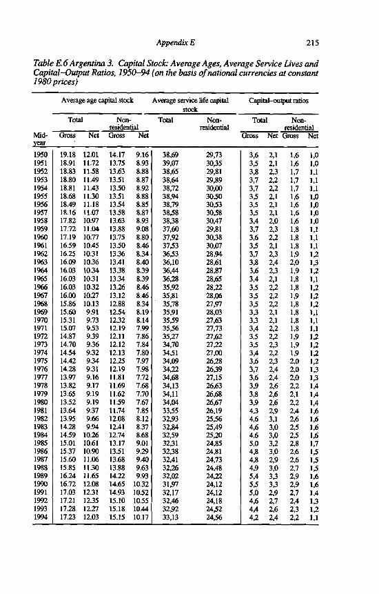
Mid-year
195019511952195319541955195619571958195919601961196219631964196519661967196819691970197119721973197419751976197719781979198019811982198319841985198619871988198919901991199219931994
Appendix E 215
E.6 Argentina 3. Capital Stock: Average Ages, Average Service Lives andal-Output Ratios, 1950-94 (on the basis of national currencies at constantprices)
Average age capital stock Average service life capital stock
Capital-output ratios
Total Non- residential
Total Non-residential
Total Non- residential
Gross Net Gross Net Gross Net Gross Net
19.18 12.01 14.17 9.16 38,69 29,73 3,6 2,1 1,6 1,018.91 11.72 13.75 8.93 39,07 30,35 33 2,1 1,6 1,018.83 11.58 13.63 8.88 38,65 29,81 3,8 2,3 1,7 1,118.80 11.49 13.51 8.87 38,64 29,89 3,7 2,2 1,7 1,118.81 11.43 13.50 8.92 38,72 30,00 3,7 2,2 1,7 1,118.68 11.30 13.51 8.88 38,94 3030 3,5 2,1 1,6 1,018.49 11.18 13.54 8.85 38,79 30,53 33 2,1 1,6 1,018.16 11.07 13.58 8.87 3838 3038 3,5 2,1 1,6 1,017.82 10.97 13.63 8.93 38,38 30,47 3,4 2,0 1,6 1,017.72 11.04 13.88 9.08 37,60 29,81 3,7 2,3 1,8 1,117.19 10.77 13.75 8.80 37,92 30,38 3,6 2,2 1,8 1,116.59 10.45 13.50 8.46 3733 30,07 33 2,1 1,8 1,116.25 10.31 13.36 8.34 3633 28,94 3,7 2,3 1,9 1,216.09 10.36 13.41 8.40 36,10 28,61 3,8 2,4 2,0 1,316.03 10.34 13.38 8.39 36,44 28,87 3,6 2,3 1,9 1,216.03 10.31 13.34 8.39 36,28 28,65 3,4 2,1 1,8 1,116.03 10.32 13.26 8.46 35,92 28,22 3,5 2,2 1,8 1,216.00 10.27 13.12 8.46 35,81 28,06 3,5 2,2 1,9 1,215.86 10.13 12.88 8.34 35,78 27,97 33 2,2 1,8 1,215.60 9.91 12.54 8.19 35,91 28,03 3,3 2,1 1,8 1,115.31 9.73 12.32 8.14 35,59 27,63 3,3 2,1 1,8 1,115.07 9.53 12.19 7.99 3536 27,73 3,4 2,2 1,8 1,114.87 9.39 12.11 7.86 35,27 27,62 3,5 2,2 1,9 1,214.70 9.36 12.12 7.84 34,70 27,22 3,5 2,3 1,9 1,214.54 9.32 12.13 7.80 3431 27,00 3,4 2,2 1,9 1,214.42 9.34 12.25 7.97 34,09 26,28 3,6 2,3 2,0 1,214.28 9.31 12.19 7.98 34,22 26,39 3,7 2,4 2,0 1,313.97 9.16 11.81 7.72 34,68 27,15 3,6 2,4 2,0 1,313.82 9.17 11.69 7.68 34,13 26,63 3,9 2,6 2,2 1,413.65 9.19 11.62 7.70 34,11 26,68 3,8 2,6 2,1 1,413.52 9.19 11.59 7.67 34,04 26,67 3,9 2,6 2,2 1,413.64 9.37 11.74 7.85 33,55 26,19 4,3 2,9 2,4 1,613.95 9.66 12.08 8.12 32,93 25,56 4,6 3,1 2,6 1,614.28 9.94 12.41 8.37 32,84 25,49 4,6 3,0 2,5 1,614.59 10.26 12.74 8.68 3239 25,20 4,6 3,0 2,5 1,615.01 10.61 13.17 9.01 32,31 24,85 5,0 3,2 2,8 1,715.37 10.90 13.51 9.29 32,38 24,81 4,8 3,0 2,6 1,515.60 11.06 13.68 9.40 32,41 24,73 4,8 2,9 2,6 1,515.85 11.30 13.88 9.63 32,26 24,48 4,9 3,0 2,7 1,516.24 11.65 14.22 9.93 32,02 24,22 5,4 3,3 2,9 1,616.72 12.08 14.65 10.32 31,97 24,12 5,5 3,3 2,9 1,617.03 12.31 14.93 10.52 32,17 24,12 5,0 2,9 2,7 1,417.21 12.35 15.10 10.55 32,46 24,18 4,6 2,7 2,4 1,317.28 12.27 15.18 10.44 32,92 2432 4,4 2,6 2,3 1,217.23 12.03 15.15 10.17 33,13 24,56 4,2 2,4 2,2 1,1

Table E. 7 Argentina 4. Capital Stock: Average Ages, Average Service Lives and Capital-Output Ratios, 1950-94 (on the basis of constant 1980 international dollars)
216 The Economic Development of Latin America
Average age capital stock Average service life capital Capital-output ratiosstock ___
Total Non- Total Non- Total Non-___________ residential re s id en tia l______________ residential
Midyear
Gross Net Gross Net Gross Net Gross Net
1950 19.27 12.05 13.88 8.96 37.40 28.58 2.3 1.3 1.0 0.61951 19.01 11.76 13.46 8.72 37.43 29.20 2.3 1.3 1.0 0.61952 18.94 11.62 13.34 8.68 37.27 28.65 2.4 1.4 1.1 0.71953 18.92 11.53 13.23 8.68 38.26 28.71 2.4 1.4 1.0 0.61954 18.93 11.47 13.22 8.74 3836 28.85 2.3 1.4 1.0 0.61955 18.79 11.33 13.23 8.69 38.58 29.35 2.3 1.3 1.0 0.61956 18.59 11.20 13.25 8.66 38.42 2939 2.3 1.3 1.0 0.61957 18.24 11.08 13.29 8.67 38.18 29.43 2.2 1.3 1.0 0.61958 17.88 10.97 13.33 8.73 37.96 2931 2.2 1.3 1.0 0.61959 17.75 11.04 13.58 8.87 37.16 28.66 2.4 1.4 1.1 0.71960 17.20 10.76 13.43 8.58 37.48 29.25 2.3 1.4 1.1 0.71961 16.57 10.42 13.17 8.23 37.06 28.94 2.2 1.4 1.1 0.71962 16.21 10.29 13.01 8.10 36.02 27.78 2.3 1.5 1.2 0.71963 16.03 10.33 13.05 8.17 35.58 27.45 2.4 1.5 1.2 0.81964 15.97 10.31 13.01 8.16 35.93 27.74 2.3 1.4 1.2 0.71965 15.97 10.28 12.97 8.16 35.76 27.52 2.2 1.4 1.1 0.71966 15.97 10,28 12.89 8.22 35.39 27.08 2.2 1.4 1.1 0.71967 15.94 10.23 12.76 8.22 35.28 26.93 2.2 1.4 1.1 0.71968 15.81 10.09 12.53 8.11 35.25 26.84 2.2 1.4 1.1 0.71969 15.55 9.86 12.20 7.96 35.36 26.90 2.1 1.4 1.1 0.71970 15.26 9.68 11.99 7.90 35.04 26.51 2.1 1.4 1.1 0.71971 15.02 9.48 11.86 7.76 34.98 26.58 2.2 1.4 1.1 0.71972 14.82 9.34 11.78 7.64 34.67 26.47 2.2 1.4 1.1 0.71973 14.64 9.31 11.78 7.61 34.11 26.09 2.2 1.5 1.2 0.71974 14.46 9.26 11.80 7.58 33.91 25.89 2.2 1.4 1.2 0.71975 14.33 9.28 11.91 7.74 33.50 25.18 2.3 1.5 1.2 0.81976 14.19 9.25 11.86 7.75 33.61 25.26 2.4 1.6 1.2 0.81977 13.89 9.11 11.49 7.50 34.05 26.01 2.3 1.5 1.2 0.81978 13.74 9.12 11.38 7.47 33.51 25.51 2.5 1.7 1.3 0.91979 13.57 9.14 11.32 7.49 33.49 25.56 2.4 1.6 1.3 0.81980 13.44 9.15 11.28 7.46 33.42 25.56 2.5 1.7 1.3 0.91981 13.54 9.31 11.41 7.61 32.95 25.13 2.8 1.9 1.5 1.01982 13.84 9.59 11.74 7.88 3232 24.49 3.0 2.0 1.6 1.01983 14.16 9.87 12.05 8.11 32.23 24.43 2.9 1.9 1.6 1.01984 14.46 10.17 1236 8.40 31.99 24.16 2.9 1.9 1.6 1.01985 14.87 10.52 12.77 8.72 31.70 23.80 3.2 2.1 1.7 1.01986 15.22 10.80 13.09 8.97 31.78 23.77 3.1 1.9 1.6 1.01987 15.44 10.96 13.24 9.06 31.82 23.70 3.1 1.9 1.6 0.91988 15.69 11.19 13.43 9.27 31.67 23.47 3.2 2.0 1.7 1.01989 16.07 11.53 13.76 9.56 31.43 23.21 3.5 2.1 1.8 1.01990 16.55 11.95 14.17 9.93 31.38 23.11 3.5 2.1 1.8 1.01991 16.86 12.18 14.44 10.12 31.59 23.11 3.2 1.9 1.7 0.91992 17.03 12.22 14.60 10.14 31.87 23.16 3.0 1.7 1.5 0.81993 17.09 12.13 14.66 10.01 32.35 23.50 2.9 1.7 1.4 0.81994 17.02 11.88 14.60 9.72 32.57 23.54 2.7 1.6 1.4 0.7

b y T
Mid-;
19501951195219531954195519561957195819591960196119621963196419651966196719681969197019711972197319741975197619771978197919801981198219831984198519861987198819891990199119921993
Appendix E 217
il 1. Gross and Net Fixed Tangible Reproducible Capital Stocks’,t, 1950-94 (constant 1980 cruzeiros)
Gross stocks
Non-residential
Total Total M&E Structures Res.
2,325 1,498 1.019 480 8272,615 1,718 1.157 562 8972,943 1,968 1.316 652 9753,240 2,178 1.419 760 1.0623,530 2,378 1.505 873 1.1523,844 2,601 1.614 987 1.2424,166 2,830 1.721 1.109 1.3364,532 3,097 1.855 1.243 1.4354,940 3,399 2.010 1.389 1.5415,378 3,722 2.173 1.549 1.6565,840 4,062 2.341 1.721 1.7786,308 4,400 2.490 1.910 1.9086,756 4,714 2.605 2.109 2.0427,184 5,008 2.705 2.303 2.1757,608 5,294 2.805 2.489 2.3148,019 5,555 2.881 2.674 2.4638,441 5,819 2.948 2.871 2.6218,894 6,102 3.016 3.086 2.7929,478 6,495 3.160 3.336 2.982
10,248 7,049 3.398 3.651 3.19911,150 7,711 3.689 4.022 3.43912,197 8,494 4.055 4.439 3.70313,412 9,413 4.486 4.927 4.00014,873 10,531 5.008 5.523 4.34216,592 11,864 5.651 6.214 4.72718,514 13,375 6.406 6.969 5.14020,612 15,028 7.232 7.796 5.58422,759 16,699 8.017 8.682 6.06024,946 18,383 8.762 9.621 6.56327,240 20,146 9.540 10.607 7.09329,764 22,087 10.391 11.696 7.67732,262 23,968 11.138 12.830 8.29434,467 25,567 11.662 13.906 8.90036,356 26,884 12.012 14.872 9.47237,963 27,953 12.223 15.729 10.01039,588 29,024 12.428 16.597 10.56441,483 30,302 12.726 17.577 11.18143,499 31,653 13.026 18.628 11.84645,308 32,806 13.153 19.653 12.50246,925 33,768 13.092 20.676 13.15748,262 34,475 12.840 21.636 13.78649,349 34,977 12.470 22.507 14.37250,346 35,417 12.097 23.320 14.92951,336 35,858 11.755 24.103 15.47952,498 36,441 11.511 24.931 16.057

Mid-;
195019511952195319541955195619571958195919601961196219631964196519661967196819691970197119721973197419751976197719781979198019811982198319841985198619871988198919901991199219931994
The Economic Development of Latin America
Net stocks
Non-residential
Res.Total Total M&E Structures
1.560 983 659 325 5771.809 1.177 775 402 6322.095 1.401 913 488 6942.348 1.584 993 591 7642.574 1.738 1.043 695 8362.793 1.886 1.093 792 9083.004 2.022 1.128 894 9823.242 2.180 1.177 1.003 1.0623.503 2.357 1.236 1.121 1.1473.792 2.554 1.303 1.250 1.2384.103 2.767 1.374 1.392 1.3364.421 2.979 1.434 1.546 1.4414.744 3.194 1.492 1.702 1.5505.052 3.393 1.544 1.849 1.6585.344 3.578 1.590 1.988 1.7665.622 3.747 1.624 2.122 1.8765.937 3.947 1.683 2.264 1.9906.303 4.189 1.769 2.419 2.1146.736 4.485 1.881 2.604 2.2517.313 4.899 2.052 2.847 2.4147.998 5.401 2.267 3.134 2.5968.782 5.984 2.530 3.454 2.7989.720 6.690 2.854 3.835 3.030
10.876 7.572 3.260 4.313 3.30312.253 8.640 3.770 4.870 3.61213.782 9.838 4.364 5.474 3.94415.414 11.110 4.979 6.131 4.30317.026 12.339 5.505 6.834 4.68618.596 13.509 5.942 7.566 5.08720.189 14.683 6.362 8.321 5.50521.917 15.956 6.799 9.157 5.96123.547 17.114 7.104 10.010 6.43324.818 17.939 7.168 10.771 6.87925.731 18.447 7.053 11.394 7.28426.386 18.735 6.846 11.889 7.65127.080 19.055 6.677 12.378 8.02528.065 19.611 6.655 12.956 8.45429.222 20.299 6.701 13.598 8.92230.235 20.866 6.665 14.201 9.36931.151 21.349 6.571 14.778 9.80231.907 21.709 6.417 15.292 10.19832.482 21.946 6.233 15.713 10.53732.932 22.100 6.038 16.062 10.83333.353 22.242 5.860 16.381 11.11133.975 22.566 5.836 16.730 11.409
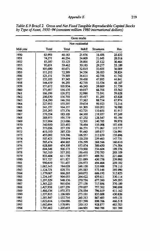
Mid-;
195019511952195319541955195619571958195919601961196219631964196519661967196819691970197119721973197419751976197719781979198019811982198319841985198619871988198919901991199219931994
Appendix E 219
il 2. Gross and Net Fixed Tangible Reproducible Capital Stocks% 1950-94 (constant million 1980 international dollars)
Gross stocks
Nan-residential
Total Total M&E Structures Res.
65,995 40.163 21.676 18.488 25.83274,271 46.254 24.609 21.645 28.01683,587 53.123 28.001 25.122 30.46492,651 59.462 30.185 29.277 33.189
101,680 65.671 32.015 33.655 36.009111,213 72.389 34.336 38.053 38.824121,111 79.369 36.611 42.758 41.742132,183 87.343 39.458 47.885 44.841144,459 96.293 42.759 53.534 48.167157,672 105.934 46.245 59.689 51.739171,697 116.135 49.817 66.318 55.562186,199 126.572 52.980 73.591 59.628200,530 136.703 55.417 81.285 63.828214,290 146.316 57.562 88.754 67.974227,913 155.597 59.674 95.923 72.316241,337 164.357 61.305 103.052 76.980255,293 173.376 62.721 110.655 81.917270,354 183.105 64.168 118.937 87.249288,973 195.779 67.232 128.547 93.194312,984 213.006 72.301 140.705 99.978340,950 233.492 78.484 155.008 107.458373,056 257.339 86.271 171.067 115.717410,310 285.320 95.443 189.877 124.991455,092 319.396 106.557 212.839 135.696507,425 359.694 120.230 239.463 147.731565,474 404.865 136.299 268.566 160.610628,809 454.305 153.874 300.430 174.504694,548 505.173 170.568 334.604 189.376762,310 557.202 186.418 370.783 205.109833,404 611.738 202.977 408.761 221.666911,727 671.827 221.089 450.738 239.900990,619 731.437 236.973 494.464 259.182
1,062,143 784.028 248.120 535.908 278.1151,124,721 828.731 255.583 573.148 295.9901,179,087 866.265 260.072 606.192 312.8231,234,147 904.033 264.422 639.611 330.1141,297,529 948.136 270.756 677.380 349.3931,365,223 995.034 277.138 717.896 370.1891,427,938 1.037.239 279.857 757.382 390.6981,486,534 1.075.373 278.554 796.819 411.1621,537,815 1.106.989 273.181 833.808 430.8261,581,847 1.132.716 265.313 867.403 449.1311,622,614 1.156.096 257.390 898.706 466.5181,662,694 1.178.991 250.113 928.877 483.7031,707,462 1.205.693 244.905 960.788 501.769

220
Tabi
Mid-;
195019511952195319541955195619571958195919601961196219631964196519661967196819691970197119721973197419751976197719781979198019811982198319841985198619871988198919901991199219931994
The Economic Development of Latin America
Net stocks
Non-residential
Total Total M&E Structures Res.
44,547 26.521 14.014 12.506 18.02651,736 31.996 16.490 15.507 19.73959,913 38.227 19.416 18.812 21.68667,781 43.905 21.130 22.775 23.87675,093 48.964 22.186 26.778 26.12982,160 53.800 23.264 30.536 28.36089,130 58.439 24.002 34.437 30.69296,865 63.689 25.050 38.639 33.175
105,333 69.498 26.289 43.209 35.835114,607 75.919 27.728 48.191 38.688124,662 82.901 29.237 53.664 41.761135,113 90.072 30.503 59.569 45.042145,763 97.325 31.738 65.588 48.438155,936 104.119 32.861 71.258 51.817165,638 110.444 33.831 76.613 55.194174,965 116.354 34.563 81.791 58.611185,247 123.047 35.813 87.234 62.201196,946 130.888 37.645 93.243 66.058210,719 140.369 40.012 100.357 70.350228,800 153.376 43.667 109.709 75.423250,153 169.022 48.242 120.780 81.131274,395 186.952 53.825 133.127 87.443303,233 208.540 60.734 147.806 94.693338,787 235.557 69.354 166.203 103.231380,791 267.909 80.213 187.696 112.882427,060 303.802 92.858 210.944 123.258476,708 342.231 105.934 236.296 134.477526,950 380.511 117.137 263.374 146.439577,006 418.024 126.434 291.591 158.982628,083 456.049 135.372 320.677 172.035683,850 497.556 144.662 352.894 186.293737,942 536.916 151.143 385.773 201.027782,593 567.614 152.506 415.108 214.979816,798 589.178 150.072 439.106 227.620842,938 603.853 145.661 458.192 239.085869,890 619.099 142.067 477.032 250.791905,082 640.892 141.588 499.304 264.190945,454 666.637 142.580 524.057 278.817981,882 689.110 141.806 547.304 292.772
1,015,635 709.337 139.809 569.528 306.2981,044,547 725.870 136.526 589.344 318.6781,067,440 738.165 132.608 605.557 329.2751,085,997 747.479 128.458 619.021 338.5181,103,217 756.006 124.691 631.315 347.2111,125,451 768.913 124.174 644.739 356.538

Mid-year195019511952195319541955195619571958195919601961196219631964196519661967196819691970197119721973197419751976197719781979198019811982198319841985198619871988198919901991199219931994
E.10 Brazil 3. Capital Stock: Average Ages, Average Service Lives and al-Output Ratios, 1950-94 (on the basis of national currencies at constant prices)
Appendix E 221
Average age capital stock Average service life capital Capital-output ratios _______ stock
Total Non- Total Non- Total Non-___________ residential re s id e n tia l_____________ residential
Gross Net Gross Net Gross Net Gross Net
11.06 6.85 8.43 4.69 26.84 21.10 1.4 0.9 0.9 0.610.37 6.34 7.72 4.30 27.29 21.80 1.5 1.0 1.0 0.79.78 6.07 7.14 4.22 26.65 21.35 1.6 1.1 1.0 0.79.54 6.11 6.94 4.41 25.81 20.52 1.7 1.2 1.1 0.89.40 6.14 6.91 4.56 26.50 21.28 1.6 1.2 1.1 0.89.44 6.28 7.10 4.80 26.41 21.26 1.7 1.2 1.1 0.89.47 6.40 7.29 5.02 26.57 21.48 1.8 1.3 1.2 0.99.49 6.48 7.47 5.17 26.95 21.95 1.8 1.3 1.2 0.99.54 6.52 7.67 5.25 26.89 21.96 1.8 1.3 1.2 0.99.52 6.53 7.76 5.29 26.98 22.13 1.9 1.3 1.3 0.99.51 6.57 7.85 5.36 26.88 22.09 1.8 1.3 1.3 0.99.53 6.64 7.97 5.46 26.85 22.08 1.8 1.3 1.3 0.89.53 6.72 8.03 5.56 26.77 22.01 1.8 1.3 1.3 0.99.58 6.86 8.18 5.71 26.96 22.21 1.9 1.4 1.3 0.99.68 7.01 8.28 5.87 27.07 22.26 2.0 1.4 1.4 0.99.85 7.21 8.45 6.08 27.18 22.30 2.0 1.4 1.4 0.99.88 7.31 8.43 6.18 27.57 22.62 2.0 1.4 1.4 1.09.95 7.43 8.45 6.31 27.87 22.84 2.1 1.5 1.4 1.09.99 7.44 8.48 6.32 28.84 23.81 2.0 1.4 1.4 0.99.90 7.36 8.39 6.25 29.09 24.10 1.9 1.4 1.3 0.99.86 7.29 8.36 6.18 29.29 24.39 2.1 1.5 1.4 1.09.78 7.17 8.30 6.06 29.43 24.61 2.0 1.5 1.4 1.09.62 7.02 8.18 5.93 29.46 24.74 2.0 1.4 1.4 1.09.41 6.83 8.00 5.77 29.74 25.11 1.9 1.4 1.4 1.09.20 6.64 7.82 5.60 29.64 25.15 2.0 1.5 1.4 1.09.04 6.53 7.71 5.52 29.45 25.11 2.1 1.6 1.5 1.18.92 6.47 7.65 5.49 29.11 24.88 2.1 1.6 1.6 1.28.92 6.49 7.71 5.56 28.62 24.47 2.2 1.7 1.6 1.28.97 6.57 7.83 5.67 28.54 24.45 2.3 1.7 1.7 1.39.07 6.65 7.97 5.78 28.45 24.41 2.4 1.8 1.8 1.39.14 6.69 8.10 5.84 28.61 24.60 2.4 1.8 1.8 1.39.37 6.88 8.36 6.06 28.07 24.08 2.7 2.0 2.0 1.49.67 7.12 8.71 6.33 28.01 24.01 2.9 2.1 2.1 1.5
10.08 7.45 9.16 6.68 27.79 23.78 3.1 2.2 2.3 1.610.47 7.78 9.59 7.02 27.94 23.89 3.1 2.1 2.3 1.510.82 8.03 9.97 7.27 28.27 24.15 3.0 2.0 2.2 1.411.05 8.15 10.23 7.38 28.75 24.57 2.9 2.0 2.1 1.411.28 8.31 10.47 7.53 28.80 24.58 2.9 2.0 2.1 1.411.55 8.50 10.75 7.71 28.87 24.60 3.1 2.0 2.2 1.411.82 8.70 11.01 7.89 29.12 24.76 3.1 2.0 2.2 1.412.12 8.97 11.30 8.16 29.28 24.85 3.3 2.2 2.4 1.512.45 9.24 11.59 8.41 29.73 25.22 3.4 2.2 2.4 1.512.82 9.56 11.93 8.71 30.15 25.59 3.5 2.3 2.4 1.513.16 9.82 12.22 8.95 30.67 26.02 3.4 2.2 2.4 1.513.43 10.01 12.45 9.10 31.24 26.55 3.3 2.1 2.3 1.4

222
TablCap\dolli
Mid-2Ê2L.195019511952195319541955195619571958195919601961196219631964196519661967196819691970197119721973197419751976197719781979198019811982198319841985198619871988198919901991199219931994
E.11 Brazil 4. Capital Stock: Average Ages, Average Service Lives and al-Output Ratios, 1950-94 (on the basis of constant 1980 international
The Economic Development of Latin America
Average age capital stock Average service life capital Capital-output ratiosstock ___ ___ _____ ____
Total Non- Total Non- Total Non- residential residential residential
Gross Net Gross Net Gross Net Gross Net
11.93 7.37 9.41 5.22 30.42 23.87 1.2 0.8 0.7 0.511.18 6.80 8.57 4.74 30.73 24.48 1.3 0.9 0.8 0.610.50 6.48 7.86 4.58 30.17 24.14 1.4 1.0 0.9 0.610.13 6.41 7.50 4.68 29.47 23.48 1.5 1.1 0.9 0.79.92 6.40 7.39 4.80 30.09 24.27 1.4 1.1 0.9 0.79.89 6.50 7.52 5.02 30.02 24.31 1.5 1.1 1.0 0.79.86 6.60 7.65 5.22 30.21 24.60 1.6 1.2 1.0 0.89.84 6.68 7.78 5.39 30.56 25.09 1.6 1.2 1.0 0.89.85 6.71 7.94 5.47 30.53 25.16 1.6 1.2 1.1 0.89.80 6.74 8.00 5.54 30.62 25.35 1.7 1.2 1.1 0.89.74 6.78 8.04 5.63 30.55 25.36 1.7 1.2 1.1 0.89.75 6.86 8.15 5.75 30.55 25.43 1.6 1.2 1.1 0.89.74 6.95 8.24 5.88 30.50 25.42 1.7 1.2 1.1 0.89.79 7.10 8.40 6.05 30.65 25.63 1.8 1.3 1.2 0.99.90 7.27 8.52 6.24 30.77 25.71 1.8 1.3 1.2 0.9
10.08 7.48 8.72 6.49 30.89 25.80 1.9 1.3 1.3 0.910.14 7.60 8.76 6.62 31.31 26.19 1.9 1.4 1.3 0.910.24 7.74 8.82 6.77 31.62 26.47 1.9 1.4 1.3 0.910.30 7.76 8.87 6.81 32.57 27.47 1.8 1.3 1.2 0.910.22 7.70 8.81 6.76 32.87 27.84 1.8 1.3 1.2 0.910.20 7.64 8.81 6.70 33.06 28.13 1.9 1.4 1.3 1.010.14 7.53 8.78 6.59 33.19 28.35 1.9 1.4 1.3 0.910.00 7.39 8.68 6.46 33.27 28.52 1.9 1.4 1.3 0.99.80 7.20 8.51 6.29 33.57 28.93 1.8 1.3 1.3 0.99.61 7.01 8.35 6.11 33.45 28.95 1.9 1.4 1.3 1.09.46 6.90 8.26 6.02 33.24 28.87 2.0 1.5 1.4 1.19.36 6.83 8.21 5.98 32.91 28.63 2.0 1.5 1.4 1.19.34 6.83 8.25 6.01 32.44 28.24 2.1 1.6 1.5 1.19.38 6.89 8.35 6.10 32.36 28.22 2.2 1.7 1.6 1.29.46 6.96 8.48 6.20 32.24 28.16 2.2 1.7 1.6 1.29.52 6.98 8.58 6.25 32.44 28.39 2.2 1.7 1.6 1.29.72 7.16 8.82 6.45 31.89 27.87 2.5 1.9 1.9 1.4
10.01 7.38 9.15 6.70 31.81 27.81 2.7 2.0 2.0 1.410.41 7.70 9.60 7.04 31.55 27.55 2.9 2.1 2.2 1.510.79 8.03 10.03 7.40 31.68 27.67 2.9 2.1 2.1 1.511.14 8.28 10.41 7.66 32.00 27.96 2.8 2.0 2.1 1.411.39 8.42 10.69 7.81 32.50 28.43 2.8 1.9 2.0 1.411.62 8.59 10.94 7.98 32.54 28.45 2.8 2.0 2.1 1.411.90 8.79 11.25 8.18 32.61 28.50 2.9 2.0 2.1 1.412.18 9.00 11.53 8.38 32.86 28.71 3.0 2.0 2.2 1.412.50 9.28 11.84 8.66 32.97 28.81 3.2 2.2 2.3 1.512.84 9.56 12.17 8.93 33.38 29.19 3.3 2.2 2.4 1.513.22 9.88 12.53 9.24 33.73 29.53 3.4 2.3 2.4 1.613.57 10.15 12.85 9.49 34.19 29.97 3.4 2.2 2.4 1.513.87 10.35 13.12 9.68 34.69 30.47 3.3 2.1 2.3 1.5
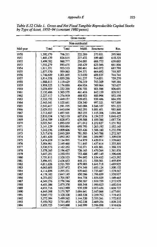
byT
Mid-:
195019511952195319541955195619571958195919601961196219631964196519661967196819691970197119721973197419751976197719781979198019811982198319841985198619871988198919901991199219931994
Appendix E 223
e 1. Gross and Net Fixed Tangible Reproducible Capital Stockst, 1950-94 (constant 1980 pesos)
Gross stocks
Non-residential
Total Total M&E Structures Res.
1,392,179 796.211 222.280 573.931 595,%81,445,139 826.915 237.432 589.483 618.2251,499,782 860.777 254.005 606.772 639.0051,555,279 893.475 268.429 625.046 661.8041,611,331 923.533 280.461 643.072 687.7981,677,570 959.063 294.371 664.692 718.5071,746,609 1.001.865 313.030 688.835 744.7441,814,558 1.055.288 341.237 714.051 759.2701,888,813 1.119.429 376.219 743.209 769.3841,958,525 1.174.888 404.924 769.964 783.6372,038,889 1.232.288 430.703 801.586 806.6012,132,486 1.303.575 461.416 842.159 828.9122,227,117 1.374.919 488.923 885.9% 852.1982,333,732 1.449.137 509.652 939.486 884.5952,443,541 1.525.661 528.340 997.321 917.8802,542,417 1.591.195 545.088 1.046.107 951.2222,629,553 1.643.694 562.293 1.081.401 985.8602,713,807 1.697.561 582.255 1.115.306 1.016.2462,810,534 1.762.110 607.836 1.154.275 1.048.4232,916,709 1.828.973 639.588 1.189.386 1.087.7363,025,541 1.893.839 671.012 1.222.827 1.131.7023,141,129 1.958.984 695.793 1.263.192 1.182.1453,242,1% 2.009.606 703.426 1.306.180 1.232.5903,317,676 2.045.289 701.503 1.343.786 1.272.3873,401,420 2.092.382 707.386 1.384.997 1.309.0383,474,659 2.134.993 714.979 1.420.014 1.339.6653,504,%1 2.149.460 711.845 1.437.614 1.355.5013,530,573 2.162.252 710.371 1.451.881 1.368.3213,578,265 2.1%.427 726.163 1.470.264 1.381.8383,647,251 2.250.555 753.406 1.497.149 1.396.6963,751,815 2.328.523 794.092 1.534.432 1.423.2923,8%,551 2.436.653 848.151 1.588.501 1.459.8994,011,628 2.521.703 879.985 1.641.718 1.489.9254,065,605 2.557.472 874.348 1.683.124 1.508.1324,114,898 2.595.331 859.643 1.735.687 1.519.5674,178,102 2.647.145 850.286 1.7%.859 1.530.9574,251,052 2.701.587 844.758 1.856.829 1.549.4654,349,276 2.776.346 856.587 1.919.759 1.572.9294,481,386 2.879.370 888.548 1.990.823 1.602.0164,651,716 3.012.989 939.559 2.073.430 1.638.7274,849,398 3.171.707 1.004.641 2.167.066 1.677.6915,047,772 3.328.320 1.068.528 2.259.792 1.719.4535,272,394 3.499.562 1.144.320 2.355.241 1.772.8325,550,702 3.711.493 1.242.238 2.469.254 1.839.2105,855,723 3.945.098 1.348.999 2.5%.098 1.910.626

224
Tabi
Mid-:
195019511952195319541955195619571958195919601961196219631964196519661967196819691970197119721973197419751976197719781979198019811982198319841985198619871988198919901991199219931994
The Economic Development of Latin America
continued) CHUNet stocks
Non--residential
Total Total M&E Structures Res.
862,635 472.214 134.211 338.004 390.421899,232 495.001 145.459 349.542 404.231940,961 523.355 158.587 364.768 417.605983,167 549.916 169.627 380.289 433.251
1,022,549 569.997 176.631 393.366 452.5521,065,442 589.818 184.247 405.570 475.6241,110,586 616.739 196.346 420.393 493.8471,157,798 655.921 215.316 440.605 501.8771,208,126 702.129 238.123 464.006 505.9971,247,053 734.316 251.774 482.542 512.7371,289,243 763.076 260.745 502.331 526.1671,342,642 802.501 276.405 526.095 540.1421,400,593 844.181 293.047 551.135 556.4111,472,314 891.183 303.799 587.384 581.1311,546,163 941.385 312.260 629.125 604.7781,607,914 983.126 318.537 664.589 624.7881,664,478 1.018.572 325.470 693.102 645.9061,722,005 1.056.214 336.903 719.310 665.7921,785,021 1.098.254 351.640 746.614 686.7671,855,445 1.142.517 367.769 774.748 712.9281,931,361 1.190.626 382.867 807.759 740.7342,006,749 1.235.769 394.637 841.131 770.9802,059,226 1.259.742 395.724 864.018 799.4852,087,779 1.269.446 392.462 876.984 818.3342,117,504 1.282.391 390.310 892.081 835.1132,136,667 1.288.356 386.710 901.645 848.3112,130,376 1.278.367 380.285 898.082 852.0092,124,671 1.272.409 378.756 893.653 852.2622,137,530 1.287.113 390.537 896.576 850.4172,168,314 1.317.730 411.808 905.923 850.5842,226,745 1.365.357 443.766 921.591 861.3872,319,492 1.442.312 488.158 954.154 877.1802,377,543 1.494.157 512.368 981.789 883.3862,373,276 1.494.504 501.620 992.885 878.7712,371,483 1.500.421 485.276 1.015.145 871.0632,392,784 1.526.083 476.346 1.049.737 866.7012,423,777 1.555.083 470.637 1.084.446 868.6932,473,149 1.597.622 473.621 1.124.000 875.5272,551,847 1.663.699 492.109 1.171.591 888.1472,667,628 1.758.516 528.499 1.230.017 909.1112,807,128 1.872.294 574.503 1.297.791 934.8342,938,631 1.974.881 612.654 1.362.226 963.7503,096,391 2.094.284 663.139 1.431.144 1.002.1083,314,028 2.260.875 743.908 1.516.967 1.053.1533,559,852 2.448.317 837.534 1.610.782 1.111.535

PRESEN TA CIÓN DE APP REVISTA CEPAL PARA D ISPO SITIV O S MÓVILES
http://app.comunicacien.net


Appendix E 225
Table E.13 Chile 2. Gross and Net Fixed Tangible Reproducible Capital Stocks by Type of Asset, 1950-94 (constant million 1980 international dollars) ~ '
Gross stocksNon-residential
Mid-year Total Total M&E Structures Res.
1950 37,077 25,638 4.384«/ 2 1 .2 5 4 / 11.4391951 38,379 26,513 4.683 21.829 11.8661952 39,745 27,480 5.010 22.470 12.2651953 41,143 28,441 5.294 23.146 12.7031954 42,547 29,346 5.532 23.814 13.2021955 44,212 30,421 5.806 24.615 13.7911956 45,977 31,683 6.174 25.509 14.2951957 47,746 33,173 6.731 26.442 14.5731958 49,710 34,943 7.420 27.522 14.7671959 51,541 36,500 7.987 28.513 15.0411960 53,661 38,179 8.495 29.684 15.4821961 56,197 40,287 9.101 31.186 15.9101962 58,810 42,453 9.643 32.810 16.3571963 61,822 44,843 10.052 34.791 16.9791964 64,971 47,353 10.421 36.932 17.6181965 67,748 49,490 10.751 38.739 18.2581966 70,059 51,137 11.091 40.046 18.9221967 72,292 52,786 11.484 41.302 19.5061968 74,857 54,733 11.989 42.745 20.1231969 77,538 56,660 12.615 44.045 20.8781970 80,240 58,518 13.235 45.283 21.7221971 83,192 60,502 13.724 46.778 22.6901972 85,902 62,244 13.874 48.370 23.6581973 88,021 63,599 13.836 49.762 24.4221974 90,366 65,241 13.952 51.289 25.1251975 92,401 66,687 14.102 52.585 25.7131976 93,295 67,277 14.040 53.237 26.0171977 94,040 67,777 14.011 53.765 26.2631978 95,292 68,769 14.323 54.446 26.5231979 97,110 70,302 14.860 55.442 26.8081980 99,803 72,485 15.663 56.822 27.3181981 103,575 75,553 16.729 58.825 28.0211982 106,749 78,152 17.357 60.795 28.5971983 108,521 79,574 17.246 62.329 28.9471984 110,397 81,231 16.955 64.275 29.1661985 112,696 83,311 16.771 66.540 29.3851986 115,163 85,423 16.662 68.761 29.7401987 118,177 87,987 16.895 71.092 30.1911988 121,998 91,249 17.526 73.723 30.7491989 126,768 95,314”"\ 18.532 76.782 31.4531990 132,267 100,065 19.815 80.250 32.2011991 137,762 104,759 21.076 83.684 33.0031992 143,816 109,789 22.570 87.218 34.0271993 151,244 115,942 \ 24.502 91.440 35.3021994 159,417 122,745 \ 26.607 96.138 36.672

226
Tabi
Mid-;
195019511952195319541955195619571958195919601961196219631964196519661967196819691970197119721973197419751976197719781979198019811982198319841985198619871988198919901991199219931994
The Economic Development of Latin America
Non-residenbal
Total M&E StructuresTotal
22.65823.57224.65125.74426.73727.78228.91930.19631.59232.67733.84435.30136.86938.89841.06442.88644.48446.061 47.76649.628 51.682 53.730 55.146 55.924 56.763 57.299 57.111 56.922 57.22757.996 59.414 61.799 63.41963.529 63.88364.904 66.115 67.770 70.13973.42377.334 81.027 85.31191.062 97.504
15.164 15.81316.636 17.428 18.051 18.65319.44120.563 21.88022.835 23.745 24.934 26.18927.744 29.45630.894 32.08633.282 34.58435.944 37.464 38.932 39.80140.217 40.734 41.017 40.75840.56440.904 41.670 42.881 44.962 46.463 46.66247.164 48.26949.442 50.96553.092 55.973 59.39162.529 66.077 70.848 76.169
Net stocks
2.6472.8693.1283.3463.4843.6343.8734.2474.697 4.966 5.143 5.452 5.7805.9926.1596.283 6.420 6.645 6.936 7.254 7.552 7.7847.805 7.7417.6987.627 7.501 7.471 7.703 8.122 8.7539.628
10.1069.8949.5729.3959.283 9.342 9.706
10.42411.33112.08413.08014.67316.519
12.51712.94413.50814.08314.567 15.01915.56816.316 17.18317.869 18.602 19.482 20.409 21.752 23.297 24.611 25.66726.637 27.648 28.690 29.913 31.14831.996 32.476 33.035 33.389 33.25733.093 33.20233.548 34.12835.33436.357 36.76837.59238.87340.159 41.623 43.38645.549 48.059 50.445 52.998 56.176 59.650
Res.
7.4947.7598.0158.3168.6869.1299.4799.6339.7129.841
10.09910.36710.68011.15411.60811.99212.39712.77913.18213.68414.21814.79815.34515.70716.02916.28216.35316.35816.32316.32616.53316.83616.95616.86716.71916.63516.67416.80517.04717.44917.94318.49819.23420.21421.335

Mid-year195019511952195319541955195619571958195919601961196219631964196519661967196819691970197119721973197419751976197719781979198019811982198319841985198619871988198919901991199219931994
Appendix E 227
E.14 Chile 3. Capital Stock: Average Ages, Average Service Lives andal-Output Ratios, 1950-94 (on the basis o f national currencies atant 1980 prices)
Average age capital stock Average service life capitalstock
Capital-output ratios
Total Non-residential
Total Non- residential
Total Non-residential
Gross Net Gross Net Gross Net Gross Net
16.10 10.24 14.47 9.13 35.28 28.42 3.6 2.3 2.1 1.215.90 10.11 14.09 8.87 35.07 28.28 3.6 2.3 2.1 1.215.68 9.91 13.73 8.49 34.80 28.05 3.6 2.2 2.0 1.215.51 9.87 13.50 8.44 34.51 27.63 3.5 2.2 2.0 1.215.42 9.98 13.50 8.67 34.42 27.48 3.6 2.3 2.1 1.315.38 9.87 13.56 8.58 34.71 27.68 3.8 2.4 2.2 1.315.28 9.82 13.38 8,35 34.32 27.61 3.9 2.5 2.2 1.415.05 9.69 12.95 7.97 34.18 27.80 3.7 2.3 2.1 1.314.92 9.80 12.72 7.98 33.55 27.36 3.7 2.4 2.2 1.415.00 9.99 12.77 8.20 32,80 26.49 3.9 2.5 2.3 1.515.00 9.97 12.80 8.15 33.05 26.80 3.8 2.4 2.3 1.415.00 9.96 12.85 8.08 32.69 26.68 3.8 2.4 2.3 1.414.95 9.89 12.90 8.02 32.44 26.40 3.8 2.4 2.3 1.414.78 9.75 12.80 7.90 32.57 26.54 3.7 2.3 2.3 1.414.75 9.66 12.76 7.75 32.46 26.56 3.8 2.4 2.4 1.514.77 9.67 12.70 7.75 32.31 26.35 3.9 2.5 2.5 1.514.67 9.81 12.53 7.97 32.21 26.26 3.7 2.3 2.3 1.414.63 9.87 12.47 8.03 32.22 26.36 3.7 2.3 2.3 1.414.58 9.80 12.40 7.92 32.37 26.48 3.7 2.3 2.3 1.414.44 9.79 12.20 7.94 32.20 26.25 3.7 2.3 2.3 1.414.32 9.80 11.90 7.97 32.09 26.09 3.7 2.4 2.3 1.514.40 9.81 11.94 8.04 32.06 25.94 3.5 2.3 2.2 1.414.71 10.02 12.25 8.30 31.76 25.61 3.7 2.4 2.3 1.415.02 10.28 12.54 8.60 31.91 25.81 3.9 2.4 2.4 1.515.30 10.42 12.85 8.74 32.38 26.26 3.9 2.4 2.4 1.515.61 10.76 13.19 9.10 32.00 25.95 4.6 2.8 2.8 1.715.91 11.07 13.52 9.35 31.76 25.74 4.5 2.7 2.8 1.616.17 11.36 13.73 9.61 32.14 26.12 4.2 2.5 2.6 1.516.32 11.49 13.75 9.60 32.32 26.39 4.0 2.4 2.4 1.416.43 11.51 13.82 9.53 32.35 26.45 3.8 2.2 2.3 1.416.41 11.38 13.75 9.34 32.57 26.67 3.6 2.1 2.2 1.316.34 11.15 13.52 9.05 32.50 26.70 3.5 2.1 2.2 1.316.69 11.38 13.79 9.25 31.47 25.72 4.2 2.5 2.6 1.517.12 11.66 14.17 9.48 31.31 25.58 4.4 2.6 2.7 1.617.37 11.79 14.36 9.55 31.74 26.14 4.2 2.4 2.6 1.517.52 11.83 14.45 9.54 32.01 26.44 4.1 2.3 2.6 1.517.67 11.91 14.57 9.64 32.29 26.74 3.9 2.2 2.5 1.417.64 11.72 14.50 9.41 32.75 27.31 3.8 2.2 2.4 1.417.57 11.53 14.40 9.24 32.88 27.48 3.6 2.1 2.3 1.317.28 11.13 14.10 8.87 33.08 27.79 3.4 2.0 2.2 1.317.05 10.76 13.90 8.52 32.80 27.63 3.5 2.0 2.3 1.316.86 10.55 13.78 8.39 32.47 27.32 3.4 2.0 2.2 1.316.52 10.19 13.48 8.13 32.58 27.47 3.2 1.9 2.1 1.316.07 9.78 13.09 7.83 32.49 27.45 3.1 1.9 2.1 1.315.67 9.45 12.79 7.60 32.11 27.15 3.2 1.9 2.1 1.3

228 The Economic Development of Latin America
Table E.15 Chile 4. Capital Stock: Average Ages, Average Service Lives andCapital-Output Ratios, 1950-94 (on the basis of constant 1980 internationaldollars)
Average age capital stock Average service life capital Capital-output ratios______________________ stock______________________________
Total Non- Total Non- Total Non-residential r e s id e n tia l_______________residential
Midyear
Gross Net Gross Net Gross Net Gross Net
1950 16.44 10.49 15.62 9.95 36.55 32.26 2.8 1.7 1.9 1.11951 16.20 10.33 15.25 9.69 36.39 32.13 2.8 1.7 1.9 1.11952 15.95 10.05 14.90 9.27 36.19 31.94 2.7 1.7 1.9 1.11953 15.76 10.00 14.66 9.20 35.93 31.57 2.7 1.7 1.8 1.11954 15.69 10.15 14.65 9.44 35.84 31.43 2.8 1.7 1.9 1.21955 15.69 10.04 14.73 9.33 36.15 31.67 2.9 1.8 2.0 1.21956 15.58 9.92 14.56 9.08 35.79 31.54 3.0 1.9 2.0 1.31957 15.30 9.73 14.12 8.69 35.73 31.68 2.8 1.8 1.9 1.21958 15.16 9.84 13.89 8.74 35.24 31.30 2.8 1.8 2.0 1.21959 15.21 10.04 13.92 8.95 34.52 30.44 2.9 1.9 2.1 1.31960 15.22 10.00 13.94 8.90 34.89 30.87 2.9 1.8 2.0 1.31961 15.26 9.99 14.02 8.83 34.58 30.72 2.9 1.8 2.1 1.31962 15.24 9.91 14.08 8.75 34.43 30.53 2.9 1.8 2.1 1.31963 15.03 9.72 13.91 8.57 34.63 30.76 2.8 1.8 2.1 1.31964 14.98 9.57 13.83 8.36 34.51 30.74 2.9 1.8 2.1 1.31965 14.94 9.54 13.72 8.33 34.26 30.44 3.0 1.9 2.2 1.41966 14.80 9.73 13.52 8.58 34.08 30.25 2.8 1.8 2.1 1.31967 14.74 9.80 13.46 8.64 34.15 30.40 2.8 1.8 2.0 1.31968 14.69 9.72 13.38 8.54 34.26 30.47 2.8 1.8 2.1 1.31969 14.51 9.73 13.14 8.57 34.05 30.20 2.8 1.8 2.0 1.31970 14.30 9.75 12.79 8.61 33.96 30.07 2.8 1.8 2.1 1.31971 14.36 9.77 12.82 8.68 33.98 30.00 2.7 1.7 2.0 1.31972 14.68 10.00 13.15 8.95 33.71 29.72 2.8 1.8 2.0 1.31973 15.00 10.28 13.47 9.26 33.80 29.87 3.0 1.9 2.1 1.41974 15.29 10.41 13.78 9.40 34.27 30.35 3.0 1.9 2.2 1.41975 15.63 10.79 14.15 9.81 33.81 29.94 3.5 2.2 2.6 1.61976 15.96 11.09 14.52 10.07 33.58 29.74 3.5 2.1 2.5 1.51977 16.24 11.42 14.78 10.39 33.90 30.06 3.2 2.0 2.3 1.41978 16.38 11.55 14.83 10.44 34.08 30.31 3.0 1.8 2.2 1.31979 16.53 11.59 14.96 10.42 34.15 30.40 2.9 1.7 2.1 1.21980 16.54 11.50 14.95 10.29 34.37 30.59 2.8 1.6 2.0 1.21981 16.46 11.28 14.75 10.03 34.42 30.71 2.7 1.6 2.0 1.21982 16.80 11.49 15.04 10.22 33.46 29.76 3.2 1.9 2.3 1.41983 17.21 11.72 15.42 10.41 33.35 29.69 3.4 2.0 2.5 1.41984 17.41 11.78 15.58 10.41 33.82 30.30 3.2 1.9 2.4 1.41985 17.51 11.75 15.64 10.34 34.05 30.57 3.2 1.8 2.3 1.41986 17.63 11.81 15.74 10.41 34.31 30.85 3.1 1.8 2.3 1.31987 17.56 11.58 15.63 10.14 34.71 31.33 3.0 1.7 2.2 1.31988 17.48 11.39 15.54 9.98 34.86 31.52 2.8 1.6 2.1 1.21989 17.20 11.01 15.24 9.61 35.05 31.78 2.7 1.6 2.0 1.21990 16.98 10.64 15.05 9.25 34.86 31.66 2.7 1.6 2.1 1.21991 16.81 10.45 14.91 9.11 34.53 31.32 2.6 1.6 2.0 1.21992 16.50 10.15 14.62 8.87 34.66 31.46 2.5 1.5 1.9 1.11993 16.09 9.79 14.26 8.60 34.63 31.46 2.5 1.5 1.9 1.21994 15.75 9.50 13.99 8.38 34.31 31.18 2.5 1.5 1.9 1.2

Mid-:
19501951195219531954195519561957195819591960196119621963196419651966196719681969197019711972197319741975197619771978197919801981198219831984198519861987198819891990199119921993
Appendix E 229
Colombia 1. Gross and Net Fixed Tangible Reproducible Capitaloe o f Asset, 1950-94 (constant 1980pesos)
Gross stocksNon-residential
Total Total M&E Structures Res.
1,023,835 767.342 171.792 595.550 256.4931,066,845 797.915 189.032 608.883 268.9301,109,494 828.205 206.327 621.878 281.2901,163,273 867.632 230.005 637.627 295.6411,233,752 920.359 262.112 658.247 313.3931,314,488 980.835 298.435 682.400 333.6531,396,601 1.042.214 335.184 707.030 354.3871,466,379 1.092.500 362.948 729.552 373.8791,524,438 1.132.724 383.390 749.334 391.7141,582,015 1.171.985 402.409 769.575 410.0311,643,413 1.214.276 422.840 791.436 429.1371,707,663 1.261.579 443.875 817.704 446.0841,768,081 1.306.677 457.916 848.761 461.4041,822,812 1.346.620 468.203 878.417 476.1921,883,237 1.392.477 485.098 907.379 490.7601,944,143 1.438.402 502.164 936.238 505.7412,002,011 1.480.588 516.311 964.277 521.4232,066,503 1.526.530 529.499 997.031 539.9732,133,822 1.572.140 536.437 1.035.703 561.6822,206,466 1.620.873 540.796 1.080.078 585.5932,293,615 1.682.163 551.451 1.130.712 611.4522,396,446 1.758.674 573.539 1.185.135 637.7722,512,209 1.850.088 610.260 1.239.827 662.1212,643,160 1.954.138 656.111 1.298.027 689.0212,791,116 2.071.384 705.849 1.365.535 719.7322,936,893 2.188.398 753.211 1.435.187 748.4953,079,312 2.303.219 798.985 1.504.234 776.0933,229,466 2.423.837 848.569 1.575.268 805.6293,390,475 2.551.779 906.151 1.645.627 838.6963,561,144 2.689.656 974.153 1.715.504 871.4883,749,496 2.847.120 1.052.652 1.794.468 902.3763,961,202 3.026.109 1.139.536 1.886.572 935.0944,184,069 3.214.747 1.229.532 1.985.215 969.3224,409,268 3.402.315 1.317.760 2.084.555 1.006.9534,629,577 3.581.279 1.396.815 2.184.464 1.048.2984,832,434 3.741.846 1.454.077 2.287.769 1.090.5885,025,749 3.890.764 1.495.560 2.395.203 1.134.9855,225,926 4.043.541 1.549.255 2.494.285 1.182.3855,442,346 4.212.006 1.619.077 2.592.929 1.230.3405,665,823 4.389.532 1.690.395 2.699.137 1.276.2915,874,741 4.555.652 1.759.343 2.796.309 1.319.0896,063,918 4.699.082 1.816.184 2.882.897 1.364.8366,257,817 4.838.757 1.870.628 2.968.129 1.419.0606,518,999 5.030.308 1.976.179 3.054.129 1.488.6916,869,693 5.289.057 2.135.437 3.153.619 1.580.636

230
Tabl
Mid-;
195019511952195319541955195619571958195919601961196219631964196519661967196819691970197119721973197419751976197719781979198019811982198319841985198619871988198919901991199219931994
The Economic Development of Latin America
continued) C.O I •>
Net stocks Non-residential
Total Total M&E Structures Res.
662,418 479.365 110.414 368.951 183.053687,788 496.627 122.709 373.918 191.161713,413 514.436 135.948 378.488 198.977750,277 541.706 155.934 385.772 208.572802,427 581.110 183.292 397.818 221.317861,074 624.821 211.654 413.167 236.252916,434 665.137 236.454 428.683 251.297953,661 688.934 247.151 441.783 264.726974,244 698.092 246.193 451.899 276.152993,395 705.648 243.338 462.310 287.747
1,019,533 719.248 245.071 474.178 300.2841,053,639 742.815 252.552 490.263 310.8241,089,216 769.729 258.877 510.852 319.4871,119,163 791.755 262.107 529.648 327.4081,149,054 814.146 266.736 547.409 334.9081,179,530 836.905 271.274 565.631 342.6241,211,528 860.688 275.691 584.997 350.8401,252,608 890.894 280.299 610.595 361.7141,304,150 928.669 285.679 642.990 375.4801,367,905 976.780 296.966 679.813 391.1251,444,600 1.036.245 317.405 718.840 408.3551,531,335 1.105.688 347.425 758.263 425.6461,616,946 1.176.380 378.953 797.428 440.5651,703,757 1.246.081 407.358 838.723 457.6761,800,442 1.322.249 436.060 886.189 478.1931,895,550 1.400.009 464.924 935.085 495.5411,990,353 1.479.426 496.155 983.270 510.9272,089,439 1.560.821 528.391 1.032.430 528.6192,193,212 1.642.803 563.159 1.079.644 550.4102,304,656 1.732.423 606.593 1.125.830 572.2322,428,871 1.837.986 657.027 1.180.959 590.8852,568,982 1.959.307 711.629 1.247.678 609.6762,712,812 2.083.184 764.685 1.318.499 629.6282,853,368 2.199.930 811.623 1.388.306 653.4382,988,340 2.307.807 849.878 1.457.929 680.5333,108,790 2.400.956 870.511 1.530.445 707.8343,224,994 2.488.052 881.838 1.606.213 736.9423,346,846 2.577.714 905.593 1.672.121 769.1323,479,527 2.677.873 941.221 1.736.652 801.6543,611,862 2.779.542 977.043 1.802.500 832.3203,721,640 2.861.560 1.009.219 1.852.341 860.0803,808,601 2.919.093 1.030.216 1.888.878 889.5073,897,184 2.970.910 1.049.081 1.921.829 926.2744,055,565 3.077.720 1.121.264 1.956.456 977.8454,310,416 3.260.201 1.252.621 2.007.581 1.050.215

Mid-:
195019511952195319541955195619571958195919601961196219631964196519661967196819691970197119721973197419751976197719781979198019811982198319841985198619871988198919901991199219931994
Appendix E 231
'olombia 2. Gross and Net Fixed Tangible Reproducible Capitaloe o f Asset, 1950-94 (constant million 1980 international
Gross stocksNon-residential
Total Total M&E Structures Res.
42,962 29,876 3.135 26.741 13.08644,510 30,789 3.449 27.340 13.72146,040 31,688 3.765 27.923 14.35247,911 32,828 4.197 28.630 15.08450,329 34,339 4.783 29.556 15.98953,110 36,087 5.446 30.641 17.02355,944 37,863 6.117 31.747 18.08158,457 39,381 6.623 32.758 19.07560,628 40,642 6.996 33.646 19.98562,818 41,898 7.343 34.555 20.92065,147 43,253 7.716 35.537 21.89567,575 44,816 8.100 36.716 22.75970,008 46,467 8.356 38.111 23.54172,282 47,986 8.544 39.442 24.29674,634 49,595 8.852 40.743 25.03977,005 51,202 9.164 42.038 25.80379,322 52,719 9.422 43.297 26.60381,980 54,431 9.662 44.768 27.55084,951 56,294 9.789 46.505 28.65788,243 58,366 9.869 48.497 29.87792,030 60,834 10.063 50.771 31.19796,220 63,680 10.466 53.214 32.539
100,588 66,806 11.136 55.670 33.782105,410 70,256 11.973 58.283 35.154110,916 74,195 12.880 61.314 36.721116,375 78,187 13.745 64.442 38.189121,719 82,122 14.580 67.542 39.597127,320 86,217 15.485 70.732 41.104133,217 90,427 16.536 73.891 42.791139,269 94,805 17.777 77.029 44.464145,823 99,783 19.209 80.574 46.040153,213 105,504 20.794 84.710 47.709161,031 111,576 22.437 89.139 49.455169,021 117,646 24.047 93.600 51.375177,060 123,575 25.489 98.086 53.485184,901 129,258 26.534 102.724 55.642192,747 134,839 27.291 107.548 57.907200,594 140,268 28.271 111.997 60.326208,744 145,971 29.545 116.426 62.772217,159 152,042 30.847 121.195 65.117224,964 157,663 32.105 125.558 67.300232,223 162,588 33.142 129.446 69.635239,810 167,409 34.136 133.273 72.401249,150 173,196 36.062 137.135 75.954261,215 180,570 38.968 141.602 80.645
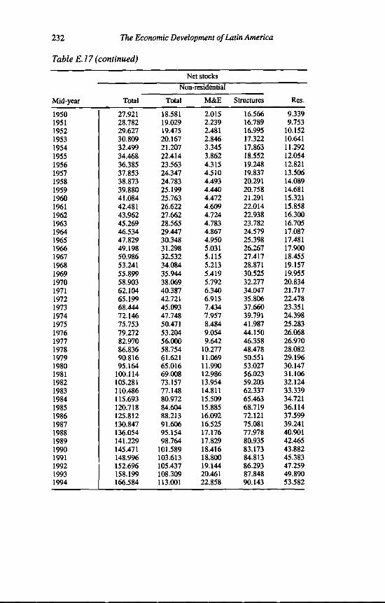
232
Tabi
Mid-;
195019511952195319541955195619571958195919601961196219631964196519661967196819691970197119721973197419751976197719781979198019811982198319841985198619871988198919901991199219931994
The Economic Development of Latin America
Net stocksNon-residential
Res.Total Total M&E Structures
27.921 18.581 2.015 16.566 9.33928.782 19.029 2.239 16.789 9.75329.627 19.475 2.481 16.995 10.15230.809 20.167 2.846 17.322 10.64132.499 21.207 3.345 17.863 11.29234.468 22.414 3.862 18.552 12.05436.385 23.563 4.315 19.248 12.82137.853 24.347 4.510 19.837 13.50638.873 24.783 4.493 20.291 14.08939.880 25.199 4.440 20.758 14.68141.084 25.763 4.472 21.291 15.32142.481 26.622 4.609 22.014 15.85843.962 27.662 4.724 22.938 16.30045.269 28.565 4.783 23.782 16.70546.534 29.447 4.867 24.579 17.08747.829 30.348 4.950 25.398 17.48149.198 31.298 5.031 26.267 17.90050.986 32.532 5.115 27.417 18.45553.241 34.084 5.213 28.871 19.15755.899 35.944 5.419 30.525 19.95558.903 38.069 5.792 32.277 20.83462.104 40.387 6.340 34.047 21.71765.199 42.721 6.915 35.806 22.47868.444 45.093 7.434 37.660 23.35172.146 47.748 7.957 39.791 24.39875.753 50.471 8.484 41.987 25.28379.272 53.204 9.054 44.150 26.06882.970 56.000 9.642 46.358 26.97086.836 58.754 10.277 48.478 28.08290.816 61.621 11.069 50.551 29.19695.164 65.016 11.990 53.027 30.147
100.114 69.008 12.986 56.023 31.106105.281 73.157 13.954 59.203 32.124110.486 77.148 14.811 62.337 33.339115.693 80.972 15.509 65.463 34.721120.718 84.604 15.885 68.719 36.114125.812 88.213 16.092 72.121 37.599130.847 91.606 16.525 75.081 39.241136.054 95.154 17.176 77.978 40.901141.229 98.764 17.829 80.935 42.465145.471 101.589 18.416 83.173 43.882148.996 103.613 18.800 84.813 45.383152.696 105.437 19.144 86.293 47.259158.199 108.309 20.461 87.848 49.890166.584 113.001 22.858 90.143 53.582

Mid-year195019511952195319541955195619571958195919601961196219631964196519661967196819691970197119721973197419751976197719781979198019811982198319841985198619871988198919901991199219931994
Appendix E 233
E.18 Colombia 3. Capital Stock: Average Ages, Average Service Lives "apital-Output Ratios, 1950—94 (on the basis of national currencies at mt 1980 prices)
Average age capital stock Average service life capital stock
Capital-output ratios
Total Non- resideutial
Total Non-residential
Total Non- residential
Gross Net Gross Net Gross Net Gross Net
14.35 9.58 14.02 9.07 34.18 30.58 2.9 1.9 2.2 1.314.42 9.64 14.04 9.10 33.63 30.02 2.9 1.9 2.2 1.414.45 9.66 14.02 9.07 33.21 29.53 2.8 1.8 2.1 1.314.27 9.45 13.77 8.80 33.40 29.69 2.8 1.8 2.1 1.314.01 9.20 13.45 8.52 32.97 29.19 2.8 1.8 2.1 1.313.78 8.99 13.17 8.29 32.45 28.65 2.9 1.9 2.1 1.413.67 8.96 13.04 8.26 31.61 27.79 2.9 1.9 2.2 1.413.84 9.17 13.21 8.50 30.68 26.84 3.0 1.9 2.2 1.414.05 9.38 13.43 8.73 30.41 26.55 3.0 1.9 2.3 1.414.23 9.51 13.62 8.85 30.29 26.37 2.9 1.8 2.2 1.314.30 9.57 13.68 8.90 30.28 26.35 2.9 1.8 2.2 1.314.32 9.57 13.64 8.81 30.11 26.25 2.9 1.8 2.1 1.314.37 9.59 13.62 8.75 29.87 25.99 2.8 1.8 2.1 1.214.49 9.70 13.69 8.81 29.92 26.05 2.8 1.7 2.1 1.214.55 9.72 13.70 8.75 30.15 26.32 2.8 1.7 2.0 1.214.65 9.81 13.73 8.78 29.82 25.97 2.8 1.7 2.0 1.214.63 9.77 13.64 8.66 29.94 26.08 2.7 1.6 2.0 1.214.57 9.69 13.51 8.54 29.99 26.08 2.7 1.6 2.0 1.214.41 9.58 13.26 8.40 30.09 26.13 2.6 1.6 1.9 1.114.24 9.47 13.01 8.27 30.45 26.45 2.5 1.6 1.9 1.114.05 9.28 12.75 8.06 30.90 26.90 2.5 1.6 1.8 1.113.89 9.14 12.53 7.89 31.13 27.18 2.4 1.6 1.8 1.113.78 9.08 12.36 7.82 31.19 27.34 2.4 1.5 1.8 1.113.70 9.00 12.27 7.75 31.06 27.19 2.4 1.5 1.7 1.113.60 8.90 12.16 7.66 30.98 27.18 2.4 1.5 1.7 1.113.58 8.88 12.08 7.63 30.48 26.74 2.4 1.6 1.8 1.213.52 8.89 11.96 7.66 30.46 26.77 2.4 1.6 1.8 1.213.48 8.89 11.92 7.67 30.26 26.58 2.4 1.6 1.8 1.213.41 8.86 11.86 7.67 30.25 26.60 2.4 1.5 1.8 1.113.34 8.83 11.78 7.65 29.95 26.38 2.3 1.5 1.8 1.113.23 8.74 11.63 7.55 29.92 26.43 2.4 1.5 1.8 1.213.13 8.66 11.50 7.46 29.62 26.19 2.5 1.6 1.9 1.213.07 8.61 11.43 7.43 29.39 26.03 2.6 1.7 2.0 1.313.03 8.61 11.41 7.46 29.03 25.69 2.7 1.7 2.1 1.313.02 8.64 11.40 7.52 28.81 25.49 2.7 1.7 2.1 1.313.06 8.74 11.46 7.66 28.49 25.17 2.7 1.8 2.1 1.413.08 8.76 11.49 7.70 28.64 25.31 2.7 1.7 2.1 1.313.11 8.83 11.55 7.82 28.70 25.36 2.7 1.7 2.1 1.313.09 8.82 11.54 7.82 28.80 25.49 2.7 1.7 2.1 1.313.18 8.91 11.67 7.92 28.62 25.33 2.7 1.7 2.1 1.313.32 9.05 11.84 8.08 28.50 25.24 2.7 1.7 2.1 1.313.52 9.22 12.10 8.29 28.28 24.97 2.7 1.7 2.1 1.313.66 9.32 12.29 8.41 28.49 25.13 2.7 1.7 2.1 1.313.58 9.17 12.26 8.30 28.87 25.44 2.6 1.6 2.0 1.213.35 8.89 12.08 8.06 28.89 25.39 2.6 1.6 2.0 1.2

234 The Economic Development of Latin America
Table E.19 Colombia 4. Capital Stock: Average Ages, Average Service Lives and Capital-Output Ratios, 1950-94 (on the basis of constant 1980 international dollars)
Average age capital stock Average service life capital Capital-output ratiosstock _ _ _ _ _ _ _ _ _
Total Non- Total Non- Total Non-residential r e s id e n tia l______________ residential
Mid-vear
Gross Net Gross Net Gross Net Gross Net
1950 15.27 10.28 15.23 9.97 39.28 35,32 2,8 1,8 1,9 1,21951 15.42 10.41 15.36 10.08 38.87 34,86 2,8 1,8 1,9 1,21952 15.53 10.48 15.45 10.12 38.65 34,53 2,7 1,8 1,9 1,21953 15.47 10.36 15.35 9.95 38.86 34,65 2,7 1,7 1,8 1,11954 15.31 10.17 15.15 9.73 38.73 34,35 2,6 1,7 1,8 1,11955 15.16 9.99 14.97 9.52 38.39 33,90 2,7 1,7 1,8 1,11956 15.09 9.96 14.87 9.49 37.77 33,19 2,7 1,8 1,8 1,11957 15.21 10.10 14.99 9.67 37.05 32,39 2,8 1,8 1,9 1,11958 15.38 10.27 15.15 9.85 36.81 32,10 2,8 1,8 1,9 1,11959 15.51 10.34 15.27 9.90 36.78 31,98 2,7 1,7 1,8 1,11960 15.57 10.41 15.33 9.96 36.75 31,93 2,7 1,7 1,8 1,11961 15.60 10.43 15.26 9.85 36.67 31,96 2,6 1,7 1,8 1,01962 15.64 10.44 15.21 9.75 36.52 31,79 2,6 1,6 1,7 1,01963 15.76 10.56 15.25 9.79 36.47 31,78 2,6 1,6 1,7 1,01964 15.82 10.60 15.23 9.73 36.64 31,98 2,5 1,6 1,7 1,01965 15.91 10.69 15.23 9.75 36.37 31,68 2,5 1,6 1,7 1,01966 15.90 10.67 15.11 9.63 36.47 31,76 2,5 1,5 1,6 1,01967 15.80 10.57 14.90 9.46 36.64 31,87 2,4 1,5 1,6 1,01968 15.61 10.45 14.60 9.29 36.77 31,97 2,4 1,5 1,6 1,01969 15.44 10.34 14.33 9.16 37.12 32,33 2,3 1,5 1,6 1,01970 15.29 10.17 14.10 8.95 37.46 32,71 2,3 1,5 1,5 1,01971 15.18 10.05 13.92 8.80 37.59 32,93 2,3 1,5 1,5 1,01972 15.11 10.03 13.76 8.73 37.51 32,95 2,2 1,4 1,5 0,91973 15.03 9.94 13.66 8.66 37.52 32,89 2,2 1,4 1,4 0,91974 14.94 9.84 13.54 8.55 37.47 32,91 2,2 1,4 1,4 0,91975 14.94 9.82 13.46 8.51 37.00 32,49 2,2 1,4 1,5 1,01976 14.91 9.85 13.35 8.56 36.96 32,50 2,2 1,4 1,5 1,01977 14.88 9.84 13.30 8.56 36.80 32,32 2,2 1,4 1,5 1,01978 14.83 9.82 13.26 8.58 36.75 32,26 2,1 1,4 1,5 0,91979 14.79 9.83 13.20 8.59 36.45 32,03 2,1 1,4 1,4 0,91980 14.71 9.76 13.06 8.49 36.46 32,12 2,1 1,4 1,5 1,01981 14.64 9.68 12.92 8.40 36.23 31,93 2,2 1,4 1,5 1,01982 14.58 9.64 12.83 8.36 36.01 31,76 2,3 1,5 1,6 1,01983 14.53 9.63 12.79 8.39 35.72 31,43 2,4 1,5 1,6 1,11984 14.50 9.64 12.76 8.44 35.53 31,26 2,4 1,6 1,7 1,11985 14.50 9.70 12.76 8.54 35.30 31,02 2,4 1,6 1,7 1,11986 14.48 9.68 12.75 8.55 35.43 31,16 2,4 1,6 1,7 1,11987 14.51 9.76 12.82 8.69 35.37 31,07 2,4 1,5 1,6 1,11988 14.48 9.75 12.80 8.70 35.49 31,24 2,4 1,5 1,6 1,1198 9 14.58 9.85 12.95 8.83 35.30 31,07 2,4 1,5 1,7 1,11990 14.73 10.01 13.16 9.03 35.13 30,93 2,4 1,5 1,6 1,11991 14.94 10.20 13.45 9.28 34.97 30,67 2,4 1,5 1,7 1,11992 15.09 10.30 13.69 9.45 35.16 30,81 2,4 1,5 1,7 1,01993 15.07 10.24 13.78 9.47 35.46 30,96 2,3 1,5 1,6 1,01994 14.90 10.01 13.70 9.31 35.60 30,96 2,3 1,5 1,6 1,0
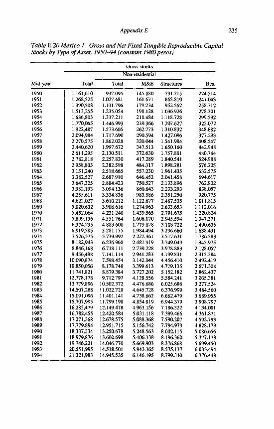
Mid-:
195019511952195319541955195619571958195919601961196219631964196519661967196819691970197119721973197419751976197719781979198019811982198319841985198619871988198919901991199219931994
Appendix E 235
\exico 1. Gross and Net Fixed Tangible Reproducible Capital>e o f Asset, 1950-94 (constant 1980 pesos)
Gross stocksNon-residential
Total Total M&E Structures Res.
1,161,610 937.095 145.880 791.215 224.5141,268,525 1.027.481 161.671 865.810 241.0431,390,508 1.131.796 179.234 952.562 258.7121,513,255 1.235.054 198.128 1.036.926 278.2011,636,803 1.337.211 218.484 1.118.728 299.5921,770,065 1.446.993 239.366 1.207.627 323.0721,922,487 1.573.605 262.773 1.310.832 348.8822,094,984 1.717.690 290.594 1.427.096 377.2932,270,575 1.862.028 320.044 1.541.984 408.5472,440,620 1.997.672 347.513 1.650.160 442.9482,611,295 2.130.511 372.630 1.757.881 480.7842,782,818 2.257.830 417.289 1.840.541 524.9882,958,803 2.382.598 484.317 1.898.281 576.2053,151,240 2.518.665 557.230 1.961.435 632.5753,382,527 2.687.910 646.452 2.041.458 694.6173,647,325 2.884.423 750.527 2.133.896 762.9023,932,193 3.094.136 860.843 2.233.293 838.0574,255,611 3.334.836 983.586 2.351.250 920.7754,622,027 3.610.212 1.122.677 2.487.535 1.011.8155,020,632 3.908.616 1.274.963 2.633.653 1.112.0165,452,064 4.231.240 1.439.565 2.791.675 1.220.8245,899,136 4.551.764 1.606.170 2.945.594 1.347.3716,374,235 4.883.600 1.779.878 3.103.722 1.490.6356,919,585 5.281.155 1.984.494 3.296.660 1.638.4317,526,375 5.739.992 2.222.361 3.517.631 1.786.3838,182,943 6.236.968 2.487.919 3.749.049 1.945.9758,846,168 6.718.111 2.739.228 3.978.883 2.128.0579,456,498 7.141.114 2.941.283 4.199.831 2.315.384
10,090,874 7.598.454 3.142.044 4.456.410 2.492.41910,850,056 8.178.748 3.399.613 4.779.135 2.671.30811,741,821 8.879.384 3.727.202 5.152.182 2.862.43712,778,178 9.712.797 4.128.556 5.584.241 3.065.38113,779,896 10.502.372 4.476.686 6.025.686 3.277.52414,507,288 11.022.728 4.645.728 6.376.999 3.484.56015,091,096 11.401.141 4.738.662 6.662.479 3.689.95515,707,995 11.799.198 4.854.819 6.944.379 3.908.79716,283,479 12.149.478 4.963.156 7.186.322 4.134.00116,782,455 12.420.584 5.031.118 7.389.466 4.361.87117,271,368 12.678.575 5.088.368 7.590.207 4.592.79317,779,894 12.951.715 5.156.742 7.794.973 4.828.17918,337,334 13.250.678 5.248.563 8.002.115 5.086.65618,979,876 13.602.698 5.406.338 8.196.360 5.377.17819,746,221 14.046.770 5.669.903 8.376.868 5.699.45020,551,995 14.518.501 5.943.365 8.575.137 6.033.49421,321,983 14.945.535 6.146.195 8.799.340 6.376.448
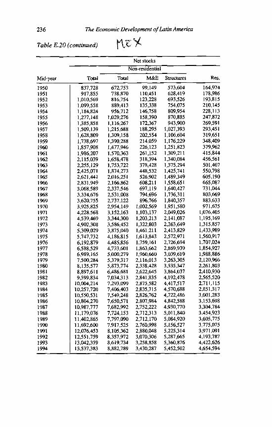
236
Tabl
Mid-:
195019511952195319541955195619571958195919601961196219631964196519661967196819691970197119721973197419751976197719781979198019811982198319841985198619871988198919901991199219931994
The Economic Development of Latin America
continued)
Net stocks Non-residential
Total Total M&E Structures Res,
837,728 672,753 99,149 573,604 164,974917,855 738,870 110,451 628,419 178,986
1,010,569 816,754 123,228 693,526 193,8151,099,558 889,413 135,338 754,075 210,1451,184,824 956,712 146,758 809,954 228,1131,277,148 1,029,276 158,390 870,885 247,8721,385,858 1,116,267 172,367 943,900 269,5911,509,139 1,215,688 188,295 1,027,393 293,4511,628,809 1,309,158 202,554 1,106,604 319,6511,738,697 1,390,288 214,059 1,176,229 348,4091,857,908 1,477,946 226,123 1,251,823 379,9621,986,207 1,570,363 261,152 1,309,211 415,8442,115,039 1,658,478 318,394 1,340,084 456,5612,255,129 1,753,722 378,428 1,375,294 501,4072,425,071 1,874,273 448,532 1,425,741 550,7982,621,441 2,016,251 526,902 1,489,349 605,1902,831,949 2,166,862 608,211 1,558,651 665,0873,068,589 2,337,546 697,119 1,640,427 731,0443,334,676 2,531,008 794,696 1,736,311 803,6693,620,755 2,737,122 896,766 1,840,357 883,6333,925,825 2,954,149 1,002,569 1,951,580 971,6754,228,568 3,152,163 1,103,137 2,049,026 1,076,4054,539,469 3,344,300 1,203,213 2,141,087 1,195,1694,902,308 3,586,452 1,322,803 2,263,649 1,315,8575,309,029 3,875,040 1,461,211 2,413,829 1,433,9895,747,732 4,186,815 1,613,843 2,572,971 1,560,9176,192,879 4,485,856 1,759,161 2,726,694 1,707,0246,588,529 4,733,601 1,863,662 2,869,939 1,854,9276,989,165 5,000,279 1,960,660 3,039,619 1,988,8867,500,284 5,379,317 2,116,013 3,263,305 2,120,9668,135,577 5,873,774 2,338,428 3,535,347 2,261,8038,897,611 6,486,681 2,622,645 3,864,037 2,410,9309,599,834 7,034,313 2,841,835 4,192,478 2,565,520
10,004,214 7,293,099 2,875,582 4,417,517 2,711,11510,257,720 7,406,403 2,835,715 4,570,688 2,851,31710,550,531 7,549,248 2,826,762 4,722,486 3,001,28310,804,270 7,650,571 2,807,984 4,842,588 3,153,69810,987,777 7,682,992 2,752,222 4,930,770 3,304,78411,179,076 7,724,153 2,712,313 5,011,840 3,454,92311,402,865 7,797,090 2,712,170 5,084,920 3,605,77511,692,600 7,917,525 2,760,998 5,156,527 3,775,07512,076,453 8,105,362 2,880,048 5,225,314 3,971,09112,551,759 8,357,972 3,070,306 5,287,665 4,193,78713,042,359 8,619,734 3,258,858 5,360,876 4,422,62613,537,383 8,882,789 3,430,287 5,452,502 4,654,594
Table E.21 Mexico 2. Gross and Net Fixed Tangible Reproducible Capital Stocks by Type of Asset, 1950—94 (constant million 1980 international dollars)
Appendix E 237
Mid-year
Gross stocks
Total
Non-residential
Total M&E Structures Res.
1950 61,878 48.020 6.881 41.138 13.8591951 67,522 52.643 7.626 45.017 14.8791952 73,952 57.982 8.454 49.527 15.9701953 80,432 63.260 9.346 53.914 17.1731954 86,966 68.473 10.306 58.167 18.4931955 94,023 74.080 11.291 62.789 19.9431956 102,086 80.550 12.395 68.155 21.5361957 111,197 87.908 13.707 74.200 23.2901958 120,489 95.270 15.096 80.174 25.2191959 129,533 102.190 16.392 85.798 27.3421960 138,654 108.976 17.577 91.399 29.6781961 147,787 115.380 19.683 95.697 32.4071962 157,113 121.544 22.845 98.699 35.5681963 167,315 128.267 26.284 101.983 39.0481964 179,514 136.637 30.493 106.144 42.8781965 193,445 146.352 35.402 110.950 47.0931966 208,456 156.724 40.606 116.118 51.7321967 225,484 168.646 46.396 122.251 56.8381968 244,751 182.293 52.956 129.337 62.4581969 265,717 197.074 60.140 136.934 68.6431970 288,414 213.054 67.904 145.150 75.3591971 312,087 228.916 75.763 153.153 83.1711972 337,346 245.331 83.956 161.375 92.0151973 366,152 265.015 93.608 171.406 101.1381974 397,994 287.724 104.828 182.896 110.2711975 432,405 312.283 117.355 194.928 120.1221976 467,448 336.087 129.209 206.878 131.3621977 500,031 357.106 138.740 218.366 142.9251978 533,769 379.916 148.210 231.706 153.8531979 573,741 408.845 160.359 248.486 164.8961980 620,387 443.694 175.811 267.882 176.6941981 674,311 485.090 194.743 290.347 189.2211982 726,780 524.464 211.164 313.299 202.3161983 765,800 550.704 219.138 331.566 215.0961984 797,706 569.931 223.522 346.409 227.7751985 831,350 590.067 229.001 361.066 241.2841986 862,942 607.757 234.111 373.645 255.1851987 890,776 621.525 237.317 384.208 269.2511988 918,168 634.662 240.017 394.645 283.5061989 946,570 648.534 243.243 405.292 298.0361990 977,627 663.635 247.574 416.062 313.9911991 1,013,102 681.177 255.016 426.161 331.9251992 1,054,813 702.995 267.448 435.547 351.8181993 1,098,641 726.203 280.347 445.855 372.4381994 1,141,035 747.427 289.915 457.513 393.608

238
Tabl
Mid-;
195019511952195319541955195619571958195919601961196219631964196519661967196819691970197119721973197419751976197719781979198019811982198319841985198619871988198919901991199219931994
Appendix E
Net stocksNon-residential
Total Total M&E Structures Res.
44,684 34.501 4.677 29.824 10.18448,932, 37.884 5.210 32.674 11.04953,836 41.872 5.813 36.059 11.96458,563 45.591 6.384 39.207 12.97263,116 49.035 6.923 42.113 14.08168,053 52.752 7.471 45.281 15.30173,849 57.208 8.131 49.077 16.64180,414 62.300 8.882 53.418 18.11486,823 67.091 9.554 57.537 19.73292,761 71.254 10.097 61.157 21.50799,208 75.753 10.666 65.087 23.454
106,059 80.390 12.318 68.071 25.669112,878 84.695 15.019 69.676 28.183120,308 89.357 17.850 71.507 30.951129,287 95.287 21.157 74.130 34.000139,648 102.291 24.854' 77.437 37.357150,784 109.730 28.689 81.040 41.055163,301 118.175 32.883 85.292 45.126177,373 127.763 37.486 90.278 49.609192,533 137.988 42.300 95.687 54.545208,741 148.761 47.291 101.470 59.980225,016 158.572 52.035 106.537 66.445241,855 168.079 56.755 111.324 73.776261,318 180.092 62.396 117.696 81.226282,947 194.430 68.925 125.505 88.518306,257 209.904 76.125 133.779 96.353330,123 224.751 82.979 141.772 105.372351,630 237.128 87.909 149.220 114.502373,297 250.526 92.484 158.042 122.771400,408 269.484 99.812 169.672 130.924433,737 294.120 110.303 183.817 139.617473,439 324.616 123.710 200.907 148.823510,398 352.032 134.049 217.984 158.365532,678 365.325 135.641 229.684 167.353547,416 371.408 133.760 237.648 176.007564,143 378.879 133.338 245.541 185.264578,910 384.237 132.452 251.785 194.673590,191 386.192 129.822 256.370 203.999601,792 388.525 127.939 260.585 213.267614,896 392.318 127.933 264.385 222.579631,373 398.344 130.236 268.108 233.029652,665 407.536 135.851 271.685 245.129678,628 419.752 144.826 274.927 258.876705,455 432.453 153.720 278.733 273.002732,624 445.303 161.806 283.497 287.321
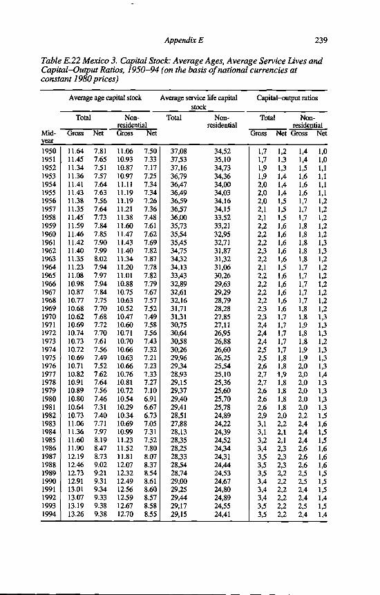
Appendix E 239
Table E.22 Mexico 3. Capital Stock: Average Ages, Average Service Lives and Capital-Output Ratios, 1950-94 (on the basis of national currencies at constant 1980prices)
Average age capital stock Average service life capital stock
Capital-output ratios
Total Non- Total Non- Total Non-residential residential residential
Mid Gross Net Gross Net Gross Net Gross Netyear1950 11.64 7.81 11.06 7.50 37,08 34,52 1,7 1,2 1,4 1,01951 11.45 7.65 10.93 7.33 37,53 35,10 1,7 1,3 1,4 1,01952 11.34 7.51 10.87 7.17 37,16 34,73 1,9 1,3 1,5 1,11953 11.36 7.57 10.97 7.25 36,79 34,36 1,9 1,4 1,6 1,11954 11.41 7.64 11.11 7.34 36,47 34,00 2,0 1,4 1,6 1,11955 11.43 7.63 11.19 7.34 36,49 34,03 2,0 1,4 1,6 1,11956 11.38 7.56 11.19 7.26 36,59 34,16 2,0 1,5 1,7 1,21957 11.35 7.64 11.21 7.36 36,57 34,15 2,1 1,5 1,7 1,21958 11.45 7.73 11.38 7.48 36,00 33,52 2,1 1,5 1,7 1,21959 11.59 7.84 11.60 7.61 35,73 33,21 2,2 1,6 1,8 1,21960 11.46 7.85 11.47 7.62 35,54 32,95 2,2 1,6 1,8 1,21961 11.42 7.90 11.43 7.69 35,45 32,71 2,2 1,6 1,8 1,31962 11.40 7.99 11.40 7.82 34,75 31,87 2,3 1,6 1,8 1,31963 11.35 8.02 11.34 7.87 34,32 31,32 2,2 1,6 1,8 1,21964 11.23 7.94 11.20 7.78 34,13 31,06 2,1 1,5 1,7 1,21965 11.08 7.97 11.01 7.82 33,43 30,26 2,2 1,6 1,7 1,21966 10.98 7.94 10.88 7.79 32,89 29,63 2,2 1,6 1,7 1,21967 10.87 7.84 10.75 7.67 32,61 29,29 2,2 1,6 1,7 1,21968 10.77 7.75 10.63 7.57 32,16 28,79 2,2 1,6 1,7 1,21969 10.68 7.70 10.52 7.52 31,71 28,28 2,3 1,6 1,8 1,21970 10.62 7.68 10.47 7.49 31,31 27,85 2,3 1,7 1,8 1,31971 10.69 7.72 10.60 7.58 30,75 27,11 2,4 1,7 1,9 1,31972 10.74 7.70 10.71 7.56 30,64 26,95 2,4 1,7 1,8 1,31973 10.73 7.61 10.70 7.43 30,58 26,88 2,4 1,7 1,8 1,21974 10.72 7.56 10.66 7.32 30,26 26,60 2,5 1,7 1,9 1,31975 10.69 7.49 10.63 7.21 29,96 26,25 2,5 1,8 1,9 1,31976 10.71 7.52 10.66 7.23 29,34 25,54 2,6 1,8 2,0 1,31977 10.82 7.62 10.76 7.33 28,93 25,10 2,7 1,9 2,0 1,41978 10.91 7.64 10.81 7.27 29,15 25,36 2,7 1,8 2,0 1,31979 10.89 7.56 10.72 7.10 29,37 25,60 2,6 1,8 2,0 1,31980 10.80 7.46 10.54 6.91 29,40 25,70 2,6 1,8 2,0 1,31981 10.64 7.31 10.29 6.67 29,41 25,78 2,6 1,8 2,0 1,31982 10.73 7.40 10.34 6.73 28,51 24,89 2,9 2,0 2,2 1,51983 11.06 7.71 10.69 7.05 27,88 24,22 3,1 2,2 2,4 1,61984 11.36 7.97 10.99 7.31 28,13 24,39 3,1 2,1 2,4 1,51985 11.60 8.19 11.23 7.52 28,35 24,52 3,2 2,1 2,4 1,51986 11.90 8.47 11.52 7.80 28,25 24,34 3,4 2,3 2,6 1,61987 12.19 8.73 11.81 8.07 28,33 24,31 3,5 2,3 2,6 1,61988 12.46 9.02 12.07 8.37 28,54 24,44 3,5 2,3 2,6 1,61989 12.73 9.21 12.32 8.54 28,74 24,53 3,5 2,2 2,5 1,51990 12.91 9.31 12.49 8.61 29,00 24,67 3,4 2,2 2,5 1,51991 13.01 9.34 12.56 8.60 29,25 24,80 3,4 2,2 2,4 1,51992 13.07 9.33 12.59 8.57 29,44 24,89 3,4 2,2 2,4 1,41993 13.19 9.38 12.67 8.58 29,17 24,55 3,5 2,2 2,5 1,51994 13.26 9.38 12.70 8.55 29,15 24,41 3,5 2,2 2,4 1,4
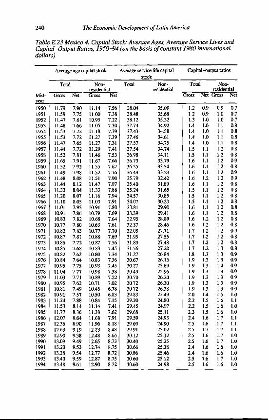
240
TabiCapidollc
Midyear195019511952195319541955195619571958195919601961196219631964196519661967196819691970197119721973197419751976197719781979198019811982198319841985198619871988198919901991199219931994
E.23 Mexico 4. Capital Stock: Average Ages, Average Service Lives and al-Output Ratios, 1950-94 (on the basis of constant 1980 international 's)
The Economic Development of Latin America
Average age capital stock Average service life capital stock
Capital-output ratios
Total Non-residential
Total Non-residential
Total Non-residential
Gross Net Gross Net Gross Net Gross Net
11.79 7.90 11.14 7.56 38.04 35.09 1.2 0.9 0.9 0.711.59 7.75 11.00 7.38 38.48 35.68 1.2 0.9 1.0 0.711.47 7.61 10.95 7.22 38.12 35.32 1.3 1.0 1.0 0.711.48 7.66 11.05 7.30 37.74 34.92 1.4 1.0 1.1 0.811.53 7.72 11.18 7.39 37.43 34.58 1.4 1.0 1.1 0.811.53 7.72 11.27 7.39 37.46 34.61 1.4 1.0 1.1 0.811.47 7.65 11.27 7.31 37.57 34.75 1.4 1.0 1.1 0.811.44 7.72 11.29 7.41 37.54 34.74 1.5 1.1 1.2 0.811.52 7.81 11.46 7.53 36.98 34.11 1.5 1.1 1.2 0.811.65 7.91 11.67 7.66 36.73 33.79 1.6 1.1 1.2 0.911.52 7.92 11.55 7.67 36.55 33.54 1.6 1.1 1.2 0.811.49 7.98 11.52 7.76 36.43 33.23 1.6 1.1 1.2 0.911.48 8.08 11.51 7.90 35.79 32.42 1.6 1.2 1.2 0.911.44 8.12 11.47 7.97 35.40 31.89 1.6 1.1 1.2 0.811.33 8.04 11.33 7.88 35.24 31.65 1.5 1.1 1.2 0.811.20 8.07 11.16 7.94 34.57 30.85 1.5 1.1 1.2 0.811.10 8.05 11.03 7.91 34.07 30.23 1.5 1.1 1.2 0.811.01 7.95 10.91 7.80 33.81 29.90 1.6 1.1 1.2 0.810.91 7.86 10.79 7.69 33.39 29.41 1.6 1.1 1.2 0.810.83 7.82 10.68 7.64 32.95 28.89 1.6 1.2 1.2 0.810.77 7.80 10.63 7.61 32.57 28.46 1.6 1.2 1.2 0.810.82 7.83 10.77 7.70 32.05 27.71 1.7 1.2 1.2 0.910.87 7.81 10.88 7.69 31.95 27.55 1.7 1.2 1.2 0.810.86 7.72 10.87 7.56 31.89 27.48 1.7 1.2 1.2 0.810.85 7.68 10.83 7.45 31.56 27.20 1.7 1.2 1.3 0.810.82 7.62 10.80 7.34 31.27 26.84 1.8 1.3 1.3 0.910.84 7.64 10.83 7.36 30.67 26.13 1.9 1.3 1.3 0.910.95 7.75 10.93 7.45 30.27 25.69 1.9 1.3 1.4 0.911.04 7.77 10.98 7.38 30.49 25.96 1.9 1.3 1.3 0.911.03 7.71 10.89 7.22 30.70 26.20 1.9 1.3 1.3 0.910.95 7.62 10.71 7.02 30.72 26.30 1.9 1.3 1.3 0.910.81 7.49 10.45 6.78 30.72 26.38 1.9 1.3 1.3 0.910.91 7.57 10.50 6.83 29.83 25.49 2.0 1.4 1.5 1.011.24 7.88 10.84 7.15 29.20 24.80 2.2 1.5 1.6 1.111.53 8.14 11.14 7.41 29.45 24.97 2.2 1.5 1.6 1.011.77 8.36 11.38 7.62 29.68 25.11 2.3 1.5 1.6 1.012.07 8.64 11.68 7.91 29.59 24.93 2.4 1.6 1.7 1.112.36 8.90 11.96 8.18 29.69 24.90 2.5 1.6 1.7 1.112.63 9.19 12.23 8.48 29.91 25.02 2.5 1.7 1.7 1.112.90 9.38 12.48 8.66 30.12 25.12 2.5 1.6 1.7 1.013.09 9.49 12.65 8.73 30.40 25.25 2.5 1.6 1.7 1.013.20 9.53 12.74 8.75 30.66 25.38 2.4 1.6 1.6 1.013.28 9.54 12.77 8.72 30.86 25.46 2.4 1.6 1.6 1.013.40 9.59 12.87 8.75 30.60 25.12 2.5 1.6 1.7 1.013.48 9.61 12.90 8.72 30.60 24.98 2.5 1.6 1.6 1.0

Mid-;
195019511952195319541955195619571958195919601961196219631964196519661967196819691970197119721973197419751976197719781979198019811982198319841985198619871988198919901991199219931994
Appendix E 241
enezuela 1. Gross and Net Fixed Tangible Reproducible Capitalie o f Asset, 1950-94 (constant 1980 bolívares)
Gross stocksNon-residential
Total Total M&E Structures Res.
128,678 112,340 50,564 61,776 16,338142,283 124,192 55,403 68,789 18,090157,815 137,135 60,709 76,426 20,680175,771 151,782 67,732 84,051 23,989195,894 168,408 75,919 92,489 27,486216,918 186,285 84,296 101,989 30,632238,672 204,481 92,175 112,306 34,191262,628 224,761 101,279 123,483 37,867287,513 245,494 111,752 133,742 42,019312,265 266,372 122,495 143,877 45,893333,325 284,677 130,439 154,238 48,648348,609 297,584 134,592 162,992 51,025361,003 307,457 137,301 170,156 53,546371,894 315,225 138,346 176,880 56,669384,093 323,595 139,129 184,466 60,499399,491 334,192 141,539 192,653 65,299416,621 345,912 145,331 200,581 70,709433,210 356,998 147,893 209,106 76,211450,128 368,323 148,561 219,763 81,804468,521 380,937 149,061 231,875 87,584487,600 393,940 149,953 243,987 93,660509,952 409,210 152,483 256,727 100,742536,703 427,396 156,070 271,326 109,307566,795 447,587 160,344 287,243 119,208597,296 468,033 165,104 302,929 129,264634,674 495,286 174,875 320,411 139,387687,762 536,684 193,783 342,901 151,078757,953 593,453 221,401 372,051 164,501839,186 660,021 254,056 405,964 179,166912,155 717,208 280,211 436,998 194,947969,938 759,418 298,010 461,407 210,520
1,023,751 799,675 315,583 484,092 224,0761,077,832 843,244 334,989 508,255 234,5881,121,769 879,592 349,234 530,358 242,1771,150,897 903,202 356,761 546,441 247,6951,175,328 923,228 365,435 557,793 252,1001,200,945 944,620 376,805 567,815 256,3251,225,619 965,059 387,481 577,578 260,5601,249,739 985,123 397,592 587,531 264,6171,267,440 999,395 404,364 595,031 268,0451,274,380 1,004,002 401,679 602,323 270,3791,279,644 1,007,455 393,154 614,301 272,1891,287,588 1,013,062 381,576 631,485 274,5261,294,572 1,017,323 365,421 651,902 277,2491,298,099 1,018,624 350,643 667,980 279,475
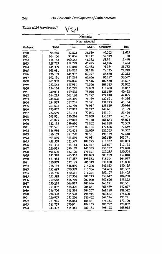
242
Tabi
Mid-;
195019511952195319541955195619571958195919601961196219631964196519661967196819691970197119721973197419751976197719781979198019811982198319841985198619871988198919901991199219931994
The Economic Development of Latin America
•ontinued)
Net stocksNon-residential
Total Total M&E Structures Res.
94,446 82,822 35,519 47,302 11,625104,166 91,036 38,117 52,919 13,130115,783 100,343 41,352 58,991 15,440129,723 111,299 46,423 64,876 18,424145,399 123,866 52,482 71,384 21,533161,081 136,862 58,128 78,733 24,219176,189 148,937 62,277 86,660 27,252192,191 161,864 66,666 95,197 30,327207,903 174,096 71,546 102,550 33,807222,843 185,911 76,396 109,515 36,932234,134 195,247 78,809 116,438 38,887240,034 199,595 78,056 121,539 40,438244,215 202,120 77,272 124,848 42,095248,626 204,310 76,739 127,571 44,316254,919 207,735 76,521 131,213 47,184263,672 212,736 76,917 135,819 50,936273,072 217,872 77,242 140,631 55,199282,599 223,144 77,043 146,101 59,456293,921 230,216 76,969 153,247 63,705307,825 239,803 78,140 161,663 68,022322,133 249,630 79,802 169,828 72,503337,591 259,732 82,104 177,628 77,859356,986 272,424 86,059 186,365 84,562380,159 287,720 91,561 196,159 92,440403,810 303,519 97,931 205,589 100,291431,559 323,527 107,275 216,252 108,033471,331 354,164 122,467 231,697 117,168526,935 399,107 145,355 253,752 127,828591,630 452,126 171,871 280,255 139,504645,399 493,352 190,093 303,259 152,048681,484 517,387 198,882 318,504 164,097710,979 537,179 206,349 330,830 173,800738,193 558,039 214,206 343,833 180,155753,689 570,307 215,904 354,403 183,382754,736 570,331 211,224 359,107 184,405751,593 567,356 207,713 359,642 184,238750,588 566,715 207,020 359,696 183,823750,298 566,937 206,696 360,241 183,361751,097 568,420 206,881 361,539 182,677746,706 565,394 204,207 361,188 181,312734,378 555,578 194,915 360,663 178,800726,927 551,206 186,462 364,744 175,721731,945 558,844 184,481 374,363 173,100741,753 570,951 184,163 386,787 170,802743,377 575,361 180,183 395,178 168,015

Mid-;
19501951195219531954195519561957195819591960196119621963196419651966196719681969197019711972197319741975197619771978197919801981198219831984198519861987198819891990199119921993
Appendix E 243
enemela 2. Gross and Net Fixed Tangible Reproducible Capitalie o f Asset, 1950-94 (constant million 1980 international dollars)
Gross stocksNon-residential
Total Total M&E Structures Res.
26,144 23,195 11,162 12,033 2,94928,894 25,629 12,230 13,399 3,26532,021 28,288 13,402 14,886 3,73335,653 31,323 14,952 16,371 4,33039,736 34,774 16,759 18,015 4,96144,003 38,474 18,608 19,865 5,52948,394 42,223 20,348 21,875 6,17253,244 46,409 22,357 24,052 6,83558,304 50,720 24,669 26,050 7,58563,349 55,065 27,041 28,024 8,28467,618 58,837 28,795 30,042 8,78170,669 61,459 29,711 31,748 9,21073,118 63,452 30,309 33,143 9,66575,222 64,993 30,540 34,453 10,22977,563 66,643 30,713 35,930 10,92080,557 68,770 31,245 37,525 11,78783,914 71,151 32,082 39,069 12,76387,134 73,377 32,647 40,730 13,75790,366 75,600 32,795 42,805 14,76693,879 78,070 32,905 45,165 15,80997,532 80,626 33,102 47,524 16,906
101,850 83,666 33,661 50,005 18,184107,032 87,301 34,452 52,849 19,731112,863 91,345 35,396 55,949 21,518118,784 95,451 36,447 59,004 23,333126,174 101,013 38,604 62,410 25,160136,838 109,568 42,778 66,790 27,270151,036 121,343 48,874 72,468 29,693167,497 135,157 56,083 79,074 32,340182,164 146,975 61,857 85,118 35,189193,659 155,659 65,786 89,873 38,000204,404 163,957 69,665 94,291 40,447215,291 172,947 73,949 98,998 42,344224,111 180,397 77,094 103,303 43,714229,901 185,191 78,755 106,436 44,710234,822 189,317 80,670 108,647 45,505240,047 193,779 83,180 110,599 46,268245,070 198,037 85,537 112,501 47,032249,973 202,208 87,769 114,439 47,765253,547 205,164 89,264 115,900 48,384254,796 205,991 88,671 117,320 48,805255,574 206,442 86,789 119,653 49,132256,787 207,234 84,233 123,001 49,553257,689 207,644 80,667 126,977 50,045257,961 207,514 77,405 130,109 50,447
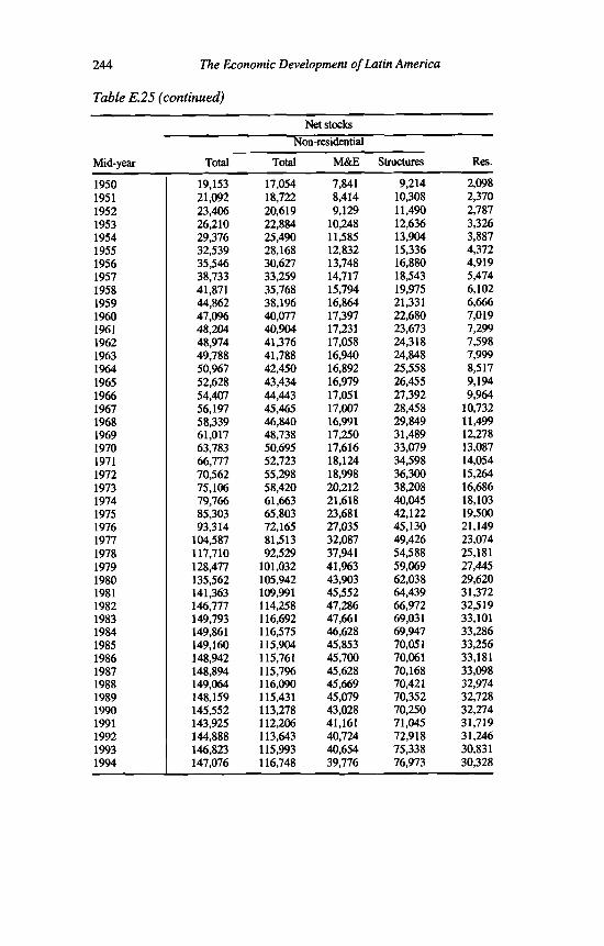
244
Tabi
Mid-;
195019511952195319541955195619571958195919601961196219631964196519661967196819691970197119721973197419751976197719781979198019811982198319841985198619871988198919901991199219931994
The Economic Development of Latin America
Net stocks Non-residential
Total Total M&E Structures Res.
19,153 17,054 7,841 9,214 2,09821,092 18,722 8,414 10,308 2,37023,406 20,619 9,129 11,490 2,78726,210 22,884 10,248 12,636 3,32629,376 25,490 11,585 13,904 3,88732,539 28,168 12,832 15,336 4,37235,546 30,627 13,748 16,880 4,91938,733 33,259 14,717 18,543 5,47441,871 35,768 15,794 19,975 6,10244,862 38,196 16,864 21,331 6,66647,096 40,077 17,397 22,680 7,01948,204 40,904 17,231 23,673 7,29948,974 41,376 17,058 24,318 7,59849,788 41,788 16,940 24,848 7,99950,967 42,450 16,892 25,558 8,51752,628 43,434 16,979 26,455 9,19454,407 44,443 17,051 27,392 9,96456,197 45,465 17,007 28,458 10,73258,339 46,840 16,991 29,849 11,49961,017 48,738 17,250 31,489 12,27863,783 50,695 17,616 33,079 13,08766,777 52,723 18,124 34,598 14,05470,562 55,298 18,998 36,300 15,26475,106 58,420 20,212 38,208 16,68679,766 61,663 21,618 40,045 18,10385,303 65,803 23,681 42,122 19,50093,314 72,165 27,035 45,130 21,149
104,587 81,513 32,087 49,426 23,074117,710 92,529 37,941 54,588 25,181128,477 101,032 41,963 59,069 27,445135,562 105,942 43,903 62,038 29,620141,363 109,991 45,552 64,439 31,372146,777 114,258 47,286 66,972 32,519149,793 116,692 47,661 69,031 33,101149,861 116,575 46,628 69,947 33,286149,160 115,904 45,853 70,051 33,256148,942 115,761 45,700 70,061 33,181148,894 115,796 45,628 70,168 33,098149,064 116,090 45,669 70,421 32,974148,159 115,431 45,079 70,352 32,728145,552 113,278 43,028 70,250 32,274143,925 112,206 41,161 71,045 31,719144,888 113,643 40,724 72,918 31,246146,823 115,993 40,654 75,338 30,831147,076 116,748 39,776 76,973 30,328

andcons
Mid-vear195019511952195319541955195619571958195919601961196219631964196519661967196819691970197119721973197419751976197719781979198019811982198319841985198619871988198919901991199219931994
E.26 Venezuela 3. Capital Stock: Average Ages, Average Service Lives 'apital-Output Ratios, 1950-94 (on the basis of national currencies at 2nt 1980 prices)
Appendix E 245
Average age capital stock Average service life capital Capital-output ratios________________ stock
Total Non- Total Non- Total Non-___________ residential re s id e n tia l_____________ residential
Gross Net Gross Net Gross Net Gross Net
9.05 6.14 8.16 5.56 27.29 25.51 2.8 2.1 2.5 1.89.01 6.13 8.24 5.65 27.01 25.05 2.8 2.0 2.4 1.88.84 6.00 8.17 5.58 27.62 25.60 2.9 2.1 2.5 1.88.70 5.92 8.15 5.59 27.56 25.37 3.0 2.2 2.6 1.98.56 5.88 8.06 5.57 27.65 25.53 3.1 2.3 2.6 1.98.59 5.99 8.14 5.71 27.14 25.03 3.1 2.3 2.7 2.08.66 6.04 8.27 5.79 27.21 25.03 3.1 2.3 2.7 1.98.77 6.14 8.41 5.89 27.29 25.17 3.1 2.2 2.6 1.98.95 6.30 8.66 6.09 26.99 24.75 3.3 2.4 2.8 2.09.14 6.43 8.84 6.19 26.70 24.61 3.3 2.4 2.8 2.09.50 6.71 9.21 6.45 25.90 23.82 3.5 2.5 3.0 2.19.91 7.09 9.63 6.80 25.66 23.60 3.5 2.4 3.0 2.0
10.28 7.45 10.01 7.17 25.67 23.53 3.3 2.2 2.8 1.910.61 7.75 10.36 7.47 25.71 23.49 3.2 2.1 2.7 1.810.83 7.93 10.61 7.66 26.27 23.93 3.0 2.0 2.5 1.610.99 8.04 10.80 7.79 26.65 24.19 3.0 2.0 2.5 1.611.14 8.20 10.97 7.97 26.90 24.35 3.0 2.0 2.5 1.611.27 8.33 11.10 8.11 26.85 24.22 3.0 2.0 2.5 1.611.35 8.38 11.18 8.14 27.33 24.61 3.0 1.9 2.4 1.511.36 8.40 11.15 8.13 27.67 24.87 3.0 2.0 2.4 1.511.46 8.49 11.25 8.20 28.09 25.20 2.9 1.9 2.3 1.511.57 8.48 11.37 8.19 28.65 25.64 2.9 1.9 2.3 1.511.62 8.40 11.44 8.11 29.05 25.90 3.0 2.0 2.4 1.511.60 8.32 11.45 8.03 29.45 26.18 3.0 2.0 2.3 1.511.66 8.33 11.49 8.03 29.53 26.20 2.9 2.0 2.3 1.511.61 8.19 11.43 7.84 30.43 27.09 2.9 2.0 2.3 1.511.38 7.90 11.15 7.48 30.81 27.46 2.9 2.0 2.3 1.510.98 7.51 10.67 7.01 31.02 27.75 3.0 2.1 2.4 1.610.68 7.25 10.32 6.71 30.38 27.15 3.3 2.3 2.6 1.810.71 7.31 10.36 6.79 29.17 25.88 3.5 2.5 2.8 1.910.92 7.53 10.60 7.03 28.75 25.44 3.8 2.7 3.0 2.011.16 7.71 10.82 7.18 28.75 25.49 4.0 2.8 3.2 2.111.45 7.93 11.07 7.35 28.55 25.40 4.2 2.9 3.3 2.211.90 8.31 11.48 7.66 27.93 24.82 4.7 3.1 3.7 2.412.41 8.76 11.94 8.05 27.69 24.61 4.8 3.2 3.8 2.412.87 9.17 12.35 8.41 27.75 24.70 4.9 3.2 3.9 2.413.27 9.49 12.67 8.63 27.66 24.62 4.7 3.0 3.7 2.213.64 9.79 12.97 8.85 27.50 24.47 4.7 2.9 3.7 2.213.96 10.05 13.19 9.03 27.46 24.45 4.5 2.7 3.5 2.014.38 10.44 13.53 9.34 27.08 24.07 5.0 2.9 3.9 2.214.84 10.81 13.90 9.60 26.93 23.93 4.7 2.7 3.7 2.115.14 11.00 14.07 9.67 27.24 24.23 4.3 2.4 3.4 1.915.30 11.01 14.07 9.56 27.54 24.51 4.1 2.3 3.2 1.815.51 11.10 14.12 9.57 27.89 24.85 4.1 2.4 3.2 1.815.83 11.35 14.32 9.73 28.30 25.26 4.3 2.5 3.4 1.9

246
Tabiandinter
Mid-vear195019511952195319541955195619571958195919601961196219631964196519661967196819691970197119721973197419751976197719781979198019811982198319841985198619871988198919901991199219931994
The Economic Development of Latin America
E.27 Venezuela 4. Capital Stock: Average Ages, Average Service Lives '.apital-Output Ratios, 1950-94 (on the basis of constant 1980 national dollars)
Average age capital stock Average service life capital stock
Capital-output ratios
Total Non-residential
Total Non-residential
Total Non-residential
Gross Net Gross Net Gross Net Gross Net
8.82 5.97 8.01 5.44 26.35 24.78 2.1 1.5 1.8 1.38.80 5.99 8.10 5.54 26.02 24.30 2.0 1.5 1.8 1.38.65 5.87 8.04 5.48 26.64 24.86 2.1 1.5 1.9 1.48.52 5.80 8.01 5.49 26.57 24.65 2.2 1.6 1.9 1.48.38 5.76 7.92 5.48 26.66 24.81 2.3 1.7 2.0 1.48.42 5.88 8.00 5.62 26.16 24.31 2.3 1.7 2.0 1.58.51 5.93 8.14 5.70 26.22 24.30 2.3 1.7 2.0 1.48.62 6.03 8.28 5.80 26.32 24.46 2.2 1.6 2.0 1.48.81 6.19 8.54 5.99 26.02 24.06 2.4 1.7 2.1 1.59.00 6.32 8.72 6.09 25.75 23.92 2.4 1.7 2.1 1.59.36 6.60 9.09 6.35 24.95 23.12 2.6 1.8 2.2 1.59.77 6.97 9.50 6.69 24.71 22.91 2.6 1.7 2.2 1.5
10.14 7.32 9.88 7.05 24.71 22.84 2.4 1.6 2.1 1.410.46 7.62 10.21 7.35 24.73 22.79 2.3 1.5 2.0 1.310.68 7.79 10.46 7.53 25.27 23.21 2.2 1.4 1.9 1.210.84 7.91 10.64 7.65 25.64 23.47 2.2 1.4 1.8 1.211.00 8.06 10.82 7.83 25.89 23.63 2.2 1.4 1.9 1.211.12 8.20 10.95 7.97 25.81 23.48 2.2 1.4 1.8 1.111.21 8.24 11.03 7.99 26.27 23.85 2.2 1.4 1.8 1.111.21 8.26 11.00 7.98 26.59 24.10 2.2 1.4 1.8 1.111.31 8.34 11.09 8.05 27.01 24.43 2.1 1.4 1.7 1.111.42 8.33 11.21 8.03 27.55 24.86 2.1 1.4 1.7 1.111.46 8.25 11.27 7.95 27.93 25.11 2.1 1.4 1.7 1.111.44 8.17 11.26 7.87 28.32 25.38 2.1 1.4 1.7 1.111.48 8.18 11.29 7.87 28.40 25.41 2.1 1.4 1.7 1.111.42 8.03 11.21 7.67 29.31 26.31 2.1 1.4 1.7 1.111.18 7.73 10.93 7.31 29.69 26.69 2.1 1.4 1.7 1.110.77 7.33 10.44 6.85 29.91 26.97 2.2 1.5 1.7 1.210.47 7.07 10.10 6.55 29.27 26.38 2.4 1.7 1.9 1.310.50 7.14 10.14 6.64 28.06 25.12 2.5 1.8 2.0 1.410.71 7.36 10.38 6.88 27.64 24.69 2.8 1.9 2.2 1.510.95 7.54 10.60 7.03 27.66 24.75 2.9 2.0 2.3 1.611.23 7.76 10.84 7.20 27.48 24.66 3.0 2.1 2.4 1.611.68 8.14 11.25 7.52 26.86 24.08 3.4 2.2 2.7 1.712.18 8.58 11.71 7.91 26.63 23.88 3.5 2.3 2.8 1.812.63 8.98 12.11 8.25 26.70 23.97 3.6 2.3 2.9 1.813.01 9.28 12.42 8.47 26.62 23.91 3.4 2.1 2.8 1.613.38 9.57 12.72 8.68 26.45 23.76 3.4 2.0 2.7 1.613.68 9.81 12.94 8.84 26.42 23.74 3.2 1.9 2.6 1.514.09 10.19 13.28 9.14 26.04 23.36 3.6 2.1 2.9 1.614.55 10.54 13.65 9.40 25.88 23.20 3.4 1.9 2.7 1.514.84 10.72 13.82 9.47 26.17 23.49 3.1 1.8 2.5 1.414.98 10.72 13.81 9.36 26.45 23.73 2.9 1.7 2.4 1.315.17 10.81 13.86 9.37 26.79 24.05 3.0 1.7 2.4 1.315.49 11.05 14.06 9.54 27.22 24.48 3.1 1.8 2.5 1.4

Appendix E 247
NOTES
1. Dollar with the same purchasing power parity over total GDP as the US dollar, but with a purchasing power over subaggregates and over detailed categories determined by average international prices rather than by US relative prices.
2. The exchange rates normally used are the (rf) series of the IMF, published in International Financial Statistics, various issues, which refer to period averages of market exchange rates for countries quoting in units of national currency per US dollar.


Appendix F. Foreign Trade*
Latin American involvement in the world economy and its role on economic development is a continuing theme in the debate on what development strategy should be chosen. In this appendix imports and exports series are presented, in current dollars and as indices representing volume movement only. For each country and each series I will give a detailed description of the sources used.
General sources
Imports and exports in current dollars for 1950-94 come from IMF (1995b). If not indicated otherwise current imports and exports for 1934-49 are from ECLAC (1976). ECLAC (1976) also provides the inport volume for the 1934-59 period (with the exception of Colombia) and the export volume for Argentina, Chile and Mexico for 1934-72 and for 1934-55 in the cases of Brazil and Venezuela.
Argentina
Current exports: 1900-1913, Lewis (1981); 1914-33, Wilkie (1974).Export volume: 1900-1933, Di Telia and Zymelman (1973); 1973-94, ECLAC, Statistics and Projections Division.Current imports: 1900-1914, Di Telia and Zymelman (1973, pp. 100-121);1915-33, Wilkie (1974, p. 259).Import volume: 1900-1933, United Nations (1959); 1960-86, IMF (1988), p. 166; 1987-94, ECLAC, Statistics and Projections Division.
Brazil
Current exports: 1900-1913, Lewis (1981, p. 57). 1914-15, intrapolated;1916-33, Wilkie (1974, p. 259).Export volume: 1900-1933, ECLAC (1951).Current imports: 1900-1915, APEC (1975); 1916-33, Wilkie (1974, p. 259).
* I am very grateful to John Hennelly who assisted me in the preparation of this appendix during his stay at ECLAC in Santiago de Chile
249

250 The Economic Development of Latin America
Import volume: 1900-1912, Villela and Suzigan (1977, p. 366); 1913-33, ECLAC (1951, p. 221); 1961-85, IMF (1988, p. 166); 1986-94, ECLAC, Statistics and Projections Division.
Chile
Current exports: 1900-1915, INE (various issues) linked for 1916-29 with Wilkie (1974, p. 262); 1930-34 from ECLAC (1976).Export volume: 1900-1930, ECLAC (1951, p. 284); 1973-93, ECLAC, Statistics and Projections Division.Current imports: 1900-1915, INE (various issues) linked for 1916-29 with Wilkie (1974, p. 262); 1930-34 from ECLAC (1976).Import volume: 1900-1930, ECLAC (1951, p. 284); 1960-86, IMF (1988, p. 170); 1987-94, ECLAC, Statistics and Projections Division.
Colombia
Current exports: 1900-1904, Lewis (1981, p. 57). 1905-30, Colombia, Contraloria General de la República (1931), Anuario de Comercio Exterior. Año 1930, vol. XXIX, p. 234; 1931-33, Wilkie (1974, p. 259).Export volume: 1900-1904: 1900, Maddison (1989, p. 138); 1901-04 are intrapolated; 1905-55, Colombia, Contraloria General de la República, Anuario de Comercio Exterior, (1926, p. 213; 1950, p. 3 and 1966, p. LID); 1956-87, IMF (1988, p. 166); 1988-94, ECLAC, Statistics and Projections Division.Current imports: 1905-30, Colombia, Contraloria General de la República (1931), Anuario de Comercio Exterior. Año 1930, vol. XXIX, p. 234; 1931-33, Wilkie (1974, p. 259).Import volume: 1900-1904, not available; 1905-67, Colombia, Contraloria General de la República, Anuario de Comercio Exterior, (1937, p. 203; 1950, p. 2 and 1967, p. LIE); 1968-87, IMF (1988, p. 170); 1988-94, ECLAC, Statistics and Projections Division.
Mexico
Current exports: 1900-1913, Lewis (1981, p. 57); 1914-17, intrapolated; 1918-33, Wilkie (1974, p. 259).Export volume: 1900-1933, ECLAC (1951, p. 424); 1973-94, ECLAC, Statistics and Projections Division.Current imports: 1900-1917, INEGI (1990, vol. II, p. 679); 1918-33, Wilkie (1974, p. 259).Import volume: 1900-1933, ECLAC (1951, p. 424); 1960-86, IMF (1988, p. 170); 1987-94, ECLAC, Statistics and Projections Division.
Appendix F 251
Venezuela
Current exports: 1900-1912, Lewis (1981, p. 57); 1913-49, Baptista (1991). Export volume: 1900-1949, Baptista (1991, pp. 35, 63); 1950-56, ECLAC (1976); 1956-83, IMF (1988, p. 166); 1984-94, ECLAC, Statistics and Projections Division.Current imports: 1900-1915, Baptista (1991); 1916-33, Wilkie (1974, p. 259). Import volume: 1900-1933, Baptista (1991, pp. 61, 63); 1960-86, IMF (1988, p. 166); 1987-94, ECLAC, Statistics and Projections Division.

252 The Economic Development of Latin America
Table F.l Latin American Exports, Six Countries, 1900-1994 (current dollars)
Argentina Brazil Chile Colombia Mexico Venezuela
1900 149 182 61 11 75 91901 162 194 63 11 77 91902 173 175 68 9 76 81903 213 177 71 12 83 71904 255 189 79 19 95 161905 312 215 97 12 97 141906 282 255 208 15 135 161907 286 263 202 15 124 161908 356 215 233 15 120 151909 386 310 228 16 115 161910 362 307 243 18 129 171911 316 325 250 22 146 191912 467 363 282 32 148 261913 515 317 292 34 150 321914 566 223 215 33 154 231915 622 262 241 32 157 261916 556 267 188 36 161 251917 534 298 260 37 165 261918 777 288 292 37 168 511919 1,000 571 116 79 180 571920 1,013 368 289 71 383 331921 651 220 162 63 339 231922 656 301 124 53 289 271923 748 336 198 60 254 311924 790 423 221 86 267 451925 793 491 229 85 203 761926 730 461 201 112 299 931927 972 431 206 109 268 1101928 1,017 475 236 134 255 1411929 907 465 279 127 255 2031930 895 736 277 113 329 1931931 814 432 173 142 258 1061932 569 312 58 98 147 1131933 475 282 49 71 121 881934 475 291 95 78 149 1431935 501 272 96 70 207 1431936 537 322 113 78 188 1671937 758 350 193 86 221 2081938 438 296 139 81 161 2011939 466 305 136 78 150 1851940 428 263 140 71 142 1771941 455 358 159 76 138 2581942 503 400 178 98 168 1811943 610 466 179 125 231 2211944 682 575 195 130 216 3031945 739 655 205 141 258 3931946 1,168 972 217 201 320 5551947 1,612 1,131 279 255 414 7181948 1,577 1,173 329 177 369 1,281

Appendix F
Table F.l (continued)
253
Argentina Brazil Chile Colombia Mexico Venezuela
1949 1,011 1,089 296 321 381 1,1641950 1,178 1,359 281 394 532 9291951 1,169 1,771 370 463 644 1,1871952 688 1,416 453 473 665 1,3501953 1,125 1,539 408 596 591 1,4631954 1,027 1,562 398 657 591 1,3961955 929 1,423 472 584 785 1,8191956 944 1,482 542 537 834 2,0991957 975 1,392 455 511 735 2,5421958 994 1,243 386 461 736 2,3261959 1,009 1,282 495 473 753 2,2141960 1,079 1,268 488 465 764 2,3051961 964 1,403 506 435 826 2,2251962 1,216 1,214 530 463 930 2,3421963 1,365 1,406 522 446 985 2,3431964 1,410 1,430 592 548 1,054 2,4721965 1,493 1,596 637 539 1,145 2,4551966 1,593 1,741 817 508 1,199 2,3731967 1,465 1,654 847 510 1,145 3,0771968 1,368 1,881 858 558 1,254 2,7791969 1,612 2,311 1,075 708 1,430 3,0831970 1,773 2,739 1,249 736 1,402 3,1691971 1,740 2,904 997 690 1,504 3,1241972 1,941 3,991 855 866 1,694 3,1661973 3,266 6,199 1,231 1,177 2,250 3,2981974 3,931 7,951 2,481 1,417 2,958 11,1531975 2,961 8,670 1,552 1,465 2,904 8,8001976 3,916 10,128 2,083 1,745 3,417 9,2991977 5,652 12,120 2,190 2,663 4,167 9,5511978 6,400 12,659 2,478 3,003 6,005 9,1871979 7,810 15,244 3,894 3,300 8,982 143171980 8,021 20,132 4,705 3,945 15,570 19,2211981 9,143 23,293 3,837 2,956 19,646 20,9801982 7,625 20,175 3,706 3,095 21,214 16,5901983 7,836 21,899 3,831 3,081 21,819 13,9371984 8,107 27,005 3,651 3,462 24,407 15,9971985 8,396 25,639 3,804 3,552 22,112 14,4381986 6,852 22,349 4,191 5,102 16,347 8,6601987 6,360 26,224 5,224 4,642 20,887 10,5771988 9,135 33,494 7,052 5,037 20,765 10,2441989 9,579 34,383 8,080 5,717 23,048 13,2861990 12,353 31,414 8,373 6,766 27,131 17,4971991 11,978 31,620 8,942 7,232 27,318 15,1551992 12,235 35,793 10,007 6,917 27,722 14,1851993 13,118 38,597 9,199 7,116 30,241 14,0661994 15,659 43,558 11,539 8,399 34,530 15,480
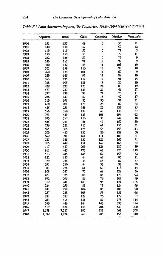
254 The Economic Development of Latin America
Table F.2 Latin American Imports, Six Countries, 1900-1994 (current dollars)
Argentina Brazil Chile Colombia Mexico Venezuela
1900 156 135 48 0 56 111901 140 110 52 0 59 121902 119 115 50 0 71 51903 159 119 53 0 72 111904 252 126 59 0 79 91905 246 112 71 12 97 91906 300 122 88 11 103 101907 303 158 110 12 98 101908 260 139 101 14 69 91909 289 145 99 11 88 101910 363 175 112 17 91 151911 388 195 131 18 80 201912 429 233 125 24 83 191913 477 247 123 29 46 171914 377 138 98 21 23 111915 298 143 57 18 42 171916 310 191 82 30 31 211917 410 201 128 25 89 241918 425 251 161 22 135 151919 556 350 137 48 138 371920 793 439 123 101 194 621921 635 217 110 33 242 181922 585 214 81 42 152 201923 736 231 117 61 155 311924 565 305 128 56 153 431925 700 412 137 89 189 601926 662 391 164 111 180 811927 721 388 132 126 160 711928 705 442 151 149 168 821929 717 417 203 126 180 891930 911 445 175 63 275 1191931 513 245 145 67 153 621932 322 182 44 49 95 411933 329 238 38 55 89 371934 291 210 44 53 92 381935 301 226 61 60 113 441936 308 247 72 68 128 561937 427 335 88 85 170 921938 392 295 89 79 109 991939 312 241 103 96 121 1051940 284 250 85 75 124 991941 241 278 104 86 188 901942 237 238 108 53 155 661943 181 317 128 76 177 671944 201 415 131 87 278 1141945 266 446 144 142 330 1841946 519 674 156 204 543 3001947 1,188 1,217 197 323 661 5681948 1,392 1,134 269 286 458 740
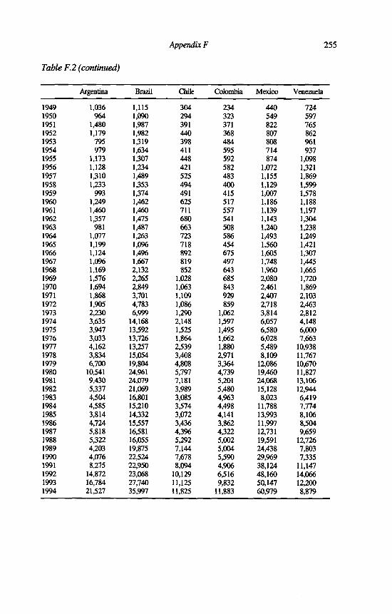
Appendix F
Table F.2 (continued)
255
Argentina Brazil Chile Colombia Mexico Venezuela
1949 1,036 1,115 304 234 440 7241950 964 1,090 294 323 549 5971951 1,480 1,987 391 371 822 7651952 1,179 1,982 440 368 807 8621953 795 1,319 398 484 808 9611954 979 1,634 411 595 714 9371955 1,173 1,307 448 592 874 1,0981956 1,128 1,234 421 582 1,072 1,3211957 1,310 1,489 525 483 1,155 1,8691958 1,233 1,353 494 400 1,129 1,5991959 993 1,374 491 415 1,007 1,5781960 1,249 1,462 625 517 1,186 1,1881961 1,460 1,460 711 557 1,139 1,1971962 1,357 1,475 680 541 1,143 1,3041963 981 1,487 663 508 1,240 1,2381964 1,077 1,263 723 586 1,493 1,2491965 1,199 1,096 718 454 1,560 1,4211966 1,124 1,496 892 675 1,605 1,3071967 1,096 1,667 819 497 1,748 1,4451968 1,169 2,132 852 643 1,960 1,6651969 1,576 2,265 1,028 685 2,080 1,7201970 1,694 2,849 1,063 843 2,461 1,8691971 1,868 3,701 1,109 929 2,407 2,1031972 1,905 4,783 1,086 859 2,718 2,4631973 2,230 6,999 1,290 1,062 3,814 2,8121974 3,635 14,168 2,148 1,597 6,057 4,1481975 3,947 13,592 1,525 1,495 6,580 6,0001976 3,033 13,726 1,864 1,662 6,028 7,6631977 4,162 13,257 2,539 1,880 5,489 10,9381978 3,834 15,054 3,408 2,971 8,109 11,7671979 6,700 19,804 4,808 3,364 12,086 10,6701980 10,541 24,961 5,797 4,739 19,460 11,8271981 9,430 24,079 7,181 5,201 24,068 13,1061982 5,337 21,069 3,989 5,480 15,128 12,9441983 4,504 16,801 3,085 4,963 8,023 6,4191984 4,585 15,210 3,574 4,498 11,788 7,7741985 3,814 14,332 3,072 4,141 13,993 8,1061986 4,724 15,557 3,436 3,862 11,997 8,5041987 5,818 16,581 4,396 4,322 12,731 9,6591988 5,322 16,055 5,292 5,002 19,591 12,7261989 4,203 19,875 7,144 5,004 24,438 7,8031990 4,076 22,524 7,678 5,590 29,969 7,3351991 8,275 22,950 8,094 4,906 38,124 11,1471992 14,872 23,068 10,129 6,516 48,160 14,0661993 16,784 27,740 11,125 9,832 50,147 12,2001994 21,527 35,997 11,825 11,883 60,979 8,879

256 The Economic Development of Latin America
Table F.3 Latin American Export Volume Indices, Six Countries, 1900—1994(1980 = 100)
Argentina Brazil Chile Colombia Mexico Venezuela
1900 16.3 0.0 23.6 0.8 8.3 4.31901 17.8 10.7 25.6 0.8 9.5 3.91902 19.0 10.2 24.3 0.7 9.8 3.11903 23.4 9.6 26.2 0.9 10.3 3.71904 27.6 7.7 28.9 1.4 10.3 4.61905 30.0 8.3 34.6 0.8 9.9 4.31906 26.3 10.6 87.2 1.0 10.3 4.01907 27.1 11.4 108.4 1.1 9.4 3.81908 33.0 9.3 99.6 1.0 9.8 3.91909 30.9 12.1 98.1 1.3 11.0 4.21910 29.6 7.9 110.6 1.5 12.6 4.21911 26.3 8.6 129.1 1.6 12.2 4.21912 38.9 9.2 123.4 1.6 12.5 4.41913 38.4 10.2 121.8 2.0 14.2 5.31914 41.7 9.1 97.0 1.9 15.8 5.51915 60.4 12.7 56.6 1.6 17.4 5.11916 52.6 10.8 81.0 1.6 19.0 5.11917 38.0 10.7 130.0 2.0 20.6 5.61918 54.6 9.1 159.0 2.0 22.2 6.51919 64.3 11.9 147.0 2.3 17.0 6.41920 62.3 10.9 166.0 2.4 36.8 6.31921 57.5 11.0 139.0 3.0 36.4 7.61922 73.0 11.6 87.0 2.6 39.9 7.61923 74.1 12.8 120.0 2.8 35.6 8.01924 91.5 11.5 133.0 3.2 32.4 9.11925 73.0 11.2 149.0 3.2 31.2 12.11926 81.8 10.9 157.0 9.0 32.4 13.71927 109.1 12.3 131.0 19.2 32.9 20.21928 101.3 11.6 146.0 25.6 31.3 29.11929 101.3 12.3 179.0 25.8 31.3 38.31930 70.1 13.5 288.0 26.6 25.2 38.21931 97.4 14.5 145.0 23.0 26.4 32.61932 89.6 9.9 44.0 21.9 18.6 32.21933 85.7 12.4 38.0 17.3 19.7 31.11934 72.5 13.6 44.0 23.2 26.2 35.71935- 76.5 15.7 61.0 23.2 26.8 38.11936 69.2 17.4 72.0 23.8 29.4 42.11937 80.5 15.7 88.0 25.6 34.6 45.81938 51.9 19.0 89.0 27.0 15.4 46.11939 66.5 19.5 103.0 27.7 14.6 47.71940 56.5 16.2 85.0 30.7 12.5 40.11941 50.5 17.6 104.0 29.2 13.7 56.01942 49.2 13.4 108.0 11.7 14.0 37.61943 50.5 13.6 128.0 16.5 16.3 44.81944 55.2 16.0 131.0 25.7 13.4 60.31945 56.5 17.4 144.0 26.9 15.7 77.21946 58.5 21.4 156.0 25.1 16.0 91.71947 63.8 20.2 197.0 27.2 16.3 101.91948 57.9 21.2 269.1 26.6 12.8 113.9
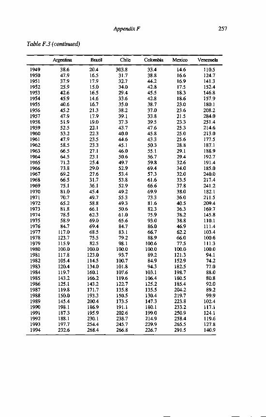
Appendix F
Table F.3 (continued)
257
Argentina Brazil Chile Colombia Mexico Venezuela
1949 38.6 20.4 303.8 33.4 14.6 110.51950 47.9 16.5 31.7 38.8 16.6 124.71951 37.9 17.9 32.7 44.2 16.9 141.31952 25.9 15.0 34.0 42.8 17.5 152.41953 42.6 16.5 29.4 45.5 18.3 146.81954 45.9 14.6 33.6 42.8 18.6 157.91955 40.6 16.7 35.0 38.7 23.0 180.11956 45.2 21.3 38.2 37.0 23.6 208.21957 47.9 17.9 39.1 33.8 21.5 284.01958 51.9 19.0 37.3 39.5 23.3 251.41959 52.5 22.1 43.7 47.6 25.3 214.61960 53.2 22.3 40.0 45.8 25.0 213.01961 47.9 23.5 44.6 43.3 25.6 177.51962 58.5 23.3 45.1 50.3 28.8 187.11963 66.5 27.1 46.0 55.1 29.1 188.91964 64.5 23.1 50.6 56.7 29.4 192.71965 71.2 25.4 49.7 59.8 32.6 191.41966 73.8 29.0 52.9 69.4 34.0 185.01967 69.2 27.6 53.4 57.3 32.0 240.01968 66.5 31.7 53.8 61.6 33.5 217.41969 75.1 36.1 52.9 66.6 37.8 241.21970 81.0 45.4 49.2 69.9 38.0 182.11971 70.7 49.7 55.3 73.3 36.0 211.51972 65.2 58.8 49.3 81.6 40.5 209.41973 81.8 66.1 50.6 82.3 36.3 169.71974 78.5 62.3 61.0 75.9 38.2 145.81975 58.9 69.0 65.6 93.0 38.8 110.11976 84.7 69.4 84.7 86.0 46.9 111.41977 117.0 68.5 83.1 66.7 62.2 103.41978 123.7 75.5 79.2 88.9 66.0 100.61979 115.9 82.5 98.1 100.6 77.5 111.31980 100.0 100.0 100.0 100.0 100.0 100.01981 117.8 123.0 93.7 89.2 121.3 94.11982 105.4 114.5 100.7 84.9 152.9 74.21983 120.4 134.0 101.8 94.3 182.5 77.01984 119.7 160.1 107.6 103.1 198.7 88.01985 143.2 166.2 119.6 106.4 180.5 80.81986 125.1 143.2 122.7 125.2 185.4 92.01987 119.8 171.7 135.8 135.5 204.2 89.21988 150.0 193.3 150.5 130.4 219.7 99.91989 145.4 200.4 173.5 147.3 223.8 102.41990 198.1 186.9 191.1 180.1 233.2 117.11991 187.3 195.9 202.6 199.0 250.9 124.11992 188.1 230.1 238.7 214.9 258.4 119.61993 197.7 254.4 245.7 229.9 265.5 127.81994 232.6 268.4 266.8 226.7 291.5 140.9
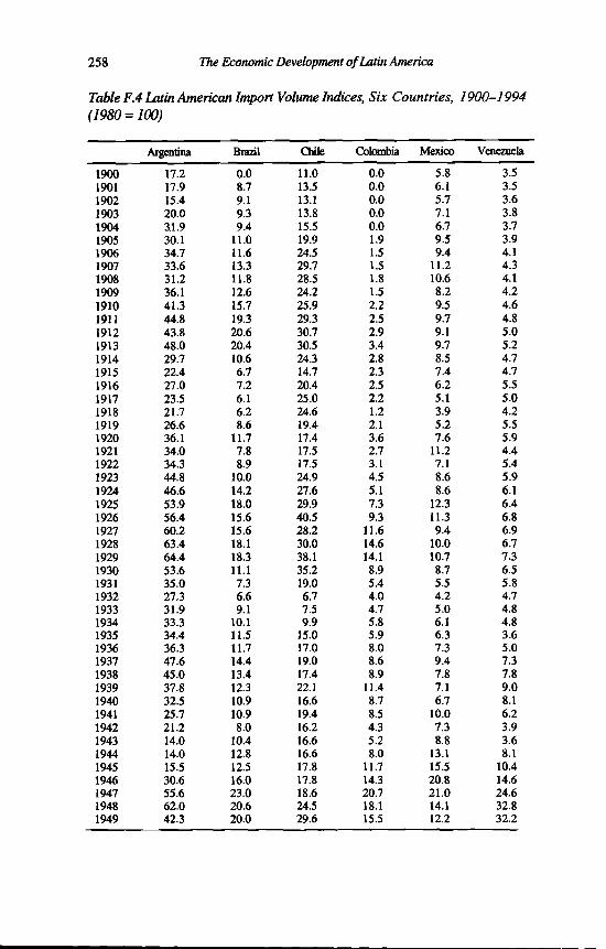
258 The Economic Development of Latin America
Table F.4 Latin American Import Volume Indices, Six Countries, 1900-1994 (1980=100)
Argentina Brazil Chile Colombia Mexico Venezuela
1900 17.2 0.0 11.0 0.0 5.8 3.51901 17.9 8.7 13.5 0.0 6.1 3.51902 15.4 9.1 13.1 0.0 5.7 3.61903 20.0 9.3 13.8 0.0 7.1 3.81904 31.9 9.4 15.5 0.0 6.7 3.71905 30.1 11.0 19.9 1.9 9.5 3.91906 34.7 11.6 24.5 1.5 9.4 4.11907 33.6 13.3 29.7 1.5 11.2 4.31908 31.2 11.8 28.5 1.8 10.6 4.11909 36.1 12.6 24.2 1.5 8.2 4.21910 41.3 15.7 25.9 2.2 9.5 4.61911 44.8 19.3 29.3 2.5 9.7 4.81912 43.8 20.6 30.7 2.9 9.1 5.01913 48.0 20.4 30.5 3.4 9.7 5.21914 29.7 10.6 24.3 2.8 8.5 4.71915 22.4 6.7 14.7 2.3 7.4 4.71916 27.0 7.2 20.4 2.5 6.2 5.51917 23.5 6.1 25.0 2.2 5.1 5.01918 21.7 6.2 24.6 1.2 3.9 4.21919 26.6 8.6 19.4 2.1 5.2 5.51920 36.1 11.7 17.4 3.6 7.6 5.91921 34.0 7.8 17.5 2.7 11.2 4.41922 34.3 8.9 17.5 3.1 7.1 5.41923 44.8 10.0 24.9 4.5 8.6 5.91924 46.6 14.2 27.6 5.1 8.6 6.11925 53.9 18.0 29.9 7.3 12.3 6.41926 56.4 15.6 40.5 9.3 11.3 6.81927 60.2 15.6 28.2 11.6 9.4 6.91928 63.4 18.1 30.0 14.6 10.0 6.71929 64.4 18.3 38.1 14.1 10.7 7.31930 53.6 11.1 35.2 8.9 8.7 6.51931 35.0 7.3 19.0 5.4 5.5 5.81932 27.3 6.6 6.7 4.0 4.2 4.71933 31.9 9.1 7.5 4.7 5.0 4.81934 33.3 10.1 9.9 5.8 6.1 4.81935 34.4 11.5 15.0 5.9 6.3 3.61936 36.3 11.7 17.0 8.0 7.3 5.01937 47.6 14.4 19.0 8.6 9.4 7.31938 45.0 13.4 17.4 8.9 7.8 7.81939 37.8 12.3 22.1 11.4 7.1 9.01940 32.5 10.9 16.6 8.7 6.7 8.11941 25.7 10.9 19.4 8.5 10.0 6.21942 21.2 8.0 16.2 4.3 7.3 3.91943 14.0 10.4 16.6 5.2 8.8 3.61944 14.0 12.8 16.6 8.0 13.1 8.11945 15.5 12.5 17.8 11.7 15.5 10.41946 30.6 16.0 17.8 14.3 20.8 14.61947 55.6 23.0 18.6 20.7 21.0 24.61948 62.0 20.6 24.5 18.1 14.1 32.81949 42.3 20.0 29.6 15.5 12.2 32.2

Appendix F
Table F.4 (continued)
259
Argentina Brazil Chile Colombia Mexico Venezuela
1950 38.2 22.7 21.7 20.4 14.5 27.41951 43.5 35.2 24.5 23.0 18.8 28.31952 32.9 33.6 24.9 23.2 18.4 30.81953 25.7 23.0 24.1 32.8 17.7 33.31954 31.4 28.3 23.3 41.0 17.5 36.71955 36.7 21.4 25.3 37.2 19.0 38.61956 35.5 20.8 24.5 37.4 22.2 43.11957 40.8 26.4 32.0 31.8 23.1 60.21958 41.2 25.4 29.6 22.4 22.0 51.01959 35.2 27.2 28.0 21.5 20.4 50.11960 45.0 28.0 36.4 26.2 21.7 35.81961 51.0 25.0 41.8 31.2 20.8 36.11962 0.0 25.0 40.5 30.9 20.9 39.11963 33.0 24.5 38.7 24.9 22.4 36.41964 36.0 21.6 41.1 32.4 26.6 36.21965 40.0 18.6 40.7 23.3 27.3 40.31966 37.0 24.8 50.1 39.1 29.5 38.31967 36.0 26.8 49.0 26.6 29.7 40.51968 39.0 33.2 49.8 37.3 33.7 47.11969 50.0 24.6 58.7 39.1 34.5 46.91970 53.7 49.1 60.4 56.3 35.8 48.71971 57.9 58.7 59.1 60.3 34.6 51.61972 54.0 69.8 63.9 54.1 38.8 55.11973 55.0 86.3 71.1 51.2 46.5 52.51974 62.5 108.1 73.6 58.9 53.2 62.21975 59.0 101.5 47.3 49.6 51.8 81.11976 47.8 101.1 48.8 56.5 45.6 103.31977 60.9 92.6 59.7 67.6 41.6 135.51978 52.5 96.1 77.8 84.4 52.9 130.51979 77.0 103.8 89.7 84.8 68.3 102.51980 100.0 100.0 100.0 100.0 100.0 100.01981 89.6 87.0 120.1 105.8 122.2 115.71982 53.6 77.1 70.3 118.1 75.6 118.91983 47.9 64.5 61.2 108.5 54.9 82.81984 51.2 62.1 69.8 101.1 68.9 73.81985 41.7 61.3 65.3 89.5 84.8 81.41986 50.3 80.4 68.9 91.5 74.3 83.81987 54.8 78.3 82.3 97.0 77.4 92.31988 46.2 74.5 94.2 109.7 109.8 118.81989 34.4 81.6 119.2 104.8 133.7 71.61990 33.3 88.7 119.1 111.0 152.0 67.11991 61.6 99.3 126.3 105.6 176.8 99.61992 109.2 98.3 156.1 138.5 221.1 123.71993 125.9 127.7 176.0 211.1 214.9 109.91994 156.3 159.9 181.5 245.9 250.0 73.3

Appendix G. Prices
In this appendix the consumer prices evolution for the 1900-1994 period is presented. I have opted for a year-to-year inflation presentation because several countries present periods with very high or even hyperinflation, which makes an indices presentation quite difficult. If not mentioned otherwise I used IMF 1995c for the 1950-94 period. For the first half of the century sources were used as follows.
Argentina
1900-1913 not available, 1913-50, IEERAL (1986, Table 6, Consumer Price Index, pp. 122-3).
Brazil
1900-1957, Goldsmith (1986): Table IH-3, p. 91 (1900-1913); Table IV-7, p. 158 (1913-45); Table V-9, p. 239 (1945-57).
Chile
1900-1950, Mamalakis (1983, vol.4, Table 4.6, p. 224).
Colombia
1900-1929, Ocampo (1981, Table 2, p. 134), representing nominal coffee prices which is a very rough approximation of the price level and 1929-50, Wilkie (1974, Table 1, p. 227).
Mexico
1900-1950, INEGI (1990, vol. II, Table 19.7, pp. 776-8) using the combined consumption and production price index, 1914-18 was interpolated.
Venezuela
1900-1950, Baptista (1991, Table VI-1, p. 287), which is an exports and imports price index.
261

262 The Economic Development of Latin America
Table G. 1 Annual Change in Consumer Price Indices in Six Latin American Countries, 1900-1994 (annual % change)
Argentina Brazil Chile Colombia Mexico Venezuela
1900 n.a. -6.0 18.5 -18.6 16.0 16.51901 n.a. -21.3 -16.4 11.4 22.8 -2.11902 n.a. -11.3 17.5 -29.5 2.8 -9.01903 n.a. 2.9 4.4 27.3 -0.5 -3.31904 n.a. 10.7 4.3 -1.4 -1.6 4.71905 n.a. -8.7 9.6 7.2 10.6 3.01906 n.a. 2.2 -3.7 12.2 -1.0 16.91907 n.a. -0.2 34.4 8.4 -1.0 -3.31908 n.a. 7.8 17.6 -8.9 3.6 -7.51909 n.a. -1.4 -0.5 -2.4 6.5 3.21910 n.a. 2.8 6.3 0.0 17.3 12.71911 n.a. 6.7 4.1 10.0 -5.2 9.81912 n.a. -0.2 -4.9 23.9 -0.8 4.71913 n.a. -4.7 4.2 20.2 -0.8 -6.91914 -0.5 -13.1 8.4 -3.8 17.5 0.31915 7.6 13.1 16.3 -2.4 17.5 6.11916 7.5 20.9 -5.1 0.8 17.5 8.81917 17.2 8.9 1.9 -4.0 17.5 13.11918 25.9 8.2 -1.5 4.2 17.5 3.41919 -5.8 8.8 22.7 62.9 -20.0 16.51920 17.1 19.1 14.6 5.4 5.0 15.11921 -11.1 -15.4 -1.7 -29.6 -8.8 -24.51922 -15.9 9.2 4.1 2.7 -16.2 -9.01923 -2.0 30.0 2.3 9.1 7.4 -0.21924 2.1 11.1 4.6 19.0 -4.4 5.61925 -2.7 18.3 7.7 29.5 5.2 4.01926 -3.1 -18.1 -0.5 5.4 -1.9 3.71927 -1.1 -2.2 1.2 -4.8 -2.5 -4.21928 1.1 11.5 0.4 1.2 -3.7 -1.21929 -1.1 -3.6 1.3 7.2 -0.6 -4.01930 1.1 -12.4 0.7 -19.2 0.6 -6.31931 -13.9 -10.8 -5.4 -23.8 -10.4 -4.81932 -10.4 1.5 10.1 -18.8 -9.0 -6.91933 13.0 -2.0 24.1 38.5 6.2 -13.21934 -11.5 6.3 0.1 16.7 3.4 -9.91935 6.0 4.7 2.1 -4.8 0.7 0.21936 8.7 1.6 8.4 20.0 6.0 6.11937 2.4 6.5 12.6 0.0 18.7 3.31938 -0.4 6.1 4.4 12.5 4.5 -4.61939 1.6 2.0 1.4 3.7 2.8 1.31940 1.9 6.7 12.7 -3.6 0.5 0.41941 2.7 10.2 15.2 0.0 6.1 4.21942 5.9 16.3 25.6 7.4 10.6 5.21943 1.0 15.6 16.3 17.2 20.0 7.11944 -0.3 21.7 11.7 20.6 28.2 7.41945 19.8 15.7 8.8 9.8 8.1 8.61946 -69.3 13.9 15.9 8.9 18.8 10.91947 334.9 7.8 33.6 18.4 2.1 10.51948 13.0 8.8 18.0 17.2 6.2 24.4

Appendix G
Table G.l (continued)
263
Argentina Brazil Chile Colombia Mexico Venezuela
1949 31.1 9.7 18.8 7.4 5.8 -5.01950 25.5 12.6 14.5 20.5 6.0 1.91951 36.7 20.8 22.5 9.0 12.6 7.11952 38.7 8.1 21.8 -2.4 14.3 1.21953 4.0 16.4 25.5 7.3 -1.5 -1.31954 3.8 22.2 72.2 8.7 4.9 0.11955 12.3 12.8 75.1 -0.8 16.0 -0.41956 13.4 33.6 56.1 6.5 4.8 0.91957 24.7 14.8 26.8 15.2 5.1 -2.11958 31.6 14.7 26.0 14.6 12.1 4.91959 113.7 39.3 38.7 7.2 2.6 5.01960 27.3 29.5 11.6 3.9 4.9 3.41961 13.4 33.4 7.7 8.7 1.6 -2.61962 28.3 51.8 14.0 2.5 1.2 -0.51963 23.9 70.1 44.1 32.0 0.6 1.11964 22.2 91.9 46.0 17.6 2.3 2.11965 28.6 65.7 28.8 3.5 3.6 1.71966 31.9 41.3 23.1 19.9 4.2 1.81967 29.2 30.5 18.8 8.2 3.0 -0.01968 16.2 22.0 26.3 5.8 2.3 1.31969 7.6 22.7 30.4 10.1 3.4 2.41970 13.6 22.4 32.5 6.8 5.2 2.51971 34.7 20.1 20.0 9.1 5.3 3.21972 58.4 16.6 74.8 13.4 5.0 2.81973 61.2 12.7 361.5 20.8 12.0 4.11974 23.5 27.6 504.7 24.3 23.8 8.31975 182.9 29.0 374.7 22.9 15.2 10.31976 444.0 42.0 211.8 20.2 15.8 7.61977 176.0 43.7 91.9 33.1 29.0 7.81978 175.5 38.7 40.1 17.8 17.5 7.11979 159.5 52.7 33.4 24.7 18.2 12.41980 100.8 82.8 35.1 26.5 26.4 21.51981 104.5 105.6 19.7 27.5 27.9 16.21982 164.8 97.8 9.9 24.5 58.9 9.61983 343.8 142.1 27.3 19.8 101.8 6.31984 626.7 197.0 19.9 16.1 65.5 12.21985 672.1 226.9 30.7 24.0 57.7 11.41986 90.1 145.2 19.5 18.9 86.2 11.51987 131.3 229.7 19.9 23.3 131.8 28.11988 343.0 682.3 14.7 28.1 114.2 29.51989 3079.8 1287.0 17.0 25.8 20.0 84.21990 2314.0 2937.8 26.0 29.1 26.7 40.81991 171.7 440.9 21.8 30.4 22.7 34.21992 24.9 1008.7 15.4 27.0 15.5 31.41993 10.6 2148.4 12.7 22.6 8.7 38.11994 4.2 2686.5 11.4 23.8 7.0 60.8


Appendix H. Previous Non-Standardised Capital Stock Estimates in Latin America
INTRODUCTION
The aim of this appendix is to examine in some detail the history of capital stock and national wealth estimation in Latin America in the twentieth century. The earliest estimates were made during the first half of the century. A second wave of estimates occurred early after World War n, influenced by the pioneering work of Goldsmith, Kuznets, Eisner, Fellner and Tinbergen. This appendix analyses all the major existing estimates. Chapter 5 presents new standardised estimates.
Reference will be made to earlier studies on capital and wealth estimates which are available in some countries such as Argentina and Chile. In Latin America no official time series of capital stock figures are prepared on a regular basis. The unofficial estimates were made by independent scholars and research institutes, and this explains why there are great differences in methodology and coverage.
Existing estimates can be useful for various types of analysis and comparisons within each country, but are difficult to use in international comparisons because of different underlying assumptions about the lives of assets, retirement patterns, and differences in the relative price of assets. Given the great difference in assumptions and methodology, this study concludes that the standardised estimates have the advantage of using the same methodology for all countries, and this facilitates comparisons between countries in terms of capital-output ratios, growth performance and the role of technical progress.
A first systematic approach to measuring capital stocks in Latin America was undertaken in the early 1950s in Argentina, Brazil, Chile, Colombia and Mexico with support from ECLAC.1 Ganz (1959) provides an indication of the importance which ECLAC gave at the time to national wealth estimates:
Investment and capital accumulation are the main basis for economic development. . . and the study of capital formation, capital accumulation, investment needs, die role of foreign capital and the use of investment resources has been undoubtedly the most important economic theme of concern to government economic policy, academic study as well as the work of international organisations such as ECLA. (p.217)
265

266 The Economic Development of Latin America
CAPITAL STOCK IN ARGENTINA
In the 1950s ECLAC made several efforts to estimate the Argentine capital stock. Before that time very few studies were available, with the exception of work carried out at the beginning of the century by Argentina’s director general of statistics, Alejandro Bunge, who studied Argentina’s wealth in comparative perspective, covering France, Germany, the United Kingdom and the United States (see Bunge, 1917). The first ECLAC study, ECLAC (1954), combined the gross investment estimates provided by an unofficial study of Belaunde2 with census benchmark estimates of the stock of capital.
Belaunde defined gross investment as; machinery and equipment, including both domestical and imported; construction and improvements, including public works, railways, private buildings and agricultural improvements; and changes in the stock of cattle. He felt that his estimates probably underestimated (a) some types of durable equipment; (b) some investment in public services, such as trolley lines and telephones, and (c) some types of construction and improvements, such as mines.
ECLAC (1954) concluded that its estimates of gross investment probably understated the level of investment in Argentina. The gross investment series, expressed in current prices, were deflated through the use of the gross product deflator for the years after 1935. A cost-of-living index was used for the 1900-1935 period. The investment series were used to estimate the stock of capital defined as the depreciated replacement value (in 1950 prices) of reproducible tangible and durable capital goods. Land, consumer durable goods, inventories other than cattle, and monetary metal were excluded from the stock.
The main benchmark sources were the 1914 Census and the 1935 Census of Industry, direct estimates of producers’ durable equipment in industry and buildings, and the value of railways. Sectors for which no comprehensive measures were available included imported vehicles and public works. The value of the capital stock for these groups was estimated for a base year by cumulating gross investment, in 1950 prices, beginning with the year 1900, for a number of years equivalent to one-half of the estimated useful life of the capital good. This methodology was based upon Goldsmith (1952). The estimates of the capital stock for benchmark years were extended by means of net annual investment series. The net investment series were derived by subtracting the estimated real depreciation of the capital stock from the gross investment series in accordance with the estimated useful life of each type of capital good. Table H.1 shows net capital stock, output and the capital-output ratio.3
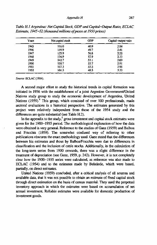
Appendix H 267
Table H.l Argentina: Net Capital Stock, GDP and Capital-Output Ratio, ECLAC Estimate, 1945—52 (thousand millions of pesos at 1950prices)
Years Net capital stock GDP Capital-output ratio
1945 116.0 40.9 2.841946 119.9 49.7 2.411947 125.9 56.8 2.221948 134.9 57.9 2.331949 142.7 53.1 2.691950 150.7 53.7 2.811951 157.3 53.3 2.951952 161.3 48.5 3.33
Source: ECLAC (1954).
A second major effort to study the historical trends in capital formation was initiated in 1956 with the establishment of a joint Argentine Government/United Nations study group to study the economic development of Argentina, United Nations (1959).4 This group, which consisted of over 100 professionals, made sectoral evaluations in a historical perspective. The estimates generated by this project were relatively independent from those of the 1954 study and the differences are quite substantial (see Table H.2).
In the appendix to the study,5 gross investment and capital stock estimates were given for the 1900-1955 period. The methodological explanation of how the data were obtained is very general. Reference to the studies of Ganz (1959) and Balboa and Fracchia (1959). The somewhat confused way of referring to other publications obscures the exact methodology used. Ganz stated that the differences between his estimates and those by Balboa/Fracchia were due to differences in classification and the inclusion of cattle stocks. Additionally, in the calculation of the long-term series from 1900 onwards, there was a slight difference in the treatment of depreciation (see Ganz, 1959, p. 242). However, it is not completely clear how the 1900-1935 series were calculated, as reference was also made to ECLAC (1954) and to the estimates made by Belaunde, which were based, partially, on direct estimates.
United Nations (1959) concluded, after a critical analysis of all sources and available data, that it was not possible to obtain an estimate of fixed capital stock through direct estimation on the basis of census material. They used the perpetual inventory approach in which the estimates were based on accumulation of net annual investment. Reliable estimates were available for domestic production of investment goods.

268 The Economic Development of Latin America
Table H.2 Argentina: Net Capital, GDP and Capital-Output Ratio, ECLAC Estimate, 1900-1955 (millions of pesos at 1950prices)
Years Netcapitalstock
GDP1 Capital-outputratio
Years Netcapitalstock
GDP* Capital-outputratio
1900 39.989 8.865 4.51 1928 145.833 33.169 4.401901 42.862 9.615 4.46 1929 154.185 34.696 4.441902 44.709 9.425 4.74 1930 160.251 33.264 4.821903 46.758 10.773 4.34 1931 161.167 30.955 5.211904 49.711 11.919 4.17 1932 160.032 29.926 5.351905 54.908 13.499 4.07 1933 159.402 31.333 5.081906 61.064 14.108 4.31 1934 160.521 33.806 4.751907 68.769 14.481 4.75 1935 161.732 35.298 4.311908 74.941 15.898 4.71 1936 161.963 35.550 4.561909 81.689 16.686 4.89 1937 165.218 38.145 4.331910 89.969 17.898 5.03 1938 169.423 38.289 4.421911 97.683 18.220 5.36 1939 171.537 39.746 4.321912 103.261 19.707 5.24 1940 172.399 40.399 4.271913 108.592 19.914 5.45 1941 172.885 42.468 4.071914 111.150 17.849 6.23 1942 173.118 42.965 4.031915 111.414 17.945 6.21 1943 173.024 42.645 4.061916 111.227 17.429 6.38 1944 174.222 47.468 3.671917 110.355 16.014 6.89 1945 175.387 45.950 3.821918 109.232 18.952 5.76 1946 178.429 50.035 3.571919 108.528 19.651 5.52 1947 187.348 55.600 3.371920 110.022 21.079 5.22 1948 196.310 58.679 3.341922 114.330 23.346 4.90 1950 208.062 58.599 3.551923 120.087 25.919 4.63 1951 214.151 60.423 3.541924 124.925 27.942 4.47 1952 218.076 56.441 3.861925 129.266 27.824 4.65 1953 221.439 59.499 3.721926 133.325 29.164 4.57 1954 226.101 62.072 3.641927 138.790 31.233 4.44 1955 231.737 64.661 3.58
Note." At factor costs.
Source: United Nations (1959, Annex I, p. 4 and Annex 3, p. 91).
Depreciation was estimated following Balboa and Fracchia (1959, pp. 280-83): (a) determination of the probable average life of groups of goods; (b) the assumption that goods would be completely worn out by the last year of their probable life (that is, they would have no scrap value); and (c) the assumption that annual depreciation would represent a constant proportion of the value when new (straight-line depreciation). In Table H.2, net capital stock, GNP and the capital-output ratio are shown for the period 1900-1955.
Recently several capital stock estimations have been published. One of these, prepared by TF.F.RAT, (1986), was based to a great extent on previous work, especially United Nations (1959). Again the methodological explanation is very general, and for details the reader is referred to other publications which are very

Appendix H 269
hard to get, being, in some cases, mimeographed manuscripts at regional universities. It is somewhat surprising that the outcome, in terms of the capital-output ratio, is so different from the 1959 United Nations study. IEERAL (1986) presents total capital stock in australes at 1960 prices, equal to the sum of fixed capital in agriculture, non-agricultural activity (excluding government) and government. Table H.3 shows net capital stock, gross domestic product and the capital-output ratio for the 1950-84 period.
Table H.3 Argentina: Net Capital Stock, GDP and Capital-Output Ratio, IEERAL Estimate, 1950-84 (australes at 1960prices)
Years Netcapitalstock
GDP“ Netcapital-outputratio
Years Netcapitalstock
GDP" Netcapital-outputratio
1950 1,700 690 2.5 1970 3,168 1,412 2.21951 1,734 717 2.4 1971 3,349 1,480 2.31952 1,784 680 2.6 1972 3,538 1,526 2.31953 1,836 717 2.6 1973 3,739 1,620 2.31954 1,873 746 2.5 1974 3,926 1,724 2.31955 1,921 800 2.4 1975 4,134 1,709 2.41956 1,967 822 2.4 1976 4,348 1,705 2.51957 2,023 864 2.3 1977 4,570 1,808 2.51958 2,076 917 2.3 1978 4,849 1,729 2.81959 2,139 858 2.5 1979 5,055 1,852 2.71960 2,185 925 2.4 1980 5,292 1,878 2.81961 2,280 991 2.3 1981 5,428 1,761 3.11962 2,392 975 2.4 1982 5,504 1,662 3.31963 2,473 951 2.6 1983 5,549 1,713 3.21964 2,537 1,050 2.4 1984 5,543 1,748 3.21965 2,602 1,146 2.31966 2,692 1,153 2.41967 2,7% 1,184 2.41968 2,890 1,235 2.31969 3,009 1,340 2.2
Note: a At factor costs.
Source: IEERAL (1986).
Another study was the Goldberg and Ianehilovici (1986) estimation of the gross stock, derived on the basis of a perpetual inventory approach. This study has the advantage of a clear and transparent description of its methodology. They applied a rectangular retirement pattern in which all assets of the same vintage are scrapped simultaneously. Repairs and maintenance were deducted from total capital formation. The average service life of assets is rather high; fluctuating between 56-71 years for construction, 15-24 years for machinery and equipment, and 13-25 years for transport equipment; given the fact that the major part (75.2 per cent) of capital stock consists of construction, this gives an estimated average
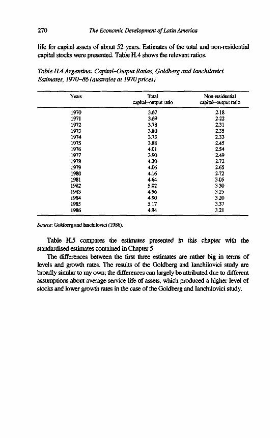
270 The Economic Development of Latin America
life for capital assets of about 52 years. Estimates of the total and non-residential capital stocks were presented. Table H.4 shows the relevant ratios.
Table H.4 Argentina: Capital-Output Ratios, Goldberg and lanchilovici Estimates, 1970-86 (australes at 1970 prices)
Years Total capital-output ratio
Non-residential capital-output ratio
1970 3.67 2.181971 3.69 2.221972 3.78 2.311973 3.80 2.351974 3.73 2.331975 3.88 2.451976 4.01 2.541977 3.90 2.491978 4.20 2.721979 4.06 2.651980 4.16 2.721981 4.64 3.051982 5.02 3.301983 4.96 3.251984 4.90 3.201985 5.17 3.371986 4.94 3.21
Source: Goldberg and lanchilovici (1986).
Table H.5 compares the estimates presented in this chapter with the standardised estimates contained in Chapter 5.
The differences between the first three estimates are rather big in terms of levels and growth rates. The results of the Goldberg and lanchilovici study are broadly similar to my own; the differences can largely be attributed due to different assumptions about average service life of assets, which produced a higher level of stocks and lower growth rates in the case of the Goldberg and lanchilovici study.

Appendix H 271
Table H.5 Argentina: Capital-Output (C/0) Ratio, 1950-86, Comparison ofStandardised and Existing Estimates (on the basis o f national currencies)
Years
ECLAC United Nations
(1954) (1959)
IEERAL(1986)
TotalnetC/Oratio
Goldberg/ Ianchilovici (1986)
Standarised estimates of this study
Total Total net net C/O C/O ratio ratio
TotalgrossC/Oratio
Grossnon-res.
C/Oratio
TotalnetC/Oratio
TotalgrossC/Oratio
Gross non- res. C/O ratio
1950 2.8 3.6 2.5 1.9 3.3 1.71951 3.0 3.5 2.4 1.9 3.2 1.71952 3.3 3.9 2.6 2.1 3.5 1.81953 3.7 2.6 2.0 3.4 1.81954 3.6 2.5 2.0 3.4 1.71955 3.6 2.4 1.9 3.2 1.71956 2.4 1.9 3.3 1.71957 2.3 1.9 3.2 1.71958 2.3 1.9 3.1 1.71959 2.5 2.1 3.4 1.91960 2.4 2.0 3.3 1.81961 2.3 2.0 3.2 1.81962 2.5 2.1 3.4 2.01963 2.6 2.3 3.6 2.11964 2.4 2.1 3.4 2.01965 2.3 2.0 3.2 1.91966 2.4 2.1 3.3 1.91967 2.4 2.1 3.4 2.01968 2.3 2.1 3.3 1.91969 2.3 2.0 3.2 1.91970 2.2 3.7 2.2 2.0 3.2 1.91971 2.3 3.7 2.2 2.1 3.3 1.91972 2.3 3.8 2.3 2.2 3.4 2.01973 2.3 3.8 2.4 2.2 3.4 2.01974 2.3 3.7 2.3 2.2 3.4 2.01975 2.4 3.9 2.5 2.3 3.5 2.11976 2.6 4.0 2.5 2.4 3.6 2.21977 2.5 3.9 2.5 2.3 3.6 2.11978 2.8 4.2 2.7 2.5 3.9 2.31979 2.7 4.1 2.7 2.5 3.7 2.31980 2.8 4.2 2.7 2.5 3.8 2.31981 3.1 4.6 3.1 2.8 4.3 2.61982 3.3 5.0 3.3 3.0 4.6 2.81983 3.2 5.0 3.3 2.9 4.6 2.81984 3.2 4.9 3.2 2.8 4.5 2.71985 5.2 3.4 2.9 4.8 2.91986 4.9 3.2 2.7 4.5 2.7
Source: Appendix E and sources indicated in headings.

272 The Economic Development of Latin America
CAPITAL STOCK IN BRAZIL
ECLAC (1954) provided the first capital stock estimates for Brazil. The general methodology was the same as for Argentina. 1940 wealth was estimated from the 1940 census. This benchmark, expressed in 1950 prices, was extended year by year, in combination with estimates of gross and net investment. For 1945 onwards, ECLAC (1954) gave figures for gross and net fixed investment that were deflated by the implicit gross product deflator. The results are shown in Table H.6.
Table H.6 Brazil: Net Capital Stock, GDP and Capital-Output Ratio, ECLAC Estimate, 1945-52 (thousands millions of cruzeiros at 1950prices)
Years Net capital stock GDP Capital-output ratio
1945 520.1 173.4 3.001946 535.5 190.9 2.811947 557.7 197.4 2.831948 576.3 209.8 2.751949 599.0 227.1 2.641950 624.6 240.6 2.601951 655.0 252.9 2.591952 693.1 271.9 2.55
Source: ECLAC (1954).
A second estimate was prepared shortly afterwards in a study of Brazil’s economic development by ECLAC and the Brazilian National Bank for Economic Development (United Nations, 1956). An initial stock (for 1939) was updated on a yearly basis with net investment over the period 1939-53, giving a series of net fixed reproducible capital as shown in Table H.7. They were shown in 1952 rather than 1950 prices. There was a significant difference between the two estimates, as reflected in the capital-output ratio.
Carlos Geraldo Langoni undertook a third study to estimate the capital stock using different assumptions with respect to disaggregated growth and depreciation rates (Langoni, 1974). On the basis of an unpublished study by the Brazilian Economic Institute, Getulio Vargas Foundation (1970), he disaggregated the capital stock into machinery and equipment (E), urban construction (U), rural construction (R) and imported capital goods (M). Table H.8 shows Langoni’s capital-output ratios and a clearly downward trend can be observed.

Appendix H 273
Table H.7 Brazil: Net Capital Stock, GDP and Capital-Output Ratio, United Nations Estimate, 1939-53 (billions of cruzeiros at 1952 prices)
Years Net capital stock GDP Capital-output ratio
1939 410 200.3 2.051940 421 200.3 2.101941 432 210.0 2.061942 443 203.5 2.181943 451 209.0 2.161944 458 219.4 2.091945 470 234.6 2.001946 477 257.7 1.851947 492 278.3 1.771948 519 294.1 1.761949 561 302.1 1.861950 593 324.1 1.831951 627 346.5 1.811952 667 360.9 1.851953 713 376.1 1.90
Source: United Nations (1956).
Table H.8 Brazil: GDP and Capital-Output Estimates, Langoni Estimate, 1948-69 (thousands of cruzeiros at 1953prices)
Years GDP Capital-output ratio
1948 286,003 2.811949 306,308 2.741950 329,612 2.641951 342,081 2.651952 381,016 2.501953 384,560 2.621954 415,399 2.511955 355,679 2.381956 466,994 2.411957 507,845 2.301958 530,055 2.301959 550,462 2.311960 608,683 2.191961 689,691 2.031962 724,401 2.031963 737,971 2.101964 n.a. n.a.1965 759,041 2.231966 783,347 2.251967 853,089 2.171968 873,808 2.221969 951,790 2.17
Note: n.a. = not available. The 1964 estimate was not included as it was impossible to reproduce GDP for that year.Source: Langoni (1974).

274 The Economic Development of Latin America
Raymond W. Goldsmith’s (1986) book about Brazil’s long-term development includes capital stock estimates for the 1913-80 period. These are based on Langoni’s initial 1948 estimate which was adjusted by Goldsmith, incorporating updated estimates for GDP and capital formation made by the Getulio Vargas Foundation. Goldsmith took Langoni’s estimate as far back as 1913, using a rather ingenious aggregation procedure in which gross fixed capital formation is assumed to be 10 per cent of GDP6 and net fixed capital formation 57 per cent of gross capital formation, the averages for the 1949-68 period. The 1972-80 estimates are by Goldsmith himself (see Table H.9).
Table H.9 Brazil: Capital Stock, Gross and Net Capital Formation and Capital-Output Ratio, Goldsmith Estimate, 1913-80 (millions of cruzeiros)
Years Net capital stock
Capital
Gross
formation
Net
Capital- output ratio
1913 366 3.211920 402 63 36 2.551924 429 48 27 2.131928 488 104 59 2.001932 525 65 37 2.451936 565 70 40 2.251940 647 143 82 2.101944 740 163 93 2.281948 841 178 101 2.111952 996 271 155 1.851956 1,165 312 169 1.721960 1,437 467 272 1.861964 1,831 648 394 2.041968 2,386 829 555 1.981972 3,281 1,316 895 1.771976 4,814 2,190 1,533 1.601980 6,758 2,700 1,944 1.96
Source: Goldsmith (1986).
Table H.10 shows a comparison of the different results and it becomes clear that the differences are rather substantial. The large difference between the Goldsmith and Langoni series is somewhat surprising. Goldsmith used the Langoni base year estimates, but his adjustment to this base year seems to have been significant.7
The standardised estimates and those of Goldsmith show similar levels around 1980, although his growth rate differs markedly. It is also difficult to compare the different performances as Goldsmith uses a four year moving average. My results are very different from those of Langoni and the earlier United Nations studies.

Appendix H 275
Table H.10 Brazil: Capital-Output (C/0) Ratio, 1950-80, Comparison of Standardised and Existing Estimates (on the basis of national currencies)
Years
ECLAC(1954)
U. Nations (1959)
Langoni(1974)
TotalnetC/Oratio
Goldsmith(1986)
TotalnetC/Oratio
This study
TotalnetC/Oratio
TotalnetC/Oratio
TotalnetC/Oratio
TotalgrossC/Oratio
Grossnon-res.OOratio
1950 2.6 1.8 2.6 0.9 1.4 0.91951 2.6 1.8 2.6 1.0 1.5 1.01952 2.5 1.8 2.5 1.8 1.1 1.6 1.01953 1.9 2.6 1.2 1.7 1.11954 2.5 1.2 1.6 1.11955 2.4 1.2 1.7 1.11956 2.4 1.7 1.3 1.8 1.21957 2.3 1.3 1.8 1.21958 2.3 1.3 1.8 1.21959 2.3 1.3 1.9 1.31960 2.2 1.9 1.3 1.8 1.31961 2.0 1.3 1.8 1.31962 2.0 1.3 1.8 1.31963 2.1 1.4 1.9 1.31964 2.0 1.4 2.0 1.41965 2.2 1.4 2.0 1.41966 2.2 1.4 2.0 1.41967 2.2 1.5 2.1 1.41968 2.2 2.0 1.4 2.0 1.41969 2.2 1.4 1.9 1.31970 1.5 2.1 1.41971 1.5 2.0 1.41972 1.8 1.4 2.0 1.41973 1.4 1.9 1.41974 1.5 2.0 1.41975 1.6 2.1 1.51976 1.6 1.6 2.1 1.61977 1.7 2.2 1.61978 1.7 2.3 1.71979 1.8 2.4 1.81980 2.0 1.8 2.4 1.8
Source'. Appendix E and sources in headings.
CAPITAL STOCK IN CHILE
The first person to estimate capital stock in Chile was Raúl Simón (1935). He compared national income and wealth with the USA for 1929-34. His estimates of net capital stock cited in ECLAC (1954) were derived from a study by Hasche (1951). I only have at my disposal the aggregated values of the United Nations study, as the original Hasche study is no longer available (see Table H .ll).

276 The Economic Development o f Latin America
Apparently it estimated the depreciated replacement value of fixed capital, by activity for 1938-49, based on the 1938 census of industry and company balance sheets for that year. The benchmark estimate for 1938 took into account detailed information on the age composition of the capital stock by type of capital good. The estimate was extended year by year, by depreciating existing capital and adding new investment.
Table H .ll Chile: Net Capital Stock, GDP and Capital-Output Ratio, ECLAC Estimate, 1945-52 (billions o f1950pesos)
Years Net capital stock GDP Capital-output ratio
1945 241.2 125.6 1.921946 247.8 123.9 2.001947 253.9 117.2 2.171948 260.9 129.6 2.011949 270.7 123.4 2.191950 277.3 124.7 2.221951 284.7 131.3 2.171952 292.0 138.2 2.11
Source-. ECLAC (1954).
The ECLAC (1954) study made various adjustments to the Hasche estimates. For the stock of capital of the agricultural sector, an estimate by the Corporación de Fomento de la Producción (CORFO) was used. Hasche’s estimates were reworked to introduce different assumptions on the average length of life of assets. Unfortunately ECLAC did not give detailed information on the numerical implications of the different assumptions. ECLAC’s stock of capital may be defined as the depreciated replacement value (in 1950 prices) of reproducible tangible and durable capital goods. Land, consumer durable goods, inventories and monetary metal were excluded from the stock of capital goods.
Recently, various estimates of net capital stock have been published (Gutiérrez, 1983) (see Table 5.12) and Haindl and Fuentes (1986) (see Table 5.13). These used the methodology developed by Harberger in his study on the rate of return to capital in Colombia (Harberger, 1972).
This methodology involved estimation of the initial capital stock, as follows:
GI = (5 + y)K
Here GI refers to gross investment, y to the annual rate of growth of the capital stock, 6 to the annual rate of depreciation and K to the capital stock at the beginning of the year. Harberger assumed the growth rate of capital stock to be equal to a normal growth rate of gross domestic product or national income, after
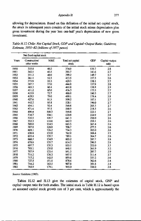
Appendix H 277
allowing for depreciation. Based on this definition of the initial net capital stock, the stock in subsequent years consists of the initial stock minus depreciation plus gross investment during the year less one-half year’s depreciation of new gross investment.
TableH.12 Chile: Net Capital Stock, GDP and Capital-Output Ratio, Gutiérrez Estimóte, 1950-82 (billions o f1977pesos)
Years
Net fixed capital stock
Construction/ other works
M&E Total net capital stock
GDP Capital-outputratio
1950 333.8 40.2 374.0 135.7 2.81951 342.1 43.5 385.7 141.6 2.71952 351.2 48.0 399.2 149.7 2.71953 361.1 52.3 413.5 157.3 2.61954 373.9 55.3 429.3 158.1 2.71955 387.7 57.0 444.8 157.9 2.81956 403.3 60.4 463.8 158.8 2.91957 411.2 65.0 476.3 175.5 2.71958 415.9 72.7 488.0 180.3 2.71959 419.5 79.0 499.1 178.4 2.81960 427.6 81.5 509.2 187.1 2.71961 442.2 85.8 528.1 196.0 2.71962 454.1 92.4 546.6 205.3 2.71963 471.4 97.5 568.9 218.3 2.61964 490.4 100.3 590.8 223.1 2.71965 516.7 104.1 620.8 224.9 2.81966 535.5 105.7 641.3 250.0 2.61967 552.3 110.0 662.3 258.1 2.61968 569.0 114.5 683.5 267.4 2.61969 587.8 120.8 708.7 277.3 2.61970 608.1 126.2 734.3 283.0 2.61971 630.8 132.0 762.8 308.4 2.51972 653.4 135.7 789.1 304.7 2.61973 668.3 134.9 803.2 287.7 2.81974 678.6 135.7 814.3 290.5 2.81975 697.7 135.3 833.1 253.0 3.31976 705.1 135.0 840.1 261.9 3.21977 707.9 133.4 841.3 287.7 2.91978 711.2 136.3 847.5 311.4 2.71979 717.2 142.5 859.8 337.2 2.61980 727.5 151.0 878.6 362.6 2.41981 744.2 163.5 907.8 381.8 2.41982 765.9 179.1 945.0 336.0 2.8
Source: Gutiérrez (1983).
Tables H.12 and H.13 give the estimates of capital stock, GNP and capital-output ratio for both studies. The initial stock in Table H.12 is based upon an assumed capital stock growth rate of 3 per cent, which is approximately the

278 The Economic Development o f Latin America
growth rate of GNP in 1940-60 (3.4 per cent). Estimates for depreciation were 2.5 per cent in construction and 10 per cent for machinery and equipment. Gross investment was calculated using national accounts. Normal investment was estimated by regression analysis of the national accounts investment series over the period 1940-80, excluding the period 1971-73. Once the initial stock estimation was made, the stock in subsequent years was estimated by the perpetual inventory method, although use was made of net fixed capital formation series.8
The initial stock in Table H.13 was based on a growth rate of 3.7 per cent (average growth during 1957-63, that is, three years before and three years after the base year), depreciation rates were 2.5 per cent for construction (40 years of service life) and 6.7 per cent for machinery and equipment (15 years). Normal investment was also estimated using regression analysis for the period 1960-70. In contrast with Harberger and Gutiérrez, Haindl and Fuentes did not depreciate gross investment for the previous year, when constructing their series.
Table H.13 Chile: Net Capital Stock, GDP and Capital-Output Ratio, Haindl and Fuentes Estimate, 1960-84 (billions o f1977pesos)
Years
Net fixed capital stock
Construction/ M&E other works
Total net capital stock
GDP Capital- output ratio
1960 430,525 125,330 555,855 187,229 2.971961 445,374 130,050 575,424 196,039 2.941962 457,542 137,260 594,802 205,169 2.901963 475,044 143,163 618,207 218,351 2.831964 500,440 146,841 647,281 223,443 2.901965 521,086 151,506 672,592 225,030 2.991966 540,184 154,012 694,196 250,329 2.771967 557,237 159,357 716,594 258,598 2.771968 574,164 165,032 739,196 267,286 2.771969 592,787 172,672 765,459 277,157 2.761970 613,871 179,482 793,353 282,695 2.811971 636,906 186,860 823,766 308,799 2.671972 659,858 191,913 851,771 304,586 2.801973 674,969 192,551 867,520 287,793 3.011974 685,423 194,709 880,132 290,257 3.031975 704,892 195,549 900,441 252,793 3.561976 712,387 196,321 908,708 262,027 3.471977 715,261 195,700 910,961 287,651 3.171978 718,630 199,684 918,314 311,226 2.951979 724,775 207,203 931,978 337,168 2.761980 735,288 217,281 952,569 363,028 2.621981 751,910 231,824 983,734 383,804 2.561982 773,902 250,350 1,024,252 329,621 3.111983 785,365 252,213 1,037,578 327,169 3.171984 795,062 248,074 1,043,136 347,923 3.00Source: Haindl and Fuentes (1986).
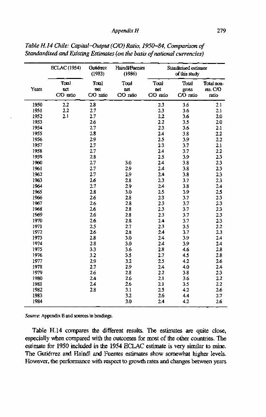
Appendix H 279
Table H. 14 Chile: Capital-Output (C/0) Ratio, 1950-84, Comparison o fStandardised and Existing Estimates (on the basis o f national currencies)
Years
ECLAC (1954) Gutiérrez(1983)
Total net
C/O ratio
Haindl/Fuentes(1986)
Total net
C/O ratio
Standarised estimate of this study
Total net
C/O ratio
Total Total net gross
C/O ratio C/O ratio
Total non- res. C/O
ratio
1950 2.2 2.8 2.3 3.6 2.11951 2.2 2.7 2.3 3.6 2.11952 2.1 2.7 2.2 3.6 2.01953 2.6 2.2 3.5 2.01954 2.7 2.3 3.6 2.11955 2.8 2.4 3.8 2.21956 2.9 2.5 3.9 2.21957 2.7 2.3 3.7 2.11958 2.7 2.4 3.7 2.21959 2.8 2.5 3.9 2.31960 2.7 3.0 2.4 3.8 2.31961 2.7 2.9 2.4 3.8 2.31962 2.7 2.9 2.4 3.8 2.31963 2.6 2.8 2.3 3.7 2.31964 2.7 2.9 2.4 3.8 2.41965 2.8 3.0 2.5 3.9 2.51966 2.6 2.8 2.3 3.7 2.31967 2.6 2.8 2.3 3.7 2.31968 2.6 2.8 2.3 3.7 2.31969 2.6 2.8 2.3 3.7 2.31970 2.6 2.8 2.4 3.7 2.31971 2.5 2.7 2.3 3.5 2.21972 2.6 2.8 2.4 3.7 2.31973 2.8 3.0 2.4 3.9 2.41974 2.8 3.0 2.4 3.9 2.41975 3.3 3.6 2.8 4.6 2.81976 3.2 3.5 2.7 4.5 2.81977 2.9 3.2 2.5 4.2 2.61978 2.7 2.9 2.4 4.0 2.41979 2.6 2.8 2.2 3.8 2.31980 2.4 2.6 2.1 3.6 2.21981 2.4 2.6 2.1 3.5 2.21982 2.8 3.1 2.5 4.2 2.61983 3.2 2.6 4.4 2.71984 3.0 2.4 4.2 2.6
Source: Appendix E and sources in headings.
Table H.14 compares the different results. The estimates are quite close, especially when compared with the outcomes for most of the other countries. The estimate for 1950 included in the 1954 ECLAC estimate is very similar to mine. The Gutiérrez and Haindl and Fuentes estimates show somewhat higher levels. However, the performance with respect to growth rates and changes between years
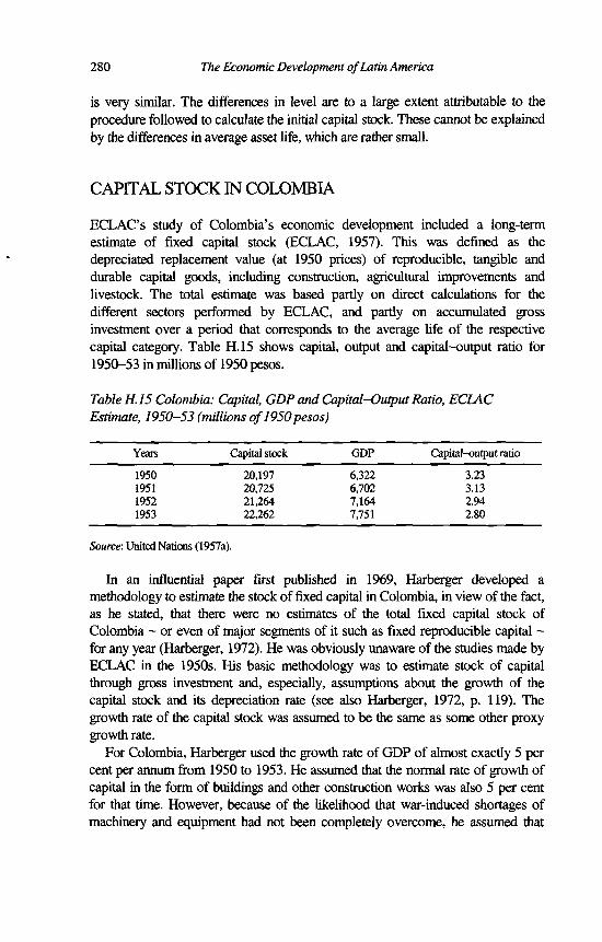
280 The Economic Development o f Latin America
is very similar. The differences in level are to a large extent attributable to the procedure followed to calculate the initial capital stock. These cannot be explained by the differences in average asset life, which are rather small.
CAPITAL STOCK IN COLOMBIA
ECLAC’s study of Colombia’s economic development included a long-term estimate of fixed capital stock (ECLAC, 1957). This was defined as the depreciated replacement value (at 1950 prices) of reproducible, tangible and durable capital goods, including construction, agricultural improvements and livestock. The total estimate was based partly on direct calculations for the different sectors performed by ECLAC, and partly on accumulated gross investment over a period that corresponds to the average life of the respective capital category. Table H.15 shows capital, output and capital-output ratio for 1950-53 in millions of 1950 pesos.
Table H.15 Colombia: Capital, GDP and Capital-Output Ratio, ECLAC Estimate, 1950-53 (millions o f1950pesos)
Years Capital stock GDP Capital-output ratio
1950 20,197 6,322 3.231951 20,725 6,702 3.131952 21,264 7,164 2.941953 22,262 7,751 2.80
Source: United Nations (1957a).
In an influential paper first published in 1969, Harberger developed a methodology to estimate the stock of fixed capital in Colombia, in view of the fact, as he stated, that there were no estimates of the total fixed capital stock of Colombia - or even of major segments of it such as fixed reproducible capital - for any year (Harberger, 1972). He was obviously unaware of the studies made by ECLAC in the 1950s. His basic methodology was to estimate stock of capital through gross investment and, especially, assumptions about the growth of the capital stock and its depreciation rate (see also Harberger, 1972, p. 119). The growth rate of the capital stock was assumed to be the same as some other proxy growth rate.
For Colombia, Harberger used the growth rate of GDP of almost exactly 5 per cent per annum from 1950 to 1953. He assumed that the normal rate of growth of capital in the form of buildings and other construction works was also 5 per cent for that time. However, because of the likelihood that war-induced shortages of machinery and equipment had not been completely overcome, he assumed that

Appendix H 281
stocks of those assets had a slightly higher normal growth rate of some 6 per cent per year during this period. Harberger used two sets of assumptions with regard to depreciation. He distinguished between asset lives of 40 to 50 years in construction and 12.5 to 20 years in machinery and equipment. The depreciation rates he chose, together with the abovementioned growth rates and gross investment data, generated the capital stocks shown in Table H.16.
Table H.16 Colombia: Alternative Capital Stock Estimates, GDP and Capital-Output Ratio, Harberger Estimate, 1952-67 (billions o f1958 pesos)
Years (1) (2) Total fixed capital stock
a b
(3)GDP
(4) (5) Capital-output ratios
(iy(3) (2V(3)
1952 31.64 36.59 16.1 1.97 2.271953 33.00 38.28 17.1 1.93 2.241954 35.30 40.91 18.3 1.93 2.241955 38.13 44.09 19.0 2.01 2.321956 41.05 47.42 19.7 2.08 2.411957 43.58 50.39 20.2 2.16 2.491958 45.83 53.08 20.7 2.21 2.561959 46.85 54.56 22.2 2.11 2.461960 48.09 56.24 23.1 2.09 2.431961 49.95 58.51 24.3 2.06 2.411962 52.08 61.04 25.6 2.03 2.381963 54.14 63.55 26.5 2.04 2.401964 55.77 65.61 28.1 1.98 2.331965 57.85 69.13 29.1 1.99 2.381966 59.58 71.30 30.7 1.94 2.321967 61.61 73.72 31.9 1.93 2.31
Notes:a asset lives: construction, 40 years and machinery and equipment, 12.5 years b asset lives: construction, 50 years and machinery and equipment, 20 years
Source-. Harberger (1972).
In a recent study, Henao presented an alternative approach to Harberger’s initial capital stock estimation methodology (Henao, 1983). Equations (1) and (2) disaggregate the capital stock in machinery and equipment and equations (3)-(5) generate the total capital stock. Table H.17 shows Henao's estimates and the resulting capital-output ratio.
(1) KPTt = KMEt + KCt KPTt = total fixed private capital stockin yeart
(2) Dt = SaKMEt + SbKCt KMEt = fixed private capital stock inmachinery and equipment in year t

(3) Dt = ScKPTt KCt = total fixed private capital inconstruction in year t
(4) KPTt = KPTt-1 + Ibt -D t 5a, 8b, Sc = depreciation rates
(5) KPTt-1 = DT (1/dc + 1)- Ibt Ibt = gross investment in year t
282 The Economic Development o f Latin America
Table H.17 Colombia: Total Fixed Capital Stock, GNP and Capital-Output Ratio, Henao Estimate, 1950-81 (thousands o f1970pesos)
Years Fixed capital stock GNP Capital-outputratio
1950 168,0391951 172,831 51,325 3.381952 177,312 54,556 3.271953 182,378 57,853 3.251954 191,222 61,816 3.151955 202,122 64,288 3.091956 213,504 66,859 3.191957 223,375 63,395 3.271958 228,310 70,063 3.261959 232,421 75,147 3.091960 237,372 78,298 3.031961 244,572 82,352 2.971962 252,860 86,750 2.911963 260,871 89,614 2.911964 267,159 95,134 2.801965 275,227 98,569 2.791966 281,943 103,040 2.711967 289,777 108,180 2.681968 298,543 114,829 2.601969 309,680 122,128 2.531970 321,283 130,861 2.461971 335,592 137,889 2.431972 350,972 148,630 2.361973 365,461 159,195 2.201974 380,770 168,787 2.261975 398,098 175,226 2.271976 414,936 183,296 2.271977 432,058 192,187 2.251978 450,094 209,369 2.151979 468,573 220,006 2.131980 493,511 228,805 2.151981 520,081 235,054 2.21
Source: Henao (1983).

Appendix H 283
Table H.18 Colombia: Capital-Output (C/0) Ratio, 1950-81, Comparison ofStandardised and Existing Estimates (on the basis of national currencies)
ECLAC Harberger Henao (1983) Standarised estimates of tins(1957) (1972) study
Years Total Total Total Total Total Grossnet net net net gross non-res.C/O C/O C/O C/O C/O C/Oratio ratio ratio ratio ratio ratio
1950 3.2 1.9 2.9 2.21951 3.1 3.4 1.9 2.9 2.21952 2.9 2.0 3.3 1.8 2.8 2.11953 1.9 3.2 1.8 2.8 2.11954 1.9 3.1 1.8 2.8 2.11955 2.0 3.1 1.9 2.9 2.11956 2.1 3.2 1.9 2.9 2.21957 2.2 3.3 1.9 3.0 2.21958 2.2 3.3 1.9 3.0 2.31959 2.1 3.1 1.8 2.9 2.21960 2.1 3.0 1.8 2.9 2.21961 2.1 3.0 1.8 2.9 2.11962 2.0 2.9 1.8 2.8 2.11963 2.0 2.9 1.7 2.8 2.11964 2.0 2.8 1.7 2.8 2.01965 2.0 2.8 1.7 2.8 2.01966 1.9 2.7 1.6 2.7 2.01967 1.9 2.7 1.6 2.7 2.01968 2.6 1.6 2.6 1.91969 2.5 1.6 2.5 1.91970 2.5 1.6 2.5 1.81971 2.4 1.6 2.4 1.81972 2.4 1.5 2.4 1.81973 2.2 1.5 2.4 1.71974 2.3 1.5 2.4 1.71975 2.3 1.6 2.4 1.81976 2.3 1.6 2.4 1.81977 2.2 1.6 2.4 1.81978 2.1 1.5 2.4 1.81979 2.1 1.5 2.3 1.81980 2.1 1.5 2.4 1.81981 2.2 1.6 2.5 1.9
Source: Appendix E and sources in headings.
Formula (5) gives capital stock and the only dependent variables are depreciation, the depreciation rate and gross investment. Thus, the main difference with the Harberger methodology is that no assumption is necessary regarding growth of the capital stock. An initial estimate was made with the depreciation rates of ECLAC (1957) (Sc = 0.0346, Sa = 0.05733 and 8b = 0.02862), resulting in a total stock of $141,305,9 million for 1950. Given this stock, Henao estimated the depreciation rates which ‘minimized’ the differences between depreciation in
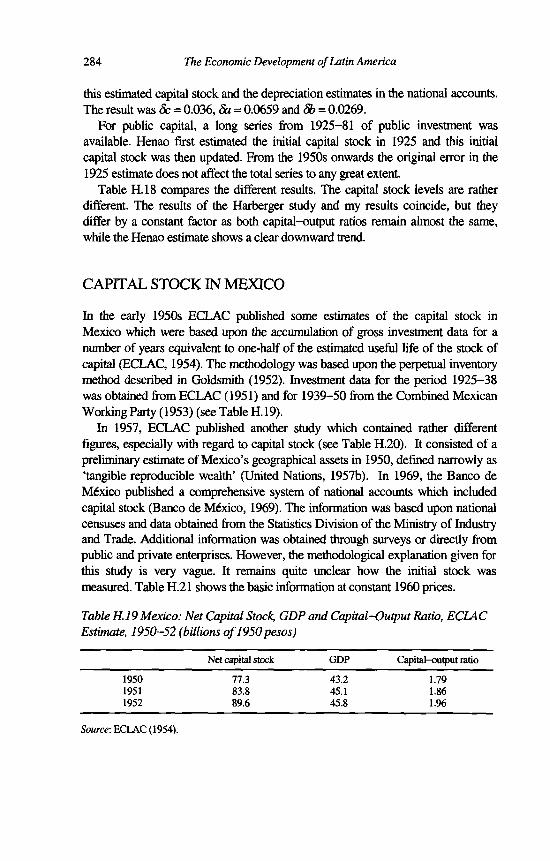
284 The Economic Development o f Latin America
this estimated capital stock and the depreciation estimates in the national accounts. The result was Sc = 0.036, da - 0.0659 and Sb = 0.0269.
For public capital, a long series from 1925-81 of public investment was available. Henao first estimated the initial capital stock in 1925 and this initial capital stock was then updated. From the 1950s onwards the original error in the 1925 estimate does not affect the total series to any great extent.
Table H.18 compares the different results. The capital stock levels are rather different. The results of the Harberger study and my results coincide, but they differ by a constant factor as both capital-output ratios remain almost the same, while the Henao estimate shows a clear downward trend.
CAPITAL STOCK IN MEXICO
In the early 1950s ECLAC published some estimates of the capital stock in Mexico which were based upon the accumulation of gross investment data for a number of years equivalent to one-half of the estimated useful life of the stock of capital (ECLAC, 1954). The methodology was based upon the perpetual inventory method described in Goldsmith (1952). Investment data for the period 1925-38 was obtained from ECLAC (1951) and for 1939-50 from the Combined Mexican Working Party (1953) (see Table H.19).
In 1957, ECLAC published another study which contained rather different figures, especially with regard to capital stock (see Table H.20). It consisted of a preliminary estimate of Mexico’s geographical assets in 1950, defined narrowly as ‘tangible reproducible wealth’ (United Nations, 1957b). In 1969, the Banco de México published a comprehensive system of national accounts which included capital stock (Banco de México, 1969). The information was based upon national censuses and data obtained from the Statistics Division of the Ministry of Industry and Trade. Additional information was obtained through surveys or directly from public and private enterprises. However, the methodological explanation given for this study is very vague. It remains quite unclear how the initial stock was measured. Table H.21 shows the basic information at constant 1960 prices.
Table H.19 Mexico: Net Capital Stock, GDP and Capital-Output Ratio, ECLAC Estimate, 1950-52 (billions o f1950pesos)
Net capital stock GDP Capital-output ratio
1950 77.3 43.2 1.791951 83.8 45.1 1.861952 89.6 45.8 1.96
Source: ECLAC (1954).

Appendix H 285
Table H.20 Mexico: Net Capital Stock, GDP and Capital-Output Ratio, ECLAC Estimate, 1950-55 (billions o f1950 pesos)
Years Net capital stock GDP Capital-output ratio
1950 93.5 43.3 2.161951 96.4 47.8 2.021952 100.9 47.4 2.131953 105.5 49.3 2.141954 109.1 53.4 2.041955 112.9 57.7 1.96
Source: United Nations (1957b).
Table H.21 Mexico: Total Fixed Net Capital Stock, Banco de Mexico Estimate, 1950-67 (millions o f1960pesos)
Years Total fixed net capital
stock
Construction M&E Permanentcropslivestock
GDP Capital-outputratio
1950 235,857 140,246 79,936 15,675 85,319 2.761951 248,873 147,395 85,456 16,022 91,732 2.711952 262,323 155,444 90,312 16,567 94,480 2.781953 273,413 161,365 94,922 17,126 99,587 2.751954 285,427 168,332 99,408 17,687 105,012 2.721955 298,637 175,756 104,502 18,379 113,315 2.641956 314,871 185,128 110,858 18,885 119,372 2.641957 331,885 194,767 117,407 19,711 128,335 2.591958 347,297 203,919 123,098 20,280 134,225 2.591959 362,825 212,902 129,000 20,923 140,058 2.591960 380,692 223,696 135,359 21,637 150,511 2.531961 399,480 234,354 142,455 22,671 156,664 2.551962 417,907 245,570 149,110 23,227 165,518 2.521963 439,482 258,672 156,977 23,833 179,920 2.441964 467,245 274,479 168,173 24,593 199,609 2.341965 495,964 289,765 181,051 25,148 212,139 2.341966 528,508 307,654 195,060 25,794 229,151 2.311967 565,805 328,082 211,245 26,478 245,499 2.30
Source: Banco de México (1969).
For the period 1960-85,1 obtained six diskettes from the Banco de México containing very detailed information, in current and constant prices, on capital formation. Table H.22 gives a summary of the information on capital stock and depreciation. These diskettes do not give any methodological explanation, and analysis of the period covered by both, 1960 and 1970 base-year Banco de México series, brings one to the conclusion that there are great discrepancies between the two series. It is probable that the Banco de México diskettes contain some kind of error, as the capital stock is very low compared, for example, with the stock in

1960 prices presented in Table H.21 and, therefore, the results are not presented in the summary Table H.23.
286 The Economic Development o f Latin America
Table H. 22 Mexico: Gross and Net Capital Stock, Banco de Mexico Estimate, 1960-85 (millions ofl970 pesos)
Total Stock Construction M&E
Gross Net Gross Net Gross Net
1960 97,304 60,304 57,586 36,469 39,718 23,8351961 105,061 65,634 62,167 39,671 42,894 25,9631962 112,154 69,010 64,817 40,572 47,337 28,4381963 123,036 75,834 69,649 43,445 53,381 32,3891964 135,387 83,286 74,377 46,058 61,010 37,2281965 145,893 88,860 78,108 47,738 67,785 41,1221966 156,874 95,715 81,039 48,467 75,835 47,2481967 171,387 104,526 85,972 51,242 85,415 53,2841968 181,674 109,109 89,474 53,326 92,200 55,7831969 195,532 116,433 93,426 54,959 102,106 61,4741970 222,241 134,742 104,720 63,658 117,521 71,0841971 242,038 145,916 111,489 67,740 130,549 78,1761972 260,358 156,690 118,128 71,572 142,230 85,1181973 283,092 170,166 124,995 75,750 158,097 94,4161974 300,485 177,349 130,177 77,801 170,308 99,5481975 323,956 190,802 133,617 79,356 190,339 111,4461976 355,915 209,363 143,441 85,270 212,474 124,0921977 378,471 218,481 150,324 88,709 228,147 129,7721978 399,354 227,553 152,704 87,732 246,649 139,8211979 419,416 237,844 155,845 87,686 263,571 150,1581980 444,374 250,815 162,857 90,982 281,517 159,8321981 478,776 276,886 170,082 95,343 308,694 181,5431982 527,167 306,424 177,438 98,022 349,730 208,4021983 536,173 297,402 180,617 96,588 355,557 200,8141984 538,302 284,509 182,176 93,632 356,126 190,8771985 543,941 276,046 182,175 89,994 361,767 186,053
Source: Banco de México (1986a).
Table H.23 compares the results of the different studies. It is clear that growth rates as well as levels of capital stock differ substantially according to the study used.

Appendix H 287
Table H.23 Mexico: Capital-Output (C/0) Ratio, 1950-67, Comparison ofStandardised and Existing Estimates (on the basis of national currencies)
ECLAC(1954)
ECLAC(1957)
Banco de Mexico (1969)
Standarised estimates of this study
Years Total Total Total Total Total gross TotalNet net net net non-res. netC/O C/O C/O C/O C/O C/O
Ratio ratio ratio ratio ratio ratio
1950 1.8 2.2 2.8 1.2 1.7 1.41951 1.9 2.0 2.7 1.3 1.7 1.41952 2.0 2.1 2.8 1.3 1.9 1.51953 2.1 2.7 1.4 1.9 1.61954 2.0 2.7 1.4 2.0 1.61955 2.0 2.6 1.4 2.0 1.61956 2.6 1.5 2.0 1.71957 2.6 1.5 2.1 1.71958 2.6 1.5 2.1 1.71959 2.6 1.6 2.2 1.81960 2.5 1.6 2.2 1.81961 2.5 1.6 2.2 1.81962 2.5 1.6 2.3 1.81963 2.4 1.6 2.2 1.81964 2.3 1.5 2.1 1.71965 2.3 1.6 2.2 1.71966 2.3 1.6 2.2 1.71967 2.3 1.6 2.2 1.7
Source: Appendix E and sources in headings.
CAPITAL STOCK IN VENEZUELA
Information regarding Venezuela’s capital stock is scarce. The only available sources are the reports by the Central Bank of Venezuela (Banco Central de Venezuela, 1958, 1968 and 1991) and the interesting work by Asdrubal Baptista (1991). The Central Bank of Venezuela gives net fixed capital stock estimates for the period 1950-65. The methodology used for the estimation of depreciated renewable fixed capital was based on a measure of gross investment, depreciation and inventories of machinery and equipment, infrastructure, construction works, buildings and livestock in each of twelve different sectors. The base year of the series was 1957 for which the best data on prices were available. To obtain a capital stock estimate for 1950, the Central Bank extended several series retroactively (see Table H.24). Unfortunately, I have not been able to obtain these series, which might facilitate estimation of a gross fixed capital stock for the period 1950-85.

288 The Economic Development o f Latin America
Table H.24 Venezuela: Capital Stock, GDP and Capital-Output Ratio, Banco Central Estimate, 1950-65 (millions o f1957 bolívares)
Years Net capital Stock
GDP Capital-outputratio
1950 26,523 12,728 2.081951 28,484 14,212 2.001952 31,326 15,248 2.051953 34,342 16,190 2.121954 37,840 17,749 2.131955 40,821 19,325 2.111956 44,033 21,366 2.061957 47,485 23,848 1.991958 50,032 24,164 2.071959 53,442 26,065 2.051960 55,250 26,433 2.091961 56,370 26,881 2.101962 57,499 28,585 2.011963 58,800 29,765 1.981964 60,769 32,326 1.881965 63,512 33,966 1.87
Source: Banco Central de Venezuela (1958,1968 and 1991).
A very complete source of information is the study by Asdrubal Baptista (1991) who gives net and gross capital stock estimates based upon the perpetual inventory method (see Table H.25). He also presents his basic investment series, making it possible to reproduce his results using different assumptions on service life, depreciation and mortality. His assumptions about service life are somewhat lower than those of the standardised method: 15 years for machinery and equipment in general; 12 years for machinery and equipment in the oil sector; 10 years for transport equipment; and 35 years for railroad equipment.
Non-residential structures have a service life of 35 years (with the exception of non-residential structures in the oil sector whose service life is 25 years). Finally, residential structures have a service life of 50 years. Baptista presents a brief but careful description of methodology and limitations of capital stock estimation. He obtained estimates of net fixed capital stock by using straight-line depreciation. In Table H.26 the summary information on Venezuela is presented.
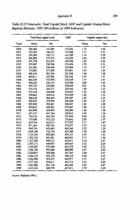
Appendix H 289
Table H.25 Venezuela: Total Capital Stock, GDP and Capital-Output Ratio, Baptista Estimate, 1950-89 (millions o f1984 bolívares)
Years
Total fixed capital stock GDP Capital-output ratio
Gross Net Gross Net
1950 204,484 151,885 118,302 1.73 1.281951 223,583 166,212 131,064 1.71 1.271952 245,283 182,771 141,209 1.74 1.291953 268,080 197,327 145,476 1.84 1.361954 291,738 214,292 159,396 1.83 1.341955 315,967 230,748 176,458 1.79 1.311956 341,693 249,444 195,804 1.75 1.271957 374,083 277,869 223,881 1.67 1.241958 409,104 302,504 221,948 1.84 1.361959 440,611 323,005 236,235 1.87 1.371960 466,434 332,950 236,538 1.97 1.411961 486,443 336,272 234,296 2.08 1.441962 502,735 339,685 250,428 2.01 1.361963 516,716 343,271 259,343 1.99 1.321964 531,818 350,269 278,625 1.91 1.261965 550,662 358,814 293,438 1.88 1.221966 568,546 366,443 295,567 1.92 1.241967 585,913 375,994 309,508 1.89 1.211968 607,822 391,681 326,847 1.86 1.201969 634,611 409,621 333,407 1.90 1.231970 663,990 428,450 356,089 1.86 1.201971 697,217 451,744 359,015 1.94 1.261972 734,131 481,329 357,839 2.05 1.351973 775,080 512,125 378,642 2.05 1.351974 819,734 541,515 377,397 2.17 1.431975 871,163 585,101 374,377 2.33 1.561976 934,716 642,443 403,266 2.32 1.591977 1,019,109 722,758 427,309 2.38 1.691978 1,121,236 805,062 439,127 2.55 1.831979 1,222,748 865,201 440,823 2.77 1.961980 1,313,760 909,513 418,811 3.14 2.171981 1,393,171 949,957 419,643 3.32 2.261982 1,459,407 979,308 423,378 3.45 2.311983 1,502,188 983,066 408,989 3.67 2.401984 1,528,847 969,200 391,765 3.90 2.471985 1,546,119 958,178 396,319 3.90 2.421986 1,562,588 955,273 419,977 3.72 2.271987 1,577,165 950,411 431,714 3.65 2.201988 1,601,080 961,136 463,540 3.45 2.071989 1,615,436 940,778 427,011 3.78 2.20
Source'. Baptista (1991).
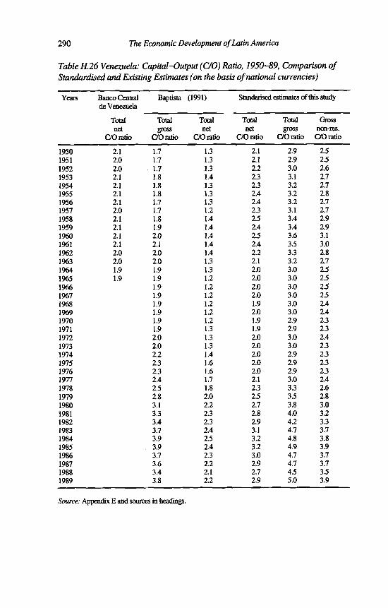
290 The Economic Development o f Latin America
Table H.26 Venezuela: Capital-Output (C/O) Ratio, 1950-89, Comparison of Standardised and Existing Estimates (on the basis of national currencies)
Years Banco Central de Venezuela
Total net
( 7 0 ratio
Baptista (1991) Standarised estimâtes of this study
Total gross
D O ratio
Total net
D O ratio
Total net
D O ratio
Total gross
D O ratio
Gross non-res.
D O ratio
1950 2.1 1.7 1.3 2.1 2.9 2.51951 2.0 1.7 1.3 2.1 2.9 2.51952 2.0 1.7 1.3 2.2 3.0 2.61953 2.1 1.8 1.4 2.3 3.1 2.71954 2.1 1.8 1.3 2.3 3.2 2.71955 2.1 1.8 1.3 2.4 3.2 2.81956 2.1 1.7 1.3 2.4 3.2 2.71957 2.0 1.7 1.2 2.3 3.1 2.71958 2.1 1.8 1.4 2.5 3.4 2.91959 2.1 1.9 1.4 2.4 3.4 2.91960 2.1 2.0 1.4 2.5 3.6 3.11961 2.1 2.1 1.4 2.4 3.5 3.01962 2.0 2.0 1.4 2.2 3.3 2.81963 2.0 2.0 1.3 2.1 3.2 2.71964 1.9 1.9 1.3 2.0 3.0 2.51965 1.9 1.9 1.2 2.0 3.0 2.51966 1.9 1.2 2.0 3.0 2.51967 1.9 1.2 2.0 3.0 2.51968 1.9 1.2 1.9 3.0 2.41969 1.9 1.2 2.0 3.0 2.41970 1.9 1.2 1.9 2.9 2.31971 1.9 1.3 1.9 2.9 2.31972 2.0 1.3 2.0 3.0 2.41973 2.0 1.3 2.0 3.0 2.31974 2.2 1.4 2.0 2.9 2.31975 2.3 1.6 2.0 2.9 2.31976 2.3 1.6 2.0 2.9 2.31977 2.4 1.7 2.1 3.0 2.41978 2.5 1.8 2.3 3.3 2.61979 2.8 2.0 2.5 3.5 2.81980 3.1 2.2 2.7 3.8 3.01981 3.3 2.3 2.8 4.0 3.21982 3.4 2.3 2.9 4.2 3.31983 3.7 2.4 3.1 4.7 3.71984 3.9 2.5 3.2 4.8 3.81985 3.9 2.4 3.2 4.9 3.91986 3.7 2.3 3.0 4.7 3.71987 3.6 2.2 2.9 4.7 3.71988 3.4 2.1 2.7 4.5 3.51989 3.8 2.2 2.9 5.0 3.9
Source: Appendix E and sources in headings.

Appendix H 291
NOTES
1. The United Nations Economic Commission for Latin America and the Caribbean undertook a series of studies on economic development and capital stock estimation which included four of our countries (Argentina, Brazil, Colombia and Mexico), in ECLAC (1954) some estimates were also given for Chile.
2. Apparently this study by Belaúnde, who formed part of the Alejandro Bunge group which studied Argentina’s wealth at the beginning of the twentieth century (see Bunge, 1917), was never published.
3. The length-of-service-life assumptions used for estimating depreciation were as follows: agricultural improvements, 50 years; agricultural machinery, 20 years; producers durable equipment (non-agricultural), 20 years; vehicles, 20 years; buildings, 50 years; railroad equipment and construction and improvements, 33 years; public works, 50 years.
4. The study was carried out in Argentina and at the United Nations Economic Commission for Latin America and the Caribbean, under the direction of Raúl Prebisch.
5. Anexo m, ‘Inversión Bruta y Capital Existente en la Argentina, por Sectores Económicos y por Tipo de Inversión y Capital, 1900-1955’, pp. 77-105.
6. Goldsmith used the GDP estimates of Haddad (1980).7. See Goldsmith (1986, p. 154).8. See Gutiérrez (1983, pp. 205-10).

References
Abramovitz, Moses (1986), ‘Catching Up, Forging Ahead and Falling Behind’, The Journal of Economic History, Vol. 46, No. 2, June, Cambridge.
Abramovitz, Moses (1989), Thinking about Growth, Cambridge, Massachusetts, Cambridge University Press.
Abramovitz, Moses (1990), ‘The Catch-Up Factor in Postwar Economic Growth’, Economic Inquiry, Vol. 28, January.
Abramovitz, Moses (1991), The Postwar Productivity Spurt and Slowdown: Factors of Potential and Realization’, in OECD (Organization for Economic Cooperation and Development), Technology and Productivity: The Challenge for Economic Policy, Paris.
Abramovitz, Moses (1993), ‘The Search for the Sources of Growth: Areas of Ignorance, Old and New’, The Journal of Economic History, Vol. 53, No. 2, June, Cambridge.
Altimir, Oscar (1987), ‘Income Distribution Statistics in Latin America and their Reliability’, Review of Income and Wealth, Series 33, No. 2, New Haven, Connecticut, June.
Altimir, Oscar (1997), ‘Desigualdades, empleo y pobreza en América Latina’, Desarrollo económico, vol. 37, No. 145, April-June, Buenos Aires.
Altimir, Oscar (1998), ‘The Long-term Evolution of Inequality and Poverty in Argentina, Colombia and Mexico’, background paper to Rosemary Thorp.
Altimir, Oscar and André A. Hofman (1990), ‘Latin American Development Problems in Historical Perspective’, paper presented at the ECLAC/University of Lund Symposium, Santiago, Chile, ECLAC (Economic Commission for Latin America and the Caribbean).
Annino, Antonio (1995), ‘Reflections on Spanish American History’, Itinerario. European Journal of Overseas History, Vol. XIX, No. 2, Leiden.
APEC (Análise e Perspectiva Económica) (1975), A Economía Brazileira e Suas Perspectivas, Year XIV, Rio de Janeiro.
Amagada, Irma (1994), ‘Changes in the Urban Female Labour Market’, CEPAL Review, No. 53, Santiago, Chile, ECLAC.
Arthur, W. Brian (1988), ‘Self-Reinforcing Mechanisms in Economics’ in P.W. Anderson, K. Arrow, and D. Pines (eds), The Economy as an Evolving Complex System, Reading, Addison-Wesley.
293

294 The Economic Development o f Latin America
Bacha, Edmar L. (1989), ‘Economic Trends in Latín America’ in Seiji Naya, Miguel Urrutia, Shelley Mark and Alfredo Fuentes (eds), Lessons in Development: A Comparative Study of Asia and Latín America, San Francisco, California, ICEG (International Center for Economic Growth).
Balassa, Bela, Gerardo M. Bueno, Pedro Pablo Kuczynski and Mario Henrique Simonsen (1986), Towards Renewed Economic Growth in Latín America, Washington, DC, HE (Institute for International Economics).
Balboa, Manuel and Alberto Fracchia (1959), ‘Fixed Reproducible Capital in Argentina, 1935-55’, Income and Wealth, series VIII, London, Bowes and Bowes.
Ballesteros, M.A. and T.E. Davis (1965), ‘El crecimiento de la producción y el empleo en sectores básicos de la economía chilena, 1908-1957’, Cuadernos de Economía, Year 2, No. 7, Santiago, Chile, Catholic University of Chile, September-December.
Banco Central de Chile, Boletín Mensual, various issues, Santiago, Chile.Banco Central de Chile (1993), Cuentas Nacionales de Chile, 1985-1992, Síntesis
anticipada, Santiago, Chile, Gerencia de División Estudios.Banco Central de Chile (1994), Cuentas Nacionales de Chile, 1985-1992,
Santiago de Chile.Banco Central de la República Argentina (1976), Cuentas Nacionales, Series
Históricas, Vol. DI, Buenos Aires.Banco Central de la República Argentina (1991), ‘Informe Final de la CEPAL’,
Proyecto Revisión de las Cuentas Nacionales y de la Distribución del Ingreso, Buenos Aires, December, mimeo.
Banco Central de la República Argentina (1993), Estimaciones Anuales de la Oferta y Demanda Globales. Periodo 1980-1992, Buenos Aires, April.
Banco Central de Venezuela (1958), Memoria Correspondiente al Ejercicio Anual 1958, Caracas.
Banco Central de Venezuela (1968), Informe Económico 1968, Caracas.Banco Central de Venezuela (1978), La Economía Venezolana en los Últimos
Treinta y Cinco Años, Caracas.Banco Central de Venezuela (1991), Informe Económico 1990, Caracas.Banco de México (1969), Cuentas Nacionales y Acervos de Capital,
Consolidadas y por Tipo de Actividad Económica, 1950-1967, México City, Departamento de Estudios Económicos, June.
Banco de México (1986a), Acervos y Formación de Capital, México City, Subgerencia de Precios.
Banco de México (1986b), Indicadores Económicos, Acervo Histórico V, México City, May.
Baptista, Asdrubal (1991), Bases Cuantitativas de la Economía Venezolana: 1830-1989, Caracas, Comunicaciones Corporativas D.

References 295
Barbera, Mattia (1990), ‘Latin America’s Place in World Trade’, CEP AL Review, No. 41, Santiago, Chile, ECLAC, August
Baumol, W.J., R.R. Nelson and E.N. Wolf (eds) (1994), International Convergence of Productivity, New York, Oxford University Press.
Becker, Gary S. (1964), Human Capital, NBER General Series, No. 80, New York, NBER (National Bureau of Economic Research, Inc.).
Belaúnde, César H., ‘Estudio de la Capitalización Bruta de la Argentina, 1900 -1950’, Buenos Aires, University of Buenos Aires, mimeo.
Bernstein, Jeffrey and Anwar Shah (1993), ‘Corporate Tax Structure and Production’, Policy Research Working Papers, No. 1196, Washington, DC, World Bank, September.
Bianchi, Andrés and Takashi Nohara (1988), A Comparative Study on Economic Development between Asia and Latin America, JRP Series, No. 67, Tokyo, Institute of Developing Economies.
Blades, Derek (1989), Capital Measurement in the OECD Countries: An Overview, Paris, OECD.
Blakemore, Harold (1992), ‘Chile, Desde la Guerra del Pacífico hasta la Depresión Mundial, 1880-1930’, in Leslie Bethell (ed.), Historia de América Latina, Barcelona, Editorial Crítica.
Bonelli, Regis (1976), Tecnología e Crescimento Industrial: A Experiencia Brasileira nos Anos 60, Rio de Janeiro, IPEA (Institute of Economie and Social Planning)/INPES (Instituto de Pesquisas).
Borges, J.G. and F.P. Vasconcellos (1974), Habitaqào para o Desenvolvimento, Rio de Janeiro, Block Editores.
Borah, Woodrow (1951), New Spain’s Century of Depression, Berkeley, California, University of California Press.
Bresser Pereira, Luis (1984), Development and Crisis in Brazil, 1930-1983, Boulder, Colorado, Westview Press.
Brito Figueroa, Federico (1966), Historia Económica y Social de Venezuela: Una Estructura para su Estudio, Caracas, Central University of Venezuela.
Bruton, Henry (1967), ‘Productivity Growth in Latin America’, American Economie Review, Vol. VII, No. 5, Washington, DC, December.
Buffon, G.L.L. (1761), Histoire Naturelle, as quoted in A. Annino (1995).Bulmer-Thomas, Victor (1994), The Economie History of Latin America since
Independence, Cambridge Latin American Studies, No. 77, New York, Cambridge University Press.
Bunge, Alejandro E. (1917), Riqueza y Renta de la Argentina: Su Distribución y su Capacidad Contributiva, Buenos Aires.
Bushnell, D. and N. Macauly (1988), The Emergence of Latin America in the Nineteenth Century, New York, Oxford University Press.
296 The Economic Development o f Latin America
Campbell, Colin (1977), ‘Capacity Capital Formation in the New Zealand Manufacturing Industries, 1952-1973’, Occasional Paper, No. 31, Wellington, Victoria University of Wellington.
Campos, Roberto (1967), Reflections on Latin America Development, Latin American Monographs, No. 8, Austin, Texas, University of Texas, Institute of Latin American Studies.
Cardoso, Eliana and Ann Helwege (1992), Latin America’s Economy: Diversity, Trends, and Conflicts, Cambridge, Massachusetts, MIT Press.
Cardoso, F.H. and Enzo Faletto (1969), Dependencia y Desarrollo en América Latina, Mexico City, Siglo XXI Editores.
Cardoso de Mello, Joao M. and Maria da Conceicao Tavares (1985), ‘The Capitalist Export Economy in Brazil, 1884-1930’, in Roberto Cortés Conde and Shane J. Hunt (eds), The Latin American Economies, New York, Holmes and Meier.
Carióla, Carmen and Osvaldo Sunkel (1985), ‘The Growth of the Nitrate Industry and Socioeconomic Change in Chile: 1880-1930’, in Roberto Cortés Conde and Shane J. Hunt (eds), The Latin American Economies, New York, Holmes and Meier.
Cavallo, Domingo and Yair Mundlak (1982), Agriculture and Economic Growth in cm Open Economy: The Case of Argentina, Washington, DC, IFPRI (International Food Policy Research Institute).
CELADE (Latin American Demographic Center) (1985a), Demographic Bulletin, Year XVIH, No. 35, Santiago, Chile.
CELADE (1985b), Demographic Bulletin, Year XVIII, No. 36, Santiago, Chile.CELADE (1990), La Mortalidad en las Americas: Progresos, Problemas y
Perspectivas, Santiago, Chile, CELADE/PAHO (Pan American Health Organization), unpublished.
CELADE (1992), ‘Economically Active Population’, Demographic Bulletin, Year XXV, No. 49, Santiago, Chile, January.
CELADE (1993), Demographic Bulletin, Year XXVI, No. 51, Santiago, Chile, January.
CELADE (1995), Demographic Bulletin, Year XXVIII, No. 55, Santiago, Chile.CELADE, Demographic Bulletin, various issues, Santiago, Chile.CELADE/ECLAC (1993), Population, Social Equity and Changing Production
Patterns, Santiago, Chile.Chenery, Hollis B. (1965), ‘The Structuralist Approach to Economic
Development’, American Economic Review, Vol. IV, No. 2, Washington, DC, May.
Clark, Colin (1940), Conditions of Economic Progress, London, Macmillan.Coeymans, Juan Eduardo (1992), ‘Productividad, Salarios y Empleo en la
Economía Chilena: Un Enfoque de Oferta Agregada’, Cuadernos de Economía, Year 29, No. 87, Mexico City, August.

References 297
Coeymans, Juan Eduardo and Yair Mundlak (1993), Sectorial Growth in Chile: 1962-82, Research report, No. 95, Washington DC, IFPRI.
Collver, Andrew 0. (1965), Birth Rates in Latin America: New Estimates of Historical Trends and Fluctuations, res. ser. No. 7, Berkeley, California, Institute of International Studies, University of California.
Colombia, Contraloria General de la República, Anuario de Comercio Exterior, various issues, Santa Fe de Bogotá.
Combined Mexican Working Party (1953), The Economic Development of Mexico, Washington, DC, World Bank.
Corbo, Vittorio (1988), ‘Problems, Development Theory, and Strategies of Latin America’, in Gustav Ranis and T. Paul Schultz (eds), The State of Development Economics. Progress and Perspectives, Cambridge, Massachusetts, Basil Blackwell.
CORFO (Corporación de Fomento de la Producción) (1957), Cuentas Nacionales de Chile, 1940-1954, Santiago, Chile.
CORFO (1963), Cuentas Nacionales de Chile, 1940-1962, Santiago, Chile.Correa, Héctor (1970), ‘Sources of Economic Growth in Latin America’, The
Southern Economic Journal, Vol. XXXVII, No. 2, July.Cortés Conde, Roberto (1985), ‘The Export Economy of Argentina, 1880-1920’,
in Roberto Cortés Conde and Shane J. Hunt (eds), The Latin American Economies, New York, Holmes and Meier.
Cortés Conde, Roberto and Shane J. Hunt (eds) (1985), The Latin American Economies, New York, Holmes and Meier.
Council for Economic Planning and Development (1994), Taiwan Statistical Data Book -1994, Seoul, Korea.
DANE (Departamento Administrativo Nacional de Estadística) (1956), Anuario General de Estadística. Colombia -1956, Santa Fe de Bogotá.
DANE (1986), XV Censo Nacional de Población y TV de Vivienda, Características Económicas, Vol. IV, Santa Fe de Bogotá.
DANE, Anuario de Comercio Exterior, various issues, Santa Fe de Bogotá.David, Paul A. (1975), Technical Change, Innovation and Economic Growth,
Cambridge, Massachusetts, Cambridge University Press.David, Paul A. (1985), ‘Clio and the Economics of QWERTY’, American
Economic Review, Vol. 75, No. 1, Washington, DC.De Gregorio, José (1991), ‘Economic Growth in Latin America’, paper presented
at the Fourth Annual Interamerican Seminar on Economics, Santiago, Chile.Denison, Edward F. (1962), The Sources of Economic Growth in the United States
and the Alternatives before us, New York, Committee on Economic Development.
Denison, Edward F. (1967), Why Growth Rates Differ, Washington, DC, The Brookings Institution.

298 The Economic Development o f Latin America
Denison, Edward F. (1974), Accounting for United States Economic Growth 1929-1969, Washington, DC, The Brookings Institution.
Denison, Edward F. (1985), Trends in American Eonomic Growth, 1929-1982, Washington, DC, The Brookings Institution.
Denison, Edward F. (1993), ‘The Growth Accounting Tradition and Proximate Sources of Growth’, in Adam Szirmai, Bart van Ark and Dirk Pilat (eds), Explaining Economic Growth - Essays in Honour of Angus Maddison, Amsterdam, Elsevier/North-Holland.
Denison, Edward F. and William K. Chung (1976), How Japan’s Economy Grew so Fast: The Sources of Postwar Expansion, Washington, DC, The Brookings Institution.
Devlin, Robert (1989), Debt and Crisis in Latin America: The Supply Side of the Story, Princeton, New Jersey, Princeton University Press.
Diaz-Alejandro, Carlos F. (1970), Ensayos sobre la Historia Económica Argentina, Buenos Aires, Amorrortu Editores.
Díaz-Alejandro, Carlos (1983), ‘Argentina, Australia and Brazil before 1929’, New Haven, Connecticut, Yale University, January, mimeo.
Diaz-Alejandro, Carlos (1984), ‘No Less Than Hundred Years of Argentine Economic History Plus Some Comparisons’ in Gustav Ranis, Robert L. West, Mark W. Leiserson and Cynthia Taft Morris (eds), Comparative Development Perspectives, Boulder, Colorado, Westview Press.
Di Telia, Guido and Manuel Zymelman (1973), Ciclos Económicos Argentinos, con la colaboración de Alberto Petrecolla, Buenos Aires, Paidos.
Domínguez, Loreto M. (1947), ‘National Income Estimates of Latín American Countries’, Studies in Income and Wealth, Vol. 10, New York, NBER.
Dombusch, Rudiger and S. Edwards (1990), ‘El Populismo Macroeconómico’, in Edmar Bacha and Sebastián Edwards (eds), Sector Externo, Políticas Financieras y Proceso de Ajuste Macroeconómico. El Trimestre Económico, Vol. LVH, Número especial, Mexico City, FCE (Fondo de Cultura Económica), December.
Dombusch, Rudiger and Mario Henrique Simonsen (1987), ‘Estabilización de la Inflación con el Apoyo de una Política de Ingresos’, El Trimestre Económico, Vol. 54, No. 2, Mexico City, FCE, April-June.
ECLAC (1951), Economic Survey of Latin America, 1949, New York, United Nations.
ECLAC (1954), Economic Survey of Latin America, 1951-52, New York, United Nations.
ECLAC (1957), Statistical Annex, to ‘The Economic Development of Colombia’, Geneva, United Nations.
ECLAC (1958), El Desarrollo Económico de la Argentina, Annex, Santiago, Chile.
References 299
ECLAC (1963), A Measurement of Price Levels and the Purchasing Power of Currencies in Latin America, 1960-1962, Santiago, Chile.
ECLAC (1965a), External Financing in Latin America, New York, United Nations.
ECLAC (1965b), ‘El Proceso de Industrialización en América Latina. Anexo Estadístico’, ST/ECLA/Conf.23/L.2/Add.2, Santiago, Chile, mimeo.
ECLAC (1972), Statistical Bulletin for Latin America, Vol. IX, No. 1-2, New York, United Nations.
ECLAC (1976), América Latina: Relación de Precios del Intercambio, Cuadernos Estadísticos de la CEPAL, Santiago, Chile.
ECLAC (1985), Evolución de las Tasas Específicas de Participación de la Población en la Actividad Económica por Sexo y Grupo de Edades. América Latina: 1950,1960,1970y 1980, LC/IN.37, Santiago, Chile.
ECLAC (1989), Antecedentes sobre la Transformación Productiva y la Competitividad de la Economía Chilena en el Período 1939-1989, Santiago, Chile.
ECLAC (1990a), Changing Production Patterns with Social Equity, LC/G.1601- P, Santiago, Chile. United Nations publication, sales N°E.90.II.G.6.
ECLAC (1990b), Magnitud de la Pobreza en América Latina en los Años Ochenta, Santiago, Chile, April.
ECLAC (1990c), Latin America and the Caribbean: Options to Reduce the Debt Burden, Santiago, Chile.
ECLAC (1992), Economic Survey of Latin America and the Caribbean 1991, Santiago, Chile.
ECLAC (1994a), Latin America and the Caribbean: Policies to Improve Linkages with the Global Economy, LC/G.1800, Santiago, Chile.
ECLAC (1994b), Open Regionalism in Latin America and the Caribbean. Economic Integration as a Contribution to Changing Production Patterns with Social Equity, Santiago, Chile.
ECLAQUNESCO (United Nations Educational, Scientific and Cultural Organization) (1992), Education and Knowledge: Basic Pillars of Changing Production Patterns with Social Equity, Santiago, Chile.
Edwards, Sebastian (1995), Crisis and Reform in Latin America: From Despair to Hope, Washington, DC, World Bank.
Eisner, Robert (1952), ‘Depreciation Allowances, Replacement Requirements and Growth’, American Economic Review, Vol. XLH, No. 5, Washington, DC, December.
Elias, Victor J. (1978), ‘Sources of Economic Growth in Latin American Countries’, The Review of Economics and Statistics, Vol. LX, Amsterdam, North-Holland, August.
300 The Economic Development o f Latin America
Elias, Victor J. (1992), Sources of Growth. A Study of Seven Latin American Economies, San Francisco, A Joint Research Project of the Fundación del Tucumán and the International Center for Economic Growth (CEG).
Fajnzylber, Fernando (1990), Unavoidable Industrial Restructuring in Latin America, Durham, NC, Duke University Press.
FAO (Food and Agriculture Organization of the United Nations) (1995), Production Yearbook, FAO Statistical Series, No. 125, Rome.
FAO, Production Yearbook, various issues, Rome.Ferrer, Aldo (1977), Crisis y Alternativas de la Política Económica Argentina,
Mexico City, FCE.Ffrench-Davis, Ricardo (1973), Políticas Económicas en Chile 1952-1970,
Santiago, Chile, CIEPLAN (Economic Research Corporation for Latín America).
Ffrench-Davis, Ricardo (1991), ‘Formación de Capital’ in Osvaldo Sunkel (ed.), El Desarrollo desde Dentro. Un enfoque neoestructuralista para la América Latina, Lecturas, No. 71, Mexico City, FCE.
Ffrench-Davis, Ricardo (1994), ‘The Macroeconomic Framework for Investments and Development: The Links between Financial and Trade Reforms’ in Colin I. Bradford (ed.), The New Paradigm of Systemic Competitiveness: Toward More Integrated Policies in Latin America, Paris, OECD Development Centre.
Ffrench-Davis, Ricardo and Stephany Griffith-Jones (eds) (1995), Las Nuevas Corrientes Financieras hacia la América Latina - Fuentes, Efectos y Políticas, Lecturas, No. 81, Mexico City, FCE.
Ffrench-Davis, Ricardo and Oscar Muñoz (1992), ‘Economic and Political Instability in Chile’ in Simón Teitel (ed.), Towards a New Development Strategy for Latin America, Washington, DC, IDB (Inter-American Development Bank)/The Johns Hopkins University Press.
Ffrench-Davis, Ricardo, Oscar Muñoz and Gabriel Palma (1994), ‘The Latin American Economies, 1950-1990’, in Lesley Bethell (ed.), The Cambridge History of Latin America, Vol. VI, Cambridge, Massachusetts, Cambridge University Press.
Fishlow, Albert (1972), ‘Origins and Consequences of Import Substitution in Brazil’, in L.E. Di Marco (ed.), International Economics and Development: Essays in Honor of Raúl Prebisch, New York, Academic Press.
Fitzgerald, E.V.K. (1984), ‘Restructuring Through the Depression: The State and Capital Accumulation in Mexico 1925-40’, in Rosemary Thorp (ed.), Latin America in the 1930s: The Role of the Periphery in World Crisis, New York, St. Martin’s Press.
Foxley, Alejandro (1983), Latin American Experiments in Neoconservative Economics, Berkeley, California, University of California Press.
Furtado, Celso (1963), The Economic Growth of Brazil, Berkeley, California, University of California Press.

References 301
Ganz, Alexander (1959), ‘Problems and Uses of National Wealth Estimates in Latin America’, Income and Wealth, Series VIH, London, Bowes and Bowes.
Garcia, Norberto (1992), Cambio Estructural y Mercado de Trabajo. Chile: 1973-1992, Santiago, Chile, PREALC (Regional Employment Programme for Latin America and the Caribbean), ILO (International Labour Organization), September.
Gettilio Vargas Foundation (1970), ‘Formaçâo Bruta de Capital’, Rio de Janeiro, mimeo.
Goldberg, Samuel and Beatriz Ianchilovici (1986), El Stock de Capital en la Argentina: Medición y Problemas Conceptuales, Buenos Aires, Secretaría de Planificación.
Goldsmith, Raymond W. (1951), ‘A Perpetual Inventory of National Wealth’, Studies in Income and Wealth, Vol. 14, New York, NBER.
Goldsmith, Raymond W (1952), The Growth of Reproducible Wealth in the United States of America from 1805 to 1950’, Income and Wealth, Series II, London, International Association for Research in Income and Wealth/Bowes and Bowes.
Goldsmith, Raymond W. (1986), Brasil 1850-1984, Desenvolvimiento Financiero sob um Sècolo de Inflaçâo, Sâo Paulo, Brazil, Harper and Row do Brasil.
Goldsmith, Raymond W. and Robert Lipsey (1963), Studies in the National Balance Sheet of the United States, Vol. 1, Princeton, New Jersey, NBER/Princeton University Press.
Gordon, Robert J. (1990), The Measurement of Durable Goods Prices, Chicago, Illinois, University of Chicago Press.
Griffin, Keith (1989), Alternative Strategies for Economic Development, London, OECD Development Centre/Macmillan Press.
Griffith-Jones, Stephany and Osvaldo Sunkel (1989), Debt and Development Crises in Latin America - The End of an Illusion, Oxford, UK, Clarendon Paperbacks/Oxford University Press.
Griliches, Zvi (1996), ‘The Discovery of the Residual: A Historical Note’, Journal of Economic Literature, Vol. XXXTV, No. 3, Nashville, Tennessee, September.
Gunder Frank, André (1969), Capitalism and Underdevelopment in Latin America, New York, Monthly Review Press.
Gutiérrez, Mario (1983), ‘Ahorro y Crecimiento en Chile en ei Periodo 1960-81’, Monetaria, Vol. VI, No. 2, Santiago, Chile, April-June.
Haddad, C.L.S. (1975), ‘Crescimento do produto real brasileiro - 1900/1947’, Revista Brasileira de Economia, Vol.29, No.l, January-March.
Haddad, C.L.S. (1980), ‘Crescimento Econòmico do Brasil, 1900-1976’, in Paulo Neuhaus (ed.), Economia Brasileira: Urna Visào Histórica, Rio de Janeiro, Campus.
302 The Economic Development o f Latin America
Haindl, Erik and Rodrigo Fuentes (1986), ‘Estimación del Stock de Capital en Chile: 1960-1984’, Estudios de Economía, Vol. 13, No. 1, Santiago, Chile, University of Chile, April.
Harberger, Arnold C. (1972), ‘On Estimating the Rate of Return to Capital in Colombia’, in Arnold C. Harberger (ed.), Project Evaluation-Collected Papers, Chicago, Illinois, University of Chicago Press.
Harbison, F. and C. Myers (1964), Human Resources, Education and Economic Growth, New York, McGraw Hill.
Hasche S. Ewald (1951), El Proceso de Capitalización en Chile, 1938-1950, Santiago, Chile, Institute of Economics, University of Chile.
Hegel, Georg W.F. (1820), Philosophic der Geschichte, Leipzig.Henao Morales, Rafael (1983), La Acumulación de Capital Fijo y los Precios:
Una Aproximación Estructural. El Caso de Colombia, Santa Fe de Bogotá, Facultad de Ciencias Económicas y Administrativas, Pontificia Universidad Javeriana.
Hibbert, J., T.J. Griffin and R.L. Walker (1977), ‘Development of Estimates of the Stock of Fixed Capital in the United Kingdom’, Review of Income and Wealth, Series 23, No. 2, New Haven, Connecticut, June.
Hofinan, André A. (1982), ‘Mexico’s Current Economic Problems in Historical Perspective’, Groningen, The Netherlands, mimeo.
Hofinan, André A. (1991a), ‘Fasi Diversa di Crescita Economica’, Política Intemazionale, Anno XIX (nuova serie), Rome, November-December,
Hofinan, André A. (1991b), ‘The Role of Capital in Latin America: A Comparative Perspective of Six Countries for 1950-89’, Working paper, No. 4, Santiago Chile, ECLAC.
Hofinan, André A. (1992a), ‘International Estimates of Capital: A 1950-1989 Comparison of Latin America and the USA’, Research memorandum, No. 509, Groningen, The Netherlands, Institute of Economic Research, University of Groningen.
Hofinan, André A. (1992b), ‘Capital Accumulation in Latin America: A Six Country Comparison for 1950-89’, Review of Income and Wealth, series 38, No. 4, New Haven, Connecticut, December.
Hofinan, André A. (1993a), ‘Economic Development in Latin America in the 20th Century - A Comparative Perspective’, in Adam Szirmai, Bart van Ark and Dirk Pilat (eds), Explaining Economic Growth, Essays in Honour of Angus Maddison, Amsterdam, Elsevier/North-Holland.
Hofinan, André A. (1993b), ‘Chile, Latin America and the World: Economic Growth in the 20th Century in a Comparative Perspective’, Encuentros Anuales de Economistas de Chile, Santiago, Chile, Department of Economics, University of Chile.

References 303
Hofman, André A. (1993c), ‘Chile, Latin America and the World: Economic Growth in the 20th Century in a Comparative Perspective’, Estudios de Economía, Vol. 20, Special Issue on Economic Growth, Santiago, Chile, Department of Economics, University of Chile, June.
Hofman, André A. (1996), ‘The Historical Experience: Growth Accounting’ in Ruud Buitelaar and Pitou van Dijck (eds), Latin America’s New Insertion in the World Economy - Towards Systemic Competitiveness in Small Economies, London, Macmillan.
Hofman, André A. (forthcoming), ‘Capital Stocks Estimates in Latin America - A 1950-1994 Update’, Cambridge Journal of Economics, Oxford, UK, Oxford University Press.
Hudson, H.R. and Russell Mathews (1963), ‘An Aspect of Depreciation’, The Economic Record, June.
Hulten, Charles R. (ed.) (1981), Depreciation, Inflation, and the Taxation of Income from Capital, Washington, DC, The Urban Institute Press.
Hulten, Charles R. (1990), The Measurement of Capital’ in Ernst R. Bemdt and Jack E. Triplett (eds), ‘Fifty Years of Economic Measurement’, Studies in Income and Wealth, Vol. 54, Chicago, Illinois, NBER.
Hulten, Charles R. (1992), ‘Growth Accounting When Technical Change Is Embodied in Capital’, American Economic Review, Vol. 82, No. 4, Washington, DC.
Hulten, Charles R. and Frank C. Wykoff (1980), ‘Economic Depreciation and the Taxation of Structures in United States Manufacturing Industries: An empirical Analysis’, in Dan Usher (ed.), The Measurement of Capital, Studies in Income and Wealth, Vol. 45, Chicago and London, The University of Chicago Press.
IBGE (Instituto Brasileiro de Geografía e Estatística), Censo Demográfico, various issues, Brazil.
IBGE (1990), Anuário Estatístico do Brasil, 1990, Rio de Janeiro.IBGE (1992), Anuário Estatístico do Brasil, 1992, Rio de Janeiro.IDB (1993), Economie and Social Progress in Latin America, 1993 Report.
Special Section: Human Resources, Washington DC.IEERAL (1986), ‘Estadísticas de la Evolución Económica de Argentina,
1913-1984’, Estudios, Year IX, No. 39, Córdoba, Argentina, Fundación Mediterránea, July-September.
ELO (1982), Conditions of Work, A Cumulative Digest 2, Geneva.ILO (1986), Economically Active Population: Estimates, Projections 1950-2025
Geneva.ILO (1995), Yearbook of Labour Statistics - 1995, Geneva.IMF (1988), International Financial Statistics, Supplements on Trade Statistics,
No. 15, Washington DC.IMF, (1995a), International Financial Statistics, Washington, DC, September.

304 The Economic Development o f Latin America
IMF, (1995b), International Financial Statistics, No. 10, Washington, DC, October.
IMF, (1995c), International Financial Statistics, Washington, DC, February.IMF, International Financial Statistics, various issues and CD-ROM, Washington,
DC.INE (Instituto Nacional de Estadística), Estadísticas Comerciales de la República
de Chile, various issues, Santiago, Chile.INEGI (Instituto Nacional de Estadística Geografía e Informática) (1992), XI
Censo General de Población y Vivienda, 1990. Resumen General, Mexico City.INEGI (1985), Estadísticas Históricas de México, Tomo I, Mexico City, August.INEGI (1990), Estadísticas Históricas de México, Aguascalientes, Mexico, June.Jain, Shail (1975), Size Distribution of Income, A Comparison of Data,
Washington, DC, World Bank.Jorgenson, Dale W. (1974), ‘The Economic Theory of Replacement and
Depreciation’, in Willy Sellekaerts (ed.), Econometrics and Economic Theory - Essays in Honour of Jan Tinbergen, London, Macmillan.
Jorgenson, Dale W. (1990), ‘Productivity and Economic Growth’ in Ernst R. Bemdt and Jack E. Triplett (eds), ‘Fifty Years of Economic Measurement’, Studies in Income and Wealth, Vol. 54, Chicago, Illinois, NBER.
Jorgenson, Dale W. and Martin A. Sullivan (1981), ‘Inflation and Corporate Capital Recovery’, in Charles R. Hulten (ed.), Depreciation, Inflation, and the Taxation of Income from Capital, Washington, DC, The Urban Institute Press.
Junguito, Roberto (1990), ‘El Programa de Ajuste de Colombia: Su Impacto Económico y Social’, in PREALC, ILO, Colombia - La Deuda Social en los 80, Informe de la misión PREALC/OIT, Colombia, Programa Mundial del Empleo.
Kaldor, H. (1961), ‘Capital Accumulation and Economic Growth, in F.A. Luti and D. Hague (eds), The Theory of Capital, London, MacMillan.
Kendrick, John W. (1961), Productivity Trends in the United States, New York, NBER.
Kravis, Irving B., Zoltán Kenessey, Alan Heston and Robert Summers (1975), A System of International Comparisons of Gross Product and Purchasing Power, Baltimore, Pennsylvania, Johns Hopkins.
Kravis, Irving B., Alan Heston and Robert Summers (1978), International Comparisons of Real Product and Purchasing Power, Baltimore, Pennsylvania, Johns Hopkins.
Kravis, Irving B., Alan Heston and Robert Summers (1982), World Product and Income, Baltimore, Pennsylvania, Johns Hopkins.
Krugman, Paul (1994), ‘The Myth of Asia’s Miracle’, Foreign Affairs, Vol. 73, No. 6, New York, Council on Foreign Relations, November-December.
Kuznets, Simon (ed.) (1952), ‘Income and Wealth of the United States - Trends and Structure’, Income and Wealth, Series II, Cambridge, Massachusetts, Bowes and Bowes.
References 305
Kuznets, Simon (1955), ‘Economic Growth and Income Inequality’, American Economic Review, Vol. XLV, No. 1, Washington, DC, March.
Kuznets, Simon (1961), Capital in the American Economy, Its Formation and Financing, Princeton, New Jersey, Princeton University Press.
Kuznets, Simon (1974), Population, Capital and Growth, London.Langoni, Carlos Geraldo (1974), As Causas do Crescimiento Económico do
Brasil, Rio de Janeiro, APEC.Lewis, Arthur (1981), ‘The Rate of Growth of World Trade, 1830-1973’ in Sven
Grassman and Erik Lindberg (eds), World Economic Order: Past and Prospects, London, Macmillan Press.
Lewis, Stephen R. (1984), ‘Development Problems of Mineral-Rich Countries’ in Moshe Syrquin, Lance Taylor and Larry E. Westphal (eds), Economic Structure and Performance - Essays in Honor of Hollis B. Chenery, Academic Press.
Lin, Ching-Yuan (1988), ‘East Asia and Latin America as Contrasting Models’, Economic Development and Cultural Change, Vol. 36, No. 3, Supplement, Chicago, Illinois, April.
Lucas, Robert E. (1988), ‘On the Mechanics of Economic Development’, Journal of Monetary Economics, Vol. 22, Amsterdam.
Lustig, Nora (1992), Mexico: The Remaking of an Economy, Washington DC, The Brookings Institution.
Lynch, John (1991), ‘Los Orígenes de la Independencia Hispanoamericana’, in Leslie Bethell (ed.), Historia de América Latina, Vol. 5, Barcelona, Editorial Crítica.
Maddison, Angus (1972), ‘Explaining Economic Growth’, Banca Naziotiale del Lavoro Quarterly Review, Rome, September.
Maddison, Angus (1980), ‘Monitoring the Labour Market. A Proposal for a Comprehensive Approach in Official Statistics’, Review of Income and Wealth, Series 26, No. 2, New Haven, Connecticut, June.
Maddison, Angus (1982), Phases of Capitalist Development, Oxford, UK, Oxford University Press.
Maddison, Angus (1985), Two Crises: Latin America and Asia 1929-38 and 1973-83, Paris, OECD Development Centre.
Maddison, Angus (1987), ‘Growth and Slowdown in Advanced Capitalist Economies: Techniques of Quantitative Assessment’, Journal of Economic Literature, Vol. XXV, No. 2, Nashville, Tennessee, June.
Maddison, Angus (1989), The World Economy in the 20th Century, Paris, OECD Development Centre.
Maddison, Angus (1991a), Dynamic Forces in Capitalist Development: A Long- Run Comparative View, Oxford, UK, Oxford University Press.
Maddison, Angus (1991b), ‘Economic and Social Conditions in Latin America, 1913-1950’ in Miguel Urrutia (ed.), Long-Term Trends in Latin American Development, Washington, DC, IDB/The Johns Hopkins University Press.
306 The Economic Development o f Latin America
Maddison, Angus (1993), Standardised Estimates of Fixed Capital: A Six Country Comparison, Essays on Innovation, Natural Resources and the International Economy, Montedison, Milan, Ferrazi Montedison Group.
Maddison, Angus (1994), ‘Explaining the Economic Performance of Nations 1820-1989’, in WJ. Baumol, R.R. Nelson and E.N. Wolf (eds), International Convergence of Productivity, New York, Oxford University Press.
Maddison, Angus (1995), Monitoring the World Economy, 1820-1992, Paris, OECD Development Centre.
Maddison, Angus (ed.) (1986), Latin America, the Caribbean and the OECD, Paris, OECD Development Centre.
Maddison, Angus and associates (1992), The Political Economy of Poverty, Equity, and Growth - Brazil and Mexico, A World Bank Comparative Study, Oxford, UK, Oxford University Press.
Mamalakis, Markos J. (1976), The Growth and the Structure of the Chilean Economy: From Independence to Allende, New Haven, Yale University Press.
Mamalakis, Markos J. (1983), Historical Statistics of Chile, Money, Prices and Credit Services, Westport, Greenwood Press.
Marcel, M. and P. Meller (1986), ‘Empalme de las Cuentas Nacionales de Chile, 1960-1985, Métodos Alternativos y Resultados’, Colección Estudios CIEPLAN, No. 20, Santiago, Chile, CIEPLAN.
Marichal, Carlos (1989), A Century of Debt Crises in Latin America: From Independence to the Great Depression, 1820-1930, Princeton, New Jersey, Princeton University Press.
McGreevey, William P. (1985), ‘The Transition to Economic Growth in Colombia’, in Roberto Cortés Conde and Shane J. Hunt (eds), The Latin American Economies, New York, Holmes and Meier.
Merrick, Thomas W. and Douglas H. Graham (1979), Population and Economic Development in Brazil 1800 to the Present, Baltimore, Pennsylvania, Johns Hopkins University Press.
Mingat, A. and J.P. Tan (1988), ‘The Economic Returns to Investments in Project- Related Training: Some Empirical Evidence’, International Review of Education, Vol. 34, No. 2.
Moguillansky, Graciela (1995), Reformas Económicas en América Latina: Una Síntesis de la Experiencia en 11 Países, Santiago, Chile, ECLAC.
Nelson, Richard R. (1981), ‘Research on Productivity Growth and Differences’, Journal of Economic Literature, Vol. XIX, No. 3, Nashville, Tennessee, September.
North, Douglas C. (1990), Institutions. Institutional Change and Economic Performance, Cambridge, Massachusetts, Cambridge University Press.
North, Douglas C. (1993), ‘The Ultimate Sources of Economic Growth’, in Adam Szirmai, Bart van Ark and Dirk Pilat (eds), Explaining Economic Growth Essays in Honour of Angus Maddison, Amsterdam, Elsevier/North-Holland.

References 307
Ocampo, José Antonio (1981), ‘El Mercado Mundial del Café y el Surgimiento de Colombia como País Cafetero’, Desarrollo y Sociedad, No. 5, Sante Fe de Bogotá, CEDE (Centro de Estudios sobre Desarrollo Económico), January.
Ocampo, José Antonio (1984), Colombia y la Economía Mundial - 1830-1910, Santa Fe de Bogotá, FEDESARROLLO (Fundación para la Educación Superior y el Desarrollo)/Siglo Veintiuno Editores.
Ocampo, José Antonio (ed.) (1987), Historia Económica de Colombia, Santa Fe de Bogotá, FEDESARROLLO/Siglo Veintiuno Editores.
OCEI (Oficina Central de Estadística e Informática) (1990), Indicadores de la Fuerza de Trabajo - Total Nacional y por Entidades Federales, 1985-1990, Caracas, May.
ODEPLAN (Oficina de Planificación Nacional) (1976), Cuentas Nacionales de Chile, 1960-1975, Santiago, Chile.
OECD (1991a), Technology and Productivity: The Challenge for Economic Policy, Paris, TEP (Technology Economy Programme).
OECD (1991b), Main Economic Indicators, Paris.OECD (1993), ‘Methods Used by OECD Countries to Measure Stocks of Fixed
Capital’, National Accounts: Sources and Methods, No. 2, Paris, Statistics Directorate, Economic Statistics and National Accounts Division.
OECD, Main Economic Indicators, various issues, Paris.Okhawa, Kazushi and Henry Rosovski (1973), Japanese Economic Growth,
Stanford, California and London, Stanford University Press and Oxford University Press.
Orlando Melo, Jorge (1987), ‘Las Vicisitudes del Modelo Liberal, 1850-1899’, in José Antonio Ocampo (ed.), Historia Económica de Colombia, Santa Fe de Bogotá, FEDESARROLLO/Siglo Veintiuno Editores.
Palma, Gabriel (1979), ‘Growth and Structure of the Chilean Manufacturing Industry from 1830 to 1935’, Ph.D. dissertation, Cambridge, UK, Cambridge University.
Palma, Gabriel (1984), ‘From an Export-Led to an Import-Substituting Economy: Chile 1914-39’, in Rosemary Thorp (ed.), Latin America in the 1930s: The Role of the Periphery in World Crisis, New York, St. Martin’s Press.
Patterson, K.D. and Kerry Schott (eds) (1979), The Measurement of Capital: Theory and Practice, Macmillan Press Ltd.
Pauw, Abbé de (1768), Recherches Philosophiques sur les Américains, as quoted in A. Annino (1995).
Pilat, Dirk (1993), The Economics of Catch Up: The Experience of Japan and Korea, Monograph Series, No. 2, Groningen, The Netherlands, Groningen Growth and Development Centre
Pilat, Dirk (1994), The Economics of Rapid Growth. The Experience of Japan and Korea, Aldershot, UK, Edward Elgar.

308 The Economic Development o f Latin America
Pilat, Dirk and André A. Hofman (1990), ‘Comparing Real Output, Purchasing Power and Labour Productivity: A Case Study for Argentina and the United States, 1973-1985’, in J. Salazar-Carrillo and D.S. Prasada Rao (eds), Comparisons of Prices and Real Products in Latin America, Contributions to Economic Analysis 194, Amsterdam, North-Holland.
PREALC (1993), Deuda Social: Desafio de la Equidad, Santiago, Chile, ILO.PREALC/ILO (1990), Colombia: La Deuda Social en los 80, Informe de la
misión PREALC/OIT, Santa Fe de Bogotá, Programa Mundial del Empleo.Prebisch, Raúl (1988), ‘Dependence, Development and Interdependence’, in
Gustav Ranis and T. Paul Schultz (eds), The State of Development Economics - Progress and Perspectives, Oxford, UK, Basil Blackwell.
Prebisch, Raúl (1991), Obras, 1919-1948, Buenos Aires, Fundación Raúl Prebisch.
Psacharopoulos, George (1984), ‘The Contribution of Education to Economic Growth: International Comparisons’, in John W. Kendrick (ed), International Comparisons of Productivity and Causes of Slowdown, Cambridge, Massachusetts, Ballinger.
Psacharopoulos, George (1993), ‘Returns to Investment in Education - A Global Update’, Policy Research Working Papers, No. 1067, Washington, DC, World Bank, January.
Psacharopoulos, George and Zafiris Tzannatos (1992), Women’s Employment and Pay in Latin America: Overview and Methodology, Washington, DC, World Bank Regional and Sectoral Studies.
Psacharopoulos, George and E. Vêlez (1992), ‘Schooling, Ability and Earnings in Colombia, 1988’, Economic Development and Cultural Change, Vol. 40, No. 3, Chicago, Illinois, April.
Quero Morales, Constantino (1978), Imagen-Objetivo de Venezuela: Reformas Fundamentales para su Desarrollo, Caracas, Banco Central de Venezuela.
Ramos, Joseph (1986), Neoconservative Economies in the Southern Cone of Latin America, 1973-83, Baltimore, Pennsylvania, The Johns Hopkins University Press.
Reisen, Helmut (1985), Key Prices for Adjustment to Less External Indebtedness, Paris, OECD Development Centre.
Reisen, Helmut (1986), ‘The Latin American Transfer Problem in Historical Perspective’ in Angus Maddison (ed.), Latin America, the Caribbean and the OECD, Paris, OECD Development Centre.
Reynolds, Lloyd G. (1983), ‘The Spread of Economic Growth to the Third World’, Journal of Economic Literature, Vol. XXI, No. 3, Nashville, Tennessee, September.
Romer, Paul M. (1989), ‘Capital Accumulation in the Theory of Long-Run Growth’, in Robert J. Barro (éd.), Modem Business Cycle Theory, Cambridge, Massachusetts, Harvard University Press.

References 309
Romer, Paul M. (1990), ‘Human Capital and Growth: Theory and Evidence’, in Allan H. Meltzer (ed.), Camegie-Rochester Conference Series on Public Policy, Vol. 32, Amsterdam, North-Holland.
Safford, Frank (1976), The Ideal of the Practical: Colombia’s Struggle to Form a Technical Elite, Austin, Texas.
Salter, W.E.G. (1960), Productivity and Technical Change, Cambridge, Massachusetts, Cambridge University Press.
Sánchez-Albomoz, Nicolás (1991), ‘The Population of Latin America, 1850-1930’, in Leslie Bethell (ed), Historia de América Latina, Barcelona, Editorial Crítica.
Schultz, Theodore W. (1961), ‘Investment in Human Capital’, American Economic Review, Vol. 51, No. 1, Washington, DC, March.
Secretaría de Planificación (1991), Stock de Capital y Productividad, Buenos Aires, Presidencia de la Nación.
Simón, Raúl (1935), Determinación de la Entrada Nacional de Chile, Santiago, Chile, Editorial Nascimiento.
Simonsen, Mario Henrique (1964), ‘Comment’, in Werner Baer and Isaac Kerstenetzky (eds), Inflation and Growth in Latin America, New Haven, Connecticut, The Economic Growth Center, Yale University.
Singer, Hans W. (1950), ‘The Distribution of Gains between Investing and Borrowing Countries’, American Economic Review, Vol. 40, No. 40, Washington, DC, May.
Smith, Adam (1776), The Wealth of Nations, 1937 edition, New York, The Modem Library, Random House.
Solow, Robert M. (1956), ‘A Contribution to the Theory of Economic Growth’, The Quarterly Journal of Economics, Vol. LXX, No. 1, Cambridge, Massachusetts, February.
Solow, Robert M. (1957), ‘Technical Change and the Aggregate Production Function’, The Review of Economics and Statistics, Vol. XXXIX, No. 3, Amsterdam, North-Holland, August.
Solow, Robert M. (1962), ‘Technical Progress, Capital Formation and Economic Growth’, American Economic Review, Vol. LII, No. 2, Washington, DC, May.
Solow, Robert M. (1988), ‘Growth Theory and After’, American Economic Review, Vol. 78, No. 3, Washington, DC, June.
Stallings, Barbara (1987), Banker to the Third World, Berkeley, California, University of California Press.
Studenski, Paul (1958), The Income of Nations, Theory, Measurement, and Analysis: Past and Present, New York, New York University Press.
Summers, Robert and Alan Heston (1991), ‘The Penn World Table (Mark 5): An Expanded Set of International Comparisons, 1950-1988’, Quarterly Journal of Economics, Vol. CVI, Issue 2, Cambridge, Massachusetts, May.

310 The Economic Development o f Latin America
Sunkel, Osvaldo (1960), ‘Inflation in Chile: An Unorthodox Approach’, International Economic Papers, No. 10, August.
Sunkel, Osvaldo (ed.) (1991), El Desarrollo desde Dentro, Lecturas, No. 71, Mexico City, FCE.
Suzigan, Wilson (1976), ‘Industrialization and Economic Policy in Historical Perspective’, Brazilian Economic Studies, No. 2, Rio de Janeiro, Brazil, IPEA/INPES.
Swan, Trevor W. (1956), ‘Economic Growth and Capital Accumulation’, The Economic Record, Vol. 32.
Syrquin, Moshe, Lance Taylor and Larry E. Westphal (eds) (1984), Economic Structure and Performance - Essays in Honor of Hollis B. Chenery, Orlando, Florida, Academic Press, Inc.
Szirmai, Adam, Bart van Ark and Dirk Pilat (eds) (1993), Explaining Economic Growth - Essays in Honour of Angus Maddison, Amsterdam, Elsevier/North- Holland.
Terborgh, George (1954), Realistic Depreciation Policy, Chicago, Illinois, Machinery and Allied Products Institute.
Thomas, Vinod (1985), Linking Macroeconomic and Agricultural Policies for Adjustment with Growth: The Colombian Experience, Washington, DC and Baltimore, Pennsylvania, World Bank/The Johns Hopkins University Press.
Thorp, Rosemary (ed.) (1984), Latin America in the 1930s: The Role of the Periphery in World Crisis, New York, St. Martin’s Press.
Tinbergen, Jan (1942), ‘Zur Theorie der Langfristigen Wirtschaftsentwicklung’, Weltwirtschaftliches Archiv, Vol. 55, No. 1, Tubingen.
Tinbergen, Jan and Hendricus C. Bos (1965), ‘A Planning Model for the Educational Requirements of Economic Development’, in OECD, Econometric Modeb of Education: Some Applications, Paris.
UNCTAD (1992), Trade Liberalization in Chile: Experiences and Prospects, Trade Policy Series, No. 1, New York.
United Nations (1956), Analysis and Projections of Economic Development - The Economic Development of Brazil, study prepared by the Joint Working Group of the Banco Nacional do Desenvolvimento Económico (Brazil) and ECLAC, Department of Economic and Social Affairs, New York.
United Nations (1957a), Análbis y Proyecciones del Desarrollo Económico III, El Desarrollo Económico de Colombia, Mexico City, Departamento de Asuntos Económicos y Sociales.
United Nations (1957b), El Desequilibrio Externo en el Desarrollo Económico Latinoamericano. El Caso de México, study prepared by ECLAC and Economic and Social Council, New York.
United Nations (1959), Análbb y Proyecciones del Desarrollo Económico V. El Desarrollo Económico de la Argentina, Mexico City, Departamento de Asuntos Económicos y Sociales.
References 311
United Nations (1968), ‘A System of National Accounts’, Studies in Methods, series F, No. 2, Rev. 3, New York.
United Nations (1993), Demographic Yearbook, 1991, New York, March.United Nations/EUROSTAT (1987), World Comparison of Purchasing Power
and Real Product for 1980, Phase IV of the International Comparison Project, Part Two: Detailed Results for 60 Countries, New York.
Urquidi, Victor (1985), ‘The World Crisis and the Outlook for Latin America’ in Wionczek Miquel S. (ed.), Politics and Economics of External Debt Crisis, The Latin American Experience, Boulder, Colorado, Westview Press.
Urrutia, Mario G. (1983), ‘Ahorro y Crecimiento en Chile en el Periodo 1960-81’, Monetaria, Vol. VI, No. 2, Santiago, Chile, April-June.
Urrutia, Miguel (ed.) (1991), Long-Term Trends in Latin American Development, Washington, DC, IDB/The Johns Hopkins University Press.
US Bureau of Labor Statistics (1983), Trends in Multifactor Productivity, 1984-81, Bulletin 2178, Washington, DC.
US Department of Commerce, Bureau of Economic Analysis (1987), Fixed Reproducible Tangible Wealth in the United States, 1925-85, Washington, DC, U.S. Government Printing Office, June.
US Department of Commerce (1993), Fixed Reproducible Tangible Wealth in the United States, 1925-89, U.S. Washington, DC, Government Printing Office, January.
Usher, Dan (ed.) (1980), ‘The Measurement of Capital’, Studies in Income and Wealth, Vol. 45, Chicago, Illinois, The University of Chicago Press.
Van Ark, Bart (1993), International Comparisons of Output and Productivity - Manufacturing Productivity Performance of Ten Countries from 1950 to 1990, Monograph Series, No. 1, Groningen, The Netherlands, Groningen Growth and Development Centre.
Veblen, Thorstein (1915), Imperial Germany and the Industrial Revolution, New York, Macmillan.
Villela, Annibal V. and Wilson Suzigan (1977), ‘Government Policy and the Economic Growth of Brazil, 1889-1945’, Brazilian Economic Studies, No. 3, Rio de Janeiro, IPEA/INPES.
Viner, Jacob (1950), The Customs Union Issue, New York, Carnegie Endowment for International Peace.
Von Furstenberg, George M. (ed.) (1980), Capital, Efficiency and Growth, Cambridge, Massachusetts, Ballinger Publishing Company.
Ward, Michael (1976a), The Measurement of Capital, Paris, OECD.Ward, Michael (1976b), ‘Problems of Measuring Capital in Less Developed
Countries’, The Review of Income and Wealth, series 22, No. 3, New Haven, Connecticut, September.
312 The Economic Development o f Latin America
Wilkie, James W. (1974), Statistics and National Policy, Supplement 3, UCLA Statistical Abstract of Latin America, Los Angeles, Latin American Center, UCLA.
Wilkie, James W. and Enrique Ochoa (eds) (1989), Statistical Abstract of Latin America, Vol. 27, Los Angeles, Latin American Center, UCLA.
Williamson, John (ed.) (1990), Latin American Adjustment: How Much Has Happened?, Washington DC, HE.
Winfrey, Robley (1935), ‘Statistical Analyses of Industrial Property Retirements’, Bulletin, No. 125, Ames, Iowa, Iowa Engineering Experiment Station, December.
World Bank (1953), The Economic Development of Mexico, Report of the Combined Mexican Working Party, Baltimore, Pennsylvania, The Johns Hopkins Press.
World Bank (1991), Proceedings of the World Bank Annual Conference on Development Economics 1990, Washington, DC.
World Bank (1993a), The East Asian Miracle - Economic Growth and Public Policy, Washington, DC.
World Bank (1993b), Latin America and the Caribbean - A Decade after the Debt Crisis, Washington DC, Latin American and the Caribbean Regional Office, September.
World Bank (1995), World Development Report, Washington DC.Young, Allan H. and John C. Musgrave (1980), ‘Estimation of Capital Stock in the
United States’ in Dan Usher (ed.), ‘The Measurement of Capital’, Studies in Income and Wealth, Vol. 45, Chicago, Illinois, The University of Chicago Press.
Young, Alwyn (1994), ‘The Tyranny of Numbers: Confronting the Statistical Realities of the East Asian Growth Experience’, NBER Working Paper, No. 4680, Cambridge, Massachusetts, NBER, March.
Young, Alwyn (1995), ‘The Tyranny of Numbers: Confronting the Statistical Realities of the East Asian Growth Experience’, The Quarterly Journal of Economics, Cambridge, Massachusetts, August.
Zerkowsky, R. and M.A. de Gusmao Veloso (1982), ‘Seis Décadas de Economía a través do PIB’, Revista Brasileira de Economía, Vol. 26, No. 3, Rio de Janeiro, July-September.

Index
Abramovitz, M. 27, 119, 124 agriculture, Mexico 9-10 Alessandri, President 131 Allende, S. 131 Altimir, O. 16, 28 Annino, A. 5, 28 Argentina
1973-80 134-5 1980-94 138-9 after independence 10 capital formation, sources of data 183-5 capital-output ratio
comparison of standardised and existing estimates 271
Goldberg and Ianchilovici estimates 270
capital productivity 83 capital stock 266-71
average ages, average service lives and capital-output ratios 215, 216
estimates 76gross and net fixed tangible
reproducible capital stocks by type of asset 211-12, 213-14
net capital stockGDP and capital-output ratio
ECLAC estimate, (1945-52) 267
IEERAL estimate (1950-84) 269
procedure for estimating alternative variants of 1950-94 estimates of stock of non-residential structures 209-10
procedure for estimating benchmark of the stocks of non-residential structures 208
creation as a nation 14 education 17 financial panic 21
foreign trade, sources of data 249 GDP
sources of data 160-162 volume movements 42
inflation 139 instability 39land system during colonial period 9 net capital, GDP and capital-output
ratio, ECLAC estimate (1900-1955)268
population 48, 49-50 post-war period 129 prices, sources of data 261 stabilisation plan 138
Amagada, I. 56, 66 Arthur, W.B. 11Asia, total factor productivity 149
Balboa, M. 267, 268 Ballesteros, M.A. 35, 162 Banco Central de la República Argentina
160, 161, 183, 184,204 Banco Central de Chile 186 Banco Central de Venezuela 77, 187 Banco de México 77, 162, 187,284 Baptista, A. 28, 77, 162, 187, 251, 261,
287, 288 Baran, P. 26 Becker, G.S. 67 Belaúde, C.H. 266, 267 Bernstein, J. 97 Bianchi, A. 129, 134 Blades, D. 71,96 Blakemore, H. 18 Bonelli, R. 174 Borah, W. 10 Borges, J.G. 185 Bos, H.C. 67 Brazil
1973-80 135 1980-94 139-40
313
314 The Economic Development o f Latin America
capital formation, sources of data 185 capital-output ratio, comparison and
standardised and existing estimates 275
capital productivity 83 capital stock 272-5
averages ages, average service lives and capital-output ratios 221, 222
gross and net capital formation and capital-output ratio, Goldsmith estimate 274
gross and net fixed tangiblereproducible capital stocks by type of asset 217-18, 219-20
net capital stock GDP and capital-output ratio
ECLAC estimate 272 Langoni estimate 273 United Nations estimate 273
capital stock estimates 767 education 17-18,64 export diversification 135 foreign trade, sources of data 249-50 GDP
sources of data 162 volume movements 42
instability 40 mining 9 population 48, 50 post-war period 130 prices, sources of data 261 Real plan 139 state 14
‘Brazilian miracle’ 130 Brazilian National Bank for Economic
Development 272 Bretton Woods 133 Brito Figeroa, L. 187 Bruton, H. 124 Buffon, G.L.L. 28 Bulmer-Thomas, V. 16, 17, 27 Bunge, A.E. 266 Bushnell, D. 5
Caicedo, J.M.T. 5 Campos, R. 27 capital
explanatory power of capital in growth 121
and investment 120-122 labour and natural resource shares in
GDP 108 capital account, liberalisation 151 capital formation PPP-Exchange rate
deviation indices 81, 207 capital input, reproducible 104-6 capital inputs, rate of growth 106 capital-output ratios 150
comparison of gross and net total capital-output ratios 95
non-residential fixed gross 94 total fixed gross 94
capital productivity 104 growth 105total and non-residential, Latin
America 83 capital stock
average age of fixed capital stocks 84 Brazil 272-5 Chile 275-80 Colombia 280-284 comparative growth of gross and net
total fixed capital stock 90 composition of gross total fixed capital
stock 91,92 difference between growth of fixed
capital stocks in national currencies and international dollars 92
gross fixed machinery and equipment capital stock per capita 89
gross fixed non-residential capital stock 90
Latin America 69-97 levels of fixed capital stock per capita
85levels of fixed capital stock per capita
of non-residential structures and machinery and equipment 86
methodology 70-76 Mexico 284-7non-residential fixed capital stock per
capita 88ratio of non-residential fixed capital
stock in total fixed capital stock 93
residential fixed capital stock per capita 87
results 76-93

Index 315
standardised estimates 205-6 total fixed capital stock per capita 87 total gross fixed capital stock, Latin
America 89 Venezuela 287-91
capital stock estimates 149-50 comparison of standardised and
national estimates 78 Latin America 76-7 standardised estimates 80-95 United States 82weighted average service life of total
and non-residential fixed capital stock, Latin America 82
Cardoso, E. 9, 15, 28 Cardoso, F.H. 26 Cardoso, President 140 Carióla, C. 9, 11,41 Cavallo, D. 124, 138 CELADE (Latin American Demographic
Center) 51, 53, 54, 56, 57, 58, 155, 173
Central Bank of Argentina 171 Central Bank of Chile 171 Central Bank of Venezuela 287 ‘centre-periphery system’ 26 Chenery, H.B. 26 Chile
1973-80 135-6 1980-94 141-2 after independence 10-11 capital formation, sources of data 186 capital-output ratio, comparison of
standardised and existing estimates 279
capital productivity 83 capital stock 275-80
average ages, average service lives and capital-output ratios 227, 228
capital stock estimates 77 devaluation 141 education 18foreign trade, sources of data 250 GDP 31
sources of data 162 volume movements 42
and the Great Depression 41 gross and net fixed tangible
reproducible capital stocks by
type of asset 223-4, 225-6 import substitution 130 instability 40-41land system during colonial period 9 mining 10 natural resources 11 net capital stock
GDP and capital-output ratio ECLAC estimate 276 Gutiérrez estimate 277 Haindl and Fuentes estimate 278
nitrate market 130sodium nitrate boom 41
overseas demand 14 pastoral economy 9 population 48, 49, 50 post-war period 130-132 prices, sources of data 261 privatisation programme 141
Clark, C. 78 climatic variations 38 Collver, A.O. 67 Colombia 18, 162
1973-80 136 1980-94 142capital, GDP and capital-output ratio,
ECLAC estimate 280 capital formation, sources of data 186 capital-output ratio, comparison of
standardised and existing estimates 283
capital productivity 83 capital stock 280-284
average ages, average service lives and capital-output ratios 233, 234
total fixed capital stock, GNP and capital-output ratio, Henao estimate 282
capital stock estimates 77 alternative capital stock estimates,
GDP and capital-output ratio, Harberger estimate 281
economic liberalism 15 exports 136foreign trade, sources of data 250 GDP
sources of data 162 volume movements 42
and the Great Depression 43
316 The Economic Development o f Latin America
gross and net fixed tangiblereproducible capital stocks by type of asset 229-30, 231-2
instability 41-3 post-war period 132 prices, sources of data 261
colonial period 23-4 Combined Mexican Working Party 284 Commission for Latin America and the
Caribbean see ECLAC consumer price indices, annual change in
six Latin American countries 262-3 Corbo, V. 25, 26CORFO (Corporación de Formento de la
Producción) 186 Correa, H. 124 Cortés Conde, R. 9, 17 crisis, Latin America 113 cyclical instability, causes 37-45
DANE (Departamento Administrativo Nacional de Estadística) 174
David, P.A. 11 Davis, T.E. 35, 162 De Gregorio, J. 124 De Gusmao Veloso, M.A. 162 de Pauw, A. 28 death rates 53 debt crisis 148 debt problems 20-22 demographic situation, comparative
characteristics (1950 and 1990) 52 Denison, E.F. 17, 47, 61, 121, 122, 124 ‘dependency theory’ 26 developing country floating-rate debt,
interest rate 22 Devlin, R. 28 Di Telia, G. 46, 249Díaz-Alejandro, C.F. 1, 9, 10, 27, 39, 46,
67, 129domestic economic policy, mistakes 38,
39Dominguez, L.M. 79 Dombusch, R. 132, 139
ECIEL 79ECLAC (Economic Commission for
Latin America and the Caribbean) 21,25, 26, 35, 54,55,60, 62, 63, 76,77,79, 128, 159, 160, 162, 171,
173, 174, 175, 183, 184, 185, 186, 249, 250, 251, 265, 266, 267, 272, 275, 276, 279, 280, 283, 284
economic activity, activity rates for six Latin American countries 177
economic crises, Latin America 127, 137-8
economic growth Latin America 1
proximate causes 1, 2 ultimate causes 2
and machinery and equipment 84 economic performance
comparative levels in 16 countries 100 comparative quantitative perspective
29-46 economic policy 24, 150 education 15, 17-18,61-6, 103, 122-3,
149average years of formal education
Latin America 62of population aged 15-64 (1950-90)
18of population of six Latin American
countries 180 average years of formal educational
experience of population of five Latin American countries 182
educational levelof population, Latin America 104 of total population and labour force,
comparison 65 Edwards, S. 132, 150 Elias, V.J. 124 employment 122-3, 149
annual hours per person employed, for six Latin American countries 178
determinants of total, Latin America 55
female 66female and male participation rates 60 and labour force 103 sectoral composition, Latin America
57sectoral employment for six Latin
American countries 179 total hours worked for six Latin
American countries 178 total and sectoral, Latin America 53
EUROSTAT 79, 160

Index 317
exchange controls 25 exchange rates
and GDP purchasing power parities 80 and purchasing power parities 77-80,
161Export Promotion Fund 132 export volume indices in six Latin
American countries 256-7 exports
in six Latin American countries 252-3 variations in volume 23
EZLN (Ejército Zapatista de Liberación Nacional) 143
factor shares 106-9 Faletto, E. 26Falklands Islands dispute 139 F AO 100female employment 66 Ffrench-Davis, R. 124, 130, 131, 144,
151financial system, Latin America 150-151 Fishlow, A. 46 Fitzgerald, E.V.K. 44 foreign capital, and economic
development 20-22 foreign trade, general sources of data 249 Foxley, A. 134, 136 Fracchia, A. 267, 268 Frank, André Gunder 26 Fuentes, R. 77, 276, 278 Furtado, C. 46
Ganz, A. 265, 267 Garcia, N. 175 GDP
capital, labour and natural resource shares in GDP 108
Latin America 30, 127-8 Latin America and United States 147 levels per capita, six Latin American
countries 169-70 levels for six Latin American countries
165-8per capita, Latin America 32, 33 purchasing power parities
and exchange rates 80 and exchange rates with respect to
the international dollar for GDP 161
share of six Latin American countries in total 36
sources of growthwith country specific factor shares
110standardised factor shares 111
and total factor productivity based on standardised factor shares
113international comparison 117
volume movements, Latin America 42-3
year-to-year percentage change, Latin America 37
GDP indiceslevels of total and per capita GDP
159-71for six Latin American countries
163-4Getulio Vargas foundation 185, 272 Gini coefficients 16,147 gold, Latin America 9 Goldberg, S. 76, 269 Goldsmith, R.W. 70,77, 96, 120, 261,
266, 274, 284 Gordon, R.J. 122 Graham, D.H. 40, 48 Great Depression 11, 21, 23, 25, 31, 127
and Brazil 40 and Chile 41 and Colombia 43 and Mexico 43, 44 and Venezuela 44
Griffin, K. 130 Griffin, TJ. 96 Griffith-Jones, S. 151 gross fixed investment
in machinery and equipment in six Latin American countries 190-191, 198-9
in non-residential structures in six Latin American countries 194-5
in residential structures in six Latin American countries 192-3
as a percentage of GDP 200-201 gross total fixed investment, in six Latin
American countries 188-9, 196-7 growth
aggregate growth performance, Latin America 29-31

318 The Economic Development o f Latin America
explanatory power of capital in growth 121
explanatory power of labour in growth 123
explanatory power of total factor productivity in growth 112
fluctuations, Latin America 35-7 Latin America 148per capita growth, Latin America 31-5
growth accounting 1-2, 120 growth accounts
(1950-94) 101-19 Latin America 99-127
growth causality, in Latin America 119-24
growth performance, basic indicators 109
Gutiérrez, M. 276, 277
Haddad, C.L.S. 163 Haindl, E. 77, 276, 278 Harberger, A.C. 76, 77, 276, 280, 283,
284 Harbison, F. 67 Hasche, S.E. 275 Hegel, G.W.F. 28 Helwege, A. 9, 15,28 Henao, M.R. 77, 281, 284 Heston, A. 80, 160 Hibbert, J. 96 Hofman, A.A. 132, 145 hours worked 58-60
total hours of labour input 59 total hours of work per person per year
59Hudson, H.R. 97Hulten, C.R. 73,97, 121, 122human capital 17-18, 47, 61, 149
Ianchilovici, B. 76, 269 IBGE (Instituto Brasileiro de Geografía e
Estatistica) 174, 185 IDB 48, 64IEERAL 76, 261, 268, 269 ILO 57, 58, 174 IMF 49, 247,249, 250,251 immigration, from Europe 48 import substitution 127, 129
Chile 130 import volume indices, in six Latin
American countries 258-9 imports, in six Latin American countries
254-5 income
distribution 147 inequality 15-17
in pre-tax income distribution (1950-90), Latin America 16
of pre-tax income of households around 1970 17
INE (Instituto Nacional de Estadística) 174, 250
INEGI (Instituto Nacional de Estadística Geografía e Informática) 175, 187, 250, 261
inflation 19-20 1900-1994 19
instability Argentina 39 Brazil 40 Chile 40-41 Colombia 41-3 Mexico 43-4 Venezuela 44-5
institutional development during colonial period 12-13
institutions, Latin America 11-15 International Comparison Project (ICP)
79purchasing power parities (PPP) 70
International Industrial Uniform Classification 54, 56
investment, and capital 120-122
Jain, S. 17joint factor inputs 148 Jorgenson, D.W. 72, 73, 97, 113 Junguito, R. 175
Kaldor, H. 96 Kenessey, Z. 80 Klein-Saks mission 130 Kravis, I.B. 80 Krugman, P. 118 Kubitschek, J. 130 Kuznets, S. 79
labourcapital and natural resource shares in
GDP 108
Index 319
explanatory power of labour in growth 123
labour force, and employment 103 labour input 47,102-4, 122, 149
Latin America 54-66 methodology and results 54-8 rate of growth 105 total hours 59
labour productivity GDP per hour worked, Latin America
181growth and levels, Latin America
35labour relations 15
under Spanish colonial rule 13 land 106
total land area per head of population (1900-1994)8
land system, Latin America 9 Langoni, C.G. 77, 124, 185, 272 Latin America
1980s3activity rates for six countries 177 capital productivity 83 capital stock
composition of gross total fixed capital stock 91,92
difference between growth of fixed capital stocks in national currencies and international dollars 92
gross fixed non-residential capital stock 90
ratio of non-residential fixed capital stock in total fixed capital stock 93
total gross fixed capital stock 89 weighted average service life of
total and non-residential fixed capital stock 82
capital stock estimates, previous non-standardised 265-6
capital stocks 69-97 central government, differences in role
14consumer price indices, annual change
in six countries 262-3 economic crises 113, 127, 137-8 economic growth 1 education
average years of formal education 62
average years of formal education of population of six countries 180
average years of formal educational experience of population of five countries 182
educational level of population 104 employment
annual hours per person employed for six countries 178
determinants of total 55 sectoral composition 57 sectoral employment for six
countries 179 for six countries 177 total hours worked for six countries
178total and sectoral 53
export volume indices in six countries 256-7
export-oriented development strategy 11
exports, in six countries 252-3 financial system 150-151 GDP 30, 127-8
levels for six countries 165-8 per capita 32, 33 share of six countries in total 36 volume movements 42-3 year-to-year percentage change 37
GDP indices, for six countries 163-4 gold 9gross fixed investment
in machinery and equipment in six countries 190-191, 198-9
in non-residential structures in six countries 194-5
in residential structures in six countries 192-3
as a percentage of GDP 200-201 total in six countries 188-9, 196-7
growth 148aggregate growth performance
29-31 fluctuations 35-7 per capita growth 31-5
growth accounts 99-127 growth causality 119-24
320 The Economic Development o f Latin America
import volume indices in six countries 258-9
imports, in six countries 254-5 income, inequality in pre-tax income
distribution (1950-1990) 16 independence 10 institutional development during
colonial period 12 institutions 11-15 labour input 54-66 labour productivity
GDP per hour worked 181 GDP per person employed 181 growth and levels 35
land, expansion of area of land in use for agriculture 106
land system 9monetary and fiscal policies 128-9 natural resource endowment 7-11 origin of term 5performance and policy 127-45 population 133, 156-7 post-war development, growth
accounts 99-127 total factor productivity
(1950-80) 3 capital augmented 116 doubly augmented 116 labour augmented 115 without augmentation 115
Lewis, A. 249, 250, 251 Lewis, S.R. 9 life expectancy 53 Lin, C.-Y. 129, 134 Lipsey, R. 96 ‘lost decade’ 127, 148 Lucas, R.E. 67 Lynch, J. 28
Macauly, N. 5 McGreevey, W.P. 41, 186 machinery and equipment
capital stock per capita 89 and economic growth 84
Maddison, A. 1, 2, 10, 13, 15, 17, 19, 25, 28, 35,43,46,49,51,61,66,91,96, 97, 100, 101, 103, 107, 119,120, 121, 122, 123, 124, 135, 155, 159, 162, 175, 176, 182, 186, 250
Mamalakis, M.J. 18, 41, 131, 261
Marichal, C. 20, 21, 28 Marxist structuralist interpretations 26 Matthews, R. 97 Menem, Carlos 138 mercantilist restrictions, in the Spanish
colonies 13 MERCOSUR 138, 171 Merrick, T.W. 40, 48 Mexican Revolution 43 Mexico
1973-80 136 1980-94 143-4 agriculture 9-10capital formation, sources of data
186-7capital-output ratio, comparison of
standardised and existing estimates 287
capital productivity 83 capital stock 284-7
average ages, average service lives and capital-output ratios 239, 240
gross and net capital stock, Banco de Mexico estimate 286
gross and net fixed tangiblereproducible capital stock by type of asset 235-6, 237-8
net capital stock GDP and capital-output ratio
ECLAC estimate (1950-52)284 (1950-55)285
total fixed net capital stock, Banco de Mexico estimate 285
capital stock estimates 77 crisis 143-4 devaluation 22, 143 education 18foreign trade, sources of data 250-251 GDP
sources of data 162 volume movements 42
and the Great Depression 43, 44 instability 43-4 post-war period 132 prices, sources of data 261 privatisation programme 143 state 14
military interventions 38

Index 321
mineral resources 8-9 Mingat, A. 63 mining, Chile 10 Mundlak, Y. 124 Munoz, O. 130 Myers, C. 67
NAFTA 143natural resource endowment, Latin
America 7-11 natural resources 147
labour and capital shares in GDP 108 neo-conservative economic policies 134 neo-conservative experiments 27 new technology 120 Nohara, T. 129, 134 North, D.C. 11, 12
Ocampo, J.A. 27,261 OCEI (Oficina Central de Estadistica e
Informatica) 175 ODEPLAN (Oficina de Olanificacion
Nacional) 186 OECD 72, 79, 96, 97, 100, 159, 171 oil crisis 37, 148 Okhawa, K. 27 OPEC price cartel 133 Orlando Melo, J. 18
Palma, G. 27 path dependence 11-12 Peron, Juan 129, 134 ‘Perpetual Inventory Method’ 69, 70, 71 perpetual inventory model 120 Pilat, D. 123 Plan Vallejo 132 political instability 24-7 political process 38 population 48-54
average growth rates 49 Latin America 133
six countries (1820-1995) 156-7 total 1900-1994 51
‘Porfiriato’ 43 PREALC 174 Prebisch, Raul 25, 26 prices, sources of data 261 primary commodity exports 24, 38 productivity, explanatory power of total
factor productivity in growth 112
‘productivity paradox’ 159 Psacharopoulos, G. 63, 64,65, 103, 124 purchasing power parities (PPPs)
159-60,205-6 and exchange rates 77-80
with respect to the international dollar for GDP 161
Quero Morales, C. 44, 187
Ramos, J. 27, 134 Reisen, H. 22 Reynolds, L.G. 46 Rosovski, H. 27
Safford, F. 18 Sánchez-Albornoz, N. 48 Schultz, T. 17Secretaría de Planificación study 76 Shah, A. 97 Simon, R. 275 Simonsen, M.H. 19, 139 Singapore, growth performance 118 Singer, H.W. 26 Singer-Prebisch thesis 26 slavery 15Smith, Adam 8, 12, 27, 28 smuggling 23 ‘social capability’ 12 sodium nitrate boom, Chile 41 Solow, R. 121 Spain
during the conquest and colonial period 12
fiscal irresponsibility 13 ‘structuralism’ 25 Structuralism II 26 Sullivan, M.A. 73, 97 Summers, R. 80, 160 Sunkel, O. 9, 11, 41 Suzigan, W. 40, 46, 185, 250
Tan, J.P. 63 taxation
in the English colonies 13 in the Spanish colonies 13
technical progress 121, 122 ‘tequila effect’ 22, 139 Terborgh, G. 96 Thomas, V. 132, 136

322 The Economic Development o f Latin America
Tinbergen, J. 67total factor productivity 117, 148
Asia 149capital augmented, Latin America
116doubly augmented
international comparison 118 Latin America 116
and GDP, international comparison 117
labour augmented, Latin America 115 without augmentation, Latin America
115trade policies 134 training 63 Tzannatos, Z. 65, 66
unemployment 103 female 56-7
unit of real value (URV) 140 United Nations 160, 249, 267, 268, 269,
272, 275, 280, 284, 285 United Nations classification 70 United Nations System of National
Accounts (SNA) 159, 183 United States
capital stock estimates 82, 85, 86 GDP 147
US Bureau of Labor Statistics 122
Van Ark, B. 120, 123 Vargas, President 130 Vasconcellos, F.P. 185 Vêlez, E. 63 Venezuela
1973-80 137 1980-94 144capital formation, sources of data 187 capital-output ratio, comparison of
standardised and existing estimates 290
capital productivity 83 capital stock 287-91
average ages, average service lives and capital-output ratios 245, 246
GDP and capital-output ratio,Banco Central estimate 288
gross and net fixed tangiblereproducible capital stocks by type of asset 241-2, 243-4
total capital stock, GDP and capital- output ratio, Baptista estimate 289
capital stock growth 86 foreign trade, sources of data 251 GDP
sources of data 162 volume movements 42
and the Great Depression 44 growth 85 instability 44-5 machinery and equipment 84 post-war period 132-3 prices, sources of data 261 total factor productivity growth 114
Villela, A.V. 40, 46, 185, 250 Viner, J. 26
Walker, R.L. 96 War of a Thousand Days 41 Ward, M. 96, 97 ‘Washington Consensus’ 27 wealth, inequality 15-17 Wilkie, J.W. 50, 249, 250, 251, 261 Williamson, J. 27, 150 Winfrey, R. 96 work year, length 61 working hours per person 103 World Bank 21, 27, 62, 136, 162, 175,
176, 187 world economy
1950-73 128 1973-80 133-4 1980-89 137
world trade 23 Wykoff, F.C. 97
Young, A. 118, 124
Zerkowsky, R. 162 Zymelman, M. 46, 249