The Early Origins of Judicial Stringency in Bail Decisions

WORKING PAPER N° 2022 – 05

The Early Origins of Judicial Stringency in Bail Decisions: Evidence from Early-Childhood Exposure to Hindu-Muslim Riots in India

Nitin Kumar Bharti Sutanuka Roy

JEL Codes: C93, I25, O15 Keywords: Early-childhood, Pretrial Detention, Judicial Bias, Communal Violence

The Early Origins of Judicial Stringency in Bail Decisions: Evidence from Early-ChildhoodExposure to Hindu-Muslim Riots in India

Nitin Kumar Bharti and Sutanuka Roy

Abstract. We estimate the causal effects of judges’ exposure to communal violence during earlychildhood on pretrial detention rates by exploiting novel administrative data on judgments anddetailed resumes of judicial officers born during 1955–1991. Our baseline result is that judgesexposed to communal violence between ages 0 and 6 years are 16% more prone to deny bail thanthe average judge, with the impact being stronger for the experience of riots between ages 3 and6 years. The observed judicial stringency is driven by childhood exposure to riots with a higherduration of state-imposed lockdowns and low riot casualties.

Date: September 2021.Key words and phrases. Early-childhood, Pretrial Detention, Judicial Bias, Communal ViolenceJEL: C93, I25, O15.We would like to thank Guilhem Cassan, Yan Chen, Mathieu Couttenier, Oliver Vanden Eynde, James Fenske,

Kareem Haggag, Namrata Kala, John List, Ameet Morjaria, Thomas Piketty, Herakles Polemarchakis, DominicRohner, Marc Sangnier, and Rabee Tourky for their comments and support. We would like to thank participantsof the Young Economist Symposium (Princeton), Applied Econometrics Conference (Hitotsubashi University),KVS (Leiden University), and seminar participants at the Paris School of Economics and the University of Namurfor suggestions and comments. We gratefully acknowledge Sudhir Gupta, Rahil Vora and Yucheng Lu for theirresearch assistance. We thank Lakshmi Iyer for providing us the dataset from their paper Bhalotra et al. 2014.We are very thankful to John Mitchell Poverty Lab for providing financial support to this project. This paper waswritten during the time Sutanuka Roy visited the Department of Economics, University of Chicago. The authorthanks the hosts for their support. This work was also supported by the Fonds Wetenschappelijk Onderzoek –Vlaanderen (FWO) and the Fonds de la Recherche Scientifique – FNRS under EOS project O020918F (EOS ID30784531) .

Early-Childhood Exposure to Riots 1

1. Introduction

About three million people are held as pretrial detainees worldwide (Walmsley 2018). Theuse of pretrial detention as a crime policy tool is motivated by its potential to reduce pretrialflight (Kling 2006), and recidivism (Ribeiro and Ferraz 2019) via incapacitation, and deterrence(W. Dobbie, Goldin, and C. S. Yang 2018). However, pretrial detention typically lasts for severalmonths and results in consequences for both the defendant and society (Kleinberg et al. 2018).Pretrial detention has been associated with an increase in the likelihood of being convictedand in the length of incarceration sentences (Stevenson 2018). In addition, it has substantialeconomic costs in terms of the loss of formal employment (W. Dobbie, Goldin, and C. S. Yang2018), increase in the accumulation of debts (Stevenson 2018), and nontrivial criminogenic ef-fects (Kling 2006; Leslie and Pope 2017).

Recent studies have documented that low-income and minority communities bear a signifi-cant portion of the economic costs of pretrial detentions (W. Dobbie and C. Yang 2021; Henrich-son et al. 2015). This finding is of particular concern since various studies have found evidenceof judicial stringency and racial disparities in bail decisions (Kleinberg et al. 2018; Arnold, W.Dobbie, and C. S. Yang 2018). Nevertheless, although a significant number of studies haveprovided evidence of biases in courtroom decisions1, little is known about the origins of suchjudicial biases or stringency.

Therefore, in this study, we examine the origins of judicial stringency in bail decisions, whichare decisions on pretrial detentions. Bail decisions affect millions worldwide; for example, inthe United States alone, these decisions affect more than 10 million people (Kleinberg et al.2018), with roughly 450,000 people awaiting trial in jail on any given day (Minton and Zang2015). The decision on whether a defendant should await trial in jail or at home potentiallyreflects the trade-offs that judges make between the perceived risks of new crimes that a de-fendant can commit while awaiting trial out of jail and the incarceration costs (Kleinberg et al.2018). Therefore, variations in judicial decisions could be driven by differences in either funda-mental preference parameters or beliefs that define these trade-offs for judges. In this regard,a growing body of causal early-childhood research in economics shows that early-life exposureto a sociopolitical environment causes the development of fundamental parameters, such aslater-life social preferences (Cappelen et al. 2020), preferences for honesty (Abeler, Falk, andKosse 2021) and political identity (Billings, Chyn, and Haggag 2020), as well as intergroup be-havior during adulthood (Couttenier et al. 2019; Fisman et al. 2020). Guided by this literature,we examine whether the early-childhood sociopolitical experiences of the judges explain varia-tions in pretrial detentions. In particular, we test whether variations in judges’ early-childhoodexposure to social disorder explain their decisions on law and order. Motivated by Cappelen

1Gazal-Ayal and Sulitzeanu-Kenan 2010; Shayo and Zussman 2011; Abrams, Bertrand, and Mullainathan 2012;Anwar, Bayer, and Hjalmarsson 2012; Depew, Eren, and N. Mocan 2017; Knepper 2018; Eren and N. H. Mocan2020

2 EARLY-CHILDHOOD EXPOSURE TO RIOTS

et al. 2020, who show that early-childhood interventions between ages 3 and 4 years affect later-life preferences for redistribution and views on fairness, we focus on examining the effects ofexposure to religious violence during ages 0–6 years, controlling for exposure in later years.

Our study setting is the judicial system of India, which has one of the highest shares ofpretrial detainees in the world: 70% of the total prisoners in India are under-trial prisoners,compared with 23% in the United States, 33% in France, and 62% in Pakistan. Further, one-third of pretrial detainees are detained for more than one year. We focus on the early-lifeexperience of Hindu–Muslim riots in India, which has recently been examined by Fisman etal. 2020 to test for the impact of exposure to violence on bank managers’ lending decisionsin India.2 Hindu–Muslim ethnic clashes occur throughout India and are recurrent events thatcontinue to plague the country and potentially have unmeasured consequences in terms ofsocial segregation, economic damages, and human capital depletion (Mitra and Ray 2014).Such riots have reportedly claimed about 6,565 lives, injured 21,429 people, and resulted in87,903 arrests in 1950–2000 with an average of 5 days of lockdown per riot.3

We analyze the bail decisions of 668 judges born in 1955–1991, who handled 323,380 bail casesin 2014–2018 in Uttar Pradesh (UP), which is the largest Indian state and has a population of199.81 million (Census of India 2011). According to Prison Statistics of India4, the percentage ofpretrial detainees in UP increased from 70.6% in 2015 to 72.5% in 2019, in line with the nationaltrend.5 Owing to the high pendency rates of cases in courts, about 32% of pretrial detaineesin UP remain incarcerated for more than a year, compared with the national average of 25%.This fact is striking, since “Bail is rule, jail is an exception” was established as a legal principleby the Supreme Court of India in a landmark judgment (State of Rajasthan v. Balchand aliasBaliya) in 1978.

Our research setting and data have several unique features that allow us to identify causal ef-fects on judicial decisions. First, our focus on Hindu–Muslim riots provides substantial within-region variations in early-childhood exposure to social disorder. Further, the recurrent natureof these riots allows us to test for the robustness of their impact across generations. Second, ouranalysis of exposure to conflict between ages 0 and 6 years helps us to rule out self-selectioninto violence exposure. One concern could be about systematic relocation decisions by fami-lies owing to the communal riots; for example, judges in non-exposed home districts could beaffected by other families migrating to their districts in response to violence. This could leadto the violation of identifying the Stable Unit Treatment Value Assumption (SUTVA) (Rubin1980). We test for the possible violation of our identifying assumption using migration data.We find that the district-years affected by the communal riots do not have differential rates ofmigration. In addition, we collect data on districts where the judges completed their secondary

2It would also be interesting to study political emergencies. However, these are usually aggregate shocks with notmuch within-country or within-state variations.3These data are obtained from Varshney and S. Wilkinson 2006 and Mitra and Ray 20144These data are for 2014–2019 and are published by the National Crime Records Bureau.5In India, the percentage of pretrial prisoners has increased from 67.6% in 2014 to 69.1% in 2019


school (age 15), high school (age 17), and undergraduate (age 21) studies. We show that thereis no treatment effect of early-childhood exposure to riots on migration from home districts tothe districts where they completed their secondary schooling degree, their higher secondarydegree, or their undergraduate degree. Further, we use home-district fixed effects to accountfor family selection into location. Third, we exploit an exogenous rotation policy for the judicialofficers in UP, which generates plausibly exogenous spatial variations in the judicial postingsof riot-exposed and not-exposed judges away from their home districts during adulthood. Thisapproach allows us to isolate the effects of riot exposure from the attributes of the district(where the judge is posted) and the home district. It also rules out the self-selection of judgesinto less crime-prone districts. Fourth, since cases are exogenously assigned, it mitigates thepossibility of judges selecting into particular types of cases. Fifth, bail is an ideal outcome todetect bias because it is purely discretionary and the judges are required to make decisionswith limited information and almost no interaction with the defendants.

Our conflict dataset includes data from two sources. One is that of Mitra and Ray 2014 for theperiod 1950–2000.6 The other is a novel dataset with data we collected on lockdowns duringriots, which we sourced from the original historical newspaper articles that Varshney and S.Wilkinson 2006 used to prepare their dataset. We use a novel dataset on judiciary officers7,which we retrieve from state administrative records containing information on judges’ date ofbirth, home district, date of recruitment, judicial posting details, and academic qualifications.We combine the riot data with these administrative records to ascertain judges’ exposure toconflict in early childhood. We obtain all the original bail judgment files for 2014–2018 fromthe judiciary website and extract case-level characteristics and bail decisions. Our extractedsample consists of 423,000 bail applications from the entire pool of cases that we downloaded(two million cases). We link these data with judiciary officers’ data to arrive at judge-level paneldata and the pretrial detention rate (which equals the total bail cases denied/the total bail casesassigned) as our primary outcome variable.

After controlling for unobserved heterogeneity (i.e., year of birth fixed effects and homedistrict × quarter and district × quarter fixed effects), our main source of identification of theviolence exposure (intent to treat) effect relates to variations in the bail decisions of judgesacross birth cohorts whose exposure to violence differs and who belong to the same homedistricts and of judges in the same birth cohort but who belong to different home districts.

We find that exposure to communal violence when aged 0–6 years causes an increase of 6percentage points (p < .01) in the share of pretrial detentions, which is an increase of 16%compared with the mean. The effect is robust to the use of various estimation techniques;the inclusion and exclusion of controls such as judge-level covariates (e.g., gender, religion,performance in the Bachelor of Law (i.e., LLB) examination, and on-the-job experience); the useof placebo checks; and the removal of outliers. Further, we sort the judges by their influence

6This dataset includes the dataset of Varshney and S. Wilkinson 2006 for the period 1950–1995, which has beenused in several studies, such as in those by Fisman et al. 2020; Sarsons 2015.7We use the terms judge and judiciary officer interchangeably.


on the regression coefficient and remove them one by one to test whether a few judges aredriving our results, but do not find evidence in this regard. A key concern could be thatit is difficult to assess whether exposure in early childhood to civil conflict directly affectsany given judges’ preferences or is associated with changes in the selection of who ultimatelybecomes a judge. To address this concern, we present the results of two exercises. First,using a representative sample of the working population from an independent data source(the 66th round of the Employment and Unemployment Survey in 2011 by the National SampleSurvey Organization (NSSO)), we find that the share of the early-childhood (0–6 years old)riot-exposed population in the entire working population in UP (in all sectors and all typesof employment) is close to the share of the early-childhood riot-exposed judges in UP. Wefind no under- or over-representation of this riot-exposed population in the sample of judges.Second, we test whether the number of judges or, the number of judges of a particular genderor religion are disproportionately, drawn from a riot-affected home district-year. We do not findany statistically significant difference between the proportions of early-childhood riot-exposedversus non-exposed judges by home district-year along gender or religion. Hence, we canrule out the possibility of selection into the judiciary due to childhood exposure to communalviolence.

A part of the total effect on bail decisions could be driven by differences in the ability of thejudges. We find that ability measured as the division8 obtained in the LLB examination doesnot explain the increase in the pretrial detention rate. Guided by the active economics literatureon endogenous preference formation, which shows early childhood as a formative period ofsocial and political preferences,9 we explore the behavioral explanations of the early-childhoodexposure effect.

We find that high-intensity state interventions, such as a high duration of lockdowns and ahigh number of arrests, which are associated with limiting the riot casualties, explain the in-crease in the observed pretrial detention rates. This finding suggests that early-childhood expo-sure to state-imposed lockdown measures that proved effective in containing violence possiblygenerated higher support for the institutions of the state in law-and-order matters. Further, wedo not find any evidence of religious bias in the observed stringency in the bail decisions ofearly-childhood riot-exposed judges, which rules out the possibility of the intergroup hostilitymechanism underlying the effect. In line with Cappelen et al. 2020, who found that early in-terventions between ages 3 and 4 years have lasting effects on social preferences, we find thatexposure to violence between ages 3 and 6 years is the key driver of the observed judicial biasestoward pretrial detentions.

8We classify the grades obtained in the LLB degree course into three divisions: I (Grades: ≥ 60%), II (Grades:≥ 45% and < 60%), and III (Grades: ≥ 33% and < 45%).9(Kohlberg 1984; Piaget 1997; Harbaugh, Krause, and Vesterlund 2002; Sutter and Kocher 2007; Fehr, Bernhard,and Rockenbach 2008; Almås et al. 2010; Bauer, Chytilová, and Pertold-Gebicka 2014; Angerer et al. 2015; Ben-Neret al. 2017; Cappelen et al. 2020)


This paper makes contributions to several strands of literature. Its’ first contribution is toprovide the first causal evidence, to the best of our knowledge, on the early origins of judicialbias. We expand the rich literature on judicial bias by providing evidence on the long-termdeterminants of judicial decisions. Our focus on linking interventions during the formativeyears of judiciary officers with stringency in their decisions relates particularly to the emergingevidence on the impact of early-childhood interventions on long-term social preferences, suchas that found by Gould, Lavy, and Paserman 2011; Giuliano and Spilimbergo 2014; Cappelen etal. 2020; Billings, Chyn, and Haggag 2020, more broadly, and on the impact of early-childhoodexposure to violence on intergroup behavior, in particular (Couttenier et al. 2019; Fisman et al.2020). We contribute to this literature by examining the effects of bureaucrats’ early childhoodexposure to violence on their public service decisions. Our study also adds to the robust empir-ical evidence on the influence of early-childhood interventions on various long-term outcomes,such as cognitive skills (J. J. Heckman 2006; Bleakley 2007; Almond, Edlund, and Palme 2009;Maccini and D. Yang 2009; Aizer and Cunha 2012; Bharadwaj, Løken, and Neilson 2013), healthoutcomes (Currie 2009; Maccini and D. Yang 2009; Almond and Currie 2011; Currie and Vogl2013; Adhvaryu, Fenske, and Nyshadham 2019), and labor market outcomes (Almond 2006;Bleakley 2010; Gould, Lavy, and Paserman 2011).

Second, our analysis reveals that human capital achievements, as measured by the divisionachieved in the LLB examination, do not explain the observed pretrial detention rates of early-childhood riot-exposed officers. Heterogeneity analyses indicate that these observed biases arepossibly driven by behavioral effects. Our results add to the literature that demonstrates theimportance of early investments during formative years in generating noncognitive outcomes(J. J. Heckman 2007; Cunha, J. J. Heckman, and Schennach 2010; J. Heckman, Pinto, and Save-lyev 2013), such as motivation, dependability (J. J. Heckman 2006), and distributive preferences(Cappelen et al. 2020), which have economic consequences independent of cognitive achieve-ments (J. J. Heckman and Rubinstein 2001; J. J. Heckman, Stixrud, and Urzua 2006).

Studies on judicial bias are now common in the literature on the economics of crime, whichmostly focuses on the Organisation for Economic Co-operation and Development (OECD)countries—a large body of literature focuses on the criminal justice system in the United States(W. Dobbie and C. Yang 2021; W. Dobbie, Goldin, and C. S. Yang 2018; Kleinberg et al. 2018;Kling 2006; Stevenson 2018; Agan and Starr 2018; Arnold, W. S. Dobbie, and Hull 2020; Doleac2021). Thus, our third key contribution is expanding this empirical examination using datafrom a country with a weak institutional context. Given the large share of pretrial detainees inIndian prisons, the examination of judicial bias in India is important in understanding the po-tential welfare consequences of institutional imperfections. Our study highlights the presenceof bias in bail decisions in India, which adds to a recent study on India that found no in-group(by gender or religion) bias in judicial sentencing (Ash et al. 2021).

An understanding of the causal processes that shape social preferences is of interest to aca-demics and policymakers alike. Our study reveals the importance of sociopolitical institutions


early in life in shaping long-term outcomes. More crucially, we show that the impact of early-childhood exposure to institutions is robust across generations, that is, regardless of whetherthe judiciary officer was born in 1955 or 1980.

The remainder of the paper is organized as follows. Section 2 presents the context of thestudy and the data used. Section 3 explains the empirical strategy, and Section 4 presents theresults of the balance test. Section 5 presents the results of the core analysis and a series ofrobustness tests. Section 6 explores potential mechanisms underlying riot effects. Section 7concludes.

2. Context and Data

Our study setting includes the judiciary in UP, the largest Indian state, which has a popula-tion of about 199.81 million (Census of India, 2011)10 and a demographic composition that issimilar to that of India as a whole.11 Next, we explain the unique features of the data and thestudy setting that allow us to estimate the causal effects of violence on bail decisions.

2.1. Indian Judiciary System. The Indian judiciary can be divided vertically into three levels.The apex court, the Supreme Court of India, is based in New Delhi. Its jurisdiction encompassesthe entire country. Next in the hierarchy of courts are the High Courts. They are the highestcourt at the state level, and their jurisdiction is limited to the state boundaries. The third levelis the district-level courts, at the district level, and their jurisdiction is restricted to the district.12

Within district-level courts, the District and Session Court has appellate jurisdiction over all theother courts, such as civil, criminal and family courts.

The district-level courts in UP have an average of 27 judges per district (i.e., 2,048 uniquejudges in 75 districts in August 2018). Districts are the smallest administrative division in Indiato which the authority of law and order are delegated.13 The total number of judges per millionpopulation is 9.1, and the average age of judges is 43.84 years. UP has 22.6% female judges,and 6.9% of its judges are Muslims.

2.2. Rotation Policy for Judicial Officers in UP. The UP judiciary follows an explicit geo-graphical rotation policy with the stated objectives of reducing corruption and collusion in thejudiciary, which induces exogenous spatial variations in the distribution of officers across dis-tricts. Generally, the tenure of judicial officers is 3 years of service in the district.14 District

10See censusindia.gov.in11Hindus and Muslims form 79.73% and 19.26% of UP’s population, as against the national average of 79.8% and14.2%, respectively.12Some newly created districts do not have courts and rely on the services of courts in adjacent districts.13District officials include an Indian Administrative Officer, tasked with administration and revenue collection, aSuperintendent of Police, tasked with maintaining law and order, and a Deputy Conservator of Forests, taskedwith maintaining environmental management. As per the Census of India, 2011, the country had 640 districts.14The guidelines for transferring officers appear in circulars issued by the Registrar General of the High Court ofJudicature at Allahabad. The tenure is of 2 years at an outlying court (courts far from district headquarters) or atSonbhadra district.


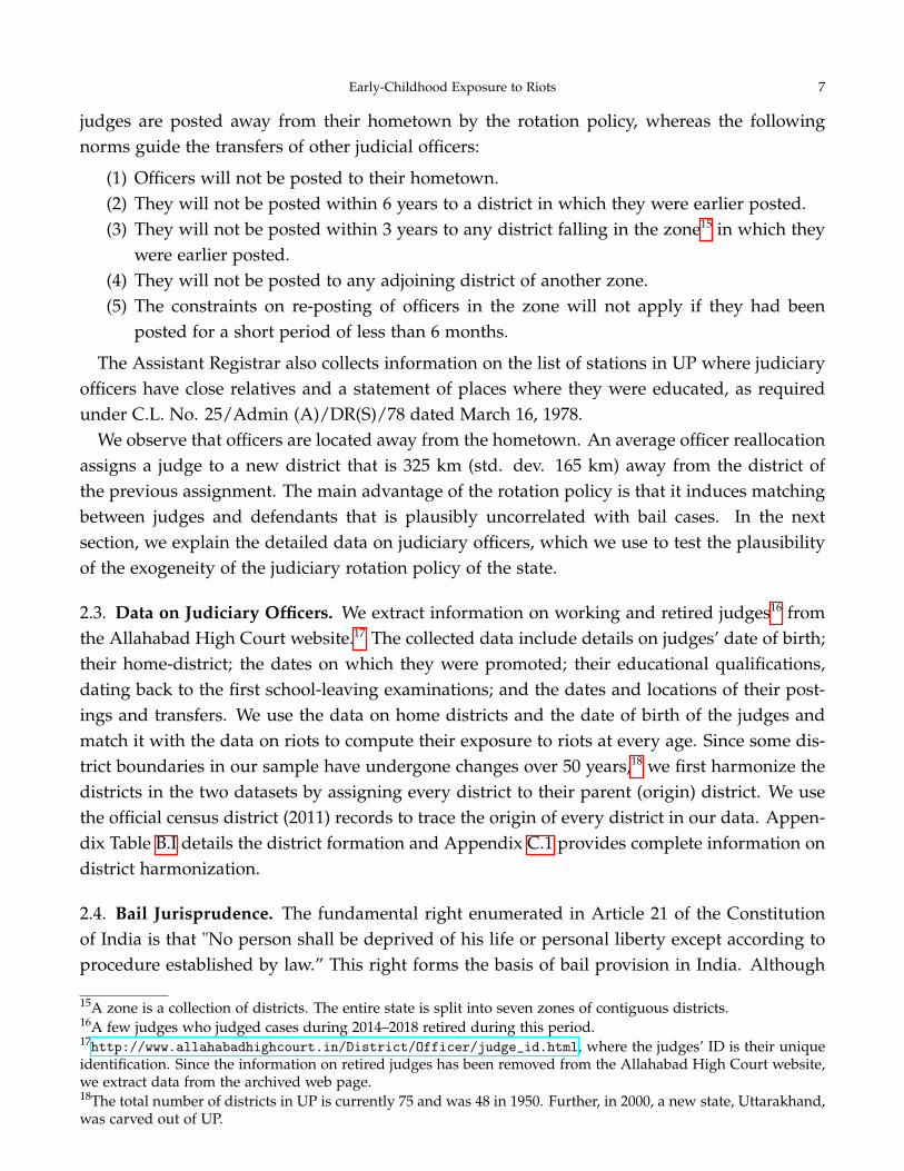
judges are posted away from their hometown by the rotation policy, whereas the followingnorms guide the transfers of other judicial officers:

(1) Officers will not be posted to their hometown.(2) They will not be posted within 6 years to a district in which they were earlier posted.(3) They will not be posted within 3 years to any district falling in the zone15 in which they

were earlier posted.(4) They will not be posted to any adjoining district of another zone.(5) The constraints on re-posting of officers in the zone will not apply if they had been

posted for a short period of less than 6 months.

The Assistant Registrar also collects information on the list of stations in UP where judiciaryofficers have close relatives and a statement of places where they were educated, as requiredunder C.L. No. 25/Admin (A)/DR(S)/78 dated March 16, 1978.

We observe that officers are located away from the hometown. An average officer reallocationassigns a judge to a new district that is 325 km (std. dev. 165 km) away from the district ofthe previous assignment. The main advantage of the rotation policy is that it induces matchingbetween judges and defendants that is plausibly uncorrelated with bail cases. In the nextsection, we explain the detailed data on judiciary officers, which we use to test the plausibilityof the exogeneity of the judiciary rotation policy of the state.

2.3. Data on Judiciary Officers. We extract information on working and retired judges16 fromthe Allahabad High Court website.17 The collected data include details on judges’ date of birth;their home-district; the dates on which they were promoted; their educational qualifications,dating back to the first school-leaving examinations; and the dates and locations of their post-ings and transfers. We use the data on home districts and the date of birth of the judges andmatch it with the data on riots to compute their exposure to riots at every age. Since some dis-trict boundaries in our sample have undergone changes over 50 years,18 we first harmonize thedistricts in the two datasets by assigning every district to their parent (origin) district. We usethe official census district (2011) records to trace the origin of every district in our data. Appen-dix Table B.I details the district formation and Appendix C.1 provides complete information ondistrict harmonization.

2.4. Bail Jurisprudence. The fundamental right enumerated in Article 21 of the Constitutionof India is that "No person shall be deprived of his life or personal liberty except according toprocedure established by law.” This right forms the basis of bail provision in India. Although

15A zone is a collection of districts. The entire state is split into seven zones of contiguous districts.16A few judges who judged cases during 2014–2018 retired during this period.17http://www.allahabadhighcourt.in/District/Officer/judge_id.html, where the judges’ ID is their uniqueidentification. Since the information on retired judges has been removed from the Allahabad High Court website,we extract data from the archived web page.18The total number of districts in UP is currently 75 and was 48 in 1950. Further, in 2000, a new state, Uttarakhand,was carved out of UP.

http://www.allahabadhighcourt.in/District/Officer/judge_id.html


bail is not defined legally in Indian codebooks,19 it implies the release of a person detained bythe police for a certain offence, by furnishing a guarantee of future attendance in the court fortrial. The two categories of bail in India are as follows:

i) Bail in bailable offences: In Section 436 of Cr.P.C, bail is the right of a person who has beenaccused of committing an offence that is bailable in nature. This provision casts a mandatoryduty on police officials as well the court to release the accused on bail if their alleged offence isbailable in nature.20

ii) Bail in nonbailable offences: When a person is charged with having committed a nonbailableoffence(s), the court has to consider many factors:21

a) whether there is any prima facie or reasonable ground to believe that the accused had com-mitted the offence; b) the nature and the gravity of the accusation; c) the severity of the pun-ishment in the event of conviction; d) the danger of the accused absconding or fleeing; e) thecharacter, behavior, means, position and standing of the accused; f) the likelihood of the offencebeing repeated; g) a reasonable apprehension of witnesses being influenced; h) the danger ofjustice being thwarted by granting bail.The subjective nature of the factors a judge must consider during bail decisions is evident.22

When a court gives bail, the accused must sign a personal bond and must usually provide twosurety bonds (from relatives or others who can vouch for the defendant) for a certain amount.If the accused breaks the bail condition, the court is liable to recover the amount from the de-fendant. A granted bond can also be cancelled later if it is found that bail conditions are notcomplied with.

2.5. Data on Defendants and Cases Registered. We web-scraped all the case-level pdfs fromthe district e-court website by court establishment23 in August 2018. We segregated about423K bail cases24 from the entire pool of two million downloaded cases. We performed opticalcharacter recognition, translated the documents to English and then extracted all the relevantvariables at the case level using text analysis. The primary details we extracted are the baildecision (whether granted/denied), the name of the defendants (which is used to identify

19The Criminal Procedure Code (Cr.P.C.) details the bail process but does not define bail. All offences are catego-rized as bailable or nonbailable.20In 2005, the Cr.P.C. was amended by adding section 436-A: A person who has undergone detention for a periodthat is half the maximum period of imprisonment imposed for a particular offence shall be released on his/herpersonal bond with or without sureties.21State of U.P. through CBI v. Amarmani Tripathi, 2005 (8) SCC 21; Prahlad Singh Bhati v. NCT, Delhi Anr. 2001(4) SCC 280; Ram Govind Upadhyay v. Sudarshan Singh Ors., 2002 (3) SCC 598.22We do not examine Anticipatory Bail. Under Section 438 of the Cr.P.C., the High Court or Court of Sessions canissue bail before a person is arrested, which is known as Anticipatory Bail, if there is an apprehension or a reasonto believe that a person may be arrested on an accusation of having committed a nonbailable offence. The courtconsiders the same list of factors mentioned in point (ii).23Website: https://districts.ecourts.gov.in/up; the District Courts for Chandauli, Etawah, Hardoi, Kheri, Pratap-garh, and Sant Kabir Nagar districts have not uploaded judgments. In the district of Varanasi, very few bail caseshave been uploaded.24The bail cases are identified from the bail application marker provided with the case number.


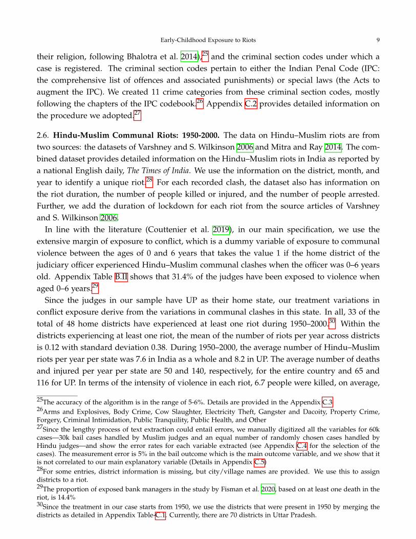
their religion, following Bhalotra et al. 2014),25 and the criminal section codes under which acase is registered. The criminal section codes pertain to either the Indian Penal Code (IPC:the comprehensive list of offences and associated punishments) or special laws (the Acts toaugment the IPC). We created 11 crime categories from these criminal section codes, mostlyfollowing the chapters of the IPC codebook.26 Appendix C.2 provides detailed information onthe procedure we adopted.27

2.6. Hindu-Muslim Communal Riots: 1950-2000. The data on Hindu–Muslim riots are fromtwo sources: the datasets of Varshney and S. Wilkinson 2006 and Mitra and Ray 2014. The com-bined dataset provides detailed information on the Hindu–Muslim riots in India as reported bya national English daily, The Times of India. We use the information on the district, month, andyear to identify a unique riot.28 For each recorded clash, the dataset also has information onthe riot duration, the number of people killed or injured, and the number of people arrested.Further, we add the duration of lockdown for each riot from the source articles of Varshneyand S. Wilkinson 2006.

In line with the literature (Couttenier et al. 2019), in our main specification, we use theextensive margin of exposure to conflict, which is a dummy variable of exposure to communalviolence between the ages of 0 and 6 years that takes the value 1 if the home district of thejudiciary officer experienced Hindu–Muslim communal clashes when the officer was 0–6 yearsold. Appendix Table B.II shows that 31.4% of the judges have been exposed to violence whenaged 0–6 years.29

Since the judges in our sample have UP as their home state, our treatment variations inconflict exposure derive from the variations in communal clashes in this state. In all, 33 of thetotal of 48 home districts have experienced at least one riot during 1950–2000.30 Within thedistricts experiencing at least one riot, the mean of the number of riots per year across districtsis 0.12 with standard deviation 0.38. During 1950–2000, the average number of Hindu–Muslimriots per year per state was 7.6 in India as a whole and 8.2 in UP. The average number of deathsand injured per year per state are 50 and 140, respectively, for the entire country and 65 and116 for UP. In terms of the intensity of violence in each riot, 6.7 people were killed, on average,

25The accuracy of the algorithm is in the range of 5-6%. Details are provided in the Appendix C.326Arms and Explosives, Body Crime, Cow Slaughter, Electricity Theft, Gangster and Dacoity, Property Crime,Forgery, Criminal Intimidation, Public Tranquility, Public Health, and Other27Since the lengthy process of text extraction could entail errors, we manually digitized all the variables for 60kcases—30k bail cases handled by Muslim judges and an equal number of randomly chosen cases handled byHindu judges—and show the error rates for each variable extracted (see Appendix C.4 for the selection of thecases). The measurement error is 5% in the bail outcome which is the main outcome variable, and we show that itis not correlated to our main explanatory variable (Details in Appendix C.5)28For some entries, district information is missing, but city/village names are provided. We use this to assigndistricts to a riot.29The proportion of exposed bank managers in the study by Fisman et al. 2020, based on at least one death in theriot, is 14.4%30Since the treatment in our case starts from 1950, we use the districts that were present in 1950 by merging thedistricts as detailed in Appendix Table-C.1. Currently, there are 70 districts in Uttar Pradesh.


in a riot in UP, which is similar to the average (6.3) for the whole of India. In terms of stateresponse variables in UP, the average duration of lockdowns following a riot was 5 days andthe average number of arrests was 144.

We set the following restrictions to arrive at our sample of judges. Since bail outcomes are ourmain outcome variable, we retain judges who are assigned to bail cases (N = 1, 268), of whichthe names of the home districts and the home states of 35 judges and 67 judges, respectively,were not available in the administrative data. Following Arnold, W. S. Dobbie, and Hull 2020,we drop judges who were assigned too few cases (the bottom 5 percentile in terms of thenumber of cases (<97 cases) assigned to the judges, which amounts to 493 judges).31 We alsodrop 10 judges because we did not have information on their LLB examination results. The LLBdegree is the minimum requirement for a judiciary officer, and 29% of the judges had passedthis course with first division and 71% with second division.The final sample consists of 668bail judges handling 323,380 cases aggregated at the judge-district-quarter level, which yieldeda sample size of 5,530. The descriptive statistics presented in Appendix Table B.III show that theanalysis sample is similar to the total sample of judges, along observables in the data. Figure A.Ireveals that the majority of the district judge transfers occurred mostly in the second quarter.Figure A.II reveals that the pattern is similar for the sample of bail judges. In Appendix TableB.II, we show that judges exposed to communal violence between the ages of 0 and 6 yearsare similar to judges without such exposure along the district covariates and the judge peersassigned to them. In terms of judges’ characteristics, the judges exposed to communal clashesin early childhood are more likely to be female, older, and more experienced.

3. Empirical Strategy

3.1. Specification. We begin with our case-level data, where the unique identifier is a bail case.Each bail case is uniquely matched to a judge; that is, only one judge handles each bail case.We observe the bail decisions of a judge corresponding to each bail case. For each judge, weaggregate the pretrial detention rate at the district-quarter level. We conduct our analysis ofpretrial decisions using the judge–district–quarter level data.32 Our results are robust to case-level regression. Section 7, the robustness checks section, explains why we have judge-levelregressions rather than case-level regressions as our preferred specification. Guided by ourdata depicted in Figure A.III in the Appendix, which shows that the proportion of bail casestrends in quarterly periods in the data, we aggregate bail decisions at the quarterly level. Ourresults are robust to aggregation at the monthly level.

31Our results are robust to changing the threshold from the bottom 1 to the bottom 10 percentile; we provide theresults of the robustness checks in Section 7. The choice of the bottom 5 percentile as the threshold„ that is, judgeshandling a minimum of 97 cases in 4 years, is to maintain a balance between not dropping too many judges andnot keeping too many judges who have handled very few cases.32We address concerns about the clustering of bail decisions at the judge level by first aggregating case-leveloutcomes at the judge–district–quarter level (Bertrand, Duflo, and Mullainathan 2004). Noting that our treatmentvariation is at the judge level (Abadie et al. 2017) and that there may be correlations across outcomes for a judgeacross quarters and districts (Bertrand, Duflo, and Mullainathan 2004), we cluster our standard errors at the judgelevel.


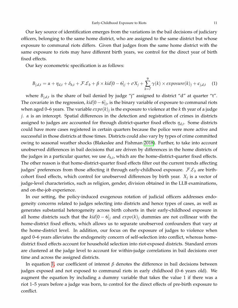
Our key source of identification emerges from the variations in the bail decisions of judiciaryofficers, belonging to the same home district, who are assigned to the same district but whoseexposure to communal riots differs. Given that judges from the same home district with thesame exposure to riots may have different birth years, we control for the direct year of birthfixed effects.

Our key econometric specification is as follows:

Bj,d,t = α + ηd,t + δh,t +F .E b + β× kid[0− 6]j + σXj +9

∑k=7

γ(k)× exposure(k)j + εj,d,t (1)

where Bj,d,t is the share of bail denied by judge “j” assigned to district “d” at quarter “t”.The covariate in the regression, kid[0− 6]j, is the binary variable of exposure to communal riotswhen aged 0–6 years. The variable expo(k)j is the exposure to violence at the k th year of a judgej. α is an intercept. Spatial differences in the detection and registration of crimes in districtsassigned to judges are accounted for through district-quarter fixed effects ηd,t. Some districtscould have more cases registered in certain quarters because the police were more active andsuccessful in those districts at those times. Districts could also vary by types of crime committedowing to seasonal weather shocks (Blakeslee and Fishman 2018). Further, to take into accountunobserved differences in bail decisions that are driven by differences in the home districts ofthe judges in a particular quarter, we use δh,t, which are the home-district-quarter fixed effects.The other reason is that home-district-quarter fixed effects filter out the current trends affectingjudges’ preferences from those affecting it through early-childhood exposure. F .E b are birth-cohort fixed effects, which control for unobserved differences by birth year. Xj is a vector ofjudge-level characteristics, such as religion, gender, division obtained in the LLB examinations,and on-the-job experience.

In our setting, the policy-induced exogenous rotation of judicial officers addresses endo-geneity concerns related to judges selecting into districts and hence types of cases, as well asgenerates substantial heterogeneity across birth cohorts in their early-childhood exposure inall home districts such that the kid[0 − 6]j and expo(k)j dummies are not collinear with thehome-district fixed effects, which allows us to separate unobserved confounders that vary atthe home-district level. In addition, our focus on the exposure of judges to violence whenaged 0–6 years alleviates the endogeneity concern of self-selection into conflict, whereas home-district fixed effects account for household selection into riot-exposed districts. Standard errorsare clustered at the judge level to account for within-judge correlations in bail decisions overtime and across the assigned districts.

In equation 1, our coefficient of interest β denotes the difference in bail decisions betweenjudges exposed and not exposed to communal riots in early childhood (0–6 years old). Weaugment the equation by including a dummy variable that takes the value 1 if there was ariot 1–5 years before a judge was born, to control for the direct effects of pre-birth exposure toconflict.


The riot information is available until 2000, and in our sample, the youngest judge is bornon October 7, 1991. Hence, we can calculate exposure to violence up to the first 9 years afterbirth for the full sample of judges in UP.33 However, as a robustness check, we test for early-lifeexposure to violence by controlling for exposure to violence in later life for the subsample forwhich we can control for exposure to violence in later years.

4. Balance Test

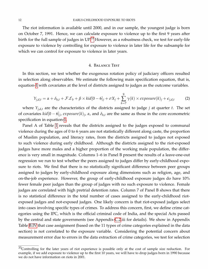
In this section, we test whether the exogenous rotation policy of judiciary officers resultedin selection along observables. We estimate the following main specification equation, that is,equation-1 with covariates at the level of districts assigned to judges as the outcome variables.

Yj,d,t = α + δh,t +F .E b + β× kid[0− 6]j + σXj +9

∑k=7

γ(k)× exposure(k)j + εj,d,t (2)

where Yj,d,t are the characteristics of the districts assigned to judge j at quarter t. The setof covariates kid[0− 6]j, exposure(k)j, α, and δh,t are the same as those in the core econometricspecification in equation-1.

Panel A of Table 1 reveals that the districts assigned to the judges exposed to communalviolence during the ages of 0 to 6 years are not statistically different along caste, the proportionof Muslim population, and literacy rates, from the districts assigned to judges not exposedto such violence during early childhood. Although the districts assigned to the riot-exposedjudges have more males and a higher proportion of the working male population, the differ-ence is very small in magnitude. Columns 1–6 in Panel B present the results of a leave-one-outregression we run to test whether the peers assigned to judges differ by early-childhood expo-sure to riots. We find that there is no statistically significant difference between peer groupsassigned to judges by early-childhood exposure along dimensions such as religion, age, andon-the-job experience. However, the group of early-childhood exposure judges do have 10%fewer female peer judges than the group of judges with no such exposure to violence. Femalejudges are correlated with high pretrial detention rates. Column 7 of Panel B shows that thereis no statistical difference in the total number of cases assigned to the early-childhood riot-exposed judges and not-exposed judges. One likely concern is that riot-exposed judges selectinto cases involving specific types of crimes. To address this concern, first, we define crime cat-egories using the IPC, which is the official criminal code of India, and the special Acts passedby the central and state governments (see Appendix-C.2.iii for details). We show in AppendixTable B.IV that case assignment (based on the 11 types of crime categories explained in the datasection) is not correlated to the exposure variable. Considering the potential concern aboutmeasurement error due to errors in the data extraction of crime categories, we test for selection

33Controlling for the later years of riot experience is possible only at the cost of sample size reduction. Forexample, if we add exposure to violence up to the first 10 years, we will have to drop judges born in 1990 becausewe do not have information on riots in 2001.


in a manually digitized random sample of judges (Appendix Table-B.V) and find no evidenceof the selection of judges into crime types.

Next, we apply the method used by Couttenier et al. 2019 to demonstrate the exogeneityin the allocation of judges determined by the rotation policy. The notion is to test whetherthe judicial postings across different district-quarters is non-random. More specifically, we testwhether the average characteristics of the judges from the same home district are similar tothose of the judges (from the same home district) posted in different district-quarters.34 We testfor the difference in means along the judge-level treatment and non-treatment covariates acrossdistrict-quarters. Formally, we estimate the following equation separately for judges from eachhome district for every quarter:

Jh,b,q,d =75

∑d=1

βd,q × Ih,b,q,d + εb (3)

where Jh,b,q,d are the judge-level characteristics of judges from home district "h", birth cohort"b", at quarter "q" in district "d". βd,q are the district-quarter specific coefficients correspondingto the indicator dummy for judges, denoted as Ih,b,q,d, that takes the value 1 if the judge fromthe home district "h", birth cohort "b", is allocated to district "d" at quarter "q". The dependentvariables are judge-level characteristics, such as exposure to communal conflict when aged0–6 years, gender, religion, age, time to promotion, and age when joining the judiciary. Foreach home district, we examine the number of district-quarters for which the F-test of the nullhypothesis ˆβd,q = µ̂h is rejected where µ̂h are the average characteristics of the judges at thehome-district level. If the allocation is exogenous, then the district-quarter specific coefficient

ˆβd,q should not differ from the home-district average, and the F-test should not be rejectedfor this district-quarter. If there is no selection in the spatial allocation of the judges, thenthe observable judge characteristics in some districts with respect to the home-district averageshould not be over- or under-represented. Each row in Table B.VI represents the share of homedistricts for which the F-test is rejected at the 10% cutoff in at most 0, 1, 5, and 10 districts. Forinstance, it shows that for 95% of the home districts, we do not have any district-quarter specificcoefficients that differ from the home-district average of Kid[0− 6] and for 100% of the homedistricts, less than five district-quarter coefficients differ from the home-district average. Weobserve similar results for the home-district averages related to the average of female judges,Muslim judges, and judges with first division in their LLB examination. Regarding the home-district average age of judges, time to promotion, and joining age, for almost all home districts,less than 10 districts have district-quarter specific coefficients that differ from the home-districtaverages. Therefore, we do not find any evidence of selection along observables in the spatialallocation of the judges.

34Suppose X judges are from home district A and the average age of these judges is 46 years. Out of these Xjudges, say x1 judges are posted in district B and (X-x1) judges are posted in district C at a given time. If thejudges are posted randomly, then the average age of x1 and (X-x1) judges would also be 46 years.


5. Main Impact of Exposure to Communal Violence

We present the results of our key econometric specification as represented by equation-1 inPanel A of Table 2. We report our coefficient of interest β controlling for exposure to violencein later years. The coefficient of interest demonstrates the causal effect of exposure to commu-nal violence when 0–6 years old on the shares of bail denied (that is, pretrial detention rates),where the control group consists of judiciary officers with either no experience of violence orwho have not been exposed to violence when 0–6 years old. Column (1) of Panel A providesthe treatment effect estimates using a variant of regression equation-1, which is a specificationwithout controls for judge-level characteristics. The treatment effects of exposure to riot arepositive and statistically significant at the 1% level of significance. The shares of bail denied byjudiciary officers exposed to violence in early years are 6.3 percentage points higher, which is anincrease of 17% (= 0.063/.37) compared with the baseline mean, than the shares of bail deniedby judiciary officers without such exposure. In Column (2), we add controls for judge-levelcharacteristics, such as experience, gender, religion, and LLB examination grades. The treat-ment effect estimates show a 6.1 percentage points increase in pretrial detention rates, whichis an increase of 16.4% (= 0.061/.37) compared with the baseline mean, which is statisticallysignificant at the 1% level of significance. In Column (3), we add controls for the occurrence ofcommunal riots 5 years before birth. Our coefficient of interest remains almost unaffected, with17% (= 0.062/.37) increase in detention rates. The effects are statistically significant at the 1%level of significance.

In Column (4), we add birth-year-quarter fixed effects (and exclude birth-year fixed effects) toflexibly account for the unobserved current time trends by judges’ birth cohort. The coefficientremains stable at 0.06 and is statistically significant at the conventional level. Even though wehave shown that riot-exposed judges do not select into types of crime, we perform one morecheck to alleviate the concern. We change the specification in Column (5) where we aggregatethe data at the judge-crime type-district-quarter level (which increases the number of observa-tions) and include crime-type fixed effects explicitly. The size of the coefficient estimate relativeto the mean is 16.87% (=.054/0.32) which is very similar to the estimates from Column(2).

Recent literature on the causal effects of exposure to violence during early-childhood in thecontext of asylum seekers in Switzerland (Couttenier et al. 2019) and bank managers in India(Fisman et al. 2020) have used ages 0–12 and 0–10 years old (for early-childhood), respectively.35

In light of this evidence, we estimate our main regression equation 1 and add controls forexposure to violence in the years after age 6 in Panel B. In Column (1) of Panel B, we controlfor exposure until age 14 years, in Column (2) of Panel B we control for exposure until age18 years, and last, in Column (3), we control for exposure until age 22 years. Adding controls

35We show in Appendix Table B.VII that exposure to riots between the age of 0-9, or 0-10 or 0-12 do not causestatistical significant effects on the share of bail denied. The coefficient is positive, consistent with the effect of riotexposure between the age of 0-6. But the riot exposure coefficients are imprecise.


for exposure reduces our sample from Columns (1) to (3) in Panel B, but our results remainpositive with a similar magnitude and are statistically significant at the 5% level of significance.

In our main table, we also report various estimates of the standard errors of the treatment ef-fect of early-childhood exposure to communal violence. The Moulton-corrected standard errorsand the wild bootstrap standard errors are both stable and demonstrate that the coefficients ofinterest across specifications are significant at the 5% level of significance. Further, in AppendixTable-B.VIII, we show that our results are robust to clustering at the level of home-district -yearof birth and home-district level. The coefficients are stable across specifications.

6. Interpretation: Selection or Exposure Effect

A key concern about the interpretation of the impact coefficient is that the coefficient couldalso include sorting into the judiciary. We adopt two empirical strategies to show that impactof early-childhood exposure to violence is not driven by the selection of exposed individualsinto the judiciary.

In the presence of the selection effect, we would observe either under- or over-representationin the judiciary of judges exposed to riots in early-childhood. In the first method, we comparethe share of the early-childhood riot-exposed population in the entire working population (inall sectors and all types of employment) in UP with the share of early riot-exposed judges in thisstate. To this end, we exploit the data from the Employment and Unemployment Survey of theNational Sample Survey Organization (NSSO) (66th round, 2011). We restrict our analysis tothe riot-affected UP districts. This survey captures information about individuals’ age (but nottheir birth date) and the district in which they were residing at the time of the survey (i.e., theircurrent district, but not their birth district), which we use to ascertain their riot exposure. Oneconstraint is that no all-India survey captures information on survey respondents’ birthplace (oreven birth district). However, the migration literature has shown a low migration rate (5–6%)for India. Further, 99% of the migration is within a district. Hence, for this exercise, we assumethat the current district is the birth district. Next, we select the sample born after 1950 (sinceour riot data start from 1950) who are employed (all types of employment). In Appendix Table-B.IX, we find that the percentage of the total working population exposed to riots when aged0–6 years is 39.2%, whereas the percentage of riot-exposed judges in the total population ofjudges in UP is 38.64%, in the sample of bail judges is 38.88%, and in our analysis sample is38.8%. It is reassuring to note that there is no over- or under-representation of riot-exposedjudges in the judiciary compared with the representation of the riot-exposed population in thetotal working population.

In the second approach, we ask whether different numbers and types of judges, where typeis defined by gender and religion, are drawn from different riot-affected districts. In particular,we test whether the home-districts that experience a riot in a given year are more likely to


have different total number and types of judges using the following specification at the home-district-riot-year level.

Judgesh,y = α + ηh + δy + βExposedh,y + εh,y (4)

where h and y denote home-district and riot-year. ηh is the home-district fixed effect, and δy

is the riot-year fixed effect. The outcome variables Judgeshy are the total number of judges, theproportion of females, and the proportion of Muslim judges. Since our focus is on the first 6years of exposure, the outcome variable includes judges born 6 years before any given home-district riot-year. For instance, if the district Agra had a riot in 1970, the total number of judgesaffected by this riot (in their early-childhood, 0-6 years) would be the judges born in Agra in1965-1970.

Appendix Table B.X shows that there is no selection of the type or total number of judges byriot-affected home-districts in any given year.

7. Robustness

7.1. Few Judges per District Concern. Our analytical sample has 668 judges over several dis-tricts, possibly resulting in a small number of judges per district, thereby raising the concernthat the impact is attributable to riot exposure among a few judges. To address this concern, wesort the judges by their influence on the regression coefficient, where Cook’s distance measuresthe influence. Figure 2 plots the coefficients from the estimates of our main specification (Col-umn (2) of Panel A of Table 2), by excluding one judge at a time—starting with the judge havingthe highest influence on the regression coefficient—and ultimately excluding 300 judges. Thecoefficient is stable and statistically significant at the 5% level of significance until the exclusionof the first 280 judges (out of 668 judges), alleviating the concern that a few judges may bedriving our result.

7.2. Case-level regressions. Our outcome variable is aggregated at the judge–district–quarterlevel. It may be argued that using case-level outcome data could account for the differences inworkload by judges within a court-quarter (i.e., across courtrooms in the same District Courtin a given quarter), which are not addressed by the district-quarter fixed effect, especially forlarger districts with multiple police stations and multiple courtrooms adjudicating criminaltrials. In Appendix Table B.XI, we test the regression at the case level instead of aggregating atthe judge–district–quarter level. Column (1) has the same controls and fixed effects as in ourbaseline results (i.e., Column (2) of Table 2). In Column (2), we add the crime-type fixed effect,and in Column (3), we further refine our specification by adding two more controls—a dummyfor whether the defendant is a Muslim and a dummy for the nonbailable nature of the case.The coefficients range from 0.038 to 0.043, which is 11 to 12% over the mean, and are close toour main result.


Although case-level data account for the different workloads per judge, there are concernsabout correct inference owing to the clustering of outcomes. Following the design-based un-certainty approach of Abadie et al. 2017, since the random variation of treatment is at the judgelevel, the data should be clustered at the judge level. However, if each judge has a differentnumber of cases, case-level data lead to misleading inferences because of the varying clustersizes (MacKinnon and Webb 2017). Assuming a sampling-based approach to clustering, in linewith (Cameron and Miller 2015), then the level at which the data should be clustered becauseof correlation is ambiguous. It can be suggested that with case-level outcomes, since the samedefendant(s) can be represented across cases assigned to judges, the correct inference wouldrequire accounting for serial correlation across cases with the same defendant in addition toclustering at the judge level. In a similar quasi-random judge assignment study, W. Dobbie,Goldin, and C. S. Yang 2018 account for two-way clustering by including the defendant- andthe judge-level clusters. This approach is not feasible for our data because we do not have aunique defendant ID.

The benefits of adding case level controls are very limited owing to data limitations. How-ever, there are inference issues as mentioned above arising from clustered data in case-levelregressions. Hence, our preferred specification aggregates the outcome data at the judge levelusing judge-level clustering for inference.

7.3. Sample Selection. We follow Arnold, W. S. Dobbie, and Hull 2020 and exclude the bottom5 percentile judges (i.e., judges handling less than 97 cases) from our primary analysis sample,to allay concerns related to judges dealing with very few cases driving our outcomes. InAppendix Table B.XII, we present the results using alternative thresholds for the exclusionof judges from analysis samples. From Column (1) to Column (10), we change the threshold ofexclusion from the bottom 1 to 10 percentile. The coefficients are very stable and close to ourmain result in all the specifications.

7.4. High-rank Judges. Another concern is that high-ranked judges may influence the casesassigned to them. In Appendix Table B.XIII, we exclude District and Session Judges and ChiefJudicial Magistrates—the two most influential judges in the district-level judiciary—and findthat our coefficient magnitudes range from 5.4 to 8.4 percentage points and are statisticallysignificant at the 95% confidence interval.

7.5. Outlier Tests. The next set of robustness tests is to check for potential outliers in ourbaseline results. In Appendix Table B.XIV, we show that judges from home districts exposedto a high number of riots do not drive our results. Column (1) in Table B.XIV presents theresults after the exclusion of judges from the home districts that have experienced the highestnumber of Hindu–Muslim riots, Column (2) presents the results after the exclusion of judgesfrom the home districts with the second-highest number of riots, and so on. We observe thatthe effect of early-childhood exposure to riots is positive and statistically significant at theconventional levels, with its magnitude ranging from an increase of 5.7 to 7.5 percentage point


in pretrial detention rates. In Appendix Table B.XV, we remove the home districts with thehighest number of riots cumulatively. Here, again we find that the treatment effect of exposureto riots when in the age group of 0–6 years is positive, and its magnitude ranges from 6.8percentage points to 8.8 percentage points, significant at the 1% level of significance. Lastly, wetest our baseline results by removing observations that are 3, 2, and 1 standard deviation awayfrom the residual mean in Column (1), Column (2), and Column (3) in Appendix Table B.XVI,respectively. In addition, we remove observations with high leverage, which shift estimates to atleast one standard error and to at least 4/N. The results are positive, with magnitudes rangingfrom 5.3 percentage point to 6.4 percentage points, and are significant at the conventional levelof significance across all specifications.

7.6. Placebo Test. In our placebo check, we follow a Monte Carlo approach and randomly reas-sign our treatment variable kid[0− 6] following a binomial distribution, based on the observeddistributions of kid[0− 6], keeping all other characteristics unchanged. We estimate our mainspecification (Column (2) of Panel A of Table 2) on the simulation data. We implement 1,000simulations. The sampling distribution of the treatment effects of kid[0− 6] Monte Carlo drawsis centered around zero. Figure A.IV demonstrates that the probability of the treatment effectfound in our main specification being spurious is negligible.

8. Threats to Identification: Migration

The migration of households from riot-hit districts to districts less likely to experience Hindu-Muslim riots would violate SUTVA (Rubin 1980), which is our identifying assumption. There-fore, we test whether the migration rates are affected by the communal riots. We use the NSSOs’microdata from the Employment and Unemployment Survey 1983, which captures migrationinformation.36 The important migration-related information we exploit are the age at whichmigration occurs, the district from where migration takes place (i.e., the origin district), andwhether migration occurs within the district or to another district. The data allow us to per-form analysis only for the migrating population. Since the violation of SUTVA in our settingoccurs in case of migration from a riot-hit district to another district, and not within a riot-hitdistrict, we show that the share of out-migration from the district in the total migration is notcorrelated with the riots.

We build the data at the district-year level and run the following regression.

MigrationRateh,y = α + ηh + δy + βExposedh,y + εh,y (5)

where h and y denote the origin of migration district and the year of migration. ηh is the districtfixed effect, and δy is the year fixed effect. The outcome variable MigrationRatehy is the ratioof migration across districts to the total migration. The coefficient to focus upon is β associated

36We could not find any nationally representative survey capturing both the origin and destination districts. Thelater rounds of the NSSO’s Employment and Unemployment Surveys do not provide data on origin districts.


with the explanatory variable Exposedh,y that captures whether the district-year cell had a riot.The β coefficient as shown in Table 3 is close to zero and statistically insignificant.

Next, we collect administrative data on the districts where the judges completed their sec-ondary schooling, higher secondary schooling and undergraduate studies for a subsample ofjudges. In Table-4 we establish there is no early childhood riot exposure effect on migrationaway from home districts to the districts where they completed their secondary schooling (atage 15), higher secondary schooling (at age 17) and undergraduate studies (at age 21).

9. Mechanisms

A growing body of economics literature on endogenous preference formation emphasizesearly childhood as a period in which fundamental preference parameters and character skillsdevelop. 37 More importantly, recent studies have highlighted that the social environment dur-ing early childhood can have persistent causal effects on preferences, such as the preference forhonesty (Abeler, Falk, and Kosse 2021), risk (Giuliano and Spilimbergo 2014), and redistribu-tion (Cappelen et al. 2020). In particular, seminal recent studies on exposure to violence in earlychildhood, such as those by Couttenier et al. 2019; Fisman et al. 2020), have found that highcasualties resulting from intergroup conflict produce lasting intergroup hostility. One possibil-ity of social environment affecting children is through parental influence. Parental traits canshape preferences of their children, for example children have been shown to become long-termoriented when observing a long-term oriented adult (Bandura and Mischel 1965). It is possiblethat parents experiencing effective state-intervention in civil clashes develop positive attitudetowards state institutions. The children who observe their parents’ confidence in the institu-tions and the functioning of the state may develop greater support for such institutions. Wefollow the emerging literature on early childhood and explore whether there is intergroup hos-tility in the observed judicial stringency or whether judicial stringency potentially representssupport for the state. We, additionally, use our data to rule out other non-behavioral channels,such as differences in cognitive abilities.

9.1. No Intergroup Bias Behavior. Early-life exposure to an intergroup conflict could generateanimosity between groups, as evidenced in the high-intensity Hindu–Muslim violence in theIndian context in the case of bank managers (Fisman et al. 2020). To estimate the intergrouphostility effect, we would need to identify the religion of the judges and the defendants but donot have such administrative data. Following Bhalotra et al. 2014, who use names to infer thereligion of electoral candidates in India, we use names to infer the religion of the judges andthe defendants.

We manually assign each judge to a religious group using the judges’ name and their fa-thers’ name. For defendants, first, we use the "Stanford Named Entity Algorithm" to extract

37Kautz et al. 2014; Alan, Boneva, and Ertac 2019; Falk et al. 2021; Kohlberg 1984; Piaget 1997; Harbaugh, Krause,and Vesterlund 2002; Sutter and Kocher 2007; Fehr, Bernhard, and Rockenbach 2008; Ben-Ner et al. 2017; Almåset al. 2010; Bauer, Chytilová, and Pertold-Gebicka 2014


their names from the judgments (see Appendix C.3 for details). Then, we use the Nilabhraname2community algorithm to identify Urdu-sounding names, which we classify as Muslimnames. To address the concern about the likely scope for error in identifying Muslim names,we test it on the dataset of Bhalotra et al. 2014. We find that this algorithm predicts the religionfrom names with a 6% error rate. However, the error rate in the classification of the defendants’religion is higher (20%) owing to additional errors in the process of extracting names from thejudgment pdfs.

In our sample of 668 judges, only 51 are Muslims, of which only 13 Muslim judges wereexposed to communal violence when 0–6 years old. In comparison, we have 617 Hindu judgesin our sample, out of which 197 Hindu judges were exposed to religious riots between ages 0and 6 years.38 However, about 20% of cases involve only Muslim defendants, as measured bythe algorithm.

We perform a subsample analysis to test whether the bail decisions of early-childhood riot-exposed Hindu judges differ in cases where all the defendants are Hindus from their decisionsin cases where all the defendants are Muslims. Columns (2) and (3) of Table 7 reveal that thecoefficient measuring the causal effect on early-childhood exposure to communal riots remainspositive for both Hindu and Muslim defendants, with the coefficient for Hindu defendants be-ing 5.1 percentage points (14% increase in pretrial detention rates) and 7.3 percentage points(20% increase in pretrial detention rates), both statistically significant at the 5% level of sig-nificance. We do a Chow test from a pooled regression and find that the early-riot exposurecoefficient for Hindu defendants is not statistically different from the early-riot exposure coef-ficient for Muslim defendants (F-stat= 0.15).

9.2. Riot Intensity and State Lockdowns. Hindu–Muslim religious clashes in India affect so-cioeconomic outcomes not only through riot casualties or social segregation but also throughstate-imposed lockdowns. S. I. Wilkinson 2006 argues that the state response to Hindu–Muslimriots in the form of arrests, lockdowns, and increased police presence plays a huge role indetermining riot damages. In other words, an effective state response can prevent the escala-tion of a riot. The early-childhood exposure of individuals to a sociopolitical environment inwhich strong state action resulted in fewer riot-related deaths can potentially generate in themsupport for, or confidence in, the state relative to the individual. Therefore, we hypothesizethat judicial stringency could be driven by judges with a positive childhood experience of stateintervention to curb civilian misconduct.

To examine this hypothesis, we analyze the heterogeneity impact of riot casualties interactedwith state lockdowns. First, we compute casualties per land area (instead of population size toavoid reverse causation bias) experienced by each judge between ages 0 and 6 years. We selectthe median value of casualty experienced by the riot-exposed judges as the threshold belowwhich we term a riot as a low-severity riot. Similarly, a state response measure, such as a high

38The sparse presence of Muslim judges is not surprising, and several studies have shown the under-representationof Muslims, including Fisman et al. 2020 who considered the exposure to violence of bank managers.


lockdown, is defined as a lockdown that lasts for more than 5 days, which is the median daysof lockdown experienced by our sample of riot-exposed judges. High arrests are defined asarrests that exceed 170, the median value of arrests that occurred in riots experienced by judgesbetween ages 0 and 6 years.

We compare the bail decisions of non-exposed judges with that of judges experiencing highstate action in terms of high lockdowns or arrests, but varying levels of riot casualties, usingthe following equation:

Bj,d,t = α + ηd,t + δh,t +F .E b + β1 × high− casualty− high− state− action[0− 6]j+

β2 × low− casualty− high− state− action[0− 6]j +9

∑k=7

γ(k)× exposure(k)j + Xj + εj,d,t(6)

where high− casualty− high− state− action[0− 6]j denote high casualty and a higher periodof lockdowns or police arrests, and low − casualty − high − state − action[0− 6]j denote lowlevels of casualty and higher period of lockdowns or police arrests. The remaining variablesare same as in our main specification in equation- 1.

Table-5 presents the heterogeneity impact by intensities of lockdown and riot-related casu-alties. We observe that among the judges who experienced early-childhood riots with intensestate response measured by the total number of police arrests or the total number of days ofstate-imposed lockdowns, it is the judges with an early-childhood experience of riots resultingin low casualties who drive judicial stringency in bail decisions.39

The above pattern is consistent with the hypothesis that the early-life experiences of judgesregarding effective lockdowns or police arrests that have effectively controlled civilian violencegenerate in them persistent confidence in the state relative to the individual.

9.3. Heterogeneity by Age of Exposure. Motivated by Cappelen et al. 2020, who show that in-terventions during ages 3 to 4 years have a long-term impact on social preferences, we examinethe heterogeneity by riot exposure to test whether our interpretation of the interaction term ofconflict severity is driven by changes in the support for the state.

We group judicial officers based on their exposure to riots into three mutually exclusiveage groups of 0–3, 3–6, and 6–9 years to test whether the effects are determined by exposurebetween ages 3 and 6 years.40 We estimate the following regression specification, which is avariant of our main specification in equation 1:

39We report riot severity results using an alternative specification in Table B.XVII. We find that by all measures ofriot intensity, low-intensity riots explain a high share of bail denied by early-childhood riot-exposed judges, whichis statistically significant at the 1% level of significance (compared with non-exposed judges). Further the resultsare robust to using alternative methods of calculating the intensity thresholds, as presented in Appendix TableB.XX40The term mutually exclusive means that if a judge is exposed when aged 0–3 years as well as when aged 3–6years, then (s)he will be categorized into the 0–3 age category.


Bj,d,t = α + ηd,t + δh,t +F .E b + β× pre− birth[0− 3]j + β1 × kid[0− 3]j+

β2 × kid[3− 6]j + β3 × kid[6− 9]j + Xj + εj,d,t(7)

In our data, a similar number of judges in each age bin were exposed to communal riots.The families of 125 judges (approximately 19% of the total judges in the estimation sample)were exposed to violence between 0 and 3 years before the judges’ birth. Further, 131 judgeswere exposed to violence when 0–3 years old, and 132 judges when 3–6 years old (which isapproximately 20% of the total judges in the estimation sample). Last, 163 judges were exposedto communal clashes when 6–9 years old (which is approximately 24% of the total judges in theestimation sample). In Appendix Table B.XVIII, we show the results on estimating the aboveequation for older cohorts of judiciary officers for whom we can control for potential exposureto violence up to age 22 years. We find a statistically significant (p < 0.05) positive treatmenteffect of exposure for the age group of 3–6 years. Figure 1 plots the coefficient estimate of eachage group. We note that the effects are primarily driven by exposure between ages 3 and 6years.

Next, we test the impact on bail decisions by the age of first exposure to communal conflicts.We construct conditional extensive margins by estimating the effects on bail decisions by theage at first exposure, denoted by f irstexposure(k). Our regression equation is as follows:

Bj,d,t = α + ηd,t + δh,t +F .E b + βn

∑k=1

f irstexposure[k]j + σXj + εj,d,t (8)

where f irstexposure(k) is defined as the age at first exposure at k. All other variables are thesame as specified for equation 1.

Figure 3 and Appendix FigureA.V plot the coefficient estimates with 95% confidence intervalsof equation 8 for the full sample, for which the effects of the age at first exposure can beestimated only up to year 9, and for the subsample, for which the effects of the age at firstexposure can be estimated up to year 22. Both plots demonstrate the causal effect on baildecisions of the age at first exposure being 4 and 5 years. Appendix Table-B.XIX shows theeffect of age at first exposure to communal violence for the full analysis sample. We observethat the effect of the age at first exposure being 4 years is 8.1 percentage points, and the effect ofthe age at first exposure being 5 years is 11.8 percentage points, which is statistically significantat the 5% and 1% levels of significance, respectively. Given the findings in the early childhoodliterature, this result provides further support for our interpretation in the above section thatthere is a causal link between early-childhood riot exposure to the support for the state incontrolling civilian misconduct.

9.4. Do Recent Riots Exposure Matter? In Figure-4, we plot the post-period effects of currentriots (2014-2017) at the weekly level for up to 12 weeks separately for early-exposed and non-exposed judges. We establish that the effects of current riots are not persistent. There is no


effect of riots on shares of bail denied for early exposed judges. For the non-exposed judgesthere are marginal positive effects up to 5 weeks post the riots, with most post-period effectsbeing statistically insignificant.

9.5. Judicial Education and Judicial Stringency. Next, we test whether differences in cognitiveskills as measured by performance in the mandatory LLB examination explain differences inbail decisions across judges. Table-6 reports that the inclusion of LLB examination results donot affect our coefficient estimates of the early-childhood riot exposure effect. Therefore, weconclude that heterogeneity in skills in law training does not explain our results.

10. Conclusion

In this study, we examine the population of judges and show that their exposure to com-munal violence at ages 0–6 years has persistent economic and statistically significant effects onpretrial detention rates. Unlike studies that have focused on estimating bias and discriminationin judicial decisions, we investigate the origins of judicial bias. We show that early-childhoodexposure to the sociopolitical environment has robust effects on adult decisions across genera-tions. We show that judges exposed to communal violence between the ages of 0 and 6 yearsare 16% more prone to deny bail than the average judge. The effect is driven by exposure to alow number of riot-related deaths and injuries and a low riot duration, as well as by exposurewhen between 3 and 6 years of age.

We provide some evidence in support of our interpretation that the experience of riot de-escalation efforts by the state that result in low riot-related damages during judges’ formativeyears has long-term effects on judicial outcomes. Further research on how preferences andbeliefs are formed owing to sociopolitical events during the formative years of childhood wouldprovide decision-makers with insights for designing effective policy tools.


References

Abadie, Alberto et al. (2017). When Should You Adjust Standard Errors for Clustering? WorkingPaper 24003. National Bureau Economic Research.

Abeler, Johannes, Armin Falk, and Fabian Kosse (2021). Malleability of Preferences for Honesty. In:Abrams, David S, Marianne Bertrand, and Sendhil Mullainathan (2012). Do Judges Vary in their

Treatment of Race? In: The Journal of Legal Studies 41.2, pp. 347–383.Adhvaryu, Achyuta, James Fenske, and Anant Nyshadham (2019). Early Life Circumstance and

Adult Mental Health. In: Journal of Political Economy 127.4, pp. 1516–1549.Agan, Amanda and Sonja Starr (2018). Ban the box, criminal records, and racial discrimination: A

field experiment. In: The Quarterly Journal of Economics 133.1, pp. 191–235.Aizer, Anna and Flavio Cunha (2012). The Production of Human Capital: Endowments, Investments

and Fertility. Working Paper 18429. National Bureau of Economic Research.Alan, Sule, Teodora Boneva, and Seda Ertac (2019). Ever failed, try again, succeed better: Results

from a randomized educational intervention on grit. In: The Quarterly Journal of Economics 134.3,pp. 1121–1162.

Almås, Ingvild et al. (2010). Fairness and the Development of Inequality Acceptance. In: Science328.5982, pp. 1176–1178.

Almond, Douglas (2006). Is the 1918 Influenza Pandemic over? Long-Term Effects of in Utero In-fluenza Exposure in the Post-1940 US Population. In: Journal of Political Economy 114.4, pp. 672–712.

Almond, Douglas and Janet Currie (2011). Killing me Softly: The Fetal Origins Hypothesis. In:Journal of Economic Perspectives 25.3, pp. 153–72.

Almond, Douglas, Lena Edlund, and Mårten Palme (2009). Chernobyl’s Subclinical Legacy: Pre-natal Exposure to Radioactive Fallout and School Outcomes in Sweden. In: The Quarterly Journal ofEconomics 124.4, pp. 1729–1772.

Angerer, Silvia et al. (2015). Donations, Risk Attitudes and Time Preferences: A Study on Altruism inPrimary School Children. In: Journal of Economic Behavior & Organization 115, pp. 67–74.

Anwar, Shamena, Patrick Bayer, and Randi Hjalmarsson (2012). The Impact of Jury Race in Crim-inal Trials. In: The Quarterly Journal of Economics 127.2, pp. 1017–1055.

Arnold, David, Will S Dobbie, and Peter Hull (2020). Measuring Racial Discrimination In BailDecisions. Working Paper 26999. National Bureau of Economic Research.

Arnold, David, Will Dobbie, and Crystal S Yang (2018). Racial Bias in Bail Decisions. In: TheQuarterly Journal of Economics 133.4, pp. 1885–1932.

Ash, Elliott et al. (2021). Measuring Gender and Religious Bias in the Indian Judiciary. WorkingPaper.

Bandura, Albert and Walter Mischel (1965). Modifications of self-imposed delay of reward throughexposure to live and symbolic models. In: Journal of personality and social psychology 2.5, p. 698.

Bauer, Michal, Julie Chytilová, and Barbara Pertold-Gebicka (2014). Parental Background andOther-Regarding Preferences in Children. In: Experimental Economics 17.1, pp. 24–46.

REFERENCES 25

Ben-Ner, Avner et al. (2017). Learned Generosity? An Artefactual Field Experiment with Parents andtheir Children. In: Journal of Economic Behavior & Organization 143, pp. 28–44.

Bertrand, Marianne, Esther Duflo, and Sendhil Mullainathan (2004). How Much Should We TrustDifferences-in-Differences Estimates? In: The Quarterly Journal of Economics 119.1, pp. 249–275.

Bhalotra, Sonia et al. (2014). Religion, Politician Identity and Development Outcomes: Evidence fromIndia. In: Journal of Economic Behavior & Organization 104, pp. 4–17.

Bharadwaj, Prashant, Katrine Vellesen Løken, and Christopher Neilson (2013). Early Life HealthInterventions and Academic Achievement. In: American Economic Review 103.5, pp. 1862–91.

Billings, Stephen B, Eric Chyn, and Kareem Haggag (2020). The Long-Run Effects of School RacialDiversity on Political Identity. Working Paper 27302. National Bureau of Economic Research.

Blakeslee, David S and Ram Fishman (2018). Weather shocks, agriculture, and crime evidence fromIndia. In: Journal of Human Resources 53.3, pp. 750–782.

Bleakley, Hoyt (2007). Disease and Development: Evidence from Hookworm Eradication in the Ameri-can South. In: The Quarterly Journal of Economics 122.1, pp. 73–117.

– (2010). Malaria eradication in the Americas: A Retrospective Analysis of Childhood Exposure. In:American Economic Journal: Applied Economics 2.2, pp. 1–45.

Cameron, A Colin and Douglas L Miller (2015). A Practitioner’s Guide to Cluster-Robust Inference.In: Journal of human resources 50.2, pp. 317–372.

Cappelen, Alexander et al. (2020). The Effect of Early-Childhood Education on Social Preferences. In:Journal of Political Economy 128.7, pp. 2739–2758.

Couttenier, Mathieu et al. (2019). The Violent Legacy of Conflict: Evidence on Asylum Seekers, Crime,and Public Policy in Switzerland. In: American Economic Review 109.12, pp. 4378–4425.

Cunha, Flavio, James J Heckman, and Susanne M Schennach (2010). Estimating the Technology ofCognitive and Noncognitive Skill Formation. In: Econometrica 78.3, pp. 883–931.

Currie, Janet (2009). Healthy, Wealthy, and Wise: Socioeconomic Status, Poor health in Childhood, andHuman Capital Development. In: Journal of Economic Literature 47.1, pp. 87–122.

Currie, Janet and Tom Vogl (2013). Early-life Health and Adult Circumstance in Developing Coun-tries. In: Annu. Rev. Econ. 5.1, pp. 1–36.

Depew, Briggs, Ozkan Eren, and Naci Mocan (2017). Judges, Juveniles, and In-Group bias. In: TheJournal of Law and Economics 60.2, pp. 209–239.

Dobbie, Will, Jacob Goldin, and Crystal S Yang (2018). The Effects of Pretrial Detention on Con-viction, Future Crime, and Employment: Evidence from Randomly Assigned Judges. In: AmericanEconomic Review 108.2, pp. 201–40.

Dobbie, Will and Crystal Yang (2021). The Economic Costs of Pretrial Detention. In:Doleac, Jennifer L (2021). Racial Bias in the Criminal Justice System. In:Eren, Ozkan and Naci H Mocan (2020). Judge Peer Effects in the Courthouse. Working Paper

w27713. National Bureau of Economic Research.Falk, Armin et al. (2021). Socioeconomic status and inequalities in children’s IQ and economic prefer-

ences. In: Journal of Political Economy 129.9, pp. 000–000.

26 REFERENCES

Fehr, Ernst, Helen Bernhard, and Bettina Rockenbach (2008). Egalitarianism in Young Children.In: Nature 454.7208, pp. 1079–1083.

Fisman, Raymond et al. (2020). Experience of Communal Conflicts and Intergroup Lending. In: Jour-nal of Political Economy 128.9, pp. 3346–3375.

Gazal-Ayal, Oren and Raanan Sulitzeanu-Kenan (2010). Let My People Go: Ethnic In-Group Bias inJudicial Decisions—Evidence from a Randomized Natural Experiment. In: Journal of Empirical LegalStudies 7.3, pp. 403–428.

Giuliano, Paola and Antonio Spilimbergo (2014). Growing up in a Recession. In: Review of EconomicStudies 81.2, pp. 787–817.

Gould, Eric D, Victor Lavy, and M Daniele Paserman (2011). Sixty Years after the Magic CarpetRide: The Long-Run Effect of the Early Childhood Environment on Social and Economic Outcomes.In: The Review of Economic Studies 78.3, pp. 938–973.

Harbaugh, William T, Kate Krause, and Lise Vesterlund (2002). Risk Attitudes of Children andAdults: Choices over Small and Large Probability Gains and Losses. In: Experimental Economics 5.1,pp. 53–84.

Heckman, James J (2006). Skill Formation and the Economics of Investing in Disadvantaged Children.In: Science 312.5782, pp. 1900–1902.

– (2007). The Economics, Technology, and Neuroscience of Human Capability Formation. In: Proceed-ings of the National Academy of Sciences 104.33, pp. 13250–13255.

Heckman, James J and Yona Rubinstein (2001). The Importance of Noncognitive Skills: Lessons fromthe GED Testing Program. In: American Economic Review 91.2, pp. 145–149.

Heckman, James J, Jora Stixrud, and Sergio Urzua (2006). The Effects of Cognitive and Noncogni-tive Abilities on Labor Market Outcomes and Social Behavior. In: Journal of Labor Economics 24.3,pp. 411–482.

Heckman, James, Rodrigo Pinto, and Peter Savelyev (2013). Understanding the Mechanisms throughwhich an Influential Early Childhood Program Boosted Adult Outcomes. In: American Economic Re-view 103.6, pp. 2052–86.

Henrichson, Christian et al. (2015). The Price of Jails: Measuring the Taxpayer Cost of Local Incarcer-ation. In:

Kautz, Tim et al. (2014). Fostering and measuring skills: Improving cognitive and non-cognitive skillsto promote lifetime success. In:

Kleinberg, Jon et al. (2018). Human decisions and Machine Predictions. In: The Quarterly Journal ofEconomics 133.1, pp. 237–293.

Kling, Jeffrey R (2006). Incarceration Length, Employment, and Earnings. In: American EconomicReview 96.3, pp. 863–876.

Knepper, Matthew (2018). When the Shadow is the Substance: Judge Gender and the Outcomes ofWorkplace Sex Discrimination Cases. In: Journal of Labor Economics 36.3, pp. 623–664.

Kohlberg, Lawrence (1984). Essays On Moral Development/2 The Psychology Of Moral Devel-opment. Harper & Row.

REFERENCES 27

Leslie, Emily and Nolan G Pope (2017). The Unintended Impact of Pretrial Detention on Case Out-comes: Evidence from New York City Arraignments. In: The Journal of Law and Economics 60.3,pp. 529–557.

Maccini, Sharon and Dean Yang (2009). Under the Weather: Health, Schooling, and Economic Con-sequences of Early-Life Rainfall. In: American Economic Review 99.3, pp. 1006–26.

MacKinnon, James G and Matthew D Webb (2017). Wild Bootstrap Inference for Wildly DifferentCluster Sizes. In: Journal of Applied Econometrics 32.2, pp. 233–254.

Minton, Todd and Zhen Zang (2015). Jail Inmates at Midyear 2014. Bureau of Justice Statistics.Mitra, Anirban and Debraj Ray (2014). Implications Of An Economic Theory Of Conflict: Hindu-

Muslim Violence In India. In: Journal of Political Economy 122.4, pp. 719–765.Piaget, Jean (1997). The Moral Judgement Of The Child. Simon and Schuster.Ribeiro, Beatriz and Claudio Ferraz (2019). Pretrial Detention and Rearrest Rates: Evidence from

Brazil. In:Rubin, Donald B (1980). Randomization Analysis of Experimental Data: The Fisher Randomization

Test Comment. In: Journal of the American Statistical Association 75.371, pp. 591–593.Sarsons, Heather (2015). Rainfall and Conflict: A Cautionary Tale. In: Journal of Development Eco-

nomics 115, pp. 62–72.Shayo, Moses and Asaf Zussman (2011). Judicial Ingroup Bias in the Shadow of Terrorism. In: The

Quarterly Journal of Economics 126.3, pp. 1447–1484.Stevenson, Megan T (2018). Distortion of Justice: How the Inability to Pay Bail Affects Case Outcomes.

In: The Journal of Law, Economics, and Organization 34.4, pp. 511–542.Sutter, Matthias and Martin G Kocher (2007). Trust and Trustworthiness Across Different Age

Groups. In: Games and Economic Behavior 59.2, pp. 364–382.Varshney, Ashutosh and Steven Wilkinson (2006). Varshney-Wilkinson Dataset On Hindu-

Muslim Violence In India, 1950-1995, Version 2. Inter-university Consortium for Political andSocial Research.

Walmsley (2018). World Pre-trial/Remand Imprisonment List. Tech. rep. urlhttp://www.prisonstudies.org.Wilkinson, Steven I (2006). Votes And Violence: Electoral Competition And Ethnic Riots In

India. Cambridge University Press.

28 REFERENCES

11. Figures

Figure 1. Treatment Effects Estimates of Riot-Exposure by Age−

.04

−.0

20

.02

.04

.06

.08

.1.1

2.1

4.1

6

0−3 yrs before birth exposure age 0−3 yrs exposure age 3−6 yrs exposure age 6−9 yrs

Notes: The figure reports the coefficients from equation-7, where we create four mutually exclusive age bins of 3 years each starting from3 years before birth up to 9 years of age for exposure to riots. The figure illustrates that exposure to riots when aged 3-6 years of age isstatistically significant.

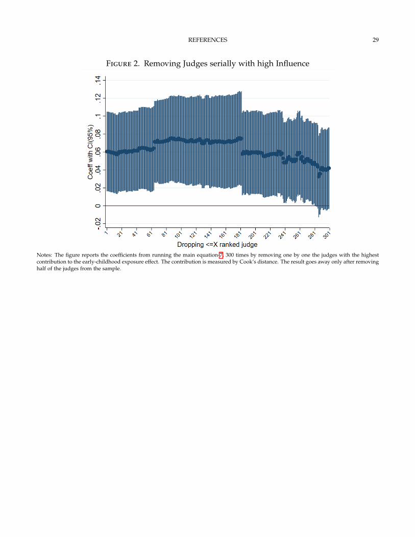
REFERENCES 29

Figure 2. Removing Judges serially with high Influence

Notes: The figure reports the coefficients from running the main equation-7, 300 times by removing one by one the judges with the highestcontribution to the early-childhood exposure effect. The contribution is measured by Cook’s distance. The result goes away only after removinghalf of the judges from the sample.

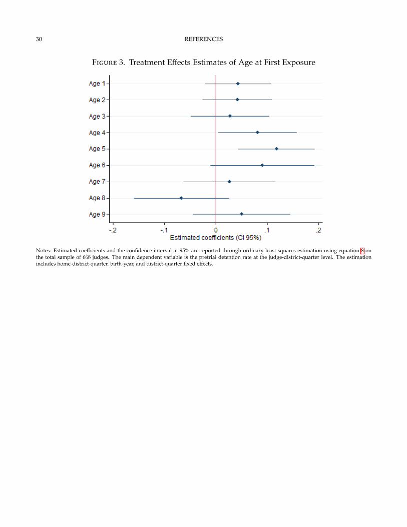
30 REFERENCES

Figure 3. Treatment Effects Estimates of Age at First Exposure

Notes: Estimated coefficients and the confidence interval at 95% are reported through ordinary least squares estimation using equation-8 onthe total sample of 668 judges. The main dependent variable is the pretrial detention rate at the judge-district-quarter level. The estimationincludes home-district-quarter, birth-year, and district-quarter fixed effects.

REFERENCES 31

Figure 4. Impact of Current Riots

Notes: This figure presents event study plots of share of bail denied up to 12 weeks post-riot exposure for riots that occurred in 2014-2017. Thefigure presents estimates of the trajectory of the share of bail denied over time separately for early-exposed and non-exposed judges followingthe specification: Yjdt = β ∗ T + ηj + δdt + εjdt; where, Yjdt is the share of bail denied by judge j, posted at district d in week t; T is the timedummy for the post and pre-exposure periods, ηj is judge fixed effect, δdt is district-weekly trends, and εjdt is the error term clustered at thejudge level.

32 REFERENCES

12. Tables

Table 1. Balance Tests

PANEL A: DISTRICT LEVEL (1) (2) (3) (4) (5) (6)Proportion Male Muslim SC/ST Working Pop Not Literate Male Primary Ed

Kid[0-6] 0.001** -0.014 0.005 0.008*** -0.004 0.000(0.000) (0.009) (0.005) (0.002) (0.006) (0.002)

Observations 38,034 38,034 38,034 38,034 38,034 38,034R-squared 0.092 0.114 0.102 0.123 0.130 0.092Mean Dep Var 0.53 0.19 0.21 0.33 0.32 0.34home-district X Quarter F.E yes yes yes yes yes yesYear of Birth F.E yes yes yes yes yes yes

Cluster Level Judge Judge Judge Judge Judge JudgeJudge 668 668 668 668 668 668

PANEL B: PEERS AND CASES (1) (2) (3) (4) (5) (6) (7)At Dist-Qtly level Total Muslim Prop. Muslim Avg. Age Avg. Exp Female Tot Bail Cases

Kid[0-6] -0.354 -0.136 -0.004 0.118 0.140 -0.018** -.921(2.016) (0.173) (0.005) (0.198) (0.218) (0.009) (6.754)

Observations 5,369 5,369 5,369 5,369 5,369 5,369 5530R-squared 0.199 0.197 0.175 0.207 0.211 0.226 0.359Mean of Dep Var 34.72 2.05 0.06 46.32 14.25 0.17 55.28home-district X Quarter F.E yes yes yes yes yes yes yesYear of Birth F.E yes yes yes yes yes yes yesDistrict X Quarter F.E no no no no no no yes

Cluster Level Judge Judge Judge Judge Judge Judge JudgeJudges 642 642 642 642 642 642 660

Notes: This table reports ordinary least squares estimations based on the judge–district–quarter level sample of 668 judges with home districtsin UP. Robust standard errors in parentheses are clustered at the judge level. The dependent variable in Panel A (District-level Characteristics interms of Proportion) are: Male (Column 1), Muslims (Column 2), Scheduled Caste (SC)/ Scheduled Tribe (ST) (Column 3), Working Population(Column 4), Illiteracy (Column 5), and Male Primary Education (Column 6). The dependent variable in Panel B (Peers of Judges with leave-me-out approach): Total Judges (Column 1), Number of Muslim Judges (Column 2), Proportion of Muslim Judges (Column 3), Average Age(Column 4), Average Experience (Column 5), Proportion of Female Judges (Column 6), and Total Bail Cases (Column 7). The sample mean andthe standard deviation of the dependent variables are reported. The explanatory variable is exposure to communal conflict between the agesof 0 and 6 years. All estimations include home district X quarter, year of birth fixed effects. Exposure to riots until 9 years of age is includedas control with a set of binary measures. The reduction from 668 is due to the dropping of singleton observations.

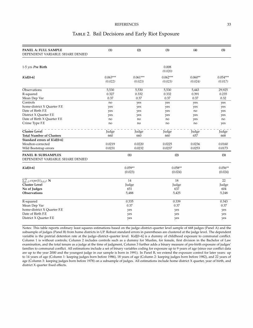
REFERENCES 33

Table 2. Bail Decisions and Early Riot Exposure

PANEL A: FULL SAMPLE (1) (2) (3) (4) (5)DEPENDENT VARIABLE: SHARE DENIED

1-5 yrs Pre Birth 0.008(0.020)

Kid[0-6] 0.063*** 0.061*** 0.062*** 0.060** 0.054***(0.022) (0.023) (0.023) (0.024) (0.017)

Observations 5,530 5,530 5,530 5,443 29,925R-squared 0.327 0.332 0.332 0.391 0.235Mean Dep Var 0.37 0.37 0.37 0.37 0.32Controls no yes yes yes yeshome-district X Quarter F.E yes yes yes yes yesDate of Birth F.E yes yes yes no yesDistrict X Quarter F.E yes yes yes yes yesDate of Birth X Quarter F.E no no no yes noCrime Type F.E no no no no yes

Cluster Level Judge Judge Judge Judge JudgeTotal Number of Clusters 660 660 660 657 668Standard errors of Kid[0-6]Moulton-corrected 0.0219 0.0220 0.0225 0.0236 0.0160Wild Bootstrap errors 0.0231 0.0232 0.0237 0.0253 0.0173

PANEL B: SUBSAMPLES (1) (2) (3)DEPENDENT VARIABLE: SHARE DENIED

Kid[0-6] 0.059** 0.058** 0.056**(0.023) (0.024) (0.024)

∑Nk=7 expo(k)h,b,t: N 14 18 22

Cluster Level Judge Judge JudgeNo of Judges 651 637 604Observations 5,488 5,425 5,248

R-squared 0.335 0.339 0.343Mean Dep Var 0.37 0.37 0.37home-district X Quarter F.E yes yes yesDate of Birth F.E yes yes yesDistrict X Quarter F.E yes yes yes

Notes: This table reports ordinary least squares estimations based on the judge–district–quarter level sample of 668 judges (Panel A) and thesubsample of judges (Panel B) from home districts in UP. Robust standard errors in parentheses are clustered at the judge level. The dependentvariable is the pretrial detention rate at the judge–district–quarter level. Kid[0–6] is a dummy of childhood exposure to communal conflict.Column 1 is without controls; Column 2 includes controls such as a dummy for Muslim, for female, first division in the Bachelor of Lawexamination, and the total tenure as a judge at the time of judgment, Column 3 further adds a binary measure of pre-birth exposure of judges’families to communal conflict. All estimations include a set of binary variables coding for exposure up to 9 years of age (since our conflict dataare up to the year 2000 and the youngest judge in our sample is born in 1991). In Panel B, we extend the exposure control for later years: upto 14 years of age (Column 1: keeping judges born before 1986), 18 years of age (Column 2: keeping judges born before 1982), and 22 years ofage (Column 3: keeping judges born before 1978) on a subsample of judges. All estimations include home district X quarter, year of birth, anddistrict X quarter fixed effects.

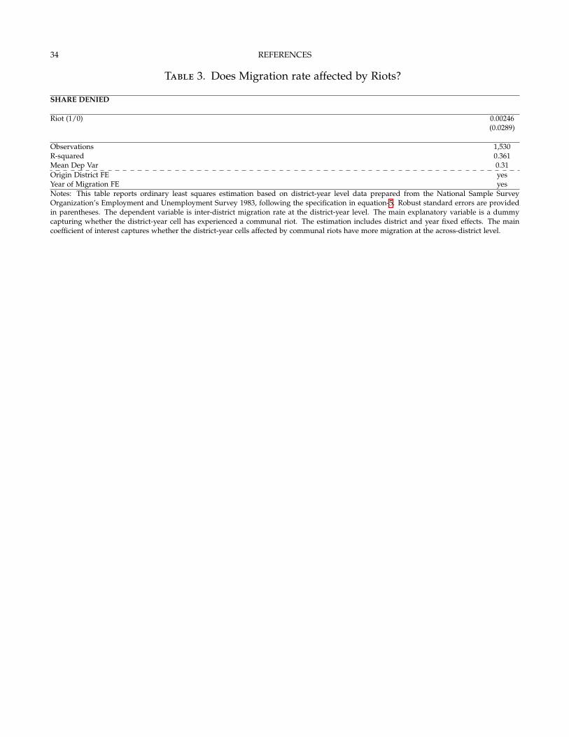
34 REFERENCES

Table 3. Does Migration rate affected by Riots?

SHARE DENIED

Riot (1/0) 0.00246(0.0289)

Observations 1,530R-squared 0.361Mean Dep Var 0.31Origin District FE yesYear of Migration FE yesNotes: This table reports ordinary least squares estimation based on district-year level data prepared from the National Sample SurveyOrganization’s Employment and Unemployment Survey 1983, following the specification in equation-5. Robust standard errors are providedin parentheses. The dependent variable is inter-district migration rate at the district-year level. The main explanatory variable is a dummycapturing whether the district-year cell has experienced a communal riot. The estimation includes district and year fixed effects. The maincoefficient of interest captures whether the district-year cells affected by communal riots have more migration at the across-district level.

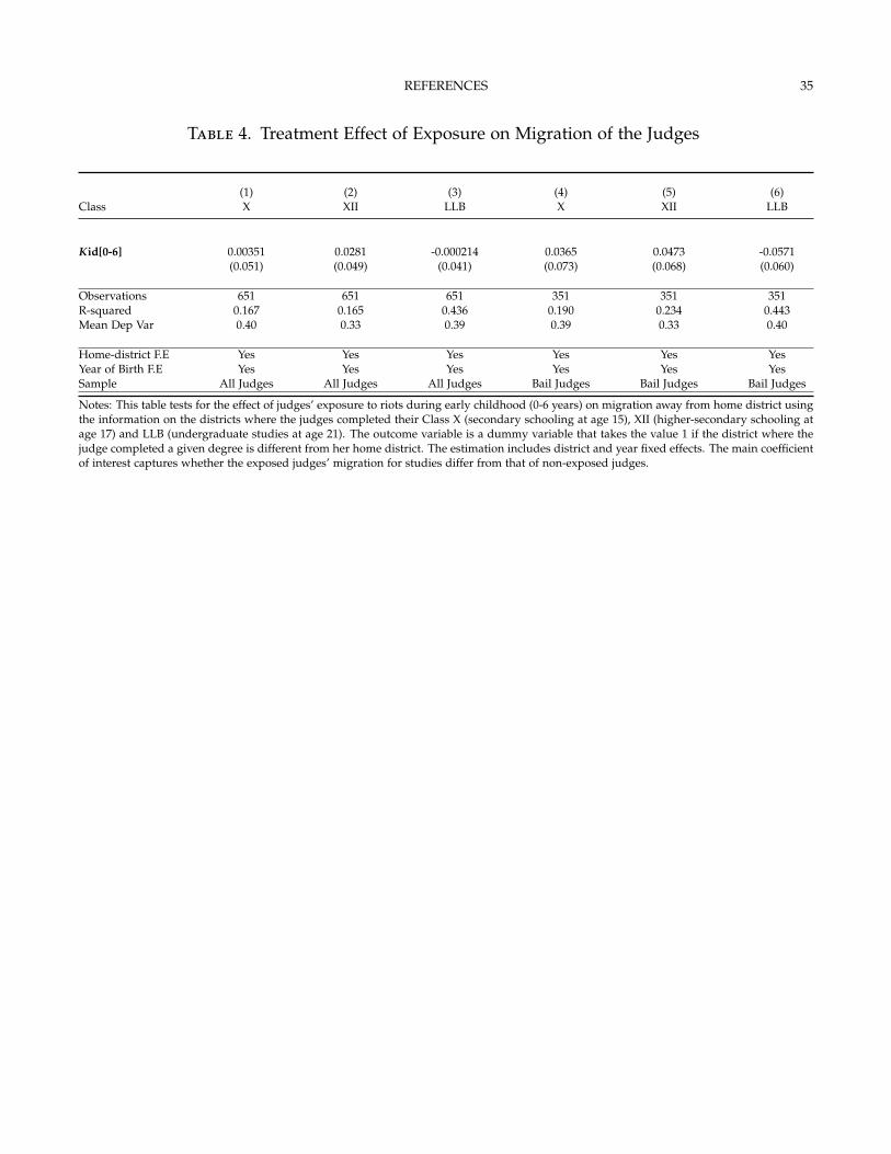
REFERENCES 35

Table 4. Treatment Effect of Exposure on Migration of the Judges

(1) (2) (3) (4) (5) (6)Class X XII LLB X XII LLB

Kid[0-6] 0.00351 0.0281 -0.000214 0.0365 0.0473 -0.0571(0.051) (0.049) (0.041) (0.073) (0.068) (0.060)

Observations 651 651 651 351 351 351R-squared 0.167 0.165 0.436 0.190 0.234 0.443Mean Dep Var 0.40 0.33 0.39 0.39 0.33 0.40

Home-district F.E Yes Yes Yes Yes Yes YesYear of Birth F.E Yes Yes Yes Yes Yes YesSample All Judges All Judges All Judges Bail Judges Bail Judges Bail Judges

Notes: This table tests for the effect of judges’ exposure to riots during early childhood (0-6 years) on migration away from home district usingthe information on the districts where the judges completed their Class X (secondary schooling at age 15), XII (higher-secondary schooling atage 17) and LLB (undergraduate studies at age 21). The outcome variable is a dummy variable that takes the value 1 if the district where thejudge completed a given degree is different from her home district. The estimation includes district and year fixed effects. The main coefficientof interest captures whether the exposed judges’ migration for studies differ from that of non-exposed judges.

36 REFERENCES

Table 5. Conflict Intensity and High State-Reponsiveness

CONFLICT INTENSITYSHARE DENIED (1) (2)

Kid[0-6]High Curfew*High Riot-Casualty 0.009(0.031)

Kid[0-6]High Curfew*Low Riot-Casualty 0.0774*(0.0418)

Kid[0-6]High Arrests*High Riot-Casualty -0.0173(0.0331)

Kid[0-6]High Arrests*Low Riot-Casualty 0.134***(0.0444)

Observations 4,573 4,609R-squared 0.362 0.371Mean Dep Var 0.36 0.36Controls yes yeshome-district X Quarter F.E yes yesDate of Birth F.E yes yesDistrict X Quarter F.E yes yesCluster Level Judge JudgeTotal Number of Clusters 549 551

Notes: We report ordinary least squares estimations based on the judge–district–quarter level sample of bail judges. Standard errors inparentheses are clustered at the judge level. The dependent variable is the pretrial detention rate at the judge–district–quarter level. Allestimations include home district X quarter, year of birth, and district X quarter fixed effects, and a set of binary variables coding for pastexposure up to 9 years of age. The main explanatory variable (Kid[0–6] is a binary measure of childhood exposure to communal conflict at 0–6years of age) where high state action is interacted with low and high conflict severity. The median of the variable under consideration definesthe threshold for severity to split treated judges equally into two groups. The median district areas’ threshold value is 23 casualties (killedand injured). The median curfew is of 5 days duration and median number of arrests is 170. In Columns (1) and (2), we compare the judgesexperiencing high state action in terms of curfew and arrests, respectively, with judges not experiencing riots in their first 6 years of life.

REFERENCES 37

Table 6. Judicial Stringency and Cognitive Skills

DEPENDENT VARIABLE: SHARE DENIED (1) (2)

Kid[0-6] 0.0605*** 0.0595***(0.0226) (0.0223)

LLB Division 0.00669(0.0163)

Observations 5,530 5,530R-squared 0.332 0.332Mean Dep Var 0.37 0.37home-district X Quarter F.E yes yesDate of Birth F.E yes yesDistrict X Quarter F.E yes yes

Number of Judges 660 660

Notes: This table reports ordinary least squares estimations based on the judge–district–quarter level sample of 660 judges who are from homedistricts within UP. Robust standard errors in parentheses are clustered at the judge level. The dependent variable is the pretrial detentionrate at the judge–district–quarter level. Kid[0–6] is a dummy of childhood exposure to communal conflict. The controls include a dummyfor Muslim, for female, and the experience of the judge at the time of judgment. Column 1 includes the dummy variable indicating whetherthe judge attained first division in the Bachelor of Law examination. Column 2 reports the estimates without including performance in thisexamination as control. All estimations include home district X quarter, year of birth, and district X quarter fixed effects.

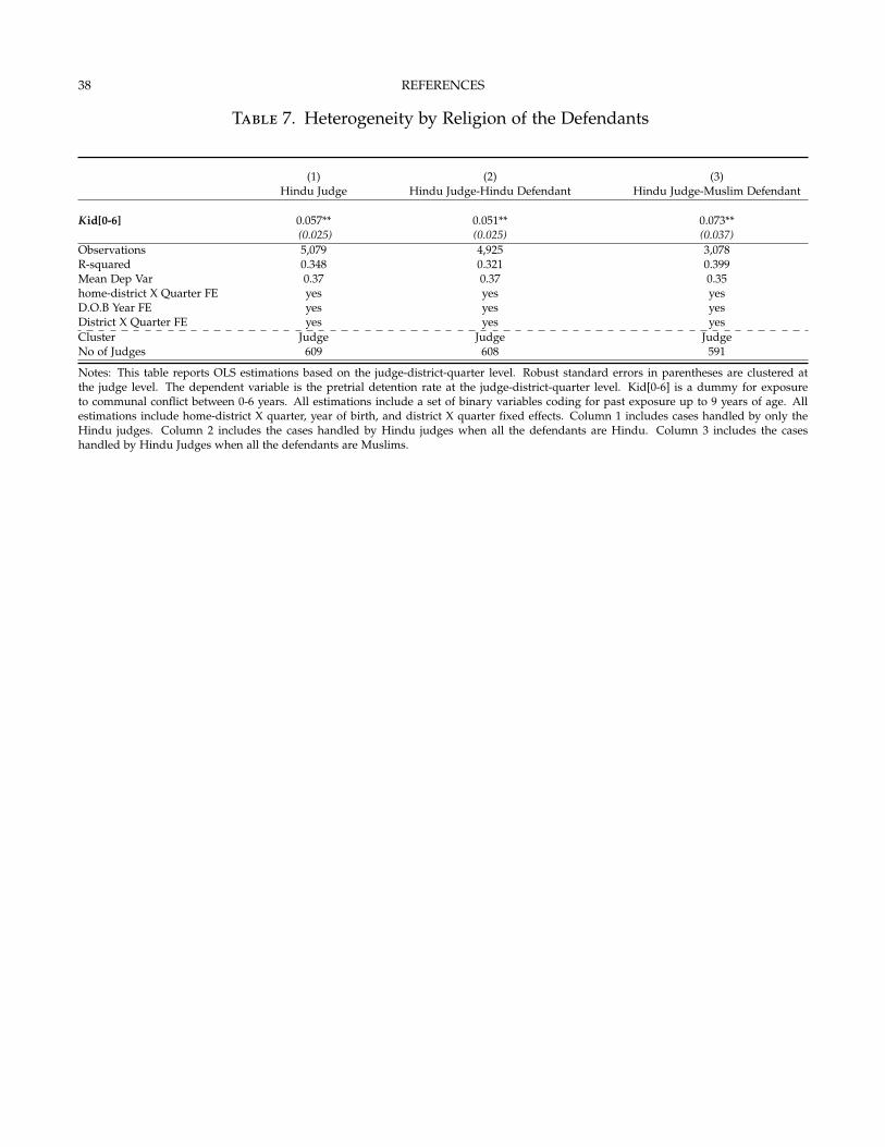
38 REFERENCES

Table 7. Heterogeneity by Religion of the Defendants

(1) (2) (3)Hindu Judge Hindu Judge-Hindu Defendant Hindu Judge-Muslim Defendant

Kid[0-6] 0.057** 0.051** 0.073**(0.025) (0.025) (0.037)

Observations 5,079 4,925 3,078R-squared 0.348 0.321 0.399Mean Dep Var 0.37 0.37 0.35home-district X Quarter FE yes yes yesD.O.B Year FE yes yes yesDistrict X Quarter FE yes yes yesCluster Judge Judge JudgeNo of Judges 609 608 591

Notes: This table reports OLS estimations based on the judge-district-quarter level. Robust standard errors in parentheses are clustered atthe judge level. The dependent variable is the pretrial detention rate at the judge-district-quarter level. Kid[0-6] is a dummy for exposureto communal conflict between 0-6 years. All estimations include a set of binary variables coding for past exposure up to 9 years of age. Allestimations include home-district X quarter, year of birth, and district X quarter fixed effects. Column 1 includes cases handled by only theHindu judges. Column 2 includes the cases handled by Hindu judges when all the defendants are Hindu. Column 3 includes the caseshandled by Hindu Judges when all the defendants are Muslims.

REFERENCES 1

Appendix A. Figures

0

200

400

600

Num

ber

of T

ransfe

rs

2014

q1

2014

q3

2015

q1

2015

q3

2016

q1

2016

q3

2017

q1

2017

q3

2018

q1

2018

q3

Quarter

Total Transfers Average transfers

Transfers by Quarter

Figure A.I. All Judges

0

40

80

120

160

200

240

Num

ber

of T

ransfe

rs

2014

q1

2014

q3

2015

q1

2015

q3

2016

q1

2016

q3

2017

q1

2017

q3

2018

q1

2018

q3

Quarter

Total Transfers Average Transfers

Transfers by Quarter(668 judges)

Figure A.II. Sample Judges

Notes: The figure reports the total and the average number of transfers of judges in the state of Uttar Pradesh for the full sample of judges

and the 668 bail judges in our analysis sample. On average, 195 judges (7% of all judges) are transferred every quarter, with most transfers

concentrated in the second quarter. Our analysis sample has a similar trend, with an average of 8.5% judges transferred every quarter.

2 REFERENCES

Figure A.III. Distribution of Bail Cases by Quarter

Notes: The figure highlights the cyclical nature of the reported bail case in UP district courts by quarter.

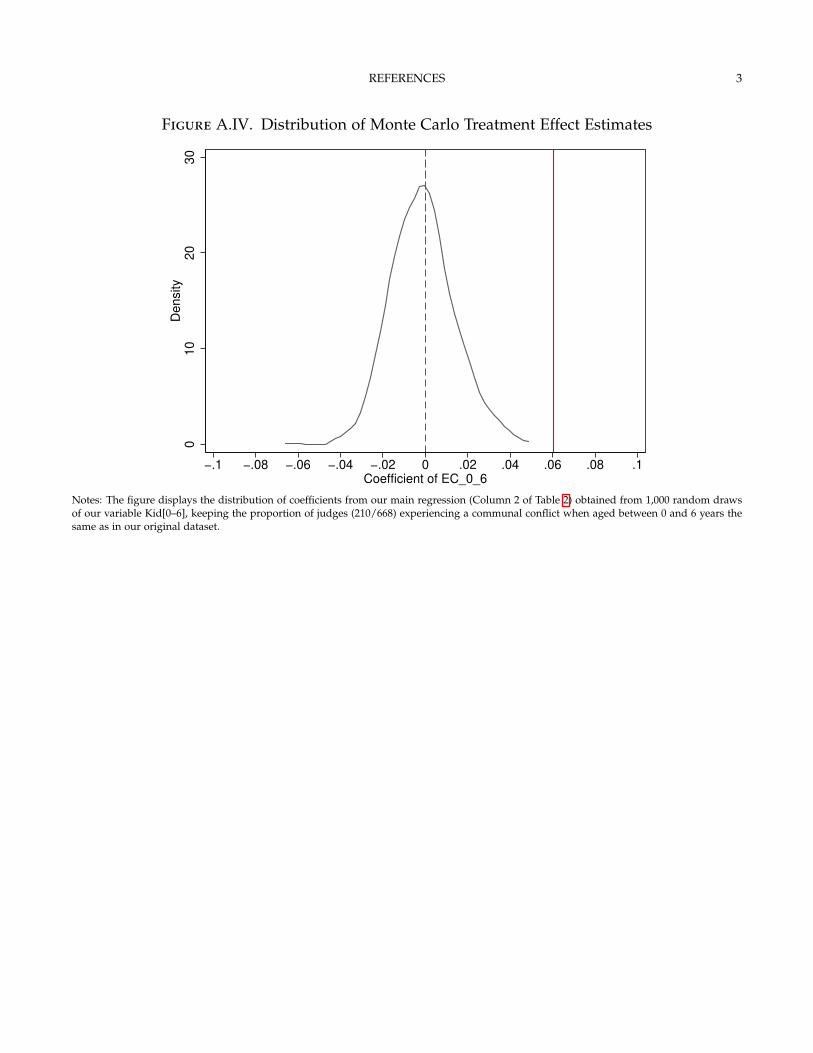
REFERENCES 3

Figure A.IV. Distribution of Monte Carlo Treatment Effect Estimates

010

20

30

Density

−.1 −.08 −.06 −.04 −.02 0 .02 .04 .06 .08 .1Coefficient of EC_0_6

Notes: The figure displays the distribution of coefficients from our main regression (Column 2 of Table 2) obtained from 1,000 random drawsof our variable Kid[0–6], keeping the proportion of judges (210/668) experiencing a communal conflict when aged between 0 and 6 years thesame as in our original dataset.

4 REFERENCES

Figure A.V. Treatment Effects Estimates of Age at First Exposure

Notes: Estimated coefficients and the confidence interval at 95% are reported from ordinary least squares estimation using equation 8 on asample of 612 judges born before 1979. The main dependent variable is the pretrial detention rate at the judge X district X quarter level. Theestimation includes home district X quarter, birth year, district X quarter fixed effects.

REFERENCES 5

Appendix B. Tables

Table B.I. Creation of New Districts in Uttar Pradesh

State New Districts Parent Districts Date of Formation Comments Source(link)UP Ambedkar Nagar Faizabad 29-09-1995 Tehsils: Akbarpur, Tanda https://ambedkarnagar.nic.in/

UP Amethi Sultanpur/Rae Bareilly 01-07-2010Sultanpur Tehsils: Amethi,

Gauriganj and Musafirkhana;Rae Bareilly Tehsils: Salon and Tiloi

https://amethi.nic.in/

UP Amroha(Jyotiba Phule Nagar) Moradabad 24-04-1997 Tehsils: Separating Amroha,

Dhanora and Hasanpur https://amroha.nic.in/

UP Auraiya Etawah 17-09-1997 Tehsils: Auraiya and Bidhuna https://auraiya.nic.in/UP Balrampur Gonda 25-05-1997 https://balrampur.nic.in/UP Baghpat Meerut 01-05-1997 Tehsil: Baghpat https://baghpat.nic.in/UP Bhadohi Varanasi 30-06-1994 https://bhadohi.nic.in/UP Chandauli Varanasi 20-05-1997 https://chandauli.nic.in/UP Chitrakoot Banda 06-05-1997 Tehsils: Karwi and Mau https://chitrakoot.nic.in/

UP Gautam Buddha Nagar Ghaziabad/Bulandshahar 06-09-1997 Ghaziabad Blocks: Dadri and Bisrakh;

Bulandshahar Blocks: Danakur and Jewar https://gbnagar.nic.in/

UP Ghaziabad Meerut/Bulandshahar 14-11-1976 https://censusindia.gov.in/2011census/dchb/

0909_PART_B_DCHB_GHAZIABAD.pdf

UP Hapur Ghaziabad 28-09-2011 Tehsils: Hapur, Garhmukteshwar andDhaulana https://hapur.nic.in/

UP Haridwar Saharanpur 1988 https://haridwar.nic.in/

UP Hathras(Mahamaya Nagar)

Aligarh/Mathura/Agra 03-05-1997 Hathras tehsil came from Aligarh.

Further it shares the Jail of Aligarh. https://hathras.nic.in/

UP Kannauj Farrukhabad 18-09-1997 https://kannauj.nic.in/

UP Kasganj(Kanshi Ram Nagar) Etah 15-04-2008 https://kasganj.nic.in/

UP Kaushambi Allahabad 04-04-1997 https://kaushambi.nic.in/

UP Kushinagar(Padrauna) Deoria 13-05-1994 https://kushinagar.nic.in/

UP Kanpur Dehat Kanpur 23-04-1981 https://kushinagar.nic.in/UP Kanpur Nagar Kanpur 23-04-1981 https://kanpurdehat.nic.in/UP Lalitpur Jhansi 1974 Exact date unknown https://lalitpur.nic.in/UP Maharajganj Gorakhpur 02-10-1989 https://maharajganj.nic.in/UP Mahoba Hamirpur 11-02-1995 Tehsil: Mahoba https://mahoba.nic.in/UP Mau Azamgarh 14-11-1988 https://mau.nic.in/UK Rudraprayag Chamoli 18-09-1997 https://rudraprayag.gov.in/UP Sambhal Moradabad 28-09-2011 https://sambhal.nic.in/

UP Sant Kabir Nagar Basti/Siddarth Nagar 05-09-1997

Formed by carving :complete Khalilabad tehsil (from Basti),

131 villages of Basti tehsil and161 villages of Santha block

(Bansi tehsil, Siddarth Nagar)

https://sknagar.nic.in/

UP Shamli Muzaffarnagar 28-09-2011 Tehsils: Shamli and Kairana https://shamli.nic.in/UP Shravasti Bahraich 01-05-1997 https://shravasti.nic.in/UP Siddarth Nagar Basti 29-12-1988 https://siddharthnagar.nic.in/UP Sonbhadra Mirzapur 04-03-1989 https://sonbhadra.nic.in/UK Uddham Singh Nagar Nainitaal 29-09-1997 https://usnagar.nic.in/

Notes: The table outlines the formation of new districts from parent (origin) districts in alphabetical order, their date/year of formation, andthe source of this information. We assign all districts to their origin districts. With this harmonization, we arrive at 47 unique home districtsfor our sample of 668 judges. The details of district merging are explained in Appendix notes C.1.

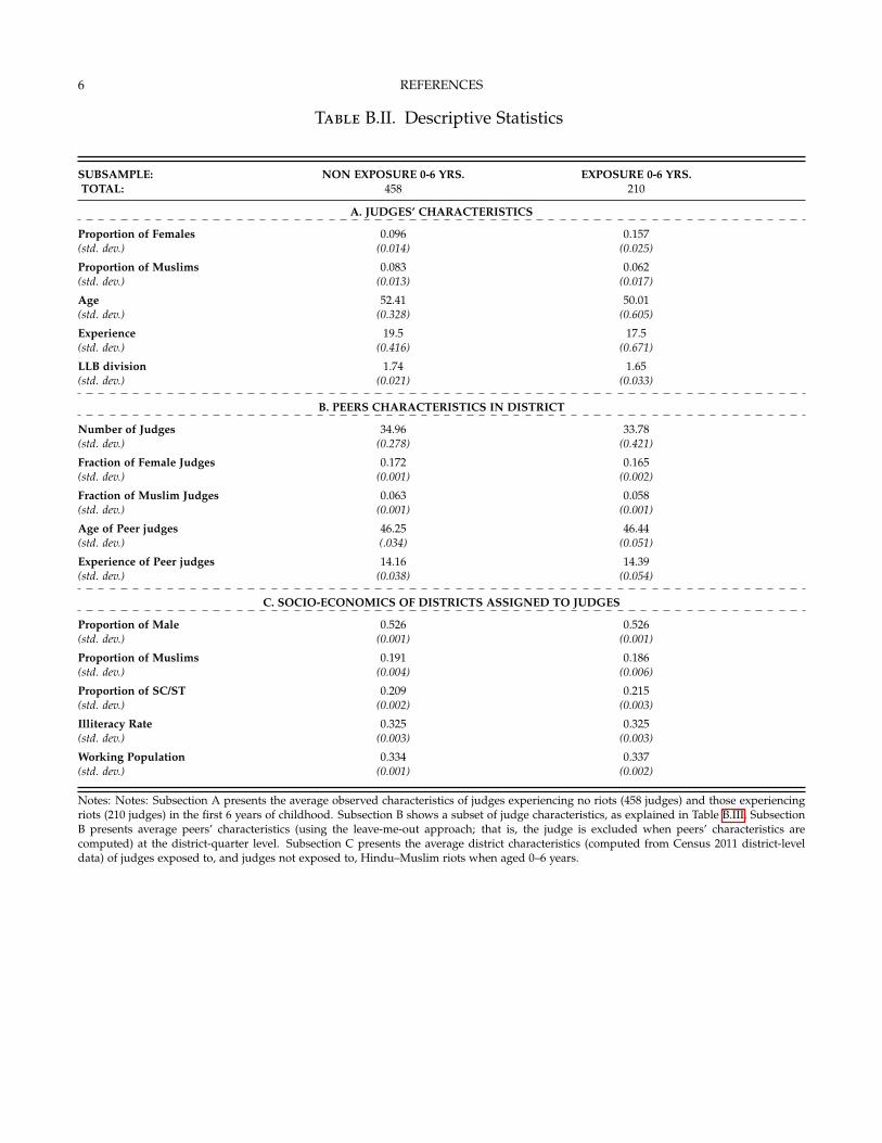
6 REFERENCES

Table B.II. Descriptive Statistics

SUBSAMPLE: NON EXPOSURE 0-6 YRS. EXPOSURE 0-6 YRS.TOTAL: 458 210

A. JUDGES’ CHARACTERISTICS

Proportion of Females 0.096 0.157(std. dev.) (0.014) (0.025)

Proportion of Muslims 0.083 0.062(std. dev.) (0.013) (0.017)

Age 52.41 50.01(std. dev.) (0.328) (0.605)

Experience 19.5 17.5(std. dev.) (0.416) (0.671)

LLB division 1.74 1.65(std. dev.) (0.021) (0.033)

B. PEERS CHARACTERISTICS IN DISTRICT

Number of Judges 34.96 33.78(std. dev.) (0.278) (0.421)

Fraction of Female Judges 0.172 0.165(std. dev.) (0.001) (0.002)

Fraction of Muslim Judges 0.063 0.058(std. dev.) (0.001) (0.001)

Age of Peer judges 46.25 46.44(std. dev.) (.034) (0.051)

Experience of Peer judges 14.16 14.39(std. dev.) (0.038) (0.054)

C. SOCIO-ECONOMICS OF DISTRICTS ASSIGNED TO JUDGES

Proportion of Male 0.526 0.526(std. dev.) (0.001) (0.001)

Proportion of Muslims 0.191 0.186(std. dev.) (0.004) (0.006)

Proportion of SC/ST 0.209 0.215(std. dev.) (0.002) (0.003)

Illiteracy Rate 0.325 0.325(std. dev.) (0.003) (0.003)

Working Population 0.334 0.337(std. dev.) (0.001) (0.002)

Notes: Notes: Subsection A presents the average observed characteristics of judges experiencing no riots (458 judges) and those experiencingriots (210 judges) in the first 6 years of childhood. Subsection B shows a subset of judge characteristics, as explained in Table B.III. SubsectionB presents average peers’ characteristics (using the leave-me-out approach; that is, the judge is excluded when peers’ characteristics arecomputed) at the district-quarter level. Subsection C presents the average district characteristics (computed from Census 2011 district-leveldata) of judges exposed to, and judges not exposed to, Hindu–Muslim riots when aged 0–6 years.

REFERENCES 7

Table B.III. Descriptive Statistics of UP District Court Judges

All Judges Bail Judges Our SampleVARIABLES N mean sd N mean sd N mean sd

Muslim Judge 2,434 0.061 0.240 1,236 0.067 0.250 668 0.0763 0.266Female Judge 2,434 0.198 0.398 1,236 0.137 0.344 668 0.115 0.320Age 2,434 46.55 11.29 1,236 49.58 8.537 668 51.66 7.687Joining Age 2,434 31.81 4.687 1,236 32.76 4.920 668 32.81 5.114Experience 2,434 14.74 11.26 1,236 16.82 9.283 668 18.85 9.202Promotion Time Taken 1,651 7.471 2.260 974 7.169 2.356 542 7.560 2.352Grade 10 Division 1,405 1.460 0.567 549 1.526 0.571 235 1.579 0.575Grade 10 Age 1,446 14.99 0.984 579 14.93 0.970 246 14.91 0.963Grade 12 Division 1,413 1.537 0.580 553 1.627 0.598 238 1.689 0.599Grade 12 Age 1,446 17.11 1.080 579 17.06 1.056 247 17.05 1.085LLB Division 2,385 1.621 0.488 1,206 1.697 0.460 668 1.711 0.454LLB Age 2,405 23.72 2.134 1,219 23.64 2.119 668 23.42 2.031Masters 2,434 0.386 0.487 1,236 0.360 0.480 668 0.356 0.479PhD 2,434 0.015 0.121 1,236 0.016 0.126 668 0.0120 0.109Number of Bachelors 2,431 1.863 0.363 1,234 1.938 0.272 668 1.958 0.253

Notes: The table presents the characteristics of all judges (including the judges who retired during 2014–2018 but had handled bail cases),bail judges, and our sample of judges (arrived at after removing judges handling less than 97 cases and judges with no information on thedivision obtained in the Bachelor of Law (LLB) examination). We notice that our sample of judges is very similar to the full sample of judgesalong different observable characteristics, such as the proportion of Muslim judges, the proportion of female judges, age (on December 31,2018), joining age (age in years at which a judge enters into judiciary), experience, time to promotion (in years to become a Class I rank ofjudge), Grade 10 division (3 divisions: I (≥ 60% marks), II (≥ 45% and < 60%), and III(≥ 33% and < 45%), Grade 12 Division (3 divisions: I(≥ 60% marks), II (≥ 45% and < 60%), and III(≥ 3% and < 45%), LLB Division(I (≥ 60% marks), II (≥ 45% and < 60%), and III(≥ 33% and< 45%), Grade 10 Age (age at which a judge completes Class 10), Grade 12 Age (age at which a judge completes Class 12/Intermediate), LLBAge (age at which a judge obtains the LLB degree), Masters (dummy = 1 if a judge has a master’s degree), PhD (dummy = 1 if a judge hasa doctorate), and Number of Bachelors (number of bachelor’s degrees of a judge). Only graduates were eligible to take the LLB examinationearlier; currently, some institutions offer integrated courses such as BA + LLB, have started).

8 REFERENCES

Table B.IV. Balance Table : Crime Categories (Full Sample)

Body Crime Prop Crime Crim Intim Cow Slaught Elec. Theft Others

Kid[0-6] -0.107 -0.770 -0.434 0.0624 -0.102 1.012(2.867) (2.418) (0.439) (0.280) (0.639) (1.783)

Observations 5,530 5,530 5,530 5,530 5,530 5,530R-squared 0.325 0.336 0.374 0.327 0.190 0.327Mean Dep Var 15.47 14.16 4.52 1.21 1.25 10.82Home Dist X Quarter F.E yes yes yes yes yes yesBirth Year F.E yes yes yes yes yes yesDist X Quarter F.E yes yes yes yes yes yesControls yes yes yes yes yes yes

Cluster Level Judge Judge Judge Judge Judge JudgeNo. of Clusters 660 660 660 660 660 660

Notes: This table reports ordinary least squares estimations based on the judge–district–quarter level on the full sample of judges. Standarderrors in parentheses are clustered at the judge level. The dependent variable is the different categories of crime: Body Crime (Column 1),Property Crime (Column 2), Criminal Intimidation (Column 3), Cow Slaughter (Column 4), Electricity Theft (Column 5), and Others (Column6). Kid[0–6] is a dummy of childhood exposure to communal conflict when aged 0–6 years. All estimations include a set of binary variablescoding for past exposure up to 9 years of age. All estimations include home district X quarter, year of birth, and district X quarter fixed effects.The classification of crime categories is based on Appendix Tables B.XXI and B.XXII

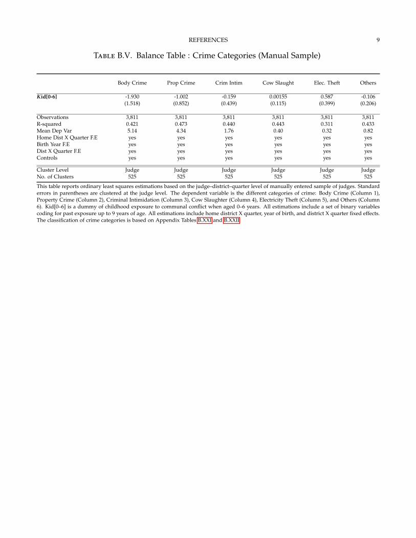
REFERENCES 9

Table B.V. Balance Table : Crime Categories (Manual Sample)

Body Crime Prop Crime Crim Intim Cow Slaught Elec. Theft Others

Kid[0-6] -1.930 -1.002 -0.159 0.00155 0.587 -0.106(1.518) (0.852) (0.439) (0.115) (0.399) (0.206)



This table reports ordinary least squares estimations based on the judge–district–quarter level of manually entered sample of judges. Standarderrors in parentheses are clustered at the judge level. The dependent variable is the different categories of crime: Body Crime (Column 1),Property Crime (Column 2), Criminal Intimidation (Column 3), Cow Slaughter (Column 4), Electricity Theft (Column 5), and Others (Column6). Kid[0–6] is a dummy of childhood exposure to communal conflict when aged 0–6 years. All estimations include a set of binary variablescoding for past exposure up to 9 years of age. All estimations include home district X quarter, year of birth, and district X quarter fixed effects.The classification of crime categories is based on Appendix Tables B.XXI and B.XXII

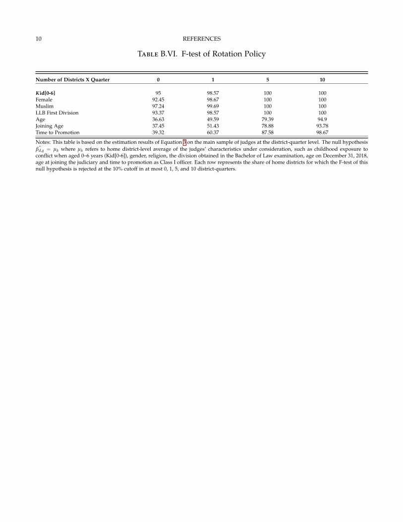
10 REFERENCES

Table B.VI. F-test of Rotation Policy

Number of Districts X Quarter 0 1 5 10

Kid[0-6] 95 98.57 100 100Female 92.45 98.67 100 100Muslim 97.24 99.69 100 100LLB First Division 93.37 98.57 100 100Age 36.63 49.59 79.39 94.9Joining Age 37.45 51.43 78.88 93.78Time to Promotion 39.32 60.37 87.58 98.67

Notes: This table is based on the estimation results of Equation 3 on the main sample of judges at the district-quarter level. The null hypothesisˆβd,q = µh where µh refers to home district-level average of the judges’ characteristics under consideration, such as childhood exposure to

conflict when aged 0–6 years (Kid[0-6]), gender, religion, the division obtained in the Bachelor of Law examination, age on December 31, 2018,age at joining the judiciary and time to promotion as Class I officer. Each row represents the share of home districts for which the F-test of thisnull hypothesis is rejected at the 10% cutoff in at most 0, 1, 5, and 10 district-quarters.

REFERENCES 11

Table B.VII. Alternative Early Childhood Definition

SHARE DENIED (N=6) (N=9) (N=10) (N=12)

0-5 years Pre Birth 0.00791 0.00853 0.00816 0.00733(0.0200) (0.0200) (0.0201) (0.0201)

Kid[0-N] 0.0623*** 0.0421 0.0428 0.0397(0.0231) (0.0277) (0.0280) (0.0260)

Observations 5,530 5,530 5,526 5,507R-squared 0.332 0.329 0.329 0.329Mean Dep Var 0.37 0.37 0.37 0.37Home-district X Quarter FE yes yes yes yesDistrict X Quarter FE yes yes yes yesYear of Birth FE yes yes yes yesControls yes yes yes yesCluster Level Judge Judge Judge JudgeTotal Number of Clusters 660 660 659 655Notes: This table reports ordinary least squares estimations based on the judge–district–quarter level. The dependent variable is pretrialdetention rates. Kid[0–N] is a dummy of childhood exposure to communal conflict when aged 0–N years, where N is 6,9,10 and 12 fromColumn 1-4 respectively. All estimations include controls as in our main table. All estimations include home district X quarter fixed effects,district X quarter fixed effects and year of birth effects.

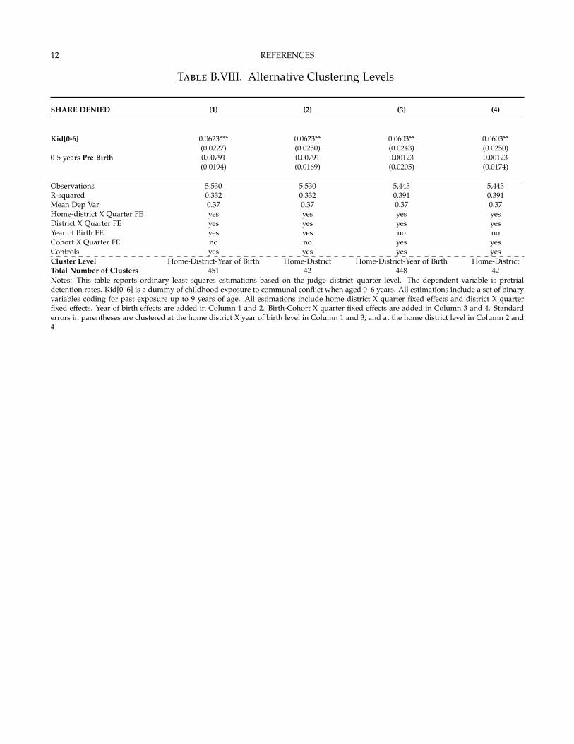
12 REFERENCES

Table B.VIII. Alternative Clustering Levels

SHARE DENIED (1) (2) (3) (4)

Kid[0-6] 0.0623*** 0.0623** 0.0603** 0.0603**(0.0227) (0.0250) (0.0243) (0.0250)

0-5 years Pre Birth 0.00791 0.00791 0.00123 0.00123(0.0194) (0.0169) (0.0205) (0.0174)

Observations 5,530 5,530 5,443 5,443R-squared 0.332 0.332 0.391 0.391Mean Dep Var 0.37 0.37 0.37 0.37Home-district X Quarter FE yes yes yes yesDistrict X Quarter FE yes yes yes yesYear of Birth FE yes yes no noCohort X Quarter FE no no yes yesControls yes yes yes yesCluster Level Home-District-Year of Birth Home-District Home-District-Year of Birth Home-DistrictTotal Number of Clusters 451 42 448 42Notes: This table reports ordinary least squares estimations based on the judge–district–quarter level. The dependent variable is pretrialdetention rates. Kid[0–6] is a dummy of childhood exposure to communal conflict when aged 0–6 years. All estimations include a set of binaryvariables coding for past exposure up to 9 years of age. All estimations include home district X quarter fixed effects and district X quarterfixed effects. Year of birth effects are added in Column 1 and 2. Birth-Cohort X quarter fixed effects are added in Column 3 and 4. Standarderrors in parentheses are clustered at the home district X year of birth level in Column 1 and 3; and at the home district level in Column 2 and4.

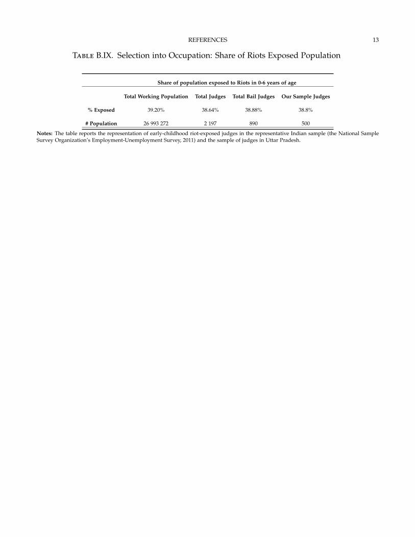
REFERENCES 13

Table B.IX. Selection into Occupation: Share of Riots Exposed Population

Share of population exposed to Riots in 0-6 years of age

Total Working Population Total Judges Total Bail Judges Our Sample Judges

% Exposed 39.20% 38.64% 38.88% 38.8%

# Population 26 993 272 2 197 890 500

Notes: The table reports the representation of early-childhood riot-exposed judges in the representative Indian sample (the National SampleSurvey Organization’s Employment-Unemployment Survey, 2011) and the sample of judges in Uttar Pradesh.

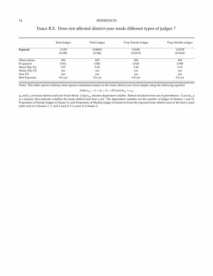
14 REFERENCES

Table B.X. Does riot affected district-year sends different types of judges ?

Total Judges Total Judges Prop Female Judges Prop Muslim Judges

Exposed -0.129 0.00603 0.0196 -0.0178(0.498) (0.346) (0.0215) (0.0160)

Observations 694 609 694 694R-squared 0.811 0.581 0.526 0.508Mean Dep Var 9.57 5.42 0.24 0.10Home Dist F.E yes yes yes yesYear F.E yes yes yes yesRiot Exposure 0-6 yrs 3-6 yrs 0-6 yrs 0-6 yrs

Notes: This table reports ordinary least squares estimations based on the home district-year level sample using the following equation

Judgesh,y = α + ηh + δy + βExposedh,y + εh,y

ηh and δy are home-district and year fixed effects. Judgesh,y denotes dependent variable. Robust standard errors are in parentheses. Exposedh, yis a dummy that indicates whether the home district-year had a riot. The dependent variables are the number of judges (Columns 1 and 2),Proportion of Female Judges (Column 3), and Proportion of Muslim judges (Column 4) from the exposed home district-year in the first 6 years(after riot) in Columns 1, 3, and 4 and in 3–6 years in Column 2.

REFERENCES 15

Table B.XI. Bail Decisions and Early Exposure to Riots (Case Level Regressions)

(1) (2) (3)

Kid[0-6] 0.0381** 0.0435** 0.0409**(0.019) (0.017) (0.017)

Muslim Defendant -0.018***(0.005)

Non Bailable 0.155***(0.014)

Observations 323,194 323,194 196,300R-squared 0.081 0.160 0.186Mean Dep Var 0.34 0.34 0.34Home Dist X Quarter F.E yes yes yesBirth Year F.E yes yes yesDist X Quarter F.E yes yes yesCrime Type FE no yes yesControls yes yes yes

Cluster Level Judge Judge JudgeNo. of Clusters 668 668 668

Notes: This table reports ordinary least squares estimations based on the case level. Standard errors in parentheses are clustered at the judgelevel. The dependent variable is a dummy for whether the bail is rejected. Kid[0–6] is a dummy of childhood exposure to communal conflictwhen aged 0–6 years. All estimations include a set of binary variables coding for past exposure up to 9 years of age and our usual controls.All estimations include home district quarter, year of birth, and district quarter fixed effects. Columns 2 and 3 further include crime-typefixed effects. Column (3) also adds a dummy for whether the defendant is Muslim and whether the case is nonbailable in nature (i.e., bookedcrimes are nonbailable according to the Indian Penal Code).

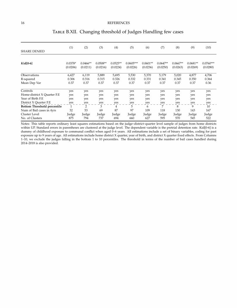
16 REFERENCES

Table B.XII. Changing threshold of Judges Handling few cases

(1) (2) (3) (4) (5) (6) (7) (8) (9) (10)SHARE DENIED

Kid[0-6] 0.0378* 0.0466** 0.0508** 0.0525** 0.0605*** 0.0601** 0.0647** 0.0667** 0.0681** 0.0760***(0.0206) (0.0211) (0.0216) (0.0224) (0.0226) (0.0236) (0.0250) (0.0263) (0.0269) (0.0280)

Observations 6,427 6,119 5,889 5,695 5,530 5,370 5,179 5,020 4,877 4,706R-squared 0.306 0.316 0.315 0.326 0.332 0.331 0.341 0.345 0.350 0.364Mean Dep Var 0.37 0.37 0.37 0.37 0.37 0.37 0.37 0.37 0.37 0.36

Controls yes yes yes yes yes yes yes yes yes yesHome-district X Quarter F.E yes yes yes yes yes yes yes yes yes yesYear of Birth F.E yes yes yes yes yes yes yes yes yes yesDistrict X Quarter F.E yes yes yes yes yes yes yes yes yes yesBottom Threshold percentile 1 2 3 4 5 6 7 8 9 10Num of Bail cases in 4yrs 32 53 69 87 97 109 118 130 143 167Cluster Level Judge Judge Judge Judge Judge Judge Judge Judge Judge JudgeNo. of Clusters 875 794 737 694 660 627 595 570 545 522

Notes: This table reports ordinary least squares estimations based on the judge–district–quarter level sample of judges from home districtswithin UP. Standard errors in parentheses are clustered at the judge level. The dependent variable is the pretrial detention rate. Kid[0-6] is adummy of childhood exposure to communal conflict when aged 0–6 years. All estimations include a set of binary variables, coding for pastexposure up to 9 years of age. All estimations include home district X quarter, year of birth, and district X quarter fixed effects. From Columns1–10, we exclude the judges falling in the bottom 1 to 10 percentiles. The threshold in terms of the number of bail cases handled during2014–2018 is also provided.

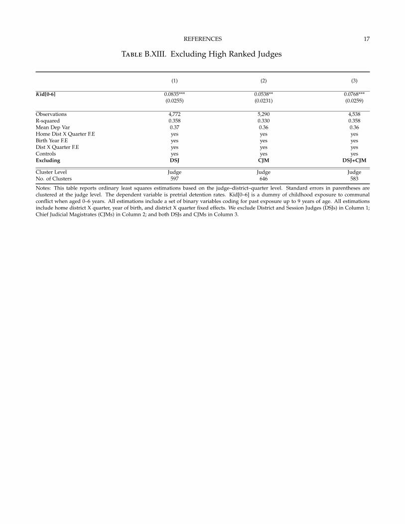
REFERENCES 17

Table B.XIII. Excluding High Ranked Judges

(1) (2) (3)

Kid[0-6] 0.0835*** 0.0538** 0.0768***(0.0255) (0.0231) (0.0259)

Observations 4,772 5,290 4,538R-squared 0.358 0.330 0.358Mean Dep Var 0.37 0.36 0.36Home Dist X Quarter F.E yes yes yesBirth Year F.E yes yes yesDist X Quarter F.E yes yes yesControls yes yes yesExcluding DSJ CJM DSJ+CJM

Cluster Level Judge Judge JudgeNo. of Clusters 597 646 583

Notes: This table reports ordinary least squares estimations based on the judge–district–quarter level. Standard errors in parentheses areclustered at the judge level. The dependent variable is pretrial detention rates. Kid[0–6] is a dummy of childhood exposure to communalconflict when aged 0–6 years. All estimations include a set of binary variables coding for past exposure up to 9 years of age. All estimationsinclude home district X quarter, year of birth, and district X quarter fixed effects. We exclude District and Session Judges (DSJs) in Column 1;Chief Judicial Magistrates (CJMs) in Column 2; and both DSJs and CJMs in Column 3.

18 REFERENCES

Table B.XIV. Outlier Tests

(1) (2) (3) (4) (5) (6) (7)SHARE DENIED

Kid[0-6] 0.0745*** 0.0567** 0.0590** 0.0675*** 0.0707*** 0.0579** 0.0622***(0.0236) (0.0229) (0.0231) (0.0247) (0.0252) (0.0230) (0.0235)

Observations 5,283 5,231 5,416 5,201 5,243 5,430 5,276R-squared 0.341 0.341 0.328 0.341 0.334 0.337 0.339Mean Dep Var 0.37 0.37 0.37 0.37 0.37 0.37 0.37

Controls yes yes yes yes yes yes yeshome-district X Quarter F.E yes yes yes yes yes yes yesDate of Birth F.E yes yes yes yes yes yes yesDistrict X Quarter F.E yes yes yes yes yes yes yesHome Dist Removed Aligarh Meerut Moradabad Bulandshahr Varanasi Lucknow AllahabadCluster Level Judge Judge Judge Judge Judge Judge JudgeNo. of Clusters 632 629 645 618 628 646 628

Notes: This table reports ordinary least squares estimations based on the judge–district–quarter level sample of judges from home districtswithin UP. Standard errors in parentheses are clustered at the judge level. The dependent variable is the pretrial detention rate. Kid[0-6] is adummy of childhood exposure to communal conflict when aged 0–6 years. All estimations include a set of binary variables coding for pastexposure up to 9 years of age. All estimations include home district X quarter, year of birth, and district X quarter fixed effects. From Column1 to Column 6, we exclude from the full sample judges coming from one of the top six home districts one at a time (Aligarh(26), Meerut(24),Moradabad(18), Bulandshahar(15), Varanasi(13), Lucknow(13), and Allahabad (13)) that have the maximum number of riots during 1950–2000.

REFERENCES 19

Table B.XV. Outlier Tests

(1) (2) (3) (4) (5) (6) (7)SHARE DENIED

Kid[0-6] 0.0745*** 0.0693*** 0.0679*** 0.0727*** 0.0880*** 0.0855*** 0.0875***(0.0236) (0.0240) (0.0246) (0.0266) (0.0298) (0.0304) (0.0329)

R-squared 0.341 0.350 0.347 0.358 0.360 0.366 0.375Observations 5,283 4,984 4,871 4,542 4,248 4,147 3,892Cluster Level Judge Judge Judge Judge Judge Judge JudgeNo. of Clusters 632 601 586 544 512 498 466Mean Dep Var 0.37 0.37 0.37 0.37 0.37 0.37 0.37Controls yes yes yes yes yes yesHome Dist X Quarter F.E yes yes yes yes yes yes yesBirth Year F.E yes yes yes yes yes yes yesDist X Quarter F.E yes yes yes yes yes yes yes

This table reports OLS estimations based on the judge-district-quarter level sample of judges coming from home-districts within UP. Standarderrors in parentheses are clustered at the judge level. Kid[0-6] is a dummy of childhood exposure to communal conflict between the age of 0-6years. All estimations include a set of binary variables coding for past exposure up to 9 years of age. All estimations include home-district Xquarter, year of birth and district X quarter fixed effects. From Column 1 to Column 6 we exclude from the full sample judges cumulativelycoming from one of the top seven home-districts (Aligarh(26), Meerut(24), Moradabad(18), Bulandshahar(15), Varanasi(13), Lucknow(13) andAllahabad (13)) that have the maximum number of riots in between 1950-2000.

20 REFERENCES

Table B.XVI. Outlier Tests

(1) (2) (3) (4) (5) (6)

Excl. 1σ 2σ 3σ Leverage Influence Influencemeasure measure(dfbeta) (Cook’s distance)

Kid[0-6] 0.0532*** 0.0577** 0.0605*** 0.0639*** 0.0605*** 0.0578***(0.0171) (0.0225) (0.0226) (0.0230) (0.0226) (0.0210)



Notes: This table reports ordinary least squares estimations based on our main analysis sample at the judge–district–quarter level. Standarderrors in parentheses are clustered at the judge level. The dependent variable is the pretrial detention rate. Kid[0–6] is a dummy for childhoodexposure to communal conflict when aged 0–6 years. All estimations include a set of binary variables coding for past exposure up to 9 yearsof age. All estimations include home district quarter, year of birth, and district quarter fixed effects. In Column 1, Column 2, and Column 3,we remove observations that are 3, 2, and 1 standard deviation away from the residual mean. In Column 4, we remove observations with highleverage. In Column 5, we remove observations that shift estimates to at least one standard error. In Column 6, we remove observations thatshift estimates at least to 4/N.

REFERENCES 21

Table B.XVII. Conflict Intensity

PANEL A: CONFLICT INTENSITY (1) (2) (3) (4)SHARE DENIED

Kid[0-6]: Killed in Riots (High) 0.021(0.031)

Kid[0-6]: Killed in Riots (Low) 0.079***(0.026)

Kid[0-6]: Casualties in Riots (High) -0.026(0.028)

Kid[0-6]: Casualties in Riots (Low) 0.096***(0.026)

Kid[0-6]: No of Riots (High) 0.016(0.028)

Kid[0-6]: No of Riots (Low) 0.076***(0.024)

Kid[0-6]: Duration of Riots (High) 0.018(0.033)

Kid[0-6]: Duration of Riots (Low) 0.070***(0.025)

Observations 5,530 5,530 5,530 5,530R-squared 0.335 0.338 0.336 0.335Mean Dep Var 0.37 0.37 0.37 0.37

Controls yes yes yes yeshome-district X Quarter F.E yes yes yes yesDate of Birth F.E yes yes yes yesDistrict X Quarter F.E yes yes yes yesCluster Level Judge Judge Judge JudgeTotal Number of Clusters 660 660 660 660

Notes: We report ordinary least squares estimations based on our main analysis sample at the judge–district–quarter level. Standard errorsin parentheses are clustered at the judge level. The dependent variable is the pretrial detention rate at the judge–district–quarter level. Allestimations include home district X quarter, year of birth, and district X quarter fixed effects, and a set of binary variables coding for pastexposure up to 9 years of age. The main explanatory variable (Kid[0-6]—a binary measure of childhood exposure to communal conflict whenaged 0–6 years) is interacted with high and low conflict severity. The median of the variable under consideration defines the threshold forseverity to split treated judges equally into two groups. The median district areas’ threshold values are four persons killed for Column 1, 23casualties (killed + injured) for Column 2, one riot exposed person in Column 3, and 3 days of riots in Column 4.

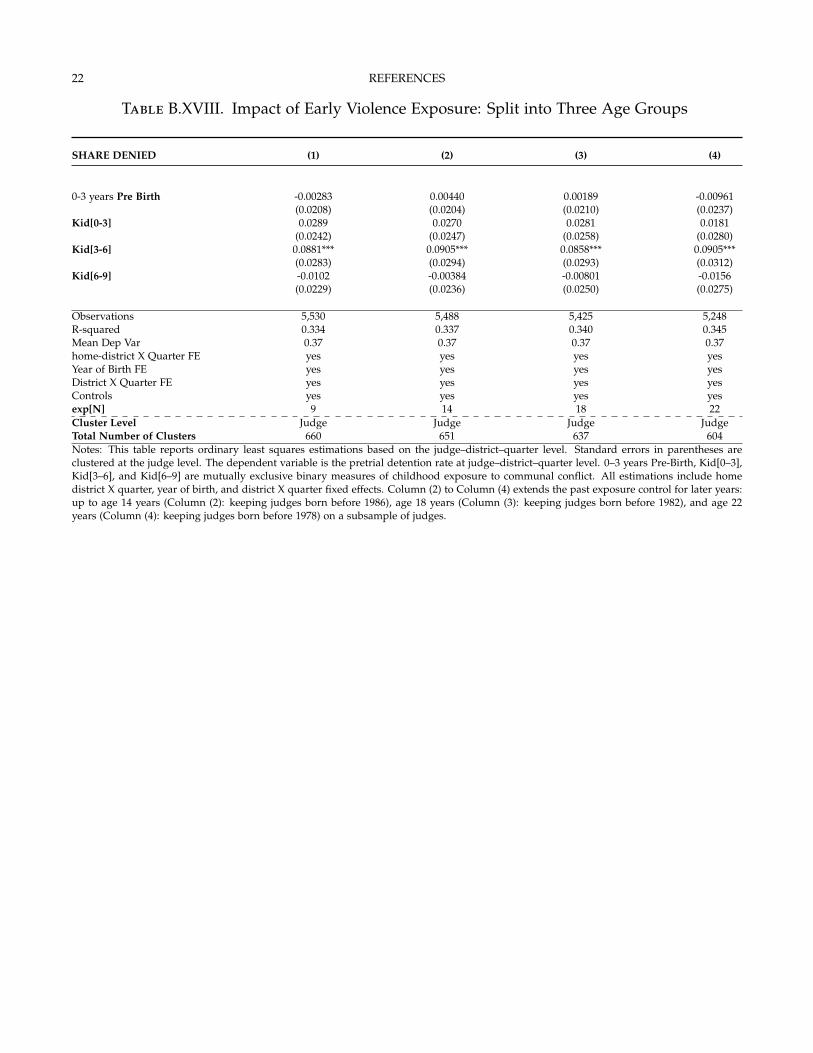
22 REFERENCES

Table B.XVIII. Impact of Early Violence Exposure: Split into Three Age Groups

SHARE DENIED (1) (2) (3) (4)

0-3 years Pre Birth -0.00283 0.00440 0.00189 -0.00961(0.0208) (0.0204) (0.0210) (0.0237)

Kid[0-3] 0.0289 0.0270 0.0281 0.0181(0.0242) (0.0247) (0.0258) (0.0280)

Kid[3-6] 0.0881*** 0.0905*** 0.0858*** 0.0905***(0.0283) (0.0294) (0.0293) (0.0312)

Kid[6-9] -0.0102 -0.00384 -0.00801 -0.0156(0.0229) (0.0236) (0.0250) (0.0275)

Observations 5,530 5,488 5,425 5,248R-squared 0.334 0.337 0.340 0.345Mean Dep Var 0.37 0.37 0.37 0.37home-district X Quarter FE yes yes yes yesYear of Birth FE yes yes yes yesDistrict X Quarter FE yes yes yes yesControls yes yes yes yesexp[N] 9 14 18 22Cluster Level Judge Judge Judge JudgeTotal Number of Clusters 660 651 637 604Notes: This table reports ordinary least squares estimations based on the judge–district–quarter level. Standard errors in parentheses areclustered at the judge level. The dependent variable is the pretrial detention rate at judge–district–quarter level. 0–3 years Pre-Birth, Kid[0–3],Kid[3–6], and Kid[6–9] are mutually exclusive binary measures of childhood exposure to communal conflict. All estimations include homedistrict X quarter, year of birth, and district X quarter fixed effects. Column (2) to Column (4) extends the past exposure control for later years:up to age 14 years (Column (2): keeping judges born before 1986), age 18 years (Column (3): keeping judges born before 1982), and age 22years (Column (4): keeping judges born before 1978) on a subsample of judges.

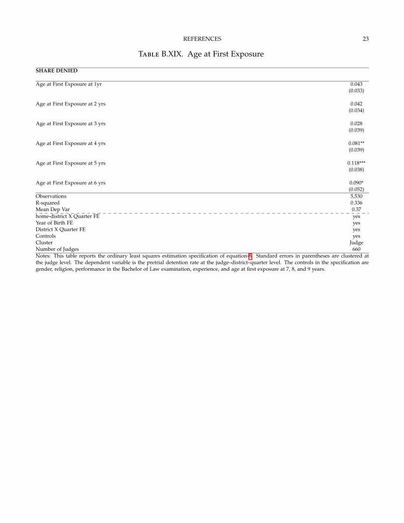
REFERENCES 23

Table B.XIX. Age at First Exposure

SHARE DENIED

Age at First Exposure at 1yr 0.043(0.033)

Age at First Exposure at 2 yrs 0.042(0.034)

Age at First Exposure at 3 yrs 0.028(0.039)

Age at First Exposure at 4 yrs 0.081**(0.039)

Age at First Exposure at 5 yrs 0.118***(0.038)

Age at First Exposure at 6 yrs 0.090*(0.052)

Observations 5,530R-squared 0.336Mean Dep Var 0.37home-district X Quarter FE yesYear of Birth FE yesDistrict X Quarter FE yesControls yesCluster JudgeNumber of Judges 660Notes: This table reports the ordinary least squares estimation specification of equation-8. Standard errors in parentheses are clustered atthe judge level. The dependent variable is the pretrial detention rate at the judge–district–quarter level. The controls in the specification aregender, religion, performance in the Bachelor of Law examination, experience, and age at first exposure at 7, 8, and 9 years.

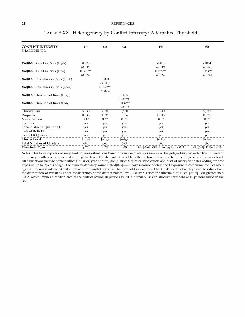
24 REFERENCES

Table B.XX. Heterogeneity by Conflict Intensity: Alternative Thresholds

CONFLICT INTENSITY (1) (2) (3) (4) (5)SHARE DENIED

Kid[0-6]: Killed in Riots (High) 0.025 -0.005 -0.004(0.036) (0.038) ( 0.037 )

Kid[0-6]: Killed in Riots (Low) 0.068*** 0.075*** 0.073***(0.024) (0.024) (0.024)

Kid[0-6]: Casualties in Riots (High) -0.004(0.033)

Kid[0-6]: Casualties in Riots (Low) 0.077***(0.026)

Kid[0-6]: Duration of Riots (High) 0.003(0.039)

Kid[0-6]: Duration of Riots (Low) 0.066***(0.024)

Observations 5,530 5,530 5,530 5,530 5,530R-squared 0.333 0.335 0.334 0.335 0.335Mean Dep Var 0.37 0.37 0.37 0.37 0.37Controls yes yes yes yes yeshome-district X Quarter F.E yes yes yes yes yesDate of Birth F.E yes yes yes yes yesDistrict X Quarter F.E yes yes yes yes yesCluster Level Judge Judge Judge Judge JudgeTotal Number of Clusters 660 660 660 660 660Threshold Type p75 p75 p75 Kid[0-6]: Killed per sq km >.002 Kid[0-6]: Killed > 10

Notes: This table reports ordinary least squares estimations based on our main analysis sample at the judge–district–quarter level. Standarderrors in parentheses are clustered at the judge level. The dependent variable is the pretrial detention rate at the judge–district–quarter level.All estimations include home district X quarter, year of birth, and district X quarter fixed effects and a set of binary variables coding for pastexposure up to 9 years of age. The main explanatory variable (Kid[0–6]—a binary measure of childhood exposure to communal conflict whenaged 0–6 years) is interacted with high and low conflict severity. The threshold in Columns 1 to 3 is defined by the 75 percentile values fromthe distribution of variables under consideration at the district month level. Column 4 uses the threshold of killed per sq. km greater than0.002, which implies a median area of the district having 10 persons killed. Column 5 uses an absolute threshold of 10 persons killed in theriot.

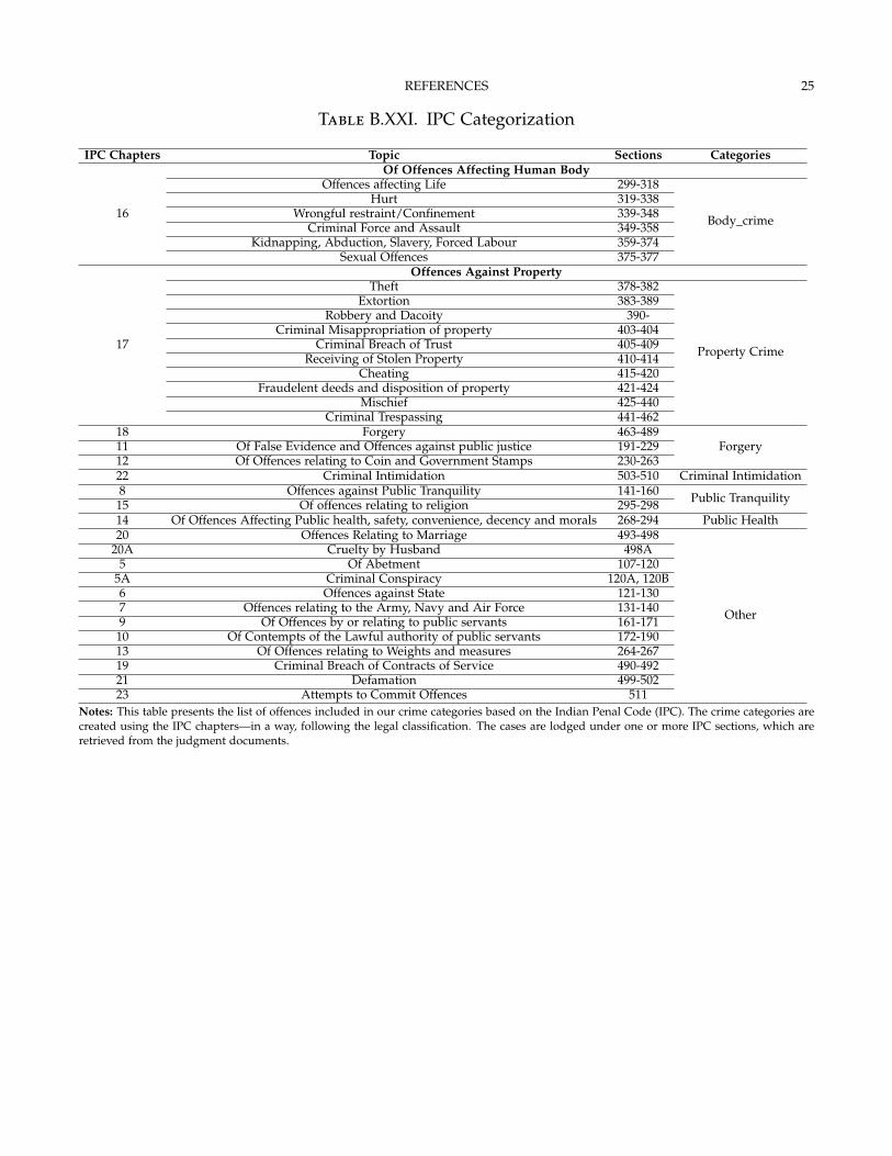
REFERENCES 25

Table B.XXI. IPC Categorization

IPC Chapters Topic Sections CategoriesOf Offences Affecting Human Body

Offences affecting Life 299-318Hurt 319-338

Wrongful restraint/Confinement 339-348Criminal Force and Assault 349-358

Kidnapping, Abduction, Slavery, Forced Labour 359-374

16

Sexual Offences 375-377

Body_crime

Offences Against PropertyTheft 378-382

Extortion 383-389Robbery and Dacoity 390-

Criminal Misappropriation of property 403-404Criminal Breach of Trust 405-409

Receiving of Stolen Property 410-414Cheating 415-420

Fraudelent deeds and disposition of property 421-424Mischief 425-440

17

Criminal Trespassing 441-462

Property Crime

18 Forgery 463-48911 Of False Evidence and Offences against public justice 191-22912 Of Offences relating to Coin and Government Stamps 230-263

Forgery

22 Criminal Intimidation 503-510 Criminal Intimidation8 Offences against Public Tranquility 141-160

15 Of offences relating to religion 295-298 Public Tranquility

14 Of Offences Affecting Public health, safety, convenience, decency and morals 268-294 Public Health20 Offences Relating to Marriage 493-498

20A Cruelty by Husband 498A5 Of Abetment 107-120

5A Criminal Conspiracy 120A, 120B6 Offences against State 121-1307 Offences relating to the Army, Navy and Air Force 131-1409 Of Offences by or relating to public servants 161-171

10 Of Contempts of the Lawful authority of public servants 172-19013 Of Offences relating to Weights and measures 264-26719 Criminal Breach of Contracts of Service 490-49221 Defamation 499-50223 Attempts to Commit Offences 511

Other

Notes: This table presents the list of offences included in our crime categories based on the Indian Penal Code (IPC). The crime categories arecreated using the IPC chapters—in a way, following the legal classification. The cases are lodged under one or more IPC sections, which areretrieved from the judgment documents.

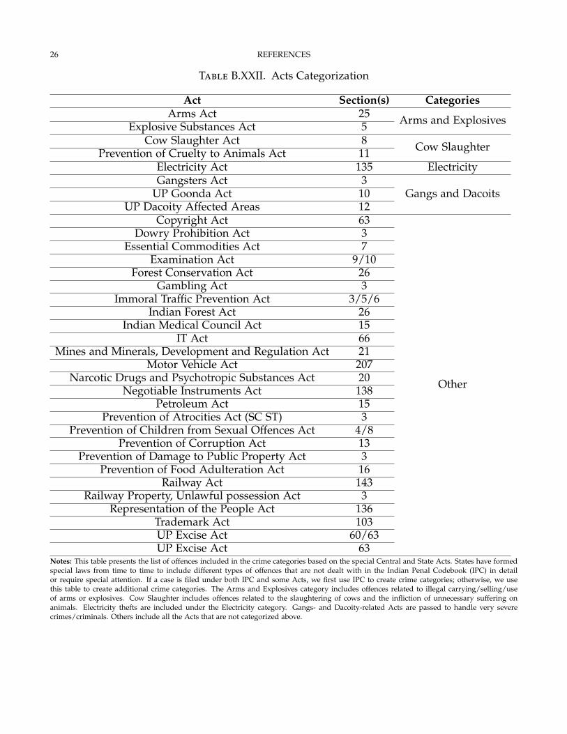
26 REFERENCES

Table B.XXII. Acts Categorization

Act Section(s) CategoriesArms Act 25 Arms and ExplosivesExplosive Substances Act 5

Cow Slaughter Act 8 Cow SlaughterPrevention of Cruelty to Animals Act 11Electricity Act 135 ElectricityGangsters Act 3

Gangs and DacoitsUP Goonda Act 10UP Dacoity Affected Areas 12

Copyright Act 63

Other

Dowry Prohibition Act 3Essential Commodities Act 7

Examination Act 9/10Forest Conservation Act 26

Gambling Act 3Immoral Traffic Prevention Act 3/5/6

Indian Forest Act 26Indian Medical Council Act 15

IT Act 66Mines and Minerals, Development and Regulation Act 21

Motor Vehicle Act 207Narcotic Drugs and Psychotropic Substances Act 20

Negotiable Instruments Act 138Petroleum Act 15

Prevention of Atrocities Act (SC ST) 3Prevention of Children from Sexual Offences Act 4/8

Prevention of Corruption Act 13Prevention of Damage to Public Property Act 3

Prevention of Food Adulteration Act 16Railway Act 143

Railway Property, Unlawful possession Act 3Representation of the People Act 136

Trademark Act 103UP Excise Act 60/63UP Excise Act 63

Notes: This table presents the list of offences included in the crime categories based on the special Central and State Acts. States have formedspecial laws from time to time to include different types of offences that are not dealt with in the Indian Penal Codebook (IPC) in detailor require special attention. If a case is filed under both IPC and some Acts, we first use IPC to create crime categories; otherwise, we usethis table to create additional crime categories. The Arms and Explosives category includes offences related to illegal carrying/selling/useof arms or explosives. Cow Slaughter includes offences related to the slaughtering of cows and the infliction of unnecessary suffering onanimals. Electricity thefts are included under the Electricity category. Gangs- and Dacoity-related Acts are passed to handle very severecrimes/criminals. Others include all the Acts that are not categorized above.

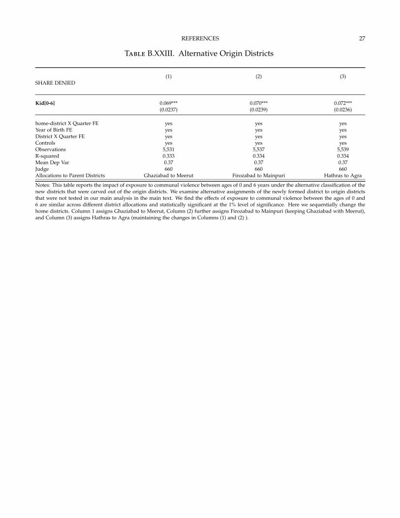
REFERENCES 27

Table B.XXIII. Alternative Origin Districts

(1) (2) (3)SHARE DENIED

Kid[0-6] 0.069*** 0.070*** 0.072***(0.0237) (0.0239) (0.0236)

home-district X Quarter FE yes yes yesYear of Birth FE yes yes yesDistrict X Quarter FE yes yes yesControls yes yes yesObservations 5,531 5,537 5,539R-squared 0.333 0.334 0.334Mean Dep Var 0.37 0.37 0.37Judge 660 660 660Allocations to Parent Districts Ghaziabad to Meerut Firozabad to Mainpuri Hathras to Agra

Notes: This table reports the impact of exposure to communal violence between ages of 0 and 6 years under the alternative classification of thenew districts that were carved out of the origin districts. We examine alternative assignments of the newly formed district to origin districtsthat were not tested in our main analysis in the main text. We find the effects of exposure to communal violence between the ages of 0 and6 are similar across different district allocations and statistically significant at the 1% level of significance. Here we sequentially change thehome districts. Column 1 assigns Ghaziabad to Meerut, Column (2) further assigns Firozabad to Mainpuri (keeping Ghaziabad with Meerut),and Column (3) assigns Hathras to Agra (maintaining the changes in Columns (1) and (2) ).

28 REFERENCES

Table B.XXIV. Treatment Effect of Riot Exposure on Measurement Error

ERROR IN TEXT EXTRACTION (1) (2)

BAIL DECISIONS DEFENDANT RELIGIONKid[0-6] 0.008 -0.003

(0.147) (0.005)

Observations 57,330 36,526R-squared 0.125 0.228Mean Dep Var 0.05 0.06home-district X Quarter FE yes yesYear of Birth FE yes yesDistrict X Quarter FE yes yesNotes: This table reports ordinary least squares estimation based on case level data for the randomly selected data for manual entry. Robuststandard errors are provided in parentheses. The dependent variable is the measurement error in the text extraction process which is equal to1 if the text extraction values differ from the manual entry and 0 otherwise. In Column(1), the dependent variable is the error rate in the bailoutcome and in Column (2) is a dummy variable if the religion of the dependent is identified correctly. All estimations include home districtX quarter, year of birth, and district X quarter fixed effects, and a set of usual controls. Column(2) also controls for the religion of defendant.The main coefficient of interest on Kid[0–6] capturing whether the error in our text extraction is correlated to our dependent variables.

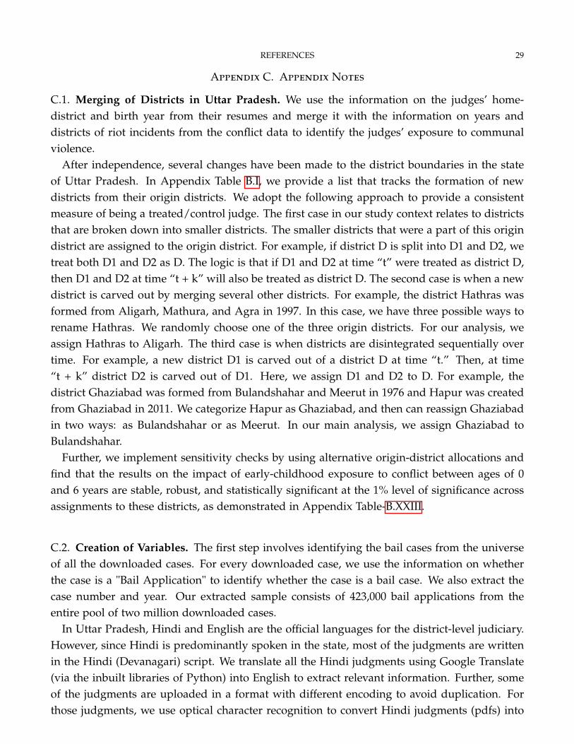
REFERENCES 29

Appendix C. Appendix Notes

C.1. Merging of Districts in Uttar Pradesh. We use the information on the judges’ home-district and birth year from their resumes and merge it with the information on years anddistricts of riot incidents from the conflict data to identify the judges’ exposure to communalviolence.

After independence, several changes have been made to the district boundaries in the stateof Uttar Pradesh. In Appendix Table B.I, we provide a list that tracks the formation of newdistricts from their origin districts. We adopt the following approach to provide a consistentmeasure of being a treated/control judge. The first case in our study context relates to districtsthat are broken down into smaller districts. The smaller districts that were a part of this origindistrict are assigned to the origin district. For example, if district D is split into D1 and D2, wetreat both D1 and D2 as D. The logic is that if D1 and D2 at time “t” were treated as district D,then D1 and D2 at time “t + k” will also be treated as district D. The second case is when a newdistrict is carved out by merging several other districts. For example, the district Hathras wasformed from Aligarh, Mathura, and Agra in 1997. In this case, we have three possible ways torename Hathras. We randomly choose one of the three origin districts. For our analysis, weassign Hathras to Aligarh. The third case is when districts are disintegrated sequentially overtime. For example, a new district D1 is carved out of a district D at time “t.” Then, at time“t + k” district D2 is carved out of D1. Here, we assign D1 and D2 to D. For example, thedistrict Ghaziabad was formed from Bulandshahar and Meerut in 1976 and Hapur was createdfrom Ghaziabad in 2011. We categorize Hapur as Ghaziabad, and then can reassign Ghaziabadin two ways: as Bulandshahar or as Meerut. In our main analysis, we assign Ghaziabad toBulandshahar.

Further, we implement sensitivity checks by using alternative origin-district allocations andfind that the results on the impact of early-childhood exposure to conflict between ages of 0and 6 years are stable, robust, and statistically significant at the 1% level of significance acrossassignments to these districts, as demonstrated in Appendix Table-B.XXIII.

C.2. Creation of Variables. The first step involves identifying the bail cases from the universeof all the downloaded cases. For every downloaded case, we use the information on whetherthe case is a "Bail Application" to identify whether the case is a bail case. We also extract thecase number and year. Our extracted sample consists of 423,000 bail applications from theentire pool of two million downloaded cases.

In Uttar Pradesh, Hindi and English are the official languages for the district-level judiciary.However, since Hindi is predominantly spoken in the state, most of the judgments are writtenin the Hindi (Devanagari) script. We translate all the Hindi judgments using Google Translate(via the inbuilt libraries of Python) into English to extract relevant information. Further, someof the judgments are uploaded in a format with different encoding to avoid duplication. Forthose judgments, we use optical character recognition to convert Hindi judgments (pdfs) into

30 REFERENCES

correctly encoded texts before translating them into English. We use these translated judgmentsto extract our essential variables.

The written judgments can be divided into three parts. The first part contains informationabout the case, such as the defendant(s)’s name (often accompanied by the father’s name,age, and address), the criminal section under which they have been charged, the date of thejudgment, and the name of the judge who delivered the judgment. The second part details theevent that led to the filing of the case. Sometimes, it also contains the legal precedents followedin arriving at the decision. The last part contains the judges’ decision on the bail application,either granting or denying bail and the bail amount if granting bail. We use the first and thelast part of the written judgments in extracting our variables. The main content we obtain isthrough text extraction and is as follows.

i) Outcome of the bail decisions: The outcome of the bail decisions is present in the last partof the judgment, and we use negative words to identify whether bail was denied41 and positivewords to identify whether bail was granted.42

ii) Name of the defendant(s): The name of defendants is used to identify their religion. Theinformation is present in the first part of the judgment. We use the "Stanford Named EntityAlgorithm.”43 One concern about using this algorithm is that it is not perfectly suitable for Hindinames. It may have missed some names (or some part of the names). Sometimes, it extracts thenames of places (partly because, in a few cases, it is difficult to differentiate between the namesof places and people. For instance, from the name Gautam Buddha Nagar district, it pickedGautam Buddha, which can be the name of a person). We filter out the names of places usingthe names of districts, subdistricts, and cities. The algorithm also selected the judges’ names(and their variants, given that it was translated using Google Translate), which we removecarefully. Further, we screen all non-names that the algorithm selected. Even after all thesechecks, some scope for error remains.

After extracting the names, we use the Nilabhra name2community algorithm to identify thedefendants’ religion. We discuss the efficiency of the Nilabhra algorithm in Subsection C3. Insome cases, only nicknames are provided (e.g., Bhura and Kaalu). In such cases, we use thename/surname of the defendant’s father to identify their religion.

iii) We use the text extraction method to extract information on the Acts44 and the IndianPenal Code (IPC) sections from the judgment documents. Criminal cases are registered either

41That is, “not granted,” “not released,” “not accepted,” “not acceptable,” “not approved,” “not freed,” “denied,”“unacceptable,” “cancelled,” “canceled,” “aborted,” “dismissed,” “rejected,” “abrogated,” “abortable,” “to be can-celed,” “terminated,” “cancellation,” “suspended,” and “revoked.”42That is, “released on bail,” “granted,” “released,” “accepted,” “acceptable,” ”approved,” “freed,” “acquit-ted,” “surrender,” “personal bond,” “bond,” “bondage,” “security bond,” "bond,” "suretages bond,” “interim,”"amount,” "money,” "acceptance,” "sureties,” and "collateral."43It associates each word to four tags: person (PER), location (LOC), organization (ORG), and miscellaneous(MISC). We consider the words tagged as PER.44We perform text extraction on these judgment files, searching for the word "Act" at the top of the document.

REFERENCES 31

through a First Information Report or a Complaint Register by the police. The IPC is the officialcriminal code of India. It provides a comprehensive list of offences and associated punishmentsand states whether the offence is bailable or not. In addition to the IPC, special Acts passedby the central and the state government guide the categorization of crimes. Appendix TableB.XXI and B.XXII provide the list of all the sections/Acts under each crime category. A casecan be lodged under one or more IPC sections and/or under special Acts. For every case, weuse the offence (IPC/Act section) carrying the maximum punishment to categorize the case.When there is a tie, we are indifferent and randomly pick one section. We create 11 crimecategories: Arms and Explosives, Body Crime, Cow Slaughter, Electricity Theft, Gangster andDacoity, Property Crime, Forgery, Criminal Intimidation, Public Tranquility, Public Health, andOther.

C.3. Accuracy of Algorithm in Classification of Religion. The religion assignment algorithmis crucial since we use it to assign the religion of the defendants and the judges. We do it intwo steps; first, we use the free Nilabhra algorithm to assign the religion, and then, we checkall the names (along with fathers’ names) manually to correct the religion. Next, we describein detail this procedure and the accuracy of the algorithm:

i) Judges’ religion assignment: We manually classify Urdu sounding names45 of all the judges(using not only their names, but also their fathers’ name) as Muslim following Bhalotra et al.2014. To test the algorithm further, we run the algorithm on the judges’ names. The error rate ofthe Nilabhra algorithm is 1.9% (20 out of 1,150 Hindu judges are incorrectly classified as Mus-lims by the algorithm, and four out of 83 Muslim judges are incorrectly classified as Hindu).This gives us confidence that the algorithm is relatively sound in predicting the religion fromthe names.

ii) Testing on a different dataset: We test our algorithm on a completely different datasetfrom Bhalotra et al. 2014, where names are categorized as Muslim and Non-Muslim. Our algo-rithm predicts with 6% error rate (880 out of 18,118 non-Muslim names are wrongly classifiedas Muslims by the algorithm, and 442 out of 3,791 Muslim names are wrongly classified asnon-Muslims).

iii) Defendants’ religion assignment : We use the Nilabhra algorithm first to assign a religionto the defendants using their names. In case the defendants’ name is neutral, we use the fa-thers’ name to categorize the defendants as Muslim or Hindu. We test for measurement errorin the defendants’ religion classification using a subsample of manually digitized entries. In thenext section, we explain how we arrive at the subsample from which we retrieve informationmanually.

45Most of the names have clear first names, such as Mohammad and Begum

32 REFERENCES

The measurement error in religion assignment for the defendants is attributable to two rea-sons: the improper extraction of names from the pdfs and incorrect religion classification. Toobtain error rate, we compare the religion of the names extracted using the algorithm with themanually assigned religion. The overall error rate in the total manually extracted sample is6% (570 out of 31,080 Hindu names are incorrectly classified as Muslim, and 1,535 out of 4,933Muslim names are incorrectly classified as Hindu). The reduction in the sample is because weignore the cases that have both Hindu and Muslim defendants are present.

C.4. Selection of Sample for Manual Entry. We manually extract all the aforementioned vari-ables from a subsample of cases to compute approximate error rates. We include all cases(30,000) handled by all Muslim bail judges in our analysis sample. Muslim judges comprisearound 7.6% (51 judges out of 668 judges) of the total number of judges and handle 9.43%(30,727/325,944) cases. We randomly select an equal number of cases, that is, 30,000 cases,handled by Hindu judges. To arrive at our random sample of cases handled by Hindu judges,we first randomly select Hindu judges and then randomly choose cases handled by them.

In selecting Hindu judges, our objective is to retain judges similar to Muslim judges alongkey covariates. First, we ensure that the Hindu judges are from the same pool of home-districtsas the Muslim judges. Second, we restrict the age range of the pool of Hindu judges to thesame age range (30–63 years) as that of Muslim judges. We stratify the random sample bycrime types of the bail cases. Within each crime category, we select a sample of Hindu judges,such that Hindu judges’ median experience is the same as that of Muslim judges.

After randomly selecting the Hindu judges based on these conditions, we randomly select thecases for every judge to ensure that the total number of cases is approximately 30,000. It shouldbe noted that the text extraction of IPC codes and Acts yielded an error rate of approximately22%.46 However, the measurement error for the crime category is random, and therefore, thesample of cases handled by Hindu judges that is selected for manual digitization is random.

C.5. Do we have classical measurement error? The overall measurement error on bail out-comes is 5% (1,525 bail cases are incorrectly classified as denied out of 38,233 bail cases granted,and similarly 1,358 cases are incorrectly classified as granted out of 19,138 bail cases denied.).In this subsection we test whether the bail outcomes and religion assignment of defendants arecorrelated with the exposure to riots variable. The measurement error is defined as the devia-tion of the text extraction values from the manual data entry is measurement. It is a dummyvariable that takes value 1 when there is measurement error and is 0 otherwise. We test itthrough the following regression.

MEj,d,t = α + ηd,t + δh,t +F .E b + β× kid[0− 6]j + σXj +9

∑k=7

γ(k)× exposure(k)j + εj,d,t (C.1)

46This error rate was computed using the manually digitized data set.

REFERENCES 33

The β coefficients as reported in the table B.XXIV are close to zero and insignificant whichindicates that the measurement errors are orthogonal to our main explanatory variable.

The Early Origins of Judicial Stringency in Bail Decisions

Documents

Transcript of The Early Origins of Judicial Stringency in Bail Decisions