
The diversity of flower-visiting insects in the gardens of ...
293
DIVERSITY ENGLISH COUNTRY HOUSES Submitted for the Degree of Doctor of Philosophy at the University of Northampton 2013 Hilary E. Erenler T, . . © Hilary E. Erenler is thesis is copyright material and no quotation from it may be published without proper acknowledgement. ’ JNIVERSITY OF NORTHAMPTON AVENUE LIBRARY SACC. No. ?3LA8S NO. vuVUUCC*
-
Upload
khangminh22 -
Category
Documents
-
view
0 -
download
0
Transcript of The diversity of flower-visiting insects in the gardens of ...

DIVERSITYENGLISH COUNTRY HOUSES
Submitted for the Degree of Doctor of Philosophyat the University of Northampton
2013
Hilary E. Erenler
T, . . © Hilary E. Erenleris thesis is copyright material and no quotation from it may be published without
proper acknowledgement.
’ JNIVERSITY OF NORTHAMPTONAVENUE LIBRARY
SACC. No.? 3LA8S NO.vuVU U C C *
Abstract
Flower-visiting insects provide essential pollination services, ensuring both globalfood security and the continuity of wild plants. Recently documented declines inpollinators give cause for concern. Identifying previously unappreciated habitats thatsupport diverse assemblages of these insects is an essential first step in mitigating further losses.
This study evaluates, for the first time, the role that large English country-housegardens play in supporting flower visitors within expanses of intensively farmedagricultural land. Focussing on 17 properties in lowland Central England, the resultsshow that these novel ecosystems are important sites for hoverflies, bees andbutterflies. In 2010 almost 10,000 flower-visitors from 174 species were recordedHoverflies were the only group to show a significant difference in species richness across the sites.
An important characteristic of these rural gardens is the high diversity of flowering plants available. More than a fifth of the world's plant families were represented, of which approximately 68% were non-native. The results showed that flower visitors did not prefer native plants over aliens, and that the dominance by aliens was no barrier for extensive use by the insects present. Both the species richness and abundance of flower visitors increased as plant richness increased.
The study revealed that half of all insect-plant interaction networks examinedexhibited a nested structure, a common feature of natural environments that has not previously been assessed in rural gardens.
In addition to flower resources influencing insect species richness, landscape-scaleeffects were also significant. Insect groups responded differently to components inthe landscape according to the time of year and the spatial scale considered.Bumblebees exhibited the greatest response to landscape factors and did so at larger scales than other groups.
The deployment of commercial trap-nests for solitary cavity-nesting red mason beesin walled gardens revealed new insights into the differential mortality suffered bymale and female progeny. Female offspring were found to be disproportionatelyaffected by a combination of development and parasitism losses. This findingsuggests that effective mitigation strategies are needed before this species can be considered for use as a managed-pollinator.
Further research assessing the benefits crops such as oilseed rape derive from the presence of insects in nearby rural gardens would be a useful addition to this work.
Overall, the gardens of English country-houses emerge as sites of important natural as well as cultural heritage.
I

The beauty and genius of a work of art may be reconceived though its
first materia! expression be destroyed.
A vanished harmony may yet again inspire the composer.
But when the last individual of a race of living beings breathes no
more, another heaven and another earth must pass before such a can be again.
William Beebe (1906)
From a plaque marking the site of Gerald Durrell's ashes.Durrell Wildlife Park, Les Augres Manor, Trinity, Jersey, Channel Islands.
one

To Michael and Tinaz.

Acknowledgements
This research project was financially supported by the Finnis Scott Foundation, a Northamptonshire-based charitable trust supporting horticultural and art-history activities, and the Leslie Church Memorial Trust.
I am extremely grateful to my two supervisors, Professors Jeff Ollerton and JonStobart for their initial belief in me and subsequent generous provision of their timeThank you both for your good humour and the intellectual and emotional support you have so freely given.
I would like to express my gratitude to the owners, head gardeners and estate managers at the seventeen properties where I was lucky enough to conduct field work. Without them there would be no project.
House ownersViscount Althorp (Althorp Estate), The Duke of Buccleuch (Boughton Estate), SirMichael and Lady Connell (Steane Park), English Heritage (Kirby Hall, Wrest Park),Sir John and Lady Greenaway (Lois Weedon House), Kelmarsh Trust (KelmarshHouse), Lamport Hall Preservation Trust (Lamport Hall), Mr and Mrs James Lowther(Holdenby House), Mr Leon Max (Easton Neston), The National Trust (Canons AshbyFamborough Hall, Upton House, Waddesdon Manor), Ian and Susie Pasley-Tyler(Coton Manor), Sulgrave Manor Charitable Trust (Sulgrave Manor) and Mr and Mrs Charles Wake (Courteennall Estate).
Head gardeners and Estate Managers:Heather Aston (Upton), Simon Bailey (Steane), Mr Drye and Carole Almond(Lamport), Katie Evans (Althorp), Paul Famell (Waddesdon), Lance Goffort-Hall andCharles Lister (Boughton), Roy Goodger (Easton Neston), Esther McMillan(Kelmarsh), Sue McNally (Sulgrave), Chris Slatcher (Wrest), Chris Smith (CanonsAshby), Beryl Spearman (Kirby), Richard White (Farnborough) and Darron Wilks (Courteenhall).
Additionally, I would like to thank the following entomologists and researchers who have both inspired and helped me: David Baldock, Adam Bates, Mike Edwards, Tim Newton, Jennifer Owen, Chris OToole, Stuart Roberts and John Showers.
I am also grateful to Mike Edwards from BWARS and Stuart Ball and Roger Morrisfrom The Hoverfly Recording Scheme for provision of vice-county Hymenoptera and hoverfly data.
At The University of Northampton I would like to extend my thanks to RobinCrockett, Nick Dimmock, Christine Fairless, Janet Jackson, Ian Livingstone, DuncanMcCoHin, Paul Phillips, Miggie Pickton, Simon Pulley, Paul Stroud, David Watson and Stella Watts.
Finally I would like to say a big thank you to my family. Without witnessing my mothers tolerance when, at age four, I placed caterpillars in her airing cupboard,
'5 0b5essi0ns with list-making and swimming, I would not have had the skills needed to get through this process.
IV

Table of Contents
AbstractPage
Quotation
Dedication
Acknowledgements
Table of contents
List of figures
List of tables
List of appendices
IV
VII
• •
XIII
Chapter 1: Introduction
Chapter overview
Pollination - an ecosystem service
Threats to UK flower-visitor insect diversity
The role of gardens in supporting pollinating insects
Scope of the research project
Project aims
Research questions
Overview of the thesis
Chapter 2: Study sites, study organisms and general methods
Chapter overview
Introduction
Study sites
Study organisms
General fieldwork principles
2010 field season
2011 field season
Chapter 3: Flower-visitor species richness and diversityChapter overview
Introduction
Aims
Methods
Results
Discussion
Conclusions
1
22
6
9
15
16
17
17
19
20
20
20
24
30
31
39
41
42
42
48
49
53
75
89

Chapter 4: The structure of plant and flower-visitor communities
Chapter overview
Introduction
Aims
Methods
Results
Discussion
Conclusions
Chapter 5: Spatial and seasonal factors affecting the diversity offlower-visitors
Chapter overview
Introduction
Aims
Methods
Results
Discussion
Conclusions
Chapter 6: Trap-nest bees in walled gardens
Chapter overview
Introduction
Aims
Methods
Results
Discussion
Conclusions
Chapter 7: Conclusion
Chapter overview
Key findings of the study
Critique of methods
Areas for further work
Concluding remarks
91
92
92
99
99
102
123
132
134
135
135
139
140
145
158
163
164
165
165
179
179
184
200
206
208
209
209
212
214
217
vi

List of figures Page
1.1
1.2
2.1
2.2
3.1
3.2
3.3
3.4
3.5
3.6
3.7
3.8
3.9
3.10
3.11
4.1
4.2
4.3
Alexander Pope's house at Twickenham (From an original painting at Orleans House Gallery, Richmond, painter unknown).
Waddesdon Manor, Buckinghamshire (centre), set within a mosaic of intensively farmed land.
Location of the 17 gardens in central lowland England used in the study.
12
14
22
Examples of flower-visitors recorded in the current study. 24
Four ways of plotting species abundance distributions. 47
Recorded species richness and the richness estimators Chao 1 and Jack 1. 56
Species richness for the actual number of species recorded and theestimators Chao 1 and Jack 1 against the abundance of individuals Der property. KRanked mean species richness for each property (four samplinq sessions). *
57
58
Mean hoverfly species richness for each property (four sampling sessions). a
Relationship between the number of species recorded and the number of records for five insect groups using data from two studies.
Shannon diversity values for each of the 17 properties (four samplingsessions, all species). y
r‘!!VehSitywt0r f?Ur inSeCt 9r0Ups (17 P a r t ie s , all sampling sessions combined) and the recalculated values for hoverflies (HF).
Dendrogram showing nearest neighbour linkage between 17 sites based on incidence data for species present (Jaccard method).
59
63
65
66
69
groups"8' CUmU,ative distribution frequency (ECDF) plots for four iinsect 70
Empirical cumulative distribution frequency (ECDF) plots for the four group'H^ SeSS'°ns- Each set of symbols represents a different insect
Illustration of typical interactions between pollinators and plants.
72
97
T re n d 7i n e s a re power "unions* * °f aVai'ab'e P'ant taxa’
a ,“ nction of availab,e plant ta*a- Trend
104
104
• •
VII

4.4
4.5
4.6
Median number of plant elements visited compared to median number of plant elements available for each property.
Median number of plant elements visited compared to the mediannumber of plant elements available for each of the four sampling sessions.
Number of plant elements visited and available plotted according to date sampled.
106
107
107
4.7 Preference index for highly represented and visited plant families in Session 1. I l l
4.8 Preference index for highly represented and visited plant families in Session 2. 112
4.9 Preference index for highly represented and visited plant familiesSession 3.
in 113
4.10 Preference index for highly represented and visited plant familiesSession 4.
in 114
4.11 Median connectance values for each property for (i) only plantelements that were visited and (ii) all plant elements available.
4.12 Decreasing connectivity as a function of matrix size for two scenarios
117
118
4.13 Median generality and vulnerability values for each of the 17properties. 119
4.14
4.15
5.1
5.2
5.3
5.4
5.5
5.6
5.7
Median generality and vulnerability values for the four sampling sessions. y
Proportion of communities within each sampling session exhibiting significantly nested interaction networks.
Use °f digital maps to assess land cover at different spatial scales using ArcGIS software (ESRI, 2011).
of variance in the flower-visitor group data according to the contribution of two subsets of environmental variables using the methods of Borcard et at. (1992)? 2 „ inh Cr! ated after redundancy analysis using the 2010Session 1 bumblebee data at a 1,500m spatial scale.
2nh u m K CrHaled 8fter redunda"c* analysis using the 2010 Session 2 bumblebee data at a 3,000m spatial scale.
S ^ ? 4 nhumhtah CT ? d after redundancy analysis using the 2010 Session 4 bumblebee data at a 1,500m spatial scale.
S e s S 'T h n '^ r fT CrHaHed f 6r redundancy analysis using the 2010 Session 3 butterfly and day-flying moth data at a 750m spatial scale.
?nrJ™ “ °.n afte[ redundancy analysis using the 2010 Session 3 hoverfly data at a 750m spatial scale.
120
121
141
144
149
150
152
153
154
w m m
VIII

5.8 Results of variance partitioning (Borcard et al., 1992) for each of thefive significant RDAs plus Session 3 for bumblebees.
5.9 Number of solitary bee individuals recorded in Session 1 at each walledgarden categorised according to whether they are ground nesting or cavity nesting.
5.10 Number of solitary bee individuals recorded in Session 2 at each walledgarden categorised according to whether they are ground nesting or cavity nesting.
6.1 Nesting and foraging resources required by bees in temperatelocations (after Westrich, 1998).
6.2 Commercial trap-nests for solitary bees (images of commercial trapnests and O. bicornis larval provisions).
6.3 Red mason bee cell provisioning and cell parasitism.
6.4 Existing cavities in the mortar between bricks in the walled garden atLamport Hall.
6.5 Flow diagram showing the fate of trap-nest cells according to 8categories, together with k values derived from the life-table staaes in Table 6.3. a
6.6 Median fraction of tubes used at each property, ranked highest tolowest.
6.7 Mean number of O. bicornis cells per nest for each property.
6.8 Total number of O. bicornis and cells of other species (Appendix X) atproperties where they co-occurred.
6.9 k2 values regressed over the starting number of O. bicornis cells.
6.10 Proportion of failed cells at each brood cell position.
6.11 Proportion of males and females at each brood cell position.
6.12 Fraction of female and male individuals lost at each brood cell position.
6.13 Difference in mean number of adult O. bicornis after losses to M.
6.14 Sunimary of losses experienced at each life stage based on k valuesl � 6 as described in Figure 6.5.
7.1 Selection of bumblebees killed as a result of ride-on mowers.
156
157
157
166
170
172
175
182
184
187
188
191
193
194
196
197
199
215

List of tables Page
1.1
1.2
2.1
2.2
2.3
2.4
3.1
3.2
3.3
3.4
3.5
3.6
3.7
3.8
3.9
3.10
Publications relating to the losses and current status of key flower visitor groups in the United Kingdom. 6
The three insect orders containing nine target groups used in the study. 16
Details of the 17 properties selected for sampling. 23
Description of the 2010 sampled components at each garden, the totaltransect length per component and the number of individual areas they comprised.
33
List of resources used to identify voucher specimens and flower visiting insects observed in the field.
Resources used to identify flowering plants.
37
38
Results of Estimates (Colwell, 2009b) Chao 1 and Jack 1 speciesrichness estimations for the 17 properties together with the actual number of species recorded.
Species richness estimates for the four most speciose flower-visitor groups.
55
58
Results of ANOVAs comparing mean species richness across 17 properties for individual insect groups.
Species richness (actual and estimates) for the 20 NT qardens sampled by Edwards (2003).
Comparison of recorded species richness for 17 gardens in the current study with that of 20 NT gardens (Edwards, 2003).
Recorded species richness for five insect groups.
59
60
60
62
Results of Morisita-Horn pair-wise comparisons for community similarity. 1
Results of Chao Abundance-based Estimated Sorensen pair-wise comparisons for community similarity.
Results of Kolmogorov-Smirnov four insect groups.
Results of Kolmogorov-Smirnov sampling sessions.
tests between sessions for each of
tests between groups for each of four
67
68
71
73
x

3.11 Honey bee abundance at each garden in each of the four sessions. 74
3.12
3.13
4.1
4.2
4.3
4.4
4.5
4.6
4.7
4.8
4.9
5.1
5.2
5.3
5.4
Results of Wilcoxon signed ranks tests for honey bee abundance between sessions.
Comparison of hoverfly species according to four larval trophic levels.
Number of plant families (F), genera (G) and elements (PE) recordedfor each property at each of four sampling sessions, together with the total number of distinct taxa for each property.
Results of linear regressions for flower-visitor species richness aqainst plant taxa.
Results of Mann Whitney U tests for each of the four sampling sessionscomparing the number of plant elements visited with the number of plant elements available.
Percentage of alien and native plant elements across each of the four sampling sessions.
Results of chi-square tests of association comparing the number of alien and native plants visited versus those available.
Range and mean proportion of alien and native plant elements acrosseach of the seventeen properties (four sessions combined) plus mean proportion for all properties.
List of highly visited families per session.
Results.of post hoc tests (Mann Whitney) for differences in median generality values between paired sessions.
Results of 68 tests for nestedness.
Landscape-scale variables for the two sampling seasons (2010 and2011) showing the three land-use categories accounting for theighest percentage of area within concentric polygons around the
properties.
Within-garden variables for the two field seasons (2010 and 2011)showing the mean number of plant genera for Sessions 1 - 4 (2010field season) and mean number of plant genera and mean blossom density for Sessions 1 and 2 (2011 field season).
Results of redundancy analysis for each insect group across four sampling sessions (2010 data) at three spatial scales.
0f R^ s for each insect group and session using the landscape scale derived from the exploratory analysis (Table 5.3).
74
78
103
105
105
108
108
110
115
120
122
145
146
147
155
xi

5.5 Results of stepwise forward multiple regressions for the log-transformed number of solitary bees in walled gardens for Sessions 1 and 2.
158
6.1 Examples of solitary bee species used as pollinators of commercial crops. 168
6.2 Studies highlighting the dominant use of trap-nests by the red mason bee. 173
6.3 Descriptions of mortality and loss factors for O. bicornis using the stages described in Raw (1972). 176
6.4 Details of the nine walled gardens used in the trap-nest study. 180
6.5 Results of post hoc tests on mean ranks of fraction of tubes used aftera Kruskal-Wallis test using the procedure described in Sieqel and Castellan (1988).
185
6.6 Use and contents of nests and tubes per property. 186
6.7 Results of Kruskal-Wallis tests for differences in 0. bicornis k values between eight properties (LW excluded).
189
6.8 Results of post hoc tests on mean ranks of k2 after a Kruskal-Wallis test using the procedure described in Siegel and Castellan (1988).
190
6.9 Results of post hoc tests on mean ranks of k4 after a Kruskal-Wallis test using the procedure described in Siegel and Castellan (1988).
191
6.10 Number of cells per category at each brood cell position. 192
6.11 Predicted number of males and females (and fraction) lost to two causes based on 1,080 individuals of known sex.
195
6.12 Observed male to female sex ratios for 0. bicornis and 0. cornuta from the current study and other published work.
205

References 218
List of appendices Page
Appendix I Details of the 17 properties used for the study. 246
Appendix II Abbreviations used in the thesis. 265
Appendix III
Appendix IV
Appendix V
Appendix VI
Summary of the seven key non-parametric species richness estimators available.
List of the 20 National Trust gardens surveyed by Edwards (2003).
V
Dunn-Sidak method for adjusting the significance level(a) when making multiple comparisons (Sokal and Rohlf 1981).
List of insect species recorded in 2010 and 2011.
267
268
268
269
Appendix VII
Appendix VIII
Appendix IX
Appendix X
List of plant families and genera recorded from the 17 gardens in 2010.
Example of the calculation of k values according to lifestages using the methods of Varley et a i, (1975) and Yamamura (1999).
Post hoc test used to assess differences between mean ranks for eight properties (each with three nests) using the method of Siegel and Castellan (1988).
Solitary bee families and genera other than O. bicornis found in occupied tubes.
274
278
279
279
UN1VER
• • • XIII
NORTHAMPTONLIBRARY

Chapter 1
Chapter 1
Introduction
1

Chapter 1
Chapter overviewThis introductory chapter sets out the case for studying flower-visitor insectdiversity. It identifies the main causes for insect pollinator declines and reviews therole gardens can play in providing suitable forage and nesting habitat A briefsynopsis of the changes English country-house gardens have experienced throuqhthe centuries is followed by a section outlining the scope of the project and the keyresearch questions that will be explored. The chapter concludes with an overview of how the thesis is arranged.
Biodiversity and ecosystem servicesAs the human population continues its climb towards a predicted total of 10.1 billion
by 2100 (United Nations, 2011), biodiversity is forecast to decline over the same
period (Pereira et at, 2010). The pressures of a burgeoning global population on the
Earth's remaining natural environments and their non-renewable capital are both a
cause for concern and an incentive for urgent action (Wilson, 2001, Butchart et at.,
2010). As the awareness of the consequences of biodiversity loss increases, so too
does the interest in understanding the patterns and processes that drive it (Liu et at., 2011).
During the 1990s both regional and global biodiversity protection measures shifted
from targeting individual species to placing increased importance on 'hotspots' of
biodiversity (Mittermeier et a!., 1998). Later, ecosystem services, defined as 'the
benefits people obtain from ecosystems' (UNEP-WCMC, 2011), were identified as
vulnerable entities in themselves that warranted assessment and conservation
strategies. The focus on these services stems from a realization that the survival
and well-being of humans is intricately related to the health and robustness of the
ecosystems they interact with (Costanza et al., 1997, Daily et at, 1997),
Pollination: An essential ecosystem serviceEcosystem services can be categorised according to whether they are cultural,
provisioning, regulating or supporting. Pollination, which is the transfer of male
gametes within pollen to receptive female flower organs, is considered an essential
regulating process (UNEP-WCMC, 2011). Following a pollination event a plant may
set seed, thus facilitating future generations of that species (Kearns and Oliveras,
2009), as well as nutritionally supporting other organisms (Dias et at, 1999). Pollen
transfer may be enabled by wind or water, but for the majority of angiosperms
(approximately 88%, Ollerton et at, 2011) it is pollination by animals that facilitates
2

Chapter 1
fertilisation and seed-set. Although animal mediated pollination does not guarantee
the long-term survival of a plant population (and the organisms that rely on it), it
can nevertheless act as a necessary first step in the process (Rathcke and Jules, 1993).
Pollinators belong to diverse groups within the animal kingdom and include birds,
bats, opossums and reptiles (Dias eta/., 1999). It is, however, certain groups of
invertebrates that are most associated with pollination. These include solitary and
social bees and wasps (Hymenoptera), butterflies and moths (Lepidoptera),
hoverflies (Diptera) and beetles (Coleoptera), (Waser, 2006). Globally, 3,000 species
of plant are grown or used for food by humans and their domesticated animals, two-
thirds of which require insect pollination (Dias et al., 1999). As a measure of how
important hymenopterans are in this process, bees have been recorded visiting 73%
of these plants (Kremen and Chaplin-Kramer, 2007).
The importance of flower-visiting insects through their role as pollinators was
formally recognised in the Sao Paulo Declaration on Pollinators in 1999 (Dias et al.
1999). The statement that 'Pollination is one of the most important mechanisms in
the maintenance and promotion of biodiversity and, in general, life on earth' (Dias et
al., 1999, p. 18) heralded the start of what has subsequently become an area of intense research focus.
Research into pollinating insects stems from their acknowledged contribution to
biodiversity together with a heightened awareness that declines in their abundance
and richness could have ecological and economic consequences. Current
international and national projects include: STEP (Status and Trends of European
Pollinators) a European-wide collaboration aiming to understand and mitigate
against the drivers and impacts of changes in pollinating insect diversity and
abundance (STEP, 2012); and a suite of UK projects under the Insect Pollinators
Initiative backed by a £10 million research investment to investigate biological and
environmental factors affecting pollinating insects (NERC, 2009). The reason behind
this increased research effort comes from reports that pollinating insect numbers are declining.
Pollinator declinesA decline in pollinators (in particular pollinating insects) is now accepted to be
occurring on a global scale (Wratten etal., 2012 and references therein). Potentially,
this has major consequences for the humans and animals that rely on the nutritive
and medicinal benefits that wild plants and crops provide (Klein eta/., 2007). Food

Chapter 1
security issues already exist on our increasingly populated planet, and pollinator
declines threaten to exacerbate these (Costanza et at., 1997, Daily et at., 1997, Fitzpatrick et a!., 2007).
Declining pollinator abundance and diversity can operate at local and global scales,
generating productivity concerns for individual growers as well as threatening to
destabilise world commodity markets (Dias et a!., 1999). The latter raises potential
nutritional and health issues for many people (Allen-Wardell eta/., 1998, Steffan-
Dewenter et a/., 2005, Kleijn and van Langevelde, 2006, Klein et at., 2007).
Countries such as China have already reported reductions in fruit and vegetable
yields as a result of pollinator declines (Partap et at., 2001).
The global decline of the world's most common managed pollinator, the honey bee
(Apis mellifera, Apidae) has received a great deal of attention in both the scientific
and popular press (vanEngelsdorp and Meixner, 2010, Breeze et at., 2011,
Thompson, 2012) and continues to exert what some consider to be a
disproportionate claim on the scientific funding available for research into the loss of
bee populations (Ollerton et at., 2012). Although the reduction in the number of
honey bees and their colonies is causing concern it is not, in the words of
vanEngelsdorp and Meixner (2010), 'universal'. Indeed, these authors suggest that
whilst North American and European populations have been hardest hit, within these
areas some countries have not experienced declines. In places where losses have
occurred the primary causes have been cited as disease, parasites, overwintering
mortality, pesticides (both direct and indirect toxicity), reduced availability of forage
and changes in climate (vanEngelsdorp and Meixner, 2010).
In contrast to the widely communicated reduction in honey bees, far less is known
about losses affecting the majority of wild pollinators. Kearns and Inouye (1997,
p.300) see this 'information imbalance' as a particular problem for wild bees, stating
that issues relating to honey bees have been 'studied extensively, often at the
expense of the other 20,000 - 30,000 bee species'. Some insect groups such as
bumblebees and butterflies are notable exceptions to this, with reductions in the
range and abundance of certain species well documented (Goulson, 2010, Fox et at 2012).
Parallel declines in pollinators and wild and cultivated plants have been reported in
Europe (Biesmeijer et at., 2006, Natural England, 2010, Potts eta/., 2010). These
declines emphasize the risk that any disruption in pollination services may bring,
including unpredictable, cascade-like effects that have the potential to disturb
multiple food webs (Rathcke and Jules, 1993, Kearns and Oliveras, 2009).

Chapter 1
Pollinating insectsNot all insects are pollinators, despite their often frequent visits to flowers, nor does
each visit by a legitimate pollinator result in a pollination event (Kwak et at., 1996)
Classifying an insect group, genus or species according to its pollinating abilities is
therefore a difficult task. In their seminal work 'The principles of pollination
ecology', Faegri and van der Pijl (1966) described in detail the range of invertebrates
that are considered as pollinators. They identified four key insect orders warranting
particular attention: beetles (Coleoptera); flies (Diptera); bees (Hymenoptera) and
butterflies and moths (Lepidoptera).
For the purposes of this study the general term 'flower-visiting insect7 will be used.
This recognises that although insects alighting on flowers may appear to be
pollinating them, the occurrence of a pollination event cannot be assumed (Kevan and Baker, 1983).
Current state of native flower-visiting insect diversitv in the UK
Assessing the state of current native flower-visitor insect diversity in the UK is
complicated by the fact that no single organisation researches and reports on all
insect groups. Instead, specialist recording societies, non-governmental
organizations (NGOs), e.g. Friends of the Earth, Government organisations (Natural
England) and academics have all taken the lead in highlighting the status of
particular groups at different times. A selection of these is given in Table 1.1.
5

Chapter 1
Table 1.1 Publications relating to the losses and current status of key flower-visitor groups in the United Kingdom.
Insect
group
Key findings
Bumblebees
Butterflies
Honey bees
Hoverflies
Solitary bees
All
3 species extinct 8 species in severe decline Worst affected are long- tongued species
UK butterflies are in serious declineTen-year trends show 72% of species declined in abundance Ongoing deterioration of habitats is main cause
UK managed colonies declined by 53% between 1985 - 2005
33% of species have declined over last 25 - 35 years Species associated with conifers and wetlands experienced the greatest declines
True status of most species not known but approx. 52% decline within English landscapes
Since 1800, 23 bee, 18butterfly and 88 moth species lost from England
Publication Reference
Decline and Conservation of bumblebees
Goulson et al. (2008)
The State of the UK's Butterflies, 2011
Fox et al. (2012)
Global pollinator declines: Trends, impacts and drivers
Potts et al. (2010)
Atlas of the Hoverflies of Great Britain (Diptera, Syrphidae)
Ball et al. (2011)
The decline of England's Bees
Breeze et al. (2012)
Lost Life: England's lost and threatened species
NaturalEngland(2010)
Threats to UK flower-visiting insect diversityFlower-visiting insect populations in the UK are under pressure for many reasons.
These include: changes in agricultural practices, fragmentation or alteration of land
use (e.g. infrastructure creation or urbanisation) and the effects of climate change. These are now considered in turn.
Changes in agricultural practices
Major changes in the rural landscape have been a feature of the UK for centuries.
From the increased use of ridge and furrow ploughing practices in the Middle Ages to
the Parliamentary Enclosure Acts of the 18th and 19th century, land management has
6

Chapter 1
been in a constant state of flux (Thomas, 1984). The changes since World War II
are, however, some of the most extensive to date. In common with the majority of
Northern Europe, agricultural intensification, in particular'modern intensive farming',
has been cited as the principal cause for the decline in biodiversity in the European
countryside (Stoate etal., 2001, Carvell et al., 2004, Dormann etal., 2007, Henle et
a'- 2008)- More ^nd than ever before has been taken into agricultural production in
the UK. Currently 17.2 million hectares (70% of the area of the UK) is designated agricultural land (Defra, 2011).
High-yield crops such as wheat and barley rely on a mixture of agri-chemicals to
control weeds, fungi and crop-pests (Defra, 2011). As such, managed and
unmanaged pollinators are exposed to an ever-increasing range of treatments
(Breeze et al., 2012). The risks from acute toxicity following direct exposure have
been largely mitigated by the introduction of pesticide-use regulations
(vanEngelsdorp and Meixner, 2010), however the sub-lethal side-effects on insects
following chemical applications are only now being fully explored. Recent research
considering the effect of neonicotinoids on bumblebee queen production and bee
foraging and homing behaviour has shown that, even at trace levels, these
pesticides are able to impair reproductive and functional behaviour (Girolami etal., 2012, Whitehorn etal., 2012).
Global and national economic drivers such as rapidly increasing commodity prices
(Mitchell, 2008), financial incentives to grow specific crops, e.g. the mass-flowering
oilseed rape (OSR), Brasslca napus (Diekotter ef a/., 2010), and the removal of
payments to landowners to leave land out of production (set-aside) (Defra, 2011)
continue to alter how agricultural land is used in the UK. The increased presence of
OSR since the 1970s has been described as one of the most dramatic changes to the
floral landscape for centuries (Cussans et a/., 2010). Attempting to understand how
the presence of OSR (which produces a single pulse of flowers in spring/early
summer) alters pollinator foraging behaviour, and how this impacts on wild plant
reproductive success, is an active research topic (Westphal eta/., 2003, Cussans et
a/., 2010, Holzschuh eta/., 2011, Jauker eta/., 2012a,b).
The withdrawal of payments for set-aside has resulted in a sharp fall in uncultivated
land on farms (Defra, 2011). The loss of field-margins that provide abundant
flowering herbaceous perennials throughout the bee-foraging season is suggested as
a major contributor to the decline in native pollinators (Osborne et al., 1991, Comba
eta/., 1999b), as is the loss of suitable sites for ground-nesting specialists (Kremen
and Ricketts, 2000). Added to this, the inappropriate timing of hedgerow
management and the regular cutting of flower-containing grass leys for silage (as

Chapter 1
opposed to a single late cut for hay) has also altered forage availability for
pollinating insects (Lagerlof et al., 1992, Fitzpatrick et al.t 2007, Hannon and Sisk, 2009).
Fragmentation and urbanisation
Habitat fragmentation has been described as 'one of the greatest threats to
biodiversity' (Rathcke and Jules, 1993). Through the reduction of patch sizes and the
subsequent isolation of species, fragmentation alters the survival potential of insect
populations (Westrich, 1998, Exeler et a!., 2010). Gene flow may be impeded and
genetic diversity reduced as options to migrate to new sites diminish (Saunders et
a!., 1991, Kwak et at., 1998). Although insect pollinators with general rather than
specific food requirements may respond differently to fragmentation, this form of
disturbance has the overall potential to disrupt plant-pollinator interactions (Rathcke and Jules, 1993).
By 2030 83% of UK residents are expected to be living in urban environments
(United Nations, 2011). The process of urbanisation is known to degrade existing
vegetated areas through land-take for building and infrastructure as well as
fragmenting remaining pockets of land that support wildlife (Fahrig, 2003). Urban
fragmentation reduces biodiversity and can lead to biotic homogenisation (Goddard
et al., 2010). The latter can result in the over-representation of generalist flower-
visiting insects at the detriment of specialist pollinators (Frankie et al. 2009,
Matteson and Langellotto, 2010).
Climate change
Changes in the phenology of flowering plants have been attributed to global warming
(UKCIP, 2012). As atmospheric C02 levels increase further, the flight periods of
pollinating insects and the opening of flowers may become increasingly dissociated,
leading to reduced food availability for insects and a reduction in pollination events
(Bartomeus etal., 2011). Although studies have suggested that the changes in the
timing of the first-flowering of some plants may be matched by correspondingly
earlier appearances of insects, e.g. butterflies (Roy and Sparks, 2000), the potential
impact on the insects themselves and plant-pollinator interactions is difficult to gauge (Memmott et at., 2007).
Summary of threats to insect diversity and potential opportunities
In summary, large-scale anthropogenic disturbance via agricultural intensification,
fragmentation and through the effects of climate change suggests a continued and
sustained negative impact on the world's insect pollinators. Despite this it is
important to recognize that not all human actions are detrimental. Two examples of
the positive effects of human-mediated interventions include the regular cutting of
8

Chapter 1
unimproved meadows, such as in Baden-Wurttemberg (Germany), where more than
132 bee species have been recorded (Westrich, 1996), and allowing ivy (Hedera
helix) to freely colonise walls in UK towns and villages, thereby indirectly
encouraging populations of the oligolectic ivy bee (Colletes hederae Schmidt &
Westrich, 1993) to establish in new areas (BWARS, 2012).
Ivy-covered walls are good examples of'synthetic ecosystems' i.e., conditions
and/or combinations of organisms not previously in existence (Odum, 1962). Hobbs
etal. (2006) recently extended this idea by suggesting that in the new ecological
world order, some ecosystems that do not fit into existing categories may be termed
novel ecosystems . The authors broadly define these ecosystems as areas containing
alternative combinations of species to those found in nature, which have come into
existence as a result of deliberate or inadvertent human intervention (Hobbs et at.,
2006). According to the definition, gardens may be considered novel ecosystems as
they contain unusual combinations of plants not normally found together as a direct
product of human actions. Gardens, as anthropogenic constructs, therefore possess
attributes that are of interest when considering insect diversity, not least because
the choice of plants used has the potential to alter the way plants and insects interact (Owen, 1981).
The role of gardens in supporting pollinating insects
Garden environments
Gardens throughout the world provide a mosaic of habitats that can support a
diverse range of invertebrates (Owen, 1983, Miotk, 1996, Smith etal., 2006c,
Fetridge et at., 2008, Frankie et al„ 2009). Plant assemblages in gardens are
regarded as notably species rich (Galluzzi etal., 2010) and often represent an
eclectic mix of native and non-native species not normally found together. These
'contrived plant collections' (Owen, 2010) offer rich habitats with the potential to
provide suitable feeding and nesting opportunities for a range of fauna (Goulson et
a!., 2002, Loram etal., 2008b). The floral and structural resources in gardens, e.g.
woody shrubs and trees, have also been shown to extend temporally and spatially
beyond those found in nearby 'semi-natural' areas (Goddard etal., 2010). The
presence (or otherwise) of these resources can act as variables that shape pollinator
diversity in an area (Potts etal., 2003, Smith etal., 2006c).
The findings of a recent Defra report into the attitudes and knowledge relating to
biodiversity and the natural environment in the UK show that of those UK residents
who had access to a garden, 74% took steps to actively encourage wildlife into it.
Additionally, 78% of respondents said they 'worry about changes to the countryside

Chapter 1
in the UK and the loss of native animals and plants' (Defra Environment Statistics
Service, 2011). As gardens represent the most frequent contact between humans
and nature in an increasingly urbanised society, they play an important role in
supporting and maintaining human physical and psychological health, as well as
providing educational opportunities for the next generation (Dunnett and Quasim,
2000).
Although individual gardens in city and urban settings may be relatively small,
aggregations of these domestic green spaces can allow the maintenance of
biodiversity in an otherwise inhospitable landscape (Loram eta/., 2008a,b, Davies et
a!., 2009, Sattler et a/., 2010). Indeed some regard urban green spaces as an
'increasingly important refuge for native biodiversity' (Goddard et al., 2010, p.90).
Detailed investigations into urban garden habitat structure and management have
revealed they make a major contribution towards providing resources for wildlife
(Smith et al., 2006a, Sattler et al., 2010). Both local (within garden) and landscape-
scale factors are possible drivers for the different levels of flower-visitors observed
(Smith et al., 2006b,c, Matteson and Langellotto, 2010).
In contrast to urban gardens, far less is known about gardens in rural areas. Engels
(2001) notes rural gardens have the potential to contribute to the functioning,
sustainability and resilience of nearby agricultural ecosystems. An example is the
nutritional support garden flowers provide to adult hoverflies. The presence of flower
resources can benefit nearby food crops through reduced herbivory. This arises
because the larvae of many species of hoverfly are important predators of aphids
(Hogg et al., 2011). The potential of forage resources in gardens is yet to be
assessed in a rigorous way, and reflects the limited evidence available generally
about how non-native flowers influence pollinator visitation (Ghazoul, 2006, Frund et
al., 2010, but see Cussans et al., 2010 and Salisbury, 2012).
Within agriculture-dominated zones, flower-rich areas such as orchard meadows and
field margins have been assessed to establish whether a diverse array of flower-
visiting insects make use of available floral and nesting resources (Steffan-Dewenter
and Tscharntke, 2001, Steffan-Dewenter and Leschke, 2003, Osborne eta/., 2008a).
However, to my knowledge, no published research has examined the potential of
large rural gardens to support these insects. This is somewhat surprising
considering the continuity and well-documented floral resources large rural gardens possess.
10

Chapter 1
English country house gardens
English country houses represent more than simply a 'large house in the country'
(Aslet, 1982). These properties frequently function as the centre piece of a landed
estate and are often accompanied by lodges and gardens associated with the
pastimes of wealthy occupants (Aslet, 1982). Littlejohn (1997) offers a more precise
definition. He describes country houses as being large private residences with twenty
rooms or more that are set in their own gardens and parkland. He adds that when
such properties were constructed they were intended to serve as the family home for
several generations and that the occupants would derive at least part of their income
from the associated agricultural estate.
Throughout the centuries English country houses have been regarded as important
architectural, artistic and economic entities that represent significant features of
British heritage (Christie, 2000). Despite a continued interest in these cultural sites -
The National Trust has more than four million members and received over nineteen
million paid visits to their sites in 20111 (The National Trust, 2012b), the fate of
country houses has often been in question.
The 1974 exhibition at the Victoria and Albert Museum entitled 'The Destruction of
the Country House', brought the plight of these properties to the fore by revealing
that a thousand country houses were lost between 1874 - 1974 (Binney, 1974). The
post-war years were particularly unforgiving; with an estimated one house lost every five days in 1955 alone (Beckett, 2012).
Although the demise of physical structures relating to country estates is reasonably
well documented (Beckett, 2012), the parallel decline of their gardens and
landscapes has received far less attention. Elton et al. (1992, p.50) note 'houses
may be burned to the ground or knocked down and replaced, but gardens are even
more likely to disappear as fashion succeeds fashion'. Despite their apparent
transient nature, Christie (2000) highlights the importance of gardens by referring to them as integral parts of each estate.
The initial design of landscapes surrounding country houses often varied
significantly. Some gardens followed the trends of the time, whilst others showed a
more individualistic style, whereby the wishes of the owner (bound up in his political,
social and educational fabric) were catered for by well-known and novice landscape
designers alike (Christie, 2000). Areas within individual gardens often ranged
between two extremes; ultra-formal terraces and parterres to self-created
1 This is the number of visits to all NT sites (including the 200 country houses it manages)

Chapter 1
naturalness (Christie, 2000, p. 138). An example of designed naturalness' was that
of Alexander Pope's garden at Twickenham (Figure 1.1).
Figure 1.1 Alexander Pope's house at Twickenham (From an original painting atOrleans House Gallery, Richmond, painter unknown). Published here with kindpermission from the Richmond Borough Art Collection, Orleans House Gallery Richmond. (WikiMedia Commons, 2005). Y'
Pope experimented by laying out his garden in harmony with nature noting, 'The first
rule - to adapt all to the nature and use of the place; the beauties not forced into,
but resulting from it' (Dutton, 1949, p. 105). He expanded on this theme in his verse
Epistles to Several Persons: Epistle IV (Warton, 1822).
To build, to plant, whatever you intend,
To rear the column, or the arch to bend,
To swell the terrace, or to sink the grot;
In all, let Nature never be forgot.
Alexander Pope (1688 - 1774)
Informed by classical texts such as Virgil's Georgies and the pastoral poems
Ecologues, Pope combined contemporary ideas about the countryside with a deeper
12

Chapter 1
appreciation of the human psyche which affected how people interacted with the
natural world (Christie, 2000). Additionally he moved the focus away from the house
and turned the attention to the different components of the garden: in his case an
orangery, orchard, kitchen garden and grotto (Christie, 2000). Tree planting
achieved the effect of dividing the garden up into small but distinct parcels. The
latter were not only aesthetically pleasing but had the effect of creating a nested set
of distinct habitats within a larger whole.
Pope's garden was more an exception than the rule, as few owners seem to have
been as keen to immerse their gardens into the surrounding landscape. Instead,
they wished to make a statement demonstrating what their wealth could achieve
(Musgrave, 2009). The sixteenth century saw the arrival of many new plants from
abroad and this gave rise to a renewed interest in gardening. William Harrison wrote
in his Description of England in 1587 that 'Many strange herbs, plants and annual
fruits are daily brought unto us from the Indies, Americas, Canary Isles and all parts
of the world' (Dutton, 1949, p.95). In parallel with the availability of new plants, the
influence of continental landscaping styles started to alter the layout of English
gardens. The skills of Italian craftsmen brought to England by Henry VIII did not
stop at the adornment of buildings; they introduced architectural and formal
gardens, complementing them with clipped yew and box, ornate marble fountains and sundials (Dutton, 1949).
Today the gardens of large English country houses are still influenced and
characterised by these two seeming incompatible trends; that of sweeping nature-
inspired landscapes versus formal flower beds, borders and parterres containing
species that boast their origins far beyond the country's shores. It is this unique
blend of mixed habitat types, often within small geographic areas, that contributes
to their potential importance as novel ecosystems.
The demand, most usually by the lady of the house, for the garden to produce
abundant cut flowers throughout the year to decorate reception rooms is all but
gone. Despite this, there is still a requirement for country house gardens to provide
flowering periods that extend well beyond the summer flush of traditional roses. The
reason behind this is related to the new ways in which some country houses are
managed. The opening of estates to the public is one of several ways that income
can be generated, thus allowing continuity of existence (Elton et al., 1992). The
fashion of opening stately homes to paying visitors saw dramatic post-war growth
when, in 1949, the sixth Marquis of Bath opened his house at Longleat. It was his
success in attracting 138,000 visitors in the first year that paved the way for other
house owners to follow (Elton eta!., 1992). Today, gardens can be hired for use as
13

Chapter 1
wedding venues or film sets as well as continuing to be places where the paying
public can visit to get inspiration and planting ideas for their own gardens (Althorp
Estate, 2012, Boughton House, 2012).
Although present-day English country-house gardens are diverse from the
perspective of ownership and design, they share a common theme. They represent
flower-rich 'islands' (Fahrig, 2003) within expanses of intensively farmed land
(Figure 1.2). As this form of agriculture is known to suppress biodiversity
(Tschamtke et a!., 2005) this raises the possibility that rural gardens may be sites
where flower-visitors successfully persist and even act as source populations which
can disperse into the wider landscape. This is an extension of the 'Circe principle'
described by Lander et al. (2011) who suggest that the existence of resource-rich
land in an otherwise inhospitable matrix may waylay flower visitors as they pass
from one area to another. Establishing whether these gardens possess an, as yet,
unappreciated natural-heritage value in addition to their acknowledged cultural
importance is central to this project.
Figure 1.2 Waddesdon Manor, Buckinghamshire (centre), set within a mosa intensively farmed land. Scale bar = 0.5km. Image GetMapping PLC, 20™

Chapter 1
Scope of the research projectThis project explores flower-visiting insect richness, diversity and community
interactions in gardens in rural areas by focussing on English country-house estates.
It utilises a suite of properties in lowland Central England to achieve this,
concentrating on several key insect groups.
Defining the area of study
Research in the field of pollination ecology is a dynamic and on-going process. A
recent poll of 66 active researchers in the field yielded 86 questions in 14 categories
which warranted further consideration (Mayer et a/., 2011). Clearly, the scope for
any research project is limited by time and resources. A Ph.D. project is no
exception. In order to incorporate as many gardens as possible into the study, whilst
balancing the need to sample them regularly, identify the species observed and
analyse the data collected, a single geographic area (that of Northamptonshire and
the nearby counties of Bedfordshire, Buckinghamshire and Warwickshire) is used.
Land use in Northamptonshire is dominated by agriculture. In 1930, 99% of the
county was used for agricultural activities; however by 2000 this had fallen to 78%
(McCollin et a!., 2000). Although wheat and barley continue to be sown, there has
been a major shift towards planting oilseed rape (OSR) (Defra, 2011).
Northamptonshire, together with others in the region, has been described as a
'yellow county' (ITV, 2012) due to the dominance of this mass-flowering crop in
early summer. The shift to OSR (with a corresponding reduction in barley) reflects a
UK-wide trend that started in the mid-1970s. The total area occupied by this crop
has increased dramatically, from 402,000ha in 2000 to 705,000ha in 2011 (Defra,
2011). It is not just this change from one intensively grown arable crop to another
that presents unknown challenges for flower-visiting insects however.
Northamptonshire, together with many other lowland central English counties, has
also seen a dramatic shift in the ratio of land described as unimproved pasture to
that of intensive agriculture, of which the latter includes grass leys for silage
purposes (King, 2002). In the 1930s two-thirds of farmland in the county was left as
pasture, but by 2000 this had dropped to just a quarter (McCollin et at., 2000).
Across the UK the most valuable areas of unimproved grassland (described as
flower-rich meadows) have decreased dramatically, with 97% reportedly lost over a seventy year period (King, 2002, 2011).
In addition to these documented land-use changes, Northamptonshire has found
itself infamous for being known as the county with the highest number of wild-plant
extinctions since 1900 (Marren, 2000, 2001, but see Walker (2003) who placed it
second). Walker and Preston (2006) suggest that the county has lost 11% of its
15

Chapter 1
native flora since 1700 and that from the 1950s onwards an average of six to eight
species have been lost each decade (Walker and Preston, 2006).
Target insect groups
As discussed above, flower-visiting invertebrates include taxa from several orders. In
the past, many studies have focussed on a single plant or pollinator species,
particularly when they are believed to have closely evolved (Burkle and Alarcon,
2011). Considering a suite of flower-visiting insects from a number of different
groups has advantages over this method as it enables a community level approach
to be taken as well as permitting the degree of generalization and specialization
between plants and insects in a geographical area to be explored (Waser and
Ollerton, 2006). For the purposes of this project, insect species from the orders
Diptera, Hymenoptera and Lepidoptera are included (Table 1.2). By concentrating on
three groups a sound understanding of the main flower-visitors in rural garden
landscapes and the plants they interact with can be formally documented for the first
time. Detailed information on the study sites and organisms selected is presented in Chapter 2.
Table 1.2 The three insect orders containing nine target groups used in the study.
Order Common name
Diptera Hoverflies (flower flies) Other flies
Hymenoptera Bees(honey)Bees (native, solitary) Bumblebees Wasps (social)Wasps (solitary)
Lepidoptera Butterflies Day-flying moths
Project aimsThe overall aim of this project is to explore the structure and composition of plant-
pollinator assemblages in English country house gardens.
Specifically, the work seeks to elicit how novel ecosystems are structured by taking a
community-level approach that considers interactions between flower-visiting insects and the plants available.
16

Chapter 1
Furthermore, by quantifying within-garden and landscape-scale factors, the project
examines whether spatial attributes help explain the observed flower-visitorrichness.
Finally, through the use of artificial trap nests, the study seeks to determine which
factors affect reproductive success for a single species of cavity-nesting bee.
Research questions
The project seeks to answer the following broad questions:
1. What is the composition of flower-visiting insect communities in large English
country house gardens and how do these compare to other sites?
2. Do communities of flower-visiting insects and the plants they visit exhibit non-
random interaction patterns?
3. How do flower-visitors respond to the temporal and spatial variation associated
with local and landscape-scale factors in and around gardens?
4. Can artificial trap nests in walled kitchen gardens provide new insights into
solitary bee nesting behaviour and reproductive success?
Overview of the thesis
Chapter 1 INTRODUCTION
This is a broad introduction to the project establishing the importance
of pollination as an ecosystem service and the threats it faces. The
role of large gardens in supporting biodiversity is discussed in general
and the dearth of information relating to rural gardens established.
The chapter concludes by stating the scope of the project and
identifying the overall aims for the work.
Chapter 2 STUDY SITES, STUDY ORGANISMS AND GENERAL METHODS
Chapter two explains the process for selecting study sites. It describes
the target flower-visiting groups and the methods employed to gather
data about them. Procedures specific to the field study seasons in
2010 and 2011 are detailed, as are generic statistical techniques.
Chapter 1
Chapter 3
Chapter 4
Chapter 5
Chapter 6
Chapter 7
FLOWER-VISITOR SPECIES RICHNESS AND DIVERSITY
In the third chapter the species richness (both actual and estimated)
of flower-visiting insects in seventeen gardens is analysed and
compared to other datasets. Differences in species diversity across
gardens and between key groups are also elucidated. Finally,
community composition similarity is explored as well as the notion of
rarity.
THE STRUCTURE OF PLANT AND FLOWER-VISITOR
COMMUNITIES
Chapter four starts by assessing the species richness of the plants
available. It quantifies the use of floral resources by flower-visiting
insects across the season and explores non-random patterns in
community interactions.
SPATIAL AND SEASONAL FACTORS AFFECTING THE DIVERSITY
OF FLOWER-VISITORS
Within-garden and landscape-scale factors are considered in Chapter
five to establish whether any observed differences in flower-visitor
species richness between properties can be explained by
environmental factors.
TRAP-NEST BEES IN WALLED GARDENS
Chapter six focuses on a subset of the gardens and looks specifically
at trap-nest usage by the solitary bee Osmia bicornis. It focuses on
differential survival rates of males and females as a result of two
different causes of mortality.
CONCLUSIONS
The thesis concludes with a summary of the findings, a critique of the
study and recommendations for future work.
18

Chapter 2
19

Chapter 2
Chapter overviewIn this chapter the location of the study and sites are introduced. The target taxaare described, with their feeding preferences and UK status included where knownInformation on the two field seasons is given, together with generic procedures for statistical tests.
Introduction
The observation and accurate identification of flower-visiting insects in the gardens
of English country-house estates was a prerequisite to achieve the aims of the
project, as set out in Chapter 1. The sections that follow describe the selection
criteria for the study sites and the methods used to collect the raw data during the
2010 and 2011 field seasons. All data (unless otherwise stated) are original field data collected solely by the author.
Study sites
English country-house estates
Properties defined as large country houses in Britain exist along a continuum of
size and age-range. Ownership also varies, and includes national organisations
such as English Heritage and The National Trust as well as private trusts set up
specifically to maintain the heritage of a site. Another cornerstone of English
country-house ownership is that of wealthy individuals. Properties of this type can
be subdivided into those estates that have been passed down from generation to
generation within the same family, such as Althorp and Courteenhall in
Northamptonshire, or those that have been acquired by individuals with no prior
connection to the site e.g. Easton Neston, Northamptonshire.
Shortlisting potential garden sites
The county of Northamptonshire in lowland Central England boasts some 63
historic gardens (Mowl and Hickman, 2008), the majority of which are associated
with country-houses. In order to minimise climatic differences, gardens were
considered as potential sites if they were located within a 50km radius of central
Northampton. This criterion extended to properties in nearby counties.
A limiting factor in the success of the research project was identified early on as
the obtaining of land-owner permission to conduct repeat sampling at country
house locations over a two-year period. In particular it was anticipated that
securing permission to access the gardens of privately owned houses which are
rarely, if ever, open to the public might prove difficult. In the light of this, the list
of potential properties to sample was compiled with the aid of published sources
20

Chapter 2
that cited owners amenable to research taking place. The reference work of Mowl
and Hickman (2008), who documented Northamptonshire's historic gardens, was
particularly useful, as was Heward and Taylor's 1996 work on the county's main
estate homes.
Selection of gardens
Favourable responses to requests to conduct garden surveys were received from
owners and estate managers at twenty-two of twenty-eight properties approached.
From these, seventeen were selected. The final selection reflected a range of
ownership types (trust, private and organisational), with house construction dates
spanning approximately five centuries (Appendix I).
As the sampling of flower-visiting insects is a weather and temperature dependent
activity (all are poikilotherms), maximum flexibility for potential site visits was
necessary. To this end, an additional criterion at the time of selection was that no
stringent access rules existed, e.g. sampling was not limited to a specific day a
week. The gardens chosen for sampling are detailed in Figure 2.1, Table 2.1 and
Appendix 1, and are hereafter referred to using the abbreviations given.

Figure 2.1 Location of the 17 gardens in central lowland England used in thestudy. Abbreviations for property names as per Table 2.1. Scale bar = 10km. Map created in ArcMap (ESRI, 2011).
22

<u
(D a;
S £ | It i f i a5 cn idi "
LU
QJ ^m ^
£ 3TJ OO .S o
= TJ gO 7 w•£ O C TO UU </) Uo O *--j w to
inoinOrsio'
pmcoo
COVinooPM
o'rvoooo
00inO
in<M
inrvin^7
oO
r>-fMo■c,<rr\o
oPM
roinpms.OrovOPv■sr
o o00 -HfNO
pm
■r
orv
■TO^rPM
rvOOro^r
o^r
Opm«*vDPMoo7
oino
pm
o'
Oro^r
o
rvPMoPM
o'OinPMo^r
roo^r
Pv
oooooin(v^r
O
pm
o'inoo
r\ooocoroPM
o'oroinin’'7
coininPM
ro'inoin^r
oooinPM
o'inooro
oroPM
in'oPMror
oo00ininroPM
inoooouo
cncQ.EfO10
a;u a)<utoioa;tQJCLOQ.
QJ
O
fO<DQ
fNa
fD
<U 0)
21 E c 2! f ro f i -lO Q. V)T3 o cir C t u«2S?'5T3 U ±i C
_ O 3 Lw cd cn o ^c ^ ^3 II IIO <u D ^
U CD CD Z >
Q)Co(Z>0)
< 3
3O
la0 io >- 0)
OJE(DC
ao
a;fO(OLUCLo
<O < Z xCO u u u
a;io
o>DOCD
lO<V)cOcroU
Oc
ou
(0
QJQJtDOu
UJ
— o(Oa;
CL<
</>t o
LU
T O
cnoo-Q
T OU_
QJ10
-QCa;
> d a;> CD CD
cu10
T O
10T O
E(L»
ocT O
o LU z< h- Z) Q_
a< CL
<n in z)
TOX
coTO
-*TO
T O
za;toD Co
T O 4-» CL QJ O T3X L.
OCLa»£ <L»C
>T O c
to(DTJCL1 #NX) ETO
10 • woTO0) _o
DoQ.
"OTO
v/)a;
iL on in 3 POP M

Chapter 2
Study organismsAs discussed in Chapter one, three insect orders containing nine flower-visiting
groups were identified for inclusion in the study (Figure 2.2). These are now considered in detail.
A R^mhiPhl « 5 fl2Wer' V,Slt0rS recorded in the current study. HymenopteraA Bumh'ehee - Bombus hortorum, B Honey bee - Apis mellifera, C Solitary bee -
Lasioglossum sp„ D Social wasp - Vespula/Dolichovespula sp„ E Solitary wasp -Bombvlh^Cm T rmeid' ° 'ptera ~ F Hoverfly - Eristalis tenax, G Bombyliid fly -Adela r u L T r il \ ep 'dopt*ra ~ H ButterflV - Aglais unicae, I Day-flying moth - Aae,a rufimitrella. Images: Erenler (2010 and 2011).
24

Chapter 2
HymenopteraThe aculeate Hymenoptera (bees, wasps and ants) comprise some of the most
economically important pollinating insects throughout the world (Faegri and van der
Pijl, 1966, Michener, 2007). Within the aculeates, bees (Apoidea) are the most
frequent flower-visitors, often collecting both pollen and nectar for their brood, as
well as imbibing nectar to meet their own energy needs (Michener, 2007)
Bees
Bumblebees (Apidae: Bombus)
Bumblebees (Figure 2.2 A) include social nesters ('true' bumblebees) and cuckoo
species (those that select the nests of other species in which to raise their young)
(Goulson, 2010). Depending on species, bumblebees make nests underground,
amongst vegetation or in tree holes (Prys-Jones and Corbet, 2011). Tongue length
also varies according to species, with longer-tongued bumblebees able to remove
nectar from flowers with tubular corollas (Prys-Jones and Corbet, 2011). Most
bumblebee colonies complete a single nesting event a year, with newly reared
queens being the only individuals to survive the winter. The following spring the
overwintered 'true' bumblebee queens emerge and commence nest building
(Goulson, 2010, Prys-Jones and Corbet, 2011).
The foraging range of most bumblebee species remains poorly understood (Goulson,
2010); however certain species have been the focus of spatial studies. Osborne et
at. (1999) found workers of Bombus terrestris L. regularly travelling 200m to forage
in an agricultural setting in the UK, whilst Kreyer et at. (2004) noted the maximum
forage distance for B. terrestris agg. in a German forested landscape was 2.2km.
In the UK there are 24 species of bumblebee. Three additional species that were
regularly found in the early part of the twentieth century are now considered extinct (BWARS, 2012).
Honey bees (Apidae: Apis)
Honey bees (Figure 2.2 B) live in colonies consisting of a single queen and many
workers, often reaching up to 60,000 individuals (Hooper, 1991). They are classed
as highly eusocial. Eusociality involves adult females from two generations working
cooperatively together, with a clearly demarked division of labour (Michener, 2007).
Within a colony the queen is responsible for egg-laying, whilst members of the
worker caste engage in a range of activities including foraging, nursing developing
brood and general guard duties (Hooper, 1991, Michener, 2007).
25

Chapter 2
Honey bees are managed pollinators, with Apis mellifera (the European honey bee)
classed as the most managed bee in the world (vanEngelsdorp and Meixner, 2010).
Human intervention, in the form of nest provision and nourishment through the
winter months (usually after honey reserves have been removed), means managed
honey bees no longer function as fully autonomous organisms (Hooper, 1991).
Honey bees make a major contribution to agriculture through the pollination services
they provide, with 52 of the leading 115 global food commodities dependent to some
extent on their presence (Klein eta!., 2007). They are classed as super-generalists
making them extremely versatile for commercial use (Michener, 2007, Kaiser-
Bunbury etal., 2009, vanEngelsdorp and Meixner, 2010). Honey bees are known to
have long foraging ranges; Beekman and Ratnieks (2000) found the mean range of
honey bees on heather {Calluna vulgaris) in the UK to be 5.5km, with 10% of
workers travelling more than 9.5km.
In the UK the native status of the dark honey bee, Apis mellifera mellifera is unclear.
Carreck (2008) makes a case for its existence based on archaeological evidence and
a study mapping its European distribution, however no formal assessment has been
made to establish the location of colonies in the UK (BWARS, 2012). It is therefore
reasonable to assume that encounters with honey bees in the UK are likely to be
with the non-native, managed, European species, Apis mellifera (Breeze et al. 20112012).
A 78% decline in beekeeping between 1953 and 2010 (Potts etal., 2010) together
with a number of diseases and parasites has drastically reduced the number of
honey bee hives in existence in the UK (Breeze etal., 2012).
Solitary bees
(Andrenidae, Apidae, Colletidae, Halictidae, Megachilidae, Melittidae)
Solitary bees (Figure 2.2 C) include aerial nesters and those that nest in the ground.
They can be further sub-divided into two distinct reproductive types: those that
provision their own nests and those that are cleptoparasitic, i.e., making use of the
resources collected by other bees (Westrich, 1996). Solitary bees that construct their
own nests do so without the assistance of other females and usually take no part in
rearing the offspring (Michener, 2007). Cleptoparasites also usually die or depart
without encountering the emergence of their progeny (Michener, 2007).

Chapter 2
Habitats that support solitary bees possess three key features: suitable space for
nests, material for nest building, and sufficient food plants to supply nectar and
pollen needs (Westrich, 1996). Some solitary bees have general pollen requirements
and are termed polylectic, whilst others are specialised on particular plants
(oligolectic). Monolectic bees restrict their visits to a single plant species (Westrich,
1996; Cane and Sipes, 2006; Michener, 2007).
Solitary bees are active from early spring to late autumn in Europe (Westrich, 1996).
Most are univoltine, timing their emergence to coincide with the peak flowering of
plants they commonly visit (Westrich, 1996). The foraging distance of solitary bees
is positively correlated with body length, with Gathmann and Tscharntke (2002)
noting that the foraging range of sixteen European solitary bee species typically varies between 150 and 600m.
Westrich (1996) suggests that solitary bees are likely to have evolved in a variety of
dynamic habitats such as shifting flood plains within large riverine systems. As
anthropogenic influences on the landscape spread, bees subsequently dispersed into new habitats (Westrich, 1996).
Solitary bees are regarded as increasingly important pollinators, due in no small part
to the dramatic declines observed in honey bee populations in some northern
temperate areas (Winfree eta/., 2007, Breeze eta/., 2011). Added to this is the
realisation that although honey bees are good generalist foragers, there are certain
crops for which their pollinating success is inferior to solitary bees. An example of
this is alfalfa (Medicago sativa). The solitary leaf-cutter bee (Megachile rotundifolia)
is used as a managed pollinator on this crop (Michener, 2007).
In the UK there are approximately 228 species of solitary bee (BWARS, 2012).
Wasps
In the majority of cases, wasps do not forage for resources from flowers to feed their
young; the exception being the pollen wasps (Vespidae; subfamily Masarinae).
Instead, they gather animal protein such as live or masticated insects or spiders
which they take back to communal nests (in the case of social wasps), or use them
to provision cells that will contain offspring (solitary wasps) (BWARS, 2012). The
target prey is generally specific to the species of wasp collecting it. Prey items
include aphids, caterpillars, flies, hoverflies, spiders and weevils, all of which may be
immobilised by sting or paralysis (BWARS, 2012), Certain wasp species do not
27

Chapter 2
collect prey; instead they are parasitoids which oviposit directly into their hosts or,
alternatively, they are cuckoos that use the nests of bees to raise their offspring in (BWARS, 2012).
Social wasps (Vespidae: Dolichovespula, Vespa, Vespula)
Social wasps (Figure 2.2 D) consist of colonies that may be ground or aerial nesting
They visit flowers for nectar to fuel their flight activity and to look for prey items.
Whilst searching, pollen adheres to hairs on the thorax and abdomen, which may
later be transferred to receptive flowers.
There are nine species of social wasp in the UK. Some of these have particularly
large populations. Crawshay (1905) noted more than 5,000 Vespula vulgaris
individuals present in a single nest. The total number of V. vulgaris workers that are
reared throughout a season can approach 10,000 (BWARS, 2012). Virtually nothing
is known about the foraging ranges of social wasps.
Solitary wasps (12 families)
Solitary wasps (Figure 2.2 E) can be either ground or aerial nesting. As with social
wasps, flower visiting is limited to trips to obtain resources to fuel flight and to
search plants for prey items. Females prepare nests and cells without assistance
from a worker caste and die or disperse before their offspring emerge (BWARS,
2012). There are approximately 314 species of solitary wasp in the UK. Virtually
nothing is known about their foraging ranges.
Diptera
Flies are an important group of flower visitors and play a key role in pollination,
second only to hymenopterans (Yeates and Wiegmann, 2005). Hoverflies are
regarded as particularly important flower visitors (Rotheray and Gilbert, 2011).
Hoverflies (Syrphidae: 3 sub-families, Eristalinae, Microdontinae, Syrphinae)
Also known as flower flies, hoverflies (Figure 2.2 F) occur on all continents except
Antarctica (Rotheray and Gilbert, 2011). Most species can be categorised according
to their larval feeding type which includes: predation of aphids and ants - termed
zoophagy; consumption of live plant material - phytophagy, and the breakdown of
detritus in soil and water - saprophagy (Gilbert eta/., 1994, Rotheray and Gilbert,
2011). in the case of zoophages, eggs are laid near food sources such as aphid
colonies or ant nests, whilst for saprophages tree sap, farmyard ditches or
bumblebee nests are sought out and used (Stubbs and Falk, 2002).
28

Chapter 2
Hoverflies do not visit flowers to collect food for their offspring; instead they visit
them to satisfy their own nutritional and energy needs (Faegri and van der Pijl,
1966). Pollen and nectar are the two most important sources of energy for adult
hoverflies, the third being honeydew excreted by aphids (Rotheray and Gilbert,2011).
The foraging ranges of hoverflies remain poorly understood, although they are easily
capable of long distance flight. This is exemplified by the migration of certain species
such as Episyrphus balteatus across the English Channel (Stubbs and Falk, 2002).
Hoverflies are usually considered generalists, visiting a range of flowers across the
season (Rotheray and Gilbert, 2011).
There are currently 282 species of hoverfly recorded from the UK (Ball et at., 2011).
Other flies (including: Bombyliidae, Conopidae and Tachinidae)
In addition to hoverflies, several other fly families contain species that are notable
flower visitors. These include (but are not limited to): Bombyliidae, Conopidae and
Tachinidae.
Bombyliids (Figure 2.2 G) are bee mimics with a rigid proboscis. They hover to
nectar-feed from flowers and their larvae are scavengers or parasites in the nests of
solitary bees. Conopids (thick-headed flies) have a long proboscis and regularly visit
flowers to feed on nectar. Their larvae are internal parasites of bees. Tachinids are
robust and often bristly flies that feed on nectar and pollen from flowers. Their
larvae are endoparasites of butterflies and moths (Colyer and Hammond, 1968).
In the UK there are 287 species of fly within these three families: Bombyliidae (9),
Conopidae (24) and Tachinidae (254) (Dipterists' Forum, 2012), however only five
commonly occurring garden species are included for the purpose of this study:
Bombylius major (Bombyliidae), Conops quadrifasciata (Conopidae), Phasia
hemiptera (Tachinidae), Sicus ferrugineus (Conopidae) and Tachina fera (Tachinidae).
LepidopteraBoth butterflies and moths visit flowers for nectar and pollen, with the latter
considered necessary for oogenesis (O'Brien et a/., 2003). These two groups often
have strong links to specific plants which are used as host sites for larval feeding,
29

Chapter 2
the exception being the lycaenids that are ant-nest associates (Brooks and Knight,
1982). For the purposes of this study, butterflies and moths are recorded together.
Butterflies (Hesperiidae, Lycaenidae, Nymphalidae, Papilionidae, Pieridae,
Riodinidae)
Although butterflies (Figure 2.2 H) are a small group, representing only about 360 of
the 5,000 species of Lepidoptera in Europe (Chinery, 1989), they are more likely to
be observed on flowers during the day than moths. Their seasonal emergence is
closely tied to the availability of their lan/al host plants (Brooks and Knight, 1982,
Chinery, 2005). There are 59 species of butterfly that regularly breed in the UK (Fox
etal., 2012).
Day-flying moths (multiple families)
Few of the > 2,400 species of moth recorded in the UK are observed visiting flowers
during the day, although some, such as the micro-moth Adela rufimitrella (Adelidae)
(Figure 2.2 I) and the macro-moth, the silver Y, Autographa gamma (Plusiinae), are
almost exclusively day feeders (Kimber, 2012).
Summary
These nine insect groups encompass a suite of species that are known from urban
gardens and parks, as well as agriculture-dominated landscapes (Carter, 2001,
Frankie et at., 2009, Bates et al., 2011b). English country-house gardens have the
potential to meet some or all of the food, nesting and egg-laying requirements for
these groups.
General fieldwork principlesFieldwork took place over two years (2010 and 2011) and was conducted between
the months of April and September. This six-month period was chosen as it
corresponds to the maximum number of days when weather conditions meet the
criteria for insect surveys (UKBMS, 2010a).
The following describes the general fieldwork principles for the two years.

Chapter 2
2010 Field seasonThe 2010 field season involved sampling predefined areas in each of the 17 gardens on four occasions during the year.
Establishing survey areas within the seventeen gardens
The types of garden area that are common to most country-house estates, such as
beds, borders and rose gardens, were identified early in 2010 using online resources
(The National Trust, 2012a) and published literature (Mowl and Hickman, 2008 and
Musgrave, 2009). From these, a list of potential garden-area categories (hereafter
referred to as components) was compiled. During in itia l site v is its to the seventeen
properties in February and March of 2010 the presence or absence of these
components was assessed. By conducting late-w inter site v isits (when the majority
of garden perennials were in the ir dorm ant phase), potential areas for sampling
could be identified w ithout bias. This was particu larly im portant for gardens with
several flower beds and borders, as it meant the most floristica lly rich areas were unknown to the researcher during the selection process.
The aim when selecting areas to sam ple at each location followed a two-stage
process: firstly, components shared by many gardens were chosen for inclusion, e.g.
herb areas and flower beds and borders. Secondly, an attem pt was made to include
all other habitats available (UKBMS, 2010b). To achieve this, a sketch map was
drawn of each garden and annotated with the components present. During a
separate v isit non-contiguous transects (with a combined length of 600m per
property) were measured out using a trundle wheel. Where only one or two
component types were present in a garden, all availab le flower beds and borders
were measured to the ir full extent first, followed by any other availab le components.
The category 'sem i-w ild ' made up the remaining length of the 600m transect (Table
2.2). Conversely, where gardens had extensive flower borders, only a proportion of
these were measured. This approach ensured that area selection did not place a
disproportionate importance on flower-rich patches in gardens where several habitat types were present.
Having measured the transects the sketch maps were updated with the start and
end locations of each area to be sampled, enabling quick and accurate relocation of transects on subsequent sampling visits.
By following th is method, transects of equal length based on a stratified sampling
approach were identified in all gardens. This enabled areas to be repeat-sampled
throughout the season. This type of sampling is sim ilar to that of Pollard walks for
31

Chapter 2
butterfly monitoring (Pollard, 1977), a robust sampling method that has been used for over th irty years.
The components included and their respective lengths at each of the seventeen gardens are given in Table 2.2.
Although walled ('k itchen ' o r'p roductive ') gardens were identified as ubiquitous
features that would have originally been present at most country-house estates, only
half of the properties selected for sampling still had these in existence. The category
'beds and borders' therefore includes areas both within and beyond walled gardens.
These walled areas became the focus of the 2011 field season (see below) and their
history, and importance is discussed in greater detail in Chapter 6.

2s
uT O
TDCt o
?
<vco
Eou0>CL
CDca;
t3a;tocro
03
o<u
ca
T 3
T O
cn
uT O
a;T O
10
a;coCLE .o -oU o_ V) T3 •—<U
E ITO U10
<U
rsia
10T O
CD
T O
O to
§ 1>
B Zuto<DQ
aiPM(N E
1 = TO *
10
l !c0
1ucOJ■o
T O
£a;ao
<H-o
t/><v
QJcn<u>
«N
IIEa>io
toa;too
toa;cn•oa;T3co
to-Q<D
sa;
■ocTOtoTD<V-D
o o o o o o o o o o oo o o o o o o o o o ovO to to to to to to to to to VOO O
o o o otO tO tO tO
o o o to to
00 mro
rH rs i
pm r o i n
rsi r i n pm
to o cr>H (N H
(N in fN n ina>t o
PMrsj<N
00torom
fNCM i n
rto■vr
fN
intr
m m pmto
oo com ■vra*
inoofN
rn 22 *-•to o INto fN m to
fN
00tO m m m
fN vo
m ro in in pv ro■vr oo oo at(N
fN
oor\ INfN
CO N o vN fN v f
vO
fN
mo 00 o00 fN
22 ____ <N
t -H mm fN 0 0
<Nin cn in to in to
ofN
in m
fNfN
fNtofN
OinfO
vo
a*fN
oofN
in
<Ncn
C O v O f N O O l C O C J i o i ' a v
r oofN
infNm
infNm
tom
mo•tr
infNt r
in■vrfN
mfN m
inin<N
in(Nt r
Oco
#<u
< *
u u
*O '<
*
O
*
LU QC*
Z > < ^ h --
LL. 31 * 2 - J z> l/ ) in
D< CC £ £
T3a>aET OtoC<U
•OT O
cn"Oa;T O
$t/><v
TD_0Uc • «■a;
in#
toT O
a;T O
intoT O
cnc$T O
i
toa;uT O
a
$0E1
$I
Ea;
(/)
T O
UO
f to</)
mm

Chapter 2
Insect surveys and timing of sampling sessions
The need to accurately identify insects to species level, together with noting the
plants they were visiting, was deemed of paramount importance to achieve the
stated aims of the project. For th is reason the collection of insects using malaise or
pan traps was not considered appropriate. Although these two methods have been
used to record the species richness of a range of invertebrates in gardens (Sm ith
e ta/., 2006c, Owen, 2010) the data collected provides no information about the
flowers the insects visit. More importantly, these methods can underestim ate the
presence of some species and lead to the destructive sampling of large numbers of
others (Cane et a/., 2000). To avoid these problems the technique of hand netting
using a standard butterfly net was used (NHBS, 2012, Pocock e ta/., 2012).
Between the 27th April and the 30th Septem ber 2010 the seventeen properties were
each sampled four times. The gardens were sampled on a rotational basis in each
of four broad sampling periods between spring and late sum m er (22 April - 5 June,
6 June - 18 July, 19 July - 9 August and 10 August - 30 Septem ber). Properties
were selected for sampling by generating random numbers from one to seventeen
in a spreadsheet then matching the num ber drawn with the a lphabetically sorted
properties. As a courtesy to property owners it was agreed that a m inimum of
twenty-four hours' notice would be given prior to any visit.
Potential sampling days were chosen using the BBC's 'next 24-hours' weather
forecast website for the region (BBC website). Perm ission to sam ple was only
sought if weather conditions were predicted to meet the standards necessary for
flower-visiting insect activity. This was e ither a tem perature of > 13°C with clear
skies, or a lternatively > 17°C and no rain. In accordance with the UK Butterfly
Monitoring Scheme protocol (UKBMS, 2010a), days when wind speeds were
predicted to reach five or more on the Beaufort scale were discounted for sampling purposes.
If a planned visit was inconvenient for the owner e.g. there was a pre-arranged
propertyto the first site rearranged. Selecting properties in th is way ensured that gardens
were not visited in the same order each time. The mean number of days (± SE)
between sampling sessions per property was 39.8 ± 1.06, n =17.
Cancellation of visits and inclement weather meant a small overlap in sampling
sessions occurred. Of the 68 sampling sessions, 91% were within the broad
34

Chapter 2
sampling periods stated above. The remainder were within ± 4 days (range 1 - 1 0 days) of the previous sampling session.
Whilst walking along a transect, a distance 1.5m perpendicular to the route was
included for surveying purposes. Where transects were contiguous with linear
components such as beds or borders, 1.5m on the flower bed or border side of the
surveyor was sampled. This observational area was set as a realistic 'space' for
observations without requiring the researcher to step onto tilled/managed flower
beds. Where transects passed through open components, e.g. orchards, 0.75m either side of the surveyor was included in the sampling. This method of belt
transect sampling is sim ilar to other studies assessing the diversity and abundance
of flower-visiting insects e.g. Lagerlof et at. (1992), Colla et at. (2008) and Friindet at. (2010). Sampling in this way gave a total surveyed area of 900m2 per property per session (600m x 1.5m = 900m2).
Sampling took place between the hours of 10.45 and 15.45, unless daytime
temperatures exceeded > 25°C, when sampling was deferred between the hours of
12.45 and 13.45 due to potential reduced insect activity. Transects were walked at
a standard pace of approximately 6m per minute (UKBMS, 2010b). In 2010, an area totalling 6.12ha was sampled in approximately 113 hours.
If a garden was open to the public on the day of the visit, care was taken to avoid
sampling in areas where visitors were present to avoid disturbance of insects.
Insects alighting on flowers and legitimately in contact with either male or female
plant reproductive organs were recorded, irrespective of whether they appeared to
be transporting pollen in scopae, corbiculae or on hairs on the body. In addition torecording the insect, the species of plant that was visited was noted. Flower-
visitors observed to be robbing nectar resources without coming into contact with
reproductive structures, e.g. Bombus spp. biting through the back of Salvia spp. flowers, were not Included.
Where possible, flower-visitors were recorded to species level in the field. If an immediate identification was not possible, insects were netted and placed in a small, labelled plastic ja r containing a ball of paper tissue to absorb excess
moisture. The plastic jars were not tightly sealed, thus allowing insects to respire To avoid heat-stress the jars were placed in an insulated cooler bag for later
identification. The time taken to net and tube each insect was excluded from the observation time. At the end of each sampling session insects in jars were
35

Chapter 2
identified and released. Where identification was not possible, individuals wereretained for processing as voucher specimens. Only those insects required under
the aims of the study were taken as voucher specimens as per the published code
of conduct for collecting insects (Joint Committee for the Conservation of British Invertebrates, 2002).
The castes of certain species of bumblebee and some morphologically sim ilar
groups of hoverfly could not accurately be separated in the field. Their high
abundance meant taking all as voucher specimens was both impractical and
unethical. For these insects, broad classifications were made as per Dicks et at.
(2002). These included the categories: Bombus terrestris/lucorum (combining the workers of the species B. terrestris and the species complex B. lucorum sensu
la to), B. vestalis/bohem icus (combining the males and females of both species) and Syrphus spp. (combining rectus, ribesii, torvus and vitripennis).
Preparation and storage of voucher specimens
Insects taken as voucher specimens for identification were prepared using ethyl
acetate or by freezing, following the descriptions in Eversham (2010). Voucher
specimens are held at The University of Northampton, School of Science and
Technology, Newton Building, St George's Avenue, Northampton, NN2 6JD, UK.
Identification of species
The identification of flower-visiting insects required the use of identification guides,
handbooks, dichotomous keys, consultation with specialists and visits to
institutions with insect collections, e.g. The Angela Marmont Centre for UK
Biodiversity at the Natural History Museum, London. The main identification
sources used are listed in Table 2.3. Eleven individuals (all solitary bees) remained
unidentified at the end of the season. As these were morphologically distinct from
all other specimens they were included in the species richness calculations for the 2010 field season, despite lacking a formal identification.

Tabl
e 2.
3 Li
st o
f re
sour
ces
used
to
iden
tify
vouc
her
spec
imen
s an
d flo
wer
-vis
iting
ins
ects
obs
erve
d in
the
fie
ld.
T3 UV) 3(/) 0) u3 OCOa> a
a3oo>0)o
<D■D
rsi
rsi
CD
rsi
V)(DCD
jD-OE£
H3
CDCLOCCDE
CODC<£CO•a
5 §■O Q U J W
CD i2 LXu
rsi
E3CDV)
CDCD
CO
•cu03Cr><D5:
CD Eo * h o
03• mmm
moCOCDCDCOCD
^ rsioal 9
P V
**- CO(/> aO' CD
1 3COr f £f
8*5V) <D O ^>• o ^ a(D ( j $ 3 O * .O Uto
-2 Q.
3 rtfE
3: O
- £IP D3 %03 <0
C Q .•o CO c ^
tox a.CT>1 5CD fP
H OV) o.2 q3u
- c O
CD y
5 ge) o
Q .V) V
° 2fDCD 3* ^
O
3 3S E 5 §
• •
V) >*
coCL<£CO
uop03CO
> 10 Q
rsi
rsi
T3c03OCD>mLXOo
T3c<T3
i)V)
T O
g
CL o ro4/1 ^ rx
V)
HD O> ° > rsiru4-» j d•o oCO o
COCD
COCDCD ClC/N
CD -Q w 1rn-Q
CDc~
cu
• V $
03• MiL_O 0 u
0X CO
V)Q .V)03$
03
OCO
V)
rsiorsi
rsiorsj oo
vO
CDU_■ocCDV)
-QD
COV)a;<ECD>O
CD
OCJV)a;CO
V) • ■§
• MB*
a5<D
V)
CO</)CD
V)CD
• M l
*ECD
03(DCL
Q
CO
<DX)E
03
rsi
rsi
rsi
$2
CD
c<0
V)CD
» MMi
<E<D£
O'00O '
CDc
UCO
••= CO COoV) ^a £7
X *ECD
OOCM
•fis. ~ 00GO ^O „
CD
o>c
03S' QCO uCD S
ouco
(D .S
e? * S ?OJ 03CL CO p -Xc o o
■OcfOCOCD
to 5 £•5 3 U c: ^
O CO < £ CD
toa;• M l
if)<v
• Mm
OiC
ai*ECD
• MBM
5Z 1 -d*-> D ru 2O CD Q E
fO
CD
Q .oCLCD

Chapter 2
Floral surveys
On the same day that insects were surveyed, a complete inventory of all plants in
flower along the sampled transects was made. This was achieved by re-walking each transect route.
A plant species was recorded as present and in flower when a m inimum of three
flowering units were observed. A flowering unit consisted of either: a so litary flower
e.g. Tulipa spp., an umbel e.g. Verbena bonariensis, a head e.g. D ipsacus
fu llonum , a spike e.g. A juga reptans or a capitulum e.g. Doronicum orienta/e
(Dramstad and Fry, 1995, Carvel! et a l.t 2007). Flowers were only included when
they possessed an intact, fresh perianth that showed stam ens presenting pollen
and/or a non-wilted stigma, as per the methods of Primack (1985).
Flowering plants were identified to species level in the field. If th is was not
possible, a photograph was taken and the image num ber noted next to a hand-
written description. Identification books were later used to identify plants to at
least genus level. A list of any plants remaining unidentified at the end of the field
season was sent to the head gardener at each property together with an electrons
folder containing flower images, site locations and dates. At the end of 2010 less
than 0.3% of all plants observed remained unidentified to genus. These were excluded from analyses.
A range of resources were used to identify plants in flower. These are detailed in
Table 2.4. Nomenclature follows the most recent Angiosperm Phylogeny Group publication (APG III, 2009).
Table 2.4 Resources used to identify flowering plants.
Book title/Website Reference
New flora of the British Isles
RHS website
RHS New encyclopedia of plants and flowers
The encyclopedia of planting combinations The flower expert
The tree and shrub expert
Wild flowers of Britain and Ireland
Stace (1997)
RHS (2012b)
Brickell (1999)
Lord (2002)
Hessayon (1995)
Hessayon (1993)
Blarney eta/. (2003)
38

Chapter 2
2011 Field seasonIn 2011 a subset of the seventeen properties was sampled. Sampling took place on three occasions at nine properties.
Survey areas
Properties that possessed walled 'k itchen ' o r 'p roductive ' gardens were the focus of the 2011 field season (marked with an asterisk in Table 2.1).
Insect surveys and tim ing of sam pling sessions
Each walled garden was visited on three occasions between the 11th April and 15th
September 2011. The selection protocol of 2010 was followed to decide the order in which the properties would be visited.
A standard sampling tim e of 1 hour 15 m inutes was allocated for insect sampling
on each of the three visits to a garden. During th is time, the inner perim eter of the
walled garden was walked at a standard pace (as per 2010), followed by two
diagonal transects, each starting at a corner, passing through the centre and
ending at the opposite comer. Finally any beds or borders not covered by the
above perimeter or diagonal walks were sampled individually. This procedure was
repeated several tim es during each v is it until the allocated sampling tim e elapsed.
The 2011 insect sampling differed from 2010 in that all flower-visiting insects
observed were noted, regardless of whether they were in contact with the
reproductive parts of flowers. This method meant individuals on the wing, those
that were resting on the ground or walls, or those walking over plants in search of
prey items were included. In addition, the activ ity of each insect was noted. Where
individuals were noted to be legitim ately in contact with flowers an identification of
the plant species was made. During the third v isit to each property large numbers
of social wasps were often found aggregating on fallen fruit. If th is occurred, the
species was noted but no attempt was made to accurately assess the num ber of wasps present.
Insects were identified, netted, prepared and identified using the same methods as in 2010.
Floral surveys
As with the 2010 sampling season an inventory of all flowering plants in the
transects was made. This included all items in flower; from flowers present in
lawns, to climbers on walls as well as both free-standing and espalier fruit trees.
39

Chapter 2
In addition to flowering-plant richness, an estimate of abundance (blossom cover)
was made. The mean area of inflorescences was measured in cm 2. For
actinomorphic flowers a circu lar shape was assumed, with the radius measured,
whilst for zygomorphic flowers lengths and widths were measured, as per Hegland
and Boeke (2006). The measured parts of flowers included both plant reproductive organs and petals (perianth).
AnalysesInformation relating to individual statistical tests is detailed within each chapter.The following refers to generic procedures.
Tests for normality were conducted using Shapiro-W ilk, with homogeneity of
variance established using Levene's test. Where tests violated assumptions, data
were transformed accordingly and re-tested. Where necessary, non-param etric tests (e.g. Kruskal-W allis) were used.
Means are presented with ± 1 standard deviation, 1 standard error or 95% confidence intervals (detailed in text).
Unless otherwise stated, tests were performed using IBM SPSS Version 20 (IBM Corp., 2012).
AbbreviationsAbbreviations used throughout the thesis are listed in Appendix II.
40

Chapter 3
Chapter 3
visitor species richnessand diversity
41

Chapter 3
Chapter overviewThis chapter describes the com m unities of flower-visiting insects in the gardens of large English country houses. Species richness and d iversity are quantified and comparisons are made with independently collected data as well as with vice-county lists. S im ilarity in flower-visitor com m unity composition is considered, and both seasonal and insect taxa-specific patterns are explored.
Introduction
Documenting insect com m unities
The collecting and cataloguing of pollinating insects to establish the ir d iversity has a
long history (Donovan, 1792, Riley, 1892). Despite numerous academ ic publications
on the subject (the search term pollinator d ive rs ity ’ in Web of Science reveals 1,511
journal articles published between 1982 and 2012), the assessm ent of, and
explanation for, the exact composition of any particu lar group of flower-visiting
insects continues to generate scientific interest (Franzen and Ockinger, 2012).
The focus on pollinator d iversity stem s from an appreciation that many natural
ecosystems rely on a range of pollinators to ensure continu ity of existence (Potts et
at., 2006). In addition, d iverse pollinator assem blages benefit crop yields, the true
economic value of which is only now being fully realised (Greenleaf and Kremen,
2006, Bommarco e t at., 2012). A greater understanding of pollinator d iversity allows
informed decisions to be made about how best to encourage, m onitor and preserve pollinating insect communities in d iverse habitats (STEP, 2012).
Target insect groups
As discussed in Chapters 1 and 2, a number of flower-visiting insect groups are
important ecosystem -service providers and therefore warrant investigation. For the
purposes of academ ic study, the decision to focus on particu lar groups has often
been driven by the specialism (s) of the lead investigator (Westphal e ta/., 2008, Lye
e ta l., 2009, Keil e ta /., 2011). Concentrating research effort on only one or two
insect orders is common, and has tangible advantages including the accurate
identification of samples to species level with the aid of specialist entomologists
(Westphal e ta/., 2008). This task is made harder if many orders are involved and
funding is limited. By focussing on identifying only bees and hoverflies Frund e ta l.
(2010) were able to answer questions about the response of insects to flower
diversity, whilst Bates et al. (2011b) used the same two groups to address questions
on how pollinator assemblages vary over urban-rural gradients. Only by working to

Chapter 3
species resolution can the biology and life history tra its of an organism be taken into
consideration when interpreting results. For example, Bates et al. (2011b) used this
approach to comment on the larval requirements of specific hoverfly species in relation to features in the landscape.
In contrast to a species-led approach, research that takes a more holistic view may
reveal hitherto unappreciated interactions between different po llinator groups and
the flowers they visit (Alarcon e ta/., 2008). However, what is gained in describing
'the bigger picture' is often tempered by a loss of resolution. For example, Lazaro
and Totland (2010) recorded the abundance o fte n flower-visitor groups by assigning
individuals to broad morphospecies classes. These were then used as surrogates for
taxonom ic classifications. Although the morphospecies method is presented as a
valuable tool where rapid assessm ent of b iodiversity is necessary (O liver and
Beattie, 1996), it is known to have several disadvantages. These include the artificial
inflation of species richness that occurs when sexual d im orphism results in male and
female specimens from the same species being erroneously classed as two separate species (Derraik et a!., 2002).
Insect assem blages within gardens
Gardens provide an excellent opportunity to observe insects visiting flowers. The
records obtained by intensively cataloguing a single-garden location, such as
Jennifer Owen's 30-year study of her Leicestershire garden (Owen, 2010), benefit
from repeat sampling over many years. Despite the sustained sampling effort, these
results are lim ited to a single site, thus restricting the interpretation of whether the garden is 'typ ica l' or not.
Studies of gardens that incorporate a replicated sampling strategy, such as that of
Smith et al. (2006c) who assessed the presence and abundance of twelve
invertebrate groups in 61 urban domestic gardens in Sheffield, increase the
robustness of species richness estimates, but also suffer lim itations. In common with
other invertebrate assessments in gardens, Sm ith eta/. (2006c) employed capture
methods (malaise traps) that failed to reveal information about the plant species theinsects
were caught simply as they passed through gardens, or whether they were visiting specifically to use the floral resources available.
A means of overcoming the lim itations described above is to use a combination of a
repeated sampling design (which focuses on several insect groups that are identified
to species rather than morphospecies level), whilst also incorporating information on
UNiVERS! TV43
: NORTHAMF LIBRARY

Chapter 3
the flowers the target insect groups are using. In this way, accurate species richness
and diversity indices can be calculated and, additionally, the community structure of
the plants and insects can be described. To my knowledge, no published data exist
using this combination of methods for insect com m unities in large rural gardens. The
current study offers a unique insight into the potential role these sites play in supporting flower-visiting insects in the countryside.
In th is chapter flower-visitor species richness, d iversity and community structure is
documented for a suite of properties. Individual sites are compared to establish
whether the com m unities observed are sim ilar. Additionally, the data are explored in
the context of other rural and large gardens. This is achieved by comparing the
results from the current study with those from a dataset of 20 National Trust (NT)
gardens in England and a published list of species compiled from three years'
sampling at Buckingham Palace Garden (BPG). The results are also considered on a
regional scale by placing them in the context of county-level records.
Flow er-visitor species richness
Baltanas (1992, p. 484) describes species richness as 'the most fundamental
meaning of biological d iversity '. Evaluating species richness has often been
considered a prerequisite when setting conservation targets or priorities (Margules
and Pressey, 2000) or comparing multiple sites of interest (Beccaloni and Gaston,
1995). For example Kearns and O liveras (2009) used species richness to compare
urban and remote grassland areas in the USA to establish which environmental
factors had the greatest effect on bee diversity. Two m ajor lim itations are associated
with the species richness metric however. Firstly, species richness is dependent on
both sample size and the extent of the area being studied (Peet, 1974). G reater
intensity of sampling generally produces a higher num ber of species records, whilst
larger areas often support more species (MacArthur and Wilson, 1967). A second
issue is the presence of rare or hard-to-detect species at the study site of interest.
Typically, the results from a sampling session document what is found, not what
m ight have been found if all species were equally abundant and had sim ilar levels of
crypsis. The absence of a species from a dataset may therefore represent a true
absence (it is genuinely not present) or a false absence (the species is there but remains undetected) (Gotelli and Colwell, 2011).
To overcome the observation that the total number of species recorded is generally a
'downward-biased' estim ator for the true richness of a local assemblage (Gotelli and
Colwell, 2011), methods and tools have been developed to correct for this. Using
44

Chapter 3
species accumulation curves as a starting point, richness estim ators extrapolate
forward to a hypothetical asymptote of a curve to predict the estimated species
richness for an assemblage. The methods use the observed number of rare species
present to adjust for those predicted to be present but not detected (Colwell and Coddington, 1994, Gotelli and Colwell, 2011).
Non-parametric methods currently provide the most reliable species richness
estim ates (Chazdon etd/., 1998, W alther and Morand, 1998). They comprise seven
main estim ators (Appendix III). Of these, three are particu larly appropriate for use
with abundance or count data, namely: ACE (abundance-based coverage estimator),
Chao 1 and Jack 1 (Gotelli and Colwell, 2011). The choice of which estim ator to use
depends on the size o f the dataset available, the relative importance of the
singletons and doubletons present and the variance and confidence intervals
associated with the estimated species richness values (Chazdon eta/., 1998). Whilst
all methods have their strengths and weaknesses, several authors have reported
favourably on a number of them. For example, Chao 1 and Jack 1 were found to be
the most robust estim ators for parasite species richness when considering hosts
from different taxonom ic groups, as these two indicators were less biased and more
precise than ACE (W alther and Morand, 1998). The re liab ility of Jack 1 has also been
reported for artificial stream -influenced com m unities (Baltanas, 1992), as well as
plant assemblages under hardwood stands (Palmer, 1990).
Species diversity
An assemblage of organisms is composed of a num ber of discrete units, with unit
classification at species level being the most common (Magurran and McGill, 2011).
The number of species occupying a site (the species richness) can be quantified or
estimated by sampling subsets of the total area. Despite generating a quantitative
measure for richness that can be used to compare one area to another, species
richness does not adequately portray the variation in abundance of individuals that
occurs between species. In short, both common and rare species are treated equally (Krebs, 2009).
Diversity indices combine evenness with richness to give a measure of how
abundance is spread between the species observed (Colwell, 2009). Both Shannon
and Simpson diversity indices are regularly used when considering pollinating insect
communities. For example, Lazaro and Totland (2010) used S im pson's diversity
index when investigating pollinator behaviour in relation to local flower composition,
as this index gives a higher weight to common taxa. In contrast to this, Hennig and
Ghazoul (2011) used the Shannon H' index to assess plant-pollinator interactions in
45
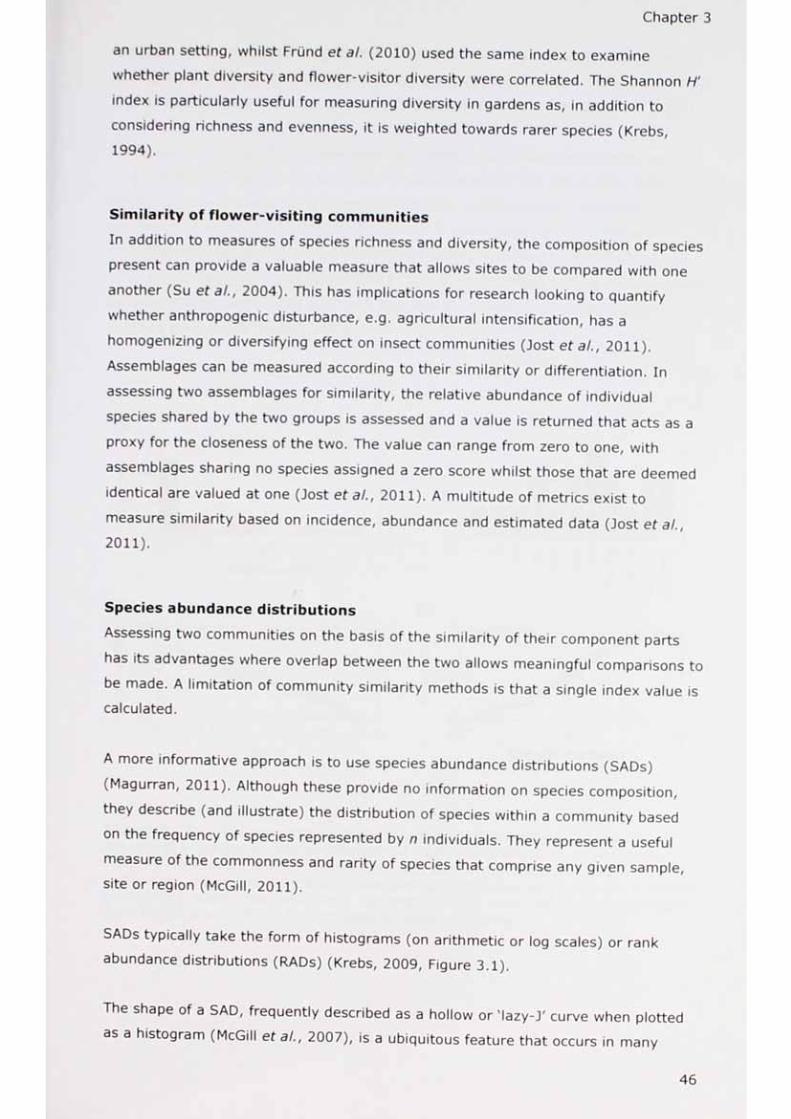
Chapter 3
an urban setting, whilst Frund et al. (2010) used the same index to exam ine
whether plant d iversity and flower-visitor d iversity were correlated. The Shannon H'
index is particu larly useful for measuring d iversity in gardens as, in addition to
considering richness and evenness, it is weighted towards rarer species (Krebs, 1994).
Sim ilarity of flow er-visiting com m unities
In addition to m easures of species richness and diversity, the composition of species
present can provide a valuable measure that allows sites to be compared with one
another (Su et al., 2004). This has im plications for research looking to quantify
whether anthropogenic disturbance, e.g. agricultural intensification, has a
homogenizing or diversifying effect on insect com m unities (Jost e ta l. , 2011).
Assemblages can be measured according to the ir s im ilarity or differentiation. In
assessing two assemblages for sim ilarity, the relative abundance of individual
species shared by the two groups is assessed and a value is returned that acts as a
proxy for the closeness of the two. The value can range from zero to one, with
assemblages sharing no species assigned a zero score whilst those that are deemed
identical are valued at one (Jost e t a l., 2011). A m ultitude of metrics ex ist to
measure sim ilarity based on incidence, abundance and estimated data (Jost e ta/., 2011 ).
Species abundance distributions
Assessing two communities on the basis of the sim ilarity of the ir component parts
has its advantages where overlap between the two allows meaningful comparisons to
be made. A lim itation of community s im ilarity methods is that a single index value is calculated.
A more informative approach is to use species abundance d istributions (SADs)
(Magurran, 2011). Although these provide no information on species composition,
they describe (and illustrate) the distribution of species within a comm unity based
on the frequency of species represented by n individuals. They represent a useful
measure of the commonness and rarity of species that comprise any given sample, site or region (McGill, 2011).
SADs typically take the form of histograms (on arithm etic or log scales) or rank abundance distributions (RADs) (Krebs, 2009, Figure 3.1).
The shape of a SAD, frequently described as a hollow or 'la zy -J ' curve when plotted
as a histogram (McGill et al., 2007), is a ubiquitous feature that occurs in many
46

Chapter 3
multispecies communities ranging from marine benthic environments to Amazonian
rainforests (McGill et a/., 2007). In fact these authors describe the hollow-curve SAD
on an arithmetic scale as 'one of ecology's true universal laws' (McGill et a!., 2007).
A drawback of using RADs is that long tails' representing species characterised by
one or a few individuals vary according to the diversity of the community. This
creates problems when trying to make meaningful mathematical comparisons
between two or more datasets (McGill, 2011). A useful extension to SADs are
empirical cumulative distribution functions (ECDFs), described by McGill (2011, p.
122) as 'the optimal way to plot SADs'. ECDFs facilitate robust testing of data (either
between distinct samples or against a standard distribution) using Kolmogorov-
Smirnov procedures (McGill, 2011).
(a)
9
15
10
5
00
(C )
500Abundance (N)
Rank
4
11000
(b)
(d)
8
CL
x s ; 9c j > r *
aoC \4
CO
S 2!
i f ) - C\
Log1d<% abundance)
8fJ>U I
Figure 3.1 Four ways of plotting species abundance distributions, (a) Histogram showing the number of species (binned) for a given abundance on an arithmetic scale (b) Histogram with abundance on a log2 scale, (c) Rank abundance distribution and (d) Scaled empirical cumulative distribution frequency with a logistic curve fitted through the data points. Copyright (2007) Wiley. Used with permission from McGill et al. (2007), Ecology Letters, Wiley publishing.

Chapter 3
AimsThe aims of this chapter are to evaluate flower-visitor species richness, diversity and
community similarity in 17 English country-house gardens and to compare these
results to other large gardens where data exist.
Research questions
1. What is the estimated flower-visitor species richness for the seventeen
gardens and how does this compare to the actual number of species
recorded?
2. Does overall flower-visitor species richness and the richness of the four most
speciose groups - bumblebees (BB), solitary bees (SB), butterflies and day-
flying moths (BDM) and hoverflies (HF), vary between gardens?
3. How does the species richness data collected for this project compare to
others, namely: a dataset summarising the species recorded at twenty
National Trust properties, a dataset recording the abundance of flower-
visitors at a single large urban garden site and Finally to county-level data?
4. Does overall flower-visitor species diversity and the diversity of the four
groups (BB, SB, BDM and HF) vary among gardens?
5. Are the communities of flower-visitors similar at each garden?
6. Are the species abundance distributions for each of the four groups consistent
across the four sampling periods?
7. Within the assemblage as a whole do any of the groups show patterns
according to season?
48

Chapter 3
Methods
Data collection
Empirical data were collected by sampling gardens in 17 large English country house
estates. Sampling took place between April and September 2010. Full details of the
sites and methods for recording and identifying flower visitors are given in Chapter 2
(2010 field season).
Additional data were collated from a report prepared by Edwards (2003) for The
National Trust. This report described entomological surveys undertaken in 20 of the
Trust's gardens in seven counties between 7 July and 22 August 2003 (Appendix IV).
For each garden a species list was provided, but this did not include insect
abundance. Only data that could be compared directly with that of the present
survey were selected from the report e.g. within the group Diptera - other flies
(Chapter 2), only fly species that corresponded to those recorded in the current
study were considered for inclusion. The data were prepared by compiling species
lists for each of the twenty properties, with each species coded according to whether
it was within the group bumblebees (BB), solitary bees (SB), butterflies and day-
flying moths (BDM), hoverflies (HF), flies (F), solitary wasps (SOLW) or social wasps
(SOCW). By doing this it was possible to calculate the overall species richness for the
twenty properties, as well as assessing the species richness of the groups of interest.
This facilitated a direct comparison between the report and the results of the present study.
A second dataset listing the aculeate Hymenoptera (hereafter referred to as
aculeates) and hoverflies recorded at Buckingham Palace Garden was also obtained.
These data, prepared by Harvey (2001) and Plant (2001), list the species recorded
in the Royal family's garden between 1995 and 1997. The dataset differs from the
current study and that of Edwards (2003) for two reasons. Firstly it represents only a
single site, and secondly the data were obtained primarily as a result of malaise and
pitfall trapping rather than hand-netting. Notwithstanding these differences, this
garden merits inclusion as it represents one of only a handful of studies that have
considered invertebrate populations in large gardens over a sustained sampling
period. Another positive aspect of using these data is that the number of individuals recorded is given.
To consider the species richness of the seventeen gardens sampled in a broader
context (and therefore their potential importance), applications for vice-county (VC)
data were made to national insect recording schemes. Aculeate data for the four
counties visited during the current study were provided by the Bees, Wasps and Ants
49

Chapter 3
Recording Society (BWARS, 2012). On receipt, the data for each county were sorted
according to age. Any species recorded prior to 1938, and not seen after that time,
were excluded e.g., Bombus cuHumdnus, B. distinguendus and B. subterrsneus. All
records for ants (Formicidae) were then removed, thereby creating an overall list for
aculeates (minus ants) for each county. These records were further subdivided into
four groups: bumblebees (BB), solitary bees (SB), solitary wasps (SOLW) and social
wasps (SOCW). The data represent all species recorded per county from January
1939 to September 2012.
Vice-county data for hoverflies were provided by the Dipterists' Forum Hoverfly
Recording Scheme, the national recording body for hoverflies in the UK (Floverfly
Recording Scheme, 2012). The data represent all hoverfly records submitted for the
four counties of interest from January 1975 to September 2012.
Species richness estimates
The statistical program Estimates (Colwell, 2012) was used to calculate the
estimated species richness for the 2010 field data and that of the twenty National
Trust properties (Edwards, 2003). The other datasets (BPG and vice-county lists)
were not suitable for examination using these methods as they were not derived
from replicated sampling sessions. The data collected during the current project
included abundance data, whilst that of Edwards was incidence (presence/absence
data). This meant that although species richness calculations could be performed for
both, they were performed using different indices (non-parametric abundance and
non-parametric incidence metrics, Appendix III).
Several calculations were performed using the data from the current project. These
were as follows: (i) each property was considered separately by using the four
sampling sessions to derive a per-property species richness estimate, (ii) all
properties {n = 17) were combined using the per-property total from each of the
four sessions to generate a single species richness value, (iii) the four most speciose
groups: BB, SB, BDM and HF were each assessed by using the total of four sampling
sessions for each property (n = 17) to generate a per-group species richness value.
For each calculation the recommended default settings for the software were used.
This resulted in the bias-corrected formula for Chao 1 being used unless the value
for doubletons was nil, in which case the alternative 'classic' formula was used
(Colwell, 2012). Two of the three non-parametric species richness estimates that use
abundance data (Chao 1 and Jack 1) are presented for comparison purposes.
50

Chapter 3
As some of the gardens sampled in the current study were sufficiently close for
target species to potentially fly between them, the data were checked for spatial
autocorrelation using Moran's I test in R (package Ape) (R Development Core Team,
2012). The variables used for this analysis were the Jack 1 species estimate values
and British national grid coordinates (Ordnance Survey, 2012).
Having checked for normality and homoscedasticity, one-way ANOVAs were used to
check for differences in species richness between properties (all species across four
sampling sessions and also for the four groups). These were followed up with Ryan-
Einot-Gabriel-Welsch Q (REGWQ) post hoc tests.
For the Edwards dataset (Edwards, 2003), only incidence data were available. Using
Estimates (Colwell, 2012), the species richness estimates for (i) all properties
combined (n = 20) and (ii) the four groups (BB, SB, BDM and HF) were calculated.
The non-parametric incidence estimators Chao 2 and Boot (Appendix III), which are
equivalent to the abundance estimators used for the current study, are presented.
Species diversity
Shannon H' diversity indices (hereafter referred to as Shannon), were calculated for
the 17 properties using Estimates (Colwell, 2012). Indices are presented for (i) all
properties combined and (ii) each of the four groups (BB, SB, BDM and HF). The
software generates a single diversity value and 95% confidence intervals (Cl).
Community similarity
The similarity between assemblages of flower-visiting insects across the 17 gardens
was assessed using Estimates (Colwell, 2012). The Morisita-Horn and also Chao's
Abundance-based Estimated Sorensen indices were calculated for comparison
purposes as they are generated using different criteria (Chao eta/., 2005, 2006;
Colwell, 2012). The former compares abundance between two sites on a species-by-
species basis and benefits from a lack of sensitivity to sample size. The downside of
this index is that similarity is measured according to the composition of dominant
species and largely ignores the effect of rare species, which can be key components
in insect communities (Magurran and McGill, 2011). The latter index is based on the
probability that two randomly chosen individuals, each drawn from one of two
samples, are both representatives of a species that is present in both samples, but
are not necessarily the same species (Chao eta/., 2005, 2006; Colwell, 2012).
The software used to compute these values allows for re-sampling to create
bootstrap-generated standard errors. In the current analysis the recommended '200 re-samples' setting was used.

Chapter 3
An advantage of using Chao s abundance-based method is that it incorporates
unseen species, i.e. it takes into account the contribution that a species can make
when it is present at both sites but not necessarily detected at one of these (Chao et
al.t 2005; Colwell, 2012), thus reducing the negative bias associated with more
traditional indices (Chao et a/., 2005). Although this index is less likely to be affected
by dominant species (as per Morisita-Horn), it does not benefit from the detailed
species-by-species analysis that the aforementioned metric performs (Magurran and McGill, 2011).
As yet, multiple comparisons across sites remain too complex to be computed easily
(Jost et a i, 2011) and therefore community similarity remains a calculation typically
performed between two sites only. This produces multiple pair-wise results that
require individual testing to establish whether a result is significantly different from
another. Although Bonferroni (Field, 2009) or Dunn Sidak (Sokal and Rohlf, 1981)
corrections help to avoid the Type I errors associated with multiple testing, when
used at such a large scale they risk introducing Type II errors.
To overcome this, a different approach was taken to assess the results generated.
Firstly, the values produced from the multiple comparisons were ranked according to
their value (n = 136). As a low similarity score represents poor congruence in
species overlap between sites, the lowest 5% of values were determined. These
values (n = 7) were then examined to establish whether a disproportionate number
were represented by an individual property. This approach was taken for both the
Morisita-Horn and the Chao Abundance-based Estimated Sorensen values.
An independent, but complementary, method of looking at community similarity is
the creation of a dendrogram using nearest neighbour hierarchical classification
techniques (Oertli et a i, 2005). The Jaccard dendrogram created using SPSS (IBM
Corp., 2012) represents a binary index that discards joint absences and gives equal
weight to matches and non-matches alike.
Species abundance distributions
To overcome the problems associated with testing rank abundance distributions,
empirical cumulative distribution function (ECDF) plots were created. For each insect
group the abundance of individuals from each species was used to examine
differences across four sampling sessions. Complementing this, the insect data were
incorporated into plots categorised by each of the four sampling sessions.

Chapter 3
In order to create the ECDFs for each insect group, the abundance of each species
(per session) was ranked in ascending order and the fraction of the total abundance
calculated. This was then plotted on a log-transformed x axis. The species data were
maintained in the same ranked order and plotted as fractions of the total species
richness on the y axis (McGill, 2011). The resulting ECDFs were tested for
differences using a two-tailed Kolmogorov-Smirnov test with critical values (a)
adjusted using the Dunn-Sidak method (Sokal and Rohlf, 1981, Appendix V).
ECDFs for the four sampling sessions in the season were created in the same way.
As honey bees are classed as a single species for the purposes of this study, the
data could not be used to prepare ECDFs. To compare the difference in honey bee
abundance across sessions, the number of honey bees observed at each property
was summed. The original and transformed data did not meet assumptions for
normality, therefore the non-parametric Wilcoxon signed ranks test was used.
Results
Overview of results
The sampling of seventeen properties in 2010 (each on four occasions) yielded a
total of 9,893 records of flower-visiting insects from 174 species (Appendix VI).
Approximately 1.5 insects were recorded per minute over a total area of 6.12ha.
Hoverflies were the most abundant group (4,430 individuals) followed by
bumblebees (2,870), honey bees (801), solitary bees (674), and butterflies and day-
flying moths (613). The remainder (505) were comprised of other flies, solitary and social wasps.
Of the four sampling sessions, Session 3 produced the most insect records (4,935).
Almost 50% of all individuals recorded in 2010 were from this session (mean 290.3
± 148.1 individuals per property).
The results of Moran's I test showed no significant autocorrelation between sites, P =
0.87, therefore independence of locations was assumed.

Chapter 3
Species richness
The total number of species recorded for each of the 17 properties ranged from 23
at Kirby (KIR) to 75 at Courteenhall (CHALL) and Steane (ST), mean 61.6 ± 12.1.
These values, together with the results of the Chao 1 and Jack 1 species richness
estimators for each property, are presented in Table 3.1 and Figure 3.2.
The per-property species richness estimates were plotted against the pooled total of
flower-visiting insects per property (Figure 3.3). The lines of best fit for Chao 1 and
Jack 1 were almost identical, although the spread of data points around the trend
line for Chao 1 was greater.
54
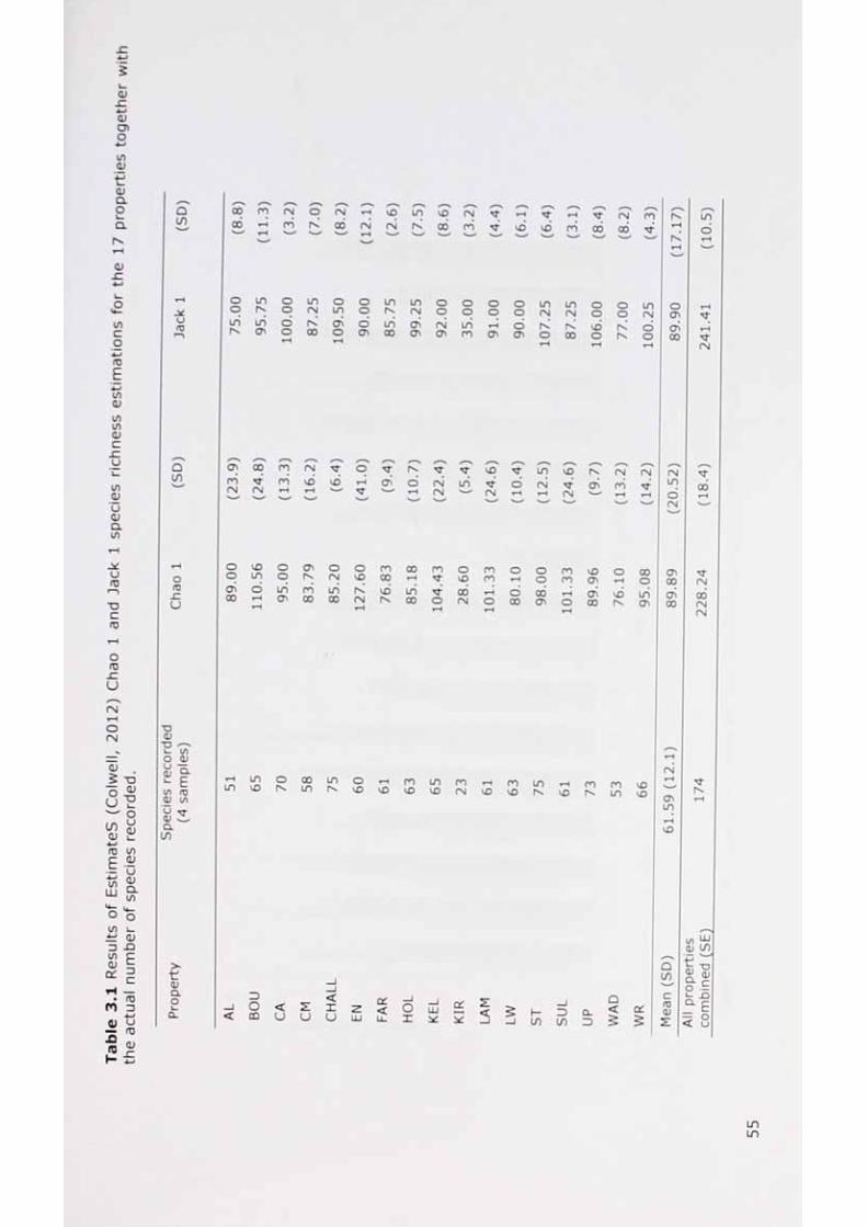
$
<D
<13cno
U)03
t03Q .OCL
i n
03
l/>co<T3E1/3 <13l/>l/>o
u
U1<vuoCLl/>
Qin
u r0
Qin
00CO
ro fNro
oin
rsico fN
sOrsj
in sOoo
fNro vO
M-sb
o in o in o o in in o o oo•
IN•
o#
rsi•
ina
o�
i n fN o o oin in o fN a s
w
o in as rsi in•
a s o 00 o as 00 a s a s ro as
O s o o
rorsi
^rrsi
inrsi
OS o
cnro
rsis b v b os
rNo rsi
rsj
■STin
so
rsi
s ro
inn i
ro
inrsiin00
■sroo
so■srrsi
voo
fNoo
ro
INOS
rNfN
fNro
inrsi
•
oo
rsi^ r
o>Os00
rsiin
fN
in
■srrsi
^ roo
uro
TDCfT3
o<33
U
oo •
sDin•
oo •
asIN•
ofN•
oVO•
ro•
00•
ro•
osO
roro
o oo
roro
SOas
o 00o £00
■sj-rsi
as00
o inas
roCO
in00
rNfN 7
6 in00
^ro
00fN
•
o
•oCO
00as
•
oa s sb
fNuoa s
as00
COfNfN
ofO
u
rsiofN
> • £ T3
U
L0003Ei/)LU
<u�aoua
toaju03C lio
° o10 i_
a>=3 -Q
IS I* irH —
• fOm oQJ U
s *
■Oa;
ioo a>
s |io no D 10<u CLc lcn
t<13CLO
in insO
OCO
<u
< X
o u
co in in IN sD so ro in ro
sO SO (N sOrosO
inIN s o
rorN
roin
CL< o UJ CL
< £ h- 32 _J _J LO in
a<< i
sosO
QC£
fN
asin
so
Oin
03a»
N-fN
</> }JJ<l» in
o -
E< 8
inLO

<L>
h
V/)<D
*
U ,
<vCl OU) 03
O U■
QinCd
£ IIO (/)< T O
£ L_o
CL3
LU•
ID -*CO U
T O
h- T3CO C
T O
OT O
6if)
3 OT O
cd E> t/)t <u
—i <U l/)LU ao
COa>c
a u•OO
T O
K
00oCD
hU
fN fN
ssauipu
U

C hap te r 3
O actua l num ber of species
A C h a o 1
Jack 1
Abundance of flower-visiting insects per property(total for 4 sampling sessions)
Figure 3.3 Species richness for the actua l num ber o f spec ies recorded (open d iam onds) the estim ators Chao 1 (filled triang les) and Jack 1 (filled squares) aga inst the abundance of ind iv idua ls per property . Each sym bo l rep resen ts fou r sam pling sessions. Solid trend line (Chao 1), dashed trend line (Jack 1).
A one-w ay ANO VA revea led a s ign ifican t d iffe rence in m ean actua l spec ies richness
between p roperties across the fou r sam p ling sess ions, F 16 51 = 2.88, P = 0.002. Post
hoc tests (REGW Q) show ed K irby (KIR) was s ign ifican tly d iffe ren t to th irteen o ther
properties (F igure 3.4).
57

C hap te r 3
Property
Figure 3.4 Ranked m ean spec ies richness fo r each p roperty ( fou r sam p lingsessions). Identica l le tte rs show hom ogeneous g roups (REG W Q p o s t hoc tests). E rror bars = 95% C l.
The species richness and estim ato rs fo r each o f the fou r insect g roups is g iven in
Tab le 3.2. H overflies w ere the m ost spec ies-rich g roup, fo llow ed by so lita ry bees.
Table 3.2 Species richness estim ates fo r the fou r m ost spec io se flow er-v is ito r groups.
G roups fo r species richness estim ates
Speciesrecorded
Chao 1 (SD) Jack 1 (SD)
Bum blebees 14 15.00 (0.3) 15.94 (0.9)
So litary bees 50 72.13 (16.4) 68.88 (5.3)
Butterflies and day-fly ing m oths 31 36.60 (3.9) 43 .35 (3.9)
Hoverflies 59 85.33 (14.5) 85.65 (4.1)
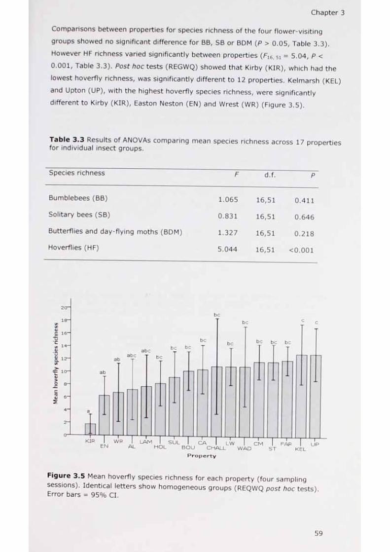
C hap te r 3
Com parisons betw een p roperties fo r spec ies richness o f the fou r flow er-v is iting
g roups show ed no s ign ifican t d iffe rence fo r BB, SB o r BDM (p > 0 .05, Tab le 3.3).
H ow ever HF richness varied s ign ifican tly betw een p roperties 51 = 5.04, P <
0.001, Tab le 3.3). Post hoc tests (REG W Q ) show ed tha t K irby (KIR), w h ich had the
low est hoverfly richness, was s ign ifican tly d iffe ren t to 12 properties. Ke lm arsh (KEL)
and Upton (UP), w ith the h ighest hoverfly spec ies richness, w ere s ign ifican tly
d iffe ren t to K irby (KIR), Easton Neston (EN) and W rest (W R) (F igu re 3.5).
Table 3.3 Resu lts o f AN O VAs com paring m ean spec ies r ichness across 17 p roperties fo r ind iv idua l in sect groups.
Species richness F d.f. P
Bum blebees (BB) 1.065 16,51 0.411
So litary bees (SB) 0.831 16,51 0.646
Butterflies and day-fly ing m oths (BDM ) 1.327 16,51 0.218
Hoverflies (HF) 5.044 16,51 <0.001
P r o p e r t y
Figure 3.5 Mean hoverfly spec ies richness fo r each property (fou r sam pling
sessions). Identica l le tters show hom ogeneous g roups (REQ W Q p o s t hoc tests) Error bars = 95% C l.
59

C hap te r 3
Species richness: Comparison with other locations
The recorded spec ies richness (toge the r w ith spec ies richness estim ates) fo r the 20
NT gardens sam pled by Edw ards (2003) is g iven in Tab le 3.4. The data presented
are fo r all p roperties com b ined and fo r the fou r insect groups. For com parison , the
datase ts from the cu rren t study and that o f Edw ards are presented toge the r in Tab le
3.5.
Table 3.4 Species richness (actua l and estim ates) fo r the 20 NT gardens sam p led byEdw ards (2003). Note, no standard dev ia tion va lues are p rov ided by the E s tim a tes so ftw are fo r Boot.
G roups fo r spec ies richness estim ates
Speciesrecorded
Chao 2 (SD) Boot
All 20 properties 178 269.88 (29 .08) 208.73
Bum blebees 12 12.24 (0.71) 13.08
So litary bees 34 44 .45 (8.09) 39.18
Butterflies and d ay -fly ing m oths 25 45 .25 (20 .19) 28.64
Hoverflies 54 83.39 (16.6) 63.63
Table 3.5 Com parison o f recorded spec ies richness fo r 17 ga rdens in the cu rren t study w ith tha t o f 20 NT gardens (Edw ards, 2003). Note 'A ll p rope rtie s ' va lue inc ludes species not w ith in the fou r g roups deta iled .
Recordedspecies
Estimatedspecies
Presentstudy
Edw ards(2003)
Jack 1 (P resen t
study)
Chao 2 (Edw ards
2003)
All p roperties 174 178
--------- - i f __
241.41 269.88
Bum blebees 14 12 15.94 12.24
Solitary bees 50 34 68.88 44.45
Butterflies and day-fly ing m oths 31 25 43.35 45.25
Hoverflies 59 54 85.65 83.39
60

C hap te r 3
Comparing species richness across gardens
Extend ing the com parison o f the cu rren t study to tha t o f a sepa ra te la rge garden
(Buck ingham Palace G arden - BPG), and a lso v ice-county data, perm itted the
inclusion o f tw o add itiona l insect groups; socia l and so lita ry w asps (SO CW and
SOLW ). The fou r v ice -coun ties listed in Tab le 3.6 co rrespond to those v is ited in the
cou rse o f the p resen t study.
61

Ta
ble
3.6
Re
cord
ed
sp
eci
es
rich
ne
ss f
or
fiv
e i
nse
ct g
rou
ps.
D
ata
are
fro
m t
he
cu
rre
nt
stu
dy
, E
dw
ard
s (2
00
3),
th
e s
pe
cie
s lis
ts f
or
BP
G (
Ha
rve
v
20
01
an
d P
lan
t, 2
00
1)
an
d v
ice
-co
un
ty (
VC
) re
cord
s. T
he
la
tte
r a
re f
rom
BW
AR
S f
or
be
es
an
d w
asp
s (1
93
9 -
20
12
) a
nd
th
e H
ov
erf
ly R
eco
rdin
aS
che
me
fo
r h
ov
erf
lies
(19
75
- 2
01
2).
Va
lue
s in
bra
cke
ts r
ep
rese
nt
(wh
ere
av
aila
ble
) th
e n
um
be
r o
f re
cord
s co
ntr
ibu
tin
g t
o t
he
sp
eci
es
rich
ne
ss
fig
ure
s. N
ha
nts
. =
No
rth
am
pto
nsh
ire
, B
ed
s. =
B
ed
ford
shir
e,
Bu
cks.
=
Bu
ckin
gh
am
shir
e a
nd
Wa
rks.
=
Wa
rwic
ksh
ire
.
O'vOChro
rooov£>in
O'rvoo
rsi
rsicncn
to rs rs cofN
oo ro
no$
in cr> O'o vo 00CD in H
rorovOco
couDCO
in ro<n
ooo
oo ooVO
oorsi
O'rv
O'in
ooco
cooovD
coT3CDCO
fOO
u
Q-CO
CO�o O
Csj fO
! cLU
rs fNN
fM lD
CD><nX
CvO'O' fN
in O'
• ccn 03
i rv O'
cocro
O r—1vD O' in<n ro cn 00ro
rH 00 rsrH vD 00
oofNfN
inO'O'
O'
O' L.' 3 C L <
< I
fN00
_ in o cr>£ 2
p .£ Q.
<Eo
CD>
in O' vD roin O' in t-HrH t-H CO
O'O'in
u03�OCD £
TDE
VD ro o VD(Nrs
ro ro
fN ro rsH ro m
ou CD
5 1
<n £
oco (j
C L Q . 03
cro CD
CO
o in fN orv CO O' CO00 vD CNfN

C h a p te r 3
Sam pling effort
The re la t io n sh ip b e tw een th e n u m b e r o f s p e c ie s re co rd e d fo r e a ch in se c t g ro u p and
th e n u m b e r o f re co rd s on w h ich e a ch v a lu e is b a sed ( th e s a m p lin g e ffo rt) is sh o w n in
F ig u re 3 .6 . T he d a ta p o in ts fo r th e c u r re n t s tu d y a re in red .
W ith th e e x ce p t io n o f SO LW , th e d a ta p o in ts fro m th e c u r re n t s tu d y a re w ith in (o r
c lo se to ) th e ra n g e o f th e o th e r tw o s tu d ie s and th a t o f th e v ic e -c o u n ty d a ta .
N um ber of records ( lo g 10 scale)
Figure 3.6 R e la t io n sh ip b e tw een th e n u m b e r o f s p e c ie s re co rd e d and th e n u m b e r o f re co rd s fo r f iv e in se c t g ro u p s u s ing d a ta fro m tw o s tu d ie s : th e c u r re n t w o rk and BPG
A l r v ic e -c o u n t ie s . D a ta a re p re se n te dus ing log s ca le s . Red d a ta p o in ts sh o w th e p o s it io n o f th e c u r re n t s tu d y w ith in th e c o n te x t o f th e o th e rs .

C h a p te r 3
Species d iversity
T he S h a n n o n d iv e rs ity in d e x v a lu e s fo r e a ch o f th e 17 p ro p e r t ie s a re g iv e n in F ig u re
3 .7 . T h e d iv e rs ity v a lu e fo r K irb y (K IR ) is s ig n if ic a n t ly lo w e r th a n e ig h t o th e r
p ro p e rt ie s . T he o v e ra ll S h a n n o n d iv e r s ity fo r a ll p ro p e r t ie s c o m b in e d is 3 .0 6 ± 0 .1 8 .
In a d d it io n , S h a n n o n d iv e r s ity v a lu e s w e re c a lc u la te d fo r th e fo u r in s e c t g ro u p s
(F ig u re 3 .8 ) . T h e h o v e r f ly (H F ) g ro u p w as s t ro n g ly d o m in a te d b y a s in g le sp e c ie s ,
Ep isyrphus ba/teatus and a se co n d c o m p o u n d -s p e c ie s , Syrphus spp . (se e C h a p te r 2,
M e th o d s). T o g e th e r th e se a c co u n te d fo r 6 1% o f th e 4 ,4 7 4 h o v e r f ly re co rd s . A s a
re su lt th e h o v e r f ly d iv e r s ity v a lu e s w e re re -c a lc u la te d to e x c lu d e th e se . Fo r
c o m p a r is o n p u rp o se s F ig u re 3 .8 in c lu d e s h o v e r f lie s ( i) in th e ir e n t ire ty , ( ii) w ith o u t
E. balteatus, and ( iii) w ith o u t E. ba/teatus an d Syrphus spp .
64

£
Q<£
to
uo
£
55
cc
LLJt;<daoa
<
u
u
<u
OCD
LOro ro
inrvj
inrsi
ari|BA A)i s j 3a ;p uouu eqs
LOo
U
o 'LDG\
infD
LLI
ina>U<DCLin
r o
in
inina;incn
O l
Er o
in
DO
ina;t :a»
oCL
(D
ufD<D
in<V
03
inQJ>T3
fD
r sn
a;
33)
• ■ ■
LLLDl D

C h a p te r 3
B B S B BD M HF HF (e x c . HF (exc .Eb ) E .b /S . sp p .)
Insect group
Fig ure 3.8 S h a n n o n d iv e r s ity fo r fo u r in s e c t g ro u p s (1 7 p ro p e r t ie s , a lls a m p lin g s e s s io n s c o m b in e d ) and th e re c a lc u la te d v a lu e s fo r h o v e r f lie s (H F).HF (e xc . Eb) = h o v e r f lie s e x c lu d in g Ep isyrphus ba ltea tus o n ly . HF (e xc . E .b /Ssp p .) = h o v e r f lie s e x c lu d in g E. ba lteatus and Syrphus spp . c o m b in e d . E r ro r b a rs = 9 5 % C l.
Com m unity sim ilarity
The re su lts o f th e p a ir -w is e s im ila r ity c o m p a r is o n s (M o r is ita -H o rn and C h a o 's
A b u n d a n ce -b a se d E s t im a te d S o re n se n in d ic e s ) a re g iv e n in T a b le 3 .7 and T a b le 3 .8 .
In each ca se th e to p h a lf o f th e m a tr ix re p o r ts th e in d e x v a lu e , w ith th e lo w e r h a lf
sh o w in g th e n u m b e r o f sh a re d sp e c ie s .
A d e n d ro g ra m u s in g n e a re s t n e ig h b o u r h ie ra rch ic a l c la s s if ic a t io n te c h n iq u e s sh o w s
K irb y (K IR ) a s a s ig n if ic a n t o u t lie r (F ig u re 3 .9 ).
66

Ta
ble
3.7
Res
ult
s o
f M
oris
ita-
Hor
n p
air-
wis
e co
mp
aris
on
s fo
r co
mm
un
ity
sim
ilari
ty.
The
top
hal
f of
th
e m
atri
x re
pre
sen
ts t
he
Mor
isit
a-H
orn
va
lues
, w
ith t
he l
ower
hal
f d
etai
ling
th
e n
um
ber
of
shar
ed s
pec
ies.
The
val
ues
in
bra
cket
s sh
ow t
he
tota
l n
um
ber
of
spec
ies
reco
rded
for
eac
h pr
oper
ty.
Val
ues
in
red
are
the
seve
n l
owes
t va
lues
(lo
wes
t 5%
). V
alu
es i
n bo
ld r
ed h
igh
ligh
t co
mp
aris
on
s th
at r
elat
e to
Kir
by
(KIR
)
> *3 VO
O<3
CLD
coLf)
corN
co cm
rNo
incoiD
OOin
ino
00fNCO
COO'00
o o
COinoo
oofNCO
O'in
'O’O'in
ininio
o o o
in
oo
fNcoin
vOooin
rocooo
inco'T
CO«oiD
OO
'O’o
inin
ioinoo
'0-'i-in
'rcr>
coiO00
fNin'0’
o o o o
fNCOiO
o o o o o o
IN
00o o o
'O’00'f
00 00 co o in O 'o in ' O ’ 00 co in CM' O ’
9in
a
in9
in iD in ino
•
o o9
o•
o9
o9
o
CM in 'O’ a> in CMID t - H O' rN o 00f H ID
•
ID9
IN•
fN fN•
o O o O9
o9
o
o rN O ' O iDCO 00 O' in ' O ’ 'O’CO fN ID in uoo
•
o•
O•
o9
o
00fN
00CO
D ID
1C
3 CO-J VD
z -< ID
CO2 ™
00 co rN in O' CO uo in CM 'O’cr> o o o 'O’ 'O’ * — < co O ' fN'O’
9'O’
9
009
'O’pID
•'O’ 'O’ co CM CO
o o o op
o•
o9
o9
o9
o9
o
rN fN CO o lO o in in coO' CO uo 00 ID 'O’ 00 ID corN in
9'O’ rN 00 iD 00 00 00 co
6 op
o•
o9
o9
o9
o9
O9
o9
o
o fN o 00 in CM (N 'O’ co INfN CO CO O' IN rN rN iD ID 'O’00
9
rN9
'O’9
00 00 ID9
00 00 00 COo o O o
p
O o9
o9
o9
o•
o
rN co 00 O' fN 00 in infN fN CO CO iD 00 CM o coIN
900 'O’ O' 00 in 00 00 00 co
O o o o•
O9
o9
o9
o9
O9
O
CO 00 in ID ID CM rf IN00 rN co O T - 4 O fN 00 00in9
co9
co9
CO 'O’9
'O’9
CO9 CM fN
o o o •
o o o o •
O•
O
rNoTT
CO00IN
ofN
00CO'0-
IDfN00
ID'O’
o o o
ID O \r co
in co r ^ in n
N fM O' h H fN H fN
'O’CO
iD O ' O ' »-4'f n ^ n tj-
id co in co idco 'T tr co co
VD id
m in^ VD
oz
COiD
a<u. VD
zLU iD
_i in< t zu
2 S 'U in
<U IN
oCD
invO
in
CO CO CM t-Hco vD t-H t-H00 in 'T CD
pp
o•
o9
o9
o
O ' iD CO o'O’ 'O’ rN rN00
Ain
9
co fN•
o O9
O9
O
'O’ CM 'T orN IN O ' O '00 in 'O’ IN
9 9 9 9
O o o o
CO fNrN o 00 iniD
MID CO uo
W
o9
O9
o9
o
00 in 'O’rN fN fN inrN rN iD 00
9 9 9 9
O o o o
in 'T O 'O ' CO rNvD
900 'O’
O9
O9
O
ID M0 rNCM CO coin
9'O’
o9
O
'O’ iD CMvD CO coin
9
O
CO fNCO CO CO
T-H iD «—i'O’ o 'O’fN9 in O 'o
9o
9o
in CO rN'O’ 00 '0-rN in O 'o
9o
9o
o rNo O '00 ino
9o
CMrN COid
•
o
00CO 'O’
ocoO'
fN'0’
O 'CO TT
inCO CO
O' H fN oo H H 'T ^
i d CO O 'O’ ^ fN
oo o oo rN m rNfO CO CO CO h
vd o in oo rN h'O’ 'O’ co co co fN
fN 'O’ lO in co co
CO CO CM fN VD in'O’ 'O’ 'O’ 'O’ 'T CO
N ' D c o i n i n H ( j \ c o^ C O ' T ' O ’ C O ' T I N C O
f N c o c o o k O O ' i r N ' O '’- H C O C O ' O ’ C O C O f N C O
n n in o in md'O’ 'O’ "O- 'O’ in co '0-
vD o hC0 'O’ 'O’
'T CO 'O’ O' 'O’
N in CO CM CO 'O’ CO CO
’-I VJD CO t-h"O’ CO 'O’ 'O’
'O’ co uo'O’ co co
co CO -O’fNCO
*-< COCO CO
'O’ CM CO CO fNCO CO CO CO CO CM CO
O < Z Z Z< co u U U LUa _j a z _i< O u j » H < g | - D Q .
G< a5 5

Tab
le 3
.8 R
esu
lts
of C
hao
Ab
un
dan
ce-b
ased
Est
imat
ed S
oren
sen
pai
r-w
ise
com
par
iso
ns
for
com
mu
nit
y si
mila
rity
. T
he t
op h
alf
of t
he
mat
rix
rep
rese
nts
the
Cha
o A
bu
nd
ance
-bas
ed E
stim
ated
So
ren
sen
val
ues
, w
ith t
he
low
er h
alf
det
ailin
g t
he
nu
mb
er o
f sh
ared
spe
cies
. V
alu
es i
n re
d ar
e th
e se
ven
low
est
valu
es (
low
est
5%).
Val
ues
in
bold
red
hig
hlig
ht
com
par
iso
ns
that
rel
ate
to K
irb
y (K
IR).
oc fN to 00 to fN in o IN rsj in r \£ 00 ON to ON H in H ON y — ( ON in O o n
■
fNON•
00•
00•
00%
ON•
O '*
ON 00 ON fN ON o n 00 ON 00 ONo o o o o o o
•
oA
o•
o•
o•
c•
1 o•
o•
o•
O
o ro in to 00 o rN in ro fN in fN< to in in ro in r—t ON t r ON vH 00 ON CO inO '
•
00•
00•
ON•
ON•
rN•
00•
•
o O ' to ONA
00• oo 00 O 'o o o o o o o o •
oV
OA
o o•
o•
o
CL to in in 00 in o ro in o fN fN CT* 00D 00 ON fN IN t r o 00 ON IN ON in rN in CD rN00•
00•
ON•
ON•
ONA
ON*
00 00 ON 00 ON ON ONV
o o o o o op
o•
oA
o•
o•
o•
o#
o•
o
t r o to ro fN fN ro to to fN IN fN ro3 fN 00 in to 00 00 to 00 00 00 O ' in O ' fN v£>to O'•
ON•
O '+
ONA
ONA
00*
ON ON ON rs O ' ON ONo o o o O
p
o•
o•
o•
o •
o•
o•
o•
o
fN in ro 00 to to in ON o ro fN inin ro ro fN fN ro ON t j - o 00 00 ON 00 to fN inO '•
ON•
00•
ON•
O '•
ONA
ON O ' ON ON ON ONo o o o o o o
•
o•
o•
o•
o•
o
rvTT
oo n00
3-
O n
o o
ors iO n
rvO'o
inO '
toooO '
00tTO '
in
o n
otOON
o o o
fNinIN
00O '
in oo h c m oo to in rv vo in
Z T—* O CO o r\ r tr< in to tO 00 CO o to tO 00ZJ O '• ON
A
ON% ON O 'A o ON ON ONo o o
A Ao o
A •o
•o
Ao
CL ON ro rv ON ON IN trV ON o m to in n to fNCO• 00
AN CO• • IN rs ON
o o •o o o o •
o#o
wO
AAA ON ON to (O tO fN roLU to ro O ' CO r to tO tOON• ONm 00A O ' ON ON ON O 'o o
wo O
#o
•o
•o
•o
ON o in o 00 Ho fN ro ON »—( m T—i ro toX ON
AO 'm 00A O ' ON ON ON
o ow
o•
o•
o•o
•o
CL 00 o ON o 00 00 to< to to <N ro fN inLi. ON• ON• CO ON ON ON
o o o•
o#
o•
o
2 00 to to O ' ON 00 in fNLU 00 in IN 00 in r t i- r\
CO• O '• ONA 00 ONo o
w
o•
o•o
_J to to o in in ro fNfN IN ro T-H in tO in< ON O ' O ' ONX • • • •
u o O o o
z 'J- fN rN ro 00 tO 00 roCJ fN ON tO ■tr ro '=3- tr 00O '
•00A O '
o o•
o
< in ON in ON 00 fNu in in tO IN tj- inON ON
rofNO'
A
o
rvrs i
to
fN
CO fN N CD Hin to to to
CO fN O in t N O'(N fN fO fN N IN h
O' 'O tr ro m n inin in fN ro in to in
^ o m o into in in O ' to to to
t CO ^
in tj- in to
oo in oon
to in in to fN to coto in fN o to tr in
ro to ro o rN to to to to rN
tj- in in to to totoTT
n tr in O' h 'f in n in O' in
Oco ON
o
t o m t o t j - ^ - T j - ^ ' ^ v O t o i n o i n t r ' ^ -
r . in ro tj- ^ o o o o o T - t O N i n o N ’t r o N t o ofr' f YN n ' T n n n n N r o t r m
<O < Z xCO ( J U ( J
< o ijj £ ^U- X ^ ^ _J
QQ_ < C L
CO CO 3 ^ ^ 0 0to

C h a p te r 3
A L
B O U
F A R
K E L
U P
H O L
S U L
C M
LA M
C H A L L
W A D
C A
EN
W R
S T
LW
K IR
Figure 3.9 D e n d ro g ra m sh o w in g n e a re s t n e ig h b o u r lin k a g e b e tw e e n 17 s ite s based on in c id e n ce d a ta fo r s p e c ie s p re se n t ( Ja c ca rd m e th o d ) .
Species abundance d istribution (ECD Fs)
The E C D F s fo r ea ch o f th e fo u r in se c t g ro u p s a re g iv e n in F ig u re 3 .1 0 . T he p lo ts
show th e d is t r ib u t io n s a c co rd in g to e a ch o f th e fo u r s a m p lin g se s s io n s . T he re s u lts o f
K o lm o g o ro v -S m irn o v te s ts fo r d if fe re n ce s b e tw een sa m p lin g s e s s io n s w ith in
in d iv id u a l g ro u p s a re p ro v id e d in T ab le 3 .9 .
69

oo+
oo+
oo
9
rsi
OO
CO(/>
cr>O
O■
fNO
OO
Vrouino
6 )o
Q)UcCO■Oc3
Ar o
roOT
oo
cotoao
roi
U .I
009
oCO
9
orsjo
oo
<3-o
009
o<x>d
rx
jo u o ij jo d o jd 3A !)e |nu in3 jo u o ij jo d o jd d A i)e |n iu n 3
fN ro rIS) t/> \A\s> \A<V a; 0/ QJLO to io tO♦ ■ ◄ X oo o
o+
X
iV
? ♦◄ ■
x ◄
♦
* *
◄
◄ ◄
COCD
oo
oIoo
rsiO
oo
rsiO
Oo
mO
oo
O
zDCO
vr o
uV)OH
Olo
VUCr o
■oc3
nr o
oco
oao
00o
CDo
rgLUO
00 IDo o
cno
jo u o j j jo d o jd 3A i)e |nu jn3 jo u o j j jo d o jd O A ije |nu jn 3
■DCr o
<E<ut*3-O
CDCO
ioa»a;-O
r o
oio
CO£coa;a;(D
Eco
• •
io Cl cu3 CO2 oi o> c
t> g-
.E IA c- ro
o 10
CO
o
<DCO2Q.2jAO
Qu EUJ
IA
OUo d) => (Ac r _2 u
ro LU
3-Q
LL-X
lAto
• ma^ma>
TD1*
(V a>>
• ammm >r o
I |o roU V
ro ^ u l j
’C CD
E ^m o2 E« ?<u '
3

Chapter 3
Table 3.9 Results of Ko lm ogorov-Sm irnov tests between sessions for each of four insect groups. P va lues in bold are s ign ificant for P < 0.05. P va lues in bold red are s ign ificant fo r an adjusted P o f < 0 .0085 (D unn-S idak method).
Kolm ogorov-
Groupsessions
com paredSm irnov Z
valueMonte Carlo
s ign ificance (P)
BB 1 2 0.64 0.704BB 1 3 0.584 0.801BB 1 4 0.605 0.741BB 2 3 0.673 0.659BB 2 4 0.355 0.996BB 3 4 0.63 0.727
SB 1 2 1.378 0.022SB 1 3 2.307 0 .0 0 0SB 1 4 2.378 0 .0 0 0SB 2 3 1.805 0 .0 0 1SB 2 4 1.601 0.005SB 3 4 1.14 0.072
BDM 1 2 0.969 0.184BDM 1 3 1.318 0.038BDM 1 4 0.378 0.979BDM 2 3 1.505 0.010BDM 2 4 0.836 0.333BDM 3 4 1.318 0.035
HF 1 2 1.202 0.062HF 1 3 2.61 0 .0 0 0HF 1 4 1.052 0.129HF 2 3 2.733 0 .0 0 0HF 2 4 1.093 0.102HF 3 4 1.943 0 .0 0 0
The ECDFs for each of the four sam pling sessions are given in Figure 3.11. The plots
show the d istribution according to each of the four insect groups. The resu lts of the
Ko lm ogorov-Sm irnov tests for d ifferences between groups w ithin the sam e session are provided in Table 3.10.
71

oo
<NCo!a(Ao</)
♦
oo
fNO
COo
oo
o
« 00 O 'S ’ fN od o d o
saioodsjo uojjjodojd 0 Aije|nujn3
00O
VOO
c m• • o o
oIL Uo
CMOOO
QJT O
uIA
O)o
uucT O
Uc3A
T O
coO
jo uoijjodojd 3Aije|nujn3
co
• M
tOao
<u0)i t
T O
IA
c<L>toQJ
C La;
V)o
Euio
QJIA
UT O
tAcoCA IA <U IA
cnc
Q.ET O
IA
<L>
CO Q a.CO LO CO x♦ □ ◄ X
Co'!a(AU(/)
co+
U J
O
Oo
fNoLU
COoIU Jo
1 oq VO <3- PM o
d o d o sopods jo
uo;jjodojd dAjjeiniur^
oo
X
9♦ ♦
Mill M i l l
Xn
co!a(Aa(/)
•>W ♦
V \ A A A A A A A Jy U Q fX X X X X X X /x j o o q o C X X X X xX jygppQ Q Q O Q fV
00o
VO
o orsjo
oo
oo
VT O
u(A
O* »
D>o
CMO
<UucT O
■ac3
T O
coO
>8888* ♦ ♦ P
co
• mm
toao
OI
oo
jo u o ij jo d o jd 0 A ije |n u jn 3
to
oCL
QUL U
Uc(D 3 CTa»
3
to•D<D
T O
E3U
T O
U
CLE
L U
cn 2<u a>□ «« 8 PMr\

Chapter 3
Table 3.10 Results of Ko lm ogorov-Sm irnov tests between groups for each of four sam pling sessions. P va lues in bold are s ign ificant for P < 0.05. P va lues in bold red are s ign ificant for an adjusted P of < 0 .0085 (D unn-S idak method).
Sam plingsession
Groupscom pared
Kolm ogorov- Sm irnov Z
value
Monte Carlo s ign ificance
1
1
1
1
1
1
BBBBBBSBSBBDM
SBBDMHFBDMHFHF
1.7840.6901.3351.9871.3110.809
0.0020.515
0.0300 .0 0 00.0360 .0 0 0
222222
BBBBBBSBSBBDM
SBBDMHFBDMHFHF
1.1730.7600.7051.1611.6432.136
0.0810.425
0.0020.070
0.0040 .0 0 0
333333
444444
BBBBBBSBSBBDM
BBBBBBSBSBBDM
SBBDMHFBDMHFHF
SBBDMHFBDMHFHF
1.2451.3191.5001.5052.7712.347
0.7560.7800.7290.9081.7631.508
0.0360.0380.0120.0090 .0 0 00 .0 0 0
0.4340.4590.5100.222
0 .0 0 10 .0 1 1
The num ber of honey bees recorded in each garden during each of the four sam pling
sessions is provided in Table 3.11. The resu lts of W ilcoxon signed ranks tests
showed that a s ign ificant d ifference in honey bee abundance was found between
sessions three and four and sessions two and four (Table 3.12).
73

Chapter 3
Table 3.11 Honey bee abundance at each garden in each of the four sessions
Session1
Session2
Session3
Session4
Total per property
AL 7 7 16 1 31BOU 1 2 30 10 43CA 15 3 8 74 100CM 3 10 7 27 47CHALL 5 19 13 42 79EN 3 1 0 1 5FAR 30 3 6 7 46HOL 1 4 5 9 19KEL 0 7 14 32 53KIR 4 0 0 0 4LAM 1 0 6 32 39LW 4 3 0 3 10ST 4 13 7 3 27SUL 2 6 29 52 89UP 2 6 1 54 63WAD 4 6 10 2 22WR 61 21 6 36 124
Total honey beesper session 147 111 158 385 801
Median value 4 6 7 1025 percentile 1.5 2.5 3.0 2.575 percentile 6.0 8.5 13.5 39.0
Table 3.12 Results of W ilcoxon signed ranks tests for honey bee abundancebetween sessions (n bold.
= 17 in all cases). S ign ifican t resu lts (P < 0.05) h igh light
Paired sessions 1 - 2 2 - 3 3 - 4 2 - 4 1 - 4 1 - 3
Z value* *
-0 .388 -0.881 -2.121 - 2.574 -1.681 -0 .996(based on negativeranks)
P values 0.698 0.379 0.034 O.OIO 0.093 0.319
74

Chapter 3
Discussion
Species richness of the 17 properties
Despite the acknow ledged species richness of flow er-v is ito rs in gardens (Sm ith et
at., 2006c, Pawelek e t a/., 2009, Owen, 2010), little is known about the richness of
gardens beyond urban m atrices. Urban areas represent a m osaic of flower patches
com prised o f ind iv idual gardens and m unicipa l parks which m obile insects may view
as a contiguous food resource (Goddard e ta l. , 2010). For th is reason, species
richness to ta ls for ind iv idual urban gardens should be viewed with caution. Rural
gardens, on the o ther hand, are often more geograph ica lly iso lated from other
s im ila r-s ized flower-rich patches. In the past, these gardens would a lso have been
part of a w ider m osaic o f flow er-rich areas; how ever the d ram atic decline in
unim proved grassland, in particu la r those areas described as w ild flower m eadows
(King, 2011), m eans th is is no longer the case. W hilst insects move between patches
w ithin the landscape as they do in urban areas, the connectiv ity between such
patches (or the lack of it) p lays an increasing ly im portant role in rural env ironm ents
(Taylor, 1993). In accepting that these gardens are like ly to be more d istan t from
sim ilar-s ized resource patches than those in urban areas, quantify ing the species
richness of flow er-v is iting insects can be seen as a va luab le activ ity tha t estab lishes
im portant baseline data for sites w ithin the UK 's large ly agricu ltu ra l landscape.
The absolute species richness va lues across the 17 s ites (m ean 61.6 ± 12.1 per
property), and for all properties taken together (174) (Table 3.1), show that rural
gardens contain a wide varie ty of species. As a resu lt of the sam pling m ethods used
in 2010 (only insects in contact w ith flowers were recorded), these resu lts suggest
that rural gardens act as im portant feeding locations for a range of species, in spite
of the fact that m any of the p lants ava ilab le may be non-native cu ltivars. The
com position of flower resources in rural gardens will be exp lored fu rther in Chapter 4.
W hilst the actual species richness data allow sites to be com pared, it is the more
inform ative species richness estim ators such as Chao 1 and Jack 1 that provide the
greatest insight into the potential richness o f flow er v is ito rs in rural gardens.
A lthough both Chao 1 and Jack 1 produced a lm ost identica l mean species richness
values of 90 per property (Table 3.1), it was the latter that gave the m ost re liable
measure based on the spread of data points (Figure 3.3). Pa lm er (1990) also found
the Jack l m etric to be the least biased and m ost precise of all the non-param etric
estim ators, although he noted the va lues generated were still like ly to be an
underestim ate of the true species richness present. W hilst underestim ation may
have im plications if whole regions are being assessed, ca lcu lations based on small
75
Chapter 3
sub-un its such as rural gardens are un like ly to be grossly affected, thereby
perm itting robust com parisons between s ites (Palm er, 1990). Overa ll, the resu lts
from the current study suggest that desp ite a high num ber o f species being recorded
in the gardens (174), many species rem ain undetected (Jack 1 value of 241, Table 3.1).
Differences in species richness between properties
Com paring the actual species richness recorded at ind iv idua l properties revea ls that,
for the m ost part, th is richness is broad ly s im ila r at all sites. An exception to th is is
K irby (KIR) which em erged as a c lear outlier. K irby 's species richness was
s ign ificantly lower than th irteen other gardens (P = 0.002). Three additional
gardens: A lthorp (AL), W addesdon (W AD) and Easton Neston (EN) were also less
species-rich, a lthough not s ign ifican tly so (F igure 3.4).
Species richness va lues are known to be affected by both sam pling effort and the
size of the area sam pled. As both the sam pling tim e and the area were standard ised
across all properties, the observed d ifferences can therefore be assum ed to re late to
genuine d ifferences in site or landscape-specific factors. The fo rm er will be explored
in greater detail in the follow ing chapter, when m easures o f flora l richness are
considered.
Differences in species richness between insect groups
Hoverflies were the m ost species rich o f the four groups exam ined, w ith 59 species
recorded in tota l across the seventeen gardens (Jack 1 estim ate 85 .7 ± 4.1),
So lita ry bees had the second h ighest species richness with 50 species (Jack 1
estim ate 68.9 ± 5.3), followed by butterflies and day-fly ing m oths and bum blebees
(Table 3.2). The high richness of hoverflies agrees with tha t o f Owen (2010) who
recorded 94 species of hoverfly in her Le icester garden over th irty years.
The d iverse array of hoverfly species that occurs in both gardens and sem i-natura l
areas is often expla ined by the range of feeding hab itats used at the larval stage
(Rotheray and G ilbert, 2011, Hoverfly Recording Schem e, 2012). Th is is in d irect
contrast to the genera lised feeding preferences of adu lt hoverflies that use pollen,
nectar or aphid excretions (Rotheray and G ilbert, 2011). Hoverfly larvae range from
prim ary and secondary consum ers to prim ary, secondary or h igher order
decom posers depending on the ir phylogenetic c lass ifica tions (Owen,-2010, Rotheray and G ilbert, 2011).
A lthough Owen (2010) found adults representing all four larval troph ic groups during
her th irty -year study, more than 81% of the 60,736 ind iv idua ls caught were from
species whose larvae used p lants infested with aphids as the ir preferred feeding
76

Chapter 3
sites. Despite the num ber of hoverflies recorded in the current study being on ly 7%
of those found by Owen, a rem arkab ly s im ila r percentage had aphid-feed ing larvae (79.9% , Tab le 3.13).
The awareness that predation by hoverfly larvae (zoophagy) a llows aphid pests to be
contro lled is one that generated in terest as fa r back as 1800 when Charles Darw in 's
grandfather, Erasm us Darw in, cham pioned the ir use (Rotheray and G ilbert, 2011).
This in terest continues today through the investigation of specia lis t and genera list
aphid feeders as su itab le agents for b io log ica l contro l of fru it and cereal crops
(Cowgill e t a/., 1993, Bergh and Short, 2008, Haenke e t a!., 2009, Leroy e t a!.,
2010). Further work to estab lish w hether the ratios observed for hoverfly larval
types also occur in non-garden flow er-rich patches in the landscape would be useful.
The resu lts could allow consideration of w hether som e hoverfly species 'sp ill over'
from gardens into agricu ltu ra l fie lds, thus benefiting crops that m ight otherw ise suffer reduced yields.
In addition to being the m ost species rich group, hoverflies were the only taxa to
show sign ificant d ifferences in species richness across the 17 properties
(P < 0.001, Table 3.3). K irby (KIR) had the lowest hoverfly species richness (mean
1.75 ± 0.96) and was s ign ificantly d ifferent to twelve o ther properties. Both
Kelmarsh (KEL) and Upton (UP) (m ean 13 ± 2.94, and 13 ± 2.58 respective ly) had
sign ificantly h igher hoverfly species richness than K irby, Easton Neston (EN) and
W rest (WR) (Figure 3.5).
77

Tabl
e 3.
13 C
ompa
rison
of
hove
rfly
spe
cies
acc
ordi
ng t
o fo
ur l
arva
l tr
ophi
c le
vels
. 1 A
dult
hove
rflie
s ca
ught
in
mal
aise
tra
ps b
etw
een
1972
-20
01 i
n O
wen
's L
eice
ster
gar
den
(Ow
en,
2010
), 2
Dat
a fr
om 1
7 la
rge
rura
l ga
rden
s (t
he c
urre
nt s
tudy
). T
he s
epar
atio
n of
tro
phic
oro
uDs
follo
ws
Ow
en (
2010
) an
d Is
bas
ed o
n th
e sy
stem
of
Wie
gert
and
Ow
en (
1971
).
w
o o
<Vu
roT D
n<
if)<vu<DCL[/)
o(N
vroorooCvr
oo00 in VOm
vO
P M
in roCN fN
<u><uu
10<DE13if)Cou
<0E
if)0)EZ3inCou
<u■O
co
03coua;
IS)
£ n3E
10<DinoQ.Eoo<DTD
0)TD
CO
■ocrsi
in(Vinoa.Eou(D
incncTD<UO
ooinEQJ
cu TDa> CDin in
■o <L> T3U)c Cn: • Q. c u
in in 03uQJ
c13 CLro
cro 03cn-Q if) CL Q o

Chapter 3
Comparison with other gardens
By using a repeated sampling strategy encompassing 17 properties, the current
study has found that, in general, these rural gardens are homogeneous in terms of
flower-visitor species richness. A potential downside is that their proximity means
interpretation beyond the counties studied could be considered limited. By
comparing these to gardens from a wider geographical range, e.g. those assessed by
Edwards (2003), and others such as Buckingham Palace Garden (Harvey, 2001,
Plant, 2001), a fuller interpretation of the value of these sites can be made.
Although the data from the 20 NT gardens (Edwards, 2003) only come from single-
site visits, they compare well to those of the present work. Despite different species
richness estimators being used (see Methods), the Jack 1 values from the current
study and the Chao 2 values derived from the Edwards data show surprising
similarities (Table 3.5). Overall, the estimate for all species for the 17 gardens is
241.4, whilst that for the 20 gardens is 269.9. Notwithstanding that these are likely
to be underestimates for the true species richness for the combined sites (Gotelli and
Colwell, 2011, Magurran and McGill, 2011), they highlight remarkably high species
richness for areas that are human constructs.
Hoverfly species richness estimates were similar between the two studies, with 85.7
species predicted for the 17 gardens and 83.4 species for the 20 NT gardens (Table
3.5). A possible explanation for this is the timing of the Edwards study relative to
Session 3 of the current study. All but three of the NT surveys took place within the
dates covering Session 3 of the present work, i.e. the time when the highest
abundance of hoverflies was recorded (Figures 3.10 and 3.11). With a greater
relative abundance of hoverflies on the wing in July and August, the opportunity to
encounter these highly mobile insects increases. As the species richness estimators
focus on rarity, i.e. the presence of singletons and doubletons (for abundance data)
and uniques and duplicates (for incidence data) (Colwell, 2012), fewer 'rare' species
are likely to be recorded during times of high abundance. This may explain why the
estimates stabilised at similar levels for both studies.
The effect of rarity may also help to explain the difference in bumblebee estimates
(Table 3.5). In the current study, 14 species were recorded against 12 by Edwards
(2003). The estimators take these actual values and suggest likely species richness
as 15.9 and 12.2 respectively, a difference of almost four species between the two
studies. The higher estimated value for the current study is probably explained by
the occasional observation of two 'rare' species, Bombus campestris and B.
ruderatus. Individuals of B. campestris were observed only twice, once at
79

Chapter 3
Farnborough (FAR) and once at Waddesdon (WAD). This cuckoo species is associated
with nests of B. pascuorum, although other carder bee nests may also be targeted
(BWARS, 2012). Being a cuckoo species there is no worker caste and no pollen
reserves are collected. For this reason visits to flowers are limited to those made by
queens and males foraging for their own energy needs. The second species, B.
ruderatus, was observed only once during the 68 site visits, (a single individual at
Canons Ashby - CA). This long-tongued bumblebee is noted as a Nationally Scarce
and BAP Priority Species (BWARS, 2012) and frequent encounters with this species
would not be expected.
The higher number of sampling events in the current study (68 versus 20) that
occurred throughout the season may have increased the chances for these less
abundant species to be recorded. In turn these 'rarer' species push species richness
estimates upwards. The fact these two bumblebee species were not recorded at the
NT properties may have more to do with differences in seasons covered, methods
used and the time spent sampling, rather than the true distribution status of the
species themselves.
The greatest discrepancy between the current study and that of Edwards is for
solitary bees, with 50 species recorded from the current study versus 34 by
Edwards, i.e. almost 50% more for the 17 properties than the 20 NT sites. The Jack
1 and Chao 2 estimates for solitary bees reveal a similar picture, (68.9 and 44.5
respectively, Table 3.5). The timing of the surveys offers the best explanation for
this difference. Where the current study encompasses four visits from early spring to
late summer, the brief of the NT study was for a single site visit in summer. Oertli et
at. (2005) note that the sampling of only a proportion of a season can grossly
underestimate bee diversity. Edwards himself comments on the depauperate nature
of solitary bee sightings and suggests further surveys spanning all seasons. Early
spring is a particularly important time for recording solitary bee species as
highlighted by the SB plot in Figure 3.10.
Other authors have also noted that spring and early summer is characterised by high
solitary bee species richness. Tommasi et at. (2004) sampled solitary bees,
bumblebees and honey bees in urban gardens and parks throughout the year in
Vancouver, Canada, and found strong seasonal variability between wild bees and
honey bees. Wild bees (47 solitary bee and 8 bumblebee species) were most
abundant in late spring, and were synchronous with the native flowers in the area,
whilst honey bees were more abundant in late summer (Tommasi eta!., 2004).
80

Chapter 3
Data from Buckingham Palace Garden serve as additional information for comparison
purposes. Differences in the duration of the study (three years), the location (an
urban context) and collecting methods (predominantly malaise traps) mean care
needs to be taken when interpreting any observed variation.
Notwithstanding the differences highlighted above, the species richness of social
wasps was similar across all three studies (6, 7 and 6 species for the present study,
Edwards' data and BPG respectively, Table 3.6). This congruence reflects the fact
that few species of social wasp occur in the UK (currently eight, BWARS, 2012) and
their relatively large colony size means encounters are frequent (BWARS, 2012).
The number of hoverfly species recorded from BPG was considerably lower than that
of the other two studies (37 species versus 59 and 54 for the current study and that
of Edwards). In terms of abundance, however, hoverflies represented the highest
number of individuals (1599) and accounted for 68.9% of the combined total of
hoverfly and aculeate (minus ants) individuals. In the current study, hoverflies were
also the most abundant group, however they accounted for 53% of hoverfly and
aculeate individuals (Table 3.6).
Solitary bee species richness at BPG was almost identical to that of Edwards (33 for
BPG against 34 recorded in the twenty NT gardens), although lower than the 50
recorded in the current study (Table 3.6). Harvey (2001) notes that the paucity of
active sampling and the use of malaise traps may have contributed to this low
species richness.
Several authors report successful use of pan and malaise traps to census solitary
bees; however unless a detailed examination of the pollen present on the bodies of
trapped insects is made, these methods fails to return information on the types of
flowers visited. Additionally, time must be allocated to process specimens that have
become wet during the collection process (Grundel et at., 2011). Ideally a
combination of capture methods should be used to comprehensively sample solitary bees.
The relatively high bumblebee species richness shared by the current study and that
of Edwards is not reflected in the BPG data (Table 3.6). The six species recorded at
BPG are the suite of bumblebees classed as the 'big six'. These species are the
most abundant and widespread in lowland UK (NHM, 2012) and are cited as
bumblebees typically encountered in urban gardens (BBCT, 2012).
81
Chapter 3
Few studies of pollinator communities provide full species lists. Of those that do, e.g.
Herrera (1988), Frankie et al. (2005), Oertli et al. (2005) and Kearns and Oliveras
(2009), few comparisons can usually be made with UK studies as the species differ,
but see Ahrne et at. (2009). An exception to this is the UK study by Bates et al.
(2011b). In this work, the authors recorded thirteen species of bumblebee, a figure
much closer to that of the current study and the Edwards report. Bates et al. found
that, of the seven species present in addition to the 'big six', five had higher mean
numbers of individuals in suburban and rural areas than in exclusively urban areas.
This finding, along with similar results from Sweden (Ahrne et al., 2009), suggests
that regardless of the size of a garden, its location within the wider landscape acts as
a driver for the variety of bumblebee species present. As a group, bumblebees
contain species that have undergone major range contractions in the recent past
(Goulson et al., 2008). The fact that so many species are recorded in large rural
gardens points to these sites being important locations.
The solitary wasp species richness figure in the current study (9) shows the greatest
anomaly when considering the data from Edwards and BPG (43 and 40 respectively),
Table 3.6. In fact, solitary wasp richness and abundance was so patchy in the
current study it was not feasible to include this group in the earlier comparisons and
estimates. The disparity is likely to have arisen because of two factors: (a) the food
preferences of solitary wasps, and (b) differences in sampling criteria between the
studies. The majority of solitary wasps (except cuckoo species) collect insect prey as
food for their offspring and only visit flowers for their own energy needs (Chapter 2).
As a consequence, the chance of encountering them on flowers may be lower than
for other groups that collect pollen or nectar reserves. As one of the main criteria for
the sampling for this project was that insects should be in contact with flowers, any
solitary wasps observed moving over plants but not directly on flowers were
discounted. Although using the same capture method as the current study (hand-
netting) Edwards recorded all insects, regardless of location. It must therefore be
assumed that the species richness totals for the seventeen gardens studied are an
underestimate of the solitary wasp species that are actually present there.
Overall, the species richness totals (both actual and estimates) suggest that large
gardens are places that support a diverse array of flower-visiting insects. The
findings presented here support the observation by Head (2012, p. 68) that gardens
are intrinsically good places for wildlife', regardless of any active attempts to
manage them to attract species.

Chapter 3
Comparison with vice-county data
One of the limitations of the current study is that flower-visitor species richness data
were not collected in non-garden sites around the areas of interest. This makes it
difficult to be sure gardens are, indeed, rich in flower-visitors compared to other
nearby areas. One of the reasons for using the sampling regime outlined in Chapter
2 was to ensure that a sufficient number of garden sites were replicated. In the
event that gardens had been paired with non-garden environments (such as
neighbouring agricultural fields), this would have necessitated halving the sample
size, and in doing so introduced many new variables, including crop type, differing
pesticide and herbicide use, and the presence and management of linear features
such as hedges.
The inclusion of vice-county (VC) data is a means of ameliorating one of the
limitations of this study and allows the species richness of the 17 gardens to be
considered in a wider regional context. As with the earlier comparisons (the Edwards
and BPG data), differences in sampling methods and the time spent collecting data
make a true comparison with the VC data difficult. Additionally, VC totals may be
inflated when counties are the 'home-turf' for some of the main specialists for the
groups of interest. Examples include Stuart Ball, Roger Morris and Alan Stubbs
(three acknowledged UK hoverfly experts who have sampled extensively in
Northamptonshire), and Steven Falk in Warwickshire, who has worked with aculeate
and hoverfly recording and conservation. Notable are the 11,643 aculeate records
contributed by Falk in 17 years, out of a total of 12,731 records (spanning 114
years) for the county. Also of relevance is that records sent in to national recording
schemes often reflect the interests of the keenest recorders in the area and that
rare, unusual and even migrant species records are more likely to be submitted than
ubiquitous generalists. The inclusion of all habitat types (ranging from woodlands,
marshes and SSSIs to urban centres and brown field sites) in VC data is both a
strength and a weakness when comparing the data with gardens; it highlights how
species-rich gardens are, but does not permit like-for-like comparisons.
Despite these acknowledged limitations, comparisons with VC data can still be
informative. Jennifer Owen compared the species richness of her Leicester garden
with that of the VC of Leicestershire and noted that, in spite of the small area
studied (741m2), half of the aculeates recorded in the county appeared in her garden
at some point during the 30-year period (Owen, 2010).
The data in Table 3.6 suggest that the gardens in the current study compare well to
county data for certain groups, but that others are noticeably different. In Table 3.6
the species richness for the 17 gardens is bulked to give a single value. To make
83

Chapter 3
comparisons more robust, the following refers only to the 13 properties in
Northants; bumblebees (BB) = 13, solitary bees (SB) = 46 and hoverflies (HF) =
56). When comparing these totals to the Northants VC species richness values, they
reveal that 93% of the bumblebee species recorded in Northants appeared in the 13
gardens, as did 75% of the county's solitary bee species, 86% of the social wasp
species and 31% of the hoverfly species.
The hoverfly species richness for the gardens is noticeably lower than that of the VC
data. A possible explanation for this is that the 2010 records relate to just a single
sampling year and that a wide variation in pollinator numbers from year to year is
common (Herrera, 1988, Oertli eta/., 2005, Owen, 2010). Additionally, records from
the 17 gardens were only made where insects were in contact with flowers (whereas
the VC data are for hoverflies taken on flowers, in flight and at rest). Also, gardens
represent one broad habitat type, whereas the VC data incorporate (amongst others)
woodlands and reservoirs; both of which support specific hoverfly species (Stubbs
and Falk, 2002).
As with the comparisons with the Edwards and BPG data, it is the solitary wasp
species richness figure that is most different to the VC records. In addition to the
causes mentioned earlier, i.e. the different sampling protocol used in the current
study and the foraging habits of this group, the greater range of habitats visited by
VC recorders compared to those present in gardens is likely to offer the best
explanation for this disparity.
Sampling effort
The above comparisons with the VC data establish that certain insect groups are well
represented in the gardens. The robustness of this claim is tested by plotting the
sampling effort of the current study alongside that of the other studies and the VC
data. In showing the number of species observed against the number of records
(Figure 3.6) the current study appears to sit well amongst data collected using a
considerably greater sampling effort. As expected, the exception to this is the
number of solitary wasp species recorded.
Species diversity
The use of species diversity metrics removes one of the problems associated with
species richness, i.e. all species (both rare and common) are treated with equal
importance (Maurer and McGill, 2011).

1
Chapter 3
The Shannon diversity values generated for the 17 properties ranged between 2.51
and 3.29, and was 3.06 for all properties combined (Figure 3.7).
These figures are broadly similar to those found by Kearns and Oliveras (2009) who
considered bee diversity in urban and remote grasslands in the USA (Shannon values
ranging between 2.68 - 2.80).
When considering diversity on a property-by-property basis, Kirby (KIR) was found
to be significantly lower than eight other gardens (Figure 3.7). This is in contrast to
the differences observed when species richness was used as a discriminator (without
recourse to an estimate of evenness). In this case, Kirby returned lower species
richness than 13 gardens (Figure 3.4).
Differences in Shannon diversity values emerged for the individual insect groups with
the exception of solitary bees and butterfly and day-flying moths (Figure 3.8).
Bumblebees exhibited the lowest diversity value due to the high abundance of
certain ubiquitous species such as Bombus pascuorum (651 individuals recorded
across all gardens), B. hortorum (483) and B. lapidarius (387). This contrasted
sharply with species with few individuals; B. rupestris (5), B. campestris (2) and B.
ruderatus (1).
Removing the two high-abundance groups from the hoverfly Shannon value revealed
that the diversity of this group was more in line with SB and BDM, although still
significantly different when confidence intervals were considered (Figure 3.8).
The importance of flower-visitor diversity has consequences beyond gardens. The
economic importance of diverse pollinator communities for the agricultural sector
was demonstrated by Klein et at. (2003), who found that solitary bee diversity (as
opposed to abundance) played a significant role in explaining variation in the fruit-
set of highland coffee. The authors found that the collective role played by a
pollinating community was important for pollination success. Klein and co-authors
further suggested that the conservation of areas proximal to coffee plantations was
crucial in helping to encourage and maintain bee diversity. Holzschuh et a i (2012)
highlighted a similar situation and called for bee habitat to be protected and
enhanced because yields of sweet cherry increased in the presence of wild bees.
They found that the deployment of honey bee hives by farmers was unlikely to
increase fruit-set or yield, but that promoting high-diversity wild bee habitats close
to orchards brought enhanced financial returns. More work is needed to establish
whether flower-visitor populations that thrive in rural gardens can bring economic benefits to nearby agricultural crops.
85

Chapter 3
Community composition
The main purpose in considering the similarity in community composition across the
gardens was to identify sites that were notably different, with a view to exploring
potential causes (Chapter 4).
The two indices of community similarity that were calculated (Morisita-Horn and
Chao's Abundance-based Estimated Sorensen) revealed different but complementary
results. The lowest seven pairings consistently included Kirby (KIR) (Tables 3.7 and
3.8). In the Morisita-Horn analysis, Kirby occurred four times out of seven, with the
remainder accounted for by SUL - KEL, SUL - WAD and WAD - UP (Table 3.7). In
the second analysis, Kirby occurred six times out of seven, the seventh pairing being
WAD - EN (Table 3.8). The fact that these pairings are independent of the number of
species recorded, lends support to the robustness of the methods used. The results
suggest that factors beyond species richness and diversity of flower-visiting insects
are driving community similarity.
The alternative similarity method (cluster analysis) revealed a similar situation, with
Kirby (KIR) a clear outlier on the dendrogram (Figure 3.9).
Species abundance distributions
Notwithstanding the fact that evenness is incorporated into species diversity
measures, and similarity metrics benefit from the estimation of'unseen' species,
both are limited by the fact they provide only a single value. Species abundance
distributions (SADs) can provide a more complete picture about a community by
describing it in terms of the number of individuals observed for each species
recorded. In addition to providing a strong visual representation of a community
along a continuum of rare to common species, SADs possess the additional useful
characteristic of being amenable to robust testing.
Although little published material exists that illustrates SADs plotted as empirical
cumulative distribution frequencies (ECDFs), the benefits of using them - both
visually and as a precursor to testing distributions using Kolmogorov-Smirnov
procedures - is not in question (McGill eta/., 2007, McGill, 2011).
The results of the current study showed that two insect groups are of particular
interest. These are solitary bees and hoverflies (Figure 3.10). In the case of solitary
bees, Sessions 1 and 2 did not differ, nor did Sessions 3 and 4, however all other
possible combinations between the sessions were significantly different (Table 3.9).
As discussed in the species richness section above, the timing of emergence and
reproduction by solitary bees is strongly linked to season (Tommasi eta/., 2004).
86
Chapter 3
The results of the Kolmogorov-Smirnov tests (without comparing the exact
composition of the species present or their numbers) confirmed that certain times in
the year were more similar for solitary bee species abundance than others e.g.
spring and early summer were similar as was mid-summer and late summer. The
implication for this is that crops in flower at these times may benefit from an
increased diversity of bees. One mass-flowering crop that may gain is oilseed rape
(OSR). In Sweden, Bommarco et al. (2012) found that the presence of insect
pollinators (including honey bees) increased seed weight, seed quality and market
value of this selfing crop. Jauker et al. (2012b) also found that seed set of OSR
increased with increasing solitary bee density but that seed weight did not alter.
In their study, Jauker and co-workers (Jauker et al., 2012b) considered the
pollinating effects of a single species of solitary bee, Osmia bicornis (the red mason
bee), by comparing its efficiency with two species of hoverfly. In the current study
O. bicornis was the second most abundant solitary bee species (61 individuals across
14 properties). Jauker and co-authors found that red mason bees were more
efficient pollinators on OSR than hoverflies, and that pollination could be achieved
using lower bee densities than those used for honey bees ( 16 -36 mason bees
versus 200 honey bees, Jauker eta/., 2012b). Although the study considered OSR
pollination in an enclosed experiment (plants were caged), the suggestion that wild
pollinators are valuable agents in the transfer of pollen in both open and closed crop
systems seems reasonable. This assumption will benefit from further testing.
The difference in hoverfly abundance distributions focuses on Session 3, (Figure
3.10) . Results of the Kolmogorov-Smirnov tests confirm that significant differences
occur between this session and the other three (Table 3.9). The ECDF plot (Figure
3.10) for hoverflies highlights both the high number of species represented by a
single individual, and also the few species possessing unusually high abundance.
Whilst flower-visitor communities generally fit the description 'rare is common and
common is rare' (McGill, 2011, p. 105), the hoverfly community in Session 3 is an
extreme example of this.
The seasonal differences between groups are highlighted in Figure 3.11. Tests for
differences reveal that Session 4 is the least different of the four, with only solitary
bees and hoverflies showing significant differences (Table 3.10).
Whilst honey bees cannot be compared in the same way using ECDFs, the significant
difference in their abundance in Session 4 when compared to Session 3 (P = 0.03)
and Session 2 (P = 0.01, Table 3.12), highlights a pattern also observed by Tommasi
eta/. (2004). These authors found that wild bees (SB and BB) were most abundant
87
Chapter 3
during late spring, whilst honey bee numbers peaked in late summer. They noted
that honey bees were less abundant than solitary bees in early spring, a time
coinciding with the majority of native flowering plants, and that, overall, honey bees
were less abundant across all sites. This finding is echoed by the present study, with
the combined number of SB and BB totalling 3,544 versus 801 honey bees (all
properties, all seasons).
At the start of the 2010 field season all property owners were asked whether honey
bee hives were present on their estates. Additionally, the county Beekeepers
Association (NBKA, 2012) was approached to establish whether registered hives
were located within 9km of any of the seventeen gardens. No hives were reported
within the stated areas. In the absence of any managed colonies, the occurrence of
honey bees in the sampled gardens is likely to have resulted from the extensive
foraging range of this species (Chapter 2 Study organisms). An alternative
explanation is that feral colonies were present, in particular at two properties,
Canons Ashby (CA) and Lois Weedon (LW). This was evidenced by activity in nearby
roof structures at the two properties, although the colony at Lois Weedon
disappeared mid-season (cause unknown). The relatively high number of honey bees
recorded at Canons Ashby (100) suggests that if a feral colony was responsible for
increased observations, another may also have been present at Wrest (WR), where
124 individuals were recorded (Table 3.11).
The peak in honey bee abundance at the end of summer coincides with the peak in
colony size at this time (Tommasi et a i, 2004). In late summer two of the three
honey bee castes (workers and males) are on the wing (Hooper, 1991). In summary,
honey bees, whilst not very abundant in gardens, are regularly recorded there. It is
unclear whether the drivers for low numbers in spring are alternative forage
resources in the wider landscape. Could more honey bees be foraging on OSR earlier
in the year and therefore not visiting gardens? Alternatively, does a spill-over into
forage-rich areas such as gardens at the end of the season reflect the increased
colony size at the time, a decline in wild flower and mass-flowering crop resources,
or both? The answer is likely to be that a combination of factors is at play. Further
experimental work placing hives near to gardens and monitoring their foraging
preferences throughout the season may reveal the true state of the relationship
between honey bees and rural gardens.

Chapter 3
Conclusions
The findings of this chapter can be summarised as follows:
• Large English country-house gardens contain a high number of species from a range of important flower-visiting groups, including hoverflies, solitary bees, bumblebees and butterflies.
• The results from species estimations, based on the singletons and doubletons observed, suggest that not all species are likely to have been encountered during sampling and that many more are likely be present.
• Whilst species richness is broadly similar across all 17 gardens, the garden at Kirby emerges as a significant outlier. Possible explanations for this will be explored in future chapters.
• Hoverflies were the only flower-visiting group to show a significant difference in species richness across properties. Kirby had the lowest hoverfly species richness whilst two gardens (Kelmarsh and Upton) had significantly higher hoverfly richness than the lowest three.
• Results from the study revealed that these 17 sites compare well to other large gardens. Congruence across certain groups (including the composition of these groups) suggests that species patterns are discernable in gardens.
• The large-scale nature of the study (almost 10,000 flower-visitors recorded) and the replicated design allows confidence to be placed in the results.
• A drawback of the work is the absence of a direct comparison with non-garden sites close to the sampled locations. Comparing the work with vice-county data allows inferences to be made about the richness of gardens in a regional context. The results suggest that large rural gardens are, indeed, species-rich locations.
• Of the individual insect groups considered, bumblebees had the lowestspecies diversity values. This was explained by certain species being highlyrepresented, whilst others were characterised by sightings of only one or two individuals.
• The use of two similarity indices and a cluster diagram allowed thecommunity similarity at individual properties to be compared using different,but complementary, methods. The garden at Kirby was the least similar of the sites considered.
• ECDFs provide a robust way of plotting and testing species abundance distributions for both individual insect groups and sampling sessions. Solitary bees emerged as a group characterised by many species in spring and early summer, which may have implications for crops and wildflowers in the neighbouring landscape. Hoverfly species abundance in the third sampling session illustrated that rare is common and common is rare.

Chapter 3
• As a single species, honey bees do not lend themselves to intra-group comparisons using species richness or diversity metrics. However comparisons of honey bee abundance across sessions showed they most frequently appeared in gardens in late summer.
Overall, the gardens of large English country-houses can be considered as important
sites for flower-visiting insects. This has implications for biodiversity at a time when
pollinator numbers are known to be in decline (Klein et a/., 2007, Wratten et a/.,
2012), and agricultural security faces severe challenges (Bommarco eta/., 2012,
Jauker eta/., 2012b).
The suggestion by Head (2012) that gardens are important areas for wildlife,
independent of whether they are specifically managed for this purpose, will be
explored further in the following two chapters.


Chapter 4
Chapter overviewIn this chapter the diversity of flowering plants in large English gardens is explored in the context of the insects that visit them. The influence of plant communities on flower-visiting insects is considered at three taxonomic levels, as well as according to their alien or native status. The effect of plant resource availability on insect visitors is examined on both a seasonal and per-property basis. Finally, patterns in networks of flower visitors and plants are elucidated. These are discussed in the light of current theories about the meaning of nestedness between these two trophic groups.
Introduction
Pollinating insects and the flowers they visit comprise some of the most ubiquitous
interactions observed on Earth (Ollerton etal., 2011). Since the dramatic radiation
of angiosperms in the Cretaceous, the foraging behaviour of insects within and
between flowers and the subsequent response of plants over generations has driven
the evolution of both groups (Kevan and Baker, 1983, Kearns and Inouye, 1997).
Highly specific interactions between pollinators and plants have been observed,
predicted, and continue to be discovered (Darwin, 1862, Waser and Ollerton, 2006,
Ryckewaert et al., 2011). Far more common, however, are generalist interactions
characterised by insects visiting flowers from a taxonomically diverse range of plants
(Waser et al., 1996, Kearns and Inouye, 1997).
Many researchers have observed that the diversity of plants available at a site
correlates with the diversity of pollinators that occurs there (Ghazoul, 2006, Frankie
et at., 2009, Friind et al., 2010). Attempts to understand whether greater flower
variety per se explains increased pollinator richness - a phenomenon described by
Frankie et al. (2005) as 'the mall effect', or whether certain combinations of plants
or the nectar and pollen resources they offer are more important, continue to
generate research attention (Potts etal., 2003, 2004, Cussans etal., 2010). In the
past, this enquiry has focussed on establishing whether abundant flower richness
facilitates pollination or generates competition between plants, both of which can
influence evolutionary processes (Ghazoul, 2006, Hegland etal., 2009). Less
attention has been paid, however, to how plant richness and composition helps to
structure pollinator diversity, particularly in novel ecosystems. As overall biodiversity
is declining (Natural England, 2010), and the ecosystem service of pollination is
considered to be in crisis (Kremen and Ricketts, 2000), research that contributes
new knowledge about plant-pollinator interactions involving whole communities is
92

Chapter 4
considered vital (Memmott and Waser, 2002, Olesen eta/., 2007, Lazaro and
Totland, 2010).
In this chapter the availability of flower resources across seventeen large gardens is
tested against a series of predictions to establish how floral resources influence and
structure the flower-visiting insect communities found there.
Insect-plant interactions: Research focus to date
Research on plant-flower community interactions is frequently focussed on sites
dominated by native plants (Ghazoul, 2006, Frund et al., 2010, but see Frankie et
a/., 2009) and often occurs as a result of assessing restoration programs (Carvell et
al., 2004, Forup et al., 2008). Studies that encompass a range of insect groups and
their interactions with non-native (alien) plants are noticeably sparse (Carvell et al.,
2004, Lazaro and Totland, 2010), with virtually nothing known about the structure of
plant-insect communities in novel ecosystems such as large, rural gardens.
Native and alien plant resources in gardens
Gardens are noted for their unusually high plant species richness (Galluzzi et a/.,
2010), with some authors commenting that many urban gardens have considerably
higher plant richness than adjacent non-residential patches (Kirkpatrick et a/., 2009
and references therein). Understanding the composition of plant assemblages in
gardens is important as it can help explain how human-created green spaces link to
elements in the wider environment (Smith et al., 2006b).
The biodiversity that large rural gardens support is important for the sites
themselves, but also as a resource that can benefit nearby crops through enhanced
pollination and pest control (Jordano, 1987, Tylianakis et al., 2007). Additionally it
plays a role in engaging interest in the natural world, which has positive effects on
human wellbeing (Loram et al., 2011). Gardens are now considered the main way
that the majority of people come into contact with wildlife (Cannon et al., 2005).
A common theme that emerges from gardens is that plant resources are dominated
by non-native exotic' or 'alien' cultivars (Loram et al., 2008b, Goddard et a/., 2010).
In two separate studies, non-natives accounted for 70% of plant species recorded
(Smith et al., 2006a, Loram et al., 2008b). A detailed analysis of garden vegetation
in five cities in the UK found that, despite geographical differences, these urban
gardens were remarkably homogeneous in plant species richness, diversity and
composition (Loram et al., 2008b). It is predicted that the ratio of alien to
93

Chapter 4
native plants is likely to be constant across a suite of large gardens in rural
locations.
Some authors have noted that alien plants in gardens are infrequently used by
native pollinating insects (Corbet et al., 2001, Goddard etaL, 2010), whilst others
comment that in the wider landscape these resources are used but not necessarily
preferred over native plants (Williams et al., 2011). Whilst this suggests that the
availability of native plants relative to aliens may help explain the insect
communities observed in gardens, this is not borne out by the work of Smith et al.
(2006c). These authors found that in 61 gardens in Sheffield, invertebrate species
richness was only rarely related to the presence and abundance of native plant
species. In summary, little empirical evidence exists to confirm the importance of
native plants in gardens. The prediction is that in large rural gardens the
species richness of flower visitors is likely to be invariant to the proportion
of native plants.
Possibly of greater importance than the ratio of native to alien plant species is the
availability of floral resources over an extended period. For some groups, such as
bumblebees, the requirement for suitable forage throughout the season is well
documented (Dramstad and Fry, 1995, Goulson, 2010), with urban parks and
gardens seen as particularly important due to their year-round availability of pollen
and nectar (Stelzer et al., 2010). For others such as solitary bees, a dearth of
flowers at a particular time (e.g. early spring), may be more critical than season-
wide availability, with a lack of resources resulting in starvation and reproductive
failure (Falk, 2011). Climate change threatens to accelerate the disassociation
between insect flight periods and the flowering time of plants (Memmott et at.,
2007). It is predicted that the proportion of available plants that are visited
by insects will vary across the season.
'Pollinator-friendly' plants
In recent years many books, magazine columns and web pages have been written
encouraging the planting of annuals, perennials and shrubs that are favoured by
bees and butterflies (Goddard et al., 2010). In 2011, the promotion of 'bee-friendly'
or butterfly-loving horticultural plants was championed by two groups with
unrelated agendas. Scientists seeking to raise awareness about the plight of
pollinating insects joined forces with the horticultural industry in the hope that more
pollinator-friendly plants would be bought and planted (Ollerton, 2012). Trading on
the messages delivered by popular gardening presenters during their broadcasts, an
increase in the prevalence of 'good' flower rewards for pollinators was seen as a win-
94

Chapter 4
win situation for all (Raven, 2012, RHS, 2012a). Evaluating the results of this
'perfect for pollinators' initiative is ongoing (Ollerton and Erenler, in prep.).
Attempts to establish which native plants and horticultural variants are preferred by
pollinators (based on empirical measures of nectar secretion and flower morphology)
have been made, albeit on a limited scale (Comba et al.t 1999a,b, Corbet eta/.,
2001), but little work has been done beyond experimental trials (but see Cussans et
a!., 2010). Collections of plants in gardens (be they native or alien, pollinator-
friendly or variants bred for aesthetic purposes), form communities that are likely to
structure flower visitor diversity in predictable ways, thereby mimicking processes in
natural ecosystems (Smith 2006b).
Plant resource similarity in gardens
Planting decisions made by households are influenced by diverse factors including
income, social class, the choice of plants available for purchase, the size of garden
and the desire (or not) to demonstrate planting creativity to others (Zmyslony and
Gagnon, 1998, Power, 2005, Loram eta/., 2008a, 2011). The question of whether
planting schemes in proximally close urban gardens are more similar than those
further away has been explored, with some authors reporting a planting 'mimicry
effect' (Goddard eta/., 2010 and references therein), though Kirkpatrick et a/.
(2009) found no such 'spatial contagion'. This raises the question of whether large
rural gardens share ubiquitous species favoured by flower visitors. It is predicted
that certain plant families will experience higher than expected visitation by
flower-visitors.
Use of metrics to assess flower-visitor and plant interactions
Assessing how flower visitors interact with available plant resources requires the use
of a suite of network metrics which allow interactions to be described, quantified and
analysed. The underlying rationale for using these is to decipher patterns within
communities, the relevance of which can be extended beyond the area of study
(Bluthgen et a!., 2008, Dormann eta/., 2009).
Networks of ecological interactions are typically described in terms of connections
(links) between species (nodes) and can be represented by binary
(presence/absence) or abundance data (Bluthgen et al., 2008). Five common
interaction metrics (connectance, generality, vulnerability, linkage density and
nestedness) are used in this study. These are now considered in turn.
95

Chapter 4
Connectance
Connectance (C) is a measure of the number of actual interactions or realized links
( ) between a sampled community of F flower-visitors and P plants, expressed as a
fraction of all possible interactions (Jordano, 1987, Dormann et a/., 2009).
C = L / (FP)
In calculating the number of realized links, a measure of the complexity of a network
can be made; a useful tool when multiple sites are to be compared. Connectance has
two main drawbacks however: it uses unweighted (presence/absence) data, thus
giving equal importance to all species regardless of their abundance (Bluthgen et a/.,
2008), and secondly, it is known to be highly sensitive to sampling intensity
(Banasek-Richter eta/., 2009).
Generality, vulnerability and linkage density
Generality (G) and vulnerability (V) characterise the number of links associated with
a particular node. In a network of F flower visitors and P plants, the mean number
of plant species visited by insects is termed generality (G = L / P), whilst the
converse, vulnerability, is the mean number of flower visitors that a plant receives
(V = L / F) (Bersier et a/., 2002, Bluthgen et a/., 2008). Linkage density is the mean
of these two values (Tylianakis et a/., 2007). Qualitative methods for calculating
these metrics have been superseded by quantitative equivalents (Bersier et a/.,2002).
Nestedness
Nestedness is a measure of how communities of interacting taxa are organised
(Bascompte et a/., 2003). The concept originates in theories postulating how islands
are colonised from a mainland source (Ulrich and Almeida-Neto, 2012). The non-
random pattern proposed by Darlington (1957) suggests that for a series of islands
of various sizes and distances from the mainland, the most efficient dispersers will
occupy the majority of islands (including the most distant ones), whilst less mobile
dispersers will only appear on closer land parcels. The result is a nested pattern of
colonists arranged according to differences in species and site traits (Ulrich and Almeida-Neto, 2012).
This concept was extended to ecological networks by Jordano (1987), Bascompte et
a/. (2003) and others to describe mutualistic interactions such as those between
plants and pollinators. Considering flowers as islands, and making pollinators
analogous to Darlington's mainland biota, the nested pattern proposed in the
96
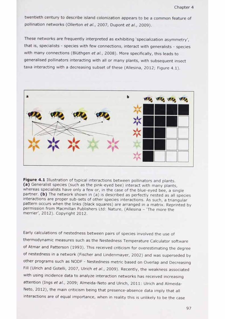
Chapter 4
twentieth century to describe island colonization appears to be a common feature of
pollination networks (Ollerton etal., 2007, Dupont eta/., 2009).
These networks are frequently interpreted as exhibiting 'specialization asymmetry',
that is, specialists - species with few connections, interact with generalists - species
with many connections (BILithgen etal., 2008). More specifically, this leads to
generalised pollinators interacting with all or many plants, with subsequent insect
taxa interacting with a decreasing subset of these (Allesina, 2012; Figure 4.1).
b^ ^
¥
¥
i
Figure 4.1 Illustration of typical interactions between pollinators and plants.(a) Generalist species (such as the pink-eyed bee) interact with many plants, whereas specialists have only a few or, in the case of the blue-eyed bee, a single partner, (b) The network shown in (a) is described as perfectly nested as all species interactions are proper sub-sets of other species interactions. As such, a triangular pattern occurs when the links (black squares) are arranged in a matrix. Reprinted by permission from Macmillan Publishers Ltd: Nature, (Allesina - 'The more the merrier', 2012). Copyright 2012.
Early calculations of nestedness between pairs of species involved the use of
thermodynamic measures such as the Nestedness Temperature Calculator software
of Atmar and Patterson (1993). This received criticism for overestimating the degree
of nestedness in a network (Fischer and Lindenmayer, 2002) and was superseded by
other programs such as NODF - Nestedness metric based on Overlap and Decreasing
Fill (Ulrich and Gotelli, 2007, Ulrich et at., 2009). Recently, the weakness associated
with using incidence data to analyze interaction networks has received increasing
attention (Ings eta/., 2009; Almeida-Neto and Ulrich, 2011: Ulrich and Almeida-
Neto, 2012), the main criticism being that presence-absence data imply that all
interactions are of equal importance, when in reality this is unlikely to be the
97

Chapter 4
(Ulrich and Almeida-Neto, 2012). In response to this, weighted metrics have been
developed offering more robust assessments of whether a community exhibits a
nested pattern, e.g. WINE - Weighted Interaction Nestedness Estimator (Galeano et
al.t 2009) and WNODF - Weighted Nestedness metric based on Overlap and
Decreasing Fill (Almeida-Neto and Ulrich, 2011; Ulrich, 2012). The need to test
calculations of nestedness against appropriate null models is necessary if correct
interpretations are to be made (Dormann et a/., 2009, Gibson et a/., 2011).
The nestedness observed in mutualistic webs has been interpreted in several, often
complementary, ways. For example, Memmott et a/. (2004) examined whether a
non-random nested pattern might indicate robustness in the face of selected
extinction events. Using 'attack tolerance curves' (Burgos et a!., 2007) they
quantified the proportion of a guild that might become extinct following the
elimination of species in another guild. Their findings suggested that the loss of core
generalists (those that are maximally packed in the top left hand corner of Figure
4.1b) posed the greatest threat to the continuation of pollinator-plant interactions.
Fontaine et at. (2006, p.129) extended this concept by suggesting that nestedness
confers resilience, and that 'generalist pollinators buffer the loss of specialist
pollinators'. Bezerra eta/. (2009) tested this by simulating species removal.
Nestedness has also been used as a conservation tool to identify keystone species
and highlight critical changes in interaction structure in advance of biodiversity
losses (Benedek eta/., 2007, Ebeling eta/., 2011).
To my knowledge, network structure in gardens has not been assessed. Olesen et a/.
(2007, p. 19891) noted that 'in natural communities, species and their interactions
are often organised as non-random networks'. As the study sites for the present
work are human constructs (and therefore likely to contain non-native plants), one
of the aims of this work is to establish whether the reported non-randomness
associated with natural environments also applies to novel ecosystems. It is
predicted that networks in gardens mimic those of natural settings by
exhibiting a nested structure. Furthermore, as plant populations in 'natural'
settings experience quantitatively and qualitatively different visits from pollinating
insects over a season (resulting in networks appearing as highly temporally dynamic
- Herrera, 1988, Ollerton eta/., 2007, Dupont eta/., 2009, Alarcon, 2010), it is
predicted that some sampling sessions will have a greater proportion of nested networks than others.

Chapter 4
AimsThe aim of this chapter is to consider how assemblages of plants influence
communities of flower-visiting insects. Specifically, the chapter seeks to answer the
following questions:
1. Does the number of plant taxa available in a garden affect the richness and abundance of flower-visiting insect species that are observed?
2. What is the relationship between the availability of plants and those visited by flower-visitors, and does this differ across properties and seasons?
3. Is the proportion of native and alien plants similar across sampling sessions?
4. Are native plants in gardens preferred by flower visitors?
5. Are certain plant families that are common to a number of gardens more favoured by flower visitors than others?
6. Does connectance vary between properties across seasons where (i) only visited plants are assessed and (ii) all available plants are assessed?
7. Do generality, vulnerability and linkage density differ between properties and are seasonal patterns evident?
8. Do the observed plant and flower-visitor communities exhibit nested structures and are these consistent across the season?
Methods
Study sites and timing of sampling
17 gardens in four counties in lowland Central England were used as the basis for
the study. Sampling took place between April and September 2010. Full details of
the sites and methods for censusing plants and flower visitors are given in Chapter 2 (2010 field season).
Plant classification
Plants were ascribed to families according to the most recent Angiosperm Phytogeny
Group publication (APG III, 2009).
Throughout this chapter the term 'plant element' is used instead of plant species.
This follows the convention of Frankie et al. (2005) and reflects the difficulty in
classifying ornamental garden plants according to standard taxonomic guidelines.
99

Chapter 4
Here, plant element refers to any species, variety, cultivar or hybrid that is
commonly used in the horticultural arena.
Due to the problems associated with reliably identifying certain plant elements, a
generic grouping was sometimes used. Examples include Lavandula spp., Nepeta
spp., and Origanum spp. This cautionary approach means overall plant species
richness across gardens is likely to have been underestimated.
The classification of plant elements according to native or alien status was made
with reference to Stace (1997) following the methods of Smith et al. (2006a) and
Loram et al. (2008a).
Data analysis
Unless otherwise stated, each sampling session at each property was considered
separately.
Relationship between plant availability and observed flower visitors
The relationship between plant family, genera or element availability and observed
insect richness and abundance was explored using nonlinear regression. Power
function trend lines were fitted through the data as these best represented the
accumulation of flower visitors with increasing plant richness. The significance of
each fit was established by performing linear regressions on log-transformed data.
Availability of plants compared to plants visited
The median number of plant elements available at each garden was compared to the
number of plant elements visited using a Mann-Whitney U test. The same test was
used to examine differences in availability and use of plants across the four sampling sessions.
Proportion of native and alien plants
Differences in the proportion of alien plants available across the four sessions were
examined using a one-way ANOVA (the data met assumptions of normality and
homogeneity). This was followed up with REGWQ post hoc tests.
The relationship between the proportion of native and alien plants available and
those used in each of the four sessions was explored using a chi-square test of
association in Excel following the methods of Dytham (2011).
Evaluating highly visited plant families
Plant elements that were common to a number of gardens within each of the four
sessions (and which were visited by flower-visitors at a minimum of five properties)
100

Chapter 4
were identified. Working at family level, a per-session visitation preference index
(VPI) was calculated. This index incorporated two factors; (i) the number of gardens
where an element was used as a proportion of the number of gardens where the
element was available and (ii) the number of elements used (within a family) as a
proportion of the total number of elements available within the family in the session
in question. The VPI values were log transformed and plotted against the (log
transformed) number of elements available within the family. A linear trend line was
fitted through the points and 95% confidence intervals added to identify those
families with a VPI lying beyond the upper limits of the confidence lines. Flowers
within families with a high VPI were characterised according to whether they were
open or tubular, following the methods of Fontaine et al. (2006).
Connectance
For each sampling session plant and flower-visitor data were arranged as a matrix.
The available and realised links were calculated according to
C = L / ( FP) (see Introduction). Connectance values were calculated for two
scenarios:
1. The number of links between plants that had a minimum of one visitor and the number of flower-visitor species.
2. The number of links between all available plants (see Chapter 2, 2010 field season) and the total number of flower-visitor species.
Median connection values (n = 68 per scenario) are presented for each property.
Differences between properties were examined using the non-parametric Kruskal- Wallis test.
Generality, vulnerability and linkage density
Generality, vulnerability and linkage density values for each session were calculated
in R (R Development Core Team) using the package Bipartite, Version 1.17
(Dormann et al., 2008). Abundance data were arranged in matrices with flower-
visitors as columns and plant elements as rows. Differences in median values
between properties (n = 4) were examined using a Kruskal-Wallis test. Median
values per session (n = 17) were also calculated and tested in the same way. Mann-
Whitney U tests, with Dunn Sidak corrected critical values (Sokal and Rohlf, 1981)
were used as non-parametric post hoc procedures.
101

Chapter 4
Nestedness
To assess whether communities of flower-visitors and plants exhibited nested
patterns, the data were examined using WNODF (weighted nestedness metric based
on overlap and decreasing fill) software, Version 2.0 (Almeida-Neto and Ulrich,
2011). To avoid the problems associated with the non-matching of species
attributes, e.g. the creation of'forbidden interactions' (Jordano, 1987, Weiner et al.,
2011), whereby spring insect species appear in matrices with late summer flowering
plants despite the two never co-occurring, data from each sampling session were
considered separately. Matrices of interacting species (n = 68) were prepared in
EcoSim format (space delimited columns of plant elements and rows of flower-
visitors), and run in the WNODF program using the following parameters: (i) matrix
sorting was by row and column species richness, with rows and columns of equal
species richness further sorted according to abundance totals and (ii) null model 're'
was selected, whereby individuals are assigned to matrix cells proportional to the
observed row and abundance column totals until total abundances for each row and
column are reached. Finally, the degree of nestedness was established by comparing
the actual distribution values with the scores obtained from 500 runs of the null
model (Almeida-Neto and Ulrich, 2011, Ulrich, 2012). The probability of the
observed network differing from random (and therefore exhibiting a nested pattern)
was considered significant at a < 0.05. Differences between seasons were quantified
by considering the proportion of significantly nested samples they contained. A chi-
square test of association was used to establish whether these observed values were
significantly different from expected.
Results
Plant richness
A total of 98 plant families, 409 genera and 988 plant elements were recorded
across all properties for sessions one to four inclusive, constituting more than 22%
of the world's total recognised plant families (APG III, 2009, Table 4.1, Appendix VII).
Relationship between plant availability and observed flower visitors
Flower-visitor species richness and abundance increased significantly as the number
of plant families, genera and elements increased (Figures 4.2 and 4.3). Flower-
visitor abundance was best explained by the number of plant genera available (R2 =
0.35, P < 0.001), with the number of plant elements being the poorest predictor of
plant species richness (R2 = 0.19, P = < 0.001), (Table 4.2).
102

incoinin<Dincn
ClET OinDO
uIDO
ro
<uClo
uT O
<U
TD<V■OOua;
UJCLin
<DE CD
CL_QJ O« Ql ■OcT O
sT O
X TO
UT O<V
<D^ cLL. X3w in in -qa;— o
to <u-QE
T O CT O
OQ) <DE
H ^
* <Da*-Q Si* S1
uj in cl c■D -2 C £
o l/>
TOa>
§c35o
UJa.
mi uja
ro
ro
rsi UJCL
rsi
fN
UJ0.
c - E S £ °.2 a cin c 0 w c xa> d totf) C h
>HaUJ
ro<*
onfM
i D o o n o o r M i o ^ oo » H f M o o o > n r vin ro in in in in ro
on o ^ *h fNoo in o on onr-l IN fO IN IN
o <rON ^
on rsrs fN
fN
m
fN<*
rvfN
i n m o N r o r N c o r o i D O N r o i n r N i o i n r o» H ' t O r - < o N T t i o f n o f N r n i o ^ T t N
N m « H o « H i n o o i o o f N « H O N i n f N f N o o Nr o ^ i n i n i n T * < t i n i n r M < f r < r m i n i n m m
ro fN ID ID N- vD 00 in rNfN ID in 00 in in vD fN ro
fN in in ID vD fN fNfN in in ID ro in vD ro
in in 00 ro in ON O ON fNfN fN ro fN fN fN ro ro
fN rN ON fN fN fN ro ININ 00 rN 00 ID ID m ON O m
m ON m O IN ON o ro IN ONIN ID ID rN m m 00 00 <r
m ID rN ro ro rN 00 ONH IN ro ro IN ro IN m IN IN
lO in •'T IN ON 00 ro o 00•<r 00 in O 00 vD in o fN fN IN
n-n
pmro
<frfN
(N
ON
3-
onfN
CO If)vD vD ln
in oo o idm m m fN
on »h*-* rf
oo oo »h ro
m <1-*H fN
ro onfN »H
cn rs fN »H
00 <T
Of Q.o 3 <>0) CL -J O < z0. < CD U u u
O'<
fNIN
■'Tro
00 00ro fN
mro fN
<r ofN fN
ON H
vD fNro »-•
IN fNro fN
in *h ro fN
<r in fN tH
ofN
ON
00
IDfN
ID
rv -*■in lo
oo ro fN ro
fN roon
nfN
oo ro in o in ro ro ro
iO00
00fN 00
ON fN 10fN ro ro
O' in ofN ON fN
ro
iD ID fN <r
m oofN ro
ON Tt TH fN
lO
fN
oo
o UJ CL Z< h- 3X 2 _j in in
fNoo
onfN
fNro
roin
fNfO
fO
vD
id ro t j - in m
00fN
idfN
inro
ro
ro rsi
onin
infN
id
iDro
00 ID
fNin
o
N-rsj
rNfN
infN
ON ON ON
a< CL£ <i
rNooN-in
inrovDn-
inN"N-fN
fNVD
fN fNro th
ONIDIN
invDroin
fNfNin
ONfN
fN00fNfN
ONinfN
ONin
cTOa; ro
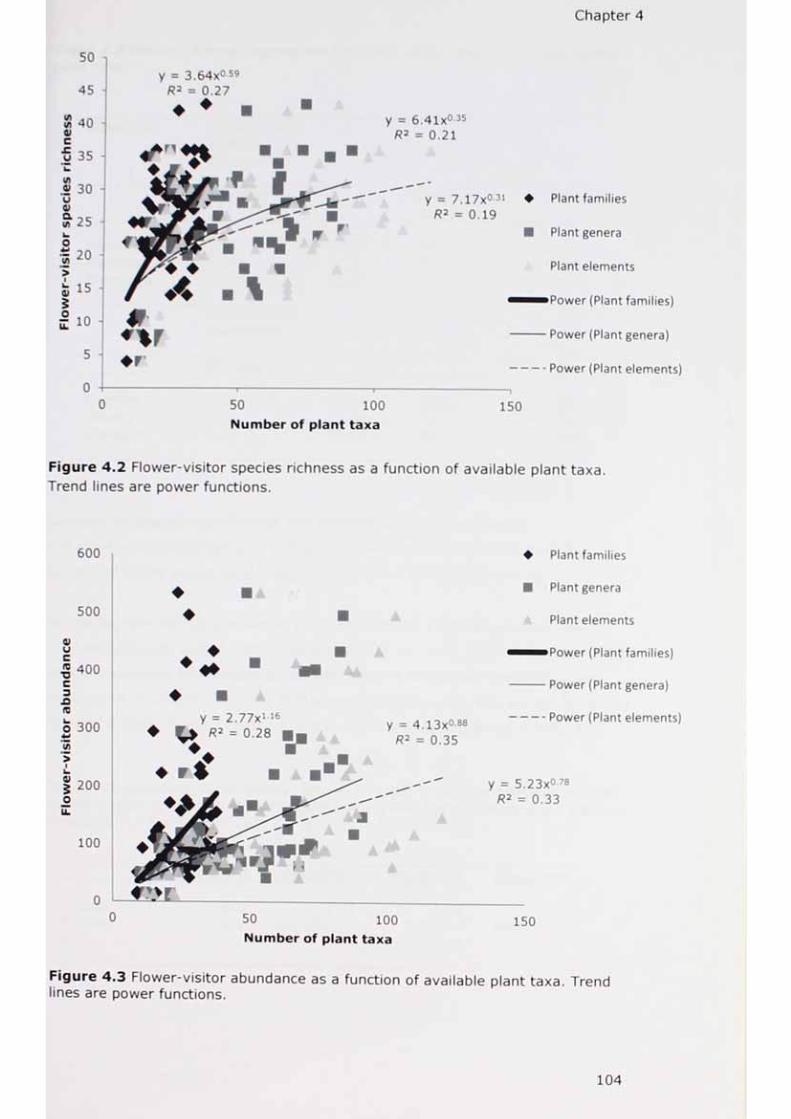
Chapter 4
104

Chapter 4
Table 4 .2 Results o f linear regressions for flower-visitor species richness against plant taxa.
Plant taxa Flower visitorspeciesrichness
R2 value F Degrees of P valuefreedom
Families 0.27 24.27 66, 1 < 0.001Genera 0.21 17.16 66, 1 < 0.001Elements 0.19 15.45 66, 1 < 0.001
Flower visitorabundance
R2 value F P value
Families 0.28 25.37 66, 1 < 0.001Genera 0.35 35.34 66, 1 < 0.001Elements 0.33 35.53 66, 1 < 0.001
Comparing plants visited w ith the num ber of plants available
The number of plants visited in each garden was significantly lower than the
number of plants available, n = 68, Z = -5.97, P < 0.001 (Figure 4.4).
Across the four sampling sessions, all except Session 1 had significantly lower
numbers of plants visited than those available (P = < 0.01, Table 4.3, Figure 4.5).
As some sampling events overlapped with dates in neighbouring sessions (see
explanation in Chapter 2 - 2010 field season) the data were also plotted according
to date. A sim ilar pattern to that found in Figure 4.5 was observed (Figure 4.6).
Table 4 .3 Results of Mann Whitney U tests for each of the four sampling sessions comparing the number of plant elements visited with the number of plant elements available. * = P < 0.05, * * = P < 0.01, * * * = P < 0.001.
Session 1 Session 2 Session 3 Session 4
Z value P value n
-2.090.04*
17
-4.46< 0 .0 0 1 ***
17
-2.950 .003**
17
-3.62< 0 .0 0 1 ***
17
105

100

Chapter 4
cE4»
Q.
O
41
E3CCro• mam*D4>2
100-
0 r3
Sampling session
Figure 4 .5 Median number of plant elements visited (dark grey bars) compared to the median number of plant elements available (ligh t grey bars) for each of the four sampling sessions (n = 17). Session 1 = 22 Apr. - 5 Jun., 2 = 6 Jun. - 18Jul., 3 = 19 Jul. - 9 Aug. and 4 = 1C Aug. - 30 Sep. Error bars = 95% confidence intervals.
140 -
</>120 -
c4)E 100
0)£ 80 (zao 60
0)nE3z
40
20 -
Oo
* 0 *o
O oOo
o
oo
o <^>
o o
0
01-Apr
oo o
♦ o o<5>
o
21-May 10-JulD a te (2 0 1 0 )
29-Aug 18-Oct
Figure 4 .6 Number of plant elements visited (dark grey squares) and available (light grey diamonds) plotted according to date sampled.
107

Chapter 4
Alien and native plant elements
The percentage of available plant elements that were classed as aliens ranged
between 62 and 79% across the four sessions (Table 4.4). A one-way ANOVA
revealed there was a significant difference in the proportion of alien plants
available (F = 5.97, d.f. 3,64, P = 0.001). Post hoc tests (REGWQ) showed that Session 1 was different to Session 4.
Table 4 .4 Percentage of alien and native plant elements across each of the four sampling sessions. Data are given for (i) plant elements available and (ii) plant elements visited by flower-visitors. Numbers in brackets represent absolute values.
Session 1 Session 2 Session 3 Session 4
% alien plant elements available
% native plant elements available
Total plant elements available
62 (295)
38 (181)
476
69 (868)
31 (384)
1252
74 (848)
26 (303)
1151
79 (734)
21 (198)
932
% alien plant elements visited
% native plant elements visited
Total plant elements visited
66 (90)
34 (46)
136
71 (147)
29 (59)
206
76 (220)
24 (69)
289
77 (148)
23 (45)
193
Chi square tests of association revealed that there was no difference in the number
of alien and native plants visited relative to those available (Table 4.5).
Table 4.5 Results of chi-square tests of association comparing the number of alien and native plants visited versus those available.
Session 1 Session 2 Session 3 Session 4
X2 0.80 0.35 0.72 0.41d.f. 1 1 1 1P value 0.37 0.56 0.40 0.52
108

Chapter 4
On a per-garden basis, the proportion of alien plants ranged from 0.45 to 0.91
across all sampling sessions, with the proportion of native plants ranging from 0.09
to 0.55 over the whole season. Overall, the mean proportion of available plants
tha t were classed as alien was 0.68 ± 0.09 (Table 4.6).

incococnQJin
cnQJtQJQ .OQ.
0GJQJ>qjinQJ
UIDQJininouidin
q j
EQJQJ
t o
a.qj>
a:
Q *■(J)-H
IDQJ
QJ>
QJCDCIDa:
(D
Q ^in n-H c
IDQJ
QJcncIDCL
inID
QJEQJQJ
tQJO
cl
N f M a > ^ i n N i n ^ ^o
o o-H -H -H -H -H -H
cD ^ rsi rsi N cD r o h r o rsjro
o-HvDro
-Hv drsi
O
CDrsi-H -H -H
ono
o
-H
n fs ^ co
o
-Ho ■ruo rsi 00 ID O rsi rsi ro
-H''Q-rsi
o o O
u ororo
ro O'*rsi rsiro ro
rsiro ro^ r
uouo ^ r
uoro
<T>rsii
sorsil
cDI
Orsii i i i iroro
cDrsi ro rsio
i&
if\
i
ro o o
i irsirsi rsi
rsi
"3-
oi
in
ro
ioo
UOuoo1uors i
r ^ r s io i^ u o r s iu o ^ j - ^ - ro ro
H -H -Hcn r ld
oocD
o o -H -H ro r0 0 CD
-H -H -H -H -H -Hco rcD cD r s N• • • •o o o o
LO CD1^.
O
-Hr \ ir v
-H -Huo| \
o
o-HcDr ^
i i i i i i i i i i i i i i
r o c n c D c o r o c o r s i c D ^ j - o o ^ o c r ^ O H f N o o o n N O D i n o o r s i r s i r o r s i r s i r s i r s i r o r n r s i r o r s if \ o
a c rsi
o < i i z < o i i j S <C cD U U U u j l l I ^ ^ in ui
o o-H -n
CD O
rsi
i
CDro
oo o
-H -H^ O ID CD
c J - ^ O O ^ N ^ c D O ^ H r o r O C O C O L D f N L D ^f ^OOCOOOi Dr v i Df N*acUOOOr^r^OOOOr ' - i D
I Ic <J» r-H 00 ro r-H 00 UO o uo r-H CD CD UO 00QJ• mmm 1 CDa UO • uo cD vD
a CDm ID A CD• CDa UO CDa a<1
•o
•O
•o
wO
•o
wo
wO
wO O
wo o o o o O
wO
•o
r
Qa. < *
<j\
o
rsiro
a»o
COCD
O
inQJ • •■■■»£QJ
ID2 oo c ®ID II* c
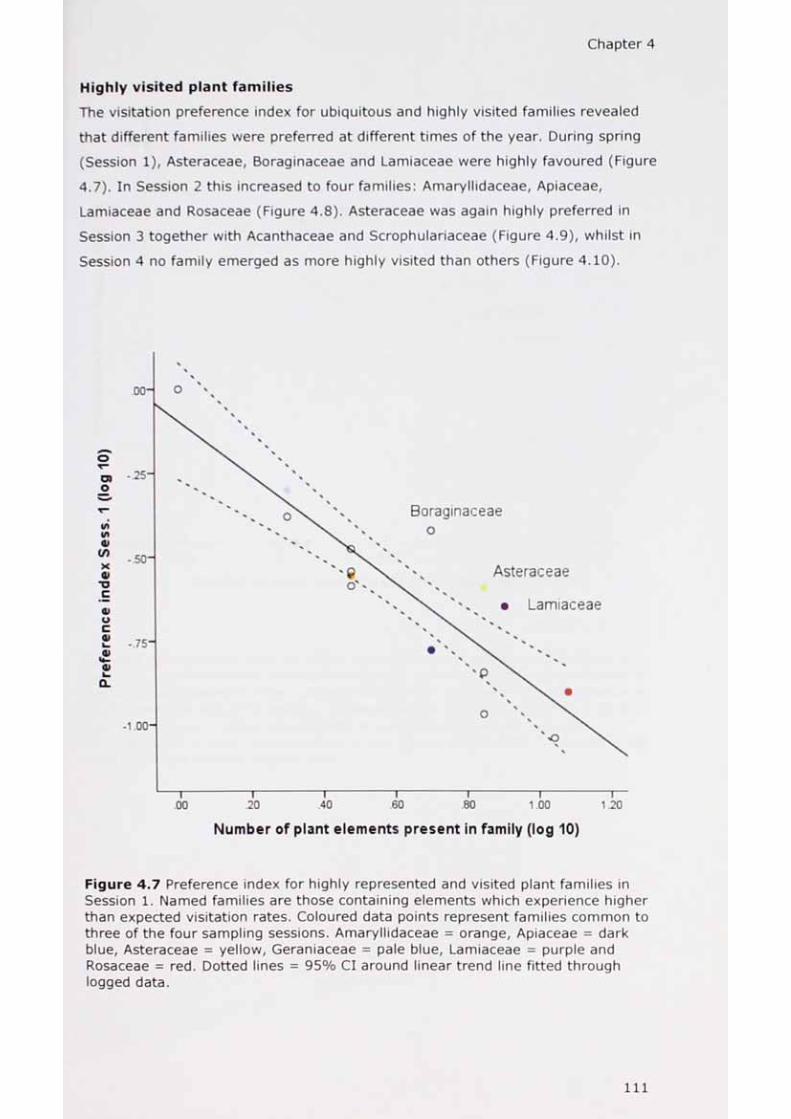
Chapter 4
Highly visited plant families
The visitation preference index for ubiquitous and highly visited families revealed
that different families were preferred at different times of the year. During spring
(Session 1), Asteraceae, Boraginaceae and Lamiaceae were highly favoured (Figure
4.7). In Session 2 this increased to four families: Amaryllidaceae, Apiaceae,
Lamiaceae and Rosaceae (Figure 4.8). Asteraceae was again highly preferred in
Session 3 together with Acanthaceae and Scrophulariaceae (Figure 4.9), whilst in
Session 4 no family emerged as more highly visited than others (Figure 4.10).
.00 .20 .40 .60 .80 1.00 1.20
Number of plant elements present in family (log 10)
Figure 4.7 Preference index for highly represented and visited plant families in Session 1. Named families are those containing elements which experience higher than expected visitation rates. Coloured data points represent families common to three of the four sampling sessions. Amaryllidaceae = orange, Apiaceae = dark blue, Asteraceae = yellow, Geraniaceae = pale blue, Lamiaceae = purple and Rosaceae = red. Dotted lines = 95% Cl around linear trend line fitted through logged data.

Chapter 4
Number of plant elements present within family (log 10)
Figure 4.8 Preference index for highly represented and visited plant families in Session 2. Named families are those containing elements which experience higher than expected visitation rates. Coloured data points represent families common to three of the four sampling sessions. Amaryllidaceae = orange, Apiaceae = dark blue, Asteraceae = yellow, Geraniaceae = pale blue, Lamiaceae = purple, Ranunculaceae = green and Rosaceae = red. Dotted lines = 95% Cl around linear trend line fitted through logged data.
112

Chapter 4
Figure 4.9 Preference index for highly represented and visited plant families in Session 3. Named families are those containing elements which experience higher than expected visitation rates. Coloured data points represent families common to three of the four sampling sessions. Amaryllidaceae = orange, Apiaceae = dark blue, Asteraceae = yellow, Geraniaceae = pale blue, Lamiaceae = purple, Ranunculaceae = green and Rosaceae = red. Dotted lines = 95% Cl around linear trend line fitted through logged data.

Chapter 4
Number of plant elements present within family (log 10)
Figure 4.10 Preference index for highly represented and visited plant families in Session 4. Coloured data points represent families common to three of the four sampling sessions. Asteraceae = yellow, Geraniaceae = pale blue, Lamiaceae = purple, Ranunculaceae = green and Rosaceae = red. Dotted lines = 95% Cl around linear trend line fitted through logged data.
A list of the plant elements within families identified using the visitation preference
index is given in Table 4.7. A measure of the availability of these elements and the
proportion of gardens where they were visited is included, as well as the colour,
general overall shape of the flowers and their native or alien status.
114

Chapter 4
Table 4.7 List of highly visited families per session (note, no specific families emerged for Session 4, Figure 4.10). Plant elements within each family that were visited by insects are listed, together with their alien or native status, their levels of occurrence and visitation across the gardens, their colour and flower morphology.
Families according to session.* indicates family occurs in multiple sessions
Plant elements visited within each family (N = native, A = alien)** indicates plant element occurs in multiple sessions
Number Proportion Colour Flowerof of gardens shape
gardens where T =where visited tubular
present 0 =(min. 5) open
Session 1
Asteraceae
Boraginaceae
Lamiaceae
Session 2
Centaurea montana (A)** Taraxacum officinale (N)**
Pulmonaria sp. (A) Symphytum sp. (N)
Glechoma hederacea (N) Lamium macula turn (A)
8 0.88 blue O12 0.92 yellow O
6 0.83 lilac/blue T9 0.56 pink/lilac/blue T
10 0.80 lilac/purple T8 1.00 pink T
Mmarymaaceae Allium sp. (A) 8 0.88 lilac/purple ONarcissus sp. (A) 7 0.71 yellow T
Apiaceae Aegopodium podagraria (A)
5 1.00 white O
Angelica archangelica (A) 5 1.00 white OAstrantia major (A) 9 0.56 pink 0
Lamiaceae* Nepeta sp. (A) 11 0.82 lilac/blue TSalvia sp. (A) 8 0.88 various TThymus sp. (A) 6 0.83 pink/lilac T
Rosaceae Alchemilla mollis (A) 13 0.38 cream 0Rosa rugosa (A) 7 1.00 red 0Rosa sp. (A) 13 0.92 various 0
Session3
Acanthaceae Acanthus mollis (A) 9 0.78 purple T
Asteraceae* Achillea sp. (A) 9 0.67 pink/white OCentaurea montana (A)** 11 0.45 blue 0Cirsium arvense (N) 6 0.83 pink/lilac 0Cosmos bipinnatus (A) 6 0.83 pink/white 0Echinacea sp. (A) o 0.75 pink 0Ech in ops sp. (A) 8 0.75
•
blue 0Leucanthemum sp. (A) 11 0.64 white 0Taraxacum officinale (N)** 6 1.00 yellow o
Scrophulariaceae Buddleja davidii (N) 11 1.00 lilac TPenstemon sp. (N) 7 0.71 various TVerba scum sp. (A) 10 0.50 yellow O

ConnectanceChapter 4
Median connectance values for each of the 17 properties for each of the two
scenarios (see Methods) are given in Figure 4.11. Connectivity was higher where
matrices were smaller (Figure 4.12), hence Kirby (KIR), with the fewest flower-
visitors and plant resources, had the highest median connectance value for both
scenarios. Results of Kruskal-Wallis tests revealed a significant difference between
median connectance values for properties under Scenario 1 (realised links between
the number of plants that were visited at least once and the number of insect
species they connected to), H = 31.47, d.f. = 16, P = 0.012. The median
connectance value for KIR (0.26) was > 80% greater than that of the second
highest connectance value (Althorp - AL, median value = 0.14). Under Scenario 2,
no difference in median connectance values between properties was observed (H =
17.56, d.f. = 16, P > 0.05).
116

OC'O

Chapter 4
Figure 4.12 Decreasing connectivity as a function of matrix size for two scenarios.Scenario 1 (dark grey diamonds) = matrix comprised only of plant elements visitedby insects, n = 68. Scenario 2 (light grey squares) = matrix comprised of all plantelements available, n = 68. Lines of best fit drawn for each scenario with R2 values included.
Generality, vulnerability and linkage density
Flower visitors interacted with a mean of 4.5 ± 3.6 plant elements across all
properties and sessions (generality) whereas plant elements interacted with an
average of 3.6 ± 1.0 flower-visiting insect species (vulnerability). Overall there was
an average of 4.1 ± 2.0 interactions per organism (linkage density).
I he median generality and vulnerability values per property are given in Figure
4.13. Kruskal-Wallis tests revealed there were no significant differences in
generality, vulnerability or linkage density values across gardens (generality: H =
18.24, d.f. = 16, P = 0.31; vulnerability: H = 24.27, d.f. = 16, P = 0.08; linkage
density: H = 17.96, d.f. = 16, P = 0.33).
118

l/>(V

Chapter 4
Across the four sampling periods, Session 3 exhibited the highest median
generality values (Figure 4.14). A Kruskal-Wallis test revealed that a significant
difference existed between sessions (H = 27.82, d.f. = 3, P =<0.001), with post
hoc tests showing that Session 3 was significantly different to all others, and that
Session 1 was different to Session 4 (Table 4.8).
Sampling sessionFigure 4.14 Median generality (dark grey bars) and vulnerability (light grey bars) values (n = 17) for the four sampling sessions. Error bars = range.
Table 4.8 Results of post hoc tests (Mann Whitney) for differences in median generality values between paired sessions. Degrees of freedom = 3 in all cases. Dunn Sidak adjustment of critical values used (Sokal and Rohlf, 1981).
Paired sessions Mann Z P (adjusted a < 0.009)examined Whitney U * = significant
_______ value
1, 2 78.0 -2.29 0.0221, 3 22.0 -4.22 <0.001*1, 4 58.0 -2.98 0.003*2, 3 38.0 -3.67 <0.001*2, 4 103.0 -1.43 0.1603, 4 56.0 -3.05 0.002*
120

Chapter 4
Nestedness
The outputs of the 68 WNODF nestedness procedures (involving 34,000 null model
simulations) are given in Table 4.9. All 17 properties had at least one session with
a significantly nested network. On average, 2.1 ± 0.7 networks were significantly
nested per property (51% were nested overall).
Assessing the results according to the different sampling sessions (Figure 4.15)
revealed that Session 2 had the highest proportion of significantly nested
communities (12 of 17 gardens), followed by Session 4 (10 out of 17 gardens).
Less than half were nested for the remaining two sessions. A chi-square test of
association showed no significant difference in observed versus expected numbers
of nested networks (X2 = 5.36, d.f. 3, P = 0.15).
Figure 4.15 Proportion of communities within each sampling session exhibiting significantly nested interaction networks.
l
�o0)
0.9
S 0.8c£ 0.7c wro 0J n ru •- 0.6
o o 0.4 uc
.2 0.3t
u
Q. 0.2 -o
0.1
01 2 3 4
Sam pling session
121

Chapter 4
Table 4.9 Results of 68 tests for nestedness. P values of < 0.05 (in red) denotematrix significantly different from random and therefore nested (Ulrich pers. comm.). Red bold < 0.01.
Property Session Flower-visitinginsectspecies
Plantelements
WNODF degree of nestedness
WNODF Z value
P value
ALALALALBOUBOUBOUBOUCACACACACMCMCMCMCHCHCHCHENENENENFARFARFARFARHOLHOLHOLHOLKELKELKELKELKIRKIRKIRKIRLAMLAMLAMLAM
1234 1 234 1 234 1 234 1 234 1 234 1 234 1 234 1 234 1 234 1 2 3 1
262623
836 31 26 20 35 35 2229 31 26 25 1927 33 442425 18 41 17 313132 2230 3037 15333828 227
1175
2326 35 23
1517185
22313916212324 294029 55 342330 4427 12 163228 22 20 32 2624 29 59 2023 39 7524 4 96 6
1825 38 18
4.036.65
19.73n.a.0.125.83
19.016.255.431.796.528.94 0.54 0.93
14.30 8.745.106.83
16.00 12.445.95 3.88
10.6212.331.976.07
20.846.124.563.83
15.659.11 0.62 4.37
21.31 4.87 n.a.
13.4113.8916.001.355.56
26.401.35
0.02-3.59-3.42-0.05-1.50-4.83-1.38- 2.11-2.39- 0.01-0.40-2.950.99
-0.84-3.46-2.69-0.92-3.46-1.18-1.67-1.43-3.86-2.05-2.56-3.66-1.85-1.03-1.32-2.77-1.38-1.46-0.650.30
-2.59-2.16-2.99-2.28-1.96-0.04-0.60-2.16-2.610.58
-2.16
0.49<0.01<0.01
0.480.07
<0.010.080.020.010.500.34
<0.010.160.20
<0.01<0.01
0.18<0.01
0.12<0.05
0.08<0.01
0.02<0.01<0.01
0.030.150.09
<0.010.080.070.260.38
<0.010.02
<0.010.010.030.480.270.02
<0.010.280.02
122

Chapter 4
Table 4.9 continued
Property Session Flower-visitinginsectspecies
Plantelements
WNODF degree of nestedness
WNODF Z value
P value
LW 1 32LW 2 37LW 3 30LW 4 16ST 1 31ST 2 31ST 3 44ST 4 27SUL 1 25SUL 2 30SUL 3 24SUL 4 28UP 1 32UP 2 39UP 3 27UP 4 35WAD 1 24WAD 2 22WAD 3 35WAD 4 11WR 1 24WR 2 31WR 3 29WR 4 23
2538411821285727 19 50 34 3728 30 48 41 11 11 167
19182216
1.492.39
19.624.712.731.59
13.824.487.416.704.579.193.142.99
14.4210.392.475.80
14.107.892.353.66
15.4414.14
-1.60-2.99-0.571.020.29
-3.43-0.430.09
-1.75-0.53-3.05-3.58-0.23-0.50-3.38-2.16-2.54-3.17-1.35-2.77-4.93-4.010.66
-1.91
0.05<0.01
0.280.150.39
<0.010.330.460.040.30
<0.01<0.01
0.410.31
<0.01<0.01<0.01<0.01
0.09<0.01<0.01<0.01
0.250.03
Discussion
Relationship between plant availability and observed flower visitors
The sampled gardens contain a remarkably high diversity of plants (Table 4.1).
As only urban garden plant diversity has been considered to date (Smith et a!.,
2006a, Loram et at., 2008a,b), the results of this study provide the first insight into how diverse estate gardens can be.
Both flower-visitor species richness and abundance were found to positively
correlate with the number of plant families, genera and elements available. Despite
all taxonomic levels of plants significantly influencing these response variables,
some were of more relevance than others. For example, the number of plant
genera within a sampled area of garden was the best predictor of insect
abundance, P < 0.001, R2 = 0.35 (Figure 4.3). The observed relationship between
plants and flower visitors echoes the findings of Fontaine et at. (2008) who
considered the response of Bombus terrestris individuals to plants in experimental
123

Chapter 4
conditions and Ebeling et al. (2008, 2011) who found the number of pollinating
insects was 'strongly positively' affected by the number of plant species available in
a grassland in Germany. Ebeling et al. (2008) noted that, as with the power
functions used here (Figures 4.2 and 4.3), the relationship was both non-linear and
saturating. Lazaro and Totland (2010) noted the effect plant richness had on
specific pollinator guilds. By considering visitation rates to two plant species placed
within patches of Taraxacum officinale (dandelion) they established that some
guilds behaved differently and that in the case of bees, eusocial and solitary
species did not respond in similar ways. Similarly, Hegland and Boeke (2006) found
that whilst the number of hoverflies responded positively to plant species richness
in a temperate grassland, bumblebees did not. Further analysis considering the
response of specific guilds to plant richness in gardens will add to these findings.
Notwithstanding the association noted in the current study, plant richness explains
only a proportion of the observed insect richness (Figure 4.2). Other factors will be explored in Chapter 5.
During the 2010 field season the assessment of plant abundance was not possible
due to time constraints. Further work incorporating the abundance of flower
resources in rural gardens into analyses will add to the knowledge gained from this
study into how pollinators behave in novel habitats.
Comparing plants available with the number of plants visited
Fewer plant elements were visited than those available (Figure 4.4). In the case of
Sessions 2, 3 and 4, the number visited was significantly lower than those
available, P < 0.01, (Figure 4.5). Whilst Session 1 was also significant, it was less
so than the others (P = 0.04). One possible explanation for this concerns the
availability of flower resources in early spring. At this time flower resources are
often scarce (pers. obs.). Optimal foraging theory states that the preference for
patches containing high densities of flowers should be the norm for the majority of
pollinators (Pyke, 1984). Therefore having arrived at a florally dense patch,
foraging is maximised by visiting several (or many) flowers within the area
(Hegland and Boeke, 2006). This generates the appearance of heightened use in flower patches within gardens.
A concern in treating the four sampling sessions as distinct was the fact that a
small amount of field-work took place on dates a few days beyond the boundary of
the previous session. As described in Chapter 2 (2010 field season), this situation
arose because of visiting restrictions imposed by some property owners. To check
124IT wmm * /.*• i.j
6 Uii-fVERSHY Or NO.Viii. tUBRARV/

Chapter 4
whether this affected the results, the number of plants available and those visited
were plotted according to the date assessed. The outcome mirrored that of the
session-wise tests, thus placing confidence in the results obtained (Figure 4.6).
Alien and native plant elements
The majority of plant elements available were classed as alien, ranging from 62% -
79% across the four sampling sessions (Table 4.4), with the percentage of alien
plants increasing as the season progressed. A one-way ANOVA revealed that
Session 4 had a significantly higher number of alien plant elements than Session 1
(P < 0.001). Overall, the mean percentage of alien plant elements was 68 (Table4.6) .
This is remarkably similar to results obtained for gardens in urban areas. For
example Loram et at. (2008b) reported that across five UK cities (incorporating 267
gardens), the percentage was 70. Similarly, Smith et al. (2006a) reported that in
61 Sheffield gardens 70% of plants were alien, as were those in a study of home
gardens in Mexico City.
Despite some variation between properties and across the seasons (Tables 4.4 and
4.6) , the congruence in the overall mean proportion of aliens is a surprising result,
raising questions about why this near consistent figure of 70% occurs, regardless
of whether gardens are urban or rural, and located in Scotland, Ireland, lowland England or Mexico.
Several authors have noted that urbanisation tends to increase the proportion of
alien plant species (Roy eta/., 1999, Smith etal., 2006b), although the exact
causes have rarely been explored. Whilst this 'urban = alien' rule may hold true for
cities (Smith eta/., 2006a, Loram eta/., 2008b), the majority of the sites sampled
in the present work are located many miles from the nearest towns. As such they
are not subject to common urban influences and characteristics including the heat
island effect and matrices of green spaces and hard surfaces. It is likely that the
proportion of aliens found in the gardens surveyed occurs due to two simple
factors: plant availability and planting preferences.
Brickell (1999) notes that some 15,000 plant species are available commercially to
garden owners in the UK. Regional variation in soil and climate are likely to affect
what grows well in an area, thus determining which plants garden centres sell, but
overall, garden nurseries almost exclusively stock alien plants (pers. obs.). Many
people see their gardens as highly visible extensions of their homes, and are
125
Chapter 4
known to be influenced by what neighbours plant (Goddard eta/., 2010). Few
choose to fill flower beds and borders exclusively with natives and indeed for many,
native flowers only feature as a side-effect of poor weed control. Instead, garden
owners can select from a wide range of nursery plants (Smith et al, 2006a).
Gardening fashions come and go, and the composition of plant communities in the
gardens of large estates is unlikely to resemble that of previous times unless an
attempt at historical planting is made (e.g. certain beds within the gardens at Kirby
and the small Elizabethan garden at Holdenby). Although earlier planting regimes
in estate gardens were also likely to contain many aliens (early plant exploration
and importation was often initiated and Financially underpinned by wealthy
landowners, Fisher, 1989), today head gardeners have access to broadly the same
plants as those available to the general public. The increasingly common activity of
opening country-house gardens to the public adds renewed vigour to the desire to
conspicuously exhibit complex planting schemes containing intriguing alien
elements.
Notwithstanding the high proportion of alien plants available, flower-visitors do not
appear to prefer native plants over their alien neighbours in mixed planting
environments. Results of a chi-square test of association revealed that the number
of alien and native plants visited by insects did not depart significantly from the
number of alien and native plants available (Table 4.5).
Overall, the domination of large rural gardens by alien plant species does not
appear to act as a barrier for flower-visiting insects looking to feed there. For
example fourteen species of bumblebee were recorded across all sites,
representing 58% of the UK total and 93% of those potentially encountered
according to current distribution maps (BWARS, 2012 and Appendix VI). In fact,
the high richness of insects recorded suggests that the presence of aliens elevates
the importance of these sites as rich habitats for pollinating insects.
A limitation of the 2010 fieldwork was that the relative abundance of native and
alien flowers was not assessed. Also, the assignment of alien or native status to
plants followed the definitions given by Stace (1997). This does not take into
account plants have become naturalised or are so morphologically similar to their
native counterparts that they may be indistinguishable to flower visitors. An
example of this is the cultivar Lamium maculatum (an alien according to Stace) and the native L. album.

Chapter 4
Highly visited plant families
Certain plant families emerged as more highly visited than others based on the
visitation preference index. Only Session 4 did not have distinct plant families that
achieved higher than expected visitation rates. There was little congruence across
the seasons with only two families (Asteraceae and Lamiaceae) appearing as highly
visited in more than one sampling session (Figures 4.7, 4.8, 4.9 and 4.10). Two
plant elements, Centaurea montana and Taraxacum officinale (both Asteraceae),
appeared in two sessions, but the general rule was for different plant elements and
families to replace others in importance as the season progressed (Table 4.7).
Although a long tail of singletons (plant elements occurring at only one garden in
any session) was the rule, the fact that many flowering plants favoured by insects
appeared in five or more gardens suggests a level of plant resource homogeneity
across sites.
In categorising the elements within the most visited families according to both
colour and flower morphology, a picture emerges of highly visited early spring
flowers being a mixture of alien and natives that are frequently lilac or blue in
colour, and tubular in shape, e.g. Pulmonaria sp. and Glechoma hederacea. As the
season progresses, increasingly more open flowers are preferred from a range of
colours with a greater emphasis on alien species. A likely explanation for this is the
phenology of the insect visitors recorded. Bumblebees (especially long-tongued
species) and solitary bees such as Anthophora plumipes are in flight early in the
year and are able to exploit resources from a variety of tubular flowers. Both
appear to favour blue/lilac plants in spring (pers. obs.). Later in the year, as the
diversity and abundance of hoverflies and butterflies increases, the diet breadth of
visitors expands and easily alighted flowers with open resources are preferred.
Taraxacum officinale (dandelion) is an interesting example of this 'open-flower'
group. Dandelions generally appear in early-spring and are known as a
'cornucopian' flowers (Kevan and Baker, 1983) as they offer copious quantities of
nectar and pollen and can attract pollinators from nearby plants (Fontaine et al.,
2008, Munoz and Cavieres, 2008, Lazaro and Totland, 2010). They are
cosmopolitan weeds that are little tolerated by gardeners who frequently eliminate
them with systemic herbicides (pers. obs). Despite their ongoing removal, the
current study found that where dandelions were allowed to persist, they were a
much visited plant. In the 2010 field season 15 hoverfly, five bumblebee, nine
solitary bee and eight butterfly and day-flying moth species, as well as the
common honey bee, were recorded visiting them. Across the two sampling years
(2010 and 2011) 41 flower-visitor species were recorded visiting this plant element
(data not presented). The flowers appeared to be particularly favoured both early
127

Chapter 4
and late In the year (Table 4.7) when forage quantity and quality elsewhere in the
gardens may have been at a premium. In Session 4 they were visited at more than
50% of the properties where they occurred (data not presented). In gardens that
are routinely managed to a high level, e.g. Coton Manor, T. officinale was
conspicuous by its absence.
A recommendation arising from this work is that, balanced with the functional
needs of a garden, patches of grass (including lawns) should be left unmowed (or
at least mowed less frequently) early and late in the season to provide additional
forage for flower visitors.
The results of this work on highly visited flower families do not serve as an
exhaustive guide to which specific plants should be included in a garden. Rather
they act as a reference for land managers, head gardeners and institutions such as
The National Trust and English Heritage, who may wish to consider whether the
green spaces in their charge are serving biodiversity in the most environmentally
profitable way.
Connectance
The connectance values revealed different results depending on the scenario used
(see Methods above). Under Scenario 1 (whereby only those plants recorded as
interacting with flower-visitors were considered), the median connectance value for
Kirby was found to be significantly higher than that of the other properties (Figure
4.11). Under Scenario 2 (where all plants in the sampled area were included,
regardless of whether they were visited) no differences in median connectance
values were observed (Figure 4.11).
Although the shift from significance in Scenario 1 to non-significance in Scenario 2
is most likely a function of network size - connectance is known to decrease as
network size increases (Jordano, 1987, Santamaria and Rodriguez-Girones, 2007,
Bluthgen et a!., 2008 and Figure 4.12), it raises questions about which scenario is
most informative.
To my knowledge, authors reporting connectance values have only performed
calculations according to Scenario 1, e.g. Jordano (1987) and Memmott and Waser
(2002). This may be because sampling involving pollinators and plants is routinely
focussed on a specific insect or plant species, with little or no consideration given
to non-target plant elements in the surrounding area (e.g. Potts et a\., 2004). The
exclusion of plants that are available (but not visited) when calculating
128

Chapter 4
connectance could be seen to undermine the very meaning of the metric:
'Connectance is the number of pair-wise interactions expressed as a fraction of the
total number of interactions possible' (Winemiller, 1989, p.960). Although in
practice it is not possible to census everything at a site (Magurran and McGill,
2011), a regime that fully samples certain patches to include all plants available is
desirable (Thompson et al.f 2004). By considering plants that are visited versus
those that are available (including sub-categories of whether these are alien or
native), a better understanding of community interactions can be gained. In the
case of gardens, this can help increase our knowledge about how these areas
interact with the wider landscape (Smith, 2006a).
As the major limitation of connectivity is its sensitivity to sampling effort, and
therefore matrix size (Bluthgen eta/., 2008, Banasek-Richter etal., 2009) direct
comparison of absolute connectance values with those of other studies as in
Tarrant (2010) was not deemed appropriate.
Generality, vulnerability and linkage density
The mean number of plants that flower-visiting insects interacted with was higher
than the mean number of insect species that visited each plant (generality 4.5 ±
3.6 versus vulnerability 3.6 ± 1.0, data not presented). Alarcon (2010) found this
situation was reversed for networks in meadows within pine forests in the USA
(mean generality value = 2.39, mean vulnerability = 8.33). Large generality values
indicate that flower-visitors connect with a diverse range of plants (Alarcon, 2010).
The difference in generality and vulnerability values between the current study and
that of Alarcon (2010) may reflect the underlying habitat type and therefore floral
availability. In large rural gardens many flowering plants are present, and
generalists such as hoverflies may visit a wide selection of these. In the Alarcon
study the number of pollinator species was typically three to four times greater
than the number of plant species, a factor that could limit generality values. In the
current study some sessions occasionally had higher numbers of pollinators than
plants, as per Alarcon's study sites, but no consistent pattern emerged. A mean
linkage density value of 4.1 ± 2.0 partners per plant or animal species was
recorded across all properties and sessions in the current study.
The suggestion above that large numbers of ubiquitous generalists such as the
hoverfly Episyrphus balteatus (the marmalade hoverfly) may significantly alter
patterns of generality can be considered in the context of the current study.
Generalisation did not differ significantly between properties (Figure 4.13),
however when considering values on a seasonal basis, Session 3 (which coincides
129

Chapter 4
with the peak occurrence of E. balteatus) had significantly higher generalisation
values than the other three sessions (Figure 4.14 and Table 4.8). Across sessions
two, three and four the marmalade hoverfly interacted with 194 different plant
elements (data not presented) making it a 'super-generalist1 (Kaiser-Bunbury et
si., 2009). This classification has also been applied to the honey bee in a network
context,* for example Ebeling et al. (2008) found honey bees accounted for almost
50% of visits to flowers in a German grassland setting. The super-generalist label
for honey bees is not always appropriate however. Lazaro and Totland (2010)
found that, despite accounting for half of all visitors, honey bees behaved as
specialists, particularly favouring Taraxacum officinale. In the current study, honey
bees represented only 8.1% of visitors (Chapter 3). They were not such extreme
generalists as E. balteatus, but neither were they specialists as they interacted with
102 plant elements (data not presented).
The increased generality observed in Session 3 (Figure 4.14) suggests that during
summer, mutualistic webs involving flower-visitors and plant species are more
complex. Some authors have interpreted this heightened complexity as a product
of the higher attractiveness of an area (Ebeling et al., 2011), whilst others have
voiced caution when invoking interpretations about generality, stating it is another
metric that is highly sensitive to species richness and sampling effort (Tylianakis et
a!., 2007, Banasek-Richter et al., 2009). A correlation between generalisation
values and the size of the respective matrix for the complete 2010 field season
found a strong positive association between the two (two-tailed Spearman's rank r
= 0.67, n = 68, P < 0.01). Suffice to say, although Session 3 show increased
complexity, the exact causes cannot easily be explained.
Although the current study incorporated a repeated sampling design across many
gardens, it was not without its limitations. A possible weakness is that the
quantified links represented only a single year. As flower-visitor dynamics are
known to vary between years (Herrera, 1988, Frond et al., 2010), and not all visits
result in a pollination event (Kwak eta/., 1996), extending the study to include
multiple seasons and/or pollen transport networks would be advantageous (Alarcon et al., 2008, Alarcon, 2010).
Nestedness
One of the aims of this chapter was to establish whether networks of flower-visiting
insects and plants in gardens exhibited a nested structure, thus mirroring those in
natural settings. Although the prediction was that there would be some temporal
differences (Dupont et al., 2009), no presumption could be made that any of the
130

Chapter 4
networks would be significantly nested. The WNODF results (Ulrich, 2012) suggest
that networks in large rural gardens do indeed exhibit nestedness. With just over
50% of sessions emerging as significant, and all properties having at least one of
their four sampling sessions categorised as such, it is reasonable to state that
mutualistic links in garden ecosystems, in common with those in grasslands, pine
forest meadows and coffee agroforests (Tylianakis eta/., 2007, Alarcon, 2010,
Gibson et a/., 2011), generate non-random, specialist asymmetry (Figure 4.1b).
Ulrich reports on the 'substantial controversy' in the literature relating to the
plethora of methods proposed to define, quantify and test patterns of nestedness
(Ulrich et at., 2009). Whilst weighted metrics seem the most logical applications to
use (and were therefore selected for this work), other researchers, such as
Vazquez et at. (2007), have suggested that abundance may be responsible for
generating asymmetry.
In addition to analyzing the data for this study in WNODF, two other nestedness
packages were used (data not presented): the incidence-based NODF package (the
non-weighted version of NODF, Ulrich, 2012) and the abundance-based WINE
(Weighted-Interaction Nestedness Estimator) package (Galeano et at., 2009),
performed in R (R Development Core Team). The former suggested that 72% of
the 68 networks were nested (c.f. 51% using WNODF, Table 4.9). The second
package (WINE) also inflated the number of significantly nested networks (pers.
obs. and Almeida-Neto and Ulrich, 2011), but posed a more significant problem for
comparison purposes as matrix size meant reliable results could not be provided
for almost 20% of networks examined. In contrast to this, Gibson ef at. (2011)
recorded that weighted and unweighted metrics both returned similar numbers of
nested networks (although the datasets examined contained more pollinators than
plants and the mean matrix size was just under half that of the current study, 809
± 601 versus 1,555 ± 1207).
From a temporal perspective, Sessions 2 and 4 both had a higher proportion of
significantly nested networks than either Sessions 1 or 3 (Figure 4.15), although a
chi-square test of association did not find these to be significantly higher. This
suggests that whilst novel ecosystems such as large rural gardens mirror natural
environments in terms of exhibiting nested patterns, they do not show a pattern of
temporal variation.
The controversy in the literature highlighted by Ulrich et at. (2009) also extends to
the interpretation of nested patterns and cuts across both natural and novel

Chapter 4
ecosystems, raising two questions. Firstly, if, according to James eta/. (2012),
greater nestedness does not imply community persistence, then what do habitats
containing networks with many core generalists actually signify? Secondly, if the
notion that networks are cohesive and provide pathways for rare species to exist
(as well as offering responses in the face of perturbations) is now held in
contention (Bascompte et a/., 2003; Bluthgen et a/., 2008), then what are their
real value7 The answers to these questions represent further work that goes
beyond the scope of this thesis.
Conclusions
The findings of this chapter can be summarised as follows:
• A high diversity of plants exists in the gardens of large English countryhouses. More than a fifth of the world's plant families appeared in the 17 gardens examined.
• A strong link exists between flower resources and the diversity of insects that visit them. Flower-visitor species number and abundance both increased as flower diversity increased.
• Despite a wide variety of plants being available, only a subset was visited.In early spring a greater proportion of the flowers available were visited than at any other time.
• Approximately 68% of plants in large rural gardens are 'aliens'. A figure of70% has been recorded in urban gardens from Mexico City to Scotland(Smith et al.f 2006a, Loram et al., 2008b). This is the first inventory takenfor rural gardens and it returns a remarkably similar level of non-native resources.
• Flower-visiting insects in novel ecosystems such as rural gardens demonstrate no preference for native plants over aliens.
• Few ubiquitous plant families showed high visitation rates in more than one sampling session. Asteraceae and Lamiaceae were the exception to this. In general, ubiquitous, frequently visited early spring flowers were blue to lilac in colour and tubular in shape. As the season progressed more open flowers were preferred.
• Dandelions emerged as important components of the diets of many different insect guilds. 41 species were recorded visiting them. There is the potentialfor estate managers to leave more of this resource available, particularly early and late in the season.
• Connectance values, calculated according to plants visited and those available, offer two separate measures of the realised links between flower visitors and plants. Under Scenario 1 (plants visited), the garden at Kirby had a significantly higher mean connectance value than others.
132

Chapter 4
• High connectance values are associated with small matrix size. Kirbynetworks are characterised by low numbers of insects and plants. Thisgenerates small interaction matrices and therefore potentially high connectance values.
• Insects interacted with more species of plant than plants did with insects. High generality values signify greater complexity in a network. The high generality observed in sampling session 3 may be a product of the high number of plants and insects recorded.
• Half of all the networks examined were found to be significantly nested. Assessing the implications for this result is problematic as the topic is a major source of controversy.
In summary, large rural gardens offer an array of nectar and pollen to flower-
visiting insects. The results of this study suggest that the predominance of alien
plant species is no barrier to extensive use by flower visitors. Plant species richness
emerges as being positively correlated with insect richness and abundance, and it
is tempting to invoke a causal link between the two. The reality is that many other
factors that affect both variables may be at play. These include garden
management and its effect on the availability of nesting materials, as well as
landscape-scale effects (Steffan-Dewenter and Schiele, 2008, Frund eta/., 2010).
The latter will be explored further in the next chapter.
133


Chapter 5
Chapter overviewIn this chapter flower-visitor diversity is explored in the context of landscape-scale and within-garden factors, with both spatial and temporal aspects considered. The response of individual insect groups is examined, as well as differences within a single group based on nest-site preferences.
IntroductionEcosystem service provision can be altered by both local and landscape-scale
factors (Haenke et at., 2009). Agricultural intensification is one of several
anthropogenic changes that can have profound effects on biodiversity and in
particular on pollinating insects (Carre et al.t 2009, Carvell et a i, 2011). Changes
resulting from agricultural intensification include increased production on new or
existing areas of land, and the decline and fragmentation of semi-natural habitats
(Klein eta/., 2007, Kremen eta/., 2007 and Henle eta/., 2008). Taken in isolation
or combination these factors have the potential to disrupt the ecosystem service of
pollination by affecting flower-visitor presence and abundance, with implications for
both wild plants and crops (Klein eta/., 2007).
Understanding how different components in the landscape drive the richness and
diversity of beneficial flower-visiting insects has received considerable interest in
the past (Steffan-Dewenter eta/., 2002, Goulson eta/., 2010). Remote sensing
techniques, the use of digital maps, and the development of multivariate analysis
software have supported this enquiry (Sdderstrom eta/., 2001, Leps and Smilauer,
2003, Schaffers eta/., 2008).
Insect interactions with the wider landscape
Flower-visiting insects are known to perceive and respond to landscape structure in
different ways according to their dispersal abilities and foraging range (Steffan-
Dewenter eta/., 2002). Foraging distance is linked to body size, meaning that
bumblebees typically fly further than solitary bees (Greenleaf et a/., 2007).
Different responses to landscape context also arise because of variation in life
history traits. As a result, central place foragers such as bumblebees and solitary
bees (which gather food and take it back to a central place, the nest) behave
differently to butterflies and hoverflies, which visit flowers to feed, but search out
specific (often different) plants or locations for egg laying (Hegland and Boeke, 2006).
135

Chapter 5
In the United Kingdom, 70% of the total land area available is used for agriculture
(Defra, 2011). In recognizing that intensively farmed areas can potentially be
hostile environments for pollinators, agri-environment schemes (which include
financial rewards for farmers who plant flower-rich strips) have been introduced in
Europe and North America (Fuentes-Montemayor et a/., 2011). As a consequence,
a strong research focus has developed to assess the value of these schemes for
beneficial insects (Haenke etal., 2009, Carvell eta!., 2011, Fuentes-Montemayor
et a!., 2011). Emerging from such studies is the view that generalized
interpretations about pollinator responses to landscape-scale factors are rarely
appropriate as different groups and guilds respond in different ways (Jauker et a!.,
2009). In addition, it has been suggested that such interpretations can lead to
'erroneous recommendations to landscape planning and conservation' Jauker et al.
(2009, p.553). Instead, insect responses to landscape variables should be assessed
using individual groups and by incorporating several spatial scales (Jauker et al.,
2009).
Despite the obvious benefits of considering a range of insect groups usually only
one or two are the focus for research. For example, Schweiger et al. (2007) and
Flaenke etal. (2009) considered only hoverflies, Fuentes-Montemayor etal. (2011)
recorded farmland moths, and Steffan-Dewenter et al. (2002) and Carre et al.
(2009) analyzed bumblebees, solitary and honey bees. Exceptions to this include
Soderstrom etal. (2001), Hegland and Boeke (2006) and Schaffers etal. (2008),
all of which considered multiple (but different) groups.
Even when a range of taxa are considered, changes in temporal responses to wider
landscape factors are rarely considered, with many studies collecting data over
only a few months. For example Haenke et al. (2009) and Jauker et al. (2009)
gathered data in only June and July, but see Hatfield and LeBuhn (2007), who
considered the seasonal aspect of bumblebee occurrence. To my knowledge no
published accounts exist of flower-visitor responses to landscape-scale factors
involving multiple groups over multiple spatial scales which also take a temporal
perspective. On this basis it is predicted that the insect groups observed in
large rural gardens will respond to landscape variables in different ways
across the season.
Gardens within the wider landscape
Gardens are known to support a diverse range of insects (Owen, 2010). As
discussed in Chapter 3, much knowledge is derived from work assessing urban and
suburban gardens, with virtually nothing known about their rural counterparts.
136

Chapter 5
Gardens often support a higher density of bumblebee nests than neighbouring
semi-natural environments (Osborne et al., 2008b). Additionally, they emerge as
the land-use class exerting the greatest effect on the success of Bombus lapidarius
and B. pascuorum nests (Goulson et a/,, 2010). Notwithstanding the potential
benefits rural gardens may bring by supporting pollinators through provision of
forage and nesting resources, work to assess whether these insects might spill-
over into neighbouring agricultural areas is rare. The research of Samnegard et at.
(2011) to assess the effect of distance from rural gardens on the abundance of wild
bees and the pollination success of a single plant Campanula persicifolia is a
notable exception to this.
The choice of spatial scale
Selecting the appropriate landscape-scale depends on the insect group of interest.
As indicated above, this can relate to both insect body-size and life history traits.
Hadley and Betts (2012, p.535) note that 'landscape spatial scale must be justified
in biological terms and should be relevant to daily foraging movements and large
spatial-scale population dynamics'.
With the exception of honey bees, the foraging range of bumblebees is better
described than most other groups, although repeat studies exist for only a few
species (Osborne et al., 2008a). Assessments of bumblebee flying distance
capacity have been made using several methods including homing experiments,
pollen analysis, mark-release-recapture techniques and harmonic radar (Osborne
et al., 1999). Bumblebees generally cover between several hundred metres to
several kilometres in search of food (Morandin and Winston, 2006, Westphal et al.,
2006). Solitary bees, on the other hand, may only forage within a few hundred
metres (Morandin and Winston, 2006, Haenke ef a/., 2009, Jauker et al., 2009).
It is predicted that bumblebees and solitary bees will respond to
landscape-scale variables at different spatial scales. In particular, it is
expected that proportions of landscape components within larger circles
around the centre of sampling sites will offer a better explanation for
observed bumblebee richness and abundance than smaller circles.
Many moths disperse over only short distances (Fuentes-Montemayor et al., 2011).
Although some butterfly species are known to migrate many kilometres, little is
known about how most species respond within smaller landscape scales (Chinery,
1989). Fuentes-Montemayor eta/. (2011) noted that both micro and macro moths
showed strong responses to landscape variables at a 250m scale from a centroid,
whilst Ockinger et al. (2009) focussed on the importance of habitat quality

Chapter 5
regardless of scale for both nectaring and ovipositing behaviour. It is predicted
that butterflies and day-flying moths will respond to landscape-scale
variables in less predictable ways than bees as they are not central place
foragers, and that finer spatial scales may be more important than larger scales.
In parallel with butterflies and day-flying moths, hoverflies also utilise the
landscape in a different way to bees. Their response may be further complicated by
the wide variety of larval feeding preferences that exist (Rotheray and Gilbert,
2011 and Chapter 3 of this work). Additionally, hoverflies exhibit a diverse range of
body sizes, are often highly mobile, and have excellent vision (Haenke et a i,
2009). Added to this is the presence of migrant species in summer, such as
Episyrphus balteatus and Scaeva pyrastri, which can occur in great numbers
(Sutherland et a/., 1999, Dipterists Forum, 2012). Haenke et al. (2009) note that
hoverflies concentrate on the most rewarding resources available in the landscape,
particularly as the proportion of arable land increases, and that these effects are
more noticeable at spatial scales of 0.5 - 1km rather than at 2km or 4km. It is
therefore predicted that the response of hoverflies to plant resources in
gardens will be stronger than individual land-use categories in the wider
landscape. If a landscape-scale effect is present, this is likely to be
revealed within smaller circles.
The competing forces of landscape-scale and within-garden factors
In Chapter 4 the species richness and abundance of flower-visitors was noted to be
significantly correlated with the richness of plants available (Figures 4.2 and 4.3). A
key finding emerging from Chapter 4 is that whilst plant richness offers a partial
explanation for the richness and abundance of the insects observed, other
landscape-scale factors are also likely to be involved. It is predicted that
landscape-scale factors will be more important for large-bodied central
place foragers such as bumblebees, whilst local plant assemblages make
take priority for hoverflies and butterflies.
For insect groups with short foraging ranges (such as solitary bees), local
landscape factors relating to nest-site suitability may play an important role
alongside plant species richness and nearby landscape characteristics. Partitioning
an insect group according to nesting characteristics may reveal more than by
analyzing the group as a whole (Krauss eta/., 2003). It is predicted that
ground-nesting and cavity-nesting solitary bees will respond differently to
environmental factors.
138

Chapter 5
Analyzing complex datasets
Various statistical techniques are available for assessing the response of insect
species to multiple environmental factors. These include multiple regression,
general linear models and generalised linear and mixed effects models (Shaw,
2003). These methods are popular when species richness or abundance data are
bulked across samples, giving a single dependent variable to test against multiple
causative factors e.g. Hatfield and Lebuhn (2007), Jauker eta/. (2009) and Carvell
eta/. (2011). If, however, the analysis benefits from multiple dependent variables
being included, then ordination using direct gradient analysis such as redundancy
analysis (RDA) or canonical correspondence analysis (CCA) can help combine
numerous species with many environmental variables (Jongman eta/., 1995, Leps
and Smilauer, 2003). These multivariate methods benefit from the lack of
assumptions made about the distribution of the species abundance values, as well
as giving good results when only patchy data are available (Jongman eta/., 1995,
Leps and Smilauer, 2003). In addition, tests for significance (Monte Carlo
permutations) can be calculated together with strong visual representations
obtained when ordination diagrams are produced (Ter Braak and Smilauer, 2002).
AimsThe aim of this chapter is to consider how spatial and temporal variation in local
and landscape-scale factors affect flower-visitors in the gardens of seventeen large
English country houses. Specifically the chapter seeks to answer the following
questions:
1. Do insect groups respond to landscape variables at different spatial scales?
2. Are seasonal patterns associated with responses to landscape variables discernible?
3. Are some flower-visitor groups more responsive to landscape variables than others, regardless of scale?
4. Which is the more important driver for flower-visitor presence in gardens: landscape composition or plant richness?
5. Do life history traits, such as nest site preferences, provide insights into which local-scale factors have the greatest influence on the composition of solitary bee communities in walled gardens?
139

Chapter 5
Methods
Study sites and timing of sampling
The gardens of 17 properties in four counties in lowland Central England were used
for the study. In 2010 all 17 were sampled four times, with a subset of nine walled
gardens sampled three times in 2011. Sampling took place between April and
September in both years. Full details of the sites and methods for assessing flower-
visitors and plant richness and abundance are given in Chapter 2 (2010 and 2011
field seasons).
Landscape-scale variables
2010 data (17 properties)
Landscape-scale variables were assessed using digital Ordnance Survey
mastermaps (EDINA, 2012) overlain with the 2007 Countryside Survey Landcover
vector map (NERC, 2011) in ArcGIS software (ESRI, 2011). The centre of each of
the seventeen houses was identified and concentric circles of 750m, 1,500m and
3,000m radius drawn around each house point. The areas within each of the three
circles categorised as 'arable and horticulture' (AH), 'broadleaved woodland' (BLW),
'built up areas and gardens' (BUG), 'fresh water' (FW), 'improved grassland' (IG)
and 'low-productivity grassland' (LPG) were calculated. An example of a single site
overlaid with circles of different radii and individual land cover parcels is given in
Figure 5.1. The values in the category 'built up areas and gardens' were adjusted
down in each case by removing the area of garden sampled. The purpose of this
was to reveal whether the presence of other gardens nearby had an effect on the
insect diversity observed at the properties sampled. For each spatial scale the
percentage contribution of each of the six categories was calculated. Percentages
were arcsine transformed before use in analyses (Sokal and Rohlf, 1981).
140

Chapter 5
Figure 5.1 Use of digital maps to assess land cover at different spatial scales using ArcGIS software (ESRI, 2011). A: For illustration, two circles of radii 750m (pink) and 1,500m (blue) are shown around the centre of Canons Ashby House (red point). B: The same two circles are overlaid with the Countryside Survey Landcover map (NERC, 2011), with each land parcel attributed to a land use category. Scale bar = 750m.
2011 data (9 walled gardens)
Landscape-scale factors were quantified by creating two concentric polygons at
500m and 750m from the perimeter of the wall at each garden, using the same
digital maps and software used for the 2010 data. Within each of the two polygons
the total land categorised as 'arable and horticulture', 'broadleaved woodland' and
'improved grassland' was summed and calculated as a percentage. Percentages
were arcsine transformed as above.
Within-garden variables
2010 data
Plant richness (assessed as the number of plant genera available in each garden at
each of four sampling sessions) was used as the within-garden variable for the
2010 flower visitor data (see Chapter 4, Table 4.1).
2011 data
Within-garden data for the 2011 flower-visitor dataset comprised plant richness
(assessed as the log-transformed number of plant genera available in each walled
garden at each of three sampling sessions) as well as blossom cover (log-
transformed values of the area of flower resources available in m2 - see Chapter 2,
2011 field season). In addition, the percentage of beds and borders within each
141

Chapter 5
walled garden was calculated by using OS Mastermaps (EDINA, 2012) overlain with
Bing Aerial maps in ArcGIS software (ESRI, 2011). Also calculated was the
combined area of the south and east facing walls within each garden. This was
done by measuring out wall lengths using a hand-held GPS device (Garmin Etrex
10) and calculating heights with a clinometer (Silva ClinoMaster).
Data analysis (2010 data)
The relative contribution of landscape-scale and local-scale variables to flower-
visitor species richness was assessed using the multivariate analysis software
Canoco Version 4.52 (Ter Braak and Smilauer, 2011). For the 2010 data, flower
visitors were assessed in each of the four sampling sessions according to four
groups: bumblebees (BB), butterflies and day-flying moths (BDM), hoverflies (HF)
and solitary bees (SB). The sampling sessions were treated separately to
incorporate differences in plant species richness across the season.
Exploratory analysis
To establish which method of direct gradient analysis to use (linear or unimodal),
gradient lengths were assessed using detrended correspondence analysis (DCA) on
log-transformed (n + 1) dependent data (Leps and Smilauer, 2003). As the
gradient lengths were all short (considerably less than 4.0 SD recommended for
unimodal techniques), the linear RDA method was the most appropriate (Ter Braak
and Smilauer, 2002).
Exploratory RDAs were performed on each insect group for each session at each of
the three spatial scales (n = 48). For each RDA the environmental variables
assessed were the six landscape categories (listed above), together with the
number of plant genera available. The response (dependent) variables were the
log-transformed (n + 1) number of individuals recorded for each insect species at
each property. Automatic forward selection was used to identify environmental
variables making the greatest contribution. To test the significance of these
variables the software was set to run 499 Monte Carlo permutation tests. These
tests shuffle the environmental variables and attribute them at random to any of
the dependent variables. The null hypothesis is that observed variation in the
dependent variable is independent of the underlying environmental variables. The
null hypothesis is rejected for environmental variables returning statistically
significant results (P < 0.05).
Redundancy analysis at specific spatial scales
For each insect group and sampling session (n = 16) the spatial scale with the
highest amount of variability explained by the first two axes, i.e. the cumulative
142
Chapter 5
percentage explained by the first two eigenvalues, was selected as per Kleijn and
Langevelde (2006). These sessions were further examined by performing repeat
RDAs (this time without forward selection, with the results plotted as ordination
diagrams using CanoDraw (Ter Braak and Smilauer, 2011). Due to space limitation
only ordination diagrams for significant RDA models are presented.
Variance partitioning
To explore the possible overlap between the six landscape categories used in the
2010 data analysis (grouped together and denoted as in Figure 5.2) and the
within-garden variable 'number of session-specific plant genera available' (X: in
Figure 5.2), the variance partitioning procedure described by Borcard eta/. (1992)
was used. This method returns the individual effect and overlap of environmental
variables split into two natural subsets. The percentage contribution of a subset
(e.g. A in Figure 5.2) is assessed by calculating the difference between the
marginal effect of XY and that of its conditional effect when the second subset X2 is
accounted for. This is achieved by re-running the redundancy analysis and noting
the sum of the eigenvalues of all canonical axes for X x measured when X2 is
considered as a covariable. The procedure is reversed to obtain the percentage
contribution represented by B. The overlap (C in Figure 5.2) is obtained by
subtracting the sum of A and B from the amount of variability obtained from an
ordination when both Xx and X2 are combined (without the use of covariables). The
variance partitioning is completed by placing the results in the context of the
unexplained (residual) variance (D) (Leps and Smilauer, 2003).

Chapter 5
Figure 5.2 Venn diagram illustrating the partitioning of variance in the flower- visitor group data according to the contribution of two subsets of environmental variables (Xj = landscape-scale variables and X 2 = within-garden plant genera in the session of interest) using the methods of Borcard et at. (1992). A represents the variance explained by X\ usirg X 2 as a covariable, with B showing the reciprocal position. C is shared variance. D represents unexplained (residual) variance. After Leps and Smilauer (2003).
Data analysis (2011 data)
Response of an insect group according to differences in nesting biology
To assess whether separation of a group of insects based on their nesting biology
delivers insights into local-scale effects, solitary bees recorded within the nine
walled gardens in 2011 were used. Due to the low number of solitary bees
recorded in the third sampling session only sessions one and two were used. Bees
in each session were classified according to whether they were either ground or
cavity nesting (BWARS, 2012). The response of each nesting group (log-
transformed n + 1 data) to three landscape-scale and four within-garden factors
was assessed using stepwise forward multiple regression. Bed and border area
percentages were arcsine transformed before use in analyses. Standard checks on
the results were made according to Field (2009).
144

Chapter 5
Results
Overview of landscape variables
The three landscape-scale categories accounting for the highest percentage of land
use for 2010 and the same three variables for 2011 are quantified in Table 5.1.
Depending on year and spatial scale the two highest categories were for arable and
horticulture (AH) and improved grassland (IG). The mean values for the within-
garden variables for the two years are given in Table 5.2.
Table 5.1 Landscape-scale variables for the two sampling seasons (2010 and 2011) showing the three land-use categories accounting for the highest percentage of area within concentric polygons around the properties. AH = arable and horticulture, BLW = broadleaved woodland, IG = improved grassland. 1 Area basedon a defined radius from the main house (17 properties); 2 area based on a defined distance from the outer wall of nine walled gardens.
2010Radius AH BLW IGofarea1
(%) (%) (%)
mean SD range mean SD range mean SD range
750m 40.2 14.0 15.6-63.6 9.4 7.6 1.0-23.0 45.5 11.3 26.2-67.71500m 55.7 13.9 24.8-81.1 6.7 4.1 1.0-13.6 30.5 9.6 13.5-43.33000m 57.9 9.0 41.8-76.7 5.3 4.0 1.9-17.1 28.7 7.1 17.4-43.0
2011Radius AH BLW IGofarea2
(%) (%) (%)
mean SD range mean SD range mean SD range
500m 31.4 17.3 8.7-56.4 13.8 10.2 3.3-30.5 50.3 15.1 30.9-81.7750m 43.0 18.0 15.2-69.1 10.2 6.9 2.4-20.2 42.0 13.0 22.1-63.8
145

Chapter 5
Table 5.2 Within-garden variables for the two field seasons (2010 and 2011) showing the mean number of plant genera for Sessions 1 - 4 (2010 field season) and mean number of plant genera and mean blossom density for Sessions 1 and 2 (2011 field season). The mean area of beds and borders and the mean combined area of the south and east facing walls are also given for the 2011 field season.
2010
Number of plant generaSession 1 Session 2 Session 3 Session 4
meanSD
range
2011
Number of plant genera
25.99.0
10.0-42.0
Session 1
57.119.0
14.0-91.0
Session 2
57.123.2
12.0- 88.0
46.420.0
14.0-84.0
Session 3 Session 4
Blossom cover (nr)
meanSD
range
13.88.2
8.0-34.0
35.422.1
10.0-83.0
meanSD
range
Beds and borders (% of walled garden)
13.9 15.1
0.8-34.4
All sessions
49.657.9
1.2-175-2
meanSD
range
18.022.8
0.2-75.1
Combined area of the south and east facing walls (m2)
meanSD
range
All sessions
350.0148.8
115.2-570.0
Exploratory redundancy analysis
The results of the redundancy analysis for each group per session according to
each of three spatial scales for the 2010 data are given in Table 5.3. The shaded
cells represent the highest variation explained by the first two axes and are
therefore the spatial scale that is deemed to have the most influence on the
diversity of flower-visitors observed.
146

cto £ -2m II
II a8 “ £ 2"* a T ^ 035
in03 £ 03 O
22 O in »*-
2 a)cn wT3
_ c03 03 C ' p5 U 5 U03 03 U w
PM m
ino
o w
u03
>Ca>
.9 J5ina;
03o > u u .
c TO03 3 C U T D O
II V a CLmo m m cn m m
o oV IIcl aVO <N rsi m
rsiooV
CL
IN
03cn
IN vO 00 VOCM
VCLo 'i n
COr\m
IIc
(Nm(N
rn
Vc
m
in
o o o
0303
a 03II
3TOO
CM
03Uc03
< 2
Eo
C ~ W r . 13 T• ? C ^l/) c >
C X3O <D
O § (O
5 $
c03
( J
00 ^r
co
\r
CL
m.5 03
x a;
^r sr LT)
in _1 X )c CD < c
o vO mVO un rsi
•
(N rsi m m
o o
03£O °ai —in L? o03 > CLin v. _ j__ 03 „? S - o= o £ _ Q in 03 03~ in a
£ xfO <D
03C
E iiin cO _, CO 03 in_ _ v#E T3 TO Q3 2 C (13in o in in u
03
cnou v E
03 - > o3
Ocn
03inc
IIe>
jn03u
un (N m
ino
o m -o
o "t J s «03 - i in
03
> c 5c o >03 U lL
C «TJ 03 3 C U T 3 O
E
1 1 - g •S' c fe co o >
C T3 O 03
C
5 E
. 03in t dc 03
_ 03 _C~ P co
w « •^ $
un .2 *fo03 X
03
v V CL CL
rn o un (Nrn fN
03
v vCL CLcT K in moo rn
in rsicn
oVCL
OVCL
rn
IN
ID<N
un
o o
CO
c03
u u
ns
ns
Q_ CD ns
ns C3
vO•
IN•
rsim
vO vO •sr03 00 00
•
IN rn rn•
rsi rsi un rsi rsi m m
03
Oinin
cn 03 03 p m
in 03 >
i
030303
03 03 TD03U *JZ
in03 .2
? t ! 33 03
03C03Eco
>c03
inO c
/ N
TDC
eCJ 03
03 3 inV4“ " p 03
• 3•
>c Co
03>
03 u
0)U
03 3 C O
- "S
a03
oin
o .. V
-O y -
03cn ;
z 13_ Q § $ m 2CL in idM QJ 03m <D
CT>ino
unIN
uno o
IICLun
vCL
m
fN
rNco
INm
VCL
cn(N(N
rn
VCL
co'VO(Nun
03in in ± ± X in Xc c CL < c < c
•CO
• O •un 00 00 m
o VO '(T•
fN 00 vO •
m rsi un rsi m rn

Ta
ble
5.3
co
nti
nu
ed
CO
E
CO
l/)k_ouro
o oS c -o 2 co
in <D
r* 3
>c<u
TO O >u U.ro
ro 3 C U D O
*= >— ro? - toto c . >
C TO O OJ
203
2CLX<D
Vc l
rsi
fN
CDCO
VO
CO
V/)c
fNirirsi
in
r\CM
CSJ
Va
rCoor\i
vo
ca;CDQ_
CO
o
VCL
in
rsj
co
o
5if) in in
CO c c c
• o COfN in in vbCO rsi fN fN
in
E
in
Ein
u<L>inC
in
§ 1
o ln
( V 3-Q
T O
in< D
T O
C O >a> u l l> c
03 TO 3 U T 3
*= >
03to ;
O <D
2 TO" X
<D
ino in
*oou
£_o c
T O
T O 3 in-O a>
• 3
>c
co
TO>
<D u lL
T O
T O
Us= >
CJ1to ;
td r
o
T O
T O
o a+3 c2 TOTO
XCD
if) _ lf )o a)
~ C3 in
oVCL
03
O
2| CDT O
> CO
03vOrsj
i f )
VO
COrsi
toc
ininrsi
rsi
ino
fN
VCL
03
rsi
vo
<
ininco
^ co
o o V v a c
oo" fC o f\co rsi
co
CD
CO
VCL
r-Toorsi
vo
a>CDCL
CO
rsi
VCL
rvoorsj
S
0)
N-
rsi
CL
oo"
rsi
r
co
0 3
r\fN
in in inc c c
rsi• a
COin vO COfN fN rsi
in CD 5 4~« in in in inc CD CL c c c c
|\•
in•
f\•
00 rsi 03 mCO in in CO
•
f\ 00•
ofN NT co rsi rsi rsi CO
COto
fN
COtf)
co
COto
COIT

Chapter 5
Redundancy analysis at specific spatial scales
Using the results in Table 5.3, secondary RDAs were performed on the landscape
scale showing the most explained variance. Full details of the significance of the
first and subsequent axes, together with correlations between environmental
variables and axes 1 and 2 are given in Table 5.4. Ordination diagrams for the five
significant models (bumblebees - Sessions 1, 2 and 4 and Session 3 for both
butterflies and day-flying moths and hoverflies) are presented in Figures 5.3, 5.4,
5.5, 5.6 and 5.7.
Figure 5.3 Ordination diagram created after redundancy analysis using the 2010 Session 1 bumblebee data at a 1,500m spatial scale. Red arrows indicate environmental variables, blue indicate individual species. Species names are composed of Bom (Bombus) plus three or four letters from the species, e.g.Bom J a p = Bombus lapidarius. Full species names are listed in Appendix VI.
Figure 5.3 shows that the first ordination axis is positively correlated with an
increasing area of land categorised as 'built up areas and gardens' (BUG) and
'broadleaved woodland' (BLW) and negatively correlated with an increasing area of
'low productivity grassland (LPG), whilst the second is positively correlated with an
increasing area of 'arable and horticultural' (AH) land and 'fresh water' (FW). The
149

Chapter 5
first axis explains 30% of the variation in the bumblebees observed (F = 3.83, P =
<0.01). The sum of all canonical axes (including those not shown) explains 57% of
variation (F = 1.68, P = 0.03). Bumblebee abundance in early spring is positively
correlated with an increased number of plant genera available in the areas sampled
as well as responding positively to the landscape variable 'arable and horticulture'.
As the latter increases, some species of bumblebee show an increased presence in
gardens.
Figure 5.4 Ordination diagram created after redundancy analysis using the 2010 Session 2 bumblebee data at a 3,000m spatial scale. Red arrows indicate environmental variables, blue indicate individual species. Species names are composed of Bom (Bombus) plus three or four letters from the species, e.g. Bom jap = Bombus lapidarius. Full species names are listed in Appendix VI.
150
Chapter 5
In the ordination diagram describing the response of bumblebees in Session 2
(Figure 5.4) the first axis is positively correlated with an increasing area of land
categorised as broadleaved woodland (BLW) and negatively correlated with
'improved grassland' (IG), whilst the second is also positively correlated with an
increasing area of BLW and negatively correlated with 'arable and horticulture'
(AH). The first axis explains 27% of the variation in the bumblebees observed (F =
3.26, P — 0.05). The sum of all canonical axes (including those not shown) explains
59% of variation (F = 1.82, P = 0.02). Bumblebee abundance in early summer is
positively correlated with increased broadleaved woodland and the number of plant
genera available, as well as responding negatively to both improved and low
productivity grassland. As arable and horticulture' land use increases, some
species of bumblebee show an increased presence in gardens.
In Figure 5.5 (bumblebees in Session 4), the first axis is positively correlated with
an increase in the number of plant genera available in the sampled area, whilst the
second is positively correlated with an increase in 'arable and horticulture' (AH) and
negatively correlated with 'broadleaved woodland' (BLW). The first axis explains
48% of the variation in the bumblebees observed (F = 8.26, P = 0.03). The sum of
all canonical axes (including those not shown) explains 71% of variation (F = 3.07,
P = 0.008). Bumblebee abundance in late summer is positively correlated with an
increase in the number of plant genera (Plt_gen) available and responds negatively
to increasing amounts of AH and BLW.
151
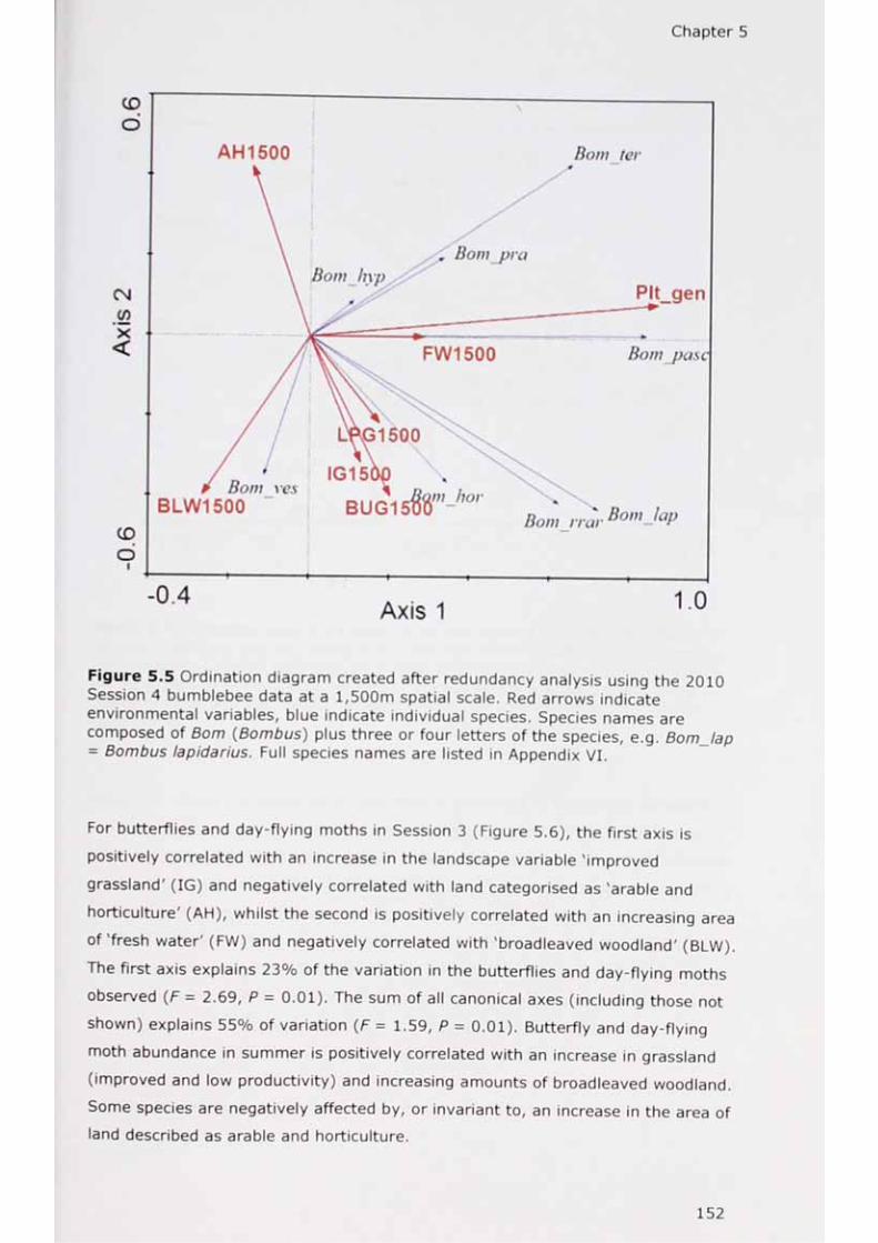
Chapter 5
Figure 5.5 Ordination diagram created after redundancy analysis using the 2010 Session 4 bumblebee data at a 1,500m spatial scale. Red arrows indicate environmental variables, blue indicate individual species. Species names are composed of Bom (Bombus) plus three or four letters of the species, e.g. Bom Ja p = Bombus lapidarius. Full species names are listed in Appendix VI.
For butterflies and day-flying moths in Session 3 (Figure 5.6), the first axis is
positively correlated with an increase in the landscape variable 'improved
grassland' (IG) and negatively correlated with land categorised as 'arable and
horticulture' (AH), whilst the second is positively correlated with an increasing area
of'fresh water' (FW) and negatively correlated with 'broadleaved woodland' (BLW).
The first axis explains 23% of the variation in the butterflies and day-flying moths
observed (F = 2.69, P = 0.01). The sum of all canonical axes (including those not
shown) explains 55% of variation (F = 1.59, P = 0.01). Butterfly and day-flying
moth abundance in summer is positively correlated with an increase in grassland
(improved and low productivity) and increasing amounts of broadleaved woodland.
Some species are negatively affected by, or invariant to, an increase in the area of
land described as arable and horticulture.
152

Chapter 5
Figure 5.6 Ordination diagram created after redundancy analysis using the 2010Session 3 butterfly and day-flying moth data at a 750m spatial scale. Red arrowsindicate environmental variables, blue indicate individual species. Species namesare composed of the first three letters of the genus followed by the first three orfour of the species, e.g. Pie_rap = Pieris rapae. Full species names are listed in Appendix VI.
Figure 5.7 shows the response of hoverflies in Session 3 to landscape variables.
The first axis is positively correlated with an increase in the landscape variable
'improved grassland' (IG) and negatively correlated with the land category 'arable
and horticulture' (AH), whilst the second is positively correlated with an increasing
area of IG and negatively correlated with the number of plant genera in the area
sampled (Plt_gen). The first axis explains 39% of the variation in the hoverflies
observed (F = 5.72, P = 0.03). The sum of all canonical axes (including those not
shown) explains 58% of variation (F = 1.75, P = 0.05). The presence and
abundance of some hoverfly species in summer is positively correlated with an
increase in land categorised as arable and horticulture as well as the number of
plant genera in the sampled area. An increase in the amount of improved grassland
and nearby built areas and gardens negatively affects the presence of certain
species.
153

Chapter 5
Figure 5.7 Ordination after redundancy analysis using the 2010 Session 3 hoverfly data at a 750m spatial scale. Red arrows indicate environmental variables, blue indicate individual species. Species names are composed of the first three letters of the genus followed by the first three or four of the species, e.g. Mya_flo = Myathropa florea. Full species names are listed in Appendix VI.
154

Tab
le 5
.4 R
esul
ts o
f RD
As
for
each
ins
ect
grou
p an
d se
ssio
n us
ing
the
land
scap
e sc
ale
deri
ved
from
the
exp
lora
tory
ana
lysi
s (T
able
5 3
) M
odel
s w
here
the
first
and
/or
all ca
noni
cal
axes
are
sig
nific
ant
are
give
n in
bol
d (P
s 0
.05)
. W
here
sig
nific
ance
occ
urs,
the
lan
dsca
pe
variab
les
exhi
bitin
g th
e hi
ghes
t co
rrel
atio
ns w
ith t
he f
irst
tw
o ax
es a
re a
lso
pres
ente
d. B
B =
bum
bleb
ees,
BD
M =
but
terf
ly a
nd d
ay-f
lyin
g m
oths
, H
F =
hove
rflie
s an
d SB
= s
olitar
y be
es.
For
desc
ript
ions
of
envi
ronm
enta
l va
riab
les
see
met
hods
.
■srfN vo 00
coO'
m o • • 00o + o
1 01 m
•a< CD B
LW
BLW
IG -0
CMfN
CO•
U0^ rNo ^
o’SJ-
•
•
Oi' d o o c
+ + <uX §
CO < . < i i LL i i i CL
00 LT) -5T^ 6
uoCM
•
fNrN rsi
uo•o + o •
l +
§
o oo 5 + iCL -J <J1 1 • 1
X_l CO 1 Li- • 1 <
rsifN
inin
+uo + fNVO
•
ocQJ
rN•
o
UO•
o1 U
1 +
u 1 K 1 1 AH
i • 1
CM 00 uo o H ■sr fN 00 inO
#o rN
#
00•o ▼H uo o
•
o o o•
o o•
o•
o#
o•
o•
oo
(N fN fN ■r O' CO 00 fN m00
•o 00
•
00 uo oA
CM O' f N•
rH rH co o d•
rH• #
o•
tH
O' CO rH o o m uo o CO 00ID uo
•
fN• •
uo#
uoA
inO o
•
o o o•
o o•
o o•
o
(N nCD CO CO CO CO CO CO CO
rs in i-fN n ^
T-t ^ -sr CM lt> h mo o o o
CO VO 00 O' CM O'
co tj- o nlt>
tH m CO o CM tH CM H CO KD LO y - 4 IN oO
m
o•
•o
A •
CO•O
• ao ▼H rH LD
o O o■
o o o •
o o o o•
o#
o•
o•
o•
o•
o
ro VO CM VO IN o' O' 00 o fN CM 00 vO00 fN
•
CMa
CM•
CO•VO IN
•
o•
O'•
fN UOa
o o O'CO CO 00 CM CM CM CM in fN CO CM
•
CM
o rN CO 00 O rN CO O' fN O' fN uo O' 00 CMCO
m
CMm
CO•<* CM
•
H•
CM CM• • •
CO CMa
CM CM•
o O oV
o O o•
o o o o •
o O#
o•
o•
o•
O
o o o oCD CD CD CD
fN m ^CO CO CO CO IS) U) C/) (/)

Chapter 5
Variance partitioning
The results of the variance partitioning procedures for each of the significant RDAs
(plus Session 3 for bumblebees for comparison) are given in Figure 5.8. The shared
variance fraction (C) is negative for all groups in Session 3. Leps and Smilauer
(2003) state negative values are not unusual and that they simply indicate the
joint explanatory effect of the two groups of variables is stronger than the sum of their marginal effects.
Figure 5.8 Results of variance partitioning (Borcard et a!., 1992) for each of the five significant RDAs plus Session 3 for bumblebees.
156

Chapter 5
The response of ground and cavity-nesting solitary bees to environmental factors
The variability in the number of ground and cavity-nesting bees recorded at each
property during Sessions 1 and 2 in 2011 is shown in Figures 5.9 and 5.10. A total
of 256 individuals from six species were recorded in Session l, versus 132
individuals from seven species in Session 2.
60 i
50 -
w<G3G 40 1 >•oc£ 30oL.V
BOU CA CHALL EN FAR HOL KEL LAM LW
Figure 5.9 Number of solitary bee individuals recorded in Session 1 at each walled garden categorised according to whether they are ground nesting (dark grey) or cavity nesting (light grey).
16
BOU CA CHALL EN FAR HOL KEL LAM LW
Figure 5.10 Number of solitary bee individuals recorded in Session 2 at each walled garden categorised according to whether they are ground nesting (dark grey) or cavity nesting (light grey).
157

Chapter 5
The results of four multiple regressions showing significant environmental factors
linked to the number of solitary bees in each nesting category for each session are
given in Table 5.5. In Session 1 the percentage area of beds and borders in a
walled garden was a significant variable explaining the abundance of cavity-nesting
bees (P — 0.04), whilst in Session 2, the number of plant genera available
explained the abundance of ground nesters (P = 0.02).
Table 5.5 Results of stepwise forward multiple regressions for the log-transformed number of solitary bees in walled gardens for Sessions 1 and 2. Only significant explanatory variables (P < 0.05) are shown. Degrees of freedom = 1,7 in all cases.
Nestingtype___
Cavitynesting
Session 1
Significant factor (R:
Ground N.S. nesting
Area ofbeds(0.48)
F P value value
6.49 0.04
ion 2
Number of plant genera (0.58)
N.S.
Significant Ffactor (R2) value
8.81 0.02
Discussion
The response of insect groups according to different landscape scales
As predicted, bumblebees consistently responded to landscape variables within
circles of greater radii than other groups. The results in Table 5.3 show that the
highest variance explained for Sessions 1 - 4 for bumblebees was in the landscape
scales measured at radii of 1,500m and 3,000m. Bumblebees may be either: (a)
nesting beyond the gardens and visiting to forage at flowers, or (b) nesting within
the gardens and making use of the available resources. Whilst sampling, several
nest locations were directly observed in transects, with their presence in other
areas of the gardens highlighted by gardeners. Goulson et al. (2010) note that
bumblebees favour garden settings for nest creation and that nests within gardens
are likely to experience higher levels of survival. What is not clear is whether this
preference for gardens is a direct response to the perceived suitability of sites for
nest creation and foraging, or a measure of the potential inhospitality of the
landscape beyond them (Goulson et al., 2010). As the aim of this study was not to
158

Chapter 5
establish the suitability of gardens or the surrounding area for nests, this remains
un-assessed in the context of large rural gardens. Hedgerows provide good nesting
opportunities for bumblebees (Osborne etal., 2008b); therefore quantifying the
presence of these linear features would be one way to establish whether
landscapes around some properties are more favourable than others.
In the current study bumblebees were considered as a single group to gain
maximum statistical power with respect to assessing the influence of spatial scales.
This allowed generalizations to be made about the group (c.f. the weakness
highlighted by Jauker et at. (2009) when all pollinators are considered together),
but ignored any differences between species. Pursuing the species-level approach
of Kreyer et al. (2004), who noted that different bumblebee species respond to the
landscape in different ways, would allow for tighter interpretation at a species
level.
Of the four insect groups considered, two (butterflies and day-flying moths, and
hoverflies) showed no discernible pattern in their landscape-scale response (Table
5.3). This was not unexpected when the life history of these groups is taken into
account, i.e. they are not centra! place foragers and some migrate over large
distances (Jauker et al., 2009).
Solitary bees exhibited the weakest response to landscape-scale factors. Only
Session 4 linked to a scale explaining a significant landscape factor (Table 5.3,
3,000m radius, broadleaved woodland, P < 0.04). Taking the known flight ranges
of sixteen European species of solitary bee into account - up to 600m (Gathmann
and Tscharntke, 2002), no obvious explanation is apparent for this result.
Temporal patterns
Clear temporal patterns were not discernible across groups. In part, this was due
to only one group (the bumblebees) having three sampling sessions containing
significant variables. Depending on the sampling session considered, different
variables took on increasing importance; a fact reflected by the composition of the
two main ordination axes. In the first sampling session two bumblebee species
Bombus pratorum and B. rupestris responded positively to the number of plant
genera available (axis 1, Figure 5.3). However many more species appeared to
respond to the landscape variable 'arable and horticulture' (axis 2, Figure 5.3) with
more bumblebees from more species observed as the area of this land category
increased. This is a surprising result in spring when flower-rich hedgerows in the
landscape are suggested to provide abundant resources (Hannon and Sisk, 2009).
159

Chapter 5
The reality however is that most hedgerows are not managed to allow regular and
abundant flowenng. More than 90% of hedgerows bordering agricultural land in a
1,000m radius around one of the properties (Lois Weedon) were severely cut back
using flails during the winter of 2010/2011 (pers. obs.), meaning few flowers were
produced. Although this observation relates to only one of the 17 properties, there
is no reason to assume that other hedgerows are being managed differently. As a
result, bumblebees may be attracted into gardens in spring because of a dearth of
flower resources in the wider landscape.
In Session 2 bumblebees appeared to primarily respond to the percentage of
broadleaved woodland and improved grassland in the wider landscape (axis 1,
Figure 5.4) and the percentage of arable land (axis 2, Figure 5.4 and Table 5.4).
Greater numbers of bumblebees from a range of species appeared in gardens as
the percentage of broadleaved woodland and arable land increased. To a lesser
extent, the variable 'number of plant genera' also influenced the diversity of
bumblebees observed in gardens. A plentiful supply of flowering plants may act as
a focus for workers visiting from nests beyond the garden (Osborne eta/., 1999),
or may signify that nest occupants within gardens are making use of resources
available.
In Session 4 the strongest influence to emerge was that of the number of plant
genera available (axis 1, Figure 5.5, which explains 48% of variation). This result
reinforces the importance of forage resources being available throughout the
season and extending into late summer, as described in Goulson eta/. (2010).
The temporal influence of monocultures such as the mass-flowering crop, oilseed
rape (OSR) is not directly obvious from these results. For example, there is no
strong response (positive or negative) to arable land in Session 2 which is when
this crop is in flower, yet OSR is known to influence bumblebee foraging behaviour
(Knight et a/., 2009, Goulson et a/., 2010). Visual inspection of photographs for the
seventeen sites show OSR growing within 1,500m of the gardens in 2009 - the
year before sampling took place (GetMapping PLC). However ground truthing to
ascertain the type of crops within the category 'arable and horticulture' was beyond
the scope of the 2010 and 2011 field seasons. A useful follow-up to this work
would be to repeat the assessment, focussing on bumblebees and quantifying the
area planted with OSR.

Chapter 5
The response of insect groups to landscape-scale variables
Whilst a seasonal pattern was not discernible, some groups appear to be
consistently influenced by certain landscape features regardless of spatial scale. An
example of this is the response of the group butterflies and day-flying moths and
that of hoverflies to the landscape variables 'arable and horticultural land' and
improved grassland (Figures 5.6 and 5.7). In both instances, there was a negative
association with the amount of improved grassland in the landscape, and more
species observed as the amount of arable land increased. This broadly agrees with
Ockinger et at. (2009) who found butterfly species richness and abundance was not
significantly related to flower abundance per se. Notwithstanding this, some
species did respond to the number of plant genera available. This effect was
stronger for hoverflies than it was for butterflies and day-flying moths (Figures 5.6
and 5.7), possibly reflecting their documented habit of preferentially selecting
flower-rich patches (Haenke et a!., 2009). This agrees with the observations of
Schweiger et at. (2007), who noted that hoverfly richness was less affected by
landscape-scale factors and more greatly influenced by flower patches.
Solitary bees were notably unresponsive to landscape variables (Tables 5.3 and
5.4), probably due to their shorter foraging ranges (Gathmann and Tscharntke,
2002, Greenleaf et a!., 2007).
Which better explains flower-visitor presence: plant richness or landscape-scale factors?
All groups with significant results from the redundancy analysis showed higher
levels of overall explained variance than unexplained variance (Figure 5.8).
The variance explained due to landscape factors alone (excluding bumblebees
Session 3 - BBS3, which is included in Figure 5.8 for comparison purposes) ranged
between 46.7% (bumblebees Session 1 - BBS1) and 50.8% (butterflies and day-
flying moths Session 3 - BDMS3). Plant genera on the other hand explained much
lower variance, ranging from 0.6% (bumblebees Session 4 - BBS4) to 15.5%
(hoverflies Session 3 - HFS3). The low variance due to plant genera for
bumblebees in Session 4 (despite being an important component of the ordination
diagram Figure 5.5), is countered by the shared effect of landscape variables and
plant genera together (accounting for 36.2% of variance, Figure 5.8). This
interacting effect of both within and beyond-garden variables only becomes
apparent when this procedure is used, highlighting its value.
161

Chapter 5
The resp°nse of ground and cavity-nesting bees to within and beyond walled garden environmental factors
The sampling in early spring of 2011 (Session 1) revealed a higher number of
solitary bees (256) than in Session 2 (132), (Figures 5.9 and 5.10). Splitting these
bees into two groups according to whether they were ground or cavity nesting
allowed an additional assessment to be made of whether proximal environmental
factors were significant. The multiple regressions considering the landscape effects
at 500m and 750m from the walls of the gardens were non-significant. This result
was partially expected as solitary bees are central place foragers and are known to
have short foraging ranges (Gathmann and Tscharntke, 2002). As such they are
restricted to collecting pollen and nectar reserves needed for their offspring in
areas geographically close to their nests (Jauker et a!., 2009).
Of the four within-garden factors only two were significant. In Session 1 the
percentage of walled gardens used as beds and borders was the significant variable
explaining the abundance of cavity-nesting bees (P = 0.04, Table 5.5), whilst in
Session 2 the number of plant genera was significantly related to the number of
ground-nesting bees (P = 0.02, Table 5.5).
The link between cavity nesting bees and the area of beds and borders probably
relates to the requirement for soil for nest construction by some species. Of all the
bees recorded in Session 1, 49% were from a single species, Osmia bicornis (data
not presented). This species uses soil to create partitions between individual cells
(Raw, 1972). The importance of this resource was noted by Westrich (1998) who
stated that even in the event that abundant nesting space and forage resources
are available, without a supply of soil, female bees cannot successfully reproduce.
By Session 2 (which occurred between 11 June and 4 July 2011) few O. bicornis
females were on the wing (pers. obs.) and they accounted for only 3% of the bees
recorded. As such, the variable 'beds and borders' was no longer significant for
cavity-nesting bees. Ground-nesting bees, on the other hand, showed a significant
positive relationship with the number of plant genera available. The ground-nesting
bees recorded were from three genera (Andrena, Lasioglossum and Nomada) and
represented approximately 45% of all the bees observed in Session 2.
In summary, the splitting of a single insect group into two based on their nesting
biology appears to offer new insights into responses to local-scale variables where
wholesale treatment fails.
162

Chapter 5
Conclusions
The findings of this chapter can be summarised as follows:
• Bumblebees responded to landscape-scale factors within circles of greater radii than all other groups. The typical radius was 1,500 - 3,000m.
• Butterflies and day-flying moths and hoverflies showed no consistent scale- dependent responses to environmental factors. This is not surprising when their life history traits are taken into account.
• Solitary bees were invariant to landscape-scale factors.
• Temporal patterns were weak, due in part to only a few groups and sessions containing significant variables. Assessing the seasonal effect of mass-flowering crops such as oilseed rape on bumblebee presence would be a useful complement to the current findings.
• Bumblebees showed a strong response to the availability of flowering plants late in the season, highlighting the important role gardens play in providing forage over an extended period.
• Butterflies and day-flying moths and hoverflies both responded to thelandscape variables 'arable and horticultural land' and 'improved grassland' in similar ways.
• As the percentage of arable land increased in the landscape, more hoverflies were observed in gardens.
• Hoverflies, which are noted for their preference for flower-rich patches, were also influenced by the number of plant genera available.
• For the three groups, bumblebees, butterflies and day-flying moths and hoverflies, landscape-scale factors rather than within-garden factors best explained the number of individuals observed.
• Bumblebees were most strongly influenced by a combination of landscape- scale and within-garden scale factors late in the summer.
• Splitting solitary bees according to their nesting biology revealed that cavity-nesting bees respond to the area of beds and borders in spring, whilst ground-nesting bees respond to the number of plant genera in summer.
The next chapter examines the nesting behaviour and reproductive success of the
most ubiquitous solitary bee species observed in walled gardens, Osmia bicornis.
163


Chapter 6
Chapter overviewIn this chapter, the potential of walled kitchen gardens to support populations of cavity-nesting bees is explored. Commercial trap-nests are used to establish the range of species present and to permit an in-depth look at the causes of mortality for Osmia bicornis, the most ubiquitous species present. By using k values, different mortality factors are compared in a consistent way across sites. The primary causes of mortality (developmental failure and parasitism) are considered in the light of their disproportionate effects on female bees.
IntroductionUnderstanding how landscape resources and natural enemies shape local populations
is a fundamental area of ecological enquiry (Kareiva, 1990). For bioindicators such
as flower-visiting insects, i.e. species that indicate changes in ecosystem-service
functioning or success, this takes on even greater importance (Christensen eta/.,
1996, Tscharntke eta/., 1998).
An important aspect of understanding how species are affected by factors at a
variety of scales is to ensure that mortality losses of juveniles are taken into account
(Steffan-Dewenter and Leschke, 2003, Carre eta/., 2009).
Nest and food requirements of solitary bees
Wild bee reproductive success is dependent on both adequate food resources and
suitable nesting sites (Westrich, 1998). Healthy wild bee offspring are the product of
an area fulfilling three basic criteria: (a) physical space for nest sites; (b) materials
for nest construction and (c) food plants that support both adults and larvae
(Westrich, 1998, Figure 6.1).
165

Chapter 6
Resources
below ground
suitable soil
rodent nests
above ground
cavities
dead wood or stems
exposed nests
empty snail shells
nectar
floral oils
Figure 6.1 Nesting and foraging resources required by bees in temperate locations (after Westrich, 1998).
In temperate climates approximately 70% of bees and wasps are ground-nesters
(Westrich, 1998). The initial occupancy and persistence of ground-nesting bees is
believed to be more closely linked to the abundance of suitable floral rewards than
nest sites per se, as suitable nest areas are rarely limited (Holzschuh et a/., 2010).
Aerial nesters, on the other hand, are more likely to be affected by limited nest
materials and sites than food resources (Tscharntke et at., 1998, Potts eta/., 2003,
Holzschuh et a!., 2010).
The availability of suitable nesting areas is an example of a resource-driven, bottom-
up effect. In general, nest site availability is density-independent, but can limit
population growth in a density-dependent fashion when organisms are spatially
aggregated (Gillman, 2009). In contrast to this, natural enemies such as predators
and parasites can have a top-down regulatory effect and act in a density-dependent
way (Steffan-Dewenter and Schiele, 2008). Efforts to understand the relative
importance and contribution of both top-down and bottom-up effects on various taxa
have involved a variety of methods including manipulation experiments, time-series
166

Chapter 6
analyses and life-tables (Raw, 1972, Preszler and Price 1988, Hunter eta/., 1997,
Hunter, 2001). To date, herbivores have been the main focus of this research, but
see Steffan-Dewenter and Schiele (2008).
The interest in native aerial-nesters comes as concerns about global honey bee
losses escalate (vanEngelsdorp and Meixner, 2010, Breeze eta/., 2011). The major
causes for the decline of the western honey bee are discussed extensively in
vanEngelsdorp and Meixner (2010) and include a range of diseases and parasites
e.g. Nosema spp. and Varroa destructor, unresolved disorders' such as Colony
Collapse Disorder (Watanabe, 2008), together with direct and indirect poisoning by pesticides.
A study using a simulation model to explore the potential of native bees to facilitate
pollination of a commercial crop in North America found these insects had the
capacity to buffer reductions in crop yields incurred as a result of honey bee losses
(Winfree et al.t 2007). How to capitalise on this potential is an area that has started
to receive increasing attention, with several species of solitary bee now managed for
commercial crop pollination (Bosch, 1994, Bosch and Kemp, 2002, Gruber eta/.,
2011, Table 6.1).

Chapter 6
Table 6.1 Examples of solitary bee species used as pollinators of commercial crops.
Bee species Crop Location and effect on
pollination
if known
Source
Meg a chile rotundata
Fabricius, 1787
(Megachilidae)
alfalfa USA
Tripled seed
production in the
second half of the 20th
century
Pitts-Singer and
Cane (2011)
Osmia cornuta
Latrielle, 1805
(Megachilidae)
apples Europe Bosch (1994),
Vicens and Bosch
(2000)
Osmia cornifrons
Radoszkowski, 1887
(Megachilidae)
apples Japan Maeta and
Kitamura (1974)
Osmia lignaria
Say, 1837
(Megachilidae)
sweet cherry USA
Doubled sweet cherry
yield in a
5-year period
Bosch et al. (2006)
Trap-nesting bees and artificial nests
Suitable solitary bee species for management comprise those that readily nest in
pre-existing cavities and are termed trap-nesting bees (Raw, 1972). In a natural
setting these bees utilise dead wood, plant stems, beetle borings and holes in
vertical landscape features to construct their nests, but when managed they occupy
artificial nests (O'Toole, 2011).
168

Chapter 6
Although a range of artificial nest materials have been used for experimental
purposes - including bundles of paper drinking straws, plant stems and drilled
wooden blocks (Free and Williams, 1970, Bosch and Kemp, 2002), the majority of
studies mimic nest cavities by using internodes of the common reed Phragmites
australis (Cav.) Trin. ex Steud, (Poaceae). The reeds are tied together and are used
to encourage females to establish cells within them. This method is inexpensive and
convenient, but has disadvantages. For example female bees, in the absence of
standard reed-widths, may create greater numbers of cells containing eggs of a
particular sex (Raw, 1972), and parasites may respond differently depending on reed
length and size of opening (Krunic et at., 2005).
Alternatives to reed-based trap-nests are available commercially. Although primarily
aimed at meeting the needs of individuals wishing to increase biodiversity in their
gardens, their design and uniformity makes them ideal for experimental use. The
nests comprise plastic hexagonal structures that are open at one end (Figure 6.2A-
C) and contain 30 individual cardboard tubes, each lined with a paper cylinder. The
outer plastic casing affords protection from inclement weather, whilst the cardboard
tubes and paper liners allow easy examination of the contents (Bates et a!., 2011a).
In addition to their value for experimental work, these nests serve as important
educational tools. The bees using them are considered safe near children and pets
and can be used to help raise the public's understanding of the importance of native
bees as pollinators of crops and wild flowers (OToole, 2002, Bates et a!., 2011a,
Everaars et a\., 2011).
There are several advantages associated with using trap nests, regardless of type.
They provide abundant nesting resources when a species is used at high densities for
a specific pollination purpose (Wilkaniec and Giejdasz, 2003); they act as effective
monitoring tools to assess Hymenoptera diversity in fragmented areas (Jenkins and
Matthews, 2004) and they can be used experimentally to explore the top-down
regulatory effects of parasites and predators (Seidelmann, 2006, Pitts-Singer and
Cane, 2011), progeny sex-ratios (Bosch and Vicens, 2005, Seidelmann et at., 2010),
and the effects of habitat management on bee species richness (Steffan-Dewenter
and Leschke, 2003, Holzschuh eta!., 2010, Schueepp etal., 2011).
169

Chapter 6
0 * -r- w
Figure 6.2 Commercial trap-nests for solitary bees: A) Placement in Lamport Hall walled garden in early spring 2011, B) Plastic grill protecting tubes from birds/squirrels, C) Public information label attached to nest, D) Contents of two O. bicornis brood cells (pollen and nectar resources plus eggs). Images: Erenler (2011)
Past research has shown that, regardless of the type of artificial nest offered,
occupancy by solitary bees is common, even in the centre of urban areas (Wilkaniec
and Giejdasz, 2003, Gaston et a!., 2005). Although bundles of reeds help augment
numbers of potential pollinators, they are less useful to assess parasitism levels and
the ratio of female to male offspring. Instead, a more standardised approach is
necessary. By controlling for differences in tube lengths and widths (through the use
of pre-prepared tubes rather than reed stems), other variables that may explain
levels of occupancy, parasitism and reproductive success may be more accurately
explored. These variables include, but are not limited to, the abundance of pre-
existing cavities in the area, floral species richness and landscape composition
(Steffan-Dewenter and Schiele, 2008, Holzschuh et a!., 2010).
170

Chapter 6
The red mason bee
Life history
The red mason bee, Osmia bicornis, syn. O. rufa, is a solitary, univoltine, trap-
nesting species with a Palaearctic distribution. It is common in England and Wales
and regularly occurs in rural and urban gardens (Edwards, 1998). This ubiquitous
bee is polylectic, visiting a variety of plants for both pollen and nectar (Edwards,
1998). Males commence their flight period in mid to late March in England (females
appear approximately one week later), and continue through to early July. Males
are 6 - 11mm in length; females are larger at 10 - 16mm (Edwards, 1998). The
flight period for this species coincides with the flowering time of a wide range of
commercially grown mass-flowering rosaceous fruit in the UK such as apples, pears
and strawberries, as well as spring and early summer native flowers (Edwards,
1998, Roberts and Dean, 2012). The red mason bee's ability to warm up at a faster
rate than expected for its body size enables it to visit flowers in high numbers at a
time when other pollinators such as bumblebees (Bombus spp.) are yet to build their
colonies to full-strength (Stone and Willmer, 1989, OToole, 2002). Despite these
qualities, O. bicornis has not yet been used as a managed pollinator in the United
Kingdom by commercial growers and farmers (Dean, pers. comm.).
A red mason bee nest consists of a linear set of brood cells. Each cell is provisioned
with a quantity of pollen and nectar, with a single egg laid atop (Figure 6.2D and
Figure 6.3A). Individual cells are separated by soil partitions and eventually sealed
with a textured mud capping, often beyond a final empty gap or vestibulum
(Seidelmann, 1999) (Figure 6.3B, C).
In common with other Hymenoptera, sex-determination is through haplodiploidy.
This occurs by means of facultative fertilization of the egg at the point of laying,
using sperm stored in the spermatheca (Gerber and Klostermeyer, 1970). Daughters
occur when fertilization takes place (diploidy) with sons the product of unfertilised
eggs (haploidy) (Bosch and Vicens, 2005). Females decide the sex of the egg they
will lay at the onset of cell construction by using a mud partition-like structure
known as Fabre's threshold (Raw, 1972). This delimits the size of the cell and the
extent of provisions that will be stored in it. Male O. bicornis are smaller than
females and are allocated less food reserves. This is similar to many other
megachilid bees, e.g. male Megachile rotundata receive 17% less provisions than
females (Pitts-Singer and Cane, 2011).
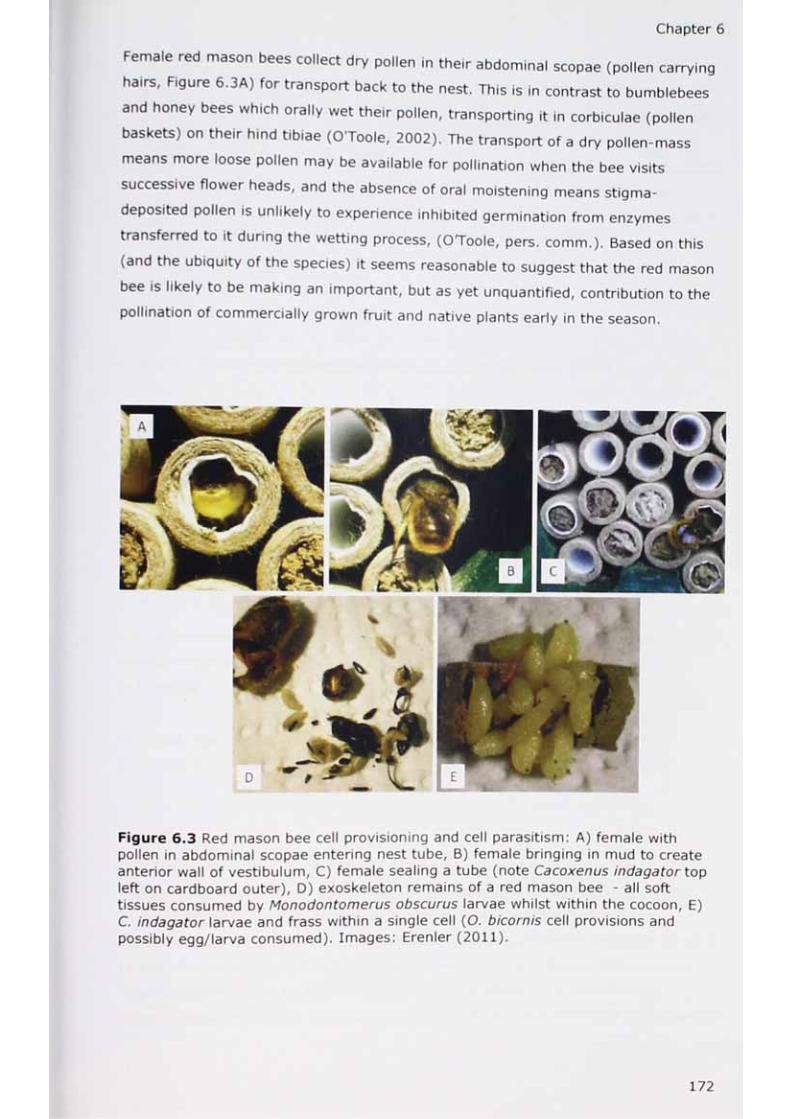
Chapter 6
Female red mason bees collect dry pollen in their abdominal scopae (pollen carrying
hairs, Figure 6.3A) for transport back to the nest. This is in contrast to bumblebees
and honey bees which orally wet their pollen, transporting it in corbiculae (pollen
baskets) on their hind tibiae (O'Toole, 2002). The transport of a dry pollen-mass
means more loose pollen may be available for pollination when the bee visits
successive flower heads, and the absence of oral moistening means stigma-
deposited pollen is unlikely to experience inhibited germination from enzymes
transferred to it during the wetting process, (OToole, pers. comm.). Based on this
(and the ubiquity of the species) it seems reasonable to suggest that the red mason
bee is likely to be making an important, but as yet unquantified, contribution to the
pollination of commercially grown fruit and native plants early in the season.
Figure 6.3 Red mason bee cell provisioning and cell parasitism: A) female with pollen in abdominal scopae entering nest tube, B) female bringing in mud to create anterior wall of vestibulum, C) female sealing a tube (note Cacoxenus indagator top left on cardboard outer), D) exoskeleton remains of a red mason bee - all soft tissues consumed by Monodontomerus obscurus larvae whilst within the cocoon, E) C. indagator larvae and frass within a single cell (O. bicornis cell provisions and possibly egg/larva consumed). Images: Erenler (2011).

m
Chapter 6
Several authors have recorded the red mason bee as the most abundant cavity-
nesting species, making it ideal for experimental purposes (Table 6.2). Another
advantage of O. bicorms is that its taxonomy, biology and associated parasites and
predators are well documented. These include the drosophilid fly Cacoxenus
indagator Loew (Diptera: Drosophilidae) which is host-specific and is known to affect
O. bicorn is cells in great numbers, and Monodontomerus obscurus Westwood
(Hymenoptera: Torymidae), a chalcid wasp whose larvae feed on pre-emerged adult
bees (Raw 1972, Krunic et al., 2005), (Figure 6.3C, D and E). Combined mortality
losses at the larval stage due to developmental failure and the presence of the
specialist C. indagator can occur in more than a third of all O. bicornis brood cells
(Steffan-Dewenter and Schiele, 2008, Jauker et a/.f 2012a).
Table 6.2 Studies highlighting the dominant use of trap-nests by the red mason bee.
Location of study Total
number of
bee brood
cells
Percentage of total
bee brood cells
created by
O. bicornis
Source
Orchard meadows in
Germany
17 278 84% Steffan-Dewenter
and Leschke (2003)
Conventional and
organic wheat fields
in Germany
8644 96% Holzschuh et al.
(2010)
Farmland sites in
Switzerland
1003 71% Schueepp et al.
(2011)
In common with other Osmia species, female red mason bee progeny are
preferentially located at the innermost part of each nest (Bosch and Kemp, 2002).
As a consequence, mortality losses occurring in anything other than a random
fashion throughout the nest have the potential to disproportionally affect the survival
of each sex. In the event that females are more adversely affected, this may have
important implications for flower visitation and pollination. This arises for two
reasons; first, females are the sole nest provisioners and therefore visit more flowers
173

Chapter 6
than males and second, reduced female numbers could eventually lead to a smaller
contribution to overall population size (Bosch and Kemp, 2002).
Previous research using O. bicornis has focussed on methods for augmenting
population numbers (Krunic and Stanisavljevic, 2006, Gruber eta/., 2011), as well
as attempting to understand the drivers for the sex ratios observed (Bosch and
Vicens, 2005, Seidelmann, 2006, Seidelmann eta/., 2010). The former emphasises
the need for supplying sufficient bees for commercial pollination purposes, whilst the
latter tests ideas about adaptive strategies used by females to alleviate the effects of open-cell parasitism.
Although parasitism losses in relation to brood cell position within the nest have
been reported (Strohm, 2011), losses due to developmental failure do not appear to
have been assessed. To my knowledge no studies have explored broad causes of
mortality in relation to both cell position and gender. In gaining an understanding of
the mortality differences experienced by males and females, the timing and control
methods needed to mitigate against these losses can be developed.
The red mason bee in gardens
The red mason bee is known to frequent both rural and urban gardens, and freely
utilises existing holes in walls and mortar (pers. obs., Figure 6.4) as well as
occupying artificial nests placed in sunny locations (Gaston eta/., 2005). During
2010, the red mason bee was recorded at fifteen of the seventeen sampling sites
(Chapter 2 - 2010 field season).
174

Chapter 6
Figure 6.4 Existing cavities in the mortar between bricks in the walled garden atLamport Hall. These holes are used by O. bicornis and other cavity nesting bees. Image: Erenler (2012).
Analysing bee life-cycles using stage-dependent life tables
Stage-dependent life tables document the key mortality events during the life of an
insect. Events are expressed in their natural order without reference to calendar
time (Varley et a!., 1975, Hunter, 2001).The term 'mortality' is used in the broadest
sense, encapsulating losses regardless of whether death occurs, e.g. when males are
discounted from a population or lost through dispersal (Yamamura, 1999).
Calculating mortality rates at each stage allows populations to be compared across
space or time. Each stage is ascribed a k value (the 'killing power'), with all stages
considered independent. The k value is calculated as the negative logarithm of
survival, with individual k values summed to give a total mortality value, expressed
as K (Yamamura, 1999). An important difference between the commonly used
mortality percentages and k survival values is that the latter are additive (Varley et
a!., 1975, Yamamura, 1999).
175
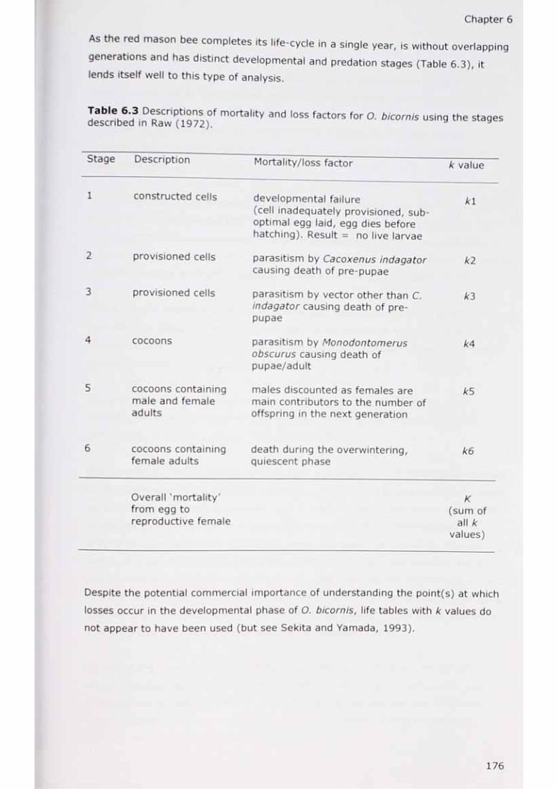
Chapter 6
As the red mason bee completes its life-cycle in a single year, is without overlapping
generations and has distinct developmental and predation stages (Table 6.3), it lends itself well to this type of analysis.
Jesbchbed3inDeRSaCwiP(1972)0f ^ '°SS faCt°rS f°r biCOmis USing the stages
btage Description Mortality/loss factor k value
1 constructed cells developmental failure (cell inadequately provisioned, sub- optimal egg laid, egg dies before hatching). Result = no live larvae
k l
2 provisioned cells parasitism by Cacoxenus indagator causing death of pre-pupae
k2
3 provisioned cells parasitism by vector other than C. indagator causing death of pre-pupae
k3
4 cocoons parasitism by Monodontomerus obscurus causing death of pupae/adult
k4
5 cocoons containing male and female adults
males discounted as females are main contributors to the number of offspring in the next generation
kS
6 cocoons containing female adults
death during the overwintering, quiescent phase
k6
Overall 'mortality' from egg to reproductive female
K(sum of
all k values)
Despite the potential commercial importance of understanding the point(s) at which
losses occur in the developmental phase of O. bicornis, life tables with k values do
not appear to have been used (but see Sekita and Yamada, 1993).

Chapter 6
Walled kitchen gardens
Historic use
Walled kitchen' or 'productive' gardens have been an integral part of the English
country-house estate for centuries. Up until the 1930s these 'rooms', bounded by
walls, hedges or simple fences, provided the household with its fruit and vegetable
needs throughout the year. The walls provided a microclimate conducive for
vegetable growing whilst keeping out unwelcome animal and human visitors (Wilson, 2003, Musgrave, 2009, Campbell, 2010).
Up until the end of the seventeenth century most walled gardens were square, with
their internal space divided into four distinct sections or'quarters' (Campbell, 2005).
The design mimicked ancient classical gardens and the partitions (comprised of
pathways) afforded country-house owners the possibility of taking visitors and family
on strolls through the highly managed garden environment (Campbell, 2010).
With a greater appreciation of the heat retention properties of certain building
materials, the design of rectangular gardens (built with brick walls) became popular
(Campbell, 2005). These allowed fruit to ripen early on espalier-grown trees trained
against the longest walls (Campbell, 2005, 2010).
The size of kitchen gardens often ranged between one acre to 20 or 30 acres
according to taste and resources, with a one acre walled garden able to supply
sufficient produce for 12 people (Campbell, 2010).
The fashions of the day usually dictated what was grown. The experimental practices
involved in raising exotic fruit and vegetable specimens led to new innovations within
walled gardens. This saw the introduction of heated glass houses, often with the aid
of hotbeds (Musgrave, 2009). In addition to growing exotics and traditional
vegetables, aromatic plants and flowers were cultivated. The popularity of preparing
herbal remedies meant these plants were needed for homemade tinctures, salves
and tonics; a practice that continued until the late 18th century. The flowers of these
aromatic shrubs, many of which originated from the Mediterranean, offered pleasing
olfactory and visual distractions from the often less pleasant muck heaps that were
needed to fuel the hotbeds (Musgrave, 2009, Campbell, 2010).
As well as their medicinal and aesthetic properties, aromatic plants would have
attracted pollinating insects. It is known that the Romans grew thyme, rosemary
and marjoram for the bees in their gardens, but it is believed this was to ensure
fragrant honey was produced rather than actively encourage bees to visit and
pollinate nearby crops (Campbell, 2005).

Chapter 6
Honey bees have actively been kept in walled gardens for centuries (Campbell,
2005). Early hives took the form of straw skeps, with some garden walls designed
specifically to incorporate recesses (or bee boles) for colonies (Campbell, 2005). As
in Roman times, the focus was purely on obtaining products from bees, e.g. honey
and beeswax (Ebert, 2011). Some early writers on the subject of apiculture were
keen to emphasize other advantages of bees, citing how bee behaviour (hard work
and a clearly demarked organisational structure) was a positive role-model for
human society (Warder, 1720). Others, meanwhile, extolled the virtues of
beekeeping as a cottage activity offering financial gain to the rural poor as well as a
stimulating intellectual hobby for the rich (Keys, 1780).
The earliest understanding of the structure of social bee colonies came with Charles
Butler's The Feminine Monarchic in 1609 (Butler, 1609), but it was not until the late
eighteenth century that observations about the inhumane methods of obtaining
honey, which required the majority of bees to be immobilised and killed with smoke
and brimstone, led to hive design moving away from skeps to formal bee hives. The
latter were both functional and decorative and were placed in walled gardens for the
amusement of owners and house guests (Campbell, 2005). The role of bees as
pollinators was only appreciated in the 18th century; with the naturalist Joseph
Kolreuter establishing that the purpose of nectar was to reward insects (Proctor et
al., 1996).
Today, few walled gardens contain hives. The gardens themselves are often shadows
of their former selves, with a minority in ruins and some with only a fraction of the
original area cultivated for fruit and vegetables (Campbell, 2010). The shift away
from high productivity came with the increased availability of cheap foodstuffs from
around the world and escalating labour costs for maintaining kitchen gardens
(Campbell, 2010). Tennis courts and swimming pools are frequently found in walled
gardens in place of land that would previously have given a continuous supply of
fresh vegetables. Examples from the present study include Courteenhall, Easton
Neston and Lois Weedon House. Another feature of today's walled gardens is the
extensive area laid to turf. Often closely mown, lawns offer few flower resources for
insects.
Despite the change in use of walled gardens, the walls themselves remain as
potential nest sites for cavity-nesting bees. The situation is helped, in part, by the
many holes remaining from the habit of driving metal pins into mortar to anchor
wires needed to support wall-grown fruit trees (Campbell, 2010).
178

Chapter 6
Aims
The aims of this chapter are to quantify nest site occupancy, cell parasitism and
reproductive success in nine walled gardens, with a strong focus on the most
ubiquitous species, Osmia bicornis. Specifically, the work seeks to answer the following questions:
1. Does tube usage by a) a range of trap-nesting bees and b) the red mason bee differ across the nine properties?
2. Is there a relationship between the abundance of O. bicornis cells created and those of other bee species, and is O. bicornis abundance correlated with the number of pre-existing cavities in the walls?
3. Do the k values relating to developmental and parasitism losses (kl-4) differ between properties?
4. Is there a relationship between the number of cells parasitized by Cacoxenus indagator and the number of cells present?
5. Do rates of developmental and parasitism loss vary according to brood celllocation in the nest and, if so, do these losses affect equal numbers of males and females?
6. Is the sex ratio of O. bicornis observed in the current study consistent with other locations and other trap-nest species?
7. Is there a difference in mortality rates for overwintering male and female bees within and between properties?
Methods
Sampling
Nine walled gardens were used for the study (Chapter 2 - 2011 field season, Table
6.4). Commercial trap-nests were placed at study sites in spring 2011, with the
experimental work completed in the spring of 2012.
The trap-nests (Vivara brand) were purchased from CJ Wildbird Food, Upton Magna,
Shrewsbury, England. Nests consisted of a green plastic casing containing thirty
cardboard tubes together with a protective grill (Figure 6.2B). Each tube contained a
paper liner measuring 150mm in length and 0.7mm in diameter that could be
withdrawn using a plastic stopper at one end. Three nests were affixed to south or
east facing walls in each garden between 15th and 24th March 2011. The nests were
attached to mortar between bricks or stone at a height of 1.6m - 1.8m in areas free
of vegetation, and separated by a minimum horizontal distance of 5m.
179

Ta
ble
6.4
Det
ails
of
the
nin
e w
alle
d g
ard
ens
used
in
the
tra
p-n
es
t st
ud
y.
E
*D Ut o
</> -ra coc '5
2 TOO $
n E E E4->V) CO• • vo•<u tHz U1 § in
in
(Nl/l(V
EvO E
COE
00
LUinLU
LUinin
E00
to
EVO
LUin(/)
EVO
in
E E E E E E E E E00• rv• vO• voA 00 00 vo VO VOt-H H # • • • •in $ in § LU § in LU in
in in in inin in in
ua>a</it o
E E E E E E E E El/>0>z
00•
r \•rH
vO•
vO•▼H
00•
00•
00•
vo•
vo•
in § in § LU § in LU inin in in in
in in in
o ^ c a;c oT O
2 o
a
T O
5
o
i/)QJ n o 1 LD o f \ ro
• OM E in00
• •Ov
•rs i
•• M B
-HVO ro H rv
>T O
U<va -H
-H-H -H
ro r ^ rv0 0 O voro LT)
• ro•
H t -H
a»coin
fN
a;coin
VO
rsj
-Hrorooorsi
ro
-H
vof \
0000
-nrororo
inLD
-Hrororsi
ro
-H
vO
QJu u
• • M B S
co u
•
u•
u• m m m
cn CO CD in CD CD CD
�D CU a;= T3TO jr> TO> o»
fN
E
T O
<UT O
ro LT) rsi ro a» 00O- O o rsi LO a> o rsi00 vO o t-H f\ ro rsj rsi rsjl\ tH r\ a» 00 00 ro
_ ° a5 ^ to _U CO c zjfl H C ^ 2 c in > a o O
coT O
> I O a; coj o-Q <
<U < z
LU
CL< O LLJ
ULL. X
<
coT Ouo
QJv/>
<UQJ cn0 oa co
(/><10cocruU
T O
Cq jq j
tou
covoQJ
VOT O
LU
T O
cn=3oo
T O
cuvo
JOcQJ
T O
VOT O
EQJ
T O
OCL
ET O
QJQJ
(O»
O
Chapter 6
Between the 24“ August and 15“ September 2011 the cardboard tubes were
removed, leaving just the nest casings in place. Each tube was marked with a unique
property, nest and tube number and stored in dry conditions (temperature range 12
- 16°C, relative humidity 40 - 45%) until it was opened.
Examination of the nest contents
To ensure the fly larvae of the specialist cleptoparasite Cacoxenus indagator were
found in situ (they are known to migrate towards nest entrances - Strohm, 2011),
the tubes were examined within three months of collection (between 11th and 23rd of November 2011).
Paper liners were removed from their tubes and opened by making a small incision
at the end opposite the stopper. The paper was then unravelled in a spiral fashion
(Bates et a!., 2011a). The contents were recorded according to the categories
described in Figure 6.5. In addition, a random subset of ten nests had their cell
contents recorded according to their exact location within each tube. The innermost
cell in each tube was designated as cell one.
Where a cell contained a cocoon, this was examined by slicing open the nipple-like
structure at one end. The sex of the occupant was determined by noting the
presence or absence of female clypeal horns on the head (Raw, 1972). In opening
the cocoons, instances where larvae of the solitary parasitic wasp Monodontomerus
obscurus had consumed the non-chitinous parts of the adult bee within were
revealed (Figure 6.3D).
For the subset of ten nests, the sex of a failed individual (resulting from
developmental failure or parasitism, Figure 6.5 categories D, E and F) was inferred
from the sex of occupants in adjacent cells. This was possible as cells are aggregated
according to sex in this species (Seidelmann eta/., 2010). As a precautionary
measure, any failed cell with a female as one neighbour and a male as another was
excluded from analyses as the occupant's sex could not reliably be inferred.
Overwintering storage and survival
After examination the cocoons were bulked according to nest and placed in plastic
disposable food containers between two layers of paper kitchen-towel. The
containers were pierced to prevent the build-up of CC^and placed in cold storage at
4°C (Sekita and Yamada, 1993, Bates et al., 2011a). Between 21st and 23rd March
2012 the overwintered cocoons were returned to their nests. In late May 2012 the
gardens were re-visited to establish the number of bees of each sex within each nest
that had failed to emerge.
181

CD J=)
leTt
a^'e
s^nT
abfe
9??
Sh0
Wi"
9 ^
^ °
f tr
ap'n
eSt
cells
acc
ordi
n9 t
0 8
cate
gori
es,
toge
ther
with
k v
alue
s de
rive
d fr
om t
he l
ife-

Chapter 6
Pre-existing wall cavities
The mean density of pre-existing cavities in the mortar was calculated by randomly
assigning six 50cm x 50cm quadrats to the south-facing wall in each garden,
counting the number of holes present in each, and generating a mean hole-density value.
Statistical analyses
In order to take account of one nest containing twenty-nine rather than thirty tubes
(Canons Ashby, Nest 3), the fraction of tubes colonised rather than the absolute
number of tubes colonised was used for analysis.
Life tables were created and k values calculated following the protocols of Varley et
al. (1975) and Yamamura (1999), Appendix VIII. The k values for Lois Weedon (LW)
were not calculated as cell numbers were low or non-existent in two of the three
nests, meaning reliable values could not be obtained. Differences between properties
were examined using Kruskal-Wallis tests on k values 1 - 4 .
Linear regression was used to examine the total number of deaths due to
developmental failure in relation to brood cell position in a tube, and also for total
deaths due to the presence of C. indagator against brood cell position.
To establish whether female or male progeny were more likely to be affected by the
mortality factors a three-step approach was taken:
Step 1: Using the subset of ten nests and only those cells where the sex of the
occupant could reliably be inferred, the actual number of females and males
recorded at each brood cell position was used to calculate the relative proportion of
each sex at each position.
Step 2: The relative proportions were multiplied by the number dying at each
position to estimate the number of females and males dying from each mortality
event at each location.
Step 3: The fraction of each sex at each location was calculated using the estimated
number dying (step 2) divided by the total number across all cells
The difference in estimated numbers of females and males dying at each location
(step 2) was analysed with a G-test for independence using the methods described
in Sokal and Rohlf (1981). As the observed values for the four outer cells (cells 7, 8,
9 and 10) were 1 or less for females, these were bulked with the nearest cell, (cell
).
183

Chapter 6
A two-sample Kolmogorov-Smirnov test was used to examine differences in the
distribution of male and female overwintering losses. This test allows the comparison
of two sets of distribution data from a population (Dytham, 2011).
Results
Use of nests and tubes by solitary bees
All twenty-seven artificial nests were occupied by solitary bees. Of the 809 available
tubes across all sites, 490 (61%) were used by a range of bees. Usage was defined
as either a) initiation of a cell(s) within a tube, b) provisioning of cells, whether
completed or not, or c) outer end of tube sealed, regardless of whether it was later
found to contain cells. Only one property, Lamport (LAM), had all thirty tubes in each
of its three nests fully used (Figure 6.6).
Figure 6.6 Median fraction of tubes used at each property, ranked highest to lowest, with range as error bars.
As the tube-usage data violated Levene's test for homogeneity of variance, both as a
fraction and when arcsine transformed (P = 0.01), the non-parametric Kruskal-Wallis
test was used. Tube usage (by all species) differed significantly between the nine
gardens, H (8) = 22.12, P = 0.005. This result was followed up with post hoc tests
as described by Siegel and Castellan (1988), (Appendix IX, Table 6.5).

Chapter 6
Kruskat-WShs testncfnn L " ° C mean rankS °f fraction of tubes used after aKRjskal Wallis test using the procedure described in Siegel and Castellan (1988).Di erences in mean ranks > 10.53 are significant (P < 0.05) and shown in bold.
BOU
BOU CA CHALL EN FAR HOLI -
CA 7.17 .
CHALL 15.17 8.00
EN 0.47 6.70 14.70FAR 12.5 5.33 2.67 11.50HOL 1.66 8.83 16.83 2.66 14.16KEL 9.0 1.83 6.17 18.00 3.50 10.66LAM 3.83 11.00 19.00 4.83 16.33 2.17LW 16.17 9.00 1.00 15.17 3.67 17.83
KEL LAM
12.30
7.17 20.00
Cell creation
Of the 490 used tubes, 467 (95.3%) contained fully provisioned cells. A total of
2,657 cells representing all bee species (Category A, Figure 6.5, Table 6.6), were
recorded from across the nine properties. Lamport Hall had the highest mean
number of cells across all three nests (174.7 ± 19.4 SD), but the nest with the
highest overall number of cells was at Easton Neston - 214 cells (nest EN3, Table
6 . 6) .
Of the 2,657 cells recorded 2,521 (94.9%) were those of O. bicornis (Category C,
Figure 6.5, Table 6.6). A one-way ANOVA revealed the mean number of cells for this
species was significantly different between properties F8/18 = 5.90, P = 0.001. Post
hoc tests (REGWQ) showed that Lois Weedon, Courteenhall and Farnborough had
significantly fewer cells than Holdenby and Lamport (Figure 6.7).
185

Ta
ble
6.6
Use
and
con
tent
s of
nes
ts a
nd t
ubes
per
pro
pert
y. *
Can
ons
Ash
by t
rap-
nest
3 c
onta
ined
onl
y 29
tub
es.
Cat
egor
ies
A-C
des
crib
ed
in F
igur
e 6.
5.
o .V)5.8•o
VOQJTO
E
.V> V/>O a>
.8-Q
roE<D
d |O-Q
VO ^
ouou
TO o <V *->
QJ TO_VO
13u
TO
^ H 0'00^0' ® H Tf (N ^ 0 ^ ^ r o r s
o oo 0 0>COrM»-«’si-o^^fnvoroo'0<tTt ' on^
C 2 XJ ^o S "o 3u Q D Uo N VOU 33 -Q
to O
o O O H PUD O O O O ^ O O N H ^
LDir'0^12il.^ ,CS fNir,0' 0 0 c ^rooo,NOOOvOTHvOVOvOO ' L' o n uun n vo n vo ncoo^^o^THtHin
j5 o; no E o ~ to
o o o in O O l H O O O O O O o O O rH
VOE 15 2 £
<n T3 t :<L>Cl >� D -Qu u o
a;U2 °TJ TOS' cto.c
j.^l^’ 'vOfnrsrNfNjooinQfNfNj0 0 . fN fNo.O•Q
00in
fN0>
o rs rr n • 1 o oin
ofN o
O O
a»
JO
13o p
l~o £ou
tj<u 0>§•'§ -Qu -E • u O° 0 ^
TO LLIro a>a>TO
tTO
^ fN -H (N r-< o o i n o o o ^ o v o r s ^ t o ^ r f N o r n i n o (N
fN
TO ^ .10 3jO ?TO OP
•Q
vou
o o in in o in min h n h h OHnNrsrNinmcoNc^^iOvOH fN in mfNTt^m Tj-TtTt
r\ ro a> m
O •voEou-Q
VO
uOOfMVOnniNTOvOvtH^vO-Hvd oo m o oo co in vo h co^
moOfNro'sj-rNfNinrscoO thvO O t hl ovovOO
r\ »h in
_VO
13u
L. • (/\<v o coO TO OP
•O
o o ^ o o O N - ^ o o o o O L n r N L n r N O O L D N - r ^ o o o ^ o o ^ o v ofN m fN m
TO
O
— to <<
a<UU
oorovororo oc7>vOTtTHTj- o in 0 3
^
rnLninoofNcococnfNinrsN-a^r^rvOOH ( H V O O H N 0 l O Q r t H f \j in
fN
C TOo a;□ VOu 3 TO
rvoo o r s v o o r ^ m r s r o o r ^ o o o o oN ^VOiOOOOo^lOO^^fNONO N n nID vD 3"
O O O O O O o m m° 0 0 0 o o o 00tH r
(/) TOo a> a;o -O to
3 13
ciQ.
o TO a>• MB* i ,TOU TO toO C cu 3
TO c C
^ O H N O O l C O f NfN n f\ H N H H o ^vDOHONOi rOOOOfrl^ 'TO r o N n H H H M n n (j ,
<r
fN fO fN fO fN nfN ro
*H f N f O H f N f O H N n _ _ _
0 0 0 < < < X X X Z Z Z < < < O O O L U Q J U J c o c o c Q U U U U U U i u u j i U L t L L i L l I l Y y Y
n nfN fOZ 2 Z r
< < < £ £ £ O

Chapter 6
Property
Figure 6 7 Mean number of O. bicornis cells per nest for each property (arithmetic mean ± SE). Identical letters show homogeneous groups (REGWQ post hoc tests).
Red mason bee cells and cells of other trap-nesting bee species
The absolute number of O. bicornis cells and those of other species (Appendix X) is
given in Figure 6.8. Three walled gardens (Canons Ashby, Easton Neston and
Lamport) only had O. bicornis cells present. For the six gardens with both O. bicornis
and other species present there was no relationship between the number of cells of
other species and those of O. bicornis, Pearson's r = 0.42, P (two-tailed) > 0.05.
187

Chapter 6
A A
Property
Figure 6.8 Total number of O. bicornis (light grey) and cells of other species (Appendix X), (dark grey) at properties where they co-occurred.
Pre-existing wall cavities and the creation of cells
No significant relationship was found between the mean number of holes in a 0.25m2
area of south-facing wall and the number of O. bicornis cells (Spearman's r, one-
tailed, 0.26, d.f. = 26, P = 0.12).
Failure and parasitism of O. bicornis cells
From the original 2,521 O. bicornis cells, only 1,700 (67.4%) individuals reached the
quiescent adult stage, hereafter called cocoons, (category G Figure 6.5, Table 6.6).
The loss of the remaining 821 cells was accounted for by: developmental failure
(639), the presence of Cacoxenus indagator (172), and the presence of other
parasites and cleptoparasites (10) - categories D, E and F (Table 6.6). Larvae of C.
indagator were present in 101 of the 468 tubes used by the red mason bee (21.6%)
and occurred in 221 (8.8%) O. bicornis cells. In general, the presence of C.
indagator usually resulted in the death of the bee larva (»78% mortality, Table 6.6).
188

Chapter 6
The results of the four Kruskal-Wallis tests to consider the differences in k l - kA life-
table values revealed that developmental failure of cells (Arl) was not significantly
different between properties, but that parasitism (K2) did vary significantly, (Table 6.7).
Table 6.7 Results of Kruskal-Wallis tests for differences in O. bicornis k values between eight properties (LW excluded). P < 0.05, degrees of freedom = 7 for eachtest.
k value Description Test statistic
(H)
P value
k l developmental
failure
8.16 0.34
k 2 cell parasitism by 15.72
Cacoxenus
indagator
< 0.01
cell parasitism by 17.08
others< 0.01
cocoon parasitism 14.23
by Monodontomerus
obscurus
< 0.02
The significant result for k2 (parasitism by C. indagator) was followed up with post
hoc tests as described by Siegel and Castellan (1988), (Appendix IX, Table 6.8).

Chapter 6
Table 6.8 Results of post hoc tests on mean ranks of k2 after a Kruskal-Wallis test using the procedure described in Siegel and Castellan (1988). Differences in mean ranks > 9.38 are significant {P < 0.05) and are given in bold.
BOU CA CHALL EN FAR HOL KEL LAMBOU :CA 1.33
CHALL 10.67 12.00EN 12.67 15.00 2.00FAR 14.34 15.67 4.33 2.33 _
HOL 5.00 6.33 5.67 7.67 9.34KEL 4.00 5.33 6.67 8.67 10.34 1.00LAM 12.00 13.33 2.67 0.67 2.34 7.67 8 .0 0
To consider the density-dependent nature of C. indagator parasitism, the k2 values
were regressed over the number of O. bicornis cells created. There was a significant
non-linear relationship between the two variables (F2,23 = 5.22, R2 = 0.31, P = 0.01,
Figure 6.9).
190

Chapter 6
k2
Figure 6.9 k2 values regressed over the starting number of O. bicornis cells.
The significant test result seen for k3 (parasitism by species other than C. indagator)
was not pursued as only 10 out of a possible 1710 cells were found to be affected.
Fourteen nests at six of the eight properties were affected by M. obscurus (kA in
analysis). Post hoc tests (Siegel and Castellan, 1988) showed significant differences
between six pairs of properties (Table 6.9).
Table 6.9 Results of post hoc tests on mean ranks of kA after a Kruskal-Wallis test using the procedure described in Siegel and Castellan (1988). Differences in mean ranks > 9.38 are significant (P < 0.05) and are given in bold.
BOU CA CHALL EN FAR HOL KEL LAM
BOU - - - - - - - -
CA 13.83 - - - - —- -
CHALL 9.00 4.83 - - - - - —
EN 0.00 13.83 9.00 - - - - —
FAR 5.17 8.66 3.83 5.17 - - - -
HOL 14.50 0.67 5.50 14.50 9.33 - - -
KEL 4.33 9.50 4.67 4.33 0.84 10.17 - -
LAM 9.17 4.66 0.17 9.17 4.00 5.33 4.84
191

Chapter 6
Position of failed and parasitized cells within tubes
The subset of ten nests examined to record brood cell category and position
consisted of 248 used tubes and 1,404 cells. The total number of cells at each
position and the relative number for each of the categories (spun cocoon,
developmental failure and mortality due to the presence of C. indagator) are given in
Table 6.10. The level of developmental failure did not differ significantly between the
subset o ften nests (one-way ANOVA, F3,6 = 1.91, P > 0.05), nor did mortality as a
result of C. indagator (Kruskal-Wallis H (3) = 6.34, P > 0.05).
Table 6.10 Number of cells per category at each brood cell position (n = 1,404).
Brood cell (1 = innermost cell)
Fate of cell 1 2 3 4 5 6 7 8 9 10
Cocoon spun 130 123 119 109 108 98 99 75 44 17
Developmentalfailure 105 82 55 50 33 30 17 8 5 1
Failure due toC. indagator 1 ? 13 10 12 13 11 7 11 4 2
Total cells 248 218 184 171 154 139 123 94 53 20
The proportion of cells failing due to developmental reasons showed a significant
relationship with position in the tube (FlfQ = 279, R2 = 0.97, P < 0.001), with a
higher proportion affected at the innermost part (Figure 6.10A). Cells failing due to
the presence of C. indagator showed the opposite effect (F18 = 7.73, R2 = 0.49, P =
0.024 - Figure 6.10B). When combined, higher mortality rates occurred at the inner
rather than the outermost part of each tube (F18 = 191.6, R2 = 0.96, P < 0.001,
Figure 6 .10C).
192
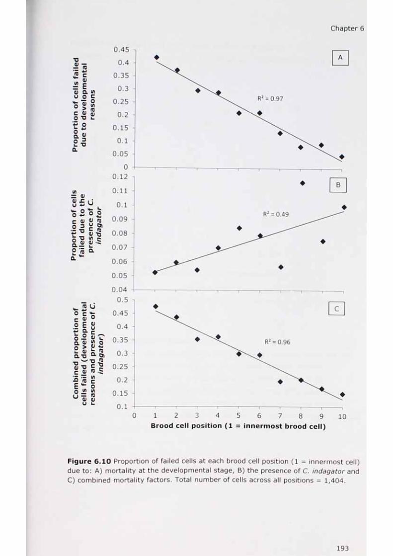
Chapter 6
* * « * i i i ------------ 1------------1
0 1 2 3 4 5 6 7 8 9 10Brood cell position (1 = innermost brood cell)
Figure 6.10 Proportion of failed cells at each brood cell position (1 = innermost cell) due to: A) mortality at the developmental stage, B) the presence of C. indagator and C) combined mortality factors. Total number of cells across all positions = 1,404.
193
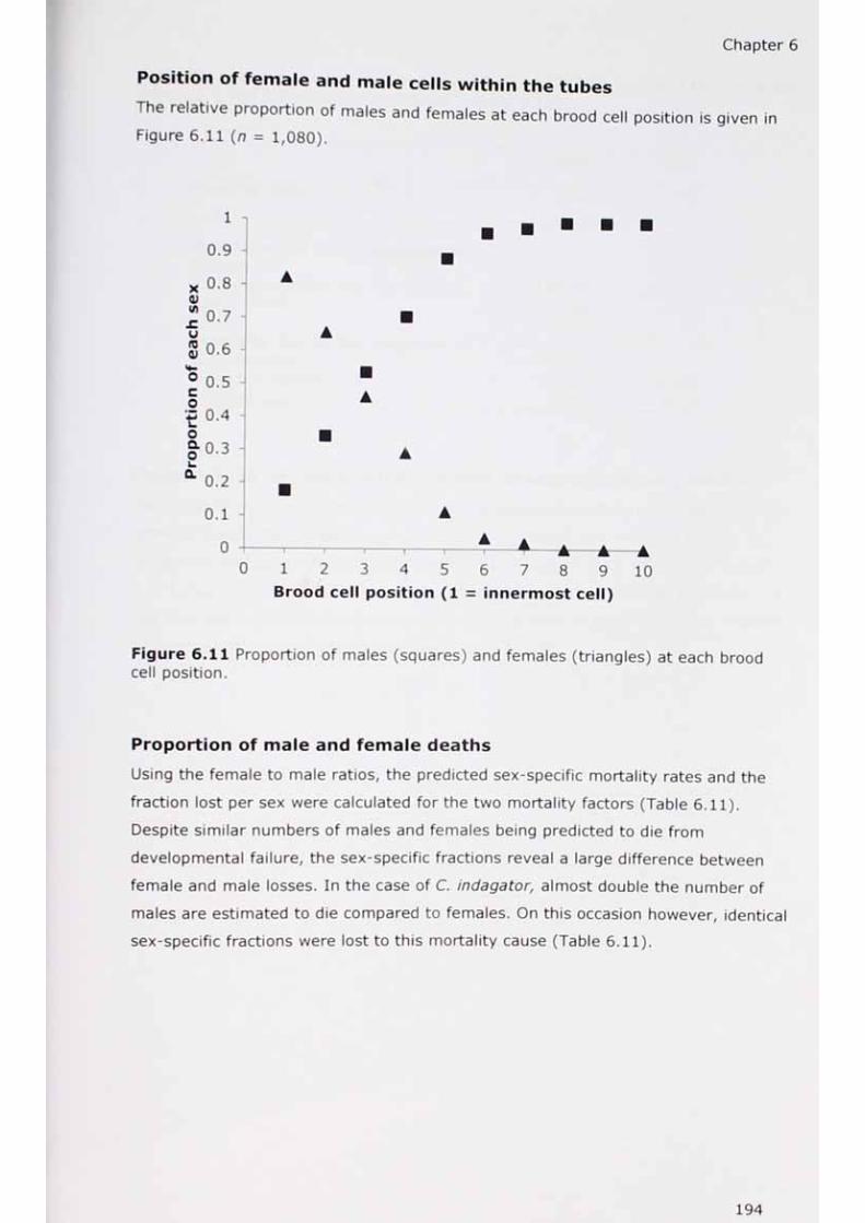
Chapter 6
Position of female and male cells within the tubes
The relative proportion of males and females at each brood cell position is given in Figure 6.11 (n = 1,080).
Figure 6.11 Proportion of males (squares) and females (triangles) at each brood cell position.
Proportion of male and female deaths
Using the female to male ratios, the predicted sex-specific mortality rates and the
fraction lost per sex were calculated for the two mortality factors (Table 6.11).
Despite similar numbers of males and females being predicted to die from
developmental failure, the sex-specific fractions reveal a large difference between
female and male losses. In the case of C. indagator, almost double the number of
males are estimated to die compared to females. On this occasion however, identical
sex-specific fractions were lost to this mortality cause (Table 6.11).
194

Chapter 6
7 ?cb l« ^n1i1 nPQrnd'C ed nU7lber ° f males and females (ar|d fraction) lost to two causes based on 1,080 individuals of known sex (Figure 6.1 1 ).
Females Males
Total in cells 342 738
Mortality due to developmental failurePredicted number lost 185.48 200.52Fraction lost 0.54 0.27
Mortality due to the presence of C. indagatorPredicted number lost 29.35 66.65Fraction lost 0.09 0.09
Proportion of fem ale and male deaths at each brood cell position
The proportion of males and females lost to developmental failure was significantly
different across the cell positions examined (G = 159.03, d.f. = 5, P < 0.001), as
were those lost as a result of the presence of C. indagator (G = 46.73, d.f. = 5, P <
0.001, Figure 6.12A-B). A greater proportion of females in brood cell positions one
and two was lost to the two combined mortality factors. In these two inner positions
160 female cells out of 342 (47%) died (Figure 6.12C).
195

Chapter 6
0.5
0.45
0.4
0.35
■o aV ° * 3c o £.Z v 2 0.25
0.2
— _
3 c TD c
i i
isTO o
V)g O*Dt
>
0.15
0.1
0.05
0
0.4
0.35
0.3~ o
*□c
8 0.25
0.2
co � �uT O
5<y m
Q. £ 0.15
0.1O
0.05
0
0.5
0.45
0.4
0.35
= = 0.3
vto</>o
r o
3�O9 m m
>
uT O
3 W *D C
0.25
0.20.15
u OE�o
C V.2 .5 oiu -2 0,1m E
ou0.05
00
A
A
I
A
A A A A A
A
A
A
A
■ a
■a
Ai A — A— A A
A
A
*A
A
1 2 3 5A6
A7
A8
A9
■10
Brood cell position (1 = innermost cell)
Figure 6.12 Fraction of female (triangles) and male (squares) individuals lost at each brood cell position (1 = innermost cell) as a result of: A) developmental failure B) the presence of C. indagator and C) the two mortality factors combined.
196

Chapter 6
Number of overw intering adults
During the examination to establish the sex of each bee, fifty cocoons were found to
contain Monodontomerus obscurus larvae. The remaining 1,650 cocoons (containing
live adults) were significantly differently distributed across the gardens (one-way
ANOVA, F8rl8= 5.19, P = 0.002). Post hoc tests (REGWQ) revealed a significant
difference between cocoon numbers at Lois Weedon, Courteenhall, Farnborough and
Canons Ashby and those at Lamport (Figure 6.13).
Figure 6.13 Difference in mean number of adult O. bicornis after losses to M. obscurus (Arithmetic mean ± SE).
O. bicornis male and female overwintering losses
The mortality rates between male and female overwintering bees (measured as the
proportion of deaths per number of live bees in cocoons pre-winter) differed
significantly, with a greater proportion of males failing to emerge (two-sample
Kolmogorov-Smirnov D24 = 1-59, P = 0.02).
197

Chapter 6
k6 life-table values - fem ale overwintering mortality
Analysis of the k6 values, representing losses due to female mortality during the
overwintering phase, revealed that there was no significant difference in female
mortality between properties (Kruskal-Wallis H (7) = 11.88, P > 0.05).
Sum m ary of k value losses
The losses experienced at each stage of the life-cycle for the red mason bee, from
developmental failure at the start of the process (Arl) to losses due to female
mortality (£6), are presented in Figure 6.14.
198

199

Chapter 6
Male and female sex ratios
The sex ratio for the subset of nests examined was 2.16:1 (males to females), n =
1,080. The pre-winter ratio for cocoons from all nests was 2.35:1 (n = 1,650).
Discussion
Nest occupancy
All species
All 27 of the commercial trap-nests were used by solitary bees (Table 6.6). This high
occupancy rate contrasts with the study by Everaars et al. (2011), who found only
46% of Phragmites nests were used in an urban location. Although all nests in the
current study contained used tubes, tube usage differed significantly between
properties (P = 0.005), (Figure 6.6, Table 6.5).
The choice of where to locate nests and the preferred light regime appears to be a
major factor affecting occupancy. Gaston et al. (2005) found nests placed in full sun
were more likely to be used than those in shade. In the present study only south
and east-facing walls were used for nest placement, taking care to avoid
overhanging vegetation. In contrast, Everaars et al. (2011) placed nests in a range
of light conditions, recording the lowest occupancy rates in nests attached to trees in
shade, and the highest occupancy on walls in full sunlight. The current study
confirms that sunny, unencumbered walls make ideal locations for artificial trap-
nests.
The red mason bee
O. bicornis is a ubiquitous species, and was present in all nine gardens in 2010. In
2011, red mason bee cells occurred in 26 of the 27 nests (Table 6.6). As with other
trap-nest studies this was the dominant species. It accounted for 95% of the created
cells in the present study, a figure similar to that found by Holzschuh et al. (2010),
(Table 6.2). Although other solitary bee species used the trap-nests provided, their
abundance was low and there was little congruence across properties. No
relationship was observed between the number of O. bicornis cells and those of
other species (P > 0.05, Figure 6.8). The number of O. bicornis cells differed
significantly between properties (P = 0.001, Figure 6.7).
High numbers of O. bicornis may be found nesting together for a number of reasons
Wilkaniec and Giejdasz (2003) noted that females aggregate if suitable cavities are
present, however the method by which bees locate suitable sites is not fully
understood. Mandibular gland secretions are believed to act as pheromone
200

Chapter 6
aggregation cues, despite the solitary nesting habits of this species (Bosch and
Kemp, 2004). A problem of nesting in close proximity to other females is that
increased parasitism and predation may occur; a cost which must be balanced with
that of searching for a more isolated nesting habitat (Rosenheim, 1990). Bischoff
(2003) suggested that for one ground-nesting species (Andrena vaga Panzer, 1799)
the high costs associated with searching for nest sites in early spring, when
provision-collecting days are limited by weather constraints, act as a strong selective
force for gregarious nesting behaviour. As red mason bees face similar weather-
imposed down-time', it is possible that newly emerged females behave like A. vaga,
i.e. they preferentially establish nests close to where they originally developed (philopatry).
The current study did not seek to establish the source of foundress populations, but
the lack of any obvious relationship between the density of wall cavities and the
number of cells created does not lend support to the idea that philopatry causes gregarious nesting.
Developmental failure and losses to parasitismDevelopmental failure
Developmental failure accounted for the greatest loss of O. bicornis cells at the pre-
pupal stage (Table 6.6, Figure 6.14). In the current study the mean developmental
failure rate across all nests was 26.3% ± 14.8, n = 26. This was higher than the
12.1% failure rate recorded by Bosch and Vicens (2005) for O. cornuta, and 16.2%
for O. bicornis by Gruber et al. (2011), but similar to that reported by Danks (1971),
who found an average developmental failure rate of 23.6% for seventeen stem-
nesting species. Of significance for the current study was the absence of any
statistical difference in developmental mortality between the eight sites analyzed and
also between the subset of properties examined (P > 0.05, Table 6.7). This suggests
a consistent background failure rate may be occurring. This observation would
benefit from further testing using additional gardens and/or greater nest density at
some properties.
Mortality from developmental failure disproportionately affected cells located towards
the innermost part of the tubes (Figure 6.10A). Although parasitism has been
recorded according to cell position (Strohm, 2011), to my knowledge this is the first
study to report on developmental failure according to cell position. The causes for
cell failure at this stage include: fungal pathogens, inadequate cell provisioning and
sub-optimal eggs (Danks, 1971, Steffan-Dewenter and Schiele, 2008). Methods to
mitigate losses have been explored for other solitary bee species include avoiding
201

Chapter 6
the re-use of nest tubes and observing good hygiene to reduce the spread of
pathogens at the nest preparation stage (Sekita and Yamada, 1993, Bosch and
Kemp, 2002). As new nests and tubes were purchased for the present study,
hygiene is unlikely to have been an issue. The observed high rate of developmental
failure demonstrates one of several important challenges that need to be overcome
if this species is to be considered a candidate for managed-pollinator use.
Losses to Cacoxenus indagator
After developmental mortality, loss to the specialist fly C. indagator was the second
highest cause of death (Table 6.6, Figure 6.14). Levels of parasitism (k2 values)
were significantly different between properties (P < 0.01, Table 6.7). Post hoc tests
showed that Boughton House and Canons Ashby had significantly higher levels of
parasitism than the other seven properties (Table 6.8). A common factor linking
these two gardens and a third, Holdenby, is that the walls in these gardens are
constructed from stone (Table 6.4). Further work exploring whether wall materials
influence rates of parasitism is needed.
Many studies have found C. indagator to be the main nest associate of the red
mason bee, and it is often cited as the primary cause of larval mortality (Krunic et
al., 2005, and Strohm, 2011). These flies are frequently observed at the entrance of
nest tubes waiting for female bees to depart, thereby allowing them access to the
pollen and nectar reserves gathered by the host. When a female leaves to collect
more larval food the fly enters and lays her own eggs on the pollen/nectar mass
(pers. obs.). In the current study the presence of fly larvae did not always result in
the death of the developing bee (22.2% of affected cells contained both fly larvae
and cocoons containing live bees), but in the majority of cases mortality ensued.
This result is similar to that found by Raw (1972) who noted that some bees were
able to develop normally alongside C. indagator.
Management techniques to prevent the build-up of large populations of these flies
when Osmia spp. are used as managed pollinators include the removal of infected
bee cells by hand during the winter months, and successive-year removal of flies by
aspirators during their flight period (Krunic et a!., 2005, Gruber et a!., 2011).
In contrast to the position of cells affected by developmental failure, mortality from
C. indagator was more likely to occur towards the outermost part of the nesting
tubes (Figure 6.10B). This pattern of increasing parasitism towards nest entrances
has also been noted by Seidelmann (2006). Strohm (2011) found no relationship
between brood cell position and parasitism rate, although the sample size was low
(total cells = 189).

Chapter 6
Parasitism and the density of O. bicornis
An unexpected result from the current work was that C. indagator-induced mortality
(measured as k2 values) was significantly related (in a non-linear way) to the
density of O. bicornis cells, with reduced mortality observed at both low and high cell densities (Figure 6.9).
The absence of a relationship between the hole-density of walls and both the mean
number of cells created and those parasitized (P > 0.05, n = 8), suggests C.
indagator may be able to locate nests independently of the presence of bees from
previous years. A possible explanation is that at low bee densities, host nests might
be patchily distributed, whilst at high densities, fly numbers may lag behind those of
nesting females; a commonly observed feature of predator-prey systems (Maynard
Smith, 1977). An alternative for the observed inverse density-dependence (where
bee abundance is high) has been proposed by Steffan-Dewenter and Schiele (2008).
These authors suggest that in areas where nests are frequented by many O. bicornis
females, increased activity may serve to disturb patrolling flies, thereby reducing the
incidence of parasitism. Observations of O. cornuta by Krunic et al. (2005)
corroborate this. The authors note that female bees proactively dispel flies and 'dive
frequently' on C. indagator females.
Differential mortality losses for males and females
Evidence from the current study shows a strong shift from predominantly female
cells in the innermost positions (brood cell position one; 82% females, 18% males),
to a more equitable distribution at position three (46% females, 54% males),
followed by increased male cell dominance towards the outer part of the tube (Figure
6.11) . The observed differences in the numbers of females and males at specific
locations within tubes, combined with differential mortality factors, make females
particularly vulnerable to the two mortality factors examined (Figure 6.10C, Figure
6.11) . Although the estimated number of females and males perishing as a result of
developmental failure did not differ greatly (185 versus 201), the fraction of females
dying was notably high (0.54, Table 6.11, Figure 6.12A). This results from the strong
male bias associated with this genus (Bosch and Vicens, 2005).
The position of O. bicornis females at the rear of the nest and males towards the
front has been attributed to protandry (Raw, 1972), but is also considered a
response to an increased risk of parasitism towards the outer part of nests
(Seidelmann, 2006). According to the hypothesis of Seidelmann (2006), open-cell
parasitism is believed to act as a selection pressure, causing females to
preferentially switch from provisioning cells for females, to creating cells for males

Chapter 6
As males are smaller than females they require less food, resulting in fewer foraging
trips of shorter duration by the mother bee. Reduced time away from the nest
therefore reduces the incidence of parasitism (Bosch and Vicens, 2005, Seidelmann,
2006, Seidelmann et a/., 2010). In contrast to this view, others have argued that a
reduction in floral quantity and quality as the season progresses leads to reduced
provisioning and therefore an increase in male offspring (Torchio and Tepedino,
1980). In some of the gardens sampled for the present study, both the number of
genera and floral area available increased as the season progressed (data not
presented), suggesting that limited floral resources are unlikely to have caused a
switch to a higher number of male offspring. Whilst offering no evidence of causality,
these results lend support to the hypothesis of Seidelmann (2006).
Male : female sex ratio
The diameter of nest materials influences the sex ratio of Osmia spp., with higher
female to male ratios reported when wider reed stems are available (Krombein,
1967, Raw, 1972, Bosch and Kemp, 2002, Seidelmann et al., 2010). Tube length
also affects sex ratios, with shorter lengths giving a more even ratio (Gruber et al.,
2011). Together, these findings highlight the importance of using nest materials of
standard widths and lengths. Despite this, to my knowledge no studies have adopted
the use of commercial trap-nests to explore male to female sex ratios and
parasitism. The use of standardised tubes with paper inners in the current study
allows confidence to be placed in the sex ratios observed. This ratio is reasonably
high (2.16 : 1), but still within the limits of other published accounts (Table 6.12).

Chapter 6
tThaeb!urfem2s?ubdv and JSlf t0 rati°S f°r blcornis and cornuta fromand then H n o r d t r n f Publ,sh,ed work- Studies are listed according to species
are for the subset of tenrneJtns9eJraam1nedfemale rati°S' f°r the CUrTent StUdy
Species M : F sex ratio n Vear(s) Source
O. bicornis 1.35 - 2.68 : 1 range 200 -1,200
1996-99 Krunic andStanisavljevic (2006)
O. bicornis 2.16 : 1 1,080 2011-12 This study (subset of 10 nests)
O. bicornis 1.59 : 1 411 1997-99 Seidelmann et at. (2010)
O. bicornis 1.11 : 1 236 1967/68 Raw(1972)
O. bicornis 0.91 - 1.53 : 1 range 2,850 - 22,633
2007-9 Gruber et al. (2011)
O. cornuta 1.46 - 3 22 : 1 range 400 - 2,500
1994-99 Krunic andStanisavljevic (2006)
0. cornuta 1.78 : 1 998 1995 Vicens and Bosch (2000)
Overwintering losses
Overwintering losses have not previously been reported for this species, and the
return of cocoons to their natal sites is rarely reported. To my knowledge, this is the
first time that cocoons have been returned to sites to establish if male and female
overwintering survival rates are similar. Results show that a significantly greater
proportion of males than females failed to emerge after being returned to their nests
(P < 0.02). Female overwintering mortality (/c6 in life-table analysis, Table 6.3) did
not differ between properties (P > 0.05).
Linking male : female sex ratios and the causes of larval mortality
In accordance with Fisher's theory of sex allocation, parental investment should be
equally distributed between male and female offspring (Fisher, 1930). Where an
organism is sexually dimorphic in terms of size - such as O. bicornis, where females

Chapter 6
are approximately 1.6 times heavier than males, (Raw, 1972), the cost to female
fitness of producing daughters is higher, and therefore a lower number of this sex
should be produced. An addendum to this is Trivers and Willard's hypothesis that
varying maternal condition results in deviations from a 50:50 investment in the two
sexes (Trivers and Willard, 1973). Seidelmann (2006) demonstrated that for O.
bicornis, body size is a good measure of maternal condition and that smaller females
overcome the disadvantage of reduced ability to forage economically (measured as
mass of reserves collected and time taken to acquire them), by shifting the sex ratio of their offspring towards smaller male progeny.
Combining these theories with Seidelmann's hypothesis that open-cell parasitism
leads to increased numbers of males (Seidelmann, 2006) suggests that multi-
faceted and sometimes competing forces operate to alter progeny sex ratios. This is
evidenced in the current study in three ways: (i) nests typically had more male than
female progeny, (Table 6.6), (ii) females experienced higher overall mortality than
males due to the combined factors of developmental failure and parasitism (Figure
6.12C), and (iii) higher proportions of males were lost during the overwintering
phase.
Teasing out whether position within the nest (and therefore incidence of parasitism
and developmental failure), maternal condition (which determines the level of food
reserves collected and therefore the sex and size of offspring) or the top-down effect
of parasitism (C. indagator shaping maternal investment as per Seidelmann, 2006),
work together or differentially to drive observed sex ratios is an area requiring
further study.
ConclusionsThe findings of this chapter can be summarised as follows:
• The standardised nature of commercial trap-nests makes them ideal for exploring the differential effects of mortality on male and female progeny of cavity-nesting bees.
• Commercial trap-nests placed in walled kitchen gardens were readily used by bees. Osmia bicornis was the most frequent occupant of these nests.
• No relationship exists between pre-existing hole density in wall mortar and the number of O. bicornis cells created and parasitized.
• The calculation of k values is a useful way of allowing O. bicornis mortality factors to be compared across sites.

Chapter 6
Lh,eJ ? 1T h k m 'T ,°/ °f bicornis progeny was observed at the developmental stage. This mortality factor disproportionately affected cells at the rear of the
The specialist parasite Cacoxenus indagator was the second highest cause oflarval mortality. This mortality factor disproportionately affected cells towards the front of the nest.
• Due to the strong male bias associated with this species, fewer female cells were created than male cells.
• Female cells were preferentially located at the rear of nests, making them particularly vulnerable to losses arising from developmental failure. More than half of all female cells were predicted to fail.
• As females are the main flower visitors, high losses have implications for the development of this species as a managed pollinator.
• C. indagator mortality was found to be related in a non-linear way to O. bicornis cell density. Density independence was observed when both low and high bee-cell densities occurred. High densities of bees may deter C. indagator from entering nests, thereby reducing parasitism.
• A significantly greater number of males did not emerge after the overwintering period than females.
In summary, walled gardens have the potential to support populations of cavity-
nesting bees. The dominance of O. bicornis, which is known to visit a wide range of
flowers in spring and early summer, has been recorded at these locations for the
first time. The importance of this species (and other solitary bees) as a backup for
commercial pollination in the face of honey bee declines is increasingly
acknowledged (Bosch and Kemp, 2002). By using commercial trap nests this work
has shown (for the first time) the differential effects of mortality on male and female
bees. If O. bicornis is to be used as a managed pollinator, suitable methods to
control for these effects will be needed.
The next chapter summarizes the findings of the study, offers a critique of the
methods and highlights areas for further investigation.
207

Chapter 7
Chapter 7
Conclusions
208

Chapter 7
Chapter overviewIn this chapter, the key findings of the study are re-visited and a critique of themethods is given. Areas for further work are suggested in the context of the study s findings.
Key findings of the studyThe results from this work offer new insights into the role that large rural gardens
play in supporting insects regarded as potential pollinators.
The key findings are presented in two parts. Firstly the diversity of insects in
gardens is discussed in relation to local and landscape-scale factors, and secondly
the knowledge gained from the experimental use of commercial trap nests is considered.
The value of gardens
Insect diversity and community structure
English country houses have long been appreciated for their cultural heritage, but
until now there has been limited focus on their natural-heritage value. This is the
first study of its kind to provide base-line data on the species richness and
abundance of a suite of flower visitors across the season in a significant sample of
country-house gardens.
The results show that rural-garden habitats support a wide range of flower-visiting
insects. In the 2010 field season almost 10,000 flower visitors, from 174 species,
were recorded in 17 gardens (Appendix VI, Chapter 3), whilst in 2011, almost
2,500 individuals were recorded from 136 species in nine walled gardens (Appendix
VI, abundance data not presented). Overall, 189 flower-visiting insect species were
identified across the 17 gardens over a two-year period (Appendix VI).
The study found that, despite gardens containing different habitat components, the
diversity they supported was highly similar, comparing favourably to vice-county
data (Chapter 3). For example, 14 of the potential 17 species of bumblebee known
from the region were found in the surveyed gardens.
By considering flower-visiting insects on a group basis it was possible to make
comparisons across the whole community. Hoverfly species richness differed

Chapter 7
significantly between properties; a result not seen for bumblebees, solitary bees or butterflies and day-flying moths (Table 3.3).
As a result of incorporating information on the flowers that insects visit, this study
has revealed, for the first time, how floral resources in novel ecosystems are used by insects.
Flower diversity
High flower diversity emerged as a common theme across the properties surveyed,
with more than a fifth of the world's plant families recorded from just 17 sites.
Despite this high richness, only a subset of these plants were visited by insects. A
higher proportion of flowering plants were visited in spring than at any other time,
suggesting that gardens help to support populations of insects when floral
resources in the landscape may be patchy or inadequate.
A strong positive link between the floral resources present and the diversity of
insects observed was noted. Both the number and abundance of flower visitors
increased as flowering plant resources increased.
The study also revealed, for the first time, the composition of floral resources in
rural gardens in terms of their native or alien status. Approximately 68% were
alien, a remarkably similar percentage to that found in urban gardens in the UK
and Mexico (Smith et al.f 2006a, Loram et al., 2008b).
Another novel finding was that the insects recorded showed no preference for
native over alien plants, and that certain families (exhibiting different colours and
morphology) were preferred in different seasons. These findings suggest that,
regardless of the domination of gardens by alien plant species, the presence of
these non-native floral resources does not act as a barrier for insects visiting
flowers for food.
Although the complexity of plant-flower interactions were considered in terms of a
number of metrics, including connectivity and nestedness, the study found that
inherent weaknesses with these meant meaningful interpretation of the results was
limited.
210
Chapter 7
Despite floral resources partially explaining the diversity of insects observed, they
were only one factor driving insect presence at a site. Landscape-scale factors were also important.
Wider landscape-scale effects
The study revealed that across the four insect groups, different landscape scales
and factors played a role in explaining species richness to a greater or lesser
extent. Bumblebees were affected by landscape factors within larger areas than
other groups, and solitary bees were invariant to landscape-scale factors; instead
being more influenced by within-garden effects. The response of bumblebees to
plant richness late in the season (a local-scale effect) provides further evidence
that the availability of resources in gardens across the whole season is an
important attribute within agriculture-dominated landscapes.
The study also revealed that splitting a group of insects according to their nesting
biology could reveal previously unappreciated responses to local-scale effects.
Ground-nesting solitary bees showed a positive response to floral diversity whilst
cavity-nesting bees responded to the area of beds and borders available. These
results highlight the value of not only identifying insects to species level, but also
incorporating an understanding of their life-history traits into interpretations about
their presence.
Trap-nest bees
This study has shown for the first time that the deployment of commercial trap-
nests can reveal new and important insights into the mortality factors affecting
males and females of a single solitary bee species, Osmia bicornis. As honey bees
are known to be suffering global declines (vanEngelsdorp and Meixner, 2010) these
results take on increasing significance as the potential for new commercially-
managed pollinators is explored.
The study found that the greatest mortality loss for O. bicornis was at the juvenile
developmental stage and that this disproportionately affected cells at the rear of
nests. Parasitism by a specialist fly, Cacoxenus indagator, was the second highest
cause for mortality; this time affecting cells at the front of the nest. Due to the
strong male bias associated with the species, and the preferential occurrence of
females at the rear of nests, this resulted in females being disproportionately
affected by these combined mortality causes. As a result, more than half of all
female cells were deemed unlikely to produce healthy bees, with potential
211
Chapter 7
consequences for future pollination effectiveness. Although offering no solutions for
this, the study has drawn attention to the fact that the issue of losses needs to be
addressed if this species is to be developed as a managed pollinator.
Summary
The main aim of this project, as described in Chapter 1, was to explore the
structure and composition of plant-pollinator assemblages in English country-house
gardens. The work addressed four broad research questions and found that these
novel ecosystems supported a diverse array of flower-visiting insects, with some
groups such as bumblebees particularly well represented. Flower resources and
their use were categorized, revealing the dominance of alien plants with no obvious
preference for natives by the insects present. Bumblebees were affected by
landscape factors at large spatial scales throughout the season, whilst solitary bees
were influenced by within-garden factors. The use of commercial trap-nests offered
new insights into the differing effects of mortality on male and female offspring of
the red mason bee. Overall, English country-house gardens emerged as previously
unappreciated novel ecosystems that can be classed as important sites for flower-
visiting insects.
Critique of methodsThe methods employed at the planning, data gathering and analysis stages are
reviewed here in turn.
Project planning
As described in Chapter 2, a Ph.D. project is necessarily limited by both time and
resources. This project is no exception. The decision to focus on a single
geographic area delivered advantages through the amelioration of potential
differences in the distribution of species, as well as allowing more time to be spent
sampling at properties.
Despite a range of country houses being selected, a possible criticism of an early
planning decision was that sufficient replicates of similar types of property were not
made. Kirby Hall is a good example. Described in the past as having 'Ye finest
garden in England7 (Burton, 1994), it was one of only two English Heritage
properties within the seventeen sites chosen. Additionally, Kirby Hall was the only
site not to possess a fully inhabitable house. Results from the study consistently
found this garden to be an outlier in terms of both insect and plant species
richness. The absence of similar sites to Kirby Hall makes it difficult to draw
conclusions about why this garden was so species poor. Was it simply because the

Chapter 7
gardens did not support a wide range of flowering plants, or were management
practices (consistently tightly mown lawns and strimmed grass banks) the
underlying cause? The percentage of land categorized as 'arable and horticulture'
within a 750m radius of Kirby Hall was relatively low compared to many others
(data not presented), but it had a moderately high percentage of improved
grassland in the same area. Could the effect of these landscape-scale
characteristics have interacted with the floristically-poor gardens to reduce the
number of flower visitors observed at Kirby Hall? Without the availability of similar
sites for comparison, it is difficult to gauge the true cause.
Another possible issue is the lack of direct comparison between the gardens
sampled and areas beyond the property boundaries. This was partly solved by
comparing the results obtained with other studies (albeit not on a like-for-like
basis) as well as to vice-county data (Chapter 3). This is considered further in the
section 'areas for further work' below.
Data gathering
The methods used at the data gathering stage allowed standardised sampling to
take place. The observation and netting of individuals by a single person (the
author) reduced recorder variation but the introduction of recorder bias cannot be
ruled out (UKBMS, 2010a).
Despite some anticipated visits to gardens being cancelled and rescheduled for
later dates (some of which occurred during the following sampling session), this did
not appear to impact on the robustness of the methods used (Figure 4.6).
A possible drawback of the method chosen to assess flower-visitors in the 2010
field season was the restriction of observations to only those where an insect was
in contact with flower reproductive structures. This decision served to limit direct
comparisons with other studies where a full inventory of all insects was made (e.g.
Edwards, 2003). In spite of this, it also yielded benefits by providing hitherto
unpublished data on the interactions between flower visitors and the many alien
plants found in rural gardens.
Data analysisThe use of standard techniques for analyzing data and the employment of null
models where appropriate (e.g. for WNODF and redundancy analysis in CANOCO)
allowed the robust testing of research questions and confidence to be placed in the
results obtained. Limitations arising from the nestedness procedures manifested
Chapter 7
themselves in the form of data interpretation issues rather than the analysesthemselves.
Areas for further workThe suggested areas for further work are discussed at scales ranging from
individual gardens to the wider-landscape, and incorporate interactions between
English country-house gardens and the visiting public.
Within-garden management
In addition to the floral resources available within gardens, the management of
these habitats is likely to influence the diversity of insects found there. The
suggestion by Galluzzi et al. (2010) that gardens are 'resilient ecosystems' that are
shaped by the close interactions between humans and nature, has not been
explicitly tested and would benefit from an assessment of the impacts of different
management approaches. Whilst a laissez-faire approach to gardening is known to
be beneficial for biodiversity (Head, 2012), this is rarely adopted at country-
houses. Instead, the management of flower-rich areas close to the house is usually
deemed a vital component of the overall appearance of a property.
To assess the effects of different management styles, the tilling and mowing
regimes adopted in individual gardens could be considered. The hoeing of soil on
flower beds and borders allows areas to be kept free of weeds, whilst at the same
time creating habitat for solitary bees that prefer vegetation-free areas for nest
sites (Roubik, 1992). The requirement for most gardens to be maintained to a high
visual standard (i.e. completely weed free), in combination with numerous
volunteer gardeners at some sites means, however, that some beds receive
continual soil disturbance, thereby reducing nesting opportunities and success.
Identifying whether continual hoeing and weeding limits the occurrence of ground-
nesting species is an area that could be investigated.
Similarly, mowing regimes (in particular the methods and frequency of mowing)
could be assessed. Enquiries at many of the sites where sampling took place
revealed external mowing contracts were in place. As a result, lawns were being
mowed on a weekly basis regardless of their growth state, resulting in flower
patches (such as red and white clover and dandelions) that were favoured by
insects being continually removed. Added to this was the mechanical destruction of
bees whilst they nectared on flowers present in lawns. This occurred due to the use
of fast-moving ride-on lawn mowers which gave insufficient time for bees to fly off
214
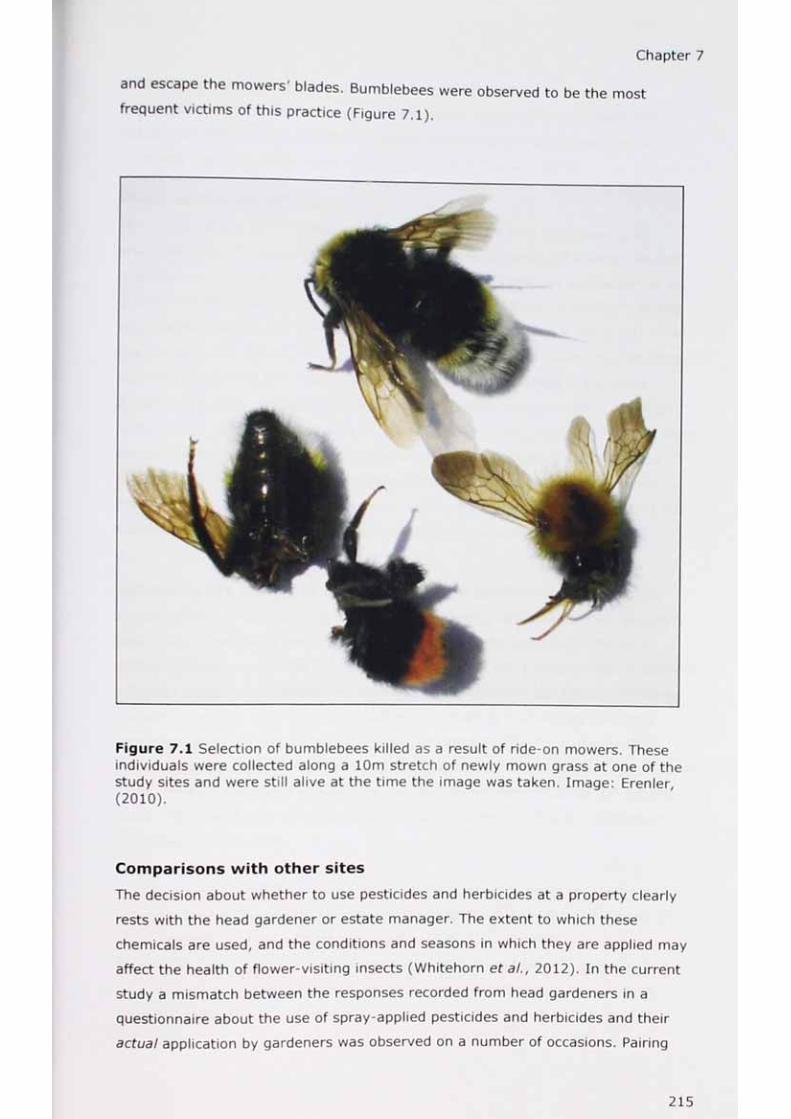
Chapter 7
and escape the mowers' blades. Bumblebees were observed to be the most
frequent victims of this practice (Figure 7 .1 ).
Figure 7.1 Selection of bumblebees killed as a result of ride-on mowers. These individuals were collected along a 10m stretch of newly mown grass at one of the study sites and were still alive at the time the image was taken. Image: Erenler, (2010).
Comparisons with other sitesThe decision about whether to use pesticides and herbicides at a property clearly
rests with the head gardener or estate manager. The extent to which these
chemicals are used, and the conditions and seasons in which they are applied may
affect the health of flower-visiting insects (Whitehorn et at., 2012). In the current
study a mismatch between the responses recorded from head gardeners in a
questionnaire about the use of spray-applied pesticides and herbicides and their
actual application by gardeners was observed on a number of occasions. Pairing
215

Chapter 7
properties where sprays are known to be used with gardens that reject the
application of chemicals may reveal differences in insect species richness and/or
abundance. The pairing of sites with reference sites is an established method of
assessing the biodiversity value of a habitat (Tarrant etal., 2012).
Wider landscape effects
The results presented in Chapter 5 of this thesis reveal that landscape-scale
processes have the potential to affect flower-visitor richness and abundance but
that this may vary according to the group of interest (Table 5.4 and Jauker et a/.,
2009). The United Kingdom, and particularly Central England, is currently seeing
an expansion of the area planted with oilseed rape (OSR) - up 9.8% in 2011 from
the previous year (Defra, 2011). Assessing the effect of this mass-flowering crop
on insect pollinators both within and beyond garden boundaries is a subject
demanding further attention. Whilst a range of pollinators is known to visit OSR
and enhance yields (Bommarco et aI., 2012, Jauker et a/., 2012b), it has also been
shown to distort plant-pollinator interactions (Diekotter eta/., 2010). Building on
the results of Chapter 5, and specifically addressing questions about seasonality,
the temporary (or otherwise) movement of beneficial insects beyond gardens into
the wider landscape to forage on OSR could be examined.
Assessing the influence of country-house gardens on the public
As the number of people living in urban environments continues to rise, people's
own gardens and those they choose to visit take on increasing importance for
human wellbeing (Davies et al., 2009). The extent to which country-house gardens
influence attitudes to biodiversity, garden design and plant purchasing decisions
remains unknown. What is not in question, however, is that visiting culturally
important sites remains a popular activity. As noted in Chapter 1, the National
Trust alone had more than 19 million paid visits to their sites in 2011 (The National
Trust, 2012b). A qualitative assessment of how these sites influence the general
public may reveal both the positive and negative aspects of highly managed and
maintained garden areas.
Whilst an increasing awareness of the importance of biodiversity is broadly
acknowledged by owners and managers of country-house gardens, this does not
always translate into a realistic appreciation of the true diversity of some groups.
Native bees are a good example of this. Improving the awareness of the habitat
requirements of a range of solitary and social bees in addition to the needs of
honey bees requires knowledge to be shared about this important group of
pollinators.

Chapter 7
Concluding remarks
The decline and potential extinction of charismatic species make headlines, whilst
cumulative losses of biodiversity rightfully raise concern (WWF, 2012, Natural
England, 2010). Less appreciated, and less easy to observe however, is the erosion
of ecological interactions (Kearns and Inouye, 1997). As the unprecedented threat
to the ecosystem service of pollination continues, English country-house gardens
emerge as important novel ecosystems capable of supporting biodiversity and ecological webs.
Humankind did not weave the web of life -
We are but one thread within it.
Whatever we do to the web we do to ourselves
All things are bound together
All things connect.
Adapted from an original version created in 1972 by Ted Perry for the film Home (Berkes, 1999).
217

ReferencesReferences
S e n t J Knd Elmqvist' T ' (2009) Bumblebees (Bombus spp) along agradient of increasing urbanization. Plos One. 4 (5) E5574.
? L l ^ aR. S 10)l^Orl9rUenCe between visitation and pollen-transport networks in a California plant-pollinator community. Oikos. 1 1 9 (l), 35-44.
Alarcon, R Waser, N. M. and Ollerton, J. (2008) Year-to-year variation in the topology of a plant-pollinator interaction network. Oikos. 117 (12), 1796-1807.
AMen-Warden, G., Bernhardt, P., Bitner, R., Burquez, A., Buchmann, S., Cane, J.,C°x P. A., Dalton, V., Feinsinger, P., Ingram, M., Inouye, D., Jones, C. E., Kennedy, K., Kevan, P., Koopowitz, H., Medellin, R., Medellin-Morales, S., Nabhan, G. P.,Pavlik, B., Tepedino, V., Torchio, P. and Walker, S. (1998) The potentialconsequences of pollinator declines on the conservation of biodiversity and stability of food crop yields. Conservation Biology. 12 (1 ), 8-17.
Allesina, S. (2012) Ecology: The more the merrier. Nature. 487 (7406), 175-176.
Almeida-Neto, M. and Ulrich, W. (2011) A straightforward computational approachfor measuring nestedness using quantitative matrices. Environmental Modelling & Software. 26 (2), 173-178.
Althorp Estate Althorp Hospitality - Wedding venue [online]. Available from: http://www.althorp.com/hospitalitv/weddinQ.DhD [Accessed 21 September, 2012].
APG III (2009) An update of the Angiosperm Phylogeny Group classification for the orders and families of flowering plants: APG III. Botanical Journal of the Linnean Society. 161 (2), 105-121.
Aslet, C. (1982) The Last Country Houses. London, England: Yale University Press.
Atmar, W. and Patterson, B. D. (1993) The measure of order and disorder in the distribution of species in fragmented habitat. Oecologia. 96 (3), 373-382.
Ball, S. G., Morris, R. K. A., Rotheray, G. E. and Watt, K. R. (2011) Atlas of the Hoverflies of Great Britain (Diptera, Syrphidae). Wallingford, England: Biological Records Centre.
Baltanas, A. (1992) On the use of some methods for the estimation of species richness. Oikos. 65 (3), 484-492.
Banasek-Richter, C., Bersier, L., Cattin, M., Baltensperger, R., Gabriel, J., Merz, Y., Ulanowicz, R. E., Tavares, A. F., Williams, D. D., De Ruiter, P. C., Winemiller, K. O. and Naisbit, R. E. (2009) Complexity in quantitative food webs. Ecology. 90 (6), 1470-1477.
Bartomeus, I., Ascher, J. S., Wagner, D., Danforth, B. N., Colla, S., Kornbluth, S. and Winfree, R. (2011) Climate-associated phenological advances in bee pollinators and bee-pollinated plants. Proceedings of the National Academy of Sciences of the United States of America. 108 (51), 20645-20649.
Bascompte, J., Jordano, P., Melian, C. J. and Olesen, J. M. (2003) The nested assembly of plant-animal mutualistic networks. Proceedings of the National Academy of Sciences of the United States of America. 100 (16), 9383-9387.
218

References
J‘ wU ° ean' R’ (2011a) Ph°t°graphic guide to pre-adult tube- nesting aculeates and their parasites. Unpublished material.
r f iS i 'h fv i ' Sadler/ 1 P- Fairbrass- A. J., Falk, S. J., Hale, J. D. and Matthews, T. J. (20 lib ) Changing bee and hoverfly pollinator assemblages along an urban-rural gradient. Plos One. 6 (8), e23459.
BBC BBC Weather - next 24 hours [online]. Available from:http://news.bbc.co.uk/weather/forecast [Accessed 18 April, 2010].
BBCT ( B u m b le Conservation Trust). BBCT Home page [online]. Available from: http://bumblebeeconservation.ora/ [Accessed 24 September, 2012].
Beccaloni, G. W. and Gaston, K. J. (1995) Predicting the species richness ofNeotropical forest butterflies - Ithomiinae (Lepidoptera, Nymphalidae) as indicators. Biological Conservation. 71 (1), 77-86.
Beckett, M. England's Lost Country Houses [online]. Available from: www.lh.matthewbeckett.com [Accessed 12 September, 2012].
Beekman, M. and Ratnieks, F. L. W. (2000) Long-range foraging by the honey-bee, Apis mellifera L. Functional Ecology. 14 (4), 490-496.
Benedek, Z., Jordan, F. and Baldi, A. (2007) Topological keystone species complexes in ecological interaction networks. Community Ecology. 8 (1 ), 1-7.
Bergh, J. C. and Short, B. D. (2008) Ecological and life-history notes on syrphid predators of woolly apple aphid in Virginia, with emphasis on Heringia calcarata. Biocontrol. 53 (5), 773-786.
Berkes, F. (1999) Sacred Ecology. 2nd Edition. New York, USA: Taylor and Francis.
Bersier, L. F., Banasek-Richter, C. and Cattin, M. F. (2002) Quantitative descriptors of food-web matrices. Ecology. 83 (9), 2394-2407.
Bezerra, E. L. S., Machado, I. C. and Mello, M. A. R. (2009) Pollination networks of oil-flowers: a tiny world within the smallest of all worlds. Journal of Animal Ecology. 78 (5), 1096-1101.
Biesmeijer, J. C., Roberts, S. P. M., Reemer, M., Ohlemueller, R., Edwards, M., Peeters, T., Schaffers, A. P., Potts, S. G., Kleukers, R., Thomas, C. D., Settele, J. and Kunin, W. E. (2006) Parallel declines in pollinators and insect-pollinated plants in Britain and the Netherlands. Science. 313 (5785), 351-354.
Binney, M. Victoria and Albert Museum. 1974 Exhibition 'The Destruction of the Country House' [online]. Available from:http ://www. vam. ac.uk/content/articles/s/save-britains-heritaae-1975-2005-30- vears-of-campaigninq/ [Accessed 12 September, 2012].
Bischoff, I. (2003) Population dynamics of the solitary digger bee Andrena vaga Panzer (Hymenoptera, Andrenidae) studied using mark-recapture and nest counts Population Ecology. 45 (3), 197-204.
Blarney, M., Fitter, R. and Fitter, A. (2003) Wild flowers of Britain and Ireland. London, England: A & C Black Publishers Ltd.
219

n w o r k " m P t r i r S J'' VKazquez' D- p- and Menzel, F. (2008) What do interaction 3387-3399 1 * US ab°Ut speciallzatjon and biological traits? Ecology. 89 (12),
R-» Marini,JL. and Vaissiere, B. E. (2012) Insect pollination enhances in r? Y e d' qua ,ty' and market value in oilseed rape. Oecologia. 169 (4), 1025-X J 2. •
Borcard, D., Legendre, P. and Drapeau, P. (1992) Partialling out the spatial component of ecological variation. Ecology. 73 (3), 1045-1055.
Bosch, J. (1994) The nesting-behavior of the mason bee Osmia cornuta (Latr) with special reference to its pollinating potential (Hymenoptera, Megachilidae). Apidologie. 25 (1 ), 84-93.
Bosch, J. and Kemp, W. P. (2002) Developing and establishing bee species as crop pollinators: the example of Osmia spp. (Hymenoptera : Megachilidae) and fruit trees. Bulletin of Entomological Research. 92 (1 ), 3-16.
Bosch, J. and Kemp, W. P. (2004) Effect of pre-wintering and wintering temperature regimes on weight loss, survival, and emergence time in the mason bee Osmia cornuta (Hymenoptera : Megachilidae). Apidologie. 35 (5), 469-479.
Bosch, J., Kemp, W. P. and Trostle, G. E. (2006) Bee population returns and cherry yields in an orchard pollinated with Osmia lignaria (Hymenoptera : Megachilidae). Journal of Economic Entomology. 99 (2), 408-413.
Bosch, J. and Vicens, N. (2005) Sex allocation in the solitary bee Osmia cornuta: females behave in agreement with Fisher's theory? Behavioral Ecology and Sociobiology. 59 (1 ), 124-132.
do
Boughton House Website for Boughton House, Northamptonshire [online]. Available from: www.bouqhtonhouse.orq.uk [Accessed 21 September, 2012].
Breeze, T. D., Bailey, A. P., Balcombe, K. G. and Potts, S. G. (2011) Pollination services in the UK, how important are honeybees? Agriculture Ecosystems & Environment. 142, 137-143.
Breeze, T. D., Roberts, S. P. M. and Potts, S. G. (2012) The Decline of England's Bees. Reading, England: The University of Reading.
Bricked, C. (ed.) (1999) RHS New encyclopedia of plants and flowers. 3rd ed.London, England: Dorling Kindersley.
Brooks, M. and Knight, C. (1982) A complete guide to British butterflies. London: Jonathan Cape Ltd.
Burgos, E., Ceva, H., Perazzo, R. P. J., Devoto, M., Medan, D., Zimmermann, M. and Delbue, A. M. (2007) Why nestedness in mutualistic networks? Journal of Theoretical Biology. 249 (2), 307-313.
Burkle, L. A. and Alarcon, R. (2011) The future of plant-pollinator diversity: Understanding interaction networks across time, space, and global change. American Journal of Botany. 98 (3), 528-538.
Burton, N. (1994) English Heritage from the air. 2nd ed. London, England: Sidgwick and Jackson Limited.

Al^ond"^R ' Collen' B - van Strien, A., Scharlemann, J. P. W.,F Tarr r m rh 3' le, J ' E- Bomhard, B., Brown, C., Bruno, J., Carpenter, K. f ' Footer M r 5anf ° nA ,V Chenery' A- M- Csirke, J., Davidson, n . C„ Dentener, Kannc^v ' flm G A\' G,alloway' J- N-> Genovesi, P., Gregory, R. D., Hockings, M.,
S r ° 'dfield' T- E E ' Pauly' D ' Quader' S., Revenga, C„Sauer, J. R., Skolmk, B., Spear, D., Stanwell-Smith, D., Stuart, S. INI., Symes, A.,Tierney, M Tyrrell, T. D., Vie, J. and Watson, R. (2010) Global biodiversity: Indicators of recent declines. Science. 328 (5982), 1164-1168.
Butler, C. (1609) The Feminine Monarchie or A treatise concerning bees and the due ordering of them. Oxford, England: Joseph Barnes.
Butterfly Conservation. BC Home page [online]. Available from: http://www.butterfly-conservation.orQ/ [Accessed 25 September, 2012].
BWARS. Bees, Wasps and Ants Recording Society [online]. Available from: www.bwars.com [Accessed 1 September, 2012].
Campbell, C. (2005) A history of kitchen gardening. London: Frances Lincoln Ltd.
Campbell, C. (2010) Walled kitchen gardens. 2nd ed. Oxford: Shire Publications Ltd.
Cane, J.H. and Sipes, S. (2006) Characterizing floral specialization by bees: Analytical methods and a revised lexicon for oligolecty. In: Waser, N. M. and Ollerton, J. (eds.) Plant-pollinator interactions: From specialization to generalization. Chicago, USA: The University of Chicago Press, pp. 99-122.
Cane, J. H., Minckley, R. L. and Kervin, L. J. (2000) Sampling bees (Hymenoptera : Apiformes) for pollinator community studies: Pitfalls of pan-trapping. Journal of the Kansas Entomological Society. 73 (4), 225-231.
Cannon, A., Chamberlain, D., Toms, M., Hatchwell, B. and Gaston, K. (2005) Trends in the use of private gardens by wild birds in Great Britain 1995-2002. Journal of Applied Ecology. 42 (4), 659-671.
Carre, G., Roche, P., Chifflet, R., Morison, N., Bommarco, R., Harrison-Cripps, J., Krewenka, K., Potts, S. G., Roberts, S. P. M., Rodet, G., Settele, J., Steffan- Dewenter, I., Szentgyorgyi, H., Tscheulin, T., Westphal, C., Woyciechowski, M. and Vaissiere, B. E. (2009) Landscape context and habitat type as drivers of bee diversity in European annual crops. Agriculture Ecosystems & Environment. 133 (1- 2), 40-47.
Carreck, N. L. (2008) Are honey bees (Apis mellifera L.) native to the British Isles? Journal of Apicultural Research and Bee World. 47 (4), 318-322.
Carter, D.J. in Plant, C.W. (Ed.) (2001) The butterflies and moths (Lepidoptera) of Buckingham Palace Garden. London Naturalist. Part 2. 80 (Suppl.), 169-191.
Carvell, C., Meek, W. R., Pywell, R. F., Goulson, D. and Nowakowski, M. (2007) Comparing the efficacy of agri-environment schemes to enhance bumblebee abundance and diversity on arable field margins. Journal of Applied Ecology. 44 (1), 29-40.

References
forM*!Ia bumShPPe PyWel1' R' F' 3nd Nowakowski' M. (2004) The response of
Biological C o n s e n t l l V ( 3 l n 7 % T " ™ 'V arabte M d mar9ins'
Ma s elf2 o ii?B u 0r^ fp h, L ' B0Urke' A- F- G-' Freeman' S’ N., Pywell, R. F. and Heard j j | , ee sPec,es responses to a targeted conservation measure1760 1771 dSCaPe C°nteXt and habitat qualitV* ^ log ica l Applications. 21 (5),
Cha°' Au _Chazdon' R* L ' Colwell, R. K. and Shen, T. J. (2005) A new statistical approach for assessing similarity of species composition with incidence and abundance data. Ecology Letters. 8 (2), 148-159.
Chao, A., Chazdon, R. L., Colwell, R. K. and Shen, T. (2006) Abundance-basedsimilarity indices and their estimation when there are unseen species in samples Biometrics. 62 (2), 361-371.
Chazdon, R.L., Colwell, R.K., Denslow, J.S. and Guariguata, M.R. (1998) Statisticalmethods for estimating species richness of woody regeneration in primary andsecondary rain forests of northeastern Costa Rica. In: Dallmeier, F. and Comiskey, J.(eds.) Forest biodiversity research, monitoring and modeling. Conceptualbackground and Old World case studies. Paris, France: The Parthenon Publishing Group. Page 309.
Chinery, M. (1989) Butterflies and day-flying moths of Britain and Europe. London: William Collins Sons and Co. Ltd.
Chinery, M. (2005) Collins complete guide to British insects. London: HarperCollins Publishers Ltd.
Christensen, N. L., Bartuska, A. M., Brown, J. H., Carpenter, S., D'Antonio, C., Francis, R., Franklin, J. F., MacMahon, J. A., Noss, R. F., Parsons, D. J., Peterson, C. H., Turner, M. G. and Woodmansee, R. G. (1996) The report of the ecological society of America committee on the scientific basis for ecosystem management. Ecological Applications. 6 (3), 665-691.
Christie, C. (2000) The British country house in the eighteenth century. Manchester, UK: Manchester University Press.
CJ Wildbird Food, Upton Magna, Shrewsbury, England.
Colla, S. R. and Packer, L. (2008) Evidence for decline in eastern North American bumblebees (Hymenoptera : Apidae), with special focus on Bombus affinis Cresson. Biodiversity and Conservation. 17 (6), 1379-1391.
Colwell, R.K. (2009) Biodiversity: Concepts, patterns, and measurement. In: Levin, S. (ed.) The Princeton guide to ecology. Princeton USA: Princeton University Press.
Colwell, R. K. (2012) Estimates 8.2 User's Guide [online]. Available from: http://vicerov.eeb.uconn.edu/estimates/EstimateSPaqes/EstSUsersGuide/EstimatpS UsersGuide.htm#Chaol [Accessed 24 September, 2012].
Colwell, R. K. and Coddington, J. A. (1994) Estimating terrestrial biodiversity through extrapolation. Philosophical Transactions of the Royal Society of London Series B-Biological Sciences. 345 (1311), 101-118.

References
Enaland^ FrprW^rwvT*m0 'S ' ' °* (1968) Flies of the British Isles. 2nd ed. London, England. Frederick Warne & Co Ltd.
m° MQQQ1;; 2 rb,et' A ' Barron' A ' Bird' A- Collinge, S.( Miyazaki, N. and Powell,. (1999a) Garden flowers: Insect visits and the floral reward of horticulturally-
modified variants. Annals of Botany. 83 (1), 73-86.
Comba, L Corbet, S. A., Hunt, L. and Warren, B. (1999b) Flowers, nectar and,n/ r VISItSM Er alUat,ng Bntish P,ant species for pollinator-friendly gardens. Annals of Botany. 83 (4), 369-383.
Corbet, S. A., Bee, J., Dasmahapatra, K., Gale, S., Gorringe, E., La Ferla, B.,Moorhouse, T., Trevail, A., Van Bergen, Y. and Vorontsova, M. (2001) Native orexotic? Double or single? Evaluating plants for pollinator-friendly gardens. Annals of Botany. 87 (2), 219-232.
Costanza, R., dArge, R., deGroot, R., Farber, S., Grasso, M., Hannon, B., Limburg,K., Naeem, S., ONeill, R. V., Paruelo, J., Raskin, R. G., Sutton, P. and vandenBelt, M.(1997) The value of the world's ecosystem services and natural capital. Nature. 387 (6630), 253-260.
Cowgill, S. E., Wratten, S. D. and Sotherton, N. W. (1993) The effect of weeds on the numbers of hoverfly (Diptera, Syrphidae) adults and the distribution and composition of their eggs in winter-wheat. Annals of Applied Biology. 123 (3), 499-
Crawshay, G. A. (1905) A large community of Vespula vulgaris. Entomologist's Monthly Magazine. 41, 8-10.
Cussans, J., Goulson, D., Sanderson, R., Goffe, L., Darvill, B. and Osborne, J. L. (2010) Two bee-pollinated plant species show higher seed production when grown in gardens compared to arable farmland. Plos One. 5 (7), e l 1753.
Daily, G. C., Alexander, S., Ehrlich, P. R., Goulder, L., Lubchenco, J., Matson, P. A., Mooney, H. A., Postel, S., Schneider, S. H., Tilman, D. and Woodwell, G. M. (1997) Ecosystem services: Benefits supplied to human societies by natural ecosystems. Issues in Ecology. 2, 2-15.
Danks, H. V. (1971) Nest mortality factors in stem-nesting aculeate Hymenoptera. Journal of Animal Ecology. 40 (1), 79-83.
Darlington, P. J. (1957) Zoogeography: the geographical distribution of animals.New York, USA: Wiley Publishing.
Darwin, C. (1862) On the various contrivances by which British and foreign orchids are fertilised by insects. London, England: John Murray.
Davies, Z. G., Fuller, R. A., Loram, A., Irvine, K. N., Sims, V. and Gaston, K. J. (2009) A national scale inventory of resource provision for biodiversity within domestic gardens. Biological Conservation. 142 (4), 761-771.
Dean, R. (The Red Beehive Company), e-mail to [email protected] 17 August 2012.
Defra. (2011) Agriculture in the United Kingdom 2011. Available online (http://www.defra.Qov.uk/statistics/files/defra-stats-foodfarm-crosscuttina-auk- auk201 l-120709.pdf) [Accessed 4 November 2012].

References
^fod%^^i amith^)v t'stics e^ 'ce• (2011) Attitudes and Knowledge Relating toh n t n riJf?* nrf ^ Natural Environment 2007 - 2011 (Report - available online, http.-//defra.qov.uk) [Accessed 5 May 2012].
Patrick*'B h ' o n S f L h ' P ' Dickinson' K- J- M- Sirvid, P.( Barratt, B. I. P. and Patrick' b. H. (2002) Arthropod morphospecies versus taxonomic species: a case1015 -1*02 3Araneae' Cole°Ptera, and Lepidoptera. Conservation Biology. 16 (4),
D'as, B. S. F. Raw, A. and Imperatri-Fonseca, V. L. (1999) International Pollinators Initiative: Sao Paulo Declaration on Pollinators. Report on the recommendations ofthe workshop on the conservation and sustainable use of pollinators in agriculture with emphasis on bees. Brasilia, Brazil: Brazilian Ministry of the Environment (MMA)
Dicks, L. V., Corbet, S. A. and Pywell, R. F. (2002) Compartmentalization in plant- insect flower visitor webs. Journal of Animal Ecology. 71 (1), 32-43.
Diekotter, T., Kadoya, T., Peter, F., Wolters, V. and Jauker, F. (2010) Oilseed rapecrops distort plant-pollinator interactions. Journal of Applied Ecology. 47 (1), 209- 214.
Dipterists Forum The Society for the Study of Flies (Diptera) [online]. Available from: www.dipteristsforum.ora.uk [Accessed 9 September, 2012].
Donovan, E. (1792) The natural history of British insects explaining them in their several states, with the periods of their transformations, their food, and oeconomy together with the history of such minute insects as require investigation by the microscope, the whole illustrated by coloured figures, designed and executed from living specimens. London, England: F & C Rivington.
Dormann, C. F., Friind, J., Bliithgen, N. and Gruber, B. (2009) Indices, graphs and null models: Analyzing bipartite ecological networks. The Open Ecology Journal. 2 7-24.
Dormann, C. F., Gruber, B. and Frund, J. (2008) Introducing the bipartite package: Analysing ecological networks. R News. 8 (2), 8-11.
Dormann, C. F., Schweiger, O., Augenstein, I., Bailey, D., Billeter, R., de Blust, G., DeFilippi, R., Frenzel, M., Flendrickx, F., Herzog, F., Klotz, S., Liira, J., Maelfait, J. P., Schmidt, T., Speelmans, M., van Wingerden, W. K. R. E. and Zobel, M. (2007)Effects of landscape structure and land-use intensity on similarity of plant and animal communities. Global Ecology and Biogeography. 16, 774-787.
Dramstad, W. and Fry, G. (1995) Foraging activity of bumblebees (Bombus) in relation to flower resources on arable land. Agriculture Ecosystems & Environment.
, 123-135.
Dunnett, N. and Quasim, M. (2000) Perceived benefits to human well-being of urban gardens. HorTechnology. 10 (1), 40-45.
Dupont, Y. L., Padron, B., Olesen, J. M. and Petanidou, T. (2009) Spatio-temporal variation in the structure of pollination networks. Oikos. 118 (8), 1261-1269.
Dutton, R. (1949) The English Country House. 3rd ed. London, England: B.T.Batsford Ltd.
224

References
2 K 2 . S - L V C.h00f ' ,l g and usin9 statistics: A biologist's guide. Third ed. Chichester, UK: Blackwell Science.
Eb, e'in, 9' i '|KI! in' t M'' Schumacher- J-/ Weisser, W. W. and Tscharntke, T. (2008)°neS, Plan,V " ?.ef S aff6Ct pollinator richness and temporal stability of flower visits? Oikos. 117 (12), 1808-1815.
Ebeling, A. Klein, A. and Tscharntke, T. (2011) Plant-flower visitor interaction webs: temporal stability and pollinator specialization increases along an experimental plant diversity gradient. Basic and Applied Ecology. 12 (4), 300-309.
Ebert, A. (2011) Nectar for the taking: The popularization of scientific bee culture in England, 1609-1809. Agricultural History. 85 (3), 322-343.
EDINA. OS Scale 1:25000 Raster Ordnance Survey, GB. © Crown Copyright [online]. Available from: http://edina.ac.uk/diQiman [Accessed 25 September, 2012].
Edwards, M. (2003) An entomological survey of National Trust gardens (Report for The National Trust). Sussex, England: Unpublished.
Edwards, M. and Jenner, M. (2009) Field guide to the bumblebees of Great Britain and Ireland. 2nd ed. England: Ocelli.
Edwards, R. (ed.) (1998) Provisional atlas of the aculeate Hymenoptera of Britain and Ireland. Part 2. Dorset: Biological Records Centre.
Elton, A., Harrison, B. and Wark, K. (1992) Researching the country house: A guide for local historans. London, England: B.T. Batsford Ltd.
Engels, J. (2001) Home Gardens - a genetic resources perspective. In: Home gardens and in situ conservation of plant genetic resources in farming systems.Rome, Italy: IPGRI.
ESRI. (2011) ArcGIS Desktop: Release 10 Environmental Systems Research Institute http://esriuk.com. [Accessed 6 June 2010].
Everaars, J., Strohbach, M. W., Gruber, B. and Dormann, C. F. (2011) Microsite conditions dominate habitat selection of the red mason bee (Osmia bicornis, Hymenoptera: Megachilidae) in an urban environment: a case study from Leipzig, Germany. Landscape and Urban Planning. 103, 15-23.
Eversham, B. (2010) Building and curating an insect collection (unpublished notes).
Exeler, N., Kratochwil, A. and Hochkirch, A. (2010) Does recent habitat fragmentation affect the population genetics of a heathland specialist, Andrena fuscipes (Hymenoptera: Andrenidae)? Conservation Genetics. 11 (5), 1679-1687.
Faegri, F. and van der Pijl, L. (1966) The principles of pollination ecology. Oxford, England: Pergamon Press Ltd.
Fahrig, L. (2003) Effects of habitat fragmentation on biodiversity. Annual Review of Ecology Evolution and Systematics. 34, 487-515.
Falk, S. J. (2011) A survey of the bees and wasps of fifteen chalk grassland and chalk heath sites within the East Sussex South Downs. Self-Published.
References
IJT rW i'a f) D ; Ascher' J - s - and Langellotto, G. A. (2008) The bee fauna ofZ S ^ l arden,S 'n 3 SUburb °f New York City (Hymenoptera: Apoidea). Annals of the Entomological Society of America. 101 (6), 1067-1077.
Fie!d Stud,es Ceunc11 (2005) Guide to the butterflies of Britain: AIDGAP guide. 2nd ed. Preston Montford, England: FSC.
Field Studies Council (2007) Guide to the bees of Britain; AIDGAP guide. Preston Montford, England: FSC.
Field, A. (2009) Discovering statistics using Publications Ltd.
SPSS. 3rd ed. London, England: Sage
Fischer, J. and Lindenmayer, D. B. (2002) Treating the nestedness temperature calculator as a ’black box” can lead to false conclusions. Oikos. 99 (1), 193-199.
Fisher, J. (1989) The origins of garden plants. London, England: Constable and Company Limited.
Fisher, R. A. (1930) The genetical theory of natural selection. Oxford, England: Clarendon Press.
Fitzpatrick, U., Murray, T. E., Paxton, R. J., Breen, J., Cotton, D., Santorum, V. Brown, M. J. F. (2007) Rarity and decline in bumblebees - A test of causes and correlates in the Irish fauna. Biological Conservation. 136 (2), 185-194.
and
Fontaine, C., Collin, C. L. and Dajoz, I. (2008) Generalist foraging of pollinators: diet expansion at high density. Journal of Ecology. 96 (5), 1002-1010.
Fontaine, C., Dajoz, I., Meriguet, J. and Loreau, M. (2006) Functional diversity of plant-pollinator interaction webs enhances the persistence of plant communities. Plos Biology. 4 (1), 129-135.
Forup, M. L., Henson, K. S. E., Craze, P. G. and Memmott, J. (2008) The restoration of ecological interactions: plant-pollinator networks on ancient and restored heathlands. Journal of Applied Ecology. 45 (3), 742-752.
Fox, R., Brereton, T. M., Asher, J., Botham, M. S., Middlebrook, I., Roy, D. B. and Warren, M. S. (2012) The state of the UK's butterflies 2011. Dorset, England: Butterfly Conservation.
Frankie, G. W., Thorp, R. W., Hernandez, J., Rizzardi, M., Ertter, B., Pawelek, J. C., Witt, S. L., Schindler, M., Coville, R. and Wojcik, V. A. (2009) Native bees are a rich natural resource in urban California gardens. California Agriculture. 63 (3), 113-120.
Frankie, G. W., Thorp, R. W., Schindler, M., Hernandez, J., Ertter, B. and Rizzardi, M. (2005) Ecological patterns of bees and their host ornamental flowers in two northern California cities. Journal of the Kansas Entomological Society. 78 (3), 227-246.
Franzen, M. and Ockinger, E. (2012) Climate-driven changes in pollinator assemblages during the last 60 years in an Arctic mountain region in Northern Scandinavia. Journal of Insect Conservation. 16 (2), 227-238.
Free, J. B. and Williams, I. H. (1970) Preliminary investigations on occupation of artificial nests by Osmia rufa L (Hymenoptera, Megachilidae). Journal of Applied Ecology. 7 (3), 559-568.

References
K' E- and B|uthgen, N. (2010) Pollinator diversity and specialisation in relation to flower diversity. Oikos. 119 (10), 1581-1590.
Fuentes-Montemayor, E., Goulson, D. and Park, K. J. (2011) The effectiveness of agri-environment schemes for the conservation of farmland moths: assessing the im porta nee of I a ndsca pe - sca |e management approach. Journal of Applied Ecology.
Galeano, 1, Pastor, J. M. and Iriondo, J. M. (2009) Weighted-Interaction Nestedness Estimator (WINE): A new estimator to calculate over frequency matrices. Environmental Modelling & Software. 24 (11), 1342-1346.
Galluzzi, G., Eyzaguirre, P. and Negri, V. (2010) Home gardens: neglected hotspotsof agro-biodiversity and cultural diversity. Biodiversity and Conservation. 19 (13), 3635-3654.
Garmin. Etrex 10 Hand-held GPS [online]. Available from: http://www.qarmin.com/uk/ [Accessed 24 March, 2012].
Gaston, K. J., Smith, R. M., Thompson, K. and Warren, P. H. (2005) Urban domestic gardens (II): experimental tests of methods for increasing biodiversity. Biodiversity and Conservation. 14 (2), 395-413.
Gathmann, A. and Tscharntke, T. (2002) Foraging ranges of solitary bees. Journal of Animal Ecology. 71 (5), 757-764.
Gerber, H. S. and Klostermeyer, E. C. (1970) Sex control by bees: a voluntary act of egg fertilization during oviposition. Science. 167 (3914), 82-83.
GetMapping PLC. Google Earth [online]. Available from: www.qooqleearth.com [Accessed 21 September, 2012].
Ghazoul, J. (2006) Floral diversity and the facilitation of pollination. Journal of Ecology. 94 (2), 295-304.
Gibson, R. H., Knott, B., Eberlein, T. and Memmott, J. (2011) Sampling method influences the structure of plant-pollinator networks. Oikos. 120 (6), 822-831.
Gilbert, F., Rotheray, G., Emerson, P. and strategies. Linnean Society Symposium 323-343.
r, R. (1994) The evolution of feeding ; Phylogenetics and Ecology. 1(1),
Gillman, M. P. (2009) An introduction to mathematical models in ecology and evolution: time and space. 2nd ed. Chichester, UK: Wiley-Blackwell.
Girolami, V., Marzaro, M., Vivan, L., Mazzon, L., Greatti, M., Giorio, C., Marton, D. and Tapparo, A. (2012) Fatal powdering of bees in flight with particulates of neonicotinoids seed coating and humidity implication. Journal of Applied Entomology. 136 (1-2), 17-26.
Goddard, M. A., Dougill, A. J. and Benton, T. G. (2010) Scaling up from gardens: biodiversity conservation in urban environments. Trends in Ecology & Evolution.(2), 90-98.
Gotelli, N.J. and Colwell, R.K. (2011) Estimating species richness. In: Magurran, A. R. and McGill, B. J. (eds.) Biological Diversity: Frontiers in measurement and assessment. Oxford: Oxford University Press.

ReferencesGoulson, D. (2010) Bumblebees Oxford: Oxford University Press.
- behaviour, ecology and conservation. 2nd ed.
Gf°“ 'S0" ' D.' Hu9hes, W. O. H., Derwent, L. C. and Stout, J. C. (2002) Colony growth°f he bun b,5bee' Borr,bus terrestris, in improved and conventional agricultural and suburban habitats. Oecologia. 130 (2), 267-273.
Goulson, D., Lepais, O., O'Connor, S., Osborne, J. L., Sanderson, R. A., Cussans, J., Goffe, L. and Darvill, B. (2010) Effects of land use at a landscape scale on bumblebee nest density and survival. Journal of Applied Ecology. 47 (6), 1207-1215.
Goulson, D., Lye, G. C. and Darvill, B. (2008) Decline and conservation of bumblebees. Annual Review of Entomology. 53, 1-38.
Greenleaf, S. S. and Kremen, C. (2006) Wild bee species increase tomato productionand respond differently to surrounding land use in Northern California. Biological Conservation. 133 (1), 81-87.
Greenleaf, S. S., Williams, N. M., Winfree, R. and Kremen, C. (2007) Bee foraging ranges and their relationship to body size. Oecologia. 153 (3), 589-596.
Gruber, B., Eckel, K., Everaars, J. and Dormann, C. F. (2011) On managing the red mason bee (Osmia bicornis) in apple orchards. Apidologie. 42 (5), 564-576.
Grundel, R., Frohnapple, K. J., Jean, R. P. and Pavlovic, N. B. (2011) Effectiveness of bowl trapping and netting for inventory of a bee community. Entomological Society of America. 40 (2), 374-380.
Hadley, A. S. and Betts, M. G. (2012) The effects of landscape fragmentation on pollination dynamics: absence of evidence not evidence of absence. Biological Reviews. 87 (3), 526-544.
Haenke, S., Scheid, B., Schaefer, M., Tscharntke, T. and Thies, C. (2009) Increasing syrphid fly diversity and density in sown flower strips within simple vs. complex landscapes. Journal of Applied Ecology. 46 (5), 1106-1114.
Hannon, L. E. and Sisk, T. D. (2009) Hedgerows in an agri-natural landscape: Potential habitat value for native bees. Biological Conservation. 142 (10), 2140- 2154.
Harvey, P. R. (2001) The bees, wasps and ants (Hymenoptera: Aculeata) of Buckingham Palace Garden. In Plant, C.W. (Ed.) The natural history of Buckingham Palace Garden, London. London Naturalist. 80 (Suppl.), 269-278.
Hatfield, R. G. and LeBuhn, G. (2007) Patch and landscape factors shape community assemblage of bumblebees, Bombus spp. (Hymenoptera : Apidae), in montane meadows. Biological Conservation. 139, 150-158.
Head, S., (2012) Living Gardens: Gardeners and wildlife gardening. RHS magazine, The Garden (September), pp. 68-71.
Hegland, S. J. and Boeke, L. (2006) Relationships between the density and diversity of floral resources and flower visitor activity in a temperate grassland community. Ecological Entomology. 31 (5), 532-538.
228

References
nnciH,?f: S .J -' Gry tnes- J- A. and Totland, O. (2009) The relative importance ofne9at've interactions for pollinator attraction in a plant community.
Ecological Research. 24 (4), 929-936.
Henle, K.f Alard, D., Clitherow, J., Cobb, P., Firbank, L.( Kull, T.( McCracken, D.,Montz, R. F. A., Niemela, J., Rebane, M„ Wascher, D., Watt, A. and Young, J. (2008)Identifying and managing the conflicts between agriculture and biodiversityconservation in Europe - A review. Agriculture Ecosystems & Environment. 124 (1- 2), 60-/1.
Hennig, E. I. and Ghazoul, J. (2011) Plant-pollinator interactions within the urbanenvironment. Perspectives in Plant Ecology Evolution and Systematics. 13 (2), 137- 150.
Herrera, C. M. (1988) Variation in mutualisms - the spatio-temporal mosaic of a pollinator assemblage. Biological Journal of the Linnean Society. 35 (2), 95-125
Hessayon, D. G. (1993) The tree and shrub expert. 2nd ed. London. England: Transworld Publishers Ltd.
Hessayon, D. G. (1995) The flower expert. 2nd ed. London, England: Transworld Publishers.
Heward, J. and Taylor, R. (1996) The country houses of Northamptonshire. Swindon, England: Royal Commission on the Historic Monuments of England.
Hobbs, R., Arico, S., Aronson, J., Baron, J., Bridgewater, P., Cramer, V., Epstein, P., Ewel, J., Klink, C., Lugo, A., Norton, D., Ojima, D., Richardson, D., Sanderson, E., Valladares, F., Vila, M., Zamora, R. and Zobel, M. (2006) Novel ecosystems: theoretical and management aspects of the new ecological world order. Global Ecology and Biogeography. 15 (1), 1-7.
Hogg, B. N., Bugg, R. L. and Daane, K. M. (2011) Attractiveness of common insectary and harvestable floral resources to beneficial insects. Biological Control. 56 (1), 76-84.
Holzschuh, A., Dormann, C. F., Tscharntke, T. and Steffan-Dewenter, I. (2011) Expansion of mass-flowering crops leads to transient pollinator dilution and reduced wild plant pollination. Proceedings of the Royal Society B-Biological Sciences. 278 (1723), 1-8.
Holzschuh, A., Dudenhoffer, J. and Tscharntke, T. (2012) Landscapes with wild bee habitats enhance pollination, fruit set and yield of sweet cherry. Biological Conservation. 153, 101-107.
Holzschuh, A., Steffan-Dewenter, I. and Tscharntke, T. (2010) How do landscape composition and configuration, organic farming and fallow strips affect the diversity of bees, wasps and their parasitoids? Journal of Animal Ecology. 79 (2), 491-500.
Hooper, T. (1991) Guide to bees and honey. 3rd ed. London, England: Blandford.
Hoverfly Recording Scheme Dipterists' Forum National Recording Scheme for Hoverflies [online]. Available from: www.hoverflyrecordinqscheme.orq.uk [Accessed10 October, 2012].
229

References
Hunter, M. (2001) Multiple approaches to estimating the relative importance of top-down and bottom-up forces on insect populations: Experiments, life tables, and time-series analysis. Basic and Applied Ecology. 2 (4), 295-309.
Hunter, M. D., Varley, G. C. and Gradwell, G. R. (1997) Estimating the relative roles°f top-down and bottom-up forces on insect herbivore populations: A classic studyrevisited. Proceedings of the National Academy of Sciences of the United States of America. 94 (17), 9176-9181.
IBM Corp. (2012) Ol.ibm. : Version 20. [online]. Available from: http://www-
. [Accessed 4 June 2010].
Ings, T. C., Montoya, J. M., Bascompte, J., Bluthgen, N., Brown, L., Dormann, C. F.,Edwards, F., Figueroa, D., Jacob, U., Jones, J. I., Lauridsen, R. B., Ledger, M. E.,Lewis, H. M., Olesen, J. M., van Veen, F. J. F., Warren, P. H. and Woodward, G.(2009) Ecological networks - beyond food webs. Journal of Animal Ecology. 78 (1), 253-269. V ''
ITV. Anglia News Report (29 May 2012): Farmers benefit from soaring prices of rapeseed oil [online]. Available from: http://www.itv.com/news/anqlia/2012-Q5- 29/farmers-benefit-from-soarinq-prices-of-rapeseed-oil/ [Accessed 22 September, 2012].
James, A., Pitchford, J. W. and Plank, M. J. (2012) Disentangling nestedness from models of ecological complexity. Nature. 487, 227-230.
Jauker, F., Peter, F., Wolters, V. and Diekotter, T. (2012a) Early reproductive benefits of mass-flowering crops to the solitary bee Osmia rufa outbalance post-flowering disadvantages. Basic and Applied Ecology. 13, 268-276.
Jauker, F., Bondarenko, B., Becker, H. C. and Steffan-Dewenter, I. (2012b) Pollination efficiency of wild bees and hoverflies provided to oilseed rape. Agricultural and Forest Entomology. 14 (1), 81-87.
Jauker, F., Diekoetter, T., Schwarzbach, F. and Wolters, V. (2009) Pollinator dispersal in an agricultural matrix: opposing responses of wild bees and hoverflies to landscape structure and distance from main habitat. Landscape Ecology. 24 (4), 547-555.
Jenkins, D. A. and Matthews, R. W. (2004) Cavity-nesting hymenoptera in disturbed habitats of Georgia and South Carolina: Nest architecture and seasonal occurrence. Journal of the Kansas Entomological Society. 77 (3), 203-214.
Joint Committee for the Conservation of British Invertebrates (Invertebrate Link). (2002) A code of conduct for collecting insects and other invertebrates. British Journal of Entomology and Natural History. 15, 1-6.
Jongman, R. H. G., Ter Braak, C. J. F. and Van Tongeren, O. F. R. (eds.) (1995)Data analysis in community and landscape ecology. Cambridge, England: Cambridge University Press.
Jordano, P. (1987) Patterns of mutualistic interactions in pollination and seed dispersal: Connectance, dependence asymmetries, and coevolution. American Naturalist. 129 (5), 657-677.
230

References
*' ^ha0/ ancJ Chazdon, R.L. (2011) Compositional similarity and p diversity. In: Magurran, A. R. and McGill, B. J. (eds.) Biological Diversity: Frontiers in measurement and assessment. New York, USA: Oxford University Press, pp. 66-84.
K,aise,^BunburY' C N < Memmott, J. and Mueller, C. B. (2009) Community structure of pollination webs of Mauritian heathland habitats. Perspectives in Plant Ecology Evolution and Systematics. 11 (4), 241-254.
Kareiva, P. (1990) Population-dynamics in spatially complex environments - theory and data. Philosophical Transactions of the Royal Society of London Series B- Biological Sciences. 330 (1257), 175-190.
Kearns, C. A. and Inouye, D. S. (1997) Pollinators, flowering plants, andconservation biology - Much remains to be learned about pollinators and plants. Bioscience. 47 (5), 297-307.
Kearns, C. A. and Oliveras, D. M. (2009) Environmental factors affecting beediversity in urban and remote grassland plots in Boulder, Colorado. Journal of Insect Conservation. 13 (6), 655-665.
Keil, P., Biesmeijer, J. C., Barendregt, A., Reemer, M. and Kunin, W. E. (2011) Biodiversity change is scale-dependent: an example from Dutch and UK hoverflies (Diptera, Syrphidae). Ecography. 34 (3), 392-401.
Kevan, P. G. and Baker, H. G. (1983) Insects as flower visitors and pollinators.Annual Review of Entomology. 28, 407-453.
Keys, J. (1780) The practical bee-master. London: The author.
Kimber, I. UK Moths: A guide to the moths of Great Britain and Ireland [online]. Available from: www.ukmoths.orq.uk [Accessed 11 September, 2012].
King, M. (2002) England's green unpleasant land? Why urgent action is needed to save England's wild flower grasslands. London: Plantlife.
King, M. (2011) Nature's Tapestry: The story of England's grasslands and why not all grass is green. England: The Grasslands Trust. [Online].Available:www.theqrasslands-trust.org [Accessed 1 September 2012].
Kirkpatrick, J., Daniels, G. and Davison, A. (2009) An antipodean test of spatial contagion in front garden character. Landscape and Urban Planning. 93 (2), 103- 110.
Kleijn, D. and van Langevelde, F. (2006) Interacting effects of landscape context and habitat quality on flower visiting insects in agricultural landscapes. Basic and Applied Ecology. 7 (3), 201-214.
Klein, A. M., Steffan-Dewenter, I. and Tscharntke, T. (2003) Fruit set of highland coffee increases with the diversity of pollinating bees. Proceedings of the Royal Society B-Biological Sciences. 270, 955-961.
Klein, A. M., Vaissiere, B. E., Cane, J. H., Steffan-Dewenter, I., Cunningham, S. A., Kremen, C. and Tscharntke, T. (2007) Importance of pollinators in changing landscapes for world crops. Proceedings of the Royal Society B-Biological Sciences. 274 (1608), 303-313.
231

Knight, M^E Osborne, J. L., Sanderson, R. A., Hale, R. J., Martin, A. P. andCoulson, D. (2009) Bumblebee nest density and the scale of available forage in arable landscapes. Insect Conservation and Diversity. 2 (2), 116-124.
Krauss, J., Steffan-Dewenter, I. and Tscharntke, T. (2003) How does landscape context contribute to effects of habitat fragmentation on diversity and population density of butterflies? Journal of Biogeography. 30 (6), 889-900.
Krebs, C. J. (1994) Ecology: The experimental analysis of distribution and abundance. 4th ed. USA: Harper Collins College Publishers.
Krebs, C. J. (2009) Ecology. 6th ed. San Francisco, USA: Pearson Benjamin Cummings.
Kremen, C. and Chaplin-Kramer, R. (2007) Insects as providers of ecosystem services: Crop pollination and pest control. In: Stewart, A. J. A., New, T. R. and Lewis, O. T. (eds.) Insect Conservation Biology: The 22nd symposium of the Royal Entomological Society, pp. 349-382. Oxford, England: CAB International.
Kremen, C. and Ricketts, T. (2000) Global perspectives on pollination disruptions. Conservation Biology. 14 (5), 1226-1228.
Kreyer, D., Oed, A., Walther-Hellwig, K. and Frankl, R. (2004) Are forests potential landscape barriers for foraging bumblebees? Landscape scale experiments withBombus terrestris agg. and Bombus pascuorum (Hymenoptera, Apidae). Biological Conservation. 116 (1), 111-118.
Krombein, K. V. (1967) Trap-nesting wasps and bees: Life histories, nests and associates. Washington DC, USA: Smithsonian Press.
Krunic, M. and Stanisavljevic, L. (2006) Augmentation of managed populations of Osmia cornuta and O. rufa (Hymenoptera: Megachilidae) in Southeastern Europe. European Journal of Entomology. 103 (3), 695-697.
Krunic, M., Stanisavljevic, L., Pinzauti, M. and Felicioli, A. (2005) The accompanying fauna of Osmia cornuta and Osmia rufa and effective measures of protection. Bulletin of Insectology. 58 (2), 141-152.
Kwak, M.M., Velterop, O. and Boerrigter, E.J.M. (1996) Insect diversity and the pollination of rare plant species. In: Matheson, A., Buchmann, S. L., O'Toole, C., Westrich, P. and Williams, I. H. (eds.) The conservation of bees, pp. 115-124. London, England: Academic Press.
Kwak, M. M., Velterop, O. and van Andel, J. (1998) Pollen and gene flow in fragmented habitats. Applied Vegetation Science. 1 (1), 37-54.
Lagerlof, J., Stark, J. and Svensson, B. (1992) Margins of agricultural fields as habitats for pollinating insects. Biotic Diversity in Agroecosystems. 1 (1), 117-124.
Lander, T. A., Bebber, D. P., Choy, C. T. L., Harris, S. A. and Boshier, D. H. (2011) The Circe Principle explains how resource-rich land can waylay pollinators in fragmented landscapes. Current Biology. 21 (15), 1302-1307.
Lazaro, A. and Totland, O. (2010) Local floral composition and the behaviour of pollinators: attraction to and foraging within experimental patches. Ecological Entomology. 35 (5), 652-661.

References
r lw n r n r P. (2003) Multivariate analysis of ecological data usingCANOCO. Cambridge, England: Cambridge University Press.
L-eroy, P. D., Verheggen, F. J., Capella, Q.# Francis, F. and Haubruge, E. (2010) An introduction device for the aphidophagous hoverfly Episyrphus balteatus De Geer (Diptera: Syrphidae). Biological Control. 54 (3), 181-188.
Littlejohn, D. (1997) The fate of the English country house. New York: Oxford University Press.
Liu, X. J., Zhang, L. A. and Hong, S. (2011) Global biodiversity research during 1900-2009: a bibliometric analysis. Biodiversity and Conservation. 20 (4), 807-826.
Loram, A., Thompson, K., Warren, P. H. and Gaston, K. J. (2008a) Urban domestic gardens (XII): The richness and composition of the flora in five UK cities. Journal of Vegetation Science. 19 (3), 321-330.
Loram, A., Warren, P. H. and Gaston, K. J. (2008b) Urban domestic gardens (XIV):The characteristics of gardens in five cities. Environmental Management. 42 (3), 361-376.
Loram, A., Warren, P., Thompson, K. and Gaston, K. (2011) Urban domestic gardens: The effects of human interventions on garden composition. Environmental Management. 48 (4), 808-824.
Lord, T. (2002) The encyclopedia of planting combinations. London, England: Octopus Publishing Grojp Ltd.
Lye, G. C., Park, K., Osborne, J., Holland, J. and Goulson, D. (2009) Assessing the value of Rural Stewardship schemes for providing foraging resources and nesting habitat for bumblebee queens (Hymenoptera: Apidae). Biological Conservation. 142 (10), 2023-2032.
MacArthur, R. H. and Wilson, E. O. (1967) The theory of island biogeography. New York, USA: Princeton University Press.
Maeta, Y. and Kitamura, T. (1974) How to manage the Mame-Ko bee (Osmia cornifrons Radoszkowski) for pollination of fruit crops. Nagaroshi, Japan: Ask Co Ltd.
Magurran, A.R. (2011) Measuring biological diversity in time (and space). In: Magurran, A. R. and McGill, B. J. (eds.) Biological Diversity; Frontiers in measurement and assessment. New York, USA: Oxford University Press, pp. 85-94.
Magurran, A. R. and McGill, B. J. (eds.) (2011) Biological Diversity: Frontiers in measurement and assessment. New York, USA: Oxford University Press.
Margules, C. R. and Pressey, R. L. (2000) Systematic conservation planning. Nature. 405, 243-253.
Marren, P. (2000) Where have all the flowers gone? A study of local extinctions as recorded in the county floras. London, England: Plantlife.
Marren, P. (2001) 'What time hath stole away': Local extinctions in our native flora. British Wildlife. 12, 305-310.
Matteson, K. C. and Langellotto, G. A. (2010) Determinates of inner city butterfly and bee species richness. Urban Ecosystems. 13 (3), 333-347.
233

References
aurcr, B.A. and McGill, B.J. (2011) Measurement of species diversity. In: Magurran, A. R. and McGill, B. J. (eds.) Biological Diversity: Frontiers in measurement and assessment. New York, USA: Oxford University Press Inc. pp. 55-
d 3 'nn''J^d eri Ln Armbruster’ w - S., Dafni, A., Eardley, C., Huang, S. Q., Kevan, P. G., Ollerton, J., Packer, L., Ssymank, A., Stout, 1. C. and Potts, S. G. (2011)o 'nation Ecology in the 21st Century: Key questions for future research. 3 (2), 8-m J •
Maynard Smith, J. (1977) Mathematical ideas in biology. Cambridge, England: Cambridge University Press.
McCollin, D., Moore, L. and Sparks, T. (2000) The flora of a cultural landscape:environmental determinants of change revealed using archival sources. Biological Conservation. 92 (2), 249-263.
McGill, B.J. (2011) Species abundance distributions. In: Magurran, A. R. and McGill, B. J. (eds.) Biological Diversity: Frontiers in measurement and assessment. New York, USA: Oxford University Press, pp. 105-122.
McGill, B. J., Etienne, R. S., Gray, J. S., Alonso, D., Anderson, M. J., Benecha, H. K., Dornelas, M., Enquist, B. J., Green, J. L., He, F., Hurlbert, A. H., Magurran, A. E., Marquet, P. A., Maurer, B. A., Ostling, A., Soykan, C. U., Ugland, K. I. and White, E. P. (2007) Species abundance distributions: moving beyond single prediction theories to integration within an ecological framework. Ecology Letters. 10 (10), 995-1015.
Memmott, J., Craze, P. G., Waser, N. M. and Price, M. V. (2007) Global warming and the disruption of plant-pollinator interactions. Ecology Letters. 10 (8), 710-717.
Memmott, J. and Waser, N. M. (2002) Integration of alien plants into a native flower-pollinator visitation web. Proceedings of the Royal Society of London Series B- Biological Sciences. 269 (1508), 2395-2399.
Memmott, J., Waser, N. M. and Price, M. V. (2004) Tolerance of pollination networks to species extinctions. Proceedings of the Royal Society B-Biological Sciences. 271 (1557), 2605-2611.
Michener, C. D. (2007) The bees of the world. Second ed. Maryland, USA: The John Hopkins University Press.
Miotk, P. (1996) The naturalized garden - A refuge for animals? First results. Zoologischer Anzeiger. 235 (1-2), 101-116.
Mitchell, D. (2008) A note on rising food prices. Policy Research Working Paper 4682. Washington: World Bank.
Mittermeier, R. A., Myers, N., Thomsen, J. B., da Fonseca, G. A. B. and Olivieri, S. (1998) Biodiversity hotspots and major tropical wilderness areas: Approaches to setting conservation priorities. Conservation Biology. 12 (3), 516-520.
Morandin, L. A. and Winston, M. L. (2006) Pollinators provide economic incentive to preserve natural land in agroecosystems. Agriculture Ecosystems & Environment.116 (3-4), 289-292.
Mowl, T. and Hickman, C. (2008) The historic gardens of England:Northamptonshire. Stroud, England: Tempus Publishing.
234

Munoz A. A and Cavieres, L. A. (2008) The presence of a showy invasive plant.. . R S Ina or service and reproductive output in native alpine species only at nigh densities. Journal of Ecology. 96 (3), 459-467.
Musgrave T. (2009) The head gardeners: Forgotten heroes of horticulture. London, England: Aurum Press Limited.
Natural England. (2010) Lost Life: England's lost and threatened species, [online].Ava,lable: fattpy/publications.naturalenQland.org.uk/Dublication/32023 [Accessed 1 November 2011].
NBKA (Northamptonshire Beekeepers' Association). NBKA Home page [online]. Available from: http://www.northantsbees.ora.uk/ [Accessed 28 January, 2010].
NERC. (2009) £10 million initiative to tackle bee and pollinator decline [online].Available from: http://www.nerc.ac.uk/press/releases/2009/10-bees.asp [Accessed 31 August, 2012].
NERC (CEH) (2011) Countryside Survey: Land Cover Map 2007.
NHBS website. Butterfly net [online]. Available from:http://www.nhbs.com/standard butterfly net tefno 163233.html [Accessed 18 September, 2012].
NHM (Natural History Museum). The 'big six' bumblebees in the UK [online]. Available from: http://www.nhm.ac.uk/research-curation/research/proiects/bombus/bumblebeeid.html [Accessed 17 October, 2012].
O’Brien, D. M., Boggs, C. L. and Fogel, M. L. (2003) Pollen feeding in the butterfly Heliconius charitonia: isotopic evidence for essential amino acid transfer from pollen to eggs. Proceedings of the Royal Society B-Biological Sciences. 270 (1533), 2631- 2636.
Ockinger, E., Dannestam, A. and Smith, H. G. (2009) The importance of fragmentation and habitat quality of urban grasslands for butterfly diversity. Landscape and Urban Planning. 93 (1), 31-37.
Odum, H.T. (1962) Ecological tools and their use. In: Waggoner, P. E. and Ovington, J. D. (eds.) Man and the Ecosystem: Proceedings of the Lockwood conference on the suburban forest and ecology. Connecticut, USA: The Connecticut Agricultural Experiment Station, pp. 57-75.
Oertli, S., Muller, A. and Dorn, S. (2005) Ecological and seasonal patterns in the diversity of a species-rich bee assemblage (Hymenoptera : Apoidea : Apiformes). European Journal of Entomology. 102 (1), 53-63.
Olesen, J. M., Bascompte, J., Dupont, Y. L. and Jordano, P. (2007) The modularity of pollination networks. Proceedings of the National Academy of Sciences of the United States of America. 104 (50), 19891-19896.
Oliver, I. and Beattie, A. J. (1996) Invertebrate morphospecies as surrogates for species: A case study. Conservation Biology. 10 (1), 99-109.
Ollerton, J., (2012) The importance of native pollinators. The Plantsman, (June), pp. 86-89.

References
Ollerton, J and Erenler, H. E. (2013) Examining the Perfect for Pollinators Scheme:rom p ant provision and sales by the horticultural industry to plant selection by
consumers. In prep. 7
Ollerton, J., Killick, A., Lamborn, E., Watts, S. and Whiston, M. (2007) Multiple meanings and modes: on the many ways to be a generalist flower. Taxon. 56 (3),
Ollerton, J., Winfree, R. and Tarrant, S. (2011) How many flowering plants are pollinated by animals? Oikos. 120 (3), 321-326.
Ollerton, J., Price, V., Armbruster, W. S., Memmott, J., Watts, S., Waser, N. M., Totland, O., Goulson, D., Alarcon, R., Stout, J. C. and Tarrant, S. (2012) Overplaying the role of honey bees as pollinators: a comment on Aebi and Neumann (2011). Trends in Ecology & Evolution. 27 (3), 141-2.
Ordnance Survey British national grid [online]. Available from:http://www.ordnancesurvey.co.uk/oswebsite/qi/nationalqrid/nqhelpl.html [Accessed20 September, 2012].
Osborne, J. L., Clark, S. J., Morris, R. J., Williams, I. H., Riley, J. R., Smith, A. D., Reynolds, D. R. and Edwards, A. S. (1999) A landscape-scale study of bumblebee foraging range and constancy, using harmonic radar. Journal of Applied Ecology. 36 (4), 519-533.
Osborne, J. L., Martin, A. P., Carreck, N. L., Swain, J. L., Knight, M. E., Goulson, D., Hale, R. J. and Sanderson, R. A. (2008a) Bumblebee flight distances in relation to the forage landscape. Journal of Animal Ecology. 77 (2), 406-415.
Osborne, J. L., Martin, A. P., Shortall, C. R., Todd, A. D., Goulson, D., Knight, M. E., Hale, R. J. and Sanderson, R. A. (2008b) Quantifying and comparing bumblebee nest densities in gardens and countryside habitats. Journal of Applied Ecology. 45 (3), 784-792.
Osborne, J. L., Williams, I. H. and Corbet, S. A. (1991) Bees, pollination and habitat change in the European community. Bee World. 72 (3), 99-116.
O'Toole, C. (2002) The Red Mason Bee - Osmia rufa: All you need to know. 2nd ed. Leicestershire, England: Osmia Publications Ltd.
O'Toole, C., (2011) Mason bees as managed pollinators of orchard crops. Bee World, (March), pp. 5-8.
Owen, J. (2010) Wildlife of a garden: A thirty-year study. Peterborough, UK: Royal Horticultural Society.
Owen, J. (1981) Trophic variety and abundance of hoverflies (Diptera, Syrphidae) in an English suburban garden. Holarctic Ecology. 4 (3), 221-228.
Owen, J. (1983) The most neglected wildlife habitat of all. New Scientist. 97 (1339), 9-11.,
Palmer, M. W. (1990) The estimation of species richness by extrapolation. Ecology.71 (3),' 1195-1198.
Partap, U., Partap, T. and He, Y. H. (2001) Pollination failure in apple crop and farmers' management strategies in Hengduan Mountains, China. Proceedings of the
236

References
f )g+.th I" ternat'onal Pollination Symposium on Pollination: Integrator of Crops and Native Plant Systems. pp. 225-230.
Pawelek, J. C., Frankie, G. W., Thorp, R. W. and Przybylski, M. (2009) Modification ofa community garden to attract native bee pollinators in urban San Luis Obispo, California. Cities and the Environment. 2 (1), 1-20.
Peet, R. K. (1974) The measurement of species diversity. Annual Review of Ecology and Systematics. 5, 285-307.
Pereira, H. M., Leadley, P. W., Proenca, V., Alkemade, R., Scharlemann, J. P. W.,Fernandez-Manjarres, J. F., Araujo, M. B., Balvanera, P., Biggs, R., Cheung, W. W.L., Chini, L., Cooper, H. D., Gilman, E. L., Guenette, S., Flurtt, G. C., Huntington, H.P.# Mace, G. M., Oberdorff, T., Revenga, C., Rodrigues, P., Scholes, R. J., Sumaila,U. R. and Walpole, M. (2010) Scenarios for global biodiversity in the 21st century. Science. 330 (6010), 1496-1501.
Pitts-Singer, T. L. and Cane, J. FI. (2011) The alfalfa leafcutting bee, Megachile rotundata: The world's most intensively managed solitary bee. Annual Review of Entomology. 56, 221-237.
Plant, C. W. (2001) Floverflies (Diptera: Syrphidae) in Buckingham Palace Garden. In Plant, C.W. (Ed.) The natural history of Buckingham Palace Garden, London. London Naturalist. 80 (suppl.), 259-267.
Pocock, M. J. O., Evans, D. M. and Memmott, J. (2012) The robustness and restoration of a network of ecological networks. Science. 335 (6071), 973-977.
Pollard, E. (1977) Method for assessing changes in abundance of butterflies.Biological Conservation. 12(2), 115-134.
Potts, S. G., Biesmeijer, J. C., Kremen, C., Neumann, P., Schweiger, O. and Kunin, W. E. (2010) Global pollinator declines: trends, impacts and drivers. Trends in Ecology & Evolution. 25 (6), 345-353.
Potts, S. G., Petanidou, T., Roberts, S., O'Toole, C., Flulbert, A. and Willmer, P. (2006) Plant-pollinator biodiversity and pollination services in a complex Mediterranean landscape. Biological Conservation. 129 (4), 519-529.
Potts, S. G., Vulliamy, B., Dafni, A., Ne'eman, G. and Willmer, P. (2003) Linking bees and flowers: How do floral communities structure pollinator communities? Ecology. 84 (10), 2628-2642.
Potts, S. G., Vulliamy, B., Roberts, S., O'Toole, C., Dafni, A., Ne'eman, G. and Willmer, P. G. (2004) Nectar resource diversity organises flower-visitor community structure. Entomologia Experimentalis Et Applicata. 113 (2), 103-107.
Power, E. R. (2005) Human-nature relations in suburban gardens. Australian Geographer. 36 (1), 39-53.
Preszler, R. W. and Price, P. W. (1988) Host quality and sawfly populations - a new approach to life table analysis. Ecology. 69 (6), 2012-2020.
Primack, R. B. (1985) Longevity of individual flowers. Annual Review of Ecology and Systematics. 16, 15-37.

References
h ic a ^ Y?°' P* anc* Lacl<, A. (1996) The Natural History of Pollination. Portland, USA: Timber Press.
Prys-Jones, O. E. and Corbet, S. A. (2011) Bumblebees. Naturalists' Handbooks 6 (Ecology and Identification). 3rd ed. Exeter, England: Pelagic Publishing.
Pyke, G. H. (1984) Optimal Foraging Theory - a critical review. Annual Review of Ecology and Systematics. 15, 523-575.
R Development Core Team R: A Language and Environment for Statistical Computing [online]. Available from: http://www.r-proiect.orQ/ [Accessed 2 July, 2012].
Rathcke, B. J. and Jules, E. S. (1993) Habitat fragmentation and plant pollinator interactions. Current Science. 65 (3), 273-277.
Raven, S. (2012) Sarah Raven's Bees, Butterflies and Blooms [online]. Availablefrom: http://www.sarahraven.com/beesbutterf1iesblooms [Accessed 9 November,2012].
Raw, A. (1972) The biology of the solitary bee Osmia rufa (L) (Megachilidae). Transactions of the Royal Entomological Society of London. 124 (3), 213-229.
RHS (2012a) Plants for Pollinators [online]. Available from:http.V/www. rhs.orq.uk/Gardeninq/Sustainable-qardeninq/Plants-for-pollinators[Accessed 9 November, 2012].
RHS (2012b) Royal Horticultural Society (Home page) [online]. Available from: http://www.rhs.orq.uk [Accessed 1 August, 2012].
Riley, C. V. (1892) Directions for collecting and preserving insects. Washington,USA: US National Museum (Bulletin No 39, part F).
Roberts, S. P. M. and Dean, R. (2012) Information Sheet No 4: Red mason bee (Osmia bicornis) [online]. BWARS (Bees, Wasps and Ants Recording Society) and Hymettus Ltd. Available from: www.bwars.com [Accessed 5 August, 2012].
Rosenheim, J. A. (1990) Density-dependent parasitism and the evolution of aggregated nesting in the solitary Hymenoptera. Annals of the Entomological Society of America. 83 (3), 277-286.
Rotheray, G. and Gilbert, F. (2011) The natural history of hoverflies. Ceredigion, Wales: Forrest Text.
Roubik, D. W. (1992) Ecology and natural history of tropical bees. Cambridge, England: Cambridge University Press.
Roy, D. B., Hill, M. O. and Rothery, P. (1999) Effects of urban land cover on the local species pool in Britain. Ecography. 22 (5), 507-517.
Roy, D. B. and Sparks, T. H. (2000) Phenology of British butterflies and climate change. Global Change Biology. 6 (4), 407-416.
Ryckewaert, P., Razanamaro, O., Rasoamanana, E., Rakotoarimihaja, T., Ramavovololona, P. and Danthu, P. (2011) Sphingidae as likely pollinators of Madagascar's baobabs. Bois Et Forets Des Tropiques. 307, 55-68.

References
Salisbury A. (2012) The future of gardening for wildlife. RHS: The Garden. (September), 69-70.
Samnegard, U., Persson, A. S. and Smith, H. G. (2011) Gardens benefit bees and enhance^polhnation in intensively managed farmland. Biological Conservation. 144
Santamaria, L. and Rodriguez-Girones, M. A. (2007) Linkage rules for plant-pollinator networks: Trait complementarity or exploitation barriers? Plos Bioloqy. (2), 354-362.
5
Sattler, T., Duelli, P., Obrist, M. K., Arlettaz, R. and Moretti, M. (2010) Response of arthropod species richness and functional groups to urban habitat structure and management. Landscape Ecology. 25 (6), 941-954.
Saunders, D. A., Hobbs, R. J. and Margules, C. R. (1991) Biological consequences of ecosystem fragmentation - a Review. Conservation Biology. 5 (1), 18-32.
Schaffers, A. P., Raemakers, I. P., Sykora, K. V. and Ter Braak, C. J. F. (2008) Arthropod assemblages are best predicted by plant species composition. Ecology. 89 (3), 782-794.
Schueepp, C., Herrmann, J. D., Herzog, F. and Schmidt-Entling, M. H. (2011) Differential effects of habitat isolation and landscape composition on wasps, bees, and their enemies. Oecologia. 165 (3), 713-721.
Schweiger, O., Musche, M., Bailey, D., Billeter, R., Diekoetter, T., Hendrickx, F., Herzog, F., Liira, J., Maelfait, J., Speelmans, M. and Dziock, F. (2007) Functional richness of local hoverfly communities (Diptera, Syrphidae) in response to land use across temperate Europe. Oikos. 116 (3), 461-472.
Seidelmann, K. (1999) The function of the vestibulum in nests of a solitary stem-nesting bee, Osmia rufa (L.). Apidologie. 30, 19-29.
Seidelmann, K. (2006) Open-cell parasitism shapes maternal investment patterns in the Red Mason bee Osmia rufa. Behavioral Ecology. 17 (5), 839-848.
Seidelmann, K., Ulbrich, K. and Mielenz, N. (2010) Conditional sex allocation in the Red Mason bee, Osmia rufa. Behavioral Ecology and Sociobiology. 64 (3), 337-347.
Sekita, N. and Yamada, M. (1993) Use of Osmia cornifrons for pollination of apples in Aomori Prefecture, Japan. Jarq-Japan Agricultural Research Quarterly. 26 (4), 264- 270.
Shaw, P. J. A. (2003) Multivariate statistics for the environmental sciences. London, England: Hodder Arnold.
Siegel, S. and Castellan, N. J. (1988) Non-parametric statistics for the behavioural sciences. 2nd ed. New York: McGraw-Hill.
Silva. ClinoMaster Model 70498 [online]. Available from:http://silva.se/products/proffessional/clinomaster [Accessed 24 March, 2012].
Smith, R. M., Thompson, K., Hodgson, J. G., Warren, P. H. and Gaston, K. J. (2006a) Urban domestic gardens (IX): Composition and richness of the vascular plant flora, and implications for native biodiversity. Biological Conservation. 129 (3), 312-322.

References
Smith R. M.Gaston, K. J., Warren, P. H. and Thompson, K. (2006b) Urban mes ,c 9^r ens (VIII): environmental correlates of invertebrate abundance.
Biodiversity and Conservation. 15 (8), 2515-2545.
Smith R. M Warren, P. H., Thompson, K. and Gaston, K. J. (2006c) Urban omes \c gar ens (VI): environmental correlates of invertebrate species richness.
Biodiversity and Conservation. 15 (8), 2415-2438.
Sbderstrom, B., Svensson, B„ Vessby, K. and Glimskar, A. (2001) Plants, insects and birds in semi-natural pastures in relation to local habitat and landscape factors.Biodiversity and Conservation. 10 (11), 1839-1863.
Sokal, R. R. and Rohlf, F. J. (1981) Biometry. Second ed. New York: W.H. Freeman and Company.
Spradbury, J. P. (1973) Wasps: An account of the biology and natural history of social and solitary wasps. London, UK: Sidgewick and Jackson.
Stace, C. A. (1997) New flora of the British Isles. 2nd ed. Cambridge: Cambridge University Press.
Steffan-Dewenter, I. and Leschke, K. (2003) Effects of habitat management on vegetation and above-ground nesting bees and wasps of orchard meadows in Central Europe. Biodiversity and Conservation. 12 (9), 1953-1968.
Steffan-Dewenter, I., Munzenberg, U., Burger, C., Thies, C. and Tscharntke, T. (2002) Scale-dependent effects of landscape context on three pollinator guilds. Ecology. 83 (5), 1421-1432.
Steffan-Dewenter, I., Potts, S. G. and Packer, L. (2005) Pollinator diversity and crop pollination services are at risk. Trends in Ecology & Evolution. 20 (12), 651-652.
Steffan-Dewenter, I. and Schiele, S. (2008) Do resources or natural enemies drive bee population dynamics in fragmented habitats? Ecology. 89 (5), 1375-1387.
Steffan-Dewenter, I. and Tscharntke, T. (2001) Succession of bee communities on fallows. Ecography. 24 (1), 83-93.
Stelzer, R. J., Chittka, L., Carlton, M. and Ings, T. C. (2010) Winter active bumblebees (Bombus terrestris) achieve high foraging rates in urban Britain. Plos One. 5 (3), e9559.
STEP Status and Trends of European Pollinators STEP home [online]. Available from: www.step-proiect.net [Accessed 31 August, 2012].
Stoate, C., Boatman, N. D., Borralho, R. J., Carvalho, C. R., de Snoo, G. R. and Eden, P. (2001) Ecological impacts of arable intensification in Europe. Journal of Environmental Management. 63 (4), 337-365.
Stone, G. N. and Willmer, P. G. (1989) Warm-up rates and body temperatures in bees - the importance of body size, thermal regime and phylogeny. Journal of Experimental Biology. 147, 303-328.
240
Strohm, E. (2011) How can cleptoparasitic drosophilid flies emerge from the closed brood cells of the Red Mason bee? Physiological Entomology. 36 (1), 77-83.

^ A' E' a" d F5 ,k/ S' J* (2002) British Hoverflies: An illustrated identification ’ n e ’ eading, England: BENHS (British Entomological and Natural History
SU' J; c *' Debinski, D. M., Jakubauskas, M. E. and Kindscher, K. (2004) Beyond species richness: Community similarity as a measure of cross-taxon congruence for coarse-filter conservation. Conservation Biology. 18 (1), 167-173.
Sutherland, J. P., Sullivan, M. S. and Poppy, G. M. (1999) The influence of floral character on the foraging behaviour of the hoverfly, Episyrphus balteatus. Entomologia Experimentalis Et Applicata. 93 (2), 157-164.
Tarrant, S. (2010) The potential of restored landfill sites to support pollinating insects. The University of Northampton. Ph.D. thesis, unpublished.
Tarrant, S., Ollerton, J., Rahman, M. L., Tarrant, J. and McCollin, D. (2012) Grassland restoration on landfill sites in the East Midlands, United Kingdom: An evaluation of floral resources and pollinating insects. Restoration Ecology. In press.
Taylor, P. D., Fahrig, L., Henein, K. and Merriam, G. (1993) Connectivity is a vital element of landscape structure. Oikos. 63 (3), 571-573.
Ter Braak, C. J. F. and Smilauer, P. (2002) CANOCO reference manual and CanoDraw for Windows user's guide: Software for canonical community ordination (version 4.5). New York, USA: Ithaca.
Ter Braak, C. J. F. and Smilauer, P. (2011) CANOCO for Windows version 4.52 (Copyright 1997-2003). Biometris, Plant Research International, Wangeningan, Netherlands.
The National Trust. (2012a) [online]. Available from: www.thenationaltrust.orq.uk [Accessed 30 August, 2012].
The National Trust. (2012b) Annual Report 2011-12. [online]. Available from: www.thenationaltrust.orq.uk [Accessed 1 November 2012].
Thomas, K. (1984) Man and the natural world: Changing attitudes in England 1500- 1800. London, England: Penguin Books Limited.
Thompson, C. (2012) Honey bee problem nearing a 'critical point': Unusual honey bee die offs have become so severe that some US bee keepers will qualify for disaster relief funds [online]. Available from:http://www.quardian.co.uk/environment/2012/ian/13/honevbee-problem-critical- point [Accessed 13 March, 2012].
Thompson, K., Hodgson, J. G., Smith, R. M., Warren, P. H. and Gaston, K. J. (2004) Urban domestic gardens (III): Composition and diversity of lawn floras. Journal of Vegetation Science. 15 (3), 373-378.
Tommasi, D., Miro, A., Higo, H. A. and Winston, M. L. (2004) Bee diversity and abundance in an urban setting. Canadian Entomologist. 136 (6), 851-869.
Torchio, P. F. and Tepedino, V. J. (1980) Sex-ratio, body size and seasonality in a solitary bee, Osmia lignaria Propinqua Cresson (Hymenoptera, Megachilidae). Evolution. 34 (5), 993-1003.

References
*• ,L W',larc*' D- Natural selection of parental ability to varysex-ratio of offspring. Science. 179 (4068), 90-92.
Tschamtke, T Gathmann, A. and Steffan-Dewenter, I. (1998) Bioindication using trap-nesting bees and wasps and their natural enemies: community structure and interactions. Journal of Applied Ecology. 35 (5), 708-719.
Tscharntke, T., Klein, A. M., Kruess, A., Steffan-Dewenter, I. and Thies, C. (2005) Lan scape perspectives on agricultural intensification and biodiversity - ecosystem service management. Ecology Letters. 8 (8), 857-874.
Tylianakis, J. M., Tscharntke, T. and Lewis, O. T. (2007) Habitat modification alters the structure of tropical host-parasitoid food webs. Nature. 445 (7124).
UKBMS. (2010a) UK Butterfly Monitoring Scheme Gl: Monitoring butterfly numbersby the transect method - summary information for recorders [online]. Available from:http:Vywww.ukbms.org/Downloads/UKBMS%20Gl%20Transect%20monitorinQ%20summary.pdf [Accessed 5 March, 2010].
UKBMS. (2012b) UK Butterfly Monitoring Scheme G2: Field guidance notes for butterfly transects [online]. Available from:http://www.ukbms.orq/Downloads/UKBMS%20G2%20Transect%20field%20Quidanc e%20%20notes.pdf [Accessed 5 March, 2010].
UKCIP UK Climate Impacts Programme [online]. Available from: www.ukcip.orq.uk [Accessed 12 September, 2012].
Ulrich, W. (2012) NODF - a FORTRAN program for nestedness analysis Version 2.0 (September 2012) [online]. Available from:http://www.home.umk.pl/~ulrichw/Downloads/NODFManual.pdf [Accessed 1 November, 2012].
Ulrich, W. and Almeida-Neto, M. (2012) On the meanings of nestedness: back to the basics. Ecography. 35, 865-871.
Ulrich, W., Almeida-Neto, M. and Gotelli, N. J. (2009) A consumer's guide to nestedness analysis. Oikos. 118 (1), 3-17.
Ulrich, W. and Gotelli, N. J. (2007) Null model analysis of species nestedness patterns. Ecology. 88 (7), 1824-1831.
UNEP-WCMC. (2011) UK National Ecosystem Assessment: Synthesis of the key findings. Cambridge, England: UNEP-WCMC.
United Nations. (2011) World Population Prospects: The 2010 Revision (Published 3 May 2011) [online]. Available from: www.unpopulation.org [Accessed 3 May, 2011].
vanEngelsdorp, D. and Meixner, M. D. (2010) A historical review of managed honey bee populations in Europe and the United States and the factors that may affect them. Journal of Invertebrate Pathology. 103, S80-S95.
Varley, G. C., Gradwell, G. R. and Hassell, M. P. (1975) Insect Population Ecology - an analytical approach. 2nd ed. Oxford, United Kingdom: Blackwell ScientificPublications.
242

References
S n eD n „ ^ Me'ian' C j - Williams, N. M., Bluthgen, N„ Krasnov, B. R. and. , * Species abundance and asymmetric interaction strength in
ecological networks. Oikos. 116 (7), 1120-1126.
Vicens, N. and Bosch, J. (2000) Pollinating efficiency of Osmia cornuta and Apis melhfera (Hymenoptera: Megachilidae, Apidae) on 'Red Delicious' Apple.Environmental Entomology. 29 (2), 235-240.
Walker, K. J. (2003) One species lost every year? An evaluation of plant extinctions in selected British vice-counties since 1900. Watsonia. 25, 359-374.
Walker, K. J. and Preston, C. D. (2006) Ecological predictors of extinction risk in the flora of lowland England, UK. Biodiversity and Conservation. 15 (6), 1913-1942.
Walther, B. A. and Morand, S. (1998) Comparative performance of species richness estimation methods. Parasitology. 116, 395-405.
Warder, J. (1720) The True Amazons: Or; the monarchy of bees. Being a new discovery and improvement of these wonderful creatures. 4th ed. London: John Pemberton.
Warton, J. (1822) The Works of Alexander Pope with notes and illustrations. Volume III. London: Richard Priestley.
Waser, N.M. (2006) Specialization and generalization in plant-pollinator interactions: A historical perspective. In: Waser, N. M. and Ollerton, J. (eds.) Plant-pollinator interactions: From specialization to generalization, pp. 3-17. Chicago, USA: University of Chicago Press.
Waser, N. M. and Ollerton, J. (eds.) (2006) Plant-pollinator interactions: From specialization to generalization. Chicago, USA: University of Chicago Press.
Waser, N. M., Chittka, L., Price, M. V., Williams, N. M. and Ollerton, J. (1996) Generalization in pollination systems, and why it matters. Ecology. 77 (4), 1043- 1060.
Watanabe, M. E. (2008) Colony collapse disorder: Many suspects, no smoking gun. Bioscience. 58 (5), 384-388.
Weiner, C. N., Werner, M., Linsenmair, K. E. and Bluthgen, N. (2011) Land use intensity in grasslands: Changes in biodiversity, species composition and specialisation in flower visitor networks. Basic and Applied Ecology. 12 (4), 292-299.
Westphal, C., Bommarco, R., Carre, G., Lamborn, E., Morison, N., Petanidou, T., Potts, S. G., Roberts, S. P. M., Szentgyorgyi, H., Tscheulin, T., Vaissiere, B. E., Woyciechowski, M., Biesmeijer, J. C., Kunin, W. E., Settele, J. and Steffan-Dewenter, I. (2008) Measuring bee diversity in different European habitats and biogeographical regions. Ecological Monographs. 78 (4), 653-671.
Westphal, C., Steffan-Dewenter, I. and Tscharntke, T. (2003) Mass flowering crops enhance pollinator densities at a landscape scale. Ecology Letters. 6 (11), 961-965.
Westphal, C., Steffan-Dewenter, I. and Tscharntke, T. (2006) Bumblebees experience landscapes at different spatial scales: possible implications for coexistence. Oecologia. 149 (2), 289-300.

References
' P' ,(o " 8n Habitat requirements of British bees and wasps. Cardiff, UK: International Bee Research Association.
Westrich, P (1996) Habitat requirements of central European bees and the problems of partial habitats. Linnean Society Symposium Series; the Conservation of Bees.18 I* 15*
Whitehorn, P. R., O'Connor, S., Wackers, F. L. and Goulson, D. (2012) Neonicotinoid
^6079) 35^ 3 5 2S bUmb,e bee co,ony 9rowth and queen production. Science. 336
Wiegert, R. G. and Owen, D. F. (1971) Trophic structure, available resources andpopulation density in terrestrial versus aquatic ecosystems. Journal of Theoretical Biology. 30, 69-81.
WikiMedia Commons (2005) Alexander Pope's house at Twickenham (From an original painting at Orleans House Gallery, Richmond). Published with kind permission from the Richmond Borough Art Collection, Orleans House Gallery, Richmond, [online]. Available from:httj3i//commons.wikimedia.org/wiki/File:Twickenham.png. [Accessed 12th September 2012].
Wilkaniec, Z. and Giejdasz, K. (2003) Suitability of nesting substrates for the cavity-nesting bee Osmia rufa. Journal of Apicultural Research. 42 (3), 29-31.
Williams, N. M., Cariveau, D., Winfree, R. and Kremen, C. (2011) Bees in disturbed habitats use, but do not prefer, alien plants. Basic and Applied Ecology. 12 (4), 332- 341.
Wilson, C. A. (ed.) (2003) The country house kitchen garden 1600-1950. Gloucestershire, England: Sutton Publishing Limited.
Wilson, E. O. (2001) The diversity of life. London, England: Penguin Books.
Winemiller, K. O. (1989) Must connectance decrease with species richness? American Naturalist. 134 (6), 960-968.
Winfree, R., Williams, N. M., Dushoff, J. and Kremen, C. (2007) Native bees provide insurance against ongoing honey bee losses. Ecology Letters. 10 (11), 1105-1113.
Wratten, S. D., Gillespie, M., Decourtye, A., Mader, E. and Desneux, N. (2012) Pollinator habitat enhancement: Benefits to other ecosystem services. Agriculture Ecosystems & Environment. 159, 112-122.
WWF. World Wildlife Fund - Tigers: Challenges and threats [online]. Available from: http://www.wwf.ora.uk/what we do/safequardinq the natural world/wildlife/tiaers /?aclid=CN7PlPTrlrOCFSHHtAodmRkAeA&pc=ALD0040Q2 [Accessed 7 January,2012].
Yamamura, K. (1999) Key-factor/key-stage analysis for life table data. Ecology. 80 (2), 533-537.
Yeates, D. K. and Wiegmann, B. M. (eds.) (2005) The evolutionary biology of flies. New York, USA: Columbia University Press.
Yeo, P. F. and Corbet, S. A. (1995) Solitary wasps. 2nd ed. Slough: The Richmond Publishing Co. Ltd.
244

References
S ? " y' J / nd 5agnon' D- (19g8) Residential management of urban front-yard a dscapes. A random process? Landscape and Urban Planning. 40 (4), 295-307.
245

Appendices
Appendix I
Hiafaihc ™ 17 Properties used for the study. Garden descriptions and accessdetails correct as at January 2013.
ALTHORP
Address: Althorp House, Althorp, Northamptonshire, NN7 4HQ
House original build date: 1508
Architect: Unknown. Remodelled in 1650 by Dorothy, the widow of the 1st Earl of Sunderland. Additions by Henry Holland in 17861
Original owner: Sir John Spencer
Garden designer/Landscape architect: Andre Le Notre2
Notable events in the garden's history:
1707 Britannia Illustrata engraving shows that part of Althorp's formal gardens were given over to vegetables, fruit trees and grass, and that formal tree-lined avenues radiated from it1Brownian' alterations, including the filling in of the moat, proposed by Henry Holland following the 1787 plans of Samuel Lapidge ('Capability' Brown's chief assistant)'Capability' Brown believed to have visited Althorp in 1780 to offer advice about future changes to the landscape1
* W.M. Teulon added terraces in the 1860s1’ Lake known as 'Round Oval' refilled in 1868 with summerhouse, later to be
dedicated to the memory of Diana, Princess of Wales, moved there in 19262* Late 1990s planting work by Dan Pearson1
Current garden:
Description
Mowl and Hickman (2008) describe the present-day garden at Althorp as 'gently elegant, but essentially bland'. The gardens are dominated by tightly mown grass and there is limited floral variety in the few beds and borders present.
During the 2010 sampling season, major restoration work was taking place. As a result the borders to the west of the main house were not fully maintained. The borders to the north-west of the Stable Block (containing Buddleja sp., Digitalis ferruginea and Rosa rugosa) were particularly popular with flower-visiting insects.
Public access
Private house. The gardens are open each day during the months of July and August.
Present owner: The Right Honourable Charles Spencer (9th Earl Spencer)
Website: http://www.althorp.com/
1 Mowl and Hickman (2008)2 Hall (1994)
246

Appendices
BOUGHTON
Address: Boughton House, Kettering, Northamptonshire, NN14 1BJ
House original build date: Late 17th century house built on Tudor foundations1
Architect/design: The design ideas of Ralph, the 1st Duke of Buccleuch, gainedduring his ambassadorial duties at the court of Louis XIV, heavily influenced the design of Boughton House2
Original owner: 1st Duke of Montagu (Montagu ancestors owned the Estate from 1528)1
Garden designer/Landscape architect: Ralph Montagu employed Leonard van der Meulan as a gardener early in the eighteenth century. The garden design is attributed to Charles Bridgeman1
Notable events in the garden's history:
• Design of garden influenced by Duke Ralph3. Series of canals, lakes andavenues laid out over 100 acres. The design included parterres, fountains and woodland
• After the death of the 2nd Duke in 1749 the estate passed through the female line. For almost 200 years 'benign neglect became the norm' as nature reclaimed the terraces and waterways silted up.4
• Management plan drawn up at the end of the twentieth century to restore areas of the estate, clean up silted ponds and re-plant lime avenues
• 'Orpheus', commissioned by the present Duke of Buccleuch and created between 2007-2009 is the first new landscape feature at the estate for 300 years1
Current garden:
Description
The garden consists of a mix of components including an extensive walled garden with a sensory area that is open to the public, ponds fringed with native plants, a dower garden (previously the private woodland garden of David Scott and Valerie Finnis) and the Duke's own garden. All areas were accessed for sampling during the current project.
Public access
Private house. Gardens open daily throughout August.
Present owner: The 10th Duke of Buccleuch, Richard Walter John Montagu Douglas Scott
Website: http://www.bouqhtonhouse.orq.uk
1 The Dicamillo Companion2 Burton (1994)3 Heward and Taylor (1996)4 Boughton House website
247

Appendices
CANONS ASHBY
Address: Canons Ashby, Daventry, Northamptonshire, NN11 3SD
House original build date: 15501
Architect/design: The Dryden family built the current house on the site originallyused by Sir John Cope. (Cope's original house reportedly used masonry from thenearby fallen priory ). In the mid-seventeenth century Sir John Dryden re-did much of the house in the Jacobean style3
Original owner(s): The Dryden family
Garden designer/Landscape architect: Edward Dryden3
Notable events in the garden's history:
• Edward Dryden laid out the formal garden in the 18th century3• Plans of the garden were published in an 1885 book History of Gardening
written by Alice Amherst and in H. Inigo Triggs' Formal Gardens in Englandand Scotland (1902). This publication went on to have significant influence on Edwardian garden design3
• After 1948 the house became unoccupied and the garden overgrown• The house was gifted to the National Trust by the Dryden family in 1980 and
was eventually reopened in 19842• Canons Ashby received > 50,000 visitors in 2011/124
Current garden:
Description
A compact garden comprising formal flower beds with annual bedding, a herb border, and semi-wild area. The 2010 sampling took place prior to the major 2011 restoration project in the lower garden.
Public access
Open several days a week depending on season.
Present owner: The National Trust
Website: http://www.nationaltrust.orq.uk/canons-ashbv-house/
1 The Dicamillo Companion2 The National Trust (Canons Ashby) website3 Hall (1994)4 The National Trust website
248

Appendices
COTON MANOR
Address: Coton Manor, Coton, Northamptonshire, NN6 8RQ
House original build date: 17th century1
Architect: unknown
Original owner: unknown
Garden designer/Landscape architect:
The current design reflects the work, skill and knowledge of the present owners, Ian and Susie Pasley-Tyler
Notable events in the garden's history:
• Prior to WWII when Ian Pasley-Tyler's parents moved into the property therewere no formal gardens. The area surrounding the house was used for cattle grazing2
• In 1990 Ian and Susie Pasley-Tyler started creating the garden• The wildflower meadow was sown in 19943
Current garden:
Description
This compact garden contains many elements including beds, borders, water gardens, a beech wood (with bluebells in spring), a herb garden, a fruit area and semi-wild patches, including a wildflower meadow.
Public access
Tuesday to Saturday from March to September
Present owners: Ian and Susie Pasley-Tyler
Website: http://www.cotonmanor.co.uk/
1 The Dicamillo Companion z Alexander-Sinclair (2011)2 Coton Manor website
249

Appendices
COURTEENHALL
Address: The Estate Office, Courteenhall, Northamptonshire, NN7 2QD
House original build date: 17931
Architect: Samuel Saxon1
Original owner: Sir William Wake2
Garden designer/Landscape architect: Humphry Repton 1790s2
Notable events in the garden's history:
• Gardens designed by Humphry Repton, the last great landscape architect of the 18th century2
• In 2008 an area of the garden was sown with wildflowers3
Current garden:
Description
This garden is comprised of many smaller components that include an arboretum, a pond and a wildflower area. Additionally there is a traditional walled garden which contains perennial borders, fruit trees and a large vegetable growing area.
Public access
Private house and garden. The gardens are not open to the public although private weddings occasionally take place there.
Present owners: Charles and Joan Wake
Website: http://www.courteenhall.co.uk/
1 The Dicamillo Companion2 Courteenhall website3 D. Wilkes (pers. comm.)
250

Appendices
EASTON NESTON
Address: Easton Neston, Towcester, Northamptonshire
House original build date: 1699-17021
Architect: Possibly William Talman or Nicholas Hawksmoor. Design executed and altered by Hawksmoor. Additions (including chimneys) by William Kent in 17352
Original owner: Sir William Fermor1
Garden designer/Landscape architect: John Raffield (entrance gate and screen to the park in 1820s)1
Notable events in the garden's history:
• Canal (known as the Long water) designed by Hawksmoor (date unknown)
Current garden:
Description
The garden is comprised of formal areas with ponds, fountains and yew hedges which adjoin a very large walled kitchen garden containing an orchard, vegetable and soft fruit growing areas plus new beds and borders (planted in 2009). Large tree-lined avenues radiate out from the house. Nearby a less formal pond with native planting at its edge exists.
Public access
Private house and garden. Not open to the public.
Present owner: Mr Leon Max
Website: None
1 Harris (1979)2 The Dicamillo Companion
251

Appendices
FARNBOROUGH HALL
Address: Farnborough Hall, Farnborough, Warwickshire, 0X17 1DU
House original build date: mid 18th century
Architect: Sanderson Miller1
Original owner: Holbech family acquired the Farnborough Estate in 16841
Garden designer/Landscape architect: Sanderson Miller in 18th century.
Notable events in the garden's history:
• William Holbech lead the design of the garden using ideas gained during his 'grand tour' in the late 18th century
• Three quarters of a mile terrace walk created (date unknown). Terrace passes an ionic building and leads to an obelisk1
• The National Trust acquired the property in 1960, but it is still run and occupied by the Holbech family.
Current garden:
Description
The main garden is approached from a long drive leading up to the house. Two borders with mirrored planting extend to the door of the property. The long terrace walk is tightly mown and bordered on one side by tall trees. At a lower level, a series of borders, including a rose garden, lead down to a pool.
Public access
Wednesday and Saturday afternoons only (Apr - Sep.).
Present owner: The National Trust. The house continues to be occupied by the Holbech family.
Website: http://www.nationaltrust.orq.uk/farnborouQh-hall/
1 The National Trust (Farnborough) website

Appendices
HOLDENBY HOUSE
Address: Holdenby House, Estate Office, Holdenby, Northamptonshire, NN6 8DJ
House original build date: 15831
Architect/designer: unknown, but the house was commissioned by Sir Christopher Hatton to be the largest private house at the time2
Original owner: Sir Christopher Hatton
Garden designer/Landscape architect: unknown
Notable events in the garden's history2 3:
• In 1647 Charles I was self-imprisoned for five months within the confines of the house and gardens following his defeat in the Civil War. King Charles' Walk, his favourite part of the Elizabethan garden, has been incorporated into the present-day garden
• Holdenby bought by Captain Adam Baynes in 1650 who demolished all but the kitchen wing (now the main house)
• House and gardens pass back to the Crown in 1660. Subsequently purchased by The Duke of Marlborough (1709). Passed down through the female line to the Lowthers (present owners)
• James Lowther initiates restoration and replanting of the garden from 1979 onwards
Current garden:
Description
Several distinct areas make up this garden, which almost completely surrounds the house. There are formal beds and borders (including the silver border), a kitchen garden, an Elizabethan garden, a pond garden and nearby woodland. The original walled garden is now the site of a commercial falconry centre.
Public access
Private house. Access to gardens on Sundays (Apr. - Sep.)
Present owners: James and Karen Lowther
Website: http://www.holdenbv.com/
1 The Dicamillo Companion2 Holdenby website2 Holdenby brochure
Appendices
KELMARSH HALL
Address: Kelmarsh Hall, Kelmarsh, Northamptonshire, NN6 9LY
House original build date: 1728-321
Architect: Built by Francis Smith of Warwick to a James Gibb design. Additions (entrance lodges) made by James Wyatt in 17781'2
Original owner: House built for William Hanbury
Garden designer/Landscape architect: unknown
Notable events in the garden's history:
• Estate purchased by Richard Naylor in 1864 for its potential as a hunting ground2
• Nancy Lancaster laid out the gardens in the 1930s during the time she lived there as a lessee with Ronald Tree. Norah Lindsay and Geoffrey Jellicoe assisted Lancaster with designs2
Current garden:
Description
The current garden is a medley of herbaceous borders, rose gardens and beds. The walled garden (containing a huge array of flowers as well as extensive vegetable beds) is unusual in that it is triangular in shape.
Public access
Open Tuesdays, Wednesdays, Thursdays and Sundays from April to September
Present owner: The Kelmarsh Trust (Charitable Trust)
Website: http://www.kelmarsh.com/
1 Mowl and Hickman (2008)2 Kelmarsh website
254

Appendices
KIRBY HALL
Address: Kirby Hall, off Kirby Lane, Corby, Northamptonshire, NN17 3EN
House original build date: 1570-751
Architect: Inigo Jones1
Original owner: Sir Humphrey Stafford
Garden designer/Landscape architect Principally designed by Christopher IV
Notable events in the garden's history:
• During the 1680s Christopher IV, who was a noted horticulturalist, created what his brother later described as 'Ye finest garden in England'2
• At their peak in 1700 the gardens covered almost 15 acres. Parterres extended to a stream, and beyond that a 'wilderness' was visible3
• Following the death of Sir Christopher Hatton IV in 1706 the gardens fell into decline. His son felled areas of woodland to pay off his debts3
• By 1810 the gardens and house were described as 'unaccountably neglected and fast going to ruin and decay'3
• During the 1930s the property became the responsibility of the Office of Works. Photographs from the 1950s show extensive rose planting3
• In 1984 English Heritage took over the property and started a garden renovation programme
Current garden:
Description
Two borders (the last remaining flower beds) have been populated with plants befitting the time of the garden's heyday. However, the remainder of the garden comprises over-mown, grass-dominated areas. These include the area occupied by the original parterres as well as others that extend to the property boundary.
Public access
Mondays, Thursdays, Fridays, Saturdays and Sundays from April to November
Present owner: English Heritage
Website: http://www.enQlish-heritaqe.orq.uk/davsout/properties/kirbv-hall/
1 The Dicamillo Companion2 Burton (1994)3 English Heritage (Kirby) Printed Information

Appendices
LAMPORT HALL
Address: Lamport Hall Preservation Trust Limited, Lamport Hall, Lamport, Northamptonshire, NN6 9HD
House original build date: 1655
Architect: John Webb (1654)1
Original owner: Sir Justinian Isham (although Lamport manor had been in the family since 1560)2
Garden designer/Landscape architect: Gardens originally planned out by Gilbert Clerke in 16553 and laid out in 16771
Notable events in the garden's history:
• In 1857 Charles Isham planted Irish yews to make Eagle Walk (a trail leading to caged eagles) and created the rockery which represents the earliest alpine garden in the UK. He placed small figures on this rocky face which are recognised today as the world's first gnomes3
• In the early part of the twenty-first century the walled garden was replanted with wide blocks of herbaceous perennials
Current garden:
Description
Iron gates dating to 1700 remain in the garden, as does Eagle Walk and a very large walled garden. The latter contains an unusual layout of herbaceous perennials, many of which could be described as candidates for prairie planting. Other beds and borders contain an interesting mix of plants of various heights, colours and flowering times, most of which receive some shelter from nearby walls. A long south-west facing border of lavender adjoins grazing pasture. In 2010 the orchard had limited ground flora as a result continuous mowing and the application of herbicides around tree bases. This changed in 2011 when a more relaxed approach to management was taken.
Public
Wednesday and Thursday afternoons, April to October
Present owner: Lamport Hall Preservation Trust (charitable trust)
Website: http://www.lamporthall.co.uk/
1 British History website2 Heward and Taylor (1996)3 Lamport website

Appendices
LOIS WEEDON HOUSE
Address: Lois Weedon House, Lois Weedon, Nr. Towcester, Northamptonshire
House original build date: Queen Anne style - but believed to have been built in 1904 for the Speaker of the House of Commons1
Architect: unknown
Original owner: unconfirmed
Garden designer/Landscape architect: unknown
Notable events in the garden's history: None documented
Current garden:
Description
This garden has a real cottage-garden feel to it. As well as possessing formal beds and borders, there are terraces that lead down to a large pond together with shady walks. A ha-ha separates the garden from grazing land on the estate. The walled garden has wide south and east facing flower borders within it, together with areas where soft fruit is grown.
Public access
This is a private house and garden. It opens twice a year to raise money for charity under the National Garden Scheme2
Present owners: Sir John and Lady Greenaway
Website: None
1 South Northants website2 National Garden Scheme website
Appendices
STEANE PARK
Address. Steane Park Garden, Brackley, Northamptonshire, NN13 6DP
House original build date: The late medieval and 16th century house no longerex|sts Only the service end survives. The complete building is known from a drawing by Tillemans dating to 17191
Architect: unknown
Original owner: Possibly built by Baron William Morley or his son Henry1
Garden designer/Landscape architect: unknown
Notable events in the garden's history:
• In 1752 the house was in ruins and is believed to have been dismantled soon after that date. Any existing garden areas are likely to have been abandoned
• The surviving part of the house was sold to a Captain Alcock in 1890. The remodelling and extensions are attributed to him. It is possible that parts of the garden came into existence at this time1
Current garden:
Description
The design of the current garden and the diversity of compartments and plants it contains can be attributed to the present owners, in particular Lady Connell. The garden has many beds and borders together with a vegetable patch, a large pond, a wildflower meadow and a bog garden. Semi-wild areas are allowed to flourish which encourages native plants to establish and flower.
Public access
This is a private house and garden. Group visits to the garden are possible by appointment.
Present owners: Sir Michael and Lady Connell
Website: http://www.steanepark.co.uk/
1 Heward and Taylor (1996)258
Appendices
SULGRAVE MANOR
Address: Sulgrave Manor, Manor Road, Sulgrave, Northamptonshire, 0X17 2SD
House original build date: 15401
Architect: unknown
Original owner: Lawrence Washington2
Garden designer/Landscape architect: Early garden designers unknown. In the 1920s Sir Reginald Blomfeld designed the garden3
Notable events in the garden's history:
• From the late 18r century to 1914 Sulgrave was used as a farmstead and all traces of the previous garden were lost2
• Herbaceous borders, a knot garden with traditional herbs and the orchard were laid out in 19202
• Garden first opened to the public in 19213• Garden became the National Garden of the Herb Society in 1997 and includes
beds containing herbs both taken to and brought from the Americas4
Current garden:
Description
In addition to the area designated for the Herb Society, the garden has an orchard, several flower borders and a Tudor vegetable garden. Native flowering plants are plentiful in areas that are left as semi-wild, in particular where the composting takes place.
Public access
Weekends from noon and Tuesdays - Fridays from 2pm (April - Oct)
Present owner: Sulgrave Manor Trust (charitable trust)
Website: http://www.suloravemanor.orq.uk/
1 The Dicamillo Companion2 Sulgrave website3 Sulgrave brochure4 The Herb Society
259

Appendices
UPTON HOUSE
Address: Upton House and Gardens, Nr. Banbury, Oxfordshire, 0X15 6HT
House original build date: Known to be a manor house in 1452, it was rebuilt inthe 20 years after that. Sir Rushout Cullen made extensive changes on purchasing it in 16951 y
Architect: House remodelled by Percy Morley-Horder in 1927-29 for the 2nd Viscount Bearsted
Original owner: Sir Rushout Cullen
Garden designer/Landscape architect: unknown
Notable events in the garden's history:
• Lord Bearsted bought the property in 1927. Lady Bearsted employed KittyLloyd-Jones to re-design the gardens which included the creation of a bog garden2
Current garden:
Description
The gardens at Upton comprise a number of borders close to the house followed by a series of wide terraces, each supported by stone walls, which contain a range of woody plants, herbaceous perennials (including the National Collection of Asters) and edible plants. These terraces lead down to a large pond. There is a separate bog garden, a semi-wild area planted with hazel, a herb garden and woodland walks. The orchard is tightly mown, as are all the lawn areas.
Public access
Open every day 11am - 5pm (except Thursdays)
Present owner: The National Trust
Website: http://www.nationaltrust.orq.uk/upton-house/
1 The National Trust (Upton House) website2 The National Trust (2009)
260

Appendices
WADDESDON MANOR
Address: Waddesdon Manor, Waddesdon, Buckinghamshire, HP18 OJH
House original build date: 1874-89
Architect: G.H. Destailleur1
Original owner: Baron Ferdinand de Rothschild
Garden designer/Landscape architect: Elie Laine (1870s)1
Notable events in the garden's history:
• House built on a cleared and levelled hilltop. Trees hauled into position to create a mature setting in the shortest time possible1
• During the second World War potatoes were grown on the large parterre at the front of the house2
• James de Rothschild died without an heir in 1957 and the house and gardens were left to The National Trust.
• In 1995 the parterre was restored to its Victorian glory by the current Lord Rothschild's daughter, Beth Tommasini1
• The rose garden, planted with 600 roses, was created in 2000. It is a tribute to the rose garden originally laid out by Miss Alice de Rothschild who inherited the estate in 1898 from her brother
• Waddesdon Manor was The National Trust's fifth most visited property in 2011/12, with more than 339 000 people touring the house and gardens3
Current garden:
Description
The gardens at Waddesdon are dominated by routes leading to and from the main house. Formal carpet bedding is a feature of the famous parterre (in 2010, five thousand Begonias were planted). Annuals are used on round beds along the drive leading to the house and there is an extensive collection of David Austin roses in the recently created rose garden. The woodland walks are extensively managed although some native ground flora is present.
Public access
Wednesday to Friday and weekends from March to December
Present owner: The National Trust
Website: http://www.nationaltrust.orq.uk/waddesdon-manor/
1 Harris (1979)2 Paul Farnell, Waddesdon Manor Head Gardener (pers. comm.)3 The National Trust (2012)
261

Appendices
WREST PARK
Address: Wrest Park, Silsoe, Luton, Bedfordshire, MK45 4HR
House original build date: Present house is a re-build dating to 18391. The original house was demolished having been owned by the de Gray's since 12602
Architect: Thomas de Grey, 2nd Earl de Grey (amateur architect)2
Original owner: John De Grey first owned Wrest Park in the 1260s2
Garden designer/Landscape architect: de Grey family, Thomas Archer and 'Capability' Brown2
Notable events in the garden's history:
• Creation of the 18r century canal with Baroque-style garden pavilion (designed by Thomas Archer and built 1709-11)3
• Henry, duke of Kent inherited the formal gardens and added a designed woodland around it between 1710 and 17402
• Jemima, marchioness Grey employed Capability' Brown to soften the formal lines created by her Grandfather2
• Old house demolished and a new house designed by Thomas, Earl de Grey built north of the original property in 1839. The gardens were redesigned at the same time using the French style of large parterres and benefited from the addition of an orangery and Italian garden2
• In 2006 Wrest Park passed into the hands of English Heritage1• In 2011 a new restoration project started in the garden. The description
below reflects the gardens as they were when sampled in 2010.
Current garden:
Description
A very formal garden. Few flower resources available in the Italian garden with the parterre dominated by red pelargoniums. The woodland walks are heavily managed and the lawn areas are tightly mown.
Public access
Open weekends only (Nov. to Apr.) then every day apart from Tuesdays and Wednesdays.
Present owner: English Heritage
Website: http://www.enQlish-heritaqe.orq.uk/daysout/properties/wrest-park/
1 English Heritage (Wrest Park) website2 English Heritage Information Boards3 Girouard (1984)
Appendices
Appendix I References
Alexander-Sinclair, J. (2011). An instinct for beauty. [Online] Available: http.y/www.worldreviewer.com/member/iamesas/ (Accessed 24/9/2012)
Boughton House: The English Versaille (2010) In-house brochure produced by The Living Landscape Trust. Available from Boughton House, Kettering,Northamptonshire
Boughton House website. [Online] Available: http://www.bouqhtonhouse.orq.uk (Accessed 23/9/2012)
British History website. Parishes: Langport with Hanging Houghton [online] Available: http://www.british-historv.ac.uk (Accessed 24/9/2012)
Burton, N. (1994) English Heritage from the air. 2nd ed. London, England: Sidgwick and Jackson Limited.
Coton Manor website. [Online] Available: http://www.cotonmanor.co.uk (Accessed 23/9/2012)
Courteenhall website, [online] Available: http://www.courteenhall.co.uk (Accessed 23/9/2012)
English Heritage (Kirby) Information Boards documenting the creation of the gardens. Available to view at Kirby House, Northamptonshire
English Heritage (Wrest Park) Information Boards documenting the creation of the house and gardens. Available to view at Wrest Park, Bedfordshire
English Heritage (Wrest Park) website [online] Available: http://www.enqlish- heritaqe.orq.uk/davsout/properties/wrest-park/ (Accessed 25/9/2012)
Farnell, P. Head gardener at Waddesdon Manor. (Personal communication to [email protected]) April, 2010
Girouard, M. (1984) Historic Houses of Britain. 2nd ed. London, England: Peerage Books.
Harris, J. (1979) The Artist and the Country House: A History of Country House and Garden View Painting in Britain 1540 - 1870. Philip Wilson for Sotheby Parke Bernet. London, England
Heward, J. and Taylor, R. (1996) The Country Houses of Northamptonshire.Swindon, England: Royal Commission on the Historic Monuments of England.
Holdenby brochure (undated) Holdenby (House, Gardens, Falconry) Produced by AH Jolly Ltd, Yelvertoft, Northamptonshire
Holdenby website [online] Available: http://www.holdenbv.com (Accessed 23/9/2012)
Kelmarsh Hall website [online] Available: http://www.kelmarsh.com (Accessed 23/9/2012)
263

Appendices
Appendix I References (continued)
24/9/2012)H WebS'te [onlineJ Avaj,able: http://www.lamporthall.co.uk (Accessed
M°w| T C. (2008) The historic gardens of England: Northamptonshire.Stroud, England: Tempus Publishing.
National Garden Scheme. NGS gardens open for charity [online] Available: http://www.nqs.oro.uk (Accessed 24/9/2012)
South Northants County Council. Village descriptions: Weedon Lois, [online]Available: http://www.southnorthants.qov.uk/Weedon Lois VDS.Ddf (Accessed 24/9/2012)
Sulgrave Manor (2010) The Birthplace of George Washington's Ancestors. In-house brochure. Available from Sulgrave Manor, Northamptonshire
Sulgrave Manor website [online] Available: http://www.sulQravemanor.orq.uk/ (Accessed 25/9/2012)
The Dicamillo Companion to British and Irish Country Houses [online] Available: http://www.dicamillocomDanion.com (Accessed 24/9/2012)
The Herb Society website [online] Available: http://www.herbsocietv.orq.uk/ (Accessed 24/9/2012)
The National Trust website. Canons Ashby [online] Available: http://www.nationaltrust.orq.uk/canons-ashbv-house/ (Accessed 25/9/2012)
The National Trust website. Upton House and Gardens [online] Available: http://www.nationaltrust.orq.uk/upton-house/ (Accessed 25/9/2012)
The National Trust (2009) A Fortune Well Spent? Leaflet documenting aspects of Upton House and Gardens. Available at Upton House, Oxfordshire
The National Trust (2012) Annual Report 2011-12 [online] Available: http://www.nationaltrust.orq.uk/about-us/annual-reports/ (Accessed 25/9/2012)
Wilkes, D. Head gardener at Courteenhall. (Personal communication to hilarv.erenler(a)northampton.ac.uk) June 2010
264

Appendix II
Abbreviations used in the thesis
AL - Althorp Estate
APG - Angiosperm Phylogeny Group
BAP - Biodiversity Action Plan
BB - Bumblebees
BBCT - Bumblebee Conservation Trust
BDM - Butterflies and day-flying moths
Beds. - Bedfordshire
BOU - Boughton House
BPG - Buckingham Palace Garden
Bucks. - Buckinghamshire
BWARS - Bees, Wasps and Ants Recording Society
CA - Canons Ashby
CHALL - Courteenhall
CM - Coton Manor
DCA - Detrended correspondence analysis
Defra - Department of the Environment, Food and Rural Affairs
ECDF(s) - Empirical cumulative distribution function(s)
EN - Easton Neston
FAR - Farnborough Hall
F - Flies
HF - Hoverflies
HOL - Holdenby House
IPI - Insect Pollinator Initiative
KEL - Kelmarsh Hall
KIR - Kirby Hall
LAM - Lamport Hall
LW - Lois Weedon House
NBKA - Northamptonshire Beekeepers' Association
NERC - Natural Environment Research Council
NGO - Non-governmental organisation

Appendices
NGS - National Garden Scheme
NHM - Natural History Museum
NODF - Nestedness Metric based on Overlap and Decreasing Fill
Northants. - Northamptonshire
NT - National Trust
OSR - Oilseed rape
Pers. comm. - Personal communication
Pers. obs. - Personal observation
RAD(s) - Rank abundance distribution(s)
RDA - Redundancy analysis
REGWQ - Ryan, Einot, Gabriel, Welsch Q (post hoc test)
SAD(s) - Species abundance distribution(s)
SB - Solitary bees
SOCW - Social wasps
SOLW - Solitary wasps
ST - Steane Park
STEP - Status and Trends of European Pollinators
SUL - Sulgrave Manor
UK - United Kingdom
UKBMS - UK Butterfly Monitoring Scheme
UKCIP - UK Climate Impacts Programme
UN - United Nations
UNEP-WCMC - UN Environment Programme - World Conservation Monitoring Centre
UP - Upton House
USA - United States of America
WAD - Waddesdon Manor
Warks. - Warwickshire
WINE - Weighted-Interaction Nestedness Estimator
WNODF - Weighted Nestedness Metric based on Overlap and Decreasing Fill
WR - Wrest Park
266

°f seven key non-parametric species richness estimators available. (20H) WG 3nd Coddjngton (1994)' Chazdon eta/. (1998) and Gotelli and Colwell
Name of estimator Suitable for abundance(A) orincidence (I) data
Description
ACEAbundance-basedcoverage estimator
A Estimator based on species with < 10 individuals in a sample
ICEIncidence-based coverage estimator
I Estimator based on species found in < 10 samples
Chao 1 A Estimates the number of species in a sample based on the number of rare species present. Uses singletons and doubletons for abundance data
Chao 2 I Estimates the number of species in a sample based on the number of occurrences of rare species. Uses 'uniques' or duplicates for incidence data
Jack 1First-order jack knife
A Estimate based on the number of species that occur only in one sample.
Jack 2Second-order jack knife
I Estimate based on the number of species that occur only in one sample and, in addition, those that occur only in two samples
BootBootstrap
I Bootstrap method based on the proportion of samples containing each species
267
Appendices
Appendix III

Appendices
Appendix IV
List of the 20 National Trust gardens surveyed by Edwards (2003).
National Trust Property Postcode County
Alfriston Clergy House BN26 5TL SussexAnglesey Abbey CB25 9EJ CambridgeshireBatemans TN19 7DS SussexChartwell TN19 IPS KentClaremont KT10 9JG SurreyClivedon SL6 OJA BerkshireEmmets TN14 6BA KentHam House TW10 7RS SurreyHinton Ampner S024 OLA HampshireIckworth IP29 5QE SurreyIgtham Mote TNI5 0NT KentNymans RH17 6EB SussexPolesden Lacey RH5 6BD SurreyScotney TN3 8JN KentSheffield Park TN22 3QX SussexSissinghurst TNI7 2AB KentStowe MK185DG BuckinghamshireUppark GU31 5QR HampshireThe Vynne RG24 9HL HampshireWimpole SG80BW Cambridgeshire
Appendix V
Dunn-Sidak method for adjusting the significance level (a) when making multiple comparisons (Sokal and Rohlf, 1981).
a' = 1 - (1 - 0.05)1//f
where k = the number of comparisons
Example: 6 independent tests
1 - (1 - 0.05)1/6
1 - (0.95)0 1667
1 - 0.9915
a = 0.0085
268

Appendix VI
List of insect species recorded in 2010 and 2011.
Bumblebees 2010
Bombus barbutellus (Kirby, 1802) 1Bom bus campestris (Panzer, 1801) 1Bombus hortorum (Linnaeus, 1761) 1Bombus hypnorum (Linnaeus, 1758) 1Bombus /apidarius (Linnaeus, 1758) 1Bombus lucorum senso latu 1Bombus pascuorum (Scopoli, 1763) 1Bombus pratorum (Linnaeus, 1761) 1Bombus ruderarius (Muller, 1776) 1Bombus ruderatus (Fabricius, 1775) 1Bombus rupestris (Fabricius, 1793) 1Bombus sylvestris (Lepeletier, 1832) 1Bombus terrestris (Linnaeus, 1758) 1Bombus vestalis (Geoffroy, 1785) 1
Solitary bees
Andrena bicolor Fabricius, 1775 1Andrena bucephala Stephens, 1846 1Andrena carantonica Perez, 1902 1Andrena chrysosceles (Kirby, 1802) 1Andrena cineraria (Linnaeus, 1758) 1Andrena dorsata (Kirby, 1802) 1Andrena flavipes Panzer, 1799 1Andrena fulva (Muller, 1776) 1Andrena haemorrhoa (Fabricius, 1781) 1Andrena labialis (Kirby, 1802) 1Andrena nigroaenea (Kirby, 1802) 1Andrena nitida (Muller, 1776) 1Andrena semilaevis Perez, 1903 1Andrena subopaca Nylander, 1848 1Andrena wilkella (Kirby, 1802) 1Anthidium manicatum (Linnaeus, 1758) 1Anthophora furcata (Panzer, 1798) 0Anthophora plumipes (Pallas, 1772) 1Anthophora quadrimaculata (Panzer, 1798) 1Chelostoma campanularum (Kirby, 1802) 0Colletes daviesanus Smith, 1846 1Halictus rubicundus (Christ, 1791) 1Halictus tumulorum (Linnaeus, 1758) 0Hylaeus communis Nylander, 1852 1Hylaeus hyalinatus Smith, 1842 1

Lasiog/ossum albipes (Fabricius, 1781) Lasioglossum calceatum (Scopoli, 1763) Lasioglossum lativentre (Schenck, 1853) Lasioglossum leucopus (Kirby, 1802) Lasioglossum malachurum (Kirby, 1802) Lasioglossum morio (Fabricius, 1793) Lasioglossum smeathmanellum (Kirby, 1802) Megachile centuncu/aris (Linnaeus, 1758) Megachile ligniseca (Kirby, 1802)Megachile versicolor Smith, F. 1844 Megachile willughbiel/a (Kirby, 1802)Melecta albifrons (Forster, 1771)Nomada fabriciana (Linnaeus, 1767)Nomada flava Panzer, 1798 Nomada goodeniana (Kirby, 1802)Nomada marshamella (Kirby, 1802)Nomada panzeri Lepeletier, 1841 Nomada ruficornis (Linnaeus, 1758)Osmia bicolor (Schrank, 1781)Osmia bicornis (Linnaeus, 1758)Osmia caerulescens (Linnaeus, 1758)Osmia leaiana (Kirby, 1802)Sphecodes ephippius (Linnaeus, 1787) Sphecodes geoffrellus (Kirby, 1802) Sphecodes monilicornis (Kirby, 1802)Species A - K1
Social wasps
Dolichovespula media (Retzius, 1783) Dolichovespula norwegica (Fabricius, 1781) Dolichovespula saxonica (Fabricius, 1793) Dolichovespula sylvestris (Scopoli, 1763) Vespa crabro Linnaeus, 1758 Vespula germanica (Fabricius, 1793)Vespula vulgaris (Linnaeus, 1758)
Solitary wasps
Agrypon tenuitarsum Kiss, 1926 Amblyteles armatorius (Forster, 1771) Ancistrocerus gaze I la (Panzer, 1798) Ancistrocerus nigricornis (Curtis, 1826) Ancistrocerus parietinus (Linnaeus, 1758) Ancistrocerus parietum (Linnaeus, 1758) Anoplius caviventris (Aurivillius, 1907) Cerceris rybyensis (Linnaeus, 1771)Chrysis ignita (Linnaeus, 1758)Crossocerus dimidiatus (Fabricius, 1781)
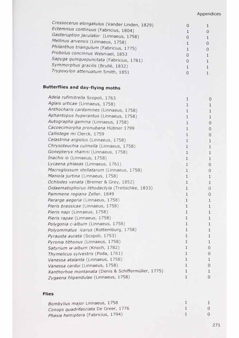
Crossocerus elongatulus (Vander Linden, 1829) Ectemnius continuus (Fabricius, 1804)Gasteruption jaculator (Linnaeus, 1758)Mellinus arvensis (Linnaeus, 1758)Philanthus triangulum (Fabricius, 1775)Probolus concinnus Wesmael, 1853 Sapyga quinquepunctata (Fabricius, 1781) Symmorphus gracilis (Brulle, 1832)Trypoxylon attenuatum Smith, 1851
Butterflies and day-flying moths
Adela rufimitrella Scopoli, 1763 Aglais urticae (Linnaeus, 1758)Anthocharis cardamines (Linnaeus, 1758)Aphantopus hyperantus (Linnaeus, 1758)Autographa gamma (Linnaeus, 1758)Cacoecimorpha pronubana Hubner 1799 Callistege mi Clerck, 1759 Celastrina argiolus (Linnaeus, 1758)Chrysoteuchia culmeUa (Linnaeus, 1758)Gonepteryx rhamni (Linnaeus, 1758)Inachis io (Linnaeus, 1758)Lycaena phlaeas (Linnaeus, 1761)Macroglossum stellatarum (Linnaeus, 1758)Man iota jurtina (Linnaeus, 1758)Ochlodes venata (Bremer & Grey, 1852) Oidaematophorus lithodactyla (Treitschke, 1833) Pammene regiana Zeller, 1849 Pararge aegeria (Linnaeus, 1758)Pieris brassicae (Linnaeus, 1758)Pieris napi (Linnaeus, 1758)Pieris rapae (Linnaeus, 1758)Polygonia c-album (Linnaeus, 1758)Polyommatus icarus (Rottemburg, 1758)Pyrausta aurata (Scopoli, 1753)Pyronia tithonus (Linnaeus, 1758)Satyrium w-album (Knoch, 1782)Thymelicus sylvestris (Poda, 1761)Vanessa atalanta (Linnaeus, 1758)Vanessa cardui (Linnaeus, 1758)Xanthorhoe montanata (Denis & Schiffermuller, 1775) Zygaena filipendulae (Linnaeus, 1758)
Flies
Bombylius major Linnaeus, 1758 Conops quadrifasciata De Greer, 1776 Phasia hemiptera (Fabricius, 1794)

Sicus ferrugineus (Linnaeus, 1761) Tachina fera (Linnaeus, 1761)
Hoverflies
Anasimyia lineata (Fabricius, 1787)Baccha elongata (Fabricius, 1775) Cheilosia albitarsis (Meigen, 1822) Cheilosia illustrata (Harris, 1780)Cheilosia pagana (Meigen, 1822)Cheilosia proxima (Zetterstedt, 1843) Cheilosia ranunculi Doczkal, 2000 Cheilosia vulpina (Meigen, 1822) Chrysogaster solstitialis (Fallen, 1817)Criorhina berberina (Fabricius, 1805) Dasysyrphus albostriatus (Fallen, 1817) Dasysyrphus tricinctus (Fallen, 1817) Epistrophe eligans (Harris, 1780) Epistrophe grossulariae (Meigen, 1822) Episyrphus balteatus (De Greer, 1776) Eristalis arbustorum (Linnaeus, 1758) Eristalis intricarius (Linnaeus, 1758) Eristalis nemorum (Linnaeus, 1758) Eristalis pertinax (Scopoli, 1763)Eristalis tenax (Linnaeus, 1758)Eumerus funeralis Meigen, 1822 Eupeodes corollae (Fabricius, 1794) Eupeodes latifasciatus (Macquart, 1829) Eupeodes luniger (Meigen, 1822)Eupeodes nielseni (Dusek & Laska, 1976) Ferdinandea cuprea (Scopoli, 1763) Helophilus pendulus (Linnaeus, 1758) Heringia vitripennis (Meigen, 1822) Leucozona latinaria (Muller, 1776) Leucozona lucorum (Linnaeus, 1758) Melangyna labiatarum (Verrall, 1901) Melangyna umbellatarum (Fabricius, 1794) Melanostoma mellinum (Linnaeus, 1758) Melanostoma scalare (Fabricius, 1794) Merodon equestris (Fabricius, 1794) Myathropa florea (Linnaeus, 1758) Neoascia podagrica (Fabricius, 1775) Parhelophilus frutetorum (Fabricius, 1775) Parasyrphus punctulatus (Verrall, 1873) Platycheirus albimanus (Fabricius, 1781) Platycheirus clypeatus (Meigen, 1822) Platycheirus manicatus (Meigen, 1822) Platycheirus peltatus (Meigen, 1822) Platycheirus scutatus (Meigen, 1822) Platycheirus splendidus Rotheray, 1998

Appendices
Platycheirus sticticus (Meigen, 1822) Platycheirus tarsalis (Schummel, 1837) Rhingia campestris (Meigen, 1822)Rhingia rostrata (Linnaeus, 1758) Riponnensia splendens (Meigen, 1822) Scaeva pyrastri (Linnaeus, 1758) Sphaerophoria scripta (Linnaeus, 1758) Syritta pipiens (Linnaeus, 1758)Syrphus rectus Osten Sacken, 1875 Syrphus ribesii (Linnaeus, 1758)Syrphus torvus Osten Sacken, 1875 Syrphus vitripennis Meigen, 1822 Volucella bombylans (Linnaeus, 1758) Volucella inanis (Linnaeus, 1758)Volucella pelluscens (Linnaeus, 1758) Volucella zonaria (Poda, 1761)Xanthandrus comtus (Harris, 1780) Xanthogramma pedissequum (Harris, 1776) Xylota segnis (Linnaeus, 1758)
1111111111111
10011
0010011101011011111
Honeybee
Apis mellifera2 Linnaeus, 1758 1 1
Eleven solitary bee species (Species A - Species K) remained unidentified from the 2010 sampling session (see explanation in Chapter 2 - Identification of species).Apis mellifera mellifera may also have been present but this was not treated as a distinct species for the purposes of this study (see Chapter 2 - Hymenoptera, honey bees).
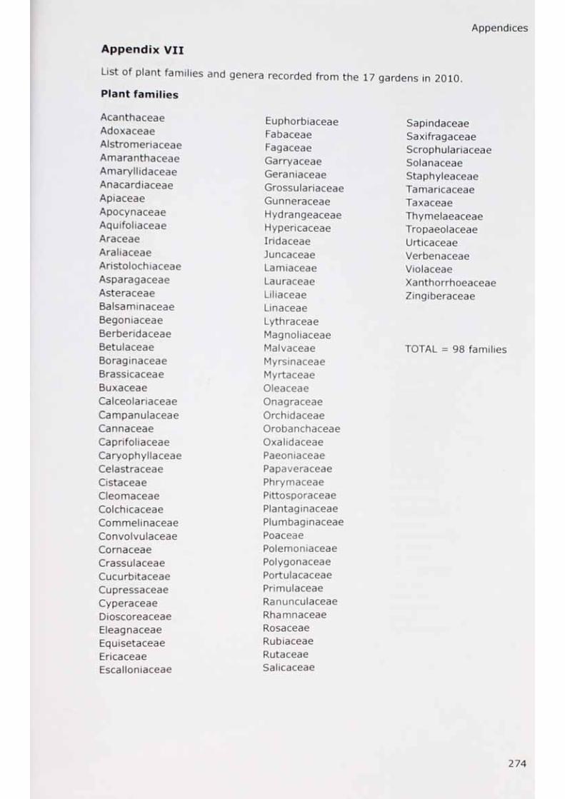
Appendices
Appendix VII
List of plant families and genera recorded from the 17 gardens in 2010
Plant families
AcanthaceaeAdoxaceaeAlstromeriaceaeAmaranthaceaeAmaryliidaceaeAnacardiaceaeApiaceaeApocynaceaeAquifoliaceaeAraceaeAraliaceaeAristolochiaceaeAsparagaceaeAsteraceaeBalsaminaceaeBegoniaceaeBerberidaceaeBetulaceaeBoraginaceaeBrassicaceaeBuxaceaeCalceolariaceaeCampanulaceaeCannaceaeCaprifoliaceaeCaryophyllaceaeCelastraceaeCistaceaeCleomaceaeColchicaceaeCommelinaceaeConvolvulaceaeCornaceaeCrassulaceaeCucurbitaceaeCupressaceaeCyperaceaeDioscoreaceaeEleagnaceaeEquisetaceaeEricaceaeEscalloniaceae
Euphorbiaceae SapindaceaeFabaceae SaxifragaceaeFagaceae ScrophulariaceaeGarryaceae SolanaceaeGeraniaceae StaphyleaceaeGrossulariaceae TamaricaceaeGunneraceae TaxaceaeHydrangeaceae ThymelaeaceaeHypericaceae TropaeolaceaeIridaceae UrticaceaeJuncaceae VerbenaceaeLamiaceae ViolaceaeLauraceae XanthorrhoeaceaeLiliaceae ZingiberaceaeLinaceaeLythraceaeMagnoliaceaeMalvaceae TOTAL = 98 familiMyrsinaceaeMyrtaceaeOleaceaeOnagraceaeOrchidaceaeOrobanchaceaeOxalidaceaePaeoniaceaePapaveraceaePhrymaceaePittosporaceaePlantaginaceaePlumbaginaceaePoaceaePolemoniaceaePolygonaceaePortulacaceaePrimulaceaeRanunculaceaeRhamnaceaeRosaceaeRubiaceaeRutaceaeSalicaceae
274

Appendices
Plant genera
AbeliaAbutilonAcaciaAcanthusAcerAchilleaAcidantheraAconitumAegopodiumAgapanthusAgastacheAgaveAgera turnAgrimoniaAgrostemmaAjugaA Ice aAlchemil/aAlliariaA IliumAlstroemeriaAlternatheraAlthaeaAlyssumAmaranthusAmaryllisAmsoniaAnagallisAnaphalisAnchusaAnemoneAnethumAngelicaAntenna riaAnthem isAnthriscusAntirrhinumApiumApocynumAquilegiaAraliaArbutusArctiumArgemoneArgyranthemumAristolochia
ArmeriaArnicaArtemisiaArumAruncusAsarinaAsclepiasAsparagusAsphodelineAsphodelusAsterAstilbeAstra ntiaAubretiaAucubaAuriniaBallotaBaptisiaBegoniaBeilisBerberisBergeniaBoragoBrassicaBrunneraBryoniaBudd/ejaBupleurumBuxusCalaminthaCalceolariaCalendulaCalthaCalystegiaCampanulaCannaCapsellaCardamineCarexCaryopterisCa tan acheCeanothusCentaureaCentranthusCephalariaCerastium
CeratostigmaCerintheCestrumChaenomelesChamerionChelidoniumCheloneChenopodiumChoisyaChrysanthemumCichoriumCimicifugaCircaeaCirsiumCistusClematisCleomeClerodendronCnicusColchicumConiumConvallariaConvolvulusCoreopsisCorn usCorylusCosmosCo tin usCotoneasterCrambeCrassulaCrataegusCrocosmiaCurcubitaCyclamenCymbalariaCynaraCynoglossumCyperusCytisusDactylorhizaDahliaDaphneDasiphoraDaucusDelphinium

Appendices
DeutziaDia n th usDicentraDigitalisDipsacusDoronicumEchinaceaEchinopsEchiumElea gnusEpilobiumEpimediumEquisetumEremurusEricaErigeronErodiumErucaEryngiumErysimumEsea I IoniaEucomisEuonymusEupatoriumEuphorbiaExochordaFeliciaFilipendulaFoeniculumForsythiaFrageriaFremon to dendro nFritillariaFuchsiaGalegaGaliumGauraGazaniaGenistaGeraniumGerberaGeumGil teniaGladiolusGlechomaGlycyrrhiza
GunneraHebeHederaHedychiumHe/eniumHelianthemumHelianthusHelichrysumHeliotropiumHelleborusHemerocallisHeracleumHesperisHeucheraHibiscusHieraciumHostaHyacinthoidesHyacinthusHydrangeaHypericumHyssopusHexImpatiensInulaIochromaIrisJasminumJuncusJuniperusKirengeshomaKnautiaKniphofiaKolkwitziaLaburnumLamia strumLamiumLantanaLapsanaLathy rusLavandulaLavateraLeonurusLeucanthemumLevisticumL ia tris
LigulariaLigu strumL iliumLimoniumLinariaLinumLobeliaLobulariaLoniceraLotusLunariaLupin usL uzulaLychnisLycopusLysimachiaLy thrumMacleayaMagnoliaMahoniaMai usMalvaMandragoraMatricariaMatthiolaMecanopsisMe lilotusMelissaMenthaMercurial isMi IliumMim ulusMonardaMona rdellaMo n tiaMorin aMuscariMy o sotisMyrrh isMyrtusNarcissusNectaroscordumNemesiaNepetaNica n draNicotian a
276

Appendices
Nige/laOenotheraOleariaOmpha/odesOnopordumOriganumOrnithogalumOsteospermumOxalisOzothamnusPaeon iaPa paverParahebePelargoniumPenstemonPerovskiaPersicariaPetasitesPetroselinumPetuniaPhaceliaPhaseolusPhiladelphusPhlomisPhloxPhygeliusPhysalisPicrisPittosporumPlantagoPoaPolemoniumPolygonumPortulacaPo ten til laPrimulaPrunellaPrun usPseudofumariaPulicariaPulmonariaPu/sa tillaPycnanthemumPyrusRanunculusRhazya
RheumRhinanthusRhodochitonRhododendronRibesRicinusRodgersiaRomneyaRosaRosmarinusRub usRudbeckiaRutaSalixSalviaSambucusSanguisorbaSantolinaSan vita HaSaponariaSaturejaSaxifragaScabiosaS ciliaScrophulariaSedumSempervivumSenecioSidalceaSileneSilphiumSilybumSisymbriumSisyrinchiumSkimmiaSolanumSolidagoSonchusSpiraeaS ta ch ysStaphyleaStellariaStephanandraSuccisaSymphoricarposSymphyotrichum
SymphytumSyringaTagetesTamarixTamusTanacetumTaraxacumTaxusTeucriumThalictrumTherm op s isThymusTiarellaTiliaTithoniaTori I isTrachystemonTradescantiaTricyrtisTrifoliumTripleurospermumTriteleiaTropaeolumTulipaUrticaVacciniumValerianaVerbascumVerbenaVeronicaVeronicastrumVestiaViburnumViciaVincaViolaWeigelaWisteriaYuccaZantedeschiaZinnia
TOTAL = 409 genera
277

>
X■ocVo .a<
03
E03E03
T3C03
ID
cn
03
QJa ;
03
oCO
03E(13
cn
lO=3
m
vb03
03
CO03cn03CO03
O ^
1*3T3
mo u u co03 03
CCO03
03
-X
O
oQ .E03
O
03
O
CO
5 vu CL03 F U c03
03X03
O03
03
i—
r= <nc cn03 cnXLU
03DOJ 10
_ t 3 OJ 1 >
£
CO10
OJt ro
II
~C3
03
Eino
03
S E=>
uOJ
COCOo
03
03cnOJto
mmrv. mm m rMmn o tHtHr\ rsfN• o• o• o• fN• A v£>o o o o W
o •
r\j co cn co cno o
CO fN m ID cn fNo m o rH o ID r \fN• oa o o t H fHO o
•o %
o •o •o •
f-H
ID fN Tf No o
o
co ^ o COcn ID ID ID m
03cn
■§c :
3
io
c:03 03
03
OJ
XOu
<3
u</> 10 03 -Q�tf O£ g
M»- c03 O
■*-o
03U
03cn
E Ea . £
Ei/ i
c :
■§oc:o
5 :
in0303E
03
E03
O — 2 OJ
03 OJ -O CL
t- oin2 com o CL - 2
OJ>oE03
OcQ .
OJ03
03cn
03
UECOou
03 _03F OJ
o 03 Eo O 03_ _ u ■*—'
03 ~Q3 o 03 —
U U u _Q D"D10•.2
•OJ
p c: ■£ OJ -XDoCJ o co 5 >OJ ft -J
? <-Q
•
•-Q•
ouo T3 “O03 h-E 0O o u OJ OJ 03 h-
ID VOic-5C-5C-ic -5C-5C
CO
fN
�H CO00 cn r sc n• fN• 00• co0 0 0
•

Appendices
Appendix IX
Post hoc test used to assess differences between mean ranks for eight properties (each with three nests) using the method of Siegel and Castellan (1988).
\RU - R V\ >\N(N + 1) / 1 1
z a/k(k-1) I ~ ( ------1"N
12 n n v
where:
K - r v \ is the magnitude of the differences between mean ranks of groups 1 and 2 (the groups being compared)
z a/kyk-1)N(N+1) / 1 1 \
1: ) is the critical difference\
Z a = 0.05
k = total number of samples
.Y= number of groups used in analysis
>i = number of nests in the first group being compared
k = number of nests in the second group being compared
Appendix X
Solitary bee families and genera other than O. bicornis found in occupied tubes
Property Nestno.
Family, genus
BOU 3 Megachilidae, OsmiaCHALL 1, 2 Colletidae, HylaeusFAR 1 Megachilidae, OsmiaFAR 2,3 Colletidae, HylaeusKEL 1 Megachilidae, OsmiaKEL 2,3 Megachilidae, MegachileLW 1 Megachilidae, Megachile, Colletidae, HylaeusLW 2 Meqachilidae, Meqachile, Osmia', Colletidae, Hylaeus
279


![Types of Gardens [Compatibility Mode] pdf](https://static.fdokumen.com/doc/165x107/631bd7dc7051d371800f3412/types-of-gardens-compatibility-mode-pdf.jpg)

