Astronomy&Astrophysics

A&A 612, A91 (2018)https://doi.org/10.1051/0004-6361/201731402© ESO 2018

The contact binary VW Cephei revisited: surface activity andperiod variation

T. Mitnyan1, A. Bódi2,3, T. Szalai1, J. Vinkó1,3, K. Szatmáry2, T. Borkovits3,4, B. I. Bíró4, T. Hegedüs4,K. Vida3, and A. Pál3

1 Department of Optics and Quantum Electronics, University of Szeged, 6720 Szeged, Dóm tér 9, Hungarye-mail: mtibor@titan.physx.u-szeged.hu

2 Department of Experimental Physics, University of Szeged, 6720 Szeged, Dóm tér 9, Hungary3 Konkoly Observatory, Research Centre for Astronomy and Earth Sciences, Hungarian Academy of Sciences, 1121 Budapest,

Konkoly Thege Miklós út 15-17, Hungary4 Baja Astronomical Observatory of University of Szeged, 6500 Baja, Szegediút, Kt. 766, Hungary

Received 19 June 2017 / Accepted 17 January 2018

ABSTRACT

Context. Despite the fact that VW Cephei is one of the most well-studied contact binaries in the literature, there is no fully consistentmodel available that can explain every observed property of this system.Aims. Our aims are to obtain new spectra along with photometric measurements, to analyze what kind of changes may have happenedin the system in the past two decades, and to propose new ideas for explaining them.Methods. For the period analysis we determined ten new times of minima from our light curves, and constructed a new O–C diagramof the system. Radial velocities of the components were determined using the cross-correlation technique. The light curves and radialvelocities were modeled simultaneously with the PHOEBE code. All observed spectra were compared to synthetic spectra and equivalentwidths (EWs) of the Hα line were measured on their differences.Results. We re-determine the physical parameters of the system according to our new light curve and spectral models. We confirmthat the primary component is more active than the secondary, and there is a correlation between spottedness and the chromosphericactivity. We propose that the flip-flop phenomenon occurring on the primary component could be a possible explanation of the observednature of the activity. To explain the period variation of VW Cep, we test two previously suggested scenarios: the presence of a fourthbody in the system, and the Applegate-mechanism caused by periodic magnetic activity. We conclude that although none of thesemechanisms can be ruled out entirely, the available data suggest that mass transfer with a slowly decreasing rate provides the mostlikely explanation for the period variation of VW Cep.

Key words. stars – activity – stars: individual: VW Cep – binaries: eclipsing – binaries: close – starspots

1. Introduction

A contact binary typically consists of two main sequence starsof the F, G or K spectral type that are orbiting around their com-mon center of mass. According to the most accepted model, bothcomponents are filling their Roche lobes and making physicalcontact through the inner (L1) Lagrangian point. The compo-nents also share a common convective envelope (Lucy 1968),which is why they have nearly the same effective temperature.Although this model is very simple and can explain a lot of theproperties of these stars, it leaves some open questions (Rucinski2010). The most obvious one is that there are a lot of systemswhere the mass ratio determined from photometry differs fromthe one obtained from spectroscopy. Nevertheless, a generalmodel that resolves all the issues is still lacking, which providesfurther motivation for studying this kind of binary system.

The light curves of contact binaries show continuous fluxvariation, even outside of eclipses, because of the heavy geo-metric distortion of both components. The orbital periods ofthese objects are usually shorter than a day. There are two maintypes of these objects according to their light curves: A-type andW-type (Binnendijk 1970). In A-type systems, the more mas-sive primary component has higher surface brightness than the

secondary. They have longer orbital periods and smaller massratios than the W-type systems, where the secondary compo-nent seems to show higher surface brightness. The most acceptedexplanation for the existence of W-type objects is that the moremassive, intrinsically hotter primary component is so heavilyspotted that its average surface brightness appears to be lowerthan that of the less massive and cooler secondary (Mullan 1975).Nevertheless, another scenario, the hot secondary model, is alsocommonly used in the literature in order to explain the lightcurves of these binaries; in this model, it is assumed that the sec-ondary star has a higher temperature, for some unknown reason(Rucinski 1974).

Many contact binaries show asymmetry in the light curvemaxima (O’Connell effect), which is likely caused by starspotson the surface of the components as a manifestation of the mag-netic activity. The difference between the maxima can changefrom orbit to orbit because of the motion and evolution ofthese cooler active regions. This phenomenon may indicate thepresence of an activity cycle similar to that seen on our Sun.

Activity cycles have been directly observed in several typesof single and binary stars (e.g., Wilson 1978; Baliunas et al.1995; Heckert & Ordway 1995; Oláh & Strassmeier 2002; Vidaet al. 2015). In the cases of contact binaries there is only indirect

Article published by EDP Sciences A91, page 1 of 14

A&A 612, A91 (2018)

evidence for periodic magnetic activity. These mostly come fromperiod analyses, which have revealed that the periodic variationbetween the observed and calculated moments of mid-eclipsescannot be simply explained by the presence of additional com-ponents in the system (or, this can only be a partial explanation).Applegate (1992) proposed a mechanism that could be respon-sible for such kind of cyclic period variations. According tohis model, the magnetic activity can modify the gravitationalquadrupole moment of the components, which induces internalstructural variations in the stars, and also influences their orbit.

Many contact binaries also have a detectable tertiary compo-nent. In fact, Pribulla & Rucinski (2006) summarized that up toV = 10 mag, 59±8% of these systems are triples on the northernsky, which becomes 42 ± 5% if the objects on the southern skyare also included. These numbers are based on only the verifieddetections, but they can increase up to 72 ± 9% and 56 ± 6%,respectively, if one takes into account even the unverified cases.These numbers are only lower limits because of unobservedobjects and the undetectable additional components; therefore,the authors suggested that it is possible that every contact binaryis a member of a multiple system. According to some models(e.g., Eggleton & Kiseleva-Eggleton 2001), the tertiary compo-nents can play an important role in the formation and evolutionof these systems.

One of the most frequently observed contact binaries,VW Cephei, was discovered by Schilt (1926). It is a popular tar-get because of its brightness (V = 7.30–7.84 mag) and its shortperiod (∼6.5 h), which allows us to easily observe a full orbitalcycle on a single night with a relatively small telescope. The sys-tem is worth observing, because it usually shows the O’Connelleffect and clearly has a third component confirmed by astrome-try (Hershey 1975); however, there is no perfect model that canexplain all the observed properties of the system.

The strange behavior of the light curve of VW Cephei wasdiscovered during the first dedicated photometric monitoring ofthe system (Kwee 1966). Several different models have beendeveloped to explain the asymmetry of maxima, for example, thepresence of a circumstellar ring (Kwee 1966), a hot spot on thesurface caused by gas flows (van’t Veer 1973), or cool starspotson the surface (Yamasaki 1982). The latter model seemed tobe the most consistent with the observations, and dozens ofpublications present a light curve model including starspots.

Instead of the huge amount of photometric data, there is alimited number of published spectroscopic observations aboutVW Cep. The first spectroscopic results are from Popper (1948)who published a mass ratio of q = 0.326 ± 0.045. Andersonet al. (1980) took two spectra at two different orbital phasesand derived a mass ratio of 0.40 ± 0.05, which was consistentwith the previous value of 0.409 ± 0.011 yielded by Binnendijk(1967). Hill (1989) measured the radial velocities of the com-ponents using the cross-correlation technique on low-resolutionspectra, and determined a new value of q = 0.277 ± 0.007. Thenext spectroscopic study of the system was presented by Frascaet al. (1996) who took a series of low-resolution spectra at theHα-line; they showed that there is a rotational modulation in theequivalent width (EW) of the Hα-profile. Kaszás et al. (1998)obtained the first series of medium-resolution spectra of the sys-tem. They used the same technique as Hill (1989) to derivethe radial velocities and the mass ratio, but they got a largervalue (q = 0.35 ± 0.01). They also investigated the variation ofHα EWs with the orbital phase and found that the more mas-sive primary component showed emission excess, which theyinterpreted as a consequence of enhanced chromospheric activ-ity. They pointed out a possible anticorrelation between the

photospheric and chromospheric activity. The latest publicationabout VW Cephei including spectroscopic analysis is a Dopplerimaging study by Hendry & Mochnacki (2000). They deriveda mass ratio of q = 0.395 ± 0.016 and found that the surfacesof both components were heavily spotted, and the more massiveprimary component had an off-centered polar spot at the time oftheir observations.

No other papers based on optical spectroscopy were pub-lished about VW Cephei after the millennium. However, therewere two publications based on X-ray spectroscopy (Gondoin2004; Huenemoerder et al. 2006), and another one based on UVspectra (Sanad & Bobrowsky 2014). Gondoin (2004) concludedthat VW Cephei has an extended corona encompassing the twocomponents and that it shows flaring activity. Huenemoerderet al. (2006) also detected the flaring activity of the system andthat the corona is mainly on the polar region of the primary com-ponent. Sanad & Bobrowsky (2014) studied UV emission linesand found both short- and long-term variations in the strength ofthese lines, which they attributed to the chromospheric activityof the primary component.

In this paper, we perform a detailed optical photometric andspectroscopic analysis of VW Cep, and examine what kind ofchanges may have occurred in the past two decades. The paperis organized as follows: Sect. 2 contains information about theobservations and data reduction process, as well as the stepsof the analysis of our photometric and spectroscopic data. InSect. 3, we discuss the activity of VW Cep based on our mod-eling results, then, in Sect. 4, we present an O–C analysis ofthe system. Finally, we briefly summarize our work and itsimplications in Sect. 5.

2. Observations and analysis

2.1. Photometry

Photometric observations took place on three nights in August2014, and two nights in April 2016 at Baja Astronomical Obser-vatory of University of Szeged (Hungary) with a 0.5 m, f/8.4 RCtelescope through SDSS g′r′i′ filters. In order to reduce photo-metric errors, bias, dark and flat correction images were takenon every observing night. The image processing was performedusing IRAF1: we carried out image corrections and aperture pho-tometry using the ccdred and apphot packages, respectively.The photometric errors are determined by the phot task of IRAF.These errors are in the order of 0.01–0.02 mag, hence they aresmaller than the symbols we used in our plots. For differentialphotometry, we used HD 197750 as a comparison star; although,it is considered as a variable in the SIMBAD catalog, we couldnot find any significant changes in its light curve compared tothe check star, BD+74880 during our observations. The Φ = 0.0phase was assigned to the secondary minimum (when the moremassive primary component is eclipsed), while the secondaryminimum time of the last observing night of both years was usedfor phase calculation for each season.

2.2. Spectroscopy

Spectroscopic observations were obtained on 12 and 13 April2016 with a R = 20 000 échelle spectrograph mounted on the 1mRCC telescope at the Piszkésteto Mountain Station of KonkolyObservatory, Hungary. The integration time was set to 10 min

1 Image Reduction and Analysis Facility: http://iraf.noao.edu

A91, page 2 of 14

T. Mitnyan et al.: The contact binary VW Cephei revisited

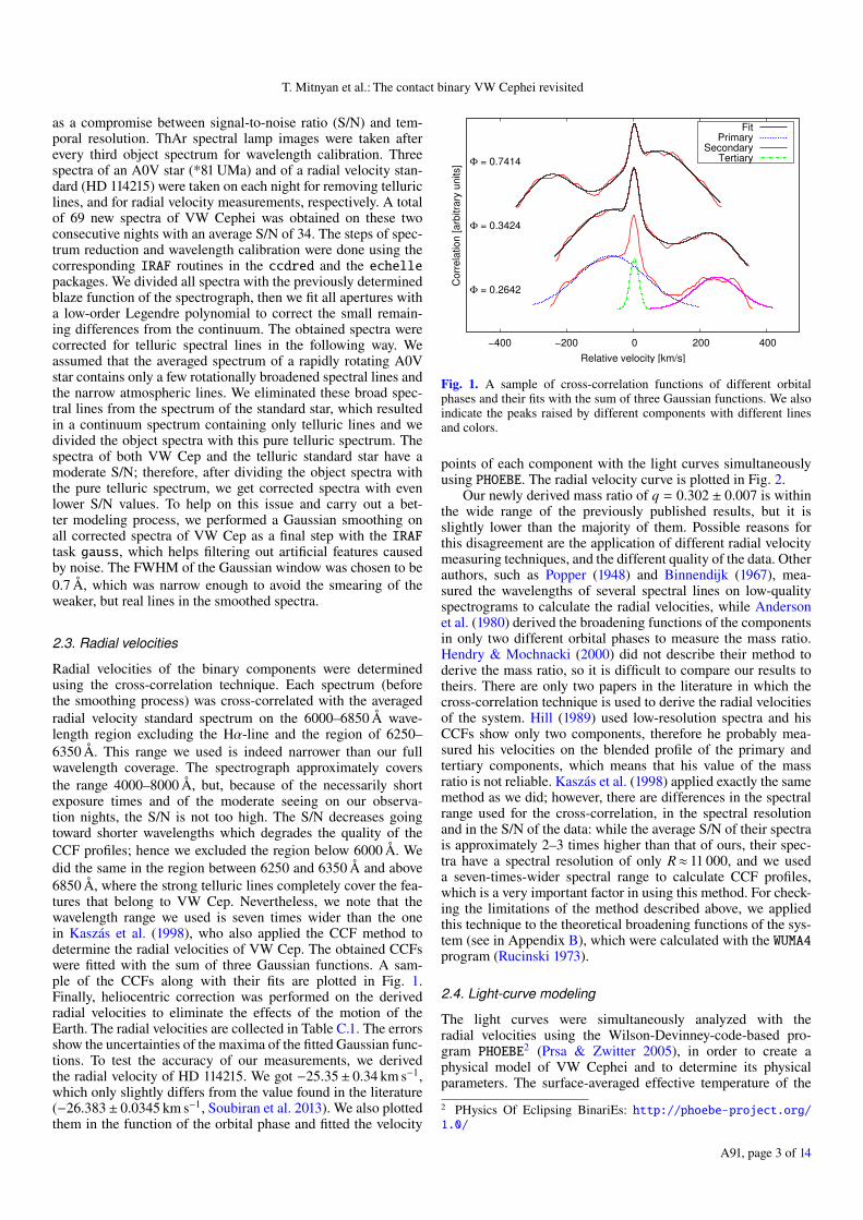
as a compromise between signal-to-noise ratio (S/N) and tem-poral resolution. ThAr spectral lamp images were taken afterevery third object spectrum for wavelength calibration. Threespectra of an A0V star (*81 UMa) and of a radial velocity stan-dard (HD 114215) were taken on each night for removing telluriclines, and for radial velocity measurements, respectively. A totalof 69 new spectra of VW Cephei was obtained on these twoconsecutive nights with an average S/N of 34. The steps of spec-trum reduction and wavelength calibration were done using thecorresponding IRAF routines in the ccdred and the echellepackages. We divided all spectra with the previously determinedblaze function of the spectrograph, then we fit all apertures witha low-order Legendre polynomial to correct the small remain-ing differences from the continuum. The obtained spectra werecorrected for telluric spectral lines in the following way. Weassumed that the averaged spectrum of a rapidly rotating A0Vstar contains only a few rotationally broadened spectral lines andthe narrow atmospheric lines. We eliminated these broad spec-tral lines from the spectrum of the standard star, which resultedin a continuum spectrum containing only telluric lines and wedivided the object spectra with this pure telluric spectrum. Thespectra of both VW Cep and the telluric standard star have amoderate S/N; therefore, after dividing the object spectra withthe pure telluric spectrum, we get corrected spectra with evenlower S/N values. To help on this issue and carry out a bet-ter modeling process, we performed a Gaussian smoothing onall corrected spectra of VW Cep as a final step with the IRAFtask gauss, which helps filtering out artificial features causedby noise. The FWHM of the Gaussian window was chosen to be0.7 Å, which was narrow enough to avoid the smearing of theweaker, but real lines in the smoothed spectra.

2.3. Radial velocities

Radial velocities of the binary components were determinedusing the cross-correlation technique. Each spectrum (beforethe smoothing process) was cross-correlated with the averagedradial velocity standard spectrum on the 6000–6850 Å wave-length region excluding the Hα-line and the region of 6250–6350 Å. This range we used is indeed narrower than our fullwavelength coverage. The spectrograph approximately coversthe range 4000–8000 Å, but, because of the necessarily shortexposure times and of the moderate seeing on our observa-tion nights, the S/N is not too high. The S/N decreases goingtoward shorter wavelengths which degrades the quality of theCCF profiles; hence we excluded the region below 6000 Å. Wedid the same in the region between 6250 and 6350 Å and above6850 Å, where the strong telluric lines completely cover the fea-tures that belong to VW Cep. Nevertheless, we note that thewavelength range we used is seven times wider than the onein Kaszás et al. (1998), who also applied the CCF method todetermine the radial velocities of VW Cep. The obtained CCFswere fitted with the sum of three Gaussian functions. A sam-ple of the CCFs along with their fits are plotted in Fig. 1.Finally, heliocentric correction was performed on the derivedradial velocities to eliminate the effects of the motion of theEarth. The radial velocities are collected in Table C.1. The errorsshow the uncertainties of the maxima of the fitted Gaussian func-tions. To test the accuracy of our measurements, we derivedthe radial velocity of HD 114215. We got −25.35± 0.34 km s−1,which only slightly differs from the value found in the literature(−26.383± 0.0345 km s−1, Soubiran et al. 2013). We also plottedthem in the function of the orbital phase and fitted the velocity

Fig. 1. A sample of cross-correlation functions of different orbitalphases and their fits with the sum of three Gaussian functions. We alsoindicate the peaks raised by different components with different linesand colors.

points of each component with the light curves simultaneouslyusing PHOEBE. The radial velocity curve is plotted in Fig. 2.

Our newly derived mass ratio of q = 0.302 ± 0.007 is withinthe wide range of the previously published results, but it isslightly lower than the majority of them. Possible reasons forthis disagreement are the application of different radial velocitymeasuring techniques, and the different quality of the data. Otherauthors, such as Popper (1948) and Binnendijk (1967), mea-sured the wavelengths of several spectral lines on low-qualityspectrograms to calculate the radial velocities, while Andersonet al. (1980) derived the broadening functions of the componentsin only two different orbital phases to measure the mass ratio.Hendry & Mochnacki (2000) did not describe their method toderive the mass ratio, so it is difficult to compare our results totheirs. There are only two papers in the literature in which thecross-correlation technique is used to derive the radial velocitiesof the system. Hill (1989) used low-resolution spectra and hisCCFs show only two components, therefore he probably mea-sured his velocities on the blended profile of the primary andtertiary components, which means that his value of the massratio is not reliable. Kaszás et al. (1998) applied exactly the samemethod as we did; however, there are differences in the spectralrange used for the cross-correlation, in the spectral resolutionand in the S/N of the data: while the average S/N of their spectrais approximately 2–3 times higher than that of ours, their spec-tra have a spectral resolution of only R≈ 11 000, and we useda seven-times-wider spectral range to calculate CCF profiles,which is a very important factor in using this method. For check-ing the limitations of the method described above, we appliedthis technique to the theoretical broadening functions of the sys-tem (see in Appendix B), which were calculated with the WUMA4program (Rucinski 1973).

2.4. Light-curve modeling

The light curves were simultaneously analyzed with theradial velocities using the Wilson-Devinney-code-based pro-gram PHOEBE2 (Prsa & Zwitter 2005), in order to create aphysical model of VW Cephei and to determine its physicalparameters. The surface-averaged effective temperature of the

2 PHysics Of Eclipsing BinariEs: http://phoebe-project.org/1.0/

A91, page 3 of 14

A&A 612, A91 (2018)

Fig. 2. Radial velocity curve of VW Cephei with the fitted PHOEBEmodel. We note that the formal errors of the single velocity points (seeTable C.1) are smaller than their symbols.

primary component (Teff,1) and the relative temperatures of thestarspots were kept fixed at 5050 K as in Kaszás et al. (1998),and 3500 K as in Hendry & Mochnacki (2000), respectively. Weassumed that the orbit is circular and the rotation of the compo-nents is synchronous, therefore, the eccentricity was fixed at 0.0,and the synchronicity parameters were kept at 1.0. For the grav-ity darkening coefficients and bolometric albedos, we adoptedthe usual values for contact systems: g1 = g2 = 0.32 (Lucy 1967)and A1 = A2 = 0.5 (Rucinski 1969), respectively. The followingparameters were varied during the modeling: the effective tem-perature of the secondary component (Teff,2), the inclination (i),the mass ratio (q), the semi-major axis (a), the gamma velocity(vγ), the luminosities of the three components, and the coordi-nates and radii of starspots. The limb darkening coefficients wereinterpolated for every iteration from PHOEBE’s built-in tablesusing the logarithmic limb darkening law.

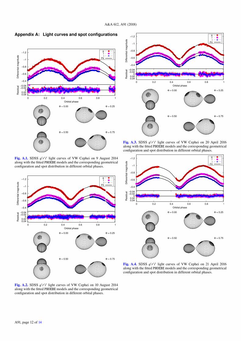
Light curves obtained on the given nights are plotted inFigs. 3, A.1–A.4 along with their model curves fitted by PHOEBEand the corresponding geometrical configurations in differentorbital phases. The residuals are mostly in the range of ±0.02magnitudes, which is comparable to our photometric accuracy.One can see that the difference of the two maxima changesslightly from night to night in each filter. This variation suggestsongoing surface activity, and it is treated by assuming coolerspots on the surface of the components. The final model and spotparameters are listed in Tables 1 and 2, respectively.

2.5. Spectrum synthesis

In order to analyze the chromospheric activity of the system,we constructed synthetic spectra for every observed spectra.For spectrum synthesis, we used Robert Kurucz’s ATLAS9(Kurucz 1993) model atmospheres selecting different tempera-tures (4500–6500 K, with 250 K steps). The model spectra wereDoppler-shifted and convolved with the broadening functionsassociated with the observed orbital phases that were computedwith the WUMA4 program. As in Kaszás et al. (1998), the tertiarycomponent is also well-resolved in our cross-correlation func-tions (Fig. 1), which means that its contribution is not negligible.Accounting for this third component, a T = 5000 K, log g = 4.0model was used: it was Doppler-shifted, then convolved witha simple Gaussian function applying the FWHM of the trans-mission function of the spectrograph. A scaled version of this

Fig. 3. SDSS g′r′i′ light curves of VW Cephei on 8 August 2014along with the fitted PHOEBEmodels and the corresponding geometricalconfiguration and spot distribution in different orbital phases.

Table 1. Physical parameters of VW Cep according to our PHOEBE light-and radial velocity curve models compared to the previous results ofKaszás et al. (1998).

Parameter This paper Kaszás et al. (1998)

q 0.302 ± 0.007 0.35 ± 0.01Vγ [km s−1] −12.61± 1.06 −16.4± 1a [106 km] 1.412 ± 0.01 1.388 ± 0.01i [] 62.86 ± 0.04 65.6 ± 0.3Teff,1* [K] 5050 5050Teff,2 [K] 5342 ± 15 5444 ± 25Ω1 = Ω2 2.58272 –m1 [M] 1.13 1.01m2 [M] 0.34 0.36R1 [R] 0.99 –R2 [R] 0.57 –

Notes. Teff,1, signed with asterisk, was a fixed parameter.

model spectrum (assuming that the third component gives 10%of the total luminosity, based on Kaszás et al. 1998) was addedto the contact binary model spectrum to mimic the presence ofthe tertiary component. We fitted the produced synthetic spectrawith different temperatures to the observed data (leaving out theHα-region), and found that T = 5750 K and log g = 4.0 givesthe best-fit model. This temperature value corresponds to theflux-averaged mean surface temperature, and it is very similarto that found by Hendry & Mochnacki (2000) for the unspot-ted mean surface temperature of VW Cep. The best-fit modelspectra were then subtracted from the observed ones at everyepoch. Finally, we measured the EWs of the Hα-profile on theresidual (observed minus model) spectra using the IRAF/splottask. It is hard to fit the Hα-line of the components with theusual Gaussian- or Voigt-profiles on the residual spectra, sowe chose the direct integration of the equivalent widths. We

A91, page 4 of 14

T. Mitnyan et al.: The contact binary VW Cephei revisited

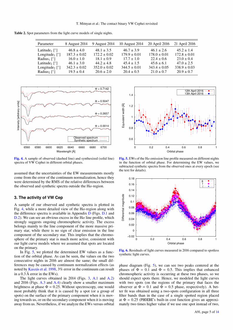
Table 2. Spot parameters from the light curve models of single nights.

Parameter 8 August 2014 9 August 2014 10 August 2014 20 April 2016 21 April 2016

Latitude1 [] 46.8 ± 4.0 48.1 ± 3.5 46.7 ± 3.9 46.1 ± 2.6 45.2 ± 1.4Longitude1 [] 187.3 ± 0.02 172.2 ± 0.02 179.9 ± 0.01 178.0 ± 0.01 172.8 ± 0.01Radius1 [] 16.0 ± 1.0 18.1 ± 0.9 17.7 ± 1.0 22.4 ± 0.6 23.0 ± 0.4Latitude2 [] 46.1 ± 3.0 44.2 ± 4.8 45.4 ± 1.5 45.6 ± 6.1 47.0 ± 2.5Longitude2 [] 342.3 ± 0.02 352.0 ± 0.02 344.5 ± 0.01 343.4 ± 0.05 338.9 ± 0.03Radius2 [] 19.5 ± 0.4 20.6 ± 2.0 20.4 ± 0.5 21.0 ± 0.7 20.9 ± 0.7

Fig. 4. A sample of observed (dashed line) and synthesized (solid line)spectra of VW Cephei in different orbital phases.

assumed that the uncertainties of the EW measurements mostlycome from the error of the continuum normalization, hence theywere determined by the RMS of the relative differences betweenthe observed and synthetic spectra outside the Hα-region.

3. The activity of VW Cep

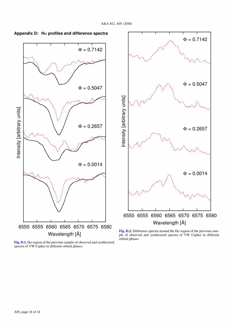
A sample of our observed and synthetic spectra is plotted inFig. 4, while a more detailed view of the Hα-region along withthe difference spectra is available in Appendix D (Figs. D.1 andD.2). We can see an obvious excess in the Hα line profile, whichstrongly suggests ongoing chromospheric activity. The excessbelongs mainly to the line component of the more massive pri-mary star, while there is no sign of clear emission in the linecomponent of the secondary star. This implies that the chromo-sphere of the primary star is much more active, consistent withour light curve models where we assumed that spots are locatedon the primary.

In Fig. 5, we plotted the determined EW values as a func-tion of the orbital phase. As can be seen, the values on the twoconsecutive nights in 2016 are almost the same; the small dif-ferences may be caused by continuum normalization effects (asnoted by Kaszás et al. 1998, 3% error in the continuum can resultin a 0.3 Å error in the EWs).

The light curves obtained in 2014 (Figs. 3, A.1 and A.2)and 2016 (Figs. A.3 and A.4) clearly show a smaller maximumbrightness at phase Φ = 0.25. Without spectroscopy, one wouldmost probably think that it is caused by a spot (or a group ofspots) on the surface of the primary component when it is mov-ing towards us, or on the secondary component when it is movingaway from us. Nevertheless, if we analyze the EWs versus orbital

Fig. 5. EWs of the Hα emission line profile measured on different nightsin the function of orbital phase. For determining the EW values, wesubtracted synthetic spectra from the observed ones at every epoch (seethe text for details).

Fig. 6. Residuals of light curves measured in 2016 compared to spotlesssynthetic light curves.

phase diagram (Fig. 5), we can see two peaks centered at thephases of Φ = 0.1 and Φ = 0.5. This implies that enhancedchromospheric activity is occurring at these two phases, so weshould expect spots there. Hence, we modeled the light curveswith two spots (on the regions of the primary that faces theobserver at Φ = 0.1 and Φ = 0.5 phase, respectively). A bet-ter fit was obtained using a two-spots configuration in all threefilter bands than in the case of a single spotted region placedat Φ = 0.25 (PHOEBE’s built-in cost function gives an approxi-mately two times higher value if we use one spot instead of two,

A91, page 5 of 14

A&A 612, A91 (2018)

keeping the same orbital configuration). We note that the single-spot fit can be improved by increasing the temperature differenceof the two stars up to 600 K; however, such a high value of ∆Tis unlikely in the case of a W UMa star, and the result of thefitting is still worse than assuming two spots. According to thebest-fit PHOEBE models, there is a larger spot at Φ = 0.5 phasewhen we see a higher peak on the EW-phase diagram (Fig. 5),and a smaller spot at Φ = 0.1 when we see a lower peak. Thisclearly shows that there is a correlation between spottedness andthe strength of the chromospheric activity. In order to visual-ize this correlation, we subtracted spotless synthetic light curvesfrom the observed light curves obtained in 2016 and plotted theresiduals in Fig. 6. One can see that the shape of Fig. 6 is verysimilar to Fig. 5.

As one can see in Figs. 3, A.1, A.2, A.3, and A.4, the modelspots we used are located at relatively high latitudes on the pri-mary component. Although, in general, latitudinal informationof spots cannot be reliably extracted from light-curve modeling(Lanza & Rodonó 1999), earlier studies concluded that high-latitude spots are expected on rapidly rotating stars (Schüssler& Solanki 1992; Schüssler et al. 1996; Holzwarth & Schüssler2003).

In our PHOEBE models, spots are situated mainly at twolongitudes separated by nearly 180 degrees in line with thecenter of the components, which is consistent with the modelof Holzwarth & Schüssler (2003). They showed that this isexpected in active close binaries, because the tidal forces canalter the surface distribution of erupting flux tubes and createspot clusters on the opposite sides of the active component. Suchactive longitudes were found in other close binaries by Oláh(2006).

This kind of longitudinal distribution of spots could alsobe the sign of the so-called flip-flop phenomenon, which isexplained as the combination of a nonaxisymmetric dynamomode with an oscillating axisymmetric mode in case of a starwith spherical shape (Elstner & Korhonen 2005). This phe-nomenon has been observed on numerous stars (mainly onFK Com and RS CVn systems, but also on the Sun and on youngsolar-like stars) that show two active longitudes on their oppo-site hemispheres with alternating spot activity level (e.g., Jetsuet al. 1993; Vida et al. 2010). In these cases, the observed vari-ations of the surface activity are somewhat periodic; flip cyclesare usually in the range of a few years to a decade. Activity cyclesof contact binaries have also been assumed previously, basedon the cyclic variations of minima seen on O–C diagrams, andon the seasonal variations of the light curves, especially of thedifferences of light-curve maxima within a cycle (Kaszás et al.1998; Borkovits et al. 2005). Recently, Jetsu et al. (2017) pre-sented a general model for the light curves of chromosphericallyactive binary stars. According to them, probably all such systemshave these two active longitudes with cyclic alternation in theiractivity (we note however, that they analyzed only RS CVn sys-tems). Our data cover a relatively short time and we can’t seeany large changes in the spot strengths. The only convincing evi-dence we found is shown in Fig. 1 of Kaszás et al. (1998), wherethe authors plotted the seasonal light curves of VW Cephei. Onecan see the relative changes in the photometric maxima on ascale of 3–4 years which could be explained by changes in thespot strengths. The only contact binary system with a detectedflip-flop phenomenon is HH UMa (based on the seasonal vari-ations of light curves, see Wang et al. 2015). Nevertheless, theobserved light-curve variations of HH UMa are very similar tothose that can be seen in the case of VW Cep (see in Fig. 1 ofKaszás et al. 1998). Thus, it could be argued that the presence of

Fig. 7. O–C diagram before (red diamonds) and after the subtraction ofthe visually observed LITE of the 3rd body. Cycle numbers are shownon the top horizontal axis.

Table 3. Times of primary and secondary minima obtained from ourphotometric data.

Date of observation Type of minimum MJDmin

08 August 2014 Primary 56 878.393508 August 2014 Secondary 56 878.534209 August 2014 Primary 56 879.506109 August 2014 Secondary 56 879.368510 August 2014 Primary 56 880.340810 August 2014 Secondary 56 880.482120 April 2016 Primary 57 499.582020 April 2016 Secondary 57 499.445121 April 2016 Primary 57 500.417221 April 2016 Secondary 57 500.5582

the flip-flop phenomenon is a viable hypothesis even in the casesof close binary stars.

4. O–C analysis

In order to analyze the periodic variations of VW Cep, weconstructed the O–C diagram of the system. For this purpose,we downloaded all the minima times from the O–C gatewaywebpage3 created by Anton Paschke and BC. Lubos Brát. Fur-thermore, we collected all other available data points from IBVS,BBSAG, BAA-VSS and BAV issues, and, finally, we added thelatest points from our measurements (see Table 3).

We only selected the most reliable measurements obtainedwith photoelectric and CCD devices. For the calculations, weused the reference epoch and period from the GCVS catalog(Kreiner & Winiarski 1981):

HJDmin = 2 444 157.4131 + 0.d27831460 × E.

The final diagram, which includes the times of both primaryand secondary minima, contains 1620 data points (Fig. 7).

The O–C diagram has a clearly visible negative parabolictrend shape. Kaszás et al. (1998) fitted the long-term perioddecrease with a parabolic function getting ∆P/P = −0.58×10−9.They assumed that this phenomenon is caused by a conservative

3 O–C gateway: http://var2.astro.cz/ocgate/

A91, page 6 of 14

T. Mitnyan et al.: The contact binary VW Cephei revisited

Fig. 8. Fitted quadratic (dashed blue curve) and cubic (dotted magentacurve) polynomial to the O–C diagram (top) and their residuals (bot-tom). Cycle numbers are shown on the top horizontal axis.

mass transfer from the primary (more massive) component tothe secondary one and determined a mass transfer rate of ∆M =1.4 × 10−7 M yr−1. They conclude that the large rate of perioddecrease and of the mass transfer indicate that this phenomenonshould be temporary. After the subtraction of the parabola, theresidual contains a periodic variation which was explained withthe presence of a light-time effect (LITE) by several authors (Hill1989; Kaszás et al. 1998; Pribulla et al. 2000; Zasche & Wolf2007). This LITE is probably caused by the third body orbit-ing around the center of mass of the VW Cep AB. Hershey(1975) confirmed the existence of this tertiary component, butthe observed amplitude of the LITE is larger than expected fromits orbital elements. After subtracting the effect of the third body,the residual shows additional periodic variations. Kaszás et al.(1998) proposed two possible explanations for this cyclic behav-ior: (i) perturbation of orbital elements induced by the tidalforce of the third body, and (ii) geometric distortions caused bymagnetic cycles (Applegate mechanism; Applegate 1992).

Regarding the significantly larger number of data points (col-lected in the last 20 years), we decided to re-analyze the rate ofperiod decrease. Furthermore, we propose new explanations forthe different cyclic variations. For these purposes, we removedthe LITE of the visually observed tertiary component as was alsodone in Kaszás et al. (1998); see Fig. 7.

As a first approach, the O–C diagram was fitted by aquadratic polynomial (Fig. 8). The residual shows periodic vari-ations, and, moreover, large deviations in the early years ofobservations (we note that it is difficult to estimate the uncertain-ties of these values), as well as near and after 20 000 cycles. Thenwe fitted the data with a cubic polynomial, which resulted in asmaller sum of squared residuals. The deviations decrease in theintervals mentioned before, which may suggest that the rate ofperiod decrease is changing in time. If we assume that the perioddecrease is due to mass transfer, then the period changes and themass-transfer rates can be calculated (see Table 4), which are ofthe same order as calculated by Kaszás et al. (1998). The cubic fityielded positive numbers both in the variation of period changeand of mass-transfer rate, which implies that the efficiency of themass transfer from the more-massive component is decreasing,in agreement with the previous expectations.

The fact that the higher-order polynomial has a better fit tothe O–C diagram could be the consequence of a periodic vari-ation, which is not covered yet due to its very long time-scale.To incorporate this assumption, we subtracted the LITE of the

Fig. 9. Fitted LITE of the hypothetical 4th body to the O–C diagramwithout the LITE of the known 3rd body (top) and the residual (bottom).Cycle numbers are shown on the top horizontal axis.

known third body, then we assumed that the long-term variationis caused by a hypothetical fourth body and fitted the residualdiagram with a LITE. The best-fit curve generated by using thenonlinear least-squares method can be seen in Fig. 9. The fittedparameters are listed in Table 5.

Defining m4 as the mass of the fourth body, the massfunction is

f (m4) =m3

4 sin i3

(mVW + m3 + m4)2 , (1)

where mVW and m3 are the mass of VW Cep AB and the knownthird body, respectively, and i is the inclination. The amplitudeof the O–C is:

AO−C =a1,2,3 sin i

c

√(1 − e2 cos2 ω), (2)

where a1,2,3 is the semi-major axis of the common center of massof VW Cep AB and the third body around the hypothetical fourthbody, c is the speed of light, e is the eccentricity, and ω is theargument of periapsis. Combining Eq. (1) and Kepler’s third law,the mass function of the fourth body can be also calculated as:

f (m4) = 3.99397 × 10−20a3

1,2,3 sin3 i

P2L

, (3)

where the semi-major axis is in km, the period is in days, andthe mass function yields the result in M. Calculated semi-majoraxes and masses of the fourth body (assuming different val-ues of inclination) can be found in Table 6. We used 1.47 M(this paper) and 0.74 M (Zasche 2008) for the total massof VW Cep AB and for the mass of the third component,respectively.

According to celestial mechanics (e.g., Reipurth & Mikkola2012), such a four-body system can only be stable if theouter periastron distance is at least 5–10 times larger than theinner apastron distance. The semi-major axis of the orbit ofVW Cep AB around the common center of mass is (647.76 ±29.92) × 106 km (Zasche & Wolf 2007). The semi-major axisof the third body, calculated from the mass ratio m3/mVW,is (1199.23 ± 55.39) × 106 km. The sum of the two values is(1846.99 ± 60) × 106 km. If we assume that the distance of thefourth body must be at least 7.5 times (average of the crite-rion given by Reipurth & Mikkola 2012) larger than the inner

A91, page 7 of 14

A&A 612, A91 (2018)

Table 4. O–C diagram: fitted (top four rows) and calculated (bottom four rows) parameters.

Quadratic fit Cubic fit

a0 – (−7.02± 0.50)× 10−3 (−9.64± 0.48)× 10−3

a1 – (−2.08± 0.02)× 10−6 (−2.38± 0.03)× 10−6

a2 – (−7.03± 0.05)× 10−11 (−6.43± 0.06)× 10−11

a3 – – (2.14± 0.14)× 10−16

Residual – 1.30× 10−1 1.03× 10−1

P day yr−1 (−1.85× 0.01) × 10−7 (−1.69× 0.02)× 10−7

M M yr−1 (−1.21× 0.05)× 10−7 (−1.11× 0.05)× 10−7

ddt P day yr−2 – (3.0× 0.2)× 10−12

ddt M M yr−2 – (2.0× 0.2)× 10−12

Notes. The a0, a1, a2 and a3 are the fitted constant, first-order, second-order and third-order coefficients, respectively. The residuals are the sum ofsquared residuals. P and M are the period variation and the mass-transfer rate, respectively, while d

dt P and ddt M are the temporal variation of the

previous parameters, respectively.

Table 5. Fitted parameters of the LITE of the hypothetical fourth body.

T0 MJD (2.42 ± 0.12)× 104

P yr 180.5 ± 2.0ω 0.0 ± 7.5e – 0.114 ± 0.005a sin i km (6482.26 ± 1.1e − 14) × 106

f (M4) Msun 2.50 ± 0.06AO−C d 0.24700 ± 0.00028

Table 6. Calculated orbital parameters, masses and proper motions ofthe hypothetical 4th body assuming different inclination angles.

i a1,2,3 a4 m4 µ() (106 km) (106 km) (M) (mas yr−1)

10 37 329.8 171.4 481.4 345.620 18 952.9 628.5 66.6 167.630 12 964.5 1201.0 23.9 111.540 10 084.6 1727.3 12.9 85.950 8462.0 2142.9 8.7 71.760 7485.1 2444.3 6.8 63.370 6898.3 2645.7 5.8 58.380 6582.3 2760.8 5.3 55.690 6482.3 2798.1 5.1 54.7

system’s periastron distance, then we get a1,2,3 ≥ (13 852.4 ±500) × 106 km. Considering the calculations in Table 6, we canput constraints on inclination, i . 30, which is in agreementwith the assumed inclination of the third body (33.6 ± 1.2;Zasche & Wolf 2007). Using this value, the mass of the fourthbody will be at least 23.9 M. A star with such a large massshould be detectable within the distance of VW Cep, so wenote that this object, if it exists, should be a black hole. Such amassive object was recently proposed as an explanation of theperiodic variation seen on the O–C diagram of an RR Lyraebinary candidate in Sódor et al. (2017).

The orbital speed of the common center of mass ofVW Cep AB and the third body around the center of mass ofthe four-body system is:

v =2πPL

a1,2,3 sin i√(1 − e2) sin i

√(1 + e2 + 2e cos ( f )), (4)

Table 7. Measured proper motion values from the literature.

µα µδ Ref.(mas yr−1) (mas yr−1) –

1241.4 ± 2.7 540.9 ± 0.6 van Leeuwen (2007)1306.5 ± 16.1 551.0 ± 4.3 Roeser & Bastian (1988)

where f is the true anomaly. The projection to the plane of thesky is:

vsky =

√v2 − v2

rad, (5)

where

vrad =2πPL

a1,2,3 sin i√

1 − e2

[cos ( f + ω) + e cos (ω)

], (6)

which is the radial velocity, from which the proper motion is:

µ[′′ yr−1] =vsky[km s−1]4.74 · d[pc]

. (7)

The parallax of the VW Cep AB system is 36.25 ± 0.58 mas(van Leeuwen 2007), which leads to a distance of 27.59+0.48

−0.21 pc.Proper motion values calculated with different inclinations arelisted in Table 6. In the literature, two measured proper motionscan be found (Table 7), which are of the same order as in ourcalculations assuming a low value of inclination. We checked theproper motion values of the nearby stars in order to investigateif such a large value is common in that field or not. We foundonly one object (LSPM J2040+7537) with a proper motion inthis order of magnitude. Unfortunately, we have not found anymeasured parallax in the literature, but the large angle distance(729.02′′) and the relatively low brightness (R = 15.2 mag) sug-gest that this star is at a large physical distance from VW Cep.Thus, the measured large proper motion values may be partiallyexplained by the presence of a fourth body.

According to previous papers, the gamma velocity ofVW Cephei is continuously changing in time; however, a sat-isfying explanation for this has yet to be found. Zasche (2008)tried to explain this variation based on the four available gammavelocities in the literature with two different models: (i) the pres-ence of a third and a fourth component in the system without

A91, page 8 of 14

T. Mitnyan et al.: The contact binary VW Cephei revisited

mass transfer between the primary and secondary, or (ii) thepresence of a third component in the system with mass trans-fer between the primary and secondary. He concluded that thefirst approach gives a better fit by 12%, but the fit is still notsatisfactory and although the assumed fourth component shouldbe detectable, a candidate has yet to be found. More precisedata and more sophisticated modeling methods are necessary tosolve this problem. However, our new value of vγ seems to be indisagreement with the predictions of Zasche (2008).

Kaszás et al. (1998) Fourier-analyzed the residual aftersubtracting both a parabolic term and a LITE component cor-responding to the orbital elements of the third body (Hershey1975). They found two significant peaks, one close to the orbitalperiod of the third body (1.29 × 10−4 day−1), and another one(3.59×10−4 day−1) that was linked to the magnetic activity cycle.We recalculated the Fourier spectrum using all published up-to-date data points, and the same fitting parameters as Kaszás et al.(1998) in order to check whether the mentioned peaks are stillvisible or not (Fig. 10; marked with an arrow). Additionally, wecalculated the Fourier spectrum after subtracting our quadraticand cubic terms as well as the effect of the third body. As onecan see, the shorter period has nearly the same amplitude andfrequency in all spectra except the cubic case, where the ampli-tude is smaller by a factor of 2. The peak in the Fourier spectrumof the data after the subtraction of LITE3 and LITE4 is presentwith nearly the same parameters as in the case of fitting a cubicfunction. Regarding the longer period, the amplitude of the cor-responding peak is larger, and, moreover, another peak appearswith a period of 73.52 yr in the longer dataset (Fig. 10b). Such aperiod caused by the LITE of another hypothetical fourth bodyhas also been proposed by Zasche (2008), but in the case ofour new quadratic fit, the peak has disappeared or been delayed,which means that this could be an artifact.

Applegate (1992) proposed a mechanism to explain theorbital period changes of eclipsing binaries. Due to the gravi-tational coupling, the variation of the angular momentum distri-bution can modify the orbital parameters (such as the semi-majoraxis, or the orbital period). The shape of the active compo-nent of the binary can be periodically distorted by its magneticcycle of a field of several kiloGauss. Such a process cannot beexcluded in the case of VW Cep because of the photosphericand chromospheric activity of the components observed in theX-ray range (Gondoin 2004; Huenemoerder et al. 2006; Sanz-Forcada et al. 2007). We calculated the value of the orbital periodmodulation (∆P), the angular momentum transfer (∆J) and thesubsurface magnetic field strength (B) required to establish theobserved period changes in the O–C diagram (Table 8) as follows(Applegate 1992):

∆PP

= 2πAO−C

Pmod(8)

∆J =GM2

R

( aR

)2 ∆P6π

(9)

B2 ∼ 10GM2

R4

( aR

)2 ∆PPmod

. (10)

We used the values of a = 1.412× 106 km (semi-major axis),P = 0.2783 d (orbital period), M1 = 1.13 M, M2 = 0.34 M(masses of the primary and the secondary components), R1 =0.99 R, R2 = 0.57 R (radii of the primary and secondary com-ponents), respectively. The AO−C values were calculated usingEq. (2) and taken from the Fourier-spectrum, respectively. Ascan be seen, the calculated subsurface magnetic field strength is

Fig. 10. Fourier spectra of the O–C diagrams. From top to bottom: (a)after the subtraction of the parabolic trend (following Kaszás et al. 1998)and the visually observed LITE of the third body using data pointsbefore MJD 50 000, (b) same as (a), but using the full dataset, (c) afterthe subtraction of our quadratic fit along with the LITE of the thirdbody, (d) after the subtraction of our cubic fit along with the LITE ofthe third body, (e) after the subtraction of the LITE of the third bodyand (f) after the subtraction of the LITE of the hypothetical fourth body.We highlight the different ranges of the vertical axes. The insert in thefifth panel shows the spectral window.

lower in the case of the shorter modulation. In Sect. 3, we showedthat the primary, more massive component is covered by coolspots, emerged as a result of the magnetic activity. If we assumethat the 7.62-year-long modulation in the Fourier spectrum islinked to the magnetic cycle of VW Cep, then the required sub-surface magnetic field strength for establishing the variation ishigher than 20 kG. If this field strength becomes lower even bytwo or three orders of magnitude at the surface, it should bedetectable with spectropolarimetric observations (see Donati &Landstreet 2009); however, the detection of strength and vari-ation of this magnetic field (via e.g., Zeeman effect) would bea challenging task due to the large rotational broadening ofspectral lines (approx. 3.3 Å at 5000 Å).

5. Summary

We obtained 69 new medium-resolution spectra of VW Cepheialong with two new light curves in April 2016, and along withthree additional light curves from two years earlier. We analyzedthe period variation and the apparent activity of the system.We modeled our new light curves and radial velocity curvesimultaneously using the PHOEBE code and also derived tennew times of minima, which were used to construct a new,extended O–C diagram of the system. We redetermined thephysical parameters of the system from our models, which are

A91, page 9 of 14

A&A 612, A91 (2018)

Table 8. Calculated angular momentum transfer (∆J) and the subsurface magnetic field strength (B) required to establish the observed periodchanges.

AO−C Pmod ∆P/P ∆P ∆J B Component(d) (yr) – (s cycle−1) (g cm2 s−1) (kG) –

0.247 180 2.36 × 10−5 0.57 6.26 × 1047 8.0 12.97 × 1047 12.6 2

0.004 7.62 9.04 × 10−6 0.22 2.39 × 1047 24.0 11.14 × 1047 37.8 2

consistent with those in Kaszás et al. (1998). All observed spec-tra were compared to synthetic spectra. We then measured theEWs of the Hα profile on every difference spectra. Accordingto the light curve and spectral models, it is confirmed that bothphotospheric and chromospheric activity are mostly occurringon the more massive primary component of the system. Basedon our PHOEBE models, the spot distribution seems to be sta-ble, and spots are located on the two opponent hemispheresof the primary in line with the center of both components.The spots also have different sizes or different temperatureswhich causes the O’Connell effect on the light curves. The EWsof the Hα line show enhanced chromospheric activity in twophases where the spots actually turn in our line of sight, whichmeans that there is a correlation between spottedness and thestrength of the chromospheric activity. We propose that this kindof spot distribution might be a consequence of the so-calledflip-flop phenomenon, which was recently detected in an othercontact binary, HH UMa by Wang et al. (2015). We note thatthe changes on the light curves of different seasons in Fig. 1of Kaszás et al. (1998) can also support this hypothesis. Nev-ertheless, more observations are still needed for confirmation,especially both photometric and spectroscopic measurementstaken simultaneously.

After subtracting the LITE of the previously known thirdcomponent from the O–C diagram, our period analysis showsthat the mass-transfer rate is decreasing, which means thatthis effect is expected to be temporary as was proposed ear-lier by Kaszás et al. (1998). In the Fourier spectrum ofthe O–C diagram, we found a significant peak at about 185years and also detected a peak at 7.62 years, which wasconnected to the magnetic activity cycling by Kaszás et al.(1998). We tested two previously suggested hypotheses toexplain these peaks: (i) the presence of an additional fourthcomponent in the system, and (ii) ongoing geometrical dis-tortions by magnetic cycle. The supporting fact of the formeris that a cubic polynomial fits the O–C diagram better thana quadratic one. This could indicate a longer periodic vari-ation that is not yet fully covered by the observations. Wetreated the long-term variation as LITE and assumed thatthis might be a consequence of the presence of a fourthbody, whose mass would be at least 23.9 M (assuming i .30). This scenario could also be a partial explanation ofthe large proper motion values of VW Cep. The other sce-nario we analyzed is that the period variation could be theconsequence of the Applegate-mechanism; from our calcula-tions, the necessary strength of the subsurface magnetic fieldrequired to maintain the observed period variation is higherthan 20 kG. Nevertheless, the available data suggest that masstransfer from the more massive primary to the less massive sec-ondary star (with a slowly decreasing mass-transfer rate) is the

most probable explanation for the observed period variation ofVW Cep.

Acknowledgements. We would like to thank our anonymous referee for his/hervaluable suggestions, which helped us to improve the paper. This project hasbeen supported by the Lendület grant LP2012-31 of the Hungarian Academyof Sciences and the Hungarian National Research, Development and InnovationOffice, NKFIH-OTKA K-113117 and K-115709 grants. K. Vida acknowledgesthe Hungarian National Research, Development and Innovation Office grantsOTKA K-109276, and supports through the Lendület-2012 Program (LP2012-31) of the Hungarian Academy of Sciences, and the ESA PECS ContractNo. 4000110889/14/NL/NDe. K. Vida is supported by the Bolyai János ResearchScholarship of the Hungarian Academy of Sciences.

ReferencesAnderson, L., Raff, M., & Shu, F. H. 1980, IAU Symp., 88, 485Applegate, J. H. 1992, ApJ, 385, 621Baliunas, S. L., Donahue, R. A., Soon, W. H. et al. 1995, ApJ, 438, 269Binnendijk, L. 1967, Publ. Dom. Astrophys. Obs., 13, 27Binnendijk, L. 1970, Vist. Astron., 12, 217Borkovits, T., Elkhateeb, M. M., Csizmadia, Sz. et al. 2005, A&A, 441, 1087Donati, J.-F., & Landstreet, J. D., 2009, ARA&A, 47, 333Eggleton, P. P., & Kiseleva-Eggleton, L. 2001, ApJ, 562, 1012Elstner, D., & Korhonen, H. 2005, AN, 326, 278Frasca, A., Sanfilippo, D., & Catalano, S. 1996, A&A, 313, 532Gondoin, P. 2004, A&A, 415, 1113Heckert, P. A., & Ordway, J. I. 1995, AJ, 109, 2169Hendry, P. D., & Mochnacki, S. W. 2000, ApJ, 531, 467Hershey, J. L. 1975, AJ, 80, 662Hill, G. 1989, A&A, 218, 141Holzwarth, V., & Schüssler, M. 2003, A&A, 405, 303Huenemoerder, D. P., Testa, P., & Buzasi, D. L. 2006, ApJ, 650, 1119Jetsu, L., Pelt, J, & Tuominen, I. 1993, A&A, 278, 449Jetsu, L., Henry, G. W., & Lehtinen, J. 2017, ApJ, 838, 122Kaszás, G., Vinkó, J., Szatmáry, K., et al. 1998, A&A, 331, 231Kreiner, J. M., & Winiarski, M. 1981, Acta Astron., 31, 351Kurucz, R. 1993, ATLAS9 Stellar Atmosphere Programs and 2 km/s Grid,

Kurucz CD-ROM No. 13 (Cambridge, MA: Smithsonian AstrophysicalObservatory)

Kwee, K. K. 1966, Bull. Astron. Inst. Netherlands, 18, 448Lanza, A. F., & Rodonó, M. 1999, in Solar and Stellar Activity: Similarities and

Differences, eds. C. J. Butler, & J. G. Doyle, ASP Conf. Ser., 158, 121Lenz, P., & Berger, M. 2005, Commun. Asteroseismol., 146, 53Lucy, L. B. 1967, Z. Astrophys., 65, 89Lucy, L. B. 1968, ApJ, 151, 1123Mullan, D. J. 1975, ApJ, 198, 563Oláh, K. 2006, Ap&SS, 304, 145Oláh, K., & Strassmeier, K. G. 2002, Astron. Nachr., 323, 361Popper, D. M. 1948, ApJ, 108, 490Pribulla, T., Chochol, D., Tremko, J., et al. 2000, CoSka, 30, 117Pribulla, T., & Rucinski, S. M. 2006, AJ, 131, 2986Prsa, A., & Zwitter, T. 2005, ApJ, 628, 426Pustylnik, I., & Sorgsepp, L. 1976, Acta Astron., 26, 319Reipurth, B., & Mikkola, S. 2012, Nature, 492, 221Roeser, S., & Bastian, U. 1988, A&AS, 74, 449Rucinski, S. M. 1969, Acta Astron., 19, 245Rucinski, S. M. 1973, Acta Astron., 23, 79

A91, page 10 of 14

T. Mitnyan et al.: The contact binary VW Cephei revisited

Rucinski, S. M. 1974, Acta Astron., 24, 119Rucinski, S. 2010, in International Conference on Binaries: In celebration of Ron

Webbink’s 65th Birthday, eds. V. Kalogera, & M. van der Sluys, AIP Conf.Proc., 1314, 29

Samus N. N., Kazarovets E. V., Durlevich O. V., Kireeva N. N., & PastukhovaE. N. 2017, Astron. Rep., 61, 80

Sanad, M. R., & Bobrowsky, M. 2014, New Astron., 29, 47Sanz-Forcada, J., Favata, F., & Micela, G. 2007, A&A, 466, 309Schilt, J. 1926, ApJ, 64, 221Schüssler, M., & Solanki, S. K. 1992, A&A, 264, L13Schüssler, M., Caligari, P., Ferriz-Mas, A., Solanki, S. K., & Stix, M. 1996,

A&A, 314, 503Soubiran, C., Jasniewicz, G., Chemin, L. et al. 2013, A&A. 552, A64

Sódor, Á., Skarka, M., Liska, J., & Bognár, Zs. 2017, MNRAS, 465,L1

van’t Veer, F. 1973, A&A, 26, 357van Leeuwen, F., 2007, A&A, 474, 653Vida, K., Oláh, K., Kovári, Zs. et al. 2010, Astron. Nachr., 331, 250Vida, K., Korhonen, H., Ilyin, I. V., Oláh, K., Andersen, M. I., & Hackman, T.

2015, A&A, 580, A64Wang, K., Zhang, X., Deng, L. et al. 2015, ApJ, 805, 22Wilson, O. C. 1978, ApJ, 226, 379Yamasaki, A. 1982, Ap&SS, 85, 43Zasche, P., & Wolf, M. 2007, Astron. Nachr., 328, 928Zasche P. 2008, Doctoral Thesis, Charles University in Prague

A91, page 11 of 14

A&A 612, A91 (2018)

Appendix A: Light curves and spot configurations

Fig. A.1. SDSS g′r′i′ light curves of VW Cephei on 9 August 2014along with the fitted PHOEBEmodels and the corresponding geometricalconfiguration and spot distribution in different orbital phases.

Fig. A.2. SDSS g′r′i′ light curves of VW Cephei on 10 August 2014along with the fitted PHOEBEmodels and the corresponding geometricalconfiguration and spot distribution in different orbital phases.

Fig. A.3. SDSS g′r′i′ light curves of VW Cephei on 20 April 2016along with the fitted PHOEBEmodels and the corresponding geometricalconfiguration and spot distribution in different orbital phases.

Fig. A.4. SDSS g′r′i′ light curves of VW Cephei on 21 April 2016along with the fitted PHOEBEmodels and the corresponding geometricalconfiguration and spot distribution in different orbital phases.

A91, page 12 of 14

T. Mitnyan et al.: The contact binary VW Cephei revisited

Appendix B: Checking the limitations of thecross-correlation technique

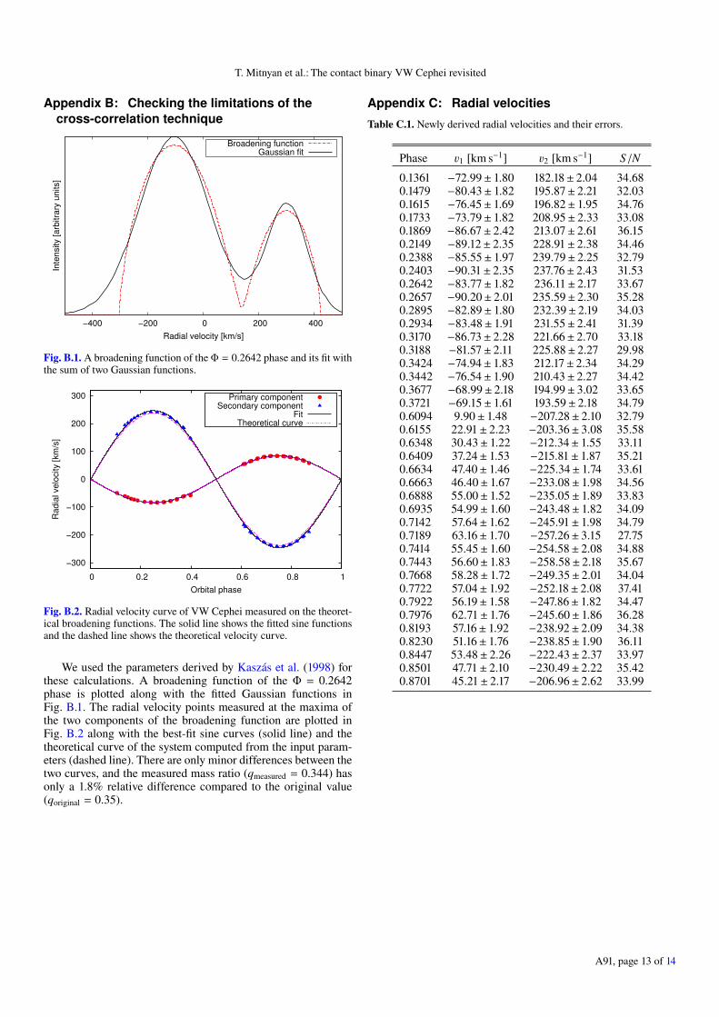
Fig. B.1. A broadening function of the Φ = 0.2642 phase and its fit withthe sum of two Gaussian functions.

Fig. B.2. Radial velocity curve of VW Cephei measured on the theoret-ical broadening functions. The solid line shows the fitted sine functionsand the dashed line shows the theoretical velocity curve.

We used the parameters derived by Kaszás et al. (1998) forthese calculations. A broadening function of the Φ = 0.2642phase is plotted along with the fitted Gaussian functions inFig. B.1. The radial velocity points measured at the maxima ofthe two components of the broadening function are plotted inFig. B.2 along with the best-fit sine curves (solid line) and thetheoretical curve of the system computed from the input param-eters (dashed line). There are only minor differences between thetwo curves, and the measured mass ratio (qmeasured = 0.344) hasonly a 1.8% relative difference compared to the original value(qoriginal = 0.35).

Appendix C: Radial velocities

Table C.1. Newly derived radial velocities and their errors.

Phase v1 [km s−1] v2 [km s−1] S/N

0.1361 −72.99± 1.80 182.18± 2.04 34.680.1479 −80.43± 1.82 195.87± 2.21 32.030.1615 −76.45± 1.69 196.82± 1.95 34.760.1733 −73.79± 1.82 208.95± 2.33 33.080.1869 −86.67± 2.42 213.07± 2.61 36.150.2149 −89.12± 2.35 228.91± 2.38 34.460.2388 −85.55± 1.97 239.79± 2.25 32.790.2403 −90.31± 2.35 237.76± 2.43 31.530.2642 −83.77± 1.82 236.11± 2.17 33.670.2657 −90.20± 2.01 235.59± 2.30 35.280.2895 −82.89± 1.80 232.39± 2.19 34.030.2934 −83.48± 1.91 231.55± 2.41 31.390.3170 −86.73± 2.28 221.66± 2.70 33.180.3188 −81.57± 2.11 225.88± 2.27 29.980.3424 −74.94± 1.83 212.17± 2.34 34.290.3442 −76.54± 1.90 210.43± 2.27 34.420.3677 −68.99± 2.18 194.99± 3.02 33.650.3721 −69.15± 1.61 193.59± 2.18 34.790.6094 9.90± 1.48 −207.28± 2.10 32.790.6155 22.91± 2.23 −203.36± 3.08 35.580.6348 30.43± 1.22 −212.34± 1.55 33.110.6409 37.24± 1.53 −215.81± 1.87 35.210.6634 47.40± 1.46 −225.34± 1.74 33.610.6663 46.40± 1.67 −233.08± 1.98 34.560.6888 55.00± 1.52 −235.05± 1.89 33.830.6935 54.99± 1.60 −243.48± 1.82 34.090.7142 57.64± 1.62 −245.91± 1.98 34.790.7189 63.16± 1.70 −257.26± 3.15 27.750.7414 55.45± 1.60 −254.58± 2.08 34.880.7443 56.60± 1.83 −258.58± 2.18 35.670.7668 58.28± 1.72 −249.35± 2.01 34.040.7722 57.04± 1.92 −252.18± 2.08 37.410.7922 56.19± 1.58 −247.86± 1.82 34.470.7976 62.71± 1.76 −245.60± 1.86 36.280.8193 57.16± 1.92 −238.92± 2.09 34.380.8230 51.16± 1.76 −238.85± 1.90 36.110.8447 53.48± 2.26 −222.43± 2.37 33.970.8501 47.71± 2.10 −230.49± 2.22 35.420.8701 45.21± 2.17 −206.96± 2.62 33.99

A91, page 13 of 14

A&A 612, A91 (2018)

Appendix D: Hα profiles and difference spectra

Fig. D.1. Hα region of the previous sample of observed and synthesizedspectra of VW Cephei in different orbital phases.

Fig. D.2. Difference spectra around the Hα region of the previous sam-ple of observed and synthesized spectra of VW Cephei in differentorbital phases.

A91, page 14 of 14