The Complexity of Derivations of Matrix Identities by Michael ...
166
The Complexity of Derivations of Matrix Identities by Michael Soltys-Kulinicz A thesis submitted in conformity with the requirements for the degree of Doctor of Philosophy Graduate Department of Mathematics University of Toronto Copyright c 2001 by Michael Soltys-Kulinicz
-
Upload
khangminh22 -
Category
Documents
-
view
4 -
download
0
Transcript of The Complexity of Derivations of Matrix Identities by Michael ...

The Complexity of Derivations of Matrix Identities
by
Michael Soltys-Kulinicz
A thesis submitted in conformity with the requirementsfor the degree of Doctor of PhilosophyGraduate Department of Mathematics
University of Toronto
Copyright c! 2001 by Michael Soltys-Kulinicz

Abstract
The Complexity of Derivations of Matrix Identities
Michael Soltys-Kulinicz
Doctor of Philosophy
Graduate Department of Mathematics
University of Toronto
2001
In this thesis we are concerned with building logical foundations for Linear Algebra,
from the perspective of proof complexity. As the cornerstone of our logical theories,
we use Berkowitz’s parallel algorithm for computing the coe!cients of the characteristic
polynomial of a matrix.
Standard Linear Algebra textbooks use Gaussian Elimination as the main algorithm,
but they invariably use the (very infeasible) Lagrange expansion to prove properties of
this algorithm.
The main contribution of this thesis is a (first) feasible proof of the Cayley-Hamilton
Theorem, and related principles of Linear Algebra (namely, the axiomatic definition of the
determinant, the cofactor expansion formula, and multiplicativity of the determinant).
Furthermore, we show that these principles are equivalent, and the equivalence can be
proven feasibly.
We also show that a large class of matrix identities, such as:
AB = I " BA = I
proposed by S.A. Cook as a candidate for separating Frege and Extended Frege proposi-
tional proof systems, all have feasible proofs, and hence polynomially-bounded Extended
Frege proofs. We introduce the notion of completeness for these matrix identities.
As the main tool to prove our results, we design three logical theories:
LA # LAP # $LAP
ii

LA is a three-sorted quantifier-free theory of Linear Algebra. The three sorts are indices,
field elements and matrices. This is a simple theory that allows us to formalize and
prove all the basic properties of matrices (roughly the properties that state that the set
of matrices is a ring). The theorems of LA have polynomially-bounded Frege proofs.
We extend LA to LAP by adding a new function, P, which is intended to denote matrix
powering, i.e., P(n, A) means An. LAP is well suited for formalizing Berkowitz’s algorithm,
and it is strong enough to prove the equivalence of some fundamental principles of Linear
Algebra. The theorems of LAP translate into quasi-polynomially-bounded Frege proofs.
We finally extend LAP to $LAP by allowing induction on formulas with $ matrix
quantifiers. This new theory is strong enough to prove the Cayley-Hamilton Theorem,
and hence (by our equivalence) all the major principles of Linear Algebra. The theorems
of $LAP translate into polynomially-bounded Extended Frege proofs.
iii

Acknowledgements
First and foremost, I would like to thank my supervisor, Stephen Cook. It is thanks to
his dedication, his patience, and our weekly meetings that this thesis has been written.
It is not possible to have a better advisor.
I want to thank the other members of my PhD committee: Toniann Pitassi, Charles
Racko", and especially Alasdair Urquhart, for their help and encouragement. Samuel
Buss, the external examiner, gave me a lot of very good comments and suggestions.
I am grateful to Zbigniew Stachniak who first told me about Complexity Theory and
Logic.
I was lucky to be part of a fantastic group of graduate students: Joshua Buresh-
Oppenheim, Valentine Kabanets, Antonina Kolokolova, Tsuyoshi Morioka, Steve Myers,
Francois Pitt, Eric Ruppert, Alan Skelley, and others. I found our theory students
seminars extremely helpful.
Finally, I want to thank my parents for their support over the years.
iv

Contents
1 Introduction 1
1.1 Motivation . . . . . . . . . . . . . . . . . . . . . . . . . . . . . . . . . . . 4
1.2 Contributions . . . . . . . . . . . . . . . . . . . . . . . . . . . . . . . . . 5
1.3 Summary of results . . . . . . . . . . . . . . . . . . . . . . . . . . . . . . 11
2 The Theory LA 13
2.1 Language . . . . . . . . . . . . . . . . . . . . . . . . . . . . . . . . . . . 13
2.2 Terms, formulas and sequents . . . . . . . . . . . . . . . . . . . . . . . . 16
2.2.1 Inductive definition of terms and formulas . . . . . . . . . . . . . 16
2.2.2 Definition of sequents . . . . . . . . . . . . . . . . . . . . . . . . . 17
2.2.3 Defined terms, formulas and cedents . . . . . . . . . . . . . . . . 18
2.2.4 Substitution . . . . . . . . . . . . . . . . . . . . . . . . . . . . . . 20
2.2.5 Standard models . . . . . . . . . . . . . . . . . . . . . . . . . . . 21
2.3 Axioms . . . . . . . . . . . . . . . . . . . . . . . . . . . . . . . . . . . . . 23
2.3.1 Equality Axioms . . . . . . . . . . . . . . . . . . . . . . . . . . . 23
2.3.2 Axioms for indices . . . . . . . . . . . . . . . . . . . . . . . . . . 24
2.3.3 Axioms for field elements . . . . . . . . . . . . . . . . . . . . . . . 25
2.3.4 Axioms for matrices . . . . . . . . . . . . . . . . . . . . . . . . . 25
2.4 Rules of inference and proof systems . . . . . . . . . . . . . . . . . . . . 27
3 The Theorems of LA 31
3.1 LA proofs of basic matrix identities . . . . . . . . . . . . . . . . . . . . . 31
3.1.1 Ring properties . . . . . . . . . . . . . . . . . . . . . . . . . . . . 32
3.1.2 Module properties . . . . . . . . . . . . . . . . . . . . . . . . . . . 39
3.1.3 Inner product . . . . . . . . . . . . . . . . . . . . . . . . . . . . . 40
3.1.4 Miscellaneous theorems . . . . . . . . . . . . . . . . . . . . . . . . 40
v

3.2 Hard matrix identities . . . . . . . . . . . . . . . . . . . . . . . . . . . . 40
4 LA with Matrix Powering 44
4.1 The theory LAP . . . . . . . . . . . . . . . . . . . . . . . . . . . . . . . . 44
4.1.1 Language . . . . . . . . . . . . . . . . . . . . . . . . . . . . . . . 44
4.1.2 Terms and formulas . . . . . . . . . . . . . . . . . . . . . . . . . . 45
4.1.3 Axioms . . . . . . . . . . . . . . . . . . . . . . . . . . . . . . . . 45
4.2 Berkowitz’s algorithm . . . . . . . . . . . . . . . . . . . . . . . . . . . . . 46
4.2.1 Samuelson’s identity . . . . . . . . . . . . . . . . . . . . . . . . . 47
4.2.2 Expressing the char poly as a product of matrices . . . . . . . . . 49
4.2.3 Expressing the char poly in LAP . . . . . . . . . . . . . . . . . . . 52
4.2.4 Expressing adj and det in LAP . . . . . . . . . . . . . . . . . . . . 54
4.3 Berkowitz’s algorithm and clow sequences . . . . . . . . . . . . . . . . . 55
5 The Characteristic Polynomial 62
5.1 Basic properties . . . . . . . . . . . . . . . . . . . . . . . . . . . . . . . . 63
5.2 Triangular matrices . . . . . . . . . . . . . . . . . . . . . . . . . . . . . . 66
5.3 Hard matrix identities . . . . . . . . . . . . . . . . . . . . . . . . . . . . 69
6 Equivalences in LAP 71
6.1 The axiomatic definition of determinant . . . . . . . . . . . . . . . . . . 72
6.2 The cofactor expansion . . . . . . . . . . . . . . . . . . . . . . . . . . . . 80
6.3 The adjoint as a matrix of cofactors . . . . . . . . . . . . . . . . . . . . . 81
6.4 The multiplicativity of the determinant . . . . . . . . . . . . . . . . . . . 83
7 Translations 90
7.1 The propositional proof system PK[a] . . . . . . . . . . . . . . . . . . . . 91
7.2 Translating theorems of LA over Z2 . . . . . . . . . . . . . . . . . . . . . 93
7.2.1 Preliminaries . . . . . . . . . . . . . . . . . . . . . . . . . . . . . 94
7.2.2 Procedure for the translation . . . . . . . . . . . . . . . . . . . . 94
7.2.3 Correctness of the procedure . . . . . . . . . . . . . . . . . . . . . 98
7.3 Translating theorems of LA over Zp and Q . . . . . . . . . . . . . . . . . 111
7.4 Translating theorems of LAP . . . . . . . . . . . . . . . . . . . . . . . . . 112
vi

8 Proofs of the C-H Theorem 115
8.1 Traditional proofs of the C-H Theorem . . . . . . . . . . . . . . . . . . . 116
8.1.1 Infeasible proof of the C-H Theorem (I) . . . . . . . . . . . . . . . 116
8.1.2 Infeasible proof of the C-H Theorem (II) . . . . . . . . . . . . . . 117
8.2 Feasible proofs of the C-H Theorem . . . . . . . . . . . . . . . . . . . . . 118
8.2.1 LAP augmented by #M1 -Induction: $LAP . . . . . . . . . . . . . . 119
8.2.2 The theory V1($, P) . . . . . . . . . . . . . . . . . . . . . . . . . 125
8.2.3 Interpreting $LAP in V1($, P) . . . . . . . . . . . . . . . . . . . . 128
8.2.4 Summary of the feasible proof of the C-H Theorem . . . . . . . . 132
8.2.5 Permutation Frege . . . . . . . . . . . . . . . . . . . . . . . . . . 133
8.2.6 Quantified Frege . . . . . . . . . . . . . . . . . . . . . . . . . . . 134
8.3 E!cient Extended Frege proofs . . . . . . . . . . . . . . . . . . . . . . . 135
8.3.1 Gaussian Elimination algorithm . . . . . . . . . . . . . . . . . . . 136
8.3.2 Extended Frege proof of det(A) = 0 " AB %= I . . . . . . . . . . 138
8.3.3 Extended Frege proof of AB = I " BA = I . . . . . . . . . . . . 139
9 Eight Open Problems 141
9.1 Can LA prove AB = I " BA = I ? . . . . . . . . . . . . . . . . . . . . . 141
9.2 Is AB = I " BA = I complete ? . . . . . . . . . . . . . . . . . . . . . . 143
9.3 Does AB = I " BA = I have NC2-Frege proofs ? . . . . . . . . . . . . . 144
9.4 Can LAP prove det(A) = 0 " AB %= I ? . . . . . . . . . . . . . . . . . . 144
9.5 Can LAP prove the C-H Theorem ? . . . . . . . . . . . . . . . . . . . . . 144
9.6 Feasible proofs based on Gaussian Elimination ? . . . . . . . . . . . . . . 145
9.7 How strong is Permutation Frege ? . . . . . . . . . . . . . . . . . . . . . 145
9.8 Does $LAP capture polytime reasoning ? . . . . . . . . . . . . . . . . . . 146
Bibliography 149
Index 153
vii

List of Tables
1.1 Propositional proof systems . . . . . . . . . . . . . . . . . . . . . . . . . 3
1.2 Summary of theories . . . . . . . . . . . . . . . . . . . . . . . . . . . . . 11
1.3 Summary of translations . . . . . . . . . . . . . . . . . . . . . . . . . . . 12
1.4 Summary of conjectures . . . . . . . . . . . . . . . . . . . . . . . . . . . 12
2.1 Function and predicate symbols in LLA . . . . . . . . . . . . . . . . . . . 14
2.2 Equality axioms . . . . . . . . . . . . . . . . . . . . . . . . . . . . . . . . 23
2.3 Axioms for indices . . . . . . . . . . . . . . . . . . . . . . . . . . . . . . 24
2.4 Axioms for field elements . . . . . . . . . . . . . . . . . . . . . . . . . . . 25
2.5 Axioms for matrices . . . . . . . . . . . . . . . . . . . . . . . . . . . . . 26
2.6 Weak structural rules . . . . . . . . . . . . . . . . . . . . . . . . . . . . . 27
2.7 Cut rule . . . . . . . . . . . . . . . . . . . . . . . . . . . . . . . . . . . . 27
2.8 Rules for introducing connectives . . . . . . . . . . . . . . . . . . . . . . 28
2.9 Induction Rule . . . . . . . . . . . . . . . . . . . . . . . . . . . . . . . . 28
2.10 Equality Rules . . . . . . . . . . . . . . . . . . . . . . . . . . . . . . . . 28
2.11 The derived Substitution Rule . . . . . . . . . . . . . . . . . . . . . . . . 29
4.1 Axioms for P . . . . . . . . . . . . . . . . . . . . . . . . . . . . . . . . . 45
6.1 Flowchart for Chapter 6 . . . . . . . . . . . . . . . . . . . . . . . . . . . 71
7.1 Axioms for MODa,i . . . . . . . . . . . . . . . . . . . . . . . . . . . . . . . 91
8.1 $-introduction in LK-$LAP . . . . . . . . . . . . . . . . . . . . . . . . . 120
8.2 The axioms of V1 . . . . . . . . . . . . . . . . . . . . . . . . . . . . . . . 127
8.3 Permutation rule . . . . . . . . . . . . . . . . . . . . . . . . . . . . . . . 133
8.4 $-introduction . . . . . . . . . . . . . . . . . . . . . . . . . . . . . . . . . 134
8.5 &-introduction . . . . . . . . . . . . . . . . . . . . . . . . . . . . . . . . . 134
viii

List of Figures
1.1 Proving claims by induction on submatrices . . . . . . . . . . . . . . . . 9
4.1 ajj, Rj, Sj, Mj . . . . . . . . . . . . . . . . . . . . . . . . . . . . . . . . . 50
4.2 G! . . . . . . . . . . . . . . . . . . . . . . . . . . . . . . . . . . . . . . . 56
4.3 Clow C . . . . . . . . . . . . . . . . . . . . . . . . . . . . . . . . . . . . 57
4.4 Clows on A and M = A[1|1] . . . . . . . . . . . . . . . . . . . . . . . . . 60
4.5 Clows of length one on all three vertices . . . . . . . . . . . . . . . . . . 60
4.6 The single clow of length two on vertices 2 and 3 . . . . . . . . . . . . . 60
4.7 Clows of length two with a self loop at vertex 1 . . . . . . . . . . . . . . 61
4.8 Clows of length two without a self loop at vertex 1 . . . . . . . . . . . . . 61
6.1 Matrix A: pMi+1(Mi+1) = 0 =' p(IiAIi) = pA . . . . . . . . . . . . . . . . 78
6.2 {Mi+1, . . . , Mj} and {M !j"1, . . . , M
!i+1} . . . . . . . . . . . . . . . . . . . 78
6.3 Example of p(I13AI13) = pA . . . . . . . . . . . . . . . . . . . . . . . . . . 79
6.4 Showing that adj(A)[1|1] = (1 + a11)adj(M)( adj(SR + M) . . . . . . . 89
8.1 Shaded area of pA(A) is zero . . . . . . . . . . . . . . . . . . . . . . . . . 122
8.2 If A is 4) 3, then |XA| = 12 . . . . . . . . . . . . . . . . . . . . . . . . . 131
ix

Chapter 1
Introduction
Proof Theory is the area of mathematics which studies the concepts of mathematical proof
and mathematical provability ([Bus98]). Proof Complexity is an area of mathematics and
theoretical computer science that studies the length of proofs in propositional logic. It
is an area of study that is fundamentally connected both to major open questions of
computational complexity theory and practical properties of automated theorem provers
([BP98]).
A propositional formula ! is a tautology if ! is true under all truth value assignments.
For example, ! given by:
p * ¬p
is a tautology. Let TAUT be the set of all tautologies. A propositional proof system is a
polytime predicate P + $# ) TAUT such that:
! , TAUT -' &xP (x,!)
P is poly-bounded (i.e., polynomially bounded) if there exists a polynomial p such that:
! , TAUT -' &x(|x| . p(|!|) / P (x,!))
The existence of a poly-bounded proof system is related to the fundamental question:
P?= NP
In 1979 Cook and Reckhow ([CR79]) proved that NP = co-NP i" there is a poly-bounded
proof system for tautologies. On the other hand, if P = NP then NP = co-NP. Thus, if
there is no poly-bounded proof system, then NP %= co-NP, and that in turn would imply
that P %= NP.
1

Chapter 1. Introduction 2
There is a one million $ cash prize o"ered by the Clay Mathematical Institute for set-
tling the P?= NP problem; see the Millennium Prize Problems on the web site of the CMI
at www.claymath.org/index.htm. Also see [Coo00b], a manuscript prepared by Cook for
the CLI for the Millennium Prize Problems, available at www.cs.toronto.edu/~sacook.
Thus, considerable e"ort goes into proving lower bounds (and separations) for propo-
sitional proof systems. The program is to show lower bounds for standard proof systems
of increasing complexity.
But the P?= NP problem is not the only motivation for finding lower bounds for
Propositional Proof Systems (PPS):
• PPS are (mathematically) interesting in their own right.
• Applications to Automated Reasoning (Artificial Intelligence).
• We can use lower bounds for PPS, to prove lower bounds for decision procedures
(for SAT). A good example of this is the exponential lower bound for resolution,
which gives us an exponential lower bound for the Davis-Putnam procedure for
satisfiability. The idea behind the correspondence is very simple: each instance of
the Davis-Putnam procedure on a particular set of clauses can be viewed (“upside
down”) as a resolution refutation. Thus, if all resolution refutations on a family
of clauses must be of a certain size, so must be all instances of the Davis-Putnam
procedure on that family of clauses. (See [BP96] for the resolution lower bound).
See Figure 1.1 for a table of the principal propositional proof systems. Exponential
lower bounds exist for the proof systems below the line. The strongest propositional proof
system (Quantified Frege) is shown in the top, and the weakest (Truth Tables) is shown
in the bottom. Each system can simulate the one below. The systems Frege and PK are
equivalent in the sense that they p-simulate each other (see below for p-simulation).
In this thesis we are concerned with all four types of Frege proof systems. There
is a separation between Bounded Depth Frege and Frege, and there exist lower bounds
for Bounded Depth Frege, but no such results exist for the remaining Frege systems.
By a separation we mean that there exists a family of tautologies "n, such that Frege
proves "n e!ciently (i.e., in polysize), but Bounded Depth Frege does not (i.e., there is no
polynomial p(n) such that Bounded Depth Frege can prove "n with derivations of length
at most p(n)). The Pigeonhole Principle (PHP) is the standard tautology for separating
Bounded Depth Frege and Frege (see [Pit92], [BIP93] and [BIK+92]).

Chapter 1. Introduction 3
Quantified Frege
Extended Frege, Substitution Frege, Renaming Frege
Permutation Frege
Frege, PK
Bounded Depth (BD) Frege
Resolution
Truth Tables
Table 1.1: Propositional proof systems
Note that even though we mention Frege, in practice in this thesis we use the sequent
calculus proof system PK. Thus we have Bounded Depth PK, PK, Extended PK, and
Quantified PK. It is easy to show that Frege and PK p-simulate each other, and hence
they can be used interchangeably.
The (alleged) separation between Frege and Extended Frege is a fundamental open
problem. The matrix identity AB = I " BA = I was originally proposed by Cook in the
context of separating Frege and Extended Frege (private communication; in [BBP94] the
authors give examples of tautology families, such as the “Odd Town Theorem”, that seem
to depend on linear algebra for their proofs, and it was this paper that inspired Cook to
think of AB = I " BA = I). The separation between Extended Frege and Quantified
Frege (again, if there is one), seems to be completely out of reach at the moment.
A fundamental notion that appears throughout this thesis is that of a feasible proof
(and feasible computation, or polytime computation). Feasible proofs were introduced by
Cook in [Coo75], and they formalize the idea of tractable reasoning; a theorem can be
proven feasibly, if all the computations involved in the proof are polytime computations,
and the induction can be unwound feasibly.
Cook’s system PV is the original system for polytime reasoning (see [CU93]). Samuel
R. Buss formalized polytime reasoning with the system S12 in [Bus86]. The importance
of the Extended Frege propositional proof system stems from the fact that first order
theorems which have feasible proofs correspond to propositional tautologies which have
uniform polysize Extended Frege proofs.
Another fundamental notion throughout this thesis is that of a p-simulation. We say
that a proof system P p-simulates a proof system P ! if there exists a function f and
a polynomial p such that every proof x in P ! corresponds to a proof f(x) in P , and

Chapter 1. Introduction 4
|f(x)| . p(|x|). In other words, all the proofs of P ! can be “reproduced” in P with a
small increase in size. Thus, coming back to the separations discussed above, for example,
Frege p-simulates Bounded Depth Frege, but Bounded Depth Frege does not p-simulate
Frege. It is not known if Frege can p-simulate Extended Frege.
1.1 Motivation
The motivation for the research presented in this thesis is establishing the complexity
of the concepts involved in proving standard theorems in Linear Algebra. We want to
understand where do standard theorems of Linear Algebra stand with respect to the Frege
proof systems (Bounded Depth Frege, Frege, Extended Frege, and Quantified Frege). In
particular, we are interested in the complexity of the proofs of the following principles:
• Standard theorems of Linear Algebra, such as the Cayley-Hamilton Theorem, the
axiomatic definition of the determinant, the cofactor expansion formula, and the
multiplicativity of the determinant.
• Universal matrix identities such as AB = I " BA = I.
Thus, we are concerned with building logical foundations for Matrix Algebra, from
the perspective of the complexity of the computations involved in the proofs. We use
Berkowitz’s parallel algorithm as the main tool for computations, and most results are
related to proving properties of this algorithm. Berkowitz’s algorithm computes the
coe!cients of the characteristic polynomial of a matrix, by computing iterated matrix
products.
Standard Linear Algebra textbooks use Gaussian Elimination as the main algorithm,
but they invariably use the (very infeasible) Lagrange expansion to prove properties of
the determinant. Berkowitz’s algorithm is a fast parallel algorithm, Gaussian Elimination
is poly-time, and the Lagrange expansion is n! (where the parameter for all three is the
size of the matrix).
We have chosen Berkowitz’s algorithm as the cornerstone of our theory of Linear
Algebra because it is the fastest known algorithm for computing inverses of matrices,
and it has the property of being field independent (and hence all the results of this thesis
are field independent). Furthermore, we show that we can feasibly prove properties of
the determinant using Berkowitz’s algorithm, while we do not know how to prove them

Chapter 1. Introduction 5
feasibly using Gaussian Elimination, or any other algorithm (granted that for this thesis,
we did concentrate our research on Berkowitz’s algorithm).
In order to carry out our proofs based on Berkowitz’s algorithm, we developed a new
approach to proving matrix identities by induction on the size of matrices.
1.2 Contributions
In Section 8.2 we present the main contribution of this thesis: a feasible proof of the
Cayley-Hamilton Theorem. It seems that we give the first such proof1; in fact we present
three feasible proofs. The first is based on interpreting the $LAP proof of the C-H
Theorem in the polytime theory in V1($, P), Section 8.2.3. This proof relies on results
spread throughout the thesis, so we summarize it in Section 8.2.4. The second proof
is based on interpreting the $LAP proof of the C-H Theorem in poly-bounded uniform
Permutation Frege (a propositional proof system), Section 8.2.5. The $LAP proof itself
is given in Section 8.2.1. The third proof is based on Quantified Frege, Section 8.2.6.
Note that many of the proofs given in this thesis are substantially more di!cult than
the corresponding proofs in an average Linear Algebra text book. An extreme example
of this is the proof of multiplicativity of the determinant. In [DF91, page 364] the
proof of the multiplicativity of the determinant takes one line; this proof relies on the
Lagrange Expansion of the determinant. Our proof of multiplicativity of the determinant
from the Cayley-Hamilton Theorem takes over six pages (see Section 6.4). The proof
of the Cayley-Hamilton Theorem takes several sections spread throughout the thesis.
However, our proofs are feasible; we can prove the propositional tautologies asserting
the multiplicativity of the determinant, with Extended Frege, for matrices which have
106 ) 106 entries. With the Lagrange Expansion which has n! terms (n is the size of the
matrices involved), it is impossible to prove multiplicativity for matrices of size 20) 20
(using Extended Frege).
In Chapter 6 we show that the C-H Theorem is equivalent to the axiomatic definition
of the determinant, and to the cofactor expansion, and that these equivalences can be
shown in the theory LAP. The theory LAP formalizes reasoning in POW (the class of
problems “easily” reducible to powers of matrices). In Section 6.4 we show that the
multiplicativity of determinant implies (also in LAP) the C-H Theorem, and we show
1In Section 8.1 we present, briefly, two typical infeasible proofs of the C-H Theorem.

Chapter 1. Introduction 6
that the C-H implies (feasibly, but we do not know if in LAP) the multiplicativity of the
determinant. The conclusion is that all these major principles of Linear Algebra have
feasible proofs.
In Section 5.3 we show that AB = I " BA = I, and hence (by the results in Sec-
tion 3.2) many matrix identities, follows, in LAP, from the Cayley-Hamilton Theorem.
Since we give a feasible proof of the C-H Theorem, it follows that these identities also
have feasible proofs.
We compute the determinant of a matrix with Berkowitz’s algorithm. Since the
Cayley-Hamilton Theorem states that the characteristic polynomial of a matrix is an
annihilating polynomial (i.e. pA(A) = 0), the Cayley-Hamilton Theorem implies the
following:
det(A) %= 0 =' A is invertible
On the other hand, we also give a feasible proof (based on Gaussian Elimination, but
still for the determinant as defined by Berkowitz’s algorithm) that:
det(A) = 0 =' A is not invertible
Therefore, we give a feasible proof of the fact that a matrix is invertible i" its determinant
is not zero.
We define the correctness of Berkowitz’s algorithm to be the following property: it
computes an annihilating polynomial of the given matrix. Thus, we can look at the
central result of this thesis as being a feasible proof of the correctness of Berkowitz’s
algorithm; the feasible proof of Berkowitz’s algorithm is the mechanism that makes a
feasible proof of the Cayley-Hamilton Theorem possible.
In Chapter 2 we design a three-sorted quantifier-free theory of Linear Algebra, and
we call it LA. The three sorts are indices, field elements and matrices. LA is field
independent, and matrix identities can be expressed very naturally in its language.
LA is a fairly weak theory, which nevertheless allows us to prove all the basic properties
of matrices (roughly the properties that state that the set of matrices is a ring). We
show this in Chapter 3, where we prove, in LA, properties such as the associativity
of matrix multiplication, A(BC) = (AB)C, or the commutativity of matrix addition,
A + B = B + A, i.e., the ring properties of the set of matrices.
In Chapter 7 we show that all the theorems of LA can be translated into poly-
bounded families of propositional tautologies, with poly-bounded Frege proofs. Thus,
LA is strong enough to prove basic properties of matrices, but at the same time the

Chapter 1. Introduction 7
truth of any theorem of LA can be verified with poly-bounded Frege. In fact, we prove
a tighter result since we show that bounded-depth Frege proofs with MOD p gates su!ce,
when the underlying field is Zp.
We identify two classes of matrix identities: basic and hard. The basic matrix iden-
tities are those which can be proven in LA, and, as was mentioned above, they roughly
correspond to the ring properties of the set of matrices. Hard matrix identities, intro-
duced in Section 3.2, are those which seem to require computing matrix inverses in their
derivations; the prototypical example of a hard matrix identity is AB = I " BA = I,
suggested by Cook in the context of separating Frege and Extended Frege. Hard matrix
identities are more di!cult to define, and their definition is related to the definition of
completeness of matrix identities. Roughly, we can say that hard matrix identities are
those which can be proven from AB = I " BA = I using basic reasoning, i.e., LA.
One of the nicer results of this thesis is identifying equivalent matrix identities, where
the equivalence can be proven in LA, hence with basic matrix properties, while the
identities themselves are believed to be independent of LA. We refer to:
AB = I, AC = I " B = C I
AB = I " AC %= 0, C = 0 II
AB = I " BA = I III
AB = I " AtBt = I IV
presented in Section 3.2. This suggests a notion of completeness for matrix identities,
which we try to make precise. We discuss the notion of completeness for matrix identities
in Section 9.2, but we do not yet have a satisfactory definition.
In Chapter 4 we design an extension of LA, called LAP. This new theory is just LA
with a new function symbol: P. The intended meaning of P(n, A) is An. The addition
of P increases considerably the expressive power of LA (however, we have no separation
result between LA and LAP—for all we know LAP might be conservative over LA, but
we conjecture otherwise). Having added matrix powering, we can now compute products
of sequences of matrices, so LAP is ideally suited for formalizing Berkowitz’s algorithm;
we express the characteristic polynomial, computed by Berkowitz’s algorithm, as a term
of LAP in Section 4.2.3.
Berkowitz’s algorithm is a fast parallel algorithm for computing the characteristic
polynomial of a matrix. It has the great advantage of being field independent, and

Chapter 1. Introduction 8
therefore all our results (e.g. the Cayley-Hamilton Theorem) hold irrespectively of the
underlying field; fields are never an issue in our proofs. We discuss Berkowitz’s algorithm
in depth in Section 4.2.
In Section 7.4 we show that all the theorems of LAP translate into quasi-poly-
bounded Frege proofs.
In Chapter 6 we use Berkowitz’s algorithm to show that LAP proves the equivalence
of several important principles of Linear Algebra:
• the Cayley-Hamilton Theorem
• the axiomatic definition of the determinant
• the cofactor expansion formula
Furthermore, we show that LAP proves that all these principles follow from the multi-
plicativity of the determinant. Thus, by giving a feasible proof of the Cayley-Hamilton
Theorem, we are able to give feasible proofs of the axiomatic definition of determinant
and the cofactor expansion.
To prove the Cayley-Hamilton Theorem we needed induction over formulas with uni-
versal quantifiers for variables of type matrix; thus we designed $LAP in Section 8.2.1.
It seems that LAP by itself cannot prove the C-H Theorem, although we have no good
evidence for this conjecture. However, we show in Section 5.2 that LAP is capable of
proving the C-H Theorem, and all the other major principles, for triangular matrices.
In Section 6.4 we show that the Cayley-Hamilton Theorem, together with the iden-
tity det(A) = 0 " AB %= I, imply (in LAP) the multiplicativity of the determinant.
Since in Section 8.3.2 we present a feasible proof of det(A) = 0 " AB %= I (based on
Gaussian Elimination), it follows that there is a feasible proof of the multiplicativity of
determinant from the C-H Theorem. Therefore, the multiplicativity of determinant also
has a feasible proof.
To show that LAP proves the equivalences mentioned above, we developed a new
approach to proving identities that involve the determinant and the adjoint. Since LAP
is a theory that relies mainly on powers of matrices and on induction on terms of type
index, we need a new method for proving properties of the determinant and the adjoint.
The main idea in this new method is to consider the following submatrices:
A =
!a11 R
S M
"

Chapter 1. Introduction 9
where a11 is the (1, 1) entry of A, and R, S are 1 ) (n(1), (n(1) ) 1 submatrices,
respectively, and M is the principal submatrix of A. So consider for example the property
of multiplicativity of the determinant, det(AB) = det(A) det(B). To prove this property,
we assume inductively that it holds for the principal submatrices of A and B, and show
that it holds for A and B. To accomplish this, we have developed many (perhaps new)
matrix identities, such as for example:
det(SR + M) = det(M) + Radj(M)S
which is identity (6.22) in Chapter 6. Another interesting identity is identity (6.23).
Both identities have feasible proofs (in LAP from the Cayley-Hamilton Theorem) given
at the end of Section 6.4.
To illustrate out method, suppose that we want to prove that det(A) = det(At). We
show that:
det(M) = det(M t) " det(A) = det(At)
(this is the induction step), and we show that since det((a)) = a, the claim also holds in
the basis case. Using induction on the size of matrices we conclude that the claim holds
for all matrices. Basically, we use induction to prove a given claim for bigger and bigger
submatrices, as the picture in Figure 1.1 shows. We can define and parameterize these
submatrices using our constructed terms (i.e., #ij0m, n, t1).
Figure 1.1: Proving claims by induction on submatrices
In Section 8.3.1 we present a feasible proof of correctness of Gaussian Elimination.
This is an interesting result because it was very di!cult to give a proof of correctness of
Berkowitz’s algorithm, so potentially, the correctness of Gaussian Elimination might have
been very problematic as well. Furthermore, we give a proof of correctness of Gaussian
Elimination using poly-time concepts, that is, concepts in the same complexity class as

Chapter 1. Introduction 10
the Gaussian Elimination algorithm. We did not manage to give a proof of correctness
of Berkowitz’s algorithm in its own complexity class; while Berkowitz’s algorithm is an
NC2 algorithm, its proof of correctness uses poly-time concepts.
In Section 8.2.1 we extend LAP to $LAP by allowing #M1 Induction in our proofs
(that is, induction on formulas with $ matrix quantifiers, with bounds on the size of the
matrix). This new theory is strong enough to prove the Cayley-Hamilton Theorem, and
hence all the major principles of Linear Algebra.
Finally, we list open problems in Chapter 9. We discuss each of the seven open
problems presented in some detail.

Chapter 1. Introduction 11
1.3 Summary of results
In this section we summarize the main results of this thesis in table format. In Table 1.2
we give brief descriptions of our logical theories LA, LAP, and $LAP, summarizing what
are the important properties that can be proved in them. In Table 1.3 we show the
propositional proof systems (and the related complexity classes), that correspond to the
theories LA, LAP, and $LAP. In Table 1.4 we conjecture what we expect to be true.
Theory Summary of properties provable in the theory
LA Ring properties of matrices (with the usual matrix addition and
multiplication); for example, associativity of matrix products:
A(BC) = (AB)C, or commutativity of matrix addition
A + B = B + A.
It can also prove equivalences of hard matrix identities.
LAP It extends LA by adding a new function symbol, P, for computing
powers of matrices.
Berkowitz’s algorithm can be defined in this theory (as a term in
the language of LAP), and it is strong enough to prove
equivalences of the Cayley-Hamilton Theorem, the axiomatic
definition of the determinant, and the cofactor expansion formula.
It can also prove that the multiplicativity of the determinant
implies the Cayley-Hamilton Theorem.
$LAP It extends LAP by allowing universal quantifiers over variables of
type matrix; in particular, it allows induction over formulas of this
type.
It is strong enough to prove the Cayley-Hamilton Theorem and
related principles, while it is still feasible.
Table 1.2: Summary of theories

Chapter 1. Introduction 12
Theory Propositional Proof System; corresponding complexity class
LA fields Zp: polybounded Bounded Depth Frege with MOD p gates; AC0[p]
field Q: polybounded Frege; NC1
LAP quasi-polybounded Frege; DET + NC2
$LAP polybounded Extended Frege; P/poly
Table 1.3: Summary of translations
Theory Related conjecture
LA LA ! AB = I " BA = I; LA does not prove any of the hard
matrix identities.
In fact, we conjecture something stronger: AB = I " BA = I
does not have polybounded Frege proofs, but it has
quasi-polybounded Frege proofs.
LAP LAP 2 AB = I " BA = I, that is, LAP proves hard matrix
identities; we are also going to make the following bold conjecture:
LAP proves the Cayley-Hamilton Theorem. We make this
conjecture because we think that it is reasonable to assume that
we can prove properties of the characteristic polynomial, as
computed by Berkowitz’s algorithm, within the complexity class
of Berkowitz’s algorithm.
$LAP Captures polytime reasoning
Table 1.4: Summary of conjectures

Chapter 2
The Theory LA
In this chapter we define a quantifier-free theory of Linear Algebra (of Matrix Algebra),
and call it LA. Our theory is strong enough to prove basic properties of matrices, but
weak enough so that all the theorems of LA translate into propositional tautologies with
short Frege proofs.
We want LA to be just strong enough to prove all the ring properties of the set of
matrices; for example, the associativity of matrix multiplication: A(BC) = (AB)C, or
the commutativity of matrix addition: A + B = B + A.
We have three sorts of object: indices, field elements, and matrices. We define the
theory LA to be a set of sequents. We use sequents, rather than formulas, for two
reasons: (i) sequents are convenient for expressing matrix identities (see, for example,
the four hard matrix identities in Section 3.2, page 40), and (ii) we use the sequent
calculus proof system to formalize propositional derivations.
We define LA as the set of sequents which have derivations from the axioms A1–33,
given below, using: rules for propositional consequence, the induction (on indices) rule,
and a rule for concluding equality of matrices. Of course, all the details will be given
below.
Note that LA is a quantifier-free theory, but all the sequents are implicitly universally
quantified.
2.1 Language
We use i, j, k, l as metasymbols for indices, a, b, c as metasymbols for field elements, and
A, B, C as metasymbols for matrices. We use x, y, z as meta-metasymbols; this is useful,
13

Chapter 2. The Theory LA 14
for example, in axiom A2 given below where x can be a variable of any sort. We use
primes or subscripts when we run out of letters.
Definition 2.1.1 The language of LA, denoted LLA, has the function and predicate
symbols given in Table 2.1 below. The indices are intended to range over natural numbers.
We have 0 and 1 indices, we also have the usual addition and multiplication of indices,
but subtraction (“(”) is intended to be “cut-o" subtraction”; that is, if i > j, then j( i
is intended to be 0. The functions div and rem are intended to be the standard quotient
and reminder functions. Then we also have field elements, with 0 and 1, and addition
and multiplication, and multiplicative inverses (where we define 0"1 to be 0). Finally,
we have . and = for indices, and = for field elements and matrices. Below we give the
details more formally.
0index, 1index, +index, 3index,(index, div, rem, condindex
0field, 1field, +field, 3field,(field,"1, condfield
r, c, e,$
.index, =index, =field, =matrix
Table 2.1: Function and predicate symbols in LLA
Intended meaning of the symbols:
• 0index, 1index and 0field, 1field are constants (i.e. 0-ary function symbols), of type index
and field, respectively.
• +index, 3index are 2-ary function symbols for addition and multiplication of indices,
and +field, 3field are 2-ary function symbols for addition and multiplication of field
elements.
• (index is a 2-ary function symbol that denotes cut-o" subtraction of index elements.
(field and "1 are 1-ary function symbols denoting the additive and multiplicative
inverse, respectively, of field elements. Again, we intend 0"1 to be 0.

Chapter 2. The Theory LA 15
• div, rem are the quotient and reminder 2-ary functions, respectively. That is, for
any numbers m, n, we have:
m = n · div(m, n) + rem(m, n) where 0 . rem(m, n) < m (2.1)
We want m, n 4 0, and when we incorporate equation (2.1) as axioms of LA, we
make sure that n %= 0 to avoid division by zero.
These two functions are not really used in LA, but become very important in
Chapter 4, where they are used to compute products of sequences of matrices with
the powering function P.
• condindex and condfield are 3-ary function symbols, whose first argument is a formula,
and the two other arguments are indices (in condindex) or field elements (in condfield).
The intended meaning is the following:
cond($, term1, term2) =
#$
%term1 if $ is true
term2 otherwise
• r and c are 1-ary function symbols whose argument is of type matrix, and whose
output is of type index. r(A) and c(A) are intended to denote the number of rows
and columns of the matrix A, respectively.
• e is a 3-ary function symbol, where the first argument is of type matrix, and the
other two are of type index, and e(A, i, j) is intended to denote Aij, i.e. the (i, j)-th
entry of A. Sometimes we will use Aij instead of e(A, i, j) to shorten formulas. It
is important to realize one technical point which is going to play a role later on;
a matrix is a finite array, and therefore, we are going to encounter the following
problem: what if we access an entry out of bounds? That is, suppose that A is a
3 ) 3 matrix. What is e(A, 4, 3)? We make the convention of defining all out of
bounds entries to be zero. Thus, we can view matrices as infinite arrays, with only
a finite upper-left portion being non-zero.
• $ is a 1-ary function whose argument is of type matrix, and the intended meaning
is that $ adds up all the entries of its argument.
We will usually omit the type subscripts index, field and matrix, for the sake of readability.
This is not a problem as the type will be clear from the context and the names of the
metavariables involved.

Chapter 2. The Theory LA 16
2.2 Terms, formulas and sequents
2.2.1 Inductive definition of terms and formulas
We define inductively the terms and formulas over the language LLA. It is customary to
define terms and formulas separately, but we define them together as the terms condindex
and condfield take a formula as an argument.
We use the letters n, m for terms of type index, t, u for terms of type field, and T, U
for terms of type matrix.
Base Case: 0index, 1index, 0field, 1field and variables of all three types, are all terms.
Induction Step:
1. If m and n are of type index, then (m+index n),(m(index n), (m3index n), div(m, n),
and rem(m, n) are all of type index.
2. If t and u are of type field, then (t +field u) and (t 3field u) are of type field.
3. If t is a term of type field, then (t and t"1 are terms of type field.
4. If T is of type matrix, then r(T ) and c(T ) are of type index, and $(T ) is of type
field.
5. If m and n are of type index, and T is of type matrix, then e(T, m, n) is of type
field.
6. If m and n are of type index, and t is of type field, then #ij0m, n, t1 is a constructed
term of type matrix. There is one restriction:
i, j do not occur free in m and n (2.2)
The idea behind constructed terms is to avoid having to define a whole spectrum of
matrix functions (matrix addition, multiplication, subtraction, transpose, inverse,
etc.). Instead, since matrices can be defined in terms of their entries (for example,
matrix addition is just addition entry by entry), we use functions of type field
to define matrix functions; the # operator allows us to do this. For example,
suppose that A and B are 3) 3 matrices. Then, A + B can be defined as follows:
#ij03, 3, e(A, i, j)+e(B, i, j)1. Incidentally, note that there is nothing that prevents
us from constructing matrices with zero rows or zero columns, i.e., empty matrices.

Chapter 2. The Theory LA 17
7. If m, n, t, u, T, U are terms, then:
m .index n
m =index n
t =field u
T =matrix U
are formulas (called atomic formulas).
8. If $ is a formula, so is ¬$, and if $ and % are formulas so are ($ / %) and ($ * %).
9. Suppose $ is a formula where all atomic subformulas have the form m .index n
or m =index n, where m and n are terms of type index. Then, if m!, n! are terms
of type index, then condindex($, m!, n!) is a term of type index, and if t and u are
terms of type field, then condfield($, t, u) is a term of type field.
This finishes the inductive definition of terms and formulas.
The # is the #-operator, and in our case it just indicates that the variables i, j are
bound. From now on, we say that an occurrence of a variable is free if it is not an index
variable i or j in a subterm of #ij0. . .1 (so in particular all field and matrix variables are
always free), and it is bound otherwise. Note that the same index variable might occur
in the same term both as a free and a bound variable.
We let $ 5 % abbreviate ¬$ * %, and $ 6 % abbreviate $ 5 % / % 5 $.
2.2.2 Definition of sequents
We follow the presentation of Samuel R. Buss in [Bus98, Chapter 1]. As we mentioned in
the introduction, LA is a theory of sequents, rather than a theory of formulas, because
sequents are more appropriate for expressing matrix identities.
A sequent is written in the form:
$1, . . . ,$k " %1, . . . , %l (2.3)
where the symbol " is a new symbol called the sequent arrow, and where each $i and
%j is a formula. The intuitive meaning of the sequent is that the conjunction of the
$i’s implies the disjunction of the %j ’s. Thus, a sequent is equivalent in meaning to the
formula:k&
i=1
$i 5l'
j=1
%j (2.4)

Chapter 2. The Theory LA 18
We adopt the convention that an empty conjunction (k = 0 above) has value True, and
that an empty disjunction (l = 0 above) has value False. Thus the sequent " $ has the
same meaning as the formula $, and the empty sequent " is false. A sequent is defined
to be valid or a tautology i" its corresponding formula is.
The sequence of formulas $1, . . . ,$k is called the antecedent of the sequent displayed
above; %1, . . . , %l is called its succedent . They are both referred to as cedents .
The semantic equivalence between (2.3) and (2.4) holds regardless of whether the $’s
and the %’s are propositional formulas, or formulas over the language LLA. However,
as was mentioned in the introduction, all sequents are implicitly universally quantified,
hence (2.3) is really equivalent in meaning to the formula:
$x1 . . . xn
!k&
i=1
$i 5l'
j=1
%j
"
where x1, . . . , xn is the list of all the free variables that appear in the sequent (2.3).
2.2.3 Defined terms, formulas and cedents
We use “:=” to define new objects. For example:
max{i, j} := cond(i . j, j, i)
denotes that max{i, j} stands for cond(i . j, j, i). This way we can simplify formulas
over LLA by providing meaningful abbreviations for complicated terms. Of course, these
abbreviations are there only to make derivations more human-readable, and they are not
part of the language LLA (for example, max is not a function symbol in LLA).
Since we can construct new matrix terms with #ij0m, n, t1, we can avoid including
many operations (such as matrix addition) as primitive operations by defining them
instead. For example, we can define the addition of two matrices A and B as follows:
A + B := #ij0max{r(A), r(B)}, max{c(A), c(B)}, Aij + Bij1 (2.5)
In the above definition of addition of matrices, we used “+” instead of “+field” on the
right-hand side, and on the left hand side “+” should be “+matrix”, but all this is clear
from the context.
We now define standard matrix functions. Let A by a variable of type matrix. Then,
scalar multiplication is defined by:
aA := #ij0r(A), c(A), a 3 Aij1 (2.6)

Chapter 2. The Theory LA 19
and the transpose by:
At := #ij0c(A), r(A), Aji1 (2.7)
The only requirement is that if A is replaced by a constructed matrix term T , then i and
j are new index variables which do not occur free in T .
The zero matrix and the identity matrix are defined by:
0kl := #ij0k, l, 01 and Ik := #ij0k, k, cond(i = j, 1, 0)1 (2.8)
respectively, where cond(i = j, 1, 0) expresses that Ik is 1 on the diagonal and it is zero
everywhere else. Sometimes we will just write 0 and I when the sizes are clear from the
context.
We define the trace function by:
tr(A) := $#ij0r(A), 1, Aii1 (2.9)
Note that #ij0r(A), 1, Aii1 is a column vector consisting of the diagonal entries of A, and
that i, j are new index variables which do not occur free in T , if T replaces A.
We let the dot product of two matrices, A, B, be A ·B, and we want it to be the sum
of the products of corresponding entries of A and B. Formally, we define the dot product
by:
A · B := $#ij0max{r(A), r(B)}, max{c(A), c(B)}, Aij 3Bij1 (2.10)
where i, j do not occur free in T, U , if T, U replace A, B.
With the dot product we can define matrix multiplication by letting the (i, j)-th entry
of A 3B be the dot product of the i-th row of A and the j-th column of B. Formally:
A 3B := #ij0r(A), c(B),#kl0c(A), 1, e(A, i, k)1 · #kl0r(B), 1, e(B, k, j)11 (2.11)
where i, j do not occur freely in T, U , if T, U replace A, B.
Finally, as was mentioned in the introduction, the following decomposition of an n)n
matrix A is going to play a prominent role in this thesis:
A =
!a11 R
S M
"
where a11 is the (1, 1) entry of A, and R, S are 1 ) (n(1), (n(1) ) 1 submatrices,
respectively, and M is the principal submatrix of A, i.e., M = A[1|1]. In general, A[i|j]

Chapter 2. The Theory LA 20
indicates that row i and column j have been deleted from A. Therefore, we make the
following precise definitions:
R(A) := #ij01, c(A)( 1, e(A, 1, i + 1)1
S(A) := #ij0r(A)( 1, 1, e(A, i + 1, 1)1
M(A) := #ij0r(A)( 1, c(A)( 1, e(A, i + 1, j + 1)
(2.12)
2.2.4 Substitution
Suppose that term is a term. We can indicate that a variable x occurs in term by writing
term(x). If term! is also a term, of the same type as the variable x, then term(term!/x)
denotes that the free occurrences of the variable x have been replaced throughout term by
term!, and we say that term(term!/x) is a substitution instance of term. If $ is a formula,
then $(term!/x) is defined analogously.
However, the existence of bound variables complicates things, and substitution is
not always as straightforward as the above paragraph would suggest. Thus, to avoid
confusion, we give a precise definition of substitution, by structural induction on term:
Basis Case: term is just a variable x; in this case x(term!/x) =synt term!. Note that
term! must be of the same type as the variable x.
Induction Step: We examine items 1–9. For example, if term is of the form (m + n),
then (m + n)(term!/x) is simply (m(term!/x) + n(term!/x)). All cases, except item 6 and
item 9, are just as straightforward, so we only present item 6 and item 9:
Suppose that term is of the form #ij0m, n, t1. If x is i or j, then the substitution has
no e"ect, as we cannot replace bound variables. So we assume that x is neither i nor j.
If term! does not contain i or j, then #ij0m, n, t1(term!/x) is just:
#ij0m(term!/x), n(term!/x), t(term!/x)1 (2.13)
If, on the other hand, term! contains i or j, then, if we substituted carelessly as in (2.13),
the danger arises that x might occur in m or n, and we would violate restriction (2.2).
Furthermore, if x also occurs in t, then the i and j from term! would “get caught” in the
scope of the #-operator, and change the semantics of t in an unwanted way.
Thus, if term! contains i or j, then, to avoid the problems listed in the above para-
graph, we rename i, j in #ij0m, n, t1 to new index variables i!, j!, and carry on as in (2.13).

Chapter 2. The Theory LA 21
A detailed exposition of substitution and # calculus can be found, for example,
in [HS86].
Suppose that term is of the form condindex($, m, n). Then the result of replacing x by
term! is simply:
condindex($(x/term!), m(term!/x), n(term!/x))
Note that the only worry is whether $(term!/x) continues to be a boolean combination of
atomic formulas with terms of type index (see item 9 above). But this is not a problem
as we require term! to be of the same type as the variable x, so, and this can be proven
by induction, substitution does not change the type of the term.
Lemma 2.2.1 Every substitution instance of a term is a term (of the same type). Simi-
larly, every substitution instance of a formula is a formula, and every substitution instance
of a sequent is a sequent.
Proof. Immediate from the above inductive definition of substitution. !
We end this section with some more terminology: if term, term1, . . . , termk are terms,
and x1, . . . , xk are variables, where xi is of the same type as termi, then:
term(term1/x1, . . . , termk/xk)
denotes the simultaneous substitution of termi for xi. On the other hand,
term(term1/x1) . . . (termk/xk)
denotes a sequential substitution, where we first replace all instances of x1 by term1, then
we replace all instances of x2 in term(term1/x1) by term2, and so on. We have analogous
conventions for formulas and sequents.
2.2.5 Standard models
In this section we define standard models for formulas over LLA; we follow the terminology
and style of [Bus98, chapter 2.1.2.]. We do not define general models as we do not need
them. A standard model is a structure where the universe for terms of type index is N,
the universe for terms of type field is F, for some fixed field F, and the universe for terms
of type matrix is M(F) =(
m,n$N Mm%n(F) and Mm%n(F) is the set of m ) n matrices
over the field F. The standard model is denoted by SF. All operations are given the

Chapter 2. The Theory LA 22
standard meaning by SF (“(index” is cut-o" subtraction). We define 0"1 to be 0, and
div(i, j) and rem(i, j) are undefined when j = 0.
If $ is a formula over LLA without free variables, i.e. $ is a sentence, then we write
SF " $ to denote that $ is true in the structure SF. However, formulas over LLA may
have free variables in them. Thus, to give meaning to a general formula $ we not only
need a structure SF, but also an object assignment , which is a mapping " from the set of
variables (at least the ones free in $) to the universe of SF. That is, " assigns values from
N to all the free index variables, values from F to all the field variables, and matrices
over F to all the matrix variables.
We write SF " $[" ] to denote that $ is true in the structure SF with the given
object assignment " . To give a formal definition of SF " $[" ], we first need to define the
interpretation of terms, i.e. we need to formally define the manner in which arbitrary
terms represent objects in the universe of SF. To this end, we define termS [" ], for a given
S = SF, by structural induction:
Basis Case: term is a variable of one of the three sorts, or a constant. For example, if
term is i, then iS [" ] is just "(i) , N.
Induction Step: Suppose that term is of the form (m+index n). Then, (m+index n)S [" ] =
mS [" ] + nS [" ], where “+” denotes the usual addition of natural numbers. Similarly we
can deal with multiplication, and the basic operations of field elements.
Suppose that term is of the form r(T ). Then (r(T ))S [" ] is the number of rows of
T S [" ], which is the number of rows of "(A) if T is the matrix variable A, and it is mS [" ],
if T is of the form #ij0m, n, t1.Suppose that term is of the form e(T, m, n). Then (e(T, m, n))S [" ] is the entry
(mS [" ], nS [" ]) of the matrix T S [" ] (and it is zero if one of the parameters is out of
bounds).
All other cases can be dealt with similarly.
Since all free variables in a formula $ are implicitly universally quantified, we say that
$ is true in the standard model, denoted SF " $, if SF " $[" ] for all object assignments
" .

Chapter 2. The Theory LA 23
2.3 Axioms
In this section we present all the axioms of the theory LA. The axioms are divided into
four groups: equality axioms (section 2.3.1), the axioms for indices which are the axioms
of Peano’s Arithmetic without induction (section 2.3.2), the axioms for field elements
(section 2.3.3), and the axioms for matrices (section 2.3.4). We have the following axiom
convention:
All substitution instances of axioms are also axioms. (2.14)
Thus, our axioms are really axiom schemas.
2.3.1 Equality Axioms
We have the usual equality axioms. The symbol “=” is a metasymbol for one of the three
equality symbols, and the variables x, y are meta-metavariables, that is, they stand for
one of the three types of standard metavariables. The function symbol f in A4 is one of
the function symbols of LLA, given in Table 2.1, and n is the corresponding arity.
A1 " x = x
A2 x = y " y = x
A3 (x = y / y = z) " x = z
A4 x1 = y1, . . . , xn = yn " fx1 . . . xn = fy1 . . . yn
A5 i1 = j1, i2 = j2, i1 . i2 " j1 . j2
Table 2.2: Equality axioms
Example 2.3.1 A particular instance of A4 would be:
i1 = i2, j1 = j2, A = B " e(A, i1, j1) = e(B, i2, j2)
Here f = e, and since e has arity 3, n = 3.

Chapter 2. The Theory LA 24
2.3.2 Axioms for indices
The axioms for indices are the usual axioms of Peano’s Arithmetic without induction1,
with A15 for cut-o" subtraction definitions, (note that i " j abbreviates ¬(i . j)), A16
for the quotient and reminder function definitions, and A17 for the conditional function
definitions (recall that $ has to satisfy the restriction of item 9 given in Section 2.2.1).
A6 " i + 1 %= 0
A7 " i 3 (j + 1) = (i 3 j) + i
A8 i + 1 = j + 1 " i = j
A9 " i . i + j
A10 " i + 0 = i
A11 " i . j, j . i
A12 " i + (j + 1) = (i + j) + 1
A13 i . j, j . i " i = j
A14 " i 3 0 = 0
A15 i . j, i + k = j " j ( i = k and i " j " j ( i = 0
A16 j %= 0 " rem(i, j) < j and j %= 0 " i = j 3 div(i, j) + rem(i, j)
A17 $" cond($, i, j) = i and ¬$" cond($, i, j) = j
Table 2.3: Axioms for indices
1Thus, the index fragment of LA does not correspond to Peano Arithmetic, since LA has no quantifiers,and the induction (introduced later in this chapter as a rule) is on quantifier-free formulas.

Chapter 2. The Theory LA 25
2.3.3 Axioms for field elements
The axioms for the field elements are the usual field axioms, plus A27 for the condi-
tional function definition (recall that $ has to satisfy the restriction of item 9 given in
Section 2.2.1).
A18 " 0 + a = a
A19 " a + ((a) = 0
A20 " 1 3 a = a
A21 a %= 0 " a 3 (a"1) = 1
A22 " a + b = b + a
A23 " a 3 b = b 3 a
A24 " a + (b + c) = (a + b) + c
A25 " a 3 (b 3 c) = (a 3 b) 3 c
A26 " a 3 (b + c) = a 3 b + a 3 c
A27 $" cond($, a, b) = a and ¬$" cond($, a, b) = b
Table 2.4: Axioms for field elements
2.3.4 Axioms for matrices
In this section we define the last six axioms which govern the behavior of matrices. Axiom
A28 states that e(A, i, j) is zero when i, j are outside the size of A. Axiom A29 defines
the behavior of constructed matrices. Axioms A30–A33 define the function $ recursively
as follows:
• First, A30 and A31, we define $ for row vectors, that is for matrices of the form:
A =)
a1 a2 . . . an
*
If n = c(A) = 1, so A = (a), then $((a)) = a. Suppose r(A) = 1 / c(A) > 1. In
that case we define $ as follows:
$(A) = $)
a1 . . . an
*= $
)a1 . . . an"1
*+ an
• If A is a column vector, A32, then At is a row vector, and so $(A) = $(At) which
is already defined.

Chapter 2. The Theory LA 26
• In A33, we extend $ to all matrices. Suppose that r(A) > 1 and c(A) > 1, that is:
A =
!a11 R
S M
"
Then, $ is defined recursively as follows:
$(A) = a11 + $(R) + $(S) + $(M) (2.15)
Note that throughout m < n is an abbreviation for (m . n / m %= n), and, of course,
m %= n is an abbreviation for ¬(m = n). Finally, see (2.7) for the precise definition of At
in A32, and see (2.12), page 20, for definitions of the terms R(A), S(A), M(A) in A33.
A28 (i = 0 * r(A) < i * j = 0 * c(A) < j) " e(A, i, j) = 0
A29 " r(#ij0m, n, t1) = m and " c(#ij0m, n, t1) = n and
1 . i, i . m, 1 . j, j . n " e(#ij0m, n, t1, i, j) = t
Ea r(A) = 0 * c(A) = 0 " $A = 0
A30 r(A) = 1, c(A) = 1 " $(A) = e(A, 1, 1)
A31 r(A) = 1, 1 < c(A) " $(A) = $(#ij01, c(A)( 1, Aij1) + A1c(A)
A32b c(A) = 1 " $(A) = $(At)
A33c 1 < r(A), 1 < c(A) " $(A) = e(A, 1, 1)+$(R(A))+$(S(A))+$(M(A))
aThe axiom E(mpty) is necessary to take care of empty matrices—matrices with zero rowsor zero columns. There is nothing that prevents us from construction a matrix !ij00, 3, t1,for example, and we want ! of such a matrix to be 0field, regardless of t.
bSee page 19 for the definition of At.cSee page 20 for the definitions of R, S, M.
Table 2.5: Axioms for matrices

Chapter 2. The Theory LA 27
2.4 Rules of inference and proof systems
We start by defining the propositional sequent calculus proof system PK, following loosely
the presentation in [Bus98, Chapter 1].
A PK proof consists of an ordered sequence of sequents {S1, . . . , Sn}, where Sn is the
endsequent and it is the sequent proved by the proof. All sequents in {S1. . . . , Sn} are
either initial sequents of the form $" $, for any formula $, or follow by one of the rules
for propositional consequence (defined below) from previous sequents in the proof.
Definition 2.4.1 A rule of inference is denoted by a figure:
S1
S
S1 S2
S
S1 S2 S3
S
indicating that the sequent S may be inferred from S1, or from the pair S1 and S2, or
from the triple S1 and S2 and S3. The conclusion, S, is called the lower sequent of the
inference; each hypotheses is an upper sequent of the inference.
Definition 2.4.2 The rules in Tables 2.6, 2.7, and 2.8, are the PK rules for propositional
consequence. These rules are essentially schematic, in that $ and % denote arbitrary
formulas and %,& denote arbitrary cedents.
exchange-left:%1,$, %,%2 " &
%1, %,$,%2 " &exchange-right:
% " &1,$, %,&2
% " &1, %,$,&2
contraction-left:$,$,%" &
$,%" &contraction-right:
%" &,$,$
% " &,$
weakening-left:% " &
$,%" &weakening-right:
%" &
% " &,$
Table 2.6: Weak structural rules
%" &,$ $,%" &
% " &
Table 2.7: Cut rule
The PK system, as a propositional proof system, is sound and complete, that is to
say, any PK-provable sequent is a propositional tautology, and every propositionally valid

Chapter 2. The Theory LA 28
¬-left:%" &,$
¬$,%" &¬-right:
$,%" &
% " &,¬$
/-left:$, %,%" &
$ / %,%" &/-right:
% " &,$ % " &, %
% " &,$ / %
*-left:$,%" & %,%" &
$ * %,%" &*-right:
%" &,$, %
% " &,$ * %
Table 2.8: Rules for introducing connectives
sequent (tautology) has a PK-proof. For a proof of this, see theorems 1.2.6 and 1.2.8
in [Bus98, Chapter 1].
We now define the sequent calculus proof system PK-LA. Besides the rules for propo-
sitional consequence, we need a rule for induction on indices, and a rule for concluding
equality of matrices.
Definition 2.4.3 Recall that $(term/x) denotes that every occurrence of the variable
x in $ is replaced by the term term (note that term must be of the same type as the
variable x). Thus we define the induction rule as in Table 2.9; note that i must be an
%,$(i) " $(i + 1/i),&
%,$(0/i) " $(n/i),&
Table 2.9: Induction Rule
index variable (as we only allow induction on indices), and n is any term of type index.
We have induction on indices because we want to prove matrix identities by induction
on the size of the matrices involved.
Definition 2.4.4 The matrix equality rules are defined in Table 2.10; the only restriction
left:r(T ) = r(U), c(T ) = c(U), e(T, i, j) = e(U, i, j),%" &
T =U,%" &
right:% " &, e(T, i, j) = e(U, i, j) %" &, r(T ) = r(U) % " &, c(T ) = c(U)
%" &, T =U
Table 2.10: Equality Rules
is that i, j do not occur free in the bottom sequent of Equality right. Note that three

Chapter 2. The Theory LA 29
types of equalities appear in this rule: equality of indices, field elements, and matrices.
(As usual, for the sake of readability, we omit the corresponding subscripts). Note that
we have the “reverse” of the equality rule by using axiom A4.
Definition 2.4.5 We define the proof system PK-LA to be a system of sequent calculus
proofs, where all the initial sequents are either of the form $ " $ (for any formula $
over LLA), or are given by one of the axiom schemas A1–33, and all the other sequents (if
any) follow from previous sequents in the proof by one of the PK rules for propositional
consequence, or by Ind, or by Eq.
Thus, a PK-LA proof of a sequent S consists of an ordered sequence of sequents
{S1, . . . , Sn}, where each Si is either of the form $" $, or is given by one of the axiom
schemas A1–33, or follows from previous Sj ’s by a PK rule for propositional consequence,
or by Ind, or by Eq. The endsequent, Sn is S. The length of this derivation is n.
Definition 2.4.6 The theory LA is the set of sequents over LLA which have PK-LA
derivations.
Note that, in particular, all the sequents given by the axiom schemas A1–33 are in
LA.
Definition 2.4.7 The substitution rule is given in Table 2.11; S is any sequent, and
Subst:S(x1, . . . , xk)
S(term1/x1, . . . , termk/xk)
Table 2.11: The derived Substitution Rule
S(x1, . . . , xk) indicates that x1, . . . , xk are variables in S. Recall that the expression
S(term1/x1, . . . , termk/xk) indicates that the terms term1, . . . , termk replace all free oc-
currences of the variables x1, . . . , xk in S, simultaneously. Here, xi has any of the three
types, and the term termi has the same type as xi.
Lemma 2.4.1 LA is closed under the substitution rule.
Proof. We prove the lemma by induction on the length of a derivation of the sequent S.
Basis Case: If S is an axiom of LA, then by the axiom convention (2.14) in section 2.3,
all the substitution instances of S are also axioms of LA.

Chapter 2. The Theory LA 30
Induction Step: S is derived by one of the rules (by one of the rules for propositional
consequence, by Ind, or by Eq). Suppose S is obtained by Ind. Then S =synt % "$(n/i),&, and it is obtained as follows:
%,$(0/i),$(i) " $(i + 1/i),&
% " $(n/i),&(2.16)
and x1, . . . , xk is a list of variables that occur in % " $(n/i),&. The first thing we do is
replace i in the premiss of (2.16) by a new variable i!. Note that this can be done by our
induction hypothesis. Now we can present the derivation of %,$(n/i) " & as follows:
%,$(0/i!),$(i!) " $(i! + 1/i!),&
% " $(n/i!),&(2.16!)
Note that (2.16!) is still a valid induction rule. Now we replace x1, . . . , xk in (2.16!) by
term1, . . . , termk. Note that since i! is a new variable, it was not replaced by any of the
terms term1, . . . , termn. Thus, we obtained a derivation of:
(% " $(n/i!),&)(term1/x1, . . . , termk/xk)
which is just S(term1/x1, . . . , termk/xk).
Suppose S is of the form % " &, T = U and it is obtained by the equality rule. We
proceed similarly to the induction rule case: we replace i, j by two new variables i!, j!
which do not occur in x1, . . . , xk. Again, we can do this by the induction hypothesis.
Then, we replace x1, . . . , xk throughout in the rule by term1, . . . , termk, and we are done.
Finally, if S is obtained by a rule for propositional consequence, then we just replace
x1, . . . , xk throughout the rule by term1, . . . , termk. !

Chapter 3
The Theorems of LA
In this chapter we will show that all the basic properties of matrices can be proven in
LA. More precisely, we will show that all the matrix identities which state that the set
of n) n matrices is a ring, and all the matrix identities that state that the set of m) n
matrices is a module over the underlying field, are theorems of LA.
The conclusion is that all the basic matrix manipulations can be proven correct in LA.
By “basic” we mean for example the associativity of matrix multiplication. However, LA
is apparently not strong enough to prove matrix identities which require arguing about
inverses; thus, it seems that LA is not strong enough to prove AB = I " BA = I.
One approach to show the independence of AB = I " BA = I from LA is by
constructing a model M of LA that does not satisfy AB = I " BA = I. A less
promising approach would be to show that AB = I " BA = I has no short Frege proofs
(whereas all the theorems of LA have short Frege proofs; see Chapter 7). In any case,
the independence of AB = I " BA = I from LA is stated as open problem 9.1.
In Section 3.2 we show that LA proves the equivalence of several hard matrix identi-
ties. This is an interesting result, as LA seems too weak to prove the identities themselves.
We also show that LA can prove combinatorial results (The Odd Town Theorem is given
here) that rely on “linear-independence results” from hard matrix identities.
3.1 LA proofs of basic matrix identities
We will use the following strategy to prove that T = U : we first show that r(T ) = r(U)
and c(T ) = c(U), and then we show e(T, i, j) = e(U, i, j), from which we can conclude
that T = U invoking the equality rule. Thus, we are showing equality of two matrices
31

Chapter 3. The Theorems of LA 32
by showing that they have the same size and the same entries. We will omit the proof of
c(T ) = c(T ) as in all cases it is analogous to the proof of r(T ) = r(U).
For the sake of readability we will omit “3” (the multiplication symbol), as it will
always be clear from the context when does multiplication apply, and what type of
multiplication is being used (product of indices, field elements or of matrices).
Recall that the formula $ is equivalent in meaning to the sequent " $. Therefore,
we can omit the arrow, but formally LA is a theory of sequents, and so the arrow is
there. Also, our derivations are informal; recall that a sequent S is in LA i" it has a
PK-LA derivation. However, providing complete PK-LA derivations would be tedious
and unnecessary, so we derive all theorems below informally, sometimes giving informal
justifications in the right margin, but we keep in mind that these informal derivations
can be formalized in PK-LA.
3.1.1 Ring properties
T1 A + 0r(A)c(A) = A
Proof. r(A + 0r(A)c(A)) = max{r(A), r(0r(A)c(A))} = max{r(A), r(A)} = r(A), and the
entries: e(A + 0r(A)c(A), i, j) = Aij + 0 = Aij . !
T2 A + ((1)A = 0r(A)c(A)
Proof. r(A + ((1)A) = max{r(A), r(((1)A)} = max{r(A), r(A)} = r(A) = r(0r(A)c(A)),
and the entries: e(A + ((1)A, i, j) = Aij + ((1)Aij = 0. !
To prove the commutativity and associativity of matrix addition we need to prove
two properties of max; hence T3 and T5.
T3 max{i, j} = max{j, i}
Proof. We have to prove that cond(i . j, j, i) = cond(j . i, i, j). We introduced the
following abbreviation: i < j stands for i . j / i %= j. Then, by A11, we have that
i < j * i = j * j < i
To see this just note that i . j propositionally implies (i . j / i %= j) * i = j.
We now consider each of the three cases in i < j * i = j * j < i separately. If i = j,
then by A13, i . j and j . i, so cond(i . j, j, i) = j and cond(j . i, i, j) = i, where

Chapter 3. The Theorems of LA 33
we used A17, but since i = j, using the equality axioms we have that cond(i . j, j, i) =
cond(j . i, i, j), and we are done.
Consider the case i < j. Then i . j, so, by A17, cond(i . j, j, i) = j. Now, if i < j,
then ¬j . i. To see this, suppose that i < j / j . i. Then, i . j / i %= j / j . i, so,
by A13, i = j / i %= j, contradiction. Thus ¬j . i. From this we have, by A17, that
cond(j . i, i, j) = j, and again, by equality axioms we are done.
The case j < i can be done similarly, and we are done. !
Now we can prove the commutativity of matrix addition:
T4 A + B = B + A
Proof. r(A + B) = max{r(A), r(B)} and by T3, this is equal to max{r(B), r(A)} =
r(B + A). Since addition of field elements is commutative (A22), we can conclude that:
e(A + B, i, j) = Aij + Bij = Bij + Aij = e(B + A, i, j). !
T5 max{i, max{j, k}} = max{max{i, j}, k}
T6 A + (B + C) = (A + B) + C
Proof. r(A + (B + C)) = max{r(A), r(B + C)} = max{r(A), max{r(B), r(C)}} and
by T5, max{r(A), max{r(B), r(C)}} = max{max{r(A), r(B)}, r(C)}, which is equal to
r((A + B) + C). Since addition of field elements is associative (A22), we have that:
e(A + (B + C), i, j) = Aij + (Bij + Cij) = (Aij + Bij) + Cij = e((A + B) + C, i, j) !
Before we prove the next theorem, we outline a strategy for proving claims about
matrices by induction on their size. The first thing to note is that it is possible to define
empty matrices (matrices with zero rows or zero columns), but we consider such matrices
to be special. Our theorems hold for this special case, by axioms A28 and E on page 26,
so we will always implicitly assume that it holds. Thus, the Basis Case in the inductive
proofs that will follow, is when there is one row (or one column). Therefore, instead of
doing induction on i (see page 28 for the Induction Rule), we do induction on j, where
i = j + 1.
Also note that the size of a matrix has two parameters: the number of rows, and the
number of columns. We deal with this problem as follows: suppose that we want to prove

Chapter 3. The Theorems of LA 34
something for all matrices A. We define a new (constructed) matrix M(i, A) as follows:
first let d(A) be:
d(A) := cond(r(A), c(A), r(A) . c(A))
that is, d(A) = min{r(A), c(A)}. Now let:
M(i, A) := #pq0r(A)( d(A) + i, c(A)( d(A) + i, e(A, d(A)( i + p, d(A)( i + q)1
that is, M(i, A) is the i-th principal submatrix of A. For example, if A is a 3) 5 matrix,
then M(1, A) is a 1) 3 matrix, with the entries from the lower-right corner of A.
To prove that a property P holds for A, we prove that P holds for M(1, A) (Basis
Case), and we prove that if P holds for M(i, A), it also holds for M(i + 1, A) (Induction
Step). From this we conclude, by the induction rule, that P holds for M(d(A), A), and
M(d(A), A) is just A. Note that in the Basis Case we might have to prove that P holds
for a row vector or a column vector, which is a k ) 1 or a 1) k matrix, and this in turn
can also be done by induction (on k).
T7 $0kl = 0field
Proof. We prove this theorem in considerable detail, making use of the induction strategy
outlined above. Recall that 0kl abbreviates #pq0k, l, 0field1, so r(0kl) = k and c(0kl) = l,
and so d(0kl) is just min{k, l}. The matrix M(i, 0kl) is given by:
#pq0k (min{k, l} + i, l (min{k, l} + i, e(0kl, min{k, l}( i + p, min{k, l}( i + q)1
Since for all p, q we have e(0kl, min{k, l} ( i + p, min{k, l} ( i + q) = 0field, using the
equality rule we can show that M(i, 0kl) = 0(k"min{k,l}+i)(l"min{k,l}+i). Therefore, we now
want to show by induction on i that:
$0(k"min{k,l}+i)(l"min{k,l}+i) = 0field
Basis Case: i = 1. Depending on whether or not k . l, 0(k"min{k,l}+i)(l"min{k,l}+i)
is a row vector of zeros, or a column vector of zeros. Assume first that k . l, and
show that $01j = 0field, by induction on j. The Basis Case is j = 1, in which case
r(01j) = c(01j) = 1, so we can use A30 to conclude that $01j = e(01j , 1, 1) = 0field. For
the Induction Step, assume that $01j = 0field is true, for j 4 1. By A31, and making use
of the equality rule, we have that:
$01(j+1) = $01j + 0field

Chapter 3. The Theorems of LA 35
By the induction hypothesis, $01j = 0field, and by A18, 0field +0field = 0field, and therefore
$01(j+1) = 0field. Now, with the induction rule we can conclude that $01j = 0field holds
for j = l ( min{k, l} + 1. If k > l, we can prove the result with A32 (by simply taking
the transpose of 01j to prove that $0j1 = 0field).
Induction Step: Assume that $0(k"min{k,l}+i)(l"min{k,l}+i) = 0field holds for i 4 1, and
show that it holds for i + 1. To show this we use the equality axioms (to show that
#pq0k ( 1, l ( 1, e(0kl, p, q)1 = 0(k"1)(l"1)), and A33. Thus:
$0(k"min{k,l}+i+1)(l"min{k,l}+i+1) = $01(l"min{k,l}+i) + $0(k"min{k,l}+i)1
+ $0(k"min{k,l}+i)(l"min{k,l}+i)
The first two terms of the RHS are 0field by the Basis Case. The last term of the RHS is
0field by the induction hypothesis. Thus, by A18, $0(k"min{k,l}+i+1)(l"min{k,l}+i+1) = 0field.
Now using the induction rule, we conclude that $0(k"min{k,l}+i)(l"min{k,l}+i) = 0field holds
for i = min{k, l}, and therefore $0kl = 0field. !
The next theorems show that Ik has the required properties, i.e. it is indeed the
identity for matrix multiplication.
T8 AIc(A) = A and Ir(A)A = A
Proof. We just derive AIc(A) = A. First note that r(AIc(A)) = r(A). Now:
e(AIc(A), i, j) = #kl0c(A), 1, Aik1 · #kl0r(Ic(A)), 1, (Ic(A))kj1
= $#pq0max{c(A), r(Ic(A))}, 1, Aip(Ic(A))pj1
= $#pq0c(A), 1, Aipcond(p = j, 1, 0)1
Now we show that:
Aij = $#pq0c(A), 1, Aipcond(p = j, 1, 0)1 (3.1)
Consider two cases: in the first case [i = 0 or r(A) < i or j = 0 or c(A) < j]. Then,
Aij = 0 and Aipcond(p = j, 1, 0) = 0, and by T7, we have that $#pq0c(A), 1, 01 = 0.
In the second case we assume [1 . i . r(A) and 1 . j . c(A)], and we prove
equation (3.1) by induction on c(A):
Basis Case: c(A) = 1. Then, by A30, the RHS of equation (3.1) is given by Ai1cond(1 =
j, 1, 0) which is just Aij , since if 1 . j . c(A) = 1, then j = 1.

Chapter 3. The Theorems of LA 36
Induction Step: #pq0c(A), 1, Aipcond(p = j, 1, 0)1 is a column vector, and its transpose
is the row vector given by #qp01, c(A), Aipcond(p = j, 1, 0)1. Now, using A31 and A32,
we can rewrite equation (3.1) as:
Aij = $#qp01, c(A)( 1, Aipcond(p = j, 1, 0)1+ Aic(A)
If j = c(A) we are done, and if not, we apply the Induction Hypothesis to Aij =
$#qp01, c(A)( 1, Aipcond(p = j, 1, 0)1. !
The next four theorems are auxiliary to proving the associativity of matrix multiplica-
tion (which is theorem T13 below). The main idea behind the derivation of associativity
of matrix multiplication is that we can sum all the entries of a matrix by summing along
the rows first, or, by summing along the columns first, and in both cases we obtain the
same result.
T9 $(cA) = c$(A)
T10 $(A + B) = $(A) + $(B)
In the next theorem we show that we can “fold” a matrix into a column vector, that
is, if we take $ of each row, then the $ of the resulting column vector is the same as
the $ of the original matrix. Using standard matrix notation this can be expressed as
follows:
$
+
,,-
a11 . . . a1n
......
an1 . . . ann
.
//0 = $
+
,,-
$( a11 . . . a1n )...
$( an1 . . . ann )
.
//0
and formally, this can be stated as follows:
T11 $A = $#ij0r(A), 1,$#kl01, c(A), Ail11
Proof. We prove this theorem by induction on the number of rows of A, that is by
induction on r(A). In the basis case, A has just one row, so we immediately have
$(A) = $(($(A))) by A30. Now the induction step. Suppose the claim holds for
r(A) < n. Then:
$
+
,,-
a11 . . . a1n
......
an1 . . . ann
.
//0 = $
!a11 R
S M
"
= a11 + $(R) + $(S) + $(M)

Chapter 3. The Theorems of LA 37
where we used (2.15). By the induction hypothesis:
$(M) = $
+
,,-
$im1i
...
$imni
.
//0
Using linearity we combine a11 and $(R), and obtain
$)
a11 r1 . . . rn
*(3.2)
and we combine $(S) and $(M) to obtain
$
+
,,-
s1 + $im1i
...
sn + $imni
.
//0 (3.3)
and now, we use linearity one more time on (3.2) and (3.3) to obtain
$
+
,,,,,-
a11 + $iri
s1 + $im1i
...
sn + $imni
.
/////0=
+
,,-
$ia1i
...
$iani
.
//0
which finishes the proof of the theorem. !
Now, the “folding” theorem above (T11), together with T12 below, can express the
fact that we can add up all the entries of a matrix by adding them along the rows first,
or, along the columns first, and obtain the same result.
T12 $(A) = $(At)
Proof. We prove it by induction on r(A). The proof is quite easy: By (2.15), $(At) =
a11 + $(St) + $(Rt) + $(M t). By A32, $(St) = $(S) and $(Rt) = $(R). Finally, by
the induction hypothesis, $(M t) = $(M), so indeed $(A) = $(At). !
We are finally ready to prove associativity of matrix multiplication, but first we intro-
duce some new notation to make the derivation more readable: instead of $#ij0m, n, t1we will write
1
i&m,j&n
t.
T13 A(BC) = (AB)C

Chapter 3. The Theorems of LA 38
Proof. First note that: r(A(BC)) = r(A) = r(AB) = r((AB)C). Now, e(A(BC), i, j) is
given by:
#kl0c(A), 1, e(A, i, k)12 34 5i
· #kl0r(BC), 1, e(BC, k, j)12 34 5ii
and max{r(i), r(ii)} = max{c(A), r(BC)} = max{c(A), r(B)} and also max{c(i), c(ii)} =
max{1, 1} = 1. From this we have that e(A(BC), i, j) is given by:
1
p&max{c(A),r(B)},q&1
Aip(BC)pj
and the (p, j)-th entry of BC is given by6
r&max{c(B),r(C)},s&1 BprCrj, which, by T12, is
equal to: 1
s&1,r&max{c(B),r(C)}
BprCrj
So putting everything together we have that e(A(BC), i, j) is given by:
1
p&max{c(A),r(B)},q&1
Aip
+
-1
s&1,r&max{c(B),r(C)}
BprCrj
.
0
and now using T9 we can put Aip inside the second $, and then “unfolding” (T11), we
obtain:
=1
p&max{c(A),r(B)},r&max{c(B),r(C)}
Aip(BprCrj)
and by associativity of multiplication of field elements (A25), and T12, we obtain:
=1
r&max{c(B),r(C)},p&max{c(A),r(B)}
(AipBpr)Crj
and “folding” back (T11 again), we obtain:
=1
r&max{c(B),r(C)},q&1
1
s&1,p&max{c(A),r(B)}
(AipBpr)Crj
using T9 and commutativity of field multiplication (A23) we obtain:
=1
r&max{c(B),r(C)},q&1
+
-1
s&1,p&max{c(A),r(B)}
AipBpr
.
0Crj
=1
r&max{c(B),r(C)},q&1
(AB)irCrj

Chapter 3. The Theorems of LA 39
Which is just e((AB)C, i, j), and we are done. !
Finally, we show left and right distributivity, but first we need one more theorem for
the defined function max:
T14 max{i, max{j, k}} = max{max{i, j}, max{i, k}}
T15 A(B + C) = AB + AC
Proof. First note that r(A(B +C)) = r(A) = max{r(A), r(A)}, and since r(A) = r(AB)
and r(A) = r(AC), we have that this is equal to: max{r(AB), r(AC)} = r(AB + AC).
Now, e(A(B + C), i, j) is given by:
#kl0c(A), 1, e(A, i, k)1 · #kl0r(B + C), 1, e(B + C, k, j)1
=$#rs0max{c(A), r(B + C)}, 1, Air(B + C)rj1
Now, using the distributivity of field multiplication (A26), we obtain:
=$#rs0max{c(A), max{r(B), r(C)}}, 1, AirBrj + AirCrj1
we use T14 to show that:
max{c(A), max{r(B), r(C)}} = max{max{c(A), r(B)}, max{c(A), r(C)}}
and also T10 to conclude:
=$#rs0max{c(A), r(B)}, 1, AirBrj1+ $#rs0max{c(A), r(C)}, 1, AirCrj1
=e(AB, i, j) + e(AC, i, j)
and we are done. !
T16 (B + C)A = BA + CA
Similar to the derivation of left distributivity given above (T15).
3.1.2 Module properties
T17 (a + b)A = aA + bA
T18 a(A + B) = aA + aB
T19 (ab)A = a(bB)

Chapter 3. The Theorems of LA 40
3.1.3 Inner product
The following theorems show that our dot product is in fact an inner product:
T20 A · B = B · A
T21 A · (B + C) = A · B + A · C
T22 aA · B = a(A · B)
3.1.4 Miscellaneous theorems
T23 a(AB) = (aA)B / (aA)B = A(aB)
T24 (AB)t = BtAt
T25 I tk = Ik / 0t
kl = 0lk
T26 (At)t = A
3.2 Hard matrix identities
In this section we present four matrix identities which we call hard matrix identities. They
are hard in the sense that they seem to require computing inverses in their derivations,
and therefore appear not to be provable in the theory LA.
AB = I, AC = I " B = C I
AB = I " AC %= 0, C = 0 II
AB = I " BA = I III
AB = I " AtBt = I IV
Identity I states that right inverses are unique, identity II states that units are not zero-
divisors, and identity III states that a right inverse is an inverse. Identity III was proposed
by Cook as a candidate for the separation of Frege and Extended Frege propositional proof
systems.
We conjecture that the identities I–IV are hard for Frege, however, it might be easier
to prove a weaker statement: the identities I–IV are independent of LA.

Chapter 3. The Theorems of LA 41
It is interesting to note that matrix products cannot be expressed feasibly in bounded-
depth Frege (directly, without extension variables). This is essentially because the parity
function is hard for bounded-depth circuits1, and computing the (i, j)-th entry of AB
over Z2 is the same as computing PARITY(ai1b1j , . . . , ainbnj).
It is an open problem whether these identities can be proven in poly-bounded Frege
or even poly-bounded NCi-Frege, for any i. In Section 8.3 we show that hard matrix
identities can be proven in poly-bounded P/poly-Frege (i.e., in poly-bounded Extended
Frege).
It turns out that it is enough to show that one of these identities (we always choose
AB = I " BA = I) can be proven in poly-bounded Extended Frege, to conclude that all
four can be proven in poly-bounded Extended Frege. The reason is that their equivalence
can be shown with poly-bounded Frege proofs (in fact, as Theorem 3.2.1 below shows,
they can be proven equivalent in LA).
Theorem 3.2.1 LA proves the equivalence I 7 II 7 III 7 IV.
Proof. We show that I ' II ' III ' IV ' I.
I ' II Assume AB = I / AC = 0. By A4, AB + AC = I + 0, and by T1 and T15,
A(B + C) = I. Using I, B = B + C, so by T2, C = 0.
II ' III Assume AB = I. By A1 and A4, (AB)A = IA, by T2, (AB)A + ((1)IA = 0,
by T13 and T23, A(BA) + A((1)I = 0, and by T15, A(BA + ((1)I) = 0. By II,
BA + ((1)I = 0, and by T2, BA = I.
III ' IV Assume AB = I. By III, BA = I, and by A29 and Eq, (BA)t = I t. By T24,
we obtain AtBt = I.
IV ' I Assume AB = I/AC = I. By T2 AB+((1)AC = 0, by T23, AB+A((1)C = 0,
by T15, A(B + ((1)C) = 0, by T13, (BA)(B + ((1)C) = 0. Now, using transpose
property T24, we get (B + ((1)C)t(BA)t = 0, and since AB = I, by IV, AtBt = I, so
by T24 again, (BA)t = I, so we obtain that (B + ((1)C)t = 0, so B + ((1)C = 0, so
B = C. !
Consider now the following identity due to C. Racko":
#ij01, c(B), Bij1 = 01c(B) " AB %= Ir(A) V
1See [SP95, Chapter 11] for a good presentation of the lower bound for the parity function due toFurst, Saxe and Sipser. The original is in [FSS84, pp. 13–27].

Chapter 3. The Theorems of LA 42
This identity states that if the top row of a matrix is zero, then the matrix cannot have
a left inverse, that is:
A
+
,,-
0 0 . . . 0.
//0 %= I
Using the rank function (where rank(A) is the largest number of linearly independent
rows/columns of A), identity V can be proven as follows:
rank(AB) = min{rank(A), rank(B)}
Since B has the top row of zeros, rank(B) < c(B), so that rank(AB) < c(B). But
c(B) = r(A), so rank(AB) < rank(I), where I is the r(A)) r(A) identity matrix.
Lemma 3.2.1 LA proves that III implies V.
Proof. Suppose the top row of B is zero. Then the top row of BA is zero. If AB = I,
then by III, BA = I, so AB %= I. !
It is an open question whether III follows from V in LA, and it is also an open
question whether LA can prove V, which, somehow, seems to be a “weaker” identity
than the four identities above. Interestingly, it can be shown in LA that the Odd Town
Theorem follows from V.
The Odd Town Theorem2 states the following: Suppose a town has n citizens, and
that there is a set of clubs, each consisting of citizens, such that each club has an odd
number of members, and such that every two clubs have an even number of members in
common. Then there is no more than n clubs.
Lemma 3.2.2 LA proves that V implies the “Odd Town Theorem”.
Proof. We want the underlying field to be Z2, so we need the condition that a = 0*a = 1.
Let A be the incidence matrix for the Odd Town problem, defined as follows: r(A) is
the number of clubs in Odd Town, and c(A) is the number of citizen in Odd Town, and,
if the assumption is true (i.e. each club has an odd number of members, and every two
clubs have an even number of members in common), then the (i, j)-th entry of AAt is
&ij , so that AAt = Ir(A).
2See [BF92, page 9] for the “Odd Town Theorem” and many related combinatorial principles. Alsosee [BBP94, page 5] for a discussion of hard combinatorial candidates for Frege from examples based onLinear Programming—the authors mention the “Odd Town Theorem”.

Chapter 3. The Theorems of LA 43
Suppose that r(A) > c(A). Then we can pad A with r(A)( c(A) columns of zeros,
and call the result A!. Then the first r(A)( c(A) rows of (A!)t consist of zeros. However
the (i, j) entry of (A!)(A!)t is the same as the (i, j) entry of AAt, i.e. (A!)(A!)t = Ir(A),
which according to V is a contradiction. This finishes the proof. !

Chapter 4
LA with Matrix Powering
In this chapter we expand LA by adding to it a new function, P, for computing powers of
matrices. We call the new theory LAP, and we give its precise definition in section 4.1.
Expressing powers of matrices allows us to define Berkowitz’s algorithm in the new
theory. Berkowitz’s algorithm, which we present in section 4.2, computes the coe!cients
of the characteristic polynomial of a matrix A via iterated matrix product. That is,
Berkowitz’s algorithm computes the coe!cients of the polynomial pA(x) = det(xI (A).
From pA(x) we can immediately obtain the adjoint of A, adj(A), and the determinant
of A, det(A). Therefore, Berkowitz’s algorithm allows us to compute and argue about
inverses.
Berkowitz’s algorithm is the fastest known algorithm1 for computing inverses and
determinants (it is an NC2 algorithm, while, for example, Gaussian Elimination is a
sequential polytime algorithm), and it yields itself to a natural and simple formalization
in our theory.
4.1 The theory LAP
4.1.1 Language
We have the same language as for LA, except for the new function symbol P, which is a
2-ary function where the first argument is of type index, and the second argument is of
1There are two other parallel algorithms for computing the coe"cients of the char polynomial of amatrix: Chistov’s algorithm and Csanky’s algorithm. Chistov’s algorithm is more di"cult to formalize,and Csanky’s algorithm works only for fields of characteristic 0; see [vzG93, section 13.4] for all thedetails.
44

Chapter 4. LA with Matrix Powering 45
type matrix. The intended meaning of P(m, A) is Am. We denote this new language by
LLAP.
4.1.2 Terms and formulas
We expand the definition of terms and formulas in LA given in section 2.2.1. The basis
case remains the same. In the induction step we add the following case:
10. If m is a term of type index, and T is a term of type matrix, then P(m, T ) is a term
of type matrix.
4.1.3 Axioms
We have the same axioms as in LA, that is A1–33, but we also add two new axioms that
define the behavior of P: A34 and A35, stated below.
In the definition of P we consider two cases: first we assume that m = 0, in which
case we want P(m, T ) to be the identity (axiom A34). In the second case, we assume
that m > 0, and compute P(m, T ) recursively (axiom A35).
A34 m = 0 " P(m, A) = Ir(A)
A35 " P(m+1, A) = P(m, A)3A
Table 4.1: Axioms for P
We now define PK-LAP analogously to PK-LA. Since both definitions are so similar,
some explanatory details are omitted this time; see section 2.4 for more explanations.
Definition 4.1.1 We define the proof system PK-LAP to be a system of sequent calculus
proofs, where all the initial sequents are either of the form $ " $ (for a formula $ over
LLAP), or are given by one of the axiom schemas A1–35, and all the other sequents (if
any) follow from their predecessor(s) in the tree by one of the rules for propositional
consequence, or by Ind, or by Eq.
Definition 4.1.2 The theory LAP is the set of sequents over LLAP which have PK-LAP
derivations.
Lemma 4.1.1 LA + LAP

Chapter 4. LA with Matrix Powering 46
Proof. Immediate from the definitions of PK-LA and PK-LAP. !
4.2 Berkowitz’s algorithm
For a given matrix A, Berkowitz’s algorithm computes the coe!cients of the characteristic
polynomial, pA(x), of A. In the context of the theory LAP, given an n) n matrix A, pA
is an (n + 1)) 1 column vector containing the coe!cients of the char poly of A, that is
pA is)
pn pn"1 . . . p0
*t. The pi’s are the coe!cients of the n-th degree polynomial
given by det(xI ( A), but we will not prove this in our theories; we will prove the
properties of the char poly directly from the definition given by Berkowitz’s algorithm
(See definitions 4.2.2 and 4.2.3). We will also denote the coe!cients of the char poly of
a matrix A by (pA)i, to avoid ambiguities.
The theory LAP has three types: indices, field elements, and matrices. Thus, it is not
possible to write a polynomial p(x) with an indeterminate x. So, we denote polynomials
by matrix variables, where the correspondence is the following:
polynomial p(x) = pnxn + pn"1xn"1 + · · ·+ p0 8" column vector p =
+
,,,,,-
pn
pn"1
...
p0
.
/////0
We can evaluate the polynomial p at field element or a matrix, using the dot product
(see (2.10) on page 19, for a definition of the dot product). So, p(a) is given by:
$(p · #ij0n + 1, 1, an+1"i1)
(see (4.11), page 54, for the definition of an+1"i), and p(A) (where A is assumed to be
n) n, but this is not a crucial assumption) is given by:
#ij0n, n, e(p · #kl0n, 1, e(P(n( k, A), i, j)1, i, j1
The usual properties of polynomials, for example (p + q)(a) = p(a) + q(a) or (c · p)(a) =
c · (p(a)), are easy to prove in LAP.
Berkowitz’s algorithm is based on Samuelson’s identity, and we present the construc-
tion of Berkowitz’s algorithm from Samuelson’s identity (and Lemma 4.2.2 due to Paul
Beame) in the next section. This construction relies on the cofactor expansion, and the

Chapter 4. LA with Matrix Powering 47
definition of the char poly given by pA(x) = det(xI ( A). This construction provides
a proof of correctness, which unfortunately is infeasible; it is infeasible because it relies
on an infeasible proof of the cofactor expansion of the determinant, and on an infeasible
proof of the Cayley-Hamilton Theorem (in order to prove Lemma 4.2.2).
4.2.1 Samuelson’s identity
We follow Berkowitz’s paper ([Ber84]), but we make some modifications (for example,
we define the char poly to be det(xI ( A) rather than det(A ( xI)). The main idea
behind Berkowitz’s algorithm is Samuelson’s identity, which relates the char polynomial
of a matrix to the char polynomial of its principal submatrix. Thus, the coe!cients of
the char polynomial of an n)n matrix A below are computed in terms of the coe!cients
of the char polynomial of M :
A =
!a11 R
S M
"
where R, S and M are 1)(n(1), (n(1))1 and (n(1))(n(1) submatrices, respectively.
Lemma 4.2.1 (Samuelson’s Identity) Let p(x) and q(x) be the char polynomials of
A and M , respectively. Then:
p(x) = (x( a11)q(x)( R 3 adj(xI (M) 3 S
Recall that the adjoint of a matrix A is the transpose of the matrix of cofactors of A; that
is, the (i, j)-the entry of adj(A) is given by ((1)i+j det(A[j|i]). Also recall that A[k|l] is
the matrix obtained from A by deleting the k-th row and the l-th column. We also make
up the following notation: A[(|l] denotes that only the l-th column has been deleted.
Similarly, A[k|(] denotes that only the k-th row has been deleted, and A[(|(] = A.
Proof.
p(x) = det(xI (A)
= det
!x( a11 (R
(S xI (M
"
using the cofactor expansion along the first row:
= (x( a11) det(xI (M) +n"11
j=1
((1)j((rj) det((S(xI (M)[(|j]2 34 5(#)
)

Chapter 4. LA with Matrix Powering 48
where R = (r1r2 . . . rn"1), and the matrix indicated by (3) is given as follows: the first
column is S, and the remaining columns are given by (xI ( M) with the j-th column
deleted. We expand det((S(xI(M)[(|j]) along the first column, i.e., along the column
S = (s1s2 . . . sn"1)T :
= (x( a11)q(x) +n"11
j=1
((1)j((rj)n"11
i=1
((1)i+1((si) det(xI (M)[i|j]
and rearranging:
= (x( a11)q(x)(n"11
i=1
!n"11
j=1
rj((1)i+j det(xI (M)[i|j]"
si
= (x( a11)q(x)( R 3 adj(xI (M) 3 S
and we are done. !
Lemma 4.2.2 Let q(x) = qn"1xn"1 + · · · + q1x + q0 be the char polynomial of M , and
let:
B(x) =n1
k=2
(qn"1Mk"2 + · · · + qn"k+1I)xn"k (4.1)
Then B(x) = adj(xI (M).
Example 4.2.1 If n = 4, then
B(x) = Iq3x2 + (Mq3 + Iq2)x + (M2q3 + Mq2 + Iq1)
Proof. First note that:
adj(xI (M) 3 (xI (M) = det(xI (M)I = q(x)I
Now multiply B(x) by (xI ( M), and using the Cayley-Hamilton Theorem, we can
conclude that B(x) 3 (xI (M) = q(x)I. Thus, the result follows as q(x) is not the zero
polynomial; i.e., (xI (M) is not singular. !
From Lemma 4.2.1 and Lemma 4.2.2 we have that:
p(x) = (x( a11)q(x)(R 3B(x) 3 S (4.2)

Chapter 4. LA with Matrix Powering 49
4.2.2 Expressing the char poly as a product of matrices
Using (4.2), we can express the char poly of a matrix as iterated matrix product. Again,
suppose that A is of the form: !a11 R
S M
"
Definition 4.2.1 We say that an n)m matrix is Toeplitz if the values on each diagonal
are the same. We say that a matrix is upper triangular if all the values below the main
diagonal are zero. A matrix is lower triangular if all the values above the main diagonal
are zero.
If we express equation (4.2) in matrix form we obtain:
p = C1q (4.3)
where C1 is an (n +1))n Toeplitz lower triangular matrix, and where the entries in the
first column are defined as follows:
ci1 =
#777$
777%
1 if i = 1
(a11 if i = 2
((RM i"3S) if i 4 3
(4.4)
Example 4.2.2 If A is a 4) 4 matrix, then p = C1q is given by:
+
,,,,,,,-
p4
p3
p2
p1
p0
.
///////0
=
+
,,,,,,,-
1 0 0 0
(a11 1 0 0
(RS (a11 1 0
(RMS (RS (a11 1
(RM2S (RMS (RS (a11
.
///////0
+
,,,,,-
q3
q2
q1
q0
.
/////0
Berkowitz’s algorithm consists in repeating this for q, and so on, and eventually
expressing p as a product of matrices:
p = C1C2 · · ·Cn
Definition 4.2.2 (Berkowitz’s algorithm) Let A be an n ) n matrix. Berkowitz’s
algorithms computes an (n + 1)) 1 column vector pA as follows:

Chapter 4. LA with Matrix Powering 50
Let Cj be an (n + 2 ( j) ) (n + 1 ( j) Toeplitz and lower-triangular matrix, where
the entries in the first column are define as follows:#777$
777%
1 if i = 1
(ajj if i = 2
(RjMi"3j Sj if 3 . i . n + 2( j
(4.5)
where Mj is the j-th principal submatrix, so M1 = A[1|1], M2 = M1[1|1], and in general
Mj+1 = Mj [1|1], and Rj and Sj are given by:)
aj(j+1) aj(j+2) . . . ajn
*and
)a(j+1)j a(j+2)j . . . anj
*t
respectively (see Figure 4.1). Then pA = C1C2 · · ·Cn.
M j
jR
jS
jja
Figure 4.1: ajj, Rj, Sj, Mj
Note that Berkowitz’s algorithm is field independent (there are no divisions in the com-
putation of pA), and therefore, since Berkowitz’s algorithm is a cornerstone of our theory
of Linear Algebra, all our results are field independent.
The following definitions (characteristic polynomial, adjoint, and determinant), are
definitions in terms of Berkowitz’s algorithm. We will show later that the adjoint and the
determinant, defined from Berkowitz’s algorithm, correspond to the usual definitions of
the adjoint and the determinant. Corollary 6.3.1 states that LAP proves, from the cofactor
expansion, that the usual definition of the adjoint (as a matrix of cofactors) corresponds
to the definition of the adjoint from Berkowitz’s algorithm. Since the cofactor expansion
formula follows from the Cayley-Hamilton Theorem (see Chapter 6 for all these results),
and we give a feasible proof of the Cayley-Hamilton Theorem (Chapter 8), we also have
a feasible proof of the fact that the usual definition of the adjoint corresponds to the
definition in terms of Berkowitz’s algorithm. Same comments apply to the determinant.

Chapter 4. LA with Matrix Powering 51
Definition 4.2.3 (Characteristic polynomial) We want to define the characteristic
polynomial (char poly) in terms of Berkowitz’s algorithm. To be precise, we define
the coe!cients of the char poly, for a given matrix A, to be the output of Berkowitz’s
algorithm, i.e., to be the entries of the column vector pA = C1C2 · · ·Cn. We define the
char poly, for a given matrix A, to be the polynomial whose coe!cients are the output
of Berkowitz’s algorithm. In practice we do not make this distinction, and when we say
char poly, we mean both the column vector of coe!cients given by Berkowitz’s algorithm,
and the polynomial pA(x) with these coe!cients.
This definition of the char polynomial corresponds to the true char polynomial in the
following sense: the output of Berkowitz’s algorithm is a column vector p, given by:
)pn pn"1 . . . p0
*t
where pi is the coe!cient of xi in det(xI (A).
Definition 4.2.4 (Adjoint) Let p be the char poly of A. Then the adjoint of A, denoted
adj(A), is defined as follows:
adj(A) := ((1)n"1(pnAn"1 + pn"2An"3 + . . . + p1I) (4.6)
Note that this definition of the adjoint is equivalent to the usual definition of the adjoint
in terms of determinants of minors; see Lemma 6.3.2, where we show that LAP proves
(from the C-H Theorem) that our adjoint is equal to the adjoint given by the transpose
of the matrix of cofactors.
Definition 4.2.5 (Determinant) Let p be the char poly of A. Then the determinant
of A, denoted det(A), is defined as follows:
det(A) := ((1)np0 (4.7)
This definition of the determinant is equivalent to the usual definition given in terms
of the cofactor expansion formula; see Section 6.1 where we show that our definition of
the determinant satisfies the axiomatic definition of the determinant, and hence the det
function computed by Berkowitz’s algorithm is the true det function.
When proving results by induction on the size of matrices, we will often use the
following identity:
det(A) = a11 det(M)( Radj(M)S (4.8)

Chapter 4. LA with Matrix Powering 52
We prove this identity in Lemma 5.1.3 (in fact, we show that LAP can prove this identity).
This identity is just Samuelson’s Identity (Lemma 4.2.1) with x replaced by zero, however,
Samuelson’s Identity uses the “traditional” definition of the adjoint in terms of cofactors,
and equation (4.8) uses our definition of the adjoint (as in Definition 4.2.4). At this
point we do not have a feasible proof of Samuelson’s Identity (we will have it when we
prove the Cayley-Hamilton feasibly in Chapter 8), so at this point we cannot conclude
(feasibly) equation (4.8) by letting x = 0 is Samuelson’s identity.
4.2.3 Expressing the char poly in LAP
The point of introducing the new symbol P into LA is that we can now express iterated
matrix products. Let A1, A2, . . . , Am, be a sequence of square matrices of equal size (if
they are not of equal size they can be padded with zeros, and the actual product can be
extracted from the product of the padded matrices at the end). To compute the iterated
matrix product A1A2 · · ·Am, we place these matrices into a single big matrix C, above
the main diagonal of C. More precisely, assume that the Ai’s are n) n matrices. Then,
C is a (m + 1)n) (m + 1)n matrix of the form:
+
,,,,,,,-
0 A1 0 · · · 0
0 0 A2 · · · 0
0 0 0. . . 0
0 0 0 · · · Am
0 0 0 · · · 0
.
///////0
Now, compute Cm. The product A1A2 . . . Am is the n) n upper-right corner of Cm.
Given a matrix A, we compute its char poly pA as follows:
pA := #ij0n + 1, 1, e(P(n, D(A)), i, n(n + 1))1 (4.9)
where n := max{r(A), c(A)} (so in e"ect, if A is not a square matrix we compute the
char poly of its padded version), and where D(A) is the following matrix:
D(A) :=
+
,,,,,,,-
0 C(1, A) 0 · · · 0
0 0 C(2, A) · · · 0
0 0 0. . . 0
0 0 0 · · · C(n, A)
0 0 0 · · · 0
.
///////0

Chapter 4. LA with Matrix Powering 53
that is, D consists of (n + 1) ) (n + 1) blocks of size (n + 1) ) (n + 1) each, and all
these blocks, except those which are above the main diagonal, are zero. Therefore, when
we raise this matrix to the n-th power, we obtain the product of the C(k, A)’s in the
upper-right corner; hence P(n, D(A)) in (4.9).
In the definition of Berkowitz’s algorithm, we see that the matrices C1, . . . , Cn are of
di"erent sizes.
Example 4.2.3 If n = 3 then C1, C2, C3 look as follows:
, ,
We want the C(k, A)’s to be square matrices of the same size to be able to define D(A),
so we pad them with zeros to convert them to (n + 1)) (n + 1) matrices.
Example 4.2.4 After the padding, the matrices from example 4.2.3 look as follows:
0
0
0
0 ,
0 0
0 0
0 0
0 0 0 0 ,
0 0 0
0 0 0
0 0 0 0
0 0 0 0
Formally, C(k, A) := #ij0n + 1, n + 1,
cond(i . k + 1 * j . k,
#7777777$
7777777%
0 i < j
1 i = j
(Akk i = j + 1
e((R(A, k) 3 P(M(A, k), i( 3) 3 S(A, k), 1, 1) j + 2 . i
877777779
7777777:
, 01
Note that the expression between “{” and “}” can be given formally with four nested
conditionals, and the defined matrix terms R, M, and S, are given as follows:
R(A, k) := #ij0n( k, 1, cond(i = 1, e(A, k, k + j), 0)1
S(A, k) := #ij0n( k, 1, cond(j = 1, e(A, k + i, k), 0)1
M(A, k) := #ij0n( k, n( k, e(A, k + i, k + j)1
(4.10)
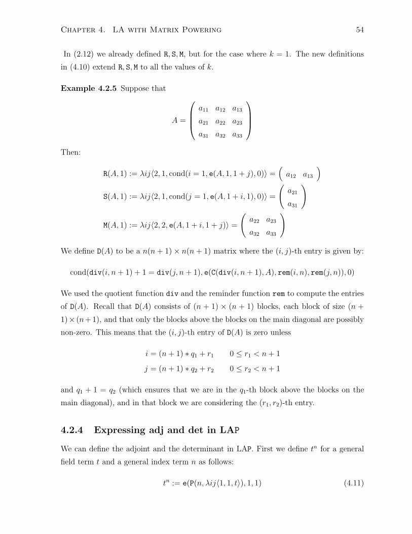
Chapter 4. LA with Matrix Powering 54
In (2.12) we already defined R, S, M, but for the case where k = 1. The new definitions
in (4.10) extend R, S, M to all the values of k.
Example 4.2.5 Suppose that
A =
+
,,-
a11 a12 a13
a21 a22 a23
a31 a32 a33
.
//0
Then:
R(A, 1) := #ij02, 1, cond(i = 1, e(A, 1, 1 + j), 0)1 =)
a12 a13
*
S(A, 1) := #ij02, 1, cond(j = 1, e(A, 1 + i, 1), 0)1 =
!a21
a31
"
M(A, 1) := #ij02, 2, e(A, 1 + i, 1 + j)1 =
!a22 a23
a32 a33
"
We define D(A) to be a n(n + 1)) n(n + 1) matrix where the (i, j)-th entry is given by:
cond(div(i, n + 1) + 1 = div(j, n + 1), e(C(div(i, n + 1), A), rem(i, n), rem(j, n)), 0)
We used the quotient function div and the reminder function rem to compute the entries
of D(A). Recall that D(A) consists of (n + 1) ) (n + 1) blocks, each block of size (n +
1)) (n+1), and that only the blocks above the blocks on the main diagonal are possibly
non-zero. This means that the (i, j)-th entry of D(A) is zero unless
i = (n + 1) 3 q1 + r1 0 . r1 < n + 1
j = (n + 1) 3 q2 + r2 0 . r2 < n + 1
and q1 + 1 = q2 (which ensures that we are in the q1-th block above the blocks on the
main diagonal), and in that block we are considering the (r1, r2)-th entry.
4.2.4 Expressing adj and det in LAP
We can define the adjoint and the determinant in LAP. First we define tn for a general
field term t and a general index term n as follows:
tn := e(P(n,#ij01, 1, t1), 1, 1) (4.11)

Chapter 4. LA with Matrix Powering 55
The idea is that tn is the (only) entry of the n-th power of the matrix (t), i.e. (t)n = (tn).
Now note that the (i, j)-th entry of adj(A) is ((1)n times the dot product of:+
,,,,,-
pn
pn"1
...
p1
.
/////0and
+
,,,,,-
e(An"1, i, j)
e(An"2, i, j)...
e(In, i, j)
.
/////0(4.12)
where the matrix on the left is just pA (without the last entry, p0), so the adjoint is given
by:
adj(A) := ((1)n"1#ij0n, n, e(pA · #kl0n, 1, e(An"k, i, j)1, i, j)1
and the determinant is simply given by:
det(A) := ((1)ne(pA, n + 1, 1)
where e(pA, n + 1, 1) is p0, i.e. the constant coe!cient of the char poly of the matrix A.
4.3 Berkowitz’s algorithm and clow sequences
Clow sequences provide a simple way of understanding the computations in Berkowitz’s
algorithm. It turns out (and this is an observation due to Valiant, see [Val92, Section 3])
that Berkowitz’s algorithm computes sums of restricted clow sequences. Clow sequences
are easy to define (they are just generalized permutations), and it is not di!cult to see
how Berkowitz’s algorithm computes sums of clow sequences.
Besides giving us insight into Berkowitz’s algorithm, clow sequences are a potential
tool for proving the Cayley-Hamilton Theorem directly in LAP (thus far, we only have a
polytime proof of the C-H Theorem, given in Chapter 8). This is especially interesting in
light of a dynamic programming algorithm for computing clows, given in [MV97, Table 1].
If we could somehow prove the correctness of this algorithm in LAP, we could use it to
prove the C-H Theorem in LAP. So far this is only speculation, but the point is that
maybe a “clow sequences approach” to the determinant could prove the C-H Theorem
in NC2, rather than in polytime.
A substantial part of the material in the rest of this section comes from [MV97] where
the authors build upon a purely combinatorial interpretation of the Cayley-Hamilton
Theorem given in [Str83]. Unfortunately, the combinatorial proof of the C-H Theorem
given in [Str83] is infeasible.

Chapter 4. LA with Matrix Powering 56
Recall the Lagrange expansion for the determinant:
det(A) =1
!$Sn
sign(')a1!(1) · · ·an!(n)
The summation is over all permutations on n elements. The sign of a permutation ',
sign('), is defined as follows:
sign(') = ((1)number of transpositions in !
To move to a combinatorial setting, we interpret ' , Sn as a directed graph G! on n
vertices.
Example 4.3.1 The permutation given by:
' =
!1 2 3 4 5 6
3 1 2 4 6 5
"
corresponds to the directed graph G! given by Figure 4.2 below.
1 2 3 4 5 6
Figure 4.2: G!
Given a matrix A, define the weight of G!, w(G!), as the product of aij ’s such that
(i, j) , G!. Consider G! given by Figure 4.2: w(G!) = a13a32a21a44a56a65. Thus, using
this new terminology:
det(A) =1
!$Sn
sign(')w(G!)
The Lagrange expression cannot be converted directly into an e!cient algorithm for
the determinant, because the summation is over n! monomials.
Any e!cient algorithm should implicitly count over all monomials; the bottleneck in
doing so directly is that permutations are not easily “factorizable” to allow for a simple
implementation. We will get around this problem by enlarging the summation from cycle
covers to clow sequences.

Chapter 4. LA with Matrix Powering 57
Definition 4.3.1 A clow is a walk (w1, . . . , wl) starting from vertex w1 and ending at
the same vertex, where any (wi, wi+1) is an edge in the graph. Vertex w1 is the least-
numbered vertex in the clow, and it is called the head of the clow. We also require that
the head occur only once in the clow. This means that there is exactly one incoming
edge (wl, w1), and one outgoing edge (w1, w2) at w1, and wi %= w1 for i %= 1. The length
of a clow (w1, . . . , wl) is l.
Example 4.3.2 Consider the clow C given by (1, 2, 3, 2, 3) on four vertices. The head
of clow C is vertex 1, and the length of C is 6. See Figure 4.3.
1 2 3 4 5
Figure 4.3: Clow C
Definition 4.3.2 A clow sequence is a sequence of clows (C1, . . . , Ck) with the following
two properties: (i) The sequence is ordered by the heads: head(C1) < . . . < head(Ck).
(ii) The total number of edges, counted with multiplicity, adds to n; that is, the lengths
of the clows add up to n.
Note that a cycle cover is a special type of a clow sequence.
We will now show how to associate a sign with a clow sequence that is consistent
with the definition of the sign of a cycle cover. The sign of a cycle cover can be shown
to be ((1)n+k, where n is the number of vertices in the graph, and k is the number of
components in the cycle cover.
Definition 4.3.3 We define the sign of a clow sequence to be ((1)n+k where n is the
number of vertices in the graph, and k is the number of clows in the sequence.
Example 4.3.3 We list the clow sequences associated with the three vertices {1, 2, 3}.

Chapter 4. LA with Matrix Powering 58
We give the sign of the corresponding clow sequences in the right-most column:
1. (1), (2), (3) ((1)3+3 = 1
2. (1, 2), (3) ((1)3+2 = (1
3. (1, 2, 2) ((1)3+1 = 1
4. (1, 2), (2) ((1)3+2 = (1
5. (1), (2, 3) ((1)3+2 = (1
6. (1, 2, 3) ((1)3+1 = 1
7. (1, 3, 3) ((1)3+1 = 1
8. (1, 3), (3) ((1)3+2 = (1
9. (1, 3, 2) ((1)3+1 = 1
10. (1, 3), (2) ((1)3+2 = (1
11. (2, 3, 3) ((1)3+1 = 1
12. (2, 3), (3) ((1)3+2 = (1
Notice that the number of permutations on 3 vertices is 3! = 6, and indeed, the clow
sequences {3, 4, 7, 8, 11, 12} do not correspond to cycle covers. Notice that we listed these
clow sequences which do not correspond to cycle covers by pairs: {3, 4}, {7, 8}, {11, 12}.Consider the first pair: {3, 4}. We will later define the weight of a clow (simply the
product of the labels of the edges), but notice that clow sequence 3 corresponds to
a12a22a21 and clow sequence 4 corresponds to a12a21a22, which is the same value; however,
they have opposite signs, so they cancel each other out. Same for pairs {7, 8} and
{11, 12}. We make this informal observation precise with the following definitions, and
in Theorem 4.3.1 we show that clow sequences which do not correspond to cycle covers
cancel out.
We will associate a weight with a clow sequence that is consistent with the contribu-
tion of a cycle cover.
Definition 4.3.4 The weight of a clow C, w(C), is the product of the weights of the
edges in the walk while accounting for multiplicity.
Example 4.3.4 Given a matrix A, the weight of clow C in example 4.3.2 is given by:
w((1, 2, 3, 2, 3)) = a12a223a32a31
Definition 4.3.5 The weight of a clow sequence C = (C1, . . . , Ck) is:
w(C) =k;
i=1
w(Ci).

Chapter 4. LA with Matrix Powering 59
Theorem 4.3.1
det(A) =1
C is a clow sequence
sign(C)w(C)
Proof. The idea of the proof of Theorem 4.3.1 (see [MV97, pp. 5–8]) is that clow sequences
which are not cycle covers cancel out. !
In [Val92, Section 3] Valiant points out that Berkowitz’s algorithm computes sums of
certain clow sequences; it computes the sums of clow sequences whose first head is the
first vertex. Since the heads are ordered, if the first head is not the first vertex, then the
given clow sequence is not a cycle cover (i.e., not a permutation), and hence it cancels
out at the end, so sums of clow sequences with this restriction still compute correctly the
determinant, and other coe!cients of the characteristic polynomial.
More precisely, let A be an n)n matrix, and let pn, pn"1, . . . , p0 be the coe!cients of
the char poly of A as computed by Berkowitz’s algorithm. Then, pn is the sum of clow
sequences of length 0, pn"1 is the sum of clow sequences of length 1, and in general pn"i
is the sum of clow sequences of length i. In particular, p0 is the determinant of A. Vertex
1 is the first head in the clow sequences computing each pn"i (i > 0), and vertex 2 is the
first head in the clow sequences computing each q(n"1)"j (j > 0), where the q(n"1)"j ’s are
the coe!cients of the char polynomial of M = A[1|1], etc.
We illustrate these computations with an example where A is a 3) 3 matrix.
Example 4.3.5 Suppose that A is a 3)3 matrix, M = A[1|1] as usual, and p3, p2, p1, p0
are the coe!cients of the char poly of A and q2, q1, q0 are the coe!cients of the char poly
or M , computed by Berkowitz’s algorithm. Thus:+
,,,,,-
p3
p2
p1
p0
.
/////0=
+
,,,,,-
1 0 0
(a11 1 0
(RS (a11 1
(RMS (RS (a11
.
/////0
+
,,-
q2
q1
q0
.
//0=
+
,,,,,-
q2
(a11q2 + q1
(RSq2 ( a11q1 + q0
(RMSq2 (RSq1 ( a11q0
.
/////0
(4.13)
The coe!cients q2, q1, q0 are computed by clow sequences on M , that is, by clow sequences
on vertices {2, 3}, where the head of the first clow is always 2. See Figure 4.4. Since q2
is the sum of clows of length zero (and 1 by default), so is p3. Now consider p2, which by
definition is supposed to be the sum of clow sequences of length one on all three vertices,
where the head of the first clow is vertex 1; see Figure 4.5. But this is the sum of clow
sequences of length one on vertices 2 and 3 (i.e., q1), plus the clow of length one on vertex

Chapter 4. LA with Matrix Powering 60
1 2 3
clows on A
clows on M
Figure 4.4: Clows on A and M = A[1|1]
1, which is just a11. All these clows have sign (1, hence the sum is (a11q2 + q1 (again,
q2 = 1).
1 2 3
Figure 4.5: Clows of length one on all three vertices
Consider p1: since p1 = p3"2, it follows that it is the sum of clow sequences of length
two. We are going to show now how the term (RSq2 ( a11q1 + q0 computes the sum of
all these clow sequences.
There is just one clow of length two on vertices 2 and 3, it corresponds to q0 and it
is shown in Figure 4.6.
1 2 3
Figure 4.6: The single clow of length two on vertices 2 and 3
There are two clows of length two which include a self loop at vertex 1. These clows
correspond to the term (a11q1. Note that the negative sign comes from the fact that
q1 has a negative value, but the parity of these clows is even. Both clows are shown in
Figure 4.7.
Finally, we consider the clow sequences of length two, where there is no self loop at
vertex 1. Since vertex 1 must be included, there are only two possibilities, both shown

Chapter 4. LA with Matrix Powering 61
1 2 3
1 2 3
Figure 4.7: Clows of length two with a self loop at vertex 1
on Figure 4.8. These clows correspond to the term (RSq2 which is equal to:
()
a12 a13
*!a21
a31
"= (a12a21 ( a13a31
since q2 = 1.
1
1
2
2
3
3
Figure 4.8: Clows of length two without a self loop at vertex 1
We do not show how to get p0, but hopefully at this point the idea is clear.

Chapter 5
The Characteristic Polynomial
In Chapter 4 we showed that the char poly can be expressed as a term over LLAP. In this
chapter we study the properties of the char poly that can be proven in LAP. In particular
we show that we LAP proves the Cayley-Hamilton Theorem, and the multiplicativity of
the determinant, for triangular matrices. It is an open question whether LAP can prove
these properties for general matrices1.
In Section 5.1 we prove some basic results in LAP that will be useful later. We
also prove (in LAP) properties of the char poly which do not depend on the matrices
being triangular. In Section 5.3 we show that hard matrix identities follow from the C-H
Theorem (in LAP).
The most important property of the characteristic polynomial (char poly) is stated
by the Cayley-Hamilton Theorem (C-H Theorem) which says the following: if pA is the
char poly of A, then pA(A) = 0. That is, the C-H Theorem states that the characteristic
polynomial of A is an annihilating polynomial of A. In general, we say that p is an
annihilating polynomial of a square matrix A, if:
p(A) = pnAn + pn"1An"1 + · · · + p1A + p0I = 0 = the zero matrix
We can also state the C-H Theorem as:
Aadj(A) = adj(A)A = det(A)I (5.1)
given our definition of the adjoint (see (4.6) on page 51).
1In Chapter 6 we show that LAP also proves the equivalence of some of the fundamental principles ofLinear Algebra (for general matrices); see Table 6.1 on page 71. In Chapter 8 we show that the extension$LAP of LAP can prove the C-H Theorem (for general matrices), and therefore the C-H Theorem has afeasible proof, as $LAP can be interpreted in a standard poly-time theory.
62

Chapter 5. The Characteristic Polynomial 63
We define the correctness of Berkowitz’s algorithm to be the following property: given
a matrix A, the polynomial obtained from Berkowitz’s algorithm, pA, is an annihilating
polynomial of A. As a small clarification, note that for a matrix A, the output of
Berkowitz’s algorithm is a column vector, so when we say that “pA is obtained from
Berkowitz’s algorithm”, we mean that the coe!cients of pA are given by the entries of
this column vector.
Thus, the correctness of Berkowitz’s algorithm is the mechanism for proving the C-H
Theorem; we define the polynomial computed by Berkowitz’s algorithm to be the char
poly, and hence, if we prove that it is an annihilating poly, then we also prove the C-H
Theorem.
Another crucial property of the char poly is the multiplicativity of the determinant,
(the determinant is defined from the constant coe!cient of the char poly; see (4.7) on
page 51) given by the identity:
det(AB) = det(A) det(B) (5.2)
The provability of (5.1) and (5.2), and other properties, is the subject of the next chapters.
It turns out that while we can prove (5.1) and (5.2) for triangular matrices (see Section 5.2
of this chapter), we need to extend LAP to $LAP (which is LAP with induction on
formulas with universally quantified matrix variables) in order to prove (5.1) and (5.2)
for general matrices.
5.1 Basic properties
In this section we prove some basic results in LAP.
Lemma 5.1.1 LAP proves that anam = an+m and AnAm = An+m.
Proof. Both claims can be proven by induction on n. The Basis Case is when n = 0,
so that n + m = m. Using (4.11) we have that a0 := e(P(0,#ij01, 1, a1), 1, 1), and by
A34, we have that P(0,#ij01, 1, a1) = Ir("ij'1,1,a() = I1, so that a0 = e(I1, 1, 1) = 1, and
1 · am = am and a0+m = am. For the Induction Step assume that the claim holds for n
and show that it holds for n + 1. Using A35, and the associativity of addition of index
elements, we can easily show that a(n+1)+m = an+ma, and an+1am = anaam = anama,
which is an+ma, by the induction hypothesis. Proving that AnAm = An+m is similar. !

Chapter 5. The Characteristic Polynomial 64
Lemma 5.1.2 LAP proves that ((1)even power = 1.
Proof. From (4.11) we know that ((1)2n := e(P(2n,#ij01, 1, ((1)1), 1, 1). So, we are
going to prove by induction on n that e(P(2n,#ij01, 1, ((1)1), 1, 1) = 1. The Basis
Case is n = 0, so using A34, we get P(0,#ij01, 1, ((1)1) = Ir("ij'1,1,("1)() = I1, and
e(I1, 1, 1) = 1. For the Induction Step, suppose that n > 0. Using basic index
operations we have that 2n = 2(n ( 1) + 2. Using the IH we have that ((1)2(n"1) = 1,
and by basic arguments we have that ((1)2 = 1. Now using Lemma 5.1.1, we have that
1 = ((1)2(n"1)((1)2 = ((1)2(n"1)+2 = ((1)2n and we are done. !
Let pA denote (as usual) the char poly of A as computed by Berkowitz’s algorithm.
Let (pA)i denote the i-th coe!cient of the char poly pA.
Lemma 5.1.3 LAP proves that for any A, det(A) = a11 det(M)( Radj(M)S.
Proof. We use Definitions 4.2.4 and 4.2.5, that is the definitions of the adjoint and the
determinant given in terms of Berkowitz’s algorithm.
det(A) = ((1)n(pA)0
by definition of the determinant,
= ((1)n((a11(pM)0 ( ((1)n"2Radj(M)S)
from Berkowitz’s algorithm, and the definition of the adjoint—this is how we compute
(pA)0 from pM ,
= a11((1)n"1(pM)0 ( Radj(M)S
by manipulating powers of ((1) and by Lemma 5.1.2, ((1)even power = 1,
= a11 det(M)( Radj(M)S
This argument can be clearly formalized in LAP. !
Lemma 5.1.4 LAP proves that for any A, (pA)n = 1, i.e., pA is a monic polynomial of
degree n.

Chapter 5. The Characteristic Polynomial 65
Proof. This can be easily proven by induction on n; just note that the top entry of
the first column of any Ci (recall that pA = C1C2 · · ·Cn) is 1, and the Ci’s are lower
triangular. Thus, the top entry of CiCi+1 · · ·Cn is always 1. More formally, suppose that
(pM)n"1 = 1. By Berkowitz’s algorithm, (pA)n = (pM)n"1 and we are done. !
Lemma 5.1.5 LAP proves that for any A, (pA)n"1 = (tr(A) = (6n
i=1 aii.
Proof. This can also be proven easily by induction on n. So suppose that the claim
holds for M , that is, (pM)n"2 = (tr(M). From Berkowitz’s algorithm we can see that
(pA)n"1 = (a11 · (pM)n"1 + 1 · (pM)n"2. By Lemma 5.1.4, (pM)n"1 = 1 and by the
induction hypothesis (pM)n"2 = (tr(M), so (pA)n"1 = (a11 ( tr(M) = (tr(A). !
The matrix Iij is obtained from the identity matrix by interchanging the i-th and the
j-th rows. The e"ect of multiplying A on the left by Iij is that of interchanging the i-th
and the j-th rows of A. On the other hand, AIij is A with the i-th and j-th columns
interchanged. We sometimes abbreviate Ii(i+1) by Ii. In Section 6.1 we show that:
Iij = Ii(i+1)I(i+1)(i+2) · · · I(j"1)jI(j"1)(j"2) · · · I(i+1)i
that is: any permutation can be written as a product of transpositions; see proof of the
Corollary 6.1.1.
Lemma 5.1.6 LAP proves that, for i %= j, det(Iij) = (1.
Proof. We prove the lemma by induction on the size of Iij. Suppose first that i, j > 1.
Then:
Iij =
!1 0
0 I(i"1)(j"1)
"
where I(i"1)(j"1) is of size one less than Iij. By Berkowitz’s algorithm we have that
det(Iij) = det(I(i"1)(j"1)), and by the Induction Hypothesis, det(I(i"1)(j"1)) = (1, so we
are done in this case.
Otherwise, suppose that i = 1, j > 1. From Berkowitz’s algorithm we have that:
det(I1j) = 0 · det(I1j[1|1])( ejadj(I1j [1|1])ej
and adj(I1j [1|1]) is a matrix of zeros, except for the (j, j)-th position where it has a 1.
To show this we argue by induction on the size of I1j[1|1] (it is not a di!cult proof using

Chapter 5. The Characteristic Polynomial 66
the definition of the adjoint, and the fact that I1j [1|1] is a “constant” matrix of 1s on the
diagonal, zeros everywhere else, except for a single zero in the (j, j) position). From this
we have that det(I1j) = (1 as required. !
Lemma 5.1.7 LAP proves that A and At have the same char poly, i.e., pA = pAt .
Proof. The proof is by induction on the size of A. The Basis Case is trivial because
(a)t = (a). Suppose now that A is an n ) n matrix, n > 1. By the IH we know that
pM = pM t . Furthermore, if we consider the matrix C1 in the definition of Berkowitz’s
algorithm, we see that the entries 1 and (a11 do not change under transposition of A, and
also, since S(M t)kR is a 1)1 matrix, it follows that S(M t)kR = (S(M t)k)R)t = RMkS,
so in fact C1 is the same for A and At. This gives us the result. !
5.2 Triangular matrices
For the proofs in this section we are going to abuse notation a little bit, and write pA(x)
for the characteristic poly of A, even though technically the char poly in LAP is a column
vector pA containing the coe!cients of the char poly of A. This will simplify our proofs.
Also note that in the Lemmas and Corollaries below, we always show that some
property can be proven in LAP. We do this by giving a high-level proof of this property,
where we only indicate what would the formal LAP proof consist of. It would be tedious
and unreadable to give complete LAP proofs in each case. LAP has been designed in
a way that permits us a certain degree of freedom when presenting proofs that can be
formalized in LAP.
Basically we assume that any proof that relies on matrix powering, and induction on
terms of type index, and uses basic matrix properties, can be formalized in LAP.
Lemma 5.2.1 LAP proves that if for all i, Ri = 0 or Si = 0, then pA(A) = 0.
Before we prove this Lemma, note that pA(A) denotes the matrix given by:
(pA)nAn + (pA)n"1An"1 + · · ·+ (pA)1A + (pA)0Ir(A)
so in fact, pA(A) = 0 should really be stated as:
r(A) = c(A) " pA(A) = 0r(A)c(A)

Chapter 5. The Characteristic Polynomial 67
where pA(A) is an abbreviation for the following constructed matrix:
#ij0r(A), c(A), e(pA · #kl0r(A), 1, e(P(r(A)( k, A), i, j)1, i, j1
where pA has been defined on page 52, definition (4.9).
Proof. The proof is by induction on the size of A. The Basis Case is trivial. For the
Induction Step assume that A is of the usual form:
A =
!a11 R
S M
"
Suppose that S = 0 (the case where R = 0 is analogous). Then, from Berkowitz’s
algorithm, we have that:
pA(x) = (x( a11)pM(x)
so pA(A) = (A( a11I)pM(A), and:
pM(A) =
!pM(a11) X
0 pM(M)
"
where X is some 1) (n( 1) matrix. Now, using the IH, pM(M) = 0. Thus:
(A( a11I)pA(A) =
!0 R
0 M ( a11I
"!pM(a11) X
0 0
"= 0
Thus, pA(A) = 0. !
Corollary 5.2.1 LAP proves the C-H Theorem for triangular matrices.
Proof. By Lemma 5.2.1, pA(A) = 0 if for all i Ri = 0 or Si = 0. If A is triangular, then
Ri = 0 for all i or Si = 0 for all i. !
Lemma 5.2.2 LAP proves that if for all i, Ri = 0 or Si = 0, then det(A) =<
i aii.
Proof. First of all, we can express<n
i=1 aii in LAP as follows:
e(n + 1, n + 1, P(n,#ij0n + 1, n + 1, cond(e(i, i, A), 0field, j = i + 1)1) (5.3)
(that is, as the (n + 1, n + 1) entry of the n-th power of the matrix with the aii’s on the
diagonal above the main diagonal, and zeros elsewhere). Suppose now that A is such

Chapter 5. The Characteristic Polynomial 68
that for all i, Ri = 0 or Si = 0. Then:
pA = C1C2 · · ·Cn, where Ci =
+
,,,,,-
1 0 . . . 0
(a11 1 . . . 0. . . 1
0 (aii
.
/////0(5.4)
Now, using induction on n, we can show that the bottom row of pA is equal to (5.3). The
Basis Case is n = 1, and it is easy since the bottom entry of A is just a11, and (5.3)
is just a11 as well. For the Induction Step assume that this holds for n ) n matrices,
so that the bottom row of C2C3 · · ·Cn is equal to a22a33 · · ·a(n+1)(n+1). Now multiply
C2C3 · · ·Cn by C1 on the left to get the result. !
Corollary 5.2.2 LAP proves that the determinant of a triangular matrix is the product
of the elements on the diagonal.
Proof. By Lemma 5.2.2 the determinant is the product of the elements on the diagonal
if for all i, Ri = 0 or Si = 0. In the case of a triangular matrix one or the other always
holds. !
Lemma 5.2.3 LAP proves that if A and B are both upper or lower-triangular, then
det(AB) = det(A) det(B).
Proof. Suppose that A, B are both upper triangular matrices (the case of lower triangular
matrices is analogous). Then AB is also an upper triangular matrix. To see this consider
the entry (i, j) of AB where i > j. This entry is given by6n
k=1 aikbkj . Since both A, B
are upper triangular, it follows that aikbkj = 0 if i > k or j < k which is always the case
as i < j. Thus the (i, j)-th entry of AB is zero when i < j, so AB is upper triangular.
By Corollary 5.2.2 the determinants of A, B and AB are the products of the elements on
the respective diagonals. It is easy to show that the (i, i) entry of AB is just aiibii (using
the same argument that we did to show that AB is upper triangular). The Lemma now
follows. !

Chapter 5. The Characteristic Polynomial 69
5.3 Hard matrix identities
In this section we show that AB = I " BA = I, and hence all hard matrix identities,
follow (in LAP) from the Cayley-Hamilton Theorem. It is interesting to note that we
know nothing about the converse; that is, what role do hard matrix identities play in the
proof of the C-H Theorem? Our proof of the C-H Theorem, given in Chapter 8, does not
come anywhere near hard matrix identities.
Theorem 5.3.1 LAP proves that the Cayley-Hamilton Theorem implies hard matrix
identities.
Proof. Suppose that AB = I, and let p be the char poly of A. First note that it can
be proven (in LA in fact) that AB = I " A(BA ( I) = 0. To see this note that
AB = I implies that (AB)A = IA = A, and by associativity A(BA) = (AB)A = A, so
A(BA) + ((1)A = 0, so A(BA + (((1)A)I = 0, so A(BA) + A(((1)I) = 0. Now using
distributivity we obtain A(BA + ((1)I) = 0.
Thus, to show that BA = I, it is enough to show that A has some left inverse C
(which of course turns out to be B) and use the identity AB = I " A(BA ( I) = 0 as
follows: C(A(BA( I)) = 0 implies (by associativity) that (CA)(BA( I) = 0, and if C
is the left inverse of A, we obtain I(BA( I) = 0, from which BA = I follows.
We construct the left inverse of A using:
The Cayley-Hamilton Theorem: p(A) = 0 (p = pA)
and the identity: 1 . i, AB = I " AiBi = I
The identity follows in LAP by induction on i; just note that the Basis Case is the claim
AB = I, and the Induction Step can be proven as follows: Ai+1Bi+1 = (AiA)(BBi), and
now using associativity, this is equal to Ai(AB)Bi which is just AiBi, which is I by the
induction hypothesis.
We now concentrate on the characteristic polynomial of A, p. By the C-H Theorem
p(A) = 0. Let pn, pn"1, . . . , p0 be the coe!cients of the characteristic polynomial, so that
p(A) = pnAn + pn"1An"1 + · · ·+ p0I = 0. Suppose that p0 is not zero. Then:
(pnAn"1 + pn"1An"2 + · · · p1I)A = (p0I
Dividing both sides by (p0 we obtain the left inverse of A as desired.

Chapter 5. The Characteristic Polynomial 70
Suppose now that p0 = 0. Let i be the largest index such that p0 = p1 = . . . = pi = 0
and pi+1 %= 0. Note that such an i exists, and furthermore, i + 1 . n, since pn = 1 (as
was proven in LAP, by induction on n, in Lemma 5.1.4). Let q be the polynomial with
coe!cients pn, pn"1, . . . , pi+1, so that 0 = p(A) = q(A)Ai. Since by the above AiBi = I,
it follows that 0 = 0Bi = q(A)AiBi = q(A)I = q(A). Since the constant coe!cient of q
is pi+1 %= 0, we can repeat the above argument to conclude that A has a left inverse. !
In Chapter 8 we give a feasible proof of the C-H Theorem, which, together with
Theorem 5.3.1 gives us a feasible proof of AB = I " BA = I, and hence, by results in
Section 3.2, feasible proofs of hard matrix identities.
Note that the main thing that we need in the above proof is an annihilating poly-
nomial. The C-H Theorem states that the char poly is an annihilating polynomial, so
AB = I " BA = I follows from the C-H Theorem, but any annihilating polynomial
would do.
Since {I, A, A2, . . . , An2} is a linearly dependent set of matrices, for A an n)n matrix,
there are non-zero coe!cients that constitute an annihilating polynomial of A; if we could
compute theses coe!cients (without using Gaussian Elimination, but rather in NC2), and
show, in LAP, that they form an annihilating polynomial, we would have an LAP proofs
of hard matrix identities without the C-H Theorem; is that possible?

Chapter 6
Equivalences in LAP
In this Chapter we show that LAP proves the following implications:
C-H Theorem =' Axiomatic dfn of det (Section 6.1)
Axiomatic dfn of det =' Cofactor Expansion (Section 6.2)
Cofactor Expansion =' C-H Theorem (Section 6.3)
Multiplicativity of det =' C-H Theorem (Section 6.4)
Table 6.1: Flowchart for Chapter 6
In Section 6.4 we show that LAP also proves the multiplicativity of the determinant
from the C-H Theorem and the following identity:
det(A) = 0 " AB %= I (6.1)
Thus, LAP proves the equivalence of the C-H Theorem, the axiomatic definition of the
determinant, and the cofactor expansion. In Chapter 8 we will give a feasible proof of
identity (6.1) (but not an LAP proof), from which it follows that we can give a feasible
proof of the multiplicativity of the determinant from the C-H Theorem.
It is an open question whether identity (6.1) has an LAP proof, and whether we
can prove, in LAP, that the multiplicativity of the determinant follows from the C-H
Theorem. In fact, our proof of identity (6.1) (see Section 8.3.2) relies on the Gaussian
Elimination algorithm.
71

Chapter 6. Equivalences in LAP 72
6.1 The axiomatic definition of determinant
The axiomatic definition of the determinant states that for any matrix A, the following
three conditions hold:
• det is multilinear in the rows and columns of A
• det is alternating in the rows and columns of A
• if A = I, then det(A) = 1
In this section we show that the axiomatic definition of the determinant follows from the
Cayley-Hamilton Theorem, and that this can be shown in LAP. The condition det(A) = 1
is easy, and multilinearity in the first row (and column) is easy as well. Thus the whole
proof hinges on a LAP proof of alternation from the C-H Theorem. Our final result,
Corollary 6.1.2, shows that alternation for a matrix A follows (in LAP) by applying the
C-H Theorem to minors of permutations of rows and columns of A.
Note that from this it follows that det (as defined in 4.2.5), is the true determinant.
Multilinearity in the first row and column follows immediately from the algorithm;
thus, we will have multilinearity for all rows and columns if we prove alternation. By
Corollary 5.2.2, det(I) = 1 as required. Thus, all we have to prove is alternation, which
is the di!cult part of the proof.
It is in fact enough to prove alternation in the rows, as alternation in the columns
will follow from alternation in the rows by det(A) = det(At)—Lemma 5.1.7.
The strategy for showing alternation in the rows is the following: we first show that
for any matrix A, A and I1AI1 have the same char poly (Lemma 6.1.1). Recall that I1
is an abbreviation for I12, which in turn is the matrix obtained from the identity matrix
by permuting the first two rows. In general, Iij is the identity matrix with rows i and
j interchanged. Therefore IijA is A with rows i and j interchanged, and AIij is A with
columns i and j interchanged. Finally, Ii abbreviates Ii(i+1).
Once we prove that A and I1AI1 have the same char poly, we can also show that
A and IiAIi have the same char poly (Lemma 6.1.2). From this we get that A and
IijAIij have the same char poly (as any permutation is a product of transpositions; see
Corollary 6.1.1).
Also in Lemma 6.1.1 we show that det(A) = ( det(I1A). From this it follows that
det(A) = ( det(I1iA) for all i, since we can bring the i-th row to the second position (via

Chapter 6. Equivalences in LAP 73
I2iAI2i), apply Lemma 6.1.1, and reorder things (by applying I2iAI2i once more). Since
Iij = I1iI1jI1i, this gives us alternation in the rows.
Note that we require the Cayley-Hamilton Theorem in the proof of every Lemma.
Also note that we prove that A and IijAIij have the same char poly, i.e. pIijAIij = pA, to
be able to reorder the matrix to prove alternation.
Lemma 6.1.1 Let A be an n) n matrix, and let M2 be the second principal submatrix
of A (i.e., M2 is A without the first two rows and the first two columns). Then, LAP
proves that pM2(M2) = 0 implies:
• p(I1AI1) = pA (i.e., I1AI1 and A have the same characteristic poly)
• det(A) = ( det(I1A)
Proof. The proof consists of Claims 6.1.1 and 6.1.2, given below. !
Since we want to study the e"ect of interchanging the first two rows and columns of
A, we let A be of the following form:
A =
+
,,-
a b R
c d P
S Q M2
.
//0
where M2 is an (n(2))(n(2) matrix, a, b, c, d are entries, and R, P, St, Qt are 1)(n(2)
matrices. We are going to consider I1AI1 and I1A. To this end we define 'A := I1AI1
and we define "A := I1A. In terms of entries of A, ' and " are given as follows:
a, b, c, d!9" d, c, b, a
R, S, P, Q!9" P, Q, R, S
M2!9" M2
a, b, c, d#9" c, d, a, b
R, P#9" P, R
S, Q, M2#9" S, Q, M2
To illustrate the main idea, we show that A and 'A have the same char poly, in the
case where M2 is a 1) 1 matrix (so A is a 3) 3 matrix). Let pA = C1C2C3.
From Berkowitz’s algorithm, C1C2 is given by:+
,,,,,,,,,,-
1 0 0
(a 1 0
()
b R*!
c
S
"(a 1
()
b R*!
d P
Q M2
"!c
S
"
()
b R*!
c
S
"
(a
.
//////////0
+
,,-
1 0
(d 1
(PQ (d
.
//0

Chapter 6. Equivalences in LAP 74
which is: +
,,,,,-
1 0
(a( d 1
(bc( RS + ad( PQ (a( d
(bPS ( cRQ(RM2S + dRS + aPQ (bc( RS + ad
.
/////0(6.2)
It is easy to see that all the entries in (6.2), except for those in the last row, remain
invariant under '.
However, the same is not true for the two entries in the bottom row. If we permute
the first two rows and columns, the left entry of the bottom row is left with (PM2Q in
place of (RM2S, and the right entry is left with (PQ, in place of (RS; neither term
appears before the permutation.
The reason why (PM2Q and (PQ do not matter is because, when we multiply (6.2)
by C3 = ( 1 (M2 )t (which is the char poly of the 1 ) 1 matrix M2) these two terms
cancel each other out: (PM2Q + PQM2 = 0.
In general, if A is any n)n matrix, then we can show that all the entries in C1C2 are
invariant under ', except for the entries in the last row. These entries will be left with
the following terms:
(PMn"22 Q (PMn"3
2 Q . . . (PQ (6.3)
which did not appear before we applied '. However, as before, they do not matter,
because C3C4 · · ·Cn computes the char poly of M2, so when we multiply all the matrices
out, the terms in (6.3) will simply disappear (by the Cayley-Hamilton Theorem).
To prove Lemma 6.1.1 we start by showing that all the entries in C1C2, except those
in the last row, are invariant under '. This is Claim 6.1.1.
Claim 6.1.1 Let A be an n) n matrix, for some n 4 3. Then, LAP proves that all the
entries in C1C2, except for those in the last row, remain invariant under '.
Proof. Note that (C1C2)[n + 1|(] is a lower-triangular Toeplitz matrix. We consider the
first column of (C1C2)[n + 1|(]. The top three entries of the first column are:
1
(a( d
()
b R*!
c
S
"
+ ad( PQ = (bc( RS + ad( PQ
By inspection, they are all invariant under '.

Chapter 6. Equivalences in LAP 75
The (k +1)-st entry in the first column, for k 4 3, is given by taking the dot-product
of the following two vectors:+
,,,,,,,,,,,,,,,,,,-
1
(a
()
b R*!
c
S
"
()
b R*!
d P
Q M2
"!c
S
"
...
()
b R*!
d P
Q M2
"k"2 !c
S
"
.
//////////////////0
,
+
,,,,,,,,,,,,,,,,,-
(PMk"22 Q
(PMk"32 Q
...
(PQ
(d
1
.
/////////////////0
(6.4)
We are going to prove that this dot-product is invariant under ', by induction on k. The
Basis Case is k = 3, where the dot product is given by:
()
b R*!
d P
Q M2
"!c
S
"
+ d)
b R*!
c
S
"
+ aPQ( PM2Q (6.5)
and the invariance under ' again follows by inspection.
For the Induction Step, consider the (k + 1)-st entry (k 4 3) of the first column of
(C1C2)[n + 1|(]:
)b R
*!w X
Y Z
"!c
S
"
+ aPMk"32 Q( PMk"2
2 Q (6.6)
where w, X, Y, Z are given as follows:!
w X
Y Z
"= (
!d P
Q M2
"k"2
+d
!d P
Q M2
"k"3
+k"41
i=0
PMk"4"i2 Q
!d P
Q M2
"i
(6.7)
Assume that (6.6) is invariant under ' (this is our Induction Hypothesis). The (k+2)-nd
entry (k 4 3) of the first column of (C1C2)[n + 1|(] is given by:
)b R
*!!d P
Q M2
"!w X
Y Z
"
+ (PMk"32 Q)I
"!c
S
"
+ aPMk"22 Q( PMk"1
2 Q
(6.8)
We must show that (6.8) is invariant under ' using the Induction Hypothesis. To see
this, first note that the expression:!
d P
Q M2
"!w X
Y Z
"
+ (PMk"32 Q)I

Chapter 6. Equivalences in LAP 76
in (6.8) is just (6.7) where instead of k( 2, k( 3, k( 4 we have k( 1, k( 2, k( 3. Since
in (6.8) we have aPMk"22 Q(PMk"1
2 Q (as opposed to aPMk"32 Q(PMk"2
2 Q in (6.6)) it
follows that the symmetry under ' is preserved. This is an elementary argument, using
powers of matrices and induction on indices, and hence it can be formalized in LAP. !
Claim 6.1.2 Let A be an n ) n matrix, for some n 4 3. Then, LAP proves that
pM2(M2) = 0 implies that the entry in the bottom row of C1C2C3 · · ·Cn remain invariant
under ' and changes sign under " .
Proof. The bottom row of C1C2 is given by the dot product of the two vectors in (6.4)
without their top rows. Thus, in the bottom row of C1C2, we are missing (PMk"22 Q’s
in the summations.
If we add these missing terms accross the bottom row (starting with the left-most),
that is, if we add:
(PMn"22 Q,(PMn"3
2 Q, . . . ,(PM2Q,(PQ (6.9)
to the entries in the bottom row, respectively, we can conclude, by the previous claim,
that the result is invariant under '.
We have that pM2(M2) = 0, so (PpM2(M2)Q = 0, and since pM2 = C3C4 . . . Cn, it
follows that if we multiply the bottom row of C1C2, where the terms listed in (6.9) have
been added, by pM2 = C3C4 · · ·Cn, these terms will disappear.
Hence, to prove the invariance under ' of the bottom entry of C1C2 · · ·Cn, we first
add the extra terms in (6.9) to the bottom row of C1C2, use the previous claim to
conclude the invariance of the resulting bottom row of C1C2 under ' (which does not
a"ect C3C4 · · ·Cn), and then show that the extra terms disappear by pM2(M2) = 0 (that
is, by the Cayley-Hamilton Theorem applied to M2).
The fact that the bottom row of C1C2C3 · · ·Cn changes sign under " is also a small
variation of the argument given here and given in the proof of Claim 6.1.1. !
Lemma 6.1.2 Let A be an n)n matrix. Then LAP proves that pMi+1(Mi+1) = 0 implies
p(IiAIi) = pA.
Proof. See Figure 6.1, and note that if i 4 n( 1 then Mi+1 is not defined, but this is not
a problem, since we do not need the C-H Theorem to prove pIn!1AIn!1 = pA.
The case i = 1 is Lemma 6.1.1, so we can assume that 1 < i < n( 1.

Chapter 6. Equivalences in LAP 77
Using the fact that I2i = I, we have:
RM jS = R(IiIi)Mj(IiIi)S = (RIi)(IiM
jIi)(IiS) = (RIi)(IiMIi)j(IiS) (6.10)
Here we use induction on j in the last step. The Basis Case is j = 1, so IiMIi = IiMIi
just by equality axioms. For the Induction Step, note that:
IiMj+1Ii = IiM
jMIi = IiMj(IiIi)MIi = (IiM
jIi)(IiMIi)
and by the induction hypothesis, IiM jIi = (IiMIi)j, so we are done.
From Berkowitz’s algorithm we know that the char poly of A is given by the following
product of matrices:
C1C2 · · ·Ci"1Ci · · ·Cn
Let C !1C
!2 · · ·C !
n be the char poly of IiAIi. As an aside, note that we defined Berkowitz’s
algorithm as a term over LLAP in Section 4.2.3. There, we padded the matrices C1, . . . , Cn
with zeros to make them all of equal size, and we put them in one big matrix C. Then,
by computing the n-th power of C, we obtain the iterated matrix product C1C2 · · ·Cn.
Here, whenever we talk of iterated matrix products, we have this construction in mind.
Using Lemma 6.1.1 and pMi+1(Mi+1) = 0, we know that if we interchange the first
two rows and the first two columns of Mi"1 (which are contained in the i-th and (i+1)-st
rows and columns of A), the char poly of Mi"1 remains invariant. This gives us:
CiCi+1 · · ·Cn = C !iC
!i+1 · · ·C !
n (6.11)
Now we are going to prove that for 1 . k . i ( 1, Ck = C !k. To see this, consider
the first column of C !k (it is enough to consider the first column as these are Toeplitz
matrices). We are going to examine all the entries in this columns:
• The first entry is 1, which is a constant.
• The second entry is akk, just as in Ck since k . i( 1.
• RkMjkSk is replaced by (RkIi+1"k)(Ii+1"kMkIi+1"k)j(Ii+1"kSk), but by (6.10) these
two are equal. (Note that 0 . j . n( k ( 1).
Thus, Ck = C !k, for 1 . k . i ( 1 and so C1C2 · · ·Ci"1 = C !
1C!2 · · ·C !
i"1. Combining this
with (6.11) gives us:
C1C2 · · ·Cn = C !1C
!2 · · ·C !
n
and so A and IiAIi have the same char polynomial, i.e., p(IiAIi) = pA. !

Chapter 6. Equivalences in LAP 78
M i+1
i-1M
row irow i+1
column icolumn i+1
Figure 6.1: Matrix A: pMi+1(Mi+1) = 0 =' p(IiAIi) = pA
Corollary 6.1.1 Let A be an n ) n matrix, and let 1 . i < j . n. LAP proves, using
the C-H Theorem on (n( 1)) (n( 1) matrices, that pIijAIij = pA.
Proof. First of all, to prove this Corollary to Lemma 6.1.2, we are going to list explicitly
the matrices for which we require the C-H Theorem: we need the following principal
submatrices of A: {Mi+1, . . . , Mj} as well as the matrices {M !j"1, . . . , M
!i+1} which are
obtained from the corresponding principal submatrices, by replacing, in A, the j-th row
by the i-th row, and the j-th column by the i-th column. The details are given in
Figure 6.2.
M j
MM
M j
MM
j-2j-1
j-2j-1
M’M’M’M’
i-th col in j-th positioni-th row in j-th position
i+1i+2
i+1i+2
Figure 6.2: {Mi+1, . . . , Mj} and {M !j"1, . . . , M
!i+1}

Chapter 6. Equivalences in LAP 79
To see why we require the C-H Theorem on precisely the matrices listed above,
we illustrate how we derive p(I13AI13) = pA (see Figure 6.3). Using pM2(M2) = 0 and
Lemma 6.1.2 we interchange the first two rows (and the first two columns, but for clarity,
we do not show the columns). Then, using pM3(M3) = 0 and Lemma 6.1.2, we interchange
rows two and three, so at this point, the original row one is in position. We still need
to take the original row three from position two to position one. This requires the use
of pM "2(M !
2) = 0 and Lemma 6.1.2. The prime comes from the fact that what used to be
row three, has now been replaced by row one. So using pM "2(M !
2) = 0, we exchange row
two and one, and everything is in position.
Now the same argument, but in the general case, relies on the fact that:
Iij = Ii(i+1)I(i+1)(i+2) · · · I(j"1)jI(j"1)(j"2) · · · I(i+1)i (6.12)
i.e., any permutation can be written as a product of transpositions. Using Lemma 6.1.2
at each step, we are done. Equation (6.12) can be proven in LAP as follows: first note
that Iij = I1iI1jI1i, so it is enough to prove that I1i is equal to a product of transpositions,
for any i.
We use induction on i. The Basis Case is i = 2, and I12 is a transposition, so there
is nothing to prove. Now the Induction Step. Assume the claim holds for I1i, and show
that it holds for I1(i+1). This follows from the fact that I1(i+1) = I1iIi(i+1)I1i. !
M 2 M 3
M’ 2
Figure 6.3: Example of p(I13AI13) = pA

Chapter 6. Equivalences in LAP 80
Corollary 6.1.2 LAP proves, using the C-H Theorem, that det is alternating in the
rows, i.e., det(A) = ( det(IijA).
Proof. Since Iij = I1iI1jI1i, it is enough to prove this for I1j . If j = 2 we are done by
Lemma 6.1.1. If j > 2, then use I2j to bring the j-th row to the second position, and
by Corollary 6.1.1, A and I2jAI2j have the same char polynomials. Now apply I12 with
Lemma 6.1.1, and use I2j once again to put things back in order. !
Example 6.1.1 Suppose that we want to show that det(A) = ( det(I15A). Consider:
A(1)(" I25AI25
(2)(" I12I25AI25(3)(" I25I12I25AI25I25 = I15A
By Corollary 6.1.1, (1) preserves the char poly, and hence it preserves the determinant.
By Lemma 6.1.1, (2) changes the sign of the determinant. By Corollary 6.1.1 again, (3)
preserves the determinant. Therefore, det(A) = ( det(I15A).
6.2 The cofactor expansion
Let A be an n) n matrix. The cofactor expansion formula for A states the following:
for 1 . i . n, det(A) =n1
j=1
((1)i+jaij det(A[i|j]) (6.13)
where A[i|j] denotes the matrix obtained from A by removing the i-th row and the j-th
column. For each i, the RHS of the equation is called the cofactor expansion of A along
the i-th row, and (6.13) states that we obtain det(A) expanding along any row of A.
Note that from (6.13), it follows by Lemma 5.1.7 that we also have the cofactor
expansion along columns.
Lemma 6.2.1 LAP proves that the cofactor expansion formula (6.13) follows from the
axiomatic definition of the determinant.
Proof. We first show that the cofactor expansion of A along the first row is equal to
det(A). Define Aj , for 1 . j . n, to be A, with the first row replaced by zeros, except
for the (1, j)-th entry which remains unchanged. Then, using multilinearity along the
first row of A, we obtain:
det(A) = det(A1) + det(A2) + · · ·+ det(An) (6.14)

Chapter 6. Equivalences in LAP 81
Consider Aj , for j > 1. If we interchange the first column and the j-th column, and then,
with (j ( 2) transpositions we bring the first column (which is now in the j-th position)
to the second position, we obtain, by alternation and Lemma 5.1.3, the following:
det(Aj) = ((1)j"1a1j det(A[1|j]) = ((1)1+ja1j det(A[1|j])
From this, and from equation (6.14), we obtain the cofactor expansion along the first
row, that is, we obtain (6.13) for i = 1.
If we want to carry out the cofactor expansion along the i-th row (where i > 1), we
interchange the first and the i-th row, and then we bring the first row (which is now in
the i-th position) to the second row with (i( 2) transposition. Denote this new matrix
A!, and note that det(A!) = ((1)i"1 det(A). Now, expanding along the first row of A!,
we obtain (6.13) for i > 1. !
6.3 The adjoint as a matrix of cofactors
In this section we show that LAP proves the Cayley-Hamilton Theorem from the cofactor
expansion formula (i.e., from (6.13)). To this end, we first show that (6.13) implies the
axiomatic definition of determinant:
Lemma 6.3.1 LAP proves the axiomatic definition of the determinant from the cofactor
expansion formula.
Proof. We want to show that we can get multilinearity, alternation and det(I) = 1
from (6.13). To show multilinearity along row (column) i, we just expand along row
(column) i. To show det(I) = 1 use induction on the size of I; in fact, showing that
det(I) = 1 can be done in LAP without any assumptions—see Corollary 5.2.2.
Alternation follows from multilinearity and from:
If two rows (columns) of A are equal " det(A) = 0
To see that alternation follows from these two things:
0 = det
+
,,,,,,,-
Ri + Rj
Ri + Rj
.
///////0
= det
+
,,,,,,,-
Ri
Ri
.
///////0
+ det
+
,,,,,,,-
Ri
Rj
.
///////0
+ det
+
,,,,,,,-
Rj
Ri
.
///////0
+ det
+
,,,,,,,-
Rj
Rj
.
///////0

Chapter 6. Equivalences in LAP 82
using multilinearity on rows Ri and Rj ; note that the first and last expressions on the
RHS are zero, since two rows are equal. So suppose that rows i and j of A are identical.
To show that det(A) = 0, we expand along row i first to obtain:
det(A) =n1
k=1
((1)i+kaik det(A[i|k])
and then we expand each minor A[i|k] along the row that corresponds to the j-th row of
A. Note that we end up with n(n( 1) terms; polynomially many in the size of A. Since
row i is identical to the row j, we can pair each term with its negation; hence the result
is zero, so det(A) = 0. !
The following lemma shows that LAP proves, from the axiomatic definition of det,
that our definition of the adjoint is equivalent to the usual definition of the adjoint as
the transpose of the matrix of cofactors.
Lemma 6.3.2 LAP proves that adj(A) = (((1)i+j det(A[j|i]))ij , i.e. that adj(A) is the
transpose of the matrix of cofactors of A, from the axiomatic definition of det.
Proof. Consider the following matrix:
C =
!0 et
i
ej A
"
where ei is a column vector with zeros everywhere except in the i-th position where it
has a 1, and ej is a row vector with a 1 in the j-th position. By Lemma 5.1.3, we have
that:
det(C) = (etiadj(A)ej = (i, j)-th entry of (adj(A)
On the other hand, from alternation on C, we have that det(C) = ((1)i+j+1 det(A[j|i]).To see this, note that we need (j + 1) transpositions to bring the j-th row of A to the
first row in the matrix C, to obtain the following matrix:
C ! =
+
,,-
1 Aj
0 eti
0 A[j|(]
.
//0
where Aj denotes the j-th row of A, and A[j|(] denotes A with the j-th row deleted.
Then, by Lemma 5.1.3, we have:
det(C !) = det
!et
i
A[j|(]
"

Chapter 6. Equivalences in LAP 83
and now with i transpositions, we bring the i-th column of
!et
i
A[j|(]
"to the first
column, to obtain:
!1 0
0 A[j|i]
"
. Therefore, det(C !) = ((1)i det(A[j|i]) finishing the
proof of the Lemma. !
Since by Lemma 6.3.1 the axiomatic definition of det follows from the cofactor ex-
pansion formula, we have the following Corollary to Lemma 6.3.2:
Corollary 6.3.1 LAP proves that adj(A) = (((1)i+j det(A[j|i]))ij from the cofactor
expansion formula.
Note that pA(A) = 0 can also be stated as Aadj(A) = det(A)I, using our definitions
of the adjoint and the determinant (see page 51). Thus, the following Lemma shows that
LAP proves the C-H Theorem from the cofactor expansion formula.
Lemma 6.3.3 LAP proves Aadj(A) = adj(A)A = det(A)I from the cofactor expansion
formula.
Proof. We show first that Aadj(A) = det(A)I. The (i, j)-th entry of Aadj(A) is by
Corollary 6.3.1 equal to:
ai1((1)j+1 det(A[j|1]) + · · ·+ ain((1)j+n det(A[j|n]) (6.15)
If i = j, this is the cofactor expansion along the i-th row. Suppose now that i %= j. Let
A! be the matrix A with the j-th row replaced by the i-th row. Then, by alternation
(which we have by Lemma 6.3.1), det(A!) = 0. Now, (6.15) is the cofactor expansion of
A! along the j-th row, and therefore, it is 0. This proves that Aadj(A) = det(A)I, and
by definition of the adjoint, adj(A)A = Aadj(A), so we are done. !
6.4 The multiplicativity of the determinant
The multiplicativity of the determinant is the property: det(AB) = det(A) det(B). This
turns out to be a very strong property, from which all other properties (including the
Cayley-Hamilton Theorem) follow readily in LAP.
Lemma 6.4.1 LAP proves that the multiplicativity of the determinant implies the C-H
Theorem.

Chapter 6. Equivalences in LAP 84
Proof. From the multiplicativity of the determinant we have that (by Lemma 5.1.6)
det(I12AI12) = det(I1) det(A) det(I1) = det(A) for any matrix A. Suppose we want to
prove the C-H Theorem for some n) n matrix M . Define A as follows:
A =
+
,,-
a b R
c d P
S Q M
.
//0 =
+
,,-
0 0 eti
0 0 0
ej 0 M
.
//0
Let C1C2C3 · · ·Cn+2 be the char poly of A (and C3 · · ·Cn+2 the char poly of M). From
Berkowitz’s algorithm it is easy to see that for A defined this way the bottom row of
C1C2 is given by:
etiM
nej etiM
n"1ej . . . etiIej 0
so the bottom row of C1C2C3 · · ·Cn+2 is simply etip(M)ej where p is the char poly of M .
On the other hand, using det(A) = det(I12AI12) and Berkowitz’s algorithm, we have
that:
det(A) = det
+
,,-
0 0 0
0 0 eti
0 ej M
.
//0 = 0
so that etip(M)ej = 0, and since we can choose any i, j, we have that p(M) = 0. !
What about the other direction? That is, can we prove the following implication in
LAP: C-H Theorem =' Multiplicativity of the determinant? The answer is “yes”, if
LAP can prove the following determinant identity:
det(A) = 0 " AB %= I (6.16)
That is, LAP can prove the multiplicativity of the determinant from the C-H Theorem
and (6.16). We suspect, however, that LAP can prove (6.16) from the C-H Theorem, so
that the C-H Theorem is enough to prove multiplicativity. At this point, we do not have
a LAP proof of (6.16)1 from the C-H Theorem.
Lemma 6.4.2 LAP can prove the multiplicativity of the determinant from the C-H
Theorem and the property given by (6.16).
1However we have a feasible proof of (6.16) based on Gaussian Elimination—see Section 8.3.2. There-fore, since we have a LAP proof of multiplicativity of det from the C-H Theorem and from (6.16)—seeLemma 6.4.2, it follows that we have a feasible proof of multiplicativity of det from the C-H Theorem;Open Problem 9.4: is there a direct LAP proof of multiplicativity of det from the C-H Theorem?

Chapter 6. Equivalences in LAP 85
Proof. We prove the Lemma by induction on the size of the matrices; so assume that
A, B are square n) n matrices. Since we assume the Cayley-Hamilton Theorem, by the
results in the previous sections we also have at our disposal the cofactor expansion and
the axiomatic definition of the determinant.
Suppose first that the determinants of all the minors of A (or B) are zero. Then, using
the cofactor expansion we obtain det(A) = 0. We now want to show that det(AB) = 0
as well.
Suppose that det(AB) %= 0. Then, by the C-H Theorem, AB has an inverse C, i.e.,
(AB)C = I. But then A(BC) = I, so A is invertible, contrary to (6.16). Therefore,
det(AB) = 0, so that in this case det(A) det(B) = det(AB).
Suppose now that both A and B have a minor whose determinant is not zero. We
can assume that it is the principal submatrix whose determinant is not zero (as A and
I1iAI1j have the same determinant, so we can bring any non-singular minor to be the
principal subminor). So assume that MA, MB are non-singular, where:
A =
!a RA
SA MA
"B =
!b RB
SB MB
"
By the Induction Hypothesis we know that det(MAMB) = det(MA) det(MB). Also note
that:
AB =
!ab + RASB aRB + RAMB
bSA + MASB SARB + MAMB
"
Now using Berkowitz’s algorithm:
det(A) det(B) = (a det(MA)( RAadj(MA)SA)(b det(MB)(RBadj(MB)SB) (6.17)
We want to show that det(AB) is equal to (6.17). Again, using Berkowitz’s algorithm:
det(AB) = (ab + RASB) det(SARB + MAMB)
( (aRB + RAMB)adj(SARB + MAMB)(bSA + MASB)(6.18)
We now show that the right hand sides of (6.17) and (6.18) are equal.
By Lemma 6.4.3:
det(SARB + MAMB) = det(MAMB) + RBadj(MAMB)SA (6.19)
Using the IH, det(MAMB) = det(MA) det(MB), and using Lemma 6.3.3 and the fact
that det(MA) %= 0 and det(MB) %= 0 we obtain: adj(MAMB) = adj(MB)adj(MA). To

Chapter 6. Equivalences in LAP 86
see this note that by the C-H Theorem (MAMB)adj(MAMB) = det(MAMB)I. We now
multiply both sides of this equation by adj(MA) to obtain, by the C-H Theorem again,
det(MA)MBadj(MAMB) = det(MAMB)adj(MA). Now multiply both sides by adj(MB)
to obtain:
det(MA) det(MB)adj(MAMB) = det(MAMB)adj(MB)adj(MA)
Since det(MAMB) = det(MA) det(MB), and det(MA) det(MB) %= 0, we obtain our result.
Therefore, from (6.19) we obtain:
det(SARB + MAMB) = det(MA) det(MB) + RBadj(MB)adj(MA)SA (6.19!)
Using Lemma 6.4.4 and adj(MAMB) = adj(MB)adj(MA), we obtain:
RBadj(SARB + MAMB) = RBadj(MB)adj(MA)
adj(SARB + MAMB)SA = adj(MB)adj(MA)SA
(6.20)
Finally, we have to prove the following identity:
RAMBadj(SARB+MAMB)MASB =
RASB det(MA) det(MB)(RBadj(MB)SBRAadj(MA)SA
+ (RASB)RBadj(MB)adj(MA)SA
(6.21)
First of all, by Lemma 6.3.3 we have:
(SARB + MAMB)adj(SARB + MAMB) = det(SARB + MAMB)
Using Lemmas 6.4.3 and 6.4.4, we get:
SARBadj(MAMB) + MAMBadj(SARB + MAMB) = (det(MAMB) + RBadj(MAMB)SA)I
We have already shown above that adj(MAMB) = adj(MB)adj(MA) using our Induction
Hypothesis: det(MAMB) = det(MA) det(MB). So, if we multiply both sides of the above
equation by adj(MA) on the left, and by MA on the right, we obtain:
adj(MA)SARBadj(MB) det(MA) + det(MA)MBadj(SARB + MAMB)MA =
det(MA)(det(MA) det(MB) + RBadj(MB)adj(MA)SA)I
Since by assumption det(MA) %= 0, we can divide both sides of the equation by det(MA)
to obtain:
adj(MA)SARBadj(MB) + MBadj(SARB + MAMB)MA =
(det(MA) det(MB) + RBadj(MB)adj(MA)SA)I

Chapter 6. Equivalences in LAP 87
If we now multiply both sides of the above equation, by RA on the left, and by SB on
the right, we obtain (6.21) as desired.
We now substitute (6.19!), (6.20), and (6.21) into (6.18), and we obtain that the right
hand side of (6.18) is equal to the right hand side of (6.17), and we are done. !
Lemma 6.4.3 LAP proves, from the axiomatic definition of det, that:
det(SR + M) = det(M) + Radj(M)S (6.22)
Proof. Consider the matrix:
C =
+
,,,,,-
1 (R
S M
.
/////0
Using Berkowitz’s algorithm (the definition of det given in 4.8), it follows that:
det(C) = det(M) + Radj(M)S
We can add multiples of the first row of C to the remaining rows of C, to clear out S,
and obtain:
C ! =
+
,,,,,-
1 (R
0 SR + M
.
/////0
Using the axiomatic definition of det, we can conclude that det(C !) = det(C), and
using (4.8) on C ! we obtain:
det(C !) = det(SR + M)
and hence the Lemma follows. !
Lemma 6.4.4 LAP proves, from the Cayley-Hamilton Theorem, that:
Radj(SR + M) = Radj(M)
adj(SR + M)S = adj(M)S

Chapter 6. Equivalences in LAP 88
Proof. By Lemma 6.3.2 we know that adj(A) is the transpose of the matrix of cofactors
of A. From this we can deduce the following identity:
adj(A) =
!det(M) (Radj(M)
(adj(M)S (1 + a11)adj(M)( adj(SR + M)
"(6.23)
To see this we are going to consider the four standard submatrices. First of all, the (1, 1)
entry of adj(A) is the determinant of the principal minor of A times ((1)1+1, i.e. det(M).
The remaining entries along the first row are given by ((1)1+i det(A[i|1]), for 2 . i . n.
Note that for 2 . i . n, A[i|1] is given by:
!R
M [i|(]
"
(6.24)
where M [i|(] denotes M without the i-th row. To compute the determinant of the
matrix given by (6.24) expand along the first row to obtain:6n"1
j=1 rj((1)i+j det(M [i|j]).This gives us (Radj(M) as desired. In the same way we can show that the entries in the
first column below (1, 1) are given by (adj(M)S.
We now show that the principal submatrix is given by (1+a11)adj(M)(adj(SR+M).
To see this first note that (SR+M)[i|j] = S[i]R[j]+M [i|j], where S[i], R[j] denote S, R
without the i-th row and j-th column, respectively. Now using Lemma 6.4.3 we have
that det((SR + M)[i|j]) = det(M [i|j]) + R[j]adj(M [i|j])S[i]. The (i + 1, j + 1) entry of
adj(A)t, 1 . i, j < n, is given by:
((1)i+j(a11 det(M [i|j])( R[j]adj(M [i|j])S[i])
as can be seen from Figure 6.4.
Therefore, the (i + 1, j + 1) entry of adj(A)t is given by:
((1)i+j(a11 det(M [i|j]) + det(M [i|j])( det((SR + M)[i|j]))
and we are done.
By Lemma 6.3.3 we know that:!
a11 R
S M
"!det(M) (Radj(M)
(adj(M)S (1 + a11)adj(M)( adj(SR + M)
"
= det(A)I
In particular this means that:
(a11Radj(M) + R(1 + a11)adj(M)( Radj(SR + M) = 0

Chapter 6. Equivalences in LAP 89
R
S M
a11
column j+1
row i+1
Figure 6.4: Showing that adj(A)[1|1] = (1 + a11)adj(M)( adj(SR + M)
and from this it follows that Radj(SR + M) = Radj(M). Similarly, we can prove the
second identity. !
Corollary 6.4.1 LAP proves, from the C-H Theorem, the anti-multiplicativity of the
adjoint for non-singular matrices, i.e.,
det(A) %= 0, det(B) %= 0 " adj(AB) = adj(B)adj(A)
Proof. The proof is given in the proof of Lemma 6.4.2. !
As a closing remark, note that our proof of multiplicativity of the determinant from
the Cayley-Hamilton Theorem is quite long and complicated. Of course, conceptually the
simplest proof is based on the cofactor expansion, but then we must prove the induction
hypothesis for too many matrices, rendering the proof infeasible. See [DF91, page 364,
Theorem 25] for a simple, yet infeasible, proof of multiplicativity of determinant based
on the Lagrange expansion.

Chapter 7
Translations
In this chapter we will show how to translate theorems of LA and LAP into families of
tautologies with short propositional proofs. These translations are a potential tool for
proving independence results. For example, if we can prove that AB = I " BA = I does
not have e!cient proofs in bounded-depth Frege with mod 2 gates, then it will follow
that AB = I " BA = I is not a theorem of LA. See Section 9.1 for more details.
We will show that the theorems of LA can be translated into families of propositional
tautologies which have poly-bounded PK derivations (see Definition 2.4.2 for the system
PK). In fact, we prove a tighter result. We are going to show that the theorems of
LA (when the underlying field is Zp, p a prime) translate into propositional tautologies
with short bounded-depth PK[p] derivations, where PK[p] is PK with MODp,i gates (i.e.,
modular gates, for counting modulo the prime p). In Lemma 7.1.1 we show that PK can
p-simulate PK[a] for any a. We will also show that the theorems of LAP have quasi-poly-
bounded (O(2log2 n)) PK derivations.
The main parameter in the translations is the size of matrices, and the underlying
field plays a minor technical role. In section 7.2, we give a detailed translation for the
case where the underlying field is Z2. This is the simplest case, since the field elements
Z2 = {0, 1} translate directly into boolean values {T, F}. We consider very briefly the
fields Zp, for a general prime p, and Q, in Section 7.3.
Since our theories LA and LAP are field independent, it is no surprise that all the
ideas necessary for the translation occur already in the case Z2. Translating over Zp,
p > 2, and over Q is just a question of finding some representation for the field elements
in terms of several boolean variables. Thus, we concentrate on the technically simplest
case: Z2.
90

Chapter 7. Translations 91
7.1 The propositional proof system PK[a]
The definition and axiomatization of modular connectives that we present in this section
come from [Kra95, Chapter 12.6].
Definition 7.1.1 Let a 4 2 be fixed and let i be in {0, . . . , a ( 1}. Then, MODa,i is a
propositional connective of unbounded arity such that:
MODa,i(%) is true i" |{j : Aj is true}| (mod a) = i
where % is a cedent of formulas, that is, % = A1, . . . , Ak, and the Ai’s are formulas, and
k 4 0. See Table 7.1 for the propositional axioms for MODa,i.
Axiom-1 " MODa,0(:)
Axiom-2 " ¬MODa,i(:)for i in {1, . . . , a( 1}
Axiom-3 " MODa,i(%, A) 6=(MODa,i(%) / ¬A) * (MODa,i"1(%) /A)
>
for i in {0, . . . , a(1}, where i(1 means i(1 (mod a), and where,
as above, % is a (possibly empty) cedent of formulas.
Table 7.1: Axioms for MODa,i
Definition 7.1.2 The system PK[a] denotes the system PK whose language is extended
by the connectives MODa,i for i in {0, . . . , a( 1}, and that is augmented by the preceding
three axiom schemas.
Lemma 7.1.1 PK p-simulates PK[a] for any a. In other words, there is a polytime
function that given a PK[a] derivation ( of a tautology " (without modular connectives),
outputs a PK proof (! of " .
Proof. We are just going to prove this Lemma in the case a = 2. The general case, for
a > 2, can be proven in a similar way. So, in the simulation we want to translate MOD2,1
into a boolean formula over over {/,*,¬} with a polynomial increase in size (polynomial
in the size of the arguments of MOD2,1).
Note that the result for MOD2,0 will follow since MOD2,0 = MOD2,1.

Chapter 7. Translations 92
First note that MOD2,1(x1, x2, . . . , xn) can be expressed as a balanced binary tree of
XOR gates, of depth log n, and size n. Now note:
XOR(x, y) 6 (x / ¬y) * (¬x / y)
XOR(x, y) 6 (x / y) * (¬x / ¬y)
So each XOR gate can be replaced by such a formula. Since for a given XOR gate in the
above mentioned balanced binary tree we need to provide the input and its negation, in
each case we need to compute XOR and XOR.
In short we obtain a circuit with gates {/,*,¬} of depth O(log n) and size O(n), and
hence we get the corresponding poly-size boolean formula. !
The following definitions come from [Kra95, Chapter 4.3].
Definition 7.1.3 The logical depth of a formula A, denoted ldp(A), is the maximum
nesting of connectives in A. More precisely:
1. ldp(F) = ldp(T) = ldp(a) = 0, for any atomic variable a.
2. ldp(¬A) = 1 + ldp(A), for any formula A.
3. ldp(A ; B) = 1 + max{ldp(A), ldp(B)} for any formulas A, B and a connective
; = /,*.
4. ldp(MODa,i(A1, A2, . . . , Ak)) = 1 + max{ldp(A1), ldp(A2), . . . , ldp(Ak)} for i in the
set {0, . . . , a( 1}.
Definition 7.1.4 The depth of a formula A, denoted dp(A), is the maximum number of
alternations of connectives in A. More precisely:
1. dp(A) = 0 i" ldp(A) = 0.
2. dp(¬¬ · · · ¬A) = dp(A) if the number of negations is even, and it is 1 + dp(A)
otherwise (we are assuming that the outermost connective of A is not “¬”).
3. Fix ; to be / or *. Then:
(a) dp(A ; B) = max{dp(A), dp(B)} if the outermost connective in both A and
B is ;.

Chapter 7. Translations 93
(b) dp(A;B) = 1+max{dp(A), dp(B)} if neither A nor B has ; as the outermost
connective.
(c) dp(A;B) = max{1+dp(A), dp(B)} if ; is the outermost connective of B but
it is not the outermost connective of A.
(d) dp(A;B) = max{dp(A), 1+dp(B)} if ; is the outermost connective of A but
it is not the outermost connective of B.
4. Consider ! = MODa,i(A1, A2, . . . , Al+k) for i in {0, 1, . . . , a( 1}. Let {A1, . . . , Al} be
the set of Aj ’s whose outermost connective is not MODa,i, and let {Al+1, . . . , Al+k}be the set of Aj ’s whose outermost connective is MODa,i. Then:
dp(!) = max{1 + dp(A1), . . . , 1 + dp(Al), dp(Al+1), . . . , dp(Al+k)}
If l or k are zero, then the corresponding sets are empty. However l + k > 0, that
is, they are not both zero.
Definition 7.1.5 Let P be a PK[a] derivation. Then, the logical depth of P , denoted
ldp(P ), is the maximal logical depth over all formulas in P . Similarly, the depth of P ,
denoted dp(P ), is the maximal depth over all formulas in P .
Definition 7.1.6 If A is a propositional formula, we define size(A) to be the number of
variables, connectives and constants (T or F) in A. If P is a PK[a] derivation, we define
size(P ) to be the sum of the sizes of all the formulas in P .
7.2 Translating theorems of LA over Z2
In this section we translate the theorems of LA over the standard model SZ2 , where the
indices are in N and the field elements are in Z2, into families of propositional tautologies
with short PK[2] derivations of bounded depth.
The main idea is the following: given a formula $ over the language LLA, we translate
it into a family of “small” propositional formulas <$<! (where ' indexes the family and
assigns values to all terms of type index in $), such that the following holds true: if
$ is true in the standard model, then <$<! is a propositional tautology for all ', and
furthermore, if $ is a theorem of LA, then, for any ', <$<! has a “short” PK[2] derivation
of depth bounded by a constant.

Chapter 7. Translations 94
The procedure for the translation is given in section 7.2.2, and the proof of correctness
of the procedure is given in section 7.2.3.
7.2.1 Preliminaries
We are concerned with standard models (see section 2.2.5) where F = Z2, i.e. with SZ2 .
We say that $ is true, if it is true in SZ2 , i.e. if SZ2 " $[" ] for all object assignments " .
Given a formula $ over LLA, we let ' be a partial object assignment of natural
numbers to all the free index variables in $, and all terms of the form r(A), c(A), for
all A. We define the norm of ', denoted by |'|, to be the largest value assignment of
', i.e. |'| = max{'(i), '(j), . . . , '(r(A)), '(c(A)), . . .}. We define '(p1/i1) · · · (pn/in) to
be the same as ', except now the free index variables i1, . . . , in are assigned the values
p1, . . . , pn, respectively.
We also let every field variable a become a boolean variable a (recall that the under-
lying field is Z2, so there is a direct and natural correspondence between field elements
and boolean values). With each matrix variable A we associate the following boolean
variables: A11, A12, . . . , A!(r(A))!(c(A)). Finally, all propositional formulas are over the
connectives {/,*,¬, MOD2,0, MOD2,1, T, F}. Note that A 5 B is an abbreviation for ¬A*B,
and A 6 B is an abbreviation for (¬A *B) / (¬B *A).
7.2.2 Procedure for the translation
We are given as input a sequent S over LLA, and a partial object assignment ' (of natural
numbers to all the free index variables in S, and to all terms r(A), c(A), for all the matrix
variables in S). The output is the propositional sequent <S<!.
A few remarks before we present the procedure: sequents are translated by translating
all formulas in the antecedent and succedent. Thus <$1, . . . ,$k " %1, . . . , %l<! becomes:
<$1<!, . . . , <$k<! " <%1<!, . . . , <%l<!
so in the procedure below we only show how to translate formulas.
All terms of type index are translated to natural numbers, that is, if m is a term of
type index, then <m<! , N. Therefore, all atomic formulas of the form m =index n and
m .index n are translated directly into T or F.
All terms of type field are translated into propositional formulas, i.e. <t<! is a propo-
sitional formula, and all formulas of the form t =field u are translated into <t<! 6 <u<!.

Chapter 7. Translations 95
Finally, all formulas of the form U =matrix T are translated into a conjunction ex-
pressing that T and U are equal entry by entry.
We now define the recursive procedure for the translation, which takes as input a
formula $ over LLA and ', and outputs a propositional formula <$<!.
If $ is given by one of the following:
$1 / $2 $1 * $2 ¬$1
then <$<! is given by one of the following:
<$1<! / <$2<! <$1<! * <$2<! ¬<$1<!
respectively. Suppose now that $ is an atomic formula. Then, $ is one of the following:
m = n m . n t = u T = U
Here is what we do in each case:
<m . n<! 9("
#$
%T if <m<! . <n<!
F otherwise
<m = n<! 9("
#$
%T if <m<! = <n<!
F otherwise
<t = u<! 9(" (<t<! 6 <u<!)
The case <T = U<! is more complicated. If T and U do not have compatible sizes, that
is, if <r(T )<! %= <r(U)<! or <c(T )<! %= <c(U)<!, then:
<T = U<! 9(" F
Suppose now that T and U have compatible sizes, and let r, c be defined as follows:
r := <r(T )<! = <r(U)<!
c := <c(T )<! = <c(U)<!
Assume that i, j are index variables that do not occur free in T or U . Then:
<T = U<! 9("&
1&p&r,1&q&c
(<e(T, i, j)<!(p/i)(q/j) 6 <e(U, i, j)<!(p/i)(q/j))

Chapter 7. Translations 96
All that is left to do is to show how to translate terms of type index and field. We give
a recursive (sub)procedure for this.
Base Case:
<0index<! 9(" 0 , N
<1index<! 9(" 1 , N
<i<! 9(" '(i) , N
<0field<! 9(" F
<1field<! 9(" T
<a<! 9(" a
Note that the “a” on the LHS is a field elements, and the “a” on the RHS is a boolean
variable.
Recursive Step: Suppose m, n are terms of type index. Then:
<m +index n<! 9(" <m<! + <n<!
<m(index n<! 9(" max{<m<! ( <n<!, 0}
<m 3index n<! 9(" <m<! · <n<!
<div(m, n)<! 9("?<m<!
<n<!
@
<rem(m, n)<! 9(" <m<! (?<m<!
<n<!
@· <n<!
<cond(%, m, n)<! 9("
#$
%<m<! if <%<!
<n<! otherwise(3)
where on the right we have the usual +,(, · of N.
Note that in the last rule (the rule marked by (3)), <%<! is either F or T because, by
definition of cond(%, m, n) (item 9 in section 2.2.1), all the atomic subformulas of % are
of type index.

Chapter 7. Translations 97
Suppose t, u are terms of type field. Then:
<t +field u<! 9(" MOD2,1(<t<!, <u<!)
<t 3field u<! 9(" <t<! / <u<!
< ( t<! 9(" <t<!
<t"1<! 9(" <t<!
<cond(%, t, u)<! 9("
#$
%<t<! if <%<!
<u<! otherwise(33)
Again, note that <%<! in rule (33) is either F or T.
We translate r(T ), c(T ) as follows:
<r(A)<! 9(" '(r(A))
<c(A)<! 9(" '(c(A))
<r(#ij0m, n, t1)<! 9(" <m<!
<c(#ij0m, n, t1)<! 9(" <n<!
With each matrix variable A we associate the following set of '(r(A))·'(c(A)) boolean
variables: A11, A12, . . . , A!(r(A))!(c(A)). Thus, we translate e(A, m, n) as follows:
<e(A, m, n)<! 9("
#7$
7%
A)m)!)n)! if1 . <m<! . '(r(A))
1 . <n<! . '(c(A))
F otherwise
and we translate constructed terms as follows:
<e(#ij0m!, n!, t1, m, n)<! 9("
#7$
7%
<t<!()m)!/i)()n)!/j) if1 . <m<! . <m!<!
1 . <n<! . <n!<!
F otherwise
Finally, we deal with $(T ) as follows:
<$(A)<! 9(" MOD2,1(A11, A12, . . . , A!(r(A))!(c(A)))
<$(#ij0m, n, t1)<! 9(" MOD2,1({<t<!(p/i)(q/j)} 1#p#$m$!1#q#$n$!
)
This ends the procedure.

Chapter 7. Translations 98
Example 7.2.1 We translate A + B = B + A where A, B are 3) 3 matrices.
<r(A + B)<! = <cond(r(A) . r(B), r(B), r(A))<!
=
#$
%<r(B)<! if <r(A) . r(B)<!
<r(A)<! otherwise
=
#$
%'(r(B)) if '(r(A)) . '(r(B))
'(r(A)) otherwise
= 3
Similarly: <r(B+A)<! = <c(A+B)<! = <c(B+A)<! = 3. Thus, from <A+B = B+A<!
we obtain: &
1#p#31#q#3
(<e(A + B, i, j)<!(p/i)(q/j) 6 <e(B + A, i, j)<!(p/i)(q/j))
and from <e(A + B, i, j)<!(p/i)(q/j) we obtain:
9(" <e(A, i, j) + e(B, i, j)<!(p/i)(q/j)
9(" MOD2,1(<e(A, i, j)<!(p/i)(q/j), <e(B, i, j)<!(p/i)(q/j))
9(" MOD2,1(A)i)!(p/i)(q/j))j)!(p/i)(q/j), B)i)!(p/i)(q/j))j)!(p/i)(q/j)
)
9(" MOD2,1(Apq, Bpq)
We do the same for e(B + A, i, j), and we obtain:
&
1#p#31#q#3
MOD2,1(Apq, Bpq) 6 MOD2,1(Bpq, Apq)
which is what we expected.
7.2.3 Correctness of the procedure
Recall that |'|, the norm of ', is the largest value assignment of '. We state the
correctness of the translating procedure in the form of the following two theorems:
Theorem 7.2.1 If S is a sequent over LLA, then, there exists a polynomial pS and a
constant dS such that for every ', size(<S<!) is bounded by pS(|'|), and dp(<S<!) is
bounded by dS. Furthermore, if S is a true sequent then, the propositional sequent <S<!
is a tautology.

Chapter 7. Translations 99
Theorem 7.2.2 If S is a sequent over LLA, and S is a theorem of LA, then, there
exists a polynomial qS and a positive integer dS such that for every ', <S<! has a PK[2]
derivation PS,! such that size(PS,!) is bounded by qS(|'|) and dp(PS,!) is bounded by
the constant dS.
Proof. (of theorem 7.2.1) Since sequents are made of (finitely many) formulas, it is
enough to prove the theorem for formulas: If $ is a formula over LLA, then $ is a boolean
combination of atomic formulas of the form m = n, m . n, t = u, and T = U . The first
two translate into T or F, for any ', so size(<m = n<!) = size(<m . n<!) = 1, regardless
of ', and hence they are trivially bounded.
The atomic formula t = u translates into <t<! 6 <u<!, and the atomic formula T = U
translates into: &
1#p#r1#q#c
(<e(T, i, j)<!(p/i)(q/j) 6 <e(U, i, j)<!(p/i)(q/j))
where r := '(r(A)) = '(r(B)) and c := '(c(A)) = '(c(B)). If the sizes are not compat-
ible, then T = U simply translates into F, in which case size(<T = U<!) = size(F) = 1,
so it is trivially bounded regardless of '.
We need the following two claims to finish the proof:
Claim 7.2.1 Given any term m of type index, there exists a polynomial pm such that
for any ', <m<! is bounded by pm(|'|).
Proof. The proof of this claim is straightforward. !
Claim 7.2.2 Given any term t of type field, there exists a polynomial pt such that for
any ', size(<t<!) is bounded by pt(|'|).
Proof. The proof is by structural induction on t.
Basis Case: t is of the form 0, 1 or a, for some field variable a. Then, t translates to F,
Tor a, respectively, and therefore size(<t<!) = 1, regardless of '.
Induction Step: we consider all the possible ways to form a term of type field; we
consider the cases that define terms of type field in the inductive definition of terms and
formulas (see section 2.2.1):
case 2. Consider t + u. Since <t + u<! 9(" MOD2,1(<t<!, <u<!), we have that:
size(<t + u<!) = size(<t<!) + size(<u<!) + 1

Chapter 7. Translations 100
and by the IH:
. pt(|'|) + pu(|'|) + 1
The case t 3 u is the same as t + u, except we have the connective / instead of
MOD2,1.
case 3. Consider (t and t"1 . Since < ( t<!, <t"1<! 9(" <t<!, it follows that:
size(< ( t<!) = size(<t"1<!) = size(<t<!)
Now we apply the IH to t.
case 4. Consider $(T ). The translation depends on whether T is a matrix variable, or a
constructed term:
<$(A)<! 9(" MOD2,1(A11, A12, . . . , A!(r(A))!(c(A)))
<$(#ij0m, n, t1)<! 9(" MOD2,1({<t<!(p/i)(q/j)} 1#p#$m$!1#q#$n$!
)
In the first case:
size(<$(A)<!) = size(MOD2,1(A11, A12, . . . , A!(r(A))!(c(A))))
= 1 + '(r(A))'(c(A)) . 1 + |'|2
In the second case:
size(<$(#ij0m, n, t1)<!) = size(MOD2,1({<t<!(p/i)(q/j)} 1#p#$m$!1#q#$n$!
))
= 1 +1
1#p#$m$!1#q#$n$!
size(<t<!(p/i)(q/j))
But by the IH size(<t<!(p/i)(q/j)) is bounded by pt(|'(p/i)(q/j)|), and by claim 7.2.1:
1 . p . <m<! . pm(|'|) and 1 . q . <n<! . pn(|'|). Thus:
pt(|'(p/i)(q/j)|) . pt(|'| + pm(|'|) + pn(|'|)) . p!t(|'|)
and we are done.
case 5. Consider e(T, m, n). If T is just a matrix variable, then:
size(<e(A, m, n)<!) = size(A)m)!)n)!) = 1

Chapter 7. Translations 101
If T is a constructed matrix, then:
size(<e(#ij0m!, n!, t1, m, n)<!) = size(<t<!()m)!/i)()n)!/j)) (7.1)
if 1 . <m<! . <m!<! and 1 . <n<! . <n!<!, and otherwise:
size(<e(#ij0m!, n!, t1, m, n)<!) = size(F) = 1
in which case we are done.
So suppose that equation (7.1) is the case. Then, by the IH, we know that
size(<t<!()m)!/i)()n)!/j)) is bounded by pt(|'(<m<!/i)(<n<!/j)|), and by claim 7.2.1,
<m<! . pm(|'|) and <n<! . pn(|'|), so we are done.
case 9. Consider cond($, t, u). Since:
<cond($, t, u)<! 9("
#$
%<t<! if <$<!
<u<! otherwise
it follows that:
size(<cond($, t, u)<!) . max{size(<t<!), size(<u<!)}
. size(<t<!) + size(<u<!)
and the claim now follows by the IH.
This finishes the proof of claim 7.2.2, and of the first part of the theorem. !
We still have to prove that if SZ2 " $, then, for any ', the propositional formula <$<!
is a tautology.
Suppose that SZ2 " $. Let ' be a fixed partial assignment to the free index variables
in $, and to all the terms of the form r(A) and c(A) for all matrix variables A in $. We
define "! to be an object assignment where "!(i) = '(i) if i is a free index variable in
$, and "!(r(A)) = '(r(A)) and "!(c(A)) = '(c(A)) if A is a matrix variable in $; "!
extends '. Since SZ2 " $, it follows that SZ2 " $["!], for all object assignment "!.
There is a natural correspondence between object assignments "! to the field and
matrix variables in $, and truth value assignments " !! to the propositional variables in

Chapter 7. Translations 102
<$<!, namely:
"!(a) = 1 , Z2 -' " !!(a) = T
"!(A) =
+
,,,,,-
a11 a12 . . . a1n
a21 a22 . . . a2n
...
am1 am2 . . . amn
.
/////0, Mm%n(Z2) -' " !!(Aij) = aij , {T, F}
for all 1 . i . m and 1 . j . n. Now, the rest of the proof will follow from the next
claim:
Claim 7.2.3 Suppose that SZ2 " $. Let ' be a fixed partial object assignment to the
free index variables in $, and to the index terms of the form r(A) and c(A), for all matrix
variables A in $. If "! and " !! are any object assignments, defined as in the paragraphs
above, then:
SZ2 " (m = n)["!] i" <m = n<! 9(" T
SZ2 " (m . n)["!] i" <m . n<! 9(" T
SZ2 " (t = u)["!] i" " !!(<t = u<!) = T
SZ2 " (T = U)["!] i" " !!(p/i)(q/j)(<e(T, i, j) = e(U, i, j)<!(p/i)(q/j)) = T
for all 1 . p . r and 1 . q . c, where r := "!(r(T )) = '(r(T )) = '(r(U)) and
c := "!(c(T )) = '(c(T )) = '(c(U)).
Proof. Let S = SZ2 , and consider the first statement: S " (m = n)["!] i" <m = n<! 9("T. S " (m = n)["!] i" mS ["!] = nS ["!]. It is easy to show, by structural induction on
terms m of type index, that mS ["!] = <m<!. Therefore, mS ["!] = nS ["!] i" <m<! = <n<!
i" <m = n<! 9(" T.
The second statement, S " (m . n)["!] i" <m . n<! 9(" T, can be proven similarly.
Consider S " (t = u)["!] i" " !!(<t = u<!) = T. S " (t = u)["!] i" tS ["!] = uS ["!].
Again, it is easy to show, by structural induction on terms t of type field, that tS ["!] =
1 , Z2 i" " !!(<t = u<!) = T. Therefore, tS ["!] = uS ["!] i" " !!(<t<! 6 <u<!) = T i"
" !!(<t = u<!) = T.
The last statement follows from the definition of <T = U<!, and from the previous
statement. This ends the proof of claim 7.2.3. !
This ends the proof of theorem 7.2.1. !

Chapter 7. Translations 103
We need the following four results for the proof of theorem 7.2.2:
Lemma 7.2.1 PK[a] derivations have the substitution property; that is, if P is a PK[a]
derivation of $(x), where x is an atom, then P [%/x] is a proof of $(%/x). (Here $
and % are propositional formulas, and x is a propositional variable. Since LA has the
(derived) substitution rule, we need an analogous thing for PK[a] in order to carry out
the translations.)
Proof. This is a straightforward proof by induction on the length of the derivation. The
Basis Case is when $(x) is an axiom, in which case $(%/x) is also an axiom (note that
% does not have modular gates, as PK[a] is a proof system for the classical tautologies).
In the Induction Step we consider all the rules (and the modular axioms), and we show
that if the property holds for the top sequent(s) it holds for the bottom. !
Lemma 7.2.2 If $(a) is a formula over LLA (and a is a field variable), then:
<$(t/a)<! =synt <$(a)<!(<t<!/a) (7.2)
for any term t of type field.
Proof. This is a straightforward proof by structural induction on the formula $. The
Basis Case is when $(a) is an atomic formula: t = u, t . u. We now prove this by
structural induction on t and u; in the inductive step of this second argument, we consider
all the steps in the procedure for translating terms of type field. The main Induction
Step is proving the result for boolean combinations of atomic formulas. !
Lemma 7.2.3 If $(i) is a formula over LLA (and i is an index variable), then:
<$(m/i)<! =synt <$(i)<!()m)!/i) (7.3)
for any term m of type index.
Proof. Same straightforward idea as in the proof of Lemma 7.2.2, but since in the
translation we actually evaluate terms of type index, in the right hand side of (7.3) we
change (accordingly to the left hand side) the value of ', rather than the boolean variables
of the formula as in (7.2). !

Chapter 7. Translations 104
Corollary 7.2.1 If S(a, i) is a sequent over LLA, and a = a1, . . . , ak and i = i1, . . . , il
are field and index variables (respectively), then:
<S(t/a,m/i)<! =synt <S(a, i)<!()m)!/i)(<t<!/a)
where t = t1, . . . , tk and m = m1, . . . , ml are terms of type field and index (respectively).
Note that t/a denotes t1/a1, . . . , tk/ak.
Proof. Since sequents are cedents of formulas, this Corollary follows directly from (7.2)
and (7.3). !
Proof. (of Theorem 7.2.2) Suppose that S is a theorem of LA. Then, by Defini-
tion 2.4.6, S has a PK-LA derivation ( = {S1, S2, . . . , Sn}, where S =synt Sn. We are
going to prove the Theorem by induction on n. There are two cases: the axiom case,
where Si is an axiom, and the rule case, where Si follows by one of the rules from previous
sequents in the derivation (. Note that in the Basis Case of the induction, S1 must be
an axiom. In the Induction Step, Si either follows from previous sequents in (, or it is
also an axiom.
The goal is to produce a PK[2] derivation P of <S<!, that satisfies the conditions of
the Theorem (it is poly-bounded in |'| and all formulas have bounded depth). The fact
that these conditions hold is obvious from the proof, so they will not be stated explicitly.
Axiom Case
We will go through the list of the axiom schemas, showing that each axiom translates
into families of propositional tautologies with short PK[2] proofs of bounded depth. Note
that by convention (2.14) — the convention that we made in section 2.3 — all substitution
instances of axioms are also axioms. Corollary 7.2.1 will take care of the case where we
replace variables of type index or field by appropriate terms. We still need to consider
the cases where we replace variables of type matrix by constructed matrices.
A1: Since this is the first axiom that we deal with, we will do it in a little bit more
detail than necessary. Recall that A1 is x = x. If we replace x by a variable i of
type index, then we get i = i. Then, <i = i<! 9(" T because <i<! = <i<! for any
index variable i, and T has a trivial PK[2] proof.
If x is the field variable a, then <a = a<! 9(" a 6 a, which has a short tree-like
PK[2] proof regardless of '.
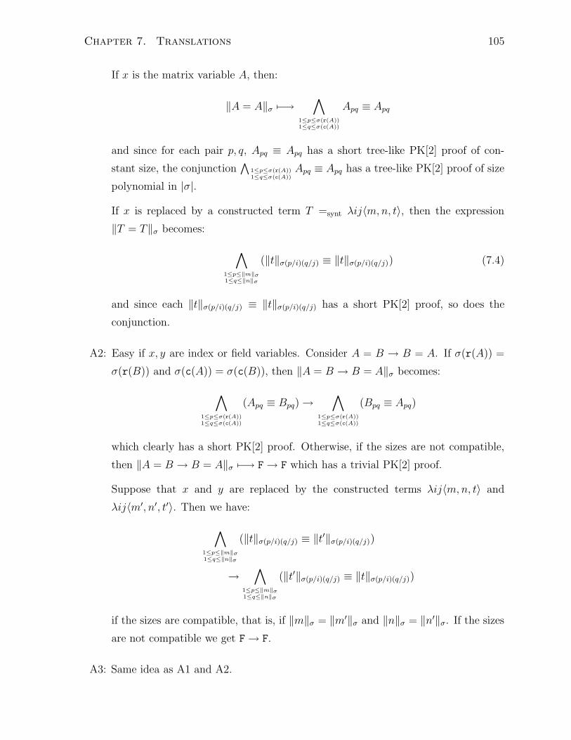
Chapter 7. Translations 105
If x is the matrix variable A, then:
<A = A<! 9("&
1#p#!(r(A))1#q#!(c(A))
Apq 6 Apq
and since for each pair p, q, Apq 6 Apq has a short tree-like PK[2] proof of con-
stant size, the conjunctionA
1#p#!(r(A))1#q#!(c(A))
Apq 6 Apq has a tree-like PK[2] proof of size
polynomial in |'|.
If x is replaced by a constructed term T =synt #ij0m, n, t1, then the expression
<T = T<! becomes:
&
1#p#$m$!1#q#$n$!
(<t<!(p/i)(q/j) 6 <t<!(p/i)(q/j)) (7.4)
and since each <t<!(p/i)(q/j) 6 <t<!(p/i)(q/j) has a short PK[2] proof, so does the
conjunction.
A2: Easy if x, y are index or field variables. Consider A = B " B = A. If '(r(A)) =
'(r(B)) and '(c(A)) = '(c(B)), then <A = B " B = A<! becomes:
&
1#p#!(r(A))1#q#!(c(A))
(Apq 6 Bpq) "&
1#p#!(r(A))1#q#!(c(A))
(Bpq 6 Apq)
which clearly has a short PK[2] proof. Otherwise, if the sizes are not compatible,
then <A = B " B = A<! 9(" F" F which has a trivial PK[2] proof.
Suppose that x and y are replaced by the constructed terms #ij0m, n, t1 and
#ij0m!, n!, t!1. Then we have:
&
1#p#$m$!1#q#$n$!
(<t<!(p/i)(q/j) 6 <t!<!(p/i)(q/j))
"&
1#p#$m$!1#q#$n$!
(<t!<!(p/i)(q/j) 6 <t<!(p/i)(q/j))
if the sizes are compatible, that is, if <m<! = <m!<! and <n<! = <n!<!. If the sizes
are not compatible we get F" F.
A3: Same idea as A1 and A2.

Chapter 7. Translations 106
A4: It is enough to consider f , {r, c, e,$} as it is easy for the other function symbols.
Suppose f = r and consider A = B " r(A) = r(B). Just note that if <r(A)<! %=<r(B)<!, then <A = B<! 9(" F.
Suppose f = e. Consider:
i1 = i2, j1 = j2, A = B " e(A, i1, j1) = e(B, i2, j2)
Just note that if <i1 = i2<! 9(" T and <j1 = j2<! 9(" T, then we have '(i1) = '(i2)
and '(j1) = '(j2).
Finally consider f = $. In this case the axiom becomes:
A = B " $(A) = $(B)
If the sizes are compatible, from <A = B " $(A) = $(B)<! we obtain:
9(" <A = B<! " <$(A) = $(B)<!
9("&
1#p#!(r(A))1#q#!(c(A))
Apq 6 Bpq
" MOD2,1({Apq} 1#p#!(r(A))1#q#!(c(A))
) 6 MOD2,1({Bpq} 1#p#!(r(A))1#q#!(c(A))
)
A5–A17: It is easy to check that each of these axioms is mapped to T for any '.
A18: < " 0 + a = a<!
9(" " <0 + a<! 6 <a<!
9(" " MOD2,1(F, a) 6 a
A19: < " a + ((a) = 0<!
9(" " <a + ((a) = 0<!
9(" " <a + ((a)<! 6 <0<!
9(" " MOD2,1(a, < ( a<!) 6 F
9(" " MOD2,1(a, a) 6 F

Chapter 7. Translations 107
A20: < " 1 3 a = a<!
9(" " <1 3 a<! 6 <a<!
9(" " (<1<! / <a<!) 6 <a<!
9(" " (T / a) 6 a
A21: <a %= 0 " a 3 (a"1) = 1<!
9("<a %= 0<! " <a 3 (a"1) = 1<!
9("¬(a 6 F) " <a 3 (a"1)<! 6 T
9("¬(a 6 F) " (a / <a"1<!) 6 T
9("¬(a 6 F) " (a / a) 6 T
A22: < " a + b = b + a<!
9(" " <a + b<! 6 <b + a<!
9(" " MOD2,1(a, b) 6 MOD2,1(b, a)
A23: < " a 3 b = b 3 a<!
9(" " <a 3 b<! 6 <b 3 a<!
9(" " a / b 6 b / a
A24: < " a + (b + c) = (a + b) + c<!
9(" " <a + (b + c)<! 6 <(a + b) + c<!
9(" " MOD2,1(a, <b + c<!) 6 MOD2,1(<a + b<!, c)
9(" " MOD2,1(a, MOD2,1(b, c)) 6 MOD2,1(MOD2,1(a, b), c)

Chapter 7. Translations 108
A25: < " a 3 (b 3 c) = (a 3 b) 3 c<!
9(" " a / (b / c) 6 (a / b) / c
A26: < " a 3 (b + c) = (a 3 b) + (a 3 c)<!
9(" " a / MOD2,1(b, c) 6 MOD2,1(a / b, a / c)
A27: <$" cond($, a, b) = a<!
9("<$<! " <cond($, a, b) = a<!
9("<$<! " <cond($, a, b)<! 6 a
Suppose <$<! 9(" T. Then <cond($, a, b)<! 9(" a, so in this case:
<$" cond($, a, b) = a<! 9(" T" a 6 a
A28: <i = 0 * r(A) < i * j = 0 * c(A) < j " e(A, i, j) = 0<! maps to
<i = 0<! * <r(A) < i<! * <j = 0<! * <c(A) < j<! " <e(A, i, j)<! 6 F
Suppose that the antecedent is true. Then, one of the formulas in the disjunction
has to be true, and so <e(A, i, j)<! 9(" F, so the succedent is F 6 F, and hence it
is valid.
A29:
< " r(#ij0m, n, t1) = m<! 9("" T
< " c(#ij0m, n, t1) = m<! 9("" T
Now consider <1 . i, i . m, 1 . j, j . n " e(#ij0m, n, t1, i, j) = t<! which maps
to:
<1. i<!, <i.m<!, <1.j<!, <j.n<! " <e(#ij0m, n, t1, i, j)<! 6 <t<!
If all the formulas in the antecedent are true, then:
<e(#ij0m, n, t1, i, j)<! 9(" <t<!
so the succedent becomes <t<! 6 <t<!, and the entire sequent becomes:
T, T, T, T" <t<! 6 <t<!

Chapter 7. Translations 109
A30: <r(A) = 1, c(A) = 1 " $(A) = e(A, 1, 1)<! becomes:
<r(A) = 1<!, <c(A) = 1<! " <$(A)<! 6 <e(A, 1, 1)<!
and if both formulas in the antecedent are true, then:
<$(A)<! 9(" MOD2,1(A11)
<e(A, 1, 1)<! 9(" A11
so in this case the sequent becomes:
T, T" MOD2,1(A11) 6 A11
A31: <r(A) = 1, 1 < c(A) " $(A) = $(#ij01, c(A)( 1, Aij1) + A1c(A)<! becomes:
<r(A) = 1<!,<1 < c(A)<!
"<$(A)<! 6 MOD2,1(<$(#ij01, c(A)( 1, Aij1)<!, <A1c(A)<!)
Suppose that both formulas in the antecedent are true. Then we have:
T, T" MOD2,1(A11, . . . , A1!(c(A))) 6
MOD2,1(MOD2,1(A11, . . . , A1!(c(A))"1), A1!(c(A)))
A32: <c(A) = 1 " $(A) = $(At)<! becomes:
<c(A) = 1<! " <$(A)<! 6 <$(At)<!
Suppose that the formula in the antecedent is true, and recall that At is defined by
#ij0c(A), r(A), Aji1. We obtain:
T" MOD2,1(A11, . . . , A!(r(A))1) 6 MOD2,1({<Aji<!(p/i)(q/j)} 1#p#!(c(A))=11#q#!(r(A))
)
which is simply:
T" MOD2,1(A11, . . . , A!(r(A))1) 6 MOD2,1(A11, . . . , A!(r(A))1)
A33: Suppose that <1 < r(A)<!, <1 < c(A)<! 9(" T. Then, the RHS of the sequent
maps to a propositional formula of the form !1 6 !2, where !1 is <$(A)<! and where

Chapter 7. Translations 110
!2 is a formula whose outermost gate is MOD2,1 with the following four arguments:
<e(A, 1, 1)<! 9(" A11
<$#ij01, c(A)( 1, e(A, 1, i + 1)1<! 9(" MOD2,1(A12, . . . , A1!(c(A)))
<$#ij0r(A)( 1, 1, e(A, i + 1, 1)1<! 9(" MOD2,1(A21, . . . , A!(r(A))1)
<$#ij0r(A)( 1, c(A)( 1, e(A, i + 1, j + 1)1<! 9(" MOD2,1(A22, . . . , A!(r(A))!(c(A)))
Thus, it comes down to proving the following assertion:
MOD2,1(A) 6 MOD2,1(A11, MOD2,1(R), MOD2,1(S), MOD2,1(M))
where MOD2,1(A) means the obvious: MOD2,1(A11, . . . , A!(r(A))!(c(A))). Similarly, R, S
and M on the RHS abbreviate the corresponding sets of propositional variables.
Rule Case
We examine the three rules, and show that if the translations of the premises have
feasible polysize PK[2] derivations of bounded depth, so does the translation of the con-
clusion.
Ind: Since by IH, <$(i) " $(i + 1/i)<! has short PK[2] derivations for all ', it follows
that for any particular fixed '0, the propositional formulas:
<$(i)<!0(p/i) " <$(i + 1/i)<!0(p/i) for 0 . p < '0(n) (7.5)
have short PK[2] derivations. From <$(0/i)<!0 and the formulas given by (7.5) we
can conclude, with a sequence of modus ponens, <$(n/i)<!0 .
Eq: Suppose that <r(T ) = r(U)<! 9(" T and <c(T ) = c(U)<! 9(" T, and that
<e(T, i, j) = e(U, i, j)<! has a short PK[2] derivation for all ', and in particu-
lar for all '(i) , {1, . . . , r} and '(j) , {1, . . . , c}, where r = <r(T )<! = <r(U)<!
and c = <c(T )<! = <c(U)<!. Therefore, <T = U<!, which is given by:
&
1#p#r1#q#c
<e(T, i, j)<!(p/i)(q/j) 6 <e(U, i, j)<!(p/i)(q/j)
also has short PK[2] derivations.
PK rules: This case is easy.
This finishes the proof of theorem 7.2.2. !

Chapter 7. Translations 111
7.3 Translating theorems of LA over Zp and Q
In this section we discuss briefly the translations of the theorems of LA over finite fields
of the form Zp (p prime), and over the field of the rationals Q. The finite field Zp, for p
a prime, is the set {0, 1, . . . , p( 1} with mod p addition and multiplication.
We will concentrate on the encoding of the field elements. We will not restate the
theorems and proofs for bigger fields since they are analogous to the Z2 case which has
been done in great detail in the previous section.
So suppose that F = Zp, for p a prime. In that case we cannot translate field elements
directly; we need several propositional variables to represent a single field variable.
Since Zp = {0, 1, 2, . . . , p ( 1} has finitely many elements, we can use the unary
notation to represent (feasibly) each field element In the translations, we are going to
associate with each field variable a the following boolean variables: a1, a2, . . . , ap"1, which
are going to encode (in unary) the value of a. For example, if p = 5 and a = 3, then
a5a4a3a2a1 is F F T T T.
If t is a term of type field, then <t<j! denotes the value of the j position in the unary
representation of t. In particular, <a<j! is aj .
We allow the connectives MODp,i, for 0 . i . p( 1, and we include its defining axioms
(see section 7.1). Also, for each sequence of variables a1, a2, . . . , ap encoding the field
variable a, we add the following set of axioms:
ai+1 5 ai for 1 . i . p( 1
This ensures that field elements are properly encoded in unary.
We need to make some changes in the procedure for the translation. First:
<t = u<! 9("&
1&j&p
<t<j! 6 <u<j
!
Now we make the following changes in the (sub)procedure that translates terms of type
index and field (we only need to modify the cases that deal with terms of type field). In
the Base Case:
<0field<j! 9(" F for 1 . j . p
<1field<1! 9(" T
<1field<j! 9(" F for 2 . j . p
<a<j! 9(" aj

Chapter 7. Translations 112
for 1 . j . p. Now consider the Recursive Step. Addition is given as follows:
<t + u<j! 9("
'
j&i&p"1
MODp,i({<t<k!}1&k&p, {<u<k
!}1&k&p)
We now show how to translate products, and additive and multiplicative inverses:
<t 3 u<j! 9("
'
1#i,k#p!1j#(ik mod p)
(<t<i! / ¬<t<i+1
! ) / (<u<k! / ¬<u<k+1
! )
< ( t<j! 9("
'
1#i#p!1j#p!i
(<t<i! / ¬<t<i+1
! )
<t"1<j! 9("
'
1#i,k#p!1j#k%ik&1 mod p
(<t<i! / ¬<t<i+1
! )
We translate e(A, i, j) in the obvious way: <e(A, i, j)<k! is Ak
ij ; thus, with each matrix A
if size m ) n, we associate m · n · p boolean variables Akij . For constructed matrices, we
do the following: <e(#ij0m, n, t1, i, j)<k! 9(" <t<k
!.
Finally, we deal with $(A) as follows:
<$(A)<j! 9("
'
j&i&p"1
MODp,i({Akxy}1&x&!(r(A)),1&y&!(c(A)),1&k&p)
We proceed in a similar way with constructed matrices. This ends the modification of
the translation for fields Zp.
We will not present the details of the translation over the rationals since field op-
erations over the integers (and we can encode the rationals as pairs of integers), have
been already formalized using boolean formulas of size polynomial in the length of the
encoding. See, for example, [Weg87, Theorems 1.2 and 1.3] for polysize circuits of depth
O(log n) that compute the addition and multiplication of integers. Also, see [Pit00].
7.4 Translating theorems of LAP
In this section we are going to show how to translate theorems of LAP into families of
boolean tautologies with quasi-poly-bounded Frege proofs. Again, we concentrate on the
field Z2 (as before, when the underlying field is Zp, p > 2, or Q, the translation is messier,
but all the results still hold). The “quasi” prefix in poly-bounded comes from the fact
that we require NC2 circuits to compute powers of matrices, and NC2 circuits correspond
to boolean formulas of size O(2log2 n).

Chapter 7. Translations 113
Most of the work has been done already, when we translated LA into families of
tautologies. In fact, we only need to show how to deal with e(P(m, A), i, j) over Z2.
The first thing we do is show how to translate <e(P(m, A), i, j)<! recursively:
Base Case: There are two cases:
case 1 <m<! = 0. <e(P(m, A), i, j)<! 9(" T i" '(i) = '(j).
case 2 <m<! = 1. <e(P(m, A), i, j)<! 9(" <e(A, i, j)<! 9(" Aij.
Recursive Step: Assume <m<! > 1. There are two cases:
case 1 <m<! is even. Then <e(P(m, A), i, j)<! is mapped to:
MOD2,1({<e(P(div(m, 2), A), i, k)<! / <e(P(div(m, 2), A), k, j)<!}k)
where k ranges in {1, . . . , max{<r(A)<!, <c(A)<!}}.
case 2 <m<! is odd. In this case, we e"ectively have to multiply three matrices; consider
the (i, j)-th entry of the product (AB)C (assume that all three are n)n matrices):
n1
k=1
(AB)ikCkj =n1
1&k&n,1&l&n
((AilBlk)Ckj) (7.6)
If we now let A and B be P(div(m(1, 2), A), and C be A, and keep the right hand
side of equation (7.6) in mind, we get the following translation:
MOD2,1({
(<e(P(div(m( 1, 2), A), i, l)<! / <e(P(div(m( 1, 2), A), l, k)<!) / <e(A, k, j)<!
}l,k)
where k and l range in {1, . . . , max{<r(A)<!, <c(A)<!}}. Basically, the idea is that
if m is odd, then m = 2n + 1, and:
Am!1
2 Am!1
2 A = AnAnA = A2n+1 = Am
We also have to show that axioms A34 and A35 (see Table 4.1 on page 45) translate to
propositional tautologies with feasible quasi-polysize (O(2log2 n)) PK[2] derivations. This
is easy to see for A34 (it follows from the base case of the above recursion). Showing it
for A35:
" P(m + 1, A) = P(m, A) 3A

Chapter 7. Translations 114
requires showing that:
&
i,j
<e(P(m + 1, A), i, j)<! 6 <e(P(m, A) 3 A, i, j)<!
and given the translation for P(m, A), this is just associativity of “/”.

Chapter 8
Proofs of the C-H Theorem
The main result of this chapter is a feasible proof of the Cayley-Hamilton Theorem. This
result gives us a feasible proof of correctness of Berkowitz’s algorithm, feasible proofs
of hard matrix identities, and feasible proofs of the main principles of Matrix Algebra
(specifically: axiomatic definition of the determinant, cofactor expansion formula, and
multiplicativity of the determinant).
We present three feasible proofs of the C-H Theorem. The first, in Section 8.2.2,
relies on translations from LAP with #M1 -Induction into a variant of the poly-time theory
V11. The second and third, in Section 8.2.5 and Section 8.2.6, respectively, rely on
translations from LAP with #M1 -Induction. We translate into families of Frege proofs
with the permutation rule in one case, and introduction of propositional quantifiers in the
second case. Permutation Frege is a fragment of Substitution Frege, which corresponds
to reasoning with poly-time concepts. The fragment of Quantified Frege that we use is
tree-like and all formulas only need one block of universal quantifiers, and this can be
p-simulated by Extended Frege.
It seems that we provide the first feasible proof of correctness of the C-H Theorem.
To support this claim we present in Section 8.1 the prototypical (infeasible) proofs of the
C-H Theorem, given in algebra textbooks. They are both infeasible as they rely on the
Lagrange formula for det(xI (A), which has n! terms for an n) n matrix A.
In section 8.3 we give a feasible proof of correctness of the Gaussian Elimination
Algorithm; a poly-time proof of a poly-time algorithm. This result is interesting in
its own right because we do not know how to give a proof of correctness of Berkowitz’s
algorithm in its own complexity class. In other words, we do not know if we can prove the
Cayley-Hamilton Theorem using NC2 concepts, rather than (feasible) poly-time concepts.
115

Chapter 8. Proofs of the C-H Theorem 116
We use the proof of correctness of Gaussian Elimination to give a direct feasible
proof (as opposed to an indirect proof via the feasible proof of the C-H Theorem) of
AB = I " BA = I (Section 8.3.3), and a feasible proof of det(A) = 0 " AB %= I
(Section 8.3.2). This last identity, together with a feasible proof of the Cayley-Hamilton
Theorem, gives us a feasible proof of multiplicativity of determinant (see Section 6.4).
At this point, it is not known if there are poly-bounded Frege proofs, or even quasi-
poly-bounded Frege proofs of hard matrix identities or of the Cayley-Hamilton Theorem.
To repeat using the language of circuit complexity: we know that hard matrix identities,
as well as the Cayley-Hamilton Theorem, have poly-bounded P/poly-Frege proofs, but
it is not known if they have poly-bounded NCi-Frege proofs, for any i. Since Berkowitz’s
algorithm is an NC2 algorithm, it is tempting to conjecture that they all have NC2-Frege
proofs.
8.1 Traditional proofs of the C-H Theorem
In this section we present two prototypical (infeasible) proofs of the Cayley-Hamilton
Theorem that are given in one form or another in most Linear Algebra textbooks. Our
(small) contribution is Claim 8.1.1 which is usually overlooked (and never proven) when
Proof I is given. These proofs are infeasible because they rely on the Lagrange expansion
of the determinant; the Lagrange expansion, for a n)n matrix, has n! terms (i.e., it is the
summation over all the permutations of n elements:6
!$Snsgn(')a1!(1)a2!(2) . . . an!(n)).
8.1.1 Infeasible proof of the C-H Theorem (I)
Proof. The most direct proof is using the Lagrange expansion on det(xI ( A). We
show that using the Lagrange expansion we can prove the axiomatic definition of the
determinant, and hence, by defining adj(xI(A) as the matrix of cofactors, we can prove
that:
(xI ( A)adj(xI ( A) = det(xI (A)I.
Let ( be the isomorphism that maps objects from M(F[x]) to (M(F))[x], and replace x
by A in the expression (xI ( A)((adj(xI ( A)) = ((det(xI ( A)I). This gives us that
pA(A) = ((det(xI ( A))|x=A = 0. !
Just for completeness we show that the map (, given in the above proof exists. This

Chapter 8. Proofs of the C-H Theorem 117
map allows us to consider every matrix whose entries are polynomials over the ring R,
as a polynomial whose coe!cients are in Mn%n(R).
Example 8.1.1 Suppose that n = 2 and R = Q. Consider:
!2x + 5 (x2 ( 7
3 x2 + 5x + 1
"=
!0 (1
0 1
"x2 +
!2 0
0 5
"x +
!5 (7
3 1
"
where the LHS is in M2%2(Q[x]) and the RHS is in (M2%2(Q))[x].
Claim 8.1.1 Mn%n(R[x]) == (Mn%n(R))[x].
Proof. Let ( : Mn%n(R[x]) (" (Mn%n(R))[x] be the natural mapping. We show first
that ( is a ring homomorphism. Let ({akij}) , Mn%n(R[x]) where {ak
ij} , R[x] is the
(i, j)-th entry, and akij is the coe!cient of the k-th power of this polynomial. Then:
((({akij}) + ({bk
ij})) = ((({akij + bk
ij}))
= {(akij + bk
ij)}
= {(akij)} + {(bk
ij)}
= ((({akij})) + ((({bk
ij}))
Now we want to show that ((({akij}) · ({bk
ij})) = ((({akij})) · ((({bk
ij})).
((({akij}) · ({bk
ij})) = ((($nl=1{ak
il} · {bklj}))
= ((($nl=1{$r+s=ka
rilb
slj}))
= {$r+s=k($nl=1a
rilb
slj)}
= {$r+s=k(arij) · (bs
ij)}
= {(akij)} · {(bk
ij)}
= ((({akij})) · ((({bk
ij}))
Thus ( is a ring homomorphism. Since ( is bijective, the claim follows. !
8.1.2 Infeasible proof of the C-H Theorem (II)
Another proof, more algebraic, considers algebraically closed fields. So let A be a matrix,
let pA(x) = det(xI(A) (also computed via the Lagrange expansion), and let #1,#2, . . . ,#n

Chapter 8. Proofs of the C-H Theorem 118
be the eigenvalues of A. As we are dealing with algebraically closed fields, we can find a
matrix P such that:
A = P"1TP
where T is an upper-triangular matrix with #1,#2, . . . ,#n on the diagonal. We factor the
characteristic polynomial as follows:
pA(x) = (x( #1)(x( #2) · · · (x( #n)
Then:
pA(A) = pA(P"1TP ) = P"1pA(T )P
and note that:
pA(T ) = (T ( #1I)(T ( #2I) · · · (T ( #nI)
Now, using induction on k, we can show that the first k columns of (T(#1I) · · · (T(#kI)
are zero, 1 . k . n. Thus, pA(T ) = 0, and therefore pA(A) = 0. !
8.2 Feasible proofs of the C-H Theorem
In this section we present three feasible proofs of the Cayley-Hamilton Theorem. All three
proofs rely on the same idea—they are the same proof expressed in slightly di"erent ways
to draw connections with di"erent propositional proof systems.
The basic intuition behind these proofs is the following: if pA(A) %= 0, that is, if the
C-H Theorem fails for A, then we can find in polytime a minor A[i|j] of A for which
pA[i|j](A[i|j]) %= 0, i.e., a minor for which the C-H Theorem fails already. Since the C-H
Theorem does not fail for 1)1 matrices, after n = (size of A) steps we get a contradiction.
This idea can be expressed with universal quantifiers over variables of type matrix: if the
C-H Theorem holds for all n2 minors of A, it also holds for A.
Also note that we do not need multiplicative inverses for field elements to prove the
C-H Theorem; that is, we do not need the function "1 and we do not need axiom A21.
Berkowitz’s algorithm does not compute inverses of field elements, and we do not need
to take inverses in the proofs of the C-H Theorem that we present below. Thus, the
C-H Theorem holds for commutative rings. On the other hand, we do use inverses in our
proof of the multiplicativity of the determinant1 (see Section 6.4).
1It is an interesting question whether it is possible to prove the multiplicativity of the determinantfor commutative rings.

Chapter 8. Proofs of the C-H Theorem 119
Here are the outlines of the proofs:
• Proof 1 with V11: In Section 8.2.1 we show that LAP, with $ quantifiers for
matrix variables (i.e., we allow #M1 formulas—see Definition 8.2.1) and augmented
by #M1 -Induction (we call the new theory $LAP), proves the C-H Theorem. In
Section 8.2.2 we define the theory V1($, P), which is conservative over the poly-
time theory V11, and in Section 8.2.3 we show that the theorems of $LAP can be
interpreted in V1($, P).
• Proof 2 with Permutation Frege: In Section 8.2.5 we use the machinery of LAP
to show that the C-H Theorem has poly-bounded uniform families of Permutation
Frege proofs. Since Permutation Frege is a fragment of Substitution Frege, which
in turn can be p-simulated by Extended Frege, once again we have feasible proofs
of the C-H Theorem.
• Proof 3 with Quantified Frege: In Section 8.2.6 we show that $LAP proofs
translate into uniform, tree-like, poly-bounded families of Quantified Frege proofs,
where all formulas either have no quantifiers at all, or a block of universal quanti-
fiers. This fragment of Quantified Frege can be p-simulated by Extended Frege.
Since LAP proves the equivalence of the C-H Theorem, the axiomatic definition of the
determinant, and the cofactor expansion (see Chapter 6), we obtain that these principles
have feasible proofs as well.
Finally, in Section 8.3.2, we show that a feasible proof of the C-H Theorem implies
that identity (6.16) has a feasible proof as well. From Section 6.4 we know that (6.16)
is enough to prove in LAP the multiplicativity of the determinant. Therefore, we can
conclude that the multiplicativity of det has feasible proofs also.
8.2.1 LAP augmented by #M1 -Induction: $LAP
Definition 8.2.1 We define #M0 to be the set of formulas over LLAP (“M” stands for
matrix). We define #M1 to be the set of formulas in #M
0 together with formulas of the
form ($A . n)$, where $ , #M0 , and where ($A . n)$ abbreviates:
($A)((r(A) . n / c(A) . n) 5 $)
where A is a matrix variable, not contained in the index term n.

Chapter 8. Proofs of the C-H Theorem 120
Definition 8.2.2 We define the proof system LK-$LAP to be the same as PK-LAP, but
where we allow #M1 formulas (hence we use LK rather then PK). Thus we need two more
rules for introducing a universal quantifier on the left and on the right of a sequent: see
Table 8.1, where T is any term of type matrix, and n is any term of type index. Also,
leftr(T ) . n, c(T ) . n,$(T ),%" &
($X . n)$(X),%" &right
r(A) . n, c(A) . n,% " &,$(A)
%" &, ($X . n)$(X)
Table 8.1: $-introduction in LK-$LAP
in $-introduction-right, A is a variable of type matrix that does not occur in the lower
sequent, and $ is a #M0 formula, because we just want a single matrix quantifier.
Definition 8.2.3 The theory $LAP is the set of sequents with formulas in #M1 which
have LK-$LAP derivations. In particular, $LAP has induction over #M1 formulas, hence-
forth #M1 -IND.
#M1 -IND is what allows us to prove the C-H Theorem.
Note that instead of $LAP, we could have proceeded by allowing alternation of quan-
tifiers (with &-introduction), and proving a Cut-Elimination Theorem.
Theorem 8.2.1 $LAP proves the Cayley-Hamilton Theorem.
Proof. We prove that for all n)n matrices A, pA(A) = 0, by induction on n. The Basis
Case is trivial: if A = (a11), then the char poly of A is x ( a11. We use the following
strong induction hypothesis: ($A . n)pA(A) = 0. Thus, in our Induction Step we
prove:
($M . n)pM(M) = 0 " ($A . n + 1)pA(A) = 0 (8.1)
So let A be an (n+1))(n+1) matrix, and assume that we have ($M . n)pM(M) = 0.
Then, by Corollary 6.1.1, we have that for all 1 . i < j . n( 1, p(IijAIij) = pA.
Suppose now that the i-th row (column) of pA(A) is not zero. Then, the first row
(column) of I1ipA(A)I1i is not zero. But:
I1ipA(A)I1i = pA(I1iAI1i) = p(I1iAI1i)(I1iAI1i)
and the first row and column of p(I1iAI1i)(I1iAI1i) are zero by Lemma 8.2.1 below (letting
C = I1iAI1i). Thus, contradiction; it follows that pA(A) = 0. This argument can be
clearly formalized in $LAP. !

Chapter 8. Proofs of the C-H Theorem 121
Lemma 8.2.1 LAP proves that if pC[1|1](C[1|1]) = 0, then the first row and the first
column of pC(C) are zero2.
Proof. We restate the Lemma using the usual notation of A and M = A[1|1]. Thus, we
want to show that LAP proves the following: if pM(M) = 0, then the first row and the
first column of pA(A) are zero. For clarity we let p = pA and q = pM .
The proof is by induction on the size of M . The Basis Case is when M is a 1 ) 1
matrix. Let p2, p1, p0 be the coe!cients of the char poly of A, and let q1, q0 be the
coe!cients of the char poly of M . By assumption q1M + q0I = 0. Note that I is also a
1) 1 matrix. From Berkowitz’s algorithm we know that:
+
,,-
p2
p1
p0
.
//0 =
+
,,-
1 0
(a11 1
(RS (a11
.
//0
!q1
q0
"=
+
,,-
q1
(a11q1 + q0
(RSq1 ( a11q0
.
//0 (8.2)
Note that:
A2 =
!a2
11 + RS a11R + RM
a11S + MS SR + M2
"
We must now show that the first row and column of pA(A) = p2A2 + p1A + p0I are zero.
We just show that the (1, 2) entry is zero; the rest follow just as easily. From (8.2) we
see that the (1, 2) entry of pA(A) is given by:
(a11R + RM)q1 + R((a11q1 + q0) + 0((RSq1 ( a11q0) = R(Mq1 + q0) = 0
Note that it is actually possible, in the Basis Case, to show that pA(A) = 0 (as this is
true), not just the first row and column of pA(A). However, this seems infeasible to carry
out in the Induction Step.
We prove the Induction Step with three claims. We indicate in Figure 8.1, which
claim corresponds to which entries in the first row and column of pA(A).
We assume that M is an (n ( 1)) (n( 1) matrix, where n( 1 4 1. We let p = pA
and q = pM , that is, p, q are the char polys of A, M = A[1|1], respectively. Define
2The original hope was that from the assumption that pC[1|1](C[1|1]) = 0 it would be possible to showthat pC(C) = 0; unfortunately, this seems to be too weak an induction hypothesis. Hence we introducedthe universal quantifiers over matrices to overcome this weakness, but then also the complexity of theproof jumped from quasi-polybounded Frege to polybounded Extended Frege.

Chapter 8. Proofs of the C-H Theorem 122
Claim 8.2.1Claim 8.2.3
Claim 8.2.2
Figure 8.1: Shaded area of pA(A) is zero
wk, Xk, Yk, Zk as follows:
A =
!w1 X1
Y1 Z1
"=
!a11 R
S M
"
Ak+1 =
!wk+1 Xk+1
Yk+1 Zk+1
"=
!wk Xk
Yk Zk
"!a11 R
S M
"for k 4 1
Note that wk, Xk, Yk, Zk cannot be defined in LAP as we cannot define new matrices
recursively. However, all that we need in the following proof are entries of powers of
A, which can be expressed in LAP. The entry wk, and the submatrices Xk, Yk, Zk are
there to make the proof more human readable; for example, instead of wk we could write
e(P(k, A), 1, 1), or instead of Xk we could write #ij01, n(1, e(P(k, A), 1, j +1)1, but then
the proof would be di!cult to read.
It is easy to see that LAP proves the following equations:
wk+1 = a11wk + XkS
Xk+1 = wkR + XkM
Yk+1 = a11Yk + ZkS
Zk+1 = YkR + ZkM
(8.3)
As was mentioned above, we are going to prove that the first row and column consist
of zeros with Claims 8.2.1, 8.2.2, and 8.2.3. Claim 8.2.3 follows from Claim 8.2.2 using
the fact that A and At have the same char poly (the details are provided in the proof

Chapter 8. Proofs of the C-H Theorem 123
of Claim 8.2.3). For the other two claims we are going to put pA(A) in a special form.
Using Berkowitz’s algorithm, it is easy to show in LAP that:
p(A) = (A( a11I)q(A)(n"11
k=1
qk
k"11
i=0
(RM iS)A (8.4)
and thus, to show that the first column of p(A) is zero, it is enough to show that the
first columns of (A ( a11I)q(A) and6n"1
k=1 qk
6k"1i=0 (RM iS)A are the same. This is the
strategy for proving Claims 8.2.1 and 8.2.2.
Claim 8.2.1 The upper-left entry of p(A) is zero.
Proof. Using (8.3) we obtain:
#777$
777%
w0 = 1
w1 = a11
wk+1 = a11wk +6k"1
i=0 (RM iS)wk"1"i for k 4 1
(8.5)
The top left entry of (A( a11I)q(A) is given by
n"11
k=1
qk(wk+1 ( a11wk) (8.6)
(notice that we can ignore the term k = 0 since the top left entry of A is the same as the
top left entry of a11I). We can compute (wk+1( a11wk) using the recursive definitions of
wk (given by (8.5) above):
wk+1 ( a11wk = a11wk +k"11
i=0
(RM iS)wk"1"i ( a11wk
=k"11
i=0
(RM iS)wk"1"i
Thus, (8.6) is equal ton"11
k=1
qk
k"11
i=0
(RM iS)wk"1"i
This proves that the top left entry of p(A) is zero (see equation (8.4) and the explanation
below it). !
Claim 8.2.2 The (n( 1)) 1 lower-left submatrix of p(A) is zero.

Chapter 8. Proofs of the C-H Theorem 124
Proof. Using (8.3) we obtain:
#777$
777%
Y0 = 0
Y1 = S
Yk+1 = a11Yk + (MkS) +6k"2
i=0 (RM iS)Yk"1"i for k 4 1
(8.7)
The lower-left (n( 1)) 1 submatrix of (A( a11I)q(A) is given by
n"11
k=0
qk(Yk+1 ( a11Yk)
and by (8.7) we have that for k 4 2,
Yk+1 ( a11Yk =
!a11Yk + MkS +
k"21
i=0
(RM iS)Yk"1"i
"( a11Yk
= MkS +k"21
i=0
(RM iS)Yk"1"i
Therefore:
n"11
k=0
qk(Yk+1 ( a11Yk) = q0(Y1 ( a11Y0) + q1(Y2 ( a11Y1)
+n"11
k=2
qk
!
MkS +k"21
i=0
(RM iS)Yk"1"i
"
= q(M)S +n"11
k=2
qk
k"21
i=0
(RM iS)Yk"1"i
and by the IH,6n"1
k=0 MkS = q(M)S = 0, and by definition Y0 = 0, thus we can conclude
that:n"11
k=0
qk(Yk+1 ( a11Yk) =n"11
k=1
qk
k"11
i=0
(RM iS)Yk"1"i
But the RHS of the above equation is equal to the (n ( 1) ) 1 lower-left submatrix of6n"1
k=1 qk
6k"1i=0 (RM iS)Ak"1"i, and hence the claim follows (once again, see equation (8.4)
and the explanation below it). !
Claim 8.2.3 The 1) (n( 1) upper-right submatrix of p(A) is zero.

Chapter 8. Proofs of the C-H Theorem 125
Proof. To prove this claim we use Lemma 5.1.7 and Claim 8.2.2. The crucial observation
is that the (n(1))1 lower-left submatrix of (At)k is X tk. Now, we know by Lemma 5.1.7
that p is also the char polynomial of At, so by Claim 8.2.2, we know that the (n( 1)) 1
lower-left submatrix of p(At) is zero. Thus the (n(1))1 lower-left submatrix of (p(A))t
is zero, and therefore the 1 ) (n ( 1) upper-right submatrix of p(A) is zero, and hence
the claim follows. !
This ends the proof of the Lemma 8.2.1. !
8.2.2 The theory V1($, P)
The theory V1, defined in [Coo98, p.41], has the same theorems as V1, defined in [Coo98,
Section 10]. Both theories correspond to V11 in [Kra95, Section 5.5]. All these theories,
V1,V1,V11 are close variants of each other, and they all correspond to feasible (i.e., poly-
time) reasoning. The theory V1 has been inspired by Domenico Zambella ([Zam96]). A
good treatment of a V1-like theory can also be found in [CK01].
The theory V1 is a second order theory over the language L2A = [0, 1, +, ·, ||;,,., =
]. There are number variables x, y, z, . . . and string variables X, Y, Z, . . .. Here |X| is
intended to denote the length of the string X, and X(t) abbreviates t , X, where t is
a number term. Equating 1 with T and 0 with F, as usual, we think of X as a binary
string:
X(0)X(1)X(2) . . .X(n( 1)
where n = |X|. See [Coo98, Section 9] for the formal syntax of the terms and formulas
over L2A.
The axioms of V1 are given in Table 8.2. We extend V1 by adding two function
symbols to L2A: $ and P, which take strings to strings. The defining axioms of $ and P in
LAP are A30–A35, so we add the translations of these axioms to V1. In Section 8.2.3 we
will show that the translations of A30–A35 are $B0 formulas (see Definition 8.2.4). The
resulting theory V1($, P) is a conservative3 extension of V1, and therefore V1($, P) also
corresponds to feasible (i.e., poly-time) reasoning4. Note that since $ and P take strings
to strings, the sorts of V1($, P) are still indices and strings.
3Here the idea is that if we add poly-time function symbols to V1, plus !B1 defining axioms for these
new function symbols, then the resulting theory is still poly-time, and a conservative extension of V1.A source for this observation is [Bus86], where the analogous result is shown for S1
2 .4Buss’s RSUV isomorphism.

Chapter 8. Proofs of the C-H Theorem 126
We form terms over L2A > {$, P) by forming terms over L2
A (see [Coo98, p. 32]), and
by adding three more cases:
• A string variable X is a string term.
• If T is a string term, then $(T ) is a string term. The intended meaning is the
following:
$(T ) =
#$
%|$(T )| = 1 and T (0) = 1 if parity of T is odd
|$(T )| = 0 if parity of T is even
Thus, the empty string corresponds to the case where the parity of T is even, and
a string consisting of a single 1 corresponds to the case where the parity of T is
odd. Therefore we need to add the following axiom: |$(X)| . 1.
• If T is a string term, and n is a number term, then P(T, n) is a string term. The
intended meaning of P is the following: if XA is the string variable correspond-
ing to the matrix A, then P(XA, n) = XAn . In the next section we explain the
correspondence A ? XA.
We define formulas over L2A > {$, P} as formulas over L2
A (see [Coo98, p. 33]). That
is, if t, u are number terms, and T is a string term, then t , T (abbreviated by T (t)),
t . u, t = u are atomic formulas. If T, U are string terms, then T = U is not a formula,
however we can take it as abbreviation of:
|T | = |U | / ($z . |T |)(T (z) ? U(z))
Note that the universe for a model for L2A > {$, P} consists of two non-empty sets U1
and U2, for number objects and string objects respectively. An element $ , U2 can be
specified as a pair (|$|, S$), where S$ = {u , U1|u , $}.
Definition 8.2.4 We define the following classes of formulas over L2A > {$, P}:
• $B0 = #B
0 is the set of formulas such that all number quantifiers are bounded, and
there are no string quantifiers. (There may be free string variables.) Incidentally,
note that all the theorems of LA, which do not require $ in their proofs, can be
be translated to $B0 formulas and proven in V0—that is, they have AC0 proofs
(see [Coo98, Section 10] for the definition of the theory V0).

Chapter 8. Proofs of the C-H Theorem 127
• $B1 is the set of formulas &X . tB, where B is a $B
0 formula, together with all $B0
formulas. Here &X . tB stands for &X(|X| . t / B), where the term t does not
involve X.
• #B1 is the set of formulas $X . tB, where B is a #B
0 formula, together with all #B0
formulas. Here $X . tB stands for $X(|X| . t 5 B), where the term t does not
involve X.
B1 x + 1 %= 0
B2 x + 1 = y + 1 5 x = y
B3 x + 0 = x
B4 x + (y + 1) = (x + y) + 1
B5 x · 0 = 0
B6 x · (y + 1) = (x · y) + x
B7 x . x + y
B8 (x . y / y . x) 5 x = y
B9 0 . x
B10 x . y 6 x < y + 1
L X(y) 5 y < |X|
IND (X(0) / $y < z(X(y) 5 X(y + 1))) 5 X(z)
$B1 -IND (A(0) / $x(A(x) 5 A(x + 1))) 5 A(y)
$B0 -COMP &X . y$z < y(|X| = y / (X(z) 6 A(z))
Table 8.2: The axioms of V1
Lemma 8.2.2 The theory V1($, P) has #B1 -IND as well. That is, for all formulas A(x),
where A(x) is $X . t(x)B(x, X) for some B , #B0 , we have:
V1($, P) 2 (A(0) / $x(A(x) 5 A(x + 1))) 5 A(y)
Proof. This is a well known result (V11 and S1
2 prove #B1 -IND and #b
1-IND, respectively).

Chapter 8. Proofs of the C-H Theorem 128
Suppose that we are given:
$X . t(0)B(0, X) (8.8)
/ ($X . t(x)B(x, X) 5 $X . t(x + 1)B(x + 1, X)) (8.9)
we want to prove:
$X . t(y)B(y, X) (8.10)
For the sake of contradiction, assume the negation of (8.10), and replace y by y ( 0 to
obtain:
&X . t(y ( 0)¬B(y ( 0, X) (8.11)
Taking the contrapositive of (8.9), and replacing x by y ( (z + 1), where z is a new
variable, we obtain:
$z(&X . t(y ( z)¬B(X, y ( z) 5 &X . t(y ( (z + 1))¬B(X, y ( (z + 1))) (8.12)
Using $B1 -IND on (8.11) and (8.12) we can conclude &X . t(y ( w)¬B(y ( w, X), for
any w. Taking w = y we get the negation of (8.8), and hence a contradiction. !
8.2.3 Interpreting $LAP in V1($, P)
We are going to interpret the theorems of $LAP in the theory V1($, P), which is a
conservative extension of the poly-time theory V1. This will show that the theorems of
$LAP have feasible proofs.
To do this, we translate the sequents over LLAP into formulas over the language of
V1($, P). The details of this translation are given below. We let the underlying field
be Z2, as this is the simplest case, but extending the result to more general fields is not
di!cult; it only requires a more complicated scheme for translating field elements.
This translation begs the following question: why not formalize Linear Algebra in V1
(or similar system) directly? The answer is that the advantage of LAP is that it is field
independent, whereas field elements would have to be encoded explicitly in a theory like
V1. Also, LAP is very natural for expressing concepts of Linear Algebra, and apparently
weaker than V1 (it corresponds to the complexity class DET rather than poly-time).

Chapter 8. Proofs of the C-H Theorem 129
Recall that #M0 is the set of formulas over LLAP without quantifiers, and #B
0 is the set
of formulas over L2A, also without quantifiers, and that the underlying field is assumed to
be Z2.
The translation < · < : #M0 9(" #B
0 preserves provability; that is, if $ , LAP, then
<$< , V1($, P). (Recall that the theorems of LAP are sequents, so $ is really the formula
corresponding to the sequent). < · < preserves all logical connectives, as well as = for all
three sorts, and . for indices. The fact that < · < preserves provability follows from the
following two observations:
• If $ is an axiom of LAP, then <$< can be proven in V1($, P). At a high level,
this can be seen from the fact that index axioms are very similar to the number
axioms, the field axioms correspond to properties of boolean connectives, and the
translations of the axioms for $ and P have been added to V1($, P).
• The rules of inference of LAP can be simulated easily in V1($, P). For example,
the LAP induction rule corresponds to $B0 -IND which we have in V1($, P).
Thus, we are just going to provide the details of the translations of the terms.
Terms of type index will be translated into number terms. Field elements and matrices
will be translated into strings: given a field element a, we associate with it the string
variable Xa, such that |Xa| = 1, and given a matrix variable A, we associate with it the
string variable XA, such that |XA| = rA·cA, where rA, cA are <r(A)<, <c(A)<, respectively.
Here is how we translate (recursively) terms of type index into number terms:
<i< 9(" i
<m + n< 9(" <m<+ <n<
<m( n< 9(" <m< ( <n<
<m 3 n< 9(" <m< · <n<
<div(m, n)< 9(" div(<m<, <n<)
<rem(m, n)< 9(" rem(<m<, <n<)
Note that {(, div, rem} are not function symbols in L2A, but they can all be defined by

Chapter 8. Proofs of the C-H Theorem 130
$B0 formulas. For example z = div(x, y) i" &w . y(z · y + w = x). Furthermore:
<r(A)< 9(" rA
<c(A)< 9(" cA
<r(#ij0m, n, t1)< 9(" <m<
<c(#ij0m, n, t1)< 9(" <n<
where rA, cA are two new number variables.
Translating cond(%, m, n) is a little bit more complicated. We do it as follows: say
that cond(%, m, n) occurs in an atomic formula $. Then, we split $ into two copies. In
$1, we replace cond(%, m, n) by m, and in $2, we replace cond(%, m, n) by n. Then, we
let <$< be:
(<%< / <$1<) * (¬<%< / <$2<)
We translate terms of type field as follows:
<a< 9(" Xa(1)
<t + u< 9(" <t< @ <u<
<t 3 u< 9(" <t< / <u<
< ( t< 9(" <t<
<t"1< 9(" <t<
Since terms of type field are translated into formulas over L2A, we can translate the field
term cond(%, t, u) as follows:
(<%< / <t<) * (¬<%< / <u<)
We associate the string variable XA with the matrix variable A, and we let |XA| = rA ·cA.
We use the standard pairing function,
0i, j1 := min z . (2i + j)2(2z = (i + j)(i + j + 1) + 2i),
to encode a matrix A over Z2 as a string of 0s and 1s. See Figure 8.2. Thus <e(A, m, n)<is mapped to:
XA(0<m< ( 1, <n< ( 11) / (<m< < rA) / (<n< < cA)

Chapter 8. Proofs of the C-H Theorem 131
=XA
A =
Figure 8.2: If A is 4) 3, then |XA| = 12
We use $B0 -COMP to translate constructed terms. So let #ij0m, n, t1 be a matrix
term; we define X"ij'm,n,t( as follows:
X"ij'm,n,t((x) 6 &i . <m<&j . <n<(x = 0i( 1, j ( 11 / (0 < i) / (0 < j) / <t(i, j)<)
we let |X"ij'm,n,t(| = <m< · <n<.Since $ and P are function symbols in L2
A > {$, P}, we translate them as follows:
<$(T )< 9(" $(<T<)
<P(n, T )< 9(" P(<n<, <T<)
Lemma 8.2.3 The axioms of LAP are translated into theorems of V1($, P).
Theorem 8.2.2 The theorems of $LAP can be interpreted in V1($, P).
Proof. We showed that #M0 formulas can be translated into #B
0 formulas, and by
Lemma 8.2.3, the axioms of LAP correspond to theorems of V1($, P).
We extend the translation < · < : #M0 (" #B
0 to #M1 formulas in the obvious way:
<($A . n)$< 9(" ($XA . (<n<·<n<))<$<
So now #M1 formulas are translated into #B
1 formulas. Since n does not contain the
matrix variable A, <n< · <n< does not contain the string variable XA.
This extension still preserves provability; that is, if $ , $LAP, then <$< , V1($, P).
This follows by Lemma 8.2.2, which states that V1($, P) proves #B1 -IND. !

Chapter 8. Proofs of the C-H Theorem 132
Corollary 8.2.1 The Cayley-Hamilton Theorem has a feasible proof.
Proof. By Theorem 8.2.1, $LAP proves the C-H Theorem. By Theorem 8.2.2, all the
theorems of $LAP have feasible proofs. !
8.2.4 Summary of the feasible proof of the C-H Theorem
In this section we are going to summarize the elements of the feasible proof of the Cayley-
Hamilton Theorem.
Let pA be the characteristic polynomial of A. The C-H Theorem states that pA(A) is
the zero matrix. We compute the coe!cients of pA using Berkowitz’s algorithm which is
explained in Section 4.2, and we use induction on the size of matrices to prove the C-H
Theorem (Theorem 8.2.1).
The Basis Case is simple, and in the Induction Step we prove:
($M . n)pM(M) = 0 " ($A . n + 1)pA(A) = 0
This argument can be formalized in $LAP. The last step of the proof is to show that $LAP
can be interpreted in a poly-time theory (we choose V1); this is done in Section 8.2.2.
Thus, the main feat is proving the Induction Step. This is achieved with Lemma 8.2.1,
and with Corollary 6.1.1.
In Lemma 8.2.1 we show that LAP proves that if pC[1|1](C[1|1]) = 0, then the first
row and the first column of pC(C) are zero. Thus, if M = A[1|1] = principal minor of A,
then pM(M) = 0 implies that the first row and column of pA(A) are zero. This is a long
and technical proof, but it is basic and it can clearly be formalized in LAP.
We need more; we need to show that all of pA(A) is zero. To this end, we use
Corollary 6.1.1, which states that LAP proves, using the C-H Theorem on n)n matrices,
that pIijAIij = pA, where A is an (n + 1)) (n + 1) matrix. The proof of this Corollary is
most of Section 6.1.
So let A be an (n+1))(n+1) matrix, and assume that we have ($M . n)pM(M) = 0.
Then, by Corollary 6.1.1, we have that for all 1 . i < j . n( 1, p(IijAIij) = pA.
Suppose now that the i-th row (column) of pA(A) is not zero. Then, the first row
(column) of I1ipA(A)I1i is not zero. But:
I1ipA(A)I1i = pA(I1iAI1i) = p(I1iAI1i)(I1iAI1i)

Chapter 8. Proofs of the C-H Theorem 133
and the first row and column of p(I1iAI1i)(I1iAI1i) are zero by Lemma 8.2.1 (by letting
C = I1iAI1i). Thus, contradiction; it follows that pA(A) = 0.
8.2.5 Permutation Frege
In this section we are going to show that Permutation Frege can prove e!ciently the
C-H Theorem. Since Permutation Frege is a fragment of Substitution Frege (Substitution
Frege is a Frege proof system with one more rule for replacing all the occurrences of a
given variable in a formula by a formula), which in turn can be simulated e!ciently by
Extended Frege, we have another proof that the C-H Theorem has feasible derivations.
Permutation Frege is Frege augmented by the permutation rule. Let S(x) be a propo-
sitional sequent whose variables are listed in x. Let ((x) denote a permutation of the
variables (i.e., if x = a1, a2, . . . , an, then ((x) = a%(1), a%(2), . . . , a%(n), where ( is a per-
mutation in the usual sense). Then, the permutation rule is given in Table 8.3.
S(x)
S(((x))
Table 8.3: Permutation rule
Suppose that we want to prove the C-H Theorem for A, that is, we want to prove
<pA(A) = 0<!. We can simulate e!ciently the proof of Theorem 8.2.1 with Permutation
Frege as follows: in the induction step, we do not actually need the C-H Theorem on all
n) n matrices to conclude that pA(A) = 0, where A is an (n + 1)) (n + 1) matrix. We
need the C-H Theorem on the principal submatrices of permutations of A (see the proof
of Corollary 6.1.1).
We can simulate e!ciently the Inductive Step of the proof of Theorem 8.2.1 with
Permutation Frege because:
<$(IijAIij)<! = ((<$(A)<!)
where ( = (ij). Note that the Permutation Frege proofs are uniform as they are obtained
from the $LAP proof.
If we could show that Permutation Frege is weaker that substitution Frege, we could
conclude that there are proofs of the Cayley-Hamilton Theorem of lesser complexity than
poly-bounded Extended Frege.

Chapter 8. Proofs of the C-H Theorem 134
8.2.6 Quantified Frege
In this section we show that poly-bounded Quantified Frege proves the Cayley-Hamilton
Theorem. In fact, we do not even need the full power of Quantified Frege; we can restrict
our derivations to be tree-like and use only universally quantified propositional formulas
without alternation of quantifiers (i.e., #q1 formulas, see Definition 8.2.6 below). Since
Extended Frege can p-simulate such proofs (see [Kra95, Lemma 4.6.3]), we have yet
another feasible proof of the C-H Theorem.
Quantified propositional calculus is formed from PK by introducing propositional
quantifiers: $x$(x) and &x$(x), whose meaning is $(F) / $(T) and $(F) * $(T), respec-
tively. Thus, propositional quantifiers do not increase the expressibility of formulas, but
allow them to be shortened.
We follow [Kra95, Definition 4.6.2.] to define Quantified propositional calculus.
Definition 8.2.5 Quantified propositional calculus, denoted G, extends the system PK
by allowing quantified propositional formulas in sequents and by adopting the quantifier
rules in Table 8.4 and 8.5 (where % is any formula, and with the restriction that the atom
p does not occur in the lower sequents of $ right and & left).
left:$(%),%" &
$x$(x),% " &right:
%" &,$(p)
%" &, $x$(x)
Table 8.4: $-introduction
left:$(p),%" &
&x$(x),% " &right:
%" &,$(%)
%" &, &x$(x)
Table 8.5: &-introduction
Definition 8.2.6 Let #q1 be the set of propositional formulas without quantifiers, or
whose prenex form is the following: ($a1 . . .$an)$, where $ is quantifier-free.
Definition 8.2.7 We define G1 to be a sub-system of G where we only allow formulas
in #q1 in the derivations.

Chapter 8. Proofs of the C-H Theorem 135
Theorem 8.2.3 The theorems of $LAP translate into #q1 tautologies with uniform, tree-
like, poly-bounded G1 proofs.
Corollary 8.2.2 All the theorems of $LAP, and in particular the C-H Theorem, have
uniform poly-bounded Extended Frege proofs.
Proof. Since Extended Frege can simulate tree-like G1 proofs (see [Kra95, Lemma 4.6.3]),
the result follows. !
Proof.(of Theorem 8.2.3) We concentrate on the case where the underlying field is Z2.
First we show how to translate #M1 formulas into families of #q
1 formulas:
<($A . n)$<! 9(" $A11$A12 . . .$A)n)!)n)!<$<!
Since $ is a formula over LLAP, we proceed as before. If the underlying field were Zp, then
instead of <n<2! propositional variables we would have p · <n<2
! propositional variables.
Now we show how to translate a PK-$LAP derivation into a family of G1 proofs. We
only have to show what to do with the two new rules given in Definition 8.2.2. Consider
$ introduction left, and suppose that:
<r(T ) . n<!, <c(T ) . n<!, <r(T ) = c(T )<!, <m . n<! all map to T
So we have to show how to derive the sequent <($X . m)$(X)<!, <%<! " <&<! from
the sequent <$(T )<!, <%<! " <&<!. But it is easy to see that this can be done in G1
with $ introduction left applied <m<2! times. The same can also be done with the second
rule. !
8.3 E!cient Extended Frege proofs
In this section we give a feasible proof of AB = I " BA = I using Gaussian Elimination
(Section 8.3.3). The fact that AB = I " BA = I has feasible proofs follows from
the feasible proof of the C-H Theorem (see Chapter 6), but here we give a direct, more
enlightening, proof.
We also give a feasible proof of the identity det(A) = 0 " AB %= I (Section 8.3.2).
This, together with the feasible proof of the C-H Theorem given in the previous section,
allows us to give a feasible proof of the multiplicativity of the determinant. To see why

Chapter 8. Proofs of the C-H Theorem 136
det(A) = 0 " AB %= I and the C-H Theorem are su!cient to prove the multiplicativity
of det, see Section 6.4.
We start by proving a correctness condition for Gaussian Elimination, and then we use
this correctness condition to prove our two claims. Gaussian Elimination is the standard
textbook approach to Linear Algebra. It is a simple poly-time algorithm, but it seems to
be inherently sequential. Therefore, we can reason about it in poly-bounded Extended
Frege (i.e., in P/poly-Frege), but it seems not possible to reason about it in poly-bounded
NCi-Frege, for any i.
Extended Frege is a Frege proof system where we allow abbreviating formulas by new
variables. See [Urq95] for details.
8.3.1 Gaussian Elimination algorithm
Let eij be a matrix with zeros everywhere except in the (i, j)-th position, where it has a
1. A matrix E is an elementary matrix if E has one of the following three forms:
I + aeij i %= j (type 1)
I + eij + eji ( eii ( ejj (type 2)
I + (c( 1)eii c %= 0 (type 3)
Let A be any matrix. If E is an elementary matrix of type 1, then EA is A with the i-th
row replaced by the sum of the i-th row of A and a times the j-th row of A. If E is an
elementary matrix of type 2, then EA is A with the i-th and j-th rows interchanged. If
E is an elementary matrix of type 3, then EA is A with the i-th row multiplied by c %= 0.
Define the function GE (Gaussian Elimination) as follows:
GE(A) = {E1, . . . , Ek}
where the Ei’s are elementary matrices, and the idea is that Ek · · ·E1A is in row-echelon
form. A matrix is in row-echelon form form if it satisfies the following three conditions:
1. If there is a non-zero row, the first non-zero entry of every row is 1. This entry is
called a pivot.
2. The first non-zero entry of row i + 1 is to the right of the first non-zero entry of
row i.
3. The entries above a pivot are zero.

Chapter 8. Proofs of the C-H Theorem 137
In short, a matrix is in row-echelon form if it looks as follows:
+
,,,,,,,,-
1 3 . . . 3 0 3 . . .3 0 3 . . .3 0
1 3 . . .3 0 3 . . .3 0. . . 1 3 . . .3 0
0 1 . . .. . .
.... . .
.
////////0
(8.13)
where the 3’s indicate that any entry can be present.
It remains to explain how to compute GE(A) given a matrix A. Each Ei+1 can be
computed from Ei · · ·E1A.
The algorithm works in two stages. After the first stage the matrix satisfies conditions
1 and 2 of the row-echelon form. We start stage one as follows: find the first column
which contains a non-zero entry. If it does not exist, then A = 0 and it is already in
row-echelon form. Interchange rows using E1 of type 2 moving the first row with the
non-zero entry to the top. If the top row already has a non-zero entry then E1 = I.
Normalize this entry to 1 using E2 of type 3. Then clear out the other entries in this
column by a sequence of Ei’s of type 1. The resulting matrix is of the form:
!0 1 B
0 0 D
"=
+
,,,,,-
0 . . . 0 1 3 . . .30 . . . 0 0 3 . . .3
......
...
0 . . . 0 0 3 . . .3
.
/////0(8.14)
We now continue, performing the same operations on the smaller matrix D, until done,
at which point the resulting matrix satisfies conditions 1 and 2. Now, in stage two, we
clear the entries above the pivots using elementary matrices of type 1, and the matrix is
in row-echelon form, as required.
Definition 8.3.1 We define the correctness of GE as follows: If GE(A) = {E1, . . . , Ek},then Ek . . . E1A is in row-echelon form.
Theorem 8.3.1 The correctness of GE can be proven feasibly.
Proof. We first prove, by induction on the size of A, that A can be put in a form that
satisfies conditions 1 and 2 of row-echelon form. The Basis Case is easy (a 1)1 matrix).
In the Induction Step assume that D (see (8.14)) is in a form that satisfies 1 and 2,

Chapter 8. Proofs of the C-H Theorem 138
and show that the entire matrix can be put in a form that satisfies 1 and 2. Then clear
the entries above the pivots, and we are done. This argument, as presented here is quite
informal; it can be formalized, however, in Buss’ system S12 or in some variant of V1
1. !
Corollary 8.3.1 The correctness of GE can be proven with poly-bounded Extended
Frege.
Proof. Since poly-bounded Extended Frege formalizes poly-time reasoning, we are done.
We can also give a direct simulation by Extended Frege of the above proof of correctness;
in fact, Extended Frege is ideal for formalizing Gaussian Elimination because of the
sequential nature of the definitions of the elementary matrices that bring A to row-
echelon form. !
Corollary 8.3.2 For any square matrix A, it can be proven with poly-bounded Extended
Frege that if GE(A) = {E1, . . . , Ek}, then Ek · · ·E1A is either the identity matrix, or its
bottom row is zero.
Proof. The proof is an application of the Pigeon-Hole Principle (PHP) to the row-echelon
form of A, i.e. PHP applied to (8.13). !
8.3.2 Extended Frege proof of det(A) = 0 " AB %= I
Recall that in Section 6.4 we needed the identity det(A) = 0 " AB %= I in the proof of
the multiplicativity of the determinant from the C-H Theorem. If we could give an LAP
proof of this identity, it would follow from the results in that section, that the equivalence
of the C-H Theorem and the multiplicativity of the determinant can be shown in LAP.
However, at this point we only have a feasible proof of this identity (given in this section),
and therefore, all that we can state is that the equivalence of the C-H Theorem and the
multiplicativity of the determinant can be proven feasibly.
However, we have, by Lemma 6.4.1, that LAP proves the C-H Theorem from the
multiplicativity of the determinant.
Theorem 8.3.2 Let A, B be square matrices. The propositional tautologies expressing
det(A) = 0 " AB %= I have poly-bounded Extended Frege proofs.

Chapter 8. Proofs of the C-H Theorem 139
Proof. Let E be an elementary matrix. Then, for any matrix A, we have:
det(EA) = det(E) det(A)
This follows from the axiomatic definition of the determinant, which in turn follows from
the C-H Theorem (see Section 6.1), and in this chapter we showed that the C-H Theorem
can be proven with uniform poly-bounded Extended Frege proofs.
Using straightforward induction, we can prove that:
det(Ek · · ·E1A) = det(Ek) · · ·det(E1) det(A)
Now suppose that det(A) = 0, and let GE(A) = {E1, . . . , Ek} be the result of running the
Gaussian Elimination algorithm on A. It follows, by Corollary 8.3.2, that the bottom
row of Ek · · ·E1A is zero, since det(I) = 1 %= 0 (see Corollary 5.2.2). Suppose that for
some B, AB = I. Then Ek · · ·E1AB = Ek · · ·E1 has the bottom row zero, which is a
contradiction since Ek · · ·E1 is invertible (the inverse of each Ei can be computed easily).
Thus, for all B, AB %= I. !
Therefore we have proven feasibly that:
det(A) %= 0 i" A is invertible
the direction “-=” is the above result, the direction “='” is the Cayley-Hamilton
Theorem.
8.3.3 Extended Frege proof of AB = I " BA = I
Now we show, using Gaussian Elimination, that AB = I " BA = I has a poly-bounded
Extended Frege proofs. From this it follows that all the matrix identities in:
Th(LA > {AB = I " BA = I})
have poly-bounded Extended Frege proofs.
We already knew all this from the feasible proof of the C-H Theorem (see Section 5.3),
but the proof based on Gaussian Elimination is more direct.
Theorem 8.3.3 The propositional tautologies expressing AB = I " BA = I have
poly-bounded Extended Frege proofs.

Chapter 8. Proofs of the C-H Theorem 140
Proof. Suppose that AB = I. Let GE(A) = {E1, . . . , Ek}. Then, by Corollary 8.3.2,
Ek · · ·E1A is either the identity matrix, or its bottom row is zero. Since AB = I, it
follows that:
Ek · · ·E1AB = Ek · · ·E1
so, if the bottom row of Ek · · ·E1A is zero, then so is the bottom row of Ek · · ·E1, which
is not possible as Ek · · ·E1 is invertible (where the inverse is E"11 · · ·E"1
k , and the inverse
of each elementary matrix is easy to compute). Thus Ek · · ·E1A = I.
Now that we know that A has a left inverse, and since we can show (in LA) that
AB = I " A(BA( I) = I, it follows that BA = I. !

Chapter 9
Eight Open Problems
9.1 Can LA prove AB = I " BA = I ?
We want to separate LA and Th(LA > {AB = I " BA = I}). In particular, this would
show that AB = I " BA = I does not follow from the ring properties of the set of
matrices.
This seems to be a much easier problem then separating Frege and Extended Frege.
The most obvious approach would be model theoretic: design a model M of the theory
LA such that M # AB = I " BA = I.
In this section we present a di"erent approach, due to Alasdair Urquhart [Urq00].
The idea is to show that if AB = I " BA = I can be shown in LA, then we could
prove the Pigeonhole Principle (PHP) in bounded-depth Frege with mod 2 gates, which
is believed to be impossible. Here we present the idea in ([Urq00]).
When translating general matrix identities (over the language LLA into bounded-
depth Frege (without mod 2 gates), we are faced with the di!culty that matrix multipli-
cation cannot be translated e!ciently into such a system, since unbounded parity gates
are not available as a primitive connective (i.e., we do not have MOD2,1 gates). However,
matrix products can be expressed if we restrict ourselves to a special class of matrices.
Let us say that a {0, 1} matrix is a partial permutation matrix if each row and column
contains at most one 1 (the terminology is taken from the monograph of Kim [Kim82]
on Boolean matrix theory). If A and B are square partial permutation matrices, then
the (i, j)-th entry of their product can be given as follows:
n'
k=1
(Aik / Bkj)
141

Chapter 9. Eight Open Problems 142
In other words, in the special case of partial permutation matrices, the normal matrix
product coincides with the Boolean matrix product (see [Kim82] for all the details).
It follows that in the special case of permutation matrices, AB = I " BA = I can
be expressed e!ciently in bounded-depth Frege. However:
Lemma 9.1.1 The matrix identity AB = I " BA = I is hard for bounded-depth Frege,
even when A, B are partial permutation matrices.
Proof. Suppose that bounded-depth Frege proves AB = I " BA = I in the case where
A, B are partial permutation matrices. We are going to use this to show that bounded-
depth Frege can give e!cient proofs of the PHP, and hence derive our contradiction1.
We shall take the PHP in the following form: If f is an injective mapping on a finite
set, then f is surjective.
A square {0, 1} matrix can be considered as the incidence matrix of a relation on
a finite set. Furthermore, the boolean product of matrices corresponds exactly to the
relative product of two relations. That is to say, if A, B are the incidence matrices
corresponding to relations R, S, respectively, then their product AB is the incidence
matrix of their relative product R|S.
Let R be a relation on a finite set that corresponds to a bijection. That is, R satisfies
the conditions:
1. (Rxy /Rxz) 5 y = z
2. $x&yRxy
3. (Rxz / Ryz) 5 x = y
Hence, the incidence matrix A corresponding to R is a partial permutation matrix. Let
B be the incidence matrix of the converse of R; this is simply the transpose of A, At.
Clearly, B is also a partial permutation matrix.
By assumption we have that R|S = Id, hence AB = I. By our matrix implication we
have that BA = I, so S|R = Id. This means that the domain of the converse of R, S, is
the whole set, and hence R is surjective.
All this can be easily formalized in bounded-depth Frege. However, the PHP requires
exponential size bounded-depth Frege derivations. Therefore, AB = I " BA = I,
1See [Pit92] where it is proven (in Chapter 3) that the proofs of the PHP in bounded-depth Fregerequire exponential size.

Chapter 9. Eight Open Problems 143
restricted to partial permutation matrices, also requires exponential size derivations in
bounded-depth Frege. !
Theorem 9.1.1 If PHP requires super polynomial proofs in bounded-depth Frege with
mod 2 gates, then LA ! AB = I " BA = I.
Proof. If PHP requires super polynomial proofs in bounded-depth Frege with mod 2
gates, then so does AB = I " BA = I.
If AB = I " BA = I is not provable e!ciently in bounded depth Frege with MOD2,1
gates, then, by Theorems 7.2.1 and 7.2.2, AB = I " BA = I is not provable in LA. !
9.2 Is AB = I " BA = I complete ?
To pose this question, we must propose some plausible definition of completeness. As
we have seen, AB = I " BA = I, is representative in some sense of a large class of
universal matrix identities: from Theorem 3.2.1, we know that an e!cient C-Frege proof
of AB = I " BA = I, where C is a complexity class such that NC1 + C, would imply
that many matrix identities have e!cient C-Frege proofs.
The C-H Theorem states that for all A, pA(A) = 0, that is, that the characteristic
poly of A is an annihilating poly of A. We know from Theorem 5.3.1 that the C-H
Theorem implies, in LAP, hard matrix identities. Thus, AB = I " BA = I can be
proven in:
Th(LAP > {pA(A) = 0})
where pA(A) = 0 can be taken to be the annihilating poly of A, not necessarily the char
poly. (In Section 5.3 we show that the C-H Theorem implies AB = I " BA = I, but all
we use about the C-H Theorem is that the char poly is an annihilating poly).
We can pose the question of the completeness of AB = I " BA = I as follows:
Th(LAP > {pA(A) = 0})|LLA
?+ Th(LA > {AB = I " BA = I})
That is, can we derive from AB = I " BA = I the same identities that we can derive
from the existence of an annihilating poly?

Chapter 9. Eight Open Problems 144
9.3 Does AB = I " BA = I have NC2-Frege proofs ?
The answer would be “Yes”, if we could show that LAP proves AB = I " BA = I.
We conjecture that AB = I " BA = I can be proven in LAP. To show that LAP
proves AB = I " BA = I, we only need to show that LAP proves that every matrix A
has a non-zero annihilating polynomial.
To see this, recall that in Section 5.3, we prove Theorem 5.3.1 which states that LAP
shows that hard matrix identities follow from the Cayley-Hamilton Theorem. The only
property of the characteristic poly that we use in the proof of this theorem, is that it is
a non-zero annihilating polynomial.
We conjecture that LAP is strong enough to show that every matrix has a non-
zero annihilating polynomial. What evidence do we have for this? The set of matrices
{I, A, A2, . . . , An2} is a linearly dependent set, with a “high degree of redundancy”; by this
we mean that already the set {I, A, . . . , An} is linearly dependent (by the C-H Theorem!).
Therefore, it seems very plausible that we can compute, using matrix powering, a set
of coe!cients c0, c1, c2, . . . , cn2 (where at least one is non-zero), and show in LAP that
c0I + c1A + c2A2 + · · · + cn2An2= 0
If LAP proves AB = I " BA = I, then it would follows that hard matrix identities
have quasi-poly-bounded Frege proofs, i.e., NC2-Frege proofs.
9.4 Can LAP prove det(A) = 0 " AB %= I ?
From Section 6.4 we know that if LAP can prove det(A) = 0 " AB %= I, then it
would follow that LAP proves the equivalence of the Cayley-Hamilton Theorem and the
multiplicativity of the determinant (see Chapter 6 for more details).
In a sense this identity is the converse of the Cayley-Hamilton Theorem: we can look
at the C-H Theorem as stating that if det(A) %= 0, then A has an inverse. Therefore,
showing that LAP can prove det(A) = 0 " AB %= I would show that LAP can prove the
equivalence of the C-H Theorem and its converse—an interesting result.
9.5 Can LAP prove the C-H Theorem ?
It is di!cult to conjecture the answer to this question. A “Yes” answer would imply
that the C-H Theorem has quasi-poly-bounded Frege proofs (more precisely, NC2-Frege

Chapter 9. Eight Open Problems 145
proofs); a major result. A “No” answer would prove the separation of Frege and Extended
Frege; a very big result.
Still, it is important to note that matrix powering is the only major operation that we
have to perform in the computation of the coe!cients of the char poly. This is an NC2
computation, therefore, it does not seem too far-fetched to assume that the correctness of
this computation can be proven in NC2-Frege. See Section 9.7 for some (slight) evidence
towards an NC2-Frege proof of the C-H Theorem. However, a uniform poly-bounded
NC2-Frege proof of the C-H Theorem, does not imply that LAP can prove the C-H
Theorem.
Finally, an NC2-Frege of the C-H Theorem, via the correctness of Berkowitz’s algo-
rithm, would be consistent with the meta-theorem which states that “the correctness of
an algorithm should be provable within the complexity of the algorithm”.
9.6 Feasible proofs based on Gaussian Elimination ?
In Section 8.3 we showed that we can give poly-bounded Extended Frege proofs of the
identity AB = I " BA = I, and of det(A) = 0 " AB %= I, based on the Gaussian
Elimination algorithm.
Is it possible to give feasible proofs based on Gaussian Elimination, of the other
fundamental properties? That is, can we give a feasible proof of the axiomatic definition
of the determinant based on Gaussian Elimination?
Such a proof would involve defining the determinant in terms of Gaussian Elimination
(rather than in terms of Berkowitz’s algorithms, as in this thesis). This definition of
the determinant would be something like the product of the elements on the diagonal,
when the matrix is reduced to row-echelon form. We would have to fix the procedure,
as otherwise, to prove uniqueness of the result, we would have to have the axiomatic
definition of the determinant.
9.7 How strong is Permutation Frege ?
It is easy to see that Permutation Frege is a restricted instance of Substitution Frege;
what about the converse? That is, can Permutation Frege p-simulate Substitution Frege?
A “No” answer would show that the C-H Theorem can be proven in propositional
proof systems strictly weaker than Extended Frege. The fact that the C-H Theorem can

Chapter 9. Eight Open Problems 146
be proven in uniform poly-bounded Permutation Frege (see Section 8.2.5) is the best
indication we have of the possibility that the C-H Theorem can be proven in systems
strictly weaker than Extended Frege. Perhaps the C-H Theorem can be proven in uni-
form NC2-Frege after all? We conjecture NC2-Frege since matrix powering, the main
computation in the proof of the C-H Theorem, is an NC2 operation.
In [Urq98] Urquhart discusses the permutation rule in the context of resolution sys-
tems (he calls the permutation rule, the symmetry rule). Urquhart proves exponential
lower bounds on the size of resolution refutations using two forms of the symmetry rule,
and discusses the relationship of symmetry rules to the extension rule (which allows the
use of definitions in proofs to abbreviate formulas).
In [Ara95] and [Ara] Arai proves properties of cut-free Gentzen systems augmented by
the permutation rule. Also, in [Ara], Arai shows that Frege p-simulates cut-free Gentzen
with the renaming rule i" Frege p-simulates Extended Frege. The renaming rule permits
arbitrary renaming of variables (so, unlike in the permutation rule, two distinct variables
can be mapped to the same variable). We call this proof system Renaming Frege.
9.8 Does $LAP capture polytime reasoning ?
In Section 8.2.3 we showed that $LAP can be interpreted in V1($, P), and from this it
follows that all the theorems of $LAP have feasible proofs. The natural question to ask
is the following: can all the feasible theorems be proven in $LAP ? That is, can V1($, P)
be interpreted in $LAP? We believe that the answer to this question is yes; however, the
actual translation has many technical di!culties that we do not see how to overcome at
the moment.
Here we present part of the translation, and we point out the major di!culties. To
see that V1($, P) can be interpreted in $LAP, we translate formulas over the language of
V1($, P) into formulas over the language of $LAP!, where $LAP! is the same as $LAP, but
we allow index quantifiers. To prove that $LAP! is a conservative extension of $LAP, we
need to prove the completeness of the sequent calculus LK-$LAP (see Definition 8.2.2).
This proof of completeness should follow the proof theoretic argument, with anchored
proofs, but the complication is the #-terms.
The translation from V1($, P) into $LAP is straightforward: index terms go to to
index terms directly ($LAP has index addition, multiplication, etc.). String variables go
to matrix variables, in such a way that a string variable X of length |X|, corresponds

Chapter 9. Eight Open Problems 147
to a row matrix X of length c(X). In the translations, F is going to be represented
by 0field, and T is going to be represented by a sum of 1field’s. We translate X(i) into
e(X, 1, i + 1) %= 0field. If A is a formula over V1($, P), we denote the translated formula
over $LAP! by A#.
In the Table 8.2 (page 127), the axioms B1–B10 of V1($, P) are presented. These
axioms either have counterparts in LA, or can be easily proven in LA. Axiom L, X(i) 5i < |X|, translates into e(X, 1, i + 1) %= 0field 5 i < c(X). This can be easily proven in
LA since out-of-bounds entries are zero by A28. The axiom IND can be simulated with
the induction rule:
e(X, 1, 0 + 1) %= 0field e(X, 1, i + 1) %= 0field 5 e(X, 1, i + 1 + 1) %= 0field
e(X, 1, j) %= 0field
The axiom $B1 -IND, (A(0) / (A(x) 5 A(x + 1)) 5 A(y), can be also presented as
#B1 -IND (as $B
1 -IND and #B1 -IND are equivalent), and $LAP has #M
1 -IND, which allows
induction over formulas of the form $X . nA, where A has no matrix quantifiers. The
only thing is that #M1 -IND allows a single matrix quantifier, but this can be fixed in one
of the following two ways: combine several matrices into one (each matrix corresponds to
a block in a single big matrix), or extend #M1 -IND to allow a block of bounded universal
matrix quantifiers.
Finally, the axiom $B0 -COMP, &X . i$j < i(|X| = i / (X(j) 6 A(j))), is the
only one that gives some di!culties. What we want to do is construct a matrix X, of
size 1 ) i, such that e(X, 1, j + 1) %= 0field i" A#(j) is true. Since we have a restriction
on the $’s that appear in cond(t, u,$) (they must be atomic formulas of type index;
item 9 in the inductive definition of terms and formulas), we cannot simply define X as
#kl01, i, cond(1field, 0field, A#)1.We resort to the following trick. We translate a formula A over V1($, P), into a term
of type field, tA, over LA, so that A# is true i" tA %= 0 is true.
Here is the translation: terms are translated as explained above, but we must show
what to do with logical connectives, with the predicate symbols = and ., and with
bounded index quantifiers. We define t¬A as 1field( (tA 3 t"1A ) (note that 0"1 = 0), tA1*A2
as tA1 3field tA2 , and tA1+A2 as tA1 +field tA2 . (Since below we add axioms that ensure that
the field is of characteristic zero, no sum of 1field’s will result in 0field).
We translate m = n into cond(1field, 0field, m = n), and similarly for .. Finally, t,i&nA
is $#kl01, n, tA1, and t-i&nA is 1field ( ($#kl01, n, t¬A1)($#kl01, n, t¬A1)"1.

Chapter 9. Eight Open Problems 148
Thus, given &X . i$j < i(|X| = i / (X(j) 6 A(j))), we can define X as follows:
#kl01, i, tA1. To ensure that a sum of 1field’s is never one (we do not want fields of finite
characteristic), we add the following axiom schema to $LAP: A# 6 (tA %= 0). This axiom
schema not only assures that the underlying field does not have a finite characteristic,
but it also asserts the correctness of the construction of the matrix variable X. However,
we have to show that these axioms are feasible; for example, we have to show that their
translations have uniform polybounded Extended Frege proofs.
It is really a characteristic zero version of $LAP that seems to capture polytime
reasoning, rather than the original $LAP; can we do it without the characteristic zero
axioms?

Bibliography
[AB95] J.L. Alperin and Rowen B. Bell. Groups and Representations. Springer, 1995.
[Ara] Noriko H. Arai. Tractability of cut-free Gentzen type propositional calculus
with permutation inference II.
[Ara95] Noriko H. Arai. Tractability of cut-free Gentzen type propositional calculus
with permutation inference. 1995.
[Art91] Michael Artin. Algebra. Prentice-Hall, 1991.
[BBP94] M. Bonet, S. Buss, and T. Pitassi. Are there hard examples for frege systems?
Feasible Mathematics, II:30–56, 1994.
[Ber84] Stuart J. Berkowitz. On computing the determinant in small parallel time using
a small number of processors. Information Processing Letters, 18(3):147–150,
1984.
[BF92] Laszlo Babai and Peter Frankl. Linear algebra methods in combinatorics.
This book is unpublished, but it is possible to obtain a copy of the monograph
(216 pages) by writing to the dept. of Computer Science at the University of
Chicago, 1100 E. 58th Street, Chicago IL 60637-1504, USA, September 1992.
[BIK+92] Paul Beame, Russell Impagliazzo, Jan Krajıcek, Toniann Pitassi, Pavel Pudlak,
and Alan Woods. Exponential lower bounds for the pigeonhole principle. Proc.
of the Twenty-Fourth Annual ACM Symposium on Theory of Computing, pages
200–220, 1992.
[BIP93] Paul Beame, Russell Impagliazzo, and Toniann Pitassi. Exponential lower
bounds for the pigeonhole principle. Computational Complexity, 3(2):97–140,
1993.
149

Bibliography 150
[BM77] John Bell and Moshe Machover. A Course in Mathematical Logic. North
Holland, 1977.
[BP96] Paul Beame and Toniann Pitassi. Simplified and improved resolution lower
bounds. FOCS, pages 274–282, 1996.
[BP98] Paul Beame and Toniann Pitassi. Propositional proof complexity: Past,
present, and future. Bulletin of the EATACS, TR98-067, 1998.
[BS90] Ravi B. Boppana and Michael Sipser. The complexity of finite functions. In
J. van Leeuwen, editor, Handbook of Theoretical Computer Science, pages 758–
804. Elsevier Science Publishers B. V., 1990.
[Bus86] Samuel R. Buss. Bounded Arithmetic. Studies in proof theory. Napoli, 1986.
[Bus98] Samuel R. Buss. An introduction to proof theory. In Samuel R. Buss, editor,
Handbook of Proof Theory, pages 1–78. North Holland, 1998.
[CK01] Stephen A. Cook and Antonina Kolokolova. A second-order system for poly-
time reasoning based on Gradel’s theorem. 2001.
[CLR97] Thomas H. Cormen, Charles E. Leiserson, and Ronald L. Rivest. Introduction
to Algorithms. The MIT Press, 1997.
[Coo75] Stephen A. Cook. Feasibly constructive proofs and the propositional calculus.
Proc. 7th ACM Symposium on the Theory of Computation, pages 83–97, 1975.
[Coo85] Stephen A. Cook. A taxonomy of problems with fast parallel algorithms.
Information and Computation, 64(13):2–22, 1985.
[Coo98] Stephen A. Cook. Proof complexity and bounded arithmetic. Notes for
CSC2429S, “Proof Complexity and Bounded Arithmetic”, given at the Fields
Institute (available on line at www.cs.toronto.edu/~sacook), 1998.
[Coo00a] Stephen A. Cook. Course notes. Notes for CSC438, 2000.
[Coo00b] Stephen A. Cook. The P versus NP problem. Clay Mathematical Institute;
The Millennium Prize Problem, 2000.
[CR79] Stephen A. Cook and Robert A. Reckhow. The relative e!ciency of proposi-
tional proof systems. JSL, 44:36–50, 1979.

Bibliography 151
[CS99] Stephen A. Cook and Michael Soltys. Boolean programs and quantified propo-
sitional proof systems. Bulletin of the Section of Logic, 28(3):119–129, 1999.
[CU93] Stephen A. Cook and Alasdair Urquhart. Functional interpretations of feasibly
constructive arithmetic. Annals of Pure and Applied Logic, 63(2):103–200,
1993.
[DF91] David S. Dummit and Richard M. Foote. Abstract Algebra. Prentice-Hall,
1991.
[Dow79] Martin Dowd. Propositional Representations of Arithmetic Proofs. PhD thesis,
University of Toronto, 1979.
[FSS84] Merrick Furst, James B. Saxe, and Michael Sipser. Parity, circuits, and the
polynomial-time hierarchy. Mathematical Systems Theory, 17(1), 1984.
[GJ79] Michael R. Garey and David S. Johnson. Computers and Intractability. W. H.
Freeman and Company, 1979.
[Hal95] Paul R. Halmos. Linear Algebra Problem Book. The Mathematical Association
of America, 1995.
[HS86] J. Roger Hindley and Jonathan P. Seldin. Introduction to Combinators and
#-Calculus. Cambridge University Press, 1986.
[Kab01] Valentine Kabanets. Nonuniformly Hard Boolean Functions and Uniform
Complexity Classes. PhD thesis, University of Toronto, 2001.
[Kim82] Ki Hang Kim. Boolean Matrix Theory and Applications. Marcel Dekker, 1982.
[Kra95] Jan Krajıcek. Bounded Arithmetic, Propositional Logic, and Complexity The-
ory. Cambridge, 1995.
[MR95] Rajeev Motwani and Prabhakar Raghavan. Randomized Algorithms. Cam-
bridge University Press, 1995.
[MV97] Meena Mahajan and V. Vinay. Determinant: Combinatorics, algorithms, and
complexity. Chicago Journal of Theoretical Computer Science, 5, 1997.
[Pap94] Christos H. Papadimitriou. Computational Complexity. Addison-Wesley, 1994.

Bibliography 152
[Pit92] Toniann Pitassi. The Power of Weak Formal Systems. PhD thesis, University
of Toronto, 1992.
[Pit00] Francois Pitt. A Quantifier-Free String Theory for ALOGTIME Reasoning.
PhD thesis, University of Toronto, 2000.
[Rut62] D. E. Rutheford. Inverses of boolean matrices. 1962.
[Sip97] Michael Sipser. Introduction to the Theory of Computation. PWS Publishing
Company, 1997.
[SP95] Uwe Schoning and Randall Pruim. Gems of Theoretical Computer Science.
Springer, 1995.
[Str83] Howard Straubing. A combinatorial proof of the Cayley-Hamilton Theorem.
Discrete Mathematics, 43:273–279, 1983.
[Urq95] Alasdair Urquhart. The complexity of propositional proofs. Bulletin of Sym-
bolic Logic, 1(4):425–467, 1995.
[Urq98] Alasdair Urquhart. The symmetry rule in propositional logic. Discrete Applied
Mathematics, 96–97:177–193, 1998.
[Urq00] Alasdair Urquhart. Matrix identities and the pigeonhole principle. Private
communication, October 2000.
[Val92] L.G. Valiant. Why is boolean complexity theory di!cult? In M. Paterson, edi-
tor, Boolean Function Complexity, volume 169 of London Mathematical Society
Lecture Notes Series, pages 84–94. Cambridge University Press, 1992.
[vzG91] Joachim von zur Gathen. Boolean circuits versus arithmetic circuits. Infor-
mation and Computation, 91:142–154, 1991.
[vzG93] Joachim von zur Gathen. Parallel linear algebra. In John H. Reif, editor,
Synthesis of Parallel Algorithms, pages 574–617. Morgan and Kaufman, 1993.
[vzGG99] Joachim von zur Gathen and Jurgen Gerhard. Modern Computer Algebra.
Cambridge University Press, 1999.
[Weg87] Ingo Wegener. The Complexity of Boolean Functions. Wiley-Teubner Series in
Computer Science, 1987.

Bibliography 153
[Zam96] Domenico Zambella. Notes on polynomially bounded arithmetic. JSL,
61(3):942–966, 1996.
[Zha99] Fuzhen Zhang. Matrix Theory. Springer, 1999.

Index
adjoint, 51
and Samuelson’s identity, 48
as matrix of cofactors, 82
defined from char poly, 51
expressed in LAP, 55
annihilating polynomial, 6, 62
and AB = I " BA = I, 70
and correctness of Berkowitz’s alg, 63
axioms
defining P, 45
equality, 23
for MODa,i, 91
for field elements, 25
for indices, 24
for matrices, 26
of LA, 23–26
substitution instances, 23
Berkowitz’s algorithm, 49, 46–63
adjoint, see adjoint
characteristic polynomial, see char
poly
correctness, 6, 63
and proof of C-H Theorem, 63
determinant, see determinant
field independent, 50
Samuelson’s identity, 47, 47–48
C-H Theorem, 6, 62
$LAP proof of, 120
combinatorial proof of, 55
equivalences, 71–89
table of, 71
implies hard matrix identities, 69
infeasible proofs of, 116–118
proven in LAP for triangular matrices,
67
proven in LAP from cofactor
expansion, 81–83
proven in LAP from multiplicativity of
det, 83
Cayley-Hamilton Theorem, see C-H
Theorem
char poly, 51
annihilating polynomial, see
annihilating polynomial
as det(xI ( A), 46, 116
as output of Berkowitz’s algorithm, 51
Cayley-Hamilton Theorem, see C-H
Theorem
coe!cients of, 51
expressed in LAP, 52
characteristic polynomial, see char poly
Chistov’s algorithm, 44n
Clay Mathematical Institute, 2
clow, 57, 55–61
head, 57
154

INDEX 155
sequence, 57
and Berkowitz’s Algorithm, 59
and cycle cover, 57
weight, 58
constructed term, 16
#, 17
Csanky’s algorithm, 44n
Davis-Putnam, 2
depth, see formula
det, see determinant
determinant, 51
axiomatic definition, 72
proven in LAP from C-H Theorem,
72–80
cofactor expansion, 80
proven in LAP from axiomatic
definition, 80–81
defined from char poly, 51
expressed in LAP, 55
Lagrange expansion, 56
multiplicativity, 63
equivalent to C-H Theorem, 83–89
feasible
computation, 3
proof, 3
fields
Zp, 111
algebraically closed, 117
formula
#B0 , 126
#M0 , 119
#B1 , 127
#M1 , 119
$B0 , 126
$B1 , 127
over LLAP, 45
over LLA, 16–17
propositional
depth, 92
logical depth, 92
quantified propositional
#q1, 134
Frege, see proof system
Gaussian Elimination, 136
algorithm, 136–137
correctness, 137
Extended Frege proof of, 138
feasible proof of, 137
identity, see matrix
#, see constructed term
matrix
Cj, 50
Iij, 65
Ii, 65
eigenvalues, 118
elementary, 136
identity
basic, 7, 31–40
Cook’s, 3, 7, 40
hard, 7, 40–43
Racko"’s, 42
lower triangular, 49
partial permutation, 141
principal submatrix, 9
rank, 42

INDEX 156
row-echelon form, 136
submatrix
Mj , Rj, Sj , 50
wk, Xk, Yk, Zk, 122
R,S,M as terms over LLAP, 54
Toeplitz, 49
upper triangular, 49
Millennium Prize Problems, 2
MODa,i, 91
axioms, see axioms
model
object assignment, 22
standard for LA, 21
Odd Town Theorem, 42
follows from Racko"’s identity, 42
p-simulation, 3
BD Frege and Frege, 4
Frege and Extended Frege, 4
Permutation Frege, 145
Pigeonhole Principle
and AB = I " BA = I, 141
and correctness of Gaussian
Elimination, 138
and separation of Frege and BD Frege,
2
poly-bounded, 1
proof system
G, see quantified propositional
LK-$LAP, 120
PK, 27
complete, 27
sound, 27
PK-LAP, 45
PK-LA, 29
propositional
PK[a], 91
Extended Frege, 136
Permutation Frege, 133
Renaming Frege, 146
Substitution Frege, 133
table of principal, 3
quantified propositional, 134
G1, 134
and C-H Theorem, 134–135
resolution, 2
rule, 27
cut rule, 27
for introducing connectives, 28
induction, 28
matrix equality, 28
permutation, 133
substitution, 29
symmetry, 146
weak structural, 27
Samuelson’s identity, see adjoint,
Berkowitz’s algorithm
separation, 2
Frege and Bounded Depth Frege, 2
Frege and Extended Frege, 3
sequent, 17
antecedent, 18
cedent, 18
empty, 18
succedent, 18
valid, tautology, 18
sign

INDEX 157
of clow sequence, 57
of permutation, 56
term
defined
dot product, 19
identity matrix, 19
matrix multiplication, 19
scalar multiplication, 18
trace, 19
transpose, 19
zero matrix, 19
over LLAP, 45
over LLA, 16–17
substitution instance, 20
theory
$LAP, 120
V1, 125
V1($, P), 125
V1, 125
V11, 125
LAP, 45
LA, 29
translation
of LAP over Z2, 112–114
of LA over Z2, 93–110
correctness, 98
procedure, 94–98
of LA over Zp and Q, 111–112